arX

iv:1

207.

0196

v1 [

mat

h-ph

] 1

Jul

201

2

Forced oscillations of a body attached to a viscoelastic rod

of fractional derivative type

Teodor M. Atanackovic∗, Stevan Pilipovic† and Dusan Zorica‡

July 3, 2012

Abstract

We study forced oscillations of a rod with a body attached to its free end so that the motionof a system is described by two sets of equations, one of integer and the other of the fractionalorder. To the constitutive equation we associate a single function of complex variable thatplays a key role in finding the solution of the system and in determining its properties. Thisfunction could be defined for a linear viscoelastic bodies of integer/fractional derivative type.

Keywords: fractional derivative, distributed-order fractional derivative, fractional vis-coelastic material, forced oscillations of a rod, forced oscillations of a body

1 Introduction

In this paper we continue our recent work on the dynamics of viscoelastic rods described throughthe fractional derivative type equations, presented in [4, 5, 6, 7, 8]. A problem that we shall bedealing with in the present paper is forced oscillations of a body attached to a viscoelastic rodwith comparable masses. A rod-body system is shown in Figure 1.

x

x u x,t( )

F

Figure 1: System rod-body.

Our new approach in the investigation of the dynamics of linear viscoelastic rods of fractionaltype, proposed in [8], is based on the properties of a specially defined function of complex

∗Department of Mechanics, Faculty of Technical Sciences, University of Novi Sad, Trg D. Obradovica, 6, 21000

Novi Sad, Serbia, atanackovic@uns.ac.rs†Department of Mathematics, Faculty of Natural Sciences and Mathematics, University of Novi Sad, Trg D.

Obradovica, 4, 21000 Novi Sad, Serbia, stevan.pilipovic@dmi.uns.ac.rs‡Mathematical Institute, Serbian Academy of Sciences and Arts, Kneza Mihaila 36, 11000 Beograd, Serbia,

dusan zorica@mi.sanu.ac.rs

1

variable M (see (18)). Function M is associated with the Laplace transform of the constitutiveequation for the material of a rod. It is defined similarly as complex moduli (a quantity obtainedafter application of Fourier transform to constitutive equation). By considering two cases ofconstitutive equations, we show in this paper (that is a continuation of [8]) that the proposedapproach can be adventitiously used in dynamics of viscoelastic rods.

We find an explicit form of the solution as a convolution of a forcing function and a solutionkernel. Moreover, we present numerical examples, corresponding to two common cases of con-stitutive equations. We analyze forced oscillations of a system consisting of a viscoelastic rodof fractional-order type and a body attached to its end. Thus, the cases of the dynamics of anelastic rod and of a light rod (mass of a rod is negligible) are special cases of our analysis. Werefer to [15] for the analysis of oscillations of an elastic rod with the mass attached to its end.

In [4], we analyzed forced oscillations of a body attached to a viscoelastic rod, described by afractional distributed-order model. We assumed that the mass of a rod is negligible compared tothe mass of a body. Similarly as in [4], we analyzed in [6, 7] the wave propagation in a viscoelasticsolid-like rod of finite length with one of its ends fixed to a rigid wall. We considered two cases(i.e. two types of boundary conditions): the case when there is a prescribed displacement andthe case when there is prescribed stress on rod’s free end. Similar problem of wave propagationwas analyzed in [5] for a rod made of viscoelastic fluid-like material. The present paper is closelyrelated to [8] where we analyze a more general form of a constitutive equation. Actually, in [8] wegave a theoretical background which we use here and analyze two models which will be describedbelow.

Let m be the mass of a body attached to a rod. The length of the rod in undeformed stateis L and its axis, at the initial time moment as well as during the motion, coincides with thex axis, see Figure 1. Let x denote a position of a material point of the rod at the initial timet0 = 0. The position of this point at the time t > 0 is x + u (x, t) . The equations of motion ofthe rod-body system are

∂

∂xσ (x, t) = ρ

∂2

∂t2u (x, t) , ε (x, t) =

∂

∂xu (x, t) , x ∈ [0, L] , t > 0, (1)

∫ 1

0

φσ (γ) 0Dγt σ (x, t) dγ = E

∫ 1

0

φε (γ) 0Dγt ε (x, t) dγ, x ∈ [0, L] , t > 0, (2)

u (x, 0) = 0,∂

∂tu (x, 0) = 0, σ (x, 0) = 0, ε (x, 0) = 0, x ∈ [0, L] , (3)

u (0, t) = 0, −Aσ (L, t) + F (t) = m∂2

∂t2u (L, t) , t > 0. (4)

We use symbols σ, u and ε, in the equation of motion (1)1 and in the strain (1)2, to denotestress, displacement and strain, respectively, depending on the initial position x at time t, whileρ denotes the density of a material. Constitutive equation (2) corresponds to the distributed-order fractional derivative model of a viscoelastic body, E is a generalized Young modulus (apositive constant having the dimension of a stress), φσ and φε are given constitutive functions ordistributions, 0D

γt is the left Riemann-Liouville fractional derivative operator of order γ ∈ (0, 1)

(see [21])

0Dγt y (t) :=

d

dt

(

t−γ

Γ (1− γ)∗ y (t)

)

, t > 0,

where Γ is the Euler gamma function and ∗ is the convolution. Recall, if f, g ∈ L1loc (R) ,

supp f, g ⊂ [0,∞) , then (f ∗ g) (t) :=∫ t

0 f (τ ) g (t− τ ) dτ , t ∈ R. We refer to [10, 16, 21] forthe basic definitions and assertions of fractional calculus. Initial conditions in (3) specify thatthe rod-body system is unstressed and in the state of rest at the initial time instant. Boundary

2

condition (4)1 means that one end of the rod is fixed. The other boundary condition (4)2 is theequation of translatory motion along the x axis of the body attached to the free end of the rod.In (4), A stands for the cross-section area of the rod and F stands for the known external forceacting on the body.

Regarding the constitutive equation (2) we consider the following two cases.

I Fractional Zener model of a viscoelastic body

(1 + a 0Dαt )σ (x, t) = E (1 + b 0D

αt ) ε (x, t) . (5)

It is obtained from (2) by choosing

φσ (γ) := δ (γ) + a δ (γ − α) , φε (γ) := δ (γ) + b δ (γ − α) , α ∈ (0, 1) , 0 < a ≤ b, (6)

where δ denotes the Dirac delta distribution.

II Distributed-order model of a viscoelastic body

∫ 1

0

aγ 0Dγt σ (x, t) dγ = E

∫ 1

0

bγ 0Dγt ε (x, t) dγ. (7)

It is obtained from (2) by choosing

φσ (γ) := aγ , φε (γ) := bγ , γ ∈ (0, 1) , 0 < a ≤ b. (8)

We note that (8) is the simplest form of φσ and φε providing dimensional homogeneity.

Equation (5) is often used in modeling viscoelastic bodies. It is used in [11] for the study ofthe wave propagation in an unbounded domain. Equation (7) is used in [2, 13] as well as in [6, 7],where the wave motion, stress relaxation and creep, are studied on a bounded domain. We alsomention that the wave motion in a body, described by a more general model than (5) is studiedin [12]. We refer to [14, 17, 20] for the detailed account of applications of fractional calculus inviscoelasticity. Problems similar to (1) - (4) were also treated in [18, 19] with the constitutiveequations related to the distributed-order model (2) in the special cases.

We treated in [7] the creep test of a material described by the constitutive equation (7)and concluded (according to numerical examples) that the material is solid-like, while in [5] theconstitutive function was given by

(1 + a 0Dαt )σ (x, t) = E

(

b0 0Dβ0

t + b1 0Dβ1

t + b2 0Dβ2

t

)

ε (x, t) , (9)

where a, b0, b1, b2 are positive constants, 0 < α < β0 < β1 < β2 ≤ 1, and the conclusion was(again based upon numerical examples) that the material is fluid-like. The constitutive equation(9) is proposed in [22]. In this work we treat numerically the creep test for solid-like materialsdescribed by (5).

Remark 1 Constitutive functions (or distributions) φσ and φε in (2) have to satisfy the re-strictions following from the Second Law of Thermodynamics, see [1, 3, 5]. We refer to [5] fora systematic review of restrictions if φσ and φε are given in the form of sums of the Dirac δ

distributions

φσ (γ) :=

N∑

n=0

an δ (γ − αn) , φε (γ) :=

M∑

m=0

bm δ (γ − βm) , αn, βm ∈ [0, 1] .

3

Remark 2 Differences between solid and fluid-like materials are observed in the creep test (i.e.when a material is subjected to a sudden, but later constant force on its free end). Namely, solid-like materials creep to a finite displacement, while the fluid-like materials creep to an infinitedisplacement.

The paper is organized as follows. In § 2 we write the system (1) - (4) in the dimensionlessform and obtain (10) - (13). Then we formally apply the Laplace transform to (10) - (13), definethe function M and obtain the solutions to (10) - (13) in the Laplace domain via the forcing termand solution kernel. Section 3 is devoted to the verification that the function M in the casesof the fractional Zener (5) and distributed-order model (7) satisfies assumptions, cited from [8],that imply the existence and uniqueness of the solutions to (10) - (13). Then, we write theoremson existence and uniqueness of solutions, that are proven in [8]. The explicit form of the solutionu, given in Theorem 4, is used in § 4 in order to plot the solution. The plots are given anddiscussed for the fractional Zener model and for two different forcing functions.

2 Formal solutions

We start from the system (1) - (4) and write it in the dimensionless form. Then, by the Laplacetransform method, we obtain the displacement u and the stress σ as the convolution of theexternal force F and solution kernels P and Q, respectively. Determination of P and Q will begiven in § 3.

The system (1) - (4) transforms into

∂

∂xσ (x, t) = κ2 ∂2

∂t2u (x, t) , ε (x, t) =

∂

∂xu (x, t) , x ∈ [0, 1] , t > 0, (10)

∫ 1

0

φσ (γ) 0Dγt σ (x, t) dγ =

∫ 1

0

φε (γ) 0Dγt ε (x, t) dγ, x ∈ [0, 1] , t > 0, (11)

u (x, 0) = 0,∂

∂tu (x, 0) = 0, σ (x, 0) = 0, ε (x, 0) = 0, x ∈ [0, 1] , (12)

u (0, t) = 0, −σ (1, t) + F (t) =∂2

∂t2u (1, t) , t > 0. (13)

This is done by introducing the square root of the ratio between the masses of a rod and a body

κ =

√

ρAL

m

and dimensionless quantities

x =x

L, t =

t√

mLAE

, u =u

L, σ =

σ

E, φσ =

φσ(√

mLAE

)γ , φε =φε

(√

mLAE

)γ , F =F

AE.

In writing (10) - (13) we omitted bar over dimensionless quantities. Note that the choice ofdimensionless quantities implies that the case of a rod without the attached mass (m = 0)cannot be studied as a special case of equations (10) - (13).

In order to solve the system (10), (11) subjected to the initial (12) and boundary data (13),we use the Laplace transform method. Recall that the Laplace transform of f ∈ L1

loc (R) , f ≡ 0in (−∞, 0] and |f (t)| ≤ cekt, t > 0, for some k > 0, is defined by

f (s) = L [f (t)] (s) :=

∫ ∞

0

f (t) e−stdt, Re s > k

4

and analytically continued into the appropriate domain D. Moreover, we consider our problemswithin the the space of tempered generalized functions supported by [0,∞) , denoted by S ′

+. TheLaplace transform within this space is an extension of the classical one, given above. Namely,any g ∈ S ′

+ of the form g := 0Dγt f, γ ∈ (0, 1) , where f is as above (polynomially bounded)

satisfies L [g (t)] (s) = sγ f (s) , Re s > 0. We refer to [23] for the properties of elements of S ′+ and

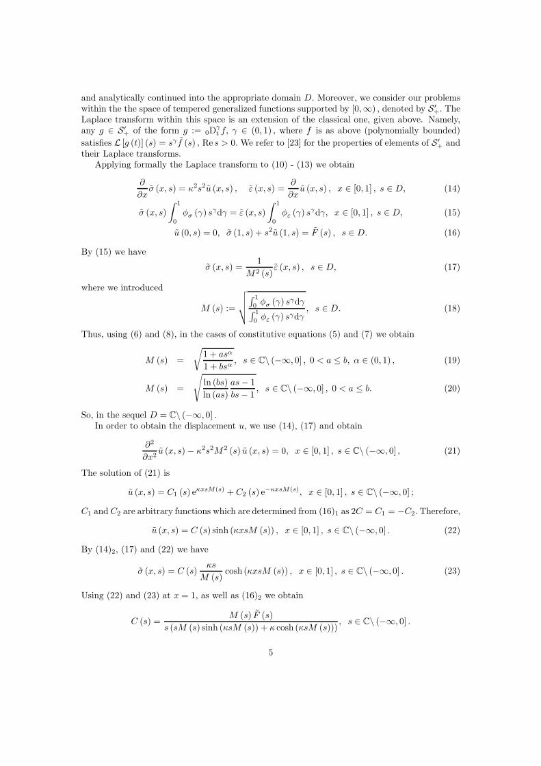
their Laplace transforms.Applying formally the Laplace transform to (10) - (13) we obtain

∂

∂xσ (x, s) = κ2s2u (x, s) , ε (x, s) =

∂

∂xu (x, s) , x ∈ [0, 1] , s ∈ D, (14)

σ (x, s)

∫ 1

0

φσ (γ) sγdγ = ε (x, s)

∫ 1

0

φε (γ) sγdγ, x ∈ [0, 1] , s ∈ D, (15)

u (0, s) = 0, σ (1, s) + s2u (1, s) = F (s) , s ∈ D. (16)

By (15) we have

σ (x, s) =1

M2 (s)ε (x, s) , s ∈ D, (17)

where we introduced

M (s) :=

√

√

√

√

∫ 1

0φσ (γ) s

γdγ∫ 1

0φε (γ) s

γdγ, s ∈ D. (18)

Thus, using (6) and (8), in the cases of constitutive equations (5) and (7) we obtain

M (s) =

√

1 + asα

1 + bsα, s ∈ C\ (−∞, 0] , 0 < a ≤ b, α ∈ (0, 1) , (19)

M (s) =

√

ln (bs)

ln (as)

as− 1

bs− 1, s ∈ C\ (−∞, 0] , 0 < a ≤ b. (20)

So, in the sequel D = C\ (−∞, 0] .In order to obtain the displacement u, we use (14), (17) and obtain

∂2

∂x2u (x, s)− κ2s2M2 (s) u (x, s) = 0, x ∈ [0, 1] , s ∈ C\ (−∞, 0] , (21)

The solution of (21) is

u (x, s) = C1 (s) eκxsM(s) + C2 (s) e

−κxsM(s), x ∈ [0, 1] , s ∈ C\ (−∞, 0] ;

C1 and C2 are arbitrary functions which are determined from (16)1 as 2C = C1 = −C2. Therefore,

u (x, s) = C (s) sinh (κxsM (s)) , x ∈ [0, 1] , s ∈ C\ (−∞, 0] . (22)

By (14)2, (17) and (22) we have

σ (x, s) = C (s)κs

M (s)cosh (κxsM (s)) , x ∈ [0, 1] , s ∈ C\ (−∞, 0] . (23)

Using (22) and (23) at x = 1, as well as (16)2 we obtain

C (s) =M (s) F (s)

s (sM (s) sinh (κsM (s)) + κ cosh (κsM (s))), s ∈ C\ (−∞, 0] .

5

Therefore, the Laplace transforms of the displacement and stress from (22) and (23) are

u (x, s) = F (s) P (x, s) , σ (x, s) = F (s) Q (x, s) , x ∈ [0, 1] , s ∈ C\ (−∞, 0] . (24)

where

P (x, s) =1

s

M (s) sinh (κxsM (s))

sM (s) sinh (κsM (s)) + κ cosh (κsM (s)), x ∈ [0, 1] , s ∈ C\ (−∞, 0] , (25)

Q (x, s) =κ cosh (κxsM (s))

sM (s) sinh (κsM (s)) + κ cosh (κsM (s)), x ∈ [0, 1] , s ∈ C\ (−∞, 0] . (26)

Applying the inverse Laplace transform to (24) we obtain the displacement and stress as

u (x, t) = F (t) ∗ P (x, t) , σ (x, t) = F (t) ∗Q (x, t) , x ∈ [0, 1] , t > 0. (27)

The validity of these formal expressions will be proved in the sequel.

3 Explicit form of solutions

In order to obtain the displacement u and stress σ by (27), we have to obtain functions P andQ, i.e., to invert the Laplace transform in (25) and (26). First, we examine the behavior of thefunction M, given by (18), in the limiting cases as |s| → ∞ and |s| → 0 (by this we mean onlythose s that belong to C\ (−∞, 0]) in the special cases when M takes any of the forms given by(19) and (20).

If M is given by (19) or (20) we have

|M (s)| ≈√

a

b, as |s| → ∞, and |M (s)| ≈ 1, as |s| → 0. (28)

We use results from [8] in order to obtain the displacement u and the stress σ. In order to doso, we recall assumptions on M that have to be satisfied.

We shall analyze a function of complex variable

f (s) := sM (s) sinh (κsM (s)) + κ cosh (κsM (s)) , s ∈ C. (29)

Let M be of the form M (s) = r (s) + ih (s) , as |s| → ∞. Then

(A1)

lim|s|→∞

r (s) = c∞ > 0, lim|s|→∞

h (s) = 0, lim|s|→0

M (s) = c0,

for some constants c∞, c0 > 0.

Let sn = ξn + iζn, n ∈ N, satisfy the equation

f (s) = 0, s ∈ V, (30)

where f is given by (29). Then:

(A2) There exists n0 > 0, such that for n > n0

Im sn ∈ R+ ⇒ h (sn) ≤ 0, Im sn ∈ R− ⇒ h (sn) ≥ 0,

where h := ImM.

6

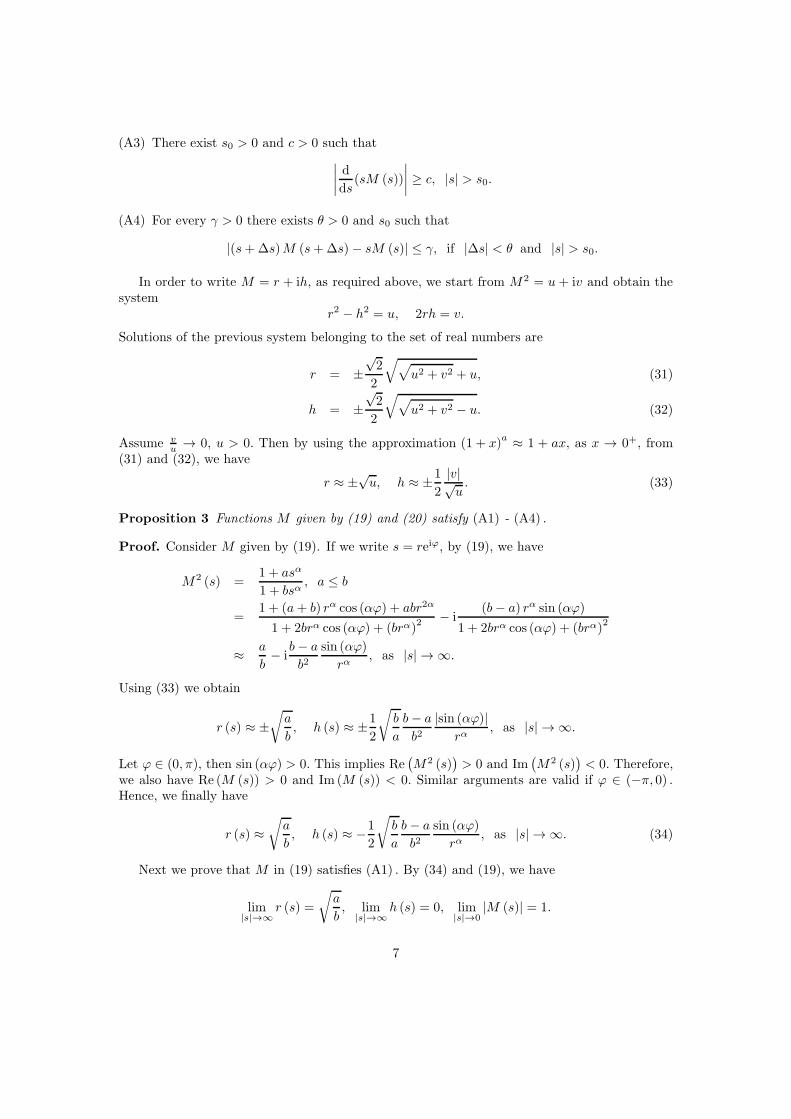
(A3) There exist s0 > 0 and c > 0 such that

∣

∣

∣

∣

d

ds(sM (s))

∣

∣

∣

∣

≥ c, |s| > s0.

(A4) For every γ > 0 there exists θ > 0 and s0 such that

|(s+∆s)M (s+∆s)− sM (s)| ≤ γ, if |∆s| < θ and |s| > s0.

In order to write M = r + ih, as required above, we start from M2 = u + iv and obtain thesystem

r2 − h2 = u, 2rh = v.

Solutions of the previous system belonging to the set of real numbers are

r = ±√2

2

√

√

u2 + v2 + u, (31)

h = ±√2

2

√

√

u2 + v2 − u. (32)

Assume vu→ 0, u > 0. Then by using the approximation (1 + x)

a ≈ 1 + ax, as x → 0+, from(31) and (32), we have

r ≈ ±√u, h ≈ ±1

2

|v|√u. (33)

Proposition 3 Functions M given by (19) and (20) satisfy (A1) - (A4) .

Proof. Consider M given by (19). If we write s = reiϕ, by (19), we have

M2 (s) =1 + asα

1 + bsα, a ≤ b

=1 + (a+ b) rα cos (αϕ) + abr2α

1 + 2brα cos (αϕ) + (brα)2 − i

(b− a) rα sin (αϕ)

1 + 2brα cos (αϕ) + (brα)2

≈ a

b− i

b− a

b2sin (αϕ)

rα, as |s| → ∞.

Using (33) we obtain

r (s) ≈ ±√

a

b, h (s) ≈ ±1

2

√

b

a

b− a

b2|sin (αϕ)|

rα, as |s| → ∞.

Let ϕ ∈ (0, π), then sin (αϕ) > 0. This implies Re(

M2 (s))

> 0 and Im(

M2 (s))

< 0. Therefore,we also have Re (M (s)) > 0 and Im (M (s)) < 0. Similar arguments are valid if ϕ ∈ (−π, 0) .Hence, we finally have

r (s) ≈√

a

b, h (s) ≈ −1

2

√

b

a

b− a

b2sin (αϕ)

rα, as |s| → ∞. (34)

Next we prove that M in (19) satisfies (A1) . By (34) and (19), we have

lim|s|→∞

r (s) =

√

a

b, lim

|s|→∞h (s) = 0, lim

|s|→0|M (s)| = 1.

7

Validity of assumption (A2) follows from (34).In order to show that M in (19) satisfies (A3) , we use (19) and obtain

d

ds(sM (s)) = M (s)

(

1− α (b− a) sα

2 (1 + asα) (1 + bsα)

)

.

Thus, by (34)∣

∣

∣

∣

d

ds(sM (s))

∣

∣

∣

∣

≈√

a

b, as |s| → ∞. (35)

We have that there exists ξ such that

|(s+∆s)M (s+∆s)− sM (s)| ≤ |∆s|∣

∣

∣

∣

∣

[

d

ds(sM (s))

]

s=ξ

∣

∣

∣

∣

∣

.

Since dds (sM (s)) , by (35), is bounded as |s| → ∞ and if |∆s| < θ for some θ > 0, we have that

(A4) is satisfied.Now consider M given by (20). With s = reiϕ we have

M2 (s) =ln (bs)

ln (as)

as− 1

bs− 1, a ≤ b

=ln (ar) ln (br) + ϕ2

ln2 (ar) + ϕ2

abr2 − (a+ b) r cosϕ+ 1

(br)2 − 2br cosϕ+ 1

− ϕ ln ba

ln2 (ar) + ϕ2

(b− a) r sinϕ

(br)2 − 2br cosϕ+ 1

−i

(

ln (ar) ln (br) + ϕ2

ln2 (ar) + ϕ2

(b− a) r sinϕ

(br)2 − 2br cosϕ+ 1

+ϕ ln b

a

ln2 (ar) + ϕ2

abr2 − (a+ b) r cosϕ+ 1

(br)2 − 2br cosϕ+ 1

)

≈ a

b− i

a

bln

b

a

ϕ

ln2 (ar), as |s| → ∞.

Using (33) we obtain

r (s) = ±√

a

b, h (s) = ±1

2

√

a

bln

b

a

|ϕ|ln2 (ar)

.

Let ϕ ∈ (0, π), then sin (αϕ) > 0. This implies Re(

M2 (s))

> 0 and Im(

M2 (s))

< 0. Therefore,we also have Re (M (s)) > 0 and Im (M (s)) < 0. Similar arguments are valid if ϕ ∈ (−π, 0) .Hence, we finally have

r (s) =

√

a

b, h (s) = −1

2

√

a

bln

b

a

ϕ

ln2 (ar). (36)

Next we prove that (20) satisfies (A1) . By (36) and (20), we have

lim|s|→∞

r (s) =

√

a

b, lim

|s|→∞h (s) = 0, lim

|s|→0|M (s)| = 1.

Validity of assumption (A2) follows from (36).In order to show M in (20) satisfies (A3) , we use (20) and obtain

d

ds(sM (s)) = M (s)

(

1− ln ba

2 ln (as) ln (bs)+

(b− a) s

2 (as− 1) (bs− 1)

)

.

8

Thus, by (36)∣

∣

∣

∣

d

ds(sM (s))

∣

∣

∣

∣

≈√

a

b, as |s| → ∞. (37)

Using the same arguments as above, we have that (A4) is satisfied, since sM (s) , s ∈ V, by(37), has bounded first derivative.

The existence and the uniqueness of u and σ, as solutions to system (10) - (13) is guaranteedby the fact that M in all two cases satisfies (A1) - (A4) . Recall, f is given by (29) and sn, n ∈ N,

are solutions of (30). The multiplicity of zeros sn is one for n large enough.

Theorem 4 ([8]) Let F ∈ S ′+ and suppose that M satisfies assumptions (A1) - (A4) . Then the

unique solution u to (10) - (13) is given by

u (x, t) = F (t) ∗ P (x, t) , x ∈ [0, 1] , t > 0,

where

P (x, t) =1

π

∫ ∞

0

Im

(

M(

qe−iπ)

sinh(

κxqM(

qe−iπ))

qM (qe−iπ) sinh (κqM (qe−iπ)) + κ cosh (κqM (qe−iπ))

)

e−qt

qdq

+2∞∑

n=1

Re(

Res(

P (x, s) est, sn

))

, x ∈ [0, 1] , t > 0,

P (x, t) = 0, x ∈ [0, 1] , t < 0.

The residues are given by

Res(

P (x, s) est, sn

)

=

[

1

s

M (s) sinh (κxsM (s))ddsf (s)

est

]

s=sn

, x ∈ [0, 1] , t > 0,

Then P ∈ C ([0, 1]× [0,∞)) and u ∈ C(

[0, 1] ,S ′+

)

. In particular, if F ∈ L1loc ([0,∞)) , then

u is continuous on [0, 1]× [0,∞) .

The following theorem is related to stress σ. We formulate this theorem with F = H, whereH denotes the Heaviside function, while the more general cases of F are discussed in Remark 6,below.

Theorem 5 ([8]) Let F = H and suppose that M satisfies assumptions (A1) - (A4) . Then theunique solution σH to (10) - (13), is given by

σH (x, t) = H (t) +κ

π

∫ ∞

0

Im

(

cosh(

κxqM(

qeiπ))

qM (qeiπ) sinh (κqM (qeiπ)) + κ cosh (κqM (qeiπ))

)

e−qt

qdq

+2

∞∑

n=1

Re(

Res(

σH (x, s) est, sn))

, x ∈ [0, 1] , t > 0, (38)

σH (x, t) = 0, x ∈ [0, 1] , t < 0.

The residues are given by

Res(

σH (x, s) est, sn)

=

[

κ cosh (κxsM (s))

s ddsf (s)

est

]

s=sn

, x ∈ [0, 1] , t > 0.

In particular, σH is continuous on [0, 1]× [0,∞) .

9

Remark 6 ([8])

1. The assumption F = H in Theorem 5 can be relaxed by requiring that F is locally integrableand

F (s) ≈ 1

sα, as |s| → ∞,

for some α ∈ (0, 1) . This condition ensures the convergence of the series in (38).

2. If F = δ, or even F (t) = dk

dtk δ (t) , one uses σH , given by (38), in order to obtain σ as thek + 1-th distributional derivative:

σ =dk+1

dtk+1σH ∈ C

(

[0, 1] ,S ′+

)

.

4 Numerical examples

The displacement u as a solution to (10) - (13) is given in Theorem 4. We present variousnumerical examples for constitutive models: fractional Zener and distributed-order model of asolid-like viscoelastic body that are distinguished by the form of M : (19) and (20), respectively.

4.1 The case F = δ

In order to plot time dependence of the displacement u for the several points of the rod as wellas for the body attached to its free end, we chose the fractional Zener model and the force actingon the body to be the Dirac delta distribution, i.e. F = δ. We fix the parameters describingthe rod: a = 0.2, b = 0.6, α = 0.45 and also fix the ratio between the masses of rod and bodyκ := κ2 = 1. Plot of u as a function of time t for various points of a rod is shown in Figure 2. It is

Figure 2: Displacement u(x, t) in the case F = δ for κ = 1 as a function of time t at x ∈{0.25, 0.5, 0.75, 1} for t ∈ (0, 40).

evident that the oscillations of the rod and a body are damped, since the material is viscoelastic.

10

One notices that initially there is a transitional regime of the oscillations. Afterwards, the curvesresemble the curves of the damped linear oscillator.

In order to examine the transitional regime more closely, in Figures 3 - 5 we present the plotsof u for smaller values of time, but for different values of κ ∈ {0.5, 1, 2}. We notice that the

Figure 3: Displacement u(x, t) in the case F =δ for κ = 0.5 as a function of time t at x ∈{0.25, 0.5, 0.75, 1} for t ∈ (0, 9).

Figure 4: Displacement u(x, t) in the case F =δ for κ = 1 as a function of time t at x ∈{0.25, 0.5, 0.75, 1} for t ∈ (0, 10).

Figure 5: Displacement u(x, t) in the case F =δ for κ = 2 as a function of time t at x ∈{0.25, 0.5, 0.75, 1} for t ∈ (0, 11).

shape of the curves depends on the ratio between the masses κ, while later, the shape resemblesto the shape of curves for damped oscillations. It could be noticed that regardless of the valueof κ there is a delay in starting oscillation for the points that are further away from the free endof a rod. This is due to the finite speed of wave propagation. Namely, the body (x = 1), whichis subject to the action of the force, starts oscillating at t = 0, while the delay in the startingtime-instant of the oscillation is greater as the point is further from the point where the forceacts. Moreover, we see that different points of the rod do not come to their initial position, forthe first time, at the same time-instant (see Figure 5). This, as well as the initial delay dependon the mass ratio κ. For the influence of κ on the initial delay compare Figures 3 - 5. Later on,again depending on κ, the motion of the points become synchronized.

Figures 6 and 7 present the plots of displacement u for fixed point of the rod x = 0.5 ifthe ratio between masses κ varies. One sees from Figure 6 that the larger the mass of a rod is

11

Figure 6: Displacement u(x, t) in the case F = δ at x = 0.5 as a function of time t ∈ (0, 40) forκ = 0.5 - dot-dashed line, κ = 1 - dashed line and κ = 2 - solid line.

(then the value of κ is greater) the quasi-period (time between two consecutive passage of a fixedpoint through its initial position) of the oscillations is greater. That is due to the increased rod’sinertia. Also, for larger times there is no significant influence of κ on the heights and widths ofthe peaks which indicates that the damping effects are only due to the parameters a, b and α

figuring in the constitutive equation. Figure 7 shows that the shape of the curve in transitionalregime strongly depends on κ. Moreover, the delay in the oscillations increases as the κ increaseswhich indicates that the speed of the wave propagation depends on the mass ratio.

4.2 The case F = H

The aim of this section is the qualitative analysis of the behavior of a displacement u when thereis a force, given in the form of the Heaviside function, i.e., F = H, acting at the attached body.Thus, our results correspond to a creep experiment. The rod is modelled by the fractional Zenermodel, i.e., the function M is given by (19). The parameters describing the rod are: a = 0.1,b = 0.9, α = 0.8. We present plots of u for the ratio between the masses of rod and body κ = 1.

Figure 8 present the long-time behavior of displacement u. One notices that the rod creepsto a finite value of displacement so that limt→∞ u (x, t) = x, x ∈ [0, 1]. Figure 9 present theshort-time behavior of u. We see that there is a delay in starting time-instant of a point of arod.

Figures 10 and 11 present the plots of time evolution of displacement u of a rod described bythe Zener model for fixed point of the rod x = 0.5 if the ratio between masses κ varies. Here, theparameters are a = 0.2, b = 0.6, α = 0.45. One sees, Figure 10, that there is no dependence ofthe finite value of displacement in creep on the value of the mass ratio κ. We see, Figure 11, thatfor small times there is an influence of κ on the height of the peaks such that its height increasesas κ increases. This is due to the inertia, while for larger times the viscoelastic properties of therod prevail. Similarly as in the previous section the delay in the oscillations starting time-instantincreases as κ increases.

Acknowledgement 7 This research is supported by the Serbian Ministry of Education and

12

Figure 7: Displacement u(x, t) in the case F = δ at x = 0.5 as a function of time t ∈ (0, 11) forκ = 0.5 - dot-dashed line, κ = 1 - dashed line and κ = 2 - solid line.

Science projects 174005 (TMA and DZ) and 174024 (SP), as well as by the Secretariat forScience of Vojvodina project 114− 451− 2167 (DZ).

References

[1] T.M. Atanackovic, A modified Zener model of a viscoelastic body, Continuum Mech. Ther-modyn. 14 (2002) 137–148.

[2] T.M. Atanackovic, A generalized model for the uniaxial isothermal deformation of a vis-coelastic body, Acta Mech. 159 (2002) 77–86.

[3] T.M. Atanackovic, On a distributed derivative model of a viscoelastic body, C. R. Mecanique331 (2003) 687–692.

[4] T.M. Atanackovic, M. Budincevic, S. Pilipovic, On a fractional distributed-order oscillator,J. Phys. A: Math. Gener. 38 (2005) 6703–6713.

[5] T.M. Atanackovic, S. Konjik, Lj. Oparnica, D. Zorica, Thermodynamical restrictions andwave propagation for a class of fractional order viscoelastic rods. Abstract and AppliedAnalysis 2011 (2011) ID975694, 32p.

[6] T.M. Atanackovic, S. Pilipovic, D. Zorica, Distributed-order fractional wave equation on afinite domain. Stress relaxation in a rod. Int. J. Eng. Sci. 49 (2011) 175–190.

[7] T.M. Atanackovic, S. Pilipovic, D. Zorica, Distributed-order fractional wave equation ona finite domain: creep and forced oscillations of a rod. Continuum Mech. Thermodyn. 23(2011) 305–318.

[8] T.M. Atanackovic, S. Pilipovic, D. Zorica, On a system of equations arising in viscoelasticitytheory of fractional type. Preprint available on arXiv:1205.5343 (2012).

13

Figure 8: Displacement u(x, t) in the creep ex-periment for κ = 1 as a function of time t atx ∈ {0.25, 0.5, 0.75, 1} for t ∈ (0, 100).

Figure 9: Displacement u(x, t) in the creep ex-periment for κ = 1 as a function of time t atx ∈ {0.25, 0.5, 0.75, 1} for t ∈ (0, 25).

[9] G. Doetsch, Handbuch der Laplace-Transformationen I. Birkhauser, Basel, 1950.

[10] A.A. Kilbas, H.M. Srivastava, J.J. Trujillo, Theory and Applications of Fractional Differen-tial Equations. Elsevier B.V, Amsterdam, 2006.

[11] S. Konjik, Lj. Oparnica, D. Zorica, Waves in fractional Zener type viscoelastic media. J.Math. Anal. Appl. 365 (2010) 259–268.

[12] S. Konjik, Lj. Oparnica, D. Zorica, Waves in viscoelastic media described by a linear frac-tional model. Integr. Transf. Spec. F. 22 (2011) 283–291.

[13] T.T. Hartley, C.F. Lorenzo, Fractional-order system identification based on continuousorder-distributions, Signal Process. 83 (2003) 2287–2300.

[14] F. Mainardi, Fractional Calculus andWaves in Linear Viscoelasticity. Imperial College Press,London, 2010.

[15] W. Nowacki, Dynamics of elastic systems. Chapman & Hall, London 1963.

[16] I. Podlubny, Fractional Differential Equations. Academic Press, San Diego, 1999.

[17] Yu.A. Rossikhin, Reflections on two parallel ways in the progress of fractional calculus inmechanics of solids. Applied Mechanics Reviews, 63 (2010) 010701-1–010701-12.

[18] Yu.A. Rossikhin, M.V. Shitikova, Analysis of dynamic behavior of viscoelastic rods whoserheological models contain fractional derivatives of two different orders. Zeitschrift fur Ange-wandte Mathematik und Mechanik, 81 (2001) 363–376.

[19] Yu.A. Rossikhin, M.V. Shitikova, A new method for solving dynamic problems of fractionalderivative viscoelasticity. International Journal of Engineering Science, 39 (2001) 149–176.

[20] Yu.A. Rossikhin, M.V. Shitikova, Application of fractional calculus for dynamic problemsof solid mechanics: Novel trends and recent results. Applied Mechanics Reviews, 63 (2010)010801-1–010801-52.

[21] S.G. Samko, A.A. Kilbas, O.I. Marichev, Fractional Integrals and Derivatives, Gordon andBreach, Amsterdam, 1993.

14

Figure 10: Displacement u(x, t) in the creep experiment at x = 0.5 as a function of time t ∈(0, 100) for κ = 0.5 - dot-dashed line, κ = 1 - dashed line and κ = 2 - solid line.

[22] H. Schiessel, Chr. Friedrich, A. Blumen, Applications to problems in polymer physics andrheology. In Applications of fractional calculus in physics (ed R. Hilfer). World Scientific,Singapore, 2000.

[23] V.S. Vladimirov, Equations of Mathematical Physics, Mir Publishers, Moscow, 1984.

15

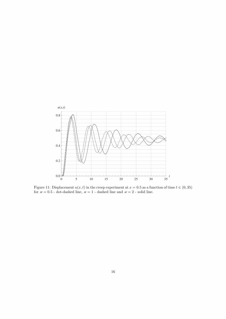
Figure 11: Displacement u(x, t) in the creep experiment at x = 0.5 as a function of time t ∈ (0, 35)for κ = 0.5 - dot-dashed line, κ = 1 - dashed line and κ = 2 - solid line.

16