for near-field and far-field terahertz applications - CORE

STATIC AND RECONFIGURABLE DEVICESFOR NEAR-FIELD AND

FAR-FIELD TERAHERTZ APPLICATIONSby

Silvia TofaniDepartment of Information Engineering, Electronics and Telecommunications

Istituto per la Microelettronica e Microsistemi

A thesis submitted in partial fulfillment of the requirements for the degree of Doctor of Philosophy in Information and Communication Engineering

at

Sapienza University of Rome

February 2018

Cycle XXX

Certified by Thesis Supervisors:

Prof. Alessandro GalliDepartment of Information Engineering,

Electronics and TelecommunicationsSapienza University of Rome

Dr. Romeo BeccherelliIstituto per la Microelettronica e Microsistemi

Consiglio Nazionale delle Ricerche

This thesis was evaluated by the two following external referees: Gaetano Bellanca, Professor, University of Ferrara, Ferrara, Italy Marco Peccianti, Reader, University of Sussex, Brighton, United Kingdom The time and effort of the external referees in evaluating this thesis, as well as their valuable and constructive suggestions, are very much appreciated and greatly acknowledged.

______________

III

CONTENTS

CONTENTS ........................................................................................................ III

LIST OF FIGURES........................................................................................... VIII

LIST OF TABLES .......................................................................................... XVII

ABSTRACT ..................................................................................................... XIX

ACKNOWLEDGMENTS ................................................................................. XXI

LIST OF SYMBOLS, ABBREVIATIONS AND ACRONYMS ...................... XXII

Symbols ........................................................................................................... XXII

Units of measurements .................................................................................... XXVI

Chemical symbols and formulas .................................................................... XXVII

Abbreviations ............................................................................................... XXVIII

Acronyms ..................................................................................................... XXVIII

INTRODUCTION ........................................................................................ XXXII

CHAPTER I

Terahertz radiation ................................................................................................ 1

1. Introduction to terahertz radiation ................................................................... 1

1.1 Terahertz in the electromagnetic spectrum ............................................... 2

1.2 Terahertz applications and challenges ...................................................... 3

2. Terahertz sources ............................................................................................ 7

3. Terahertz detectors ......................................................................................... 9

4. Terahertz passive components ....................................................................... 11

4.1 Terahertz waveguides ............................................................................ 12

4.2 Quasi-optical components ..................................................................... 13

4.2.1 Polarizers ...................................................................................... 13

IV

4.2.2 Waveplates .................................................................................... 14

4.2.3 Filters ............................................................................................ 15

4.2.4 Lenses ............................................................................................ 16

CHAPTER II

Passive devices for terahertz radiation: zone plates as planar diffractive lenses ..... 17

1. Introduction ................................................................................................... 17

2. Planar diffractive lenses: zone plates.............................................................. 18

3. Zone plates for terahertz radiation and their applications ................................ 21

4. Zone plates theoretical background ................................................................ 23

4.1 Diffraction efficiency ............................................................................. 24

4.2 Comparison between properties of zone plates and traditional lenses ...... 24

4.3 Zone plates aberrations .......................................................................... 25

5. Materials for terahertz diffractive devices ...................................................... 26

6. Fabrication methods and techniques .............................................................. 29

CHAPTER III

Methods for numerically design and fabricate polymeric zone plates .................... 31

1. Introduction ................................................................................................... 31

2. Numerical methods in computational electromagnetic ................................... 33

3. Numerical investigation of zone plates for terahertz focusing ......................... 35

3.1 Material choice ...................................................................................... 37

3.2 Number of zones .................................................................................... 37

3.3 Frequency behavior ............................................................................... 38

3.4 Comparison with a conventional refractive lens ..................................... 39

4. Fabrication .................................................................................................... 39

CHAPTER IV

Numerical investigation and fabrication of terahertz zone plates ........................... 42

1. Material choice .............................................................................................. 42

2. Number of zones ........................................................................................... 43

3. Frequency behavior ....................................................................................... 45

V

4. Comparison with a conventional refractive lens ............................................ 46

5. Conclusions about the numerical investigation and zone plates fabrication .... 47

CHAPTER V

Methods for the experimental characterization of diffractive lenses at terahertz

frequencies .......................................................................................................... 49

1. Introduction .................................................................................................. 49

2. Set-ups for terahertz metrology ..................................................................... 50

2.1 Set-ups employing time-domain methods .............................................. 51

2.2 Set-ups employing frequency-domain methods ...................................... 51

3. Terahertz diffractive lenses characterization: measurements set-up ................ 53

4. Terahertz beam characterization: knife-edge technique.................................. 56

4.1 Knife-edge set-up .................................................................................. 56

4.2 Knife-edge measurements automation ................................................... 59

4.3 Post-processing of data from knife-edge measurements: terahertz imaging 61

5. Iris sampling method: focal length characterization ....................................... 62

6. Terahertz spectrometer calibration ................................................................ 63

6.1 Near-field antenna images on cross-sections of emitted radiation ........... 64

6.2 Distribution of the field intensity employed as lenses excitation ............ 64

CHAPTER VI

Experimental characterization of polymeric zone plates ........................................ 67

1. Introduction .................................................................................................. 67

2. Zone plates focal length ................................................................................ 67

3. Zone plates focal plane ................................................................................. 69

4. Focal plane experimental comparison between ideal and real illumination: multilevel zone plate case of study ........................................................................ 72

5. Conclusions .................................................................................................. 73

CHAPTER VII

Future perspectives in developing planar diffractive lenses ................................... 74

VI

1. Introduction ................................................................................................... 74

2. Tunable zone plates ....................................................................................... 74

2.1 Material with tunable properties: liquid crystals ..................................... 75

2.1.1 Effects of an external electric field on nematic liquid crystals ......... 77

2.1.2 Q-tensor formulation ...................................................................... 79

2.2 Double-sided zone plate with two focal lengths ...................................... 81

3. Metal zone plates ........................................................................................... 88

3.1 Zone plates in reflection mode ............................................................... 89

CHAPTER VIII

Leaky-wave antennas for terahertz far-field applications ...................................... 92

1. Introduction ................................................................................................... 92

2. Historical path in the development of a leaky-wave theory ............................. 93

3. Classification of leaky-wave antennas............................................................ 95

3.1 One-dimensional uniform leaky-wave antennas ..................................... 95

3.2 One-dimensional periodic leaky-wave antennas ..................................... 97

3.3 Two-dimensional leaky-wave antennas .................................................. 98

4. Operation principles of leaky waves .............................................................. 99

5. Leaky-wave antenna analysis and design techniques overview ..................... 102

5.1 Transverse resonance technique ........................................................... 104

6. Leaky-wave antennas at terahertz frequencies .............................................. 105

7. Conclusions ................................................................................................. 109

CHAPTER IX

Fabry-Perot cavity leaky-wave antennas based on liquid crystals for terahertz beam-

steering .............................................................................................................. 110

1. Introduction ................................................................................................. 110

2. Liquid crystals for the design of a tunable leaky-wave antenna .................... 111

3. Tunable Fabry-Perot cavity leaky-wave antenna design ............................... 114

4. Terahertz implementation of a Fabry-Perot cavity leaky-wave antenna with liquid crystals: numerical results ......................................................................... 116

4.1 Dispersion analysis of fundamental leaky modes: lossless case of study117

VII

4.2 Terahertz Fabry-Perot cavity leaky-wave antenna radiation patterns: lossless case of study ....................................................................................... 120

4.3 Terahertz Fabry-Perot cavity leaky-wave antenna: dispersion curves and radiation patterns in the case of materials with dielectric losses ........................ 122

5. Conclusions ................................................................................................. 125

CHAPTER X

Terahertz leaky-wave antennas based on homogenized metasurfaces .................. 126

1. Introduction ................................................................................................. 126

2. Design constraints of terahertz metasurface leaky-wave antennas ................. 127

3. Impedance synthesis of three partially reflective sheet geometries ................ 130

4. Radiating behavior of Fabry-Perot cavity leaky-wave antennas based on fishnet-like metasurface ....................................................................................... 134

4.1 Full-wave analysis of the truncated structure ........................................ 138

5. Conclusions ................................................................................................. 141

REFERENCES .................................................................................................. 142

LIST OF PUBLICATIONS ................................................................................ 167

Journal papers ..................................................................................................... 167

Conference proceedings ...................................................................................... 167

Doctoral school book and e-book contributions ................................................... 168

VIII

LIST OF FIGURES

Fig. 1 Electromagnetic spectrum. ................................................................................ 2

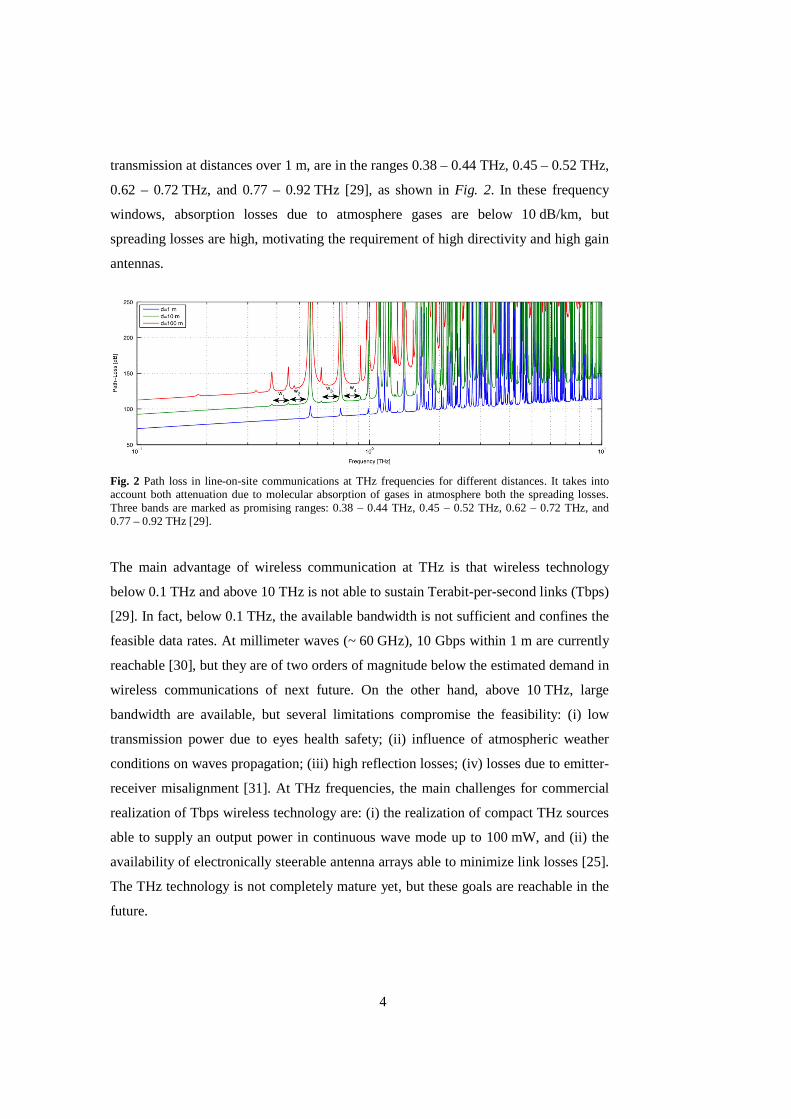
Fig. 2 Path loss in line-on-site communications at THz frequencies for different

distances. It takes into account both attenuation due to molecular absorption of gases in

atmosphere both the spreading losses. Three bands are marked as promising ranges:

0.38 – 0.44 THz, 0.45 – 0.52 THz, 0.62 – 0.72 THz, and 0.77 – 0.92 THz [29]. ........... 4

Fig. 3 Comparison between novel polarizers (red) and commercially available

polarizers (blue) at the frequency of 1 THz. Figure is taken from [91] where a

description of the polarizers in the legend is driven in detail. ..................................... 14

Fig. 4 Behavior of some filter categories widely employed at THz frequencies [88]. . 16

Fig. 5 Huygens-Fresnel principle for zone plate construction. A plane wave is

propagating towards the point of the space P0. O, R1, and R2 are point of the wave

front, which have a fixed distance with respect to P0.................................................. 18

Fig. 6 a) Fresnel ZP for a microlight emitting diode [119]; b) ZP constructed for 12-cm

waves [120]. ............................................................................................................. 20

Fig. 7 Multiple and virtual foci in a ZP. Undiffracted radiation is commonly called

zero-order of diffracted radiation. The focus “+1” is associated to the first order of

diffraction. The focus “+3” represents a higher-order focus, corresponding to i = 2 in

equation II.8. Foci “-1” and “-3” are the equivalent virtual foci of the positive ones. .. 25

Fig. 8 Diffraction efficiency by increasing the number of discretization of zones phase

step [117]. ................................................................................................................. 32

Fig. 9 Overview of the numerical approaches to the electromagnetic problems. ......... 35

IX

Fig. 10 Comparison between sources in terms of frequency and output power. This

plot is from [5] and it is based on data until the year 2011. For additional information

about THz sources until the year 2017, compare Table 1. ......................................... 38

Fig. 11 Milling cutters used throughout this work for ZP fabrication. The diameter of

each cutter is indicated. ............................................................................................ 41

Fig. 12 Comparison between the focusing properties of a binary ZP made of a) Zeonex

E48R and b) HRFZ-Si. A plane wave of 1 V/m is incident perpendicularly to both

lenses. The E-field modulus is represented in a 3-D space, filled by air. Both ZPs,

ending at z = 2 mm, have same external diameter, number of zones and thickness. ... 42

Fig. 13 Comparison between the focusing properties of a binary ZP made of Zeonex

E48R (blue line) or HRFZ-Si (red line). A plane wave of 1 V/m is incident

perpendicularly to both lenses. z-axis is the perpendicular one to the ZP plane. z = 0

mm corresponds to the end of the lens, where a free space, filled by air, starts. Both

ZPs have the same external diameter, number of zones and thickness. ...................... 43

Fig. 14 Focusing behavior of a binary ZP with a fixed diameter and an increasing

number of ring zones. A plane wave of 1 V/m is incident perpendicularly to the lens.

All color maps represents ZP central section and optical axis, z, where THz radiation,

coming from z = 0, is focused. .................................................................................. 45

Fig. 15 Frequency behavior of a multilevel ZP from 0.5 THz to 1.1 THz with a step of

0.1 THz. z-axis is the perpendicular one to the ZP plane. Minor peaks in the square

modulus of the E-field for z from 1 mm to 3 mm are related to multiple reflections

within the 2 mm thick slab in which ZP is fabricated (no antireflection coating is used).

For z < 1 mm and z > 3 mm, a free space filled by air for THz waves propagation is

considered. ............................................................................................................... 46

Fig. 16 Frequency behavior of a biconvex refractive lens from 0.5 THz to 1.1 THz

with a step of 0.1 THz. z -axis is the lens optical axis. Extremely short peaks in the

square modulus of the E-field for z from 2 mm to 4 mm are related to few multiple

reflections inside the lens. For z < 2 mm and z > 4 mm, a free space, filled by air, for

THz waves propagation is considered. ...................................................................... 47

X

Fig. 17 Fabricated ZP lenses: a) multilevel ZP, b) double-sided ZP, c) binary ZP. The

little roughness perceived in visible light is introduced by milling process, but it does

not affect the lens behavior at THz because it is several orders of magnitude below the

wavelength at 1 THz. ................................................................................................ 48

Fig. 18 Overview of the experimental approaches to the THz measurements. ............ 50

Fig. 19 Schematic representation of photoconductive antennas in their a) emitting and

b) receiving configuration. PI is the photogenerated current. ..................................... 54

Fig. 20 Standard configuration of the commercial TDS TERA K15 by Menlo Systems.

PAT: photoconductive antenna in transmission mode; L1 and L3: convex-plane lenses;

L2 and L4: plano-convex lenses; PAR: photoconductive antenna in receiving mode

[180]. ........................................................................................................................ 55

Fig. 21 TDS set-up configurations for the characterization of the THz beam emitted by

the lens antenna (PAT). Three planes are imaged by knife-edge technique: a) plane 1,

at a distance of 3 mm from the PAT; b) plane 2, at a distance of 9 mm from the PAT;

c) plane 3, at the position in which the test ZPs will be located. PAT: photoconductive

antenna in transmission mode; L1 and L3: convex-plane lenses; L2 and L4: plano-

convex lenses; KE: knife-edge blade; PAR: photoconductive antenna in receiving

mode......................................................................................................................... 57

Fig. 22 Schematic representation of a THz TDS for focal spot measurements. PAT:

photoconductive antenna in transmission mode; L1 and L3: convex-plane lenses; L4:

plano-convex lens; KE: knife-edge blade; PAR: photoconductive antenna in receiving

mode......................................................................................................................... 58

Fig. 23 Experimental set-up for standard knife-edge measurements. PAT:


plano-convex lens; KE: knife-edge blade; PAR: photoconductive antenna in receiving

mode......................................................................................................................... 59

Fig. 24 LabVIEW front panel for knife-edge measurements automation. It employs

drivers for the instruments and puts them in communication. The user can choose

XI

several parameters. Program also shows an updated plot of saved data and blade

position. ................................................................................................................... 60

Fig. 25 Schematic representation of a THz TDS for focal length measurements. PAT:


plano-convex lens; I: iris; PAR: photoconductive antenna in receiving mode. ........... 62

Fig. 26 Field distribution at 1 THz at a) 3 mm and b) 9 mm from the hemispherical

lens of the emitting photoconductive antenna............................................................ 64

Fig. 27 THz field distribution collimated by a commercial lens and imaged on a planar

surface by knife-edge technique. .............................................................................. 65

Fig. 28 Experimental and numerical evaluation of the focal length of three ZPs by

means of the optical axis sampling of a) binary ZP, b) double-sided ZP, and c)

multilevel ZP. Measurements are performed with the iris sampling method, which is

also reproduced in the simulation environment. ........................................................ 69

Fig. 29 Acquired data for a) a conventional binary ZP, b) a double-sided ZP, and c) a

multilevel ZP; their difference quotient for d) a conventional binary ZP, e) a double-

sided ZP, and f) a multilevel ZP; and focal plane images obtained by knife-edge

measurements for g) a conventional binary ZP, h) a double-sided ZP, and i) a

multilevel ZP. Negative values of the |E|/|E|max are due to diffraction and scattering

among the components in the THz optical path. ........................................................ 71

Fig. 30 Normalized amplitude of the electric field in the focal plane for the multilevel

ZP acquired with knife-edge technique by rotating a) the lens, or b) the blade. .......... 73

Fig. 31 Liquid crystals mesophases: a) nematic, b) cholesteric, and c) smectic. ......... 76

Fig. 32 Orientation of rod-like molecules in a nematic LC cell without any applied

voltage or in presence of a voltage with strength higher than Freedericksz threshold.

Typically, an alternating voltage in the few kilohertz range is chosen for preventing

electrochemical degradation. .................................................................................... 78

XII

Fig. 33 a) A ZP configuration with a uniform electrode on top and a ZP-patterned

electrode on bottom substrate. The rest condition of the LC is tilted 2° from the y-axis.

b) tilt angle and c) y-component of refractive index tensor distributions in a LC cell

387 µm thick, 2 ms after the application of a 70 V step voltage (steady state). ........... 83

Fig. 34 a) A ZP configuration with a uniform electrode on top and a ZP-patterned

electrode on bottom substrate. The rest condition of the LC is tilted 2° from the y-axis.

b) tilt angle and c) y-component of refractive index tensor distributions in a LC cell

193 µm thick, 2 ms after the application of a 35 V step voltage (steady state). ........... 84

Fig. 35 Cross section of geometrical radial-symmetric model and data for the materials

chosen for a dual-focus double-sided ZP. The ZP is symmetric and only the profile

along the radius of the lens is represented in the picture. ............................................ 86

Fig. 36 Computed square modulus of the electric field component along the optical

axis (z-component) at 1 THz for a dual-focus double-sided phase-reversal ZP lens. The

green line is for zero applied voltage (rest), while the blue line is for LC molecules

parallel to the lens optical axis (V∞). .......................................................................... 86

Fig. 37 Computed normalized square modulus of the z-component of the electric field

at 0.5 THz along the optical axis of a Fresnel ZP working in transmission (red) or in

reflection mode (blue). .............................................................................................. 90

Fig. 38 Comparison between the computed square module of the electric field

normalized to the square module of the incident electric field, at 0.5 THz, along the

optical axis of a Fresnel ZP reflector and a multilevel phase-reversal ZP (compare Ch.

IV). ........................................................................................................................... 90

Fig. 39 A rectangular waveguide, as an example of 1-D uniform LWAs. The

electromagnetic field propagates in z-direction. An infinite ground plane surrounds the

slot [222]. ................................................................................................................. 96

Fig. 40 An example of periodic 1-D LWA. This antenna configuration has a width, w,

larger than the operative wavelength. The electric field is in y-direction and the

electromagnetic wave propagates in z-direction. ........................................................ 97

XIII

Fig. 41 An example of a 2-D LWA: the substrate-superstrate LWA. It can produce a) a

pencil beam at broadside or b) a conical beam with an angle θ with respect to the

broadside direction. .................................................................................................. 98

Fig. 42 Ray diagram of a forward leaky-wave. The intensity of the field is given by

arrows separation: closer arrows correspond to a stronger field [222]. ...................... 100

Fig. 43 Ray diagram of a backward leaky-wave. The intensity of the field is given by

arrows separation: closer arrows correspond to a stronger field [222]. ...................... 101

Fig. 44 Ray diagram of a leaky-wave excited by a source located in z = 0 [222]. ..... 101

Fig. 45 Terminated equivalent network representing a waveguide cross-section [223].

............................................................................................................................... 104

Fig. 46 LC cell driven by a gold fishnet electrode. ................................................... 111

Fig. 47 Real part of the three main components of the LC permittivity tensor mapped

in the xy-plane, in the middle of the LC cell (z = 0). The LCs behavior is show in

absence of an external field (first row), for a voltage above the threshold (last row), and

for an intermediate value of driving voltage (middle row) [with courtesy of Dr. W.

Fuscaldo]. ............................................................................................................... 112

Fig. 48 Real and the imaginary part of the LC dielectric permittivity along a line

perpendicular to the xy-plane and passing through three selected points of the LC cell

[with courtesy of Dr. W. Fuscaldo]. ......................................................................... 113

Fig. 49 Schematic representation of the proposed FPC-LWA and its equivalent

transmission line model. .......................................................................................... 115

Fig. 50 Dispersion curves of the fundamental TM for different THz FPC-LWA with

LC: a) Layout 1, b) Layout 2, c) Layout 3, d) Layout 4. Colors gradually shade from

blue to red as the applied external voltage decreases from V∞ to zero [with courtesy of

Dr. W. Fuscaldo]. .................................................................................................... 118

XIV

Fig. 51 Radiation patterns predicted by leaky-wave theory (dashed lines) or by means

of reciprocity theorem (solid lines): a) Layout 1, b) Layout 2, c) Layout 3, and d)

Layout 4 (see Table 3.5). The condition of the THz beam pointing at broadside (blue

lines) and the radiation at the maximum pointing angle (red lines) are presented [with

courtesy of Dr. W. Fuscaldo]. ................................................................................. 121

Fig. 52 Dispersion curves of the fundamental TM when losses of the materials are

taken into account: a) Layout 2, and b) Layout 4. Colors gradually shade from blue to

red as the applied external voltage decreases from V∞ to zero [with courtesy of Dr. W.

Fuscaldo]. ............................................................................................................... 122

Fig. 53 THz FPC-LWA unit cell model, as implemented in CST full-wave simulation.

A probe for evaluating the tangential magnetic field at the ground plane is added as a

light blue arrow. ...................................................................................................... 123

Fig. 54 Radiation patterns of a) Layout 2 and b) Layout 4 for radiation at broadside

(solid) and at the maximum pointing angle (dashed). Radiation patterns are calculated

by means of reciprocity theorem in the lossless (in red) and the lossy (in black) case.

Patterns from leaky-wave theory are also shown (blue). Full-wave simulations with

CST are reported, in the lossy case, for radiation at broadside (filled green circles) and

at the maximum pointing angle (empty green circles) [with courtesy of Dr. W.

Fuscaldo]. ............................................................................................................... 124

Fig. 55 Directivity at broadside as a function of the characteristic impedance of a PRS

(see equation X.1). Black, blue, green, and red dashed lines selects the reactance values

required for achieving theoretical directivities of 15, 20, 25 and 30 dB, respectively.

............................................................................................................................... 128

Fig. 56 A model for evaluating the surface impedance of a periodic PRS. A Floquet

wave impinges on the PRS. The impedance matrix is obtained in correspondence of the

PRS, fixing a suitable de-embedding distance. An equivalent circuit model can be

derived for retrieving the value of the surface impedance from the impedance matrix

parameters. ............................................................................................................. 129

XV

Fig. 57 Illustrative example of a FPC-LWA based on PRS with three different

elements geometry. ................................................................................................. 130

Fig. 58 Surface reactance Xs of a) a patch-based PRS, as a function of the normalized

gap g between the patches, and b) a strip-based PRS, as a function of the normalized

width w of the strips. ............................................................................................... 131

Fig. 59 Surface reactance Xs of a fishnet-based PRS as a function of both g and w. The

iso-lines of the reactance at 15, 25, 45, and 75 Ω are reported in white dashed lines. 132

Fig. 60 Surface reactance of a fishnet-like unit cell as a function of frequency. The

family of curves is obtained changing the angle of incidence from 0° to 80° (the color

shades from blue to red, respectively). ..................................................................... 133

Fig. 61 a) Surface reactance as a function of the frequency for the four layouts

presented in Table 14: behavior at 15 Ω is in red, at 25 Ω is in blue, at 45 Ω is in green,

and at 66 Ω is in black. b) Section of the proposed FPC-LWA and its equivalent circuit

model. Z0 and Z1 are the modal impedances in the air and in the medium, respectively,

whereas kx0 and kx1 are the vertical wavenumbers in the air and in the medium,

respectively. ............................................................................................................ 135

Fig. 62 Dispersion curves βz/k0 (solid lines) and αz/k0 (dashed lines) as a function of the

frequency. In the insets, the frequency range is limited to 0.8 – 1.2 THz to highlight the

behavior around the operative frequency of the dominant leaky modes for both TE (in

green) and TM (in blue) polarizations. ..................................................................... 135

Fig. 63 Radiation patterns normalized to broadside radiation calculated with the leaky-

wave approach (black solid lines) and reciprocity theorem (black dashed lines) are

reported over the E-plane for the four layouts of Table 14. ...................................... 136


wave approach (black solid lines) and reciprocity theorem (black dashed lines) are

reported over the H-plane for the four layouts of Table 14. ...................................... 137


wave approach (red solid lines) and reciprocity theorem (blue asterisks), and validated

XVI

with full-wave simulations (black circles) are reported over the E-plane for the four

layout of Table 14. .................................................................................................. 139


wave approach (red solid lines) and reciprocity theorem (blue asterisks), and validated

with full-wave simulations (black circles) are reported over the H-plane for the four

layout of Table 14. .................................................................................................. 140

XVII

LIST OF TABLES

Table 1 Comparison between the main THz radiation sources. ................................... 7

Table 2 Comparison between some techniques employing optical and near-infrared

lasers for generating THz radiation by optical pumping. ............................................. 8

Table 3 Commercially available THz time-domain spectrometers generating THz

radiation by photoconductive antennas (readapted from [76]). .................................... 9

Table 4 Commercial available detectors for THz radiation [25]. ............................... 10

Table 5 Comparison of THz conventional materials refractive index and absorption

coefficient at 1 THz. ................................................................................................. 27

Table 6 Dependence of the number of operations to the frequency f and the number of

iterations Nit [161]. ................................................................................................... 33

Table 7 Comparison between lenses fabrication techniques [167]. ............................ 40

Table 8 Leaky-wave antennas typologies and examples, working in the frequency

range of 0.3 - 3 THz. In the headers, f is the frequency at which the antennas are

investigated, while η is the radiation efficiency. ....................................................... 106

Table 9 Metasurfaces FPC-LWAs in the frequency range 0.3 - 3 THz. In the headers, f

is the frequency at which the antennas are investigated, while η is the radiation

efficiency. ............................................................................................................... 107

Table 10 Leaky-wave antennas with a reconfigurable pointing angle, working in the

frequency range between about 0.3 THz and 3 THz. In the headers, f is the frequency at

which the antennas are investigated, η is the radiation efficiency, and ∆θ is the

maximum variation of the pointing angle. ................................................................ 108

Table 11 Design parameters for different THz FPC-LWA layouts. .......................... 117

XVIII

Table 12 Figure of merits for radiating performance of different layouts of a FPC-

LWA with LCs: beam reconfigurability (θpM), directivity (D0) and beamwidth (∆θ). 119

Table 13 Comparison between radiation properties of Layout 2 and 4, with and

without dielectric material losses. ............................................................................ 124

Table 14 Relevant geometrical parameters and radiating properties of the FPC-LWAs

based on the considered PRSs with fishnet-like elements. ........................................ 134

XIX

ABSTRACT

The terahertz frequency electromagnetic radiation has gathered a growing interest from

the scientific and technological communities in the last 30 years, due to its capability

to penetrate common materials, such as paper, fabrics, or some plastics and offer

information on a length scale between 100 µm and 1 mm. Moreover, terahertz

radiation can be employed for wireless communications, because it is able to sustain

terabit-per-second wireless links, opening to the possibility of a new generation of data

networks.

However, the terahertz band is a challenging range of the electromagnetic spectrum in

terms of technological development and it falls amidst the microwave and optical

techniques. Even though this so-called “terahertz gap” is progressively narrowing, the

demand of efficient terahertz sources and detectors, as well as passive components for

the management of terahertz radiation, is still high. In fact, novel strategies are

currently under investigation, aiming at improving the performance of terahertz

devices and, at the same time, at reducing their structure complexity and fabrication

costs.

In this PhD work, two classes of devices are studied, one for near-field focusing and

one for far-field radiation with high directivity. Some solutions for their practical

implementation are presented.

The first class encompasses several configurations of diffractive lenses for focusing

terahertz radiation. A configuration for a terahertz diffractive lens is proposed,

numerically optimized, and experimentally evaluated. It shows a better resolution than

a standard configuration. Moreover, this lens is investigated with regard to the

possibility to develop terahertz diffractive lenses with a tunable focal length by means

of an electro-optical control. Preliminary numerical data present a dual-focus capability

at terahertz frequencies.

The second class encompasses advanced radiating systems for controlling the far-field

radiating features at terahertz frequencies. These are designed by means of the

formalism of leaky-wave theory. Specifically, the use of an electro-optical material is

considered for the design of a leaky-wave antenna operating in the terahertz range,

XX

achieving very promising results in terms of reconfigurability, efficiency, and radiating

capabilities. Furthermore, different metasurface topologies are studied. Their analytical

and numerical investigation reveals a high directivity in radiating performance.

Directions for the fabrication and experimental test at terahertz frequencies of the

proposed radiating structures are addressed.

XXI

ACKNOWLEDGMENTS

The work described in this PhD thesis has been possible thanks to the help and the

support of several people.

At first, I would like to thank my supervisors, prof. Alessandro Galli and Dr. Romeo

Beccherelli, for their suggestions and patience during these three years.

I thank prof. Renato Cicchetti, prof. Emanuele Piuzzi, and prof. Antonio d’Alessandro

from Department of Information Engineering, Electronics and Telecommunications of

“Sapienza” University, who have been members of my Advisory Board, for their

valuable doubts and questions.

I thank Alfonso Morbidini from Istituto Nazionale di Astrofisica (INAF) for his

willingness and the time he spent for the lenses fabrication.

I thank Dr. Mauro Missori from Istituto dei Sistemi Complessi of Consiglio Nazionale

delle Ricerche (ISC-CNR) and prof. Renato Fastampa from Physics Department of

“Sapienza” University for their precious supervision and help during terahertz

experimental measurements.

I thank Dr. Dimitrios Zografopoulos from Istituto per la Microelettronica e

Microsistemi of Consiglio Nazionale delle Ricerche (ISC-CNR) for the time he spent

teaching me the numerical tools employed in the study of liquid crystals.

I thank Dr. Walter Fuscaldo from Department of Information Engineering, Electronics

and Telecommunications of “Sapienza” University for introducing me, with patience

and dedication, in the field of leaky-wave antennas.

I thank my labmates for the stimulating discussions and for all the fun we have had

together.

Last but not the least, I would like to thank my family, my boyfriend and my friends

for supporting me spiritually throughout this PhD and my life in general.

XXII

LIST OF SYMBOLS, ABBREVIATIONS AND ACRONYMS

Symbols

angle between the optical axis and the principal ray

attenuation constant due to material losses

radial attenuation constant

attenuation constant in z-direction

normalized attenuation constant

phase constant vector

radial phase constant

phase constant in x-direction

phase constant in z-direction

normalized phase constant

ratio between the viscosity of a nematic liquid crystal

and the order parameter

scattering frequency

Δ dielectric anisotropy

∆θ beamwidth

∆λ interval of wavelengths

Δ transverse wavenumber perturbation

∆n birefringence

∆r width of the outermost ring of a zone plate

dielectric permittivity tensor

dielectric permittivity in direction perpendicular to the

polarization direction of an applied electric field

∥ dielectric permittivity in direction parallel to the

XXIII

polarization direction of an applied electric field

vacuum dielectric permittivity

extraordinary dielectric permittivity

average dielectric anisotropy

ordinary dielectric permittivity

relative dielectric permittivity

radiation efficiency

diffraction efficiency

vacuum impedance

θ azimuthal angle

angle between the z-axis and the phase vector

θm angle between the long molecular axes of a liquid

crystal and its director

beam reconfigurability

λ wavelength

wavelength in vacuum

!,#,$ eigenvalues of the Q-tensor

% wavelength in an alumina layer

& arbitrary wavelength value in a wavelength range

'( wavelength in a liquid crystal layer

)* wavelength in a polymeric substrate

+ vacuum permeability

σ electric conductivity

, phase shift

- angular frequency

-. plasma frequency

A arbitrary constant

a radius of the central circle of a zone plate

ath thermotropic coefficient

bth thermotropic coefficient

cth thermotropic coefficient

d distance

XXIV

D electromagnetic displacement vector

D dissipation function

D0 directivity

E electric field

EF electric field for the Freedericksz transition

Em average electric field

Emax maximum electric field

/ efficiency

/,0 efficiency contribution due to the substrate losses

ER extinction ratio

f frequency

f/# f-number of a lens

f0 design frequency

12 free energy density

1 elastic energy density

13 electromagnetic energy density

fop operating frequency

14 thermotropic energy density

G gain

g gap

ℎ6 convolution kernel

hair distance between the unit cell and the waveguide port

hi thickness of the i-th layer

i positive integer

7 identity matrix

K local field factor

free-space wavenumber

radial wavenumber

propagation wavenumber

8 transverse wavenumber

8 transverse wavenumber of an unperturbed mode

l focal length

XXV

L straight line

L1 collimating refractive lens

L1,2,6 elastic parameters

L2 focalizing refractive lens

L3 collimating refractive lens

L4 focalizing refractive lens

m number of Fresnel zones

m integer (only in chapters VIII, IX, and X)

m director of the short molecular axis

N number of layers in a multistack

n refractive index

n integer (only in chapter IX)

n director of the long molecular axis

ne extraordinary refractive index

no ordinary refractive index

Nit number of iterations

p object distance

p period (only in chapters VIII and X)

p integer (only in chapters IX)

p1,2 polarization coefficients

P polarization vector

Pd diffracted power

PI photogenerated current

Pin incident power

q image distance

9: Q-tensor

qi i th element of the Q-tensor

;< responsivity

S order parameter

Seq order parameter in the equilibrium state

t thickness

TTE transverse-electric component of transmitted power

XXVI

TTM transverse-magnetic component of transmitted power

V∞ asymptotic value of the voltage for an infinite time

VF voltage for the Freedericksz transition

Vi voltage signal of the ith pixel of a detector array

=> voltage spectral dentisity

w width

Xs surface reactance

Y admittance

Y’ normalized admittance

Y0 admittance in vacuum

Z impedance

Z’ normalized impedance

Z0 impedance in vacuum

Zi,j elements of the impedance matrix of a two-port

network

Zin input impedance

ZL characteristic impedance of the Floquet port in the

substrate

Zs surface impedance

Units of measurements

µm micrometers

µW microwatt

cm centimeter

dB decibel

fps foot per second

fs femtosecond

GB gigabyte

GHz gigahertz

Hz hertz

K kelvin

XXVII

kΩ kiloohm

kHz kilohertz

km kilometer

kW kilowatt

m meters

mm millimeter

mPa millipascal

ms millisecond

MW megawatt

mW milliwatt

nm nanometer

ns nanosecond

nW nanowatt

pN piconewton

ps picosecond

pW picowatt

rad radian

s second

S siemens

THz terahertz

V volt

W watt

Chemical symbols and formulas

Au gold

Al aluminum

Al 2O3 alumina

CF4 tetrafluoromethane

Cr chromium

GaAs gallium arsenide

HfO2 hafnium dioxide

XXVIII

InGaAs indium gallium arsenide

LiTaO3 lithium tantalite

Ni nickel

p-Ge germanium doped with an acceptor

SF6 sulfur hexafluoride

Si silicon

SiNx silicon nitride

SiO2 silica

Ti titanium

VOx vanadium oxide

Abbreviations

c.w. continuous wave

e.g. exempli gratia

Fig. figure

i.e. id est

min minutes

viz. videlicet

Acronyms

1D, 1-D one-dimensional

2D, 2-D two-dimensional

3D, 3-D tridimensional

ABS acrylonitrile butadiene styrene

AF array factor

CAD computer-aided drafting

CMOS complementary metal-oxide semiconductor

CNT carbon nanotubes

COP cyclo-olefin polymer

XXIX

DBR distributed Bragg reflector

DC direct current

DNA deoxyribonucleic acid

EBG electronic bandgap

FBW fractional bandwidth

FD frequency domain

FDTD finite difference time domain

FEM finite element method

FET field-effect transistor

FF filling factor

FIT finite integration technique

FPA focal-plane array

FPC Fabry-Perot cavity

FTIR Fourier transform infrared spectrometer

FTS fast tool servo (only in chapter III)

FTS Fourier transform spectroscopy

FWHM full width at the half maximum

Gbps gigabit-per-second

GDS grounded dielectric slab

HD high definition

HDPE high-density polyethylene

HEMT high electron mobility transistor

HMD horizontal magnetic dipole

HPBW half power beamwidth

HRFZ high resistivity floating zone

HSS high-speed steel

IR infrared

ITO indium tin oxide

KE knife-edge

LC liquid crystals

LEO low Earth orbit

LOS line-on-site

LWA leaky-wave antenna

XXX

MM micro-milling

MMW millimeter-waves

MoM method of moments

MOSFET metal-oxide-semiconductor field-effect transistor

MPIE mixed-potential integral equation

NEP noise equivalent power

QCL quantum cascade laser

QW quantum well

PAR photoconductive antenna in reception mode

PAT photoconductive antenna in transmission mode

PEDOT:PSS poly(3,4-ethylenedioxythiophene):poly(4-

styrenesulfonate)

PEC perfect electric conductor

PET polyethylene terephthalate

PGF periodic Green’s function

PMMA poly(methyl methacrylate)

PP polypropylene

PRS partially reflective sheet

PS polystyrene

PTFE polytetrafluoroethylene

RAM random access memory

RIE reactive ion etching

RT Radon transform

SNR signal-to-noise ratio

SPDT single point diamond turning

STS slow tool servo

Tbps terabit-per-second

TD time domain

TDS time domain spectrometer, time domain spectroscopy

TE transverse-electric

TEN transverse equivalent network

TM transverse-magnetic

TPX polymethylpentene

XXXI

TRT transverse resonance technique

US$ USA dollars

UV ultraviolet

VGA video graphics array

VIS visible

VNA vector network analyzer

WG waveguide

WP waveplate

ZP zone plate

XXXII

INTRODUCTION

“Since we have become accustomed to think of waves of electrical energy and

light waves as forming component parts of a common spectrum, the attempt

has often been made to extend our knowledge over the wide region which

has separated the two phenomena, and to bring them closer together, either

by cutting down the wave length of electrical oscillations […] or by the

discovery and measurement of longer heat waves.”

― H. Rubens and E.F. Nichols1, 1897.

This statement is the opening of a significant paper for the development of a terahertz

science. Even though this was only a first stage, it was clear that there were two

approaches for the development of a terahertz technology: the optical and the

electronic route. The terahertz range has been associated for long time to its lack in

technical capabilities. It was only during 1970s that the first terahertz benchtop set-ups

suitable for spectroscopic investigations have been developed. This was the starting

point for the experimental test of passive components and detectors, which have been

allowed for reducing the technological gap.

Nowadays, terahertz radiation has become crucial in several fields, such as, for

example, the objects inspection for industrial and security applications or the wireless

communications. Thus, there is a high requirement of affordable high-performance

terahertz devices, suitable for mass production and for the integration in complex

systems.

The Chapter I introduces the terahertz radiation, starting from a definition of the

frequency band and its main application fields, passing through the state-of-art of

terahertz generation and detection, and concluding with a brief overview of the most

employed passive components for terahertz radiation. Among them, this PhD thesis is

devoted to the development of planar diffractive lenses. Thus, the Chapter II discusses

1 H. Rubens and E.F. Nichols, “Heat rays of great wave length,” Phys. Rev. (Series I), vol. 4, no. 4, pp. 314-323, 1897.

XXXIII

this choice, comparing the diffractive lenses with the most conventional refractive

lenses and parabolic mirrors for terahertz focusing. Moreover, the Chapter II provides

the theoretical background of diffractive lenses design, as well as an overview of the

materials and the fabrication processes suitable for their practical implementation.

The numerical investigation of the diffractive lenses is described in Chapter III. It aims

at optimizing the lenses geometry and comparing their behavior with the one of a

refractive lens of equal diameter. The numerical data coming from this analysis are

reported and discussed in Chapter IV and constitute the design basis for their

fabrication. The available experimental techniques for terahertz characterization are

introduced in Chapter V, which also includes the description and the calibration of the

available instrument and of the set-up built for the lenses measurements. The data

resulting from the experimental characterization of the fabricated lens prototypes are

reported in Chapter VI.

The design and the experimental characterization presented in Chapters III-VI are the

starting point for a preliminary study on advanced diffractive lens configurations, such

as a tunable dual-focus diffractive lens and a diffractive lens working in reflection

mode (Chapter VII). This last device opens also the possibility to design terahertz lens

antennas employing such diffractive lenses.

In terms of radiating systems for terahertz applications, an interesting device is the

Fabry-Perot cavity leaky-wave antenna. It has the advantage to be scalable from

microwaves to optical frequencies, due to the ubiquity of the leaky-wave phenomena

(introduced in Chapter VIII). Thus, two main configurations of Fabry-Perot cavity

leaky-wave antenna are presented for working at terahertz frequencies. In Chapter IX,

a leaky-wave antenna based on a multistack of isotropic and anisotropic material layers

is theoretically investigated for steering the THz beam. In Chapter X, leaky-wave

antennas made with different metasurface topologies are theoretically studied for the

design of high directivity terahertz antennas. Furthermore, their practical

implementation is discussed.

1

CHAPTER I

Terahertz radiation

1. Introduction to terahertz radiation

The so-called terahertz (THz) radiation is an electromagnetic radiation with a

frequency between 100 GHz and 10 THz [1]–[5]. However, this definition is not

completely accepted and the THz range is sometimes extended from 100 GHz to

30 THz [6] or limited to a narrower region, between 300 GHz and 3 THz. About this

issue, in 2002 Siegel wrote [7]: “Below 300 GHz, we cross into the millimeter-wave

bands (best delimited in the author’s opinion by the upper operating frequency of WR-

3 waveguide — 330 THz). Beyond 3 THz, and out to 30 µm (10 THz) is more or less

unclaimed territory, as few if any components exist. The border between far-IR and

submillimeter is still rather blurry and the designation is likely to follow the

methodology (bulk or modal — photon or wave), which is dominant in the particular

instrument.”

Sometimes, the designation of a range as THz frequencies band is influenced by the

specific field of application. For example, the technological interest towards THz

radiation arose in connection with the development of space-based instruments for

astrophysics and Earth missions. The 98% of total photons emitted in the history of the

Universe since the Big Bang has a frequency below 30 THz, with a peak emission at

around 3 THz (cosmic microwave background radiation, which have a spectral

radiance peak at about 160 GHz [8], is excluded) [3], [5]. For this reason, in this field,

30 THz can be considered the upper limit of the THz band. However, most of the

scientific and technological community refers as THz the radiation between 300 GHz

and 10 THz.

2

1.1 Terahertz in the electromagnetic spectrum

A first experimental effort towards material characterization by THz radiation was in

1897 [9], [10]. It consisted of measurements of black body radiation employing a

bolometer. In [10], the authors wrote: “since we have become accustomed to think of

waves of electrical energy and light waves as forming component parts of a common

spectrum, the attempt has often been made to extend our knowledge over the wide

region that separates the two phenomena, and bring them closer together”. It appears as

a first explicit reference to the fact that a technological gap exists in the

electromagnetic spectrum. It is set between photonics and electronics (Fig. 1).

Fig. 1 Electromagnetic spectrum.

A summary of the historical developments in this range of the spectrum is beyond the

aim of the preset work. An interesting review can be found in [11]. However, it may be

worthy to mention the key discoveries that contribute to the establishment of a THz

technology. The first THz detectors were initially proposed for FIR radiation sensing.

In 1959, the first carbon bolometer [12] as well as a photoconductive detector [13]

were developed. During 1960s, several progresses were achieved in the field of

detection: germanium bolometer [14], pyroelectric [15] and tunable FIR detectors [16]

were introduced. With regard to the generation of THz radiation, in 1962, optical

rectification mechanism was experimentally demonstrated for the first time [17]. It is

still now one of the main THz generating mechanism [18]. In 1971, the first THz pulse

was generated using a benchtop resource [19]. Finally, in 1984, the first laser operating

3

between 390 – 1000 µm was constructed, with a peak power up to 10 kW [20],

whereas, in 1986, a THz emitting antenna was demonstrated for the first time [21].

Several progresses have been made until now in the field of THz sources and detectors.

Starting from the 1950s, many attractive applications have been developed, as will be

described in the following sections.

1.2 Terahertz applications and challenges

Historically, THz detection was conceived for interstellar dust sensing between

100 GHz and 3 THz. Nowadays, space-borne THz sensors have been developed both

for interstellar and Earth observation. Associated payload can be located at different

orbits. Low Earth orbit (LEO, i.e., an orbit around Earth with an altitude of 2000 km or

less, and an orbital period of about 84 – 127 min) allows for astronomy research [22]

and Earth control [23]. Large space observatories [24] have more distant and relatively

stable dislocation points and are usually devoted to deep space astronomy. In this

situation, there are important limitations in terms of maximum mass (few tens of

kilograms) and power supply availability (tens of watts) per instruments.

Miniaturization, integration, and the employment of materials able to guarantee

sensitivity and responsivity (see Ch. I Sec. 3) at high temperatures, are the main goal of

THz technology for space application [25].

The THz measurements for Earth observations from LEO suffer from radiation

attenuation due to water molecules absorption. Generally, water molecules in

atmosphere create small clusters by means of hydrogen bonds. The rotation and

vibration of water molecules in clusters determine absorptions in THz radiation

spectrum. The number of molecules in the cluster establishes at which THz frequency

there will be radiation absorption. For example, a cluster of 38 water molecules causes

absorption at 20 THz [26], a cluster of 8 water molecules is responsible of absorption

at 1.4 THz [27], while a mixture of ring clusters of 4, 5 and 6 molecules gives

absorption lines at 0.56 THz, 0.76 THz, 0.98 THz, 1.1 THz, 1.17 THz, and

1.41 THz [28].

Due to water absorption, THz radiation can be exploited only in specific spectral bands

for wireless communication. Most promising bands, for line-on-site (LOS) data

4

transmission at distances over 1 m, are in the ranges 0.38 – 0.44 THz, 0.45 – 0.52 THz,

0.62 – 0.72 THz, and 0.77 – 0.92 THz [29], as shown in Fig. 2. In these frequency

windows, absorption losses due to atmosphere gases are below 10 dB/km, but

spreading losses are high, motivating the requirement of high directivity and high gain

antennas.

Fig. 2 Path loss in line-on-site communications at THz frequencies for different distances. It takes into account both attenuation due to molecular absorption of gases in atmosphere both the spreading losses. Three bands are marked as promising ranges: 0.38 – 0.44 THz, 0.45 – 0.52 THz, 0.62 – 0.72 THz, and 0.77 – 0.92 THz [29].

The main advantage of wireless communication at THz is that wireless technology

below 0.1 THz and above 10 THz is not able to sustain Terabit-per-second links (Tbps)

[29]. In fact, below 0.1 THz, the available bandwidth is not sufficient and confines the

feasible data rates. At millimeter waves (~ 60 GHz), 10 Gbps within 1 m are currently

reachable [30], but they are of two orders of magnitude below the estimated demand in

wireless communications of next future. On the other hand, above 10 THz, large

bandwidth are available, but several limitations compromise the feasibility: (i) low

transmission power due to eyes health safety; (ii) influence of atmospheric weather

conditions on waves propagation; (iii) high reflection losses; (iv) losses due to emitter-

receiver misalignment [31]. At THz frequencies, the main challenges for commercial

realization of Tbps wireless technology are: (i) the realization of compact THz sources

able to supply an output power in continuous wave mode up to 100 mW, and (ii) the

availability of electronically steerable antenna arrays able to minimize link losses [25].

The THz technology is not completely mature yet, but these goals are reachable in the

future.

5

From the point of view of biological applications, strong absorptions due to water

molecules allow for the monitoring of water content in human tissues or the hydration

level of plants [32]. Water allows for high contrast imaging at THz frequencies. With

more detail, THz absorption depends on: (i) salts concentration; (ii) protein and DNA

content; (iii) macromolecules structural changes, due to bonds with ligand or

denaturing processes. Because all of these factors are also involved in the cellular

metabolism, it is possible to distinguish between a healthy tissue and a tissue with a

disease by means of THz radiation measurements [33]–[36]. Moreover, THz is a non-

ionizing radiation and can be exploited for in vivo measurements. For example, one of

the first applications in this field was presented in [37], where a change in skin

hydration is detected in vivo by means of THz radiation. After that, THz radiation

allowed for a high contrast imaging of hidden margins of basal cell carcinoma, a skin

cancer, before a surgery intervention [38]. The THz radiation is able to penetrate under

the skin in a non-invasive way and has a negligible scattering inside tissues. Moreover,

time-domain systems (see next section) can offer quasi-3D information [25]. However,

the availability of sources with yet limited power, when compared to the power

required to cope with absorption due to water, confines THz penetration depth inside

aqueous systems, such as human body. For this reason, at the present, THz radiation

can be employed only for the diagnosis of superficial skin cancers.

The THz radiation has the great advantage to penetrate into non-metallic materials and

to distinguish between them, thanks to specific band absorptions which provide a

fingerprint for the material. In fact, THz radiation can be exploited for security

applications and non-destructive packaging inspection. Examples of security

applications are body-scanning imager [39] and explosives detection by spectrometer

analysis [40]. Commercially available body-scanners work in the frequency range of

0.15 – 0.68 THz [41], [42] and have the advantages of being compatible with compact

hardware systems, such as wearable devices. Moreover, they could combine imaging

with spectroscopic information for the identification of dangerous substances. In fact,

every molecule has its own fingerprint at THz frequencies, i.e. a unique spectrum of

absorption due not only to the bounds between atoms in functional groups, but to the

bound between atoms constituting a molecule [40]. However, in body-scanning, THz

imaging detectors need to have an extremely large area, able to cover the dimensions

of a human body. It constitutes a big issue, especially in the maintaining of good

6

imaging performance (compare Ch. I Sec. 3) with low times for image acquiring and

affordable costs of the whole technology.

Penetrative capability of THz radiation in several common materials such as plastics,

fabrics, ceramics, and paper, linked to the possibility to distinguish between them, can

be applied in non-destructive and non-contact test of several objects and coatings. For

example, marine structures are protected from environmental corrosion agents by

specific coatings. The corrosive process is able to modify both chemical and physical

properties of materials causing defects, as bubbles or cracks, which are usually located

under the external surface of objects [43]. THz radiation is able to penetrate inside

coatings and discloses every defect larger than the incident wavelength [44], [45]. In

this way, it is possible to check coatings and prevent failures by substituting them

before compromising the covered structure or object. By applying the same principles,

it is also possible to employ THz radiation for monitoring and preserving the cultural

heritage [46], [47]. Moreover, it is also possible to investigate under the surface of

paintings or frescos and discover details hidden by their creator. THz spectroscopic

imaging complements the information obtained by other consolidated techniques, such

as the imaging at near-infrared frequencies. For example, in [48] a Pablo Picasso

painting on canvas was analyzed by THz pulsed time-domain imaging. Different areas

of this painting show different numbers of layer, confirming that the author repainted

some parts of his artwork.

From a technological point of view, the main effort in the THz field is to provide a

suitable source of radiation [49]. Available sources are usually expensive, bulky, and

emit weak radiation. This problem can be approached from the millimeter-wave

(MMW) side or from the infrared (IR) side [50]. From a MMW point of view, it is

difficult at THz to create circuits for high-frequency waves. From an IR point of view,

THz optical systems are challenging due to the fact that optical elements have

dimensions comparable to the wavelength [51]. Some solutions and the state-of-art

about THz sources will be discussed in the next section.

7

Table 1 Comparison between the main THz radiation sources.

Frequency [THz]

Output power Advantages Disadvantages Reference

Direct generation

Quantum cascade lasers

0.85 - 5

< 250 mW (pulsed)

< 139 mW (c.w.)

• high output power • can operate

in c.w. and in pulsed mode

• require cooling (<199.5 K) • limited

bandwidth

[52]

Semiconductor laser

1 - 10 ~ mW

• broadband multimode emission • can operate

in c.w. and in pulsed mode

• applications of p-Ge laser are mainly restricted to research laboratories • require cooling

[53]

Free electron laser

1.25 – 7.5 < 20 W

(Novosibirsk: 500 W)

• broadband • high output

power

• relatively low efficiency • large and heavy

[54]

THz vacuum tube sources (in strong magnetic

field)

0.1 - 0.3 ~ mW • high power

and frequency tuning range

• large and heavy • expensive • high power

requirement • narrowband

[55]–[57]

Up-converters

Frequency multipliers

0.84 - 1.9 (commercial

available: 1.1 – 1.7)

< 2 mW (commercial

available: 60 µW – 1.6 mW)

• low levels of dc power • inherently

phase lockable • can work at

room temperature

• cooling can be required • very

narrowband

[58], [59] (commercially available:

[60])

Transistors (InGaAs HEMT,

Si MOSFET, FET)

0.3 - 3 - • possible

integration in a single chip

• require cooling • two peaks of

emission [61], [62]

Down-converters

IR-pumped gas lasers

0.5 – Far-IR (discrete)

1–400 mW • extremely

high power

• not all frequencies covered • narrowband • bulky

[63]–[65]

Sources pumped by visible or

Near-IR lasers See Table 2

2. Terahertz sources

Sources are the most difficult components to realize in the THz band. Conventional

electronic sources of power, such as amplifiers or oscillators, are limited by several

factors: (i) their components, i.e. transistors and Gunn diodes, have characteristic

8

transit times that cause a frequency roll-off, even at the lower THz range; (ii) carriers

in device components have a saturation velocity, typically of about 105 m/s; (iii) there

are contact parasitic effects; (iv) there is a maximum electric field that materials are

able to sustain before breakdown [7], [51].

These factors are the main cause of the fact that the output power falls as the square

root of the frequency [66]. However, electronic sources are relatively compact and

could open to the possibility of creating integrated devices.

Sources inspired by photonics, such as lasers, produce coherent powers in the order of

tens of milliwatts until several watts, and they enable broadband emission. On the

other hand, they are usually heavy instruments or require large apparatus for working

(such as, for example, the cooling systems), can be often expensive, and difficult to use

in outdoor applications.

A comparison of some of the most used sources and generation techniques for THz

radiation can be found in Table 1, where features of (i) direct generation, (ii) up-

conversion (i.e. frequency multiplication) and (iii) down-conversion (i.e. frequency

difference generation) approaches are reviewed.

Optical and near-IR lasers generating THz radiation by optical pumping are the most

employed sources, especially for spectroscopy applications, because they do not need

cooling and are enough compact to be portable. They can operate in pulsed or

continuous wave mode (c.w.). A comparison of properties for some examples of these

two operational modes can be found in Table 2.

Table 2 Comparison between some techniques employing optical and near-infrared lasers for generating THz radiation by optical pumping.

Laser operation

Frequency [THz]

Bandwidth [THz] Output Reference

Photomixer c.w. 0.1 – 10 (tunable)

0.9 Power: < mW

[67]

Mechanical resonance

c.w. 0.2 – 0.9 0.54 Power: < 7 mW

[68]

Photoconductive antenna

pulsed 0.1 – 10 > 20 Power:

3.8 mW (in a band of 5 THz)

[69], [70]

Gas photoionization

pulsed 0.1 – 10 > 20 |E| peak:

21 MW/cm [71]

Optical rectification in

crystals pulsed 0.1 – 6 ~ 6

|E| peak: 200 kW/cm to 6.3 MW/cm

[72]

9

Continuous lasers can be mixed for generating radiation in the THz band. This kind of

sources are called photomixers and generate THz radiation by optical heterodyning

[73]. They have a better spectral resolution than pulsed emitters and output powers in

the order of milliwatts [74]. Moreover, they can be employed as sources for

spectroscopy as well as for THz communications. However, they operate in

narrowband and have limited tuning ranges.

Pulsed lasers are employed for exciting a photoconductive switch or antenna. They are

also able to produce THz by three different mechanism: (i) gas photoionization, (ii)

optical rectification in a non-linear crystal, and (iii) drift or diffusion of transient

currents in a semiconductor with high charge mobility [75]. Pulsed lasers generation

technology is the base of time-domain spectroscopy (TDS). The configuration of a

typical TDS set-up with photoconductive antennas will be described in detail in

chapter V. In Table 3, properties of several commercial available TDS with

photoconductive antennas are compared.

Table 3 Commercially available THz time-domain spectrometers generating THz radiation by photoconductive antennas (readapted from [76]).

Company Model Bandwidth [THz] Output power Peak dynamic

range [dB] Teraview TPS Spectra 3000 4 ~ 1 µW 80 Teraview TeraPulse 4000 6 - 80

Picometrix T-ray 5000 4 ~ 0.5 µW 80 Advantest TAS 4 - 60 Toptica TeraFlash 5 ~ 30 µW 90 Ekspla T-Spec 4.5 - 70

NTT Electronics OD-PMAN-13001 2.2 < 1 µW 20 Menlo System TERA ASOPS 3 - 60 Menlo System TERA K8 3.5 - 70 Menlo System TERA K15 4 > 60 µW 75

3. Terahertz detectors

Unlike detectors for visible and infrared radiation, detectors for THz waves have not

reached the quantum limit yet [77]. In fact, detector characteristics are not limited by

noise due to photons, except for measurements at some frequencies or at sub-kelvin

temperatures [78].

The performance of a THz set-up is influenced by sensitivity, responsivity, and frame

rate of its detector(s). The sensitivity is expressed by a figure of merit, the noise

10

equivalent power (NEP). NEP is defined as the incident power that gives a signal-to-

noise ratio (SNR) equal to one in an output bandwidth of 1 Hz. Low values of NEP

express a high sensitivity. Mathematically [79]:

NEP = CDEF (I.1)

where, vn is the noise voltage spectral density, i.e. the noise power per unit of

bandwidth, and Rv is the responsivity, i.e. the input-output gain of the detector.

For an imaging detector, constituted by a certain number of pixels, a NEPcamera is

usually indicated, where: NEP = NEPGH3H √bandwidth⁄ . NEP is expressed

in W/√Hz. The NEPcamera is expressed in W and can be computed as [79]:

NEPGH3H = CDWXD∑ Z[\]]\^ (I.2)

where Pin is the total incident THz power and Vi is the signal of the ith pixel of the

detector array.

Table 4 Commercial available detectors for THz radiation [25].

Frequency [THz]

Responsivity [V/W]

NEP or NEPcamera

Frame rate or response

time

Number of pixels Company

Schottky barrier diode

0.11 – 0.17 2000 13.2

pW/Hz½ 42 ns

Single detector

VDI


0.1 – 4.0 - - - Single

detector EKSPLA

Photoconductive folded dipole

antenna 0.6 – 1.0 800

66 pW/Hz½

- Single

detector STM


0.3 – 4.5 - - - Single

detector Menlo System

FET array

0.7 – 1.1 115·103 12 nW 25 Hz 32x32 STM

Bolometer 4.25 - 24.7 pW 50 Hz 384x288 INO

Golay cell 0.2 – 20 10·103 10

nW/Hz½ 25 ms

Single detector

Microtech

Micro-bolometer 1.0 – 7.0 - < 100 pW 30 Hz 320x240 NEC LiTaO 3

pyroelectric 0.1 – 300 - 96 nW 50 Hz 320x320

Ophir photonics

Pyroelectric 0.3 1.0

3.010 18.3·103

440 pW/Hz½

10 Hz Single

detector QMC

α-Si micro-bolometer

2.4 14·106 30 pW - 320x240 CEA-Leti

VOx micro-bolometer

2.8 200·103 35 pW 30 Hz 160x120 Infrared Systems

VOx micro-bolometer

3.1 - 280 pW 16 ms

(each pixel) 640x480 NEC

Antenna QW cavity

2.0 – 4.0 126 32 pW 25 Hz 320x240 CEA-Leti

11

In Table 4, parameters of several commercially available THz detectors are compared.

According to The 2017 terahertz science and technology roadmap [25], detectors

based on CMOS technology, such as photoconductive antennas and FET arrays, are the

most promising tools for THz sensing and imaging. In fact, they are suitable for

miniaturization and integration in compact devices and are able to operate at room

temperature. However, improvements are needed for increasing responsivity,

sensitivity and response times, as well as, in imaging, the number of available

pixels [25]: “Future expectations for terahertz imaging systems include video rate

imaging (at least 25 fps) at VGA resolution. Further into the future, HD format will be

the normal expectation for any imaging system. Image resolution (as opposed to

display resolution), noise and dynamic range are all expected to improve. These

improvements will rely on advancement in source, detector and optical/system design

technology. Specifically, compact, room temperature terahertz sources in the region of

10 mW average power are essential in order to enable stand-off imaging at distances

greater than 1 m. Such sources when coupled with a Si CMOS FPA would render a

low-cost THz camera (we estimate < US$ 5000 per unit) that could find wide spread

use in applications such as stand-off detection of hidden objects and non-invasive

medical (e.g. oncology) and dental diagnostics.”

It means that the development of THz detection tools cannot ignore a progress of the

whole THz components technology, included not only sources and detectors, but

passive THz devices too, as discussed in the next section.

4. Terahertz passive components

Generally, when the availability of high power is fundamental for a specific

application, quasi-optical devices are preferred to guided-wave structures. For

example, in a commercially available metallic rectangular waveguide (WG) losses are

equal to 1 dB/cm at 1 THz (Virginia Diodes VM250 (WR-1.0) [80]). In fact, at

microwaves, metals behave as perfect conductors, while they are lossy at THz.

Additionally, most of dielectrics extremely transparent at optical frequencies absorb

THz waves (compare Ch. II Sec. 5). Guided structures, however, offer several

12

advantages. They (i) allow for the integration of compact and light THz systems; (ii)

provide better isolation; (iii) do not need optical alignment accuracy [25].

4.1 Terahertz waveguides

Metallic WGs are mainly suitable for transmission of THz waves at distances of the

order of millimeters because they cannot guarantee both mode confinement and

negligible metallic losses [81]. For example, parallel-plate WGs show low losses: if

plates are made of copper and are located at a distance of 0.1 mm each other, the loss is

approximately 1.2 dB/cm at 1 THz [82]. Moreover, their group velocity dispersion can

be considered negligible. However, they offer no confinement in lateral directions.

Co-planar WGs and co-planar strip-lines are employed in photoconductive transmitters

and receivers for propagation distances in the order of millimeters. In fact, they suffer

from strong attenuations of 40 dB/cm or higher [83], [84], but they continue to be

attractive because their small dimensions and planar geometry [82].

At THz frequencies, most dielectric materials suffer from high absorption coefficient

or from frequency dispersion in refractive index value, except for high-resistivity

silicon and few polymeric materials (compare Ch. II Sec. 5). These properties need to

be taken into account in the design of dielectric WGs. Optical fibers are an example of

possible dielectric guiding structure largely studied at THz frequencies. Three core

structures can be compared [81]:

1) Solid-core fibers: they are reasonably simple to fabricate and offer a wide

bandwidth in single mode operation. On the other hand, they are deeply

influenced by material absorption. Example [85]: a fiber with a diameter of

0.42 mm, made of TOPAS polymer (compare Ch. II Sec. 5), has losses of

0.78 dB/cm over 0.35 – 0.65 THz and a dispersion of less than 1 ps/THz·cm

over 0.5 – 1.5 THz.

2) Porous-core fibers: they reduce losses due to material losses and show low

THz dispersion. Because porous are filled by air, they are sensitive to

waveguide perturbations. Example [86]: a fiber with a diameter of 0.445 mm,

made of polyethylene (compare Ch. II Sec. 5), with circular holes filled by air

13

in its core, has losses below 0.17 dB/cm over 0.1 – 0.5 THz and a dispersion of

less than 1 ps/THz·cm over 0.1 – 0.5 THz.

3) Hollow-core fibers: they show the lowest losses and dispersion, but they work

in a limited frequency band, are difficult to fabricate, and have a larger

diameter than the other fiber typologies. Example [87]: a fiber with a diameter

of 2 mm, made of Teflon (compare Ch. II Sec. 5), with a core made of air, has

losses below 0.17 dB/cm at 1 THz.

The main drawback of dielectric WGs is that they are subjected to diffraction limit and

the mode propagation area cannot be reduced beyond it. Because of dimensions, their

integration inside extremely compact THz devices could be a critical issue.

4.2 Quasi-optical components

The most encountered way to propagate THz radiation is the quasi-optical one. THz

transmission in free space is possible when the electromagnetic beam is collimated and

is not completely warped by diffraction. However, the maximum beam size is

restricted to a moderate number of wavelengths. For this reason, diffraction is a

significant issue in the design of quasi-optical components. Diffraction theory can be

successfully applied as design tool, but its formulation is quite complex. In most cases,

however, THz radiation has a Gaussian amplitude distribution, which is transverse to

beam propagation axis. Gaussian optics is widely employed in the THz propagation

theoretical analysis, because it is accurate and allows for a rapid design of passive

components [88].

4.2.1 Polarizers

A Gaussian beam can have, in principle, any polarization state. Many THz emitters

have both vertical and horizontal polarization components because of the antenna

structure [89] or bulk contributions to optical rectification [90]. Sometimes, THz

antennas are not characterized in terms of polarization and it can affect set-up optical

properties [91]. Polarizers are able to separate polarization components by means of a

grating with different geometries and made of different materials. The power

14

transmitted across a linear polarizer is given by two components: TTM, which is the

component parallel to the grating vector, and TTE, which is perpendicular. A figure of

merit is the extinction ratio, defined as: ER B 10 loge fgh / fgij. For an ideal

polarizer, TTE = 0 and ER = 0. Fig. 3 shows the state of art of polarizers comparing

them with commercial ones in terms of transmitted power and extinction ratio at

1 THz. A description of different structures and materials for THz polarizers goes

beyond the aim of this works and can be found in [91]. Commercially available

polarizers have high transmittance and good extinction ratio. However, they are well-

known metallic wire grid polarizers and could be substituted in the next future by

polarizers made of novel materials, such as carbon nanotubes (CNT).

Fig. 3 Comparison between novel polarizers (red) and commercially available polarizers (blue) at the frequency of 1 THz. Figure is taken from [91] where a description of the polarizers in the legend is driven in detail.

4.2.2 Waveplates

Waveplates (WPs) are material slabs able to introduce a differential phase shift

between the components of a linearly polarized radiation. A quarter WP introduces a

phase shift of 90°, transforming a linear polarization into a circular polarization [92]. A

half WP leads to a phase shift of 180°, rotating the polarization plane of a linear

polarized beam [88].

At THz, the main issue is the availability of a transparent material, with low frequency

dispersive refractive index. Natural or artificial anisotropic dielectrics are both suitable.

15

As will be discussed in detail in Ch. II Sec. 5, some anisotropic polymeric materials are

transparent and affordable choices.

4.2.3 Filters

There are several different filters at THz frequencies that can be employed for various

applications. According to [88], THz filters can be divided in four categories:

1) Two-dimensional structures: planar structures with a pattern of conductors that

is periodic in two dimensions. Simple geometries, such as strips with spacing

higher than a half of the operational wavelength, behave as high-pass filters in

transmission. According to the Babinet principle [93], a complementary

geometry, i.e. patches, acts as a low-pass filter in transmission. Rings, crosses

or other geometries [94] exhibit a resonant behavior.

2) Three-dimensional structures: planar structures with a pattern of conductors

that is periodic in two dimensions and with an arbitrary size in the third

direction. Examples are perforated plates and dichroic plates [95]. They work

as high-pass filters in transmission.

3) Dual-beam interferometers: devices that, employing a dielectric slab or a wire

grid structure, divide the incident beam into two parts, introduce a delay in one

of them and recombine the two parts in a single beam [96]. They are the THz

counterparts of the Michelson interferometer widely used in optics or in the IR

region. The output spectrum is a sinusoid with properties depending on the

introduced delay and on the imperfections in the two beams recombination.

4) Multi-beam interferometers: stacks of partially reflective mirrors. They are

also called Fabry-Perot interferometers [97]. Dielectric slabs as well as planar

structures with periodic conductors can act as mirrors. The frequency response

is deeply influenced by reflectivity of the mirrors and by their thickness. The

amplitude of transmitted radiation can be compromised by absorption losses in

materials constituting the mirrors.

A summary of filters behavior described above can be found in Fig. 4.

16

Fig. 4 Behavior of some filter categories widely employed at THz frequencies [88].

4.2.4 Lenses

Lenses are important passive components for the manipulation of THz beams. They are

devices able to focus incident radiation in a small area, ideally of circular shape and

with a diameter comparable to the wavelength. In practice, however, it is hard to focus

THz waves at the diffraction limit. Several solutions for increasing THz lenses

resolution without losing radiation power in the focal area are possible and they will be

discussed in the following chapters.

17

CHAPTER II

Passive devices for terahertz radiation: zone plates as planar diffractive lenses

1. Introduction

Electromagnetic radiation can be focused by refraction, reflection, diffraction and

interference of waves. At THz frequencies, most common choices are refraction or

reflection.

Plano-convex or biconvex lenses [98]–[100] are usually employed in broadband THz

set-ups, because they are compact, light and highly familiar to those skilled in visible

optics. However, in contrast to visible optics, material losses, finite thickness and low

power of THz sources limit the effectiveness of refractive lenses. Off-axis parabolic

mirrors do not introduce significant absorption loss, but they are rather bulky and

require significant space in the free-space electromagnetic path. Furthermore, they

suffer from comatic aberration and from the presence of various polarization states of

the THz wave in the focal area [101]. Therefore, for example, when an off-axis

parabolic mirror is employed for performing polarization-resolved terahertz time-

domain spectroscopy experiments, the sample has to be set exactly in focus to prevent

changes in the radiation polarization state.

Another way to focalize electromagnetic radiation is by diffraction [102]–[104].

Diffractive lenses introduce lower absorption losses than refractive lenses, because

they can be thinner. However, they are highly chromatic devices and are not suitable

for broadband applications. This capability of a diffractive lens to focus different

electromagnetic wavelengths at different focal lengths has been used for tomographic

applications [105]. Among diffractive lenses, the zone plate (ZP) is a thin and ideally

planar device, which introduces one of the lowest absorption losses.

18

2. Planar diffractive lenses: zone plates

A ZP is a circular grating able to focalize electromagnetic waves by interference

instead of refraction or reflection. It has been introduced in 1875 by Soret [106], who

described it as an alternation between ring-shaped zones completely opaque or

transparent to an incident radiation.

Zone construction follows the Huygens-Fresnel principle [93]. It can be explained

from Fig. 5, where a plane wave is travelling in free space.

Fig. 5 Huygens-Fresnel principle for zone plate construction. A plane wave is propagating towards the point of the space P0. O, R1, and R2 are point of the wave front, which have a fixed distance with respect to P0.

P0 is a point at distance OP0 from the wave front of the plane wave. According to

Huygens principle, every point of the wave front acts as a source of electromagnetic

waves. These secondary waves (i) have same amplitude, (ii) are in phase and (iii) are

propagating to P0. The wave front can be divided in zones by constructing circles

centered in O. The first circle radius is such that the distance OP0 differs from R1P0 by

λ/2; for the second circle radius, the distance OP0 differs from R2P0 by 2λ/2; and so on.

In this way, the radiation passing through a single zone arrives in phase at the point P0.

If only the radiation coming from alternate zones is collected, it constructively

interferes in P0. A ZP is a screen, which stops wave propagation only in alternated half-

period zones for a point of the space.

19

Developments and applications of ZP lenses, similar to those in electromagnetics, have

also been made in acoustics. Acoustical Fresnel zones are, sometimes, called Huygens’

zones [107].

Fresnel ZPs are not often employed because their efficiency in radiation collection is

poor for two main reasons: (i) only 1/π2 of incident power on a ZP can be focused in its

primary focus; (ii) 1/4 of the incident light is not diffracted and creates a continuous

background in the image plane. Moreover, ZP focal length is proportional to 1/λ and

changes according to the operational frequency (highly chromatic lenses). ZPs can be

difficult to fabricate when, for example, the ZP has to focus electromagnetic radiation

at high frequencies (UV and higher).

To overcome difficulties linked to ZP efficiency, Lord Rayleigh proposed a phase-

reversal ZP in 1888 [108]. The main difference between a conventional and a phase-

reversal ZP is that in the phase-reversal ZPs all zones are, ideally, made of a low-

absorbing material. The phase-reversal device continues to consist of an alternation of

concentric ring-shaped zones: some zones are open; the others retard the incident

radiation phase by the amount of π radians by adding λ/2 to the optical path of

radiation rays. The simplest way to implement such retardation is by employing a

dielectric material with an appropriate thickness. In this way, at the ZP primary focus,

the power intensity could be increased four times.

Starting from 1898, Wood further developed Lord Rayleigh idea. He demonstrated

phase-reversal ZPs advantages over conventional Fresnel ZPs. In fact, in [109] he

wrote: “In a paper published in Poggendorff’s Annalen (1875) Soret showed that if we

describe a number of small concentric circles on a glass plate, with radii proportional

to the square roots of the natural numbers, and blacken the spaces between the alternate

rings, the plate will have the property of bringing parallel rays of light to a focus, like a

condensing-lens. […] [Soret] showed that such a plate forms real images of luminous

objects and could be used as the objective of a telescope or as the eyepiece. He also

showed that in addition to acting as a condensing lens, the zone plate acted as a

concave or dispersing lens. Moreover, he pointed out that the plate has multiple foci at

distances a2/λ, a2/3λ, a2/5λ, where a is the radius of the central circle. […] It has been

pointed out by Lord Rayleigh that if it were possible to provide that the light stopped

alternate zones were replaced by phase-reversal, a fourfold effect would be produced.

After some experimenting I have succeeded in producing such a zone plate, perfectly

20

transparent over its entire extent. […] Using one of the new plates as the objective of a

telescope in connection with a low-power eyepiece, I have distinctly seen the lunar

craters and have constructed telescopes in which both objective and eyepiece were

zone-plates.”. Wood proposed several ways for realizing phase-reversal ZPs [109],

[110] and also suggested some possible and successful applications for these devices at

visible frequencies. However, ZPs are of little practical use in this range of the

electromagnetic spectrum where refractive lenses and mirrors are available. Until the

first half of the 20th century, optical ZPs were considered by most scientific literature

only a mean for experimentally demonstrating the Huygens-Fresnel principle [111],

[112].

Because ZPs operation principle is valid at any wavelength, it is applicable beyond the

visible range. Starting from 1950s, ZPs were reconsidered for the focusing of X-rays

[113], [114] and extreme UV radiation [115], [116] and their fabrication constrains

were actively discussed. At these frequencies, mirrors can efficiently focus radiation,

with a small spot size and achromatic behavior, but ZPs offer the advantage to be more

compact, lighter and easier to align, even if they have a relatively low efficiency. Some

strategies have been recently developed for increasing the intensity in the first-order

focus area, such as the binary ZPs stacking [117], [118].

Fig. 6 a) Fresnel ZP for a microlight emitting diode [119]; b) ZP constructed for 12-cm waves [120].

On the contrary, at microwaves, ZPs show some differences compared to their optical

counterpart (Fig. 6). In the visible, the zone number is high; Wood’s plate had 100

ring-shaped zones, for example. Moreover, the relative aperture, i.e. the ratio of

aperture diameter to focal length, is small. On the other hand, a microwave ZP has

21

usually few zones and a large relative aperture. In [120], Brown wrote: “Assume one

[ZP] for 12-cm waves and having an aperture of f/4. Computations show that its

primary focal length is 16 m, its aperture 11.5 m! Dimensions suitable for lecture room

apparatus can be attained only with much larger relative apertures. It then follows that

a microwave zone plate can be designed exactly for only a single pair of conjugate

foci, this restriction being the same as for a lens of large relative aperture.”

For wavelengths in the order of centimeters or lower, ZPs can be used as antennas

[121]–[123]: as emitting antenna, they have small gain, but good bandwidth; as

receiving antenna, they behave as converging lenses [122].

3. Zone plates for terahertz radiation and their applications

Along with emerging of a THz technology, ZPs have also been developed for this

frequency region. However, common materials at optical and microwave frequencies

are not suitable for THz ZPs due to THz absorption. Thus, ZP fabrication process

needs to be different as well.

From the point of view of ZPs applications, they take inspiration from both optics and

microwaves: ZPs could be used to focus electromagnetic radiation, for example in THz

spectroscopy or imaging, or they can be coupled with antennas for increasing

directivity. It is important to underline that, in most cases, when ZPs are employed as

lens antenna, they usually work in reflection mode, while, when ZPs are developed for

quasi-optical applications, they mainly work in transmission mode.

The use of ZPs as lens antennas can be found in [124]–[127]. For example, a ZP

designed for a specific microwave frequency is effective also at its odd harmonic

frequencies [125]. A ZP lens antenna was designed for operation at 90 GHz, but it was

also investigated at 0.27 THz, 0.45 THz, until 1.35 THz. The authors have showed that

for all these odd harmonics of the design frequency, the gain peak has the same shape,

top value, and bandwidth. It opens up the opportunity to create a multiple band THz

lens antenna, by simply employing a suitable emitting source. However, antenna

resolution and efficiency of a ZP designed for microwave but operated at higher odd

harmonics up to THz frequency are not comparable to those achievable by a ZP

antenna designed specifically to operate at THz with the first harmonic. Moreover, all

22

applications of a ZP as lens antenna in the THz range have been mainly investigated

analytically or numerically; experimental evidences have been present so far only at

sub-THz frequencies, between 0.1 THz and 0.28 THz [128].

The ZPs can be slightly modified in their shape for obtaining interesting features. For

example, in [129] a sensor was integrated on the bottom side of a substrate and a

spiral-shape ZP is designed on the top side of the same substrate. This device behaved

as a receiving antenna at 28 THz. In fact, it was designed in the way that the spiral ZP

focal length at 28 THz corresponds to the substrate thickness. Moreover, at the same

time, the whole device has been able to work as lens for waves at 0.4 THz. In this way,

if a detector was placed at a distance corresponding to spiral ZP focal length at

0.4 THz, a dual-band detection could be operated.

In the THz central frequency band, ZPs are mainly employed as focusing elements. In

[102], [130], [131] two Fresnel ZPs have been compared: a conventional one and a ZP

made by cross-shaped resonant elements. The two ZP lenses have been designed to

have the same focal length and numerical aperture, but it has been shown that they also

have the same beam waist. The main difference is the maximum intensity of the THz

beam in the focus area: this is almost twice as high for the conventional Fresnel ZP

with respect to the ZP with resonant elements. Both ZPs considered in [102], [130],

[131] were metallic lenses and they induced the presence of standing waves when other

metallic elements were present in the same THz radiation path. A phase-reversal ZP

could prevent it since it is made with a dielectric material. An application suggested by

the same authors for their ZPs has been the coupling of the metallic ZPs [132] or the

phase reversal ZP [133] with InGaAs-based THz detectors for enhancing their

detection power.

The refractive nature of ZPs implies that they behave as highly chromatic lenses.

However, it is possible to tune (i) the frequency at which they are optimized for, or (ii)

their focal length at a fixed frequency. Currently, the only way known at THz to

operate a tuning of ZP focal length is to photo-induce a ZP pattern on a silicon

substrate and change the number of the photo-induced ring zones, for a fixed overall

lens diameter [134], [135].

23

4. Zone plates theoretical background

A ZP has a geometry composed of concentric rings with an increasing radius. When a

plane wave impinges on the ZP, the path of the rays contributing to the focus grows as

the distance from the center of the lens increases. Considering two adjacent zones, the

path increases by λ from the beginning of the first zone to the end of the second one.

The phase, in the first ring of these two zones, increases from 0 to π. In the second

zone, the phase increases from π to 2π. For this reason, radiation coming from the

second zone destructively interferes with radiation from first zone. In a Fresnel zone

plate, radiation from second zone is completely stopped by a non-transmitting material.

In phase reversal zone plates, radiation phase is changed by choosing an opportune

difference of thickness between two adjacent zones. Since the path difference between

two adjacent zones is required to be λ/2, the zone radius is given by

kl# = mn +lpqpr (II.1)

where rm is the radius of the mth zone, and l is the focal length. ZPs are not usually

employed for finite object distances, because they introduce spherical aberrations.

When m ≪ n, the expression calculating the radius is simplified to

kl ≈ √mn (II.2)

In this approximation, all zones occupy the same area and contribute equally to the

focus. The expression II.2 is accurate only for objects or images at infinity. If object p

and image q distances are finite, equation II.1 has to be expanded in powers of mλ

[109]:

kl# = mn +lpqpr u1 −$wexywjxp z + ul|q|

x z (II.3)

The second term in equation II.3 becomes significant if m# > n ⁄ . Higher-order terms

remain negligible for all object distances unless the following constrain holds m$ #⁄ ≥5n ⁄ .

In a phase-reversal ZP, the zone thickness is a critical parameter. It can be derived

from the phase shift φ that a material introduces in the ray path:

, = #q e − 1j (II.4)

where n is the ZP material refractive index and t is the ZP thickness. In the case of a

half-period zone plate, , = and thus zone thickness equals

24

= q#ey!j (II.5)

A more rigorous geometrical construction of all the formulas presented in this section

can be found in [112], [113].

4.1 Diffraction efficiency

ZP diffraction efficiency is an important parameter for evaluating the ZPs focusing

performance in terms of power throughput. It is defined as the ratio between the power

diffracted by the ZP, Pd, and the power incident onto the ZP, Pin:

= WWXD (II.6)

In a ZP, the diffraction efficiency can be analytically evaluated by Fresnel-Kirchhoff

theory and corresponds to about 40.5%. In a phase-reversal ZP, if the zone thickness t

is lower than the ratio between the square value of the width of the narrowest and

outermost ring, ∆r, and the wavelength, λ, i.e.

< ∆pq (II.7)

the Fresnel-Kirchhoff theory is valid and the diffraction efficiency of the phase-

reversal ZP is the same of a conventional ZP. On the contrary, for high values of zone

thickness, a more rigorous analytical calculation is needed. Details can be found in

[136].

4.2 Comparison between properties of zone plates and traditional

lenses

The resolving power of a ZP is very similar to that of a conventional lens of the same

diameter [137]. However, the image of a ZP can suffer from both chromatic and

spherical aberrations when this lens is used at a frequency different from the one for

which it was designed [138].

On the other hand, a ZP has higher-order foci in addition to the primary real focus

(with a focal length l) at distances

n = n e2 + 1j⁄ , = 1, 2, … (II.8)

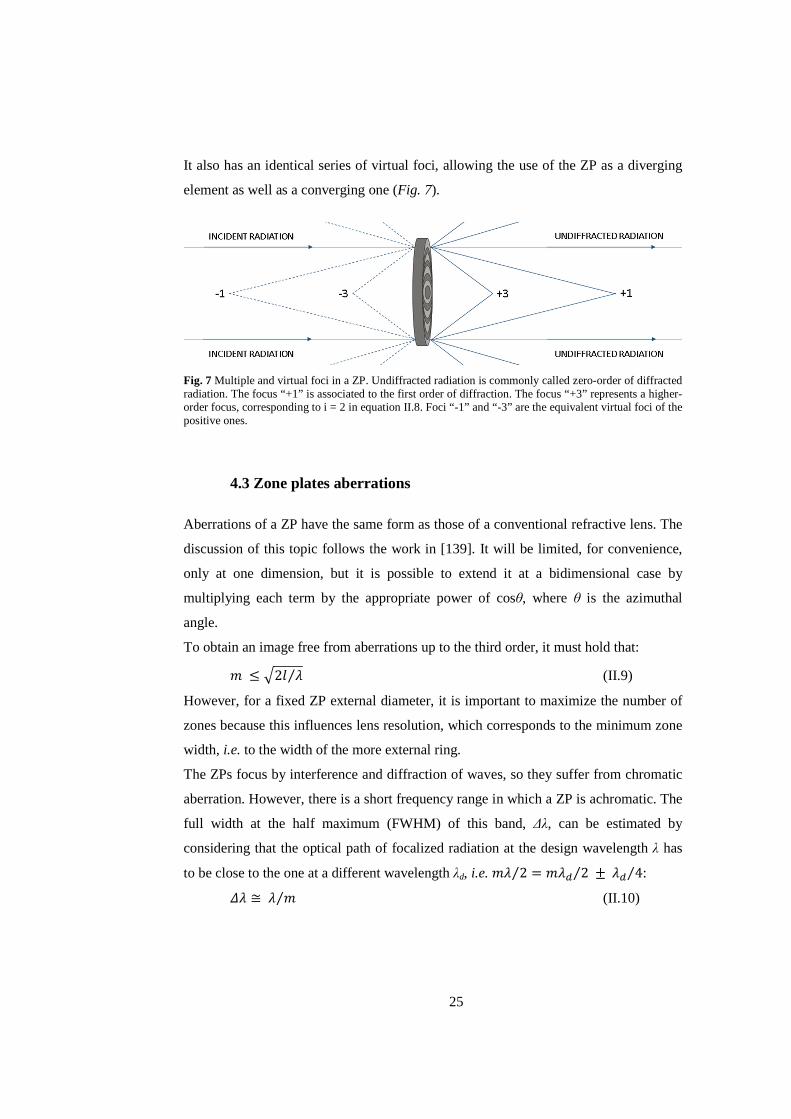
25

It also has an identical series of virtual foci, allowing the use of the ZP as a diverging

element as well as a converging one (Fig. 7).

Fig. 7 Multiple and virtual foci in a ZP. Undiffracted radiation is commonly called zero-order of diffracted radiation. The focus “+1” is associated to the first order of diffraction. The focus “+3” represents a higher-order focus, corresponding to i = 2 in equation II.8. Foci “-1” and “-3” are the equivalent virtual foci of the positive ones.

4.3 Zone plates aberrations

Aberrations of a ZP have the same form as those of a conventional refractive lens. The

discussion of this topic follows the work in [139]. It will be limited, for convenience,

only at one dimension, but it is possible to extend it at a bidimensional case by

multiplying each term by the appropriate power of cosθ, where θ is the azimuthal

angle.

To obtain an image free from aberrations up to the third order, it must hold that:

m 2n ⁄ (II.9)

However, for a fixed ZP external diameter, it is important to maximize the number of

zones because this influences lens resolution, which corresponds to the minimum zone

width, i.e. to the width of the more external ring.

The ZPs focus by interference and diffraction of waves, so they suffer from chromatic

aberration. However, there is a short frequency range in which a ZP is achromatic. The

full width at the half maximum (FWHM) of this band, ∆λ, can be estimated by

considering that the optical path of focalized radiation at the design wavelength λ has

to be close to the one at a different wavelength λd, i.e. m 2 B m & 2 & 4⁄⁄⁄ :

≅ m⁄ (II.10)

26

Off-axis aberrations can be considered as a sum of coma, astigmatism and field

curvature. If α is the angle between the principal ray and the optical axis, off-axis

aberrations become manifest when their sum equals 4⁄ :

kl$ 2n# − 3kl# # 4⁄ n B⁄ 4⁄ (II.11)

Fixing the value of a ZP external radius, the first zone diameter increases as the

number of zones decreases. Thus, the angle between the principal ray and the optical α

is high when the number of zones is low. In this condition, the second term of the sum,

linked to astigmatism and field curvature, is dominant on the first term, due to coma

aberration. The half field over which the image is diffraction limited can be set by

B e3mjyp (II.12)

If coma dominates, the half field can be evaluated by

B em nj⁄ yp e1 2mj⁄ (II.13)

It is worth pointing out that formulas II.9-13 describe wave front aberrations in terms

of deviation from a diffraction-limited situation, as analyzed in [139], and not in terms

of distribution of light according to geometrical optics.

5. Materials for terahertz diffractive devices

In most cases, THz sources emit radiation with a power in the order of tens of

microwatts. Thus, lenses for THz waves should not absorb incoming radiation.

Moreover, they should be hydrophobic because water exhibits several absorption bands

in the THz spectrum. High resistivity floating zone silicon (HRFZ-Si) is a single-

crystal silicon, with a resistivity exceeding 10 kΩ/cm. Below 1.5 THz, silicon

resistivity is important because the presence of carriers due to impurities deeply

influences absorption coefficient. In THz range, HRFZ-Si shows a refractive index

essentially constant and equal to 3.418, which changes less than ±0.001 for frequencies

between 100 GHz and 2 THz [140]. In the same frequency range, absorption

coefficient is less than 0.05 cm-1.

The THz high refractive index of the HRFZ-Si allows for thin devices. However, the

high cost and crystalline nature of the material makes it suitable only for some

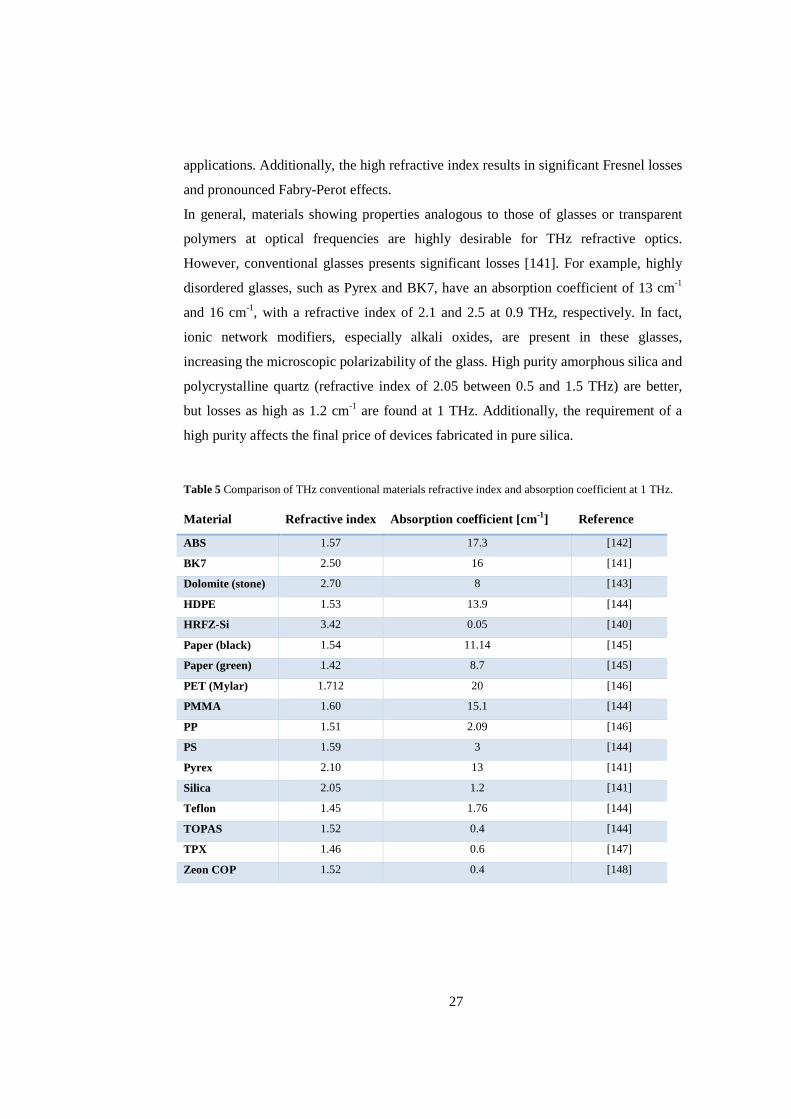
27

applications. Additionally, the high refractive index results in significant Fresnel losses

and pronounced Fabry-Perot effects.

In general, materials showing properties analogous to those of glasses or transparent

polymers at optical frequencies are highly desirable for THz refractive optics.

However, conventional glasses presents significant losses [141]. For example, highly

disordered glasses, such as Pyrex and BK7, have an absorption coefficient of 13 cm-1

and 16 cm-1, with a refractive index of 2.1 and 2.5 at 0.9 THz, respectively. In fact,

ionic network modifiers, especially alkali oxides, are present in these glasses,

increasing the microscopic polarizability of the glass. High purity amorphous silica and

polycrystalline quartz (refractive index of 2.05 between 0.5 and 1.5 THz) are better,

but losses as high as 1.2 cm-1 are found at 1 THz. Additionally, the requirement of a

high purity affects the final price of devices fabricated in pure silica.

Table 5 Comparison of THz conventional materials refractive index and absorption coefficient at 1 THz.

Material Refractive index Absorption coefficient [cm-1] Reference

ABS 1.57 17.3 [142]

BK7 2.50 16 [141]

Dolomite (stone) 2.70 8 [143]

HDPE 1.53 13.9 [144]

HRFZ-Si 3.42 0.05 [140]

Paper (black) 1.54 11.14 [145]

Paper (green) 1.42 8.7 [145]

PET (Mylar) 1.712 20 [146]

PMMA 1.60 15.1 [144]

PP 1.51 2.09 [146]

PS 1.59 3 [144]

Pyrex 2.10 13 [141]

Silica 2.05 1.2 [141]

Teflon 1.45 1.76 [144]

TOPAS 1.52 0.4 [144]

TPX 1.46 0.6 [147]

Zeon COP 1.52 0.4 [148]

28

Therefore, there is a need of alternative materials showing the following properties: (i)

low absorption losses, (ii) suitable refractive index, typically 1.4 - 1.7 to limit Fresnel

losses, (iii) no dispersion, (iv) hydrophobicity, to prevent absorption of atmospheric

vapor; (iv) processability, also in limited volumes for low cost affordable components.

A few polymers have been considered in the literature to fulfill some of these

requirements. Between polymeric materials, there are, for example, high-density

polyethylene (HDPE) [149], polytetrafluoroethylene (PTFE) or Teflon [150],

polymethylpentene (TPX), TOPAS [151], and Zeonex® [148], [152] , two cyclo-olefin

polymers.

Currently, 3D printable materials are employed in the low-THz spectrum, like HDPE,

acrylonitrile butadiene styrene (ABS) or other plastics [142]. Paper [145], [153] and

natural stone [143] are interesting alternatives in very dry environments where water

absorption is not an issue. In Table 5 a comparison of refractive index and absorption

coefficient value, between the discussed materials, is presented.

In the design of ZPs and, in general, of lenses for THz frequencies, the choice of the

material is often influenced by the refractive index value. A high refractive index

increases Fresnel losses due to the huge difference of refractive index between the lens

material and air. In this situation, an antireflection coating is needed. These coatings, in

their simplest form, are thin films with two main characteristics: (i) their refractive

index is equal to the square root of the refractive index of the material to be coated; (ii)

their optical thickness corresponds to the ¼ of a chosen wavelength that will determine

an antireflection operative band. This means that an ideal antireflection coating has an

optical thickness of 75 µm at a frequency of 1 THz. Assuming the lens material is

HRFZ-Si (refractive index of about 3.418), the coating material needs to have a

refractive index of 1.849 and a physical thickness of 40.56 µm. Such material should

also have low absorption at the operating wavelength. Moreover, the deposition

process of the antireflection coating has not to introduce water molecules in the

materials because water induces high THz absorptions.

Polymeric materials with a refractive index lower than 2 are often convenient choices

as THz devices substrates. In this situation, losses due to material absorption have to be

as low as possible. In fact, in most applications, the materials thickness has to be set

proportional to the wavelength in the medium (i.e., ∝ ⁄ , where is the

wavelength in the vacuum and n is the material refractive index). Thus, as low the

29

refractive index is as high the thickness of the structure will be, inducing an increment

of absorption losses. The preferred range of refractive index for the UV-VIS-IR-THz

is, usually, between 1.4 and 1.7.

6. Fabrication methods and techniques

Until the 1960s, lens technology was essentially based on three fabrication techniques:

cutting, grinding and polishing. The main reason is that lenses were mainly

manufactured for optics and were made of glass. A grinding process allows for

obtaining a surface profile that is as close as possible to the desired shape. A final

surface quality with tolerances in the nanometer range, i.e. deeply sub-wavelength, can

be reached by polishing, which is a mechanical or chemical process. This level of

control is needed to avoid scattering induced by roughness. The optimized form of

these techniques is still used today for creating macroscopic devices with an excellent

surface quality, in absence of micrometric features.

Meanwhile, with the massive progress of semiconductor processing and

photolithografic techniques, (i) the mass production, (ii) the integration of different

elements in the same device, and (iii) a reduction of production expenses became

feasible. However, until 1960s, the minimum feature size was of the order of tens of

micrometers [154].

For all these reasons, the first method to produce a ZP for optical applications was to

draw a ZP on a white sheet of paper, filling alternate zones with black. Its photograph

negative works as a ZP device [113]. This technique has serious limitations linked to

the quality of the photographic film. Sizes and other characteristics of silver salt

crystals and the quality of emulsion in the photographic film determine the sensitivity,

contrast and resolution of the negative image. For example, a Velvia RVP100 from

Fujifilm has fundamental particles between 200 nm and 2 µm of diameter and a

corresponding film resolution of about 8 µm [155], which is more than 10 times higher

than the optical wavelength.

It was only during 1980s that standard lithography became to offer feature size of

about one micrometer. Moreover, dry etching techniques started to be employed to

make micro-optical devices like, in particular, diffractive optical elements in glass or

30

silicon. Lithography and etching are consolidated steps in ZP fabrication, but some

issues remain in the fabrication of diffractive optics [156]: “The simplicity of repeated

masking and etching makes it possible to fabricate complex binary optical elements

cheaply and in volume, but the manufacturing technique does leave its traces in one

significant drawback. It produces not the curved and angled surfaces of conventional

optics but rather a series of flat steps that approximates the desired shape. Deviations

from the ideal shape scatter light out of its intended path. Losses of even 5 percent at

the surface of each binary optical element can seriously degrade the performance of

optical trains containing half a dozen elements or more.”

In recent years, technology has definitely entered in the era of sub-micrometer features.

The ZPs for X-rays or extreme ultraviolet radiation are, now, able to nano-focus waves

by means of novel diffractive optical elements, such as photon sieve and modified

Fresnel ZP [157].

Another revolution is currently undertaken: 3D printing manufacturing. Cutting,

grinding, and polishing, such as photolithography and etching are subtractive methods

that remove unwanted material to give a final device. The 3D printing is an additive

method, because it fabricates a device layer by layer. It also has the great advantages to

use a compact hardware and to be computer-controlled and integrated with several

simulation softwares.

All discussed techniques are also well established for the fabrication of diffractive

elements in the THz range. In particular, 3D-printing prototyping is often suitable at

THz [151], [158], [159] because, in line of principle, only roughness higher than 10⁄

can interfere with lens properties. It gives more tolerances than fabrication constrains

in optics or X-rays regions. However, currently, materials suitable for 3D printing have

absorptions at central THz frequencies larger than cyclo-olefins or HRFZ-Si [142].

Such absorptions could compromise lenses performance in that applications in which

THz power is an important feature to preserve.

Another strategy for mass production of THz lenses is micro-powder compression

[98]. This technique is very fast and cheap, but lens properties are not exactly

repeatable, because they could locally change from device to device according to

impurities and material powder distribution.

31

CHAPTER III

Methods for numerically design and fabricate polymeric zone plates

1. Introduction

Zone plates are able to focus electromagnetic radiation by diffraction. They are highly

chromatic lenses and are suitable for all those applications in which the main issues are

(i) the achievement of the lowest radiation attenuation in the focal area, (ii) a good

resolution, and (iii) the integration in compact devices.

Phase-reversal ZPs can be a good choice in the THz range. In particular, binary ZPs

have a low diffraction efficiency (of about 40.5%), but are simple to fabricate. On the

other hand, in multilevel ZPs several rings of different thickness and width are

fabricated as sub-zones. These sub-zones all together perform the phase shift of two

adjacent rings in a binary ZP, and an efficiency of 68.4% or more is obtained, as

illustrated in Fig. 8. In a multilevel ZP with four levels, diffraction efficiency is 81.1%.

However, manufacturing becomes complicated as the number of levels increases.

Moreover, multilevel ZPs are more susceptible to damage than binary ZPs.

For these reasons, a new configuration of ZP in the THz range has been devised and

investigated in this work. It consists of a stacked version of two binary ZP. In general,

when two ZPs are placed within each other’s near field zone, they act as a single lens.

For this reason, in this work, this kind of ZP has been realized on the same device, by

reproducing a binary ZP on both sides of a substrate plate. This configuration will be

called ‘phase reversal double-sided ZP’, or simply ‘double-sided ZP’.

32

Fig. 8 Diffraction efficiency by increasing the number of discretization of zones phase step [117].

A ZP stacking and a double-sided ZP have been already employed for focusing X-rays

with the aim to increase the field intensity in the first-order focus area [160]. However,

this device has not been considered yet at THz frequencies. The main difference

between stacked or double-sided ZPs known in the scientific literature and this new

one for THz applications is in the zone thickness, i.e. in the phase shift introduced by

zones. The THz double-sided ZP is made by two binary phase reversal ZPs and each

ZP introduces a π/2 phase difference between polymeric material and air. The idea is

that the first ZP shifts the phase of π/2 and the second ZP, placed in previous ZP near

field, introduces another shift of π/2. In this way, the total phase shift of the incident

radiation at the end of double-sided ZP stays π. On the contrary, in stacked and double-

sided ZPs from literature, the total retardation at the end of the device is higher than π.

Moreover, the ZPs for X-rays in the stacked configuration are sometimes metallic

Fresnel ZP and not dielectric phase reversal ZPs.

From now on, we shall refer to binary and multilevel ZPs by assuming they are all

phase reversal binary and multilevel ZPs, for need of brevity. The aim of the present

work is to investigate the focusing properties of a THz double-sided ZP and to

compare its lens behavior with a binary ZP and a four-levels (multilevel) ZP. For doing

that, a thorough numerical investigation of the proposed lenses is needed for the design

and their optimization (Sec. 3). On the basis of numerical results, some ZP prototypes

have been fabricated by employing a suitable technique, as discussed in section 4.

33

2. Numerical methods in computational electromagnetic

Any numerical analysis or optimization has the goal to achieve a sufficient accuracy

with a minimum effort, where the effort is usually the computational cost in terms of

computational time and memory requirements.

In general, there are several aspects that could influence the choice of a computational

method: (i) the electromagnetic problem may involve boundary conditions difficult to

treat; (ii) materials could have nonlinear, anisotropic, or non-homogeneous

characteristics; (iii) the problem could have a length scale of several wavelengths in

vacuum; (iv) the problem could contain a combination of length scales due to its

physics or geometry; (vi) the excitation can be non-stationary; (vii) the material can be

frequency dispersive [161].

In some situations, one method could be competitive for a portion of the problem and,

at the same time, another algorithm could be better suited for the remaining parts. In

these situations, for example, a so-called hybrid method could be developed and

applied. However, such methods are challenging to construct while preserving all

important properties of Maxwell’s equations.

For modeling electrically large systems, i.e., systems in which the extension in the 3-D

space corresponds to many wavelengths, it could be useful to compare how the number

of floating-point operations and the memory requirements scales with the

electromagnetic frequency f. Table 6 summarizes the scaling with frequency for a

given computational domain size for two main class of computational methods.

Table 6 Dependence of the number of operations to the frequency f and the number of iterations Nit [161].

Differential equation methods Integral equation methods 2-D space f 3 Nit f

2 3-D space f 4 Nit f

4

Differential equation methods solve Maxwell’s equations in their differential

formulation. They can be used for computations in frequency-domain as well as in

time-domain. This choice does not influence the relationship between the number of

operations and the frequency of the problem. However, the time-domain method

requires a higher computation time than the frequency-domain method but it returns a

complete frequency spectrum analyses. Conversely, a standard frequency-domain

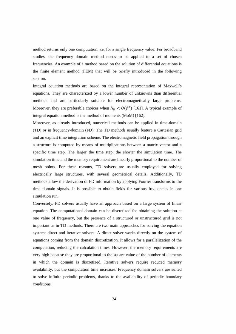
34

method returns only one computation, i.e. for a single frequency value. For broadband

studies, the frequency domain method needs to be applied to a set of chosen

frequencies. An example of a method based on the solution of differential equations is

the finite element method (FEM) that will be briefly introduced in the following

section.

Integral equation methods are based on the integral representation of Maxwell’s

equations. They are characterized by a lower number of unknowns than differential

methods and are particularly suitable for electromagnetically large problems.

Moreover, they are preferable choices when < e#j [161]. A typical example of

integral equation method is the method of moments (MoM) [162].

Moreover, as already introduced, numerical methods can be applied in time-domain

(TD) or in frequency-domain (FD). The TD methods usually feature a Cartesian grid

and an explicit time integration scheme. The electromagnetic field propagation through

a structure is computed by means of multiplications between a matrix vector and a

specific time step. The larger the time step, the shorter the simulation time. The

simulation time and the memory requirement are linearly proportional to the number of

mesh points. For these reasons, TD solvers are usually employed for solving

electrically large structures, with several geometrical details. Additionally, TD

methods allow the derivation of FD information by applying Fourier transforms to the

time domain signals. It is possible to obtain fields for various frequencies in one

simulation run.

Conversely, FD solvers usually have an approach based on a large system of linear

equation. The computational domain can be discretized for obtaining the solution at

one value of frequency, but the presence of a structured or unstructured grid is not

important as in TD methods. There are two main approaches for solving the equation

system: direct and iterative solvers. A direct solver works directly on the system of

equations coming from the domain discretization. It allows for a parallelization of the

computation, reducing the calculation times. However, the memory requirements are

very high because they are proportional to the square value of the number of elements

in which the domain is discretized. Iterative solvers require reduced memory

availability, but the computation time increases. Frequency domain solvers are suited

to solve infinite periodic problems, thanks to the availability of periodic boundary

conditions.

35

A summary of the main subdivisions of the computational electromagnetic problems is

presented in Fig. 9. In the next section, such methods are discussed in the specific

context of the numerical design of diffractive lenses.

Fig. 9 Overview of the numerical approaches to the electromagnetic problems.

3. Numerical investigation of zone plates for terahertz focusing

Numerical simulations are performed with the aim to take into account material losses

and geometrical tolerances due to the ZP fabrication process (for details about

fabrication, see Ch. III Sec. 4). In fact, it is difficult to investigate the ZPs behavior in

presence of such constrains by only theoretical formulas presented in chapter II section

4.

The ZPs are simulated by COMSOL Multiphysics® [163], a commercial software

which employs a finite element method (FEM) of simulation in the FD. All ZPs

investigated have a radial symmetry: it makes it possible to simulate the full-wave

propagation through the lens structure employing a simplified 2D-axisymettric model.

After the ZP, a free space 50 mm long is accounted for wave propagation. At the

frequency of 1 THz, thanks to the radial symmetry, the computational domain is a 2-D

36

space of about 43 × 167 , where is the wavelength in the vacuum. For this

reason, a workstation with 64 GB of main RAM has been needed for performing the

ZPs numerical simulations.

In a FEM, the object under investigation is divided into subdomains. Each subdomain

is described by a set of simple equations. All these equations are, then, recombined

into a global system of equations that is solved starting from initial values of the whole

system and taking into account boundary conditions of the electromagnetic problem.

Moreover, for validating the 2D-axisymmetric assumption, the 2-D FEM simulation

has been compared with a 3-D full-wave simulation by means of another commercial

software, CST Microwave Studio® [164], employing a finite integration technique

(FIT) to numerically solve electromagnetic field problems in TD.

The major advantage of a FEM is its high geometrical flexibility for modeling complex

geometries with discontinuous media parameters. However, FEM discretization

requires large storage memory due to the number of unknowns. On the contrary, a FIT

is simple to implement and it is able to perform an efficient parallel computing.

However, the time step depends on the grid size. For those applications, in which a

very small mesh size is required, the time step becomes significantly small. It results in

longer simulation time.

It also has to take into account that COMSOL Multiphysics® employs a method in FD,

while in CST Microwave Studio® a TD solver is selected for lenses simulation. As

discussed above, with TD computation, only one simulation is required for a

broadband solution with a fine frequency resolution. However, diffractive lenses are

chromatic devices and do not need of broadband studies, which are time consuming.

About RAM occupancy, for example, in a 8 GB RAM workstation, it is possible to

solve an electromagnetic problem of about 40 wavelengths in each directions by

employing a TD technique, while a frequency method is restricted to about 10

wavelengths [165].

In ZP lenses design, some numerical studies have been considered: (i) the choice of the

right material; (ii) the choice of the number of zones; (iii) the behavior at frequencies

different, but close, to the design one; (iv) the comparison with a conventional

refractive lens.

37

3.1 Material choice

The starting point of the numerical study is the choice of a suitable material. The only

commercially available binary ZPs are made of HRFZ-Si [166]. It is a material with

very low absorption at THz and simple to process by photolithography and etching.

However, wafers are expensive due to energy and time consuming crystal growth

process. Furthermore, 43.9 µm deep trenches need to be etched to provide π phase

difference at 1 THz. These are usually made by deep reactive ion etching (RIE) in a

suitable plasma (typically a mixture of CF4 and SF6), which is material, time and

energy intensive process. Moreover, its refractive index of 3.416 at 1 THz is quite far

from the refractive index of air, which is close to 1. Hence, a ZP made of HRFZ-Si

needs of an antireflection coating to limit Fresnel losses. The solution devised in this

work employs a polymeric material (i) with a lower refractive index, (ii) lower cost,

(iii) easy to process, and (iv) with very low absorption at 1 THz. Zeonex® E48R is a

specialty cyclo-olefin by Zeon Corporation which satisfies the above requirements. In

fact, it has a refractive index of 1.516 at 1 THz. A 2 mm thick slab of this material has

a transmittance larger than 0.8 up to 1 THz. In practice, it behaves in the THz range

nearly as well as glass does in the visible range.

However, minor absorption losses do exist at the targeted frequency. So a pure phase-

control behavior cannot be assumed. Hence, a FEM simulation has been performed in

order to compare the focusing properties of two binary ZPs with same geometry, but

made by different materials: one by Zeonex® and one by HRFZ-Si. Both Fresnel and

absorption losses are fully accounted for either cases.

3.2 Number of zones

Another important characteristic of a ZP is the number of zones. It influences the focal

length as well as the focal spot resolution. A binary ZP, with a fixed external diameter

of 25.4 mm corresponding to a typical size for common 1” lens holders, is evaluated

by changing the number of rings from 9 to 42. All these FEM simulations are

performed at 1 THz, which corresponds to a wavelength of about 300 µm. All ZPs are

excited under the same condition of plane wave illumination. When a binary ZP is

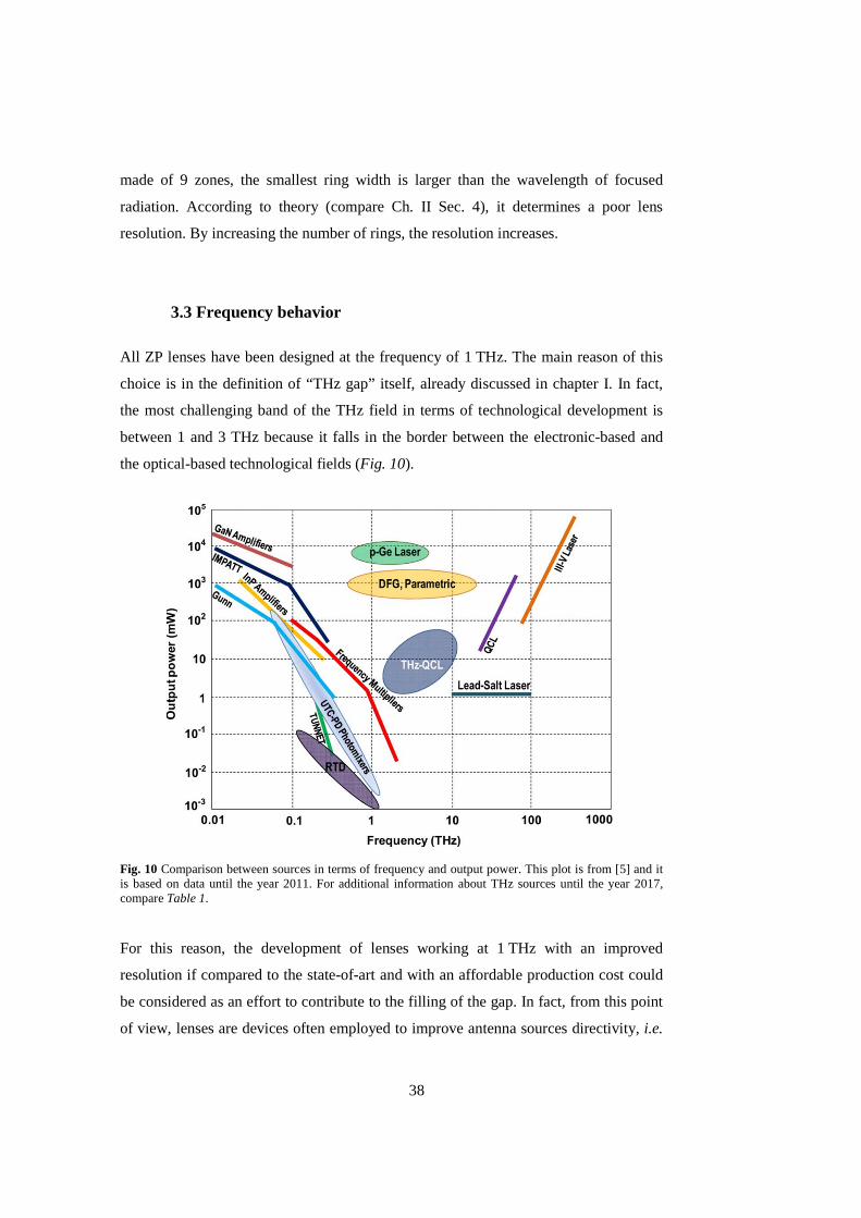
38

made of 9 zones, the smallest ring width is larger than the wavelength of focused

radiation. According to theory (compare Ch. II Sec. 4), it determines a poor lens

resolution. By increasing the number of rings, the resolution increases.

3.3 Frequency behavior

All ZP lenses have been designed at the frequency of 1 THz. The main reason of this

choice is in the definition of “THz gap” itself, already discussed in chapter I. In fact,

the most challenging band of the THz field in terms of technological development is

between 1 and 3 THz because it falls in the border between the electronic-based and

the optical-based technological fields (Fig. 10).

Fig. 10 Comparison between sources in terms of frequency and output power. This plot is from [5] and it is based on data until the year 2011. For additional information about THz sources until the year 2017, compare Table 1.

For this reason, the development of lenses working at 1 THz with an improved

resolution if compared to the state-of-art and with an affordable production cost could

be considered as an effort to contribute to the filling of the gap. In fact, from this point

of view, lenses are devices often employed to improve antenna sources directivity, i.e.

39

lenses are able to concentrate the power density of the emitted radiation in a single

direction.

Moreover, ZPs have a design perfectly scalable at almost every frequency value, as

discussed in chapter II. Thus, the choice of a working frequency of 1 THz could be

also considered as the select of a round number for easily conveying the design

concept. Some examples of devices based on the ZP and operating at frequency values

different from 1 THz can be found in chapter VII.

A method in the FD, such as the one employed by COMSOL, has been selected for the

numerical analysis of the ZPs at the frequency of 1 THz. It is a reasonable choice for

evaluating the behavior of diffractive planar elements, which are highly chromatic and

work in a narrow band of frequencies, centered in their design frequency (compare

Ch.II Sec. 4.3). However, an additional investigation of ZPs behavior from 500 GHz to

1.2 THz with a step of 100 GHz has been performed.

3.4 Comparison with a conventional refractive lens

The behavior of a refractive lens and a binary ZP can be numerically obtained by FEM

simulations. It will help to understand focusing properties of a ZP by directly

comparing it with a conventional refractive lens. The refractive and the diffractive

devices have both the same maximum thickness of 2 mm and are illuminated by a

plane wave at the frequency of 1 THz.

4. Fabrication

The fabrication process has been selected on the base of the ZP design and the

numerical optimization process. In optics, the lens fabrication can be operated by

employing machining or non-machining techniques [167]. Single point diamond

turning (SPDT), slow tool servo (STS), fast tool servo (FTS), and three-axis micro-

milling (MM) are machining techniques able to produce high quality optical devices.

In particular, SPDT is a two-axis lathe technique and needs a manual positioning over

the third axis. STS and FTS are fully automated techniques, but are limited by diamond

40

tool relief angle. MM overcomes most limitations on lens geometries. It makes it

possible to produce several shapes including aspheres, asymmetric lenses and other

freeform optics, but it is a slow technique. These techniques can be compared to non-

machining ones (see Table 7), such as grayscale lithography, thermal reflow, inkjet

printing, and non-cutting techniques, as laser direct writing and deep lithography with

protons.

Table 7 Comparison between lenses fabrication techniques [167].

Fabrication technique Automatic Arbitrary

shapes Sag limit

(mm) Dimensions limit (mm)

Edge slope (°)

Fabrication rate

SPDT No Yes No No 0-90 5-25 mm/min

STS Yes Yes No No 0-40 0.1

mm/min FTS Yes Yes 0-6 No 0-40 0.25 mm/min

MM Yes Yes No No 0-90 0.4-1.25 mm/min

Thermal reflow

Yes No 0-2 0.005-2 0-90 0.5 min

Microjet printing

Yes No 0-5 0.02-5 0-180 0.5-5 mm/min

Grayscale lithography

Yes Yes 0-0.06 >0.0006 0-90 1.33 min

A three-axis milling technique is chosen for ZPs fabrication because it offers a shape

control with tolerances suitable for THz frequencies. In fact, ZPs are designed for

working at a wavelength of 300 µm and errors in geometrical dimensions lower than

30 µm do not influence lenses performance. Furthermore, only few ZP prototypes are

fabricated and the slow rate of the milling process is not an issue for research purposes.

For these reasons, all polymeric ZP lenses subject of this work have been fabricated by

milling a 2 mm thick slab of Zeonex®. In particular, it is a subtractive method of

fabrication, in which a rotatory cutter removes material from a workpiece on fixed

structure. Milling cutters can advance in every direction and at every angle. Cutters can

be of very different sizes and shapes, according to the material and the final machined

profiles. A set of high-speed steel (HSS) milling cutters with end diameters from 1.4

mm to 0.2 mm have been employed for THz ZPs manufacturing (Fig. 11).

This technique can produce structures with a tolerance of about 10 µm, in the plane

perpendicular to the cutter axis, and of about 5 µm, in the parallel direction.

41

Fig. 11 Milling cutters used throughout this work for ZP fabrication. The diameter of each cutter is indicated.

42

CHAPTER IV

Numerical investigation and fabrication of terahertz zone plates

1. Material choice

Two binary ZP made of different materials (i.e., one of Zeonex E48R and one of

HRFZ-Si) are numerically compared, as shown in Fig. 12. The two ZP have same

geometrical constrains except for zone thickness, which depends on material refractive

index. Material losses, already discussed in Ch. II Sec. 5, are included.

Fig. 12 Comparison between the focusing properties of a binary ZP made of a) Zeonex E48R and b) HRFZ-Si. A plane wave of 1 V/m is incident perpendicularly to both lenses. The E-field modulus is represented in a 3-D space, filled by air. Both ZPs, ending at z = 2 mm, have same external diameter, number of zones and thickness.

43

Most of the focusing parameters are the same for both ZP. From Fig. 13, ZPs have a

focal length of 40 mm, for the primary focus. They also show two secondary foci at

10 mm and 17.5 mm from their external surface. The ZPs depth of field can be

considered as the full width half maximum (FWHM) of the curves representing the

square module of the E-field at 1 THz along the optical axis. It is equal to 5.3 mm ±

0.1 mm for both lenses.

The main difference is in the value of the E-field square modulus: at the focus of the

Zeonex® ZP, it is twice as high as for the HRFZ-Si ZP, thanks to the lower refractive

index of the polymer and lacks of antireflection coatings. Zeonex E48R is affordable,

easy to processing, has low absorption at THz, and does not need a coating for

avoiding reflection losses due to refractive index mismatch with air. It is perfectly

suitable for the fabrication of THz devices and, in this situation, it results a better

choice than HRFZ-Si.

Fig. 13 Comparison between the focusing properties of a binary ZP made of Zeonex E48R (blue line) or HRFZ-Si (red line). A plane wave of 1 V/m is incident perpendicularly to both lenses. z-axis is the perpendicular one to the ZP plane. z = 0 mm corresponds to the end of the lens, where a free space, filled by air, starts. Both ZPs have the same external diameter, number of zones and thickness.

2. Number of zones

The number of zone is chosen by taking into account: (i) resolution, linked to the width

of the most external zone, (ii) easy fabrication, and (iii) losses due to a high number of

zones with dimensions comparable to operation wavelength. Moreover, as discussed in

Ch. II Sec. 4.3, there is a limit in the number of zones due to the introduction of third

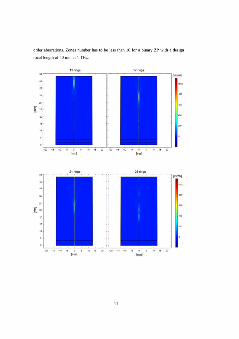
44

order aberrations. Zones number has to be less than 16 for a binary ZP with a design

focal length of 40 mm at 1 THz.

45

Fig. 14 Focusing behavior of a binary ZP with a fixed diameter and an increasing number of ring zones. A plane wave of 1 V/m is incident perpendicularly to the lens. All color maps represents ZP central section and optical axis, z, where THz radiation, coming from z = 0, is focused.

Because of these constrains, a suitable number of zones is 13. In fact, the resolution

decreases when the number of zones is below 13, while the lens introduces losses and

aberrations above it.

A numerical study of a binary ZP is performed by fixing the external diameter at 25.4

mm and increasing the number of zones, with the aim to elucidate how the number of

zones can affect the ZP focusing behavior. The THz power density in the plane

perpendicular to the lens and passing through the optical axis is shown in Fig. 14. The

focal length decreases by increasing the zone number, but the ZP is no longer able to

focus incident radiation.

3. Frequency behavior

The ZPs are highly chromatic lenses. Their frequency behavior depends on the number

of rings and on the central frequency at which they work (for more details, see Ch. II),

but it is independent from the ZP configuration, i.e. binary, multilevel or double-sided.

The ZP configuration influences the lens resolution and its diffraction efficiency. The

numerical study of the multilevel ZP designed for operation at 1 THz is presented in

46

Fig. 15 for the frequency band 0.5 – 1.1 THz, which has been sampled with a step of

100 GHz. Chromatic behavior is confirmed: each wavelength of the incident THz

radiation is focused at a different focal length, with a different intensity in focal area,

and with a different depth of field.

For this reason, a ZP can be also seen as a spatial and frequency filter [168].

Fig. 15 Frequency behavior of a multilevel ZP from 0.5 THz to 1.1 THz with a step of 0.1 THz. z-axis is the perpendicular one to the ZP plane. Minor peaks in the square modulus of the E-field for z from 1 mm to 3 mm are related to multiple reflections within the 2 mm thick slab in which ZP is fabricated (no antireflection coating is used). For z < 1 mm and z > 3 mm, a free space filled by air for THz waves propagation is considered.

4. Comparison with a conventional refractive lens

A biconvex lens is numerically studied for evaluating the behavior of a ZP in focusing

THz radiation instead of a more conventional refractive lens. The biconvex lens is

designed with the constraint that its maximum thickness is equal to ZP thickness, i.e.

2 mm. Biconvex lens material is Zeonex E48R and material losses are taken into

account, as done for the simulation of the multilevel ZP.

47

Fig. 16 Frequency behavior of a biconvex refractive lens from 0.5 THz to 1.1 THz with a step of 0.1 THz. z -axis is the lens optical axis. Extremely short peaks in the square modulus of the E-field for z from 2 mm to 4 mm are related to few multiple reflections inside the lens. For z < 2 mm and z > 4 mm, a free space, filled by air, for THz waves propagation is considered.

As can be seen by comparing Fig. 15 and Fig. 16, a biconvex lens is able to focus THz

waves with different wavelength at the same focal length. Moreover, it has a higher

focal depth, which is more than 9 mm at 1 THz instead of 5.3 mm of the multilevel ZP.

On the other side, the multilevel ZP is able to concentrate THz radiation in the focus

with an intensity that is twice as high as for a biconvex lens. It makes ZPs a more valid

lens than a conventional refractive lens for THz narrowband applications.

5. Conclusions about the numerical investigation and zone plates

fabrication

As a result of the numerical studies already discussed, a ZP configuration which

consists of 13 Fresnel zones has been selected as a promising diffractive lens structure.

Moreover, the Zeonex E48R has been revealed as a very suitable material for THz

lenses.

The ZP lenses prototypes are fabricated with the 3-D MM technique described in

chapter III section 4 and are shown in Fig. 17. They have an external diameter of

25.4 mm (1 inch) and consist of 13 rings for the two binary configurations (b) and c) in

48

Fig. 17) and 28 rings at four different levels of deepness for the multilevel ZP (a) in

Fig. 17).

Fig. 17 Fabricated ZP lenses: a) multilevel ZP, b) double-sided ZP, c) binary ZP. The little roughness perceived in visible light is introduced by milling process, but it does not affect the lens behavior at THz because it is several orders of magnitude below the wavelength at 1 THz.

In the following chapter, some methods required for the experimental characterization

of such ZP prototypes will be outlined and deeply discussed.

49

CHAPTER V

Methods for the experimental characterization of diffractive lenses at terahertz frequencies

1. Introduction

The numerical studies discussed in the previous chapter have been instrumental in the

design of ZPs with the specific aim of elucidating the elements that contribute to the

increase of their performances with respect to currently used diffractive lenses. It is

worth reminding that, in contrast to lenses designed for the visible range where losses

are comfortably neglected, for THz range these must be taken in the account. Hence,

the lossless formula provided in chapter II section 4 are not fully adequate.

Nevertheless, simulations could not fully describe the real operational conditions. In

fact, some idealizations are usually necessary to keep the problem within

computational manageable limits. In the specific case, a linearly polarized plane wave,

impinging normally to the lens, is used as excitation both in the analytical and

numerical problems discussed in the previous chapters. On the other hand, the

experimental conditions are far less simple because the wavefront of the incident

radiation is not an ideal plane wave. Hence, the lens performance cannot be confirmed

without a prior knowledge of this wavefront.

In this chapter, the calibration of the set-up available for ZPs characterization is

presented after a brief overview on experimental set-ups for THz measurements. The

calibration consists in the acquisition of shape, dimensions and intensity distribution of

the THz beam emitted by the photoconductive antenna and its hemispherical silicon

lens. As a matter of fact, upon specific requests made to the instrument manufacturers,

they explicitly replied that the radiation pattern of the emitting THz antenna was

unknown to them. This additional experimental step influenced the way in which it

50

was more convenient to perform the measurements on ZP lenses. Moreover, a detailed

description of the experimental configurations and methods employed in the ZPs

characterization will be outlined.

2. Set-ups for terahertz metrology

In chapter I, several THz sources, detectors and components have been introduced and

discussed. On the basis of them, a variety of set-ups for THz spectroscopy had been

developed from both microwave and optics communities (Fig. 18). The main

distinction that can be operated between available THz spectrometers is between TD

and FD set-ups. In fact, some THz set-ups employ spectroscopic techniques which

allow for conducting measurements directly in the FD via, e.g., frequency sweeping or

broadband exposure. Examples of set-up for measurements in FD are vector network

analyzers (VNAs) or IR-Vis-UV spectrometers. Conversely, measurements in the TD

can be performed: (i) indirectly, via interferometry, as made by Fourier-transform

infrared spectrometers (FTIRs), or (ii) directly, such as the THz TDS, which is based

on a sampling with an ultrafast laser pump-probe configuration [169].

Fig. 18 Overview of the experimental approaches to the THz measurements.

51

2.1 Set-ups employing time-domain methods

The TDS is the premier technique for THz measurements due to its high dynamic

range (compare Table 3 for specifications about the commercially available TDSs) and

its ability to detect both amplitude and phase of the transmitted THz radiation. In

material science, for example, these informations can be translated in the measurement

of the absorptions and the refractive index [170]. However, they could be also useful in

the characterization of quasi-optical devices (introduced in Ch. I Sec. 4.2). Even if a

detailed description of a TDS set-up will be made in section 3, it could be of interest to

anticipate a brief explanation of a pump-probe TDS. The THz TDS system is triggered

by an ultrafast laser with pulses of duration usually shorter than 100 fs. The laser beam

is split into two: the majority of the power is employed in THz generation; a minor

fraction is used as a probe. The probe pulses can be arranged for temporally and

spatially overlapping the THz pulses, in the way to recombine with them on the

detector (coherent detection). The resulting measured signal is proportional to the

product between the probe pulses intensity and the THz field [171].

THz TDS emitters and detectors could be of photoconductive type or of optical

rectification type [170]. Any combination of them between emitter and detector may be

employed; however, commercial set-ups (as the ones compared in Table 3) mostly

have photoconductive emitters and detectors.

The Fourier transform spectroscopy (FTS) operates over a larger bandwidth and has a

higher frequency resolution than TDS. However, it enables only the acquirement of the

optical intensity and its dynamic range is significantly smaller than TDS [170]. The

FTS is an older and more established technique than TDS, but it is employed mainly

for measurements at frequencies above 15 THz.

2.2 Set-ups employing frequency-domain methods

VNAs employ a radically different measurement modality from the TD spectrometers.

In fact, VNAs are usually configured for measuring the complex scattering of

electromagnetic signals impinging on a test device. For doing that, the VNA utilizes

ports, i.e., interfaces through which the signal going to and coming from the element

52

under test can flow. The VNA measures the magnitude and phase of the signals at each

port and operates a ratio of these quantities, presenting the scattering coefficients for a

structure under test. These coefficients are often called scattering parameters or S-

parameters. The measurement of the S-parameters allows a direct computation of other

parameters. For example, the propagation delay through the test object can be obtained

by differentiating the transmission phase with respect to the frequency [171].

The VNAs for THz frequencies are usually instruments with two ports. It means that

they are useful for measuring the reflection and transmission behavior of one-port and

two-port THz structures, such as antennas, filters, amplifiers and signal-transmission

structures. In fact, VNAs are mainly employed for testing devices at THz frequencies,

while TDSs are usually devoted to materials characterization.

Even if the VNAs manage THz radiation in propagation mode through a waveguide

(see Ch. I Sec. 4.1), they can also operate with THz beams in free space. In this

configuration, the VNAs can operate measurements similar to TDSs [172]. A

comparison between a free-space VNA and the TDS performance in the measurement

of the complex relative permittivity in the frequency range 0.22 – 0.33 THz can be

found in [173]. The VNA employs a method in FD and the limitations in the

measurements frequency depend on the waveguide size. Conversely, the TDS operates

in TD and can operate measurements in a broad frequency range. Moreover, VNA time

resolution is worse than TDS and the VNA may result unsuitable for precisely

separating multiple reflections in the material under test. On the other hand, in the low

THz range, the TDS shows a SNR worse than the VNA, resulting in a lower accuracy

of TDS measurements. Authors suggest to select the measurement method by

essentially considering the accuracy and the frequency range of the measurement.

However, according to their data, the maximum difference between the two methods

was less than 0.22 in relative permittivity and less than 0.17 in dielectric loss when a

R1661 glass 486.50.5 µm thick is employed as a test material.

In [174], a VNA operating in waveguide configuration in the frequency band of 0.14 –

0.22 THz and a TDS working at 0.1 – 4 THz are compared measuring the complex

relative permittivity of two petroleum jellies at 0.2 THz. Measurements show an

agreement within the estimated uncertainties for each system. However, authors

underline the importance of the sample material on the measurement accuracy. The

material for the comparison between the two techniques has to be homogeneous (free

53

from air bubbles) and semi-solid (capable of completely filling both a TDS sample cell

and a section of a VNA hollow waveguide). In absence of these qualities, experimental

data from both FD and TD methods are difficult to compare each other due to

measurement artifacts.

3. Terahertz diffractive lenses characterization: measurements set-up

In this work, the available set-up for ZP characterization at the frequency of 1 THz was

a commercial TDS by Menlo Systems (Germany) [175], the TERA K15, a state-of-art

product. It is a compact, fiber-coupled device with a usable range of 0.2 – 3.5 THz

with a maximum frequency resolution of 1.2 GHz. The frequency resolution is limited

by the dynamic range of the delay line. It might be argued that for the characterization

of lenses with a highly chromatic behavior, a FD set-up could represent the most

natural choice. However, as discussed in the previous section, FD and TD techniques

lead to comparable experimental results. Thus, a TD system is also a suitable

alternative, but more efforts have been done in the experiments design and in the

resulting data processing, as it will be deeply analyzed in the following.

The employed TDS set-up consists of a 1560 nm wavelength fiber laser, coupled by

means of a 2.5 m optical fiber patch cord to a photoconductive antenna. At the end of

the fiber, emitted pulses are shorter than 90 fs and imping onto a biased high-resistivity

semiconductor inside the antenna, in correspondence of a gap between two electrodes.

Photons excite electrons across the electronic bandgap of the semiconductor into the

conduction band. Photocarriers generated increase semiconductor conductivity in the

sub-picosecond time scale. Photogenerated current is accelerated by a bias field

applied by electrodes on the semiconductor. Carriers start to recombine, trap, or scatter

emitting radiation with a frequency in the THz range. Subsequently, the conductivity

decreases from sub-picosecond to nanosecond time scale according to the

semiconductor properties [176], [177].

Femtosecond pulses generated by the laser are split off in two beams. The first beam

travels in a fixed distance and excites the emitting antenna. The second beam travels a

variable distance and excites a detector photoconductive antenna. An optical delay line

54

is used to vary the timing of these detection pulses and synchronize them with the

incoming THz radiation [178].

Photoconductive antennas are usually dipole antennas and they are coupled to a

hemispherical HRFZ-Si lens. This lens collects the emitted electromagnetic field and

gives directivity to the beam. A narrow radiated beam is possible thanks to the large

refractive index of HRFZ-Si (compare Ch. II Sec. 5). In fact, total internal reflection

angle of THz rays is low if the difference of refractive index between hemispherical

lens material and air is high. However, radiation patterns of the photoconductive

antenna with silicon lens are frequency dependent. At large distances, only a central

lobe propagates forward with a Gaussian-like distribution. However, it diverges with

an angle proportional to the wavelength: at a fixed distance from the antenna, the

FWHM of the emitted radiation decreases as the beam frequency increases [179].

Fig. 19 Schematic representation of photoconductive antennas in their a) emitting and b) receiving configuration. PI is the photogenerated current.

In the standard configuration of the TDS delivered by Menlo Systems (Fig. 20), the

presence of two convex-plane (L1 and L3) and two plano-convex lenses (L2 and L4),

made by TPX and with a diameter of 38.1 mm (1.5 inches), are useful in most

measurements. The lens L1 has to collimate the beam coming from the hemispherical

lens on the emitting antenna (PAT). The choice of the L1 lens focal length is

fundamental due to the divergent nature of the emitted radiation: the longer the focal

length, the wider the beam diameter at each frequency. The lens L2 has to focus

radiation on the sample; L3 collects the radiation passing through the sample,

collimating the THz beam; L4 focuses again the radiation on a receiving antenna.

55

Receiving THz antennas (such as PAR of Fig. 20) are photoconductive antennas with a

structure close to emitting ones, but they do not receive a biasing from an external

circuit (Fig. 19 b)). The detector is biased by the THz signal itself, focused on the

antenna, where interacts with detection pulses. THz field drives a current between

antenna electrodes. This electrical signal depends on whether the detection pulse

arrives when the electric field of the THz pulse is low or high. A transimpedance

amplifier receives the photogenerated current, which corresponds to the THz field

strength, and amplifies it, converting to a usable voltage.

Fig. 20 Standard configuration of the commercial TDS TERA K15 by Menlo Systems. PAT: photoconductive antenna in transmission mode; L1 and L3: convex-plane lenses; L2 and L4: plano-convex lenses; PAR: photoconductive antenna in receiving mode [180].

As was previously pointed out, the TERA K15 TDS set-up was the only available

instrument for the experimental characterization of the focusing properties of designed

and fabricated ZP lenses. However, ZP design has been numerically studied assuming

the THz excitation as an ideal one: a linearly polarized plane wave. Unfortunately, the

wavefront after neither the TPX lens nor after the hemispherical HRFZ-Si lens is

unknown to the manufacturer of the instrument. Hence, for comparing numerical and

experimental data, it has arisen the need to carefully characterize the radiation emitted

by the photoconductive antenna and collimated by the TPX lens (L1 of Fig. 20). This is

the real excitation of the ZPs.

In the following section, the methods employed for the beam characterization will be

described. These methods have regarded the imaging of the THz beam emitted by the

56

set-up source as well as the THz beam focused by the ZP lens. Thus, they will be

discussed with regard of both experimental situations.

4. Terahertz beam characterization: knife-edge technique

The method employed for the beam characterization is the imaging on a plane

perpendicular to the ZPs optical axis by means of knife-edge measurements. They

consist of the gradual eclipsing of the THz beam by a sharp knife-edge. The blade

translates in the direction perpendicular to the optical axis thus intersecting the beam,

while the PAR measures the total intensity of the unmasked portion of the radiation.

When the beam is spatially described by a Gaussian line shape, the detector measures

an electric field sigmoidal profile along the blade translation direction. The spatial

derivative of the measured signal yields the two-dimensional Gaussian field profile

across the imaging plane and its FWHM represents the focal spot diameter.

4.1 Knife-edge set-up

In every knife-edge measurement, it was made sure that the edge of the blade

employed has a roughness and a waviness well below 1 µm by careful inspection with

a diffraction limited optical microscope (resolution less than 0.3 µm). Smoothness

down to the deepest subwavelength level guarantees that no artifact is introduced by

the blade itself. The blade has been fixed on the top of linear stage and was always

perpendicular to the wave propagation direction. The translation stage carrying the

blade has been bolted onto a graduated rotation stage, which has allowed for setting the

angle at which translation can be operated. The rotation axis has coincided with the

THz set-up optical axis.

The linear and rotation stages from Newport Corporation© [181] are motorized and can

be controlled by a software provided by manufacturer. The linear stage has a weight of

less than 1 kg and moves 25 mm. Rotation stage can rotate above 360° and it is also

possible to manually control it, with a precision of 1°. When stages are driven by the

57

software, they can move with a sensitivity of 0.1 µm, for the linear one, and with a

0.001° resolution and 0.05° absolute accuracy, for the rotation stage.

Knife-edge measurements for the TDS emitted beam characterization have been

performed with the set-up configurations illustrated in Fig. 21. Three planar surfaces

have been imaged. All of them are planes perpendicular to THz waves propagation

direction. Plane 1 (Fig. 21 a)) and 2 (Fig. 21 b)) have been set at 3 mm and 9 mm from

the hemispherical lens on the emitting photoconductive antenna, respectively. Plane 3

(Fig. 21 c)) has been located at the position past the lens L1 where the ZPs will be later

placed.

The blade has been scanned 16.2 mm across plane 1 and 2 with a 0.18 mm step, and

25 mm across plane 3 with a step of 0.125 mm. For each plane, the scans and

acquisitions have been repeated for eight angular positions with a step of 22.5°.

Fig. 21 TDS set-up configurations for the characterization of the THz beam emitted by the lens antenna (PAT). Three planes are imaged by knife-edge technique: a) plane 1, at a distance of 3 mm from the PAT; b) plane 2, at a distance of 9 mm from the PAT; c) plane 3, at the position in which the test ZPs will be located. PAT: photoconductive antenna in transmission mode; L1 and L3: convex-plane lenses; L2 and L4: plano-convex lenses; KE: knife-edge blade; PAR: photoconductive antenna in receiving mode.

In fact, if the focal spot is ideally circular, a knife-edge measurement for only one

angle of scanning is necessary and sufficient for the beam characterization. However,

in this experimental study, both the focal spot and the wavefront of the wave

58

impinging ZPs have been assumed a priori unknown. Hence, an accurate beam

characterization demands repeating knife-edge measurements for different angles

between the knife-edge translation direction and THz field polarization direction.

The ZPs’ focal plane has been characterized employing a modified version of the

knife-edge technique already discussed. The THz TDS set-up is shown in Fig. 22. The

ZP has been illuminated by THz radiation emitted by photoconductive antenna (PAT)

and passing through a collimating convex-plane lens (L1). At a distance matching the

focal length, a razor blade (KE) has been mounted on a linear stage. After the blade,

the uncovered radiation has been collected by a convex-plane TPX lens (L3) and, then,

focused on the receiving antenna (PAR) by a plano-convex TPX lens (L4).

Fig. 22 Schematic representation of a THz TDS for focal spot measurements. PAT: photoconductive antenna in transmission mode; L1 and L3: convex-plane lenses; L4: plano-convex lens; KE: knife-edge blade; PAR: photoconductive antenna in receiving mode.

A practical implementation of this scheme is illustrated in Fig. 23. The ZP has been

positioned on a 1” circular mount and it has been centered with respect to the set-up

optical axis to cut away radiation with a beam diameter larger than 25.4 mm. A

stainless steel razor blade (KE) has been fixed on the translation stage start position, in

which all the emitted radiation at 1 THz arrived on the detector, to an end position, in

which the whole beam was stopped.

In general, when an ideal THz source is assumed, the standard knife-edge set-up

configuration is the most conventional choice for the focal plane imaging. In fact, if the

THz radiation incident on test ZP is uniform, all distortions in the ZP focus spot size,

59

position and shape are introduced only by the ZP lens. On the other hand, the knife-

edge technique could be performed in a different way if the THz radiation impinging

on the ZP shows asymmetries due to reflections in optical path before the test lens. In

this second set-up configuration, the blade is again on the translation stage and linearly

moves, gradually covering the focal spot. However, it is the ZP lens that rotates, while

the blade never changes its angle. The knife-edge always translates with a direction

parallel to the polarization of incident THz radiation. In this way, results do not depend

on set-up asymmetries but only on ZP lens, for every angle of measurement. This

needs only to be carefully centered and normal to the propagation direction.

Fig. 23 Experimental set-up for standard knife-edge measurements. PAT: photoconductive antenna in transmission mode; L1 and L3: convex-plane lenses; L4: plano-convex lens; KE: knife-edge blade; PAR: photoconductive antenna in receiving mode.

4.2 Knife-edge measurements automation

A program with LabVIEW System design software from National InstrumentsTM [182]

has been developed throughout this work for measurements automation. It allows for a

synchronization between knife-edge movements and THz TDS pulses acquisition at

every blade position. The final program is realized by employing instruments drivers

provided by Newport and Menlo and displays a graphic user interface in which several

60

parameters belonging to Newport stages and to Menlo TDS can be chosen, as shown in

Fig. 24.

Fig. 24 LabVIEW front panel for knife-edge measurements automation. It employs drivers for the instruments and puts them in communication. The user can choose several parameters. Program also shows an updated plot of saved data and blade position.

The program has been designed for working in the following way:

1) Linear and rotation stages are reset in their zero position. This is determined by

the manufacturer as a physical limit for the translation stage, while the rotation

stage has an optical stop.

2) Both stages move towards a start position for knife-edge measurements. It can

be set from the program user interface.

3) TDS starts the acquisition of THz pulse. Integration time, pulse duration, and

starting temporal point can be set from the program user interface.

4) THz temporal pulse and its Fourier transform are saved as text files in a

specific desktop folder, chosen by the user.

5) Linear stage moves the blade for a fixed distance, set according to the Nyquist

criterion.

61

6) Steps 3, 4, and 5 are repeated until the last position of the blade for that angle

is reached. It can be set from the program user interface.

7) Rotation stage moves a predetermined angular step the linear stage and the

blade above it. The angular step can be set from the program user interface.

8) Steps 3, 4, 5, 6 and 7 are repeated until the last position of the blade for the last

angle is reached.

4.3 Post-processing of data from knife-edge measurements:

terahertz imaging

Once knife-edge measurements have been acquired and saved, resulting data can be

plotted as total measured THz electric field (total |E|), which is the amplitude of total

field passing through the uncovered area at every blade position. They appear as

sigmoidal-like curves. To extract the variation of the total |E| collected along the

direction of blade translation, it is necessary to compute the first derivative of the

acquired data plot with respect to the blade scan direction. This curve has a Gaussian-

like shape. Gaussian representation can be seen as a projection of the |E| distribution

corresponding to a specific angle of view [183].

It is possible to reconstruct an image of the focal spot by increasing the number of

projections at different angles of view. In this way, the image is constructed by an

iterative process. Image quality depends on the number of the angle acquired.

From a mathematical point of view, each projection is a Radon transform [184], RT, of

the |E| distribution along a straight line L in the focal plane xy, /ej: RTej = /ej| |¡ (III.1)

If the straight line L is parametrized with respect to arc length z,

n = ¢£e¤j, ¥e¤j¦ = ¢e¤sin + cosj, e−¤cos + sinj¦ (III.2)

where d is the distance between the line L and the optical axis (i.e., the axis origin) and

α is the angle between the vector normal to line L and the x axis. Radon transform can

be expressed in the form

RTe , j = /¢e¤sin + cosj, e−¤cos + sinj¦ ¤0y0 (III.3)

62

Hence, the Inverse Radon transform can be used to reconstruct the |E| field distribution

from projection curves. Inverse Radon transform is also called filtered back-projection

formula:

/ej = ¢RTe∙, j ∗ 56¦e«, ¬®j (III.4)

where 56 is the convolution kernel, a matrix used for filtering the image.

5. Iris sampling method: focal length characterization

The focal length is usually well estimated analytically or numerically, because depends

on the operating wavelength, the number of zones and the most external radius of the

ZP (compare Ch. II Sec. 4). Conversely, the spot shape and diameter (i.e., the lens

resolution) are influenced by the fabrication process and some differences between the

numerical and the experimental data are usually unavoidable. Hence, starting from the

standard TDS set-up previously discussed, other optical elements have been introduced

in the THz beam path for characterizing the ZP lenses focal length, as shown in Fig.

25.

Fig. 25 Schematic representation of a THz TDS for focal length measurements. PAT: photoconductive antenna in transmission mode; L1 and L3: convex-plane lenses; L4: plano-convex lens; I: iris; PAR: photoconductive antenna in receiving mode.

Terahertz radiation is emitted from the photoconductive antenna PAT. After the L1

lens, which collimates the THz radiation emitted by the photoconductive antenna PAT,

the ZP under investigation is positioned. The iris aperture is set equal to 3 mm (i.e.,

~10 λ). It was verified that such aperture is wider than the focal spot width: all focused

63

radiation passes through the aperture and can be detected by the photoconductive

antenna PAR. Thus, a 3-mm aperture iris is scanned from 17 mm after the lens to 20

mm past the estimated focus to confirm its actual position. The ZP focal length

corresponds to the position of the iris that results in the maximum THz electric field

amplitude.

The TPX lens L3 with a 54 mm focal length follows the iris in the optical path. This

lens has the role to collect radiation coming from iris aperture and to parallelize the

THz beam. Collimated THz radiation is focused by the last plano-convex lens on the

receiving antenna.

The experiment has been performed as follows. The iris and the lens L3 have been

translated jointly by maintaining their separation equal to the lens focal length, i.e.,

54 mm. The range of distance scanned by iris is 17 mm to 60 mm past the ZP lens,

with a step of 1 mm. These distances are chosen by taking into account: (i) information

about ZPs behavior from numerical study (compare Ch. IV), (ii) (ii) the distance of the

set-up’s antennas, related to the delay line’s optical fiber length, and (iii) the space

physically occupied by elements in the optical axis, such as post holders and their

bases.

6. Terahertz spectrometer calibration

Several commercial TDSs have the emitting antenna coupled with the hemispherical

HRFZ-Si lens that radiates a broadband THz radiation with a frequency dispersive

beam diameter. However, the frequency dependence of beam diameter is not declared

by the Menlo TERA K15 manufacturers. Hence, it has been necessary to perform a

careful characterization of the TDS set-up itself. Experimental data have been acquired

over the entire spectrum (an intrinsic feature on any TDS technique) and have been

fully processed in detail at 1 THz. This step fundamentally constitutes a calibration of

the TDS set-up for the characterization of the lenses.

The planar surfaces defined in Fig. 21 a) (plane 1) and b) (plane 2) have been selected

for the imaging of the radiation emitted by lens antenna PAT, while the imaging of the

surface selected in Fig. 21 c) (plane 3) has allowed a calibration of the radiation

impinging on the ZPs under test.

64

6.1 Near-field antenna images on cross-sections of emitted radiation

The THz field distribution at plane 1 and 2 is shown in Fig. 26. At plane 1, the pattern

of emitted THz beam is almost circular with a diameter here assumed as the FWHM of

the electric field, namely 4.68 mm. At plane 2, the pattern has an irregular shape with a

FHWM equal to 5.76 mm and 6.3 mm along the directions perpendicular and parallel

to electric field polarization, respectively. This indicates that the pattern of the emitted

THz field has a divergence of 5.1°, in the direction perpendicular to electric field

polarization, and of 7.7°, in the direction parallel to electric field polarization.

Fig. 26 Field distribution at 1 THz at a) 3 mm and b) 9 mm from the hemispherical lens of the emitting photoconductive antenna.

6.2 Distribution of the field intensity employed as lenses excitation

The ZPs have been fabricated to fit a standard 1” mount, i.e., with a total diameter of

25.4 mm. The incident radiation should have a width equal or higher than ZPs’ one,

which is of about 25 mm. A TPX refractive lens with a focal length of 100 mm has

been chosen as L1 to collimate the emitted beam. An image of the radiation profile at

plane 3 is presented in Fig. 27.

The THz beam does not show a homogeneous distribution on the plane, but it has two

zones in which the electric field has a maximum and two other zones in which

radiation is 0.65 times the maximum electric field value. One of them is in the middle

of the beam area. One of the reasons of a non-uniform distribution of the THz field

65

could be due to reflections of the THz radiation introduced by the polymeric lens of the

set-up.

The THz beam coming from photoconductive antenna shows irregular shape and

intensity distribution just after 9 mm from the antenna. Thus, the field distribution after

the collimating lens placed at a distance of about 100±4 mm from the emitting antenna

cannot be considered ideal.

Fig. 27 THz field distribution collimated by a commercial lens and imaged on a planar surface by knife-edge technique.

However, all THz field with a modulus equal or higher than the half maximum is

concentrated in a spot of approximately elliptical shape, with a minor axis of about

24 mm and a major axis of more than 25 mm. For this reason, it has been employed as

the incident excitation for ZPs characterization. In order to avoid errors owing to the

asymmetric distribution of the incident radiation in the imaging of the ZPs focal plane,

the knife-edge technique has been performed by rotating the lenses under test, without

changing the blade angle.

A plano-convex lens with a longer focal length, suitably placed further away from the

emitting antenna would have allowed to fully cover the ZP. However, the range of

allowable distances between the antennas is ruled by the delay line. The minimum

distance is ruled by the polarization maintaining optical fibre patch cords. This is

66

carefully glued by the manufacturer onto the antenna to maintain the femtosecond laser

polarization. Unfortunately, the instrument in the knife-edge configuration of Fig. 23

does not allow for inserting a lens L1 with a focal length longer than 100 mm and it has

been considered not advisable to modify the instrument internal configuration.

67

CHAPTER VI

Experimental characterization of polymeric zone plates

1. Introduction

A suitable material for THz devices has been analysed and compared to a more typical

one by means of ZPs numerical studies. A number of 13 zones is found to be a good

compromise, following theory and simulations.

Besides to a convenient lens design, it is also important to find experimental

configurations suitable for characterization and comparison of the properties of three

different fabricated ZP configurations. Uniformity in the incident radiation is one of

the most important starting point for measurements. For this reason, THz radiation

emitted by photoconductive antenna has to be collimated by a plano-convex TPX lens

with a diameter of 1.5” and a focal length of 100 mm. In this situation, the radiation

pattern a 1 THz is fairly paraxial with a 25 mm waist and it is able to illuminate ZPs

completely.

Moreover, preliminary knife-edge measurements have been performed on the TDS set-

up in order to evaluate the asymmetries in the emitted radiation due to the coupling

between photoconductive antenna, its hemispherical silicon lens and the collimating

TPX lens. It has allowed for developing a modified version of the knife-edge technique

for the characterization of the ZP lenses.

2. Zone plates focal length

All measurements are made in air leading to the manifestation of water vapor

absorption at several THz frequencies [185]. The most critical, in this experimental

characterization, is the absorption peak at 1.1 THz due to its vicinity to the design

68

frequency of the lenses. Hence, averaging acquired data in a frequency band 100 GHz

wide centered in 1 THz is found the most appropriate choice to both filter noise and

avoid very high losses associated with water absorption. Moreover, as discussed in

chapter II section 4.3, there is a frequency band in which a ZP is achromatic which

corresponds to about 71 GHz for ZPs working at 1 THz. Thus, the filtered data are

marginally influenced by the lenses frequency dispersive behavior.

The ZP focal length was simulated and experimentally evaluated. It does not depend

on the ZP configuration because the number of zones and the external diameter is the

same for all investigated ZPs (compare equation II.2). Fig. 28 displays simulated and

experimental values of the average electric field amplitude |E|m in presence of the

focusing ZP, normalized to the average amplitude |E|mair obtained when the ZP is

removed and only a portion of the collimated beam passes through the iris aperture. In

this way, the magnification effect of the ZP on the electric field amplitude in the focal

area is evaluated.

The core part of the experimental set-up is also transposed in the COMSOL modeling

environment. In the model, a circular aperture 3 mm wide is added after the lens and it

is translated along the optical axis with a 2 mm step from 17 mm after the lens to

20 mm past the focus, as performed during the experiment. Still, the numerical results

are obtained under idealized conditions, as some features of the experimental set-up

cannot be transposed in the numerical model: (i) the field profile of the real source

radiated from the antenna and silicon lens assembly does not correspond to a plane

wave, (ii) imperfections in the employed metallic iris may result in diffraction and

scattering, (iii) the TPX lenses of the set-up as well as the silicon lens of PAT and PAR

are not included in the numerical model, thus ignoring possible reflections within

them, and (iv) the coupling between TPX lenses, the silicon lens of the PAR and the

PAR itself is not taken into account in the numerical study. This partially explains the

differences between simulated and experimental data which can be seen in Fig. 28.

In addition, since the Menlo TERA K15 THz TDS is a fiber-coupled device, when

femtosecond THz pulses propagate from the laser to the photoconductive antenna the

fiber material is subject to a temperature increase and some temporal drift is observed

as well as some amplitude modulation. This phenomenon does not reach a steady-state

even if the instrument has been on for more than 12 hours and it cannot be taken into

account in the simulation layout.

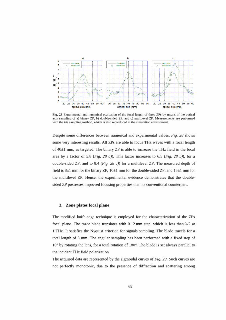
69

Fig. 28 Experimental and numerical evaluation of the focal length of three ZPs by means of the optical axis sampling of a) binary ZP, b) double-sided ZP, and c) multilevel ZP. Measurements are performed with the iris sampling method, which is also reproduced in the simulation environment.

Despite some differences between numerical and experimental values, Fig. 28 shows

some very interesting results. All ZPs are able to focus THz waves with a focal length

of 40±1 mm, as targeted. The binary ZP is able to increase the THz field in the focal

area by a factor of 5.8 (Fig. 28 a)). This factor increases to 6.5 (Fig. 28 b)), for a

double-sided ZP, and to 8.4 (Fig. 28 c)) for a multilevel ZP. The measured depth of

field is 8±1 mm for the binary ZP, 10±1 mm for the double-sided ZP, and 15±1 mm for

the multilevel ZP. Hence, the experimental evidence demonstrates that the double-

sided ZP possesses improved focusing properties than its conventional counterpart.

3. Zone plates focal plane

The modified knife-edge technique is employed for the characterization of the ZPs

focal plane. The razor blade translates with 0.12 mm step, which is less than λ/2 at

1 THz. It satisfies the Nyquist criterion for signals sampling. The blade travels for a

total length of 3 mm. The angular sampling has been performed with a fixed step of

10° by rotating the lens, for a total rotation of 180°. The blade is set always parallel to

the incident THz field polarization.

The acquired data are represented by the sigmoidal curves of Fig. 29. Such curves are

not perfectly monotonic, due to the presence of diffraction and scattering among

70

passive components in the optical path. Sigmoidal curves start from different values

because the three ZPs have different focusing capabilities: the double-sided ZP (Fig.

29 b)) has an intermediate focusing behavior between a binary ZP and a multilevel ZP.

In fact, the mean value of the electric field in the whole focal spot for the double-sided

ZP is greater than for a conventional ZP, but lower than for a multilevel ZP, validating

the conclusion that the double-sided ZP outperforms the standard binary ZP.

The Gaussian-like curves of Fig. 29 are the difference quotient of the acquired data,

thus showing some negative values due to reflections among components of the THz

set-up. The Gaussian-like curves can be seen as a projection of the |E|-field distribution

corresponding to a specific angle of view. The electric field amplitudes are normalized

with respect to their maximum value for each lens. This allows for better evaluating

and comparing the focal spot size and shape without considering the focusing

efficiency of each lens configuration. In the |E|-field projections, some secondary

peaks, with a height less than a half of the main peak, especially for the binary ZP, are

present (Fig. 29 a)). Moreover, the binary ZP is more influenced by the alignment to

the experimental set-up optical axis than the others ZP configurations. The alignment

of the ZP in the lens holder has an uncertainty deeply subwavelength, in the order of

few micrometers. However, the field distribution slightly changes when different

angles of view are selected. This does not occur for the other two ZP configurations.

Resulting images for the lenses under test are depicted in the inserts of Fig. 29. The

focus spots (from yellow to red in Fig. 29 g)-i), whose diameter is the FWHM of the

Gaussian-like curves) are fairly circular, with a diameter of 0.7±0.12 mm for the binary

ZP, of 0.65±0.12 mm for the double-sided ZP, and of 0.55±0.12 mm for the multilevel

ZP. These sizes are comparable to 2λ at 1 THz.

On the other hand, from the comparison of reconstructed images of the focal spots, the

binary ZP appears the only ZP with the maximum of the focus coinciding with the

geometrical center, i.e. with the optical axis. The focuses of the double-sided ZP and

multilevel ZP show a 0.12 and 0.06 mm offset above the optic axis, respectively. Fig.

29 d)-f) clearly shows that, above |E|/|E|max = 0.5, the curves for double-sided and

multilevel ZPs are not completely symmetric. This influences image reconstruction

showed in Fig. 29 g)-i) with an offset in the maximum field value position. However,

the position of the center of the focus may be influenced by the manual alignment of

71

the ZP under test in its lens holder, performed under a diffraction limited optical

microscope.

Fig. 29 Acquired data for a) a conventional binary ZP, b) a double-sided ZP, and c) a multilevel ZP; their difference quotient for d) a conventional binary ZP, e) a double-sided ZP, and f) a multilevel ZP; and focal plane images obtained by knife-edge measurements for g) a conventional binary ZP, h) a double-sided ZP, and i) a multilevel ZP. Negative values of the |E|/|E|max are due to diffraction and scattering among the components in the THz optical path.

72

4. Focal plane experimental comparison between ideal and real

illumination: multilevel zone plate case of study

All experimental data presented in Fig. 29 are obtained by employing the modified

knife-edge technique, i.e., minimizing the influence of the THz source asymmetries on

the devices characterization. As discussed in chapter V section 4, in a standard knife-

edge technique, it is the blade that rotates, creating the real image of the focus.

However, all changes in incident radiation, due to a non-ideal THz source and non-

ideal behavior of THz optical components (compare Ch. V), compromise the focus

quality. On the other hand, in the modified knife-edge technique, all data are collected

by fixing the blade angle with respect to the THz field polarization and by rotating the

lens. It has the advantage of obtaining a lens characterization in which excitation

dishomogeneities do not affect the acquisition of the distribution of the field amplitude

in the focal plane.

To the best of the author’s knowledge, this modified knife-edge technique has not been

discussed so far. Thus, to prove the effectiveness of the modified technique, a direct

comparison can be made between the normalized |E|-field distribution in the four-level

ZP focal plane, as imaged by the standard and modified knife-edge technique (Fig. 30).

It is clear that, instead of a circular shape, the ZP focus area is irregular. The whole

THz electric field is no more collected in a zone of maximum dimension of 1.2 mm,

but radiation fringes of a 35% of the maximum field are present over an area of more

than 6 mm of dimensions.

The situation presented in Fig. 30 is strongly influenced by the diffractive nature of the

test lens, which amplifies differences between the real incident THz field and an ideal

plane wave. It also underlines the importance of the THz source characterization. In

general, it is not appropriate to assume that the radiation emitted by a photoconductive

antenna has a Gaussian-like distribution nor to approximate it as a plane wave.

73

Fig. 30 Normalized amplitude of the electric field in the focal plane for the multilevel ZP acquired with knife-edge technique by rotating a) the lens, or b) the blade.

5. Conclusions

All investigated ZP configurations show good properties in focusing THz waves. The

new double-sided ZP lens proposed and investigated in this work is a binary ZP, in

which the total zone thickness is split in two halves. This new THz diffractive lens is

simple and cheap to fabricate, can be realized by milling both sides of a polymeric

substrate and delivers better performances than conventional ZPs.

By comparing its focalizing properties with ones of a conventional binary ZP, a

double-sided ZP shows (i) an efficiency of 1.12 times higher (Fig. 28), (ii) a depth of

field of approximately 7λ longer (Fig. 28), (iii) a resolution increased of (1/6)λ (Fig. 29

g) and h)), (iv) the total electric field is completely contained in a circle of confusion

with a diameter of 1.4±0.12 mm instead of 2.6±0.12 mm (Fig. 29 g) and h)). Focal

spots have both a circular shape.

Although the double-sided ZP performances do not fully match those delivered by the

four-levels ZP, double-sided ZP is simpler to fabricate, is less susceptible to damage,

and can be an interesting alternative for increasing the ZPs resolution.

74

CHAPTER VII

Future perspectives in developing planar diffractive lenses

1. Introduction

The development of THz applications and a market thereof is hampered by limitations

of the available components. Limitations for sources and detectors were briefly

addressed in chapter I. Among the pending issues for passive components for the

manipulation of THz radiation, the fabrication costs and the lack of tunability are of

particular relevance.

Hence, this chapter presents a design of a tunable diffractive lens by means of liquid

crystal cells. It also presents a design of a focusing device working in reflection mode.

This is based on a metal Fresnel ZP and is much lighter, smaller and cheaper than a

conventional parabolic mirror. Some preliminary numerical results and new ideas for

diffractive focusing elements will be shown in following sections.

2. Tunable zone plates

The focal length is the most appealing lens property to tune. However, the only way to

tune a ZP focal length is by changing the number of zones. In fact, from equation II.2

(compare Ch. II):

n = plq (VII.1)

where rm is the radius of the whole ZP, m is the zone number, and λ is the wavelength.

In most applications, the ZP external radius and the operational wavelength are fixed.

It could be interesting to find a way to change the distance at which a ZP is able to

focus THz waves. A successfully demonstated solution is to photoinduce an electron

plasma ZP pattern on a silicon wafer [186]. Thus, a virtual ZP can be optically tuned

75

by changing the electron plasma distribution. However, this solution requires an

additional laser beam and a metal ZP masks. Every mask has to be projected on the

silicon wafer and needs to be manually changed for obtaining different electron plasma

patterns.

On the other side, an alternative can be offered by electro-optical tuning by means of

liquid crystals (LCs). Several typologies of LC tunable lenses are successfully

fabricated in the visible range [187]–[191]. At THz, LCs are employed in many

devices, but only one tunable LC refractive lens prototype [192] and no diffractive

lenses with LC have been proposed yet. However, exploiting the design rules of the

double-sided ZPs, a change in ZP focal length is ideally feasible by electro-optical

control and it will be numerically demonstrated.

2.1 Material with tunable properties: liquid crystals

LCs are materials that exhibit a solid crystalline phase, a liquid phase and intermediate

phases in which they flow like a liquid, but show a preferred orientation. These

intermediate phases are called mesophases. It is possible to distinguish several

mesophases by changing temperature, concentration, constituents, substituents, or

other LCs or environmental properties [193].

LCs can be also classified in lyotropic, thermotropic and polymeric, according to the

physical parameters that control the existence of the liquid crystalline phases.

Lyotropic LCs can be obtained when a suitable concentration of a material, usually

amphiphilic molecules, is dissolved in a solvent, like water. This kind of LCs is of

interest in biological field [194]. Thermotropic LCs are the most extensively studied

LCs. They exhibit different mesophases as temperature increases. There are three main

classes of thermotropic LCs: nematic, cholesteric, and smectic. Polymeric LCs are

produced from monomers showing a liquid-crystal phase. These monomers are

polymerized trough main chain or side chain reactions into a LC polymer. They have,

in general, higher viscosity than other LC monomers due to bonds between polymeric

chains [193]. Due to their excellent thermal and mechanical properties and low

electromagnetic losses, they are also used as microwave substrates [195].

76

Materials constituted by molecules with an anisotropic shape could reveal mesophases.

For this reason, it is common to refer to LCs as rod-like or disk-like molecules [196].

Thermotropic LCs have rod-like molecules. When the thermotropic LC is in a nematic

phase (Fig. 31 a)), its rod molecules have a random position. It could remind a liquid;

however, LC molecules are aligned in the same direction defined by a unit vector

called director. In most cases, nematic molecules have a permanent dielectric dipole

and the rods are arranged in a way that the resulting dipole moment of the bulk

material vanishes. In fact, nematic LC molecules are centrosymmetric [193].

Fig. 31 Liquid crystals mesophases: a) nematic, b) cholesteric, and c) smectic.

Cholesterics (Fig. 31 b)) are also called chiral nematic LCs. They are nematic LC in

which the alignment follow a helical arrangement. Smectic LCs (Fig. 31 c)), unlike

nematics and cholesterics, have a positional order too: LC molecules are located in an

ordered pattern. According to the configuration of rods positions, the smectic phase

can be divided in subphases [196].

The amount of order in a LC can be measured by the scalar order parameter. It is a

weighted average of the molecular orientation angles θm between the long molecular

axes and the director [197]:

° = !# ⟨3cos#3 v 1⟩ (VII.2)

where the chevrons represents a thermal or statistical average. LCs in equilibrium state

have usually a positive order parameter, which can change from Seq = 0, in the isotropic

state (high temperature), to Seq = 1 in the crystalline phase (low temperature). A

nematic LC has usually Seq = 0.6 at the temperature of operation [152].

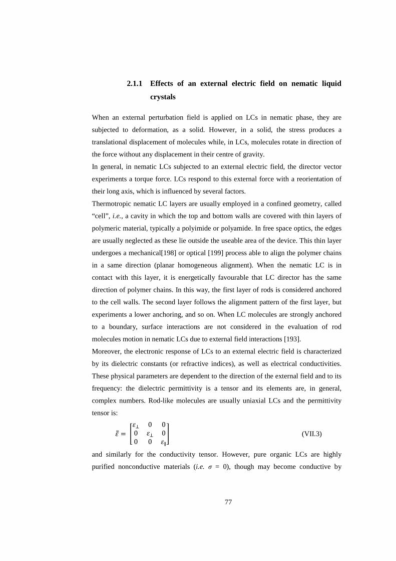
77

2.1.1 Effects of an external electric field on nematic liquid

crystals

When an external perturbation field is applied on LCs in nematic phase, they are

subjected to deformation, as a solid. However, in a solid, the stress produces a

translational displacement of molecules while, in LCs, molecules rotate in direction of

the force without any displacement in their centre of gravity.

In general, in nematic LCs subjected to an external electric field, the director vector

experiments a torque force. LCs respond to this external force with a reorientation of

their long axis, which is influenced by several factors.

Thermotropic nematic LC layers are usually employed in a confined geometry, called

“cell”, i.e., a cavity in which the top and bottom walls are covered with thin layers of

polymeric material, typically a polyimide or polyamide. In free space optics, the edges

are usually neglected as these lie outside the useable area of the device. This thin layer

undergoes a mechanical[198] or optical [199] process able to align the polymer chains

in a same direction (planar homogeneous alignment). When the nematic LC is in

contact with this layer, it is energetically favourable that LC director has the same

direction of polymer chains. In this way, the first layer of rods is considered anchored

to the cell walls. The second layer follows the alignment pattern of the first layer, but

experiments a lower anchoring, and so on. When LC molecules are strongly anchored

to a boundary, surface interactions are not considered in the evaluation of rod

molecules motion in nematic LCs due to external field interactions [193].

Moreover, the electronic response of LCs to an external electric field is characterized

by its dielectric constants (or refractive indices), as well as electrical conductivities.

These physical parameters are dependent to the direction of the external field and to its

frequency: the dielectric permittivity is a tensor and its elements are, in general,

complex numbers. Rod-like molecules are usually uniaxial LCs and the permittivity

tensor is:

= ³ 0 00 00 0 ∥´ (VII.3)

and similarly for the conductivity tensor. However, pure organic LCs are highly

purified nonconductive materials (i.e. σ = 0), though may become conductive by

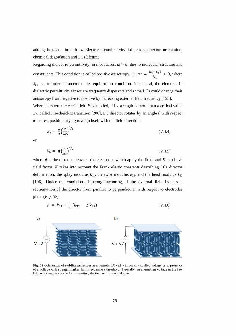
78

adding ions and impurities. Electrical conductivity influences director orientation,

chemical degradation and LCs lifetime.

Regarding dielectric permittivity, in most cases, ε∥ > ε⊥ due to molecular structure and

constituents. This condition is called positive anisotropy, i.e. Δ B ¢¶∥y¶·¦¸¹º 0, where

Seq is the order parameter under equilibrium condition. In general, the elements in

dielectric permittivity tensor are frequency dispersive and some LCs could change their

anisotropy from negative to positive by increasing external field frequency [193].

When an external electric field E is applied, if its strength is more than a critical value

EF, called Freedericksz transition [200], LC director rotates by an angle θ with respect

to its rest position, trying to align itself with the field direction:

»¼ B½& u ¾¿¶z

! #À (VII.4)

or

Á¼ B πu ¾¿¶z

! #À (VII.5)

where d is the distance between the electrodes which apply the field, and K is a local

field factor. K takes into account the Frank elastic constants describing LCs director

deformation: the splay modulus k11, the twist modulus k22, and the bend modulus k33

[196]. Under the condition of strong anchoring, if the external field induces a

reorientation of the director from parallel to perpendicular with respect to electrodes

plane (Fig. 32):

Ã B!! o!r e$$ v2##j (VII.6)

Fig. 32 Orientation of rod-like molecules in a nematic LC cell without any applied voltage or in presence of a voltage with strength higher than Freedericksz threshold. Typically, an alternating voltage in the few kilohertz range is chosen for preventing electrochemical degradation.

79

The rod molecules reorientation determines a change in a LC dielectric permittivity as

well as in its refractive index. In fact, as discussed above, in absence of external fields,

LC permittivity is expressed by equation VII.3. For values of applied voltage higher

than the Freedericksz transition, it becomes:

= ³∥ 0 00 00 0 ´ (VII.7)

An equivalent notation that will be useful in following sections is:

= ³Ä 0 00 00 0 ´ (VII.8)

where the dielectric permittivity is considered as the product of the vacuum

permittivity ε0 and the extraordinary relative permittivity εe of the LC, when the

director is parallel to the applied field, and it is the product of the vacuum permittivity

ε0 and the ordinary relative permittivity εo of the LC, when the director is perpendicular

to the applied field.

2.1.2 Q-tensor formulation

Freedericksz transition provides a static description of LCs by introducing a threshold

behaviour. However, a rigorous study of LC orientation in confined geometries

requires the development of a model which involves the minimization of the LC free

energy. It can be carried out following the Q−tensor formulation [197] that allows for

the numerical study of edge effects, defect singularities, and order parameter

variations.

In the more general case of a biaxial nematic LC, a symmetric traceless matrix, which

represents the LC tensor order parameter, can be introduced as [201]:

9: = °!e¬ ⊗ ¬j + °#eÆ ⊗Æj −!$ e°! +°#j7 = ÇÈ! È# È$È# Èr ÈÉÈ$ ÈÉ −È!−ÈrÊ

(VII.9)

where S1 is the parameter order of the molecular axis with director n, S2 is the

parameter order of the molecular axis with director m, and 7 is the identity matrix so

that the trace of 9: is zero. The eigenvalues of the Q-tensor are [197]:

80

! = !$ e2°! −°#j (VII.10)

# = − !$ e°! +°#j (VII.11)

$ = !$ e2°# −°!j (VII.12)

If the LC is uniaxial, two of these eigenvalues are equal and the Q-tensor is [201]:

9: = ° Ëe¬⊗ ¬j −!$ 7Ì (VII.13)

The total free energy of a bulk LC, under the condition of strong surface anchoring, is

given by the contribution of thermotropic, elastic and electromagnetic energy density

functions. The thermotropic energy density function is [201]:

14 = Í4tr¢9:#¦ +#2ÏÐ$ tr¢9:$¦ + ÑÏÐ# Òtr¢9:#¦Ó# (VII.14)

where a, b and c are the thermotropic coefficients, i.e., a temperature dependent

coefficients, and tr(·) indicates the trace of a matrix.

The elastic energy density is the energy due to a distortion of the LC molecules, i.e. of

a variation of the Q-tensor in the space [201]:

1 =∑ Ô¡# uÕÖ[×ÕØ z# + ¡p# ÕÖ[×Õ× ÕÖ[ØÕØ Ù +∑ Ë¡Ú# 9wÛ ÕÖ[×ÕÜ ÕÖ[×ÕØ Ì,Ý,Û,wÞ!,#,$,Ý,ÛÞ!,#,$

(VII.15)

L1, L2 and L6 are elastic parameters related to Frank elastic constants k11, k22 and k33.

The electromagnetic energy density in presence of only an external electric field E is

given by the electrostatic energy:

13 =−ß ∙ dà (VII.16)

where the electric displacement field ß =à+ á depends on the spontaneous

polarization vector P and the LC permittivity tensor that, for a nematic LC, can be also

expressed in terms of the Q-tensor:

=∆9: +Äx 7 (VII.17)

where ∆ε is the dielectric anisotropy and Äx = e∥ + 2j 3⁄ .

Spontaneous polarization derives from asymmetries in shape of LC molecules and can

be written in terms of Q-tensor. The ith components is given by:

â =ã! ∑ ÕÖ[×Õ×ÝÞ!,#,$ +ã#∑ 9Ý ÕÖ×ØÕØÝ,ÛÞ!,#,$ (VII.18)

with p1 and p2 that are polarization coefficients [197].

81

The Q-tensor formulation is based on the minimization of the free energy density

function 1* =14 +1 +F3 via the solution of a system of five equations

(i = 1 … 5):

∑ ÕÕ×$ÝÞ! åÕæçÕx[,×è −ÕæçÕx[ = 0 (VII.19)

in which È,Ý =éÈ é£Ý⁄ . Equations VII.19 represent the LC static equations and can

be solved together with suitable boundary conditions. In a strong anchoring regime,

Dirichlet conditions are commonly employed: the Q-tensor at boundaries has a

specified value defined by chosen alignment. In a weak anchoring regime, however, a

surface energy density has to be added in the evaluation of the total free energy density

of the LC [197].

When the study of the dynamic evolution of the Q-tensor is required, equations VII.19

become:

∑ ÕÕ×$ÝÞ! åÕæçÕx[,×è −ÕæçÕx[ = Õê

Õxë [ (VII.20)

where D is the dissipation function ì = tr u¢é9: é⁄ ¦#z, γ is the ratio between the

standard viscosity of the nematic LC and the order parameter obtained when the

viscosity is measured, and Èë =éÈ é£⁄ .

By means of equations VII.20, it is possible to study the switching dynamics of devices

employing LCs as well as the tunable properties of such devices. Equilibrium order

parameter, standard viscosity, polarization coefficients, dielectric permittivity tensor

elements, Frank elastic constants, and thermotropic coefficients change according to

LC mixture chosen: their values will be indicated during the discussion of specific

applications (compare Ch. VII Sec. 2.2 and Ch. IX). In the next section, the Q-tensor

formulation has been employed in the numerical study of an electro-optical controlled

planar diffractive lens able to switch between two different focal lengths.

2.2 Double-sided zone plate with two focal lengths

There are two main technological issues that have so far hampered LC-based electro-

optical tunable phase-reversal ZPs at THz frequencies. The first one dwells in the

thickness of a LC layer able to introduce a phase difference of π in the incident THz

82

waves path (see equation II.5). As discussed in the previous subsection, a layer of LCs

in a nematic phase is able to change its dielectric permittivity, i.e. its refractive index,

according to a voltage externally applied to the LCs layer. In order to obtain a phase-

reversal ZP dynamically tuned by means of the electro-optical effect of LCs, it is

necessary to employ electrodes with alternative conductive and nonconductive annular

zones shaped as ZP. Three configurations are possible. In a first configuration, the top

and bottom are equally patterned and aligned. In a second configuration, only the

electrodes on one substrate are pattern, whereas the other substrate is uniformly

conducting. In a third configuration, only the electrodes on one substrate are pattern,

and there is no electrode on the other substrate. Different director profiles result from

these configurations.

However, an issue arises when an electrode is ZP-patterned. In fact, the electric field

could short-circuit between two adjacent conductive rings of the same electrode when

their distance is comparable to the separation between the top and bottom electrodes,

i.e., with the thickness of the LC cell. It involves that the LCs above non-conductive

zones could change the refractive index together with the LCs above conductive zones.

Consequently, the most external rings of the phase-reversal ZP could become a wide

single zone and the ZP pattern is lost.

The second configuration is illustrated in Fig. 33 a). The LC behavior is numerically

investigated with the Q-tensor formulation discussed in the previous section by

implementing it in a FEM model (described in Ch. III Sec. 2). This model provides the

solution of the dynamic equations VII.19. A voltage of 70 V is applied between the

two electrodes, which have a distance of about 386 µm. The distance between the top

and bottom electrodes corresponds to the thickness of the phase-reversal ZP. The

thickness is evaluated from equation II.5 by substituting the difference of refractive

index between the polymer and the air with the LC birefringence ∆n = ne – no. All the

other ZP geometrical parameters match with the ones of the polymeric binary phase-

reversal ZP described in chapter III.

The selected LC material 1825 has been synthesized by the Military University of

Technology of Warsaw and has complex ordinary and extraordinary refractive indices

equal to no = 1.554 − j0.018 and ne = 1.941 − j0.022 at 1 THz, low-frequency (1.5 kHz)

permittivities εo = 4.7 and εe = 21.7, Frank elastic constants k11 = 12.5 pN, k22 = 7.4 pN,

k33 = 32.1 pN, and viscosity γ = 311.55 mPa·s [202], [203]. This nematic mixture has

83

been selected because it exhibits a high birefringence at THz and moderate losses [152]

and it is available through an established collaboration.

Fig. 33 a) A ZP configuration with a uniform electrode on top and a ZP-patterned electrode on bottom substrate. The rest condition of the LC is tilted 2° from the y-axis. b) tilt angle and c) y-component of refractive index tensor distributions in a LC cell 387 µm thick, 2 ms after the application of a 70 V step voltage (steady state).

In absence of applied voltage, the LC director is parallel to the electrode plane, with a

pretilt angle of 2°. When the voltage is applied, the LCs show a switching behavior.

After 2 ms from voltage switching (i.e., in the steady state), the director has a tilt angle

of 90° in the middle of the LC cell (Fig. 33 a)). Here, in fact, the anchoring forces do

not influence the director orientation. An angle of 90° corresponds to a director

orientation perpendicular to the electrode plane. However, LC is tilted only 55° − 60°

between the most external adjacent electrodes in correspondence of a nonconductive

ring. As it can be seen from (Fig. 33 b)), it corresponds to a y-component refractive

index of about 1.6 – 1.65 in direction parallel to the polarization direction of the

applied electric field. However, Fig. 33 shows that the transition of the refractive index

component from the fully switched and fully unswitched zones is not sharp. It gets

84

significantly blurred for the outer rings where the thickness approaches the cell gap and

the fringe field effects rule. Hence, the diffractive effect is reduced and the device

becomes ineffective as a tunable lens.

Clearly, the fringe field effects play a detrimental role. Ideally, these should be reduced

or avoided altogether. One way to reduce them is by recalling that, for double-sided

phase-reversal ZPs, the phase shift introduced by each binary phase-reversal ZP is π/2

instead of π (see Ch. II). When this concept is transferred to a LC phase-reversal ZP,

each LC cell needs to provide only half the overall retardation. Hence, the cell can be

thinner and the fringe field effects can be reduced. As a straightforward example, a half

thickness cell, 193 µm thick, is here considered.

The LC switching behavior can be numerically evaluated by applying a voltage of

35 V and employing the same electrode configuration of the one presented in Fig. 33

a).

Fig. 34 a) A ZP configuration with a uniform electrode on top and a ZP-patterned electrode on bottom substrate. The rest condition of the LC is tilted 2° from the y-axis. b) tilt angle and c) y-component of refractive index tensor distributions in a LC cell 193 µm thick, 2 ms after the application of a 35 V step voltage (steady state).

85

The LC director tilt angle and refractive index in direction parallel to the polarization

direction of the applied electric field for the half-thick cell are presented in Fig. 34.

The maximum tilt angle of LC director in the middle of the cell above nonconductive

rings is now always below 25°. It follows that the y-component of the refractive index

differs appreciably from its rest value in the most external non-conductive ring and it is

equal to about 1.9. This suggests that a double-sided LC phase-reversal ZP is a better

candidate as electro-optical tunable diffractive lens than conventional binary phase-

reversal ZP. Additionally, thinner LC devices require a lower driving voltage for the

same switching time. More importantly, in real devices, the quality of the alignment is

usually better, especially for 100s µm thick devices.

As a confirmation of this idea, a tunable LC double-sided phase-reversal ZP has been

designed and numerically investigated. At the beginning of this chapter, it was argued

that the only way to dynamically tune ZP focal length is by changing the number of

Fresnel zones. Here, it is proposed that if two lenses with a different number of rings

are stacked and one of them is electro-optically controlled, it is possible to change

between two focal lengths simply by applying a voltage. In fact, when the voltage is

turned off, the first ZP, which is a polymeric phase-reversal ZP as described in chapter

III, is able to focus the incident THz radiation with its own focal length. When the LC

is switched on, the waves passing through the first polymeric phase-reversal ZP are re-

focused with a focal length corresponding to the number of zones of the LC phase-

reversal ZP. In Fig. 35, a cross section perpendicular to the lens plane is shown and

some geometrical parameters and materials information are presented. The numerical

model has a radial symmetry and includes materials losses at 1 THz. However, this is a

preliminary investigation and the LC is considered to have an asymptotic behavior, i.e.,

its y-component switches from a uniform profile of ne to a uniform profile of no.

The behavior of the dual-focus double-sided phase-reversal ZP is presented in Fig. 36.

The z-direction is the one parallel to the ZP lens optical axis. When no voltage is

applied to the LC, the lens focuses the 1 THz radiation 59.5 mm past the lens. The

FWHM, which could be considered as the depth of field of the lens, is 9.2 mm

approximately.

86

Fig. 35 Cross section of geometrical radial-symmetric model and data for the materials chosen for a dual-focus double-sided ZP. The ZP is symmetric and only the profile along the radius of the lens is represented in the picture.

Fig. 36 Computed square modulus of the electric field component along the optical axis (z-component) at 1 THz for a dual-focus double-sided phase-reversal ZP lens. The green line is for zero applied voltage (rest), while the blue line is for LC molecules parallel to the lens optical axis (V∞).

When the LC molecules are aligned in the z-direction, the focal length switches in

~2 ms to 42.1 mm approximately. The FWHM also changes to 4.5 mm.

The square modulus of the electric field in the focus area is about 35.5 times larger

than the square modulus of the incident electric field on the lens, when the lens is

switched off, and about 39 times larger, when the lens is switched on. However,

several ripples are also present along the optical axis. These peaks are due to multiple

reflections between the polymer facets. They disappear by changing the thickness of

87

the polymer between the two ZPs. However, this distance is fundamental in the

double-sided ZP design and could not be varied without changing the lens focusing

properties. Further investigation is needed to suppress these peaks due to reflections

and optimize the design. Moreover, an additional study is required for exploiting the

dual-focus behavior when the asymptotic profile of the LC refractive index is

substituted with the one computed by the Q-tensor model and presented in Fig. 34 c).

The dual-focus double-sided phase-reversal ZP here described shows a switchable

focal length and could offer a good starting point for developing ZP stacks optimized

for working at different focal lengths by means of the electro-optical control of the LC

orientation. It is a device simple to integrate in compact instruments, flat, and ideally

suitable for miniaturization.

The main problem in the experimental demonstration of such devices is linked to the

second technological issue in the development of tunable and compact devices at THz

frequencies: the availability of a highly transparent conductive material for electrodes

fabrication. In the visible range, indium tin oxide (ITO) is ubiquitously used [204].

However, it is opaque at THz frequencies. One of the most promising conductive

polymer for transparent electrodes at THz is the poly(3,4-

ethylenedioxythiophene):poly(4-styrenesulfonate) (PEDOT:PSS). However, the

conductivity of a PEDOT:PSS film is usually no more than 10 S cm−1. It is not

completely suitable for replacing ITO, because it has, typically, a conductivity of about

4000 S cm−1 [205]. Several methods can be applied for improving PEDOT:PSS

conductivity, such as treatments with acid solutions or the addition of organic

compounds. However, only films with conductivity no more than 1000 S cm−1 allows

for a PEDOT:PSS transmittance at THz comparable with ITO transmittance in the

visible range (i.e. ~90%) [205].

An alignment film of polyimide decreases THz transmittance of about 10%, but the

homogeneity of this effect does not compromise LC-ZP performance. In fact, the main

problem due to the presence of a non-transparent ZP-patterned electrode is that it

behaves as a Fresnel ZP itself. It implies that, in a dual-focus double-sided ZP, the

polymeric phase-reversal ZP performance is affected by the LC electrode and the

incident radiation will be focused at both focal lengths, losing power in the focus area.

A thorough optimization of the devices is required which takes into account both the

phase modulation and the exact effect of the conductive layer on the THz field.

88

Different formulations of PEDOT:PSS exist; some have been supplied for this work

and have been preliminarily tested. However, the extraction of the real and imaginary

component of PEDOT:PSS at THz is a challenging and still unaccomplished task. It

would require a very elaborated ellipsometric technique because practical films are

submicron, i.e., roughly one thousandth the wavelength.

For this reason, the fabrication and experimental investigation of proposed LC

switchable diffractive lens have not been planned yet, even if double-sided ZPs

significantly reduce the problem of the LC thickness and should provide an effective

solution for the dynamic focusing of THz radiation.

3. Metal zone plates

Fresnel ZPs can be also investigated at THz frequencies. As discussed in chapter II, a

phase-reversal ZP has a higher efficiency than a Fresnel ZP due to the fact that all the

incident radiation passes through the device. According to the zone construction, a

portion of incident radiation is phase shifted and constructively interferes with the

other portion, inducing a concentration of radiation in a small area, i.e., the focus.

However, some losses occur because of low efficiency of the diffraction mechanism

and absorptions in the material.

In a Fresnel ZP, there is no phase shift of the radiation which destructively interferes to

the focus construction. This part of the incident radiation is stopped by adding a

patterned mirror. Hence, the transmitted wave suffers from losses to reflection. These

losses sum up with those due to diffraction efficiency and material absorptions.

Therefore, the Fresnel ZP lens shows a lower focusing efficiency than a phase-reversal

ZP.

Interestingly, all reflected radiation is in phase and create virtual foci (Fig. 7). Thus, it

is possible to combine synergistically the power transmitted with the power reflected

from the Fresnel ZP in a novel device working in reflection mode with maximum

efficiency. This device encompasses a homogenous mirror on the other side of the

substrate on which the Fresnel ZP is patterned. The distance between the Fresnel ZP

and the mirror must be equal to λ/4 in the material [206]. In this way, the main focus is

89

superposed to the virtual focus with an increasing of the THz field strength in the focus

area.

Fresnel ZP lenses working in reflection mode do not already exist at THz frequencies.

This is on the side of the plane wave source. At the design frequency, this device

behaves very similarly to a bulky parabolic mirror, but is very thin (50 µm for

operation at 1 THz with a dielectric with a 1.5 refractive index). However, they have

been often employed as lens antennas at millimeter-waves and at microwaves.

3.1 Zone plates in reflection mode

The performance of a Fresnel ZP working in reflection mode can be numerically

compared with the behavior of the same Fresnel ZP working in transmission mode.

Again, Zeonor is chosen as lens substrate for its low THz absorption (for material

properties, compare Ch. II Sec. 5). However, the design was made for the available

100 µm foils due to the current unavailability of 50 µm thick foils working a λ/4

waveplates. This rules that the working frequency is about 0.5 THz.

A FEM model (as discussed in Ch. III Sec. 2) of both lenses has been developed under

the condition of normal incidence of a plane wave. Both ZPs have 25 Fresnel zones

made with an aluminum layer thicker than the skin depth at 0.5 THz. The thinnest zone

is 610 µm and the lens diameter is 25.4 mm (i.e., 1 inch). In the ZP reflector model, an

aluminum film thicker than the skin depth at 0.5 THz is considered on the opposite

side of the Zeonor substrate. The permittivity of aluminum is described by Drude

model:

% = 1 − -.#-# − ð- where -. = 2.243 ∙ 10!òrad/s is the plasma frequency and = 1.243 ∙ 10!rrad/s is

the scattering frequency [207].

Fig. 37 shows a comparison between the square modulus of the electric field at

0.5 THz of the two Fresnel ZP lenses. The THz power in the focus area is about 5

times higher if the ZP works in reflection mode instead of transmission mode.

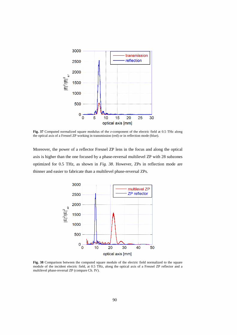
90

Fig. 37 Computed normalized square modulus of the z-component of the electric field at 0.5 THz along the optical axis of a Fresnel ZP working in transmission (red) or in reflection mode (blue).

Moreover, the power of a reflector Fresnel ZP lens in the focus and along the optical

axis is higher than the one focused by a phase-reversal multilevel ZP with 28 subzones

optimized for 0.5 THz, as shown in Fig. 38. However, ZPs in reflection mode are

thinner and easier to fabricate than a multilevel phase-reversal ZPs.

Fig. 38 Comparison between the computed square module of the electric field normalized to the square module of the incident electric field, at 0.5 THz, along the optical axis of a Fresnel ZP reflector and a multilevel phase-reversal ZP (compare Ch. IV).

91

ZP reflectors are much thinner and easier to fabricate than parabolic mirrors. They are

also thinner than a multilevel phase-reversal ZPs. It could open to innovative

applications, especially if they are linked to the possibility to consider ZP reflectors as

THz antennas. Currently, lens designs for a 45° incident THz plane waves are under

investigation.

92

CHAPTER VIII Leaky-wave antennas for terahertz far-field applications

1. Introduction

In the previous chapter, the possibility to develop planar THz antennas based on

patterned metallic surfaces was introduced. Only few examples of Fresnel ZP antennas

already exist at THz frequencies (for example, [127], [208], [209]): new configurations

can be implemented and tested, such as the stacked diffractive zone plate. However, a

structured study about the design of this device and its radiating performance goes

beyond the scope of this thesis.

On the other side, as discussed in chapter I, there is a growing interest toward THz

communications, connected to the possibility to have access to Tbps wireless links. For

this reason, it could be useful to develop antennas, which (i) could be fabricated with

low-cost materials, (ii) are light and simple to integrate, (iii) could be conformable, and

(iv) may exhibit reconfigurable properties.

In the field of planar antennas obtained by covering grounded dielectric slabs with

patterned metallic screens, leaky-wave antennas (LWAs) are promising devices at THz

frequencies. LWAs are travelling-wave antennas successfully employed as radiating

systems at microwaves from decades. In LWAs, radiation phenomena are interpreted

as the ‘energy leakage’ of a wave that propagates in a partially open structure and

progressively loses its energy due partly to the losses (if any) in the medium and partly

to the radiation losses [210]. Leaky waves are characterized by a generally complex

propagation wavenumber, due to the energy leakage: = − ð, where βz is the

phase constant and αz is the attenuation constant. Moreover, in order to effectively

radiate [211], [212], the leaky wave propagating in the structure has to be a fast wave,

i.e., characterized by || < , where k0 is the free-space wavenumber. Therefore, the

operation of a LWA is quite different from a slow-wave or a surface-wave type of

antenna, for which radiation mainly takes place at discontinuities (e.g., at the edge of

93

the structure) [213]. In the absence of ohmic losses, αz takes into account only power

losses due to radiation and it is called “leakage constant”: it represents the rate of

decreasing of the aperture field due to the leakage mechanism of radiation.

The main advantages of LWAs dwell in the easiness of fabrication and design, the

simple feeding network, as well as in the ubiquity of leaky-wave phenomena from

microwaves, which are the historical starting point of the leaky-wave theory, to nano-

optics, thanks to the current developments in metasurfaces and nanostructured

materials. For this reason, they are perfectly suitable for being scaled at THz

frequencies.

2. Historical path in the development of a leaky-wave theory

At the end of 1930’s, Hansen proposed an antenna made of a rectangular waveguide, in

which there was a longitudinal cut for letting leaking away the guided electromagnetic

power [214]. It was a very simple and promising device. However, it was only during

1950’s that it was re-examined, but first experimental attempts failed because leaky-

wave theoretical fundamentals were unclear. About it, in 1984 Oliner, one of the

pioneer of leaky-wave theory, wrote [215]: “It was […] recognized that the leaking

waveguide possessed a complex propagation constant, with the usual phase constant

and an attenuation constant due to the leakage (in addition to an attenuation constant

due to wall losses). The field struggled with two basic problems:

1) Was the leaky wave truly real?

2) How should one determine the leakage constant theoretically?

Since it was obvious that leakage was being produced, why did people question the

reality of the leaky wave? If one recalls simply that the squares of the wavenumbers in

the three orthogonal directions must sum to the square of the free-space wavenumber,

then, if there is decay longitudinally, corresponding to power leakage, the wave

amplitude must increase in the transverse (or cross-section) plane. Since the cross

section outside of the waveguide is unbounded, this implies that the leaky wave must

increase transversely to infinity, yielding an unphysical result. The state of skepticism

and uncertainty was so great that the Ohio State group, under V. H. Rumsey, made

direct probe measurements [216]. They found that near to the waveguide the field did

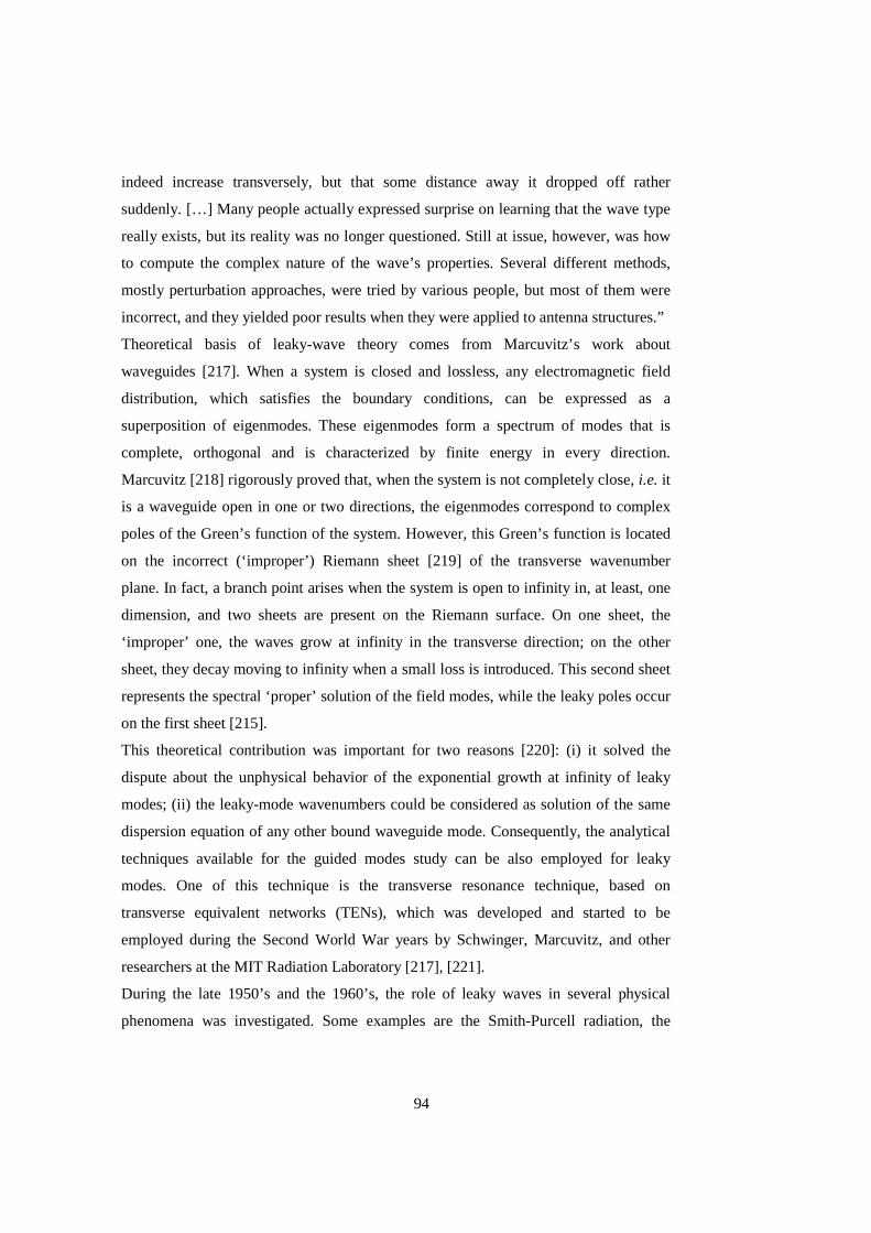
94

indeed increase transversely, but that some distance away it dropped off rather

suddenly. […] Many people actually expressed surprise on learning that the wave type

really exists, but its reality was no longer questioned. Still at issue, however, was how

to compute the complex nature of the wave’s properties. Several different methods,

mostly perturbation approaches, were tried by various people, but most of them were

incorrect, and they yielded poor results when they were applied to antenna structures.”

Theoretical basis of leaky-wave theory comes from Marcuvitz’s work about

waveguides [217]. When a system is closed and lossless, any electromagnetic field

distribution, which satisfies the boundary conditions, can be expressed as a

superposition of eigenmodes. These eigenmodes form a spectrum of modes that is

complete, orthogonal and is characterized by finite energy in every direction.

Marcuvitz [218] rigorously proved that, when the system is not completely close, i.e. it

is a waveguide open in one or two directions, the eigenmodes correspond to complex

poles of the Green’s function of the system. However, this Green’s function is located

on the incorrect (‘improper’) Riemann sheet [219] of the transverse wavenumber

plane. In fact, a branch point arises when the system is open to infinity in, at least, one

dimension, and two sheets are present on the Riemann surface. On one sheet, the

‘improper’ one, the waves grow at infinity in the transverse direction; on the other

sheet, they decay moving to infinity when a small loss is introduced. This second sheet

represents the spectral ‘proper’ solution of the field modes, while the leaky poles occur

on the first sheet [215].

This theoretical contribution was important for two reasons [220]: (i) it solved the

dispute about the unphysical behavior of the exponential growth at infinity of leaky

modes; (ii) the leaky-mode wavenumbers could be considered as solution of the same

dispersion equation of any other bound waveguide mode. Consequently, the analytical

techniques available for the guided modes study can be also employed for leaky

modes. One of this technique is the transverse resonance technique, based on

transverse equivalent networks (TENs), which was developed and started to be

employed during the Second World War years by Schwinger, Marcuvitz, and other

researchers at the MIT Radiation Laboratory [217], [221].

During the late 1950’s and the 1960’s, the role of leaky waves in several physical

phenomena was investigated. Some examples are the Smith-Purcell radiation, the

95

Cherenkov radiation, Wood’s anomalies on optical gratings, and prism and grating

couplers for integrated optics [215].

Since the 1970’s, several radiating structures based on leaky-waves have been

designed and deeply studied and a detailed account of them can be found in [210],

[220], [222]. However, it is important to just mention that, starting approximately from

the new millennium and up to present, LWAs based on metamaterials, metasurfaces,

and reconfigurable materials opened new possibilities and new operative frequency

ranges. This will be deeply discussed in chapter IX and X.

3. Classification of leaky-wave antennas

Leaky-wave antennas can be divided in several categories, according to their

geometrical structure and their principle of operation [222]. A first distinction can be

made between one-dimensional (1-D) and two-dimensional (2-D) LWAs. This has

influence on the radiation features: a 1-D antenna usually produces fan beams, while a

2-D structure mainly irradiates pencil beams or fully conical beams.

Then, LWAs can also be divided, according to their structure, in uniform, quasi-

uniform and periodic antennas. This distinction can affect the antenna scanning

characteristics. In fact, a uniform LWA usually scans inside the forward spatial

quadrant by varying the operating frequency, while a periodic LWA can scan the

radiation beam in both forward and backward quadrants.

However, some exceptions could exist. A brief overview of these categories will be

made in the following subsection.

3.1 One-dimensional uniform leaky-wave antennas

In 1-D LWAs, the antenna guiding structure is essentially one-dimensional: the

structure supports a wave that travels in only one direction. A rectangular waveguide

with a longitudinal slit (see Fig. 39), which allows the radiation, is an example of 1-D

LWA [223]. It can also be considered a uniform LWA because the transverse cross

section does not change along the longitudinal axis. In general, a 1-D LWA is

96

characterized by a length equal to several wavelengths, while the cross section is

usually in the order of the wavelength. A 1-D LWA radiates along its length L and its

radiating behavior is comparable with the one of a conventional 1-D aperture antenna

[224]. The main difference is that the aperture field of a LWA is dominated by the

distribution of the relevant leaky mode of the structure [220], and thus has an

exponentially-decaying profile.

In Fig. 39, a ground plane is employed as wave deflector; on it, a very narrow slot can

be etched at one lateral end of the structure. It is equivalent to an infinite magnetic line

current flowing in free space in the direction coinciding with the propagation direction

of electromagnetic waves, i.e., the z-direction of Fig. 39. If the LWA has a finite

length, the line source is of finite length. The corresponding radiation pattern has the

form of a cone with the axis coinciding with the z-axis: the radiation is limited to the

forward quadrant (¤ > 0). As the angle between the cone and the z-axis approaches

90°, the radiated beam comes near to a broadside beam with a narrow-beam donut

broadside pattern.

Fig. 39 A rectangular waveguide, as an example of 1-D uniform LWAs. The electromagnetic field propagates in z-direction. An infinite ground plane surrounds the slot [222].

97

However, if a 1-D uniform LWA is fed at one end, it can difficultly obtain a beam at

broadside. A broadside beam can be achieved by feeding the antenna at both ends, or at

the center of the structure. In this way, two beams are created, each pointing close to

broadside but on opposite sides of it, shaping a single broadside beam [222].

Moreover, the range of scanning can include both forward and backward quadrants if

nonconventional materials, such as ferrites or metamaterials, are loaded in 1-D uniform

structures [225].

3.2 One-dimensional periodic leaky-wave antennas

An example of periodic 1-D LWA is the structure illustrated in Fig. 40. It is a 1-D

antenna because the waves propagate in one direction, even if the width of the antenna,

in the perpendicular direction with respect to the propagation direction, is large.

Because of the width of the structure, this antenna can irradiate a fan beam or a pencil

beam [222]. However, the beam can scan only one plane, i.e., the forward quadrant,

unless the unloaded structure is fed from both ends.

Fig. 40 An example of periodic 1-D LWA. This antenna configuration has a width, w, larger than the operative wavelength. The electric field is in y-direction and the electromagnetic wave propagates in z-direction.

In general, a periodic 1-D LWA derives from a dielectric waveguide periodically

loaded by perturbations. The unperturbed waveguide usually supports an operating

guided mode as a surface wave, which is slow ( < ), and is not able to radiate. A

suitable periodic loading of the guide permits to describe the overall field in terms of a

series expansion of Floquet’s modes or space harmonics with phase constants:

98

, = o 2m ã⁄ , where m is an integer and p is the period. Typically, in open

structures, one of these space harmonics (usually the m B v1) becomes a fast wave

(i.e., a leaky-wave with ). The phase constant of the leaky wave could assume

positive and negative values as the operating frequency changes: this LWA allows for

radiation both in the forward and in the backward quadrant. However, the scanning

region of simple LWA geometries, as the one in Fig. 40, usually shows a degradation

in the radiation efficiency around broadside; specific more complex geometrical

periodic patterns could be introduced for avoiding it [220], [222], [226].

The periodic LWAs considered above are characterized by a period comparable with

the operating wavelength. Conversely, when the period is ã 4⁄ , the fast harmonic

can be obtained for m B 0. These structures are called homogenizable periodic LWAs

[220] or, similarly, quasi-uniform LWAs [222]. These antennas are structures based,

e.g., on metamaterials and metasurfaces, and can work both in 1-D and 2-D

configuration.

3.3 Two-dimensional leaky-wave antennas

Two-dimensional LWAs are 2-D open waveguiding structures where a single source

excites partially-guided electromagnetic fields [222]. An example of this LWA

category is shown in Fig. 41, which represents a planar multilayered dielectric

structure based on substrates and superstrates.

Fig. 41 An example of a 2-D LWA: the substrate-superstrate LWA. It can produce a) a pencil beam at broadside or b) a conical beam with an angle θ with respect to the broadside direction.

99

When a 2-D LWA is centrally fed, a cylindrical leaky wave is excited and radially

propagates in the structure. Therefore, the leaky wave is characterized by a radial

complex wavenumber, = − ð, and the leakage mechanism in the upper space

is associated with an outward wave propagation. Radiation features are derived by

exploiting the cylindrical symmetry: the radiated beam usually has a conical shape

(Fig. 41 b)) with an elevation main-beam pointing angle that continues to be regulated

by the leaky-wave phase constant, while the attenuation constant affects the beam

width [220].

However, if the normalized phase and leakage constants are almost equal and much

less than unity, a pencil beam at broadside is achievable (Fig. 41 a)). In this regard,

several techniques can be employed for controlling the leakage mechanism, such as the

arrangement of substrate–superstrate layers (as in distributed Bragg reflectors (DBRs)

[227]), the use of partially reflecting surfaces with periodic perturbations, the

introduction of artificial homogenizable structures, and the use of special complex

media, such as plasmas or graphene [210]. More details about 2-D LWAs will be given

in the following chapters, where a substrate-superstrate 2-D LWA (Ch. IX) and several

designs for a metasurface 2-D LWA (Ch. X) are developed and widely analyzed at

THz frequencies.

4. Operation principles of leaky waves

A simple case of an aperture can be considered for evaluating the electromagnetic field

behavior in a LWA (for example, compare Fig. 39) [222]. In correspondence of the

aperture, i.e., £ = 0, the electric field »óe£, ¤j is

»óe0, ¤j = ô/yÝÛõ (VIII.1)

where A is an arbitrary constant and the leaky-wave wavenumber is complex: = − ð.

In the air region above the aperture, i.e., £ > 0, the electric field is

»óe£, ¤j = ô/yÝÛõ/yÝÛö (VIII.2)

where the vertical wavenumber is = # − #, with being the wavenumber of

the free space. It means that

100

= − (VIII.3)

When a wave is forward, > 0 and 0. If it is propagating away from the

structure, in vertical direction, it follows from equation VIII.3 that 0, and the

wave propagating in the air region is exponentially increasing. Therefore, even if the

wave is decaying in the propagation direction (z-direction) due to leakage losses, it

exponentially increases in the surrounding air region. For this reason, the leaky wave is

called ‘improper’ [222].

At a first glance, as said, it could seem an unphysical behavior. However, its physical

meaning can be explained by considering a ray diagram [211], [212], as the one in Fig.

42.

Fig. 42 Ray diagram of a forward leaky-wave. The intensity of the field is given by arrows separation: closer arrows correspond to a stronger field [222].

For an inhomogeneous plane wave, such as a leaky-wave, the power flow is in the

direction of the phase vector, which is the real part of the complex wavenumber vector:

B ÷ø o ù B ;/eúj B ;/e÷ø o ùj (VIII.4)

The angle between the z-axis and the phase vector is

tanej B ûöûõ (VIII.5)

It can be approximated to

cosej B ⁄ (VIII.6)

if the attenuation constant α is small. Equation VIII.6 is a very useful relation for

evaluating the beam angle in several practical problems.

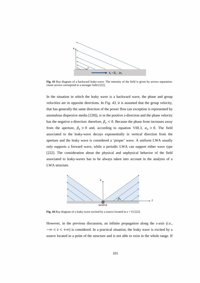
101

Fig. 43 Ray diagram of a backward leaky-wave. The intensity of the field is given by arrows separation: closer arrows correspond to a stronger field [222].

In the situation in which the leaky wave is a backward wave, the phase and group

velocities are in opposite directions. In Fig. 43, it is assumed that the group velocity,

that has generally the same direction of the power flow (an exception is represented by

anomalous dispersive media [228]), is in the positive z-direction and the phase velocity

has the negative z-direction: therefore, < 0. Because the phase front increases away

from the aperture, 0 and, according to equation VIII.3, 0. The field

associated to the leaky-wave decays exponentially in vertical direction from the

aperture and the leaky wave is considered a ‘proper’ wave. A uniform LWA usually

only supports a forward wave, while a periodic LWA can support either wave type

[222]. The consideration about the physical and unphysical behavior of the field

associated to leaky-waves has to be always taken into account in the analysis of a

LWA structure.

Fig. 44 Ray diagram of a leaky-wave excited by a source located in z = 0 [222].

However, in the previous discussion, an infinite propagation along the z-axis (i.e.,

v∞ ¤ o∞) is considered. In a practical situation, the leaky wave is excited by a

source located in a point of the structure and is not able to exist in the whole range. If

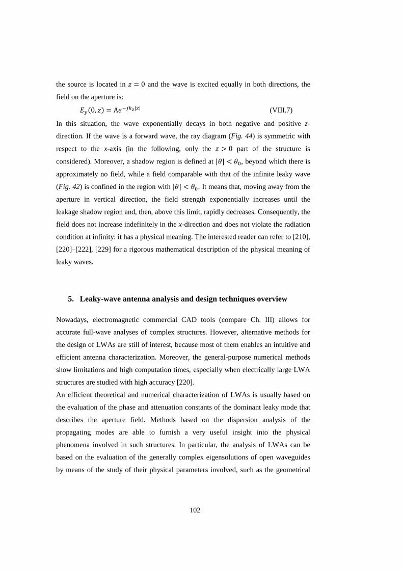
102

the source is located in ¤ = 0 and the wave is excited equally in both directions, the

field on the aperture is:

»óe0, ¤j = A/yÝÛõ|| (VIII.7)

In this situation, the wave exponentially decays in both negative and positive z-

direction. If the wave is a forward wave, the ray diagram (Fig. 44) is symmetric with

respect to the x-axis (in the following, only the ¤ > 0 part of the structure is

considered). Moreover, a shadow region is defined at || < , beyond which there is

approximately no field, while a field comparable with that of the infinite leaky wave

(Fig. 42) is confined in the region with || < . It means that, moving away from the

aperture in vertical direction, the field strength exponentially increases until the

leakage shadow region and, then, above this limit, rapidly decreases. Consequently, the

field does not increase indefinitely in the x-direction and does not violate the radiation

condition at infinity: it has a physical meaning. The interested reader can refer to [210],

[220]–[222], [229] for a rigorous mathematical description of the physical meaning of

leaky waves.

5. Leaky-wave antenna analysis and design techniques overview

Nowadays, electromagnetic commercial CAD tools (compare Ch. III) allows for

accurate full-wave analyses of complex structures. However, alternative methods for

the design of LWAs are still of interest, because most of them enables an intuitive and

efficient antenna characterization. Moreover, the general-purpose numerical methods

show limitations and high computation times, especially when electrically large LWA

structures are studied with high accuracy [220].

An efficient theoretical and numerical characterization of LWAs is usually based on

the evaluation of the phase and attenuation constants of the dominant leaky mode that

describes the aperture field. Methods based on the dispersion analysis of the

propagating modes are able to furnish a very useful insight into the physical

phenomena involved in such structures. In particular, the analysis of LWAs can be

based on the evaluation of the generally complex eigensolutions of open waveguides

by means of the study of their physical parameters involved, such as the geometrical

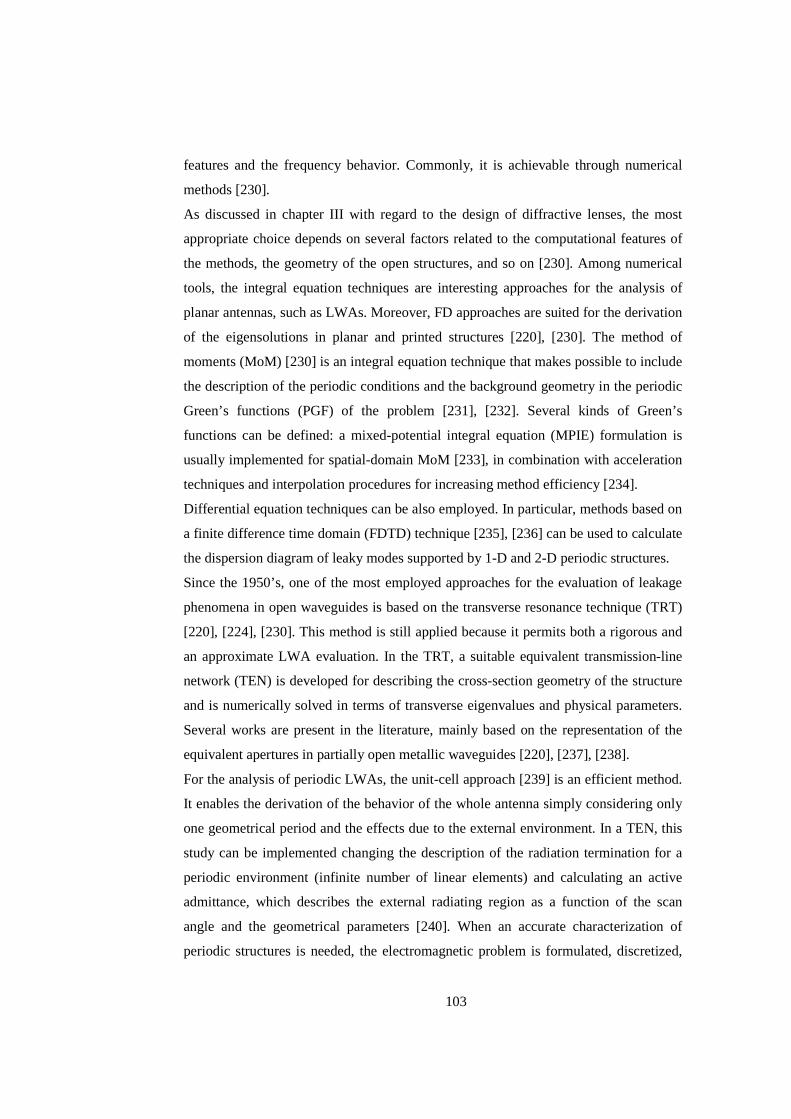
103

features and the frequency behavior. Commonly, it is achievable through numerical

methods [230].

As discussed in chapter III with regard to the design of diffractive lenses, the most

appropriate choice depends on several factors related to the computational features of

the methods, the geometry of the open structures, and so on [230]. Among numerical

tools, the integral equation techniques are interesting approaches for the analysis of

planar antennas, such as LWAs. Moreover, FD approaches are suited for the derivation

of the eigensolutions in planar and printed structures [220], [230]. The method of

moments (MoM) [230] is an integral equation technique that makes possible to include

the description of the periodic conditions and the background geometry in the periodic

Green’s functions (PGF) of the problem [231], [232]. Several kinds of Green’s

functions can be defined: a mixed-potential integral equation (MPIE) formulation is

usually implemented for spatial-domain MoM [233], in combination with acceleration

techniques and interpolation procedures for increasing method efficiency [234].

Differential equation techniques can be also employed. In particular, methods based on

a finite difference time domain (FDTD) technique [235], [236] can be used to calculate

the dispersion diagram of leaky modes supported by 1-D and 2-D periodic structures.

Since the 1950’s, one of the most employed approaches for the evaluation of leakage

phenomena in open waveguides is based on the transverse resonance technique (TRT)

[220], [224], [230]. This method is still applied because it permits both a rigorous and

an approximate LWA evaluation. In the TRT, a suitable equivalent transmission-line

network (TEN) is developed for describing the cross-section geometry of the structure

and is numerically solved in terms of transverse eigenvalues and physical parameters.

Several works are present in the literature, mainly based on the representation of the

equivalent apertures in partially open metallic waveguides [220], [237], [238].

For the analysis of periodic LWAs, the unit-cell approach [239] is an efficient method.

It enables the derivation of the behavior of the whole antenna simply considering only

one geometrical period and the effects due to the external environment. In a TEN, this

study can be implemented changing the description of the radiation termination for a

periodic environment (infinite number of linear elements) and calculating an active

admittance, which describes the external radiating region as a function of the scan

angle and the geometrical parameters [240]. When an accurate characterization of

periodic structures is needed, the electromagnetic problem is formulated, discretized,

104

and solved inside the unit cell by applying Floquet periodic boundary conditions along

the directions of periodicity.

All of these computational techniques are essential tools in the development of

efficient and accurate analysis of leakage phenomena on several different LWA

structures. Among the methods outlined in this brief list, the TRT will be illustrated

with more detail in the following subsection.

5.1 Transverse resonance technique

A standard method for the analysis of complex structures is: (i) to formulate the

general solution of Maxwell’s equations in a homogeneous region of the domain of

interest; (ii) to apply the boundary conditions; (iii) to enforce the determinant of the

coefficients to 0; (iv) to find the complex roots of the resulting equation, which is

called dispersion equation. This procedure can be time consuming, especially if the

domain of interest is composed by more than one medium.

In the situation in which only the determination of the eigenvalues is of interest, the

transverse resonance technique represents an appropriate tool. In fact, the eigenvalues

of a waveguide problem correspond to pole singularities of a suitable characteristic

Green’s function in the complex plane of the propagation wavenumber. This Green’s

function can be identified as the voltage (or current) on a transmission line along one

of the transverse direction of the waveguide axial direction [221], [223]. The pole

singularities correspond to the TEN model resonances and are usually computed using

analytical methods.

A general form of terminated TEN is given in Fig. 45.

Fig. 45 Terminated equivalent network representing a waveguide cross-section [223].

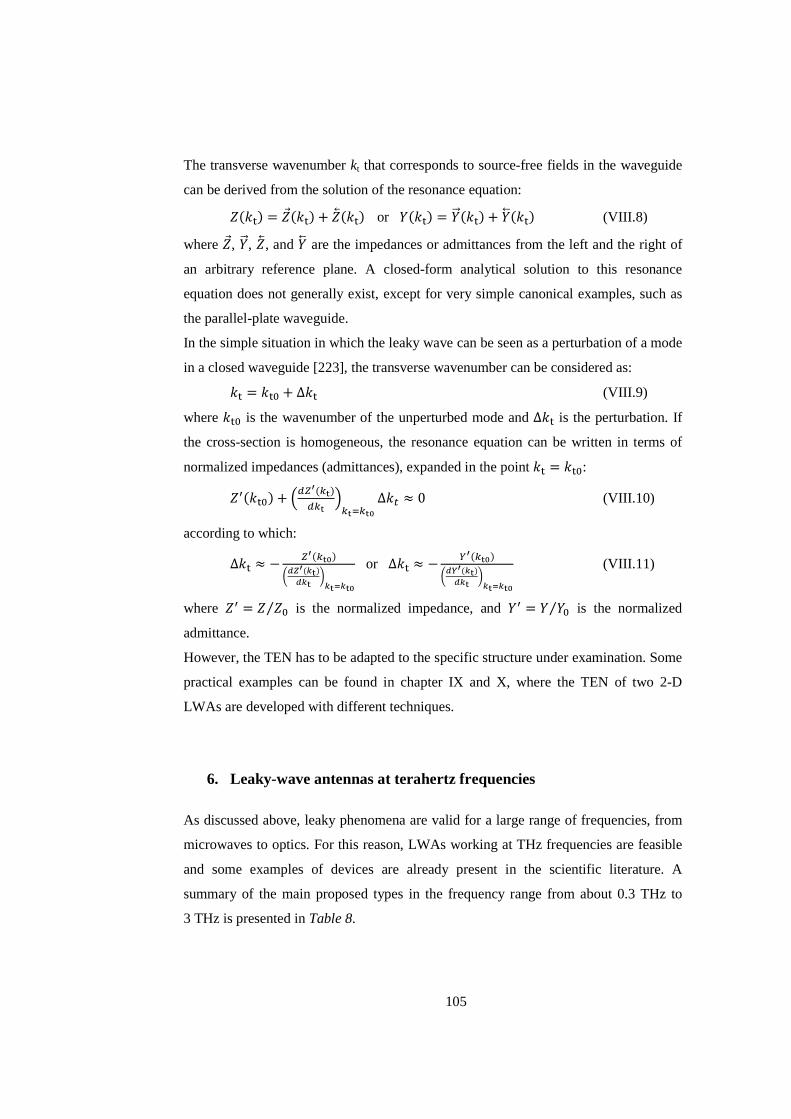
105

The transverse wavenumber kt that corresponds to source-free fields in the waveguide

can be derived from the solution of the resonance equation:

þej = þej + þej or ej = ej + ej (VIII.8)

where þ, , þ, and are the impedances or admittances from the left and the right of

an arbitrary reference plane. A closed-form analytical solution to this resonance

equation does not generally exist, except for very simple canonical examples, such as

the parallel-plate waveguide.

In the simple situation in which the leaky wave can be seen as a perturbation of a mode

in a closed waveguide [223], the transverse wavenumber can be considered as:

= + ∆ (VIII.9)

where is the wavenumber of the unperturbed mode and ∆ is the perturbation. If

the cross-section is homogeneous, the resonance equation can be written in terms of

normalized impedances (admittances), expanded in the point = :

þej + u&eÛÏj&ÛÏ zÛÏÞÛÏ

∆8 ≈ 0 (VIII.10)

according to which:

∆ ≈ − eÛÏjåeØÏj

ØÏ èØÏØÏ

or ∆ ≈ − eÛÏjå eØÏj

ØÏ èØÏØÏ (VIII.11)

where þ = þ þ⁄ is the normalized impedance, and = ⁄ is the normalized

admittance.

However, the TEN has to be adapted to the specific structure under examination. Some

practical examples can be found in chapter IX and X, where the TEN of two 2-D

LWAs are developed with different techniques.

6. Leaky-wave antennas at terahertz frequencies

As discussed above, leaky phenomena are valid for a large range of frequencies, from

microwaves to optics. For this reason, LWAs working at THz frequencies are feasible

and some examples of devices are already present in the scientific literature. A

summary of the main proposed types in the frequency range from about 0.3 THz to

3 THz is presented in Table 8.

106

Table 8 Leaky-wave antennas typologies and examples, working in the frequency range of 0.3 - 3 THz. In the headers, f is the frequency at which the antennas are investigated, while η is the radiation efficiency.

Measured device?

Materials Feeding f [THz] Directi-

vity [dB]

η [%]

Beam width

[°] Ref.

Lens antenna

yes Si, SiNx, Au, Al

wave-guide

0.3 – 2.8 (discrete values)

< 42.1 < 75 - [241]–[246]

Periodic corrugated

metallic wire no PEC -

0.9655 – 0.9829

- 90 22 [247]

Flat corrugated

antenna yes gold slot 0.566 16 - 7

[248], [249]

Composite right/left-handed

metamaterial waveguide

yes

GaAs/Al0.

15Ga0.85As + Cr/Au +

Ni + Ti/Au/Ni

metal-metal QCL cavity

2.48 and 2.59

- -

10 (at 2.48 THz) 15 (at 2.59 THz)

[250]

Metasurface antennas

no see Table 9

Tunable antennas

see Table 10

The choice of this specific frequency band is linked to the technological issues already

discussed in chapter I: even if the border between millimeters waves and far-IR has not

been delimited yet, below 0.3 THz, facilities developed for the millimeter waves are

available, while, above 3 THz, the mechanisms connected to the description of far-IR

radiation are predominant.

The most studied THz LWA is a leaky-wave waveguide coupled with a hemispherical

silicon lens. It is able to operate at a fixed value of frequency [241], [246] or in a

frequency band of 0.2 THz [242] until 1.4 THz [243]–[245] wide. When the device

works at a single frequency, it can show a very high directivity; for example [241], of

42.1 dB. Lens LWAs able to operate in a frequency band wider than 1 THz can be

employed for practical applications, such as THz detectors (described in Ch. I, Sec. 3).

However, independently from the operating frequencies of the antenna, the radiation

efficiency is always below 75%, due to losses introduced by the coupling with a silicon

lens (see Ch. V).

107

Table 9 Metasurfaces FPC-LWAs in the frequency range 0.3 - 3 THz. In the headers, f is the frequency at which the antennas are investigated, while η is the radiation efficiency.

Materials Feeding f [THz]

Gain (max) [dBi]

η [%] 3-dB gain

Bandwidth [%]

Ref.

5x5 square patches array

GaAs + metal

open-ended slotline or an

array of 5 slit

0.34 - 0.4

9.8 (single feed)

15.5 (feed array)

69 (single feed)

73 (feed array)

16 (single feed)

17.3 (feed array)

[251]

7x7 circular patches array

GaAs + metal

open-ended slotline

0.315 11.3 72 3 [252]

7x7 ring patches array

GaAs + metal

open-ended slotline

0.315 11.4 75 22.5 [252]

7x7 circular

hole array

GaAs + metal

open-ended slotline

0.318 15.3 60 1.3 [252], [253]

Another class of LWAs, widely employed at THz frequencies, is that of Fabry-Perot

cavity (FPC) LWAs. They are 2-D LWAs inspired by the Fabry-Perot concept: the

radiation phenomenon is interpreted in terms of multiple reflections between a ground

plane and a partially reflective sheet (PRS). In this kind of LWAs, the maximum

radiated power at broadside is connected to the resonance condition of the multiple

reflections. For this reason, they usually work at a single frequency, i.e. at the

resonance frequency of the FPC. The PRS can assume several forms. In Table 9, the

performances of FPC-LWAs with different metasurface geometries are compared. A

metasurface is, in general, a metallic patterned surface, in which the geometrical

elements composing the pattern have dimensions deeply below the operative

wavelength. It means that this surface can be considered as a homogeneous surface

with properties depending on the specific geometrical pattern chosen for the

metasurface synthesis. Even if several geometries have been investigated in the THz

range as PRS for FPC-LWAs, none of them has been fully characterized yet. However,

they show advantages common to many LWAs, such as the suitability to

miniaturization and integration on complex devices or the scalability at every THz

frequency value of operation. In addition, they are also: (i) simple to fabricate, (ii) with

an affordable fabrication cost, and (iii) suitable for mass production. The radiation

efficiencies, computed for the structures presented in Table 9, do not go beyond the

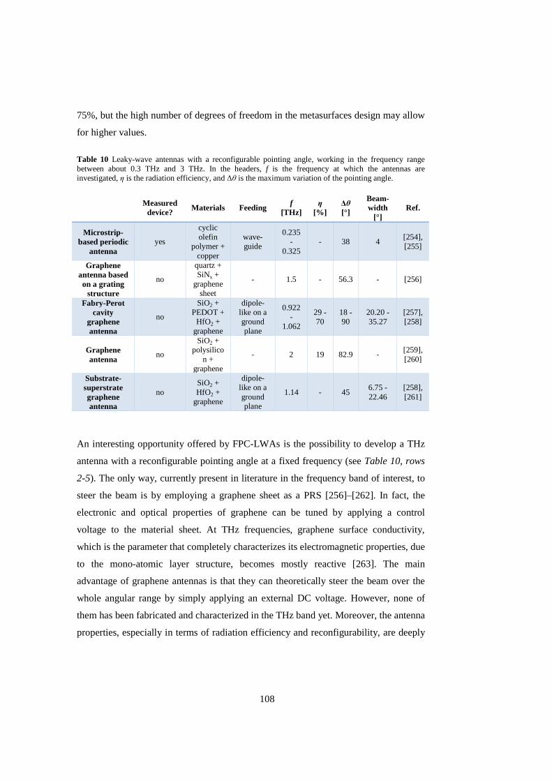
108

75%, but the high number of degrees of freedom in the metasurfaces design may allow

for higher values.

Table 10 Leaky-wave antennas with a reconfigurable pointing angle, working in the frequency range between about 0.3 THz and 3 THz. In the headers, f is the frequency at which the antennas are investigated, η is the radiation efficiency, and ∆θ is the maximum variation of the pointing angle.

Measured device? Materials Feeding f

[THz] η

[%] ∆θ [°]

Beam-width

[°] Ref.

Microstrip-based periodic

antenna yes

cyclic olefin

polymer + copper

wave-guide

0.235 -

0.325 - 38 4

[254], [255]

Graphene antenna based on a grating

structure

no

quartz + SiNx +

graphene sheet

- 1.5 - 56.3 - [256]

Fabry-Perot cavity

graphene antenna

no

SiO2 + PEDOT +

HfO2 + graphene

dipole-like on a ground plane

0.922 -

1.062

29 -70

18 - 90

20.20 - 35.27

[257], [258]

Graphene antenna

no

SiO2 + polysilico

n + graphene

- 2 19 82.9 - [259], [260]

Substrate-superstrate graphene antenna

no SiO2 + HfO2 +

graphene

dipole-like on a ground plane

1.14 - 45 6.75 - 22.46

[258], [261]

An interesting opportunity offered by FPC-LWAs is the possibility to develop a THz

antenna with a reconfigurable pointing angle at a fixed frequency (see Table 10, rows

2-5). The only way, currently present in literature in the frequency band of interest, to

steer the beam is by employing a graphene sheet as a PRS [256]–[262]. In fact, the

electronic and optical properties of graphene can be tuned by applying a control

voltage to the material sheet. At THz frequencies, graphene surface conductivity,

which is the parameter that completely characterizes its electromagnetic properties, due

to the mono-atomic layer structure, becomes mostly reactive [263]. The main

advantage of graphene antennas is that they can theoretically steer the beam over the

whole angular range by simply applying an external DC voltage. However, none of

them has been fabricated and characterized in the THz band yet. Moreover, the antenna

properties, especially in terms of radiation efficiency and reconfigurability, are deeply

109

influenced by the graphene quality mainly determined by the synthesis technique and

the interaction with the substrate, as well.

An alternative way to steer the beam is to change the operating frequency. An example

is presented in Table 10, row 1, where a microstrip LWA with periodic elements is

investigated as a THz radar and show a beam steering over an angular range of 38°,

with a very narrow radiated beam. However, this kind of device has a limited

application as radar to a short range object detection [254].

Other forms of PRS for FPC-LWAs working in the THz range will be widely analyzed

in chapter IX and X, where a reconfigurable multilayered structure as well as some

metasurface geometries will be designed and numerically investigated.

7. Conclusions

Leaky-wave antennas are fast traveling-wave antennas, in which radiation occurs

thanks to a power leakage during the wave propagation. They are antennas

characterized by a high directivity and by the possibility to be employed as radiating

systems at microwaves as well as at optical frequencies.

For these reasons, LWAs seem to be particularly suitable for being integrated in THz

systems. Among the several existing LWAs typologies, FPC-LWAs are attractive

structures because they allow for tuning the radiation beam steering by applying an

external voltage.

In the next chapters, two different FPC-LWAs will be designed and deeply

investigated as promising devices for THz far-field applications.

110

CHAPTER IX Fabry-Perot cavity leaky-wave antennas based on liquid crystals for terahertz beam-steering2

1. Introduction

Two-dimensional (2-D), bidirectional, quasi-uniform LWAs are a class of 2-D LWAs

obtained as a perturbation of a metallic parallel-plate waveguide, where the upper plate

is replaced by a PRS to allow radiation. Among them, FPC-LWAs are characterized by

two features: (i) the thickness of the slab constituting the antenna substrate is close to

half a wavelength in the medium; (ii) the PRS can be described by a single

homogenized impedance. In fact, PRSs can take several forms, such as: a denser

dielectric superstrate [264], a graphene sheet [262], a metamaterial or a metasurface,

etc.. For most of PRSs constituted by a periodic arrangement of sub-resonant elements,

homogenization formulas can be derived [265]–[267], permitting to derive the

homogenized impedance of the PRS.

In this chapter, a PRS based on a metamaterial is introduced. The metamaterials are

artificial materials obtained by the combination of different materials, present in

nature, with spacing and geometrical features below the wavelength dimension. Since

metamaterials can show values of dielectric permittivity and permeability that are

impossible for natural materials, they allow for a considerable control of the

electromagnetic radiation, helping in the development of interesting applications [268],

[226].

2Most of information reported in this chapter is with courtesy of Dr. Walter Fuscaldo and was born from a collaboration with him. More details about theoretical background in the development of Fabry-Perot cavity leaky-wave antennas for THz applications can be found in his PhD thesis: “Advanced radiating systems based on leaky waves and nondiffracting waves”.

111

Even if several metasurface designs already exist for microwave applications [269]–

[271], only few implementations have been proposed in the THz range [272], [273]. In

this chapter, the possibility to develop an electro-optically tunable metasurface LWA is

investigated. In fact, as discussed in chapter VII, LCs can be employed for the

realization of different THz devices, such as, for example, composite free-space

materials [274]–[276] as well as guided-wave THz phase shifters [277], [278].

However, only few works have considered the possibility of designing LCs

reconfigurable THz LWAs. In the following sections, a THz FPC-LWA based on LCs

is discussed in terms of theoretical and numerical modeling, underlining the conditions

at which a device fabrication is feasible.

2. Liquid crystals for the design of a tunable leaky-wave antenna

As discussed in chapter VII, the application of a voltage to LCs change the direction of

the molecules director, tuning the LCs dielectric properties. Therefore, the phase

constant of the leaky-wave modes changes too, causing the radiation beam-steering at a

fixed frequency. Among the different kinds of LC mixtures, the uniaxial nematic LCs,

already employed in the numerical study of LC tunable diffractive lenses (see Ch. VII),

is considered because of its high birefringence and moderate losses at THz frequencies

[152].

Fig. 46 LC cell driven by a gold fishnet electrode.

112

Thanks to the Q-tensor analysis (described in Ch. VII Sec. 2.1.2), values of all

components of permittivity tensor can be numerically evaluated by changing the

voltage from zero until the threshold value. For this computation, the LC cell, as

presented in [152] and reported in Fig. 46, has a total thickness of 9.7 µm and its

threshold voltage can be set equal to 7 V. Differently from the dual-focus diffractive

lens which works in the absence of external voltage or with a voltage above the

threshold, in this situation the device is designed for operating at every value of voltage

from zero until the threshold.

As can be seen from Fig. 47, the ordinary value of the real part of LC dielectric

permittivity is Reej ≅ 2.42, while the real part of extraordinary permittivity is

Reej ≅ 3.76. Moreover, the LC director does not change along the y-direction and it

is possible to consider ó B .

Fig. 47 Real part of the three main components of the LC permittivity tensor mapped in the xy-plane, in the middle of the LC cell (z = 0). The LCs behavior is show in absence of an external field (first row), for a voltage above the threshold (last row), and for an intermediate value of driving voltage (middle row) [with courtesy of Dr. W. Fuscaldo].

113

It is worth to stress that the chosen mixture contains uniaxial LCs. This would allow

for a simplified electromagnetic description of LC layers in the equivalent circuit

model (compare Ch. VIII Sec. 5.1). On the contrary, when the LC is not uniaxial, off-

diagonal components of the permittivity tensor are no longer negligible and more

complicated equivalent networks have to be considered [279].

Fig. 48 Real and the imaginary part of the LC dielectric permittivity along a line perpendicular to the xy-plane and passing through three selected points of the LC cell [with courtesy of Dr. W. Fuscaldo].

In addition to the real permittivity map of the xy-plane of the LC cell, it is also

important to know the permittivity profile in z-direction for values of voltage from 0 V

until the threshold, i.e., 7 V. Three different points, as indicated in Fig. 46, are chosen:

A ((x0, y0) = (0, 0) µm) is in the middle of the electrode, B ((x0, y0) = (54, 54) µm) is at

the edge of the electrode, and C ((x0, y0) = (75, 75) µm) is outside the electrode. The

plot of the real and the imaginary part of the LC dielectric permittivity along a line

perpendicular to the xy-plane and passing through these three points is shown in Fig.

48, with regard of the εx and εz components. The variation is quite uniform in

correspondence of the middle and the edge of the electrode: anchoring forces change

permittivity profile in the first micrometer of thickness in contact with boundaries;

however, away from boundaries, the applied voltage is completely able to pilot the LC

molecules, determining a uniform permittivity profile. No variation is seen outside the

fishnet, where there is no applied electric field. As expected from uniaxial LC physics,

114

εx and εz exhibit a specular nonlinear variation as the bias changes from 0 V (unbiased

state) to 7 V (fully biased state).

For the sake of brevity, in the design of a tunable FPC-LWA, only averaged values of

LC layers permittivity and the two limiting voltage cases (i.e., unbiased and fully-

biased states) are studied to investigate the maximum tunability range of the THz

LWA.

3. Tunable Fabry-Perot cavity leaky-wave antenna design

The proposed THz FPC-LWA consists of a multistack of materials: high-permittivity

dielectric material layers, such as the alumina (Al2O3), are alternated with low-

permittivity material layers, such as the LCs described in the previous section.

The multistack of alternating layers could be interpreted as a distributed Bragg

reflector (DBR), meaning that it is a periodic electronic bandgap (EBG) structure

operating in a stopband [280]. A leaky-wave explanation of the phenomenon is

provided in [281].

Material layers in the multistack need to have a thickness equal to the odd multiples of

a quarter wavelength in their respective media. In this way, the alternation of such

layers allows for obtaining a narrow radiated beam at broadside [281]. The multistack

is placed above a grounded dielectric slab (GDS), as shown in Fig. 49. The material

chosen for the substrate layer is the Zeonor because, in the THz range, the real part of

its dielectric permittivity (~2.3) is almost matched with the real part of the ordinary

dielectric permittivity (~2.42) of the LC mixture [152], [203]. It is required to properly

enhance the resonance condition in a FPC [281]. Moreover, Zeonor is a low absorption

material at THz frequencies and introduces negligible losses overall (for a discussion

of Zeonor properties, see Ch. II Sec. 5).

In the proposed device, the innovating feature is represented by the use of LCs as low-

permittivity layers, which leads to the beam-steering at a fixed THz frequency.

115

Fig. 49 Schematic representation of the proposed FPC-LWA and its equivalent transmission line model.

A circuit model of the proposed device is shown in Fig. 49. It takes into account the

anisotropy of LC layers considering:

eÁj = ³eÁj 0 00 00 0 eÁj´ (IX.1)

According to the reference frame shown in Fig. 49, when no bias is applied, LC

molecules are aligned along the horizontal z-axis and eÁ B 0j B . When a

sufficiently large driving voltage (V∞) is applied to LC molecules, their director is

reoriented along the vertical x-axis and eÁ B Á0j B .

With regard to the transverse transmission line model (Fig. 49), the characteristic

admittances, Y3, and the normal wavenumbers, kx3, of the LC layers for both

transverse-electric (TE) and transverse-magnetic (TM) polarizations (with respect to

the xz-plane) are functions of the bias voltage. Their expression is given by:

$gh B Ûö and $gi B ¶¶õpeZjÛö (IX.2)

$gh B #ó v # and $gi B¶õeZj¶öeZj #eÁj v # (IX.3)

116

where k0 is the vacuum wavenumber, kx is the radiation wavenumber in x-direction, kz

is the radiation wavenumber in z-direction, ε0 is the vacuum dielectric permittivity, and

µ0 is the vacuum permeability.

However, the selected LC mixture is uniaxial and εy does not depend on the applied

voltage: only the fundamental TM leaky mode is affected by the external bias and,

thus, the TE leaky mode is not of interest in this investigation. It also allows for

showing the LWA radiation features only in the E-plane (i.e., the xz-plane, with respect

to the reference system in Fig. 49), that is the plane affected by the TM leaky mode

[282].

The dispersion equation relates the frequency and the complex longitudinal

wavenumber. The dispersion equation can be obtained by applying the transverse

resonance technique to the transverse equivalent network of Fig. 49. As discussed in

chapter VIII, this method consists of considering the sum between the admittance

looking upwards Yup and downwards Ydw at an arbitrary cross section and to equal it to

zero:

). + = 0 (IX.4)

Equation IX.4 evaluated at the cross section correspondent to £ = ℎ! is:

>, − ðgi cot¢,ℎ¦ = 0 (IX.5)

where the input admittance of the i-th layer can be written as:

>, = gi XD,[ G¢Ûö,[[¦[ >¢Ûö,[[¦[ G¢Ûö,[[¦XD,[ >¢Ûö,[[¦ (IX.6)

where gi is the characteristic admittance of the i-th layer, , is the transverse

wavenumber of the i-th layer, and ℎ can be considered as the i-th layer thickness.

4. Terahertz implementation of a Fabry-Perot cavity leaky-wave

antenna with liquid crystals: numerical results

The dispersion curves for an ideal layout (Layout 1) can be derived as a proof-of-

concept of the proposed antenna at the frequency of 0.59 THz. In this design, the

number of layers, N, is set equal to four and the layers are made with lossless materials

(the effect of losses on antenna performance will be examined further). Relevant

parameters for the antenna designs are listed in Table 11.

117

Table 11 Design parameters for different THz FPC-LWA layouts.

Layout N h1 [µm] h2 [µm] h3 [µm] f0 [THz] 1 4 167 127 82 0.59 2 8 167 127 82 0.56 3 6 100 75 145 1.00 4 4 188 127 82 0.56

For the evaluation of materials thickness, (compare design rules in Fig. 49), the

wavelength in the media is considered as: '( = ⁄ , for LC layers; % = ,%⁄ , for alumina layers; and )* = ,)*⁄ , for the substrate of Zeonor;

where is the vacuum wavelength, i.e., the wavelength corresponding to the design

frequency. Moreover, m, n, and p, appearing in Fig. 49, are integer values that indicate

which odd multiple of the quarter wavelength is considered. m = 1, n = 2, and p = 1

are chosen in Layout 1; for higher values of m, n, and p higher-order modes may

appear in certain frequency ranges, and possibly degrade the antenna performance.

Finally, in Layout 1, the choice of a design frequency, f0, of 0.59 THz is due to the

minimum commercially available thickness for alumina layers (127 µm). At 0.59 THz,

alumina exhibits a relative permittivity ,% = 9 and a loss tangent of about tan % ≅0.01 [283].

4.1 Dispersion analysis of fundamental leaky modes: lossless case of

study

Dispersion curves of the fundamental TM leaky mode for the frequency range 0.50–

0.75 THz are presented in Fig. 50. They are a family of curves obtained gradually

changing the voltage between zero (red curve) and the threshold voltage V∞ (blue

curve). For the proposed LC cell thickness, values below 20 V are sufficient to cover

almost the complete switching range. For simplifying the analysis, it is assumed that

LC relative permittivity linearly varies with the applied voltage. For this reason, the

unbiased and biased states are always correctly predicted. Conversely, the dynamic

variation of = ⁄ and = ⁄ , corresponding to voltage values between 0

and 20 V, could change if the voltage-dependence of LC permittivity is completely

predicted by Q-tensor computations (compare Ch. VII Sec. 2.1.2).

118

Fig. 50 Dispersion curves of the fundamental TM for different THz FPC-LWA with LC: a) Layout 1, b) Layout 2, c) Layout 3, d) Layout 4. Colors gradually shade from blue to red as the applied external voltage decreases from V∞ to zero [with courtesy of Dr. W. Fuscaldo].

The frequency at which the splitting condition ≅ is achieved can be considered

as the operating frequency. For this application, the operative frequency is fixed by the

value obtained when the voltage is equal to V∞ (blue curve), which corresponds to the

design frequency. In fact, once the operating frequency is fixed, it is possible to change

the value of the normalized phase constant by simply decreasing the external

voltage. On the contrary, the value of the normalized attenuation constant remains

almost the same, such that > . This would allow the steering of the THz beam

with a quasi-constant beamwidth (because it is proportional to that does not change

with the voltage) at a fixed frequency. Some relevant radiating features for the Layout

1 are reported in the first row of Table 12.

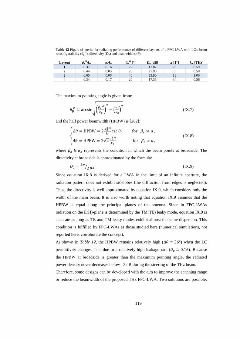
119

Table 12 Figure of merits for radiating performance of different layouts of a FPC-LWA with LCs: beam reconfigurability (θp

M), directivity (D0) and beamwidth (∆θ).

Layout βzM /k0 αz/k0 θp

M [°] D0 [dB] ∆θ [°] fop [THz] 1 0.37 0.16 22 17.87 26 0.59 2 0.44 0.05 26 27.98 8 0.59 3 0.65 0.08 40 23.90 13 1.00 4 0.34 0.17 20 17.35 34 0.56

The maximum pointing angle is given from:

.i ≅ arcsinåûõÛ è# − uõÛz# (IX.7)

and the half power beamwidth (HPBW) is [282]:

= HPBW = 2 õÛ cscfor ≫ = HPBW = 2√2 õÛ for ≅ (IX.8)

where ≅ represents the condition in which the beam points at broadside. The

directivity at broadside is approximated by the formula:

ì = 4 #À (IX.9)

Since equation IX.8 is derived for a LWA in the limit of an infinite aperture, the

radiation pattern does not exhibit sidelobes (the diffraction from edges is neglected).

Thus, the directivity is well approximated by equation IX.9, which considers only the

width of the main beam. It is also worth noting that equation IX.9 assumes that the

HPBW is equal along the principal planes of the antenna. Since in FPC-LWAs

radiation on the E(H)-plane is determined by the TM(TE) leaky mode, equation IX.9 is

accurate as long as TE and TM leaky modes exhibit almost the same dispersion. This

condition is fulfilled by FPC-LWAs as those studied here (numerical simulations, not

reported here, corroborate the concept).

As shown in Table 12, the HPBW remains relatively high ( ≅ 26°) when the LC

permittivity changes. It is due to a relatively high leakage rate ( ≅ 0.16). Because

the HPBW at broadside is greater than the maximum pointing angle, the radiated

power density never decreases below –3 dB during the steering of the THz beam.

Therefore, some designs can be developed with the aim to improve the scanning range

or reduce the beamwidth of the proposed THz FPC-LWA. Two solutions are possible:

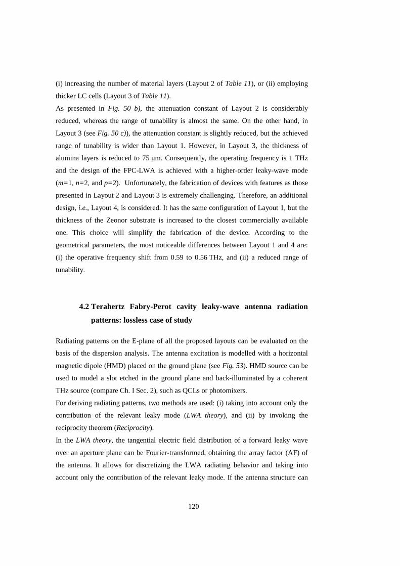
120

(i) increasing the number of material layers (Layout 2 of Table 11), or (ii) employing

thicker LC cells (Layout 3 of Table 11).

As presented in Fig. 50 b), the attenuation constant of Layout 2 is considerably

reduced, whereas the range of tunability is almost the same. On the other hand, in

Layout 3 (see Fig. 50 c)), the attenuation constant is slightly reduced, but the achieved

range of tunability is wider than Layout 1. However, in Layout 3, the thickness of

alumina layers is reduced to 75 µm. Consequently, the operating frequency is 1 THz

and the design of the FPC-LWA is achieved with a higher-order leaky-wave mode

(m=1, n=2, and p=2). Unfortunately, the fabrication of devices with features as those

presented in Layout 2 and Layout 3 is extremely challenging. Therefore, an additional

design, i.e., Layout 4, is considered. It has the same configuration of Layout 1, but the

thickness of the Zeonor substrate is increased to the closest commercially available

one. This choice will simplify the fabrication of the device. According to the

geometrical parameters, the most noticeable differences between Layout 1 and 4 are:

(i) the operative frequency shift from 0.59 to 0.56 THz, and (ii) a reduced range of

tunability.

4.2 Terahertz Fabry-Perot cavity leaky-wave antenna radiation

patterns: lossless case of study

Radiating patterns on the E-plane of all the proposed layouts can be evaluated on the

basis of the dispersion analysis. The antenna excitation is modelled with a horizontal

magnetic dipole (HMD) placed on the ground plane (see Fig. 53). HMD source can be

used to model a slot etched in the ground plane and back-illuminated by a coherent

THz source (compare Ch. I Sec. 2), such as QCLs or photomixers.

For deriving radiating patterns, two methods are used: (i) taking into account only the

contribution of the relevant leaky mode (LWA theory), and (ii) by invoking the

reciprocity theorem (Reciprocity).

In the LWA theory, the tangential electric field distribution of a forward leaky wave

over an aperture plane can be Fourier-transformed, obtaining the array factor (AF) of

the antenna. It allows for discretizing the LWA radiating behavior and taking into

account only the contribution of the relevant leaky mode. If the antenna structure can

121

be considered infinite in the y- and z-directions, the AF assumes the following

expression: AFej = y#ÝÛõGejÛõpyÛp>pej (IX.10)

For Reciprocity, an in-house MATLAB code is developed for deriving the one-

dimensional Green’s functions of the transverse equivalent network (TEN) model by

means of the ABCD-matrix formalism [284]. Afterward, the reciprocity theorem is

applied for calculating the E-plane far field radiation patterns. The far-field intensity at

a given angle θ can be considered equivalent to the magnetic field excited at the source

position by a plane wave, incident with the same angle θ and coming from a testing

dipole source [285].

Fig. 51 Radiation patterns predicted by leaky-wave theory (dashed lines) or by means of reciprocity theorem (solid lines): a) Layout 1, b) Layout 2, c) Layout 3, and d) Layout 4 (see Table 3.5). The condition of the THz beam pointing at broadside (blue lines) and the radiation at the maximum pointing angle (red lines) are presented [with courtesy of Dr. W. Fuscaldo].

Radiation patterns are reported in Fig. 51 for all discussed layouts. Fig. 51 a), b), and

d), show a very good agreement between LWA theory and Reciprocity. However, in

122

Fig. 51 c), the LWA theory does not provide an accurate evaluation. This is probably

because Layout 3 is developed with a higher-order design and a higher-order leaky-

wave mode could be present, increasing the sidelobe level. Reciprocity, however,

correctly predicts this effect.

Some relevant radiating features are listed in Table 12. Layout 2 considerably

improves the directivity and, consequently, the beamwidth of the THz FPC-LWA. On

the other side, the proposed device, designed according to Layout 3, has an increased

reconfigurable capability. In fact, a higher thickness of the LC layers in Layout 3

extends the range of tunability, but degrades the radiation patterns. Conversely, a

higher number of material layers, as presented in Layout 2, increases the antenna

directivity, but the structure becomes difficult to fabricate and could suffer from non-

negligible dielectric and ohmic losses.

4.3 Terahertz Fabry-Perot cavity leaky-wave antenna: dispersion

curves and radiation patterns in the case of materials with

dielectric losses

Dispersion properties of the fundamental TM leaky-wave modes in the lossy case are

investigated for evaluating the effect of losses on the proposed THz FPC-LWAs.

Fig. 52 Dispersion curves of the fundamental TM when losses of the materials are taken into account: a) Layout 2, and b) Layout 4. Colors gradually shade from blue to red as the applied external voltage decreases from V∞ to zero [with courtesy of Dr. W. Fuscaldo].

123

In particular, the performance of Layout 2, which has a better directivity than the other

layouts, is compared with Layout 4, which is easier to fabricate than the other

discussed layouts. However, only dielectric losses are taken into account. At a first

approximation, ohmic losses due to LCs electrodes could be neglected if PEDOT:PSS

is employed as conductive material (compare Ch. VII Sec. 2.2).

The value of increases when dielectric losses are introduced (Fig. 52), determining

a deterioration of the FPC-LWA performance in terms of both HPBW and directivity.

For the lossy case, full-wave numerical simulations are performed for Layout 2 and 4

employing CST Microwave Studio (compare Ch. III Sec. 2) together with reciprocity.

This setting can be modelled in CST [286] as represented in Fig. 53: a unit cell of

period p is excited with a waveguide port at the distance hair.

Fig. 53 THz FPC-LWA unit cell model, as implemented in CST full-wave simulation. A probe for evaluating the tangential magnetic field at the ground plane is added as a light blue arrow.

The FPC-LWA is electrically large in the transverse plane and could be assumed

transversely infinite: Floquet boundary conditions can be applied to the unit cell. If λop

is the wavelength that corresponds to the operative frequency, the period of the unit

cell is ã = . 4⁄ and the distance between the unit cell and the waveguide port is

ℎH = . 2⁄ , in order to prevent the excitation of higher-order Floquet modes [287].

LC layers are modelled as layers of anisotropic material in the two limit cases of LC

director aligned along x- and z-axis.

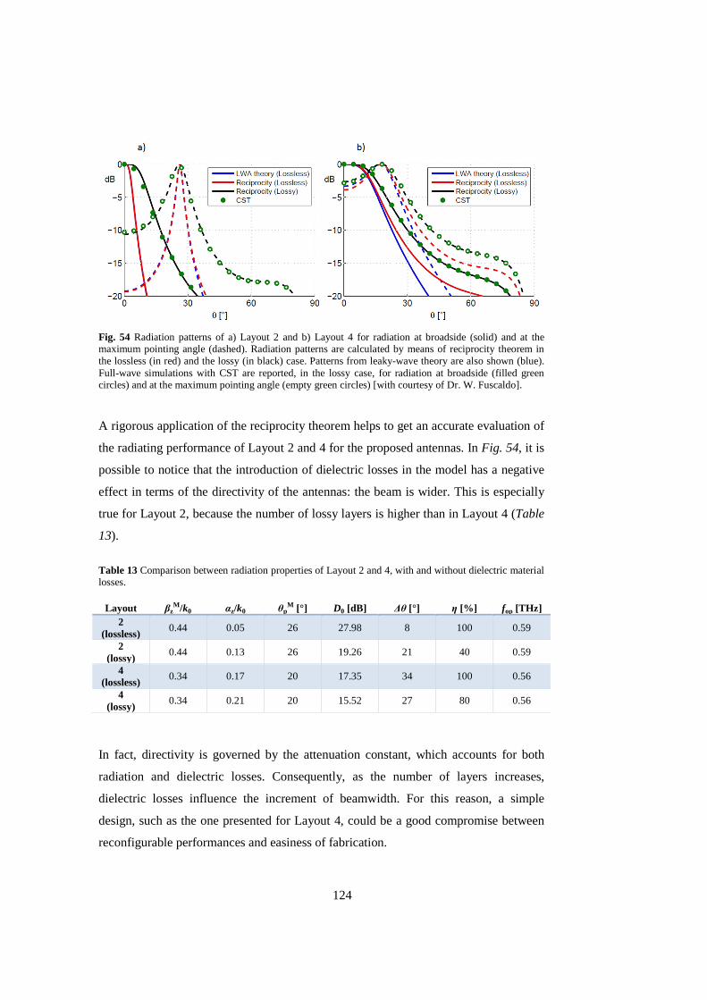
124

Fig. 54 Radiation patterns of a) Layout 2 and b) Layout 4 for radiation at broadside (solid) and at the maximum pointing angle (dashed). Radiation patterns are calculated by means of reciprocity theorem in the lossless (in red) and the lossy (in black) case. Patterns from leaky-wave theory are also shown (blue). Full-wave simulations with CST are reported, in the lossy case, for radiation at broadside (filled green circles) and at the maximum pointing angle (empty green circles) [with courtesy of Dr. W. Fuscaldo].

A rigorous application of the reciprocity theorem helps to get an accurate evaluation of

the radiating performance of Layout 2 and 4 for the proposed antennas. In Fig. 54, it is

possible to notice that the introduction of dielectric losses in the model has a negative

effect in terms of the directivity of the antennas: the beam is wider. This is especially

true for Layout 2, because the number of lossy layers is higher than in Layout 4 (Table

13).

Table 13 Comparison between radiation properties of Layout 2 and 4, with and without dielectric material losses.

Layout βzM/k0 αz/k0 θp

M [°] D0 [dB] ∆θ [°] η [%] fop [THz] 2

(lossless) 0.44 0.05 26 27.98 8 100 0.59

2 (lossy)

0.44 0.13 26 19.26 21 40 0.59

4 (lossless)

0.34 0.17 20 17.35 34 100 0.56

4 (lossy)

0.34 0.21 20 15.52 27 80 0.56

In fact, directivity is governed by the attenuation constant, which accounts for both

radiation and dielectric losses. Consequently, as the number of layers increases,

dielectric losses influence the increment of beamwidth. For this reason, a simple

design, such as the one presented for Layout 4, could be a good compromise between

reconfigurable performances and easiness of fabrication.

125

5. Conclusions

In this chapter, a FPC-LWA containing material layers with reconfigurable electro-

optical properties is investigated at THz frequencies. Specifically, different

multistacked Fabry-Perot cavity-like configurations have been considered for the

design of a THz radiator with a tunable pointing angle. The benefits and drawbacks of

ideal designs against those of more practical configurations have been carefully

addressed. Ideal designs show excellent radiating features, but are not easy to fabricate,

whereas practical designs show a considerably reduced performance, but are very

straightforward to fabricate. Moreover, even if material losses are taken into account, a

practical multistack LWA design shows a radiation efficiency higher of a 10% or more

than the state-of-art reconfigurable graphene FPC-LWAs (compare Table 10 and Table

13).

The proposed multistack FPC-LWA can be considered as a promising solution for the

current requirement of tunable THz antennas for THz wireless links. The antenna

fabrication and characterization will start to be performed in a short time.

126

CHAPTER X Terahertz leaky-wave antennas based on homogenized metasurfaces

1. Introduction

In the previous chapter, a FPC-LWA with a tunable pointing angle by means of

electro-optical control is introduced as a promising device for THz beam-steering. It is

constituted by a grounded dielectric slab with a PRS above, in the form of a distributed

Bragg Reflector (DBR) [93]. In this chapter, another kind of PRS for FPC-LWAs is

investigated, i.e., the metallic patterned metasurface3. These periodic PRSs are studied

in the situation in which the period is much smaller than the wavelength, that is called

homogenization limit [288]. Under this condition, a single impedance boundary

condition is sufficient to accurately describe the electromagnetic response of the PRS

as a whole.

In the following sections, the effect of a unit cell’s geometrical parameters on the value

of the homogenized impedance is shown for three different topologies: the patch, the

strip, and the fishnet [266], [288], [289]. The aim of the analysis is to identify the

design with the highest reflectivity to improve the FPC-LWA directivity. However,

differently from patches and strips for which homogenization formulas exist [266], no

analytical expressions have been reported so far for fishnet PRSs. This motivates a

deeper study of this PRS topology.

3 The topic, described in this chapter, was developed in collaboration with Dr. Walter Fuscaldo, who is the main author of the work.

127

2. Design constraints of terahertz metasurface leaky-wave antennas

The PRSs, studied in this chapter, are characterized by a periodic arrangement of sub-

resonant lossless elements, i.e., elements with a period ã ≪ . Under this hypothesis,

the homogenized PRS can be modeled as a purely imaginary impedance: þ = ð . Ohmic losses are not taken into account because the metal is treated as a perfect

electric conductor (PEC). However, as discussed further, ohmic losses can be also

neglected by employing a high-conductive metal layer, as copper or aluminum, of

suitable thickness.

The directivity at broadside of a LWA with a PRS described by a surface impedance ≪ , where = 120 is the vacuum impedance, is inversely proportional to the

square of Xs [290]:

ì ≅ p!p¶"|#$p (X.1)

where is the dielectric permittivity of the substrate material.

On the contrary, the fractional bandwidth (FBW), i.e., the range of frequency,

normalized to the operating frequency, for which the radiated power density at

broadside has not decreased more than 3 dB, is directly proportional to the square Xs:

FBW = 2 #$p!p √ + tan (X.2)

where tan is the loss tangent of the substrate material.

For this reason, lower impedance values lead to highly-directive FPC-LWA designs

working in a narrow bandwidth, whereas higher impedance values lead to moderately-

directive FPC-LWA designs working in a considerable bandwidth.

Furthermore, the FPC-LWAs have to be optimized for working in the THz range. This

adds some technological constrains: (i) the availability of low-loss THz materials, (ii)

the accessibility to efficient THz sources, (iii) the mechanical tolerances in the

fabrication process. With regard to (i), a commercially available substrate of Zeonor,

with a thickness ℎ = 100+m, is considered (compare Ch. II Sec. 5). For the antenna

excitation, a slot can be etched in y-direction on the ground plane, as for the LWA in

chapter IX. A suitable dimension for the slot could be 200 × 100+m#. In fact,

considering a guided-wave excitation, such dimension is comparable with the cross

section of commercial THz waveguides operating in the 0.9−1.4 THz range [80]; if a

128

free-space excitation is considered, this dimension could provide a good energy

coupling with THz beams focalized by commercial lenses. As discussed in previous

chapters, the focus area of a commercial focusing device at about 1 THz has a diameter

of around 1 mm, with an approximately bidimensional Gaussian profile. Moreover, the

suggested dimensions allow for modeling the slot as a resonant HMD source, as

required for exciting a pair of TE-TM leaky modes in a FPC-LWAs [282]. Finally, the

period of the PRS unit cell can be set to ã = 5⁄ = 60μm to facilitate the

manufacturing process. It is important to underline that p should not preferably be set

greater than 4⁄ for fulfilling the homogenization limit [266]. The smallest detail

commonly allowed in a standard photolithographic process should be greater than

3 µm to avoid fabrication issues in a low-cost large-area production [291].

Fig. 55 Directivity at broadside as a function of the characteristic impedance of a PRS (see equation X.1). Black, blue, green, and red dashed lines selects the reactance values required for achieving theoretical directivities of 15, 20, 25 and 30 dB, respectively.

Equation X.1 is represented in Fig. 55 as a function of the characteristic reactance Xs.

The four directivity values correspond to theoretical directivities at broadside of 15, 20,

25, and 30 dB, and can be reachable by employing PRSs with a reactance value of 75,

45, 25, and 15, respectively. However, the curve in Fig. 55 does not accurately

describe the relationship between directivity and reactance when Xs increases, because

equation X.1 is given for ≪ . For high values of reactance, the theoretical curve

in Fig. 55 should be intended as an upper bound.

129

The method for the impedance synthesis is based on the extraction of the surface

impedance of the PRS from a full-wave simulation [266], [282]. Differently from the

literature, the presence of the ground is neglected because it is supposed to not affect

the actual value of the PRS impedance due to a plate separation of ℎ = 0.5 √⁄ .

The unit cell (Fig. 56) is excited from the top with a Floquet-wave impinging on the

PRS with a normal angle of incidence = 0° for evaluating radiation at broadside.

Fig. 56 A model for evaluating the surface impedance of a periodic PRS. A Floquet wave impinges on the PRS. The impedance matrix is obtained in correspondence of the PRS, fixing a suitable de-embedding distance. An equivalent circuit model can be derived for retrieving the value of the surface impedance from the impedance matrix parameters.

The PRS is deposited on a dielectric substrate that terminates with another Floquet

port. In this configuration, the surface impedance is:

þ = eþ>y! − þ¡y!jy! (X.3)

where Zin is the input impedance [284]:

þ> = þ!! − ppppy' (X.4)

þ,Ý , , ð = 1,2 are the elements of the impedance matrix of the two-port network (see

Fig. 56) and ZL is the characteristic impedance of the Floquet port in the substrate:

þ¡ B þ √⁄ (X.5)

The proposed method has a considerable advantage with respect to the one proposed in

[266], [282], where a short-circuit termination replaces the Floquet port in the

130

modeling of the ground plane. In this situation, þ¡ = ð √⁄ tane√ℎ)*j and the

argument of the tangent introduces some resonances in the surface impedance, when

simulations are performed over more than one octave frequency band. On the contrary,

the method proposed in [266], [282] should be preferred when the PRS is above an

extremely thin substrates, i.e., when ℎ)* ≪ . However, this situation is of scarce

interest for THz applications. In such conditions, the capacitive effect introduced by

the ground plane may alter the electromagnetic response of the PRS and the short-

circuit termination in the unit-cell is required for an accurate modeling. Such a model

is accurate only for a given value of substrate thickness: it limits the use of this method

to specific problems.

3. Impedance synthesis of three partially reflective sheet geometries

Full-wave simulations are carried out for obtaining the surface reactance of the PRS,

which has a period ã = 5 = 60μm⁄ , at the frequency of 1 THz.

Fig. 57 Illustrative example of a FPC-LWA based on PRS with three different elements geometry.

As shown in Fig. 57, the PRS unit cell can take various forms, such as a square patch,

a strip or a fishnet element. The proposed fishnet geometry can be considered as the

superposition of the other two elements: the patch and the strip. All elements are

131

symmetric along the principal planes (viz., the xz-, and the yz-plane, i.e., the E- and H-

plane, respectively). The reactance Xs is evaluated by employing commercial software

based on a FEM (compare Ch. III Sec. 2).

A wide variation of their relevant geometrical parameters is considered: the gap, g, for

the patches, the width, w, for the strips, and the combination of both g and w, for the

fishnet. Specifically, g and w are varied from 0.05p to 0.4p, with a step of 0.05p. These

values represent the lower and upper constrains due to the fabrication tolerances and

the homogenization limit. The simulations are carried out at the single frequency of

1 THz since, as long as ≪ , the operating frequency does not differ much from

the design frequency of 1 THz.

Fig. 58 Surface reactance Xs of a) a patch-based PRS, as a function of the normalized gap g between the patches, and b) a strip-based PRS, as a function of the normalized width w of the strips.

The simulated surface reactance for the three PRS configurations is reported in Fig. 58

and Fig. 59 as a function of the relevant geometrical parameters. The reactance of the

patch-based PRS is negative (see Fig. 58 a)) because the capacitive behavior is

dominant. Moreover, the absolute value of the impedance decreases as the gap

decreases, due to an increment of the capacitive effect. On the other side, the reactance

of the strip-based and fishnet-based PRS is positive because the inductive behavior is

dominant (see Fig. 58 b) and Fig. 59).

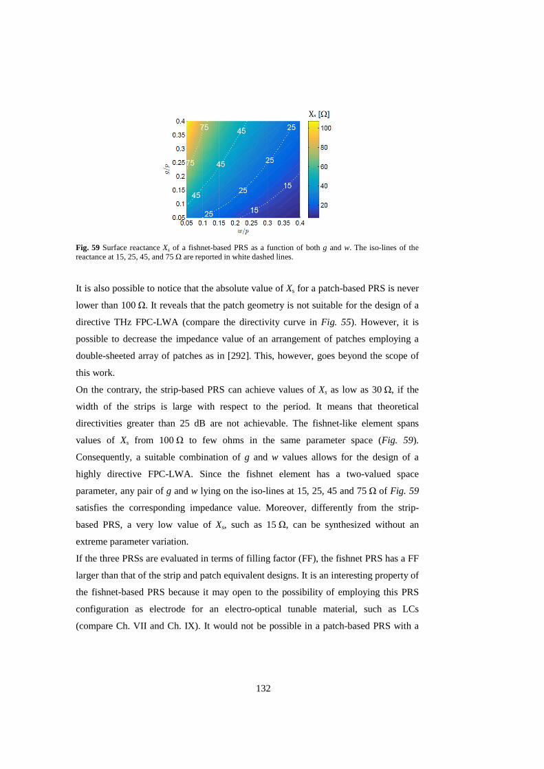
132

Fig. 59 Surface reactance Xs of a fishnet-based PRS as a function of both g and w. The iso-lines of the reactance at 15, 25, 45, and 75 Ω are reported in white dashed lines.

It is also possible to notice that the absolute value of Xs for a patch-based PRS is never

lower than 100 Ω. It reveals that the patch geometry is not suitable for the design of a

directive THz FPC-LWA (compare the directivity curve in Fig. 55). However, it is

possible to decrease the impedance value of an arrangement of patches employing a

double-sheeted array of patches as in [292]. This, however, goes beyond the scope of

this work.

On the contrary, the strip-based PRS can achieve values of Xs as low as 30 Ω, if the

width of the strips is large with respect to the period. It means that theoretical

directivities greater than 25 dB are not achievable. The fishnet-like element spans

values of Xs from 100 Ω to few ohms in the same parameter space (Fig. 59).

Consequently, a suitable combination of g and w values allows for the design of a

highly directive FPC-LWA. Since the fishnet element has a two-valued space

parameter, any pair of g and w lying on the iso-lines at 15, 25, 45 and 75 Ω of Fig. 59

satisfies the corresponding impedance value. Moreover, differently from the strip-

based PRS, a very low value of Xs, such as 15 Ω, can be synthesized without an

extreme parameter variation.

If the three PRSs are evaluated in terms of filling factor (FF), the fishnet PRS has a FF

larger than that of the strip and patch equivalent designs. It is an interesting property of

the fishnet-based PRS because it may open to the possibility of employing this PRS

configuration as electrode for an electro-optical tunable material, such as LCs

(compare Ch. VII and Ch. IX). It would not be possible in a patch-based PRS with a

133

comparable filling factor, due to the intrinsic topology of patches, which are not

interconnected elements.

It is also important to evaluate if the PRS with fishnet-like elements exhibits frequency

and spatial dispersion. In general, when a dense array of elements is modeled in the

homogenization limit, the dependence on the angle of incidence (spatial dispersion)

and on the frequency (frequency dispersion) has to be taken into account. The grid

impedance of patches for TE polarization and the grid impedance of strips for TM

polarization, as a consequence of Babinet principle (invoked because the strips array is

the complementary structure of the patches array) [293], exhibit a spatially-dispersive

character.

In Fig. 60 the surface reactance Xs of a fishnet-like unit cell of period ã = 10⁄ , and

geometrical parameters ( B ) B ã 10⁄ is presented. The unit cell is simulated with a

commercial software employing a FEM, in the frequency range between 0.5 THz and

1.5 THz, for angles of incidence varying from 0° (blue curve of Fig. 60) to 80° (red

curve of Fig. 60). These numerical simulations show that the fishnet PRS surface

impedance is essentially spatially nondispersive. This property might be of particular

interest in the future perspective of developing a FPC-LWA based on a metasurface,

with tunable radiation properties (as already proposed for the multilayered FPC-LWA

described in Ch. IX).

Fig. 60 Surface reactance of a fishnet-like unit cell as a function of frequency. The family of curves is obtained changing the angle of incidence from 0° to 80° (the color shades from blue to red, respectively).

According to the impedance analysis, the fishnet-like PRS (i) allows for a high

directivity, in combination with a flexible choice in its geometrical parameters, and (ii)

134

is suitable for the design of a FPC-LWA with a reconfigurable pointing angle (compare

Ch. IX). In the following section, the radiating properties of four FPC-LWAs based on

four different fishnet-based PRSs are fully characterized.

4. Radiating behavior of Fabry-Perot cavity leaky-wave antennas

based on fishnet-like metasurface

Four different pairs of w and g are selected among those lying on the same iso-line of

Fig. 59, with the aim to develop PRSs with impedances of 15, 25, 45 and 75 Ω (for

details, see Table 14). The choice of a specific pair of parameters is mainly due to the

easiness of fabrication and to the good fulfillment of the homogenization limit. In fact,

all the pairs lying on the same iso-reactance line lead to the same antenna performance.

The surface impedance is characterized over a frequency range from 0.5 THz to

1.5 THz, to have a frequency-dispersive model of the four fishnets. As shown in Fig.

61 a), almost all designs lead to a reactance with a linear frequency dependence: it is a

consequence of the dominant inductive behavior of the PRS.

Table 14 Relevant geometrical parameters and radiating properties of the FPC-LWAs based on the considered PRSs with fishnet-like elements.

Xs [Ω] g/p w/p

fopTE(TM)

[THz] BWTE(TM)

[GHz] αρTE(TM) αloss

er,∞ [%]

er [%]

D0 [dB]

G [dB]

∆θH(E) [°]

15 0.2 0.4 0.982

(0.982) 2.34

(2.34) 0.051

(0.052) 0.013 75 69 27.74 26.13

8.25 (8.42)

25 0.2 0.25 0.967

(0.967) 5.72

(5.72) 0.079

(0.082) 0.008 90 88 23.34 22.96

12.73 (13.25)

45 0.3 0.2 0.949

(0.950) 12.90

(12.90) 0.115

(0.123) 0.005 96 95 20.23 19.78

18.67 (19.98)

66 0.3 0.1 0.925

(0.926) 29.65

(29.68) 0.167

(0.186) 0.003 98 98 17.04 16.26

27.09 (30.12)

An exception is the design represented by the black solid line of Fig. 61 a), which

seems to show a quadratic behavior. This can be explained by considering the

geometrical parameters of the layout: ( ã⁄ = 0.3 and ) ã⁄ = 0.1. Such values reveal a

geometry with very narrow strips and a lower filling factor (FF = 0.61) that the layout

chosen for an impedance of 15 Ω (FF = 0.8). Consequently, the inductive behavior is

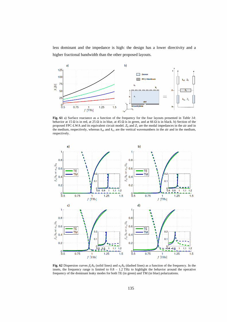
135

less dominant and the impedance is high: the design has a lower directivity and a

higher fractional bandwidth than the other proposed layouts.

Fig. 61 a) Surface reactance as a function of the frequency for the four layouts presented in Table 14: behavior at 15 Ω is in red, at 25 Ω is in blue, at 45 Ω is in green, and at 66 Ω is in black. b) Section of the proposed FPC-LWA and its equivalent circuit model. Z0 and Z1 are the modal impedances in the air and in the medium, respectively, whereas kx0 and kx1 are the vertical wavenumbers in the air and in the medium, respectively.

Fig. 62 Dispersion curves βz/k0 (solid lines) and αz/k0 (dashed lines) as a function of the frequency. In the insets, the frequency range is limited to 0.8 – 1.2 THz to highlight the behavior around the operative frequency of the dominant leaky modes for both TE (in green) and TM (in blue) polarizations.

136

Because the PRS with fishnet elements is spatially nondispersive (compare Fig. 60),

the surface impedance Zs(f) can be modeled as a function of the sole frequency,

without including the dependence on the wavenumber, which is supposed to be almost

constant for all designs. The Zs(f) is then implemented in an equivalent circuit model

(as in Fig. 61 b)) and the dispersion analysis of the radiating structure is performed

[294].

Fig. 63 Radiation patterns normalized to broadside radiation calculated with the leaky-wave approach (black solid lines) and reciprocity theorem (black dashed lines) are reported over the E-plane for the four layouts of Table 14.

Numerical results for the four FPC-LWAs are reported in Fig. 62: the behavior of the

complex-mode normalized phase (solid lines) and attenuation constants (dashed lines)

is presented in the frequency range 0.5 – 1.5 THz for both TE (green) and TM (blue)

polarizations. It is possible to notice from Fig. 62 that, as the impedance increases, as

well as the operating frequency differs from the design frequency of 1 THz (compare

Table 14). This circumstance determines a non-negligible disequalization of the

radiating performance over the E- and H-planes, as shown in Fig. 63 and Fig. 64.

137

However, when ≪ , the change in the operating frequency can be analytically

predicted with good accuracy by [290]:

+,-y++ = !

arccot å !√¶"#.e+,-jè (X.6)

In addition, a higher impedance value increases the normalized attenuation constant

value in correspondence of the operative frequency: this effect is predictable, due to a

weaker reflectivity of a higher impedance value.

Consequently, as the impedance value increases, the radiation patterns at broadside of

the corresponding LWA have wider beamwidths and reduced directivities. Both leaky-

wave theory [222] and reciprocity theorem [285] confirm this behavior, as shown in

Fig. 63 for the E-plane (primarily determined by the TM leaky mode) and in Fig. 64

for the H-plane (primarily determined by the TE leaky mode). Some relevant radiating

properties for all layouts are listed in Table 14.

Fig. 64 Radiation patterns normalized to broadside radiation calculated with the leaky-wave approach (black solid lines) and reciprocity theorem (black dashed lines) are reported over the H-plane for the four layouts of Table 14.

138

With regard to the efficiency of these devices, the loss tangent of the Zeonor (see Ch.

II Sec. 5 for a comparison between THz suitable materials properties) contributes to

raise the leakage rates in all layouts. Hence, the amount of leakage due to radiation

H and due to absorption can be determined for calculating the efficiency as

proposed in [295]:

/ = /,0 = ]\/ e1 − /y/¡j (X.7)

where 0 = H + , L is the dimension of the structure in y- and z-direction,

/,0 = lim¡→0 / is the efficiency contribution due to the substrate losses, and is

the efficiency contribution due to the finiteness of the structure. The values of /,0 and

/ are reported in Table 14 for = 20 which allows to have > 90% for all

layouts. The gain can be calculated as 2 = /ì. It results just few dB lower than the

predicted theoretical directivities, confirming the remarkable radiating performance of

FPC-LWAs based on the metasurfaces with fishnet elements. The impact of the

substrate loss is more evident for highly-directive layouts: it leads to a reduction of the

efficiency of 20% more than the layouts with a lower directivity.

4.1 Full-wave analysis of the truncated structure

Full-wave simulations of the truncated FPC-LWAs based on PRSs with fishnet-like

elements are performed by employing CST Microwave Studio (compare Ch. III Sec.

2), with the aim to evaluate the effect of diffraction from edges. The structure is

excited by modeling a y-oriented HMD (compare Ch. IX) with a slot of lateral

dimensions 2⁄ and 4⁄ along the y- and x-axis, respectively.

As shown in Fig. 65 a)-b) and Fig. 66 a)-b), the effect of the lateral truncation

( = 20 ) is almost negligible due to the weak contribution of the field at the edge of

the structure ( > 90%).

139

Fig. 65 Radiation patterns normalized to broadside radiation calculated with the leaky-wave approach (red solid lines) and reciprocity theorem (blue asterisks), and validated with full-wave simulations (black circles) are reported over the E-plane for the four layout of Table 14.

The agreement between full-wave simulations (small black circles of Fig. 65 and Fig.

66), the leaky-wave approach (red solid lines of Fig. 65 and Fig. 66), and the

reciprocity theorem (blue asterisks of Fig. 65 and Fig. 66) is remarkably good. Some

differences can be just observed on the E-plane for the last two layouts (Fig. 65 c)-d)),

probably due to a weaker validity of the homogenization hypothesis. A period of

10⁄ for the unit cell could lead to a closer agreement. However, for that value of the

period, the mask details for the PRS fabrication are at the limit of the standard

tolerances for the targeted low-cost large area photolithographic process.

140

Fig. 66 Radiation patterns normalized to broadside radiation calculated with the leaky-wave approach (red solid lines) and reciprocity theorem (blue asterisks), and validated with full-wave simulations (black circles) are reported over the H-plane for the four layout of Table 14.

Finally, the same simulations have been performed: (i) by assuming a lossy layer of

aluminum, with a thickness larger than its skin depth at 1 THz, in place of the ideal

PEC modeling the metallic part of the fishnet-like element; (ii) by considering possible

errors due to fabrication process, such as the misalignment of the slot with respect to

the center of the structure, a rotation of the slot with respect to the xy-plane, and so on.

Corresponding numerical results are not shown because they do not present

appreciable differences if compared to data in Fig. 65 and Fig. 66. The only exception

is when the slot has a misalignment of 10 µm in the transverse plane and a rotation

around the vertical axis of about 15 mrad. This configuration barely affects the

symmetry of the radiation pattern below the level of the sidelobes (around -20 dB),

showing a further confirmation of the validity of the homogenization limit.

141

5. Conclusions

The proposed fishnet-like PRS has interesting features with respect to other existing

PRSs. At first, it provides a very low purely imaginary impedance in the THz range

without an extreme variation of its geometrical parameters, as is required for the design

of similar homogenized metasurfaces, such as patches or strips [38]. Consequently, a

FPC-LWA based on a fishnet PRS can have a very high directivity.

Secondly, this PRS has a high filling factor, i.e., a high ratio between the area covered

by the metal and the unit-cell area. Moreover, the fishnet is a topologically-connected

geometry and its surface impedance is spatially nondispersive: the fishnet PRS is an

attractive candidate as top electrode in a FPC-LWA filled with an electro-optically

tunable material, such as LCs.

Finally, differently from patches and strips, for which already exist homogenization

formulas [266], no analytical expressions have been reported so far for such PRSs, thus

motivating the in-depth study carried out on this PRS geometry.

142

REFERENCES

[1] B. Ferguson and X.-C. Zhang, “Materials for terahertz science and technology,”

Nat. Mater., vol. 1, no. 1, pp. 26–33, 2002.

[2] E. Pickwell and V. P. Wallace, “Biomedical applications of terahertz technology,”

J. Phys. Appl. Phys., vol. 39, no. 17, pp. R301–R310, 2006.

[3] T. Nagatsuma, “Terahertz technologies: Present and future,” IEICE Electron.

Express, vol. 8, no. 14, pp. 1127–1142, 2011.

[4] T. Nagatsuma et al., “Terahertz wireless communications based on photonics

technologies,” Opt. Express, vol. 21, no. 20, pp. 23736–23747, 2013.

[5] G. Chattopadhyay, “Technology, capabilities, and performance of low power

terahertz sources,” IEEE Trans. Terahertz Sci. Technol., vol. 1, no. 1, pp. 33–53,

2011.

[6] M. Tonouchi, “Cutting-edge terahertz technology,” Nat. Photonics, vol. 1, no. 2,

pp. 97–105, 2007.

[7] P. H. Siegel, “Terahertz technology,” IEEE Trans. Microw. Theory Tech., vol. 50,

no. 3, pp. 910–928, 2002.

[8] M. White, D. Scott, and J. Silk, “Anisotropies in the cosmic microwave

background,” Annu. Rev. Astron. Astrophys., vol. 32, pp. 319–70, 1994.

[9] E. F. Nichols, “A method for energy measurements in the infra-red spectrum and

the properties of the ordinary ray in quartz for waves of great wave length,” Phys.

Rev. Ser. I, vol. 4, no. 4, pp. 297–313, 1897.

[10] H. Rubens and E. F. Nichols, “Heat rays of great wave length,” Phys. Rev. Ser. I,

vol. 4, no. 4, pp. 314–323, 1897.

[11] M. F. Kimmitt, “Restrahlen to T-Rays – 100 Years of Terahertz Radiation,” J.

Biol. Phys., vol. 29, no. 2–3, pp. 77–85, Jun. 2003.

[12] W. S. Boyle and K. F. Rodgers, “Performance Characteristics of a New Low-

Temperature Bolometer,” JOSA, vol. 49, no. 1, pp. 66–69, Jan. 1959.

[13] S. J. Fray and J. F. C. Oliver, “Photoconductive detector of radiation of

wavelength greater than 50 µ,” J. Sci. Instrum., vol. 36, no. 4, p. 195, 1959.

143

[14] F. J. Low, “Low-Temperature Germanium Bolometer,” JOSA, vol. 51, no. 11, pp.

1300–1304, Nov. 1961.

[15] E. H. Putley, “Solid state devices for infra-red detection,” J. Sci. Instrum., vol. 43,

no. 12, p. 857, 1966.

[16] M. A. C. S. Brown and M. F. Kimmitt, “Far-infrared resonant photoconductivity

in indium antimonide,” Infrared Phys., vol. 5, no. 2, pp. 93–97, Jun. 1965.

[17] M. Bass, P. A. Franken, J. F. Ward, and G. Weinreich, “Optical Rectification,”

Phys. Rev. Lett., vol. 9, no. 11, pp. 446–448, Dec. 1962.

[18] K. Aoki, J. Savolainen, and M. Havenith, “Broadband terahertz pulse generation

by optical rectification in GaP crystals,” Appl. Phys. Lett., vol. 110, no. 20, p.

201103, May 2017.

[19] K. H. Yang, P. L. Richards, and Y. R. Shen, “Generation of Far‐Infrared Radiation

by Picosecond Light Pulses in LiNbO3,” Appl. Phys. Lett., vol. 19, no. 9, pp. 320–

323, Nov. 1971.

[20] L. R. Elias, J. Hu, and G. Ramian, “The UCSB electrostatic accelerator free

electron laser: First operation,” Nucl. Instrum. Methods Phys. Res. Sect. Accel.

Spectrometers Detect. Assoc. Equip., vol. 237, no. 1, pp. 203–206, Jun. 1985.

[21] M. B. Ketchen et al., “Generation of subpicosecond electrical pulses on coplanar

transmission lines,” Appl. Phys. Lett., 19860324.

[22] U. Frisk et al., “The Odin satellite - I. Radiometer design and test,” Astron.

Astrophys., vol. 402, no. 3, pp. L27–L34, May 2003.

[23] “EOS MLS.” [Online]. Available: https://mls.jpl.nasa.gov/index-eos-mls.php.

[Accessed: 31-Aug-2017].

[24] “Orbiter Instruments.” [Online]. Available: http://sci.esa.int/rosetta/35061-

instruments/?fbodylongid%EF%BB%BF=%EF%BB%BF1641. [Accessed: 31-

Aug-2017].

[25] S. S. Dhillon et al., “The 2017 terahertz science and technology roadmap,” J.

Phys. Appl. Phys., vol. 50, no. 4, p. 043001, 2017.

[26] L. Huang, S. G. Lambrakos, A. Shabaev, N. Bernstein, and L. Massa, Passive and

Active Millimeter-Wave Imaging XVII, vol. 9078. 2014.

[27] J. O. Richardson et al., “Investigation of terahertz vibration–rotation tunneling

spectra for the water octamer,” J. Phys. Chem. A, vol. 117, no. 32, pp. 6960–6966,

Aug. 2013.

144

[28] Y. D. Wu, T. Zhou, Z. W. Yao, and J. C. Cao, “Theoretical and experimental

investigation of terahertz absorption spectra for water clusters (H2O)n (n = 4, 5, 6)

in the atmosphere,” J. Appl. Spectrosc., vol. 83, no. 3, pp. 362–366, Jul. 2016.

[29] I. F. Akyildiz, J. M. Jornet, and C. Han, “Terahertz band: Next frontier for wireless

communications,” Phys. Commun., vol. 12, pp. 16–32, Sep. 2014.

[30] T. S. Rappaport, J. N. Murdock, and F. Gutierrez, “State of the art in 60-GHz

integrated circuits and systems for wireless communications,” Proc. IEEE, vol. 99,

no. 8, pp. 1390–1436, Aug. 2011.

[31] R. Miles, X.-C. Zhang, H. Eisele, and A. Krotkus, Terahertz Frequency Detection

and Identification of Materials and Objects. Springer Science & Business Media,

2007.

[32] R. Gente and M. Koch, “Monitoring leaf water content with THz and sub-THz

waves,” Plant Methods, vol. 11, p. 15, Mar. 2015.

[33] N. Q. Vinh, M. S. Sherwin, S. J. Allen, D. K. George, A. J. Rahmani, and K. W.

Plaxco, “High-precision gigahertz-to-terahertz spectroscopy of aqueous salt

solutions as a probe of the femtosecond-to-picosecond dynamics of liquid water,”

J. Chem. Phys., vol. 142, no. 16, p. 164502, Apr. 2015.

[34] D. M. Leitner, M. Havenith, and M. Gruebele, “Biomolecule large-amplitude

motion and solvation dynamics: modelling and probes from THz to X-rays,” Int.

Rev. Phys. Chem., vol. 25, no. 4, pp. 553–582, Oct. 2006.

[35] M. Hishida and K. Tanaka, “Long-range hydration effect of lipid membrane

studied by terahertz time-domain spectroscopy,” Phys. Rev. Lett., vol. 106, no. 15,

p. 158102, Apr. 2011.

[36] B. B. Hu and M. C. Nuss, “Imaging with terahertz waves,” Opt. Lett., vol. 20, no.

16, pp. 1716–1718, Aug. 1995.

[37] R. F. Haglund, J. Neev, R. F. Wood, and S. of P. I. Engineers, Commercial and

biomedical applications of ultrashort pulse lasers; laser plasma generation and

diagnostics. SPIE, 2001.

[38] V. p. Wallace et al., “Terahertz pulsed imaging of basal cell carcinoma ex vivo

and in vivo,” Br. J. Dermatol., vol. 151, no. 2, pp. 424–432, Aug. 2004.

[39] E. Heinz et al., “Passive 350 GHz video imaging systems for security

applications,” J. Infrared Millim. Terahertz Waves, vol. 36, no. 10, pp. 879–895,

Oct. 2015.

145

[40] M. R. Leahy-Hoppa, M. J. Fitch, X. Zheng, L. M. Hayden, and R. Osiander,

“Wideband terahertz spectroscopy of explosives,” Chem. Phys. Lett., vol. 434, no.

4, pp. 227–230, Feb. 2007.

[41] C. Mann, “First demonstration of a vehicle mounted 250 GHz real time passive

imager,” presented at the Terahertz Physics, Devices, and Systems III: Advanced

Applications in Industry and Defense, 2009, vol. 7311, p. 73110Q.

[42] R. Appleby and S. Ferguson, “Submillimetre wave imaging and security: imaging

performance and prediction,” presented at the Millimetre Wave and Terahertz

Sensors and Technology IX, 2016, vol. 9993, p. 999302.

[43] C. G. Soares, Y. Garbatov, A. Zayed, and G. Wang, “Influence of environmental

factors on corrosion of ship structures in marine atmosphere,” Corros. Sci., vol.

51, no. 9, pp. 2014–2026, Sep. 2009.

[44] W. Tu, S. Zhong, Y. Shen, and A. Incecik, “Nondestructive testing of marine

protective coatings using terahertz waves with stationary wavelet transform,”

Ocean Eng., vol. 111, pp. 582–592, Jan. 2016.

[45] D. J. Cook, S. Lee, S. J. Sharpe, and M. G. Allen, “Accuracy and linearity of time-

domain THz paint thickness measurements,” presented at the Terahertz

Technology and Applications, 2008, vol. 6893, p. 68930H.

[46] J. B. Jackson et al., “A survey of terahertz applications in cultural heritage

conservation science,” IEEE Trans. Terahertz Sci. Technol., vol. 1, no. 1, pp. 220–

231, Sep. 2011.

[47] K. Krügener et al., “Terahertz meets sculptural and architectural art: Evaluation

and conservation of stone objects with T-ray technology,” Sci. Rep., vol. 5, Oct.

2015.

[48] K. Fukunaga, T. Ikari, and K. Iwai, “THz pulsed time-domain imaging of an oil

canvas painting: a case study of a painting by Pablo Picasso,” Appl. Phys. A, vol.

122, no. 2, p. 106, Feb. 2016.

[49] A. Borak, “Toward bridging the terahertz gap with silicon-based lasers,” Science,

vol. 308, no. 5722, pp. 638–639, Apr. 2005.

[50] W. L. Chan, J. Deibel, and D. M. Mittleman, “Imaging with terahertz radiation,”

Rep. Prog. Phys., vol. 70, no. 8, p. 1325, 2007.

146

[51] J. M. Chamberlain, “Where optics meets electronics: recent progress in decreasing

the terahertz gap,” Philos. Trans. R. Soc. Lond. Math. Phys. Eng. Sci., vol. 362, no.

1815, pp. 199–213, Feb. 2004.

[52] B. S. Williams, “Terahertz quantum-cascade lasers,” Nat. Photonics, vol. 1, no. 9,

pp. 517–525, Sep. 2007.

[53] H.-W. Hübers, S. G. Pavlov, and V. N. Shastin, “Terahertz lasers based on

germanium and silicon,” Semicond. Sci. Technol., vol. 20, no. 7, p. S211, 2005.

[54] B. A. Knyazev, G. N. Kulipanov, and N. A. Vinokurov, “Novosibirsk terahertz

free electron laser: instrumentation development and experimental achievements,”

Meas. Sci. Technol., vol. 21, no. 5, p. 054017, 2010.

[55] D. W. Sprehn, C. L. Rettig, and N. C. Luhmann, “Phase locking and frequency

locking of a 140 GHz klystron and a 280 GHz carcinotron,” Rev. Sci. Instrum.,

vol. 63, no. 10, pp. 4685–4687, Oct. 1992.

[56] J. E. Walsh, J. H. Brownell, M. J. Goldstein, J. C. Swartz, J. Urata, and M. F.

Kimmitt, “A new tunable coherent FIR-THz source,” Opt. Photonics News, vol. 9,

pp. 51–52, Dec. 1998.

[57] P. H. Siegel, A. Fung, H. Manohara, J. Xu, and B. Chang, “Nanoklystron: A

monolithic tube approach to THz power generation,” 2001.

[58] A. Maestrini et al., “A frequency-multiplied source with more than 1 mW of

power across the 900-GHz band,” IEEE Trans. Microw. Theory Tech., vol. 58, no.

7, pp. 1925–1932, Jul. 2010.

[59] A. Maestrini et al., “A 1.7-1.9 THz local oscillator source,” IEEE Microw. Wirel.

Compon. Lett., vol. 14, no. 6, pp. 253–255, Jun. 2004.

[60] “Frequency Multipliers.” [Online]. Available: http://vadiodes.com/en/frequency-

multipliers. [Accessed: 18-Oct-2017].

[61] J. Lusakowski et al., “Voltage tuneable terahertz emission from a ballistic

nanometer InGaAs⁄InAlAs transistor,” J. Appl. Phys., vol. 97, no. 6, p. 064307,

Mar. 2005.

[62] A. Lisauskas, A. Rämer, M. Burakevič, V. Krozer, W. Heinrich, and H. G.

Roskos, “Terahertz emission from large AlGaN/GaN field-effect transistors,” in

2016 41st International Conference on Infrared, Millimeter, and Terahertz waves

(IRMMW-THz), 2016, pp. 1–1.

147

[63] G. Chin, “Optically pumped submillimeter laser heterodyne receivers:

astrophysical observations and recent technical developments,” Proc. IEEE, vol.

80, no. 11, pp. 1788–1799, Nov. 1992.

[64] H.-P. Röser, “Heterodyne spectroscopy for submillimeter and far-infrared

wavelengths from 100 µm to 500 µm,” Infrared Phys., vol. 32, pp. 385–407, Jan.

1991.

[65] G. Dodel, “On the history of far-infrared (FIR) gas lasers: Thirty-five years of

research and application,” Infrared Phys. Technol., vol. 40, no. 3, pp. 127–139,

Jun. 1999.

[66] J. M. Chamberlain and R. Miles, New Directions in Terahertz Technology.

Springer Netherlands, 1997.

[67] M. Scheller, J. M. Yarborough, J. V. Moloney, M. Fallahi, M. Koch, and S. W.

Koch, “Room temperature continuous wave milliwatt terahertz source,” Opt.

Express, vol. 18, no. 26, pp. 27112–27117, Dec. 2010.

[68] X. L. Wu et al., “Green light stimulates terahertz emission from mesocrystal

microspheres,” Nat. Nanotechnol., vol. 6, no. 2, pp. 103–106, Feb. 2011.

[69] N. T. Yardimci, S. H. Yang, C. W. Berry, and M. Jarrahi, “High-power terahertz

generation using large-area plasmonic photoconductive emitters,” IEEE Trans.

Terahertz Sci. Technol., vol. 5, no. 2, pp. 223–229, Mar. 2015.

[70] S. Kono, M. Tani, P. Gu, and K. Sakai, “Detection of up to 20 THz with a low-

temperature-grown GaAs photoconductive antenna gated with 15 fs light pulses,”

Appl. Phys. Lett., vol. 77, no. 25, pp. 4104–4106, Dec. 2000.

[71] D. Kuk, Y. J. Yoo, E. W. Rosenthal, N. Jhajj, H. M. Milchberg, and K. Y. Kim,

“Generation of scalable terahertz radiation from cylindrically focused two-color

laser pulses in air,” Appl. Phys. Lett., vol. 108, no. 12, p. 121106, Mar. 2016.

[72] H. A. Hafez et al., “Intense terahertz radiation and their applications,” J. Opt., vol.

18, no. 9, p. 093004, 2016.

[73] K. A. McIntosh, E. R. Brown, K. B. Nichols, O. B. McMahon, W. F. DiNatale,

and T. M. Lyszczarz, “Terahertz photomixing with diode lasers in

low‐temperature‐grown GaAs,” Appl. Phys. Lett., vol. 67, no. 26, pp. 3844–3846,

Dec. 1995.

148

[74] A. J. Deninger et al., “Precisely tunable continuous-wave terahertz source with

interferometric frequency control,” Rev. Sci. Instrum., vol. 79, no. 4, p. 044702,

Apr. 2008.

[75] R. A. Lewis, “A review of terahertz sources,” J. Phys. Appl. Phys., vol. 47, no. 37,

p. 374001, 2014.

[76] N. M. Burford and M. O. El-Shenawee, “Review of terahertz photoconductive

antenna technology,” Opt. Eng., vol. 56, no. 1, p. 010901, Jan. 2017.

[77] A. Rogalski and F. Sizov, “Terahertz detectors and focal plane arrays,” Opto-

Electron. Rev., vol. 19, no. 3, pp. 346–404, 2011.

[78] F. Sizov and A. Rogalski, “THz detectors,” Prog. Quantum Electron., vol. 34, no.

5, pp. 278–347, Sep. 2010.

[79] H.-J. Song and T. Nagatsuma, Handbook of Terahertz Technologies: Devices and

Applications. CRC Press, 2015.

[80] “Virginia Diodes, Inc - Application Notes.” [Online]. Available:

http://www.vadiodes.com/en/app-notes/app-notes. [Accessed: 02-Oct-2017].

[81] A. Barh, B. P. Pal, G. P. Agrawal, R. K. Varshney, and B. M. A. Rahman,

“Specialty fibers for terahertz generation and transmission: a review,” IEEE J. Sel.

Top. Quantum Electron., vol. 22, no. 2, pp. 365–379, Mar. 2016.

[82] S. R. Andrews, “Microstructured terahertz waveguides,” J. Phys. Appl. Phys., vol.

47, no. 37, p. 374004, 2014.

[83] L. Cao, A.-S. Grimault-Jacquin, N. Zerounian, and F. Aniel, “Design and VNA-

measurement of coplanar waveguide (CPW) on benzocyclobutene (BCB) at THz

frequencies,” Infrared Phys. Technol., vol. 63, pp. 157–164, Mar. 2014.

[84] Y. Kadoya, “THz wave propagation on strip lines: Devices, properties, and

applications,” in 2007 19th International Conference on Applied Electromagnetics

and Communications, 2007, pp. 1–4.

[85] K. Nielsen, H. K. Rasmussen, A. J. L. Adam, P. C. M. Planken, O. Bang, and P.

U. Jepsen, “Bendable, low-loss Topas fibers for the terahertz frequency range,”

Opt. Express, vol. 17, no. 10, pp. 8592–8601, May 2009.

[86] A. Dupuis, A. Mazhorova, F. Désévédavy, M. Rozé, and M. Skorobogatiy,

“Spectral characterization of porous dielectric subwavelength THz fibers

fabricated using a microstructured molding technique,” Opt. Express, vol. 18, no.

13, pp. 13813–13828, Jun. 2010.

149

[87] A. Hassani, A. Dupuis, and M. Skorobogatiy, “Porous polymer fibers for low-loss

Terahertz guiding,” Opt. Express, vol. 16, no. 9, pp. 6340–6351, Apr. 2008.

[88] P. F. Goldsmith, “Quasi-optical techniques,” Proc. IEEE, vol. 80, no. 11, pp.

1729–1747, Nov. 1992.

[89] Y. Cai, I. Brener, J. Lopata, J. Wynn, L. Pfeiffer, and J. Federici, “Design and

performance of singular electric field terahertz photoconducting antennas,” Appl.

Phys. Lett., vol. 71, no. 15, pp. 2076–2078, Oct. 1997.

[90] M. Reid, I. V. Cravetchi, and R. Fedosejevs, “Terahertz radiation and second-

harmonic generation from InAs: Bulk versus surface electric-field-induced

contributions,” Phys. Rev. B, vol. 72, no. 3, p. 035201, Jul. 2005.

[91] F. Yan, C. Yu, H. Park, E. P. J. Parrott, and E. Pickwell-MacPherson, “Advances

in polarizer technology for terahertz frequency applications,” J. Infrared Millim.

Terahertz Waves, vol. 34, no. 9, pp. 489–499, Sep. 2013.

[92] B. Vasić, D. C. Zografopoulos, G. Isić, R. Beccherelli, and R. Gajić, “Electrically

tunable terahertz polarization converter based on overcoupled metal-isolator-metal

metamaterials infiltrated with liquid crystals,” Nanotechnology, vol. 28, no. 12, p.

124002, 2017.

[93] M. Born and E. Wolf, Principles of Optics: Electromagnetic Theory of

Propagation, Interference and Diffraction of Light. Elsevier, 2013.

[94] M. E. MacDonald, A. Alexanian, R. A. York, Z. Popovic, and E. N. Grossman,

“Spectral transmittance of lossy printed resonant-grid terahertz bandpass filters,”

IEEE Trans. Microw. Theory Tech., vol. 48, no. 4, pp. 712–718, Apr. 2000.

[95] C. Winnewisser, F. Lewen, and H. Helm, “Transmission characteristics of dichroic

filters measured by THz time-domain spectroscopy,” Appl. Phys. A, vol. 66, no. 6,

pp. 593–598, Jun. 1998.

[96] N. R. Erickson, “A directional filter diplexer using optical techniques for

millimeter to submillimeter wavelengths,” IEEE Trans. Microw. Theory Tech.,

vol. 25, no. 10, pp. 865–866, Oct. 1977.

[97] Z. G. Lu, J. B. Tan, and Z. G. Fan, “Terahertz Fabry-Perot interferometer

constructed by metallic meshes with micrometer period and high ratio of

linewidth/period,” Key Eng. Mater., vol. 437, pp. 286–290, 2010.

150

[98] B. Scherger, M. Scheller, C. Jansen, M. Koch, and K. Wiesauer, “Terahertz lenses

made by compression molding of micropowders,” Appl. Opt., vol. 50, no. 15, pp.

2256–2262, May 2011.

[99] Y. H. Lo and R. Leonhardt, “Aspheric lenses for terahertz imaging,” Opt. Express,

vol. 16, no. 20, pp. 15991–15998, Sep. 2008.

[100] M. Wichmann et al., “Terahertz plastic compound lenses,” Appl. Opt., vol. 52,

no. 18, pp. 4186–4191, Jun. 2013.

[101] M. Takai, K. Shibata, M. Uemoto, and S. Watanabe, “Spatial polarization

variation in terahertz electromagnetic wave focused by off-axis parabolic mirror,”

Appl. Phys. Express, vol. 9, no. 5, p. 052206, Apr. 2016.

[102] L. Minkevičius et al., “Compact diffractive optical components for terahertz

beam manipulation,” in 2015 40th International Conference on Infrared,

Millimeter, and Terahertz waves (IRMMW-THz), 2015, pp. 1–2.

[103] A. Siemion et al., “Diffractive paper lens for terahertz optics,” Opt. Lett., vol.

37, no. 20, pp. 4320–4322, Oct. 2012.

[104] A. Siemion et al., “Off-axis metallic diffractive lens for terahertz beams,” Opt.

Lett., vol. 36, no. 11, pp. 1960–1962, Jun. 2011.

[105] S. Wang and X.-C. Zhang, “Terahertz technology: Terahertz tomographic

imaging with a Fresnel lens,” Opt. Photonics News, vol. 13, no. 12, pp. 59–59,

Dec. 2002.

[106] J. L. Soret, “Ueber die durch Kreisgitter erzeugten Diffractionsphänomene,”

Ann. Phys., vol. 232, no. 9, pp. 99–113, Jan. 1875.

[107] E. Skudrzyk, The Foundations of Acoustics. Springer-Verlag, 1971.

[108] Lord Rayleigh, “Wave theory,” Encycl. Br., p. 422, 1890.

[109] R. W. Wood, “LIII. Phase-reversal zone-plates, and diffraction-telescopes,”

Philos. Mag. Ser. 5, vol. 45, no. 277, pp. 511–522, Jun. 1898.

[110] R. W. Wood, Physical Optics. The Macmillan Company, 1934.

[111] R. A. Houstoun, A treatise on light. London, New York etc.: Longmans, Green

and co., 1930.

[112] M. Sussman, “Elementary diffraction theory of zone plates,” Am. J. Phys., vol.

28, no. 4, pp. 394–398, Apr. 1960.

[113] O. E. Myers Jr., “Studies of transmission zone plates,” Am. J. Phys., vol. 19,

no. 6, pp. 359–365, Sep. 1951.

151

[114] A. V. Baez, “A study in diffraction microscopy with special reference to X-

rays,” JOSA, vol. 42, no. 10, pp. 756–762, Oct. 1952.

[115] A. V. Baez, “Fresnel zone plate for optical image formation using extreme

ultraviolet and soft X-radiation,” JOSA, vol. 51, no. 4, pp. 405–412, Apr. 1961.

[116] J. Kirz, “Phase zone plates for x rays and the extreme uv,” JOSA, vol. 64, no.

3, pp. 301–309, Mar. 1974.

[117] I. Mohacsi et al., “High-efficiency zone-plate optics for multi-keV X-ray

focusing,” J. Synchrotron Radiat., vol. 21, no. 3, pp. 497–501, May 2014.

[118] S.-C. Gleber et al., “Fresnel zone plate stacking in the intermediate field for

high efficiency focusing in the hard X-ray regime,” Opt. Express, vol. 22, no. 23,

p. 28142, Nov. 2014.

[119] R. Mirjalili and B. A. Parviz, “Microlight-emitting diode with integrated

Fresnel zone plate for contact lens embedded display,” J. MicroNanolithography

MEMS MOEMS, vol. 11, no. 3, pp. 033010–033010, 2012.

[120] T. B. Brown, “Microwave zone plates,” Am. J. Phys., vol. 30, no. 1, pp. 55–60,

Jan. 1962.

[121] R. Ruben, “An electronically scanned antenna using fresnel zone techniques,”

in 1958 IRE International Convention Record, 1966, vol. 14, pp. 244–251.

[122] G. S. Sanyal and M. Singh, “Fresnel zone plate antenna,” IETE J. Res., vol. 14,

no. 6, pp. 265–281, Jun. 1968.

[123] K. K. Dey and P. Khastgir, “A study of the characteristics of a microwave

spherical zone plate antenna,” Int. J. Electron., vol. 35, no. 1, pp. 97–103, Jul.

1973.

[124] H. D. Hristov, “Microwave Fresnel zone plate antenna runs at multiple

terahertz frequencies,” presented at the Proceedings of the IASTED International

Conference on Antennas, Radar and Wave Propagation, ARP 2010, 2010, pp. 9–

13.

[125] H. D. Hristov, “Terahertz harmonic operation of microwave Fresnel zone plate

lens and antenna: Frequency filtering and space resolution properties,” Int. J.

Antennas Propag., vol. 2011, p. e541734, Dec. 2011.

[126] J. M. Rodríguez, H. D. Hristov, and W. Grote, “Fresnel zone plate and

ordinary lens antennas: Comparative study at microwave and terahertz

frequencies,” presented at the European Microwave Week 2011: “Wave to the

152

Future”, EuMW 2011, Conference Proceedings - 41st European Microwave

Conference, EuMC 2011, 2011, pp. 894–897.

[127] H. D. Hristov, J. m. Rodriguez, and W. Grote, “The grooved-dielectric Fresnel

zone plate: An effective terahertz lens and antenna,” Microw. Opt. Technol. Lett.,

vol. 54, no. 6, pp. 1343–1348, Jun. 2012.

[128] J. C. Wiltse, “Phase-correcting zone plate antennas at terahertz frequencies,”

presented at the Proceedings of SPIE - The International Society for Optical

Engineering, 2003, vol. 5070, pp. 98–107.

[129] A. E. Torres-García, B. Orazbayev, R. Gonzalo, and I. Ederra, “A quasi-spiral

antenna for THz - IR dual-band sensors,” in 2016 Global Symposium on

Millimeter Waves (GSMM) ESA Workshop on Millimetre-Wave Technology and

Applications, 2016, pp. 1–2.

[130] L. Minkevičius et al., “Study of terahertz zone plates with integrated cross-

shape apertures,” in 2013 38th International Conference on Infrared, Millimeter,

and Terahertz Waves (IRMMW-THz), 2013, pp. 1–2.

[131] L. Minkevičius et al., “Terahertz zone plates with integrated laserablated

bandpass filters,” Electron. Lett., vol. 49, no. 1, pp. 49–50, 2013.

[132] L. Minkevičius et al., “On-chip integration solutions of compact optics and

detectors in room-temperature terahertz imaging systems,” 2015, vol. 9585, p.

95850M–95850M–6.

[133] L. Minkevičius, V. Tamošiunas, K. Madeikis, B. Voisiat, I. Kašalynas, and G.

Valušis, “On-chip integration of laser-ablated zone plates for detection

enhancement of inGaAs bow-tie terahertz detectors,” Electron. Lett., vol. 50, no.

19, pp. 1367–1369, Sep. 2014.

[134] L. Liu et al., “Tunable and reconfigurable THz devices for advanced imaging

and adaptive wireless communication,” Proceeding SPIE, vol. 9934, pp. 993407-

993407–13, 2016.

[135] M. I. B. Shams, Z. Jiang, J. Qayyum, S. Rahman, P. Fay, and L. Liu, “A

terahertz reconfigurable photo-induced fresnel-zone-plate antenna for dynamic

two-dimensional beam steering and forming,” in 2015 IEEE MTT-S International

Microwave Symposium, 2015, pp. 1–4.

[136] V. E. Levashov and A. V. Vinogradov, “Analytical theory of zone plate

efficiency,” Phys. Rev. E, vol. 49, no. 6, pp. 5797–5803, Jun. 1994.

153

[137] D. J. Stigliani, R. Mittra, and R. G. Semonin, “Resolving power of a zone

plate,” JOSA, vol. 57, no. 5, pp. 610–613, May 1967.

[138] G. Schmahl and D. Rudolph, “High power zone plates as image-forming

systems for soft X-rays,” May 1977.

[139] M. Young, “Zone plates and their aberrations,” JOSA, vol. 62, no. 8, pp. 972–

976, Aug. 1972.

[140] J. Dai, J. Zhang, W. Zhang, and D. Grischkowsky, “Terahertz time-domain

spectroscopy characterization of the far-infrared absorption and index of refraction

of high-resistivity, float-zone silicon,” JOSA B, vol. 21, no. 7, pp. 1379–1386, Jul.

2004.

[141] M. Naftaly and R. E. Miles, “Terahertz time-domain spectroscopy: A new tool

for the study of glasses in the far infrared,” J. Non-Cryst. Solids, vol. 351, no. 40,

pp. 3341–3346, Oct. 2005.

[142] S. F. Busch, M. Weidenbach, M. Fey, F. Schäfer, T. Probst, and M. Koch,

“Optical properties of 3D printable plastics in the THz regime and their application

for 3D printed THz optics,” J. Infrared Millim. Terahertz Waves, vol. 35, no. 12,

pp. 993–997, Dec. 2014.

[143] D. Han, K. Lee, J. Lim, S. S. Hong, Y. K. Kim, and J. Ahn, “Terahertz lens

made out of natural stone,” Appl. Opt., vol. 52, no. 36, pp. 8670–8675, Dec. 2013.

[144] P. D. Cunningham et al., “Broadband terahertz characterization of the

refractive index and absorption of some important polymeric and organic electro-

optic materials,” J. Appl. Phys., vol. 109, no. 4, pp. 043505-043505-5, Feb. 2011.

[145] A. Siemion, P. Kostrowiecki-Lopata, A. Pindur, P. Zagrajek, and M. Sypek,

“Paper on designing costless THz paper optics,” Adv. Mater. Sci. Eng., vol. 2016,

p. e9615698, Nov. 2016.

[146] Y.-S. Jin, G.-J. Kim, and S.-G. Jeon, “Terahertz dielectric properties of

polymers,” J. Korean Phys. Soc., vol. 49, no. 2, pp. 513–517, 2006.

[147] A. Podzorov and G. Gallot, “Low-loss polymers for terahertz applications,”

Appl. Opt., vol. 47, no. 18, pp. 3254–3257, Jun. 2008.

[148] P. A. George, W. Hui, F. Rana, B. G. Hawkins, A. E. Smith, and B. J. Kirby,

“Microfluidic devices for terahertz spectroscopy of biomolecules,” Opt. Express,

vol. 16, no. 3, pp. 1577–1582, Feb. 2008.

154

[149] M. Sypek et al., “Highly efficient broadband double-sided Fresnel lens for

THz range,” Opt. Lett., vol. 37, no. 12, pp. 2214–2216, Jun. 2012.

[150] J. R. Middendorf, D. A. LeMaster, M. Zarepoor, and E. R. Brown, “Design of

multi-order diffractive THz lenses,” in 2012 37th International Conference on

Infrared, Millimeter, and Terahertz Waves, 2012, pp. 1–2.

[151] S. F. Busch, M. Weidenbach, J. C. Balzer, and M. Koch, “THz optics 3D

printed with TOPAS,” J. Infrared Millim. Terahertz Waves, vol. 37, no. 4, pp.

303–307, 2016.

[152] D. C. Zografopoulos and R. Beccherelli, “Tunable terahertz fishnet

metamaterials based on thin nematic liquid crystal layers for fast switching,” Sci.

Rep., vol. 5, Aug. 2015.

[153] B. Scherger, M. Scheller, N. Vieweg, S. T. Cundiff, and M. Koch, “Paper

terahertz wave plates,” Opt. Express, vol. 19, no. 25, pp. 24884–24889, Dec. 2011.

[154] J. Jahns, Q. Cao, and S. Sinzinger, “Micro- and nanooptics – an overview,”

Laser Photonics Rev., vol. 2, no. 4, pp. 249–263, Aug. 2008.

[155] “AF3-202E - velvia_100_datasheet.pdf.” [Online]. Available:

http://www.fujifilm.com/products/professional_films/pdf/velvia_100_datasheet.pd

f. [Accessed: 16-Aug-2017].

[156] W. B. Veldkamp and T. J. McHugh, “Binary optics,” Sci. Am., vol. 266, no. 5,

pp. 92–97, 1992.

[157] L. Kipp et al., “Sharper images by focusing soft X-rays with photon sieves,”

Nature, vol. 414, no. 6860, pp. 184–188, Nov. 2001.

[158] W. D. Furlan, V. Ferrando, J. A. Monsoriu, P. Zagrajek, E. Czerwińska, and

M. Szustakowski, “3D printed diffractive terahertz lenses,” Opt. Lett., vol. 41, no.

8, pp. 1748–1751, Apr. 2016.

[159] J. Suszek et al., “3-D-printed flat optics for THz linear scanners,” IEEE Trans.

Terahertz Sci. Technol., vol. 5, no. 2, pp. 314–316, Mar. 2015.

[160] I. Mohacsi et al., “High resolution double-sided diffractive optics for hard X-

ray microscopy,” Opt. Express, vol. 23, no. 2, pp. 776–786, Jan. 2015.

[161] T. Rylander, P. Ingelström, and A. Bondeson, Computational

Electromagnetics. Springer Science & Business Media, 2012.

[162] A. J. Poggio and E. K. Miller, Integral Equation Solutions of Three-

dimensional Scattering Problems. MB Assoc., 1970.

155

[163] “COMSOL Multiphysics® Modeling Software.” [Online]. Available:

https://www.comsol.com/. [Accessed: 09-May-2017].

[164] “CST.” [Online]. Available: https://www.cst.com/. [Accessed: 09-May-2017].

[165] T. Weiland, M. Timm, and I. Munteanu, “A practical guide to 3-D simulation,”

IEEE Microw. Mag., vol. 9, no. 6, pp. 62–75, Dec. 2008.

[166] “TYDEX Research&Industrial Optics.” [Online]. Available:

http://www.tydexoptics.com/. [Accessed: 09-May-2017].

[167] B. McCall and T. S. Tkaczyk, “Rapid fabrication of miniature lens arrays by

four-axis single point diamond machining,” Opt. Express, vol. 21, no. 3, pp. 3557–

3572, Feb. 2013.

[168] F. Rui and W. Li, “A zone plate as a tunable terahertz filter,” Chin. Phys. Lett.,

vol. 27, no. 6, p. 064201, 2010.

[169] W. Withayachumnankul and M. Naftaly, “Fundamentals of measurement in

terahertz time-domain spectroscopy,” J. Infrared Millim. Terahertz Waves, vol. 35,

no. 8, pp. 610–637, Aug. 2014.

[170] M. Naftaly, Terahertz Metrology. Artech House, 2015.

[171] M. Naftaly, R. G. Clarke, D. A. Humphreys, and N. M. Ridler, “Metrology

state-of-the-art and challenges in broadband phase-sensitive terahertz

measurements,” Proc. IEEE, vol. 105, no. 6, pp. 1151–1165, Jun. 2017.

[172] W. Sun, B. Yang, X. Wang, Y. Zhang, and R. Donnan, “Accurate

determination of terahertz optical constants by vector network analyzer of Fabry–

Perot response,” Opt. Lett., vol. 38, no. 24, pp. 5438–5441, Dec. 2013.

[173] T. Tosaka, K. Fujii, K. Fukunaga, and A. Kasamatsu, “Development of

complex relative permittivity measurement system based on free-space in 220

GHz range,” IEEE Trans. Terahertz Sci. Technol., vol. 5, no. 1, pp. 102–109, Jan.

2015.

[174] M. Naftaly, N. Shoaib, D. Stokes, and N. M. Ridler, “Intercomparison of

terahertz dielectric measurements using vector network analyzer and time-domain

spectrometer,” J. Infrared Millim. Terahertz Waves, vol. 37, no. 7, pp. 691–702,

Jul. 2016.

[175] “Menlo TERA K15.” [Online]. Available:

http://www.menlosystems.com/products/thz-time-domain-solutions/all-fiber-

coupled-terahertz-spectrometer/. [Accessed: 10-May-2017].

156

[176] E. Castro-Camus and M. Alfaro, “Photoconductive devices for terahertz pulsed

spectroscopy: a review [Invited],” Photonics Res., vol. 4, no. 3, pp. A36–A42, Jun.

2016.

[177] P. U. Jepsen, D. G. Cooke, and M. Koch, “Terahertz spectroscopy and imaging

– Modern techniques and applications,” Laser Photonics Rev., vol. 5, no. 1, pp.

124–166, Jan. 2011.

[178] P. R. Smith, D. H. Auston, and M. C. Nuss, “Subpicosecond photoconducting

dipole antennas,” IEEE J. Quantum Electron., vol. 24, no. 2, pp. 255–260, Feb.

1988.

[179] P. U. Jepsen and S. R. Keiding, “Radiation patterns from lens-coupled

terahertz antennas,” Opt. Lett., vol. 20, no. 8, pp. 807–809, Apr. 1995.

[180] “MENLO-SYSTEMS-Terahertz-Time-Domain-Solution-TERA-K15-

THzStrecke-Extern-pr.jpg (2721×1814).” [Online]. Available:

http://www.menlosystems.com/assets/PR/MENLO-SYSTEMS-Terahertz-Time-

Domain-Solution-TERA-K15-THzStrecke-Extern-pr.jpg. [Accessed: 22-Oct-

2017].

[181] “Motion Control.” [Online]. Available: https://www.newport.com/c/motion-

control. [Accessed: 16-May-2017].

[182] “LabVIEW System Design Software - National Instruments.” [Online].

Available: http://www.ni.com/labview/i/. [Accessed: 16-May-2017].

[183] G. T. Herman, Image Reconstruction from Projections. Berlin: Springer, 1979.

[184] A. G. Lindgren and P. A. Rattey, “The inverse discrete radon transform with

applications to tomographic imaging using projection data,” Adv. Electron.

Electron Phys., vol. 56, pp. 359–410, Jan. 1981.

[185] D. M. Slocum, E. J. Slingerland, R. H. Giles, and T. M. Goyette,

“Atmospheric absorption of terahertz radiation and water vapor continuum

effects,” J. Quant. Spectrosc. Radiat. Transf., vol. 127, pp. 49–63, Sep. 2013.

[186] X. Wang et al., “Focusing and imaging of a virtual all-optical tunable terahertz

Fresnel zone plate,” Opt. Lett., vol. 38, no. 22, pp. 4731–4734, Nov. 2013.

[187] P. Valley, M. R. Dodge, J. Schwiegerling, D. Mathine, G. Peyman, and N.

Peyghambarian, “Flat liquid crystal diffractive lenses with variable focus and

magnification,” presented at the Current Developments in Lens Design and

157

Optical Engineering XI; and Advances in Thin Film Coatings VI, 2010, vol. 7786,

p. 77860H.

[188] H. Ren and S.-T. Wu, “Adaptive liquid crystal lens with large focal length

tunability,” Opt. Express, vol. 14, no. 23, pp. 11292–11298, Nov. 2006.

[189] H. Ren, Y.-H. Fan, and S.-T. Wu, “Liquid-crystal microlens arrays using

patterned polymer networks,” Opt. Lett., vol. 29, no. 14, pp. 1608–1610, Jul. 2004.

[190] L.-C. Lin, H.-C. Jau, T.-H. Lin, and A. Y.-G. Fuh, “Highly efficient and

polarization-independent Fresnel lens based on dye-doped liquid crystal,” Opt.

Express, vol. 15, no. 6, pp. 2900–2906, Mar. 2007.

[191] B. Wang, M. Ye, and S. Sato, “Liquid crystal lens with stacked structure of

liquid-crystal layers,” Opt. Commun., vol. 250, no. 4, pp. 266–273, Jun. 2005.

[192] H. Li et al., “Terahertz electrically controlled nematic liquid crystal lens,”

Infrared Phys. Technol., vol. 54, no. 5, pp. 439–444, Sep. 2011.

[193] I.-C. Khoo, Liquid Crystals: Physical Properties and Nonlinear Optical

Phenomena. John Wiley & Sons, 2007.

[194] S. V. Shiyanovskii et al., “Lyotropic chromonic liquid crystals for biological

sensing applications,” Mol. Cryst. Liq. Cryst., vol. 434, p. 259/[587]-270/[598],

2005.

[195] D. C. Thompson, O. Tantot, H. Jallageas, G. E. Ponchak, M. M. Tentzeris, and

J. Papapolymerou, “Characterization of liquid crystal polymer (LCP) material and

transmission lines on LCP substrates from 30 to 110 GHz,” IEEE Trans. Microw.

Theory Tech., vol. 52, no. 4, pp. 1343–1352, Apr. 2004.

[196] S. Chandrasekhar, Liquid Crystals. Cambridge University Press, 1992.

[197] N. J. Mottram and C. J. P. Newton, “Introduction to Q-tensor theory,”

ArXiv14093542 Cond-Mat, Sep. 2014.

[198] D. W. Berreman, “Solid surface shape and the alignment of an adjacent

nematic liquid crystal,” Phys. Rev. Lett., vol. 28, no. 26, pp. 1683–1686, Jun.

1972.

[199] O. Yaroshchuk and Y. Reznikov, “Photoalignment of liquid crystals: basics

and current trends,” J. Mater. Chem., vol. 22, no. 2, pp. 286–300, Dec. 2011.

[200] V. Fréedericksz and V. Zolina, “Forces causing the orientation of an

anisotropic liquid,” Trans. Faraday Soc., vol. 29, no. 140, pp. 919–930, Jan. 1933.

158

[201] D. C. Zografopoulos, R. Beccherelli, and E. E. Kriezis, “Beam-splitter

switches based on zenithal bistable liquid-crystal gratings,” Phys. Rev. E, vol. 90,

no. 4, p. 042503, Oct. 2014.

[202] R. Dąbrowski, P. Kula, and J. Herman, “High birefringence liquid crystals,”

Crystals, vol. 3, no. 3, pp. 443–482, Sep. 2013.

[203] M. Reuter et al., “Highly birefringent, low-loss liquid crystals for terahertz

applications,” APL Mater., vol. 1, no. 1, p. 012107, Jun. 2013.

[204] R. Bel Hadj Tahar, T. Ban, Y. Ohya, and Y. Takahashi, “Tin doped indium

oxide thin films: Electrical properties,” J. Appl. Phys., vol. 83, no. 5, pp. 2631–

2645, Mar. 1998.

[205] Y. Du, H. Tian, X. Cui, H. Wang, and Z.-X. Zhou, “Electrically tunable liquid

crystal terahertz phase shifter driven by transparent polymer electrodes,” J. Mater.

Chem. C, vol. 4, no. 19, pp. 4138–4142, May 2016.

[206] H. D. Hristov, Fresnel Zones in Wireless Links, Zone Plate Lenses and

Antennas. Artech House, 2000.

[207] A. Ferraro, D. C. Zografopoulos, M. Missori, M. Peccianti, R. Caputo, and R.

Beccherelli, “Flexible terahertz wire grid polarizer with high extinction ratio and

low loss,” Opt. Lett., vol. 41, no. 9, pp. 2009–2012, 2016.

[208] A. E. Torres-Garcia, B. Orazbayev, I. Ederra, and R. Gonzalo, “IR-Fresnel

zone plate lens acting as THz antenna,” in 2017 10th Global Symposium on

Millimeter-Waves, 2017, pp. 129–131.

[209] C. H. Chan, K. B. Ng, and S. W. Qu, “Gain enhancement for low-cost

terahertz fresnel zone plate lens antennas,” in 2015 International Workshop on

Antenna Technology (iWAT), 2015, pp. 66–69.

[210] F. Monticone and A. Alù, “Leaky-wave theory, techniques, and applications:

from microwaves to visible frequencies,” Proc. IEEE, vol. 103, no. 5, pp. 793–

821, May 2015.

[211] T. Tamir and A. A. Oliner, “Guided complex waves. Part 1: Fields at an

interface,” Proc. Inst. Electr. Eng., vol. 110, no. 2, pp. 310–324, Feb. 1963.

[212] T. Tamir and A. A. Oliner, “Guided complex waves. Part 2: Relation to

radiation patterns,” Proc. Inst. Electr. Eng., vol. 110, no. 2, pp. 325–334, Feb.

1963.

159

[213] W. Croswell and F. J. Zucker, “Surface-wave antennas,” in Antenna

Engineering Handbook, 4th ed., vol. Chap. 10, J. L. Volakis, Ed. New York:

McGraw-Hill, 2007.

[214] W. W. Hansen, “Radiating electromagnetic wave guide,” US2402622 A, 25-

Jun-1946.

[215] A. A. Oliner, “Historical perspectives on microwave field theory,” IEEE

Trans. Microw. Theory Tech., vol. 32, no. 9, pp. 1022–1045, Sep. 1984.

[216] J. N. Hines, V. H. Rumsey, and C. H. Walter, “Traveling-wave slot antennas,”

Proc. IRE, vol. 41, no. 11, pp. 1624–1631, Nov. 1953.

[217] N. Marcuvitz, Waveguide Handbook. IET, 1951.

[218] N. Marcuvitz, “On field representations in terms of leaky modes or

Eigenmodes,” IRE Trans. Antennas Propag., vol. 4, no. 3, pp. 192–194, Jul. 1956.

[219] H. M. Farkas and I. Kra, Riemann Surfaces. Springer Science & Business

Media, 2012.

[220] A. Galli, P. Baccarelli, and P. Burghignoli, “Leaky-Wave Antennas,” in Wiley

Encyclopedia of Electrical and Electronics Engineering, J. G. Webster, Ed. John

Wiley & Sons, Inc., 2016.

[221] L. B. Felsen and N. Marcuvitz, Radiation and Scattering of Waves. John Wiley

& Sons, 1994.

[222] D. R. Jackson and A. A. Oliner, “Leaky-Wave Antennas,” in Modern Antenna

Handbook, C. A. Balanis, Ed. John Wiley & Sons, Inc., 2008, pp. 325–367.

[223] L. Goldstone and A. Oliner, “Leaky-wave antennas I: Rectangular

waveguides,” IRE Trans. Antennas Propag., vol. 7, no. 4, pp. 307–319, Oct. 1959.

[224] C. H. Walter, Traveling Wave Antennas. Peninsula Publishing, 1990.

[225] F. Capolino, Theory and Phenomena of Metamaterials. CRC Press, 2009.

[226] C. Caloz and T. Itoh, Electromagnetic Metamaterials: Transmission Line

Theory and Microwave Applications. John Wiley & Sons, 2005.

[227] G. Chartier, Introduction to Optics. Springer Science & Business Media, 2005.

[228] L.-G. Wang, N.-H. Liu, Q. Lin, and S.-Y. Zhu, “Superluminal propagation of

light pulses: A result of interference,” Phys. Rev. E, vol. 68, no. 6, p. 066606, Dec.

2003.

160

[229] H. Shigesawa, M. Tsuji, and A. A. Oliner, “The nature of the spectral gap

between bound and leaky solutions when dielectric loss is present in printed-

circuit lines,” Radio Sci., vol. 28, no. 6, pp. 1235–1243, Nov. 1993.

[230] R. Sorrentino, Numerical Methods for Passive Microwave and Millimeter

Wave Structures. New York: IEEE Press, 1989.

[231] P. Baccarelli, C. D. Nallo, S. Paulotto, and D. R. Jackson, “A full-wave

numerical approach for modal analysis of 1-D periodic microstrip structures,”

IEEE Trans. Microw. Theory Tech., vol. 54, no. 4, pp. 1350–1362, Jun. 2006.

[232] G. Valerio, P. Baccarelli, P. Burghignoli, and A. Galli, “Comparative analysis

of acceleration techniques for 2-D and 3-D Green’s functions in periodic structures

along one and two directions,” IEEE Trans. Antennas Propag., vol. 55, no. 6, pp.

1630–1643, Jun. 2007.

[233] K. A. Michalski and J. R. Mosig, “Multilayered media Green’s functions in

integral equation formulations,” IEEE Trans. Antennas Propag., vol. 45, no. 3, pp.

508–519, Mar. 1997.

[234] G. Valerio et al., “Efficient computation of 1-D periodic layered mixed

potentials for the analysis of leaky-wave antennas with vertical elements,” IEEE

Trans. Antennas Propag., vol. 63, no. 6, pp. 2396–2411, Jun. 2015.

[235] P. Kosmas, A. P. Feresidis, and G. Goussetis, “Periodic FDTD analysis of a 2-

D leaky-wave planar antenna based on dipole frequency selective surfaces,” IEEE

Trans. Antennas Propag., vol. 55, no. 7, pp. 2006–2012, Jul. 2007.

[236] T. Kokkinos, C. D. Sarris, and G. V. Eleftheriades, “Periodic finite-difference

time-domain analysis of loaded transmission-line negative-refractive-index

metamaterials,” IEEE Trans. Microw. Theory Tech., vol. 53, no. 4, pp. 1488–1495,

Apr. 2005.

[237] P. Lampariello and A. A. Oliner, “New equivalent networks with simple

closed-form expressions for open and slit-coupled E-plane tee junctions,” IEEE

Trans. Microw. Theory Tech., vol. 41, no. 5, pp. 839–847, May 1993.

[238] M. Guglielmi and A. A. Oliner, “Multimode network description of a planar

periodic metal-strip grating at a dielectric interface-II: small-aperture and small-

obstacle solutions,” IEEE Trans. Microw. Theory Tech., vol. 37, no. 3, pp. 542–

552, Mar. 1989.

[239] R. E. Collin and F. J. Zucker, Antenna Theory. McGraw-Hill, 1969.

161

[240] P. Baccarelli et al., “Full-wave analysis of printed leaky-wave phased arrays,”

Int. J. RF Microw. Comput.-Aided Eng., vol. 12, no. 3, pp. 272–287, May 2002.

[241] M. Alonso-delPino, T. Reck, C. Jung-Kubiak, C. Lee, and G. Chattopadhyay,

“Development of silicon micromachined microlens antennas at 1.9 THz,” IEEE

Trans. Terahertz Sci. Technol., vol. 7, no. 2, pp. 191–198, Mar. 2017.

[242] N. Hussain and I. Park, “Optimization of a small lens for a leaky-wave slit

dipole antenna at the terahertz band,” in 2016 International Symposium on

Antennas and Propagation (ISAP), 2016, pp. 782–783.

[243] A. Neto, N. Llombart, J. J. A. Baselmans, A. Baryshev, and S. J. C. Yates,

“Demonstration of the leaky lens antenna at submillimeter wavelengths,” IEEE

Trans. Terahertz Sci. Technol., vol. 4, no. 1, pp. 26–32, Jan. 2014.

[244] J. Bueno et al., “Photon noise limited performance over an octave of

bandwidth of kinetic inductance detectors for sub-millimeter astronomy,” in 2016

41st International Conference on Infrared, Millimeter, and Terahertz waves

(IRMMW-THz), 2016, pp. 1–2.

[245] N. Llombart, J. Bueno, O. Yurduseven, J. Baselmans, and A. Neto, “Dual

polarized leaky wave antenna coupled KIDs for THz space applications,” in 2014

39th International Conference on Infrared, Millimeter, and Terahertz waves

(IRMMW-THz), 2014, pp. 1–2.

[246] N. Llombart, G. Chattopadhyay, A. Skalare, and I. Mehdi, “Novel terahertz

antenna based on a silicon lens fed by a leaky wave enhanced waveguide,” IEEE

Trans. Antennas Propag., vol. 59, no. 6, pp. 2160–2168, Jun. 2011.

[247] I.-H. Chung, J. J. Wu, J. Q. Shen, and P. J. Huang, “Properties of transmission

and leaky modes in a plasmonic waveguide constructed by periodic subwavelength

corrugated metallic wire with open hollow rings in THz regime,” Appl. Opt., vol.

54, no. 31, pp. 9120–9126, Nov. 2015.

[248] U. Beaskoetxea et al., “Flat THz leaky wave antennas: Analysis and

experimental results,” in 2014 8th International Congress on Advanced

Electromagnetic Materials in Microwaves and Optics, 2014, pp. 55–57.

[249] U. Beaskoetxea et al., “Low profile THz periodic leaky-wave antenna,” in

Proceedings of 2014 Mediterranean Microwave Symposium (MMS2014), 2014,

pp. 1–4.

162

[250] A. A. Tavallaee, P. W. C. Hon, Q.-S. Chen, T. Itoh, and B. S. Williams,

“Active terahertz quantum-cascade composite right/left-handed metamaterial,”

Appl. Phys. Lett., vol. 102, no. 2, p. 021103, Jan. 2013.

[251] N. Hussain and I. Park, “Design of a wide-gain-bandwidth metasurface

antenna at terahertz frequency,” AIP Adv., vol. 7, no. 5, p. 055313, May 2017.

[252] N. Hussain, T. K. Nguyen, and I. Park, “Performance comparison of a planar

substrate-integrated Fabry-Perot cavity antenna with different unit cells at

terahertz frequency,” in 2016 10th European Conference on Antennas and

Propagation (EuCAP), 2016, pp. 1–4.

[253] T. K. Nguyen, B. Q. Ta, and I. Park, “Design of a planar, high-gain, substrate-

integrated Fabry–Perot cavity antenna at terahertz frequency,” Curr. Appl. Phys.,

vol. 15, no. 9, pp. 1047–1053, Sep. 2015.

[254] K. Murano et al., “Demonstration of short-range terahertz radar using high-

gain leaky-wave antenna,” in 2016 41st International Conference on Infrared,

Millimeter, and Terahertz waves (IRMMW-THz), 2016, pp. 1–2.

[255] K. Murano et al., “Low-profile terahertz radar based on broadband leaky-wave

beam steering,” IEEE Trans. Terahertz Sci. Technol., vol. 7, no. 1, pp. 60–69, Jan.

2017.

[256] J. Li, M. He, C. Wu, and C. Zhang, “Radiation-pattern-reconfigurable

graphene leaky-wave antenna at terahertz band based on dielectric grating

structure,” IEEE Antennas Wirel. Propag. Lett., vol. 16, pp. 1771–1775, 2017.

[257] W. Fuscaldo, P. Burghignoli, P. Baccarelli, and A. Galli, “Graphene Fabry-

Perot cavity leaky-wave antennas: Plasmonic versus nonplasmonic solutions,”

IEEE Trans. Antennas Propag., vol. 65, no. 4, pp. 1651–1660, Apr. 2017.

[258] W. Fuscaldo, P. Burghignoli, P. Baccarelli, and A. Galli, “A reconfigurable

substrate-superstrate graphene-based leaky-wave THz antenna,” IEEE Antennas

Wirel. Propag. Lett., vol. 15, pp. 1545–1548, 2016.

[259] J. Cheng, S. Jafar-Zanjani, and H. Mosallaei, “Real-time two-dimensional

beam steering with gate-tunable materials: a theoretical investigation,” Appl. Opt.,

vol. 55, no. 22, pp. 6137–6144, Aug. 2016.

[260] M. Esquius-Morote, J. S. Gómez-Diaz, and J. Perruisseau-Carrier,

“Sinusoidally modulated graphene leaky-wave antenna for electronic

163

beamscanning at THz,” IEEE Trans. Terahertz Sci. Technol., vol. 4, no. 1, pp.

116–122, Jan. 2014.

[261] W. Fuscaldo, P. Burghignoli, P. Baccarelli, and A. Galli, “A graphene-loaded

substrate-superstrate leaky-wave THz antenna,” in 2016 10th European

Conference on Antennas and Propagation (EuCAP), 2016, pp. 1–3.

[262] W. Fuscaldo, P. Burghignoli, P. Baccarelli, and A. Galli, “Complex mode

spectra of graphene-based planar structures for THz applications,” J. Infrared

Millim. Terahertz Waves, vol. 36, no. 8, pp. 720–733, Aug. 2015.

[263] G. W. Hanson, “Dyadic Green’s functions for an anisotropic, non-local model

of biased graphene,” IEEE Trans. Antennas Propag., vol. 56, no. 3, pp. 747–757,

Mar. 2008.

[264] D. R. Jackson and A. A. Oliner, “A leaky-wave analysis of the high-gain

printed antenna configuration,” IEEE Trans. Antennas Propag., vol. 36, no. 7, pp.

905–910, Jul. 1988.

[265] A. B. Yakovlev, Y. R. Padooru, G. W. Hanson, A. Mafi, and S. Karbasi, “A

generalized additional boundary condition for mushroom-type and bed-of-nails-

type wire media,” IEEE Trans. Microw. Theory Tech., vol. 59, no. 3, pp. 527–532,

Mar. 2011.

[266] O. Luukkonen et al., “Simple and accurate analytical model of planar grids and

high-impedance surfaces comprising metal strips or patches,” IEEE Trans.

Antennas Propag., vol. 56, no. 6, pp. 1624–1632, Jun. 2008.

[267] S. Tretyakov, Analytical Modeling in Applied Electromagnetics. Artech

House, 2003.

[268] A. Alù and N. Engheta, “Achieving transparency with plasmonic and

metamaterial coatings,” Phys. Rev. E, vol. 72, no. 1, p. 016623, Jul. 2005.

[269] S. Maci, G. Minatti, M. Casaletti, and M. Bosiljevac, “Metasurfing:

Addressing waves on impenetrable metasurfaces,” IEEE Antennas Wirel. Propag.

Lett., vol. 10, pp. 1499–1502, 2011.

[270] D. Blanco, E. Rajo-Iglesias, S. Maci, and N. Llombart, “Directivity

enhancement and spurious radiation suppression in leaky-wave antennas using

inductive grid metasurfaces,” IEEE Trans. Antennas Propag., vol. 63, no. 3, pp.

891–900, Mar. 2015.

164

[271] D. Di Ruscio, P. Burghignoli, P. Baccarelli, and A. Galli, “Omnidirectional

radiation in the presence of homogenized metasurfaces,” Prog. Electromagn. Res.,

vol. 150, pp. 145–161, 2015.

[272] T. Ao et al., “Terahertz band-pass filters based on fishnet metamaterials

fabricated on free-standing SiNx membrane,” Opt. Commun., vol. 405, no.

Supplement C, pp. 22–28, Dec. 2017.

[273] C. Jansen, I. A. I. Al-Naib, N. Born, and M. Koch, “Terahertz metasurfaces

with high Q-factors,” Appl. Phys. Lett., vol. 98, no. 5, p. 051109, Jan. 2011.

[274] J. A. Bossard et al., “Tunable frequency selective surfaces and negative-zero-

positive index metamaterials based on liquid crystals,” IEEE Trans. Antennas

Propag., vol. 56, no. 5, pp. 1308–1320, May 2008.

[275] I. C. Khoo, D. H. Werner, X. Liang, A. Diaz, and B. Weiner, “Nanosphere

dispersed liquid crystals for tunable negative-zero-positive index of refraction in

the optical and terahertz regimes,” Opt. Lett., vol. 31, no. 17, pp. 2592–2594, Sep.

2006.

[276] G. Isić, B. Vasić, D. C. Zografopoulos, R. Beccherelli, and R. Gajić,

“Electrically tunable critically coupled terahertz metamaterial absorber based on

nematic liquid crystals,” Phys. Rev. Appl., vol. 3, no. 6, p. 064007, Jun. 2015.

[277] C.-F. Hsieh, R.-P. Pan, T.-T. Tang, H.-L. Chen, and C.-L. Pan, “Voltage-

controlled liquid-crystal terahertz phase shifter and quarter-wave plate,” Opt. Lett.,

vol. 31, no. 8, pp. 1112–1114, Apr. 2006.

[278] Y. Garbovskiy et al., “Liquid crystal phase shifters at millimeter wave

frequencies,” J. Appl. Phys., vol. 111, no. 5, p. 054504, Mar. 2012.

[279] R. E. Collin, Field theory of guided waves, 1st ed. New York: McGraw-Hill,

1960.

[280] M. Thevenot, C. Cheype, A. Reineix, and B. Jecko, “Directive photonic-

bandgap antennas,” IEEE Trans. Microw. Theory Tech., vol. 47, no. 11, pp. 2115–

2122, Nov. 1999.

[281] D. R. Jackson, A. A. Oliner, and A. Ip, “Leaky-wave propagation and radiation

for a narrow-beam multiple-layer dielectric structure,” IEEE Trans. Antennas

Propag., vol. 41, no. 3, pp. 344–348, Mar. 1993.

[282] A. Ip and D. R. Jackson, “Radiation from cylindrical leaky waves,” IEEE

Trans. Antennas Propag., vol. 38, no. 4, pp. 482–488, Apr. 1990.

165

[283] K. Z. Rajab et al., “Broadband dielectric characterization of aluminum oxide

(Al2O3),” J. Microelectron. Electron. Packag., vol. 5, no. 1, pp. 2–7, Jan. 2008.

[284] D. M. Pozar, Microwave Engineering. Wiley India Pvt. Limited, 2009.

[285] T. Zhao, D. R. Jackson, J. T. Williams, and A. A. Oliner, “General formulas

for 2-D leaky-wave antennas,” IEEE Trans. Antennas Propag., vol. 53, no. 11, pp.

3525–3533, Nov. 2005.

[286] M. Lorente-Crespo and C. Mateo-Segura, “Highly directive Fabry-Perot leaky-

wave nanoantennas based on optical partially reflective surfaces,” Appl. Phys.

Lett., vol. 106, no. 18, p. 183104, May 2015.

[287] B. H. Fong, J. S. Colburn, J. J. Ottusch, J. L. Visher, and D. F. Sievenpiper,

“Scalar and tensor holographic artificial impedance surfaces,” IEEE Trans.

Antennas Propag., vol. 58, no. 10, pp. 3212–3221, Oct. 2010.

[288] C. L. Holloway, E. F. Kuester, J. A. Gordon, J. O’Hara, J. Booth, and D. R.

Smith, “An overview of the theory and applications of metasurfaces: The two-

dimensional equivalents of metamaterials,” IEEE Antennas Propag. Mag., vol. 54,

no. 2, pp. 10–35, Apr. 2012.

[289] F. Costa, A. Monorchio, and G. Manara, “Efficient analysis of frequency-

selective surfaces by a simple equivalent-circuit model,” IEEE Antennas Propag.

Mag., vol. 54, no. 4, pp. 35–48, Aug. 2012.

[290] G. Lovat, P. Burghignoli, and D. R. Jackson, “Fundamental properties and

optimization of broadside radiation from uniform leaky-wave antennas,” IEEE

Trans. Antennas Propag., vol. 54, no. 5, pp. 1442–1452, May 2006.

[291] A. Ferraro, D. C. Zografopoulos, R. Caputo, and R. Beccherelli, “Broad- and

narrow-line terahertz filtering in frequency-selective surfaces patterned on thin

low-loss polymer substrates,” IEEE J. Sel. Top. Quantum Electron., vol. 23, no. 4,

pp. 1–8, Jul. 2017.

[292] W. Fuscaldo, G. Valerio, A. Galli, R. Sauleau, A. Grbic, and M. Ettorre,

“Higher-order leaky-mode Bessel-beam launcher,” IEEE Trans. Antennas

Propag., vol. 64, no. 3, pp. 904–913, Mar. 2016.

[293] R. F. Harrington, Time-Harmonic Electromagnetic Fields. Wiley, 2001.

[294] V. Galdi and I. M. Pinto, “A simple algorithm for accurate location of leaky-

wave poles for grounded inhomogeneous dielectric slabs,” Microw. Opt. Technol.

Lett., vol. 24, no. 2, pp. 135–140, Jan. 2000.

166

[295] C. Di Nallo, F. Frezza, A. Galli, and P. Lampariello, “Rigorous evaluation of

ohmic-loss effects for accurate design of traveling-wave antennas,” J.

Electromagn. Waves Appl., vol. 12, no. 1, pp. 39–58, Jan. 1998.

167

LIST OF PUBLICATIONS

Journal papers

[J5] S. Tofani, D.C. Zografopoulos, R. Fastampa, M. Missori, and R. Beccherelli,

“High resolution binary zone plate in double-sided configuration for terahertz radiation

focusing,” submitted.

[J4] S. Tofani, D.C. Zografopoulos, M. Missori, R. Fastampa, and R. Beccherelli,

“Terahertz focusing properties of polymeric zone plates characterized by a modified

knife-edge technique,” submitted.

[J3] W. Fuscaldo, S. Tofani, D.C. Zografopoulos, P. Baccarelli, P. Burghignoli, R.

Beccherelli, and A. Galli, “Systematic design of THz leaky-wave antennas based on

homogenized metasurfaces,” IEEE Trans. Antennas Propag., Early access,

doi:10.1109/TAP.2018.2794393.

[J2] W. Fuscaldo, S. Tofani, D.C. Zografopoulos, P. Baccarelli, P. Burghignoli, R.

Beccherelli, and A. Galli, “Tunable Fabry-Perot cavity THz antenna based on leaky-

wave propagation in nematic liquid crystals,” Antennas Wireless Propag. Lett., vol. 16,

pp. 2046-49, Apr. 2017.

[J1] D.C. Zografopoulos, K.P. Prokopidis, S. Tofani, O. Chojnowska, R. Dąbrowski,

E.E. Kriezis, and R. Beccherelli, “An ADE-FDTD formulation for the study of liquid-

crystal components in the terahertz spectrum,” Mol. Cryst. Liq. Cryst., vol. 619, pp. 49-

60, Sep. 2015.

Conference proceedings

[P5] W. Fuscaldo, S. Tofani, P. Burghignoli, P. Baccarelli, A. Notargiacomo, S.

Cibella, M. Pea, P. Carelli, N. Mishra, C. Coletti, and A. Galli, “Graphene-based

Fabry-Perot cavity leaky-wave antennas: towards an experimental validation,”

European Microwave Week 2018, accepted.

168

[P4] S. Tofani, W. Fuscaldo, D.C. Zografopoulos, P. Baccarelli, P. Burghignoli, R.

Beccherelli, and A. Galli, “Spatial dispersion analysis of homogenized metafurfaces

for terahertz leaky-wave antennas,” Eur. Conf. Antennas Propag. (EuCAP 2018),

accepted.

[P3] W. Fuscaldo, S. Tofani, P. Baccarelli, P. Burghignoli, D.C. Zografopoulos, R.

Beccherelli, and A. Galli, “A reconfigurable multilayered THz leaky-wave antenna

employing liquid crystals,” Eur. Conf. Antennas Propag. (EuCAP 2017), Paris, France,

19-24 Mar. 2017.

[P2] S. Tofani, D.C. Zografopoulos, M. Missori, and R. Beccherelli, “Polymeric zone

plates for THz focusing,” 41st International Conference on Infrared, Millimeter and

Terahertz Waves, IRMMW-THz 2016, Bella Center Copenhagen, Denmark, 25-30 Sep.

2016.

[P1] W. Fuscaldo, S. Tofani, P. Baccarelli, P. Burghignoli, D. C. Zografopoulos, R.

Beccherelli, and A. Galli, “Reconfigurable Fabry-Perot cavity leaky-wave antennas

based on nematic liquid crystals for THz applications,” XXI RiNEm, Parma, Italy, 12-

14 Sep. 2016.

Doctoral school book and e-book contributions

[1] S. Tofani, W. Fuscaldo, A. Galli, and R. Beccherelli, “Static and tunable devices

for terahertz focusing and beam steering,” in Quantum Nano-Photonics, NATO

Science for Peace and Security Series B: Physics and Biophysics, Springer Verlag, in

press.

[2] S. Tofani, “Le nuove frontiere dell’Elettromagnetismo: come la creatività aiuta lo

sviluppo tecnologico”, in press.

for near-field and far-field terahertz applications - CORE

Documents

Transcript of for near-field and far-field terahertz applications - CORE