Imaging that Exploits Spatial, Temporal, and SpectralAspects of Far-Field Radar Data

Margaret Cheneya and Brett Bordenb

aRensselaer Polytechnic Institute, Troy, NY, USA;bNaval Postgraduate School, Monterey, CA, USA

ABSTRACT

We develop a linearized imaging theory that combines the spatial, temporal, and spectral aspects of scatteredwaves. We consider the case of fixed sensors and a general distribution of objects, each undergoing linearmotion; thus the theory deals with imaging distributions in phase space. We derive a model for the data that isappropriate for any waveform, and show how it specializes to familiar results when the targets are far from theantennas and narrowband waveforms are used.

We develop a phase-space imaging formula that can be interpreted in terms of filtered backprojection ormatched filtering. For this imaging approach, we derive the corresponding point-spread function. We showthat special cases of the theory reduce to: a) Range-Doppler imaging, b) Inverse Synthetic Aperture Radar(isar), c) Spotlight Synthetic Aperture Radar (sar), d) Diffraction Tomography, and e) Tomography of MovingTargets. We also show that the theory gives a new SAR imaging algorithm for waveforms with arbitrary ridge-likeambiguity functions.

Keywords: radar imaging, ambiguity function

1. INTRODUCTION

Many imaging techniques are based on measurements of scattered waves and, typically, overall image resolutionis proportional to the ratio of system aperture to signal wavelength. When the physical (real) aperture is small incomparison with wavelength, an extended “effective aperture” can sometimes be formed analytically: examplesinclude ultrasound, radar, sonar, and seismic prospecting. For the most part, these synthetic-aperture methodsrely on time-delay measurements of impulsive echo wavefronts and assume that the region to be imaged isstationary.

For an imaging region containing moving objects, on the other hand, it is well-known that measurementsof the Doppler shift can be used to obtain information about velocities. This principle is the foundation ofDoppler ultrasound, police radar systems, and some Moving Target Indicator (mti) radar systems. The classical“radar ambiguity” theory5,13,24 for monostatic (backscattering) radar shows that the accuracy to which one canmeasure the Doppler shift and time delay depends on the transmitted waveform. There is similar theory for thecase when a single transmitter and receiver are at different locations.22–24 Some recent work3 develops a way tocombine range and Doppler information measured at multiple receivers in order to maximize the probability ofdetection.

In recent years a number of attempts to develop imaging techniques that can handle moving objects havebeen proposed. Space-Time Adaptive Processing (stap)12 uses a moving multiple-element array together with areal-aperture imaging technique to produce Ground Moving Target Indicator (gmti) image information. VelocitySynthetic Aperture Radar (vsar)10 also uses a moving multiple-element array to form a sar image from eachelement; then from a comparison of image phases, the system deduces target motion. Other work17 uses aseparate transmitter and reciever together with sequential pulses to estimate target motion from multiple looks.Another technique18 uses backscattering data from a single sensor to identify rigid-body target motion, which is

Further author information: (Send correspondence to M.C.)M.C.: E-mail: cheney@rpi.edu, Telephone: 1 518 276 2646B.B.: E-mail: bhborden@nps.edu, Telephone: 1 831 656 2855

Algorithms for Synthetic Aperture Radar Imagery XV, edited by Edmund G. Zelnio, Frederick D. GarberProc. of SPIE Vol. 6970, 69700I, (2008) · 0277-786X/08/$18 · doi: 10.1117/12.777416

Proc. of SPIE Vol. 6970 69700I-12008 SPIE Digital Library -- Subscriber Archive Copy

then used to form a three-dimensional image. Other work14 extracts target velocity innnation by exploitingthe smearing that appears in SAR images when the a'ong-track target ve'ocity is incorrecfly identified. All ofthese techniques make use of the so-called "start-stop approximation," in which a target in motion is assumed tobe momentarily stationary while it is being interrogated by a radar pulse. In other words, Doppkr measurementsare not actually made by these systems.

Imaging techniques that rely on Doppler data are generally real-aperture systems, and provide spatia' in-formation with very ow resdiution. An exception is Dopp'er SAR,2 a synthetic-aperture approach to imagingfrom a moving sensor and fixed target. Another approach that explicitly considers the Doppler shift is Tomog-raphy of Moving Targets (TMT),11 which uses multiple transmitters and receivers (together with matched-filterprocessing) to both form an image and find the ve'ocity.

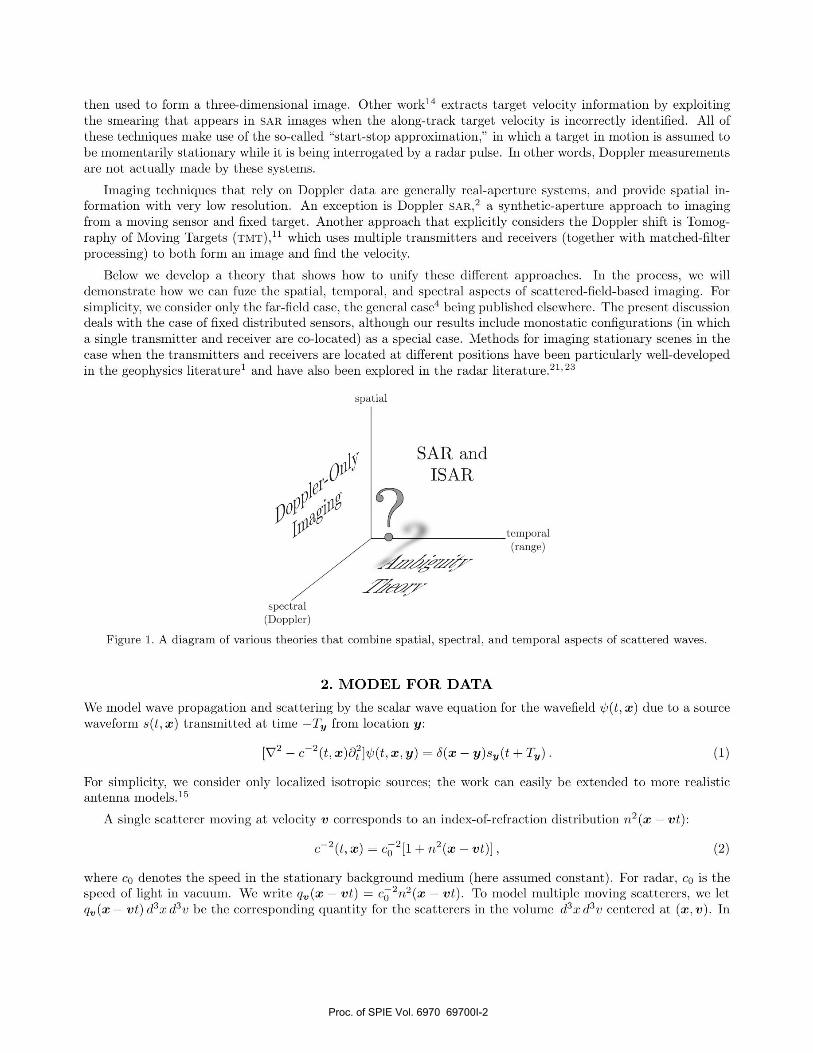
Below we develop a theory that shows how to unify these different approaches. In the process, we willdemonstrate how we can fuze the spatial, temporal, and spectral aspects of scattered-field-based imaging. Forsimplicity, we consider only the far-field case, the general case4 being published elsewhere. The present discussiondea's with the case of fixed distributed sensors, although our resuks indude monostatic configurations (in whicha single transmitter and receiver are co-'ocated) as a special case. Methods for imaging stationary scenes in thecase when the transmitters and receivers are 'ocated at different positions have been particularly well-developedin the geophysics literature1 and have a'so been exp'ored in the radar literature.21'23

spatial

SAR andTSAR

poP_______________temporal

(range)

spectral(Doppler)

Figllre 1. A diagram of variolls theories that combine spatial, spectral, and temporal aspects of scattered waves.

2. MODEL FOR DATAWe model wave propagation and scattering by the scalar wave equation for the wavefied '(t, x) due to a sourcewaveform s(t, x) transmitted at time —Tn from location y:

[V2 — c2(t, x)O](t, xy) = J(x — y)s(t + Tn). (1)

For simplicity, we consider on'y 'ocalized isotropic sources; the work can easily be extended to more realisticantenna models.15

A singk scatterer moving at ve'ocity v corresponds to an index-of-refraction distribution n2(x —Vt):

62(t, x) = + m2(x vt)I, (2)

where c0 denotes the speed in the stationary background medium (here assumed constant). For radar, c0 is thespeed of light in vacuum. We write qv(x — Vt) = c2n2(x — Vt). To model multiple moving scatterers, we etq(x — Vt) d3x d3v be the corresponding quantity for the scatterers in the vdlume d3x d3v centered at (xv). In

Proc. of SPIE Vol. 6970 69700I-2

other words, q is a distribution in phase space, and qv is the spatial distribution, at time t = 0, of scatterersmoving with velocity v. Consequently, the scatterers in the spatial volume d3x (at x) give rise to

c−2(t, x) = c−20 +

∫qv(x − vt) d3v . (3)

We note that the physical interpretation of qv involves a choice of a time origin. A choice that is particularlyappropriate, in view of our assumption about linear target velocities, is a time during which the wave is interactingwith targets of interest. This implies that the activation of the antenna at y takes place at a negative time whichwe denote by −Ty. The wave equation corresponding to (3) is then[

∇2 − c−20 ∂2

t −∫

qv(x − vt) d3v ∂2t

]ψ(t,x) = sy(t + Ty)δ(x − y) . (4)

2.1 The Transmitted FieldWe consider the transmitted field ψin in the absence of any scatterers; ψin satisifies the version of equation (1)in which c is simply the constant background speed c0, namely

[∇2 − c−20 ∂2

t ]ψin(t, x,y) = sy(t + Ty)δ(x − y) . (5)

Henceforth we drop the subscript on c. We use the Green’s function g, which satisfies

[∇2 − c−20 ∂2

t ]g(t,x) = −δ(t)δ(x)

and is given by

g(t, x) =δ(t − |x|/c)

4π|x| =1

8π2|x|∫

e−iω(t−|x|/c) dω (6)

where we have used 2πδ(t) =∫

exp(−iωt) dω. We use (6) to solve (5), obtaining

ψin(t, x,y) = −∫

g(t − t′, |x − x′|)sy(t′ + Ty)δ(x′ − y) dt′ dx′ = −sy(t + Ty − |x − y|/c)4π|x − y| . (7)

2.2 The Scattered FieldWe write ψ = ψin + ψsc, which converts (1) into

[∇2 − c−20 ∂2

t ]ψsc =∫

qv(x − vt) d3v ∂2t ψ . (8)

The map q �→ ψsc can be linearized by replacing the full field ψ on the right side of (8) by ψin. This substitutionresults in the Born approximation ψsc for the scattered field ψsc at the location z:

ψsc(t, z) = −∫

g(t − t′, |z − x|)∫

qv(x − vt′) d3v ∂2t′ψ

in(t′,x) dt′ d3x

=∫

δ(t − t′ − |z − x|/c)4π|z − x|

∫qv(x − vt′) d3v ∂2

t′sy(t′ + Ty − |x − y|/c)

4π|x − y| d3x dt′. (9)

In equation (9), we make the change of variables x �→ x′ = x − vt′, (i.e., change to the frame of reference inwhich the scatterer qv is fixed) to obtain

ψsc(t, z) =∫

δ(t − t′ − |x′ + vt′ − z|/c)4π|x′ + vt′ − z|

∫qv(x′)

sy(t′ + Ty − |x′ + vt′ − y|/c)4π|x′ + vt′ − y| d3x′ d3v dt′. (10)

The physical interpretation of (10) is as follows: The wave that emanates from y at time −Ty encounters atarget at time t′. This target, during the time interval [0, t′], has moved from x′ to x′ + vt′. The wave scatterswith strength qv(x′), and then propagates from position x′ + vt′ to z, arriving at time t.

Proc. of SPIE Vol. 6970 69700I-3

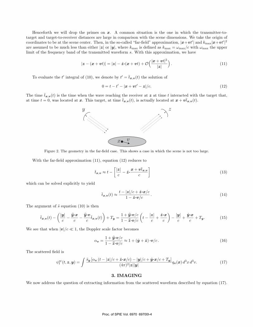
Henceforth we will drop the primes on x. A common situation is the one in which the transmitter-to-target and target-to-receiver distances are large in comparison with the scene dimensions. We take the origin ofcoordinates to be at the scene center. Then, in the so-called “far-field” approximation, |x+vt′| and kmax|x+vt′|2are assumed to be much less than either |z| or |y|, where kmax is defined as kmax = ωmax/c with ωmax the upperlimit of the frequency band of the transmitted waveform s. With this approximation, we have

|z − (x + vt)| = |z| − z·(x + vt) + O( |x + vt|2

|z|)

. (11)

To evaluate the t′ integral of (10), we denote by t′ = tx,v(t) the solution of

0 = t − t′ − |x + vt′ − z|/c. (12)

The time tx,v(t) is the time when the wave reaching the receiver at z at time t interacted with the target that,at time t = 0, was located at x. This target, at time tx,v(t), is actually located at x + vtx,v(t).

Figure 2. The geometry in the far-field case. This shows a case in which the scene is not too large.

With the far-field approximation (11), equation (12) reduces to

tx,v ≈ t −[ |z|

c− z·x + vtx,v

c

](13)

which can be solved explicitly to yield

tx,v(t) ≈ t − |z|/c + z·x/c

1 − z·v/c. (14)

The argument of s equation (10) is then

tx,v(t) −( |y|

c− y·x

c− y·v

ctx,v(t)

)+ Ty =

1 + y·v/c

1 − z·v/c

(t − |z|

c+

z·xc

)− |y|

c+

y·xc

+ Ty. (15)

We see that when |v|/c � 1, the Doppler scale factor becomes

αv =1 + y·v/c

1 − z·v/c≈ 1 + (y + z) ·v/c . (16)

The scattered field is

ψscf (t, z,y) =

∫sy [αv (t − |z|/c + z·x/c) − |y|/c + y·x/c + Ty]

(4π)2|z||y| qv(x) d3x d3v. (17)

3. IMAGING

We now address the question of extracting information from the scattered waveform described by equation (17).

Proc. of SPIE Vol. 6970 69700I-4

We form an image I(p,u) of the objects with velocity u that, at time t = 0, were located at position p. ThusI(p,u) is constructed to be an approximation to qu(p). The strategy for the imaging process is to write thedata in terms of a Fourier Integral Operator F : qv �→ ψsc, and then find an approximate inverse for F .

To write (17) as a Fourier Integral Operator, we write sy(t) in terms of its inverse Fourier transform:

sy(t) =12π

∫e−iω′tSy(ω) dω′ . (18)

We note that by the Paley-Weiner theorem, S is analytic since it is the inverse Fourier transform of the finite-duration waveform s. With (18), we convert (17) into

ψscf (t, z,y) =

∫(−iω)2

(4π)2|z||y| exp(− iω [αv (t − |z|/c + z·x/c) − |y|/c + y·x/c + Ty]

)Sy(ω) dωqv(x′) d3x d3v.

(19)

The corresponding imaging operation is a filtered version of the formal adjoint of the “forward” operator F .Thus we form the phase-space image I(p,u) as

I∞(p,u) =∫

eiω[αu(t−|z|/c+z·p/c)−|y|/c+y·p/c+Ty ]Q∞(ω, p,u,z,y) dω ψsc(t,z,y) dt dnz dmy. (20)

The specific choice of filter is dictated by various considerations;1,25 here we make choices that connect theresulting formulas with familiar theories. We take the filter to be

Q∞(ω, p,u,z,y) = −(4π)2ω−2|z||y|S∗y(ω)J(ω, p,u,z,y)αu , (21)

which leads (below) to the matched filter. Here the star denotes complex conjugation, and J is a geometricalfactor that depends on the configuration of transmitters and receivers.

Our image formation algorithm depends on the data we have available. In general, we form a (coherent)image as a filtered adjoint, but the variables we integrate over depend on whether we have multiple transmitters,multiple receivers, and/or multiple frequencies. The number of variables we integrate over, in turn, determineshow many image dimensions we can hope to reconstruct. If our data depends on two variables, for example,then we can hope to reconstruct a two-dimensional scene; in this case the scene is commonly assumed to lieon a known surface. If, in addition, we want to reconstruct two-dimensional velocities, then we are seekinga four-dimensional image and thus we will require data depending on at least four variables. More generally,determining a distribution of positions in space and the corresponding three-dimensional velocities means thatwe seek to form an image in a six-dimensional phase space.

To determine the point spread function, we substitute (19) into (20) to obtain

I∞(p,u) =∫

exp (iω[αu(t − |z|/c + z·p/c) − |y|/c + y·p/c + Ty]) Q∞(ω, p,u,z,y)

×∫

e−iω′[αv(t−|z|/c+z·x/c)−|y|/c+y·x/c+Ty ] ω′2Sy(ω′)25π3|z||y| dω′ dω qv(x) d3x d3v dt dnz dmy . (22)

For smooth Sy, we can apply the method of stationary phase to the t and ω′ integrations in (22). The criticalconditions are

0 = ωαu − ω′αv

0 = αv(t − |z|/c + z·x/c) − |y|/c + y·x/c + Ty (23)

and the Hessian of the phase is αv. This converts the kernel of (22) into

K∞(p,u;x,v) =∫

exp(−iω∆τ f

y,z

)S∗

y(ω)Sy

(ω αu

αv

)J(ω, p,u,z,y)

α3u

α3v

dω dnz dmy (24)

Proc. of SPIE Vol. 6970 69700I-5

where ∆τf is defined by

c∆τ fy,z = αu

(|z| − z·x +

|y| − y·x − cTy

αv− |z| + z·p)

)− |y| + y·p + cTy

= αuz·(p − x) +(

αu

αv− 1

)(|y| − cTy) − y·

(αu

αvx − p

)

= αuz·(p − x) +(

αu

αv− 1

)(|y| − cTy) − y·

(αu

αv− 1

)x − y·(x − p)

= (αuz + y) ·(p − x) +(

αu

αv− 1

)(|y| − cTy) −

(αu

αv− 1

)y·x

≈ (αuz + y) ·(p − x) +(

u − v

c

)· (y + z) y·x, (25)

where in the last line we have assumed that the transmitters are activated so that Ty = |y|/c and where we haveused (16) to write

αu

αv≈ 1 − (u − v)·(y + z)/c . (26)

The choice Ty = |y|/c corresponds to activating the transmitters so that waves from different transmitters arriveat the origin at the same time.

To write (24) in terms of the ambiguity function, we assume that J = J/ω2 is independent of ω and use thedefinition of the inverse Fourier transform

Sy(ω) =∫

eiωtsy(t) dt (27)

to obtain

K∞(p,u;x,v) =∫

s∗y(

αu

αvt − ∆τ f

y,z, y)sy(t)J(p,u,z,y)αu

αvdt dnz dmy. (28)

If we use the the wideband radar ambiguity function19 Ay for the waveform s, defined by

Ay(σ, τ) =∫

s∗y(σt − τ)sy(t) dt, (29)

then we can write (28) as

K∞(p,u;x,v) =∫

Ay

(αu

αv,∆τ f

y,z

)J(p,u,z,y)

αu

αvdnz dmy . (30)

This exhibits the wideband point-spread function for phase-space imaging in terms of a weighted, coherentsum of wideband bistatic ambiguity functions.

Many radar systems use a narrowband waveform, which is of the form

sy(t) = sy(t) e−iωyt (31)

where s(t, y) is slowly varying, as a function of t, in comparison with exp(−iωyt), where ωy is the carrier frequencyfor the transmitter at position y. For a narrowband waveform (31), the ambiguity function (29) becomes

Ay(σ, τ) = −ω2y

∫s∗y(σt − τ) sy(t) eiωte−iωyτ dt (32)

where ω = ωy(σ − 1). Since sy(t) is slowly varying, Ay(σ, τ) ≈ −ω2yAy(ω, τ), where Ay is the narrowband

ambiguity function

Ay(ω, τ) = e−iωyτ

∫s∗y(t − τ) sy(t) eiωt dt . (33)

Proc. of SPIE Vol. 6970 69700I-6

We note that our definition of the ambiguity function includes a phase.

In the narrowband case, (30) reduces to

K(NB)∞ (p,u;x,v) = −

∫ω2

yAy

(ky(y + z)·(u − v), (z + y)·(x − p)/c

)eiΦy,z J dnz dmy , (34)

whereeiΦy,z(x,v,p,u) = exp [i(ϕx,v − ϕp,u)] exp (−iky(βu − βv)(z + y)·x) (35)

with ky = ωy/c, βv = (y + z) ·v/c, and

ϕx,v − ϕp,u = ωy

c [[(1 + βu)z + y] ·p − [(1 + βv)z + y] ·x]= ky [(z + y)·(p − x) + z·(βup − βvx)] (36)

The narrowband result (34) clearly exhibits the importance of the bistatic bisector vector y + z.

4. REDUCTION TO FAMILIAR SPECIAL CASES

4.1 Range-Doppler Imaging

In classical range-Doppler imaging, the range and velocity of a moving target are estimated from measurementsmade by a single transmitter and coincident receiver. Thus we take z = y, J = 1, and remove the integrals in(34) to show that the point-spread function is simply proportional to the ambiguity function. In particular, forthe case of a slowly moving distant target, (34) reduces to the familiar result

K(NB)RD (p,u;x,v) ∝ Ay

(2ωc(u − v)·y

c, 2

(p − x)·yc

). (37)

We see that only range and down-range velocity information is obtained.

4.1.1 Range-Doppler Imaging of a Rotating Target.

If the target is rotating about a point, then we can use the connection between position and velocity to form atarget image. We choose the center of rotation as the origin of coordinates. In this case, a scatterer at x movesas q(O(t)x), where O denotes an orthogonal matrix. This is not linear motion, but we can still apply our resultsby approximating the motion as linear over a small angle.

In particular, we write O(t) = O(0) + tO(0), and assume that O(0) is the identity operator. In this case, thevelocity at the point x is Ox, so in our notation, the phase-space distribution is qv(x) = qO(0)x(x).

For the case of two-dimensional imaging, we take y = (1, 0), and O is given by

O(t) =[

cos ωt sin ωt− sin ωt cos ωt

], O(0) = ω

[0 1

−1 0

], (38)

so (37) becomes

K(NB)RD (p,u;x,v) ∝ Ay

(2ωc(u1 − v1)

c, 2

(p1 − x1)c

)∝ Ay

(2ωcω(p2 − x2)

c, 2

(p1 − x1)c

). (39)

Thus we have the faimilar result that the delay provides the down-range target components while the Dopplershift provides the cross-range components. Note that even though the velocity v1 = ωx1 can be estimated fromthe radar measurements, the cross-range spatial components x1 are distorted by the unknown angular velocityω.

The psf depends on only two variables, which implies that the image obtained is an approximation to∫q(x1, x2, x3) dx3.

Proc. of SPIE Vol. 6970 69700I-7

4.1.2 Imaging with Ridge-like Ambiguity Functions

For an ambiguity function that is a narrow ridge along the line τ = mν, the ambiguity function is of the form

Ay(ν, τ) = Ay(τ − mν), (40)

and equation (39) becomes

K(NB)RD (p,u;x,v) ∝ Ay

(2(p1 − x1) − mωcω(p2 − x2)

c

). (41)

This leads to the Feig-Grunbaum imaging method,9 in which ambiguity functions with different slopes providedifferent slices of a target, and the target is then reconstructed by backprojection.

4.2 High Range-Resolution Imaging

Many radar systems use high range-resolution (hrr) pulses, for which the ambiguity function is a narrow ridgeextending along the ν axis. In these cases, we write

Ay(ν, τ) = Ay(τ), (42)

with Ay(τ) sharply peaked around τ = 0.

4.2.1 Inverse Synthetic-Aperture Radar (ISAR)

In spite of the confusion between range-Doppler imaging and isar, modern isar methods do not actually requireDoppler-shift measurements. Rather, the technique depends on the target’s rotational motion to establish apseudo-array of distributed receivers. To show how isar follows from the results of this paper, we fix thecoordinate system to the rotating target. Succeeding hrr pulses of a pulse train are transmitted from andreceived at positions z = y that rotate around the target as y = y(θ). With this geometry and an ambiguityfunction of the form (42), equation (34) reduces to

K(NB)ISAR(p,u;x,v) = −ω2

0

∫Ay

(2(p − x)·y(θ)

c

)J |y| dθ . (43)

where we have written ωy = ω0 because the pulses typically have the same center frequency.

Note that the set of all points p such that (p − x)·y(θ) = 0 forms a plane through x with normal y(θ).Consequently, since Ay(τ) is sharply peaked around τ = 0, the support of the integral in (43) is a collection ofplanes, one for each pulse in the pulse train, and isar imaging is seen to be based on backprojection.

Because knowledge of y(θ) is needed, isar depends on knowledge of the rotational motion; it is typicallyassumed to be uniform, and the rotation rate ω must be determined by other means.

4.2.2 Spotlight Synthetic-Aperture Radar (SAR)

Sar also uses hrr pulses, transmitted and received at locations along the flight path y = y(ζ), where ζ denotesthe flight path parameter. For a stationary scene, u = v = 0, which implies that βu = βv = 0. In this case, (34)reduces to

K(NB)SAR (p, 0;x, 0) ∝

∫Ay

(2(p − x)·y(ζ)

c

)J |y| dζ (44)

where again we have used (42).

Proc. of SPIE Vol. 6970 69700I-8

4.3 Diffraction Tomography

Diffraction tomography uses a single frequency waveform s(t) = exp(−iω0t) (with s = 1) to interrogate astationary object (i.e., v = 0, which implies αv = 1). We also activate the transmitters at times −Ty = −|y|/c,so that all the transmitted waves arrive at the scene center at the same time, and evaluate ψsc

fN at t′ = t + |z|/cto write (17) as

ψ∞ω0

(t, z,y) ≈ e−ik0t

(4π)2|z||y|F∞(y, z) , (45)

where the (Born-approximated) far-field pattern or scattering amplitude is

F∞(y, z) =∫

e−ik0(z+y)·xq(x) d3x . (46)

and where k0 = ω0/c. We note that our incident-wave direction convention (from target to transmitter) is theopposite of that used in the classical scattering theory literature (which uses transmitter to target).

In this case the data is the far-field pattern (46). Our inversion formula is (20), where there is no integrationover t. The resulting formula is

Ik0(p) =∫

eik0(z+y)·p Qk0(z, y)F∞(y, z) dy dz (47)

where Qk0 is the filter7

Qk0 =k30

(2π)4|y + z|. (48)

which corrects for the Jacobian that is ultimately needed. Here the factor of k30 corresponds to three-dimensional

imaging.

The associated point-spread function is obtained from substituting (46) into (47):

Ik0(p) =∫

eik0(z+y)·pQk0(z, y)∫

e−ik0(z+y)·xq(x) d3x dy dz

= k30

(2π)4

∫eik0(z+y)·(p−x)|z + y| dy dz q(x) d3x

=∫

χ2k(ξ)eiξ·(p−x) d3ξ q(x) d3x (49)

where χ2k denotes the function that is one inside the ball of radius 2k and zero outside and where we have usedthe Devaney identity7 ∫

χ2k(ξ)eiξ·rd3ξ =k3

(2π)4

∫S2×S2

eik(y+z)·r|y + e′| dy dz . (50)

The two-dimensional version is8∫χ2k(ξ)eiξ·rd2ξ =

∫S1×S1

eik(y+z)·r∣∣∣∣ ∂ξ

∂(y, z)

∣∣∣∣ dy dz (51)

where y = (cos θ, sin θ), z = (cos θ′, sin θ′), and∣∣∣∣ ∂ξ

∂(y, z)

∣∣∣∣ =√

1 − (y·z)2 . (52)

4.4 Moving Target Tomography.

Moving Target Tomography11 models the signal using a simplified version of (17). For this simplified model,our imaging formula (20) reduces to matched-filter processing11 with a different filter for each location p and foreach possible velocity u.

Proc. of SPIE Vol. 6970 69700I-9

5. CONCLUSIONS AND FUTURE WORK

We have developed a linearized imaging theory that combines the spatial, temporal, and spectral aspects ofscattered waves.

This imaging theory is based on the general (linearized) expression we derived for waves scattered from movingobjects, which we model in terms of a distribution in phase space. The expression for the scattered waves is ofthe form of a Fourier integral operator; consequently we form a phase-space image as a filtered adjoint of thisoperator.

The theory allows for activation of multiple transmitters at different times, but the theory is simpler whenthey are all activated so that the waves arrive at the target at roughly the same time.

The general theory in this paper reduces to familiar results in a variety of special cases. We leave for thefuture further analysis of the point-spread function. We also leave for the future the case in which the sensorsare moving independently, and the problem of combining these ideas with tracking techniques.

ACKNOWLEDGMENTS

This work was supported by the Office of Naval Research, by the Air Force Office of Scientific Research∗ underagreement number FA9550-06-1-0017, by Rensselaer Polytechnic Institute, and by the National Research Council.

REFERENCES[1] N. Bleistein, J.K. Cohen, and J.W. Stockwell, The Mathematics of Multidimensional Seismic Inversion,

(Springer: New York, 2000)[2] B. Borden and M. Cheney, “Synthetic-Aperture Imaging from High-Doppler-Resolution Measurements,”

Inverse Problems, 21, pp. 1–11 (2005)[3] I. Bradaric, G.T. Capraro, D.D. Weiner, and M.C. Wicks, “Multistatic Radar Systems Signal Processing”,

Proceedings of IEEE Radar Conference 2006.[4] M. Cheney and B. Borden, “Imaging Moving Targets from Scattered Waves,” to appear in Inverse Problems.[5] C.E. Cook and M. Bernfeld, Radar Signals (Academic: New York, 1967)[6] J. Cooper, “Scattering of Electromagnetic Fields by a Moving Boundary: The One-Dimensional Case”,

IEEE Antennas and Propagation, vol. AP-28, No. 6, pp. 791–795 (1980).[7] A.J. Devaney, “Inversion formula for inverse scattering within the Born approximation,” Optics Letters, 7,

pp. 111–112 (1982).[8] A.J. Devaney, “A filtered backpropagation algorithm for diffraction tomography”, Ultrasonic Imaging, 4,

pp. 336–350 (1982).[9] E. Feig E and A. Grunbaum, “Tomographic Methods in Range-Doppler Radar,” Inverse Problems, 2,

pp. 185–95 (1986)[10] B. Friedlander and B. Porat, “Vsar: A High Resolution Radar System for Detection of Moving Targets,”

IEE Proc. Radar, Sonar, Navig., 144, pp. 205–18 (1997)[11] B. Himed, H. Bascom, J. Clancy, and M.C. Wicks, “Tomography of Moving Targets (TMT)”, in Sensors,

Systems, and Next-Generation Satellites V., ed. H. Fujisada, J.B. Lurie, and K. Weber, Proc. SPIE Vol.4540 (2001) pp. 608 – 619.

[12] R. Klemm, Principles of Space-Time Adaptive Processing, (Institution of Electrical Engineers: London,2002)

[13] N. Levanon, Radar Principles, (Wiley, New York, 1988)[14] M.J. Minardi, L.A. Gorham, and E.G. Zelnio, “Ground Moving Target Detection and Tracking Based on

Generaized Sar Processing and Change Detection,” Proceedings of SPIE, 5808, pp. 156–165 (2005)∗Consequently the U.S. Government is authorized to reproduce and distribute reprints for Governmental purposes

notwithstanding any copyright notation thereon. The views and conclusions contained herein are those of the authorsand should not be interpreted as necessarily representing the official policies or endorsements, either expressed or implied,of the Air Force Research Laboratory or the U.S. Government.

Proc. of SPIE Vol. 6970 69700I-10

[15] C.J. Nolan and M. Cheney, “Synthetic Aperture Inversion,” Inverse Problems, 18, pp. 221–36 (2002)[16] M. Reed and B. Simon, Methods of Modern Mathematical Physics. I. Functional Analysis (Academic Press:

New York, 1972)[17] M. Soumekh, “Bistatic Synthetic Aperture Radar Inversion with Application in Dynamic Object Imaging”,

IEEE Trans. Signal Processing, Vol. 39, No. 9, pp. 2044–2055 (1991).[18] M. Stuff, M. Biancalana, G. Arnold, and J. Garbarino, “Imaging Moving Objects in 3D From Single Aperture

Synthetic Aperture Data,” Proceedings of IEEE Radar Conference 2004, pp. 94–98[19] D. Swick, “A Review of Wideband Ambiguity Functions,” Naval Research Laboratory Rep. 6994 (1969)[20] T. Tsao, M. Slamani, P. Varshney, D. Weiner, H. Schwarzlander, and S. Borek, “Ambiguity Function for a

Bistatic Radar,” IEEE Trans. Aerospace & Electronic Systems, 33, pp. 1041–51 (1997)[21] N.J. Willis, Bistatic Radar (Artech House: Norwood, MA, 1991)[22] N.J. Willis and H.D. Griffiths, Advances in Bistatic Radar (SciTech Publishing, Raleigh, North Carolina,

2007)[23] N.J. Willis, “Bistatic Radar,” in Radar Handbook, M. Skolnik, ed., (McGraw-Hill: New York, 1990)[24] P.M. Woodward, Probability and Information Theory, with Applications to Radar, (McGraw-Hill: New

York, 1953)[25] B. Yazici, M. Cheney, and C.E. Yarman, ”Synthetic-aperture inversion in the presence of noise and clutter”,

Inverse Problems 22, pp. 1705-1729 (2006) .

Proc. of SPIE Vol. 6970 69700I-11