Tunable Graphene-based Pulse Compressor for Terahertz ...

i

1925 K. N. Toosi University of Technology

Faculty of Electrical Engineering

Tunable Graphene-based Pulse Compressor for Terahertz Application

A Thesis Submitted in Partial Fulfillment of the Requirements for the Degree

of Doctor of Philosophy in Electrical Engineering

By:

Seyed Mohammadreza Razavizadeh

Supervisor:

Prof. Ramezanali Sadeghzadeh

Advisor: Dr. Zahra Ghattan-kashani

September, 2020

i

Dedication

I would like to dedicate this thesis to little prince of Imam Hussain (As), Baby Ali Asghar (As)…

“Who was scarified in way of his grandfather Prophet Muhammed”

and to:

my beloved wife, mother and the precious memories of my father who was my biggest

supporter in my life and in choosing telecommunication engineering as my major like himself, and to

follow my dreams. Alas, no words can express my love, feelings for him. May God Bless Him.

تائیدیه هیات داوران جلسه دفاع از رساله دکتري

طراحی و تحلیل سامانه فشرده کننده پالس تراهرتزي کنترل پذیر مبتنی بر ساختار نوار گرافنی

امضا دانشگاه

خواجه نصیرالدین

طوسیخواجه نصیرالدین

طوسی

علم و صنعت ایران

تهران


طوسی


طوسی

ii

تائیدیه هیات داوران جلسه دفاع از رساله دکتري

دانشکده مهندسی برق

سیدمحمدرضا رضوي زاده


1399

مهندسی برق

مخابرات میدان

نام و نام خانوادگی مرتبه

دانشگاهیدانشگاه

استاد راهنمارمضانعلی صادق دکتر

زاده استاد


طوسی

استادیار دکتر زهرا قطان کاشانی استاد مشاورخواجه نصیرالدین

طوسی

استاد مدعو

علم و صنعت ایران استاد همایون عریضیدکتر

استاد مدعو

تهران استادیار محمد نشاطدکتر

استاد مدعو

محمدصادق دکتر

ابریشمان استاد


طوسی

استاد مدعو

استادیار سید آرش احمديدکتر


طوسی

دانشکده مهندسی برق: نام دانشکده

سیدمحمدرضا رضوي زاده: نام دانشجو

طراحی و تحلیل سامانه فشرده کننده پالس تراهرتزي کنترل پذیر مبتنی بر ساختار نوار گرافنی : عنوان رساله

مارپیچی

31/6/1399: تاریخ دفاع

مهندسی برق: رشته

مخابرات میدان : گرایش

سمت ردیف

استاد راهنما 1

استاد مشاور 2

3 استاد مدعو

خارجی


خارجی


داخلی


داخلی

iii

تائیدیه صحت و اصالت نتایج

بسمه تعالی

دانشجوي رشته مهندسی برق گرایش 9300576به شماره دانشجویی سیدمحمدرضا رضوي زادهاینجانب

نمایم که کلیه نتایج این رساله حاصل کار اینجانب و مخابرات میدان مقطع تحصیلی دکتري تخصصی تایید می

برداري شده از آثار دیگران را با ذکر کامل مشخصات منبع ذکر بدون هرگونه دخل و تصرف است و موارد نسخه

قانون (درجات فوق، به تشخیص دانشگاه مطابق با ضوابط و مقررات حاکم در صورت اثبات خالف من. ام کرده

حمایت از حقوق مولفان و مصنفان و قانون ترجمه و تکثیر کتب و نشریات و آثار صوتی، ضوابط و مقررات

با اینجانب رفتار خواهد شد و حق هرگونه اعتراض درخصوص احقاق حقوق ...) آموزشی، پژوهشی و انضباطی

در ضمن، مسئولیت هرگونه . نمایم و تشخیص و تعیین تخلف و مجازات را از خویش سلب میمکتسب

صالح، اعم از اداري و قضایی، به عهده اینجانب پاسخگویی به اشخاص اعم از حقیقی و حقوقی و مراجع ذي

. خواهد بود و دانشگاه هیچ مسئولیتی در این خصوص نخواهد داشت

سیدمحمدرضا رضوي زاده: نام و نام خانوادگی

1399 /06 / 31 :تاریخ

:امضا

iv

نامه برداري از پایان مجوز بهره

نامه در چهارچوب مقررات کتابخانه و با توجه به محدودیتی که توسط استاد راهنما به برداري از این پایان بهره

:شود بالمانع است شرح زیر تعیین می

همگان بالمانع استنامه براي برداري ازین پایان بهره.

نامه با اخذ مجوز از استاد راهنما، بالمانع است برداري ازین پایان بهره.

ممنوع است..................................... نامه تا تاریخ برداري ازین پایان بهره.

رمضانعلی صادق زاده :نام استاد راهنما

1399 /06 / 31 :تاریخ

:امضا

v

ACKNOWLEDGEMENTS

I would like to thank my wife first, as without her love, care, and constant support I wouldn’t be

here. I am greatly thankful to my advisers, Professor Ramezanali Sadeghzadeh and Dr. Zahra

Ghattan, for their insight, guidance, and patience during the course of this research project. I also

thank them for the encouragement, helpful advice, and for teaching me all of the terahertz

technology that I know today. In addition, I would like to express sincere appreciation to

Professor Miguel Navarro-Cia for his key comments and tips regarding our publications.

It was a great pleasure to my former graduate teachers, who were around at the time when I

started: Professor Mohammad Sadegh Abrishamian and Dr. Arash Ahmadi for sharing their

invaluable experimental tips, and their guidance. I would also like to thank Dr. Oriezi, , and Dr.

Neshat for being on my defense committee. I am thankful to Mrs Eeieni, and the staff at the K.

N. Toosi University for their assistance in all the general matters.

I would like to extend many heart-felt thanks to my family, to my parents, and especially to my

wife who was the primary motivational factor in achieving the Doctor of Philosophy degree.

vi

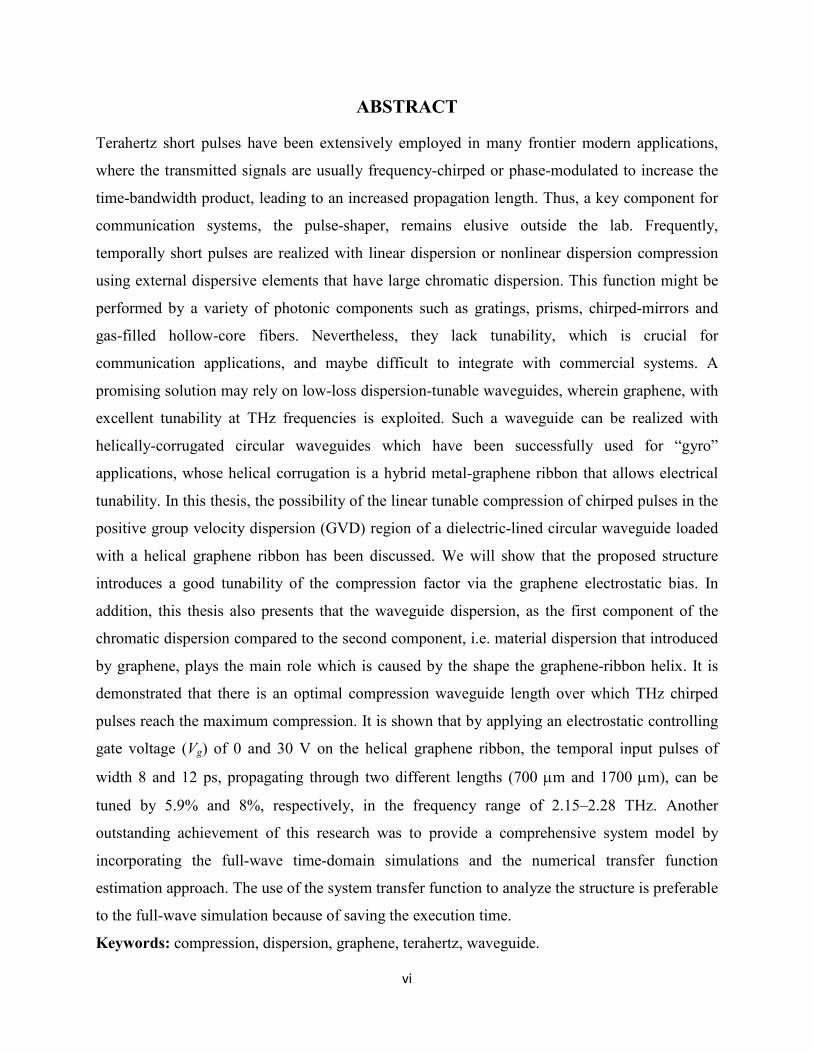
ABSTRACT

Terahertz short pulses have been extensively employed in many frontier modern applications,

where the transmitted signals are usually frequency-chirped or phase-modulated to increase the

time-bandwidth product, leading to an increased propagation length. Thus, a key component for

communication systems, the pulse-shaper, remains elusive outside the lab. Frequently,

temporally short pulses are realized with linear dispersion or nonlinear dispersion compression

using external dispersive elements that have large chromatic dispersion. This function might be

performed by a variety of photonic components such as gratings, prisms, chirped-mirrors and

gas-filled hollow-core fibers. Nevertheless, they lack tunability, which is crucial for

communication applications, and maybe difficult to integrate with commercial systems. A

promising solution may rely on low-loss dispersion-tunable waveguides, wherein graphene, with

excellent tunability at THz frequencies is exploited. Such a waveguide can be realized with

helically-corrugated circular waveguides which have been successfully used for “gyro”

applications, whose helical corrugation is a hybrid metal-graphene ribbon that allows electrical

tunability. In this thesis, the possibility of the linear tunable compression of chirped pulses in the

positive group velocity dispersion (GVD) region of a dielectric-lined circular waveguide loaded

with a helical graphene ribbon has been discussed. We will show that the proposed structure

introduces a good tunability of the compression factor via the graphene electrostatic bias. In

addition, this thesis also presents that the waveguide dispersion, as the first component of the

chromatic dispersion compared to the second component, i.e. material dispersion that introduced

by graphene, plays the main role which is caused by the shape the graphene-ribbon helix. It is

demonstrated that there is an optimal compression waveguide length over which THz chirped

pulses reach the maximum compression. It is shown that by applying an electrostatic controlling

gate voltage (Vg) of 0 and 30 V on the helical graphene ribbon, the temporal input pulses of

width 8 and 12 ps, propagating through two different lengths (700 m and 1700 m), can be

tuned by 5.9% and 8%, respectively, in the frequency range of 2.15–2.28 THz. Another

outstanding achievement of this research was to provide a comprehensive system model by

incorporating the full-wave time-domain simulations and the numerical transfer function

estimation approach. The use of the system transfer function to analyze the structure is preferable

to the full-wave simulation because of saving the execution time.

Keywords: compression, dispersion, graphene, terahertz, waveguide.

vii

TABLE OF CONTENTS

List of Figures .............................................................................................................................ix

List of Tables ..............................................................................................................................xiii

List of Abbreviations ................................................................................................................ xiv

List of Physical Symbols .......................................................................................................... xvi

Chapter 1: Introduction

1.1 Temporary Pulse Compression and Stretching Development………………………...…..1

1.1.1 Microwave Pulse Compression Approaches ……………………………………. 2

1.1.2 Optical Pulse Compression Approaches ……………………………………….. 5 1.2 Fixed and Tunable Graphene-based THz Devices ………………………….………….. 9

1.2.1 Graphene ………………………………………………………………………... 9

1.2.2 EM characterization of graphene ………………………………………….…….. 9

1.2.3 Graphene based circuit/components ………………………………………….... 10

1.2.4 Motivation for Tunable Terahertz Pulse compression …………………………. 12

1.2.5 Thesis Outline ……………………………………………………..…………… 13

Chapter 2: Literature Review

2 2.1 Terahertz Pulse Compressors ……………………………………………….………….. 15 2.1.1 Approach(THz): Temporal delay/advancement when a pulse passes through the aperture ………………………………………………………………………………...……. 16 2.1.2 Approach (Microwave) ………………………………………………….…….. 17 2.1.3 Approach (Optics-region) ……………………………………………………… 19

Chapter 3: Important Concepts and Basic Theory

2 3 3.1 Chromatic Dispersion ………………………………………………………………..… 21 3.1.1 Material Dispersion: Modeling of Dispersive Material in Terahertz …………... 21 3.1.2 Waveguide Dispersion …………………………………………….…………… 23 3.2 Dispersion Analysis ……………………………………………………...…………….. 23 3.2.1 Group Velocity …………………………………………………………………. 23 3.2.2 Group Delay …………………………………………………………………..... 25 3.2.3 Group Velocity Dispersion ………………………………………….…………. 25 3.3 Normal and Anomalous Dispersion ……………………………………………………. 27 3.4 Dispersion-based Pulse Compressor …………………………………..……………….. 28 3.4.1 Chirped Linear FM Pulse ………………………………………………………. 28 3.5 Broadening Factor ………………………………………………………………...……. 31 3.6 Attenuation ……………………………………………………………………………... 31

viii

3.7 LFM Generation ………………………………………………………………………...31

Chapter 4: Tunable Terahertz Pulse Compressor Design Based on Helical Graphene Ribbon

3 4 4.1 Model Description and Design Principles ………………………………..……………. 33 4.1.1 Model Description ……………………………………………………………... 34 4.1.2 Design Methodology Principle ……………………………………………...… 35 4.2 Definition of Material ………………………………………………………………….. 38 4.2.1 Graphene …………………………………………………..…………………… 38 4.2.2 HDPE ……………………………………………………………..……………. 42 4.2.3 Nobel Metals: Gold ……………………………………………….……………. 42 4.2.4 Silicon Dioxide ……………………………………………………...…………. 42 4.3 Results and Discussion ………………………………………………………………… 43 4.3.1 DC-Controlled Dispersion Mechanism ……………………………………...… 43 4.3.2 Pulse Compression Performance ……………………………………….……….47

Chapter 5: Numerical Analysis Validation based on a Fixed Terahertz Pulse Compressor

5.1 Validation of Numerical Analysis Results ……………………………….…………….. 57 5.1.1 Graphene-based Tunable THz Pulse Compression Waveguide ……………..… 58 5.1.2 Gold-based Fixed THz Pulse-shaper Waveguide ………………………...……. 59 5.2 A System Identification of Au-based Fixed THz Pulse-shaper Waveguide ………….... 67

Chapter 6: A Comparative Study on Helical Ribbon Material Dependence

6.1 Dispersion and Matching Performance of PEC, Au, and Graphene-ribbon ……....….. 71 6.2 Pulse Compression Analysis ……………………………………………………..…… 75

Chapter 7: Conclusion and Future Works …………………………………….……………. 77

Appendix A: A Brief Theory on Dispersion and Pulse Compression ………………………81

Appendix B: The General Modeling Consideration and Simulation Characteristics ...….. 83

Appendix C: MATLAB Codes ………………………………………………………………. 94

Appendix D: Proposed Fabrication Method ………………………..……………..……….100

List of Publications ..................................................................................................................102

References ……………………………………………………………………………….…… 103

ix

LIST OF FIGURES

1.1 Helically corrugated waveguide the surface equation in cylindrical (J. Appl. Phys. 108,

054908 (2010); doi: 10.1063/1.3482024 )……………………….……………………… 4

1.2 Measured characteristics of helically corrugated waveguide used in the compression

experiment: group velocity of the operating mode dashed line and losses solid line for

the whole compressor (J. Appl. Phys. 108, 054908 (2010); doi: 10.1063/1.3482024 ).

…………………………………………………………….…………………………...…4

1.3 Input pulse details for pulse compression experiment (J. Appl. Phys. 108, 054908 (2010);

doi: 10.1063/1.3482024 )………………………………………………………………...4

1.4 Measured solid line and simulated dashed line compressed pulse (J. Appl. Phys. 108,

054908 (2010); doi: 10.1063/1.3482024 )……………………………………………….5

1.5 3-D picture of the proposed single-mode TPCF………………………………………....6

1.6 The input and output pulse of TPCF at 1550 nm………………………………………..6

1.7 (a) The 2D model of graphene lattice structure, and (b) external perpendicular electric

and magnetic fields applied on it as the controlling static bias……………………..….10

1.8 Schematic of the antenna with HIS: (a) cross-sectional view and (b) top view (with

permission)………………………………………………………………………………11

1.9 (a) General reflectarray concept, and (b) Graphene reflective cell…………………….11

1.10 (a) Experimental setup used for the terahertz time-domain reflection measurements. (b)

Variation of phase (radians) and intensity (dB) of the THz reflection of the devices with

different DC-controlling voltages……………………………………………………....12

2.1 Temporal deformation of the intrinsically chirped THz pulse due to transmission through

the 10 mm aperture. The dashed lines indicate squared, normalized electric-field wave

functions, and the shaded area shows theGaussian envelopes of the pulses. Ratio of the

peak intensity of the transmitted pulse to that of the incident pulse is 1.410-(Fig. 3 from

[41])………………………………………………………………………………….….17

2.2 Scheme of the experimental setup [42]. ………………………………………………. 18

2.3 (a) Group velocity normalized to the speed of light of the helical waveguide operating

wave(Fig. 2 from [18]), and (b) the resultant compressed pulse solid curve shown in

contrast with the relativistic backward-wave oscillator output pulse dashed curve (Fig. 4

from [42])………………………………………………………………………………. 18

2.4 Schematic depiction of a cholesteric liquid crystal cell (CLC) for femtoseconds laser

pulse compression or stretching, caused by nonlinear phase modulation and dispersion at

the band edge [43]……………………………………………………………………….19

3.1 A time domain illustration of a down-chirped sinusoidal linear FM pulse……………..29

3.2 (a) group velocity profile with negative gradient variation in terms of frequency of a

dispersion managed device and (b) a representation of how a down-chirped LFM

x

waveform with duration of T0 can produce a grater peak amplitude after traveling an

optimal length of a the dispersive waveguide.………………………………………..…30

4.1 Schematic-diagram, 3D geometry, and side view of an internally dielectric-coated

hollow-core waveguide loaded by a helical graphene ribbon (inset: the graphene ribbon

is grown on a thin SiO2 layer and sandwiched between two gold ribbons to facilitate the

DC controlling of the device)…………………………………………………………...35

4.2 The THz spectral of real and imaginary parts of the effective permittivity of an infinite

graphene sheet for T=300K, EF=0eV, and different values of =[1, 10, 50]nm. ………40

4.3 The THz spectral of (a) real and (b) imaginary parts of the effective permittivity of an

infinite graphene sheet for T=300K, =1 nm, and different values of EF= [0.0-1.0] eV.

The Effect of Substrate …………………………………………………………………41

4.4 DC controlling voltage Vg versus Fermi level EFin terms of various SiO2 thickness..…42

4.5 The equivalent circuit modeling of a cylindrical metallic tube which contains a metallic

helix from [80]…………………………………………………………………………..44

4.6 Variation of phase constant for five modes TE11, TM01, TE21,TM11, and TE01 vs relative

thickness t/ at =22.4 S/m and f=31 GHz, Fig.6b of [83]……………………………....45

4.7 (a) Magnitude and (b) phase of the S-parameters of the proposed device biased at Vg D 0

and 30 V……………………………………………………………………………...… 45

4.8 (a) Group velocity dispersion (GVD), (b) normalized group velocity, and (c) real and

imaginary parts of the effective refractive index of the proposed device biased at Vg= 0

and 30 V…………………………………………………………………………..……. 46

4.9 Waveform evolution of the proposed device with the optimal length of 720 µm,

corresponding to input pulse duration of 8 ps, based on two border values of controlling

DC voltage (a) 0 V and (b) 30 V……………………………………………………….. 48

4.10 Waveform evolution of the proposed device with the optimal length of 1700 µm,

corresponding to input pulse duration of 12 ps, based on two border values of controlling

DC voltage (a) 0 V and (b) 30 V………………………………………………………..49

4.11 Envelope of the compressed output pulses monitored transverse and axial electric field

components of Ey and Ez, respectively, for two model lengths of (a) 720m and (b) 1700

m……………………………………………………………………………………….50

4.12 The electric field distributions of: (a) Ey and (b) Ez on the output aperture of the

proposed pulse compressor of length 700m, at 2.15 THz…………………………..…51

4.13 (a) Time and (b) spectral descriptions of the pulse compressor output for Vg = 0 and 30

V for a length of 720 µm (the mode patterns at the end of the helix are presented in the

insets of the figure)………………………………………………………………………52

4.14 .(a) Time and (b) spectral descriptions of the pulse compressor output for Vg = 0 and 30

V for a length of 1700 µm (the mode patterns at the end of the helix are presented in the

insets of the figure). …………………………………………………………………….53

xi

4.15 Parametric study of sensitivity of (a) refractive index of inner dielectric coating layer,

and (b) its thickness of td , (c) width and (d) pitch size of the helical zero-biased

graphene-ribbon of the proposed graphene-based pulse compressor on the compressed

output pulse……………………………………………………………………………...55

5.1 (a) GVD and (b) normalized group velocity of the proposed graphene-based tunable

pulse compression waveguide in various mesh resolution using by FIT analysis………59

5.2 3D geometry and side view of an internally dielectric-coated hollow-core waveguide

loaded by a helical gold ribbon……………………………………………………….....60

5.3 (a) Transmittance, and (b) absorption spectra ofthe proposed device using the FIT and

the FEM……………………………………………………………………………….....61

5.4 The phase of S21 of the proposed device using the FIT and the FEM………………….61

5.5 Group delay and normalized group velocity extracted from the phase of the transmission

coefficient (FIT-method)………………………………………………………………...62

5.6 (a) The output y-polarized E-field probe signals at various positions of the proposed

structure (a) front position (z = 50m), (b) before, and (d) after, and (c) optimal length of

L0=575 m………………………………………………………………………………64

5.7 The electric field distributions at the optimum positions and the corresponding peak time

positions of (b) tA, (c) tB, and (d) tC as marked on the (a) the probe signal output…….65

5.8 the output envelope waveforms of the proposed device based on a chirped-input signal

using two different numerical approaches of FIT and FEM…………………………….66

5.9 The fundamental mode pattern(TE11) of the proposed pulse shaper structure in xz-planes

at (a) 2.15 THz, and (b) 2.25 THz obtained by using FEM……………………………..67

5.10 (a) Chirped-input signal, (b) reference output signal obtained from the FEM-method

analysis, and (c) output signal obtained from the estimated transfer function model of the

proposed device………………………………………………………………………….69

5.11 The magnitude and phase diagram of the Bode plot of the estimated transfer

function………………………………………………………………………………….70

5.12 The pole-zero map of the estimated transfer function………………………………..…70

6.1 Schematic-diagram, 3D-geometry in a, and side-view of an internally dielectric-coated

hollow-core waveguide loaded by a helical metal ribbon……………………………….72

6.2 The magnitude and phase of reflection coefficients of a gold-air and graphene-air

interface at normal incidence of a plane wave………………………………………….72

6.3 A comparative illustration of (a) Magnitude and (b) phase of the S-parameters of the

proposed device based on different helical ribbon materials…………………………..74

6.4 The influence of helical ribbon materials on (a) Group velocity dispersion (GVD) and (b)

normalized group velocity of the proposed device……………………………………..74

6.5 The impact of helical-ribbon material on the (a) time and (b) frequency responses of the

pulse compressor………………………………………………………………………...75

xii

6.6 The waveform evolution of the proposed device m, corresponding to an input pulse

duration of 8 ps in case of (a) Au- and (b) Au-graphene-coated ribbons……………….76

C-1 The linear frequency modulated sinusoidal pulse and its frequency spectrum……..…104

C-2 The modulated raised cosine pulse and its frequency spectrum………….…….….….106

D-1 Schematic of the THz-TDS transmission-mode setup designed for the optical

characterization of the hollow-core THz waveguides(Figure 7 with permission from

[108])…………………………………………………………………………………….…..110

xiii

LIST OF TABELS

4-1 Optimal dimensions of the proposed graphene-based pulse compressor………………........43

4-2. Tuning Percentage of the Proposed Graphene-Based Pulse Compressor…………………..53

5-1 Mesh characteristics and the corresponding computation-time of the proposed graphene-

based pulse compressor…………………………………………………………………....58

5-2.The resulting coefficients of the numerators and denomerators of the estimated transfer

function…………………………………………………………………………………….68

6-1.The optimized dimensions of the proposed helical x-ribbon loaded waveguide……………72

xiv

LIST OF ABBREVIATIONS

Acronyms / Abbreviations

A absorption

Au Gold

CVD chemical vapor deposition

D dispersion coefficient

DL dielectric lined

FDTD Finite Difference Time Domain

FEM finite element method

FIT finite integral technique

FWHM Full Width at Half Maximum

GaAs Gallium Arsenide

GD group delay

GV group velocity

GVD group velocity dispersion

Gyro gyrotron

HCW hollow-core waveguide

HDPE high density polyethylene

HE hybrid electric mode

HIS high impedance surface

IR infrared

LFM linear frequency modulation

LTI linear time invariant

PEC perfect electric conductor

PMMA poly methyl meth acrylate

QCL quantum-cascade lasers

MW microwave

RF radio frequency

Si silicon

xv

SiC silicon carbide

SiO2 silicon dioxide

SLG single layer grapgene

SWS slow wave structure

R reflection

T transmission

T temprature

TE transverse electric

TIIS terahertz interferometric imaging system

TWTA traveling wave tube amplifier

THz terahertz

THz-TDS THz Time Domain Spectroscopy

xvi

LIST OF PHYSICAL SYMBOLS

Symbol Meaning Typical SI units

Electric permittivity F/m

e Electron energy (1.602176634×10−19) eV

Absorption coefficient m-1

Axial phase constant Rad/m

Skin depth M

Angular frequency Rad/s

Pi number -

Conductivity S/m

h Plank constant (6.62607015×10−34) J.s

ħ Modified Plank constant (h/) Js

kB Boltzmann constant (1.380 649 x 10-23) JK-1

Magnetic permeability NA-2

Wave reflection coefficient 1/s

phenomenological electron scattering rate 1/s

EF Fermi-level eV

C Chemical potential eV

Chirp factor Rads-2

Relaxation time S

vF Fermi velocity m/s

p Plasma angular frequency Rad/s

0 Resonance angular frequency Rad/s

1

Chapter 1

Introduction

This chapter provides the general background for specifics of pulse compression techniques, and

graphene-based terahertz devices, motivating the work presented in the majority of this thesis.

1.1 Temporary Pulse Compression and Stretching Development

Pulse shaping, compression, and stretching is an important area of research in anywhere part of

the electromagnetic spectrum of frequencies from microwave up to optical frequencies, with

important applications for high-resolution imaging, linear accelerators, radar, and non-linear

testing. Principles and methods of pulse compression are quite different, depending on its

application [1]. Here we survey some of the major approaches that can be common between

microwave and optical frequencies.

Numerous uses of THz radiation have been explored, including trace gas detection, medical

diagnosis, security screening, and defect analysis in complex materials. Many THz applications

rely on the use of broadband pulses for time-domain analysis and spectroscopic applications [2].

In recent times, short pulses have received much attention owing to their applications in various

areas such as optical sampling systems, time-resolved spectroscopy, ultrafast physical processes.

Although several techniques are being used for generating short pulses [3].

Pulse shaping, compression, and stretching is an important area of research in anywhere part of

the electromagnetic spectrum of frequencies from microwave up to optical frequencies, with

important applications for high-resolution imaging, linear accelerators, radar, and non-linear

testing. Principles and methods of pulse compression are quite different depending on their

application. Here we survey some of the major approaches that can be common between

microwave and optical frequencies.

2

Numerous uses of THz radiation have been explored, including trace gas detection, medical

diagnosis, security screening, and defect analysis in complex materials. Many THz applications

rely on the use of broadband pulses for time-domain analysis and spectroscopic applications.

In recent times, short pulses have received much attention owing to their applications in various

areas such as optical sampling systems, time-resolved spectroscopy, ultrafast physical processes.

Although several techniques are being used for generating short pulses [3].

In radar applications, for good system performance, a transmitted waveform is desired that has 1)

wide bandwidth for high range resolution and 2) long duration for the high-velocity resolution

and high transmitted energy. In a pulse-compression system, a long pulse of duration T and

bandwidth B (product of T and B greater than one) is transmitted. The ration of the duration of

the long pulse to that of a short pulse is an important system parameter called the compression

ratio [4].

Pulse compression ratio (CR) in radar is the ratio of the range resolution of an unmodulated pulse

length T to that of the modulated pulse of the same length and bandwidth B �� =��

��

��

= ��

The quantity BT is called the “time-bandwidth product” or “BT product” of the modulated pulse.

1.1.1 Microwave Pulse Compression Approaches

In modern radar systems, for increasing the radar range resolution and detection distance, where

the transmitted signals are usually frequency-chirped or phase-modulated to increase the time-

bandwidth product (TBWP), the microwave pulse compression has been extensively employed

[5].

In a dispersive medium with the anomalous-group velocity dispersion (GVD), the group velocity

of any wave propagating through it is dependent, descending on the frequency of the wave.

Therefore, if a microwave pulse is produced in which the wave is swept from a frequency with a

low group velocity to a frequency with a high group velocity, the tail of the pulse will move to

overtake the front of the pulse, resulting in pulse shortening and a corresponding growth in

3

amplitude if the losses are sufficiently small. One example of performing of this approach is

using the dispersive delay line (DDL). The Bo Xiang, was proposed through his PhD thesis [6] an

integrated DDL to provide dispersion to the chirped signal, which operates from 11 GHz to 15

GHz and is capable of compressing a 2 ns pulse into a 1 ns pulse.

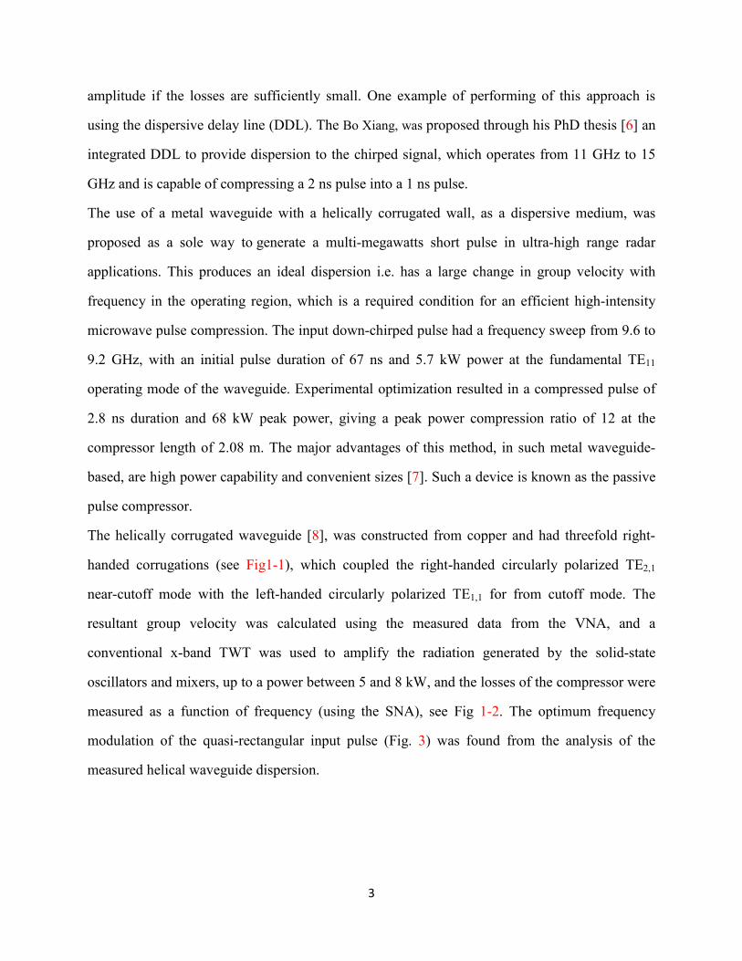
The use of a metal waveguide with a helically corrugated wall, as a dispersive medium, was

proposed as a sole way to generate a multi-megawatts short pulse in ultra-high range radar

applications. This produces an ideal dispersion i.e. has a large change in group velocity with

frequency in the operating region, which is a required condition for an efficient high-intensity

microwave pulse compression. The input down-chirped pulse had a frequency sweep from 9.6 to

9.2 GHz, with an initial pulse duration of 67 ns and 5.7 kW power at the fundamental TE11

operating mode of the waveguide. Experimental optimization resulted in a compressed pulse of

2.8 ns duration and 68 kW peak power, giving a peak power compression ratio of 12 at the

compressor length of 2.08 m. The major advantages of this method, in such metal waveguide-

based, are high power capability and convenient sizes [7]. Such a device is known as the passive

pulse compressor.

The helically corrugated waveguide [8], was constructed from copper and had threefold right-

handed corrugations (see Fig1-1), which coupled the right-handed circularly polarized TE2,1

near-cutoff mode with the left-handed circularly polarized TE1,1 for from cutoff mode. The

resultant group velocity was calculated using the measured data from the VNA, and a

conventional x-band TWT was used to amplify the radiation generated by the solid-state

oscillators and mixers, up to a power between 5 and 8 kW, and the losses of the compressor were

measured as a function of frequency (using the SNA), see Fig 1-2. The optimum frequency

modulation of the quasi-rectangular input pulse (Fig. 3) was found from the analysis of the

measured helical waveguide dispersion.

4

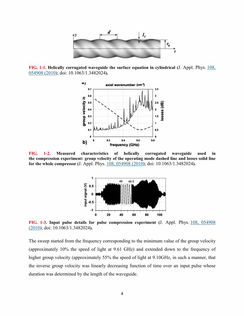
FIG. 1-1. Helically corrugated waveguide the surface equation in cylindrical (J. Appl. Phys. 108, 054908 (2010); doi: 10.1063/1.3482024).

FIG. 1-2. Measured characteristics of helically corrugated waveguide used in the compression experiment: group velocity of the operating mode dashed line and losses solid line for the whole compressor (J. Appl. Phys. 108, 054908 (2010); doi: 10.1063/1.3482024).

FIG. 1-3. Input pulse details for pulse compression experiment (J. Appl. Phys. 108, 054908 (2010); doi: 10.1063/1.3482024).

The sweep started from the frequency corresponding to the minimum value of the group velocity

(approximately 10% the speed of light at 9.61 GHz) and extended down to the frequency of

higher group velocity (approximately 55% the speed of light at 9.10GHz, in such a manner, that

the inverse group velocity was linearly decreasing function of time over an input pulse whose

duration was determined by the length of the waveguide.

5

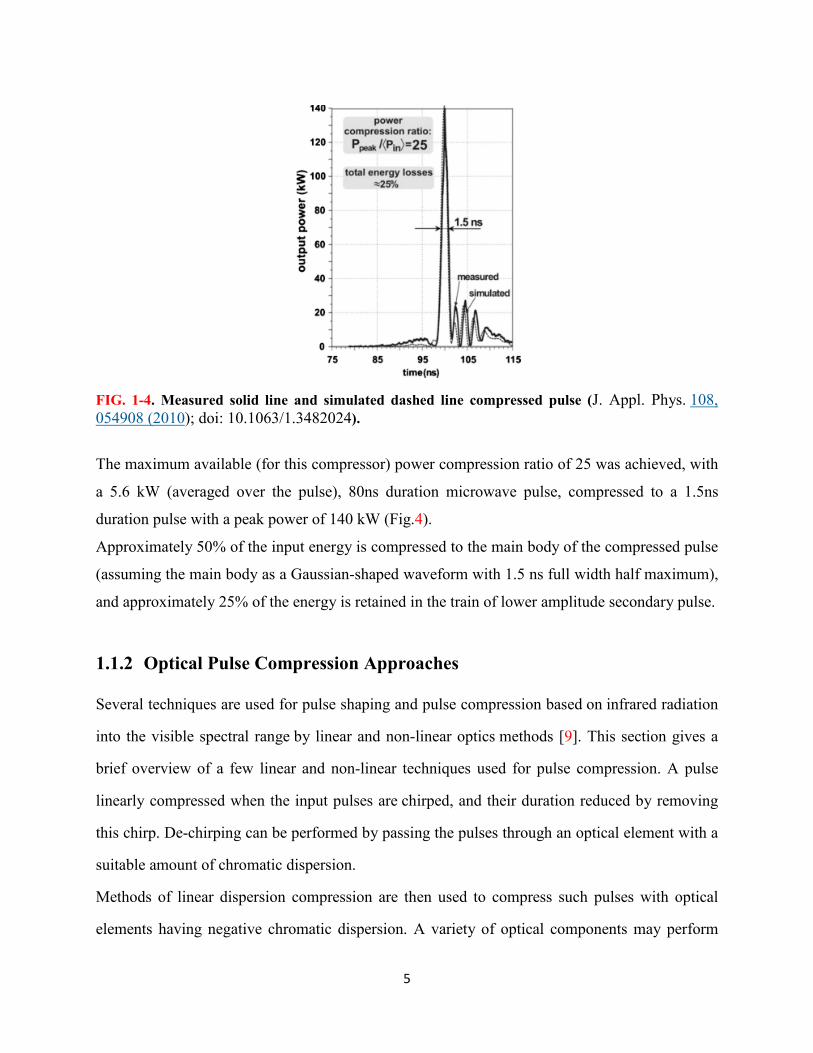
FIG. 1-4. Measured solid line and simulated dashed line compressed pulse (J. Appl. Phys. 108, 054908 (2010); doi: 10.1063/1.3482024).

The maximum available (for this compressor) power compression ratio of 25 was achieved, with

a 5.6 kW (averaged over the pulse), 80ns duration microwave pulse, compressed to a 1.5ns

duration pulse with a peak power of 140 kW (Fig.4).

Approximately 50% of the input energy is compressed to the main body of the compressed pulse

(assuming the main body as a Gaussian-shaped waveform with 1.5 ns full width half maximum),

and approximately 25% of the energy is retained in the train of lower amplitude secondary pulse.

1.1.2 Optical Pulse Compression Approaches

Several techniques are used for pulse shaping and pulse compression based on infrared radiation

into the visible spectral range by linear and non-linear optics methods [9]. This section gives a

brief overview of a few linear and non-linear techniques used for pulse compression. A pulse

linearly compressed when the input pulses are chirped, and their duration reduced by removing

this chirp. De-chirping can be performed by passing the pulses through an optical element with a

suitable amount of chromatic dispersion.

Methods of linear dispersion compression are then used to compress such pulses with optical

elements having negative chromatic dispersion. A variety of optical components may perform

6

this function, both discrete (diffraction or Bragg grating, prisms, chirped mirrors, etc.) and fiber-

based [10]. Chirped mirror, pair of diffraction grating [11], fiber Bragg grating, and prism pair

[12], are the most common linearly dispersive optical elements [13]. Pulse compression in fiber

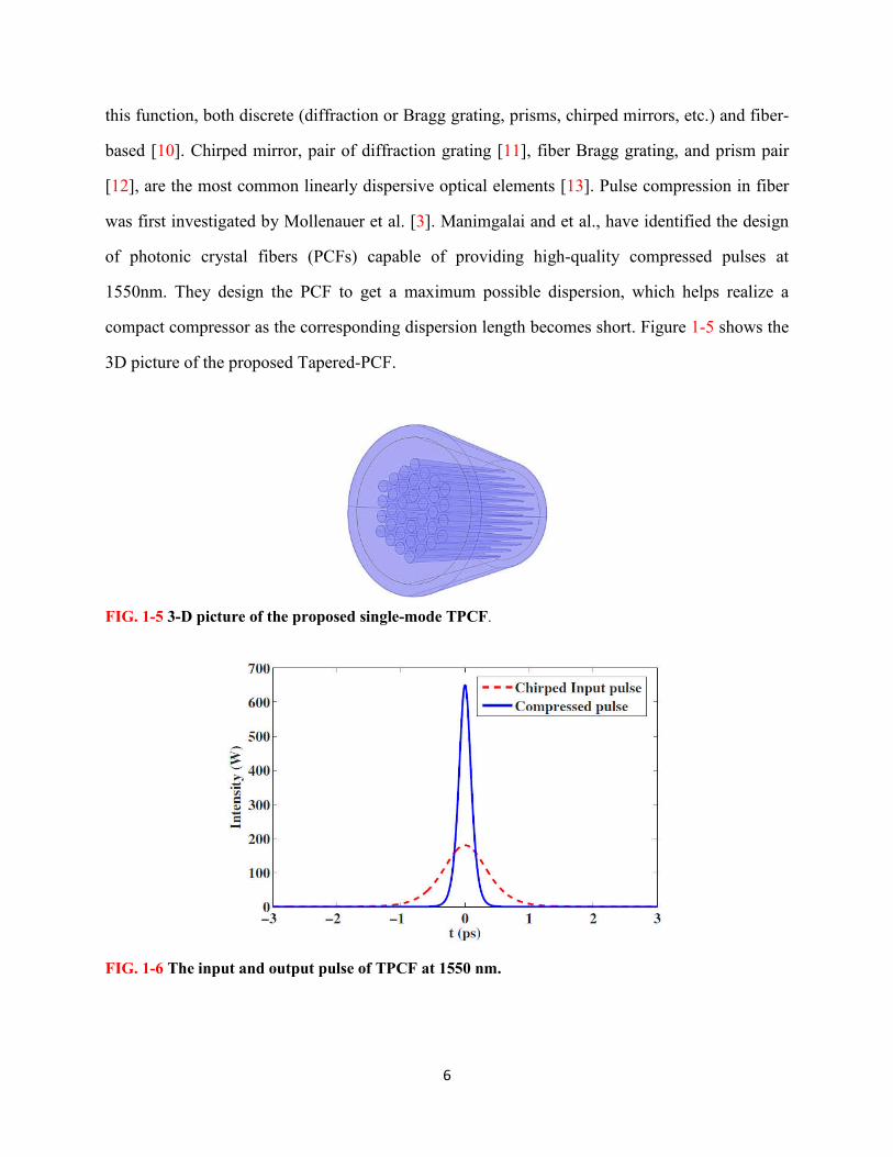
was first investigated by Mollenauer et al. [3]. Manimgalai and et al., have identified the design

of photonic crystal fibers (PCFs) capable of providing high-quality compressed pulses at

1550nm. They design the PCF to get a maximum possible dispersion, which helps realize a

compact compressor as the corresponding dispersion length becomes short. Figure 1-5 shows the

3D picture of the proposed Tapered-PCF.

FIG. 1-5 3-D picture of the proposed single-mode TPCF.

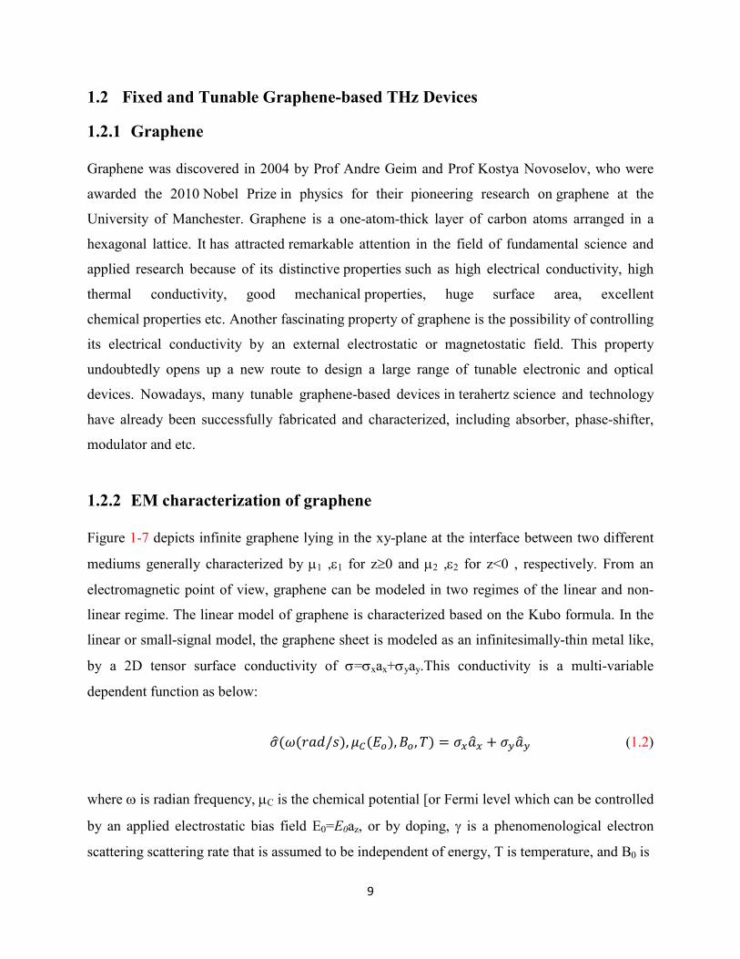
FIG. 1-6 The input and output pulse of TPCF at 1550 nm.

7

For both increasing dispersion and nonlinearity profiles, which are obtained by arbitrarily vary

the design parameters, including air-hole diameter and pitch. Fig. 1-6 shows the compression of

the chirped self-similar pulse at 1550 nm [3].

In a non-linear pulse compressor, first of all, the optical bandwidth typically with a non-linear

interaction such as self-phase modulation is increased. Spectral broadening of the optical pulses

can be performed via self-phase modulation using noble-gas-filled hollow fibers. Subsequent

compression with chirped mirrors shortens the pulses by more than a factor 10.[14].

Generally, non-linear pulse compression depends on the interplay between the self-phase

modulation and group-velocity dispersion (GVD) [3]. In most cases, this results in shortened

chirped pulses in duration in compared with the original input pulses. Moreover, the pulse

duration can be sharply reduced by linear compression, which removes or at least decreases the

chirp. The single-mode laser can have a very narrow optical frequency spectrum. However, short

pulse generation requires a broad optical bandwidth and hence multiple longitudinal mode

operation. Methods for forcing a great number of modes to oscillate to obtain broad bandwidths

and characteristics of a laser, which we assume already have the multimode operation. To

generate ultrashort optical pulses, a mode-locked laser is needed via incorporation either active

or non-linear pulse-forming elements (modulators) into the laser cavity. Passive mode-locking

refers to situations in which the pulse forms its own modulation through nonlinearities; both

amplitude and phase nonlinearities can be important. Active mode-locking is achieved with the

aid of an externally driven intracavity loss modulator. During the early 1990s, passively mode-

locked dye lasers were largely supplanted by passively mode-locked solid-state lasers. Today,

such lasers produce femtosecond pulses at a variety of wavelengths, with pulses down to roughly

5fs [15] and with average powers up to several watts. This solid-state laser mode-locking is

usually achieved using artificial saturable absorbers based on the non-linear refractive index, also

known as the optical Kerr effect. The non-linear refractive index is usually written

� = �� + ��(�) (1.1)

Where I(t) is the pulse intensity.

8

The optical Kerr effect is allowed for gases, liquids, and solids. Furthermore, the non-linear

refractive index also leads to new effects due to self-phase modulation (SPM). For a medium

with n2>0, SPM gives rise to lower frequencies (red shift) on the front edge of the pulse and

higher frequencies (blue shift) on the trailing edge. This variation of instantaneous frequency as a

function of time is called a chirp, in this case e.g. an up-chirp, means that this instantaneous

frequency raises with time, while a down-chirp means that the instantaneous frequency decreases

with time. [16].

Quasi-phase-matching (QPM) is a technique for compensating phase-velocity mismatch through

periodic inversion of the non-linear coefficient. Chirped QPM structures have been used for the

demonstration of non-linear crystals with engineered phase responses suitable for pulse

compression and dispersion management [16]. Additionally, longitudinally-patterned QPM

devices have enabled the demonstration of pulse compression during the second harmonic

generation (SHG) [17]. The hollow-core fiber filled with a noble gas, can spectrally broaden

high-energy input pulses by non-linear interaction with a noble gas of adjustable gas pressure

inside a hollow fiber [18]. Terahertz (THz) spectroscopy is gaining increasing interest thanks to

its several potential applications. THz pulse shaping has been addressed in literature by

manipulating the generation with photoconductive antennas and periodically poled Lithium

Niobate. In a recent report, Sato et al., demonstrated strong control on the generated THz pulse

using shaping the pulse generation. Pulse shaping has also been achieved through linear filtering

of a freely propagating THz in masks and waveguide [19]. M. Shalaby and et al. [20], presented

a tunable THz pulse shaping technique operating in the time domain, capable of tailoring the

temporal and spectral wave contents. Their technique operates via non-linear excitation of free

carriers in semiconductors using the optical pump-THz probe technique [21].

9

1.2 Fixed and Tunable Graphene-based THz Devices

1.2.1 Graphene

Graphene was discovered in 2004 by Prof Andre Geim and Prof Kostya Novoselov, who were

awarded the 2010 Nobel Prize in physics for their pioneering research on graphene at the

University of Manchester. Graphene is a one-atom-thick layer of carbon atoms arranged in a

hexagonal lattice. It has attracted remarkable attention in the field of fundamental science and

applied research because of its distinctive properties such as high electrical conductivity, high

thermal conductivity, good mechanical properties, huge surface area, excellent

chemical properties etc. Another fascinating property of graphene is the possibility of controlling

its electrical conductivity by an external electrostatic or magnetostatic field. This property

undoubtedly opens up a new route to design a large range of tunable electronic and optical

devices. Nowadays, many tunable graphene-based devices in terahertz science and technology

have already been successfully fabricated and characterized, including absorber, phase-shifter,

modulator and etc.

1.2.2 EM characterization of graphene

Figure 1-7 depicts infinite graphene lying in the xy-plane at the interface between two different

mediums generally characterized by 1 ,1 for z0 and 2 ,2 for z<0 , respectively. From an

electromagnetic point of view, graphene can be modeled in two regimes of the linear and non-

linear regime. The linear model of graphene is characterized based on the Kubo formula. In the

linear or small-signal model, the graphene sheet is modeled as an infinitesimally-thin metal like,

by a 2D tensor surface conductivity of =xax+yay.This conductivity is a multi-variable

dependent function as below:

��(�(��/�), ��(��), ��, �) = �� + �� (1.2)

where is radian frequency, C is the chemical potential [or Fermi level which can be controlled

by an applied electrostatic bias field E0=E0az, or by doping, is a phenomenological electron

scattering scattering rate that is assumed to be independent of energy, T is temperature, and B0 is

10

FIG. 1-7 (a) The 2D model of graphene lattice structure, and (b) external perpendicular electric and magnetic fields applied on it as the controlling static bias.

an applied magnetostatic bias field. Generally, based on bias applied on a graphene sheet, three

cases of Eq.(1.2) be considered. Spatial dispersion, neither electrostatic nor magnetostatic bias

(E0=B0=0), is applied on the grapheme. Electrostatic bias, no magnetostatic bias, nor spatial

dispersion (E00, B0=0 ). In this case, the conductivity matrix is diagonal:

�� = �� = ��(��(��))

�� = �� = 0� (1.3)

When the graphene sheet is applied by a magnetostatic external field (B00), and possibly

electrostatic bias (E00), this case refers to the local Hall Effect regime. In chapter 4 we describe

the modeling of graphene in detail.

1.2.3 Graphene based circuit/components

The tunability of the graphene has attracted tremendous research interests in the realization of

tunable terahertz-graphene-based devices include plasmonic filter [22], waveguide [23] antenna

related [24-26], metamaterial [27] and modulators [28] in recent years. Figure 1-8 shows a new

beam reconfigurable antenna is proposed for THz application based on switchable graphene high

impedance surface (HIS) [24]. The graphene-based HIS has a switchable reflection

characteristic, due to the voltage-controlled surface conductivity of graphene.

11

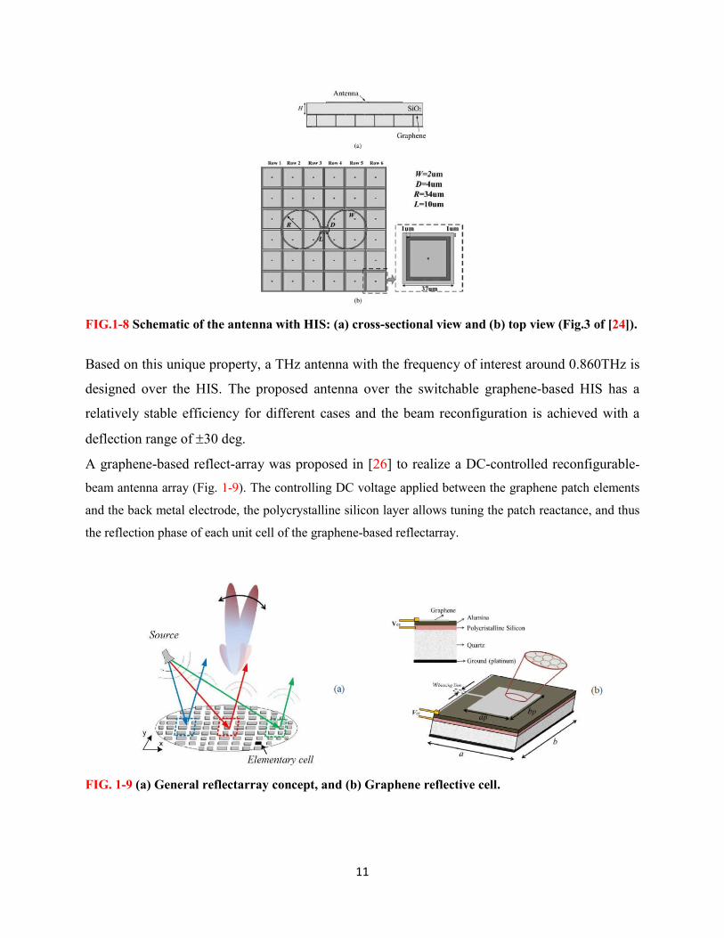
FIG.1-8 Schematic of the antenna with HIS: (a) cross-sectional view and (b) top view (Fig.3 of [24]).

Based on this unique property, a THz antenna with the frequency of interest around 0.860THz is

designed over the HIS. The proposed antenna over the switchable graphene-based HIS has a

relatively stable efficiency for different cases and the beam reconfiguration is achieved with a

deflection range of 30 deg.

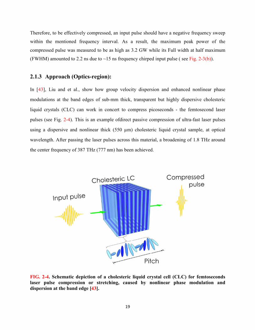
A graphene-based reflect-array was proposed in [26] to realize a DC-controlled reconfigurable-

beam antenna array (Fig. 1-9). The controlling DC voltage applied between the graphene patch elements

and the back metal electrode, the polycrystalline silicon layer allows tuning the patch reactance, and thus

the reflection phase of each unit cell of the graphene-based reflectarray.

FIG. 1-9 (a) General reflectarray concept, and (b) Graphene reflective cell.

12

FIG. 1-10 (a) Experimental setup used for the terahertz time-domain reflection measurements. (b) Variation of phase (radians) and intensity (dB) of the THz reflection of the devices with different DC-controlling voltages.

An efficient terahertz phase and amplitude modulation using electrically tunable graphene

devices is presented in [28]. The device structure consists of electrolyte-gated graphene placed at

quarter wavelength distance from a reflecting metallic surface. As shown in Fig. 1-10, in this

geometry graphene operates as a tunable impedance surface, which yields an electrically

controlled reflection phase. Terahertz time-domain reflection spectroscopy reveals the voltage-

controlled phase modulation of and the reflection modulation of 50 dB.

1.2.4 Motivation for Tunable Terahertz Pulse compression

Terahertz frequency range (0.1-10 THz) has received considerable attention in recent decades,

due to its huge bandwidth and broad applications. High-field terahertz radiation is important to

probe for a variety of fundamental scientific investigations and a wide range of applications.

The [29] summarized the two decades of advances of THz imaging, and how it is worth noting

the role of THz time-domain spectroscopy (THz-TDS) as a versatile technique for medical and

industrial imaging.

13

Terahertz radar has recently attracted great interest from both the academic and the industrial

societies due to its applications of high center frequency, as well as large bandwidth, which

possesses high penetration, and anti-stealth capabilities to support high-resolution imaging, under

cloth detection, and so on [30]. A number of terahertz short pulse generation systems have

recently been established based on an optical approach, which typically needs expensive and

bulky setup and high energy laser pulse [31]. In digital data transmission, pulse broadening is a

limitation on the maximum achievable data rate due to inter symbol interference [32]. Terahertz

time-domain spectroscopy (THz-TDS) is a spectroscopic technique in which the properties of

matter are probed with short pulses of terahertz radiation. The high-energy THz short pulse

generation is vital for application in non-linear THz optics and spectroscopy.

Currently, intense THz radiation pulses exceeding tens of micro-Joules can be obtained from

large accelerator facilities such as linear accelerators, synchrotrons, and free-electron lasers.

However, due to the high cost of building and operating those facilities and limited access, there

is a present and growing demand for high-energy, compact THz sources at a tabletop scale.

Generally, in order to measure an event in the time domain, a shorter one has been needed. If a

shorter reference pulse is available, then it can be used to measure the unknown pulse, such

method is named as time-domain interferometry. The terahertz interferometric imaging systems

(TIIS) is used to examine THz imaging of biological tissue using terahertz pulses [33-34].

These applications provide strong motivation to advance the state of the art terahertz graphene-

based technology for DC-controlled pulse compression.

In this thesis, we explore for the first time numerically possibilities and limitations of linear

compression of chirped pulses in the positive dispersion region of a helical graphene ribbon-

loaded hollow-core waveguide. Interest in this type of temporal pulse compression stems from

this fact that a graphene-based linear compressor complies with the concept of all waveguide

configurations and may be simply integrated with a THz chirped pulse generator.

1.2.5 Thesis Outline

This thesis starts with an overview of the pulse compression development in the microwave and

optical frequencies, using the graphene in tunable optical and terahertz devices and a brief study

of the dielectric and conductivity modeling of graphene in optics and terahertz region are given.

In Chapter 2, a literature review in passive terahertz pulse compression has been presented.

14

Chapters 3 introduce important concepts and fundamental theory in pulse compression based on

dispersion controlling techniques. In Chapter 4, we discuss how the tunable chromatic dispersive

properties of a helical graphene ribbon can be exploited in a compact waveguide component to

generate a DC-controlled compressed pulse. Validation of numerical analyses have been

provided in Chapter 5 based on introducing a fixed terahertz pulse compressor with replacing the

helical graphene ribbon with gold one, with two different numerical methods of Finite integral

techniques (FIT) and Finite elements method (FEM). Moreover, a system identification transfer

function for the proposed fixed terahertz pulse compressor is presented in Chapter 5. A

comparative study on how the material of helical ribbon can affect the pulse compressor

performance between non-biased graphene, Perfect electric conductor (PEC) and gold, as

illustrated in Chapter 6. Chapter 7 concludes this thesis, with a summary of work done and

contributions, along with possible future work related to this thesis.

15

Chapter 2

Literature Review

2.1 Terahertz Pulse Compressors

Nowadays, broadband THz pulses have found a wide range of applications, from imaging to

communications. Although in high-speed broadband systems, dispersion is one of the crucial

factors in the performance degradation of microwave and optical transmission media [35], it

could be a beneficial characteristic in many specific applications. Nonlinear optical phenomena

such as electro-optic effect and optical rectification are attractive options for the short pulse

generation and detection of terahertz radiation due to the dispersion management [2, 35-37].

With the proliferation of advanced solid-state laser technology, methods based on nonlinear

optical frequency conversion of high power infrared or far-infrared laser radiation laser have

gained ground. Certainly, they have produced the best optical-to-terahertz conversion

efficiencies and peak electric fields to date [2, 36-39].Besides, laser-driven approaches offer

precise synchronization possibilities, which are instrumental for spectroscopic experiments. The

significant problem of such intense laser-based THz sources is bulky set-up and necessary to

cryogenic temperature.In contrast to the optical and near-infrared (NIR) domain where ultrashort

pulse generation can be readily achieved in devices such as mode-locked semiconductor diodes

and vertical external cavity surface emitting lasers, to generate ultrashort pulses, the following

components are required i) a gain medium within a laser cavity; ii) a mode-locking mechanism

such as the fast modulation of the losses or gain at the cavity round-trip and iii) dispersion

compensation. Nevertheless, a table-top, compact and tunable source of THz short pulses is most

interested by researchers for different applications ranging from spectroscopy to imaging. In Ref.

[40], a monolithic on-chip compensation scheme is realized for a mode-locked QCL, permitting

THz pulses to be considerably shortened from 16ps to 4ps.

16

In this thesis, it was demonstrated that the tunable chromatic dispersive properties of a helical

graphene ribbon could be exploited in a compact waveguide component to generate a DC-

controlled compressed pulse. To the best of our knowledge, there are a few published works on

engineered dispersion devices made possible passively temporal THz pulse shortening.

Moreover, no other studies have examined the combination of graphene and pulse-compression

techniques in the THz regime. It is helpful, however, to review some relevant literature to

quantitatively justify our work with different passive pulse compression using dispersion in THz-

gap and both lower and upper-frequency spectrums, microwave and optics, respectively.

2.1.1 Approach(THz): Temporal delay/advancement when a pulse passes

through the aperture

Short electromagnetic pulses experience significant spectral and temporal deformation when

they are diffracted on subwavelength apertures. Temporal delay/advancement is one of the

effects that occur when a pulse passes through the aperture. Mitrofanov and et al. [41], were

demonstrated that the intrinsic negative chirp of terahertz pulses is the origin of the temporal

advancement in the limit that the aperture is much smaller than the wavelength of the pulse. The

advancement is shown to disappear for unchipped terahertz pulses. Based on this phenomenon,

they proved that a circular aperture in a gold-film GaAs could be considered as a passive THz

pulse compressor.

The chirped pulses are naturally generated using 100 fs pulses from the Ti:sapphire laser, which

excite a biased photoconductive antenna fabricated on the low-temperature grown GaAs. The

same pulses are used to gate the detecting antenna. The spectrum of the detected pulse peaks at

0.5 THz with a bandwidth of 0.57 THz and the pulse duration is 2.0 ps. After transmission

through a 10 µm circular aperture, the center of the chirped pulse shifts forward by 0.3 ps, as

shown in Fig. 1. The trailing edge of the pulse is suppressed, which results in pulse compression

from 2.0 ps to 1.4 ps with FWHM of 0.07 THz. In such a passive pulse compression system, the

bandwidth of the input pulse increases to 0.64 THz.

17

One of the significant drawbacks of this structure is the extremely low output to input peak

intensity ratio of1.4 × 10-4, as shown in Fig. 2-1.

FIG. 2-1.Temporal deformation of the intrinsically chirped THz pulse due to transmission through the 10 mm aperture. The dashed lines indicate squared, normalized electric-field wave functions, and the shaded area shows the Gaussian envelopes of the pulses. Ratio of the peak intensity of the transmitted pulse to that of the incident pulse is 1.410-4 (Fig. 3 from [41]).

2.1.2 Approach (Microwave):

In a series of publications [1, 42], the well-known phenomenon of passive pulse compression

reduction in duration accompanied by an increase in amplitude, widely used in the microwave.

The method is based on the generation of a frequency modulated FM pulse by a relativistic

backward-wave oscillator (RBWO) following its compression due to propagation through a

dispersive media (DM) in the form of a hollow metallic waveguide with helical corrugation of

18

the inner surface. In [42], Bratman and et al, present the pulse compression experiment in which

multigigawatt peak power of X-band radiation has been achieved. The experimental setup

comprises two key elements Fig. 2-2: the source of FM radiation, an RBWO, and the DM a

helical-waveguide (HW) compressor.

FIG. 2-2. Scheme of the experimental setup [42].

The most favorable frequency region for the pulse compression is a part of the dispersion

characteristic where the operating wave normalized group velocity (Vgr/c) has a large negative

gradient as a function of frequency (where c denotes the speed of light in free space) which, for

the HW under consideration, is the region from 9.4 to 9.95 GHz Fig. 2-3(a).

FIG. 2-3. (a) Group velocity normalized to the speed of light of the helical waveguide operating wave(Fig. 2 from [18]), and (b) the resultant compressed pulse solid curve shown in contrast with the relativistic backward-wave oscillator output pulse dashed curve (Fig. 4 from [42]).

19

Therefore, to be effectively compressed, an input pulse should have a negative frequency sweep

within the mentioned frequency interval. As a result, the maximum peak power of the

compressed pulse was measured to be as high as 3.2 GW while its Full width at half maximum

(FWHM) amounted to 2.2 ns due to ~15 ns frequency chirped input pulse ( see Fig. 2-3(b)).

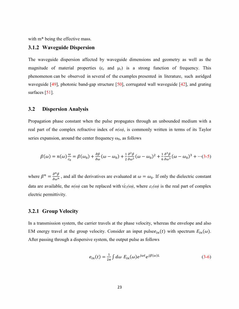
2.1.3 Approach (Optics-region):

In [43], Liu and et al., show how group velocity dispersion and enhanced nonlinear phase

modulations at the band edges of sub-mm thick, transparent but highly dispersive cholesteric

liquid crystals (CLC) can work in concert to compress picoseconds - the femtosecond laser

pulses (see Fig. 2-4). This is an example ofdirect passive compression of ultra-fast laser pulses

using a dispersive and nonlinear thick (550 µm) cholesteric liquid crystal sample, at optical

wavelength. After passing the laser pulses across this material, a broadening of 1.8 THz around

the center frequency of 387 THz (777 nm) has been achieved.

FIG. 2-4. Schematic depiction of a cholesteric liquid crystal cell (CLC) for femtoseconds laser pulse compression or stretching, caused by nonlinear phase modulation and dispersion at the band edge [43].

20

To design a terahertz pulse compression structure with simply electronically tunable pulse

shaping, it would be found that graphene with the excellent dispersion characteristics tunability

at THz frequencies [44-46] could be one of the best candidates. Furthermore, using a dielectric-

lined hollow-core waveguide where loaded with a helical graphene ribbon based on large

negative gradient profile of the normalized group velocity (Vgr/c) due to the waveguide and

material dispersions introduced by helical geometry and graphene, respectively, (as the main

requirement to realize a passive pulse compression aforementioned in microwave approach) was

motivated us for getting the main idea to design a tunable graphene-based device in this

dissertation.

In the next chapter we review the fundamental concepts and basic theory of dispersion and linear

passive pulse compression.

21

Chapter3

Important Concepts and Basic Theory

As noted in Chapter 1, control of dispersion is key to obtaining short pulse in both RF and

optical pulse shaping systems, including high power LFM microwave pulse compressor and

femtosecond pulse generation. One of the most frequently used ways to generate ultra-short

temporal pulses is linear dispersion compression by means of external dispersion elements [47].

Before discussing using dispersion control devices in a pulse compression application, it is useful

briefly to review dispersion fundamentals and concepts.

1 2

3.1 Chromatic Dispersion

Dispersion and attenuation are the key propagation properties determining the ultimate

performance of any transmission medium used in telecommunication applications. It is

worthwhile reviewing the fundamental mechanisms giving rise to pulse dispersion in waveguides

and fiber systems. Pulse spreading or pulse dispersion results from both waveguide and material

properties of a fiber. Dispersive effects are most important for optical and terahertz fibers. We

may note that shorter pulses are affected more strongly by dispersion than longer ones. Longer

pulses have a narrower spectrum and because of the Fourier-transform relation: fT=constant,

where f is the spectral and T is the transform-limited temporal width.

The important dispersion mechanisms are material dispersion, waveguide dispersion, nonlinear

effects, and polarization mode dispersion, the two most important are material and waveguide

dispersion when taken together, are referred to as chromatic dispersion.

3.1.1 Material Dispersion: Modeling of Dispersive Material in Terahertz

The dispersion in any single-mode waveguides originates from material dispersion and

waveguide dispersion. Material dispersion arises from the frequency-dependent variation of the

intrinsic material electrical and magnetic properties, whereas the waveguide dispersion part is

22

due to the frequency-dependent power distribution in the non-homogenous cross-section of the

waveguide.

In optical dielectric-based waveguide such as single-mode (SM) and multi-mode (MM) fiber, all-

dielectric materials are dispersive, this means that the refractive index varies with wavelength,

i.e., n=n(). There are several ways to measure dispersion in transparent materials. A simple

measure is the Abbe number, VD. The Abbe number is obtained by measuring the index at

several key wavelengths, or

�� =��

�� (3-1)

where nF, nD, and nc , are the refractive indices at three standard visible wavelengths : F=486.1

nm (blue), D=589.2 nm (yellow), and c=656.3 nm (red). High dispersive materials have low

VD, and materials with low dispersion introduce large VD. Another measure of dispersion is the

derivative dn/d, which may be most easily obtained from dispersion data like dispersion

coefficients vs. wavelength, once a curve fits the data has been made to determine n as a function

of wavelength. It is quite common to fit the dispersion data using a Sellmeier power-law fit. The

Sellmeier equation is of the form

�� = 1 + ∑��

�� (3-2)

where Ai and oi are the Sellmeier constants, oi is a vacuum wavelength related to natural

vibrational frequencies o/voi=c. The Sellmeier constants for many of the standard IR materials

are given in the Handbook of Optical Constants Series by Palik [48].

The Drude model can be used to describe the dielectric function of a conducting medium as

�̃(�) = �� −��

�

�(��) (3-3)

Γ is the momentum relaxation time of the material and the plasma frequency, ��, is defined as

�� =��

��∗ (3-4)

23

with m* being the effective mass.

3.1.2 Waveguide Dispersion

The waveguide dispersion affected by waveguide dimensions and geometry as well as the

magnitude of material properties (r and r) is a strong function of frequency. This

phenomenon can be observed in several of the examples presented in literature, such asridged

waveguide [49], photonic band-gap structure [50], corrugated wall waveguide [42], and grating

surfaces [51].

3.2 Dispersion Analysis

Propagation phase constant when the pulse propagates through an unbounded medium with a

real part of the complex refractive index of n(), is commonly written in terms of its Taylor

series expansion, around the center frequency 0, as follows

�(�) = �(�)�

��= �(��) +

��

��(� − ��) +

�

�

��

��(� − ��)� +

�

�

��

��(� − ��)� + ⋯(3-5)

where �� =��

�� , and all the derivatives are evaluated at � = ��. If only the dielectric constant

data are available, the n() can be replaced with1(), where 1() is the real part of complex

electric permittivity.

3.2.1 Group Velocity

In a transmission system, the carrier travels at the phase velocity, whereas the envelope and also

EM energy travel at the group velocity. Consider an input pulse��(�) with spectrum ��(�).

After passing through a dispersive system, the output pulse as follows

��(�) =�

��∫ �� (�)��(�)� (3-6)

24

Now if we introduce the typical notation for envelope function, where the positive frequency part

of ��(�) is replaced by �(��) and �� = � − �� , we can rewrite the output pulse as follows

��(�) = ��(��)��(�)� (3-7)

where

��(�) =�

��∫ �� (��)��[�� (��/�)�� … ��] (3-8)

Thus ��(�)is the product of a carrier term ��(��)and the envelope function ��(�) . The

carrier term propagates at the phase velocity

�� =��

�� (3-9)

and is unaffected by the variation of �with �. The envelope function��(�) , however, it is

affected by the form of �(�). One significant case occurs when it is a linear function of �.

�(�) = �� + �� (3-10)

In this case, we find that

��(�) = ��(� − ��) (3-11)

Thus, the output pulse is an undistorted replica of the input pulse, which travels witha

velocity��. This velocity is called the group velocity ��, where

�� = �� = ��

��

��

��

(3-12)

We now proceed to give a useful formula for the group velocity, specifically the material

dispersion, encountered during propagation in a bulk medium. Starting with

25

�(�) =��(�)

�=

��(�)

� (3-13)

We find that

�� =�

��

=�

��(��

��) (3-14)

It turns out that it is also useful to express vg in terms real part of complex permittivity of ��(�)

�� =�

√��(�√��

��) (3-15)

3.2.2 Group Delay

We can also look at the concept of group delay () using simple Fourier transform identities. The

Fourier transform of a delayed pulse �(� − �) is given by �(�)��, so � = −��

��= −

�(��)

��,

using this equation and eq.(4-8), we find that � = �� = �/��, which isconsistent with our

discussion above, where L is an electromagnetic wave is traveling distance. As in all full-wave,

electromagnetic solvers, the scattering parameters results of [S] are available after frequency

domain calculations, we can simply compute group delay (GD) parameters via phase angle of

insertion loss of S21 (21) using Eq. (3-16).

��(��. ) = −�

��

��(��.)

��(��) (3-16)

It is noteworthy that the other required dispersion parameters such as group velocity (GV) and

axial phase constant () can be calculated in postprocessing using above mentioned relation

and Vg incorporation with Eq. (3-16).

3.2.3 Group Velocity Dispersion

26

When �(�) is not a linear function of �[i.e., Eq.(3-10) does not hold], ��(�)is changed

compared to ��(�). The part of �(�) that is not linear in � is called dispersion. The

��/�� term contributes a quadratic spectral phase variation, which leads to a linear variation

in delay with frequency; this imparts a linear chirp to the output pulse. The ��/��term

contributes a cubic spectral phase leading to a quadratic variation in delay with frequency. This

results in an asymmetric pulse distortion with an oscillatory or ringing on the tail part of the

pulse.

Group velocity dispersion (GVD) is important in any fast and ultrashort optical systems when the

path lengths are relatively large and the pulses are very short. In the case of nonzero GVD,

different frequencies have slightly different traveling times, and this can be an important pulse

broadening mechanism. Now we turn our attention to the quadratic dispersion term. In this case

we can mathematically treat the dispersion by considering the frequency dependence of the

propagation constant , based on a second-order Taylor series expansion, as follow

�(�) = �(��) + ��(� − ��) + 0.5��(� − ��) (3-17)

For a particular frequency component, the time required to propagate through a length L of a

dispersive medium is �/��(�). The propagation time relative to that corresponding to the

frequency �� is given by

�(�)��(��)�∆�(�)��

��(��)

��

��

��(��)��(��)�

(3-18)

Using Eq.(3.18), we obtain

∆�(�) = �2��

��+ �

��

��(��)

�� (3-19)

In some applications, notably fiber optics, it is customary to express Vg and in terms of the

wavelength.

Here we use

27

� =��

� ��

��

��= −

��

�� =��

�� (3-20)

The results using the chain rule are

�� =�

��(��/��) (3-21)

∆�(�) =��

��

��(� − ��)� =

��∆��

�� (3-22)

Fiber dispersion is usually described in terms of a dispersion parameter D with units ps nm-1 km-

1, defined by

∆�(�) = ��

�� ∆�� = �∆�� (3-23)

where

� =��

��

��=

��

�� =��

�� (3-24)

3.3 Normal and Anomalous Dispersion

In the classical optics terminology, normal and anomalous dispersion appears to refer

specifically to the sign of ��/��. However, in the ultrafast optics community, one is usually

more interested in temporal dispersion, which in the case of material dispersion is governed by

��/��. It is therefore customary to utilize the terms normal and anomalous material

dispersion to mean ��/�� > 0 or ��/�� < 0, respectively. However, these can lead to

confusion since they are used differently by different communities. Within ultrafast optics, these

terms usually refer to ∂τ/∂ω, whereas in fiber optics, they usually refer to D, which is

proportional to ��/�� [15].

28

Refer to Eq.(3-18), generally, dispersion can be interpreted based on GVD. Thus, for 2>0

(called normal dispersion), higher frequencies (shorter wavelengths) travel more slowly and are

displaced toward the trailing edge of the pulse. This leads to an up-chirped. For 2<0 (anomalous

dispersion), higher frequencies move faster and are displaced to the leading edge of the pulse,

leading to down-chirp.

3.4 Dispersion-based Pulse Compressor

Although in high-speed broadband systems, dispersion is usually considered as a negative effect,

it could be a beneficial characteristic in many specific applications such as pulse shaping,

including pulse stretcher or compressor. The use of waveguide operating close its cutoff

frequency, as an approximation to a dispersive line, is one of the historical approaches in a

passive generation a short pulse in high-resolution microwave radar systems. LFM pulse

compression techniques based on using waveguide operating close its cutoff frequency, as an

approximation to a dispersive line has been demonstrated in early radar systems. In such

compression systems, the dispersive line being the vital component. R. A. Biomley and et

al.[52], more than fifty years ago, showed how a 91.5 meter length short-circuited rectangular

copper waveguide No. 11A, can be successfully used to realize a dispersive line for S-band pulse

compression applications. For a pulse compressor based on conventional waveguide the

operating frequencies should haven close (few percents above) to the cutoff [53], where the wave

dispersion is sufficiently large, but one problem in close to the cutoff frequency is the higher

attenuation losses. Phelps and et al. [54], show that with enhancing waveguide dispersion

component of chromatic dispersion via creation a helical corrugation on a circular waveguide

wallpermits the realization of the necessary dispersion for pulse compression without having to

operate close to cutoff which makes it possible to use such a compressor at the output of a high-

power amplifier.The most favorable region for pulse compression in the helically corrugated

waveguide is the part of the dispersion characteristic, where the group velocity has a negative

gradient as a function of frequency (see Fig.2-3a). Correspondingly, the input pulse should be a

linear frequency-modulated (chirped), which has a negative slope(down-chirped) in contrast to

the case when a smooth waveguide is used. In this case, all frequency components can be

reached simultaneously at the end of the waveguide to make a short or compressed pulse.

29

3.4.1 Chirped Linear FM Pulse

The basic idea of pulse compression is based on Linear Frequency Modulation (LFM) which was

invented by R. Dicke in 1945 for RADAR applications. The algorithm for LFM pulse

compression involves mainly two steps which are: generation of LFM waveform and the

management of the traveling time delay of the head and the tail of the square-shaped LFM pulse

using a dispersive element.

An LFM signal (Fig. 3-1.) is a frequency modulated waveform in which carrier frequency is

linearly swept over a specific period of time.

FIG.3-1 – A time domain illustration of a down-chirped sinusoidal linear FM pulse.

To investigate the pulse-compression performance of a passive linear dispersion-based pulse

compressor with the group velocity, which has a negative gradient as a function of the frequency

component, it is assumed that the input pulse is a chirped sine function, as stated in Eq. (3-25),

� = �� sin(2�� − ��) , �� ≤ ��

0, ��ℎ�� (3-25)

where fHi is the upper-band frequency of the negative dispersion region, T0 is the input pulse

width, E0 is the electric field amplitude, and µ is the chirp factor. The chirp factor for a uniform

input pulse spectrum in the positive GVD region from fLo to fHi, respectively, can be calculated

using Eq. (3-26):

� =�(��)

�� (3-26)

30

A pulse compressor uses a system with a proper time delay or equivalently group velocity profile

in terms of frequency (Fig.3-2a) to delay one end of the pulse relative to the other one and

consequently, to produce a temporal narrower with the greater peak amplitude. This phenomenon

can be simply presented by two lower and higher frequency edge components of the LFM

waveform (Fig. 3-2b). This system could be a matched filter or a dispersion managed waveguide.

FIG. 3-2(a) group velocity profile with negative gradient variation in terms of frequency of

a dispersion managed device and (b) a representation of how a down-chirped LFM

waveform with duration of T0 can produce a grater peak amplitude after traveling an

optimal length of a the dispersive waveguide.

Based on the normalized group velocity profile, shown in Fig.3-2(a), and the instantaneous

frequency, which can be obtained from the time derivative of the phase argument of Eq. (3-25)

proves that the tail of the chirped pulses with low-frequency components and faster group

velocities will move to overtake the front high-frequency components of the pulses, resulting in

temporal pulse shortening with growth in amplitude.

A unique optimal compression length can be easily achieved based on a significant value of the

chirped LFM pulse duration (��) and the group velocity profile as follows:

�� = ��(��) − ��(��) (3-27)

�� = ��(��)��(��) = ��(��)��(��) (3-28)

31

By using the relation of ��(��)given in (1), the optimal length for maximum compression is

computed in terms of the LFM input pulse duration (T0) and the boarder values of group velocity

values as follows:

��(��) =��

��

��

and (3-28) �� =��(��)

��

��

�� (3-29)

3.5 Broadening Factor

One of the important parameters in the pulse compression applications where the compressed

pulse in the time domain is not symmetric is the broadening factor (F), which is defined as the

ratio of full-width at half-maximum (FWHM) of the compressed pulse to the FWHM of the input

pulse. The percentage of the spectral broadening change as a figure of merit of a tunable pulse

compressor can be defined. This parameter is also known as the modulation depth defined by

(F /F0)×100%, where F is the changes of F due to tuning factor, and F0 is the average of the

minimum and maximum obtainable F [55].

3.6 Attenuation

Absorption is caused by three different mechanisms: Impurities in material, intrinsic absorption,

and radiation defects. The attenuation of an electromagnetic wave power flow through a lossy

medium is followed an exponential form of exp(-L) where is called the absorption

coefficient, and L is the propagation distance. In general, the absorption coefficient () can be

related to the imaginary parts of the effective refractive index by 2k0Im(ne f f), where is effective

refraction index of the medium or equivalent medium of a radiating system such as fiber or

waveguide. In an equivalent radiating system, the conservation of energy leads to the statement

that the sum of the transmission (T), reflection (R) ,and absorption (A) of electromagnetic power

flow is equal to unity, i.e., T + R + A = 1 wherein the absence of nonlinear effect (i.e. Raman

effect, etc), this equation is held for any angular frequency of as T() + R() + A() = 1 [56].

As the T() and R() are related to the square of the scattering parameters of |S21| and |S11|,

respectively, the A() easily can be calculated.

32

3.7 LFM Generation

The generation of a high quality linear FM pulses for RADAR applications are commonly with

frequency range centered at microwave and millimeter-wave bands from gigahertz to tens of

gigahertz. In these frequency ranges the most common method to achieve LFM signals is using

voltage controlled oscillator (VCO) circuits.

Recently, practical generations of LFM waveforms in sub-millimeter and terahertz bands have

been reported based on some optical techniques such as optical interferometer and optoelectronic

oscillator (OEO).

33

Chapter 4

Tunable Terahertz Pulse Compressor Design Based on Helical

Graphene Ribbon

Novel ideas for tunable THz pulse compression using a graphene-based waveguide are proposed

here. In this research, we explore for the first time numerically possibilities and limitations of

linear compression of negatively chirped pulses in the positive group velocity dispersion (GVD)

region of a dielectric-lined circular waveguide loaded with a helical graphene ribbon. We

show that the proposed structure introduces a good tunability of the compression factor via the

graphene electrostatic bias.

This chapter is dedicated to explaining the design details and results for terahertz's direct pulse

compression in a dielectric-lined circular waveguide with tunability based on a strong both

waveguide and material dispersions introduced by helical graphene-loading. A theoretical

investigation backed by transient numerical analysis has led to a thorough understanding of the

passive pulse compression principles and constraints.

3

4.1 Model Description and Design Principles

Microwave, infrared, and optical regions have mature technologies as a result of extensive

development. However, in the THz band, i.e., from 0.3 to 3 THz, components, system

architectures and experimental techniques are still emerging. In the quest to develop the THz

band, THz waveguides have become an active research area [60]. Among the microwave and

optical waveguide technologies, the use of optical fibers for THz application has attracted

considerable attention in recent years [61]. However, conventional optical fibers such as silica

glass ones are not suitable for guiding THz wave owing to their high transmission loss mainly

coming from intrinsic absorption responses of core and clad dielectrics, scattering loss and low

free-space THz coupling efficiency. Hollow-core waveguides (HCWs) due to the inherent

advantage of their air-core have received a great deal of attention for THz applications. As

mentioned in [62] at the IR region, HCWs are categorized based on the refractive index of the

34

inner dielectric coating material into two groups, which are leaky guides if the refractive index is

greater than one and the attenuated total reflectance(ATR) guides otherwise.

Recently, researchers have proposed, fabricated, and tested a variety of single-mode low-loss

waveguides entitled “dielectric-lined hollow metallic waveguides (DL-HMWs).”DL-HMWs

become a strong candidate for the effective single-mode terahertz propagation with possible

transmission loss below 1dB/m [61], [63-65]. Since the goal of this context is to design a single-

mode waveguide having low-loss with tunable dispersion, the DL-HMW is an appropriate

candidate.

Another important element of the structure is the helical ribbon. Helix generally used in slow-

wave structures (SWS) in high power microwave sources such as traveling wave tube (TWT) or

Gyro which should have two crucial characteristics of low-loss and controlled dispersion in a

wide operating bandwidth. In recent years, several reports can be found in the

literature demonstrating the techniques to shape the dispersion characteristics of a helix RF

circuit with acceptable electronic efficiency across the entire operating frequency band [66].

4.1.1 Model Description

Figure 1 shows the 3D geometry and side view of the proposed graphene ribbon loaded

waveguide: a graphene ribbon with thickness tgr, ribbon width w, and pitch size p is helically

wrapped and inserted inside a metalized dielectric tube of thickness td. By carefully choosing the

geometric parameters, dielectric material, and DC-controlling bias, an optimum condition for an

arbitrary dispersion profile, large mode confinement, minimum mismatch, and propagation loss

with maximum tunability can be achieved. The length of the waveguide section loaded with the

helical graphene ribbon is L0. As shown in the side-view illustration of the yz-plane, the two

ends of the waveguide are tapered sections to ensure the lowest possible return loss when

interfacing the THz pulse compressor with a standard smooth circular waveguide.

These identical sections are two simple conical circular waveguides of length L2 that gradually

connect the helix to the ends of L1 long circular waveguides. Next section provides initial

concepts of design methodology principle of the proposed graphene-based tunable pulse

compressor.

35

FIG. 4-1. Schematic-diagram, 3D geometry, and side view of an internally dielectric-coated hollow-core waveguide loaded by a helical graphene ribbon (inset: the graphene ribbon is grown on a thin SiO2 layer and sandwiched between two gold ribbons to facilitate the DC controlling of the device).

4.1.2 Design Methodology Principle

As the first design parameters, we start with calculating the cutoff frequency of fundamental

transverse electric field of TE11modes in a circular waveguide with a radius of R, filled with air

as follows:

��,��=

�

��

�.��

� (4-1a)

��,��(��) =

��.��

�(��) (4-1b)

When a waveguide is filled partially with dielectric with relative permittivity larger than air

(r>1), one can expect that the cutoff-frequency shifts to lower. Another factor that can be

affected by the cutoff-frequency is internal loading waveguide with a helically wrapped

conductive ribbon, which shifts up the cutoff-frequency inversely proportional to helix inner

radius related to our proposed device. It should be noted that for a circular waveguide loaded

with a dielectric-coated helically wrapped graphene ribbon, which is a material with Re[r]<0

36

and Im[r] >0, we cannot expect analytically to find an exact estimation of the cutoff-frequency.

Hence, based on the initial value of R, which is calculated based on Eq.(4-1) for operating

bandwidth around our target center frequency of 2 THz, the structure design numerically is

optimized using a finite integral technique (FIT) [67]. We previously stated in Section 3.4 that

one problem in close to the cutoff frequency is the higher attenuation losses, an air-filled circular

waveguide with R=100 m has a cutoff frequency of about 0.9 THz, which is far from the center

frequency of 2 THz for minimum insertion loss.

As shown in Fig.1, adding a dielectric coating (stated as a dielectric tube with a thickness of td)

on the inner surface of the metallic cylindrical hollow THz waveguide has two major benefits.

Firstly, this dielectric film coating allows the propagation of the fundamental mode TE11 for

which the tangential electric field component on the metal boundary surface can be significantly

reduced and minimizes the ohmic losses due to the reduced penetration of the electric field into

the waveguide walls [64]. Secondly, this inner dielectric layer substantially is required as a

tuning parameter to adjust wave-material interaction with respect to the relative distance between

helical graphene-ribbon and metal waveguide walls or metal-cladding.

Miyagi and Kowakami [68] efforts in theoretically loss analysis for an oversized DL-HCW

composed of a single-dielectric layer which carries fundamental hybrid modes of HE11, the

minimum loss occurs when the thickness td is given by a multiplication factor of the central free-

space wavelength as

�� = ��

��∙ (��

� − 1)��/� ∙ ��/(�� − 1)�/�� .l� (4-2)

where nd is the real part of the refractive index of the dielectric film. A dielectric coating layer

much smaller than this estimated thickness may cause a condition for only traveling the TE

modes, which is considered for our normal-sized DL-HCW [69]. As we state later, non-

absorptive polymeric dielectrics recently used as coating layer in the THz DL-HCW waveguides

have refractive index nd in range of (1.3-1.6), using Eq.(4-2) result in td around 30 m, that for

only TE mode td<< 30 m is recommended.

The design procedure of helix as slow-wave structure (SWS) in TWTA application is based on

the desired phase velocity (Vp≅Ve), where Vp and Ve are phase velocity and electron-beam

37

velocities in TWT, respectively, and has been performed in terms of the radial propagation

constant (kr) of the traveling EM wave along the helix axis. There are many configurations of

helix-SWS commonly used in TWT applications with or without metal shields as well as

dielectric coatings. The important structural parameters in the design of all helix-SWS

configurations are the inner helix radius (a), the metal shield inner radius (ash), the tape-width

(w) for the tape-helix (or the diameter of a wire wounded helix), and the pitch size (p). The krr is

known as the most important parameter, where r is cylindrical radial coordinate which is in

0<r<ash. It is due to the fact that the variation of the axial electric field inside the helix, in the

radial direction, is a function of Io(krr), where Io is the modified Bessel function of the first kind

and zero-order. In order to minimize the field variations across the bore area of a helix, it is

desirable to keep kra above 1.5 [70].It is worth mentioning that the strip width over the pitch size

ratio (w/p) and the inner radius of the helix are the most influencing parameters to control the

overall dispersion of the helix. With the help of the numerical results mentioned in [71], it has

been clarified that, in TWTA applications, the helix tape width (w) should be chosen in the

0.4<w/p<0.8 range. This reduces the transmission loss for the fundamental wave by minimizing

the coupling between the fundamental and harmonic space modes. Finally, as we use helix in our

structure as a main dispersion controlling element, the inequality w/p<0.8 can be used as a

design margin.

As in THz frequencies, most materials, including metals and dielectrics, can show a frequency-

dependent or dispersive behavior, the next section is devoted to discussing all material

considerations that we use in the proposed device.

38

4.2 Definition of Material

4.2.1 Graphene

The demand for tunable or reconfigurable components at terahertz and optical frequencies

increased during the last years. Tunable THz devices for controllable systems such as tunable

filters, modulators, or phase shifter are becoming more and more important. At mm-wave

frequencies, piezoelectric materials and actuators have been proposed for the dynamic

reconfiguration of phase-shifting surfaces. At lower mm-wave frequencies, micro-

electromechanical systems (MEMs) component when is integrated to each element of the

periodic structure, such as high impedance surface (HIS) or metamaterials, can be realized

tunable phase shift. The actuators exhibit a displacement under a voltage bias, which is translated

to a dynamic control of the reflection phase [72]. But for shorter wavelengths, including Far-IR,

Mid-IR, Near-IR, and optical regions, the aforementioned techniques are not feasible. At this

range of frequencies, a promising solution may rely on using graphene-based devices. Moreover,

excellent tunability of graphene in terahertz [44–46] motivated us to use the graphene as the

main element of the proposed to realize a tunable terahertz pulse compressor.

As this work deals with a passive compact pulse compression can be expected that the graphene

relay in the linear regime, thus the graphene sheet can be modeled as an ultra-thin, nonlocal two-

sided surface characterized by a surface conductivity tensor ��(�, ��(��), �, �, ��) based on

Kubo formalism [73] where is the angular frequency, EF is Fermi energy (or C the

electrochemical potential which can be controlled by a normal applied electrostatic bias field E0,

or by doping), is the carrier relaxation time, T is temperature, and B0 is a normal applied

magnetostatic bias field.

For a graphene sheet (in xy-plane) under only an electrostatic field bias, the conductivity is a

scalar:

[�] = �� 0

0 �� (4-3)

graphene’s scalar conductivity (g) is described with the combination of two components of

interband and intraband as follows:

39

�� = �� + ��

�� (4-4)

In the THz spectral region where the photon energy ℏ� ≪ ��, the interband part (��) is

negligible compared to the intraband part (��).

Drude-like Model

Accordingly, in the THz regime and in case of no magnetostatic bias, graphene could be well

introduced by the Drude-like surface conductivity:

σ��(ω) =

��

πℏ� ln (2cosh��

��)

�

ω��τ�� (4-5)

Where kB is the Boltzmann constant, and ℏ is the modified Plank constant (h/). The relaxation

time at the band of interest (<10 THz), can be considered � = �ℏ√��/(�� ) ≅ 10�� [71],

where vF is the Fermi velocity (≅106 m/s), qe is electron charge and n is the carrier density.

Effective permittivity of Graphene

For the numerical simulation monolayer-graphene is usually represented as a layer of material of

a very small thickness Δ with two in-plane(eff,t) and normal-plane(eff,n) effective permittivities

as following [73, 75]:

��,�(�) = 1 + �σ�

��(ω)

��∆ , ��,�(�) = 1 (4-6)

The effective permittivity of a multilayer-graphene, which is frequently observed in the chemical

vapor deposition (CVD) synthesis, can also be calculated using Eq. (4-6) with a good precision

[76-77].

40

(a)

(b)

FIG. 4-2. The THz spectral of real and imaginary parts of the effective permittivity of an infinite graphene sheet for T=300K, EF=0eV, and different values of =[1, 10, 50]nm.

Fig.4-2 shows the real and the imaginary parts of the effective permittivity of an infinite

graphene sheet in the spectral range of interest (0.1-10 THz). The effective permittivity of

graphene for T=300K and EF =0eV and the different values of is shown in Fig.4-2. For a

single-layer graphene (SLG) the thickness was reported between 0.4 and 1.7 nm [78]. As shown

in Fig.4-2 (a) and (b) with increasing the thickness of graphene, the variation rate of both real

and imaginary parts of the eff drastically decreases. The electrochemical dependence of the

equivalent effective dielectric constant of single layer graphene (SLG) is illustrated in Fig. 4-3.

The most important conclusion of these curves can be the best frequency limits for maximum

tunability, which might be from 1.8 THz up to 5 THz, which the real part of graphene

permittivity has maximum variation respect to EF. In contrast, it has a good guard-band far from

region that the imaginary part of graphene permittivity has relatively large variation respect to EF

that it might cause a strong amplitude distortion on the traveling electromagnetic field waves.

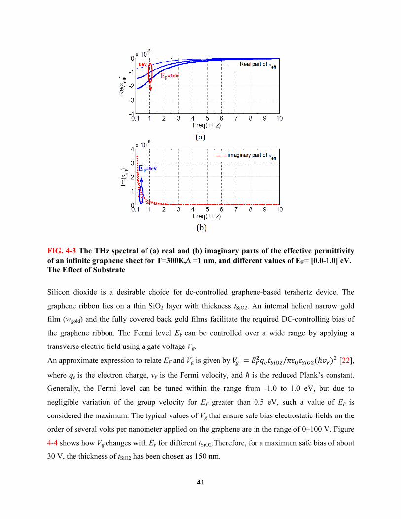
41

FIG. 4-3 The THz spectral of (a) real and (b) imaginary parts of the effective permittivity of an infinite graphene sheet for T=300K, =1 nm, and different values of EF= [0.0-1.0] eV. The Effect of Substrate

Silicon dioxide is a desirable choice for dc-controlled graphene-based terahertz device. The

graphene ribbon lies on a thin SiO2 layer with thickness tSiO2. An internal helical narrow gold

film (wgold) and the fully covered back gold films facilitate the required DC-controlling bias of

the graphene ribbon. The Fermi level EF can be controlled over a wide range by applying a

transverse electric field using a gate voltage Vg.

An approximate expression to relate EF and Vg is given by �� = ��/��(ℏ��)� [22],

where qe is the electron charge, vF is the Fermi velocity, and ħ is the reduced Plank’s constant.

Generally, the Fermi level can be tuned within the range from -1.0 to 1.0 eV, but due to

negligible variation of the group velocity for EF greater than 0.5 eV, such a value of EF is

considered the maximum. The typical values of Vg that ensure safe bias electrostatic fields on the

order of several volts per nanometer applied on the graphene are in the range of 0–100 V. Figure

4-4 shows how Vg changes with EF for different tSiO2.Therefore, for a maximum safe bias of about

30 V, the thickness of tSiO2 has been chosen as 150 nm.

42

FIG. 4-4. DC controlling voltage Vg versus Fermi level EFin terms of various SiO2 thickness.

4.2.2 HDPE

High-density polyethylene (HDPE) is used for the dielectric tube given its good THz

transparency (n = 1.524 and α = 0.2 cm-1 at 1 THz [79]).

4.2.3 Nobel Metals: Gold

As shown in Fig. 1, the dielectric tube is completely covered by a gold film layer as a metal

cladding. Gold is modeled with the Drude parameters as follows: = 9.1, p= 1.38 × 1016 rad/s,

and = 1.075 × 1014 Hz [80].

4.2.4 Silicon Dioxide

From a technological perspective, the effect of a substrate and the impurities therein cannot be

ignored for graphene-based, microwave optical, and terahertz device applications. Sule and et al.

[81] demonstrate that the substrate has a significant influence on carrier transport at low

frequencies (< 1 THz), while its influence becomes less pronounced at higher frequencies. In this

work, the graphene ribbon lies on a thin SiO2 layer with r= 3.9 and tan δ=0.0056 [82].

43

4.3 Results and Discussion

The optimized dimensions of the proposed tunable graphene-based waveguide for optimal pulse

compression performance and maximum tunability are listed in Table 4-1.

Table 4-1. Optimal dimensions of the proposed graphene-based pulse compressor.

R P w wgold tgold

100 m 126 m 42 m 30 m 1m

tSiO2 td tgr L1 L2

150 nm 7.5 m 100 nm 40 m 100 m

4.3.1 DC-Controlled Dispersion Mechanism

The inner dielectric layer of the circular waveguide and the helical graphene ribbon provides the

main functionality in the proposed graphene-based pulse compressor. The propagation

characteristics of an electromagnetic structure can be studied with two common approaches: one

is directly focused on circuit theory using the equivalent circuit model, and the other is based on

electromagnetic mode analysis. The circuit model of the helical waveguide, as shown in Fig. 4-5

can be expressed by one inductance per unit length and two radial and inter-turn capacitances per

unit length [83, 84]. Thus, a strong dispersion due to helix-shield capacitive coupling voltages

and helix equivalent inductive currents can be introduced. This effect mainly depends on the

dielectric tube parameters (td, d) for the former, and the helix characteristics (σ , w, p) for the

latter, where is the conductivity of helix-tape that in our proposed structure is an equivalent

dispersive conductivity resulted from hybrid graphene-ribbon and DC-bias facilities of gold-

ribbon as shown in Fig. 4-1.The dependence of the propagation constant in optical and RF

waveguides, including shape, size, and inner-coating material layer, has been explored and

shown in articles [85-87]. In principle, the mode propagation constant can be obtained from the

dispersion equation solved from electromagnetic field solutions. The numerical analysis for

tackling these problems is reportedly available in the literature [86, 87].

44

FIG. 4-5. The equivalent circuit modeling of a cylindrical metallic tube which contains a metallic helix from [83].

In a simple structure such as an internally coated circular waveguide with a lossy layer, the

approximated analytical solutions of the characteristic equation in studying the physical features

of the propagation constants have been presented in Ref. [86]. In this case, Luo et al. show how

the variation of the lossy layer thickness (t) affects the propagation constants for all five modes

(TE11, TM01, TE21, TM11, and TE01); the effect in the propagation constants is great when t/δ

<1.5 (where δ is the skin depth of electromagnetic waves in the good conductor), while for t/δ

>2.5 the propagation constants become stable (see Fig.4-6).

Rao [87], using the boundary value method, has obtained the dispersive equation of a circular

waveguide that is coated on the inside with a metamaterial and compared with a dielectric coated

one. He shows that the variation of the normalized phase constant (β/k0) with frequency for

dielectric (r>0, µr>0) and metamaterial coating (r<0, µr<0) is exactly opposite. Thus, for a

circular waveguide loaded with a dielectric-coated helically wrapped graphene

ribbon, which is a material with Re[r] <0 and Im[r] >0, we can expect strong dispersion

suitable for passive pulse compression. The influence of the Fermi level on the propagation

properties depicted in Figs. 4-5 and 4-6.

45

FIG. 4-6. Variation of phase constant for five modes TE11, TM01, TE21,TM11, and TE01 vs

relative thickness t/ at =22.4 S/m and f=31 GHz, Fig.6b of [86].

FIG. 4-7. (a) Magnitude and (b) phase of the S-parameters of the proposed device biased at

Vg D 0 and 30 V.

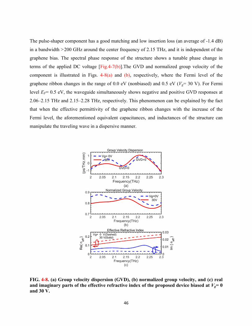
46

The pulse-shaper component has a good matching and low insertion loss (an average of -1.4 dB)

in a bandwidth >200 GHz around the center frequency of 2.15 THz, and it is independent of the

graphene bias. The spectral phase response of the structure shows a tunable phase change in

terms of the applied DC voltage [Fig.4-7(b)].The GVD and normalized group velocity of the

component is illustrated in Figs. 4-8(a) and (b), respectively, where the Fermi level of the

graphene ribbon changes in the range of 0.0 eV (nonbiased) and 0.5 eV (Vg= 30 V). For Fermi

level EF= 0.5 eV, the waveguide simultaneously shows negative and positive GVD responses at

2.06–2.15 THz and 2.15–2.28 THz, respectively. This phenomenon can be explained by the fact

that when the effective permittivity of the graphene ribbon changes with the increase of the

Fermi level, the aforementioned equivalent capacitances, and inductances of the structure can

manipulate the traveling wave in a dispersive manner.

FIG. 4-8. (a) Group velocity dispersion (GVD), (b) normalized group velocity, and (c) real and imaginary parts of the effective refractive index of the proposed device biased at Vg= 0 and 30 V.

47

Second, as the overall wavefront inside a metallic hollow waveguide has been formed by

successive reflections from the inner walls of the waveguide, one can expect the presence of a

very high chromatic dispersive structure such as a helical graphene ribbon to be able to

manipulate the phase of the resultant propagation mode.

For completeness, Fig. 4-8(c) Re[neff]= β/k0, where k0 is the free-space wave number, β is the

wave propagation phase constant, and Im[neff]. The former encapsulates the group velocity and

group velocity dispersion, whereas the latter accounts for the loss. Notice that Im[neff]is easily

computed via the absorption coefficient α = 2k0Im[neff] [56], which is estimated from the

scattering parameters |S21| and |S11| shown in Fig. 4-7.

4.3.2 Pulse Compression Performance

To investigate the pulse-compression performance of the component, it is assumed that the input

pulse is a y polarized chirped sine function, as stated in Eq. (3-25), where f0 is the upper-band

frequency of the negative dispersion region, T0 is the input pulse width, E0 is the electric field

amplitude, and µ is the chirp factor. The chirp factor for a uniform input pulse spectrum in the

positive GVD region from fLo to fHi, 2.15 to 2.28 THz, respectively, can be calculated using Eq.

(3-26):

� = �� sin(2�� − ��) , �� ≤ ��

0, ��ℎ�� (3-25)

� =��(��)

�� (3-26)

The instantaneous frequency can be obtained from the time derivative of the phase argument of

Eq. (3-25) proves that the tail of the chirped pulses with low-frequency components and faster

group velocities move to overtake the front high-frequency components of the pulses, resulting

in temporal pulse shortening with growth in amplitude. To validate the performance of the

device and highlight the presence of a unique optimal length for each arbitrarily selected pulse

width, two optimal compression lengths corresponding to the two chosen pulse widths of 8 and

12 ps have been numerically obtained as720 and 1700 µm, respectively. The optimization goals

in our design are maximum compression ratio and minimal residual pulse pedestal, which

48

ensures a high-quality compression. Figures 4-9 and 4-10 show the temporal waveform evolution

of the envelope of the device for these two optimal lengths, 720 and1700 µm, for the two bias

states, zero-bias, and 30 V.

FIG. 4-9. Waveform evolution of the proposed device with the optimal length of 720 µm, corresponding to input pulse duration of 8 ps, based on two border values of controlling DC voltage (a) 0 V and (b) 30 V.

49

FIG. 4-10. Waveform evolution of the proposed device with the optimal length of 1700 µm, corresponding to input pulse duration of 12 ps, based on two border values of controlling DC voltage (a) 0 V and (b) 30 V.

Proof of the TE11 mode of the proposed structure

As shown in Figure 4-11, it can be seen that the final output temporal pulse axial electric field

component (Ez) of the structure with increasing the length of the structure (or equivalently

periods number) is sharply reduced.

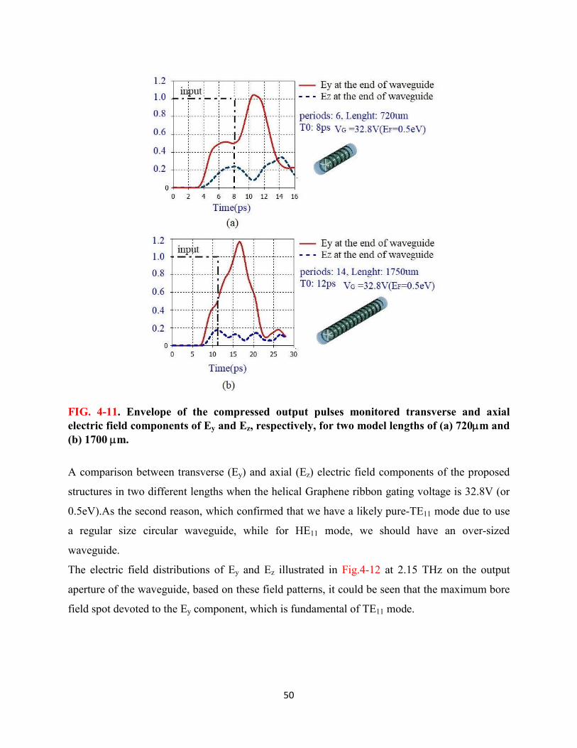
50

FIG. 4-11. Envelope of the compressed output pulses monitored transverse and axial electric field components of Ey and Ez, respectively, for two model lengths of (a) 720m and (b) 1700 m.

A comparison between transverse (Ey) and axial (Ez) electric field components of the proposed

structures in two different lengths when the helical Graphene ribbon gating voltage is 32.8V (or

0.5eV).As the second reason, which confirmed that we have a likely pure-TE11 mode due to use

a regular size circular waveguide, while for HE11 mode, we should have an over-sized

waveguide.

The electric field distributions of Ey and Ez illustrated in Fig.4-12 at 2.15 THz on the output

aperture of the waveguide, based on these field patterns, it could be seen that the maximum bore

field spot devoted to the Ey component, which is fundamental of TE11 mode.

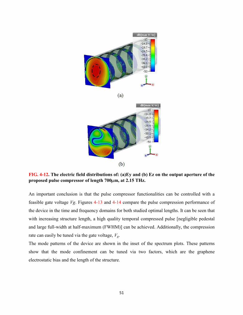
51

FIG. 4-12. The electric field distributions of: (a)Ey and (b) Ez on the output aperture of the proposed pulse compressor of length 700m, at 2.15 THz.

An important conclusion is that the pulse compressor functionalities can be controlled with a

feasible gate voltage Vg. Figures 4-13 and 4-14 compare the pulse compression performance of

the device in the time and frequency domains for both studied optimal lengths. It can be seen that

with increasing structure length, a high quality temporal compressed pulse [negligible pedestal

and large full-width at half-maximum (FWHM)] can be achieved. Additionally, the compression

rate can easily be tuned via the gate voltage, Vg.

The mode patterns of the device are shown in the inset of the spectrum plots. These patterns

show that the mode confinement can be tuned via two factors, which are the graphene

electrostatic bias and the length of the structure.

52

FIG. 4-13.(a) Time and (b) spectral descriptions of the pulse compressor output for Vg = 0 and 30 V for a length of 720 µm (the mode patterns at the end of the helix are presented in the insets of the figure).

One of the important parameters in the pulse compression applications is the broadening factor

(F), which is defined as the ratio of FWHM of the compressed pulse to the FWHM of the input

pulse. Table 4-2 summarizes the broadening (FWHM) of the two studied model lengths and

their tuning percentages, which is defined as the percentage of the broadening change. This

parameter is also known as the modulation depth defined by (F /F0)× 100%, where F is the

changes of F due to Vg = 30 V, and F0 is the average of the minimum and maximum obtainable

F [55]. A theoretical detail of how the pulse broadening is caused by the group velocity

dispersion is given in Appendix A.

53

FIG. 4-14.(a) Time and (b) spectral descriptions of the pulse compressor output for Vg = 0 and 30 V for a length of 1700 µm (the mode patterns at the end of the helix are presented in the insets of the figure).

Table 4-2. Tuning Percentage of the Proposed Graphene-Based Pulse Compressor.

Model Lengths 720 m 1700 m

FWHM @ Vg = 0.0 V 3.96 GHz 12.20 GHz

FWHM @ Vg = 30.0 V 1.11 GHz 9.46 GHz

Tuning % 5.9 % 8.04 %

To the best of our knowledge, no other studies have examined the combination of graphene and

pulse-compression techniques in the THz regime. It is helpful, however, to review the literature

54

to quantitatively justify our work. In Ref. [41], a THz passive pulse compressor shows a 2 ps, 0.5

THz chirped-pulse after transmission through a 10 µm circular aperture in a gold-film GaAs. The

pulse was compressed to 1.4 ps with FWHM of 0.07 THz. One of the major drawbacks of this

structure

is the extremely low output to input peak intensity ratio of 3.7 × 10-5. Another example is direct

compression of ultra-fast laser pulses using a dispersive and nonlinear thick (550 µm)

cholesteric liquid crystal sample [43]. After passing the laser pulses across this material, a

broadening of 1.8 THz around the center frequency of 387 THz (777 nm) has been achieved.

Comparing the numerical results shown in Table 4-2 with the literature, one can conclude that

the proposed graphene-based tunable pulse compressor holds promise for THz applications.

Sensitivity

In this study, a primary concern is to investigate the sensitivity of the proposed graphene-based

pulse shaping device to the crucial device parameters including the geometric dimensions and

the refractive index of the dielectric coating. As illustrated in Fig.4-15, the compressed output

signal of the proposed zero-biased graphene-based pulse compressor has shown no significant

sensitivity to the variation of refractive index of the inner dielectric coating (nd), the dielectric

thickness of td, and the helical graphene-ribbon dimensions: width(w) and pitch size(p).

55

FIG. 4-15 Parametric study of sensitivity of (a) refractive index of inner dielectric coating

layer, and (b) its thickness of td , (c) width and (d) pitch size of the helical zero-biased

graphene-ribbon of the proposed graphene-based pulse compressor on the compressed

output pulse.

56

(This page intentionally left blank)

57

Chapter 5

Numerical Analysis Validation based on a Fixed Terahertz Pulse

Compressor

Numerical techniques could be a great help in theoretical studies of challenging electromagnetic

problems such as complex structures where exact analytical solutions are difficult to obtain.

In this chapter, to confirm the accuracy of the previously achieved results of the proposed

tunable graphene-based pulse compressor, first of all, the mesh size sensitivity is analyzed by

modeling the of the proposed device with the optimal length of 720 µm, corresponding to an

input pulse duration of 8 ps, when controlling DC voltage has been set at 30 V. Then we made a

step forward for a passive fixed pulse-shaper by replacing the helical graphene ribbon with a

gold ribbon, and compared with our previous work, graphene-based one. Moreover, to prove the

validity of the numerical analysis, the proposed device has been examined using the finite

element method (FEM) and the finite integral technique (FIT).

The need for system identification in engineering is interesting [88], because of its ability to

describe phenomena, which are not to be fully explained by analytic approaches in complicated

problems. The use of the system transfer function to analyze the structure is preferable to the

full-wave simulation because of saving the execution time. Once the transfer function is

determined, one could apply it for the subsequent time-domain analysis of the pulse shaper with

various inputs. Finally, the rest of the chapter describes how to estimate the transfer function of

the proposed structure from the time domain simulation response.

4

5.1 Validation of Numerical Analysis Results

Fast computer-based simulation tools that allow the designers them precisely model their ideas

can be responsible for undiscovered model errors. The mesh size sensitivity and convergence test

are of importance, so that broadly employed in the various engineering computer-aided designer

tools to ensure high accuracy of the final numerical results. Moreover, using different numerical

approaches can be helpful to verify the simulation results.

58

5.1.1 Graphene-based Tunable THz Pulse Compression Waveguide

Meshing a complex geometry (see Fig. 3-1), including a dispersive infinitesimal thin layer such

as graphene is an essential part of the simulation. Thus, after a convergence test, we have chosen

a graphene thickness of tgr= 100 nm as the minimum cell size for the helix ribbon, while the

material properties of graphene were defined based on its real thickness of 1 nm. Due to

computational constraints, a smaller graphene thickness was not viable. This tradeoff approach is

commonly found in the literature [89]. As a mesh sensitivity convergence test based on different

mesh resolutions of the overall model meshes and the helical ribbons curvatures (graphene and

SiO2 spacer) of 20, 50, and 100 segmentations per turn have been performed, Fig. 5-1 shows the

dispersion performances of the proposed graphene-based structure. As we can see for smaller

mesh resolution, the results do not change significantly.

Execution time is an essential factor in determining the effectiveness of the numerical analysis,

which depends on two factors of the minimum machine requirements and mesh cells number of

the electromagnetic problems after time-spatial discretization operations. The total mesh cell

number, mesh methods, and corresponding computation-time of each mesh resolution are

illustrated in Table 5-1.

TABLE 5-1. Mesh characteristics and the corresponding computation-time of the proposed graphene-based pulse compressor.

Mesh setting

Total mesh cells Computation time Mesh cells per wavelength

for curved elements (helical ribbon)

segmentation No. 6 20 2,290,570 0 h, 28 min, 38 s 10 50 7,223,424 1 h, 49 min, 53 s 10 100 13,727,583 3 h, 15 min, 29 s

For the published article, the default mesh line limit is set at 10 lines per wavelength, resulting in

3,958,080 and 12,533,920 hexahedral mesh units for the 720 and 1700 µm long pulse

compressor, respectively.

59

FIG. 5-1. (a) GVD and (b) normalized group velocity of the proposed graphene-based tunable pulse compression waveguide in various mesh resolution using by FIT analysis.

5.1.2 Gold-based Fixed THz Pulse-shaper Waveguide

In this section in order to prove the validity of the numerical analysis results, another example of

our previous work (graphene-based pulse-compressor), a passive fixed pulse-shaper by replacing

the helical graphene ribbon with a gold ribbon has been introduced. The idea of using helical-

ribbon loaded circular waveguide as a controllable dispersion device can be verified using two

different numerical approaches finite element method (FEM) and the finite integral technique

(FIT).We see that the results for both methods are in an excellent agreement.

Figure 5-2 sketches the passive waveguide-based terahertz fixed-pulse shaper. A gold ribbon of

thickness tgold= 1 µm, width w (41 µm), and pitch size p (126 µm) is helically wrapped and

inserted inside a metalized dielectric tube with inner radius R of 100 µm and thickness t of8.5

µm. By carefully choosing the geometric parameters and the dielectric material, an optimum

condition for an arbitrary dispersion profile, large mode confinement, minimum mismatch and

60

FIG. 5-2. 3D geometry and side view of an internally dielectric-coated hollow-core

waveguide loaded by a helical gold ribbon

propagation loss with maximum tunability can be achieved. High-density polyethylene (HDPE)

is used for the dielectric tube given its good THz transparency (n = 1.524,and α = 0.2 cm-1 at 1

THz). A gold film layer completely covers the dielectric tube as a metal cladding. Gold is

modeled with the Drude parameters as stated previously in Chapter 4.

First of all, to prove the accuracy of the numerical analysis, the proposed device has been

analyzed using the FEM and the FIT. Fig.5-3a and b, show the transmittance and absorption

coefficients of the proposed device across the whole operating bandwidth (2.14 - 2.34 THz) for

the dominant TE11 mode.

The phase difference between the input and the output signals of the 2-port device is expressed

by the phase of the transmission coefficient (S21) as depicted in Fig.5-4. The phase of the

transmission coefficient, which is calculated numerically using both aforementioned numerical

methods demonstrate the dispersion characteristics of the signal transmission. It determines how

the input signal delayed when it travels between the input and output ports of the device in the

desired frequency spectrum. As shown in Chapter 4, a passive pulse compressor can be designed

in a portion of electromagnetic spectra where the normalized group velocity (Vgr/c) profile has a

large negative gradient.

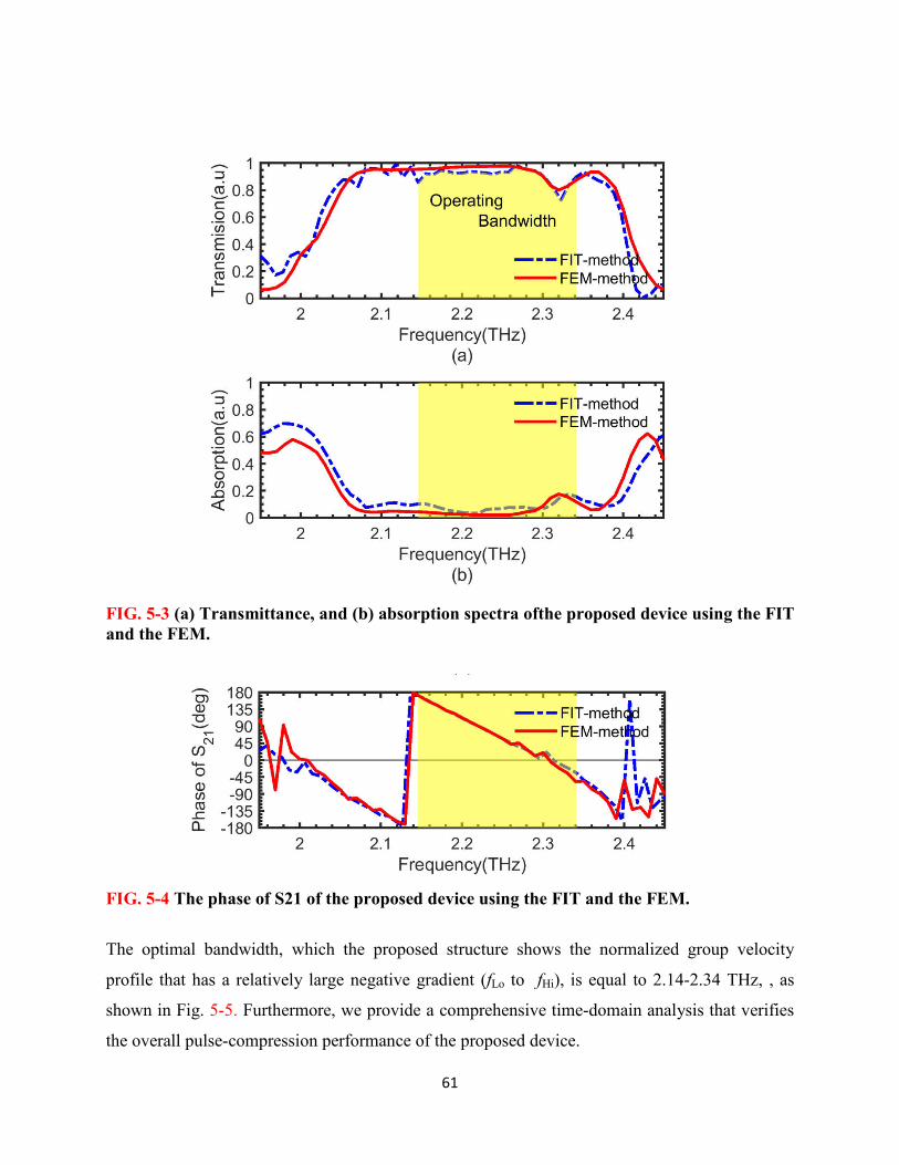
61

FIG. 5-3 (a) Transmittance, and (b) absorption spectra ofthe proposed device using the FIT and the FEM.

FIG. 5-4 The phase of S21 of the proposed device using the FIT and the FEM.

The optimal bandwidth, which the proposed structure shows the normalized group velocity

profile that has a relatively large negative gradient (fLo to fHi), is equal to 2.14-2.34 THz, , as

shown in Fig. 5-5. Furthermore, we provide a comprehensive time-domain analysis that verifies

the overall pulse-compression performance of the proposed device.

62

FIG. 5-5 Group delay and normalized group velocity extracted from the phase of the transmission coefficient (FIT-method).

The chirped-input signal is a y-polarized chirped sine function (Ey), as stated in Eq. (3-25),

where f0 is the upper-band frequency of the negative slope of the GV profile (2.34 THz), T0 is the

input pulse width , E0 is the electric field amplitude, and µ is the chirp factor. The chirp factor for

a uniform input pulse spectrum in the negative slope of the GV region from fLo to fHi, 2.14 -2.34

THz, can be calculated using Eq. (3-26) as 157.0791021 [S-2].

As a theoretical background, it is evident that the energy of electromagnetic waves in a

dispersive medium travels in a group velocity profile which is dependent on the frequency, as the

proposed structure which is shown in Fig.5-5. Therefore, if such dispersive structure is excited

by using a linearly down-chirped pulse like Ey, it can be expected in a group velocity profile with

negative gradient in terms of the frequency spectrum the front pulses with lower group velocity

travels with larger delay of Td, Hi than the tail of the input pulses with delay of Td, Lo as described

in Eq. (5-1).

0 0

, ,,

| |Hi Lo

d Hi d Lo

gr f gr f

L LT T

V V (5-1)

where L0 is the optimum length of the structure. If the input chirped-pulse duration is chosen as

(T0=Td,Hi-Td,Lo), one can be expected that the tail of the input pulse travel to overtake the front

63

one. Based on the numerically obtained information of group velocity, shown in Fig.5-5, we

obtained the optimal traveling length of L0 as 579 m. As shown in Fig.5-6, the maximum

compressed pulse shape is obtained at the output of y-polarized electric field which is located at

the distance of 575 m from the input reference plane of the proposed device. Figure 5-6(a)

shows the traveled input pulses just after traveling 50 m, about 10% of the optimal length while

Figs.5-6 (b) and (d) are illustrated the probe outputs located at 525 m and 625 m, before and

after the optimal position. These figures clearly show that how the probe output signal starts to

grow to a peak at the tail position before the optimal position while after passing the optimum

length the temporary narrowed pulse peak starts to downgrade.

The 3D demonstration of the spatial temporal electric field distribution along the proposed

waveguide device can be used to characterize the field confinement performance for future

applications possibilities such as material detection sensors or time domain spectroscopy (TDS).

Figure 5-7 gives a comprehensive description of the y-polarized electric field distributions at the

optimal probe position in three important moments of the compressed pulse duration, assigned as

tA, tB, and tC those are correspondent to pedestal, peak and ringing positions. As depicted in Figs.

5-7b-d, the field distribution of the peak moment (tA) is significantly more confined than pedestal

(tB) and ringing (tC) moments. This ensures the proposed device can be employed as an efficient

pulse shaper for various pulse-based THz applications including fast data communications,

TDS and imaging. Another important conclusion from the electric field distribution would be the

mode purity of the proposed structure at the fundamental propagation linear polarized mode

pattern of circular waveguide (TE11).

The next Section will describe how to estimate the transfer function of the proposed structure

from the time-domain simulation response.

64

FIG.5-6 (a) The output y-polarized E-field probe signals at various positions of the proposed structure (a) front position (z = 50m), (b) before, and (d) after, and (c) optimal length of L0=575 m.

FIG5-7 The electric field distributions at the optimum positions and the corresponding peak time positions of (b) tA, (c) t

65

electric field distributions at the optimum positions and the corresponding , (c) tB, and (d) tC as marked on the (a) the probe signal output.

electric field distributions at the optimum positions and the corresponding as marked on the (a) the probe signal output.

66

Figure 5-8 depicts the output envelope waveforms of the proposed device based on a chirped

input signal obtained using the FIT and the FEM. As the simulation results exhibit, there is a

good agreement between the results of the FIT and the FEM methods over the entire operating

bandwidth (2.14- 2.34 THz); moreover, it can be assumed as a time-domain results validation. In

Fig. 5-9, we demonstrated the calculated longitudinal electric field distributions (using FEM

method) for the fundamental mode at 2.15 THz and 2.25 THz, inside of the proposed structure,

the single-mode pattern of the waveguide with good confinement have been maintained. Some of

the general modeling consideration and simulation characteristics such as the mesh setting,

dispersive material definition in both time and frequency domains, in CST Microwave Studio

v.2015 and COMSOL 5.2a besides the postprocessing operations for extracting the principal

results are explained in Appendix B.

FIG. 5-8 the output envelope waveforms of the proposed device based on a chirped-input signal using two different numerical approaches of FIT and FEM.

67

FIG. 5-9 The fundamental mode pattern(TE11) of the proposed pulse shaper structure in xz-planes at (a) 2.15 THz, and (b) 2.25 THz obtained by using FEM.

5.2 A System Identification of Au-based Fixed THz Pulse-shaper Waveguide

A transfer function is an important notion in signal processing, which allows one to relate an

output signal and an input. System identification, which represents the transfer function allows a

great deal of flexibility in building mathematical models by using measurements of the systems

input and output signals in the terahertz spectrum [90-93]. Although transfer functions are

generally used in the analysis of systems such as single-input single-output filters in the fields of

signal processing, control theory, and communication theory, it could also be applied to provide

comprehensive system models of electromagnetic problems. This section focuses on the

estimation of the general transfer function of the proposed device. In pulse shaping, knowledge

of the transfer function makes it possible to achieve the temporal output pulse from any arbitrary

68

input pulses. Here, by incorporating the full-wave time-domain simulations (obtained in the

previous section), and the numerical transfer function estimation approach, it becomes possible

to extend the application of the system theory to a wider range of optical problems. The proposed

waveguide-based structure is assumed as a linear time-invariant (LTI) system, which is stable

and can be described by a transfer function of the form Eq.(5-1):

�(�) =��⋯��

��⋯�� (5-1)

where b0, b1, …, bm, a0, a1, …, an are coefficients to be estimated, and 0, 1, …, m, 0, 1, …,

n are positive real valued exponents.

The proposed identification approach is based on the transfer function estimation using the

input/output temporal data, which are generated in the full-wave transient simulation of the

proposed waveguide under a chirped input signal. In this work, the MATLAB signal processing

toolbox was employed to estimate the transfer function coefficients given in Table 5-2 based on

the obtained time samples of the compressed signal. Figure 5-10 presents the input-chirped

signal and the results of the estimated transfer function and those obtained by the FEM

simulation. It is noteworthy that the coefficients of the numerators and denominators of H(s)

with four zeros and nine poles are determined so that the highest similarity between the FEM

output, Fig. 5-10b, and the reconstructed one by using H(s), Fig. 5-10c, has been achieved.

Table 5-2.The resulting coefficients of the numerators and denomerators of the estimated transfer function.

0 1 2 3 4 5 6 7 8 9 - 7.17e113 2.8e100 - 2.7e88 4.9e74 -2.5e62 0 0 0 0 0

0 1 2 3 4 5 6 7 8 9 1.4e115 6.7e102 1.3e90 5.3e77 4.7e64 1.5e52 7.0e38 2.0e26 3.8e12 1

69

FIG. 5-10 (a) Chirped-input signal, (b) reference output signal obtained from the FEM-method analysis, and (c) output signal obtained from the estimated transfer function model of the proposed device.

The Bode plot of the estimated transfer function of the proposed pulse-shaper, as shown in Fig.

5-11, resemble an equivalent active bandpass filter as |H(s)|>1 has happened at the passband

spectrum. The pole-zero pattern of the H(s) also illustrated in Fig. 5-12, which all poles placed in

left side ensure a real estimated system. All the MATLAB codes that were used throughout this

thesis, especially including transfer function estimation, have been shared with readers in

Appendix C.

70

FIG. 5-11 The magnitude and phase diagram of the Bode plot of the estimated transfer function.

FIG. 5-12 The pole-zero map of the estimated transfer function.

71

Chapter 6

A Comparative Study on Helical Ribbon Material Dependence

In many optical devices, investigation of the impact of the material of comprised parts is a

crucial part of the study. As an example, the helical-ribbon in the proposed pulse compressor,

which was introduced and studied in Chapters 4 and 5, has an essential influencer.

5

6.1 Dispersion and Matching Performance of PEC, Au, and Graphene-

ribbon

A comparative study of material dependence on our proposed terahertz waveguide-based pulse

compressor has been presented. Based on dielectric-lined hollow-core waveguide loaded with a

helical conductive x-ribbon (where x can be a perfect electric conductor (PEC), Au or graphene-

coated Au), pulse compression of a linear chirped sine wave is investigated numerically for

different material helical ribbon in cases of (i) PEC, (ii) Au, and (iii) graphene-coated Au with

different biases.

Figure 6-1 shows the 3D-geometry and side view of the proposed metal ribbon loaded

waveguide: a metal ribbon with the thickness tm, ribbon width w, and pitch size p is helically

wrapped and inserted inside a metalized dielectric tube with a thickness of td. The length of the

helical x-ribbon loaded waveguide section was introduced with L0. As shown in the side view

illustration of the yz-plane, the two ends of the waveguide are tapered sections to ensure the

lowest possible reflections when interfacing the THz pulse compressor with a standard smooth

circular waveguide. These identical sections are two simple conical circular waveguides with the

length of L2 that gradually connect the helix to the ends of the circular waveguides with the

length of L1. The dielectric is HDPE with a refractive index of 1.524, and Au is modeled as the

Drude model parameter, which stated in Sec. (4.2.3). The optimized dimensions of the proposed

helical x-ribbon loaded waveguide are listed in Table 6-1.

Table 6-1. The optimized dimensions of the proposed helical x

p W

126 m 42.5m

FIG. 6-1. Schematic-diagram, 3Dcoated hollow-core waveguide loaded by a helical metal ribbon.

FIG. 6-2. The magnitude and phase of reflection coefficients of a goldinterface at normal incidence of a plane wave.

72

The optimized dimensions of the proposed helical x-ribbon loaded waveguide.

td tm L0 L1

8.5m 2m 665m 40m 100

diagram, 3D-geometry in a, and side-view of an internally dielectriccore waveguide loaded by a helical metal ribbon.

The magnitude and phase of reflection coefficients of a gold-air and graphenel incidence of a plane wave.

ribbon loaded waveguide.

L2

100m

view of an internally dielectric-

air and graphene-air

73

As successive reflections have formed the overall wavefront inside a metallic hollow waveguide

from the inner walls of the waveguide, one can expect the presence of a very high chromatic

dispersive structure such as a helical x-ribbon to be able to manipulate the phase of the resultant

propagation mode. Hence, the reflection coefficient () of a normal incident of each material

could be a comprehensive measure that describes how the reflective material can manipulate the

transmission phase of the structure; Fig. 6-2 gives a spectral description of the reflection

coefficient of Au and graphene films. It can be found that graphene compared to gold-film, as a

terahertz dispersive metal, has a more dispersive reflection coefficient in the frequency span of

1.9-2.3 THz that results in equivalently a dispersive transmission coefficient. Of course, PEC

with ||=1 and =180o besides graphene and Au in upcoming qualitative compression

performance could be helpful. The S-parameters characteristics of the three cases, as shown in

Fig. 6-3, could be better interpreted with the reflection coefficients data, since that the Au and

PEC with the better reflectivity than Au-graphene coated ribbon result in the same transmission

amplitude (|S21|) and phase responses (S21).

As illustrated in Fig. 6-4(a), depending on which one of two bands of 2.0 - 2.15THz and 2.15 –

2.25 THz, can be excited in this device, the dispersion can be either normal or anomalous with

group velocity dispersion (GVD) values of −0.5 ps/(THz.mm) or 1.2 ps/(THz.mm), respectively,

approximately independent of helical-ribbon material. This reveals that the dispersion

mechanism is significantly due to helical geometry rather than material dispersion. As we

mentioned in Sec.(2.1.1), for passive pulse compression application, the most favorable

frequency region is a part of the dispersion characteristic where the operating wave normalized

group velocity (Vgr/c) has a large negative gradient as a function of frequency which one can see

in Fig. 6-4(b) all cases have likely the same proper bandwidth, but Au and PEC compared to

graphene-coated Au-ribbon have a significantly larger negative gradient of the normalized group

velocity.

74

FIG. 6-3. A comparative illustration of (a) Magnitude and (b) phase of the S-parameters of the proposed device based on different helical ribbon materials.

FIG. 6-4. The influence of helical ribbon materials on (a) Group velocity dispersion (GVD) and (b) normalized group velocity of the proposed device.

75

6.2 Pulse Compression Analysis

As shown in Fig.6-5, by comparison, we find the pulse compression performance (compression

factor and pedestal) in the case of (ii) is further better than that for other ones. High compression

factor with low-pedestal is helpful to produce needle-shaped pulses which are required for low

ISI data communication. As we have seen earlier in Fig.6-4(a) and (b), the high dispersive

behavior of the graphene coating can result in more spectral broadening, as well as more

compression ratio, but we should pay the cost of this with more power dissipation. To validate

the performance of the device, a unique optimal compression length corresponding to the pulse

width (here we choose pulse duration of 8 ps) can be expected.

FIG. 6-5. The impact of helical-ribbon material on the (a) time and (b) frequency responses of the pulse compressor.

76

The optimization goal in our study is the maximum compression ratio and minimal residual pulse

pedestal, which ensures a high-quality compression. Figures 6-6 (a) and (b) show the temporal

waveform evolution of the envelope of the proposed device in cases of helical Au- and graphene-

coated Au-ribbon, respectively. The corresponding optimal lengths of both cases are around 665

m distance from the input reference plane. As shown in Fig. 6-6, pulse side lobes of Au-

graphene coated compared to Au-ribbon have lower amplitudes and in conclusion higher pulse

quality, this could be predicted from higher dispersion that was seen from the phase of the

graphene reflectivity coefficient (E) which was shown in Fig. 6-2.

Fig. 6-6. The waveform evolution of the proposed device m, corresponding to an input pulse duration of 8 ps in case of (a) Au- and (b) Au-graphene-coated ribbons.

77

Chapter 7

Conclusion and Future Works

Right from the outset of this thesis, the aim of the work presented was to see how far dispersion

tailored pulse shaping devices, in particular DC-controlled graphene-based pulse compression,

can go in overcoming some of the challenges in tunable passive THz pulse shaping research. It is

hoped that by taking the first steps in applying graphene to a passive hollow-core waveguide, the

idea of DC-controlled graphene-based pulse compression could begin to gain traction and help

propel tunable graphene-based terahertz devices one step closer to real-world applications where

the benefits of THz characterization can be brought out fully.

The first proposed idea was undertaken in this PhD thesis used material and waveguide

(chromatic) dispersion in helically wrapped graphene-ribbon inside a dielectric-lined hollow-

core waveguide as the passive pulse-shaping mechanism. To the best of our knowledge, no other

studies have examined the combination of graphene and pulse-compression techniques in the

THz regime.

A spectral pulse broadening factor FWHM of 0.07 THz, the highest for passive THz temporal

pulse compression at the time of publication, was achieved from passing a 2 ps, 0.5 THz chirped-

pulse through a 10 um circular aperture in a gold-film GaAs [41]. One of the major drawbacks of

this structure is the extremely low output to input peak intensity ratio of 3.7 × 10-5.

More importantly, the conclusions of this work highlighted certain key factors in THz passive

pulse compression:

High-quality compression

Large mode confinement

Excellent tunability of the compression factor

Minimum mismatch, and low propagation loss, and

Potential for easy integration into chip-based devices.

For the first time, a proof-of-principle demonstration of THz passive pulse compression was

shown based on the portion of electromagnetic spectra where the normalized group velocity

(Vgr/c) profile has a large negative gradient.

78

The possibilities of terahertz's direct pulse compression in a dielectric-lined circular waveguide

with tunability based on a strong both waveguide and material dispersions introduced by helical

graphene-loading have been demonstrated. We use helix in our structure as a primary waveguide

dispersion controlling element. We show that the proposed structure introduces an excellent

tunability of the compression factor via the graphene electrostatic bias (see Chapter 4). The

circuit model of the helical waveguide can be expressed by one inductance per unit length and

two radial and inter-turn capacitances per unit length (see Fig. 4-5). Thus, a strong dispersion due

to helix-shield capacitive coupling voltages and helix equivalent inductive currents can be

introduced. This effect mainly depends on the dielectric tube parameters (td, d) for the former,

and the helix characteristics (σ, w, p) for the latter, where is the conductivity of helix-tape that

in our proposed structure is an equivalent dispersive conductivity resulted from hybrid graphene-

ribbon and DC-bias facilities of gold-ribbon. It is demonstrated that there is an optimal

compression waveguide length over which THz chirped pulses reach the maximum compression.

It is shown that by applying an electrostatic controlling gate voltage (Vg) of 0 and 30 V on the

helical graphene ribbon, the temporal input pulses of width 8 and 12 ps, propagating through two

different lengths (700 m and 1700 m), can be tuned by 5.9% and 8%, respectively, in the

frequency range of 2.15–2.28 THz.

In chapter 5, to confirm the accuracy of the previously achieved results of the proposed tunable

graphene-based pulse compressor, first of all, the mesh size sensitivity is analyzed,and then we

made a step forward for a passive fixed pulse-shaper by replacing the helical graphene ribbon

with a gold ribbon and compared to the previous proposed tunable pulse compressor, graphene-

based one. Moreover, to prove the validity of the numerical analysis, the proposed device has

been examined using the finite element method (FEM) and the finite integral technique (FIT).A

good agreement was found between the results of the FIT and the FEM methods.

Another outstanding achievement of this research was to provide a comprehensive system model

by incorporating the full-wave time-domain simulations and the numerical transfer function

estimation approach. The use of the system transfer function to analyze the structure is preferable

to the full-wave simulation because of saving the execution time. Once the transfer function is

determined, one could apply it for the subsequent time-domain analysis of the pulse shaper with

various inputs.

79

Based on a comparative study that was performed on the impact of helical-ribbon material on the

proposed terahertz waveguide-based pulse compressor performance for different material of

helical ribbon in cases of (i) PEC, (ii) Au, and (iii) graphene-coated Au, the material-dispersion

of the structure was highlighted. As shown in Fig. 6-6, pulse side lobes of Au-graphene coated

compared to Au-ribbon have lower amplitudes and in conclusion higher pulse quality, this could

be predicted from higher dispersion that was seen from the phase of the graphene reflectivity

coefficient (E) which was shown in Fig. 6-2 .

Moving on from this thesis, there are three areas of further development that would be interesting

for direct passive pulse compression. Firstly, work can be done with a comparison of different

waveguide platforms based on geometry (planar/non-planar). In this thesis, a normal size hollow-

core waveguide (HCW) as the main platform was used while usually the over-sized HCWs with

the emphasis on the low loss transmission of the HE11 mode in the infrared and THz regions

should be used. In some applications that an integration development is required, the planar

platform is the most popular solution.

Another area in which additional research can be carried out is the THz sensing/spectroscopy

experiments have been targeted at particular substances such as toxic materials or biological

samples using conventional methods such as transmission spectroscopy. Comparatively, work

done on THz materials sensing has been focused on detecting refractive index changes caused by

using different materials to come into contact with the materials sensor. Among different types

of the optical waveguide, hollow core, and porous core for sensing applications as it allows a

greater analyte volume inside its core area are more suitable. Moreover, the guided mode in a

hollow-core fiber is strongly confined in the core area that greatly reduces the effect of the

background material in the waveguiding properties of the fiber [93]. Therefore, as a possible

solution, we can propose a terahertz sensor based on our proposed tunable hollow-core

waveguide for chemical or biological sample detection.

In order to realize a compact high-speed optical communications system, nonlinear photonics is

seen as a key technology. Optical fiber materials exhibit a nonlinear response to strong electric

fields, such those of optical signals confined within the small fiber core [94]. The third research

direction would be to incorporate nonlinearity onto the graphene-based pulse compressor for

optical waveform generation and pulse shaping and in the applications of advanced pulse profiles

in all-optical signal processing. Silicon carbide (SiC), a high-transparency nonlinear material,

80

has very promising properties for THz applications, including extremely low loss, ultrabroad

transparency window, very high optical damage threshold, moderate nonlinearity, and

birefringence [95]. Of course, these previously proposed ideas are only some suggestions for

terahertz pulse shaping on the basis of the development of the waveguide-based structure, there

is no doubt that many more ways could be found via the creative use of various materials and

geometries.

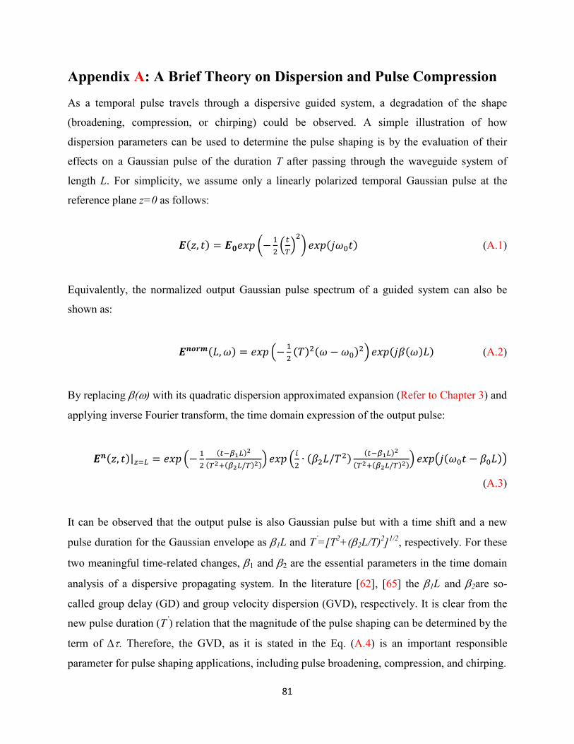
81

Appendix A: A Brief Theory on Dispersion and Pulse Compression

As a temporal pulse travels through a dispersive guided system, a degradation of the shape

(broadening, compression, or chirping) could be observed. A simple illustration of how

dispersion parameters can be used to determine the pulse shaping is by the evaluation of their

effects on a Gaussian pulse of the duration T after passing through the waveguide system of

length L. For simplicity, we assume only a linearly polarized temporal Gaussian pulse at the

reference plane z=0 as follows:

�(�, �) = �� −�

��

�

��

�

� ��(��) (A.1)

Equivalently, the normalized output Gaussian pulse spectrum of a guided system can also be

shown as:

��(�, �) = �� −�

�(�)�(� − ��)�� (��(�)�) (A.2)

By replacing () with its quadratic dispersion approximated expansion (Refer to Chapter 3) and

applying inverse Fourier transform, the time domain expression of the output pulse:

��(�, �)|�� = �� −�

�

(��)�

(��(��/�)�)� ��

�

�∙ (��/��)

(��)�

(��(��/�)�)� ��(�� − ��)�

(A.3)

It can be observed that the output pulse is also Gaussian pulse but with a time shift and a new

pulse duration for the Gaussian envelope as 1L and T’=[T2+(2L/T)2]1/2, respectively. For these

two meaningful time-related changes, 1 and 2 are the essential parameters in the time domain

analysis of a dispersive propagating system. In the literature [62], [65] the 1L and 2are so-

called group delay (GD) and group velocity dispersion (GVD), respectively. It is clear from the

new pulse duration (T’) relation that the magnitude of the pulse shaping can be determined by the

term of . Therefore, the GVD, as it is stated in the Eq. (A.4) is an important responsible

parameter for pulse shaping applications, including pulse broadening, compression, and chirping.

82

=��

�= �� ∙

�

� (A.4)

For a dispersive medium, generally, we can suppose three cases of normal dispersion (>0) and

anomalous dispersion (<0) or even zero-dispersion (=0). Another helpful parameter to

express the overall dispersion effect of optical or THz fibers is the total induced dispersion

coefficient D in ps/kmnm, as:

�(�) = −��

��∙

�= −

��

��∙ �� (A.5)

Chromatic dispersion coefficient D can be zero, negative, or positive over an operating

frequency range of interest. The frequency, at which D is zero, is referred to as zero-dispersion

frequency. In the case of D>0(anomalous dispersion), the higher frequency components travel

faster than lower frequency ones, but for the frequency region where the dispersion coefficient D

is negative (normal dispersion), the lower frequency components travel faster than higher

frequency ones. As an important conclusion, parameter D versus the angular frequency is an

essential graph in the dispersion analysis.

83

Appendix B

The General Modeling Consideration and Simulation Characteristics

B1. Model Designing of a Helix with Rectangular Cross-section

The following section deals with the procedure of creating a helix with the rectangular cross

section in CST Microwave Studio and COMSOL environment.

CST Microwave Studio v.2015

Drawing a z-axis aligned helix with the design parameters of: tape helix thickness of

tgr=0.1[um], width and pitch of helix {w1=41[um], p1=126[um]}, helix internal radius

R=100[um], n_seg=40, and helix final turns nt=6.

1 Define a zero thickness Brick: xmin=R xmax=R+tgr, ymin=ymax=0, zmin=0

zmax=w1

2 From Modeling>Picks select Pick face

3 Double click on the Brick face

4 From Modeling>Shapes select Rotate

5 Ask you “Do you wish to define a rotation axis numerically?” click OK, then click

ESC button to open “Enter Edge Numerically” window, then set z2=1 and leave all in

zero value, click OK. The “Rotate Face” window will be open.

6 Complete “Rotate Face” window as follows:

Name: Helix, Angle: nt*360, Height: nt*p1, Radius Ratio: 1.0 and Segments per turn:

n_seg.

COMSOL 5.2a

Drawing a helix, x-axis aligned, with rectangular cross section first of all we define the

parameters as tape helix thickness of tgr=0.1[um], width and pitch of helix {w1=41[um],

p1=126[um]}, helix internal radius R=100[um] and helix final turns nt=6.

Work Plane 1 (wp1)

1 On the Geometry toolbar, click Work Plane.

2 In the Settings window for Work Plane, click Show Work Plane.

3 In plane Definition, from the Plane list, choose yx-plane.

84

Rectangle 1 (r1)

1 On the Work Plane toolbar, click Primitives and choose Rectangle.

2 In the Settings window for Rectangle, locate the Size and Shape section.

3 In the Width text field, type tgr.

4 In the Height text field, type w1.

5 Locate the Position section. From the Base list, choose Corner, with xw=R and yw=0.

6 Right-click Rectangle 1 (r1) and choose Build Selected.

Next add a parametric curve using the helical profile.

Parametric Curve 1 (pc1)

1 On the Work Plane toolbar, click Primitives and choose Parametric Curve.

2 In the Settings window for Parametric Curve, in the Parameter section type the

parameter Name text field s.

3 In the Maximum text field, type 2*pi.

4 Locate the Expressions section. In the x text field, type (s*nt*p1)/(2*pi).

5 In the y text field, type cos(nt*s).

6 In the z text field, type sin(nt*s).

7 Locate the Position section. In the x text field, type 1, and 0 in the y and z fields.

8 Locate the Axis section. From the Axis list, choose z-axis.

9 Build all.

As the final step we should sweep the rectangular cross section wp1 along the helical parametric

curve of pc1.

Sweep 1 (swe1)

1 On the Geometry toolbar, click Sweep.

2 In the Settings window for Sweep, in the Cross Section field locate the wp1 as the Face

to sweep.

3 In the Spine Curve field locate the pc1 as the Edges to follow.

B2. Transient Solver

85


In CST MICROWAVE STUDIO two time domain solvers are available. One is based on the

Finite Integration Technique (FIT), just called Transient solve and another is Transmission Line

Model (TLM) which work both on hexahedral meshes, we used in this study FIT method. For

better postprocessing operations for obtaining dispersive reports such as GD, GV, and GVD its

strongly recommended to use a broadband Raised-cosine pulse (generated based on MATLAB

codes presented in C2) for limited number of time samples to avoid unnecessary extra

computation time and minimum ringing on the tail of the output pulse. The pulse responses of

the proposed structure is obtained based on our generated chirped signal using MATLAB codes

of C1 instead of default chirped pulse defined in the software.

COMSOL 5.2a

In COMSOL the time samples needed for excitation can be directly defined as follows:

First of all define the required new parameters as E0=30[V/m], T0=8[ps], Tao=0.2[ps],

Tf=14[ps], f1=1.95[THz], f2=2.45[THz], Df=f2-f1, and mue=-2*pi*Df/Tf.

Then we should define a Rectangle function with ON and OFF time windows of [0-T0] and [T0-

Tf], respectively.

Rectangle 1 (rect1)

1 On the Home toolbar, click Difinition and choose More Functions>Rectangular.

2 In the Settings window for Step function, Locate the Parameters section. In the Lower and

Upper Limits text field, type: 0 and T0, respectively.

Analytic 1 (an1)

1 On the Home> Definition toolbar, click Local Variables.

2 In the Settings window for Local Variable, type Echp in the variable name text field.

3 In the Expression text field, type:

E0*rect1(t[1/s])*(1-exp(-(t/Tao)))*sin(2*pi*t*f2+0.5*mue*t^2)

For transient analysis of the waveguide problems we define two Scattering Boundary Conditions

on input and output ports and then the first boundary is chosen as excitation port with the

following setting:

Scattering Boundary Condition 1

1 On the Physics toolbar, click Boundaries and choose Scattering Boundary Condition.

86

2 In the Settings window for Scattering Boundary Condition, locate the Boundary

Selection section and choose the input aperture of the waveguide.

3 In Scattering Boundary Condition, from the Incident field list, choose Wave given by

E field.

4 Then type the Incident electric field vector as E0: [0, 0, Echp].

B3. Frequency Domain Solver


It is recommended that for a proper comparison condition in the Frequency Domain Solver

Parameter, in Frequency Samples Section, set the type at “Equidistance” with Samples number

equal with that will use in COMSOL.

COMSOL 5.2a

In electromagnetic problem with more complexity in geometry including dispersive materials,

such as our structure the Generalized Minimal Residual Method (GMRES), which is an iterative

method for the numerical solution of a nonsymmetric system of linear equations has been chosen

for fast convergence.

B4. Dispersive Material Definition

At optical frequencies and lower (THz), noble metals such as Silver and Gold, behave like

“plasmas”, this model of the classical gas of free electrons is called the Drude model or Drude–

Lorentz model. The optical response of a free electron gas is approximately described by

the Drude–Lorentz model as stated in Eq.(3-3) in terms of three fundamental drude parameters of

ωp (plasma frequency), ϵ∞ (dielectric function at infinite frequency), and τ (relaxation time).

Graphene is also can be modeled in linear mode via Drude-like model based on the Kubo

formula which was described in Sec (4-2-1) and Eq.(4-5). Here we introduce the instruction of

defining Drude-modeled metals such as gold and Drude-like model of graphene in two forms of

(i) as a zero-thickness impedance surface of equivalent conductivity and (ii) a dielectric thin-

layer with a Drude-like material with complex permittivity.


87

Definition of Gold

Nobel metals such as Gold in optical regime can be modeled by using Drude model as follows:

1. Material Properties>Dispersion>Dielectric dispersion, from Disp. Model list choose

Drude.

2. In the Epsilon infinity field type 9.1, and type 1.38e16 (rad/s) in Plasma frequency text

field, then type in collision frequency text field 1.075e14 (1/s).

Definition of Graphene

Graphene can be defined as (i) a thin-layer dispersive dielectric with complex permittivity, or (ii)

zero thickness surface boundaries with complex surface impedance. First of all, there is a

common operation for both two cases, as follows:

1. As a common step go to Home>Macros>Material>Create Graphene Material for

Optical Applications.

2. Type the required preconditions of the problem in their text fields in “Define Graphene

Materials” window as the following Table:

Temperature [K]

Chemical Potential

[eV]

Relaxation Time [ps]

Thickness [nm]

Frequency [THz]

Number Of

Points Minimum Maximum

300 0 10 1 1.7 3 500

These items will be appeared in Parameter list table. Then, two subfolders of Graphene and

Graphene1, including Dielectric constants and Surface Impedance data, can be used to assign the

proper model.

Graphene as Dispersive Dielectric

1. Right-click on the helical ribbon with thickness of tgr, choose Change material.

2. In Change Material window, from Material list select Graphene_Eps.

Graphene as Complex Surface Impedance

1. Right-click on the helical ribbon with zero thickness, choose Change material.

2. In Change Material window, from Material list select Graphene.

COMSOL 5.2a

88

Definition of Gold

In COMSOL dispersive materials can be defined by creating a separate wave equation the

material domain as follows:

Wave Equation, Electric 2

Create a separate wave equation feature for the Gold-ribbon domains.

1. On the Physics toolbar, click Domains and choose Wave Equation, Electric.

2. In the Settings window for Wave Equation, Electric, locate the Domain Selection

section.

3. From the Domain Selection, choose Helical Ribbon.

4. Locate the Electric Displacement Field section. From the Electric displacement field

model list, choose Drude-Lorentz dispersion model.

5. In the value field type 9.1, and in ωP text field, type 1.38e16 rad/s.

6. In the table, enter the following settings:

Oscillator strength (1) Resonance frequency (rad/s) Damping in time (rad/s)

1 0 (1.075e14)/(2*pi)

Definition of Graphene

Definition of Graphene is similar a dispersive material but the main difference lies in

the expressed Plasma frequency (ωP). In the Model Builder window, under Component 1

(comp1) right-click Definitions and choose Variables.

Variables 1

1. In the Settings window for Variables, locate the Variables section.


Name Expression Unit Description

temp 300[K] [K] Temperature

Ef 0[eV] J Fermi level

tgr 1[nm] m Graphene thickness

tau 1e-13[s] [s] Relaxation time

gamma_1 1/tau [1/s] Damping in time

omega_1 0 [rad/s] [rad/s] Resonance freq.

omega_p sqrt(log(2*cosh(Ef/(2*k_B_const*temp)))* (2*(e_const^2)*k_B_const*temp)/( pi*(hbar_const^2)* (epsilon0_const*tgr)))

[rad/s] Plasma frequency for Ef (eV)

In addition, there is a small difference in the required setting of Drude-Lorentz dispersion model

in TD and FD.

89

Time Domain Study


1. In the Model Builder window, under Component 1 (comp1)>Electromagnetic Waves,

Transient (ewt) click Wave Equation, Electric.

2. In the Settings window for Wave Equation, Electric, locate the Electric Displacement

Field section.

3. From the Electric displacement field model list, choose Drude-Lorentz dispersion

model.

4. From the Relative permittivity, high frequency list, choose User defined. From the list,

choose Diagonal.

5. In the Relative permittivity, high frequency table, enter 1 for all diagonal elements.

6. In the ωP text field, type omega_p.

7. Locate the Magnetic Field section. From the μr list, choose User defined. Accept the

default value 1.

8. Locate the Conduction Current section. From the σ list, choose User defined. Accept the

default value 0.

Next, you add a Drude-Lorentz Polarization feature, as a sub feature to the wave equation. There,

more material parameters will be defined for the polarization field.

Drude-Lorentz Polarization 1

1. On the Physics toolbar, click Attributes and choose Drude-Lorentz Polarization.

2. In the Settings window for Drude-Lorentz Polarization, locate the Drude-Lorentz

Dispersion Model section.

3. In the fn text field, type 1.

4. In the ωn text field, type omega_1.

5. In the Γn text field, type gamma_1.

Frequency Domain Study


Create a separate wave equation feature for the Gold-ribbon domains.

1. On the Physics toolbar, click Domains and choose Wave Equation, Electric.

2. In the Settings window for Wave Equation, Electric, locate the Domain Selection

section.

3. From the Domain Selection, choose Helical Ribbon.

4. Locate the Electric Displacement Field section. From the Electric displacement field

model list, choose Drude-Lorentz dispersion model.

90

5. In the value field type 1, and in ωP text field, type omega_p.


Oscillator strength (1) Resonance frequency (rad/s) Damping in time (rad/s)

1 omega_1 gamma_1/(2*pi)

91

B5. Dispersion Reports Post-processing


As the important part of our simulation task is the extraction of the required dispersion results

such as group delay (GD), normalized group velocity (Vgr/c) and group velocity dispersion

(GVD). In CST MWs, in Filter Analysis section of bout Frequency and Transient solvers, in Post

processing>Template Based Post Processing, the main parameter of GD is available, then

from GD-report all required dispersion results can be calculated. Here is a brief about the Post

processing operation to produce Vgr/c, GVD and axial propagation phase constant from GD

results.

Vgr/c

1 Choose General 1D>0D or 1D Results from 1D Results.

2 In Specify Action section choose Axes: Scale with Function f(x.y) from the list of

1D(C).

3 Type in the text field the rescaled relation of Vgr/c and GD based on the current unit set

of the CST MWs, here is the proper text field compatible with the unit presets:

�� ⁄ � =�(�)

3�8(�/�)��(�) (�. 1)

As an example if the CST MWs units that was set on THz, m and Second the text field can be

rescaled as Eq.(B.2)

�� ⁄ � =�(��)

3�8((1�6)��/�)��(�) = (1� − 14) ∗ (

�

3 ∗ �) (�. 2)

4 Choose Apply to: y-axis.

5 Set 1D-Results field from the list on GDelay_2(1)1(1).

6 Evaluate.

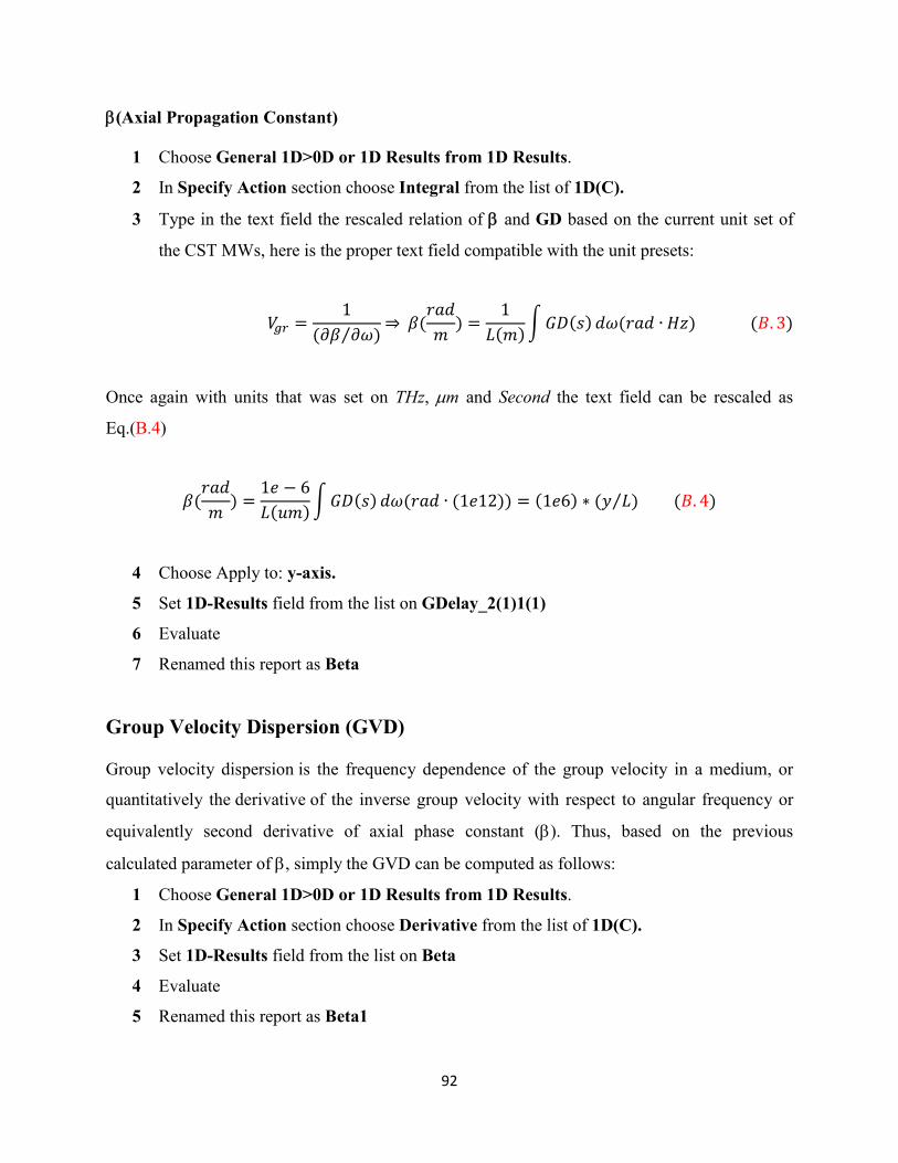
92

(Axial Propagation Constant)


2 In Specify Action section choose Integral from the list of 1D(C).

3 Type in the text field the rescaled relation of and GD based on the current unit set of

the CST MWs, here is the proper text field compatible with the unit presets:

�� =1

(�� )⁄⇒ �(

��

�) =

1

�(�)� ��(�) ��(�� ∙ ��) (�. 3)

Once again with units that was set on THz, m and Second the text field can be rescaled as

Eq.(B.4)

�(��

�) =

1� − 6

�(��)� ��(�) ��(�� ∙ (1�12)) = (1�6) ∗ (� �⁄ ) (�. 4)

4 Choose Apply to: y-axis.

5 Set 1D-Results field from the list on GDelay_2(1)1(1)

6 Evaluate

7 Renamed this report as Beta

Group Velocity Dispersion (GVD)

Group velocity dispersion is the frequency dependence of the group velocity in a medium, or

quantitatively the derivative of the inverse group velocity with respect to angular frequency or

equivalently second derivative of axial phase constant (). Thus, based on the previous

calculated parameter of , simply the GVD can be computed as follows:


2 In Specify Action section choose Derivative from the list of 1D(C).

3 Set 1D-Results field from the list on Beta

4 Evaluate

5 Renamed this report as Beta1

93

Repeat these steps as the second derivation of to obtain GVD.


2 In Specify Action section choose Derivative from the list of 1D(C).

3 Set 1D-Results field from the list on Beta1

4 Evaluate

5 Renamed this report as GVD

COMSOL 5.2a

In COMSOL the dispersion reports such as Vgr, and GVD, as previously stated, can be

calculated based on GD using S21, see Eq. (3-16).

Phase Angle of S21

1D Plot Group 1

1 On the Home toolbar, click Add Plot Group and choose 1D Plot Group.

Global 1

1 On the 1D Plot Group 1 toolbar, click Global.

2 In the Settings window for Global, locate the y-Axis Data section for Expression the

following expression: arg(emw.S21)*180/pi

3 Renamed this report as angle of S21(deg)

This command would be generate S21 in degree.

94

Appendix C

MATLAB Codes

C.1 Linear Chirped Signal Generation

%----------------Linear FM f1=1.18e12; %Lower Freq of Sweeping Range1THz f2=2.32e12; %Upper Freq of Sweeping Range5THz BW=max(f1,f2); % Bandwidth m1=15; %coef. of resolution Tao=0.2e-12; %1.4e9 Fs=m1*BW; % Sampling frequency T0=12.0e-12; td=0; % Pulse duration 2e-9 Tf=35.0e-12; % Time Window for seeing the time signal with a good view!6e-9 DelF=f2-f1; mue=-2*pi*DelF/Tf;%mue=-2*pi*(f2-f1)/Tf; %-------------- Create a FM sine wave in Hz. DT=1/Fs; N=Tf*Fs; t=zeros(1,N); x=zeros(1,N); for n=1:N t =n*DT; % Time vector of Tf second if t<T0 %for sin %x(n) = exp(-((t-T0-td)/Tao).^2).*sin(2* pi*t*f2+0.5*mue*t.^2); x(n) = (1-exp(-(t/Tao))).*sin(2* pi*t*f2+0.5*mue*t.^2); else %for sin x(n)=0;%for sin end %for sin end %-------------- Take fft, padding with zeros so that length(X) nfft = 2^18; % Length of FFT X = fft(x,nfft); %-------------- FFT is symmetric, throw away half X = X(1:nfft/2); %-------------- Take the magnitude of fft of x Fx = abs(X); AFx=angle(X); %-------------- Frequency vector f = (0:nfft/2-1)*Fs/nfft; % %-------------- Generate the plot, title and labels. figure(1); subplot(2,1,1) n=1:N;

95

plot(n*DT,x); title('Linear Swept FM Signal No chirped Per14-4.txt ');legend(['Tao: ',num2str(Tao*1e12),'T0: ',num2str(T0*1e12),';Sample No.:',num2str(N),'; Tf=',num2str(Tf),'; f1=',num2str(f1*1e-12),'; f2=',num2str(f2*1e-12),'','; m1=',num2str(m1),'']); xlabel('Time (s)'); ylabel('x(t) a.u.');ylim([-1.5 1.5]);grid on data1=[n*DT;x]; data=transpose(data1); dlmwrite('Per14_4.txt',data) subplot(2,1,2) plot(f,Fx); title('Magnitude Frequency Spectrum of a chirped Signal'); xlabel('Frequency (Hz)');xlim([0 2*BW]);grid on ylabel('|X(f)|a.u.'); print -djpeg -r300 Per14-4.jpg

FIG. C-1 The linear frequency modulated sinusoidal pulse and its frequency spectrum.

x(t)

a.u

.|X

(f)|

a.u

.

96

C.2 Raised Cosine Signal Generation

clear all; close all; clc; %--------------- RaisedCosinePulseMod.m --------------% a1=1.5; % Roll off Fator f0=2.0e12; % Lower Freq of Sweeping Range1THz BW=max(f0); % Bandwidth Ts=1.5e-12; % Symbol Duration Fs=20*BW; % Sampling frequency T0=5.0e-12; % Pulse duration 2e-9 Tf=20.0e-12; % Time %-------------- Create a Raised Cosine Pulse in Hz. DT=1/Fs; N=Tf*Fs; t=zeros(1,N); x=zeros(1,N);x1=zeros(1,N);x2=zeros(1,N); for n=1:N t =n*DT; % Time vector of Tf second x1(n)=( sin(((t-T0)/Ts))./(((t-T0)/Ts))); x2(n)=(cos(2*pi*a1*(t-T0)/Ts)./(1-(16*(a1*(t-T0)/Ts).^2))); x(n) =x1(n)*x2(n)*cos(2*pi*f0*t); end %-------------- Take fft, padding with zeros so that length(X) nfft = 2^18; % Length of FFT X = fft(x,nfft); %-------------- FFT is symmetric, throw away half X = X(1:nfft/2); %-------------- Take the magnitude of fft of x Fx = abs(X); AFx=angle(X); %-------------- Frequency vector f = (0:nfft/2-1)*Fs/nfft; % %-------------- Generate the plot, title and labels. figure(1); subplot(2,1,1) n=1:N; plot(n*DT,x,'r' ,'linewidth', 1.75);set(gca,'linewidth', 1.5,'fontsize',12.5,'fontname','Arial') title('Moulated Raised Cosine Pulse');%legend(['Ts: ',num2str(Ts*1e12),'T0: ',... % num2str(T0*1e12),';Roll-off Fator:',num2str(a1),... % ' Tf=',num2str(Tf),';Sample No.:',num2str(N),'; f0=',num2str(f0*1e-12),'']); xlabel('Time (s)');set(gca,'XMinorTick','on','YMinorTick','on') ylabel('x(t) a.u.');grid on %ylim([-1.5 1.5]); data1=[n*DT;x]; data=transpose(data1); dlmwrite('RaisedCosinePulseMod1.txt',data) subplot(2,1,2)

97

plot(f,abs(Fx)./max(abs(Fx)),'linewidth', 1.75 );set(gca,'linewidth', 1.5,'fontsize',12.5,'fontname','Arial') title('Frequency Spectrum');set(gca,'XMinorTick','on','YMinorTick','on') xlabel('Frequency (Hz)');grid on xlim([0 2*BW]); ylabel('|X(f)|a.u.'); print -djpeg -r300 RaisedCosinePulseMod1.jpg

FIG. C-2 The modulated raised cosine pulse and its frequency spectrum.

98

C3. Transfer Function Estimation based on Time Data

%%% Transfer Function Estimation Based on %%% Time data obtained from simulation %%% Copyright Line: If you want to use this code %%% The following notice must appear with the material %%% (please fill in the citation information): %%% Reproduced from [FULL CITATION], with the permission of Author.” clc;clear;tic clear;Ratio_x=3.6;Ratio_y=1.2; A=xlsread('data011eV.xls'); B = A(:,1)*(1e12); DT = B(15,1)- B(14,1); u1=A(:,2);%input y1=A(:,3);%output Ts=(B(5,1)-B(4,1))*(1e-12);fs = 1/Ts; length(A(:,3)); data=iddata(y1,u1,Ts); %figure(1) %plot(data);grid on np=9 ;nz=4; sys_est =tfest( data,np,nz) [num,den] = tfdata(sys_est,'v') ; %----------------------- Gz=zpk(sys_est) ; options = bodeoptions; options.FreqUnits = 'Hz'; % or 'rad/second', 'rpm', etc. options.FreqScale = 'log'; options.Title.FontSize = 12; options.XLabel.FontSize = 12; options.YLabel.FontSize = 12; options.TickLabel.FontSize = 12; figure(2) %bode(sys_est,{5e12 12e12}, options);grid on %------------------------ [mag,phase,wout] = bode(sys_est,{2e12 1e13}, options); Mag=20*log10(mag(:));Phase=phase(:); subplot(2,1,1) set(gca,'fontsize',13); semilogx(wout,Mag,'LineWidth',1.25);grid on; title('Estimated TF Mag. of Bode Plot');ylabel('dB'); xlabel('Frequency(Hz)'); subplot(2,1,2) set(gca,'fontsize',13); semilogx(wout,Phase,'r','LineWidth',1.25);grid on; title('Estimated TF Phase of Bode Plot');ylabel('deg'); xlabel('Frequency(Hz)'); %-----------------------

99

figure(3) [y_out, time] = lsim(sys_est,u1,B(:,1)*(1e-12) ); M=length(time); for m=1:M time1(m,1)=(m-1)*(14e-12)/M; end subplot(3,1,1); plot(time1*(1e12), u1/max(u1), 'b','linewidth',1.25); set(gca,'linewidth', 1.5,'fontsize',11.5,'fontname','Arial') legend('Input Chirped Sig.', 'Box','off','fontsize',11.0,'Location','northwest'); grid off ;xlim([0 12]);ylim([-2 2]);yticks([-2 -1 0 1 2]); %------------- set(gca,'XMinorTick','on','YMinorTick','on') xlabel({'Time (ps)';'(a)'},'fontsize',12.5); ylabel('Electric Field (V/m)','fontsize',12.0); %-------------------------- subplot(3,1,3); plot(time1*(1e12), 1.66*y_out/max(y_out), 'r','linewidth',1.25); set(gca,'linewidth', 1.5,'fontsize',11.5,'fontname','Arial') %title('Output based on Estimated TF'); legend('Output Sig.(Estimated TF)', 'Box','off','fontsize',11.0,'Location','northwest'); grid off ;xlim([0 12]);ylim([-2 2]);yticks([-2 -1 0 1 2]); %------------- set(gca,'XMinorTick','on','YMinorTick','on') xlabel({'Time (ps)';'(c)'},'fontsize',12.5); ylabel('Electric Field (V/m)','fontsize',12.0); %---- hold on subplot(3,1,2); plot(time1*(1E12), 1.66*y1/max(y1),'b','linewidth',1.25); set(gca,'linewidth', 1.5,'fontsize',11.5,'fontname','Arial') %title('Output based on CST Simulation '); legend('Output Sig.(FEM-method)', 'Box','off','fontsize',11.0,'Location','northwest'); grid off ;xlim([0 12]);ylim([-2 2]);yticks([-2 -1 0 1 2]); %------------- set(gca,'XMinorTick','on','YMinorTick','on') xlabel({'Time (ps)';'(b)'},'fontsize',12.5); ylabel('Electric Field (V/m)','fontsize',12.5); pbaspect([Ratio_xRatio_y 1]) set(gca,'XMinorTick','on','YMinorTick','on') %------------------- set(gcf,'position',[100 100 500 1500]) print -dtiff -r300 Figure3_abc_1 %print('Figure3_abc1','-deps') %----------------- figure(4) [p,z] = pzmap(sys_est) set(gca,'fontsize',12.5 ); pzmap(sys_est) toc

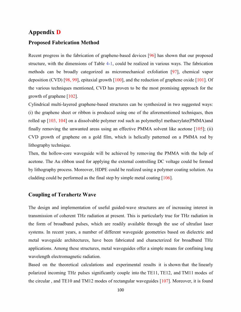
100

Appendix D

Proposed Fabrication Method

Recent progress in the fabrication of graphene-based devices [96] has shown that our proposed

structure, with the dimensions of Table 4-1, could be realized in various ways. The fabrication

methods can be broadly categorized as micromechanical exfoliation [97], chemical vapor

deposition (CVD) [98, 99], epitaxial growth [100], and the reduction of graphene oxide [101]. Of

the various techniques mentioned, CVD has proven to be the most promising approach for the

growth of graphene [102].

Cylindrical multi-layered graphene-based structures can be synthesized in two suggested ways:

(i) the graphene sheet or ribbon is produced using one of the aforementioned techniques, then

rolled up [103, 104] on a dissolvable polymer rod such as polymethyl methacrylate(PMMA)and

finally removing the unwanted areas using an effective PMMA solvent like acetone [105]; (ii)

CVD growth of graphene on a gold film, which is helically patterned on a PMMA rod by

lithography technique.

Then, the hollow-core waveguide will be achieved by removing the PMMA with the help of

acetone. The Au ribbon used for applying the external controlling DC voltage could be formed

by lithography process. Moreover, HDPE could be realized using a polymer coating solution. Au

cladding could be performed as the final step by simple metal coating [106].

Coupling of Terahertz Wave

The design and implementation of useful guided-wave structures are of increasing interest in

transmission of coherent THz radiation at present. This is particularly true for THz radiation in

the form of broadband pulses, which are readily available through the use of ultrafast laser

systems. In recent years, a number of different waveguide geometries based on dielectric and

metal waveguide architectures, have been fabricated and characterized for broadband THz

applications. Among these structures, metal waveguides offer a simple means for confining long

wavelength electromagnetic radiation.

Based on the theoretical calculations and experimental results it is shown that the linearly

polarized incoming THz pulses significantly couple into the TE11, TE12, and TM11 modes of

the circular , and TE10 and TM12 modes of rectangular waveguides [107]. Moreover, it is found

101

that using focusing lenses in combination with collimating lenses a high-efficient coupling

between terahertz beam and waveguide aperture can be obtained. Figure D-2 shows the

schematic a THz-TDS transmission mode setup designed for the optical characterization of the

hollow-core THz waveguides with input/output coupling setup [108].

FIG.D-1 Schematic of the the THz-TDS transmission-mode setup designed for the optical

characterization of the hollow-core THz waveguides(Figure 7 with permission from [108]).

102

LIST OF PUBLICATIONS

The work presented in this thesis has been published in the following peer-

reviewed journal articles:

Razavizadeh, S. M., Ghattan-Kashani, Z., Sadeghzadeh, R., and NavarroCía,

M. "Tunable compression of THz chirped pulses using a helical graphene

ribbon-loaded hollow-core waveguide," Applied Optics 59, no. 14 (2020):

4247-4253.

Razavizadeh, S. M., Ghattan-Kashani, Z., Sadeghzadeh, R. "Terahertz

Waveguide-Based Pulse-Shaper System Analysis and Modeling," Applied

Science, Accepted on Aug. 18, 2020.

Additional Published Work

In addition to the published works in this dissertation, the author has also published

a paper in the research field of terahertz at the following scientific conference:

Razavizadeh, S. M., Ramezanali Sadeghzadeh, Zahra Ghattan, and Miguel

Navarro-Cía. "Compact THz waveguide filter based on periodic dielectric-

gold rings," In 2018 Fifth International Conference on Millimeter-Wave and

Terahertz Technologies (MMWaTT), pp. 42-44. IEEE, (2018).

103

References

[1]. Macinnes, Philip, Kevin Ronald, Graeme Burt, A. W. Cross, A. R. Young, A. D. R. Phelps, I. V. Konoplev et al. "RF pulse compression using helically corrugated waveguides." In AIP Conference Proceedings, vol. 807, no. 1, pp. 474-479. American Institute of Physics, 2006.

[2]. Wang, Kanglin, and Daniel M. Mittleman. "Guided propagation of terahertz pulses on metal wires." JOSA B 22, no. 9 (2005): 2001-2008.

[3]. Manimegalai, Annamalai, Krishnamoorthy Senthilnathan, Kaliyaperumal Nakkeeran, and Padmanabhan Ramesh Babu. "Tapering photonic crystal fibers for generating self-similar ultrashort pulses at 1550 nm." Optical Engineering 55, no. 6 (2016): 067108.

[4]. Ramp, H. O., and E. R. Wingrove. "Principles of pulse compression." IRE Transactions on Military Electronics 2 (1961): 109-116.

[5]. D. K. Barton, Radar System Analysis and Modeling. Boston, MA: Artech House, 2005. [6]. Xiang, Bo. "Integrated Dispersive Delay Line (Ddl) For Real Time Analog Signal

Processing." (2012). [7]. Macinnes, Philip, Kevin Ronald, A. W. Cross, A. D. R. Phelps, Ar Young, Wenlong He, G.

Burt et al. "Helically corrugated waveguides for compression of frequency swept pulses." In 2006 European Microwave Conference, pp. 1320-1322. IEEE, 2006.

[8]. McStravick, M., S. V. Samsonov, K. Ronald, S. V. Mishakin, W. He, G. G. Denisov, C. G. Whyte et al. "Experimental results on microwave pulse compression using helically corrugated waveguide." Journal of Applied Physics 108, no. 5 (2010): 054908.

[9]. Chauhan, Vikrant Chauhan Kumar. "Pulse compression and dispersion control in ultrafast optics." PhD diss., Georgia Institute of Technology, 2011.

[10]. Smirnov, S. V., S. M. Kobtsev, and S. V. Kukarin. "Linear compression of chirped pulses in optical fibre with large step-index mode area." Optics Express 23, no. 4 (2015): 3914-3919.

[11]. O. E. Martínez et al., “Negative group-velocity dispersion using refraction”, J. Opt. Soc. Am. A 1 (10), 1003 (1984)

[12]. R. L. Fork et al., “Negative dispersion using pairs of prisms”, Opt. Lett. 9 (5), 150 (1984) [13]. www.rp-photonics.com/pulse_compression.html [14]. Hädrich, Steffen, Jan Rothhardt, Tino Eidam, Jens Limpert, and Andreas Tünnermann.

"High energy ultrashort pulses via hollow fiber compression of a fiber chirped pulse amplification system." Optics express 17, no. 5 (2009): 3913-3922.

[15]. Weiner, Andrew. Ultrafast optics. Vol. 72. John Wiley & Sons, 2011. [16]. Schober, Andrew Michael. Parametric interactions of short optical pulses in quasi-phase-

matched nonlinear devices. Stanford University, 2005. [17]. Arbore, M. A., O. Marco, and M. M. Fejer. "Pulse compression during second-harmonic

generation in aperiodic quasi-phase-matching gratings." Optics letters 22, no. 12 (1997): 865-867.

[18]. Homoelle, Doug, Alexander L. Gaeta, V. Yanovsky, and G. Mourou. "Pulse contrast enhancement of high energy pulses using a gas-filled hollow waveguide." In Nonlinear Optics: Materials, Fundamentals and Applications, p. TuC2. Optical Society of America, 2002.

[19]. Sato, Masaaki, Takuya Higuchi, Natsuki Kanda, Kuniaki Konishi, Kosuke Yoshioka, Takayuki Suzuki, Kazuhiko Misawa, and Makoto Kuwata-Gonokami. "Terahertz polarization pulse shaping with arbitrary field control." Nature Photonics 7, no. 9 (2013): 724.

104

[20]. Shalaby, Mostafa, Marco Peccianti, David G. Cooke, Christoph P. Hauri, and Roberto Morandotti. "Temporal and Spectral Shaping of Broadband THz Pulses in a Photoexcited Semiconductor." arXiv preprint arXiv:1409.6148 (2014).

[21]. Navaeipour, Parvin, and Marc M. Dignam. "Optimized nonlinear terahertz response of graphene in a parallel-plate waveguide." APL Photonics 4, no. 3 (2019): 034401.

[22]. D. Correas-Serrano, J. S. Gomez-Diaz, J. Perruisseau-Carrier and A. Álvarez-Melcón, "Graphene-Based Plasmonic Tunable Low-Pass Filters in the Terahertz Band," in IEEE Transactions on Nanotechnology, vol. 13, no. 6, pp. 1145-1153, Nov. 2014.

[23]. D. A. Smirnova, et al, “Multilayer Graphene Waveguides,” JETP Letters, 2014, Vol. 99, No. 8, pp. 456–460, 2014.

[24]. Y. Huang, L. S. Wu, M. Tang and J. Mao, "Design of a Beam Reconfigurable THz Antenna With Graphene-Based Switchable High-Impedance Surface," in IEEE Transactions on Nanotechnology, vol. 11, no. 4, pp. 836-842, July 2012.

[25]. D. Correas-Serrano, J. S. Gomez-Diaz, A. Alù and A. Álvarez Melcón, "Electrically and Magnetically Biased Graphene-Based Cylindrical Waveguides: Analysis and Applications as Reconfigurable Antennas," in IEEE Transactions on Terahertz Science and Technology, vol. 5, no. 6, pp. 951-960, Nov. 2015.

[26]. Carrasco, Eduardo, Michele Tamagnone, and Julien Perruisseau-Carrier. "Tunable graphene reflective cells for THz reflectarrays and generalized law of reflection." Applied Physics Letters 102, no. 10 (2013): 104103..

[27]. L Ju, Long, Baisong Geng, Jason Horng, Caglar Girit, Michael Martin, Zhao Hao, Hans A. Bechtel et al. "Graphene plasmonics for tunable terahertz metamaterials." Nature nanotechnology 6, no. 10 (2011): 630.

[28]. Kakenov, Nurbek, M. Said Ergoktas, Osman Balci, and Coskun Kocabas. "Graphene based terahertz phase modulators." 2D Materials 5, no. 3 (2018): 035018.

[29]. Mittleman, D. M., M. Gupta, Ramesh Neelamani, R. G. Baraniuk, J. V. Rudd, and M. Koch. "Recent advances in terahertz imaging." Applied Physics B 68, no. 6 (1999): 1085-1094.

[30]. Cooper, K. B., R. J. Dengler, G. Chattopadhyay, E. Schlecht, J. Gill, A. Skalare, I. Mehdi, and P. H. Siegel. "A high-resolution imaging radar at 580 GHz." IEEE Microwave and wireless components letters 18, no. 1 (2008): 64-66.

[31]. Zhang, Hangkai, Shiwei Wang, Shi Jia, Xianbin Yu, Xiaofeng Jin, Shilie Zheng, Hao Chi, and Xianmin Zhang. "Experimental generation of linearly chirped 350 GHz band pulses with a bandwidth beyond 60 GHz." Optics letters 42, no. 24 (2017): 5242-5245.

[32]. Dolatsha, Nemat, Cheng Chen, and Amin Arbabian. "Loss and dispersion limitations in mm-wave dielectric waveguides for high-speed links." IEEE Transactions on Terahertz Science and Technology 6, no. 4 (2016): 637-640.

[33]. Mittleman, Daniel M. "Twenty years of terahertz imaging." Optics express 26, no. 8 (2018): 9417-9431.

[34]. Lim, Yah Leng, Thomas Taimre, Karl Bertling, Paul Dean, Dragan Indjin, Alexander Valavanis, Suraj P. Khanna et al. "High-contrast coherent terahertz imaging of porcine tissue via swept-frequency feedback interferometry." Biomedical optics express 5, no. 11 (2014): 3981-3989.

[35]. B. J. Eggleton et al., "Integrated tunable fiber gratings for dispersion management in high-bit rate systems," in Journal of Lightwave Technology, vol. 18, no. 10, pp. 1418-1432, Oct. 2000.

105

[36]. M. C. Hoffmann, K.-L. Yeh, J. Hebling, and K. A. Nelson, “Efficient terahertz generation by optical rectification at 1035 nm,” Opt. Exp.,vol. 15, pp. 11706–11713, 2007.

[37]. S.-W. Qu et al., “Controlling dispersion characteristics of terahertz metasurface,” Sci. Rep., vol. 5, pp. 1–6, Mar. 2015.

[38]. Yardimci, Nezih T., Shang-Hua Yang, Christopher W. Berry, and Mona Jarrahi. "High-power terahertz generation using large-area plasmonic photoconductive emitters." IEEE Transactions on Terahertz Science and Technology 5, no. 2 (2015): 223-229.

[39]. Bodrov, S. B., A. N. Stepanov, M. I. Bakunov, B. V. Shishkin, I. E. Ilyakov, and R. A. Akhmedzhanov. "Highly efficient optical-to-terahertz conversion in a sandwich structure with LiNbO 3 core." Optics Express 17, no. 3 (2009): 1871-1879.

[40]. Wang, Feihu, Hanond Nong, Tobias Fobbe, Valentino Pistore, Sarah Houver, Sergej Markmann, Nathan Jukam et al. "Short terahertz pulse generation from a dispersion compensated modelocked semiconductor laser." Laser & Photonics Reviews 11, no. 4 (2017): 1700013.

[41]. O. Mitrofanov, M. Lee, L. Pfeiffer, and K. West, “Effect of chirp in diffraction of short electromagnetic pulses through subwavelength apertures,” Appl. Phys. Lett. 80, 1319–1321 (2002).

[42]. Bratman, VL., Denisov, GG., Kolganov, NG., Mishakin, S.V., Samsonov, S .V., Cross, A., He, W., Zhang, L., McStravick, M., Whyte, CG and others: ‘ Generation of 3 GW microwave pulses in X-band from a combination of a relativistic backward-wave oscillator and a helical-waveguide compressor ’, Physics of Plasmas ,2010, 17, (11), pp. 110703

[43]. Y. Liu, Y. Wu, C.-W. Chen, J. Zhou, T.-H. Lin, and I. C. Khoo, “Ultrafast pulse compression, stretching-and-recompression using cholesteric liquid crystals,” Opt. Express 24, 10458–10465 (2016).

[44]. P. Tassin, T. Koschny, and C. M. Soukoulis, “Graphene for terahertz applications,” Science 341, 620–621 (2013).

[45]. B. Orazbayev, M. Beruete, and I. Khromova, “Tunable beam steering enabled by graphene metamaterials,” Opt. Express 24, 8848–8861 (2016).

[46]. T. Zhang, J. Dai, Y. Dai, Y. Fan, X. Han, J. Li, F. Yin, Y. Zhou, and K. Xu, “Tunable plasmon induced transparency in a metallodielectric grating coupled with graphene metamaterials,” J. Lightwave Technol. 35, 5142–5149 (2017).

[47]. T. Fobbe, S. Markmann, F. Fobbe, N. Hekmat, H. Nong, S. Pal, P. Balzerwoski, J. Savolainen, M. Havenith, A. D. Wieck, and N. Jukam, “Broadband terahertz dispersion control in hybrid waveguides,” Opt. Express 24, 22319–22333 (2016).

[48]. E. D. Palik, Handbook of Optical Constants of Solids (Academic, 1998), Vol. 3 [49]. Huang, Jiayao, MS Aruna Gandhi, and Qian Li. "Self-Similar Chirped Pulse Compression in

the Tapered Silicon Ridge Slot Waveguide." IEEE Journal of Selected Topics in Quantum Electronics 26, no. 2 (2019): 1-8.

[50]. Zheltikov, Aleksei M. "Controlling light pulses and light beams with photonic band-gap structures." In AIP Conference Proceedings, vol. 560, no. 1, pp. 259-272. American Institute of Physics, 2001.

[51]. Droulias, Sotiris, Kyriakos Hizanidis, Demetrios N. Christodoulides, and Roberto Morandotti. Waveguide array-grating compressors." Applied Physics Letters 87, no. 13 (2005): 131104.

106

[52]. Bromley, R. A., and B. E. Callan. "Use of a waveguide dispersive line in an fm pulse-compression system." In Proceedings of the Institution of Electrical Engineers, vol. 114, no. 9, pp. 1213-1218. IET Digital Library, 1967.

[53]. Burt, Graeme, Sergey V. Samsonov, Alan DR Phelps, Vladimir L. Bratman, Kevin Ronald, Gregory G. Denisov, Wenlong He, Alan R. Young, Adrian W. Cross, and Ivan V. Konoplev. "Microwave pulse compression using a helically corrugated waveguide." IEEE transactions on plasma science 33, no. 2 (2005): 661-667.

[54]. Phelps, A. D. R., S. V. Samsonov, G. C. Burt, G. G. Denisov, A. W. Cross, V. L. Bratman, W. He, K. Ronald, and H. Yin. "Compression of frequency modulated microwave pulses in wave-guides." In 4th IEEE International Conference on Vacuum Electronics, 2003, pp. 54-55. IEEE, 2003.

[55]. Liu, Chunlin, Xiaoyong He, Zhenyu Zhao, Fangting Lin, Feng Liu, and Wangzhou Shi. "Tunable graphene near-IR dielectric loaded waveguides." Journal of Physics D: Applied Physics 49, no. 26 (2016): 265102.

[56]. Bass, Michael, Eric W. Van Stryland, David R. Williams, and Williams L. Wolfe. "Handbook of Optics Volume II Devices, Measurements." Handbook of Optics Volume II Devices, Measurements, and Properties 2nd edition by Michael Bass, Eric W. Van Stryland, David R. Williams, William L. Wolfe New York, NY: McGraw-Hill, INC, 1995 (1995).

[57]. Levy, J.S., Burke, P.J., Cohen, L.D. and Cecchini, R., 1993, June. “VCO based chirp generation for broad bandwidth compressive receiver applications (in EW)”. In 1993 IEEE MTT-S International Microwave Symposium Digest, pp. 1113-1115 (1993).

[58]. Zhang H., Yamei, Xingwei Ye, Qingshui Guo, Fangzheng Zhang, and Shilong Pan. "Photonic generation of linear-frequency-modulated waveforms with improved time-bandwidth product based on polarization modulation." Journal of lightwave technology 35, no. 10: 1821-1829 (2017).

[59]. Zhou, Pei, Fangzheng Zhang, and Shilong Pan. "Generation of linear frequency-modulated waveforms by a frequency-sweeping optoelectronic oscillator." Journal of Lightwave Technology 36, no. 18, 3927-3934 (2018).

[60]. Navarro-Cia, Miguel, Carlos M. Bledt, Miriam S. Vitiello, Harvey E. Beere, David A. Ritchie, James A. Harrington, and Oleg Mitrofanov. "Modes in silver-iodide-lined hollow metallic waveguides mapped by terahertz near-field time-domain microscopy." JOSA B 30, no. 1 (2013): 127-135.

[61]. A. Barh, B. P. Pal, G. P. Agrawal, R. K. Varshney and B. M. A. Rahman, "Specialty Fibers for Terahertz Generation and Transmission: A Review," in IEEE Journal of Selected Topics in Quantum Electronics, vol. 22, no. 2, pp. 365-379, March-April 2016.

[62]. Harrington, J.A., “Infrared Fibers and Their Applications,” SPIE Press, Bellingham, WA (2004)

[63]. M. Navarro-cia et al, “Guided propagation of terahertz pulses on metal wire,” J. opt. Soc. Of A., vol.30, no.1, pp.127-136, Jant. 2013.

[64]. M Navarro-Cía, JE Melzer, JA Harrington, O Mitrofanov, “Silver-coated Teflon tubes for waveguideing at 1-2 THz,” J. of Infrared, Millimeter, and Terahertz Waves, pp.542-555, 2015.

[65]. X. Tang, “Elliptical metallic hollow fiber inner-coated with non-uniform dielectric layer,” Opt. Exp., vol. 23, no. 17, pp.8-24, Aug.2015.

[66]. Frisoni, Michael A. Theoretical design study of a 2-18 GHz bandwidth helix TWT amplifier. Rome Air Development Center, Air Force Systems Command, 1987.

107

[67]. S E Zhu, S Yuan, and G C A M Jansse, “Optical transmittance of multilayer graphene,” EPL 108, 17007, 2014.

[68]. Miyagi, Mitsunobu, and Shojiro Kawakami. "Design theory of dielectric-coated circular metallic waveguides for infrared transmission." Journal of lightwave technology 2.2 (1984): 116-126.

[69]. Litchinitser, N. M., et al. "Antiresonant reflecting photonic crystal optical waveguides." Optics letters 27.18 (2002): 1592-1594.

[70]. Foulds, K. W. H., and J. R. Mansell. "Propagation of an electromagnetic wave through a helical waveguide." Proceedings of the Institution of Electrical Engineers. Vol. 111. No. 11. IET, 1964.

[71]. Tsutaki, Kunio, Yoshio Yuasa, and Yosihiro Morizumi. "Numerical analysis and design for high-performance helix traveling-wave tubes." IEEE Transactions on Electron Devices 32.9 (1985): 1842-1849.

[72]. Mavridou, Marina, Konstantinos Konstantinidis, and Alexandros P. Feresidis. "Continuously tunable mm-wave high impedance surface." IEEE Antennas and Wireless Propagation Letters 15 (2015): 1390-1393.

[73]. G. W. Hanson, “Dyadic Green’s functions for an anisotropic, nonlocal model of biased graphene,” IEEE Trans. Anntenas Propag. 56, 747–757 (2008).

[74]. W. Xu, Z. Zhu, K. Liu, J. Zhang, X. Yuan, Q. Lu, and S. Qin, “Dielectric loaded graphene plasmon waveguide,” Opt. Express 23, 5147– 153 (2015).

[75]. A. Andryieuski, F. Pizzocchero, T. Booth, P. Bøggild and A. V. Lavrinenko, "Effective surface conductivity approach for graphene metamaterials based terahertz devices," 2013 Conference on Lasers & Electro-Optics Europe & International Quantum Electronics Conference CLEO EUROPE/IQEC, Munich, 2013, pp. 1-1.

[76]. I-Tan Lin et al., “Terahertz optical properties of multilayer graphene: Experimental observation of strong dependence on stacking arrangements and misorientation angles,” Phys. Rev. B, American Phys. Soc., Dec.2012.

[77]. I. H. Baek, K. J. Ahn, B. J. Kang, S. Bae, B. H. Hong et al., “Terahertz transmission and sheet conductivity of randomly stacked multi-layer graphene,” Appl. Phys. Lett. 102, 191109 (2013).

[78]. C. J. Shearer et al., “Accurate thickness measurement of graphene,” Nanotechnology, vol. 27, no.12 (2016) 125704.

[79]. R. Piesiewicz, C. Jansen, S. Wietzke, D. Mittleman, M. Koch, and T. Kürner, “Properties of building and plastic materials in the THz range,” Int. J. Infrared Millim. Waves 28, 363–371 (2007).

[80]. M. Ordal, L. Long, R. Bell, S. Bell, R. Bell, R. Alexander, and C. Ward, “Optical properties of the metals Al, Co, Cu, Au, Fe, Pb, Ni, Pd, Pt, Ag, Ti, and W in the infrared and far infrared,” Appl. Opt. 22, 1099–1119 (1983).

[81]. Sule, N., K. J. Willis, S. C. Hagness, and I. Knezevic. "Numerical simulation of ac transport in graphene on an SiO2 substrate." In The International Conference on. 2012.

[82]. J. Wang, M. Liang, Y. Fang, T. Qiu, J. Zhang, and L. Zhi, “Rod-coating: towards large-area fabrication of uniform reduced graphene oxide films for flexible touch screens,” Adv. Mater. 24, 2874–2878 (2012).

[83]. A. Aïssi, F. André, and F. Doveil, “New model of a travelling-wave tube,” in 35th EPS Conference on Plasma Phys. Hersonissos (2008), Vol. 32, p. 5090.

108

[84]. R. G. Carter and P. Wang, “Design of helix applicators for microwave heating,” J. Microwave Power Electromagn. Energy 32, 199–204 (1997).

[85]. S. K. Chatterjee, K. Mondal, S. N. Khan, and P. R. Chaudhuri, “Exact mode field solutions and dispersion characteristics of n-layered highindex-core Bragg fiber,” in International Conference on Fiber Optics and Photonics (Photonics) (IEEE, 2012), pp. 1–3.

[86]. J. Luo and C. Jiao, “Effect of the lossy layer thickness of metal cylindrical waveguide wall on the propagation constant of electromagnetic modes,” Appl. Phys. Lett. 88, 061115 (2006).

[87]. T. Rao, “Propagation characteristics of a circular waveguide coated inside with a metamaterial,” Int. J. Electron. 94, 935–942 (2007).

[88]. Banos, A. and Gomez, F. : ‘ Parametric identification of transfer functions from frequency response data ’, Computing & Control Engineering Journal ,1995, 6, (3), pp.137-144.

[89]. I. Llatser, C. Kremers, A. Cabellos-Aparicio, J. Jornet, E. Alarcón, and D. N. Chigrin, “Graphene-based nano-patch antenna for terahertz radiation,” Photon. Nanostr. Fundam. Appl. 10, 353–358 (2012).

[90]. Taschin, A., Bartolini, P., Tasseva, J., Striova, J., Fontana, R., Riminesi, C. and Torre, R.: ‘ Drawing materials studied by THz spectroscopy ’, arXiv preprint arXiv:1703.01770,2017, 6, (3), pp.137-144

[91]. Zaytsev, K. I., Gavdush, A. A., Lebedev, S. P. and Yurchenko, S. O.: ‘ Novel algorithm for sample material parameter determination using THz timedomain spectrometer signal processing ’, Journal of Physics: Conference Series ,2014, 486, (1), pp. 012018

[92]. Huang, Y., Sun, P., Zhang, Z. and Jin, C.: ‘ Numerical method based on transfer function for eliminating water vapor noise from terahertz spectra ’, Applied optics ,2017, 56, (20), pp. 5698-5704

[93]. Islam, Md Saiful, Jakeya Sultana, Ahmmed A. Rifat, Alex Dinovitser, Brian Wai-Him Ng, and Derek Abbott. "Terahertz sensing in a hollow core photonic crystal fiber." IEEE Sensors Journal 18, no. 10 (2018): 4073-4080.

[94]. Naftaly, M., J. F. Molloy, B. Magnusson, Y. M. Andreev, and G. V. Lanskii. "Silicon carbide—a high-transparency nonlinear material for THz applications." Optics express 24, no. 3 (2016): 2590-2595.

[95]. Boscolo, Sonia, and Christophe Finot. "Nonlinear pulse shaping in fibres for pulse generation and optical processing." International Journal of Optics 2012 (2012).

[96]. L. Ye, Y. Chen, G. Cai, N. Liu, J. Zhu, Z. Song, and Q. H. Liu, “Broadband absorber with periodically sinusoidally-patterned graphene layer in terahertz range,” Opt. Express 25, 11223–11232 (2017).

[97]. M. Yi and Z. Shen, “A review on mechanical exfoliation for the scalable production of graphene,” J. Mater. Chem. A 3, 11700–11715 (2015).

[98]. Y. Zhang, Y. Fu, M. Edwards, K. Jeppson, L. Ye, and J. Liu, “Chemical vapor deposition grown graphene on Cu-Pt alloys,” Mater. Lett. 193, 255–258 (2017).

[99]. G. Deokar, J. Avila, I. Razado-Colambo, J.-L. Codron, C. Boyaval, E. Galopin, M.-C. Asensio, and D. Vignaud, “Towards high quality CVD graphene growth and transfer,” Carbon 89, 82–92 (2015).

[100]. H. Chen, W. Zhu, and Z. Zhang, “Contrasting behavior of carbon nucleation in the initial stages of graphene epitaxial growth on stepped metal surfaces,” Phys. Rev. Lett. 104, 186101 (2010).

109

[101]. J.Wang, M. Liang, Y. Fang, T. Qiu, J. Zhang, and L. Zhi, “Rod-coating: towards large-area fabrication of uniform reduced graphene oxide films for flexible touch screens,” Adv. Mater. 24, 2874–2878 (2012).

[102]. V. Kaushik, H. Sharma, A. Shukla, and V. Vankar, “Sharp folded graphene ribbons formed by CO2 laser ablation for electron field emission studies,” Vacuum 110, 1–6 (2014).

[103]. D. Yu and F. Liu, “Synthesis of carbon nanotubes by rolling up patterned graphene nanoribbons using selective atomic adsorption,” Nano Lett. 7, 3046–3050 (2007).

[104]. O. Kit, T. Tallinen, L. Mahadevan, J. Timonen, and P. Koskinen, “Twisting graphene nanoribbons into carbon nanotubes,” Phys. Rev. B 85, 085428 (2012).

[105]. L. G. Martins, Y. Song, T. Zeng, M. S. Dresselhaus, J. Kong, and P. T. Araujo, “Direct transfer of graphene onto flexible substrates,” Proc. Natl. Acad. Sci. USA 110, 17762–17767 (2013).

[106]. Y. Zhang, N. W. Franklin, R. J. Chen, and H. Dai, “Metal coating on suspended carbon nanotubes and its implication to metal–tube interaction,” Chem. Phys. Lett. 331, 35–41 (2000).

[107]. Gallot, Guilhem, S. P. Jamison, R. W. McGowan, and D. Grischkowsky. "Terahertz waveguides." JOSA B 17, no. 5 (2000): 851-863.

[108]. Katyba, Gleb M., Kirill I. Zaytsev, Nikita V. Chernomyrdin, Irina A. Shikunova, Gennady A. Komandin, Vladimir B. Anzin, Sergey P. Lebedev et al. "Sapphire photonic crystal waveguides for terahertz sensing in aggressive environments." Advanced Optical Materials 6, no. 22 (2018): 1800573.

110

چکیده

مخـابراتی بموجـب نیـاز روز افـزون بـه مبحث فشرده سازي حوزه زمان پالس هاي فرکانس باال در سیستمهاي

در کاربردهاي مدرن مخابراتی باند تراهرتز، استفاده . ظرفیت حداکثري انتقال داده از نقش کلیدي برخوردار است

از سیگنالهاي مدوله شده بطریقه مدوالسیون فاز یا با چرپ شدگی فرکانس، ضمن بهبود برد انتقال شـرایط الزم

انتقال را از طریق افزایش حاصضرب دوره زمانی در پهناي باند پالس فراهم کرده اسـت، براي افزایش پهناي باند

. کماکان بعنوان یک عنصر کلیدي در سیستمهاي مخابراتی مورد توجـه میباشـد ازینرو واحد شکل دهنده پالس

گی خطـی یـا شیوه غالب یک پالس زمانی با دوره زمانی حضور کوتاه بوسیله فشرده سازهاي بـا ویژگـی پاشـند

چنـین . غیرخطی که از یک سیستم، خط انتقال یا موجبر بـا پاشـندگی بـاال شـکل گرفتـه، قابـل تحقـق اسـت

ساختاري میتواند از مکانیزم هاي متنوع نوري مبتنی بر افزارهاي مربوطه نظیر منشورها، سطوح متناوب دندانـه

یک . ی با ضریب شکست غیرخطی تحقق یابنداي، آئینه هاي چرپ کننده و موجبرهاي توخالی پرشده با گازهای

بهـره . ویژگی بسیار اساسی و کامل کننده براي هر کاربرد مخابراتی قابلیت کنترل پذیري خروجی نهایی میباشد

گیري از گرافن در تحقق یک سیستم با پاشندگی باالي کنترل پذیربا افـت کـم و بـا قابلیـت کـارکرد در حـوزه

تغییرات مشخصه پاشـندگی آن در ایـن بانـد و هـم تغییرپـذیري قابـل مالحظـه فرکانسی تراهرتز، بموجب هم

در . مشخصه پاشندگی آن با اعمال یک میدان الکتریکی استاتیک بیرونی، راه حلی فن آورانه به حساب می آیـد

یسـی بـا گام نخست انتخاب موجبر دایروي با دیواره تابیده مارپیچی وار بعنوان یک ساختار انتقـال الکترومغناط

قابلیت تامین شرایط پاشندگی باال که از گذشته براي تولید پالسهاي پرقـدرت مـایکروویو و مبتنـی بـر فشـرده

سازي خطی پالس ورودي استفاده شده است میتواند الگوي مناسبی براي هدف ما در ابداع یک سامانه موجبري

مارپیچی در دیـواره مـوجبر اسـتوانه اي، داخـل در این تحقیق ما به جاي ایجاد تابیدگی. مبتنی بر گرافن باشد

طال و بعنوان الکترودهاي اعمال ولتاژ (موجبر استوانه اي یک ترکیب مارپیچی نوار گرافنی بر بستر نوارهاي فلزي

هدف نهایی چنین ساختاري دستیابی به یـک . را با فاصله مناسب تعبیه کرده ایم) کنترل پاشندگی DCبایاس

راهرتزي کنترل پذیر می باشد که با پذیرش یک پالس چرپ با پهناي باندي منطبق بر ناحیه فشرده ساز پالس ت

فرکانسی از ساختار که مشخصه پاشندگی سرعت گروه مثبت میباشد، قادر خواهد بود در خروجی موجبر بارشده

. یجـه نهـایی ارایـه کنـد با نوار گرافنی، پالسی فشرده با کنترل پذیري الکتریکی و فشردگی قابل قبول بعنوان نت

جـایگزین شـده اسـت، چگـونگی ) طـال (عالوه بر آن، با بررسی ساختار دیگري که نوار گرافنی با یک نوار فلـزي

مشارکت پاشندگی ماده بموجب استفاده از گرافن عالوه بر سـاختار هندسـی مـارپیچی نـوار کـه مبـین مولفـه

بطور خالصه مکانیزم عملکرد سـاختار . داده شده است پاشندگی موجبري از پاشندگی کروماتیک میباشد، نشان

درهر دو سوژه مورد بررسی، اینگونه است که به ازاي هر پالس ورودي با دوره زمانی حضور مشـخص تنهـا یـک

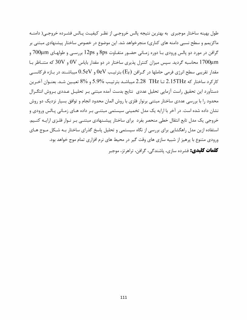
111

دامنـه ( طول بهینه ساختار موجبري به بهترین نتیجه پالس خروجـی از نظـر کیفیـت پـالس فشـرده خروجـی

این موضوع در خصوص ساختار پیشنهادي مبتنی بر . منجرخواهد شد) هاي کناريماکزیمم و سطح نسبی دامنه

و 700mبررسـی و طولهـاي 12psو 8psگرافن در مورد دو پالس ورودي بـا دوره زمـانی حضـور متفـاوت

1700m 0سپس میزان کنترل پذیري ساختار در دو مقدار بایاس . محاسبه گردیدV 30وV که متنـاظر بـا

میباشـند در بـازه فرکانسـی 0.5eVو 0eVبترتیـب (EF)بی سطح انرژي فرمی حاملها در گـرافن مقدار تقری

بعنـوان آخـرین . تعیـین شـد %8و %5.9میباشـد بترتیـب THz 2.28تـا 2.15THzکارکرد ساختار که

دستآورد این تحقیق راست آزمایی تحلیل عددي نتایج بدست آمده مبتنی بـر تحلیـل عـددي بـروش انتگـرال

محدود را با بررسی عددي ساختار مبتنی برنوار فلزي با روش المان محدود انجام و توافق بسیار نزدیک دو روش

در آخر با ارایه یک مدل تخمینی سیستمی مبتنـی بـر داده هـاي زمـانی پـالس ورودي و . نشان داده شده است

. مبتنـی بـر نـوار فلـزي ارایـه کنـیم خروجی یک مدل تابع انتقال خطی منحصر بفرد براي ساختار پیشـنهادي

استفاده ازین مدل راهگشایی براي بررسی از نگاه سیستمی و تحلیل پاسخ گذراي ساختار بـه شـکل مـوج هـاي

.ورودي متنوع با پرهیز از شبیه سازي هاي وقت گیر در محیط هاي نرم افزاري تمام موج خواهد بود

تراهرتز، موجبرفشرده سازي، پاشندگی، گرافن، :کلیدي کلمات

112

1307

دانشگاه صنعتی خواجه نصیرالدین طوسی

دانشکده مهندسی برق


مارپیچی

میدان-دکتري مخابراترساله براي دریافت درجه

:پدید آورنده

سید محمدرضا رضوي زاده

:استاد راهنما

دکتر رمضانعلی صادق زاده

:استاد مشاور

دکتر زهرا قطان کاشانی

1399شهریور ماه

Tunable Graphene-based Pulse Compressor for Terahertz ...

Documents

Transcript of Tunable Graphene-based Pulse Compressor for Terahertz ...