1-165 ?59 THE NCCLELLRN-KERR UATERNAY AND REGIONAL ECONOMIIC /DEVELOPMENT - PHASE 11 STUDY(U) OKLRHOMA UNIV NORMAN

CLIEN ET AL. NOV 85 IWR-CR-65-C-5 DC2-79-C-W4UNCLASSIFIED F/ 53 NL

moImomm flllllllfffffffEEmohmhmhhhEohEmEmmhhohmhmhhhE

Eh~~EhhEhEh

'44

li1.0 16i I "~ E 132 *6

-112 1. 6-

'I °I

MICROCOPY RESOLUTION TEST CHART

-1-1401 -. %rNAOAS-1Q63 A

US Army Corpsof EngineersEngineer Institute forWater Resources

AD-A165 759

The McClellan-Kerr

Waterway and DTICSLECTERegional Economic "2O08M

Development - -

Phase II Study IE:.i

Final Report

* C=,

(..- .'.

November 1985 Contract Report 85-C-58r s! 002

.- , , . %

. . ..-.-: ' .- -. : : . -. ' -- " -- -' - ' - ' " . , , . • • . - '- - ' . . i - ' .: . , ' . .Y : , ,- ' .'.: . ' , '- " •" - -- -

UNCLASSIFIED_

REPORT DOCUMENTATION PAGE BE~FORE COMPLETING FORMI REORT UMBE .2.GOVTACCESID14 W . ECIPIENT'S CATALOG NUMBER

Contract Report 85-C-54. T~V~ 17 Elad Suilfor TYPE OF REPORT b PERIOD COVERED

The McClellan-Kerr Waterway and Regional EconomicDevelopment - Phase 11 Study Contract Report

a PERFORMING ORG. REPORT NUMBEIR

___________________________________ Contract Report 85-C-57. AUTHOR(a) 8. CONTRACT OR GRANT NUMUetR(s)

Chong K. Liev, Professor of Economics and Directorof Econometric Program, and Chung J. Liew, A0Adjunct Assistant Professor of Economics DACW72-79-C-004

9. PERFORMING ORGANIZATION NAME AND ADDRE8S 10. PROGRAM ELEMENT. PROJECT. TASK -:-

Econometric Program, Center for Economic and AE OKUI UUR

Management Research, College of Business Admin.-University ofOklahoma,_Norman,_Oklahoma _____________

IS. CONTROLLING OFFICE NAME AND ADDRESS 12. REPORT DATE

Office, Chief of Engineers, U.S. Army (DAEN-CW) Noebr18Pulaski Building, 20 Massachusetts Avenue, N.W. IS NUMBER OF PAGES

Washington, D.C. 20314-1000 292-14. MONITORING AGENCY NAME A ADDRESS(II different from, ContrelindI Office) IS. SECURITY CLASS. (of Shia report)

jUNCLASSIFIED -_________

IS&. OECL ASSI FI CATION/ DOWN GRADING P.' %SCHEDULE

ft. DISTRIBUTION STATEMENT (of dta Report)

1A;

17. DISTRIBUTION STATEMENT (of the abstract entered in Block 20, It differenat from Report)

Approved for public release--distribution unlimited.

IS. SUPPLEMENTARY NOTES .

)4KEY WORDS (Continue on reveres aids if necooaar)and idenlby b) block number)

_)Multiregional Variable Input-Output Model-,

4 equilibrium price impact ,

20. ABSTRACT tCams a to eee afde If ane.,,ar sd ldenfw, 6v block number)

This study presents estimates of the economic development impacts due tothe savings In delivered Costs of commodities transported on the navigationsystem. Description of the multi-regional variable input/output model'sformulation, calibration, and implementation is presented.

DD , M 1473 cDITIOu oF I MOV 651 ISOL RTE f

SECURITY CLASSIFICATION OF THIS Ph.E fWoe. note Entered)V

. . . . .. . . .7. . . . . . . . . . .

The McClellan-Kerr Waterway and Regional Economic Development-Phase II Study- .*..

Final Report

rSubmitted to the U.S. Army Engineer

Institute for Water Resources

By

Chong K. Liew F

Professor of Economics and Director of Econometric Program

And

Chung J. Liew '

Adjunct Assistant Professor of Economics

(Revised)

Econometric ProgramCenter for Economic and Management Research

College of Business AdministrationUniversity of Oklahoma

This research was performed under a contract funded by the U.S. ArmyEngineer Institute for Water Resources (Contract No. DACW72-79-C-004).We are grateful to Dr. Lloyd Antle for many valuable discussion andassistance sessions on entire manuscript. Credit to the computationof transportation cost saving goes to Dr. Antle. Mr. Ui Choi, Mr. JaiChoi, and Mr. Hai Park provided contribution to this study more than anormal call of duty as research assistants. Any remaining errors are, .... ,however, our responsibility.

November 1985 Contract Report 85-C-5 .'- -

* * * * -.. ..

.**.'**..*.*****.x*** .** . . . " * %..** .*.*-***"

* . .. *. * * * * . , - .... . . . . . . . . .*. , .,

-O-

FOR EWORD

--,Thi5 report presents estimates of the economic development impacts due

to savings in delivered costs of commodities transported on the McClellan- ",-4.

Kerr Arkansas River Navigation System. The multiple-region variable

input/output model is p-&-yed to generate the estimates of project impacts.

This model presents a national view of development impacts from this

transportation system. From $50 million transport savings in 1978 the model

estimates that 454 additional jobs were created In the 26 waterway counties

in Oklahoma and Arkansas, 337 additional jobs were created in the rest of -

Oklahoma and Arkansas and 1,929 jobs were created In the rest of the U.S. '..* . C'? -

These results make a potentially important contribution to the understanding

of the way that transportation projects influence economic development. Far

more jobs are created In those areas which receive the savings in delivered

costs.-% Thus waterway projects should be viewed as contribution to widespread

development impacts. If more "local" development Impacts are sought, other

projects should be sought.

• ' This model has been used to generate estimates of the development

Impacts due to the flood control, hydropower, and recreation features of the

McClellan-Kerr Arkansas River Navigation System. Other applications have

included the Coosa River Navigation Project (Alabama) and the Oklahoma Water

Resources Plan. . y, ) .

E3 R. M .°-H.'-

AE .HAN """ '

iectorstitute for Water Resources ;.

A,.-.

. -. -. . - . -. . . . . . . :*. .i-. -- . . ' -. .... -.. .. ' ', : . - .- " . . . ' '. . . .

17.~~~ ~~~~ an:- 'r 7-l72 '-0

% .

CONTENTS

Page No.

Chapter 1 Introduction ......... ..................... . ...

(1.1) Explanation of this Study ... ............. . . 1

(1.2) Methodology ....... .................... .. . 11(1.3) Summary of Development Impact.. .. ........ . ... 14

Chapter 2 Background Studies ....... .................... ... 21

Chapter 3 The Multiregional Variable Input-Output Model ...... . 29

Chapter 4 Transportation Cost Simulation Models .... . .. '..... 39

Chapter 5 Explanation on the Data ..... ................. ... 49

(5.1) An Estimation of Regional Output and Value Added. ., 49

(5.2) An Estimation of Regional Technical Coefficients. 56(5.3) An Estimation of Regional Final Demand. ...... 58

(5.4) An Estimation of Trade Coefficients ......... . 58."-."

(5.5) Estimation of Industrial Price, Wage Rate and

Service Price of Capital ... ............ . 61

Chapter 6 Estimation of Lowered Transportation Cost . ........ . 63.

Chapter 7 Empirical Findings .................... 79 %

(7.1) Impacts of Industrial Output .. ........... ... 80(7.2) Impact on Gross Regional Products, Wage Payment,

and Tax Receipts ... ................ . 86

(7.3) Employment Impacts ..... ............... . 9 .. 90(7.4) Equilibrium Price Impact ... ............. ... 91(7.5) Structural Impact ................. 96 - -(7.6) Impact on Regional Trade Structure . ........ . 97

TABLES

Table 1.0 Summary of Impact Estimates McClellan-Kerr Arkansas River ..

Navigation System ......... ................... 4

Table 1.1 Annual Change in Industrial Output by Region ... ....... 5

Table 1.2 Transportation Savings as a Fraction of Shipment Value 9 ".

Table 1.3 Composition of the Multiregional. Variable Input-OutputModel (MRVIO) ...... ..................... 13

Table 1.4 The Industrial Impact of the Lowered Transportation Cost 16Table 1.5 Percentage of Transportation Cost Savings by Chemical and

Primary Metal Products. ..... ................ -17

vii

........................ . S

TABLES (continued) "."

Page No. %

Table 1.6 Increase in Output by Sector and Year .......... 19Table 4.1 Input-Output Parameters and Variables in MRVIO Model and

Those in Other Models ..... ................. .. 40Table 5.1 The Variables Employed to Allocate the National Total to

Regional Level ......... .................... 53Table 5.2 Prorated Variables Employed to Allocate the Farm Statis-

tics from State to County Level . . . . . .. .. . .. 54 -Table 6.1 Petroleum Trade Flows and Transportation Cost Saving in

1978 ....................... 68Table 6.2 Chemical Trade Flow in 1978. ............... 68Table 6.3 1978 Transportation Cost Saving ............. 71Table 6.4 The Percentage of Transportation Cost Savings ...... . 77....Table 6.5 Ton's Shipment by Commodity Group in 1977 ........ .. .. 78Table 7.1 The 35 Sector Industrial Classification .. ......... ... 81Table 7.2 Summary of Estimated Changes in Output by Year from

Transport Cost Savings Provided by McClellan-KerrArkansas River Navigation System .. ........... ... 82

Table 7.3 The Five Most Gainers by the Lowered Waterway Transporta-tion Costs (Demand Adjusted Model) ... ........... ... 85

Table 7.4 The Output Multipliers in 1972 ... ............. ... 87Table 7.5 Top Five Gainers in Value Added in 1978 .. ......... .. 88Table 7.6 Top Five Gainers in Wage Payment in 1978 ........... ... 88Table 7.7 Number of Jobs Created by the Waterway in 1978 . . . . . 92Table 7.8 The Percentage Decrease in Equilibrium Prices Because of

the Waterway Transportation in 1978 .......... 94Table 7.9 Percentage Change in Technical Coefficients for Selected

Inputs in 1978 . .. .............. 98Table 7.10 Trade Coefficients of IndL! cy Groups Between Regions in

MRVIO Model, McClellan-Kerr Arkansas River Navigation 100Table 7.11 Change in Regional Imports from the Rest of the U.S. if

the Waterway Wasn't Built ............... 101Table 7.12 Summary of Impacts from Mr 1) Model, McClellan-Kerr

Arkansas River Navigation -. :em, 1978 .. ........ . 102

APPENDICES

APPENDIX I ...... ..................... ............ 107APPENDIX II .......... ............................. 177APPENDIX III ............. ................................ 243

viii I

....... * . °.. -

. . . . . . . . . . . . . . . . . . . . . . . . . .. .. .

Chapter 1

Introduction

ment) impactifth waterway (the McClellan-Kerr Arkansas River Navigation

This iseeoend peart ofaestudy ici he valuaste en omipu deelp

industry sector directly using the waterway and in output by these industries

indirectly affected due to the interaction among industries. The waterway

j decreases costs to users over alternatives or it would not be used. De-

creased costs lead to increased output.

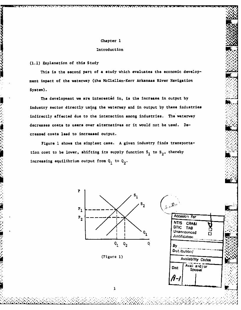
Figure 1 shows the simplest case. A given industry finds transporta-P.9

tion cost to be lower, shifting its supply function S 1 to S 2, thereby

increasing equilibrium output from Qto Q2

P

Si

-- - - Accesion ForNTIS CRA&DTIC TAB

U Q Unannounced__ __ _ __ _ __ __L _ __ _ __ _ Justificatgit

I Q2B

~1 Q2 0 Dist buti;iI. .

(Figure 1) AaIbIt oeAvail ailor

Dist/ ~GI

1pca

. . .

The navigation system is a large multiple purpose river basin develop-

ment project which includes 3 major upstream lakes, 4 main stream multiple ]

purpose dams and 14 single purpose navigation dams. Eighteen (110 ft. by 600 .-\,:;.". .

ft.) locks provide access between the Mississippi River and Catoosa (near

Tulsa) Oklahoma, a route of about 458 miles.

One result is that the shipping cost of many commodities are lowered by

the waterway. The system also provides water and electricity supplies and

offers water related recreational facilities. The upstream dams substantially

lower the risk of the potential flood damages to the riverside communities.

The navigation system provided other benefits; the $1.2 billion con-

struction related spending directly and indirectly stimulated both regional

and national economies. More jobs and income were created because of the con-

struction spending. Kim (1977) estimated that the construction spending in-

creased national industrial outputs by $6.4 billion (1963 constant dollars)

and the income by $2.1 billion. About one half of increased output and about

one third of the income is accrued to the waterway area.

Recreation attendance at the waterway has rapidly increased from 9.4 mil-

lion visitor days (mvd) in 1970 to 23.2 mvd in 1976, a 20.97% regional increase.

A sample survey by Oklahoma State University (Badger, et. al. (1977))

indicates that a visitor spends approximately $9.50 per day. It implies that

" - the recreation-related expenditure in 1976, for example, was $220.5 million.

This spending further stimulated the regional and national economies through "

the multiplier effects. Over 5800 new recreational homes have been developed

around lakes and along the waterway. Recreation users have invested about

2

W".. .. - ..4 _h _' U r r.JM..

.

$11.5 million in recreation equipment in 1974-75. Table 1.0 provides summary

of impact estimates of McClellan-Kerr Arkansas River Navigation System. Rec-

reational impacts were surveyed by Badger et al (1977) and its direct and in-

direct impact was estimated by Antle (1979). Flood damage has been reduced

on an average about $10 million per year since the project was dedicated in

1971. Bank erosion loss has been decreased by about $7 million each year. ,-.

The waterway also offers efficient and cheaper transportation service.

The waterway, paralleling with the highway and railway, provides firms easy £).-

access to the national markets and to the sources of the raw materials. A

relatively inexpensive local wage and tax structure further encouraged the

relocation of industries to the water regions.

A University of Oklahoma survey (Kerr-Foundation (1977)) shows that

cheap labor and land, easy accessibility of markets and raw materials, lower

transportation cost and favorable living conditions were the most important

factors affecting manufacturing locations in the water region. During 1970

to 1975, 144 manufacturing plants expanded their facilities and 353 new plants

were relocated in the water region. More than 40% of these new plants con- ,-.

sidered those factors important in their decision to relocate the plants in

the water counties. The development impact of the cheaper labor and land

cost was quantified by Liew-Liew (1980a, 1980b).

The water counties in Oklahoma and Arkansas experience shift from net out- -

migration to net inmigration in the 1960s. During 1950-60, the water counties

lost 98.6 thousand people through out-migration. However, during 1970-75,

53.3 thousand people migrated into the water counties.

The water counties have grown faster than the rest of the U.S. During the

recession years 1974-75, the industrial output in the water counties was down

only 0.47% while the U.S. experienced severe contraction, down 3.53%. Indus-

. . .. , I - - - . - - . . - " - . -.-.

TT°-7- 77 .7

(Table 1.,0)

Summary of Impact EstimatesMcClellan-Kerr Arkansas River Navigation System

Type Period of Estimates Source

Transportation Demand/Savings 1970-1978 IWR derived from surveysconducted by ResourcesMgmt Project Inc.(1978)Richard BigdaAssociates (1978)University of MissouriRolla (1978)

Recreation 1970-1977 Oklahoma StateUniversity (1975)

Hydropower 1970-1974 Southwestern Division

(1975)

Flood Control 1970-1978 Southwestern Division1980 and Little RockDistricts (1970-78)

Economic DevelopmentImpacts due to 1970-1976

Transporation Savings 1974-1978 University of Oklahoma 1980

Recreation 1974-1975 Oklahoma State University1975.. ~and 1978 Oklahoma State".-- -'

1970-1978n University (1978)Ate(1980)

Construction 1958-1970 Catholic University (1975)

Environmental ImpactsArkansas 1970-1976 University of Arkansas (1980)Okhahoma 1970-1977 Al Young Associates, 1979

Social ImpactsPopulation and Migration 1960-1974 University of Missouri and

Columbia (1975)Small Urban Areas 1960-1974 Dr. Annabelle Motz (1975)Public Sector Response 1960-1976 Texas A&M University 1980

4

e . .• . .. . . . . - .. . ... . .

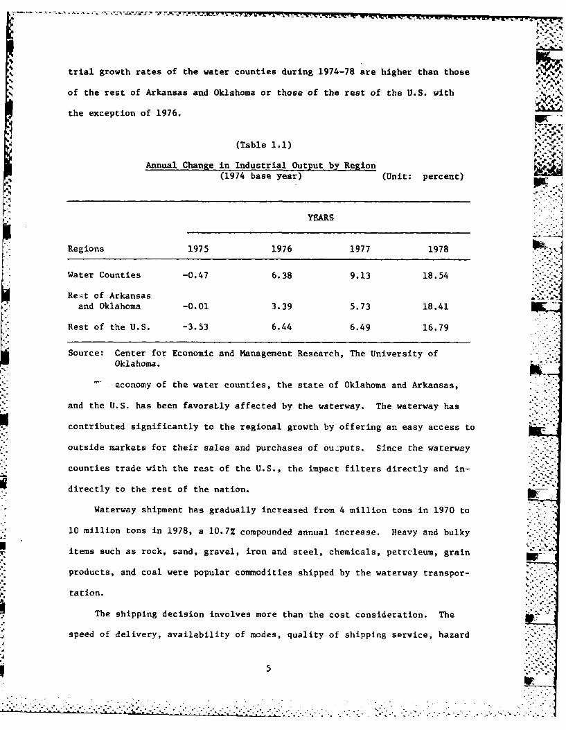
trial growth rates of the water counties during 1974-78 are higher than those

of the rest of Arkansas and Oklahoma or those of the rest of the U.S. with

the exception of 1976.-ao 1,

(Table 1.1)

Annual Change in Industrial Output by Region(1974 base year) (Unit: percent) -9

YEARS

Regions 1975 1976 1977 1978

* Water Counties -0.47 6.38 9.13 18.54

Rest of Arkansas .-and Oklahoma -0.01 3.39 5.73 18.41

Rest of the U.S. -3.53 6.44 6.49 16.79

Source: Center for Economic and Management Research, The University ofOklahoma.

economy of the water counties, the state of Oklahoma and Arkansas,

and the U.S. has been favoraLly affected by the waterway. The waterway has

contributed significantly to the regional growth by offering an easy access to

outside markets for their sales and purchases of outputs. Since the waterway

counties trade with the rest of the U.S., the impact filters directly and in-

directly to the rest of the nation.

Waterway shipment has gradually increased from 4 million tons in 1970 to

10 million tons in 1978, a 10.7% compounded annual increase. Heavy and bulky

items such as rock, sand, gravel, iron and steel, chemicals, petrcleum, grain wproducts, and coal were popular commodities shipped by the waterway transpor-

tation.

The shipping decision involves more than the cost consideration. The

speed of delivery, availability of modes, quality of shipping service, hazard

5-- - -* . .

:-:-:-:-:-:-

5 *':2:":.

and fragility of merchandise, and value of shipments influence the shipping

decision. Therefore, small lightweight products are usually shipped by

trucks, while excessively heavy and bulky items are carried by the waterway,

and railways usually handle moderately heavy and intermediate size items.

But many factors can combine to result in truck and rail, carrying heavy

and bulky contents. Therefore, waterway shipment may complement or substi-

tute for other modes. For example, inland-located plants use trucks for parts

to haul and the waterway for the rest because this combination provides the "" "

best and most economic service. The complementary nature of water and truck

modes stimulates development of both waterway and highway system. One of

the significant development in the waterway area has been development of an

interstate and toll road system paralleling the waterway, essentially in the

same area where the waterway was developed. These development has probably

diverted traffic from rail. However, it will be shown that increase in rail

traffic due to increased industrial output replaces much of the traffic and

provides higher revenue products to be carried by rail and truck.

This study shows how the lowered transportation cost stimulates the eco-

nomies of the water counties, the rest of Oklahoma and Arkansas, and the rest

of the U.S. The Phase I Study (Liew-Liew (1980a)) introduced a multiregional

variable input-output model and analyzed the economic impact of the lowered -'-

transportation costs on the regional. and national development.

The three-region ten sector model in the Phase I Study was based on the

1963 interindustry and interregional flow data compiled by Kim (1977). The

Phase I Study employed a hypothetical transportation cost change for the eco-

nomic simulation. The study demonstrated that a change in transportation

cost changes the regional trade pattern and the industrial structure of all Nd-.

three regions. Changes in structure occurs as using industries substitute

6* . .. . - -. .- -'

Map 1

REGIONAL CLASSIFICATION FOR THE MRVIO MODEL

1. THE WATERWAY COUNTIES

Twenty-eight counties In Arkansasand Oklahomna surround the ArkanaRiver navigation plan. This 22.000 -2j -- :square mile area Includes the following

1. Osage 15. Sebastian2. Nowata 16. Franklin3. Rogers 17. Johnson

14. Tulsa 18. Logan-75. Pawnee 19. Popej46.: Creek 20. Yeill

7. Wagoner 21. Conway8. Muskogee 22. Perry9. McIntosh 23. Faulkner p

* 10. Pittsburg 24. Pulaski.. -- -- .11. Haskell 25. Jefferson

___ 12. Sequoyah 26. Arkansas17.' 13. Crawford 21. Lincoln

-P12 1 14. LeF lore 28. Desha

g 5 ~9

7 27

. . . . . . . . .-.- - - - -- - - - - - --.

more of those inputs whose costs have decreased via transport savings.

The Phase I Study provided interesting insights for transportation

planners and decision makers about the development potential of the lowered d-"P

transportation cost on regional and national economies. It also demonstrated

the workings of the multiregional variable input-output model.

The waterway system was open for navigation to Catoosa. in early 1971.

The waterway reduces shipping costs for the heavy and bulky items such as

grains, chemicals, iron and steel, rock, sand, petroleum, and coal. How much

does the lowered transportation cost contribute to the regional national de-

velopment? To answer the question, the base year 1963 were updated to the

1972 level, and the industries were further disaggregated into 35 sectors.

The thirty-five industrial classifications cover every important industry in the

region. The regional classification has been changed from the Phase I Study

so that it reflects finer details of the economy of the water region. The

Phase I Study employs three OBE areas (117-119) as region 1, the rest of the

Southwest (Oklahoma, Arkansas, Louisiana, Texas) as region 2 and the remainder

of the U.S. as region 3.

The Phase II Study defines the 28 waterway counties as one region, the

rest of Oklahoma and Arkansas as another region, and the remainder of the U.S.

as the third region.

A reliable estimate of the lowered transportation cost is the most im-

portant input for accurate estimation of its development impact. The Phase I ..

Study simulated the multiregional variable input-output model under hypotheti-

cally chosen value of the transportation cost change. This study estimated

the costs of transportation with and without the waterway transportation, and

calculated the percent change in transportation cost by sector and region.

The waterway statistic series published by Corps of Engineers annually

show complete statistics by commodity and waterway. Two Tulsa consulting

* 8 . . . *

F . . . . . . . . . . .. . . . . . . . ' . . . . ; .. . .. . .. . . 1 -: = . . : . _. - . -_ ' . - . " 1 . .; . -': . .. - -" " - - " "." - - - ' - " '; ' " -". .-"*

firms in Oklahoma (Resource Management Inc. and Richard Bigda Associates)

and University of Missouri, Rolls, Missouri conducted surveys on the shipments

-, which utilized the waterway and other transport modes. They gathered inf or-

mation on tons shipped, transit time, value of shipment, mode chosen, rate

per ton-mile, handling cost, hauling distance and origin-destination.

Transportation cost is defined to include hauling, handling and time

costs. Transportation cost saving by waterway transportation over the most

-' competitive alternative modes was computed for each commodity for years of

1978 to 1974. For example, wheat is the major item in grain sector carried by

* the waterway transportation. During 1978, the transportation cost saved by

the wheat was estimated $1.39 million. Half of the saving ($695 thousand)

- was made by shipment originating in waterway counties tcu the rest of the U.S.,

* and the remaining half was saved by the shipment originating in the rest of

* Oklahoma and Arkansas to the rest of the U.S. The total value of grain trans-

* action from the waterway counties to the rest of the U.S. was approximately

$165.2 million. Therefore, the transportation cost saving for grain shipment

from the watir counties to the rest of the U.S. was computed to be a 0.4207

percent, (- 100 x 695/165200), or about one half of one percent of the value

of grain shipped from the waterway counties to the rest of the U.S. in 1978.

(Table 1.2)

Transportation Savings as a Fractionof Shipment Value(ni: ernt

Commodity Origin Dest. 1978 1977 1976 1975 1974

Grain Farm (5)* 1 3 0.42 0.11 0.36 0.25 0.24

Oil Bearing CropFarm (6) 1 3 1.54 1.87 1.73 1.49 1.21

Chemicals (14) 1 3 6.37 4.48 4.07 4.11 4.72

Petroleum (15) 2 3 0.67 0.79 0.56 0.22 0.40

Primary Metal (19) 3 1 0.50 0.62 0.34 0.39 0.12

Coal (25) 2 3 5.17 2.29 1.09 0.79 1.37*Other Mining (27) 1 3 8.53 15.47 9.19 8.43 27.52

*The figure inside the parenthesis is industry number. -

9

A'.Q~K: ~:-

Aggregates which belong to other mining have substantial-reduction of%

* ~transportation cost by the waterway shipment (26%0-50% transportation costa.. V

savings), followed by coals (0.8%,,,20%), chemicals (0.8%,,-9.3%), primary metal

(0.036%,%,0.67%), and petroleum (0.16%,Q.7%).1 afcthan

How does this change in transportation cost afettenationalan

regional output? To answer this question, we present an underlying relation

between transportation cost and industrial output. a-

The output in the multiregional 1-0 model is determined by the following

balance equations; i.e.,

x- (I-TA) Ty(-)

*where x is a vector of regional output;

T is atradecoefficients matrix;

* A is a regional technical coefficient matrix;

y is a vector of all regions "final demand received."2

As an illustration, we consider 1972 trade coefficients (T) of chemical

* goads (industry 14), their final demand received (y), and their final demand

* shipped (F).

S12.58 0.02355 0.0176 0.0003 134\

94.70 0.1289 0.1212 0.00271 258

17343.72 0.8476 0.8612 0.9970 17059)

F T y

The trade coefficient denotes that 2.3% of chemicals consumed in the

water counties was from local chemical company, 13% of them was from the rest

of Oklahoma and Arkansas and 84.7% was from the rest of the U.S. The waterway

lowers the transportation cost which in turn changes the trade coefficients... .

tDetails of transportation cost saving are in Table 6.4 in Chapter 6.

2 Following Moses' (1955) terminology.

10

For example, the 1978 trade coefficients of chemical products associated with

the lowered transportation cost become;

0.2358 0.01693 0.00033

112905 0.12139 0.00266

,0.84737 0.86168 0.99702)

It is evident either F or y should be altered to maintain the balance

equations (F=Ty). We assume that final demand shipped (F) is fixed and final

demand received (y) is varied because it is more likely that the endusers will

adjust their consumptions when trade coefficients chanp

(1.2) Methodology

The transportation facilities and services available in a region play a

crucial role in promoting regional development and trade flow. The economic

impact of the McClellan-Kerr Arkansas River System is not confined to the

waterway counties. The impact is evident in all areas which trade directly or

indirectly with the waterway system. Land use, industrial location, interin-

dustry flow, physical distribution of goods, market structure, employment, and

interregional trade flow are directly and indirectly affected by the navigation

system and services.

The multiregional variable input-output model (MRVIO) introduced in this

study investigates the interrelationship between the navigation system and its

regional impact. The model requires input elasticities and technical progress

coefficients as input parameters. The input parameters for the Phase II study

were estimated from the 1972 1/0 tables and various census materials. Under

the Cobb-Douglas production frontiers, the value share after tax becomes the .-.

input elasticity. The technical progress parameters were obtained from the

input elasticities. The exogenous variables of the model are transportation

:'"' -' " "- -"* " "a ' ' ' " ' . .. . .... . . -" -....- - • - .. .. . .... " i

cost, wage rates, service price of capital, tax rates, and final demands.

The transportation costs include both terminal, linehaul, and time costs. In-

put parameters and exogenous variables determine the endogenous variables:

output, income, employment, regional technical coefficients, trade coefficients,

industrial prices, and various multipliers. These variables can predict many -

variables of policy interest such as regional growth, development, and indus- .

trial locations; structural changes of industries; trade flow patterns; physi-

cal distribution of goods; and regional inflation. Table 1.3 shows details of

these relationships, however this study will concentrate on the impact of lowered ~

transport costs due to the waterway on regional and national development for

the period of 1974 to 1978.

The MRVIO model is consistent with the well-developed theory of firms.

* The basic hypothesis of the model is that firms are sensitive to cost change.

* A change in one input cost will result in a remix of inputs in order to maxi-

mize profit. A change in input composition and output distribution will alter

*regional technical and trade coefficients .Unfortunately, the conventional

multiregional input-output models assume a fixed regional technical coefficient

and a fixed trade coefficient. These technical and trade coefficients enter

the conventional input-output model as fixed parameters. In our analysis, the

* technical and trade coefficients are endogenous variables to the model.

The Arkansas Navigation System has provided energy-efficient transporta-

tion services to ix'dustries located in the waterway region. These industries

can buy and sell within a large market area at relatively low costs. The n~avi-

gation system not only lowers the cost of inputs, but also encourages outside

*industries to relocate in the waterway region. Easy access to the waterway

Exception is Leontief-Strout's gravity model (Leontief-Strout (1963)).The model assumed affixed regional technical coefficients. However, the tradecoefficients are endogenously determined by the gravity model.

* 12

00 1 to 0 %93 . 2 %6- 0 44r* 10 .

60 ov4 0 .0 0 0 .0 "o0) .jtou t N0 :3 4) 5.) $14 0 6-14

X:0 4JH0 c: A-5) U) 01)4 00. 60a L) " 4

cc0. C: -44 '-' v40 C

to 5.. 04 -0 0) v4 w vi t:>4 v--0v- 10 w 0s 4 v4 0 W1d-o 4 coI 0- 5

w4 V.04-' I p~ 404 0 000 t or 0 di- 0)04 0 -45 FA 41 0 ) -01 1 -4 0 0 'L0V10 -1440 : )~ 10 0 0 4 1 to 0-H "4I 4 41N 60z 1 010C .0 0 w 54 0o ;-0%obo 00 0 :

4) 9 54 p- m1 IJ w z.5 .- 141i w 0 0V4 1 .In H)C~- 044' >~ E-4)

01 0a0 93 r~v4 0

050 0 co4 0 14-I001 a E- o0 '44 00 r4 I .v4

al1. c 0-H 0 0 01 0-- 01 -0 0d u-I 1JDo0t -4 w r4 4 C) t -0 4 0 0io -I V14 :5-r0 -- m-4 V~ 0d u010 u. 05z. 5.4 *0 ato-4

00 wO. &j- cov 0 d -v)4 wO 51 0)0 5 41 0.u0-I 0 us COO 0O-4 0Ov-40 544 014- 541 (Afl ) 1 - 4

:) - : w 00. v-4e Vr 1 V1 '. u' 00 0 m 0.14V-0 4- C60 000 u0 .40 0o0o) 41J '0v-or41 4J 1 -

030 Oo o-H41 14- 1-av- 4 .0 4 054 $-4 r4 001H 10 P4~0 g:44 E41- 1-0 6-14 P.0. 0 00

0"4' &j w

' 40 -r (A0jc -r4 w ,

1.54 &J0

04 0 P4 0 M

to ,-q c001r4j t.4 0

0H 0 $40

* 0

0'0 0 0

to 4 v4 A

000 w 01on Ou- 41

>1 . 0I 0 (010 0 4' 4-1 5) 0

5.v 05 0 00 0

v- 4 -r4 "4 V) cc 1-ca :M 03 -4U1~

04'4Go 15 00 0 4.0W - .-J '-4 t

U) 1 01 0Cd W

01 Lo.- .,4 V40d01 015 41 Ai a1 40 0

4 Ai w & 0 4) 0 0 s : '4)W)I 1 0 0 0 rA 0 -4 V)AlAB

to W 0 A .,4 0 0 01 4.'4j U :3 ., 0 0 03 54 cO q

, 04 &j-454 .14- t

0 FA-l 4 0(na-v-I 0 0 ) 01

00 . 1-4 %64. >) V4U nq

13

encourages the product mix in favor of purchasing inexpensive materials from

a wide area. This optimizing behavior of firms is reflected in the MRVIO model. .-

The model is derived from the dual relationship between the production .. '. "

frontier and the price frontier. Any cost-minimizing input or output quantity .

can be expressed in terms of the input prices. The price frontier is obtained ,-

by replacing the quantity variables in the production frontier with the equili- W.C.

brium price variables. The price frontier is expressed in terms of input

elasticity, transportation cost, wage rates, service price of capital, and tech-

nical progress parameters. A change in transportation cost will change the ._.

profit-maximizing price level which in turn determines the regional input-

putput coefficients and the trade coefficients. Industrial output, income,

and employment in each region identify the industrial location, land use pat-

terns, and regional growth. The trade flow identifies the physical distribu-

tion of commodities and the regional market structures. The model answers

many policy-sensitive questions. It measures the impact of the waterway on

regional development and predicts industrial location, interregional trade

flow, interindustry purchases, and market structure of industrial sales. In

the present study, the model was employed to determine the influence of lowered

transportation costs, due to the waterway, on regional economic development;

but it could be employed to measure the impact of other transportation services.

The potential advantages of this model were documented in previous re-

search (Liew-Liew (1980a, 1980b)). Finally, the MRVIO model is relatively

- inexpensive to construct since most of the data can be obtained from secondary

sources; i.e., published data.

(1.3) Summary of Development Impact

The U.S. economy was divided into three regions; the first region is the

* waterway counties which include 28 water counties in Oklahoma and Arkansas.

14. - . . .• .o-

&. % ' -- - " " ." " AP.a'a - -.r--'-... - -

"-" - _ _._ . . .. _ - - -

The second region comprises the remaining counties of Oklahoma and Arkansas.

The last region is the rest of the U.S. (the remaining 48 states and District

of Columbia). ~

The industry in each region was disaggregated into 35 industrial sectors.

This classification represents the details of industrial structure of each

regional economy.

The waterway lowers the cost of transportation. The lowered transporta-

tion cost reduces sales price of industrial outputs and the lowered price

expands its markets. The enlarged market stimulates industrial production,

employment, and personal income.

The lowered transportation cost stimulated U.S. industrial output by

$118.82 million per year over that which would have occurred without the pro-

E ject during the sample period of 1974-1978. The waterway counties and the

rest of Oklahoma and Arkansas have gained approximately $20 million of indus-

trial output each, and the rest of the U.S. $79 million. The expanded output

generates more value added and personal income. Total U.S. personal income

was increased by 34..26 million because of the lowered transportation cost.

The waterway counties and the rest of Oklahoma and Arkansas both gained more

than 5.7 million of personal income each, and the rest of the U.S. $22.8 million.

Average transportation cost saving per year was approximately $38 million

during the sample period. This $38 million transportation cost savings re-

sulted in industrial expansion of $119 million, making the output-transportation

cost saving ratio approximately 3.13. Transportation cost savings vary

over year, ranging from $51.5 million in 1977 to 22.7 million in 1975. Impact

on industrial output differs year to year because of (1) the magnitude of

transportation cost savings and (2) the composition of commodities involved in

the transportation cost savings. In general, the larger the transportation

U 15

(Table ..j 4)

'The Industrial Impact of the deLowered Transportation Coat

(Unit: Million current dollars)

1978* 1977 1976 1975 1974 Average

1) Waterway Counties 27.54 22.64 17.06 13.36 18.50 19.82

2) The Rest of Arkansasand Oklahoma 24.82 22.71 18.00 15.00 20.07 20.01

3) The Rest of U.S. 102.00 89.95 66.58 63.16 72.70 78.87

4) Total U.S. 154.86 135.30 101.64 9.1.52 111.27 118.82

*5) Tranup. CostSavings bythe Waterway 50.06 51.51 32.20 22.76 33.21 37.95

6) The Ratio(4/5)*3.08 2.63 3.15 4.02 3.35 3.13

Medium estimate

Ratio of total industrial impact to transportation cost saving.

*cost was saved for the year, the greater the industrial output was expanded in

the economy. In 1975, the industrial impact was the smallest among five sample

because the transportation cost saving was minimal in that year. However, the

industries which had largest transportation cost savings did not necessarily

increase output most. The importance of the composition of transportation

saving is shown, for example, in large transportation cost savings in 1977,

but in the year's industrial output increase was smaller than in 1978. The

industrial output was stimulated by $135.3 million in 1977 which was smaller

than $154.36 million of 1978. The 1977 transportation cost saving was $51.51

million which is slightly higher than $50.06 million of 1978.

The ratio of industrial expansion to the transportation cost saving varied

over the sample period largely because of the composition of commodities in-

volved in transportation cost savings. The ratio becomes as high as 4.02 in

16

in 1975 and as low as 2.63 in 1977.

What are the industries whose transportation cost (tc) is more sensitive

to the industrial output? A closer look reveals that chemical products and

primary metal products have a strong industrial impact when they are traded

with the rest of the U.S.

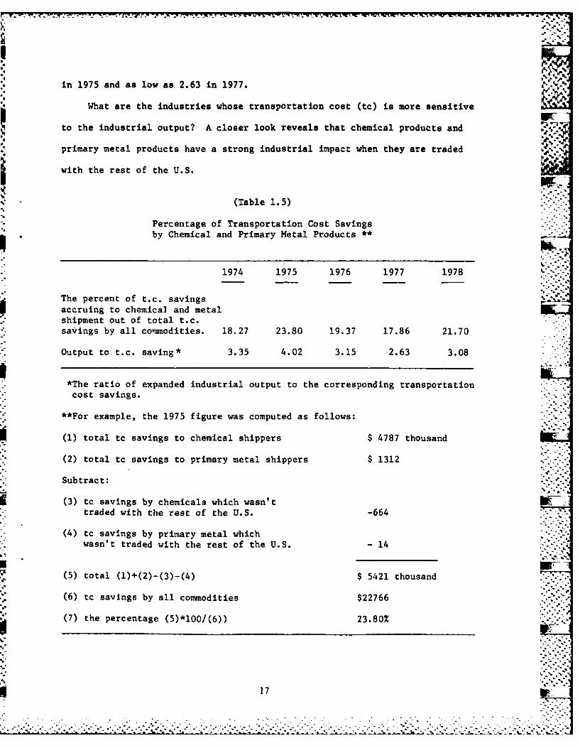
(Table 1.5)

Percentage of Transportation Cost Savingsby Chemical and Primary Metal Products **

1974 1975 1976 1977 1978 - -

The percent of t.c. savingsaccruing to chemical and metalshipment out of total t.c.savings by all commodities. 18.27 23.80 19.37 17.86 21.70

Output to t.c. saving* 3.35 4.02 3.15 2.63 3.08 .

*The ratio of expanded industrial output to the corresponding transportation .cost savings.

**For example, the 1975 figure was computed as follows:

(1) total tc savings to chemical shippers $ 4787 thousand

(2) total tc savings to primary metal shippers $ 1312

Subtract: -.

(3) tc savings by chemicals which wasn'ttraded with the rest of the U.S. -664 ---

(4) tc savings by primary metal which -,.-wasn't traded with the rest of the U.S. - 14

(5) total (1)+(2)-(3)-(4) $ 5421 thousand

(6) tc savings by all commodities $22766

(7) the percentage (5)*100/(6)) 23.80% ""-

17. -X - A- .- -. . . . .. . . . . . . . . . . . . . . . . . . . ..

~~~~~~~~~~~~~~~~~~....-......• ..............- >..........-... ...-... . .. - . .. -- -a... r.." ...--

'S F W P . - r % , n , - . . w j -- J . N. . P j F . M . . d - -. V W 1 i? L . W W ... *"" .5 . . f W J 7-W-.- " * 7o- * -' - ' _ * - -

V

The year 1975 which has the highest percentage of transportation cost

(tc) savings by chemical and primary metal products (23.80%) yielded the lar-

gest output to tc ratio. Similarly, in 1977 when this percent is the smallest

among five sample, the output to tc ratio becomes the smallest among sample.

The output to tc saving ratio may depend on many other factors such as the

trade structure, the industrial structure, and spatial patterns of market.

However, the table (1.5) clearly indicates that output changes are very sen-

sitive to transportation savings by either chemical product or primary metal

product.

What are the industries which were benefitted most by the waterway trans-

portation?

In the waterway counties, other mining (sand, gravel, crushed rock,

bauxite) is the most conspicuous gainer because of the waterway transporta-

tion. Coal, chemicals, petroleum, primary metal, rubber, and grain also show

strong gains during the sample period.

In the rest of Oklahoma and Arkansas, grain and other farm alternate the

top gainer spot. Chemicals, petroleum, primary metal and rubber are other top

gainers due to the waterway transportation.

In the rest of the U.S., chemical industry becomes a commanding gainer,

followed by primary metal, service, other mining, petroleum, and utility ser-

vice.

Table (1.6) shows the impact of the waterway on industrial output for

selected industries in each region.

18

........................................

, . .-.*,.-'i".: .i:i? ?: ",. - . " ' _ _ _._.'._._-..__ _ _ _ -__ _ _ _ -_'_ _ ._ _ _.. " _. _.r _ _" _ _ __" " " " " " _ _ "

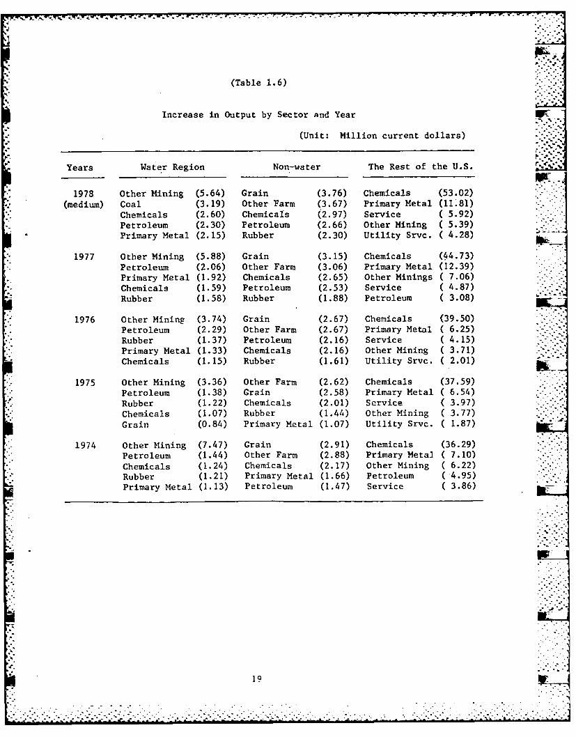
(Table 1. 6)

Increase in Output by Sector and Year

(Unit: Million current dollars)

Years Water Region Non-water The Rest of the U.S.

1978 Other Mining (5.64) Grain (3.76) Chemicals (53.02)(medium) Coal (3.19) Other Farm (3.67) Primary Metal (11'81) .1

Chemicals (2.60) Chemicals (2.97) Service ( 5.92)

Petroleum (2.30) Petroleum (2.66) Other Mining ( 5.39)Primary Metal (2.15) Rubber (2.30) Utility Srvc. ( 4.28)

1977 Other Mining (5.88) Grain (3.15) Chemicals (44.73)

Petroleum (2.06) Other Farm (3.06) Primary Metal (12.39)

Primary Metal (1.92) Chemicals (2.65) Other Minings (7.06)Chemicals (1.59) Petroleum (2.53) Service (4.87)Rubber (1.58) Rubber (1.88) Petroleum (3.08)

1976 Other Mining (3.74) Grain (2.67) Chemicals (39.50)Petroleum (2.29) Other Farm (2.67) Primary Metal ( 6.25)Rubber (1.37) Petroleum (2.16) Service ( 4.15)

Primary Metal (1.33) Chemicals (2.16) Other Mining ( 3.71)Chemicals (1.15) Rubber (1.61) Utility Srvc. ( 2.01)

1975 Other Mining (3.36) Other Farm (2.62) Chemicals (37.59)Petroleum (1.38) Grain (2.58) Primary Metal (6.54)Rubber (1.22) Chemicals (2.01) Service (3.97)Chemicals (1.07) Rubber (1.44) Other Mining (3.77)Grain (0.84) Primary Metal (1.07) Utility Srvc. (1.87)

* 1974 Other Mining (7.47) Grain (2.91) Chemicals (36.29)Petroleum (1.44) Other Farm (2.88) Primary Metal ( 7.10)Chemicals (1.24) Chemicals (2.17) Other Mining ( 6.22)Rubber (1.21) Primary Metal (1.66) Petroleum ( 4.95)Primary Metal (1.13) Petroleum (1.47) Service (3.86)

r-1

19-

'p.'p.

I.

4.

rA~0

a, SI

a'

K-..

'

I-

I. ~

SI

' .N.

p

r

' . '

Chapter 2

Background Studies%

Economists have long been aware that transportation facilities such as

highways, expressways, waterways, and railways contribute to regional growth

by influencing industrial and trade structures. Recently, interest in trans-

portation planning has focused on developing an accurate, workable model for

evaluating the economic impact of transportation facilities on the surrounding Il

regional economics. A number of interesting models were introduced to measure

the economic effect of transportation facilities. The transportation facilities

were assumed to lower the transportation costs, and several models identified

the relationship between cost of transportation and regional development.

One of the models that has successfully related transportation cost to re-

gional development is Harris's multiregional, multi-industry forecasting (MRMI)

model. (Harris (1973, 1974)

21..-. I

.4-5.°

* 212

- ~ *2- . .--

The Harris model is a regional econometric model which covers 216 sectors.

N The structural equations of the model were fitted by the county data for the

period from 1965 to 1966. Changes in regional output were explained by input

prices and the agglomeration variables that firms faced in the location. The ,

input prices include marginal transportation costs, wage rates, land prices,

and cost of capital. The agglomeration variables include all other key non-

price variables that affect the industrial location. An example of such a

variable is congestion.

The output variables determine other regionally important variables such

as employment, population, earnings, personal income, personal consumption,

government expenditures, investment, and foreign exports.

The marginal transportation cost, which is computed by the transportation

cost linear programming algorithms, plays a key role in determining industrial

location and influences regional economic activity. Improving a transportation

facility lowers the marginal transportation cost which, in turn, stimulates

regional output and other regional economic activity. The MRMI model forecasts

regionally important economic variables from 1979 to 1985 for each county with-

in each standard metropolitan statistical area (SMSA). The regional forecasts

from MRMI model were adjusted to conform with Almon's national forecasts (Almon

(1974)). Determining supply and demand simultaneously is considered the strong

point of this model. Another interesting feature of the MRMI model is that

transportation cost is included in the output share equation. But like many

other regional econometric models, a paucity of regional data forces the model

builder to select the explanatory variables on empirical rather than theore-

tical grounds. The estimated coefficients may vary from one sample to another.

On-going economic forecasting and impact analyses require stable estimated coef-

199 industrial, 28 construction, 8 governmental, 69 equipment purchasing,--

6 population, 2 extra imports and 4 extra sections.

j 22*..* . . .. .. . . . . . . . . . . .

.. .. .. .. .. .. . .. .. .. .. .. .. .. .. .. .. .. . . . .

ficients; the lack of such stability necessitates re-estimation of the coef-

ficients each year. Another weakness of the model is that it fails to consider

the maximizing behavior of firm. According to a well-developed theory, a firm

mixes its variable input costs to maximize profit. Transportation cost is

simply one of many input costs, along with the purchase price of intermediate

input, wages, land cost, and the service price of capital. The MRMI fails to

incorporate all these input costs into the model calibrated, since many esti-

mates were statistically insignificant. Currently, Harris is expanding the

data base to improve his empirical results. _

Another popular approach to relating trade flows to regional development

are multiregional input-output (MRIO) models developed by Isard (1951), Moses

(1955), Leontief-Strout (1963), and Polenske (1970). The MRIO models utilize

three sets of basic data: regional technical coefficients, trade coefficients,

and regional final demand. Under the assumption of fixed technical coefficients

and fixed trade coefficients, 1 the models predict industrial output, income,

employment, trade flow, and interindustry transactions. Regional final demand

enters the models as an exogenous variable. Regional growth is usually identi-

fied by a change in the final demand component. Output, income, and employment

multipliers are popular tools to identify this change. These multipliers are

the chain reaction of a one-dollar change in final demand in one region on the

industrial output, income, and employment in all regions. Occasionally, a

model is simulated by changing a set of technical coefficients or a set of

trade coefficients. New technology or energy conservation measures justify

a change in technical coefficients. A decrease in transportation cost due to ___

a better transportation facility justifies a change in both the technical coef- .

ficients and the trade coefficients. The simulation method is often used to

ILeontief-Strout (1963) specifies that the trade coefficients areendogenously determined. ?-'

23

S* r. ..... . .

determine the regional economic impact of new technology, energy conservation-'-.,'

methods, or highway construction.

The MRIO model is one of the most promising tools currently used to fore- -

cast regional growth and interregional trade structure. However, the most 'Hserious drawback of this approach is its assumption of fixed technical coef-

vicients and fixed trade coefficients.

Amano-Fujita (1970).modified the multiregional input-output model so that

transportation cost explicitly entered the model. Following Moses' multi-

regional input-output model (1955), the regional input-output coefficient is

assumed to be the product of the trade coefficient and the regional technical

coefficient. This model specifies that regional technical coefficients and

hi trade coefficients depend on transportation cost. Improving a transportation

facility in a region lowers the transportation cost which in turn increases

the trade coefficient and decreases the transportation purchase coefficient.

The transportation purchase coefficient denotes the input coefficient of trans-

*portation service by industry (the row coefficients of the ttansportation

sector or a a r J-1,...n; r=l,...m, T=transportation service sector). An in-

* crease in the trade coefficient and a decrease in the transportation purchase

coefficient create a chain impact which affects both the regional and the

* national economy. -The economic impact of improving transportation facilities

can be measured by tracing these two changes.

The Amano-Fujita econometric model suggests an interesting way to intro-

duce transportation cost into the multiregional input-output model. However, ' 'j

it assumes that orly one row of technical coefficients--the transportation

purchase coefficients--depend on the cost of transportation and that all other

technical coefficients remain unchanged. Any change in a transportation pur-

chase coefficient is completely absorbed by a value-added coefficient. The

24

model also assumes that only trade coefficients between regions where trans- A

portation costs were changed are affected by the cost change. All other trade

coefficients are assumed to remain unchanged. The model also implicitly as-

sumes that both trade coefficients and technical coefficients are independent

of any change in labor cost, land price, capital cost, purchase price of input,

2, or sales price of output. The major drawback of this approach is its inability

to incorporate input costs other than transportation cost into the trade and

technical coefficients. The model is not capable of responding to the input-

substitution behavior of firms in response to input cost change nor is it

capable of tracing the import-substitution behavior of the firms in response

to regional price differentials.

The third popular approach to relate the. transportation costs and

regional development is the spatial equilibrium analysis developed by Tinbergen

(1957), Bos-Koyck (1962), and Liew-Shim (1978).

Spatial equilibrium analysis divides an economy into several geographi-

cally identifiable regions. Each region trades commodities with other regions. .

Usual market demand and supply schedules represent the buying and selling

.*- behavior of each region. The spatial equilibrium model hypothesizes that im- 4

proving transportation facilities lowers transportation costs which in 'turn

stimulates interregional trade. The economic impact analysis based on the

spatial equilibrium model is a theoretically well-founded and empirically

promising approach. The major weakness of this approach is its assumption

that demand and supply equations are linear. Furthermore, in many cases, it

is difficult to make a reliable estimate of demand and supply equations for

each commodity in each region. .

Recently, Liew-Liew (1980) has introduced a multiregional variable

-input-output (MRVO) model which analyze the development impact of transpor-

tation costs.

W 25

% . ..

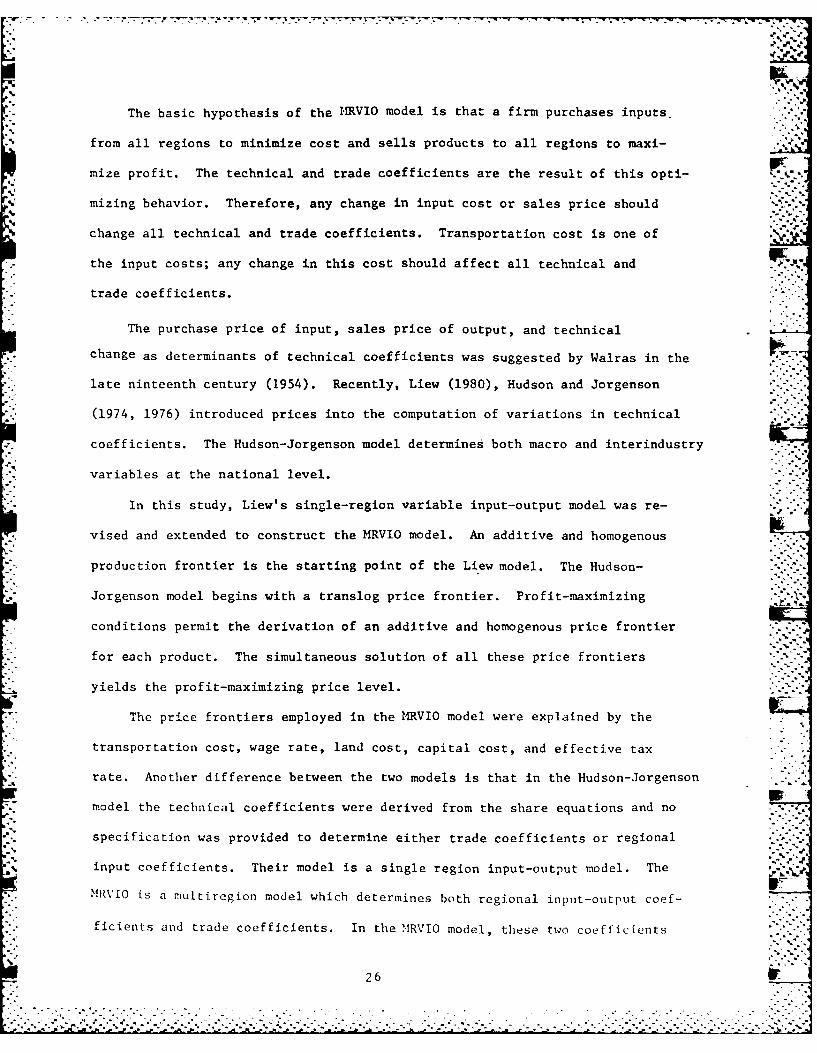
The basic hypothesis of the MRVIO model is that a firm purchases inputs.

from all regions to minimize cost and sells products to all regions to maxi-

mize profit. The technical and trade coefficients are the result of this opti-

mizing behavior. Therefore, any change in input cost or sales price should

change all technical and trade coefficients. Transportation cost is one of -*

the input costs; any change in this cost should affect all technical and

trade coefficients.

The purchase price of input, sales price of output, and technical

change as determinants of technical coefficients was suggested by Walras in the ...

late ninteenth century (1954). Recently, Liew (1980), Hudson and Jorgenson

(1974, 1976) introduced prices into the computation of variations in technical

coefficients. The Hudson-Jorgenson model determines both macro and interindustry

variables at the national level.

In this study, Liew's single-region variable input-output model was re-

vised and extended to construct the MRVIO model. An additive and homogenous

production frontier is the starting point of the Liew model. The Hudson-

Jorgenson model begins with a translog price frontier. Profit-maximizing

conditions permit the derivation of an additive and homogenous price frontier

for each product. The simultaneous solution of all these price frontiers

yields the profit-maximizing price level.

The price frontiers employed in the I4RVIO model were explained by the

transportation cost, wage rate, land cost, capital cost, and effective tax

rate. Another difference between the two models is that in the Hudson-Jorgenson

model the technical coefficients were derived from the share equations and no

specification was provided to determine either trade coefficients or regional

input coefficients. Their model is a single region input-output model. The

MRViO is a multiregion model which determines both regional input-output coef-

ficients and trade coefficients. In the MRVIO model, these two coefficients

26 or

7. .71 1. TO -. -- W. -IT

were derived from the input-output transformations.

The MRVIO model is consistent with the neoclassical theory of firm. The

model assumes neither fixed technical coefficients nor fixed trade coeffi-

cients. These coefficients are endogenous variables in the model and are de-

termined by intermediate purchase price, transportation cost, tax rate, wage

rate, land cost, capital cost, and input elasticity.

The set of price frontier equations is derived from the dual relation-

ship between production and price-possibility frontiers. The equilibrium

price of each industrial output in each region was determined by simultaneously

solving the price equations. The equilibrium price enters the input-output

transformation function as an explanatory variable. Technical coefficients .

and trade coefficients are obtained from the input-output transformation

relationship. Wage rate, land price, capital cost, transportation cost, and

local tax rate affect the equilibrium price which, in turn, determines the "-.-.

technical and trade coefficients.

27

Chapter 3

Sc The Multiregional Variable Input-Output Model -

5, -'

Consider an economy which has m regions and n commodities. Each industrial

output in each region is produced by a Cobb-Douglas production frontier with a

constant return to scale:

m rn""; _L

r r sr sr r r 6 inK. 0 (31)inx3 - a oJ a Ej lnxij y YJ inL. _ r kr 0

sffil i=l ij ij1 3 -

(j=l, .n; rfl, ... m)

wherer -outut-ox output of industry j located in region r;3

sr "% ".

xij " intermediate purchase of the ith industrial productfrom region s by industry J located in region r;

Lr = labor service employed by industry j located in region r;

Kr. service of capital employed by industry j located in region r.

,r sr r r

0 ij and 6 are parameters of the Cobb-Douglas production

frontiers. The linear homogeneity is assumed to be:

m na s + Y + 6~ (3-2).sl il j J'J

(j=l, ...n; r=l, ... m)

The supply of output is demanded by industries and final users. The usual balance

equations show the market clearing relations; i.e., .. .

E sr sr Xs(r i X ij + E F i (3

rj r-. ° '

I" ~~R E V I O U s P A G E

O''''"l

29

" - -' -- ° 4 - - -' " - -' -.. .. - . -.- -. - - - ."-. --- " '. -. -. ' '- " -". .. . . . - .' . " - " .- , " "* . "* "' * S.'. .-- .'-' . * . S.'- . ' - - , "

..-------- U ' ~ ~ ' .- - - . , •- - -

Fs is the amount of final demand i produced in region s and delivered toi

region r. The final demand denotes the commodity delivered to the final users.

The industries in each region are assumed to maximize their profits with the

technological constraints (3-1) and the balancing constraints (3-3). The problem

is formulated as the usual equality constrained maximization problem.

Z MAX Ur xr sr sr r r r Kr.

MAX E E p x - v K (3-4)s ij xij 1j i i

Subject to production frontiers (3-1)

and balance equation (3-3)

*r r rp , w and v denote respectively the producer price, wage rate and the -

rservice price of capital of industry j located in region r. t is an effective

srtax rate for industry j located in tegion r. Pij is the purchase price of in-

put i produced in region s and purchased by industry j located in region r.

The Lagrangian solutions yield to the following necessary conditions:-

-- r ) P*r + r 1 + - 0 (3-5)j.-+ X j 3J-"

sr

__ _ sraF sr r a .i'--".

X,- - - s 0 (3-6).. xij • ij,-""[' '. .

*rJaF r r Y i

r : (3-7)jL L

r -vt ,r 0 (3-8) !:Z'aKr K

IThe Lagrangian Equationr) *r r Psr sr r r r r

F E ((l-t. . - w_ - - v K )ri jr j r r :

+ E E ri (lnx r a - zs lnx - y lfT r Vr i nl r)r j s 0i i - J

+ s (x- E E xsr _EF sr.s i r

30I,..". ."." ' ." . - "." -" ." ".''' .:.. .. : ' "" '" " "' , , "' ' ' " " . " . . ,... .' " . , . . Ii . :I .', , .. ' ., -, " .- .' , -" , ' , .. .-.'., '-, ,'-' ,'. .'. ., .. , .c ..., .. t. ; :. '. . '.- . *- . . ' .'. ' , .." _ ' .' , , .. . : ' .: --- -" .- -.

-a r ~ ~ .-- L. r sr6 r. r.. r

V.

j o si 1...-.j~Y

_F S sr sr (3-10)-.ax 1 r iJ r i 0I

Pr adrf a are the Lagrangian multipliers of the jth production frontier and

.

the ith balancing equation in region r and region s respectively.

Equations (3-5) yield the following solutions;

-x (3-11)(31 1

whererAr *r "'.'

p p. +j rj (l-t.

p is an exogenously determined producer price of the commodity j in region

r There is no guarantee that this price could clear the market. The Lagrangian

multipliers (Xr is the additional price which ensures the market clearing con-

ditlon. pj is the equilibrium price of the commodity j in region r. This price

could balance the demand and supply of the commodity j produced in region r. Since

A r is unknown, the equilibrium price is unknown and is to be solved from the model.

sr... .-'The input purchase price of p s is determined by (3-11a). As in the case of

ijproducer price (p. ), there is no guarantee that these input purchase prices

aswill clear the markets. The shadow price A is the additional price which

insures market clearing conditions. ...

The equilibrium price (p ) multiplied by the transportation cost fac-

tor (ci = 1 + percentage of transportation cost per a dollar sale) are

aRsumed to be equal to the market clearing prices; i.e.,

1 5 *The equilibrium price (p.) is sum of the supplier price (pis ) and tax

adjusted shadow price (As i as defined in (3-11).

31 .

_-_. . .. .. .-._._.__"._'..'_.."_.__.__.._.____. ..._._"__.._--_--___-_____.- ... . ' . .A<.22-'.-P .-. .-.'-.- s.-. ..

c sr s sr + X(311acij " i = ij + i (-1)

The input purchase price (pi' varies from region to region because of

sr -differing degress of the transportation cost factor (c ). Linehaul, terminal,• i,

and time cost constitute the transportation cost. Interest income lost during

the shipping period was considered as a proxy to the time cost.

Equations ((3-6), 3-7), (3-8), (3-11), (3-11a)) provide the profit maxi-

mizing intermediate inputs (x.), labor input (L), and capital service (K) in

terms of the equilibrium prices (p);

Sij ij (t) pr x/(cr p) (312)

Lr r r rr r (3-13)L.= T. (l-t ) p x /w.3 3 - p iJ

S r tr) r r r (-4

By replacing the right hand side of the expression in equations (3-12) to.(3-14) with ,

the Cobb-Douglas production frontier (3-1), the following relationship was obtained:

r r sr sr r r r r s.nx- ao0- ci ln(a i (l-t ) p. x /(ci pi)'

y r l. r r r r r r ry. lny.Cl j j px/W)6. ln(i5(lt)p x./vr) =0

.J .1 3.) .3 333

or

1 sr srci f c . (see equation 3-19)

32 '.

32~~ ...- -*

:- 32

", '; - - '. -" '. " : " - -' - - - - . " " '--." ' . " ... .' . -. " .' - -'.: - [ -1 -' ' ' -' -- - ' ' ' ' ' ' ' " ' -' .-,

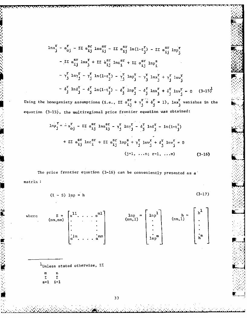
rr s r sr sr sr - smx. aa. a. Erl-. a. lnp:3j 0: ij 1 J113 :

r s r _ r sr sr sr ry i ny i I (I inc ln j -~ a,, nx lnp

61J 1 1)6 1 ~r p

:3j :3 j3: : 3 j *j :

- r -r r sr rs r r nx .r r =6.p En E 6. nat 6. lnp. 6. lv, (3-15#':3 :3 :3: 3 3 : j j :

sr sr sr ls +r r r r+ EE a.. inc. + EE a. lp.+y nw. + . nv. 0

(j=l,..n r1,.m)(-) L

The price frontier equation (3-16) can be conveniently presented as a'

matrix

(I -S) lnp =h (-7

1ml 1 hmwhere S a . . . .aC lnp lnph

(nm,nm) .(nm,l) (ml

a .. . . a lnp hm

'Unless stated otherwise, IE

m n

s1l i1I

33 W

and

sr " sr sr "r r r ra al 1 . a nl lnp l nPl I hI ."

(n, n) .(n. 1) ( n,) • 'k'

rsr ar r hrSln. . .nn n .v.-

I is an (n.m) by (n-m) identity matrix.

hr is the sum of all variables except the price variable; i.e.,

r sr sr r r r r rh.=- a.. ina.. + y_ my + 6 n ) - a3 iJ 13 oj

+ EE aisr lnc sr ln(l-t rij i2

+ r inw r + 6 r lnv r (3-18)

In the price frontier equation, it was implicitly assumed that the transportation its-

cost of delivering commodity i from region s to region r is the same regardless

of the type of buyer; i.e.,

sr sr-(39)Kc i c .-.-91 ij

A region does not constitute a single point in a geographical area.

*'" Therefore, shipments of commodities within a region also require a transportation

cost. This is called "intra regional transportation cost" and takes the form

srci when s=r reflects the intra regional transportation cost. The Arkansas

waterway system not only reduces the transportation cost of delivering a

' commodity from the waterway counties to the rest of the U.S., but also reduces the

* shipping cost of carrying a commodity within the waterway counties. In contrast to

the intra regional transportation cost, the shipping cost charged to delivering

a commodity between two regions is called "inter regional transportation cost"

34

sror, c. when sr reflects the inter regional transporation cost.

A price frontier is expressed in terms of the transportation cost, (cr .

effective tax rate t local wage rate (w.), service price of capital (v)

input elasticity (asr ijoyi 6r1), and technical pro gress parameter (a o Zj ~

In general, the profit-maximizing price level has a positive relationship

with the transportation cost, effective tax rate, wage rate, service price of

capital and a negative relationship with the technical progress parameter. ".

By simultaneously solving the price froniters (3-17), the nm profit-maximizing

price level was obtained in terms of the transportation cost, effective tax rate,

local wage rate, service price of capital, input elasticity, and the technical

*] progress parameter; i.e.,

rr r r. sr r r r (3-20)p (Csr , t, r -sr

This is the equilibrium prices which equate the balancing equation.

The input demand equations (3-12) provide the multiregional input-output co- k" jefficients. These coefficients are expressed in terms of the equilibrium prices,

* "effective tax rates, and the transportation cost; i.e.,

sr r

sr 4j sr p.ra. a ni(l-t.) s (3-21)

From equations (3-20) and (3-21), it is evident that the regional input-output

coefficients depend on transportation cost, tax rate, wage rate, service price of

capital, input elasticity, and technical progress parameters;

sr sr sr r , sr r r r.- ai aii (Ci , tip wi ij, yj, Yip 6 oa (3-22)

Regional technical coefficient is the sum of the regional input-output coef-

ficient over the region; i.e.,

35

-*:.: " *. . . . . . . . .

9 mr sr (-3

(i='=1 .n il m

Moses (1955] caicuiares the regional input-output coefficient, by multiplying

the trade coefficien .t (t ) by the regional technical coefficient; i.e.,.

srsr r (3-24)~a =t... a.

Ci, J=l, -.-.n; s,r=1, . m

From equations (3-24), the following relationship is evident:

tsr asr /ar -(3-25)

Ui , . .. n; s,r1i, .

The variable trade coefficient, which is expressed in terms of transporta-

*tion cost, primary input price, tax rate and input parameter, was obtained from

* equations (3-22), (3-23), and (3-25); i.e.:,

sr sr sr r r r sr r r rt.. t.. (c.,t.,WVvi)O, . 6. , a. (3-26)

The average trade coefficient is estimated as:

nsr 1 sr (-71 nfl= ij

Following Moses' specif ications,i t was assumed that each industry within region r

consumes the same fraction of the import of commodity i from region s so that the

trade coefficient (t..) is the same regardless of the final user; i.e.,P

~sr tsr (3-28)

ij i

1 sr srMioses [1955] assumes that t

d 36 1

.2 *

The average trade coefficient (tsr) in equation (3-27) is derived from

Moses'

" specifications. In the MVRIO model it is derived from the dual relationship between

the .'b :

the production frontier and the price frontier.

Similarly, the labor coefficient Lr /x r and the capital coefficient (Kr /Xr

iiJ iiJ

are obtained. .

r r r r r r (3_29 .-.

L /x ( (3-30)i JK./ ff = j ( 1- tj)p j / v .- (3-3-

So far, the system solved equilibrium prices p + Xr/(l-tr)), regional

input-output coefficients (asr= x/x, trade coefficients (t ), labor coeffi-

cients (L and capital coefficients (KeIXr).i J

Regional output (xr) is determined by the balance equations (3-3) with given

fnsr Fsr denotes amounts of the commodity i produced in-', final demand shipped (F r) Fi .'-'

region s and shipped to the final demand account in region r.

rAnother important concept on final demand is the final demand received (y ).ir

y denotes the amount of the commodity i received by region r in its final demand

account. - -

srThe final demand shipped (F ) and the final demand received have the fol-

lowing relations. i

s rn r r - '

F r tlsY (3-31)

The balance equations (3-3) and the equation (3-31) are combined and are

expressed as a matrix form;

x= (I - TA) - Ty (3-32)

-Moses [19551 defines as the "final demand shipment."

37

ro...

i.-: ;211 .i ? i , '?:-:i2 2 : -2. - 7 -.-222 ;2 . ..". / -.- + . +. - "".. . .- .--+..+. . - -. - .- • , ?-. i -

:. --..

where xI T. . ...T A .0 Y

x T A A2 Y

(nm,1) (nm,nm) . (nm,nm) (nm, •

m o.T ....

srx and - -. .0? n ar Or* r K"(n,l1) - (n~n) •(n, n) " . (n,1) ..-- .-,.

r sr1.r 0•a......-.-

n al nn n

and y are n-m component vectors of regional output and regional final demand,

respectively. T and A are nm by n~m matrices of the trade coefficient and the

regional coeffi'cient.This balance equation solves the industrial output (x which identifies all

profit maximizing input demands (x labor input (L), and the service price of

capital (K r

381..-

12 i

~p.'

.,, 38 .

~~. . --.-.-. . . . . ....-. V ." -. .- . . . . . . .." ..'. " .- . . -. . .. .- . , ... . - - . . . .

Chapter 4

Transportation Cost Simulation Models

The multiregional variable input-output model responds to an industry's effort

to minimize input costs. Transportation cost is one of many input costs; i.e.,

wage rate, capital cost, and land cost, which a firm faces in a local economy. A

* change in any one of the input costs in one region results in changes in equilibrium

output, prices, regional technical coefficients, trade coefficients, and various

multipliers in every region. Table 4-1 lists the input-output parameters and vari-

ables of the MRVIO model. The exogenous variables were determined before ther'Were

entered into the model. The input parameters are assumed to remain unchanged. The

endogenous variables are the dependent variables of the model.

This chapter describes step by step how a change in one of the exogenous vari-

ables affects the endogenous variables of the model. The impact of such a change .' .

affects equilibrium prices in every region. To understand the relationship between

exogenous variables and price level, the price frontier equation is rewritten as

follows:

rEr n sr + y n + r 1 r rInp - + yZ ai I

kcsr s1+ Er 0 Pi (4-1)

where

g9 a o ZZ a Inal- y inTy - ln...-

n a B r -r -r-

Unless stated otherwise, LE denotes Z. I , . ,sal i-l

39

0 -4bwV I ) 0.0

%o 44 0 0 u0rA 44 0) Io 0 w 4 * oHr

g3 4 0 o ow :x -4 -H) 4J h .j w-4) -H

* , . H . ) V .'0 .) w . .. :

14 (-4 C4 -4 H 4 -4- WC)E - C)44 -

41 0 W 2 .

4) ) u c~1

0W> 44 441U

-H 0) ~(A or

14 1- 0 r44

NO 0J 0 H U 4 C oc

cc wUH0 0-

44 Uo to A0. -4 = uEnL 4 4(

k r a 5.44 0 U44cW 4)-* C )

A-i 0

01 0 V

F! 40

~g~ The price frontier equation can be presented as a matrix:

(I - S) lnp =g + W Inc + y lnw + 6 Inv - n(1-t) (4-2)

where

- 1 ~ - 1~r Ir Ir mr mr

(nm, 1) (nm,nmm) S2 . (n ,nm)

m ir ir mr mrg0 a1n ann a1 am

ry diagonal matrix of y.

(mn,mn) 1InC In

A r (nmm,l)6 = diagonal matrix of 6.;

1mw~ ~ vetrofn.

-v-component vector of Inv rnc ~ .Ivmni I 1 -41

In(l-t) = m-n component vector of ln(1-t r)ncmj n

(The figure inside the parenthesis is the size of the matrix.)

The relationship between a change in a cost variable and its impact on

equilibrium price can be shown by taking the derivative of the price frontier

vector function (4-2) with respect to each cost vector:

alnpM-' W),_ (4-3) --

B lnv

alnp -

31n(l-t)

The prime ()denotes the transpose.

* 41

((I-S)-W)' is an (n.m.m) by (n-m) transportation cost-related price multiplier.

It explains a corresponding change in equilibrium price in each industry in each re-

gion resulting from a 1 percent change in car . The transportation cost-related price

multiplier explains in detail the impact of a transportation cost change on indus- e

trial prices in all regions. .6

A change in transportation cost for a single commodity between two regions

could affect the equilibrium price of all commodities in every region. An identi-

cal rate increase in transportation cost for two different commodities results in

a different impact on price in each region. From a policy point of view, these two

statements are very important. They imply that the construction of a waterway in

Oklahoma and Arkansas could affect the price of bread in New York. An increase in

motor fuel cost may have a varying price impact based on the weight, bulk, and value

of commodities shipped by vehicles using the fuel. The transportation cost-related

price multipliers provide interesting details of the effect of a change in transpor-

tation cost.

The price multipliers (right hand expressions) of equations (4-4), (4-5), and

(4-6) relate to wages, service, price of capital, and tax rates. Because all regional

economies are interrelated, a change in one of these prices or tax rates in one

- region affects industrial prices in all regions. This chain reaction can be-traced

* by the price multipliers.

The new price structure resulting from a change in transportation cost or a

change in a primary input price, such as the wa~e rate or the service price of cap-

* ital, affects the multiregional input-output coefficiints. These coefficients are

decomposed into regional technical coefficients and trade coefficients.

. From equation (3-21) in chapter 3, the following relationship is evident:

sr nasr (__r)r)lnar n1is + ln(l-tr) - lnc8r 1np8 + lnpr (47)

42

1.................................. . .. . .. . . . . . . . .

rr~~.;.;... .. .. . .. . . . .. . . ....... ,..,......%_.v..... --.....

If only transportation cost is changed in an economy, the rate of change in

the miiltiregional input-output coefficient can be easily identified as follows:

ze

sr r 's 6. .

31n a sr .31n pa rin pa p

(4-8)n sr sr

aln c"r ain c - aln ci

sr r sr sor 31n aij 31n p i3n ci - p. (4-9)

The right hand expressions of equation (4-8) is simply the transportation cost-

related price multiplier obtained in equation (4-3).

Assume a base year multiregional input-output coefficient: (a(t)). A

new input-output coefficient resulting from a change in transportation cost

(asr (t)) can be evaluated:ij 1

sr sr r rai(t a (t) EXP (aln p - aln r - Bln pS) (4-10)

.j 1j i 0

sr sr sr sr sr-. ~ na~t/ais(to))

(Note: aln aij is approximated by inaij(t) Inaij(t ) or in(a iji(to)/a. "(t0)).

Similarly, a change in wage rate, service price of capital, and effective tax*6• *%.-

rate is traced as follows: • s

sr a r31n a ap 31P (41)

aln wr a1 wr 3n wr

sr n aIn ai] 31in pj J ln pi (4-12)

r r slnr

a1la ar rin l n pj ;in pi(-3ala - ap. (4-13)

rs

3ln (1-t.) alna1-t ) in1-) -.-,.

The multiregional input-output coefficient (a is disaggregated into the

Car) and the trade coefficient (tsr) This was

.. .. . . .. . .. .... . . . . .... .. ..... . . . . .

............. •"-. _e. .. .. .. ..... . .. .. t,..., -....- " -_ ,,,. ,-€. . ._ --....

shown in equations (3-23) to (3-28) in chapter 3.A change in regional technical and trade coefficients results in a change in

industrial output, income, and employment.

A one-dollar change in final demand creates a chain impact on industrial out-

put.which can be traced by the output multipliers. The multiregional variable input-

output model yields the following output, income, and employment multipliers;

Definitions:

-l srM = (I-TA) = (H I an n-m by n-m direct and indirect requirement matrix

of the multiregional input-output coefficients(ar sr ar The matrices T and A are defined in

chapter 2;

I an n-m by n-m identity matrix;

K (Kr : an n-m component income coefficient vector;

E= le an n-m component employment coefficient vector;

Calculations:

m n srOutput multiplie rs Tr E. Z 1s (4 -14)

S=1 i="

r m nIncome multipliers IN E E M . iK (4-15) .

s-l i-l

m nEmployment multipliers EM - £ £ sr le (4-16) ...

s,-li-i J ii"--

for r-1, ...m, J-l, ...n.

The transportation cost, wage rate, and service price of capital could affect

the regional technical coefficient (a ) and the trade coefficient (t r). There- --

fore, they could also affect output, income, and employment multipliers.

44

-'.*."*..

-- " "- " " "' " " " . -" " - "" ""',-." "'" ,"-" ' " ,-" ,".."""" - -'' ,--< ' -"- - '." . .--. "",,- " ,," , ," ." . ' "-", -' ""

A change in transportation cost will have an initial effect on equilibrium

prices, industrial output, income, employment, trade coefficients, and regional

technical coefficients. This is the short run transportation impact. The changes

in these variables will cause changes in local wage rates, land costs, and tax

rates. These secondary changes in cost elements will have a feedback effect

which will alter equilibrium prices, industrial output, income, employment, trade

coefficients, and regional technical coefficients. Combining the secondary

changes with the short run impact constitutes the long run transportation impact. jThe basic structure of the model is illustrated as below. The transporta-

tion cost changes both regional technical coefficients (AA) and the trade coef-

ficients (AT). Given final demand, these changes affect the regional growth.

In the multiregional study, the final demand has two meanings; one is final demand

shipped (F) and the other is final demand received (y).

Which final demand should we assume to be given? When the final demand

shipped (F) is given, the model is named as the demand adjusted model. Instead

of estimating the final demand (F) each time, we employ the following formula

which does not require the final demand to compute the industrial impact.

The balance equation is;

x (I -TA) Ty (4-17) ". .-

The final demand shipped (F) and the final demand received (y) has this relation;

F = Ty (4-18)

By combining these two equation, we have the balance equation expressed in terms IFof the final demand shipped.

x (I -TA) F (4-19) .[:.-or

x-TAx = F (4-20) .*.

45

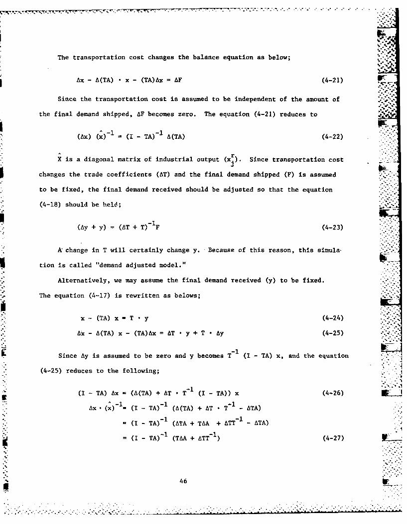
The transportation cost changes the balance equation as below; ', "

Ax- A(TA) • x- (TA)Ax - AF (4-21) F _

Since the transportation cost is assumed to be independent of the amount of

the final demand shipped, AF becomes zero. The equation (4-21) reduces to

(Ax) (x)-- (I- TA) A(TA) (4-22)

rX is a diagonal matrix of industrial output (x ), Since transportation cost

J

changes the trade coefficients (AT) and the final demand shipped (F) is assumed

to be fixed, the final demand received should be adjusted so that the equation

(4-18) should be held;

(Ay + y) = (AT + T) F (4-23)

A change in T will certainly change y. Because of this reason, this simula-

tion is called "demand adjusted model."

Alternatively, we may assume the final demand received (y) to be fixed.

The equation (4-17) is rewritten as belows;

x - (TA) x f T • y (4-24)

Ax - A(TA) x - (TA)Ax = AT • y + T • Ay (4-25)

-1Since Ay is assumed to be zero and y becomes T (I - TA) x, and the equation

(4-25) reduces to the following;

(I - TA) Ax = (A(TA) + AT • T (I - TA)) x (4-26) .

Ax. (x)- = (I - TA) -I (A(TA) + AT * T - ATA)

-1 -= (I - TA) (ATA + TAA + ATT -ATA)

= (I - TA)'-I (TAA + ATT- I) (4-27)

46

'i~~~~~~~~~~~~~~.....-."- .+. . .. . . ......:-.-i :. .. ,........ . .i-..-.. . .....- , ." --. 2-.. i. . : '..''. -' -+..._'.."._'. .... .'.. _." 'i . . _:...

• ... . ._ _ . _. o .. .:.:_ I•,. .. \-' - -?r ' -"' . . --' --.. "-' " " " 'q -Y

d

The rate of change in industrial output (Ax (x) ) due to the transportation

cost change becomes the right hand expression of equation (4-27). Since the

final demand received (y) is assumed to be independent of the transportation cost

change, and transportation cost affect the trade coefficients. The final demand

supplied (F) has to be changed to ensure the equation (4-18); i.e.,

(F + AF) = (T + AT) y (4-28)

Because the final demand supplied has to adjust the transportation cost impact,

this simulation is called "supply adjusted model."

IF I

47 W

S-.-. *...-.. - .

IALI

Chapter 5

Explanation on the Data

The multiregional variable input-output model requires extensive data

gathering:

1. Estimates of output and value added for each region

2. Estimates of regional technical coefficients

3. Estimates of final demand for each region

4. Estimates of trade coefficients

5. Estimates of industrial price, wage rate and service price of capital.

Our three regional classification requires data at the county, state and

national levels. Region 1 consists of 13 Oklahoma counties and 5 Arkansas

counties. Region 2 requires the Oklahoma and Arkansas State data since it is

the rest of Oklahoma and Arkansas. Region 3 requires the national data.

Region 3 includes all other states except Oklahoma and Arkansas.

It is essential to have controls at the national, state and county levels

to ensure that all data are consistent with each other.

(5.1) An Estimation of Regional Output and Value Added

The 496 order BEA input-output tape for 1972 contains value added and out-

put data for each sector at the national level. Also, the 88 order BEA input-

output tape for 1972 disaggregates the value added data into wage, nonwage and

tax payments for each industry. Employment and payroll information are com-

piled from the Bureau of Labor Statistics, Employment and Earnings. The state

and county data for employment and payrolls are available from the Department

• .of Commerce publication entitled County Business Patterns.

PREVIOUS PAGE

4 9 . ." .

.. i...

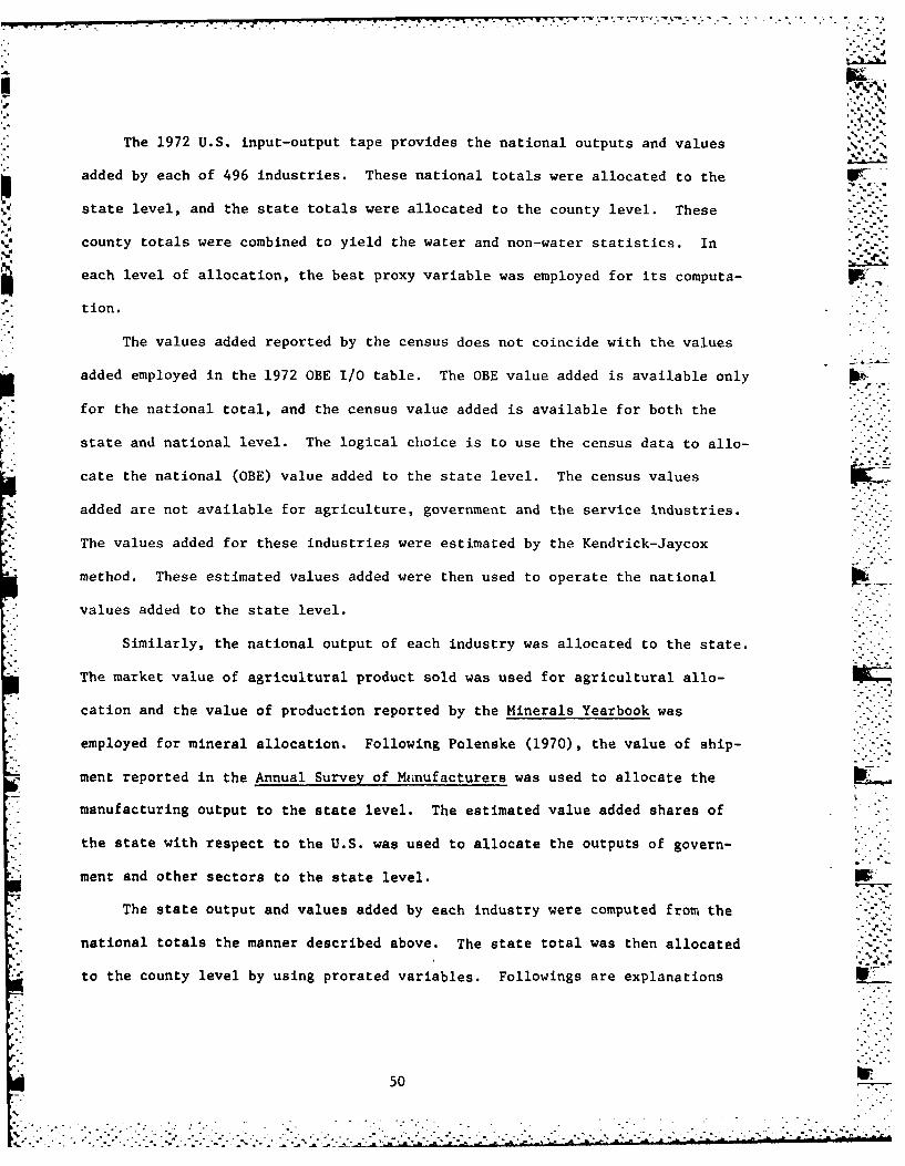
The 1972 U.S. input-output tape provides the national outputs and values

added by each of 496 industries. These national totals were allocated to the

state level, and the state totals were allocated to the county level. These

county totals were combined to yield the water and non-water statistics. In

each level of allocation, the best proxy variable was employed for its computa-

t ion. i I" ii

The values added reported by the census does not coincide with the values

added employed in the 1972 OBE 1/0 table. The OBE value added is available only

for the national total, and the census value added is available for both the

state and national level. The logical choice is to use the census data to allo- -

cate the national (OBE) value added to the state level. The census values

added are not available for agriculture, government and the service industries.

The values added for these industries were estimated by the Kendrick-Jaycox

method. These estimated values added were then used to operate the national

values added to the state level.

Similarly, the national output of each industry was allocated to the state.

The market value of agricultural product sold was used for agricultural allo-

cation and the value of production reported by the Minerals Yearbook was

employed for mineral allocation. Following Polenske (1970), the value of ship-

ment reported in the Annual Survey of Manufacturers was used to allocate the

manufacturing output to the state level. The estimated value added shares of

the state with respect to the U.S. was used to allocate the outputs of govern-

ment and other sectors to the state level.

*The state output and values added by each industry were computed from the

national totals the manner described above. The state total was then allocated

to the county level by using prorated variables. Followings are explanations -

50

;... . ...- .. ..-- -.. :.-.. . .-- _._,_.._-_--, .. ,_.__.,__.. . ._.. ___,_,_,

of the methods by which estimates were made for agriculture, mining, 5.%..\ j.

manufacturing, government and other sectors.

(5.1.1) Agricultural Sector

We estimate the gross farm product for Oklahoma and Arkansas for the years -

of 1972-1977 by the Kendrick-Jaycox method. For example, 1972 Oklahoma gross

farm product was estimated as below:

Gross Farm Product of Oklahoma, 1972(in million dollar)

Amounts

I. Cash receipts from marketing 1,395.0

2. Value of home consumption 17.5

3. Gross rental value of dwellings 70.2

(Less: net rent to nonoperator landlords) 78.8

4. Net change in inventories 34.2 I

5. Value of total farm output (1+2+3+4) 1,438.1

6. Purchase of raw materials 600.7

Feed 215.3

Livestock 318.4

Seed 18.5

Fertilizer 48.5

7. Repairs and operation of equipment 118.7

.8. Miscellaneous operating expenses 189.9

9. Total current expenses (6+7+8) 909.3

Gross Farm product (5-9) 528.8

.

51

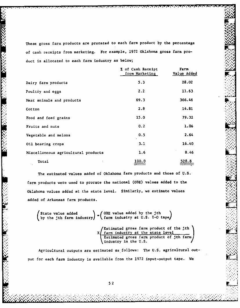
These gross farm products are prorated to each farm product by the percentage

of cash receipts from marketing. For example, 1972 Oklahoma gross farm pro-

duct is allocated to each farm industry as below;

% of Cash Receipt Farm

from Marketing Value Added

. Dairy farm products 5.3 28.02

* Poultiy and eggs 2.2 11.63

Meat animals and products 69.3 366.46

Cotton 2.8 14.81

" Food and feed grains 15.0 79.32

Fruits and nuts 0.2 1.06

Vegetable and melons 0.5 2.64

Oil bearing crops 3.1 16.40

Miscellaneous agricultural products 1.6 8.46

Total 100.0 528.8

The estimated values added of Oklahoma farm products and those of U.S.

* . farm products were used to prorate the national (OBE) values added to the

Oklahoma values added at the state level. Similarly, we estimate values ,'-'-

added of Arkansas farm products.

%°I (State value added OBE value added by the jth )by the jth farm industry farm industry at U.S. I-0 tape)

/Estimated gross farm product of the Jth

X farm industry at the state level

Estimated gross farm product of jth farm)\industry in the U.S. ./

Agricultural outputs are estimated as follows: The U.S. agricultural out-

put for each farm industry is available from the 1972 input-output tape. We

5 2

.......... ..... ..... ,.."

• :4. ::. ."

use the market value of agricultural product sold to allocate national

agricultural outputs to state agricultural outputs for Oklahoma and Arkansas.

Table (5.1) provides the list of prorated variables used for state allocation

from the national total.

These state values added and outputs by each farm sector are further

allocated at the county level using the production data as the blow-up vari-

able.

TABLE 5.1

The Variables Employed to Allocate the National Total to Regional Level

State Level County Level

Value Added Output Value Added Output

Agriculture Cash Receipt by Market Value Production ProductionAgricultural of Agricultu-Commodity ral Product Sold

Mining Census Value Value of Value of Value ofAdded Production Production Production

Manufacturing Value Added re- Value of ship- Taxable Taxableported by the ments reported Payrolls PayrollsAnnual Survey of by the AnnualManufacturer Survey

Other Sectors Estimated Value Value added by Taxable TaxableAdded by Kendrick Kendrick-Jaycox Payrolls PayrollsJaycox Method Method

Because of the differences between the state and county industrial classification

in the agricultural sector, a representative product was employed. Table (5.2)

provides the blow-up variables for each farm industry. For example, to estimate

the Oklahoma water county output for meat animals and products, we collect the

number of cattle in each of Oklahoma's water county. Then, we calculate the

percentage of cattle in the water counties to total number of cattle in Oklahoma

53

,>.7 -

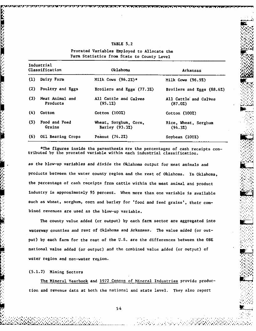
,,. .8

wiv 1- J "9i. I;v - --

,% % 8-,

TABLE 5.2

Prorated Variables Employed to Allocate theFarm Statistics from State to County Level

" IndustrialClassification Oklahoma Arkansas It -,

(1) Dairy Farm Milk Cows (96.2%)* Milk Cows (96.9%)

(2) Poultry and Eggs Broilers and Eggs (77.3%) Broilers and Eggs (88.6%)

(3) Meat Animal and All Cattle and Calves All Cattle and CalVes ..

Products (95.1%) (87.0%) ,

(4) Cotton Cotton (100%) Cotton (100%)

(5) Food and Feed Wheat, Sorghum, Corn, Rice, Wheat, SorghumGrains Barley (93.3%) (94.3%)

(6) Oil Bearing Crops Peanut (74.2%) Soybean (100%) _-_

*The figures inside the parenthesis are the percentages of cash receipts con- -tributed by the prorated variable within each industrial classification.

as the blow-up variables and divide the Oklahoma output for meat animals and

products between the water county region and the rest of Oklahoma. In Oklahoma,

the percentage of cash receipts from cattle within the meat animal and product

industry is approximately 95 percent. When more than one variable is available

such as wheat, sorghum, corn and barley for 'food and feed grains', their com-

bined revenues are used as the blow-up variable.

The county value added (or output) by each farm sector are aggregated into

waterway counties and rest of Oklahoma and Arkansas. The value added (or out-

put) by each farm for the rest of the U.S. are the differences between the OBE

national value added (or output) and the combined value added (or output) of

water region and non-water region.

(5.1.2) Mining Sectors

The Mineral Yearbook and 1972 Census of Mineral Industries provide produc-

tion and revenue data at both the national and state level. They also report

54

FV ~ ~~ -k.w . .

county statistics of mineral industries. However, the county data is either . ,-

too aggregated or incomplete because data on many counties are withheld due

to the limited number of firms in these counties. Instead, we use Oklahoma

Tax Commission data. The Oklahoma Tax Commission reports the value of oil

production and the value of natural gas production on which gross production

taxes are paid. County coal production data was compiled from reports of the

Chief Mine Inspector, State of Oklahoma.

The 1972 OBE mineral output and value added are prorated by using value of

. production for state output and census value added for state value added. ThenV

the state value added and output are prorated into county level value added

and output by using value of production as blow-up variable.-.6

(5.1.3) Manufacturing, Government and Others

Annual Survey of Manufacturers and 1972 Census of Manufactures provide

detailed statistics on employment, wage payment, value added and value of ship-

ment at national and state level. They also supply county statistics. However,

county statistics are either too aggregated or were withheld due to confiden-

tiality requirements. Using the value of shipments as the blow-up variable,

the 1972 OBE output data is prorated into state level. These state output data

are futhter disaggregated into the county levels by using the payroll from the

County Business Patterns as the blow-up variable.

Using value added by Annual Survey of Manufacturers the OBE value added

is prorated into state value added. State manufacturing statistics on wage

and value added are disaggregated into the county level by using the payroll

as the blow-up variable.

Employment at national, state and county level was obtained from theCounty Business Patterns.

"- 55

7. .~ . . .. . .

Values added in government and other sectors were estimated at state

level for Oklahoma and for Arkansas by the method suggested by Kendrick-Jaycox.

The values added which we estimated may not add up to the OBE value added. To

maintain consistency with the 1972 OBE values added, the OBE data are prorated

into state level by using the estimated value added as a blow-up variable.

The OBE outputs for government and other sectors are prorated into state outputs - -

using the estimated values added as blow-up variable. By using the county pay- . .L,

roll data as a blow-up, the state values added and outputs are prorated into

county level once more.

(5.2) An Estimation of Regional Technical Coefficients

Regional technical coefficients were estimated from the 1972 U.S. input-

output tape (496-industrial classification) by using a product mix method.

It assumes that the different degress of industrial mix in each region make

the regional coefficients vary from one region to another. For example, Food

and Kindred products is an aggregation of forty-four 6-digit OBE industries.

It includes a wide range of industries from meat packing to chewing gum plants.

At the county level, the industrial composition differs from one county to

another. For each county, thc industrial location was identified by the 1972

County Business Patterns which reports the number of four digit SIC industries

located in each county. Industries located in each county are sorted from the

tape and each is identified as to whether it is located in water or non-water

regions of Oklahoma and Arkansas.-.

When the industries were aggregated for the Food and Kindred products

industry for a region, for example, only the industries (out of forty-four

6-digit OBE industries) located in the region were included for its aggregation.

However, the deletion was done only columnwise on the ground that the industry

56 r

-L L, 23 '. " %

"'" - -- %. %. , .7 _7 -7.- -aq 'Vo 2 7. V-:W W V- W L -3 . . .. AZ - -r7L -L -

located in the region could import its inputs if those commodities were not

available from the local producers.

Once this aggregation was done for a region, the percentage share of the

intermediate purchase of Food and Kindred products industry with respect to % N

existing total output (excluding value added) of all 35 sectors was computed

for the region. This percentage share differs from region to region because

of varying degrees of industrial mix.

Since the value added and the industrial output by each industry in each

region are available, the regional intermediate total is computed for each

industry by subtracting its value added from the industrial output. This

intermediate total is multiplied by the percentage shares of intermediate

purchases to obtain the regional interindustry flows.

The procedure is described step by step.

Step 1. Identifies the six-digit OBE industry which is located in the region.

Step 2. Delete columns of all non-existing industries from the 1972 U.S. input-

output tables (only delete columns, not rows) by refering to 1972

County Business Patterns.

Step 3. Aggregate the interindustry transaction table to 35 sector table for

each region and compute percentage shares of intermeidate purchases

by each industry for each region.

Step 4. Compute regional total intermediate purchase by each industry by

subtracting the industry's regional values added from its regional

output. W9

Step 5. This regional total intermediate purchase by each industry is

multiplied by the percentage shares of intermediate purchase by each-.'..

industry and the regional interindustry flows are obtained.

.57 OF

-k-

• . . .

Step 6. This regional interindustry flow is divided by its regional output

to obtain-the regional technical coefficients. F

(5.3) An Estimation of Regional Final Demand

In the multiregional analysis, final demand has two meanings. One is final

demand shipped (F) and the other final demand received (y). The state final

demand estimated by Jack Faucett Associates (Scheppack (1972)) coincides with

the final demand received. This final demand (1970 forecast) after adjusting

the 1972 level was used as the basis for computing the regional final demand.

Using following variables, each component of the final demand was prorated to

the county level and these county final demands were added up to make a

regional final demand. Following variables were employed to prorate the state

final demand at county level.

Final Demand Component Prorated Variables

Consumption County personal incomeGovernment spending Local government expendituresInvestment and others County industrial output

(5.4) An Estimation of Trade Coefficients

Each region purchases commodities produced in other regions. The percentage

of a commodity received from each region is called trade coefficients. The

trade coefficients are region by region table for each commodity flow. An esti-

mation of trade coefficients requires complete set of interregional trade flows.

The census of transportation, Carload way bill Statistics, Waterborne Commerce

of the U.S., Census of Mineral Industries, and Census of Manufacturers provide

the basic data for the trade flows estimation. Major problem of estimating the

trade flows from these sources is that it is too much time consuming. Each cen-

sus is using diffirent accounting frameworks and different industrial classifi-

cation, it takes a great deal of efforts to make them consistent each other.

58

Alternatively, the trade coefficients can be estimated from the commodity

received and the commodity shipped. The commodity received is the column sum

and the commodity shipped is the row sum of the trade flows. The commodity

shipped is approximately by the industrial output produced (xj) and the commodity

.rreceived (R.) is estimated by summing final demand received (y and the inter-

* mediate inputs received (E E x ) in the region.

r r sBased on x and R the trade coefficients are estimated. There are three

methods to estimate the trade coefficients.

First method is to employ the linear transportation cost minimization

algorithms. This approach requires the estimation of cost delivering a commodity

between region. Distance between two regions (or combined area of two region

is the popular proxy to the cost estimation; the trade flow (xr) for the com-

modity i is computed from the following model;

sr sr

Min EE ci ~xSubject to

Exsr • r

Exar <-ri

srxi > 0

The complementary pivot algorithms (Dantzig - Cottle algorithm) efficiently

compute this computation. The compulational routines used for this computation

are LEMKE, PIVOT, DECOM, aid SORT which are in Appendix III. Second method is to

use a modified version of the gravity model. The usual gravity model computes W, A

the trade flows by the following equations;

xs rsr i i 1xi = ---- f[i

x ci

5 rwhere xi s x= E R

r "

*.*.*.***.59...... 01

-~ , -~ j - -J... .- I..r.f~~r -.. ~r. ~ ~- VJ 1-- ~ - 7 "T77

Ig

This trade flow (xr) is scanned by the RAS method so that the row sum of

ran rthe trade flows becomes x. and the column sum becomes Rr .

Third method is to use a base year trade flows and to update the trade

flows at the target year. Kim (1977) has compiled 1963 trade flows data which

was revised from Polenske's data (Polenske (1970)). This data was updated in

1972 level by using the RAS method. In this study the trade coefficients are

estimated by the third method.

In RAS, the column sum of the table is equal to the regional output

received and the row sum becomes the regional output produced. The RAS met'd

requires base year data and target year row and column sums. Using the 1972

output received and output produced as the target year row sum and column sum

we update the 1963 trade flows to the 1972.

The 1963 trade flows were aggregated from 79 commodities to 35 commodities

into Oklahoma, Arkansas and the rest of the U.S. Using the output shares be-

tween water and non-water as the prorate variable, Oklahoma trade flows were

further disaggregated into the water, the non-water regions of Oklahoma. Simi-

larly, the Arkansas trade flows were disaggregated into the water and the non-

water regions in Arkansas. Then the trade flows of the water counties are

obtained by combining those of Oklahoma and Arkansas. Similarly the trade flows

of the non-water regions of Oklahoma and Arkansas are obtained. Thus three

regions, 35 commodity trade coefficients are obtained. By means of RAS, 1963

trade coefficients are updated to 1972 trade coefficients.

The RAS is computed as follows:

(ref: Bacharach, M. Biproportional Matrices and input-output - .change, Cambridge, 1970) .-

60IM

___________________________________________ .. **'..* .. *....* *..%.

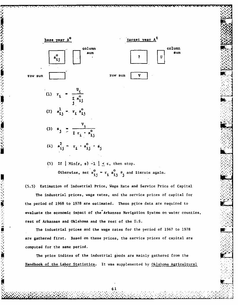
,B.- V V9I:.;'

base yea" Ar target year At

column ____column Du sum

I..°.

row sum rowsu

(1) -" a0 'i":

(2) ai= r I a i . '"- '

V

(3)' i • ij ".'''

2 0ri a

(4) aij = r i •aij j

(5) If Min{r, s) -1 j < E, then stop.

0 0Otherwise, set aij ri ai s. and iterate again.

(5.5) Estimation of Industrial Price, Wage Rate and Service Price of Capital

The industrial prices, wage rates, and the service prices of capital for

the period of 1968 to 1978 are estimated. These price data are required to

evaluate the economic impact of the Arkansas Navigation System on water counties,

rest of Arkansas and Oklahoma and the rest of the U.S.

The industrial prices and the wage rates for the period of 1967 to 1978

are gathered first. Based on these prices, the service prices of capital are

computed for the same period.

The price indices of the industrial goods are mainly gathered from the

Handbook of the Labor Statistics. It was supplemented by Oklahoma Agricultural

*- ".

OF". ~61 "- '

:-- 1 .9 '.:.- -''--'', " ,'',,'',-''- '. "' . ". ',.. " '-,''.-''- "- '-.'" -''- "- °-.- -- ".' " .- ''- "-" "- - ' " "% "*'. '. ,. -, .,,

Statistics, and Oklahoma Energy Assessment and Forecasting.

The Employment and Earnings published by the Bureau of the Labor Statis-

tics is the main source of the wage data. Farm wage rates were gathered from .-. -.

the Agricultural Statistics.

The service price of capital is not available. It was estimated from the

wage and the price series by using the Divisia Index Method. The Divisia

Index is the best known method for such computation;

we define;

P: price index of the industrial output

w: wage index of the wage rate

r: the service price index of capital (the service of capital includes

the lands, machines, and plants)

SL = the value added share of the wage payment

K = the value added share of the non-wage payment (since the indirectK

taxes are excluded from the value added, (s + sK) becomes a unity)L K

From the Divisia Index,

log (r/rl) = 1 (log PIe L) - SLlO1 w/wi j

~:KK

The log is a natural log. To make it consistent with other series, we

set the 1972 service price of capital index equal to 100. (i.e., 1972

becomes a base year). We also establish 1972 as a base year.for all other

price indexes. Since log (r/r_) is a rate of change in the service price of

capital and the 1972 service price is 100, the service prices of all other

years can be computed. These three price indices are needed to measure the

economic impact of the Arkansas Navigation' System.

62

%L21-i:

L

Chapter 6

Estimation of Lowered Transportation Cost

The basis for our estimates of the economic development impacts of the

McClellan Kerr Arkansas River Navigation Project is derived from the percent

savings in total transport costs due to the project. The estimates of savings -.. ,

in transport costs were provided by IWR (Institute of Water Resources) based

on surveys done by Resources Management Inc. (Tulsa, Oklahoma), Richard Bigda

Associations (Tulsa, Oklahoma), and University of Missouri (Rolla, Missouri).

These surveys gathered the data on all shipments in and out of the firm, by all

modes. The selection of firms to be interviewed was a stratified random sample

of firms in each two digit SIC group such that at least 50 percent of total

employment in each SIC was included. As a control, the estimates of trade flows

by T-0 Sector and among the 3 regions of the T-0 Model were utilized. Another

control was Waterway Statistics produced by the Corps of Engineers which shows

total waterway flows by commodity. Following information was gathered from the

sample surveys.

1. Primary SIC Code of firm at 4 digit level

2. Tons shipped each year by origin & destination

3. Transit time for shipment

4. Value of shipment per ton

5. Transport mode utilized for shipment

6. Transportation rate by selected mode

7. Handling costs, those costs in excess of the transport rate neces-

sary for the shipment

8. Distance by the chosen mode

63

Total costs of shipment were derived by adding hauling costs, terminal

costs and time costs. Each cost was computed as follows; F2

(a) Hauling costs = (rate per ton-mile) * (tons shipped) * (distance in miles)

(b) Terminal costs = (handling costs per ton) * (tons shipped)

(c) Time costs = (value of time) * (time in transit) * (value of shipment)

Time osts reflect the carrying costs of the goods during transit computed

at 18 percent per year.

Total transport costs were estimated for each 4-digit SIC industry group

reflected in the sampel survey and aggregated for the thirty-five sector input

output model. The cost of transporting commodities in the absence of the water-

way was determined by estimating the cost of the mode which could move the

shipment most economically. Origin and destination were assumed to remain fixed.

Flow of a commodity between regions was identified on the basis of those

surveys. For example, soybean which belongs to oil bearing crop sector was

shipped mostly from waterway counties to the rest of the U.S. In 1978, $1.98

million of transportation cost was saved by the waterway shipment of soybeans.

89.3 percent of the soybean shipment was made between waterway counties to the

rest of the U.S. and the remaining 10.7 percent from the rest of the Oklahoma

and Arkansas to the rest of the U.S.

In the case of grains, productive soils suitable for cash crop production -

occur at each end of the McClellan-Kerr System while the area between Little

Rock, Arkansas and Sallisaw, Oklahoma is an importer of grain to feed chickens

and other livestock. At the lower end of the waterway grain shippers can .

choose between shipping on the Arkansas White and Mississippi river systems.

In the upper waterway, grain is traveled up to 150 miles by truck from Kansas..-

and Oklahoma counties to elevators on the waterway. Rail competition to

Houston via Enid, Oklahoma blocks shipment further west about 80 miles west

64

S. -. . -. . . . . . . .

1, 3

of Tulsa. This results in a competitive crescent that extends further north

in Kansas where truck hauls up to 150 miles have been made to ship grain at

Catoosa. No transshipment by rail to the waterway has developed, although the

Tulsa Port of Catoosa has rail handling facilities to transfer grain between

rail and barge. Outgoing grain shipments therefore are hauled solely by truck

for an average of 40-80 miles to Catoosa and downstream to Oklahoma waterway

grain terminals and about 40 miles in the lower end of the waterway. During

1978, the grain industry saved $1.39 million of the shipping cost by the water- ..

way transportation.

Residual fuel oil is a large user of the waterway, increasing to about -

2 million tons in 1978. In 1978, $15.68 million of transportation cost was

* saved by the waterway transportation. Approximately 37 percent of the petroleum

shipment originated from Oklahoma waterway counties and shipped downstream to

the Little Rock area which is still in the waterway counties. Another 37 per-

cent of petroleum shipments originated outside of the waterway counties deliv-

ered to downstream waterway counties. The remaining 26 percent of petroleum

trade was made between the rest of Oklahoma and Arkansas and the rest of the U.S.

Fertilizers and caustic soda comprised the largest share of hemical items

carried by barge. Fertilizer users saved approximately $7 million by waterway

shipment in 1978. During the same year, the transportation cost saving by the

caustic soda was estimated to be $2.4 million. It implies that if these chemical

products were shipped by rail and truck, the industry would have paid $9.4 million

more transportation costs. Caustic soda originated in the rest of the U.S. and F

was delivered to the waterway counties and to the rest of Oklahoma and Arkansas.

However, half of the fertilizer trade originated in the waterway counties and

delivered to the rest of Oklahoma and Arkansas and the rest of the U.S. The

other half was produced by plants located in the rest of the U.S., and shipped

65

. , . *. .* * . . .. .* . . . . . . . . . . .

.''- . 2 w - p- -p-.7 ." v u-. Z : .- -. ". .v - 'v ~ .'~j~ ~ .... - '. " ".' -. 'V Tv TV Ii* , . . r ,--'-

... .'. .

to the waterway counties and the rest of Oklahoma and Arkansas. These products

are heavily used as intermediate inputs to many industries. Because of this

reason, the transportation cost change in chemical industry is very sensitive

to the industrial output.

Both metallurgic and steam coal are frequently shipped by the waterway.

The coal shipments by waterway are mostly from coal mines in the waterway

counties to the industrial plants located in the rest of the U.S. The transpor-

tation cost saving of the coal shipment was estimated to be approximately $6.53

million in 1978.

The waterway is very competitive to ship heavy and bulky items. Because

of this reason, iron and steel products were intensively shipped by the waterway

during the sample period of 1974-1978. Most of these steel products were pro-

duced by plants in the rest of the U.S. and shipped to the industries located

in the waterway counties and the rest of Arkansas and Oklahoma. In 1978, the

transportation cost saving by primary metal products was approximately $3.89

million.

Sand, gravel, rocks which were heavily used for construction and for water-

way improvement are substantial tonnage carried by the waterway. Aggregates

generally involve short waterway hauling distances. Some materials used in the

waterway improvement were hauled from the waterway counties to the local

Mississippi river basin. Bauxite (actually alumina) is another item frequently

shipped by the waterway. The material is imported from South America through

New Orleans, shipped to Little Rock by barge and to Bauxite plants in Arkansas

by trucks. If the waterway was not available, the material would be shipped

to Mobil and from Mobil, it would be shipped to Bauxite plants in Arkansas by

rail. The alumina is mixed with natural bauxite about three to one ratio for

processing intermediate products or into alumina. Combined transportation

66 I

cost saving estimated to be approximately $7.10 million in 1978.

Much of the transportation cost savings are subject to sampling errors.

For year 1978, we provide low, middle, and high estimates so that we may trace

the sensitivity of the transportation cost on industrial output.

Total transportation cost saving varied year to year. The saving was

$33.21 million in 1974 and declined to $22.76 in 1975. It steadily increased

to $32.20 million in 1976, $51.51 million in 1977, and $50.06 million in 1978.

Table 6.1 provides the complete statistics on the transportation cost

savings by each commodity shipped by the waterway.

To what extent does the transportation cost saved by each commodity reduce

A7 the industry's transportation cost? For example,-petroleum refining and related

industry (no. 15) includes various • kinds of petroleum products, most of which -"

are shipped by pipelines, truck, rail and barge. The petroleum product shipped

mostly by the waterway is residual fuel oil for power plants.

The trade flow of the petroleum products within the waterway counties was

$2671.17 million. The amount of transportation cost saving because of the use

of the waterway within the waterway counties was estimated to be around $5,765

thousands. Therefore, the transportation cost saving for this transaction isapproximately 0.2158 percent ( 5.765 * 100/2671.17).

Similarly, total shipment of petroleum products from the rest of Arkansas

and Oklahoma to the waterway counties valued approximately $862.98 million in

1978. Some portion of shipment was made by the waterway. If the waterway

wasn't built, the petroleum products would have been shipped by alternative

. modes with an estimated additional cost of $5.7 million. Therefore, with the

waterway, the petroleum industry saved 0.6682 percent (= 5.765% * 100/862.98)

of the transportation cost from its shipment from the rest of Arkansas and

Oklahoma to the waterway counties.

67

_______ _______--•. ...- * . °' C.*

-~~~~I - - - : 1-

(Table 6. 1) - .

Petroleum Trade Flows

and Transportation Cost Saving

in 1978

A (unit: million dollars)

Receiving Region

The Rest of Arkansas

The Waterway Counties and Oklahoma The Rest of the U.S.

Shipping Region trade tc savings trade tc savings trade tc savings

The Waterway Counties 2671.17 .05765 225.65 -677.94-

The Rest of Arkansasand Oklahoma 862.98 .05765 135.88 -309.85 .02076

The Rest of the U.S. 887.29 -271.07 .02076 56560.14-

Total 4421.44 .1153 632.60 .02076 57547.93 .02076

(Table 6.2)

Chemical Trade Flow in 1978

(unit: million do.Llars)

Receiving Region -

The Rest of ArkansasShipping Region The Waterway Counties and Oklahoma The Rest of the U.S. -

The Waterway Counties 40.506 36.112 32.066

The Rest of Arkansas

and Oklahoma 221.708 248.824 244.217

The Rest of the U.S. 1457.872 1768.043 91604.360

Total 1720.086 2052.979 91188.643

68

The chemical trade flow matrix shows that the waterway counties imported -

$221.7 million of chemical products from the rest of Arkansas and Oklahoma and

$1457.9 million from the rest of the U.S. The rest of Arkansas and Oklahoma

imports $36.1 million of chemical products produced by the plants located in

the waterway counties and $1768 million from the rest of the U.S. This trade

flow table shows the actual amount of transaction of chemical products among

regions. The waterway saved the transportation cost as shown in Table 6.3

We estimated value of shipment of each commodity and computed the trans-

portation cost savings. The percentage of transportation cost saving.becomes

smaller as the small portion of the commodity or small number of commodities

within the industry group is shipped by the waterway. For example, the chemi-

, cal industry (no. 14) in the model includes various kinds of chemical products

(SIC 27), plastic (SIC 28), drugs (SIC 29), and paints (SIC 30). However, the

chemical products shipped by the waterway are limited to sodium hydroxide (caus-

tic soda), chemical fertilizers, synthetic rubber, alcohols, and other basic

chemicals. The rest of Arkansas and Oklahoma has imported $36,112, thousand of

chemical products from the waterway counties and the rest of the U.S. imported

$32,066 thousand from the waterway counties in 1978. The transportation cost

L savings because of the waterway were $1,432 thousands from the waterway counties

to the rest of Arkansas and Oklahoma and $2,043 thousands from the waterway

counties to the rest of the U.S. Therefore, the percentage of transportation

cost saving for chemical industry was computed by dividing the transportation

g cost saving because of the waterway by the value of shipment involved in the

trading. The chemical industry saved 3.964 percent (= 1,432 * 100/36,112) from

its shipment from the waterway counties to the rest of Arkansas and Oklahoma

and saved another 6.371 percent ( 2.043 * 100/32,066) from the waterway coun-

ties to the rest of the U.S.

69

. . "

., ... rt.-W. . 'VW rW=re-a tw-.-.- .-. .-4x.rr u - - .- .o.. . .. . i-.

I

The percentage of transportation cost saving because of the waterway was

estimated in that manner for all commodities. However, for two cases (chemical- .- --

shipment from the rest of the U.S. to the waterway counties and its shipment

from the rest of the U.S. to the rest of Arkansas and Oklahoma region), the

estimates appear to be biased downward. We found that the value of shipment

represented by our surveys and the estimate of value of shipment in the input-

output tables were significantly different. We therefore used the sample data

to estimate percentage reduction total costs of chemical shipment among three

regions.

, .' .

70 w

(Table 6.3)

1978 Transportation Cost Saving ($: 000)

15. Petroleum

Saving

Origin Destination %H M L

1 1 36.76 7,013 5,765 4,5102 1 36.76 7,013 5,765 4,5102 3 13.24 2,526 2,076 1,6243 2 13.24 2,526 2.076 1,624

100.00 19,077 15,682 12,268

25. Coal

.Saving " -

Origin Destination % H M L

1 3 93.95 23,843 6,140 4,5102 3 6.05 1,535 395 290

100.00 25,378 6,535 4,800

5. Grain

Saving

Origin Destination 1M L

1 3 50.00 871 695 5152 3 50.00 871 695 515

100.00 1,741 1,390 1,030

6. Oil bearing crops

Saving

Origin Destination % H M L

1 3 89,28 2,215 1,768 1,3112 3 10.72 266 212 157

100.00 2,481 1,980 1,468

Note on O-D pair: 1 - Waterway counties

2 - Rest of Arkansas and Oklahoma " .

3 - Rest of the U.S.

71

......................

1978 Transportation Cost Saving (continued)

14. Chemicalsa) Fertilizer and all others

Saving

Origin Destination %H M L

1 2 20.60 2,092 1,432 7721 3 29.40 2,985 2,043 1,1023 1 29.40 2,985 2,043 1,1023 2 20.60 2,092 1,432 772

100.00 10,154 6,950 3,747 S

14. Chemicals

b) Caustic Soda fSaving

Origin Destination %H - M L *

3 1 50.00 1,646 1,204 762*3 2 50.00 1,646 124762

100.00 3,291 2,407 1,523

* Combined Savings

Saving

Origin Destination %H M L

1 2 NA 2,092 1,432 7721 3 NA 2,985 2,043 1,1023 1 NA 4,631 3,247 1,8643 2 NA 3,738 2,636 1,534

13,445 9,357 5,270

19. Primary Metal Productsa) Scrap metal

Saving

origin Destination %H M L

*1 1 100.00 1,169 948 728

b) Steel

Saving

Origin Destination %H M L

3 1 90.00 3,443 2,650 1,8543 2 10.00 383 295 206 4

100.00 3,826 2,945 2,060

- 72

1978 Transportation Cost Saving (continued)

Combined Savings "

Saving

Origin Destination % H M L

1 1 NA 1,169 948 7283 1 NA 3,443 2,650 1,8543 2 NA 383 295 206

4,995 3,893 2,788

27. Other Mininga) Water improvement materials

Saving

Origin Destination % H M L

1 3 100.00 3,302 2,626 1,943

b) Aggregate

Saving

Origin Destination % H M L

1 1 100.00 1,946 1,497 1,048

c) Bauxite

Saving

Origin Destination % H M L

3 2 100.00 8,935 7,104 5,273 .' "

Combined Savings

Saving

Origin Destination % H M L

I 1 NA 1,946 1,497 1,0481 3 NA 3,302 2,626 1,9433 2 NA 8,935 _7104 5,273

14,183 11,227 8,264

H M L

Total Transportation Saving 81,300 50,064 35,888

73

".',N.E". .

1974-1977 Transportation Cost Saving ($: 000)

15. Petroleum

Saving

Origin Destination % 1974 1975 1976 1977

1 1 36.76 2,267 1,301 3,775 6,0882 1 36.76 2,267 1,301 3,775 6,0882 3 13.25 817 469 1,359 2,1933 2 13.24 817 469 1,359 2,193

100.00 6,168 3,539 10,268 16,562

25. Coal

Saving

Origin Destination % 1974 1975 1976 1977

1 3 93.95 818 607 971 2,1302 3 6.05 53 39 62 137

100.00 871 646 1,033 2,267

5. Grain

Saving

Origin Destination % 1974 1975 1976 1977

1 3 50.00 491 478 625 7262 3. 50.00 491 478 625 726

1-00.00 982 956 1,250 1,451

6. Oil Bearing Crops :-

Saving

Origin Destination % 1974 1975 1976 1977

1 3 89.28 1,250 1,217 1,590 1,8452 3 10.72 150 1.46 191 221

100.00 1,400 1,363 1,781 2,066

14. Chemicalsa) Fertilizer and all others

Saving

Origin Destination 2 1974 1975 1976 1977

1 2 20.60 734 664 733 9161 3 29.40 1,048 947 1,047 1,3073 1 29.40 1,048 947 1,047 1,3073 2 20.60 734 664 733 916

100.00 3,563 3,221 3,560 4,445

74

..... ...........................- .......

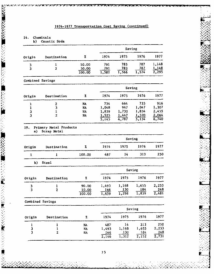
1974-1977 Transportation Cost Saving (continued) -'I

14. Chemicals '.

b) Caustic Soda

Saving

Origin Destination % 1974 1975 1976 1977

3 1 50.00 791 783 787 1,1483 2 50.00 791 783 787 1,148

100.00 1,582 1,566 1,574 2,295

Combined Savings

Saving

Origin Destination 1974 1975 1976 1977

1 2 NA 734 664 733 9161 3 NA 1,048 947 1,047 1,3073 1 NA 1,839 1,730 1,834 2,4553 2 NA 1,525 1,447 1,520 2,064

5,145 4,787 5,134 6,740

19. Primary Metal Productsa) Scrap Metal

Saving

Origin Destination % 1974 1975 1976 1977

1 1 100.00 487 14 313 250

b) Steel

Saving

Origin Destination % 1974 1975 1976 1977

3 1 90.00 1,493 1,168 1,655 2,2333 2 10.00 166 130 184 248

100.00 1,659 1,298 1,839 2,481

Combined Savings

Saving

Origin Destination % 1974 1975 1976 1977

1 1 NA 487" 14 313 2503 1 NA 1,493 1,168 1,655 2,2333 2 NA 166 130 184 248

2,146 1,312 2,152 2,731

75"......

1974-1977 Transportation Cost Saving (continued)q~

27. Other Mining

a) Water improvement materials

Saving

Origin Destination % 1974 1975 1976 1977

1 3 100.00 5,387 1,830 2,174 3,836

*' b) Aggregate

Saving

Origin Destination % 1974 1975 197' 1977----

1 1 100.00 1,116 1,161 1,164 1,400

c) Bauxite

Saving

Origin Destination % 1974 1975 1976 1977

3 2 100.00 9,995 7,172 7,247 14,459

Combined Savings

Saving

Origin Destination % 1974 1975 1976 1977

1 1 NA 1,116 1,161 1,164 1,4001 3 NA 5,387 1,830 2,174 3,836

" 3 2 NA 9,995 7,172 7,247 14,45916,498 10,163 10,585 19,695

1974 1975 1976 1977-

Total Transportation Saving 33,210 22,766 32,203 51,512

-".

d ~~76 "'""

--..................................-......'....','".....-..-.-.."...-,"-.-,.-.'....,....... -"...-.,-..-............ ,- .. i

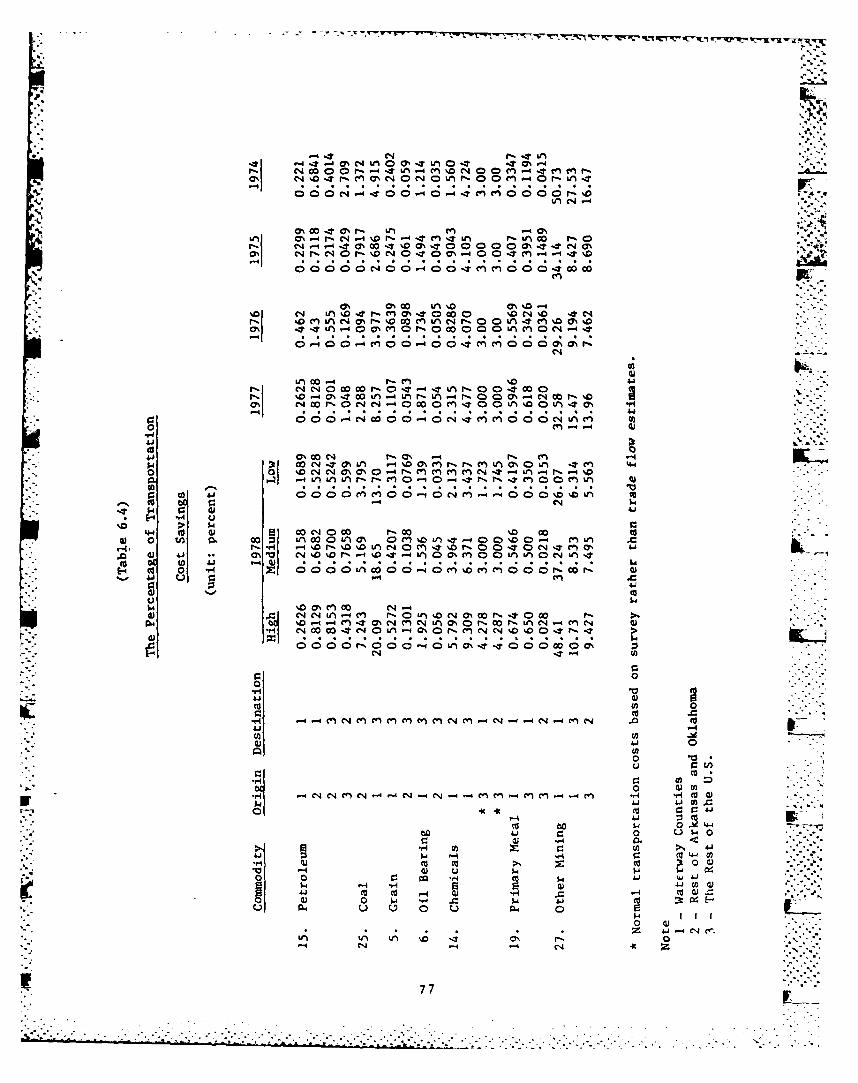
-4- 4 7 4 - C% -r0C%-

000 ItOOc-4-4 I nc 0 OO0O F,.-o%~~tO~LM Uii * . s

-7 O%4 " 0 .

0O CD 0 .t.C) 01.t0c0 -. n %n0e'C0 W co

ONr - 0 %%

. . . . . . ao -4-4. 0 - -4c 1

'.44

'a0 4 -c

I-h V 4 nr 0n c4 t- c c=O (7% ,-4 N 0-1

go cn -4-4 4V4

41 ;el

to0,00=O00-r (n

04o 1(NL D M m r , n u s0 w Te

UC)

r-u CU

40rIC O % 0 "- 0 : 4 V)0 O CO 0 'na 0"L ,at-t -4 .c 0 r4C C4 CU8C39C 9 a

N eq Ln r- a ) C)"0 c * *0 0 r%. - - nIm mC l N0r or n C A-JOG en

CUC 0 - ' - U) 9. -.- C.!CI i - 0 0 0 - a L ON4 -T -IT 0. C0 C> o -

C4 .T ..

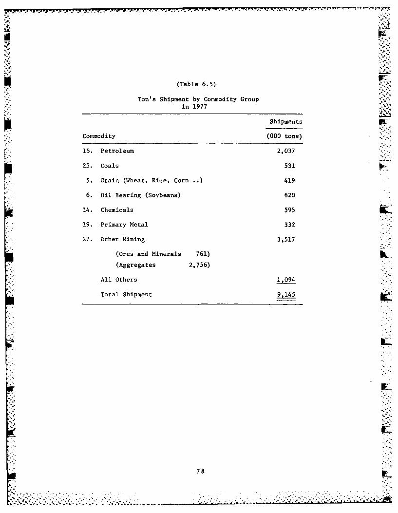
(Table 6.5)

Ton's Shipment by Commodity Groupin 1977

Shipments

Commodity (000 tons)

15. Petroleum 2,037

25. Coals 531

5. Grain (Wheat, Rice, Corn .)419

6. Oil Bearing (Soybeans) 620

14. Chemicals 595

19. Primary Metal 332

27. Other Mining 3,517

(Ores and Minerals 761) IL

(Aggregates 2,756)

All Others 1,094

Total Shipment 9,145

78

IIChapter 7

Empirical Findings

The following chapter summarizes the results of reductions in transport-.

costs discussed in Chapter 6 on output, employment, tax receipts and trade

flows and other factors in the three regions and across 35 industry sectors. .i

The regions are: the waterway counties - 28 waterway counties in Arkansas and

Oklahoma, the rest of Arkansas and Oklahoma - remaining counties in Arkansas

and Oklahoma, and the test of the U.S. - remaining 48 states of the U.S. and

the District of Columbia (see Map 1). The resulting multiregional variable

input-output model is based on the 1972 National Input-Output Tables published

by the US. Department of Commerce. The national tables were developed with

496 sectors which were aggregated to 35 sectors for the input-output model and

regional tables were based on industry detail at the 2 digit SIC level. Chapter

5 discusses the details of the adjustments made to the technical requirements

matrix and to update trade flow and final demand relationships.

From chapter 4, the industrial output is determined by the following

balance equations,

x (I-TA) F (4.22)

where x = output

T = trade flows among regions (a matrift of trade coefficients).

A - Input to output ratios by each industry sector (a matrix of tech-nical coefficients).

F - Value of shipments to final demand sector

I - Diagonal unit matrix (an identity matrix).

This model shows that a change in T (trade flows) and A (technical rela-

tions) will produce a change in industrial output (x). Changes in transporta-

tion cost alters the trade structure and the technical coefficients as in-

dustries act to achieve the most economical mix of inputs to produce their

U 79 17 ' ,

output. Industries in each region could purchase less expensive intermediate

inputs to produce their output if transportation costs are lowered and the "

lowered input costs allow them to produce output at lower costs. The industry

thus favored has a comparative advantage which allow them to expand sales to

all regions. The model estimates equilibrium shift in output costs, equili-

brium change in output and equilibrium change in trade flows from the input-

output table by taking the inverse of the (I-TA) matrix and multiplying it by

the final demand shipped (F).

Table 7.1 shows the 35 sector industrial classification used in the model.

We also show SIC classification which compares with input-output sector codes.

Dummy industries (81, 82, 83), nongovernment special industries (84, 85), and

noncomparable inports (80) were reallocated by using the method suggested by

McCarthy (1967). In the subsequent sections we discuss the results of the

model.

(7.1) Impacts on Industrial Output.

The model shows gross output increase by an average of $118.8 million due

to transport cost savings of averaging $37.95 million for analysis period of

1974-1978. These transportation costs savings are those accruing to users of

the McClellan-Kerr Arkansas waterway. Increases in output are larger for rest

of U.S. than waterway counties and rest of Arkansas and Oklahoma. The average

increase in industrial output was $19.82 million for the waterway counties

$20.01 million for the rest of Arkansas and Oklahoma, and $78.87 million for

the rest of the U.S. This unexpected result due to the substantial degree of nt

openness of trade between the waterway counties and the rest of Arkansas and Okla-

homa with the rest of the U.S. and, as we will see later in the evaluation of

the impacts, that trade volume is increased due to the waterway. Table 7.2

shows a summary of increases in estimated output for years 1974 through 1978.

so

,.,,,. ,.. ...,.

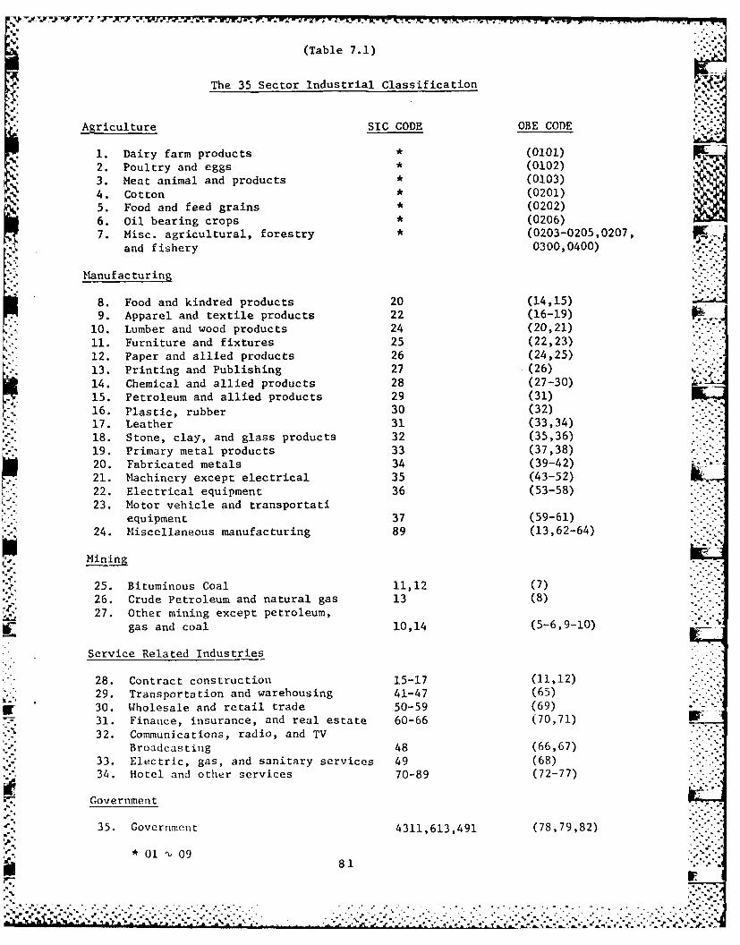
* (Table 7.1) %

The 35 Sector Industrial Classification

Agriculture SIC CODE OBE CODE

1. Dairy farm products * (0101)

2. Poultry and eggs * (0102)

3. Meat animal and products * (0103)

4. Cotton * (0201)

5. Food and feed grains (0202)

6. Oil bearing crops * (0206)

7. Misc. agricultural, forestry * (0203-0205,0207,

and fishery 0300,0400)

Manufac turing

8. Food and kindred products 20 (14,15)

9. Apparel and textile products 22 (16-19)

10. Lumber and wood products 24 (20,21)11. Furniture and fixtures 25 (22,23)12. Paper and allied products 26 (24,25)13. Printing and Publishing 27 (26)

14. Chemical and allied products 28 (27-30)15. Petroleum and allied products 29 (31)

16. Plastic, rubber 30 (32)17. Leather 31 (33,34)18. Stone, clay, and glass products 32 (35,36)

19. Primary metal products 33 (37,38)20. Fabricated metals 34 (39-42)21. Machinery except electrical 35 (43-52)

22. Electrical equipment 36 (53-58)

23. Motor vehicle and transportatiequipment 37 (59-61)

24. Miscellaneous manufacturing 89 (13,62-64)

Mining

25. Bituminous Coal 11,12 (7)26. Crude Petroleum and natural gas 13 (8)27. Other mining except petroleum,

i- gas and coal 10,14 (5-6,9-10)

Service Related Industries

28. Contract construction 15-17 (11,12)29. Transportation and warehousing 41-47 (65)

30. Wholesale and retail trade 50-59 (69)

31. Finance, insurance, and real estate 60-66 (70,71)32. Communications, radio, and TV

Broadcasting 48 (66,67)

33. Electric, gas, and sanitary services 49 (68)

34. Hotel and other services 70-89 (72-77)

Government

35. Covernment 4311,613,491 (78,79,82)

*01 09 81"-' ~81 ' ""

. 7: -7 V. V. W. Vz.

(Table 7.2)

Summary of Estimated Changes in Outputby Year from Transport Cost Savings Provided byMcClellan-Kerr Arkansas River Navigation System (Unit: million dollars) Err

Change in Output

Rest of

Transport Cost 28 Water Arkansas and RestYear Savings Counties Oklahoma of U.S. Total U.S.

1974 33.21 18.50 20.07 72.70 111.27

* 1975 22.76 13.36 15.00 63.16 91.52

1976 32.20 17.06 18.00 66.58 101.64

1977 51.51 22.64 22.71 89.95 135.30

1978 Low (35.89) (18.90) (16.13) (63.97) (99.00)

Base 50.06 27.54 24.82 102.00 154.36

High (81.30) (42.37) (34.91) (150.50) (227.78)

AnnualAverage 37.95 19.82 20.01 78.87 118.82

These impacts represent the impacts of reduced transport costs from the

* accounting point of view of transportation users in the three regions. Net

* increases to the economy would necessarily have to account for the costs, since

-" the public resources expended to build and operate the system could have been

invested in alternative ways (including other waterways) which would also pro-

duce multiple effects. The impacts identified above show what occurred in the

MRVIO model when actual transport cost savings to shippers are used in the

model. We believe that they represent a realistic set of assumptions with re-

gard to the question; What kinds of impacts has the McClellan-Kerr Arkansas

River Navigation System had on industrial output due to the transport savings

which accrue to transport users?

82

What are the industries which were benefited most by the waterway trans-

portation?

The "other mining" sector is the most conspicious gainer in the waterway

counties, In 1978, the industry was stimulated to produce additional $5.6

million because of the waterway transportation. Transportation of aggregates

(sand, gravel, rock), the material used in the waterway improvement, and

bauxite contributed the growth of the "other mining" sector in the waterway I icounties. Coal, chemical, petroleum, primary metal, and grain sectors are

also strong gainers due to the waterway transportation. In 1978, the coal

industry increased its output as much as $3.2 million, followed by chemical

$2.6 million; petroleum, $2.3 million; primary metal, $2.2 million, and

grains, $1.3 million due to the waterway.

In the rest of Arkansas and Oklahoma grain farms is the most benefited

industrial sector. The waterway transportation stimulated the grain industry

to produce an additional $3.8 million output in 1978. "Other farm" industry

is also benefited by the waterway transportation and increased its output as

much as $3.7 million. Large shipments of wheat, soybeans, rice, corn, and

sorghum grain directly and indirectly benefited agriculture. Poultry-eggs

and meat animal producers were indirectly benefited by the waterway since feed

costs were lowered. Agricultural chemicals and fertilizer costs were also

reduced by the waterway.

Chemical, petroleum, plastic, and primary metal sectors are strong gainers

because of waterway transportation. Chemical, petroleum, and primary metal

industries are gainers of the direct shipment of their products by the water-

way, and the plastic industry was benefited by the lower cost chemical inputs.

The chemical industry increased its output by $3 million because of the water-

way. Petroleum, plastic, and primary metal industries also increased their

83

.. . . .. . . .. . .. .

7 Z...-

outputs by $2.7 million, 2.3 million, and $1.4 million in 1978 respectively.

The waterway contributed greatly the industrial expansion of the re-

mainder of the U.S. Almost half of the added output was from the chemical

industry which increased output by $53 million because of the McClellan %

waterway. The primary metal sector is the second largest gainer and increased

its output by $11.8 million due to the waterway. The other major gainers are

service ($5.9 million), other mining ($5.4 million), utility ($4.3 million),

food processing ($3.2 million), and petroleum ($3.0 million)..'"

The most industrial gainers in 1978 are in percentage-wise, "other mining"

(13.88%), chemicals (2.39%), coals (1.95%), oil bearing crops (0.85%), and

"other farms" (0.68%) in the waterway counties. In the rest of Arkansas and

Oklahoma in 1978 the percentage increase in intdustrial outputs was the largest

in petroleum (0.73%) followed by other farms (0.67%), cotton (0.49%), chemicals

(0.42%), and plastic (0.36%). There was no direct shipment of dotton by the

waterway in 1978. However, the cotton industry was indirectly stimulated be-

cause of its use of chemical fertilizers which have been shipped in a great

deal by the waterway transportation. The largest gainers in the rest of the

U.S. in 1978 is chemical industry which increased output by 0.056 percent be-

cause of the waterway.

In general, the industries in the waterway counties had the largest per--

centage gains because the waterway counties depend on interregional trade for

most of their economic activities. Since trade with the waterway counties is

a relatively small fraction of U.S. economic activity, the percentage impact is

small in the rest of the U.S.

A one dollar purchase in final demand creates a chain effect on the eco-

nomy. For example, a one dollar grain sale to Russia requires the grain

farmers to produce more grain. To do so, they need to purchase more ferti-

lizer. Then the chemical industry needs to consume more electricity and the

4.84

-.. . , a. ,. _, ,, : :, ..................- _ X.i z '-:. '._.'.,. '. .* ,. ' -. U ' . -' .,*: ' ''' '"..e_ _Ze '' _ . _ -

; -'

- .. -- Irv .- -N ' "WIWI

No,...1

(30 V4. 0 nbo 4

00 o C) 0 o4Ec

v-4 V-4 . .- ul '.H %%

A 10 00 54 -.. 0o co co H 0U

0 0$ 0 U) H 0 0000 0 0 0 0 u o

0A H L4 1.. C4 C. LA $

U)~v- .

* .

0 4.1

4) 4)M* .- f 4H-4C4M

0 0n

o0 0~ ) nLcc4 co. C4 r4 1 C -$4 b-. rA 0 n tv 03 n0- .9 %s. 4J 44. r-. D

.,0 0d 01 P0 A

U) $4 W 0 04 .4 0 H 4- o 4 (r- 41 0 ) 4 *E

r- 0 U) W. ('a 0j 0 ) 0) .00 l

'-1 410 0 0 0 41 0 4- $4

u a% n 0 Pz4 P4 ~ P4 s ) 0

W 04 0 . . U 44 0 H4 'A1 04 C4 04 U) 0

01

* 4-4

U) U)CDIFor 04 CoC1

19 %- 0-% 0 0 .4.U) * 4 0 _D %, 0.0 0- CI c (A..W .

V4 Go (n 0% 0 r >1 0. IA H 1 '

0n ., i- 0-0 * H

-7 0 ) * 00 U)

0 :3 0o :o 00) 4 4 -0) Uj $4 0 4J p 4 4) C0 U) u4 u 4$ 0 0$ 04 0 (

114 .4 C4 4.1 $4 14 0T Ln 4 4'ii 0 0 $

7- -71" YNYY~~n

electricity industry needs to generate more electricity. Industries depend

on each other. How much output each industry could produce more when there

is one dollar increase in every component of final demand is conveniently

measured by the output multipliers.

In general, as the industry purchases more intermediate inputs to its

sales, the industry's output multiplier becomes larger. The government in-

dustry which spends approximately 6.4% of its sales for the purchase of inter-

mediate input has the smallest output multiplidr (1.12 for all three regions).

The poultry and eggs sector which spends approximately 88% of its sales for

the intermediate purchases has the largest output multipliers (3.15 for the

waterway counties, 3.14 for the rest of Arkansas and Oklahoma, and 2.92 for

the rest of the U.S.) table 7.4 shows those multipliers.

(7.2) Impact on Gross Regir ',al Products, Wage Payment, and Tax Receipts

How could the decrease in -qnsportation cost affect the gross regional

product, wage payments, and tax rec'ipts? It expands the industrial output

which increases the gross regional proc'ict, wage payment, and tax receipt.

The gross regional product is sum of the "v:.lue added" by each industry in

the region.

In 1978, the gross regional product increa:;ed $10.67 million in the water-

way counties, $7.75 million in the rest of Arkansas and Oklahoma, and $43.95 - 1million in the rest of the U.S. due to the waterway. These increases in gross

regional product are due to the lowered transportation cost. Estimated wage

payment increased $6.2 million in the waterway counties, $3.6 million in thei5

rest of Arkansas and Oklahoma, and $25.5 million in the rest of the U.S.

Excise tax receipt has boosted by 0.51 million in the water region, 0.48 mil-

lion in the non-water region, and 2.5 million in the rest of the U.S.

86

...... ,............. ..... . . * ..*.

%-. -

(Table 7.4)

6' The Output Multipliersin 1972 "-

The Rest ofThe Water- Arkansas and The

way Counties Oklahoma Rest of U.S.

1. Dairy Farm 2.709 2.781 2.142

2. Poultry and Eggs 3.153 3.144 2.918

3. Meat Animals 2.913 2.915 2.937

4. Cotton 2.425 2.424 2.264

5. Grains 2.263 2.102 1.869

6. Oil Bearing 1.686 1.685 1.664

7. Other Farm 2.535 2.592 1.750

8. Food Product 2.952 2:924 2.645

9. Textile 2.525 2.540 2.588

10. Lumber 2.331 2.331 2.272

11. Furniture 2.264 2.269 2.218

12. Paper 2.350 2.369 2.282

. 13. Printing 1.942 1.955 1.991

14. Chemicals 2.240 2.265 2.162

* 15. Petroleum 2.498 2.401 2.307

16. Plastic, rubber 2.108 2.121 2.071

17. Leather 2.191 2.183 2.331

18. Stone, Clay 1.896 1.880 1.962

19. Primary Metal 2.215 2.464 2.371

20. Fabricated Metal 2.225 2.221 2.210

21. Machinery 2.087 2.096 2.055

22. Electrical Equipment 2.097 2.063 2.059

23. Motor Vehicle 2.619 2.555 2.380

24. Miscellaneous Manufacturing 2.085 2.088 1.998

25. Coal 1.777 1.747 1.762

26. Petroleum and Natural Gas 1.617 1.612 1.573

27. Other Minings 2.182 2.155 1.819

28. Construction 2.071 2.070 2.066

29. Transportation 1.651 1.660 1.730

30. Trade 1.394 1.393 1.392

31. Financial Service 1.430 1.430 1.437

32. Communication 1.377 1.377 1.374 "

' 33. Utility 1.919 1.917 1.909

34. Commercial Service 1.787 1.786 1.772

35. Government 1.120 1.120 1.120

Total

, ~~8 7"-'-.

A, A . . .• . . . - -.2"." " '" ,

(Table 7.5) %

Top Five Gainers in Value Idded in 1978 (unit: thousand dollars)

The Rest of

The Waterway Counties Arkansas and Oklahoma The Rest of U.S.

Industry Values Added Industry Values Added Industry Values Added --

Chemicals 975 Grains 1,609 Chemicals 21,790

Plastic 888 Chemicals 1,082 Primary Metal 4,062

Primary Metal 861 Plastic 1,047 CoumercialService 3,541

Fabricated Metal 726 Other Farm 783

Other MinIna 3,024Oil Bearing 579 Petroleum 531

Utility Service 2,160"-.-'

Regional* Regional Regionaltotal 10,670 total 7,747 total 43,950

(Table 7.6)

Top Five Gainers in Wage Payment in 1978 (unit: thousand dollars)

The Rest ofThe Waterway Counties Arkansas and Oklahoma The Rest of U.S

Industry Wage Industry Wage Industry Wage

Other Mining 1,093 Plastic 661 Chemicals 12,230

Primary Metal 658 Chemicals 607 Primary Metal 3,105

Plastic 562 Other Farm 429 Commercial

Service 2,414Chemical 548 Primary Metal 308

Other Minings 1,524Fabricated Metal 536 Stone, Clay 300

Transportation 971

Regional Regiona Regional

total 6,222 total 3,628 total 25,530

*Regional total means total of all 35 industries. "

88 * .. - . * * * -

V7. rum W -T

The chemical industry is the single largest gainer in value added. The

chemical industry in the rest of the U.S. produced additional $21,790 thousand

because of the Waterway. Primary metal ($4,062 thousand), commercial services

($3,541 thousand) "other minings" ($3,024 thousand), and utility services

($2,160 thousand) constitute the top five gainers in 1978. In the rest of

Arkansas and Oklahoma, the most value added gainer is the grain industry which

contributed additional $1,609 thousand for the economy. It was followed by

chemicals, $1,082 thousand; plastic, $1,047 thousand; other 'farm, $738 thousand;

and petroleum refinery, $531. In the waterway counties, the chemical industry

increased its value added by $975 thousand because of the waterway and plastic

primary metal fabricated metal, and oil bearing crop sector made the top gainer

in the waterway counties in 1978.

The value added included wage payment, the payment for the capital ser-

vice, interest and excise taxes. Since the labor intensity differs from one _

industry to another, wages are not proportional to the values added.

The "other minings" sector paid additional $1,093 thousand to its workers

because of the waterway transportation. Primary metal industry paid $658

thousand to its workers, plastic industry, $562 thousand; chemical industry,

$548 thousand. These wage payments were direct result of economic stimulation

which the waterway has initated in 1978.

The plastic industry is the largest gainer in wage payment in the rest of

Arkansas and Oklahoma in 1978. The plastic industry increased wage payment

$661 thousand because the waterway. Chemical ($607 thousand), other farm P

($429 thousand), primary metal ($308 thousand), and stone-clay ($300 thousand)

are other major gainers in wage payment because of the waterway transportation.

As expected, the chemical industry in the rest of the U.S. paid $12,230

thousand for the additional labor services. The farmers purchased more

89.. 4

Z.I

%7%

fertilizers because the waterway provided relatively inexpensive fertilizers.* ..

To meet these expanded demands, the chemical industry employed more labors ____

and paid more wages for their services. Because of similiar reasons primary

metal increased its wage payment by $3,105 thousand, followed by commercial

service ($2,414 thousand), "other mining" ($1,524 thousand), and transportation

($971 thousand). It is evident that the expanded market activities require

more transportation services. Tables 7.5 and 7.6 provides those statistics.

(7.3) Employment Impacts

The waterway stimulates the industrial outputs which increase the employ-

ment. The increase in employment was estimated from the wage increase. For

example, in 1978, the wage payment of other minings has increased by $1,093

thousand because of shipment of rocks, gravel, and sands in the waterway

counties. Average wage in typical workers in other mining industry was $6.31

per hour in the waterway counties. The $1,093 thousand wage payment could em-

ploy approximately 173.2 thousand hours. A full time equivalent worker was

assumed to work 2040 hours per year (51 week x 40 hours per week). Dividing

173.2 thousand hours by the full time equivalent 2040 hours, we obtain the

employment statistics of the industry (85 jobs for the other minings in the

waterway counties).

The total jobs created by the waterway are 1929 for the rest of the U.S.,

454 for the waterway counties and 337 for the rest of Arkansas and Oklahoma in

1978. This is based on the medium estimate of transportation cost. This fig-

ure could be much higher if we use the high estimate of the transportation cost.

The largest employment impact in a single industry comes from the chemical

industry in the rest of U.S. which created 855 more jobs because of the waterway .-

*It implies that the ferti2izer price would have been higher If the water-

way wasn't built.

90

* transportation. The commercial service, primary metal, and other mining have

gained their employment significantly. The waterway created 327 new jobs for

commercial service, 186 for primary metal, and 118 for other minings in 1978.

In the waterway counties, the largest gains in employment were made in

% other mining (85 new jobs), followed by coal (64 jobs), plastic (50), fabricated

metal (41), primary metal (39), and chemicals (38) in 1978. The major employment

*gainers in the non-water regions are other farms (67 new jobs) followed by rub-

ber (59), chemicals (42), grains (33), lumber (24), and ston~e-clay (23). Table

7.7 provides the detail of the employment statistics.

(7.4) Equilibrium Price Impact

A supplier will supply a larger quantity of goods and services when its

* sales price is increased. Conversely, the purchaser of such goods and services

* will buy more when the price is lowered. Because of this conflicting desire,

any arbitrary price could not clear the market; i.e., the quantity demanded by

buyers may not equal to the quantity which the supplier is willing to provide.

However, there is one price level which makes the demand and supply equal. This

price is called the "equilibrium price." ~p

*Under MRVIO model, both demand and supply of each of the 35 commodities in

* each region are endogenously determined. There is only one set of prices which

will equate all demands and all supplies of the commodities. These equilibrium

* prices are determined by the price frontier equations as discussed in chapter 3.

The Arkansas waterway system reduces these equilibrium prices of all com-

modities in all regions because the commodities are shipped at lower costs with

the waterway.

Which is the region and what are the industries most affected by the water-

way?

The model estimates that the waterway reduces equilibrium prices of farm,

manufacturing, and mining products produced in both the waterway counties and

the rest of the Arkansas and Oklahoma. Equilibrium prices in the chemical

industry which was directly benefited by its shipment on the waterway were

reduced by 0.7988 percent in the rest of Arkansas and Oklahoma and 0.6975

N percent in the waterway counties in 1978.

(Table 7.7)

Number of Jobs Created bythe Waterway in 19781

Top Ten Industries

The Rest ofThe Waterway Counties Arkansas and Oklahoma The Rest of U.S.

Industry Jobs Industry Jobs Industry Jobs

Other Mining 85 Other Farms 67 Chemicals 855

Coal 64 Plastic 59 CommercialService 327

Plastic 50 Chemicals 42Primary Metal 186

*Fabricated Metal 41 Grains 33Other Mining 118

Primary Metal 39 Lumber 24Transportation 61

Chemicals 38 Stone, Clay 23Utility Service 38

Stone, Clay 30 Primary Metal 18Food Processing 38

Paper 20 Paper 13Fabricated Metal 36

Other Farms 14 Textile 12Machinery 35

Machinery 13 Other Mining 10Construction 34

Total of all Total of all Total of all35 industries 454 35 industries 337 35 industries 1,929

~Full time equivalent (2040 hours per year)

7-

AD-RI65 759 THE MCCLELLAN-KERR URTERNAY AND REGIONAL ECONONIC21,DEVELOPMENT - PHASE 11 STUDY(U) OKLAHONA UNIV NORMAN

LIEN ET AL. NOY 85 IUR-CR-85-C-5 DRC2-79-C-66S4

UNCLASSIFIED F/G 5/3 NL

EhEE h hhEEEE mhhmhhl

4 ..

'v''

Illl ,__oLA' 113.2

% . .

I., -,

:9 , .111 ,,.25 _-.. .4 .... , -.. .. 1 .6. . . .,. . .

K . . . , . .,., . . ,.,.. - .'. .,. . . . .,. . - . . .,.-. .,..

Number of Jobs Created by the Waterway- (1974-1978)

Regions 1974 1975 1976 1977 1978

The Waterway Counties 560(5.56)* 555(6.05) 496(5.80) 500(6.40) 454(6.22)

The Rest of Arkansasand Oklahoma 478(3.85) 354(3.09) 320(2.96) 320(3.16) 337(3.63)

The Rest of U.S. 2123(20.44) 1795(18.69) 1671(18.83) 1757(21.45) 1929(25.53)

The figures inside the parenthesis is total wage payment in million dollars.The lower wage rate in 1974 could hire more employment than ln 1978.

The equilibrium prices for the "other farm" sector increase 0.6818 percent _"

lower in the water regiona and 0.6414 percent lower in the rest of Arkansas and

Oklahoma. Equilibrium prices were lowered by somewhere between 0.16 percent-

. and 0.59 percent in the cotton, grains, oil bearing, dairy farm, poultry and egg

. sectors. Equilibrium price reductions were noted in chemical industry, rubber,

primary fabricated metal, and miscellaneous manufacturing. The other way of

saying this is that the equilibrium prices would have to be raised in the absence

of the waterway.

Chemical, primary metal (iron & steel), fabricated metal, petroleum, coals,

and grains are the industries which were directly benefited by the shipment of

their products by the waterway. The dairy farm, poultry and eggs which purchase

a lot of grains are affected because they purchase grain for feed. In the water-

way counties, the dairy farm purchases an average of 34.34 cent grain to produce

one dollar output. The poultry and egg industry spends 16.37 cent for the pur-

chase of grains to produce $1 worth of its product. Grain farmers, cotton and

plastic industries save their costs because chemical inputs are relatively in-.-.*- ..

expensive. The cotton farmer purchases 15.04 cents of chemical fertilizer to

produce one dollar worth of cotton. Plastic industry spent almost 20 percent

of its sales for the purchase of chemical input.

93

.- - - - --S..

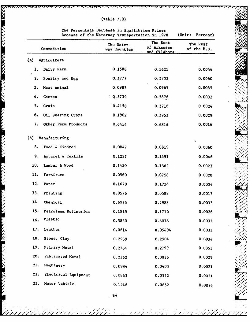
(Table 7.8)

The Percentage Decrease in Equilibrium PricesBecause of the Waterway Transportation in 1978 (Unit: Percent)

The Water- The kest The RestCommodities way Counties of Arkansas of the U.S.

(A) Agriculture .

1. Dairy Farm 0.1586 0.1625 0.0054

2. Poultry and Egg 0.1777 0.1752 0.0060

3. Meat Animal 0.0987 0.0965 0.0085

4. Cotton Q.5739 0.5876 0.0032 - -

5. Grain 0.4158 0.3716 0.0024

6. Oil Bearing Crops 0.1902 0.1953 0.0029

7. Other Farm Products 0.6414 0.6816 0.0016

(B) Manufacturing

8. Food & Kindred 0.0847 0.0819 0.0060

9. Apparel & Textile 0.1237 0.1491 0.0046

10. Lumber & Wood 0.1420 0.1362 0.0023

11. Furniture 0.0960 0.0758 0.0028

12. Paper 0.1670 0.1734 0.0034

13. Printing 0.0576 0.0588 0.0017

14. Chemical 0.6975 0.7988 0.0033

15. Petroleum Refineries 0.1815 0.1710 0.0026

16. Plastic 0.5850 0.6078 0.0032

17. Leather 0.0614 0.05494 0.0031

18. Stone, Clay 0.2939 0.2504 0.0034

19. Primary Metal 0.2784 0.2799 0.0051

20. Fabricated Metal 0.2162 0.0836 0.0029

21. Machinery 0.0984 0.0403 0.0021

- 22. Electrical Equipment 0.0863 0.0572 0.0021

. 23. Motor Vehicle 0.1546 0.0652 0.0026

94

The Rest The RestTh Weatest-TheCouotie Water-s of Arkansas of the U.S.

SCommodities vay Cute ,Af~n~,n________

24. Miscell. Mfg. 0.1636 0.1050 0.0021 % A

(C) Mining

25. Bituminous Coal 0.0552 0.0480 0.0064

*," 26. Crude Petroleum &Natural Gas .0.0370 0.0341 0.0006

27. Other Mining 0.2493 0.2060 0.0028

(D) Service

28. Contract Construction 0.1254 0.1062 0.0022

29. Transportation 0.0281 0.0299 0.0010

30. Trade 0.0126 0.0131 0.0005

31. Financial Service 0.0104 0.0106. 0.0003

32. Communication 0.0111 0.0108 0.0004

33. Electric, Gas Service 0.0405 0.0413 0.0004

34. Motel 0.0481 0.0491 0.0001

* (E)

35. Government 0.0101 0.0103 0.0003

-7'

95 "-•"j

.- -.-. .

:: -- :

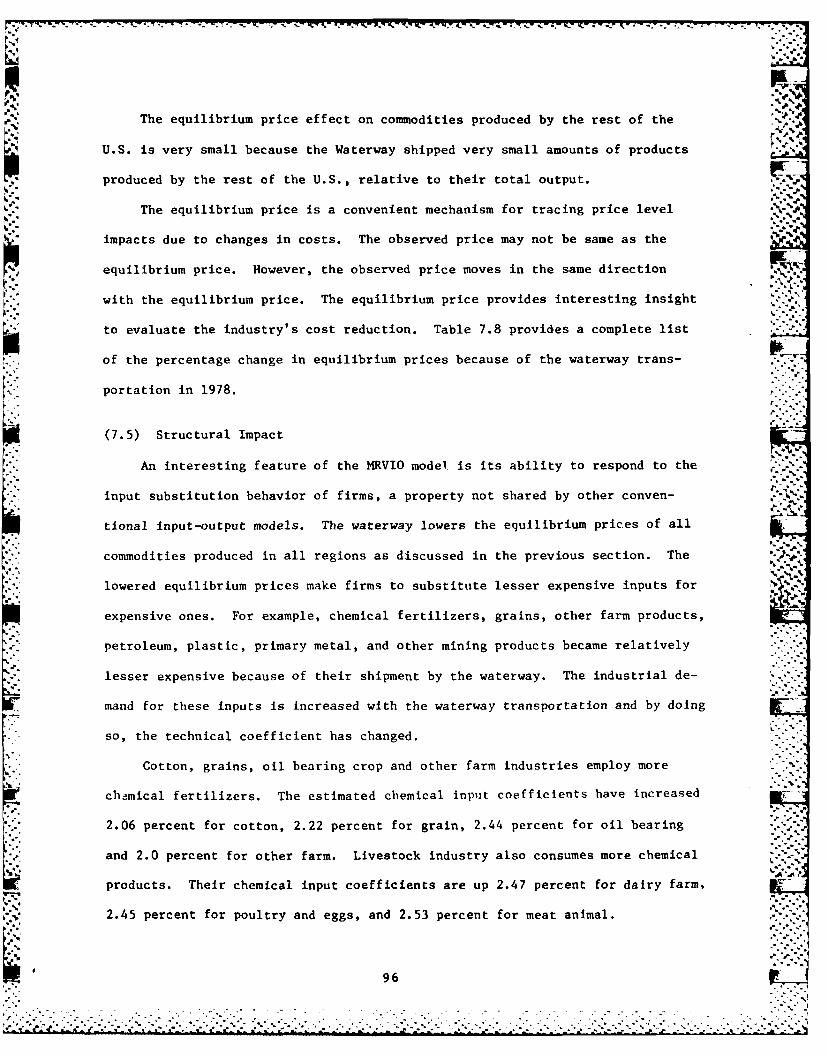
The equilibrium price effect on commodities produced by the rest of the

3U.S. is very small because the Waterway shipped very small amounts of productsproduced by the rest of the U.S., relative to their total output.

The equilibrium price is a convenient mechanism for tracing price level .

impacts due to changes in costs. The observed price may not be same as the

equilibrium price. However, the observed price moves in the same direction

with the equilibrium price. The equilibrium price provides interesting insight

to evaluate the industry's cost reduction. Table 7.8 provides a complete listp of the percentage change in equilibrium prices because of the waterway trans-

portation in 1978.

(7.5) Structural Impact

An interesting feature of the MRVIO model is its ability to respond to the

input substitution behavior of firms, a property not shared by other conven- .-

tional input-output models. The waterway lowers the equilibrium prices of all

commodities produced in all regions as discussed in the previous section. The -

lowered equilibrium prices make firms to substitute lesser expensive inputs for %

expensive ones. For example, chemical fertilizers, grains, other farm products,

petroleum, plastic, primary metal, and other mining products became relatively

lesser expensive because of their shipment by the waterway. The industrial de-

mand for these inputs is increased with the waterway transportation and by doing

so, the technical coefficient has changed.

Cotton, grains, oil bearing crop and other farm industries employ more

chemical fertilizers. The estimated chemical input coefficients have increased

2.06 percent for cotton, 2.22 percent for grain, 2.44 percent for oil bearingI.-and 2.0 percent for other farm. Livestock industry also consumes more chemical

products. Their chemical input coefficients are up 2.47 percent for dairy farm,

2.45 percent for poultry and eggs, and 2.53 percent for meat animal.

96

. ..---.. . . ..

Food processing idustry consumes more grains, poultry and eggs, oil bearing,

and other farm products because these items become relatively inexpensive be-

cause of the waterway transportation.

The input coefficients for the food processing have changed; the grain in-

put coefficient for the food processing was up by 0.173 percent; poultry and

egg input coefficient by 0.416 percent; oil bearing input coefficient by 0.0731

percent.

Table 7.9 provides the percentage change in technical coefficients in 1978

for selected inputs.

Waterway transportation brings two important structural changes. Ono

is a result of firms' optimizing behavior of input mix within the industry

i.e., purchase more portion of inexpensive input and lesser portion of expen-

sive inputs). Another is a result of changes in industrial mix. The indus-

trial mix impact of the waterway differs from one industry to another. Some

industries gain their strength and some industries lose their relative industrial

shares. Chemical, petroleumn, primary metal, other mining, service, utility

service, grains, food processing, and other farm are strong industrial gainers

*." because of the waterway transportation. Relative losers are furniture and fix-

ture industries which have relatively lesser industrial gains because of the

waterway transportation.

(7.6) Impact on Regional Trade Structure

Each firm purchases its inputs and sells its output so that the firm could

get the maximum possible profit. Transportation cost is a part of such business

cost which affects the profit maximizing decision. The waterway lowers the

transportation cost of chemicals, coal, petroleum, primary metal, grains, and

other mineral products. How would the transportation cost affect the regional

trade structure?

97 p

:"•-"" -"" -.".,,-','- ." ..' '"""", '""2-""',' .' .-" ' "-. '." ." .. . - i -" -" -".'i i'- " "." "" ' -"2 " - "-A°

(Table 7. 9)

Percentage Change in TechnicalCoefficients for Selected Inputs in 1978 (Unit: Percent)

Input Industry

The Waterway Counties Meat Animals Food Processing Gas and Oil Service .

Grains 0.159 0.173 -0.210

Chemical 2.530 2.544 2.591 2.580

Petroleum 0.305 0.319 0.366 0.355

Primary Metal 0.428 0.442 3.489 0.478

* The Rest of Arkansas and Oklahoma

*Grains 0.153 0.167 - 0.200 -

Chemicals 2.631 2.645 2.691 2.677

Petroleum 0.333 0.348 0.395 0.381

Primary Metal -0.021 -0.004 0.042 0.027

The Rest of the U.S.

Grains 0.007 0.010 -0.015

*Chemicals 0.000 0.002 0.007 0.007

Petroleum 0.001 0.003 0.009 0.008

*Primary metal -0.001 0.001 0.006 0.006

98

.. .4 ... . . .

%. %.

The transportation cost affects the equilibrium prices of all commodities

in all regions. These changes in equilibrium prices result in reformulation

of industry's marketing strategies. Industries tend to purchase their inputs .. .

from the regions where the equilibrium price plus unit transportation cost is

the least expensive. The waterway lowered the equilibrium prices of commodities

produced by the waterway counties and the rest of Arkansas and Oklahoma. Be-

cause of these price effects, the waterway stimulated the purchase of all com-

modities produced by the waterway counties and by the rest of Arkansas and

Oklahoma. If the waterway wasn't built, the percent of the commodity purchased

from the waterway counties and the percent from the rest of Arkansas and Okla-

homa could have been smaller than we observe now. That implies that the relative

portion of the commodity purchased from the rest of the U.S. would have been

more than we observe now if the waterway wasn't built.

Table 7.10 shows the impact of the waterway on grain trade coefficient

among three regions in 1978. The trade coefficient denotes the percent of com-

modity shipped between each set of regions.

The waterway counties consumes 17.1 percent of its grain from its local

production, 50.2 percent from the rest of Arkansas and Oklahoma, and 32.7 per-

cent from the rest of U.S. If the waterway wasn't built, the lesser grain

would have been produced by the waterway counties and the rest of Arkansas and

Oklahoma. The local grain growers would have to pay more expensive fertilizer

and its equilibrium price of grains would have been more expensive if the water-

way wasn't built. Because of these reasons, the region's consumption of grain

from the waterway counties would have been 0.157 percent smaller and its con- W

sumption from the rest of Arkansas and Oklahoma would have been 0.113 percent

lesser than the trade coefficients with the waterway.

In general, without the waterway the water region and the non-water region

would have produced the industrial outputs at higher cost. Because of this

99

. . -

L . . _

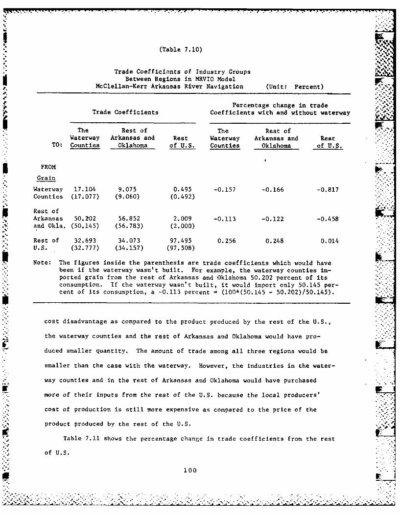
(Table 7.10)

Trade Coefficients of Industry GroupsBetween Regions in MRVIO Model

McClellan-Kerr Arkansas River Navigation (Unit: Percent)

Percentage change in tradeTrade Coefficients Coefficients with and without waterway

The Rest of The Rest ofWaterway Arkansas and Rest Waterway Arkansas and Rest

TO: Counties Oklahoma of U.S. Counties Oklahoma of U.S.

5 FROM* °Grain

Waterway 17.104 9.075 0.495 -0.157 -0.166 -0.817* Counties (17.077) (9.060) (0.492)

Rest of - . 5Arkansas 50.202 56.852 2.009 -0.113 -0.122 -0.458and Okla. (50.145) (56.783) (2.000)

Rest of 32.693 34.073 97.495 0.256 0.248 0.014U.S. (32.777) (34.157) (97.508)

Note: The figures inside the parenthesis are trade coefficients which would havebeen if the waterway wasn't built. For example, the waterway counties im-ported grain from the rest of Arkansas and Oklahoma 50.202 percent of itsconsumption. If the waterway wasn't built, it would import only 50.145 per-cent of its consumption, a -0.113 percent = (100*(50.145 - 50.202)/50.145).

cost disadvantage as compared to the product produced by the rest of the U.S.,

the waterway counties and the rest of Arkansas and Oklahoma would have pro-

duced smaller quantity. The amount of trade among all three regions would be

smaller than the case with the waterway. However, the industries in the water-

S6way counties and in the rest of Arkansas and Oklahoma would have purchased

more of their inputs from the rest of the U.S. because the local producers'

cost of production is still more expensive as compared to the price of the

product produced by the rest of the U.S.

Table 7.11 shows the percentage change in trade coefficients from the rest

of U.S.

1000o"V

(Table 7.11)Change in Regional Imports from

The Rest of the U.S. if the Waterway wasn't Built (Unit: Percent)

The Rest ofThe Water- Arkansas and The Rest

Industry way Counties Oklahoma of the U.S.

1. Dairy Farm 0.060 0.056 0.004

2. Poultry, Eggs 0.120 0.118 0.016

3. Meat Animal 0.031 0.030 0.002

4. Cotton 0.532 0.529 0.066

5. Grains 0.256 0.248 0.014

*6. Oil Crops 0.155 0.155 0.028

7. Misc. Agriculture 0.000 0.000 0.000

*8. Food and Kindred 0.041 0.036 0.001

S9. Textile 0.045 0.037 0.001

* 10. Lumber 0.119 0.099 0.002

11. Furniture 0.016 0.016 0.002

*12. 'Paper 0.035 0.031 0.004

13. Printing 0.050 0.051 0.000

*14. Chemicals -0.341 -0.241 0.004

15. Petroleum Refinery 0.402 -0.338 0.007

-16. Plastic, Rubber 0.173 0.171 0.011

17. Leather 0.009 0.009 0.001

18. Stone, Clay 0.161 0.171 0.002 -

19. Primary Metal 0.022 0.049 0.002

*20. Fabricated Metal 0.086 0.088 0.001

S21. Machinery 0.023 0.022 0.001

22. Electrical Equipment 0,021 0.015 0.001

23. Vehicle Equipment 0.023 0.031 0.001

KK24. Misc. Manufacturing 0.042 0.041 0.001

25. Coal 0.010 0.008 0.035

26. Crude Petroleum &Gas 0.028 0.028 0.001

27. Other Mining 3.299 -.4.320 0.021

*28. Construction 0.0 0.0 0.0

*29. Transportation 0.0 0.0 0.0

30. Trade 0.0 0.0 0.0

31. Finance 0.007 0.007 0.0

*32. Communication 0.0 0.0 0.0

33. Electric, Gas Service 0.0 0.0 0.0

*34. Hotel 0.028 0.030 0.0 O

35. Government 0.0 0.0 0.0...

101

Summary

Our empirical findings of the impact of the waterway are summarized in

the Table 7.12; the impact was measured by output, employment, tax revenue,

and government receipts. The estimates were based on actual transportation

cost reductions accruing to shippers who actually used the waterway-in 1978.

Not included are the effect which would accrue to rail industries by other

modes. The rest of the U.S. increased its industrial output by $102 million

* and its regional gross product by $43.95 million. The number of jobs created

by the waterway were 1,929 in year 1978. The waterway counties and the rest

of Arkansas and Oklahoma both enjoyed economic growth because of the water-

way. Regional gross output has increased by $10.67 million in the waterway

counties and $7.75 million in the rest of Arkansas and Oklahoma solely due to

the waterway. More jobs were created. 454 full time equivalent jobs were

created in 1978 because of the waterway transportation in the waterway counties

5 and 337 jobs in the rest of Arkansas and Oklahoma.

(Table 7.12)

Summary of Impacts from MRVIO ModelMcClellan-Kerr Arkansas River Navigation System

-1978*-

The Rest ofTotal The Water- Arkansas and The RestU.S. way Counties Oklahoma of the U.S.

I. Output 0$ Million) 154.36 27.54 24.82 102.00

2. Employment (Jobs)** 2720 454 337 1929 K

3. Regional GrossOutput ($ Million) 62.37 10.67 7.75 43.95

4. Exercise Tax($ Thousand) 3,496.3 506.9 486.4 2,503.0

5. Federal Income($ Thousand) 5,086.9 907.3 817.0 3,362.6

*Based on the medium estimate of the transportation cost savings.*Full-time equivalent.

102

REFERENCES

1. AloC and other, Interindustry Forecasts of the American Economy, Heath,

2. Amano, K. and Fujita, M., "A Long Run Economic Effect Analysis of Alternative ...Transportation Facility Plan - Regional and National," Journal of Regional

Science, Vol. 10, No. 3, 1970.

3. Antle, G., "Recreation at the McClellan-Kerr Arkansas River Navigation System,"Water Resource Bulletin, Vol. 15, No. 5, Oct., 1979.

4. Army Corp of Engineer, Survey of Transport Users Along th McClellan-KerrK' Arkansas Navigation System, IWR Contract (DACW72-79-C-4), June, 1980.

5. Bacharach, M. Biproportional Matrices and Input-Output Change. Cambridge:Cambridge University Press, 1970.

6. Bader, et al., Analysis of Expenditures for Outdoor Recreation at the McClellan-Kerr, IWR Contract Report 77-5, 1977.

7. Bos, H. C. and Koyck, L. M., "The Appraisal of Road Construction Projects:A Practical Example," The Review of Economics and Statistics, May, 1962.

8. Brody, A., and Carter, A. P., eds. Input-Output Techniques. Amsterdam:North-Holland Publishing Company, 1972. O.

9. Carter, A. P., and Brody, A., eds. Contributions to Input-Output Analysis,Vols. I and 2. Amsterdam: North-Holland Publishing Company, 1972.

10. Carter, A. P. Structural Changes in the American Economy. Cambridge: HarvardUniversity Press, 1970.

11. Carter, A. P. and Brody, A., eds. Applications of Input-Output Analysis, Vols.1 and 2. Amsterdam: North-Holland Publishing Company, 1970

12. Christensen, L. R., D. W. Jorgenson, and L. J. Lau, "Transcendental Logarith-mic Production Frontiers," Review of Economics pnd Statistics, Feb., 1973,Vol. 55.

13. Isard, W., "Interregional and Regional Input-Output Analysis: A Model of aSpace-Economy," Review of Economics and Statistics, XXXIII, November, 1951,pp. 318-328. '

1 . Harris, C., Jr., Regional Economic Effects of Alternative Highway Systems,Ballinger Publishing Company, Cambridge, Mass., 1974.

15 Harris, C., Jr., The Urban Economies, 1985; A Multiregional Multi-IndustryForecasting Model, D. C. Heath and Company, Lexington, Mass., 1973.

103* . .-.. .

% 16. Hudson, E. A. and D. W. Jorgenson, "U.S. Energy Policy and Economic Growth,

1975-2000," The Bell. Journal of Economics and Management Science, Vol. 5,No. 2 (1974).

17. Hudson, E. A. and D. W. Jorgenson," U.S. Tax Policy and Energy Conservation,"Econometric Studies of U.S. Energy Policy edited by D. W. Jorgenson, North- .-

Holland, Amsterdam, 1976.

18. Kim, Wong Soo, An Application of the Interregional I/O Model for the Study ofthe Impact of the McClellan-Kerr Arkansas River Multiple Purpose Project,March, 1977. IWR Contract Reports 77-2.

19. Kerr Foundation, The Waterway, A Report on the Arkansas River Navigation Sys-

tem and Regional Growth, The Kerr Foundation, Inc., Oklzhoma City, June, 1977.

20. Lee, T. H., D. P. Lewis and J. R. Moore, "Multiregion Intersectoral Flow

Analysis," Journal of Regional Science, Vol. 11, No. 1, 1971, pp. 47-56.

21. Leontief, W. and A. Strout, "Multiregional Input-Output Analysis," in T.

Barna (ed.) Structural Interdependence and Economic Development. St. Martin'sPress, Inc., New York, 1963.

22. Liew, C. K., "A Computer Program for Dynamic Multipliers," EconometricaNovember, 1973).

23. Liew, C. K., The Structure of the Oklahoma Economy, 1975, Center for Economicand Management Research, College of Business Administration, University of

Oklahoma.

- 24. Liew, C. K., "Dynamic Multipliers for a Regional Input-Output Model," TheAnnals of Regional Science, Vol. XI, No. 3 (November, 1977).

25. Liew, C. K., "The Impact of Higher Energy Prices on Growth and Inflation inan Industrializing Economy: the Korean Case," Journal of Policy Modeling

Vol. 2, No. 3, 1980.

26. Liew, C. K. and Shim, J. , "A Spatial Equilibrium Model: Another View,"Journal of Urban Economics, 5, 1978.

27. Liew, C. K. and C. J. Liew, Re1oonal Economic Development Impact Model:Phase I Study, IJR Contract Report, ]980 (forthcoming).

28. Liew, C. K. and C. J. Liew, "Use of a Multiregional Variable Input-OttputModel to Analyze Fconomic Impacts of Transportation Costs," TransportationResearch Record .747, National Research Council, 1980.

29. McCarthy, "On the Aggregation of the 1958 Direct Requirement Input-Output

Table," The Review of Economics and Statistics, XLIX, 4 (1967).

30. Moses, L. , "The Stability of Interregiona1 Trading Patterns and Input-Ou tputAnalygis," T1ie American Economic RevieW, Vol. XLV, No. 5, 1955. 1

104 ,_

-.........................- ........ ' -... "......- .... 1". . . . ."

SL

31. Polenske, K. R., State Estimates of the Gross National Product, 1947, 1958

and 1963. Lexington, Virginia: Heath and Company, 1972.

32. Polenske, K. R., A Multiregional Input-Output Model for the United States.Harvard Economic Research Project; Economic Development Administration,1970.

33. Saito, M., "An Interindustry Study of Price Formation," The Review of Economics

and Statistics, Vol. Llll, No. 1 (February, 1971).

34. Schaffer, W. A., "Estimating Regional Input-Output Coefficients," Review ofRegional Studies 2 (1972): 57-71.

35. Scheppach, R. C., Jr., State Projections of the Gross National Product, 1970and 1980. Lexington, Virginia: Heath and Company, 1972.

36. Tinbergen, J., "The Appraisal of Road Construction: Two Calculation Scheme,"The Review of Economics and Statistics, August, 1957.

37. Walras, L., Elements of Pure Economics, (English Edition), George Allen and* Urwin, London, 1954.

r~h

105

- . . o-. . . . .

...........

. . . . . . . . . . . . . . . . . . . . . . . . . . . . .. . . . . . . .

~r .~

r.

- . * ~~*.. .\Zj%~

4

.p

APPENDIX I

Empirical Results of the Phase II Study

.4

.~ A

V

WI

IS9LANKG~ * *.

107

. . .......... . . .

APPENDIX I: EMPIRICAL RESULTS

.4 Paze No.

TABLE 1 Technical Coefficients in 1972

. 1. The Waterway Counties 113 , .2. The Rest of Arkansas and Oklahoma 119 .*.-

3. The Rest of the U.S. 121

* TABLE 2 Interindustry Transaction Matrix in 1972

1. The Waterway Counties 125

2. The Rest of Arkansas and Oklahoma 130

3. The Rest of the U.S. 135

TABLE 3 Trade Coefficients in 1972

"Industry '1: Dairy farm products 141

Industry 2: Poultry and eggs 141

Industry 3: Meat animals and products 141

Industry 4: Cotton 141

Industry 5: Food and feed grains 142

Industry 6: Oil bearing crops 142

Industry 7: Misc. agricultural products 142

Industry 8: Food and kindred products 142

Industry 9: Apparel and textile products 143'

Industry 10: Lumber and wood products 143

Industry 11: Furniture and fixture 143

Industry 12: Paper and allied products 143'Industry 13: Printing and publishina 144 .

Industry 14: Chemicals and allied products 144

Industry 15: Petroleum and allied products 144

Industry 16: Rubber, plastic 144

109

'>~~. .'">. .. '.. .. ". • -".". . ."*." . . " . " . *•. . . ..- . .. """."~~~ ~~~~ " -"""" '' "" " """ "" '" .',_ "-.'.".-'-.-. _- ",."." ",-,-,".- .""-",.-.-.-, -',,:.,'' ,","*.-"" * ''", .".,

. . . . . . .. . .. , _ _ , , _ ,_ ," ,- ," _ . ' % .. - ' , '-' •-,- ,' . '

Page No.

Industry 17: Leather 145

Industry 18: Stones clay and glass 145

%Industry 19: Primary metal products 145

Indus Itry 20: Fabricated metal 145

Industry 21: Machinery except electrical 146%

<.Industry 22: Electrical equipment 14.6

Industry 23: Motor vehicle and transportation equipment 1416

Industry 24: Miscellaneous manufacturing 146

Industry 25: Bituminous coal 1.47

Industry 26: Crude petroleum and natural gas 147.

Industry 27: Other mining except petroleum, gas and coal 1'47 >Industry 28: Contract Construction 147

Industry 29: Transportation 1-48

Industry 30: Wholesale and retail trade 148-

Industry 31: Finance, insurance and real estate 14"S

Industry 32: Communications, radio and TV broadcasting 148

Industry 33: Electric, gas and sanitary services 149

Industry 34: Hotel and other services 149

Industry 35: Government 149

TABLE 4 Development Impact of the Waterway Evaluated by Demand Adjusted Model

1974 Industrial Impact in Water Counties 150

1974 Industrial Impact in the rest of Arkansas and Oklahoma 151

1974 Industrial Impact in the Rest of the U.S. 152.

1975 Industrial Impact in Water Counties 153

1975 Industrial Impact in the rest of Arkansas and Oklahoma 154

1975 Industrial Impact in the Rest of the U.S. 1.55

1976 Industrial Impact in Water Counties .156

1976 Industrial Impact in the rest of Arkansas and Oklahoma 157

11*0

Page No.

1976 Industrial Impact in the Rest of the U.S. 158

1977 Industrial Impact in Water Counties 159

1977 Industrial Impact in the rest of Arkansas and Oklahoma 160

1977 Industrial Impact in the Rest of the U.S. 16-1

1978 Industrial Impact in Water Counties (HIGH) 162

1978 Industrial Impact in the rest of Arkansas and Oklahoma (HIGH) 163

1978 Industrial Impact in the Rest of the U.S. (HIGH) 164

1978 Industrial Impact in Water Counties (MEDIUM) *16 5

1978 Industrial Im pact in the rest of Arkansas and Oklahoma (MEDIUM) 16.6

1978 Industrial Impact in the Rest of the U.S. (MEDIUM) 1.67 'Jj

1978 Industrial Impact in Water Counties (LOW) 168 -. ~

1978 Industrial Impact in the rest of Arkansas and Oklahoma (LOW) 169

1978 Industrial Impact in the Rest of the U.S. (LOW) 170

TABLE 5 Regional Deflation Impact of the Waterway Transportation

in 1978 (Medium Estimate) 1-7.1

TABLE 6 The Change in Trade Coefficients by the Waterway Transportation

for the Agricultural Products 172:. -

TABEL 7 The Change in Trade Coefficients by the Waterway Transportation

for the Manufacturing 173;

TABLE 8 The Change in Trade Coefficients by the Waterway Transportation

for the Mining 175

TABLE 9 The Change in Trade Coefficients by the Waterway Transportation

*for the Service and Others 176

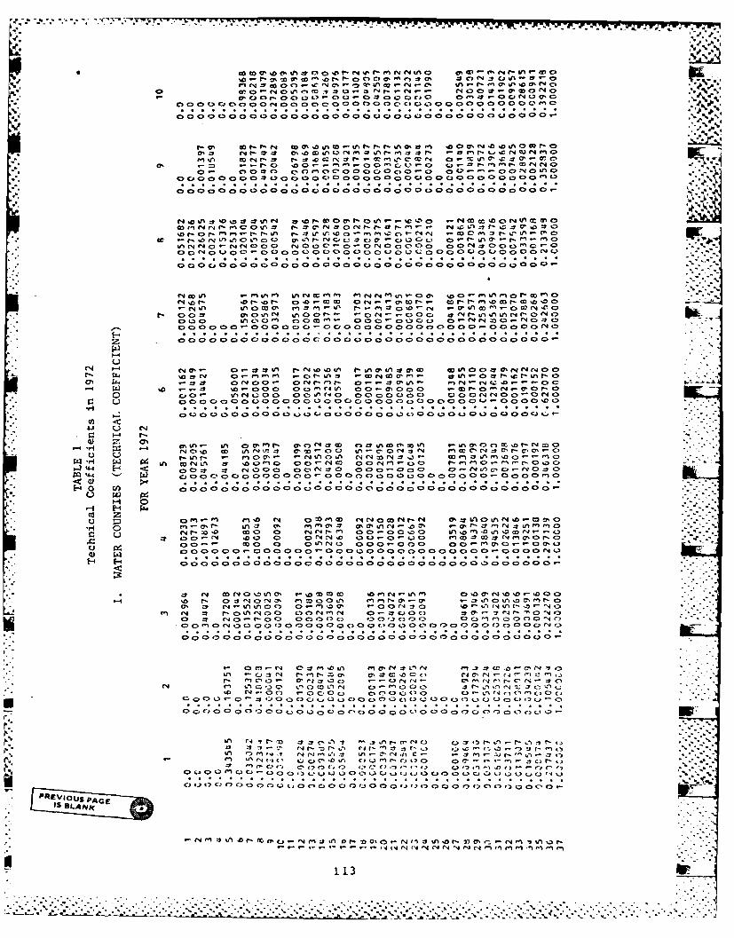
W. f 00 toC.~ * 0~ NC4 INN 04C5

*~~I C, oE0 u~~ r, 0' *~.td. e...'0 "

CP0 0 C-) 00i C00 - C000 fC 0 C00C00'00O, 0 0 0~.~~ .9 .~ .9 CC c...1 . .C

C; 000t;Csc00 0 0 00o0)0a 0 0 Cp 0OC u ac.c.00Q

0 0 uJO 0OO.

- 0t ( l mk MP -t 4, I-1 0 %A 0C- 0 C~ CDr-rN C al

*0 _ C. *1

o C 0 t U - ' 0 ,' 4 C4 1C0

00~ ~ a~ 000 ~0 0 C0 0 0 00 ci 00 0 0 00 C.C

a cl n U a0 Q Q00 L aQ0 0a > > P1N0lnv-Do -0o - r0

,- kn. -f u'C vC- %D~~ ~0 :2aLMO '*a, a 0 A CI "w 1 0 mC000 'M O r f ac C -r aC0~ z0~ V)000 IO - %Z:I =r

oC) a0 CL C)a NQ 04 C a a0 0 0 00a0G,0 cC>0 00QCII0a -)0C>r4

0 00 0 k 0 r 0000 0 M0000 00 00-0 0 0 Cy

%DOC -T-JA O~0 r l c at JLn- ~ 0 -S C- O Coo U- rl r-~s C ~ ra - W A r4 C.; D 0%0 0 C.~- 0 -o~ -4~ V% '~-o m Oe.,'ao .4-o C,-o

CL INOOQ O 0 n "0 0 C) 0 o0

0 C., 010 C "CCz~7 0 oo ~ ~ o 0 C 0 0 O 0 00C3 o 0O0a oO'

C) 0 > 0 Cd) 0 tz00v c00ci C:'0C.)00 0 00 0 0 Q 'D '_

r4U NC-, %D 0D Nf-f'r 0f00no 000 0 w ,C 1C - Cu I- f-4 .fn0 a, t'~ 0 -0-o to C4 '' c en = In

44 E- -C0 - 4%)1 )< vvC ) c, 0

CAC0 C 0 C)- .C.Oc) C. 40 0 0 0 -) 00 C4OD 0.

0 ~ ~ f V) C; f-0u 0 c ; )C ' .C V C)N0' 0- 00 C. 0 ~ A0 0

00 .~~ 00 0 0 0 N 04 0 0 C C> 0 co zt 0D 02 m 0

00 00 000 00 00 00 000 00 00 0 0 0 00

CA 0"A C 0-0 C OC. ~0 C' C

(4A . 0 0 '04 Q a' 0 0 - O C.,400C '0C(U C40C -oc'o 01:1) 0-l'o0'm0,

C; O 0 00 0 r0 C. 000; C> a C; C0 ; 0 0 40 0 00 a

N CCVQD C z 3c) enN e 4Daa" c1 00cl

CA -C Ln o ,l C- I (~-1 "' a 0 040.-..A- A C0C.0 CDe. .- f-C **C Cr1 c. 0)C00C 0,~ACC) 0 ~ ' 0 -4 r

0 0co 00 'C' 00 C> 00 ' (00 0 0 01'000000>00 C) C) 0 4 0 )

Q01 cpC C> 0 0 C) o 0 C3 0 0 0 00 C-1 C 00 0 0 C ) C) 0 (0 C 0 0 0 0 .

v~vlu PAGEp v-t "e cS3L Nn C- 10 lr4 r4 1

-. ~~ /COf- ~.C- c:> C_ 0f C-. 0 C -0 O C) C),a C .)30 C-4 N fC M C' 0 C

9 p 113

4C Cl(> 0* * * ~ ** . - s. - S . a .. . 5 . - C- - - . .0 -4 -0. C C lC : C : "0 : 111- C C

cE4'p .4m: r o 0- vEi SU~ ~N 0 -

4 N 0 00 000 0 oa 0.C0~400 00N rdc.,-E O N..% I%. i.:. , :.. :.00 0 00 0 0 zaOzoOOQ4ooaoOooo0o 0 00 0 00 0 oo -

00 0 00 00m0 0 r. m4(0C' 0C0 0000 0 0 f4 C a0 00 NO 0000:000;; 000P O* 0 .A O

0 >>>D 0-fo .n0u C'l 0 ; zC.C o a m0440000 0 C,-(0nOr~0-

.C Ct C: 0 . f ' . . . C: 1 0t CO'I- L'

o- 0 0000 at NOI m -~ 4 4f";w0 %CV-0 00co0 Co0 N- CD 0 C' ON %.%V -I40 %n o rooooM catoom .- OODOaC' f"OIcc wf O.(1,Or

0 a o C>0 'D C40zr-0 I0f-rQd4 0 a n r- ~ r..f0

4v*n: C4 0 0 O.010%00 0 0 .c 4 0 coOCa MfCV- .NC, C n0C) a C n m1 - nf

C* 0 C,0 CD D 2 0 000 00 00 00 000 000C>0C04-IC !H ! 1 C

MonenU r-%D0ri CD W-1 0 - e 0W=n.-otrc C U a0%D.)Cl to enf' 40 00 Qc C -, -0 0m00 L 001'.'0aC'aOaCa_ 4C a ' >C 00)0Q0C>00000C000>0M00.4.),000a0u0000 C0

,sC ,. 7r o D (-,c f.-C-N2 WN% V)-0' 04-A , 0g 03C> .. a (4 0n C0 0 N 00 Ntc (D G

i ~ n 40.- 0 %0C.,im 0N0.4"00a-.04-0g e m.O t.- ~ ~ ~ ~ ~ ~ ~ 2 000 0D Co O0 o C,4- .... ~~'0

-o %D4 c0000s000m0r00w0a0Lm0%n000m0001or 00o 00m c o -o

C.aa0 Cb 0' .)00Q 0C '400)- 00a'0r- C)0 ;aC aaC 000.a 00 Q0 a- .~ 0000 CIaC>-0~ C M0 a m > ) C) C

OOO 00 00, 04 000 0 .v 000 0 0 00 0 0 00, 0 - '4 0

N % ' ' C 4r- %D 00 O'%nQ 0 0a n 0C><.t00o ca P ~ 10 %n*= 0'O ' 0 .2 to

V-5 C> C.- '3 C> r'i00O0 'D M C4%lV 0- 00 in - o0oLM0 C 0 4 ,C, r--0

a0000 0 00 0 00 000000%Ar % L1r 00 00 00 000 000 00Dr-Wc,,

92 0 D ol. vO M f-M r4c- nr, , -'.OI -1 m 0 - ) C1 -4 C.> l~ r 0*lac 11 uoo a' 4 -1 mv * mc' c- r -, m c, r- L, Q

C vi t0'0- * 00 .c -T C.440 0 N) 0- c1(04 00 O (, _,0 .,, ~ ,r n0r 3C

0Q a0dC. 0 30, - 0.OC 0o 4Coc o o o 0 L t4fr 0 i en4 . . . * *000 Q0C0 0 30co00c0DQ0 0 0000 n000000000000

0 000 C 0 0i 000 Q 0 k)- 0 W 0 0 a Q 0 0 a C.3 CZ C% 0. 00 0 0 C2 0 f.' 0o 42 C

in0 %D 00 0 0 0 f4 on 9 00 ai r. 00 L% 00 0q CO M' VN a00( 00 '0

114

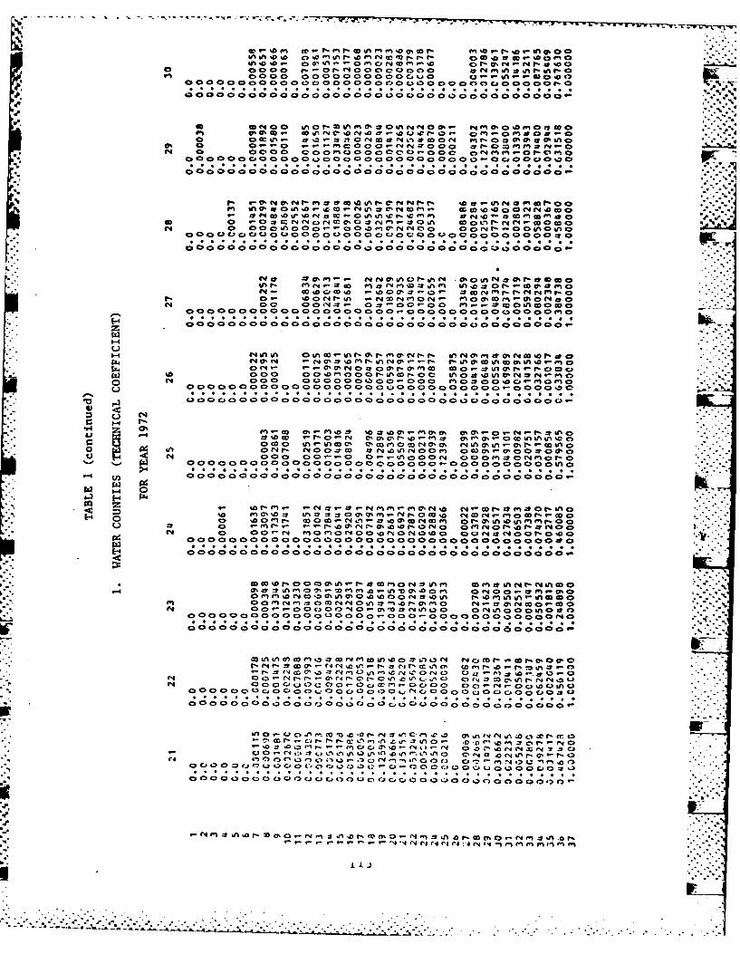
f-~.. - 0 - N o0 a m'9s-v'0 a r@ r.- r- v% -

0 W"00 e 0t N 0 o c 0

'9~~ 000 ooo oooAos7

440 a 4 Qoa 4.ao co .,q M0 foO ~ o O o o 000000 0 m0 a

e a 0 0 0 a i 0 . - 0 % 2 ' 9 0 0 - r 4 5 0 * f . 0aN 0

0 O0 1 0 'O OO )00% D c n - o" 0( 5 0CMt0

00 i 000 0 00 C) 00 C 0 C00 Q C 0 0 Ci 0 00 0000003 0

~nr- '9'.s.-3v'b*m.n' 000'@p o

CO0-00 o ~ o. 003Ca* N S -

1; 0 caQ400a0 0-0* 0 Q a0 0 0aQCQ00 30 0 a 000

1- I4Ilf 0Sn N D E , 0% rf SnvO'M m~ - C.~d

42000- C0 0 * aV r- mCo C 5 0 %n43 r- 49W0Qo aC ,C 00 0 090>0a.a 0a0 a a 0CI00.Q:20 (n a04903

N~~~ a .0 .)

a.'U ~~ 0000000 0 00 0 0 90 0 0 o o o oo o o

00m 0 : A 00 .- V.-01 0.-f t-4 0 %a f00 CD4S0 04ft4 c 3

0 .0 00 >0Q00 00 00 Q Oa0 a0 00 00 0al0 0 a0 o a0 a0 0 aE- 0C ;Z 41;1 z1

0qC Q0C a9. r31 T0'. =~ - 0noiPc1> n0I.afin 4o c0~ ~~~~ 00N E9fo4 0or4N w 0'4 O I 0

1;49c 0 0*01000 aaoa coo 30c> 00a0000oa000a06a0000.-

co in &M 0) w m D -70G f' f coL - zoaL,)L>( 4C CDr- t W 0N0 ,- 4*C cW mel"c 61m wmr 0 00 r to00 * 0

'9t)0-C 00 9N N0 t4 0O 9 0 bn' U.W16c ,C 0 C 0.0,0 0 0 o3r.jfC4 oaaaC 0 '4USOaOamc.4;3O 4

00

0 0 0 0 00 0 0 s 0 ' 1;OOOOOOOOOOONO1

* . . .. .I.F%n a ci000 .m00 m 30co 00040a000pr 000n0n0N0 o 00mo. C

C, W 40-- In ' - L#-T0

00 0 0 Q >CU 0000f C i 0000, C> n Nj 0 000) AInC)0 C) 000 0 0 C)

-so n I o.0 r mi m ~4 a N n(1' 0 3,. F,4 ' '4XN13C

-.- . . -. ' - 4 "S 4 I'l (4 ('4 (4 :A ('4 (-a n e-I fn m9 m94 e 9 M'

C44

r-~ ~ ~ ~ N -: a.'a~~~~~~~p LD a 40* aN 01 '

on 00Q 0 I 0aNJ C1 0 0 o o 0q

00c) QOC oc.0

C4 ~ ~ ~ ~ ~ ~ ~ ~ ~ ~ ~ ,. kA*,4P i O f % 0:0 co0m(

0 F" " Cjf" CO0% -b0. ;;Ms 2

.2~~~~~ ~ ~ ~ t!% 4.?.i D is Q-J

in N~ UN 4 nda0f n4Mf naa %m4

ap0% 0( 0f.' :

A ,C 4 C ,' ,L 7 0N(%000 4 o~

0~~~~4 N mI.% U

LmC nf A I 0# OM t 0 40-

%D it 4 v a4.

'-14 j 4 r t %r

at CU~4 CL 0 Mas ~m , ( 0mn i C,

0000f0N0 Df4 M00c0000cr-0 td CI '0%. N 0

0 000 -N ,1* 0 0 4 oa l .)0 o - .tQ

~~C 00 0000 0 ell0 00 o a 0 0 00 C. Oa.

C4 Vb1 - of 0 4Dw P. Mi)@( ~ 0 . t ?40 f4 ra~., 0n .6-- --- - -al-' .6 N C -"N Cf4 N .-4N f" bafn en In I

* '0 *~0 ~0~ 0N~flN 0 116f

AnN0 00 0 (4o0 .- %N N- m0%t 04~ . 0

OOOOO OOOO O~oO OO 00 0000 0000 000000'

GOl ~ f0 O m f.0 f 0 , 2 0-%D r0N0 Mt0 4C CDN o41% OOM on 00f0 6C ~ # 0N O co .4/otoc ~ a nr ,r

00 c

oot No or .a afu4o r--e r m N C

I- C ,,!o %f~0- 10 N.o0 * M ! 0 ! : : V0 0 00 o .; 0 C 0 a0 - 0 00 0-O0ooO a0 0(40 0

00000 G 0%0 0 0 0 0 0 o a0 00 O000I'4

C. 0 N4

O'."~ow "- a ('C)D.r E aN CO a JVto-o400 CDo "O11 en r- 40~ - --j . - er.-. N--o Q C

E -. aA O O 40 0N 0 0 00 a 0 " a0 . - r J

Ai~.0 0~S 0 C 0 M I 4tinC n 1 OU mC .% 4 a D -C co 0

o cr w , o t 4omE--I. - O nL D -so Na ,fM0

OM = m Coin.-) 0 C Mrr.. c aot)0o o-'oo.Dao-4 a 40 C)0404 00 o ib a0 0N a a C.a 0 a0 0 0 va a-.o

C4 i O o CO 0A NA .(40I NfNi rn QCO aQ o% r 1 wN- 0oo-s oUi a a N 4 o aUs 0'4 0 0 m W7 w_- " 0%0-oC

00-, 0D0 o0 41 o 0 0 a a a 'M-% -0OC:' %D 01 0(1'4f 00 4.'0 C! : C 4 s0: 40%rl o

: zro CO M ON b '4 00 00 OOmM CO.-O0

v)* 000a000000000000000000o0000 00A0t-0F- C

0'~~~~ ,0 o-r o oM 00 a' 0~ a a a o C>t.&

0 > LA C'0l O 0 oa,0 0% cc o rfl om r- a M

07 %iCA*r G "C * . ao =3C4'0'4N 04 i&M1-4 Mr M -- yOOON 92 #-.N .0 C4c('N o' GN-' . :

0 N0 0000ooi 0 0030 0 U% 4 >00 0o

CO0 00

0 000 0000000;,C ,; oo ooo o

0000N j 0-% -09 :; F00 0 0 00 0 000 C, l 400 0. 0r.r l

- r- oe-.jm ,4rAI)S eqW a n - r- u =.

Q 0 C3 Q* 0'~ o .;, "o o V~~ , ' . i- IN

000 M ) o 4D . CO % 0 000r C.'N a o , C 0 r O 0A C) el 0D 00 .) 4.4 0

-,r

%b %D N i rC. 4 c Mf MNO~~ ,- cr-oM N r4 CO

0f in~ r4 0EN00 c0 r-

000 000 000 C 0000 C i C 0 CN 00 0 00 0 00 0 M ~ C4 a n C

0 0a40o4 000N0o a0 aa a0 00 0 0a a0 0a CP0 00O

000 000 000 0 C % 000 zr N 000 P. 00 0 N. 00 0 4 0m w .M. A 1 , DN C - awt !"1'...

MMDI rO L Ub OI t- M w

a 000 0 N N ao C, 0 00,4 i0n :! 0I C)0 00 0 00 0Q - C u~0 C, 0 0 = 0 a 00 0 0, 0,

C:I .%% !I C . ! . . . * . . . .* 000000000>QQO00000cj00000CIO00 000000000OOO 00

coat n C 4*r iC c Cr M2 (O'O s : a V 0 a C...~

M a- 40 000m t- a.0 aO a0V0.a - f -Z 00mM 4 o.404 0mc 0 4oooo:oaoaooa-o4oaoao0oooooaooo. a-

00 00 a 0 00 a00 4 0 00 00 0 000 000 a0 00000 00m o00 n-

a: 1 I-' 0000r-00l00P.Ca r-0w0 C.0r-0o000 NaU0 0 F

mca i *C 00CoZ0 a o0 N nr in 6.. . . . . . . . . . . . . . . . . . . . . . . . .

@0000000000% 000 T 00OCi c 4 oOOOO4o4oooA

C 0a0 a a0 aa aa aa aaa40a aa aa

.- 0- wO O O O O O O O O O O O O ~ o O O 0a0 0

O0O0 000O 0000 000O 0000 0000 0ciO 00..! z< 09 f ai

0%aCO- o0 (4~... r- an0 0 c % r- P- C 'r4- 0 0 C C

Iii 00000000 l o %ac. Q ink C o00.- ain 00 N a ,!z; ,; 4

00 0 00 :> . r 0 ,c 400 ) v -3 C -0 a 0 0 00000 0000Cka 0 00) 0 o0 a0 000C%0 00 0 a0 0000 0 0 000 0 .

En 0I) - CCO N.D 0 -i ,o mm ,c4a-w-I .- m-A oo co r cD m in en 0 ,-m:tm- -L Ac na n

000 00Q 000000 Ci 000000000000000000?ci OcD

0 100) 0,0 00 ao 0~ 0 a a 0 o Qi 0- 0 Ci 0 QCQ 0o 0 ai a 0 ai aa 0 a0 a

00 00 a $io: 0000 0r000 N00 000 000 00 f- o

C;~~ .. .. .

40a00 C a4 CC) ,C> 3,CCiCalQ a04

*~-' -. .. .w. . . . I

tdO.DD 0 1,.: C)'m r. m 0 m mN Nr M%; a aa0 00#AN. a m- 0CN O O O O rN)J Iom 4 wr.r-t aw ws0o

%n 0 00) 000000000 -n wm I 0 f400 N0000 D14:

m0 D 0 0 a C, % C0 0-NC, 'fla 0 In 0P),4 i0* ~~~~~~~~ ~O ? o o C o'0 00 O 0 o O ?CtO O

00000000 ;1;Z z1 C ; C;C C) 00 0 0 00 0 0 C 00 00 00 C, C; 0;C ; j888C

10 . OD .n w w * t- 0 m .y w m .' m 0wC -ain000 0000000w0o00f-000"mm-0000-00 m 000I-p;

C 0 0c 0 0 ,a8 C a aaN 0 0 o o c. o 0 C a

co- - 0 fl4± O 0*Not;aou co A r 4;C > C

a 0 O 0~ Lna CO. 10m~rr.- 01r 0 L

0-. C00O000 OO0Oi Co00000C,0 C! o 00oo c:

000000 0 C 0 000 0 0 0 aQC 0 a Q 0 0 0 0 0 C.) 000 o 40

N :r r 'mf , (,i Cc - C n 0 f r....-2 aV4 %. .n .r 4. fn *0 10 10 10Mc *C. r c . ,0 I% N

00000000 -70 C, 000000000 0 C. 0 00 PGj nr 000000

a 0C~ C>* Cm C-0C) > C aC>C', C C) ~ ~ 9

fa. %

10 0 ; 01 4.. 0; 1; 0 1; . . 004. C .C; 0 0. U 0 U0 a0 a 0. a. . . 0 0 0 C, Q)OC C0 , CCC.0)) C. C- 'O~,~.,,.o~ C *

oa( o c c U0 C> C CC> C> C) - > C. C3 La C>. 4D (D 0 0 fr-j~,( 0 - N 1 0 fn C3,m

C119

E-4 a-

_4 01 C4 N 01 tr's 0 C> LM , m a3 r - 0 Mo.m a II .flm 1

r- LM in;:-Tel_-T m~no cl _-j IN 0 w CNL I )(3I r u ,Q C -ra) 0- ) )C 3 I Z C-C . ) I ) m _.

C C C)C3 C C, C),C, . C C) C C, -:: c QC> , C, C> C) ) C, C) , .

C> C C.0 C C, i C C)C> CDC3 ) C C) C) C30 0C) ) 0 j 0CD C) > C)C, > (, C

r;C ; C - ;C ;1 ; ;C ;c c; C 1 3C

C.,

m.

IN m lmm 0 -T -2- 1r4mC

C, C' C. tC W L>r.qf1.J -

C> C1 0--..fi C3 0

- . r *

'D C- 0, 0 C>bO , CJ 0 0 0(0 C, C) < C30> c

00 00 0 0 C) C-)00 0 C) 0 0 0 0000000= cC C"0, cf C0 D' DC

C)0 000000, C) 00 00,C.00000000003000000000000 (3C 3

IN 11C '0', INC)j, 'n00(. C

0CC)~~~~~~~~~~~~~~ C) -j '4 -4 N,. 0 0 a.j~ ,~C )0

C ~0 '0 ~ 'c )

00 ) 0 00 0 0 000 0) 12'0 0 0 0 00 00 0-

- I~ oJc' tN'J0 l~t.J..J.2) *-c') r..7-- -r r-z

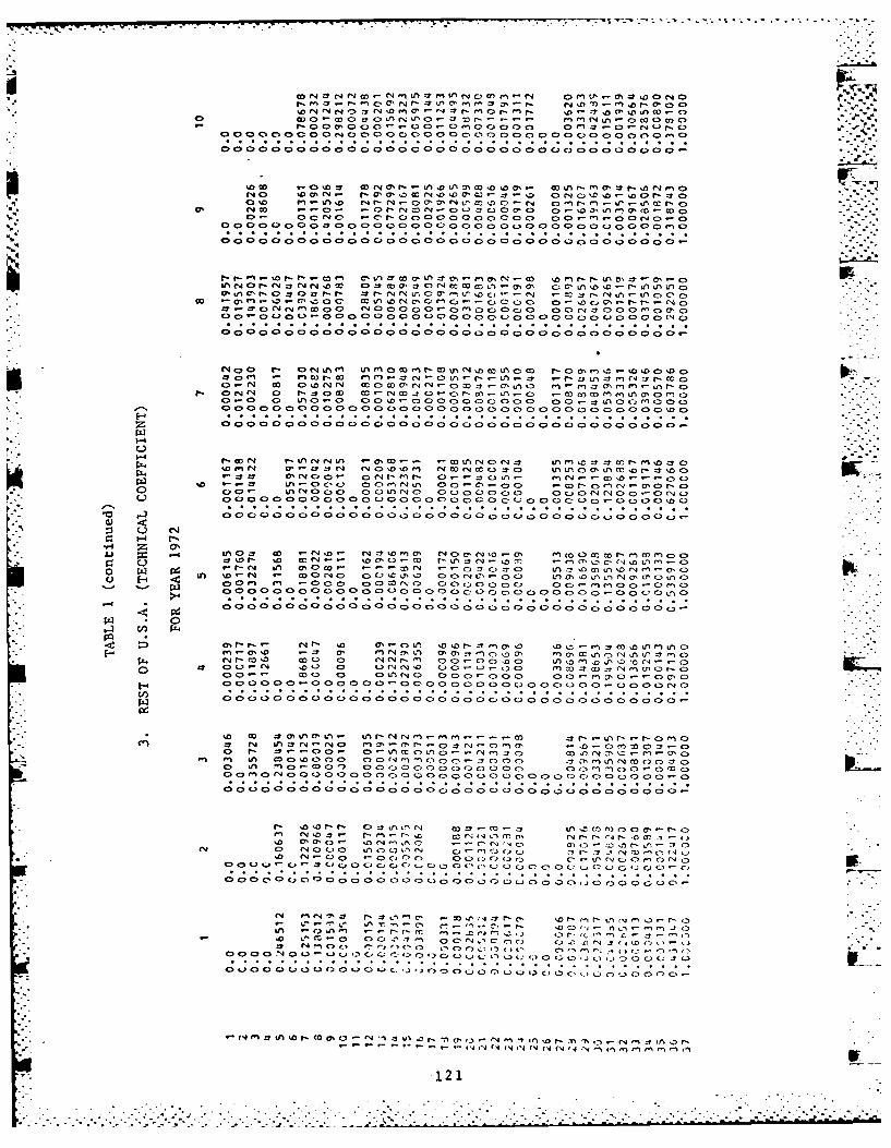
0 0 04 In 0n 0 0 0000 0 . 0~ 0 C) 0 40 C> 0-

Oo~oOOO O~oOOOm 000I r C) 0 0 0 0 0 0 0 0

'D I.- 4 o 4 -7 0 m Coo j' .- oy r - c n m 2 r =t00 00 00 00 0 00 0 0000 00 00 00 wDr-C n -HO:C

000 c *>8O Q -0Q aco0 0 000Zo OO )0 C-( )c 0 . .)o .C.oo .> ,oO

c- cc:, ~ rO -~~ cc:,0- ml 0 ccC> LAO

.% .o a . - . 0-. 0o . O'col a0 01J aD- 0= )C >C 0 C) 40 0 C>CC) Q 0 c mQo)0 .' .1 000 >Ol C>

00 Ln 0 P 0~COs (7,omoTm .n-oc o %0 r-r LI- -cHt O O O O . O O O O ocoo o'oo ~ ,~

C>C)C 0 00SO000N

20 In~0 ZY In -7 CQ;4r (P.0o C 00 c 0)liE 00 -~.'a -,~7 y r

ClC 0 CD 0 0) 0 0> 0 0 0 C) 0: C> c 0 0C) Dc>C) (D o > 0 ) > c) > c o c0 0 c>

=r-T C 0 .t ~C f- In-~--.r fn C' .- n ro- ~ ~ C ifl -cJd) Z~~-.1 m -n0.:C 11C0 ~~

wA WM "1-".C CC)

tun (O C'Ci 0 ^ r. C, C rqC) :> C,(IjCpv >o >C)C CS c ~ C L' L~lC 0aCD )C)c; '0c )0121 SC c

1;~~~~~ ~ ~ ~ c; c. c. c; c .c;1 -c c l1- - - - - - - -- - - - - - - - - - - - - -

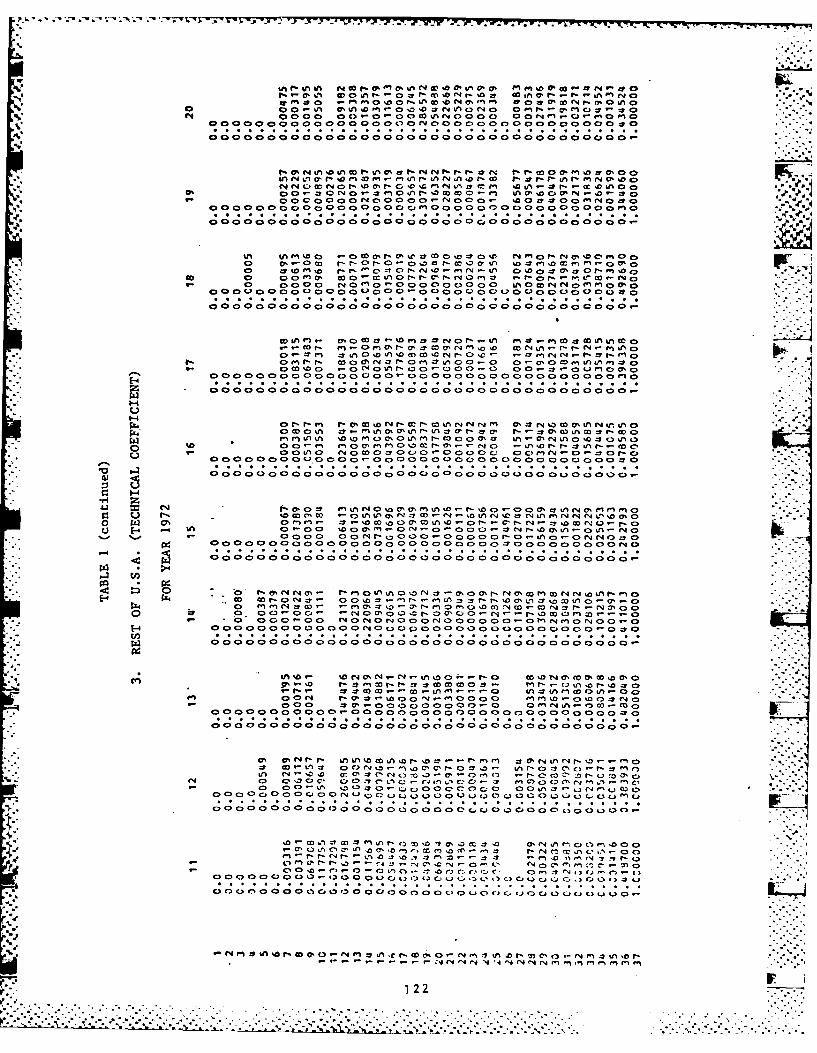
a,- -, w a 0 1:;0z.. . . . CI. . t. 2 n ,r -f -U m"

c-. 000 40C3 -0 0 0 0 %n4 0 0 0 00fin -c.. f" pnoc0200C20 0 0 00 000 C, 0 NO 0 0 00 0 C, 0

inr .1o We n .L vI or O V t-Fr-d - (4 ) 0 C)N 4 0 cc(40 %a a, r r_ t %i N or fnE .0.to in OU40

0000000 0000000 0 ' 0 0000000000co0 00., CJ..-.:

00 0 00000000N 0000 ~ ~ a;: C 0 00 C.. 000 000 0

%n %A mto a oaw 0% 11 C', Nr 000crC 0a 0.a CIn m C0 rl g Nr- 0; 0-o 9oat- cc A %D n t rr a cmP :aV

C>o of oo'.'a - t-01 10 rr- C'- m mL 1 0a T -tO- r Ck coW.-N%

*p a N C. In 0 z . .2 C.C . C n0we qC

OD f- C r- _r.4uM .01 ' 2 0 0 t c w w0

-~~: 00.0 I-4u-r o o o-- oo.-. .- o Loo'1-4 r fn z ) %a t en CD'C eq000 C> CO!00 n ,004 u r, m

0000C-. 0 000 0 0 4 0 0 0 0 0 00C0 00C0 000 0 0000 C> 40

440- -m r tw o"4 ,w0 m O' OO .%

P4, CI c-o a n - L lL O r, L0-r Mr- M r o.#.,.,,.r~

P, m- -n oow' o io chc) n m - m a c3c7% = n at " n o to a inCo ;I; m~ m~4 al m. 00 0 inC t C .07 C 'tN4 10 , x 6 _ (o~D 1-4 (D "40 C000OZ 0 C> A C; rN

CC 'j. 0 0 0 OO -C; C>oOOOC.C C 2o 0c.C C oN 4O n 0 4D-c:, alCNo oI000000000000000o0000 ; - C;C;1 c;0 0 C; OOOa O OON

* .~ 1-4

41C- - ,cn-t enL r00000mam mto r 0000 00 00 000 00 =0 00 00 m0 00 0 n 0 09i %0c *c 3L n " YC 1 oL f 4t 4r D0

- 0Oac 0000000 CN0 0.00 00 C>co0 0 .C00? r.40N00.CC>C4:

c fl' cor-.0C - C> 10 -r- r- - In CA =*v - PO 10 VIz0t'o M LM 0 . 0<D0

0 C, C> ) N *0 4 0-V " '>0 0 a ~c m M C. N 0 CCON CO> .0 O 0.00 0 4D 0 0.N

0000Q 0 0 0 0 0 0 Cor 00C)0 C>0C 0>0 0 0C>0000 0 0 )0 000C,0 0 ?0 0

inNaoC ,N 4 k oC r . t 0r a,'4~f (0 Ol co 10- .010 r- - (n) co 0- f)Ns . :T CD cro c . mA NI 0n r- f> t 'o- to ? '4

N= 0 0 0 J.7 'f>-~t~0-.

0C 0 C;X>0 0 0 0 0 0 0 0 0 a 0 40 0 0 C) C, > C. > P a C. C> C0 v 0 0 U

oo000000000 C 4 .1 I 00 0 000000,0P 0 000 -T n OO C) ).f -

.D-w Do. M4 C .c, 0 .cC n 0 C. a 0 L% 4. 0 C-)CA C

8 Pi mA '00N 0 a 0 430 N " 0 1; 00C-0 QC'. 0 CN Qi %D 0I.O )0'0 L -CN Q~' L .1' 9.0N

'a to tm - M f- .- -4- -f o, N N .1 'o *4 In N N- N) mw' 4 14 j4 a

0 Cr M M ,% , .t ; cr. 122

.-~~~r u. C4 - 4 * ~. *...2 .. .4.~,..2.,.~,-.- . V .. .

a. c0 000 1%O % f Oat fmD 7.0 a t% %D 0 0 a N a % %

.0O 00 00 ;0ar -0Q0C1 0 00 0t ! :00 00 000 0000 000 000 -00

%a co0 5O'fl *03 0I 0, "WIC" J.0i r, 03 C, 50 0f'J- *- -~..OD00'~('d0 0a0 .tC.-.J O ~ 0'a~ 0: 0000 00 E I0 , 4? 0N a ; N; d*.O.mOC.

Q .> Q 0, . 4n co C,.C m Co C

Q000 00QQ0000 0 aa o cOO O O OO o ~ o o 0 -

0 .- 03WN"Qr'Jam 0* NM *OI CI C OLNI1 .Wt-C

*00 a . . . .

0 C, 0 40a0 000 0 0 00 0 0 0 0 0 0 000 0 0 0 0 0 0 0Q0 0

(~ " "0,V.- 0. N CN soLn L 0,CN ~f r0

9%I4 000 0C>0 N. 0 N -- 0C0 0 kn-t'.035000o

o4 C,0 0 2 0O C,0C. C3 c. 0 -QC, 0 n0 O 0 I rA 0 f C) n

CP .pa 101 0aaaaQ 0 0 QC0QQ0, 0 0 QQQu,0Q00 0 00 0 Cn

ON0 0 0 0 0 0 0 0 0)0 0 0 0 0 . O O I C.- r .3 N *4 . *tC t0 0% M e f %0 >-1t"c

w M ~ 0 0 0 0 0 0 0 0 0 000000 lC - nr 4c M a0 % e000C0000.-' L cI- Co0 nL c k %40 C -0fla z Dc %a

- JL 94 0000 oo r- C oooof o 0 000 0 0, -4 000040 r4 OO f 0% 1 C C

E-oNC Co P.0 - 0 0 0 0O% *PC.Q L v O C n 40 0-C>lC.Paaa 0 0 N04ICJ0a .N 0 00d C,~00.o

9zl 0 Coo o Q a a 0 , 0 4 0 0 0 a O Q C , 00 c o a C .o o coo o o oaoo o o o o o a

...................................................... ..................................z % 30%r wr th S5J LnF I JrJCtL.tI tC00tNV% 400C40 0%0c

m C.0. o 0 0:: 10 m n :r co d r2V '.- n r r.4 110C.0oC4 C) a 0 C3 0, 0 a 0*00' OC)-> 0 -03f , 1.0 , nC3

C 00 00 00 0 0 000 000-0 00 00 I 0nc 0 0 0000-L CC0 C->

00 0 0 0 0 00 0 0 0 0 00 0 0 0 0 0 v)

00 0 0 00 LI 000C000000C)LAO C, 000 f- LI ( LC 00t - I 0

in %D -0 r ,D -orr- r4 I 0(1 O In c>N C3 . -,

C4 0 ) -0 -'1 0c-0~ ~ ~ 5( I .~-

a IA .0 r. CO -0. %0 .fl ' 10. 0' .1 - 1. A0 f- 7n 0' 0, - 4 1" -1 11 r. P-

123

-~~. t. z . ~2,

461 - -

w oW 1 P w% M-4mr r Dm0 0 mm i0 0 r MU, i naa- mr mmNtN"Ni

"-N44 a ( = xrm c D C . of m 4

E-io )4 J 0C . G 00c u c ;-.2 n C,0C ,Q Q0 0C C 0C - I 0 C>4 a 0 , 0C3 C

-4 .9 9 C9 .. 9. !: CC 9 4

40 o ~ f' Q r' %a 0 0 00 4 0C. .0 C NsC3

_4r NV 00 00 CO - 0 00N Ln% 4C a( 4 0 . tor-0 n O0 a0AVJ O VCOO"OC-C)0 Z coo o o o o o -7 4 -oo- -t'. Co

fnI a a' CI 4fl 0%0>f 0UC:0NQ0-ft f3ten IV A t -. 0 C4 -10

.4; 1; C;C;a*a s00 0 Ca 0 0 C> 0 C.) 0.0*DI0 a a 40 C.)a 0 -0 0

o~0c, c fn In NU10 .0 .0'.* if-v.. C) ILANmw ONOOm O%n 40c0 C. zC. C430 a,0I 00N d4I-N, O" No,(-33L 10

v , ' C ic C)N0 0 0 ' s 0 ' Int. "-0 a

40 0 -1Q 0 LjOO N O 0 4 %f" 0 1'f3000C3 O r'0 0 0 0 0 0 a Q -Q 0 r o> 0 a0 C

000000000 00 0000 z I 0000- I 0000000 I00000C e00 V

WO'~~~ N 4, C%40. Cs 0 VIC~

('400 , C40 ",OO J O , W 3,43en ~ ~~~ .i' "m

0 . >C. L.

400a C) 0Ci 0 0 C3 0 0 0 000 0 0 0 000 r0 (.A C. 0 0> 03 c 00 0- C,

124

'N. m i0 . aD0 0 i0 w%0 m0 N 4 f- a 00% N w w am M N.0 I N 0 LO % 0% rP.- 0 .00%M j20

%00 ~ ~ ~ P. %O xI9 % at 0 . . -l I- am 0oC 0 f" @p 0~ t-0 N 40 - N a -41-n 0 en ont c 9*o=U ;c%_

ClO0MIOCONOO- .00000000P.P-0.00%0 4'C0 -LAO a m

00 ti N %V C. 0 c do N m 000 N o %V &A .0 0 0% aD eq a00 f" eq , 0% C4 0 ev M fInt wwt.mc . .O

wv0nn P.004000 09a -fNCh _-G

N4 N N N4

0 0f" Li oC 0P..o %)% 0 0%M %M01 wlCDt-0% NP1P b 0 40my

N0 cc I a IC , 0 D Na0 f

'-4

.H ~ @0% 0 2tC% NN? O (V NP' U, P.fn C% N 1 0C IONa, ~010% w0%m%o- 0D . i NIAO Ona00 a-0%N@Y D%D LMf"C.wO 00N a%n a a 1N in0 0 0 0 0 mN000U,0 0.'11OOAOOO Q 3tc4 c z - C NP Wt

0 (U 0 .

* N

0 CJd 0)

C, 1 .; c (%1.- -.-4 _rO 0Y Q. 0 %DNI * 1 i m.1 r nw00co-rv- P1 N A % NoN 40 IA0I' 0PN 0 OA I O O 0 0 nnN 0000 r0w 4- W 'na I.n C);

0 M 0 ID cy N a 0a0: Q0 M% DT ' . _

a- C; 0

f,4sl loop N a' a rl r ,N4.AZ, a0 %D 0g* v , IA0NP.I0%O

0- a3 Pn 0 10A NO00 0 Q-'0C. O Co0 0 ra 000C.C Cn. n LA QOP0 LM -COU en enOOO OO100' O O *700 wP11 ~f00'

4-4 M% P. a-IO-. %aOIM NP0 n C3 A I00Pt V- mn IP. .0 -~I0 -0 0*~I*.0P. N.IA'~Dw 3.O w-!I0N-

(4 0%4a NMI01 r4 "4,'n r

0% -0 - ~rjmI 0 -- g25.

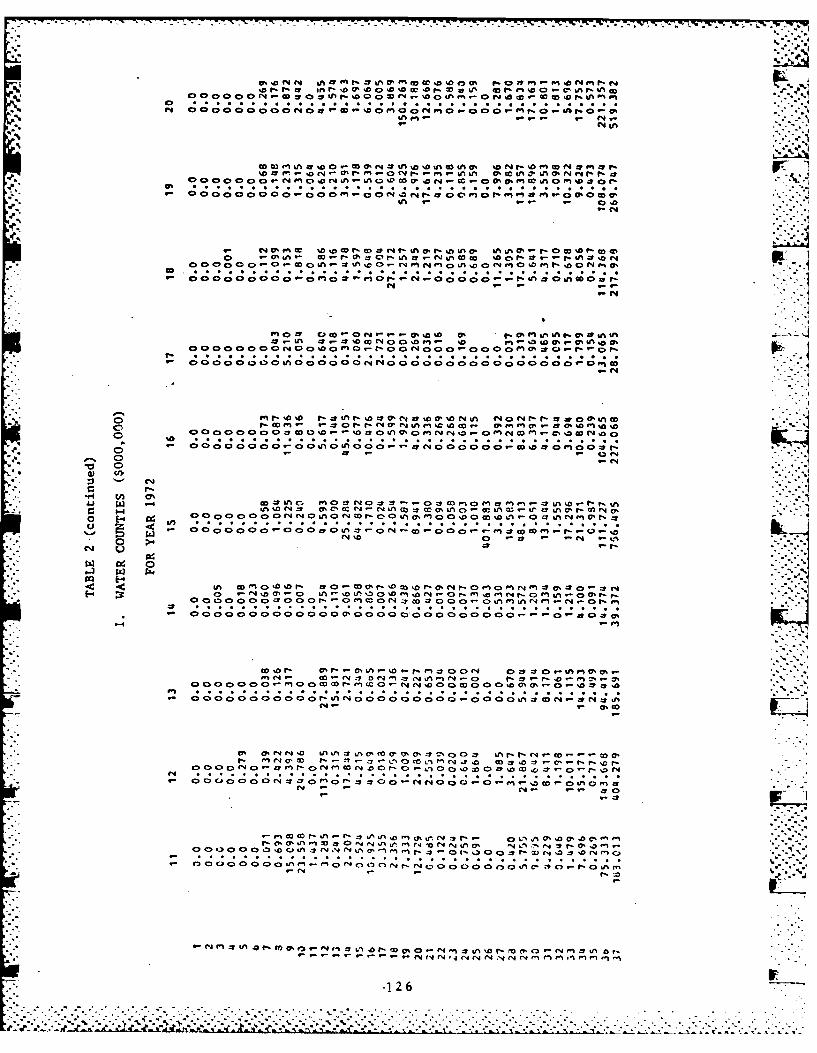
*D-r -0 100 0oc r w*. art. C. ~-b 1, h *o

C ~ ~ ~ % r.4 V4 mD C4 in r- %DO ~ -0 n L~-0N' 00I.i

f4 t- --- 0 f0r - ( ) . o-

.4.4

C4 .Y e.m % 0 % Df tNt- N o% a. &A km m ar

000:C0.0,- CO. n' in.' 00 C!N 0 -0 '. 0i ' C! - 0:-0p 0 >4 0C ,'lQc - 0000 -U >000ar~C

ifl v D C)C>1 0% ,0 > t - 0 toa

00 00 ' 0- 0 ' I- in 0 t w0.- N fz4 (.D 0 %n0 N i00 ' - 0 a 4.i LM

Oac0000 CD a M a C,0r

00 00 0 N; C C; C ;C 00 ' 0 - 00 N 00 000 a' a ~ CO C -ws %D0 t4 a ma'-'4

C>-'' ir's'noi in 'o r- n OiNo

-%0

an . . * . .o0 10 0.. C 0aQn2OD-Q) 0 el 5 '- W MM

N% C>4 f4 %

* ~~n Df C> in %I40D r- 42 - toot, '0 colv'-a'ei- ae~m r'4' N 'o.

f-4 -0 e'0O 0 > M- 1n0 u 0 CI M. n 0 C r e 0 m 4I C>fnLn a ,r-

m N o e4 7 r, "

000 000' 4 0 0D (0 r- 'i cy 0c- (r.a -.% 0 0 , 00 0M 00 P'.- .to to n

000 CO r- n r-1 0 V N 0 LA %o rn 0 r. r4 0 -00 V% 0, a, '0 00 Zi 4r N

4.4C4

N - - N- -- - ., n0 lne

-1 26

o ..U, . . I.. . . . 1-1 N *% r. *4 N * . . w . .4M C a00 cc a00wf 0OO0O00m.0OLot000000Oa'aOfO%00 N'

4p, N v

m ~ ~ ~ . -000 C ;C ;C ;C ;C 1C ;Z C -0N4' A ViC j

g 00 00 00 0 00 0 IOOOmOf4 o Ate %0 Na V fn0. cWS r, Of c

I'..~~c r. a 0, 0 % 0 atea ( f4%t.%

ON .* . * * . * . .V LC .9r .-0 * .9 * 0: * i r. . *

04alN% - tDft~t N0 * 'go..t on So

N 0 00C0 00 0 0 0 eVE'1" -M9 0 00 0 N% 0 0 0 N 0 0 UI 0% 0. -

0 P 0f O0 4 Ufkn- r E10 ~% 0 0 U D0 N Oo em- %D ~ a Ut e l 4 r . -m n0 Z NkU1E

0 I

a, 0 C ,o3

O. N

C14

000

P- OO

.- ~ ~~~~~~ N-- 0 O~a 0% % N O %

000000 v tow 1- % %otfomz 0 rN0U 0tE 0% -m 2 via t- 0% %D 000 km Nr NE M Do~~~~~ ~ ~ ~ ~ C4 In a -f %n *n m :2CA* )(.f .N1 4mz AO a Q

C; 8 ONC ; to :Z - C 4 A 6 4C-4 n fn qO n m D N

M C 0%W to f C., M M 0 C).Mt %nm IDN a N- t

It9 N9 ! 0.U i i0 U O fE0 N.J' t1t U 1!E000 9 i 1-9.1 1

94 a 0ca~ 0 - f a " 1 m*Nr lr m;0 -.. k-l,4 -nu I-t

0 0 0- C U O t f t m N C4 r4 Nto 43,

000000 ~ ~ ~ f U4 C4 r4 c4 r.4 ri en era Mo M0. #", M% U 0 0 0er 0

N . . .. . . 27

1% Nr. %

0. 0' NO0.t0 ot0COQ~~~~~~~~ ~ ~ ~ ~ ~ 40aaa0 a0aa0n0a, )aaaaaaC

Q 0 0 N.0 a C c; c;c; ; ; ; c c c;1c c; c; c;0 iolm r A c,00 V

C44

V.00 m r- m n mCO. 0 '. = 0 c >ac, 0 a

00000000 C 0 0 .0 N > % 00 ' - :2 ' 000>

W . 4

(- t %DU 0- o ) IC> ~ ~ ~ ~ ~ V N % In.0010o ,ol CL 1 Dr-~ a noI 0

_V a,0 . 0 .. rN 0 M I4 0C O > - n C

o V 0I I" D CO 0 f- m 0'. N- .% - -V s %0 00 - W IA %n IA O In 0

M I- r-.cm n0 C 0IC WA t, -NU r, C% e0'0 CO " V.04-00Tc.Q V 0 CW.'1' 0, .C4 ,n Len : : 8r:V;0 V 419 I A I.V - 04 04A' 14W 0 z1 ;4V oc ; 9 1 c

cC 7 hNAAWVC 'WVOOI, N ' OMQt- L Ca, Lm 0 C .D 0 r- I aIA V -

0

N 5-, 0 -MMLm M< n ,11

0 C> M C A In a M O , L LA nINInr- r 0 0* 4 rWV

evIn0, : InJ C) ID'O A InN0f . L,% C) (3 IN 1 pc:3 MI

~ -4

on1 - ( 1c , ma0N OOzi'N O VA'0. CO4. VLn01a 'r._U-CY

r. r- 0 o4-L n .3 C t r(1 a 1,-f.'

NJ~~C e O.4

0l .0 IN-

CIAN~ .f0 s f'N VNO 11 C4r4q4 4 1 1 I nn

N'0C .0 . ~ A C'.rJ', 'O01285~sA~

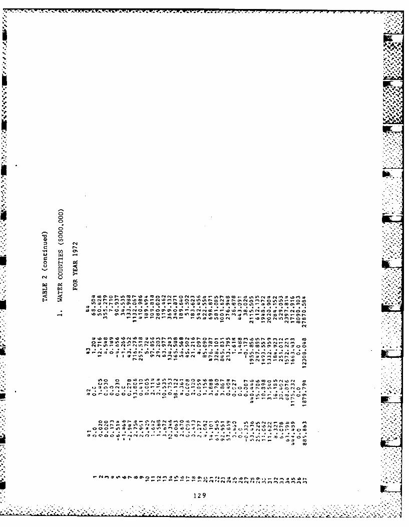
-S..

bkb

.1*1i-

-44

4-4 (4(4JDrCC

a %D w ,0 a aw wr ,m 0r 0r nM n mr ,m m c

0 - r Zkm * M r Ln r-* * 0 ODr- n m - M -

zqr n zc _( _cor40r nI

4 C4A I ;A 44z LA9944 44 C

4eJ C.4

E-.M M r- r

101- A >* " (t01%0 a0 3

'1'tl'0In0'0 10 O f. IT, C> k^I

w - OD VIq ;vN II D -to C-f4 Z?10a ,W)4 q a %%

0.-4~~~r r4~L% 1 C400 0 r.4%'~-~0 jl N~ 4n ,,%

N -~A ' N NU.I- 0N %N f .l4AN00 -~1 - 04 0 0I129~ N40

1~~ '-4 4 7, 4 -A 0 IOr0A4 I'* ,e~r-

onP4 " C4 %D M, in --.- W000 0% 69t'qn- lnP-IhI- Ara%~

14 pa 10 .r a . M 4m C * %o m *

ON4 400002f UrI-.-lf-Oo~-,N.DN 9 N.0A-'

000IA000'Ma69 WON.-0 0 almIaoOmo.0.0oo%-wIa" I0.-o.0%~~i - - Ir6

c. IA r. M91 1 9

IA %a C. D I'-09 1"N 0 00 00 0 I' N %Ce N 0 - WN INM 90,, V N1 As V 11- - At on0. %D '-

N4 N Mc

o0% 000 IA 0n N lin 0 Il w 0 30 9 3 N.- ;000lI l tL % W INw (P.0 0 m r- a) N0

04

%a3I3'- W'0 0. m0-.-0 %DD"9%6. 0 Cw LmN r- D.-0IWO l t'--.-69 C OIna C n_. M 3U -- r 36N M .-r %D6w9w wI .0 VC a * *

ON

a a <- a.? zy 410 )i0 IC) C)Z2 ,4 r 0 C) r- 40C030 -r :cq. Dv C> CD c

3'-30I In03 NN 0000 N, 300 0=0 0 1 N n '' f-0 00 an Ln Nl %- NN . N .n - t I N N - Mow0 4cm%

*i '.-M n 0 0 aa M >a )a ,w C,0% N 0I.In C), a .0c; c.4 0 IAI I- a:. c; IAIA- c;---3 -c; c4z; ; ; ; c c c;c; 4 z : 9%06 C

0* A 0 0 00 00 3 90 0 .- 00 r W ooin00 .3C

00 NN00F0 0 0 N 3 0 00 N 0 0 0.4 ) ~ N 3

IA 0 r 03. 1 00 0%C> ) - M Na 0. C. In N a C>000 0 I'l N rIA7 N 10 co l a

0%, V% -%0 NN (4 C

0 000.-O rf-I- 000.C,0069el INO 00 ) 0 r.) 00 C.00 69 C wCm MIN 00%a 10

enI66

tn. o'r- Ir- on"I0' MIn 40 m2 &10) -9

t. C O6 00000 . 0 3> 00 0 ... c, I ~ O0 '.-=3

- --- - - N N - 4 C4 N el N ('4 r., M I 696969M

1307

(40 - C0~ . 0 L Nr4w -0 C.0U CSOr'., 0009 Vl.C.% Or mO a)- Cr- m .. .

cooC4 o 0oo oooo 9-9 e.~~oo- -o~oovn~o'aeow 4

km r- .~ .

*. A. ,% 00-Cr mr 4( m% % . - a M * &N

-0 *PN 0 %0 1 r 0 OU)'f r o in o0A vC 0 mC ~" o -7 r

r 9- 4- -

co 0

v...........................................................................to . . .T

O0O0OO00~~~00'0O~ nC) 0 ~ 0 0 0 . . ~ ' c c

C4'

0 C4-'%' Lm'N0LN0- N - -

oQ4 0> f C .flD

j4~~~~C r 00o-o0io'*o

.2 co 0 a 00 C) V0 C) - NN C, 10N a ' %0r

C4 onJ 1 9

U%49 M- r-C A j ar- 0r n r

O0 0 C14 0- M tn -(4 0' 0 ~ .r ~ a-Co~00~9 0, U- cc C -4 U.1 N A

N1 '\ U- r .

a a- -, c9 -A 'a'A

0I- 0 J-N%. ' 'nI .- r CI - N M C) 0 * .Or ChI 0 "m~.~* ~

9- -9-9-~~ N ('4 I-4 -4 IN 4 N r%4 (4 .4 o.,% M-~9 ~ -V

131

.~ .WL .. . .. ; . . . . . . .' .. . . . .

fn 0 0 0 C 0 a- -~ -tP 0 a z? 0 r LA C3 0 La 0 Q~ r.0 0 - N M 0 w a' 0 0oV 0

r4 ~ ~ ~ ~ ~ ~ 9 r- N a .NNAMO- imkc 2

000 a0 a- 0 0 0LA ) a 0 L', &A 0 I 0 0 ' N a 000 0' mN 000 0 0 A m 0N%'r

a9 r%9-

co O N OO O O O O ON 10mN a 4 M ma i w'n o oo- ooCo a 00 Ck c -4 cr -M laf o % m oO W LCC

N0' NALAw % f-MNNafn %0 C o0 f 0m rf

r . . . . . . . . . . . . . .N OO O C OO o o t

0 ' 0fn00 0 o A fi A A ~ 0

C>' 0 M 0

C) 0& N n9-nc nz 3 t Vk 74 ," - 0 o

Zn a a- n 01c

U < < %n . . . ...

C-, <n fDnl 0L -l0'~~~% lo'o 0'1 M ' N'I r' 00 o.l m in

00000 Lf ON woIA000NOL 7-arnr'. . r-4 f c ,-7 Ln a %

m fn 0 ' 'O ~ r-O - 0 I n~A c5 0l 31 10 0o 0% O 0'

- - 'ONN

0 0 0 0 0 a 0 -ap c ..O)r a aA c ) , 0 N* 0 04. c :r r -I Q0 0 'aL 4 44 ft ) 0 e n % W > c % 4 t

cL. i- - r'

00 0 0 .- .- .O . . .. .. . a . . . ' . .. .~ .0 .0. .' . ' . .4 . . .3 N .-r-

b ~ ~ ~ ~ ~ ~ ~ ~ ~ ~ ~ ~ ~ ~ * In, 3l .Mcc5 e TL Dr no r4mc 4- t or

- 132

4;hc~o a 0 caoa o ooeOO0 0 000 0 a 040O)aoO -'49490.001

0 Go -m m oaN- rlr oNW .20mN Nc aC

@a 0 mo C4 a0 . m N r- *0 n .N 0 *00 a' c.

*0 0 ; % 0---W %0m 0w 0''0(

0000000 O 00 0 0049 0 * 000 a ON a 0000 U>

m~'. .m*049~ cooN4 en c a "O P0 I QaW nj oc 0N~~ GO 4D "1 0 nG

N rN

10~'4 % 0* . o rZt'. 49N.'C 4

N~~N m NW Nr

enri04L a' r'49 (4 n' %0 en4N 4 NN N C14 C4 N' 04

N 49 m N %0 w0 0N 0 a o N ;0 W N ;' N N- N C90.- N- m-9 r-* W00 m9 " %N 4P %C m

%0 M9 N*0NrN N ON.4- "fn949N.- N Uzro-49o *0

f4 LA 0 C4 mr.(-S% U r-A n t- %DwUr 0 Lei t, tA " Lm NO'.0*N0 * 0 ., In kn wm 4O.a- t- r- .) r- 0n 4 %D .. o it.0U'

a ~ ~ ~ ~ ~ ~ ~ 4 NN 0 aNf. A-tC %:

E- *040* 1'0* O0 l 0 9NU 4 *0 0)-Y4 -a -' 03 0n %0 0'* o 0' N r- v0

I-' C4 N. D N M ;

UN -0 coI M ")en , L 0 a a LM r-** -449 s 'a N N z 0

C4 '

'of e - NO 1, 0 r-N 7 MI 04

a -C Pr r n N 0 5

0: C 4 C N

00 ~ ~ ~ ~ ~ ~ ( 0 000 0C 0C '4 N '-0 04 .4 047 '4 N N- n 'n en n * 'n

-1331

W t..7 . W. I.

-5'.

ILI'

0 F7

*% %

* --. 0

L* C en %D 0 0 mc fO a oN ac %-r

e'i

a %D m' a -~(2~ 0's 0 ~ r a o in a6%-v a- o co ( -4 co40 c

s0 '2--.2"00- r soLo'aU- ("4""-M "--.-

(,7 471 - ( oz %0 in rM' CD m- nD , .a 0 t% rC 0% a (f 4 f% ( o ;2 M e 0 W . CO - 0% (Y. C C.

OD D' M f-c ot M' a' "4D' M VI' OD 0 00 rN rw0 0 n ('4 sf2 0 C D g 0% C, ( 0 CM j, 0M o , ,%D( n mor,4 c4 %o LS'0c' - - en'2m-in a ,0 .o r 0 D 0CN4 -P aOC0 so

- ('4 en M( ' .

('1a .0 (S0(SOl~a~asflt-'2t-W~a) sflila0'so40fi0 a

0D -' CO 00 to 0 T () -t N -- zf fn4 " m2 m'4 0 - n a l 0 w0 0 o4 Cf4 C, VS N' ('4 LM sf 03

N z- M 0 0 a M % r D • C, I D 0 il 0 z W 0 0 a, w - % a a S • • if

.

a, en* * *0 z n I

C-4 4N nf, 0 li M'1. n3 (4 0 f ' - 0 0.0 r4 4 W N) a CD- in n . 3s 0 In "2sf sIS 00 0 sf5

a r> Ni S> C> CD, co ' CD. 0, a 2 a~ C4 C C 0 ai3( 0 e co ~( C) 'o Q 0. 0 m S ('D X? v )V 0 Lm

S* 0 *

C4 r%.

~C~rN 'sS.t W0cr l 5% - - a I M Mo.N' M '2.m Lm UCo N .1 mi~'

*, m

- -*s-** S.. - -- -S C1N4 (( .~ .~ . ne SVe

1K - C! - .r: -. . . . ..- j1*- -.. -. .C: '-. s--' 0: 0: IL C 1 0

C> C 000 N 0' r% 0 i :t _t4 - (" Cy, m ~ in0 N a)s - r- .0 C) r0 in M~ %D r, (00'0

CD 00 0 0 w fn0 in 00r T 0 ,i q 4o o c o10r -c no

r,,. ,4 19 'D Nn 'o, N.1 ('. in o 11 nC!. - .0 (0.- C! C !

CO t Di 7 n O ; nZan M c 0 .N 0-C2e%

0..0. O~-(.- 0 0 0 m4r ( co CONN00

C', in A- oa-n &I C> V1) CI 0 > o a) 0 a, 00 0 -y i CD N ~ C4 V40 f" ina N(

0:N 19N0'C 1;; 19 r: r- 19 4*.. C; 'o,0,0,m 0- -r , - 1- Y- C = '.~ ;z.

'0C' m '3C NC 0 km C4ChN m4 e.I.Aoc %a.0 1 0a

.0a-v N r- 0 )0 v -r io t- m -o m -l w ) %0 m 0 Nn 0 w 0 0.)n m en %D a- 0,N %

%0 on -2 C -I w C>C a 1 - 0 10 m InI zwenwi

0*mrn a v.0 w-00. a-r 0)I a - no m, fn r c,

(-. in 01 f-C (N 0 o( % 0% UN - n wA %D a-co 0r ('4 fN CO NDOr

'-A C)i--2 Z

- .04~ in w-IC .03o~ l 0 3N 1) Uar.CN)

(0 q n o 0 C, r 190 C)O 1 1 In in' %D) a -- --m U",)00 (C) 0 0 m1 N- ="

w D o . 01 m 1 OnC ,0r N m -en0(1IarInwi C) NO CN Nd mN NC) w w N m w N- Nc'j .-- 4 c;a-*N4 ;c

4n Ln Min C)'-'o "M 4t2m 0

N 0 .

("J 0; fd. .- N I1 Nm,

C! .0 . . .' . .; OO amO o ,- 19m 0 : 1 r I N m I ma.-rIA~~~r .0 -ir-O'a '.Cq 004'fldN

r .. 0.00 0% 001 0 .0 coC3 C3CO )0C3 ) m m 0 0 0 N l 41 . N, i ff) a,a-i 10 tnr 10az- C 0' N 0 3 C mC' 0 .CC.3 l"i -) 00L

0o (N N -NC)c . AC N' 31. C4 10)19 1%

.0 041 en in- m(

Q 0 00 0 IN .0.0 C1 ~-1 "N'O 00)~3 0 ./> CI 0. 0 1 0 N In a C3 MA :t

'o in In 4 e N 0

r4 -4 v rA. '0- N IN 0 '.) C3 N a 0 CC f.1 0 N 5 n' 1)' 0 , -*. 19 m IA0 ) o . % n 1 0 eNrj 4 IC.* ('4 N a)i a. iN N P N1 ('4 0% 4= 4'r um .

C; 4 C; 1 14 : 1 1 C-1 .0C; 1 r 4 . . .4 .1 ;.-..,

Cl)~~~ ~ ~ ~ ~ ~ ol -r 4M mC O 0O ' 3 -c -

N .lo C , I 4C

C A 0 0 N3 ' ' l 0S0 r-0p,-r-04 O o3r -3 0 3 r-c 4 oa omc noL -L -c , % om

U.4 rP :- Ln c% '- c m y N-V O ~~nNa. . .

N 9- in N ClV m% D 0 % ,=L

- >oc nL ,COO N oO N- .r- m - >- O ~ r n ,0 0co 43 C,

- DO, co t 0 n 'C - 0 .7 0% %00 .7 u m 0 f eqw (.- % V) f-I C- - 9 3% &

NI

*cQ0 oo o o or- m coCa c4 t- m en

tn 00 00 4 4D .- 0%0 t % 1 t

ef -(7, -o--0coc, r- .0te C4m co -I C t~~- t. r- 47, 0 L-T N.

C) ID - 'o C - n'o 0:0*:' '!0 !-C t* r I tc> a 0> oNa% -c >% 4c 4c o oc ,v 4w c= 0w--%

V C ..

C49 COOOC rr r- r- r 0C' 0(Ns r~itn :1 - > 0V3 . 0'n 01A N~0: N oNn-0..r

[-4J

E-4 w o N. *9C ,L t ODI -C o(4k lC 3 D C 0( Ttn C3 C,

H ~ z 3 r 1:~~~ e0.'e 00 r) 30*9-O0'!n C!-V!.os..P:3C .

*NN .0 10 0 %0 tn -o~ -t co o, tn 0tn. c>u .03 aIe~ c..cr*

9- 9 .- - - 9-'A N 3

0% C4 co %D L* CAf 4 C T1 0 lO 0 c 4C 7 0t n-

C 00000o r- c. IA 00> c>4- r tn -30 r- 0.03 -, rn 0' = N4 000 co o 0n r- Q. 7 0 a) aM . . . . . . . . . . . . .

3r N r4 N 70

In a<.>Ln :> 0 r 10 10 C, n 0r- .-

10a -F 0000 ONL*0 c,09 3.00n n z,-r- -0' .2 .4 rl

FN

0 e0 0n L d ) 'L* 0 C N C) -Y r, M r% (N CJN 0C I , r-44 :to e rC n c

C>I' CDj C) -C-.' ...er 11 N, 74 -1 1 C3m1t

el .n tn .0! , 0o olci In -t -n. fl (9 . 9010 C3 .. A In -0 f

136

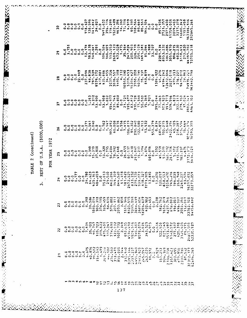
~~~~~~~~~~r w-. N ~ 4- m- w.- 'D 0J C, %0 .r - /~~IlZ~W w.~, '- C . cc -n 00 Nl -" I

Ca,! c ma U. 10W % 0- 0%0 .'o 10 r'oC LoI,- awl' '.0

en a 00 0 ao 0 o w1 . . r) CD0~ 0 C, ' .4 C 0 00 0% 9 3 0 Mn

'n~ ~~ 't0.-W -

f- ona , )k0C4- 3~ ' # 0 0% 3 0 .w Co 0.0mOm w

IA ~ ~ 1 V C l-43 foA e4 ' Nl)W 0 MMr-- O -

ON-00 as ND C4 %D a% 0tD I- ~ a' C4 t0 00" r-00 Na N %0 ̂ 1 C cc

N4fL l0r l N' M .0 3

co3 r

C4 C, '0D C, C>0.1 C4N Mo r- 0M 3, oza '0N ''0 M -

~~~~~c C-4 r'% Nto co0 j- f- mA 'D C> CC 'n PO3M5 - f 0- Mn -

OO O3 0 C c I rOWc ( r t I.000 %

No oM LN0O'n r

C! % . . . C!

co NM. CIA, - 3NN 0% - 3M

00 0 0 N "o000 a 0% r-' (90 'n 0~ N2 =A sm 0 00 ,0 . -T C, C> w '0 'o40C >C >MN )C C cc )LA- nC DouC nc oC DI

N0, 00 0 0 f. , O, M.3

":0% ON . N IA--..N v '--C4 ~ ~ ~ .C; .0M C,~5 U 0%c0' CMLI'

5 -C0 Z C r ; l9C;1 > A 1W

C)Ic C> CC4 V) C (21 _- -TMNc-- ?L

~k , NN W S IA % O M 03A (9IA In C, 1O N 33 5030% NIA.030.~M M~.- C-4 9A.r c

C) Co N) C> 40r en fn~f co F -- " ' , c c . k. 4'

t* In caL- 1

0%0 NC003 IM'3' C M In n

N 0 4coM -,Y IDN N~C n -r 0 3.0-. I- L n r W O -t

N .0 N "MIn

:T m94'I Wo A ~ ~ eJ~. N .0%NIwADN5-Mm3MNCC4m'o 4 t)-(

7 3 N .' .- 0 0 3 .0 N N CNU

Nn -l C) r- 1 r > f

0 0 0 0 0 0i - Z7 MM .3oD -In In. In C' r-.0 3 3 0, VI 10M 0

LA , nW n I ) c o 3 0 I N V. -00 * Ll r '

tnN I I= r0.. 0 0I~ . C f , 1 > t-L.( .- n Ino nr-r4 7N N0 3C 0N 0 LA 0

IA5C. % "A D 5-5-D'3'0N3Cl V W M.3 11 CC C4 I

ca CN C'P ,5 C3

zy 3s I-0 y Dr . r r. U.'IN

10 CO a C T - 3J r, to - 4 ' % -,%

137

. . .. . .' . . . *b.. . . . .V .~ . . ' . . . . . .~ . .

aj 00 0 ,oobooe o oo o eo w 4.o m gtS' f-CfN TN N* %WV C M INN- ll~-N00a0 " w00 c, a -- % 0 0 N0M000 0CC %A %D f0I "~ Go

;;0.~ 0. o r c e *a )aM 22mNNMNNC 0 a f"v otz -0i

OD %D C.4 it0 0.i I -. a .a I - a .%

vcM 0.n.5Sn.#-.fede%. a* Nbf.0.s01..0"&m ind5 4,

r.000N - %D - 0 aw.

ton

OD 04 40 U~fI 00*5-*N5% NSOP-g-O 0 (f 4I ' %D0' a,0a- N 0 an

SI~r. ~ @ 0 -1 , 4%a mC 0'M0 a C00S '0 U5~ 47 -V a M is

m -Mf a n-"f - %0C4C- in.O N -n- I c % rd

r- ~ ~ r N4 anC4M -N n C

M ' n :240 m 0 N %C 0 %D In W 3, IS~r fl N = C" a -- -W M5 -~ Daa na na

rl m In N0 Cr 0% in5 W~ a 5 Nd'. 0% 4f a 0 t- . -Na - a %D r. CD t- -V-U C o a a c 0%00.zVCI D tC- 4:bO ~~'o 47,D dO m r m n e.0r-.Sn(O'%oMdo,)r- O -n m ci o, n - r n

"'c '%om - o -i *N W i n Ma4Q0,r c D g n - c *a

Vs a, NN N n m r Sn..DO C

r. in ~ 5 0O00S e t- f - n; rwo' aO tC.55 C-4''~ 0 c--w ttmM0lm ,0 - n-o

u in Cd . Sa. : nC!5 ! *Z : !1 . r a

00.0 ' 5-00 n in M~r e' s0 5 5 C A-(d 5- 0' r- q0 , co 0. 40

9' ('.0-. O -d -

- '59- .. 0man~~ t. -C%0%

in an N M - -

ama ,M MV Wm 0a- -.- 0% -- - a5 O'D -% NO ' x0~~ ~ ~ ~ 0 bMf a -M y wa - Nc3 - -. i-~n oo 5N

.0 ~ ~ ~ ~ 0 f an9 h4.'-'S ~ ~ . M 0 N ed0"0..0 .

11.) an 05

.- 03ac a l , %% r M-C

M o 0 0;O 'MI0 ~ n M nNm ., SS-0% *-e A - a, l5 0r- a 10 "N --

At ~ ~ ~ ~ ~ ~ ~ ~ I M -m CC% c05* " n-L n t y cX

n v45-5 0 Sn' -C SC-('49. S .0 %m 0 50 an 0t -% N 5 02 uA . 7% M9 -.'t '4(n .0 t

-5- a - (4 C N N ('-4 N pa1 r4 N' N an M9 rn M' M9 M9 M M

138

'a .2

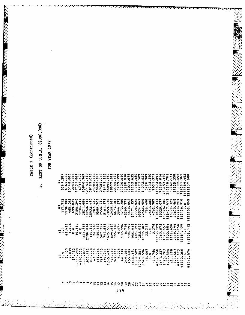
aj -4

0 0.

2p1 -1 'C C r )- nI < h c 0 rw wC

-I.c).

CN1 : C 1 i

at z nmmC - .No wwammclC awk %t

o 2m c.%00C 2- ,r Ir %C a0 4:ro6a ,z nQm=0L ,on00ar onh>14 Ce - -u~f nr lC -ra D"c4 ejc * nc4c 4% so nc ar rM0Mmi

C4 r,4 94

U~ 1f "Ic 4 : 0:Cl : C

0 ~0 'm-a 1~ % rd - - -4 In r"1 in. r- VI IA 00. 1 00 -7 0 %n- 'n C4 C4. N

C>- 4 o m N. - L 000P M 0, -A r0 C. a, co tr- Ln zs ( l - l U" m. P-0O I . 0

V; 40 10 r* > w :tl C> a0 (1 P- trV m0 IA4 0. , a i 4 N C> 1(1 0. IA M P-C '- r1 a, 0 CcmC)ftvIna 70f,=I m n c C0P *P 0 O1 044 L 0O Of -2 m Ln

- -. *N Wi 10r 4 - -

. . . . . . . . . . . . . . . .. . . . . . . . . . . . . . . . .... .... .

.1 0 N 0 n I 0.N 'a C3 N r V% f0

- .'N N 4C'r C,-

4 ~ ~ ~ 4C IA V'I0P I.4 .0- eg NI %Z1 1 44'0NO ~ ~ ~ ~ ~ ~ ~ - 94 t'CaCI cc0I- . P- A . knPII0%.A '

(4I4 1,4-.0 ., 10.4N C4 P- -.'.4I r-r

N I~ N ~ "40139I

-

Footnote to TABLE 2

1. Rowwise 36 indicates values added and 37 indicates total output.

2. Columnwise 36 through 44 indicate the following: I

36: Intermediate Total

37: Personal Consumption Expenditure

38: Gross Private Domestic Fixed Investment

39: Change in Business Inventories .

40: Net Exports

41: Federal Government Purchases

42: State and Local Government Purchases

43: Final Demand

44: Total Output

1-40

.. . .. . . . . . . . . . . ."

TABLE 3

TBADE COEFFICIENTS IN 1972

I : DAIRY FARM PROD

WATER No 4ATER REST USA

WiAT .R 0.07287 0.060954 C.C04041

NO WATER 0.308002 0.297753 0.021146

REST USA 0.619111 0.641293 0.974811

2 : PCULTRY AND EGG

WATER NO WATER REST USA

WATER 0. 156243 0.148478 0.019508

NO WATER 0.552913 0.549061 0.075538

REST USA 0.290844 0.302461 0.904954

3 M MEAT ANIM'AL PROD

WAT ER NO WATEiR REST USA

WATER C.059447 0.054020 O.003469

NO WATER 0.289210 0.280169 0.018983

REST USA 0.651344 0.665811 0.977548

: CO7TON

WATER NO WATER REST USA

WATER . 191142 0.116879 C .019556

No WATER 0.720776 0.739055 0 .C941425

REST USA 0.08 82 0.09'406G 0.986C19

".141

TABLE 3

TR-ADE CCEFFICIENTS IN 1972

5 : FOOr,FEEvD,GRAT:N

WATER NO WATER REST USA

WATER 0.171043 0.090754 0.004956

NO0 W A2'ER 0.502C23 0.568519 0.C20091

REST USA 0.326934 0.340727 0.974951

6 :OILBEARING CROP

WATER NO WATER REST USA

WATER 0. 155043 0.1539903 001027 9

NO 'AATER 0.654370 0.654608 0.042390

-:REST USA 0.190587 0.191402 0.947331

7 FORE STR YFISHPiE Y

WATER NO WATER REST USA

WATER C. 175465 0.165883 0.0

*NO WATER 0.824535 0.834117 0.0

REST USA 0.0 0.0 1.000000

8 :FCOD,KINDiED PROD FWTEZ NO WA'rEP REST USA

WATER 0. 276223 C.207795 C.004254

NO WATER 0.25567%^ 0.258222 C .00 4 fI9

REST USA 0.4603137 0.533984 0.991056..

142

- 7.. '- - -7 1. ..

TABLE 3

T?ADE COEFFICIENTS IN 1972 .-

9 : APPAREL & TEXTILE

N WATER NO WATER REST USA

WATER 0.102890 0.085264 0.001318

NO WATER 0.225762 0.189916 0.003501 .

REST USA 0.6713,q 0.724821 0.995162 "I.--

10 " LUMBER,WOOD PROD

WATEF NO WATER REST USA

WATER 0.193595 0.156441 0.002964

NO WATTR 0.686475 0.378687 0.011945

REST USA 0.119930 0.264872 0.985C71

II :FURNITURE,FIXTURE

WATER NO WATER REST USA

WATER 0. 12C026 0.115072 0.014644

NO WATER 0.067540 0.066600 0.007951

REST USA 0.812434 0.818327 0.977405

12 PAPER & ALLIED

WATER NO ATER REST USA

WATEF 0. 128840 0. 106894 0.0123)3 -"

NO WATZCR 0.C8C215 0.077992 0.008261

REST USA 0.790945 0.15113 0.97934b

143'

, , .,.. ., , .... ,,....- .. , .. 4'z: * • ' ,.-..... •... ". . .*. * .' - .'. '°- -.... '-. 'j'. . '

TABLE 3

TRADE COEFFIC:ZNfS III 1972 **.*

13 :PaIN'2ING,PUBLIS~i

WATEi NO WATER REST USA

WATER 0.509210 0.426639 C.001538

NO WATER 0.-384C71 0.469259 0 .C 01 C5 9

REST USA 0. 106719 0. 104103 0.997403

14 CHEM4ICAL &ALLIED

WATER NO WATER REST USA

*WATER 0.023553 0.017590 0.C00349

NO WATER 0.128891 0.121234 0.002658

REST USA 0.847556 0.861176 0.996993

15 PET20L~i'1,Ai.LIBD

W A T ER NO WATER REST USAW A TF 0.604179 0.356699 0.011776

*NO WATER 0. 195155 0.214768 0.005384

REST USA 0.200666 0.428534 0.982840

16 RUBBFR, PLASTIC

WATER 110 WATER REST Us,,

AER0.141587 0.135034 0.C083C1

NO WATER 0. 150396 0. 133532 O-CC9666

REST USA 0.708017 0.711434 0.9841034

144

TABLE 3 k

TRADE CGEFFICIENS It' 1972'

17 LETE

*WATEr INO WATER REST USA

W ATE R C.032244 0.033877 0 .004 32 7 ~

NO WAT~a 0. 129871 0. 138462 0 .cia^)('

REST USA 0.837885 0.827661 0.977668

18 STON7,CLAY,GLASS

WATER NO WATER REST USA

WATER 0.327641 0.305222 0.004907

*NO WATFR 0 .26767 6 0.332390 0.0014419

REST USA 0.404683 0.362388 0.990774

19 P.2IM'ARY MIETAL

WATZR NO WATER REST USA

WAT ER 0.099821 0.060652 0 .CC32'44

NO ' ATEi 0.042251 0. 133867 0.003072

LREST USA 0.857929 0.8305481 0.993684

r 20 FABrICATEI) METAL

viA TE-"- NO WATEi REST USA

w A 2Er- 0.351216 0.355481 0.0C05264

NO WATER 0. 137247 0.1i45465 G.OUG2CS&SL

REST USA 0.511537 0.499054 0.99-678 -

145

TABLE 3

TRADE COLFFICIE:4TS 1IN 1972

21 :MACINERy

WATER NO WATER REST USA

WATER 0. 188399 0.178250 0.CC5987

NO WATER 0.130335 0.128497 0.0C4796

REST USA 0.681266 0. 6932; 3 0.989217

22 :ELECTRICAL EQUIP

V ATE NO WATER REST USA

WATER 0.211337 0.125433 O-CO9088

NO WATER 0.065174 0.074332 0.CG4144

R EST USA 0.723488 0.800235 0.986768

23 :MOTOR VEHICLE

SWATE NO WATER REST USA

WATER 0.135390 0.173339 0.003717

NO WATER 0.044304 0.065330 0.001261

FREST USA 0.820306 0.761330 0.995022

124 :ICH~FCU1

WATER NO WATER R ES U E;A

WAMF 0. 194186 0. 183343 0.C0327%r

NO0 WATER 0. 100221 0.107323 0 . C, 18 1

REST UsA 0.705593 0.7080335 C.994929

0' 146

-a" PL

TABLE 3

TRADE COEFFICIENTS IN 1972

25 : BITUMiINUUS COAL

WATER NO WATER REST USA

WAVE R 0. 191024 0.140149 0 .C01904

NO WATER 0.028814 0.034651 O.C00442

REST USA 0.780163 0.825200 0.997654

26 :PZTROLZUii.NAT.GAS

WATER NO WATER REST USA

WATER 0.097258 0.094338 G.CC3966

NO WATE--R 0.730064 0.746647 0.033326

REST USA 0.172678 0.159016 0.

27 :OTHER IIIING

WATER NO WTE REST USA

WATER 0.098956 0.096220 0.C02121

NO WATER 0.493721 0.501279 0.013302

REST USA 0.407323 0.402502 0.984576

28 :CCNSTIRUCTION

WATER~ NO WATE2 FREST USA

aWATE? 0. 521785 0.415419 0.0

NO WATE3 0.478215 0.5d4531 0.0

REST USA 0. C 0.0 1.000000

................................ 147

TABLE 3 -

TRADE COEFFICIE4IS IN 1972 ~

29 : PANSPORTATION

WAT.Er NO0 WATER REST USA

WATEF 0.444606 0.219220 0.0

NO WATERl 0.555394 0.700780 0.0

REST USA 0.0 0.0 1.COOCOO

30 :WHOLE SALE,RETAIL

WATER NO WATER REST USA

WATER 0.452775 0.409690 0.0

NO WATER 0.547225 C 5 903 10 0.0

REST USA 0.0 0.0 1.000COO

31 :FINAi4CE,INSURANCZ

WATER NO WATER REST USA

W A TEF. 0.341506 0.286305 0.0

NO WATER 0.324844 0.407110' 0.0

REST USA 0.333649 0.306579 1.000000

32 :COMUNICATION

WATER NO Whiva REST USA

WA'EE. 0.598161 0.457547 0.0 -.

NO WATER 0.L401839 0.542453 0.0G

RZST USA 0.0 0.0 1.ccococ

148

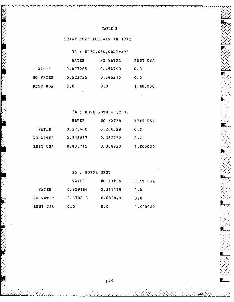
r~w -a

TABLE 3

TRAD)E COEFFICIEN"S IN 1972

33 : ELEC,GAS,SANITARY

WATER NO WATER REST USA

WATER 0.477265 0.454790 0.0

NO WATER 0.522735 0.545210 C.0

*REST USA 0.0 0.0 10000000

34 : BOTE-L, OTHE'R SE-RV.

WATER NO WATER RESTr USA

WATER 0.275448 0.268328 0.0

*NO WATER 0. 315837 0. 362752 0 .0

REST USA 0.408715 0.368920 1 .COOCOC

35 :GOVERIINT

WATEP NO WATER REST UST,

WATEF 0.329184 0.317179 0.0

NO WATER 0.670816 0.682821 0.0

REST USA 0.0 0.0 1.000000

149

TABLE 4

DEM.AND ADJUSTED SIAULATICNDEVELOPM1ENT IMPACT OF THE WATERWAY

FOR YEAR 1974REGION : WATER

Counties (UNIT:MILLION DOLLARS)

OUTPUT WITH OUTPUT W/CINDUSTRY WATER WAY WATER WAY DIFFERENCE PERCENTAGE

(A) (B) (A) - (1) - (C/B)*1001.DAIRY FARM PROD 61.272 61.215 0.057 0.09%2.POULTRY AND EGG 177.484 177.335 0.149 0.08%3. 'EAT ANIMAL PROD 165.220 165.072. 0.148 0.09%4.COTTON 34.269 34.077 0.192 0.56%5..OOD,FEED,GRAIN 431.585 430.780 0.805 0.19%6.OILBEARING CBOP 192.565 192.014 0.552 0.29%7.FOEESTRY, FISHERY 64.690 64.172 0.517 0.81%

8.FOOD,KINDRED PROD 1952.919 1952.647 0.272 0.01-9.APPAREL & TEXTILE 234.921 234.851 0.070 0.03S10.LUMBER,WOOD PROD 175.204 175.005 0.199 0.11%11.FURNITURE,FIXTURE 212.722 212.706 0.017 0.01, %12.PAPER & ALLIED 587.257 586.521 0.737 0.13%13.PRINTING,PUBLISH 244.09C 244.073 0.018 0.01%14.CHEMIICAL & ALLIED 65.454 64.217 1.237 1.93%15.PETROLEU'I,ALLIED 1496.254 1494.810 1.444 0.10T16.RUEBER, PLASTIC 334.073 332.860 1.213 0.36%17.LEATHER 32.181 32.177 0.004 0.01% ..- *

18.STONE,CLAY,GLASS 222.364 221.534 0.830 0.37%19.PRIMARY METAL 436.187 435.059 1.128 0.26%20.FABRICATED M ETAL 744.736 744.29C 0.446 0.06% - --

21.MACHINERY 830.077 829.828 0.250 0.03722.ELECTRICAL EQUIP 914. 161 914.003 0.158 0.02%23.t!,OTO;R VEHICLE 925.660 925.545 0.11;4 0.01%24.MISC.MANUFACTURE 313.005 312.932 0.073 0.02%25.BITUHINOUS COAL 34.593 34.011 0.583 1.71Y,26.PETR CLZU, ,NAT. GAS 244.108 244.103 0.005 0.000-27.OTHER MINING 22.231 14.760 7.470 50.61Y.26.CONS7rUCTION 1739.439 1739.179 0.259 0.01%129.IRANSPORTATION 470.376 470.464 -0.088 -0.02%3C.WHOLE SALE,.EETAIL 1926.747 1927.018 -0.271 -0.01%31. FINANCE, INSURANCE 1985.720 1986.043 -0.322 -0.029,32.COMIMUNICATICN 379.189 379.244 -0.055 -O.015[33.ELEC,GASISANITARY 570.197 569.982 0.215 0.04534.HOTEL,GTHEZP SE2V. 2196.851 2196.765 0.086 0.0c035 GOV. MENT 1120.874 1120.884 -0.010 -0. C07;

TOTAL 21538.68 21520.17 18.50 0.091

150

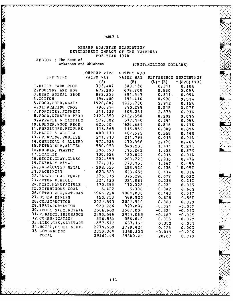
&I fl'L -. 7 K 4,:' <7 k7 -- 7--7 -' 4

TABLE 4

DEMAND ADJUSTED SIMULATIONDEVELOPMENT IMPACT OF THE WATERWAY

FOR YEAR 1974 '-.

REGION • The Rest ofArkansas and Oklahoma (UNIT:IILLION DOLLARS)

.OUTPUT WITH OUTPUT W/OI 'DUSTRY WATER WAY WATER WAY DIFFERENCE PERCENTAGE

(A) (B) (A)- (B) - (C/B)*1001.DAIRY FARM PROD 303.447 303.136 0.311 0.10%2.POULTRY AND EGG 679.280 678.700 0.580 0.09%3.MEAT ANIMAL PROD 892.258 891.447 0.811 0.097-_4.COTTON 194.400 193.410 0.990 0.51% - -

5.FOOD,F-EED,GPAIN 1928.642 1925.73C 2.912 0.15%6.0ILBEARING CROP 790.814 790.299 0.515 0.07%7.FORESTRY,FISHERY 311.139 308.261 2.878 0 .938.FOOD,KINDRED PROD 2122.850 2122.558 0.292 0.01%9.APPAREL & TEXTILE 577.382 577.140 0.241 0.04%

10.LUMIBER, WOOD PROD 625.504 '624.689 0.816 0.13%11.FURNITURE, FIXTURE 116.868 116.859 0.009 0.01 IN12.PAPER & ALLIED 408.133 407.575 0.558 0.14%13.PRINTING,PUBLISH 211.813 211.798 0.015 0.01."14.CHElICAL & ALLIED 472.536 470.366 2.170 0.46%15.PETRCLEUM,ALLIED 550.053 548.583 1.471 0.27.16.RU13BER, PLASTIC 396.698 395.245 1.453 0.37417.LEATHER 130.658 130.642 0.016 0.01%18.STCNE,CLAY,GLASS 201.659 200.723 0.936 0.47%19.PRIMARY METAL 374.815 373.155 1.66C 0.44%20.FABRICATED METAL 298.555 298.420 0.136 0.057.21..1AC!iINZRY 623.829 623.655 0.174 0.03%22. ELECTrICAL EQUIP 375.375 375.298 0.077 0.02%23.MOTOP VEHICLE 321.120 321.087 0.033 0.0124.MISC.]ANUFACTURE 170.353 170.323 0.031 0.02"25.BITUMINOUS COAL 6.422 6.380 0.042 0.66% .*--26. PETROLEUN, NAT. GAS 1961.224 1961.080 0.143 0.01--27.OTHER MINING 150.750 149.922 0.828 0.55%28.CONS7TRUCTION 2021.893 2021.510 0.383 0.02,;29.TRANSFORTATION 920.786 920.807 -0.021 -0.00v30.;WHOLE SALE, RETAIL 2586.680 2587.004 -0.324 -0.01%31.FINANCE,INSURANCE 2490.596 2491.063 -0.467 -0.027 .32.COAUFI'ICATON 356.584 356.640 -0.055 -0 .02!"33.ELEC,GAS,SANITARY 657.512 657.161 0.352 0.05S34. hOTEL,OTH'ER SERV. 2779.550 2779.424 0.126 0 0.oc 3 "

35 OVRNHIENT 2350.304 2350.323 -0.019 -0.00%TOTAL 29360.49 29340.41 20.07 0.07%

151

. . .

K- vc k7-

TABLE 4

DEMAND ADJUSTED SIMULATICN w..DEVELOPOENT IMPACT OF THE WATERWAY

FOR YEAR 1974REGION :RrST USA '--'(UNIT:MILLION DOLLARS) ml

OUTPUT WITH OUTPUT W/CINDUSTRY WATER WAY WATER WAY DIFFERENCE PERCENTAGE

(A) (B) (A)- (B) -(C/B)*1001.DAIRY FARM PROD 9726.718 9726.844 -0.126 -0.00%742.POULTRY AND EGG 5465.710 5465.687 0.023 0.00%3.:iEAT ANIMAL PROD 32735.397 32735.199 0.198 0.00%4.COTTON 3077.403 3077.425 -0.022 -0.005.5. FOOD, FEED, GRAIN 40874.056 40874.877 -0.821 -0.00%6.0iL3EARING CROP 10018.766 10018.850 -0.084 -0.00%1'7.FOR7SRY,FISHERY 22894.059 22894.31 1 -0.252 -0.00%8.FOOD,KINDPED PROD 141420.055 141418.695 1.360 0.00%9.APPAREL & TEXTILE 64625.026 64625.162 -C.136 -0.00-10.LUNBEE,WCOD PROD 25891.359 25891.343 0.016 0.00%...ll.FURNITURE, FIXTURE 12470.146 12470.155 -0.009 -0.0%12.PAPER & ALLIED 32677.047 32676.070 0.977 0.0017,13.PR-INTING,PUBLISH 33492.009 33491.874 0. 135 0.00%14.CIIEMICAL & ALLIED 65547.996 65511.704 36.292 0.06..15.PETROLEU I,ALLI E D 37529.352 37524.404 4.948 0.01 '-11b.RUBBER, PLASTIC 24627.537 24626.644 0.893 0.00%17.LEAT HER 5594.832 5594.836 -0.004 -0.007,18. STONE,CLAY, GLASS 24287.285 24286.365 0.919 0.00519.PRIMARY METAL 81471.528 81464.520 7.008 0.01%20.FABRICATED METAL 56143.009 56141.605 1.404 0.00%21. MACHINERY 82881.472 82880.205 1.268 0.00" ""22.L-CTRICAL EQUIP 64283.777 64283.799 -0.022 -0.0071.23..%IoToR VEHICLE 92789.880 92789.562 0.318 0.00%24.MISC.MANUFACTURE 39173.964 39173.846 0.118 0.00%25.BITU*IINOUS COAL 8790.587 8790.236 0.351 0.CO-"26.PETFCL:UM, NAT. GAS 29860.449 29858.511 1.938 0.01%27.OTHER MINING 9226.010 9219.790 6.220 0.07723.CONSIRUCTION 194519.365 194517.971 1.393 0.00%29.TRANSPOETATION 88900.045 88898.608 1.436 0.00130.WHOLE SALE,FETAIL 261431.613 261431.555 0.057 0.C0 !"131.FINANCE, INSURA NCE 280364.455 280363.562 0.873 0.00..32.- CO M ,.UN IC ATIO! 45008.683 45008.583 0.099 0.00%33.ELECCAS,SAN'IARY 61396.996 61394.990 2.006 0.00%-3 .4.HOT-L, CIIIEr SERV. 327796.068 327792.206 3.861 0.00 "35 GOVETN'U-ENT 181243.196 181243.135 0.061 0.00%"

TCTAL 2498235.85 2498163.15 72.70 0.00%..

152

- . . . * * . -*.* . -

*e. t . t-tt .f . ..-. &% t s t-ostt'.. C

TABLE 4

DEM~AND ADJUSTiED SI.9ULATICNDEVELCPMENT IMPACT OF THE~ WATERWAY

FOR YEAR 1975..R.EGION WATER%

Counties (UNIT:MILLION DOLLARS) __

OUTPUT WITH OUTPUT W/GINDUSTRY WATER WAY WATER WAY DIFFERENCE PERCENTAGF

(A) (B) (A)-,(B) (C/E)*1001.DAIRY FARM PROD 55.145 55.091 0.054 0.10%2.POJLTRY AND EGG 187.812 187.667 0. 145 0.087,3.MEAT ANIMAL PROD 173.683 173.543 '0.140 0.08%4.COTTON 67.941 67.757 0.184 0.2755.FOOD,FEED,G.:AIN 375.425 374.586 0.839 0.22%

*6.OILi3EARTNG CROP 110.248 109.567 0.681 0 .625,* 7.FOESTRYFISHERY 55.114 54.60. 0.513 '.94%

*8.FOOD , INDEED PROD 2038.281 2033.01C 0.271 0.01%9.APPA'EL & TEXTILPE 225.598 225.531 0.066 0.03%

E10.LUMZPWCOD PROD 167.231 167.044 0.187 0.1111. F U PNIT U RE, FIX TU RE 179.432 179.414 0.017 0.01%*12.PAE on & ALLIED 594. 193 593.486 0.708 0.12'13.PRNTINGPUBLISH 254.837 254O.U82C 0.017 0.0114.CHEICAL & ALLIED 79.385 78.319 1.066 10.3% 615.PETROLEUALLI.ED 1947.513 1946.128 1.385 0.071;16.RUBEF., PLASTIC 370.052 368.832 1.223 0 0. 33"17. L EAT HE R 33.589 33.585 0.004 0.0%18.STONZ--,CLAY,GLASS 254. 125 253. 52 6 0.599 0 .24e-"19.PRIRiy MEROAL 284.305 23.542 0.623 0. 29 , "20.FABRICATID METAL 819.614 E18.840 C.775 0.09%21.FOACHINEEY 955.979 955.739 0.240 0 .0 3 722.ZLECTRICAL EQUIP 838.831 833.626 0.205 0.02%

*23).?iOTORi VEHICLE 823.661 823.496 0.166 0 .0 2%j24.AISC.MANUFACTURE 314.778 314.694 0.084 0.03525.BITUMINGUS COAL 63.756 63.382 0.374 0.11% . -

26.PUTlCLEURE, NAT.GAS 262.209 262.245 -0.037 -0.01 127.OTER MINING 34.369 31.007 3.362 10.84 ___

28.CONS'IICTION 1251.778 1851.562 0.216 0.01"%l"2 9.TRA NSPO TATN 488.345 478.502 -0.157 -0.03%530.PHOLE SALERETAIL 22171.089 2271.402 -0.312 -0.01%31.FINANCZ,INUANCE 2190.876 2191.273 -0.397 -0.0232.COMUNICA ICN 434.159 434.221 -0.062 0.01t.33.SOZELE,,CSANITARY 732.644 732.625 0.019 0 cO " -34.IOTELO'r En SESV. 2520.549 2520.563 -0.014 -0.001

.35 GLETLENT 1262.210 1262.221 -0.015 0.02"

.TOTAL 23318.81 23305.45 13.36 0.CV '_

153

S1 ,778 1 ,69 , 0.08, o...

TABLE 4

DEMAND ADJUSTED SIMULATIONDEVELOPMENT IMPACT OF THE WATERWAY

* FOR YEAR 1975

* REGION The Rest ofArkansas and Oklahoma (UNIT:MILLION DOLLARS)

OUTPUT WITH OUTPUT W/O

INDUSTRY WATER WAY WATER WAY DIFFERENCE PERCENTAGE(A) (B) (A)- (B) -(C/B)*1O0

1.DAIRY FARM PROD 267.733 267.459 0.275 0.10%

2.POULTRY AND EGG 717.604 717.067 0.537 0.07%

3.MEAT ANIVAL PrFCD 894.014 893.299 0.715 0.08%4.COTTON 326.983 326.089 0.894 0.27

5.FOOD,FEED,GRAIN 1751.735 1749.151 2.584 0.15.-6.0ILBTARING CROP 455.595 455.121 0.474 0.107.7.FORESTRYFIS ErY 273.008 270.385 2.623 0.97%

8.FOOD,KINDREC PROD 2226.732 2226.463 0.269 0.01%9.APPAREL & TEXTILE 556.304 556.079 0.226 0.04%

IO.LUMBER,WOOD PROD 597.602 596.948 0.653 0.11%

11.FURNITUFEZ,FIXTURE 100.366 100.358 0.008 0.01%12.PAP-R , ALLIED 407.204 406.719 0.485 0.12%

13.PRINT!NG,PUBLIS11 231.573 231.560 0.013 0.011 -.-

14.CHEMICAL & ALLIED 588.134 586.125 2.009 0.3,4%15.PETROLEUM,ALLIED 946.303 945.269 1.034 0.11%16.RUB3ER, PLASTIC 441.861 440.424 1.438 0.33%17.LEATHER 135.532 135.517 0.014 0.01%I13.STO: E,CLAY,GLASS 242.602 242.059 0.54.3 0.220/..19.PR:IARY METAL 259.556 258.487 1.068 0.41%20.FABRICATED METAL 325.274 325.114 0.160 0.05%21. IACHINERY 727.106 726.990 0.116 0.02722.ELECTICAL EQUIP 387.511 387.435 0.076 0.02e; W---

23.MOTO, VEHICLE 308.601 308.568 0.033 0.01%

24.MISC.ANUFACTURE 166.952 166.922 0.029 0.02%

25.0ITUMINOUS COAL 12.436 12.410 0.026 0.21%26.PETROLEUM, NAT. GAS 2095.146 2095.450 -0.3C4 -0.01%27.OTHER MININJG 205.053 204.631 0.422 0.21%28.CCON 31FUCTION 2133.270 2133.058 0.212 0.01%

29 T RAN SPORTA TION 969.065 969.523 -0.457 -0.05%30.WHOLE SALE,IiETAIL 3080.485 3080.934 -0.450 -0.01" 'It3 1. FINAICE, INSURANCE 2759.441 2760.000 -0.558 -0.02 32. CO'MMU NICATION 403.242 403.302 -0.060 -0.01%33. ELEC,GAS,SA11ITARY 839.036 839.119 -0.034 -0. C0

34.i{OTEL,OCT1EF SERV. 3203.286 3203.328 -0.042 -0.00=

-35 GOVE3R ,,I 2631.308 2631 .340 -C.033 -0. 00"

TOTAL 31667.70 31652.7C 15.00 0 .051

154

".'. . _ . . .:._. .'-'--_ . t t. _: '": ''' " 'L .':''' .: "._-_ ,' . t -- *.- -, - '- '- """"" " """"" " -" " " " -

TABLE 4

DEMAND ADJUSTED SInULATIONDEVELOPMENT IMPACT OF THE WATERWAY

FOR YEAR 1975BEGION :REST USA

(UNIT:MILLO1 DOLLARS)

OUTPUT WITH OUTPUT W/CINDUSTRY WATER WAY WATER WAY DIFFERENCE PERCENTAGE

(A) (B) (A)- (B) -(C/B)*1001.DAIRY FARM PROD 1 C941.633 10941.734 -0.101 -0.00%2.PCULTFY AND EGG 6481.171 6481.145 0.026 0.00-3.3EAT ANIMAL PROD 35756.905 35756.611 0.294 0.00c.4.COTTON 2423.875 2423.898 -0.024 -0.00%5.FOOD,FEED,GRAIN 38568.300 38569.036 -0.736 -0.00%6.OILBEARING CROP 7926.137 7926.191 -0.054 -0.00%7.FORESTRY,FISHERY 25478.235 25478.449 -0.213 -0.00%8.FOCD,KINDRED PROD 153083.574 153082.155 1.419 0.00%9.APPAREL & TEXTILE 63425.637 63425.739 -0.102 -0.00% l-

10.LUNBER, WOOD PROD 27125.536 27125.394 0.143 0.00%11.FURNITURE,FIXTURE 10971.514 10971.520 -0.005 -0.00%12.PAPER & ALLIED 33177.277 33176.361 0.916 0.00%13.PRINTING,PUBLISHi 35018.426 35018.282 0.144 0.00%14.CHEMICAL & ALLIED 68889.684 68852.094 37.590 0.05._-15.PETROLEUM,ALLIED 40665.217 40664.54C 0.677 0.00 .16.RUBBER, PLASTIC 24075.321 24074.483 0.838 0.00%17.LEATHER 5372.820 5372.822 -0.C03 -0 .0 o

* 18.STON ,CLAY, GLJSS 24202.495 24202.075 0.420 0.00%19.PRIMARY METAL 74937.659 74931.123 6.536 0.01%20.FABRICATED METAL 61063.831 61062.964 0.867 0.00%21.MACHINERY 85355.942 85355.174 0.769 0.00%22.ELEZTRICAL EQUIP 61052.169 61052.241 -0.072 -0.00%23.MOTOR VEHICLE 90229.163 90229.021 0.142 0.0 0"24.MISC.MANUFACTURE 42779.758 42779.672 0.086 0.00%25.ITUMINOUS COAL 11313.492 11313.160 0.332 0.00%26. PETROLEIM, NAT. GAS 33286.660 33286.733 -0.073 -0.00%-27.OTHER MINING 10238.301 10234.530 3.771 0..04%28.C0NS IRUCTION 190920.839 190919.878 0.960 0.00%129.TRANSFORTATION 90176.723 90175.197 1.527 0.00%30.WHiOLE SALE,RETAIL 280092.69C 280092.193 0.496 0.0' r-Ti31.FINANCE,INSURANCE 300837.822 300837.281 0.541 0.00."-32.COtMUNICATION 50801.449 50801.318 0. 132 0.00%33.tL2C,GAS,SANITABY 66252.244 66250.372 1.872 0. 0? c 7l34.H0TEL,OTllER SEFV. 363345.254 363341.281 3.973 0.00.35 GOVE:Ii,IZNT 199312.609 199312.537 0.C72 C.00 1

TOTAL 2625580.36 2625517.20 63.16 C.00 %""

1.

... .... .i. i-..-... -.* .*.. .... :........... .:... .. . . ,

TABLE 4

DEMAND ADJUSTED SIaULATIONDEVELOPMENT IMPACT OF THE WATERWAY

FOE YEAR 1976REGION WATER '

Counties (UNIT:MILLION DOLLARS)

OUTPUT WITH OUTPUT W/C -INDUSTRY WATER WAY WATER WAY DIFFERENCE PERCENTAGE

(A) (B) (A)- (B) - (C/B) *1001.DAIRY FARM PROD 53.530 53.469 0.061 0.11%2.POULT.Y AND EGG 156.868 156.707 0.160 0.10%3.?'EA? ANIMAL PROD 162.072 161.916. 0.156 • 0.10%4.COTTON 48.986 48.773 0.213 0.44%5.FOOD,FEED,GRAIN 311.144 310.190 0.954 0.31,6.0ILBEARING CROP 116.928 116.069 0.859 0.74%7.FORESTRY,FISHEFY 56.520 55.988 0.532 0.95%8.FOOD,KINDRED PROD 2187.001 2186.677 0.324 0.01%9.APPAREL & TEXTILE 278.164 278.088 0.076 0.03%10.LUMBER,WOOD PROD 197.152 196.927 0.225 0.11%11.FURNITURE,FIXTURE 234.473 234.453 0.020 0.01%12.PAPER & ALLIED 711.885 711.061 0.805 0.11%13.PRINTiZNG,PUBLISH 277.048 277.026 0.022 0.01%14.CiEMICAL & ALLIED 91.682 90.532 1.149 1.27%15.PETROLEUM,ALLIED 2244.212 2241.919 2.294 0.10%16.RUBBER, PLASTIC 450.922 449.546 1.376 0.31% o17.LEATHFER 38.069 38.064 0.005 0.01%18.STONE,CLAY,GLASS 320.367 319.772 0.595 0.19S19.PRIMARY METAL 365.782 364.447 1.335 0.37%_20.FABRICATED .ETAL 914.976 914.079 0.897 0.10%21. MACH NERY 1009.777 1009.487 0.290 0.03%22.ELECTRICAL EQUIP 1020.701 1020.461 0.240 0.020c'23.4,OTOR VEHICLE 1007.526 1007.324 0.202 0.02%24.MISC.MANUFACTURE 291.773 291.677 0.096 0.03%25.BITUMINOUS COAL 77.161 76.583 0.579 0.76%26.PETROLEU;i,NAT.GAS 325. 131 325. 115 0.016 0.00%.27.OTHER MINING 40.198 36.456 3.743 10.27%28.CONSTRUCTION 1986.918 1986.713 0.285 0.015-29•TRAASPORTATION 551.481 551.569 -0.089 -0.02%30.WHOLE SALE, RETAIL 2444.005 2444.326 -0.241 -0.015

31•FIANCE, INSURANCE 2465.370 2465.567 -0.197 -0.015 c "32.COMIUN'ICATION 509.667 509.723 -0.056 -0.01 '-33.ELEC,GAS,SANITARY 817.590 817.483 0.107 0.01 "34.1-OT".L,OTHER SERV. 2759.054 2759.008 0.046 0.CO%35 GCVERN MET 1401.219 1401 .233 -0.014 -0. 00 It

TOT'AL 25925.31 25908.44 17.06 0.071

.. r.

156

"-.... . - . . ~. . -* * * .- .. . : .-.--- .-. - .. . . .. . .- .

TABLE 4

D:E.MAND ADJUSTED SIMIULATION

DEVELOPMiENT IMPACT OF THE WATERWAY vFOR YEAR 1976

REGION :The Rest ofArkansas and Oklahoma (UNITIMILLION DOLLARS)

OUTPUT WITH OUTPUT W/OINDUSTRY WATER WAY WATER WAY DIFFERENCE PERCENTAGE

(A) (B) (A) -(B) -(C/B)*10OL1.DAIRY FARM PROD 268.501 268.198 0.303 0.11%

2.rOULTRY ANr EGG 601.975 601.385 0.590 0.10%3.KE-AT ANIM.AL PRCD 8161.897 861,113. 0.784. 0,0954.COTTON 241.761 240.735 1.026 0.43%5.FOOD FEED,GRAIN 1328.464 1325.792 2.672 0.20%6.OILBE ARING CROP 482.717 482.178 0.539 0.11%7.FOF.ESTRY,FISIIERY 279.821 277.148 2.672 0. 96,5

*8.FOOD,KINDRED PROD 2344.010 2343.69C 0.320 0.01%*9.APPAREL & TEXTILE 694.665 694.406 0.259 0.04%

10.LUMBER,WCOD PROD 698.273 697.518 0.756 0.11%11. FURN ITUR E, FIXTURE 130.128 130.120 0.009 0.01%12.PAPER & ALLIED 492. 548 492.009 0.539 0. 11%13.PRINTINGPUBLISUi 247.666 247.649 0.017 0.01%14.CHE7MICAL & ALLIED 682. 455 680.294 2.161 0. 32%15. PETROLEUMI,ALLIrD 1045.585 1043.418 2. 167 0.21%lb.PUBBER, PLASTIC 516.267 514.652 1.615 0.31% b17,LEATHIER 153.561 153.544 0.016 0.01%18.ST ONE,CLAY,GLASS 315.183 314.648 0.535 0.17%19.PRIMARY METAL 365.258 364.255 1.002 0.28520.FABRlICATED METAL 358.473 358.363 0.110 0.03%.

22.ELECTSICAL EQUIP 515.621 515.547 0.074 0.01%

23.MOTOfl VEHICLE 381.717 381 .689 0.028 0.01%24.MIISC.ANUFACTURE 145.801 145.771 0.030 0.02%25.BITUMINOUS COAL 15.069 15.029 0.040 0.26%26. PETROLEUM, NAT. GAS 2595.065 2594.997 0.069 0.00%27.OTHER MlINING 241.293 240.860 0.434 0.18%26. C 0 NS 7R 11C TI0N 2237. 542 2237. 283 0.259 0.01,1%2 9. T RA NSPO RTA TI10N 1092.199 1092.590 -0.391 -0.045.30.WHOLE SALE,RETAI:L 3263.789 3264. 164 -0.375 -0.017%31.FINANCEINSURANCE 3059.210 3059.523 -0.314 -0. 01 T32.CONiMUNICATI0ON 471.025 471.079 -0.0511 -0. 01%33.ELEC,GAS,SANIIARY 938.597 938.580 0.017 0.007.34.H0TAEL,OTHEF SEiRV. 3470. 192 3470.173 0.018 0.00%35 GOVERNMENT 2922.423 2922.454 -0.031 -0.0357

TOTAL 34223.02 34205.02 18.00 0 5.".

4157

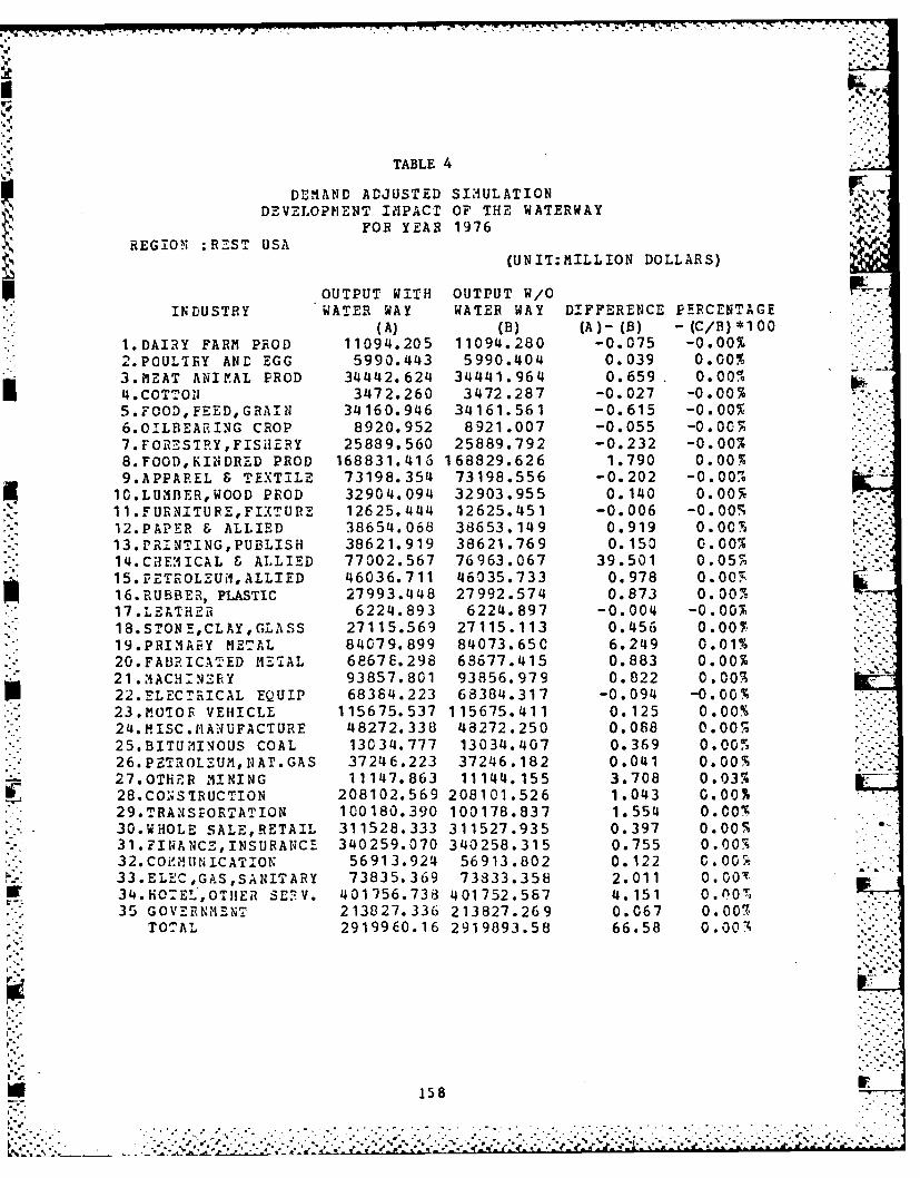
717 7 7 7

TABLE 4

DEMAND ADJUSTED SIMULATIONDEVELOPMENT IMPACT OF THE WATERWAY

FOR YEAR 1976,,,' -"

REGION :REST USA(UNIT:MILLION DOLLARS)

OUTPUT WITH OUTPUT W/OINDUSTRY WATER WAY WATER WAY DIFFERENCE PERCENTAGE

(A) (B) (A)- (B) - (C/B)*1 00

1.DAIRY FARM PROD 11094.205 11094.280 -0.075 -0.00%2.POULTRY AND EGG 5990.443 5990.404 0.039 0.00%3.MEAT ANIMAL PROD 34442.624 34441.964 0.659. 0.00"64 .COTTO1 3472.260 3472.287 -0.027 -0.00%-5.FOOD,FEED,GRAIN 34160.946 34161.561 -0.615 -0.00%6.01LBEARING CROP 8920.952 8921.007 -0.055 -0.00%7.FORESTRY,FISiiERY 25889.560 25889.792 -0.232 -0.00%8.FOOD,KINDRED PROD 168831.416 168829.626 1.790 0.00% - -

9.APPAREL & TEXTILE 73198.354 73198.556 -0.202 -0.00"s10.LUMRBER,WOOD PROD 32904.094 32903.955 0.140 0.00%11.FURNITURE,FIXTURE 12625.444 12625.451 -0.006 -0.00%9-12.PAPER & ALLIED 38654.068 38653.149 0.919 0. 00%

' 13.PRINTING,PUBLISH 38621.919 38621.769 0.150 0.00%- 14.CHE:ICAL & ALLIED 77002.567 76963.067 39.501 0.05%

15.FETFOLvUd1,ALLIED 46036.711 46035.733 0.978 0.00,-l16.RUBBER, PLASTIC 27993.448 27992.574 0.873 0.00--17.LEATHER 6224.893 6224.897 -0.004 -0.007418.STON E,CLAY, GLASS 27115.569 27115.113 0.456 0.007.19.PRIMAFY METAL 84079.899 84073.650 6.249 0.01%20.FABRICATED METAL 6867E.298 68677.415 0.883 0.00%21.MACH:NZFY 93857.801 93856.979 0.822 0.00-%22.ELECTRICAL EQ UIP 68384.223 68384.317 -0.094 -0.00%23.MOIOF VEHICLE 115675.537 115675.411 0.125 0.00%24.MISC.MANUFACTURE 48272.338 48272.250 0.088 0.00"25.BITUMINOUS COAL 13034.777 13034.407 0.369 0.00526. PETROLEUM, NAT. GAS 37246.223 37246.182 0.041 0.00%27.OTHER MINING 11147.863 11144.155 3.708 0.03%28. CO:;SR UCTION 208102.569 208101.526 1.043 0.00-29.TRANSPORTATION 100180.390 100178.837 1.554 0.00!30.WHOLE SALE,RETAIL 311528.333 311527.935 0.397 0.00%31.FINANCE,INSURANCe- 340259.070 340258.315 0.755 0.007t32.COi',UNICATION 56913.924 56913.802 0.122 C.00033.ELEC,GAS,SANITARY 73835.369 73833.358 2.011 0.00T

r 34. HO EL,OTHER SE V. 401756.738 401752.567 4.151 0.00 r ,35 GOVERNMENT 213827.336 213827.269 0.067 0.001

TOTAL 2919960.16 2919893.58 66.58 0.00,

U 158

,r -.'. * . . . . . . . . . . . . . . .-

L--~~1. - -N%

TABLE 4 p

DEMIAND ADJUSTED SIMULATIONDEVELOPMJENT IMPACT OF THE WATERWAY

FOR YEAR 1977 -

N10.O W4ATERCounties (UNI'I:IILLION DOLLARS)

S OUTrUT WITH OUTPUT W/C14 DU 5TY WATER WAY WATER WAY DIFFERENCE PERCENTAGE

(A) (B) (A)- (B) -(C/B) *1001. DAIRY FARM PROD 53.485 53.417 0.068 0.13%2.PCULTRY AND EGG 174.674 174.492 C.182 0.10%3.MEAT ANIMAL PROD 168.571 168.395 0.176 0.10%

4.OTN61.928 61.698 0.230 0.37%5.70OD,FEED,GRAIN 365.686 364.612 1.074 0.29%6.0ILTBEARING CEOP 109.598 108.601 0.997 0.92%7.FO!ESTrRY,FISHERY 58.175 57.602 0.572 0.99%8.FOCD,KINDRED PROD 2128.628 2128.247 0.381 0.02%9.APPAREL & TEXTILE 297.504 297.424 0.080 0.03%

10.LUN8 BER, WOOD PROD 213.576 213.318 0.258 0.12%ll.-URNITURE,FIXTURE 269.279 269.252 0.027 0.01%12.PAPZiB & ALLIED 785.321 74140.907 C.12%13.PRINTING,PUBLISH 319.726 319.703 0.024 0.01%14.CHEMICAL & ALLIED 89.304 87.710 1.594 1.82%15. PETIROLEUM, ALLIED 3100292 3098.236 2.056 0.07%

16RBEPLASTIC 530.693 529. 112 1.581 0.30%1I.LEABBER 40.891 40.886 0.005 0.010.18.STONE,CLAY GLASS 290.495 289.750 0.745 0.26%19.PRIMARY M ETAL 443.045 441.123 1.923 0.44%20.FAIJPICATED METAL 1216.669 1215.103 1.566 0.13%2 1 . VA CZ1 NEiY 1175.945 1175.456 0.488 0.04%22.ELECTRICAL EQUIP 1326.999 1326.632 0.367 0.03%23.M'OTOii VEHICLE 1152.534 1152.180 0.354 0.03%24.MUSC.MIANUFACTURE 430.773 430.648 0.124 0.03%25.3ITtJMINOUS COAL 1C 4. 844 103.552 1.292 1 .2 5126.PEATROLFUM,NAT.GAS 403.206 403.246 -0.040 -0.01%27.OTHER MINING 43.419 37.536 5.883 15.67%2B.CONSIFUICTION 2376.176 2375.808 0.367 0.02%29.TRANSPOP.TATION 620.097 620.268 -0.172 -0.03%30.WHOLE SALE,F.ETAIL 2745.827 2746.153 -0.326 -0.01%31.FIhANCE,INSURANCE 2806.569 2806.821 -0.253 -0.017,3 2 -CO0 M MUN I C A TI0N 572.967 573.038 -0.071 -0.01733.ELEC,-AS,SANITARY 893.170 893.024 0.146 0.02%34.llOTEL,OTHFR SERV. 3153.051 3153.004 0.047 0.00%35 GOVERNM~;ENT 1522. 387 1522.404 -0.017 -0.00;

TOTAL 30045.50 30022.86 22.64 0.081Z

159

i::... . ..

TABLE 4

DEMAND ADJUSTED SIMULATICNDEVELOPMENT IMPACI OF IHE WATERWAY

FOR YEAR 1977 . -.REGION The Rest of

Arkansas and Oklahoma (UNIT:MILLION DOLLARS)

OUTPUT WITH OUTPUT W/CINDUSTRY WATER WAY WATER WAY DIFFERENCE PERCENTAGE

(A) (B) (A)- (1) - (C/B) *1 co1.DAIRY FARM PROD 256.002 255.646 0.357 0.14%2.POULTRY ANE EGG 665.708 665.017 0.690 0. I "3.MEAT ANIMAL PPCD 833.532 832.605 0.927 0.114.COTTON 303.421 302.260 1.161 0.38%5.FOODFEDGAIN 1495.143 1491.988 3.156 0.215'6.GILBEA2ING CROP 453.320 452.686 0.633 0.14%7.FORESTRY, FISHERY 277.502 274.443 3.058 1.117

. 8.FUOD,KINERED PROD 2328.976 2328.576 0.400 0.02'.9.APPAREL & TEXTILE 731.985 731.702 0.283 0.04O'

1O.LUMIBER,WOOD PROD 784.780 783.836 0.944 0. 12%[ II.FURNITURE,FIXTURE 149. 122 149.112 0.011 0.01%

12.PAPER & ALLIED 510.052 5C9.381 0.671 0. 13%"13.PR:NTING,PUHLISH 278.902 278.883 0.020 0.01 ?14.C11EMICAL ALLIED 607.462 604.816 2.6146 0.44%15.PETRCLEUM,ALLiED 1131.503 1128.972 2.531 0.22"16.IRUBBEF, PLASTIC 643.904 642.017 1.886 0.29% IN17.LEATHER 162.491 162.473 0.018 0.01%-.18.STONE,CLAY, GLASS 251.969 250.950 1.019 0.41%19.PRIMAEY METAL 514.784 512.927 1.857 0.36".20.FABRICATED EIAL 479.788 479.658 0.130 0.03.-21.HACHINERY 858.196 858.042 0.154 0.02722.ELECTRICAL EQUIP 590.910 590.822 0.087 0.01" .

" 23.1lOTOF VEHICLE 490.649 490.613 0.037 0.01%- 24.:ISC.MANUFACTURE 226.218 226.182 0.036 0.025"" 25.BITU INOUS COAL 22.551 22.461 0.090 0. 407 -

26. PETROLEUm,NAT.GAS 3236.563 3236.891 -0.329 -0.01.27.OTHIR MINING 257.381 256.574 0.807 0.315

. 28.CONS'IRUCIION 2664.718 2664.266 0.451 0.02X -* 29.TRATISPORTATION 1256.512 1256.843 -0.330 -0.03%-. 30.WHOLE SALE,RETAIL 3675.803 3676.241 -0.438 -0.011%,

31.FINANCE,INSURANCE 3467.403 3467.784 -0.381 -0.01S32. CO-MT'INICATION 523.993 524.061 -0.068 -. 01 "33.ELLC,GAS,SANITAFY 1C26.896 1026.721 0.175 0.02,,34.10 OTL,OTIiER SE-IV. 3964.915 3964.861 0.055 0.OC%35 GOVERNMENT 3 17 4 . 40-4 3174.499 -0.035 -0.00:"

TOTAL 38297.521 38274.81 22.71 0 .06%

160*~• . .. -. ,.

" . -7 .. + "+++- .- & -,. .-. 2- .. -..--. .. " - . "* * - " _ -*. " '* .. + .- . - ... ,- -- -.-. .. *. . -sJ

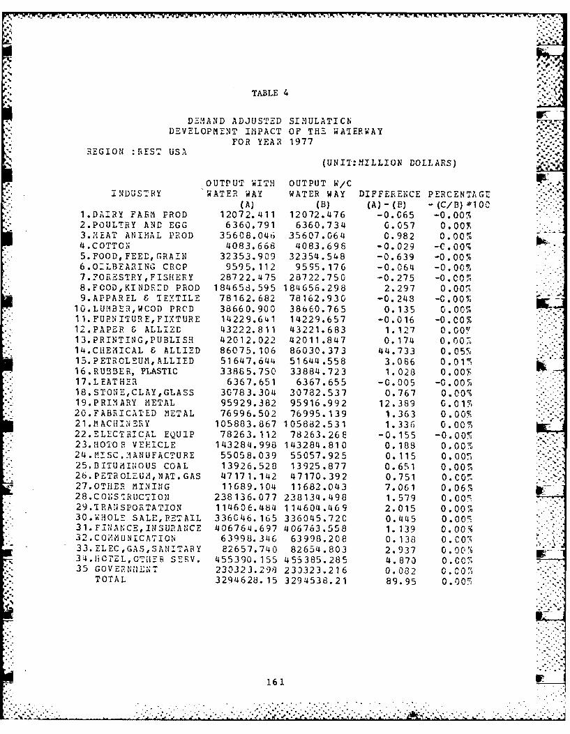
I;. .*.. S .

TABLE 4

DZ11AND ADJUSTED SI .ULATICNDEVELOPMENT IMPACT OF THE WATERWAY

FOR YEAR 1977 9:-...REGION :RiEST USA .- ::

(UNIT:NILLION DOLLARS)

OUTPUT WITH OUTPUT W/CINDUSTRY WATEIR WAY WATER WAY DIFFERENCE PERCENTAG.

(A) (B) (A) - (B) -(C/ )*1001.DI¥RY FARM PROD 12072.411 12072.476 -0.065 -0.00"-2.POULTRY AND EGG 6360.791 6360.734 0.057 0.00y3.;tEAT ANIMAL PROD 35608.046 35607.064 0.982 0.00 %4.COTTON 4083.668 4083.698 -0.029 -C.00%5.FOOD,FEED, GRAIN 32353.909 32354.548 -0.639 -0.00%6.O-LBEARING CROP 9595.112 9595.176 -0.064 -0.00%.7.?ORESTRY,FISHERY 28722.475 28722.750 -0.275 -0.00%8.FOOD,KINDRED PROD 184658.595 184656.298 2.297 0.00%9.APPAREL & TEXTILE 78162.682 78162.930 -0.243 -0.00%

10.LUMBER,WCOD PRCD 38660.900 38660.765 0.135 0.00%11. FURNITURE, FIXTURE 14229.641 14229.657 -0.016 -0.00%

. 12.PAPER & ALLIED 43222.811 43221.683 1.127 0.00Y13. PRINTING,PUBLISH 42012.022 42011.847 0.174 0.00714.CliEMICAL & ALLIED 86075.106 86030.373 44.733 0.05%13. PETROLEUM, ALLIED 51647.644 51644.558 3.086 0.0116.RU!3BER, PLASTIC 33885.750 33884.723 1.028 0.00"-17.LEATHER 6367.651 6367.655 -0.005 -0. 00% lli18.STONE,CLAY,GLASS 30783.304 30782.537 0.767 0.00%"--19.PRI.MARY METAL 95929.382 95916.992 12.389 0.0171.20.FABRICATED METAL 76996.502 76995.139 1.363 0.00s21.MACHINERY 105883.867 105882.531 1.33 G 0.00%22.ELECTRICAL EQUIP 78263.112 78263.266 -0.155 -0.00%23.I0TOF VEHICLE 143284.998 143284.810 0.188 0.00,24.MIISC."ANUFACTURE 55058.039 55057.925 0.115 0.00".25.BITUiiINOUS COAL 13926.528 13925.877 0.651 0.00%,26.PETROLEU4, NAT.GAS 47171.142 47170.392 0.751 0.Co%"27.OTHER MINING 11689.104 11682.043 7.061 0.06% V-728.CONS IRUCTION 238136.077 238134.498 1.579 0.00 7 '29.TRANSPORTATION 114606.484 114604.469 2.015 0.00 .-30.WHOLE SALE,PETAIL 336046.165 336045.720 0.445 0.00"'31.FINANCE,INSURANCE 406764.697 406763.558 1.139 0.00%32.COV*MUNICATION 63998.346 63998.208 0.138 0.C0%33. ELEC,GAS, SANITAR Y 82657.740 82654.803 2.937 0.00.34.ICrZL,OTllZr SERV. 455390.155 455385.285 4.870 0.00 .

35 GOVE.NNENT 23C323.298 233323.216 0.082 0.00%-.TOTAL 3294628. 15 3294538.21 89.95 0.00%7

161S- - ~ . ~'- .- -

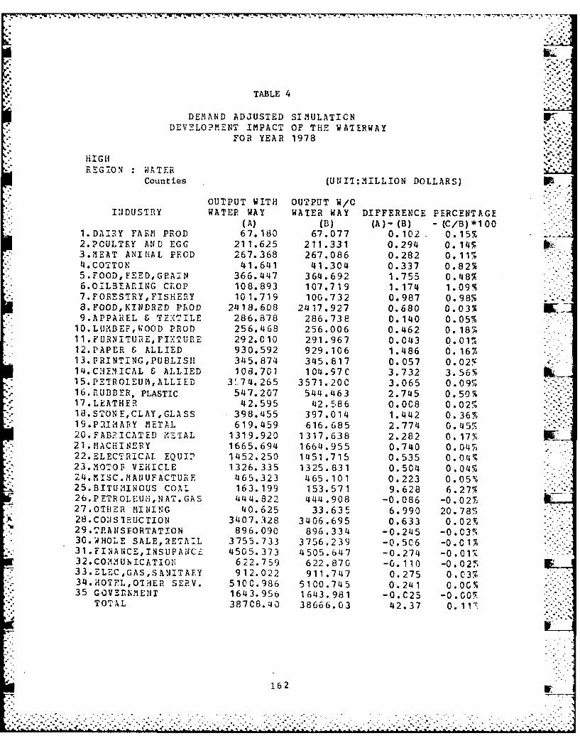
TABLE 4

DEMAND ADJUSTED SIMULATICNDEVELOPMENT IMPACT OF THE WATERWAY

FOR YEAR 1978i I Gi -:S..

HIGHREGION :WATER

Counties (UN II: IILLION DOLLARS)

OUTPUT WITH OUTPUT W/INDUSTRY WATER WAY WATER WAY DIFFERENCE PERCENTAGE

(A) (3) (A)- (B) - (C/B) *1 001.DA:RY FARM PROD 67.180 67.077 0.102. 0.15%2.POULTFY AND EGG 211.625 211.331 0.294 0.14%-3.IEAT ANIMAL PROD 267.368 267.086 0.282 0.11%4.COTTON 41.641 41.304 0.337 0.82%5.FOOD,FEED,GPRA7N 366.447 364.692 1.755 0.48%6.OITLBEAnING CROP 108.893 107.719 1.174 1.09%7.FOFESTRY,FISHERY 101.719 100.732 0.987 0.98%8.FOOD,KINDRED PROD 2418.608 2417.927 0.680 0.03%9.APPAREL & TEXTILE 286.878 286.738 0.140 0.05%10.LUMBEF,WOOD PROD 256.468 256.006 0.462 0. 18"11.FURNITURE,FIXTURE 292.010 291.967 0.043 0.01,"A12.PAPER & ALLIED 930.592 929.106 1.486 0.16,'13.PRINTING,PUBLIS11 345.874 345.817 0.057 0.02"-14.CHE.ICAL & ALLIED 108.701 104.97C 3.732 3.56%15.PETROLEUM,ALLIlD 374.265 3571.200 3.065 0.0911-"16.,UBBER, PLASTIC 547.207 544.463 2.745 0.50%17.LEATHER 42.595 42.586 0.0C8 0.02%

* 18.STON E,CLAY, GLASS 398.455 39.1142 03619. PITMARY METAL 619. 459 616.685 2.774 0.45

24.,ISC.AANUFACTURE 465.323 465.101 0.223 0. 05%-25.BITUMINOUS COAL 163.199 153.571 9.628 6.27%26.PETROLEUH,NAT. GAS 444.822 444.908 -0.086 -0.027,27.OTHER MINING 40.625 33.635 6.990 20.78--28.CON SI RUCTION 3407.328 3406.695 0.633 0.02,-29.TRANSFORTATION 896.090 896.334 -0.245 -0.037-30.wHOLE SALE,RETA:L 3755.733 3756.239 -0.5C6 -0.01%31.FINANCE,INSUPANCz 4505.373 4505.647 -0.274 -0.01"32.COmU ICATIOu 622.759 622.870 -0.110 -0.027,

*33 .ELEC GAS S ANITAEY 912.022 911.747 0.275 0. C37,34.iIOTFL,OTHER SERV. 5100.986 5100.745 0.241 0 .0CG%35 GOVERNME1IT 1643.956 1643.981 -0.C23 -0.00F

TOTAL 38708.40 38666.03 42.37 0. 1""""

162

. .".

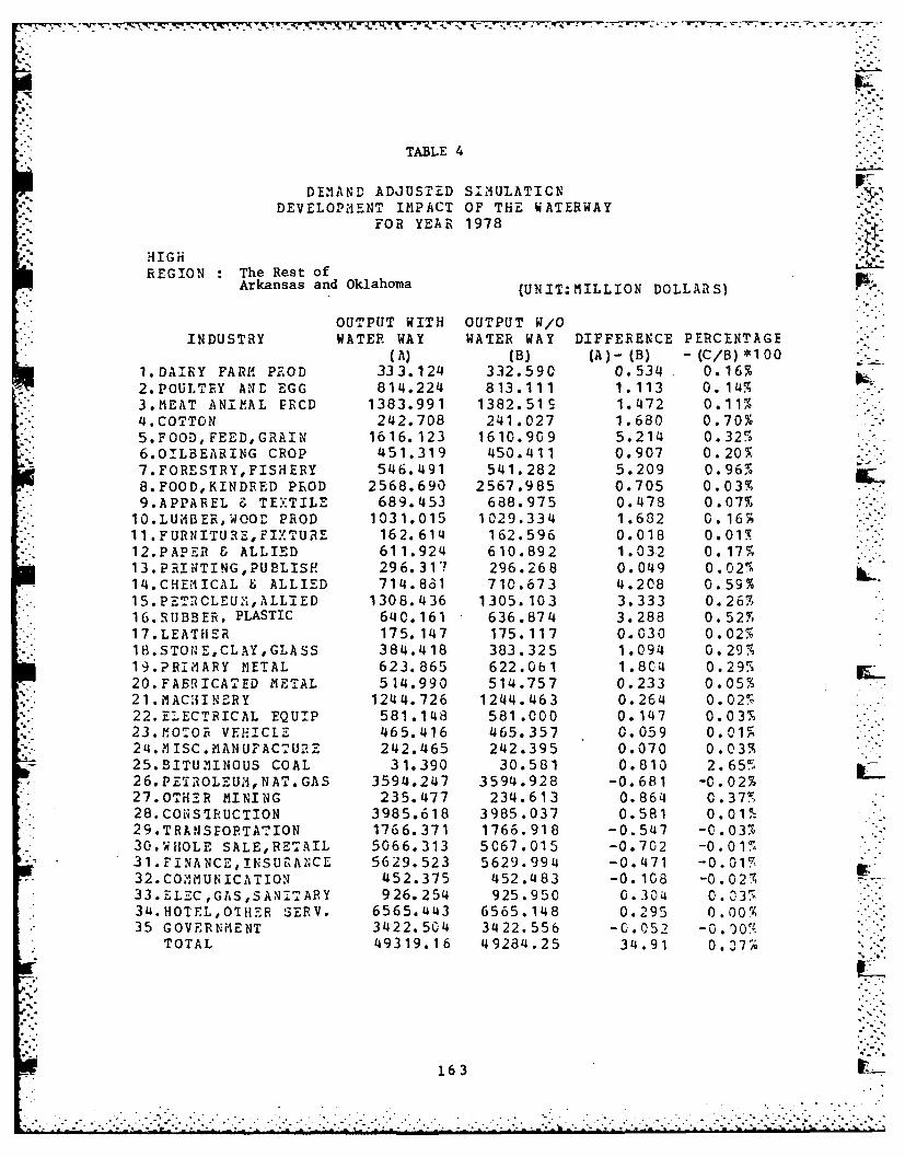
TABLE 4

DEMAND ADJUSTED SIIULATICNDEVELOPMENT IMPACT OF THE WATERWAY

FOR YEAR 1978

HIGHREGION The Rest of

Arkansas and Oklahoma (UNIT:MILLION DOLLARS)

OUTPUT WITH OUTPUT W/OINDUSTRY WATER WAY WATER WAY DIFFERENCE PERCENTAGE

(A) (B) (A)- (B) -(C/B)*1001.DAIRY FARI. PROD 333.124 332.590 0.534 0.16%2.POULTRY ANT[ EGG 814.224 813.111 1.113 0.14%3.MEAT ANIM.AL FRCD 1383.991 1382.51S 1.472 0.11%4.COTTON 242.708 241.027 1.680 0.70%5.FOOD,FEEDGRAIN 1616.123 1610.909 5.214 0.326.0ILBEARING CROP 451.319 450.411 0.907 0.20%7.FORESTRY,FISHERY 546.491 541.282 5.209 0.967.8.FOOD,KINDRED PROD 2568.690 2567.985 0.705 0.03%9.APPAREL & TEXTILE 689.453 688.975 0.478 0.07%

1O.LUNBER,WOOD PROD 1031.015 1029.334 1.682 0.16;11 .FURNITURZ,FI .TURE 162.614 162.596 0.018 0 0112.PAPER & ALLIED 611.924 610.892 1.032 0 .17 %13. PRI NTING,PULBLISH 296.317 296.268 0.049 0.02%14.CHE.MiICAL & ALLIED 714.8 1 710.673 4.208 0.59%15.PETRCLEUM,ALLIED 1308.436 1305.103 3.333 0.267416.RUBBER, PLASTIC 640.161 636.874 3.288 0.52%17.LEATHER 175.147 175.117 0.030 0.02%18.STONE,CLAYGLASS 384.418 383.325 1.094 0.29%19.PR:MARY METAL 623.865 622.061 1.8C4 0.297,20.FABRICATED METAL 514.990 514.757 0.233 0.05%21.MACHINERY 1244.726 1244.463 0.264 0.02! -

*j. 22.ELECTRICAL EQUIP 581.148 581.000 0.147 0.03%-. 23.m 4OO EIL 65.416 /465.357 0.059 0 . 01

2 4. ISC.MANUFACTUFE 242.465 242:395 0:070 0.03,;25.BITUMINOUS COAL 31.390 30.581 0.810 2.65526.PETROLEUM;,NAT.GAS 3594.247 3594.928 -0.681 -0.02%27.OTHER MINING 235.477 234.613 0.864 0.37%28.CONSIRUCTION 3985.618 3985.037 0.581 0.01!-29.TRANSPOPRTATION 1766.371 1766.918 -0.547 -0.03%30.WiIOLE SALE,RETAIL 5066.313 5067.015 -0.702 -0.01531.FINANCE,INSURANCE 5629.523 5629.994 -0.471 -0.017132.COMMUNICATION 452.375 452.483 -0.108 -0.02%,33.ELZC,GAS,SAN:TARY 926.254 925.950 0.304 0 .03 %

*. 34.HOTEL,O11jER SERV. 6565.443 6565.148 0.295 0.00'35 GOVERNMENT 3422.504 3422.556 -0.052 -0..00

TOTAL 49319.16 49284.25 34.91 0 07

163

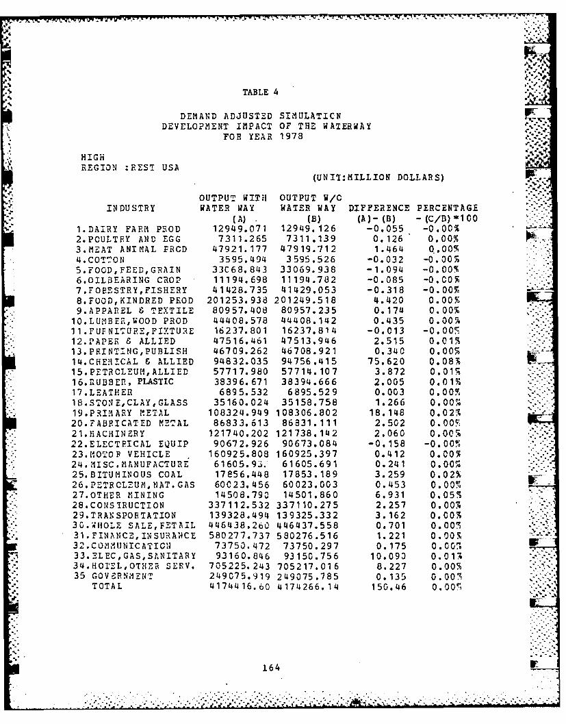
TABLE 4

DEMAND ADJUSTED SIMULATICNDEVELOPMENT IMPACT OF THE WATERWAY

FOR YEAR 1978 ~

HIGH .1.'%REGION :RE"4ST USA

(UNIT:MILLION DOLLARS)

OUTPUT WITH OUTPUT W/CINDUSTRY WATER WAY WATER WAY DIFFERENCE PERCENTAGE

(A) (B) (A) -(B) -(C/B)*100S8.DA ,DRY FAE PROD 12949.071 12949.126 -0.055 -0.00%

2.PULTEY AND EGG 7311.265 7311.139 0.126 0.00%3.MEAT ANIMAL PROD 47921.177 47919.712 1.464 0. 00

* ~ 4.COTTON 3595.494 3595.526 -0.032 -0.00%5.FOOD,FEEDGRAIN 33C68.843 33069.938 -1.094 -0.00.--6.OALPEARING CROP 11194.698 11194.782 -0.085 -0.00%

" 7.FOPISTRY,FISHIHY 41428.735 41429.053 -0.318 -0.00%8.FOODKINDRED PROD 201253.938 201249.518 4.420 0.00F

*9.APPAP.EL & TEXTILE 80957.408 80957.235 0.174 0.00%10.LUMETR,WOOD PROD 44408.578 44408.142 0.435 0.0011.ll1.FUFNITURE,FI'TURE 16237.801 16237.814 -0.013 -0.00512.PAPER & ALLIED 47516.461 47513.946 2.515 0.01%13.PRINT-NG,PUBLISH 46709.262 46708.921 0.340 0.00%14.CHE.-12CAL & ALLIED 94832.035 94756.415 75.620 0. 08% K15.PETRCLE-UM,ALLIED 57717.980 57714.107 3.872 0.01%16.rEUBSEP, PLASTIC 38396.671 38394.666 2.005 0.01%17.LEATHER 6895.532 6895.529 0.003 0.00%18.STOIE,CLAY,GLASS 35160.024 35158.758 1.266 0.001/%0-19.PRIMARY METAL 108324.949 108306.802 18.148 0.0271.20.FABPICATED METAL 86833.613 86831.111 2.502 0. 00'2 1.ACHIN.RY 121740.202 121738.142 2.060 0 .00%

22.rrCTEICAL EQUIP 90672.926 90673.084 -0.158 -0.00%23.110TOR VEHICLE *160925.808 160925.397 0.412 0.00%

*24.:ISC.MANUFACTURE 61605. 9:;. 61605.691 0.241 0 .0 025.DITMINOUS COAL 17e56.448 17853.189 3.259 0.02%26. PETECLEUM, NAT. GAS 60023.456 60023.003 0.453 0.00%

* 27.OTHER MINING 14508.790 14501.860 6.931 0.05%28.CONSTRUCTION 337112.532 337110.275 2.257 0.00%29. TRAN SPORTATION 139328.494 139325.332 3.162 0.00%3GWIIOLE SALE,FETAIL 446438.260 446437.558 0.701 0.001--3 1. F IN AN1Cz, IN SU RA'CE 580277.737 580276.516 1.221 0.00%32.COMMUNICATICU 73750.472 73750.297 0.175 0.00"33.ELEC,GAS,SANITARY 93160.846 93150.756 10.093 0.01%-34.HOT:EL,OTtlZR SERV. 705225.243 705217.016 8.227 0.00% -".'"35 GOVORNMPENT 249075.919 249075.785 0.135 0.007,

TOTAL 4174416. 60 4174266. 14 150.46 0. 00-.

164

_- ..

TABLE 4

DEMAND ADJUSTED SIMULATIONDEVELOPMENT IMPACT OF THE WATERWAY

FOB YEAR 1978 ,

MEDIUMREGION : WATER

Counties (UNIT:MILLION DOLLARS)

OUTPUT WITH OUTPUT W/CINDUSTRY WATER WAY WATER WAY DIFFERENCE PERCENTAGE

(A) (B) (A)- (B) -(C/B)*100

1.DAIRY FARM PROD 67.180 67.107. 0.073 0.11%2.POULTRY AND EGG 211.625 211.417 0.208 0.10%3.MEAT ANIMAL PROD 267.368 267.167 0.201 0.085

4.COTTON 41.641 41.403 0.238 0.57%

5. FOOD, FEED, GRAIN 366.447 365.145 1.302 0.36%

6.0ILBEARING CROP 108.893 107.969 0.924 0.86%

7.FORESTRY,FISHERY 101.719 101.022 0.697 0.69%

8.FOODKINDRED PROD 2418.608 2418.124 0.483 0.02%

9.APPAREL & TEXTILE 286.878 286.781 0.097 0.037o

IO.LUMBER,WOOD PROD 256.468 256.150 0.318 0.12%

11. FURNITURE, FIXTURE 292.010 291.979 0.031 0.01%

12.PAPER & ALLIED 930.592 929.535 1.056 0.11%

13.PRINTING,PUBLISH 345.874 345.835 0.039 0.01114.CHEMICAL & ALLIED 108.701 106.102 2.600 2.45%

15.PETRCLEU,IALLIED 3574.265 3571.952 2.313 0.06%

16.RUBBE.R, PLASTIC 547.207 545.279 1.928 0.35%17.LEATHER 42.595 42.58S 0.006 0.01%

18. STON E, CLAY, GLASS 398.455 397.373 1.082 0. 27%19.PRIMARY METAL 619.459 617.310 2. 149 0 .35/%.20.FABRICATED METAL 1319.920 1318.215 1.705 0.13%

21.MAACHINERY 1665.694 1665.171 0.523 0.03%

22. ELECTRICAL EQUIP 1452.250 1451.855 0.395 0.03% .-

23.MOTOP VEHICLE 1326.335 1325.954 0.382 0.03%

24.MISC.MANUFACTURE 465.323 465.164 0.159 0.03%25.B3ITUNINOUS COAL 163. 199 16C.010 3.189 1.995

26.PETROLEUl,,NAT.GAS 444.822 444.869 -0.047 -0.01,1.27.OTHER MINING 40.625 34.988 5.637 16.11%

28.CONSTRUCTION 3407.328 3406.866 0.462 0.01 29.TRANSPORTATION 896.090 896.268 -0.178 -0.02'3C.WHOLE SALE,P.ETAIL 3755.733 3756.144 -0.411 -0.01%31.FINANCE,INSURANCE 4505.373 45C5.605 -0.231 -0.0132.COM UNICAT:ON 622.759 622.842 -0.082 -0.01" •33.ELEZ,GAS,SANITARY 912.022 911.844 0. 178 C.020a34.HOTEL,OTHER SERV. 5100.986 5100.852 0.134 0.00%35 GOVERi.9JEENT 1643.956 1643.975 -0.019 -0.00%

TOTAL 38708.40 38680.86 27.54 Q.Q7 'l

C..

165

F

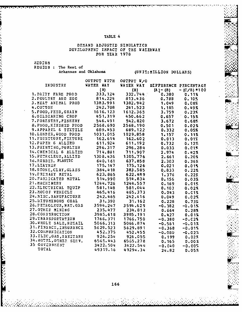
,lo -. -K

TABLE 4 "-

DEMAND ADJUSTED SIMULATICE __

DEVLOPMENT IIPACT OF THE WATERWAY .-FOR YEAR 1978

M1EDIUMiREGION : The Rest of ,%,- *

Arkansas and Oklahoma (UNIT:MILLION DOLLARS)

OUTPUT WITH OUTPUT W/OINDUSTRY WATER WAY WATER WAY DIFFERENCE PERCENTAGE

(A) (B) (A I- (B) - (C/B) *1001.DAI2Y FARN PROD 333.124 332.744 0.380 0.11%2.POULTEY AND EGG 814.224 813.436 0.788 0.10%3.MEAT ANIMAL PROD 1383.991 1382.942 1.049 0.C8%4.COTON 242.708 241.523 1.185 0.49%5.FOODFEEDGRAIN 1616.123 1612.365 3.759 0.23%6.OILBEARING CROP 451.319 450.662 0.657 0.15-'7.FORESTRY,FISHERY 546.491 542.820 3.672 0.68%

8.FOOD,KINDRED PROD 2568.690 2568.190 0.501 0.02%9.APPAREL & TEXTILE 689.453 689.122 0.332 0.05%

10.LUhiBER,WOOD PROD 1031.015 1029.858 1.157 0.11%11.FURNIT URE,FIXTURE 162.614 162.602 0.013 0.01%12.PAPER & ALLIED 611.924 611.192 0.732 0.12%13.PRINT-NG,PUBLISH 296.317 296.284 0.033 0.C1%1.CHEMICAL & ALLIED 714.881 711.907 2.974 0.42%15.PETR CLEUM,ALLIED 1308.436 1305.776 2.661 0.20%16.RUBBER, PLASTIC 640.161 637.858 2.303 0.36-17.LEATHER 175.147 175.126 0.021 0.01%18.STONE,CLAY,GLASS 384.418 383.585 0.833 0.22%19.:R.IA.Y METAL 623.865 622.489 1.376 0.22%20. FABaqICATED M2TAL 514.990 514.834 0.156 0.03% :'21.IIACHINERY 1244.726 1244.557 0.169 0.01%22.ELECTRICAL EQUIP 581.148 581.044 0.103 0.027h23. O-oF VEHICLE 465.416 465.373 0.043 0.C1%2L4.IISC.MANUFACTURE 242.465 242.416 0.049 0.02%25.B3ITUMINOUS COAL 31.390 31.162 0.228 0 .73%26.PETROLEUi,NAT.GAS 3594.247 3594.629 -0.382 -0. 0 1 %27.OTHEF MINING 235.477 234.813 0.664 0.28%28.CONSIRUCTION 3985.618 3985.191 0.427 0.01%29.TRANSPOETATION 1766.371 1766.750 -0.380 -0.C2%

, 30.WIiOLE SALE,RETAIL 5066.313 5066.874 -0.561 -0.01%3 1.FINANCZ,INSURANCE 5629.523 5629.891 -0.368 -0.01%32•CO~HMU NICATIONJ 452.375 452.455 -0.080 -0.02%33.ELC,GAS,SANITARY 926.254 926.055 0.199 0.02%

* 34.iiOTFL,OTHE" SEPFV. 6565.443 6565.278 0.165 0.00%-35 GOV.RNr.ENT 3422. 504 3422.544 -0.040 -0.00--

TOTAL 49319.16 49294.34 24.82 0.05%

166

." - • . .. °-,

-" .:, " .

° . . . . . . .* ' ."* ..- ~~~. .-- ~ -°

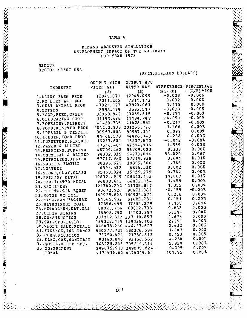
TABLE 4

DEMAND ADJUSTED SIMULATICNDEVELOPIENT IMPACT OF THE WATERWAY

FOR YEAR 1978

* ~MEDIUM I.REGION :REST USA

(UNI1Ii:ILLION DOLLARS)

OUTPUT WITH OUTPUT W/C

INDUSTRY WATER WAY WATER WAY DIFFERENCE PERCENTAGE(A) (B) (A).- (B) - (C/B) *100

1.DAIRY FARM PROD 12949.071 12949.099 -0.028 -0.00%

2.POULTRY AND EGG 7311.265 7311.173 0.092 0.00%

3.MEAT ANIMAL PROD 47921.177 47920.061 1.115 0.00%

4.COTTON 3595.494 3595.517 -0.023 -0.00%5.FOOD,FEED,GPAIN 33068.843 33069.615 -0.771 -0.00%

6.OILBEARING CROP 11194.698 11194.749 -0.051 -0.007

7.FORESTRY,FISHERY 41428.735 41428.952 -0.217 -0.00%

8.FOOD,KINDRED PROD 201253.938 201250.770 3.168 0.00%

9.APPAREL & TEXTILE 80957.408 80957.311 0.097 0.00%

10.LUM3ER,WOOD PROD 44408.578 44408.340 0.238 0.00%11.FURNITUREFIXTURE 16237.801 16237.813 -0.012 -0.00%12.PAPER & ALLIED 47516.461 47514.905 1.555 0.00%

13.PRINTING,PUBLISH 46709.262 46709.023 0.238 0.00%

14.CHEMICAL & ALLIED 94832.035 94779.016 53.020 0.067.15.PETROLEUJ,ALLIED 57717.980 57714.938 3.041 0.01%

16.UBBER, PLASTIC 38396.671 38395.306 1.365 0.00% O

17.LZATiIER 6895.532 6895.530 0.002 0.00%

16.STONE,CLAY,GLASS 35160.024 35159.279 0.744 0.00%19.PRI IARY METAL 108324.949 108313.143 11.807 0.01%--20.FABRICATED METAL 86833.613 86832.154 1.458 0.00,"421.MACIIINERY 121740.202 121738.847 1.355 0.00%

22.ELECTRICAL EQUIP 90672.926 90673.081 -0.155 -0.00%23.MOTOE. VEHICLE 160925.808 160925.571 0.238 0.00%

24.IISC.MANUFACTURE 61605.932 61605.781 0.151 0.00%25.BITUMINOUS COAL 17856.448 17855.279 1.169 0.01%26.PETROLEUM,NAT.GAS 60023.456 60022.798 0.658 0.00-,27.OTIHZR MINING 14508.790 14503.397 5.394 0.04%28.CONSrIEUCTION 337112.532 337110.853 1.678 0.00%29. T RANSPORTATION 139328.494 139326.103 2.391 0.00%30.WHOLE SALE,RETAIL 446438.260 4406437.627 0.632 0.00;;

31.FINANCE,INSURIANCE 580277.737 580276.594 1.143 0.00%32. COMM UN ICATON' 73750.472 73750.313 0.153 0.00%33. ELEC,GAS,SANITArY 93160.846 93156.562 4.284 0.001%34.HOTEL,OTliEP SERV. 705225.243 705219.319 5.924 0.00, Oi%35 GOVERNMENT 249075.919 249075.824 0.095 0C0"'

TOTAL 4174416.60 4174314.64 101.95 0. c0

167

%...................................................

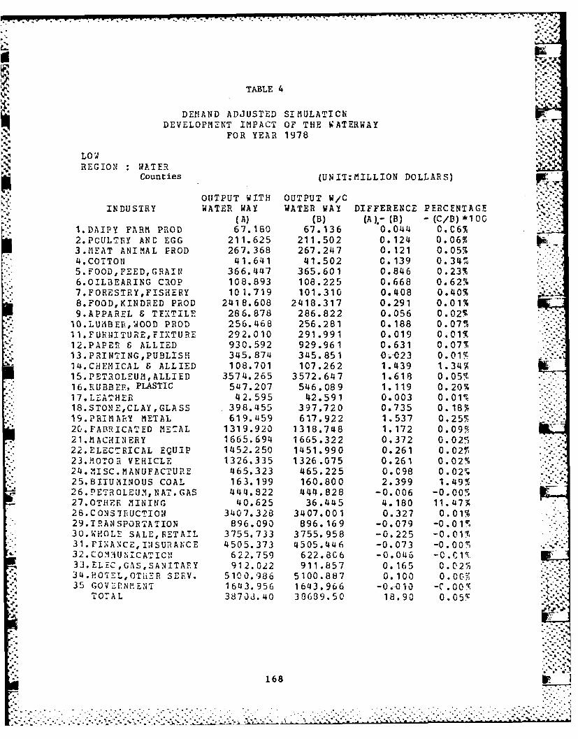
TABLE 4

DEMIAND ADJUSTED SIMULATICNDEVELOPMENT IMPACT OF THE WATERWAY

FOR YEAR 1978

LOWREGION WATER WTEAY WTWA DIERNEECNAG

Counties (UNIT:.MILLION DOLLARS)

OUTPUT WITH OUTPUT W/C,tINDUSTRY WATER WAY WATER WAY DIFFERENCE PERCENTAGE :'-,'_ A) (B) (A).- (B) -(C/B) *1 00

1.DAIPY FARK PROD 67.160 67.136 0.044 0.C6%2.PCULTRY AND EGG 211.625 211.502 0.124 0.06%3.MSEAT ANIMAL PROD 267.368 267.247 0.121 0.05%4.COTTONI 41.641 41.502 0.139 0.34,";

5.FOOD, FEED,GRAIN 366.447 365.601 0.846 0.23%6.01LBEARING CROP 108.893 108.225 0.668 0.62%7.FORESTRY,FISHERY 101.719 101.310 0.408 0.40%8.FOOD,KINDRED PROD 2418.608 2418.317 0.291 0.01%9.APPAREL & TEXTILE 286.878 286.822 0.056 0.02%10.LUMBER,WOOD PROD 256.468 256.281 0.188 0.07%11. FURNITURE, FIXTURE 292.010 291.991 0.019 0.01%12.PAPER ALLIED 930.592 929.961 0.631 0.07%

- ~ 13. PRI NTI NG, PUBLISH 345.874 345.851 0.-023 0.01F14.CHEI iCAL & ALLIED 108.701 107.262 1.439 1.34%15.PETROLEUU,ALLIED 3574.265 3572.647 1.618 0.05%."

* 16.RUBBEE, PLASTIC 547.207 546.089 1.119 0.20%17.LEATHER 42.595 42.591 0.003 0.01 %18.STONE,CLAY,GLASS 398.455 397.720 0.735 0.18%19.PRIMARY METAL 619.459 617.922 1.537 0.2552C.FAB]RICATED METAL 1319.920 1318.748 1.172 0.09121. MACHINERY 1665.694 1665.322 0.372 0.02522.ELECTRICAL EQUIP 1452.250 1451.990 0.261 O. 027123.MOTOR VEHICLE 1326.335 1326.075 0.261 0.02%24.k ISC.MANUFACTURE 465.323 465.225 0.098 0.02%.25. BITUMINOUS COAL 163.199 160.800 2.399 1.49%26.PETROLEUM,NAT.GAS 444.822 444.828 -0.006 -0.00-7327.OTIIEE MINING 40.625 36.445 4. 180 11.47%26.CONS7EUCTION 3407.328 3407.001 0.327 0.01%29.TRANSPORTATION 896.090 896. 169 -0.079 -0.01% .

* 30.WHOLE SALE, FETAIL 3755.733 3755.958 -0.225 -0.01%31.PIA CE,INSURANCE 4505.373 4505.446 -0.073 -0.00,32.CO ,1UINCAT I C 622.759 622.8C6 -0.046 -C.C1 133.ELECGAS,SANITAtY 912.022 911.857 0.165 0.027134.HOTEL,OTHER SEFV. 5100.986 5100.887 0.100 0.O - .35 GOVE RNMiE:NT 1643.956 1643.966 -0.-013 -C. 00

TOTAL 3870d.40 30699.50 18.90 0.0 5

168. . . .

% • -. -" ..

TABLE 4

DEMAND ADJUSTED SIMULATIONDEVELOPMENT IMPACT OF THE WATERWAY

.j"

FOR YEAR 1978 %? %I

LOW

REGION The Rest of

Arkansas and Oklahoma (UNIT:MILLION DOLLARS)

OUTPUT WITH OUTPUT W/C

INDUSTRY WATER WAY WATER WAY DIFFERENCE PERCENTAGE

(A) (B) (A).- (B) -(C/B)*100

1.DA. RY FARM PaCD 333.124 332.896 0.228 0.07%

2.POULTRY AND EGG 814.224 813.755 0.469 0.06%

3.n-AT ANIMAL PROD 1383.991 1383.359 0.633 0.057

4.COTTON 242.703 242.008 0.699 0.29 %

5.FOODFEED,G.AIN 1616.123 1613.796 2.327 0.14%

6.OILBEARING CROP 451.319 450.909 0.410 0.09%

7.FORESTRY,FISEZY 546.491 544.318 2.173 0.40%

8.FOCD,KINrRED PRCD 2568.690 2568.387 0.303 0.01%

9.APP AEIL & TEXTILE 689.453 689.260 0.193 0.03%

" 1O.LUJYBER,WCOD PROD 1031.015 1030.332 0.683 0.07%

"11.FUNITUE,FITU?,E 162.614 162.607 0.008 0.00.

-12.PAPER ALLIED 611.924 611.484 0.441 0.07%

13.PINTiNG,PUBLISH 296.317 296.297 0.020 0.01%

14.CHEMICAL & ALLIED 714.881 713.107 1.774 0.25% /3

15.PETROLEUIi,ALLIED 1308.436 1306.427 2.009 0. 15F,

* 16.RUBBER, PLASTIC 640.161 638.814 1.348 0.21%

" 17.LEATHER 175.147 175.135 0.013 0.01%"

18.STONE,CLAY, GLASS 384.418 383.833 0.586 0.15%

19.PRIiARY METAL 623.865 622.902 0.963 0. 15% J -%

20.FABPICATED I'7TAL 514.990 514.891 0.098 0.02%

21.MAC1IT NERY 1244.726 1244.605 0.121 0.01%

22.2LECTRICAL EQUIP 581.148 581.085 0.062 0.01%

23.OOTOF VEHICLE 465.416 465.389 0.027 0.01%

24.MISC.MANUFACTURE 242.465 242.435 0.029 0.01%

25.BITUNINOUS COAL 31.390 31.222 0.168 0. 54'%

26. PETROLEUMi,NAT.GAS 3594.247 3594.305 -0.058 -0.00%

27.OTHER MINING 235.477 235.010 0.467 0.20%

28.CO-:SIRUCTION 3985.618 3985.307 0.311 0.01%

29.T RANSPOETATION 1766.371 1766.534 -0.163 -0.01%

30.WHOLE SALE, RETAI-L 5C66. 313 5066.621 -0.308 -0.01%

31. FINANCE, INSUF.ANCE 5629.523 5629.671 -0.148 -0.00%o

* 32.COmIUNICATICN 452.375 452.420 -0.045 -0. 01%"

33.ELE.,GASSAN1TARY 926.254 926.066 0.188 0.02t

34.:fOTEL,OT~i22 SEEV. 6565.443 6565.318 0.125 0.007."

35 GOVERNM 1ZNT 3422.504 3422.525 -C.021 -0.00-'

STOTAL 49319.16 49303.C3 16.13 0.03%

169

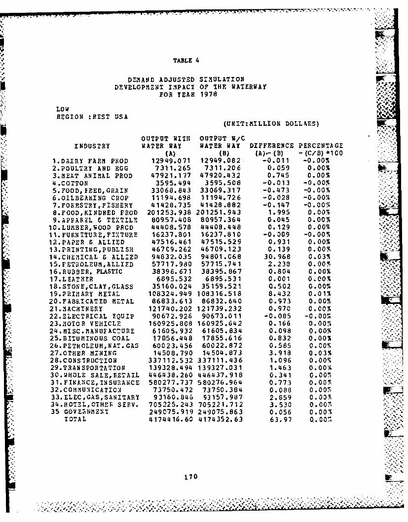
* -- " .L . .. ...

TABLE 4

DENAND ADJUSTED SIMULATIONDEVELOPMENT IMPACT OF THE WATERWAYFOR YEAR 1978 '"

LOWREGION :REST USA

(UNIT:KILLION DOLL}.S)

OUTPUT WITH OUTPUT W/CINDUSTRY WATER MAY WATER WAY DIFFERENCE PERCENTAGE

(A) (B) (A).- (B) - (C/B) *1001.DAIRY FARM PROD 12949.071 12949.082 -0.011 -0.00%2.POULTRY AND EGG 7311.265 7311.206 0.059 0.00%3.MEAT ANIMAL PROD 47921.177 47920.432 0.745 0.00%4.COTTON 3595.494 3595.508 -0.013 -0.00%5. FOOD, FEED, GRAIN 33068.843 33069.317 -0.473 -0.00%6.0ILBEARING CROP 11194.698 11194.726 -0.028 -0.00%7.FORESTRY,FISHERY 41428.735 41428.882 -0.147 -0.00%8.FOOD,KINDRED PROD 201253.938 201251.943 1.995 0.00%9.APPAREL & TEXTILE 80957.408 80957.364 0.045 0.00%

10 LUMBER,4W OOD PRCD 44408.578 44408.448 0.129 0.00%

11. FURN ITURE, FIXTURE 16237.801 16237.810 -0.009 -0.00"12.PAPER & ALLIED 47516.461 47515.529 0.931 0.00%13.PRINTING,PUBLISH 467C9.262 46709.123 0.139 0.00%14.CiEMICAL & ALLIED 94832.035 94801.068 30.968 0.03%15. FETROLEUM,ALLIED 57717.980 57715.741 2.238 0.00;16.RUBBER, PLASTIC 38396.671 38395.867 0.804 0.00%17.LEATHER 6895.532 6895.531 0.001 0.00%18.STONE,CLAY,GLASS 35160.024 35159.521 0.502 0.00%19.PRIIARY METAL 108324.949 108316.518 8.432 0.01%20.FABEICATED MZTAL 86833.613 86832.640 0.973 0.00%21.AACHINERY 121740.202 121739.232 0.970 0.00%22.ZLECTRICAL EQUIP 90672.926 90673.011 -0.085 -0.00%

" 23.MoTOR VEPICLE 160925.808 160925.642 0.166 0.00%- 24MIISC.MANVUACTURE 61605.932 61605.834 0.098 0.00%

25.BITUMINOUS COAL 17856.448 17855.616 0.832 0.00%• 26.PETHOLEUh,NAT.GAS 60023.456 60022.872 0.585 0.00%

27.OTHER MINING 14508.790 14504.873 3.918 0.03%. 28.CONSIRUCTION 337112.532 337111.436 1.096 0.00%

29.T.ANSPORTATION 139328.494 139327.031 1.463 0.00 .

" 30.WHOLE SALE,BETAIL 446438.260 446437.918 0.341 0.00"3 1. F IN .,CE, IN SURAiNCE 580277.737 580276.964 0.773 0.00",32.COMMUNICATIO:N 73750.472 73750.384 0.088 0.00,33.ELEC,GAS,SANITARY 93160.846 93157.987 2.859 0.03N34.HOT3L,THErb SERV. 705225.243 705221.712 3.530 0.007-35 GOVEaNMEN7 249075.919 249075.863 0.056 0.00-.

TOTAL 4174416.60 4174352.63 63.97 O..00.

170..........................................

... ". ° % -I%

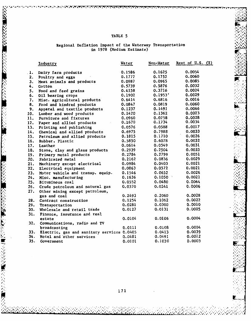
'V%

TABLE 5

Regional Deflation Impact of the Waterway Transportationin 1978 (Medium Estimate)

Industry Water Non-Water Rest of U.S. (.

1. Dairy farm products 0.1586 0.1625 0.00542. Poultry and eggs 0.1777 0.1752 0.00603. Meat animals and products 0.0987 0.0965 0.00854. Cotton 0.5739 0.5876 0.00325. Food and feed grains 0.4158 0.3716 0.00246. oil bearing crops 0.1902 0.1953' 0.00297. Misc. agricultural products 0,6414 0.6816 0.00168. Food and kindred products 0.0847 0.0819 0.0060

*9. Apparel and textile products 0.1237 0.1491 0.0046 h10. Lumber and wood products 0.1420 0.1362 0.0023

*11. Furniture and fixtures 0.0960 0.0758 0.002812: Paper and allied products 0.1670 .0.1734 0.0034

1.Printing and publishing 0.0576 0.0588 0.001714. Chemical and allied products 0.6975 0.7988 0.003315. Petroleum and allied products 0. 1815 0. 1710 0.002616. Rubber, Plastic 0.5850 0.6078 0.003217. Leather 0.0614 0.0549 0.003118. Stone, clay and glass products 0.2939 0.2504 0.003319. Primary metal products 0. 2784 0.2799 0. 005120. Fabricated metal 0.2162 0.0836 0.002921. Machinery except electrical 0.0984 0.0403 0.0021

*22. Electrical equipment 0.0863 0.0572 0.002123. Motor vehicle and transp. equip. 0.1546 0.0652 0.002624. Misc. manufacturing 0.1636 0.1050 0.002125. Bituminous coal 0.0552 0.0480 0.006426. Crude petroleum and natural gas 0.0370 0.0341 0.0006

*27. Other mining except petroleum,gas and coal 0.2493 0.2060 0.0028

*28. Contract construction 0.1254 0.1062 0.002229. Transportation 0.0281 0.0300 0.001030. Wholesale and retail trade 0.0127 0.0131 0.000531. Finance, insurance and real

estate 0.0104 0.0106 0.000432. Commuinications, radio and TV

broadcasting 0.0111 0.0108 0.000433. Electric, gas and sanitary services 0.0405 0.0413 0.003934. Hotel and'other services 0.0481 0.0491 0.0012

F35. Goverrnent 0.0101 0. 1030 0.0003

171

Go~% ~%D 4 e Nf 0' C4 O%~ 000

U-% In 04 0000 a~* 1 %0 L", 0000 QC

-_4 0 A PAL -4 00 -4 co .4 r- N c CO4 Go tn oM1 0 %n 40 0-1 00 ?V 00C -4~ %; 0.- L e 00£0 coo 11 1 0 10 1r- r40 10 010co

u~~~~~* -V-C.q h 4r-l%

ON CA %0 4 L f0L A Col 0n cv 'Ln 00'4 knm l n c.4,-4 0 U 4 coo 0 0%O f40r4 O 99- o

%0inTin r-00 tnAO 10U CA40 04%00 L o %eO v4 o w . .- f %1 ON .4r.. .- 2 0 ON -CA t eQ0vo 0 0 0 0 0 0k' f 0 0 0 O 0. 0 0M 0 04 0 0-.C4 r- -* 0*a 0 0 0 0 0 0 0 0 000 0 04'-4

£0 Or,- coo, -tO0A cog 0 0 M~I

cc 00 000 000 00c00o0o0

C'J O0 % cj C OIT-4 00 -Go0 a r4N' ULg4 Ul4 0% %D Go-

f0I 000 00 0C4% 4r0 0 00 000 0 q r00 0

CO 4.

co 4 40CIL Go Q C4 r... O'C'0 ChL On- 0%00 O % %D 4 ~0 0v% . -40%10 ccr r144 04% ni 4u0 00 000 000 llt lfc~ 0 400 -C 4 nn 000 000 0 -4

0a kAL ObO D r- n 4 0

C-4 % -I - Ln en)r 4%' j H CIO

01% C O4 0 4 0% ' -4 0~ '-100 0'O L 0' 0%OH 0c-4~ 00 -7It~~ v-1 .-0r~ 0LA ,aIT04%G Cha 4 '-4000

&U - . . . . . . . . . . .'ar-P . 000 000 000 000 000 co0 000

* 4j 0 T% ITb PO. 00 M-4a. CO 0 'A 'D0Ln 0'.40 a0E-e cd 0 r- -4 0 .40l -0u ODar I%-D- 0'.40 ,pH .a0 0 -0 f4 ' 0 C *4 - '-10c 0,-r- a#.i u

40 00 0 0 0 0 0 0 0 0 0 0 0 0 0 C 0 0o10 X

(n% - e N 041 %Q H -44,

0. ~Ci0 .00

Cc co (a5.Iae 010 -4 0)

&0 0, A 4 0-.4 41 A1 -0 . V0 C2

0 4

172 IF

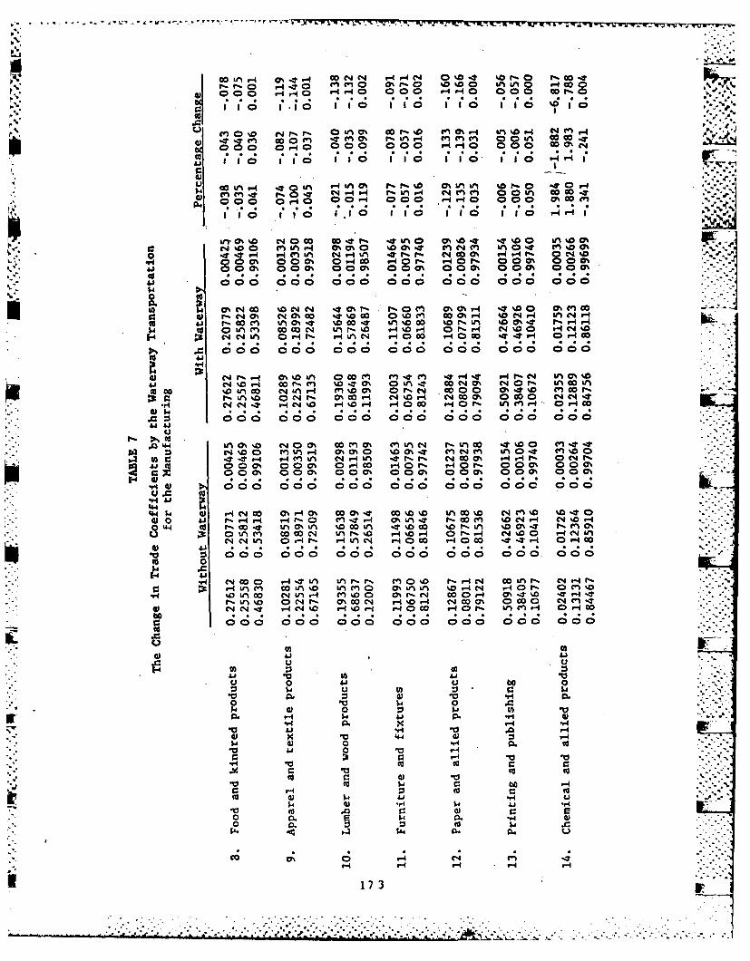
co Ln04 c O D-t C4N 04 -4 -4 IN 0 %D 0 'O-0a r- co -

rjI 00 enO ~ 0 00 -0 %0%00 &00n0 P4 o0

1.r4 -4P 011 11 0 114 40 a10 0 toIo

000 O99 000,0 o 000 -H0 000 0

% e

co I~ i s 1 5 ~

0i0

1a 0 Ul 9.O 110U 4LMa P 0 11N &M&n % 1r0 ,-EHI.

M en It C0 ~ C*?. -4n O%%0 -W'.Or NM 0 W WO%

ooo r- 0o C ,-or ,-40H1 0 00 C o m

1Wt CA %0 C 0 c r -Pr N% a% 0 L 00

t N ~%Do' m Cn r %% % 00? m 0'e ' V)C1 M in 0 e 0 47

.7000m 000% 00 0ON0C0 00 00042 000 .

c* . . . . .I- cc 0 0 000 000 000 000 000 000 ;6

oW 401

to3 CA 0 00 D04 PC-4 .0% - f 0A m CJO m N - -%0 % enc

wi r- 04 O 4 0%1 c '0,- N'O %aGo 0%0m 0o0% 0 0 NNW)C4t*0 e Lf).CC p-Ch .0 H'0 O C.oO -At% &n.- %0G 00a n % T P -40 V--

C) '0 00 C IA coo '0 0 0 CA( 0 A- 0 coo co

.7.4 ..IU.

Ial0 @ %N0 c 4i 0%H en 0 4m. 0 0'.DN.D 10 0O 0%~' -T.D0-t oa3 . r- HH% ,4.0 (. O -4 " O%DA r-4 00(co O '0(l co0 4 4 & L

C'N ' 4r- IT "U1C0 - 4 4 e-50 00 t-4 0 t-.MtH 0 r-4

0 000 000a 0% cenck niN P 00 000 0 00 00 000

41 ~ 0 Cm C % C - 140 H* V-4F C0'. r.HC 0 0 % m Coas

a Cm 0 CIA. mA2 000% COO 0.H CON 0 Q at

-H 41 0 0 a 0J. 0 %0C coo O CJ;0 000 c; c N ; c; 8

Elq C4 o -4H '0 co o"?-E 0 0 w o 4c0 %a U H 0H

0 00 e 0 000 0 0 nr 0 V- 000- 000 00 D0 0004 i

v @2 00 * c ;

14 A 2004.1o0 - TLn L rl n % r. 4 N 0 1 l C4 -1r

:R 0- 4J) en cUn% nc 0 nL D- _ 0 r 0 n%

%0 si co 0 uT4 e hr 4 D 0 0 ON-r 0 Q 'I-o-L O 0V , ONc 4 H% -Cuj c.. 0 7 0 0 4S.' C4 C4I - 4% -0 r -40 c .' US - &ne C r4C

0~. bo 0 0.1Cu~ U U

0 PC 0p wU 00 U

0l r-4 0 1r1

cc 9: (0U"

0' 4 H. NH4

17 3

-4l00 40Cu r0 -000 co 1c40 ( C44 N 00f 0 000 -4u 7 - -00 u.4-4I fo ON -o an 10 Go11 0 110 11V ,0 %000I 110 in10 I S

Uo C 4'0 D aCN -4 0% cn m 0-.0 -4 C410 'ONQr- Go - 04 0 0 l ,-4 C4 -1 -4 C4ITt0f .- Ch0 N-4r 0 0- IT o 0 r -1 C4 r,- .. enC en .

CO 0 01 1 10 110 10 1 10 too I 10 1 10 10 110I

r..

u IT 00r-4 (n Cl) N c I' 9-CJ-4 *?r00 ''I) D m iOn c " O'- (ON r -4 C4C) 'T ' IT 17r-4 C) 0O r- -4 C- 140 - Qa Q a.0% at% 0.4r -ca 0 ~ o -.4

v.00 0 0.-r- 000 0n4C4 -00 %0 00 000 000 000 000%',4 r oc0 (00 m 000 C oI 000 000' 00 000 CDD 0% 00 00a 0- r C ) C00 O

Ci r-4 C 00 C3 ) c ID.. -4% caf,9

' ' N 04 C o00- a NIe- 00'~ C) m 0 C~0

C! 000 00 00 00 00 0 0 0 000% 000 0 o00

C) C' m C;c .r.' 4 0 NA ' *U.? 0,r. *rs % 0 0 - ' 0

C). c M n(n 0 % .0 C m 0 & r 0 (N00- %DS-- 0' .,4n. 0- ,-4(' r)-t m % .1w r r t C -tn 1 COC* %0 CN e)00 %Dc -417u W% 'r-o4 Wio C4 ITOe cn e 0%cn00 0L) % T0 0n en-4 r4- 1- 0-0 inN-.? 00 C 0 inkON Go in* 0 A in4l% N r ,-10 P-.r0

000 000 000% 00 04 1 m00 00C L n 0 00IT 0 000 000 000

W1 40 IA.4- Nn1 1 0 00 'D-00 0%0 0% C0 00' Anl enC4-4HTOnin n C14001 r 0 C C'J4o 00 " inO' V%-# 'Tor 0%o~ "'-' 0f-r r-I-a H H C4 %

m C)UrV C.tr)s 00'C4'e C4 ODrO-. L &n tO Hnni OD-J. U~40 ' -4 "qn any- u 'T -4o .Go40 00n 0. 1 00H 000 004 000 000 00 4 000Q '00H 000'- - 0 r00 000C ' 0C00 c)HL 004' 000' 000' 00 000 f

s3D -T 0 ) L fT )00 0 0 0 0 0% N00 400 00 0 0c 0 00 r- 0'n0 m NID-4 M '0. %Dr. inOT%0 * 0 ci 0%0 0% -4 rOA i -40 ce.

H Lt.'4 co~ A- ain Oi4' 0Oin 'A 0 00 Nr4. -0 C4 00 0C(-)CN-. ,-04- 0,nc tnc". en-4 in w- 4 ,-%O l r0%I0 Cn -40 n V) H4'-4.1 . 0. C. C. .0 -4 . C. C. . 0 0* 0 * Q C ) 0* 9 . .1 .. .

0 C000 00o0 000 000 0 0 000 00 co0 0 00CD0 000

4()., cn.-mr 0 -ut C

9n w.0 0 Lf %0O TA HN OtA% 0%' co n O0'0

40J n m -Tco%D o * N0r C.I=L 00'J Hr'-- LMr r0AC in n 0k C4AOCSA00 H at? IANn (N '00 0'tU 'A-4 0C-T H-'O IA-T 0%0 Hen'O.r-4n 9 .-4IT-"r-4 0y-4 cA -. 000 nLn0 oc c n- MA-U s-v-' H~r en40 r.,I-

:Y .n H 4 9n n H .n M 4 a en C *0 en * W% 9% .l m .o .

00 00 000 00CD0 000 000 C 000 000 000 000

4A

o3 5.4 m 5C om -. n uiMH. "a n%IT. 5.4 0- M qO -% n 0 400.L h"c - oC qw en 4.1?4 c 0. 4C> mC tIo n n 0 0 .o% --T 0n u nr4 c nG 0C1

004 0D v-I 0 0 c 4 0 00 o

A i u- C S

1.4 00 0w-4~4 VA. u- . .403 r. 0. 0

10 w IC0 (0 0 C z0

0c 0 4a c:Ur

cc rz4 0 . 04 mcc ca U0 0

941-4 cc S-u UH 0

la .0US- 0 U Q 4) to.10 0 0r. w _4 .0 ou U

0i 4) 4. 0 0o -H H4 00 .u 0 a i U

nr ca r0 0'0v4 n

9-49- 94 -4.94 *4 C4 C4 (

174

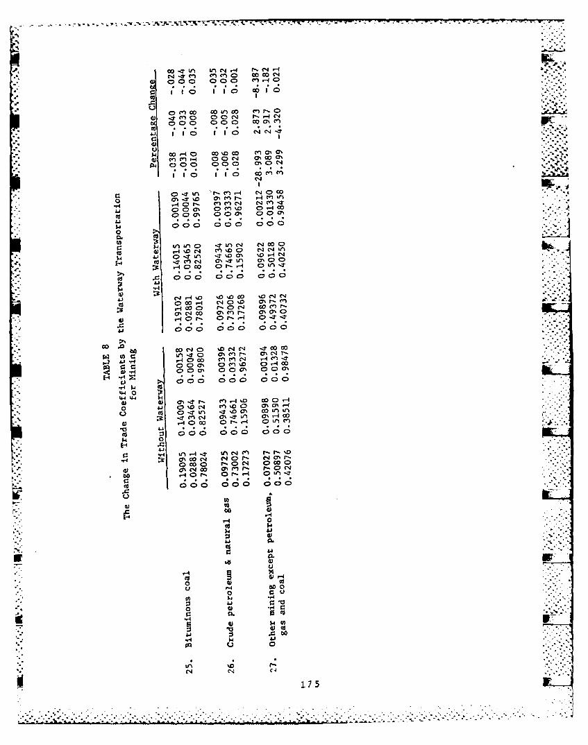
cc-Ttn L 4I4 C -

w 000 000 (N r-4 O

C> 0 0 ) 00 r-4CV)

0 000 C 000 Go c 7

0 n m~v 0 C>' 00rO

14C0 110

It a'.~ 0co)r H cn

I kI

0 H i0n 0 cn C4

C>aC0C fn~- %.0' C> 4

0 0 - r- ON 0 (% C)0a

cd 4a r c'0 - 4 ) e qt

441~- 00 ' 4 000 000'j

r-4 *r4 co C ,.- n z

411a

-4 C- - 03 ~o0 0C4e411- 0 0 -4 C4(D%

0 0 0.N CD r C CO0-oy Qc,4 ~0 0' - o~.0

01 -40wr C Or-H 0r,

04 co 000 0) % 4 100 000

P.4 0 D Clm n'

a)0 0 C7% C r0 Ch 0C 0

44 0

0 00 ; C00

ov % 4 o N r t 0

0$4

a Ud

o0oo -,

00

0

'-.4 ('4175

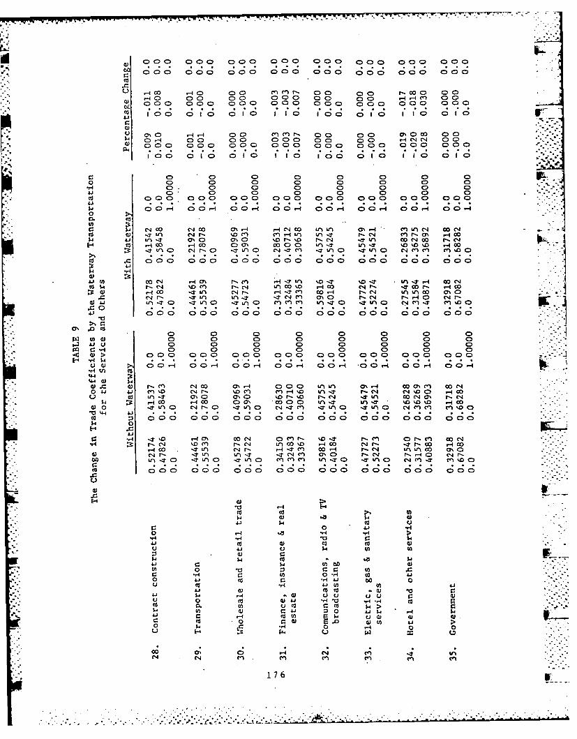
0 0 000 000 000 00 00 000 000

000 000 00CD C)0 000 00C)0 0)C -00 000 000

r -4 0 C) 0 00 C C) Ch 0 0 00C r-cc 00C) DCt .- 40 00 C0 0000 c -~c) 0

(0 100C 0 10C ( 010 o1 I10 0 010 1 10C C 01 0

0) 00 CD 0 C)0 0 000 00 CD 0 > CD 0 00 000Al . ~ 0 . .4rr. ~ ~ 0

0 C 0 0 0 0* 0; 0; 0; C ;

C0 0 0 0 0 0 0 00 C 0 0 0 CD 0 C> 0D

. 0 0 0D 0 0D 0D 0 0Dco00 0 0 0C C >0 000 00C0 000 o 000 000

00. C0.- 00.- 00.- 00.- 00r 00;- 00

COjc eco O'.-I r-4 -co tn Ln ON.-4 C4

n'Ac- cocq'0 d c 'JzLnr- % n c'(.H4LI) Ln -.T cfr-o ",n- N qCO

$-4 tn 'TI ON 01 0%r % cc " -T W) .o~ " co c

X C C N ;- C. C ; C 4~ ..; ~ C; C 4'C ;C ) 0

to $4 000 000 000 0-C 00 01100 000 000 000of- q

4-I o o ITC' - ( 0" r- ~ - I .4 1 L I c 1.-. ? W )- I A - . -c o ca %

0 ~ C C) 0 0 0 0 0 0 0 0 0 0 00 00T coo %2

C>3 0 0 00.I .400 00.D-CD CD0D-C) C.-I 00-i 88C

0 CD C) C>

0C (U CD- C>. CD. Cor- r-0 CD'o~ -;A a 0.' C)4 0-c 00 CDO C>~ u)D. '0D a

wU > 000 00C>0 0 0C)0 0 00 00 0 C )0 000) 0al0r14 0

444

440)

10 4-4 A-Cd1~ :3 C) 6 0 6 6 66

0 .

4 m co( - % . - n C l n cs-IZ: rc % r- 4 CO % *4 00 - 0'-4 co S-i U)0 " q I n c 4 r 4 0 n0 N

00 0n -a0I n0 L nc n V T0 U) .0C T n%

to C) (DCU 0 0 . 4 0)C D C QC D 0 0 Ci0 00C

4-i~ ~ 41U( -0- S. -4 a0 OU4 -H >

(U~ c. Co w( 0 sa1-'u 04 OA- U)~- ~ .4

0~E .- 0 a)O 00n 0 r 0 0 ~0_ .,0 U 0 -H 0a 01

a ra -H. 0 J 1. 0

14. m w u(a) WC4)

176

APPENDIX II

Basic Supporting Data

177

APPENDIX II: BASIC SUPPORTING DATA

Page No. ,.

TABLE 1 Industrial Classification 1.81* ,

TABLE 2 State Shares of Outputs and Value Added(Oklahoma and Arkansas) 186

Supporting Data for TABLE2 andA2anas

(TABLE 2-1) Market Value of Agricultural Products Sold: 1974 188(U.S., Oklahoma and Arkansas) .2-

(TABLE 2-2) Values Added in Agricultural Sector, 1972(U.S., Oklahoma and Arkansas) 189

(TABLE 2-3) Value of Shipments in Manufacturing Sector, 1972(U.S., Oklahoma and Arkansas) 190 -

(TABLE 2-4) Values Added in Manufacturing Sector, 1972(U.S., Oklahoma and Arkansas) 191

(TABLE 2-5) Value of Production in Mining Sector, 1972(U.S., Oklahoma and Arkansas) 192

(TABLE 2-6) Values Added in Mining Sector, 1972(U.S., Oklahoma and Arkansas) 192

(TABLE 2-7) Values Added in Service and Other Sectors, 1972

(U.S., Oklahoma and Arkansas) 193 t

TABLE 3 Regional Shares of Outputs and Values Adde-•(Oklahoma and Arkansas) 194

Supporting Data for TABLE 3

(TABLE 3-1) Agricultural Production in Oklahoma Water Region, 1972 1:96

(TABLE 3-2) Agricultural Production in Arkansas Water Region, 1972 196

(TABLE 3-3) Regional Output in Agricultural Sector, 1972(Water and Non-Water Regions of Oklahoma and Arkansas) 197

(TABLE 3-4) Values and Ratios of Mineral Production in Water Countyand Non-Water County, 1972 198

(Oklahoma and Arkansas)

TABLE 4 Industrial Classification for Price Indexes 199

TABLE 5 Industrial Price Indexes, 1967-1978 201

TABLE 6 Industrial Classification for Wage Indexes 204

PRVOSPAGE

179

..- - . - , - , . .: . . :.. . . . . : -, . < . -... . '. . . .:. . . .: . .: .c . . . . . . . . . . . . . .

i Page No.

TABLE 7 Wage Rates by Industry, 1967-1978 206

Supporting Data for TABLE 7

(TABLE 7-1) Farm Wage Rates 209

(TABLE 7-2) Governmental Employment and Payrolls 210

TABLE 8 Capital Price Indexes by Industry, 1967-1978 211

TABLE 9 Industrial Outputs, 1970-1978(Water Region in Oklahoma and Arkansas) 214

TABLE 10 Industrial Outputs, 1970-1978(Non-Water Region in Oklahoma and Akansas) 216

TABLE 11 Industrial Outputs, 1970-1978(Rest of the U.S.A.) 218

TABLE 12 Ratios of Final Demand of Oklahoma to U.S. (1970) 22.1

TABLE 13 Ratios of Final Demand of Arkansas to U.S. (1970) 223

TABLE 14 Wage Index (1972-1978) 225

TABLE 15 Hourly Wage (1972-1978) 226

TABLE 16 Estimated Employment Statistics for Year 1972 227 i

TABLE .17 Estimated Employment Statistics for Year 1973 229

TABLE 18 Estimated Employment Statistics for Year 1974 231

TABLE 19 Estimated Employment Statistics for Year 1975 233

TABLE 20 Estimated Employment Statistics for Year 1976 235

TABLE 21 Estimated Employment Statistics for Year 1977 237

TABLE 22 Estimated Employment Statistics for Year 1978 239'

TABLE 23 The 40 Sector Industrial Classification 241

Jr 180

. - .,. . .

.. . . . . . . . . . . . . . . . . . . . . . . . . . . . . . ... ,. .

TABLE 1

Industrial Clasdification

,,,.'

The 35 industry SIC Code 1972 I/O Transactionclassification in manufacturing sector Table classification

(OBE) ..-..

Agricultural Sector

Code Industry Code Industry Code Industry01 Dairy farm products Dairy products ...... 10100 Dairy farm products

02 Poultry and eggs Poultry and eggs 1..... 10200 Poultry and eggs

03 Meat animals & pro- Meat animals 10301 Meat animalsducts

Misc..livestock ..... 10302 Misc. livestock

04 Cotton Cotton 20100 Cotton

05 Food and feed grains Food grains 20201 Food grains

Feed crops 20202 Feed grains

Seed crops 20203 Grass seeds

06 Oil bearing crops Oil crops 20600 Oil bearing crops o

07 Misc. agricultural pro-ducts

Fruits and nuts Fruits and nuts 20401 Fruits

20402 Tree nuts

Vegetables & melons Vegetables 20501 Vegetables

All other crops 20502 Sugar crops .20503 Misc. crops

Misc. agricultural Greenhouse & 20300 Tobaccoproducts, forestry nursery& fishery

'Forest products 20701 Forestry products

Tobacco 20702 Greenhouse & nursery

products

30000 Forestry & fisharyproducts . -

40000 Agricultural, forestry& fishery services

181

OF

.. .-_._. . , -_ _. p_.' . . ._. ... '.'._'. .._, '. ._'.-- _-". , am'."a . 'j .--e . _ , -_ -. • ._ - . .... ; ,".r -

0

V44 *~ 0 v4Hus ~.0 41 0 40~ 0(4 rVI 0l 0 .t v

.00 C: -H r4-40 m 0 CL $4~~C 140 Ad 00 0 -0 0 00 4) V40 4) .)5 0 b4 4jo1.4 to U4 14 -H mW t.o o-A : v4 0.4 en 4 w ) Ori44 # to co r:. .u44 -4 .

I0 u )Li r- 0

.4 0 0,

to k 80 .0 c 1 Vw q cr 4 r 41- 0ca 0 to to c4 0- :3 r 0 - :3s $- w r0 . 1-4 44 0 0 44 to 0i r. toI 4) U)coco ' U1 $4 u W 14 4i) ~ . m0000 ~ ~ ~ - M0 40 00 80 0 V 0 JU O0().4 0 .0 0 0. U) S0 :3C C 16 - 0 L -. ,A .0 d0 c 00 O 4 1''40.M.-4 :3 0 4-J 00 cc .0W $ 0) j 0O.-4

.4 t r-4 4.4-4 NNC NC4 '4N N 4 C4 495n Mcn cn

r4 o) 0) . D 00 a 40 CI 0uD 0>t 0 00 C c) 1-4t n 00 C*0 r-4 C4 C 1 en 0 . . .40 . O . 0 . C1 0c .NN (95 C

* * 00 w 003 $4 .0 * 4 V Q. -AC 093 0 14 a) 0 0 $4 w 11*14~ 1- . la * X 14 V . 4 -.4 r-4 FAU~ ~~ 0 C . - 4 0d 0 .

0 1fi 0 440 0 '0 0- -0 .w' to m- .4 .4 0o

bc w0 44) 0 1 0) b4r- :1 r0 5-. 84 C- 10- 0.$4 0d 0o 0cc0 a0 0 A- 0 V- go *,4 0C - W

'4*4a 00 cc i 0i 4 L -- 0 04 0 .

'0 0 U) 0- .0 u i W 5. . W U44 0 0 -H 0. 0 0. c4 00. U . 0

0 0 0.d A 0 0 0) 0

0 14 .0 w 4Is 0C 0

'0 0 Cd :34

'0~P 0. * cn-. 4

.M N .4 C4 U . .4 -4 -'4.0. 0. 14 .4 04 u-4 * q 80'0 U1 .0 o '-4 C'

0 0'010 0. 0 O0.C

0 0 4 '0U) 0 '41 0 '-) "a 0

r4 C6 x-w 0 4 0 1-0

0 0 14'4.J 00 1-

:3 0 0 0 co 0ur. 0) 10 Ua S 4LaLo 0 4 CW U -4 0 C 0 0

000 (3 ra0. 4 0 U .0 00~~1 co 0 0 0C- ~~ ~ $ (U- n. 0 0

0o1 co a, 0 -4 N- n. C

182

A* c0 00

$44 NJ "4 - .1.ai 0o o 0 .544)

U ~~ C) $400 " 9 .*5du~ (a I c! C CU

to U4 OW 0. (Au0 4440U r 0 . . 440

54 -05

C 0) 0 00 -A.

0~~ Ca V4001.'.L$4 0 $U Q.1.0 U ...-41 00.0.0~. IT g0.'u&$4 V0

M ~ C $4 $4I 10 in r4 -4 0 a l4 0

oj 4 W4 4in 4IL' 0-I .74 (r -I. 0 0 0 0 0$44 -A0 m0 C,2 0 44- 40U1 0r.-go 14'. $

5I C'L NC) N 0) I(I C SA lin I% O ' 'a 4) '0) a. C:1

o-4 -

0. a 0 I * ~ 0 01 o (7) C; (4 R; C4 C4 C4 (U (UWM "n S.' In Un

t- to- U' . ii

*a C-I 0 0 0 0Ra 0 0 40 0 7)0(U 141 14 S-n 1.' (U -4 C40 454 11T 1-sqra -6 ( %" - r 4 Crco OC- MI C1 USA co- CP4-ne 0 0 43 a o 0w7 0)cn Cn t 1 )'nn L 0 %0 740. fl a! tn %

(U~~~~~- 4. (U7Ws- .(70. 50

0 u

-HI.P ' 5 *a 93 $4

4I 0 (U 41 0r :3- ) U0U RI P.' m (U uT P d : %c

0 4-T4 0 4) .4 u n 10) cd14- 3 o oZ..

14I 0 1-4 (UW .

0 0 C. -1 c 0% 7 4 :j 03 00t -(U C." 4 w 4 4 U La4 M *-7% 1)-

V4 >% t nV (DU r 0 4.8n COO . 0 6-H~~~~7~. C4U4 " H 4 ) t)-

0 0)

41140 .% 18 u 1 cU ~ ~~ ~ ~ -A -43.. . .. . . . . .

M. 1 4 dr C a % 0cSd ~ ~ . **4 Cl W 4(nv

T - T-7- -T -cq '-.T

U~ .015'

0 ~ 4w co cc (1 to 0

-I .o r. 0 coI ~ ~ b 0 4)00 4.504 uO )$ 4 .

Li U--4 0 1.0 t2 4 U O 0 co U '4 r -

O 4U .'~ t44 4) 4C3 W X P (

:j0 04 im.~ 0 4)$ 4 eq I i54-40 C60 cc0 41 - >

w0) J 0~-" to U w 4 i - A)4.4 4j 0d C:00 v U

a s4

ci0 0 00 000 0 0J- A14 ' .: 000.r40 0r 000 00 000 0I

C3 0 0 -4 0,C C 0 0 > 0 0 D 0 0 0 0D 01-4 ~ ~ ~ ~ ~ U~ A AnO 00.-4.-nIT C t % , 4C-I C4 a f

0 8-Q% 0r 0o 00 a 0 C )C ? m01 C

'1 -4 C-4 4-' )n tn- *.-i n nt O 0 a - 0

to 4) i 0 00W $ 0 Ai 45u

V () 0 4 $4 $4 $

i) 0 to 0 0 00)

r.4 co Dt- 4.4w Q M 4 0 *l0 $ in M044 r

.14 4.J ca .,I &0 41$ 44 4

0 0 0 p 14 u- )*240 (A i.4 ~

U $-4 p $4 4 )4 0tn 04)- c c

u E 4)

0~d -H *r 0 0 ''

41 *0 0 oc

La 60 w 1- in 0W r4 m o " 0 0

01 0 (L 41 $4 0ar0m. 0$OO 44 0 4( 4-1 H4 "4 .4

o1 >~ ..4 t

0 - .5 0) 0 0 04 006 -H 0. )- 0. Li

0E n -0 40$ f-4

.r014 0)H 0 U000'4 c U*-b

184

U))

> ~ 0 -

U) I) m1 w &jr3 4 . CL. U4

0u U) 0 11.4)4 . -f%4 0 r to

0 W > c: 0to ->a -~ (A .w , 4 U )

* -r.

00 L-Cw 34 0 4j >r.

*- 4j aW 0 V c V6to toU) r4 0 - tW 4) w bo > o cc z4j - 40 : C o A oU ) LI.400 0 IJ* U -H. U) -4OJ- d) 4 a jw- cd 4 0 0 4J 4 0 :3(no 003 r.0 d :3 f

Co2 0@11 00 1 00 00 0 0 0 000CD C -4 .- 4 '-4- a~Cr tA Cl C)- a ) )to(DC C

00 GO 0 C- l D % .C lc o m 0. 0

4j

o 4.

00

4.34u w

L) '1)U

> cn

cc -I-* ~ -4 0

'C OW 4

4j 1-4 ow

-4 03

CV)

5.. @fn

U)IF

4-18 5

TABLE 2

SLate Shares of Outputs and Values Added :.

(Oklahoma and Arkansas)

3. ~Output Value Added

Code Inuty .0/us gAK/US OK/US ARK/Us ,

* 1. Dairy farm products 0.026064 0.006347 0.007801 0.005647

2. Poultry and eggs 0.009007 0.102426 0.005442 0.091364

3. Meat animals & products 0.026064 0.006347 0.030015 0.008300

4. Cotton 0.015938 0.105752 0.015938 0.105752

5. Food and feed grains 0.016264 0.025523 6.016525 0.016008

* 6. Oil bearing crops 0.007349 0.056286 0.007349 0.056286

7. Miscellaneous Agricultural products*Fruits and nuts 0.000815 0.002437 0.000815 0.002437

Vegetables and melons 0.001923 0.003460 0.001923 0.001460Misc. agricultural products,forestry & fishery 0,009865 0.005450 0.002542 0.003050 -

* 8. Food and Kindred products 0.007651 0.013292 0.006264 0.009498

9. Apparel and textile products 0.004183 0.006413 0.003980 0.007547

.1. Lumber and wood products 0.006735 0.025263 0.006848 0.026217

11. Furniture and fixture 0.003843 0.022588 0.003625 0.021682

12. Paper and allied products 0.004193 0.020031 0.003490 0.018746

13. Printing and publishing 0.006329 0.005440 0.006482 0.005839

14. Chemical and allied products 0.001034 0.004684 0.001016 0.004069

15. Petroleum and allied products 0.030685 0.004377 0.017970 0.00599C

16. Rubber 0.012947 0.010672 0.011928 0.010675

17. Leather 0.001915 0.024578 0.002104 0.028315 .

18. Stone, clay and glass products 0.012908 0.007341 0.014222 0.00753:

19. Primary metal products 0.002826 0.005814 0.003945 0.00479!

20. Fabricated metal 0.008690 0.007183 0.008809 0.00680.

* 21. Machinery except electrical 0.013216 0.003616 0.012683 0.00357

22 lcrclequipment 0.006469 0.011775 0.006619 0.01112,

186

TABLE 2 .v

(continued)

Output Value Added."j Ind.-de Industry OK/US ARK/US OK/Us ARK/US ::~~

13. Motor Vehicle &transp. equip. 0.005293 0.004004 0.004083 0.002548

.r4. Misc, manufacturing 0.002759 0.008162 0.002440 0.00754'/

-t~5. Bituminous coal 0.004189 0.000923 0.004260 0.000923

1.:6. Crude petroleum &natural gas 0.063629 0.004514 0.062048 0.004514

7. Other mining except petroleum,gas and coal 0.008597 0.011482 0.004813 0.011482

,-8 Contract construction 0.009332 0.006058 0.009332 0.006058

*9. TransportationRailroad and related service 0.007848 0.012942 0.007848 0.012942

*Motor freight transportation 0.012953 0.008087 0.012953 0.008087-Water transportation - 0.000456 - 0.000456-Other transportation 0.017442 0,002326 0.017442 0.002326

S0. Wholesale & retail trade 0.010084 0.006269 0.010084 0.006260~j~

-1. Finance, insurance & real estate 0.009540 0.005758 0.009540 0.005758

-12. Communications, radio and TVbroadcasting 0.009562 0.005661 0.009562 0.005661

k3. Electric, gas & sanitary services 0.012710 0.007604 0.012710 0.007604

:-3. Hotel and other services 0.009252 0.005422 0.009252 0.005422

. Government 0.012871 0.005821 0.012871 0.005821

187

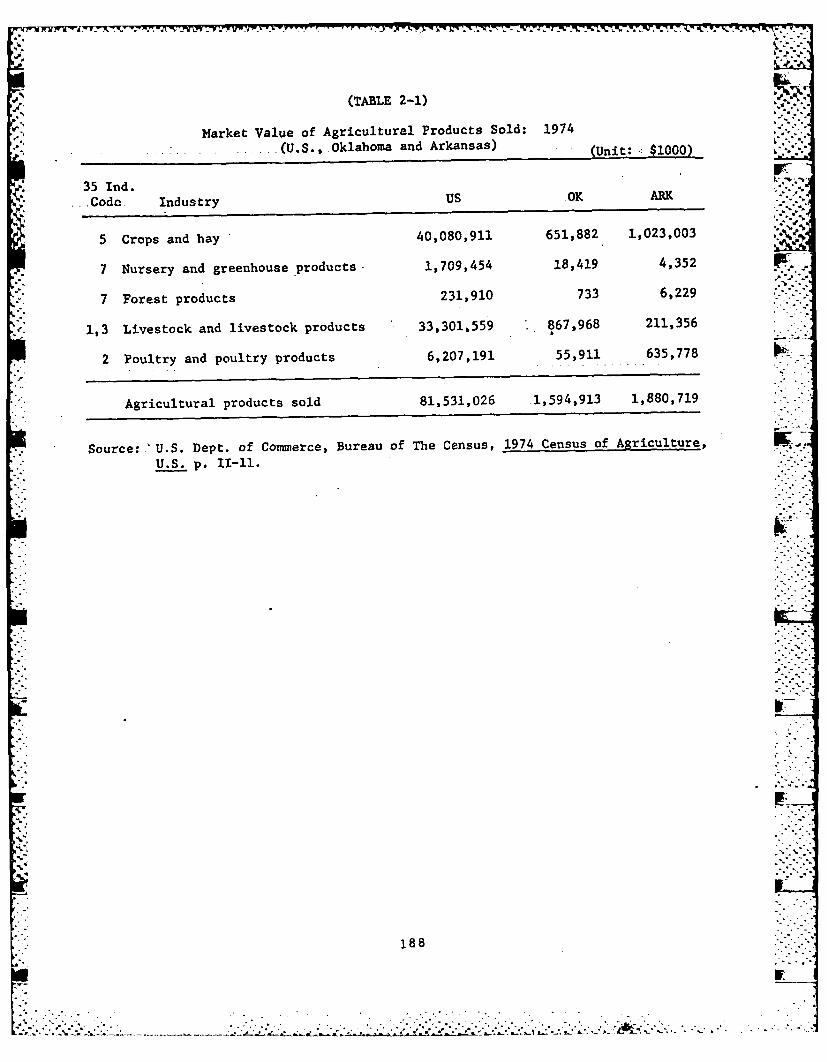
(TABLE 2-1)

Market Value of Agricultural Products Sold: 1974. ....... (U.S., Oklahoma and Arkansas) (Unit: $1000)

35 Ind.-...Code. Industry US OK ARK

-.. ',,,

5 Crops and hay 40,080,911 651,882 1,023,003

7 Nursery and greenhouse products- 1,709,454 18,419 4,352 .

7 Forest products 231,910 733 6,229

1,3 Livestock and livestock products 33,301,559 867,968 211,356

2 Poultry and poultry products 6,207,191 55,911 635,778

Agricultural products sold 81,531,026 1,594,913 1,880,719

Source: U.S. Dept. of Commerce, Bureau of The Census, 1974 Census of Agriculture,

U.S. p. 11-11.

188

,. .o

.*.i-+----.-* * . .* ...... ..... .....

.. . . . .. .• - v,, -- .. "J" ,' ' 'Z J 'J .. "

'. '. . . . .- . .- . . . ..-. .-. .

(TABLE 2-2)

Values Added in Agricultural Sector, 1972." (U.S., Oklahoma and Arkansas) (Unit: Mllion Dollars)

35 Ind.Code Industry us Ox ARK

Livestock products 18,027.44 408.76 317.633 Meat animals 12,111.22 366.46 98.271 Dairy products 3,593.10 28.03 20.292 Poultry and eggs 2,137.27 11.63 195.273 Misc. livestock 185.85 2.64 3.80

Crops 12,947.55 120.04 316.375 Food grains 1,765.57 57.64 69.115 Feed crops 2,973.60 21.68 8.245 Seed crops 92.93 0.53 -

4 Cotton 929.25 14.81 98.276 Oilcrops 2,230.20 16.39 125.537 Vegetables 1,672.65 2.64 7.617 Greenhouse and nursery 557.55 3.70' 1.90

*7 Fruits and nuts 1,300.95 1.06 3.177 Forest products 154.88 - 2.547 Tobacco 743.40 - -

7 All other crops 526.57 1.59

Total 30,974.99 528.80 634.00

Source: U.S. Dept. of Agriculture, Economic Research Service, State Farm IncomeStatistics, Supplement to Statistical Bulletin No. 547, Sept. 1975"Cash Receipts by Agricultural Commodities, 1972".

,*.....

189

• .. " .' ..i. . . . i " :i i ; ;

(TABLE 2-3)

Value of Shipments in Manufacturing Sector, 1972(U.S., Oklahoma and Arkansas) (nt Milodla.U.., o (Unit: Million dollars).-",

35 Ind.Code Industry us OK ARK

" 8. Food and kindred products 115,051.5 925.6 1,608.0

8. Tobacco 5,920.2 -

9. Textile mill products 28,063.9 86.4 150.8

*9. Apparel, other textile products 27,809.2 147.3 207.5

10. Lumber and wood products 23,829.7 160.5 602.0

11. Furniture and fixture 11,320.3 43.5 255.7

12. Paper and allied products 28,261.9 118.5 566.1

- 13. Printing and publishings 30,146.4 190.8 164.0

14. Chemicals and allied products 57,349.6 - 268.6

15. Petroleum and coal products 28,694.7 880.5 125.6

16. Rubber, misc. plastic products 20,923.7 270.9 223.3

17. Leather and leather products 5,769.5 - 141.8

18. Stone, clay, glass products 21,537.5 278.0 158.1

19. Primary metal industries 58,429.7 - 339.7

20. Fabricated metal products 51,739.3 425.4 351.6

21. Machinery except electrical 65,820.7 869.9 238.0

22. Electric, electronic equipments 53,394.3 345.4 628.7

23. Transportation related products 94,704.9 271.9 205.7

24. Instruments related products 15,526.7 - -

24. Misc. manufacturing industries 12,173.2

" Sources: U.S. Department of Commerce, Social and Economic Statistics Administra-tion, Bureau of the Census, 1972 Census of Manufactures, Vol. III. Part ...1 pp.6-21, 4-7-11, Part 2 pp. 37-7-10. ..

190

• " . " .i " ". A . ." 2 . ..

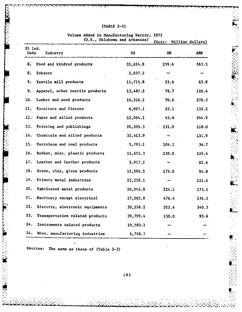
*1 (TABLE 2-4)

Values Added in Manufacturing Sector, 1972(U.S., Oklahoma and Arkansas) (Ut* Mlindlas

35 Ind. FCode Industry us 'OKAR

.8; Food and kindred products 35,614.8 239.6 363.3

8. Tobacco2,3. __

*9. Textile mill products 11,715.8 23.6 63.8

9. Apparel, other textile products 13,487.5 76.7 126.4

10. Lumber and wood products 10,310.2 70.6 270.3

11. Furniture and fixture 6,097.1 22.1 132.2

*12. Paper and allied products 13,064.1 45.6 244.9

13. Printing and publishings 20,209.5 131.0 118.0

14. Chemicals and allied products 32,413.9 -131.9

*15. Petroleum and coal products 5,793.1 104.1 34.7

16. Rubber, misc. plastic products 11,653.3 139.0 124.4

17. Leather and leather products 2,917.2 -82.6

18. Stone, clay, glass products 12,586.5 179.0 94.8

19. Primary metal industries 23,258.1 -111.6

*20. Fabricated metal products 26,945.8 224.1 173.1

21. Machinery except electrical 37,562.9 476.4 134.2

22. Electric, electronic equipments 30,558.2 202.4 340.3

23. Transportation related products 39,799.4 150.0 93.6

*24. Instruments related products 10,580.1-

24. Misc. manufacturing industries 6,768.7-.

Sources: The same as those of (Table 2-3)

191

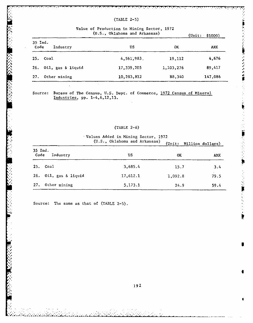
(TABLE 2-5)

Value of Production in Mining Sector, 1972

(U.S., Oklahoma and Arkansas)(Ui: $0)

35 Ind.

Code Industry us OK ARK

25. Coal 4,561-983- 19,112 4,676

26. Oil, gas & liquid 17,339,205 1,103,276 89,417

27. Other mining 10,283,812 88,340 147,086

Source: Bureau of The Census, U.S. Dept. of Commerce, 1972 Census of MineralIndustries, pp. 1-4,6,12,13.

(TABLE 2-6)

Values Added in Mining Sector, 1972(U.S., Oklahoma and Arkansas) (Ui: Mlondlas

35 Ind.Code Industry us OK ARK

25. Coal 3,685.4 15.7 3.4

26. Oil, gas & liquid 17,612.1 1,092.8 79.5

27. Ocher mining 5,173.1 24.9 59.4

Source: The same as that of (TABLE 2-5).

192

'AD-A±65 ?59 THE MCCLELLAN-KERR NATERURY AND REGIONAL ECONOMICDEVELOPMENT - PHASE 11 STUDYCU) OKLAHOMA UNIV NORMANC K LIEN ET AL. NOV 05 INR-CR-B5-C-5 DACU2-79-C-Sff4

UNCLAIFEEDF/53 L~

mommhhhmhhl

Ehhmhhmhh

N

.4

,.'i .'s

MICROCOPY RESOLUTION TEST CHART

-f!

'iii.

uI...L*I~

,,* .q "= " * -'.-'k-' %',,Z.-,.,'.[',..._. ,

.- ,= .,,.,,, ... ". ..., -. -a ,. .... •' g.. . . .- ,,o .- .. ... ..

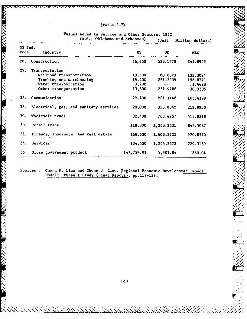
(TABLE 2-7)

Values Added in Service and Other Sectors, 1972

(U.S., Oklahoma and Arkansas) (Unit: Million dollars)

35 Ind.Code Industry US OK ARK

28. Construction 56,600 528.1778 342.8945

29. TransportationRailroad transportation 10,300 80,8323 133.3024Trucking and warehousing 19,400 251.2939 156.8771Water transportation 3,200 - 1.4628Other transportation 13,300 231.9786 30.9305

32. Communication 29,400 281.1148 166.4199

33. Electrical, gas, and sanitary services 28,000 355.8842 212.8950

30. Wholesale trade 82,400 760.6257 415.8318

30. Retail trade 118,800 1,268.2631 845.5087

31. Finance, insurance, and real estate 168,600 1,608.3725 970.8570

34. Services 134,500 1,244.3378 729.3169

35. Gross government product .147,759.91 1,901.84 860.04

. .. °°.!

Sources Chong K. Liew and Chung J. Liew, Regional Economic Development ImpactModel: Phase I Study (Final Report), pp.117-139. ..

- ..

193

.................................................... * ,* **... .*.. *',*.. *

TABLE 3

Regional Shares of Outputs and Values Added(Oklahoma and Arkansas)

35 Ind. OK Water ARK WaterCode Industry OK ARK

1. Dairy farm products 0.138768 0.272705

2. Poultry and eggs 0.146680 0.212421

3. Meat animals & products 0.142163 0.222682

4. Cotton 0.028173 0.192195

5. Food and feed grains 0.030475 0.279234

6. Oil bearing crops 0.171337 0.197402

7. Miscellaneous Agricultural productsFruits and .nuts -

Vegetables and melonsMisc., forestry and fishery 0.133320 0.232461

8. Food and kindred products 0.273079 0.590979

9. Apparel and textile products 0.234562 0.333333

10. Lumber and wood products 0.073035 0.244761 A11. Furniture and fixture 0.488837 0.672897

12. Paper and allied products 0.280000 0.666667

13. Printing and publishing 0.383146 0.701149

14. Chemical and allied products 0.274878 0.093378

15. Petroleum and allied products 0.754413 0.208333

16. Rubber 0.388496 0.558824 -_

17. Leather 0.312500 0.185185

18. Stone, clay and glass products 0.400883 0.719047

19. Primary metal products 0.934807 0.310345

20. Fabricated metal 0.665251 0.778503

21. Machinery except electrical 0.544149 0.650231 ''.5

22. Electrical equipment 0.428571 0.837088

23. Motor vehicle & transp. equip. 0.576154 0.962453 * . -

24. Misc. manufacturing 0.770789 0.600403

•194

. .K : .~ .. .. *. .*. . .-..... *...C.

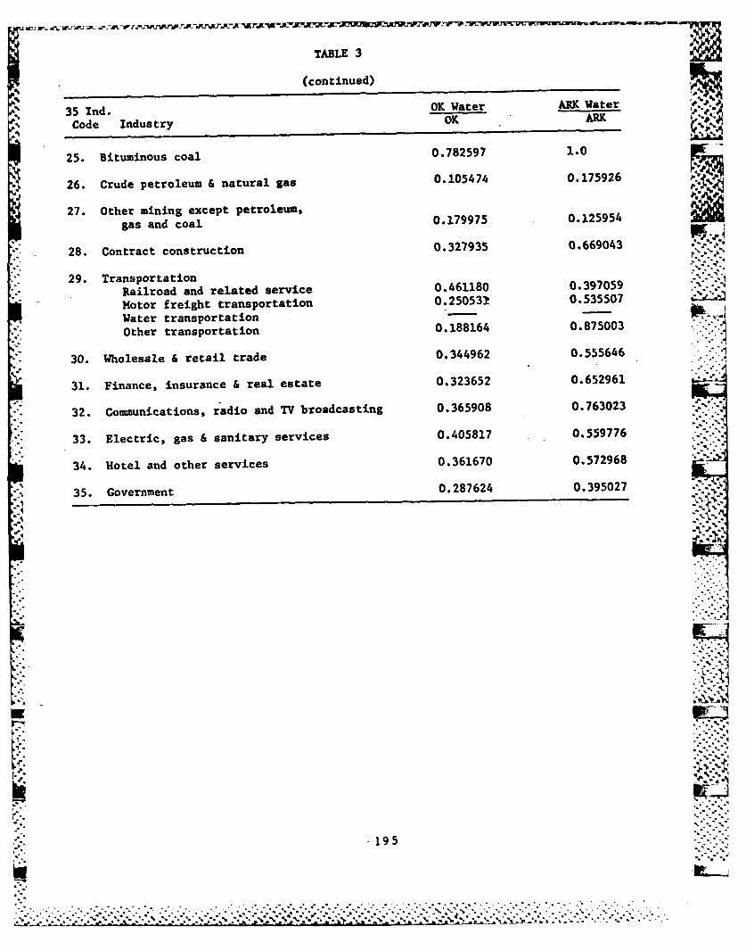
TABLE 3

(continued)

35 Ind. OK Water ARK Water

Code Industry OK ARK

25. Bituminous coal 0.782597 1.0

27.~~~~~~~ Ote inn xcp etoem

26. Crude petroleum &natural gas 0.105474 0.175926

gas and coal 0.179975 0.125954

28. Contract construction 0.327935 0.669043 *.

29. TransportatJion

Railroad and related service 0.461180 0.397059

Motor freight transportation 0.250531 0.535507

Water transportationOther transportation 0.188164 0.875003

30. Wholesale & retail trade 0.344962 0.555646

31. Finance, insurance &real estate 0.323652 0.652961

*32. Communications, radio and TV broadcasting 0.365908 0.763023

33. Electric, gas &sanitary services 0.405817 0.559776

34. Hotel and other services 0.361670 0.572968

35. Government 0.287624 0.395027

195'

(TABLE 3-1)

Agricultural Production in Oklahoma Water Region, 1972

Unit Water State 'Water/State

1. Milk cow (Number) 19,150 138,000 0.138768

2. Broiler (Number) 751,529 5,123,587 0.146680

3. All cattle and calves (Number) 849,000 5,972,000 0.142163

4. Cotton (1000 Bales) 9.3 330.1 0.028173

5. Wheat, Sorghum, Corn, Barley (Dollars) 7,295,645.0 ::239,397,000.8 0.030475

6. Peanut, Soybean (Dollars) 8,385,680.0 48,942,611.2 0.171337

Source: Oklahoma Crop and Livestock Reporting Service, Oklahoma Agriculture, 1973,* pp. 30-33, 48-59, 64-67, 78-81.

(TABLE 3s-2)

Agricultural Production in Arkansas Water Region, 1972

Unit Water State Water/State ~

1. Milk cow (Number) 20,283 749'377 0.272705

- ~2. Broiler (Number) 18,847,984 88,729,568 0.212421

3. All cattle and calves (Number) 436,396 1,959,725 0.222682

4. cotton (ae)275,800 1,435,000 0.192195

5. Rice (100 lbs) 6,126,100 21,938,912 0.279234 \

6. Soybean (Bushels) 15,989,500 80,999,824 0.197402 -..

Source: Arkansas Crop And Livestock Reporting Service.

196A"7-71

(TABLE 3-3)

Regional Output in Agricultural Sector, 1972(Water and Non-water Regions of Oklahoma and Arkansas)

(Unit:.Millions of dollars)

35 Ind. OKWaeOKiuWtr ARK pCod Wadustr Non-Water AKWtr Non-Water

1. Dairy farm products Value 27.156 168.535 12.995 34.658Share 0.138768 0.861232 0.272705 0.727295

NO 2. Poultry and eggs Value 5.628 32.740 92.680 343.624-~Share 0.146680 0.853320 0.212421 0.787579

3. Heat animals and Value 116.982 705.887 44.621 155.760products Share 0.142163 0.857837 0.222682 0.777318

4. Cotton Value 0.940 32.420 42.542 178.807 .Share 0.028173 0.971827 0.192195 0.807805

5. Food and feed grains Value 8.827 280.814 126.920 327.611Share 0.030475 0.969525 0.279234 0.720766

6. Oil bearing crops Value 6.042 . 29.222. 53.316 216.773Share 0.171337 0.828663 0.197402 0.802598

Total Value 165.575 1,249.618 373.074 1,257.233Share1 0.136223 0.885550 0.234025 0.772702

*This sha're represents a weighted average of 6 shares. For example,

0.136223 -0.138768 (i 2716 4 0.146680 + .5.68411198165.,75.6.71 .426 l555

0.940 +0 045 8.827 6.042+ 0.028173 + 0.030475 65:75 + 0.171337 1575

2Regional output shares in Miscellaneous Agricultural Products (7) can be estimated asfollows.

OK Water: 0.362 0.1333200.136223 + 0.885550

LARK Water. 0.2344250.234025 + 0.772702 -0226

or

197

~~~V 04 N % t i

$4n -. * t0 T 0 n-T~'. 0 co w -0 0 .41

r-4 07% N~ r- C- 4.1 Ns I- en ~ o

cc2 C4 o o co o ca co Go 0o 0 0_%

0 -A 0 co c

'Z _7% 1y

94 (U A

.3 "( o COOC

CA C7% &.0. U4J In C4

IN '.0 0 04 km 0.2w

-t $ CiIS > 0. N) C4 2 .

010

0 Q

to **' 0

w4( *4 C4.;84

.4 000 0% '0 000 I= IV- N) 05~ 0

*0 (D c1

z.- 44t " LI4V) o. V 0 v

0U (U V* 002,0

.,..g~~c 4.0 r4 4 LJ

0. CA 0.VA C~

* (U ~ . .. ~~ U~ 0 r. V44 c uC..aai 03 41( :3 L 0 01U IJ-

oa . 0 v 0 11 0010 (0 1-5 In an $45 40 cc Goto =

0. C) .5 4 % 4 0. &n C-4 W. ,4 0

T on cc ad Ai cl

ccE Go$ r- % 0(12 U) cc$ to 4 00a. 0i 44I ca 93 U)- %- 0 .4 C4 ~ ,IIIIN

C4 $45 $4I 10 .. $45 34 C-

P3~ 0c cc I0

o. W ** $4 gu ~~& X. 4# 0)( . -

02. 00 $41

z. CA c- ___ 9:

0 0.

- . . . . . -H

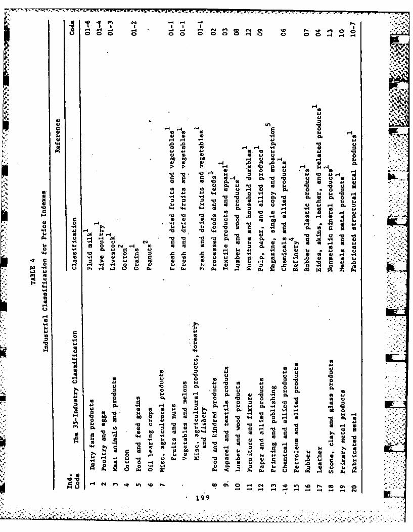
0 . .4 4 4 en Go @ C4 C 0 % '~ 0

8 ~ o 0 0 0a1 0a 00 94 ,-4

10144-

40 0 -

w41 14-0 41, 4

41 41 4 4 N 4V4~'~ r- a. _00

10 r o 0o. 4 1

0 A 1 rI 00.r4 H 46 a &

0- r-4 41 H ? Ifu V4 $4 1 4 0

'' 44 01 0- C4 r4.l4 A )

in' )4 0 O L.I64 O ,41 L w4L 0. to o C*A 0 91 40 W

:3 > > 1 c ca ) 00 i LW La r4 600 4 .0 10 AiLW *J14 ~ ,-4 4 - L

6W LiAt I a.

%4% 00 ~ v ~ir o . @O - (4 L'- I s N @ '

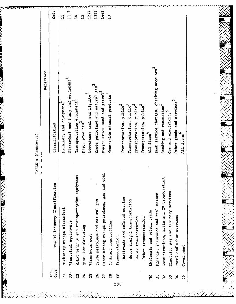
~--~-.w -.- ~ ~ r - 4 -. --- - 74 . . .-

1r 1 - -1 -.10 -4 1-4 - n US i (4 ITS M.

o . - 4 r-4 r-4 4 -I4

41 r-4

-ri 60 cn 0. . * -

c) a) U- 1 t9-I 1.4 4) U

Uo -C d 0 i u u :0 r4 0: 10 W - r H -b0 "

.14 " 0 V t

tr 4 4) p 4)4

01 u - 0

cc 4 3 00 w

to~~ 41 0 "4

P -4 - -ri 0 w w k

00

0 be

00>

V44 0o cc

cc 41 (a 4 U

bo)- 4) (0 0*04 4.0 u 0 14) 14 U r 0 4 tV) Uj bo *U U 0 s0 4 14 4) 4) s

(a (0 W 4) 0a .U ) 0 .- 0 0 0 .0 4)4.5 " .

U-H 00#A 4.8 4)

41 r. 4) o 0 4 .94 .4 u4 . U 0o UO V, Vr 4)4 0 U: 0 - 4 0 U 04)U) 4 4) w ~ 0 o 41 41 (a >4 1 6 - 4 t-4 4 0

c6- 4zj o0 o.. 01) 04

.4Q)r 4 u 0 cu F

N0 u 44 CA IA 90 'a W k wN cc r- rI >11 (N s VN (-4 0N (-U co( N~e~ ) ~

.................................

c -4 C% "4 U, C N 94-4 9-40 U-i r '.D % 0l0% -4 f- COC4 Nq " 0%C- "4 C4. N4 N4 -4 N* .-4 .-4 .- 4 .4 9-4 (.JC4 C4 4 .4

%. - 0 0' 4 N T eq e4 C4 N 4 ON C ' -.7 in 4, '.4 %n tn. 'T Nl Go '. 4 '0 .- . - N £-

C% 0) r. a-. .' %0. C.. 0% m0% C iri4 toLn 0 C > 0%.- '0 C O 0 0 Co a COC14 1- r4 - 4 1-4 .-4 1-4N eq -4 9-4 eq .4 .-4 C, N- N -4

00 (,- -4N %0 - 0: C% V!~ .0 N. . C,- , N 0( % C

r, 4 '.0 M -4 ", 0 CO C O C C U U , L4 U : ". -0 m '. f, %0 LM fm 0 '.0 r- %D O r-D a- a-. -T r-O W4 co v- CO 4 1 ' % 0%

N4 GO 0% N4 .3 C4 r- r I-.'.D 0% % r- C4 M 00 N U 0 '0

0 0 % I -. N ( 0% (0 en eOn r- %o 0% 0 -4- -4 NO C -. CO 'T .-4 M0% CO CO o C 4 '- .-4 CO CO Cc 4,1'. 4,1'- '0 CO .-4 tn -#-T r co CO '.0

94 .4 w4 -4 NvI 4 4-4 4 4-4 . q- H4 9-4 .- I u .- q44 -q

C? O - .0 0 ( 0440 '.00 NO CO I"! Ni N - 0! N -

co N- Nq rN 00% m r N " N Oe 0%( a-- 9 -4 CO .D ,-4 '.D '04,.-4 -4 0%r- C% N U, r- N 90 W-4 C% 0%% (n Go C4 U) 4, a*~ 4 en -T tn r- 'D0enC% 1-1 r-4 - r4 C4 v-4 9-9 -49-944--44- .4 r r q -4 r-4 -4 -44F-4 4

'.0 0- %0r4 4 U " w w ,

IT U, . m T0 -% 00 %D .0 O C 4r'. -4 CN m, 0q r4 N ON en cn C4v- -4 4 -4 .I r-4 -4- -4 -4- .- r4 r-4 -4I H4 9 -4 - 9-4

P'. c; c4 0%? C - . .'0 - a. vI 4 4 , , N

N O U,4 0% 0 . . D C . 4 r-i -4 -4 CO4 4 ,- , .' 0

N N -4 cN U, N% .1 N N ,4 ( I - t 0 ~ . 4

pi ON 0 I NO -4 , NO I-I N4 Nq N -4 -4 a " . -44,O 0 4,(. N N -419 U i u- - - -4 .-4 ,-4- V- -I-4 4 -4 v-

4 r-4 H- '-4 '4-4 -

1 4 CO L r,4,0 '.o C - -. U 4 0r-4 .- CO ,-4 -4-a N- %D L-4 U %

.d a % %0 COO CO CO 4 00-. 04 00 U, m~ -4 - N CO CO 4 424q0 -40 -I N O% 4 r- PN 4 -I N v4 0 0 C). C> V- 3 ,.. 4 v-4 .-44J 9-4 -4 - 4 -4- 4 4 -4 -4 -4 -4. - 4 -4 H r-4 -4 -4 r-- v-4

P4 CO U, NO, CO N4 0 '.0 H '.0 CD Nn 0 0 N a% 4,4,0% 'n 00 'n

CN r % r-4 4 Nj 0% v-4 4- - -4-4) 0 -400C -40 0A C) C I -4 0 - -4-4 - - 4-4 -4 --4 -4 r -4 -4 -4 -4 -- 4 H 4 -4 ,-4

4, 4, n m 4 o w , '

Z i enCO 0 % co 4, N 0 %0 0 4, 0; 14 4% 0 ; CO 0% N 1 4, 0% n U U

0. ON N 4 CO 4 o N) 00 N 0 Po . .-4 % ~ U, O N C O CD a 0 0 Cr~94 - 4 - 4 -- 4 --4 4 4 -4 -4 -4 -4 -4 -4 -4 -4

CO'.0 U, CD,4o - C) o- o. cl'. ND Q ,4 N 0 - U, o % 4, 4,4 N N c o c

a% 0 0 CO Hr 000r00 H00% 000000 C-4 - 4 - - 44 --4 9-4 -4 -4 -4 -4 -4 I -4 -4 -14

201 Ir

1%.W W.-

en9-- -* 4 'A 4 V-4 r4 4 4 H H H4 .- 4 -. C'4 4 H4

g% C.7 C; 5701 00 N4 r 4 'A C., 'a , 0 -4 ~5'- . ' 000-1 0 00 0 D00 00'e in -4U 0nct-4 H 9-4 CV) 4 9 r-4 -v.4 W-4e44 r4 N r -4H

%a c% ~ o 'T 'n N1 N1 4 CIA %n N OI 'A4 'A i

%0' * M P . . . . r. fl . In wHq '4 H 4 C4 - 4 H r -r4#-

0% ~ ~ ~ ~ ~ ~ % 0 %0A 1 .0 % ' t - to .t 0 % - 0

r4 17 TA w% N in0 r 0 0 . N0 N4 %1.0 It N0

In O H 1% 0% 1% .4 0 0 0 - 0%. M % 1%k99- Hq m'T .q-4 H -4 4 9-4 r -I r4 H -4 r4r

r4 OmA in.0 C- .4 000m w0 w Nr. a z

r4 - A - . 4N- H 0-4 H H H- H- r4 H 0

Ln~~~~~' C4 - '0n. J'M W0 in in00 ri0%~~~~' ON N N; '48A;r. ,V44 H4 H4 HM

V-4 H V-4u 4 H r4 H N N m7 m. Nm N- - N N4r4 ~ ~ ,. H1r H H H 'A H- Hq 4 -4 Hq H-

M '' 0% en 'A % 0-% WN in- In en '4 %I 1l a% en

r-4 0 O N A -0 N t1% C4 C,4 C4 H- a 0 .7 4* H HH NA A ' A ' .V H q r u-I H u 4 u- H- V4 H4 H4 H- H- H- r-I r4 4

~ .0% V H '.0 r%'A N 000.01% 'A C4 '0 0%H -4 H- V-I r r4 v-4 0-I - H .- 4 H- H H v.4

en o N O 'A N0 01% N0 N4 N4 N 0% -70 NO 4

v.4 0 0 0-4 4 0 0 -T uI -4 0 0 0 0 0

H 0000000 00 0 00 00 0-4 P4 9-4 -4 9--4 -4 -4 -4 0-4--4 -44 -1 4- 4

IZ 0 0

'5 Q 0 0 0 0 0 0 0 0 0 0 0 0 0aV4 P4 -4 - -4 -4 ,4 r4 -4 -4 -4 -4 H H4 uI r4

% ~ tA 0 1 o ' 0* N 'A4 enNM N4 N4 N4 N N N N 'A 'AmAA '

202

• A, .o

Footnotes for Tables 4 and 5

1. Source: U.S. Department of Labor, Bureau of Labor Statistics, Handbook~of Labor Statistics, 1978, Table 127, pp. 437-454. Monthly !!

Labor Review, Dec. 1979, pp. 94-95.

2. Source: Oklahoma Crop and Livestock Reporting Service, Oklahoma Agricul-tural Statistics, 1978, 1977, 1976, 1978: p. 88, 1977: p. 90, j

3. Source: U.S. Department of Labor, Bureau of Labor Statistics, Handbookof Labor Statistics, 1978, Table 129, pp. 456-465. MonthlyLabor Review, Dec. 1979, pp. 96-98.

4. Source: Chong K. Liew and Chung J. Liew, Oklahoma Energy Assessment andForecasting: An Application of the Variable Input-Output Model,p. 76.

5. Source: U.S. Department of Labor, Bureau of Labor Statistics, Handbookof Labor Statistics 1978, Table 122, pp. 415-426. MonthlyLabor Review, Dec. 1979, pp. 87-90.

6. Source: U.S. Department of Labor, Bureau of Labor Statistics, Handbookof Labor Statistics, 1978, Table 117 p. 398. Monthly Labor.Review, Dec. 1979, p. 85.

A. Cents per pound1978 value: forecast

B. 1978 value: '78 Sept. (12/77 100)

K: C. Dollars per barrel1978 value: forecast

D. (12/68 100)

E. 1978 value: '78 Sept.

* Due to change of classification into "Insurance and Finance"in April 1978, 1978 value is estimated as follows:

1979 Sep. price index of "Insurance and Finance"1977 value X 1978 Sep. price index of "Insurance and Finance"198v

(133.5 x 283.5 156.5)241.9

203

. . . . . .

".- 4 '- ..". .. ". , ." - " •.' .% . % .. ,.-'. ." '. .. .- ,. . - % . , . . .- 2 2 .. . ; . .".."..'.'.

1.-4

04

?

u

0 C4

41 N 0 o

uO 0C4 C4 4J 1: U

W 0 C4 o u :3 0 41 di (a 41 C 0 V p a .1l.* .

0 V w 0. 0 g93 14 41 O 44 H 409-9-

M~~~~~~- 0 0PO -I0 641 V 44 0 cc u u A 4 t

14 ccU .9 r co0 -

di44

%D 0 14 "-1 J-H o ) 4 c -

94 0 CL r= C o 0 .

O A 4 P 4 i

0 00) *

to C) U) 4 * 0cc :3 4 0 41 .-

-4 00 0 u 0.L) 0 00m 3 0 ~

0w V. 0 * 0u0 41 u 0 u:30 0 4 0 0 0 0 0A~.*a. 14 1-4 m w V .00 09. U) M o 0 4 014 04.W 0 0 1 0 o 0 W. cc :3

:3 M4 U4 P4 -H - fl P*0 W 41 j. - 4p P-0 tob 1 4 w0ci n- 0 -? QI '$4 t 00 -4 0d9

cn $ 4) 4 'a Ul -q V%:6 4) :s c: 4) $ 24 o f

.. .0 4) to U CC - C 4**C'- v v C 0C.. .. . . . . . . . .4C "1 . . . . . .0 9 0;.

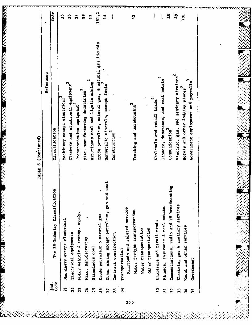
V IN %D !ra 0' N N 0 eP

-4

v C44

040 4

Nll 4 .1 9: 9

4) H-. 'o-

N) 0~ 0)I No 0H'

4W 0; 4 54 0 w. 4)0V- 45 :3 V- A

C:~~ 010 o 4N A0 0 P. 04 cO0W)I

rd01 .. T 4 ,' 0 0 0 4000 14 0 $3 -I

CO 0 0 0 0 -. V~ ,0 n_ 5 . 414 U 44 to0 0

_0 0 41 u

to U 0 M50 0 594r4 W4 "' -rk E00

E --4- 494 ..

* '0

1+4

V40 0 4

go 4 ~.:

0 41 tco W- A )4

co- w00419 00 0j 0 0u 1 0d 9: 14 0 0'

V o -4 cc 45 4j - 0 0H .bO4 0 'aH a V

M9 -P4 &a 0 0 0 0 cc 60 4a ca go' 00 0 (Awk 0

v Q 00 04 "4w 4 00 *9 a (aP.4 0 r.4 0 ) w k 0 0

%4 '0 01 4 a)1. 45 0 150. 14 0 " a o a 0 w w mCL*9 0S 4 H 0 P. P. 14A V,0 1 $4 4) $- (0C 0 14 0 J r

IU u 2 o 000 4 2 94 r. :S 0 4 0 vV-40 0 0 . 4 o o 004

zo 0, -Va 4 1 4 0 *

9:~a ~ a 0 '

H0. w 0 -C 4 m4C4 en en (no~

205 p

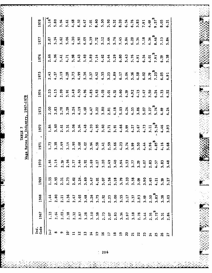
0o %0 -0 N r-. %- 0 O~* '0 en 4~ r. Ln -4 FL.a' 400a', '0 '0 kn .4 'T 0 %D n M~ n C4 en r-o 00 '0 I 0 enC.4 en ; C4 V; ;n llt '0 W0 EC- 0 Cn en '.0 0 g0 '0 I 'z

i-s l- -4 N 0 0 N 0N m% 'I4 N D - 0 in 'T 0 .4 M .? eD m '

- M N Qn mn In .4 In0 '0 P'. wA mn m~ w- n 'I -- 4

w0 m0 '0 C- - n 0 % I4 N c. 0 mn '0 . 4 T C-e cor-. '0 0% .T r-. 0% '1 %0 0o -4 '.0 'T 4 N o 0 -t 0% IA 0 a n e

c!.14 N- e -t %; In; In I i. 4 LAIn ' LA I .4 '0. i-- '0I. In#6

t; j

In e r!- 0' w &n c% '.0 &-N n an % r- -* M0 Ni' n Inv. -tn -4 N r, 0% mn en i4 mn NO - 0 n 0 -N 0 '

0%

-4 LN - -t - n In o0% en -t q0 %p In m0 mn C-4 '

"t -n o, m% .4 0n a, In o~ an N 00 N n 9% 0 .il- Na4 0 % I ' 0 0 0 0 I 0 I % -4 .4 in m en AICA

0% .0i

'0 cn 0 D e 0 oo '0 0 0% %D NO -4 %D C- 0 en t n' !-. 9-. -4 mt0% .- 0 . InN. 0 N 0 - 0 N I O O - O

r- Nl en -N en eN %D 7- Q Ain &n c - 4 -# e% n In e 0 %0

N- .40 -4 --4 00 t %O In 0 4 T. '0 wl- en co. in In -

9- ' in in 00' M4 0% 0 P -. %D W 0O N3 M 0 W - tn 4 r,%D -Ln N n en en C4%o - 0 en N I n- en-tn ON % en A e

ON* -4 en C4 C% C4 A C4 N 1; V; .0% 14 en -; 0. A 'C In '0 4

OD -?% n o % n c 0% o i -. r- In m% co .- n* 0 -1 eO C n N 'T N en C4 ente C e WN -4 e en en, .0 kN .4 n

O4 4 0 C4' C- 4 N V % V; 00 0. en1 A C 4 C4 1 ;

w' 0 n 0.4c n NN N) en en) en-t n N en en0 en en r- I N-en en c

C4 I 4 I 4 .. 4 en N 4 !-4 .4 C4 '000 enC 4 A 4 1 4 ;A

'0 fn r' en r- ' 0 40 en ? kn %o~ ,'-4 ~ ~ ~ ~ ~ ~ ~ ~ % C-4 N1 N- N n e nt n N en e n e n e 4 en en

206

% %%

Go %n an '.D 0 m" -.t

0%

.. %4

ON 0 % . W N -

r- -T M0 M c t n U') 0 VI)v-4 C4 40 c' A~ '090t)

C14C

&n &n in m' 6% 44 C- Nt- 04 '.0 - v- f 0 - 4 60'

0%0

_ 4 0 an (A rA-4 00 N0 Wk

V;- LA C4/

cn '-0 a N4 in 'T MA (D3'- 0T " 0 %0 %D W N

0 0'

U c0 - C * co C0 N%

C34

'A 4 C AN '0 4 -4

4-aC-4 I n - 4 N -4 CA %0 0

0 o Nn %0 N- m% -4 "4 '0r-- %D in Go* co0

-4 1; A N W C4 In -4

Go o 04 '0 ND 4 4G%D 8- '0 I r %0 D -4

C 4 C4 A; 4 4

Ln

%A N 4 t'-4 C4n ..

' 0 C oo C t 6% -4'M '0-40 4 C4 m n n4n.

0%%

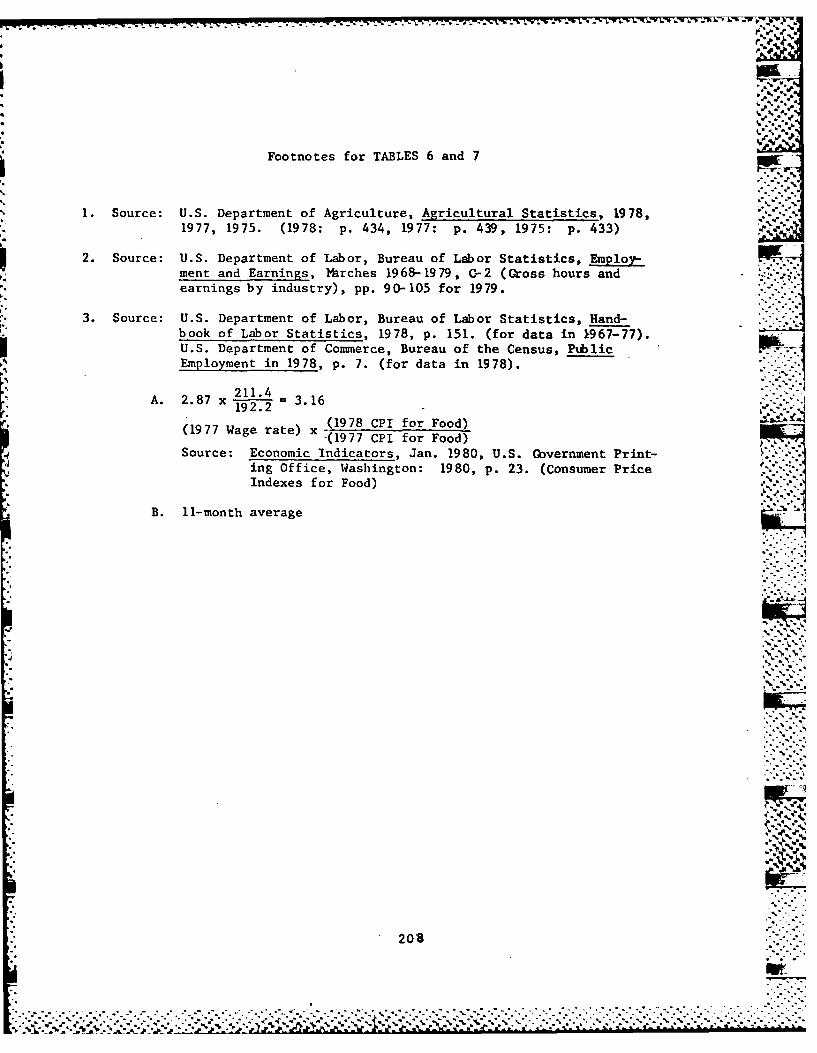
1 - - - ~ - 7- - 7 ' ' V -

Footnotes for TABLES 6 and 7

1. Source: U.S. Department of Agriculture, Agricultural Statistics, 1978,1977 1975 (1978: p. 434, 1977: p. 439, 1975: p. 433) .

2. Source: U.S. Department of Labor, Bureau of Labor Statistics, Employ-ment and Earnings, larches 1968-1979, C-2 (Gross hours andearnings by industry), pp. 90-105 for 1979.

3. Source: U.S. Department of Labor, Bureau of Labor Statistics, Hand- .book of Labor Statistics, 1978, p. 151. (for data in 1967-77).U.S. Department of Commerce, Bureau of the Census, PublicEmployment in 1978, p. 7. (for data in 1978).

A. 2 . 8 7 x 21.2 = 3.16.(1977 Wage rate) x (1978 CPI for Food)

-(1977 CPI for Food)

Source: Economic Indicators, Jan. 1980, U.S. Government Print-ing Office, Washington: 1980, p. 23. (Consumer PriceIndexes for Food)

B. 11-month average

':. ***'..'

208

5**

................................................. . . .i .~i...,".".. . " .... .... . .. . ..'. '.. -'$:- .j_'°."-.-. .-.-.-c-'--- ... "."....S-- '... -.- '.,'.-..." .. '.'-.' .. '.. , .... "..*-.'-.. .- -.

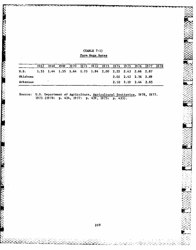
T-ITS M.~~*. -r-7: M

(TABLE 7-1)

Farm Wage Rates

1967 1968 1969 1970 1971 1972 1973 1974 1975 1976 1977 1978

U.S. 1.33 1.44 1.55 1*.64 1.73 1.84 2.00 2.25 2.43 2.66 2.87

Oklahoma 2.02 2.42 2.36 2.69

Arkansas 2.10 2.19 2.44 2.65

Source: U.S. Department of Agriculture, Agricultural Statistics,. 1978, 1977.1975 (1978: p. 434, 1977: p. 439, 1975: p.'433).

.209

4 .

(TABLE 7-2)

Governmental Employment and Payrolls

06 A

Years Total Employees Total ftnthly Payroll )bnthly Income

(in thousands) (in million dollars) (in dollars)

1967 11,867 6,056 510.32

19 68 12";342 6,889 558.18 .- -'

1969 12,685 7,587 '598.11

1970 13,028 8,334 639.70

1971 13,316 8,911 669.19

1972 13,759 9,950 723.16

1973 14,139 11,027 779.90

1974 14,668 12,127 826.77

1975 14,973 13,223 883.12

1976 15,012 13,924 927.52 .- %

1977 15,406 15,197 986.43

1978* 15,631 16,483 1,054.51

Source: U.S. Department of Labor, Bureau of Labor Statistics, Handbookof Labor Statistics, 1978, p. 151. (for data in 1967-77). '-

U.S. Department of Commerce, Bureau of The Census, Public Em-ployment in 1978, p. 7. (for data in 1978).

October 1978

210

. -o- . -

. . . . . . . . . . . . . . . . . . . . . . . .. . . . . . . .

. ~ . -

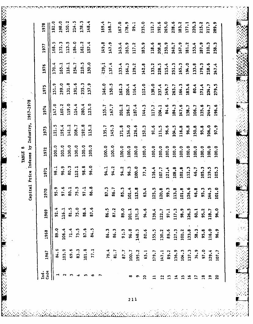
C O N O T'. CA vii W .4 00% '- 0. W. '00 V0 IF:- W. IA N

"% N o Q 00 0 o % co r- 00% IA 4 C4 I% Go cn r- 0 A -. 00 W M0 IA V-4 1- T %C0 'D 'D C- co CA - ON%'0 - C 01- NC -4 -4 01-4 H -4 H- 4 1-4 V-4 -4 i-I V-4 - N* -4 4 N, 4 v-4 -4 4 Nq q C4

IA MA IA ON 4 0 C. 0% M*0 C N 0% ID00 0% f*- 0% N t %CAC

3%4O C4 - 4 C C.;- z .- 03 4 CA 3% 00 G0% 03 r-, 0 'o 0 IA1 %D - 4 '0 co 0 in - C ' D In C0 -1 W%'.4 v- -i H 4 r- 4 r -I H f- 4 N, 4 N V4 '.4 -4 . N~ N4

- 4 V -4 I O &M * - C14 N o in I -0 MA M 0 0 A' -

r- %o A0- Ia H- in C en CA %0 N4 .1 CA N %4 I 0 % A 3H- T - - - ~ ~ . -i '-4 -4 N414 C N4 N V-1 -4.- Nq N4

* ~ ~ C CD CO '0 CA0 0n IA CA-.1 0 0 : 3 %CA'-- %1-4 o- 0 Hy % '00 1O' N ;0 C

%C IA 0 A 0 CAA - I ' 0-4 V4 CA mA-* %C~ c G I- C4 %9I H u-I H H N4 H H H H N4 -4 4 P-4 N4 W-14 - 14 N N194

0%

r. .M .M in I-. .q .D r -. w %D in %D%T 3%00 4 OC c IA % H0 0% Go . -4 00-t 00 ' 0 IA. '0

%D H -H -H q V-4 H N 4 H H q C4 N H I 4 1-4 N4 -4 04 CA4 N

*n 0% -.1 r- No c - C 0 0 % C wl% n G o c c

GoCA C!# N % ON CA 00 '0 C 0 C '0 IA 00 0 0 0 .04.3 C) a4 IA H O N IA 0 IA H '0 N .4 C4 '0 '0 '00 IA '0?A NC 0% 0 0 H CA .4 Q% IA N IA 0D ' 0 IA 0 0 0w - 1-4 u-I q Ni H- H- H -H - r-4 H. -4 v-4 4 9.4 14 r 4 -4 .4

0 0 0 00CO 0 00 0 0 0 00 0 0 0 0 0

%- A -4 0 H N N C %0 r% co e4- 0 CA io CAm CA i

u 0% 0% 0 Go 0% 0% 0% 0% a 3% -0 N4 00 a -4-0' 01H4 P

toH

kn 0%0 IA Ho CA3 CADt m* IA COC 00 '0-I*z ul C4 IA 9%0 I % ' % ' A H C A I 0 C .4 '0 '0 I. %C9

0l% w% 0%0 3% 0C O uI '0 Nn N% m " -40a N %D 0%. 0"H r 9-4 '.4 V-4 u -I 4 u-I-4 9-4 -4 -

'0 '0 IA 0_% 0% 0% 0- 8~ ;% N; 03, 3 CO '00 IA V 00'w 0c co0% % -403 00 00 00 CD -5 CA Nn a%'4% 0% -40%

H V44-4 - 4 4-

0-7- IA '0I0A A C 00 CA '0 IA N '0 CN 0 CA 0 000%T

'0 ~ 0 IA 3 - 0 00 0 IA 0 % %D 0 CA CO IA '0 '000C>%0 co 0 0 00 0% %0 IA CA% ON 00 CA IA 0% .0

r- H -4i 14-4-4 -4 -

-S4 --- 4

'0 % 0 ' 0 -4 -: 3 3 3 . 3 . 0 C 211 - 3

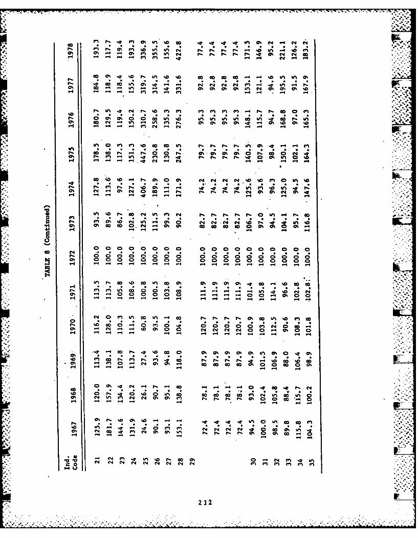
0n u l t%~ ~ 0 n C 4 0 0 C00 0 . n 0 4 C - N0

p. . ; W. . z . 4 C4 4 C4 4 ; W. -: g0 " -4 4% .4 mn Sn N% m% 3 (4 m% m Ch N %C4 -4 r-4. v- ~ . . .4 -

*00% C14 - 03 S^- n '0j '0 0000 a 0 %1-4 '0 Sn Sn 03% -4 -4 -4 en 4 -4 .4 -I 4q 4 * 4

W! c!00 Sn 0D co co- NLet 4 7 n~ 3co co4S 4. C; £z 0 % % 0% Sn - o 0 C4 'C

3% ~ f 00% I%0 0 n '0 S n S n 00 n 100 3 Sn r

In %0 % 00 1 gI S n Ec 3 C,4 P. 0% 0% P.- r- 0 % 0 0A- aZ 94 4 ; N NA 84 4 .- 4 p

Sn0 0 0 '0 0 0 0 S %3 %3 n0 0 -

SnI 4 . 4 *4 v* 4 4 *- V4 w* v- r4 r

0% 3 - %D M Sn m0 co0 3 % 3 % 0 n 0 'A ;' "C;C 4 c .4 4 N4 -4 Np -44-40

00 %0 '4 0 - % 0% 00 Q N N - V-0'0 4 n

-- 1 --4 -4 - - -4 -4 14 -1 -1 -4 - -4 4 -4

Si S n N Sn (': N p.3 3% 3 % 0 n0 %C 0% '0 N4 Sn 0 N . N '03 .04 Sn'C-4 -4 -4 % 0%000 .N - 0 0 ( 00 0 0 C4 - 4)*~ _4 r-4 -4 -P4- 4 -4

4-4 -4-4- -4 -4 - -- 4 -4 4 4 4 4 -40- - -

Sn C4 I 0 0 n 0004 % % 0% r- r, F%0 '000o-40

C4 *4 *4 C . .4 4 4; 4 4% C4 G %T S " 00 0C '4 'h a N f-4r P% r'- S 0% 0 N N

0, r- - 4 0 0 0 a% -4 4- 0 " 0 0LOC- -4 4 4- -444 -4 -4 4- -4 -4 V4 -4- n m m e

1.4 u

* N O (C, Sn 0 Sn -40 3% 3% 3 3% 0% 0 Sn'2 C12

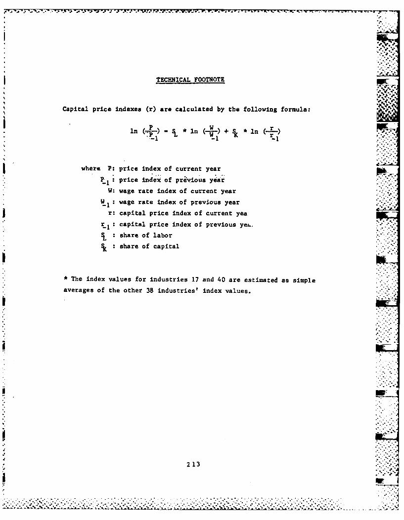
TECHNICAL FOOTNOTE

Capital price Indexes (r) are calculated by the following formula:

I hr~~ In P - *In + In in

wher P:price index of current year

tjprice index of previous year

Wwage rate index of current year

wage rate index of previous year

r: capital price index of current yeacapital price index of previous ye..

share of labor

share of capital

*The index values for industries 17 and 40 are estimated as simple

averages of the other 38 industries' index values.

213

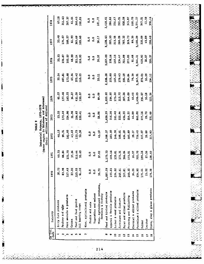
0)t . .t," I10 4 ID . 0 C., 0 ., 6 0 . ' 0 *~6 1 4.(4 61-4 'O -%0. *0 .6 n A', -f~t 0- .41 -

4 (4 C4 r% t. *. . 4-(4 (44 0% in vi W% An 0

C.4 0 ' D .

600 0.0 0%0 . 0 ' 0 40 A,40 00% a, w at tv 0% 040 I % ' . 0 , V-4 An 44 (40 AMA ' (4 .0 0 4

4.. %CA W4I0 0 0 6 0 0 % A, 0% V % 0 0 0 0 r rIn~C 0. .00 0 .n . .. 6 .4 0 . 0. . . .

40 1,. 0'V .4 4 44 4 1,0 . 4 4r 444o(44 A0a'l 4 A, - n r

s~~~~ .1* "'" 4".C 4 o

0'0.% P co A.4Wk0 CD 0.0 I 0% n -0440 .0m0% W 4000 (4 00 'a 0 e. . 64 a% ft0M't r

"I r-14044 on 60%0 44 .0 0% .4 in0'

P4 .4.N4 P 0. A, 44 44.a 44 %D0. Art .4% r 0'D

(4 I4 C4 44 Wo %0

.: W; AMat~ 0' In AM0 % 0 . -1 4 0.4 .4 .4 0'.4 0 4 4 (44 C% 0 4

UN 04. 0% % 0. 0 4%4%C40(4 0 C3, 'a 00.

A4 0AMA* I n c .4 -a .4.4 'a( .44 A a . 4

C4 .n 4 4 1- Go.44

2. .4

10% 00 0' * .h P.In 40 .4(. (4% 0 060; 0; 9 '0.4(4.0.4 4(40.0 % (

In. 0 In .1 ( on 0 ( .2 ( G4o In .4CIA.04

48.4 m. .4 4

44 o-4 .4 -4 o 4 P -

C. 0r:. Ch .4 04 m-' '1 C04 0 4 %0 a. C4 0 CO

1, In F%' 0.I600. 4 " T C41 I. on co C040 100 0% 04 %0 As a' In ('4 "4 11A % .0 .4 onI 1- ' -

* CIA4

.0 0.1. -

14 Al064 .

. 0IS40 '4 000 In" n n'0 .0 In0..6U (t w04W r . 'a4 4 0 (4 0 4 .

0.0 v~( 0%. 0 0 ( 40% .06 0 In1 0% .40

t. 600 0..1( 00. 44 1.( 00 4 4 In

1- -4. 01. . 0 .4 ' .4 .

A, Q to 1 J USo A~* 0 A: Q c

44 1* 0 .

l I.0. Ir. n.: to i. 0 .

C- .44 %^ 0 r. t 0 ,.~

I. 0 4 4 04 4 0214.

.)~ ~~ ~~~~ .74. 1 0 . 0 (. 5 . * .4 J . 44

-0 44 04^ 44 0 ~ fn el C4 gn eb P. 00Del * *! . . .i IV

1%~~C .4 A A0 Ai @ 04 3 4 0 L 3 i L 0 1 4 09 ..0~~~W r0.4. i.3 .. 3 L 4 Is %ft %D 0.k .

.4 ~ ~ - aaa

Li 1 -At 81 - .4 4-4'00 -0. Mi 1% 1 % % LLi 1%02@4 C34 .4 0: 026 .

0 C4 ,. 3 41 % co 0 94 OW% .0 04 el.3 44 Li .4 3. .W% Li f. th A 02 o- at Vk Lir

.484. .4 @ @4 @ 028

as * amc 0 0 t4 aa

C 01 001 @n an241 14 3 4 0% 4L 0

%b L 4 0 0 0 en % CC % 0 a*i D I. . .3 L 1 4

M on. t4 A 4 -a #A @4.40 c

a- 40 LW .30 H 0.4 en.0 .40 1% 0w W% 40C Li

-4 0l2 400 m 91% 4 01 04 4 0 at 02 i0~. on 4.4 .302 ri4 4 .

cm c @40 00 02 ( 0: @4 t .4 @4 4 A3 1%L1.

' " "'r IV 0 t U

F 402. 408 08 Li 40 co. CM v4 A4 0 L4 do on .

040. a i 020. @40 .4. 01 40 V% 0 04

Ch 41 0 2 eni %0 0%~. 0 i Lal a a1 o e q. a

.ND 4 Go .4 0 4 .4e

* 8

c~ 0%D 04 W. 02 11 C4 10 C 04 .1 01% 94 0 .L % 00.491 A a,4484 0 ell@44 02 Ch T.3 44 4 L .0

lf 0 1 0 %02 .4 C4 W% go1 2 i 0 0

co ko 4 WN at iT P. .7% , %Pco1 * . 4 f- -1 020 r31 00 m0 0% W% .4 0

en M CO 4 -0 ob C- C44 8 a4 .4 11 @4 .84 Li 8.. a 0

06 a

.4. 4 u4 a

k20. L. 01-43 0 4 . 0 4 4 ri 1%

a 1 6 V4 4.1 .0 0 21 4 " .84 @4. Ci V. a% w2 . C3 . i @4.4 14 02. % 3 i0

.4. r- .4 . .L L a a , a

.4 0 4 1 2 24 0 3 3 i w a3 02 0L

4 U 8 4 ( 8 4.0 u0 4.

U ~ t 43U W 0. C '8 4 1 484ol 4u to &J 0 #A4. 41 8

44-4 c *

8.

431

f4 U% ul 9.0 r% to4 C.9 U C 14 .a C 8.4 U 4 14 4 44 9I C4~ M8 r4 f" el 8 '44.

-. ~~~~~~~~~ .. . .1~ .:.: 21 . -. . **.--..* . .. .. A u

C' r4 Ch .4 C4 N m' a 4 (3 . ' ' 0 ' 'f 4

00 CA (3' I" I(' 0 ' D. ( ' (1 '

0 0 -4 C; Cac ' 'l *4 '0 .2(' 4 -n- 4,1- '.0 (a en 10 .4 a' -(' O( ! N4 .4tIn wi 41.0 .'4 a0 C4 11. ('D Ir

.4 .4 ('4 .4 -

-.0 4 m' c4 't( 04 W at MD (4 ( 0 '00 a' C. .

'0.a tn e v% rl8- 0 0 to - -4 -1t 500 c (' .48- N

In %a M1 0 O ( In r. I ro en Go 2 11 4 (. 0 ('1 I? '0 1

('4 Go m' elf '.'2 r'4 ('1 8-. 4 %A '4 %o %o '0 4 4'

C0 0 0 SD CON C'4 4 '0 % en W%1 r, (' a r, %o co

Go.4.4.- -4N 00 4A IT ? Co 08-C4 ('.8-4 V% '0- en0D C .o T f o). m2 m50 m'a m .IT -m T 4 "'.

(A co1 SD v!1 ND lo4 8I A

. 4

'0 (1-1 'i(4 c' cA (A .481. ('18-18o 14 cno

I~'. (4 05 SD (A 8I enI a' (A r, a2 (' - " a0 8-4 (0 8 'n C4

-2ko r4 o "~ on " '' m o" 08 m0. ? 4'.m .

c2. a' 00 .405-2(3L 1 SD -n m'1 ( 4 4

.4

c 8 f 05 8'. SD '2 a' 0 0 4 0 f' -1 ID W- 4A C4 ID 0 0.4

M5 No c4-1 (a r- cl ! - '0(0 .4-C'4 00v '0r 4c

. ' '0. 'N a 4 N4 a'- Nn co 4 N, 8-1.a%4.

o'4

1.4

o a%* %o Ul Cn Cn0 % r T .G xc 4, C4 0 't> 0 P i e

.j ( e o 4 04 aa :3 c4 m *v-. a~ 0A -4 U. .'m 0- c>. 03 pn ,l D90 o.0 c4 (* ~ U .. . , ~ (.((4 c c 0 4 (4 C, 0. 'I n 4 . '4 c4 (.34 c

:03 -,4 (3 4 , 1 "Aj~ 4

W- 43o 00 IT Ln r4 IT4 lo u T r, o 0 4

'0 .4 19( n ei .41'. P ti ' r .:3 w 1 en co ' r,' '.4o'. I en C> V% '.f8c T

4 'T 4o . (r 14 o o0 '0 '0 ( , - n'o C4 co4 .tq 'o j vN c 4 m u.. Ct "4 m *1 4

'.1l 'n 'T c4 (1 c 3o.j . ~ 4 U

-4 ~ ~ ~ ~ ( cu C- m c p 40.c o n G 4 4 c n Cl c

I8 ' 1 4 I e'('2 1c0 8- o' 0 'D 0 - 'A - .J ( S% ('D

.4 i 'o 4 -4 et r Ir 4 -4 v4 c 14 4 -

. . . . . . . . . . . . . . .. . .216.. . . . . .

* .''a ~ ... ,...a.z. (4A L ,. 3 3 ttA1p *. .2 ' A-

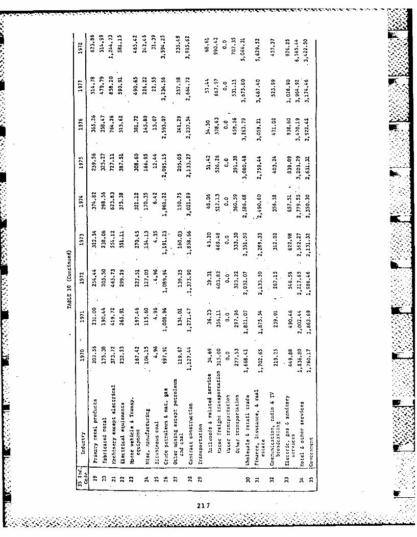
C).'0. 04-na-'V4-! .- '7 02 In 'A -n .n .% 'Ico M- -r '00 -1 10 0% (8 nV

-0 'A 4 (C9 %n C4-c4 aVi, C's 10 -jen

'I -. D W% C7 CC0-4 n 0 cOlr %0 C4 "' %a rVi ", It N0 s-I 'A N C)%0 7

0 0% r, ( 0 C4 '.4 Vi Cfl In 04 C3 Vi . . .

, "ti N I 4, o i N 0! n 4 C A '0 V N 4 '. 4-

m In '00 '0. (07%', 14 In (00b w-i as t, W o1 'A "i .4- C'D 0 0% '7

N- N , ,4,-

') w% CN 4 n4 '0 (o00 17 0. 0% .4IC- CZ w; 9 r4D .0 C4 LNeO 4, q4 m~ .7 N O s _4

.4 'n N ( 0 0 '0 .4I0% 0 Mi . . 0 4 0 , 0 ,Nq M. =4,m 4m .4 a Nl .4 n N4 0% (0 Vi 0 n C> en

Vi; m O a 7i MO '0c. 04 (CI- 444

en '0 , 0 N4 'An (C4 'n m% en % (0 0 ( .

0% '7 004, CD, 40 0 4 0.- W c4 (3 ( D.)

. -.. 0% N4 rN Nf c. '0% 'A N ' 0 0 0 '0 N 04-i N '04 4-). 0% .4D '7. In( Go t- 'A 41!~~~V 1, 1A It I4!, '1 4 nL n C C-4 4,

47 NN N N- 4 3 IN2 4 I

A7. N .4 Vi 4, CA 4 4,1 . . . . . . . . ."7 4 cn f, 0n 43, N0'

(n C4 W Nn c47. 0-7 7. 0(0 ,0 M4 00 N4 N4 N M.4 Nn 4, C4 'Ak N0 'A '4'0

Ani N0 C, 4, N4 C4 P. '., C) to w% N 0'0, a. '7 4,4 NY r, P0 'A o' C, v

-S '.4 ) N4 N4 Nc 0

14 In 0% 4 'D 04 4 Vfni '0 c, Vi 0Y ) (o4 -4 ;r 'A N enO 0% ON 0 4 N N Nq 0, fn h0 'A 0

o ~ ~ ~ ~ ~ ~ ~ ~ l C............................4 (00 NO V 4 17 C3) '7

c" k-C 0% C3 N- Nn 00 r,~N N '4- N 0 .44 410 N 0 i ' 0 l 0 00

V;~ .4 .Z .7 aZ m 4, 4 ANm4 .c C M - 4 C; az a; Oz O a

0 4 fn Nn .4 '00 '00 C> NIn'C . . .. . . . . . . 40 4 10 r, C4 c7.7.0

ao a 4, 0 7 (

0~~~ wi 4, 0 Vi 1340 0 '0Ow% 0 , ~ C V 0

u, 4, NJ '0 NA N0 a

ci .0. 4 4 .43 0

4 to LL ' L

u) 4) .0 4) 3*.X 40 IC 0 CC to r >ej V ~ C4 4) 0 *- 0 ~ uC &A-

'A U >0 CD 0) Ci vC w 0 Cj 4 .0 --u ri CL. > .31 C; m IC.' a~ C.2 .4 4) O ~ ' .D ~ nC 0 -

U. C1 t. Al r.C-N u0 o C fC :12 Ci 0. A C. C4

0. 2CC. *4 8 : .- 4 0! c . ' 0 C) 4 i ' )

C) 4 C 4 4n U7 "N a C ca SC C'3 m- '.r Cs C4 C 4 C4 r) C4.- 0' 0l en" m m m0 el m C4 (C

C- GD .s ~ NC 2 n~ ~ *.4) U CI 0 nC 321 7U ~j. .P- 4L rs 4 CL i 2 U C 0 C - - . D G U .

7'.C r4a -i . 'n C-4 ma 0 > ^0' ', 47 ~ ''

4~~~C w' 7 ' % ' 0 0 73 .4 11 ..1 0 0

-40 0 T -4 C

C4 I'.' 0, 'a 4%e 0 '4 'a '4a C 0% 'a a) % 0 r'a..

'a .' 'a 0 co va % o, r4 'a 'a o c4 4 F.r ' o 'a o007! 't 0 cl~' . a 4' Nt 00t 'a a) Mt 'I

'a "a * N I% ma'~' )-7 N a n- 07 'a n

-4 cn-c

0 4 Nr 'm % A 'n 'a N l 'a 1%' I'. N ''. - *' 044 N 7 'a 04 ' a P- M4 '700 a%'..

4 c4 8 'a, 01 '.' g %I 4 4 a 's v0% m % r, % c4c M cm o w % c , e4

.4 " % 'T 'a1 "' .0v o " c 4 c73 o %a. P. N D Nr-4 -I e r4 ID r M cl cq r 'T o-4

M ,. 04'. 0'77. 'T H 7'4 4n Ma) N4 N4 c4

-4 C4 -n7. ' a %' ' '7 c4 0% 4 0 'a 0

0 ' 'a N 'a e'.. Q 7'.0 M V% ' 0 '7 Wa 'c. Q

.4!

7-.I' W; 4 0.- 0 0 0 n 0 0 7. 4 0 04 M m a r N,

N ~ ~ ~ 'a M 117 - %7'' C .' ell UN N % '

0'. 'a N O .j 7 'a oN 'D 4"' '74 7

-% .4 e 4 1 3 c

0 ; - 4 7-' N M lo g'3' 'a 7- 0.0 ' ' ' o '7,

'a .: 0; r; N"a' M a 'a 4 N, '7 r e q 0 n n- 'a

- 40 4

0a In 0n % a ( 'n 'o 'o 'a N M 4 0% 'o 'ao

'A o :' '7 'a 7'. ' Q 0 > 0 m4 N 'a 0 'a M 4 0> 'a 'a Mn r'.

.- ) rl4" M -47'.- In .T o 4 'a -4 % '70nc 0-VI 0

-4 It4

u).,. r- 'a oN ' 0 -4 .-4 'D 7.. 4 N4 -4 C00 M 'a0C ;; -3 %

ID ~ ~ ~ ~ . 'a N .4 'De N'0 c N 4a No .-4 W%N4 4- -4C4 - r

0 a W '. P % ch o - In. 7' MN 'a No 0% ' . ' 4 4

'a Ma) N 010 0 a 0% M4 'a 'a 17 0 4 0% 'a4 fn4 'a n'7- 'a 0)i 'a 'aN ma 00 'a ' 7 4 0. 04 N

ct 0t Mc! 'a 0.-4 %a N! N' I) .. ' a'a ~ ~ ~ ~ ~ ~ I -4 'a N 4 7'C7 ' a N .4 0% M 'a ' 7'

-4 j Q MA

1, pA .U a ,

a IA ., t4 34 4' o. :3 :3 1,aa0.3 t, n -o to :,0, 0a. a 'u oA fa U ~

o4 a 0 .4 4 -4 64 0 .444 .'1, 0j '. .4 I '- ' U 43 0 4 '0U 3 3 'AI -a '. -4 -, 0 'uU 74I

4'4 oo :, 13 .- U A4 In. 'U ' ' 4 30. IA tj a4 n Gj .43r i 4

~ .. C i 3.1 w 0. c: '- 3 , 3 1'. m3 Vi u

o to 0 '1 IA - u' 1 ' 0 '1 -4 v. v3

Oj '. W. 4 ~0 j~: ~ ~ c

218

f~49 CN V%. WN '0 m g-s a.I M0 a 04 9

a. '0 N .j a. .3 -3 P 4 ~ f'4'0 Ps# Np PC C3 0 r-a* . .U43 '0 0 0 r, a "I. .3-. 4 0. b 4 n a0 00 a. % ',4 ' ' 4. w N '.4 .s 3 ro~ CMs

~I4.o P .4 04 1~4 0 . 0 .- Go Ps 0% a9 4

94 .'0 9 4 0 '0.acc Le 4 a. '0 a 00 . 0 00 0 %co 0 m

. a. , at O t 'I -1. - 't. -1 ." 0 "" o a . '4 9.4o 0 9 'a w%4 Pors 49 Nt .9

Fr O~ r. 49V%.to 10 or%494

m0 jo r Nj %A N3 .70c It a. 0 P '

~ -1 N4 M 9 0 .-4C0s43 . N 4 '4.4

%C a. -t r 4 Ps '0 490 Na3 9. - N N '49 on.a V%. 00 on 'co aIT e 47, NS Ps . N4 V% (4

4 N -1 C4 N Nn a. 4N 00 P_ a %D M9494D 00 %0 0% 00 rl 49 a. P% 00 0o 0 04 a

r, a. .. 4 .4 O0 4 '0toaV, 00 CO % (0% 0 '.1 .4 40%4 .-

4.4 on - 0n 0.0 -M A9 toa .a P

44 r 4 C 00 % 0on 04 a. OD.. to '0 . -4 0 n -I. P -a* in No %o 0%4 N 0 3 0

C4 N4 9

494o9CO007.3 0 a. '0 a. 490 % '00.3 .Co '0 N4 .4.0 Ps

on In9 Ps 4o! Ps! '049 4 : a.4!NN . 49 Ps 0 l a.s -4 Ps N; '0 49 9. 4% Ps v% -4049C . In P, to N 0S 4 0 '0 N4 0o Ps N 0 M-4 '0 0 0Pr, 9 N 0 -

Ps 49 Ps '0 a. 49 o 0 144 No on 4 Ps al 1013. N N ' * N4 0.

434

o-4 4 .-4 r- 9 a. '0 O -a .3 ' 0 9 P. '0 0G 0 44

o1 N 1 -4 on '00 P, N r 4 N a. 91 co 4> Vs a. 04 a. 0.

(n .4 a. 04 A- N4 4% a. %0 0494 a. 0% P0 49 .4'.4- - - - - - - - - - - - - - - - - - - - - -- , . rl-.4 '03 04 a 4 . ' 4 4 N4 -4 %0 49w%.4

C4 N 4 N. o -4

a* 'a0 N- OR). 0 %a 0 r 49 N N 49. N4 4 Ps f, 0. '0 '04m49 a'. l 04 e9 Ps 0 Ps %a. C4 Ps 4 .4 a. o-4 0 .3049%

on9 0 4 %n NO 0 on w9-4.4 0 17 on 0.049:r, 4 0% C3 44 049 0 0 0 0. '3 49 N 0 r 00.4-

.2 in '0 Ps 49. e-3. M0 ' 01 '0 In' 4 .

4. 4 4 O r, .4i P4 InI N0 ro a. Non9 4

16 2 Q- o N4 a.4 m -4

V3 0 -% .4 '3 Ps 049 -30 14 N4 e s P '0 to C 0 Ps a.2 . 40 ' o N 049 NT 0.4 0 Ps P 04 0 49 t'Z I.;02v% 94 Pst on P, C49. Ps % . N V4 Ps N GO 0 ell N 4 C4.a. 30 4 N '0 49 '0 49 0. .4 C3 '3 N 49

.4 N4N.1

0 in 0U -6

to4 Lo.4 44 0. n4s3o ,

-4 34 to U U to0C% to -4 j 1* a4

U~0 " 439:0.

u- n .5 ' IA 0i C. C; 3 ~LA to 4j or 43 4.. v3 .0 II OA a

4.1~ ~~~~~~ IA I A 0. C : IL .. IA' 4U 0 ca 43 0 4 1 3 43 L -4 I.443~ ~~~ ~ j3 4 3 L . . 4 ..L U - -4 30 c3 S L 5 0 W . 4 j C) I to

Is -I A C to4 5 * . ~ L .40.43L to. to :1. to U. L: 8 L . A A 0 0 Ito V32L 3 2 4 . 3 '4 4 3 4 . 4

0 0 4 5 - 0x IA X3 3 3. . 3 4 IA

-: -. t

IA A 4 U 0,0 of 3 .43 4) 47, 4 0 4 . -I ~ * U 34 4C35 -.4 4 ISO INS on In In4 , ~ I A ~ . * 4 1 .wI3 U . . 4 4

.A.

219

.-- I"wM %

Footnotes for TABLES 9, 10 and 11

Sources: U.S. Department of Agriculture, National EconomicDivision, Economics, Statistics, and CooperativeService, 1) Farm Income State Estimates 1957-1972, .":

FIS 222 Supplement/August 1973, pp. 60-61 and pp.87-90. 2) State Farm Income Statistics, Supplementto Statistical Bulletin, No. 627, Jan. 1980, pp. P.50-51, 54, 79.

U.S. Department of Commerce, Social and EconomicStatistics Administration, Bureau of EconomicAnalysis, Survey of Current Business (Washingt~n,D.C.): U.S. Government Printing Office.August 1973/ Volume 53 Number 8August 1975/ Volume 55 Number 8August 1977/ Volume 57 Number 8August 1979/ Volume 59 Number 8

'U.S. Department of Commerce, Social and EconomicStatistics Administration, Bureau of the Census,

"'* 1972 Census of Manufactures, Oklahoma, p.37-7through 37-10,1972 Census of Manufactures, Arkansas,p. 4-7 through 4-1i, Annual Survey of Manufactures,1973, pp. .176, 178-1801974, pp. 192-1931975, pp. 187, 1891976, pp. 182, 184-186

Other: Center for Economic and Management Research, Collegeof Business Administration, University of Oklahoma.

220

.- . . . . ... . . .. . . . . . . . . . . . . . . . . . .. . . ..

1 0 46 'T o r coo a 7% 4 m %0r, 0 Goo e 'T o c 1

0,0 0"4 0-, 0 0 .0 0 00 N0%0in00 0-N0M 4-40.-400 a,0 c.Jo&>~ 00Q00 000 000000 0000

L)., 00 0000 0 000 o o N0000000o - D T0-I0mm0w0n00V0004

0.1 000000 00aenm 4 n 04 " m .7L D ~lr-f Sn 4? %0-~fn e en 4 -4 -f -4 "NM0 Y-4TTt04N(4 04C4 -4 Cv C-4-' -4 4 " 4 4 i -4 0 4 . 4 -4 - 4 -- 4 -1 4 -4 -4 .. 4 -4 .4-4 4 .4 -. 4 -4 .. 4 -4

C40 0 0 D0 0 0 0 0 0 0 0 0 0 0 00 0 0 0

-l4 0 o * C%0~I Iz~J

0 04

CA*

ZC o 0 00fQ 000o '-0

0. Z >z4 C C; C;0 C;C;C

> *-4 -4 -4000: 0C)0 )0 0(Z00 0 00 M0 l-4 0 .- 4 0 40 0 0Cz 0000 0 0C)0 0 0 000 0 00 0 00 00 00 0 00 a0

r-44

w-4C-4

> . )ML a 0 ON C-

00 5In c44 en4:- NO'O -4 0* ~ ~~~ 0- 0 0E5 CA)~. 0'0

U) 10 0 .. .... . .

0 A

Z C144~ 0fL~~4 14 4.4 ""-- - 4- t-4 O 4 - N

W 4 C - -4 -4 -- 4 -4 -4-4 -- 4--4 -4 -4 -4-4 -4 -4 -1 4-4 -4 -4 4-4 -4 -4o0Z0 000000 000000000000000000000000o

*j 0~ 04 0 )00000C

41 ~ ~~ ~ ~ :3 *41C)) 3 1 H6

00 0 :3 1 41' "0 00 4J U. -*10 0$ O U'0 0. U 0i0 C j u 4-i

0 . ~0. 0 4U0 0 U cJ 41 0 ca 0(a 1.4 0 W a, O 40. 0 j -4~C~ 0 5o . -4.' 0. 0 '- -4 -40 '0 V4 0~ C M4a.W ru :0 c w0 Cca~ 0J~ - O EO 4J-1 -H -Z

"0oooCo 0o~ p m z u 40ICLX .r-4 - 4 bO COC -4 a Z-4E $40O00co $4 p41 41 1 4J1 p4 .4 '0.0 4-4 41 QJ A.)U~ J

4) 60 U a*- X- a 4 4 Co a Q) u a w 0 Q) 0

-0-4 10 00 U - 4 'a-4 -a00 41 () L 4 0rr. c 14 0 . V00 H 0O.1- - 4 U.f-Q a a ..)- -4'4:3C4 -r

cc EJ 0 .04.1. * 0 w a 0O0to S -4 *.dl *z0): 13) - 11- 14 >, - tl m U .0 m 4 acmw p > c )-q> m

00 a)- 0' 0 -H -14 4) -.4 CA r-' 0Z a) 4-J W ~ Mr 'o 4

221

0 0 0 0Ln 11 C4 e n%) 0P.

C4 (N%4 C-40% -4 0% r- C4N 0w od Q -4 6 -4 -4 0 4 '4 -4 " 4 N.

w 000000 o 0 000 r.

u~ w 4 Dt

0000 0; 000 0

E-1 -

rn -r 0c n Qa

kmL nk t - 0% coc 0%z COOD00%0' D ON W) (14OE- cn cn n O % tn 0% -r.~. E-4I.W4 00000 0 0 0

Cl 0~ 000000) 0 0 0

04

E- E- 00CD00

4J wZ 0 00 00 0>U 0C)0000C)0 0 000 44

0 Z -*1-4 00 0 0 000 oC

coo

> 0%0%C N o C

00

.. 0 o j-4- 0000 0- 0 C)C 4 3E- 9- 0 4 3.

0000 0 0

0 ' ..

04 0Y 0*. 0.O10r, - . r )E-4 0-- 0% c - n DN *"4 3

0 o4. .- ! '95 0 %0 0% -. 0 14 4 0%-4c~ -q W

z2 1- - 4 -- 4 -I -4 - 4 - 4-

(A W 0 00 0 00 0 00 0

V64 A40 0x 0 0000 0 00404.1 C)~zto

01 10

w cc1 P~@ -a 0t0 0 4~ 0 %,4 CL 0

ro . - *I 4 ) 0 co 0 . U

4J~ $4- 0 0 .0 r

.6I 00.0 CA nO-ar. O@3U60U

Aj 4) 0@ (a00() C1 1 > 00 r_ 0 0

m- 0(A CU00~C WCAU)$ $fl 4 $S~4 0 4 -4~ w C

1- 0.-W0@3@3-40 co E C) a

m ca 0

0 :33

u

ZOC 0% o cna~

222

% -,

.4 %00% 0 0 40j 0 l41 1L n t- . .

'T-T 4 - . v)Mk "' 0 0 0 % "&M0DW C .4 f~%D0 -4 0 f C

0 0~ oooooooooooooooo

%~u z 43 c00 0 0 ChM 0o.)- 4 N co Inm - M0 0 Lm ~0 com

0 C 0 0 0000 0 0 0 00 0 0 0

!4 004 00 0 0 0 0 0 0 0 0 0 0 00 0 0

z4 0 000 o00 0000000000000000000

9z4 9 0 0000o0 000000000000000000000000

z 4 00 0 0 0 00 0 0 0 0 0 00 0 0 0 0

r%%T%10%-Wa'-.? IT*zJ 44 I-~- 4 H a %00 C r-r V%- l~ -0 0 00000 04-4 000000 Q00000000000000000000000

En M- 9 000000 : 0000c000000000000000000 0U C)o0 0C C ;0C;C

0 140

04 0 2vc 0 o 4w W W1 Eooo 4Oooobeo0oooIoAiouo 01oo 0

0 W~0 00000 O-4 oO CLoa wo0= 10 (A oo0 0 ow c o$4 9:0v4)t ) 0 4 v 0 64 v

E 0 0 4 : : 0 0 4 1 :3 -4. CV 441 *0 u0 4CL (U -Hd. . 0J X4 4( U -4 0CV -1 0 uU U - 4 -a PA -. 4 0 _

a e 4 . r 0to" 9- -a a to 0 - " Ii W ".4 Uto ' 0 00 L W- C0 W.L WJ a0.ccc 0"r44 4 4 w o o k 0-OL w tO 00 0 0.. a QU 44 "

(IV.- 0. la 0 U U0 0 0 0J4J -H 0 - 4W UC 4 c41 0 0 4 j -W di 40 4 00)X. (0 - 4 4J 4 0) w w4. 0J LU' -H u- 0-4.40 $0 & U0 a w G= u 0 u4-v ' A00 CO4 -4 (1AZ 0C U 0 C1440..W W.41 .0-CC 444 0. Li w )4 00 0 -v4 4 1v0 -A-4- X W :1 41.j8W-45 w 4w0->0xw.o wii44~4i w.. - tol 4 U 0 44

4.a41~~~~ %n~~~.&.a0-L %D w at 0 -4J LI. LU %DP O 00-4-4. -OG - .. .t0L CUX I4 4 00 .s C4FHUI ~0 J.-400-4 . .J 0) 0- 0OW 01w40U.-M~ ~'00 U 0 -~223.4 .

r0 01 -Uo~U~04

00 ~0 0 000 0- 4 DO%(

14 %D %0 %0%0 C'J-r4 %C %D 'i0%

.)P% . ..u,0. 00000nLnL I n 0 000 -

0 ra En -4 c'J-4 -- ('4 ~ 0%r n mc~Cr% cN a% 0% -en 0 (l4 -'D- r'D- Dp D .- r, %D Z

0. ~ ZI 0 00000 0 0 c( )0 co..e 000000 C O 4.1C

z 0 00 00GO 00 M F

W 00 0 DC

4. ZC4 00000oc )0 0 0 01

C)

C; C; C C 8

0i.IM 0N ON4 CA000 0

c~ 0000o )DDo0

w 4.- 0* 000

z )0C 0 C) CE4E 0CCr ' C~0 0 00

0 C).. 00000 0 c0 00 4Q.'4- ca4 u .

04- E-44>-4 cc z C4 4)Cl-. C1 300%%C2

> C r r r r % 4

0 )C)0 0 .04 C) E08 1 P4C o0 0 a-4 0.0(D c0

93 ~ ~ ~ CQ 8 C.4~i~4'4'C4~'4 ~ 44

0 .J.l44'

0- OCU Co1C, Jb. 4

F- Mc C-0W) -40 " 0 4 ) 0

&j U

coj

22 01

*~~~~~ 4.. > .... . . . . . . .

.77

u~e . ta.li

-~~~~~~~ ~ ~ ~ ~ ~ --. j - -----------c

.44

4

14 .".1" '.

'o '.4-..

4.

" " ~4.4 ' '

.,"0 0 .% .-1 5 0 .3,r 0 el C n 0 0 X 0 o.. o C0 o 0 ej 0 -7 tv 0 -1 0 e.l CA a,, )0 000 -.. '"

-,." 0 0 0 0 C f, "- .,' CA r, o' .. c. , c' ( ' ,( , 1. 0 0. o e3 "0 0) C), .r 0 0 o' 0 c -0.0 0.

7 o . ..i - 4' inv r ic - i o t o 1.

0 e..t l .11 7 1 r' ) M.' P,1 : el .C) 1 l 'i I N N.' eI ) CA r41 N N, N; ^;4 eeq Na .', . ;. . " : ,1

4 . . .. . . . . . . .

.. . . . . .. . . .. . .. .. . . ..

n 0 fin flIfPfl ' 'j

I' )0 0000 "t 00 0 0000 00 00flOO00000 (")S ,~4 14 * * .0 4. CA

n~ in I. y ,

* * ... . .. . . .. . . .. ..4 * . 4 *, . . .. o, ... . 4 , ,. ., ... . ., . . .. ,

04 A" 0° C,

~225

.- - .c .... . .'-... .. , . ....- ...... " ', , nn-- .' . 4 , _4 .4 , ,, .. 4. , .. " ... ,.' . "

I F I

1001 .C. . 0 at 0M I.V nI nW Ia0P ff k A

bc0 Nm 0 4 0 c1 .t ' a. l c

m m rl -) n 11m .1in ') U N 4 tot.) 000% 14 C% g -4)0) be1,J. q t 1

P.f .0 . %6 Ye 3 0 ar YN" M' Of

0 *30 0 OOM M-00 OOM . 1 .0 dy m 0 00 0 V 0rli10,00 .

r. PI t P) 43. z 'a c

01. 0.

V.. 0 f. .. n M t.. . . in -. 0, N5c -I *e ** *l * e-.. ..-......

fPP U".U

to f* cee. * ewe... Pa ?4 C. m e on11qc.

Co O1 4r. 01 qi Vi A1 6.) Is pe 0i rf 11 .i a, -Q. ;j .3 P..0 4 Vt Cien ef.)nLi~1I

4 ~ 44

4~ ~ 226

VIAA~~~~~~~~~~ of.N~ N 0 ~ p f ~ J ~ O O O O O 1 4 . .

f's n -10 00% - 3 ckQ - 0 N-r t 0 , 04 'MN0 N AI M 1 ;Ngo o -

ICI

0 0 's MIC4 flNvm U)0Itf- ~ 5 w n s f 01 y 3 M I'S,. 401 2 - M MV m~ P

4 1fr0V. M n ot

Ot . .. . . O. . 4

Ia i o 0 m o 0* .0 N c

0 n 4:11O 00 4 N0 0 m "m 0N 0~ 0ft 4 0f01- 1,.00N4M 0 M 0 0 1-I. NIa o1 c 4Z j-94 Z 4 ji 9 - ; 44 t- 401. u,!

IA Jo M In to r-

lu - M4 FI -

61 #1 IN. 3 N m4010 Y-4$

U

(L cc - In ) ~ - N-0 ( -N 4 -.

.4 . v . Y M N . Q N .Y 010'A~~I Iii1 4

I 11 M04 0 - N431JP N44 61. 4 ).4 0In 4 t- 20 N ~N i 0 4 4V).0 .1 -n A.o 65' ?. nAAn W M - c i( 6 . a 1 % 016 1154 4

4 r)~E e to M

- y .0 dymr N Is-m~ In.3-. ell N) 04 b4 Q11 LO

4)

*~ M -- .J -'4PN Np InF I~u~ -)11.- 10 4

SAL -t or Of0 1 G7r' * - -,*

*f .1

Q 0 .)- .,. if, .4y? prC ' i . . , ~ h.rf)-

*. .. ~ . . . ..

0 0 som 00 U)UN N 4O' 0. 4)0 t- N O mN m ON 0 0E0N .NIn 0

04 tl '0 '0 .3NN 0N t y0 1 .z 1 w - N n)I~ N W 0 4 0MN M 0a..SrJI.

ly -1p0r 1 - -. -yMM yI

W N '0 - 0 t-4 0 M 0 0 N 0 0a M Q 1 0 f a .1 *..

z - -1 .0 C4N0

00-~# 1, \00 0 ,N0N040 P mm1 .0a-4P

M 0 - 04 N N-- C- ~ - -N '0 k P) 0 -

0 a,*~) z 4040to fl 0n '0 01001 -m nm00 Nam0o

(0.0M P NNN'0-.--.C'00J - P)IA ) 4 m M 0-MO MO N N Nt-0 4.

. .tn .4 OM 'l . ., . . P. 0. w

J. ( - Y in - M "N -a

N- 0 01 01,0 Il0 N O~f'-t-0 M 0 0 0.0 0 0 0O' t- 0 N.00 0N 4.J

- - N (YL o 04

P4 4 . 0 0ON#. 0 E o.n 10t-OI- o O P"I m) N # 0lt.i~ N ~ -in mc 1 C 01 - N NV)0 c 0t.

00

4 w O M N M 'D 00 C 04) '01 0V)N.UN01 0 N MN M M 0'0N0 0 P, mNS1.- 0 y00p 10 Ym 0000NM0 0 0 0-0f

-C . x

0 0 -l N- -y -4z, 0 10 0 - 0t-t- MN N P- N 01 ON 0 U rN M

oo I - r rC

wi -. i 0 .U.

0 0 Yt - 040P N -0 00 -0 - t N sA 0~- NO P-OOI OONOeJ fr 0V4NP2 C - - --O O N m yNq F - N tN '0 C

o 0 (Y- 0 C C - O4 x t I -

C* -E-4~

- -0) -y t,0 oo n

I- x.9Nl F ) 0r fN~0 N~ '000C'-N1 o N~ O N 4 )04ON'N

~ ..-~ . . .. *% t . . 6. . .. A- - * * *

44 1, C) I* C% Ul * Cy 0 * ' M W Q * t t' C- 44rV WW r 91 l t.*I-*. .*

et 0)' -C.'.C q4 C. P.001 t a14 0,I 70% 11 :o a4f*Y . -r-- t

a l1, 4 0 ca * Me * . W n 4 9. c0. *c*

t. t- -1 00 M M V t-C Pn* ,NW 4rl4N.WO0N.Y Or, t- L;) M N I.x o - . . .C. a . 0 0 4 . 1

it .3i N. - C oM6 ,C - )4P , , )(J III IN00V

lpC a. C~C~C 0.'). V.) -h I- N nl U) 0 II. M N U; m~ N 0 I N N N t- m 3 'a F

-C cc II Ie t m 14 * 11 P" V. *0 N ie 0 )1 -0f WI

ir - CY.4- P-1r -

0l

0 In D- CO # M 0 0 M N 0 - N -0 0 0 If r Mfa ,-4N 0 0O0N N ) 4CN *C.-0i~~ n M W. 0 -WV.0 %09 0

0 M II It fl) PN, I-Q aN - M CY q N 0NY t 11 0N f-4I- zI Fl- ML 0 1

010 -Nfa, 4 - C 0 0 I q V.'. C..

w 400 0 r-0 N0 00N 0ONC M4 01- 0 t M01- 0 WN 0 0 M0 N0 00 f

1IC MC M m # 0 * Q ,0 0 by P).............NCQ Vlp W It I

ot4

x - 4 Ci )

4l 0tiC 4 CYMClNt N M r

14 2 ~C4 N -N DC-C J1

c-4

440

*~I 10O ~C

9.3 4% (1 )I Z 0 rCI l)4 -1IIC! I * . :- , -.

.),.- -- Nl N L ,m0 - C0 t ejU 4 f

.M CCC,

s -h -L C* .. r . C c: C, - *, c I, I k, C, o, 'e 0 1. U

ff -1 1% th 1.1

*% %o, a z %. N . .p N 4 . .k oo o & & in * N 4 l m 0 0 * N P4 P4 * N 4 4 k 0 . P

~ ~4*

1 - or,0-. N W N4)lV U4 N.c .. fl 4 a * I-Y C P24 )

MNON OO , 40 0P,0.N P. 0 0QU~)

N O0N 10 41o -n cy cy t- 100 Ot. - m .0 M v , 0' "- tye- .0..0 U)O .0 N0 4ONNN EQ -NtoO

-tP A09 .0 00N N-1)U uNf 1( nF). 0 M 0 aa 10 a.OEN V . 0m t. r) m4. o- .o o4 m. m 6 nN ni

D~~ -U)Y

N CYN

ILN -d N 1 0

w m NN M F 0. 00 0 It 0. 04 -Of)9 N 04t

ot 0 0 Mi 0-O I- t-to 0 U) O N U N I 4'-. U N 4 9NNO #0 -lo p-

I I~) I- N fl.OONN OONON 00 4 Q ~ .0f4 )N 4.1

"40.0 * r0). r, to W tNI 4 M 00 00N40Nt U)0m U)Nr )O@N0U10

U)~ ~ Wi N~4 0. O UN M N 9U U)b.y rQN 04 4N N Ut) - -

4- N1 -- m- 4-N N. . . 0

* i

-4In U) A. 4; 0 I M4CO0 nomto.00

a In -OA C4-- i in N- .0 04 W4. NW) r4m

Uo n)N NO . NU N m in 0 0?-O 4NIL in in

ty 40 0 ~0 )?O0 l0 N o -4 Q0 N MNo401, 0t.0 )- )# - O N O .0-i -. 0 -- - - - -. NNNNN. 9N N?- U)M

* I 23-

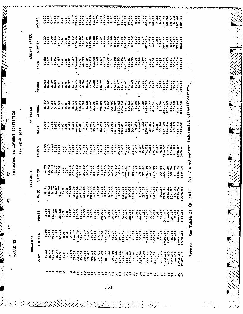
is wIt 4 ** * M 44444... 0 4 MN N I gym.4* 4 "0 4111 1

-r flN"0 - N -aN n -11- 000IA4

-p-

-00

t . 14 i

1- 2 . N Mi to flp.)oc - r-1 .lf v) I 41 ..9-i t .F~ O U-

N .1, in .41 3M 0e~y m-N M No'O N J 0 1 4~ *0M 4; 4 Z g 14

61 AN . I V C P. *400Int-0NM) .O'C mto M0 * O.I.Wb40Y M D4 0m0Q0I) II t 4I n04.

41

M I I Df .1 0 . .0 *. C4* M* 4 . M 44C . *4 0 0 4* 4**

Io Io! U.,111 to INSNNmNr -- .F r. 0 1. t4 QllIf0 ' M .?~l , faI ) 11140 .4.4 - 1014 fIi U,

m C' o t- V0 OrIn O' 0 Min , 9D 1 4 CN I t.0~ ~ O ~4 'aN 04:r.I

0... O 00 00 Q r- 0 m e) Q, -01 0f.0 0 C. - .M 1 .W~0 .10 1 t 0* -4 q It C. -4 4 444 111 0 f- *0 L- :* P; * *; P:r7e

-*40Vm0 0 0 n I 0- MMC M l4 In 0tti.C4 N IN MN In 4 4

0 * 4 - .10 4 *4 - ..

oo SO uv to to~.. M4

P. Oil 0' r) AL OIn)S~ C)0 4' -'.IC#In n . t i L .O I N 0a 0 a * . .44 0* . .* . 6 . . .. . . . . . . . . . . . . . . A

onN - In 1~-.t.v 4v ~ N iN flu'14fCtIt 0L'.4e44pn.w.N..an"110nif NL 00 N 0l. ~ e C . 111~'.~I 0'-~ -. Nf..' N

It 0

.4 41 41 'U- 1'NI In --6; F4P *

.d 4 v- 2F IiC4 4 N* II II -.I to4. to .4 11 *1 -1 *. P" M4 In 0 4 !. f

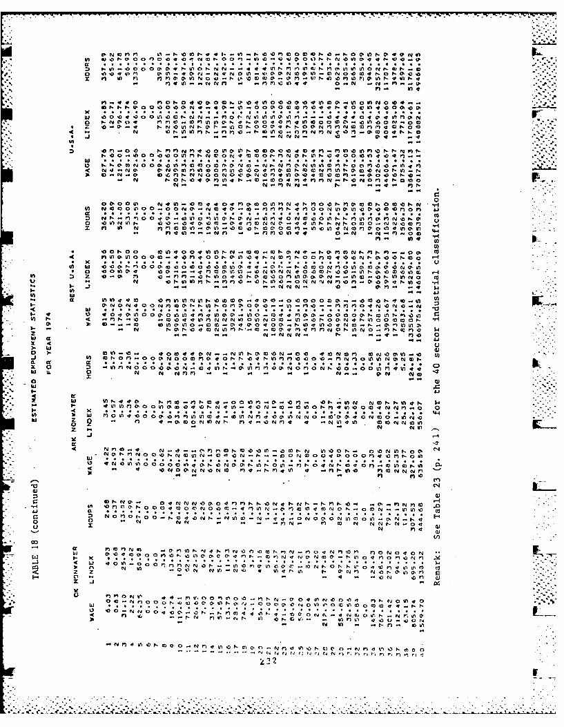
ID N - M M on --.- t---- 10 03 f- -to -. f- V) f- .n" OD 0 CO CD 0- -0 N. -, O- 0- r- V Va i

O~~ 4 VI4 V~ fV ~ O L O 44~ O .. I

"N r), In.4

M4

w 0 0 04 00 f0 0 NO N t N0W4a'O V0 0 - '40M In 0'..InO n0 0 .'..P. I- a'O04M M0 0'Ma. f4- 0 -O() '0 4 1 M C,0, 00 40 In 0 0 M 00C

w .'O' % % I j

0 .J - lP Ql -0II0C 0f tf -- -D-NN %- 0 wm"- 044- .. 40CY - -l Ye )P

0 W0004000Inl- VO 4I 0-N- 00Qf40P..hi...................4 . . . . . . . . . 4.

1-1 -1000n001-0 -NM0M04 N V) P, 0N0 4IAVIV0F'4mn 04E1N 4Wl 0 P, N t.00I0 NON '00 M

CY MI~.0 WflNNN00) NOVI wo 00 m 0 04 0 ~0 4 N 0 m 0 V 0 n c .-- N t- ~ o4 4 V ~ t- W . 0 O 4 4 A '~ N 4p 40 N f ~ r. tfl 0 V

N-. -N-~N - I. - -- 4 iq 7

0i10 0 P00 0 4 01-N 0 -00 M M 0a

j- M4Ifl- -N -Y -A)OV4 In. -'N' -- ~ ~ 4.2

ul w

* 0 400f0.0000000.4M4AV 0 C, 0 0 0 ItNm4aVI Y0 0I o 0 0 n m a -0#A ~ f-0 .2 40 4 .4 nnN O4.O ow04I0 N-.NflVp-''O00Ifw fl0 P,

NY P.0P 4 tC Yc D 01 m m M cj 40A0 ''On 044 t' .l1,a m~. - t -- -.. NN 0 - Q1- ..I- er-- J

a ).- :0 9 N0 : 4 0 44 VI N 0A 00Q.4..-NI.A0 4 0 N 0 MO4NN Y 0 N

o. ly '. N-N .. 4 i I24 0Ui IL0U y tyF nC - . UYCYC

o tn LV..O no 0ai (.a 40V 0 1-.N. Vfl .0.'D N 0 0 P44 N010 0 CD 4 .Ifl...0 M-C x . ; ; 4 Z 4 Z0;- ; 0inoZo8 Z In)O OI4ON -. 0 n 40oo N AOo .0o4o ;A inmW 2I0 C 0 N ) NAI - - M . D. QM .- Y O -) N , CONCC W

-4

-4. 0-1- m. N. -0 0N-t - -w 04 0o # m o

1;z884 UC : 1 9 44;8;41 ,zL

CL o N No tno l

M 40 m NA in0Wn.. N' N-.C A V -W 00Vo.m'OP IN mA40n n 0'N 0lS.-ON

hi . . .Ol '0

4 (\OjNO 4 ~ V f .4 I I ~ j 'o

w ..- . . . . .I .~ . . .. . . . . . . . .

00 -0 N N -D P- ; N)N m VI N 4 N q z .-N

C, N ) ir vn r, )

-A -)

._lk . %" %" ° "

. 12,'i g ..... .

:C2Or -00

-' Is r.-22-

3'- w y 0 0 Q Z -L 0 OD 0 -f 00 M" CO" M 0' 14 0 d) It" I: MO M N CC Mq 0 1) 0 U)

Mt O 4 0 a . C in . , * , * , in N M a* ,

~m

o I-* 'N- - N 4.t.. N NI' I-- -. . .'

It

.0 0 .,-t.- " 0 t 0 P F4 .. A .6 1- .C P 0 0 t - C M O y 0 N C

4|.in t * 9 *,, *In 0 ' N Q Ir 0 0eI - -* 0 * L 14 . * .

. - Z,- A. It r-' ukV NPI, m o 0- N C4I. 4 M It in t Na- C ( i

U) es f. .. .

t t-1- Ck C O V Q 4%s o C f - ) ? 0 W 4

z -L1

cc4 .J.

Z) 00 -2Il00 0.0 10 L 0- MC 01.0t. 0 G%) Of-e In Na N Vn 0 (A 40 0 'C) 0 ) N .. N It

. . . . U * * * U * U * * * 4 4 # 4 U * U * * U U * * "

e4 in III - . -

.pt.

4.00 1 4.004'm t

- ..4." .0.

M 0 t M p N , ) %0 * N to " * * " 1* N P " In U t C OD M 0 Cq N O t m

. • F. 0 • 4 , m , ". . . M 4 P. 0. 0a. - . J ' .. '. 0- n 0

* 0 '0 f It ID 40 - ?

w M A 4 M 0 0 Mq (4' 1111I

0 i t ., V) *) 4 - N r. M * c 0 At 4% 1, N3 4 N -01. .0 N * 4 0 . 1* 4 JH

0,1 no 0.0 4 1 4f s N I M-I Q1 *' I n a)N O NL mI 0 F~)0 eifl 00It IV 4 n 401- sN1 N 03 N-. )1 - nc l

sI#3

0 -7 l ,; nm0 4N0mm0 . )I %M ?- 7 -d

C. N , .) o * * ID IN o)r .0 U)I 1N 0 % i jP %I t t I

hi U. C0I 4'i As 040 44 WV.'0 ~ i-N N a0'.1 i)CNI II )

m 0)

J 4

C..

Mi .j n ejM 0e l 1 1 t1 Irj C 0a n C . .P. N In 0 .

-0A , M00,0N . * N )4 ' n( 4 1-.'CI 0 111 1,0.C4 0 N G

In .N f O-E'0111 4 00 )4)1N-NI'Z 4a0z4'. 1;NC.1ml (

1A -t .1~' 1,4 o l)Q - 14 C 0 JP (4

J , ~ - .'3 't) '? a, 10 tol0 "a

x cc

.4 -0 I' .)t.0

J' 1 4- o 0.P

In Is

%

9p.' na 4 l &wnf %Ms Vv 0I Df 4f f .0f 0t

inIV OFWI mf rw f s9 -I -A -0f.t -C ) 4aNt r ,l,0rit ***** * * * * 9 9 * * 9 * * * * .D t a 0 C 0 cmI')n ZCO N 40 Il . dr 4 0 - 0 t-. n 't N.Li,4 n I

Z 1. n 9 '0 N I~f.U49jI'l ..' - 6 ofN - t. 1 00 P 4 1- .~ qr an (% co N oM fh4 CY i - -P T1V fl4 M-c -(4 - M- M

*. Z '0. in V4 1 OP) cL14 m*c~ n ir.0.N . r- M 0 a) 2 OO M i.0 CP 0 aO-cl -0 t- bl m f. N-%% D400r 1MN00N-4 ,04t

41F on 90 9j m 0 * # I- C *9 . 14 . j Us . It . 9 0 9% p 00 * is IV 0) * F) . K

NI- N I!. U. IF ' 4 O IFO09f9 . 4. *:~V~ N~-f- .,ov - l)0- %D0 0 P-0. 0 0 N0z0 cr.f-o N-1 V% I -V . 1 0N00 V. M n mf- ly.0

-C Nk rQ y C b) al ;;4 0 0N 0(b10 4P.401-0 n m c tyN.....- OO apa-4 o .- - ' ' r0 - X . 4 n aj- 0 .4C 0n@4 r. m in. I f

(.4~~~9 4rj( -- t- I

4t-V.3 ~~ 4(fl~-VI~499-N9-4C'INQ0 9ON 9M~f4.1en I.D- in 0 tv 1 1 4 to o f-In 4 4 M a, N 10W I 409. .M . N a, M N

1: * * 99 9 * * * 0.4 of *6 1* C9 F?* 9.* 99 54.4

~~I flr-4 w

.1..t .F OO -M 00.4 . NN t-7Of -l.P.4. N0 1t- 0 .4I

WIz 0- f' f0o CP4 %ON tN40i o% a 04 n. ~o t- f ) Q ..)%3 41 n ..*Y inI -W 9--?-. 0y I. (v I o , nov1 10 ) U I9PINEin c (I- a . N at

P0'10 W 00 0 - q 4 P ) Flo,' 4 Q Vin 0 0 0 NY i 4 -0 Cal I'l in 4 .0 C) M 5) 4 4 -In N 4 N10000 .0.1d0 104 n 100~01". ryO0 0,VON0VI4O0..h)NI)44 f C -110 0 0 ~o- O N O t000000i,00P

I- -~4 - ly CV-.f 4N Q C P N ID.. ecge. U

J )0 - 0Oi nN4 o*4 n- P N -w0 m4 o # o o tr - C C.

mW- h6 0 oIN

7. 0t 0, in ** . * go** in99999v)%9m9t . 4 . .t. . *9* 99999oIn99. *)I -C 0 - -ii!N - -.. 4 .. N -; ON I!0

Z.C

I- 0,c t n 0 00 1t- a. CDo0 *v )1)( t a t .t 1 AWf , C 02 40MC a01

0 61) i - C l4P 1 4 4NaU tf %- 0P 0 M 1110. N

- 0

in#A 4 01t.t *e~-1 .t-I .-- N0 u) 0 W 10 NCPP1C 0' 'I 0 0I-. 5 0 0 0 f. r. r, no N wV N : t - In I.- C - CI C J 'r 0 0 t M 1C 1 '.

__- Wi A 9 'o; A. .. .. . .9 * .9 .9 9. . . .9 .9 .

I CA y .4P 0 Vl- . . , 0444- m pn W . c a '0 %. OVI'4O t 5 N 10 inx 2 " - P1 r..N -

0% N et -of - .. P1 0'01 -fl S mNt~~_ _

0 I 0 , aco i VP 1:,0 Vt 16U I..P~~(CIl. Oc I.WI) 0.ei I- a% e1 )0 1 4 . sV # l Q 0" f ' , , Fa*%A CV ara 9 9 9**. 99 9 9 9 9 999 9 9 9 64~3 %ifO 4 ~ . O l~ - .0e O~ e0 ~ 9 1000- O I -.. c

...-.

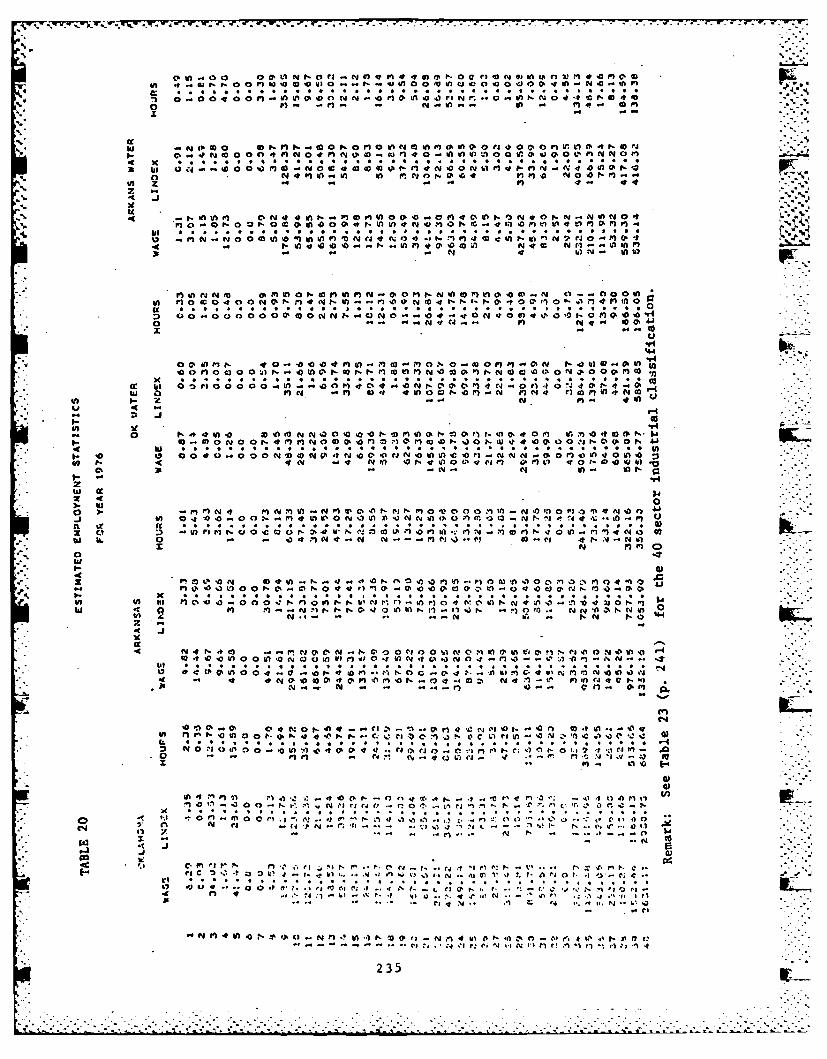
,, '. ..{1 0 1, N 1i),,,,VJ P. # 0 e,, III C* ItM I 4 i ' olt ) I LP 0 2J M ,0 a' P) 4D .

ul"

1 0N 0( v 00 . O .. NN 4 m af 0 a I'll 4 In I N O0 4 OZ 0P.0 N "

E .* .* *. . .. 9.... * * .* 9 ** **

0 b) r) - ' pi

cc

w- P1 CQ 0 to ' N m st toen cr p- a t t o on i (, In e4 oe c-, ore m o,- vi , 4n iN l N ._'''"

1 - n Io . "."

"" x I I.t"""

x us -40 .0 4 1 1 ; 10

o. t~ m aZin I' N4 MP)1 0 ""M

"% idIt in I MaN

0r M0 0.- M 1 M -.

3C - N l )- M nf.h

U? )

n 0 -a. N0Nm4 -0 6t 4 ,1

x . .. . 1 , . . . . . .. ... "I ..

o ~ ~ ~ ~ 9 z<, ,:,4 to- o:,.... ..,. ... , ..... ON "'0 -". 0-°9" Oln; oa -

a: INm m v

0 0 , - -c:..: .,

- oI % - . .... % . i, . . ., . ..-.--

a: II e 1.40 0C 0 I 404-0Nr 4 N -O0OP P1? -? 0 1,4 *O4 OI4 hi~O0 O P 4 __f__L c

* I. ll I' " 4.5 ."

m , . . It I o o t. o" n - u .. . .. .. 4 "* . ,--

.. W) 4 4 N% -M m 0 1 It n o111 4 W It N in N I0N 01m 4m0 401- 40 r- a

z

Ix .. I, . 02?t .In0N%ni IL t- 00- ,014W 1 .4 tl -.).W*- . P;-q'I3. 4 Q 4 on )., cm

o. 0 tPlN o , 1. 1 0 r -- j N9

M "3 Lo 0N woo - N ,gI,% n piown, n n3 4

loo 11 lo z 4 4 ZI 6V 4 1-1 41 * * 91 * 4 4 ;; . 9

to1?~ .2. .- N .? 9 4

-11-

IL 0 lW0 P ilI AI % l ' 1 o n-040 0 -N 0 N?.* M to v4f yrGNjc

a a...4..............4 4 * f 4 4 in.. M 4 . . . . . . 4 o;

C 0 0CA01 0 %M' 0. K C..3 CO -. N 4 71 m C4 Iftc 1-1I)

04 n' L...0

41ft n *-4 4 *. . lo*,4 n' %c . rIU

.0 0 M Cl4 - N .1 * .A J4 -i @2,on I" G En -4

el~6 -30C - t-1'1 1 1

0-

'8 C i r N. el -~t I P.. t- -. .% ej 1. .. Cj -T V, (I PXP .! . 4'. M~ P. I:

ell C :9tul . n

3f4 .9. fiV. . t1 p IA .$ .. J 4

-N M -4 111 0 1, -P (c I m I? %A 'D .2 . 1) 0 - ?4U P, 'A? 04 M J14 , 0 I4 I. al (iI t

235

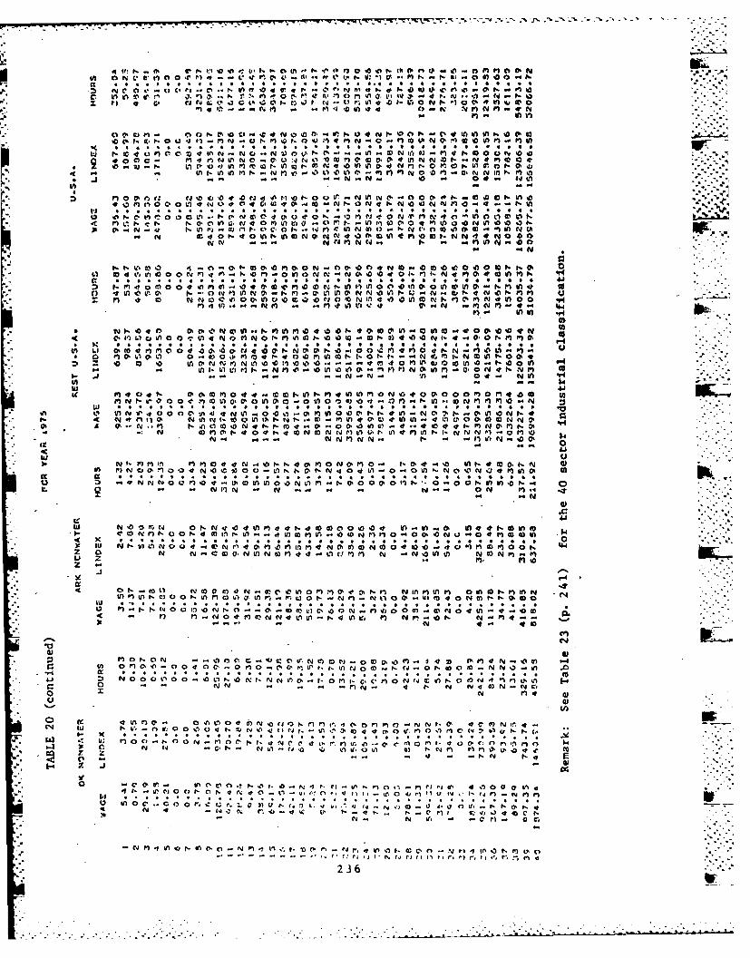
a I)01in 4 r. N II 1 o0 n0 1 ,-M 00 1P!I. %,:1 o %M a.J U . 114y4

t)4N 1-.f N fI-.

4 0 M . -ol nCi- N0-C r o -- . - I -ID tro0) M41N0 C -

iIn

M~ V*t . t ,coI . N 0, 9 99 9nt. ,F -- I 0C%0 wI o00 o00ot

cy V Ny C~~0 iQ 0 N M OY N~P90. N 00

NN~~N It NF).. T~ .lf~.

0 0 0 f- 0IN . - 00 N 00 P QN 0N- -N *

4 o N c *oo.i 0I N0Ni 4 00 IN00mN0M4.) .04 O0fnO nONV-N.0E0I-0t-N, MONeMfln4 -

C)P toro In Ut4) P40' 0 Do 00N00 f .040O D 00 0w 00

* CoJ~. 00 0- 0 t N i.t 0 E * N 0CaI. I.- fl0.C.EoI in 0,

N -C) - Y) - 0' 4t

w 41It O 4 - C C -- 1 - ~- Mf -1 In M N~f %0 00 P0n1 f.

M Nn f- In 0 0tM000,O 00 0 t

iti

CY . - Y(.

.0 0 N. r)9 I.f NN a. -N llNI - tI C r. 0' N )M -0OO 04MCc4

(Y - 0 O0 nCAC 4 1)0- Y C ni DC ou z 1 0

nn MI N 0 WON 0 -. 40 M I , tft 9 9 9 9 * 9 9 999 9949 94 * 94 * 49 *4 949 9(9

hi NO 0 ONN4.0 V1P)4N40009IV Nf-n.0 Ifl4IN. N C,

U I-) x . . . .

31 C, cy II C P - Nul ria .1 W 11 m~l~ff Oi 0, lo,f )47 1 P) if -0C -I )C-Il0-M- * - N 100- -d C040N Y 9 -* 0

t- I ,t- C-at ,p , 1 1N4 ) 0 N in n N I L a ft)'.99 114- u ,(4r1

N VN

Cy m . A 4 - o .I q . . ) I I N r n - , M00r, N01t oF, t

U 2364.OF

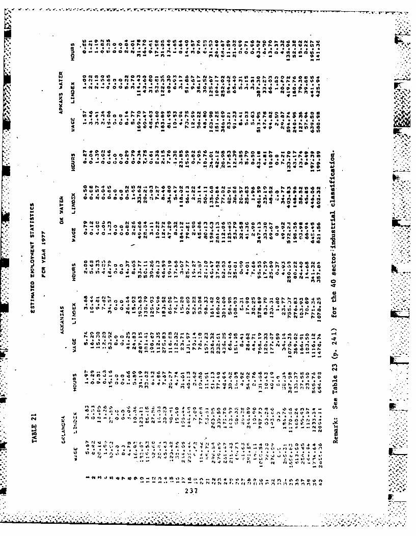
WI- t y n "a 0. )h0 0in4 0 V p 00.0.00qp N00P44Q 0 O N lN N%

ids a l a4f -y NlJ3. 10 ckn9 Pin ;. z 4 ".4a o

a, 0N0aI

.3 W "N4N-0 00)1tI.~dO)4Ogq~n~.)9 o~9.

IA~f - 99.) *- 6

NA 4~ 04 00 to C- P.k 0 '0I (F In 0 0 in 4 ok N I 6%4 'a 0 N ' 0 0 ' . in 0 . 9 Fl 0 0n 41-

60"049. 060p.

90 S a 4 0 9 9 a 9 c9 N 04 9 in M 9i V in 40 40 0 9 N 9.43 OO 9OMWN wF 6 ON 4 4N eolWaP fl )F .N #j 0

d04.

0pN- t1 N 4M00 NV Mf1 4Po 0041 Q1.0Cv PI Iqe N

39 onin10t

W 00

kiL0V)b *043P (' 4 4NNNNq0O I).0O)900M 10P. C'9064V0 V) 4

4~~* ' MOO N.4 0M 0O'040 N81 . 00 P.,. M 4O§N0 F)9..M.00904i9"O N 4.8104t 4. 40 C.4 ON In cl 0 9) N 1*1 1 4 t-M 40P

zY G% M. .94ct O , Aa 00C V .4 4 N ot -t

~. 0000

Ino0 n N mmmPo O No. NOON 81 O00N 04 00 a

~ 0 460in400040 0 0N O -0 N1'.3 v0 01004 8 6 0 0 4 . N~

N9N4F) OF) % 91 -.. l 0N.1.4m0 " c

-00 1, ;. C180

F).P004 M1 v0 M.1f ON81).qf 0 It..9.%'0 4: M O'0I QC friQ ,na'o 0 C) Noe .,.4 p o0 F o 0 1..'1 1 01 9 N 0N0%., o ~ 0 .. 1 -O 'T'80.80 0. . ,

I ~ ~ej *' N 9.9 ** I* 0; 09 0* *r 9 9 9 * *i* 9 9

* .1 -9.~~.'6N 9t4 C . N.N N .0 M~) 01 011 -,9NO .0

:,I .90 4 .% N f)9?. .99 ON...4 '0it~~~~- P.t ;- 1N M i ,)Va- M 99

' "~)' '0 ' ( I ' 'j -4-M4 . % .;.8150oj04;; 0 ' .Ot-fnIOC

ry I. ... f) %. -9 x 90 *9 9 . 6-I4_ '. -V

N Pg 0 *i M) -f In 0 N. 0 U. 4 1CI0.i 0 P. 1- a~ 0 - q M f V%8 d P- cc 0 C)

ri cl t -I f%)-- VI N M . - N 1.

239 7 1

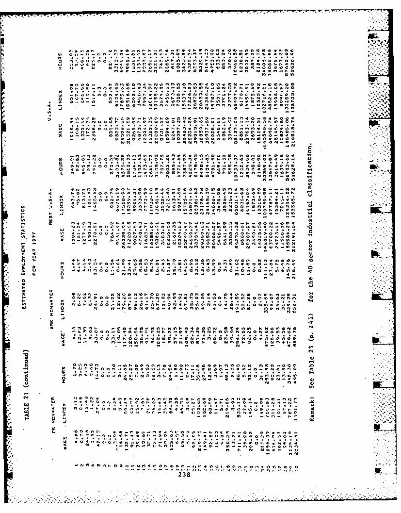
*I7c ~ .. r r r too C. f. N t- N r. 41 0-~ -In 04 0 InC Cr11 0 )It1,C

In or - C IA -I mI r o)4~ ~F lV0.)F I in 0 M 0 . in 0. N -0 wY~-~

WIf)

Ft 2 e- ;; -; AZ ! t 1 1f $4 - J -0 f nf VI)a t

J N- -- CV.N N - -0 6 rnin4A - --

tC . ) F'A N q N 0 O ' f) C t- ~ 0 I.) 0 4 N C ' '0) ; 0 - ' 0 N Q n ifl -Joi 0 Q 'lt Ft In o 00 up N w * m 0 0 W m * *Y 0 * 0 *t * .4 1

- * ~ ~ ~ ~ ~ N M M NCiONiin0Ain 0 N NV-I4 .0 -

0-. CYOD -.lIn N -l0 Ill)' In 0-I 0PC% N 0 M 4'0N100 -

In .4 *- N M a. * * N . . M N.. . ..- . 1, in I . . " CIO 0 0 1. % 0 44

F)4 .44' N fl0114 0 -NC N M M M - 0- ..

13.*n 4C0P o00P IC N0'0WC.D.NF)Cin.., N P)) 4t-'; M -aNVI l

4 .t a 0.. . . . . . . . . . . . . . .. . . .N.. . . . . . . .f- M InI ; on I 7I F100 ~ F F C- N ) V ~ n 0 ).0NF0 o tno I41%In

l- N ll1 -0 -- w

1-I- o" 0 o )C'0N C

l' 0 d 0*0 0 I4 COt"fl CNF)N CC00'0 M 0 1-4 0 0 .0 -' C'00 n%0 01 . NM 0fD4O

C% it- - N 1-40 N 0 fl.0 0 4 NoNVINC0 m0)in In)NCI on 3 o"- in t $z Z N N n NfN i N to N -4'a-0 0 .CD

C* Of- nI 0 -n K 0II -Of F) In- NN 4-11 von i -1P2v N 4

0o

w QrNN-. ONNO0.mot CM;O M0)Jn-VFi4F M004 LNw I P M47Oi- 41.- ON') I0N N -. N O n0IA00.VOF4VLIO0()'0P:)

o z C N -rCO0. 'N - Y0 - 4 0- 0M Inl. 1 4 -NII'Iin to Ill .N m Y I)

C, (I'Cinflp. O44 -tM0 NNo, F40 0 0N I6)taInin 0N)N ' N oin

10 . . * * *.. . * * * . . . .Io . .. . . . * . . . . . .

4 "1 In F. N in m 0 ei fA W.0 0 0 r- 1) e~l61 110 t-T n * 1- 0

PII.. -P-00n 0N000001 IC - N 4- 100

11, t: 4 1; e! tyC 7 *It8 CU CI e* .Y It CD In M . t

o N won

I.-4up Inll WC N 00 40 0 tN-0CJte tfl *I4 t o a I 0 ~0 0q 0 0 4, )0C

4 I) 0

z .

C.~~ P-Nt.. C

- M F 4 Vp .fl 1, V) 0. o N in L'1 o~ P- W, It- C - to M kfl '0 1. on C, ea V% I 4 1, 1, ID i 0 0

238

- 0 0 4U S 1ww U .WW1 -f 1. M nt4

44 40 -- 0-W % A

-P..10 CI 43 0 m o e o r *eii oe w pvN ot i

ek! ON N044NQ

*. N a 000 P M M. y1 4 . 0 M * M in V . a, 'ao 40 j-t M4e4 n0 0 In ~tN.O mp~ 4O o tI- '.m0 N 400

inN eq In PN. 0-0

v 0 0 N. '40.40ea 1C. N W) n 00 . 0 0-O0 0oi 40004 $104*o *C *4 0- 4* * N N * * in q 44. . * M . 4 ***.4

-t 0 on M 00. 00N MP.4 N M 40 oo0 0E400 W n 0..,OQU)m)0 0M 0 PI0o -c t.,aI 0tt -t 0 N4 0 .4M0 0 0

. . .. . . . . .4 .I

44 * Y 0 a** * 0 0 * IN *Y f* M0 i m0 * * .4 In .-O OM - 4l

0- 61 -- M4,04000l00N 0 %000Nmt0 0"0 M4 0 0 w nUNO C

M Mw ni 4 e* 1* *4 * *444 m 4 * 4* m* N 4 444 6!0

4 ) aN .4..t -0 nt LNOOMN)NO t- M 0 NC.Nl-#M 0

o4 x pi Ne-. In - N.p M 0

X ..9M~ In-0 - 3 £N9 I - a0o oN-D0 4m0I

J In 0 061)C%- 0 a-,-TV0,a0P N 1 to r- - 0 C 0O40N 0 V N 1- I4 01tG

2 0 :3 4 j4 4 0 00 N1 N0In* 0 P10 P.0 0?PI 04 C 0 O 0 0IxN4 NN N4 0 M I .4 Ml 04

-t * t

4 01

4A ~ 4 * 1.) M 4 *4 0 * 04I 0. WN0 4 aI- .4tP M. * *4) 4 *1 in M4 * 0 * M

W. M 0. 4...) . 4 Q4. 00 0

-C .3

4M - 4 N 4000-4- -4 '

00, * r o 11t. Q. .11 04* 4.. * 0 * Y 4 , Q 4 .** . . . . . .P)M-t --- 1t e YI-(mnoo C

M faNa.PIM . Y (V Ogn~ 0-N fy vIfn CY -' - V

-t .4 a, P- 4 VN1 - -Ne nI 4L N OnN 01 10 C

44)0 00-NN4 01,00. 0 N of- .- NOO..OO I 0 - f- .. NO C"

C) in C0V001( NO Al1-V 0 N to 40 E.f C0a * . . * * 4~* 4 * *4 * * 4 01

Ci Q C. QC 0M 0 M U6V .. itP 0 d 4 -f1040 4 in ? r- -0a an 4a.. 4Ci 00

S.1

0 2 a. . . y. N INa - .a

- .1 - co

UI . Z)ca0 P).:~ - If.. -~i 0-4) ,( W'.Q4. - 06 '.f C-a I no . .1

a. ~ ~ ~ ~ ~ f F3 v1 40 ey 0 Nn 4) 11 i'. N M" 'p ~ 0 -J P 1. 04 ~0.p 4 f 35. 0) 0- - - - - - - - - - - - - --

. . . . . . . .. . .

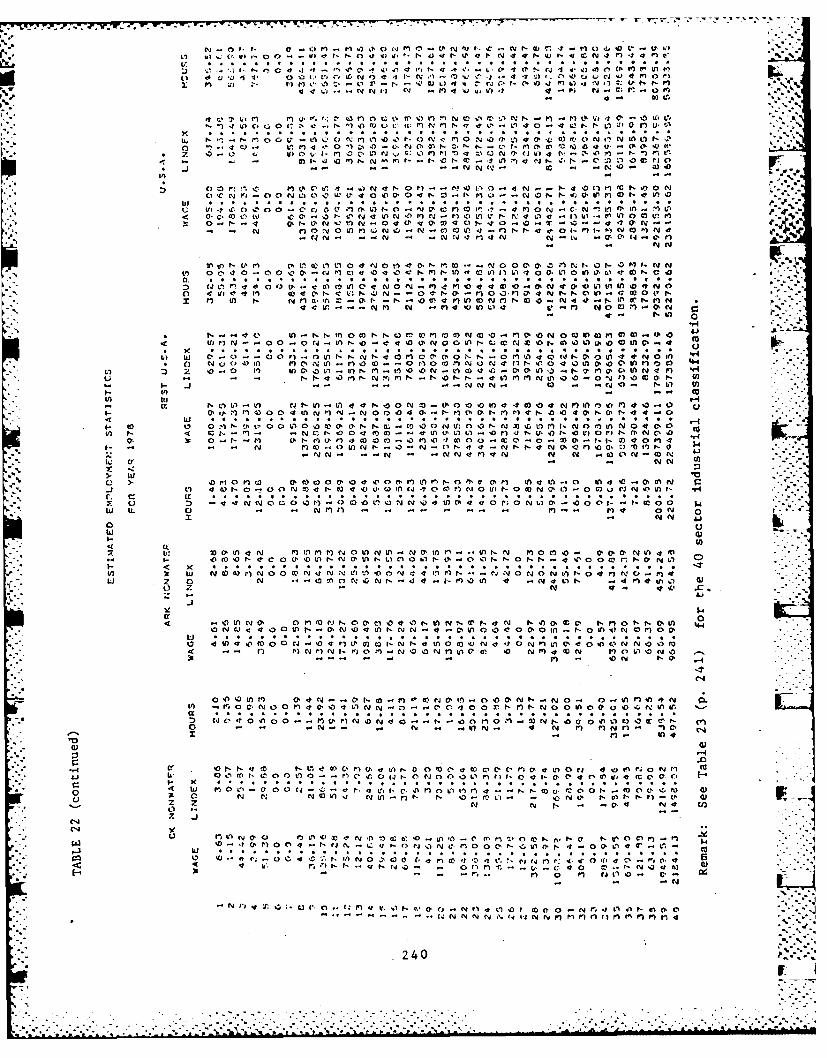
OC E ~1. 1.3r .Pl0 1 nf, 0N4 Yr UC. P

I;., * *

0 4 - 4 f Y1,A It U-(v 1 O N'3r.,'4'3 O N. iN i nL0N '

It f. N. r,- I M 0 '3C. va n3 0 .t 0I 0t -' n y 01 rp I-" . N P, C1 C- V) 0', U'l 4' 1, C'- tr

- ) -! N -4 U-- - - - - ) -N 'r~* N10 W~'43 '

C. r) q ( O0U -. O' ' NiC3'4''3tN a'tffC'0.)0 % '3n3F. t

t- t-)'tr (C 41 ) PrZ ~ ~ ~ ~ ~ C cc 4) I- N0n' N. ~ II ' NO ''', 4 ~ N f( N

0 4 0-- C' N 0M f' a,1) N 1 I -0 11.)PI 1'W.)-' N

P.inN 4 0'U aa - 0 0 _I 1C

*~~c N~4'3~

n. 0. "1, 1."1"1I *.I. l, I!

11 tn I-O'Nfl cc In O I

I-I ) 0 C ) D 0 ( In t- P- -0 <v tr.UIf CY m oI ll40

fN ty NCN im I 00 20Il0c I iI P n0 't c* 4'D CO '3 01 CU Ci O'D 0 (C'N o (O'0 NU:0 I-NC.3o.Ltn )I.Nt- .'In nOC4'M

I-I n--C -n r, N- t C .. I N -3 'N r, It n m CY n -0 0 3 'D Cc0- 1f-- J- NN.V CY ca N N ~COO I- l t

tn - - - to'

> hi0 P- .O OU' 0C O0 4 f- 0)'oI'N 0o o0t 0'" Iftfl-0 3InO'n i 0

C... % . i I? . P: %

CD IL C. -- 9% A. C ')010kr 311 r- Q; 0 N : 0- N. M- -Z, ON M )tV) - C t 00 ( I I I ( 0 0 I 1 U - t 0V)0 i - M N c

ND 00nNN) t 0 Q 0 )' 0 1

cy (2 In

Q) 1- hi NC C O 0 O'3N w IN o ! ), ca n C 4i T C P N U)O- No N q. I >O Q VJ'0 tn -

Li LL N - N, M N-l4.ICrl3f M P)IU .4F)03U' 0 tN Nl 41C

-- 4.2

-L

tn Nr w .IN N 00 0 N 4' ~N 3L N N V, 'I -n C. fv 0* V) n - 0 0 0 (A - 0 IA m4 N 0 m) 00

:*m ao a * f 00 0 -- r, 0 NN) N 0 0!') 4 ' 3NffAO'C '3 NI) CO I'r)OIUN'fON. 4

m 10 - Y 1- N0.

C4

Q AU rmAC1) 1) 0N 01 , 0U Mtl'A4tN Q

0~ ,I )N' a1 m -) rN-. t- 0 a o-UN 4 N 0~ a)f C '

x -. It: V.,

0.

IN

o to V No NL NCC- IN -N ( a ko Inon - A I ML NN U Z,0k 01f' -

7, 0,4

It fl-N'C (. 'ofO 'C)' 0

Ni Il 4 (' O 0 0 - , I " A t

-. N~ ry-:- Yr )F1r) m I r )m r

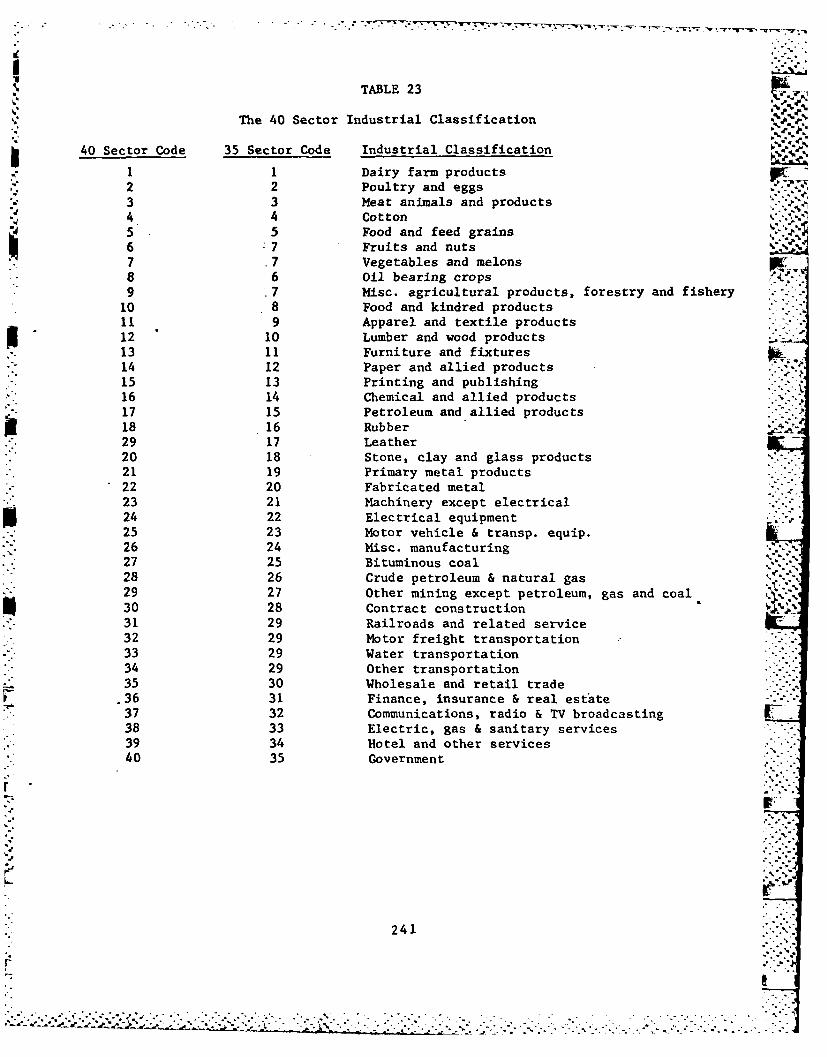
% TABLE 23

The 40 Sector Industrial Classification%

40 Sector Code 35 Sector Code Industrial Classification

1 1 Dairy farm products2 2 Poultry and eggs

*3 3 Meat animals and products4 4 Cotton5 .5 Food and feed grainsI6 ~7 Fruits and nuts7 . 7 Vegetables and melons P.8 6 0Oi. bearing crops

10 8 Food and kindred products

11 9 Apparel and textile productsp -12 10 Lumber and wood products

13 11 Furniture and fixtures14 12 Paper and allied products15 13 Printing and publishing16 14 Chemical and allied products17 15 Petroleum and allied products18 .16 Rubber29 17 Leather20 18 Stone, clay and glass products21 19 Primary metal products22 20 Fabricated metal23 21 Machinery except electrical324 22 Electrical equipment25 23 Motor vehicle & transp. equip.26 24 Misc. manufacturing27 25 Bituminous coal28 26 Crude petroleum & natural gas29 27 Other mining except petroleum, gas and coal30 28 Contract construction31 29 Railroads and related service32 29 Motor freight transportation33 29 Water transportation34 29 Other transportation35 30 Wholesale and retail trade

.36 31 Finance, insurance & real estate37 32 Communications, radio & TV broadcasting38 33 Electric, gas & sanitary services39 34 Hotel and other services40 35 Government

r

241

APPENDIX III

COMPUTER ALGORITHKS

I7-

PRVOS S.

I OLN

24

APPENDIX III: COMPUTER ALGORITHMS

iwiz op unouiuz.PAGE

DBLOCK 245DECOMPJ 246DECOMP 247DMINV248IWINUS 250INITIA* 25 1LEIM* 252..LPRINT* 25.3,MAT 254MULT 255MULTCO 256NEWDAS* 257NULL 258PATINV 259PCHNGE 262PIVOT* 263PRINT 264PRINT 265PTRADE 266RAS 267SELAST 269SORT* 270WLNC 271

*Program needed to solve the linear transportationalgorithms.

EXPLARATION OF SUBROUTINES 273

Entry TA 275SELAST 276PTRADE 276PRINT 276PPRINT 276DBLOCK 276IMINUS 277PATINV 277DMINV 279WLNC 279TCHNGE 28]- w; " '

PCHNGE 281Entry ATB 282HULTCO 282DECOMP 282DECOMPJ 282 %MULT 2B3RAS 283 -

244

SUBROUTINE DBLOCK(ACNollvFU)REAL*8 A (1) PC (1)

DO 20 J1l,HDo 20 1=1,K

CALL NULL (AN)DO 21 J3=1,NDO 21 I1-1,V

LKII1+C33-1) *IYCII -EQ. JJ) A (LK)-C (LL)

* 21 CONTINUE20 RITE(NU'L) (A(KKg,KK=1,WN)

20 CONTINUERETURNEND

4,W.

245S

SUBROUTINE DCOPJ(A,B,CNS,J,N,B,91)RZAL*8 A(1),B(1),C(1)NN=N*NCILL NtILL(B,N) 44

DO 10 I=1,kLL=I+(J-1) *1FIND (N1'LL)JtEAD(N1LL) (A (KK) ,KKlN N)-DO 10 JJ=1,N

DO 10 II=1,NLJ=II+ WJ-1) *N f

10 B (LJ)=B (LJ) +A(LJ)C COMlPUTE THE TRADE COEFFICIENTS

DO 11 I11h

FINDWI1LL)READ (Ni LL) (A (KK) ,KK=1, NN)DO 11 II11,kIC (NS)=0. 0NCT=NDO 12 J1,S

IF (A (L) .EQ.0.O) NCT=NCT-1IF((A(LJ) .EQ. 0.) .OR. (B(LJ) ZEQ.,0.)) G3 TO 12C (NS) =C (NS) +A (UJ)/B (LJ)

12 CONTINUEe'. IF(NCT.LE.0) NCT=1

C (NS) =C (NS) /NCTNS=NS4 1

11 CONTINUERETURNEND

246

V SUBROUTINE DECOMP(AB,C,N,N1,N2)REAL*8 A (1) *B (1) *C(1)

NS= 1+(P-l1) *N*MCALL DCOZIPJ (k,B, C, NS, J, N,M, N1)IIRITE(6,100) 3CALL PRINT (BIS ',NN)VRITE (N2'J) (5(1(K) .KK=1,NN)

10 CONTINUECALL PTRADE (C,NN) x

100 FORMAT'(lHO,1OX,tREGION lo IS,/)RETURNE ND

247

Tv.

CDO 65 1=1,NIK=NK+IJOLD=A (1K)

Do 65 J=1,N* IJ-zIJ+N

IF (I-K) 60,65,6060 IF (J-K) 62,65,6262 KJ=I3-IeK

A (I3) =HOLD*A (KJ) +A (IJ)65 CONTINUE

CC DIVIDE ROW BY PIVOTC OL

KJ=K-NDo 75 J=1,NKJ=KJ4 NIF(J-K) 70,75,70

70 A (KJ) =A (KJ) /BIGA75 CONTINUE

CC PRODUCT OF PIVOTSC

D=D*BIGA

C REPLACE PIVOT BY RECIPROCAL

CA (KK) 1. 0/BIGA

* 80 CONTINUE .-

CC FINAL ROW AND COLUMIN INTERCHANGEC

K=N100 K=(K-l)

IP (K) 150,150,105*105 I=L (K)

18IF(I-K) 120,120,10818JQ=N* (K-i)

DO 110 J=1,NJK=JQ+JHOLD=A(JK)JI=JR+JA (JK) =-A (31)

110 A(JI) =HOLD120 J=LI(K)

IF(J-K) 100,100,125

125 KI=K-NDo 130 1=1,NKI=KI+NHOLD=A (KI)K 3JI=KI -K+J

A(KI) =-A (JI)*130 A(JI) =HOLD 249

GO TO 100150 RETURN I

END

C ~'DO 65 1=1,NIK=NK+IHOLD=A (IK)1J=I-NDO 65 J=I,NIJ=IJ+NIF (I-K) 60,65,60

60 IF(J-K) 62,65,6262 KJ=IJ-I4K

A (IJ) =HOLD*A (KJ) +A (IJ)65 CONTINUE

* CC DIVIDE ROW BY PIVOT

C KJ=K-N -"

DO 75 J=1,NKJ=KJ+ NIF(J-K) 70,75,70

70 A(KJ)=A(KJ)/BIGA75 CONTINUE

cC PRODUCT OF PIVOTS

* CD= D*BIGA

CC REPLACE PIVOT BY RECIPROCALC

A(KK) =1.0/BIGA80 CONTINUE

CC FINAL ROW AND COLUMN INTERCHANGEC

K=N100 K=(K-l)

IF(K) 150,150,105105 1=L (K)

IF(I-K) 120,120,108108 JQ=N* (K-i)

JR=N* (I-1) ."-

DO 110 J=1,NJK=JQ+JHOLD=A (JK)JI=JR+JA (JK) =-A (JI)

110 A(JI) =HOLD120 J=M (K) -

IF(J-K) 100,100,125125 KI=K-N

DO 130 I=1,NKI=KI+NHOLD=A (KI)JI=KI-K+JA (KI) =-A (J1)

130 A(JI) =HOLD 249GO TO 100 -' .

150 RETURN

END * . . .D

SUBROUTINE IlMINUS(A,B,T,N,tf,Nl,N2,MODE)C SUBROUTINE IIIINUS CALCULATE (I-S)

* C IF IIODE=O (I-S) *(I-T HEAD) INVERSEC IF tIODE1l (I-S) t*(I-THEAD) INVERSEC IF (I-S) IS DESIRED, SET THEAD=O AND fODE=0._ 6

REAL*8 A (1) ,T(1) ,B(1) ,TEMPNN=N*NDO 180 .3=1,11DO 180 I=1, M

FIND (Ni' L)READ (Ni 'L) (A (KK) ,KK=1,NN)DO 182 JJ=1,N

DO 182 II=1,NLL=II+ (JJ-l) *NIF((I.EQ.J) .AND. (II.EQ.JJ)) GO TO 181B(LL)=-A(LL)/(1 .-T(JL))GO TO 182

181 D3 (LL) = 1 .- (A (LL) /(1 . -T (J1L))182 CONTINUE

IF (1ODE. EQ. 0) C-O TO 200C TRANSPOSE B

DO 183 K1=1,N1wDO 183 KJ=KI,NKITKJ=KJ+ (KI-1) *NKJKI=KI+ (KJ-1) *N

I TEMP=B(KIKJ)B (KIKJ) =B (KJKI)

*183 B(KJKI)=TEMP*C TRANSPOSE THE BLOCKS

20IF (MkODE . NE. 0.) L=J + (1-1) *

*180 CONTINUERETURNEND

250

-. -. . .o

SUBROUTINE INITIAC SOBROUTINE INITIA WHICH FINDS THE INITIAL A.C. SOLN

COMMON /DUAL/ G(25),H(25)COMION/LPSA/AK (25,25) Q (25)COMION/QPDATA/B(25,25),A(25),MBASIS(50), L1,NLI,NL2,NE1,NE2,IR,.-COMM ON /DATA/ N,MKODE

C SET UP BASE

DO 5 I=1,N,DO 5 J=1,NB (1,3) =o.0B(I,I) =1.0 "'V.

5 CONTINUE

J=29 IF(Q(I) .LE. Q(J))GO TO 18

18 =J+lIF(J .LE. N)GO TO 9I R= IT1=-Q (IR)IF (Ti .GT. 0.0) GO TO 19 =QZ 0I-

1000 FOPtAT(1H0,IINITIAL Q-VECTOR IS NON-NEGATIVE. W Q, Z 0 IS Ox lIHAL.1)

DO 123 I=1,NG (I) =Q (I) I

123 H (I) =0.0

RETURN

19 DO 10 I=1,NQ(I) Q (I) T1

Q (I) =T1DO 12 J=1,NB(J,IR)=-1.0MBASIS (J) =1L= N+JK=K+1MBASIS (L) =K

12 CONTI.UE -

NL1=1L=N+IRNL2=IRMBASIS (IR)=3MBASIS (L)=0ZO=Q(IR)

RETURN 251END i

SUBROUTINE LErMKE(XADS,KDIMENSION XA(1),DS(1)COMMlON/LPSA/AM (25,25) ,Q (25)CO1MON/QPDAT/B(25",25),A(25),BBASIS(50), L1,NL1,NL2,NS1,NE2,IR,M 1 PECOMMON /DATA/ NMNKODE

N=KDO 100 I=1,N

100 Q(I)=DS(I)ICHOI= 0DO 40 J=1,N -! !DO 40 I=I,NICHO I=MCHOI+ 1

40 AmII(,3)=XA(AIMCHOI)C READ H AND Q MATRIX

CALL INITIAIF(.EQ.1) GO TO 51

50 CALL NEWBASIFU (MEQ. 1) GO TO 51CALL SORTIF(i .EQ. 1) GO TO 51CALL PIVOTGO TO 50 H5 1 R E T U R N .-"-

END

252

• .. . . .. . . . . . •.* * *. . * .* : .- ~

SU R UT N S - - - -

-'.

C PRITS OU CURRNT S..TI-

PUROTIN 1000 N

C

IF (HON/QPDATA/B(EQ. ) GO25.BAI (50) 20N1N2NEER

P0RIOTT1000

DOO10

20 1(2 = MBASIS (I)IF (K(2 .EQ. 2) G0 TO 40

30 G (0)=Q (I)H (J)=0.0PRINT 1010,J,Q(I)

1010 FOR NAT (2 1 X,13, 8X G 15. 8)GO TO 100

40 H (J)Q(I)G (J)0O.0PRINT 1020,J,Q(I)

1020 FOPMAT (21X,13,27X,G15.8)GO TO 100

C90 IF (NL1 .LT. 3) GO TO 50

=MiIF (NEI .EQ. 1) GO TO 30GO TO 40

50 G(J)0O.OH (p) =0. 0PRINT 103C),J,Q(h1)

1030 FORMAT (21X,1I3,46XGI5.8)100 CONTINUE

PRINT 150, (G(I) H(I) I=1,N)150 FORrATc1H-,10X,'THIS IS A W VECTOR'.1OXslTHIS IS A Z VECTOR'/

*1 (1OX,F15.8,14X,G15.8))RETURNEND

* 253

77r

•- %

SUBROUTINE MAT(XO,R,C,NR,NC)" REAL XO(NRNC),R(1),C(1),XA(25,25),DS(25),EP(25,25),X1(625)

Kl=NR*NCK2=NR+NC1(3=1(1+12

,, DO 10 3=1 ,K3DO 10 I=1,K3

10 XA(I,J)=O.O . -.

.DO 15 J=1,K1DO 15 1=1,K2

15 TEIP (I,J) =0. 0

DO 20 1=1,NRIT=IDO 20 J=1,NCTEMP (IIT) =-1.0

20 IT= IT+ NRC

DO 30 I=1,NCI=I+NRDO 30 J=1,NR3J=3J+ 1

30 TEMP(II,JJ)=1.0C" '..C GENERATE XA MATRIX FOR REHKEC

DO 40 I=1,K2DO 40 J=1,K ..1

40 XA (I+K1,J) =TEMP (I,J)DO 50 J=1,K1DO 50 I=1,K2

50 XA (J, I+K1) =-TEHP (I,J)KT=0DO 80 J=1,NC-DO 80 1=1,NRKT=KT+ 1

80 DS (KT) =XO (I)KT=K1DO 60 I=1,NR

60 DS (KT+I) =R (1)KT=K +NR -DO 70 J=1,. C

70 DS (KT+J) =-C (3)IU=0-DO 18 J=1,K3,DO 18 I=1,K3IU=IU+ 1

18 Xl (IU)=XA(IJ)CALL LEMKE(X1,DS,K3) -'

RETURNEll D " -: "

254

%, ." ."*" ".% "* , . - - . . . ."."

.'-" .,. .

-~~ SUBROUTINE HULT(AB*C,tI,X1NU1,NU2,NU3)

CC SUBROUTINE MULT COMPUTES THE PARTITIONED MULTIPLICATION A*B C

p.NN=N*NDO 12 K=1NfDO 12 3=1.1*NC=J+(K-i) *dCALL NULL (C,N)DO 11 I=1,NLB=I* (K-i) *5LA=J+(I-i) *MREAD (NU1OLA) (A (KK) KK=l1N)READ (N U21LB) (B (KK) .KK=l NN)DO 11 J3=1,N -

DO 11 11=1,3DO 11 KK=1,N

KA=114 (KK-1)*NKB=KK+ (J3-1)*N

11 C (LC) =C (LC) +A (KA) *B (KB)12 WRITE JN13 INC) (C KK) , K= 1,,NN)

RETURNEND

4..t -77.-

SUBROUTINE ?ULTCO(B,C,D,A,N,M,N1,N2)REAL*8 A (1) ,B(l) C(l) ,D(l)NN=N*N ,

DO 10 J=1,MSDO 10 1=1,ML=I+ (J-1) *NREAD(N1'L) (B (KK) ,KK= 1,NN)DO 11 JJ31,NDO 11 II=1,NLL114 (JJ- 1 )*N

ILSRIII+ (1- ) *N+ (J-1) *N*liLSI=II+ (I-1) *NA (LL) D (LRJ) -C (LSRI) -D (LSI)A (LL) =B (LL) *DEXP (A (LL))

11 CONTINUEWITE (N2tL) (A (KK) ,KK1lNN)

-P.-.10 CONTINUERETURN

* END

or.

256

SUBROUTINE MEWDAS -COHMION/LPS A/ANi (2 5, 25) Q0(25)COZ1MON/QPDATA/B(25,25) ,A(25),EB&SIS (50), L1,NL1,NL2,NZ1,VE2,IR.H1COMMION /DATA/ N,31,KODZIF((NLI .LT. 3) .AND. (Q(11) .Gr..I.E-12)) GO TO 20

1000 FORMIAT (IH1, 'ITERATIONI NUM53B T4,& COMPLEMENTARY SOLUTION.')

RETURNIC

.20 NEI = 3 NOI~NE2 = NL2

17 (INLl GT. 1) GO TO 21

*27 DO 26 1-1,N

DO 28 3=1,128 TI = TI - B(1.3) *ANl(J,NE2)

A (1)=T126 CONTINUE

29 A ()=B (,N2RETURN

41.1

257

SUBROUTINE NULL (D, N)REAL*8 D(l)N N= N* NDO 10 1=1,NN

10 D(I)0.0 PFR ETURBNEND

-258

SUBRIOUTINE PATINV(ABCDNM,UlU2,U3,LX,MX)REAL*8 A (1) gB (1) ,C (1) rD (1) oDDINTEGER U1,12vU3,G,HRLX(1)sHX(1)fill M-i1NNIN*NFIND(U1'1)READ(U1'1) (A(KK)gXK=1.NN)CALL DMilNV(A,N,DD,LXNX)WRITE (U21 1) (A (K K) ,KK=V11)DO 200 B=1,MI1Do 30 G=1,RCALL ZIULL(D,3)DO 30 H=1,RFIND (U 21 (G ft*(Of- 1))READ(U2@(G+*ff*CB1))) (A(KK)sKK1.NXN)FIND (U 1' (R*1M+H) )R BAD (U I (R*M+Hi) (B (KK) ,KK= 1, N)DO 10 .1=1,NDO 10 J=1,N

DO 10 L-1,V

LJ=L+(J-l)*N10 D (IJ)=D (IJ)+A (IL) *B(LJ)

*30 WfITE(U3'G) (D (KK) ,KK1, pNN)CC COMPUTE (D-CA(-1) B)C#

CALL NULL CAN)DO 40 G=1,ltFIN4D(U 11 I*(G- 1) +R+1))READ(U1' (H* (G-1) +R+1)) (C(KK) KK=1,NN)FIND(U38G)READ(TJ3'G) (D(KK),KK=1,NI)

CC MULTIPLY AND ACCUMULATEC

DO 40 J=1,NDO 40 1=1,N

DO 40 L-1#1

LJ3L4(3-1)*N* 40 A (r3) =A (13) +C (IL) *D (LJ)

CC OBTAIN Hr-(D-C*A (-I) *B) (-1)

FIND (Ul 1(I1*+)

READ (U1'((,i+1) *Rl)) (D (KK) KKzsl NN)DO 70 J=1,NDO 70 1=1,9

CALL DKINV(DN,DD,LXMX)

WRT U#cMl Rl (D(KK).ICK=1,INI-

C BIN )'1

VC**.~***,**...* .* 259. *t

DO 100 G=1,RREAD(U3'G) (B(KK),KK=1,NN)DO 90 J=1,NDO 90 1=1,NIJ=I J-1) *NC (IJ) =O. 0DO 90 L=1,NIL-I (L-1)*NLJ=L+(J-1)*N p- '

90 C (IJ) =C (Iu) -B (IL) *D (LJ)100 WEITZ (U21 (R*11+G)) (C (KR) ,KK=1,NN)

cC OBTAIN C*A(-1)C

DO 120 G=1,RCALL NULL (DN)DO 110 H=1,RFIND (U2' (H+M* (G-l)))READ (U2' (H+M* (G-1)) (A (KK),KK=lNN)FIND (Ul' (1+R+M*(H-1)))READ (Ul' (1+E+M* (H-1)) ) (C (KK) ,KK=I,NN)DO 110 1=1,NDO 110 J=1,N.IJ=I+ (J-l) *N-DO 110 L=1,NIL=I+ (L-i)*N.LJ=L+ (J-1) *N

110 D (I) =D (IJ) +C (IL)*A (LJ)120 WRITE(U3' (M M+G)) (D(KK) ,KK=1,NN)

CC COMPUTE G=-HCA(-1)C AND STOREC

FIND (U2' ( (M ) *R+I))READ (U21 {( ( I) *R+I)} ( KK , =I N )- . .

DO 141 G=1,RCALL NULL (A,N)FIND (U3' (MM+G))READ (U3' (MM G)) (C (KK) ,KK= 1,NN)DO 140 J=1,NDO 140 =I,N13=1+ (J-1) *NDO 140 L=1,NIL=I+ (L-1)*NLJ=L+ (J-1) *N

140 A (IJ) =A (IJ) -B (IL) *C (LJ)141 WRITE (U2' (1+f+M* (3-I))) (A (KK) ,KK=1,NN)

CC COMPUTE A (-1)B*GC

DO 180 G=1,RFIND (U2' (1+R+M*(G-1)))READ (U2' (I+l+li* (G-1))) (A (KK) ,KK=1,N N)DO 180 11=,RFIND (U 3' I1)READ (U3'H) (B (KK) ,KK= 1, NNFIND(U2' (H+M*(G-I1)READ (U2' (H +1* (3- 1))) (C (KK) ,KK= I, NN)

260

._ . '.; . . . . . ., - . ' -. . - -. - . . . . - . . -_ -_ - . ,: - .. . . . ., . . . . ' - . . , . " .

'a. c

DO 160 J=1,NDo 160 1=1,NIJ=1+ (3-1) *1

DO 160 L=1,N7L=I+ (L-1) *NL.'L+ (J-1) *N

160 : .13) =D (13) +B (IL) *A (LJ)DO 161 J=1,NDO 161 I=1,N13J=T+ (J-1) *N

.161 C (IJ)=C (13)-D (IJ)180 WRITE (U21 (H +,I*(G-1) (C (KK) KK= 1, NN)

CC END 0F ROUNDc

20 MRITE(6,1000) R100FORMAT(1OX,lROUND 11L4,f IS OVER')

RETURNEND

.261 -

SUBROUTINE PCHNGE(A, B, DP, N, 11,0)INTEGER UlREAL*8 A(l),B(l),DP(1)LCK=OGO TO 20ENTRY ATB (A,D,DP,N,l1,U1)LCK=1

20 CONTINUEN ?1N * tNN=N*NDO 9 KK=1,Nft

9 DP(KK)=O.CIF(LCK .EQ. 1) GO TO 21DO 10 I=1,11

* DO 10 3=1,11L=14'(J-1)*HFIND(U1'L)

LK1=14 (3-1) *NDO 11 11=1,NKK=II+ (I-i)*NDO 11 JJ=1,NLL=II. (J3-1)*NLK=LK1 33-1

*11 DP (KK) =DP (KK) +A (LL) *B (LK).10 CONTINUE

RETURN21 CONTINUE

DO 22 3=1,11DO 22 1=1,H1L=1 (J-1) *11RED(U1'L) (A(K),IC=1,NN)LX1=1.(J-1)*NDO 23 J3=1,NKK=JJ P-1) *NDO 23 11=1,N1

* LL=II+ (JJ-1) *NLK=LK 1+11-1

23 DP (KK) =DP (KK) +A (LL) *B (LK)22 CONTINUE

RETURNEND

262

Or -7-

SUBROUTINE PIVOTCOMMlON/LPSA/AM1(25,25) ,Q (25)COflHON/QPDATA/B(25,25) ,A(25),!MBASIS(5O), L1,NL1,3L2,V.E1,NE2,IR,Ni1COMM1ON /DATA/ N,fl,KODEDO 301=,14

30 B (IR, I)=B (IR, I)/A (IR)Q (IR) =Q(I R) /A(IR)DO 31 I = 1,N4IF (I .EQ. IR)GO TO 31Q (I) =Q (I) - Q (IR) A 1(I)DO 32 J =1,N '

B(I,J) =B(I,J) -B(IR,J) *A(I)32 CONTINUE31 CONTINUE33 NL1=MBASIS (IR)

L 14+11kL2=IBASIS (L)?IBASIS (IR) =NE1MBIASIS (L)=NE2L1=L141RETURBNEND

w

263

SUBROUTINE PRNtvs*l

BEAL*8 A(1)vBNN= N*NDO 10 J=1,MDO 10 I=1,M f z1L=I+ W3-1) *tNREAD(Nl#L) (A(KK),KK=1,NN)

10 CALL PRINT (A,N*N)RETURNENTRY S PRINT (A, BN,tN, Ni)NN=N*NDO 11 3=1,MREAD(N1'J) (A (KK) , K=1 ,NN)

11 CALL PRINT (A, BeN, N)RETURNEND

.2 61

SUBROUTINE~ PRINT (X,k,NRNC)4. PEAL*8 X(1) ,A

WHITE(6,1O1) A 3%33

4. KK-011=1NJI=NCNN=110

33 CONTINUEI? (N1. GT.N111) NPF10-NN+NJ 1IF(NII.GT.NJ1) KK=1IF (KK. EQ. 1) NN=NJ1

114 FORMUAT (/,6X,10 (8X,14) ,/)NRNN=NB*NNDO 43 1=1,NRLB=I+NB* (NN-10)IF(KK.EQ.1) LB=I+NR*(NN-NP)

413 WRITE (6, 115) 1, (X (J) , JLB, NRNN, K R)

115 FORflIAT(5XI£1,5X,1OG11.1)IF (NN. EQ. NC) GO To 34

INNN+ 10GO To 33

34 RETURNEND

26 5

SUBROUTINE PTRADE(CNI!1)

DO 10 11=1,NWHITE(6,100) IIWRITE(6, 1 O1) (J,J=1,H)DO 11 1=1#M1LS= 114 (I-i) *N

LI= N*I111 VRITE(6,102) To (C(LL) LL=LS,LT,LT)10 CONTINUE

* 100 FOPIIAT(l0,20X.'INDUSTRY 0 ,13,//)* 101 FORMAT (13X,10(1I,13,4X) /

102 FORIHAT (57,I5*5X.1O (77.5, iX))RETURNEND

26A~

SUBROUTINE RAS(A,U,VRS,N1,N2,XA,T,IR,ERR)REAL*8 U (1) ,V (1) ,XA() ,A(1) ,R) ,S (1) ,T (1)INTEGER IR(1)

C XA: INPUT BASE MATRIXC A OUTPUT NEW MATRIX,.'_"C V COLUMN VECTOR-"-,.C V :ROW VECTOR""':'";'

c VI: NUMBER OF ROWC N2: NUMBER OF COLUMN

* C T & IR ARE WORKING VECTORSC SIZE OF T & IR SHOULD BE MAX(N1,N2)

* CN12=N1 *N2DO 60 I=1,1112 3-.

60 A (I) = XA MI ..

DO 65 1=1,1"'65 R (1) 1.0

DO 66 J=1,N2.66 S(J)-1.0

KSTOP=O -.

70 CONTINUEKSTOP=KSTOP+-IF (KSrOP-100) 222,223, 222

223 RITE(6,1)1 FORMATC('0, 'INFINITELOP********4******'/

RETURN222 DO 75 I1=,Nl75 IR (I) =0

DO 80 1=1,N1T (I) =0. 0DO 85 3=I,N12,N'

85 T (I) =T (I) +A (J)IF(TI) .EQ. 0.0) GO TO 71

T (I) =U (I)/T (I)R(I)=R(I)* T(I)IF(DABS(DABS( T(I))-1.0) .LT. ERR ) IR(I)=1GO TO 80

71 T(MI=1. 0 .R(I) =1.0IR (I) = 1

80 CONTINUEKK=ODO 90 J=1,N2

* DO 90 1=l,N1KK=KK+-

90 A (KK) =T (I) *A (KK)DO 115 1=1,N1IF(I(I) .NE.1) GO TO 70

115 CONTINUEC

DO 76 3=1,N276 IR (J) =0

NU=ODO 95 J=I,N2 267T (J) =0.0DO 100 1=1,N1NU=NU + 1

5..... .-.. -. , ..--* ,.* - A-. ., ,, . . -... .. .. . ...

100 T(J) =T (3) +A (NOl)IFP(T (J) . EQ. 0. 0) GO TO 102TCW) =V P)/T (J)S PJ) =S (J) *T (J)IF (DABS (DABS( T(3f)l.0).LT. ERR )IR(J)=1GO -TO 95

102 T()=1.0S (3)=1.0IR (J)=1

95 CONTINUEDO 105 I1,N1KK=IDO 105 J1l,N2A (KK) =A (KK) *T (3)

105 KK=KK+N1* DO 110 J=1,N2

IF (IR (J).NE.1) GO TO 70110 CONTINUE

RETURNEND

-

268

SUBROUTINE SELkSTITr3 9 C,A,N,H1,N1.N 2 )

GOTO 12

ENTRY TA(TB,AONl,N1.N2)

12 LCK=O12 CONTINUE

U N=N* NDO 10 Jw1.M

DO 10 1=1#ML.+ (J-1) *11DO 11 JJ=1,NJL=J3t(J-1)*NDO 11 II=1,N

A (LL) =T(LT) *B (LL)IF (LCK. EQ. 1) A(LL) uA(LL) /(1.-C (JL))

11 CONTINUEWRITE(1N2'L) (A(KK),oKK=1*NN)

10 CONTINUERETURNEND

269

-'-* " J~ ~ ~ ,W "~ " I-~~.- - r - * ,"~- ~ '~ T J . "bwI-

SUBROUTINE SORTCOMMON INOSO/ NSOKCOMZiON/LPSA/AI (25,25) ,Q (25).COMMON/QPDATA/B (25,25) ,A (25), iBASIS (50), LI, NLI, NL2, NE1, NE2, IR,Ml 1COMMON /DATA/ N,M,KODECOMMON /CHOI/ KKCDIMENSION IVAR(2)DATA IVAR/2HW(,21Z(/I=I52 IF (A(I).GT.O0)GO TO 51

I=I+1GO TO 52

51 T1=Q (I)/A (I)IR=I

55 I=I+1IF (I.GT.N) GO TO 56

53 IF (A (I) .GT. 0.0) GO TO 54GO TO 55

54 T2=Q(I)/A(I)IF(T2.GE.T1)GO TO 55IR=ITl=T2GO TO 55 ,-%

56 IRTYP = MBASIS(IR)IF (IRTYP .GT. 2) GO TO 100

K2 = MBASIS (IR.+N)100 RETURN .--57 CONTINUE

250 FORMAT(IH0,OITERATION NUMBER 1,14,0. PROBLEM HAS NO COMPLEMENTARY1 SOLUTION.')

M=l'KKC=2NSOK=NSOK+KODE=MRETURNEND

270 .

%H

7 w-~ -,,7 o- -- ;- Z -- W- r'oW

SUBROUTINE WLNC(VC*ZNflrfil)REkL*8 W (1)*C (1)PZC(1)N N=N* N

DO 9 I=1,NH

DO 10 J=1,11DO 10 I=1,M

FIND (N1'L)REkD(Nl'L) (W (KK) KK=1, ON)DO 11 JJ=1,NLA=JJ+ (3-1) *NDO 11 11=1,NLL=II+ (JJ-1)*N

11 7. (LA) = Z (LA) +W (LL) *C (LB)

-10 CONTINUERETURN

-' END

L27.

* EXPLANATION OF SUBROUTINES

'O'J$' . ,

ff, VtS :8LAGE

273

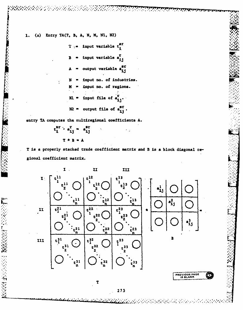
1. (a) Entry TA(T, B, A, N, M, N, 1N2) V.. :

T m input variable tr

rB Input variable a

A -output variable a

N input no. of industries.

M -Input no. of regions.

rHl Input file of aii

Sr _O-

N2- output file ofai•-

entry TA computes the multiregional coefficients A.

ar. r or a"to a - a lI aT B A

T is a properly stacked trade coefficient matrix and B is a block diagonal re-

gional coefficient matrix.

*1,-I. II III

: t n

22 2 S :::t ;12 0 \ " .n

t~l 2 2 23

2 22 230

2 0 2 0 2

2 ...

n n n

275 _***f 32 33

7* 7

all a.12 a 1 3

a21 a22 a23ii ii

a31 a32 a33ij ij ij

(b) Subroutine SELAST (T, Bs C, A, N, M9 Ni, N2)

Sinput T,B, C,N, M, N1output -A, N2

Subroutine SELAST computes input elasticities after obtaining multiregional

4coefficients as entry TA.- L where tistax rate.

i-t

-.2. (a) Subroutine PTBADE (C, N, M)

Subroutine PTRADS prints out trade coefficients among regions of each

commodity._

(b) Subroutine PRINT (X, A, NR, NC)

Subroutine PRINT prints out X values under name 'A' in matrix form with no.

of rows - HR and no. of columns - NC.

(cSubroutine PPRINT (A, B, N, H, NI)

Subroutine PPRINT reads all nine A's from file W1 and prints out all A's

under name B with no. of rows -N and No. of columns MN.

entry SPRINT (A, B, N, M, Ni)

entry SPRINT reads 1st three A's from file Ni and prints out lot three A's

under name B with no. of rows *N and no. of columns Ml.

(d) Subroutine DBLOC( (A, C, N, M, NU)

276

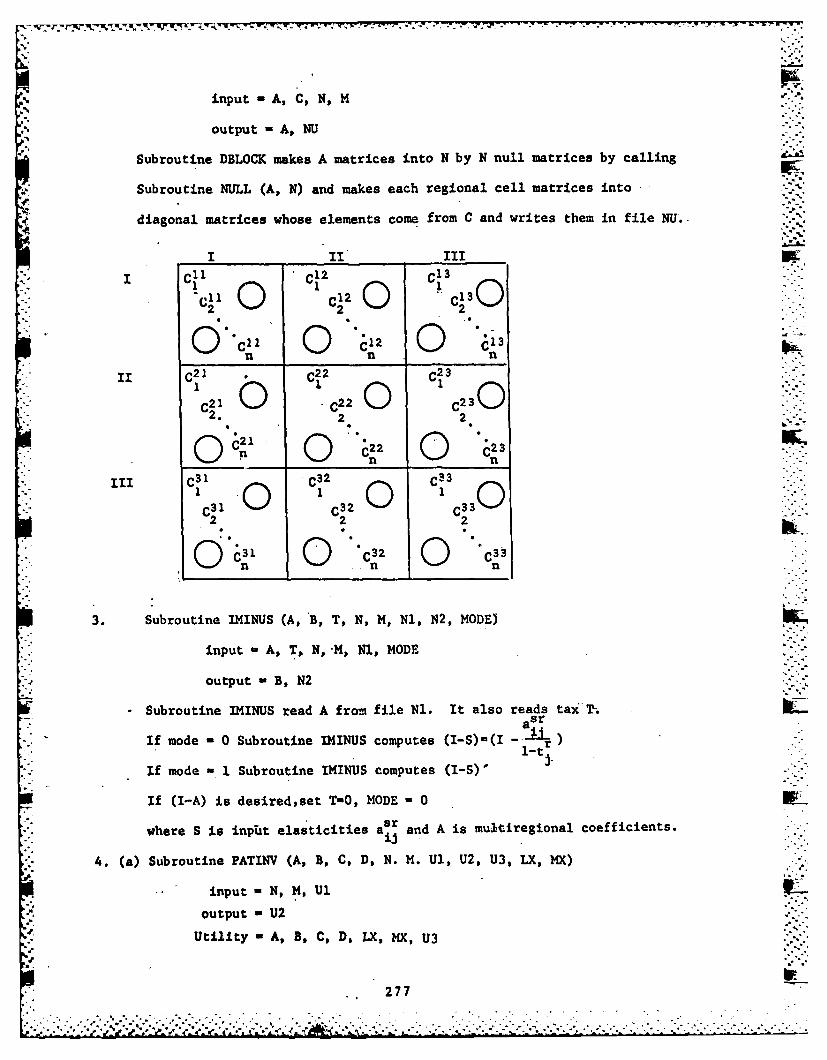
input -A, C, N, M

output - A, NU

Subroutine DBLOCK makes A matrices into N by N null matrices by calling

Subroutine NULL (A, N) and makes each regional cell matrices into

diagonal matrices whose elements come from C and writes them in file NU..

'-. cC 2 c13O" 0 0 2:"--- 0l 2 613 00

)C2 C22 C)-3,.-C21 0 c22 0c230..2

2.2

SC2' C2

0 A 0 *n 0 -n

01i C3 3

0101320C02 2 2

QC n *n n

3. Subroutine IMINUS (A, 'B, T, N, M, Nl, N42, MODE)

input - A, T, N, HM, 141, MODE

output -1B, +2

Subroutine IMINUS read A from file Nl. It also reads tax?. C.

sIIf mode 0 Subroutine IINUS computes (I-S)( r

If mode -1 Subroutine IMINUS computes (I-S)'

If (I-A) is desired,set TO0, MODE - 0 L

where S is inplit elasticities asr and A is multiregional coefficients.

4. (a) Subroutine PATINV (A, B, C, D, N. M. Ul, U2, U3, LX, MX)

input N, M, Ul

output U2

SUtility - A, B, C, D, LX, MX, U3

277

.. . ..... . . . c

. .. .-. * .

- ..- * 9*

Subroutine PATINV is the partitioned bordering inversion routine.

-,. This algorithm is necessary to invert the hugh interregional flow matrices,

i.e. it can invert the multi-region, multi-industry variable input-output

matrices. Efficient use of computer time and space is the key problem of

multi-regional input-output study.

By using block-data system and decomposition of the inverting process,

we call only the blocks which are required for computation (i.e., block-

wise computation is feasible)..

To invert 3 region 35 industry input-output matrices: - II

(1) On 1st Iteration, we set 11 12 M3M. '

-- T~ I21 23.. ~~2

'.-I I , 1! M 3.

.,.

L.L LO I4 1II .C DFi.o

where M is 35 by 35 matrix.where I is a 35 by 35 identity matrix. -,

'FA B "" ""'

:.: ~ ~~21 M22 :-1.-;'

We compute E, F, G, H as follows:

H (D CA -B)

F -- A7 B H._ ;-:-(Ref: Goldberger, Econometric Theory,

C - HCA I 1963, John Wiley & Sons, Inc.)

.E A-BG

(2) .On 2nd Iteration, we set

'" III .where A = -E-I--H],A B G ;H_,=.-.

III B M

-13

"' 23 . .

C M31132]D [ M3

278

a _,o -. . -,.° *-.. . *. .* a . . -

":" ,".' ... '" , , . .. . " . . .. ". . . -. . .. ., , ." _ . . . .- '-'".', ," ,,." '- . . .,

and

'00III C H.

We can find new H, F,*G, E from the formula in (1).

Since our present study is 3 region 35 industry I-0 matrices, we stop after

2nd iteration. For a regions n industry I-0 matricep, we need to stop after

* (m-l)th iterations.

4. (b) Subroutine DHINV (At N, D, L9 M)

*input - A, N

output - D

utility =L; M

5. Subroutine 14LNC (W, C, Z, N, M, Ni)

-input iW,C, N,M, Nl

output Z

*Subroutine WLNC computes the weighted rate of change in transportation costs.

Z W lnC

(nm, 1) (nm, nmm) (nmm, 1

* ~~~279..5....

H- 1- H

H H H H H 4' H H

H- HPH H H-

H- H - 14

.- 4 C 4 -4 r- -4 C -4 .*4 C: enC - C

0 -

1-4 1- - 4 i- - . '4 ,4s

Cj r,-4r

1-41-

H3

H .)

Ht

H-

1-41-

N4- INC-

04 0. e. r"W N

H28

where Z C1 a ~ 2 nC11 + all inC11 + .. + ctll inC11 + l nC2 1 + a21 inC2 +1%11 11 1 21 2 ni n 11 1. 21 2 V

* .. + 2 1 inC2 1 + a31 inC 31 + a~l inC31 + .. + a131 nC31

*nl n 1n1 2 l ~~41 21

in general

:m n ~ rZ i E E a ij nC (for i1 1,2,3 and j =1,2, .. ,n)

r1l k=l k

* 6. Subroutine TCHNCE (TCC, ICC, C, I, J, K, N, M)

input =TCC, ICC, I, J, K, N, N

output =C

aSubroutine TCHNGE assigns selected transport cost changed industries among

*the regions and computes the transport cost changes in dollars.

7. (a) Subroutine PCHNGE (A, B, DP, N, M, Ul)

input = A, B, N, M, Ul

output = DP

Subroutine-PCHNGE computes the multiplication of partitioned

matrices with partitioned vector to get partitioned vector.

dln' (I-S) *WdlnC

DP A B

Subroutine PCHNGE is used to compute rate of change in regional output

prices.

2g 1

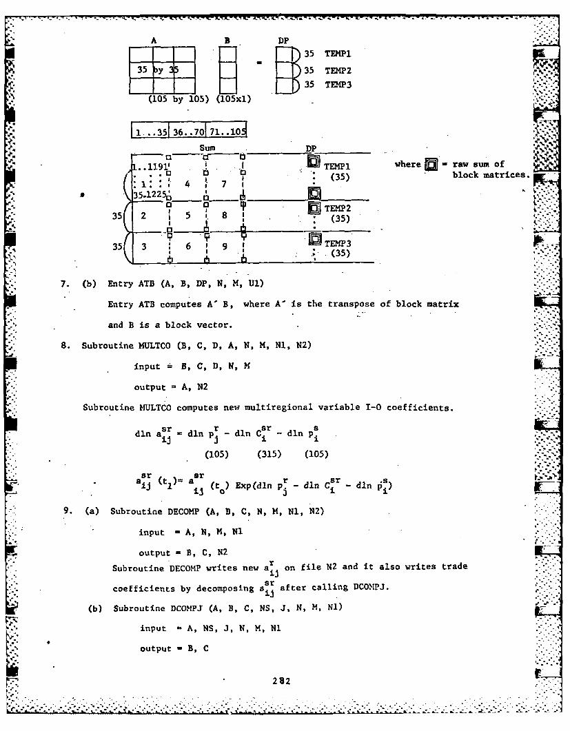
A B - DP 5 TEMP •1

I I * 35 TEMPI

35 y 35 TEMP235 TDIP3 ;:-,_e

(105 by 105) ( 1),'.-,

11 ..35 36..70 71.-10

Sum DP __-,______

.-1191, i . whee .raw sum of.• 3 .3 ,3• (35) block matrices.0y.. ,4 7 I .. (35)

\35.12255 j.I

35 2 050o'----p --TEMP235 2 5 (3'YII - I, lS

35 3 6 ' 9 ,1. 3 Ia. -

_a . .. -..(35) .

7. (b) Entry ATB (A, B, DP, N, M, UI)

Entry ATB computes A' B, where A' is the transpose of block matrix

and B is a block vector.

8. Subroutine MULTCO (B, C, D, A, N, M, NI, N2)

input = B, C, D, N, H

' output - A, N2

" Subroutine MULTCO computes new multiregional variable 1-0 coefficients.

dnar r Sr dnpsdlnan -dinCi - din p ,

(105) (315) (105) .. *..

sr s adrin '..Ba aj (t I a (t) Exp(dn pr dln Cs - dln

9. (a) Subroutine DECOMP (A, B, C, N, M, NI, N2)

input - A, N, M, Ni

output = B, C, N2

Subroutine DECOMP writes new a ijon file N2 and it also writes trade

srI .. coefficients by decomposing a after calling DCOMPJ.

ij

(b) Subroutine DCOMPJ (A, B, C, NS, J, N, M, NI)

V input A, NS, J, N, M, NI

output B, C

~282

sr r sSubroutine DCOMPJ decomposes a into ajad t1 yuinrh

following formulas.

.J*.*E sr r

sr

ai. s

n ij ±ij

10. Subroutine HULT (A, B,:C, N, M, NU1, NU2, NU3)

input -A, B, N, M, NUl, N1J2

output - C, NU3

Subroutine MULT computes the partitioned multiplication A-B=C

A B -- C

All A12 A1 11 312 B23 '1 C12 01 3

A21 A22 A23 * 21 322 323 = c2l c22 c23

31 32 33 31 32 33 31 32 33A A JA B B B- C C C

where each cell is a matrix of 35 by 35 elements.

11. Subroutine RAS (A, U, V, R, S, Ml, N2, XA, T, IR, ERR) --

input mA, U, V, Nl, N2, ERR

output -R, S, XA, IR

utility-= T

* Subroutine RAS estimates each elements of trade flow matrices of the target

year 1972. The RAS requires a base year 1963 data (A) and target year row

sums(V) and column sums(U).

283

The RAS is computed as follows:

(ref: Bacharach, M. Biproportional Matrices and input-outputchange, Cambridge, 1970)

base year A " target year At

S. column column

sumsu

E°-a°Ij I PEI

row sum row sum

0

(2) a" r-i aij

(3) Si0

- Zr-*a

Ui ia

2 0

i .at i-j-i(4) aij - e a '

(5) if MinVr, s) -1 c, then stop.

0 0Otherwise, set a -r ai a

i. i i.'

284

73: --. ..

- . ~ - .

~. .%*.

5~4

I F

4

g 9-.

9.

**1

,.~1

1.4 491~~~~~~

'V(I-

* * .

$tg.rh ~ ~ i~-~9 - A.~",? .. '.pYi> 2:: .:-~.i..-x ,~ - * *.