The Eh-pH Diagram and Its Advances - MDPI
30
metals Article The Eh-pH Diagram and Its Advances Hsin-Hsiung Huang Received: 29 July 2015; Accepted: 28 December 2015; Published: 14 January 2016 Academic Editors: Suresh Bhargava, Mark Pownceby and Rahul Ram Metallurgical and Materials Engineering, Montana Tech, Butte, MT 59701, USA; [email protected]; Tel.: +1-406-496-4139; Fax: +1-406-496-4664 Abstract: Since Pourbaix presented Eh versus pH diagrams in his “Atlas of Electrochemical Equilibria in Aqueous Solution”, diagrams have become extremely popular and are now used in almost every scientific area related to aqueous chemistry. Due to advances in personal computers, such diagrams can now show effects not only of Eh and pH, but also of variables, including ligand(s), temperature and pressure. Examples from various fields are illustrated in this paper. Examples include geochemical formation, corrosion and passivation, precipitation and adsorption for water treatment and leaching and metal recovery for hydrometallurgy. Two basic methods were developed to construct an Eh-pH diagram concerning the ligand component(s). The first method calculates and draws a line between two adjacent species based on their given activities. The second method performs equilibrium calculations over an array of points (500 ˆ 800 or higher are preferred), each representing one Eh and one pH value for the whole system, then combines areas of each dominant species for the diagram. These two methods may produce different diagrams. The fundamental theories, illustrated results, comparison and required conditions behind these two methods are presented and discussed in this paper. The Gibbs phase rule equation for an Eh-pH diagram was derived and verified from actual plots. Besides indicating the stability area of water, an Eh-pH diagram normally shows only half of an overall reaction. However, merging two or more related diagrams together reveals more clearly the possibility of the reactions involved. For instance, leaching of Au with cyanide followed by cementing Au with Zn (Merrill-Crowe process) can be illustrated by combining Au-CN and Zn-CN diagrams together. A second example of the galvanic conversion of chalcopyrite can be explained by merging S, Fe–S and Cu–Fe–S diagrams. The calculation of an Eh-pH diagram can be extended easily into another dimension, such as the concentration of a given ligand, temperature or showing the solubility of stable solids. A personal computer is capable of drawing the diagram by utilizing a 3D program, such as ParaView, or VisIt, or MATLAB. Two 3D wireframe volume plots of a Uranium-carbonate system from Garrels and Christ were used to verify the Eh-pH calculation and the presentation from ParaView. Although a two-dimensional drawing is still much clearer to read, a 3D graph can allow one to visualize an entire system by executing rotation, clipping, slicing and making a movie. Keywords: Pourbaix diagram; Eh-pH diagram; Eh-pH applications; ligand component; equilibrium line; mass balance point; Gibbs phase rule; 3D Eh-pH diagrams; ParaView; VisIt; MATLAB 1. Introduction All Eh-pH diagrams are constructed under the assumption that the system is in equilibrium with water or rather with water’s three essential components, H(+1), O(´2) and e(´1); the oxidation states are presented using Arabic numbers with a + or a ´ sign. The diagrams are divided into areas, each of which represents a locally-predominant species. Eh represents the oxidation-reduction potential based on the standard hydrogen potential (SHE), while pH represents the activity of the hydrogen ion (H + , also known as a proton). An Eh-pH diagram can describe not only the effects of potential and pH, Metals 2016, 6, 23; doi:10.3390/met6010023 www.mdpi.com/journal/metals
-
Upload
khangminh22 -
Category
Documents
-
view
1 -
download
0
Transcript of The Eh-pH Diagram and Its Advances - MDPI
metals
Article
The Eh-pH Diagram and Its AdvancesHsin-Hsiung Huang
Received: 29 July 2015; Accepted: 28 December 2015; Published: 14 January 2016Academic Editors: Suresh Bhargava, Mark Pownceby and Rahul Ram
Metallurgical and Materials Engineering, Montana Tech, Butte, MT 59701, USA; [email protected];Tel.: +1-406-496-4139; Fax: +1-406-496-4664
Abstract: Since Pourbaix presented Eh versus pH diagrams in his “Atlas of Electrochemical Equilibriain Aqueous Solution”, diagrams have become extremely popular and are now used in almostevery scientific area related to aqueous chemistry. Due to advances in personal computers, suchdiagrams can now show effects not only of Eh and pH, but also of variables, including ligand(s),temperature and pressure. Examples from various fields are illustrated in this paper. Examplesinclude geochemical formation, corrosion and passivation, precipitation and adsorption for watertreatment and leaching and metal recovery for hydrometallurgy. Two basic methods were developedto construct an Eh-pH diagram concerning the ligand component(s). The first method calculatesand draws a line between two adjacent species based on their given activities. The second methodperforms equilibrium calculations over an array of points (500 ˆ 800 or higher are preferred), eachrepresenting one Eh and one pH value for the whole system, then combines areas of each dominantspecies for the diagram. These two methods may produce different diagrams. The fundamentaltheories, illustrated results, comparison and required conditions behind these two methods arepresented and discussed in this paper. The Gibbs phase rule equation for an Eh-pH diagram wasderived and verified from actual plots. Besides indicating the stability area of water, an Eh-pHdiagram normally shows only half of an overall reaction. However, merging two or more relateddiagrams together reveals more clearly the possibility of the reactions involved. For instance, leachingof Au with cyanide followed by cementing Au with Zn (Merrill-Crowe process) can be illustratedby combining Au-CN and Zn-CN diagrams together. A second example of the galvanic conversionof chalcopyrite can be explained by merging S, Fe–S and Cu–Fe–S diagrams. The calculation ofan Eh-pH diagram can be extended easily into another dimension, such as the concentration ofa given ligand, temperature or showing the solubility of stable solids. A personal computer is capableof drawing the diagram by utilizing a 3D program, such as ParaView, or VisIt, or MATLAB. Two 3Dwireframe volume plots of a Uranium-carbonate system from Garrels and Christ were used to verifythe Eh-pH calculation and the presentation from ParaView. Although a two-dimensional drawingis still much clearer to read, a 3D graph can allow one to visualize an entire system by executingrotation, clipping, slicing and making a movie.
Keywords: Pourbaix diagram; Eh-pH diagram; Eh-pH applications; ligand component; equilibriumline; mass balance point; Gibbs phase rule; 3D Eh-pH diagrams; ParaView; VisIt; MATLAB
1. Introduction
All Eh-pH diagrams are constructed under the assumption that the system is in equilibrium withwater or rather with water’s three essential components, H(+1), O(´2) and e(´1); the oxidation statesare presented using Arabic numbers with a + or a ´ sign. The diagrams are divided into areas, eachof which represents a locally-predominant species. Eh represents the oxidation-reduction potentialbased on the standard hydrogen potential (SHE), while pH represents the activity of the hydrogen ion(H+, also known as a proton). An Eh-pH diagram can describe not only the effects of potential and pH,
Metals 2016, 6, 23; doi:10.3390/met6010023 www.mdpi.com/journal/metals
Metals 2016, 6, 23 2 of 30
but also of complexes, temperature and pressures. By convention, Eh-pH diagrams always show thethermodynamically-stable area of water by two dashed diagonal lines.
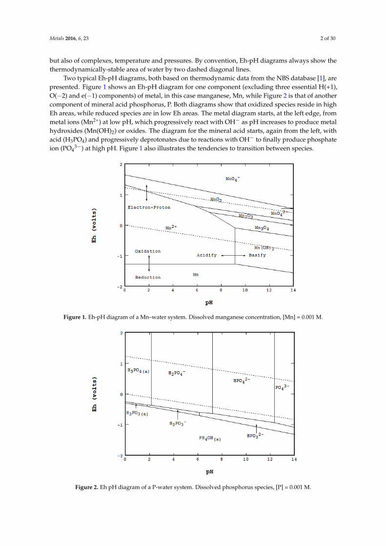
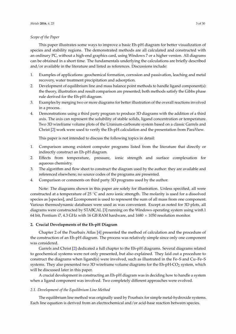
Two typical Eh-pH diagrams, both based on thermodynamic data from the NBS database [1], arepresented. Figure 1 shows an Eh-pH diagram for one component (excluding three essential H(+1),O(´2) and e(´1) components) of metal, in this case manganese, Mn, while Figure 2 is that of anothercomponent of mineral acid phosphorus, P. Both diagrams show that oxidized species reside in highEh areas, while reduced species are in low Eh areas. The metal diagram starts, at the left edge, frommetal ions (Mn2+) at low pH, which progressively react with OH´ as pH increases to produce metalhydroxides (Mn(OH)2) or oxides. The diagram for the mineral acid starts, again from the left, withacid (H3PO4) and progressively deprotonates due to reactions with OH´ to finally produce phosphateion (PO4
3´) at high pH. Figure 1 also illustrates the tendencies to transition between species.
Metals 2016, 6, 23 2 of 30
and pH, but also of complexes, temperature and pressures. By convention, Eh-pH diagrams always
show the thermodynamically-stable area of water by two dashed diagonal lines.
Two typical Eh-pH diagrams, both based on thermodynamic data from the NBS database [1],
are presented. Figure 1 shows an Eh-pH diagram for one component (excluding three essential H(+1),
O(−2) and e(−1) components) of metal, in this case manganese, Mn, while Figure 2 is that of another
component of mineral acid phosphorus, P. Both diagrams show that oxidized species reside in high
Eh areas, while reduced species are in low Eh areas. The metal diagram starts, at the left edge, from
metal ions (Mn2+) at low pH, which progressively react with OH- as pH increases to produce metal
hydroxides (Mn(OH)2) or oxides. The diagram for the mineral acid starts, again from the left, with
acid (H3PO4) and progressively deprotonates due to reactions with OH- to finally produce phosphate
ion (PO43-) at high pH. Figure 1 also illustrates the tendencies to transition between species.
Figure 1. Eh-pH diagram of a Mn–water system. Dissolved manganese concentration, [Mn] = 0.001 M.
Figure 2. Eh pH diagram of a P-water system. Dissolved phosphorus species, [P] = 0.001 M.
Figure 1. Eh-pH diagram of a Mn–water system. Dissolved manganese concentration, [Mn] = 0.001 M.
Metals 2016, 6, 23 2 of 30
and pH, but also of complexes, temperature and pressures. By convention, Eh-pH diagrams always
show the thermodynamically-stable area of water by two dashed diagonal lines.
Two typical Eh-pH diagrams, both based on thermodynamic data from the NBS database [1],
are presented. Figure 1 shows an Eh-pH diagram for one component (excluding three essential H(+1),
O(−2) and e(−1) components) of metal, in this case manganese, Mn, while Figure 2 is that of another
component of mineral acid phosphorus, P. Both diagrams show that oxidized species reside in high
Eh areas, while reduced species are in low Eh areas. The metal diagram starts, at the left edge, from
metal ions (Mn2+) at low pH, which progressively react with OH- as pH increases to produce metal
hydroxides (Mn(OH)2) or oxides. The diagram for the mineral acid starts, again from the left, with
acid (H3PO4) and progressively deprotonates due to reactions with OH- to finally produce phosphate
ion (PO43-) at high pH. Figure 1 also illustrates the tendencies to transition between species.
Figure 1. Eh-pH diagram of a Mn–water system. Dissolved manganese concentration, [Mn] = 0.001 M.
Figure 2. Eh pH diagram of a P-water system. Dissolved phosphorus species, [P] = 0.001 M. Figure 2. Eh pH diagram of a P-water system. Dissolved phosphorus species, [P] = 0.001 M.
Metals 2016, 6, 23 3 of 30
Scope of the Paper
This paper illustrates some ways to improve a basic Eh-pH diagram for better visualization ofspecies and stability regions. The demonstrated methods are all calculated and constructed withan ordinary PC, without a high-end graphics card, using Windows 7 or a higher version. All diagramscan be obtained in a short time. The fundamentals underlying the calculations are briefly describedand/or available in the literature and listed as references. Discussions include:
1. Examples of applications: geochemical formation, corrosion and passivation, leaching and metalrecovery, water treatment precipitation and adsorption.
2. Development of equilibrium line and mass balance point methods to handle ligand component(s):the theory, illustration and result comparison are presented; both methods satisfy the Gibbs phaserule derived for the Eh-pH diagram.
3. Examples by merging two or more diagrams for better illustration of the overall reactions involvedin a process.
4. Demonstrations using a third party program to produce 3D diagrams with the addition of a thirdaxis. The axis can represent the solubility of stable solids, ligand concentration or temperature.Two 3D wireframe volume plots of the Uranium-carbonate system based on a classic Garrels andChrist [2] work were used to verify the Eh-pH calculation and the presentation from ParaView.
This paper is not intended to discuss the following topics in detail:
1. Comparison among existent computer programs listed from the literature that directly orindirectly construct an Eh-pH diagram.
2. Effects from temperature, pressure, ionic strength and surface complexation foraqueous chemistry.
3. The algorithm and flow sheet to construct the diagram used by the author: they are available andreferenced elsewhere; no source codes of the programs are presented.
4. Comparison or comments on third party 3D programs used by the author.
Note: The diagrams shown in this paper are solely for illustration. Unless specified, all wereconstructed at a temperature of 25 ˝C and zero ionic strength. The molarity is used for a dissolvedspecies as [species], and Σcomponent is used to represent the sum of all mass from one component.Various thermodynamic databases were used as was convenient. Except as noted for 3D plots, alldiagrams were constructed by STABCAL [3] running on the Windows operating system using win8.164 bit, Pentium i7, 4.3 GHz with 16 GB RAM hardware, and 1680 ˆ 1050 resolution monitor.
2. Crucial Developments of the Eh-pH Diagram
Chapter 2 of the Pourbaix Atlas [4] presented the method of calculation and the procedure ofthe construction of an Eh-pH diagram. The process was relatively simple since only one componentwas considered.
Garrels and Christ [2] dedicated a full chapter to the Eh-pH diagrams. Several diagrams relatedto geochemical systems were not only presented, but also explained. They laid out a procedure toconstruct the diagrams when ligand(s) were involved, such as illustrated in the Fe–S and Cu–Fe–Ssystems. They also presented two 3D wireframe volume diagrams for the Eh-pH-CO2 system, whichwill be discussed later in this paper.
A crucial development in constructing an Eh-pH diagram was in deciding how to handle a systemwhen a ligand component was involved. Two completely different approaches were evolved.
2.1. Development of the Equilibrium Line Method
The equilibrium line method was originally used by Pourbaix for simple metal-hydroxide systems.Each line equation is derived from an electrochemical and/or acid-base reaction between species.
Metals 2016, 6, 23 4 of 30
Garrels and Christ used Fe–S as an example to show that the same procedure presented byPourbaix could be applied to a multicomponent system. Basically, it involved two separate steps:domain areas of ligand S were first constructed, then all Fe species (including Fe–S complexes) weredistributed in each isolated area of the ligand species. Huang and Cuentas [5] presented a computeralgorithm to construct this type of diagram using an early personal computer.
2.2. Development of the Mass Balance Point Method
Forssberg et al. [6] constructed several Eh-pH diagrams related to chalcopyrite, CuFeS2, byperforming equilibrium calculations for the whole system at once at each given Eh and pH. By doingso, the Cu:Fe:S ratio could be strictly maintained to 1:1:2 at all points. They used the SOLGASWATERprogram developed by Eriksson [7] to perform the calculation. This point-by-point mass balancemethod identifies the predominant species at each given point of Eh and pH. Points of the same specieswere combined into an area for the final diagram. The SOLGASWATER program used free energyminimization, which is commonly used for equilibrium calculation. Woods et al. [8] also presenteddiagrams for the Cu–S system using SOLGASWATER.
The mass balance method can also be computed considering the law of mass action(Huang et al. [9]). This approach simultaneously solves all equations, equilibria and mass balances, ateach given point of Eh and pH. As with the free energy minimization method, the final diagram has tobe plotted by grouping calculated results together. presented later, was reconstructed using the law ofmass action for Cu–S and matched with from Woods et al. [8].
Besides matching the mass input, these diagrams reveal the presence of multiple solids asrestricted only by the Gibbs phase rule. The key to the success of using the point-by-point method,however, is the resolution of the grids used in the calculation. Except for 3D diagrams, all mass balancediagrams in this paper were constructed using grids of at least 400 ˆ 800.
3. Applications for the Diagrams
Eh-pH diagrams are widely used in many areas where an aqueous system is affected byoxidation-reduction and/or acid-base reactions, ligand complexation, temperature or pressure.The following three examples are presented to illustrate these effects.
3.1. Geochemical Formation
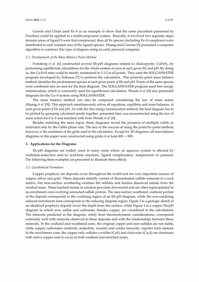
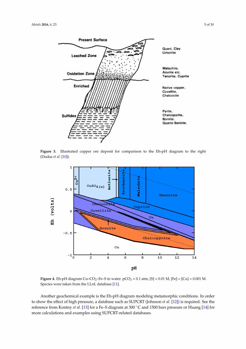
Copper porphyry ore deposits occur throughout the world and are very important sources ofcopper, silver and gold. These deposits initially consist of disseminated sulfide minerals in a rockmatrix, but near-surface weathering oxidizes the sulfides and leaches dissolved metals from theresidual mass. These leached metals in solution percolate downward and are often reprecipitated inan enrichment zone overlying unreacted sulfide protore. The near-surface weathered, oxidized portionof the deposit corresponds to the oxidizing region of an Eh-pH diagram, while the non-oxidizingreduced enrichment zone corresponds to the reducing diagram region. Figure 3 is a geologic sketch ofan idealized porphyry deposit versus the depth from the surface, while Figure 4 is a copper Eh-pHdiagram in which iron, sulfur and carbonate, besides copper, are considered in the calculations.The minerals predicted in the diagram, solely from thermodynamic considerations, correspondextremely well with minerals observed in these deposits and with the relationships between theseminerals. In the oxidized and weathered zone, the original copper and iron sulfides are not stable,while copper carbonates (antlerite, malachite, azurite) and oxides (tenorite, cuprite) form instead.In the enrichment zone, the copper-only sulfides covellite (CuS) and chalcocite (Cu2S) are dominant,with native copper seen to occur in both oxidized and enriched zones.
Metals 2016, 6, 23 5 of 30Metals 2016, 6, 23 5 of 30
Figure 3. Illustrated copper ore deposit for comparison to the Eh-pH diagram to the right (Dudas et al. [10]).
Figure 4. Eh-pH diagram Cu–CO2–Fe–S in water. pCO2 = 0.1 atm, [S] = 0.01 M, [Fe] = [Cu] = 0.001 M.
Species were taken from the LLnL database [11].
Another geochemical example is the Eh-pH diagram modeling metamorphic conditions. In
order to show the effect of high pressure, a database such as SUPCRT (Johnson et al. [12]) is required.
See the reference from Kontny et al. [13] for a Fe–S diagram at 300 °C and 1500 bars pressure or
Huang [14] for more calculations and examples using SUPCRT-related databases.
Figure 3. Illustrated copper ore deposit for comparison to the Eh-pH diagram to the right(Dudas et al. [10]).
Metals 2016, 6, 23 5 of 30
Figure 3. Illustrated copper ore deposit for comparison to the Eh-pH diagram to the right (Dudas et al. [10]).
Figure 4. Eh-pH diagram Cu–CO2–Fe–S in water. pCO2 = 0.1 atm, [S] = 0.01 M, [Fe] = [Cu] = 0.001 M.
Species were taken from the LLnL database [11].
Another geochemical example is the Eh-pH diagram modeling metamorphic conditions. In
order to show the effect of high pressure, a database such as SUPCRT (Johnson et al. [12]) is required.
See the reference from Kontny et al. [13] for a Fe–S diagram at 300 °C and 1500 bars pressure or
Huang [14] for more calculations and examples using SUPCRT-related databases.
Figure 4. Eh-pH diagram Cu–CO2–Fe–S in water. pCO2 = 0.1 atm, [S] = 0.01 M, [Fe] = [Cu] = 0.001 M.Species were taken from the LLnL database [11].
Another geochemical example is the Eh-pH diagram modeling metamorphic conditions. In orderto show the effect of high pressure, a database such as SUPCRT (Johnson et al. [12]) is required. See thereference from Kontny et al. [13] for a Fe–S diagram at 300 ˝C and 1500 bars pressure or Huang [14] formore calculations and examples using SUPCRT-related databases.
Metals 2016, 6, 23 6 of 30
3.2. Corrosion and Passivation
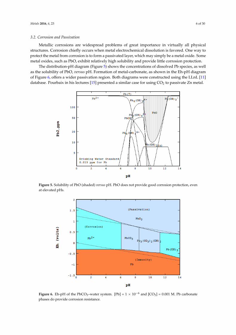
Metallic corrosions are widespread problems of great importance in virtually all physicalstructures. Corrosion chiefly occurs when metal electrochemical dissolution is favored. One way toprotect the metal from corrosion is to form a passivated layer, which may simply be a metal oxide. Somemetal oxides, such as PbO, exhibit relatively high solubility and provide little corrosion protection.
The distribution-pH diagram (Figure 5) shows the concentrations of dissolved Pb species, as wellas the solubility of PbO, versus pH. Formation of metal-carbonate, as shown in the Eh-pH diagramof Figure 6, offers a wider passivation region. Both diagrams were constructed using the LLnL [11]database. Pourbaix in his lectures [15] presented a similar case for using CO2 to passivate Zn metal.
Metals 2016, 6, 23 6 of 30
3.2. Corrosion and Passivation
Metallic corrosions are widespread problems of great importance in virtually all physical
structures. Corrosion chiefly occurs when metal electrochemical dissolution is favored. One way to
protect the metal from corrosion is to form a passivated layer, which may simply be a metal oxide.
Some metal oxides, such as PbO, exhibit relatively high solubility and provide little
corrosion protection.
The distribution-pH diagram (Figure 5) shows the concentrations of dissolved Pb species, as
well as the solubility of PbO, versus pH. Formation of metal-carbonate, as shown in the Eh-pH
diagram of Figure 6, offers a wider passivation region. Both diagrams were constructed using the
LLnL [11] database. Pourbaix in his lectures [15] presented a similar case for using CO2 to passivate
Zn metal.
Figure 5. Solubility of PbO (shaded) versus pH. PbO does not provide good corrosion protection, even
at elevated pHs.
Figure 6. Eh-pH of the PbCO3–water system. [Pb] = 1 × 10⁻⁶ and [CO3] = 0.001 M. Pb carbonate phases
do provide corrosion resistance.
Figure 5. Solubility of PbO (shaded) versus pH. PbO does not provide good corrosion protection, evenat elevated pHs.
Metals 2016, 6, 23 6 of 30
3.2. Corrosion and Passivation
Metallic corrosions are widespread problems of great importance in virtually all physical
structures. Corrosion chiefly occurs when metal electrochemical dissolution is favored. One way to
protect the metal from corrosion is to form a passivated layer, which may simply be a metal oxide.
Some metal oxides, such as PbO, exhibit relatively high solubility and provide little
corrosion protection.
The distribution-pH diagram (Figure 5) shows the concentrations of dissolved Pb species, as
well as the solubility of PbO, versus pH. Formation of metal-carbonate, as shown in the Eh-pH
diagram of Figure 6, offers a wider passivation region. Both diagrams were constructed using the
LLnL [11] database. Pourbaix in his lectures [15] presented a similar case for using CO2 to passivate
Zn metal.
Figure 5. Solubility of PbO (shaded) versus pH. PbO does not provide good corrosion protection, even
at elevated pHs.
Figure 6. Eh-pH of the PbCO3–water system. [Pb] = 1 × 10⁻⁶ and [CO3] = 0.001 M. Pb carbonate phases
do provide corrosion resistance. Figure 6. Eh-pH of the PbCO3–water system. [Pb] = 1 ˆ 10´6 and [CO3] = 0.001 M. Pb carbonatephases do provide corrosion resistance.
Metals 2016, 6, 23 7 of 30
3.3. Water Treatment and Adsorption
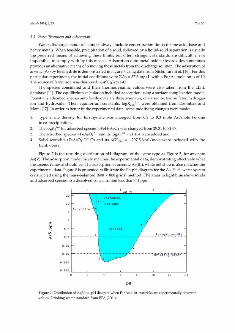
Water discharge standards almost always include concentration limits for the acid, base andheavy metals. When feasible, precipitation of a solid, followed by a liquid-solid separation is usuallythe preferred means of achieving these limits, but often, stringent standards are difficult, if notimpossible, to comply with by this means. Adsorption onto metal oxides/hydroxides sometimesprovides an alternative means of removing these metals from the discharge solution. The adsorption ofarsenic (As) by ferrihydrite is demonstrated in Figure 7 using data from Nishimura et al. [16]. For thisparticular experiment, the initial conditions were ΣAs = 37.5 mg/L with a Fe/As mole ratio of 10.The source of ferric iron was dissolved Fe2(SO4)3:5H2O.
The species considered and their thermodynamic values were also taken from the LLnLdatabase [11]. The equilibrium calculation included adsorption using a surface complexation model.Potentially adsorbed species onto ferrihydrite are three arsenates, one arsenite, two sulfates, hydrogenion and hydroxide. Their equilibrium constants, logKads
int, were obtained from Dzombak andMorel [17]. In order to better fit the experimental data, some modifying changes were made:
1. Type 2 site density for ferrihydrite was changed from 0.2 to 0.3 mole As/mole Fe dueto co-precipitation,
2. The logK1int for adsorbed species ”FeH2AsO4 was changed from 29.31 to 31.67,
3. The adsorbed species ”FeAsO42´ and its logK3
int = 21.404 were added and4. Solid scorodite (FeAsO4:2H2O) and its ∆G0
25C = ´297.5 kcal/mole were included with theLLnL dbase.
Figure 7 is the resulting distribution-pH diagram, of the same type as Figure 5, for arsenateAs(V). The adsorption model nicely matches the experimental data, demonstrating effectively whatthe arsenic removal should be. The adsorption of arsenite As(III), while not shown, also matches theexperimental data. Figure 8 is presented to illustrate the Eh-pH diagram for the As–Fe–S–water systemconstructed using the mass-balanced (600 ˆ 800 grids) method. The areas in light blue show solidsand adsorbed species to a dissolved concentration less than 0.1 ppm.
Metals 2016, 6, 23 7 of 30
3.3. Water Treatment and Adsorption
Water discharge standards almost always include concentration limits for the acid, base and
heavy metals. When feasible, precipitation of a solid, followed by a liquid-solid separation is usually
the preferred means of achieving these limits, but often, stringent standards are difficult, if not
impossible, to comply with by this means. Adsorption onto metal oxides/hydroxides sometimes
provides an alternative means of removing these metals from the discharge solution. The adsorption
of arsenic (As) by ferrihydrite is demonstrated in Figure 7 using data from Nishimura et al. [16]. For
this particular experiment, the initial conditions were As = 37.5 mg/L with a Fe/As mole ratio of 10.
The source of ferric iron was dissolved Fe2(SO4)3:5H2O.
The species considered and their thermodynamic values were also taken from the LLnL
database [11]. The equilibrium calculation included adsorption using a surface complexation model.
Potentially adsorbed species onto ferrihydrite are three arsenates, one arsenite, two sulfates,
hydrogen ion and hydroxide. Their equilibrium constants, logKadsint, were obtained from Dzombak
and Morel [17]. In order to better fit the experimental data, some modifying changes were made:
1. Type 2 site density for ferrihydrite was changed from 0.2 to 0.3 mole As/mole Fe
due to co-precipitation,
2. The logK1int for adsorbed species ≡FeH2AsO4 was changed from 29.31 to 31.67,
3. The adsorbed species ≡FeAsO42− and its logK3int = 21.404 were added and
4. Solid scorodite (FeAsO4:2H2O) and its ΔG025C = −297.5 kcal/mole were included with the
LLnL dbase.
Figure 7 is the resulting distribution-pH diagram, of the same type as Figure 5, for arsenate
As(V). The adsorption model nicely matches the experimental data, demonstrating effectively what
the arsenic removal should be. The adsorption of arsenite As(III), while not shown, also matches the
experimental data. Figure 8 is presented to illustrate the Eh-pH diagram for the As–Fe–S–water
system constructed using the mass-balanced (600 × 800 grids) method. The areas in light blue show
solids and adsorbed species to a dissolved concentration less than 0.1 ppm.
Figure 7. Distribution of As(V) vs. pH diagram when Fe/As = 10. Asterisks are
experimentally-observed values. Drinking water standard from EPA (2001).
Figure 7. Distribution of As(V) vs. pH diagram when Fe/As = 10. Asterisks are experimentally-observedvalues. Drinking water standard from EPA (2001).
Metals 2016, 6, 23 8 of 30Metals 2016, 6, 23 8 of 30
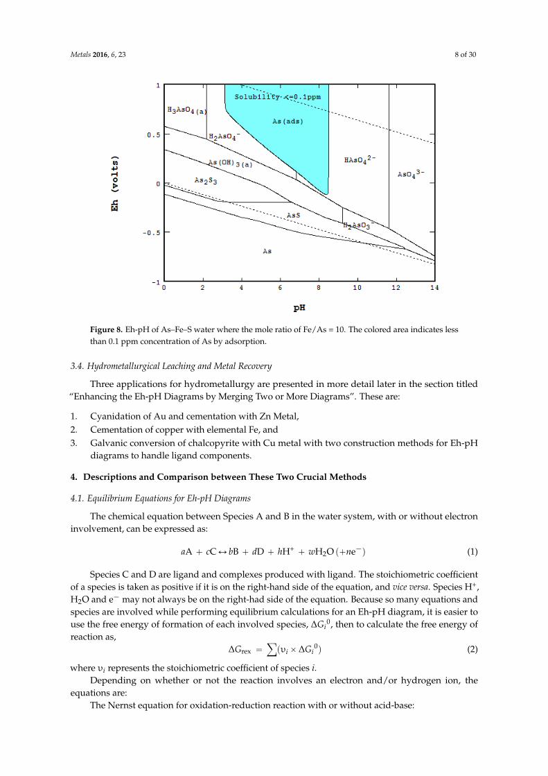
Figure 8. Eh-pH of As–Fe–S water where the mole ratio of Fe/As = 10. The colored area indicates less
than 0.1 ppm concentration of As by adsorption.
3.4. Hydrometallurgical Leaching and Metal Recovery
Three applications for hydrometallurgy are presented in more detail later in the section titled
“Enhancing the Eh-pH Diagrams by Merging Two or More Diagrams”. These are:
1. Cyanidation of Au and cementation with Zn Metal,
2. Cementation of copper with elemental Fe, and
3. Galvanic conversion of chalcopyrite with Cu metal with two construction methods for Eh-pH
diagrams to handle ligand components.
4. Descriptions and Comparison between These Two Crucial Methods
4.1. Equilibrium Equations for Eh-pH Diagrams
The chemical equation between Species A and B in the water system, with or without electron
involvement, can be expressed as:
aA + cC ↔ bB + dD + hH+ + wH2O (+ne−) (1)
Species C and D are ligand and complexes produced with ligand. The stoichiometric coefficient
of a species is taken as positive if it is on the right-hand side of the equation, and vice versa. Species
H+, H2O and e- may not always be on the right-had side of the equation. Because so many equations
and species are involved while performing equilibrium calculations for an Eh-pH diagram, it is easier
to use the free energy of formation of each involved species, ΔGi0, then to calculate the free energy of
reaction as,
ΔGrex = ∑(υi × ΔGi0) (2)
where υi represents the stoichiometric coefficient of species i.
Depending on whether or not the reaction involves an electron and/or hydrogen ion, the
equations are:
The Nernst equation for oxidation-reduction reaction with or without acid-base:
Figure 8. Eh-pH of As–Fe–S water where the mole ratio of Fe/As = 10. The colored area indicates lessthan 0.1 ppm concentration of As by adsorption.
3.4. Hydrometallurgical Leaching and Metal Recovery
Three applications for hydrometallurgy are presented in more detail later in the section titled“Enhancing the Eh-pH Diagrams by Merging Two or More Diagrams”. These are:
1. Cyanidation of Au and cementation with Zn Metal,2. Cementation of copper with elemental Fe, and3. Galvanic conversion of chalcopyrite with Cu metal with two construction methods for Eh-pH
diagrams to handle ligand components.
4. Descriptions and Comparison between These Two Crucial Methods
4.1. Equilibrium Equations for Eh-pH Diagrams
The chemical equation between Species A and B in the water system, with or without electroninvolvement, can be expressed as:
aA ` cCØ bB ` dD ` hH+ ` wH2O p`ne´q (1)
Species C and D are ligand and complexes produced with ligand. The stoichiometric coefficientof a species is taken as positive if it is on the right-hand side of the equation, and vice versa. Species H+,H2O and e´ may not always be on the right-had side of the equation. Because so many equations andspecies are involved while performing equilibrium calculations for an Eh-pH diagram, it is easier touse the free energy of formation of each involved species, ∆Gi
0, then to calculate the free energy ofreaction as,
∆Grex “ÿ
pυiˆ∆Gi0q (2)
where υi represents the stoichiometric coefficient of species i.Depending on whether or not the reaction involves an electron and/or hydrogen ion, the
equations are:The Nernst equation for oxidation-reduction reaction with or without acid-base:
Metals 2016, 6, 23 9 of 30
Eh “ Eh0`
lnp10qRTpnˆ Fq
ˆ
«
log
˜
tBubtDud
tAuatCuc
¸
´ hpH
ff
(3)
where Eh0“
∆Grexpnˆ Fq
, where R is the universal gas constant, 8.314472(15) J/(K¨mol); T is in kelvins; F is
the Faraday constant 96,485.3399(24) J/(V¨ equivalent); and {A} and the others species are defined as theactivities of Species A. The activities of solid and liquid are normally assumed to be one; gas is takenas the atmosphere (atm). The activity of an aqueous solution is the multiplication of the concentrationin mol/L, symbolized as [A], with its activity coefficient. The coefficient can be computed from oneof the appropriate models. Without having the acid-base, the “hpH” term in the equation will bedropped out.
The equilibrium equation for acid-base reaction without redox reaction:
pH “1hˆ
«
log
˜
tBubtDud
tAuatCuc
¸
`∆Grex
lnp10q ˆ RT
ff
(4)
The equation for reaction involves neither an electron nor a hydrogen ion:
log Q´ log K “ log
˜
tBubtDud
tAuatCuc
¸
`∆Grex
lnp10q ˆ RT(5)
Species A will be favored if logQ ´ logK is positive, and vice versa.As mentioned earlier, two different approaches may be used to construct an Eh-pH diagram.
One is to calculate equilibrium equations between pairs of species and to construct the diagramby plotting the resulting equilibrium lines. The other is to perform equilibrium calculations fromall involved species at each point in a grid, then selecting the predominant species at each point.Regardless of which method is used, these equilibrium equations have to be satisfied.
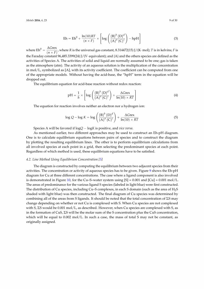
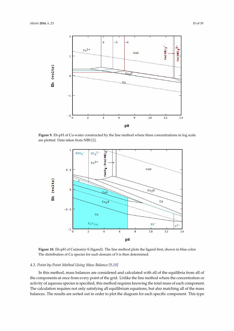
4.2. Line Method Using Equilibrium Concentration [5]
The diagram is constructed by computing the equilibrium between two adjacent species from theiractivities. The concentration or activity of aqueous species has to be given. Figure 9 shows the Eh-pHdiagram for Cu at three different concentrations. The case where a ligand component is also involvedis demonstrated in Figure 10, for the Cu–S–water system using [S] = 0.001 and [Cu] = 0.001 mol/L.The areas of predominance for the various ligand S species (labeled in light blue) were first constructed.The distribution of Cu species, including Cu–S complexes, in each S domain (such as the area of H2Sshaded with light blue) was then constructed. The final diagram of Cu species was determined bycombining all of the areas from S ligands. It should be noted that the total concentration of ΣS maychange depending on whether or not Cu is complexed with S. When Cu species are not complexedwith S, ΣS would be 0.001 mol/L, as described. However, when Cu species are complexed with S, asin the formation of CuS, ΣS will be the molar sum of the S concentration plus the CuS concentration,which will be equal to 0.002 mol/L. In such a case, the mass of total S may not be constant, asoriginally assigned.
Metals 2016, 6, 23 10 of 30Metals 2016, 6, 23 10 of 30
Figure 9. Eh-pH of Cu-water constructed by the line method where three concentrations in log scale
are plotted. Data taken from NBS [1].
Figure 10. Eh-pH of Cu(main)–S (ligand). The line method plots the ligand first, shown in blue color.
The distribution of Cu species for each domain of S is then determined.
4.3. Point-by-Point Method Using Mass Balance [9,18]
In this method, mass balances are considered and calculated with all of the equilibria from all of
the components at once from every point of the grid. Unlike the line method where the concentration
or activity of aqueous species is specified, this method requires knowing the total mass of each
component. The calculation requires not only satisfying all equilibrium equations, but also matching
all of the mass balances. The results are sorted out in order to plot the diagram for each specific
component. This type of diagram is particularly important for Eh-pH diagrams, which include solids
Figure 9. Eh-pH of Cu-water constructed by the line method where three concentrations in log scaleare plotted. Data taken from NBS [1].
Metals 2016, 6, 23 10 of 30
Figure 9. Eh-pH of Cu-water constructed by the line method where three concentrations in log scale
are plotted. Data taken from NBS [1].
Figure 10. Eh-pH of Cu(main)–S (ligand). The line method plots the ligand first, shown in blue color.
The distribution of Cu species for each domain of S is then determined.
4.3. Point-by-Point Method Using Mass Balance [9,18]
In this method, mass balances are considered and calculated with all of the equilibria from all of
the components at once from every point of the grid. Unlike the line method where the concentration
or activity of aqueous species is specified, this method requires knowing the total mass of each
component. The calculation requires not only satisfying all equilibrium equations, but also matching
all of the mass balances. The results are sorted out in order to plot the diagram for each specific
component. This type of diagram is particularly important for Eh-pH diagrams, which include solids
Figure 10. Eh-pH of Cu(main)–S (ligand). The line method plots the ligand first, shown in blue color.The distribution of Cu species for each domain of S is then determined.
4.3. Point-by-Point Method Using Mass Balance [9,18]
In this method, mass balances are considered and calculated with all of the equilibria from all ofthe components at once from every point of the grid. Unlike the line method where the concentration oractivity of aqueous species is specified, this method requires knowing the total mass of each component.The calculation requires not only satisfying all equilibrium equations, but also matching all of the massbalances. The results are sorted out in order to plot the diagram for each specific component. This type
Metals 2016, 6, 23 11 of 30
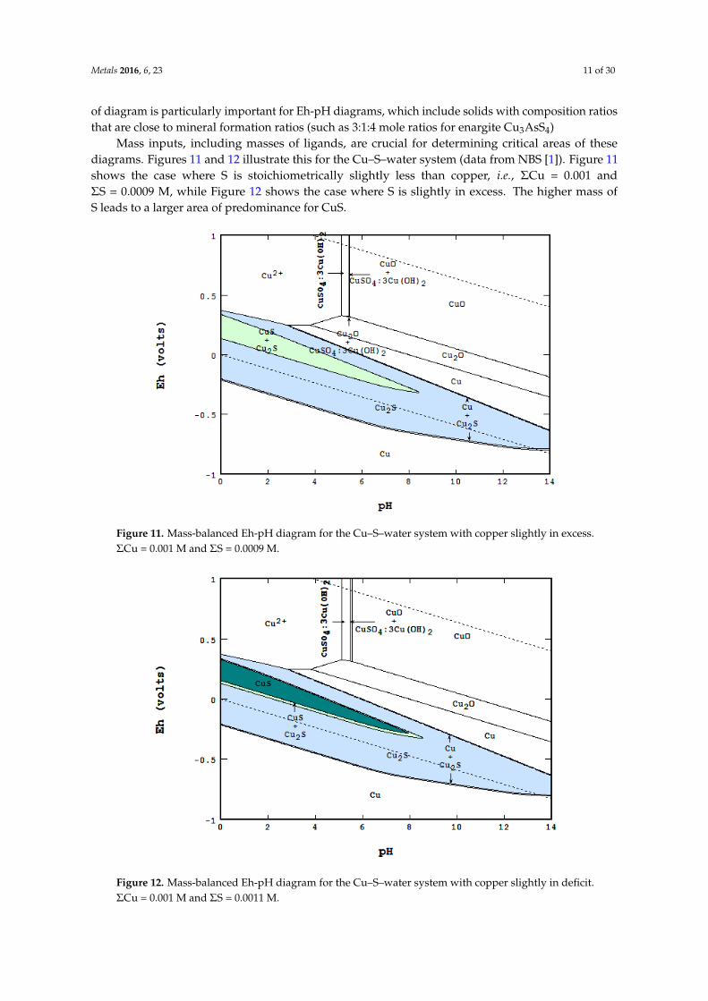
of diagram is particularly important for Eh-pH diagrams, which include solids with composition ratiosthat are close to mineral formation ratios (such as 3:1:4 mole ratios for enargite Cu3AsS4)
Mass inputs, including masses of ligands, are crucial for determining critical areas of thesediagrams. Figures 11 and 12 illustrate this for the Cu–S–water system (data from NBS [1]). Figure 11shows the case where S is stoichiometrically slightly less than copper, i.e., ΣCu = 0.001 andΣS = 0.0009 M, while Figure 12 shows the case where S is slightly in excess. The higher mass ofS leads to a larger area of predominance for CuS.
Metals 2016, 6, 23 11 of 30
with composition ratios that are close to mineral formation ratios (such as 3:1:4 mole ratios for
enargite Cu3AsS4)
Mass inputs, including masses of ligands, are crucial for determining critical areas of these
diagrams. Figures 11 and 12 illustrate this for the Cu–S–water system (data from NBS [1]). Figure 11
shows the case where S is stoichiometrically slightly less than copper, i.e., Cu = 0.001 and S = 0.0009 M,
while Figure 12 shows the case where S is slightly in excess. The higher mass of S leads to a larger
area of predominance for CuS.
Figure 11. Mass-balanced Eh-pH diagram for the Cu–S–water system with copper slightly in excess.
Cu = 0.001 M and S = 0.0009 M.
Figure 12. Mass-balanced Eh-pH diagram for the Cu–S–water system with copper slightly in deficit.
Cu = 0.001 M and S = 0.0011 M.
Figure 11. Mass-balanced Eh-pH diagram for the Cu–S–water system with copper slightly in excess.ΣCu = 0.001 M and ΣS = 0.0009 M.
Metals 2016, 6, 23 11 of 30
with composition ratios that are close to mineral formation ratios (such as 3:1:4 mole ratios for
enargite Cu3AsS4)
Mass inputs, including masses of ligands, are crucial for determining critical areas of these
diagrams. Figures 11 and 12 illustrate this for the Cu–S–water system (data from NBS [1]). Figure 11
shows the case where S is stoichiometrically slightly less than copper, i.e., Cu = 0.001 and S = 0.0009 M,
while Figure 12 shows the case where S is slightly in excess. The higher mass of S leads to a larger
area of predominance for CuS.
Figure 11. Mass-balanced Eh-pH diagram for the Cu–S–water system with copper slightly in excess.
Cu = 0.001 M and S = 0.0009 M.
Figure 12. Mass-balanced Eh-pH diagram for the Cu–S–water system with copper slightly in deficit.
Cu = 0.001 M and S = 0.0011 M. Figure 12. Mass-balanced Eh-pH diagram for the Cu–S–water system with copper slightly in deficit.ΣCu = 0.001 M and ΣS = 0.0011 M.
Metals 2016, 6, 23 12 of 30
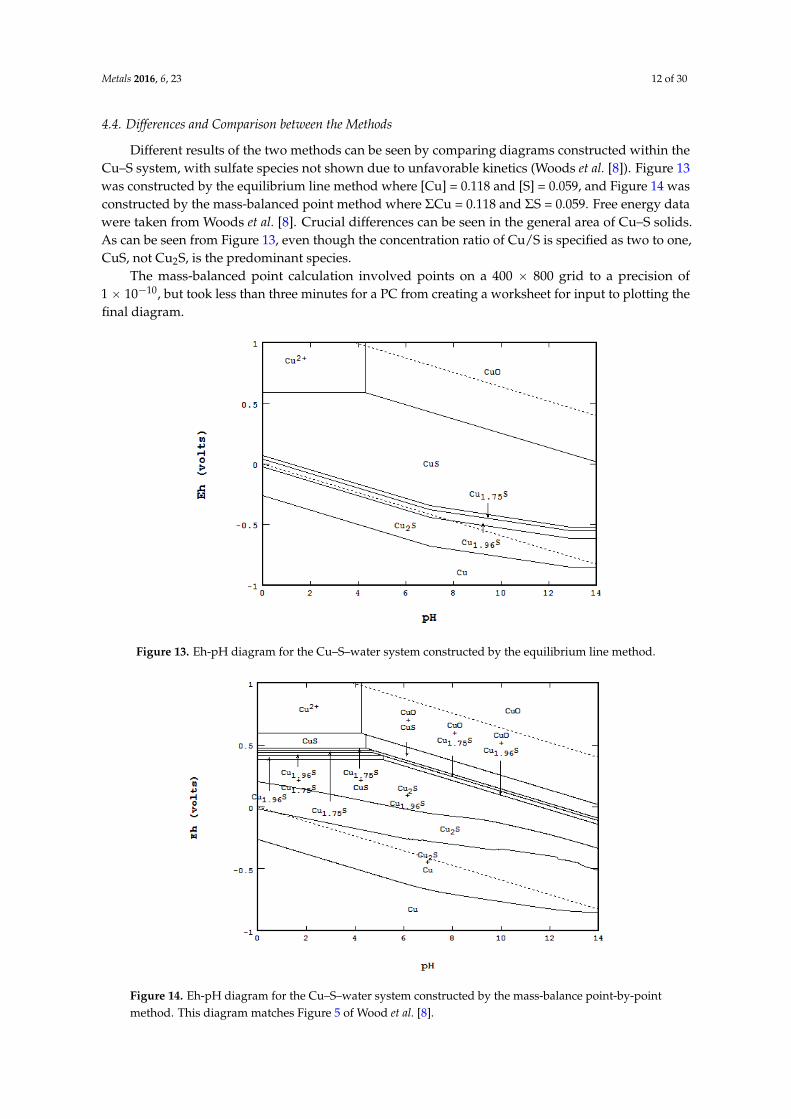
4.4. Differences and Comparison between the Methods
Different results of the two methods can be seen by comparing diagrams constructed within theCu–S system, with sulfate species not shown due to unfavorable kinetics (Woods et al. [8]). Figure 13was constructed by the equilibrium line method where [Cu] = 0.118 and [S] = 0.059, and Figure 14 wasconstructed by the mass-balanced point method where ΣCu = 0.118 and ΣS = 0.059. Free energy datawere taken from Woods et al. [8]. Crucial differences can be seen in the general area of Cu–S solids.As can be seen from Figure 13, even though the concentration ratio of Cu/S is specified as two to one,CuS, not Cu2S, is the predominant species.
The mass-balanced point calculation involved points on a 400 ˆ 800 grid to a precision of1 ˆ 10´10, but took less than three minutes for a PC from creating a worksheet for input to plotting thefinal diagram.
Metals 2016, 6, 23 12 of 30
4.4. Differences and Comparison between the Methods
Different results of the two methods can be seen by comparing diagrams constructed within the
Cu–S system, with sulfate species not shown due to unfavorable kinetics (Woods et al. [8]).
Figure 13 was constructed by the equilibrium line method where [Cu] = 0.118 and [S] = 0.059, and
Figure 14 was constructed by the mass-balanced point method where ΣCu = 0.118 and ΣS = 0.059.
Free energy data were taken from Woods et al. [8]. Crucial differences can be seen in the general area
of Cu–S solids. As can be seen from Figure 13, even though the concentration ratio of Cu/S is specified
as two to one, CuS, not Cu2S, is the predominant species.
The mass-balanced point calculation involved points on a 400 × 800 grid to a precision of
1 × 10⁻¹⁰, but took less than three minutes for a PC from creating a worksheet for input to plotting the
final diagram.
Figure 13. Eh-pH diagram for the Cu–S–water system constructed by the equilibrium line method.
Figure 14. Eh-pH diagram for the Cu–S–water system constructed by the mass-balance point-by-point
method. This diagram matches Figure 5 of Wood et al. [8].
Figure 13. Eh-pH diagram for the Cu–S–water system constructed by the equilibrium line method.
Metals 2016, 6, 23 12 of 30
4.4. Differences and Comparison between the Methods
Different results of the two methods can be seen by comparing diagrams constructed within the
Cu–S system, with sulfate species not shown due to unfavorable kinetics (Woods et al. [8]).
Figure 13 was constructed by the equilibrium line method where [Cu] = 0.118 and [S] = 0.059, and
Figure 14 was constructed by the mass-balanced point method where ΣCu = 0.118 and ΣS = 0.059.
Free energy data were taken from Woods et al. [8]. Crucial differences can be seen in the general area
of Cu–S solids. As can be seen from Figure 13, even though the concentration ratio of Cu/S is specified
as two to one, CuS, not Cu2S, is the predominant species.
The mass-balanced point calculation involved points on a 400 × 800 grid to a precision of
1 × 10⁻¹⁰, but took less than three minutes for a PC from creating a worksheet for input to plotting the
final diagram.
Figure 13. Eh-pH diagram for the Cu–S–water system constructed by the equilibrium line method.
Figure 14. Eh-pH diagram for the Cu–S–water system constructed by the mass-balance point-by-point
method. This diagram matches Figure 5 of Wood et al. [8].
Figure 14. Eh-pH diagram for the Cu–S–water system constructed by the mass-balance point-by-pointmethod. This diagram matches Figure 5 of Wood et al. [8].
Metals 2016, 6, 23 13 of 30
The equilibrium line method was favored in the past due to its relative ease of construction.When diagrams were constructed using manual calculation (as by Pourbaix), the equilibrium linemethod was the only practical approach. As greater computational power became available, themass-balanced point-by-point method came into favor. The following list includes some areas wherethe mass balance method should be considered over the line method.
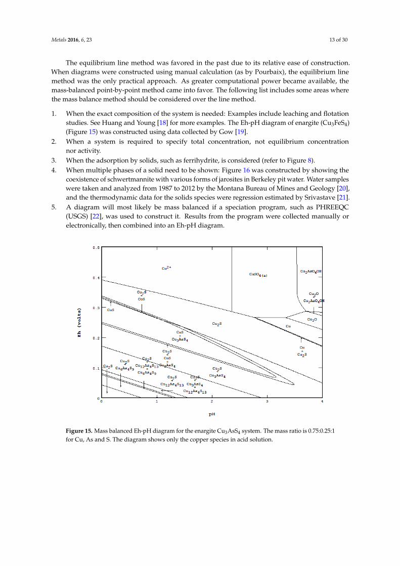
1. When the exact composition of the system is needed: Examples include leaching and flotationstudies. See Huang and Young [18] for more examples. The Eh-pH diagram of enargite (Cu3FeS4)(Figure 15) was constructed using data collected by Gow [19].
2. When a system is required to specify total concentration, not equilibrium concentrationnor activity.
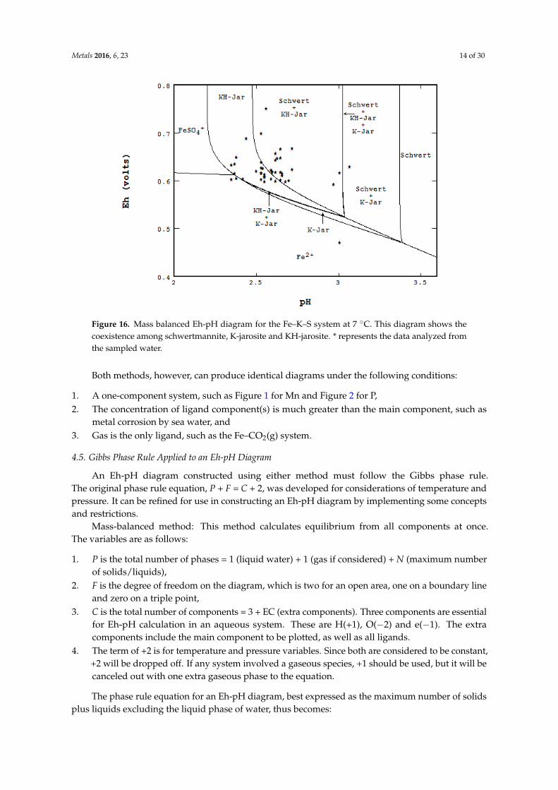
3. When the adsorption by solids, such as ferrihydrite, is considered (refer to Figure 8).4. When multiple phases of a solid need to be shown: Figure 16 was constructed by showing the
coexistence of schwertmannite with various forms of jarosites in Berkeley pit water. Water sampleswere taken and analyzed from 1987 to 2012 by the Montana Bureau of Mines and Geology [20],and the thermodynamic data for the solids species were regression estimated by Srivastave [21].
5. A diagram will most likely be mass balanced if a speciation program, such as PHREEQC(USGS) [22], was used to construct it. Results from the program were collected manually orelectronically, then combined into an Eh-pH diagram.
Metals 2016, 6, 23 13 of 30
The equilibrium line method was favored in the past due to its relative ease of construction.
When diagrams were constructed using manual calculation (as by Pourbaix), the equilibrium line
method was the only practical approach. As greater computational power became available, the
mass-balanced point-by-point method came into favor. The following list includes some areas where
the mass balance method should be considered over the line method.
1. When the exact composition of the system is needed: Examples include leaching and flotation
studies. See Huang and Young [18] for more examples. The Eh-pH diagram of enargite (Cu3FeS4)
(Figure 15) was constructed using data collected by Gow [19].
2. When a system is required to specify total concentration, not equilibrium concentration
nor activity.
3. When the adsorption by solids, such as ferrihydrite, is considered (refer to Figure 8).
4. When multiple phases of a solid need to be shown: Figure 16 was constructed by showing the
coexistence of schwertmannite with various forms of jarosites in Berkeley pit water. Water
samples were taken and analyzed from 1987 to 2012 by the Montana Bureau of Mines and
Geology [20], and the thermodynamic data for the solids species were regression estimated
by Srivastave [21].
5. A diagram will most likely be mass balanced if a speciation program, such as PHREEQC
(USGS) [22], was used to construct it. Results from the program were collected manually or
electronically, then combined into an Eh-pH diagram.
Figure 15. Mass balanced Eh-pH diagram for the enargite Cu3AsS4 system. The mass ratio is 0.75:0.25:1
for Cu, As and S. The diagram shows only the copper species in acid solution. Figure 15. Mass balanced Eh-pH diagram for the enargite Cu3AsS4 system. The mass ratio is 0.75:0.25:1for Cu, As and S. The diagram shows only the copper species in acid solution.
Metals 2016, 6, 23 14 of 30Metals 2016, 6, 23 14 of 30
Figure 16. Mass balanced Eh-pH diagram for the Fe–K–S system at 7 °C. This diagram shows the
coexistence among schwertmannite, K-jarosite and KH-jarosite. * represents the data analyzed from
the sampled water.
Both methods, however, can produce identical diagrams under the following conditions:
1. A one-component system, such as Figure 1 for Mn and Figure 2 for P,
2. The concentration of ligand component(s) is much greater than the main component, such as
metal corrosion by sea water, and
3. Gas is the only ligand, such as the Fe–CO2(g) system.
4.5. Gibbs Phase Rule Applied to an Eh-pH Diagram
An Eh-pH diagram constructed using either method must follow the Gibbs phase rule. The
original phase rule equation, P + F = C + 2, was developed for considerations of temperature and
pressure. It can be refined for use in constructing an Eh-pH diagram by implementing some concepts
and restrictions.
Mass-balanced method: This method calculates equilibrium from all components at once.
The variables are as follows:
1. P is the total number of phases = 1 (liquid water) + 1 (gas if considered) + N (maximum number
of solids/liquids),
2. F is the degree of freedom on the diagram, which is two for an open area, one on a boundary
line and zero on a triple point,
3. C is the total number of components = 3 + EC (extra components). Three components are essential
for Eh-pH calculation in an aqueous system. These are H(+1), O(−2) and e(−1). The extra
components include the main component to be plotted, as well as all ligands.
4. The term of +2 is for temperature and pressure variables. Since both are considered to be
constant, +2 will be dropped off. If any system involved a gaseous species, +1 should be used,
but it will be canceled out with one extra gaseous phase to the equation.
The phase rule equation for an Eh-pH diagram, best expressed as the maximum number of solids
plus liquids excluding the liquid phase of water, thus becomes:
Figure 16. Mass balanced Eh-pH diagram for the Fe–K–S system at 7 ˝C. This diagram shows thecoexistence among schwertmannite, K-jarosite and KH-jarosite. * represents the data analyzed fromthe sampled water.
Both methods, however, can produce identical diagrams under the following conditions:
1. A one-component system, such as Figure 1 for Mn and Figure 2 for P,2. The concentration of ligand component(s) is much greater than the main component, such as
metal corrosion by sea water, and3. Gas is the only ligand, such as the Fe–CO2(g) system.
4.5. Gibbs Phase Rule Applied to an Eh-pH Diagram
An Eh-pH diagram constructed using either method must follow the Gibbs phase rule.The original phase rule equation, P + F = C + 2, was developed for considerations of temperature andpressure. It can be refined for use in constructing an Eh-pH diagram by implementing some conceptsand restrictions.
Mass-balanced method: This method calculates equilibrium from all components at once.The variables are as follows:
1. P is the total number of phases = 1 (liquid water) + 1 (gas if considered) + N (maximum numberof solids/liquids),
2. F is the degree of freedom on the diagram, which is two for an open area, one on a boundary lineand zero on a triple point,
3. C is the total number of components = 3 + EC (extra components). Three components are essentialfor Eh-pH calculation in an aqueous system. These are H(+1), O(´2) and e(´1). The extracomponents include the main component to be plotted, as well as all ligands.
4. The term of +2 is for temperature and pressure variables. Since both are considered to be constant,+2 will be dropped off. If any system involved a gaseous species, +1 should be used, but it will becanceled out with one extra gaseous phase to the equation.
The phase rule equation for an Eh-pH diagram, best expressed as the maximum number of solidsplus liquids excluding the liquid phase of water, thus becomes:
Metals 2016, 6, 23 15 of 30
Nmaxsolid “ C´F´ 1 (6)
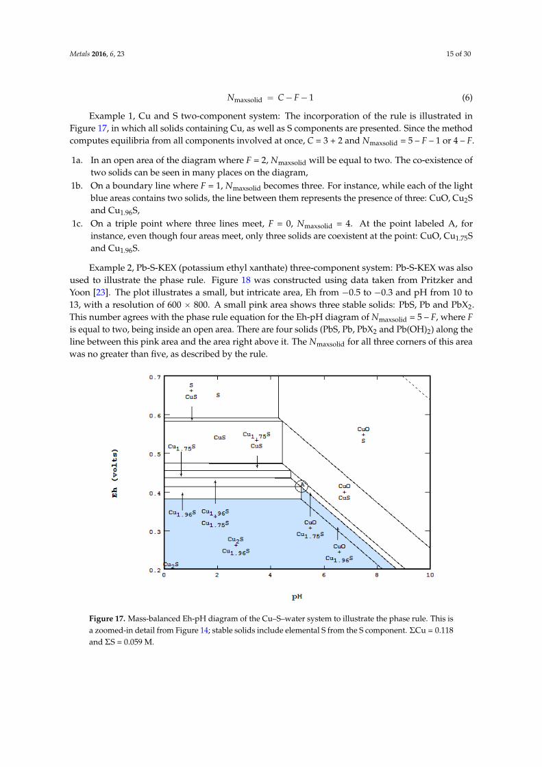
Example 1, Cu and S two-component system: The incorporation of the rule is illustrated inFigure 17, in which all solids containing Cu, as well as S components are presented. Since the methodcomputes equilibria from all components involved at once, C = 3 + 2 and Nmaxsolid = 5 – F – 1 or 4 – F.
1a. In an open area of the diagram where F = 2, Nmaxsolid will be equal to two. The co-existence oftwo solids can be seen in many places on the diagram,
1b. On a boundary line where F = 1, Nmaxsolid becomes three. For instance, while each of the lightblue areas contains two solids, the line between them represents the presence of three: CuO, Cu2Sand Cu1.96S,
1c. On a triple point where three lines meet, F = 0, Nmaxsolid = 4. At the point labeled A, forinstance, even though four areas meet, only three solids are coexistent at the point: CuO, Cu1.75Sand Cu1.96S.
Example 2, Pb-S-KEX (potassium ethyl xanthate) three-component system: Pb-S-KEX was alsoused to illustrate the phase rule. Figure 18 was constructed using data taken from Pritzker andYoon [23]. The plot illustrates a small, but intricate area, Eh from ´0.5 to ´0.3 and pH from 10 to13, with a resolution of 600 ˆ 800. A small pink area shows three stable solids: PbS, Pb and PbX2.This number agrees with the phase rule equation for the Eh-pH diagram of Nmaxsolid = 5 – F, where Fis equal to two, being inside an open area. There are four solids (PbS, Pb, PbX2 and Pb(OH)2) along theline between this pink area and the area right above it. The Nmaxsolid for all three corners of this areawas no greater than five, as described by the rule.
Metals 2016, 6, 23 15 of 30
Nmaxsolid = C − F − 1 (6)
Example 1, Cu and S two-component system: The incorporation of the rule is illustrated in
Figure 17, in which all solids containing Cu, as well as S components are presented. Since the method
computes equilibria from all components involved at once, C = 3 + 2 and Nmaxsolid = 5 – F – 1 or 4 – F.
1a. In an open area of the diagram where F = 2, Nmaxsolid will be equal to two. The co-existence of two
solids can be seen in many places on the diagram,
1b. On a boundary line where F = 1, Nmaxsolid becomes three. For instance, while each of the light blue
areas contains two solids, the line between them represents the presence of three: CuO, Cu2S
and Cu1.96S,
1c. On a triple point where three lines meet, F = 0, Nmaxsolid = 4. At the point labeled A, for instance,
even though four areas meet, only three solids are coexistent at the point: CuO, Cu1.75S
and Cu1.96S.
Example 2, Pb-S-KEX (potassium ethyl xanthate) three-component system: Pb-S-KEX was also
used to illustrate the phase rule. Figure 18 was constructed using data taken from Pritzker and
Yoon [23]. The plot illustrates a small, but intricate area, Eh from −0.5 to −0.3 and pH from 10 to 13,
with a resolution of 600 × 800. A small pink area shows three stable solids: PbS, Pb and PbX2. This
number agrees with the phase rule equation for the Eh-pH diagram of Nmaxsolid = 5 – F, where F is
equal to two, being inside an open area. There are four solids (PbS, Pb, PbX2 and Pb(OH)2) along the
line between this pink area and the area right above it. The Nmaxsolid for all three corners of this area
was no greater than five, as described by the rule.
Figure 17. Mass-balanced Eh-pH diagram of the Cu–S–water system to illustrate the phase rule. This
is a zoomed-in detail from Figure 14; stable solids include elemental S from the S component.
ΣCu = 0.118 and ΣS = 0.059 M.
Figure 17. Mass-balanced Eh-pH diagram of the Cu–S–water system to illustrate the phase rule. This isa zoomed-in detail from Figure 14; stable solids include elemental S from the S component. ΣCu = 0.118and ΣS = 0.059 M.
Metals 2016, 6, 23 16 of 30Metals 2016, 6, 23 16 of 30
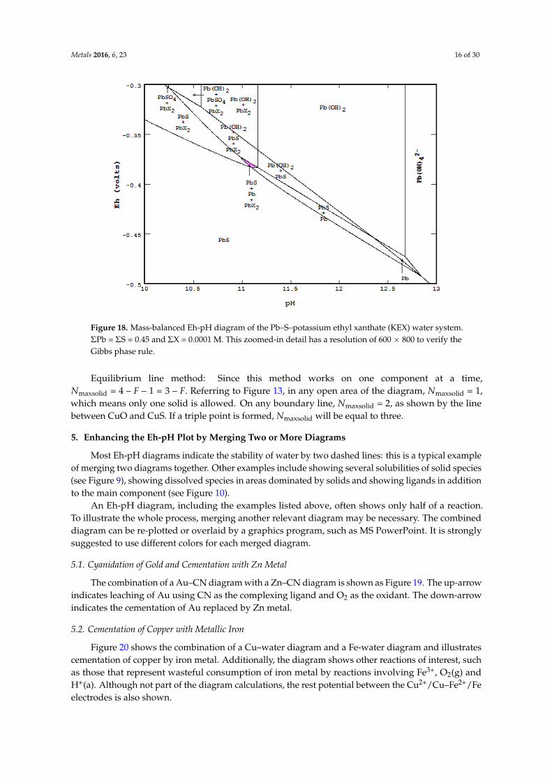
Figure 18. Mass-balanced Eh-pH diagram of the Pb–S–potassium ethyl xanthate (KEX) water system.
ΣPb = ΣS = 0.45 and ΣX = 0.0001 M. This zoomed-in detail has a resolution of 600 × 800 to verify the
Gibbs phase rule.
Equilibrium line method: Since this method works on one component at a time,
Nmaxsolid = 4 – F – 1 = 3 – F. Referring to Figure 13, in any open area of the diagram, Nmaxsolid = 1, which
means only one solid is allowed. On any boundary line, Nmaxsolid = 2, as shown by the line between
CuO and CuS. If a triple point is formed, Nmaxsolid will be equal to three.
5. Enhancing the Eh-pH Plot by Merging Two or More Diagrams
Most Eh-pH diagrams indicate the stability of water by two dashed lines: this is a typical
example of merging two diagrams together. Other examples include showing several solubilities of
solid species (see Figure 9), showing dissolved species in areas dominated by solids and showing
ligands in addition to the main component (see Figure 10).
An Eh-pH diagram, including the examples listed above, often shows only half of a reaction.
To illustrate the whole process, merging another relevant diagram may be necessary. The combined
diagram can be re-plotted or overlaid by a graphics program, such as MS PowerPoint. It is strongly
suggested to use different colors for each merged diagram.
5.1. Cyanidation of Gold and Cementation with Zn Metal
The combination of a Au–CN diagram with a Zn–CN diagram is shown as Figure 19. The
up-arrow indicates leaching of Au using CN as the complexing ligand and O2 as the oxidant. The
down-arrow indicates the cementation of Au replaced by Zn metal.
5.2. Cementation of Copper with Metallic Iron
Figure 20 shows the combination of a Cu–water diagram and a Fe-water diagram and illustrates
cementation of copper by iron metal. Additionally, the diagram shows other reactions of interest,
such as those that represent wasteful consumption of iron metal by reactions involving Fe3+, O2(g)
and H+(a). Although not part of the diagram calculations, the rest potential between the
Cu2+/Cu–Fe2+/Fe electrodes is also shown.
Figure 18. Mass-balanced Eh-pH diagram of the Pb–S–potassium ethyl xanthate (KEX) water system.ΣPb = ΣS = 0.45 and ΣX = 0.0001 M. This zoomed-in detail has a resolution of 600 ˆ 800 to verify theGibbs phase rule.
Equilibrium line method: Since this method works on one component at a time,Nmaxsolid = 4 – F – 1 = 3 – F. Referring to Figure 13, in any open area of the diagram, Nmaxsolid = 1,which means only one solid is allowed. On any boundary line, Nmaxsolid = 2, as shown by the linebetween CuO and CuS. If a triple point is formed, Nmaxsolid will be equal to three.
5. Enhancing the Eh-pH Plot by Merging Two or More Diagrams
Most Eh-pH diagrams indicate the stability of water by two dashed lines: this is a typical exampleof merging two diagrams together. Other examples include showing several solubilities of solid species(see Figure 9), showing dissolved species in areas dominated by solids and showing ligands in additionto the main component (see Figure 10).
An Eh-pH diagram, including the examples listed above, often shows only half of a reaction.To illustrate the whole process, merging another relevant diagram may be necessary. The combineddiagram can be re-plotted or overlaid by a graphics program, such as MS PowerPoint. It is stronglysuggested to use different colors for each merged diagram.
5.1. Cyanidation of Gold and Cementation with Zn Metal
The combination of a Au–CN diagram with a Zn–CN diagram is shown as Figure 19. The up-arrowindicates leaching of Au using CN as the complexing ligand and O2 as the oxidant. The down-arrowindicates the cementation of Au replaced by Zn metal.
5.2. Cementation of Copper with Metallic Iron
Figure 20 shows the combination of a Cu–water diagram and a Fe-water diagram and illustratescementation of copper by iron metal. Additionally, the diagram shows other reactions of interest, suchas those that represent wasteful consumption of iron metal by reactions involving Fe3+, O2(g) andH+(a). Although not part of the diagram calculations, the rest potential between the Cu2+/Cu–Fe2+/Feelectrodes is also shown.
Metals 2016, 6, 23 17 of 30Metals 2016, 6, 23 17 of 30
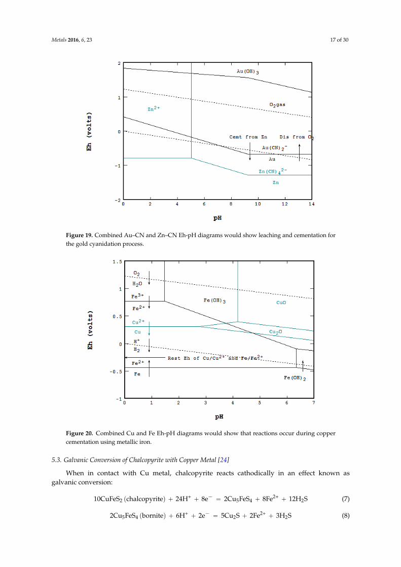
Figure 19. Combined Au–CN and Zn–CN Eh-pH diagrams would show leaching and cementation
for the gold cyanidation process.
Figure 20. Combined Cu and Fe Eh-pH diagrams would show that reactions occur during copper
cementation using metallic iron.
5.3. Galvanic Conversion of Chalcopyrite with Copper Metal [24]
When in contact with Cu metal, chalcopyrite reacts cathodically in an effect known as
galvanic conversion:
10CuFeS2 (chalcopyrite) + 24H+ + 8e− = 2Cu5FeS4 + 8Fe2+ + 12H2S (7)
2Cu5FeS4 (bornite) + 6H+ + 2e− = 5Cu2S + 2Fe2+ + 3H2S (8)
Figure 19. Combined Au–CN and Zn–CN Eh-pH diagrams would show leaching and cementation forthe gold cyanidation process.
Metals 2016, 6, 23 17 of 30
Figure 19. Combined Au–CN and Zn–CN Eh-pH diagrams would show leaching and cementation
for the gold cyanidation process.
Figure 20. Combined Cu and Fe Eh-pH diagrams would show that reactions occur during copper
cementation using metallic iron.
5.3. Galvanic Conversion of Chalcopyrite with Copper Metal [24]
When in contact with Cu metal, chalcopyrite reacts cathodically in an effect known as
galvanic conversion:
10CuFeS2 (chalcopyrite) + 24H+ + 8e− = 2Cu5FeS4 + 8Fe2+ + 12H2S (7)
2Cu5FeS4 (bornite) + 6H+ + 2e− = 5Cu2S + 2Fe2+ + 3H2S (8)
Figure 20. Combined Cu and Fe Eh-pH diagrams would show that reactions occur during coppercementation using metallic iron.
5.3. Galvanic Conversion of Chalcopyrite with Copper Metal [24]
When in contact with Cu metal, chalcopyrite reacts cathodically in an effect known asgalvanic conversion:
10CuFeS2 pchalcopyriteq ` 24H+ ` 8e´ “ 2Cu5FeS4 ` 8Fe2+ ` 12H2S (7)
2Cu5FeS4 pborniteq ` 6H+ ` 2e´ “ 5Cu2S ` 2Fe2+ ` 3H2S (8)

Metals 2016, 6, 23 18 of 30
An anodic reaction takes place on the metallic copper as:
2Cu ` H2S “ Cu2S ` 2H+ ` 2e´ (9)
A schematic diagram for all these reactions is shown as Figure 21. In order to present all of thespecies involved, three Eh-pH diagrams are superimposed and shown as Figure 22.
1. The three diagrams used are: S species in cyan, Fe and Fe–S in red and Cu–Fe–S in black.2. Areas of predominance are shown as: chalcopyrite in yellow, bornite in gray, chalcocite in light
blue and metallic copper in orange.3. The down-arrow indicates where galvanic conversion occurs down from chalcopyrite to bornite
and, finally, to Cu2S. The up-arrow indicates where the anodic reaction occurs up from metalliccopper to Cu2S.
4. The diagram indicates that both cathodic and anodic reactions lead to the formation of Cu2S, andother final species match what Hiskey and Wadsworth [24] described.
Metals 2016, 6, 23 18 of 30
An anodic reaction takes place on the metallic copper as:
2Cu + H2S = Cu2S + 2H+ +2e− (9)
A schematic diagram for all these reactions is shown as Figure 21. In order to present all of the
species involved, three Eh-pH diagrams are superimposed and shown as Figure 22.
1. The three diagrams used are: S species in cyan, Fe and Fe–S in red and Cu–Fe–S in black.
2. Areas of predominance are shown as: chalcopyrite in yellow, bornite in gray, chalcocite in light
blue and metallic copper in orange.
3. The down-arrow indicates where galvanic conversion occurs down from chalcopyrite to bornite
and, finally, to Cu2S. The up-arrow indicates where the anodic reaction occurs up from metallic
copper to Cu2S.
4. The diagram indicates that both cathodic and anodic reactions lead to the formation of Cu2S, and
other final species match what Hiskey and Wadsworth [24] described.
Figure 21. Schematic diagram of reactions occurring upon galvanic conversion of chalcopyrite with
metallic copper [24].
Figure 22. Combination of three Eh-pH diagrams showing the galvanic conversion reactions of
chalcopyrite with metallic copper.
Figure 21. Schematic diagram of reactions occurring upon galvanic conversion of chalcopyrite withmetallic copper [24].
Metals 2016, 6, 23 18 of 30
An anodic reaction takes place on the metallic copper as:
2Cu + H2S = Cu2S + 2H+ +2e− (9)
A schematic diagram for all these reactions is shown as Figure 21. In order to present all of the
species involved, three Eh-pH diagrams are superimposed and shown as Figure 22.
1. The three diagrams used are: S species in cyan, Fe and Fe–S in red and Cu–Fe–S in black.
2. Areas of predominance are shown as: chalcopyrite in yellow, bornite in gray, chalcocite in light
blue and metallic copper in orange.
3. The down-arrow indicates where galvanic conversion occurs down from chalcopyrite to bornite
and, finally, to Cu2S. The up-arrow indicates where the anodic reaction occurs up from metallic
copper to Cu2S.
4. The diagram indicates that both cathodic and anodic reactions lead to the formation of Cu2S, and
other final species match what Hiskey and Wadsworth [24] described.
Figure 21. Schematic diagram of reactions occurring upon galvanic conversion of chalcopyrite with
metallic copper [24].
Figure 22. Combination of three Eh-pH diagrams showing the galvanic conversion reactions of
chalcopyrite with metallic copper.
Figure 22. Combination of three Eh-pH diagrams showing the galvanic conversion reactions ofchalcopyrite with metallic copper.
Metals 2016, 6, 23 19 of 30
6. Third Dimension to an Eh-pH Diagram
Even more information may be shown by adding a third dimension to a base Eh-pH diagram.The third dimension can be the simple solubility of solid or an independent variable, such astemperature or ligand concentration. First, the data needed for a 3D Eh-pH diagram must be calculated.Thereafter, 3D programs for PC, such as ParaView [25], VisIt [26] or MATLAB [27], combine all ofthe data into a single diagram. These programs can also provide other functions, such as animatedrotation, clipping and slicing. This section presents some 3D examples by considering extension ofthe Eh-pH diagram into a third dimension. Data creation and setup input files for a 3D program arebriefly presented. Three areas are illustrated:
1. Eh-pH along with the solubility of stable solids; two example diagrams are illustrated: passivationof lead (Figure 6) and adsorption of As(III) and As(V) onto ferrihydrite (Figure 8).
2. Eh-pH with an extra axis for ligand CO2: two wireframe volume diagrams of Eh-pH-CO2 takenfrom Garrels and Christ [2] are used for verifying the results; these two are:
(a) Figure 7.32b: in order to match the given ΣCO2 for the third axis, the mass balance methodhas to be used; the output of 3D and discussion for this case are presented in more detail.
(b) Figure 7.32a: since the third axis is given as the pressure of CO2(g), the equilibrium linemethod can be applied; the time required for the Eh-pH calculation was much less.
3. Presentation of a system in which two or more solid phases, such as CuS and Cu2S, can coexist.
6.1. Eh-pH with Solubility
Including the solubility of solids in an Eh-pH diagram can give a much clearer view of whatcan happen to the solid. The following two diagrams constructed by MATLAB extend the 2D Eh-pHdiagrams presented earlier. In order for MATLAB to plot 3D solubility diagrams, the Eh-pH programneeds to create two files: the (name).m file contains instructions to be executed by MATLAB, andthe data file contains solubility from each Eh and pH from the grid. A MATLAB plot can show thematching contour (iso-solubility) lines below the 3D feature.
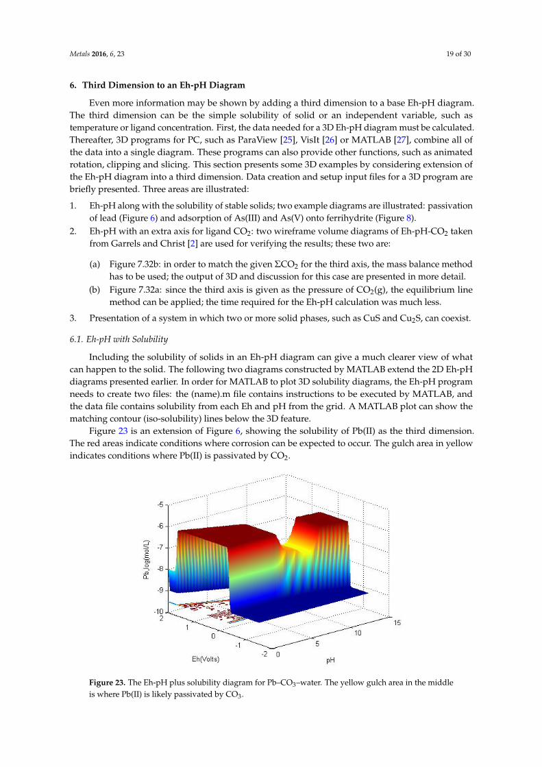
Figure 23 is an extension of Figure 6, showing the solubility of Pb(II) as the third dimension.The red areas indicate conditions where corrosion can be expected to occur. The gulch area in yellowindicates conditions where Pb(II) is passivated by CO2.
Metals 2016, 6, 23 19 of 30
6. Third Dimension to an Eh-pH Diagram
Even more information may be shown by adding a third dimension to a base Eh-pH diagram.
The third dimension can be the simple solubility of solid or an independent variable, such as
temperature or ligand concentration. First, the data needed for a 3D Eh-pH diagram must be
calculated. Thereafter, 3D programs for PC, such as ParaView [25], VisIt [26] or MATLAB [27],
combine all of the data into a single diagram. These programs can also provide other functions, such
as animated rotation, clipping and slicing. This section presents some 3D examples by considering
extension of the Eh-pH diagram into a third dimension. Data creation and setup input files for a 3D
program are briefly presented. Three areas are illustrated:
1. Eh-pH along with the solubility of stable solids; two example diagrams are illustrated:
passivation of lead (Figure 6) and adsorption of As(III) and As(V) onto ferrihydrite (Figure 8).
2. Eh-pH with an extra axis for ligand CO2: two wireframe volume diagrams of Eh-pH-CO2 taken
from Garrels and Christ [2] are used for verifying the results; these two are:
a. Figure 7.32b: in order to match the given CO2 for the third axis, the mass balance method has
to be used; the output of 3D and discussion for this case are presented in more detail.
b. Figure 7.32a: since the third axis is given as the pressure of CO2(g), the equilibrium line method
can be applied; the time required for the Eh-pH calculation was much less.
3. Presentation of a system in which two or more solid phases, such as CuS and Cu2S, can coexist.
6.1. Eh-pH with Solubility
Including the solubility of solids in an Eh-pH diagram can give a much clearer view of what can
happen to the solid. The following two diagrams constructed by MATLAB extend the 2D Eh-pH
diagrams presented earlier. In order for MATLAB to plot 3D solubility diagrams, the Eh-pH program
needs to create two files: the (name).m file contains instructions to be executed by MATLAB, and the
data file contains solubility from each Eh and pH from the grid. A MATLAB plot can show the
matching contour (iso-solubility) lines below the 3D feature.
Figure 23 is an extension of Figure 6, showing the solubility of Pb(II) as the third dimension. The
red areas indicate conditions where corrosion can be expected to occur. The gulch area in yellow
indicates conditions where Pb(II) is passivated by CO2.
Figure 23. The Eh-pH plus solubility diagram for Pb–CO3–water. The yellow gulch area in the middle
is where Pb(II) is likely passivated by CO3. Figure 23. The Eh-pH plus solubility diagram for Pb–CO3–water. The yellow gulch area in the middleis where Pb(II) is likely passivated by CO3.
Metals 2016, 6, 23 20 of 30
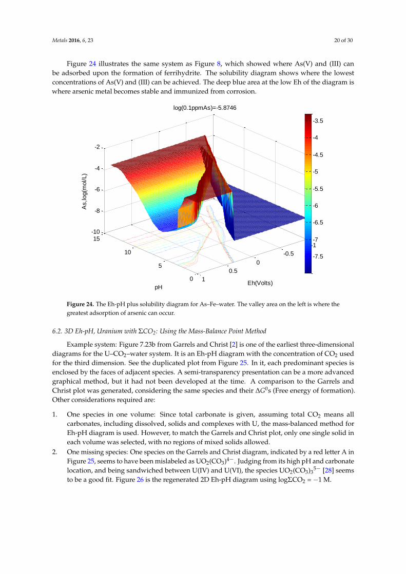
Figure 24 illustrates the same system as Figure 8, which showed where As(V) and (III) canbe adsorbed upon the formation of ferrihydrite. The solubility diagram shows where the lowestconcentrations of As(V) and (III) can be achieved. The deep blue area at the low Eh of the diagram iswhere arsenic metal becomes stable and immunized from corrosion.
Metals 2016, 6, 23 20 of 30
Figure 24 illustrates the same system as Figure 8, which showed where As(V) and (III) can be
adsorbed upon the formation of ferrihydrite. The solubility diagram shows where the lowest
concentrations of As(V) and (III) can be achieved. The deep blue area at the low Eh of the diagram is
where arsenic metal becomes stable and immunized from corrosion.
Figure 24. The Eh-pH plus solubility diagram for As–Fe–water. The valley area on the left is where
the greatest adsorption of arsenic can occur.
6.2. 3D Eh-pH, Uranium with CO2: Using the Mass-Balance Point Method
Example system: Figure 7.23b from Garrels and Christ [2] is one of the earliest three-dimensional
diagrams for the U–CO2–water system. It is an Eh-pH diagram with the concentration of CO2 used
for the third dimension. See the duplicated plot from Figure 25. In it, each predominant species is
enclosed by the faces of adjacent species. A semi-transparency presentation can be a more advanced
graphical method, but it had not been developed at the time. A comparison to the Garrels and Christ
plot was generated, considering the same species and their ΔG0s (Free energy of formation). Other
considerations required are:
1. One species in one volume: Since total carbonate is given, assuming total CO2 means all
carbonates, including dissolved, solids and complexes with U, the mass-balanced method for
Eh-pH diagram is used. However, to match the Garrels and Christ plot, only one single solid in
each volume was selected, with no regions of mixed solids allowed.
2. One missing species: One species on the Garrels and Christ diagram, indicated by a red letter A
in Figure 25, seems to have been mislabeled as UO2(CO3)4−. Judging from its high pH and
carbonate location, and being sandwiched between U(IV) and U(VI), the species UO2(CO3)35− [28]
seems to be a good fit. Figure 26 is the regenerated 2D Eh-pH diagram using logCO2 = −1 M.
0
5
10
15-1
-0.5
0
0.5
1
-10
-8
-6
-4
-2
Eh(Volts)
log(0.1ppmAs)=-5.8746
pH
As,log(m
ol/L)
-7.5
-7
-6.5
-6
-5.5
-5
-4.5
-4
-3.5
Figure 24. The Eh-pH plus solubility diagram for As–Fe–water. The valley area on the left is where thegreatest adsorption of arsenic can occur.
6.2. 3D Eh-pH, Uranium with ΣCO2: Using the Mass-Balance Point Method
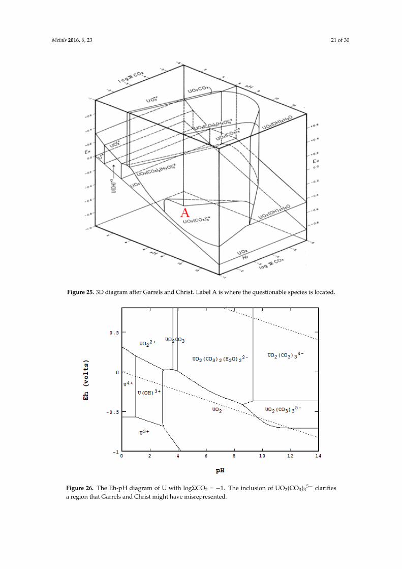
Example system: Figure 7.23b from Garrels and Christ [2] is one of the earliest three-dimensionaldiagrams for the U–CO2–water system. It is an Eh-pH diagram with the concentration of CO2 usedfor the third dimension. See the duplicated plot from Figure 25. In it, each predominant species isenclosed by the faces of adjacent species. A semi-transparency presentation can be a more advancedgraphical method, but it had not been developed at the time. A comparison to the Garrels andChrist plot was generated, considering the same species and their ∆G0s (Free energy of formation).Other considerations required are:
1. One species in one volume: Since total carbonate is given, assuming total CO2 means allcarbonates, including dissolved, solids and complexes with U, the mass-balanced method forEh-pH diagram is used. However, to match the Garrels and Christ plot, only one single solid ineach volume was selected, with no regions of mixed solids allowed.
2. One missing species: One species on the Garrels and Christ diagram, indicated by a red letter A inFigure 25, seems to have been mislabeled as UO2(CO3)4´. Judging from its high pH and carbonatelocation, and being sandwiched between U(IV) and U(VI), the species UO2(CO3)3
5´ [28] seemsto be a good fit. Figure 26 is the regenerated 2D Eh-pH diagram using logΣCO2 = ´1 M.
Metals 2016, 6, 23 21 of 30Metals 2016, 6, 23 21 of 30
Figure 25. 3D diagram after Garrels and Christ. Label A is where the questionable species is located.
Figure 26. The Eh-pH diagram of U with logCO2 = −1. The inclusion of UO2(CO3)35− clarifies a region
that Garrels and Christ might have misrepresented.
Example diagrams and conditions: Figures 27–32 are three-dimensional diagrams created using
ParaView (Version 4.3.1) based on the data generated by the STABCAL program. Although the
Figure 25. 3D diagram after Garrels and Christ. Label A is where the questionable species is located.
Metals 2016, 6, 23 21 of 30
Figure 25. 3D diagram after Garrels and Christ. Label A is where the questionable species is located.
Figure 26. The Eh-pH diagram of U with logCO2 = −1. The inclusion of UO2(CO3)35− clarifies a region
that Garrels and Christ might have misrepresented.
Example diagrams and conditions: Figures 27–32 are three-dimensional diagrams created using
ParaView (Version 4.3.1) based on the data generated by the STABCAL program. Although the
Figure 26. The Eh-pH diagram of U with logΣCO2 = ´1. The inclusion of UO2(CO3)35´ clarifies
a region that Garrels and Christ might have misrepresented.

Metals 2016, 6, 23 22 of 30
Example diagrams and conditions: Figures 27–32 are three-dimensional diagrams created usingParaView (Version 4.3.1) based on the data generated by the STABCAL program. Although thecomplete ParaView diagram allows such functions as continuous rotation, clipping and slicing, thesestatic diagrams demonstrate the range of features that can be achieved. A color map (bar), shown inFigure 27, indicates that the names of the species should be added at least once to one of the figures.Computational conditional limits include:
‚ Ranges: Eh = ´1 to 0.8, pH = 0 to 14 and logΣCO2 = ´6 to ´1,‚ Grid point: 250 ˆ 250 ˆ 250,‚ Computer: 64 bit, 3.40 GHz, 16 G of RAM,‚ Program algorithm: mass balance point method using mass action law,‚ Accuracy (sum of squared residual) <1 ˆ 10´8 and‚ Time to complete the calculation: 1:36:25 (h:mm:ss) from i7 PC or 2:00:51 from i5; contrary to
using the line method, shown later, which took less than 30 s.
In order for ParaView to plot a 3D diagram, the Eh-pH program needs to create a (name).vtkfile [29] that specifies the type of grid, the values of all X, Y and Z coordinates followed by all of thepoint data that indicate which species are to be plotted for each point on all three axes.
Metals 2016, 6, 23 22 of 30
complete ParaView diagram allows such functions as continuous rotation, clipping and slicing, these
static diagrams demonstrate the range of features that can be achieved. A color map (bar), shown in
Figure 27, indicates that the names of the species should be added at least once to one of the figures.
Computational conditional limits include:
Ranges: Eh = −1 to 0.8, pH = 0 to 14 and logΣCO2 = −6 to −1,
Grid point: 250 × 250 × 250,
Computer: 64 bit, 3.40 GHz, 16 G of RAM,
Program algorithm: mass balance point method using mass action law,
Accuracy (sum of squared residual) <1 × 10⁻⁸ and
Time to complete the calculation: 1:36:25 (h:mm:ss) from i7 PC or 2:00:51 from i5; contrary to
using the line method, shown later, which took less than 30 s.
In order for ParaView to plot a 3D diagram, the Eh-pH program needs to create a (name).vtk
file [29] that specifies the type of grid, the values of all X, Y and Z coordinates followed by all of the
point data that indicate which species are to be plotted for each point on all three axes.
Figure 27. Eh-pH-logCO2 of uranium where the species are shown by colors. A color bar is inserted
to show the corresponding species. Figure 27. Eh-pH-logΣCO2 of uranium where the species are shown by colors. A color bar is insertedto show the corresponding species.
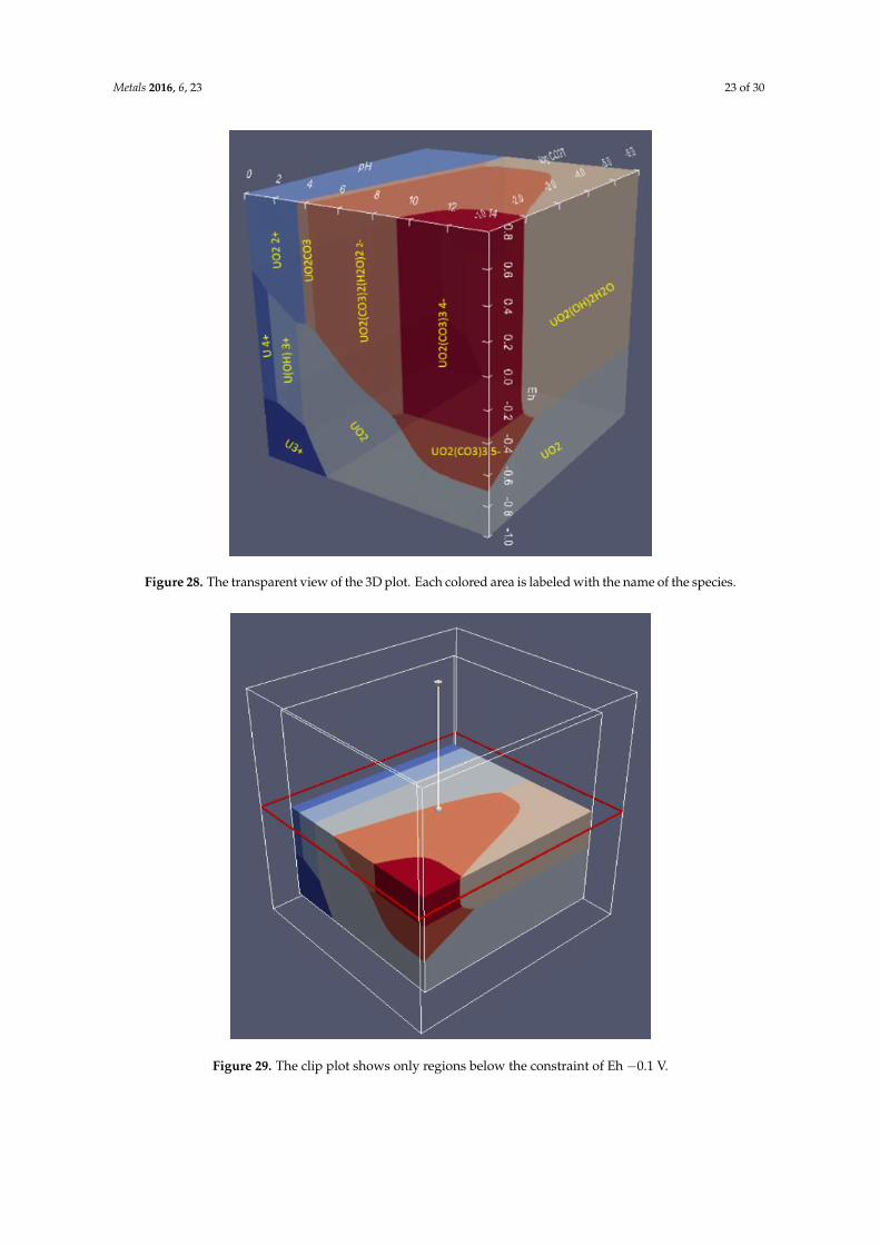
Metals 2016, 6, 23 23 of 30Metals 2016, 6, 23 23 of 30
Figure 28. The transparent view of the 3D plot. Each colored area is labeled with the name of the species.
Figure 29. The clip plot shows only regions below the constraint of Eh −0.1 V.
Figure 28. The transparent view of the 3D plot. Each colored area is labeled with the name of the species.
Metals 2016, 6, 23 23 of 30
Figure 28. The transparent view of the 3D plot. Each colored area is labeled with the name of the species.
Figure 29. The clip plot shows only regions below the constraint of Eh −0.1 V. Figure 29. The clip plot shows only regions below the constraint of Eh ´0.1 V.
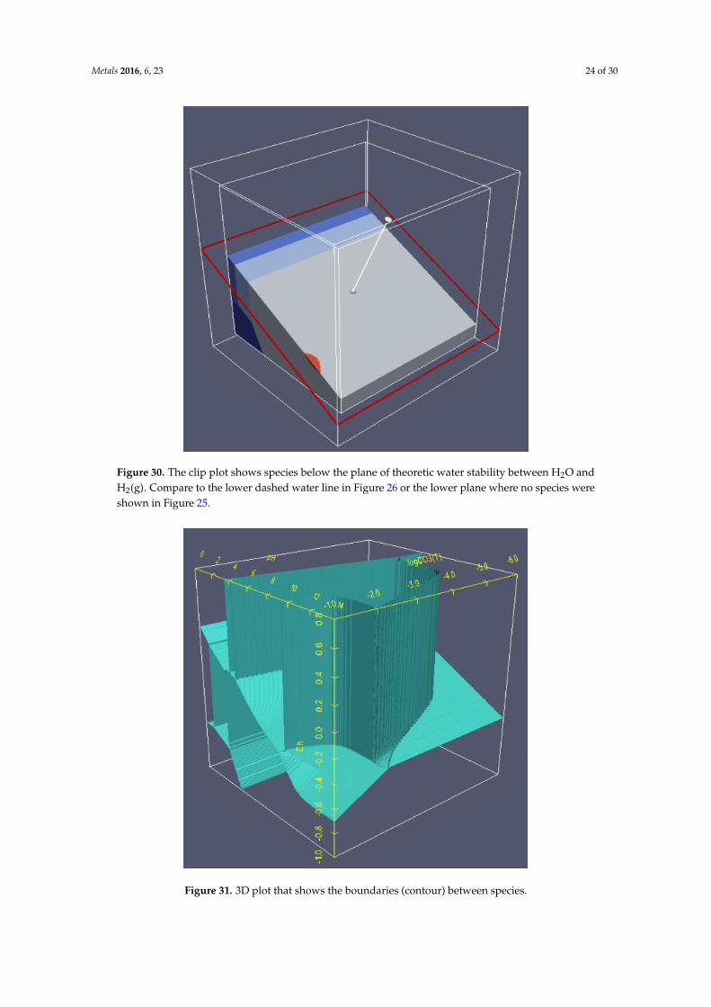
Metals 2016, 6, 23 24 of 30Metals 2016, 6, 23 24 of 30
Figure 30. The clip plot shows species below the plane of theoretic water stability between H2O and
H2(g). Compare to the lower dashed water line in Figure 26 or the lower plane where no species were
shown in Figure 25.
Figure 31. 3D plot that shows the boundaries (contour) between species.
Figure 30. The clip plot shows species below the plane of theoretic water stability between H2O andH2(g). Compare to the lower dashed water line in Figure 26 or the lower plane where no species wereshown in Figure 25.
Metals 2016, 6, 23 24 of 30
Figure 30. The clip plot shows species below the plane of theoretic water stability between H2O and
H2(g). Compare to the lower dashed water line in Figure 26 or the lower plane where no species were
shown in Figure 25.
Figure 31. 3D plot that shows the boundaries (contour) between species. Figure 31. 3D plot that shows the boundaries (contour) between species.

Metals 2016, 6, 23 25 of 30Metals 2016, 6, 23 25 of 30
Figure 32. Semi-transparent plot that shows the stability region of UO2(CO3)2(H2O)22− species.
A three-dimensional plot has the great advantage of being able to show the effects of multiple
variables at once. Tools, such as rotate, slice and clip, can easily identify areas of particular interest.
For a complicated system, however, a three-dimensional image may not be as clear as a two-dimensional
drawing due to the memory and screen resolution imposed by an ordinary PC. It is therefore wise to
choose or combine the use of 2D and 3D to have the best presentation.
A simple way to turn a set of line-drawn diagrams into a three-dimensional object is to arrange
six two-dimensional surface plots (two from each of Eh-pH, Eh-ligand and pH-ligand) into a cube. It
may be necessary to reverse the x- or y-axis direction for this purpose. Simple plastic cubes, intended
for use with photographs, are readily available. See Figure 33, where the section on the left (three
plots combined) is the top-front view and the section on the right is the bottom-rear view. The two
sections are jointed along the Eh axis, at pH = 14 and log ΣCO3 = −1 M. Rotating the right sections to
the left will make a complete cube. To show the continuity between plots, species UO2 was purposely
colored in light blue.
Figure 33. Combination of six surface plots of the U Eh-pH-logCO2 system to form a cube.
Figure 32. Semi-transparent plot that shows the stability region of UO2(CO3)2(H2O)22´ species.
A three-dimensional plot has the great advantage of being able to show the effects of multiplevariables at once. Tools, such as rotate, slice and clip, can easily identify areas of particularinterest. For a complicated system, however, a three-dimensional image may not be as clear asa two-dimensional drawing due to the memory and screen resolution imposed by an ordinary PC. It istherefore wise to choose or combine the use of 2D and 3D to have the best presentation.
A simple way to turn a set of line-drawn diagrams into a three-dimensional object is to arrangesix two-dimensional surface plots (two from each of Eh-pH, Eh-ligand and pH-ligand) into a cube.It may be necessary to reverse the x- or y-axis direction for this purpose. Simple plastic cubes, intendedfor use with photographs, are readily available. See Figure 33, where the section on the left (three plotscombined) is the top-front view and the section on the right is the bottom-rear view. The two sectionsare jointed along the Eh axis, at pH = 14 and log ΣCO3 = ´1 M. Rotating the right sections to the leftwill make a complete cube. To show the continuity between plots, species UO2 was purposely coloredin light blue.
Metals 2016, 6, 23 25 of 30
Figure 32. Semi-transparent plot that shows the stability region of UO2(CO3)2(H2O)22− species.
A three-dimensional plot has the great advantage of being able to show the effects of multiple
variables at once. Tools, such as rotate, slice and clip, can easily identify areas of particular interest.
For a complicated system, however, a three-dimensional image may not be as clear as a two-dimensional
drawing due to the memory and screen resolution imposed by an ordinary PC. It is therefore wise to
choose or combine the use of 2D and 3D to have the best presentation.
A simple way to turn a set of line-drawn diagrams into a three-dimensional object is to arrange
six two-dimensional surface plots (two from each of Eh-pH, Eh-ligand and pH-ligand) into a cube. It
may be necessary to reverse the x- or y-axis direction for this purpose. Simple plastic cubes, intended
for use with photographs, are readily available. See Figure 33, where the section on the left (three
plots combined) is the top-front view and the section on the right is the bottom-rear view. The two
sections are jointed along the Eh axis, at pH = 14 and log ΣCO3 = −1 M. Rotating the right sections to
the left will make a complete cube. To show the continuity between plots, species UO2 was purposely
colored in light blue.
Figure 33. Combination of six surface plots of the U Eh-pH-logCO2 system to form a cube. Figure 33. Combination of six surface plots of the U Eh-pH-logΣCO2 system to form a cube.
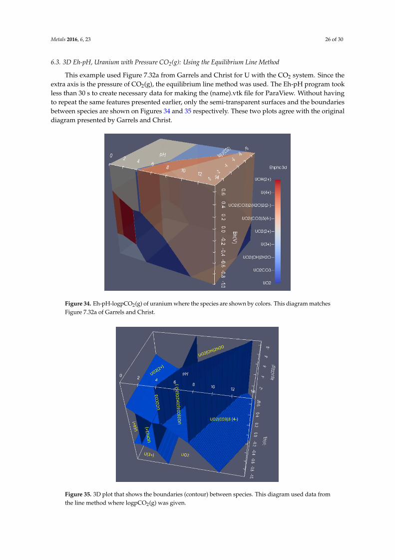
Metals 2016, 6, 23 26 of 30
6.3. 3D Eh-pH, Uranium with Pressure CO2(g): Using the Equilibrium Line Method
This example used Figure 7.32a from Garrels and Christ for U with the CO2 system. Since theextra axis is the pressure of CO2(g), the equilibrium line method was used. The Eh-pH program tookless than 30 s to create necessary data for making the (name).vtk file for ParaView. Without havingto repeat the same features presented earlier, only the semi-transparent surfaces and the boundariesbetween species are shown on Figures 34 and 35 respectively. These two plots agree with the originaldiagram presented by Garrels and Christ.
Metals 2016, 6, 23 26 of 30
6.3. 3D Eh-pH, Uranium with Pressure CO2(g): Using the Equilibrium Line Method
This example used Figure 7.32a from Garrels and Christ for U with the CO2 system. Since the
extra axis is the pressure of CO2(g), the equilibrium line method was used. The Eh-pH program took
less than 30 s to create necessary data for making the (name).vtk file for ParaView. Without having
to repeat the same features presented earlier, only the semi-transparent surfaces and the boundaries
between species are shown on Figures 34 and 35, respectively. These two plots agree with the original
diagram presented by Garrels and Christ.
Figure 34. Eh-pH-logpCO2(g) of uranium where the species are shown by colors. This diagram
matches Figure 7.32a of Garrels and Christ.
Figure 35. 3D plot that shows the boundaries (contour) between species. This diagram used data from
the line method where logpCO2(g) was given.
Figure 34. Eh-pH-logpCO2(g) of uranium where the species are shown by colors. This diagram matchesFigure 7.32a of Garrels and Christ.
Metals 2016, 6, 23 26 of 30
6.3. 3D Eh-pH, Uranium with Pressure CO2(g): Using the Equilibrium Line Method
This example used Figure 7.32a from Garrels and Christ for U with the CO2 system. Since the
extra axis is the pressure of CO2(g), the equilibrium line method was used. The Eh-pH program took
less than 30 s to create necessary data for making the (name).vtk file for ParaView. Without having
to repeat the same features presented earlier, only the semi-transparent surfaces and the boundaries
between species are shown on Figures 34 and 35, respectively. These two plots agree with the original
diagram presented by Garrels and Christ.
Figure 34. Eh-pH-logpCO2(g) of uranium where the species are shown by colors. This diagram
matches Figure 7.32a of Garrels and Christ.
Figure 35. 3D plot that shows the boundaries (contour) between species. This diagram used data from
the line method where logpCO2(g) was given. Figure 35. 3D plot that shows the boundaries (contour) between species. This diagram used data fromthe line method where logpCO2(g) was given.
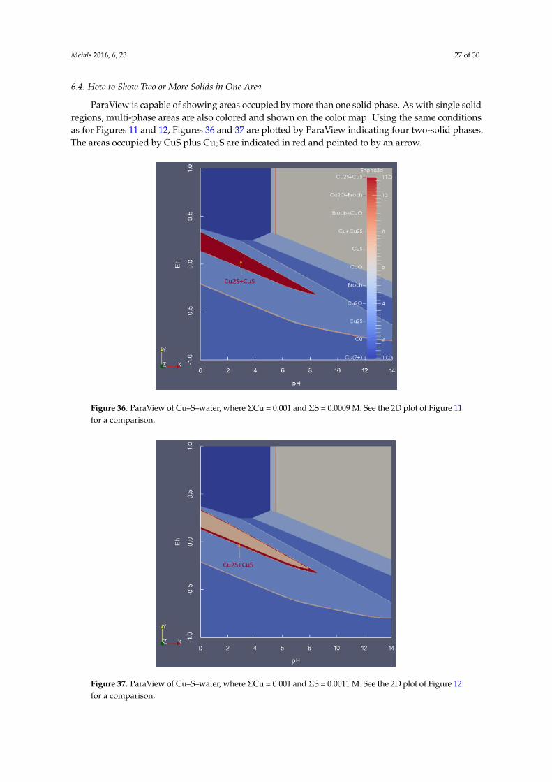
Metals 2016, 6, 23 27 of 30
6.4. How to Show Two or More Solids in One Area
ParaView is capable of showing areas occupied by more than one solid phase. As with single solidregions, multi-phase areas are also colored and shown on the color map. Using the same conditionsas for Figures 11 and 12, Figures 36 and 37 are plotted by ParaView indicating four two-solid phases.The areas occupied by CuS plus Cu2S are indicated in red and pointed to by an arrow.
Metals 2016, 6, 23 27 of 30
6.4. How to Show Two or More Solids in One Area
ParaView is capable of showing areas occupied by more than one solid phase. As with single
solid regions, multi-phase areas are also colored and shown on the color map. Using the same
conditions as for Figures 11 and 12, Figures 36 and 37 are plotted by ParaView indicating four
two-solid phases. The areas occupied by CuS plus Cu2S are indicated in red and pointed to by
an arrow.
Figure 36. ParaView of Cu–S–water, where Cu = 0.001 and S = 0.0009 M. See the 2D plot of
Figure 11 for a comparison.
Figure 37. ParaView of Cu–S–water, where Cu = 0.001 and S = 0.0011 M. See the 2D plot of
Figure 12 for a comparison.
Figure 36. ParaView of Cu–S–water, where ΣCu = 0.001 and ΣS = 0.0009 M. See the 2D plot of Figure 11for a comparison.
Metals 2016, 6, 23 27 of 30
6.4. How to Show Two or More Solids in One Area
ParaView is capable of showing areas occupied by more than one solid phase. As with single
solid regions, multi-phase areas are also colored and shown on the color map. Using the same
conditions as for Figures 11 and 12, Figures 36 and 37 are plotted by ParaView indicating four
two-solid phases. The areas occupied by CuS plus Cu2S are indicated in red and pointed to by
an arrow.
Figure 36. ParaView of Cu–S–water, where Cu = 0.001 and S = 0.0009 M. See the 2D plot of
Figure 11 for a comparison.
Figure 37. ParaView of Cu–S–water, where Cu = 0.001 and S = 0.0011 M. See the 2D plot of
Figure 12 for a comparison.
Figure 37. ParaView of Cu–S–water, where ΣCu = 0.001 and ΣS = 0.0011 M. See the 2D plot of Figure 12for a comparison.

Metals 2016, 6, 23 28 of 30
7. Summary
An Eh-pH diagram, commonly known as a Pourbaix diagram, is an effective way of presentingthe effects from oxidation-reduction potential, acid and base, complexing ligands, temperature andpressure for an aqueous system. It can be used in many scientific fields, including hydro- andelectro-metallurgy, geo and solution chemistry and corrosion science. Diagrams describing naturalcopper deposits, lead corrosion prevention and arsenic adsorption by ferrihydrite and leaching andmetal recovery were illustrated. The fundamental principles behind the diagram were briefly described.
To handle ligand components for these diagrams, two separate methods developed over time,the line of equilibrium concentration and the point of complete mass balances, were described andillustrated. Both satisfy the Gibbs phase rule in their own way of calculation. The comparison andapplications from these two methods are mentioned and illustrated.
Many advances of the Eh-pH diagrams are presented. These are:Merging diagrams: Most of the Eh-pH diagrams describe only half of the reactions. Merging
several same-sized Eh-pH diagrams together can better illustrate the overall system. Examples includecyanidation of Au plus cementation with Zn metal, cementation of Cu with metallic Fe and galvanicconversion of chalcopyrite with metallic Cu.
Creating 3D diagrams: Expanding the Eh-pH program to create data from an extra axis isrelatively simple. However, a more professional third party 3D program is the best choice fordrawing the final diagram. The author has tested ParaView, VisIt and MATLAB for 3D Eh-pHdiagrams. Most of these programs can perform animations, such as rotation, clipping and slicing.The diagram can be semi-transparent or show the boundary for better illustration. The followingexamples are demonstrated:
1. An Eh-pH diagram that shows solubility. Examples include: lead corrosion prevention withCO2 and concentrations of arsenic adsorption by ferrihydrite; MATLAB was used for morecolorful pictures.
2. An Eh-pH with an independent variable; diagrams created by ParaView were illustrated for itsfunctionality, and example are:
The mass balance point method for the Uranium system where the extra axis is log(ΣCO3);The equilibrium line method for the Uranium system where the third axis is logp(CO2(g));The Cu–S system for showing the coexistence of two or more solids in one volume.
When a 3D picture becomes too complex to label all of the species involved, two-variable diagrams(Eh-pH, Eh-ligand, Eh-temperature or pH-ligand) can be presented side-by-side for clarity.
Acknowledgments: The author would like to thank Dave Tahija, Hecla Greens Creek Mining, for editing thismanuscript and Chen-Luh Lin, Metallurgical Engineering University of Utah, for introducing the use of ParaView.Thanks to colleagues in the Department of Metallurgical and Materials Engineering at Montana Tech for theirsupport, in particular Courtney A. Young, Chairman of the Department, for introducing the mass balance methodand encouragement for continuing development of the STABCAL program, and to Steve McGrath for his valuablediscussion on the 3D Uranium-carbonate diagrams from Garrels and Christ.
Conflicts of Interest: The author declares no conflict of interest.
References
1. Wagman, D.D.; Evans, W.H.; Parker, V.B.; Schumm, R.H.; Halow, I.; Bailey, S.M.; Churney, K.L.; Nuttall, R.L.The NBS tables of chemical thermodynamic properties. J. Phys. Chem. Ref. Data 1982. [CrossRef]
2. Garrels, R.M.; Christ, C.L. Eh-pH. In Solutions, Minerals, and Equilibria; Freeman, Cooper & Company:New York, NY, USA, 1975; Chapter 7; pp. 172–277.
3. STABCAL, version 2015; Stability Calculation for Aqueous and Nonaqueous System; Montana Tech: Butte,MT, USA, 2015.
4. Pourbaix, M. Atlas of Electrochemical Equilibria in Aqueous Solution, 1st ed.; Pergamon Press: Bristol, UK, 1966.
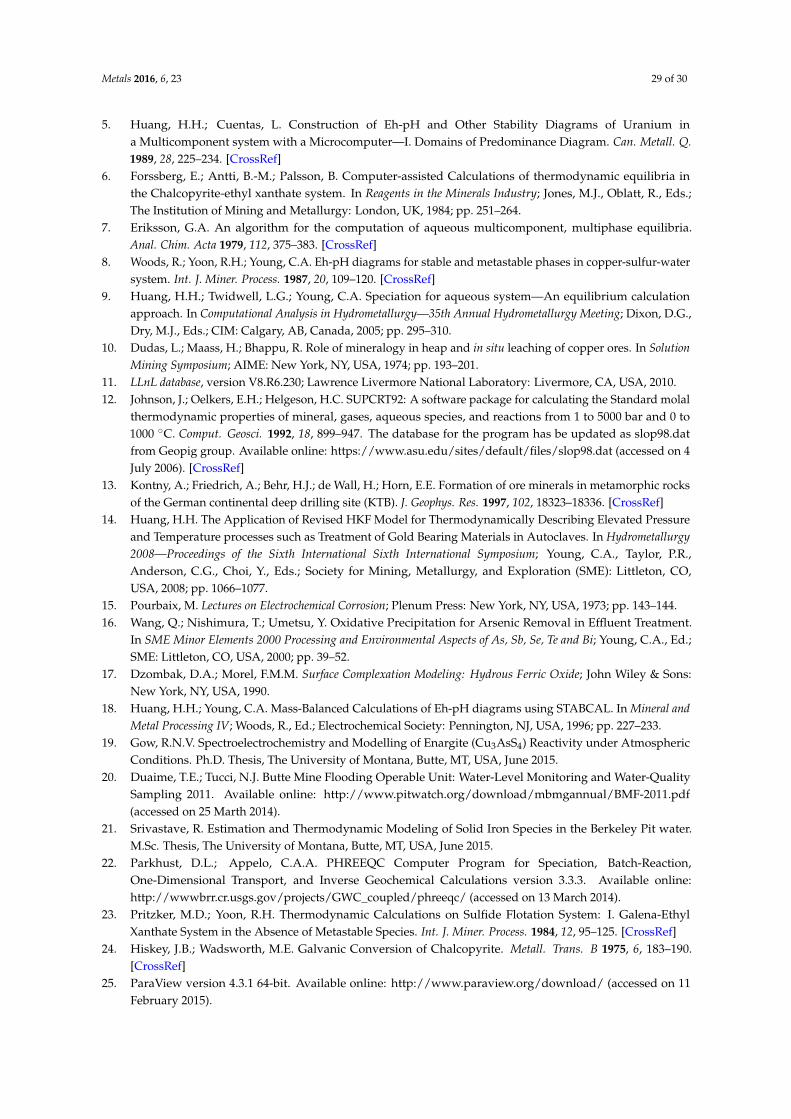
Metals 2016, 6, 23 29 of 30
5. Huang, H.H.; Cuentas, L. Construction of Eh-pH and Other Stability Diagrams of Uranium ina Multicomponent system with a Microcomputer—I. Domains of Predominance Diagram. Can. Metall. Q.1989, 28, 225–234. [CrossRef]
6. Forssberg, E.; Antti, B.-M.; Palsson, B. Computer-assisted Calculations of thermodynamic equilibria inthe Chalcopyrite-ethyl xanthate system. In Reagents in the Minerals Industry; Jones, M.J., Oblatt, R., Eds.;The Institution of Mining and Metallurgy: London, UK, 1984; pp. 251–264.
7. Eriksson, G.A. An algorithm for the computation of aqueous multicomponent, multiphase equilibria.Anal. Chim. Acta 1979, 112, 375–383. [CrossRef]
8. Woods, R.; Yoon, R.H.; Young, C.A. Eh-pH diagrams for stable and metastable phases in copper-sulfur-watersystem. Int. J. Miner. Process. 1987, 20, 109–120. [CrossRef]
9. Huang, H.H.; Twidwell, L.G.; Young, C.A. Speciation for aqueous system—An equilibrium calculationapproach. In Computational Analysis in Hydrometallurgy—35th Annual Hydrometallurgy Meeting; Dixon, D.G.,Dry, M.J., Eds.; CIM: Calgary, AB, Canada, 2005; pp. 295–310.
10. Dudas, L.; Maass, H.; Bhappu, R. Role of mineralogy in heap and in situ leaching of copper ores. In SolutionMining Symposium; AIME: New York, NY, USA, 1974; pp. 193–201.
11. LLnL database, version V8.R6.230; Lawrence Livermore National Laboratory: Livermore, CA, USA, 2010.12. Johnson, J.; Oelkers, E.H.; Helgeson, H.C. SUPCRT92: A software package for calculating the Standard molal
thermodynamic properties of mineral, gases, aqueous species, and reactions from 1 to 5000 bar and 0 to1000 ˝C. Comput. Geosci. 1992, 18, 899–947. The database for the program has be updated as slop98.datfrom Geopig group. Available online: https://www.asu.edu/sites/default/files/slop98.dat (accessed on 4July 2006). [CrossRef]
13. Kontny, A.; Friedrich, A.; Behr, H.J.; de Wall, H.; Horn, E.E. Formation of ore minerals in metamorphic rocksof the German continental deep drilling site (KTB). J. Geophys. Res. 1997, 102, 18323–18336. [CrossRef]
14. Huang, H.H. The Application of Revised HKF Model for Thermodynamically Describing Elevated Pressureand Temperature processes such as Treatment of Gold Bearing Materials in Autoclaves. In Hydrometallurgy2008—Proceedings of the Sixth International Sixth International Symposium; Young, C.A., Taylor, P.R.,Anderson, C.G., Choi, Y., Eds.; Society for Mining, Metallurgy, and Exploration (SME): Littleton, CO,USA, 2008; pp. 1066–1077.
15. Pourbaix, M. Lectures on Electrochemical Corrosion; Plenum Press: New York, NY, USA, 1973; pp. 143–144.16. Wang, Q.; Nishimura, T.; Umetsu, Y. Oxidative Precipitation for Arsenic Removal in Effluent Treatment.
In SME Minor Elements 2000 Processing and Environmental Aspects of As, Sb, Se, Te and Bi; Young, C.A., Ed.;SME: Littleton, CO, USA, 2000; pp. 39–52.
17. Dzombak, D.A.; Morel, F.M.M. Surface Complexation Modeling: Hydrous Ferric Oxide; John Wiley & Sons:New York, NY, USA, 1990.
18. Huang, H.H.; Young, C.A. Mass-Balanced Calculations of Eh-pH diagrams using STABCAL. In Mineral andMetal Processing IV; Woods, R., Ed.; Electrochemical Society: Pennington, NJ, USA, 1996; pp. 227–233.
19. Gow, R.N.V. Spectroelectrochemistry and Modelling of Enargite (Cu3AsS4) Reactivity under AtmosphericConditions. Ph.D. Thesis, The University of Montana, Butte, MT, USA, June 2015.
20. Duaime, T.E.; Tucci, N.J. Butte Mine Flooding Operable Unit: Water-Level Monitoring and Water-QualitySampling 2011. Available online: http://www.pitwatch.org/download/mbmgannual/BMF-2011.pdf(accessed on 25 Marth 2014).
21. Srivastave, R. Estimation and Thermodynamic Modeling of Solid Iron Species in the Berkeley Pit water.M.Sc. Thesis, The University of Montana, Butte, MT, USA, June 2015.
22. Parkhust, D.L.; Appelo, C.A.A. PHREEQC Computer Program for Speciation, Batch-Reaction,One-Dimensional Transport, and Inverse Geochemical Calculations version 3.3.3. Available online:http://wwwbrr.cr.usgs.gov/projects/GWC_coupled/phreeqc/ (accessed on 13 March 2014).
23. Pritzker, M.D.; Yoon, R.H. Thermodynamic Calculations on Sulfide Flotation System: I. Galena-EthylXanthate System in the Absence of Metastable Species. Int. J. Miner. Process. 1984, 12, 95–125. [CrossRef]
24. Hiskey, J.B.; Wadsworth, M.E. Galvanic Conversion of Chalcopyrite. Metall. Trans. B 1975, 6, 183–190.[CrossRef]
25. ParaView version 4.3.1 64-bit. Available online: http://www.paraview.org/download/ (accessed on 11February 2015).

Metals 2016, 6, 23 30 of 30
26. VisIt 2015 Version 2.4.2. Available online: https://wci.llnl.gov/simulation/computer-codes/visit/ (accessedon 23 April 2012).
27. MATLAB, Version R2013a; Mathworks Computer program: Natick, MA, USA, 2013.28. Grossmann, K.; Arnold, T.; Lkeda-Ohno, A.; Steudtner, R.; Geipel, G.; Bernhard, G. Fluorescence properties of
a uranyl(V)-carbonate species [U(V)O2(CO3)3]5´ at low temperature. Spectrochim. Acta A 2009, 72, 449–453.[CrossRef] [PubMed]
29. VTK Format. The VTK User’s Guide, Version 4.2, Kitware. 2010. Available online: http://www.vtk.org/wp-content/uploads/2015/04/file-formats.pdf (accessed on 19 February 2015).
© 2016 by the author; licensee MDPI, Basel, Switzerland. This article is an open accessarticle distributed under the terms and conditions of the Creative Commons by Attribution(CC-BY) license (http://creativecommons.org/licenses/by/4.0/).