ssecorp fo trap tnatropmi na si gnitoliP si tnalp elacs-llams a erehw ngised

lacisyhp a ni ssecorp eht tset ot derutcafunam eht gnipleh era stnalp toliP .tnemnorivne

rieht etaulave ot sreenigne lacimehc eht ot noitulos dnfi dna snoitalumis retupmoc

.noitarepo ssecorp fo segnellahc,gnitolip ni dnert wen a si gnitolip elacs-orciM

yb sesnepxe eht ecuder ot si mia eht erehw siht nI .stnalp tolip fo sezis eht gnicuder

lluf a fo noitarepo fo ytilibissop eht ,krow si elacs-orcim ni ssecorp lacimehc

tsrfi eht fo eno si krow sihT .detagitsevni a ,rotcaer a erehw seiduts elacs-orcim

erew maerts elcycer a dna tinu noitarapes leufoib etelpmoc a nur ot denibmoc suounitnoc ehT .ssecorp noitcudorp

syad 11 revo rof ssecorp siht fo noitarepo fo sessenkaew dna shtgnerts eht wohs dluoc

.tnempoleved ssecorp rof gnitolip elacs-orcim esahp tnaveler fo seires a ,yllanoitiddA ot edam erew stnemerusaem airbiliuqe

,revoeroM .krow eht fo gnilledom eht troppus si nmuloc noitallitsid elbatnirp D3 a

gnisu fo ytilibissop eht evresbo ot depoleved .gnitolip elacs-orcim ni gnitnirp D3

-otl

aA

DD

9

9/

810

2

+cgaai

a*GMFTSH

9 NBSI 2-6008-06-259-879 )detnirp( NBSI 9-7008-06-259-879 )fdp( NSSI 4394-9971 )detnirp( NSSI 2494-9971 )fdp(

ytisrevinU otlaA

gnireenignE lacimehC fo loohcS gnireenignE lacigrullateM dna lacimehC fo tnemtrapeD

if.otlaa.www

+ SSENISUB YMONOCE

+ TRA

+ NGISED ERUTCETIHCRA

+ ECNEICS

YGOLONHCET

REVOSSORC

LAROTCOD SNOITATRESSID

ina

dra

M de

eaS

stn

alp

elac

s-or

cim

gnis

u se

ssec

orp l

aci

mehc

fo t

nemp

olev

eD

yti

srev

in

U otl

aA

8102

gnireenignE lacigrullateM dna lacimehC fo tnemtrapeD

lacimehc fo tnempoleveD elacs-orcim gnisu sessecorp

stnalp

inadraM deeaS

LAROTCOD SNOITATRESSID

seires noitacilbup ytisrevinU otlaASNOITATRESSID LAROTCOD 99 / 8102

sessecorp lacimehc fo tnempoleveD stnalp elacs-orcim gnisu

inadraM deeaS

fo rotcoD fo eerged eht rof detelpmoc noitatressid larotcod A eht fo noissimrep eht htiw ,dednefed eb ot )ygolonhceT( ecneicS

cilbup a ta ,gnireenignE lacimehC fo loohcS ytisrevinU otlaA eht fo )muirotiduA appmoK( 2EK muirotiduA eht ta dleh noitanimaxe

.21 ta 7102 yaM ht52 no loohcs

ytisrevinU otlaA gnireenignE lacimehC fo loohcS

gnireenignE lacigrullateM dna lacimehC fo tnemtrapeD gnireenignE lacimehC fo puorG hcraeseR

rosseforp gnisivrepuS dnalniF ,ytisrevinU otlaA ,sueapolA elliV .forP

rosivda sisehT

dnalniF ,ytisrevinU otlaA ,ynyyK-isuU irteP .cS .D

srenimaxe yranimilerP ynamreG ,ytisrevinU dnumtroD UT ,nnamkcoK trebroN .gnI-.rD .forP

sdnalrehteN ,)e/UT( ygolonhceT fo ytisrevinU nevohdniE ,lesseH rekloV.rd.forP

tnenoppO ynamreG ,ygolonhceT fo etutitsnI ehurslraK ,reyemttiD dnaloR .libah .gnI-.rD .forP

seires noitacilbup ytisrevinU otlaASNOITATRESSID LAROTCOD 99 / 8102

© 8102 inadraM deeaS

NBSI 2-6008-06-259-879 )detnirp( NBSI 9-7008-06-259-879 )fdp( NSSI 4394-9971 )detnirp( NSSI 2494-9971 )fdp(

:NBSI:NRU/if.nru//:ptth 9-7008-06-259-879

yO aifarginU iknisleH 8102

dnalniF

tcartsbA otlaA 67000-IF ,00011 xoB .O.P ,ytisrevinU otlaA if.otlaa.www

rohtuA inadraM deeaS

noitatressid larotcod eht fo emaN stnalp elacs-orcim gnisu sessecorp lacimehc fo tnempoleveD

rehsilbuP gnireenignE lacimehC fo loohcS

tinU gnireenignE lacigrullateM dna lacimehC fo tnemtrapeD

seireS seires noitacilbup ytisrevinU otlaA SNOITATRESSID LAROTCOD 99 / 8102

hcraeser fo dleiF gnireenignE lacimehC

dettimbus tpircsunaM 7102 rebmevoN 03 ecnefed eht fo etaD 8102 yaM 52

)etad( detnarg hsilbup ot noissimreP 8102 hcraM 32 egaugnaL hsilgnE

hpargonoM noitatressid elcitrA noitatressid yassE

tcartsbAniam ehT .tnempoleved ssecorp rof stnalp elacs-orcim gnisu fo ytilibissop eht detaulave krow sihT )D3( lanoisnemid 3 a fo tnempoleved ,seitreporp lacisyhp fo tnemerusaem erew yduts siht ni sksat

-4,4,2-yxohtem 2 fo noitcudorp rof ssecorp a fo tnempoleved dna nmuloc noitallitsid detnirp .tnalp elacs-orcim a gnisu )EMOT( enatneplyhtemirt

rof ssecorp eht ni tneserp slacimehc eht no gnisucof erew seitreporp lacisyhp derusaem ehT

,dnuopmoc erup a rof ytisned edulcni seitreporp lacisyhp derusaem ehT .EMOT fo noitcudorp ehT .serutxim yranret dna yranib rof muirbiliuqe diuqil-diuqil dna yplahtne ssecxe

lasrevINU ro )LTRN( diuqil-owt modnar noN sa hcus sledom tneicfifeoc ytivitca nommoc .tnemerusaem airbiliuqe esahp eht fo gniledom rof desu erew )CAUQINU( lacimehCisAUQ

seitilibapac eht revocsid ot detagitsevni saw ,ygolonhcet gnirutcafunam wen a sa ,gnitnirp D3 ehT

raludom a ,krow siht nI .sesutarappa lacimehc detacilpmoc fo noitcudorp ni euqinhcet siht fo eht ni detaulave dna ,retnirp D3 a htiw detnirp ,dengised saw gnikcap sti dna nmuloc noitallitsid tnereffid htiw dna sgnikcap fo epyt tnereffid gnisu detset saw nmuloc detnirp D3 ehT .yrotarobal elbissop ti edam gnirutcafunam dipar ylbaredisnoc dna ngised eht fo ytiraludom ehT .soitar xufler

eb dluoc taht nmuloc noitallitsid lacitcarp a poleved dna semit lareves rof ngised eht evorpmi ot .noitallitsid-orcim rof desu

ssecorp fo sessenkaew dna shtgnerts ,ytilibissop eht yduts ot desu saw tnalp elacs-orcim A

noitacfiirehte na gnisu EMOT fo noitcudorp saw yduts esac ehT .stnalp-orcim ni tnempoleved fo spets lareves ,krow siht nI .nmuloc noitallitsid a dna rotcaer a dedulcni ssecorp sihT .ssecorp

- noitalumis ,sutarappa ssalg a gnisu lacimehc eht fo noitcudorp hctab sa hcus ,ngised ssecorp eht fo stluser ehT .enod erew ssecorp eht fo gnitolip elacs-orcim dna ssecorp eht fo noitazimitpo

lanoitarepo dna setarwofl ,snoitisopmoc eht sa hcus noitamrofni elbaulav evag stnemerusaem .gniledom eht htiw llew gnidnopserroc erew hcihw serutarepmet

sdrowyeK ,gnitnirp D3 ,CAUQINU ,LTRN ,yplahtne ssecxE ,muirbiliuqe )diuqil + diuqiL( ;tnalp-orciM ,erutcurts raludoM ,gnikcap noitallitsiD ,gnirutcafunam evitiddA

tnalp tolip ;noitallitsiD ;rotcaeR ;tnempoleved ssecorp lacimehC )detnirp( NBSI 2-6008-06-259-879 )fdp( NBSI 9-7008-06-259-879

)detnirp( NSSI 4394-9971 )fdp( NSSI 2494-9971

rehsilbup fo noitacoL iknisleH gnitnirp fo noitacoL iknisleH raeY 8102

segaP 021 nru :NBSI:NRU/fi.nru//:ptth 9-7008-06-259-879

i

Acknowledgements

From the first steps of my studies in Iran, up to the end of this study in Aalto University, there was a long way that I passed. I overcame the challenges with the support and kindness of the people who were near me on the happy and rainy days.

This project would have been impossible without the support of Academy of Finland and Aalto University.

I would like to offer my special thanks to Professor Ville Alopaeous for his supervision and advisory of the work. His great talent, knowledge and support in modeling of the work opened a new scope in my chemical engineering understanding.

I also thank Helena Laavi, Emeline Bouget, Juha-Pekka Pokki, Leo S. Ojala and Petri Uusi-Kyyny for their contribution in the published papers. Additionally, I thank all other members of the VLE/LLE laboratory; it was great to share experience and the equipment with you.

During the doctoral studies, I met many new friends, whose friendship made a wonderful experience in my life. I should gratefully thank Susanna, Elina, Anne, Anna, Tuomas, Esko, Ngoc, Ali Afzalifar, Ali Ahi and Navid for the great moments we had together in the last years.

Finally, I would like to say my sincere thanks to my family: my parents, Zahra, Samira and Farshad for their support throughout this study and my life in general.

Espoo, 28th March 2018

Saeed Mardani

ii

Contents Acknowledgements ................................................................................... i

List of Abbreviations and Symbols ......................................................... iv

Abbreviations ...................................................................................... iv

Symbols ............................................................................................... iv

List of Publications.................................................................................. vi

Author Contributions ............................................................................. vii

1. Introduction .................................................................................. 1

1.1 Background ............................................................................... 1

1.2 Scopes of this work .................................................................... 3

2. Physical properties measurements ............................................... 5

2.1 Background ............................................................................... 5

2.2 Measurement ............................................................................. 6

2.2.1 Density measurement ............................................................ 6

2.2.2 Liquid-Liquid Equilibrium (LLE) measurement with ............ analytical method .................................................................. 7

2.2.3 Liquid-Liquid Equilibrium (LLE) measurement..................... by turbidimetry ..................................................................... 9

2.2.4 Excess enthalpy (HE) measurements ..................................... 9

2.3 Modeling of the measured data ............................................... 10

2.3.1 Non Random Two-Liquid (NRTL) activity coefficient ............ model ................................................................................... 13

2.3.2 UNIversal QUAsiChemical (UNIQUAC) activity coefficient ... model ................................................................................... 14

2.4 Evaluation of the data ............................................................. 15

3. Design and manufacturing of a 3D printed distillation column . 17

3.1 Background ............................................................................. 17

3.2 Selection of 3D printing technology ........................................ 17

3.2.1 Fused deposition modeling (FDM)...................................... 18

3.2.2 Digital light processing (DLP) ............................................. 18

3.2.3 Selective laser sintering (SLS) ............................................. 19

3.3 Design specification of the 3D printed distillation column .... 20

3.3.1 General concept for designing the distillation column ....... 20

3.3.2 Modularity of the distillation column .................................. 21

3.3.3 The improvements in design of different sections .............. 22

3.3.4 Design of the packing .......................................................... 22

3.4 Results and Conclusion ........................................................... 23

4. Process development with a microscale plant ............................ 27

iii

4.1 Background .............................................................................. 27

4.2 The studied process ................................................................ 28

4.3 Development of the process for production of TOME ........... 30

4.3.1 Step 1. Batch production of TOME ..................................... 30

4.3.2 Step 2. Operation of the micro-plant ................................... 31

4.3.3 Step 3. Process simulation ................................................... 36

4.4 Preparation of the micro-plant ................................................ 41

4.4.1 Reactor ................................................................................. 41

4.4.2 Distillation column .............................................................. 42

4.4.3 Instrumentation ................................................................... 43

5. Conclusion ................................................................................... 47

6. Suggestions for future works ...................................................... 49

References .............................................................................................. 51

Publication I

Publication II

Publication III

Publication IV

iv

List of Abbreviations and Symbols Abbreviations

2D 2 dimensional 3D 3 dimensional CAD computer-aided design DC direct current DLP Digital Light Processing DME dimethyl ether EU European Union FDM fused Deposition Modeling FQD fuel quality directive GC gas chromatograph GC/MS gas chromatography/mass spectrometry HE excess enthalpy IOT internet of things KF Karl-Fischer titrator LLE liquid-liquid equilibrium LOM laminated object manufacturing MEOH methanol NTS number of theoretical stages (NTS) NRTL non-random two-liquid model PAHs polycyclic aromatic hydrocarbons PFD process flow diagram RED renewable energy directive SLS selective laser sintering TMP-1 2,4,4-trimethyl-1-pentene TMP-2 2,4,4-trimethyl-2-pentene TOME 2-methoxy-2,4,4-trimethylpentane (tertiary octyl methyl ether) UNIFAC UNIQUAC functional-group activity coefficients UNIQUAC UNIversal QUAsiChemical VLE vapor-liquid equilibrium Symbols

aij, aji, bij, bji, cij, dij, eij, eji, fij, fji binary interaction parameters for activity coefficient models

A mass transfer area, m2 A-C component specific parameters for Antoine vapor pressure

equation A-D Rackett correlation parameters

fugacity of chemical i, Pa standard fugacity, Pa

v

F flow rate, mol·s-1 HE excess enthalpy, J·mol-1

kj reaction rate constant, mol·kgcat-1·s-1 Ki vapor-liquid distribution ratio Kjeq equilibrium constant for reaction j N molar flux, mol· m-2·s-1 p control parameters for the flow rates P pressure, Pa

liquid vapor pressure of component i, Pa ri rate of reaction for the compound i, mol·kgcat-1·s-1 T temperature, K V molar volume, m3·mol-1

superficial vapor velocity, m·s-1 composition of component i in the liquid phase composition of component i in the vapor phase non-randomness parameter for NRTL activity coefficient model

specified vapor volume fraction for each stage of the distillation column

chemical potentials of chemical i Density, kg·m-3

Activity coefficient of component i fugacity coefficients of chemical i

vi

List of Publications This doctoral dissertation consists of a summary and of the following publications, which are referred in the text by their numerals. I. Mardani, S., Laavi, H., Bouget, E., Pokki, J.-P., Uusi-Kyyny, P., Alopaeus, V., 2015. Measurements and modeling of LLE and HE for (methanol + 2,4,4-trimethyl-1-pentene), and LLE for (water + methanol + 2,4,4-trimethyl-1-pentene). The Journal of Chemical Thermodynamics, 85, 120–128. doi:10.1016/j.jct.2015.01.013

II. Mardani, S., Uusi-Kyyny, P., Alopaeus, V., 2015. Measurements and modeling for the density of 2-methoxy-2,4,4-trimethylpentane, HE for (methanol + 2-methoxy-2,4,4-trimethylpentane), LLE for (water + 2-methoxy-2,4,4-trimethylpentane) and LLE for (water + methanol + 2-methoxy-2,4,4-trimethylpentane). The Journal of Chemical Thermodynamics, 91, 313–320. doi:10.1016/j.jct.2015.08.011

III. Mardani, S., Ojala, L.S., Uusi-Kyyny, P., Alopaeus, V., 2016. Development of a unique modular distillation column using 3D printing. Chemical Engineering and Processing: Process Intensification, 109, 136–148. doi:10.1016/j.cep.2016.09.001

IV. Mardani, S., Uusi-Kyyny, P., Alopaeus, V., 2017. Micro-scale piloting of a process for production of 2-methoxy-2,4,4-trimethylpentane. Chemical Engineering and Processing: Process Intensification, 122, 143–154. doi:10.1016/j.cep.2017.09.016

vii

Author Contributions Publication I: Measurements and modeling of LLE and HE for (methanol + 2,4,4-trimethyl-1-pentene), and LLE for (water + methanol + 2,4,4-trimethyl-1-pentene) SM participated in the LLE measurement, performed the excess enthalpy measurement and regressed the model parameters and wrote the manuscript; HL participated in the excess enthalpy measurement, EB contributed in the LLE measurements; JPP and PUK were instructors of the work; VA supervised the project. All co-authors commented the manuscript. Publication II: Measurements and modeling for the density of 2-methoxy-2,4,4-trimethylpentane, HE for (methanol + 2-methoxy-2,4,4-trimethylpentane), LLE for (water + 2-methoxy-2,4,4-trimethylpentane) and LLE for (water + methanol + 2-methoxy-2,4,4-trimethylpentane) SM synthetized and purified 2-methoxy-2,4,4-trimethylpentane, measured the physical properties, regressed the model parameters and wrote the manuscript; PUK was instructor of the work, VA supervised the project. All co-authors commented the manuscript. Publication III: Development of a unique modular distillation column using 3D printing. SM designed and printed the modular distillation column, conducted the experiments, evaluated the results and wrote the manuscript; LSO participated in early stage investigation of the material used in the work and 3D models; PUK was instructor of the work, VA supervised the project. All co-authors commented the manuscript.

Publication IV: Micro-scale piloting of a process for production of 2-methoxy-2,4,4-trimethylpentane SM contributed in development of the micro-scale plant (micro-plant), operated the micro-plant, participated in the modeling of the work and wrote the manuscript; PUK was instructor of the work, VA contributed in the modeling of the process and supervised the project. All co-authors commented the manuscript.

viii

1

1. Introduction

1.1 Background

The chemical industry is an immense collection of chemical processes, operations, and organizations that are working together to manufacture thousands of different chemicals. This industry is one of the most dynamic businesses in the world and actively affecting the global economy. Therefore, manufacturing of new chemicals or optimization of the qualities and quantities of the products are continuously investigated to increase the profitability of the chemical industries. Vogel (2006) mentioned that around 7 % of the turnovers in chemical industries during 1990 to 2000 were invested in research and development. This investment is helping the companies to remain in the competitive market. For all the companies, the target is to be faster in production of newly developed chemicals, reduce the costs, increase the environmental compatibility, and raise the quality of the chemicals.

Haan (2015) described the product family tree, Figure 1.1, where 10 raw materials are used to produce 20 basic products, which later transformed to around 300 chemicals. Finally, they are used to produce almost 30000 refined chemicals and consumer products. In this description, the basic and intermediate products are hugely used to produce the subproducts, which makes them to remain in the market for a long time. However, the refined chemicals and consumer-end products are updating time to time to make higher qualifications based on the marketing demand.

2

Figure 1.1. Product family tree of chemical industry.

The invention of chemicals are done in laboratories, mostly in batch mode and in several independent steps. After having success in production of the chemical, and exploring the suitable catalyst, the process can be proposed for mass production.

The chemical process designers are mainly focusing on production of chemicals in large scales. After invention of a new chemical, the chemical engineers start to design and implement the process. In industrial process design (Kaibel, Schoenmakers, H., 2002), the capacities, purities, and an overview of the process, such as batch-continuous production have to be decided in the first steps. Later, the physical and chemical properties should be determined. The reaction kinetics and the chemical equilibrium study is mandatory for designing the reactor. And, for designing the separation units, storage vessels and the transfer lines, the thermo-physical properties such as vapor pressures, densities, vapor-liquid equilibria (VLE), liquid-liquid equilibria (LLE), thermal stability, etc. are necessary. The integrity of the data, at least for the main components, is an important factor in designing a process. By having these sort of data, it is possible to design the reactors, find the viable methods of separation and find the best type of vessels needed for the process. After understanding the necessary vessels and combining them in the most efficient order, the flowsheet should be optimized using computer programs to find the optimum conditions. Finally, an economic evaluation can show if the process is worthy, or should the design be modified.

When the economic evaluation was completed, the process should be tested (Vogel, 2006) using different scales of pilot plants to observe the possible challenges that can appear in the chemical process. Conventionally, the first

3

piloting is done in miniplants which have production rates of ≈0.100 - 1 kg·h-1. The mini-plants are usually complete plants, which include synthesis section (reactor), workup (separation units), and all the recycle streams. After a successful run in mini scale plant, a trial plant with a higher production capacity of ≈10-100 kg·h-1 would be designed. The products of this plant can be used to test the applications of the produced chemicals or it can be delivered to customers for checking the qualification of the product. The operation of the pilot plant gives the information needed to verify the models made during the flowsheet optimization and complete documentary information needed to start building the main plant. According to Palluzi (2000) and McConville (2000), the pilot plants can have a building price range from US $ 10 thousand to 10 million. This is mainly dependent to the size of the pilot plants. By increasing the size, the project expenses also increase. Additionally, the expenses for the operators and feedstock can make larger scales more expensive. As a result, many research groups are trying to miniaturize the pilot plants.

1.2 Scopes of this work

This work focused on miniaturization of a piloting case to a micro-scale plant (micro-plant). The micro-plant with a total holdup of 120 cm3 was implemented to study the possibilities for miniaturization of a pilot plant. The mentioned micro-plant includes a reactor where the reaction takes place, a distillation column for the separation of the reactor output chemicals, and a recycle stream to return the non-reacted material back to the reactor. Figure 1.2 is presenting the block flow diagram of the micro-plant. The main objective of this work was to make measurements using the micro-plant, and make a model using the conventional modeling methods to describe the system. This work present the capabilities of micro-scale piloting of a process and introduce the advantages and drawbacks of the micro piloting. The studied case was production of 2-methoxy-2,4,4-trimethylpentane (also known as tertiary octyl methyl ether or TOME). TOME is an ether that was proposed as a fuel oxygenate to be added to gasoline (Rihko-Struckmann et al., 2004). The TOME can be produced by etherification of methanol + diisobutylene (a mixture of 2,4,4-trimethyl-1-pentene (TMP-1) and 2,4,4-trimethyl-2-pentene (TMP-2)). The paper IV is focusing on the results obtained from the piloting of the process for production of TOME in the micro-plant.

Figure 1.2. A block flow diagram of the micro-plant.

4

The papers I & II focused on the phase equilibria of the chemicals present in the work. This was due to the demand of the simulation section of the piloting work for the models to describe the system. Moreover, it could make better understanding of the phenomena happening in the system. The necessary data were either obtained from the literature or measured in this study.

In paper III, the application of 3 dimensional (3D) printing for manufacturing of a distillation column was successfully implemented. One of the current drawbacks of piloting in microscale is the lack of vessels needed for piloting in small scales. Therefore, many research groups are trying to manufacture new devices to be used in micro-milli scale operations. The 3D printing, which is currently a trending technology, can be used in the micro-scale piloting for manufacturing complicated small-scale devices. In this work, a distillation column was designed using a 3D designing software and printed with a 3D printer.

5

2. Physical properties measurements

2.1 Background

Finding the physical properties of the chemicals that are present in the system is one of the first blocks in development of a process. The physical properties are used to regress parameters of the thermodynamic models. The thermodynamic models are used to simulate the process with chemical process optimization software. In addition, the physical properties can help the operators to understand the nature of the system and direct the operation towards the optimal condition.

In this study, the focus of the physical properties measurements were on the compounds which were available in the process for production of 2-methoxy-2,4,4-trimethylpentane (also known as tertiary octyl methyl ether or TOME). Table 2.1 is presenting the compounds that were available in the TOME production process and the physical properties used in the modeling of the work.

In papers I & II, several physical properties such as density of TOME, excess enthalpies for binary mixtures, and liquid-liquid equilibrium (LLE) for binary and ternary systems were measured, and the model parameters were regressed to describe their properties. The focus on LLE measurement was due to appearance of water in the process, which was causing phase separation. The LLE measurement and model could show the available phases in the system and lead the system towards a one-phase condition. Moreover, the excess enthalpy (heat of mixing) data could increase the temperature dependency of the activity coefficient models for extrapolation using the Gibbs–Duhem equation (Walas, 1985, and Laavi et al., 2012).

6

Table 2.1. Physical properties used in this work.

Pure Methanol Vapor Pressure (Uusi-Kyyny, 2001a) and (Selected

Values of Properties of Chemical Compounds 1980) and density (Wilhoit, 1973)

TMP (1&2) Vapor Pressure (Selected Values of Properties of Hydrocarbons and Related Compounds 1980-extant. American Petroleum Institute Research Project 44), (Camin and Rossini, 1955) and densities (Daubert, 1992),(Nhu et al. 1988)

TOME Vapor Pressure (Uusi-Kyyny, 2001) and density (I) Water Vapor Pressure (haar et al. 1984) and (Gallagher et al.

1984) and density (Wang et al., 2013) DME Vapor Pressure and density (Timmermans, 1965) Binary Methanol +TMP (1&2) VLE (Uusi-Kyyny, 2001), LLE (I), HE (I)

Methanol +TOME VLE (Uusi-Kyyny, 2001), LLE (II), HE (II) Methanol + Water VLE (Álvarez, V.H. et al., 2011) Methanol + DME VLE was estimated with UNIFAC method. TMP (1&2) + TOME Considered to be ideal. TMP (1&2) + Water LLE (I), VLE was estimated with UNIFAC

method. TMP (1&2) + DME VLE was estimated with UNIFAC method. TOME + Water LLE (II), VLE was estimated with UNIFAC

method. TOME + DME VLE was estimated with UNIFAC method. Ternary systems Water + Methanol + TMP 1 LLE (I) Water + Methanol + TOME LLE (II)

2.2 Measurement

2.2.1 Density measurement The density of the chemicals are necessary for modeling the systems. The density for methanol, TMP-1&2, water, and DME were available from literature. The density of TOME was measured in paper II using a density meter. Figure 2.1 is presenting the measured densities for TOME.

7

Figure 2.1. The measured density for 2-methoxy-2,4,4-trimethylpentane: × measured liquid density, — Rackett correlation (II).

2.2.2 Liquid-Liquid Equilibrium (LLE) measurement with analytical method

In this work, the LLE measurements for 3 binary and 2 ternary systems were conducted. The LLE measurements for papers I & II were done inside isothermal-jacketed cells. The temperatures were controlled using a water thermostat connected to the jacket of the cells. A thermocouple was used to check the temperature inside the cells. A magnetic mixer and 3-4 stirrers were used to mix the liquids. Later, the cells were kept in vertical mode to settle and samples were obtained from both phases to check the compositions using a gas chromatograph (GC), moreover, water contents were checked using a Karl-Fischer titrator (KF). Figure 2.2 is presenting the schematic and the photo of the device used in LLE measurements (Papers I & II). Figure 2.3 is giving the measured and the non-random two-liquid (NRTL) model (Renon and Prausnitz, 1968) for the ternary system of water + methanol + TMP-1.

680

720

760

800

280 320 360 400

ρ/

kg·m

-3

T / K

8

Figure 2.2. The isothermal-jacketed cell for LLE measurement. Left: mixing mode, right: Settling mode. 1- Thermometer, 2- Equilibrium cell, 3- magnetic mixer, 4 sampling syringe.

Figure 2.3. LLE for the ternary system of (water (1) + methanol (2) + TMP-1 (3)) at atmospheric pressure (101 kPa) and T = 283 K: ■ Measured tie lines; ● turbidimetry; - - - NRTL model tie lines; – miscibility gap boundaries by NRTL model.

9

2.2.3 Liquid-Liquid Equilibrium (LLE) measurement by turbidimetry

The turbidimetry method (Raal and Mühlbauer, 1998), which is a visual method, was used to find the phase split borders for the binary and ternary systems. The cell used for this measurement had a jacket to control the temperature inside the cell. A water thermostat was connected to adjust the temperature. A thermometer was showing the temperature in the cell. A mixer with magnetic stirrer was used to mix the chemicals. By modifying compositions or the temperature inside the cell, the transparency of the mixing system could change. The turbidity of the system was showing the two-phase region, while one phase region was clear. The turbidimetry results can be seen in Figure 2.3. More detail about the device used for this measurements are available in papers I and II.

2.2.4 Excess enthalpy (HE) measurements The excess enthalpy (HE) measurement were done with an isothermal calorimeter. Two syringe pumps were injecting pure liquid streams to a preheater to adjust the stream temperatures to a set point. Then, the streams were mixed inside an isothermal calorimeter. The amount of heat generated was recorded and analyzed by a computer. Figure 2.4 is showing the diagram of the equipment used for excess enthalpy measurement. Figure 2.5 is presenting the excess enthalpy measurement for the binary system of methanol + TOME.

Figure 2.4. Schematic diagram of the excess enthalpy measurement device. 1-syringe pumps, 2- calorimeter, 3- liquid preheater, 4- isothermal furnace.

10

Figure 2.5. The excess enthalpy measurements for the binary system of methanol + TOME, the line is representing the model.

2.3 Modeling of the measured data

Josiah Willard Gibbs, 1839-1903, defined the principles of the modern thermodynamics during 1875-1882. The Gibbs’ article entitled “On the Equilibrium of Heterogeneous Substances” in 321 pages was the first article to explain the modern thermodynamics with the current form (Ott and Boerio-Goates, 2000). For describing the phase equilibria, Gibbs introduced an imaginary thermodynamic quantity called chemical potential of the phases. He explained that the two phases are in equilibrium if the chemical potentials are equal (equation 2.1).

(2.1)

Where and are the chemical potentials of chemical i in phase and . Later, Lewis showed that this condition can be achieved when the isofugacity of both phases are equal (equation 2.2):

(2.2)

Where and are the fugacities of chemical i in phase and , Pa. At low pressures, except for strongly associating compounds, the fugacities are equal to vapor pressure or sublimation pressure of the chemical. And for the chemical mixtures, at low pressures, the fugacities are almost similar to the partial pressure of the considered compound. Since these quantities cannot be directly measured, auxiliary quantities such as fugacity coefficient ( ) and activity coefficients ( ) are introduced to enhance the phase separation calculations.

0

300

600

0 0.25 0.5 0.75 1

HE

/ J·m

ol-1

x1

11

The fugacity coefficients of liquid and vapor are calculated using equation 2.3 and 2.4:

(2.3)

(2.4)

where and are fugacity coefficients of chemical i in liquid and vapor respectively. and are fugacities of liquid and vapor. and are compositions in the mixtures and is the system pressure. According to Dalton’s law (Dalton, 1802), the term can be changed to partial pressure, .

In another approach, the activity coefficient ( ) is defined as (equation 2.5):

(2.5)

where is an arbitrary value known as standard fugacity.

Using the fugacity coefficients or the activity coefficients we can calculate the compositions of the compounds in different phases. As an example, for calculation of the vapor-liquid equilibrium (VLE) case, we can write (equation 2.6):

(2.6)

The fugacities of the two phases ( and ) can be calculated either by using fugacity calculation for both phases which is also known as ( ) approach (equation 2.7) or it is possible to use activity coefficients for the liquid phase which is known as ( ) approach (equation 2.8).

(2.7)

(2.8)

12

For the ( ) approach, the fugacity coefficients are calculated using the equation of states, and for ( ) approach, for the liquids the activities should be calculated using the activity coefficient models, the standard fugacity is considered as the fugacity of pure compound at the same temperature and pressure1. For nonassociating compounds at moderate pressures, with some simplifications, it is possible to change equation 2.8 to equation 2.9:

(2.9)

Where is saturation (vapor) pressure of component I, Pa; and are compositions in the mixtures; is the system pressure, Pa; and is activity coefficient of component i. By using the ( ) approach or ( ) approach it is possible to find vapor-liquid distribution ratio ( ) and relative volatilities ( ) (equation 2.10 and 2.11) which are giving the compositions of the chemicals in equilibrium:

(2.10)

(2.11)

Similar kind of equations can be derived to describe LLE. By considering equation 2.2, we can write equation 2.12:

(2.12)

where and are the fugacities of component i in phase 1 and 2. By using the activity coefficient approach, equation 2.13 can be obtained:

(2.13)

By removing the standard fugacity value from both sides, the equation 2.14 is achieved:

(2.14)

The activities in this equation can be calculated using the activity coefficient models. By using the fugacity approach, a similar equation can be derived

1 For different conditions, this value can be different, as an example, for calculation of solubilities of super critical compounds, Henry constants are often used as standard fugacity. More details about this topic can be found in books such as Gmehling et al. (2012)

13

(equation 2.15) where the fugacities can be calculated using the equation of states:

(2.15)

2.3.1 Non Random Two-Liquid (NRTL) activity coefficient model To describe the system, the model parameters for the binary and ternary systems containing water, methanol, TMP-1 were regressed using the non-random two-liquid (NRTL) (Renon and Prausnitz, 1968) activity coefficient model (equation 2.16). After regressing all the temperature dependent parameters of the NRTL activity coefficient model, the VLE, LLE and excess enthalpy could be described with the model:

(2.16)

Where:

Where, is the activity coefficient; is non-randomness parameter; aij, bij, cij, dij, eij, fij are binary interaction parameters. In the NRTL activity coefficient model, cij= cji and dij=dji. Figure 2.6 is presenting the modeling of the binary system of methanol + TMP-1. Figure 2.3 is showing the ternary LLE measured and the NRTL model. The details of the modeling are provided in paper I.

14

Figure 2.6. Modeling of the binary system of methanol + TMP-1 using NRTL activity coefficient model. 1- isobaric (101 kPa) VLE, 2- isothermal (331 K) VLE, excess enthalpy (298 K), 4- isobaric (101 kPa) LLE

2.3.2 UNIversal QUAsiChemical (UNIQUAC) activity coefficient model

In paper II, due to challenges in modeling with NRTL activity coefficient model for describing VLE, LLE and excess enthalpy with one set of parameters, the UNIversal QUAsiChemical (UNIQUAC) (Abrams and Prausnitz, 1975) activity coefficient model (equation 2.17) was used to model the data:

Where:

(2.17)

15

where, is the activity coefficient; aij, bij, cij, dij, eij, fij are binary interaction parameters. Figure 2.5 is presenting the measured excess enthalpy and the UNIQUAC activity coefficient model. The results of the VLE and LLE modeling for the binary system of (methanol + TOME) and the LLE for the ternary system of (water + methanol + TOME) using UNIQUAC activity coefficient model are available in paper II.

Density. The Rackett density correlation (equation 2.18) was used to model the density of TOME:

(2.18)

Where, is the density of the TOME, A-D are the Rackett correlation parameters and T is temperature, K. Figure 2.1 is representing the measured data and the correlation.

2.4 Evaluation of the data

The smoothness and reliability of LLE measurements were tested using the Othmer–Tobias (Othmer and Tobias, 1942) method (equation 2.19):

(2.19)

where was mass fraction of water in the aqueous phase, and was the mass of TMP-1 (paper I) or TOME (paper II) in hydrocarbon phase. Figure 2.7 is a plot of Othmer–Tobias correlation for the ternary system of (water + methanol + 2-methoxy-2,4,4-trimethylpentane) at T = 283.15 and 298.15 K measured in paper II.

16

Figure 2.7. Othmer-Tobias correlation for the ternary system of (water + methanol + 2-methoxy-2,4,4-trimethylpentane): ○ T = 298.15 K , □ T = 283.15 K, — Othmer - Tobias correlation for T = 298.15 K, - - Othmer - Tobias correlation for T = 283.15 K.

17

3. Design and manufacturing of a 3D printed distillation column

3.1 Background

The pilot plants need vessels to run the process. The researchers around the world are continuously trying to invent new process devices to improve the chemical piloting in micro or milli scale. For example, Schwolow et al. (2016), Vaccaro et al. (2010) and Johnson et al. (2016) designed new milli or micro-scale reactors, MacInnes et al. (2010) built a spinning spiral distillation column, Adiche and Sundmacher (2010) developed a membrane-distillation equipment and Hohmann et al. (2016) manufactured a crystallizer.

The 3 dimensional (3D) printing is generally referred to the techniques that form a 3D object from a computer-aided design (CAD). Due to the nature of this technique, which is forming a solid part from a raw material, in some cases, it can manufacture complex geometries, which could not be produced using conventional machining methods. This technique have had great progress during recent years. There are many 3D printing methods available for different applications. Some of the most well known methods are fused deposition modeling (FDM) (Crump, 1992), photopolymerization (Nakamura, 2014), selective laser sintering (SLS) (Deckard, 1989 and 1997), and laminated object manufacturing (LOM) (Feygin et al., 1998).

Paper III focused on development of a 3D printable modular distillation column where the parts could be printed separately and assembled together using flanges.

3.2 Selection of 3D printing technology

In the beginning of this work, an investigation was done to choose an appropriate 3D printing technology to be used for manufacturing the distillation column. Between the variety of the options, based on the possibility of using the technique and availability of the equipment, three different techniques were further studied to see the best option for 3D printing. The fused deposition modeling (FDM), digital light processing (DLP) technology, and

18

selective laser sintering (SLS) technology were the three best options for manufacturing a distillation column. For all of these techniques, firstly, a 3D CAD design is made and sliced in 2 dimensional (2D) layers, which can be given to the 3D printer for manufacturing the final part.

3.2.1 Fused deposition modeling (FDM) The FDM printing technology (Crump, 1992) is working in several steps. First, a polymer is melted and pushed through an extruder to form a molten string. This polymer string is used to draw the first layer of the 3D model by moving the extruder in x-y axis on a build platform. By moving the build platform one step down, it is possible to print the second layer on top of the first layer. This method is probably the easiest way to 3D print the objects and the printed parts can be larger than in the other two considered methods. However, by observation of the final prints, it can be seen that the printed layers are not completely attaching together and the produced surfaces are not smooth enough for attachment to other 3D printed pieces. These qualifications can cause liquid or gas leakage from the 3D printed pieces which make them unfavorable for designing vessels to be used in chemical process design. Gaal et al. (2017) reported such type of leakages for using this technique. Due to the final print qualifications, it was not possible to print the distillation column modules straightly with this technique; however, it could be possible to make molds, which later could be used for making the modules. Figure 3.1 is presenting a schematic of the FDM printing technology.

Figure 3.1. A schematic of fused deposition modeling (FDM) 3D printing technology.

3.2.2 Digital light processing (DLP) The other option was the DLP printing technology (Nakamura, 2014). In this method, the layers are formed by focusing a light source to a photopolymerizable resin. In this technique, for most printers, the build platform locates on top of a glass resin basin (vat). The build platform moves to a position where a narrow layer of liquid resin stays between the build platform and the resin basin (vat). Then, by focusing a light source from the bottom of

19

the vat to desired locations, the first layer form. At this point, the build platform moves up, and the next layer is formed on top of the previous layer. This method was producing smooth leak proof parts within few hours. Additionally, the print costs were affordable. Therefore, this method was reasonably a good choice for printing the distillation column. Figure 3.2 is presenting a schematic of DLP 3D printing technology.

Figure 3.2. Schematic of digital light processing (DLP) printing technology.

3.2.3 Selective laser sintering (SLS) The third option was selective laser sintering (SLS) (Deckard, 1989 and 1997). In this method, the layers are formed by dispersal of a layer of a powder on a flat surface and focusing the laser light on some desired sections to sinter the metal or polymer particles together. Later, the next layers are formed on top of the previous layers. This method is completely robust, and could probably give the best 3D prints for this work. However, the SLS 3D printers are expensive, which reduce their availability in the market. Due to the demand for try and error in design and manufacturing of the distillation column, and the time needed for ordering and receiving the parts, and because of the high expenses in manufacturing the parts, it was very challenging to use this method. Figure 3.3 is presenting a schematic of the SLS printing technology.

20

Figure 3.3. Schematic of selective laser sintering (SLS) printing technology.

Therefore, the DLP technology was finally chosen to be used for making the 3D printed distillation column. This was giving the chance to design and manufacture prototypes in less than a day. The rapid manufacturing made it possible to test several prototypes and modify the design up to the point that an acceptable design was achieved (III).

3.3 Design specification of the 3D printed distillation column

3.3.1 General concept for designing the distillation column This study was focusing on the capabilities of 3D printing on manufacturing the devices that could be used for micro-scale piloting. The preliminary idea was development of a semi horizontal distillation column. Due to size limitations of the 3D printer, and to save the space in the laboratory hood, the distillation column was made with a coil shape. The coil shape could make it possible to add extra modules to the column without occupying a large length in the laboratory hood.

The body of the distillation column was designed with a hexagonal shape to let the liquid to flow at the bottom with an even distribution, whereas the round shape could make variation in depth of the flowing liquid in the bottom of the cross section.

For the inlets and outlets, the distillation column was designed to add metal union tee fittings from Swagelok® to the 3D printed column. This design helped in adding thermocouples and the material inlet/outlets to the distillation column simultaneously. The thermocouples could measure the temperatures at different sections of the column. Figure 3.4 is presenting the final design of the distillation column.

21

Figure 3.4. The designed distillation column. Left: the interior of the distillation column; right: the body of the distillation column.

3.3.2 Modularity of the distillation column During this work, it was noticed that by increasing the size of the prints, the risk of print failure was raising. The failure could be small, such as a 0.05 cm2 hole, or it could be a major failure with the size of 1-2 cm2. By having any failure, the device could not be used due to leakage problems. To overcome this challenge, the distillation column was designed in modular pieces. The separate modules could be designed and manufactured faster.

The modular structure needed a leak tight connection interface. A flange connection with Viton® O-ring gaskets was designed to connect the pieces together. The flange connectors were connected together using bolts and nuts. This arrangement was giving leak tight interfaces up to 500 kPa of pressure at ambient temperature. Figure 3.5 is presenting the flange connectors.

Figure 3.5. The flange interface and the assembly of the modules.

22

3.3.3 The improvements in design of different sections One of the main benefits of the 3D printing is rapid manufacturing of the parts. This allowed to improve the design to achieve the best possible results. The design of the bottom section was one of the most challenging tasks in this work. In the beginning, the holdup in the bottom section was low. This was decreasing the flexibility of the system against sudden fluctuations. By sudden decrease in the liquid level of the column, the vapor was sucked out from the bottom outlet. In this condition, the high flowrate of boilup was leaving the column from the bottom. The vapor was condensed in the heat exchanger at the bottom and pumped back to the system. The high flowrate of the vapor was not letting the liquid to move downward. This was making the flooding phenomena to happen in the distillation column. To solve this condition, an interior heating system was designed which was not successful due to the liquid fluctuation in the bottom. The fluctuation of the liquid level in the bottom was raising or reducing the temperature in the integrated thermocouple of the heater cartridge. In this condition, the control system could not adjust the temperature to the setpoint. This phenomenon was making the controller system to heat up the cartridge to the maximum possible temperature. The high temperature of the heater cartridge reduced its lifetime to less than an hour, which was not suitable for the distillation column operation. Then, a larger bottom section with an external evaporator was made. The larger bottom section was keeping more liquid in the bottom. The larger holdup was letting the system to overcome the sudden liquid level fluctuations. After some tests, a window was added to the bottom to monitor the liquid level in the bottom. The observation of the bottom section increased the experience needed for operation of the column. Finally, the windowless bottom section was used to decrease the possibility of leakage and final measurement were made which are presented in paper III. Figure 3.6 is presenting the improvements made for the bottom section of the column.

Figure 3.6. The bottom section progress. 1- The bottom section with a low holdup. 2- The interior evaporator. 3- The bottom with higher holdup. 4- Addition of the window for better monitoring. 5- Using the same bottom section without the window for final measurements.

3.3.4 Design of the packing The designed column was considered to be a packed column. The high printing resolution of the 3D printer allowed to manufacture a cubic type of packing that could be added to the column. The column was tested with three different types of interiors. First, it was tested without packing. Later, a stainless steel spring type packing was used in the column, and finally the 3D printed packing was

23

put in the column. The 3D printed packing was having less wettability, which could cause flooding for higher flowrates in the column. However, this was showing that smaller scale devices could also be manufactured with the current 3D printers. Figure 3.7 is showing a stack of the packing manufactured with the 3D printer. They were cut to individual pieces and added to the distillation column.

Figure 3.7. The 3D printed packing used in the measurements.

3.4 Results and Conclusion

The designed distillation column was studied using seven different cases, where the number of equilibrium stages varied from 1.4 stages (for the column without packing) up to 4.6 stages for the stainless steel packing. In one of the runs, the distillation column was used for a continuous distillation, which gave 3.5 equilibrium stages. Table 3.1 is presenting the number of theoretical stages obtained in 4 cases of this work and the results obtained in publications by some other groups. Figure 3.8 is showing the calculation of the stages using McCabe-Thiele (McCabe and Smith, 1976) method. The complete set of results obtained in this work are available in Paper III.

Figure 3.8. Calculation of the number of the stages using the McCabe–Thiele method for a full reflux case (left) and continuous mode (right).

24

Table 3.1. Number of theoretical stages (NTS) and height equivalent of a theoretical plate (HETP) for some of the measured cases in this work and other studies.

Reference Description NTS HETP / cm

Paper III No packing - Full reflux distillation

1.4 23.1

Paper III SS spring packing- Full reflux distillation

4.6 7

Paper III SS spring packing - Continuous distillation

3.5 9.5

Paper III 3D printed packing- Full reflux distillation

3.7 8.8

Seok and Hwang, 1985

Zero-gravity distillation utilizing the heat pipe principle

4-5

6 -16

Ziagos et al., 2012 microrectification apparatus 12 1

Zhang et al., 2010 multilayered microchip for vacuum distillation

1.8 14.4

Hartman et al., 2009 micro-distillation system using capillary forces and segmented flow

1 -

Lom et al., 2011 micro-distillation on a chip 5.4 -

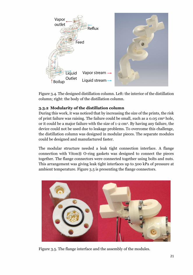
Paper 3 showed that 3D printing can effectively be used in designing small scale piloting devices. During the design process, it is possible to modify the equipment to achieve the best results. The design of the device can be divided to smaller pieces, which can be later assembled together. This is a possible method for manufacturing larger equipment. Based on the experience from the development of the packing, it should be possible to manufacture smaller scale devices to be used in chemical piloting as well. Figure 3.9 is presenting the final distillation column manufactured and used in the measurement.

25

Figure 3.9. The final 3D printed distillation column used in the measurement.

26

27

4. Process development with a microscale plant

4.1 Background

The renewable energy directive (RED), (Directive 2009/28/EC), and fuel quality directive (FQD), (Directive 2009/30/EC) of the European Union (EU), are giving the road map of the fuels in the EU during the future years. In both of these directives, the application of bio-based components are encouraged.

The ethers with partial bio-based feed stock can be used as oxygenates in gasoline. These compounds can be added to gasoline to increase the oxygen content of the fuel, reduce the emission of ozone and carbon monoxide, and increase the octane number (Poulopoulos and Philippopoulos, 2000). Moreover, the fuel oxygenates were used in gasoline to improve the combustion, and as a substitute for aromatics. Bio-based methanol can be used as a partial feedstock for production of 2-methoxy-2,4,4-trimethylpentane (also known as tertiary octyl methyl ether or TOME). TOME is an ether that can be used as an oxygenate in gasoline.

The industrial production of ethers are normally done through etherification reactions. In this reaction, the alcohol dehydrates to form ethers. In this process, the separation of reactants from the product is usually done with a distillation column. Usually, this process includes a recycle stream to return the reactants back to the reactor. This method can be combined in one vessel which is known as reactive distillation or catalytic distillation (Sakuth et al., 2000), The reactive distillation is a commonly used process in oil industries for processing the fuels. The main application of this method in fuel industries are etherification processes, hydrogenation of aromatics and light sulfur, and hydrodesulfurization (Harmsen, G.J., 2007). The recent works on reactive distillation by Shah et al. (2012), Holtbruegge et al. (2013), Liu et al. (2013), Hasan et al. (2015), Li et al. (2016) are showing the importance and demand of this technique in different industrial processes.

28

4.2 The studied process

One of the proposed methods for production of TOME is by an etherification process proposed by Rihko-Struckmann et al. (2004). In this method, methanol reacts with diisobutylene to produce TOME. The diisobutylene is a mixture of 2,4,4-Trimethyl-1-pentene (TMP-1) and 2,4,4-Trimethyl-2-pentene (TMP-2). The catalyst of the reaction is a macroreticular, cationic, strongly acidic ion exchange resin. In addition to the main reaction, the formation of dimethyl ether (DME) and water is observable. This side reaction is mentioned in the similar etherification processes and in presence of the same type of catalysts by Kiviranta-Pääkkönen et al. (1998). The studied reactions for production of TOME is presented in Figure 4.1.

Figure 4.1. The reactions involved in the process for production of TOME.

Rihko-Struckmann et al. (2004) proposed a reactive distillation column for production of TOME. In this technique, the reactants are fed to a column where a catalytic section is on the top and there is a distillation section at the bottom. By evaporation of the lower boiling point compounds (reactants), they enter the catalytic section and react to produce TOME, while the heavier compound (TOME) is leaving the system from the bottom. Figure 4.2 is presenting a schematic of a reactive distillation column described by Rihko-Struckmann et al. (2004).

29

Figure 4.2. The original reactive distillation method described by Rihko-Struckmann et al. (2004)

In this work, several steps of the process development for production of TOME were investigated. The study included the preliminary batch production of the chemical in the laboratory, micro-scale piloting of the process in the micro-plant and simulation and optimization of the process using a simulator. For the micro-scale piloting, to increase the flexibility in design and manufacturing of the units, the catalytic section (reactor) and the separation section (distillation column) were planned to operate separately. However, the same idea was considered where the volatile compound (distillate stream) was going to the reactor by a recycle stream. And the reacted material with higher boiling point was leaving the system as the bottom product. In this setup, all the distillate was returning to the reactor. The vent on the top of the distillation column was releasing the air at the startup, keeping the distillation column at atmospheric pressure and some of the unfavorable produced DME (reaction R-4 in Figure 4.1) could be released by the vent. Figure 4.3 is presenting the block flow diagram of the micro-plant used in this work.

Figure 4.3. The block flow diagram of the process for production of TOME used in this work.

30

4.3 Development of the process for production of TOME

4.3.1 Step 1. Batch production of TOME

To study this process, at the beginning, a laboratory scale batch reactive distillation column was built. This column was used to test the possibility of using reactive distillation technique for production of TOME. The reactor was filled with AmberlystTM 36 Wet, and the distillation column was filled with glass Raschig rings. The column was having 2.5 ideal stages during the batch reactive distillation. This column confirmed that TOME is producible using the reactive distillation technique. Further, this experiment showed that water is forming, which meant that a side reaction is taking place. The laboratory investigation, including testing the products using a GC and literature review (Kiviranta-Pääkkönen et al. 1998) confirmed that water and dimethyl ether (DME) is forming during the etherification process.

The product of this setup had a mass fraction purity of 0.65 for TOME. Later, a vacuum distillation column with 5.5 ideal stages was made to increase the purity. The final mass fraction purity was 99.3%. This product was pure enough to be used in the physical properties measurements. The produced compound was tested using gas chromatography/mass spectrometry (GC/MS) technique to make sure that the produced chemical is precisely TOME. More details are available in paper II. Figure 4.4 is presenting a schematic of the reactive distillation column, and the distillation column made for synthesis and purification of TOME.

Figure 4.4. Schematic of the reactive distillation column for production of TOME. 1- The reactive distillation column, 2- Extra purification with distillation.

31

4.3.2 Step 2. Operation of the micro-plant

In this work, the preliminary test runs, including the reactor tests, the separate operation of the distillation column and one full process run (see Figure 4.3) was completed at the same time as the computer simulation was in progress. This was helping to verify that the developed simulator is able to describe the measurement with sufficient accuracy. The developed model also helped in optimization of the process. Later, the second micro-plant run was completed to validate the model. The validated model can be used to predict the behavior of the system in different conditions. The model can be used to optimize the process for having the maximum purity or other factors such as less energy consumption.

Reactor. To understand the behavior of the plug flow reactor in production of TOME, a reactor with the volume of 100 cm3 was manufactured and filled with AmberlystTM 16wet ion exchange resin as the catalyst (more details in section 4.4.1). In this experiment, mixtures of methanol and diisobutylene with different compositions were fed to the reactor, and the outlet compositions were analyzed online with 30 minute intervals to observe the equilibrium composition after reaching steady state. Figure 4.5 is presenting the composition of the reactor output with the time for the feed inlet composition of xmethanol=0.497 and xdiisobutylene=0.503. This experiment was done for six different feed compositions. The results are available in paper IV. Figure 4.6 is showing the steady state compositions for all the runs and the comparison with the model developed to describe the system.

Figure 4.5. The reactor output composition vs. time. Methanol, □; TMP-1, ○; TMP-2, ; TOME, ; water, +; DME, ×.

32

Figure 4.6. The measured compositions of the reactor output based on the feed composition. The feed was consisting of methanol + diisobutylene. The diisobutylene is a mixture of TMP-1+TMP-2. The lines are representing the model: methanol, □; TMP-1, ○; TMP-2, ; TOME, ; water, +; DME, ×.

Distillation column. The distillation column (more details in section 4.4.2) was tested by feeding one mixture containing methanol, TMP-1, TMP-2, TOME, and water to it. This test could show the possibility of separation of TOME using this distillation column. The results were showing that the produced TOME was mostly enriching in the bottom product. On the other hand, the TMP-1, TMP-2, methanol, water, and DME were having the tendency to enrich in distillate. However, due to the limited number of stages, the separation was not sharp and some of the TMP-1 and TMP-2 was escaping from the bottom of the distillation column. On the other hand, a few percent of TOME was appearing in the distillate. Figure 4.7 is presenting the results of the distillate and bottom product of the distillation column.

33

Figure 4.7. The time - composition diagram of the distillation column during the separate run of the column. (a) is the reflux stream and (b) is the boilup stream: methanol, □; TMP-1, ○; TMP-2, ; TOME, ; water, +. The water content was checked with KF titrator at the end of the run. The model is presented with the lines.

First process run for production of TOME. The full process operation, including the reactor, distillation column and the recycle stream (see chapter 4.2) was completed to observe the behavior of the system during a long-term run. The process flow diagram (PFD) is presented in Figure 4.8. In this process, the feed with equimolar composition of methanol and diisobutylene was fed to a mixer and warmed up to the set point temperature using a preheater. Later, it was going to the reactor. The reactor output was preheated and fed to the horizontal distillation column. This column was separating reactants from the TOME. TOME, which has a higher boiling point, was accumulating in the bottom

34

product while the reactants were obtained through the top of the column. So, the distillate was recycled back to the reactor.

The distillation column had a reflux stream at the top of the column and a boilup stream in the bottom of the distillation column. The recycle (distillate) stream, the reflux stream and the boilup stream were equipped with pumps and flow meter-controllers. The flowrates in the boilup and recycle stream were kept constant during the runs. The reflux stream was recycling the extra condensate from the top of the column back to the distillation column using a level controller system. The compositions were analyzed in the inlet and outlet of the reactor, as well as, the reflux stream and the boilup stream.

The distillation column (more detail in section 4.4.2) had 3.4 ideal stages. Due to the separation efficiency of the distillation column, the TOME was not completely separating in the bottom product. Additionally, the diisobutylene was partially leaving the column from the bottom output. As a result, by having equimolar amount of methanol and diisobutylene in the feed, the composition of methanol in different sections of the system was raising gradually. Since methanol had lower boiling point compared to the other components, this chemical was accumulating in the recycle stream and the reactor. The high content of methanol in the reactor was increasing the production rate of water and DME, which was unfavorable.

Second process run for production of TOME. Finally, after completion of the model (see section 4.3.3), it could be possible to optimize the system in such a way that the water - DME production rate would be decreased. This was achieved by decreasing the methanol composition in the feed. In this run, the methanol composition in the feed was decreased to xmethanol=0.242. This modification decreased the composition of methanol in the recycle stream, consequently, the side reaction rate was decreased. This modification considerably helped in having an stabilized operation of the micro-plant. This run was operated for over 8 days and reached steady state condition. The results of the measurements are available in Figure 4.9.

35

Figure 4.8. The process flow diagram of the micro-plant. 1 is feed, 2 is recycle stream, 3 is reflux, 4 is distillation column feed (reactor output), 5 is boilup, 6 is distillate, 7 is bottom product.

36

Figure 4.9. The time-composition diagram of the process. a) is reactor output, b) is reflux, c) is boilup stream compositions during the run. methanol, □; TMP-1, ○; TMP-2, ; TOME, ; water, +; DME, ×. The model is presented with the lines. (The water and DME mole fractions were considered the same due to equimolar production rate).

4.3.3 Step 3. Process simulation

After having success in batch production of TOME in the laboratory using the glass apparatus, the process needed to be simulated and optimized. So, a series of preliminary laboratory runs and simulation of the process in computer were

37

considered to be done simultaneously. The process was simulated using a dynamic model developed in Matlab 2016a®. The simulator was consisting of a rate based model. In this model, the input was fed to an isothermal reactor and the reactor product was fed to a distillation column. The distillate was recycled back to the reactor and the bottom outlet was considered as product. For solving the ordinary differential equations (ODE) which were used in the dynamic simulator, the Matlab “ode15s” solver was used.

Reactor model. The model for isothermal reactor was consisting of 50 equal size reactor compartments with equal amount of catalyst. The total mass of catalyst and the total volume of the reactor was considered to be the same as the micro-plant. The reactor was assumed to work only in liquid phase with heterogeneous solid catalyst. In each compartment, the reaction rates were calculated based on the weight of the catalyst. For the initial condition, the reactor was filled with a liquid with the same composition as the feed.

To start the calculations, the feed of the process was added to the first reactor compartment and the reaction model was calculated. The results, including the compositions and the volume of the material was calculated for this compartment. The extra volume from this compartment was forwarded to the second compartment. Then, the calculation was conducted for the second compartment and this process was continued to reach the last compartment. In this model, it was assumed that the contents of each compartment are completely mixed, and the compartments does not have any back flow. By calculation of the last stage, the output was fed to the second stage of the distillation column.

Based on Rihko-Struckmann et al. (2004) and Karinen et al., (2001), the TOME formation reactions and the TMP-1&2 isomerization reaction (R-1, R-2 and R-3 in Figure 4.1) assumed to be elementary reactions. However, for the water-DME formation (R-4 in Figure 4.1), the model was defined based on the mechanism described by Kiviranta-Pääkkönen et al., (1998). However, the chemicals they used in their study were isoamylenes (2-methyl-1-butene +2-methyl-2-butene) and methanol. The difference between the chemicals in their work and the chemicals used in paper IV was reducing the precision of the model. Therefore, the model coefficients were adjusted according to the reactor experiments carried out in this work. This made the model to have better correspondence with the compositions obtained from the measurements.

Since the formation rate parameters from Rihko-Struckmann et al. (2004), Karinen et al., (2001) and Kiviranta-Pääkkönen et al., (1998) were not available for the planned reactor temperature (333 K), equation 4.1, was used to obtain the formation rates. This equation, which is based on Arrhenius’ law, gives the formation rates at the reactor temperature:

4.1

38

Where and are the reaction rate constants (mol·kgcat-1·s-1) at T1 (K) and T2 (K), E is activation energy (kJ·mol-1) and R is the ideal gas constant.

Equation 4.2-4.6 are showing the reaction rates of the compounds available in the reactor:

4.2

4.3

4.4

4.5

4.6

Where, ri is the rate of reaction for the compound i (mol·kgcat-1·s-1), kj is the reaction rate constants (mol·kgcat-1·s-1) for reaction j, Kjeq is the equilibrium constant for reaction j, and ai is the activity of the component i. The necessary parameters are available in paper IV.

The activities needed in equation 4.2-4.6 were calculated using equation 4.7:

4.7

Where ai is activity, xi is the mole fraction of compound i, and is the activity coefficient for component i. The activity coeffeicints for the reactor model was calculated by the original UNIQUAC functional-group activity coefficients (UNIFAC) group contribution method (Fredenslund et al., 1975).

Distillation column model. The number of ideal stages of the distillation column was estimated based on a correlation between the flooding factor and the height of an ideal stage. The flooding factor is defined as (equation 4.8):

4.8

Where is superficial vapor velocity, m·s-1 and is the vapor density, kg·m-3. According to Sundberg et al. (2013) the distillation column had 3.4 vapor-liquid equilibrium stages for the flooding factor used in the distillation column. For the modeling of the work, similar to Sundberg et al. (2013), the number of stages rounded up to 4. Additionally, based on the structure of the distillation column (see section 4.4.2), the vapor holdup fraction was estimated to be 0.4.

39

The distillation column model was consisting of 4 stages where stage 1 was representing the top of the column with the most volatile compounds and stage 4 was the bottom of the distillation column. In this model, similar to the reactor model, the equilibrium was calculated in each stage and the extra volumes of each stage was forwarded to the next stage. For the distillation column, the vapor stream was moving towards the top of the column (lower stage numbers) and the liquid stream was moving towards the bottom of the distillation column (higher stage numbers). For the initial value, the composition was considered to be similar to the compositions obtained from the first test runs of the micro-plant. In the beginning, the mole fractions and number of the moles in each stage were calculated. For the vapor phase, the number of moles were calculated using the ideal gas law. For the liquid phase, the molar volume were calculated using equation 4.9. In this equation, the excess volumes of mixing were not considered:

4.9

In this equation, was the molar volume of the mixture (m3·mol-1); xi was the mole fraction of component i; and was the molar volume of component i, (m3·mol-1). The molar volumes were assumed constant for all temperatures in the dynamic model.

The vapor and liquid material balance were calculated using equation 10 and 11:

4.10

4.11

Where and were the rate of accumulation during the time period of dt, (mol·s-1); is the flow rate from the lower stage, (mol·s-1); is the flow rate moving to the next stage, (mol·s-1); is the mass transfer area (m2); is molar flux mol· m-2·s-1; and is the mole transfer rate, (mol·s-1). Flow rates between stages were calculated based on the difference between specified and calculated volumes, by using a P – controller type of approach (Equation 4.12 for the vapor phase and 13 for the liquid phase):

4.12

4.13

Where and are control parameters for the flow rates; these parameters were selected to be = . This value was high enough to keep the volumes close to the specified but not too high to avoid numerical problems.

and are total molar volumes for each stage, is specified vapor volume fraction on each stage, and Vj is the specified stage total volume; yij and xij are

40

presenting the mole fractions of the compound i for the vapor and liquid respectively, and are amount of moles on a stage.

The mass transfer rate, was calculated using a simple overall mass transfer coefficient (equation 4.14):

4.14 Where the volumetric mass transfer coefficient is and A is mass transfer area and Kij was vapor-liquid distribution ratio. By choosing , it was assumed that the stages are ideal.

In this model, energy balances were not calculated, so, the temperatures for each stage was obtained from the distillation column measurements. The temperature for each stage was assumed to be constant, which is reasonably a good assumption for such small microscale distillation column with a reasonably low heat loss (see section 4.4.2).

For calculation of the vapor-liquid distribution ratio in equation 4.14, the NRTL activity coefficient model (equation 2.16) was used to calculate the Vapor-Liquid Equilibrium (VLE) at 4 different stages. The temperatures for all stages were obtained from the distillation column runs. With the Antoine vapor pressure equation (equation 4.15) and the column temperature, the vapor pressures were calculated:

4.15

Where is liquid vapor pressure of component i (Pa); P0 is a pressure unit to make the logarithm expression dimensionless; A, B, C are component specific parameters and T is temperature (K). By having the activity coefficients and liquid vapor pressures, the vapor-liquid distribution ratio were calculated using equation 4.16:

4.16

Where, Ki is the vapor-liquid distribution ratio, is the activity coefficient, is vapor pressure of component i (Pa), and P is the total pressure.

In this model, the volume of each stage was constant. After calculation of all stages, the extra liquid on stage four was considered as the bottom product of the system and the extra vapor on stage one was the distillate. The distillate was returned back to the reactor.

Optimization of the process. According to the measurement, and the developed model, the high amount of methanol was accumulating in the recycle stream. Consequently, the production of DME and water was increasing. The high amount of DME in the system was causing the distillation column to work inefficiently, and high amount of water was inhibiting the catalyst, which could cause the process to stop. The developed model helped in finding a better

41

composition where the side reaction was limited and the process could be operated in a stabilized condition for a long time.

4.4 Preparation of the micro-plant

In this study, the main workload for preparation and development of the micro-plant was focused on reactor, distillation column (Sundberg, 2013) and installation of the instrumentation. Due to importance of mass balance in these measurements, it was very important to make the vessels completely leak tight. As a result, the design and manufacturing of a leak tight reactor, and checking the distillation column for making it leak proof was an important part of the work. Moreover, the procurement and installation of the instrumentation was a very sensitive work, which was done for several cases.

4.4.1 Reactor

A plug flow reactor was designed to be used in this work. The reactor was consisting of a stainless steel tube with the length of 24 cm, internal dimeter (ID) of 2.3 cm and outer diameter (OD) of 3 cm. The catalyst was Amberlyst™ 16wet provided by Dow Chemical Company®. The inlet and outlet were covered by stainless steel nets to keep the catalyst inside the reactor. A back pressure regulator was installed after the reactor to adjust the pressure in the reactor.

The reactor was kept isothermal at 333 K using a water thermostated coil surrounding it. In addition, a layer of rubber silicon insulator provided by Oy Meyer-Vastus Ab was used to reduce the heat transfer between the heating coil and the surrounding air.

The pressure in the reactor was raised to 800 kPa. This high pressure was keeping all the chemicals in liquid phase during the run. The reactor was operated vertically with upward flow. This was facilitating the air to be released from the reactor during the first hours of run by pushing the gas out through the outlet. Figure 4.10 is presenting a schematic of the reactor.

Figure 4.10. A schematic of the reactor.

42

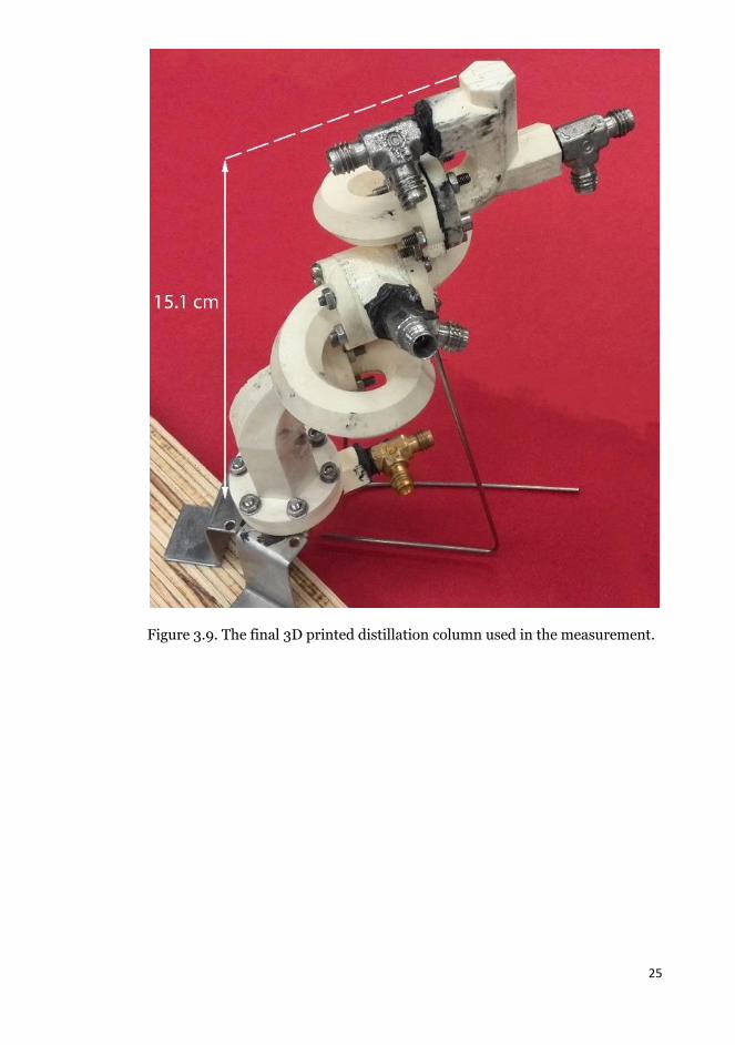
4.4.2 Distillation column

The basic distillation columns consist of vertical vessels, where the feed stream is entered from the middle section of the column, reflux – distillate streams are available at the top, and boilup – bottom outlet streams are in the bottom. This structure can be modified by adding more inlets and outlets in different sections. Additionally, it is possible to make many different types of interior structures to obtain adequate purity. In this setup, the boilup stream has an evaporator to evaporate and return a fraction of the bottom outlet back to the column. On the other hand, a reflux stream condense the vapor outlet and returns a fraction of the top outlet back to the distillation column. Normally, in distillation columns, the liquid phase, which has a higher density moves downward and the vapor phase moves upward.

However, in this work, a cuboid horizontal vessel designed by Sundberg et al. (2013) was used as the distillation column. In this setup, the liquid was fed from the feed inlet stream (middle of the column) and the reflux stream. The liquid was spreading in the bottom of the distillation column on a highly porous metal foam. The high porosity was making the metal foam to have high capillary action. The capillary action of the metal foam was bringing the liquid to all the surface of the metal foam. The vapor was fed from the boilup inlet and moved towards the top of the column. The counter current movement of the vapor and liquid was making the mass transfer to take place. The temperatures through the column were measured in different sections using thermocouples.

Since the distillation column had a large surface to volume ratio, the heat transfer from the walls of the unit was very high. This was cooling down the unit, and making it impossible to run. Therefore, the column was insulated with a layer of rock-wool and supported by two heating blocks at the top and bottom to adjust the temperature of the column. The heating blocks were warmed up using two heater cartridges located on the warmer (right) side of the column. Figure 4.11 is presenting a schematic of the distillation column.

43

Figure 4.11. A schematic representation of the distillation column. a) 3D view of the horizontal micro-distillation column. TI1-TI13 are the thermometer pockets, and S1-S3 are sampling outlets (not used in this work). b) interior of the distillation column. c) The side view of the distillation column. Pink is the rock-wool layer, and blue is the aluminum heater blocks.

4.4.3 Instrumentation

One of the main challenges in this work was the automation of the devices. Since the system was planned for 24/7 operations, it was necessary to design robust automated systems to control the micro-plant. In this work, the temperature and flowrates were needed to be measured and controlled at different sections of the system; an online system was needed to analyze the compositions of different streams; and the reflux stream needed a level controller system. Some examples of the process automation developed during this work are provided here:

Composition analysis automation. One of the targets in papers III and IV was observation of the compositions at different sections of the micro-plant with respect to time. The online composition analysis was helping to understand the dynamic behavior of the system, and check the final compositions after reaching steady state. In the beginning of this work, two GCs were used for measuring the compositions of the reflux and boilup stream. However, the other streams such as reactor input and output could not be checked during 24/7 service.

During this work, a selector valve and one online sampling valve were added to a GC to collect samples from different streams. With this arrangement, the

44

compositions for up to six streams could be analyzed using one GC. In this setup, the selector valve was trapping one of the streams and directing it towards the online sampling valve. The online sampling valve was collecting a 0.001 cm3 sample from the selected stream. The rest of this stream was passing through the two valves and following the stream line. In this setup, the other streams were flowing through the selector valve without any stream relocation. Figure 4.12 is presenting a schematic view of the sampling system. More details can be found in paper III.

Figure 4.12. The automated sampling valves used for analysis of the composition from different sections of the micro-plant. a) the bottom product is passing through the sampling valve, b) a sample is obtained from the bottom product stream, c) the distillate stream is passing the sampling valve.

Pump control using Arduino®. During recent years, several affordable microcontroller hardware were introduced by Arduino® open source platform, which can be used to control small or large scale systems. Arduinos are able to read sensor (input) values, process the data and give feedbacks based on the processed data. This can be very beneficial in the piloting projects due to the possibility of controlling different equipment using easy to understand microcontrollers.

45

In this work, the workload on the reflux and distillate (recycle) stream pumps were higher than their operating limits. This was causing time to time pump failure. It was noticed that the electric motors of the pumps could not provide the adequate torque to run the pumps. By increasing the load on the electric motors, they were warming up. This was causing the pumps to stop, which was making the micro-plant to lose the steady state condition. Therefore, the original servo motors were changed to two direct current (DC) electric motors with higher torques. This was making it possible to run the pumps during the micro-plant runs without serious failures. The Arduino Uno® micro-controller and a circuit board based on the L298N DC electromotor driver provided by STMicroelectronics® were assembled to run the DC motors. Since the reflux stream needed level control, a differential pressure transmitter was used to compare the liquid pressure in the collector vessel and the ambient pressure (see Figure 4.8). When the pressure was raising in the collector vessel, the pump was activating to reflux the material back to the distillation column. Figure 4.13 is presenting the schematic diagram of the electromotor driver designed to run the pumps.

Figure 4.13. The schematic of the driver made for running the pump electric motors. 1- 24 V power supplies for powering the devices, 2- Differential pressure transmitter, 3- 250 Ω resistor for conversion of the electric current to voltage, 4- L298N dual H-Bridge motor controller, 5- Arduino Uno®, 6-Pumps.

46

47

5. Conclusion

The old mindsets, which believed that the biggest scale is the best scale, is changing during recent years. The new generation of the processes should focus on the maximum efficiencies with respect to space, time, energy, safety, environment, etc.

The target of this study was development and introduction of micro-scale plants for development of new processes. This work was done in three major parts. The first part was focusing on the phase equilibria and thermodynamic measurement related to the work (papers I and II). The second part was development of a new distillation column using the 3D printing method (paper III). And the last part was development of the process for production of TOME using a micro-scale plant (paper IV), which was done in several steps including literature review of the earlier works, laboratory synthesis of TOME, phase equilibria and kinetic measurements, and finally piloting the process using the micro-scale plant.

In this study, the development of a process for production of TOME from different aspects were investigated. At the beginning, a lab scale batch column was made to synthesize the TOME (paper II). This work was showing that the TOME can be produced with reactive distillation method. Then, the liquid-liquid equilibria (LLE) and excess enthalpies (HE) of the main chemicals which were present in the process were studied in papers I & II. These measurements were showing the possibility of unfavorable phase split in the process. Moreover, the developed thermodynamic models could be used in the modeling of the process for production of TOME. Later, different mole fractions of the feed were fed to the reactor of micro-plant to study the kinetics in this plug flow reactor. Finally, the piloting of TOME in the micro-scale plant was investigated using the reactor and a distillation column. Since the distillate was completely recycled, the accumulation of the chemicals in the recycle stream and the methods for overcoming the problem was investigated. In this work, due to accumulation of the chemicals in the recycle stream, a dynamic model was needed to predict the behavior of the system. The dynamic model was developed using the UNIFAC and NRTL models. The use of such type of

48

conventional models was showing that the micro-scale can be suitable as a part of piloting and scale up of similar processes.

The development of micro-scale devices for piloting of chemical processes were in progress during recent years. In this work, a new micro distillation column was designed and manufactured with 3D printing method (paper III). A modular distillation column was designed and printed, piece-by-piece, using a digital light processing (DLP) 3D printer. Later, the distillation column was tested and characterized in the laboratory using two different types of packings. This study was showing that the 3D printing can be an effective tool for design and manufacturing of new micro-scale devices to be used in micro-plants.

49

6. Suggestions for future works

For the future works, after having the experience from this study, it is possible to integrate the etherification process in to one device and make a reactive distillation column. To overcome the challenges with complications in manufacturing, the application of 3D printing can be considered. The process can be printed from polymeric materials and coated with electroless plating or it is possible to print them using metal laser sintering. In both cases, the equipment can be printed using modular parts, which can be added or removed depending on the demands of the process. Another suggestion is the possibility of using the trending internet of things (IOT) for running the micro-plant. Currently, in a normal operating day, the micro-plant is operated for 14-16 hours without supervision, the IOT can help the operator to have a time-to-time observation of the process and make the necessary modifications from home or wherever the internet is available. The outcomes would probably show more smoothed results with less deviations from the stabilized condition.

The micro-plant project has the possibility to be used in future for education. Based on these experiments, the operation of this process is safer than many laboratory experiments that are already given to bachelor’s and master’s degree students. Therefore, it is possible to let students to operate the micro-plant and learn about the process operation in a reasonably safe environment. The observation of the streams using transparent tubes can give a better understanding of the phenomena happening in the process to students.

On the other hand, the micro-plant can be used as an effective tool in industrial process development projects. The development of the process for production of TOME was showing that it is possible to pilot similar type of processes in this scale. The micro-scale is reasonably cheaper to build (McConville, 2000 and Palluzi, 2000) and operate. Therefore, it is possible to build several micro-plants and test several cases at the same time. This can effectively improve the process development by testing several cases in a reasonable time. As a result, the simulations can be compared against more number of measurements, which can lead to simulations that are more accurate. The higher accuracy in simulation can help in designing processes with higher efficiencies.

50

51

References Abrams, D.S., Prausnitz, J.M., 1975. Statistical thermodynamics of liquid mixtures: A new expression for the excess Gibbs energy of partly or completely miscible systems. AIChE Journal 21, 116–128. doi:10.1002/aic.690210115

Adiche, C., Sundmacher, K., 2010. Experimental investigation on a membrane distillation based micro-separator. Chemical Engineering and Processing: Process Intensification 49, 425–434. doi:10.1016/j.cep.2010.02.009

Álvarez, V.H., Mattedi, S., Iglesias, M., Gonzalez-Olmos, R., Resa, J.M., 2011. Phase equilibria of binary mixtures containing methyl acetate, water, methanol or ethanol at 101.3 kPa. Physics and Chemistry of Liquids 49, 52–71. doi:10.1080/00319100903012403

Bredig, G.; Bayer, R. Z. Phys. Chem., Stoechiom. Verwandschaftsl., 1927, 130, 15 II vapor pressure of the ternary system methyl alcohol + methyl acetate + ethyl acetate

Camin, D.L., Rossini, F.D., 1955. Physical Properties of Fourteen API Research Hydrocarbons, C9 to C15. J. Phys. Chem. 59, 1173–1179. doi:10.1021/j150533a014

Crump, S.S., 1992. Apparatus and method for creating three-dimensional objects. US5121329 A.

Dalton, J.; 1802, Essay IV. On the expansion of elastic fluids by heat. Memoirs of the Literary and Philosophical Society of Manchester, vol. 5, pt. 2, pages 595–602.

Daubert, T.E.; Danner, R.P. 1992-extant Technical Data Book-Petroleum Refining, 5th Edition American Petroleum Institute, Washington, D.C.

Deckard, C.R., 1989. Method and apparatus for producing parts by selective sintering. US4863538 A.

Deckard, C.R., 1997. Apparatus for producing parts by selective sintering. US5597589 A.

Directive 2009/28/EC of the European Parliament and of the council of 23 April 2009, on the promotion of the use of energy from renewable sources and amending and subsequently repealing Directives 2001/77/EC and 2003/30/EC, Official Journal of the EuropeanUnion,52, L 140/ 16-62, EN. doi:10.3000/17252555.L_2009.140.eng, ISSN 1725-2555

Directive 2009/30/EC of the European Parliament and of the council of 23 April 2009, amending Directive 98/70/EC as regards the specification of petrol,

52

diesel and gas-oil and introducing a mechanism to monitor and reduce greenhouse gas emissions and amending Council Directive 1999/32/EC as regards the specification of fuel used by inland waterway vessels and repealing Directive 93/12/EEC, Official Journal of the EuropeanUnion,52, L 140/88-113, EN. doi:10.3000/17252555.L_2009.140.eng, ISSN 1725-2555

Evans, B., 2012. Practical 3D Printers: The Science and Art of 3D Printing. Apress, New York. ISBN: 978-1-4842-1173-1

Feygin, M., Shkolnik, A., Diamond, M.N., Dvorskiy, E., 1998. Laminated object manufacturing system. US5730817 A.

Fredenslund, A., Jones, R.L., Prausnitz, J.M., 1975. Group-contribution estimation of activity coefficients in nonideal liquid mixtures. AIChE J. 21, 1086–1099. doi:10.1002/aic.690210607

Gaal, G., Mendes, M., de Almeida, T.P., Piazzetta, M.H.O., Gobbi, Â.L., Riul Jr., A., Rodrigues, V., 2017. Simplified fabrication of integrated microfluidic devices using fused deposition modeling 3D printing. Sensors and Actuators B: Chemical 242, 35–40. doi:10.1016/j.snb.2016.10.110

Gallagher, J.S., Haar, L., Kell, G.S., 1984. NBS/NRC Steam Tables. Thermodynamic and Transport Properties and Computer Programs for Vapor and Liquid States of Water in SI Units. Hemisphere Publishing Corporation, Washington.

Gibbs, J. W., (Oct. 1875-May 1876- Part 1). On the Equilibrium of Heterogeneous substances., Transactions of the Connecticut Academy of Arts and Sciences. 3: 108–248.

Gibbs, J. W., (May 1877-July 1878- Part 2). On the Equilibrium of Heterogeneous substances., Transactions of the Connecticut Academy of Arts and Sciences. 3: 343–524.

Gmehling, J., Kolbe, B., Kleiber, M., Rarey, J., 2012. Chemical Thermodynamics for Process Simulation, 1st ed. Wiley-VCH. ISBN: 3-527-31277-3

Haan, A.B. de, 2015. Process Technology: An Introduction. Walter de Gruyter GmbH & Co KG.

Haar, L.; Gallagher, J.S.; Kell, G.S., 1984. NBS/NRC Steam Tables. Thermodynamic and Transport Properties and Computer Programs for Vapor and Liquid States of Water in SI Units. Hemisphere Publishing Corporation, Washington

Hasan, S.U., Mahajani, S., Malik, R., 2015. Selectivity engineering with single feed multi-side draw hybrid reactive distillation columns. Chemical Engineering Journal, Tailoring Sustainability through Chemical Reaction Engineering 278, 479–491. doi:10.1016/j.cej.2014.11.095

53

Harmsen, G.J., 2007. Reactive distillation: The front-runner of industrial process intensification: A full review of commercial applications, research, scale-up, design and operation. Chemical Engineering and Processing: Process Intensification, Selected Papers from the European Process Intensification Conference (EPIC), Copenhagen, Denmark, September 19-20, 2007 46, 774–780. doi:10.1016/j.cep.2007.06.005

Hartman, R.L., Sahoo, H.R., Yen, B.C., Jensen, K.F., 2009. Distillation in microchemical systems using capillary forces and segmented flow. Lab Chip 9, 1843–1849. https://doi.org/10.1039/B901790A

Hohmann, L., Gorny, R., Klaas, O., Ahlert, J., Wohlgemuth, K., Kockmann, N., 2016. Design of a Continuous Tubular Cooling Crystallizer for Process Development on Lab-Scale. Chem. Eng. Technol. 39, 1268–1280. doi:10.1002/ceat.201600072

Holtbruegge, J., Heile, S., Lutze, P., Górak, A., 2013. Synthesis of dimethyl carbonate and propylene glycol in a pilot-scale reactive distillation column: Experimental investigation, modeling and process analysis. Chemical Engineering Journal 234, 448–463. doi:10.1016/j.cej.2013.08.054

Johnson, M.D., May, S.A., Calvin, J.R., Lambertus, G.R., Kokitkar, P.B., Landis, C.R., Jones, B.R., Abrams, M.L., Stout, J.R., 2016. Continuous Liquid Vapor Reactions Part 1: Design and Characterization of a Reactor for Asymmetric Hydroformylation. Org. Process Res. Dev. 20, 888–900. doi:10.1021/acs.oprd.5b00407

Kaibel, G., Schoenmakers, H., 2002. Process Synthesis and Design in Industrial Practice, in: Schijndel, J.G. and J. van (Ed.), Computer Aided Chemical Engineering, European Symposium on Computer Aided Process Engineering-1235th European Symposium of the Working Party on Computer Aided Process Engineering. Elsevier, pp. 9–22. doi:10.1016/S1570-7946(02)80035-9

Karinen, R.S., Lylykangas, M.S., Krause, A.O.I., 2001. Reaction Equilibrium in the Isomerization of 2,4,4-Trimethyl Pentenes. Ind. Eng. Chem. Res. 40, 1011–1015. doi:10.1021/ie000526s

Kiviranta-Pääkkönen, P.K., Struckmann, L.K., Linnekoski, J.A., Krause, A.O.I., 1998. Dehydration of the Alcohol in the Etherification of Isoamylenes with Methanol and Ethanol. Ind. Eng. Chem. Res. 37, 18–24. doi:10.1021/ie970454d

Laavi, H., Zaitseva, A., Pokki, J.-P., Uusi-Kyyny, P., Kim, Y., Alopaeus, V., 2012. Vapor–Liquid Equilibrium, Excess Molar Enthalpies, and Excess Molar Volumes of Binary Mixtures Containing Methyl Isobutyl Ketone (MIBK) and 2-Butanol, tert-Pentanol, or 2-Ethyl-1-hexanol. J. Chem. Eng. Data 57, 3092–3101. doi:10.1021/je300678r

54

Lam, K.F., Sorensen, E., Gavriilidis, A., 2011. Towards an understanding of the effects of operating conditions on separation by microfluidic distillation. Chemical Engineering Science 66, 2098–2106. https://doi.org/10.1016/j.ces.2011.02.013

Li, H., Meng, Y., Li, X., Gao, X., 2016. A fixed point methodology for the design of reactive distillation columns. Chemical Engineering Research and Design 111, 479–491. doi:10.1016/j.cherd.2016.05.015

Liu, C.-C., Wang, Y.-N., Fu, L.-M., Chieh, C., 2016. Micro-distillation system for formaldehyde concentration detection. Chemical Engineering Journal 304, 419–425. doi:10.1016/j.cej.2016.06.114

Liu, J., Yang, B., Lu, S., Yi, C., 2013. Multi-scale study of reactive distillation. Chemical Engineering Journal 225, 280–291. doi:10.1016/j.cej.2013.03.046

MacInnes, J.M., Ortiz-Osorio, J., Jordan, P.J., Priestman, G.H., Allen, R.W.K., 2010. Experimental demonstration of rotating spiral microchannel distillation. Chemical Engineering Journal 159, 159–169. doi:10.1016/j.cej.2010.02.030

McCabe, W. L. & Smith, J. C., 1976. Unit Operations of Chemical Engineering (3rd ed.). McGraw-Hill. ISBN 0-07-044825-6.

McConville, F.X., 2000. Pilot Plants, in: Kirk-Othmer Encyclopedia of Chemical Technology. John Wiley & Sons, Inc. doi:10.1002/0471238961.1609121516011212.a01.pub2

Nakamura, K, 2014. Photopolymers: Photoresist Materials, Processes, and Applications, CRC Press, Oxon, UK. ISBN: 978-1-4665-1731-8

Nhu, N.; Nowak, G.; Svejda, P., 1988. Excess Gibbs Energies of Some Liquid Mixtures with Polar Components, Effects of Local Polarizability 1537 Ber. Bunsen-Ges., 92.

Othmer, D., Tobias, P., 1942. Liquid-Liquid Extraction Data - The Line Correlation. Ind. Eng. Chem. 34, 693–696. doi:10.1021/ie50390a600

Ott, J.B., Boerio-Goates, J., 2000. Chemical Thermodynamics: Principles and Applications. Academic Press. P. 1. ISBN: 9780080500980

Palluzi, R.P., 2000. Pilot Plants, in: Ullmann’s Encyclopedia of Industrial Chemistry. Wiley-VCH Verlag GmbH & Co. KGaA. doi:10.1002/14356007.c19_c01

Poulopoulos, S., Philippopoulos, C., 2000. Influence of MTBE addition into gasoline on automotive exhaust emissions. Atmospheric Environment 34, 4781–4786. doi:10.1016/S1352-2310(00)00257-0

55

Raal, J.D., Mühlbauer, A.L., 1998. Phase Equilibria: Measurement and Computation. Taylor & Francis.

Renon, H., Prausnitz, J.M., 1968. Local compositions in thermodynamic excess functions for liquid mixtures. AIChE J. 14, 135–144. doi:10.1002/aic.690140124

Rihko-Struckmann, L.K., Karinen, R.S., Krause, A.O.I., Jakobsson, K., Aittamaa, J.R., 2004. Process configurations for the production of the 2-methoxy-2,4,4-trimethylpentane—a novel gasoline oxygenate. Chemical Engineering and Processing: Process Intensification 43, 57–65. doi:10.1016/S0255-2701(02)00185-X

Sakuth, M., Reusch, D., Janowsky, R., 2000. Reactive Distillation, in: Ullmann’s Encyclopedia of Industrial Chemistry. Wiley-VCH Verlag GmbH & Co. KGaA. doi:10.1002/14356007.c22_c01.pub2

Selected Values of Properties of Chemical Compounds 1980-extant Data Project Thermodynamics Research Center, Texas A&M University, College Station, Texas

Selected Values of Properties of Hydrocarbons and Related Compounds 1980-extant. American Petroleum Institute Research Project 44 Thermodynamic Research Center, Texas A&M University, College Station, Texas. loose-leaf data sheets

Seok, D. R., Hwang, S. T., 1985. Zero-gravity distillation utilizing the heat pipe principle (micro-distillation)” AIChE Journal 31, 2059-2065. doi: 10.1002/aic.690311215

Schwolow, S., Neumüller, A., Abahmane, L., Kockmann, N., Röder, T., 2016. Design and application of a millistructured heat exchanger reactor for an energy-efficient process. Chemical Engineering and Processing: Process Intensification 108, 109–116. doi:10.1016/j.cep.2016.07.017

Shah, M., Kiss, A.A., Zondervan, E., de Haan, A.B., 2012. Pilot-scale experimental validation of unsaturated polyesters synthesis by reactive distillation. Chemical Engineering Journal 213, 175–185. doi:10.1016/j.cej.2012.10.003

Sundberg, A.T., Uusi-Kyyny, P., Jakobsson, K., Alopaeus, V., 2013. Control of reflux and reboil flow rates for milli and micro distillation. Chemical Engineering Research and Design 91, 753–760. doi:10.1016/j.cherd.2012.08.009

Timmermans, J. 1965, Physico-Chemical Constants of Pure Organic Substances, Vol II, Elsevier, New York

56

Uusi-Kyyny, P., Pokki, J.-P., Aittamaa, J., Liukkonen, S., 2001. Vapor−Liquid Equilibrium for the Binary Systems of Methanol + 2,4,4-Trimethyl-1-pentene at 331 K and 101 kPa and Methanol + 2-Methoxy-2,4,4-trimethylpentane at 333 K. J. Chem. Eng. Data 46, 1244–1248. doi:10.1021/je010076q

Uusi-Kyyny, P., Pokki, J.-P., Aittamaa, J., Liukkonen, S., 2001. Vapor Liquid Equilibrium for the Binary Systems of 2-Methyl-2-propanol + 2,4,4-Trimethyl-1-pentene at 333 K and 348 K and 2-Butanol + 2,4,4-Trimethyl-1-pentene at 360 K. J. Chem. Eng. Data 46, 686–691. doi:10.1021/je0002742

Vaccaro, S., Malangone, L., Ciambelli, P., 2010. Micro-Scale Catalytic Reactor for Syngas Production. Ind. Eng. Chem. Res. 49, 10924–10933. doi:10.1021/ie100464b

Vogel, G.H., 2006. Process Development: From the Initial Idea to the Chemical Production Plant. John Wiley & Sons.

Walas, S. M., 1985, Phase equilibria in Chemical Engineering, Oxford, U.K.: Butterworth-Heinemann, ISBN: 978-0-409-95162-2

Wang, X.; Kang, K.; Wang, W.; Tian, Y., 2013, Volumetric Properties of Binary Mixtures of 3-(Methylamino)propylamine with Water, N-Methyldiethanolamine, N,N-Dimethylethanolamine, and N,N-Diethylethanolamine from (283.15 to 363.15) K, J. Chem. Eng. Data, 2013, 58, 3430-3439

Wilhoit, R.C., Zwolinski, B.J., 1973. Physical and thermodynamic properties of aliphatic alcohols. American Chemical Society.

Zhang, Y., Kato, S., Anazawa, T., 2010. Vacuum membrane distillation by microchip with temperature gradient. Lab Chip 10, 899–908. https://doi.org/10.1039/B915534A

Ziogas, A., Cominos, V., Kolb, G., Kost, H.-J., Werner, B., Hessel, V., 2012. Development of a Microrectification Apparatus for Analytical and Preparative Applications. Chem. Eng. Technol. 35, 58–71. https://doi.org/10.1002/ceat.201100505

ssecorp fo trap tnatropmi na si gnitoliP si tnalp elacs-llams a erehw ngised

lacisyhp a ni ssecorp eht tset ot derutcafunam eht gnipleh era stnalp toliP .tnemnorivne

rieht etaulave ot sreenigne lacimehc eht ot noitulos dnfi dna snoitalumis retupmoc

.noitarepo ssecorp fo segnellahc,gnitolip ni dnert wen a si gnitolip elacs-orciM

yb sesnepxe eht ecuder ot si mia eht erehw siht nI .stnalp tolip fo sezis eht gnicuder

lluf a fo noitarepo fo ytilibissop eht ,krow si elacs-orcim ni ssecorp lacimehc

tsrfi eht fo eno si krow sihT .detagitsevni a ,rotcaer a erehw seiduts elacs-orcim

erew maerts elcycer a dna tinu noitarapes leufoib etelpmoc a nur ot denibmoc suounitnoc ehT .ssecorp noitcudorp

syad 11 revo rof ssecorp siht fo noitarepo fo sessenkaew dna shtgnerts eht wohs dluoc

.tnempoleved ssecorp rof gnitolip elacs-orcim esahp tnaveler fo seires a ,yllanoitiddA ot edam erew stnemerusaem airbiliuqe

,revoeroM .krow eht fo gnilledom eht troppus si nmuloc noitallitsid elbatnirp D3 a

gnisu fo ytilibissop eht evresbo ot depoleved .gnitolip elacs-orcim ni gnitnirp D3

-otl

aA

DD

9

9/

810

2

+cgaai

a*GMFTSH

9 NBSI 2-6008-06-259-879 )detnirp( NBSI 9-7008-06-259-879 )fdp( NSSI 4394-9971 )detnirp( NSSI 2494-9971 )fdp(

ytisrevinU otlaA

gnireenignE lacimehC fo loohcS gnireenignE lacigrullateM dna lacimehC fo tnemtrapeD

if.otlaa.www

+ SSENISUB YMONOCE

+ TRA

+ NGISED ERUTCETIHCRA

+ ECNEICS

YGOLONHCET

REVOSSORC

LAROTCOD SNOITATRESSID

ina

dra

M de

eaS

stn

alp

elac

s-or

cim

gnis

u se

ssec

orp l

aci

mehc

fo t

nemp

olev

eD

yti

srev

in

U otl

aA

8102

gnireenignE lacigrullateM dna lacimehC fo tnemtrapeD

lacimehc fo tnempoleveD elacs-orcim gnisu sessecorp

stnalp

inadraM deeaS

LAROTCOD SNOITATRESSID