Flexible electricity use in the cement industry: Laying

the foundation for a not so concrete future

A scenario analysis about the flexibility potential of European cement plants in 2050 to

estimate the potential electricity costs savings and the impact on the electricity grid.

11-07-2021

Key words: Carbon neutral industries, Cement industry, Deep decarbonization, Demand

response, Flexible industries, Linear programming, Scenario analysis

Martijn Rombouts (6202055)

Utrecht University

MSc Sustainable Development – Track: Energy and Materials

Supervisor : dr. ir. Wina Crijns-Graus

Daily supervisor: Annika Boldrini MSc

Second reader prof. dr. Ernst Worrell

1

The image on the front shows a piece called Solar Storm (2017) made by Amélie Bouvier.

The rest of this page is left intentionally blank.

2

PREFACE

The reason I began this master’s programme was because I wanted to learn how I can contribute to a

sustainable future. At the end of this master’s program I can safely say that I achieved my goals and I

am thankful for all the wonderful support I got from the University of Utrecht.

I would mainly thank both my supervisors, dr. ir. Wina Crijns-Graus and Annika Boldrinini MSc for

the great support they provided during this thesis. Finally, I would like to thank my parents for

encouraging me to enrol in this master’s program.

Martijn Antonius Rombouts

July, 2021

ABSTRACT

Limiting the global warming levels to 1.5 °C above pre-industrial levels will substantially reduce the

effect of global warming on our everyday lives. Because greenhouse gasses are the main contributor to

climate change, the EU aims to combat global warming by shifting towards carbon neutral industries in

2050.

By implementing more variable renewable energy sources (VRES) the EU aims to decarbonize the

electricity system. Because it is costly to store electricity the demand must become more flexible so

VRES can be better integrated. This thesis estimates the flexibility demand of a cement plant. Focussing

on the cement industry is interesting since it is a mayor emitter of CO2, it is energy intensive, and it is

at present not clear which decarbonation pathway the industry should choose. The main research

question this thesis aims to answer is: “What is the technical and economic flexibility potential of a

carbon neutral cement plant in 2050?”

At currently operating cement plants, the carbon emissions originate from two sources: the burning of

fossil fuels and the formation of clinker (calcination emissions). To answer the research question, the

flexibility potential of cement plants when using the four most likely decarbonization pathways were

estimated - one scenario where all emissions are captured of a plant with a conventional fuel mix, three

scenarios where a renewable heat source is used and only calcination emissions are captured. By

understanding the flexibility potential, the future role of cement plants in matching electricity supply

and demand can be understood.

This thesis estimates the amount of cost savings and the amount of electrical load that can be shifted.

Price signals were used to incentivise flexible operation.

Using a linear program the monthly savings and amount of electricity shifted for the four most likely

decarbonization pathways were calculated. Use of hydrogen fuel has the highest load shift potential,

followed by the reference fuel. Both scenarios also show the highest electricity consumption, and

therefore put the most strain on the electricity grid. Using 100% biofuels puts the least strain on the

electricity grid and has the benefit that some of the fuel used (sewage sludge) can be prepared flexibly.

It was found that the electrification scenario has the lowest flexibility potential, but has the benefit that

it uses less electricity than the hydrogen scenario.

Word count summary (maximum 400): 380

3

1 TABLE OF CONTENTS

Preface .................................................................................................................................................... 2

Abstract ................................................................................................................................................... 2

List of abbreviations ............................................................................................................................... 6

1. Introduction ..................................................................................................................................... 6

2 Background information ................................................................................................................. 7

2.1 Cement production process ..................................................................................................... 7

2.2 CO2 emissions from the cement industry ................................................................................ 8

2.3 Demand response. ................................................................................................................... 9

3 Research objective ........................................................................................................................ 10

3.1 Research gap ......................................................................................................................... 10

3.2 Research aim ......................................................................................................................... 10

3.3 Scope ..................................................................................................................................... 11

3.4 Relevance .............................................................................................................................. 11

3.5 Research questions ................................................................................................................ 11

3.6 Research framework ............................................................................................................. 11

4 Energy demand profile and CO2 emissions of a European cement plant (RQ1) .......................... 13

4.1 Methodology ......................................................................................................................... 13

4.1.1 Main formulas ............................................................................................................... 14

4.1.2 Parameters: Quantity of (semi-)finished goods ............................................................. 16

4.1.3 Parameters: Consumption values Electrical processes.................................................. 17

4.1.4 Parameters: Thermal energy consumption .................................................................... 17

4.1.5 Parameters: Emissions .................................................................................................. 19

4.1.6 Key assumptions ........................................................................................................... 21

4.2 Results ................................................................................................................................... 21

4.2.1 Electricity consumption different processes ................................................................. 21

4.2.2 Thermal energy consumption ........................................................................................ 22

4.2.3 CO2 emissions ............................................................................................................... 22

4.3 Conclusion ............................................................................................................................ 23

5 Energy consumption of the different decarbonization pathways (RQ2) ....................................... 24

5.1 Description different scenarios ............................................................................................. 24

5.1.1 Reference fuel mix scenario .......................................................................................... 25

5.1.2 100% biofuel scenario ................................................................................................... 25

5.1.3 Hydrogen scenario ........................................................................................................ 25

5.1.4 Electrification scenario ................................................................................................. 26

5.2 Methodology ......................................................................................................................... 26

5.2.1 Main formulas ............................................................................................................... 26

4

5.2.2 Quantity of (semi-) finished goods in 2050 .................................................................. 27

5.2.3 Efficiency electrical equipment in 2050 ....................................................................... 27

5.2.4 Drying of blast furnace slag .......................................................................................... 28

5.2.5 Energy and fuel consumption cement kilns in 2050 ..................................................... 28

5.2.6 CCS ............................................................................................................................... 33

5.2.7 Key assumptions ........................................................................................................... 36

5.3 Results ................................................................................................................................... 37

5.4 Conclusion ............................................................................................................................ 39

6 Flexibility of a European cement plant (RQ3) .............................................................................. 40

6.1 Methodology ......................................................................................................................... 40

6.1.1 Generic cement production processes ........................................................................... 44

6.1.3 Milling sewage sludge .................................................................................................. 50

6.1.4 Hydrogen ....................................................................................................................... 51

6.1.5 CCS ............................................................................................................................... 53

6.2 Results ................................................................................................................................... 58

6.2.1 Generic cement production processes ........................................................................... 58

6.2.2 Milling of sewage sludge .............................................................................................. 59

6.2.3 Flexibility of the hydrogen production ......................................................................... 60

6.2.4 Flexibility of the CCS system ....................................................................................... 60

6.2.5 Overview daily load shift potential of all processes ..................................................... 62

6.4 Conclusion ............................................................................................................................ 63

7 Economic flexibility potential of a European cement plant (RQ4) ............................................... 64

7.1 Methodology ......................................................................................................................... 64

7.1.1 Linear programming and limitations ............................................................................. 65

7.1.2 Electricity price profile ................................................................................................. 66

7.1.3 Variables used in all LPs ............................................................................................... 70

7.1.4 Modelling generic cement production .......................................................................... 74

7.1.5 Modelling reference fuel mix ........................................................................................ 78

7.1.6 Modelling 100% biofuel scenario ................................................................................. 81

7.1.7 Modelling hydrogen processes ...................................................................................... 82

7.2 Results ................................................................................................................................... 83

7.2.1 Generic cement processes ............................................................................................. 83

7.2.2 Reference fuel mix ........................................................................................................ 86

7.2.3 100% biofuel mix .......................................................................................................... 90

7.2.4 Hydrogen processes ...................................................................................................... 91

7.2.5 Overview relative costs savings .................................................................................... 93

7.2.6 Overview total costs savings ......................................................................................... 96

5

7.2.7 Overview electricity shifted .......................................................................................... 98

7.3 Conclusion ............................................................................................................................ 99

8 Discussion ................................................................................................................................... 101

8.1 Uncertainties related to this study ....................................................................................... 101

8.2 Comparison with literature.................................................................................................. 103

9 Conclusion .................................................................................................................................. 104

References ........................................................................................................................................... 107

6

LIST OF ABBREVIATIONS

BFS Blast Furnace Slag

CCS Carbon Capture and Storage

CF Capacity Factor

CO2 Carbon Dioxide

CV Consumption Value

DR Demand Response

LP Linear Program

TSO Transmission Service Operator

VRES Variable Renewable Electricity Sources

1. INTRODUCTION

Cement is the main component used to make concrete, plaster, blocks and mortar, which are essential

for the construction industry (CEMBUREAU, 2020a; Scrivener et al., 2018). As of 2014 cement was

the second most consumed material worldwide (Gagg, 2014). This wide use is one of the reasons why

about 4.3 %-8% of the annual CO2 emissions originate from the cement industry (Our World in Data,

2021; Rogers, 2018). To limit global warming a strong reduction in CO2 emissions is needed. The EU

has as goal to become completely carbon neutral by 2050 to combat climate change (European

Commission, n.d.). Multiple scenarios are proposed by the industry on how to decarbonize by 2050.

These scenarios range from using CCS to capture all emissions, biofuels to supply the heat,

electrification or using hydrogen for heat (Bataille et al., 2018; European Union, 2020; Mathisen, 2019).

Because the calcination of limestone releases CO2 and is an essential process for the creation of cement,

using a carbon neutral heat source is not enough to decarbonize the cement industry. Currently there

are no substitutes for limestone. Therefore, even with a carbon neutral heat source, Carbon Capture and

Storage (CCS) is the only method to completely decarbonize the cement industry.

Parallel to the cement industry the electricity sector also needs to become carbon neutral by 2050. In

almost all pathways the share of Variable Renewable Electricity Sources (VRES) (European

Commission, 2012; Gasunie & TenneT, 2020) will increase. The increase of VRES will also lead to the

need of Demand Response (DR) (adopting the electricity demand to better match the energy supply).

The integration of VRES into the energy mix will require joint action across the whole economy

(European Union, 2019). Especially industries with large thermal loads, such as the cement industry,

could have a big flexibility potential and thus could help with the integration of VRES (IEA, 2019). An

analyst of BrainPool predicts that because of the increase of VRES into the electricity mix the electricity

prices will fluctuate more in 2050 (Perez-Linkenheil, 2019). The combination of more fluctuating

electricity prices and the possible change in electricity consumption for the cement plants could create

an incentive for cement plants to link their production to the electricity prices. Linking the production

process to the electricity prices lowers the electricity costs and could help with the integration of VRES.

Studies have shown that operating flexible is currently possible at cement plants and that it already

could be economically beneficial (Lidbetter & Liebenberg, 2014; Summerbell et al., 2017; Zhao et al.,

2014). According to Madlool et al. (2011) at the world’s most efficient cement plant 8% of the total

energy is consumed in the form of electricity. It is expected that the share of energy from electricity

will increase for carbon neutral cement plants because of the implementation of CCS and possible other

extra production processes associated with alternative methods of supplying heat.

7

No studies were found that incorporate the extra flexibility potential of these pathways, this thesis

addresses this research gap and estimate the economic and technical flexibility potential of a typical

carbon neutral cement plant in 2050 in the EU for the following scenarios (Bataille et al., 2018;

European Union, 2020; Mathisen, 2019):

• reference fuel mix (uses the current fuel mix but all emissions are captured with CCS)

• bio-fuel (fuel mix consists of only bio-fuels and CCS for the emissions caused by the

calcination)

• hydrogen (hydrogen generated on-site as fuel source and CCS for the emissions caused by the

calcination)

• electrification pathways (uses an electric kiln and CCS for the emissions caused by the

calcination)

Both technical (how much electricity could maximum be shifted during a day) and economic potential

(how much could the plant save on electricity costs) were estimated. The technical potential is beneficial

for integrating VRES into the electricity infrastructure of 2050, while the economic potential helps

mapping the costs and benefits for every decarbonization pathway. The main research question this

thesis will answer is:

“What is the flexibility potential of a carbon neutral cement plant in 2050?”

2 BACKGROUND INFORMATION

This chapter briefly explains background information needed for the research objective in Chapter 3.

The topics that are explained in this chapter are:

• Description of how cement is manufactured, paragraph 2.1

• Which processes emit CO2, paragraph 2.2

• Flexible operation of electric equipment, paragraph 2.3

2.1 CEMENT PRODUCTION PROCESS Cement is an adhesive material which is used as a binding material for construction. Limestone is used

as raw material and through chemical reactions and adding certain additives cement is created. After

the limestone is mined from a quarry it is mixed with clay to form a powder. The moisture contained in

this mix is evaporated inside the raw mill or with help of a dryer (Alsop, 2019). Once most water is

evaporated the mix will be preheated to 800 °C and feed into a rotary kiln where it is further heated to

1400°C to create clinkers (Afkhami et al., 2015; ENCI, n.d.). These clinkers will later be cooled down,

crushed and mixed with additives. Depending on the amount and type of additives different types of

cement can be created. Once these production steps are completed the cement is ready and it can be

packed and transported to the costumer. The typical unit capacity for plants in Europe is around 3000

to 5000 tonnes clinker/day (Schorcht et al., 2013). A more detailed overview of the production process

is shown in Figure 1.

8

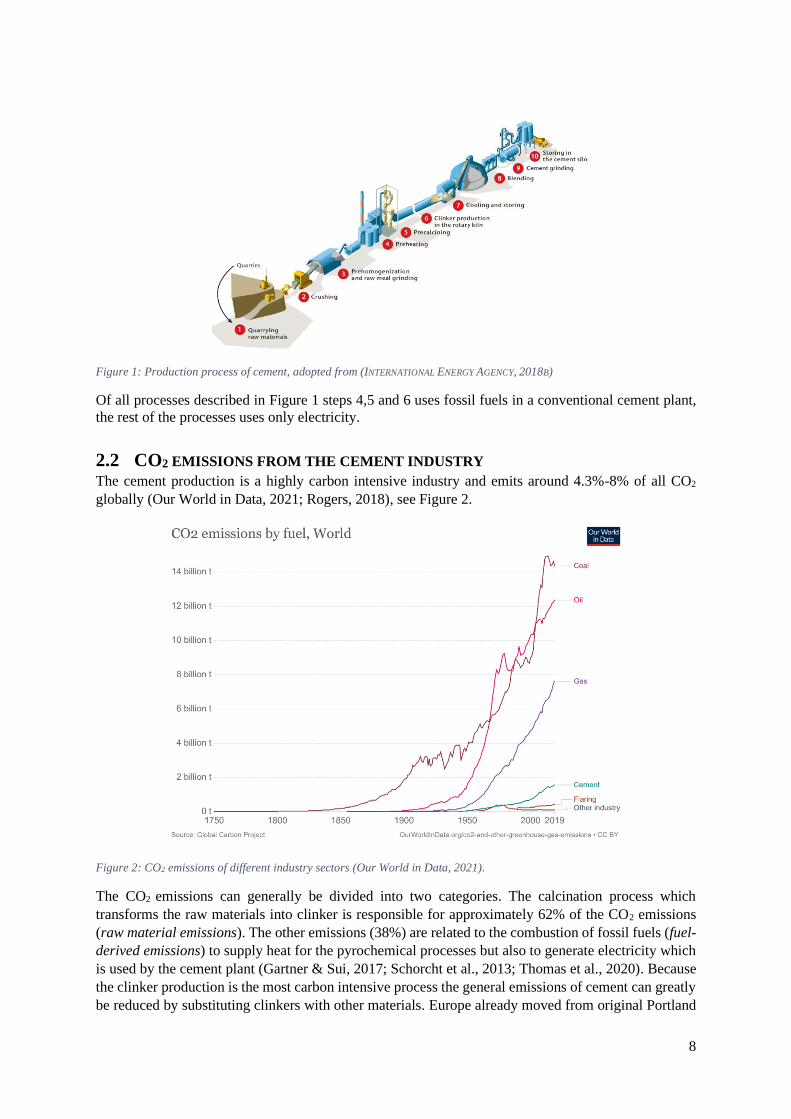
Figure 1: Production process of cement, adopted from (INTERNATIONAL ENERGY AGENCY, 2018B)

Of all processes described in Figure 1 steps 4,5 and 6 uses fossil fuels in a conventional cement plant,

the rest of the processes uses only electricity.

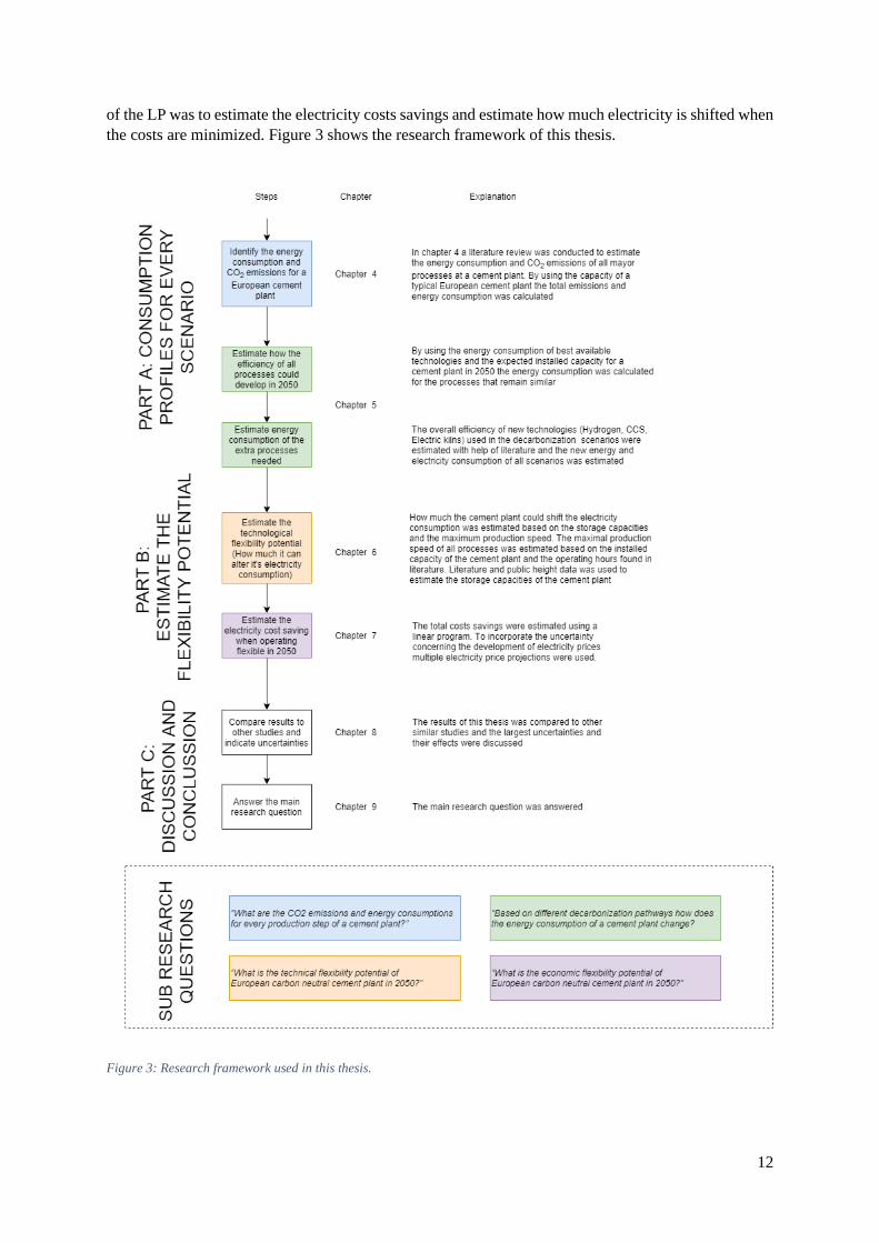
2.2 CO2 EMISSIONS FROM THE CEMENT INDUSTRY The cement production is a highly carbon intensive industry and emits around 4.3%-8% of all CO2

globally (Our World in Data, 2021; Rogers, 2018), see Figure 2.

Figure 2: CO2 emissions of different industry sectors (Our World in Data, 2021).

The CO2 emissions can generally be divided into two categories. The calcination process which

transforms the raw materials into clinker is responsible for approximately 62% of the CO2 emissions

(raw material emissions). The other emissions (38%) are related to the combustion of fossil fuels (fuel-

derived emissions) to supply heat for the pyrochemical processes but also to generate electricity which

is used by the cement plant (Gartner & Sui, 2017; Schorcht et al., 2013; Thomas et al., 2020). Because

the clinker production is the most carbon intensive process the general emissions of cement can greatly

be reduced by substituting clinkers with other materials. Europe already moved from original Portland

9

cement (95-100%) to a clinker-cement ratio of 77% in 2017. By substituting more parts of the clinker

with other material this ratio and thus the emissions can be lowered (CEMBUREAU, 2020b; Favier et

al., 2018; Kermeli et al., 2019).

Raw material emissions

To create clinkers which can be used as a binder for cement the limestone must be decarbonated to form

calcium oxide. This is done by heating the limestone to around 900 °C:

𝐶𝑎𝐶𝑂3(𝑙𝑖𝑚𝑒𝑠𝑡𝑜𝑛𝑒) + (𝐻𝑒𝑎𝑡) → 𝐶𝑎𝑂(𝑆𝑜𝑙𝑖𝑑) + 𝐶𝑂2(𝑔𝑎𝑠)

(Gartner & Sui, 2017)

The CO2 emissions from the calcination process could be reduced by using different materials but could

only become carbon neutral if Carbon Capture and Storage (CCS) is utilized. According to Gartner &

Sui (2017), it could be possible to create carbon negative cement by using magnesium oxides derived

from magnesium silicates (MOMS), instead of limestone. MOMS based cement does not contain any

carbon an thus no carbon could be released during the chemical process. MOMS uses CO2 from the

atmosphere to harden itself and therefore the process could become carbon neutral or carbon negative.

However, after the bankruptcy of the company in 2012 that produces MOMS based cement no industrial

companies invested in researching the feasibility of this type of cement and the research on this subject

came to a stop (Gartner & Sui, 2017). Since CO2 emissions are unavoidable when cement is produced

using CCS the only method of making the cement industry carbon neutral (Favier et al., 2018).

Next to the calcination process which emits CO2, cement products also uptake carbon from the

atmosphere through the carbonation process (Lukovic, 2016):

𝐶𝑎(𝑂𝐻)2 + 𝐶𝑂2 → 𝐶𝑎𝐶𝑂3 + 𝐻2𝑂

According to one study up to 25% of the emitted CO2 could be absorbed back into the cement during

its lifetime, something which is not considered into current carbon inventories (Xi et al., 2016). This

effect is however undesirable when cement is used in combination with steel reinforcements because

this process increases the corrosion rate of steel. According to Gartner & Sui (2017) this is the reason

why the industy does not claim CO2 credits for this absorbed CO2. Because not all emissions could be

reabsorbed in the cement a CCS system is still necessary to make this industry carbon neutral.

Fuel-derived emissions

Currently most cement plants use the combustion of fuels to heat up the limestone. The carbon emitted

from the combustion is dependent on the carbon intensity of the fuel, adding biofuels to the mix will

result in lower overall emissions. The Dutch cement plant in Maastricht for example decreased their

CO2 emissions by switching to a more bio-based fuel mixed (Junginger et al., 2007). Decarbonizing

this process would mean to switch to 100% bio fuels or using alternative methods for heating such as

electric heaters or hydrogen as a fuel source. Electricity consumed for other processes (Conveyers,

Crushers, mill, etc.) indirectly cause CO2 emissions because the electricity mix is not carbon neutral. It

will be assumed that in 2050 all electricity needed will be generated using carbon free methods.

2.3 DEMAND RESPONSE. Demand Response (DR) refers to the ability to change the consumption of electricity according to

electricity generation. This can be incentivised with price signals, when wind and solar energy is largely

available the electricity prices will drop (Perez-Linkenheil, 2019; Suraj & Sentil, 2016). With an

increase of VRES into the mix the need for flexible electricity consumption also increases. A report

from 2017 for example estimated that the need for demand flexibility (both up and down) in the

Netherlands needs to increase by around 9 times to make it possible to decarbonize the electricity mix

10

(Sijm et al., 2017). The cement industry could provide part of this flexibility by for example make more

use of the mill when there is an excess of electricity produced. According to Suraj & Sentil (2016)

flexibility can be achieved by the following strategies:

• Reducing the demand by improving the efficiency.

• Encourage customers to shift their demand to off-peak, this can be done by lowering the

electricity prices during off-peak.

• Utilities could pay a fee to force a costumer to lower their demand in real time to decrease the

demand. An example is the Smart AC program in California which pays users to turn their AC

off for a short period.

• Adjusting the consumption to keep the frequency of the grid stable, this adjusting will be done

in a timescale of seconds.

Depending on the chosen decarbonization pathway the energy consumption of a cement plant could

increase or decrease in 2050. Furthermore, because of the possible introduction of extra processes the

flexibility of a cement plant could increase. This potential increase in flexibility and the potential

increase of electricity price fluctuations could increase the incentive to operate a cement plant flexible.

3 RESEARCH OBJECTIVE

In this chapter the objective of the research will be explained by stating the Research gap (3.1), research

aim (3.2), scope (3.3), relevance (3.4), research questions (3.5) and the research framework (3.6)

3.1 RESEARCH GAP Multiple articles have been published on how to decarbonize the cement industry by 2050 (Favier et

al., 2018; Hasanbeigi & Springer, 2019; Karlsson et al., 2020; Obrist et al., 2021; Schneider, 2015).

However, these articles have mostly a broad view of the industry and do not look in depth at the new

energy or electricity consumption profiles of these new plants. These demand profiles could be useful

for designing the energy system in 2050 so the energy supply can better match the demand.

Another research gap was found in the lack of information there is about the flexibility potential of

carbon neutral cement plants. Some research is already conducted on the application of DR in the

cement industry (Lidbetter & Liebenberg, 2014; Summerbell et al., 2017; Zhao et al., 2014). The

scientific consensus is that cement plants have a DR potential. For example, Summerbell et al. (2017)

concluded that a cement plant in the UK could save 4.2% of the electricity cost (£350,000) and lower

the electricity generation during peak times with around 1 MW. However, no study is found that tries

to estimate the flexibility potential of carbon neutral cement plants in 2050.

3.2 RESEARCH AIM This thesis addresses the aforementioned research gaps. Energy demand profiles were estimated for

carbon neutral cement plants. Because there are multiple pathways of decarbonizing the cement

industry, the electricity demand profiles of all pathways were estimated.

The second aim is to address the knowledge gap of what the technological and economic flexibility

potential of a carbon free cement plant could be. This flexibility potential is expressed in possible

change in electricity consumption (e.g. it could shift 10 MWh per day). The flexibility potential is also

economically expressed in how much a cement plant could save on electricity costs if it were to operate

flexible.

11

3.3 SCOPE The research conducted is limited to all the production processes of a cement plant (e.g. transport is not

included). As mentioned previously, assessing when a cement plant would be carbon neutral is highly

complex since some of the CO2 emissions will later be absorbed by cement products and therefore act

as a carbon sink (Gartner & Sui, 2017; Xi et al., 2016). Moreover, it is hard for CCS systems to capture

all CO2 emitted. To demarcate this problem it was assumed that it possible for CCS technologies to

capture 100% of the emissions. To stay within the timeframe of 30 ECTS it is decided to only research

the costs savings of electricity based on the day-ahead market. This means that costs such as installation

and operating costs will fall outside the scope of this research. Additional costs savings that could be

achieved by acting as a frequency containment reserve for the electricity grid will not be investigated.

Furthermore, it was assumed that all electricity supplied in 2050 will come from carbon neutral sources.

3.4 RELEVANCE The ambition of the European cement association is to become carbon neutral by 2050 (CEMBUREAU,

2020b), this is in line with the green deal with as goal to create carbon neutral industries in 2050

(European Commission, 2012; Government of the Netherlands, 2020). Since no alternatives are

available for cement it will remain an essential industry for the entire world. This thesis will add to the

knowledge base to map out the economic benefits associated with certain pathways to decarbonize the

cement industry.

Flexibility is also beneficial for the TSO (Transmission System Operator) since it can be used for

balancing the electricity grid. Estimating the flexibility potentials gives the TSO a better insight in the

role that industries could play in maintaining a stable electricity grid. Understanding the flexibility

potential of the cement industry could also help by estimating the feasibility of integrating VRES into

the fuel mix. The methodology of this study can also be used to determine the flexibility potential of

other industries.

3.5 RESEARCH QUESTIONS The main research question of this thesis will be:

“What is the flexibility potential of a carbon neutral cement plant in 2050?”

To answer this research question the following sub-questions will be answered.

“What are the CO2 emissions and energy consumptions for every production step of a European cement

plant”

“Based on different decarbonization pathways how does the energy consumption of a European cement

plant change?”

“What is the technical flexibility potential of a European carbon neutral cement plant in 2050?”

“What is the economic flexibility potential of a European carbon neutral cement plant in 2050?”

3.6 RESEARCH FRAMEWORK The research is divided into three parts. Part A is about estimating the energy and electricity demand of

the reference scenario and the decarbonization scenarios (RQ1 and RQ2). In Part B the flexibility

potential was estimated. After these demand profiles were constructed the maximum technological

flexibility potential of these scenarios was estimated based on the storage capacity of the intermediate

goods and the installed capacity of the cement plant (RQ3). After the maximum flexibility potential was

estimated the actual flexibility was estimated in (RQ4). With help of a linear program (LP). The purpose

12

of the LP was to estimate the electricity costs savings and estimate how much electricity is shifted when

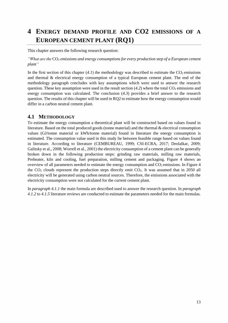
the costs are minimized. Figure 3 shows the research framework of this thesis.

Figure 3: Research framework used in this thesis.

13

4 ENERGY DEMAND PROFILE AND CO2 EMISSIONS OF A

EUROPEAN CEMENT PLANT (RQ1)

This chapter answers the following research question:

“What are the CO2 emissions and energy consumptions for every production step of a European cement

plant”

In the first section of this chapter (4.1) the methodology was described to estimate the CO2 emissions

and thermal & electrical energy consumption of a typical European cement plant. The end of the

methodology paragraph concludes with key assumptions which were used to answer the research

question. These key assumption were used in the result section (4.2) where the total CO2 emissions and

energy consumption was calculated. The conclusion (4.3) provides a brief answer to the research

question. The results of this chapter will be used in RQ2 to estimate how the energy consumption would

differ in a carbon neutral cement plant.

4.1 METHODOLOGY To estimate the energy consumption a theoretical plant will be constructed based on values found in

literature. Based on the total produced goods (tonne material) and the thermal & electrical consumption

values (GJ/tonne material or kWh/tonne material) found in literature the energy consumption is

estimated. The consumption value used in this study lie between feasible range based on values found

in literature. According to literature (CEMBUREAU, 1999; CSI-ECRA, 2017; Deolalkar, 2009;

Galitsky et al., 2008; Worrell et al., 2001) the electricity consumption of a cement plant can be generally

broken down in the following production steps: grinding raw materials, milling raw materials,

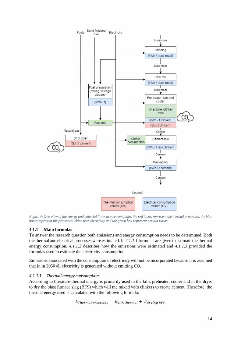
Preheater, kiln and cooling, fuel preparation, milling cement and packaging. Figure 4 shows an

overview of all parameters needed to estimate the energy consumption and CO2 emissions. In Figure 4

the CO2 clouds represent the production steps directly emit CO2. It was assumed that in 2050 all

electricity will be generated using carbon neutral sources. Therefore, the emissions associated with the

electricity consumption were not calculated for the current cement plant.

In paragraph 4.1.1 the main formula are described used to answer the research question. In paragraph

4.1.2 to 4.1.5 literature reviews are conducted to estimate the parameters needed for the main formulas.

14

Figure 4: Overview of the energy and material flows in a cement plant, the red boxes represent the thermal processes, the blue

boxes represent the processes which uses electricity and the green box represent certain ratios.

4.1.1 Main formulas

To answer the research question both emissions and energy consumption needs to be determined. Both

the thermal and electrical processes were estimated. In 4.1.1.1 formulas are given to estimate the thermal

energy consumption, 4.1.1.2 describes how the emissions were estimated and 4.1.1.3 provided the

formulas used to estimate the electricity consumption.

Emissions associated with the consumption of electricity will not be incorporated because it is assumed

that in in 2050 all electricity is generated without emitting CO2.

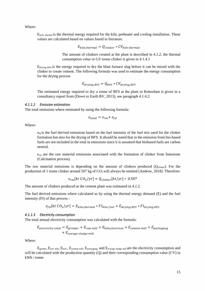
4.1.1.1 Thermal energy consumption

According to literature thermal energy is primarily used in the kiln, preheater, cooler and in the dryer

to dry the blast furnace slag (BFS) which will me mixed with clinkers to create cement. Therefore, the

thermal energy used is calculated with the following formula:

𝐸𝑇ℎ𝑒𝑟𝑚𝑎𝑙 𝑝𝑟𝑜𝑐𝑒𝑠𝑠𝑒𝑠 = 𝐸𝑘𝑖𝑙𝑛,𝑡ℎ𝑒𝑟𝑚𝑎𝑙 + 𝐸𝑑𝑟𝑦𝑖𝑛𝑔 𝐵𝐹𝑆

15

Where:

EKiln, thermal is the thermal energy required for the kiln, preheater and cooling installation. These

values are calculated based on values found in literature.

𝐸𝑘𝑖𝑙𝑛,𝑡ℎ𝑒𝑟𝑚𝑎𝑙 = 𝑄𝑐𝑙𝑖𝑛𝑘𝑒𝑟 ∗ 𝐶𝑉𝑘𝑖𝑙𝑛 𝑡ℎ𝑒𝑟𝑚𝑎𝑙

The amount of clinkers created at the plant is described in 4.1.2, the thermal

consumption value in GJ/ tonne clinker is given in 4.1.4.1

EDrying BFS is the energy required to dry the blast furnace slag before it can be mixed with the

clinker to create cement. The following formula was used to estimate the energy consumption

for the drying process

𝐸𝑑𝑟𝑦𝑖𝑛𝑔 𝐵𝐹𝑆 = 𝑄𝐵𝐹𝑆 ∗ 𝐶𝑉𝑑𝑟𝑦𝑖𝑛𝑔 𝐵𝐹𝑆

The estimated energy required to dry a tonne of BFS at the plant in Rotterdam is given in a

consultancy report from (Down to Earth BV, 2013), see paragraph 4.1.4.2.

4.1.1.2 Emission estimation

The total emissions where estimated by using the following formula:

𝑒𝑡𝑜𝑡𝑎𝑙 = 𝑒𝑟𝑚+ 𝑒𝑓𝑑

Where:

efd is the fuel derived emissions based on the fuel intensity of the fuel mix used for the clinker

formation but also for the drying of BFS. It should be noted that in the emission from bio-based

fuels are not included in the total in emissions since it is assumed that biobased fuels are carbon

neutral.

erm are the raw material emissions associated with the formation of clinker from limestone

(Calcination process).

The raw material emissions is depending on the amount of clinkers produced (Qclinker). For the

production of 1 tonne clinker around 507 kg of CO2 will always be emitted (Andrew, 2018). Therefore:

𝑒𝑟𝑚[𝑘𝑡 𝐶𝑂2/𝑦𝑟] = 𝑄𝑐𝑙𝑖𝑛𝑘𝑒𝑟[𝑘𝑡/𝑦𝑟] ∗ 0.507

The amount of clinkers produced at the cement plant was estimated in 4.1.2.

The fuel derived emissions where calculated as by using the thermal energy demand (E) and the fuel

intensity (FI) of that process :

𝑒𝑓𝑑[𝑘𝑡 𝐶𝑂2/𝑦𝑟] = 𝐸𝑘𝑖𝑙𝑛,𝑡ℎ𝑒𝑟𝑚𝑎𝑙 ∗ 𝐹𝐼𝑘𝑖𝑙𝑛 𝑓𝑢𝑒𝑙 + 𝐸𝑑𝑟𝑦𝑖𝑛𝑔 𝐵𝐹𝑆 ∗ 𝐹𝐼𝑑𝑟𝑦𝑖𝑛𝑔 𝐵𝐹𝑆

4.1.1.3 Electricity consumption

The total annual electricity consumption was calculated with the formula:

𝐸𝑒𝑙𝑒𝑐𝑡𝑟𝑖𝑐𝑖𝑡𝑦 𝑡𝑜𝑡𝑎𝑙 = 𝐸𝑔𝑟𝑖𝑛𝑑𝑒𝑟 + 𝐸𝑟𝑎𝑤 𝑚𝑖𝑙𝑙 + 𝐸𝑘𝑖𝑙𝑛,𝑒𝑙𝑒𝑐𝑡𝑟𝑖𝑐𝑎𝑙 + 𝐸𝑐𝑒𝑚𝑒𝑛𝑡 𝑚𝑖𝑙𝑙 + 𝐸𝑝𝑎𝑐𝑘𝑎𝑔𝑖𝑛𝑔

+ 𝐸𝑠𝑒𝑤𝑎𝑔𝑒 𝑠𝑙𝑢𝑑𝑔𝑒 𝑚𝑖𝑙𝑙

Where:

Egrinder, Eraw mill, Ekiln , Ecement mill, Epackaging, and Esewage sludge mill are the electricity consumption and

will be calculated with the production quantity (Q) and their corresponding consumption value (CV) in

kWh / tonne

16

𝐸𝐺𝑟𝑖𝑛𝑑𝑒𝑟 = 𝑄𝑟𝑎𝑤 𝑚𝑒𝑎𝑙 ∗ 𝐶𝑉𝑔𝑟𝑖𝑛𝑑𝑒𝑟

𝐸𝑟𝑎𝑤 𝑚𝑖𝑙𝑙 = 𝑄𝑟𝑎𝑤 𝑚𝑒𝑎𝑙 ∗ 𝐶𝑉𝑟𝑎𝑤 𝑚𝑖𝑙𝑙

𝐸𝑘𝑖𝑙𝑛 = 𝑄𝑐𝑙𝑖𝑛𝑘𝑒𝑟 ∗ 𝐶𝑉𝑘𝑖𝑙𝑛

𝐸𝑐𝑒𝑚𝑒𝑛𝑡 𝑚𝑖𝑙𝑙 = 𝑄𝐶𝑒𝑚𝑒𝑛𝑡 ∗ 𝐶𝑉𝑐𝑒𝑚𝑒𝑛𝑡 𝑚𝑖𝑙𝑙

𝐸𝑝𝑎𝑐𝑘𝑎𝑔𝑖𝑛𝑔 = 𝑄𝑐𝑒𝑚𝑒𝑛𝑡 ∗ 𝐶𝑉𝑝𝑎𝑐𝑘𝑎𝑔𝑖𝑛𝑔

𝐸𝑠𝑒𝑤𝑎𝑔𝑒 𝑠𝑙𝑢𝑑𝑔𝑒 𝑚𝑖𝑙𝑙 = 𝑄𝑐𝑒𝑚𝑒𝑛𝑡 ∗ 𝐶𝑉𝑠𝑒𝑤𝑎𝑔𝑒 𝑠𝑙𝑢𝑑𝑔𝑒 𝑚𝑖𝑙𝑙

The amount of produce goods (Q) was estimated in 4.1.2 and the CVs in 4.1.3.

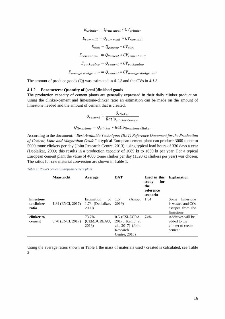
4.1.2 Parameters: Quantity of (semi-)finished goods

The production capacity of cement plants are generally expressed in their daily clinker production.

Using the clinker-cement and limestone-clinker ratio an estimation can be made on the amount of

limestone needed and the amount of cement that is created.

𝑄𝑐𝑒𝑚𝑒𝑛𝑡 =𝑄𝑐𝑙𝑖𝑛𝑘𝑒𝑟

𝑅𝑎𝑡𝑖𝑜𝑐𝑙𝑖𝑛𝑘𝑒𝑟 𝐶𝑒𝑚𝑒𝑛𝑡

𝑄𝑙𝑖𝑚𝑒𝑠𝑡𝑜𝑛𝑒 = 𝑄𝑐𝑙𝑖𝑛𝑘𝑒𝑟 ∗ 𝑅𝑎𝑡𝑖𝑜𝑙𝑖𝑚𝑒𝑠𝑡𝑜𝑛𝑒 𝑐𝑙𝑖𝑛𝑘𝑒𝑟

According to the document: “Best Available Techniques (BAT) Reference Document for the Production

of Cement, Lime and Magnesium Oxide” a typical European cement plant can produce 3000 tonne to

5000 tonne clinkers per day (Joint Research Centre, 2013), using typical load hours of 330 days a year

(Deolalkar, 2009) this results in a production capacity of 1089 kt to 1650 kt per year. For a typical

European cement plant the value of 4000 tonne clinker per day (1320 kt clinkers per year) was chosen.

The ratios for raw material conversion are shown in Table 1.

Table 1: Ratio's cement European cement plant

Maastricht Average BAT Used in this

study for

the

reference

scenario

Explanation

limestone

to clinker

ratio

1.84 (ENCI, 2017)

Estimation of

1.73 (Deolalkar,

2009)

1.5 (Alsop,

2019)

1.84 Some limestone

is wasted and CO2

escapes from the

limestone

clinker to

cement

0.70 (ENCI, 2017)

73.7%

(CEMBUREAU,

2018)

0.5 (CSI-ECRA,

2017; Kemp et

al., 2017) (Joint

Research

Centre, 2013)

74% Additives will be

added to the

clinker to create

cement

Using the average ratios shown in Table 1 the mass of materials used / created is calculated, see Table

2

17

Table 2:Annual material consumption and (Semi-) finished goods produced at a typical European cement plant

Typical European cement plant

Cement produced [kt/yr] 1,808

Clinker produced [kt/yr] 1,320

limestone input [kt/yr] 2,435

4.1.3 Parameters: Consumption values Electrical processes

The total electricity consumption is calculated based on the electricity consumption values (kWh/tonne)

of all processes and the estimated quantities, see 4.1.2.

Four different sources were used to estimate the consumption values (CEMBUREAU, 1999; Deolalkar,

2009; Galitsky et al., 2008; Worrell et al., 2001). It is acknowledged that these sources are old and it is

possible that these consumption values do not represent state of the art. The assumption is made that

there was not much innovation in terms of energy efficiency in the cement industry and that these

numbers represent a current plant, an assumption that is supported by the fact that technology is replaced

every 20-30 years at a cement plant (CSI-ECRA, 2017). Therefore it is plausible that these old

technologies still operate at current cement plants.

Table 3 shows the consumption values for the electrical equipment according to various sources and

the values used in this study. According to Novem (2016) the electrcity consumption of the sewage

sludge mill is 40 kWh per tonne of sewage sludge processed.

Table 3: Electrical consumption values found in literature

(CEMBUREAU,

1999)

(Deolalkar,

2009)

(Worrell et

al., 2001)

(Galitsky et al.,

2008)

Chosen

value for

the

typical

plant

Grinding [kWh/t raw meal] - 2 0.5-1.6 0.5 1

Raw mill [kWh/t raw meal] 7 - 20 12 - 24 12 - 22 14.45 20

Preheater, kiln and cooling [kWh/t

raw meal]

7.5 25 26 22.5 24

Cement mill (type not specified)

[kWh /t clinker]

- - - 16 - 19.2 -

Ball mill [kWh/t cement] 32 - 36.5 35 47 - 45

Roller press + Ball mill [kWh/t

cement]

21 - 25.5 26 39 - 41 - -

Packaging [kWh/t cement] - 1.5 - - 1.5

4.1.4 Parameters: Thermal energy consumption

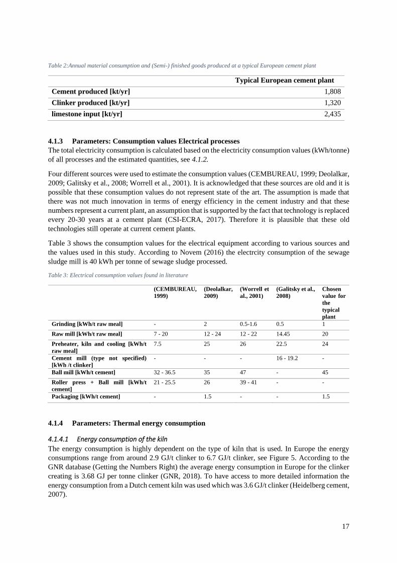
4.1.4.1 Energy consumption of the kiln

The energy consumption is highly dependent on the type of kiln that is used. In Europe the energy

consumptions range from around 2.9 GJ/t clinker to 6.7 GJ/t clinker, see Figure 5. According to the

GNR database (Getting the Numbers Right) the average energy consumption in Europe for the clinker

creating is 3.68 GJ per tonne clinker (GNR, 2018). To have access to more detailed information the

energy consumption from a Dutch cement kiln was used which was 3.6 GJ/t clinker (Heidelberg cement,

2007).

18

Figure 5: Average thermal energy consumption of different types of kilns in Europe (GNR, 2018).

It should be noted that the drying of the raw meal also consumes some thermal energy. However,

because the drying step is combined with the raw mill (Alsop, 2019) and the waste heat from the kiln

is used for this process which leads to an increased efficiency (ENCI, 2009) the thermal energy

requirements for the drying of raw meal is neglected in this study.

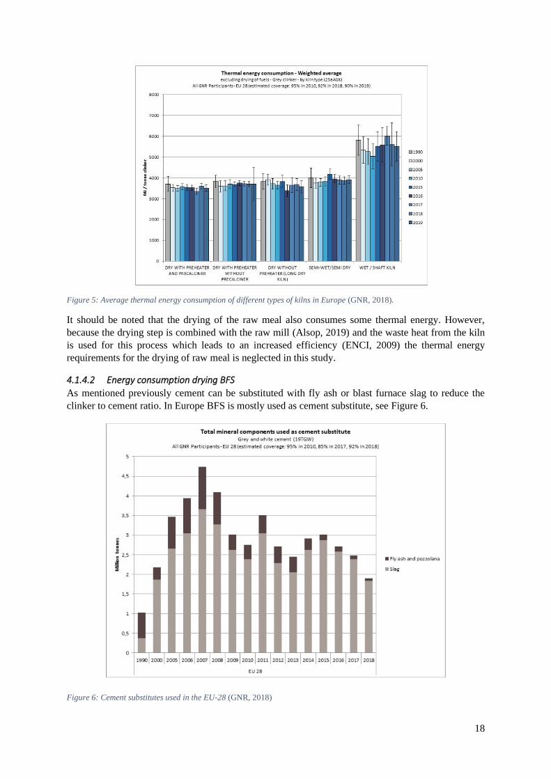
4.1.4.2 Energy consumption drying BFS

As mentioned previously cement can be substituted with fly ash or blast furnace slag to reduce the

clinker to cement ratio. In Europe BFS is mostly used as cement substitute, see Figure 6.

Figure 6: Cement substitutes used in the EU-28 (GNR, 2018)

19

The old cement plant in Maastricht used to imports wet blast furnace slag and dry it onsite (ENCI &

Haskoning, 1997; Xavier & Oliveira, 2021) with a natural gas fired dryer. A report from a consultancy

company (Down to Earth BV, 2013) estimates that an optimised dryer consumes 18.09 m3 (693 MJ)

natural gas per tonne blast furnace slag. If we assume that cement only consist of clinker and BFS it

can be concluded that cement with a clinker-cement ratio of 74% has a BFS share of 26%. Based on

these values the amount of energy and CO2 emissions associated with the drying BFS were estimated,

see Table 4. Waste heat could theoretically be used to dry BFS but no sources were found that supported

this.

Table 4: Installed capacity, cement production and estimated natural gas consumption and CO2 emissions for the drying of

blast furnace slag.

European cement plant

Cement produced 1,808 kt /year

BFS used (26 % of the cement) 476 kt /year

Energy needed to dry 1 tonne of BFS 693 MJ /year

Total energy used for the heating of BFS 338 TJ /year

4.1.5 Parameters: Emissions

4.1.5.1 Fuel derived emissions, kiln

As mentioned in 4.1.4.1 the old cement plant in Maastricht was used for reference. Using an reference

plant instead of the average the values of all European plants has the benefit that this allows for access

to more detailed information such as the fuel mix.

According to ENCI (2017a) the fuel mix of the plant in Maastricht’s consists of 27.6% biofuels, 36 %

alternative fuels (waste) and 36.4% fossil fuels, for a more description of the fuel mix see Figure 7. This

mix uses more alternative fuels compared to average fuel mix of Europe which consist of 18.1%

biofuels, 32.1% alternative fuels and 49.8% fossil fuels (GNR, 2018).

Figure 7: The fuel mix of the ENCI plant in Maastricht when it was still operational (ENCI, 2017a)

It is stated that the 798 kg CO2 will be emitted when 1 tonne clinker is produced (ENCI, 2017a). Due

to the calcination process 507 kg of CO2 will always be emitted when 1 tonne clinker is formed

(Andrew, 2018) and because biofuels are considered to be carbon neutral we can estimate that 291 kg

CO2 per tonne clinker produced originate from fossil and alternative fuels combined. These emissions

36.40%

5.15%24.68%

25.63%

7.06% 1.08%

Fuel mix of the kiln at the old cement plant in Maastricht

Fossils (coal Liquid residues Coke Residuels

Sewage sludge PPDF (Paper and plastic) Other fuel products

20

are slightly lower than the average emissions of 813 kg per tonne clinker for all European countries in

2017 (GNR, 2018).

When the kiln of the plant in Maastricht was still in operation around 27.6% of the energy originate

from biobased fuels (0.90 GJ per tonne clinker) (ENCI, 2017), the exact emissions associated with these

biobased materials is not provided by ENCI but according to Vreuls (2004) the emission intensity of

solid biofuels is 109.6 kg CO2 / GJ which would correspond to 108.5 kg CO2 per clinker produced.

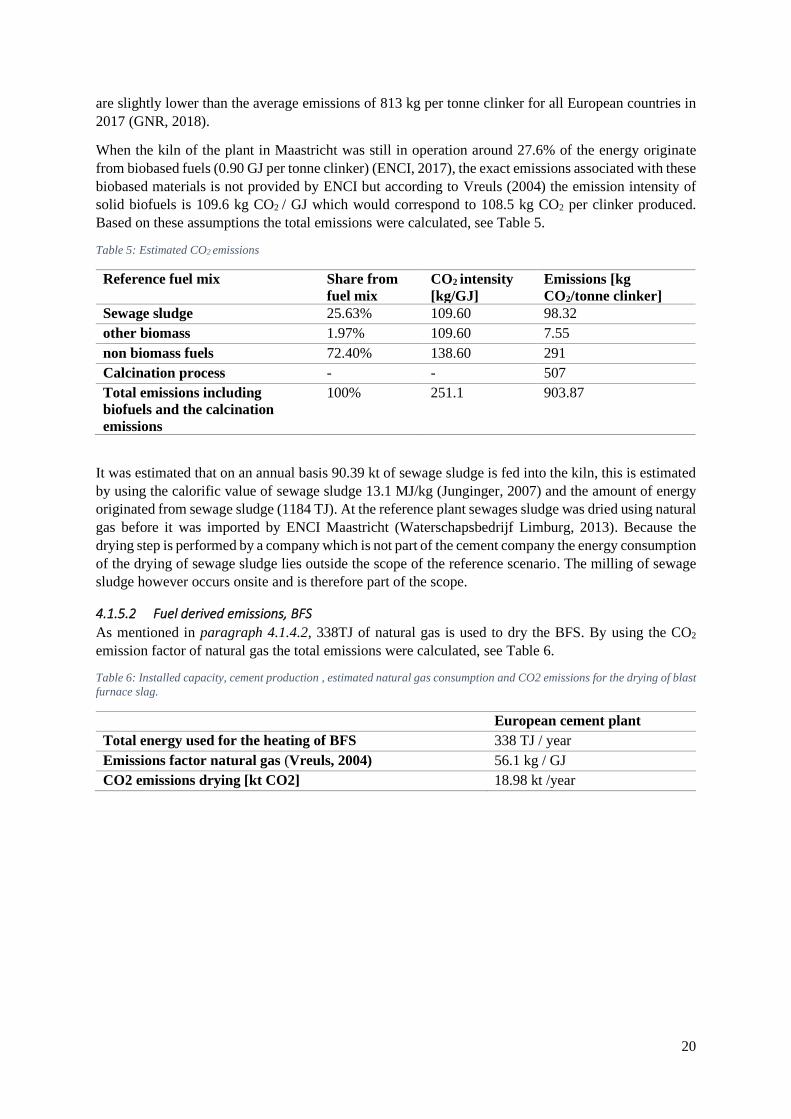
Based on these assumptions the total emissions were calculated, see Table 5.

Table 5: Estimated CO2 emissions

Reference fuel mix Share from

fuel mix

CO2 intensity

[kg/GJ]

Emissions [kg

CO2/tonne clinker]

Sewage sludge 25.63% 109.60 98.32

other biomass 1.97% 109.60 7.55

non biomass fuels 72.40% 138.60 291

Calcination process - - 507

Total emissions including

biofuels and the calcination

emissions

100% 251.1 903.87

It was estimated that on an annual basis 90.39 kt of sewage sludge is fed into the kiln, this is estimated

by using the calorific value of sewage sludge 13.1 MJ/kg (Junginger, 2007) and the amount of energy

originated from sewage sludge (1184 TJ). At the reference plant sewages sludge was dried using natural

gas before it was imported by ENCI Maastricht (Waterschapsbedrijf Limburg, 2013). Because the

drying step is performed by a company which is not part of the cement company the energy consumption

of the drying of sewage sludge lies outside the scope of the reference scenario. The milling of sewage

sludge however occurs onsite and is therefore part of the scope.

4.1.5.2 Fuel derived emissions, BFS

As mentioned in paragraph 4.1.4.2, 338TJ of natural gas is used to dry the BFS. By using the CO2

emission factor of natural gas the total emissions were calculated, see Table 6.

Table 6: Installed capacity, cement production , estimated natural gas consumption and CO2 emissions for the drying of blast

furnace slag.

European cement plant

Total energy used for the heating of BFS 338 TJ / year

Emissions factor natural gas (Vreuls, 2004) 56.1 kg / GJ

CO2 emissions drying [kt CO2] 18.98 kt /year

21

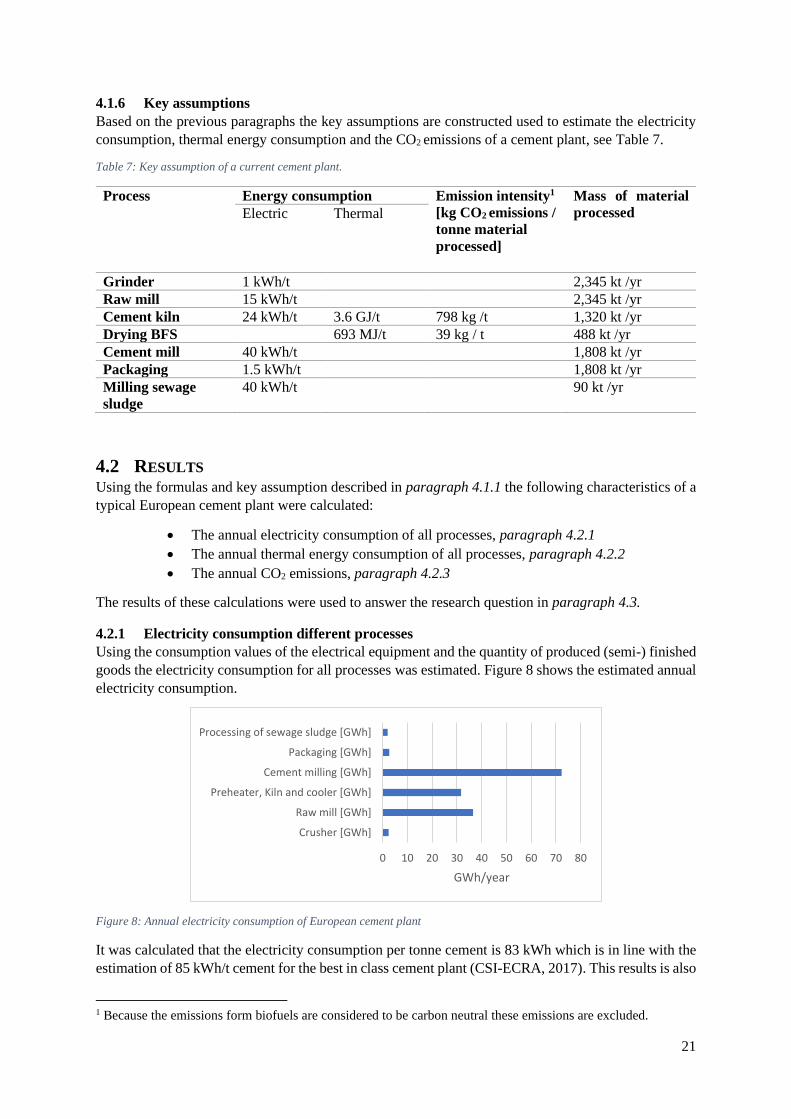
4.1.6 Key assumptions

Based on the previous paragraphs the key assumptions are constructed used to estimate the electricity

consumption, thermal energy consumption and the CO2 emissions of a cement plant, see Table 7.

Table 7: Key assumption of a current cement plant.

Process Energy consumption Emission intensity1

[kg CO2 emissions /

tonne material

processed]

Mass of material

processed Electric Thermal

Grinder 1 kWh/t 2,345 kt /yr

Raw mill 15 kWh/t 2,345 kt /yr

Cement kiln 24 kWh/t 3.6 GJ/t 798 kg /t 1,320 kt /yr

Drying BFS 693 MJ/t 39 kg / t 488 kt /yr

Cement mill 40 kWh/t 1,808 kt /yr

Packaging 1.5 kWh/t 1,808 kt /yr

Milling sewage

sludge

40 kWh/t 90 kt /yr

4.2 RESULTS Using the formulas and key assumption described in paragraph 4.1.1 the following characteristics of a

typical European cement plant were calculated:

• The annual electricity consumption of all processes, paragraph 4.2.1

• The annual thermal energy consumption of all processes, paragraph 4.2.2

• The annual CO2 emissions, paragraph 4.2.3

The results of these calculations were used to answer the research question in paragraph 4.3.

4.2.1 Electricity consumption different processes

Using the consumption values of the electrical equipment and the quantity of produced (semi-) finished

goods the electricity consumption for all processes was estimated. Figure 8 shows the estimated annual

electricity consumption.

Figure 8: Annual electricity consumption of European cement plant

It was calculated that the electricity consumption per tonne cement is 83 kWh which is in line with the

estimation of 85 kWh/t cement for the best in class cement plant (CSI-ECRA, 2017). This results is also

1 Because the emissions form biofuels are considered to be carbon neutral these emissions are excluded.

0 10 20 30 40 50 60 70 80

Crusher [GWh]

Raw mill [GWh]

Preheater, Kiln and cooler [GWh]

Cement milling [GWh]

Packaging [GWh]

Processing of sewage sludge [GWh]

GWh/year

22

consistent with the MER (Dutch: Milieueffectrapportage, English: Environmental impact report) of

2009 (ENCI) where it is stated that for 1,325 kt of cement 120 GWh electricity is needed (90 kWh/t

cement). The values found in Madlool et al. (2011) are also similair to the calculated electricity

consumption.

4.2.2 Thermal energy consumption

There were two processes identified where thermal energy is consumed. BFS is dried with an gas-fired

dryer and the raw meal is heated in the pre-heater and kiln to create clinkers. The drying of BFS

consumes only 7% of the energy compared to the energy required to create clinkers, see Figure 9.

Figure 9: Thermal energy consumption of a European cement plant that produced cement with 30% BFS and 70% clinkers.

4.2.3 CO2 emissions

Three different sources of CO2 emissions were identified.

• Burning natural gas to dry of BFS

• Calcination emissions, the CO2 released from the limestone when clinkers are created

• The burning of alternative-fuels, bio-fuels and fossil-fuels in the kiln to provide heat for the

creation of clinkers.

The annual emissions are shown in Figure 10. Because the biofuels are considered to be carbon neutral

the emissions form these fuels do not need to be accounted for.

Figure 10: Annual CO2 emissions of a typical European cement plant

When the bio-fuel emissions are excluded the calcination emissions account for 62% of the total

emissions which is in line the findings of paragraph 2.2(Gartner & Sui, 2017; Schorcht et al., 2013;

Thomas et al., 2020).

4,620 TJ

338 TJ

Annual energy consumption [TJ]

Thermal energy use kiln Thermal energy drying BFS

0 100 200 300 400 500 600 700 800

CO emissions from biobased fuels [kt]

CO2 emissions from fossil/non biobased fuels [kt]

CO2 emissions drying BFS [kt]

CO2 emissions from the calcination process [kt]

CO2 emissions per year [kt]

23

4.3 CONCLUSION In this chapter the following research question was answered.

“What are the CO2 emissions and energy consumptions for every production step of a European cement

plant”

A typical European cement plant produces 4,000 tonne clinkers per day which would translate to an

annual cement production of 1,808 kt cement. For the production of 1,808 kt clinker it was estimated

that 1,320 kt clinkers are needed and 2,435 kt of limestone.

To produce 1,808 kt of cement around 5,622 TJ of energy is consumed. only 9% of the energy

consumption is used for electrical processes. The processes which consume the most electricity are: the

cement mill, the raw mill and the operation of the kiln. No emissions were calculated associated with

the use of electricity. This is done because for the main research question a cement plant in 2050 is

envisioned where it was assumed that the electricity originates from carbon neutral sources.

85% of the energy is mainly used for the production of clinker and only 6% is used for drying of BFS.

When the emissions of biofuels are excluded a typical cement plant emit around 1072 kt CO2 annually.

CO2 emissions mainly occur in the kiln where fuels are burned and the CO2 is released from the

limestone when clinkers are created. The calcination process contribute to 62% of all emissions.

In RQ2 the development of the energy consumption for multiple decarbonization pathways was

analysed.

24

5 ENERGY CONSUMPTION OF THE DIFFERENT

DECARBONIZATION PATHWAYS (RQ2)

The aim of this chapter is to provide an overview of technologies used in the different decarbonization

pathways and how this impact the total energy consumption. The results were used in RQ3 and RQ4 of

this thesis to model how much electricity could be shifted, and how much electricity cost could be

saved. The following research question was used for this:

“Based on different decarbonization pathways how does the energy consumption of a European cement

plant change?

As mentioned in the introduction, four likely decarbonization scenarios were identified and for these

four scenarios the energy consumption was estimated. These decarbonization scenarios are described

more in-depth paragraph 5.1.

The methodology used to answer the research question is described in paragraph 5.2, this paragraph

will conclude with a table showing all the key assumptions used to calculate the energy consumption.

The results of this research question can be found in paragraph 5.3. The main research question is

answered in paragraph 5.4.

5.1 DESCRIPTION DIFFERENT SCENARIOS According to the literature multiple methods are possible to decarbonize the cement industry in 2050

(Bataille et al., 2018; European Union, 2020; Mathisen, 2019). As mentioned previously the CO2

emissions are caused by the burning of fossil fuels and due to the creation of clinker. The burning of

fossil fuels could be replaced by a carbon neutral alternative but the CO2 emissions from the calcination

cannot be prevented and always need to be captured.

In all scenarios is was assumed that the current technologies at a cement plant will be replaced by the

current best available technologies, this was done because it was assumed that in 2050 due to

technological improvement these efficient technologies become more affordable. Another energy

efficiency measure that was implemented was the use of more clinker substitutes. It was estimated that

the production of cement remains similar in Europe from 2015-2017 till 2050 (European Commission,

2020; International Energy Agency, 2018a), see Figure 11. Therefore it is assumed that the installed

capacity of a typical European cement plant will remain the same. According to Alsop (2019) the

stabilization of demand in Europe is caused by fact that Europe has a mature economy and urbanization

has already taken place.

Figure 11:Forecast of the global cement demand, adopted from (INTERNATIONAL ENERGY AGENCY, 2018A)

25

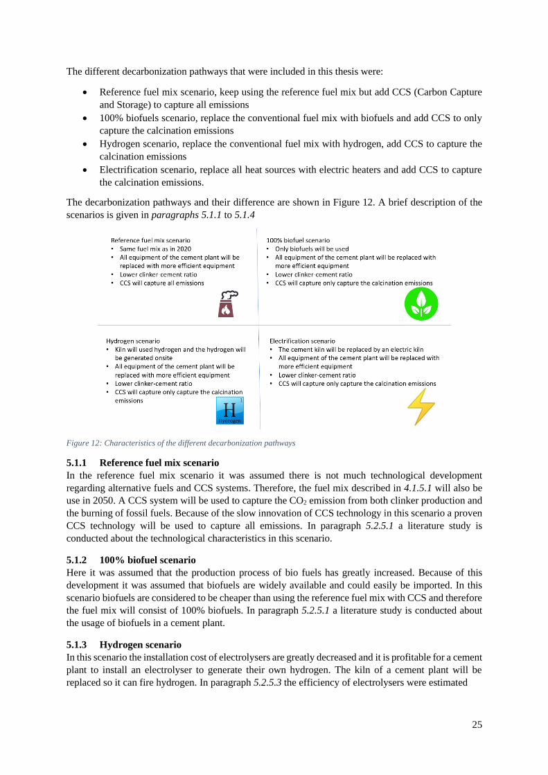
The different decarbonization pathways that were included in this thesis were:

• Reference fuel mix scenario, keep using the reference fuel mix but add CCS (Carbon Capture

and Storage) to capture all emissions

• 100% biofuels scenario, replace the conventional fuel mix with biofuels and add CCS to only

capture the calcination emissions

• Hydrogen scenario, replace the conventional fuel mix with hydrogen, add CCS to capture the

calcination emissions

• Electrification scenario, replace all heat sources with electric heaters and add CCS to capture

the calcination emissions.

The decarbonization pathways and their difference are shown in Figure 12. A brief description of the

scenarios is given in paragraphs 5.1.1 to 5.1.4

Figure 12: Characteristics of the different decarbonization pathways

5.1.1 Reference fuel mix scenario

In the reference fuel mix scenario it was assumed there is not much technological development

regarding alternative fuels and CCS systems. Therefore, the fuel mix described in 4.1.5.1 will also be

use in 2050. A CCS system will be used to capture the CO2 emission from both clinker production and

the burning of fossil fuels. Because of the slow innovation of CCS technology in this scenario a proven

CCS technology will be used to capture all emissions. In paragraph 5.2.5.1 a literature study is

conducted about the technological characteristics in this scenario.

5.1.2 100% biofuel scenario

Here it was assumed that the production process of bio fuels has greatly increased. Because of this

development it was assumed that biofuels are widely available and could easily be imported. In this

scenario biofuels are considered to be cheaper than using the reference fuel mix with CCS and therefore

the fuel mix will consist of 100% biofuels. In paragraph 5.2.5.1 a literature study is conducted about

the usage of biofuels in a cement plant.

5.1.3 Hydrogen scenario

In this scenario the installation cost of electrolysers are greatly decreased and it is profitable for a cement

plant to install an electrolyser to generate their own hydrogen. The kiln of a cement plant will be

replaced so it can fire hydrogen. In paragraph 5.2.5.3 the efficiency of electrolysers were estimated

26

5.1.4 Electrification scenario

The installation costs for using electric heaters in industries is greatly decreased in this scenario.

Because of these low costs the cement industry has switched to electric cement kilns. In paragraph

5.2.5.4 it was estimated which electric heating technology is most suited for a cement kiln and what

their efficiency would be.

5.2 METHODOLOGY

5.2.1 Main formulas

The energy consumption is calculated similar to in chapter 4 (RQ1) with the only difference that:

• Because of the lower clinker-cement ratio there will be less limestone used and more BFS.

• More efficient technology will be used for all processes, the consumption values used in the

2050 scenario are based on the BAT of the reference scenario.

• CCS will be added to all scenarios.

By lowering the quantities of limestone and clinker (Q), and using more efficient technologies (CV) the

energy consumption can be lowered. However, adding CCS will increase the energy consumption. The

new quantities of (semi-)finished goods (Q) were estimated in paragraph 5.2.2 and the new

consumption values (CV) were estimated in paragraph 5.2.3.

The thermal processes are replaced by a carbon neutral alternatives which depending on the scenario

consumes electricity or carbon neutral fuels. Therefore, the total energy consumed by the new plant was

calculated with the following formula:

𝐸𝑛𝑒𝑤 𝑠𝑐𝑒𝑛𝑎𝑟𝑖𝑜 = 𝐸𝐶𝐶𝑆,𝑛𝑒𝑤 𝑠𝑐𝑒𝑛𝑎𝑡𝑖𝑜 + 𝐸𝑛𝑜𝑛 𝑡ℎ𝑒𝑟𝑚𝑎𝑙 𝑝𝑟𝑜𝑐𝑒𝑠𝑠𝑒𝑠,𝑛𝑒𝑤 𝑠𝑐𝑒𝑛𝑎𝑟𝑖𝑜

+ 𝐸𝑡ℎ𝑒𝑟𝑚𝑎𝑙 𝑝𝑟𝑜𝑐𝑒𝑠𝑠𝑒𝑠,𝑛𝑒𝑤 𝑠𝑐𝑒𝑛𝑎𝑡𝑖𝑜

Where

ECCS is the electricity required for the CCS system, this will be calculated based on the

consumption values found in literature (GJe / t CO2) and the mass of CO2 being emitted. It

should be noted that in the scenario of where fossil fuels or biomass is used in the kiln the

amount of emitted CO2 is higher and therefore more energy is required for the CCS installation.

The energy needed for CCS is calculated with the formula:

𝐸𝐶𝐶𝑆 = 𝑚𝐶𝑂2 ∗ 𝐶𝑉𝐶𝐶𝑆

Where

mCO2 is the mass of CO2 that needs to be captured and CVCCS is the consumption value

of a CCS system found in literature in GJ per tonne CO2 .

In both the reference fuel mix and the 100% biofuel scenario it was assumed that the imported

fuels (with the exception of sewage sludge) could directly be used in the kiln without pre-

treatment. Therefore, the same formula can be used as shown in chapter 4 but with updated

values for the quantities (Q) and consumption values (CV). In the hydrogen scenario the

hydrogen first needs to be generated. Therefore, the energy consumption for the kiln in the

hydrogen scenario was calculated as:

𝐸𝑘𝑖𝑙𝑛,ℎ𝑦𝑑𝑟𝑜𝑔𝑒𝑛 =𝑄𝑐𝑙𝑖𝑛𝑘𝑒𝑟𝐶𝑉𝑘𝑖𝑙𝑛,𝐵𝐴𝑇

𝜂𝑒𝑙𝑒𝑐𝑡𝑟𝑜𝑙𝑦𝑧𝑒𝑟

The efficiency of the electrolyser was estimated in 5.2.5.3.

27

The consumption value of an electric kiln could not be found (GJ needed for the creation of

one tonne clinker) and therefore the CV of an electric kiln is calculated with the following

formula:

𝐶𝑉𝑒𝑙𝑒𝑐𝑡𝑟𝑖𝑐 𝑘𝑖𝑙𝑛 =𝐸𝑡ℎ𝑒𝑜𝑟𝑒𝑡𝑖𝑐𝑎𝑙 𝑒𝑛𝑒𝑟𝑔𝑦 𝑛𝑒𝑒𝑑𝑒𝑑 𝑓𝑜𝑟 𝑜𝑛𝑒 𝑡𝑜𝑛𝑛𝑒 𝑐𝑙𝑖𝑛𝑘𝑒𝑟

𝜂𝑒𝑙𝑒𝑐𝑡𝑟𝑖𝑐 ℎ𝑒𝑎𝑡𝑖𝑛𝑔 𝑡𝑒𝑐ℎ𝑛𝑜𝑙𝑜𝑔𝑦

In 5.2.5.4 a literature study is conducted about suitable technologies for the electrification of

the kiln so the efficiency (η) of an electric kiln can be estimated.

It was assumed that in all scenarios the natural gas dryer used for the drying of BFS will be

replaced by an electric dryer. The reasoning behind this assumption was that in all scenarios in

2050 the electric heater would be the most cost-effective option. The electricity consumption

of an electric heater was estimated by first estimating the actual heat required for the drying

process and then converting it to the actual electricity consumption, see 5.2.4.

𝐸𝑒𝑙𝑒𝑐𝑡𝑟𝑖𝑐 𝐵𝐹𝑆 𝑑𝑟𝑦𝑖𝑛𝑒𝑟 =𝐸𝑑𝑟𝑦𝑒𝑟 𝐵𝐹𝑆,𝑛𝑎𝑡𝑢𝑟𝑎𝑙 𝑔𝑎𝑠 ∗ 𝜂𝑔𝑎𝑠 𝑓𝑖𝑟𝑒𝑑 𝑑𝑟𝑦𝑒𝑟

𝜂𝑒𝑙𝑒𝑐𝑡𝑟𝑖𝑐 𝑑𝑟𝑦𝑒𝑟

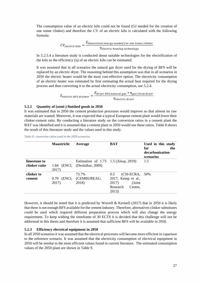
5.2.2 Quantity of (semi-) finished goods in 2050

It was estimated that in 2050 the cement production processes would improve so that almost no raw

materials are wasted. Moreover, it was expected that a typical European cement plant would lower their

clinker-cement ratio. By conducting a literature study on the conversion ratios in a cement plant the

BAT was identified and it is assumed that a cement plant in 2050 would use these ratios. Table 8 shows

the result of this literature study and the values used in this study.

Table 8: conversion ratios used in the 2050 scenarios

Maastricht Average BAT Used in this study

for the

decarbonization

scenarios

limestone to

clinker ratio

1.84 (ENCI,

2017)

Estimation of 1.73

(Deolalkar, 2009)

1.5 (Alsop, 2019) 1.5

clinker to

cement

0.70 (ENCI,

2017)

73.7%

(CEMBUREAU,

2018)

0.5 (CSI-ECRA,

2017; Kemp et al.,

2017) (Joint

Research Centre,

2013)

50%

However, it should be noted that it is predicted by Worrell & Kermeli (2017) that in 2050 it is likely

that there is not enough BFS available for the cement industry. Therefore, alternatives clinker substitutes

could be used which required different preparation process which will also change the energy

requirement. To keep withing the timeframe of 30 ECTS it is decided that this challenge will not be

addressed in this thesis and therefore it is assumed that sufficient BFS will be available in 2050.

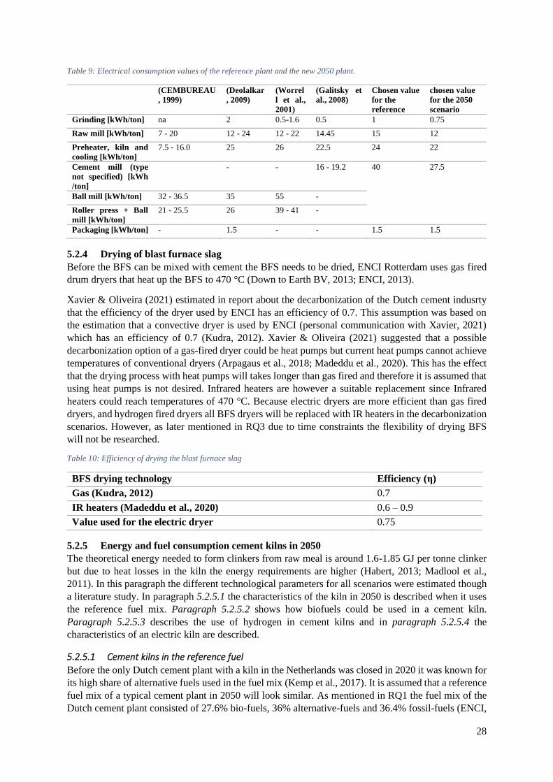
5.2.3 Efficiency electrical equipment in 2050

In all 2050 scenarios it was assumed that the electrical processes will become more efficient in caparison

to the reference scenario. It was assumed that the electricity consumption of electrical equipment in

2050 will be similar to the most efficient values found in current literature. The estimated consumption

values of the 2050 plant are shown in Table 9.

28

Table 9: Electrical consumption values of the reference plant and the new 2050 plant.

(CEMBUREAU

, 1999)

(Deolalkar

, 2009)

(Worrel

l et al.,

2001)

(Galitsky et

al., 2008)

Chosen value

for the

reference

chosen value

for the 2050

scenario

Grinding [kWh/ton] na 2 0.5-1.6 0.5 1 0.75

Raw mill [kWh/ton] 7 - 20 12 - 24 12 - 22 14.45 15 12

Preheater, kiln and

cooling [kWh/ton]

7.5 - 16.0 25 26 22.5 24 22

Cement mill (type

not specified) [kWh

/ton]

- - 16 - 19.2 40 27.5

Ball mill [kWh/ton] 32 - 36.5 35 55 -

Roller press + Ball

mill [kWh/ton]

21 - 25.5 26 39 - 41 -

Packaging [kWh/ton] - 1.5 - - 1.5 1.5

5.2.4 Drying of blast furnace slag

Before the BFS can be mixed with cement the BFS needs to be dried, ENCI Rotterdam uses gas fired

drum dryers that heat up the BFS to 470 °C (Down to Earth BV, 2013; ENCI, 2013).

Xavier & Oliveira (2021) estimated in report about the decarbonization of the Dutch cement indusrty

that the efficiency of the dryer used by ENCI has an efficiency of 0.7. This assumption was based on

the estimation that a convective dryer is used by ENCI (personal communication with Xavier, 2021)

which has an efficiency of 0.7 (Kudra, 2012). Xavier & Oliveira (2021) suggested that a possible

decarbonization option of a gas-fired dryer could be heat pumps but current heat pumps cannot achieve

temperatures of conventional dryers (Arpagaus et al., 2018; Madeddu et al., 2020). This has the effect

that the drying process with heat pumps will takes longer than gas fired and therefore it is assumed that

using heat pumps is not desired. Infrared heaters are however a suitable replacement since Infrared

heaters could reach temperatures of 470 °C. Because electric dryers are more efficient than gas fired

dryers, and hydrogen fired dryers all BFS dryers will be replaced with IR heaters in the decarbonization

scenarios. However, as later mentioned in RQ3 due to time constraints the flexibility of drying BFS

will not be researched.

Table 10: Efficiency of drying the blast furnace slag

BFS drying technology Efficiency (η)

Gas (Kudra, 2012) 0.7

IR heaters (Madeddu et al., 2020) 0.6 – 0.9

Value used for the electric dryer 0.75

5.2.5 Energy and fuel consumption cement kilns in 2050

The theoretical energy needed to form clinkers from raw meal is around 1.6-1.85 GJ per tonne clinker

but due to heat losses in the kiln the energy requirements are higher (Habert, 2013; Madlool et al.,

2011). In this paragraph the different technological parameters for all scenarios were estimated though

a literature study. In paragraph 5.2.5.1 the characteristics of the kiln in 2050 is described when it uses

the reference fuel mix. Paragraph 5.2.5.2 shows how biofuels could be used in a cement kiln.

Paragraph 5.2.5.3 describes the use of hydrogen in cement kilns and in paragraph 5.2.5.4 the

characteristics of an electric kiln are described.

5.2.5.1 Cement kilns in the reference fuel

Before the only Dutch cement plant with a kiln in the Netherlands was closed in 2020 it was known for

its high share of alternative fuels used in the fuel mix (Kemp et al., 2017). It is assumed that a reference

fuel mix of a typical cement plant in 2050 will look similar. As mentioned in RQ1 the fuel mix of the

Dutch cement plant consisted of 27.6% bio-fuels, 36% alternative-fuels and 36.4% fossil-fuels (ENCI,

29

2017). Of these bio-fuels the largest share of energy comes from sewage sludge which is milled at the

ENCI plant. Using biofuels in combination with CCS could even create a negative carbon emission for

the cement industry. Having negative emissions could be beneficial to compensate for other processes

where the CO2 could not be captured or the negative CO2 credits could be sold on the European emission

trading system (European Commission, 2015). Due to the scope of this thesis it is assumed that all

emissions related to biofuels will be released into the atmosphere so the electricity costs of the CCS

system will be reduced.

As mentioned earlier, the energy consumption of the kiln used in RQ1 is around 3.5 GJ/t clinker

(efficiency of 46% - 53%). This is slightly lower than the average cement kiln in Europe. Literature

shows that is possible to have more efficient kilns and therefore it was assumed that in 2050 most of

the kilns will be replaced by more efficient ones. This assumption is based on the fact that kilns have a

lifetime of 30 to 50 years (CSI-ECRA, 2017) so it is likely that in 2050 most kilns will be replaced. A

literature study was conducted where the efficiencies of different kilns were compared and it was found

that lowest energy consumption for the creating of 1 tonne clinker is around 2.9 GJ (efficiency of 55%

- 64%), see Table 11.

Table 11: Thermal consumption values of the clinker production

Sources Consumption Value (CV) Kiln,

preheater[GJ/t Clinker]

(CEMBUREAU, 1999) 2.9 - 3.2

(Deolalkar, 2009) 2.929 - 3.138

(Worrell et al., 2001b) 2.9 - 3.2

(Galitsky et al., 2008) 3.347

(Heidelberg cement, 2007) 3.5

(Alsop, 2019) 3.1-3.6

Average EU-28 in 2018 (GNR, 2018) 3.68

Chosen value for the reference scenario 3.5

chosen value for the 2050 scenario 2.9

As mentioned in paragraph 4.1.4, 25.63% of the energy comes from sewage sludge. In all scenarios a

total of 904.1 kt clinkers will be created annually and with a consumption value of 2.9 GJ/t clinker we

can estimate that the total amount of energy from the sewage sludge will be around 672 TJ. By assuming

that the sewage sludge has a calorific value of 13.1 MJ/kg (Junginger, 2007) it was estimated that 51.3

kt of sewage sludge will be co-fired.

5.2.5.2 Cement kilns in the 100% biofuel mix scenario

Because biofuels are considered carbon neutral increasing the share of biomass decreases the CO2

emissions that need to be captured. Combining biofuels with CCS could even achieve negative

emissions (Platform, 2012). A fuel mix consisting of 100% biomass could however not directly be used

in the kiln, according to CSI-ECRA (2017) the calorific value of fuels should be at least 20 to 22 GJ/t

while the calorific value of biomass is around 10 to 18 GJ/t. Therefore, biomass should be mixed with

other fuels to increase the calorific value of the fuel mix. To keep within the timeframe of this thesis

the fuel mix of 100% biofuel scenario will consist of the same share sewage sludge as the reference fuel

mix but all the other energy comes for synthesised methane. It was assumed that methane fired cement

plants have the same efficiency as conventional kilns. Theoretically other biofuels can also be used but

because it was assumed that the biofuels will be imported and do not need to be prepared onsite (except

sewage sludge) the type of biofuel used will not change the results of this study.

30

Synthetic methane can be produced by the anaerobic digestion of biomass, similarly how swamp gas is

produced (IEA, 2020b; Müller-Langer et al., 2014; Nsair et al., 2020). Generally biogas consist CO2

and CH4:

𝐶6𝐻12𝑂6 → 3𝐶𝑂2 + 3𝐶𝐻4

To create pure methane the CO2 could be removed which gives a higher calorific value but according

to Ellersdorfer & Weiß (2011) this is not needed for a cement plant.

Another method to create biogas is to break down woody biomass at high temperature in a high pressure

and low oxygen environment (IEA, 2020b). The share of CH4 in the biogas is mainly determined by the

feedstock used (Falk, 2011).

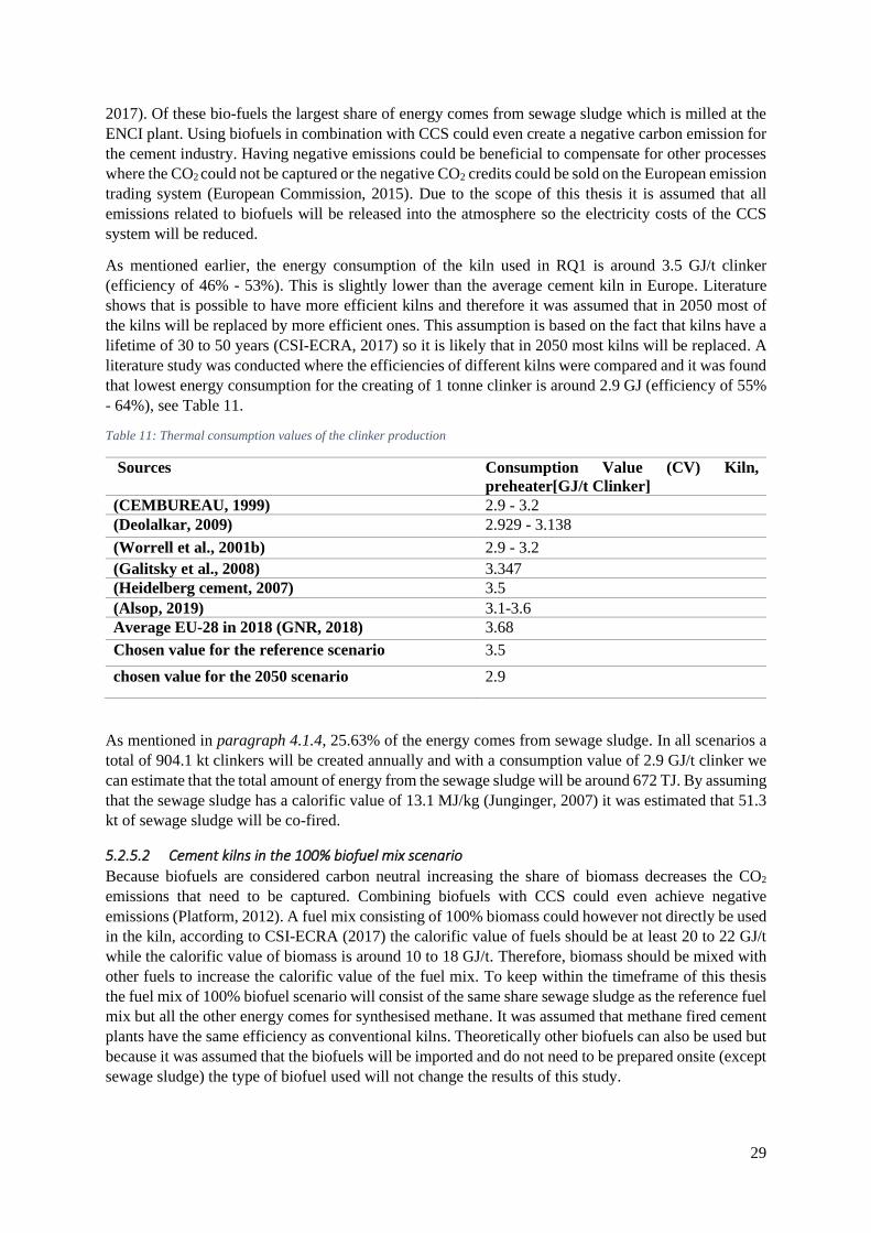
Due to time constraints an in depth analysis of different biofuels could not be conducted. However

because of the cost and emissions of biogas is comparable to other bio fuels, see Figure 13, it was

assumed that a mix of sewage sludge and biomethane/biogas is a feasible fuel mix in this scenario.

Figure 13: Production costs of different biofuels from (Müller-Langer et al., 2014), the white dots show the show the production

cost gathered from the Deutsches Biomasseforschungszentrum (DBFZ) database.

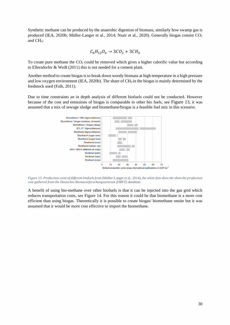
A benefit of using bio-methane over other biofuels is that it can be injected into the gas grid which

reduces transportation costs, see Figure 14. For this reason it could be that biomethane is a more cost

efficient than using biogas. Theoretically it is possible to create biogas/ biomethane onsite but it was

assumed that it would be more cost effective to import the biomethane.

31

Figure 14: Proposed infrastructure for the usage of bio-methane (IEA, 2020b).

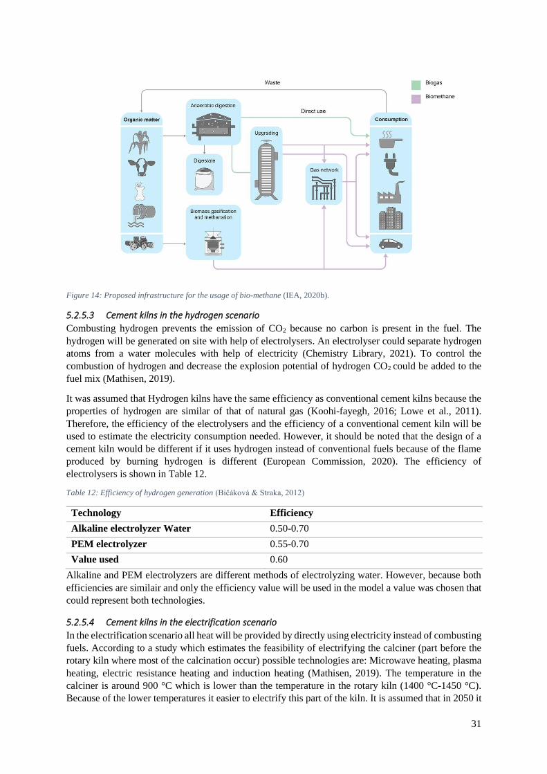
5.2.5.3 Cement kilns in the hydrogen scenario

Combusting hydrogen prevents the emission of CO2 because no carbon is present in the fuel. The

hydrogen will be generated on site with help of electrolysers. An electrolyser could separate hydrogen

atoms from a water molecules with help of electricity (Chemistry Library, 2021). To control the

combustion of hydrogen and decrease the explosion potential of hydrogen CO2 could be added to the

fuel mix (Mathisen, 2019).

It was assumed that Hydrogen kilns have the same efficiency as conventional cement kilns because the

properties of hydrogen are similar of that of natural gas (Koohi-fayegh, 2016; Lowe et al., 2011).

Therefore, the efficiency of the electrolysers and the efficiency of a conventional cement kiln will be

used to estimate the electricity consumption needed. However, it should be noted that the design of a

cement kiln would be different if it uses hydrogen instead of conventional fuels because of the flame

produced by burning hydrogen is different (European Commission, 2020). The efficiency of

electrolysers is shown in Table 12.

Table 12: Efficiency of hydrogen generation (Bičáková & Straka, 2012)

Technology Efficiency

Alkaline electrolyzer Water 0.50-0.70

PEM electrolyzer 0.55-0.70

Value used 0.60

Alkaline and PEM electrolyzers are different methods of electrolyzing water. However, because both

efficiencies are similair and only the efficiency value will be used in the model a value was chosen that

could represent both technologies.

5.2.5.4 Cement kilns in the electrification scenario

In the electrification scenario all heat will be provided by directly using electricity instead of combusting

fuels. According to a study which estimates the feasibility of electrifying the calciner (part before the

rotary kiln where most of the calcination occur) possible technologies are: Microwave heating, plasma

heating, electric resistance heating and induction heating (Mathisen, 2019). The temperature in the

calciner is around 900 °C which is lower than the temperature in the rotary kiln (1400 °C-1450 °C).

Because of the lower temperatures it easier to electrify this part of the kiln. It is assumed that in 2050 it

32

is possible to also electrify the kiln and that the technologies mentioned to heat of the calciner have the

same advantages and disadvantages when applied to the kiln. The benefits and disadvantages of those

technologies are shown in Table 13. Mathisen (2019) deemed resistance heating the most feasible

technology for the cement industry.

Table 13: Advantages and disadvantages of electric heating technologies for the cement industry adopted from Mathisen

(2019)

Technology Description Advantage Disadvantage

Microwave Use electromagnetic

waves from a

magnetron to make

molecules vibrate to

generate heat.

Temperature is easy to

control, could calcinate

faster than an electric

furnace

Local hot spots could

occur which could melt

the raw meal, safety

concerns for personnel.

Plasma heating Ionising gas so it

becomes conductive

which makes heat

transfer from an

electric arc to the

process possible. In the

cement industry CO2

could be used as gas.

Lower operating costs,

high thermal

efficiency. A pilot

study has been

conducted which

concluded that plasma

heating could be

feasible for the cement

industry (Vattenfall,

2019)

Short operating hours (

600 – 1000 hours)

water cooling is

required.

Electrical resistance

heating

Heat a metal through

resistance heating so

the raw meal be heated

through convection,

radiation or by putting

the raw meal in direct

contact with the hot

surface.

Simple and proven

technology, relatively

safe.

Induction heating Heating a conductive

object through

electromagnetic

induction. The currents

in the conductive

object heat up the

material by resistive

heating.

Proven technology,

relatively safe.

Inductive heating

equipment must be

cooled, raw meal is not

electrically conductive

and could therefore not

be heated directly.

Challenging to

generate steady

temperatures.

Vattenfall (2019) conducted a pilot study and concluded that plasma technology could be used for the

creation of clinker. Because of the study from Vattenfall (2019) and the analysis by Mathisen (2019) it

was decided that electrical resistance heating or plasma technology could be a feasible technology for

the cement industry in 2050. A benefit of using an electric kiln is that this the flue gas consist of pure

CO2 from the calcination of limestone which makes it easier to capture (Mathisen, 2019).

The efficiency of these technologies are estimated with help of a paper from Madeddu et al. (2020) and

Rao et al. (2013), see Table 14. By using the theoretical energy requirement for the calcination process

of 1.7 GJ/ clinker (Habert, 2013; Madlool et al., 2011) it is estimated that the energy consumption of an

electric kiln would be 2.3 GJ/clinker.

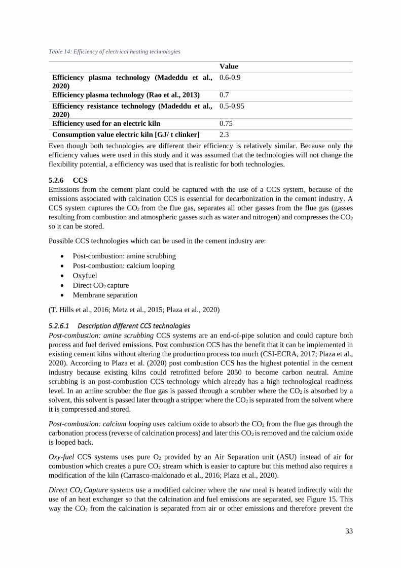
33

Table 14: Efficiency of electrical heating technologies

Value

Efficiency plasma technology (Madeddu et al.,

2020)

0.6-0.9

Efficiency plasma technology (Rao et al., 2013) 0.7

Efficiency resistance technology (Madeddu et al.,

2020)

0.5-0.95

Efficiency used for an electric kiln 0.75

Consumption value electric kiln [GJ/ t clinker] 2.3

Even though both technologies are different their efficiency is relatively similar. Because only the

efficiency values were used in this study and it was assumed that the technologies will not change the

flexibility potential, a efficiency was used that is realistic for both technologies.

5.2.6 CCS

Emissions from the cement plant could be captured with the use of a CCS system, because of the

emissions associated with calcination CCS is essential for decarbonization in the cement industry. A

CCS system captures the CO2 from the flue gas, separates all other gasses from the flue gas (gasses

resulting from combustion and atmospheric gasses such as water and nitrogen) and compresses the CO2

so it can be stored.

Possible CCS technologies which can be used in the cement industry are:

• Post-combustion: amine scrubbing

• Post-combustion: calcium looping

• Oxyfuel

• Direct CO2 capture

• Membrane separation

(T. Hills et al., 2016; Metz et al., 2015; Plaza et al., 2020)

5.2.6.1 Description different CCS technologies

Post-combustion: amine scrubbing CCS systems are an end-of-pipe solution and could capture both

process and fuel derived emissions. Post combustion CCS has the benefit that it can be implemented in

existing cement kilns without altering the production process too much (CSI-ECRA, 2017; Plaza et al.,

2020). According to Plaza et al. (2020) post combustion CCS has the highest potential in the cement

industry because existing kilns could retrofitted before 2050 to become carbon neutral. Amine

scrubbing is an post-combustion CCS technology which already has a high technological readiness

level. In an amine scrubber the flue gas is passed through a scrubber where the CO2 is absorbed by a

solvent, this solvent is passed later through a stripper where the CO2 is separated from the solvent where

it is compressed and stored.

Post-combustion: calcium looping uses calcium oxide to absorb the CO2 from the flue gas through the

carbonation process (reverse of calcination process) and later this CO2 is removed and the calcium oxide

is looped back.

Oxy-fuel CCS systems uses pure O2 provided by an Air Separation unit (ASU) instead of air for

combustion which creates a pure CO2 stream which is easier to capture but this method also requires a

modification of the kiln (Carrasco-maldonado et al., 2016; Plaza et al., 2020).

Direct CO2 Capture systems use a modified calciner where the raw meal is heated indirectly with the

use of an heat exchanger so that the calcination and fuel emissions are separated, see Figure 15. This

way the CO2 from the calcination is separated from air or other emissions and therefore prevent the

34

need for separation technologies (T. P. Hills et al., 2017). The fuel derived emissions could be captured

with other CCS technologies but when biofuels or hydrogen are used this is not needed to achieve

carbon neutrality. Because heat exchangers are used instead of directly heating the raw meal it is

expected that the energy consumption will slightly increase (Plaza et al., 2020). It was estimated that

the energy consumption will increase with around 2% (T. Hills et al., 2016). the pure CO2 still needs to

be compressed before it can stored which consumes around 100 kWh/ tonne CO2 (Aspelund & Jordal,

2007; Roussanaly et al., 2017).

Figure 15: Schematic of a direct CO2 capturing CCS system (Plaza et al., 2020)

Membrane separation separates the CO2 from the flue gas with a membrane. Because membrane

systems need to operate under pressurised conditions an additional compressor is needed. According to

Plaza et al. (2020) membrane separation has a capture range of 60%-70%. Despite the low energy

consumption of membrane separation the retrofit costs are higher than other technologies.

The technological readiness levels of all discussed technologies are shown in Figure 16.

Figure 16: Technology Readiness Level of different CO2 post combustion and oxyfuels capture methods for the cement industry

(IEA, 2020a) as shown in Plaza et al. (2020).

5.2.6.2 CCS technology for the different decarbonization scenarios

According Hills et al. (2016) and Plaza et al. (2020) if the current cement industry is pressured in

decarbonizing the sector Amine scrubbing technology will likely be chosen due to his high

technological maturity. However, if CCS is not directly needed and other technologies have enough

time to develop these technologies would likely be more cost efficient than amine scrubbing. In the

35

reference fuel scenario it was estimated that there is not much technological development and therefore

amine scrubbing will be used in the reference fuel mix scenario.

One method to decrease the energy consumption of CCS is to utilize the waste heat from the kiln (Bjerge

& Brevik, 2014; Metz et al., 2015). However, is should be noted that most waste heat is already used

for the drying of material and therefore in some cases it is estimated that only 15% of waste heat can be

used (Koring et al., 2013). In this study it was assumed that the reuse of waste heat is not possible.

An overview of the different CCS technologies for a cement plant are shown in Table 15.

Table 15: Overview CCS technologies that can be used in the cement industry, adopted from Plaza et al. (2020), T. Hills et al.

(2016) and Wang et al. (2017)

Separation

technology

Energy

consumption

(GJe/t CO2)

Capture rate Main benefits and disadvantages

Chemical

absorption

8.3 >90% + Proven technology

- High energy consumption

Amine

scrubbing

2.0 - 4.0 >90% +Proven technology, considered

benchmark technology

-if other technologies have time to develop

they would likely outperform amine

scrubbing

Membrane

separation

1.2-3.22 60-70%, could go

higher but this

greatly increases

the electricity

costs

+Small footprint

+Low energy consumption

-Low capture rate

Calcium

looping

3.17-4.42 98% +high capture rate

+considered by Plaza et al. (2020) to be

one of the more promising technologies

+materials needed for this technology are

present at cement plants (limestone)

Oxyfuel 1.63 >90% +high capture rate and increased fuel

efficiency

-need to generate pure O2

-could not be retrofitted

Chilled

ammonia

process

3.75 90% +could be retrofitted

+lower energy consumption than amine

scrubbing

Direct

capture

0.36 GJ/t for

compressions

(Aspelund &

Jordal, 2007;

Roussanaly et

al., 2017) ,

+2% fuel

consumption

Only calcination

emissions

+Low energy/electricity consumption

+Could be retrofitted

-Can only capture the calculation emission

Based on the characteristics shown in Table 15 a suited CCS technology was chosen for the different

decarbonization pathways. Direct capture is a promising technology which separates the calcination

emissions from the fuel derived emissions. A benefit of direct capturing is that it has the lowest energy

requirements of all CCS systems mentioned in this chapter. It was assumed that in scenarios were carbon

neutral heat sources are used direct capture will be implemented. The direct capture technology in the

36

electrification scenario is slightly different than the other scenarios because here there is no combustion

thus the fuel derived emissions do not need to be separated. This has the effect that there will be no

energy penalty of 2% in the electrification scenario. As mentioned in paragraph 5.1, in the reference

fuel mix it was assumed that there will not be much technological development on CCS technologies.

For this reason it was assumed the reference fuel mix would use a proven technology, it was assumed

that amine scrubbing would be used in the reference fuel mix scenario. Table 16 shows which CCS

technologies will be used in the different decarbonization scenarios.

Table 16: Chosen CCS systems and their assumed effect for all decarbonization scenarios.

Scenario Type CCS Assumed capture rate Effect

Reference fuel

mix

Amine scrubbing 100% 3.5 GJ/ tonne CO2

100% fuel mix Direct capture 100% of the calcination

emissions

2% extra fuel use +

compression of CO2 (100 kWh

/ tonne CO2)

Hydrogen Direct capture 100% of the calcination

emissions

2% extra fuel use +

compression of CO2 (100 kWh

/ tonne CO2)

Electrification Compression only 100% of the calcination

emissions

compression of CO2 (100 kWh

/ tonne CO2)

For simplification it was assumed that the amine scrubbing CCS system has a capture rate of 100%.

Moreover, it was assumed that the thermal energy needed for this CCS system can be provided by

electrical sources.

5.2.7 Key assumptions

All parameters needed to estimate the energy consumption of the different decarbonization scenarios

are shown in the tables below. Table 17 shows the parameters of the generic cement processes (the

production steps that are included in all scenarios). Table 18 shows the parameters needed for the

milling of sewage sludge which is used in the reference fuel and biofuel scenario. The energy

consumption of the kilns in the different decarbonization scenarios are shown in Table 19

Table 17: Quantities of processed materials (Q) and the consumption values (CV) of generic cement processes.

Process Material processed (Q) Consumption Value (CV)

Grinder 1,356 kt raw meal /yr 0.75 kWh / tonne

Raw mill 1,356 kt raw meal /yr 12 kWh / tonne

Cement kiln, electric 904 kt clinkers /yr 22 kWh / tonne

Cement mill 1,808 kt cement /yr 27.5 kWh / tonne

packaging 1,808 kt cement /yr 1.5 kWh/ tonne

Drying BFS 904 kt BFS /yr 164 kWh/ tonne

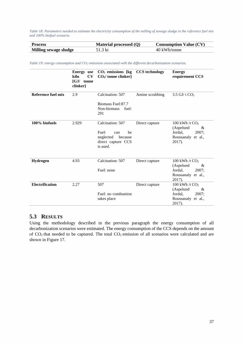
37

Table 18: Parameters needed to estimate the electricity consumption of the milling of sewage sludge in the reference fuel mix

and 100% biofuel scenario.

Process Material processed (Q) Consumption Value (CV)

Milling sewage sludge 51.3 kt 40 kWh/tonne

Table 19: energy consumption and CO2 emissions associated with the different decarbonization scenarios.

Energy use

kiln CV

[GJ/ tonne

clinker]

CO2 emissions [kg

CO2/ tonne clinker]

CCS technology Energy

requirement CCS

Reference fuel mix 2.9 Calcination: 507

Biomass Fuel:87.7

Non-biomass fuel:

291

Amine scrubbing 3.5 GJ/ t CO2

100% biofuels 2.929 Calcination: 507

Fuel: can be

neglected because

direct capture CCS

is used.

Direct capture 100 kWh /t CO2

(Aspelund &

Jordal, 2007;

Roussanaly et al.,

2017).

Hydrogen 4.93 Calcination: 507

Fuel: none

Direct capture 100 kWh /t CO2

(Aspelund &

Jordal, 2007;

Roussanaly et al.,

2017).

Electrification 2.27 507

Fuel: no combustion

takes place

Direct capture 100 kWh /t CO2

(Aspelund &

Jordal, 2007;

Roussanaly et al.,

2017).

5.3 RESULTS Using the methodology described in the previous paragraph the energy consumption of all

decarbonization scenarios were estimated. The energy consumption of the CCS depends on the amount

of CO2 that needed to be captured. The total CO2 emission of all scenarios were calculated and are

shown in Figure 17.

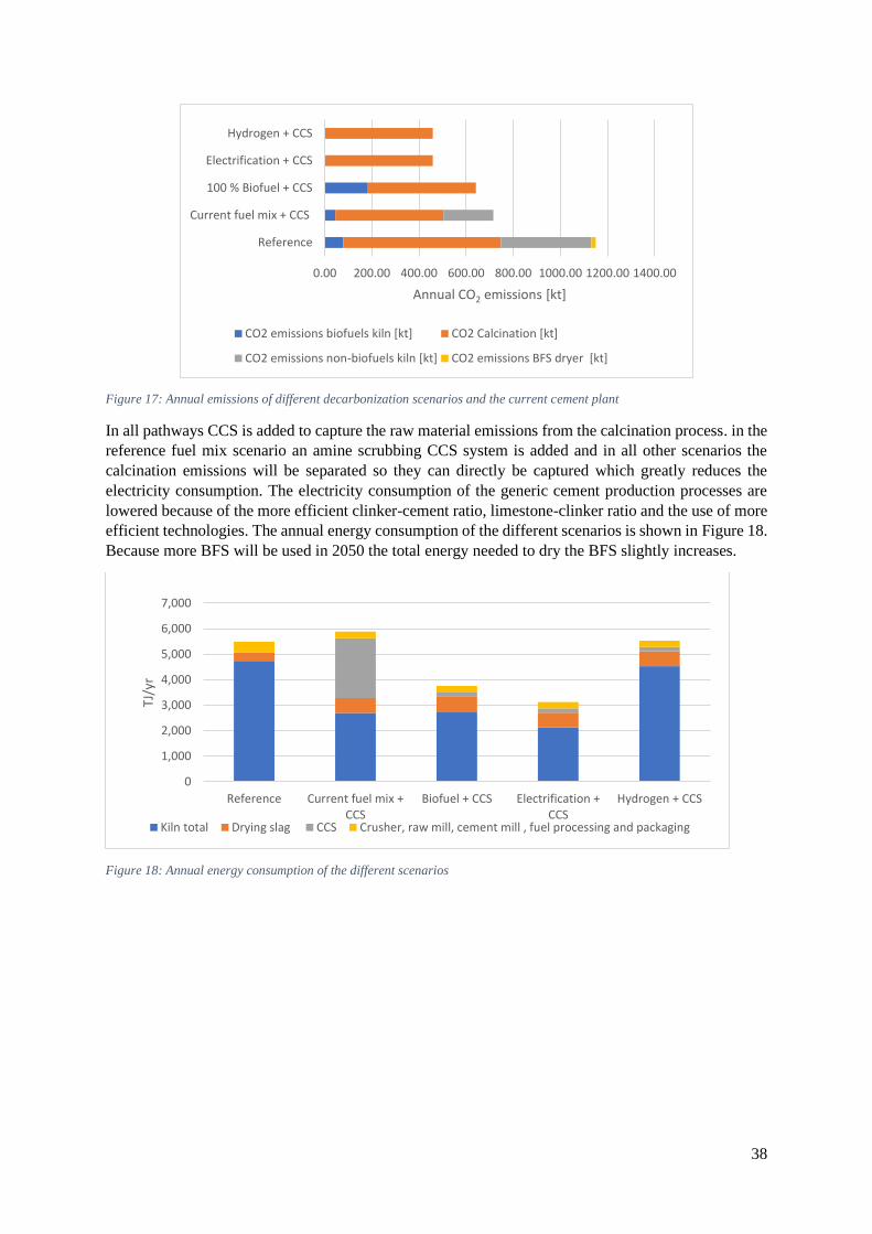
38

Figure 17: Annual emissions of different decarbonization scenarios and the current cement plant

In all pathways CCS is added to capture the raw material emissions from the calcination process. in the

reference fuel mix scenario an amine scrubbing CCS system is added and in all other scenarios the

calcination emissions will be separated so they can directly be captured which greatly reduces the

electricity consumption. The electricity consumption of the generic cement production processes are

lowered because of the more efficient clinker-cement ratio, limestone-clinker ratio and the use of more

efficient technologies. The annual energy consumption of the different scenarios is shown in Figure 18.

Because more BFS will be used in 2050 the total energy needed to dry the BFS slightly increases.

Figure 18: Annual energy consumption of the different scenarios

0.00 200.00 400.00 600.00 800.00 1000.00 1200.00 1400.00

Reference

Current fuel mix + CCS

100 % Biofuel + CCS

Electrification + CCS

Hydrogen + CCS

Annual CO2 emissions [kt]

CO2 emissions biofuels kiln [kt] CO2 Calcination [kt]

CO2 emissions non-biofuels kiln [kt] CO2 emissions BFS dryer [kt]

0

1,000

2,000

3,000

4,000

5,000

6,000

7,000

Reference Current fuel mix +CCS

Biofuel + CCS Electrification +CCS

Hydrogen + CCS

TJ/y

r

Kiln total Drying slag CCS Crusher, raw mill, cement mill , fuel processing and packaging

39

5.4 CONCLUSION In this chapter the following research question was answered:

“Based on different decarbonization pathways how does the energy consumption of a European cement

plant change?

The four most likely decarbonization pathways for the cement industry were identified as:

• Reference fuel mix scenario (keep using the same fuel mix but implement an amine scrubbing

CCS system to capture all emissions)

• 100% biofuel mix scenario (Switch to a fuel mix consisting of 100% biofuels and capture all

the calcination emissions)

• Hydrogen scenario (Generate hydrogen onsite so it can be used in the kiln and use a CCS system

to capture all the calcination emissions)

• Electrification scenario (Use electricity directly to provide heat and capture all the calcination

emissions with a CCS system)

The hydrogen and the reference fuel mix scenario consume the most energy and their total energy

consumptions are comparable to that of a current cement plant without CCS. This is because despite

the use of a more efficient kiln and electrical equipment the CCS system and the hydrogen generation

requires much more energy. In the reference fuel scenario it was assumed that an amine scrubbing CCS

system would be used which is highly energy intensive. In the hydrogen scenario a direct capture CCS

system could be used which has a much lower energy requirement but because the generation of

hydrogen has a relative low efficiency the overall energy remains similar compared to the reference

scenario.

Direct capture is also used in the 100% biofuel scenario, using direct capture slightly increases the

energy requirements of the kiln with 2% but greatly decreases the energy consumption of the CCS

system because the CO2 does not need to be separated from the flue gas. Because biofuels are used the

fuel derived emissions can be released into the atmosphere while still remaining carbon neutral.

It is estimated that a cement plant in the electrification scenario consumes the least amount of energy

because electric kilns have a high efficiency. The pure CO2 stream of an electric kiln makes it possible

to directly compress these CO2 emissions without the need for an energy intensive separation process.

40

6 FLEXIBILITY OF A EUROPEAN CEMENT PLANT (RQ3)

This chapter will answer the following research question:

“What is the technical flexibility potential of European carbon neutral cement plant in 2050?”

In chapter 5 Energy consumption of the different decarbonization pathways (RQ2) the technological

characteristics of cement plants for all decarbonization pathways were described. This chapter estimate

which processes could be made flexible and what their flexibility is. The flexibility potential was

expressed in how much energy could be shifted during a day in MWh/day.

Some processes identified in previous chapters are only applicable in certain scenarios while other are

present in all scenarios, for comparison the production processes are divided into the following

categories.

• Generic cement production processes (grinding, milling and packaging)

• Processing sewage sludge

• Hydrogen production

• CCS

The aim of this chapter is to quantify the flexibility of all the flexible processes. This chapter provides

most of the constraints which will be used in chapter 7

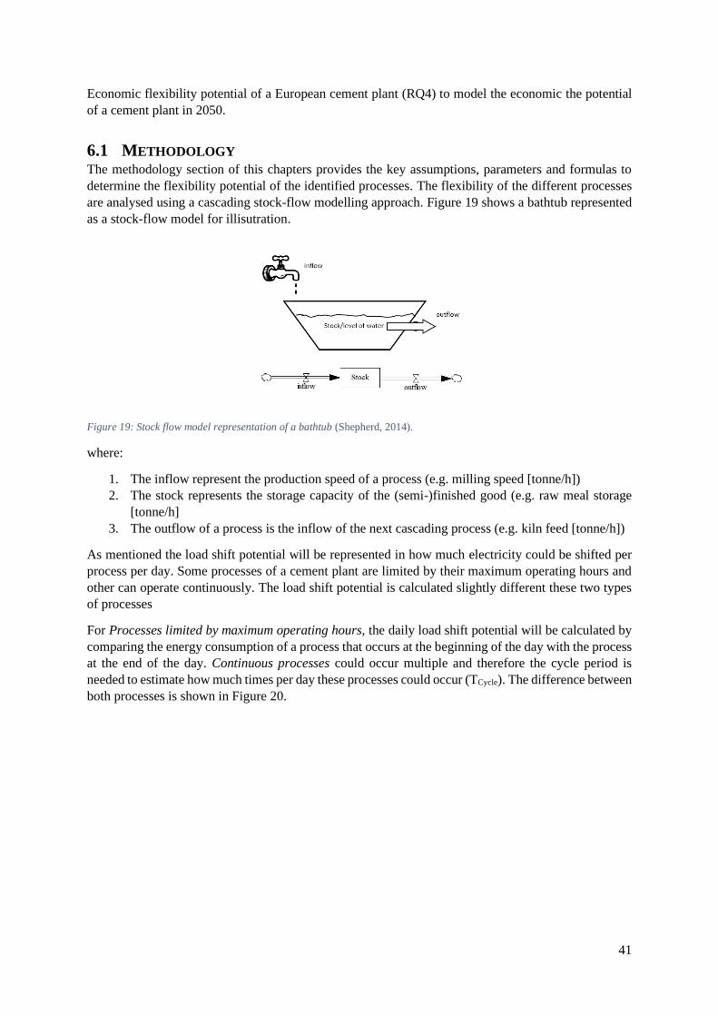
41

Economic flexibility potential of a European cement plant (RQ4) to model the economic the potential

of a cement plant in 2050.

6.1 METHODOLOGY The methodology section of this chapters provides the key assumptions, parameters and formulas to

determine the flexibility potential of the identified processes. The flexibility of the different processes

are analysed using a cascading stock-flow modelling approach. Figure 19 shows a bathtub represented

as a stock-flow model for illisutration.

Figure 19: Stock flow model representation of a bathtub (Shepherd, 2014).

where:

1. The inflow represent the production speed of a process (e.g. milling speed [tonne/h])

2. The stock represents the storage capacity of the (semi-)finished good (e.g. raw meal storage

[tonne/h]

3. The outflow of a process is the inflow of the next cascading process (e.g. kiln feed [tonne/h])

As mentioned the load shift potential will be represented in how much electricity could be shifted per

process per day. Some processes of a cement plant are limited by their maximum operating hours and

other can operate continuously. The load shift potential is calculated slightly different these two types

of processes

For Processes limited by maximum operating hours, the daily load shift potential will be calculated by

comparing the energy consumption of a process that occurs at the beginning of the day with the process

at the end of the day. Continuous processes could occur multiple and therefore the cycle period is

needed to estimate how much times per day these processes could occur (TCycle). The difference between

both processes is shown in Figure 20.

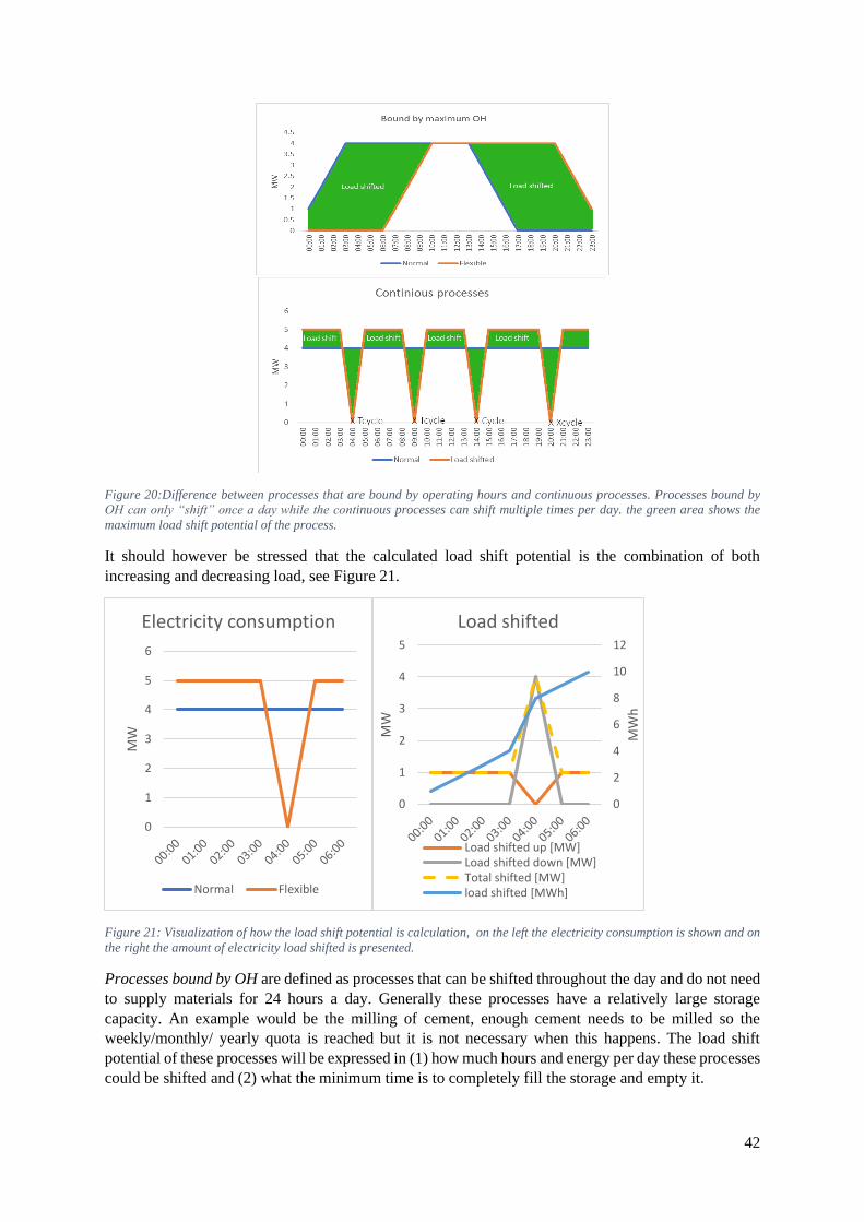
42

Figure 20:Difference between processes that are bound by operating hours and continuous processes. Processes bound by

OH can only “shift” once a day while the continuous processes can shift multiple times per day. the green area shows the

maximum load shift potential of the process.

It should however be stressed that the calculated load shift potential is the combination of both

increasing and decreasing load, see Figure 21.

Figure 21: Visualization of how the load shift potential is calculation, on the left the electricity consumption is shown and on

the right the amount of electricity load shifted is presented.

Processes bound by OH are defined as processes that can be shifted throughout the day and do not need

to supply materials for 24 hours a day. Generally these processes have a relatively large storage

capacity. An example would be the milling of cement, enough cement needs to be milled so the

weekly/monthly/ yearly quota is reached but it is not necessary when this happens. The load shift

potential of these processes will be expressed in (1) how much hours and energy per day these processes

could be shifted and (2) what the minimum time is to completely fill the storage and empty it.

0

1

2

3

4

5

6

MW

Electricity consumption

Normal Flexible

0

2

4

6

8

10

12

0

1

2

3

4

5M

Wh

MW

Load shifted

Load shifted up [MW]Load shifted down [MW]Total shifted [MW]load shifted [MWh]

43

The daily load shift potential of processes bound by maximum operating hours were calculated as the

difference in electricity consumption when operating flexibly compared to normal operations:

𝐸𝐷𝑎𝑖𝑙𝑦 𝑠ℎ𝑖𝑓𝑡𝑒𝑑,𝑏𝑜𝑢𝑛𝑑 𝑏𝑦 𝑂𝐻 ∑|𝐸𝑛𝑜𝑟𝑚𝑎𝑙 𝑜𝑝𝑒𝑟𝑎𝑡𝑖𝑜𝑛,𝑖 − 𝐸𝑚𝑜𝑠𝑡 𝑓𝑙𝑒𝑥𝑖𝑏𝑙𝑒,𝑖|

24

𝑖

When calculating the daily load shift potential the assumption was made that the storage of materials

was not a limiting factor. To also provide a metric for the storage capacity it the minimum time it takes

to fill up and empty the storage was calculated. The purpose of this metric is to provide information on

how long a process can be turned off without disrupting the material flows. This metric was calculated

with the formula:

𝑡𝑓𝑖𝑙𝑙 𝑎𝑛𝑑 𝑒𝑚𝑝𝑡𝑦,𝑝𝑟𝑜𝑐𝑒𝑠𝑠 = 𝑡𝑓𝑖𝑙𝑙,𝑝𝑟𝑜𝑐𝑒𝑠𝑠 + 𝑡𝑒𝑚𝑝𝑡𝑦,𝑝𝑟𝑜𝑐𝑒𝑠𝑠

Where the time it takes to fill up the storage and empty the storage is calculates with the

maximum inflow (ṁinflow), outflow (ṁoutflow) and the storage capacity (S) of the process:

𝑡𝑓𝑖𝑙𝑙,𝑝𝑟𝑜𝑐𝑒𝑠𝑠 =𝑆𝑝𝑟𝑜𝑐𝑒𝑠𝑠

ṁ𝑖𝑛𝑓𝑙𝑜𝑤,𝑝𝑟𝑜𝑐𝑒𝑠𝑠 ,𝑚𝑎𝑥 𝑡𝑒𝑚𝑝𝑡𝑦,𝑝𝑟𝑜𝑐𝑒𝑠𝑠 =

𝑆𝑝𝑟𝑜𝑐𝑒𝑠𝑠

ṁ𝑜𝑢𝑡𝑓𝑙𝑜𝑤,𝑝𝑟𝑜𝑐𝑒𝑠𝑠,𝑚𝑎𝑥

Continuous processes: Processes that need to supply materials for 24 hours a day and the only flexibility

potential is through the addition of a buffer. Generally continuous processes have a small storage

capacity because storage is not needed and costly. An example would be the production of hydrogen in

the hydrogen scenario, here hydrogen always need to be supplied to the kiln but it is possible to build

up a small buffer so the electrolyser can be turned off. In addition to the amount of electricity shifted

the daily load shift potential of these processes was calculated using the time needed to completely fill

up the storage and the time it takes to empty it (Tcycle). The daily load shift potential of continuous

processes was calculated as:

𝐸𝐷𝑎𝑖𝑙𝑦 𝑠ℎ𝑖𝑓𝑡𝑒𝑑,𝑐𝑜𝑛𝑡𝑖𝑛𝑖𝑜𝑢𝑠 = ∑ |𝐸𝑛𝑜𝑟𝑚𝑎𝑙 𝑜𝑝𝑒𝑟𝑎𝑡𝑖𝑜𝑛,𝑖 − 𝐸𝑚𝑜𝑠𝑡 𝑓𝑙𝑒𝑥𝑖𝑏𝑙𝑒,𝑖| ∗24ℎ

𝑇𝑐𝑦𝑐𝑙𝑒

𝑇𝑐𝑦𝑐𝑙𝑒

𝑖

Table 20 on the next page shows which processes show flexibility potential, are considered the be

continuous and in which chapter their methodology is described.

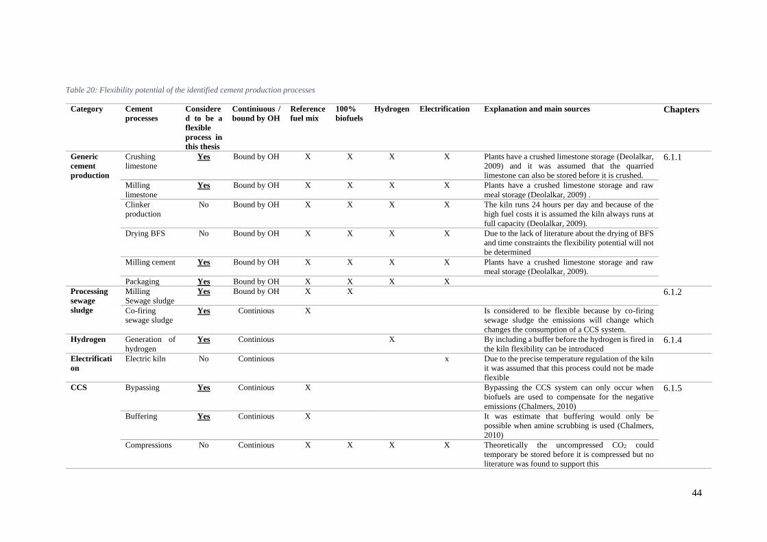
44

Table 20: Flexibility potential of the identified cement production processes

Category Cement

processes

Considere

d to be a

flexible

process in

this thesis

Continiuous /

bound by OH

Reference

fuel mix

100%

biofuels

Hydrogen Electrification Explanation and main sources Chapters

Generic

cement

production

Crushing

limestone

Yes Bound by OH X X X X Plants have a crushed limestone storage (Deolalkar,

2009) and it was assumed that the quarried

limestone can also be stored before it is crushed.

6.1.1

Milling

limestone

Yes Bound by OH X X X X Plants have a crushed limestone storage and raw

meal storage (Deolalkar, 2009) .

Clinker

production

No Bound by OH X X X X The kiln runs 24 hours per day and because of the

high fuel costs it is assumed the kiln always runs at

full capacity (Deolalkar, 2009).

Drying BFS No Bound by OH X X X X Due to the lack of literature about the drying of BFS

and time constraints the flexibility potential will not

be determined

Milling cement Yes Bound by OH X X X X Plants have a crushed limestone storage and raw

meal storage (Deolalkar, 2009).

Packaging Yes Bound by OH X X X X

Processing

sewage

sludge

Milling

Sewage sludge

Yes Bound by OH X X 6.1.2

Co-firing

sewage sludge

Yes Continious X Is considered to be flexible because by co-firing

sewage sludge the emissions will change which

changes the consumption of a CCS system.

Hydrogen Generation of

hydrogen

Yes Continious X By including a buffer before the hydrogen is fired in

the kiln flexibility can be introduced 6.1.4

Electrificati

on

Electric kiln No Continious x Due to the precise temperature regulation of the kiln

it was assumed that this process could not be made

flexible

CCS Bypassing Yes Continious X Bypassing the CCS system can only occur when

biofuels are used to compensate for the negative

emissions (Chalmers, 2010)

6.1.5

Buffering Yes Continious X It was estimate that buffering would only be

possible when amine scrubbing is used (Chalmers,

2010)

Compressions No Continious X X X X Theoretically the uncompressed CO2 could

temporary be stored before it is compressed but no

literature was found to support this

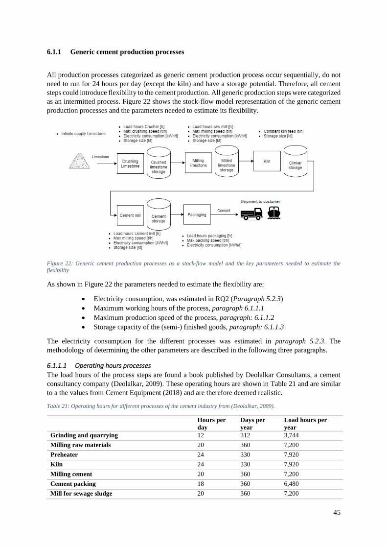
45

6.1.1 Generic cement production processes

All production processes categorized as generic cement production process occur sequentially, do not

need to run for 24 hours per day (except the kiln) and have a storage potential. Therefore, all cement

steps could introduce flexibility to the cement production. All generic production steps were categorized

as an intermitted process. Figure 22 shows the stock-flow model representation of the generic cement

production processes and the parameters needed to estimate its flexibility.

Figure 22: Generic cement production processes as a stock-flow model and the key parameters needed to estimate the

flexibility

As shown in Figure 22 the parameters needed to estimate the flexibility are:

• Electricity consumption, was estimated in RQ2 (Paragraph 5.2.3)

• Maximum working hours of the process, paragraph 6.1.1.1

• Maximum production speed of the process, paragraph: 6.1.1.2

• Storage capacity of the (semi-) finished goods, paragraph: 6.1.1.3

The electricity consumption for the different processes was estimated in paragraph 5.2.3. The

methodology of determining the other parameters are described in the following three paragraphs.

6.1.1.1 Operating hours processes

The load hours of the process steps are found a book published by Deolalkar Consultants, a cement

consultancy company (Deolalkar, 2009). These operating hours are shown in Table 21 and are similar

to a the values from Cement Equipment (2018) and are therefore deemed realistic.

Table 21: Operating hours for different processes of the cement industry from (Deolalkar, 2009).

Hours per

day

Days per

year

Load hours per

year

Grinding and quarrying 12 312 3,744

Milling raw materials 20 360 7,200

Preheater 24 330 7,920

Kiln 24 330 7,920

Milling cement 20 360 7,200

Cement packing 18 360 6,480

Mill for sewage sludge 20 360 7,200

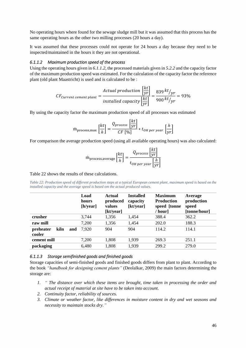
46

No operating hours where found for the sewage sludge mill but it was assumed that this process has the

same operating hours as the other two milling processes (20 hours a day).

It was assumed that these processes could not operate for 24 hours a day because they need to be

inspected/maintained in the hours it they are not operational.

6.1.1.2 Maximum production speed of the process

Using the operating hours given in 6.1.1.2, the processed materials given in 5.2.2 and the capacity factor

of the maximum production speed was estimated. For the calculation of the capacity factor the reference

plant (old plant Maastricht) is used and is calculated to be :

𝐶𝐹𝐶𝑢𝑟𝑟𝑒𝑛𝑡 𝑐𝑒𝑚𝑒𝑛𝑡 𝑝𝑙𝑎𝑛𝑡 =𝐴𝑐𝑡𝑢𝑎𝑙 𝑝𝑟𝑜𝑑𝑢𝑐𝑡𝑖𝑜𝑛 [

𝑘𝑡𝑦𝑟]

𝑖𝑛𝑠𝑡𝑎𝑙𝑙𝑒𝑑 𝑐𝑎𝑝𝑎𝑐𝑖𝑡𝑦 [𝑘𝑡𝑦𝑟]

=839 𝑘𝑡

𝑦𝑟⁄

900 𝑘𝑡𝑦𝑟⁄

= 93%

By using the capacity factor the maximum production speed of all processes was estimated

ṁprocess,max [𝑘𝑡

ℎ] =

𝑄𝑝𝑟𝑜𝑐𝑒𝑠𝑠 [𝑘𝑡𝑦𝑟]

𝐶𝐹 [%]∗ 𝑡𝑂𝐻 𝑝𝑒𝑟 𝑦𝑒𝑎𝑟 [

ℎ

𝑦𝑟]

For comparison the average production speed (using all available operating hours) was also calculated:

ṁprocess,average [𝑘𝑡

ℎ] =

𝑄𝑝𝑟𝑜𝑐𝑒𝑠𝑠 [𝑘𝑡𝑦𝑟]

𝑡𝑂𝐻 𝑝𝑒𝑟 𝑦𝑒𝑎𝑟 [ℎ

𝑦𝑟]

Table 22 shows the results of these calculations.

Table 22: Production speed of different production steps at a typical European cement plant, maximum speed is based on the

installed capacity and the average speed is based om the actual produced values.

Load

hours

[h/year]

Actual

produced

values

[kt/year]

Installed

capacity

[kt/year]

Maximum

Production

speed [tonne

/ hour]

Average

production

speed

[tonne/hour]

crusher 3,744 1,356 1,454 388.4 362.2

raw mill 7,200 1,356 1,454 202.0 188.3

preheater kiln and

cooler

7,920 904 904 114.2 114.1

cement mill 7,200 1,808 1,939 269.3 251.1

packaging 6,480 1,808 1,939 299.2 279.0

6.1.1.3 Storage semifinished goods and finished goods

Storage capacities of semi-finished goods and finished goods differs from plant to plant. According to

the book “handbook for designing cement plants” (Deolalkar, 2009) the main factors determining the

storage are:

1. “ The distance over which these items are brought, time taken in processing the order and

actual receipt of material at site have to be taken into account.

2. Continuity factor, reliability of sources.

3. Climate or weather factor, like differences in moisture content in dry and wet seasons and

necessity to maintain stocks dry.”

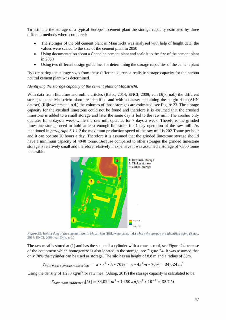
47

To estimate the storage of a typical European cement plant the storage capacity estimated by three

different methods where compared:

• The storages of the old cement plant in Maastricht was analysed with help of height data, the

values were scaled to the size of the cement plant in 2050

• Using documentation about a Canadian cement plant and scale it to the size of the cement plant

in 2050

• Using two different design guidelines for determining the storage capacities of the cement plant

By comparing the storage sizes from these different sources a realistic storage capacity for the carbon

neutral cement plant was determined.

Identifying the storage capacity of the cement plant of Maastricht.

With data from literature and online articles (Batec, 2014; ENCI, 2009; van Dijk, n.d.) the different

storages at the Maastricht plant are identified and with a dataset containing the height data (AHN

dataset) (Rijkswaterstaat, n.d.) the volumes of those storages are estimated, see Figure 23. The storage

capacity for the crushed limestone could not be found and therefore it is assumed that the crushed

limestone is added to a small storage and later the same day is fed to the raw mill. The crusher only

operates for 6 days a week while the raw mill operates for 7 days a week. Therefore, the grinded

limestone storage need to hold at least enough limestone for 1 day operation of the raw mill. As

mentioned in paragraph 6.1.1.2 the maximum production speed of the raw mill is 202 Tonne per hour

and it can operate 20 hours a day. Therefore it is assumed that the grinded limestone storage should

have a minimum capacity of 4040 tonne. Because compared to other storages the grinded limestone

storage is relatively small and therefore relatively inexpensive it was assumed a storage of 7,500 tonne

is feasible.

Figure 23: Height data of the cement plant in Maastricht (Rijkswaterstaat, n.d.) where the storage are identified using (Batec,

2014; ENCI, 2009; van Dijk, n.d.)

The raw meal is stored at (1) and has the shape of a cylinder with a cone as roof, see Figure 24.because

of the equipment which homogenize is also located in the storage, see Figure 24, it was assumed that

only 70% the cylinder can be used as storage. The silo has an height of 8.8 m and a radius of 35m.

𝑉𝑅𝑎𝑤 𝑚𝑒𝑎𝑙 𝑠𝑡𝑜𝑟𝑎𝑔𝑒,𝑚𝑎𝑎𝑠𝑡𝑟𝑖𝑐ℎ𝑡 = 𝜋 ∗ 𝑟2 ∗ ℎ ∗ 70% = 𝜋 ∗ 452𝑚 ∗ 70% = 34,024 𝑚3

Using the density of 1,250 kg/m3 for raw meal (Alsop, 2019) the storage capacity is calculated to be:

𝑆𝑟𝑎𝑤 𝑚𝑒𝑎𝑙 ,𝑚𝑎𝑎𝑟𝑡𝑖𝑐ℎ𝑡[𝑘𝑡] = 34,024 𝑚3 ∗ 1,250 𝑘𝑔/𝑚3 ∗ 10−6 = 35.7 𝑘𝑡

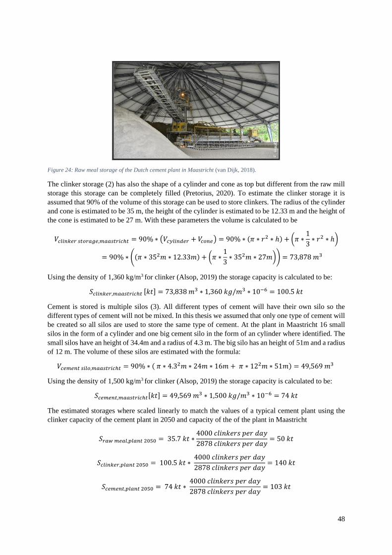
48

Figure 24: Raw meal storage of the Dutch cement plant in Maastricht (van Dijk, 2018).

The clinker storage (2) has also the shape of a cylinder and cone as top but different from the raw mill

storage this storage can be completely filled (Pretorius, 2020). To estimate the clinker storage it is

assumed that 90% of the volume of this storage can be used to store clinkers. The radius of the cylinder

and cone is estimated to be 35 m, the height of the cylinder is estimated to be 12.33 m and the height of

the cone is estimated to be 27 m. With these parameters the volume is calculated to be

𝑉𝑐𝑙𝑖𝑛𝑘𝑒𝑟 𝑠𝑡𝑜𝑟𝑎𝑔𝑒,𝑚𝑎𝑎𝑠𝑡𝑟𝑖𝑐ℎ𝑡 = 90% ∗ (𝑉𝑐𝑦𝑙𝑖𝑛𝑑𝑒𝑟 + 𝑉𝑐𝑜𝑛𝑒) = 90% ∗ (𝜋 ∗ 𝑟2 ∗ ℎ) + (𝜋 ∗1

3∗ 𝑟2 ∗ ℎ)

= 90% ∗ ((𝜋 ∗ 352𝑚 ∗ 12.33𝑚) + (𝜋 ∗1

3∗ 352𝑚 ∗ 27𝑚)) = 73,878 𝑚3

Using the density of 1,360 kg/m3 for clinker (Alsop, 2019) the storage capacity is calculated to be:

𝑆𝑐𝑙𝑖𝑛𝑘𝑒𝑟,𝑚𝑎𝑎𝑠𝑡𝑟𝑖𝑐ℎ𝑡 [𝑘𝑡] = 73,838 𝑚3 ∗ 1,360 𝑘𝑔/𝑚3 ∗ 10−6 = 100.5 𝑘𝑡

Cement is stored is multiple silos (3). All different types of cement will have their own silo so the

different types of cement will not be mixed. In this thesis we assumed that only one type of cement will

be created so all silos are used to store the same type of cement. At the plant in Maastricht 16 small

silos in the form of a cylinder and one big cement silo in the form of an cylinder where identified. The

small silos have an height of 34.4m and a radius of 4.3 m. The big silo has an height of 51m and a radius

of 12 m. The volume of these silos are estimated with the formula:

𝑉𝑐𝑒𝑚𝑒𝑛𝑡 𝑠𝑖𝑙𝑜,𝑚𝑎𝑎𝑠𝑡𝑟𝑖𝑐ℎ𝑡 = 90% ∗ ( 𝜋 ∗ 4.32𝑚 ∗ 24𝑚 ∗ 16𝑚 + 𝜋 ∗ 122𝑚 ∗ 51𝑚) = 49,569 𝑚3

Using the density of 1,500 kg/m3 for clinker (Alsop, 2019) the storage capacity is calculated to be:

𝑆𝑐𝑒𝑚𝑒𝑛𝑡,𝑚𝑎𝑎𝑠𝑡𝑟𝑖𝑐ℎ𝑡[𝑘𝑡] = 49,569 𝑚3 ∗ 1,500 𝑘𝑔/𝑚3 ∗ 10−6 = 74 𝑘𝑡

The estimated storages where scaled linearly to match the values of a typical cement plant using the

clinker capacity of the cement plant in 2050 and capacity of the of the plant in Maastricht

𝑆𝑟𝑎𝑤 𝑚𝑒𝑎𝑙,𝑝𝑙𝑎𝑛𝑡 2050 = 35.7 𝑘𝑡 ∗4000 𝑐𝑙𝑖𝑛𝑘𝑒𝑟𝑠 𝑝𝑒𝑟 𝑑𝑎𝑦

2878 𝑐𝑙𝑖𝑛𝑘𝑒𝑟𝑠 𝑝𝑒𝑟 𝑑𝑎𝑦= 50 𝑘𝑡

𝑆𝑐𝑙𝑖𝑛𝑘𝑒𝑟,𝑝𝑙𝑎𝑛𝑡 2050 = 100.5 𝑘𝑡 ∗ 4000 𝑐𝑙𝑖𝑛𝑘𝑒𝑟𝑠 𝑝𝑒𝑟 𝑑𝑎𝑦

2878 𝑐𝑙𝑖𝑛𝑘𝑒𝑟𝑠 𝑝𝑒𝑟 𝑑𝑎𝑦= 140 𝑘𝑡

𝑆𝑐𝑒𝑚𝑒𝑛𝑡,𝑝𝑙𝑎𝑛𝑡 2050 = 74 𝑘𝑡 ∗ 4000 𝑐𝑙𝑖𝑛𝑘𝑒𝑟𝑠 𝑝𝑒𝑟 𝑑𝑎𝑦

2878 𝑐𝑙𝑖𝑛𝑘𝑒𝑟𝑠 𝑝𝑒𝑟 𝑑𝑎𝑦= 103 𝑘𝑡

49

Storage capacity of a Canadian cement plant

Websites of European cement manufacturers where consulted to find their storage capacities by due to

the language barrier and time constraints no data was found. As substitution the storage capacities of a

Canadian cement plant from the company McINNIS where used, see Table 23.

Table 23: storage capacity of the McINNIS cement plant in Canada (McInnis cement, 2021)

McINNIS Scaled to a typical European plant in 2050

Installed capacity [tonne clinkers/day] 6,000 4,000

Raw meal storage [tonne] 150,000 100,000

Clinker storage [tonne] 120,000 80,000

Cement storage [tonne] 120,000 80,000

Determine storage capacities with guidelines

Next to using existing plant as reference two design guidelines were used to estimate the storage

capacity of the new cement plant:

1. A small cement plant with a capacity of 100 tonne clinker per day (Power Correction Systems,

2004).

2. Rule of thumps when choosing the capacity proposed by Deolalkar (2009)

The values estimated for a small cement plant (SCP) of 100 clinkers per day are scaled up to match

the clinker capacity of the new cement plant, see Table 24.

Table 24: the storage capacity of a small cement plant (SCP) scaled to a European cement plant in 2050

SCP (Power Correction Systems,

2004)

Scaled to a typical European plant in

2050

raw meal

[kt]

0.75 30

clinker [kt] 1.5 60

cement [kt] 0.9 36

Deolalkar (2009) expresses the storage capacity as daily production, the daily production values are

based on the load hours and production capacity which were described in paragraph 5.2.2. Table 25

shows the storage capacity of a European cement plant using this method.

Table 25: Storage capacity based on guidelines proposed by Deolalkar (2009)

days Daily production [t/d] Storage capacity [kt]

Raw meal 2 6,764 13.53

Clinker 14 4,000 56.00

cement 7 5,022 35.16

Estimation of the storage capacities of an European cement plant in 2050

The results of all different methods of estimating the storage capacity were compared and a realistic

storage capacity was chosen for a typical European cement plant, see Table 26.

50

Table 26: Storage sizes of different cement plants scaled to the same installed capacity of the typical European plant and the

storage size deemed realistic for this study.

Maastricht

(scaled)

Guidelines

from

Deolokar

Guidelines

from for

Power

Correction

Systems

(2004)

Mcinnis

(scaled)

Assumed

storage

for a

cement

plant in

2050

Storage grinded

limestone [kt]

n/a n/a n/a n/a 8.0

Storage raw meal [kt] 49.6 13.5 30.0 100 60.0

Storage clinkers [kt] 139.6 56.0 60.0 80 80

Cement storage [kt] 103.3 35.2 36.0 80 70

6.1.1.4 Key assumptions

Based on the findings of this chapters key assumptions were made so the flexibility potential could be

calculated, the key assumptions are shown in Table 27.

Table 27: Key assumptions for determining the flexibility potential of generic cement production processes

Process Type of

process

Inflow Storage Outflow Maximum

operating

hours

Electricity

consumption

[kWh/ tonne]

Limestone

grinding

Bound by

OH

388.4

t/h

8.0 kt 202.0 t/h 12h/day,

312

days/year

0.75

Limestone

milling

Bound by

OH

202.0

t/h

60.0 kt 114.2 t/h 20h/day,

360

days/year

12.0

Clinker

production

Bound by

OH

114.2

t/h

80.0 kt 269.3 t/h 24h/day,

330

days/year

Not applicable

because there is no

flexibility

potential, it is

assumed that the

kiln runs at

maximum

capacity at 24

hours a day

Cement

milling

Bound by

OH

269.3

t/h

70.0 kt 299.2 t/h 20h/day,

360

days/year

27.5

Cement

packaging

Bound by

OH

299.2

t/h

n/a n/a 18h/day,

360

days/year

1.5

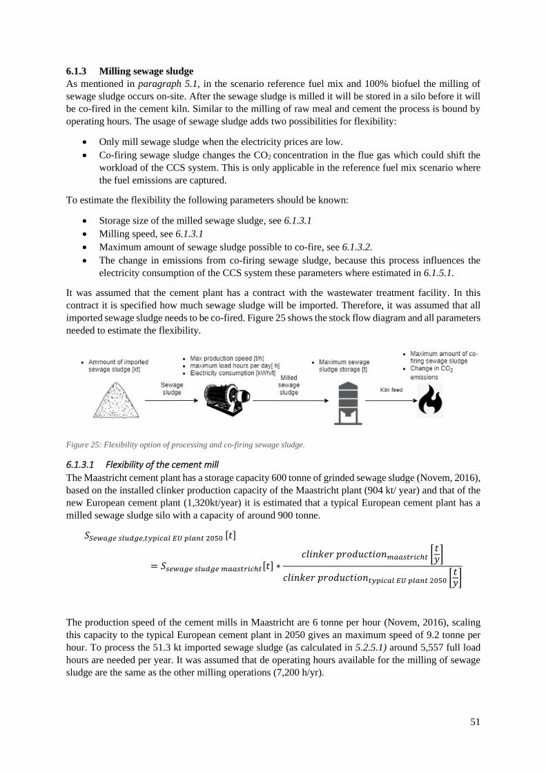
51

6.1.3 Milling sewage sludge

As mentioned in paragraph 5.1, in the scenario reference fuel mix and 100% biofuel the milling of

sewage sludge occurs on-site. After the sewage sludge is milled it will be stored in a silo before it will

be co-fired in the cement kiln. Similar to the milling of raw meal and cement the process is bound by

operating hours. The usage of sewage sludge adds two possibilities for flexibility:

• Only mill sewage sludge when the electricity prices are low.

• Co-firing sewage sludge changes the CO2 concentration in the flue gas which could shift the

workload of the CCS system. This is only applicable in the reference fuel mix scenario where

the fuel emissions are captured.

To estimate the flexibility the following parameters should be known:

• Storage size of the milled sewage sludge, see 6.1.3.1

• Milling speed, see 6.1.3.1

• Maximum amount of sewage sludge possible to co-fire, see 6.1.3.2.

• The change in emissions from co-firing sewage sludge, because this process influences the

electricity consumption of the CCS system these parameters where estimated in 6.1.5.1.

It was assumed that the cement plant has a contract with the wastewater treatment facility. In this

contract it is specified how much sewage sludge will be imported. Therefore, it was assumed that all

imported sewage sludge needs to be co-fired. Figure 25 shows the stock flow diagram and all parameters

needed to estimate the flexibility.

Figure 25: Flexibility option of processing and co-firing sewage sludge.

6.1.3.1 Flexibility of the cement mill

The Maastricht cement plant has a storage capacity 600 tonne of grinded sewage sludge (Novem, 2016),

based on the installed clinker production capacity of the Maastricht plant (904 kt/ year) and that of the

new European cement plant (1,320kt/year) it is estimated that a typical European cement plant has a

milled sewage sludge silo with a capacity of around 900 tonne.

𝑆𝑆𝑒𝑤𝑎𝑔𝑒 𝑠𝑙𝑢𝑑𝑔𝑒,𝑡𝑦𝑝𝑖𝑐𝑎𝑙 𝐸𝑈 𝑝𝑙𝑎𝑛𝑡 2050 [𝑡]

= 𝑆𝑠𝑒𝑤𝑎𝑔𝑒 𝑠𝑙𝑢𝑑𝑔𝑒 𝑚𝑎𝑎𝑠𝑡𝑟𝑖𝑐ℎ𝑡[𝑡] ∗𝑐𝑙𝑖𝑛𝑘𝑒𝑟 𝑝𝑟𝑜𝑑𝑢𝑐𝑡𝑖𝑜𝑛𝑚𝑎𝑎𝑠𝑡𝑟𝑖𝑐ℎ𝑡 [

𝑡𝑦]

𝑐𝑙𝑖𝑛𝑘𝑒𝑟 𝑝𝑟𝑜𝑑𝑢𝑐𝑡𝑖𝑜𝑛𝑡𝑦𝑝𝑖𝑐𝑎𝑙 𝐸𝑈 𝑝𝑙𝑎𝑛𝑡 2050 [𝑡𝑦]

The production speed of the cement mills in Maastricht are 6 tonne per hour (Novem, 2016), scaling

this capacity to the typical European cement plant in 2050 gives an maximum speed of 9.2 tonne per

hour. To process the 51.3 kt imported sewage sludge (as calculated in 5.2.5.1) around 5,557 full load

hours are needed per year. It was assumed that de operating hours available for the milling of sewage

sludge are the same as the other milling operations (7,200 h/yr).

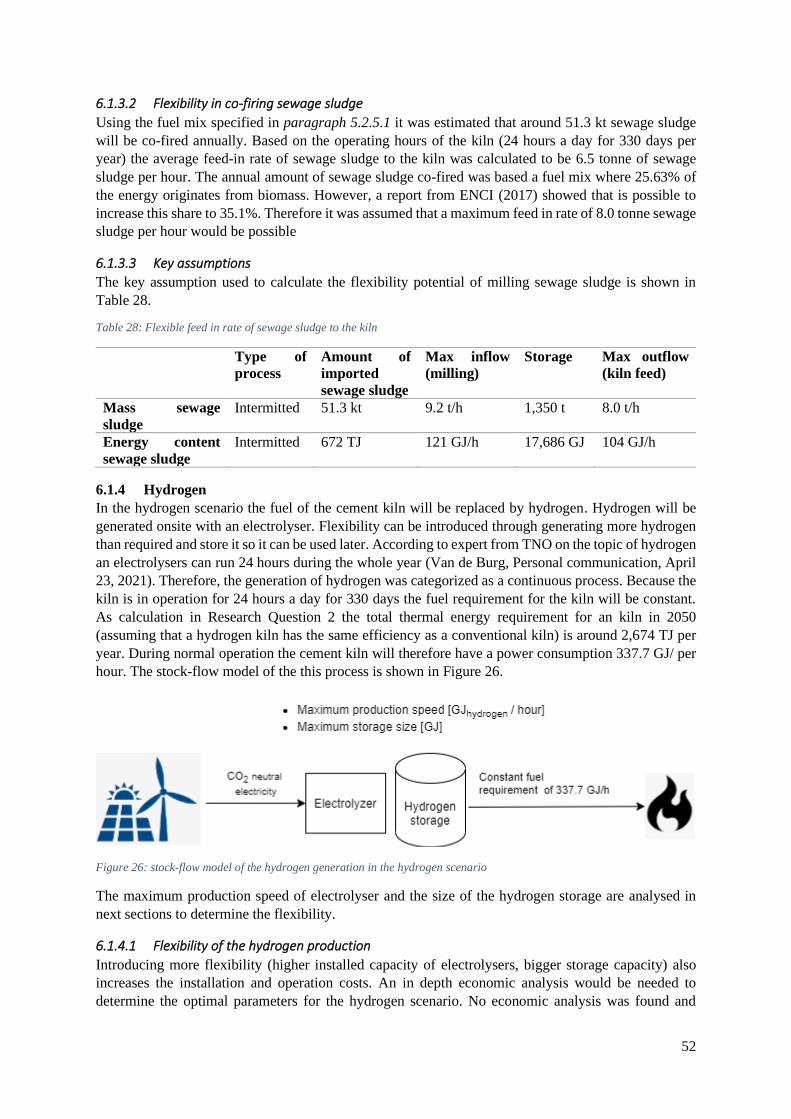
52

6.1.3.2 Flexibility in co-firing sewage sludge

Using the fuel mix specified in paragraph 5.2.5.1 it was estimated that around 51.3 kt sewage sludge

will be co-fired annually. Based on the operating hours of the kiln (24 hours a day for 330 days per

year) the average feed-in rate of sewage sludge to the kiln was calculated to be 6.5 tonne of sewage

sludge per hour. The annual amount of sewage sludge co-fired was based a fuel mix where 25.63% of

the energy originates from biomass. However, a report from ENCI (2017) showed that is possible to

increase this share to 35.1%. Therefore it was assumed that a maximum feed in rate of 8.0 tonne sewage

sludge per hour would be possible

6.1.3.3 Key assumptions

The key assumption used to calculate the flexibility potential of milling sewage sludge is shown in

Table 28.

Table 28: Flexible feed in rate of sewage sludge to the kiln

Type of

process

Amount of

imported

sewage sludge

Max inflow

(milling)

Storage Max outflow

(kiln feed)

Mass sewage

sludge

Intermitted 51.3 kt 9.2 t/h 1,350 t 8.0 t/h

Energy content

sewage sludge

Intermitted 672 TJ 121 GJ/h 17,686 GJ 104 GJ/h

6.1.4 Hydrogen

In the hydrogen scenario the fuel of the cement kiln will be replaced by hydrogen. Hydrogen will be

generated onsite with an electrolyser. Flexibility can be introduced through generating more hydrogen

than required and store it so it can be used later. According to expert from TNO on the topic of hydrogen

an electrolysers can run 24 hours during the whole year (Van de Burg, Personal communication, April

23, 2021). Therefore, the generation of hydrogen was categorized as a continuous process. Because the

kiln is in operation for 24 hours a day for 330 days the fuel requirement for the kiln will be constant.

As calculation in Research Question 2 the total thermal energy requirement for an kiln in 2050

(assuming that a hydrogen kiln has the same efficiency as a conventional kiln) is around 2,674 TJ per

year. During normal operation the cement kiln will therefore have a power consumption 337.7 GJ/ per

hour. The stock-flow model of the this process is shown in Figure 26.

Figure 26: stock-flow model of the hydrogen generation in the hydrogen scenario

The maximum production speed of electrolyser and the size of the hydrogen storage are analysed in

next sections to determine the flexibility.

6.1.4.1 Flexibility of the hydrogen production

Introducing more flexibility (higher installed capacity of electrolysers, bigger storage capacity) also

increases the installation and operation costs. An in depth economic analysis would be needed to

determine the optimal parameters for the hydrogen scenario. No economic analysis was found and

53

because of the time constraints of this thesis no economic analysis was performed. To include the effect

different parameters would have on the flexibility potential three different scenario will be constructed.

The scenarios and parameters used in this thesis are: Moderate flexibility, medium flexibility and high

flexibility where the electrolyser could generate 105%, 116.67% and 125% of the hydrogen needed for

the cement kiln and the storage could hold enough fuel for 1h , 2h and 3h of kiln operations respectively.

Future research should be conducted to estimate which scenario is the most cost efficient.

The installed capacity and storage size expressed in GJ will be calculated with the following formulas:

𝐼𝑛𝑠𝑡𝑎𝑙𝑙𝑒𝑑 𝑐𝑎𝑝𝑎𝑐𝑖𝑡𝑦 [𝐺𝐽

ℎ] = 𝐼𝑛𝑠𝑡𝑎𝑙𝑙𝑒𝑑 𝑐𝑎𝑝𝑎𝑐𝑖𝑡𝑦 [%] ∗ 𝐹𝑢𝑒𝑙 𝑐𝑜𝑛𝑠𝑢𝑚𝑝𝑡𝑖𝑜𝑛 𝑘𝑖𝑙𝑛 [

𝐺𝐽

ℎ]

𝑆𝑡𝑜𝑟𝑎𝑔𝑒 𝑠𝑖𝑧𝑒 [𝐺𝐽] = 𝐹𝑢𝑒𝑙 𝑐𝑜𝑛𝑠𝑢𝑚𝑝𝑡𝑖𝑜𝑛 𝑘𝑖𝑙𝑛 [𝐺𝐽

ℎ] ∗ 𝑠𝑡𝑜𝑟𝑎𝑔𝑒 𝑠𝑖𝑧𝑒 [ℎ]

The flexibility is determined by using the following parameters

𝑃𝑙𝑜𝑎𝑑 𝑠ℎ𝑖𝑓𝑡 𝑝𝑜𝑤𝑒𝑟[𝑀𝑊] =𝑆𝑡𝑜𝑟𝑎𝑔𝑒 𝑠𝑖𝑧𝑒 [𝐺𝐽] ∗ 0.277778 MWh

𝑇𝑐𝑦𝑐𝑙𝑒 𝑡𝑖𝑚𝑒[ℎ]∗

1

𝜂𝑒𝑙𝑒𝑐𝑡𝑟𝑜𝑙𝑦𝑧𝑒𝑟[%]

𝐸𝑑𝑎𝑖𝑙𝑦 𝑙𝑜𝑎𝑑 𝑠ℎ𝑖𝑓𝑡 𝑝𝑜𝑡𝑒𝑛𝑡𝑖𝑎𝑙[𝑀𝑊ℎ] = 𝑃𝑙𝑜𝑎𝑑 𝑠ℎ𝑖𝑓𝑡 𝑝𝑜𝑡𝑒𝑛𝑡𝑖𝑎𝑙 [𝑀𝑊] ∗ 24ℎ

Where the efficiency of the electrolyser was assumed to be 0.6, see paragraph 5.2.5.3. The cycle period

is considered to be the time it takes for the hydrogen storage to be filled and emptied.

6.1.4.2 Key assumptions

To introduce flexibility into the generation it was assumed that electrolysers could produce more than

is needed for the kiln and temporary store this hydrogen. Due to the uncertainties about the installed

capacity and storage size three different hydrogen scenarios were constructed see Table 29.

Table 29: Different scenarios for the generation of hydrogen.

Degree of

flexibility

Type of

process

Installed capacity

electrolyser [inflow]

Storage size hydrogen Energy

needed for

the kiln

[outflow]

Expressed

in [%]

Expressed

in [GJ/h]

Time to

fill

storage

[h]

Time

needed to

empty

storage

[h]

Storage

expressed

in [GJ]

Energy

consumption

[GJ/h]

No

flexibility

Continuous 100% 337.7 GJ/h 0 h 0 h 0 GJ 337.7 GJ/h

Moderate

flexibility

Continuous 105% 354.7 GJ/h 20 h 1 h 337.7 GJ 337.7 GJ/h

Medium

flexibility

Continuous 116.67% 394.0 GJ/h 12 h 2 h 675.4 GJ 337.7 GJ/h

High

flexibility

Continuous 125% 422.2 GJ/h 12 h 3 h 1013.2 GJ 337.7 GJ/h

54

6.1.5 CCS

By looking at possible flexibility introducing measures found in powerplants three strategies were

identified that could also be used in the cement industry (Chalmers, 2010; Chalmers et al., 2009, 2011;

Stuart M Cohen et al., 2011; Nimtz & Krautz, 2013).

• Change the fuels so the flue gas consists of a higher or lower concentration CO2

• Load shifting: The CO2 from the flue gas will be stored before energy intensive processes occur

so it can be processed at a later moment in time when the electricity prices are lower.

• Load shedding: the whole CCS system is bypassed so flue gas is released into the atmosphere.

In powerplants this can be done when the price at which the plant it could sell its produced

electricity is higher than the price it has to pay to release CO2 into the atmosphere. Bypassing

will only occur at times when the electricity prices are the highest and when biomass is used in

the fuel mix.

However, it was assumed that all these measures can only be implemented in the reference fuel mix

scenario. Only in the reference fuel mix emissions from biofuels will be captured which allows for

bypassing and the flexible use of fuels. Theoretically, when adding a buffer load shifting should be

possible in all scenarios but because no literature was found about a flexible direct capture system it

was assumed that it is not likely this method will be employed.

Table 30 shows the flexibility options for CCS for different scenarios.

Table 30: Proposed type of CCS and possible flexibility methods for the different scenarios.

Scenario Proposed type of CCS Flexible

concentration

CO2 to the

CCS system

Possibility

to bypass

Possibility to

shift

processes

Reference fuel Amine scrubbing X X X

100% biofuels Direct capture

Hydrogen Direct capture

Electrification Flue gas consists of pure CO2

and therefore it is assumed that

only the compression of CO2 is

needed (Mathisen, 2019)

6.1.5.1 Flexible concentration CO2

As mentioned in paragraph 5.2.5.1 the CO2 concentration of the flue gas is dependent on the emissions

from the calcination process and the burning of carbon based fuels. In all scenarios it is assumed that

the kiln operates always at full capacity therefore the amount of CO2 of the calcination process remains

constant. In the reference scenario and 100% biofuel scenario sewage sludge is being co-fired. However,

only in the reference fuel mix scenario the fuel emissions will be captured and therefore only in the

reference fuel scenario flexibly co-firing the sewage sludge has benefits. By varying the amount of

sewage sludge burned the CO2 the concentration of the flue gas can differ.

When using the reference fuel mix, around 26% (0.76 GJ/ tonne clinker) of the energy for the calcination

process comes from sewage sludge, the other 74% ( 2.16 GJ/ tonne clinker) will come waste materials

and fossil fuels. By using the CO2 intensity of all these fuel mixes and the fact that the sewage sludge

fed into the kiln during normal operations is around 6.5 tonne/h a linear model for the emissions could

be constructed. The CO2 intensities of methane and sewage sludge was found in literature (Vreuls, 2004)

and the CO2 intensity of the reference fuel mix without sewage sludge is calculated with the formula:

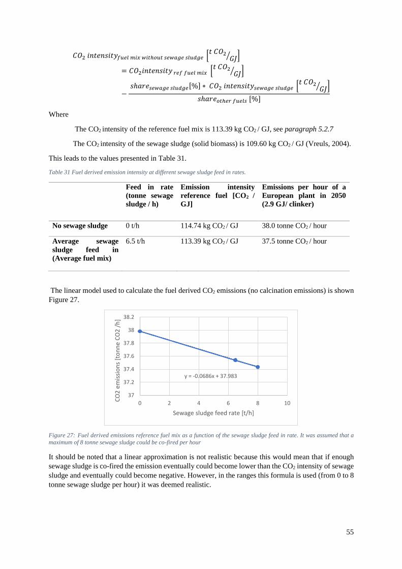
55

𝐶𝑂2 𝑖𝑛𝑡𝑒𝑛𝑠𝑖𝑡𝑦𝑓𝑢𝑒𝑙 𝑚𝑖𝑥 𝑤𝑖𝑡ℎ𝑜𝑢𝑡 𝑠𝑒𝑤𝑎𝑔𝑒 𝑠𝑙𝑢𝑑𝑔𝑒 [𝑡 𝐶𝑂2

𝐺𝐽⁄ ]

= 𝐶𝑂2𝑖𝑛𝑡𝑒𝑛𝑠𝑖𝑡𝑦 𝑟𝑒𝑓 𝑓𝑢𝑒𝑙 𝑚𝑖𝑥 [𝑡 𝐶𝑂2

𝐺𝐽⁄ ]

− 𝑠ℎ𝑎𝑟𝑒𝑠𝑒𝑤𝑎𝑔𝑒 𝑠𝑙𝑢𝑑𝑔𝑒[%] ∗ 𝐶𝑂2 𝑖𝑛𝑡𝑒𝑛𝑠𝑖𝑡𝑦𝑠𝑒𝑤𝑎𝑔𝑒 𝑠𝑙𝑢𝑑𝑔𝑒 [

𝑡 𝐶𝑂2𝐺𝐽⁄ ]

𝑠ℎ𝑎𝑟𝑒𝑜𝑡ℎ𝑒𝑟 𝑓𝑢𝑒𝑙𝑠 [%]

Where

The CO2 intensity of the reference fuel mix is 113.39 kg CO2 / GJ, see paragraph 5.2.7

The CO2 intensity of the sewage sludge (solid biomass) is 109.60 kg CO2 / GJ (Vreuls, 2004).

This leads to the values presented in Table 31.

Table 31 Fuel derived emission intensity at different sewage sludge feed in rates.

Feed in rate

(tonne sewage

sludge / h)

Emission intensity

reference fuel [CO2 /

GJ]

Emissions per hour of a

European plant in 2050

(2.9 GJ/ clinker)

No sewage sludge 0 t/h 114.74 kg CO2 / GJ 38.0 tonne CO2 / hour

Average sewage

sludge feed in

(Average fuel mix)

6.5 t/h 113.39 kg CO2 / GJ 37.5 tonne CO2 / hour

The linear model used to calculate the fuel derived CO2 emissions (no calcination emissions) is shown

Figure 27.

Figure 27: Fuel derived emissions reference fuel mix as a function of the sewage sludge feed in rate. It was assumed that a

maximum of 8 tonne sewage sludge could be co-fired per hour

It should be noted that a linear approximation is not realistic because this would mean that if enough

sewage sludge is co-fired the emission eventually could become lower than the CO2 intensity of sewage

sludge and eventually could become negative. However, in the ranges this formula is used (from 0 to 8

tonne sewage sludge per hour) it was deemed realistic.

y = -0.0686x + 37.983

37

37.2

37.4

37.6

37.8

38

38.2

0 2 4 6 8 10

CO

2 e

mis

sio

ns

[to

nn

e C

O2

/h

]

Sewage sludge feed rate [t/h]

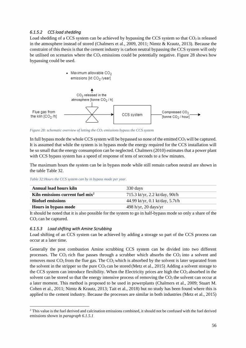
56

6.1.5.2 CCS load shedding

Load shedding of a CCS system can be achieved by bypassing the CCS system so that CO2 is released

in the atmosphere instead of stored (Chalmers et al., 2009, 2011; Nimtz & Krautz, 2013). Because the

constraint of this thesis is that the cement industry is carbon neutral bypassing the CCS system will only

be utilised on scenarios where the CO2 emissions could be potentially negative. Figure 28 shows how

bypassing could be used.

Figure 28: schematic overview of letting the CO2 emissions bypass the CCS system

In full bypass mode the whole CCS system will be bypassed so none of the emitted CO2 will be captured.

It is assumed that while the system is in bypass mode the energy required for the CCS installation will

be so small that the energy consumption can be neglected. Chalmers (2010) estimates that a power plant

with CCS bypass system has a speed of response of tens of seconds to a few minutes.

The maximum hours the system can be in bypass mode while still remain carbon neutral are shown in

the table Table 32.

Table 32:Hours the CCS system can by in bypass mode per year.

Annual load hours kiln 330 days

Kiln emissions current fuel mix2 715.3 kt/yr, 2.2 kt/day, 90t/h

Biofuel emissions 44.99 kt/yr, 0.1 kt/day, 5.7t/h

Hours in bypass mode 498 h/yr, 20 days/yr

It should be noted that it is also possible for the system to go in half-bypass mode so only a share of the

CO2 can be captured.

6.1.5.3 Load shifting with Amine Scrubbing

Load shifting of an CCS system can be achieved by adding a storage so part of the CCS process can

occur at a later time.

Generally the post combustion Amine scrubbing CCS system can be divided into two different

processes. The CO2 rich flue passes through a scrubber which absorbs the CO2 into a solvent and

removes most CO2 from the flue gas. The CO2 which is absorbed by the solvent is later separated from

the solvent in the stripper so the pure CO2 can be stored (Metz et al., 2015). Adding a solvent storage to

the CCS system can introduce flexibility. When the Electricity prices are high the CO2 absorbed in the

solvent can be stored so that the energy intensive process of removing the CO2 the solvent can occur at

a later moment. This method is proposed to be used in powerplants (Chalmers et al., 2009; Stuart M.

Cohen et al., 2011; Nimtz & Krautz, 2013; Tait et al., 2018) but no study has been found where this is

applied to the cement industry. Because the processes are similar in both industries (Metz et al., 2015)

2 This value is the fuel derived and calcination emissions combined, it should not be confused with the fuel derived

emissions shown in paragraph 6.1.5.1

57

it is assumed that this load shifting method is also possible in the cement industry. The workings of a

flexible amine scrubbing CCS system with bypass and solvent storage is shown in Figure 29.

Figure 29: A flexible CCS system with bypass and solvent storage. The optional bypass is added to the original figure

(Chalmers, 2010)

Cohen (2012) and Cohen et al. (2013) estimated that 90% of the energy for a CCS system at powerplant

is attributed to the energy consumption of the stripping and compression. By using the assumed energy

electricity of 3.5GJ/ tonne of cement it was found that 3.15 GJ per tonne CO2 is needed for the stripping

and compression part while only 0.35GJ per tonne CO2 would be needed for the scrubbing.

After a buffer event occurs the stripper and compressor need to process the normal CO2 emissions in

addition to the stored CO2. Chalmers et al. (2011) estimated that the stripper and compressor of a CCs

system at a powerplant could operate at 125% of its normal capacity. This study will use the same

assumption.

Stuart M Cohen et al. (2011) estimated based on a cost benefit analysis that the optimal solvent storage

capacity coal-fired powerplant can hold up to 22.5 Minutes of CO2 which is around 170 tonne of CO2.

It is therefore assumed that a solvent storage tank of 170 tonne CO2 is a feasible option for the cement

industry. It is assumed that the installed stripper and compressor can operate at 125% capacity compared

to their normal capacity. Table 33 shows how long it takes to fill and empty the buffer.

Table 33:CO2 storage capacity of the CO2 buffer for the CCS system used in the reference scenario.

Maximum CO2 absorption

in solvent [Tonne CO2 per

hour]

Hours until

storage tank is

full [h]

Hours until CO2 in

the tank is processed

[h]

Reference fuel mix

(bypassing biomass )

136.9 1.3 4.6

Reference fuel mix

(no bypass)

149.5 1.2 4.6

An economic analysis should be performed to estimate the optimum storage capacity but due to time

constraints the size of the solvent storage will be based on existing literature.

6.1.5.4 Key assumptions

The table on the next page, Table 34, shows all key assumption made based on the findings of this

section.

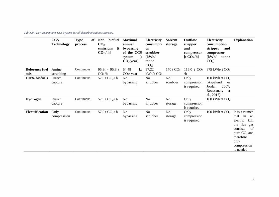
58

Table 34: Key assumptions CCS systems for all decarbonization sceanrios.

CCS

Technology

Type of

process

Non biofuel

CO2

emissions [t

CO2 / h]

Maximal

annual

bypassing

of the CCS

system [t

CO2/year]

Electricity

consumpti

on

scrubber

[kWh/

tonne

CO2]

Solvent

storage

Outflow

stripper

and

compressor

[t CO2 /h]

Electricity

consumption

stripper and

compressor

[kWh/ tonne

CO2]

Explanation

Reference fuel

mix

Amine

scrubbing

Continuous 95.3t - 95.8 t

CO2 /h

64.48 kt

CO2/ year

97.22

kWh/ t CO2

170 t CO2 116.0 t CO2

/h

875 kWh/ t CO2

100% biofuels Direct

capture

Continuous 57.9 t CO2 / h No

bypassing

No

scrubber

No

scrubber

Only

compression

is required.

100 kWh /t CO2

(Aspelund &

Jordal, 2007;

Roussanaly et

al., 2017)

Hydrogen Direct

capture

Continuous 57.9 t CO2 / h No

bypassing

No

scrubber

No

storage

Only

compression

is required.

100 kWh /t CO2

Electrification Only

compression

Continuous 57.9 t CO2 / h No

bypassing

No

scrubber

No

storage

Only

compression

is required.

100 kWh /t CO2

It is assumed

that in an

electric kiln

the flue gas

consists of

pure CO2 and

therefore

only

compression

is needed

59

6.2 RESULTS Based on the established key assumptions the daily load shift potential for all processes was calculated,

the results are shown in paragraph 6.2.1 to paragraph 6.2.4. The load shift potential will me expressed

in how much electricity in MWh can be shifted per day. In paragraph 6.2.5 an overview is given of the

load shift potential for all different processes.

6.2.1 Generic cement production processes

The load shift potential of the generic cement production processes was determined by estimated how

much the energy could be shifted per day while still producing enough to satisfy the daily production

quota. This is done by comparing difference in electricity consumption when the process occurs at

normal production speed in the morning and the at maximum production speed in the evening. The

production speed was found in Paragraph 6.1.1.2. The load shift potential of all generic cement

production processes is shown in Figure 30.

Figure 30: Daily load shift potential generic cement production processes. It should be noted that due to the software used to

plot the graphs the lines appear to be skewed while they should be vertical.

The results are shown in Table 35.

Table 35: Daily load shift potential of the production processes of a 4000 tpd cement plant in 2050

Processes Daily load shift potential [MWh/day]

Crusher 6.52

Raw Mill 23.96

Cement mill 73.20

Packaging 5.99

Total 109.66

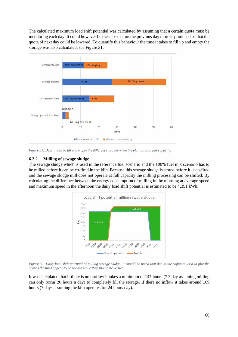
60

The calculated maximum load shift potential was calculated by assuming that a certain quota must be

met during each day. It could however be the case that on the previous day more is produced so that the

quota of next day could be lowered. To quantify this behaviour the time it takes to fill up and empty the

storage was also calculated, see Figure 31.

Figure 31: Days it take to fill and empty the different storages when the plant runs at full capacity.

6.2.2 Milling of sewage sludge

The sewage sludge which is used in the reference fuel scenario and the 100% fuel mix scenario has to

be milled before it can be co-fired in the kiln. Because this sewage sludge is stored before it is co-fired

and the sewage sludge mill does not operate at full capacity the milling processing can be shifted. By

calculating the difference between the energy consumption of milling in the morning at average speed

and maximum speed in the afternoon the daily load shift potential is estimated to be 4,391 kWh.

Figure 32: Daily load shift potential of milling sewage sludge. It should be noted that due to the software used to plot the

graphs the lines appear to be skewed while they should be vertical.

It was calculated that if there is no outflow it takes a minimum of 147 hours (7.3 day assuming milling

can only occur 20 hours a day) to completely fill the storage. If there no inflow it takes around 169

hours (7 days assuming the kiln operates for 24 hours day).

61

For comparison it was assumed that in the morning the same amount of sewage sludge was milled as in

the evening. Because the storage could hold up to 7 days of sewage sludge it could happen that no

milling is needed for several days and thereby greatly increasing the daily load shift potential.

6.2.3 Flexibility of the hydrogen production

In the hydrogen scenario hydrogen will be used as fuel for the kiln and is created through the electrolysis

of water. The hydrogen can be fired directly in the kiln or stored in a storage so it can be used when the

electricity prices are lower. An in depth economic analysis is needed to determine the optimal storage

size and capacity of the electrolysers but due to time constraints multiple scenarios are constructed with

different degrees of flexibility to show the effect of different installed capacities and storage sizes. The

daily load shift potential was estimated by calculating the difference in electrcity consumption between

the normal and flexible operating mode, see Figure 33.

Figure 33: Load shift potential of the electrolyser in the three different flexibility scenarios. The X shows the cycle period (The

time it takes to fill and empty the hydrogen storage). It should be noted that due to the software used to plot the graphs the

lines appear to be skewed while they should be vertical.

The results are shown in Table 36

Table 36: Calculated daily load shift potential of the electrolyser

Shifted per cycle Cycle period [h charged

and h discharged]

Maximum daily

shifted

Moderate flexibility 312.7 20 + 1 357.3

Medium flexibility 625.38 12 + 2 1,072.1

High flexibility 938.0 12 + 3 1,500.8

6.2.4 Flexibility of the CCS system

As mentioned earlier it was assumed that a flexible CCS system is only feasible in the reference fuel

mix scenario, three methods were identified to introduce flexibility:

• By changing the amount of sewage sludge co-fired the CO2 emissions of the flue gas change

and therefore the energy consumption of the CCS system.

• Let the flue gas bypass the CCS system (load shedding)

• Add a buffer to the CCS system so the energy intensive stripping process can be performed

later.

The load shift potential of flexible co-firing sewage sludge was estimated by comparing the energy

consumption of the normal operation with the flexible one. Here it was assumed that in the normal mode

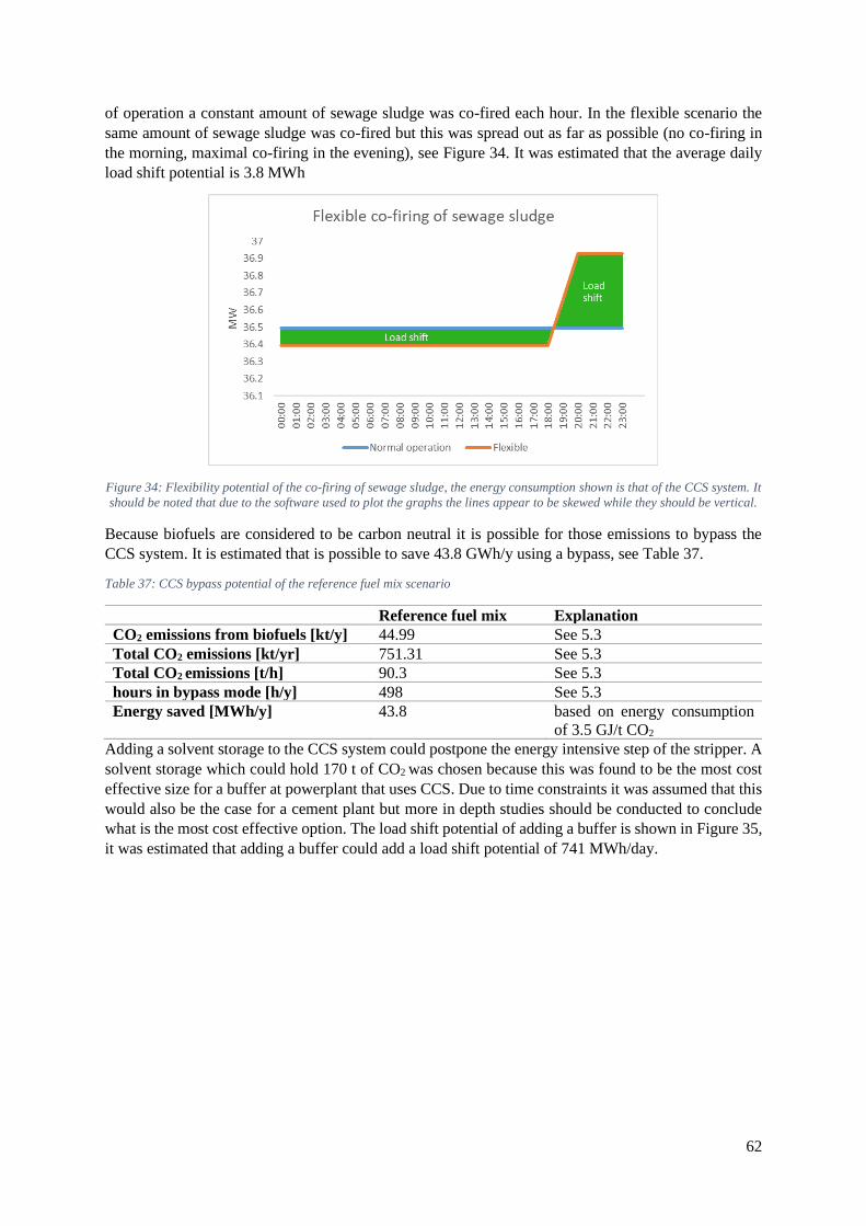
62

of operation a constant amount of sewage sludge was co-fired each hour. In the flexible scenario the

same amount of sewage sludge was co-fired but this was spread out as far as possible (no co-firing in

the morning, maximal co-firing in the evening), see Figure 34. It was estimated that the average daily

load shift potential is 3.8 MWh

Figure 34: Flexibility potential of the co-firing of sewage sludge, the energy consumption shown is that of the CCS system. It

should be noted that due to the software used to plot the graphs the lines appear to be skewed while they should be vertical.

Because biofuels are considered to be carbon neutral it is possible for those emissions to bypass the

CCS system. It is estimated that is possible to save 43.8 GWh/y using a bypass, see Table 37.

Table 37: CCS bypass potential of the reference fuel mix scenario

Reference fuel mix Explanation

CO2 emissions from biofuels [kt/y] 44.99 See 5.3

Total CO2 emissions [kt/yr] 751.31 See 5.3

Total CO2 emissions [t/h] 90.3 See 5.3

hours in bypass mode [h/y] 498 See 5.3

Energy saved [MWh/y] 43.8 based on energy consumption

of 3.5 GJ/t CO2

Adding a solvent storage to the CCS system could postpone the energy intensive step of the stripper. A

solvent storage which could hold 170 t of CO2 was chosen because this was found to be the most cost

effective size for a buffer at powerplant that uses CCS. Due to time constraints it was assumed that this

would also be the case for a cement plant but more in depth studies should be conducted to conclude

what is the most cost effective option. The load shift potential of adding a buffer is shown in Figure 35,

it was estimated that adding a buffer could add a load shift potential of 741 MWh/day.

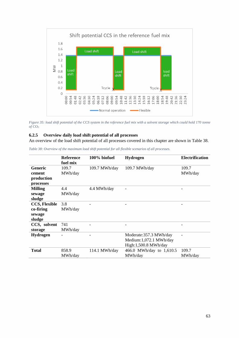
63

Figure 35: load shift potential of the CCS system in the reference fuel mix with a solvent storage which could hold 170 tonne

of CO2.

6.2.5 Overview daily load shift potential of all processes

An overview of the load shift potential of all processes covered in this chapter are shown in Table 38.

Table 38: Overview of the maximum load shift potential for all flexible scenarios of all processes.

Reference

fuel mix

100% biofuel Hydrogen Electrification

Generic

cement

production

processes

109.7

MWh/day

109.7 MWh/day 109.7 MWh/day 109.7

MWh/day

Milling

sewage

sludge

4.4

MWh/day

4.4 MWh/day - -

CCS, Flexible

co-firing

sewage

sludge

3.8

MWh/day

- - -

CCS, solvent

storage

741

MWh/day

- - -

Hydrogen - - Moderate:357.3 MWh/day

Medium:1,072.1 MWh/day

High:1,500.8 MWh/day

-

Total 858.9

MWh/day

114.1 MWh/day 466.0 MWh/day to 1,610.5

MWh/day

109.7

MWh/day

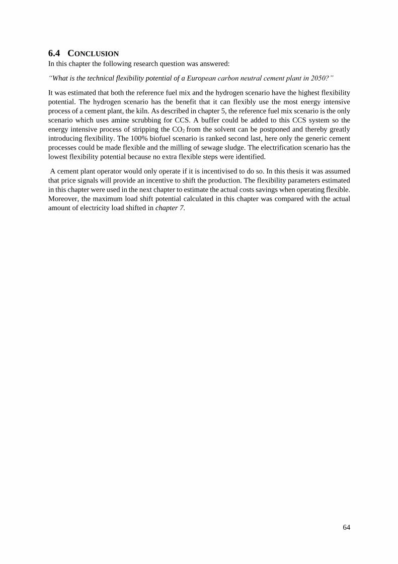
64

6.4 CONCLUSION In this chapter the following research question was answered:

“What is the technical flexibility potential of a European carbon neutral cement plant in 2050?”

It was estimated that both the reference fuel mix and the hydrogen scenario have the highest flexibility

potential. The hydrogen scenario has the benefit that it can flexibly use the most energy intensive

process of a cement plant, the kiln. As described in chapter 5, the reference fuel mix scenario is the only

scenario which uses amine scrubbing for CCS. A buffer could be added to this CCS system so the

energy intensive process of stripping the CO2 from the solvent can be postponed and thereby greatly

introducing flexibility. The 100% biofuel scenario is ranked second last, here only the generic cement

processes could be made flexible and the milling of sewage sludge. The electrification scenario has the

lowest flexibility potential because no extra flexible steps were identified.

A cement plant operator would only operate if it is incentivised to do so. In this thesis it was assumed

that price signals will provide an incentive to shift the production. The flexibility parameters estimated

in this chapter were used in the next chapter to estimate the actual costs savings when operating flexible.

Moreover, the maximum load shift potential calculated in this chapter was compared with the actual

amount of electricity load shifted in chapter 7.

65

7 ECONOMIC FLEXIBILITY POTENTIAL OF A EUROPEAN

CEMENT PLANT (RQ4)

In this chapter the economic flexibility potentials were estimated for all constructed scenarios to answer

the research question:

“What is the economic flexibility potential of a carbon neutral cement plant in 2050?”

By answering this research question the main research question can be answered in the conclusion,

chapter 9.

As mentioned in the introduction the flexible electricity prices could create an incentive for the cement

plant to shift its processes to times with low electricity demand thus high renewable supply. This

behaviour not only favours the integration of VRES, but it also reduces the electricity costs for the

cement plant.

The economic flexibility is estimated with a linear program and the constraints of this program are

based on data gathered in the previous chapters. Despite the goals of the European Union to create a

carbon neutral electricity system by 2050, the effects this will have on the electricity prices is mostly

unknown. To incorporate this uncertainty into the results, electricity prices from multiple scenarios are

used. Due to time constraints, instead of analysing all countries in Europe, only four countries are

analysed with each representing a specific part of Europe (Northern, Western, Southern and Eastern

Europe).

7.1 METHODOLOGY In the first paragraph (7.1.1) the theory behind a linear program (LP) is briefly explained followed by

a description of the tools used to implement the linear program and its limitations. The paragraph

(7.1.2) thereafter describes which electricity price time-series are applied for the estimation of the

economic flexibility potential. As described in chapter 6 the generic cement processes will be the same

in all scenarios but their CCS technology and heat source differ. Therefore, one LP is constructed for

the generic cement production processes and 3 different LPs are constructed for the reference fuel mix,

100% biofuel and hydrogen scenario. In chapter 6 it was estimated that the electrification scenario has

no extra flexibility potential. Creating four different LPs instead of one has the benefit that the models

are smaller and therefore more comprehensive. Moreover, larger models have a larger computing time

and therefore debugging becomes more time consuming. Because the different processes behave

separate from each other it has no effect on the results.

The connection between the LPs and the decarbonization scenarios is shown in Table 39.

Table 39: Connection between the different linear programs and the constructed scenarios

Scenario: Purpose

LP: Generic cement processes Section:

7.1.3

Estimates the economic flexibility potential

of flexible operation of the grinder, raw mill,

cement mill and packaging unit.

LP: Reference fuel mix

Section: 7.1.5

Estimates the economic potential of the

milling of sewage sludge, flexible co-firing of

sewage sludge and a flexible amine

scrubbing CCS system

LP: 100% biofuel mix

Section: 7.1.6

Estimates the economic flexibility potential

of milling sewage sludge

LP: Hydrogen scenario

Section: 7.1.7

Estimates the economic flexibility potential

of flexible hydrogen generation.

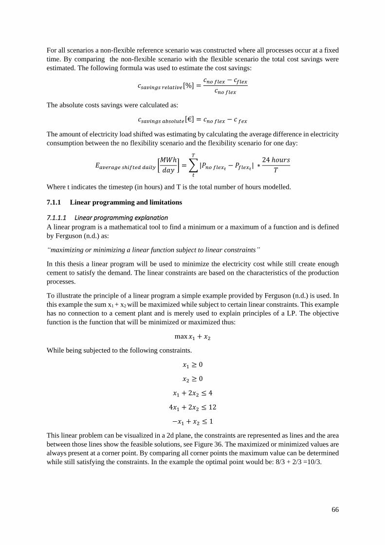
66

For all scenarios a non-flexible reference scenario was constructed where all processes occur at a fixed

time. By comparing the non-flexible scenario with the flexible scenario the total cost savings were

estimated. The following formula was used to estimate the cost savings:

𝑐𝑠𝑎𝑣𝑖𝑛𝑔𝑠 𝑟𝑒𝑙𝑎𝑡𝑖𝑣𝑒[%] =𝑐𝑛𝑜 𝑓𝑙𝑒𝑥 − 𝑐𝑓𝑙𝑒𝑥

𝑐𝑛𝑜 𝑓𝑙𝑒𝑥

The absolute costs savings were calculated as:

𝑐𝑠𝑎𝑣𝑖𝑛𝑔𝑠 𝑎𝑏𝑠𝑜𝑙𝑢𝑡𝑒[€] = 𝑐𝑛𝑜 𝑓𝑙𝑒𝑥 − 𝑐 𝑓𝑒𝑥

The amount of electricity load shifted was estimating by calculating the average difference in electricity

consumption between the no flexibility scenario and the flexibility scenario for one day:

𝐸𝑎𝑣𝑒𝑟𝑎𝑔𝑒 𝑠ℎ𝑖𝑓𝑡𝑒𝑑 𝑑𝑎𝑖𝑙𝑦 [𝑀𝑊ℎ

𝑑𝑎𝑦] = ∑ |𝑃𝑛𝑜 𝑓𝑙𝑒𝑥𝑡

− 𝑃𝑓𝑙𝑒𝑥𝑡|

𝑇

𝑡

∗24 ℎ𝑜𝑢𝑟𝑠

𝑇

Where t indicates the timestep (in hours) and T is the total number of hours modelled.

7.1.1 Linear programming and limitations

7.1.1.1 Linear programming explanation

A linear program is a mathematical tool to find a minimum or a maximum of a function and is defined

by Ferguson (n.d.) as:

“maximizing or minimizing a linear function subject to linear constraints”

In this thesis a linear program will be used to minimize the electricity cost while still create enough

cement to satisfy the demand. The linear constraints are based on the characteristics of the production

processes.

To illustrate the principle of a linear program a simple example provided by Ferguson (n.d.) is used. In

this example the sum x1 + x2 will be maximized while subject to certain linear constraints. This example

has no connection to a cement plant and is merely used to explain principles of a LP. The objective

function is the function that will be minimized or maximized thus:

max 𝑥1 + 𝑥2

While being subjected to the following constraints.

𝑥1 ≥ 0

𝑥2 ≥ 0

𝑥1 + 2𝑥2 ≤ 4

4𝑥1 + 2𝑥2 ≤ 12

−𝑥1 + 𝑥2 ≤ 1

This linear problem can be visualized in a 2d plane, the constraints are represented as lines and the area

between those lines show the feasible solutions, see Figure 36. The maximized or minimized values are

always present at a corner point. By comparing all corner points the maximum value can be determined

while still satisfying the constraints. In the example the optimal point would be: 8/3 + 2/3 =10/3.

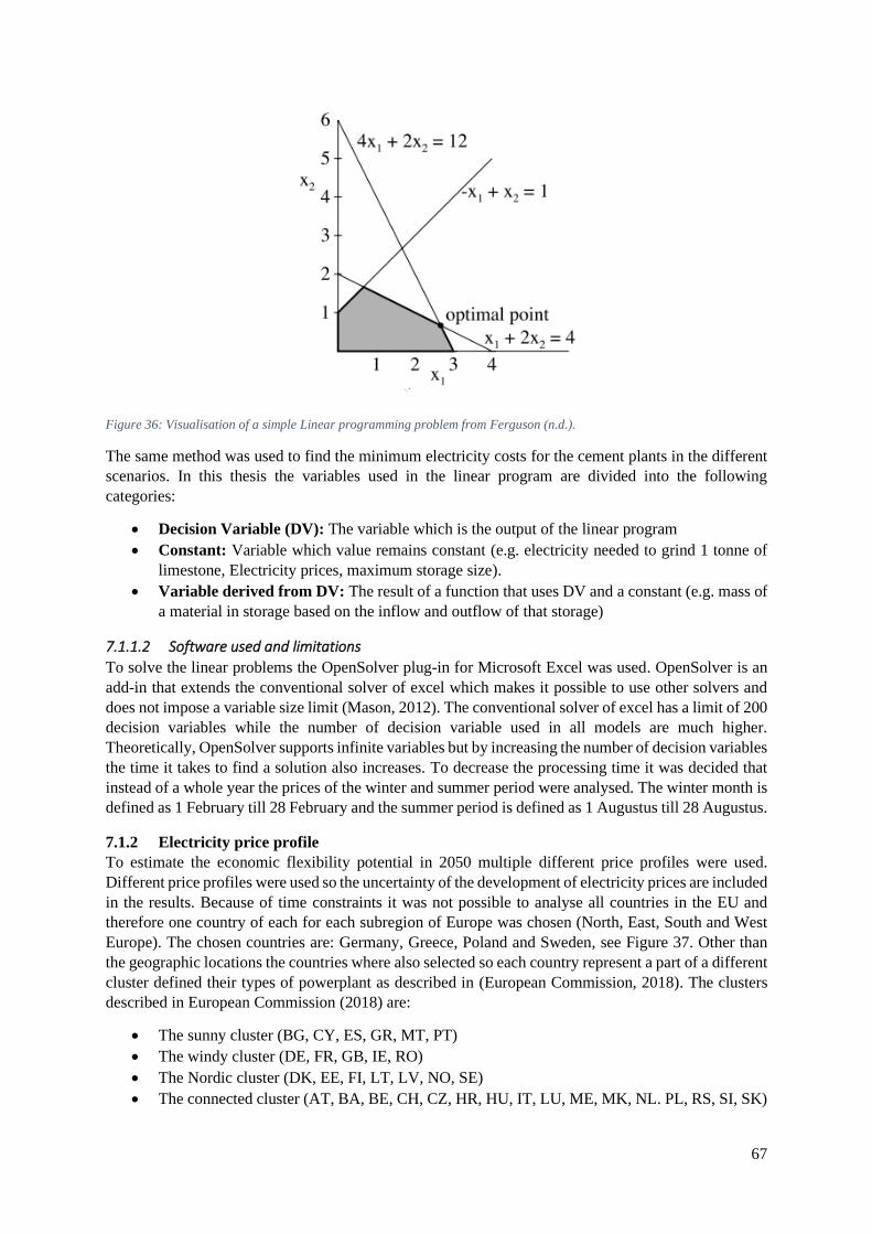
67

Figure 36: Visualisation of a simple Linear programming problem from Ferguson (n.d.).

The same method was used to find the minimum electricity costs for the cement plants in the different

scenarios. In this thesis the variables used in the linear program are divided into the following

categories:

• Decision Variable (DV): The variable which is the output of the linear program

• Constant: Variable which value remains constant (e.g. electricity needed to grind 1 tonne of

limestone, Electricity prices, maximum storage size).

• Variable derived from DV: The result of a function that uses DV and a constant (e.g. mass of

a material in storage based on the inflow and outflow of that storage)

7.1.1.2 Software used and limitations

To solve the linear problems the OpenSolver plug-in for Microsoft Excel was used. OpenSolver is an

add-in that extends the conventional solver of excel which makes it possible to use other solvers and

does not impose a variable size limit (Mason, 2012). The conventional solver of excel has a limit of 200

decision variables while the number of decision variable used in all models are much higher.

Theoretically, OpenSolver supports infinite variables but by increasing the number of decision variables

the time it takes to find a solution also increases. To decrease the processing time it was decided that

instead of a whole year the prices of the winter and summer period were analysed. The winter month is

defined as 1 February till 28 February and the summer period is defined as 1 Augustus till 28 Augustus.

7.1.2 Electricity price profile

To estimate the economic flexibility potential in 2050 multiple different price profiles were used.

Different price profiles were used so the uncertainty of the development of electricity prices are included

in the results. Because of time constraints it was not possible to analyse all countries in the EU and

therefore one country of each for each subregion of Europe was chosen (North, East, South and West

Europe). The chosen countries are: Germany, Greece, Poland and Sweden, see Figure 37. Other than

the geographic locations the countries where also selected so each country represent a part of a different

cluster defined their types of powerplant as described in (European Commission, 2018). The clusters

described in European Commission (2018) are:

• The sunny cluster (BG, CY, ES, GR, MT, PT)

• The windy cluster (DE, FR, GB, IE, RO)

• The Nordic cluster (DK, EE, FI, LT, LV, NO, SE)

• The connected cluster (AT, BA, BE, CH, CZ, HR, HU, IT, LU, ME, MK, NL. PL, RS, SI, SK)

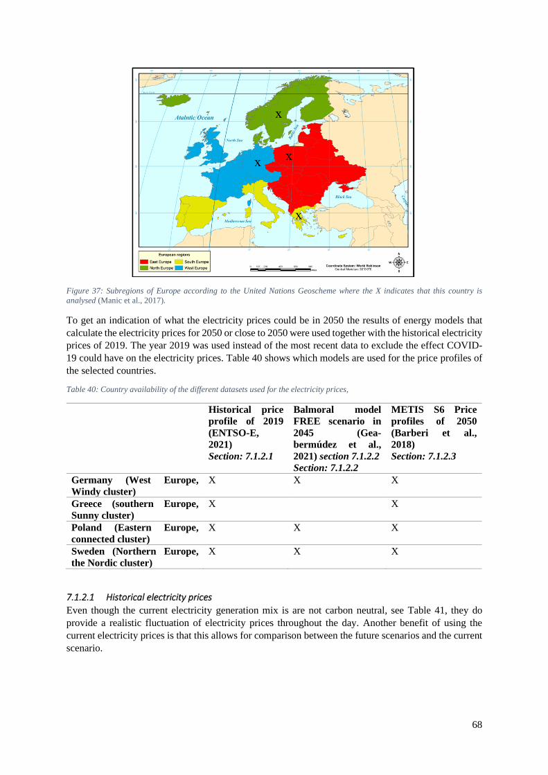
68

Figure 37: Subregions of Europe according to the United Nations Geoscheme where the X indicates that this country is

analysed (Manic et al., 2017).

To get an indication of what the electricity prices could be in 2050 the results of energy models that

calculate the electricity prices for 2050 or close to 2050 were used together with the historical electricity

prices of 2019. The year 2019 was used instead of the most recent data to exclude the effect COVID-

19 could have on the electricity prices. Table 40 shows which models are used for the price profiles of

the selected countries.

Table 40: Country availability of the different datasets used for the electricity prices,

Historical price

profile of 2019

(ENTSO-E,

2021)

Section: 7.1.2.1

Balmoral model

FREE scenario in

2045 (Gea-

bermúdez et al.,

2021) section 7.1.2.2

Section: 7.1.2.2

METIS S6 Price

profiles of 2050

(Barberi et al.,

2018)

Section: 7.1.2.3

Germany (West Europe,

Windy cluster)

X X X

Greece (southern Europe,

Sunny cluster)

X X

Poland (Eastern Europe,

connected cluster)

X X X

Sweden (Northern Europe,

the Nordic cluster)

X X X

7.1.2.1 Historical electricity prices

Even though the current electricity generation mix is are not carbon neutral, see Table 41, they do

provide a realistic fluctuation of electricity prices throughout the day. Another benefit of using the

current electricity prices is that this allows for comparison between the future scenarios and the current

scenario.

69

Table 41: Electricity share from renewable energy for the countries used in this report in 2019 (Ritchie & Roser, 2020)

Electricity share from renewable energy

sources in 2019

Germany 17.48%

Greece 12.11%

Poland 6.18%

Sweden 42.24%

The electricity prices for the summer and winter period are shown in Figure 38 and are gathered from

the European Network of Transmission System Operators (ENTSO-E). As shown in Figure 38 a high

share of VRES does not necessary contribute to lower electricity prices. In all countries the electricity

prices are lower in the winter but there is also more variance in the winter. Therefore, it is likely that

the electricity savings will be higher in the winter when operating flexibly. The figure also shows that

Germany sometimes has negative electricity prices. Negative prices can occur when there is a high

supply of variable renewable energy and a low electricity demand. The higher prices in the winter are

likely caused by the fact that there is less PV generation and more electricity demand than in the

summer.

Figure 38: Actual electricity prices of 2019 (ENTSO-E, 2021)

7.1.2.2 Balmoral

Though personal communication (Gea-Bermúdez, Personal Communication, April 29, 2021) the hourly

electricity prices calculated with the Balmoral software were acquired. The model is described in Gea-

bermúdez et al. (2021) and features a flexible demand. The aim of the balmoral model was to minimize

the total system costs (investment costs, fuel costs CO2 tax, etc) while still satisfying the energy demand.

The hourly electricity costs are determined by using the merit order. The balmoral model has a hourly

time resolution.

Gea-Bermúdez offered multiple electricity price profiles but only the price profile for the scenario with

the lowest emissions was used in this thesis (the FREE scenario). In the FREE scenario the CO2

emissions are reduced to 76% compared to 1990 levels. Despite the fact that this scenario is not fully

carbon neutral it could still provide valuable information because it is closer to a carbon neutral

electricity mix than the current mix. The electricity prices of this model are shown in Figure 39.

-500

50100150200250300

Elec

tric

ity

pri

ce [

€/M

Wh

]

Electricity prices in Winter 2019

DE GR PL SW

-60-40-20

020406080

100

Elec

tric

ity

pri

ce [

€/M

Wh

]

Electricty prices Summer 2019

DE GR PL SW

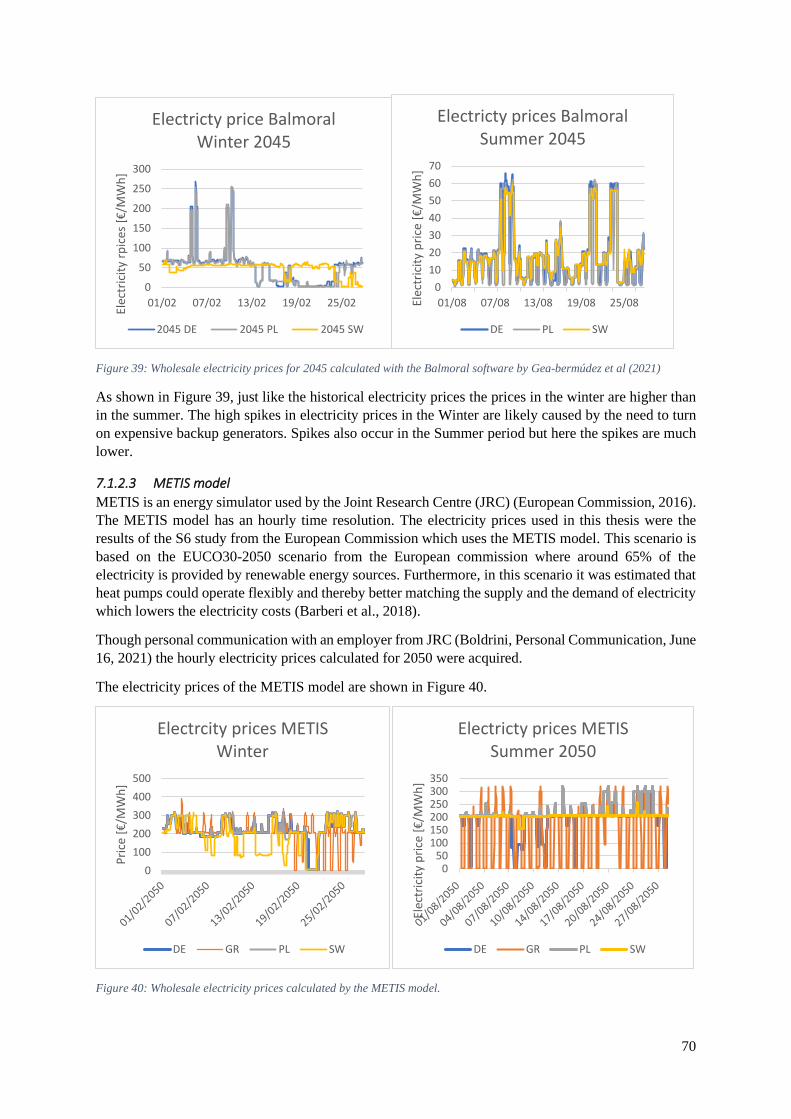
70

Figure 39: Wholesale electricity prices for 2045 calculated with the Balmoral software by Gea-bermúdez et al (2021)

As shown in Figure 39, just like the historical electricity prices the prices in the winter are higher than

in the summer. The high spikes in electricity prices in the Winter are likely caused by the need to turn

on expensive backup generators. Spikes also occur in the Summer period but here the spikes are much

lower.

7.1.2.3 METIS model

METIS is an energy simulator used by the Joint Research Centre (JRC) (European Commission, 2016).

The METIS model has an hourly time resolution. The electricity prices used in this thesis were the

results of the S6 study from the European Commission which uses the METIS model. This scenario is

based on the EUCO30-2050 scenario from the European commission where around 65% of the

electricity is provided by renewable energy sources. Furthermore, in this scenario it was estimated that

heat pumps could operate flexibly and thereby better matching the supply and the demand of electricity

which lowers the electricity costs (Barberi et al., 2018).

Though personal communication with an employer from JRC (Boldrini, Personal Communication, June

16, 2021) the hourly electricity prices calculated for 2050 were acquired.

The electricity prices of the METIS model are shown in Figure 40.

Figure 40: Wholesale electricity prices calculated by the METIS model.

0

50

100

150

200

250

300

01/02 07/02 13/02 19/02 25/02

Elec

tric

ity

rpic

es [

€/M

Wh

]Electricty price Balmoral

Winter 2045

2045 DE 2045 PL 2045 SW

0

10

20

30

40

50

60

70

01/08 07/08 13/08 19/08 25/08Elec

tric

ity

pri

ce [

€/M

Wh

]

Electricty prices Balmoral Summer 2045

DE PL SW

0

100

200

300

400

500

Pri

ce [

€/M

Wh

]

Electrcity prices METIS Winter

DE GR PL SW

050

100150200250300350

Elec

tric

ity

pri

ce [

€/M

Wh

]

Electricty prices METIS Summer 2050

DE GR PL SW

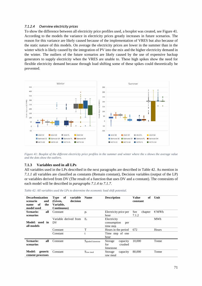
71

7.1.2.4 Overview electricity prices

To show the difference between all electricity price profiles used, a boxplot was created, see Figure 41.

According to the models the variance in electricity prices greatly increases in future scenarios. The

reason for this variance are likely caused because of the implementation of VRES but also because of

the static nature of this models. On average the electricity prices are lower in the summer than in the

winter which is likely caused by the integration of PV into the mix and the higher electricity demand in

the winter. The outliers of the future scenarios are likely caused by the use of expensive backup

generators to supply electricity when the VRES are unable to. These high spikes show the need for

flexible electricity demand because through load shifting some of these spikes could theoretically be

prevented.

Figure 41: Boxplot of the different electricity price profiles in the summer and winter where the x shows the average value

and the dots show the outliers.

7.1.3 Variables used in all LPs

All variables used in the LPs described in the next paragraphs are described in Table 42. As mention in

7.1.1 all variables are classified as constants (Remain constant), Decision variables (output of the LP)

or variables derived from DV (The result of a function that uses DV and a constant). The constraints of

each model will be described in paragraphs 7.1.4 to 7.1.7.

Table 42: All variables used the LPs to determine the economic load shift potential.

Decarbonization

scenario and

name of the

model used

Type of variable

(Given, decision

Variable,

Continuous)

Name Description Value of

constant

Unit

Scenario: all

scenarios

Model: used in

all models

Constant pt Electricity price per

hour

See chapter

7.1.2

€/MWh

Variable derived from

DV

Et Electricity

consumption per

time step

MWh

Constant T Hours in the period 672 Hours

Constant t Time step of one

hour

Scenario: all

scenarios

Model: generic

cement processes

Constant Sginded limestone Storage capacity

for crushed

limestone

10,000 Tonne

Constant Sraw meal Storage capacity

raw meal

80,000 Tonne

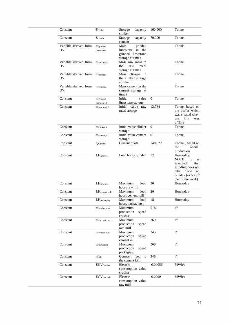
72

Constant Sclinker Storage capacity

clinker

160,000 Tonne

Constant Scement Storage capacity

cement

70,000 Tonne

Variable derived from

DV

mgrinded

limestone,t

Mass grinded

limestone in the

grinded limestone

storage at time t

Tonne

Variable derived from

DV

mraw meal,t Mass raw meal in

the raw meal

storage at time t

Tonne

Variable derived from

DV

mclinker,t Mass clinkers in

the clinker storage

at time t

Tonne

Variable derived from

DV

mcement,t Mass cement in the

cement storage at

time t

Tonne

Constant mgrinded

limestone, 0

Initial value

limestone storage

0 Tonne

Constant mraw meal,0 Initial value raw

meal storage

12,784 Tonne, based on

the buffer which

was created when

the kiln was

offline

Constant mclinker,0 Initial value clinker

storage

0 Tonne

Constant mcement,0 Initial value cement

storage

0 Tonne

Constant QCement Cement quota 140,622 Tonne , based on

the annual

production

Constant LHgrinder Load hours grinder 12 Hours/day,

NOTE it is

assumed that

grinding does not

take place on

Sunday (every 7th

day of the week)

Constant LHraw mill Maximum load

hours raw mill

20 Hours/day

Constant LHcement mill Maximum load

hours cement mill

20 Hours/day

Constant LHpackaging Maximum load

hours packaging

18 Hours/day

Constant ṁrrusher, max Maximum

production speed

crusher

518 t/h

Constant ṁram mill, max Maximum

production speed

ram mill

269 t/h

Constant ṁcement mill Maximum

production speed

cement mill

245 t/h

Constant ṁpackaging Maximum

production speed

packaging

269 t/h

Constant ṁkiln Constant feed to

the cement kiln

245 t/h

Constant ECVCrusher Electric

consumption value

crusher

0.00056 MWh/t

Constant ECVraw mill Electric

consumption value

raw mill

0.0090 MWh/t

73

Constant ECVkiln Electric

consumption value

kiln

0.02200 MWh/t

Constant ECVcement mill Electric

consumption value

cement mill

0.02750 MWh/t

Constant ECVpackaging Electric

consumption value

packaging

0.00150 MWh/t

DV OHgrinder, t Operating hours at

timestep t of the

grinder

h/h

DV OHraw mill, t Operating hours at

timestep t of the

raw mill

h/h

Constant OHkiln, t Operating hours at

timestep t of the

kiln

1 h/h

DV OHcement mill, t Operating hours at

timestep t of the

cement mill

h/h

DV OHpackaging, t Operating hours at

timestep t of the

packaging unit

h/h

Variable derived from

DV

Egrinder,t Energy

consumption

grinder during

timestep t

MWh

Variable derived from

DV

Eram mill,t Energy

consumption raw

mill during

timestep t

MWh

Variable derived from

DV

Ekiln, t Energy

consumption kiln

during timestep t

MWh

Variable derived from

DV

Ecement mill,t Energy

consumption

cement mill during

timestep t

MWh

Variable derived from

DV

Epackaging Energy

consumption

packaging during

timestep t

MWh

Variable derived from

DV

ṁgrinder, t Amount of

limestone

processed at

timestep t

t/h

Variable derived from

DV

ṁRaw mill, t Amount of

limestone milled to

raw meal at

timestep t

t/h

Constant derived from

another constant

ṁkiln,t Amount of raw

meal fed into the

kiln

245 t/h

Variable derived from

DV

ṁcement mill, t Amount of clinkers

milled at timestep t

t/h

Variable derived from

DV

ṁpackaging, t Amount of cement

being packaged and

transported at

timestep t

t/h

Variable derived from

DV

Daily

OHgrinder, i

Hours the grinder is

in operation on day

i

Hours

Variable derived from

DV

Daily OHRaw

mill, i

Hours the Raw Mill

is in operation at

day i

Hours

74

Variable derived from

DV

Daily

OHCement mill, i

Hours the Cement

mill is in operation

at day i

Hours

Variable derived from

DV

Daily

OHPackaging,i

Hours being

packaged at day i

Hours

Scenario:

reference fuel

mix and 100%

biofuel

Model:

Reference fuel

mix and 100%

biofuel

Constant Ss Storage sewage

sludge

1,350 Tonne

Constant Qs Sewage sludge

quota

3,935 Tonne

Variable derived from

DV

ms Amount of sewage

sludge burned

Tonne

Constant ṁmilling sewage

sludge max

Maximum sewage

sludge milling

speed

9.2 Tonne/h

Constant ṁkiln feed max Maximum sewage

sludge kiln feed

8.0 Tonne/h

DV msewage sludge, t Mass sewage

sludge in the

sewage sludge

storage at time t

Tonne

DV ṁmilling sewage

sludge, t

Milling speed at

time t

Tonne/h

DV ṁkiln feed, t Sewage sludge kiln

feed at time t

Tonne/h

Constant Ssewage sludge Storage size of the

sewage sludge

1350

Constant ECVsewage

sludge mill

Electric

consumption value

sewage sludge mill

0.04 MWh/t

Variable derived from

DV

ESewage sludge

mill,t

Electricity use of

the sludge mill at

time step t

MWh

Variable derived from

DV

OHsewage sludge

mill, t

Amount of time the

sewage sludge mill

is on in timestep t.

h/h

Variable derived from

DV

Daily OH

sewage sludge mill,

max

The maximum

amount of time the

sewage sludge mill

can be turned on

20 Hours/day

Variable derived from

DV

Daily

OHsewage sludge

mill, i

Amount of hours

the sewage sludge

mill is in operation

at day i

Hours/day

Scenario:

reference fuel

mix

Model:

Reference fuel

Constant QCO2,scenario Max bypassed CO2 3,817

Tonne

Constant SCO2 Storage size CO2 in

the buffer

170

DV ṁscrubber, t Amount of CO2 fed

into the scrubber at

time t

DV ṁstripper, t Amount of CO2 fed

into the stripper at

time t

Constant ṁstripper max Maximum of CO2

the stripper could

process

t/h

Constant ECVScrubber Electric

consumption value

scrubber

0.0972 MWh/tonne CO2

Constant ECVstripper Electric

consumption value

stripper

0.875 MWh/tonne CO2

Variable derived from

DV

Escrubber,t Electricity use of

the scrubber at time

step t

MWh

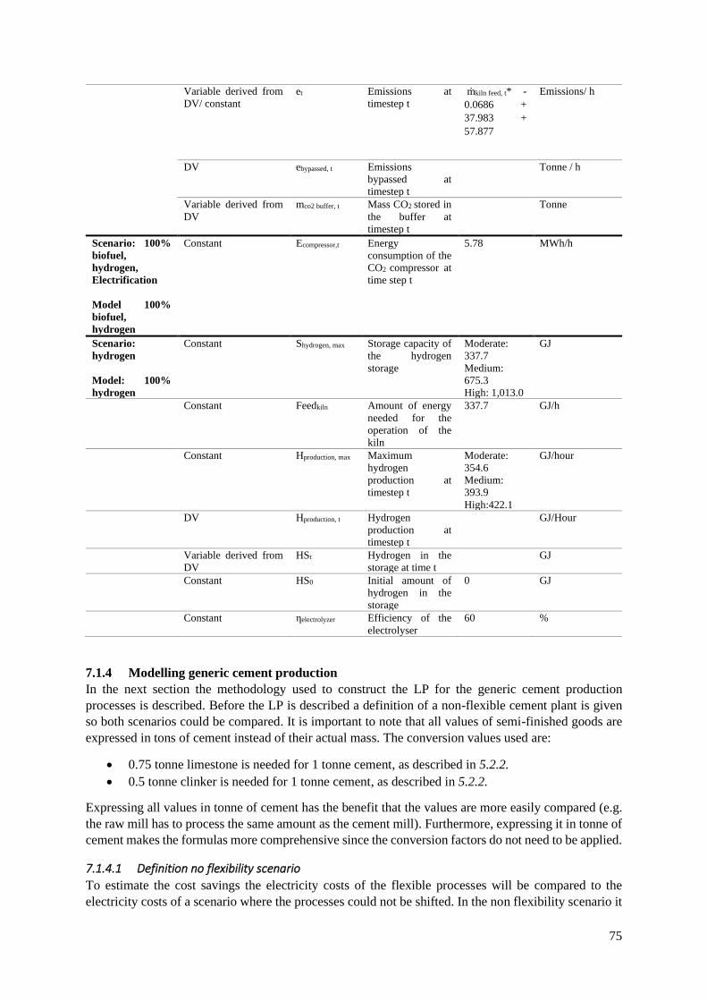
75

Variable derived from

DV/ constant

et Emissions at

timestep t

ṁkiln feed, t* -

0.0686 +

37.983 +

57.877

Emissions/ h

DV ebypassed, t Emissions

bypassed at

timestep t

Tonne / h

Variable derived from

DV

mco2 buffer, t Mass CO2 stored in

the buffer at

timestep t

Tonne

Scenario: 100%

biofuel,

hydrogen,

Electrification

Model 100%

biofuel,

hydrogen

Constant Ecompressor,t Energy

consumption of the

CO2 compressor at

time step t

5.78 MWh/h

Scenario:

hydrogen

Model: 100%

hydrogen

Constant Shydrogen, max Storage capacity of

the hydrogen

storage

Moderate:

337.7

Medium:

675.3

High: 1,013.0

GJ

Constant Feedkiln Amount of energy

needed for the

operation of the

kiln

337.7 GJ/h

Constant Hproduction, max Maximum

hydrogen

production at

timestep t

Moderate:

354.6

Medium:

393.9

High:422.1

GJ/hour

DV Hproduction, t Hydrogen

production at

timestep t

GJ/Hour

Variable derived from

DV

HSt Hydrogen in the

storage at time t

GJ

Constant HS0 Initial amount of

hydrogen in the

storage

0 GJ

Constant ηelectrolyzer Efficiency of the

electrolyser

60 %

7.1.4 Modelling generic cement production

In the next section the methodology used to construct the LP for the generic cement production

processes is described. Before the LP is described a definition of a non-flexible cement plant is given

so both scenarios could be compared. It is important to note that all values of semi-finished goods are

expressed in tons of cement instead of their actual mass. The conversion values used are:

• 0.75 tonne limestone is needed for 1 tonne cement, as described in 5.2.2.

• 0.5 tonne clinker is needed for 1 tonne cement, as described in 5.2.2.

Expressing all values in tonne of cement has the benefit that the values are more easily compared (e.g.

the raw mill has to process the same amount as the cement mill). Furthermore, expressing it in tonne of

cement makes the formulas more comprehensive since the conversion factors do not need to be applied.

7.1.4.1 Definition no flexibility scenario

To estimate the cost savings the electricity costs of the flexible processes will be compared to the

electricity costs of a scenario where the processes could not be shifted. In the non flexibility scenario it

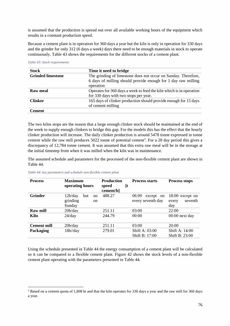
76

is assumed that the production is spread out over all available working hours of the equipment which

results in a constant production speed.

Because a cement plant is in operation for 360 days a year but the kiln is only in operation for 330 days

and the grinder for only 312 (6 days a week) days there need to be enough materials in stock to operate

continuously. Table 43 shows the requirements for the different stocks of a cement plant.

Table 43: Stock requirements

Stock Time it need to bridge

Grinded limestone The grinding of limestone does not occur on Sunday. Therefore,

6 days of milling should provide enough for 1 day raw milling

operation

Raw meal Operates for 360 days a week to feed the kiln which is in operation

for 330 days with two stops per year.

Clinker 165 days of clinker production should provide enough for 15 days

of cement milling

Cement

The two kilns stops are the reason that a large enough clinker stock should be maintained at the end of

the week to supply enough clinkers to bridge this gap. For the models this has the effect that the hourly

clinker production will increase. The daily clinker production is around 5478 tonne expressed in tonne

cement while the raw mill produces 5022 tonne of potential cement3. For a 28 day period this gives a

discrepancy of 12,784 tonne cement. It was assumed that this extra raw meal will be in the storage at

the initial timestep from when it was milled when the kiln was in maintenance.

The assumed schedule and parameters for the processed of the non-flexible cement plant are shown in

Table 44.

Table 44: key parameters and schedule non-flexible cement plant

Process Maximum

operating hours

Production

speed [t

cement/h]

Process starts Process stops

Grinder 12h/day but no

grinding on

Sunday

488.27 06:00 except on

every seventh day

18:00 except on

every seventh

day

Raw mill 20h/day 251.11 03:00 22:00

Kiln 24/day 244.79 00:00 00:00 next day

Cement mill 20h/day 251.11 03:00 20:00

Packaging 18h//day 279.01 Shift A: 03:00

Shift B: 17:00

Shift A: 14:00

Shift B: 23:00

Using the schedule presented in Table 44 the energy consumption of a cement plant will be calculated

so it can be compared to a flexible cement plant. Figure 42 shows the stock levels of a non-flexible

cement plant operating with the parameters presented in Table 44.

3 Based on a cement quota of 1,808 kt and that the kiln operates for 330 days a year and the raw mill for 360 days

a year.

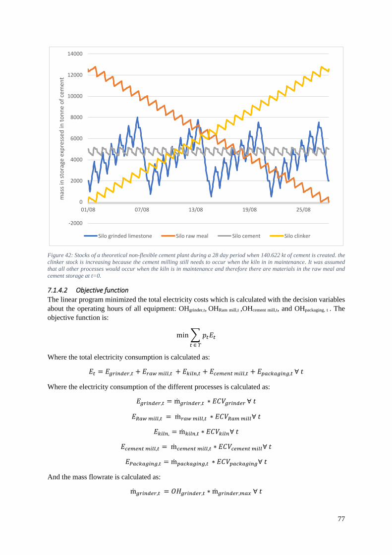
77

Figure 42: Stocks of a theoretical non-flexible cement plant during a 28 day period when 140.622 kt of cement is created. the

clinker stock is increasing because the cement milling still needs to occur when the kiln in in maintenance. It was assumed

that all other processes would occur when the kiln is in maintenance and therefore there are materials in the raw meal and

cement storage at t=0.

7.1.4.2 Objective function

The linear program minimized the total electricity costs which is calculated with the decision variables

about the operating hours of all equipment: OHgrinder,t, OHRam mill,t ,OHcement mill,t, and OHpackaging, t . The

objective function is:

min ∑ 𝑝𝑡𝐸𝑡

𝑡 ∈ 𝑇

Where the total electricity consumption is calculated as:

𝐸𝑡 = 𝐸𝑔𝑟𝑖𝑛𝑑𝑒𝑟,𝑡 + 𝐸𝑟𝑎𝑤 𝑚𝑖𝑙𝑙,𝑡 + 𝐸𝑘𝑖𝑙𝑛,𝑡 + 𝐸𝑐𝑒𝑚𝑒𝑛𝑡 𝑚𝑖𝑙𝑙,𝑡 + 𝐸𝑝𝑎𝑐𝑘𝑎𝑔𝑖𝑛𝑔,𝑡 ∀ 𝑡

Where the electricity consumption of the different processes is calculated as:

𝐸𝑔𝑟𝑖𝑛𝑑𝑒𝑟,𝑡 = ṁ𝑔𝑟𝑖𝑛𝑑𝑒𝑟,𝑡 ∗ 𝐸𝐶𝑉𝑔𝑟𝑖𝑛𝑑𝑒𝑟 ∀ 𝑡

𝐸𝑅𝑎𝑤 𝑚𝑖𝑙𝑙,𝑡 = ṁ𝑟𝑎𝑤 𝑚𝑖𝑙𝑙,𝑡 ∗ 𝐸𝐶𝑉𝑅𝑎𝑚 𝑚𝑖𝑙𝑙∀ 𝑡

𝐸𝑘𝑖𝑙𝑛, = ṁ𝑘𝑖𝑙𝑛,𝑡 ∗ 𝐸𝐶𝑉𝑘𝑖𝑙𝑛∀ 𝑡

𝐸𝑐𝑒𝑚𝑒𝑛𝑡 𝑚𝑖𝑙𝑙,𝑡 = ṁ𝑐𝑒𝑚𝑒𝑛𝑡 𝑚𝑖𝑙𝑙,𝑡 ∗ 𝐸𝐶𝑉𝑐𝑒𝑚𝑒𝑛𝑡 𝑚𝑖𝑙𝑙∀ 𝑡

𝐸𝑃𝑎𝑐𝑘𝑎𝑔𝑖𝑛𝑔,𝑡 = ṁ𝑝𝑎𝑐𝑘𝑎𝑔𝑖𝑛𝑔,𝑡 ∗ 𝐸𝐶𝑉𝑝𝑎𝑐𝑘𝑎𝑔𝑖𝑛𝑔∀ 𝑡

And the mass flowrate is calculated as:

ṁ𝑔𝑟𝑖𝑛𝑑𝑒𝑟,𝑡 = 𝑂𝐻𝑔𝑟𝑖𝑛𝑑𝑒𝑟,𝑡 ∗ ṁ𝑔𝑟𝑖𝑛𝑑𝑒𝑟,𝑚𝑎𝑥 ∀ 𝑡

-2000

0

2000

4000

6000

8000

10000

12000

14000

01/08 07/08 13/08 19/08 25/08

mas

s in

sto

rage

exp

ress

ed in

to

nn

e o

f ce

men

t

Silo grinded limestone Silo raw meal Silo cement Silo clinker

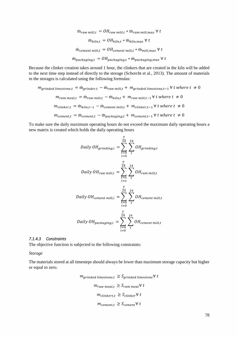
78

ṁ𝑟𝑎𝑤 𝑚𝑖𝑙𝑙,𝑡 = 𝑂𝐻𝑟𝑎𝑤 𝑚𝑖𝑙𝑙,𝑡 ∗ ṁ𝑟𝑎𝑚 𝑚𝑖𝑙𝑙,𝑚𝑎𝑥 ∀ 𝑡

ṁ𝑘𝑖𝑙𝑛,𝑡 = 𝑂𝐻𝑘𝑖𝑙𝑛,𝑡 ∗ ṁ𝑘𝑖𝑙𝑛,𝑚𝑎𝑥 ∀ 𝑡

ṁ𝑐𝑒𝑚𝑒𝑛𝑡 𝑚𝑖𝑙𝑙,𝑡 = 𝑂𝐻𝑐𝑒𝑚𝑒𝑛𝑡 𝑚𝑖𝑙𝑙,𝑡 ∗ ṁ𝑚𝑖𝑙𝑙,𝑚𝑎𝑥 ∀ 𝑡

ṁ𝑝𝑎𝑐𝑘𝑎𝑔𝑖𝑛𝑔,𝑡 = 𝑂𝐻𝑝𝑎𝑐𝑘𝑎𝑔𝑖𝑛𝑔,𝑡 ∗ ṁ𝑝𝑎𝑐𝑘𝑎𝑔𝑖𝑛𝑔,𝑚𝑎𝑥 ∀ 𝑡

Because the clinker creation takes around 1 hour, the clinkers that are created in the kiln will be added

to the next time step instead of directly to the storage (Schorcht et al., 2013). The amount of materials

in the storages is calculated using the following formulas:

𝑚𝑔𝑟𝑖𝑛𝑑𝑒𝑑 𝑙𝑖𝑚𝑒𝑠𝑡𝑜𝑛𝑒,𝑡 = ṁ𝑔𝑟𝑖𝑛𝑑𝑒𝑟,𝑡 − ṁ𝑟𝑎𝑤 𝑚𝑖𝑙𝑙,𝑡 + 𝑚𝑔𝑟𝑖𝑛𝑑𝑒𝑑 𝑙𝑖𝑚𝑒𝑠𝑡𝑜𝑛𝑒,𝑡−1 ∀ 𝑡 𝑤ℎ𝑒𝑟𝑒 𝑡 ≠ 0

𝑚𝑟𝑎𝑚 𝑚𝑒𝑎𝑙,𝑡 = ṁ𝑟𝑎𝑤 𝑚𝑖𝑙𝑙,𝑡 − ṁ𝑘𝑖𝑙𝑛,𝑡 + 𝑚𝑟𝑎𝑤 𝑚𝑖𝑙𝑙,𝑡−1 ∀ 𝑡 𝑤ℎ𝑒𝑟𝑒 𝑡 ≠ 0

𝑚𝑐𝑙𝑖𝑛𝑘𝑒𝑟,𝑡 = ṁ𝑘𝑖𝑙𝑛,𝑡−1 − ṁ𝑐𝑒𝑚𝑒𝑛𝑡 𝑚𝑖𝑙𝑙,𝑡 + 𝑚𝑐𝑙𝑖𝑛𝑘𝑒𝑟,𝑡−1 ∀ 𝑡 𝑤ℎ𝑒𝑟𝑒 𝑡 ≠ 0

𝑚𝑐𝑒𝑚𝑒𝑛𝑡,𝑡 = ṁ𝑐𝑒𝑚𝑒𝑛𝑡,𝑡 − ṁ𝑝𝑎𝑐𝑘𝑎𝑔𝑖𝑛𝑔,𝑡 + 𝑚𝑐𝑒𝑚𝑒𝑛𝑡,𝑡−1 ∀ 𝑡 𝑤ℎ𝑒𝑟𝑒 𝑡 ≠ 0

To make sure the daily maximum operating hours do not exceed the maximum daily operating hours a

new matrix is created which holds the daily operating hours

𝐷𝑎𝑖𝑙𝑦 𝑂𝐻𝑔𝑟𝑖𝑛𝑑𝑖𝑛𝑔,𝑖 = ∑ ∑ 𝑂𝐻𝑔𝑟𝑖𝑛𝑑𝑖𝑛𝑔,𝑡

24

𝑡

𝑇24

𝑡=0𝑖=0

𝐷𝑎𝑖𝑙𝑦 𝑂𝐻𝑟𝑎𝑤 𝑚𝑖𝑙𝑙,𝑖 = ∑ ∑ 𝑂𝐻𝑟𝑎𝑚 𝑚𝑖𝑙𝑙,𝑡

24

𝑡

𝑇24

𝑡=𝑜𝑖=𝑜

𝐷𝑎𝑖𝑙𝑦 𝑂𝐻𝑐𝑒𝑚𝑒𝑛𝑡 𝑚𝑖𝑙𝑙,𝑖 = ∑ ∑ 𝑂𝐻𝑐𝑒𝑚𝑒𝑛𝑡 𝑚𝑖𝑙𝑙,𝑡

24

𝑡

𝑇24

𝑡=0𝑖=0

𝐷𝑎𝑖𝑙𝑦 𝑂𝐻𝑝𝑎𝑐𝑘𝑎𝑔𝑖𝑛𝑔,𝑖 = ∑ ∑ 𝑂𝐻𝑐𝑒𝑚𝑒𝑛𝑡 𝑚𝑖𝑙𝑙,𝑡

24

𝑡

𝑇24

𝑡=0𝑖=0

7.1.4.3 Constraints

The objective function is subjected to the following constraints:

Storage

The materials stored at all timesteps should always be lower than maximum storage capacity but higher

or equal to zero.

𝑚𝑔𝑟𝑖𝑛𝑑𝑒𝑑 𝑙𝑖𝑚𝑒𝑠𝑡𝑜𝑛𝑒,𝑡 ≥ 𝑆𝑔𝑟𝑖𝑛𝑑𝑒𝑑 𝑙𝑖𝑚𝑒𝑠𝑡𝑜𝑛𝑒∀ 𝑡

𝑚𝑟𝑎𝑤 𝑚𝑒𝑎𝑙,𝑡 ≥ 𝑆𝑟𝑎𝑚 𝑚𝑒𝑎𝑙∀ 𝑡

𝑚𝑐𝑙𝑖𝑛𝑘𝑒𝑟𝑡,𝑡 ≥ 𝑆𝑐𝑙𝑖𝑛𝑘𝑒𝑟∀ 𝑡

𝑚𝑐𝑒𝑚𝑒𝑛𝑡,𝑡 ≥ 𝑆𝑐𝑒𝑚𝑒𝑛𝑡∀ 𝑡

79

𝑚𝑔𝑟𝑖𝑛𝑑𝑒𝑑 𝑙𝑖𝑚𝑒𝑠𝑡𝑜𝑛𝑒,𝑡 ≤ 0 ∀ 𝑡

𝑚𝑟𝑎𝑤 𝑚𝑒𝑎𝑙,𝑡 ≤ 0 ∀ 𝑡

𝑚𝑐𝑙𝑖𝑛𝑘𝑒𝑟,𝑡 ≤ 0 ∀ 𝑡

𝑚𝑐𝑒𝑚𝑒𝑛𝑡,𝑡 ≤ 0 ∀ 𝑡

Production speed

All processes should have production speed lower than their maximum defined production speed

ṁ𝑔𝑟𝑖𝑛𝑑𝑒𝑟,𝑡 ≤ ṁ𝑔𝑟𝑖𝑛𝑑𝑒𝑟,𝑚𝑎𝑥 ∀ 𝑡

ṁ𝑟𝑎𝑚 𝑚𝑖𝑙𝑙,𝑡 ≤ ṁ𝑟𝑎𝑚 𝑚𝑖𝑙𝑙,𝑚𝑎𝑥 ∀ 𝑡

ṁ𝑐𝑒𝑚𝑒𝑛𝑡 𝑚𝑖𝑙𝑙,𝑡 ≤ ṁ𝑐𝑒𝑚𝑒𝑛𝑡 𝑚𝑖𝑙𝑙,𝑚𝑎𝑥 ∀ 𝑡

ṁ𝑝𝑎𝑐𝑘𝑎𝑔𝑎𝑛𝑖𝑛𝑔,𝑡 ≤ ṁ𝑝𝑎𝑐𝑘𝑎𝑔𝑖𝑛𝑔,𝑚𝑎𝑥 ∀ 𝑡

And the production speed should be higher or equal to 0:

ṁ𝑔𝑟𝑖𝑛𝑑𝑒𝑟,𝑡 ≥ 0 ∀ 𝑡

ṁ𝑟𝑎𝑚 𝑚𝑖𝑙𝑙,𝑡 ≥ 0 ∀ 𝑡

ṁ𝑐𝑒𝑚𝑒𝑛𝑡 𝑚𝑖𝑙𝑙,𝑡 ≥ 0 ∀ 𝑡

ṁ𝑝𝑎𝑐𝑘𝑎𝑔𝑎𝑛𝑖𝑛𝑔,𝑡 ≥ 0 ∀ 𝑡

Cement quota

At the end of the period the cement plant should have at least produced enough cement to satisfy the

cement quota.

∑ ṁ𝑝𝑎𝑐𝑘𝑎𝑔𝑎𝑛𝑖𝑛𝑔,𝑡

𝑡 ∈ 𝑇

≥ 𝑄𝑐𝑒𝑚𝑒𝑛𝑡

Operating hours

The operating hours of the all processes should be lower than their maximum specified operating hours

and the grinder should be turned off on Sundays. That the grinder should be off on Sunday is

implemented as no grinding on day 6, 13, 20 and 27.

𝐷𝑎𝑖𝑙𝑦 𝑂𝐻𝑔𝑟𝑖𝑛𝑑𝑒𝑟,𝑖 ≤ 𝐿𝐻𝑔𝑟𝑖𝑛𝑑𝑒𝑟,𝑖 ∀ 𝑖 𝑤ℎ𝑒𝑟𝑒 𝑖 ≠ 6, 𝑖 ≠ 13, 𝑖 ≠ 20 𝑎𝑛𝑑 𝑖 ≠ 27

𝐷𝑎𝑖𝑙𝑦 𝑂𝐻𝑔𝑟𝑖𝑛𝑑𝑒𝑟,6 = 0, 𝐷𝑎𝑖𝑙𝑦 𝑂𝐻𝑔𝑟𝑖𝑛𝑑𝑒𝑟,13 = 0, 𝐷𝑎𝑖𝑙𝑦 𝑂𝐻𝑔𝑟𝑖𝑛𝑑𝑒𝑟,20 = 0,𝐷𝑎𝑖𝑙𝑦 𝑂𝐻𝑔𝑟𝑖𝑛𝑑𝑒𝑟,27 = 0

7.1.5 Modelling reference fuel mix

As described in chapter 6 the sewage sludge processes are connected to the amine scrubbing CCS

process because the amount of sewage sludge being co-fired changes the CO2 emissions. This is relevant

because for example when the electricity prices are low it is favourable to have much CO2 in the flue

gas so the CCS system can process more CO2 at a lower price. In the 100% biofuel scenario fuel derived

emissions are not captured and therefore the amount of sewage sludge co-fired has no effect on the total

electricity consumption.

80

7.1.5.1 Definition no flexibility scenario

In the non-flexibility scenario it is assumed that sewage sludge milling will start each day at 03:00 and

stops at 23:00 so the mill is turned on for 20 hours a day with a production speed of 7.77 t sewage

sludge per hour (this results in 4,352 tonne sewage sludge being milled in a 28 day period). It was

assumed that the sewage sludge being co-fired remains constant and therefore the CO2 emissions will

also remain constant.

7.1.5.2 Objective function

The electricity costs will be calculated by multiplying the energy consumption per time step by the

electricity price of the given timestep. The aim of this program is to minimize the electricity cost.

min ∑ 𝑝𝑡𝐸𝑡𝑜𝑡𝑎𝑙,𝑡

𝑡 ∈ 𝑇

Where the electricity consumption is calculated using the following formula:

𝐸𝑡𝑜𝑡𝑎𝑙,𝑡 = 𝐸𝑠𝑒𝑤𝑎𝑔𝑒 𝑠𝑙𝑢𝑑𝑔𝑒 𝑚𝑖𝑙𝑙,𝑡 + 𝐸𝑠𝑐𝑟𝑢𝑏𝑏𝑒𝑟,𝑡 + 𝐸𝑠𝑡𝑟𝑖𝑝𝑝𝑒𝑟,𝑡 ∀ 𝑡

Where the variables derived from DVs are calculated with the following formulas

𝐸𝑠𝑒𝑤𝑎𝑔𝑒 𝑠𝑙𝑢𝑑𝑔𝑒 𝑚𝑖𝑙𝑙,𝑡 = ṁmilling sewage sludge,t ∗ ECVmilling sewage sludge,t ∀ 𝑡

𝐸𝑠𝑐𝑟𝑢𝑏𝑏𝑒𝑟,𝑡 = ṁscrubber,t ∗ 𝐸𝐶𝑉𝑠𝑐𝑟𝑢𝑏𝑏𝑒𝑟,𝑡 ∀ 𝑡

𝐸𝑠𝑡𝑟𝑖𝑝𝑝𝑒𝑟,𝑡 = ṁstripper,t ∗ 𝐸𝐶𝑉𝑠𝑡𝑟𝑖𝑝𝑝𝑒𝑟,𝑡 ∀ 𝑡

The emissions which are not bypassed are directly fed into the scrubber. Therefore, the mass flowrate

of the scrubber is defined as:

ṁscrubber,t = 𝑒𝑡 − 𝑒𝑏𝑦𝑝𝑎𝑠𝑠𝑒𝑑,𝑡∀ 𝑡

The total emissions is dependent on the sewage sludge feed in rate and will be calculated with the linear

formula constructed in pargraph 6.1.5.1:

𝑒𝑡 = −0.0686 ∗ ṁ𝑘𝑖𝑙𝑛 𝑓𝑒𝑒𝑑,𝑡 + 37.983 + 57.877

The amount of sewage sludge in the storage at every timestep is calculated with the following formula:

𝑚𝑠𝑒𝑤𝑎𝑔𝑒 𝑠𝑙𝑢𝑑𝑔𝑒,𝑡 = 𝑚𝑠𝑒𝑤𝑎𝑔𝑒 𝑠𝑙𝑢𝑑𝑔𝑒,𝑡−1 + ṁmilling sewage sludge,t − ṁ𝑘𝑖𝑙𝑛 𝑓𝑒𝑒𝑑,𝑡 ∀ 𝑡 𝑤ℎ𝑒𝑟𝑒 𝑡 ≠ 0

At timestep 0 there is no sewage sludge in the storage.

𝑚𝑠𝑒𝑤𝑎𝑔𝑒 𝑠𝑙𝑢𝑑𝑔𝑒,0 = 0

The following formula is used to calculate how many hours per day the sewage sludge mill is on:

𝐷𝑎𝑖𝑙𝑦 𝑂𝐻𝑆𝑒𝑤𝑎𝑔𝑒 𝑠𝑙𝑢𝑑𝑔𝑒 𝑚𝑖𝑙𝑙,𝑖 = ∑ ∑ 𝑂𝐻𝑆𝑒𝑤𝑎𝑔𝑒 𝑠𝑙𝑢𝑑𝑔𝑒 𝑚𝑖𝑙𝑙,𝑡

24

𝑡

𝑇24

𝑡=0𝑖=0

7.1.5.3 Constraints reference fuel mix

Sewage sludge processes

The storage sludge can only be feed into the kiln when there is sludge in the storage and the feed-in

speed is lower than the defined maximum. Burning sewage sludge cannot be reversed therefore the feed

into the kiln must be positive.

81

ṁ𝑘𝑖𝑙𝑛 𝑓𝑒𝑒𝑑,𝑡 ≤ 𝑚𝑠𝑒𝑤𝑎𝑔𝑒 𝑠𝑙𝑢𝑑𝑔𝑒,𝑡 ∀ 𝑡

ṁ𝑘𝑖𝑙𝑛 𝑓𝑒𝑒𝑑,𝑡 ≤ ṁkiln feed,max ∀ 𝑡

ṁ𝑘𝑖𝑙𝑛 𝑓𝑒𝑒𝑑,𝑡 ≥ 0 ∀ 𝑡

All sewage sludge imported from a wastewater treatment plant should be co-fired at the end of the

period.

∑ ṁ𝑘𝑖𝑙𝑛 𝑓𝑒𝑒𝑑,𝑡

𝑡 ∈ 𝑇

= 𝑄𝑠

Before the sewage sludge could be co-fired it first should be milled, this milling process is subjected to

the following constraints:

ṁmilling sewage sludge,t ≤ ṁmilling sewage sludge,max ∀ 𝑡

ṁmilling sewage sludge,t ≥ 0 ∀ 𝑡

After the sludge is milled but before it can be co-fired it will be stored in a silo, the storage of sewage

sludge is subjected to the following constraints:

𝑚𝑠𝑒𝑤𝑎𝑔𝑒 𝑠𝑙𝑢𝑑𝑔𝑒,𝑡 ≤ 𝑆𝑠∀ 𝑡

𝑚𝑠𝑒𝑤𝑎𝑔𝑒 𝑠𝑙𝑢𝑑𝑔𝑒,𝑡 ≥ 0 ∀ 𝑡

The sewage sludge mill cannot be on for more hours during the day than the specified maximum:

𝐷𝑎𝑖𝑙𝑦 𝑂𝐻𝑆𝑒𝑤𝑎𝑔𝑒 𝑠𝑙𝑢𝑑𝑔𝑒 𝑚𝑖𝑙𝑙,𝑖 ≤ 𝐷𝑎𝑖𝑙𝑦 𝑂𝐻𝑆𝑒𝑤𝑎𝑔𝑒 𝑠𝑙𝑢𝑑𝑔𝑒 𝑚𝑖𝑙𝑙,𝑚𝑎𝑥 ∀ 𝑖

CCS processes

As mentioned previously the bypassing of the CCS system can only occur in reference fuel mix

scenario. The total CO2 bypassed should be lower or equal to the calculated maximum:

∑ 𝑒𝑏𝑦𝑝𝑎𝑠𝑠𝑒𝑑,𝑡

𝑡 ∈ 𝑇

≤ 𝑄𝐶𝑂2,𝑠𝑐𝑒𝑛𝑎𝑟𝑖𝑜 ∀ 𝑡

The amount of CO2 that is being bypassed should be lower or equal to the amount of CO2 in the flue gas

𝑒𝑏𝑦𝑝𝑎𝑠𝑠𝑒𝑑,𝑡 ≤ 𝑒𝑡 ∀ 𝑡

And is bound by a non-negativity constraint

𝑒𝑏𝑦𝑝𝑎𝑠𝑠𝑒𝑑,𝑡 ≥ 0 ∀ 𝑡

In the reference fuel mix scenario amine scrubbing is used which could be flexible and therefore has

additional constraints than other scenarios. The emissions that are not bypassed are fed into the scrubber

and potentially could be stored in the solvent storage (buffer).

𝑚𝐶𝑂2 𝑏𝑢𝑓𝑓𝑒𝑟,𝑡 = ṁscrubber,t − ṁstripper,t + 𝑚𝐶𝑂2 𝑏𝑢𝑓𝑓𝑒𝑟,𝑡−1 ∀ 𝑡 𝑤ℎ𝑒𝑟𝑒 𝑡 ≠ 0 𝑎𝑛𝑑 𝑤ℎ𝑒𝑟𝑒 𝑡 ≠ 𝑇

In the beginning of the simulation the buffer should be empty and at the last timestep the buffer should

also be emptied so all CO2 is processed

𝑚𝐶𝑂2 𝑏𝑢𝑓𝑓𝑒𝑟,0 = 0

𝑚𝐶𝑂2 𝑏𝑢𝑓𝑓𝑒𝑟,𝑇 = 0

The CO2 in the buffer should always be lower than the max capacity of the storage.

82

𝑚𝐶𝑂2 𝑏𝑢𝑓𝑓𝑒𝑟,𝑡 ≤ 𝑆𝐶𝑂2 ∀ 𝑡

The buffer should not be emptied more quickly than the maximum operating speed of the stripper and

should have a value higher than 0.

ṁ𝑠𝑡𝑟𝑖𝑝𝑝𝑒𝑟,𝑡 ≤ ṁ𝑠𝑡𝑟𝑖𝑝𝑝𝑒𝑟 𝑚𝑎𝑥 ∀ 𝑡

ṁ𝑠𝑡𝑟𝑖𝑝𝑝𝑒𝑟,𝑡 ≥ 0 ∀ 𝑡

7.1.6 Modelling 100% biofuel scenario

In the 100% biofuel scenario the only step that adds extra flexibility to the production process is the

milling of sewage sludge. Because the fuel derived emissions are not captured in this scenario the

amount of sewage sludge co-fired will not impact the energy consumption of the CCS system, as was

the case in the reference fuel mix. Because the CO2 streams are separated bypassing is not possible in

this scenario.

7.1.6.1 Definition no flexibility scenario

In the non-flexibility scenario the sewage sludge will be milled at the same times as the non-flexibility

scenario of the reference fuel mix, see paragraph 7.1.5.1.

7.1.6.2 Objective function

The electricity costs will be calculated by multiplying the energy consumption per time step by the

electricity price of the given timestep. The aim of this program is to minimize the electricity cost.

min ∑ 𝑝𝑡𝐸𝑡𝑜𝑡𝑎𝑙,𝑡

𝑡 ∈ 𝑇

Where the electricity consumption is calculated using the following formula:

𝐸𝑡𝑜𝑡𝑎𝑙,𝑡 = 𝐸𝑠𝑒𝑤𝑎𝑔𝑒 𝑠𝑙𝑢𝑑𝑔𝑒 𝑚𝑖𝑙𝑙,𝑡 + 𝐸𝐶𝐶𝑆,𝑡 ∀ 𝑡

Where the variables derived from DVs are calculated with the following formulas

𝐸𝑠𝑒𝑤𝑎𝑔𝑒 𝑠𝑙𝑢𝑑𝑔𝑒 𝑚𝑖𝑙𝑙,𝑡 = ṁmilling sewage sludge,t ∗ ECVmilling sewage sludge,t ∀ 𝑡

The amount of sewage sludge in the storage at every timestep is calculated with the following formula:

𝑚𝑠𝑒𝑤𝑎𝑔𝑒 𝑠𝑙𝑢𝑑𝑔𝑒,𝑡 = 𝑚𝑠𝑒𝑤𝑎𝑔𝑒 𝑠𝑙𝑢𝑑𝑔𝑒,𝑡−1 + ṁmilling sewage sludge,t − ṁ𝑘𝑖𝑙𝑛 𝑓𝑒𝑒𝑑,𝑡 ∀ 𝑡 𝑤ℎ𝑒𝑟𝑒 𝑡 ≠ 0

At timestep 0 there is no sewage sludge in the storage.

𝑚𝑠𝑒𝑤𝑎𝑔𝑒 𝑠𝑙𝑢𝑑𝑔𝑒,0 = 0

The following formula is used to calculate how many hours per day the sewage sludge mill is on:

𝐷𝑎𝑖𝑙𝑦 𝑂𝐻𝑆𝑒𝑤𝑎𝑔𝑒 𝑠𝑙𝑢𝑑𝑔𝑒 𝑚𝑖𝑙𝑙,𝑖 = ∑ ∑ 𝑂𝐻𝑆𝑒𝑤𝑎𝑔𝑒 𝑠𝑙𝑢𝑑𝑔𝑒 𝑚𝑖𝑙𝑙,𝑡

24

𝑡

𝑇24

𝑡=0𝑖=0

7.1.6.3 Constraints 100% biofuel scenario

All sewage sludge imported from a wastewater treatment plant should be co-fired at the end of the

period.

∑ ṁ𝑘𝑖𝑙𝑛 𝑓𝑒𝑒𝑑,𝑡

𝑡 ∈ 𝑇

= 𝑄𝑠

83

Before the sewage sludge could be co-fired it first should be milled, this milling process is subjected to

the following constraints:

ṁmilling sewage sludge,t ≤ ṁmilling sewage sludge,max ∀ 𝑡

ṁmilling sewage sludge,t ≥ 0 ∀ 𝑡

After the sludge is milled but before it can be co-fired it will be stored in a silo, the storage of sewage

sludge is subjected to the following constraints:

𝑚𝑠𝑒𝑤𝑎𝑔𝑒 𝑠𝑙𝑢𝑑𝑔𝑒,𝑡 ≤ 𝑆𝑠∀ 𝑡

𝑚𝑠𝑒𝑤𝑎𝑔𝑒 𝑠𝑙𝑢𝑑𝑔𝑒,𝑡 ≥ 0 ∀ 𝑡

The sewage sludge mill cannot be on for more hours during the day than the specified maximum:

𝐷𝑎𝑖𝑙𝑦 𝑂𝐻𝑆𝑒𝑤𝑎𝑔𝑒 𝑠𝑙𝑢𝑑𝑔𝑒 𝑚𝑖𝑙𝑙,𝑖 ≤ 𝐷𝑎𝑖𝑙𝑦 𝑂𝐻𝑆𝑒𝑤𝑎𝑔𝑒 𝑠𝑙𝑢𝑑𝑔𝑒 𝑚𝑖𝑙𝑙,𝑚𝑎𝑥 ∀ 𝑖

7.1.7 Modelling hydrogen processes

In this section the LP used to determine the minimal electricity costs for the production of hydrogen is

described.

7.1.7.1 Definition no flexibility scenario

In the no flexibility scenario there will be no storage for hydrogen and no overcapacity of the

electrolysers, the electrolyser will constantly provide enough fuel for the kiln (337.7 GJ/h)

7.1.7.2 Objective function

The electricity costs will be calculated by multiplying the energy consumption per time step by the

electricity price of the given timestep. The aim of this program is to minimize the electricity cost.

min ∑ 𝑝𝑡𝐸𝑡

𝑡 ∈ 𝑇

Where the electricity consumption is calculated by the energy consumption of the electrolyser and of

the compressor. Due to the constant clinker production the CO2 are also constant and thus also the

energy consumption of the compressor.

𝐸𝑡 =𝐻𝑝𝑟𝑜𝑑𝑢𝑐𝑡𝑖𝑜𝑛,𝑡

𝜂𝑒𝑙𝑒𝑐𝑡𝑟𝑜𝑙𝑦𝑧𝑒𝑟+ 𝐸𝑐𝑜𝑚𝑝𝑟𝑒𝑠𝑠𝑜𝑟,𝑡∀ 𝑡

And amount of hydrogen in the storage is calculated as:

𝐻𝑆𝑡 = 𝐻𝑆𝑡−1 + 𝐻𝑝𝑟𝑜𝑑𝑢𝑐𝑡𝑖𝑜𝑛,𝑡 − 𝐹𝑒𝑒𝑑𝑘𝑖𝑙𝑛 𝑤ℎ𝑒𝑟𝑒 𝑖 ≠ 0

Where Hproduction is the decision variable.

7.1.7.3 Constraints Hydrogen feed kiln

For the kiln to operate 24 hours a day there need to be a constant amount of hydrogen being feed into

the kiln from the hydrogen storage.

To always satisfy this hydrogen demand a constraint is added which makes it impossible for the tank to

be empty. This constraint has two purposes:

1. Create a realistic storage because it cannot hold a negative amount of hydrogen.

2. Because of the constant flow of hydrogen to the kiln (constant outflow from the storages) this

constraint makes sure that there will always be enough hydrogen generated to meet the

hydrogen demand.

84

𝑆ℎ𝑦𝑑𝑟𝑜𝑔𝑒𝑛,𝑡 ≥ 0 ∀ 𝑡

Hydrogen generation

The production process is limited by the maximum capacity of the storage and the maximum production

speed.

𝐻𝑃𝑟𝑜𝑑𝑢𝑐𝑡𝑖𝑜𝑛,𝑡 ≤ 𝐻𝑃𝑟𝑜𝑑𝑢𝑐𝑡𝑖𝑜𝑛,𝑚𝑎𝑥∀ 𝑡

The storage should be limited to the maximum amount of hydrogen it can hold.

𝑆ℎ𝑦𝑑𝑟𝑜𝑔𝑒𝑛,𝑡 = 𝑆ℎ𝑦𝑑𝑟𝑜𝑔𝑒𝑛,𝑡 ≤ 𝑆ℎ𝑦𝑑𝑟𝑜𝑔𝑒𝑛 ,𝑚𝑎𝑥∀ 𝑡

7.2 RESULTS In this paragraph the behaviour of the LP was analysed so the results could be verified. By checking the

variables of each different model it was determined that the constraints described in previous paragraph

were successfully implemented. After the behaviour was verified the results of all different scenarios

are presented. Al models are checked with the German price profile of summer 2019 because this dataset

has smooth fluctuations which makes the results easier to interpret.

7.2.1 Generic cement processes

In paragraph 7.2.2.1 the model is verified and in paragraph 7.2.2.2 the results are shown. As mentioned

previously to simplify the model the mass of all semi-finished goods is expressed in tonne of cement

rather than the actual mass.

7.2.1.1 Validation results

As mentioned in the description of the LP the operating hours of all equipment should not exceed the

maximum operating hours. Table 45 shows the operating hours of a flexible European cement plant

while subjected to the German electricity prices of the summer of 2019.

Table 45: operating hours of the different cement processes

Day Grinder Raw mill Cement mill Packaging

1 12.00 19.00 16.45 13.91

2 12.00 17.00 17.78 15.00

3 12.00 20.00 20.00 18.00

4 12.00 20.00 20.00 18.00

5 7.01 13.33 14.00 10.00

6 12.00 19.00 19.00 18.00

7 0.00 20.00 20.00 18.00

8 12.00 20.00 20.00 18.00

9 12.00 20.00 20.00 18.00

10 12.00 20.00 20.00 18.00

11 12.00 20.00 20.00 18.00

12 12.00 20.00 20.00 18.00

13 12.00 20.00 20.00 18.00

14 0.00 19.00 19.00 18.00

15 12.00 20.00 20.00 18.00

16 12.00 20.00 20.00 18.00

17 12.00 20.00 20.00 18.00

18 12.00 20.00 20.00 18.00

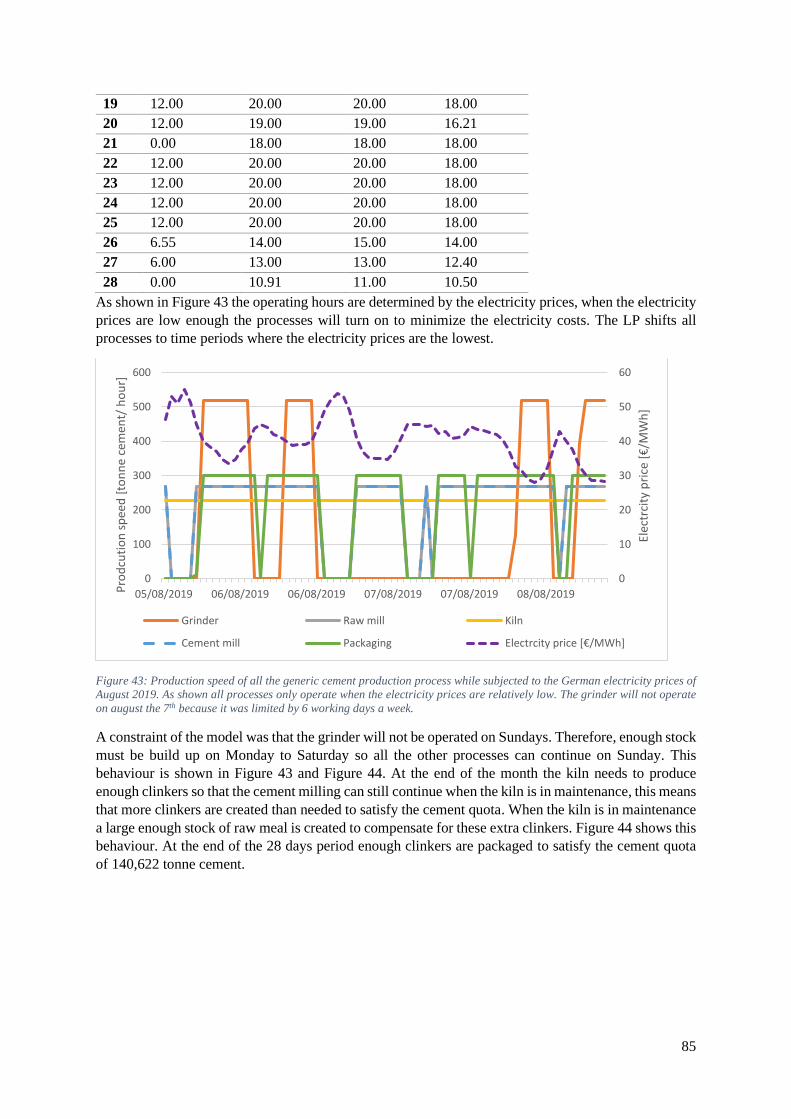
85

19 12.00 20.00 20.00 18.00

20 12.00 19.00 19.00 16.21

21 0.00 18.00 18.00 18.00

22 12.00 20.00 20.00 18.00

23 12.00 20.00 20.00 18.00

24 12.00 20.00 20.00 18.00

25 12.00 20.00 20.00 18.00

26 6.55 14.00 15.00 14.00

27 6.00 13.00 13.00 12.40

28 0.00 10.91 11.00 10.50

As shown in Figure 43 the operating hours are determined by the electricity prices, when the electricity

prices are low enough the processes will turn on to minimize the electricity costs. The LP shifts all

processes to time periods where the electricity prices are the lowest.

Figure 43: Production speed of all the generic cement production process while subjected to the German electricity prices of

August 2019. As shown all processes only operate when the electricity prices are relatively low. The grinder will not operate

on august the 7th because it was limited by 6 working days a week.

A constraint of the model was that the grinder will not be operated on Sundays. Therefore, enough stock

must be build up on Monday to Saturday so all the other processes can continue on Sunday. This

behaviour is shown in Figure 43 and Figure 44. At the end of the month the kiln needs to produce

enough clinkers so that the cement milling can still continue when the kiln is in maintenance, this means

that more clinkers are created than needed to satisfy the cement quota. When the kiln is in maintenance

a large enough stock of raw meal is created to compensate for these extra clinkers. Figure 44 shows this

behaviour. At the end of the 28 days period enough clinkers are packaged to satisfy the cement quota

of 140,622 tonne cement.

0

10

20

30

40

50

60

0

100

200

300

400

500

600

05/08/2019 06/08/2019 06/08/2019 07/08/2019 07/08/2019 08/08/2019

Elec

trci

ty p

rice

[€

/MW

h]

Pro

dcu

tio

n s

pee

d [

ton

ne

cem

ent/

ho

ur]

Grinder Raw mill Kiln

Cement mill Packaging Electrcity price [€/MWh]

86

Figure 44: Grinded limestone, Raw meal, clinker and cement storage of a European cement plant subjected to the German

electricity prices of August 2019

7.2.1.2 Overview economic potential for different price scenarios

By using all different electricity price profiles the economic flexibility potential of the generic cement

processes was calculated, see Figure 45. Because the electricity prices are higher in the METIS scenario

the absolute economic savings are much higher in this scenario compared to the other scenarios. In the

Balmoral scenarios the electricity costs are generally lower than the historic electricity prices but

because of their increased fluctuations the relative saving potential (expressed in %) is higher.

Figure 45: Monthly electricity costs and relative savings for the generic cement production processes

Because of the high electricity consumption of the cement mill this process contributes the most to the

saving potential followed by the raw mill, see Figure 46.

-60

-40

-20

0

20

40

60

80

100

-2,000

0

2,000

4,000

6,000

8,000

10,000

12,000

14,000

16,000

01/08/2019 07/08/2019 13/08/2019 19/08/2019 25/08/2019

Elec

trci

ty p

rice

[€

/MW

h]

Mas

s in

sto

rage

exp

ress

ed in

to

nn

e ce

men

t

Silo grinded limestone Silo raw meal Silo clinker

Silo cement Electrcity price [€/MWh]

0%

5%

10%

15%

20%

25%

30%

0

0.2

0.4

0.6

0.8

1

1.2

1.4

Win

ter

Sum

mer

Win

ter

Sum

mer

Win

ter

Sum

mer

Win

ter

Sum

mer

Win

ter

Sum

mer

Win

ter

Sum

mer

Win

ter

Sum

mer

Win

ter

Sum

mer

Win

ter

Sum

mer

Win

ter

Sum

mer

Win

ter

Sum

mer

Win

ter

Sum

mer

DE GE PL SW DE GE PL SW DE GE PL SW

Historic Balmoral METIS

Savi

ngs

[%

]

Elec

trci

ty c

ost

s [m

ln €

]/m

on

th]

no flex [mln €] flex [mln €] savings [%]

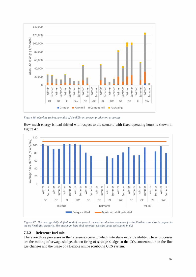
87

Figure 46: absolute saving potential of the different cement production processes

How much energy is load shifted with respect to the scenario with fixed operating hours is shown in

Figure 47.

Figure 47: The average daily shifted load of the generic cement production processes for the flexible scenarios in respect to

the no flexibility scenario. The maximum load shift potential was the value calculated in 6.2

7.2.2 Reference fuel mix

There are three processes in the reference scenario which introduce extra flexibility. These processes

are the milling of sewage sludge, the co-firing of sewage sludge so the CO2 concentration in the flue

gas changes and the usage of a flexible amine scrubbing CCS system.

0

20,000

40,000

60,000

80,000

100,000

120,000

140,000

Win

ter

Sum

mer

Win

ter

Sum

mer

Win

ter

Sum

mer

Win

ter

Sum

mer

Win

ter

Sum

mer

Win

ter

Sum

mer

Win

ter

Sum

mer

Win

ter

Sum

mer

Win

ter

Sum

mer

Win

ter

Sum

mer

Win

ter

Sum

mer

Win

ter

Sum

mer

DE GE PL SW DE GE PL SW DE GE PL SW

Ab

solu

te s

avin

gs [

€/m

on

th]

Grinder Raw mill Cement mill Packaging

0

20

40

60

80

100

120

Win

ter

Sum

mer

Win

ter

Sum

mer

Win

ter

Sum

mer

Win

ter

Sum

mer

Win

ter

Sum

mer

Win

ter

Sum

mer

Win

ter

Sum

mer

Win

ter

Sum

mer

Win

ter

Sum

mer

Win

ter

Sum

mer

Win

ter

Sum

mer

Win

ter

Sum

mer

DE GE PL SW DE GE PL SW DE GE PL SW

Historic Balmoral METIS

Ave

rage

dai

ly s

hif

ted

[M

Wh

/day

]

Energy shifted Maximum shift potential

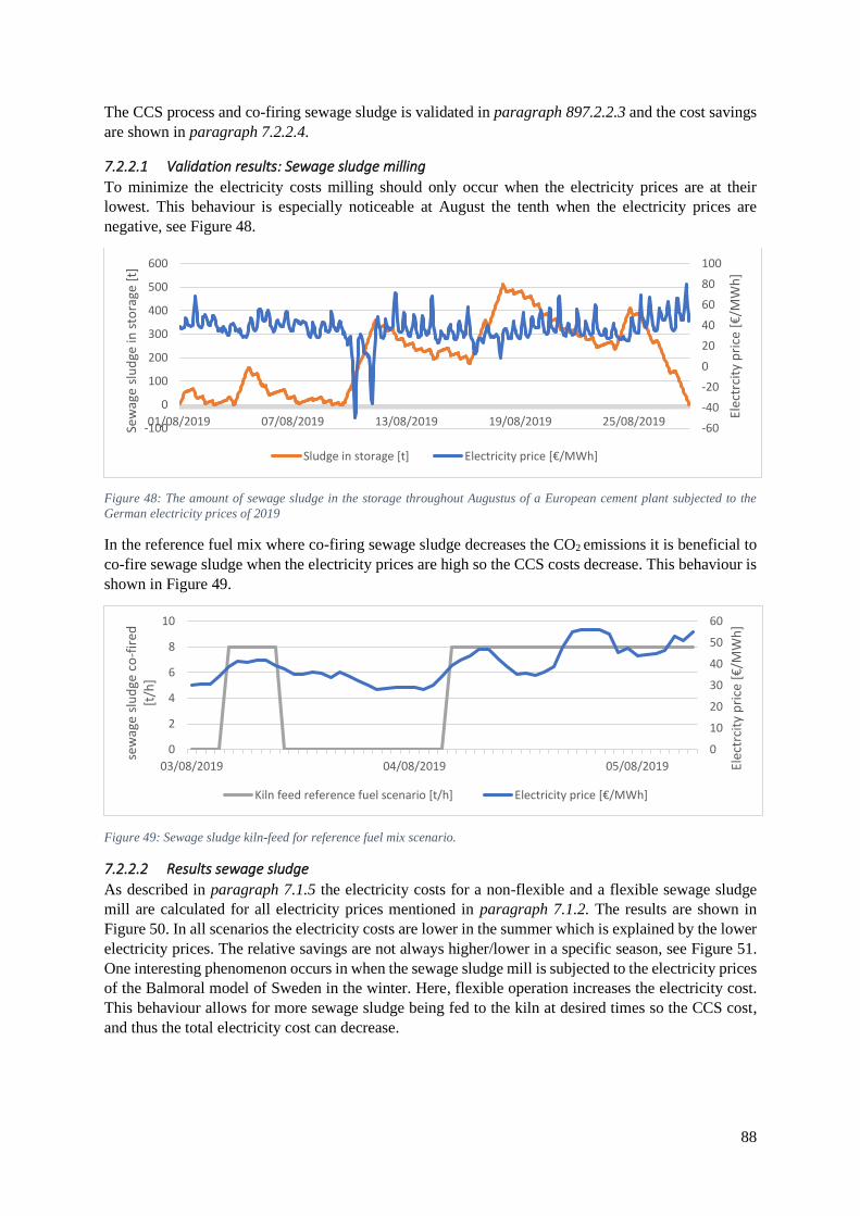
88

The CCS process and co-firing sewage sludge is validated in paragraph 897.2.2.3 and the cost savings

are shown in paragraph 7.2.2.4.

7.2.2.1 Validation results: Sewage sludge milling

To minimize the electricity costs milling should only occur when the electricity prices are at their

lowest. This behaviour is especially noticeable at August the tenth when the electricity prices are

negative, see Figure 48.

Figure 48: The amount of sewage sludge in the storage throughout Augustus of a European cement plant subjected to the

German electricity prices of 2019

In the reference fuel mix where co-firing sewage sludge decreases the CO2 emissions it is beneficial to

co-fire sewage sludge when the electricity prices are high so the CCS costs decrease. This behaviour is

shown in Figure 49.

Figure 49: Sewage sludge kiln-feed for reference fuel mix scenario.

7.2.2.2 Results sewage sludge

As described in paragraph 7.1.5 the electricity costs for a non-flexible and a flexible sewage sludge

mill are calculated for all electricity prices mentioned in paragraph 7.1.2. The results are shown in

Figure 50. In all scenarios the electricity costs are lower in the summer which is explained by the lower

electricity prices. The relative savings are not always higher/lower in a specific season, see Figure 51.

One interesting phenomenon occurs in when the sewage sludge mill is subjected to the electricity prices

of the Balmoral model of Sweden in the winter. Here, flexible operation increases the electricity cost.

This behaviour allows for more sewage sludge being fed to the kiln at desired times so the CCS cost,

and thus the total electricity cost can decrease.

-60

-40

-20

0

20

40

60

80

100

-100

0

100

200

300

400

500

600

01/08/2019 07/08/2019 13/08/2019 19/08/2019 25/08/2019

Elec

trci

ty p

rice

[€

/MW

h]

Sew

age

slu

dge

in s

tora

ge [

t]

Sludge in storage [t] Electricity price [€/MWh]

0

10

20

30

40

50

60

0

2

4

6

8

10

03/08/2019 04/08/2019 05/08/2019 Elec

trci

ty p

rice

[€

/MW

h]

sew

age

slu

dge

co

-fir

ed

[t/h

]

Kiln feed reference fuel scenario [t/h] Electricity price [€/MWh]

89

Figure 50: Electricity costs for the milling of sewage sludge

Figure 51: Relative electricity costs savings for the milling of sewage sludge in the reference fuel mix scenario

Surprisingly, the average electricity load shifted per day is in some scenarios almost the same as the

calculated maximum potential in RQ3, see Figure 52. This behaviour could be explained by the high

milling speed.

Figure 52: the average amount of electricity shifted per day for the milling of sewage sludge and the maximum load shift

potential as calculated in RQ3.

05,000

10,00015,00020,00025,00030,00035,00040,00045,000

Win

ter

Sum

mer

Win

ter

Sum

mer

Win

ter

Sum

mer

Win

ter

Sum

mer

Win

ter

Sum

mer

Win

ter

Sum

mer

Win

ter

Sum

mer

Win

ter

Sum

mer

Win

ter

Sum

mer

Win

ter

Sum

mer

Win

ter

Sum

mer

Win

ter

Sum

mer

DE GR PL SW DE GR PL SW DE GR PL SW

Historic Balmoral METIS

Elec

tric

ty c

ost

s [€

/mo

nth

]]

No flex [€] Flex [€]

-10%0%

10%20%30%40%50%

Win

ter

Sum

mer

Win

ter

Sum

mer

Win

ter

Sum

mer

Win

ter

Sum

mer

Win

ter

Sum

mer

Win

ter

Sum

mer

Win

ter

Sum

mer

Win

ter

Sum

mer

Win

ter

Sum

mer

Win

ter

Sum

mer

Win

ter

Sum

mer

Win

ter

Sum

mer

DE GR PL SW DE GR PL SW DE GR PL SW

Historic Balmoral METIS

Rel

ativ

e co

sts

savi

ngs

[%

]

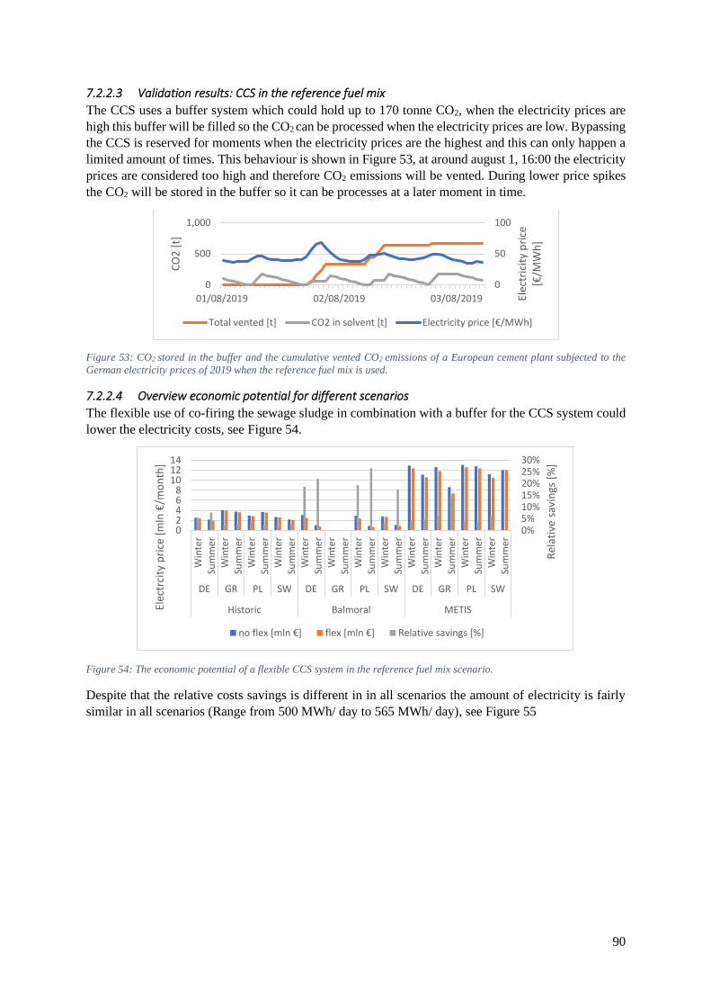
90

7.2.2.3 Validation results: CCS in the reference fuel mix

The CCS uses a buffer system which could hold up to 170 tonne CO2, when the electricity prices are

high this buffer will be filled so the CO2 can be processed when the electricity prices are low. Bypassing

the CCS is reserved for moments when the electricity prices are the highest and this can only happen a

limited amount of times. This behaviour is shown in Figure 53, at around august 1, 16:00 the electricity

prices are considered too high and therefore CO2 emissions will be vented. During lower price spikes

the CO2 will be stored in the buffer so it can be processes at a later moment in time.

Figure 53: CO2 stored in the buffer and the cumulative vented CO2 emissions of a European cement plant subjected to the

German electricity prices of 2019 when the reference fuel mix is used.

7.2.2.4 Overview economic potential for different scenarios

The flexible use of co-firing the sewage sludge in combination with a buffer for the CCS system could

lower the electricity costs, see Figure 54.

Figure 54: The economic potential of a flexible CCS system in the reference fuel mix scenario.

Despite that the relative costs savings is different in in all scenarios the amount of electricity is fairly

similar in all scenarios (Range from 500 MWh/ day to 565 MWh/ day), see Figure 55

0

50

100

0

500

1,000

01/08/2019 02/08/2019 03/08/2019 Elec

tric

ity

pri

ce

[€/M

Wh

]

CO

2 [

t]

Total vented [t] CO2 in solvent [t] Electricity price [€/MWh]

0%5%10%15%20%25%30%

02468

101214

Win

ter

Sum

mer

Win

ter

Sum

mer

Win

ter

Sum

mer

Win

ter

Sum

mer

Win

ter

Sum

mer

Win

ter

Sum

mer

Win

ter

Sum

mer

Win

ter

Sum

mer

Win

ter

Sum

mer

Win

ter

Sum

mer

Win

ter

Sum

mer

Win

ter

Sum

mer

DE GR PL SW DE GR PL SW DE GR PL SW

Historic Balmoral METIS

Rel

ativ

e sa

vin

gs [

%]

Elec

trci

ty p

rice

[m

ln €

/mo

nth

]

no flex [mln €] flex [mln €] Relative savings [%]

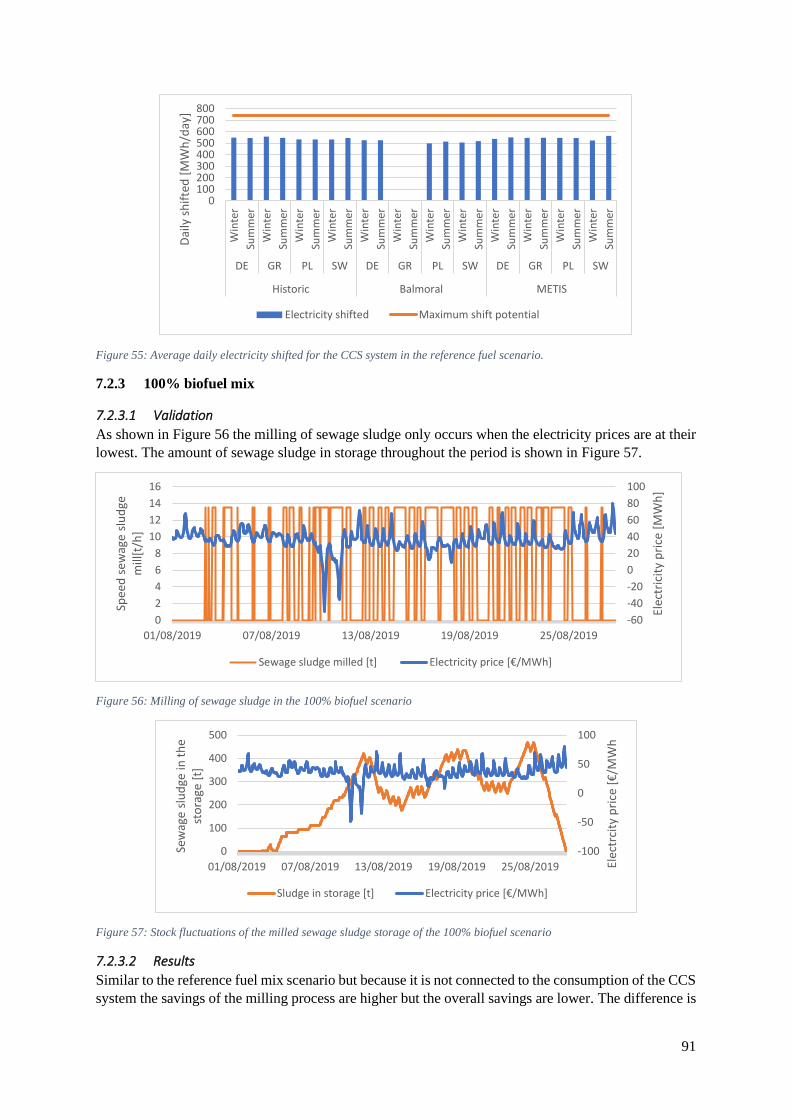
91

Figure 55: Average daily electricity shifted for the CCS system in the reference fuel scenario.

7.2.3 100% biofuel mix

7.2.3.1 Validation

As shown in Figure 56 the milling of sewage sludge only occurs when the electricity prices are at their

lowest. The amount of sewage sludge in storage throughout the period is shown in Figure 57.

Figure 56: Milling of sewage sludge in the 100% biofuel scenario

Figure 57: Stock fluctuations of the milled sewage sludge storage of the 100% biofuel scenario

7.2.3.2 Results

Similar to the reference fuel mix scenario but because it is not connected to the consumption of the CCS

system the savings of the milling process are higher but the overall savings are lower. The difference is

0100200300400500600700800

Win

ter

Sum

mer

Win

ter

Sum

mer

Win

ter

Sum

mer

Win

ter

Sum

mer

Win

ter

Sum

mer

Win

ter

Sum

mer

Win

ter

Sum

mer

Win

ter

Sum

mer

Win

ter

Sum

mer

Win

ter

Sum

mer

Win

ter

Sum

mer

Win

ter

Sum

mer

DE GR PL SW DE GR PL SW DE GR PL SW

Historic Balmoral METIS

Dai

ly s

hif

ted

[M

Wh

/day

]

Electricity shifted Maximum shift potential

-60

-40

-20

0

20

40

60

80

100

0

2

4

6

8

10

12

14

16

01/08/2019 07/08/2019 13/08/2019 19/08/2019 25/08/2019

Elec

tric

ity

pri

ce [

MW

h]

Spee

d s

ewag

e sl

ud

ge

mill

[t/h

]

Sewage sludge milled [t] Electricity price [€/MWh]

-100

-50

0

50

100

0

100

200

300

400

500

01/08/2019 07/08/2019 13/08/2019 19/08/2019 25/08/2019 Elec

trci

ty p

rice

[€

/MW

h

Sew

age

slu

dge

in t

he

sto

rage

[t]

Sludge in storage [t] Electricity price [€/MWh]

92

clearly shown when the model was subjected to the electricity prices of the balmoral model for Sweden

in the winter. In the reference fuel mix the costs savings were negative because the sewage sludge

processes were combined with the CCS system. In the 100% biofuel scenario the relative costs savings

are positive.

Figure 58: Electricity costs and relative savings of milling sewage sludge in the 100% biofuel scenario

The average amount of electricity shifted per day is shown in Figure 59. The electricity that is shifted

ranges from arround 3 MWh/day to 4.2 MWh/day

Figure 59: Average amount of electricity shifted per day when sewage sludge is milled flexibly in the 100% biofuel scenario.

the maximum potential was calculated in RQ3.

7.2.4 Hydrogen processes

The LP used to minimize the electricity cost for the production of hydrogen is validated in paragraph

7.2.4.1 and the results are shown in paragraph 7.2.4.2.

7.2.4.1 Validation

Throughout the whole month the electrolyser provides enough hydrogen for the kiln, this is seen in

Figure 60 because the hydrogen storage never has a negative amount of hydrogen stored. Figure 60 also

shows that hydrogen is being produced and stored when the electricity prices are low and the hydrogen

is used from this storage when the electricity prices are high.

0%5%10%15%20%25%30%35%40%45%

05,000

10,00015,00020,00025,00030,00035,00040,00045,000

Win

ter

Win

ter

Win

ter

Win

ter

Win

ter

Win

ter

Win

ter

Win

ter

Win

ter

Win

ter

Win

ter

Win

ter

DE GR PL SW DE GR PL SW DE GR PL SW

Historic Balmoral METIS

Rel

ativ

e sa

vin

gs [

%]

Elec

trci

ty c

ost

s [€

]

no flex [€] flex [€] Savings [%]

00.5

11.5

22.5

33.5

44.5

5

Win

ter

Win

ter

Win

ter

Win

ter

Win

ter

Win

ter

Win

ter

Win

ter

Win

ter

Win

ter

Win

ter

Win

ter

DE GR PL SW DE GR PL SW DE GR PL SW

Historic Balmoral METIS

Ave

rage

dai

ly s

hif

ted

[M

Wh

/day

]

Electricity shifted Maximum shift potential

93

Figure 60: Behaviour electrolyzer in the summer.

7.2.4.2 Overview economic potential for different scenarios

Using the LP the minimal electricity costs for the different price profiles were calculated, see Figure

61. The scenarios with where the variance in electricity costs the highest also has the highest electricity

saving potential.

Figure 61: Electricity costs for the production of hydrogen of a European cement.

0

10

20

30

40

50

60

70

80

-200

0

200

400

600

800

1000

1200

01/08 02/08 03/08

Elec

tric

ity

pri

ce [

€/M

Wh

]

Hyd

org

en p

rod

uct

ion

[G

J/h

]

Hydrogen storage [GJ]

Electricity price [€/MWh]

0

10

20

30

40

50

60

70

80

0

50

100

150

200

250

300

350

400

450

01/08 02/08 03/08

Elec

tric

ty p

rice

[€

/MW

h]

Hyd

roge

n p

rod

uct

ion

[G

J/h

]

Axis Title

Hydrogen production [GJ]

Electricity price [€/MWh]

0

5

10

15

20

25

Win

ter

Sum

mer

Win

ter

Sum

mer

Win

ter

Sum

mer

Win

ter

Sum

mer

Win

ter

Sum

mer

Win

ter

Sum

mer

Win

ter

Sum

mer

Win

ter

Sum

mer

Win

ter

Sum

mer

Win

ter

Sum

mer

Win

ter

Sum

mer

Win

ter

Sum

mer

DE GR PL SW DE GR PL SW DE GR PL SW

Actual prices 2019 Balmoral model 2045 METIS model 2050

Elec

tric

ity

cost

s [m

ln €

]

No flexibility Moderate flexibility Medium flexibility High flexibility

94

The total average amount of electricity which is shifted throughout the days is shown in Figure 62.

Figure 63: Relative costs savings of the hydrogen scenario.

7.2.5 Overview relative costs savings

The relative costs savings for all flexible technologies are added together to estimate the total absolute

cost savings, for each scenario see Figure 64, Figure 65, Figure 66 and Figure 67. The Reference fuel

mix scenario and the hydrogen scenario both have the highest economic flexibility potential which can

be explained by their high electricity demand, See paragraph 5.3 and high load shift potential see

paragraph 6.2.5. These figures also shows that the Reference fuel mix scenario has similar economic

potential than the hydrogen scenario when subjected to the historic and Balmoral prices. However,

when subjected to the METIS prices the high flexible hydrogen scenario can achieve more total savings.

This is likely due to the high price fluctuations of this model and because the hydrogen scenario has a

large storage and overcapacity installed so it can better handle these fluctuations than the CCS system.

The electrification and 100% biofuel scenario has the lowest economic saving potential because

compared to the other scenarios not much processes could be made flexible.

It should however be stressed that the absolute savings are the savings of the flexible operation

compared to the not flexible scenario. This has the effect that all scenarios are compared to another

reference. The absolute saving potential does not necessarily provide information about which scenario

has the lowest electricity costs. For example, the savings of the hydrogen scenario are higher than the

savings of the electrification scenario. But because the electrification scenario uses almost 50% less

0%2%4%6%8%

10%12%14%16%18%20%

W S W S W S W S W S W S W S W S W S W S W S W S

DE GR PL SW DE GR PL SW DE GR PL SW

Historic Balmoral METIS

Moderate relative saving [%] Medium relative savings [%] High relative savings [%]

Figure 62: Daily electricity shifted when the electrolyser is used flexibly

95

electricity than the hydrogen scenario, the total electricity costs of the electrification scenario would

almost always be lower.

Figure 64: Total electricity costs savings of the reference fuel scenario

Figure 65: Total electricity costs savings of the 100% biofuel scenario

-0.20

0.20.40.60.8

11.21.41.6

Win

ter

Sum

mer

Win

ter

Sum

mer

Win

ter

Sum

mer

Win

ter

Sum

mer

Win

ter

Sum

mer

Win

ter

Sum

mer

Win

ter

Sum

mer

Win

ter

Sum

mer

Win

ter

Sum

mer

Win

ter

Sum

mer

Win

ter

Sum

mer

Win

ter

Sum

mer

DE GE PL SW DE GE PL SW DE GE PL SW

Historic Balmoral METIS AverageAb

solu

te s

avin

gs [

mln

€/m

on

th]

Electrcity costs savings Reference fuel scenario

Generic cement production processes Milling sewage sludge CCS

00.02

0.040.06

0.08

0.1

0.120.14

Win

ter

Sum

mer

Win

ter

Sum

mer

Win

ter

Sum

mer

Win

ter

Sum

mer

Win

ter

Sum

mer

Win

ter

Sum

mer

Win

ter

Sum

mer

Win

ter

Sum

mer

Win

ter

Sum

mer

Win

ter

Sum

mer

Win

ter

Sum

mer

Win

ter

Sum

mer

DE GE PL SW DE GE PL SW DE GE PL SW

Historic Balmoral METIS Average

Ab

solu

te s

avn

gs [

mln

€ /

mo

nth

]

Electrcity costs savings 100% biofuels

Generic cement production processes Milling sewage sludge

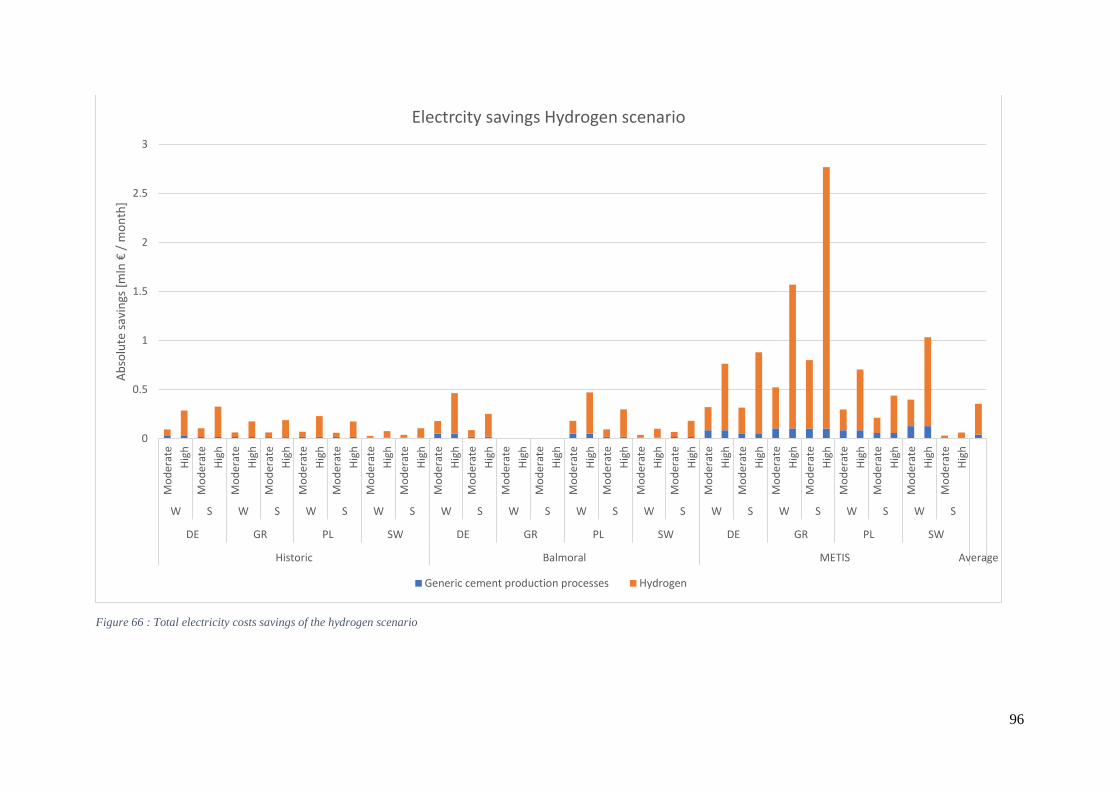
96

Figure 66 : Total electricity costs savings of the hydrogen scenario

0

0.5

1

1.5

2

2.5

3

Mo

der

ate

Hig

h

Mo

der

ate

Hig

h

Mo

der

ate

Hig

h

Mo

der

ate

Hig

h

Mo

der

ate

Hig

h

Mo

der

ate

Hig

h

Mo

der

ate

Hig

h

Mo

der

ate

Hig

h

Mo

der

ate

Hig

h

Mo

der

ate

Hig

h

Mo

der

ate

Hig

h

Mo

der

ate

Hig

h

Mo

der

ate

Hig

h

Mo

der

ate

Hig

h

Mo

der

ate

Hig

h

Mo

der

ate

Hig

h

Mo

der

ate

Hig

h

Mo

der

ate

Hig

h

Mo

der

ate

Hig

h

Mo

der

ate

Hig

h

Mo

der

ate

Hig

h

Mo

der

ate

Hig

h

Mo

der

ate

Hig

h

Mo

der

ate

Hig

h

W S W S W S W S W S W S W S W S W S W S W S W S

DE GR PL SW DE GR PL SW DE GR PL SW

Historic Balmoral METIS Average

Ab

solu

te s

avin

gs [

mln

€ /

mo

nth

]Electrcity savings Hydrogen scenario

Generic cement production processes Hydrogen

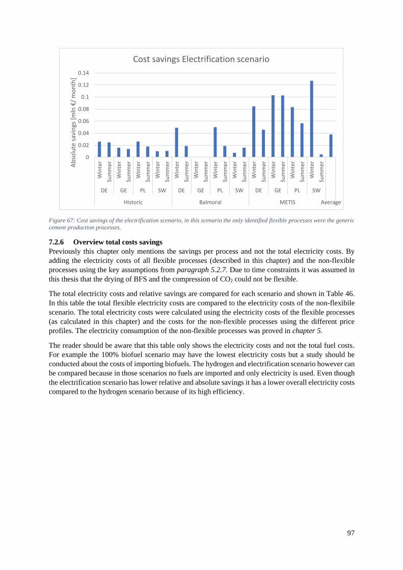
97

Figure 67: Cost savings of the electrification scenario, in this scenario the only identified flexible processes were the generic

cement production processes.

7.2.6 Overview total costs savings

Previously this chapter only mentions the savings per process and not the total electricity costs. By

adding the electricity costs of all flexible processes (described in this chapter) and the non-flexible

processes using the key assumptions from paragraph 5.2.7. Due to time constraints it was assumed in

this thesis that the drying of BFS and the compression of CO2 could not be flexible.

The total electricity costs and relative savings are compared for each scenario and shown in Table 46.

In this table the total flexible electricity costs are compared to the electricity costs of the non-flexibile

scenario. The total electricity costs were calculated using the electricity costs of the flexible processes

(as calculated in this chapter) and the costs for the non-flexible processes using the different price

profiles. The electricity consumption of the non-flexible processes was proved in chapter 5.

The reader should be aware that this table only shows the electricity costs and not the total fuel costs.

For example the 100% biofuel scenario may have the lowest electricity costs but a study should be

conducted about the costs of importing biofuels. The hydrogen and electrification scenario however can

be compared because in those scenarios no fuels are imported and only electricity is used. Even though

the electrification scenario has lower relative and absolute savings it has a lower overall electricity costs

compared to the hydrogen scenario because of its high efficiency.

0

0.02

0.04

0.06

0.08

0.1

0.12

0.14

Win

ter

Sum

mer

Win

ter

Sum

mer

Win

ter

Sum

mer

Win

ter

Sum

mer

Win

ter

Sum

mer

Win

ter

Sum

mer

Win

ter

Sum

mer

Win

ter

Sum

mer

Win

ter

Sum

mer

Win

ter

Sum

mer

Win

ter

Sum

mer

Win

ter

Sum

mer

DE GE PL SW DE GE PL SW DE GE PL SW

Historic Balmoral METIS Average

Ab

solu

te s

avin

gs [

mln

€/

mo

nth

]

Cost savings Electrification scenario

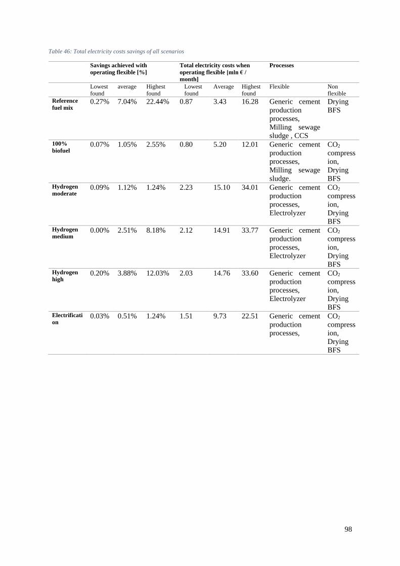
98

Table 46: Total electricity costs savings of all scenarios

Savings achieved with

operating flexible [%]

Total electricity costs when

operating flexible [mln € /

month]

Processes

Lowest

found

average Highest

found

Lowest

found

Average Highest

found

Flexible Non

flexible

Reference

fuel mix 0.27% 7.04% 22.44% 0.87 3.43 16.28 Generic cement

production

processes,

Milling sewage

sludge , CCS

Drying

BFS

100%

biofuel 0.07% 1.05% 2.55% 0.80 5.20 12.01 Generic cement

production

processes,

Milling sewage

sludge.

CO2

compress

ion,

Drying

BFS Hydrogen

moderate 0.09% 1.12% 1.24% 2.23 15.10 34.01 Generic cement

production

processes,

Electrolyzer

CO2

compress

ion,

Drying

BFS Hydrogen

medium 0.00% 2.51% 8.18% 2.12 14.91 33.77 Generic cement

production

processes,

Electrolyzer

CO2

compress

ion,

Drying

BFS Hydrogen

high 0.20% 3.88% 12.03% 2.03 14.76 33.60 Generic cement

production

processes,

Electrolyzer

CO2

compress

ion,

Drying

BFS Electrificati

on 0.03% 0.51% 1.24% 1.51 9.73 22.51 Generic cement

production

processes,

CO2

compress

ion,

Drying

BFS

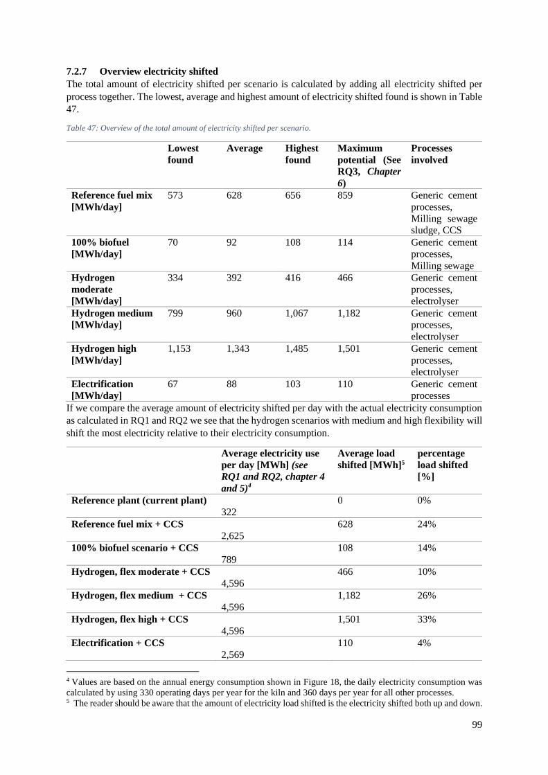
99

7.2.7 Overview electricity shifted

The total amount of electricity shifted per scenario is calculated by adding all electricity shifted per

process together. The lowest, average and highest amount of electricity shifted found is shown in Table

47.

Table 47: Overview of the total amount of electricity shifted per scenario.

Lowest

found

Average Highest

found

Maximum

potential (See

RQ3, Chapter

6)

Processes

involved

Reference fuel mix

[MWh/day]

573 628 656 859 Generic cement

processes,

Milling sewage

sludge, CCS

100% biofuel

[MWh/day]

70 92 108 114 Generic cement

processes,

Milling sewage

Hydrogen

moderate

[MWh/day]

334 392 416 466 Generic cement

processes,

electrolyser

Hydrogen medium

[MWh/day]

799 960 1,067 1,182 Generic cement

processes,

electrolyser

Hydrogen high

[MWh/day]

1,153 1,343 1,485 1,501 Generic cement

processes,

electrolyser

Electrification

[MWh/day]

67 88 103 110 Generic cement

processes

If we compare the average amount of electricity shifted per day with the actual electricity consumption

as calculated in RQ1 and RQ2 we see that the hydrogen scenarios with medium and high flexibility will

shift the most electricity relative to their electricity consumption.

Average electricity use

per day [MWh] (see

RQ1 and RQ2, chapter 4

and 5)4

Average load

shifted [MWh]5

percentage

load shifted

[%]

Reference plant (current plant)

322

0 0%

Reference fuel mix + CCS

2,625

628 24%

100% biofuel scenario + CCS

789

108 14%

Hydrogen, flex moderate + CCS

4,596

466 10%

Hydrogen, flex medium + CCS

4,596

1,182 26%

Hydrogen, flex high + CCS

4,596

1,501 33%

Electrification + CCS

2,569

110 4%

4 Values are based on the annual energy consumption shown in Figure 18, the daily electricity consumption was

calculated by using 330 operating days per year for the kiln and 360 days per year for all other processes. 5 The reader should be aware that the amount of electricity load shifted is the electricity shifted both up and down.

100

7.3 CONCLUSION Based on the results of previous chapters a linear program was constructed which could with help of

different electricity price profiles estimate the electricity costs savings for a European cement plant in

2050. The results of this model were used to answer the research question:

“What is the economic flexibility potential of a carbon neutral cement plant in 2050?”

How the electricity prices would develop in 2050 will be highly uncertain and to incorporate this

uncertainty into the results multiple electricity profiles were used. Electricity prices calculated with

models for 2050 and actual electricity prices from 2019 were used as data sources. A total of 11 price

profiles for 4 different European countries where used where each country represented a specific part

of Europe. Two of the data sources (The historic data and the Balmoral model) provides prices in the

similar range but the average electricity price of the METIS model lies around 5 times higher. Moreover,

the METIS model has larger outliers which greatly increases the economic flexibility potential. The

economic flexibility potential was calculated for all proposed decarbonization pathways of a cement

plant.

The processes: grinding, raw meal milling, cement milling and packaging are processes shared in each

decarbonization scenario and therefore their economic potentials are the same for all decarbonization

scenarios. Based on different electricity prices the monthly savings for these processes range from

€5,000 to almost €130,000 per month. The large difference between these two values clearly shows that

different electricity price profiles have a big impact on the total savings. On average is was calculated

that 10% of the electricity costs for grinding, milling, and packaging could be saved by operating

flexibly and around 90 MWh will be shifted per day.

In both the reference fuel mix scenario and the biofuel scenario sewage sludge will be milled, when this

process is made flexible another €400 to €5,000 could be saved monthly depending on the electricity

price profiles. Because the milling of sewage sludge is connected to the CCS system of the reference

fuel mix scenario there was found the be a slight discrepancy between the milling in the 100% biofuel

scenario and the reference fuel mix scenario. This difference was in most scenarios relatively small and

could therefore be neglected. On average around 14% of the electricity cost for milling could be saved

when the mill is operated flexibly. When the sewage sludge mill is operated flexible around 3.7 MWh

will be shifted per day.

In the reference fuel mix an Amine scrubbing CCS system was used. As mentioned in RQ3 a buffer

will be added to this CCS system so the CO2 from the flue gas can be temporary stored before it is

processed. Assuming electricity is used to supply heat for the CCS system a buffer could greatly reduce

the electricity costs. Because the emissions from biomass are captured in the reference fuel mix scenario

there is also the possibility to let some of the emissions bypass the CCS system. Bypassing introduces

flexibility since the emissions could bypass the whole CCS system when the electricity prices are high

and make up for these emissions by capturing the CO2 from the biofuels when the electricity prices are

low. Depending on the price profiles used a flexible CCS system could save between 0.03 and 1.3

million euro per month with an average of 0.3 million euro. The average relative savings of all price

profiles of a CCS system are around 8% of the electricity costs for a CCS system. When operating the

CCS system flexibly around 536 MWh will be shifted throughout the day which is around 73% of the

maximum load shift potential found in Chapter 6.

In the hydrogen scenario an electrolyser will be used which could generate hydrogen when the

electricity prices are low and store it so it can be used when the prices are high. Because of the

uncertainty related to the storage size and the installed capacity of the electrolyser three different

flexibility potential scenarios were constructed. The average amount of electricity load shifted in the

moderate, medium and high flexibility scenarios was 304 MWh, 871 MWh and 1,255 MWh

respectively which in all scenarios is around 83% of their maximum load shift potential. The average

101

savings of the electricity costs of a electrolyser in the moderate, medium and high flexible scenarios

were calculated to be 2%, 4% and 6% respectively.

Comparing the calculated load shifted electricity with the total electricity consumption for each scenario

the relative load shifting was calculated. The High hydrogen, Medium hydrogen, and reference fuel mix

scenario have the highest relative load shifting of 33%, 26% and 24% respectively. In the 100% biofuel,

moderate hydrogen and electrification scenarios the relative load shifting is lower and around 14%,

10% and 4% of the total electricity consumption, respectively.

Looking at the total electricity costs (flexible and non-flexible processes combined) it was estimated

that the reference fuel mix, 100% biofuel, hydrogen and electrification scenario could save 7.04%,

1.05%, 1.12% and 0.5% on the total electricity costs respectively. If future research concludes that the

drying of BFS and the compression of CO2 could be made flexible these savings could increase.

102

8 DISCUSSION

This study has shown the extent to which a cement plant could apply demand response strategies that

would favour the integration of variable renewable energy sources. Meanwhile, it highlighted the

large uncertainties related to the scope of the study. In the first part (8.1) of this chapter these

uncertainties are discussed, in the second part (8.2) the connection to other studies is highlighted.

8.1 UNCERTAINTIES RELATED TO THIS STUDY The uncertainties related to this study can be categorized as (I) the pathway of decarbonisation of the

cement industry, (II) the development of electricity prices in 2050, (III) the modelling performed, (IV)

the data used to estimate the flexibility potential, and (V) the definition of a carbon neutral cement

plant.

(I) How the cement industry achieves carbon neutrality in 2050 is highly uncertain, and this

uncertainty is incorporated into this thesis by analysing multiple scenarios. For all scenarios, key

assumptions about the used technologies were made to define each scenario. However, it is possible

that a cement plant in 2050 will use different technologies than assumed and thereby changing the

result of this thesis. Probable changes of key parameters and assumptions are listed below

CCS technology

The Amine scrubbing CCS of the reference fuel mix scenario could utilize an energy source different

from electricity. In that case, the flexibility potential would decrease together with the electricity

consumption. It was also assumed that the amine scrubbing CCS system has a capture rate of 100%

but the electricity consumption was based on systems with a lower capture rate (90%). Increasing the

capture rate greatly increases the electricity consumption. Therefore, it is likely that if amine

scrubbing would be used in 2050 the capture rate would remain around 90%. Using a lower capture

rate has the effect that less emissions from the bio-fuels can be bypassed which makes the CCS

system less flexible. A less flexible CCS system would lead to higher electricity costs. However, not

all emission have to be captured to become carbon neutral. Biofuels emissions are considered carbon

neutral and some of the calcination emissions are reabsorbed during the lifecycle of cement, point (V)

addresses the effect of reabsorption more in depth. A brief analysis showed that if more than 6% of

the calcination emissions are absorbed into the cement throughout its lifecycle, the reference fuel mix

scenario will still remain carbon neutral, even though the CCS system only captures 90% of the total

emissions6. If 6% of the calcination emissions are reabsorbed with a capture rate of 90% there is no

possibility for the flue gas to bypass the CCS system and thereby decreasing the flexibility potential.

Oxyfuel CCS technology could be a promising technology too. However, due to time constraints this

was not researched. In an oxyfuel kiln pure O2 is used for combustion which lowers the energy

demand and makes CO2 easier to capture. One study showed that using oxyfuel could make the fuels

54% more efficient (Han et al., 2018) and theoretically, the creation of pure oxygen could be made

flexible (Nimtz & Krautz, 2013).

6 By using the CO2 emissions shown in Figure 17 of chapter 5 and using a capture rate of 90% it was calculated

that only 644 kt of the 715 kt CO2 emitted annually would be captured. Because of the use of biofuels only 670kt

CO2 needs to be captured per year to become carbon neutral. The total calcination emissions were 458 kt of CO2

per year so if 6% of these emissions are reabsorbed into the cement, the plant would still remain carbon neutral.

103

Hydrogen technology

Hydrogen could be imported and thereby the load shift potential would be allocated to the producer of

hydrogen instead of the cement plant.

The usage of BFS as clinker substitute

Because of time constraints it was assumed that the drying of BFS uses electricity and could not be

made flexible. If future research concludes that the drying of BFS could be made flexible than the

flexibility potential could greatly increase. Especially because the drying of BFS contribute to around

10% to 19% of the total electricity demand for all decarbonization scenarios.

The assumed clinker to cement ratio of 50% will likely be higher due to the scarcity of additives. In

fact, a study showed that it is likely that there will be a supply problem of fly-ash and BFS if all

cement plants use this clinker cement ratio (Kermeli et al., 2019; Worrell & Kermeli, 2017).

Especially because the availability of these substitution materials is linked to the steel industry and

amount of coal-fired powerplants available. To decarbonize all industries in 2050 it is likely that most

coal-fired power plants will close and that the size of the steel industry will decrease. Alternative

clinker substitutes are available but they are either expensive, cannot offer the same replacement

ratios or are unavailable in some countries (Kermeli et al., 2019; Worrell & Kermeli, 2017).

CEMBUREAU (2020b) stated that they target for an average clinker cement ratio of 65% in Europe

2050. Clinker production is a highly energy intensive process and therefore the energy consumption

would increase. Moreover, creating more clinkers also increases the calcination emissions and

therefore more electricity will be needed for the CCS systems. A higher clinker ratio could have one

of the following effects on the flexibility.

(1) If the installed capacity would remain similar, producing more clinkers results in less flexibility

for the processes grinding and raw milling. This decrease in flexibility is caused by the increased need

for raw meal which is used to create clinker. The flexibility potential of the cement mill and

packaging unit would remain similar because the same amount of cement is produced. (2) If the

installed capacity increases to match the increased need of raw meal, the absolute savings and amount

of electricity shifted of the grinder and raw mill would increase while the relative savings would

remain similar. However, the electricity consumption of the raw mill and packaging unit would

remain similar.

Electrification scenario

In this thesis no flexibility potential was identified for the electrification scenario. Theoretically, it

should be possible to use a hybrid system where bio-gas or hydrogen could be used to lower the

electricity demand (D. Rennie, personal communication, July 22, 2021). The use of a hybrid system

was researched but no scientific sources were found and therefore it was chosen to exclude it from

this thesis. If the costs of installing a hybrid system are relatively low, a hybrid system could be a

good way of adding flexibility to an electric cement plant, but more research is needed to determine

this.

(II) The economic flexibility potential is largely influenced by the development of electricity prices in

2050. A larger variance in electricity prices throughout the day increases the potential savings on

electricity costs. The electricity prices time series are outputs of models that apply multiple and

different assumptions on the highly uncertain future energy system and climate. All these assumptions

introduce uncertainties which makes the results of these models highly uncertain. To incorporate these

uncertainties, multiple price profiles were used. These assumptions get more certain the closer we get

to 2050. Therefore, it is suggested that both flexibility potential and electricity price projections

studies keep getting conducted so benefits of flexible industries could better be estimated.

104

(III) The aim of the model was to minimize the electricity costs for a month of operations based on

perfect future knowledge. Realistically, a cement plant only has knowledge of the day-ahead prices of

electricity. For more realistic results the cement plant should be modelled per day while using

prediction software to predict the electricity prices for the coming days. Because of the minimization

of electricity costs, the model will never build up stock for the next months because this would require

more energy. Realistically, it could be beneficial to build up stock before the next month especially if

it is expected that the electricity prices would rise. Because of these limitations, it is likely that the

actual costs savings would be lower than calculated.

(IV) Uncertainties concerning the data used to estimate the flexibility potential arise from the fact that

almost no large scale projects were yet conducted to test the feasibility of the decarbonization

technologies. The electricity consumption of these new technologies is estimated using the efficiency

of relatively small pilot projects or estimations found in literature. To decrease these uncertainties,

more research should be conducted on the performances of these decarbonization technologies.

The load shift potential is mainly determined by the capacity factor of the cement plant. Lowering the

capacity factor while still supplying the same amount of cement requires a larger installed capacity

which increases investment costs, not taken into account in this study. More in depth studies should

be conducted to estimate the capacity factor of each production step and storage sizes where the profit

is maximized.

(V) In this thesis, a carbon neutral cement plant is described as a cement plant that does not emit CO2,

excluding emissions from bio-fuels. According to literature CO2 is also being absorbed into the

cement (CEMBUREAU, 2020b; Gartner & Sui, 2017; GCCA, 2020; Xi et al., 2016) but is not

considered in emission inventories nor in this thesis. In 2050, when a carbon neutral cement industry

is envisioned, the amount of possible CO2 uptake should be included in the definition of a carbon

neutral cement plant. The actual amount of uptake varies in the literature from 23% (CEMBUREAU,

2020b) to 100% (GCCA, 2020) of the calcination emissions.

8.2 COMPARISON WITH LITERATURE No studies where found regarding the flexibility of a carbon neutral cement plant. However, studies

about the economic flexibility potential of current cement plants state that it is possible to achieve

electricity savings between 3.7 % and 10% (Lidbetter & Liebenberg, 2014; Summerbell et al., 2017;

Swanepoel, 2012). If we only look at the generic processes of the cement plant (so the same processes

as in a current cement plant) in 2050 and only the historic price profiles this study concludes that

between 1% and 21% with an average of 9% could be saved. Therefore, it is concluded that at least the

costs for the generic cement production processes lie between a feasible range. The difference could be

explained by the use of other price profiles and that this study uses more electricity saving measures.

The results of research question 2, the energy consumption of carbon neutral cement plant, is compared

to similar literature. In the factsheet from the JRC (European Union, 2020) it was found that only using

CCS in combination with fossil fuels slightly lowers the energy consumption of a cement plant. The

same factsheet state that a fully electrified cement plant uses around 60 % energy of that of the reference

plant. Both findings are in line with the results present in this thesis, see chapter 5, Figure 18.

105

9 CONCLUSION

The aim of this research was to estimate the technical and (partially) economical flexibility potential of

a carbon neutral cement plant in 2050. These results are valuable for estimating the role the cement

industry could play in integrating VRES into the mix, but also for helping to map out the costs and

benefits associated with creating a carbon neutral cement plant. The research question this thesis aimed

to answer is:

“What is the flexibility potential of a carbon neutral cement plant in 2050?”

The research was structured into two parts. Part A of the thesis estimated the energy consumption of a

carbon neutral cement plant (RQ1) and how this would develop for four different decarbonization

scenarios (RQ2). Part B of this thesis uses the results of part A to model the technical flexibility potential

(RQ3) and the electricity costs savings of all scenarios (RQ4).

(RQ1) “What are the CO2 emissions and energy consumptions for every production step of a European

cement plant?”

The cement industry is a highly carbon intensive industry and it is responsible for around 4% of the

total global CO2 emissions. Depending on the fuel source, around 40% of the emissions originate from

the combustions of fuels and 60% of the CO2 emissions are released when the semi-finished product

clinker is created. The burning of fuels to create clinker consumes the most energy and it occurs in the

calciner and kiln. Nowadays, electricity accounts for only 8% of the energy consumption and it is

mainly used for milling and to operate the kiln.

(RQ2) “Based on different decarbonization pathways, how does the energy consumption of a European

cement plant change?

To create a carbon neutral cement plant it was assumed that (I) efficiency measures would be

implemented, (II) carbon neutral heating technologies could supply heat to create clinkers, and (III) that

CCS would be implemented to capture the clinker related emissions and, if needed, the CO2 emissions

from fossil fuel combustion. It was assumed that the electricity in 2050 would be supplied by a carbon

neutral power system.

(I) In this study, energy consumption is lowered by decreasing the clinker-to-cement ratio to 50%. By-

products from the steel industry (BFS) are used as clinker replacements in this thesis. By using a lower

clinker to cement ratio and more efficient equipment, the electricity consumption of generic cement

production processes could decrease by 40%. Furthermore, it was assumed that in 2050 the current

cement kilns are replaced by more efficient ones decreasing the energy consumption by 20%.

(II) To become fully carbon neutral a cement plant is likely to decarbonize in 2050 by one of the

following decarbonization pathways:

• Keep using the same fuel mix but install a CCS system to capture the fuel combustion – and

calcination emissions.

• Use biofuels for process heat so only the calcination emissions need to be captured with CCS.

• Use hydrogen that is generated onsite so only the calcination emissions need to be captured

with CCS. Conventional kilns need to be modified to fire hydrogen but it was assumed that the

efficiency would remain the same.

• Use an electric kiln and CCS to capture the calcination emissions. It was assumed that an

electric kiln has a higher efficiency compared to a conventional kiln.

(III) Only using carbon neutral energy sources does not fully decarbonize the cement industry because

of the CO2 emissions released when clinkers are created. Therefore, in all scenarios CCS is needed.

106

When the CO2 that needs to be captured is mixed with other gasses the CO2 needs to be separated before

it can be stored. This separation process greatly increases the electricity consumption and is the case in

the reference fuel mix scenario. Moreover, it was assumed that in the reference fuel mix scenario there

was almost no technological advancements related to CCS technologies. Therefore it was assumed that

the current benchmark technology was used, which is inefficient compared to promising future

technologies. In all other scenarios it was estimated that there were more technological advancements

so that the calcination emissions could be separated from the fuel emissions with help of a direct

capturing unit, creating a pure CO2 stream which is easier to handle. It is estimated that because of the

carbon neutral fuels and pure CO2 emissions the only electricity consumption in these scenario are from

the compression of CO2. The compression of CO2 only consumed 7% of the electricity compared to the

CCS system of the reference fuel mix scenario.

In all decarbonization scenarios the energy consumption of the kiln and the generic cement production

processes decrease due to energy saving measures. However, due to the CCS used in the reference fuel

mix scenario the total energy consumption is similar to the energy consumption of the reference plant.

In the hydrogen scenario the energy consumption is also similar to that of the reference plant due to the

energy loss associated with generating hydrogen. In the 100% biofuel and electrification scenario the

same savings measures were implemented. Because the usages of CCS in the 100% biofuel and

electrification scenario only slightly increases the electricity consumption the overall energy

consumption decreases by as much as 40% compared to the reference cement plant.

With the estimated energy consumption estimated in part A (RQ1 & RQ2) the flexibility potential was

modelled in part B (RQ3 & RQ4).

(RQ3) “What is the technical flexibility potential of a European carbon neutral cement plant in 2050?”

To answer this research question the flexibility of all processes is defined by the maximum amount of

electricity that can be shifted throughout the day.

It is possible for a cement plant to operate flexible mainly because:

• A typical cement plant does not operate at full capacity

• There is enough storage capacity between production steps

• Except for the kiln not all processes happen 24 hours a day and could therefore be shifted

In all scenarios the production of cement could be made flexible but depending on the decarbonization

pathway additional technologies could add to this flexibility. The amine scrubbing CCS system in the

reference fuel mix scenario greatly increases the energy consumption. By implementing a buffer into

the amine scrubbing system load shifting becomes possible. The combination of biofuels and a CCS

systems allows for load shedding by bypassing the CCS system. Moreover, despite that this scenario

uses the most energy only 60% of the energy in this scenario comes from electricity, which lowers the

strain on the electricity grid. Using hydrogen also has a high flexibility potential but because in this

scenario all energy comes from electricity this scenario would put the most stress on the electricity grid.

In the electrification scenario all energy is also provided in the form of electricity, but because of the

higher efficiency there is less electricity needed compared to the hydrogen scenario. No extra flexibility

potential was identified when using an electric kiln. The biofuel scenario has a low flexibility potential

compared to the reference fuel mix and hydrogen scenario, but because of its low energy consumption

and use of fuels it is expected that this scenario has the lowest impact on the electricity grid.

Load shifting can be incentivised by price signals. High electricity prices at certain times could stimulate

to shift processes to times when the electricity prices are low. In RQ4 the economic potential of shifting

these processes will be estimated for all scenarios.

107

(RQ4) “What is the economic flexibility potential of a European carbon neutral cement plant in 2050?”

A linear program was constructed for all decarbonization scenarios to estimate their potential electricity

costs savings. To incorporate the uncertainty of the development of price signals, multiple electricity

price projections were used. By applying these different price signals it was found that on average the

actual amount of electricity shifted ranges from 73% to 90% of the theoretical calculated load shift

potential at RQ3.

By comparing the total electricity costs of a flexible cement plant with the electricity costs of a cement

plant with fixed operating hours the relative and absolute electricity cost savings were calculated for all

decarbonization scenarios.

It was estimated that in the reference fuel mix scenario the relative electricity cost savings is the highest

ranging from 0.27% to 22.44%, with an average of 7.04%. It was calculated that the absolute savings

in this scenario range from €40,000 to €1,375,000 per month with an average of €380,000 per month.

Comparing the electricity shifted to the total electricity consumption shows that around 24% of the

electricity consumption could be shifted.

The hydrogen scenario has the second largest relative electricity costs savings range from 0.09% to

12.03% with an average of 3.88%. This large difference is caused by the uncertainties related to the

installed capacity of the electrolyser and the storage capacity. It was found that the absolute electricity

costs savings in this scenario range from €27,000 to €2,800,000 per month with an average of €350,000

per month. Compared to the total electricity consumption to the electricity shifted it was found that

around 33% for the high flexibility, 26% for the medium flexibility and 14% for the moderate flexibility

scenario could be shifted.

The 100% biofuel scenario has the second lowest relative electricity cost savings ranging from 0.07%

to 2.55% with an average of 1.05%. The absolute savings in this scenario range from €5,000 to

€139,000 per month with an average of €45,000 per month. By comparing the amount of electricity

shifted it was calculated that 14% of the total electricity consumption could be shifted.

The electrification scenario has the lowest relative electricity cost savings ranging from 0.03% to 1.24%

with an average of 0.51%. The absolute electricity costs savings of this scenario range from €4,900 to

€127,000 per month with an average of €42,000 per month. Comparing the total electricity consumption

of this scenario to the amount of electricity shifted shows that only 4% of the consumed electricity could

be shifted.

It should be noted that due to time constraints the flexibility of drying BFS was not researched and

therefore the impact of drying BFS lies outside the scope of this thesis. The higher the flexibility

potential the better the cement plant could help integrating VRES into the electricity mix. However, the

reference fuel mix and 100% biofuel scenario uses less total electricity compared to the other scenarios

and therefore it could prevent the need for new power plants.

It was estimated that despite the energy savings measures, the electricity consumption of a carbon

neutral cement plant would increase mainly because of the need for CCS. By flexible operating the

cement plant electricity costs could be saved while simultaneously favour the integration of VRES.

However, plant operators would only operate flexibly if it is profitable and therefore more research is

needed on the costs associated to conclude if this strategy is profitable.

108

REFERENCES

Afkhami, B., Akbarian, B., Beheshti A., N., Kakaee, A. H., & Shabani, B. (2015). Energy consumption

assessment in a cement production plant. Sustainable Energy Technologies and Assessments, 10,

84–89. https://doi.org/10.1016/j.seta.2015.03.003

Alsop, P. A. (2019). The Cement Plant Operations Handbook. Tradeship Publications Ltf.

Andrew, R. M. (2018). Global CO2 emissions from cement production. Earth System Science Data,

10(1), 195–217. https://doi.org/10.5194/essd-10-195-2018

Arpagaus, C., Bless, F., Uhlmann, M., Schiffmann, J., & Bertsch, S. S. (2018). High temperature heat

pumps: Market overview, state of the art, research status, refrigerants, and application potentials.

Energy. https://doi.org/10.1016/j.energy.2018.03.166

Aspelund, A., & Jordal, K. (2007). Gas conditioning — The interface between CO 2 capture and

transport. 1, 343–354. https://doi.org/10.1016/S1750-5836(07)00040-0

Barberi, P., Bossmann, T., & Fournié, L. (2018). METIS S6: Decentralised heat pumps: system benefits

under different technical configurations. December, 47.

Bataille, C., Åhman, M., Neuhoff, K., Nilsson, L. J., Fischedick, M., Lechtenböhmer, S., Solano-

Rodriquez, B., Denis-Ryan, A., Stiebert, S., Waisman, H., Sartor, O., & Rahbar, S. (2018). A

review of technology and policy deep decarbonization pathway options for making energy-

intensive industry production consistent with the Paris Agreement. Journal of Cleaner Production,

187(April), 960–973. https://doi.org/10.1016/j.jclepro.2018.03.107

Batec. (2014, April 20). Betonherstel HOC-silo’s ENCI - Batec. https://batec.nl/betonherstel-hoc-silos-

enci/

Bičáková, O., & Straka, P. (2012). Production of hydrogen from renewable resources and its

effectiveness. International Journal of Hydrogen Energy, 37(16), 11563–11578.

https://doi.org/10.1016/j.ijhydene.2012.05.047

Bjerge, L., & Brevik, P. (2014). CO 2 Capture in the Cement Industry , Norcem CO 2 Capture.

63(1876), 6455–6463. https://doi.org/10.1016/j.egypro.2014.11.680

Carrasco-maldonado, F., Spörl, R., Fleiger, K., & Hoenig, V. (2016). International Journal of

Greenhouse Gas Control Oxy-fuel combustion technology for cement production – State of the

art research and technology development. International Journal of Greenhouse Gas Control, 45,

189–199. https://doi.org/10.1016/j.ijggc.2015.12.014

CEMBUREAU. (1999). “ BEST AVAILABLE TECHNIQUES ” FOR THE CEMENT INDUSTRY.

December.

CEMBUREAU. (2018). Clinker Substitution. https://lowcarboneconomy.cembureau.eu/5-parallel-

routes/resource-efficiency/clinker-substitution/

CEMBUREAU. (2020a). Cement.

CEMBUREAU. (2020b). Cementing the European Green Deal.

Cement Equipment. (2018). 2018 Target Operating Hours in Cement industry.

https://www.cementequipment.org/home/process-operation-and-important-formulas/2018-

target-operating-hours-cement-industry/

Chalmers, H. (2010). Flexible operation of coal-fired power plant with CO 2 capture (Vol. 2, Issue

February).

Chalmers, H., Leach, M., & Gibbins, J. (2011). Built-in flexibility at retrofitted power plants: What is

109

it worth and can we afford to ignore it? Energy Procedia, 4, 2596–2603.

https://doi.org/10.1016/j.egypro.2011.02.158

Chalmers, H., Leach, M., Lucquiaud, M., & Gibbins, J. (2009). Valuing flexible operation of power

plants with CO 2 capture. Energy Procedia, 1(1), 4289–4296.

https://doi.org/10.1016/j.egypro.2009.02.241

Chemistry Library. (2021). 23.9: Electrolysis of Water - Chemistry LibreTexts.

https://chem.libretexts.org/Bookshelves/Introductory_Chemistry/Book%3A_Introductory_Chem

istry_(CK-12)/23%3A_Electrochemistry/23.09%3A_Electrolysis_of_Water

Cohen, Stuart M., Rochelle, G. T., & Webber, M. E. (2011). Optimal operation of flexible post-

combustion CO2 capture in response to volatile electricity prices. Energy Procedia, 4, 2604–2611.

https://doi.org/10.1016/j.egypro.2011.02.159

Cohen, Stuart M., Rochelle, G. T., & Webber, M. E. (2013). Optimal CO2 capture operation in an

advanced electric grid. Energy Procedia, 37, 2585–2594.

https://doi.org/10.1016/j.egypro.2013.06.142

Cohen, Stuart M, Rochelle, G. T., & Webber, M. E. (2011). Energy Procedia Optimal operation of

flexible post-combustion CO 2 capture in response to volatile electricity prices. Energy Procedia,

4, 2604–2611. https://doi.org/10.1016/j.egypro.2011.02.159

Cohen, Stuart Michael. (2012). A Techno-economic Plant- and Grid-Level Assessment of Flexible CO

2 Capture.

CSI-ECRA. (2017). CSI/ECRA - Technology Papers 2017 Development of State o f the Art Techniques

in Cement Manufacturing: Trying to Look Ahead. Technology Papers, March, 190.

Deolalkar, S. P. (2009). Handbook for designing cement plants. BS publications.

Down to Earth BV. (2013). Integrale Aanpak Energieverbruik ENCI Rotterdam Operationele

procesbesturing en - beheersing. december.

Ellersdorfer, M., & Weiß, C. (2011). Integration of biogas plants in the building materials industry.

1560–1567.

ENCI. (n.d.). Cement productieproces.

ENCI. (2009). MER KLINKER- EN CEMENTPRODUCTIE.

ENCI. (2013). Rotterdam IJmuiden Bedrijfsprofiel.

ENCI. (2017). ENCI Maastricht Veiligheid en milieu. 1–7.

ENCI, & Haskoning. (1997). AANVRAAG VOOR EEN DEEL-REVISIEVERGUNNING IN HET

KADER VAN DE WET MILIEUBEHEER (WM).

ENTSO-E. (2021). Transparency Platform. https://transparency.entsoe.eu/dashboard/show

European Commission. (n.d.). EU climate action and the European Green Deal | Climate Action.

Retrieved February 24, 2021, from https://ec.europa.eu/clima/policies/eu-climate-action_en

European Commission. (2012). Energy roadmap 2050. https://doi.org/10.2833/10759

European Commission. (2015). EU ETS Handbook. Climate Action, 138.

http://ec.europa.eu/clima/publications/docs/ets_handbook_en.pdf

European Commission. (2016). Questions and Answers on Metis.

European Commission. (2018). METIS Studies Study S14 - Wholesale market prices, revenues and risks

for producers with high shares of variable RES in the power system. December.

110

https://ec.europa.eu/energy/sites/ener/files/documents/metis_s14_electricity_prices_and_investo

r_revenue_risks_in_a_high_res_2050.pdf

European Commission. (2020). Deep decarbonisation of industry : The cement sector Headlines

Decarbonisation options.

European Union. (2019). Clean energy for all Europeans. https://doi.org/10.2833/9937

European Union. (2020). Deep decarbonisation of industry : The cement sector.

Falk, H. M. (2011). Monitoring the anaerobic digestion process. Logo_JacobsUniversity.Svg Seite, 17,

55.

Favier, A., Wolf, C. DE, Scrivener, K., & Habart, G. (2018). A sustainable future for the European

Cement and Concrete Industry. https://doi.org/https://doi.org/10.3929/ethz-b-000301843

Ferguson, T. (n.d.). Linear Programming: A consise introduction. https://doi.org/10.1007/978-1-4039-

3769-8_2

Gagg, C. R. (2014). Cement and concrete as an engineering material: An historic appraisal and case

study analysis. Engineering Failure Analysis, 40, 114–140.

https://doi.org/10.1016/j.engfailanal.2014.02.004

Galitsky, C., Price, L., & Nan Zhou. (2008). Guidebook for Using the Tool BEST CEMENT:

Benchmarking and Energy Savings Tool for the Cement Industry. July, 98.

Gartner, E., & Sui, T. (2017). Cement and Concrete Research Alternative cement clinkers. Cement and

Concrete Research. https://doi.org/10.1016/j.cemconres.2017.02.002

Gasunie, & TenneT. (2020). Infrastructure Outlook 2050 Fase II. 68.

GCCA. (2020). GCCA Climate Ambition Statement. https://gccassociation.org/wp-

content/uploads/2020/09/GCCA_ClimateAmbitionStatement_English_Screen_AW.pdf

Gea-bermúdez, J., Græsted, I., Münster, M., Koivisto, M., Gustav, J., Chen, Y., & Ravn, H. (2021). The

role of sector coupling in the green transition : A least-cost energy system development in

Northern-central Europe towards 2050. Applied Energy, 289(March), 116685.

https://doi.org/10.1016/j.apenergy.2021.116685

GNR. (2018). GNR Project. https://gccassociation.org/gnr/

Government of the Netherlands. (2020). Climate policy | Climate change | Government.nl.

Habert, G. (2013). Assessing the environmental impact of conventional and “green” cement production.

In Eco-Efficient Construction and Building Materials: Life Cycle Assessment (LCA), Eco-

Labelling and Case Studies. https://doi.org/10.1533/9780857097729.2.199

Han, S. H., Lee, Y. S., Cho, J. R., & Lee, K. H. (2018). Efficiency analysis of air-fuel and oxy-fuel

combustion in a reheating furnace. International Journal of Heat and Mass Transfer, 121, 1364–

1370. https://doi.org/10.1016/j.ijheatmasstransfer.2017.12.110

Hasanbeigi, A., & Springer, C. (2019). Deep Decarbonization Roadmap for the Cement and Concrete

Industries in California. Global Efficiency Intelligence, September, 47.

Heidelberg cement. (2007). Alternative fuels at ENCI Maastricht. https://exergia.gr/projectsites/ALF-

CEMIND-CD/files/presentations/29-30_study_tour/AF at ENCI Maastricht.pdf

Hills, T., Leeson, D., Florin, N., & Fennell, P. (2016). Carbon Capture in the Cement Industry:

Technologies, Progress, and Retrofitting. Environmental Science and Technology, 50(1), 368–

377. https://doi.org/10.1021/acs.est.5b03508

Hills, T. P., Sceats, M., Rennie, D., & Fennell, P. (2017). LEILAC : Low cost CO 2 capture for the

111

cement and lime industries. Energy Procedia, 114(November 2016), 6166–6170.

https://doi.org/10.1016/j.egypro.2017.03.1753

IEA. (2019). Demand Response.

IEA. (2020a). ETP Clean Energy Technology Guide. https://www.iea.org/articles/etp-clean-energy-

technology-guide

IEA. (2020b). Outlook for biogas and biomethane: Prospects for organic growth.

https://www.iea.org/reports/outlook-for-biogas-and-biomethane-prospects-for-organic-

growth/an-introduction-to-biogas-and-biomethane

International Energy Agency. (2018a). Technology Roadmap.

International Energy Agency. (2018b). Technology Roadmap Low-Carbon Transition in the Cement

Industry.

Joint Research Centre. (2013). BAT document for the production of Cement.

https://doi.org/10.2788/12850

Junginger, M. (2007). Biomass use in the Dutch cement industry ENCI , Maastricht , The Netherlands.

1–6.

Junginger, M., Alakangas, E., Kati, V., & Theulen, J. (2007). Biomass use in the Dutch cement industry

ENCI , Maastricht , The Netherlands. 1–6.

Karlsson, I., Rootzén, J., Toktarova, A., Odenberger, M., Johnsson, F., & Göransson, L. (2020).

Roadmap for decarbonization of the building and construction industry—A supply chain analysis

including primary production of steel and cement. Energies, 13(6).

https://doi.org/10.3390/en13164136

Kemp, R., Barteková, E., & Türkeli, S. (2017). The innovation trajectory of eco-cement in the

Netherlands: a co-evolution analysis. International Economics and Economic Policy, 14(3), 409–

429. https://doi.org/10.1007/s10368-017-0384-4

Kermeli, K., Edelenbosch, O. Y., Crijns-Graus, W., van Ruijven, B. J., Mima, S., van Vuuren, D. P., &

Worrell, E. (2019). The scope for better industry representation in long-term energy models:

Modeling the cement industry. Applied Energy, 240(January), 964–985.

https://doi.org/10.1016/j.apenergy.2019.01.252

Koohi-fayegh, M. A. R. S. (2016). The prospects for hydrogen as an energy carrier : an overview of

hydrogen energy and hydrogen energy systems. Energy, Ecology and Environment, 1(1), 10–29.

https://doi.org/10.1007/s40974-016-0005-z

Koring, K., Hoening, V., Hoppe, H., Horsch, J., Suchak, C., Klevens, V., & Emberger, B. (2013).

DEPLOYMENT OF CCS IN THE CEMENT INDUSTRY. December.

Kudra, T. (2012). Drying Technology : An International Journal Energy Performance of Convective

Dryers Energy Performance of Convective Dryers. February 2013, 37–41.

https://doi.org/10.1080/07373937.2012.690803

Lidbetter, R. T., & Liebenberg, L. (2014). Load-shifting opportunities for a typical South African

cement plant plants. January 2011.

Lowe, C., Brancaccio, N., Batten, D., Leung, C., & Waibel, D. (2011). Technology assessment of

hydrogen firing of process heaters. Energy Procedia, 4, 1058–1065.

https://doi.org/10.1016/j.egypro.2011.01.155

Lukovic, M. (2016). Carbonation of cement paste : Understanding , challenges , and opportunities.

117, 285–301. https://doi.org/10.1016/j.conbuildmat.2016.04.138

112

Madeddu, S., Ueckerdt, F., Pehl, M., Peterseim, J., Lord, M., Kumar, K. A., Krüger, C., & Luderer, G.

(2020). The CO2reduction potential for the European industry via direct electrification of heat

supply (power-to-heat). Environmental Research Letters, 15(12). https://doi.org/10.1088/1748-

9326/abbd02

Madlool, N. A., Saidur, R., Hossain, M. S., & Rahim, N. A. (2011). A critical review on energy use and

savings in the cement industries. Renewable and Sustainable Energy Reviews, 15(4), 2042–2060.

https://doi.org/10.1016/j.rser.2011.01.005

Manic, E., Mitrovic, D., & Popovic, S. (2017). The European economic space: New aspects of

regionalization. Glasnik Srpskog Geografskog Drustva, 97(1), 57–80.

https://doi.org/10.2298/gsgd1701057m

Mason, A. J. (2012). OpenSolver - An Open Source Add-in to Solve Linear and Integer Progammes in

Excel (pp. 401–406). https://doi.org/10.1007/978-3-642-29210-1_64

Mathisen, A. (2019). Combined calcination and CO2 capture in cement clinker production by use of

electrical energy COMBINED CALCINATION AND CO 2 CAPTURE IN CEMENT CLINKER.

February 2020.

McInnis cement. (2021). The Project. https://mcinniscement.com/the-projects/#the-plant

Metz, B., Davidson, O., de Conick, H., Loos, M., & Meyer, L. (2015). CARBON DIOXIDE CAPTURE.

Müller-Langer, F., Majer, S., & O’Keeffe, S. (2014). Benchmarking biofuels—a comparison of

technical, economic and environmental indicators. Energy, Sustainability and Society, 4(1), 1–14.

https://doi.org/10.1186/s13705-014-0020-x

Nimtz, M., & Krautz, H. J. (2013). Flexible operation of CCS power plants to match variable renewable

energies. Energy Procedia, 40, 294–303. https://doi.org/10.1016/j.egypro.2013.08.034

Novem. (2016). Sewage sludge : from residue to fuel and raw material.

Nsair, A., Cinar, S. O., Alassali, A., Qdais, H. A., & Kuchta, K. (2020). Operational Parameters of

Biogas Plants: A Review and Evaluation Study. Energies, 13(15).

https://doi.org/10.3390/en13153761

Obrist, M. D., Kannan, R., Schmidt, T. J., & Kober, T. (2021). Decarbonization pathways of the Swiss

cement industry towards net zero emissions. Journal of Cleaner Production, 288, 125413.

https://doi.org/10.1016/j.jclepro.2020.125413

Our World in Data. (2021). CO2 emissions by fuel.

Perez-Linkenheil. (2019). Update December 2019 – EU Energy Outlook 2050.

Platform, E. B. T. (2012). Biomass with CO2 Capture and Storage ( Bio-CCS ) The way forward for

Europe.

Plaza, M. G., Martínez, S., & Rubiera, F. (2020). CO2 Capture, Use, and Storage in the Cement

Industry: State of the Art and Expectations. Energies, 13(21), 5692.

https://doi.org/10.3390/en13215692

Power Correction Systems. (2004). BUILDING MATERIALS INDUSTRIAL TECHNOLOGIES SMALL

VSK CEMENT & CLINKER GRINDING PLANTS P OWER CORRECTION SYSTEMS L OS

ANGELES , CA USA An Introduction to Cement Plants. 310, 1–12.

Pretorius, J. (2020). Volumetric Scan of Clinker Silo | LinkedIn.

https://www.linkedin.com/pulse/volumetric-scan-clinker-silo-jason-

pretorius/?articleId=6634016901154648064

Rao, L., Rivard, F., & Carabin, P. (2013). Thermal plasma torches for metallurgical applications. TMS

113

Annual Meeting, 57–65. https://doi.org/10.1002/9781118663448.ch8

Rijkswaterstaat. (n.d.). Actueel Hoogtebestand Nederland | Rijkswaterstaat. Retrieved April 21, 2021,

from https://www.rijkswaterstaat.nl/zakelijk/open-data/actueel-hoogtebestand-nederland

Ritchie, H., & Roser, M. (2020). Renewable Energy. Our World in Data.

https://ourworldindata.org/renewable-energy

Rogers, L. (2018). Climate change: The massive CO2 emitter you may not know about - BBC News.

https://www.bbc.com/news/science-environment-46455844

Roussanaly, S., Fu, C., Voldsund, M., & Anantharaman, R. (2017). Techno-economic analysis of MEA

CO 2 capture from a cement kiln – impact of steam supply scenario. Energy Procedia, 114(1876),

6229–6239. https://doi.org/10.1016/j.egypro.2017.03.1761

Schneider, M. (2015). Process technology for efficient and sustainable cement production. Cement and

Concrete Research, 78, 14–23. https://doi.org/10.1016/j.cemconres.2015.05.014

Schorcht, F., Kourti, I., Scalet, B. M., Roudier, S., & Sancho, L. D. (2013). Best Available Techniques

(BAT) Reference Document for the Production of Cement, Lime and Magnesium Oxide. In

European Commission. https://doi.org/10.2788/12850

Scrivener, K. L., John, V. M., & Gartner, E. M. (2018). Eco-efficient cements: Potential economically

viable solutions for a low-CO2 cement-based materials industry. Cement and Concrete Research,

114, 2–26. https://doi.org/10.1016/j.cemconres.2018.03.015

Shepherd, S. P. (2014). A review of system dynamics models applied in transportation. 2(2), 83–105.

https://doi.org/10.1080/21680566.2014.916236

Sijm, J., Gockel, P., van Hout, M., Özdemir, Ö., van Stralen, J., Smekens, K., van del Welle, A., de

Joode, J., van Westering, W., & Musterd, M. (2017). Demand and supply of flexibility in the power

system of the Netherlands ,.

Summerbell, D. L., Khripko, D., Barlow, C., & Hesselbach, J. (2017). Cost and carbon reductions from

industrial demand-side management: Study of potential savings at a cement plant. Applied Energy,

197, 100–113. https://doi.org/10.1016/j.apenergy.2017.03.083

Suraj, S., & Sentil, K. (2016). DEMAND SIDE MANAGEMENT : DEMAND RESPONSE ,

INTELLIGENT ENERGY SYSTEMS. Internation Journal of Electrical Engineering &

Technology, 10(1), 17–23.

Swanepoel, J. A. (2012). Modelling for integrated energy optimisation in cement production plants

Modelling for integrated energy optimisation in cement production plants. November.

Tait, P., Buschle, B., Milkowski, K., Akram, M., & Pourkashanian, M. (2018). International Journal of

Greenhouse Gas Control Flexible operation of post-combustion CO 2 capture at pilot scale with

demonstration of capture-e ffi ciency control using online solvent measurements. International

Journal of Greenhouse Gas Control, 71(March), 253–277.

https://doi.org/10.1016/j.ijggc.2018.02.023

Thomas, C., Sebastian, R., Patrick, S., & Ken, S. (2020). Laying the foundation for zero-carbon cement.

van Dijk, H. (n.d.). enci Maastricht. Retrieved April 21, 2021, from http://www.bouwmachinesvantoen-

archief.nl/bedrijvenpagina/Enci/enci.htm

van Dijk, H. (2018). Maastricht - ENCI groeve.

http://www.bouwmachinesvannu.nl/nederland/maastricht/maastricht.enci.sjabloon.htm

Vattenfall. (2019). Vattenfall and Cementa take the next step towards a climate neutral cement.

https://group.vattenfall.com/press-and-media/pressreleases/2019/vattenfall-and-cementa-take-

the-next-step-towards-a-climate-neutral-cement

114

Vreuls, H. H. . (2004). The Netherlands: list of fuels and standard CO 2 emission factors. Vrom,

December 2004, 12. www.broeikasgassen.nl

Wang, Y., Zhao, L., Otto, A., Robinius, M., & Stolten, D. (2017). A Review of Post-combustion CO 2

Capture Technologies from Coal-fired Power Plants. Energy Procedia, 114(November 2016),

650–665. https://doi.org/10.1016/j.egypro.2017.03.1209

Waterschapsbedrijf Limburg. (2013). Mededeling aan het AB. https://docplayer.nl/18395174-

Mededeling-aan-het-ab.html

Worrell, E., & Kermeli, K. (2017). MEETING OUR MATERIAL SERVICES WITHIN PLANETARY

BOUNDARIES. 461–470.

Worrell, E., Price, L., Martin, N., Hendriks, C., & Meida, L. O. (2001). Carbon Dioxide Emission from

the Global Cement Industry. November. https://doi.org/10.1146/annurev.energy.26.1.303

Xavier, C., & Oliveira, C. (2021). Decarbonisation options for the Dutch Cement Industry. February,

63. https://www.pbl.nl/sites/default/files/downloads/pbl-2021-decarbonisation-options-for-the-

dutch-cement-industry-4339.pdf

Xi, F., Davis, S. J., Ciais, P., Crawford-brown, D., Guan, D., Pade, C., Shi, T., Syddall, M., Lv, J., Ji,

L., Bing, L., Wang, J., & Wei, W. (2016). Substantial global carbon uptake by cement

carbonation. 1(November). https://doi.org/10.1038/NGEO2840

Zhao, X., He, B., Xu, F., Lai, L. L., Yang, C., Lu, S., & Li, D. (2014). A Model of Deman Response

Scheduling for Cement Plant. IEEE Internation Conference on Systems, Man, and Cybernetics,

3042–3047.