Estudos e Documentos de Trabalho

Working Papers

16 | 2010

FISCAL STIMULUS IN A SMALL EURO AREA ECONOMY

Vanda AlmeidaGabriela Castro

Ricardo Mourinho FélixJosé Francisco Maria

July 2010

The analyses, opinions and fi ndings of these papers represent the views of the authors, they are not necessarily those of the Banco de Portugal or the Eurosystem.

Please address correspondence to

Vanda Almeida

Banco de Portugal, Av. Almirante Reis no. 71, 1150-012 Lisboa, Portugal;

Tel.: 351 21 313 0136, vralmeida@bportugal.pt

BANCO DE PORTUGAL

Edition

Economics and Research Department

Av. Almirante Reis, 71-6th

1150-012 Lisboa

www.bportugal.pt

Pre-press and Distribution

Administrative Services Department

Documentation, Editing and Museum Division

Editing and Publishing Unit

Av. Almirante Reis, 71-2nd

1150-012 Lisboa

Printing

Administrative Services Department

Logistics Division

Lisbon, July 2010

Number of copies

170

ISBN 978-989-678-037-1

ISSN 0870-0117

Legal Deposit no. 3664/83

Fiscal stimulus in a small euro area economy∗

Vanda Almeida Gabriela Castro Ricardo Mourinho Felix

Jose Francisco Maria

Economics and Research Department, Banco de Portugal†

July 21, 2010

Abstract

The international economic and financial crisis elicited an intensive debate on fiscal

stimulus programmes. Although the topics have been diverse, most of the research

is focused on large countries, some of them in autarky. The literature covering small

economies is thinner and for those integrated in a monetary union is virtually non-

existent. This paper is a contribution to fill this gap. The discussion draws on a

New-Keynesian general equilibrium model introduced in Almeida, Castro and Felix

(2008), which features a small euro area economy. Contrary to most of the literature

that considers infinitely lived households, the model features stochastic finite lifetime

households following Blanchard (1985), which are a source of non-Ricardian behaviour

and allow for pinning-down the steady state net foreign asset position endogenously.

Since in a small euro area economy monetary policy is not an available business cycle

stabilisation tool, the use of fiscal policy to pursue this goal seems the only alter-

native. The results reveal that permanent government expenditure increases should

be avoided, as opposed to temporary stimulus. This outcome is identical to the one

obtained in the literature for large economies. Lags in the program implementation

and limited credibility can however undermine the objectives of a temporary stimu-

lus. In particular, in financial distress circumstances, under which the stimulus may

trigger a hike in the country’s risk premium, the effectiveness of the stimulus might

be negligible.

Keywords: fiscal stimulus; fiscal multiplier; DSGE model; small-open economy.

JEL classification numbers: E62, F41, H62

∗This article largely benefitted from the discussion in the December 2009 meeting of the WGEM at theEuropean Central Bank we are indebted to all participants. We would like to thank to Juha Kilponen,Massimiliano Pisani and Vıtor Gaspar for the valuable comments and suggestions. The views expressedin this paper are those of the authors and do not necessarily reflect the views of Banco de Portugal. Anyerrors and mistakes remain ours.†Address for correspondence: Banco de Portugal, Departamento de Estudos Economicos, Rua

Francisco Ribeiro, 2, 1150-165 Lisboa. E-mails: vralmeida@bportugal.pt, ggcastro@bportugal.pt, rfe-lix@bportugal.pt and jfrmaria@bportugal.pt.

1

1 Introduction

The international economic and financial crisis elicited an intensive debate and research on

the impact of fiscal stimulus programmes. The analysis using general equilibrium models

was wide open, and included the assessment of temporary vs. permanent fiscal stimulus,

the key role of private demand (in particular the response of households consumption),

the implications of standard monetary policy reactions vs. the binding zero lower bound,

the assessment of alternative fiscal policy instruments, the analysis of both supply and

demand-side impacts and credibility issues, among others. Without completeness, relevant

studies include Christiano, Eichenbaum and Rebelo (2009), Eggertsson (2009), Freedman,

Kumhof, Laxton and Lee (2009), Hall (2009), Kumhof, Muir, Freedman, Mursula and

Laxton (2009), Cogan, Cwik, Taylor and Wieland (2009), and Erceg and Linde (2010).

The relative performance of seven structural models is presented in Coenen, Erceg, Freed-

man, Furceci, Kumhof, Lalonde, Laxton, Linde, Mourougane, Muir, Mursula, de Resende,

Roberts, Roeger, Snudden, Trabandt and in’t Veld (2010).

So far the debate seems to have been focused primarily in large economies with in-

dependent monetary policy reaction functions guided by Taylor-type rules, some of them

operating in autarky. The literature becomes thinner if one moves into the small open econ-

omy (henceforth SOE) environment, and is virtually non-existent in the case of economies

integrated in monetary unions. An exception can be found in Kumhof and Laxton (2009),

in which the impact of a fiscal stimulus on the current account was discussed for both the

SOE and large economy cases. It is well known that in a SOE operating in a complete

markets framework, households and the government can buy insurance against all states

of nature without affecting world prices of contingent claims and that in this case optimal

fiscal policy corresponds to a fully-fledged tax smoothing (Goodfriend and King 2001).

However, this is hardly the case for many small euro area economies, in which the access

to world markets is intermediated by a few domestic banks and, therefore, country risk

is highly concentrated, which may lead to risk discrimination in international markets,

thereby invalidating the complete markets assumption.

This article widens the fiscal stimulus discussion by focusing on a SOE integrated in

the euro area and represents a contribution to fill the aforementioned gap in the debate

over fiscal stimulus programmes. The discussion is based on PESSOA, a New-Keynesian

overlapping generations model introduced in Almeida et al. (2008), whose structure draws

on several contributions, notably Kumhof and Laxton (2007a). The general equilibrium

model was designed and calibrated to fit the characteristics of a SOE integrated in a

monetary union, under the assumption that international trade in goods and assets is

only performed with the rest of the union. The economy is assumed to be small enough

to have negligible impact in the union aggregates and ultimately in monetary authority

decisions. Therefore, all foreign variables, namely foreign interest rates, output and prices,

are assumed to be exogenous, as in Adolfson, Laseen, Linde and Villani (2007). Hence,

nominal stability is ensured by the full credibility of the inflation objective set by the

2

monetary authority. In addition, the dynamic stability stems from large elasticities of real

trade variables to real exchange rate fluctuations. In the presence of a shock (be it a real or

a relative price shock), the adjustment to the long-run equilibrium requires adjustments

in domestic real variables and relative prices. The model operates de facto like a real

model (similarly to a fully credible fixed nominal exchange rate model), since domestic

price levels are pinned down by the external constraint that sets a unique steady-state

real exchange rate. To use an expression from Giavazzi and Pagano (1988), the SOE in

PESSOA is effectively “tying its hands” with the rest of the euro area. Also noteworthy is

the existence of a foreign risk premium that allows for the existence of a spread between

domestic and foreign interest rate.

Contrary to most DSGE models in the literature on SOE, PESSOA is intrinsically non-

Ricardian, featuring stochastic finite lifetime households (Blanchard 1985, Yaari 1965),

distortionary taxation and a share of liquidity constrained households (Galı, Lopez-Salido

and Valles 2007). These, coupled with a rich fiscal block, make the model particularly

suited to analyse fiscal policy issues. In particular, the stochastic finite lifetime framework

creates a non-trivial role for fiscal policy over the medium and long-run, introducing a

source of non-Ricardian behaviour absent in the workhorse infinitely lived agents model.

In addition, the Blanchard-Yaari framework allows for the endogenous determination of

the net foreign asset position (Harrison, Nikolov, Quinn, Ramsay, Scott and Thomas 2005),

thereby delivering a more realistic co-movement between public debt and the net foreign

asset position, in contrast with the infinitely lived agents case (Schmitt-Grohe and Uribe

2003).

The outcome of a fiscal stimulus in a SOE operating in a monetary union depends

upon several factors. Fiscal policy management has operational limits not only due to the

need of ensuring a sustainable public debt path, but also by possible institutional limits,

which in the case of the euro area are imposed by the Stability and Growth Pact. Other

conditioning factors are the degree of credibility of the domestic fiscal authorities and the

nature of the fiscal stimulus. This article shows that while temporary boosts under full

credibility may be used to achieve macroeconomic stabilisation goals, the permanent case

should be avoided, a result similar to the one encountered for large economies (Cogan

et al. 2009, Freedman, Kumhof, Laxton and Lee 2009, Coenen et al. 2010). The fiscal

stimulus outcome in a SOE is also conditioned by a timely implementation of the pro-

gramme, a result also highlighted in the literature (Erceg and Linde 2010). Finally, this

article also claims that when a temporary fiscal policy is not conducted under full cred-

ibility, either because the stimulus is perceived as being permanent, at least initially, or

because the economy may face an higher risk premium, which may be conditioned by the

initial public debt levels, then the macroeconomic stabilisation goals may be hindered. If

the implementation of a fiscal stimulus programme triggers a sharp increase in the risk

premium, it may partially backfire the intentions behind the programme.

The paper is organized as follows. The model is presented in section 2. A special focus

is placed on the fiscal block and on its non-Ricardian features. Section 3 evaluates the

3

impact of five temporary fiscal measures under full credibility and timely implementation:

(i) an increase in government consumption; (ii) an increase in general transfers (transfers

to all households); (iii) an increase in targeted transfers (transfers to liquidity-constrained

households); (iv) a decrease in labour income tax; and (v) a decrease in private consump-

tion tax. Section 3 also evaluates the impact of implementation lags and of a permanent

stimulus. Section 4 uses the model to analyse the impact of a fiscal stimulus under limited

credibility, and section 5 concludes.

2 A model for a small euro area economy

This section presents PESSOA, the New-Keynesian dynamic general equilibrium model

behind the analysis of the macroeconomic impact of the fiscal stimulus. The model was

introduced and calibrated for Portugal in Almeida et al. (2008) and used to analyse shocks

that hit the Portuguese economy over the last decade in Almeida, Castro and Felix (2009).

It can however be easily re-calibrated to fit the characteristics of any other small euro area

economy. The model has intrinsic non-Ricardian features largely inspired in the IMF’s

Global Integrated Monetary and Fiscal model presented in Kumhof and Laxton (2007a).

The current setup was enhanced to allow for richer fiscal policy simulations. The SOE

structure implies assuming that the rest of the monetary union is not affected by domestic

shocks. This is tantamount to say that union aggregates and, therefore, monetary policy

decisions are orthogonal to developments in the SOE, as in Adolfson et al. (2007).

It is well known that breaking the Ricardian equivalence is of paramount importance

to generate realistic impulse response functions of private consumption in the advent of

a fiscal shock (Blanchard 1985, Galı et al. 2007). Contrary to most DSGE models in

the literature on SOE, PESSOA is intrinsically non-Ricardian, featuring: finitely-lived

households in line with the stochastic lifetime framework proposed by Blanchard (1985)

and Yaari (1965); distortionary taxation on households consumption, labour and capital

income; and liquidity constrained households as in Galı et al. (2007). The fiscal block of

the model is rich enough to account for several types of distortionary taxation, lump-sum

transfers to households (to all or to a targeted group), and government expenditure.

This setup generates a non-trivial role for fiscal policy not only in the short-run but also

in the medium and long-run. As clarified in Frenkel and Razin (1996) and in Kumhof and

Laxton (2009), the finitely lived agents framework implies that households discount future

events at a higher rate than the Government (the so-called over-discounting behaviour).

This creates sizeable wealth effects of public debt, which are absent in the workhorse

infinitely-lived agent framework. In particular, households strongly prefer debt issuance

to tax financing of Government expenditure, since they attach a positive probability to

the fact that they might not be around in the future when taxes required to meet debt

issued today are levied. It should be mentioned that technically it is not the event that

current generations will die that generates the non-Ricardian effect, but rather the fact

that future generations will bear some of the tax burden (Buiter 1988). In addition, the

4

Blanchard-Yaari framework allows for the endogenous determination of the net foreign

asset position (Harrison et al. 2005), since in a finite lifetime the amount of assets/debt

that a household can accumulate is inevitably limited by life expectancy.1 This represents

an appealing feature for the simulation of permanent fiscal shocks, since it generates a

positive correlation between public debt and the net foreign debt position of the economy.

On the contrary, in the workhorse infinitely lived agents model, the steady-state net foreign

asset position is pinned down exogenously (Schmitt-Grohe and Uribe 2003), implying

that changes in steady-state public debt are fully offset by private saving and are, by

assumption, uncorrelated with the net foreign debt.

Since PESSOA is designed for a SOE integrated in a monetary union, the adjustment

mechanism of the economy to domestic shocks is rather different from the standard setup,

in which monetary policy and real interest rate movements are crucial to render the model

dynamically stable. In PESSOA, monetary policy is trivial in the sense that the domestic

interest rate is orthogonal to domestic shocks and can only deviate from the rest of the

union rate by a risk premium that is assumed to be exogenous. This implies that domestic

shocks affecting domestic inflation developments tend to generate powerful effects on the

real interest rate, amplifying the fluctuations of the economy. The dynamic stability of

the model is ensured instead by an active role of the real exchange rate (which in the case

of an irrevocably fixed nominal exchange rate simply reflects the relative price of domestic

goods vs. foreign goods), in the adjustment of international trade in goods and assets.

Domestic agents in PESSOA are assumed to only trade in goods and assets/debt with

agents in the monetary union. Therefore, real exchange rate fluctuations have sizeable

impacts on competitiveness, trade and thus in the net foreign asset/debt position of the

economy. This position is pinned down in the steady state by the foreign asset/debt level

constraint and its impact in households financial wealth (and, ultimately, in consumption).

Since foreign prices developments are assumed to be independent of domestic shocks, the

real exchange rate pins down uniquely the domestic price level.

PESSOA features a number of nominal and real rigidities and frictions that give rise to

realistic short-run impulse functions. On the nominal side, there is differentiation in the

labour and product markets, allowing for monopolistic competition and staggered wage

and price inflation. On the real side, the model incorporates external habit formation,

and adjustment costs on investment and import contents.

The model is populated by households, which will be presented in detail in subsection

2.1, unions, presented in subsection 2.2, and firms (intermediate goods producers and final

goods producers), which will be presented in subsection 2.3. All these agents interact with

a Government, which is described in subsection 2.4. The rest of the world, corresponding

to the rest of the monetary union, is presented in subsection 2.5, while the market clearing

conditions are presented in section 2.6. The model is calibrated, as detailed in subsection

1It should be pointed out that by definition a SOE does not affect the world investment-savings balanceand, therefore, the world real interest rate. Hence, infinitely lived agents will be able to borrow or lendin infinite amounts that can be paid or received in the indefinite future. For further details refer to Barroand Sala-i-Martin (1995).

5

2.7.

2.1 Households

Households evolve in line with the overlapping generations scheme first proposed in Blan-

chard (1985). All of them have a finite lifetime, facing an instant probability of death 1−θin each period (θ is the probability of surviving between two consecutive periods), which is

constant throughout life, independent of age, and equal for all households.2 However, the

overall size of the population is assumed to remain constant and equal to N households,

implying that in each period N(1− θ) households die and the same number of households

is born. In addition, two types of households coexist: type A, the asset holders, who

can access asset/debt markets and perform both intra and inter-temporal optimisation,

smoothing out their consumption over lifetime by trading assets; and type B, the liquid-

ity constrained households that do not access asset/debt markets and are, therefore, not

allowed to engage in inter-temporal optimisation, consuming all of their income in each

and every period as in Galı et al. (2007). The share of type B households is assumed to

be ψ, implying that in each period there coexist N(1− ψ) households holding assets and

Nψ liquidity constrained households.

A representative household of type H ∈ {A,B} with age a derives utility from con-

sumption, CHa,t, and leisure, 1 − LHa,t, according to a CRRA utility function (with LHa,t

representing labour supply). The household’s expected lifetime utility is:

Et

∞∑s=0

(βθ)s1

1− γ

( CHa+s,t+s

HabHa+s,t+s

)ηH(1− LHa+s,t+s)

1−ηH

1−γ

(1)

where Et is the expectation operator, 0 ≤ β ≤ 1 stands for the standard time discount

factor, γ > 0 is the coefficient of risk aversion and 0 ≤ ηH ≤ 1 is a distribution pa-

rameter. HabHt represents habits, defined in per capita terms as[CAt−1/(N(1− ψ))

]vand[

CBt−1/(Nψ)]v

for type A and B households, respectively, with parameter 0 ≤ v ≤ 1

controlling for the degree of habit persistence.3

Households of type A save in both domestic and foreign government bonds, Ba,t and

B∗a,t, which yield gross nominal interest rates it and i∗t , respectively, from period t to

period t+ 1 (by convention, it is paid at the beginning of period t+ 1). Domestic public

debt is assumed to be solely held by domestic agents (full home bias). Besides returns

from financial assets, these households also receive labour income, earning a wage rate,

Wt, adjusted by the household’s respective productivity, Φa = kχa, where k is a scaling

2The probability of an individual dying after t periods of life is equal to (1 − θ)θt−1 and the expectedlife horizon at any point in time is equal to (1 − θ)−1. Probability 1 − θ can also be taken as a proba-bility of “economic death” or the degree of “myopia” (Blanchard 1985, Frenkel and Razin 1996, Harrisonet al. 2005, Bayoumi and Sgherri 2006). It represents the inverse of the average planning horizon of thehousehold, which is likely to be far more shorter than its whole lifetime. Bayoumi and Sgherri (2006)present econometric evidence for the US.

3Aggregation across generations is made possible by assuming that habits are multiplicative instead ofadditive. However, it should be recognised that this generates a low habit persistence.

6

factor and 0 ≤ χ ≤ 1 the labour productivity rate of decay per period that mimics life-

cycle profile. Furthermore, they receive dividends from firms and from labour unions

(representing a wage premia that will be motivated later on). These are represented by

DAa,t(x) where x can be: intermediate goods producer of tradable (T ) and non-tradable

goods (N ), final goods producer of private consumption (C), government consumption

(G), capital (I), or export goods (X ), and labour unions (U). Finally, they are taxed by

the government in their consumption and labour activities by τC,t and τL,t, respectively,

and receive transfers from the domestic Government and from abroad, TRGAt and TRXAt ,

respectively.

The asset holders’ optimisation problem consists in setting the path of consumption,

labour, domestic and foreign asset holdings, that maximises (1) subject to the following

budget constraint:

PtCAa,t +Ba,t +B∗a,t ≤

1

θ

[it−1Ba−1,t−1 + i∗t−1ΨtB

∗a−1,t−1

]+ (2)

+WtΦaLAa,t(1− τL,t) +

∑x=N ,T ,C,G,I,X ,U

DAa,t(x) + TRGAt + TRXAt

where Pt = (1+τCt )PCt , the after-tax price of the final consumption good, is the numeraire

price of the economy and PCt is the before-tax price of the final consumption good.

Type A households are not indifferent between financing government expenditure with

current tax levies or with debt issuance (which corresponds to future taxes). They strongly

prefer debt issuance and take part of government bond holdings as net wealth. This non-

Ricardian feature results essentially from finite lifetime and is amplified by the life-cycle

income profile due to declining lifetime productivity. The intuition is that if government

expenditure is financed with debt issuance, a finite lifetime household will hold part of

this debt, but may not be around at the time taxes are levied, implying that part of the

debt can be used to finance private consumption expenditures during lifetime, instead of

being used to face future taxes payments. These effects are magnified by the fact that the

labour income tax represents an important part of all tax revenues. The life-cycle profile

implies that even if a household is alive at the time taxes are levied, it can be at very low

productivity and wage levels, which reduces its tax payments. Finite lifetime and life-cycle

income profile create myopic and relatively more short-term oriented households, as they

over-discount future events.

For type B households, the lack of access to assets/debt market implies that the inter-

temporal optimisation problem collapses to an intra-temporal optimisation problem (due

to the impossibility of shifting consumption across periods). These households cannot

save, merely choosing consumption and labour that maximise their instant period-by-

period utility introducing an additional layer of non-Ricardian behavior that is crucial

to obtain realistic impact responses of consumption to fiscal stimulus (Galı et al. 2007).

Therefore, shocks occurring in a given period are totally reflected in the budget constraint

7

of that period and create powerful income effects.

The optimisation problem of liquidity constrained households is then to maximise (1)

subject to the following budget constraint:

PtCBa,t ≤WtΦaL

Ba,t(1− τL,t) +DBa,t(U) + TRGBt + TRXBt (3)

where all variables have the interpretation previously defined for asset holders.

The households utility maximisation problem delivers a condition for each type of

households that yields their optimal consumption-leisure decision, the consumption func-

tion, which depends on wealth in the case of asset holders and on per-period income in

the case of liquidity constrained households and a degenerated interest rate parity con-

dition that defines the equilibrium in the bonds market and that essentially implies that

domestic interest rates deviate from foreign interest rates by the exogenous risk premium,

Ψ (in short, it = i∗tΨ).

2.2 Unions

There is a continuum of labour unions in the economy, indexed by h ∈ [0, 1], who buy

the homogeneous labour from households and transform it into different varieties, Ut(h).

The labour differentiation scheme gives market power to each union over its respective

variety, allowing it to charge manufacturers a wage, Vt(h), higher than the one paid to

households. The different varieties are then combined to produce a labour bundle, Ut(j),

sold to manufacturer j at an aggregate wage, Vt, higher than Wt. This wedge reflects

the fact that manufacturers are willing to pay a higher price for Ut(j), as it incorporates

differentiated labour inputs, contrary to the labour supplied by households.

Each manufacturer demands a certain quantity of all varieties of labour to be included

in the labour bundle. Aggregating across manufacturers, the demand for variety h is given

by:

Ut(h) =

(Vt(h)

Vt

)−σU,tUt (4)

where 0 ≤ σU,t ≤ ∞ is the elasticity of substitution across different varieties of labour,

which determines the degree of union h market power, i.e., the markup charged over the

wage paid to households.

The wage-setting process is costly, with abrupt union wage (Vt(h)) changes being more

costly than smooth wage adjustments. This is implemented by assuming that labour

unions incur in wage adjustment costs, ΓUt (h). In the spirit of Kim (2000), Ireland (2001)

and Laxton and Pesenti (2003), the following quadratic adjustment costs are used:

ΓUt (h) =φU2TtUt

(Vt(h)/Vt−1(h)

Vt−1/Vt−2− 1

)2

(5)

where φU is the adjustment cost parameter and Tt the level of the labour-augmenting

8

technical progress, which enters as a scaling factor, ensuring that adjustment costs do not

vanish along the balanced growth path.

Each labour union h solves the following maximisation problem:

maxVt(h)

Et

∞∑s=0

Rt,sDUt+s(h) (6)

subject to labour demand conditions and adjustment costs. Rt,s =∏sl=1

θrt+l−1

for s > 0

(1 for s = 0) stands for the subjective real discount factor and r = it/(Pt/Pt+1) is the real

interest rate. Period t dividends, DUt (h), are defined as:

DUt (h) = (1− τL,t)[(Vt(h)−Wt)Ut(h)− PtΓUt (h)

](7)

It should be noted that households are usually the ones who directly provide the differ-

entiated services and explore the corresponding market power in New-Keynesian general

equilibrium models, while wages are subject to a staggered adjustment process a la Calvo

in line with Erceg, Henderson and Levin (2000), with indexation, as in Smets and Wouters

(2007) and Altig, Christiano, Eichenbaum and Linde (2005). This is not the case in the

model used herein. Such option creates heterogenous labour and wages across households

that can jeopardise aggregation in a model with an overlapping generations environment

and a life-cycle income profile (since it increases the degree of wage heterogeneity across

cohorts already in place due to the life-cyle income profile). Therefore, to keep the model

tractable, the differentiated wage-setting problem is performed by the union, as in Kumhof

and Laxton (2007a), while wage stickiness is modeled as (5).

2.3 Firms

The production block of the model features two types of firms: manufacturers, who pro-

duce intermediate goods, and distributors, who produce final goods. Manufacturers com-

bine labour and capital to produce different varieties of tradable (T ) and non-tradable (N )

intermediate goods. Labour is purchased from unions, while capital is obtained through

the accumulation of investment goods bought from distributors. The intermediate goods

are then sold to distributors, who combine them with imports from the rest of the world to

produce a differentiated final good variety. There are four types of final goods: consumer

goods (C); capital goods (I); government consumption goods (G) and export goods (X ),

which differ in its content of tradables, non-tradables and imports.

Manufacturers

For each type of intermediate good J ∈ {T ,N} there is a continuum of manufacturing

firms j ∈ [0, 1]. Each firm produces a different variety of the good, ZJt (j), using capital,

KJt (j), and labour, UJt (j), as inputs. It sell its good at price P Jt (j), which is higher than

their marginal cost, reflecting the market power generated by product differentiation.

9

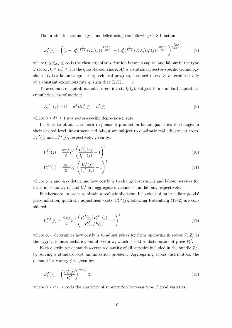
The production technology is modelled using the following CES function:

ZJt (j) =

((1− αJU )

1ξZJ

(KJt (j)

) ξZJ−1

ξZJ + (αJU )1

ξZJ

(TtA

Jt U

Jt (j)

) ξZJ−1

ξZJ

) ξZJξZJ−1

(8)

where 0 ≤ ξZJ ≤ ∞ is the elasticity of substitution between capital and labour in the type

J sector; 0 ≤ αJU ≤ 1 is the quasi-labour share; AJt is a stationary sector-specific technology

shock; Tt is a labour-augmenting technical progress, assumed to evolve deterministically

at a constant exogenous rate g, such that Tt/Tt−1 = g.

To accumulate capital, manufacturers invest, IJt (j), subject to a standard capital ac-

cumulation law of motion:

KJt+1(j) = (1− δJ)KJ

t (j) + IJt (j) (9)

where 0 ≤ δJ ≤ 1 is a sector-specific depreciation rate.

In order to obtain a smooth response of production factor quantities to changes in

their desired level, investment and labour are subject to quadratic real adjustment costs,

ΓIJt (j) and ΓUJt (j), respectively, given by:

ΓIJt (j) =φIJ

2IJt

(IJt (j)/g

IJt−1(j)− 1

)2

(10)

ΓUJt (j) =φUJ

2UJt

(UJt (j)

UJt−1(j)− 1

)2

(11)

where φIJ and φUJ determine how costly is to change investment and labour services for

firms in sector J ; IJt and UJt are aggregate investment and labour, respectively.

Furthermore, in order to obtain a realistic short-run behaviour of intermediate goods’

price inflation, quadratic adjustment costs, ΓPJt (j), following Rotemberg (1982) are con-

sidered:

ΓPJt (j) =φPJ

2ZJt

(P Jt (j)/P Jt−1(j)

P Jt−1/PJt−2

− 1

)2

(12)

where φPJ determines how costly is to adjust prices for firms operating in sector J ; ZJt is

the aggregate intermediate good of sector J , which is sold to distributors at price P Jt .

Each distributor demands a certain quantity of all varieties included in the bundle ZJt ,

by solving a standard cost minimisation problem. Aggregating across distributors, the

demand for variety j is given by:

ZJt (j) =

(P Jt (j)

P Jt

)−σJ,tZJt (13)

where 0 ≤ σJ,t ≤ ∞ is the elasticity of substitution between type J good varieties.

10

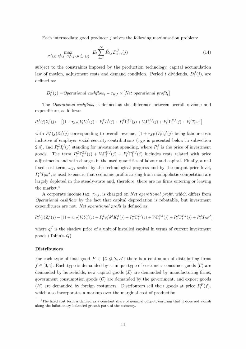
Each intermediate good producer j solves the following maximisation problem:

maxPJt (j),IJt (j),UJt (j),KJ

t+1(j)Et

∞∑s=0

Rt,sDJt+s(j) (14)

subject to the constraints imposed by the production technology, capital accumulation

law of motion, adjustment costs and demand condition. Period t dividends, DJt (j), are

defined as:

DJt (j) =Operational cashflowt − τK,t ×

[Net operational profitt

]The Operational cashflowt is defined as the difference between overall revenue and

expenditure, as follows:

P Jt (j)ZJt (j)−[(1 + τSP )VtU

Jt (j) + P It I

Jt (j) + P It ΓIJt (j) + VtΓ

UJt (j) + P Jt ΓPJt (j) + P Jt Ttω

J]

with P Jt (j)ZJt (j) corresponding to overall revenue, (1 + τSP )VtUJt (j) being labour costs

inclusive of employer social security contributions (τSP is presented below in subsection

2.4), and P It IJt (j) standing for investment spending, where P It is the price of investment

goods. The term P It ΓIJt (j) + VtΓUJt (j) + P Jt ΓPJt (j) includes costs related with price

adjustments and with changes in the used quantities of labour and capital. Finally, a real

fixed cost term, ωJ , scaled by the technological progress and by the output price level,

P Jt TtωJ , is used to ensure that economic profits arising from monopolistic competition are

largely depleted in the steady-state and, therefore, there are no firms entering or leaving

the market.4

A corporate income tax, τK,t, is charged on Net operational profit, which differs from

Operational cashflow by the fact that capital depreciation is rebatable, but investment

expenditures are not. Net operational profit is defined as:

P Jt (j)ZJt (j)−[(1 + τSP )VtU

Jt (j) + P It q

Jt δ

JKJt (j) + P It ΓIJt (j) + VtΓ

UJt (j) + P Jt ΓPJt (j) + P Jt Ttω

J]

where qJt is the shadow price of a unit of installed capital in terms of current investment

goods (Tobin’s-Q).

Distributors

For each type of final good F ∈ {C,G, I,X} there is a continuum of distributing firms

f ∈ [0, 1]. Each type is demanded by a unique type of costumer: consumer goods (C) are

demanded by households, new capital goods (I) are demanded by manufacturing firms,

government consumption goods (G) are demanded by the government, and export goods

(X ) are demanded by foreign costumers. Distributors sell their goods at price PFt (f),

which also incorporates a markup over the marginal cost of production.

4The fixed cost term is defined as a constant share of nominal output, ensuring that it does not vanishalong the inflationary balanced growth path of the economy.

11

Each distributor uses a two-stage production technology. In the first stage, the distrib-

utor combines domestic tradable goods, ZT Ft (f), with imported goods, MFt (f), to obtain

Y AFt (f), which is an assembled good of variety f ; in the second stage, the distributor

combines the assembled good with domestic non-tradable good, ZNFt (f), to produce va-

riety f of the final good Y Ft (f), which is then sold to final costumers. The production

technology is formalised as a sector specific nested CES technology.

The production function for variety f of the assembled good of type F is defined as:

Y AFt (f) =

[(αAF )

1ξAF

(ZT Ft (f)

) ξAF−1

ξAF+ (1−αAF )

1ξAF

(MFt (f)

[1−ΓAFt (f)

]) ξAF−1

ξAF

] ξAFξAF−1

(15)

where 0 ≤ ξAF ≤ ∞ is the elasticity of substitution between the domestic and the imported

tradable goods; 0 ≤ αAF ≤ 1 is a home bias parameter; and ΓAFt (f) stands for a real

adjustment cost on changes in variety f import content MFt (f)/Y AFt (f), given by:

ΓAFt (f) =φAF

2

(AAFt (f)− 1

)21 +

(AAFt (f)− 1

)2 with AAFt (f) =MFt (f)/Y AFt (f)

MFt−1/Y

AFt−1

(16)

where φAF is a sector-specific adjustment cost parameter; MFt and Y AFt represent aggre-

gate imports and assembled goods, respectively.

The production function for variety f of the final good of type F is defined as:

Y Ft (f) =

[(1− αF )

1ξF

(Y AFt (f)

) ξF−1

ξF

+ (αF )1ξF

(ZNFt (f)

) ξF−1

ξF

] ξFξF−1

(17)

where 0 ≤ ξF ≤ ∞ is the elasticity of substitution between the assembled good and the

non-tradable good; and 0 ≤ αF ≤ 1 is the non-tradable goods bias parameter.

As in the case of labour unions and manufacturers, distributors also face quadratic costs

in the adjustment of the final good price, ΓPFt (f), which take the following quadratic form:

ΓPFt (f) =φPF

2Y Ft

(PFt (f)/PFt−1(f)

PFt−1/PFt−2

− 1

)2

(18)

where φPF is the sector-specific price adjustment cost parameter; Y Ft is the aggregate final

good F , to be sold at price PFt .

Aggregate demand for variety f of final good F is given by:

Y Ft (f) =

(PFt (j)

PFt

)−σF,tY Ft (19)

where 0 ≤ σF,t ≤ ∞ is the elasticity of substitution between type F good varieties.

12

Each final goods producer f solves the following dividend maximisation problem:

maxPFt (f),ZT Ft (f)ZNFt (f),MF

t (f)Et

∞∑s=0

Rt,sDFt+s(f) (20)

subject to the constraints imposed by production technology, adjustment costs and de-

mand conditions. Period t dividends, DFt (j), are defined as:

DFt (f) = (1− τK,t)

[PFt (f)Y Ft (f)− P Tt ZT Ft (f)− PNt ZNFt (f)− P ∗t MF

t (f)− PFt ΓPFt (f)− PFt TtωF]

which corresponds to the after-tax difference between total revenue PFt (f)Y Ft (f) and total

expenditure, which includes input costs, P Tt ZT Ft (f) + PNt Z

NFt (f) + P ∗t M

Ft (f) and ad-

justment and fixed costs, PFt (f)ΓPFt (f)+PFt (f)TtωF . Finally, P ∗t is the price of imported

goods MFt (f), set in the rest of the world market.

2.4 The Government

The fiscal block of the model is detailed enough to allow for the assessment of macroeco-

nomic impacts of alternative fiscal policy strategies. Government has a number of fiscal

instruments that can be used to stabilise the business cycle that affect macroeconomic ag-

gregates differently. In addition, Government may also finance current expenditure using

future tax revenues by managing a public debt stock subject to full home bias. The public

sector account disaggregation considered is illustrated in Table 1.

On the expenditure side, the government faces spending with: the government con-

sumption good, P Gt Gt (recall that P Gt is the price charged by distributors for the gov-

ernment consumption good); lump-sum transfers to households, TRGt; and debt interest

outlays, (it−1 − 1)Bt−1, where Bt−1 are one-period bonds which pay an interest rate

it−1 at the beginning of period t. On the revenue side, the government receives funds

from: foreign transfers from the rest of the world, TREt; the labour income tax paid on

wage income, RVL,t = τL,t(VtUt − PtΓUt

); the tax paid by households on consumption

expenditures, RVC,t = τC,tPCt Ct; employers’ social security contributions due on payroll,

RVSP,t = τSPVtUt; corporate income taxes paid by firms (both manufacturers and distrib-

utors) on operational profits, RVK,t, defined as:

RVK,t =∑

J=T ,NτK,t

[P Jt(ZJt − ΓPJt − TtωJ

)− (1 + τSP )VtU

Jt − P It

(qJt δ

JKJt + ΓIJt

)]+

+∑

F=C,I,G,XτK,t

[PFt

(Y Ft − ΓPFt − TtωF

)− PTt ZTFt − P ∗t MF

t − PNt ZNFt]

It should be noted that the government finances its expenditures mostly through tax-

ation (present or future), and that most taxes are distortionary. For instance, higher

taxation on labour income and/or higher social security contributions rate induce house-

holds to substitute consumption by leisure and/or manufacturers to use technologies with

higher capital intensity. An increase in the consumption tax rate also induces households

to substitute away from consumption.

13

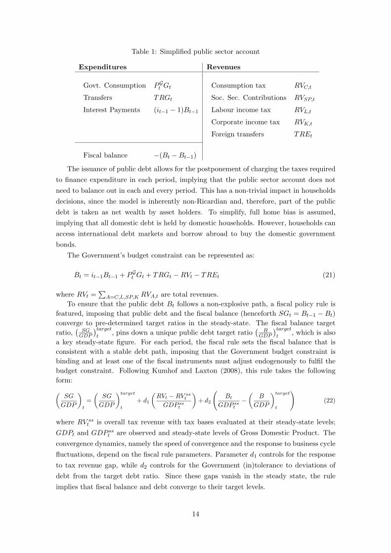
Table 1: Simplified public sector account

Expenditures Revenues

Govt. Consumption P Gt Gt Consumption tax RVC,t

Transfers TRGt Soc. Sec. Contributions RVSP,t

Interest Payments (it−1 − 1)Bt−1 Labour income tax RVL,t

Corporate income tax RVK,t

Foreign transfers TREt

Fiscal balance −(Bt −Bt−1)

The issuance of public debt allows for the postponement of charging the taxes required

to finance expenditure in each period, implying that the public sector account does not

need to balance out in each and every period. This has a non-trivial impact in households

decisions, since the model is inherently non-Ricardian and, therefore, part of the public

debt is taken as net wealth by asset holders. To simplify, full home bias is assumed,

implying that all domestic debt is held by domestic households. However, households can

access international debt markets and borrow abroad to buy the domestic government

bonds.

The Government’s budget constraint can be represented as:

Bt = it−1Bt−1 + P Gt Gt + TRGt −RVt − TREt (21)

where RVt =∑

A=C,L,SP,K RVA,t are total revenues.

To ensure that the public debt Bt follows a non-explosive path, a fiscal policy rule is

featured, imposing that public debt and the fiscal balance (henceforth SGt = Bt−1 −Bt)converge to pre-determined target ratios in the steady-state. The fiscal balance target

ratio,(SGGDP

)targett

, pins down a unique public debt target ratio(

BGDP

)targett

, which is also

a key steady-state figure. For each period, the fiscal rule sets the fiscal balance that is

consistent with a stable debt path, imposing that the Government budget constraint is

binding and at least one of the fiscal instruments must adjust endogenously to fulfil the

budget constraint. Following Kumhof and Laxton (2008), this rule takes the following

form:(SG

GDP

)t

=

(SG

GDP

)targett

+ d1

(RVt −RV sstGDP sst

)+ d2

(Bt

GDP sst−(

B

GDP

)targett

)(22)

where RV sst is overall tax revenue with tax bases evaluated at their steady-state levels;

GDPt and GDP sst are observed and steady-state levels of Gross Domestic Product. The

convergence dynamics, namely the speed of convergence and the response to business cycle

fluctuations, depend on the fiscal rule parameters. Parameter d1 controls for the response

to tax revenue gap, while d2 controls for the Government (in)tolerance to deviations of

debt from the target debt ratio. Since these gaps vanish in the steady state, the rule

implies that fiscal balance and debt converge to their target levels.

14

At this point, the fiscal instrument that becomes an endogenous variable remains

to be defined. This is an open fiscal policy decision and is largely a political matter.

Ex-ante, the government has the following fiscal instruments: government consumption

(Gt), lump-sum transfers to households (TRGt) (which can be targeted at asset holders

or liquidity constrained households), the labour income tax rate (τL,t), the consumption

tax rate (τC,t), the employer’s social security contributions rate (τSP ) and the corporate

income tax rate (τK,t).5 However, ex-post one of this instruments is endogenously ad-

justed to met the fiscal balance imposed by the fiscal rule.6 The most common option

relies on the use of the labour income tax rate as the endogenous fiscal policy instrument

(Harrison et al. 2005, Kilponen and Ripatti 2006, Kumhof and Laxton 2007a, Kumhof

and Laxton 2007b). The benchmark specification of PESSOA also takes this option, but

it allows for other possibilities, including not only the remaining taxes, but also transfers

to households or Government consumption. In addition, it is also possible to consider

alternative combinations of instruments.

Finally, a word of caution is needed. Although the above-mentioned fiscal block is

suited to implement several types of fiscal simulations, the model remains a simplifica-

tion of reality that is crucial to keep it tractable. In particular, government consumption

represents a pure distortion, since it does not affect the marginal utility of consumption

and leisure or firms productivity level. Therefore, the only tangible impact of Govern-

ment consumption is changing demand conditions for a specific type of final good, which

is particulary intensive in non-tradable intermediate goods and has a negligible import

content. The model is thus silent to other roles of the Government, for instance as em-

ployer or investor. If Government purchases includes more spending on law enforcement,

road buildings or other public stock with likely future effects, these are not considered.

As Hall (2009) clarifies, it is not the case that effects operating through externalities are

unimportant, but simply that the fiscal stimulus has to be undertaken as an experiment on

a limited and controlled macroeconomic environment. It is beyond the scope of this paper

to define externalities’ effects conditional on different fiscal policies. Note also that the

model does not feature unemployment benefits explicitly, since labour market details are

reduced to the minimum and, therefore, unemployment developments are not explicitly

modelled.

2.5 The rest of the world

By assumption the rest of the world (RoW) corresponds to the rest of the monetary union,

and therefore the nominal effective exchange rate is irrevocably set to unity, as all trade

and financial flows are in the same currency.

Regarding financial flows, it is assumed that changes in the net foreign asset/debt

5The distinction between government consumption and investment is not considered in the model.6In many studies, the budget constraint is simplified to include a non-distortionary lump-sum tax.

Though it may be an appealing academic benchmark, it is largely unrealistic since the role played bylump-sum taxation is very limited.

15

position of the domestic economy have no impact on foreign macroeconomic aggregates

and therefore on monetary policy decisions. As for trade flows, the demand for imports by

domestic distributors results from the dividend maximisation problem presented in section

2.3 and reflects demand conditions and competitiveness. Concerning exports, let Y A∗t (f∗)

be the good demanded by a continuum f∗ ∈ [0, 1] of importers located abroad. This

good is assumed to result from the assembling of a domestic exported good Xt(f∗) and an

intermediate tradable good ZT∗t (f∗) produced by foreign manufacturers. The production

process is given by the following CES technology:

Y A∗t (f∗) =

((1− α∗)

1ξ∗(ZT∗t (f∗)

) ξ∗−1ξ∗ + (α∗)

1ξ∗ (Xt(f

∗))ξ∗−1ξ∗

) ξ∗ξ∗−1

(23)

where ξ∗ is the elasticity of substitution between foreign tradable goods and home exports

and α∗ is the foreign economy bias parameter.

Each foreign distributor will set the demand for the export good produced in the SOE

and for the tradable goods produced in his country that minimises the cost of producing

the desired quantity of assembled good, subject to the technology constraint imposed by

(23). Aggregating across importers and export goods varieties, the demand for exports is:

Xt = α∗(PXtP T∗t

)−ξ∗Y A∗t (24)

where PXt is the price of the final export good charged by distributors, P T∗t is the price of

the foreign tradable good and Y A∗t is aggregate production of the foreign assembled good.

It should be noted that this equation is highly relevant to render the model dynamically

stable, namely due to a large elasticity to real exchange rate movements. The model

operates de facto like a real model (or a fully credible fixed nominal exchange rate model),

since domestic price levels are pinned down by the external constraint that uniquely sets

the steady-state real exchange rate level. Like all foreign variables, both P T∗t and Y A∗t are

assumed to be independent of domestic developments.

Finally, some comments should be made concerning the external environment of PES-

SOA. Firstly, though restricting the RoW to the rest of the monetary union may be a

limiting assumption of the external environment for the purpose of analysis in many euro

area SOE, for fiscal policy analysis it does not seem very stringent and allows for min-

imising the dimension of the external block of the model. More specifically, under this

assumption one does not need to explicitly model interactions between the euro area and

the world excluding the euro area. Obviously, this breakdown becomes clearly relevant in

case one wants to assess the impact on the domestic economy of shocks originated abroad,

in particular if a high share of external trade in goods and assets is done with countries

outside the euro area. Secondly, while a country’s exports in a multi-country model are

endogenously determined by imports demand of their trading partners, in a SOE model

foreign economy developments influence the domestic economy significantly, but are not

16

influenced by domestic economy developments (Adolfson et al. 2007). Therefore, it seems

reasonable to assume that total foreign demand and prices are exogenous, with endoge-

nous movements in exports being simply determined by the behaviour of the real exchange

rate.

2.6 Market clearing conditions and GDP definitions

The model relies on a set of equilibrium conditions, which ensure that all markets clear in

each and every period.

In the labour market, overall labour supply by households must equal overall labour

demand by manufacturers:

LAt + LBt = UTt + UNt (25)

In the intermediate goods’ market, the output produced by each type of manufacturer

must meet demand by distributors and cover price adjustment and fixed costs:

ZTt = ZT Ct + ZT It + ZT Gt + ZT Xt + ΓPTt + TtωT (26)

ZNt = ZNCt + ZNIt + ZNGt + ZNXt + ΓPNt + TtωN (27)

In the final goods’ market, output supplied by each type of distributor must meet

demand by its respective costumer and cover adjustment and fixed costs:

Y Ct = CAt + CBt + ΓPCt + TtωC (28)

Y It = ITt + INt + ΓT It + ΓNIt + ΓPIt + TtωI (29)

Y Gt = Gt + ΓPGt + TtωG (30)

Y Xt = Xt + ΓPXt + TtωX (31)

In the foreign bond market, households’ net bond holdings must equal the economy’s

trade net position:

B∗t − i∗t−1ΨB∗t−1 = PXt Xt − P ∗t Mt + TREt (32)

Finally, nominal GDP is given by:

GDPt = PtCt + PGt Gt + P It It + PXt Xt − P ∗t Mt (33)

while real GDP is defined as GDP evaluated at the prevailing initial steady-state price

levels.7

7This mimics the national accounts definition of GDP at reference year prices.

17

2.7 Calibration

PESSOA was calibrated using actual data of the Portuguese economy and information

from several studies on the Portuguese and euro area economies, including DSGE models.

The model parameters are presented in detail in Appendix A.

The data on the Portuguese economy was mainly taken from the Banco de Portugal

quarterly database (included in the 2009 Summer issue of the Economic Bulletin), and from

the National Accounts data released by Statistics Portugal. These data were primarily

used to pin down those parameters affecting the steady-state key macroeconomic ratios.

As reported in Appendix A, the model matches fairly reasonably the key ratios of the

Portuguese economy and delivers a plausible capital-to-output ratio.

Among the relatively large set of parameters and assumptions behind the model, it

seems worth mentioning that the steady-state real GDP growth was assumed to be iden-

tical in the entire monetary union, which ensures the existence of a balanced growth path.

Labour-augmenting productivity’s annual growth rate was set to 2 per cent, which is con-

sistent with the estimates for the euro area’s long-run potential output growth (Musso

and Westermann 2005, Proietti and Musso 2007). This figure also seemed plausible for

Portugal (Almeida and Felix 2006). Regarding inflation, the ECB inflation objective was

assumed to be fully credibility. Hence, the steady-state was solved under the assumption

that foreign inflation stands at 2 per cent per year. The euro area nominal interest rate

in the steady-state was set to 4.5 per cent (Coenen, McAdam and Straub 2007). The

parameters related with the Blanchard-Yaari households behaviour, namely the instant

probability of death and the decay in productivity over the lifetime were calibrated as in

Kumhof and Laxton (2007a). The elasticities of substitution in the production functions

of manufacturers and distributors, the parameters governing wage, price markups and ad-

justment costs, and also the fiscal rule parameters were calibrated using mainly Kumhof

and Laxton (2007a) and Coenen et al. (2007) or estimates for Portugal, whenever they

were available.

3 Fiscal stimulus under full credibility

The impact of fiscal policy instruments on the economy is a crucial piece of information for

the policy making process. In the light of perfect foresight and full government credibility,

this section addresses the following questions: how effective is a temporary fiscal stimulus

on aggregate demand and output in a SOE operating in a monetary union? What is the

best instrument in order to boost economic activity? Can implementation lags reduce the

short-run multiplier? Is there a case for a permanent fiscal stimulus?

Figure 1 depicts a stylised example, where permanent and temporary fiscal stimulus

are based on government consumption (G), though any instrument presented in subsection

2.4 could be used. The first relevant date of Figure 1 is tl, when the government announces

that a stimulus will be implemented. This is a relevant date as the government may feel the

18

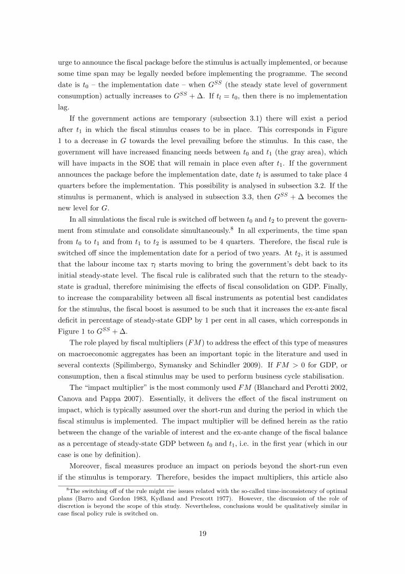
urge to announce the fiscal package before the stimulus is actually implemented, or because

some time span may be legally needed before implementing the programme. The second

date is t0 – the implementation date – when GSS (the steady state level of government

consumption) actually increases to GSS + ∆. If tl = t0, then there is no implementation

lag.

If the government actions are temporary (subsection 3.1) there will exist a period

after t1 in which the fiscal stimulus ceases to be in place. This corresponds in Figure

1 to a decrease in G towards the level prevailing before the stimulus. In this case, the

government will have increased financing needs between t0 and t1 (the gray area), which

will have impacts in the SOE that will remain in place even after t1. If the government

announces the package before the implementation date, date tl is assumed to take place 4

quarters before the implementation. This possibility is analysed in subsection 3.2. If the

stimulus is permanent, which is analysed in subsection 3.3, then GSS + ∆ becomes the

new level for G.

In all simulations the fiscal rule is switched off between t0 and t2 to prevent the govern-

ment from stimulate and consolidate simultaneously.8 In all experiments, the time span

from t0 to t1 and from t1 to t2 is assumed to be 4 quarters. Therefore, the fiscal rule is

switched off since the implementation date for a period of two years. At t2, it is assumed

that the labour income tax τl starts moving to bring the government’s debt back to its

initial steady-state level. The fiscal rule is calibrated such that the return to the steady-

state is gradual, therefore minimising the effects of fiscal consolidation on GDP. Finally,

to increase the comparability between all fiscal instruments as potential best candidates

for the stimulus, the fiscal boost is assumed to be such that it increases the ex-ante fiscal

deficit in percentage of steady-state GDP by 1 per cent in all cases, which corresponds in

Figure 1 to GSS + ∆.

The role played by fiscal multipliers (FM) to address the effect of this type of measures

on macroeconomic aggregates has been an important topic in the literature and used in

several contexts (Spilimbergo, Symansky and Schindler 2009). If FM > 0 for GDP, or

consumption, then a fiscal stimulus may be used to perform business cycle stabilisation.

The “impact multiplier” is the most commonly used FM (Blanchard and Perotti 2002,

Canova and Pappa 2007). Essentially, it delivers the effect of the fiscal instrument on

impact, which is typically assumed over the short-run and during the period in which the

fiscal stimulus is implemented. The impact multiplier will be defined herein as the ratio

between the change of the variable of interest and the ex-ante change of the fiscal balance

as a percentage of steady-state GDP between t0 and t1, i.e. in the first year (which in our

case is one by definition).

Moreover, fiscal measures produce an impact on periods beyond the short-run even

if the stimulus is temporary. Therefore, besides the impact multipliers, this article also

8The switching off of the rule might rise issues related with the so-called time-inconsistency of optimalplans (Barro and Gordon 1983, Kydland and Prescott 1977). However, the discussion of the role ofdiscretion is beyond the scope of this study. Nevertheless, conclusions would be qualitatively similar incase fiscal policy rule is switched on.

19

Figure 1: Fiscal stimulus based on G

Time

G

GSS

GSS + ∆

t0

Permanent

Temporary

t1 t2

tl

Notes: t0 is the starting date of the fiscal stimulus and when the fiscal policy ruleis deactivated; t1 is the ending date if the stimulus is temporary; t2 corresponds tothe starting date of the consolidation period in both the temporary and permanentcases, defined as a time when the fiscal policy rule is again fully operational; GSS isthe steady-state level of government consumption before the stimulus; ∆ is the actualstimulus (it correspond in all experiments to a level that implies an ex-ante increasein the fiscal deficit of 1% of steady-state GDP); tl is a possible announcement date(otherwise tl = t0). In all experiments, the time span between tl and t0 (if tl 6= t0),or t0 and t1, or t1 and t2 is assumed to represent 4 quarters.

presents the impulse response functions over a period of 10 years and the “present value

multiplier” (PVM), following the proposal by Mountford and Uhlig (2009). The PVM

corresponds to the present discounted value of the impact of a 1 per cent fiscal stimulus

from period 0 up to period k at a discount rate that reflects economic agent relative

concerns with impacts that occur farther in time vis-a-vis short-term impacts.9

Finally, the effects of a permanent increase in government consumption can also be

assessed by analysing the welfare impacts associated with a permanent increase in gov-

ernment consumption.10 In this paper, we consider a discrete time counterpart of the

suggestion of Calvo and Obstfeld (1988), which has also been used in the literature

(Ganelli 2005, Kumhof, Laxton and Leigh 2008). Welfare analysis can be seen as a bench-

mark metric for the impact of a particular policy experiment in households welfare, as

measured through the aggregate lifetime utility, which is a function of goods valued by

households (consumption and leisure in the case at hand). Hence, welfare corresponds to

a weighted average of the utility of the individuals alive in current and future periods,

where a weighting factor W reflects the importance of future generations in the welfare

from the viewpoint of the policymaker. The welfare impact is synthesised in the stan-

dard compensated variation of consumption measure proposed in Lucas Jr. (1987), which

transforms utility into additional units of consumption good in the steady-state. It is

9A brief description of the methodology used to compute the PVM is presented in Appendix B.10In the case of the temporary shocks, the welfare effects are not mentioned because the impact is limited,

given the temporary nature and the magnitude of the stimulus.

20

Table 2: Impact multipliers under alternative fiscal instruments

(deviation from steady-state)

G TRG TRGB τl τcGDP 1.02 0.24 0.57 0.37 0.38Private consumption 0.90 0.78 1.86 0.71 0.96Government consumption and investment 4.37 0.00 0.00 0.00 0.00Private investment -0.62 -0.18 -0.40 0.06 -0.09Exports -0.66 -0.32 -0.78 0.06 -0.19Imports 0.65 0.29 0.71 0.29 0.37

Hours 1.66 0.23 0.63 0.48 0.40Real wage rate 0.94 0.42 1.04 -0.79 1.56Real exchange rate -0.27 -0.13 -0.31 0.02 -0.08

Inflation (in %) 0.29 0.09 0.22 -0.03 -1.62NFA (as a % of SS GDP) -0.02 -0.03 -0.08 0.69 -1.07Public debt (as a % of SS GDP) 0.12 0.46 0.18 -0.11 1.21

Notes: All variables are measured in percent deviations from the steady-state levels, except forinflation, net foreign assets, public debt and fiscal balance where deviations are in percentage points.“SS GDP” indicates steady-state GDP. Higher real exchange rate corresponds to a depreciation. Thefiscal instruments are labour income taxes (τL); taxes on consumption goods (τC); general transfers(TRG); targeted transfers (TRGB); government consumption (G). Inflation is defined as the annualchange in Pt, which is the numeraire price of the economy. The real exchange rate is computed withthe prices of export goods.

worth mentioning that the current setup assumes that public consumption goods are not

valued by households, an assumption that might be stringent. Nevertheless, the analysis

is still useful to motivate the idea that permanent increases in government consumption

negligibly valued by households, though expanding economic activity, are hardly welfare

improving.11

3.1 Temporary stimulus without implementation lags

Table 2 presents the impact multipliers for the five fiscal instruments considered (govern-

ment consumption, general transfers, targeted transfers, labour income tax and consump-

tion tax), under the assumption of no implementation lags. The results indicate that all

expansionary measures have positive effects on GDP and consumption in the first year,

suggesting that fiscal stimulus may be envisaged to perform business cycle stabilisation.

However, the impact on GDP is, in most experiments, significantly below unity, due to

non-negligible leakages, namely related with savings and imports. In other words, the

results suggest that, in most cases, a fiscal stimulus of 1 per cent of steady-state GDP

causes actual GDP to increase by less than 1 per cent on impact.

The impact multiplier on GDP from a fiscal stimulus based on government consumption

is 1.0 per cent. In case the fiscal stimulus is based on targeted transfers (transfers to

liquidity-constrained households) the impact is 0.6 per cent, while if it is based on taxes,

11A brief description of the methodology used for the welfare analysis is presented in the Appendix C.

21

both labour income and consumption, the impact is close to 0.4 per cent over the first year.

Finally, the smaller impact on GDP (0.2 per cent) is obtained from an increase in general

transfers (transfers to all households regardless of whether they are liquidity-constrained

or not). Hence, the most effective fiscal instrument to stimulate the economy on impact

is government consumption. This result is in line with the literature that points to larger

multipliers from fiscal measures based on government consumption and public investment

than those based on transfers or tax cuts.

A major reason behind the different magnitudes in the impact multipliers is the fact

that fiscal stimulus delivered from government consumption feeds directly into aggregate

demand, whereas the stimulus delivered from transfers or tax cuts operate mainly through

the effect on current income and wealth (which is only partly used by asset holding house-

holds to increase private spending), as well as through their effects on incentives in case of

changes in distortionary taxes. Moreover, while the increase in government consumption

induces a small increase in the demand for imports, the remaining stimulus instruments

increases demand for private consumption goods, which has a much higher import content.

Besides the direct effect, government consumption also has indirect effects in demand de-

rived from higher spending, which raises labour income and dividends and in turn increases

private spending.

Finally, it is also important to stress that in a SOE integrated in a monetary union,

with exogenous monetary policy, the impacts of fiscal stimulus measures on aggregate

demand are amplified through the effect on real interest rates. This augmented effect is

also present in the case of economies with endogenous monetary policy if the zero lower

bound binds (Eggertsson 2009, Christiano et al. 2009) or under monetary accommodation

(Freedman, Kumhof, Laxton, Muir and Mursula 2009). A fiscal expansion that puts

upward pressure on inflation as demand increases, implies a decline in the real interest

rates, since nominal interest rates are fixed, supporting and increasing the impact of fiscal

policy on private spending. In the case of a fiscal stimulus based on targeted transfers and

government consumption this effect is also key to explain the magnitude of the impact on

aggregate demand.

Figure 2 presents the impulse response functions for the different stimulus measures

over a ten years period. In most cases, given the temporary nature of the stimulus, the

impact on GDP dies out or becomes even negative as soon as the shock is reversed. It

is worth mention that of major importance will be the medium-run adjustment in real

variables to cope with the impact of the fiscal shock that needs to be financed, which

implies a protracted decline of aggregate demand to a level below the steady-state in the

medium-run. Moreover, all shocks share the same outcome in which debt, fiscal balance

and NFA to steady-state GDP return in the medium to long-run to their initial values due

to the temporary nature of the stimulus.

Following the government consumption shock, households that access financial mar-

kets smooth their consumption by saving part of their additional income while liquidity-

constrained households increase significantly their consumption. On the other hand, man-

22

ufacturing firms have no incentive to adjust their capital stock upwards since the positive

effect on domestic demand is highly temporary. Moreover, part of the increase in domestic

demand is offset by the decrease in exports, due to a loss in competitiveness driven by

higher prices. Indeed, the boom in public consumption implies an increase in demand

for intermediate non-tradable goods, which are more intensive in labour services. Thus,

the stimulus generates substantial demand side pressure on hours, implying higher wage

inflation in the short-run to induce households to supply enough labour. This translates

into higher marginal costs of intermediate goods production. Despite the downward ad-

justment in profit margins, domestic prices increase temporarily, leading to a significant

real exchange rate appreciation with non-negligible temporary consequences on the econ-

omy’s competitiveness. However, wage income does not increase significantly beyond the

stimulus period, due to the absence of a sustained increase in demand, and therefore nei-

ther does the post-stimulus consumption of liquidity constrained households. After the

first year, the nominal wage rate inflation reverts and the price level starts to gradually

converge to the initial steady-state level. It should be mentioned that the impact on GDP

is amplified by the anticipation of private consumption expenditures due to the temporary

decline in the real interest rate.

The simulated impact of an increase in general transfers on GDP is small, since the

main effect comes from the increase in consumption of liquidity-constrained households.12

The remaining households save part of these additional transfers as additional taxes will

have to be paid in the future and so only a part of the increase in transfers is taken as a net

wealth increase. Therefore, the shock based on targeted transfers provides a much more

powerful stimulus than the one based on general transfers, more than two times larger in

both GDP and consumption. Given that the transmission channels behind the two shocks

are very similar, the rest of the discussion will be centered on the one that has a higher

effect, that is, the targeted transfers.

The qualitative impact on the macroeconomic scenario of increasing targeted transfers

is similar to that of government consumption, though in a smaller magnitude. An increase

in targeted transfers stimulates the economy through the demand for private consumption

goods and, as in the previous scenario, it implies a protracted decline of GDP and private

consumption to below steady-state level as soon as the fiscal stimulus is reverted. The

short-run increase in the demand for private consumption goods induces significant de-

mand side pressure on labour and so an higher wage rate is required in order to motivate

households to supply enough labour. The rise in firm’s marginal costs is transmitted to

intermediate and final goods prices. The temporary increase in inflation implies, on the

one hand, a real exchange rate appreciation and a decrease in exports with the consequent

deterioration in the net foreign asset position. On the other hand, it implies lower real in-

terest rates which fosters some anticipation of consumption expenditures from households

that have access to assets markets. However, the increase in wages is less marked than in

12Liquidity-constrained households are calibrated to represent about 40 per cent of total population. SeeAppendix A.

23

Figure 2: Impulse responses under alternative fiscal instruments

(deviations from steady-state)

‐1.0

‐0.5

0.0

0.5

1.0

Y1 Y2 Y3 Y4 Y5 Y6 Y7 Y8 Y9 Y10

GDPLabour income taxConsumption taxGeneral transfersTargeted transfersGov. consumption

‐1.0

‐0.5

0.0

0.5

1.0

1.5

2.0

Y1 Y2 Y3 Y4 Y5 Y6 Y7 Y8 Y9 Y10

Private consumption

‐1.2

‐0.7

‐0.2

Private investment

‐1.0

‐0.5

0.0

Exports

‐0.5

0.0

0.5

Imports

‐1.0

‐0.5

0.0

0.5

1.0

1.5

Y1 Y2 Y3 Y4 Y5 Y6 Y7 Y8 Y9 Y10

Hours

‐1.0

‐0.5

0.0

0.5

1.0

Y1 Y2 Y3 Y4 Y5 Y6 Y7 Y8 Y9 Y10

GDPLabour income taxConsumption taxGeneral transfersTargeted transfersGov. consumption

‐1.0

‐0.5

0.0

0.5

1.0

1.5

2.0

Y1 Y2 Y3 Y4 Y5 Y6 Y7 Y8 Y9 Y10

Private consumption

‐1.2

‐0.7

‐0.2

Y1 Y2 Y3 Y4 Y5 Y6 Y7 Y8 Y9 Y10

Private investment

‐1.0

‐0.5

0.0

Y1 Y2 Y3 Y4 Y5 Y6 Y7 Y8 Y9 Y10

Exports

‐0.5

0.0

0.5

Y1 Y2 Y3 Y4 Y5 Y6 Y7 Y8 Y9 Y10

Imports

‐1.0

‐0.5

0.0

0.5

1.0

1.5

Y1 Y2 Y3 Y4 Y5 Y6 Y7 Y8 Y9 Y10

Hours

‐3.0

‐2.0

‐1.0

0.0

1.0

2.0

3.0

Y1 Y2 Y3 Y4 Y5 Y6 Y7 Y8 Y9 Y10

Real wage

‐0.4

‐0.3

‐0.2

‐0.1

0.0

0.1

0.2

Y1 Y2 Y3 Y4 Y5 Y6 Y7 Y8 Y9 Y10

Real exchange rate

‐2.0

‐1.5

‐1.0

‐0.5

0.0

0.5

1.0

1.5

2.0

Y1 Y2 Y3 Y4 Y5 Y6 Y7 Y8 Y9 Y10

Inflation

‐1.3

‐0.8

‐0.3

0.2

0.7

Y1 Y2 Y3 Y4 Y5 Y6 Y7 Y8 Y9 Y10

NFA(as a % of SS GDP)

‐1.5

‐1.0

‐0.5

0.0

0.5

Y1 Y2 Y3 Y4 Y5 Y6 Y7 Y8 Y9 Y10

Structural fiscal balance(as a % of SS GDP)

‐0.2

0.3

0.8

1.3

Y1 Y2 Y3 Y4 Y5 Y6 Y7 Y8 Y9 Y10

Public debt(as a % of SS GDP)

Notes: All variables are measured in percent deviations from the steady-state levels, except for inflation, net foreignassets, public debt and fiscal balance where deviations are in percentage points. “SS GDP” indicates steady-stateGDP. Higher real exchange rate implies depreciation. Inflation is defined as the annual change in Pt, which is thenumeraire price of the economy. The real exchange rate is computed with the price of export goods.

the case of public consumption expansion, reflecting the fact that private consumption is

less intensive in labour services.

In the case of labour income tax cut the positive impact on GDP and consumption

extends beyond the stimulus period, although the impact multiplier is smaller than those

reported for government consumption and targeted transfers. First, the labour income tax

24

is distortionary, having significant effects on the households’ consumption/leisure decision.

The tax cut implies that households earn a higher labour income for the same wage paid by

firms and, therefore, labour supply increases and the equilibrium wage declines, contrary

to what happens in the case of the increase in government consumption and/or government

transfers. The decline in wages on impact translates into a slight decrease in inflation over

the first two years. In contrast with the effect of an expenditure based fiscal stimulus, this

fiscal policy shock induces a slight short-run real exchange rate depreciation, improving

competitiveness of domestic goods, which has a positive short-run effect on exports and

on the net foreign asset position. The indirect effect from the decline in the real interest

rate is negligible in the case of labour income tax cut, since the increase in inflation is

small.

Finally, the impact multiplier of a consumption tax-based stimulus on GDP is similar

to the one obtained for labour income tax, although the impact is less persistent. A con-

sumption tax cut increases real wages, augmenting households’ real income and therefore

consumption. The cut in consumption tax produces a huge relative price change imply-

ing a broadly based increase in relative prices of all goods (both intermediate and final).

This implies a stronger increase of the fiscal deficit and public debt, reflecting the sizeable

increase in expenditure due to the hike in the relative price of public consumption. On

the external side, the increase in the relative price of exports and imports implies a hike

in the current account deficit that translates into a deterioration of the NFA position of

the the SOE on impact. As soon as the shock is reversed, the increase in domestic de-

mand pressures wages upwards in order to induce households to supply labour, inducing

an increase in firms marginal costs and in domestic prices, which is similar to what was

described for the fiscal stimulus based on government expenditures and transfers.

A slightly different way of assessing the impact of the fiscal stimulus in medium-term

perspective relies on the present value multiplier (PVM) definition. Figure 3 presents

the present value multiplier for the five fiscal stimulus measures up to period 10 years

(40 quarters) ahead. The results reinforce the conclusion that in the medium run a fiscal

stimulus has a negative effect on aggregate demand, which translates into a negative PVM

from the second year onwards in the case of transfers (both general and targeted transfers)

and from the seventh year onwards in the case of the labour income tax cut. The remaining

cases lie in between.

Summing up, a fiscal stimulus can be effective in providing some temporary support

to a SOE, nonetheless with non-negligible adverse impacts over the medium run. Similar

fiscal multipliers have been reported in the literature for large economies, namely if the

zero lower bound binds (Eggertsson 2009, Christiano et al. 2009) or under monetary ac-

commodation (Freedman, Kumhof, Laxton, Muir and Mursula 2009). A major difference

is nevertheless that while the (fixed) zero lower bound in large economies is an exception

(of operating with positive interest rates), the exogenous (fixed) interest rate for a SOE

in a monetary union is a predictable event.

Moreover, the size of the fiscal multiplier largely depends on the type of instrument

25

Figure 3: Present value multipliers

(deviation from steady-state)

‐1.2

‐0.7

‐0.2

0.3

0.8

1.3

1.8

GDP

Labour income taxConsumption taxGeneral transfersTargeted transfersGov. Consumption

‐1.5

‐1.0

‐0.5

0.0

0.5

1.0

1.5

2.0 Private consumption

‐1.5

‐1.0

‐0.5

0.0

0.5

1.0

1.5

2.0 Hours

‐1.2

‐0.7

‐0.2

0.3

0.8

1.3

1.8

Y1 Y2 Y3 Y4 Y5 Y6 Y7 Y8 Y9 Y10

GDP

Labour income taxConsumption taxGeneral transfersTargeted transfersGov. Consumption

‐1.5

‐1.0

‐0.5

0.0

0.5

1.0

1.5

2.0

Y1 Y2 Y3 Y4 Y5 Y6 Y7 Y8 Y9 Y10

Private consumption

‐4.0

‐3.0

‐2.0

‐1.0

0.0

1.0

Y1 Y2 Y3 Y4 Y5 Y6 Y7 Y8 Y9 Y10

Private investment

‐2.5

‐2.0

‐1.5

‐1.0

‐0.5

0.0

0.5

Y1 Y2 Y3 Y4 Y5 Y6 Y7 Y8 Y9 Y10

Exports

‐0.5

0.0

0.5

1.0

Y1 Y2 Y3 Y4 Y5 Y6 Y7 Y8 Y9 Y10

Imports

‐1.5

‐1.0

‐0.5

0.0

0.5

1.0

1.5

2.0

Y1 Y2 Y3 Y4 Y5 Y6 Y7 Y8 Y9 Y10

Hours

Notes: The reported figures were defined in equation 34 and represent the PVM(k), where 0 < k < 40.

used and thus the fiscal stimulus package should be carefully designed. The highest impact

on GDP comes from fiscal measures based on government consumption, notwithstanding

that in what concerns investment projects it could imply long lags in planning and imple-

menting. Fiscal measures based on targeted transfers have also a high short-term impact

on GDP and have the advantage of being faster to implement. However, there is some risk

of difficulty of reversal. Finally, it should be emphasized that in most cases, particularly

in tax cuts, the fiscal stimulus implies significant leakages into saving and imports, and

thus have a lower impact on GDP.

3.2 Temporary stimulus with implementation lags

This subsection analyses the sensitivity of aggregate demand to the timing of the fiscal

stimulus. In practice, some changes in fiscal policy are likely to involve a particulary long

period between the time of the announcement and its implementation. We define the

time span between the former and the later as the “implementation lag”. The presence of

these lags is widely pointed against using fiscal policy as a tool to pursue business cycle

stabilisation effects.

In the rest of this subsection all experiments are conducted assuming a fiscal stimulus

based on government consumption, though conclusions would be qualitatively similar if

the exercise had been conducted using the alternative instruments. As described in Figure

1, tl is the date when the government announces that a stimulus will be implemented, and

one year after, in t0 (the implementation date), is when the government actually increases

26

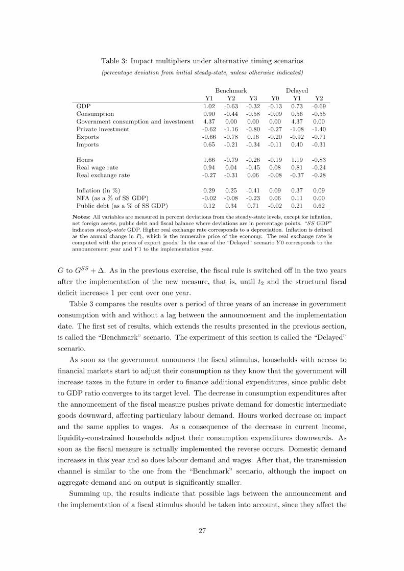
Table 3: Impact multipliers under alternative timing scenarios

(percentage deviation from initial steady-state, unless otherwise indicated)

Benchmark DelayedY1 Y2 Y3 Y0 Y1 Y2

GDP 1.02 -0.63 -0.32 -0.13 0.73 -0.69Consumption 0.90 -0.44 -0.58 -0.09 0.56 -0.55Government consumption and investment 4.37 0.00 0.00 0.00 4.37 0.00Private investment -0.62 -1.16 -0.80 -0.27 -1.08 -1.40Exports -0.66 -0.78 0.16 -0.20 -0.92 -0.71Imports 0.65 -0.21 -0.34 -0.11 0.40 -0.31

Hours 1.66 -0.79 -0.26 -0.19 1.19 -0.83Real wage rate 0.94 0.04 -0.45 0.08 0.81 -0.24Real exchange rate -0.27 -0.31 0.06 -0.08 -0.37 -0.28

Inflation (in %) 0.29 0.25 -0.41 0.09 0.37 0.09NFA (as a % of SS GDP) -0.02 -0.08 -0.23 0.06 0.11 0.00Public debt (as a % of SS GDP) 0.12 0.34 0.71 -0.02 0.21 0.62

Notes: All variables are measured in percent deviations from the steady-state levels, except for inflation,net foreign assets, public debt and fiscal balance where deviations are in percentage points. “SS GDP”indicates steady-state GDP. Higher real exchange rate corresponds to a depreciation. Inflation is definedas the annual change in Pt, which is the numeraire price of the economy. The real exchange rate iscomputed with the prices of export goods. In the case of the “Delayed” scenario Y 0 corresponds to theannouncement year and Y 1 to the implementation year.

G to GSS + ∆. As in the previous exercise, the fiscal rule is switched off in the two years

after the implementation of the new measure, that is, until t2 and the structural fiscal

deficit increases 1 per cent over one year.

Table 3 compares the results over a period of three years of an increase in government

consumption with and without a lag between the announcement and the implementation

date. The first set of results, which extends the results presented in the previous section,

is called the “Benchmark” scenario. The experiment of this section is called the “Delayed”

scenario.

As soon as the government announces the fiscal stimulus, households with access to

financial markets start to adjust their consumption as they know that the government will

increase taxes in the future in order to finance additional expenditures, since public debt

to GDP ratio converges to its target level. The decrease in consumption expenditures after

the announcement of the fiscal measure pushes private demand for domestic intermediate

goods downward, affecting particulary labour demand. Hours worked decrease on impact

and the same applies to wages. As a consequence of the decrease in current income,

liquidity-constrained households adjust their consumption expenditures downwards. As

soon as the fiscal measure is actually implemented the reverse occurs. Domestic demand

increases in this year and so does labour demand and wages. After that, the transmission

channel is similar to the one from the “Benchmark” scenario, although the impact on

aggregate demand and on output is significantly smaller.

Summing up, the results indicate that possible lags between the announcement and

the implementation of a fiscal stimulus should be taken into account, since they affect the

27

effectiveness of fiscal instruments to pursue business cycle stabilisation objectives. This

result is also highlighted in the literature (Erceg and Linde 2010). Thus, the stimulus mea-

sures must be enacted quickly, minimizing the lags associated with their design, approval

and implementation.

If domestic authorities are not prepared to choose timely fiscal stimulus, particulary

if they are conditioned by a complex decision process or by time-consuming bureaucracy

standards, the initial objectives may be hindered. In addition, the higher the delay the

higher the probability of inadequacy, namely if the economy was in the meantime hit by

other shocks.

3.3 A permanent increase in government consumption

When a fiscal stimulus is implemented there is a significant risk of being difficult to reverse

it in the near future. Therefore, it seems important to analyse the short-run and long-run

consequences on aggregate demand and output of a permanent increase in government

consumption.

In this subsection two scenarios are implemented. As illustrated in Figure 1, the

first one corresponds to a permanent increase in government consumption of 1 per cent

of the initial steady-state GDP level, announced and implemented in t0 of (henceforth

“Permanent” scenario). The second scenario corresponds also to a permanent increase in

government consumption of the same magnitude, announced also in t0 but implemented

only in t1 (henceforth “Permanent” scenario - Delayed). The fiscal rule is switched off

during the two years after the implementation of the stimulus. Thereafter, the Govern-

ment starts to consolidate by increasing the labour income tax rate in order to bring the

government debt ratio back to its target value. The stimulus package and the fiscal in-

strument used to consolidate are announced from the outset and are assumed to be fully

credible.

Figure 4 illustrates the impulse response functions for the two scenarios and highlights

the negative long-run effects of a permanent increase in government consumption. The

impact multiplier on GDP of a permanent increase in government consumption is smaller

than in the case of a temporary shock and is even smaller if the implementation is lagged

by one year, mainly reflecting the wealth effects of the fiscal stimulus on consumption of

households with access to asset markets. The increase in the present discounted value

of taxes implies a negative wealth effect that crowds out partially private demand in the

short-run.

After the second year, as the fiscal consolidation begins, the impact on GDP and on

demand components becomes strongly negative, as a result of the real exchange rate appre-

ciation and the increase in labour income tax rate required to finance permanently higher

government spending. The permanent increase in the labour income tax rate, which is

highly distortionary, implies a strong disincentive to supply labour, which affects signif-

icantly the consumption/leisure choice. In the final steady-state, real wages and hours

28

Figure 4: A permanent increase in government consumption

(deviation from initial steady-state)

‐3.0

‐2.0

‐1.0

0.0

1.0

Y1 Y3 Y5 Y7 Y9 Y20 Y40 LR

GDP

'Permanent' scen.

'Permanent' scen.‐Delayed

‐5.0

‐4.0

‐3.0

‐2.0

‐1.0

0.0

1.0

Y1 Y3 Y5 Y7 Y9 Y20 Y40 LR

Private consumption

‐4.0

‐3.0

‐2.0

‐1.0

0.0

1.0

Y1 Y3 Y5 Y7 Y9 Y20 Y40 LR

Private investment

‐4.0

‐3.0

‐2.0

‐1.0

0.0

Y1 Y3 Y5 Y7 Y9 Y20 Y40 LR

Exports

‐2.0

‐1.0

0.0

1.0

Y1 Y3 Y5 Y7 Y9 Y20 Y40 LR

Imports

‐4.0

‐3.0

‐2.0

‐1.0

0.0

1.0

2.0

Y1 Y3 Y5 Y7 Y9 Y20 Y40 LR

Hours

Inflation0 0

Real exchange rate Real wages

‐3.0

‐2.0

‐1.0

0.0

1.0

Y1 Y3 Y5 Y7 Y9 Y20 Y40 LR

GDP

'Permanent' scen.

'Permanent' scen.‐Delayed

‐5.0

‐4.0

‐3.0

‐2.0

‐1.0

0.0

1.0

Y1 Y3 Y5 Y7 Y9 Y20 Y40 LR

Private consumption

‐4.0

‐3.0

‐2.0

‐1.0

0.0

1.0

Y1 Y3 Y5 Y7 Y9 Y20 Y40 LR

Private investment

‐4.0

‐3.0

‐2.0

‐1.0

0.0

Y1 Y3 Y5 Y7 Y9 Y20 Y40 LR

Exports

‐2.0

‐1.0

0.0

1.0

Y1 Y3 Y5 Y7 Y9 Y20 Y40 LR

Imports

‐4.0

‐3.0

‐2.0

‐1.0

0.0

1.0

2.0

Y1 Y3 Y5 Y7 Y9 Y20 Y40 LR

Hours

‐1.0

0.0

1.0

Y1 Y3 Y5 Y7 Y9 Y20 Y40 LR

Inflation

‐2.0

‐1.0

0.0

Y1 Y3 Y5 Y7 Y9 Y20 Y40 LR

Real exchange rate

‐1.0

0.0

1.0

2.0

3.0

Y1 Y3 Y5 Y7 Y9 Y20 Y40 LR

Real wages

‐6.0

‐5.0

‐4.0

‐3.0

‐2.0

‐1.0

0.0

1.0

2.0

Y1 Y3 Y5 Y7 Y9 Y20 Y40 LR

NFA(as a % of SS GDP)

‐1.0

0.0

1.0

Y1 Y3 Y5 Y7 Y9 Y20 Y40 LR

Structural fiscal balance(as a % of SS GDP)

‐1.0

0.0

1.0

2.0

3.0

Y1 Y3 Y5 Y7 Y9 Y20 Y40 LR

Public debt(as a % of SS GDP)

‐3.0

‐2.0

‐1.0

0.0

1.0

Y1 Y3 Y5 Y7 Y9 Y20 Y40 LR

GDP

'Permanent' scen.

'Permanent' scen.‐Delayed

‐5.0

‐4.0

‐3.0

‐2.0

‐1.0

0.0

1.0

Y1 Y3 Y5 Y7 Y9 Y20 Y40 LR

Private consumption

‐4.0

‐3.0

‐2.0

‐1.0

0.0

1.0

Y1 Y3 Y5 Y7 Y9 Y20 Y40 LR

Private investment

‐4.0

‐3.0

‐2.0

‐1.0

0.0

Y1 Y3 Y5 Y7 Y9 Y20 Y40 LR

Exports

‐2.0

‐1.0

0.0

1.0

Y1 Y3 Y5 Y7 Y9 Y20 Y40 LR

Imports

‐4.0

‐3.0

‐2.0

‐1.0

0.0

1.0

2.0

Y1 Y3 Y5 Y7 Y9 Y20 Y40 LR

Hours

‐1.0

0.0

1.0

Y1 Y3 Y5 Y7 Y9 Y20 Y40 LR

Inflation

‐2.0

‐1.0

0.0

Y1 Y3 Y5 Y7 Y9 Y20 Y40 LR

Real exchange rate

‐1.0

0.0

1.0

2.0

3.0

Y1 Y3 Y5 Y7 Y9 Y20 Y40 LR

Real wages

‐6.0

‐5.0

‐4.0

‐3.0

‐2.0

‐1.0

0.0

1.0

2.0

Y1 Y3 Y5 Y7 Y9 Y20 Y40 LR

NFA(as a % of SS GDP)

‐1.0

0.0

1.0

Y1 Y3 Y5 Y7 Y9 Y20 Y40 LR

Structural fiscal balance(as a % of SS GDP)

‐1.0

0.0

1.0

2.0

3.0

Y1 Y3 Y5 Y7 Y9 Y20 Y40 LR

Public debt(as a % of SS GDP)

Notes: All variables are measured in percent deviations from the steady-state levels, except forinflation, net foreign assets, public debt and fiscal balance where deviations are in percentagepoints. “SS GDP” indicates steady-state GDP. Higher real exchange rate implies depreciation.Inflation is defined as the annual change in Pt, which is the numeraire price of the economy. Thereal exchange rate is computed with the prices of export goods. LR indicates the long-run impactand corresponds to a time horizon of 238 years

will be, respectively, above and below the initial steady-state. Given that households are

non-Ricardian, part of the increase in public debt is taken by households as net wealth.

Therefore, the public debt increase is partly financed by resorting to external debt, im-

plying only a limited crowding-out of private expenditure.

The impact on households’ welfare measured by the compensated consumption varia-

tion from a permanent increase in government consumption is presented in Table 4. The

results are very similar for both scenarios and point to a significant negative impact of a

permanent increase in government consumption expenditures in households welfare vary-

29

Table 4: Welfare assessment - compensating variation in consumption

(in percentage)

Discount rate

0.1% 2.8% 6.3% 30%Average planing horizon of agents (years) 1000 36 16 3

”Permanent” scenarioAll -11.0 -10.3 -9.4 -5.7

OLG -11.4 -10.5 -9.5 -5.7LIQ -10.0 -9.7 -9.2 -5.7

”Permanent” scenario - DelayedAll -10.9 -10.0 -8.9 -4.5

OLG -11.3 -10.3 -9.0 -4.7LIQ -10.0 -9.5 -8.7 -4.1

ing from −4.1 per cent to −11 per cent according to the scenario considered and the above

mentioned weighting factor.

Summing up, the simulation presented in this subsection illustrates the importance of

the fiscal stimulus reversal to sustain economic performance and maintain macroeconomic

stability in the medium and long-run. If a fiscal stimulus is not reversed the impact could

be positive in the short-run (although less favourable than in the case of a temporary

fiscal expansion), but with very unfavourable consequences in the long run. The output

losses from a permanent increase in government consumption are higher than the short-

run stimulus effects. In other words, the long-run costs far exceed the short-run benefits.

This result is similar to the one reported in the literature (Cogan et al. 2009, Freedman,

Kumhof, Laxton and Lee 2009, Coenen et al. 2010).

4 Fiscal stimulus under limited credibility

This section illustrates how credibility issues can affect the results obtained in the pre-

vious section. In particular, the mis-perception by the private sector on the government

commitment to reverse the fiscal stimulus is addressed in subsection 4.1. Furthermore,

the question whether the authorities should implement a fiscal stimulus should not be

addressed without taking into account other possible effects, particularly the impact on

foreign risk premium. The increase in the foreign risk premium on public debt has ac-

quired importance recently, specially in the case of economies participating in the euro

with sizeable fiscal imbalances and high levels of external indebtedness. Therefore, it seems

important to analize the possibility that the fiscal stimulus may bring about an increase

in the risk premium. This issue is studied in subsection 4.2.

4.1 The withdraw of a fiscal boost

Table 5 presents the effects of a fiscal stimulus under mis-perception of government ac-

tions, but abstaining from any impact on the risk premium on government debt. As in the

previous simulations, the fiscal stimulus corresponds to an increase in the structural fiscal

30

Table 5: Impact multipliers under alternative credibility scenarios

(percentage deviation from steady-state level, unless otherwise indicated)

Bechmark Mis-perceptionY1 Y2 Y3 Y1 Y2 Y3

GDP 1.02 -0.63 -0.32 0.79 -0.73 -0.30Private consumption 0.90 -0.44 -0.58 0.20 -0.79 -0.64Government consumption and investment 4.37 0.00 0.00 4.37 0.00 0.00Private investment -0.62 -1.16 -0.80 -0.24 -0.96 -0.66Exports -0.66 -0.78 0.16 -0.69 -0.87 0.06Imports 0.65 -0.21 -0.34 0.45 -0.36 -0.38

Hours 1.66 -0.79 -0.26 1.30 -0.97 -0.33Real wage rate 0.94 0.04 -0.45 0.56 -0.45 -0.46Real exchange rate -0.27 -0.31 0.06 -0.28 -0.35 0.03

Inflation (in %) 0.29 0.25 -0.41 0.34 0.30 -0.53NFA (as a % of SS GDP) -0.02 -0.08 -0.23 0.59 0.07 -0.15Public debt (as a % of SS GDP) 0.12 0.34 0.71 -0.25 0.64 1.09

Notes: All variables are measured in percent deviations from the steady-state levels, except for inflation, net foreignassets, public debt and fiscal balance where deviations are in percentage points. “SS GDP” indicates steady-stateGDP. Higher real exchange rate corresponds to a depreciation. Inflation is defined as the annual change in Pt, whichis the numeraire price of the economy. The real exchange rate is computed with the prices of export goods.

deficit by 1 per cent of steady-state GDP over one year due to higher government con-

sumption. The “Benchmark” scenario is the same as before, while the “Mis-perception”

scenario corresponds to a situation in which the government announces and implements a

temporary fiscal measure, but the private sector assumes that the stimulus is permanent.

It is only in the second year, when the government actually suppresses the stimulus, that

households and firms recognise that the government kept its original promise.13

The results from the simulation of the “Mis-perception” scenario point to a smaller

impact on GDP and consumption in the first years of the stimulus when compared with

the “Benchmark” scenario. This difference mainly reflects the wealth effect of the fiscal

stimulus on consumption of households with access to asset markets, since they assume

during the first year that the increase in government consumption is permanent and that

the government will further increase labour income taxes in the future in order to bring

the debt ratio to its target level. From the second year onwards, when the private sector

realizes that the government will in fact deliver its originally promised deficit profile, the

effects are similar to the ones from the “Benchmark” scenario although less favourable.

All in all, the effectiveness of fiscal policy to stimulate aggregate demand is smaller in the

case of mis-perception on the reverse of the fiscal expansion than in the case of perfect

credibility.

13If one were to use Figure 1, this experiment corresponds to a situation where the temporary fiscalstimulus takes place in tl = t1 but, due to lack of credibility, all agents of the SOE assume that thestimulus is permanent. It is only at time t1 that is recognised that the government actually suppresses thestimulus.

31

4.2 Risk premium effects

In the run up to the euro, government debt yield spreads of euro area countries vis-a-

vis Germany Bunds declined to very low levels. However, the outbreak of the financial

crisis in mid-2007 and its intensification at the end of 2008 triggered a very significant

increase in the sovereign risk premium, which has been particulary marked in some euro

area countries, notably in Greece, Portugal and Spain, albeit with different magnitudes.

Therefore, it seems important to assess the impact of a fiscal stimulus in a context of

financial distress, in which case it might be reflected in an increase in the interest rate risk

premium.

In the previous simulations, it was assumed that the risk premium on government debt

is not affected by the debt issuance required to finance the fiscal stimulus. This implies

that domestic and international financial conditions are regular and that the consolidation

strategy is fully credible. In the case of limited credibility, i.e. when there are doubts about

the future of fiscal sustainability, the implementation of a stimulus programme may imply

a rise in the risk premium that can diminish or even offset the impact of the programme.

This scenario is illustrated in this subsection.

To assess the impact of an increase in the risk premium stemming from the implemen-

tation of a temporary increase in government consumption, the risk premium demanded

by investors to hold domestic bonds is assumed to depend on the deviation of public debt

from target. The larger the deviation from actual to target debt ratio, the higher the risk

premium. When the debt returns to its steady state value, the risk premium returns to

its initial value. A sensitivity analysis is conducted using alternative calibrations for the

impact on the risk premium from deviations of the debt ratio from its target level. The

benchmark level, 10 basis points for each one-percentage-point increase in the debt ratio,

was based on Ardagna, Caselli and Lane (2004) and corresponds to the impact on a coun-

try with above-average levels of debt (in a panel of 16 OECD countries) over the period

1960 to 2002. The other two calibrations (30 and 40 basis points) are closer to the recent

situation of turbulence in the financial markets, when the risk premium on public debt

increased sharply in some euro area countries with high levels of external indebtedness

(Schuknecht, von Hagen and Wolswijk 2010).

Figure 5 illustrates the results from the above-mentioned exercise comparing different

calibrations for the sensitivity of the risk premium. The results point to a restrictive impact

in domestic demand from an increase in the risk premium, implying that the government

consumption multiplier on economic activity is lower in case the risk premium rises as a

response to higher government debt. Moreover, if the stimulus triggers a sizeable increase

in the risk premium, the impact of the stimulus may be fully offset.

The increase in the risk premium directly affects households and firms decisions, with

a negative impact on private consumption and investment, and implies an increase in

Government interest outlays. In fact, it leads to a significant protracted decline in private

consumption, mainly resulting from changes in decisions concerning consumption and asset

32

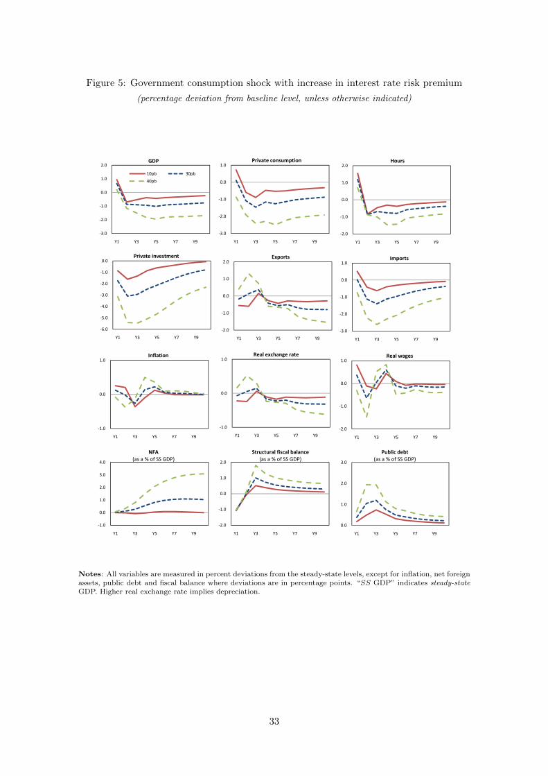
Figure 5: Government consumption shock with increase in interest rate risk premium

(percentage deviation from baseline level, unless otherwise indicated)

‐3.0

‐2.0

‐1.0

0.0

1.0

2.0

Y1 Y3 Y5 Y7 Y9

GDP

10pb 30pb

40pb

‐3.0

‐2.0

‐1.0

0.0

1.0

Y1 Y3 Y5 Y7 Y9

Private consumption

‐6.0

‐5.0

‐4.0

‐3.0

‐2.0

‐1.0

0.0

Y1 Y3 Y5 Y7 Y9

Private investment

‐2.0

‐1.0

0.0

1.0

2.0

Y1 Y3 Y5 Y7 Y9

Exports

‐3.0

‐2.0

‐1.0

0.0

1.0

Y1 Y3 Y5 Y7 Y9

Imports

‐2.0

‐1.0

0.0

1.0

2.0

Y1 Y3 Y5 Y7 Y9

Hours

Inflation1 0

Real exchange rate Real wages

‐3.0

‐2.0

‐1.0

0.0

1.0

2.0

Y1 Y3 Y5 Y7 Y9

GDP

10pb 30pb

40pb

‐3.0

‐2.0

‐1.0

0.0

1.0

Y1 Y3 Y5 Y7 Y9

Private consumption

‐6.0

‐5.0

‐4.0

‐3.0

‐2.0

‐1.0

0.0

Y1 Y3 Y5 Y7 Y9

Private investment

‐2.0

‐1.0

0.0

1.0

2.0

Y1 Y3 Y5 Y7 Y9

Exports

‐3.0

‐2.0

‐1.0

0.0

1.0

Y1 Y3 Y5 Y7 Y9

Imports

‐2.0

‐1.0

0.0

1.0

2.0

Y1 Y3 Y5 Y7 Y9

Hours

‐1.0

0.0

1.0

Y1 Y3 Y5 Y7 Y9

Inflation

‐1.0

0.0

1.0

Y1 Y3 Y5 Y7 Y9

Real exchange rate

‐2.0

‐1.0

0.0

1.0

Y1 Y3 Y5 Y7 Y9

Real wages

‐1.0

0.0

1.0

2.0

3.0

4.0

Y1 Y3 Y5 Y7 Y9

NFA(as a % of SS GDP)

‐2.0

‐1.0

0.0

1.0

2.0

Y1 Y3 Y5 Y7 Y9

Structural fiscal balance(as a % of SS GDP)

0.0

1.0

2.0

3.0

Y1 Y3 Y5 Y7 Y9

Public debt(as a % of SS GDP)

‐3.0

‐2.0

‐1.0

0.0

1.0

2.0

Y1 Y3 Y5 Y7 Y9

GDP

10pb 30pb

40pb

‐3.0

‐2.0

‐1.0

0.0

1.0

Y1 Y3 Y5 Y7 Y9

Private consumption

‐6.0

‐5.0

‐4.0

‐3.0

‐2.0

‐1.0

0.0

Y1 Y3 Y5 Y7 Y9

Private investment

‐2.0

‐1.0

0.0

1.0

2.0

Y1 Y3 Y5 Y7 Y9

Exports

‐3.0

‐2.0

‐1.0

0.0

1.0

Y1 Y3 Y5 Y7 Y9

Imports

‐2.0

‐1.0

0.0

1.0

2.0

Y1 Y3 Y5 Y7 Y9

Hours

‐1.0

0.0

1.0

Y1 Y3 Y5 Y7 Y9

Inflation

‐1.0

0.0

1.0

Y1 Y3 Y5 Y7 Y9

Real exchange rate

‐2.0

‐1.0

0.0

1.0

Y1 Y3 Y5 Y7 Y9

Real wages

‐1.0

0.0

1.0

2.0

3.0

4.0

Y1 Y3 Y5 Y7 Y9

NFA(as a % of SS GDP)

‐2.0

‐1.0

0.0

1.0

2.0

Y1 Y3 Y5 Y7 Y9

Structural fiscal balance(as a % of SS GDP)

0.0

1.0

2.0

3.0

Y1 Y3 Y5 Y7 Y9

Public debt(as a % of SS GDP)

Notes: All variables are measured in percent deviations from the steady-state levels, except for inflation, net foreignassets, public debt and fiscal balance where deviations are in percentage points. “SS GDP” indicates steady-stateGDP. Higher real exchange rate implies depreciation.

33

holding of households with access to asset markets. It reflects a higher discount on future

income, which reduces wealth and has a negative effect on consumption (wealth effect).

Additionally, the rise in the risk premium induces, ceteris paribus, an increase in the real

interest rate, which increases the return on savings (or cost of debt), measured in terms

of future consumption, thereby providing a further desincentive to present consumption

(substitution effect). Additionally, the increase in government interest outlays and debt

increases labour income taxes, implying an additional negative wealth effect and a shift

away from consumption to leisure. Private investment also suffers a protracted decline

reflecting a lower desired capital level, due to both the increased real interest rate and the

lower demand prospects which have a negative effect on dividends prospects.

In summary, when the private sector worries about fiscal sustainability drive up the

interest rate risk premium, the positive effects of a fiscal stimulus are clearly mitigated.

Therefore, a credible promise of fiscal discipline is critical even for the short-run effective-

ness of the stimulus. All depends on the actual risk premium increase. The credibility of

the fiscal stimulus and its adequacy to the prevailing financing conditions and government

debt levels should always be assessed to gauge the downside risks surrounding the impact

of fiscal stimulus packages.

5 Conclusions

This paper discussed alternative fiscal stimulus for a SOE operating in a monetary union.

The discussion was conducted using PESSOA, a New-Keynesian dynamic general equilib-

rium model with exogenous monetary policy, specially designed to fit the characteristics

of a small euro area economy.

The fiscal stimulus was assumed to imply an increase in government deficit of 1 per-

cent of steady-state GDP for one year. In addition, the fiscal policy rule that prevents

unsustainable public debt developments was assumed to be deactivated for two years. Un-

der these circumstances, the most effective policy instrument to promote growth in the

sort run is a temporary increase in government consumption. The results indicate that

such stimulus also increases actual GDP by around 1 per cent of its steady-state value

during one year. In case the fiscal stimulus is based on targeted transfers (transfers to

liquidity-constrained households) the impact is 0.6 per cent, while if it is based on taxes,

both labour income and consumption, the impact is close to 0.4 per cent. The smaller

impact (0.2 per cent) is obtained from an increase in general transfers (transfers to all

households regardless of whether they are liquidity-constrained or not). The main rea-

son behind that outcome is twofold. On the one hand, government consumption feeds

directly into aggregate demand, whereas the other instruments operate mainly through

wealth effects, with leakages to savings, which reduces the fiscal multiplier on impact. On

the other hand, government consumption has a much lower import content than private

consumption, implying less leakages to imports.

The government should however refrain from implementing a permanent increase in

34

government consumption, since the long-run costs far exceed the short-run benefits. Wel-

fare analysis showed that a permanent increase in government consumption would be

equaled by a permanent decrease in wealth measured by a decrease in private consump-

tion in the new steady-state.

The results also point that the government should avoid to take actions that are not

timely or fully credible. In both cases the fiscal multipliers are diminished and the stimulus

may even backfire, having counterproductive effects. This is likely to be the case for

economies in financial distress, in which the stimulus may trigger a surge in the sovereign

risk premium. In this case, not to implement any stimulus might be the best strategy from

an economic point of view, in particular in case the rest of the monetary union is engaged

in a fiscal stimulus program, from which the domestic economy can beneficiate indirectly

through the trade channel. However, one must be aware that this corresponds to a free-

riding behaviour, which may raise issues on a common euro area strategy. Nevertheless,

it should also be taken into account that a surge in the sovereign risk premium in a

small euro area economy may generate spill-over effects over the other member states

and ultimately jeopardise the credibility of the area as a whole in international financial

markets. Therefore, the design of a successful stimulus programme for the area as a whole,

in a situation of financial distress, should take into account the specific financial situation

of each one of the constituent economies.

Finally, even when the fiscal stimulus is fully credible and without implementation lags,

national governments should expect adverse impacts over the medium and longer run. The

fiscal stimulus is always an option that needs to be financed after some well-defined point

in the future. Given that the model operates de facto like a real model, regaining stability

requires real adjustments, including negative GDP and private consumption growth.

The main qualitative result is therefore that although national governments can use

fiscal policy to pursue some macroeconomic stabilisation objectives, namely in the short

run, the available instruments are far from being Panacea, the Greek goddess of healing.

35

References

Adolfson, M., Laseen, S., Linde, J. and Villani, M. (2007), ‘Bayesian estimation of an

open economy DSGE model with incomplete exchange rate pass-through’, Journal of

International Economics 72(2), 481–511.

Almeida, V., Castro, G. and Felix, R. M. (2008), Improving competition in the non-

tradable goods and labour markets: the Portuguese case, Working Paper No. 16/2008,

Banco de Portugal.

Almeida, V., Castro, G. and Felix, R. M. (2009), The portuguese economy in the european

context: structure, shocks and policy, in ‘The Portuguese economy in the context of

economic, financial and monetary integration’, Banco de Portugal, pp. 65–162.

Almeida, V. and Felix, R. (2006), Computing potential output and the output-gap for the

Portuguese economy, Economic Bulletin, Banco de Portugal.

Altig, D., Christiano, L., Eichenbaum, M. and Linde, J. (2005), Firm-specific capital,

nominal rigidities and the business cycle, NBER Working Papers 11034, National

Bureau of Economic Research, Inc.

Ardagna, S., Caselli, F. and Lane, T. (2004), Fiscal discipline and the cost of public debt

service. some estimates for OECD countries, Working Paper No. 411/2004, European

Central Bank.

Barro, R. and Gordon, D. (1983), ‘A positive teory of monetary policy in a natural rate

model’, Journal of Political Economy 91(4), 589–610.

Barro, R. J. and Sala-i-Martin, X. (1995), Economic Growth, McGraw-Hill, New York.

Bayoumi, T. and Sgherri, S. (2006), Mr Ricardo’s Great Adventure: Estimating Fiscal

Multipliers in a Truly Intertemporal Model, Working Paper No. 06/168, International

Monetary Fund.

Blanchard, O. (1985), ‘Debts, deficits and finite horizons’, Journal of Political Economy

93(2), 223–247.

Blanchard, O. and Perotti, R. (2002), ‘An empirical characterization of the dynamic effects

of changes in government spending and taxes on output’, The Quarterly Journal of

Economics 117(4), 1329–1368.

Buiter, W. (1988), ‘Death, birth, productivity growth and debt neutrality’, Economic

Journal 98, 279–293.

Calvo, G. A. and Obstfeld, M. (1988), ‘Optimal time-consistent fiscal policy with finite

lifetimes’, Econometrica 56(2), 411–32.

36

Canova, F. and Pappa, E. (2007), ‘Price differentials in monetary unions: The role of fiscal

shocks’, Economic Journal 117(520), 713–737.

Castro, G. (2006), Consumption, disposable income and liquidity constraints, Economic

Bulletin, Banco de Portugal.

Christiano, L., Eichenbaum, M. and Rebelo, S. (2009), When is the government spending

multiplier large?, Working Paper No. 15394, National Bureau of Economic Research.

Coenen, G., Erceg, C., Freedman, C., Furceci, D., Kumhof, M., Lalonde, R., Laxton,

D., Linde, J., Mourougane, A., Muir, D., Mursula, S., de Resende, C., Roberts, J.,

Roeger, W., Snudden, S., Trabandt, M. and in’t Veld, J. (2010), Effects of fiscal

stimulus in structural models, Working Paper No. 10/73, International Monetary

Fund.

Coenen, G., McAdam, P. and Straub, R. (2007), Tax reform and labour-market perfor-

mance in the euro area: a simulation-based analysis using the new area-wide model,

Working Paper No. 747, European Central Bank, Frankfurt, Germany.

Cogan, J. F., Cwik, T., Taylor, J. B. and Wieland, V. (2009), New keynesian versus

old keynesian government spending multipliers, Working Papers No. 14782, National

Bureau of Economic Research.

Eggertsson, G. B. (2009), What fiscal policy is effective at zero interest rates?, Staff Report

No. 402, Federal Reserve Bank of New York.

Erceg, C. J., Henderson, D. W. and Levin, A. T. (2000), ‘Optimal monetary policy with

staggered wage and price contracts’, Journal of Monetary Economics 46(2), 281–313.

Erceg, C. and Linde, J. (2010), Is there a fiscal free lunch in a liquidity trap?, Discussion

Paper No. 7624, Centre for Economic Policy Research.

Fagan, G., Gaspar, V. and Pereira, A. (2004), ‘The New Keynesian Microfoundations’,

pp. 69–104.

Freedman, C., Kumhof, M., Laxton, D. and Lee, J. (2009), The case for the global fiscal

stimulus, Staff Position Note No. 09/03, International Monetary Fund.

Freedman, C., Kumhof, M., Laxton, D., Muir, D. and Mursula, S. (2009), Fiscal stimu-

lus to the rescue? short-run benefits and potential long-run costs of fiscal deficits,

Working Paper No. 09/255, International Monetary Fund.

Frenkel, J. and Razin, A. (1996), Fiscal Policies and Growth in the World Economy, 3

edn, MIT Press, Cambridge, Massachussets.

Galı, J., Lopez-Salido, J. D. and Valles, J. (2007), ‘Understanding the effects of government

spending on consumption’, Journal of the European Economic Association 5(1), 227–

270.

37

Ganelli, G. (2005), ‘The new open economy macroeconomics of government debt’, Journal

of International Economics 65(1), 167–184.

Giavazzi, F. and Pagano, M. (1988), ‘The advantage of tying one’s hands: EMS discipline

and central bank credibility’, European Economic Review 32, 1055–1075.

Goodfriend, M. and King, R. G. (2001), The case for price stability, in A. Garcia-Herrero,

V. Gaspar, L.Hoogduin, J. Morgan and B. Winkler, eds, ‘Why price stability?’, Eu-

ropean Central Bank, Frankfurt am Main, pp. 53–94.

Hall, R. E. (2009), By how much does gdp rise if the government buys more output?,

Working Paper No. 15496, National Bureau of Economic Research.

Harrison, R., Nikolov, K., Quinn, M., Ramsay, G., Scott, A. and Thomas, R. (2005), The

Bank of England Quarterly Model, Bank of England.

Høj, J., Jimenez, M., Maher, M., Nicoletti, G. and Wise, M. (2007), Product market

competition in OECD countries: taking stock and moving forward, Economics De-

partment Working Paper No. 575, Organisation for Economic Co-operation and De-

velopment.

Ireland, P. (2001), ‘Sticky-price models of business cycle: specification and stability’,

Journal Monetary Economics 47, 3–18.

Kaplow, L. (2007), ‘Discounting dollars, discounting lives: Intergenerational distributive

justice and efficiency’, University of Chicago Law Review (79).

Kilponen, J. and Ripatti, A. (2006), Labour and product market competition in a small

open economy: Simulation results using a DGE model of the Finnish economy, Dis-

cussion Paper No. 5/2006, Bank of Finland, Helsinki.

Kim, J. (2000), ‘Constructing and estimating as realistic optimizing model of monetary

policy’, Journal of Monetary Economics 45, 329–359.

Kumhof, M. and Laxton, D. (2007a), The Global Integrated Monetary and Fiscal Model,

Mimeo, International Monetary Fund.

Kumhof, M. and Laxton, D. (2007b), A party without a hangover? On the effects of U.S.

government deficits, Working Paper No. 07/202, International Monetary Fund.

Kumhof, M. and Laxton, D. (2008), Chile’s Structural Fiscal Surplus Rule: a model based

evaluation, Research Paper forthcoming, International Monetary Fund.

Kumhof, M. and Laxton, D. (2009), Fiscal deficits and current account deficits, Working

Paper No. 09/237, International Monetary Fund.

Kumhof, M., Laxton, D. and Leigh, D. (2008), To starve or not to starve the beast ?, in

mimeo, International Monetary Fund.

38

Kumhof, M., Muir, D., Freedman, C., Mursula, S. and Laxton, D. (2009), Fiscal stimu-

lus to the rescue? short-run benefits and potential long-run costs of fiscal deficits,

Working Paper No. 09/255, International Monetary Fund.

Kydland, F. and Prescott, E. (1977), ‘The inconsistency of optimal plans’, The Journal

of Political Economy 85(3), 473–492.

Laxton, D. and Pesenti, P. (2003), ‘Monetary rules for small, open, emerging economies’,

Journal of Monetary Economics 50, 1109–1146.

Leeper, E. M., Plante, M. and Traum, N. (2009), Dynamics of fiscal financing in the united

states, Working Papers No. 15160, National Bureau of Economic Research, Inc.

Lucas Jr., R. E. (1987), Models of Business Cycles, Oxford, New York: Basil Blackwell.

Mendoza, E. (2005), Real exchange rate volatility and the price of non-tradables in sudden-

stop-prone economies, Working Paper No. 11691, National Bureau of Economic Re-

search, Cambridge, Massachussets: National Bureau of Economic Research.

Mountford, A. and Uhlig, H. (2009), ‘What are the effects of fiscal policy shocks?’, Journal

of Applied Econometrics 24(6), 960–992.

Musso, A. and Westermann, T. (2005), Assessing potential output in the euro area: a

growth accounting perspective, Occasional paper No. 22, European Central Bank,

Frankfurt, Germany.

Proietti, T. and Musso, A. (2007), Growth accounting for the euro area: a structural

approach, Working Paper No. 804, European Central Bank, Frankfurt, Germany.

Ramsey, F. (1928), ‘A mathematical theory of saving’, Economic Journal 38, 543–549.

Rotemberg, J. J. (1982), ‘Monopolistic price adjustment and aggregate output’, Review of

Economic Studies 49, 517–531.

Schmitt-Grohe, S. and Uribe, M. (2003), ‘Closing small open economy models’, Journal

of International Economics 61(1), 163–185.

Schuknecht, L., von Hagen, J. and Wolswijk, G. (2010), Government bond risk premium in

the eu revisited: the impact of the financial crisis, Working Paper No. 1152, European

Central Bank.

Smets, F. and Wouters, R. (2007), ‘Shocks and frictions in us business cycles: A bayesian

dsge approach’, American Economic Review 97(3), 586–606.

Spilimbergo, A., Symansky, S. and Schindler, M. (2009), Fiscal multipliers, Staff Position

Note No. 09/11, International Monetary Fund.

Yaari, M. (1965), ‘Uncertain lifetime, life insurance and the theory of the consumer’,

Review of Economic Studies 32(2), 137–150.

39

Appendices

A Model calibration

This appendix reports in some detail the model parameters (see Table 1). As reported

in the main text, the model matches fairly reasonably the key ratios of the Portuguese

economy and delivers a plausible capital-to-output ratio by industry standards, as depicted

in Table 2.14

The calibration of households’ parameters took into consideration that the model com-

prehends Blanchard-Yaari overlapping generations, while most DSGE models consider the

infinitely-lived agents framework. These parameters were therefore largely based on Fa-

gan, Gaspar and Pereira (2004), Harrison et al. (2005), Kumhof and Laxton (2007a) and

Kumhof and Laxton (2007b). ηA and ηB were calibrated so as to ensure that the elasticity

of labour supply to real wage is 0.5, a value commonly found in the literature. Since the

Blanchard-Yaari overlapping generations households framework allows for an endogenous

determination of the net foreign asset position, the discount rate was calibrated to ensure

a net foreign debt position of 60 per cent in the steady-state. The coefficient of relative

risk aversion was set to calibrate the intertemporal elasticity of substitution to 0.2, which

might seem a low figure in comparison with the values typically used in infinitely-lived

agents models, but it is in the range of the values regularly used in models featuring

Blanchard-Yaari households. The share of liquidity constrained households was set to 40

per cent, broadly in line with the estimates for Portugal presented in Castro (2006).

In terms of labour unions’ parameters, we considered a 25 per cent wage markup, which

is at the upper limit of the values usually found in the literature. Note, however, that

since the labour market in Portugal is strongly regulated, one may argue that the markup

could be even higher than the figures usually found in the DSGE literature. Nominal wage

rigidity was calibrated to ensure that wages adjust to the new equilibrium in 6 quarters,

a value slightly above euro area estimates published in Coenen et al. (2007), but still in

the range usually found in the literature.

Turning to manufacturers, the depreciation rate was assumed to be identical across

firms and was calibrated to get the investment-to-GDP ratio in line with the NA data.

As regards the production function, a standard Cobb-Douglas function between capital

and labour was assumed and the distribution parameters were calibrated to match the

labour income share in the NA data. The price markup of tradable and non-tradable

goods’ manufacturers was calibrated using OECD product market regulation indicators

and the correlation between tradable and non-tradable goods markups and product mar-

ket regulation indicators found in Høj, Jimenez, Maher, Nicoletti and Wise (2007). In

particular, the non-tradable goods markup was set to 20 per cent, which is at the upper

bound of the range of values commonly found in the literature, but consistent with the

evidence pointing to low competition in the Portuguese non-tradable goods market. As for

14The Portuguese national accounts do not include figures for capital stock.

40

Appendix - Table 1: Main parameters

Parameter ValueMonetary union parameters

Euro area interest rate (annualised) i∗ 1.05Euro area labour-augmenting prod. growth (annualised) g 1.02Euro area inflation target (annualised) π∗ 1.02Euro area EoS between domestic and imported goods ξ∗ 2.50

Households and Unions

Households discount rate (annualised) β 0.97Intertemporal elasticity of substitution 1

γ 0.20

Households instant probability of death (annualised) 1− θ 0.04Households habit persistence ν 0.70Consumption share - Type A households ηA 0.74Consumption share - Type B households ηB 0.66Lifetime productivity decline rate (annualised) 1− χ 0.04Share of type B households ψ 0.40Wage mark-up σU

σU−1 1.25

Wage rigidity - Adjustment cost φU 200

Manufacturers

Depreciation rate (annualised) δ 0.09EoS between capital and labour ξJ 0.99Price markup - tradables σT

σT−1 1.10

Price markup - non-tradables σNσN−1 1.20

Capital adjustment cost φIJ 10Labour adjustment cost φUJ 5Price adjustment cost φPJ 200Quasi labour income share - tradables αT 0.56Quasi labour income share - non-tradables αN 0.60

Distributors

EoS domestic tradable/imported good ξAF 1.50EoS assembled/non-tradable good ξF 0.50Price markup (domestic distributors) σF

σF−1 , F 6= X 1.05

Price markup (exporters) σXσX−1 1.03

Import content adjustment cost φAF 2Price adjustment cost φPF 200

Government

Labour income tax rate τL 0.23Consumption tax rate τC 0.31Capital income tax rate τK 0.17Employers’ social security contribution rate τSP 0.19Debt to GDP ratio (annualised) b

gdp 0.53

Fiscal stance parameter d1 1.00Speed adjustment towards the target debt ratio parameter d2 0.10

41

Appendix - Table 2: Steady-state key ratios

Data ModelExpenditure (as a % of GDP)

Private consumption 0.64 0.61Government consumption and GFCF 0.22 0.21Private investment 0.21 0.21Exports 0.29 0.29Imports 0.37 0.33

Labour income share (as a % of overall income) 0.57 0.56

Tradable goods 0.54 0.54Non-tradable goods 0.58 0.58

Capital-output ratio (as a % of output) NA 2.34

Tradable goods NA 2.53Non-tradable goods NA 2.21

Government (as a % of GDP)

Debt stock 0.57 0.53Fiscal balance -0.07 -0.02Overall revenues 0.38 0.39Overall expenditure 0.45 0.41

External account (as a % of GDP)

Net foreign assets -0.60 -0.60Current account -0.06 -0.02Trade balance -0.08 -0.04

42

real rigidities, capital adjustment costs were calibrated so as to ensure plausible impulse

responses in terms of investment volatility. Regarding nominal rigidities, price growth ad-

justment costs were calibrated to match average adjustment time spans, in line with what

is suggested in the literature. In particular, we impose that the adjustment of prices in the

non-tradable goods’ sector is slightly slower than in the tradable goods’ sector, reflecting

the fact that fiercer competition and lower markups imply lower price stickiness.

We now consider distributors’ parameters. In the assemblage stage, the elasticity

of substitution between domestic tradable goods and imports was taken to be identical

across distributors and set above unity, as in most of the literature on open economy

DSGE models (see for instance Coenen et al. (2007), Harrison et al. (2005), Erceg et al.

(2000) or Kumhof and Laxton (2007b)); on the other hand, in the distribution stage,

assembled goods (which are basically a composite tradable good) and non-tradable goods

were assumed to feature a low substitutability as in Mendoza (2005) and Kumhof and

Laxton (2007b). The distribution parameters of the production function in each stage were

calibrated to match the NA import content and non-tradable goods’ content of each type

of final good. The degree of monopolistic competition among distributors was assumed to

be lower than among manufacturers, with the markup being set to 5 per cent, except in

the case of exporters, where fiercer competition is likely to determine a lower markup. In

terms of price stickiness, an average duration of price contracts of 2 quarters was assumed

for all distributors except for exporters, whose prices are assumed to adjust slightly faster.

Real rigidities related to the import content adjustment costs were set to ensure a smooth

adjustment of import contents to real exchange rate fluctuations.

Government’s average tax rates were calibrated to match the share of revenue-to-GDP

ratio in the data. The same applies to EU transfers and to expenditure components

(government consumption and investment and government transfers). The parameters of

the fiscal policy rule were calibrated to impose a structural budget balance rule (unit fiscal

policy stance parameter) and to ensure a smooth labour income tax rate adjustment. The

target debt-to-GDP ratio was set to 53 per cent, implying a fiscal balance-to-GDP ratio

of −2.1 per cent in the steady-state.15

15The values assumed for the debt-to-GDP target and the implied fiscal balance can be questioned in viewof the medium term objective that has been set by the European Commission for Portugal (a structuralbudget balance of −0.5 per cent, implying a debt-to-GDP ratio of close to 12 per cent). However, since inthe historical period that was used to calibrate the model the debt-to-GDP ratio averaged 57 per cent, itdoes not seem reasonable to calibrate it to match something substantially different from historical figures.

43

B Present value multipliers

The present value multiplier (PVM) is computed following the proposal by Mountford

and Uhlig (2009) that has already been used in the context of general equilibrium models

(Leeper, Plante and Traum 2009). For any variable of interest, the assessment delivered

by the present value multiplier up to period k can be expressed as:

PVM(k) =

∑kj=0(βθ)j Yt+j

Et∑k

j=0(βθ)j sgt+j(34)

where Yt refers to deviation from steady-state of variable Y in period t, sgt refers to

deviation from steady-state of fiscal balance-to-GDP ratio in period t and βθ stands for

the household discount factor β adjusted by θ, the degree of myopia. Typical candidates

for Y can be, for instance, GDP or private consumption.

C Welfare analysis

Welfare analysis can be seen as a benchmark metric for the impact of a particular policy

experiment in social welfare, as measured through the aggregate lifetime utility, which is

a function of goods valued by households (consumption and leisure in the case at hand).

In a general equilibrium framework, welfare can be seen as the present value multiplier

of households’ utility (as k → ∞). A widely used metric based on welfare analysis is the

compensated consumption variation in the spirit of Lucas Jr. (1987). In infinite horizon

models, it is natural to consider the representative agent utility function as the welfare

criterion (Ganelli 2005). In overlapping generation models, welfare analysis is much less

straightforward, since individuals have finite lifetimes and in each period an infinite number

of generations coexist. Hence, the choice of a welfare criteria in these models is far more

debatable than in infinitely-lived agents models, since it involves a subjective weighting of

the utility of current and future generations.

In this paper, we use a discrete time counterpart of the suggestion of Calvo and Obstfeld

(1988), which has also been used in the literature (Ganelli 2005, Kumhof et al. 2008). The

method consists in using the utility function of the representative agent, for each period

t, at the average per-capita consumption (ct+s) and leisure (1 − lt+s), where lt+s stands

for hours worked. Since these figures in period t + s result from optimal decisions of

representative agents of all generations alive in that period, the utility level is a measure

of the average utility level in the period. The synthetic welfare indicator is obtained as a

weighted average of the utility of the individuals alive in the current and in future periods,

where a weighting factor W reflects the importance of future generations in the welfare

44

from the viewpoint of the policymaker. This welfare indicator can be expressed as:

Welfare =

∞∑s=0

(W )s

1

1− γ

( cHt+s(cHt+s−1

)v)ηH

(1− lHt+s)1−ηH

1−γ (35)

Given that the choice of W involves ethical considerations, namely on fairness to-

wards born and unborn generations, we conducted a sensitivity analysis using alternative

discount rates. The benchmark value WB will be the households discount factor corre-

sponding to an annualised discount rate of 6.3 per cent. Alternative schemes are: the

steady-state real market interest rate WK , in line with the rationale proposed in Kaplow

(2007) and used in Kumhof et al. (2008), which corresponds to an annualised discount

rate of 2.8 per cent; a very low discount rate WL = 0.1 per cent, which is closer to the

view of Ramsey (1928), who advocates that all generations should be treated alike; and,

finally, a very high discount rate WH , corresponding to an annual discount rate of 30 per

cent that is a proxy for the view of a very short-sighted government (caring more about

the immediate impact of the stimulus, than for instance on the need to also envisage an

adequate exit strategy).

The implied weighting scheme over ten years (40 quarters) is illustrated in Figure

1. The lower the discount rate the more future events matter. For instance, an annual

discount rate of 0.1 per cent implies that events occurring in 10 years ahead are weighted

as much as an event occurring at t = 0, while a discount rate of 30 per cent implies that

events occurring more than 8 years ahead are to a large extent not considered. The average

lifetime of the discount window is simply 11−W , implying that it is virtually unlimited in

the first case and limited to slightly more than 3 years in the last case. The remaining

cases lie in between.

Once the welfare measure is obtained, then the compensating variation can be com-

puted, which consists in expressing welfare gains (losses) in terms of equivalent increase

in consumption in the steady-state. This simply consists in obtaining the value for CV

such that:

∞∑s=0

(W )s

1

1− γ

( cHt+s · (1 + CV )(cHt+s−1 · (1 + CV )

)v)ηH

(1− lHt+s)1−ηH

1−γ = Welfare

(36)

45

Appendix - Figure 1: Welfare weighting scheme

(in percentage)

40%

50%

60%

70%

80%

90%

100%

0%

10%

20%

30%

40%

50%

60%

70%

80%

90%

100%

0 1 2 3 4 5 6 7 8 9 10

Years

W_L = 0.1% W_K = 2.8%

W_B = 6.3% W_H = 30.0%

46

Banco de Portugal | Working Papers i

WORKING PAPERS

2008

1/08 THE DETERMINANTS OF PORTUGUESE BANKS’ CAPITAL BUFFERS — Miguel Boucinha

2/08 DO RESERVATION WAGES REALLY DECLINE? SOME INTERNATIONAL EVIDENCE ON THE DETERMINANTS OF RESERVATION WAGES

— John T. Addison, Mário Centeno, Pedro Portugal

3/08 UNEMPLOYMENT BENEFITS AND RESERVATION WAGES: KEY ELASTICITIES FROM A STRIPPED-DOWN JOB SEARCH APPROACH

— John T. Addison, Mário Centeno, Pedro Portugal

4/08 THE EFFECTS OF LOW-COST COUNTRIES ON PORTUGUESE MANUFACTURING IMPORT PRICES — Fátima Cardoso, Paulo Soares Esteves

5/08 WHAT IS BEHIND THE RECENT EVOLUTION OF PORTUGUESE TERMS OF TRADE? — Fátima Cardoso, Paulo Soares Esteves

6/08 EVALUATING JOB SEARCH PROGRAMS FOR OLD AND YOUNG INDIVIDUALS: HETEROGENEOUS IMPACT ON UNEMPLOYMENT DURATION

— Luis Centeno, Mário Centeno, Álvaro A. Novo

7/08 FORECASTING USING TARGETED DIFFUSION INDEXES — Francisco Dias, Maximiano Pinheiro, António Rua

8/08 STATISTICAL ARBITRAGE WITH DEFAULT AND COLLATERAL — José Fajardo, Ana Lacerda

9/08 DETERMINING THE NUMBER OF FACTORS IN APPROXIMATE FACTOR MODELS WITH GLOBAL AND GROUP-SPECIFIC FACTORS

— Francisco Dias, Maximiano Pinheiro, António Rua

10/08 VERTICAL SPECIALIZATION ACROSS THE WORLD: A RELATIVE MEASURE — João Amador, Sónia Cabral

11/08 INTERNATIONAL FRAGMENTATION OF PRODUCTION IN THE PORTUGUESE ECONOMY: WHAT DO DIFFERENT MEASURES TELL US?

— João Amador, Sónia Cabral

12/08 IMPACT OF THE RECENT REFORM OF THE PORTUGUESE PUBLIC EMPLOYEES’ PENSION SYSTEM — Maria Manuel Campos, Manuel Coutinho Pereira

13/08 EMPIRICAL EVIDENCE ON THE BEHAVIOR AND STABILIZING ROLE OF FISCAL AND MONETARY POLICIES IN THE US

— Manuel Coutinho Pereira

14/08 IMPACT ON WELFARE OF COUNTRY HETEROGENEITY IN A CURRENCY UNION — Carla Soares

15/08 WAGE AND PRICE DYNAMICS IN PORTUGAL — Carlos Robalo Marques

16/08 IMPROVING COMPETITION IN THE NON-TRADABLE GOODS AND LABOUR MARKETS: THE PORTUGUESE CASE — Vanda Almeida, Gabriela Castro, Ricardo Mourinho Félix

17/08 PRODUCT AND DESTINATION MIX IN EXPORT MARKETS — João Amador, Luca David Opromolla

Banco de Portugal | Working Papers ii

18/08 FORECASTING INVESTMENT: A FISHING CONTEST USING SURVEY DATA — José Ramos Maria, Sara Serra

19/08 APPROXIMATING AND FORECASTING MACROECONOMIC SIGNALS IN REAL-TIME — João Valle e Azevedo

20/08 A THEORY OF ENTRY AND EXIT INTO EXPORTS MARKETS — Alfonso A. Irarrazabal, Luca David Opromolla

21/08 ON THE UNCERTAINTY AND RISKS OF MACROECONOMIC FORECASTS: COMBINING JUDGEMENTS WITH SAMPLE AND MODEL INFORMATION

— Maximiano Pinheiro, Paulo Soares Esteves

22/08 ANALYSIS OF THE PREDICTORS OF DEFAULT FOR PORTUGUESE FIRMS — Ana I. Lacerda, Russ A. Moro

23/08 INFLATION EXPECTATIONS IN THE EURO AREA: ARE CONSUMERS RATIONAL? — Francisco Dias, Cláudia Duarte, António Rua

2009

1/09 AN ASSESSMENT OF COMPETITION IN THE PORTUGUESE BANKING SYSTEM IN THE 1991-2004 PERIOD — Miguel Boucinha, Nuno Ribeiro

2/09 FINITE SAMPLE PERFORMANCE OF FREQUENCY AND TIME DOMAIN TESTS FOR SEASONAL FRACTIONAL INTEGRATION

— Paulo M. M. Rodrigues, Antonio Rubia, João Valle e Azevedo

3/09 THE MONETARY TRANSMISSION MECHANISM FOR A SMALL OPEN ECONOMY IN A MONETARY UNION — Bernardino Adão

4/09 INTERNATIONAL COMOVEMENT OF STOCK MARKET RETURNS: A WAVELET ANALYSIS — António Rua, Luís C. Nunes

5/09 THE INTEREST RATE PASS-THROUGH OF THE PORTUGUESE BANKING SYSTEM: CHARACTERIZATION AND DETERMINANTS

— Paula Antão

6/09 ELUSIVE COUNTER-CYCLICALITY AND DELIBERATE OPPORTUNISM? FISCAL POLICY FROM PLANS TO FINAL OUTCOMES

— Álvaro M. Pina

7/09 LOCAL IDENTIFICATION IN DSGE MODELS — Nikolay Iskrev

8/09 CREDIT RISK AND CAPITAL REQUIREMENTS FOR THE PORTUGUESE BANKING SYSTEM — Paula Antão, Ana Lacerda

9/09 A SIMPLE FEASIBLE ALTERNATIVE PROCEDURE TO ESTIMATE MODELS WITH HIGH-DIMENSIONAL FIXED EFFECTS

— Paulo Guimarães, Pedro Portugal

10/09 REAL WAGES AND THE BUSINESS CYCLE: ACCOUNTING FOR WORKER AND FIRM HETEROGENEITY — Anabela Carneiro, Paulo Guimarães, Pedro Portugal

11/09 DOUBLE COVERAGE AND DEMAND FOR HEALTH CARE: EVIDENCE FROM QUANTILE REGRESSION — Sara Moreira, Pedro Pita Barros

12/09 THE NUMBER OF BANK RELATIONSHIPS, BORROWING COSTS AND BANK COMPETITION — Diana Bonfi m, Qinglei Dai, Francesco Franco

Banco de Portugal | Working Papers iii

13/09 DYNAMIC FACTOR MODELS WITH JAGGED EDGE PANEL DATA: TAKING ON BOARD THE DYNAMICS OF THE IDIOSYNCRATIC COMPONENTS

— Maximiano Pinheiro, António Rua, Francisco Dias

14/09 BAYESIAN ESTIMATION OF A DSGE MODEL FOR THE PORTUGUESE ECONOMY — Vanda Almeida

15/09 THE DYNAMIC EFFECTS OF SHOCKS TO WAGES AND PRICES IN THE UNITED STATES AND THE EURO AREA — Rita Duarte, Carlos Robalo Marques

16/09 MONEY IS AN EXPERIENCE GOOD: COMPETITION AND TRUST IN THE PRIVATE PROVISION OF MONEY — Ramon Marimon, Juan Pablo Nicolini, Pedro Teles

17/09 MONETARY POLICY AND THE FINANCING OF FIRMS — Fiorella De Fiore, Pedro Teles, Oreste Tristani

18/09 HOW ARE FIRMS’ WAGES AND PRICES LINKED: SURVEY EVIDENCE IN EUROPE — Martine Druant, Silvia Fabiani, Gabor Kezdi, Ana Lamo, Fernando Martins, Roberto Sabbatini

19/09 THE FLEXIBLE FOURIER FORM AND LOCAL GLS DE-TRENDED UNIT ROOT TESTS — Paulo M. M. Rodrigues, A. M. Robert Taylor

20/09 ON LM-TYPE TESTS FOR SEASONAL UNIT ROOTS IN THE PRESENCE OF A BREAK IN TREND — Luis C. Nunes, Paulo M. M. Rodrigues

21/09 A NEW MEASURE OF FISCAL SHOCKS BASED ON BUDGET FORECASTS AND ITS IMPLICATIONS — Manuel Coutinho Pereira

22/09 AN ASSESSMENT OF PORTUGUESE BANKS’ COSTS AND EFFICIENCY — Miguel Boucinha, Nuno Ribeiro, Thomas Weyman-Jones

23/09 ADDING VALUE TO BANK BRANCH PERFORMANCE EVALUATION USING COGNITIVE MAPS AND MCDA: A CASE STUDY

— Fernando A. F. Ferreira, Sérgio P. Santos, Paulo M. M. Rodrigues

24/09 THE CROSS SECTIONAL DYNAMICS OF HETEROGENOUS TRADE MODELS — Alfonso Irarrazabal, Luca David Opromolla

25/09 ARE ATM/POS DATA RELEVANT WHEN NOWCASTING PRIVATE CONSUMPTION? — Paulo Soares Esteves

26/09 BACK TO BASICS: DATA REVISIONS — Fatima Cardoso, Claudia Duarte

27/09 EVIDENCE FROM SURVEYS OF PRICE-SETTING MANAGERS: POLICY LESSONS AND DIRECTIONS FOR ONGOING RESEARCH

— Vítor Gaspar , Andrew Levin, Fernando Martins, Frank Smets

2010

1/10 MEASURING COMOVEMENT IN THE TIME-FREQUENCY SPACE — António Rua

2/10 EXPORTS, IMPORTS AND WAGES: EVIDENCE FROM MATCHED FIRM-WORKER-PRODUCT PANELS — Pedro S. Martins, Luca David Opromolla

3/10 NONSTATIONARY EXTREMES AND THE US BUSINESS CYCLE — Miguel de Carvalho, K. Feridun Turkman, António Rua

Banco de Portugal | Working Papers iv

4/10 EXPECTATIONS-DRIVEN CYCLES IN THE HOUSING MARKET — Luisa Lambertini, Caterina Mendicino, Maria Teresa Punzi

5/10 COUNTERFACTUAL ANALYSIS OF BANK MERGERS — Pedro P. Barros, Diana Bonfi m, Moshe Kim, Nuno C. Martins

6/10 THE EAGLE. A MODEL FOR POLICY ANALYSIS OF MACROECONOMIC INTERDEPENDENCE IN THE EURO AREA — S. Gomes, P. Jacquinot, M. Pisani

7/10 A WAVELET APPROACH FOR FACTOR-AUGMENTED FORECASTING — António Rua

8/10 EXTREMAL DEPENDENCE IN INTERNATIONAL OUTPUT GROWTH: TALES FROM THE TAILS — Miguel de Carvalho, António Rua

9/10 TRACKING THE US BUSINESS CYCLE WITH A SINGULAR SPECTRUM ANALYSIS — Miguel de Carvalho, Paulo C. Rodrigues, António Rua

10/10 A MULTIPLE CRITERIA FRAMEWORK TO EVALUATE BANK BRANCH POTENTIAL ATTRACTIVENESS — Fernando A. F. Ferreira, Ronald W. Spahr, Sérgio P. Santos, Paulo M. M. Rodrigues

11/10 THE EFFECTS OF ADDITIVE OUTLIERS AND MEASUREMENT ERRORS WHEN TESTING FOR STRUCTURAL BREAKS IN VARIANCE

— Paulo M. M. Rodrigues, Antonio Rubia

12/10 CALENDAR EFFECTS IN DAILY ATM WITHDRAWALS — Paulo Soares Esteves, Paulo M. M. Rodrigues

13/10 MARGINAL DISTRIBUTIONS OF RANDOM VECTORS GENERATED BY AFFINE TRANSFORMATIONS OF INDEPENDENT TWO-PIECE NORMAL VARIABLES

— Maximiano Pinheiro

14/10 MONETARY POLICY EFFECTS: EVIDENCE FROM THE PORTUGUESE FLOW OF FUNDS — Isabel Marques Gameiro, João Sousa

15/10 SHORT AND LONG INTEREST RATE TARGETS — Bernardino Adão, Isabel Correia, Pedro Teles

16/10 FISCAL STIMULUS IN A SMALL EURO AREA ECONOMY — Vanda Almeida, Gabriela Castro, Ricardo Mourinho Félix, José Francisco Maria