The macroeconomics of fiscal consolidations in euro

area countries

Lorenzo Forni Andrea Gerali Massimiliano Pisani ∗

December 23, 2009

Abstract

We quantitatively assess the macroeconomic implications of per-manently reducing the public debt-to-gross domestic product (GDP)ratio in euro area countries. The simulations of a currency union dy-namic general equilibrium model, calibrated to the euro area, give thefollowing results. First, tax distortions are quantitatively significant.Second, the best fiscal consolidation strategy is to permanently reduceboth expenditures and tax rates. Third, the transition is generallynot costly, as the GDP and investment would grow, while private con-sumption would not fall. Finally, spillovers to the rest of the euro areaare generally expansionary.

JEL: E62, H63Keywords: fiscal consolidation, monetary union, distortionary tax-

ation, general equilibrium models

1 Introduction

Recent forecasts by the European Commission and the International Mon-

etary Fund point to huge increases in the level of public debt in the next

few years in almost all euro area countries. The grim perspectives of the

public accounts are compounded by the very high level of implicit public

debt, related to the promises of the health and pension systems in our aging

societies. Therefore, inevitably, in the near future there will be a renewed

debate on how to consolidate the fiscal position.∗Bank of Italy, Forecasting and Modeling Division. Corresponding author: L. Forni.

Tel.:+39 06 4792 2740. E-mail address: lorenzo.forni@bancaditalia.it.

1

This paper contributes to the debate by quantitatively assessing the

macroeconomic and welfare implications of different region-specific fiscal

consolidation scenarios in the euro area. We model a single country as part

of the euro area in order to properly take into account the role of the common

monetary policy and the spillovers from (and to) the rest of the area. We

consider Germany as the benchmark, given its relative large size.

Euro area countries are relatively homogenous in terms of GDP compo-

nents (as private consumption and investment as a ratio to GDP) and also

in terms of fiscal variables (as the total level of expenditures and revenues).

They mainly differ in size, degree of openness and level of public debt. We

therefore repeat our analysis of fiscal consolidation calibrating the model

also on the Belgian economy. Belgium has rather different structural fea-

tures with respect to Germany, given that it is a small economy with a high

degree of intra-euro area trade openness and with a relatively higher level

of public debt. The analysis of Germany and Belgium, therefore, provides

enough cases to assess the situation of most euro area countries.

The basic structure of the model is akin to the Global Economy Model

(GEM) developed at the IMF.1 There are monopolistic competition in the

goods and labor markets, standard real and nominal frictions to match the

persistence and inertia usually found in the data, an interest rate feedback

rule for the monetary authority. Differently from other similar models, ours

is rich in the terms of fiscal features, that allow to realistically analyze fiscal

issues in a general equilibrium context. Fiscal policy is conducted at regional

level. In each region we break down the Ricardian equivalence by introduc-

ing distortionary taxes on labor income, capital income and consumption,1See Pesenti (2008). See also Bayoumi (2004) for a non-technical description of the

GEM. Several central banks have developed DSGE models for policy analysis. Among theothers, the Fed has developed SIGMA (see Erceg et al. (2006)), the European CentralBank the New Euro Area Wide Model (see Coenen et al. (2007)).

2

allowing for a realistic treatment of fiscal policy. On the expenditure side, we

depart from the simplifying assumption that public expenditures are “pure

waste”. We carefully distinguish between different uses of public money.

Specifically, we consider spending on final goods and services produced by

the private sector, public employment and transfer to families. Decompos-

ing public expenditures in its main components is important, as each one

has different macroeconomic implications.2 In particular, we assume that

public spending on private final goods is used as intermediate good and

combined with public employment to produce public goods that positively

affects the households’ utility function. In this way, a trade-off between the

welfare-enhancing public good and the misallocation of (goods and labor)

resources induced by its production is introduced in the model.

We focus on consolidation scenarios where the German (Belgian) fis-

cal authority permanently reduces the public debt-to-annual gross domestic

product (GDP from now on) ratio target from 65% to 55% (85% to 75%)

over a five-year horizon. The scenarios differ in terms of tax rates and ex-

penditure items that are changed to reach the target. The model parameters

are calibrated to values commonly used in the literature and to replicate the

great ratios of Germany (Belgium) and rest of the euro area. We assume

that in the rest of the euro area lump-sum transfers are tuned in order to

leave the public debt-to-GDP ratio unchanged.

We run simulations under perfect-foresight and assume that the only

shocks perturbing the economy are the German or Belgian fiscal ones. We

use Dynare to compute initial and final steady states and related transi-

tion path. We abstract from considerations related to lack of credibility,2Rogerson (2007) argues that “it is essential to explicitly consider how the government

spends tax revenues when assessing the effects of tax rates on aggregate hours of marketwork.” For a formal analysis along these lines, see Leeper and Yang (2006).

3

uncertainty, optimal Ramsey policy, the use of fiscal instrument to stabi-

lize business cycle and to fiscal coordination issues between Germany (or

Belgium) and rest of the euro area.3

Along the transition nominal and real rigidities contribute, jointly with

the gradual implementation of fiscal measures, to prolong the adjustment

of the economy towards the new long run equilibrium. So we report long

run (final steady state) and short-medium run (transition) macroeconomic

domestic effects and spillovers to the rest of the euro area. We also provide

a measure of the effects on welfare in terms of consumption equivalents.

Finally, we perform sensitivity analysis to check for the robustness of results.

Results are as follows. First, we show that fiscal distortions are quanti-

tatively relevant. For a given public debt-to-GDP ratio, tax rate cuts com-

pensated by lower lump-sum transfers have clear welfare-improving implica-

tions. To the contrary, increases in expenditures (financed by lower lump-

sum transfers) aimed at the provision of welfare-enhancing public goods,

have negative welfare effects. The reason is that the increase in welfare re-

lated to the higher level of public good is more than compensated by the

increase in economic distortions (on private goods and labor supply) associ-

ated to its production. Second, and consistently with the above results, the

best way to accomplish a reduction in the public debt-to-GDP ratio is by

lowering tax rates while, at the same time, reducing expenditures by more

than would be needed with unchanged tax rates. In particular, a simultane-

ous reduction in public expenditures and tax rates that achieves the targeted

reduction of the public debt has the highest long run (steady-state) expan-

sionary effects on GDP and on all its components. In the case of Germany,

the former increases by 7 to 10% of the initial steady state level, depending3On the optimal Ramsey problem see Juillard and Pelgrin (2007).

4

on the exact composition of the adjustment. Moreover, among expenditures

it is preferable to cut purchases of goods and services or public employment

rather than transfers to households. Similar results are obtained in the case

of Belgium. The macroeconomic effects on domestic output, income and

aggregate demand are smaller than in the German case, given that the Bel-

gium is a more open economy, with a relatively high import weight in the

consumption and investment baskets. The domestic Belgian effects, how-

ever, are not negligible. Third, in the case of Germany spillovers to the

rest of the euro area are expansionary and sizeable (long run GDP in the

rest of the euro area increases by 2.5-4%). Spillovers are negligible in the

case of Belgium, because of its small size. Finally, on impact and along

the transition GDP and investment would grow, while private consumption

would not fall. When public purchases (a component of internal demand) or

government employment (as GDP includes also the public sector wage bill)

are being cut GDP growth is subdued.

Our findings are interesting along several dimensions. We contribute

to the debate on the quantitative relevance of the macroeconomic effects

of fiscal measures. Feldstein (2008) discusses “how the effects of taxes

on economic behavior are important for revenue estimation, for calculat-

ing efficiency effects, and for understanding short-term macroeconomic con-

sequences.” Mankiw and Weinzierl (2006) use standard growth models to

assess the supply side effects of tax cuts and conclude that “in all models

considered, the dynamic response of the economy to tax changes is too large

to be ignored”. They also show that the results obtained using the standard

neoclassic growth model with infinitely lived agents - the framework consid-

ered in this paper - are robust to departures, like that of assuming agents

5

with finite horizons or including a share of rule of thumb consumers.4

One of the results that we obtain is that there is a wide margin to reduce

public expenditures with limited welfare costs. This conclusion supports

those obtained by Afonso, Schuknecht and Tanzi (2005), although from a

completely different perspective. Their study applies Data Envelope Analy-

sis to assess the “efficiency frontier” of the public sector in the provision of

public services and conclude that the same level of public services could be

attained with 1/4 less public spending. This result is surprisingly close to

what we find.

Our contribution is also related to the empirical literature on the non-

Keynesian effects of fiscal policy.5 This literature has considered (variously

defined) fiscal consolidations in OECD countries in order to obtain some in-

dications on the characteristics that most likely would lead to successful (i.e.

lasting) adjustments. The main conclusion are that (i) adjustments concen-

trated on the expenditure side of the budget more than on the revenue side

and (ii) large adjustments (measured by the reduction in the debt-to-GDP

ratio) tend to have more non-Keynesian effects. The main theoretical argu-

ment behind these results is that agents are forward looking and therefore

any sustainable reduction in public expenditure would generate a wealth

effect (agents foresee less taxes) leading to an increase in consumption, in-

vestment and economic activity. This wealth effect could – under certain

circumstances (as in cases of very high debt-to-GDP ratio at the begin-

ning of the consolidation phase) – dominate against the (Keynesian) direct

depressing effect coming from cuts in public expenditures. Our general equi-4We have extended the model in order to include non Ricardian (or rule-of-thumb)

agents and we confirm the findings of Mankiw and Weinzierl (2006). Results are availablefrom the authors upon request.

5See, among the others, Alesina and Perotti (1995, 1997), Giavazzi and Pagano (1990,1996), McDermott and Wescott (1996), Alesina and Ardagna (1998).

6

librium model formalizes most of these channels and allows weighting them

in a sound quantitative manner.

Other papers strongly related to ours are Coenen, McAdam and Straub

(2006) and Coenen, Mohr and Straub (2006). In particular, the latter an-

alyzes costs and benefits of fiscal consolidation scenarios in the euro area,

using a less detailed description of fiscal policy that we use. Their results

point to significant positive long-run effects on the main macroeconomic

variables, mainly when the improvement in the budget position is used to

decrease distortionary taxes.

The paper is organized as follows. Section 2 provides a discussion of

the setup of the model. Section 3 presents the results of the baseline fiscal

consolidation scenarios. Section 4 discusses the transition dynamics of the

different fiscal consolidation strategies, while section 5 provides robustness

checks. Section 6 concludes.

2 The Model

In this section we initially illustrate the model setup, focusing mainly on the

fiscal features. We then report the calibration and the model-based fiscal

consolidation scenarios.

2.1 The Setup

There are two regions, Home and rest of the euro area, having different

sizes and sharing the monetary policy and currency. In each region there

are households and firms. Each household consumes a final good, which

is a composite made of intermediate nontradable and tradable goods. The

latter are produced domestically or imported. Households participate in

7

financial markets and smooth consumption by trading a risk-free one-period

nominal bond. They also own domestic firms and capital stock. The latter

is rented to domestic firms in a perfectly competitive market. All households

supply differentiated labor services to domestic firms and act as wage setters

in monopolistically competitive labor markets by charging a markup over

their marginal rate of substitution between consumption and leisure.

On the production side, there are perfectly competitive firms that pro-

duce the final goods and monopolistic firms that produce the intermediate

goods. The two final goods (consumption and investment goods) are sold

domestically and are produced combining all available intermediate goods

using a constant-elasticity-of-substitution (CES) production function. Inter-

mediate tradable and nontradable goods are produced combining domestic

capital and labor, that are assumed to be mobile across sectors. Intermediate

tradable goods can be sold domestically and abroad. Because intermediate

goods are differentiated, firms have market power and restrict output to

create excess profits. We also assume that markets for tradable goods are

segmented, so that firms can set two different prices, one for each market.

To capture the empirical persistence of the aggregate data and generate re-

alistic dynamics, we include adjustment costs on real and nominal variables,

ensuring that, in response to a shock, consumption and production react in

a gradual way. On the real side, quadratic costs prolong the adjustment of

the capital stock. On the nominal side, they make wages and prices sticky.6

In the following section we describe in detail the fiscal policy setup and

the households problem. In the Appendix we laid down the rest of the

model.6See Rotemberg (1982).

8

2.2 Fiscal policy

Fiscal policy is set at the regional level. The government budget constraint

is: [Bg

t+1

Rt−Bg

t

]= (1 + τ c

t )PtCgt + WtL

gt + Trt − Tt (1)

where Bgt ≥ 0 is nominal public debt. It is a one-period risk-free nominal

bond issued in the euro area wide market that pays a gross nominal interest

rate Rt controlled by the monetary authority of the currency union. The

variable Cgt represents government purchases of goods and services, WtL

gt is

compensation for public employees (Wt is the nominal wage, Lgt is the total

number of hours worked in the public sector), Trt are lump-sum transfers

to households. We assume that Cgt has the same composition as private

consumption. Hence it is pre-multiplied by the private consumption price

index Pt.7

Total government revenues Tt are given by the following identity:

Tt ≡ τ `t WtLt + τ c

t [PtCt + PtCgt ] + τk

t

[Rk

t Kt−1 + ΠPt

](2)

where the τs are tax rates on labor income (τ `t ), capital income (τk

t ) and

consumption (τ ct ), Lt is total amount of hours worked (in the public sector,

Lgt , and in the private sector, Lp

t , that is Lt = Lpt +Lg

t ), Rkt is the rental rate

of existing physical capital stock Kt−1 and ΠPt stands for dividends from

7Among government expenditure items we do not consider public investment. Thereason is twofold. On one side public investment has both demand effects (being part ofaggregate demand, exactly as government purchases) and supply side effects (as, for ex-ample, public infrastructures enhance private productivity). Therefore, from a qualitativepoint of view, it should be the last item to be cut within a consolidation plan (or, statedotherwise, it is the item with the highest output multiplier). On the other hand, froma quantitative point of view, there is limited evidence that can be used to calibrate theeffect of public investment on private production. For these two reasons we decided not toconsider this item. On this topic the interested reader can refer to Straub and Tchakarov(2007).

9

ownership of domestic monopolistic firms.

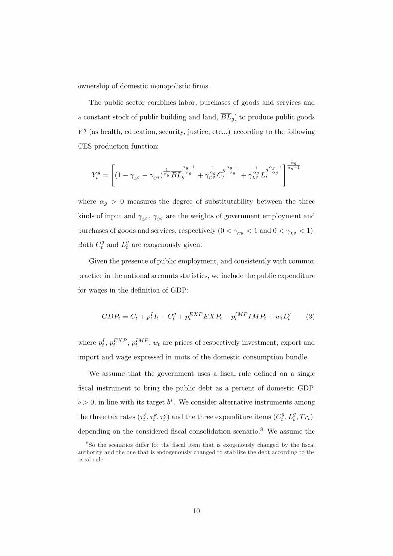
The public sector combines labor, purchases of goods and services and

a constant stock of public building and land, BLg) to produce public goods

Y g (as health, education, security, justice, etc...) according to the following

CES production function:

Y gt =

[(1− γ

Lg − γCg )

1αg BL

αg−1

αgg + γ

1αgCg C

gαg−1

αg

t + γ1

αgLg L

gαg−1

αg

t

] αgαg−1

where αg > 0 measures the degree of substitutability between the three

kinds of input and γLg , γ

Cg are the weights of government employment and

purchases of goods and services, respectively (0 < γCg < 1 and 0 < γ

Lg < 1).

Both Cgt and Lg

t are exogenously given.

Given the presence of public employment, and consistently with common

practice in the national accounts statistics, we include the public expenditure

for wages in the definition of GDP:

GDPt = Ct + pIt It + Cg

t + pEXPt EXPt − pIMP

t IMPt + wtLgt (3)

where pIt , pEXP

t , pIMPt , wt are prices of respectively investment, export and

import and wage expressed in units of the domestic consumption bundle.

We assume that the government uses a fiscal rule defined on a single

fiscal instrument to bring the public debt as a percent of domestic GDP,

b > 0, in line with its target b∗. We consider alternative instruments among

the three tax rates (τ `t , τ

kt , τ c

t ) and the three expenditure items (Cgt , Lg

t , T rt),

depending on the considered fiscal consolidation scenario.8 We assume the8So the scenarios differ for the fiscal item that is exogenously changed by the fiscal

authority and the one that is endogenously changed to stabilize the debt according to thefiscal rule.

10

following fiscal rule:

itit−1

=(

bt

b∗

)φ1(

bt

bt−1

)φ2(

GDPt

GDPt−1

)φ3

(4)

where it is one of the six fiscal instruments considered. Parameters φ1,

φ2 and φ3 are lower than zero when the rule is defined on an expenditure

item calling for a reduction in expenditures whenever the debt level is above

target and for a larger reduction whenever the dynamics of the debt is not

converging and/or the GDP growth is positive. To the contrary, they are

greater than zero when the rule is on tax rates. Overall,the fiscal setup

of the model is able to take into account many implications of different

tax and expenditure items. This is essential in order to understand the

macroeconomic effects of fiscal consolidation scenarios.

2.3 Households

In each country there is a continuum of symmetric households. Home house-

holds are indexed by j ∈ [0; s] and Foreign households by j∗ ∈ (s; 1].9 House-

holds’ preferences are additively separable in consumption and labor effort.

Households receive utility from consuming and disutility from working Lt

hours. The expected value of household j lifetime utility is given by:

E0

{ ∞∑

t=0

βt

[C̃t (j)1−σ

(1− σ)− κ

τLt (j)τ

]}

where E0 denotes the expectation conditional on information set at date 0,

β is the discount factor (0 < β < 1), 1/σ is the elasticity of intertemporal9The population of the monetary union is normalized to one. The parameter s is the

size of the Home population, which is also equal to the number of firms in each Homesector (final nontradable, intermediate tradable and intermediate nontradable). Similarassumptions hold for 1− s in the rest of the euro area.

11

substitution (σ > 0) and 1/ (τ − 1) is the labor Frisch elasticity (τ > 0).

The consumption bundle C̃t (j) is given by:

C̃t (j) =[ω

1θ Ct (j)

θ−1θ + (1− ω)

1θ Y g

t

θ−1θ

] θθ−1

where θ > 0 measures the degree of substitutability between private (C)

and public goods (Y g) while 0 ≤ ω ≤ 1 is the weight of the private good in

the consumption bundle. When ω = 1, the level of the public good does not

alter private consumption decisions.

The budget constraint of agent j is:

Bt (j)(1 + Rt) µt

−Bt−1 (j) ≤ (1− τkt )

(ΠP

t (j) + RKt Kt−1 (j)

)+

+(1− τ `t )Wt (j) Lt (j)− (1 + τ c

t )PtCt (j)− P It It (j)

+Trt (j)−ACWt (j)

Home agents hold a one-period risk-free bond, Bt, denominated in the cur-

rency of the monetary union. The short-term nominal rates Rt is paid at

the beginning of period t and is known at time t. It is directly controlled

by the monetary authority. A financial friction µt is introduced to guar-

antee that net asset positions follow a stationary process and the economy

converges to the steady state.10 We assume that government and private

bonds can be traded internationally in the same market. Households own all

domestic firms and there is no international trade in claims on firms’ prof-

its. The variable ΠPt includes profits accruing to the Home household. We

assume that profits are equally shared across households. The variable It is

investment bundle in physical capital and P It the related price index, which

10Revenues from financial intermediation are rebated in a lump-sum way to agents inthe rest of euro area. See Benigno (2009).

12

is different from the price index of consumption because the two bundles

have different composition.11 Home agents accumulate physical capital Kt

and rent it to domestic firms at the nominal rate Rkt . The law of motion of

capital accumulation is:

Kt (j) = (1− δ) Kt−1 (j) +(1−ACI

t (j))It (j)

where δ is the depreciation rate. Adjustment cost on investment ACIt is :

ACIt (j) =

φI

2

(It (j)

It−1 (j)− δ

)2

, φI > 0

Finally, Home households act as wage setters in a monopolistic competitive

labor market. Each household j set her nominal wage Wt (j) taking into

account of labor demand and adjustment costs ACWt :

ACWt (j) =

κW

2

(Wt (j)

Wt−1 (j)− 1

)2

WtLt, κW > 0

The costs are proportional to the per-capita wage bill of the overall economy,

WtLt. Similar relations hold in the Foreign country, with the exception of

the intermediation frictions in the financial market.

2.4 Calibration

The model is calibrated at quarterly frequency. We set some parameter

values so that steady-state ratios are consistent with 2007 national account

data, which are the most recent and complete available data. We choose

to not use projection for 2010 public debt-to-GDP ratios, even if available,

for two reasons. First, remaining data on fiscal variables are not available11See the Appendix for more details.

13

yet or are surrounded by a high degree of uncertainty. Second, given that it

is likely that 2010 public expenditure and debt are higher than the current

levels, our estimates represent a lower bound of the effects, so that we put

ourselves on the conservative side. For remaining parameters we resort to

previous studies and estimates available in the literature.12 Table 1 contains

parameters related to preferences and technology. Parameters with a “∗”are related to the rest of the euro area region. We assume that discount

rates and elasticities of substitution have the same value across the two

regions. The discount factor β is set to 0.9875, so that the steady state real

interest rate is equal to 5 per cent on an annual basis. The value for the

intertemporal elasticity of substitution, 1/σ, is 1. The Frisch labor elasticity

is set to 2. The weight of the private good ω in the utility function is 0.8.13

The elasticity of substitution between private and public goods, θ, is set to

1.5.14 The depreciation rate of capital δ is set to 0.025.

In the production functions of tradables the elasticity of substitution be-

tween labor and capital is set respectively to 0.85 for Germany and Belgium

and 0.9 for the rest of the euro area. In the German and Belgian production

functions of nontradables the elasticity is set to 0.79, for the rest of the euro

area to 0.95. The bias towards private capital is set to 0.75 in the German

and Belgian tradable sectors, and to 0.7 for the rest of the euro area. The

bias is set to 0.7 in the nontradable sector of each region. In the German and

Belgian production functions of the public sector the elasticity of substitu-

tion between inputs (labor, stock of public capital and intermediate goods)12Among others, see Forni, Gerali and Pisani (2009a) and Forni, Monteforte and Sessa

(2009).13There is not clear empirical evidence that we can use in the calibration of this param-

eter. We check the robustness of the results in section 5.14In the robustness section we will discuss also the results when the elasticity of sub-

stitution is lower (we will assume θ = 0.8). Most contributions assume that private andpublic consumption are substitutes. For example, Prescott (2002) assumes they are perfectsubstitutes.

14

αg is equal to 0.79, to 0.95 in the rest of the euro area. The biases towards

intermediate goods γCg and labor γ

Lg are set to 0.15.

In the final consumption and investment goods the elasticity of sub-

stitution between domestic and imported tradable is set to 1.5, while the

elasticity of substitution between tradables and nontradables to 0.5. The

bias for the composite tradable is set to 0.55 for Germany, to 0.8 for Bel-

gium and to 0.5 for the rest of the area. The biases for the domestically

produced tradables and for composite tradable goods are set to match the

Germany (Belgium)-rest of the euro area import and export to GDP ratios.

The population size of Germany (Belgium), n, is set to 0.3 (0.03) and we

normalize the population of the euro area to 1.

Table 2 reports gross markups in the tradable, nontradable and labor

markets. We assume markups are higher in the nontradable and labor mar-

kets. We obtain these figures by calibrating the sector-specific elasticities of

substitution between varieties.15

Table 3 contains parameters that regulate the dynamics. Adjustment

costs on investment change are set to 3.5. Nominal wage and price quadratic

adjustment costs are set in such a way to get an average frequency of wage

and price adjustment roughly equal to 4 quarters. The two parameters

regulating the adjustment cost paid by the Home households on their net

financial position are set to 0.01.

Parametrization of systematic feedback rule followed by the fiscal and

monetary authorities are reported in Table 4. In the fiscal policy rule (4)

we set φ1 = ±0.5, φ2 = ±5 and φ3 = ±5 for Germany, Belgium and rest of

the euro area. The chosen values allow reaching the public debt target in15For an analysis of the macroeconomic effects of different degree of markups in a model

similar to the one used in this paper, see Forni, Gerali and Pisani (2009b).

15

more or less ten years in all the simulations. Their sign is positive when the

fiscal instrument in the rule is a tax rate, it is negative when the instrument

is a public expenditure. The central bank of the euro area targets the

contemporaneous euro area wide consumer price inflation (the corresponding

parameter is set to 1.7) and the output growth (the parameter is set to

0.4).16 Interest rate is set in an inertial way and hence its previous-period

value enters the rule with a weight equal to 0.9.

Table 5 reports model-based and actual steady-state great ratios and

tax rates under our baseline calibration. Private consumption, investment,

bilateral imports and exports match the data rather well. In particular,

the Belgian economy is more open than the Germany (the shares of exports

and imports are higher). We assume a zero steady state net foreign asset

position for the German and, alternatively, Belgian economy. This implies

that - in steady state - the net financial position of the German private sector

equals the level of the German public debt (a similar assumption holds for

Belgium).17

As for fiscal policy variables, it must be noted that some expenditure

items (as purchases Cg as a ratio to GDP) are perfectly matched as they

are exogenous. For other items, as the public wage bill and the interest ex-

penditure, we calibrate the share of public employees over the total number

of employees and the level of public debt-to-annual GDP ratio to replicate

the actual data. As the wage and interest rates are endogenous, however, we16The euro area-wide consumer price inflation rate and GDP are weighted (by the

regional size) geometric average of the corresponding regional variables.17The zero net foreign asset assumption holds in both the initial and final steady state,

but not along the transition. We have done robustness analysis assuming steady stateGerman net financial position different from zero in the initial steady state and a valuedifferent from zero in the final steady state. Results, available from the authors uponrequest, are not greatly affected. This is to be expected. Because we have a monetaryunion framework, we don’t have a flexible nominal exchange rate that induces “valuationeffects” on the financial position through its fluctuations.

16

don’t match exactly the corresponding expenditure components. Tax rates

are calibrated using effective average tax rates estimates for 2007 taken from

Eurostat (2008). The tax rate on wage income τ ` is set to 39 per cent in

Germany, 42 per cent in Belgium and to 34 in the rest of the euro area. The

tax rate on capital income τk respectively to 21, 20 and 23, while the tax

rate on consumption τ c to 20 and to 22. The public debt-to-yearly GDP

ratio is calibrated to 65 per cent for Germany, 85 for Belgium and to 60 for

the rest of the euro area.

3 Results

In what follows we simulate the model to quantitatively assess the macroe-

conomic effects of several fiscal consolidation strategies implemented in the

Home economy, alternatively calibrated to Germany and Belgium. The anal-

ysis of Germany and Belgium provides enough cases to assess the situation

of most euro area countries. As argued, in fact, euro area countries are rela-

tively homogenous in terms of expenditure shares of GDP and also in terms

of fiscal variables (as the total level of expenditures and revenues). They

mainly differ in size, in the degree of openness and in the level of public

debt. In section 5 we provide robustness exercises along several dimensions

(size and openness of the country among the others) in order to show how

one can adjust the basic insights gained from the German and Belgian cases

to the rest of euro area countries. For public debt, simulations show that

the initial level of public debt-to-GDP ratio does not greatly affect the main

results, that mainly depend upon the initial level of distortionary public

expenditure and taxation. To save on space we do not report them.18

18They are available from the authors upon request.

17

We initially assess the optimal composition of the budget (in terms of

expenditures and revenues) for given level of Home public debt-to-GDP

ratio (section 3.1). We proceed in two related steps. First, we show that

reductions in tax rates or expenditure items can have significant welfare

gains. Second we simulate a simultaneous cut in tax rates and expenditure

items such that the debt level remains unchanged and compute the level

of tax rates and expenditure items that maximizes the welfare level. For

simplicity, we focus on steady state comparisons and discuss results only for

Germany, as the results for Belgium are similar.

In section 3.2 we present the main results of the paper, those regarding

fiscal consolidation. We permanently reduce the Home public debt-to-annual

GDP ratio by 10 percentage points over a five-year horizon and show results

for both Germany and Belgium. The reduction can be obtained through ad-

justments in revenues and expenditures by appropriately changing the fiscal

instrument in the fiscal rule (4). We show the long run (steady-state) and

dynamic (transitional) macroeconomic and welfare impact of the possible

alternative fiscal consolidation strategies.

The main result is that reductions of fiscal distortions have sizeable ex-

pansionary effects on the Home economy and positive effects on Home wel-

fare. In particular, fiscal consolidations based on simultaneous reductions of

tax rates and expenditure items can have strong positive effects on activity

and welfare both in the long and short run.

3.1 Optimal expenditure and revenue composition for given

level of public debt

To show the quantitative relevance of tax and expenditure distortions, that

is how much we can improve welfare if we reduce them, we simulate under

18

perfect foresight the effects of compensated reductions in the level of dis-

tortionary taxation and government expenditures. These exercises also help

in understanding the transmission mechanism of the model and the results

of the consolidation scenarios, reported in the next section. The reductions

in tax distortions are achieved via reductions in tax rates compensated by

reductions in lump-sum transfers. The reduction in expenditure distortions

is obtained reducing Cg and Lg while at the same time increasing trans-

fers. Remember that in our setup not only tax rates, but also expenditures

are distortionary as they change the optimal allocations of private agents

(through both the wealth effect and the public goods in the utility function).

Table 6 shows the percentage changes with respect to the initial steady

state levels for the main macroeconomic variables in Germany. We report

also the percent change in welfare between initial and final steady state.

The measure is expressed in terms of consumption equivalents, that is the

constant percentage change in consumption level (C̃) that would deliver the

same utility as the one achieved in the scenario under consideration. The

measure does not take into account the welfare effects during the transi-

tion, that are illustrated in the next section. Although our welfare measure

is standard for the type of model that we consider, nonetheless a word of

caution is necessary. Our model in fact does not consider involuntary un-

employment. That is, every reduction in hours worked results in an increase

in welfare. If we would allow for involuntary unemployment, that would not

be the case.

The first three columns of the table show the long-run effects of reducing

transfers to households (Tr) by 1 per cent of GDP and exactly compensating

this expenditure reduction with tax rates reductions (either on labor income,

capital income or consumption) as to leave the level of public debt as a ratio

19

to GDP unchanged. Since transfers are in the model equivalent to a nega-

tive lump-sum tax, this procedure delivers a reduction in tax rates leaving

unchanged the total amount of net taxes (that is taxes minus transfers, as

a percentage of GDP) that agents have to pay.

The table shows that the reduction in tax rates, compensate by lower

lump-sum transfers, produces an increase in welfare between 0.4 and 1.2 per

cent. The reduction in labor income tax rate (column 1) induces a decrease

in real wages (w) while at the same time a substantial increase in after-

tax real wages ((1− τ `)w), employment and consumption. The increase in

employment brings about also an increase in investment. Similarly, the cut

in consumption tax rate (column 3) leads to a reduction in real wages and

to an increase in employment. At the same time it favors consumption over

investment and therefore limits capital accumulation. In sum, a cut in this

tax rate leads to a limited increase in employment, investment, output and

welfare. Also, cuts to the consumption tax rate apply to both domestically

produced and imported goods, while cuts to labor income or capital income

taxes reduce the cost of production only of domestically produced goods.

Finally, in the case of a reduction in the capital income tax rate (column 2),

the increase in investment drives up output, while consumption is subdued

as the reduction in capital income taxes makes it relatively more costly.19

As the welfare and efficiency gains related to cuts in consumption tax

rates tend to be significantly smaller than those due to cuts in labor and

capital income rates, the analysis in the rest of the paper will focus on those

two latter rates. It must be kept in mind, however, that consumption taxes19The size of the welfare gains are rather robust to alternative calibrations. In particular,

we have done some robustness check with respect to the parameters of the productionfunction (as the elasticity of substitution between labor and capital) and utility function(as the intertemporal elasticity of substitution and the level of the disutility of the workingeffort) and there are not substantial changes in the results.

20

are still in the model (although fixed) and contribute to the calibration of

steady state values.

The columns 4 and 5 of the table show the effects of reducing expenditure

distortions. This is achieved by increasing lump-sum transfers by 1 per cent

of GDP while at the same time reducing by the same amount government

purchases (column 4) or public employment (column 5). As the increase

in transfers corresponds to a reduction in net taxes, without reductions in

tax rates, the move achieves a reduction in the overall level of taxation

without changing tax rates. On the one hand, welfare improves due to

the positive income effect; on the other, the reduction in the provision of

the utility-enhancing public good has a negative effect on welfare. Overall,

in both columns 4 and 5 the welfare gain is positive, although tend to be

smaller than the gain obtained by reducing labor and income tax rates. GDP

decreases, mainly because of the reduction in its public component (both

purchases of goods and services or the public wage bill are part of GDP; see

equation 3).

Up to this point we have analyzed the gains in implementing compen-

sated tax rates and expenditure cuts. We now assess the trade-off exist-

ing when the reduction in tax rates is achieved through the reduction in

welfare-improving public expenditures. That is, the cuts in tax rates are

compensated not by lump-sum transfers but via reduction in purchases Cg

or public employment Lg, that are used to produce the public good.

In Figure 1 we report the welfare level for different combinations of labor

and capital income taxes, while setting all other parameters at their baseline

values. The figure plots the welfare level assuming that the reduction in

tax rates is compensated by cuts in one of the three expenditure items

(purchases Cg, public employment Lg and transfers Tr) in order to leave

21

the public debt-to-GDP ratio unchanged. The point in the figure labelled

initial steady state has a welfare level normalized to 1 (in the initial steady

state τ ` = 0.390 and τk = 0.207). The picture shows that reducing one or

both rates increases the welfare level, regardless of the expenditure item that

is being reduced. Welfare increases almost linearly when the reduction in

tax rates is compensated by cuts in transfers, as the change simply reduces

tax distortions. When the expenditure reduction is concentrated on Cg, the

welfare increases up to a maximum of about 3.5%. At the maximum τ `

is about 21% and τk about 11%. This implies a cut in the former of 18

points and in the latter of 10 points. When it is concentrated on Lg, welfare

goes up to about 2% (with τ ` at 24% and τk at 16%). In both cases total

expenditure in Germany would decrease by about 1/4, roughly the same

number that Afonso, Schuknecht and Tanzi (2005) find, using a completely

different approach.

To sum up, based on our calibration, tax and expenditure distortions

seem to be sizeable. Moreover, there is a wide margin to cut tax rates and

expenditures while increasing the level of welfare. In particular, our results

suggest that welfare would increase for simultaneous cuts in the labor and

capital income tax rates, compensating the revenue loss by reducing public

expenditures.

3.2 The long-run effects of the fiscal consolidation

We now consider scenarios where the target level of debt-to-GDP ratio is

permanently reduced by 10 percentage points over five years in Germany

and, alternatively, in Belgium. The size of this reduction is realistic, al-

though rather ambitious.

We consider fully credible and fully anticipated consolidation plans and

22

run perfect-foresight simulations. In this section we compare steady states

before and after the consolidation, while in the next one we study the ad-

justment path of endogenous variables towards the new steady state level.

Table 7a and 7b report steady state results, for Germany and Belgium

respectively. The first two columns - labelled (B, τ `), (B, τk) - assume that

the consolidation is achieved increasing along the transition one tax rate

at a time (on labor income and capital income, respectively) following the

fiscal rule (4), leaving public expenditure for goods and services (as ratio to

GDP) and for employment (as ratio to total employment) unchanged.20

In the next three columns of Table 7 - labelled (B, Cg), (B,Lg) and

(B, Tr) - the consolidation is achieved imposing along the transition the

fiscal rule defined on one expenditure item at a time (purchases of goods

and services, public employment and transfers, respectively), leaving tax

rates unchanged. The columns after the fifth consider scenarios where, in

order to reduce the Home public debt-to-GDP ratio to the target, tax rates

are exogenously reduced by five percentage points and one expenditure item

at a time is endogenously reduced through the fiscal rule. By reducing both

tax rates by 5 percentage points, total primary expenditures have to be cut

by about 4% of GDP, quite a significant amount.21

The intuition behind the steady-state results is as follows. In the scenar-

ios of tax-based consolidation, tax rates are increased along the transition.

Once the debt target is achieved and interest expenditure on public debt is20Results are only slightly different if we assume that expenditures remain unchanged

in real terms, instead of as a percentage of GDP. Since GDP increases for all three taxcuts, fixed expenditures in real term would imply that they would decrease in terms ofGDP. Therefore, the positive effects (on the macro variables and on steady state welfare)would be larger. As expenditures tend to grow with GDP, we feel more confident withour baseline assumption.

21We could have considered larger tax cuts. These, however, would have implied reduc-tions in total primary expenditures larger than 4% of GDP, an amount difficult to achievein the horizon that we consider for the transition.

23

reduced, tax rates can stabilize at a final steady-state level lower than the

initial one. Similarly, in the scenarios of public expenditure-based consolida-

tion, public expenditures are cut along the transition but eventually end up

to a final steady-state level higher than the initial one, substituting for the

lower interest outlays. Lastly, reducing both expenditures and taxes along

the transition implies that the lower steady-state interest rate payment is

divided between lower expenditures and taxes.

The first two columns of Table 7a (German case) shows that reduc-

ing tax rates induces an increase in output, which is slightly stronger for

lower labor income tax rate. In the latter case there is a positive reaction

in hours worked, that induces higher consumption (households substitute

consumption for leisure) and investment (capital is more productive when

employment is higher). In the case of lower capital income tax, investment

strongly increases while the increase in consumption and employment is rel-

atively low.

Columns 3-5 show the effects of higher steady state public expenditure

for goods, employment and lump-sum transfers. The latter have zero effect,

given that the net financial asset position of the Italian economy (equal to

the sum of private and public sector asset positions) is equal in both the

initial and final steady state and change in transfers do not affect households’

first order conditions. In the other two cases, output increases by the same

amount, albeit for different reasons. Higher public expenditure for goods

and services induces a decrease in private demand for consumption and an

increase in supply driven by employment and capital (higher investment).

Higher public expenditure for employment induces an increase in the wage

component of output (see equation 3), while private demand decreases.

Columns 6-8 report the results assuming a reduction in labor income

24

taxes equal to 5 percentage points. Output increases less when public con-

sumption and employment are reduced, because, differently from lump-sum

transfers, they directly affect the GDP. To the contrary, private consumption

increases more, as more resources are made available for private (households

and firms) demand.

A similar picture emerges from columns 9-11. Similarly to the previously

considered scenarios, in the new steady state both capital income taxes and

public expenditures are reduced. Also in this case, the lower increase in

GDP and the higher increase in private consumption is associated to the Cg

and Lg scenarios.

A similar ranking and logic apply when both taxes are simultaneously

reduced (columns 12-14). There are expansionary effects on the economic

activity, that are roughly equal to the sum of effects obtained when tax

reductions are implemented separately.

The results for Belgium (Table 7b) are similar. The macroeconomic ef-

fects in Belgium are smaller than in Germany. The reason is that the Belgian

economy is more open than Germany (the import contents of consumption

and investment baskets are higher), so reductions in tax rates and public

expenditures have a lower expansionary effect on domestic output, income

and, as a consequence, aggregate demand. However, even if smaller than in

the German case, the effects are not negligible.

We conclude that all tax-based reforms have positive effects on the steady

state welfare, which increases with respect to the initial one. The biggest

effect is obtained when all taxes and expenditures are reduced. This means

that utility provided by the public good is more than compensated by the

distortions associated to taxation, public employment and purchases. Con-

sistently with this statement, the steady state welfare deteriorates in the

25

scenarios reported in columns 4 and 5, when tax rates are not changed and

public expenditures increase in the steady state.

Finally, spillovers to the rest of the euro area are significant in the case

of Germany, while they are negligible in the case of Belgium. The effects on

the rest of the euro area, relative to the domestic ones, are approximately

equal to the relative size of the country. They are generally positive, given

that the expansionary effects of reforms on the Home supply side imply

higher Home imports and cheaper Home goods for all households in the

area. Consistently, the Home terms of trade, defined as the price of Home

imports to the price of Home exports (both expressed in terms of Home

consumption units), deteriorate while the Home real exchange rate, defined

as the ratio of rest of euro area to Home consumer prices, depreciates.

Overall, the main result is that in the euro area country specific fiscal

consolidation strategies that reduce taxes and public expenditures have long-

run expansionary effects on the domestic production and hence on economic

activity and welfare as well as positive spillovers on the rest of the euro area.

4 Transition dynamics

In the previous section we have seen that the permanent reduction in the

public debt-to-GDP ratio can induce a significant long run steady-state in-

crease in economic activity and welfare gains when steady state expenditures

and revenues are reduced at the same time. In this section we analyze the

related transition from the initial steady state to the final one. After a

permanent fiscal shock, the economy does not jump immediately from one

steady state to the other, because (a) the shock is implemented in a gradual

manner and (b) presence of nominal and real rigidities (nominal sticky prices

26

and wages, adjustment costs on investment) slows the adjustment process.

In the following we focus on scenarios where - over a five-year horizon

- the target level of the debt-to-GDP ratio permanently decreases by 10

percentage points and both labor and capital income tax rates are cut by

5 percentage points. As shown in the previous section, this policy strategy

induces the higher increase in the long-run steady state welfare (columns

12-14 in Table 7a and 7b). As usual, we consider three scenarios. The

first (scenario Cg) corresponds to the case where the cut falls on public

expenditure for intermediate goods. In the second (scenario Lg) the cut

falls on the expenditure for public employment. Finally, the scenario Tr

is characterized by a reduction in lump-sum transfer to households. Each

expenditure item is adjusted according to the fiscal rule (4). In order to

save space we will report results only for the case of Germany.22

Figure 2 shows the path of the main fiscal variables and of GDP, while

Figure 3 the path of the remaining main macroeconomic variables. Figure

2 shows that the path of public debt is similar across scenarios. It slowly

converges to the target in about 10 years. Also the GDP shows a similar

path across scenarios. It is always above the baseline and increases gradually

over time. The other macroeconomic variables display a somehow different

pattern depending on the type of fiscal consolidation considered (Figure 3).

In the scenario Cg there is a strong increase in consumption of private goods

on impact, driven by the amount of resources made available by the lower

public good. The Home inflation rate increases, contributing to lower the

domestic real interest rate (not reported). The latter decreases because the

increase in domestic inflation is not compensated by an increase in the euro

area wide nominal interest rate. As employment increases and the supply22Results for Belgium are similar. They are available from the authors upon request.

27

of goods expands, compensating for the increase in aggregate demand, the

inflation rate moderates and consumption slows. In the medium run con-

sumption persistently increases, as tax distortions and public expenditures

are reduced. In the other two scenarios consumption does not increase on

impact, as the cut in transfers or the public wage bill reduces households

disposable income and therefore moderates initially the increase in private

consumption.

The described macroeconomic paths have a positive effect on welfare.

Table 8 reports a measure of welfare along the transition path and in the

final steady state for Germany and Belgium. It is measured in terms of

consumption equivalents, that is the constant change, x, in initial steady

state (ss) consumption that induces the same discounted flow of utility as

the actual one, that is:

x s.t.∑∞

i=1βiU (xCss,Lss) =

∑∞i=1

βiU (Ci,Li)

According to our results, consolidations based on simultaneous reductions

in tax rates and public expenditures on employment and purchases of goods

and services produce the highest increase in welfare, due to the strongest

wealth effect associated to the reduction in fiscal distortions. This is true in

general for both Germany and Belgium.

5 Robustness

In this section we perform robustness checks on important dimensions of the

model. In Table 9 we show how the results for Germany concerning the long

run effects of the fiscal consolidation change as we change size and openness,

28

as these are the dimensions that most differ among euro area countries.23

We then show that our results are robust to changes in some other im-

portant parameters of the model (Table 10), such as the elasticity of labor

supply, the weight (ω) of the public good in the utility function and its

degree of complementarity/substitutability with the private one (θ). The

latter checks are meant to increase the negative welfare effects of cutting

expenditures and see whether, for realistic alternative calibration of these

parameters, our main results (in particular, that the positive effects due to

tax cuts more than compensate the negative effects coming from expendi-

tures cuts) can be overturned.24

The first three columns of Table 9 report the baseline scenario. Columns

4-6 report results obtained by increasing the German degree of openness to

the Belgian level. Finally, columns 7-9 report results when German openness

and size are the same as the Belgian ones. The main result is that higher

openness and lower size reduce the magnitude of the domestic macroeco-

nomic effects of the consolidation, given that they imply a high share of

imported tradables in the consumption and investment bundles. Note that23As for the public debt, steady state results are not greatly affected by different levels

of debt to GDP. This is mainly due to the fact that in our model the steady state interestrate is not affected by its level (as it would be for example in an OLG model). Thereforedifferent sizes of debt affect the economy only through different levels of interest rateexpenditures. This effect in our baseline scenario is not very significant, as the reductionwe assume for the public debt (10 percentage points) entails a limited decline in interestexpenditure (around 0.5 per cent of GDP). It must be said that the cross-country empiricalevidence on the relation between level of debt and the real interest rate is rather weak(Ardagna, Caselli and Lane 2005).

24We have also evaluated the robustness of our results with respect to the introductionof a share of non Ricardian agents (NR) equal to 35 per cent. Non Ricardian agents areassumed to consume their current disposable income, that is:

(1 + τ ct )PtC

NRt (j) = (1− τ `

t )Wt (j) LNRt (j) + Trt (j)

The results - not reported - are only slightly different from the baseline. This is in linewith the finding of Mankiw and Weinzierl (2006), among others. The reason is that nonRicardian agents do not smooth consumption and therefore do not contribute to pin downthe steady state level of the capital stock.

29

the lower size contributes to increase the welfare, because it augments the

monopolistic power of the country relatively to the rest of the euro area (the

supply of Home tradable goods becomes smaller), and hence limits the dete-

rioration of the international relative prices, favoring the Home purchasing

power.

As in Table 9, the first three columns of Table 10 report our baseline

scenario (same as in the last three columns of Table 7). The columns from

forth to sixth assume τ = 3, thus a Frisch labor elasticity of 0.5 (instead

of 2 as in the baseline scenario), a rather extreme value given that most

estimated models place this elasticity in a range between 1 and 2. Results are

somehow expected: employment increases by less, leading to a lower increase

in investment, consumption and output. The columns (7)-(9) replicate the

baseline scenario assuming ω = 0.5 (instead of 0.8), thus giving a weight

equal to one half to the public good in the consumption bundle. In this case

we observe a drop in the welfare gains of the fiscal consolidation, consistently

with the fact that it requires cuts in expenditures. The drop is higher

especially for cuts to public employment and purchases, as these expenditure

items affect directly the production of the public good, while is much more

limited for cuts to transfers. It must be noted, in any case, that welfare gains

remain in general positive and significant. As for the effects on the macro

variables, since public and private goods are substitutes (in the baseline

we assume θ = 1.5), the drop in the public good leads to a slightly higher

increase in private consumption.

In the next three columns, (10)-(12), we assume that public and private

goods are complements (θ = 0.8). This implies that reductions in purchases

or public employment (that reduce the provision of the public good) decrease

the marginal utility of private consumption. Therefore in this scenario pri-

30

vate consumption increases by less, although moderately.

Overall these robustness checks broadly confirm our baseline results.

In particular in all cases we find that reductions in the debt-to-GDP ratio

obtained via a concomitant reduction in expenditures and revenues is welfare

improving. In general, the consequences of the different assumptions on the

parameter values that we have considered are rather limited, both on the

macroeconomic variables and on the welfare levels.

6 Concluding remarks

We have simulated a monetary union DSGE model of the euro area to

analyze the macroeconomic and welfare effects of alternative fiscal consol-

idation strategies in euro area countries. We have presented the effects of

a permanent reduction of the public debt-to-GDP ratio of 10 percentage

points achieved over five years. We have shown that a significant debt-to-

GDP ratio reduction obtained via reducing both expenditure and taxes can

be welfare improving.

Our simulations have highlighted a series of other results. A simultane-

ous reduction in public expenditures and tax rates that achieves the targeted

reduction of the public debt has long run steady-state expansionary effects

on the region-specific GDP and on all its component. The former increases

by 7% to 10% of the initial steady state level for Germany (by 5% to 7%

for Belgium), depending on the exact composition of the adjustment. For

a sizable country (as Germany) the spillovers to the rest of the euro area

are expansionary and significant (long run GDP in the rest of the euro

area would increase by 2.5-4%). For a small economy such as Belgium, the

spillovers to the rest of the euro area are small. Finally, along the transi-

31

tion GDP, private consumption and investment do not fall. The results are

robust to alternative calibrations.

Acknowledgements

We thank Francesco Lippi, Alberto Locarno, Fabio Panetta, Morten

Ravn, Stefano Siviero, Piero Tommasino, Aleh Tsyvinski, Joseph Zeira and

from seminar participants at the Bank of Italy (Rome, November 2007),

Computing in Economic and Finance annual meeting (Paris, June 2008),

Society for Economic Dynamics annual meeting (Boston, July 2008), Italian

Society of Public Finance annual meeting (Pavia, September 2008), Einaudi

Institute for Economics and Finance (Rome, October 2008), LUISS Uni-

versity (Rome, October 2008) and Dynare conference (Oslo, August 2009).

We thank Fabio Coluzzi for excellent research assistance. Usual disclaimers

hold.

32

References

[1] Afonso, A, Schuknecht L. and V. Tanzi (2005), “Public Sector Effi-

ciency: an International Comparison”, Public Choice 123 (3-4).

[2] Alesina, A. and S. Ardagna (1998), “Tales of Fiscal Adjustment”, Eco-

nomic Policy, No. 27.

[3] Alesina, A. and R. Perotti (1995), “Fiscal Expansions and Adjustments

in OECD Countries”, Economic Policy, No. 21.

[4] Alesina, A. and R. Perotti (1997), “Fiscal Adjustment in OECD Coun-

tries: Composition and Macroeconomic Effects”, IMF Staff Paper, Vol.

44, No. 2.

[5] Bayoumi, T. (2004), ”GEM: A New International Macroeconomic

Model”, IMF Occasional Paper No. 239.

[6] Bayoumi, T., D. Laxton and P. Pesenti (2004), ”Benefits and spillovers

of greater competition in Europe: a macroeconomic assessment”,

NBER Working Paper No. 10416.

[7] Benigno P. (2009): “Price Stability with Imperfect Financial Integra-

tion”, Journal of Money, Credit and Banking, Vol. 41, No. 1.

[8] Coenen G., P. McAdam and R. Straub (2007): “Tax reform and labour-

market performance in the euro area: a simulation-based analysis using

the New Area-Wide Model”, Journal of Economic Dynamics and Con-

trol.

[9] Coenen G., M. Mohr, R. Straub (2006): “Fiscal consolidation in the

euro area: long-run benefits and short-run costs”, ECB Working Paper.

33

[10] Ergeg, C., C. Gust and L. Guerrieri (2006), ”SIGMA: A New Open

Economy Model for Policy Analysis”, International Journal of Central

Banking 2, 1-50.

[11] Eurostat (2008): “Taxation trend in the European Union”.

[12] Feldstein M. (2008): “Effects of taxes on economic behavior”, NBER

Working Paper 13745.

[13] Forni L., A. Gerali, M. Pisani (2009a): “The macroeconomics of fiscal

consolidations in Euro area countries, mimeo, Banca d’Italia.

[14] Forni L., A. Gerali, M. Pisani (2009b): “Macroeconomic effects of

greater competition in the service sector: the case of Italy”, Macroeco-

nomic Dynamics, forthcoming.

[15] Forni L., L. Monteforte, L. Sessa (2009): “The general equilibrium

effects of fiscal policy: Estimates for the euro area”, Journal of Public

Economics 93 559-585.

[16] Giavazzi, F. and M. Pagano (1990), “Can Severe Fiscal Contractions

be Expansionary? Tales of Two Small European Countries”, in O.

J. Blanchard and S. Fischer (eds.), NBER Macroeconomics Annual,

Cambridge, Massachusetts, MIT Press.

[17] Giavazzi, F. and M. Pagano (1996), “Non-Keynesian Effects of Fis-

cal Policy Changes: International Evidence and Swedish Experience”,

Swedish Economic Policy Review, Vol. 3, No. 1.

[18] Juillard M. and F. Pelgrin (2007): “Computing Optimal Policy in a

Timeless Perspective: an Application to a Small-Open Economy”, Bank

of Canada Working Paper 2007-32.

34

[19] Mankiw N.G. and M. Weinzierl (2006): “Dynamic scoring: a back-of-

the-envelope guide”, Journal of Public Economics, Vol. 90.

[20] Leeper E.M. and S. S. Yang (2006): “Dynamic Scoring: Alternative

Financing Schemes”, mimeo.

[21] McDermott, C. J. and R. F. Wescott (1996), “An Empirical Analysis

of Fiscal Adjustment”, IMF Staff Paper, Vol. 43, No. 4.

[22] Pesenti, P. (2008), “The Global Economy Model (GEM): Theoretical

framework”, IMF Staff Papers, Vol. 55, No. 2.

[23] Prescott, E.C. (2002): “Prosperity and depression”, American Eco-

nomic Review, Vol. 92 no.2.

[24] Rogerson R. (2007): “Taxation and market work: is Scandinavia an

outlier?”, NBER Working Paper no. 12890.

[25] Rotemberg, Julio J. (1982), ”Monopolistic price adjustment and aggre-

gate output. Review of Economic Studies 49, 517-31.

[26] Straub, R. and I. Tchakarov (2007), ”Assessing the impact of a change

in the composition of public spending: a DSGE approach”, ECB Work-

ing Paper No. 795.

35

Appendix

In this Appendix we report a detailed description of the model, excluding

the fiscal policy part and the description of the Households optimization

problem that are reported in the main text. 25

There are two regions, the Home country and rest of the euro area,

having different sizes and sharing the currency and the central bank. In

each region there are households and firms. Each household consumes a fi-

nal composite good made of non-tradable, domestic tradable and imported

intermediate goods from the rest of the area. Households have access to

financial markets and smooth consumption by trading a risk-free one-period

nominal bond. They also own domestic firms and capital stock, which is

rent to domestic firms in a perfectly competitive market. Households sup-

ply differentiated labor services to domestic firms and act as wage setters

in monopolistically competitive markets by charging a markup over their

marginal rate of substitution.

On the production side, there are perfectly competitive firms that pro-

duce the final goods and monopolistic firms that produce the intermediate

goods. The three final goods (a private consumption, a private investment

and a public consumption good) are produced combining all available inter-

mediate goods in a constant-elasticity-of-substitution matter. Tradable and

non-tradable intermediate goods are produced combining capital and labor

in the same way. Tradable intermediate goods are split in domestically-

consumed and export goods. Because intermediate goods are differentiated,

firms have market power and restrict output to create excess profits. We

assume that Home and the rest of the euro area are segmented markets and25For a detailed description of the main features of the model see also Pesenti (2008).

the law of one price for tradables does not hold. Hence, each firm producing

a tradable good sets two prices, one for the domestic market and the other

for the export market. Since the firm faces the same marginal costs regard-

less of the scale of production in each market, the different price-setting

problems are independent of each other.

To capture the empirical persistence of the aggregate data and generate

realistic dynamics, we include adjustment costs on real and nominal vari-

ables, ensuring that, in response to a shock, consumption and production

do not immediately jump to a new long-term equilibrium. On the real side,

quadratic costs prolong the adjustment of the capital stock. On the nominal

side, quadratic cost make wage and prices sticky.

Imperfect competition in product and labor markets is reflected in markups

over marginal costs. The elasticity of substitution between products of dif-

ferent firms determines the market power of each profit-maximizing firm.

The setup in the labor market is similar. Each worker offers a differentiated

kind of labor services that is an imperfect substitute for services offered by

other workers. The lower the degree of substitutability, for example because

of skill differences or anti-competitive regulation, the higher is the markup

and the lower employment in terms of hours. Hence, markups are modeled

by a single parameter.

In what follows we illustrate the Home economy. The structure of the

Foreign economy (the rest of the euro area) is similar and to save on space

we do not report it.

A Final consumption and investment goods

There is continuum of symmetric Home firms producing Home final non-

tradable consumption under perfect competition. Each firm producing the

37

consumption good is indexed by x ∈ (0, s], where the parameter 0 < s < 1

is a measure of country size. Foreign firms producing the Foreign final

consumption goods are indexed by by x∗ ∈ (s, 1] (the size of the monetary

union is normalized to 1). The CES production technology used by firm x

is:

At (x) ≡

a1

φAT

(a

1ρAH QHA,t (x)

ρA−1

ρA + (1− aH)1

ρA QFA,t (x)ρA−1

ρA

) ρAρA−1

φA−1

φA

+(1− aT )1

φA QNA,t (x)φA−1

φA

φAφA−1

where QHA, QFA and QNA are bundles of respectively Home tradable, For-

eign tradable and Home non-tradable intermediate goods, ρ > 0 is the

elasticity of substitution between tradables and φ > 0 is the elasticity of

substitution between tradable and non-tradable goods. The parameter aH

(0 < aH < 1) is the weight of domestic tradable, aT (0 < aT < 1) the weight

of tradable goods.

The production of investment good is similar. There are symmetric

Home firms under perfect competition indexed by y ∈ (0, s], and symmetric

Foreign firms by y∗ ∈ (s, 1]. Output of Home firm y is:

Et (y) ≡

v1

φET

(v

1ρEH QHE,t (y)

ρE−1

ρE + (1− vH)1

ρE QFE,t (y)ρE−1

ρE

) ρEρE−1

φE−1

φE

+(1− vT )1

φE QNE,t (y)φE−1

φE

φEφE−1

Finally, we assume that public expenditure Cg has the same composition as

that of private consumption.

38

B Intermediate goods

B.1 Demand

Bundles used to produce the final consumption goods are CES indexes of

differentiated intermediate goods, each produced by a single firm under con-

ditions of monopolistic competition:

QHA (x) ≡[(

1s

)θT∫ s

0Q (h, x)

θT−1

θT dh

] θTθT−1

(5)

QFA (x∗) ≡[(

11− s

)θT∫ 1

sQ (f, x)

θT−1

θT df

] θTθT−1

(6)

QNA (x) ≡[(

1s

)θN∫ s

0Q (n, x)

θN−1

θN dn

] θNθT−1

(7)

where firms in the Home tradable and non-tradable intermediate sectors

and in the Foreign intermediate tradable sector are respectively indexed by

h ∈ (0, s), n ∈ (0, s), f ∈ (s, 1]. Parameters θT , θN > 1 are respectively the

elasticity of substitution between brands in the tradable and non-tradable

sector. The prices of the non-tradable intermediate goods are denoted p(n).

Each firm x takes these prices as given when minimizing production costs of

the final good. The resulting demand for non-tradable intermediate input

n is:

QA,t (n, x) =(

1s

)(Pt (n)PN,t

)−θN

QNA,t (x) (8)

where PN,t is the cost-minimizing price of one basket of local intermediates:

PN,t =[∫ s

0Pt (n)1−θN dn

] 11−θN

(9)

39

We can derive QA (h, x), QA (f, x), CgA (h, x), Cg

A (f, x), PH and PF in a sim-

ilar way. Firms y producing the final investment goods have similar demand

curves. Aggregating over x and y, it can be shown that total demand for

intermediate non-tradable good n is:

∫ s

0QA,t (n, x) dx +

∫ s

0QE,t (n, y) dy +

∫ s

0Cg

t (n, x) dx (10)

=(

Pt (n)PN,t

)−θN (QNA,t + QNE,t + Cg

N,t

)(11)

where CgN is non-tradable component of the public sector consumption.

Home demands for Home and Foreign tradable intermediate goods can be

derived in a similar way.

B.2 Supply

The supply of each Home non-tradable intermediate good n is denoted by

NS(n):

NSt (n) =

((1− αN )

1ξN LN,t (n)

ξN−1

ξN + α1

ξN KN,t (n)ξN−1

ξN

) ξNξN−1

(12)

Firm n uses labor LpN,t (n) and capital KN,t (n) with constant elasticity of

input substitution ξN > 0 and capital weight 0 < αN < 1. Firms producing

intermediate goods take the prices of labor inputs and capital as given.

Denoting Wt the nominal wage index and RKt the nominal rental price of

capital, cost minimization implies:

LpN,t (n) = (1− αN )

(Wt

MCN,t (n)

)−ξN

NSt (n) (13)

KN,t (n) = α

(RK

t

MCN,t (n)

)−ξN

NSt (n)

40

where MCN,t (n) is the nominal marginal cost:

MCN,t (n) =((1− α)W 1−ξN

t + α(RK

t

)1−ξN) 1

1−ξN (14)

The productions of each Home tradable good, TS (h), is similarly character-

ized.

B.3 Price setting in the intermediate sector

Consider now profit maximization in the Home country’s nontradable in-

termediate sector. Each firm n sets the price pt(n) by maximizing the

present discounted value of profits subject to demand constraint (10) and

the quadratic adjustment costs:

ACpN,t (n) ≡ κp

N

2

(Pt (n)

Pt−1 (n)− 1

)2

QN,t κpN ≥ 0

paid in unit of sectorial product QN,t and where κpN measures the degree of

price stickiness. The resulting first-order condition, expressed in terms of

domestic consumption, is:

pt (n) =θN

θN − 1mct (n)− At (n)

θN − 1(15)

where mct (n) is the real marginal cost and A (n) contains terms related to

the presence of price adjustment costs:

At (n) ≈ κpN

Pt (n)Pt−1 (n)

(Pt (n)

Pt−1 (n)− 1

)(16)

−βκpN

Pt+1 (n)Pt (n)

(Pt+1 (n)Pt (n)

− 1)

QN,t+1

QN,t(17)

41

The above equations clarify the link between imperfect competition and

nominal rigidities. As emphasized by Bayoumi et al.(2004), when the elas-

ticity of substitution θN is very large and hence the competition in the

sector is high, prices closely follow marginal costs, even though adjustment

costs are large. To the contrary, it may be optimal to maintain stable prices

and accommodate changes in demand through supply adjustments when the

average markup over marginal costs is relatively high. If prices were flexi-

ble, optimal pricing would collapse to the standard pricing rule of constant

markup over marginal costs (expressed in units of domestic consumption):

pt (n) =θN

θN − 1mcN,t (n) (18)

Firms operating in the intermediate tradable sector solve a similar problem.

We assume that there is market segmentation. Hence the firm producing

the brand h chooses pt (h) in the Home market and p∗t (h) in the Foreign

market as to maximize the expected flow of profits (in terms of domestic

consumption units):

Et

∞∑τ=t

Λt,τ [pτ (h) yτ (h) + p∗τ (h) y∗τ (h)−mcH,τ (h) (yτ (h) + y∗τ (h))]

subject to quadratic price adjustment costs similar to those considered for

nontradables and standard demand constraints. The term Et denotes the

expectation operator conditional on the information set at time t, Λt,τ is the

appropriate discount rate and mcH,t (h) is the real marginal cost. The first

order conditions with respect to pt (h) and p∗t (h) are:

pt (h) =θT

θT − 1mct (h)− At (h)

θT − 1(19)

42

p∗t (h) =θ∗T

θT − 1mct (h)− A∗t (h)

θT − 1(20)

where θ∗T is the elasticity of substitution of tradable intermediate goods in

the Foreign country, while A (h) and A∗ (h) involve terms related to the

presence of price adjustment costs:

At (h) ≈ κpH

Pt (h)Pt−1 (h)

(Pt (h)

Pt−1 (h)− 1

)(21)

−βκpH

Pt+1 (h)Pt (h)

(Pt+1 (h)Pt (h)

− 1)

QH,t+1

QH,t(22)

A∗t (h) ≈ θT∗ − 1 + κp

H∗ P ∗

t (h)P ∗

t−1 (h)

(P ∗

t (h)P ∗

t−1 (h)− 1

)(23)

−βκpH∗P ∗

t+1 (h)P ∗

t (h)

(P ∗

t+1 (h)P ∗

t (h)− 1

)Q∗

H,t+1

Q∗H,t

(24)

where κpH > 0 (κp

H∗

> 0) measure the degree of nominal rigidity in the Home

(Foreign) country. If nominal rigidities in the (domestic) export market are

highly relevant (that is, if is relatively large), the degree of inertia of Home

goods prices in the Foreign market will be high. If prices were flexible

(κpH = κp

H∗) and θT = θ∗T , then optimal price setting would be consistent

with the cross-border law of one price:

pt (h) =θT

θT − 1mct (h) = p∗t (h) (25)

C Labor Market

In the case of firms in the nontradable intermediate sector, the labor input

LN (n) is a CES combination of differentiated labor inputs supplied by do-

mestic agents and defined over a continuum of mass equal to the country

43

size (j ∈ [0, s]):

LN,t (n) ≡(

1s

) 1ψ

[∫ s

0Lt (n, j)

ψ−1ψ dj

] ψψ−1

(26)

where L (n, j) is the demand of the labor input of type j by the producer of

good n and ψ > 1 is the elasticity of substitution among labor inputs. Cost

minimization implies:

Lpt (n, j) =

(1s

)(Wt (j)

Wt

)−ψ

LpN,t (j) , (27)

where W (j) is the nominal wage of labor input j and the wage index W is:

Wt =[(

1s

) ∫ s

0Wt (h)1−ψ dj

] 11−ψ

. (28)

Similar equations hold for firms producing intermediate tradable goods.

Each household is the monopolistic supplier of a labor input j and sets

the nominal wage facing a downward-sloping demand, obtained by aggre-

gating demand across Home firms. The wage adjustment is sluggish because

of quadratic costs paid in terms of the total wage bill:

ACWt =

κW

2

(Wt

Wt−1− 1

)2

WtLt (29)

where the parameter κW > 0 measures the degree of nominal wage rigidity

and L is the total amount of labor in the Home economy.

44

D Monetary Policy

The monetary authority controls the short-term rate according to a Taylor

rule of the form:

(1 + it1 + i

)=

(1 + it−1

1 + i

)ρi

(ΠMU,t)(1−ρi)ρπ

(GDPMU,t

GDPMU,t−1

)(1−ρi)ρGDP

(30)

The parameter ρi (0 < ρi < 1) captures inertia in interest rate setting, while

parameters ρπ and ρGDP are respectively the weights of currency union’s

CPI inflation rate ΠMU,t and GDP GDPMU,t. The CPI inflation rate is a

geometric average of CPI inflation rates in the Home and Foreign country

(respectively Πt and Π∗t ) with weights equal to the correspondent country

size:

ΠMU,t ≡ (Πt)s (Π∗t )

1−s (31)

The union-wide GDP is the sum of the Home and Foreign GDPs (respec-

tively GDPt and GDP ∗t ), both evaluated at the steady state prices:

GDPMU,t ≡ GDPt + rer ∗GDP ∗t (32)

where rer is the Home real exchange rate, defined as the ratio of rest of the

euro area to Home consumer prices.

E Market Clearing

The model is closed by imposing the following resource constraints and mar-

ket clearing conditions. The resource constraint for Home nontradable final

consumption good is:

∫ s

0At (x) dx ≥

∫ s

0Ct (j) dj + Cg

t (33)

45

The resource constraint for Home nontradable final investment good is:

∫ s

0Et (x) dx ≥

∫ s

0It (j) dj (34)

The resource constraint for good n is

NSt (n) ≥

∫ s

0Qt (n, x) dx (35)

The Home tradable h can be used by Home firms or imported by Foreign

firms:

TSt (h) ≥

∫ s

0Qt (h, x) dx +

∫ 1

sQt (h, x∗) dx∗ (36)

The resource constraints for factor market are:

∫ s

0Lt (j) dj ≥

∫ s

0Lt (n) dn +

∫ s

0Lt (h) dh + Lg

t (37)

∫ s

0Kt−1 (j) dj ≥

∫ s

0Kt (n) dn +

∫ s

0Kt (h) dh (38)

The bond market clearing condition is:

∫ s

0Bt (j) dj +

∫ 1

sBt (j∗) dj∗ + Bg

t + Bg,∗t = 0 (39)

F The equilibrium

We find a symmetric equilibrium of the model. In each country there is a rep-

resentative agent and four representative sectorial firms (in the intermediate

tradable sector, intermediate nontradable sector, consumption production

sector and investment production sector). The equilibrium is a sequence of

allocations and prices such that, given initial conditions and the sequence

of exogenous shocks, each private agent and firm satisfy the correspondent

46

first order conditions, the private and public sector budget constraints and

market clearing conditions for goods, labor, capital and bond holdings.

47

Table 1. Parametrization of Germany, Belgium and the Rest of the EuroArea

(Base-Case Parameters)

Rest of theParameter Germany Belgium euro area

Rate of time preference(1/β4 − 1

) ∗ 100 5.00 5.00 5.00Intertemporal elasticity of substitution 1/σ 1.00 1.00 1.00Frisch elasticity of labor 1/ (τ − 1) 2.00 2.00 2.00Depreciation rate of (private and public) capital δ, δ∗ 0.025 0.025 0.025Elasticity of substitution between private and public goods θ 1.50 1.50 1.50Bias towards public goods 1− ω 0.20 0.20 0.20Tradable Intermediate GoodsEl. of substitution btw factors of production ξT , ξ∗T 0.85 0.85 0.90Bias towards capital αT , α∗T 0.75 0.75 0.70Nontradable Intermediate GoodsEl. of substitution btw factors of production ξN , ξ∗N 0.79 0.79 0.95Bias towards capital αN 0.70 0.70 0.70Production function of the public goodEl. of substitution btw factors of production αg 0.79 0.79 0.95Bias towards intermediate goods γCg , γ∗Cg 0.15 0.15 0.15Bias towards public employment γLg , γ∗Lg 0.15 0.15 0.15Final consumption goodsSubstitution btw domestic and imported tradables φA, φ∗A 1.50 1.50 1.50Bias towards domestic tradables aH , a∗F 0.60 0.30 0.70 (0.97)Substitution between tradables and nontradables ρA 0.50 0.50 0.50Bias towards tradable goods aT , a∗T 0.55 0.80 0.50Final investment goodsSubstitution btw domestic and imported tradables φE 1.50 1.50 1.50Bias towards domestic tradables υH , υ∗F 0.30 0.30 0.70 (0.97)Substitution btw tradables and nontradables ρ 0.50 0.50 0.50Bias towards tradable goods υT , υ∗T 0.55 0.80 0.50Size n and (1− n) 0.30 0.03 0.70 (0.97)

Note: between brackets, values for rest of the euro area parameters specific to the

Belgium-rest of the euro area model.

48

Table 2. Gross Markups

Markups (Implied Elasticities of Substitution)Tradables Non-tradables Wages

Germany 1.2 (θT =6.0) 1.3 (θN=4.3) 1.3 (ψ=4.3)Belgium 1.2 (θT =6.0) 1.3 (θN=4.3) 1.3 (ψ=4.3)Rest of the euro area 1.2 (θ∗T =6.0) 1.2 (θ∗N=4.3) 1.2 (ψ∗=4.3)

Note: between brackets, the elasticity of substitution between brands/labor varieties

consistent with the markup value

49

Table 3. Real and Nominal Adjustment Costs (Base-Case Parameters)

Rest of theParameter (“∗” refers to rest of the euro area) Germany Belgium euro area

Real Adjustment CostsInvestment φI , φ∗I 3.50 3.50 3.50Households’ financial net position parameter φb1 0.01 0.01 -Households’ financial net position parameter φb2 0.01 0.01 -Nominal Adjustment CostsWages κW , κ∗W 150 150 150Price of nontradables κN , κ∗N 200 200 200Domestic price of tradables κH , k∗F 200 200 200Price of imported tradables κF , κ∗H 200 200 200

Table 4. Fiscal and Monetary Policy Rules

Rest of theParameter Germany Belgium euro area Euro Area

Regional fiscal policy ruleDeviation of public debt from target φ1, φ

∗1 ±0.5 ±0.5 ±0.5 -

Public deficit φ2, φ∗2 ±5.0 ±5.0 ±5.0

GDP growth φ3, φ∗3 ±5.0 ±5.0 ±5.0 -

Common monetary policy rule - -Lagged interest rate at t− 1 ρi - - 0.9Inflation ρΠ - - 1.7GDP growth ρGDP - - 0.4

50

Table 5. Great Ratios and tax rates(Base-Case Parameters)

Germany Belgium Rest of the euro areadata model data model data model

MACRO VARIABLESPrivate consumption C 55 56 53 55 57 56Private Investment I 20 20 21 22 22 21Export 20 20 52 47 - -Imports 17 20 50 47 - -Net Foreign Asset Position 0 0 0 0 - -

FISCAL VARIABLESPublic purchases Cg 11 11 11 11 10 10Transfer to households Tr 17 11 15 12 16 12Wage bill WLg 7 11 12 11 10 11Public Investment Ig 2 2 2 2 3 3Interests 3 3 4 4 3 3.0

Debt (ratio to annual GDP) 65 65 85 85 60 60

Tax Rateson wage 39 39 42 42 34 34on rental rate of capital 21 21 20 20 23 23on price of consumption 20 20 22 22 22 22

Data sources: National Account data for macroeconomic variables (2008 values).

For fiscal variables: expenditure data (2008 values) are from AMECO database. Tax

rates (in percent) are taken from Eurostat (2008). Macro and fiscal variables are

expressed as a ratio to GDP.

51

..

Table

6.

Ste

ady

stat

eco

mpar

ison

s:re

duct

ion

inta

xan

dex

pen

dit

ure

dis

tort

ions

(%ch

ange

s)

Tax

dis

tort

ions

Exp

endit

ure

dis

tort

ions

(1%

ofG

DP

)(1

%of

GD

P)

[ Tr,

τ`]

[ Tr,

τk]

[Tr,

τc]

[Tr,

Cg]

[Tr,

Lg]

(1)

(2)

(3)

(4)

(5)

Ger

many

GD

P1.

72.

20.

5-0

.6-0

.5P

riva

teco

nsu

mpti

on(C

)2.

11.

50.

70.

90.

8P

ublic

good

(Yg)

0.2

0.3

0.1

-1.3

-2.6

Inve

stm

ent

1.9

4.1

0.6

-0.7

0.5

Exp

ort

0.2

0.3

0.1

-0.1

0.1

Impor

t2.

12.

80.

7-0

.80.

6H

ours

wor

ked

(L)

2.1

0.6

0.7

-0.8

-1.8

Rea

lw

age

(w)

-0.9

1.7

-0.3

0.3

-0.3

Aft

er-t

axre

alw

age

((1−

τ`)w

)3.

11.

7-0

.30.

3-0

.3Ter

ms

oftr

ade

(+=

det

erio

rati

on)

1.4

1.8

0.4

-0.5

0.4

Rea

lex

chan

gera

te(+

=dep

reci

atio

n)

0.9

1.0

0.3

-0.3

0.3

Wel

fare

1.2

1.1

0.4

0.7

0.6

Res

tofth

eeu

roare

aG

DP

0.6

0.7

0.2

-0.2

0.2

Pri

vate

Con

sum

pti

on(C

∗ )0.

60.

80.

2-0

.20.

2

52

..

Tab

le7a

.St

eady

stat

eco

mpa

rison

s(%

chan

ges)

No

chan

gein

expe

nditu

res

No

chan

gein

tax

rate

sR

educ

tion

inla

bor

tax

rate

Red

uctio

nin

capi

talt

axra

teR

educ

tion

inbo

thta

xra

tes

[ B,τ

`][B

,τk]

[B,C

g]

[B,L

g]

[B,T

r][B

,Cg]

[B,L

g]

[B,T

r][B

,Cg]

[B,L

g]

[B,T

r][B

,Cg]

[B,L

g]

[B,T

r](1

)(2

)(3

)(4

)(5

)(6

)(7

)(8

)(9

)(1

0)(1

1)(1

2)(1

3)(1

4)

Ger

man

yG

DP

1.2

1.1

0.3

0.3

0.0

2.9

3.0

3.5

4.6

4.9

6.2

7.3

7.9

9.9

Priv

ate

cons

umpt

ion

(C)

1.5

0.7

-0.4

-0.4

0.0

5.1

5.0

4.2

6.3

6.2

4.1

12.2

12.0

8.5

Publ

icgo

od(Y

g)

0.2

0.2

0.6

1.2

0.0

-0.8

-2.1

0.5

-2.4

-6.0

0.8

-4.4

-11.

01.

3In

vest

men

t1.

42.

00.

4-0

.30.

03.

24.

43.

910

.013

.311

.813

.118

.616

.1Ex

port

0.2

0.2

0.0

0.0

0.0

0.4

0.5

0.5

0.7

1.0

0.9

1.0

1.6

1.4

Impo

rt1.

51.

40.

4-0

.30.

03.

54.

94.

35.

99.

47.

99.

215

.212

.5H

ours

wor

ked

(L)

1.5

0.3

0.4

0.9

0.0

3.6

2.6

4.3

-0.3

-2.9

1.6

2.8

-1.2

6.0

Rea

lwag

e(w

)-0

.70.

8-0

.20.

20.

0-1

.5-2

.1-1

.85.

63.

94.

74.

21.

52.

8A

fter-

tax

real

wage

((1−

τ` )w

)2.

20.

8-0

.20.

20.

06.

65.

96.

25.

63.

94.

712

.79.

811

.3Te

rms

oftr

ade

(+=

dete

riora

tion)

1.0

0.9

0.3

-0.2

0.0

2.3

3.2

2.8

3.8

6.1

5.1

6.0

9.7

8.1

Rea

lexc

h.ra

te(+

=de

prec

iatio

n)0.

70.

50.

2-0

.10.

01.

52.

11.

92.

03.

52.

83.

45.

84.

8W

elfa

re0.

90.

6-0

.3-0

.30.

03.

13.

02.

54.

74.

63.

18.

37.

85.

7R

est

ofth

eeu

roar

eaG

DP

0.4

0.4

0.1

-0.1

0.0

1.0

1.3

1.2

1.6

2.5

2.1

2.4

3.9

3.3

Priv

ate

Con

sum

ptio

n(C

∗ )0.

40.

40.

1-0

.10.

01.

01.

31.

21.

62.

52.

12.

54.

03.

3

53

..

Tab

le7b

.St

eady

stat

eco

mpa

rison

s(%

chan

ges)

No

chan

gein

expe

nditu

res

No

chan

gein

tax

rate

sR

educ

tion

inla

bor

tax

rate

Red

uctio

nin

capi

talt

axra

teR

educ

tion

inbo

thta

xra

tes

[ B,τ

`][B

,τk]

[B,C

g]

[B,L

g]

[B,T

r][B

,Cg]

[B,L

g]

[B,T

r][B

,Cg]

[B,L

g]

[B,T

r][B

,Cg]

[B,L

g]

[B,T

r](1

)(2

)(3

)(4

)(5

)(6

)(7

)(8

)(9

)(1

0)(1

1)(1

2)(1

3)(1

4)

Bel

gium

GD

P0.

80.

70.

20.

40.

01.

71.

42.

13.

32.

34.

24.

93.

56.

5Pr

ivat

eco

nsum

ptio

n(C

)1.

00.

4-0

.6-0

.30.

03.

93.

42.

84.

93.

62.

19.

67.

55.

0Pu

blic

good

(Yg)

0.1

0.1

0.7

1.5

0.0

-1.0

-2.6

0.3

-2.9

-7.7

0.7

-5.2

-13.

71.

0In

vest

men

t1.

11.

80.

3-0

.20.

02.

43.

32.

99.

111

.610

.511

.515

.513

.8Ex

port

0.0

0.0

0.0

0.0

0.0

0.1

0.1

0.1

0.1

0.2

0.1

0.2

0.2

0.2

Impo

rt1.

41.

10.

4-0

.20.

03.

34.

44.

04.

77.

96.

57.

813

.010

.7H

ours

wor

ked

(L)

1.6

0.3

0.4

1.0

0.0

3.7

2.7

4.5

-0.4

-3.3

1.5

2.9

-1.6

6.1

Rea

lwag

e(w

)-1

.30.

5-0

.30.

30.

0-2

.8-3

.9-3

.44.

31.

42.

81.

7-2

.8-0

.7A

fter-

tax

real

wage

((1−

τ` )w

)1.

80.

5-0

.30.

30.

05.

64.

55.

04.

31.

42.

810

.55.

67.

9Te

rms

oftr

ade

(+=

dete

riora

tion)

1.0

0.7

0.2

-0.2

0.0

2.2

2.9

2.6

3.1

5.2

4.3

5.1

8.5

7.0

Rea

lexc

h.ra

te(+

=de

prec

iatio

n)0.

50.

30.

1-0

.10.

01.

01.

41.

21.

22.

21.

82.

13.

73.

0W

elfa

re0.

50.

3-0

.5-0

.30.

02.

41.

91.

43.

92.

81.

56.

84.

83.

0R

est

ofth

eeu

roar

eaG

DP

0.1

0.1

0.0

0.0

0.0

0.2

0.2

0.2

0.2

0.4

0.3

0.4

0.6

0.5

Priv

ate

Con

sum

ptio

n(C

∗ )0.

10.

10.

00.

00.

00.

20.

20.

20.

20.

40.

30.

40.

60.

5

54

Table 8. Welfare (% changes)

Germany BelgiumNo change in expenditures

[B, τ `

]-0.2 0.0[

B, τk]

0.0 0.0No change in tax rates [B,Cg] -0.1 0.0

[B,Lg] -0.1 0.0[B, Tr] 0.0 0.0

Reduction in labor tax rate [B,Cg] 2.8 2.2[B,Lg] 2.0 1.4[B, Tr] 1.5 0.8

Reduction in capital tax rate [B,Cg] 2.0 2.6[B,Lg] 1.3 1.0[B, Tr] 0.7 -0.1

Reduction in both tax rates [B,Cg] 4.7 4.8[B,Lg] 3.1 1.9[B, Tr] 2.2 0.7

55

..

Table

9.

Robust

nes

s,st

eady

state

com

pari

sons(

%ch

anges

)B

ase

line

Bel

gia

nopen

nes

sB

elgia

nopen

nes

sand

size

[B,C

g]

[B,L

g]

[B,T

r]

[B,C

g]

[B,L

g]

[B,T

r]

[B,C

g]

[B,L

g]

[B,T

r]

(1)

(2)

(3)

(4)

(5)

(6)

(7)

(8)

(9)

Germ

any

GD

P7.3

7.9

9.9

6.3

5.6

8.1

4.9

3.5

6.4

Pri

vate

consu

mpti

on

(C)

12.2

12.0

8.5

11.2

9.4

6.4

9.6

7.3

4.9

Public

good

(Yg)

-4.4

-11.0

1.3

-5.0

-11.2

1.2

-5.3

-14.3

1.0

Inves

tmen

t13.1

18.6

16.1

13.1

17.8

15.6

11.5

15.5

13.8

Export

1.0

1.6

1.4

0.3

0.4

0.4

0.1

0.2

0.2

Import

9.2

15.2

12.5

8.5

13.8

11.3

7.6

12.8

10.6

Hours

work

ed(L

)2.8

-1.2

6.0

3.0

-1.7

6.1

2.7

-1.7

5.9

Rea

lw

age

(w)

4.2

1.5

2.8

3.0

-1.4

0.8

2.0

-2.6

-0.4

Aft

er-t

ax

realw

age

((1−

τ`)w

)12.7

9.8

11.3

11.4

6.7

9.1

10.3

5.4

7.7

Ter

ms

oftr

ade

(+=

det

erio

rati

on)

6.0

9.7

8.1

5.6

9.0

7.4

5.0

8.4

6.9

Rea

lex

ch.

rate

(+=

dep

reci

ati

on)

3.4

5.8

4.8

2.6

4.3

3.5

2.1

3.6

3.0

Wel

fare

:st

eady

state

8.3

7.8

5.7

6.4

4.5

3.7

6.8

4.6

2.8

Wel

fare

:w

ith

transi

tion

5.5

3.7

2.4

4.0

1.2

1.1

4.8

1.9

0.6

Rest

ofth

eeuro

area

GD

P2.4

3.9

2.0

0.6

1.0

0.8

0.3

0.6

0.5

Pri

vate

Consu

mpti

on

(C∗ )

2.5

42.0

0.7

1.0

0.9

0.4

0.6

0.5

56

..

Table

10.

Rob

ustn

ess,

stea

dyst

ate

com

pari

sons

(%ch

ange

s)B

asel

ine

τ=

3ω

=0.

5θ

=0.

8[B

,Cg]

[B,L

g]

[B,T

r]

[B,C

g]

[B,L

g]

[B,T

r]

[B,C

g]

[B,L

g]

[B,T

r]

[B,C

g]

[B,L

g]

[B,T

r]

(1)

(2)

(3)

(4)

(5)

(6)

(7)

(8)

(9)

(10)

(11)

(12)

Ger

many

GD

P7.

37.

99.

96.

17.

87.

67.

88.

410

.16.

36.

59.

5P

riva

teco

nsum

ptio

n(C

)12

.212

.08.

510

.711

.55.

612

.912

.79.

011

.310

.68.

0P

ublic

good

(Yg)

-4.4

-11.

01.

3-4

.7-2

1.4

1.0

-4.2

-8.1

1.4

-4.7

-11.

21.

3In

vest

men

t13

.118

.616

.111

.718

.213

.213

.819

.316

.512

.017

.215

.6E

xpor

t1.

01.

61.

40.

81.

51.

01.

21.

91.

60.

81.

31.

1Im

por

t9.

215

.212

.57.

714

.79.

410

.015

.812

.98.

013

.712

.0H

ours

wor

ked

(L)

2.8

-1.2

6.0

1.6

-1.6

3.4

3.3

-0.4

6.0

1.7

-2.9

5.5

Rea

lw

age

(w)

4.2

1.5

2.8

4.8

1.6

4.1

3.9

1.3

2.7

4.6

1.9

2.9

Aft

er-t

axre

alw

age

((1−

τ`)w

)12

.79.

811

.313

.410

.012

.612

.49.

611

.213

.210

.311

.4Ter

ms

oftr

ade

(+=

dete

rior

atio

n)6.

09.

78.

15.

09.

36.

16.

310

.08.

25.

39.

07.

9R

ealex

ch.

rate

(+=

depr

ecia

tion

)3.

45.

84.

82.

85.

43.

53.

66.

04.

93.

05.

44.

7W

elfa

re:

stea

dyst

ate

8.3

7.8

5.7

7.7

6.3

4.0

5.5

4.5

4.8

7.2

6.2

5.2

Wel

fare

:w

ith

tran

siti

on5.

53.

72.

45.

22.

01.

43.

11.

12.

24.

72.

12.

3R

est

ofth

eeu

roare

aG

DP

2.4

3.9

2.0

2.0

3.7

2.4

2.7

4.2

3.5

2.0

3.4

3.0

Pri

vate

Con

sum

ptio

n(C

∗ )2.

54

2.0

2.0

3.8

2.5

2.8

4.3

3.6

2.0

3.4

3.0

57

Figure 1. Welfare (% deviation from steady state), compensating the taxcuts with different expenditure items

0.080.10.120.140.160.180.20.220.2

0.250.3

0.350.4

0.98

0.99

1

1.01

1.02

1.03

1.04

1.05

cuts to Cg

cuts to Lg

cuts to Tr

58

Figure 2. Baseline scenario: fiscal variables

5 10 15 20 25 30 35 40 45 50 55 60−1

0

1

5 10 15 20 25 30 35 40 45 50 55 6060

80

100Public debt, % annualized gdp

scenario Tr scenario Lg scenario Cg debt target

5 10 15 20 25 30 35 40 45 50 55 6025

30

35

40Public expenditures, %gdp

5 10 15 20 25 30 35 40 45 50 55 6010

15

20Labor income tax revenues, %gdp

5 10 15 20 25 30 35 40 45 50 55 606

8

10Capital income tax revenues, %gdp

5 10 15 20 25 30 35 40 45 50 55 60−5

0

5

10Gdp, %dev from ss

59

Figure 3. Baseline scenario: macroeconomic variables

5 10 15 20 25 30 35 40 45 50 55 60−5

0

5

10Private consumption, %dev from ss

scenario Tr scenario Lg scenario Cg

5 10 15 20 25 30 35 40 45 50 55 60−40

−20

0

20Public goods, %dev from ss

5 10 15 20 25 30 35 40 45 50 55 600

20

40Investment, %dev from ss

5 10 15 20 25 30 35 40 45 50 55 60−10

0

10Total employment, %dev from ss

5 10 15 20 25 30 35 40 45 50 55 60−10

−5

0

5Real wage, %dev from ss

60