Fiscal Policy Shocks in the Euro Area and the US: An Empirical Assessment

FISCAL POLICY SHOCKS IN THE EURO AREA AND THE US: AN EMPIRICAL ASSESSMENT

Pablo Burriel, Francisco de Castro,Daniel Garrote, Esther Gordo,Joan Paredes and Javier J. Pérez

Documentos de Trabajo N.º 0930

2009

FISCAL POLICY SHOCKS IN THE EURO AREA AND THE US: AN EMPIRICAL

ASSESSMENT

FISCAL POLICY SHOCKS IN THE EURO AREA AND THE US: AN

EMPIRICAL ASSESSMENT

Pablo Burriel, Francisco de Castro, Daniel Garrote

and Esther Gordo

BANCO DE ESPAÑA

Joan Paredes

EUROPEAN CENTRAL BANK

Javier J. Pérez

BANCO DE ESPAÑA

(*) We thank Pablo Hernández de Cos, Ad van Riet, Michele Lenza, seminar participants at the Bank of Spain, ECB and Working Group of Public Finance (WGPF) and an anonymous referee for useful comments.

Documentos de Trabajo. N.º 0930

2009

The Working Paper Series seeks to disseminate original research in economics and finance. All papers have been anonymously refereed. By publishing these papers, the Banco de España aims to contribute to economic analysis and, in particular, to knowledge of the Spanish economy and its international environment. The opinions and analyses in the Working Paper Series are the responsibility of the authors and, therefore, do not necessarily coincide with those of the Banco de España or the Eurosystem. The Banco de España disseminates its main reports and most of its publications via the INTERNET at the following website: http://www.bde.es. Reproduction for educational and non-commercial purposes is permitted provided that the source is acknowledged. © BANCO DE ESPAÑA, Madrid, 2009 ISSN: 0213-2710 (print) ISSN: 1579-8666 (on line) Depósito legal: M. 53377-2009. Unidad de Publicaciones, Banco de España

Abstract

We analyse the impact of fiscal policy shocks in the euro area as a whole, using a newly

available quarterly dataset of fiscal variables for the period 1981-2007. To allow for

comparability with previous results on euro area countries and the US, we use a standard

structural VAR framework, and study the impact of aggregated and disaggregated

government spending and net taxes shocks. In addition, to frame euro area results, we apply

the same methodology for the same sample period to US data. We also explore the

sensitivity of the provided results to the inclusion of variables aiming at measuring “financial

stress” (increases in risk) and “fiscal stress” (sustainability concerns). Analysing US and euro

area data with a common methodology provides some interesting insights on the

interpretation of fiscal policy shocks.

Keywords: Euro area, SVAR, Fiscal Shocks, Fiscal multipliers.

JEL classification: E62, H30.

BANCO DE ESPAÑA 9 DOCUMENTO DE TRABAJO N.º 0930

1 Introduction

In the course of 2008 policymakers have implemented a wide array of discretionary

fiscal measures to stimulate the economic activity and soften the economic downturn.

By June 2009 almost all OECD economies and many emerging countries had announced or

implemented some sort of fiscal stimulus packages. In the case of European economies, the

European Commission launched at the end of 2008 the “European Economic Recovery Plan”

(EERP), aimed at providing a coordinated fiscal stimulus for the European Union (EU) as a

whole. At the current juncture, the impact of such fiscal packages remains uncertain.

This is certainly the case for the euro area, given the scarcity of relevant studies.

Given the single monetary policy in the euro area since 1999, and the synchronization of

monetary policies already since the beginning of the 1990s among core euro area countries,

the aggregate analysis of fiscal policy shocks for the area as a whole is a pertinent endeavour.

Even though fiscal policy has been a country-specific issue over the last two decades,1 the

use of historical data in euro area wide models is of practical relevance for policy makers.2

And given the potential importance of spillover effects of fiscal policy in a highly integrated

area such as the EMU, the results available for some specific countries3 do not necessarily

provide a good guidance for analysing the macroeconomic impact of fiscal shocks in the euro

area as a whole.

Thus, the main aim of this paper is to assess the impact of fiscal policy shocks in a

(weighed) representative euro area country (the euro area aggregate) on inflation and GDP,

the key macroeconomic variables of interest for the ECB. In order to frame our results, we

also include in every step of our analysis the parallel responses obtained with a common

methodology for the US, an economic area similar in size, though historically more integrated,

for which a large number of reference studies exist. Due to data availability for the euro area,

we focus on the sample 1981-2007.

The scarcity of results analysing the impact of fiscal shocks for the euro area as a

whole and the countries thereof, is ultimately due to the lack of quarterly data for the general

government sector. In fact, until very recently, official data following national accounts

conventions for the EMU and the countries comprising it, covering a wide set of variables,

were only available in non-seasonally adjusted terms for the period 1999Q1 onwards. This

limitation has been recently overcome by Paredes et al. (2009) that provide a quarterly fiscal

database for the euro area aggregate for the period 1980Q1-2007Q4. The raw ingredients

they use are closely linked to the ones used by national statistical agencies to provide their

best estimates (intra-annual fiscal data, mostly on a cash basis), and they preserve full

coherence with official, annual data.

1. This has been the case even under the operation of the Stability and Growth Pact, the fiscal policies’ coordination

agreement in place in the EU since 1999.

2. See, for instance, Smets and Wouters (2003 and 2005), Fagan et al. (2005), Christoffel et al. (2008) and Ratto

et al. (2009).

3. For euro area country studies see Heppke-Falk et al. (2006) for Germany, de Castro (2006) and de Castro and

Hernández de Cos (2008) for Spain, Giordano et al. (2007) for Italy, Marcellino (2006) for the four largest countries

of the euro area or Afonso and Sousa (2009a, 2009b) for Germany, Italy and Portugal, and Bénassy-Quéré

and Cimadomo (2006) and Beetsma and Giuliodori (2009) for a group of EU countries. On different grounds, Jacobs

et al. (2007) incorporate a fiscal closure rule in a VAR for the euro area.


Along the lines of the most recent and standard strand of the literature that started

with Blanchard and Perotti (2002), the effects of fiscal policy shocks area assessed within a

SVAR framework where identification of fiscal policy shocks is achieved by exploiting

decision lags in policy making and information about the elasticity of fiscal variables to

economic activity. Therefore, apart from the novelty of the results for the euro area itself,

by relying on a common standard methodology and sample period, our analysis provides

comparability and consistency between the results for the euro area and the US.

Our identified government spending shocks can be neatly interpreted in the light of

historical episodes both in the euro area and the US, as well as net taxes’ shocks in the euro

area. In addition, net taxes’ shocks in the case of the US tend to match the episodes

identified by Romer and Romer (2007) in their “dummy variable” approach.

We find for the euro area standard qualitative responses of GDP and inflation to

government spending and net-tax shocks. Our results are within the standard ranges

of results obtained in similar empirical studies for the US and euro area countries.4 To make it

short: expansionary fiscal shocks do have a short-term positive impact on GDP and private

consumption, with government spending shocks entailing, in general, higher effects on

economic activity than (net) tax reductions. At the same time, we find that spending

multipliers are of similar size and lower than 1 in both the euro area and the US, whereas

multipliers of net taxes are less persistent in the former case. However, in the case of a

spending shock the reaction of fiscal variables differs markedly between the euro area and the

US, both, in terms of the persistence of spending and in terms of the accompanying reaction

of taxes. Furthermore, we find that the shape of the dynamic response of government

consumption shocks in the US is determined by military expenses, a factor not present in the

case of the euro area. Moreover, although our US multipliers of government expenditure

for the sample comprising 1981-2000 are broadly consistent with those obtained by

Perotti (2004), we provide empirical evidence that these multipliers have increased during the

last years. A similar behaviour is also observed for the euro area aggregate. Finally, we show

that when we control for a measure of “fiscal stress” (changes in government debt), fiscal

multipliers turn out to be higher and more persistent than in the baseline case. However,

when we control for a measure of “financial stress” fiscal multipliers do not change

significantly.

The rest of the paper is organised as follows: section 2 describes the data, section 3

methodological issues and section 4 the results. Finally, we present some concluding remarks

in section 5.

4. For a discussion on fiscal multipliers in simulation models see Cwik and Wieland (2009) and Cogan et al. (2009).


2 The data

As in Blanchard and Perotti (2002) and Perotti (2004), the baseline VAR estimated in this

paper includes quarterly data on public expenditure (gt), net taxes (tt) and GDP (yt), all in real

terms,5 the GDP deflator (pt) and the ten-year interest rate of government bonds (rt).6

All variables are seasonally adjusted and enter in logs except the interest rate, which enters

in levels.

The definition of fiscal variables follows Blanchard and Perotti (2002). In particular,

government spending (gt) is defined as the sum of government consumption and investment,

while net taxes (tt) are defined as total government current receipts, less current transfers and

interest payments on government debt.7 The reason for this grouping is that government

spending on goods and services might have different effects, as it affects directly the

aggregate demand of the economy, while transfers and taxes exert their effects through real

disposable income that could be partially saved. These definitions have become

commonplace in the most recent empirical literature. Given this definitions, the general

government primary balance is obtained as the difference between the levels of tt and gt.

We use data covering the period 1981:Q1 to 2007:Q4.8 For the US, both fiscal and

national accounts data have been taken from the NIPA accounts from the Bureau of

Economic Analysis. In the case of the euro area (EMU henceforth), fiscal data have been

taken from a newly available quarterly fiscal data set compiled by Paredes et al. (2009). They

employ intra-annual fiscal data, mostly on a cash basis, in a mixed-frequencies state space

model to obtain quarterly fiscal data for the aforementioned period. These data ensure

consistency with annual and quarterly national accounts data where available. The main

advantage of the new Paredes et al. (2009) data set is that it avoids the endogenous bias that

arises if fiscal data interpolated on the basis of general macroeconomic indicators were used

with macroeconomic variables to assess the impact of fiscal policies. These variables are

seasonally adjusted according to the statistical model used to draw the corresponding

quarterly data9. Other macroeconomic data for the euro area are taken from ECB’s Area Wide

Model Database [see Fagan et al. (2005)].

5. In all cases the GDP deflator is employed so as to obtain the corresponding real values.

6. The long-term interest rate is preferred to the short-term one because of its closer relationship with private

consumption and investment decisions. However, this choice turned out to be immaterial to the results in that

the inclusion of short-term rates in the VAR led to similar conclusions.

7. More concretely, transfers include all expenditure items except public consumption, public investment and interest

payments.

8. For comparison purposes with Blanchard and Perotti (2002) and other more recent studies, we have estimated

also the baseline VAR for the US employing data covering the period 1953:Q2-2007:Q4. The results we obtain are

qualitatively and quantitatively similar to those of these authors and are available upon request.

9. Another alternative would consist in using TRAMO-SEATS [see Gómez and Maravall (1996)] to extract the seasonal

component.


3 The (S)VAR model

3.1 Specification

We apply the structural vector autoregressive approach proposed by Blanchard and

Perotti (2002) and Perotti (2004). The basic point in this approach is that identification of fiscal

policy shocks is achieved by exploiting decision lags in policy making and information about

the elasticity of fiscal variables to economic activity.

The reduced-form VAR is specified in levels and can be written as

ttt UXLDX 1)( (1)

where Xt ≡ (gt, tt, yt, pt, rt) is the vector of endogenous variables and D(L) is an autoregressive

lag polynomial. The benchmark specification includes a constant term, but no deterministic

time trends. The vector Ut ≡ (rt

pt

yt

tt

gt uuuuu , , , , ) contains the reduced-form residuals,

which in general will present non-zero cross-correlations. The VAR includes two lags of each

endogenous variable according to the information provided by LR tests, the Akaike, Schwarz

and Hannan-Quinn information criteria and the final prediction error.10

3.2 Identification strategy

The reduced-form residuals have little economic significance in that they are linear

combinations of structural shocks. In particular, the reduced-form residuals of the gt and tt

equations, gtu and

ttu , can be thought of as linear combinations of three types of shocks:

a) The automatic responses of spending and net taxes to GDP, price and interest rate

innovations, b) systematic discretionary responses of fiscal policy to the macro variables in the

system (for instance, reductions in tax rates that some countries could implement

systematically in response to recessions), and c) random discretionary fiscal policy shocks,

which are the truly uncorrelated structural fiscal policy shocks. Thus, from (1) the

reduced-form residuals in the first two equations can be expressed as:

gt

tttg

rtrg

ptpg

ytyg

gt eeuuuu ,,,, (2a)

and

tt

gtgt

rtrt

ptpt

ytyt

tt eeuuuu ,,,, (2b)

where gte and

tte are the “structural” discretionary fiscal shocks. As we are interested in

analysing the effects of gte and

tte , on the rest of the variables of the system, estimations

for the αi,j’s and βi,j’s in (2) are needed.

10. In order to assess the robustness of our results to different specifications and transformations, we tried several

alternatives, including estimating with variables in per capita terms, adding a time trend, allowing for four lags instead

of two and substituting the long-term interest rate by a short-term one. These different alternatives showed broadly the

same qualitative results and are available upon request.


The approach we follow here is based on Blanchard and Perotti (2002). The key to

this approach is the observation that approving and implementing new measures in response

to innovations in the main macroeconomic variables typically takes longer than three months.

Hence, the use of quarterly variables allows for setting the discretionary contemporaneous

response of government expenditure or net taxes to GDP, prices or interest rate innovations

to zero. Therefore, the coefficients αi,j’s in (2a) and (2b) only reflect the automatic responses of

fiscal variables to innovations in the rest of the variables of the system, the first component

aforementioned, and they can be estimated using institutional information on the elasticity of

taxes and spending to GDP, prices and the interest rate. In particular, given that interest

payments on government debt are excluded from the definitions of expenditure and net

taxes, the semi-elasticities of these two fiscal variables to interest rate innovations, i.e. αg,r and

αt,r, are set to zero. While this assumption appears justified for government expenditure

and plays no role when analysing its effects, it is slightly more controversial for net taxes.11

Consider now equation (2a). Our choice of the items included in the definition of

government expenditure, notably public consumption and investment, makes it hard to think

about any automatic response of public expenditure to economic activity. Accordingly, we

can set αg,y= 0. The case of the price elasticity is different, though. Some share of purchases

of goods and services is likely to respond to the price level. In addition, the wage component

is typically indexed (either formally or via ex-post adjustements) to the CPI, even though

indexation takes place with some delay. Thus, we adopted the same eclectic approach as in

Perotti (2004), according to which the price elasticity of government expenditure was set

to -0.5.12

The output and price elasticities αi,j in (2b) are weighted averages of the elasticities

of the different net-tax components, including transfers, computed on the basis of information

like statutory tax rates and estimations of the contemporaneous responses of the different

tax-bases and, in the case of transfers, the relevant macroeconomic aggregate to GDP

and price changes. In general, contemporaneous output elasticities of net taxes can be

calculated as:

T

TiyB

iBTyt iii ,,, (3)

with iTT being the level of net taxes13, ii BT , the elasticity of the ith category of net

taxes to its own tax base and yBi , the GDP elasticity of the tax base of the ith category of

net taxes. Price elasticities for some components of net taxes were, however, obtained

directly by econometric estimation, whereas others were calibrated.

According to our estimations, output elasticities are 1.94 and 1.54 for the US and

the euro area, respectively, whereas price elasticities amount to 1.15 in the US and 1.14 in

11. In many cases, the income tax base includes interest income as well as dividends, which in general co-vary

negatively with interest rates. Nevertheless, the full set of effects of interest rate innovations on the different tax

categories are very complex to analyse, especially in the euro area, and, on the other hand, their contemporaneous

effects are deemed to be very small.

12. While this assumption is immaterial for the EMU results, the two extreme values for this elasticity, 0 and -1,

affect the magnitude of output multipliers of government spending in the US to a greater extent. Section 4.6 presents

these results.

13. The Ti’s are positive in the case of taxes and negative in the case of transfers.


the EMU.14 These elasticities are similar to those obtained in previous papers. For instance,

Perotti (2004) gauges an output elasticity of 1.97 for the USA (for the subsample 1980-2000),

while the price elasticity is set to 1.4. There are no reference values for the euro area though.

The closer available results would be those for Germany, estimated at 0.72 and 0.98 in

Heppke-Falk et al. (2006). The higher euro area results compared to Germany might indicate,

among other factors, the presence of cross-country spill-over effects that potentially lead to

higher multipliers than at the national level.

Once output and price elasticities have been estimated, the so-called “adjusted”

fiscal shocks (uCA) can be derived as follows:

gt

tttg

rtrg

ptpg

ytyg

gt

CAgt eeuuuuu ,,,,

, )( (3a)

tt

gtgt

rtrt

ptpt

ytyt

tt

CAtt eeuuuuu ,,,,, )( (3b)

As mentioned in Perotti (2004), there is little guidance, theoretical or empirical, on

how to identify the two structural shocks in (3a) and (3b), We assume that expenditure

decisions are prior to tax ones, which implies a zero value for βg,t. This allows us to

retrieve gte directly from (3a) and to use it in (3b) in order to estimate βt,g by OLS15. Since we

are interested in studying the effects of fiscal policy shocks, the ordering of the remaining

variables is immaterial to the results. Accordingly, the reduced-form output residuals are

assumed to be a linear combination of the fiscal shocks.

yt

ttty

gtgy

yt euuu ,, (4)

By definition, some contemporaneous correlation between the reduced-form

residuals of the fiscal equations and yte is expected. Hence (4) is estimated by instrumental

variables, using the structural uncorrelated fiscal shocks gte and

tte as instruments for

gtu

and ttu , respectively. Likewise, the coefficients of Γ corresponding to the price and interest

rate equations can be obtained in turn in a similar way.

The innovations model can be written as tt VU , where Vt ≡

(rt

pt

yt

tt

gt eeee e , , , , ) is the vector containing the orthogonal structural shocks. The respective

matrixes Γ and Β can be written as

14. Table A1 provides further details about the different elasticities behind these aggregate output and price elasticities.

In particular, it is worth noting that the higher output elasticity in the US is mainly explained by a higher wage elasticity of

employment, on the one hand, and a higher GDP elasticity of employment, on the other.

15. As shown in Perotti (2004), the correlation between the two cyclically adjusted fiscal shocks is very low, so the

ordering is immaterial for the results.


10000

01000

00100

0001

0001

and

1

01

001

10

01

,

,

,,,,

,,,

,,

,,,

,,,

gt

tg

pryrtrgr

yptpgp

tygy

rtptyt

rgpgyg

(5)

Accordingly, the reduced-form residuals are linear combinations of the orthogonal

structural shocks of the form tt VU 1.

3.3 Possible weaknesses of the SVAR approach to model fiscal policy shocks

One frequent criticism to the identification of quarterly fiscal policy shocks is that fiscal

decisions are mainly taken on a year-by-year basis as embedded in the budget. However,

while acknowledging that the yearly budget incorporates important policy measures,

supplements to it and other decisions affecting fiscal policy during the year are always

possible and, indeed, have been commonplace in most of the sample period under

consideration.

Another important criticism relates to implementation lags, i.e the typical long

lag between the announcement of a fiscal measure, and the time the measure is

actually adopted. Under rational expectations, economic agents adjust their decisions on

consumption, saving and labour supply as soon as they have information on future changes

in fiscal policy. If this is the case, the VAR-based estimated effects on the basis of quarterly

data might be biased, although the sign of the bias is not clear. In particular, Ramey (2007)

finds that failing to account for the anticipation effect causes the SVAR to capture shocks too

late, missing some non-keynesian effects of fiscal policy (the initial decline in consumption

that occurs as the news is known). By contrast, Blanchard and Perotti (2002) and

Heppke-Falk et al. (2006) try to address this criticism including an indicator of future fiscal

policy measures in their estimation procedure, finding qualitatively similar results. Perhaps,

the existence of liquidity constrains or the presence of shortsighted consumers might

reduce the significance of the announcement effect. Leeper et al. (2008) analyse the

difficulties that fiscal foresight introduces in the estimation and interpretation of conventional

analyses of fiscal shocks; even though they show that not accounting for anticipation effects

might distort the interpretation of net taxes’ shocks16, they also hint that under certain

circumstances foresight might not impinge on the identification of other shocks, like

government spending shocks. However, Yang (2007) argues that including lagged interest

rates and prices leads to lower responses to tax shocks in that lagged interest rates and

prices contain information about macroeconomic variables related to current tax changes.

16. See also Yang (2005).


Thus, the inclusion of prices and interest rate in our VAR might help assuage the foresight

problem.

Finally, Favero and Giavazzi (2007) argue that the omission of public debt in the VAR

leads to biased results as they fail to take into account the debt dynamics that arises after a

fiscal shock and, more importantly, overlook the possibility of taxes and spending responding

to the level of debt. We address this issue and include debt (changes in debt) in a similar way

as Favero and Giavazzi in subsection 4.4 below.


4 The effects of government spending and tax shocks

4.1 Interpreting the fiscal shocks

Figure 1 represents the fiscal shocks that we estimate in our baseline VAR for US and

the EMU. In general, the largest fiscal shocks tend to be associated with episodes of

discretionary government actions. Beginning with the US, in the case of net taxes the shocks

tend to match the changes in net taxes episodes identified by Romer and Romer (2007)

in their “dummy variable” approach. The Bush tax cuts in 2001 and 2003 are by far the

largest tax cuts episodes identified in our sample. We identify also some positive shocks

related to the Omnibus Budget Reconciliation Acts of 1987, 1990 and 1993. In the case of

government spending, we identify most of the episodes of military build-ups that have taken

place in our sample (the Reagan build-up in the first part of the 80s: the I Golf War military

build-up in 1991; another in 1998 when there was a significant increase in defence spending;

and the 2001 increase in defence spending, after the September 11 terrorists attacks).

In terms of contractionary shocks, we estimate negative shocks in the late 1980s and early

1990s, which might be associated with the fiscal consolidation process accomplished in the

Clinton administration.

In the case of EMU, negative shocks in public spending are found throughout the

period 1994-1997 related to the fiscal consolidation episodes previous to the euro adoption,

as the decision whether or not a country entering EMU was taken on the basis of the fiscal

deficit recorded in 1997. We identify also positive shocks in 1990-1991 associated with the

German reunification process that was followed by a significant increase in public spending.

In the case of net revenue, we estimate positive residuals along the years 1995-1997, related

also to the fiscal consolidation process previous to the EMU accession.

Figure 1: Estimated shocks to fiscal variables

The dotted line indicates the one-standard deviation band-width.

Expenditure shock in USA

-0.025

-0.020

-0.015

-0.010

-0.005

0.000

0.005

0.010

0.015

0.020

81:3

83:3

85:3

87:3

89

:3

91

:3

93

:3

95

:3

97

:3

99

:3

01:3

03:3

05:3

07:3

-0.01

-0.008

-0.006

-0.004

-0.002

0

0.002

0.004

0.006

0.008

Quarterly shocks Two years moving average shock (rhs)

Net taxes shock in USA

-0.15

-0.10

-0.05

0.00

0.05

0.10

81

:3

83

:3

85

:3

87

:3

89

:3

91

:3

93

:3

95

:3

97

:3

99:3

01

:3

03

:3

05

:3

07

:3

-150

-100

-50

0

50

100

Quarterly shocks Romer & Romer (rhs)

Expenditure shock in EMU

-0.025

-0.020

-0.015

-0.010

-0.005

0.000

0.005

0.010

0.015

0.020

0.025

81:3

83:3

85:3

87:3

89:3

91:3

93:3

95:3

97:3

99:3

01:3

03:3

05:3

07:3

-0.025

-0.020

-0.015

-0.010

-0.005

0.000

0.005

0.010

0.015

0.020

0.025

Quarterly shocks Two years moving average shocks (rhs)

Net taxes shock in EMU

-0.025

-0.020

-0.015

-0.010

-0.005

0.000

0.005

0.010

0.015

0.020

0.025

81:3

83:3

85:3

87:3

89:3

91:3

93:3

95:3

97:3

99:3

01:3

03:3

05:3

07:3

Quarterly shocks


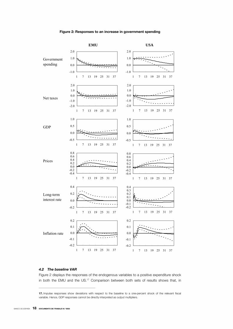
Figure 2: Responses to an increase in government spending

4.2 The baseline VAR

Figure 2 displays the responses of the endogenous variables to a positive expenditure shock

in both the EMU and the US.17 Comparison between both sets of results shows that, in

17. Impulse responses show deviations with respect to the baseline to a one-percent shock of the relevant fiscal

variable. Hence, GDP responses cannot be directly interpreted as output multipliers.

Governmentspending

Net taxes

GDP

Prices

Long-term interest rate

Inflation rate

USAEMU

-1.0

0.0

1.0

2.0

1 7 13 19 25 31 37

-2.0

-1.0

0.0

1.0

2.0

1 7 13 19 25 31 37

-0.5

0.0

0.5

1.0

1 7 13 19 25 31 37

-0.4-0.20.00.20.40.60.8

1 7 13 19 25 31 37

-0.2-0.10.00.10.20.30.4

1 7 13 19 25 31 37

-0.2

-0.1

0.0

0.1

0.2

1 7 13 19 25 31 37

-1.0

0.0

1.0

2.0

1 7 13 19 25 31 37

-2.0

-1.0

0.0

1.0

2.0

1 7 13 19 25 31 37

-0.5

0.0

0.5

1.0

1 7 13 19 25 31 37

-0.4-0.20.00.20.40.60.8

1 7 13 19 25 31 37

-0.2

0.0

0.2

0.4

1 7 13 19 25 31 37

-0.2

-0.1

0.0

0.1

0.2

1 7 13 19 25 31 37


general, the responses of the macroeconomic variables display similar patterns. Firstly, GDP

increases and remains significant for five quarters in both cases, becoming non-significant

thereafter. These results are largely in line with previous evidence for the US and other

countries. In general, government spending shocks are found to yield positive output

responses in the short-term [Perotti (2004); Neri (2001); Mountford and Uhlig (2009)], although

the size and persistence of output multipliers varies significantly across studies.18

As for the impact of a government spending shock on the other variables in the

system, prices increase with respect to the baseline, leading to a hump-shaped response of

inflation in both cases. Despite being a rather intuitive and, on the other hand, expected

result, previous evidence is far from conclusive. For example, Fatás and Mihov (2001) and

Mountford and Uhlig (2009) find negative effects on prices and inflation, whereas in the case

of Marcellino (2006) the impact found is not significant in the case of Germany, Spain and Italy

and positive in the case of France. In turn, Perotti (2004) reports mixed evidence depending

on the country and period under consideration. Likewise, the long-term interest rate rises in

response to the shock. However, some slight differences can be noticed here, notably US

rates’ reaction is quicker but shorter lived, whereas the positive reaction of long-term rates in

the euro area appears slightly more gradual and remains significant for more than 2 years.19

In any case, the most salient differences between the euro area and the US are

related to the responses of fiscal variables. Specifically, government spending shocks seem

to be more persistent in the US than in the euro area.20 In order to assess the reasons behind

such a difference in persistence, government expenditure in the US VAR was replaced by

non-military government spending. Interestingly, Figure 3 shows that non-military spending

shocks in the US display a very similar degree of persistence to the impulse response of total

government spending in the euro area. Therefore, the higher persistence of government

expenditure shocks in the US can be attributed to the higher persistence of military spending

shocks.

Another important difference relates to the reaction of net taxes. Hence, while net

taxes fall in the US, their response turns out to be positive in the euro area. In order to

disentangle the reasons behind such different responses, net taxes in our baseline VARs were

replaced in turn by total receipts (mainly tax revenues) and transfers. Figure 4 represents the

impulse responses of these variables to government spending shocks. As expected, transfers

fall in the US due to the improvement in economic activity. Conversely, and surprisingly

we admit, transfers rise slightly in the euro area. In turn, the response of taxes also shows a

markedly different behaviour, increasing in the euro area in the first two years after the shock

and declining persistently in the US. These patterns reveal a different design of fiscal

packages in the US and the EMU and/or dissimilar fiscal policy reaction functions of net

taxes. While expenditure build-ups in the US have often been accompanied by tax cuts,

18. Caldara and Kamps (2008) show that, after controlling for differences in the specification of the reduced form model,

all identification approaches used in the literature yield qualitatively and quantitatively very similar results for government

spending shocks. By contrast, they find strongly diverging results for the effects of tax shocks. These differences

stem from differences in the size of the automatic stabilisers estimated or calibrated under alternative identification

approaches.

19. In the literature, the impact of expansionary government spending shocks on interest rates tends to be positive,

although rather small [see for instance Perotti (2004)].

20. The persistence in the response of US government spending to its own shocks is also found in Blanchard and

Perotti (2002). Similarly, de Castro and Hernández de Cos (2008) also observe highly persistent spending shocks

in Spain. By contrast, Giordano et al. (2007) find little persistence with Italian data.


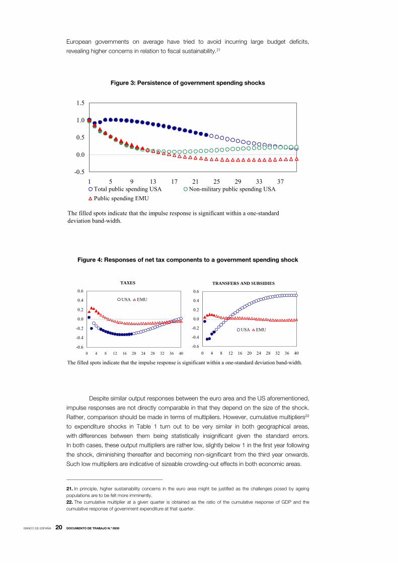
European governments on average have tried to avoid incurring large budget deficits,

revealing higher concerns in relation to fiscal sustainability.21

Figure 3: Persistence of government spending shocks

Figure 4: Responses of net tax components to a government spending shock

Despite similar output responses between the euro area and the US aforementioned,

impulse responses are not directly comparable in that they depend on the size of the shock.

Rather, comparison should be made in terms of multipliers. However, cumulative multipliers22

to expenditure shocks in Table 1 turn out to be very similar in both geographical areas,

with differences between them being statistically insignificant given the standard errors.

In both cases, these output multipliers are rather low, slightly below 1 in the first year following

the shock, diminishing thereafter and becoming non-significant from the third year onwards.

Such low multipliers are indicative of sizeable crowding-out effects in both economic areas.

21. In principle, higher sustainability concerns in the euro area might be justified as the challenges posed by ageing

populations are to be felt more imminently.

22. The cumulative multiplier at a given quarter is obtained as the ratio of the cumulative response of GDP and the

cumulative response of government expenditure at that quarter.

The filled spots indicate that the impulse response is significant within a one-standard deviation band-width.

TAXES

-0.6

-0.4

-0.2

0.0

0.2

0.4

0.6

0 4 8 12 16 20 24 28 32 36 40

USA EMU

TRANSFERS AND SUBSIDIES

-0.6

-0.4

-0.2

0.0

0.2

0.4

0.6

0 4 8 12 16 20 24 28 32 36 40

USA EMU

The filled spots indicate that the impulse response is significant within a one-standarddeviation band-width.

-0.5

0.0

0.5

1.0

1.5

1 5 9 13 17 21 25 29 33 37Total public spending USA Non-military public spending USA

Public spending EMU


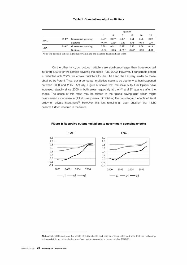
Table 1: Cumulative output multipliers

On the other hand, our output multipliers are significantly larger than those reported

in Perotti (2004) for the sample covering the period 1980-2000. However, if our sample period

is restricted until 2000, we obtain multipliers for the EMU and the US very similar to those

obtained by Perotti. Thus, our larger output multipliers seem to be due to what has happened

between 2000 and 2007. Actually, Figure 5 shows that recursive output multipliers have

increased steadily since 2000 in both areas, especially at the 4th and 8th quarters after the

shock. The cause of this result may be related to the “global saving glut” which might

have caused a decrease in global risks premia, diminishing the crowding-out effects of fiscal

policy on private investment23. However, this fact remains an open question that might

deserve further research in the future.

Figure 5: Recursive output multipliers to government spending shocks

23. Laubach (2009) analyses the effects of public deficits and debt on interest rates and finds that the relationship

between deficits and interest rates turns from positive to negative in the period after 1999:Q1.

EMU

-0.4-0.20.00.20.40.60.81.01.2

2000 2002 2004 2006

q1 q4 q8

USA

-0.4-0.20.00.20.40.60.81.01.2

2000 2002 2004 2006

q1 q4 q8

1 4 8 12 16 2081-07 Government spending 0.75* 0.87* 0.85* 0.61 0.26 0.02

Net taxes -0.79* -0.63* -0.49 -0.49 -0.58 -0.7481-07 Government spending 0.76* 0.91* 0.67* 0.46 0.30 0.19

Net taxes -0.02 -0.06 -0.35* -0.65* -0.90 -1.11Note: The asterisks indicate significance within the one-standard deviation band-width

Quarters

EMU

USA


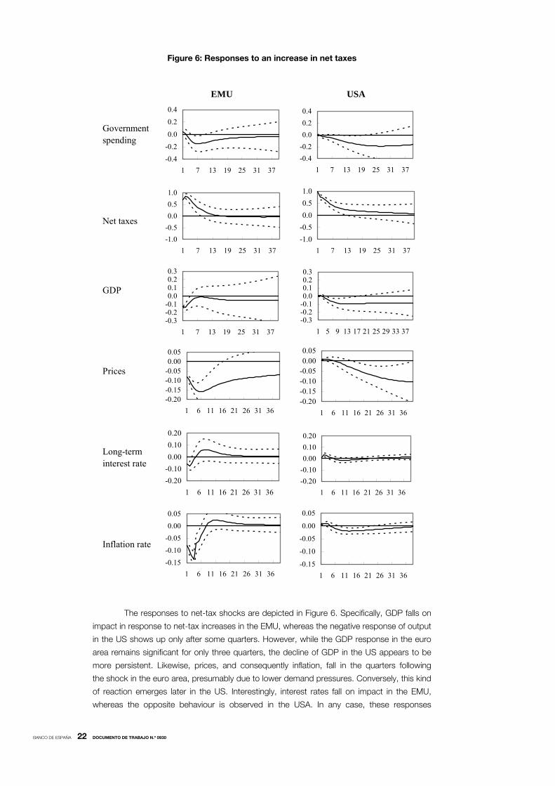
Figure 6: Responses to an increase in net taxes

The responses to net-tax shocks are depicted in Figure 6. Specifically, GDP falls on

impact in response to net-tax increases in the EMU, whereas the negative response of output

in the US shows up only after some quarters. However, while the GDP response in the euro

area remains significant for only three quarters, the decline of GDP in the US appears to be

more persistent. Likewise, prices, and consequently inflation, fall in the quarters following

the shock in the euro area, presumably due to lower demand pressures. Conversely, this kind

of reaction emerges later in the US. Interestingly, interest rates fall on impact in the EMU,

whereas the opposite behaviour is observed in the USA. In any case, these responses

Governmentspending

Net taxes

GDP

Prices


Inflation rate

USAEMU

-0.4

-0.2

0.0

0.2

0.4

1 7 13 19 25 31 37

-1.0

-0.5

0.0

0.5

1.0

1 7 13 19 25 31 37

-0.3-0.2-0.10.00.10.20.3

1 7 13 19 25 31 37

-0.20-0.15-0.10-0.050.000.05

1 6 11 16 21 26 31 36

-0.20

-0.10

0.00

0.10

0.20

1 6 11 16 21 26 31 36

-0.15

-0.10

-0.05

0.00

0.05

1 6 11 16 21 26 31 36

-1.0

-0.5

0.0

0.5

1.0

1 7 13 19 25 31 37

-0.4

-0.2

0.0

0.2

0.4

1 7 13 19 25 31 37

-0.3-0.2-0.10.00.10.20.3

1 5 9 13 17 21 25 29 33 37

-0.20-0.15-0.10-0.050.000.05

1 6 11 16 21 26 31 36

-0.20

-0.10

0.00

0.10

0.20

1 6 11 16 21 26 31 36

-0.15

-0.10

-0.05

0.00

0.05

1 6 11 16 21 26 31 36


become non-significant three quarters after the shock. Finally, government expenditure

eventually falls in both the EMU and the US. In turn, output multipliers turn out to be negative

and lower in absolute value than government spending output multipliers when significant

(see again Table 1). Moreover, despite net-tax output multipliers being larger in the EMU24,

they are only significant during the first year after the shock. However, the delayed but more

persistent GDP response in the US leads to significantly negative output multipliers during

the second and third year.

As in the case of spending shocks, these results are qualitatively similar to the

findings in previous studies. In general, many empirical papers find that tax multipliers

are lower than spending ones in the short-term, which is consistent with the theoretical

prediction that part of the higher disposable income stemming from tax cuts is saved. This is

the case in Blanchard and Perotti (2002) and Mountfourd and Uhlig (2009). However, some

evidence suggests that in the longer term tax multipliers could be higher than spending

multipliers.

4.3 Financial and fiscal stress and the impact of fiscal policy

The estimates presented in the baseline VAR section should be considered as average

effects in “normal times”. However, there is considerable evidence showing that fiscal

multipliers could be country-, time-, and circumstances-dependent. As a consequence,

in addition to the stability test performed in previous sections, it is interesting to contrast to

what extent our findings depend on the cyclical conditions of the economy or are conditioned

by the presence of financial constrains25 or fiscal stress [Perotti (2004)].

Controlling for financial stress leaves the baseline results broadly unchanged. In order

to approximate financial stress, we included the spread of US corporate bonds in the VAR as

an exogenous variable.26 As regards impulse response functions, the results are qualitatively

equal to those drawn with the baseline VAR in both the EMU and the US, with only some

differences concerning the magnitude of some multipliers (see Table 2). In particular,

controlling for financial stress leads, in general, to slightly higher output multipliers to spending

shocks in the US, whereas the opposite is true for the EMU. Net-tax shocks also offer some

discrepancies, with larger negative multipliers in the US and similar to the baseline

specification in the EMU, although in this latter case the cumulative negative multiplier

displays higher persistence. These results suggest that, in periods of uncertainty and financial

stress, EMU consumers could be “less Ricardian” than their American counterparts where

24. It is worth noting here that the selection of the seasonal adjustment method affects output multipliers, even

though qualitative and quantitative results are quite similar when using alternative methods. This sensitivity to the

seasonal-adjustment method is a well-know issue in the specialised econometric literature. For the sake of transparency,

we report alternative results in this footnote. If instead of using the model-consistent seasonally-adjusted time

series and alternative method like TRAMO-SEATS were used (see Gómez and Maraval, 1996), cumulative output

multipliers to public spending shocks would have been estimated at 1.04 in q1, 1.13 in q4, 1.16 in q8, 1.03 in q12,

0.90 in q16 and 0.80 in q20, being still significant along the third year after the shock. These multipliers are somewhat

higher than those reported in Table 1. In the case of shocks to net taxes multipliers are somewhat smaller than those

in Table 1: -0.32 in q1, -0.30 in q4, -0.26 in q8, -0.19 in q12, -0.12 in q16 and -0.06 in q20, although only significant

during the first year following the shock.

25. Tagkalakis (2008), with a panel of nineteen OECD countries, finds that in the presence of binding liquidity constraints

on households, fiscal policy is more effective in boosting private consumption in recessions than in expansions.

26. In the case of the Euro area, there is not a market for corporate bonds before 1999. However, given that financial

markets are highly integrated, the spread of US corporate bonds appears as a sensible proxy. IN any case, we also

included in the analysis a similar spread for Germany as a proxy for the euro area. The results in this latter case are

almost indistinguishable from those with the US spread.


households prefer to save.27 However, in view of the width of confidence intervals, differences

in point estimates with respect to the baseline do not seem significant, except maybe for the

case of shocks to net taxes in the US.

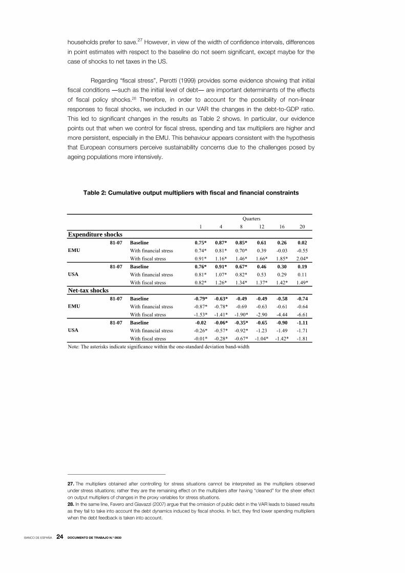
Regarding “fiscal stress”, Perotti (1999) provides some evidence showing that initial

fiscal conditions ―such as the initial level of debt― are important determinants of the effects

of fiscal policy shocks.28 Therefore, in order to account for the possibility of non-linear

responses to fiscal shocks, we included in our VAR the changes in the debt-to-GDP ratio.

This led to significant changes in the results as Table 2 shows. In particular, our evidence

points out that when we control for fiscal stress, spending and tax multipliers are higher and

more persistent, especially in the EMU. This behaviour appears consistent with the hypothesis

that European consumers perceive sustainability concerns due to the challenges posed by

ageing populations more intensively.

Table 2: Cumulative output multipliers with fiscal and financial constraints

27. The multipliers obtained after controlling for stress situations cannot be interpreted as the multipliers observed

under stress situations; rather they are the remaining effect on the multipliers after having “cleaned” for the sheer effect

on output multipliers of changes in the proxy variables for stress situations.

28. In the same line, Favero and Giavazzi (2007) argue that the omission of public debt in the VAR leads to biased results

as they fail to take into account the debt dynamics induced by fiscal shocks. In fact, they find lower spending multipliers

when the debt feedback is taken into account.

1 4 8 12 16 20

Expenditure shocks81-07 Baseline 0.75* 0.87* 0.85* 0.61 0.26 0.02

With financial stress 0.74* 0.81* 0.70* 0.39 -0.03 -0.55

With fiscal stress 0.91* 1.16* 1.46* 1.66* 1.85* 2.04*

81-07 Baseline 0.76* 0.91* 0.67* 0.46 0.30 0.19

With financial stress 0.81* 1.07* 0.82* 0.53 0.29 0.11

With fiscal stress 0.82* 1.26* 1.34* 1.37* 1.42* 1.49*

Net-tax shocks81-07 Baseline -0.79* -0.63* -0.49 -0.49 -0.58 -0.74

With financial stress -0.87* -0.78* -0.69 -0.63 -0.61 -0.64

With fiscal stress -1.53* -1.41* -1.90* -2.90 -4.44 -6.61

81-07 Baseline -0.02 -0.06* -0.35* -0.65 -0.90 -1.11

With financial stress -0.26* -0.57* -0.92* -1.23 -1.49 -1.71

With fiscal stress -0.01* -0.28* -0.67* -1.04* -1.42* -1.81

Note: The asterisks indicate significance within the one-standard deviation band-width

USA

EMU

USA

EMU

Quarters


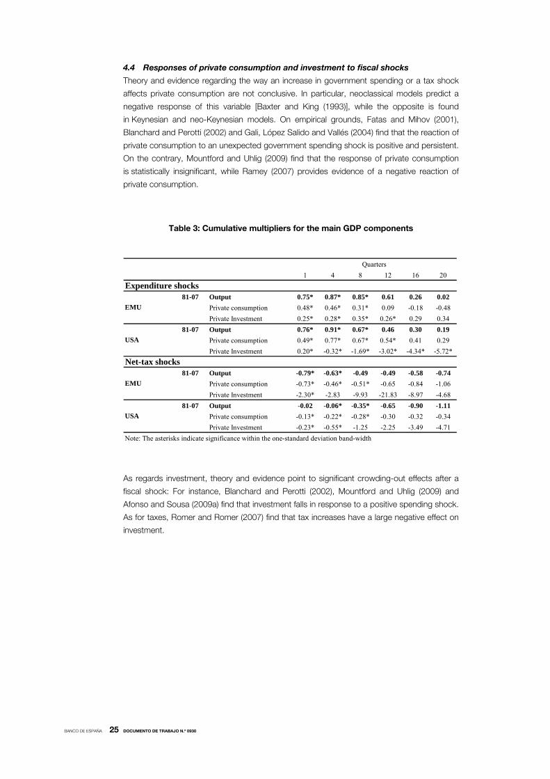
4.4 Responses of private consumption and investment to fiscal shocks

Theory and evidence regarding the way an increase in government spending or a tax shock

affects private consumption are not conclusive. In particular, neoclassical models predict a

negative response of this variable [Baxter and King (1993)], while the opposite is found

in Keynesian and neo-Keynesian models. On empirical grounds, Fatas and Mihov (2001),

Blanchard and Perotti (2002) and Gali, López Salido and Vallés (2004) find that the reaction of

private consumption to an unexpected government spending shock is positive and persistent.

On the contrary, Mountford and Uhlig (2009) find that the response of private consumption

is statistically insignificant, while Ramey (2007) provides evidence of a negative reaction of

private consumption.

Table 3: Cumulative multipliers for the main GDP components

As regards investment, theory and evidence point to significant crowding-out effects after a

fiscal shock: For instance, Blanchard and Perotti (2002), Mountford and Uhlig (2009) and

Afonso and Sousa (2009a) find that investment falls in response to a positive spending shock.

As for taxes, Romer and Romer (2007) find that tax increases have a large negative effect on

investment.

1 4 8 12 16 20

Expenditure shocks81-07 Output 0.75* 0.87* 0.85* 0.61 0.26 0.02

Private consumption 0.48* 0.46* 0.31* 0.09 -0.18 -0.48

Private Investment 0.25* 0.28* 0.35* 0.26* 0.29 0.34

81-07 Output 0.76* 0.91* 0.67* 0.46 0.30 0.19

Private consumption 0.49* 0.77* 0.67* 0.54* 0.41 0.29

Private Investment 0.20* -0.32* -1.69* -3.02* -4.34* -5.72*

Net-tax shocks81-07 Output -0.79* -0.63* -0.49 -0.49 -0.58 -0.74

Private consumption -0.73* -0.46* -0.51* -0.65 -0.84 -1.06

Private Investment -2.30* -2.83 -9.93 -21.83 -8.97 -4.68

81-07 Output -0.02 -0.06* -0.35* -0.65 -0.90 -1.11

Private consumption -0.13* -0.22* -0.28* -0.30 -0.32 -0.34

Private Investment -0.23* -0.55* -1.25 -2.25 -3.49 -4.71


USA

EMU

Quarters

USA

EMU


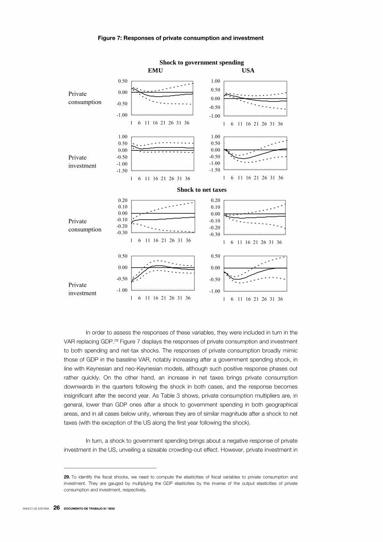
Figure 7: Responses of private consumption and investment

In order to assess the responses of these variables, they were included in turn in the

VAR replacing GDP.29 Figure 7 displays the responses of private consumption and investment

to both spending and net-tax shocks. The responses of private consumption broadly mimic

those of GDP in the baseline VAR, notably increasing after a government spending shock, in

line with Keynesian and neo-Keynesian models, although such positive response phases out

rather quickly. On the other hand, an increase in net taxes brings private consumption

downwards in the quarters following the shock in both cases, and the response becomes

insignificant after the second year. As Table 3 shows, private consumption multipliers are, in

general, lower than GDP ones after a shock to government spending in both geographical

areas, and in all cases below unity, whereas they are of similar magnitude after a shock to net

taxes (with the exception of the US along the first year following the shock).

In turn, a shock to government spending brings about a negative response of private

investment in the US, unveiling a sizeable crowding-out effect. However, private investment in

29. To identify the fiscal shocks, we need to compute the elasticities of fiscal variables to private consumption and

investment. They are gauged by multiplying the GDP elasticities by the inverse of the output elasticities of private

consumption and investment, respectively.

Private consumption

Private investment

Private consumption

Private investment

USAEMU

Shock to net taxes

Shock to government spending

-1.00

-0.50

0.00

0.50

1.00

1 6 11 16 21 26 31 36

-0.30-0.20-0.100.000.100.20

1 6 11 16 21 26 31 36

-1.00

-0.50

0.00

0.50

1 6 11 16 21 26 31 36

-0.30-0.20-0.100.000.100.20

1 6 11 16 21 26 31 36

-1.50-1.00-0.500.000.501.00

1 6 11 16 21 26 31 36

-1.00

-0.50

0.00

0.50

1 6 11 16 21 26 31 36

-1.50-1.00-0.500.000.501.00

1 6 11 16 21 26 31 36

-1.00

-0.50

0.00

0.50

1 6 11 16 21 26 31 36


the euro area increases after this type of shocks, in line with the accelerator hypothesis. This

different behaviour of private investment might be related to the slower reaction of interest

rates in the euro area, assuaging thereby the crowding-out of private expenditure.30 In the

case of a shock to net taxes, private investment falls in both the euro area and the US.

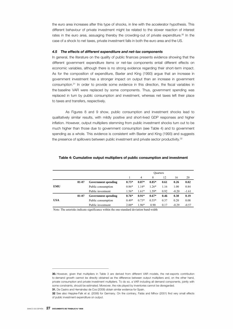
4.5 The effects of different expenditure and net-tax components

In general, the literature on the quality of public finances presents evidence showing that the

different government expenditure items or net-tax components entail different effects on

economic variables, although there is no strong evidence regarding their short-term impact.

As for the composition of expenditure, Baxter and King (1993) argue that an increase in

government investment has a stronger impact on output than an increase in government

consumption.31 In order to provide some evidence in this direction, the fiscal variables in

the baseline VAR were replaced by some components. Thus, government spending was

replaced in turn by public consumption and investment, whereas net taxes left their place

to taxes and transfers, respectively.

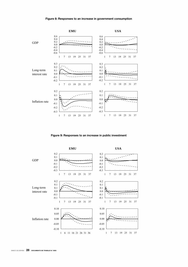
As Figures 8 and 9 show, public consumption and investment shocks lead to

qualitatively similar results, with mildly positive and short-lived GDP responses and higher

inflation. However, output multipliers stemming from public investment shocks turn out to be

much higher than those due to government consumption (see Table 4) and to government

spending as a whole. This evidence is consistent with Baxter and King (1993) and suggests

the presence of spillovers between public investment and private sector productivity.32

Table 4: Cumulative output multipliers of public consumption and investment

30. However, given that multipliers in Table 3 are derived from different VAR models, the net-exports contribution

to demand growth cannot be directly obtained as the difference between output multipliers and, on the other hand,

private consumption and private investment multipliers. To do so, a VAR including all demand components, jointly with

some constraints, should be estimated. Moreover, the role played by inventories cannot be disregarded.

31. De Castro and Hernández de Cos (2008) obtain similar evidence for Spain.

32 See also Heppke-Falk et al. (2006) for Germany. On the contrary, Fatás and Mihov (2001) find very small effects

of public investment expenditure on output.

1 4 8 12 16 20

81-07 Government spending 0.75* 0.87* 0.85* 0.61 0.26 0.02

Public consumption 0.86* 1.14* 1.26* 1.16 1.00 0.84

Public investment 1.56* 1.61* 1.59* 0.92 -0.20 -1.61

81-07 Government spending 0.76* 0.91* 0.67* 0.46 0.30 0.19

Public consumption 0.49* 0.73* 0.55* 0.37 0.20 0.08

Public investment 2.00* 1.96* 0.90 0.17 -0.29 -0.57


USA

Quarters

EMU


Figure 8: Responses to an increase in government consumption

Figure 9: Responses to an increase in public investment

GDP


Inflation rate

USAEMU

-0.6-0.4-0.20.00.20.40.6

1 7 13 19 25 31 37

-0.2-0.10.00.10.20.3

1 7 13 19 25 31 37

-0.3

-0.2

-0.1

0.0

0.1

0.2

1 7 13 19 25 31 37

-0.6-0.4-0.20.00.20.40.6

1 7 13 19 25 31 37

-0.2-0.10.00.10.20.3

1 7 13 19 25 31 37

-0.3

-0.2

-0.1

0.0

0.1

0.2

1 7 13 19 25 31 37

GDP


Inflation rate

USAEMU

-0.3-0.2-0.10.00.10.2

1 7 13 19 25 31 37

-0.1-0.10.00.10.10.2

1 7 13 19 25 31 37

-0.10

-0.05

0.00

0.05

0.10

1 6 11 16 21 26 31 36

-0.3-0.2-0.10.00.10.2

1 7 13 19 25 31 37

-0.1-0.10.00.10.10.2

1 7 13 19 25 31 37

-0.10

-0.05

0.00

0.05

0.10

1 7 13 19 25 31 37


As for the components of net taxes, higher taxes entail negative responses of GDP in

both areas, although consumers in EMU seem to react more quickly to discretionary taxes

changes. In both cases, the inflation rate falls below the baseline whereas long-term interest

rates barely react to this type of shocks (see Figure 10).

Figure 10: Responses to an increase in taxes

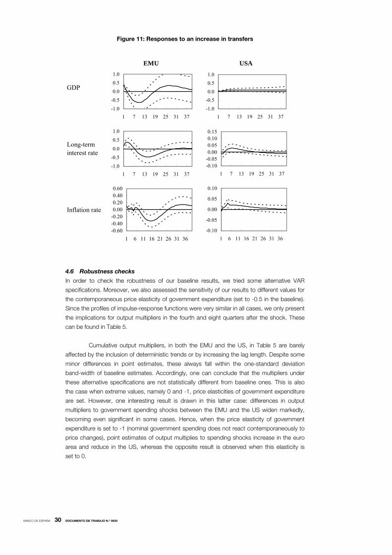
Responses to transfers shocks appear different, though. While the subsequent

output rise in the US is quite persistent, the initial increase in the EMU reverts after some

quarters, turning to negative (see Figure 11). In fact, this different behaviour might be related

to the upward response of interest rates on impact in the euro area. As far as inflation is

concerned, it goes up in the short run in the US, phasing out after the 6th quarter after the

shock. By contrast, inflation in the euro area only declines in the medium term.

GDP


Inflation rate

EMU USA

-0.4

-0.2

0.0

0.2

0.4

1 7 13 19 25 31 37

-0.2

-0.1

0.0

0.1

0.2

1 7 13 19 25 31 37

-0.30

-0.20

-0.10

0.00

0.10

1 6 11 16 21 26 31 36

-0.6-0.4-0.20.00.20.4

1 7 13 19 25 31 37

-0.2

-0.1

0.0

0.1

0.2

1 7 13 19 25 31 37

-0.30

-0.20

-0.10

0.00

0.10

1 6 11 16 21 26 31 36


Figure 11: Responses to an increase in transfers

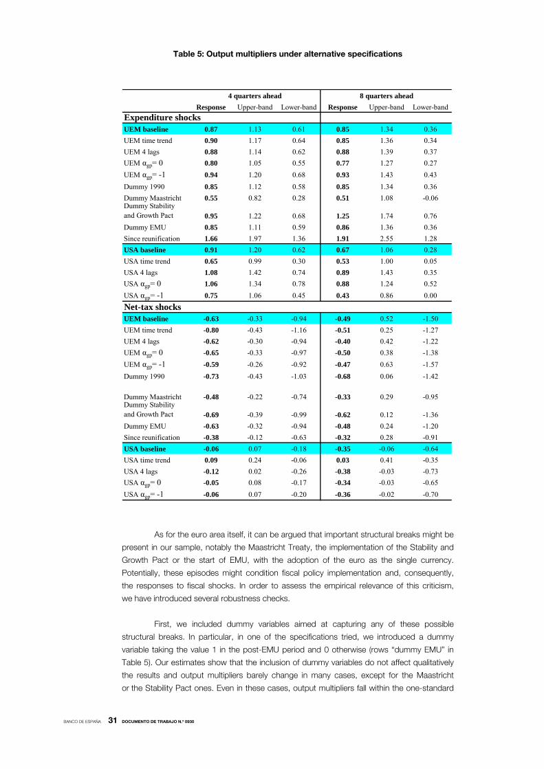
4.6 Robustness checks

In order to check the robustness of our baseline results, we tried some alternative VAR

specifications. Moreover, we also assessed the sensitivity of our results to different values for

the contemporaneous price elasticity of government expenditure (set to -0.5 in the baseline).

Since the profiles of impulse-response functions were very similar in all cases, we only present

the implications for output multipliers in the fourth and eight quarters after the shock. These

can be found in Table 5.

Cumulative output multipliers, in both the EMU and the US, in Table 5 are barely

affected by the inclusion of deterministic trends or by increasing the lag length. Despite some

minor differences in point estimates, these always fall within the one-standard deviation

band-width of baseline estimates. Accordingly, one can conclude that the multipliers under

these alternative specifications are not statistically different from baseline ones. This is also

the case when extreme values, namely 0 and -1, price elasticities of government expenditure

are set. However, one interesting result is drawn in this latter case: differences in output

multipliers to government spending shocks between the EMU and the US widen markedly,

becoming even significant in some cases. Hence, when the price elasticity of government

expenditure is set to -1 (nominal government spending does not react contemporaneously to

price changes), point estimates of output multiplies to spending shocks increase in the euro

area and reduce in the US, whereas the opposite result is observed when this elasticity is

set to 0.

GDP


Inflation rate

USAEMU

-1.0

-0.5

0.0

0.5

1.0

1 7 13 19 25 31 37

-1.0

-0.5

0.0

0.5

1.0

1 7 13 19 25 31 37

-0.60-0.40-0.200.000.200.400.60

1 6 11 16 21 26 31 36

-1.0

-0.5

0.0

0.5

1.0

1 7 13 19 25 31 37

-0.10-0.050.000.050.100.15

1 7 13 19 25 31 37

-0.10

-0.05

0.00

0.05

0.10

1 6 11 16 21 26 31 36


Table 5: Output multipliers under alternative specifications

As for the euro area itself, it can be argued that important structural breaks might be

present in our sample, notably the Maastricht Treaty, the implementation of the Stability and

Growth Pact or the start of EMU, with the adoption of the euro as the single currency.

Potentially, these episodes might condition fiscal policy implementation and, consequently,

the responses to fiscal shocks. In order to assess the empirical relevance of this criticism,

we have introduced several robustness checks.

First, we included dummy variables aimed at capturing any of these possible

structural breaks. In particular, in one of the specifications tried, we introduced a dummy

variable taking the value 1 in the post-EMU period and 0 otherwise (rows “dummy EMU” in

Table 5). Our estimates show that the inclusion of dummy variables do not affect qualitatively

the results and output multipliers barely change in many cases, except for the Maastricht

or the Stability Pact ones. Even in these cases, output multipliers fall within the one-standard

Response Upper-band Lower-band Response Upper-band Lower-band

Expenditure shocksUEM baseline 0.87 1.13 0.61 0.85 1.34 0.36

UEM time trend 0.90 1.17 0.64 0.85 1.36 0.34

UEM 4 lags 0.88 1.14 0.62 0.88 1.39 0.37

UEM αgp= 0 0.80 1.05 0.55 0.77 1.27 0.27

UEM αgp= -1 0.94 1.20 0.68 0.93 1.43 0.43

Dummy 1990 0.85 1.12 0.58 0.85 1.34 0.36

Dummy Maastricht 0.55 0.82 0.28 0.51 1.08 -0.06Dummy Stabilityand Growth Pact 0.95 1.22 0.68 1.25 1.74 0.76

Dummy EMU 0.85 1.11 0.59 0.86 1.36 0.36

Since reunification 1.66 1.97 1.36 1.91 2.55 1.28

USA baseline 0.91 1.20 0.62 0.67 1.06 0.28

USA time trend 0.65 0.99 0.30 0.53 1.00 0.05

USA 4 lags 1.08 1.42 0.74 0.89 1.43 0.35

USA αgp= 0 1.06 1.34 0.78 0.88 1.24 0.52

USA αgp= -1 0.75 1.06 0.45 0.43 0.86 0.00

Net-tax shocksUEM baseline -0.63 -0.33 -0.94 -0.49 0.52 -1.50

UEM time trend -0.80 -0.43 -1.16 -0.51 0.25 -1.27

UEM 4 lags -0.62 -0.30 -0.94 -0.40 0.42 -1.22

UEM αgp= 0 -0.65 -0.33 -0.97 -0.50 0.38 -1.38

UEM αgp= -1 -0.59 -0.26 -0.92 -0.47 0.63 -1.57

Dummy 1990 -0.73 -0.43 -1.03 -0.68 0.06 -1.42

Dummy Maastricht -0.48 -0.22 -0.74 -0.33 0.29 -0.95Dummy Stabilityand Growth Pact -0.69 -0.39 -0.99 -0.62 0.12 -1.36

Dummy EMU -0.63 -0.32 -0.94 -0.48 0.24 -1.20

Since reunification -0.38 -0.12 -0.63 -0.32 0.28 -0.91

USA baseline -0.06 0.07 -0.18 -0.35 -0.06 -0.64

USA time trend 0.09 0.24 -0.06 0.03 0.41 -0.35

USA 4 lags -0.12 0.02 -0.26 -0.38 -0.03 -0.73

USA αgp= 0 -0.05 0.08 -0.17 -0.34 -0.03 -0.65

USA αgp= -1 -0.06 0.07 -0.20 -0.36 -0.02 -0.70

4 quarters ahead 8 quarters ahead


deviation confidence bands of baseline estimates, for which differences cannot be deemed as

statistically significant. In fact, these dummies are non-significant in most of the equations,

which is consistent with the idea that the process to EMU accession has been a rather

smooth process that started affecting the respective economic systems well before its official

start, at least from the point of view of fiscal policy.

Moreover, in order to test the stability of our results to the German-reunification and

whether or not this event entailed a fiscal policy regime shift, we have also constrained the

estimation to the sample ranging as of 1991. Albeit our results are qualitatively similar to our

baseline VAR, output multipliers turn out to be somewhat different. Specifically, output

multipliers to expenditure shocks are remarkably higher (row “since reunification” in Table 5),

whereas multipliers to net-tax shocks become non-significant.

Finally, one could argue that assessing the effects of fiscal shocks in the euro area

does not make much sense before its start in 1999. In order to take into account such

criticism, we split our sample in 199533 and estimated the VAR for the more recent period.

The results, however, did not differ qualitatively from those reported in the previous

sub-section. In particular, GDP, inflation and interest rates showed positive responses to

spending shocks, although estimated very imprecisely mainly due to the few observations

relative to the number of coefficients to be estimated. Furthermore, we estimated the VAR for

the period 1981-1998. While the short-term responses displayed the same signs as with the

baseline VAR, output multipliers to spending shocks were significantly lower, estimated

at around 0.3 although non-significant. However, as we showed before, rather than being

exclusively due to changeover to the euro, such slow multipliers are also observed in the US

for a similar period.

33. Even though the decision on EMU entry was taken on the basis of the Commission fiscal estimates/projections

for 1998, reflecting planned deficits, we decided to take as break point for the sample 1995. The decision reflects

the fact that the 1999-2007 period is too short for the estimation of the VARs; nevertheless, a usual argument in the

literature is to claim that agents already anticipated the start-up of the EMU before the actual start in 1999, and thus,

1995 or 1997 is typically chosen in empirical studies as a sensible date for the purposes of estimation.


5 Conclusions

This paper contributes to previous literature analysing the effects of fiscal policy for the euro

area as a whole, employing a new database that contains quarterly fiscal variables. The use

of a common methodology for the euro area and the US economy allows drawing some

interesting conclusions.

In line with previous evidence, we find that GDP and inflation increase in response to

government spending shocks, although output multipliers are, in general, very similar in both

areas and small, typically below unity. However, we provide evidence of output multipliers

increasing steadily after 2000 in both the EMU and the US, possibly related to the “global

saving glut”. On the other hand, government expenditure shocks show a higher degree of

persistence in the US, which seems to be explained by the persistence of military spending.

In turn, net-tax increases weight on economic activity, with the negative response being

shorter-lived in the euro area. In any case, these effects do not appear sizeable. In line with

previous studies, we find that tax multipliers are lower than spending ones in the short-term.

As for the reaction of the main GDP components, as expected, private consumption

displays similar pattern responses to GDP in both the euro area and the US. Private

investment responses are not so homogeneous though: it declines in response to higher

government spending or net taxes in the US, whereas in the EMU only tax increases seem to

entail a negative reaction of private investment.

Finally, we allow for the possibility of non-linear effects of fiscal policy depending on a

set of circumstances. In particular, we analyse the implications of financial and fiscal stress

prevailing in the economy. Controlling for these stress situations does not change the pattern

of impulse responses, although it may affect output multipliers. In particular, in the case

of financial stress, differences with respect to the baseline VAR, in general, do not seem to be

statistically significant. However, when we control for fiscal stress, spending and tax

multipliers become higher and more persistent, especially in the EMU.


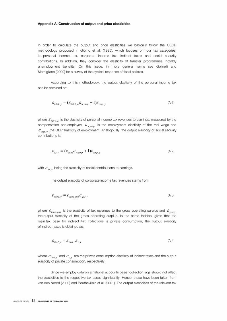
Appendix A. Construction of output and price elasticities

In order to calculate the output and price elasticities we basically follow the OECD

methodology proposed in Giorno et al. (1995), which focuses on four tax categories,

i.e. personal income tax, corporate income tax, indirect taxes and social security

contributions. In addition, they consider the elasticity of transfer programmes, notably

unemployment benefits. On this issue, in more general terms see Golinelli and

Momigliano (2009) for a survey of the cyclical response of fiscal policies.

According to this methodology, the output elasticity of the personal income tax

can be obtained as:

yempempwwtdirhytdirh ,,,, )1( (A.1)

where wtdirh, is the elasticity of personal income tax revenues to earnings, measured by the

compensation per employee, empw, is the employment elasticity of the real wage and

yemp, the GDP elasticity of employment. Analogously, the output elasticity of social security

contributions is:

yempempwwssyss ,,,, )1( (A.2)

with wss, being the elasticity of social contributions to earnings.

The output elasticity of corporate income tax revenues stems from:

ygosgostdircytdirc ,,, (A.3)

where gostdirc, is the elasticity of tax revenues to the gross operating surplus and ygos,

the output elasticity of the gross operating surplus. In the same fashion, given that the

main tax base for indirect tax collections is private consumption, the output elasticity

of indirect taxes is obtained as:

ycctindytind ,,, (A.4)

where ctind , and yc, are the private consumption elasticity of indirect taxes and the output

elasticity of private consumption, respectively.

Since we employ data on a national accounts basis, collection lags should not affect

the elasticities to the respective tax-bases significantly. Hence, these have been taken from

van den Noord (2000) and Bouthevillain et al. (2001). The output elasticities of the relevant tax


bases were, however, obtained from econometric estimation on a quarterly basis. In general,

the general equation used for estimating these elasticities was:

ttiit YLnBLn )()( (A.5)

where Bi is the relevant tax base for the ith tax category and εi is the output elasticity of such

tax base. These equations, given the likely contemporaneous correlation between the

independent variable and the error term, were estimated by instrumental variables. However,

if the variables Bi and Y are cointegrated, (A.5) contains a specification error. In this case,

the following ECM specification would be preferable:

t

k

j

ijtj

k

jjtj

titit

it

BLnYLn

YLnYLnBLnBLn

11

11

)()(

)())()(()(

(A.6)

where λ measures the long-term contemporaneous elasticity we are interested in.

Information on the output elasticity of net transfers is more limited than in the former

cases. Although unemployment benefits respond to the underlying economic conditions,

many expenditure programmes do not have built-in conditions that make them respond

contemporaneously to employment or output. Therefore, recalling Perotti’s argument,

an output elasticity of net transfers of -0.2 has been assumed.

As for price elasticities, following van der Noord (2000) the elasticity of direct taxes

paid by households, corporate income taxes and social contributions were obtained as

1,, wtdirhptdirh (yielding 0.9), 1,, gostdircptdirc (with a value equal to 0)

and 1,, wsspss (being -0.1), respectively. Indirect taxes are typically proportional.

Hence, following Perotti (2004), a zero price elasticity was assumed. Finally, although

transfer programmes are indexed to the CPI, indexation occurs with a considerable lag.

Thus, the price elasticity of transfers was set to -1. Table A.1 shows the resulting output

and price elasticities.


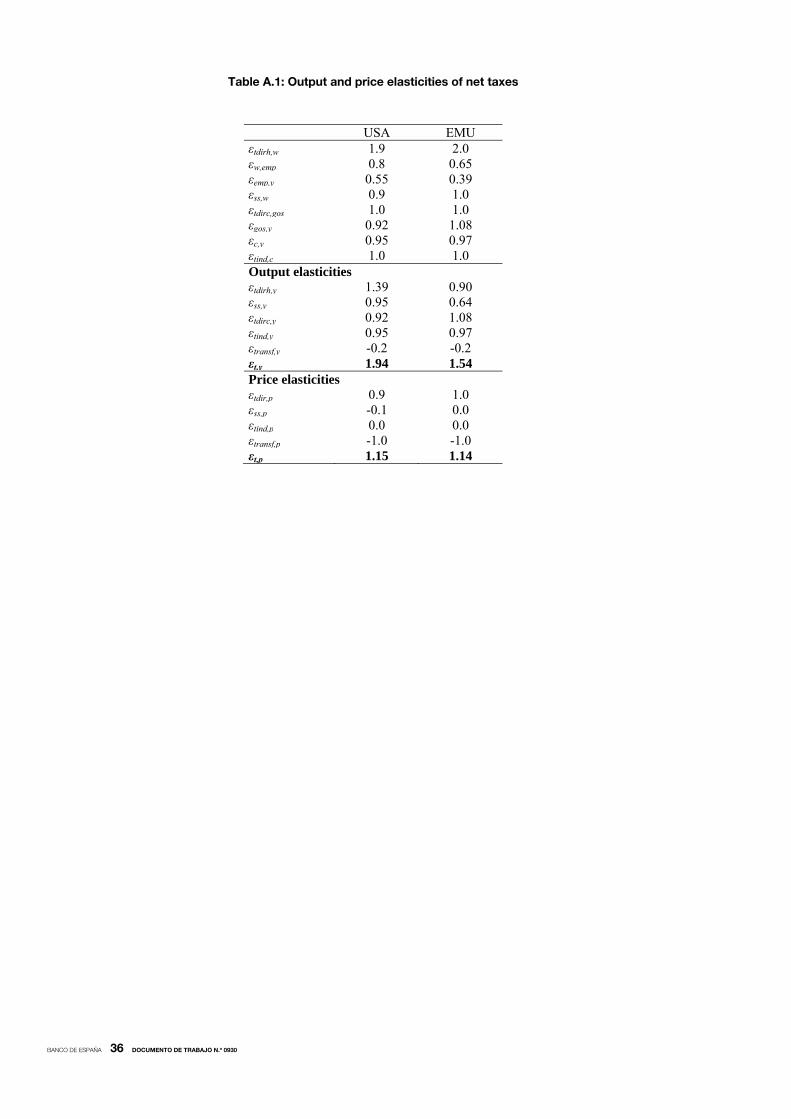
Table A.1: Output and price elasticities of net taxes

USA EMU εtdirh,w 1.9 2.0 εw,emp 0.8 0.65 εemp,y 0.55 0.39 εss,w 0.9 1.0 εtdirc,gos 1.0 1.0 εgos,y 0.92 1.08 εc,y 0.95 0.97 εtind,c 1.0 1.0 Output elasticities εtdirh,y 1.39 0.90 εss,y 0.95 0.64 εtdirc,y 0.92 1.08 εtind,y 0.95 0.97 εtransf,y -0.2 -0.2 εt,y 1.94 1.54 Price elasticities εtdir,p 0.9 1.0 εss,p -0.1 0.0 εtind,p 0.0 0.0 εtransf,p -1.0 -1.0 εt,p 1.15 1.14


REFERENCES

AFONSO, A., and R. M. SOUSA (2009a). The macroeconomic effects of fiscal policy, ECB Working Paper Series

No. 991, January.

― (2009b). The macroeconomic effects of fiscal policy in Portugal: a Bayesian SVAR analysis. School of Economics and

Management, Working Papers No. 09/2009/DE/UECE.

BAXTER, M., and R. KING (1993). “Fiscal policy in general equilibrium”, American Economic Review, 83, pp. 315-334.

BÉNASSY-QUÉRÉ, A., and J. CIMADOMO (2006). Changing patterns of domestic and cross-border fiscal policy

multipliers in Europe and the US, CEPII WP No. 2006-24.

BEETSMA, R., and M. GIULIODORI (2009). Discretionary fiscal policy: review and estimates for the EU, Mimeo.

BLANCHARD, O. J., and R. PEROTTI (2002). “An Empirical Characterization of the Dynamic Effects of Changes in

Government Spending and Taxes on Output”, Quarterly Journal of Economics, 117, pp. 1329-1368.

BOUTHEVILLAIN, C., P. COUR-THIMANN, G. VAN DEN DOOL, P. HERNÁNDEZ DE COS, G. LANGENUS, M. MOHR,

S MOMIGLIANO and M. TUJULA (2001). Cyclically adjusted budget balances: An alternative approach, ECB

Working Paper Series No. 77.

CALDARA, D., and C. KAMPS (2008). What are the effects of fiscal policy shocks? A VAR-based comparative analysis,

ECB Working Paper Series No. 877, March.

CHRISTOFFEL, K., G. COENEN and A. WARNE (2008). The New Area-Wide Model of the euro area: a micro-founded

open-economy model for forecasting and policy analysis, ECB Working Paper Series No 944, October.

COGAN, J., T. CWIK, J. B. TAYLOR and V. WIELAND (2009). New Keynesian versus Old Keynesian Government

Spending Multipliers, CEPR Discussion Paper 7236, March.

CWIK, T., and V. WIELAND (2009). Keynesian government spending multipliers and spillovers in the Eurozone, CEPR

Discussion Paper No. 7389, August.

DE CASTRO, F. (2006). “The macroeconomic effects of fiscal policy in Spain”, Applied Economics, 38, pp. 913-924.

DE CASTRO, F., and P. HERNÁNDEZ DE COS (2008). “The economic effects of fiscal policy: the case of Spain”, Journal

of Macroeconomics, 30, pp. 1005-1028.

FAGAN, G., J. HENRY and R. MESTRE (2005). “An area-wide model (AWM) for the euro area”, Economic Modelling, 22,

pp. 39-59.

FATÁS, A., and I. MIHOV (2001). The effects of fiscal policy on consumption and employment: theory and evidence,

CEPR Discussion Paper Series No. 2760.

FAVERO, C., and F. GIAVAZZI (2007). Debt and the effects of fiscal policies, NBER Working Paper Series No. 12822.

GALÍ, J., D. LÓPEZ-SALIDO and J. VALLÉS (2007). “Understanding the effects of government spending on

consumption”, Journal of the European Economic Association, 5, pp. 227-270.

GIORDANO, R., S. MOMIGLIANO, S. NERI and R. PEROTTI (2007). “The effects of fiscal policy in Italy: Evidence from a

VAR model”, European Journal of Political Economy, 23, pp. 707-733.

GIORNO, C., P. RICHARDSON, D. ROSEVEARE and P. VAN DEN NOORD (1995). Potential output, output gaps and

structural budget balances, OECD Economic Studies 24.

GOLINELLI, R., and S. MOMIGLIANO (2009). “The cyclical reaction of fiscal policies in the euro area: the role of

modelling choices and data vintages”, Fiscal Studies, 30, pp. 39-72.

GÓMEZ, V., and A. MARAVALL (1996). Programs TRAMO (Time series Regression with ARIMA noise, Missing

observations, and Outliers) and SEATS (Signal Extraction in ARIMA Time Series). Instructions for the User, Working

Paper No. 9628, Banco de España.

HEPPKE-FALK, K. H., J. TENHOFEN and G. B. WOLFF (2006). The macroeconomic effects of exogenous fiscal policy

shocks in Germany: a disaggregated SVAR analysis, Deutsche Bundesbank, Discussion Paper Series 1: Economic

Studies No. 41/2006.

JACOBS, J. P. A. M., G. H. KUPER and J. VERLINDEN (2007). Monetary policy in the euro area: the impact of fiscal

closure rules, Working Paper 2007/01, Institute of Economics and Econometrics, University of Groningen.

LAUBACH, T. (2009). “New evidence on the interest rate effects of budget deficits and debt”, Journal of the European

Economic Association, 7 (4), pp. 858-885.

LEEPER, E. M., T. B. WALKER and S. S. YANG (2008). Fiscal foresight: analytics and econometrics, NBER Working

Paper Series No. 14028.

MARCELLINO, M. (2006). “Some stylized facts on non-systematic fiscal policy in the euro area”, Journal of

Macroeconomics, 28, pp. 461-479.

MOUNTFORD, A., and H. UHLIG (2009). “What are the effects of fiscal policy shocks?”, forthcoming in the Journal of

Applied Econometrics.

NERI, S. (2001). Assessing the effects of monetary and fiscal policy, Banca d’Italia Discussion Papers No. 425.

PAREDES, J., D. J. PEDREGAL and J. J. PÉREZ (2009). A quarterly fiscal database for the euro area based on

intra-annual fiscal indicators, ECB Working Paper Series, No. 1132.

PEROTTI, R. (1999). “Fiscal policy in good times and bad”, Quarterly Journal of Economics, 114, pp. 1399-1436.

― (2004). Estimating the effects of fiscal policy in OECD countries, Proceedings, Federal Reserve Bank of San

Francisco.

RAMEY, V. (2007). Comment on "In search of the transmission mechanism of fiscal policy", in NBER Macroeconomics

Annual 2007, Vol. 22.

RATTO, M., W. ROEGER, and J. IN’T VELD (2009). “Quest III, An estimated open-economy DSGE model of the

Eurozone with fiscal and monetary policy”, Economic Modelling, 26, pp. 222-233.

ROMER, C., and D. H. ROMER (2007). The macroeconomic effects of tax changes: estimates based on a new measure

of fiscal shocks, NBER Working Paper Series No. 13264.


SMETS, F. and R. WOUTERS (2003). “An estimated dynamic stochastic general equilibrium model of the euro area”,

Journal of the European Economic Association, 1, pp. 1123-1175.

― (2005). “Comparing shocks and frictions in US and euro area business cycles: a Bayesian DSGE approach”, Journal

of Applied Econometrics, 20, pp. 161-183.

TAGKALAKIS, A. (2008). “The effects of fiscal policy on consumption in recessions and expansions”, Journal of Public

Economics, 92, pp. 1486-1508.

VAN DEN NOORD, P. (2000). The size and role of automatic fiscal stabilizers in the 1990s and beyond, OECD Working

Paper No. 230.

YANG, S.-C.S. (2005). “Quantifying tax effects under policy foresight”, Journal of Monetary Economics, 52 (8),

pp. 1557-1568.

― (2007). “Tentative evidence of tax foresight”, Economics Letters, 96, pp. 30-37.

BANCO DE ESPAÑA PUBLICATIONS

WORKING PAPERS1

0821 GABRIEL JIMÉNEZ, JOSÉ A. LÓPEZ AND JESÚS SAURINA: Empirical analysis of corporate credit lines.

0822 RAMÓN MARÍA-DOLORES: Exchange rate pass-through in new Member States and candidate countries of the EU.

0823 IGNACIO HERNANDO, MARÍA J. NIETO AND LARRY D. WALL: Determinants of domestic and cross-border bank

acquisitions in the European Union.

0824 JAMES COSTAIN AND ANTÓN NÁKOV: Price adjustments in a general model of state-dependent pricing.

0825 ALFREDO MARTÍN-OLIVER, VICENTE SALAS-FUMÁS AND JESÚS SAURINA: Search cost and price dispersion in

vertically related markets: the case of bank loans and deposits.

0826 CARMEN BROTO: Inflation targeting in Latin America: Empirical analysis using GARCH models.

0827 RAMÓN MARÍA-DOLORES AND JESÚS VAZQUEZ: Term structure and the estimated monetary policy rule in the

eurozone.

0828 MICHIEL VAN LEUVENSTEIJN, CHRISTOFFER KOK SØRENSEN, JACOB A. BIKKER AND ADRIAN VAN RIXTEL:

Impact of bank competition on the interest rate pass-through in the euro area.

0829 CRISTINA BARCELÓ: The impact of alternative imputation methods on the measurement of income and wealth:

Evidence from the Spanish survey of household finances.

0830 JAVIER ANDRÉS AND ÓSCAR ARCE: Banking competition, housing prices and macroeconomic stability.

0831 JAMES COSTAIN AND ANTÓN NÁKOV: Dynamics of the price distribution in a general model of state-dependent

pricing.

0832 JUAN A. ROJAS: Social Security reform with imperfect substitution between less and more experienced workers.

0833 GABRIEL JIMÉNEZ, STEVEN ONGENA, JOSÉ LUIS PEYDRÓ AND JESÚS SAURINA: Hazardous times for monetary

policy: What do twenty-three million bank loans say about the effects of monetary policy on credit risk-taking?

0834 ENRIQUE ALBEROLA AND JOSÉ MARÍA SERENA: Sovereign external assets and the resilience of global imbalances.

0835 AITOR LACUESTA, SERGIO PUENTE AND PILAR CUADRADO: Omitted variables in the measure of a labour quality

index: the case of Spain.

0836 CHIARA COLUZZI, ANNALISA FERRANDO AND CARMEN MARTÍNEZ-CARRASCAL: Financing obstacles and growth:

An analysis for euro area non-financial corporations.

0837 ÓSCAR ARCE, JOSÉ MANUEL CAMPA AND ÁNGEL GAVILÁN: asymmetric collateral requirements and output

composition.

0838 ÁNGEL GAVILÁN AND JUAN A. ROJAS: Solving Portfolio Problems with the Smolyak-Parameterized Expectations

Algorithm.

0901 PRAVEEN KUJAL AND JUAN RUIZ: International trade policy towards monopoly and oligopoly.

0902 CATIA BATISTA, AITOR LACUESTA AND PEDRO VICENTE: Micro evidence of the brain gain hypothesis: The case of

Cape Verde.

0903 MARGARITA RUBIO: Fixed and variable-rate mortgages, business cycles and monetary policy.

0904 MARIO IZQUIERDO, AITOR LACUESTA AND RAQUEL VEGAS: Assimilation of immigrants in Spain: A longitudinal

analysis.

0905 ÁNGEL ESTRADA: The mark-ups in the Spanish economy: international comparison and recent evolution.

0906 RICARDO GIMENO AND JOSÉ MANUEL MARQUÉS: Extraction of financial market expectations about inflation and

interest rates from a liquid market.

0907 LAURA HOSPIDO: Job changes and individual-job specific wage dynamics.

0908 M.a DE LOS LLANOS MATEA AND JUAN S. MORA: La evolución de la regulación del comercio minorista en España y

sus implicaciones macroeconómicas.

0909 JAVIER MENCÍA AND ENRIQUE SENTANA: Multivariate location-scale mixtures of normals and mean-variance-

skewness portfolio allocation.

0910 ALICIA GARCÍA-HERRERO, SERGIO GAVILÁ AND DANIEL SANTABÁRBARA: What explains the low profitability

of Chinese banks?

0911 JAVIER MENCÍA: Assessing the risk-return trade-off in loans portfolios.

0912 MAXIMO CAMACHO AND GABRIEL PEREZ-QUIROS: Ñ-STING: España Short Term INdicator of Growth.

0913 RAQUEL VEGAS, ISABEL ARGIMÓN, MARTA BOTELLA AND CLARA I. GONZÁLEZ: Retirement behaviour and

retirement incentives in Spain.

1. Previously published Working Papers are listed in the Banco de España publications catalogue.

0914 FEDERICO CINGANO, MARCO LEONARDI, JULIÁN MESSINA AND GIOVANNI PICA: The effect of employment

protection legislation and financial market imperfections on investment: Evidence from a firm-level panel of EU

countries.

0915 JOSÉ MANUEL CAMPA AND IGNACIO HERNANDO: Cash, access to credit, and value creation in M&As.

0916 MARGARITA RUBIO: Housing market heterogeneity in a monetary union.

0917 MAXIMO CAMACHO, GABRIEL PEREZ-QUIROS AND HUGO RODRÍGUEZ MENDIZÁBAL: High-growth

Recoveries, Inventories and the Great Moderation.

0918 KAI CHRISTOFFEL, JAMES COSTAIN, GREGORY DE WALQUE, KEITH KUESTER, TOBIAS LINZERT,

STEPHEN MILLARD AND OLIVIER PIERRARD: Wage, inflation and employment dynamics with labour market

matching.

0919 JESÚS VÁZQUEZ, RAMÓN MARÍA-DOLORES AND JUAN-MIGUEL LONDOÑO: On the informational role of

term structure in the U.S. monetary policy rule.

0920 PALOMA LÓPEZ-GARCÍA AND SERGIO PUENTE: What makes a high-growth firm? A probit analysis using

Spanish firm-level data.

0921 FABIO CANOVA, MATTEO CICCARELLI AND EVA ORTEGA: Do institutional changes affect business cycles?

Evidence from Europe.

0922 GALO NUÑO: Technology, convergence and business cycles.

0923 FRANCISCO DE CASTRO AND JOSÉ LUIS FERNÁNDEZ: The relationship between public and private saving in

Spain: does Ricardian equivalence hold?

0924 GONZALO FERNÁNDEZ-DE-CÓRDOBA, JAVIER J. PÉREZ AND JOSÉ L. TORRES: Public and private sector

wages interactions in a general equilibrium model.

0925 ÁNGEL ESTRADA AND JOSÉ MANUEL MONTERO: R&D investment and endogenous growth: a SVAR

approach.

0926 JUANA ALEDO, FERNANDO GARCÍA-MARTÍNEZ AND JUAN M. MARÍN DIAZARAQUE: Firm-specific factors

influencing the selection of accounting options provided by the IFRS: Empirical evidence from Spanish market.

0927 JAVIER ANDRÉS, SAMUEL HURTADO, EVA ORTEGA AND CARLOS THOMAS: Spain in the euro: a general

equilibrium analysis.

0928 MAX GILLMAN AND ANTON NAKOV: Monetary effects on nominal oil prices.

0929

0930

JAVIER MENCÍA AND ENRIQUE SENTANA: Distributional tests in multivariate dynamic models with Normal and

Student t innovations.

PABLO BURRIEL, FRANCISCO DE CASTRO, DANIEL GARROTE, ESTHER GORDO, JOAN PAREDES AND

JAVIER J. PÉREZ: Fiscal policy shocks in the euro area and the US: an empirical assessment.

Unidad de PublicacionesAlcalá, 522; 28027 Madrid

Teléfono +34 91 338 6363. Fax +34 91 338 6488Correo electrónico: [email protected]

www.bde.es

Fiscal Policy Shocks in the Euro Area and the US: An Empirical Assessment

Documents

Transcript of Fiscal Policy Shocks in the Euro Area and the US: An Empirical Assessment