FINITE ELEMENT SIMULATION OF CHIP FORMATION IN MACHINING PROCESS

S. A. Everton Ruggeri1

1 State University of Santa Catarina- UDESC CCT

Departamento de Engenharia Mecânica Rua PauloMalschitzki,s/n 89219-710 Joinville-SC,Brazil

1 INTRODUCTION To improve the manufacturing quality, performance of the tool, optimum cutting conditions and cost reduction many industries and academic centers are looking for alternatives that helps of a better understanding of the metal cutting process. One of these alternatives is the Finite element method. The numeric method able to discretize domains and solve differential equations is the most technique used to follow the results of a realistic process without the need to perform a series of experimental tests and it’s capable to solve non-linear/complex problems efficiently. First simulations and surveys of the machining simulation appeared in 80’s decade and the research has been centered around two-dimensional orthogonal cutting based plain strain models. According to [22] the objective of numerical simulation is to predict cutting forces, temperature, roughness, residual stresses, etc. accurately improving the machining environment. To enhance product dimensional accuracy and surface integrity, the effect of the rake angle of the tool is very important. This parameter affects the surface quality, the chip shape, the cutting force and the stress distribution. The purpose of this paper is investigate the effect of rake angle in the distribution of stress, strain energy and residual stress providing the main mechanisms to make a reliable simulation for any material employed applying different parameters, boundaries conditions and geometries. The material adopted is AISI 1045 steel widely applied nowadays because of great mechanical properties and commonly used in mechanical constructions as also part design. It’s a material with good machinability and has proven to be capable of providing engineers a good and reliable solution when submitted to effort, corrosion, etc. The paper is divided as follows: The chapter 2 provides a brief review of several works published in this field, the chapter 3 present the necessary tools to make a suitable simulation for any kind of material, chapter 4 discuss the results and chapter 5 ends presenting the appropriate conclusions.

2 BACKGROUND OF THE MACHINING PROCESS SIMULATION In the last years of research most papers focuses on the physical variables of the machining, like the kinematic of chip formation, influence of angles, wear and position of the tool with validation of the models by experimental tests. The models are applied for all the types of ductile materials and chip formation and his morphology is one of main case of study aimed by researchers affecting the surface quality of material, temperature distribution and cutting forces. A robust work made by [4] highlight a wide range of physical phenomena involved at the chip formation. [6] accosted four models of chip formation with an explicit integration and compared the models with empirical tests of

the orthogonal cutting of AISI 4340 steel. [21] highlighted the process involved at the tool-chip interface, associating parameters like stress, strain and temperature with global variables as the friction, contact length and chip morphology comparing the results between numerical, analytical and empirical models. [16] analyzed techniques for chip formation and separation with damage models coupled based in the concept of sacrificial layers(Element-deletion technique). Similar to the formation of chips [35] analyzed the burr formation effect for three different materials: Ti-6Al-4V, AISI 4340 and Al2024T3 in orthogonal machining and compared the results of positive/negative burr predictions with experimental tests. [36] explained the effect of adiabatic shear banding in of Ti6Al4V machining on the chip formation sorting the different regimes of shear banding and [8] studied the chip segmentation simulation phenomena for ductile metals using a physical parameter called SIR(Segmentation intensity ratio) which is a parameter that defines the ratio between the plastic strains inside and outside the shear bands in the chip. The residual stress on the machined surface is an important factor in machining determining the performance and fatigue strength of the workpiece and also are objects of study. [3] induced a residual stress at the machining of 20NiCrMo5 steel in the finished work and analyzed the effect of this parameter in your simulation. Due to the high computational cost for predicting residual stress. [11] validated a model to explore the tool wear effect in machining induced residual stress considering the flank wear, crater wear and wear of a rounded cutting edge and [18] used an implicit technique of integration under plane strain conditions to investigate the influence of cutting edge radius on the residual stress after the material removal in a micro-milling process In the field of the effect of cutting parameters [22] simulated the cutting forces in machining of AISI 4340 and compared with experimental data for face milling. [9] investigated the effects of the friction in the interface tool-workpiece analysing the influence of limiting shear stress at the tool–chip contact on frictional condition.[19] considered the effect of cutting parameters on surface roughness varying the depth of cut, feed, cutting speed and type of tool in orthogonal turning of AISI 1020 steel. [28] predicted the cutting temperature involved in high-speed machining of AISI 1018 and the dependence of crater wear in their simulation. The model considered the friction mechanisms and the results were validated with experimental prediction of temperature. [32] simulated the orthogonal milling of Ti6Al4V alloy, varying the feed rate and analyzed the effect on surface roughness, feed cutting force and cutting forces.. To predict the cutting forces of the high-speed milling [12] made a simulation for Aluminium 2014-T6 alloy with Arbitrary Lagrangian-Eulerian(ALE) formulation and compared with experimental tests. [27] Analyzed the effect of initial chip thickness and rake angle on serrated chip of Ti6Al4V alloy in high-speed machining. [23] investigated the limiting shear stress at the tool-chip interface analyzing the effect of the coefficient of friction, cutting speed and tool-rake angle and [17] predicted the micro-milling forces by means of cutting coefficients simulation comparing with slip-line field based model and experimental data. As innovative methods [15] presented a modified time-efficient finite element approach for residual stress analysis in orthogonal machining to reduce time in this analysis. During the formation of shear bands in chip segmentation another contribution for machining simulations was made by Shams & Mashayekhi [20] The authors redefined the common local damage variable to a nonlocal damage through a gradient

formulation. The nonlocal field was obtained by the solution of partial differential equations, therefore the numerical problem was solved by a specific algorithm able to integrate all material points of the process. In this paper the temperature effect was neglected in order to avoid the thermal softening of the material and the non-local damage provides a solution for the element size problem in primary shear zone of cutting simulation which usually needed a heavy and denser mesh. [7] presented a new set of fracture constants for AISI 1045 steel based in the concept of the classical Lagrangian simulation modifying this method. In this work the authors argued that an unique fracture model is not enough to present the material ductility in the machining zones, [29] modified the Johnson-Cook flow stress model in orthogonal machining of titanium alloys considering the thermal softening effect which also [24] done after but the authors added an exponential term in the thermal softening part of the equation. On the other hand [34] employed an enhanced micromechanical model based in Zerilli-Armstrong flow stress equation in machining of Ti6Al4V alloy similar to [29,24] to identify a mechanism responsible for adiabatic shear band formation combining the model with a failure function that captures the loss in load bearing capacity of the alloy at high strains and strain rates and [5] presented an inverse identification of the material parameter for the Johnson-Cook model. The aim of the authors is re-identify the J-C parameters independently using the chip morphology and the cutting force comparing with a standard simulation. The biggest challenge nowadays is conduct simulation for materials like the titanium alloys widely used in aerospace industry. [29] made a finite element simulation to investigate the effect of cutting speed, cutting forces and feed rate in the formation of segmented chip for titanium alloys. To predict a reliable chip the authors applied a different material model taking into account the thermal softening and the Coulomb–Tresca friction law. At different cutting conditions the traditional Johnson-Cook model demonstrated little accuracy compared to the other model. In the same way but just with analysis simulation at high cutting speeds of titanium alloys [30] confirmed the inaccuracy from J.C. equation for this case applying three different material model parameters and affirmed that a good prediction of both principal cutting force and chip morphology can be achieved only if the material constants for the Johnson–Cook’s constitutive equation were identified using experimental data obtained by the methodology which permits to cover the ranges of true strain, strain rate and temperature similar to those reached in conventional and high speed machining. [33] made a simulation of Ti6Al4V alloy with the same models employed by [29] for flow stress model analyzing parameters like the chip morphology, stress, strain, temperature distribution, feed force and cutting force but the specimen was a tube and only the cutting speed was varied and [14] made a 3D thermo-mechanical simulation of the milling process of Ti-6Al-4v alloy to analysis the stress distribution considering speed, feed and depth of cut.

3 COMPUTATIONAL/NUMERICAL SIMULATION USING ABAQUS

3.1. Finite element modeling In machining simulations three solution methods are usually employed: Lagrangian formulation, Eulerian formulation and Arbitrary Lagrangian-Eulerian (ALE) approach.

In the Lagrangian formulation according to [4] the elements of the mesh are attached to material and follows it deformations. An advantage of this formulation is the simpler scheme to simulate transient process, crack initiation and discontinuous chip formation [3]. As drawbacks all the concerns focus in the element distortion and according to [12] as the material is highly sheared on passing through the shear plane/primary shear zone, the elements in this area will distort. The Eulerian formulation usually applied for large deformation problems the mesh is fixed in space and material flows through the element faces allowing large strains without causing numerical problems [4]. According to [10] Eulerian formulation don’t need remeshing algorithms and other advantage is that a mix of material through cell is allowed however as drawback a higher time consumption as a fine mesh is needed and [1] affirm that the major disadvantage of the Eulerian formulation is the assumption of a steady-state mesh configuration The ALE(Arbitrary Lagrangian-Eulerian) approach combines the features of the two primary mathematical formulations above and adopts an explicit integration solution for fast convergence. [10] affirm that the one advantage of this technique is that the freedom in dynamically defining the mesh configuration, so allows a combination of the best features of Lagrange and Eulerian formulations and [12] mention another advantage is the fact in machining simulation using this approach the separation criterion is not required in the formulation.

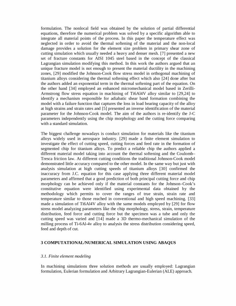
3.2. Types of elements and mesh domain To simulate the machining process the most commercial software’s used are ABAQUS™, ANSYS™ and DEFORM2D™. According to [6] “it’s an important tool suitable to solve linear and nonlinear problems as dynamic or static problems, contact between solids and ability to model large changes in the form of solids”. Many authors developed different models and techniques for specific cases in the field of machining simulation. The mesh domain has different boundary conditions, geometry, and regions for the analysis but all the models aims at the effects of the cutting parameters, chip morphology and tool geometry. Each model employed has, basically, the same type of elements which are usually quadrilateral elements with thermo-mechanical properties coupled(CPE4RT,CP4RT,etc). By means of this assumption a two-dimensional plane strain analysis is performed in ABAQUS for the orthogonal cutting process. 3.2.1 Algorithms for mesh type In Abaqus mesh controls the type of Algorithms used must be specified, usually two different techniques are applied to assign the element shapes for two and three dimensional problems. The default method is the Free technique with medial axis and advancing front algorithms available. The figure 1 show the difference between the algorithms and the main advantage is the possibility to shape complex geometries accurately in advancing front even with holes and corners.

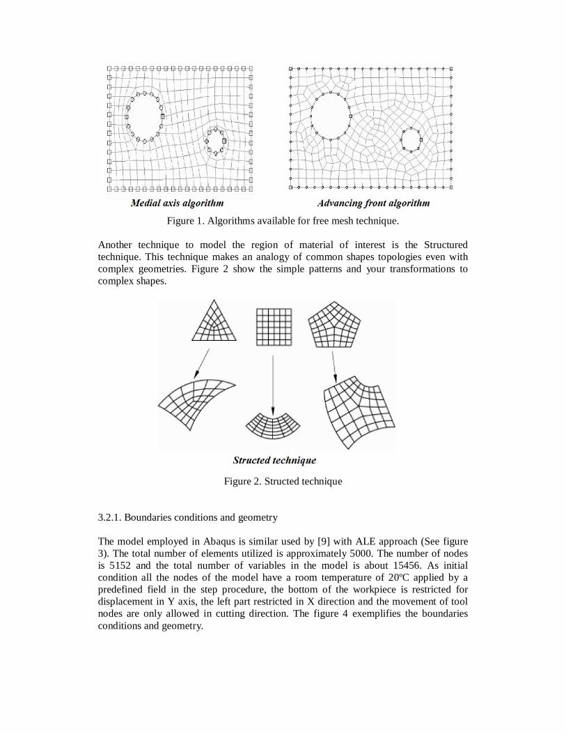
Figure 1. Algorithms available for free mesh technique.

Another technique to model the region of material of interest is the Structured technique. This technique makes an analogy of common shapes topologies even with complex geometries. Figure 2 show the simple patterns and your transformations to complex shapes.

Figure 2. Structed technique

3.2.1. Boundaries conditions and geometry The model employed in Abaqus is similar used by [9] with ALE approach (See figure 3). The total number of elements utilized is approximately 5000. The number of nodes is 5152 and the total number of variables in the model is about 15456. As initial condition all the nodes of the model have a room temperature of 20ºC applied by a predefined field in the step procedure, the bottom of the workpiece is restricted for displacement in Y axis, the left part restricted in X direction and the movement of tool nodes are only allowed in cutting direction. The figure 4 exemplifies the boundaries conditions and geometry.

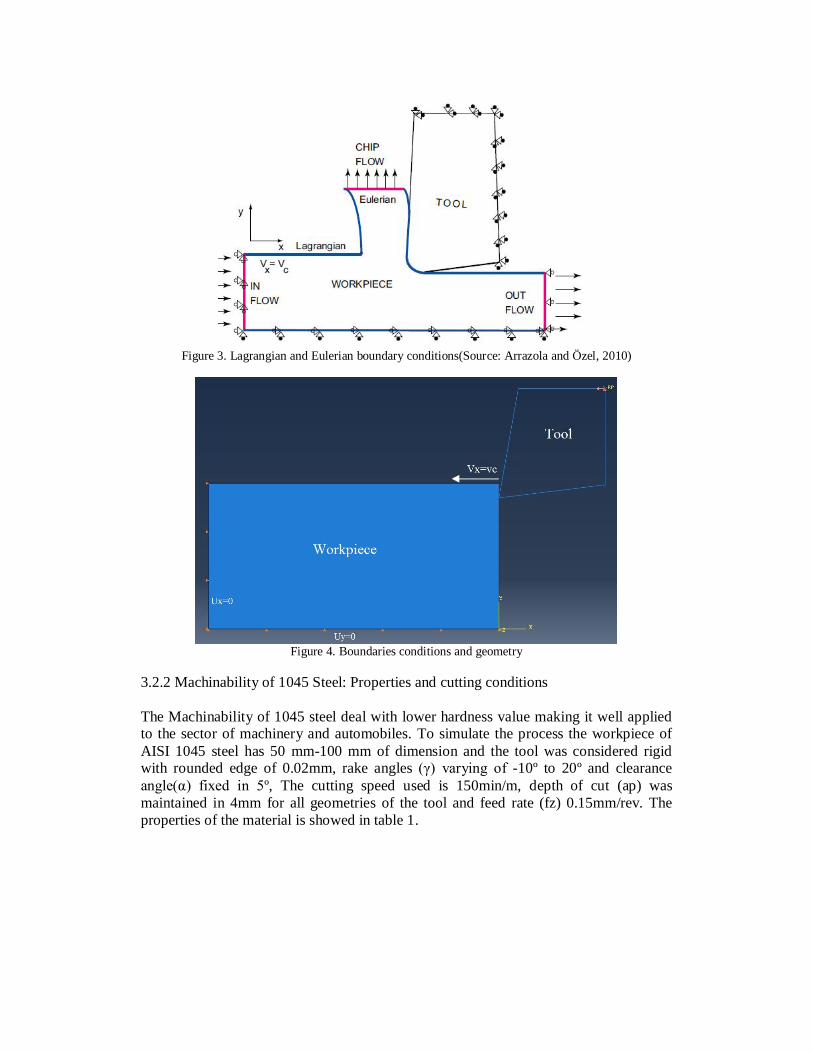
Figure 3. Lagrangian and Eulerian boundary conditions(Source: Arrazola and Özel, 2010)

Figure 4. Boundaries conditions and geometry

3.2.2 Machinability of 1045 Steel: Properties and cutting conditions The Machinability of 1045 steel deal with lower hardness value making it well applied to the sector of machinery and automobiles. To simulate the process the workpiece of AISI 1045 steel has 50 mm-100 mm of dimension and the tool was considered rigid with rounded edge of 0.02mm, rake angles (γ) varying of -10º to 20º and clearance angle(α) fixed in 5º, The cutting speed used is 150min/m, depth of cut (ap) was maintained in 4mm for all geometries of the tool and feed rate (fz) 0.15mm/rev. The properties of the material is showed in table 1.

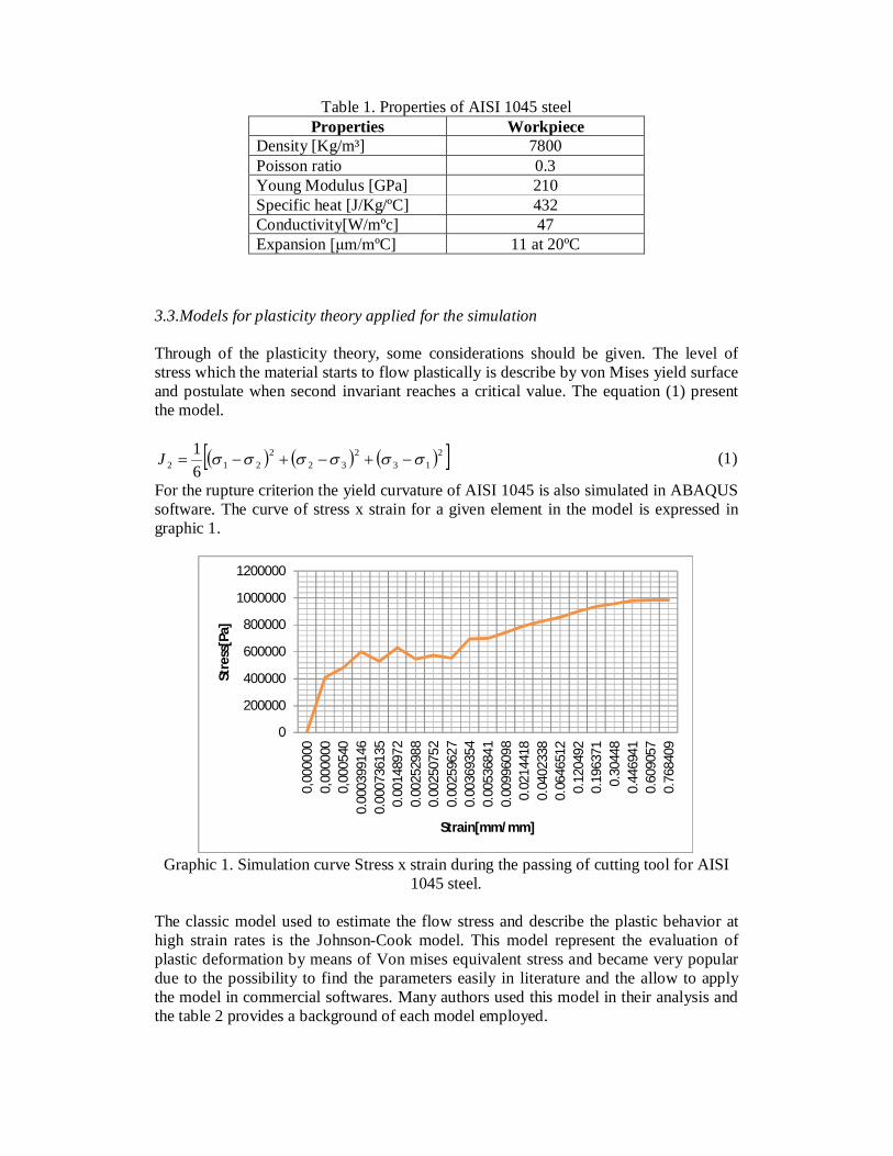
Table 1. Properties of AISI 1045 steel Properties Workpiece

Density [Kg/m³] 7800 Poisson ratio 0.3 Young Modulus [GPa] 210 Specific heat [J/Kg/ºC] 432 Conductivity[W/mºc] 47 Expansion [μm/mºC] 11 at 20ºC

3.3.Models for plasticity theory applied for the simulation

Through of the plasticity theory, some considerations should be given. The level of stress which the material starts to flow plastically is describe by von Mises yield surface and postulate when second invariant reaches a critical value. The equation (1) present the model.

213

232

2212 6

1 J (1)

For the rupture criterion the yield curvature of AISI 1045 is also simulated in ABAQUS software. The curve of stress x strain for a given element in the model is expressed in graphic 1.

Graphic 1. Simulation curve Stress x strain during the passing of cutting tool for AISI

1045 steel. The classic model used to estimate the flow stress and describe the plastic behavior at high strain rates is the Johnson-Cook model. This model represent the evaluation of plastic deformation by means of Von mises equivalent stress and became very popular due to the possibility to find the parameters easily in literature and the allow to apply the model in commercial softwares. Many authors used this model in their analysis and the table 2 provides a background of each model employed.

0

200000

400000

600000

800000

1000000

1200000

0,00

0000

0,00

0000

0,00

0540

0.00

0399

146

0.00

0736

135

0.00

1489

720.

0025

2988

0.00

2507

520.

0025

9627

0.00

3693

540.

0053

6841

0.00

9960

980.

0214

418

0.04

0233

80.

0646

512

0.12

0492

0.19

6371

0.30

448

0.44

6941

0.60

9057

0.76

8409

Stre

ss[P

a]

Strain[mm/mm]

Table 2. Types of constitutive models employed Type

of models

Models Authors

1 Johnson-Cook

[1],[3],[6],[22],[14],[15],[16],[17],[8],[23],[16],[9],[10],[11], [21],[26], [27], [28], [30],[33]

2 Modified J-C.

[5],[20],[18],[24],[29]

3 Zerili-Armstrong

[26], [34]

4 Oxley [1],[26] 5 Others [1],[12],[25],[19],[24]

The Johnson-Cook equation (2) describes the flow stress as a product of the equivalent strain, strain rate, temperature dependent terms and several parameters to adequate the real behavior of the materials.

m

roommelt

roomn

TTTT

CBA

1ln1)(

0

. (2)

Where: A represent the yield strength at room temperature, B pre-exponential factor related with the yield strength at the beginning of the plastic deformation, C is a strain-rate factor, equivalent plastic deformation. 0 is the reference strain rate, strain rate of the material, n is the work-hardening exponent, m the thermal-softening exponent and sT ' are variables related in the room temperature, melt temperature and material temperature. The parameters for J.C. equation for AISI 1045 steel are showed in table 3.

Table 3. Parameters for J.C. model(AISI 1045) Model A[MPa] B[MPa] n m Tmelt C

0 (s^-1) M1 553.1 600.8 0.234 1 1460 0.013 7500

3.4 Thermal effect considerations At the machining process, the thermodynamic effect is crucial. All the models has two regions of major deformations called primary and secondary deformation zones (see figure 5). In the primary deformation zone according to [4] the heating is due to energy dissipation from the plastic deformation; in the secondary deformation zone, heat is generated due to the plastic deformation and friction between the cutting tool and the chip.

Figure 5. Deformation zones (Source: Vaz Jr. et al. [4]).

In the primary deformation zone the average temperature can be express as function of the specific work for metal removal Wc. The equation 4 represent the estimation of the temperature:

0Tc

WT c

(3)

Where Wc is the specific work for metal removal, ρ is the density of the material, c specific heat e T0 is the initial temperature without deformation.

The secondary region of deformation is divided in two parts: Sticking region and sliding region. According to [21] Sticking contact occurs in the vicinity of the tool tip and is controlled by the magnitude of the shear flow stress of the work material which is itself governed by the chip temperature at the tool rake face. List et. al. [28] affirm that the transformation of frictional energy to heat is largely responsible for increase in temperature in secondary zone. The heat frictional generated can be express as follow:

WlVF

RqC

chipTsT

)1( (4)

Where: η is a factor of conversion of mechanical energy into thermal energy, FT is the tangential force, Vchip chip velocity, lc the contact length and Rs is the fraction of heat moving into the chip. More information about how to calculate Rs can be found in [28].

3.5 Friction models The contact between the tool and the workpiece determine the generation of energy and surface quality. According to Arrazola and Özel [9] Interfacial friction characteristics on tool–chip and tool–work contacts should be modeled fairly accurately in order to account for additional heat generation and stress developments due to friction. The most simple friction model is the Coulomb friction expressed bellow:

(5) where is the frictional shear stress, the friction coefficient and the normal stress to surface. However, many authors do not agree with this simple model for machining process and at high stress variations the shear friction model kmp can be used. [9] still affirm that when the normal stress (σ) distribution over the rake face is fully defined and the coefficient of friction (μ) is known, the frictional stress (τ) can be determined assuming the sticking region and sliding region on the secondary deformation zone. According to [17] in the sticking contact region, a critical frictional stress τ is reached due to the high normal stress on the cutting tool and in the sliding contact satisfies the coulomb friction law with a constant coefficient of friction μ and [23] affirm that in the sliding region the frictional stress is lower than the yield shear stress. The frictional stress distribution on the tool rake face can be represented in these distinct regions: where the plastic contact occurs (eq. 6) and where the elastic contact occurs (eq. 7). chipkx when mkxn and plx 0 , (6)

xn when mkxn )( and lcxlp . (7)

Where chipk is the average shear flow stress at tool–chip interface in the chip, lp is the length of sticking region and lc the length of the chip-tool contact. The figure 6 shows the distribution of the normal and frictional stress on the tool rake face.

Figure 6. Normal and frictional stress on the tool (Source: Arrazola and Özel [9])

3.5.2 Contact properties Tangential and Normal behavior was adopted, the friction formulation for tangential behavior is the Penalty method with friction coefficient taken 0.6 here and the maximum shear stress was 400Mpa. A hard contact is used in normal behavior and for heat generation in the region of contact of tool and workpiece the fraction of dissipated energy caused by friction converted to heat is 1/0.5 respectively for master and slave surface.

3.6 Damage models The beginning of failure and material separation are defined by local damage criterions and nodal distance of elements existing in literature. The damage models is only present in Lagrangian formulations and your application not required in ALE approach. [20] affirm that one of the difficulties in the finite element (FE) simulation of the metal cutting is to find a proper separation criterion, directly related to the application of a proper material failure. Many damage models exists among them the ductile criterion, J-C. damage model, Steinberg-Guinan model, Zerilli-Armstrong model, Lemaitre model, etc. The ductile damage defines the points of initiation of the stiffness degradation of the workpiece and according to [2] Ductile damage is normally associated with the presence of large plastic deformations in the neighborhood of crystalline defects. [3] affirm that the ductile damage initiation criterion corresponds to the shear strain value reaches to a certain critical plastic strain value and thenceforth the material will deform. The most popular damage model applied still the J.-C. model. The model is postulate that the fracture occurs when the accumulated plastic strain reaches a critical value, the equation 8 present this model initially.

f

Ddestressstatf

0

, (8)

where f is the history dependent a damage function, is the equivalent strain, f the equivalent strain-to-fracture and D is a material constant.

Extending the model with f

f1

and the equivalent strain-to-failure parameter express

as a function of: *

54*

321 1*ln1)exp( TDDDDDf , (9)

whereupon the stress triaxiality parameter * is defined by

m* which are

correspondent with the average of the three normal stress and the Von mises equivalent

stress. * is the dimensionless plastic strain defined by 0

*

p

, T* is a variable

dependent of the room temperature and melting temperature represented by

roommelt

room

TTTT

T

* and finally D1,D2,D3,D4,D5 are fracture constants. Therefore,

replacing the terms we got:

]1[]ln1[]exp[ 50

4321

roommelt

roomp

mf

TTTTDDDDD

, (10)

Finally, the damage parameter is defined as:

f

D . (11)

where is the increment of the equivalent plastic strain during an integration cycle and f the equivalent strain to fracture under current specifically conditions. The parameters for the J.C. damage model is expressed in table 4.

Table 4. Parameters for J.C. damage model(AISI 1045) Damage Model

D1 D2 D3 D4 D5

M1 0.25 4.38 2.68 0.002 0.61 To propose the new set of parameters of J-C model [7] used the Arbitraty Lagrangian-Eulerian (ALE) solution in simulation of machining for the accumulate damage at fracture point adjacent to the tool tip. The necessary time-histories were obtained via post-processing calculations on the data available in ALE simulation output files. In this paper, the nonlinear least-squares optimization procedure is used to directly identify the five constants of the J–C fracture model in addition to an updated Lagrangian approach employed.

3.7 ALE Adaptive meshing To avoid errors in the final stage between the numerical simulation and empirical/analytical tests, the part distortion concerning the researchers and many techniques are proposed. The elements in the cutting path must be deleted, and then machining forces and the heat fluxes must be introduced in the new surface [1]. According to [25] the goal of this type of meshing is to reduce the distortion and improve the aspect ratio of the elements, thus, preserving the accuracy of the analysis and reducing the likelihood of numerical instabilities that may force the analysis to terminate early. The ALE adaptive operator provides the possibility to put away the application of damage models for the chip separation criteria and also reduce significantly the necessary time to complete the simulation. The figure 7 shows how the ALE operator split works when an element distort.

Figure 7. ALE operator split to reduce the element distortion and preserve properties

(Source: Vaz, Jr. et. al., 2007)

3.7.1 ALE adaptive mesh domain The ALE adaptive mesh domain is employed in the region of the workpiece where the material will deform. The adaptive domain of the mesh defines the portions of a finite element model where mesh movement is independent of material deformation [3]. This characteristic helps to preserve the properties of each node and two parameters are very important: The frequency for the remeshing and the remeshing sweep. The frequency of remeshing is associated at each increment of simulation and the remeshing of the domain will be done after a predetermined number of frequency committing the accuracy and computational time, reducing these parameters at large values. During the passing of cutting tool in the material, the mesh sweep is associated with the mesh domain increasing the intensity of adaptive meshing. In this step of ALE remeshing the nodes are relocated based on the current positions of neighbouring nodes/elements and at each sweep, the nodes are adjusted slightly to reduce element distortion. Large sweep values increases the computational time and accuracy of the model. 3.7.2 Mesh smoothing Another important tool of ALE adaptive meshing is the mesh smoothing used to smooth the element distortion and to maintain good element aspect ratios at regular intervals. Three smoothing methods are explored: volume, laplacian and equipotential method. The “volume smoothing relocates a node by computing a volume weighted average of the element centers in the elements surrounding the node”, Laplacian smoothing relocates a node calculating the average of the positions of each of the adjacent nodes connected by an element edge to the node in question and Equipotential smoothing is a higher-order method that relocates a node by calculating a higher-order, weighted average of the positions of the node's eight nearest neighbor nodes in two dimensions

4 Results and discussion To compare the results of the simulation, two different approaches were employed, one using lagrangian approach and the others with ALE approach. Due to the excessive computational time required and extreme element distortion in Lagrangian approach, the analysis of the effects of tool geometry are conduced by ALE formulation. The difference between the two solution methods are shown in figure 8 and graphic 2.

Figure 8. Differences between Lagrangian formulation and ALE formulation

Graphic 2. Stress distribution with different solution methods for a given element

Has been noted that the ALE formulation provides better results than Lagrangian formulation for chip formation. However some materials need of damage models and others parameters which ALE approach neglects. Lagrangian technique cannot be totally replace by algorithms with ALE adaptive domain, but for this kind of material this approximation works well.

0

200000

400000

600000

800000

1000000

1200000

1 3 5 7 9 11 13 15 17 19 21

Stre

ss[P

a]

Lagrangian approach

ALE approach

4.1 Effect of tool geometry on chip morphology and stress distribution Four different rake angles was adopted for the tool geometry: -10º, 0º, 10º and 20º. In each case, the chip formed was continuous which follow the real behavior of this kind of material. Figures 9 shows the differences between the models.

Rake angle: -10º

Rake angle: 0º

Rake angle: 10º

Rake angle: 20º

Figure 9. Effect of rake angles in chip morphology

As the rake angle increase the chip tends to narrow due to low adhesion in tool-workpiece region, moreover the work for chip folding is smallest. It’s also noticeable that the increase of rake angle leads to smooth the tip of chip. The main reason for the above phenomena is that given a small rake angle, the cutting action often transforms into a pushing and squeezing force. For the Von mises stress distribution, an increase in the tool rake angle reduces the area of equivalent stress in the primary deformation zone

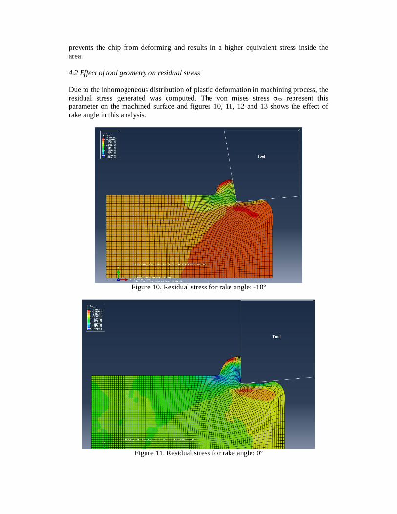
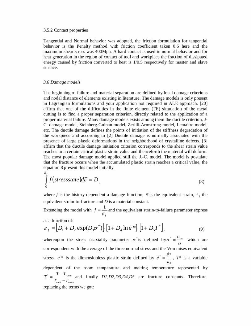
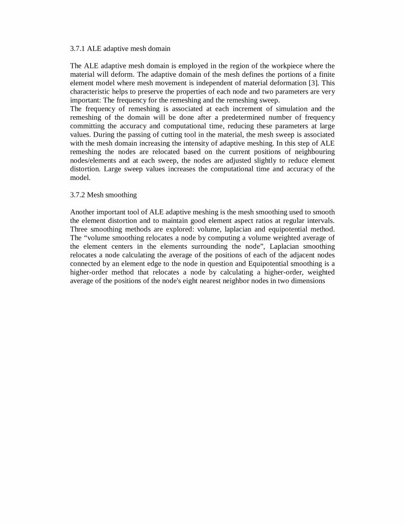
prevents the chip from deforming and results in a higher equivalent stress inside the area. 4.2 Effect of tool geometry on residual stress Due to the inhomogeneous distribution of plastic deformation in machining process, the residual stress generated was computed. The von mises stress σxx represent this parameter on the machined surface and figures 10, 11, 12 and 13 shows the effect of rake angle in this analysis.

Figure 10. Residual stress for rake angle: -10º

Figure 11. Residual stress for rake angle: 0º

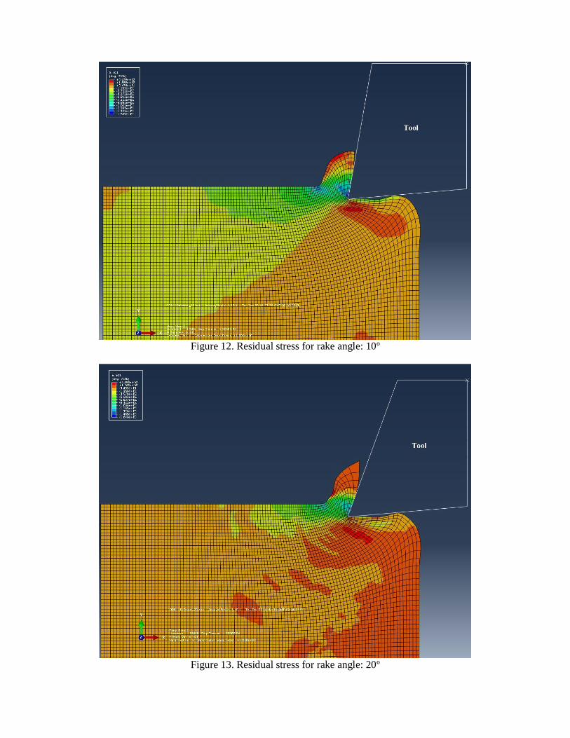
Figure 12. Residual stress for rake angle: 10º

Figure 13. Residual stress for rake angle: 20º

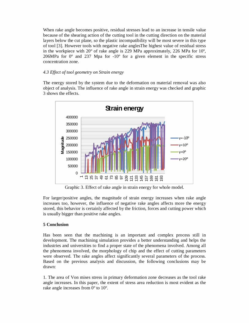
When rake angle becomes positive, residual stresses lead to an increase in tensile value because of the shearing action of the cutting tool in the cutting direction on the material layers below the cut plane, so the plastic incompatibility will be most severe in this type of tool [3]. However tools with negative rake anglesThe highest value of residual stress in the workpiece with 20º of rake angle is 229 MPa approximately, 226 MPa for 10º, 206MPa for 0º and 237 Mpa for -10º for a given element in the specific stress concentration zone. 4.3 Effect of tool geometry on Strain energy The energy stored by the system due to the deformation on material removal was also object of analysis. The influence of rake angle in strain energy was checked and graphic 3 shows the effects.

Graphic 3. Effect of rake angle in strain energy for whole model.

For larger/positive angles, the magnitude of strain energy increases when rake angle increases too, however, the influence of negative rake angles affects more the energy stored, this behavior is certainly affected by the friction, forces and cutting power which is usually bigger than positive rake angles. 5 Conclusion Has been seen that the machining is an important and complex process still in development. The machining simulation provides a better understanding and helps the industries and universities to find a proper state of the phenomena involved. Among all the phenomena involved, the morphology of chip and the effect of cutting parameters were observed. The rake angles affect significantly several parameters of the process. Based on the previous analysis and discussion, the following conclusions may be drawn: 1. The area of Von mises stress in primary deformation zone decreases as the tool rake angle increases. In this paper, the extent of stress area reduction is most evident as the rake angle increases from 0º to 10º.

0

50000

100000

150000

200000

250000

300000

350000

400000

1 13 25 37 49 61 73 85 97 109

121

133

145

157

169

181

193

Mag

nitu

de

Strain energy

γ=-10º

γ=10º

γ=0º

γ=20º

2. The top of the chip contour becomes smoother as the tool rake angle increases due to lower adhesion zone. An increase of this rake angle also fold the chip. 3. The energy stored due to the deformation of material is highest for negative rake angles due to tendency of smooth the force/cutting power of tool with positive rake angles. 4. The layers in the workpiece where residual stress appears is larger for -10º of rake angle. The residual stress increases as the angles raise too. This phenomena occurs due to the shearing action of cutting tool. At specific cutting conditions the Jonhson-Cook model to the flow stress is suitable and the use of commercials softwares enabling many analysis which in the past were unable due to the limitations existing. 5 REFERENCES [1] Arrazola P.J. ; Özel, T. ; Umbrello, D. ; Davies, M.; Jawahir, I. S. Recent advances

in modelling of metal machining processes. Journal of Manufacturing technology. 2013.

[2] E. A. de Souza Neto. Computational methods for plasticity: theory and applications.

New Jersey:Willey, 2008. [3] Prasad, C. S. Finite element modeling to verify residual stress in orthogonal

machining. Master’s degree thesis. Blekinge Institute of technology. Sweden. 2009 [4] M. Vaz Jr. ; Owen, D.J.R. ; Kalhori, V. ; Lundblad, M. ; Lindgren, L.-E. Modelling

and simulation of machining processes. Arch computer methods Eng 14:173-204. 2007.

[5] Shrot, A. ; Bäker, M. Determination of Johnson-Cook parameters from machining

simulations. Journal of computational materials science 52:298-304. Elsevier. 2012 [6] Hui, H. H. Simulação da formação de cavacos usando FEM(Finite element method)

– Temperatura e força. Master’s degree thesis. University of São Paulo. São Carlos. Brazil. 2007

[7] Vaziri, M.R. ; Salimi,M. ; Mashayekhi, M. A new calibration method for ductile

fracture models as chip separation criteria in machining. Journal of Simulation modeling practice and theory -18:1286-1296. Elsevier. 2010

[8] Atlati, S.; Haddag, B.; Nouari, M.; Zenasni, M. Analysis of a new segmentation

intensity ratio “SIR” to characterize the chip segmentation process in machining

ductile metals. International journal of machine tools & manufacture – 51:687-700. Elsevier. 2011

[9] Arrazola,P. J. ; Özel,T. Investigations on the effects of friction modeling in finite

element simulation of machining. International journal of mechanical sciences 52:31-42, 2010.

[10] Zouhar, J.; Piska, M. Modelling the orthogonal machining process using cutting

tools with different geometry. MM Science Journal, vol.1, No.4:.49-52, MM publishing Ltd. 2008

[11] Muñoz-Sánchez, A.; Canteli, J.A.; Cantero,J.L.; Miguélez, M.H. Numerical analysis of the tool wear effect in the machining induced residual stress. Journal of Simulation modeling practice and theory-19:872-886. Elsevier. 2011

[12] Adetoro, M. B.; Wen, P.H. Simulation of end milling on FEM using ALE

formulation. Abaqus User’s Conference. New Port, Rhode Island. USA. 2008 [13] Rosa, P. A. R., P. A. F. Martins, A.G. Atkins. Revisiting the fundamentals of metal

cutting by means of finite elements and ductile fracture mechanics. International Journal of Machine Tools and Manufacture, vol. 47(3-4), pp. 607-617, 2007.

[14] Escamilla, I.; Zapata, O.; Gonzalez, B.; Gámez, N.; Guerrero, M. 3D finite element

simulation of the milling process of a TI 6AL 4V alloy. Simulia Customer conference. Providence, Rhode Island. USA. 2010.

[15] Nasr, M. N. A.; E.-G. NG; Elbestawi, M.A. A modified time-efficient FE approach

for predicting machining induced residual stress. Journal of Finite element in analysis and design. v.44, pp.149-161, 2008.

[16] Vaziri, M.R.; Salimi, M.; Mashayekhi, M. Evaluation of chip formation simulation

models for material separation in the presence of damage models. Journal of Simulation modeling practice and theory. v.19, pp.718-733, 2011.

[17] Jin, X.; Altintas, Y. Prediction of Micro-Milling Forces With Finite Element

Method. Journal of materials processing technology. v.212, pp.542-552, 2012. [18] Schulze, V.; Autenrieth, H.; Deuchert, M.; Weule, H. Investigation of surface near

residual stress after micro-cutting by finite element simulation. CIRP Annals – Manufacturing technology. v. 59, pp. 117-120, 2010.

[19] John, M. R. S.; Shrivastava, K.; Banerjee, N.; Madhukar, P. D.; Vinayagam, B. K.

Finite element method-based machining simulation for analyzing surface roughness during turning operation with HSS and carbide insert tool. Arabian journal for science and engineering, v.38, pp.1615-1623, 2013.

[20] Shams, A.; Mashayekhi, M. Improvement of orthogonal cutting simulation with

nonlocal damage model. International journal of mechanical sciences, v.61, pp.88-96, 2012.

[21] Molinari, A.; Cheriguene, R.; Miguelez, H. Numerical and analytical modeling of

orthogonal cutting: The link between local variables and global contact characteristics. International journal of mechanical sciences, v. 53, pp.183-206, 2011

[22] Sadeghina, H.; Razfar, M.R.; Takabi, J. 2D finite element modeling of face milling

with damage effects. 3rd WSEAS International Conference on APPLIED and THEORETICAL MECHANICS, Spain. 2007

[23] Zhang, Y.C.; Mabrouki, T.; Nelias, D.; Gong, Y.D. Chip formation in orthogonal

cutting considering interface limiting shear stress and damage evolution based on fracture energy approach. Journal of Finite elements in analysis and design. v.47, pp.850-863, 2011

[24] Sima, M.; Özel, T. Modified material constitutive models for serrated chip

formation simulations and experimental validation in machining of titanium alloy Ti–6Al–4V,International Journal of Machine Tools and Manufacture 50 (11) pp.943–960, 2010.

[25] Vavourakis, V.; Loukidis, D.; Charmips,D.C.; Panastasiou, P. Assessment of

remeshing and remapping strategies for large deformation elastoplastic finite element analysis. Journal of computers and structures, v.114-115, pp.133-146, 2013

[26] Kiliçaslan, C. Modelling and simulation of metal cutting by finite element method.

Master’s degree thesis. Ýzmir Institute of Technology, Turkey, 2009. [27] Gao, C.; Zhang, L. Effect of cutting conditions on the serrated chip formation in

high-speed cutting. Machining Science and Technology: An International Journal, 17:1, 26-40, 2013.

[28] List, G.; Sutter, G.; Bouthiche, A. Cutting temperature prediction in high speed

machining by numerical modeling of chip formation and its dependence with crater wear. International journal of machine tools & manufacture, v. 54-55, pp. 1-9, 2012

[29] Calamaz, M.; Coupard, D.; Girot, F. A new material model for 2D numerical

simulation of serrated chip formation when machining titanium alloy Ti–6Al–4V. International journal of Machine tools & manufacture, v.48, pp.275-288, 2008.

[30] Umbrello, D. Finite element simulation of conventional and high speed machining

of Ti6Al4V alloy. Journal of materials processing technology , v. 196, pp.79-87, 2008

[31] Arrazola, P.J.; Villar, A.; Ugarte, D.; Marya, S. Serrated chip prediction in finite

element modeling of the chip formation process. Machining Science and Technology, 11: 367–390, 2007

[32] Ali Moaz, H.; Khidir, B. A.; Ansari, M.N.M.; Mohamed, B. FEM to predict the

effect of feed rate on surface roughness with cutting force during face milling of titanium alloy. Housing and building national research center journal, v.7, pp.263-269, 2013.

[33] Vijay Sekar, K.S.; Kumar, M.P. Finite element simulations of Ti6Al4V titanium

alloy machining to assess material model parameters of the Johnson-Cook constitutive equation. Journal of Brazilian society of Mechanical Science & Engineering, v.23, n.2, 2011.~

[34] Liu, R.; Melkote, S.; Pucha, R.; Morehouse,J.; Man,X.; Marusich, T. An enhanced

constitutive material model for machining of Ti-6Al-4V alloy. Journal of materials processing technology, v.213, pp.2238-2246, 2013

[35] Long, Y.; Guo, C. Finite element modeling of Burr formation in orthogonal

cutting. Machining science and technology: An international Journal, 16:3, 321-336, 2012.

[36] Molinari, A.; Soldani, X.; Miguélez, M.H. Adiabatic shear banding and scaling laws in chip formation with application to cutting of Ti-6Al-4V. Journal of the mechanics and Physics of solids, v.61, pp.2231-2359, 2013.