ULTRA-HIGH PRECISION MACHINING OF CONTACT LENS ...

i

ULTRA-HIGH PRECISION MACHINING OF

CONTACT LENS POLYMERS

OLUFAYO, OLUWOLE AYODEJI

(s210026162)

2015

ii

COPYRIGHT STATEMENT

The copy of this thesis has been supplied on condition that anyone who consults it

understands and recognises that its copyright rests with the Nelson Mandela

Metropolitan University and that no information derived from it may be published

without the author’s prior consent, unless correctly referenced.

iii

ULTRA-HIGH PRECISION MACHINING OF CONTACT

LENS POLYMERS

By

Olufayo, Oluwole Ayodeji

Submitted in fulfilment/partial fulfilment of the requirements for the

degree of Doctor of Philosophy: Engineering: Mechatronics at the

Nelson Mandela Metropolitan University

July 2015

Promoter/Supervisor: Prof. Khaled Abou-El-Hossein

iv

DECLARATION

I, Oluwole Ayodeji OLLUFAYO & s210026162, hereby declare that the treatise/

dissertation/ thesis for Students qualification to be awarded is my own work and that it

has not previously been submitted for assessment or completion of any

postgraduate qualification to another University or for another qualification.

Official use:

In accordance with Rule G5.6.3,

5.6.3 A treatise/dissertation/thesis must be accompanied by a written declaration on the part of the candidate to the effect that it is his/her own work and that it has not previously been submitted for assessment to another University or for another qualification. However, material from publications by the candidate may be embodied in a treatise/dissertation/thesis.

v

ACKNOWLEDGEMENTS

Unto the Lord be the glory, honour and adoration for his infinite mercies and favour

upon my life.

Sincere gratitude and appreciation go to my promoter, Prof Khaled Abou-El-Hossein,

for his support and guidance through the period of study.

I would also like to acknowledge the Technology Innovation Agency /Department of

Science and Technology of South Africa, National Research Foundation of South

Africa (NRF) and Research Capacity development of NMMU for the financial support

provided for this research.

Special gratitude also goes to my parents, Prof. and Dr (Mrs) Olufayo, who have

instilled in me a deep love for the academics. You encouraged me to be an engineer

like you. Thank you dad! To my big auntie, Prof (Mrs) Esther Titilayo Akinlabi, I say a

big “Thank you”, for your support and mentorship. Also, my appreciation goes to my

uncle Mr Akinlabi, my nephew and niece; Akinkunmi, and Stephanie, I also thank Dr

and Mrs F. A. Emuze, Dr and Mrs K. A. Olowu, Mrs Olutobi, Liliane Creppy, Mr.

Emmanuel Oyeyemi and my dear sister Mrs. Motunrayo Oyeyemi. Special thanks

also to my one love and best friend, Samira, who believed in me though this period

of my studies.

I remain grateful to all my friends, colleagues; Timothy Otieno, John Fernandes, Ikho

Bambiso, Dr. Michael Ayomoh and Munir Kadernani who have supported me in

many ways through this period of study. Further thanks go to Prof. Theo van Niekerk

and members of AMTC / Siemens who have been of great support throughout my

time at the Nelson Mandela Metropolitan University. Thank you.

vi

ABSTRACT

Ultra-High Precision Machining of Contact Lens Polymers

Olufayo, O. A.

Faculty of Engineering, the Built Environment and Information Technology

P.O. Box 77000, Nelson Mandela Metropolitan University,

Port Elizabeth, South Africa

July, 2015

Contact lens manufacture requires a high level of accuracy and surface integrity in

the range of a few nanometres. Amidst numerous optical manufacturing techniques,

single-point diamond turning is widely employed in the making of contact lenses due

to its capability of producing optical surfaces of complex shapes and nanometric

accuracy. For process optimisation, it is ideal to assess the effects of various

conditions and also establish their relationships with the surface finish. Presently,

there is little information available on the performance of single point diamond

turning when machining contact lens polymers. Therefore, the research work

undertaken herewith is aimed at testing known facts in contact lens diamond turning

and investigating the performance of ultra-high precision manufacturing of contact

lens polymers.

Experimental tests were conducted on Roflufocon E, which is a commercially

available contact lens polymer and on Precitech Nanoform Ultra-grind 250 precision

machining. Tests were performed at varying cutting feeds, speed and depth of cut.

Initial experimental tests investigated the influence of process factors affecting

surface finish in the UHPM of lenses. The acquired data were statistically analysed

using Response Surface Method (RSM) to create a model of the process.

Subsequently, a model which uses Runge-Kutta’s fourth order non-linear finite series

scheme was developed and adapted to deduce the force occurring at the tool tip.

These forces were also statistically analysed and modelled to also predict the effects

process factors have on cutting force. Further experimental tests were aimed at

establishing the presence of the triboelectric wear phenomena occurring during

polymer machining and identifying the most influential process factors.

vii

Results indicate that feed rate is a significant factor in the generation of high optical

surface quality. In addition, the depth of cut was identified as a significant factor in

the generation of low surface roughness in lenses. The influence some of these

process factors had was notably linked to triboelectric effects. This tribological effect

was generated from the continuous rubbing action of magnetised chips on the

cutting tool. This further stresses the presence of high static charging during cutting.

Moderately humid cutting conditions presented an adequate means for static charge

control and displayed improved surface finishes. In all experimental tests, the feed

rate was identified as the most significant factor within the range of cutting

parameters employed.

Hence, the results validated the fact that feed rate had a high influence in polymer

machining. The work also established the relationship on how surface roughness of

an optical lens responded to monitoring signals and parameters such as force, feed,

speed and depth of cut during machining and it generated models for prediction of

surface finishes and appropriate selection of parameters. Furthermore, the study

provides a molecular simulation analysis for validating observed conditions occurring

at the nanometric scale in polymer machining. This is novel in molecular polymer

modelling.

The outcome of this research has contributed significantly to the body of knowledge

and has provided basic information in the area of precision manufacturing of optical

components of high surface integrity such as contact lenses. The application of the

research findings presented here cuts across various fields such as medicine, semi-

conductors, aerospace, defence, telecom, lasers, instrumentation and life sciences.

viii

TABLE OF CONTENTS

ACKNOWLEDGEMENTS .......................................................................................... V

ABSTRACT .............................................................................................................. VI

TABLE OF CONTENTS .......................................................................................... VIII

ABBREVIATIONS.................................................................................................... XII

NOMENCLATURE .................................................................................................. XIII

LIST OF TABLES .................................................................................................. XIV

LIST OF FIGURES................................................................................................. XVI

GLOSSARY OF TERMS ........................................................................................ XXI

CHAPTER 1 INTRODUCTION.............................................................................. 1

1.1 Preamble ....................................................................................................... 1

1.2 The general concept for the study ................................................................. 1

1.3 Optical manufacturing techniques for contact lenses .................................... 2

1.4 Significance of the study ............................................................................... 4

1.5 Problem statement ........................................................................................ 4

1.6 Research aim and objective .......................................................................... 5

1.7 The hypothesis statement ............................................................................. 6

1.8 Research scope ............................................................................................ 6

1.9 Structure of the thesis ................................................................................... 7

CHAPTER 2 LITERATURE REVIEW ................................................................... 8

2.1 Introduction ................................................................................................... 8

2.2 Eye polymer optics ........................................................................................ 8

2.3 Contact lenses and their materials .............................................................. 10

2.3.1 Classes of polymers used in medicine ................................................. 13

2.3.2 Fabrication of contact lenses ................................................................ 15

2.3.3 Commercially available contact lens materials ..................................... 17

2.4 Manufacturing of contact lenses .................................................................. 20

2.4.1 Spin casting .......................................................................................... 21

2.4.2 Plastic injection moulding ..................................................................... 22

2.4.3 Ultra high precision machining technique ............................................. 24

2.4.4 Research & barriers in the ultra-high precision manufacturing of polymers ............................................................................................................ 28

ix

2.4.4.1 Elastic recovery in polymer machining ........................................... 29

2.4.4.2 Diamond wear in polymer machining ............................................. 30

2.4.4.3 Tribo-chemical wear in polymer machining .................................... 30

2.4.4.4 Triboelectric wear in polymer machining ........................................ 33

2.5 General behaviour of polymers in diamond machining ............................... 39

2.5.1 Parameters to evaluate surface roughness .......................................... 42

2.6 Modelling of ultra-high precision machined polymers .................................. 43

2.6.1 Response surface method .................................................................... 43

2.6.1.1 Box-Behnken response surface method ........................................ 44

2.6.2 Atomistic Simulation methods ............................................................... 45

2.6.3 Molecular Dynamics (MD) Simulation method ...................................... 46

2.6.4 MD simulation of machining operations ................................................ 48

2.6.5 MD simulation in polymer machining .................................................... 50

2.6.5.1 Principles of MD simulation and model .......................................... 51

2.6.5.2 Some potential energy functions in MD simulations ....................... 53

2.7 Summary ..................................................................................................... 56

CHAPTER 3 MOLECULAR DYNAMICS SIMULATION OF POLYMERS .......... 57

3.1 Introduction ................................................................................................. 57

3.2 Molecular properties of Roflufocon E lens ................................................... 58

3.3 Molecular structure of contact lens polymers .............................................. 59

3.4 Use of MD in nanomachining simulation ..................................................... 63

3.5 Methodology of MD simulation of Polymer nanomachining ......................... 65

3.5.1 Pre-processing and export of molecular structure ................................ 66

3.5.2 Main MD processing ............................................................................. 68

3.5.3 Post processing and visualisation ......................................................... 68

3.6 Molecular Dynamics (MD) constituent parts ................................................ 69

3.6.1 System configuration ............................................................................ 69

3.6.2 The workpiece ...................................................................................... 70

3.6.3 The tool ................................................................................................. 71

3.7 General overview of MD simulation conditions ............................................ 72

3.7.1 Initialization ........................................................................................... 72

3.7.2 Boundary conditions ............................................................................. 72

3.7.3 Relaxation of the system ...................................................................... 74

3.7.4 Potential energy function ...................................................................... 74

3.7.5 Scope of the simulation ........................................................................ 76

x

CHAPTER 4 EXPERIMENTAL PROCEDURES ................................................. 77

4.1 Introduction ................................................................................................. 77

4.2 Experimental setup ..................................................................................... 78

4.3 Workpiece ................................................................................................... 81

4.4 Diamond tool ............................................................................................... 82

4.5 Surface finish measurements (Atomic Force microscopy) .......................... 83

4.6 Cutting force measurements ....................................................................... 86

4.6.1 Measurement instruments .................................................................... 86

4.6.2 Cutting mechanics ................................................................................ 87

4.7 Electrostatic discharge measurements ....................................................... 90

4.7.1 Electrostatic sensor .............................................................................. 91

4.7.2 Electrostatic humidity procedure ........................................................... 93

CHAPTER 5 RESULTS AND DISCUSSION ...................................................... 94

5.1 Statistical evaluation of factors affecting surface finish of contact lens polymers ............................................................................................................... 94

5.1.1 Theoretical value to surface finish ........................................................ 95

5.1.2 Determination of appropriate polynomial equation to represent RSM model 102

5.1.2.1 ANOVA analysis of the response surface quadratic model for surface roughness ....................................................................................... 104

5.1.2.2 Determination of significant factors influencing surface roughness 106

5.1.3 Analysis of cutting chips ..................................................................... 110

5.1.3.1 The influence of rake angle on material properties of the workpiece 117

5.1.3.2 The influence of cutting parameters on material properties of the workpiece .................................................................................................... 118

5.1.4 Experimental observations of factors affecting surface finish ............. 119

5.1.5 Summary of results ............................................................................. 121

5.2 Predictive modelling of cutting force at the tool tip .................................... 123


5.3 Predictive modelling of cutting force and the influence of cutting parameters 128


5.4 Statistical evaluation of triboelectricity ....................................................... 135

5.4.1 Analysis for triboelectric phenomenon at 60% relative humidity ......... 135


xi


5.4.4 Modelling summary ............................................................................ 163

5.4.5 Conclusion and physics of the triboelectric phenomenon ................... 164


5.5 Molecular modelling overview of polymer nanomachining ........................ 166

5.5.1 Introduction ......................................................................................... 166

5.5.2 Thermodynamic information analysis ................................................. 166

5.5.3 Comparison of various potentials between tool and workpiece .......... 169

5.5.4 Correlation of MD results to machining conditions .............................. 175

5.5.5 Summary ............................................................................................ 180

CONCLUSION ....................................................................................................... 181

RECOMMENDATION ............................................................................................ 186

REFERENCES ....................................................................................................... 187

PUBLICATIONS .................................................................................................... 201

APPENDIX A: ULTRA-PRECISION G-CODE ....................................................... 203

APPENDIX B: POLYMER USAN WORKSHEET .................................................. 206

APPENDIX C: LAMMPS ........................................................................................ 207

xii

ABBREVIATIONS

ADC - Allyldiglycol carbonate

AFM - Atomic Force Microscopy

ANOVA - Analysis of Variance

CL - Contact Lens

EWC - Equilibrium Water Content

FDA - Food Drug Administration

FEM - Finite Element Analysis

GP - Gas permeable

HDPE - High Density Poly Ethylene

HEMA - Hydroxyethyl Methacrylate

IOL - Intraocular Lens

IR - Infrared

MD - Molecular Dynamics

NMMU - Nelson Mandela Metropolitan University

PC -Polycarbonate

PDMS - Poly (dimethyl-siloxane)

PE - Polyethylene

PHEMA - Polyhydroxyethyl Methacrylate

PMMA - Polymethyl Methacrylate

PP - Polypropylene

PS - Polystyrene

UHPM - Ultra-high precision machining

RH - Relative Humidity

RGP - Rigid Gas Permeable

Rpm - Revolution per minute

RSM - Response Surface Method

SEM - Scanning Electron Microscope

SMSS - Sequential Model sum of squares

SPDT - Single Point Diamond Turning

UHPDT - Ultra High Precision Diamond Turning

RDX - Cyclotrimethylenetrintramine

xiii

NOMENCLATURE

(Fc) - Advancing force in the direction of cutting (N)

(Fy) - Uniaxial force perpendicular to the Fx during cutting

(Fz) - Vertical downward force on the tool (N).

D - Depth of cut (µm).

𝑓 - Feedrate (µm/rev).

ɸ - Diameter.

𝑉𝑐 - Cutting speed (rev/min)

Φ - Shear angle

ß - Friction angle

α - Rake angle

µ - Coefficient of friction

𝑡2 - Uncut chip thickness

𝑡1 - Sheared away thickness

ω - Width of tool

l - Length of tool

h - Tool thickness

E - Young’s modulus of material

ε - Strain

xiv

LIST OF TABLES

Table 2.1 FDA grouping and modern RGP materials, divided into four groups

based on their contents. ................................................................ 17

Table 2.2 Properties of common optical polymers [26] .................................. 18

Table 2.3 Types of contact lens buttons and their respective properties ....... 19

Table 2.4 Summary of triboelectric charging mechanisms by Williams [64] .. 36

Table 2.5 Comparison of some atomistic simulation methods [13] ................ 46

Table 2.6 Comparison of nanometric cutting and conventional cutting

mechanics [13] .............................................................................. 48

Table 3.1 Monomers of Roflufocon E and ending bonds ............................... 61

Table 3.2 Assignment of CP/MAS 13CNMR Chemical Shifts of PMMA [108]

and Roflufocon E ........................................................................... 63

Table 3.3 Monomer ratios per molecule in Roflufocon E ............................... 63

Table 3.4 Comparison of Some Atomistic Simulation Methods[13] ............... 64

Table 3.5 Parametric values used in MD simulation ...................................... 70

Table 3.6 Quantification of atoms per element type ...................................... 70

Table 3.7 Physical properties of diamond tools ............................................. 71

Table 3.8 Parametric values used in MD simulation ...................................... 72

Table 4.1 Diamond machining parameters of contact lens polymer .............. 81

Table 4.2 Workpiece and Diamond tool geometry ......................................... 82

Table 4.3 Surface measurement matrix of experiments ................................ 85

Table 4.4 Specification of electrostatic sensor .............................................. 91

Table 5.1 Experimental runs and results of Surface Roughness ................... 94

Table 5.2 Sequential model sum of squares (SMSS) analysis for surface

roughness .................................................................................... 103

Table 5.3 Lack of fit test for surface roughness ........................................... 103

Table 5.4 ANOVA for model coefficient for Surface Roughness in UHPM of

contact lens polymer .................................................................... 104

Table 5.5 Experimental run and results of surface roughness .................... 110

Table 5.6: Cracking and microstructural ripple occurrence on cutting chips

based on high cutting depth at SEM different image magnification

.................................................................................................... 113

xv

Table 5.7 Smooth and large folding on cutting chips based on low cutting feed

.................................................................................................... 115

Table 5.8 Tear edges on cutting chips at low depth of cut and cutting speed

.................................................................................................... 116

Table 5.9 Analysis of Force at the tool-tip for the experimental runs ........... 126

Table 5.10 Experimental run 15 (0.15m-sec, 12 µm –rev and 25 µm) analysis of

Force at the tool-tip...................................................................... 127

Table 5.11 Experimental run and results of cutting Force ............................. 129

Table 5.12 Lack of fit test for cutting Forces .................................................. 130

Table 5.13 Sequential model sum of squares (SMSS) analysis for cutting

Forces ......................................................................................... 130

Table 5.14 ANOVA for model coefficient for Cutting Forces in UHPM of contact

lens polymer ................................................................................ 131

Table 5.15 Experimental run and results of cutting Force ............................. 134

Table 5.16 Experimental run and results of Surface Roughness .................. 135

Table 5.17 Sequential model sum of squares (SMSS) analysis for electrostatics

at 60% humidity ........................................................................... 139

Table 5.18 Lack of fit test for electrostatics at 60% humidity ......................... 139

Table 5.19 ANOVA for model coefficient for the electrostatics at 60% humidity

in UHPM of contact lens polymer ................................................ 140

Table 5.20 Sequential model sum of squares (SMSS) analysis for electrostatics

at 40% RH ................................................................................... 150

Table 5.21 Lack of fit test for electrostatics at 40% RH ................................. 151

Table 5.22 ANOVA for model coefficient for the electrostatics at 40% humidity

in UHPM of contact lens polymer ................................................ 151

Table 5.23 Sequential model sum of squares (SMSS) analysis for negative

electrostatics at 20% humidity ..................................................... 162

Table 5.24 Lack of fit test for negative electrostatics at 20% humidity .......... 162

Table 5.25 Polynomial equations to represent the developed models .......... 163

Table 5.26: Cutting parameters and interactions that significantly influence the

triboelectric effect ........................................................................ 163

Table 5.27 Comparison of various LJ force potentials during MD simulation 171

Table 5.28 Hybrid force simulation with (a) CPK; (b) VDW representation ... 174

xvi

LIST OF FIGURES

Figure 1.1 Taniguchi Curve [5] ......................................................................... 3

Figure 2.1 Diagram of the eye and a contact lens ............................................ 9

Figure 2.2 Diagram of the eye and positioning plane for an IOL implant [16] . 10

Figure 2.3 Typical IOL (a) traditional (b) plate designs [17] ............................ 10

Figure 2.4 Chart of contact lens classification ................................................ 11

Figure 2.5 Homopolymers used in Medicine [20]............................................ 14

Figure 2.6 The spin-casting process [21] ........................................................ 22

Figure 2.7 Moulding process flow diagram, 3D mould design and machined

mould ............................................................................................. 22

Figure 2.8 Ultra-precision machining technology [33] ..................................... 24

Figure 2.9 Ultra-precision diamond turning of freeform optics ........................ 25

Figure 2.10 Various optical objects used in critical industries [33] .................... 26

Figure 2.11 Ultra-precision diamond tools [40] ................................................. 27

Figure 2.12 Ultra-precision machined lens wit 3D image and low form accuracy

...................................................................................................... 28

Figure 2.13 Elastic recovery phenomenon after diamond cutting ..................... 29

Figure 2.14 Diamond tool wear [44] .................................................................. 30

Figure 2.15 Methyl methacrylate (MMA) ester bond ......................................... 31

Figure 2.16 Chemical wear on a diamond tool [46] .......................................... 31

Figure 2.17 Lichtenberg figure on a diamond tool [9, 56] ................................. 34

Figure 2.18 Triboelectric series [63], ................................................................ 35

Figure 2.19 The Triboelectric Charge –(a) materials make intimate contact (b)

materials separate (c) saturation point. Adapted from: Asuni [65] . 37

Figure 2.20 Flow concept of static charge [9] ................................................... 37

Figure 2.21 Glass transition temperatures during machining [74]..................... 40

Figure 2.22 Three types of errors from turning operation: form, figure and finish

[71] ................................................................................................ 41

Figure 2.23 Description of surface parameter [77] ............................................ 42

Figure 2.24 Box-Behnken statistical model ...................................................... 44

Figure 2.25 Schematic for multi-scale damage modelling [78] ......................... 47

Figure 2.26 MD simulation of nanometric cutting of silicon [82] ........................ 49

Figure 2.27 Atomistic Interaction in Nanometric Machining [103] ..................... 51

xvii

Figure 2.28 Atomistic Interaction in Nanometric Machining [103] ..................... 52

Figure 2.29 Morse potential function and the effect of atomic distance on

intermolecular force[82] ................................................................. 54

Figure 3.1 Chemical composition of Roflufocon E .......................................... 59

Figure 3.2 Chemical structure of Roflufocon E molecule ............................... 60

Figure 3.3 Solid state CP/MAS 13C NMR spectrum of Roflufocon E............... 62

Figure 3.4. Software Methodology flowchart ................................................... 65

Figure 3.5 Representative cross-linked epoxy chain (left), and amorphous cell

composed of 10 epoxy chains from Material Studio ...................... 67

Figure 3.6 MATLAB shell window ................................................................... 68

Figure 3.7 CPK drawing method of Roflufocon E in VMD .............................. 69

Figure 3.8 (a) & (b) Crystal structure of the diamond atom as the cutting tool 71

Figure 3.9 Schematic of the MD Simulation of Nanometric Cutting ................ 73

Figure 3.10 MD of simulation model of Roflufocon E (a) VDW (b) bonds

representations .............................................................................. 74

Figure 3.11 MD of simulation model of bonds acting on the polymer and tool

within the boundary structure ........................................................ 75

Figure 3.12 Lennard-Jones interaction energy Aziz [131] ................................ 76

Figure 4.1 Sub-classifications of areas for investigation into UHPM process . 77

Figure 4.2 Precitech Nanoform 250 ultra-high precision machine .................. 78

Figure 4.3 Precitech Nanoform 250 ultra-high precision machine .................. 79

Figure 4.4 Diffractive and aspheric lens generating software (Diffsys) ........... 80

Figure 4.5 Precitech Nanoform 250 Ultragrind machine controller interface .. 80

Figure 4.6 Diamond machining setup of contact lens polymers on UHPM ..... 81

Figure 4.7 Roflufocon E contact lens button ................................................... 81

Figure 4.8 Roflufocon contact lens button ...................................................... 82

Figure 4.9 Atomic Force Microscope/ Nano-indenter by CSM ® .................... 83

Figure 4.10 Atomic Force Microscope setup for surface measurements .......... 83

Figure 4.11 Surface AFM topographic images of contact lens ......................... 84

Figure 4.12 Force sensor setup schematic on UHP Machine ........................... 86

Figure 4.13 (a) Micro-force sensor (b) Charge amplifier (c) Data acquisition

system ........................................................................................... 87

Figure 4.14 Diamond machining setup of Contact lens polymers on UHPM [136]

...................................................................................................... 88

xviii

Figure 4.15 Diagram of (a) diamond cutting tool (b) cutting force representation

...................................................................................................... 89

Figure 4.16 Setup for diamond turning of Contact lens polymer ....................... 90

Figure 4.17 Schematic for measuring the surface potential with electrostatic

voltmeter ........................................................................................ 91

Figure 4.18 Electrostatic sensor (IZD10-510) [139] .......................................... 92

Figure 4.19 Sensor output vs charged potential for differing installation distance

(IZD10-510) [139] .......................................................................... 92

Figure 4.20 Triboelectric setup for diamond turning of contact lens button ...... 93

Figure 5.1: Theoretical surface height for face turning operation [73] .............. 95

Figure 5.2: Comparison between theoretical and experimental values of

surface roughness as a function of depth of cut (a) at 2 µm/rev

feedrate (b) at 7 µm/rev feedrate ................................................... 96

Figure 5.3 Comparison between theoretical and experimental values of

surface roughness as a function of feedrate (a) (at 10 µm depth of

cut (b) at 25 µm depth of cut .......................................................... 97

Figure 5.4 Surface AFM topographic images of contact lens ....................... 102

Figure 5.5 Box-Behnken statistical model .................................................... 103

Figure 5.6 Normal probability plot of residuals in surface roughness modelling

.................................................................................................... 105

Figure 5.7 Probability plot of residuals vs. predicted points .......................... 105

Figure 5.8 Normal Probability plot of surface roughness vs speed ............... 106

Figure 5.9 Normal Probability plot of surface roughness vs depth of cut ...... 107

Figure 5.10 2D Normal Probability plot of surface roughness vs feed and depth

of cut ............................................................................................ 108

Figure 5.11 3D Plot of the influence of feed and depth of cut on surface

roughness .................................................................................... 109

Figure 5.12 Lamella structure on the cutting chip (a) 2.5m/s, 7µm/rev, 40µm (b)

2.5m/s, 2µm/rev, 25µm ................................................................ 111

Figure 5.13 Photomicrographs made by SEM of cutting chips (Cutting

conditions: f = 30 μm/rev, depth of cut = 10 μm) Jasinevicius et al.

[138] ............................................................................................ 112

Figure 5.14 Photomicrographs made by SEM of cutting chip splits (Cutting

conditions: f = 30 μm/rev, depth of cut = 10 μm) ......................... 112

xix

Figure 5.15 (a) Diamond machining of a contact lens button (b) top surface of

mounted lens button .................................................................... 120

Figure 5.16 Evaluation of force dissipation across the cutting tool ................. 126

Figure 5.17 Normal probability plot of residuals in cutting force modelling ..... 131

Figure 5.18 Probability plot of residuals vs predicted in cutting force modelling

.................................................................................................... 132

Figure 5.19 Normal Probability plot of feed on cutting force ........................... 133

Figure 5.20 3D Plot of the influence of feed and depth of cut on cutting force 133

Figure 5.21 Chip build up on the diamond tool [55] ........................................ 136

Figure 5.22 Basic cycle chart of the static charging during diamond machining

of polymers [55] ........................................................................... 136

Figure 5.23 Static charging effects in experiment 13 (60% - humidity) ........... 138

Figure 5.24 Static magnitudes at 60% humidity experiments ......................... 138

Figure 5.25 Normal probability plot of residuals of statics at 60% humidity .... 140

Figure 5.26 Probability plot of residuals vs predicted response for the statics at

60% humidity ............................................................................... 141

Figure 5.27 Behaviour of 60% RH in response to variation in feed at (a) 239 rpm

(b) 2109 rpm (c) 3979 rpm ........................................................... 142

Figure 5.28 Behaviour of 60% humidity in response to variation in speed at (a)

2µm/rev (b) 7 µm/rev (c) 12 µm/rev ............................................. 143

Figure 5.29 Behaviour of 60% humidity relative to interaction between feed and

speed ........................................................................................... 144

Figure 5.30 Normal Probability plot of 60% relative humidity ......................... 145

Figure 5.31 3D Plot of the influence of feed and depth of cut on cutting force 146

Figure 5.32 Static magnitudes in high humidity experiments (40% humidity) . 147

Figure 5.33 Static charging fluctuations in experiment 4 at 𝑠 =2109 rpm, 𝑓=

2µm/rev, d= 40µm and 40% humidity) ......................................... 148

Figure 5.34 Chip builds up and static charging effects (40% humidity) .......... 148

Figure 5.35 Static charging effects in experiment 12 at 𝑠 =2109 rpm, 𝑓=

7µm/rev, 𝑑= 25µm and 40% humidity .......................................... 149

Figure 5.36 Static charging effects in experiment 15 at 𝑠 =239 rpm, 𝑓=

12µm/rev, 𝑑= 25µm and 40% humidity ........................................ 150

Figure 5.37 Normal probability plot of residuals of statics at 40% humidity .... 152

xx

Figure 5.38 Probability plot of residuals vs. predicted for the statics at40%

humidity ....................................................................................... 153

Figure 5.39 Behaviour of 40% RH in response to variation in speed at (a) 10µm

(b) 25 µm (c) 40 µm ..................................................................... 154

Figure 5.40 Behaviour of 40% humidity in response to variation in depth of cut

at (a) 239 rpm (b) 2109 rpm (c) 3979 rpm ................................... 155

Figure 5.41 Interaction between feed and depth of cut (at 239 rpm) .............. 156

Figure 5.42 Normal probability plot of electrostatic discharge at 40% relative

humidity ....................................................................................... 157

Figure 5.43 3D Plot of the influence of parameters on electrostatic discharge at

40% humidity ............................................................................... 158

Figure 5.44 Strong triboelectric effects at very low humidity ........................... 159

Figure 5.45 Triboelectric discharge effects during experiment 4 at 𝑠 =2109

rpm, 𝑓= 2µm/rev, 𝑑= 40µm (20% humidity) ................................. 160

Figure 5.46 Triboelectric effect and sudden discharge at experiment 12 at 𝑠

=2109 rpm, 𝑓= 7µm/rev, 𝑑= 25µm and 20%humidity ................... 160

Figure 5.47 Comparison of cutting chip in experiment 4 & 12 ........................ 161

Figure 5.48 Triboelectric effect and sudden discharge at experiment 6 at 𝑠

=4109 rpm, 𝑓= 12µm/rev, 𝑑= 25µm and 20%humidity ................. 161

Figure 5.49 Various cutting conditions during MD simulation ......................... 166

Figure 5.50 MD simulation of (a) temperature ................................................ 167

Figure 5.51 MD simulation of energy .............................................................. 168

Figure 5.52 Hyper-elastic polymer property .................................................... 169

Figure 5.53 MD of simulation model of Roflufocon ......................................... 173

Figure 5.54 Various complexities involved in the cutting of polymers [147] .... 175

Figure 5.55 MD showing atomic movement within the silicon workpiece ....... 176

Figure 5.56 Cutting force component of MD simulation of polymer ................ 177

Figure 5.57 Temperature component of MD simulation of polymer ................ 178

Figure 5.58 Energy observed during MD simulation of polymer ..................... 178

xxi

GLOSSARY OF TERMS

A

Acrylic – related to resins or textile fibres made from polymers of acrylic acid

or acrylates:

Aspheric – property of a surface or lens deviating slightly from a specific

spherical shape and relatively free from aberrations.

Astigmatism - A defect in the eye or in a lens caused by a deviation from

spherical curvature, which results in distorted images, as light rays are

prevented from meeting at a common focus.

E

Elastomers – any material such as natural or synthetic rubber, that is able to

resume its original shape when a deforming force is removed.

F

Freeform – a form of lens surface not organized in a planned conventional

way; without restrictions or preconceptions.

H

Hydrogel – a form of lens type whose liquid constituent composition is water.

Hydrophilic – a form of lens which holds high affinity for water

Hydrophobic – a form of lens or substance having little affinity for water or

tending not to dissolve in, mix or be wetted by water.

L

Ligands – an atom, molecule, radical or ion forming a complex with a central

atom

N

Nanometric – a term to describe measurements in the scale of study equal to

one billionth of a meter and also equal to 10 Angstroms.

Neighbouring – In atomic study, it defines distance found between atoms in

a molecule and used to estimate conditions linked to molecular formation and

force interaction.

xxii

P

Pair-potential – In mechanics, it is a function that describes the potential

energy of two interacting objects

Permeable – a substance or material capable of permitted water passing

through it.

Polymers – a substance of high molecular weight derived by either the

addition of many smaller molecules, or by the condensation of smaller

molecules with the elimination of water.

Precision – In mechanical study, it is the state of scientific exactness in

accuracy.

Presbyopia – a progressively diminishing ability of the eye to focus, caused

by loss of elasticity of the crystalline lens. Also termed as farsightedness.

1

Chapter 1

Introduction

1.1 Preamble

Optics are a foundational component of our daily lives. Their applications transcend

various spheres of human living such as electronics, medical and purely optical

uses. Various sorts of optical materials exist; there is the collection of optical

glasses, special materials (e. g. active laser glass, IR-Materials, sapphire), polymers,

ultra-thin glass, high-precision optical components, wafers, and optical filter glasses.

Applications of optics seen in the field of medicine are in the manufacture of vision

lenses, fluorescence microscopy and phosphate laser glasses for dermatology.

However, it can be stated that a great portion of optical materials used in medical

research is focused on contact lenses.

In the years since polymers’ introduction, contact lens technology has been

increasing at a rapid rate. There have been improvements in manufacturing

techniques, as well as an increase in the type of polymer used in the lens. Today,

contact lenses can be manufactured via injection moulding or lathe techniques.

While all injection moulding techniques provide easy and adequate solution to mass

production of lenses, even so it is cost intensive for manufacturing prototype designs

for specific medical needs. Therefore, the need to access the performance of ultra-

high precision machining (UHPM) as an alternate technique suited for the

manufacturing of high-end optics with divers surface profiles is necessary for

improved contact lens production.

1.2 The general concept for the study

In a simple definition, optical lenses are worn in the eye to rectify vision [1]. Optical

lenses are considered medical tools and can be worn for ocular rectification,

aesthetic or therapeutic reasons. They provide a safe and effective way to visual

conditions such as myopia, hypermyopia, presbyopia, and astigmatism. Some

2

applications of coloured contact lenses are however meant to enhance cosmetic

appearance. They are used to change iris colour through tinted optic frames. Gupta

and Aqil [2] in their article, reviewed the therapeutic contact lenses as an upcoming

technology for ocular drug delivery. Their article discusses the various administration

techniques discovered till now, i.e. soaking, particle laden contact lenses, molecular

imprinting and ion ligands, etc. They conclude by stating the need for more efforts

and techniques to make this novel concept to reach market after proper clinical trials.

Patient compliance with timely delivery should be the aim in development of

therapeutic contact lens [2].

The basic concept behind this medical application of optics is to place a thin plastic

polymer lens over a layer of tears directly over the cornea as visual corrective

substitute. Advantages of the contact lens over its predecessor, the spectacle, are its

size and comfort. These lenses are also a preferred aesthetic choice for most people

and could in certain medical cases provide better correction.

The idea behind this study is to provide insight into the optimisation of ultra-high

precision machining of contact lens polymers and an evaluation of associated

influential parameters.

1.3 Optical manufacturing techniques for contact lenses

The use of contact lenses for vision correction stresses on high precision and

surface integrity in the nanometric ranges for lens functionality. Precision, the quality

of being exact and accurate is one of the major properties in optics. Furthermore,

optical aberrations on these lenses caused by geometrical deviations, surface

roughness and sub-surface defects resulting from the fabrication process could

greatly influence their functionality. Heinrich and Wildsmith [3] in their study,

emphasize that the design, manufacture and metrology of contact lenses is a field

heavily dependent on the existence and advancement of precision engineering.

Various manufacturing techniques for contact lens fabrication exist. Older fabrication

methods such as moulding techniques span over an enormous range of

manufacturing procedures and test configurations. These include spin casting, cast

moulding and injection moulding. The manufacture of conventional contact lenses

3

often begins with the creation of moulds using a lathe and proceeds to the

generation of the optical surface by the use of earlier mentioned moulding

methodologies. Additional finishing procedures are then performed to achieve

required optical quality [2]. Modern approaches however involve direct lathing of

contact lens material in their unhydrated state, known as buttons [3]. At the present

time the ultra-precision machining process of single point diamond cutting is

regarded as an effective process for the generation of high quality functional

surfaces. In nanotechnological lathing systems, surfaces with minimal defects in the

superficial layer are produced from various materials especially from thermoplastic

amorphous polymers of material composition designed for optical, photonic and

bioengineering applications [4]. Taniguchi [5] in 1974 was the first to use the term

“nanotechnology”. In his research he describes diverse measures of machining

(Figure 1.1). Ultra-high precision machining (UHPM) is a machining method used to

describe technologies with the highest possible dimensional accuracies achievable

[5]. Most recent trends in machining address the removal of machine part at atomic

level for highly precise surfaces that are employed in device parts for mechanical,

optical and electronic applications. These trends corroborate Taniguchi’s model of

increasing precision over time (Figure 1.1).

Figure 1.1 Taniguchi Curve [5]

4

Ultra-high precision machining (UHPM) has been used as a direct production

method for making contact lenses due to its capability for high accuracy. Similarly,

polymer machining has also been widely seen on the macro/nano machining

landscape with polycarbonate, nylon and other plastics [6-8]. However, UHPM

machining of these polymers within a few nanometric ranges of surface roughness is

yet to be fully understood. Gubbels [9] in his research into glassy polymers

expatiated on underlining mechanisms believed to be present in nanometric polymer

machining. His research works forms part of foundational knowledge in micro-

mechanisms identified between diamond and polymeric materials. His research

further exposes the void present in the clear understanding of other underground

mechanisms such as wear, effects of cutting parameter, electrostatics and atomistic

reactions.

1.4 Significance of the study

The market of contact lens technology is well established in today’s world. With

annual increase, report shows estimates of about 125 million people wearing contact

lenses worldwide in 2004 [10]. In 2011, worldwide contact lens market was

estimated at $6.8 billion with a growth of 11% over the previous year. In the same

year, a demographic report showed that 67% of contact lens fits were to female

users [11].

Based on the growing demand for the contact lens, an increase in the performance

of the ultra-high precision of modern polymeric contact lens material would pioneer

this field of bioengineering in South Africa. Furthermore, it creates an avenue for the

manufacture of polymer lenses with specific design interface based on racial trait for

the African landscape at low cost.

1.5 Problem statement

The need for high surface integrity and accuracy is imperative in contact lenses used

in bioengineering applications [12]. The fabrication process of the contact lens is

therefore an important process to control and produce functional lenses. However,

based on its output accuracy, Single Point Diamond Turning (SPDT) is also highly

5

sensitive to changes within the machining environment. Thus instability could directly

affect micro-forces occurring between the cutting tool edge and the workpiece and

thus may lead to poor finishes. Therefore, evaluating the effects of cutting

parameters on machining performance of the process is essential.

Furthermore, micro- and Nano-machining are known to occur at the tool tip in

contact with the workpiece. This interface which contains few atoms or layers of

atoms is not continuous as assumed by continuum mechanics [13]. Based on the

scale of operation, atomistic simulation methods present possible solutions in

evaluating nano conditions of cutting. This form of modelling is needed to further

understand atomic responses and thus control quality of products at reduced costs.

Diamond tool edge is a major factor influencing optical geometry, surface roughness

and sub-surface defects in the polymeric lens. The need to ascertain wear causing

mechanisms and performance criteria influencing the process of contact lens

fabrication is an integral part of identifying machining performance.

In conclusion, due to the limited amount of research in this field of polymer

machining and especially at this scale of cutting, it is essential to ascertain sub-

surface mechanisms responsible for degrading conditions in machined optical grade

polymers, understand the correlations of forces to machining conditions and

molecular shifts at the atomic level.

1.6 Research aim and objective

The aim of this research is to evaluate the performance of ultra-high precision

machining of polymeric materials for contact lens manufacture, explain the

triboelectric phenomena occurring in polymer nanomachining and identify the

boundaries of machining parameters for optimal performance. The performance

would be evaluated in terms of surface roughness.

The specific objectives of this research are:

Evaluate the performance of ultra-high precision machining of a commercially

available polymeric material used for contact lens manufacture;

6

Create curve fitting models to study the effects of cutting parameters on

surface finish and also the relationship of cutting force to cutting parameters;

Determine the effects of electrostatic charging in nanomachining of polymers

and its causative agents;

Simulate a nanomachining process of polymers using the Molecular

Dynamics (MD) method to understand underlining atomic phenomenon during

cutting; and

Validate the models using experimental results received.

1.7 The hypothesis statement

Monitoring sensing techniques and careful microscopic correlation and analysis of

machining conditions can be used to estimate the influence of diamond turning

parameters on the achievable surface roughness in the ultra-high-precision

machining of polymeric lenses. A molecular dynamic simulation of contact lens

polymers would assist in understanding subsurface sub-structural effects occurring

during cutting.

1.8 Research scope

The research encompasses a detailed analysis of monitoring signals of the ultra-high

precision cutting process at specific machining conditions. Machining parameters

such as the feed rate, depth of cut, and speed were predetermined for experimental

design. Monitored signals results obtained were used to model the surface integrity

of the polymeric lens, determine the influential factors in machining, improve

efficiency and assess wear mechanisms experienced. An analysis of triboelectric

wear mechanism that usually accompanies diamond precision cutting of polymers

was also performed. Furthermore, the research includes a molecular dynamics

simulation of a prototype contact lens polymer and this was used to evaluate the

atomic reaction during nanoscale machining of contact lenses.

7

1.9 Structure of the thesis

The thesis is subdivided into five chapters:

Chapter 1 explains the motivation, aim and the objectives of the research work.

Chapter 2 provides a review of the theory of nanometric machining, contact lens

polymers and highlights various nanometric machining research works. It further

reviews the molecular dynamics method, with consideration to the various

thermodynamic ensembles, the commonly used interatomic potentials, algorithms for

the integration of the equations of motion and examples of MD simulation in

nanomachining.

Chapter 3 explains the methodology used for the MD simulation of nanometric

machining of the contact lens polymer; the MD software used for the simulations and

its hardware platform. It also shows the general overview of MD simulation systems.

Chapter 4 provides the experimental setup involved in the research. It includes the

setup for the investigation of process factors affecting surface finish on SPDT of CL

which observes the effects of speed, feed and depth of cut as cutting parameters

influencing surface quality and creates a model using the response surface method,

as well as the setup for investigation of triboelectric wear in the single point diamond

turning of contact lens.

Chapter 5 explains the results obtained from each experimental test and displays all

results obtained. It gives a statistical evaluation of cutting force and creates a model

based on Runge-Kutta’s equation to determine the actual force experienced at the

tool tip and a model of the influence of cutting parameters on obtainable surface

roughness. It also reveals the MD simulation results of single-pass nanometric

machining.

The last section is a summary and conclusion of the contribution of this research

work and proposes directions for future work.

8

Chapter 2

Literature Review

2.1 Introduction

A lens is an optical device which transmits or refracts light in a concentrated or

diverged beam. Early records of lenses date as far back as ancient Greece and were

applied as artefacts by artisans for fine work and magnification. Their use in modern

applications has evolved and are now seen in medicine, astronomy, and imaging

systems. Lenses over the years have evolved from various surface forms to suit

various industrial applications. Examples of these forms are: spherical, aspheric,

micro-prisms, freeform, and micro-lens arrays. Biomedical applications also employ

lenses as prosthetics for correction of visual impairments such as congenital

disorders, injury, and other medical conditions. These conditions could be treated

using divers types of contact lenses.

Since the majority of biomedical optical applications is focused on visual correction,

therefore; lenses are crucial, therefore, in ophthalmology studies. Biomedical lenses

serve as substitute rectifying lenses to the damaged corneal surface. There are two

basic types of biomedical lenses usually employed: contact lenses or intraocular

lenses.

2.2 Eye polymer optics

Medical optical applications such as those related to the use of contact lenses

however require high precision for relevance [14]. Surface integrity of dimensions in

the nanometric scale (<10 nm) is necessary to cure visual imperfections. Biomedical

ocular lenses are used to focus light beam on the retina for clear image formation

(Figure 2.1). These lenses are necessitated due to imperfections found on the

cornea of the eye leading to adverse medical conditions. Other medical uses of

optics are seen in fluorescence microscopy and phosphate laser glasses for

dermatology. However, most biomedical optical applications are focussed on visual

correction.

9

(Source: http://coopervision.co.uk)

Figure 2.1 Diagram of the eye and a contact lens

Over the years, contact lenses have evolved to better suit various intricate medical

conditions. One of the sub-conceptions of the contact lens is the creation of the intra-

ocular lens. The invention of the implantable, biocompatible intraocular lens (IOL) for

treatment in cataract surgery has been a ground-breaking medical discovery. Harold

Ridley was the first to introduce the intraocular lens for visual correction in 1949 [15].

An intraocular lens (IOL) is an implantable contact lens in the eye, usually directly

replacing the existing crystalline lens because it has been clouded over by a

cataract, or as a form of refractive surgery to change the eye's optical power. An

example of this lens type is shown in Figure 2.2. These lenses can be made from

acrylic, silicone, or collamer polymers, designed as a one-piece lens or a multi-piece

lens. Pseudophakic IOLs are most widespread type of IOL for cataract treatment.

They permit a superior restoration of sight following the extraction of the cataractous

crystalline lens. Its placement in a plane that approximates the plane of the normal

lens prevents the optical and physical shortcomings of spectacle correction and

prevents cultural contemptuous conventions associated with thick cataract glasses.

http://coopervision.co.uk/your-vision/vision-conditions/astigmatism

10

Figure 2.2 Diagram of the eye and positioning plane for an IOL implant [16]

IOLs share the same basic structure as contact lenses; a round, corrective central

portion forms the lens. However, some IOLs are equipped with 2 arms, or haptics,

for stable positioning within the eye. Most of today's IOLs are about a quarter of an

inch or less in diameter and soft enough to be folded and injected through a syringe

into the eye via a minute incision. Figure 2.3 shows a typical intraocular lens in both

traditional and plate designs.

Figure 2.3 Typical IOL (a) traditional (b) plate designs [17]

2.3 Contact lenses and their materials

As earlier mentioned, a contact lens is a device worn in the eye to rectify vision [1].

Contact lenses (CL) could be classified by their primary functions or material

composition. CLs are considered medical tools and can be worn for ocular

11

rectification, aesthetic or therapeutic reasons. They provide a safe and effective way

to visual conditions such as myopia, hypermyopia, presbyopia, and astigmatism.

Three types of contact lenses exist based on materials composition. These are: soft,

hard, and gas-permeable lenses. Figure 2.4 shows a detailed classification of

contact lenses.

Figure 2.4 Chart of contact lens classification

The contact lens records date back to the end of the Second World War. Early

invention of the optical lens was certainly not comfortable enough to attain well-

known recognition. Prime lens recognition came from polymethyl methacrylate

(PMMA or Perspex/Plexiglas) lenses. However, a known disadvantage of early

PMMA lenses is that they did not allow oxygen to pass through to the cornea, which

caused a number of adverse clinical events. Following this discovery, further

research studies on PMMA by the copolymerization of methyl methacrylate with

different monomers gave life to rigid gas permeable (RGP) lenses. Based on the

Contact lens

Based on function

Corrective use

Myopia

Hypermyopia

Presbyopia

Astigmatism

Aesthethic

Iris colour

Pattern

Special

effects

Therapeutic

Congenital disorder

Prosthetics for injury

Based on material

Hard Polymer lens

Soft lens

Silicone gels

Others

12

need for biocompatible polymers, the 2-hydroxyethyl-metacrylate (HEMA) soft lens

hydrogel contact lens was then introduced leading to the evolution of a more

versatile contact lens industry with new biocompatible polymers. Soft lens hydrogels,

known as water-loving polymers are hydrophilic in nature and possess acceptable

gas permeability.

A brief view of historical facts of the contact lens over the years is shown below [18]:

1508 Leonardo da Vinci illustrates the concept of contact lenses

1888 First contact lens manufactured from glass, by Adolph Eugene Fick

1936 Rohm and Haas create first contact lenses made from plastic

1948 Plastic contact lenses designed to cover only the eye's cornea

1965 Silicon elastomer lenses

1972 Introduction of soft contact lenses

1974 Introduction of RGP contact lenses

1988 Introduction of disposable soft contact lenses

1994 Introduction of one-day disposable soft lenses

1998 Silicone-hydrogel contact lenses first marketed

2010 Custom-manufactured silicone-hydrogel lenses became available

Another review of the soft lens evolution by Nicolson and Vogt [16] shows that the

evolution has been driven by an increased understanding of the physiological needs

of the cornea, beginning with the first hydrogel lenses developed by Wichterle,

followed by a variety of high water hydrogels. Oxygen transmission requirements

have been addressed through the use of siloxane and fluorosiloxane containing

hydrogels. Further developments have been the appreciation of the importance of

polymer phase morphology on lens movement on the eye.

While several factors can affect a lens’ biocompatibility, perhaps the most important

is the wettability of the lens; therefore gas-permeable lenses formed a compromise

between the hard and soft lenses. These allow greater comfort yet with an optimal

functionality. Soft and hard lenses employ a similar framework setup of refracting

light by thickness and shape variation of the lens for vision correction. Various

standards exist for contact lens design in specifying tolerance limits [19].

13

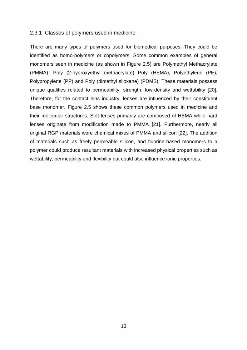
2.3.1 Classes of polymers used in medicine

There are many types of polymers used for biomedical purposes. They could be

identified as homo-polymers or copolymers. Some common examples of general

monomers seen in medicine (as shown in Figure 2.5) are Polymethyl Methacrylate

(PMMA), Poly (2-hydroxyethyl methacrylate) Poly (HEMA), Polyethylene (PE),

Polypropylene (PP) and Poly (dimethyl siloxane) (PDMS). These materials possess

unique qualities related to permeability, strength, low-density and wettability [20].

Therefore, for the contact lens industry, lenses are influenced by their constituent

base monomer. Figure 2.5 shows these common polymers used in medicine and

their molecular structures. Soft lenses primarily are composed of HEMA while hard

lenses originate from modification made to PMMA [21]. Furthermore, nearly all

original RGP materials were chemical mixes of PMMA and silicon [22]. The addition

of materials such as freely permeable silicon, and fluorine-based monomers to a

polymer could produce resultant materials with increased physical properties such as

wettability, permeability and flexibility but could also influence ionic properties.

14

Poly (methyl methacrylate)

(PMMA)

Poly (2-hydroxyethyl methacrylate)

Poly (HEMA)

Polyethylene

(PE)

Poly (vinyl Chloride)

(PVC)

Ethylene glycol dimethacrylate

(EGDM)

Polypropylene

(PP)

Poly (dimethyl siloxane)

(PDMS)

Poly (tetrafluoroethylene)

(PTFE)

Polycarbonate

Nylon

Figure 2.5 Homopolymers used in Medicine [20]

C

CH3

CH2

CO

CH3

O

C

CH3

CH2

CO

CH2

O

CH2 OH

CH2 CH2

CH2 CH

Cl

C

CH3

CH2

C

O CH2

O

CH2 O

C O

C CH2

CH3

CH2 CH

CH3

Si O

CH3

CH3

C C

FF

F F

C

CH3

CH3

OHOH + CCl Cl

O

C

CH3

CH3

O C

O

OOH C

CH3

CH3

OH

n

CH2

CH2

CH2

CH2

CH2

CH2NH2

NH2

+

C

CH2

CH2

CH2

CH2

COH

OH

O

O

CH2

CH2

CH2

CH2

CH2

CH2NH

NH

C

CH2

CH2

CH2

CH2

C

O

O

n

+ OH2n

15

2.3.2 Fabrication of contact lenses

Chemistry is known to be the foundation of contact lens materials, and lens

fabrication may be visualised as a form of "cooking" with ingredients and

mixing/manufacturing steps. Known ingredients of contact lens materials include the

monomers and polymers mentioned earlier in the previous section, which are

combined into macromers and copolymers. These lenses are then processed to

produce an optically clear, chemically stable, durable, oxygen permeable and

wettable contact lenses polymer which is biologically inert.

Normally, carbon-based molecules are the basis for the original contact lens

polymers including cellulose acetate butyrate (CAB) and polymethyl methacrylate

(PMMA). Subsequently, newer contact lens polymers may be partially silicon-based

(silicone-methacrylate and fluorosilicone acrylate) and hydrogel (silicone hydrogel)

lenses. Final formulations of lens polymers only include constituents that improve

lens features and characteristics. Beside the effects on surface wetting

characteristics and water content, others link the polymers together (crosslinking) to

achieve fitting equilibrium between stiffness, flexibility and durability [23].

More common monomers in contact lens materials include Snyder [23]:

Methyl methacrylate (MMA), which contributes hardness and strength

Silicone (SI), which increases flexibility and gas permeability through the

material's silicon-oxygen bonds but has the disadvantage of poor wettability

Fluorine (FL), which also adds a smaller degree of gas permeability and

improves wettability and deposit resistance in silicone-containing lenses

Hydroxyethyl-methacrylate (HEMA), the basic water-absorbing monomer of

most soft lenses

Methacrylic acid (MAA) and n vinyl pyrolidone (NVP) monomers, both of

which absorb high amounts of water and are usually adjuncts to HEMA to

increase lens water content

Ethylene glycol dimethacrylate (EGDMA), a cross-linking agent that adds

dimensional stability and stiffness but reduces water content.

16

Some distinct monomers and additives may permit the polymer chains to change

structure more freely within the material; others may prevent the transmission of

ultraviolet light and yet others may aid the material repel dehydration.

A hydrogel polymer must possess certain physical properties if it is going to be

suitable as a contact lens material. These include [21]:

being optically transparent

having a refractive index similar to that of the cornea, i.e. approximately 1.37

being sufficiently oxygen-permeable

having sufficient hydraulic permeability

having sufficient dimensional stability

having adequate mechanical properties

being biocompatible in the ocular environment.

The equilibrium water content (EWC) for a lens is measured by:

EWC =weight of water in polymer

total weight of hydrated polymer× 100 (2.1)

Oxygen permeability was identified to be related to EWC in conventional hydrogels.

This is linked to the movement of oxygen molecules through the water instead of the

material itself. This relationship was identified as [21]:

𝐷𝑘 = 1.67𝑒0.0397EWC (2.2)

Where 𝐷𝑘 is the oxygen permeability constant.

Minor differences from the processing and material formula have great influence on

the final chemical and physical properties of individual lens materials. For instance,

adding NVP or MAA to a 38% (low-water content) HEMA monomer can result in a

medium (about 50%) or even high (about 70%) final polymer water content. Adding

MMA and/or EGDMA to HEMA increases material durability, elasticity and stability

but decreases water content [23].

Various other properties of the polymers are altered in polymerisation. Properties

such as electrical, magnetic, mechanical, acoustic and optical are amidst the most

notable. Despite the widely accepted perspective of polymers been insulators, there

17

exists a separate class of polymers with conducting abilities. Many polymeric

materials can be formed into thin, mechanical strong films and it is desirable to

confer the additional property of electrical conductivity on polymers in addition to the

flexibility and compatible advantages.

Table 2.1 combines the Food and Drug Administration (FDA) groups of contact lens

polymers, and reviews some electrical properties achieved by observing the

polymers’ susceptibility to charge with their base constituents materials. In this

research work, a “group three” fluoro-silicon acrylate polymer was studied.

Table 2.1 FDA grouping and modern RGP materials, divided into four groups based on their contents.

Group Water content Ionicity Description Material

I Low (<50%) Non-ionic Contains no silicone or

Fluorine

Cellulose acetate

butyrate

II High (>50%) Non-ionic Contains silicone but no

Fluorine

Silicone acrylate

III Low (<50%) Ionic (can

charge)

Contains silicone and

Fluorine

Fluorosilicon

acrylate

IV High (>50%) Ionic (can

charge)

Contains Fluorine but no

silicone

Fluorocarbon

Adapted from FDA tables in [23, 24]

2.3.3 Commercially available contact lens materials

There exist various industrial optical polymers available for use in today’s market.

Amidst optical polymers, Allyldiglycol carbonate (ADC), sometimes called CR-39, is

popularly employed. This polymer was developed as a substitute for glass and is

often called organic glass. It has almost the same refractive index, chemical

resistance and similar mechanical properties as glass. ADC monomer has been

used for many years in the manufacture of ophthalmic lenses. Nowadays more than

80% of ophthalmic lenses are made of ADC. Table 2.2 shows some other properties

of common optical polymers like ADC used commercially [25].

.

18

Table 2.2 Properties of common optical polymers [26]

Unit Acrylic Acrylic

Copolymer Polystyrene

Poly

etherimide

Poly-

carbonate

Methyl

pentene ABS

Cyclic Olefin

Polymer Nylon NAS SAN

Trade Name

Plexiglas UVT Styron Ultem Lexan TPX Acrylon Zeonex Poly-

amide Methyl

Styrene

Acrylon

itrile

Refractive

Index

nf

(486.1 nm)

1.497 — 1.604 1.689 1.593 1.473 1.537 1.575 1.578

nd

(589 nm)

1.491 1.49 1.590 1.682 1.586 1.467 1.538 1.530 1.535 1.533–

1.567

1.567–

1.571

nc

(656.3 nm)

1.489 — 1.585 1.653 1.580 1.464 1.527 1.558 1.563

Abbe Value Vd 57.2 50–53 30.8 18.94 34 51.9 55.8 35 37.8

Transmission %1 92–95 92–95 87–92 82 85–91 90 79–

90.62 90–92 88 90 88

Max

Continuous °F 161 190 180 338 255 253 179.6 199.4

174–

190

Service Temp. °C 72 88 82 170 124 123 82 93 79–88

Water

Absorption

%3

0.3 0.25 0.2 0.25 0.15 <0.01 3.3 0.15 0.2–

0.35

Haze % 1–2 2 2–3 1–3 5 12 1–2 7 3 3

dN/dT x10-

5/ºC –8.5 –10 to

–12 –12

–11.8–

14.3 –8 –14 –11

Color/Tint Water

clear

Water

clear

Water

clear Amber

Water

clear

Slight

yellow

Water

clear

Water

clear

Water

clear

More recent inventions however are in the fluorosilicate materials, which possess

added oxygen and wetting qualities. Numerous variations of fluorosilicate polymers

exist, amidst which Roflufocon A, B, C, D and E manufactured by Contamac® ltd,

UK. These contact lens polymers buttons manufactured by Contamac® ltd are well

known for their improved wetting, oxygen permeability (Dk) index and flexibility.

Table 2.3 shows the comparison of the most prominent Contamac® ltd contact lens

materials available in the market.

19

Table 2.3 Types of contact lens buttons and their respective properties

Silicone Hydrogel

Gas Permeable Hydrophilic

Classification Filcon V3 Focon III 2 Focon III 4 Filcon I 2 Filcon II 2

USAN* Efrofilcon A Roflufocon A

Roflufocon E

Acofilcon B Acofilcon A

Swell factor 1.63 at 20 oC

- - 1.28 at 20 oC

1.36 at 20 oC

Water content 74-75% - - 49-50% 59-60%

Refractive index

1.375 1.450 1.432 1.417 1.400

Dry Refractive index

1.510 - - 1.510 1.510

Light transmission

>99% >97% >94% >94% >94%

Handling tints Blue Blue/green Blue Blue Blue

UV blocker - On request On request

On request On request

Diameter 12.70 mm 12.70 mm 12.70 mm 12.70 mm 12.70 mm

Thickness Standard 4.70 mm 4.70 mm 5.00 mm 5.00 mm

Tensile Strength

0.39 - - 0.35 MPa 0.14 MPa

Elongation to break

180 - - 210% 140%

Modulus 0.35 - - 0.36 MPa 0.16 MPa

Hardness (Shore D)

84 83 77 86 83

Cutting speed (RPM)

7-10,000 7-9,000 7-9,000 8-10,000 8-10,000

Permeability (ISO)

60 26 125

*USAN - United States Adopted Names

As depicted in the Table 2.3, the Contamac® ltd silicon hydrogel polymer possesses

a high light transmission value greater than that of the other polymers but at an

average permeability. Roflufocon E as a gas permeable polymer possesses the

highest permeability as compared to that of the other polymers shown. This is a

desired feature to prevent dryness in the eyes in hot climatic regions such as those

found in Africa. Also, this gas permeable polymer is the softest with a value of 77

Shore-hardness. For the hydrophilic polymers shown, though they possess a high

water content level ranging from 50 to 60% and a high elongation index,

nevertheless these polymers do not have a permeability constant value. Therefore,

Roflufocon E was the selected polymer in this study.

20

2.4 Manufacturing of contact lenses

The manufacture of biomedical lenses also requires high precision and tolerance

with a surface accuracy of few microns or less [14]. Optical aberrations on these

lenses caused by geometrical deviations, surface roughness and sub-surface

defects of lens from the fabrication process could greatly influence the functionality.

Heinrich and Wildsmith [27] state that the tools to evaluate manufacturability and

compensation for system dynamics, as well as real-time process feedback are

required in contact lens manufacturing of freeform surfaces. Special freeform contact

lenses such as the toric lenses are just an entry level of freeform lenses. These

lenses are used by patients that have significant complex wave-front aberrations.

Therefore, it is necessary to understand and conduct a careful analysis of the optical

fabrication process to achieve high optical precision irrespective of optical design.

Traditional optical fabrication spans over an enormous range of manufacturing

procedures and test configurations. The manufacture of a conventional lens begins

with a glass blank manufacturing and proceeds to the generation of the optical

surface. This is done by various diamond shaping techniques such as grinding and

polishing. In more recent approaches, IOLs are basically fabricated via compression

moulds, injection moulds or precision machining technologies. Three basic

techniques are identified for contact lenses manufacture.

They are:

Spin casting method

Moulding methods

Ultra High precision machining.

Based on material choice and size requirement, moulding and spin casting of optical

polymer components have long been used for high volumes, low cost and lightweight

capability over precision cutting. However, these processes have not been readily

accepted in the precision optical fabrication industry because of several difficult

issues such as geometry deviation, inhomogeneous index distribution, birefringence

and freeform fabrication. Machining has advanced to be a cost effective option for

21

polymeric materials, since for small to average sized batch production or specific

designs, the cost of tooling for moulds and extrusion dies is insignificant.

PMMA lenses can be dry machined with acceptable surface finish due to the high

stiffness of the material at room temperature. However, the industry trend is towards

selection of more flexible polymers generally characterized by glass transition

temperatures that are well below room temperature. The attractiveness of these

polymers from a medical standpoint relates to a smaller incision during implanting as

well as better oxygen permeability with some of the newer materials. However,

machinability is a very difficult proposition for these polymers, since softer polymers

lack the stiffness at room temperature to be machined with an acceptable surface

finish. Nonetheless, GP lenses may contain very little water, remaining rigid on the

eye. GP contacts are made with a computerized precision lathe cutting process

similar to that used for lathe-cut soft lenses.

The next section briefly discusses each basic technique employed in the

manufacturing of contact lenses, and points out the advantages and disadvantages

observed.

2.4.1 Spin casting

Hydrogel lens designs have been successfully created by the original Wichterle

method of spin casting for about 40 years. Spin casting offers the advantage of

reliable production and low lens cost, However, this process is limited in optical

powers as confined by the physical design of the lens [28]. Spin casting, unlike other

methods such as lathing, is preferably aimed at the production of low volume to

surface area ratio polymer lenses; it is also not employed in the production of

polymeric lens susceptible to surface degradation [29]. Spin casting involves

spinning the cast into which the monomer mix will be injected, whilst undergoing

centrifugal forces, forcing the monomer to fill the required space provided for the lens

shape. The injected polymer liquid spreads to the edges of the mould at specific

speeds and defines lens properties. Figure 2.6 shows the various steps involved in

spin casting, from the polymer insertion to packaging.

.

22

Figure 2.6 The spin-casting process [21]

In this process, the optical mould is responsible for the interior quality of the inner

face of the lens. The final power of the finished lens is dependent on several factors.

These are gravity, centrifugal force, surface tension, volume of monomer mix and

spin speed [29]. This lens manufacturing process however faces issues during the

creation freeform due to its low flexibility.

2.4.2 Plastic injection moulding

Moulding the lens can be carried out in several ways. The various available moulding

techniques are spin cast, injection and compression moulding. Figure 2.7 shows a

diagram of the moulding process flow, a sample manufactured mould and its

computer design.

*adapted from: Presentation by Rapidly Solidified technologies, 2010

Figure 2.7 Moulding process flow diagram, 3D mould design and machined mould

Insert and cast manufacture

Dosing with cast monomer

Spinning and UV cure

Lens hydration and packaging

23

Lenses produced from moulding techniques are seen in numerous technological

applications such as surveillance systems, projection lenses, and optical heads.

Injection moulding as an optical production method, offers a more reliable mass

production moulding technique than its counterparts. This process presents a cost-

efficient method for manufacturing optical surfaces such as flats, spheres and also

aspheres that are meanwhile state-of-the-art in the field of plastic optics [30]. A

review of the manufacturing process shows that moulded plastic is firstly injected at

high pressure into the plastic mould and then it is allowed to cool and solidify before

shaped lenses are extracted. The demands for image quality of optical components

produced through injection moulds, however, are less severe than machining.

Nonetheless, for the replication of optical plastic or glass components, moulding

inserts with specific functional surface and subsurface requirements are needed to

withstand the thermal and mechanical loads during the replication process and to

ensure the desired optical part quality with a nanometric surface roughness and high

form accuracy. Therefore, Brinksmeier et al. [12] in their research presented a

process chain consisting of a thermo-chemical surface treatment and a sub-sequent

diamond cutting process for the manufacturing of optical moulding inserts to achieve

such surface requirements.

Despite its advantage in large production, injection moulding is faced with drawbacks

in geometrical deviation of mould design and inhomogeneous index distribution

during manufacturing [31]. The geometry deviation resulted from volume shrinkage

and warpage are strongly dependent on process conditions. The inhomogeneous

index distribution resulted from the residual stresses and non-uniform molecular

orientation in the injection moulded parts. Plastic moulds are also limited in their

flexibility in creating complicated geometries such as freeform based on mould

design limitations. Furthermore, tooling expenses for injection moulded plastic optics

differ greatly, with some more complex optics demanding more expensive tooling.

These are the main reasons that injection moulded polymer optics are not

particularly suited for all high precision applications. Therefore, the investigation into

alternate machining processes with higher performance for high precision polymer

lenses is essential and ultimate to providing an affordable high precision

manufacturing process for satisfactory optical performance.

24

2.4.3 Ultra high precision machining technique

Ultra-precision machining dates back to 1966 and since then this technology has

greatly progressed due to considerable advances in materials, tools and other

supporting technologies [32]. Chiu and Lee [32] stated that the ultra-precision

technique based on single-point diamond turning (SPDT) and ultra-precision

diamond grinding (UPDG) have become an indispensable tool for economic making

of ultra-high-quality products.

Figure 2.8 Ultra-precision machining technology [33]

Manufacturing of precision optics with diverse freeform surfaces is also a core

component of contact lens production. Due to some isolated medical conditions,

custom optical solutions have become a necessity in ophthalmology. Today’s ultra-

precision machining system is built on fundamental precision engineering principles

coupled with leading edge technologies in controls, drive and feedback devices [34].

Ultra-high precision diamond turning (UHPDT) has thus become a generally

acceptable manufacturing technique with the ability to produce freeform optics of

various custom surface profiles for such applications. Some complex optical forms

which can be produced through SPDT are: aspheric, toric and complex geometrical

lens profiles. This optical manufacturing technique also boasts of a nanometric range

25

tolerance below < 10nm. UHPM techniques encapsulate tool and material

technology, inspection technology, machining technology, Machine forms and

environmental control (Figure 2.8).The growing market of precision, optics and micro

technologies systems has pushed combined advances in process technologies, as

well as measuring and testing quality assurance linked to this production process.

Major advances in UHPM over the years have been achieved in the area of machine

control, feedback systems, servo drives and general machining design [35].

Figure 2.9 Ultra-precision diamond turning of freeform optics

At present, the ultra-precision machining of single point diamond cutting is the most

effective process for the generation of high quality functional surfaces with minimal

defects in the superficial surface layer [4]. This perspective is viewed from various

materials, especially from thermoplastic amorphous polymers and their composition

for optical, photonic and bioengineering applications. Applications of UHPM are seen

in divers fields of study such as aerospace, automotive, solar energy harvesting,

control and sensing, communication (fibre optics), entertainment (display devices)

and medical. Figure 2.9 shows some applications in the use of ultra-precision

diamond turning of free form optics. Figure 2.10 shows some various optical forms

produced for distinct industrial uses.

26

Figure 2.10 Various optical objects used in critical industries [33]

According to Bylinsky [36], it is estimated that the world market share value of ultra-

high precision machines is approximately $100 million with a constant growth rate of

about 5% annually. Freedonia Market Research in 2011 identified the World demand

for machine tool products rise to a strong 9.4% per year through 2014 to $121 billion.

In their survey they identified the global market for metal cutting machine tools to

expand to 8.6% per year through 2014 to $61 billion, with growth aided by a recovery

in key end-use markets in the developed world. According to their research, metal

cutting tools will continue to account for a majority of the total machine tools market

in 2014 [37].

Currently, the technology of UHPM is found concentrated in established economies

such as the United States, Germany and Japan, as well as emerging and

economies, for example Brazil, India and South Korea. There is also a rapid growth

in other countries such as Singapore and Hong Kong which mainly serve as high

tech support to optical instruments.

Major advances in UHPM over the years have been achieved in the area of machine

control, feedback systems, servo drives and general machining design [35]. A

commonly used UHPM process in contact lens manufacture is single-point diamond

turning (SPDT).

Spherical Frenell

Micro-prisms

Freeform

Micro-lens arrays Aspheric

27

SPDT as a sub-form of UHP machining technique uses a finely polished

monocrystalline diamond cutting tool (Figure 2.11). This nanometric process is

capable of producing complex-shaped surfaces with a form accuracy of 1µm or less

and roughness under 10 nanometres [38] as shown in Figure 2.12. Its capacity for

high accuracy has also made this process widely used in the production of micro-

electromechanical devices and medical optics [39]. Some complex optical forms

which can be produced through SPDT are: aspheric, toric and complex geometrical

lens profiles (Figure 2.10).

Figure 2.11 Ultra-precision diamond tools [40]

Based on its accuracy, SPDT is also highly sensitive to changes within the

machining environment. Thus, instability could directly affect micro-forces occurring

between the cutting tool edge and the workpiece and this may further result in poor

attainable surface finish in optical manufacturing.

28

Figure 2.12 Ultra-precision machined lens wit 3D image and low form accuracy

2.4.4 Research & barriers in the ultra-high precision manufacturing of

polymers

Despite the increased acceptance and use of optics in the biomedical industry [14],

nevertheless some challenges are still experienced in the manufacturing optical of

polymers. These are experienced as geometrical deviation of mould design, wear

and inhomogeneous index distribution occurring during optical manufacture.

Furthermore, the effects of elastic recovery after machining hinges upon the choice

of parameter combinations and machining conditions. These disadvantages

constitute some of the barriers experienced in polymer optics manufacture. The

section below evaluates some of the barriers and challenges in contact lens

manufacturing.

Some additional barriers experienced in UHPM are:

Machine programming for freeform surfaces

Micro-chatters

Thermal instability (environment control needed)

The continuous development of new materials

Unavailability of micro sensors for UHPM

Courtesy: www.zygo.com

NMMU Talysurf PGI

Dimension profilometer

29

2.4.4.1 Elastic recovery in polymer machining

Elastic recovery is the inherent ability of a material surface to return to a deformed

state after unloading during cutting operation. It operates based on the

rearrangement of atoms within the material based on changes in temperature, stress

and strain experienced from loading. Elastic recovery of the deformed region after

unloading yields to a change in the granular structure of the surface of the lens. This

phenomenon in machining causes huge losses of surface quality in optics.

(a)

(b)

Figure 2.13 Elastic recovery phenomenon after diamond cutting

Gauthier et al. [41] in their study evaluated the elastic recovery of a scratch on a

polymeric surface. Within their study, they modelled the recovery rate during full

plasticity on PMMA around a moving conical/spherical tip. Also, Friedrich et al. [42]

in their research show the elastic recovery and scratch resistance found in certain

high performance polymers. From their research they explain the phenomenon of

elastic recovery during the cutting of a commercial grade PMMA polymer. There is

thus a need to consider the effects of elastic recovery in UHPM and take account of

the grain structures of material during manufacturing of optics.

Machined surface

(Ideal situation)

Elastic recovery of material grains

30

Figure 2.13(a) and (b) show the initial grain structure of an ideal machined surface

and the actual surface reactions with elastic recovery of the grain structure after

unloading.

2.4.4.2 Diamond wear in polymer machining

Despite high accuracy produced in UHPM of polymers, relatively large diamond wear

formed on the tool may largely influence surface quality (Figure 2.14). Since no

research work exists for this polymer it is necessary to consider a wider look at

diamond wear in SPDT. Lane et al. [43] studied the thermo-chemical wear model

and worn tool for single crystal diamond while cutting tool steel. In their study they

identify diffusion based on elevated temperatures as a factor for wear formation in

diamond tools. Abou-El-Hossein et al. [44] also in their research on rapidly solidified

aluminium machining, identified a tribo-chemical reaction as a probable cause of

wear formation at elevated temperatures. Other research works have identified other

wear mechanisms found during the UHPM of polymers [4, 45]. Gubbels, van der

Beek et al. [41 ]in their research on ultra-high precision turning of polymers identifies

two dominant wear mechanisms, namely:Gubbels et al. [45]

Tribo-chemical wear

and triboelectric wear

Figure 2.14 Diamond tool wear [44]

2.4.4.3 Tribo-chemical wear in polymer machining

This wear mechanism is also depicted as the breaking of the tightly bonded diamond

lattice. When this happens, a carbon atom of the diamond may diffuse into the

Tool

Tool

edge

31

workpiece, graphitize, and react with oxygen to form a dioxide, or with the workpiece

to form carbide. In the monomer below (Figure 2.15), the ester bond in methyl

methacrylate breaks away to combine with carbon atoms of the diamond tool under

extreme temperatures leading to a gradual degradation of the diamond tool tip

(Figure 2.16).

𝐶(diamond) + 𝑂2 → 𝐶𝑂2

2𝐶(diamond) + 𝑂2 → 2𝐶𝑂

Figure 2.15 Methyl methacrylate (MMA) ester bond

Figure 2.16 Chemical wear on a diamond tool [46]

Ester

Methyl Methacrylate (MMA)

(Prevalent monomer in Optimum extreme)

32

Commonly used types of diamond wear are: adhesion, abrasion, tribo-thermal and

tribo-chemical. These wear mechanisms are known to be able to operate

independently or in combination with others during machining. Besides that fact, one

of these mechanisms takes precedence in impact over others during research and is

accountable for rapid tool wear. Adhesive wear based on the weak interactive forces

of the workpiece causes the transference of mother material between workpiece and

tool. This reaction is easily observed in macro and micro machining tools based on

the types of cutting tools used. The adhesion reaction during cutting, however, is

directed towards the softer material. In UHPM of contact lenses, adhesive reactions

are drawn towards the polymer (the softer material) creating negligible adhesive

effects on the tool. Therefore, adhesive wear is considered only as a collaborative

wear mechanism in polymer machining. Abrasion in the same manner reacts based

on the dissimilarity in the hardness of two materials. And thus based on hardness of

diamond it is postulated its effects are minimal except in extensively prolonged

polymer machining.

The influence of temperature cannot be ignored in tool wear formation. Research

works have identified various temperatures recorded during diamond machining [47].

Jasinevicius et al. [47] identified the temperature during the single point diamond

turning of non-ferrous metals. In their article of silicon crystal they established that

the temperature on the cutting edge and rake face is not sufficiently high to thermally

reduce diamond strength. Abdel-Aal et al. [48] in their paper indicated that the rise in

workpiece surface temperature was comfortably lower than the thermal softening

temperatures for non-ferrous metallic materials under the conditions applied.

Particularly the temperature rise was of about 80 oC for germanium and less than

400 oC for silicon. According to Hurt and Decker [49], during diamond machining

temperatures may reach values as high as 427 oC (or 700 oK). Such temperatures

may influence the physical properties of the diamond. At additional levels of 700 oC

diamond oxidizes in air to form gaseous by-products, such as carbon monoxide and

carbon dioxide as shown in Figure 2.15. This oxidation effect from high temperatures

represents a mechanism of wear-occurring polymer machining known as tribo-

thermal wear which precipitates chemical wear formation. Other publications [50, 51]

have identified cutting temperatures in diamond machining to be between 90-380 oC

in turning metal alloys. Despite the number of studies done in temperature

33

measurement, machining is challenged by cutting scale and heat detection at that

scale. Due to these challenges various attempts at estimating temperature have

been devised, some of which relate the influence of some cutting parameters on

temperature for estimation, FEA analysis of heat point and molecular simulation [51-

53]. In plastics machining, Gubbels [9] integrated a thermocouple into the diamond

tool for temperature measurement and identified temperatures obtained in machining

to be around or above 200 oC.

Tribo-chemical wear can be explained in diamond turning by the chain scission of

monomers which forms highly reactive radicals [54]. This chemical reaction could be

observed by a “chipped” effect on the diamond surface. In their research Gubbels et

al. [45] account wear patterns observed on PC and PMMA to chemical causes.

Another wear mechanism associated with elevated temperatures is Triboelectric

wear which originates from the presence of tribocharging reflected by the adhesion

of the chip around the tool [55, 56]. This form of wear was studied by Gubbels [9]

who identified them to be one of major importance to diamond during the machining

of glassy polymers.

2.4.4.4 Triboelectric wear in polymer machining

UHPM technology has also spurred research in the catastrophic wear of diamond

tools when machining various materials [54, 57]. Despite all known advantages in

nano-machining, UHPM of polymers using single point diamond tools is challenged

by the presence of various wear mechanisms which affect surface quality. Currently

there exists a limited amount of research work in polymer machining and diamond

machining of contact lens polymers despite the great application of this technology in

daily electronics. Current findings in the field still need additional experimentation for

validation and expansion with a wider range of tested polymeric materials.

Despite its recognition as an adequate manufacturing technique for optical polymer

production by various researchers [39, 58], another important cause of wear on the

tool is due to triboelectric phenomenon. Contour Fine Tooling [56], a UK tooling firm,

states that the wear in monocrystalline diamond tools when cutting polymers, is

generally 5 to 10 times higher than when cutting copper with the same parameters.

This phenomenon was explained by the difference in hardness between diamond

34

and plastic. This discovery is fairly recent and it is postulated to be responsible for

notable wear formed on diamond tools as to polymer machining.

During polymers machining, Olufayo and Abou-El-Hossein [55], [59] have identified

that the adhesion of the tool chip around the tool dictates the presence of an

electrostatic force field. This phenomenon known as triboelectric charging is

responsible for tool wear and poor surface finish. Triboelectric wear can occur due to

significant electrostatic discharge and the occurrence of electric fields on polymer

surfaces. Research in the ultra-high precision of glassy polymers identifies

Lichtenberg wear patterns on the tool as yields resulting from significant static

charging and discharging (Figure 2.17).

Figure 2.17 Lichtenberg figure on a diamond tool [9, 56]

Gubbels in his thesis [36] also presents substantial information on the presence of

tribo charge in the machining of glassy polymers. However, questions about its

causing agents, natural occurrence amidst materials, magnitude and control are yet

to be answered. Hence, attaining a clear understanding of triboelectricity in polymer

machining poses significant importance in ensuring surface integrity of optical

profiles.

Triboelectric charging also known as “contact electrification” is generated from the

frictional rubbing of two dissimilar materials of varying electric field strength and

polarity. It can be experienced during various human activities such as walking on a

rug with plastic shoes or hair combing. Daily human activities could create charges

as high as 3000kV [60]. From literature, it is seen that the influence of frictional

electrification on dielectrics in textiles, micro photonics, pneumatics transport and

nano-machining [9, 61, 62]. Figure 2.18 shows the triboelectric series which

Lichtenberg figure

35

indicates the tendency of inclination in acquired charge of a material after

tribocharging.

+ Wool More positive Nylon

Fur Silk Poly (vinyl alcohol) (PVA) Poly (vinyl acetate) (PVAc) Cotton Steel Poly (methyl methacrylate) Poly (ethylene terephthalate) (polyester) Polyacrylonitrile (PAN) Poly (vinyllidene chloride) Polystyrene (PS) Polypropylene (PP)

More negative Poly (vinyl chloride) (PVC) - Polytetrafluorethylene (Teflon ®, PTFE)

Figure 2.18 Triboelectric series [63],

Understanding the mechanism by which static charge is generated on or disappears

from polymer surfaces has proven to be difficult. Questions remaining largely

unanswered include [63]:

The chemical and physical origins of the triboelectric series

The mechanism of contact and tribocharging of polymer surfaces

The mechanism by which the charge disappears from the surface after

generation.

The mode by which materials applied to the polymer surface can substantially effect

either the generation of static charge or the dissipation of the charge. Table 2.4

shows a summary of triboelectric charging mechanisms and how charges or ions

move from one material surface to another

36

Table 2.4 Summary of triboelectric charging mechanisms by Williams [64]

Interface Charge exchange agent Interpretation

METAL-METAL

METAL-INSULATOR

Insulator non-ionic

Insulator with mobile

ions

ELECTRONS

ELECTRONS

Mobile transfer (hypothesis)

Mobile ions , when

present predominate

over other mechanisms

INSULATOR-INSULATOR

Mobile Ions present

Both non-ionic

MOBILE IONS

MOBILE IONS

H3O+OH (in presence of water)

Mobile ions , when

present predominate

over other mechanisms

In understanding the mechanism of contact and tribocharging of polymer surfaces,

Figure 2.19 gives a pictorial explanation of the triboelectric formation. During

triboelectric effect, electrostatic voltage is generated on materials surface due to the

transfer of free electrons or ions during the rubbing action between the tool and the

surface of the polymeric workpiece. This situation is derived from the electrons

restriction in material due to their inability to escape from the material surface (Figure

2.19(a)). As electrons fail to reach a conducting path to ground a stage is reached

where electrons jump across from a highly electron concentration surface to a

surface lower magnitude until static saturation occurs (Figure 2.19(b)). They initially

remain concentrated at the surface at the polymer due to its low atomic conductivity.

At saturation, electrostatic potential difference exceeds the dielectric breakdown

threshold of air (being the common medium between the material surfaces) through

the path of least resistance for charge stabilization. This saturation point indicates

high magnitudes and can be seen as a transient spark during static discharge

(Figure 2.19(c)).Charge separation could occur through the following processes [9]:

Rubbing of dissimilar materials

Diffusion of charges in a living cell

Convection separation of charge in clouds

Chemical separation of charge in batteries.

37

Figure 2.19 The Triboelectric Charge –(a) materials make intimate contact (b)

materials separate (c) saturation point. Adapted from: Asuni [65]

Electrostatic which could be also identified as isolated charges is seen as in the

charge concept flow in (Figure 2.20) which refers to the unintentional build-up static

charges on material surfaces. This is created by the generation of ions. In reality, the

Electrostatic phenomenon is as a consequence of the atomic nature of matter. It

spurs of from an electrical atomic imbalance from the separation charge.

Figure 2.20 Flow concept of static charge [9]

This phenomenon is often found in non-conductors which trap freely moving

electrons. Eq. 2.3 shows the potential voltage equation generated between

dielectrics.

Electric Charge

Separation of charges

Coulomb’s law

Electric filed lines Fields and surface charges Distributions of

charges on surface

of conductors

Electrostatic shielding

Electric fields Forces between charges Isolated charges

38

𝑉 =𝑞

𝐶=

𝑞 ∙ 𝑑

𝜀 ∙ 𝐴 (2.3)

Where, V is the voltage difference, q is the charge, C the capacitance of the

capacitor, 𝜀 is called the permittivity of the dielectric material between the plates, d

the diameter and A is the area of the plates. Gubbels et al. [9, 66] in their study

measured this static voltage using an electrostatic voltmeter, and using Eq. 2.3

linked the voltage to the estimated amount of charge to identify the amount of energy

for electrostatic discharge. For evaluating triboelectric wear equation 2.4 below forms

the baseline. It describes the kinetic energy (U) on an ion during acceleration.

𝑈 = 𝐸 ∙ 𝑄 ∙ 𝜆 (2.4)

Where, the energy U during acceleration, 𝜆 the mean free path of the particle and E

is the electric field strength. For an electron in atmospheric air the mean free path is

λe = 10−5 m, and for an ion in atmospheric air the mean free path is λi = 10−7 m. The

acquired energy can be used for damaging the diamond surface by impingement of

the particle and detachment of a carbon atom, which requires energy of 7.4 eV [9].

Williams [64] in a review of triboelectric charging of insulating polymers identified the

effects of force exerted during polymer rubbing and depth of material removed as

factors which influence static charge magnitude. Generally ESDs suggest a transfer

of electrons from a high concentration surface to a lower concentration across

dissimilar materials. From literature [60] it is identified that electrostatics transfer high

electron concentration measured in Coulombs from a surface of a relatively

negatively statically charged surface to a relatively positively statically charged

surface.

A lucid explanation of charge in atoms is necessary to comprehend the principle

ESDs occurring in UHPM. In insulating materials, electrons are not able to

redistribute from the negatively charged area to the positively charged area due to

the large band gap required to move electrons from the valence band to the

conduction band. In conductor materials, electron conduction occurs easily because

the energy band gap between the valence electron shell and the conduction band is

infinitely small or they may overlap. In either case it takes very little to no energy to

39

promote an electron from the valence shell to the conduction band. This small

amount of energy can easily be supplied by any thermal energy above zero K°.

Conductive surfaces will, therefore, have uniform charge distributions as electrons

are easily transported from regions of high concentration to areas of low

concentration [60]. This follows the law of conservation of charge, which states: “that

charge can neither be created nor destroyed, but only transferred from one entity to

the other” [67].

Diaz and Felix-Navarro [68] created a semi-quantitative triboelectric series for

polymeric materials. In their study they examine the influence of chemical structure

and properties of the polymers on their charging magnitudes. Their study not only

connects the results of various triboelectric series from research but also relates the

overlapping results of several reports and gives an estimate of the relative charging

capacity of numerous polymeric materials. They also reaffirm that charging results

are due to proton or ion transfer between the surfaces in contact.

Experiments have also shown that relative humidity (RH) has a very big influence on

the electrostatic charging and therefore, on the tool life. Below 60% RH strong

electrostatic charging occurs; 60% to 70% RH is a transition area and above 70%

RH no electrostatic charging is observed [56]. In a study on the influence of relative

humidity on Aeolian electric field by Xie and Han [69], they found that low humidity

below 30oC generated far higher magnitudes than higher humidity ranges. In their

study, they explained the effects of high humidity in deionising sand particles from

the wind vane fans.

2.5 General behaviour of polymers in diamond machining

Various polymeric materials have been machined in UHPM processes. Numerous

research works have studied the various effects of machining polymers with diamond

tools [4, 6, 7, 45, 70-73]. These materials range from polycarbonate (PC),

polystyrene (PS), nylon and poly methyl methacrylate (PMMA) [6, 45] to industrial

co-polymers.

Based on the differences between polymers and metals during machining, this

section therefore gives a short introduction to the behaviour of polymers in

40

machining. Polymers, depending on their molecular weights, could respond as brittle

or ductile materials. Intrinsic material behaviour in polymers could also be explained

based on temperature. A study by Carr and Feger [70] on PC and PS, expresses

that material is removed via ductile, brittle, or transitional mechanisms and this

depends on polymer properties such as glass transition temperature (Tg), relaxation

time, degree of crosslinking, and viscosity. Above glass transition temperatures,

polymers enjoy thermodynamic equilibrium for ductile mode machining. However

below this Tg (as seen in Figure 2.21), a thermodynamic condition called "aging"

occurs. This condition yields a rough surface from the brittle fracture of the polymer

after machining. Aging is caused by the shrinking of free volume space as lower

temperature and atomic movement foster a readjustment of atomic positions.

Gubbels et al. [72] in their research identified aging as an influential factor in

mechanical response of a polymer.

Figure 2.21 Glass transition temperatures during machining [74]

For a ductile workpiece, the melt viscosity of the polymer is important. The change

from ductile to brittle mode in polymers could be also be experienced on polymers by

changing operating and tool parameters. Research [70] identifies that in brittle

materials, the surface roughness is largely controlled by the rake face angle of the

diamond.

41

Three main factors are known to influence the roughness and product shape [70,

73]. These are:

Machine environment such as vibration isolation, temperature stability

Process parameters e.g. cutting speed, depth of cut, feed rate and geometry

of the diamond insert

The physical and chemical properties of the material.

As discussed earlier, in polymeric materials, these physical properties of polymers

are significant factors in determining the quality of the surface integrity. Surface

deformations can be identified through specific defined optical errors. These errors

and surface parameters are clearly explained below.

There are three types of errors that may occur on a machined surface during SPDT.

These are the form, figure and roughness errors. Due to their close proximity in

definition, these types of errors are identified by their causes. “Roughness error” is

formed due to irregularities inherent in the machining process (e.g. cutting tool, and

feed rates). “Figure error” or waviness may result from vibrations, chatter or

workpiece deflections and strain in the material. “Form error” is the general shape

deviation of the surface from the intended shape, neglecting variations due to

roughness and figure error [71]. Figure 2.22 shows the three types of errors that may

occur on a lens profile, after being machined by the diamond tool.

Figure 2.22 Three types of errors from turning operation: form, figure and finish [71]

This research consists of seven experiments derived from a combination of three

machining parameters via a statistical approach. Each experiment would encompass

a detailed analysis of the surface roughness of an area of 24×24 µm2 of the lens

42

buttons using atomic force microscopy (AFM). Research has shown that AFM is a

powerful characterization tool for polymer science, capable of revealing surface

structures with superior spatial resolution. AFM is thus extremely useful for studying

the local surface profile and roughness properties of a broad range of polymer

material [75].

The results obtained were used to correlate the surface finish of the polymeric lens

to influential cutting parameters.

2.5.1 Parameters to evaluate surface roughness

Surface roughness measurements are done using profilometer which directly

measure the texture of a surface and represent the acquired surface in the form of

profile graph [76]. The commonly used parameter for characterizing the surface

roughness is the average roughness Ra which is defined as:

𝑅𝑎 = [1

𝑁∫ |z|𝑑𝑥

𝑁

0] (2.5)

Where z=f(x) is the dimensional surface profile or roughness curve that can be

obtained by several methods, L the length of the profile been accessed [76].

Figure 2.23 Description of surface parameter [77]

The Figure 2.23 shows a description of the surface parameters in estimating the

surface roughness of an optical component. From the Figure, Ra shows an average

band of mean roughness of the surface line based on the peak magnitudes of either

side.

43

2.6 Modelling of ultra-high precision machined polymers

Different modelling methods have been employed to study machining operations.

These methods range from statistical methods as mentioned in the previous section

to graphically represented simulations such as curve fitting models. Dandekar and

Shin [78] in their review of modelling of machining composite materials, identify

methods such as finite element modelling (FEM), molecular dynamics simulations

and multi-scale modelling as methods of interest in physical modelling techniques.

Finite element simulations have been successfully used to predict flow of chip, fibre-

based composite interactions and temperature change during cutting [78, 79]. The

multi-scale modelling method alternatively, seeks to understand the evolution and

progression of the damage from the molecular to the macroscale [78]. It is

implemented by a modelling combination of atomic simulations and continuum

mechanics solutions.

2.6.1 Response surface method

The response surface method (RSM) is a suitable method in establishing the effects

of parameters in machining. This technique optimises responses which are directly

influenced by known system variables using a developed spatial model. It does this

by creating an n-dimensional surface using a collection of design techniques in the

experimental study of relationship between the measured responses and a number

of input descriptive variables. As a modelling technique, RSM seeks to establish the

relationship between descriptive variables and single or more responses. The n-

dimensional surface characterizes all balanced and possible designs. This surface

consists of a finite number of points in space. These points are carefully selected

and determined by a created response surface experiment software design and not

the designer. These selected points can be used to interpolate other design points

on the surface and establish predicted responses. Examples of response surface

model techniques are the three-factorial design model, The Box-Menken (BB) model

and the central composite design model (CCD). In summary, the response surface

design can be used to perform predictions of parameters on created surface plot.

Generally, the response surface method is described as an equation in the form:

44

𝑌𝑢 = 𝛽𝑜 + ∑ 𝛽𝑖𝑋𝑖𝑊𝑖=1 + ∑ 𝛽𝑖𝑖𝑋2

𝑖𝑖𝑊𝑖=1 + ∑ 𝛽𝑖𝑗𝑋𝑖𝑋𝑗

𝑊𝑖,𝑗=1 + €, (2.6)

where Yu , is the corresponding response, e.g. the surface roughness value (Ra)

produced by the various process variables in UHPM and the Xi (1, 2 . . . , S) are

coded levels of W quantitative process variables, the terms βo, βi , βii and βij, are

the first and second order regression coefficients and € the experimental error or the

lack of system fit. The designer can rectify poor fitting of the model by adjusting

design space and alternating levels of descriptive variables. The second term under

the summation sign of this polynomial equation is attributable to linear effect,

whereas the third term corresponds to the higher-order effects; the fourth term of the

equation includes the interactive effects of the process parameters.

2.6.1.1 Box-Behnken response surface method

The Box-Behnken response surface method is a class of response surface design

used in statistic modelling. This design class offers the possibility of addressing

experimental boundaries and avoids factor combinations that are at extremes. It

does this by creating a spatial representation of an experimental problem using

centre points on frame edges and not corners of its spatial design. Extreme

conditions depict parametric combinations found at the corners of its spatial model.

Figure 2.24 Box-Behnken statistical model

The Box-Behnken is an RSM method with three-level nearly orthogonal, resolution V

design used for modelling factors with three levels. The slight non-orthogonal design

45

matrix is not a concern if the analysis is conducted using least squares regression.

Figure 2.24 shows an example of a scatterplot diagram with various calculated

spatial points used to determine the influence of descriptive variables on one or a set

of responses. As shown earlier, for three factors, the Box-Behnken design does not

include any corner points of the design space. Therefore, if the corner points are

infeasible, the Box-Behnken design should be used to generate the quadratic curved

response surface. Yet the disadvantage is that the BB design will produce a higher

uncertainty of prediction near the corner points [80] but requires fewer data points for

predictions. The main advantages of this experimental design method are that it only

requires three levels for each factor; its design’s ability to rotate and its lower

requirement for experimental runs for 3 or 4 factors.

With the combination of parameters in diamond turning of polymers, RSM Box-

Behnken can be applied to the polymer machining concept in response areas such

as surface generation, cutting force determination and tribological wear

determination. These various output responses from UHPM of polymers hold the

necessary variables required for modelling and could be used to examine the impact

of changing factors on the response.

2.6.2 Atomistic Simulation methods

There are numerous atomistic simulation methods that exist. Some commonly

known are the Ab initio Molecular Dynamics Method, the Semi-empirical Molecular

Dynamics method, the Empirical Molecular Dynamics method and the Monte Carlo

Method. These various MD techniques have been applied in various spheres of

molecular predictions and have different notable differences when applied. Table 2.5

shows the advantages and disadvantages of each method.

46

Table 2.5 Comparison of some atomistic simulation methods [13]

Method Applications and Advantages

Disadvantages

Ab initio Molecular Dynamics

Methods

More accurate solution Computationally expensive –suitable for hundreds of atoms

Semi Empirical Molecular Dynamics Methods

A trade-off between ab-initio and classical MD methods. Can handle up to thousands of atoms

Less accurate solution than in

ab initio methods

Empirical/Classical Molecular

Dynamics Methods

Less computationally expensive than ab initio MD

Simulations are for shorter

times than in MC

Monte Carlo Methods

More efficient /time saving, can be used for larger time frames, time is controllable

Doesn’t allow the time

evolution of the system in a suitable form for viewing

2.6.3 Molecular Dynamics (MD) Simulation method

MD studies as a modelling technique was initiated in the late 1950s at the Lawrence

Radiation Laboratory (LRL) in the United States by Alder and Wainwright in the fields

of equilibrium, as well as non-equilibrium statistical mechanics, to calculate the

response of several hundred interacting classical particles using the then available

highly powerful mainframe computers at LRL. Since then, MD simulation has been

applied to a range of fields including crystal growth, indentation, tribology, low-

pressure [81]. Amidst its numerous fields of applications, MD’s have been seen in

protein simulations and organic simulations, but in engineering its applications have

been seen in indentation and nanometric cutting of materials. Figure 2.25 illustrates

the full multi-scale schematics for the effects of damage occurring at the macroscale

consistently involve damages along the full length of the scale. The need to observe

nanoscale scale conditions to understand molecular mechanics of materials is

essential [78].

47

Figure 2.25 Schematic for multi-scale damage modelling [78]

Most nanometric MD simulations have been used in the simulation of single crystals

due to the ease of determining molecular conditions, interatomic potential functions,

and interatomic forces and are also based on reduced computational demands for

single element simulations. Some examples are seen in the molecular dynamic

modelling of silicon and copper [82, 83].

Table 2.6 below shows specific distinctions between conventional cutting and

nanometric cutting. Also highlighted are relevant parameters to each cutting

technique. The Table shows the suitability of molecular modelling for the nanometric

cutting process due to the discrete molecular mechanics and the heterogeneous

nature of its workpiece. At nanometric scale length, MD simulations are needed to

adequately express the continuum representation of the problem.

48

Table 2.6 Comparison of nanometric cutting and conventional cutting mechanics [13]

Nanometric Cutting Conventional Cutting

Fundamental Cutting

Principles

Discrete Molecular Mechanics

Continuum Mechanics

Workpiece Material Heterogeneous Homogeneous

Cutting Physics Atomic Cluster Model Shear Plane Model

Energy Consideration Interatomic Potential

Functional

Shear/Friction Power

Cutting Force Interatomic Forces Plastic Deformation

Chip Formation Inner Crystal Deformation

(Point Defects or Dislocation)

Inter Crystal Deformation

(Grain Boundary Void)

Deformation and Stress Discontinuous Continuous

Cutting Tool Edge Radius

Significant Ignored

Cutting Tool Wear Cutting Face and Cutting Edge

Rake Face

2.6.4 MD simulation of machining operations

Molecular dynamics as a computer simulation technique uses a time-based

statistical mechanics method to study the interrelation of atoms for conditions

prediction and analysis. Estimation of atomistic information such as forces, bonds,

angles and positions forms tools used in MD to statistically predict material

conditions. Unlike the FEM, in MD simulation, nodes and the distance between

nodes are selected not on an arbitrary basis but on more fundamental units of the

material, namely, centres of the atoms could represent the nodes, the crystal lattice

is similar to the FEM mesh and interatomic distance to the distance between nodes

[81].

Thus the process can be reduced to the materials’ fundamental units for analysis.

Also, MD techniques give higher temporal and spatial resolution of the cutting

process than is possible by a continuum mechanics approach. Consequently, certain

phenomena of necessity neglected in continuum analysis can be effectively

investigated by MD simulation [81].

49

Numerous researchers have used MD as a tool to assess cutting behaviour in

diamond machining of various materials with distinct mechanical properties [84].

Oluwajobi and Chen also produced extensive work on MD simulation of

nanomachining of copper [85, 86]. In their studies, they investigated various

parameters in nanomachining such as minimum depth of cut, tool geometry and

interatomic potential [84]. In addition, MD simulations results have also been

successful in the past to address number of problems concerning the nanometric

cutting process of brittle materials such as silicon [87-89]. Other works have been

seen with nickel [90], nickel-titanium [91], zirconium and germanium [92, 93] and

other materials.

Ultra-precision machining of monocrystalline silicon is key in microelectronics,

micromechanical and optical element manufacturing; and thus the mechanism of

nanometric cutting of monocrystalline silicon is a focused research topic. Molecular

Dynamics (MD) simulation has provided an effective way for studying the removal of

silicon at nanometric scale [84, 94]. Komanduri et al. [95] conducted an MD

simulation of nanometric cutting of single-crystal, defect-free, pure silicon using the

Tersoff potential. In their study the effects of rake angle, width of cut, depth of cut

and clearance angle on material removal and surface generation were investigated.

Olufayo and Abou-El-Hossein [82] in their research in the MD simulation of

nanoscale silicon analysed the change in force during an MD simulation. Figure 2.26

shows the representation in their research of the nanometric cutting of silicon and

the underlining atomic movement within the silicon workpiece. They identified MD as

an efficient method in representing the nanoscale chip build-up.

Figure 2.26 MD simulation of nanometric cutting of silicon [82]

50

Goel et al. [96] in their research investigated the atomistic aspects of ductile

response of SiC during the nanometric cutting process. They discovered the

presence of an sp3-sp2 order-disorder transition which finally results in the

graphitisation of diamond. This bread in the carbon coupling is as a cause of the

formation of SiC-graphene during the nanometric cutting of SiC. Cai et al. [89] used

MD to study the nanoscale ductile mode cutting of silicon. Their study observes the

tool cutting edge and its effects on the shear stress in the workpiece material. Arafin

et al. [97] discussed the effect of cutting edge radius in nanoscale ductile mode

cutting of silicon wafer. The use of scanning electron microscope (SEM) images was

employed to determine the subsurface quality and findings were further analysed

based on Cai’s MD study [89]. However, limited conclusive findings based on MD

outcomes could be postulated. Aly et al. [87] conducted validation of MD simulated

nanometric machining for silicon using a finite element analysis of force values. Their

conclusion suggests several future perspectives to conclusively determine material

behaviour. Various other researchers also highlighted the conditions in

nanomachining of silicon using MD simulations based on investigations of cutting

forces [89, 94], depth of cut , temperature [96], shear stress [89] and other

parameters. Fang and Wu [98] performed MD simulations on multi-layered films. The

films consisted of layers of aluminium, carbon and nickel. They observed jump-

contact behaviour in some of their changing indentation conditions.

2.6.5 MD simulation in polymer machining

Molecular dynamic modelling of polymer is used in the field of chemistry for the

reproduction of molecular compounds during design. This modelling technique offers

a wide range of possibilities in modelling polymers, polymer chains and various

structural make-ups in polymer building.

Limited research exists on nanoidentation of polymer material. There is a lack of

adequate experimental validations in this area. A few other researchers’ work have

also sought to design of a reliable MD technique for predicting the physical

properties of polymers from chain constitution [99]. Research work by Rocha et al.

[100] nonetheless shows the application of MD in the nanoidentation of high density

polyethylene (HDPE) polymer. Few articles portray research into the MD simulation

of polymers. Starr et al. [101] performed the MD simulation on a bead spring polymer

51

surrounding a nanoscopic particle. In their study they observe the polymer/particle

interactions. They identify the influence of surface interactions as an important factor

in polymer dynamics.

Further research work by Chen et al. [102] studies the application of the MD

technique on the cyclotrimethylenetrintramine (RDX) polymer. This energetic

material (RDX) showed heating and decomposition of molecules during simulation.

Representations of atomic motions within the material were also clearly captured by

the MD simulation.

2.6.5.1 Principles of MD simulation and model

A brief overview of the principles of MD simulation below is given to assist in

understanding its process and modelling procedures.

Atomistic representations identify all materials as atoms of various elements. These

representations over a span in time (t), change in positions based on interatomic

forces acting upon them and interact with their surrounding neighbouring atoms.

Atoms within a molecule are further represented by spatial coordinates based on

their constituent elements to determine their arrangement and spatial movements.

Such coordinates are atomic distance ®, bonds, bonds angles, dihedrals, improper

and torsion coefficients. Figure 2.27 depicts a diagram of the atomistic interaction

between the atoms within the tool and workpiece.

Figure 2.27 Atomistic Interaction in Nanometric Machining [103]

The atomic movement follows Newton’s second law of motion based on the acting

force experienced.

52

During nanometric machining after the three-dimensional tool made contact with the

workpiece, the motion of the mobile atoms act according to Newton’s second law of

motion which can be computed from their interatomic forces. For a set of N particles

or atoms,

𝐹𝑖 = 𝑚𝑖𝑎𝑖 (2.7)

Where mi is the mass of atom 𝑖,ai =d2ri

dt2 the acceleration of the atom i and 𝐹𝑖 is the

force acting on atom 𝑖. The resultant force 𝐹𝑖 acting on the forces can be obtained

from a potential energy function, 𝐸(𝑟), which is a function of all atomic positions.

𝐹𝑖 = −𝜕𝐸(𝑟)

𝜕𝑟 (2.8)

The energy function is instrumental in determining the accuracy of the MD simulation

and the computational times. The general sequence of steps employed in an MD

simulation can be seen in Figure 2.28.

Figure 2.28 Atomistic Interaction in Nanometric Machining [103]

t > tmax

Analysis and visualisation

Initialisation

Compute forces, energies on each atom based

on the neighbour list

Apply boundaries condition, thermostats based

on requirement

Obtain new velocities and positions of atoms

using time integration algorithm

Compute magnitudes of interest

No

Yes

53

2.6.5.2 Some potential energy functions in MD simulations

During the estimation of force fields on atoms, cross-terms between all contributing

atoms in a body could be considered. Such examples of cross terms are stretch-

stretch, bend-bend, stretch-bend, stretch torsion etc. [84]. The presence of cross

terms is used to characterise force potentials. Some known potential classes are:

Class I: Harmonic potential with no cross terms e.g. CHARMM, AMBER

Class II: Potential with cross terms and harmonic terms. It is aimed at

producing both geometries and vibrational frequencies during simulation. E.g.

COMPASS, PCFF, DREIDING

Class III: The potential additionally accounts for electronegativity, polarizability

and hyperconjugation.

Additional terms added to energy potentials aids in obtaining more accurate force

fields. The points below identify some common interatomic force potentials used in

MD simulations.

The most commonly used potential is the Lennard-Jones potential [84]; others are

Morse potential, Born-Mayer potential, et cetera. These form part of the pair

potentials, used for the interaction of a set of particles. In addition, there exist multi-

body potentials such as Tersoff and embedded-Atom method (EAM) potentials.

Lennard-Jones potential energy function

The Lennard-Jones potential is given by the following equation [104]:

𝐸 = 4 𝜖[ (𝜎

𝑟)12 − (

𝜎

𝑟)6 ] (2.9)

Where E is the intermolecular potential between the two atoms or molecules. ϵ is the

well depth and measure of attraction between the particles, 𝑟 is the distance of

separation between both particles, σ is the finite distance between particles at an

intermolecular potential value of zero. It also indicates the maximum proximity two

nonbonding particles can be to each other, also known as the van der Waals radius.

54

Morse potential energy functions

Morse potential is a pairwise potential energy function for bonded interactions. Many

researchers have supplied different constants for the Morse potential for different

materials [86, 94]. From Figure 2.29, the potential trails a reaction curve of energy to

distance between atoms, yielding a repulsive force down the curve in the short

range, attractive force along the rising curve in the medium range and a decay which

stabilises in the long range of atomic force energy [82].

Figure 2.29 Morse potential function and the effect of atomic distance on

intermolecular force[82]

𝜑(𝑟𝑖𝑗) = 𝐷(𝑒𝑥𝑝[−2𝛼(𝑟𝑖𝑗 − 𝑟𝑜)] − 2 𝑒𝑥𝑝[−𝛼(𝑟𝑖𝑗 − 𝑟𝑜)]) (2.10)

Where φ (rij) is a pair-potential function, and D, α and r0 correspond to the cohesion

energy, the elastic modulus and the atomic distance at equilibrium, respectively. The

Morse potential is known for its suitability for cubic metals.

EAM potential energy functions

The Embedded atomic model potential is given by the following equation [104]:

𝐸 = 𝐹𝛼(∑ 𝜌𝛽(𝑟𝑖𝑗)𝑖≠𝑗 ) + 1

2∑ 𝜙𝛼𝛽𝑖≠𝑗 (𝑟𝑖𝑗) (2.11)

where 𝑟𝑖𝑗 is the distance between atoms 𝑖 and 𝑗, 𝜙𝛼𝛽 is a pair-wise potential function,

𝜌𝛽 is the contribution to the electron charge density from atom 𝑗 of type 𝛽 at the

55

location of atom 𝑖 and 𝐹 is an embedding function that represents the energy

required to place atom 𝑖 of type 𝛼 into the electron cloud.

Tersoff potential energy functions

The Tersoff potential models the total energy of the system as a sum of pair-like

interactions. The potential function is based on the concept of bond order. In this

potential, the strength of a bond found between two atoms is not constant, but

depends on the local environment. The potential energy thus is in the form of [85]:

𝐸(𝑟) = ∑ 𝐸𝑖 =1

2∑ ∑ 𝑉𝑖𝑗𝑖≠𝑗𝑖𝑖 (2.12)

𝑉𝑖𝑗 = 𝑓𝑐(𝑟𝑖𝑗)[𝑎𝑖𝑗𝑓𝑅(𝑟𝑖𝑗) + 𝑏𝑖𝑗𝑓𝐴(𝑟𝑖𝑗) (2.13)

where

𝑓𝑐(𝑟) = {

1, 𝑟 < 𝑅 − 𝐷1

2−

1

2𝑠𝑖𝑛 [

𝜋

2(𝑟 − 𝑅) 𝐷⁄ ]

0, 𝑟 > 𝑅 + 𝐷

, 𝑅 − 𝐷 < 𝑟 < 𝑅 + 𝐷

𝑏𝑖𝑗 = (1 + 𝛽𝑛𝜁𝑖𝑗𝑛)−1/2𝑛 (2.14)

where 𝐸(𝑟), 𝐸𝑖 are the energies of interacting atoms, 𝑉𝑖𝑗is the pair potential, 𝑅 and 𝐷

are cut-off parameters [85]. Also 𝑏𝑖𝑗 is a function of the cut-off radius.

The term 𝜁𝑖𝑗 (Eq. 2.14) defines the effective coordination number of atom 𝑖, i.e. the

number of nearest neighbours, taking into account the relative distance of two

neighbours 𝑟𝑖𝑗 − 𝑟𝑖𝑘 and the angle between the atomic bonds (Eq. 2.15). This angle

𝜃 within function 𝑔 (𝜃) has a minimum for ℎ = 𝑐𝑜𝑠 (𝜃) , in which the

parameter 𝑞 determines how sharp the dependence on angle is, and 𝑝 expresses

the strength of the angular effect.

𝜁𝑖𝑗𝑛 = ∑ 𝑓𝑐(𝑟𝑖𝑘)𝑔(𝜃𝑖𝑗𝑘)𝑒[𝜆3

3(𝑟𝑖𝑗−𝑟𝑖𝑘)3]𝑘(≠𝑖,𝑗) (2.15)

Where:

56

𝑔(𝜃) = 1 +𝑝2

𝑞2−

𝑝2

[𝑞2+(ℎ−𝑐𝑜𝑠 𝜃)2] (2.16)

𝑓𝑅(𝑟)&𝑓𝐴(𝑟) in Eq. 2.13, are the repulsive and attractive forces between atoms 𝑖 and

𝑗 can be represented as (Eq. 2.17) [87]

𝑓𝑅(𝑟) = 𝐴𝑒(−𝜆1𝑟), 𝑓𝐴(𝑟) = −𝐵𝑒(−𝜆2𝑟), (2.17)

2.7 Summary

In this chapter, a brief introduction into optics and their various applications in our

society was shown. An inside look at optics in biomedical applications, identified

contact lenses as one of the major applications of high end optics in medicine.

Based on their constituting material base, contact lenses have different

characteristics. Characteristics of importance to contact lenses are optical power,

wettability, permeability, etc. For this reason, Roflufocon E (also known as Optimum

Extreme) was selected as a polymer as choice in this study. Ultra-high precision

machining amidst other manufacturing techniques was identified as a suitable

contact lens manufacturing technique due to its ability to produce high-ends optics of

various optical profiles. This technique is, however, challenged by the formation of

tribo-chemical and triboelectric wear mechanisms which influence achievable

surface quality. To control these wear mechanisms the need for an evaluation of this

technique using an experimental and statistical approach is necessary. For

evaluation two main techniques have been identified. These are: molecular

modelling and the Box-Behnken statistical response surface method. These two

modelling techniques offer a system for the evaluation of machining condition during

the UHPM of contact lens polymers.

57

Chapter 3

Molecular Dynamics simulation of Polymers

3.1 Introduction

This section of the thesis is concerned with the modelling and simulation of

Roflufocon E contact lens polymer as a tool to observe the nanomachining effects at

molecular level. Prior to simulation, a back-track of some molecular properties of the

polymer was performed to determine some properties of the polymer needed for

simulation.

Predominantly, MD studies of the nanomachining were conducted by coding using

the LAMMPS (Large Scale Atomic/Molecular Massively Parallel Simulator) which is

an open source MD coding platform. The effects of some simulation conditions and

observations are recorded in this study. Molecular dynamics is an atomistic

simulation technique used to represent nanoscale interactions occurring between

atoms of molecules. It involves the nanoscale depiction of interactive force

mechanisms and arrangement found between atoms based on known potential

constant known interatomic force potentials. This atomistic simulation method is

founded on establishing adequate force potential and interaction between atoms for

an appropriate representation of nanoscale interaction.

Although MD simulations allow the user to study many atomic scale physical

phenomena, the drawbacks are that it is valid only for nanometric cutting.

Furthermore, cutting speeds associated with MD simulations are not realistically

implementable in experimentation, and its computational cost is too prohibitive for

simulating macroscopic machining. An implementable MD simulation was generated

and run in this research limited to computational demands exclusively to study the

atomic scale physical phenomena of the material and not to validate its finding, but

as a supplemental piece of information on its molecular sub-surface mechanism.

Despite the fact that this simulation technique is not used to validate experimental

results, it is carried out in the hope of understanding the properties of assemblies of

molecules in terms of their structure and the microscopic interactions between them.

58

This serves as a complement to conventional experiments, enabling a deeper

understanding that cannot be found out in other ways. [105]

Brinksmeier and Preuss [10] noted that mechanical engineers previously relied on

knowledge of classical mechanics, electrodynamics and thermodynamics. While all

of the mechanical, chemical and electronic properties of matter are governed by

atomic motions and could be better understood through quantum mechanics, yet it

was not absolutely necessary for working engineers to understand quantum physics

because they were not dealing with individual atoms but with clusters. Now with the

emergence of ultra-precision machining methods, such as diamond machining, this

course of study is changing.

3.2 Molecular properties of Roflufocon E lens

Prior to modelling, a depiction of molecular properties of the selected contact lens

polymer is essential. Roflufocon E, also known as Optimum Extreme, forms part of

the optimum range GP contact lens polymers produced by Contamac®, ltd. The

optimum range of GP materials offers the lowest wetting angles in the industry,

outstanding oxygen permeability and high stability, all to achieve one goal – on eye

comfort. Optimum is FDA approved for a full range of indications such as myopia,

hyperopia, astigmatism and aphakia. The balanced properties of Optimum make this

material ideally suited for a range of lens designs such as toric, multifocal,

kerataconusor corneas with a high oxygen demand. The Optimum range of materials

also has FDA approval for the enhancement of surface wettability through the use of

plasma treatment.

59

Figure 3.1 Chemical composition of Roflufocon E

Roflufocon E is a copolymer which comprises of methacrylic acid, hydroxyethyl

methacrylate, methyl methacrylate and other fluoro and silane monomers. Methyl

methacrylate (MMA) contributes hardness and strength while Fluorosilicon acrylate

increases flexibility, gas permeability and wettability of the hydrophobic contact lens

material. Figure 3.1 and Table 2.3 show the chemical composition of Roflufocon E

lens material and a comparison of various contact lens buttons manufactured by

Contamac® and their respective properties.

3.3 Molecular structure of contact lens polymers

As mentioned earlier, for a clear representation of Roflufocon E, one must obtain

some properties such as spatial arrangement, polymerisation ratios and force fields

present within the polymeric molecule. However, because of the commercial nature

of the selected polymer and unavailability of some necessary information, a back-

track method to estimate these properties of the polymer was employed in this study.

Methyl Methacrylate

Methacrylic acid

1,1,1,3,3,3-hexafluoro- 2-propanyl methacrylate

Hydroxyethyl Methacrylate

(3-Methacryloyloxypropyl) tris (trimethylsiloxy)silane

Optimum Extreme

Roflufocon E (hydrophobic)

60

To obtain some of these parameters, an NMR (Nuclear Magnetic resonance)

analysis of the polymer was conducted. The NMR analysis provides a spectrum of

composing monomers ratios within the polymer.

NMR is a prominent technique for determining the structure of organic compounds. It

uses the magnetic properties of the atomic nuclei in molecules, to derive specific

information about its state. Through NMR analysis, information about the monomer

ratios and molecular weights was obtained.

Figure 3.2 Chemical structure of Roflufocon E molecule

OHO

O

O

OH

O

O

OO

O

O

Si

O

OO

SiF

F

FF

F

F

Si

Si

61

Table 3.1 Monomers of Roflufocon E and ending bonds

Roflufocon E Monomers Terminal bonds/molecular weight

Methyl Methacrylate (MMA) C5H8O2 100.11

Methacrylic acid (MAA) C4H6O2 86.08

Hydroxyethyl methacrylate (HEMA) C6H10O3 130.14

(3-Methacryloyloxypropyl)tris(trimethylsiloxy)silane (TMS)

C16H38O5Si4 422.81

1,1,1,3,3,3-hexafluoro-2-propanyl methacrylate (TFA)

C7H6F6O2 236.11

Table 3.1 shows the constituent monomers in the polymer and their connecting end

bonds. From the designed Figure 3.2, it can be seen that a proposed polymer

molecule is arranged by combining just one ratio of each monomer. To obtain a

more accurate representation of the polymer, an estimation of the monomer ratios is

done in the study.

Nuclear Magnetic Resonance spectroscopic analysis (NMR)

Roflufocon E was mechanically crushed and subsequently ground using a mortar

and pestle. The acquisition was performed at an ambient probe temperature of 25oC

and dissolved in chloroform solvent (CDCl3).

The 2D NMR spectra were recorded on an Agilent VNMRS Wide Bore 500 MHz

NMR spectrometer in CDCl3. Carbon-13(13C) measurements were made at

frequency of 125MHz, and calibrated with respect to the solvent signal. A 4mm HX

MAS (X-channel Magic-Angle Spinning) radio frequency configuration probe was

used to collect the NMR spectra. The MAS (magic-angle spinning) rate of 17 000 Hz

was found to yield the best results. The spectra results obtained were successively

Fourier transformed from associated NMR software, baseline corrected and the

relevant peaks were identified.

A carbon-13NMR analysis of the polymethyl based methacrylate polymer did provide

additional evidence as to the structure of this highly functionalized polymer. In

interpreting of constituent monomers during the NMR analysis, a connection of

O

O

O

OH

O

O

OH

Si Si

Si

Si

OO

O

O

O

FF

F

FF

F

O

O

http://www.chemspider.com/Molecular-Formula/C5H8O2



http://www.chemspider.com/Molecular-Formula/C16H38O5Si4

http://www.chemspider.com/Molecular-Formula/C7H6F6O2

62

known peak values to chemical ending bonds is obtained from literature. The peak at

174.87 parts per million (ppm) corresponded to the carbonyl carbon. The peak at

120 ppm indicates the presence of the trifluoromethyl-ethyl ester monomer. It is

postulated that the peak at 65 ppm must correspond to the methylene carbon

adjacent to the hydroxyl group. Also, the peak at 54.25 ppm is assumed to

correspond to the methylene carbon of the methacrylate group as seen by

Rasmussen [106] in his research. The sharp peak at 45 ppm also corresponds to

those seen in literature for methine carbon [106-108]. Rasmussen [106] and Souto

[108] in their research work, identified the peak at 41 ppm to also correspond to the

quaternary carbon of the methacrylate group. This shows resemblance to the minor

peaks seen on the NMR spectra for the polymer. The peaks between 10 ppm to 18.5

ppm are presumed to corresponded to the methyl group found in MMA, MAA,

HEMA, TMS, and TFA methacrylate group as seen in literature [108].

In this study, the methyl peak was very broad, so it was not possible to reliably

determine the tacticity using this analytical method. The last major peak at 1 ppm is

presumed to depict the trimethylsiloxy-silane group which possess a low chemical

shift [109].This analysis and the interpretations were not an unequivocal proof of the

sequential arrangement of the polymer composition or its composition ratios, but

nonetheless provided a baseline for replica in simulations. Table 3.2 shows some of

the identified peaks in the polymers compared to PMMA. Figure 3.3 shows the solid

state CP/MAS 13C NMR spectrum of Roflufocon E.

Figure 3.3 Solid state CP/MAS 13C NMR spectrum of Roflufocon E

63

Table 3.2 Assignment of CP/MAS 13CNMR Chemical Shifts of PMMA [108] and Roflufocon E

δ (ppm from TMS)

>C=O -CH2- -OCH3 >C< -a-CH3

PMMA 178.1 52.2 52.2 45.2 16.7

Roflufocon E 174.87 54.25 50.71 44.87 15.84

The assignments of the signals on the spectra of the copolymers are presented in

Table 3.2. The resolved solid state CP/MAS 13C NMR spectrum of the copolymer

was obtained. Major peaks identified from the Roflufocon E signal are represented at

174.87, 120.25, 66.84, 54.25, 50.71, 44.87, 22.09, and 1.16 ppm. The spectra of the

copolymers presented some similar peaks as PMMA, at essentially the same

chemical shifts. These peaks represent end bonds of known monomers found within

the analysis. From the NMR examination; the following estimation of the monomer

ratio is obtained (Table 3.3). From the table a depiction of scaled values of the

rations of the independent monomers are shown. The last entry in the table gives a

full integer ratio of monomers.

Table 3.3 Monomer ratios per molecule in Roflufocon E

Roflufocon E

MAA MMA TFA HEMA TMS 4 4 5.5 9.5 24 5 5 7 12 30

The next sections give examples of MD research work in nanomachining and

introduce the chosen system flow in the thesis.

3.4 Use of MD in nanomachining simulation

The use of MD simulations in nanomachining is still an area of research under

investigation. Table 3.4 shows a tabular presentation of some of the research works

done over the years.

64

Table 3.4 Comparison of Some Atomistic Simulation Methods[13]

Reference Year Model Potential/s

used

Workpiece Material

Tool

Shimada et al[110] 1992 2D Morse Copper Diamond

Rentsch and Inasaki

[111] 1994 2D/ 3D Lennard-Jones Copper Diamond

Komanduri et al[112] 1999 3D Morse Copper Tungsten

Shimada et al[113] 1999 2D Tersoff Silicon Diamond

Han et al[114] 2002 2D Tersoff Silicon Diamond

Ye et al[115] 2002 2D/ 3D EAM Copper Abrasive

Lin et al[116] 2003 3D Tersoff Silicon Diamond

Cheng et al[117] 2003 2D MEAM Silicon Diamond

Rentsch and Inasaki

[118]

2006 2D/ 3D EAM Copper Diamond

Shimizu et al[119] 2006 2D Morse Aluminium Diamond

Pei et al[120] 2006 2D EAM Copper Diamond

Cai et al[121] 2007 2D/ 3D Tersoff Silicon Diamond

Shimizu et al[122] 2008 2D Morse Copper Diamond

Noreyan and Amar[123] 2008 3D Tersoff SiC Diamond

Oluwajobi[84] 2012 3D More/Tersoff Copper Diamond

Olufayo and Abou-El-

Hossein[82]

2013 3D Morse/Tersoff Silicon Diamond

*Adapted and expanded; from Oluwajobi [13]

From literature, there is no record of a nanomachining test involving the MD cutting

of polymers. One research paper by Du et al. [124] investigates the velocity-

dependent nano scratching of amorphous polystyrene. In their research a diamond

probe is used to make micro scratching marks on polystyrene at a velocity of 500

m/s. Their simulations revealed that inter-chain sliding and intra-chain change of

phenyl group rotation are two competing permanent deformation modes of

polystyrene specimen. Tests of their research were conducted on a group of 400

packed polystyrene chains. This research study addresses an area of research into

the actual nanomachining simulation of a commercially available optical grade

polymer.

65

3.5 Methodology of MD simulation of Polymer nanomachining

There exist numerous MD software platforms available for simulation. Leading open

source programs available are LAMMPS, XenoView, Metadise, et cetera. Each

application has been identified with specific advantages for distinct simulations

patterns. Oluwajobi [13] in his research work, compared both open-source and

commercial based MD software to various MD applications. He identified these

software’s classifications based on their supported operating platforms and

capabilities. Some observed capabilities are seen in modelling bimolecular systems,

metals and ceramics, inorganics, polymers and proteins, as well as some general

purpose-MD uses. Examples of such applications are CHARMM (Chemistry at

Harvard Macromolecular Mechanics), GROMACS (Groningen Machine for Chemical

Simulation), LAMMPS (Large-scale Atomic/Molecular Massively Parallel Simulator),

Moldy, NAMD, TINKKER, et cetera.

Based on the high computing demands MD simulations require, an 8 core with 2.93

GHz processing power computer was used for the simulation, with 8 Gigabytes of

RAM and 1 terabyte of storage space. Additional virtual memory of 4 Gigabytes was

created to ease on memory demands. In this thesis, LAMMPS, in combination with a

VMD molecular viewer, was employed for the running of the simulation due to its

variety of empirical potentials available and open source architecture. Oluwajobi [84]

used LAMMPS in combination with OVITO® for the MD simulation of copper. Sun et

al. [125] also used this tool in the determination of abrasive wear of nanoscale single

crystal silicon. Figure 3.4 shows the software flow chart employed for the simulation.

Figure 3.4. Software Methodology flowchart

Material Studio

• Pre-processing and export

MATLAB

• shell window

Lammps

• Main MD processing

VMD

• Post processing and visualisation

66

3.5.1 Pre-processing and export of molecular structure

Initial pre-processing of molecular structure is the first step in polymer simulation as

seen in Figure 3.4. Pre-processing and simulations were performed using Material

Studio 6.0 software package. The Condensed-phase Optimized Molecular Potentials

for Atomistic Simulation Studies (COMPASS) and Polymer Consistent Force Field

(PCFF) were utilized in molecular mechanics (MM) and dynamics (MD) simulations.

Material Studio is a commercial program which can read a coordinate molecular file,

generate bonds by distance, and angle topology. It is one of the few MD applications

which possess the capability of assigning force fields on created molecular

structures from existing potential files. This system technically regulates the force-

field parameters for an intended molecular system using a "canned" force field.

Despite its automatically calculated implementation, this technique of assigning

requires a clear understanding of the fundamental structure of optimization

algorithms and associated performance to make their application both efficient and

correct in terms of their physical interpretation [126].

A canned force-field refers to a predefined force field coordinate built for general

application to an associated type of molecule. These predefined force-field files allow

you to omit all details except for the atom types, and bond topology, charges, and

coordinates. They are normally found in MD platforms and easily assigned to

molecules and atoms. Examples of canned force-fields are GAFF, DREIDING,

COMPASS, CVFF, PCFF and UNIVERSAL. In fact, virtually all of the popular turn-

key molecular modelling computer packages offer at least one "canned" force-field

procedure with provisions for conducting energy minimizations and a variety of MD

simulation procedures [127].

The PCFF and COMPASS are known as second generation or class II force fields.

As members of consistent force fields family, they are parameterized against a wide

range of organic compounds. PCFF is also applicable for polycarbonates, melamine

resins, polysaccharides and inorganic materials, as well as for carbohydrates, lipids,

and nucleic acids [128].

The COMPASS for field was created as an evolution from the PCFF field parameter.

It is a commercial, ab-initio replica, with parameters suited for organic/inorganic

67

molecules, and polymers. Parameters included in this force field are categorized into

valence and non-bonded interaction terms. Valence terms describe both diagonal

and off-diagonal cross-coupling terms. However, non-bonded interactions depicted

from short range van der Waals (VDW) and long range electrostatic interactions, are

described by Lennard-Jones (LJ) 9-6 and coulombic functions, respectively [128].

Figure 3.5 shows a crossed linked epoxy chain of Roflufocon E polymer created in

Material Studio in its amorphous form non-bounded and also bounded within a

lattice. From the figure it can be seen how the polymer exists in its natural

amorphous form; however, it is compressed within a lattice form to generate a flat

surface for ease in simulated cutting.

Figure 3.5 Representative cross-linked epoxy chain (left), and amorphous cell

composed of 10 epoxy chains from Material Studio

The designed and modelled molecular systems from the pre-processing step were

subjected to energy minimization using the combination of steepest descent and

conjugate gradient (Fletcher-Reeves) algorithms, to reach the nearest local minimum

just as seen from literature [128].

68

Figure 3.6 MATLAB shell window

3.5.2 Main MD processing

Due to LAMMPS software operating interface through a shell window, MATLAB was

employed for interactive programming of LAMMPS MD files (Figure 3.6). LAMMPS

as classical MD software runs on both single and parallel processing. It is used to

compute the effects of force on molecular structures and implement the required

potential and boundary conditions.

3.5.3 Post processing and visualisation

VMD (Visual Molecular Dynamics) is a commonly used visual molecular dynamics

platform developed by the University of Illinois. It is used to generate 3D graphical

representation of MD files and perform fairly moderate atomistic operations. Figure

3.7 shows a visual representation of the polymer through the CPK conventional

drawing method. This representation (Figure 3.7) was generated during this study

solely as a depiction of the visual appearance of the polymer and its individual atoms

for an enhance performance view.

69

Figure 3.7 CPK drawing method of Roflufocon E in VMD

3.6 Molecular Dynamics (MD) constituent parts

In the creation of the simulation various parts and system conditions are to be

considered for representation. These are: the tool, workpiece, initialization condition,

boundary conditions and scope of simulation. The section below identifies each of

the following sub-classes and gives a brief explanation of chosen setup employed at

each of these levels within this thesis.

3.6.1 System configuration

Numerous configurations are set in the study; the simulated model specimen

contains 41,633 atoms in total from the combination of its constituent part. Table 3.5

shows atomic counts of the various constituent parts of the simulated polymer. From

the data file generated from material studio, atoms, bonds angle, impropers and their

various types are obtained.

70

Table 3.5 Parametric values used in MD simulation

Component part numbers

atoms 19216

bonds 19208

angles 36640

impropers 23096

atom types 16

bond types 23

angle types 50

dihedral types 65

improper types 37

3.6.2 The workpiece

The workpiece is described in Chapter 4. It is a fluoroacrylate polymer, commercially

available for optical applications. Some physical properties of the polymer have been

determined from its nanoidentation tests such as young modulus which has a value

of 1.426GPa which was obtained from a nanoidentation test performed on the AFM.

During simulation after the generation of the polymer chain from material studio, the

workpiece was constituted of the various quantities of its elements (Table 3.6). A

Face centred cubic structure (FCC) was used to represent a crystal lattice which

enclosed the atomic arrangement used for the workpiece. This atomic arrangement

system possesses four atoms at the corners and one at the centre for each

individual crystal face.

Table 3.6 Quantification of atoms per element type

Component part numbers

Hydrogen 10992

carbon 5168

Oxygen 1760

Fluorine 336

Silicon 960

71

3.6.3 The tool

A diamond tool was simulated as the cutting tool used in the simulation. Based on

the diamond being the hardest known substance, a rigid profile was adopted for the

whole tool during cutting test. Known parametric properties of diamond are shown in

Table 3.7 below.

Table 3.7 Physical properties of diamond tools

Chemical Symbol C

Density 3500kg/m3

Melting Point 3820K

Young Modulus 1050GPa

Thermal Conductivity 400W/mK

Crystal Structure Diamond

Hardness 45GPa

Source : Oluwajobi [84]

The structure of the diamond is shown in the Figure 3.8. The figure shows the spatial

arrangement of the repeating carbon atoms and the strong covalent bonds holding

the structure. Figure 3.8a also shows 1,790 atoms of the cutting tool arranged in the

diamond cubic crystal structure.

[84]

Figure 3.8 (a) & (b) Crystal structure of the diamond atom as the cutting tool

(a) (b)

72

3.7 General overview of MD simulation conditions

3.7.1 Initialization

The Table 3.8 below gives a summary of the parametric values used in the course of

the simulation. These simulation dimensions were chosen based on the processing

limitation of the computer used.

Table 3.8 Parametric values used in MD simulation

Configuration 3D

Lattice constant (r0) 5.43 A0 (0.543 nm)

Diamond lattice (r1) 3.57 A0 (0.357 nm)

WP dimensions 18 r0 × 18 r0× 18 r0

Crystal orientation [001]

Depth of cut 1.086 nm

Width of cut 1.428 nm

Cutting Speed 65 m/s

Temperature 293K

Time steps 0.2 fs (2 x 10--15)

The MD model was initialized by setting the atomic, bond, angle, dihedral and

improper style used in the simulation. Class2 potential styles were used in all

instances to correspond with applied Material Studio force field. Also, an FCC crystal

structure and a lattice constant of 3.57 used in diamonds were used.

3.7.2 Boundary conditions

Boundary conditions were fixed as non-periodic and initial conditions for temperature

and integration constants were set. Selected potential energy functions were then

applied to simulate atomic reactions. A set control volume covering the area tool and

workpiece of 144x X 144y X 144z is prepared with the predefined lattice crystal

structure.

In nanometric machining, initial boundary conditions are set to recreate the effects of

atoms within the workpiece and tool. A schematic diagram of the nanometric cutting

simulation model is shown in Figure 3.9.The workpiece is divided into three different

atomic zones: newton/movable atoms, thermostatic atoms and boundary atoms. The

73

boundary atoms have no set force acting on them, remain fixed during simulation

and therefore avoid unexpected movement of the workpiece during cutting [129].

These atoms aid in maintaining lattice symmetry and reduce boundary effects during

simulation. The thermostats layer is set to a temperature of 293oK which assists to

dissipate high heat generated from cutting away from the cutting zone and

implemented from the velocity scaling of the thermostat atoms in simulation.

Figure 3.9 Schematic of the MD Simulation of Nanometric Cutting

The simulation portrayed in Figure 3.10, shows the atomic representation of the

polymer using two different drawing representation methods; the Van der Wall

representation and CPK technique. The simulation comprises of a single crystal

diamond cutting tool with a nose radius of 500 nm.

Direction

of cutting

Boundary atoms

Peripheral atoms

Moving atoms

Rake

angle

Depth

of cut Workpiece

Tool

74

Layer numbers

Boundary atoms 2368

Peripheral/thermostat atoms 2464

Moving atoms 16848

Tool 1790

Figure 3.10 MD of simulation model of Roflufocon E (a) VDW (b) bonds

representations

3.7.3 Relaxation of the system

Following to MD settings, the simulation is then brought to equilibrium by allowing

current atoms settle to a relax state to mimic real materials [84]. This is done using

an energy minimization of the system which was run during simulation by iteratively

adjusting atom coordinates. A total of 10000 iterations were set with a stopping

condition of 1.0×10-6. This is used to find a potential energy minimum before

nanomachining simulations begin to compute system dynamics for tool motion. At

the end of initialization of a system, all setup parameters are given time to stabilise at

this stage.

3.7.4 Potential energy function

Force potentials encompass the force fields interactions amidst the various atoms in

a simulation. It accounts for the stability of the atomic environment and in turn

defines the reliability and accuracy of MD simulation [130]. Three different force

interactions exist amidst various atoms [94]:

75

Amidst the workpiece atoms

Between the workpiece and the cutting tool

Within the cutting tool

The interactions possess different potential forces acting on the atoms during the

cutting process. In this study, canned force fields consisted of Lennard-Jones 9/6

potentials and these were implanted between the atoms of the workpiece. The

diamond tool as earlier stated was classified as a single rigid body and thus no

forces were integrated amidst its atoms. The relations of some of the interacting

forces between the diamond atoms and the polymer were defined using the Tersoff

potential. From the Figure 3.11, a representation of the polymer, through

combinations of both its CPK and bonds drawing, offers a representation of the

generated MD assembly.

Figure 3.11 MD of simulation model of bonds acting on the polymer and tool within

the boundary structure

The interactive force potentials are programmed in LAMMPS using the Lennard-

Jones class II pair style. Figure 3.12 [131] indicates the influence of changing atomic

76

distance and interaction energy. In the LJ potential there are two basic parameters of

importance: one parameter governs the strength of the attractive interaction and one

of the repulsive interactions. Here, one parameter can be used as the minimal

potential depth, and another as the atomic separation for the potential minimum i.e.

σ and∈. At short distances the function is strongly repulsive, but at longer distances it

actually becomes attractive [132]. These two parameters were altered in the running

the experiments in this study to obtain a fitting simulation output.

Figure 3.12 Lennard-Jones interaction energy Aziz [131]

3.7.5 Scope of the simulation

In this research study, the MD method is used purely for the study of the underlining

mechanism during the nanometric machining using monocrystalline diamond tool to

cut fluorosilicon acrylate polymer workpiece. The simulation only considers the

applicability of canned forces in polymer simulation and evaluated force and energy

changes.

77

Chapter 4

Experimental procedures

4.1 Introduction

As a diamond tool process, research works in UHPM have studied the wear, effects

of tool geometry and influence of machine tools and control. Some research works

have likewise beforehand addressed the effects of cutting parameters on the surface

quality of various optical profiles and metallic materials. However, few research

works exist in the evaluation of the diamond machining of polymers. Precision

machining of polymers though has been in existence for a few decades now, yet is

still an untapped field for new research investigation. This cutting edge technology

with divers applications from medical, imaging and micro-electrical systems still

needs an adequate prognostic system to ensure optimal performance.

This study seeks to address this gap in research and present an experimental

approach for the prediction of the influence of process factors high precision

machining of polymers. In this study an investigation into process factors and their

effects on surface quality is determined. Figure 4.1 below shows the various sub-

classifications areas for conducting an investigation into the UHPM process.

Figure 4.1 Sub-classifications of areas for investigation into UHPM process

This chapter gives an overview of the experimental setup used. A comprehensive

description of equipment and components is also shown. These following sections

address the type of cutting tool, workpiece, choice of machine, sensing methods and

analytical steps employed in machining predictions.

Process factors

• Cutting Speed

• Feed rate

• Depth of cut

Diamond tools

• Tool wear

• Tool geometry

Machine tools and control

• Backlash and friction

• Spindle error

• Vibration isolation

78

4.2 Experimental setup

Machining tests were performed on the Precitech Inc. Nanoform Ultra-grind 250

ultra-high precision lathe which is available at the Nelson Mandela Metropolitan

University, Precision engineering laboratory (Figure 4.2). The Nanoform 250 ultra-

grind precision machine is a 4-axis diamond machining system designed for

precision manufacturing of optics, optical moulds and mechanical components,

ferrous and nonferrous. This precision machine is equipped with a vacuum chuck,

ultra-high precision air-bearing spindle, granite base, oil hydrostatic slides and

optimally located air isolation mounts [35]. The system is on a sealed natural base to

eliminate machine contamination. Self-levelling isolation minimises vibration

influences during machining. The system is driven by linear motors and hydrostatic

oil bearing sideways, with advanced stiffness characteristics, provides ultimate

performance. Nanoform 250 ultra-grind is also equipped with a spindle, which

provides 25nm motion accuracy. The feedback resolution of the machining system is

1.4nm. Additionally, the programming resolution is 1.0 nm.

Figure 4.2 Precitech Nanoform 250 ultra-high precision machine

79

Specifications of the machine tool used can be summarised as follows:

Slide travel: X-350 mm, Z-250 mm

Maximum feedrate: 1500 mm/min

Swing Capacity: 350 mm

Load capacity: 68kg

Work holding Spindle speed: <5000

Prior to machining, several calibration steps were done on the machine to ensure the

accuracy of results. These steps range from the simple calibration, spindle

balancing, workpiece alignment and tool capture. A spindle balance with an offset of

8nm was achieved prior to cutting with a workpiece alignment of less than 5µm

swing. Figure 4.3 shows a preview of the spindle balance calibrating step performed.

Figure 4.3 Precitech Nanoform 250 ultra-high precision machine

A diffractive and aspheric lens generating software called Diffsys® was used in

designing the lens profile for machining (Figure 4.4). A machine “G-code” was

prepared following the designed profile and then transferred to the machine

controller. (See Appendix A for machine G-codes)

80

Figure 4.4 Diffractive and aspheric lens generating software (Diffsys)

Figure 4.5 and Figure 4.6 show the machine controller interface during machining

experiments and the actual diamond machining setup of contact lens polymers on

the high precision lathe. A highly sensitive piezoelectric micro-force sensor was also

affixed below the diamond tool tip to monitor the cutting force experienced during

cutting. Table 4.1 shows the diamond machining parameters used in the study.

Figure 4.5 Precitech Nanoform 250 Ultragrind machine controller interface

81

Figure 4.6 Diamond machining setup of contact lens polymers on UHPM

Table 4.1 Diamond machining parameters of contact lens polymer

Cutting Speed 0.15 m/s , 1.325 m/s, 2.5 m/s

Depth of cut 10 µm, 25 µm, 40 µm

Feed rate 2, 7and 12 (µm/rev)

4.3 Workpiece

Roflufocon E, which is a silicon-acrylate industrial grade contact lens copolymer, is

used in this research. It is a rigid gas permeable polymer with hydrophobic

properties. This commercially available contact lens polymer (Figure 4.7) is made by

Contamac®, and is well known for its high permeability and wettable properties.

Figure 4.7 Roflufocon E contact lens button

Lens button

Lens

wax

Copper

Mount

82

Based on these properties it was selected for this study. Roflufocon E as earlier

mentioned in Chapter Two and Three, consists of methyl methacrylate which

contributes to its hardness and a silicon acrylate for increased flexibility and

permeability. The contact lens polymer was supplied as a button and block-mounted

on a copper mount (Figure 4.7). Table 4.2 shows some the physical properties of the

workpiece and diamond tool used.

Table 4.2 Workpiece and Diamond tool geometry

Workpiece Silicon acrylate co-polymer

Diameter 12.7 mm

Thickness 5 mm

Tool Single-crystal diamond

Rake angle -5o

Relief angle 15o

Tool nose radius 0.508mm

4.4 Diamond tool

Experimental testing was conducted on a range of cutting parameters using diamond

tools. Contour® ltd fine tooling monocrystalline diamond tool were employed to

machine the polymer. Main geometry of the diamond tool used is presented in Table

4.2. Figure 4.8 shows a CAD drawing of the tool used during the study.

Figure 4.8 Roflufocon contact lens button

Various experimental procedures were performed during the research, based on

surface roughness, measurement cutting force measurement and triboelectric

measurement. The next sections address each of these procedures individually.

83

4.5 Surface finish measurements (Atomic Force microscopy)

Surface roughness measurements were performed on the CSM Nano

indenter/Atomic force microscope which is available at the Nelson Mandela

Metropolitan University (Figure 4.9). The AFM method is an extremely accurate and

versatile technique for measuring surface topography at the nanoscale range. The

technology possesses a very fine sensor tip mounted to the end of a small deflecting

cantilever which is brought into contact with the front surface of the contact lens

button. Figure 4.10 shows the AFM setup during surface roughness measurements.

Figure 4.9 Atomic Force Microscope/ Nano-indenter by CSM ®

Figure 4.10 Atomic Force Microscope setup for surface measurements

84

During furrow scans, the indenter tip is moved across the surface in numerous line

scans to produce a three-dimensional image of the surface with ultra-high resolution.

The scribing direction is perpendicular to the machining axis. Though research works

have shown greater roughness values in this direction, minimal effects are believed

to be experienced at a polishing range (<10nm within few nanometres) of machining

[133]. During furrowing of the measured area, a constant force is applied on the

cantilever. Each test procedure involved the selection of a new testing site on the

material specimen, followed by furrowing, and finally topographic measurement. The

surface roughness was measured at three different positions on the surface of the

workpiece: at the edge, centre of the radial axis and close to the centre of the

workpiece. The measurements were compared and a variation of less than 0.3nm

surface roughness was found. The measurements are done at 256 × 256 pixels and

24.42 × 24.42 µm. Statistical quantities of the measurement furrows are calculated

and a topographic image representation is generated. Figure 4.11 shows an

example of a 3D measured scan of the polymeric surface and statistical results of

roughness.

Average value: 52.5 nm

Minimum: 0.0 nm

Maximum: 177.8 nm

Median: 52.4 nm

Ra: 8.8 nm

Rms: 11.2 nm

Skew: 0.235

Kurtosis: 1.8

Surface area: 601.779 µm2

Projected area: 596.493 µm2

Inclination θ: 0.0 deg

Inclination φ: 173.3 deg

Figure 4.11 Surface AFM topographic images of contact lens

Experimental testing was conducted using a range of cutting parameters but at a

fixed cutting depth of 25µm based on preliminary testing. Two distinct experimental

procedures for roughness measurements were conducted. The first four

experimental runs in Table 4.3 were used to evaluate the effects of the machining

parameters on the surface roughness. From a choice of two different feed rates

(0.15 and 2.5 m/s) based on recommended values set by the polymer manufacturer

first experimental tests were run with changing speeds of (2 and 12 μm/rev).

85

Table 4.3 Surface measurement matrix of experiments

Exp. No. Cutting speed

(m/s)

Feed rate

(µm/rev)

Depth of cut

(µm)

1 0.15 2 25

2 0.15 12 25

3 2.5 2 25

4 2.5 12 25

5 1.325 7 25

6 1.325 7 25

7 1.325 7 25

The last three experimental runs in Table 4.3 focussed on the change in surface

roughness and cutting force due to electrostatic charging. The parametric choice of

this procedure was based on an average of the speeds and feeds of the first

experimental procedure.

86

4.6 Cutting force measurements

This section of the experimental study considers the performance in the manufacture

of UHPM contact lenses, by establishing the effects of the cutting force and its

relationship with cutting parameters. Additionally a model is created to evaluate if the

force sensor’s position on a tool exerts an influence on recorded force values. The

study therefore observes the cutting micro-force at the tool-tip and relates this to the

cutting parameter. Figure 4.12 shows a schematic of the procedural steps for force

measurements.

Figure 4.12 Force sensor setup schematic on UHP Machine

4.6.1 Measurement instruments

During the cutting force acquisition, a highly sensitive Kistler® piezoelectric as seen

in (Figure 4.13a) was used. The micro-force sensor was affixed below the diamond

tool to monitor the cutting force experienced during polymer cutting. The force

sensor was set to a calibrated range of 0–20N at a sensitivity of -83,68pC/N. This

sensor is plugged into Kistler® multichannel charge amplifier which converts sensor

charge signals into a proportional output voltage (Figure 4.13b). This proportional

voltage is further transferred through Kistler® Data acquisition system Type 5697 for

force measurement and processing through Dynoware software.

x

c b

z= f(x,)

Cutting

tool

workpiece

4-axis Turning lathe machine

Main machine spindle

Tool holder Force

Microsensor

Electrostatic

sensor

87

Fifteen experimental force experiments were recorded based on the Box Behnken

statistical from cutting parameters shown in Table 4.1.Three force measurements

were collected for each experimental run and an average value of magnitude of the

three was selected for the model.

Figure 4.13 (a) Micro-force sensor (b) Charge amplifier (c) Data acquisition system

An understanding of the force mechanics occurring during cutting is helpful in

interpreting acquired results. The sub-section below, gives a brief depiction of cutting

mechanics involved in the study.

4.6.2 Cutting mechanics

From the literature [134, 135], micro-force sensing similarly could present an

effective way in monitoring surface quality. During the modelling of micro-cutting

forces occurring during diamond machining, it is essential to revisit the cutting

mechanics equation linked to this diamond machining experimentation. Also, a brief

insight into orthogonal force distribution in diamond turning for negative rake angle

tools could assist in understanding the importance of cutting forces in UHPM. For

this purpose, this section modifies known cutting mechanics equations to suit this

experiment. The Merchant's model is the most famous approach of orthogonal

cutting. It is extensively used in introductive courses on machining. In the model, the

cutting edge is perpendicular to the relative cutting velocity between the tool and the

workpiece (See Figure 4.14). The model could represent all forms of cutting levels

and the materials are considered as continuous media.

88

Figure 4.14 Diamond machining setup of Contact lens polymers on UHPM [136]

A metal chip with a width of cut (𝑡2) and uncut chip thickness (𝑡1) is sheared away

from the workpiece. The cutting forces are exerted only in the direction of velocity

𝑉𝑐 and uncut chip thickness, namely tangential force and feed force [13].The

Merchant’s shear angle can be obtained from the equation below:

𝜑 =Π

4+

𝛼

2−

𝜆

2 (3.1)

where 𝛼 is the rake angle and 𝜆 is the friction angle defined by µ = 𝑡𝑔(𝜆), µ and is

the coefficient of friction.

The following assumptions are considered for a cutting model to be applicable in

representing machining operations:

The tool tip is a perfectly sharp edge free of defects and alterations which

could represent changes in force vectors

The deformation is considered in only two planes (2D) for the action and

direction of forces for representation

Stresses on the shear plane are uniformly distributed i.e. considered as equal

for the purpose of calculation

The resultant force on the chip applied at the shear plane is equal, opposite

and collinear to the force applied to the chip at the tool-chip interface [13].

Figure 4.15 below shows the cutting force interactions during the diamond turning

operation. From the diagram below Fc, Fs, Fn, Ft, Fsn and Fr are the cutting force,

shear plane force, normal force, thrust force, normal force along the rake plane of

89

the tool and resultant force during cutting. This orthogonal force diagram was

readapted from [137, 138] using the negative rake angle of the tool for application in

this thesis.

Adapted from orthogonal cutting force model [137, 138]

Figure 4.15 Diagram of (a) diamond cutting tool (b) cutting force representation

Where 𝑉𝑐 is the cutting speed, φ, ß and α are the shear angle, friction angle and

rake angle. For a negative rake angle tool, the orthogonal cutting force can be

interpreted as:

Fc = R cos( ß + α ) (3.2)

Fs = τ As = τ ( Ao / sinφ ) (3.3)

Fs = R cos( φ + ß + α ) (3.4)

Rearranging the equation 3.2, 3.3 and 3.4, the equation 3.5 is obtained.

R = Fs / cos( φ + ß + α ) = ( τ Ao ) / sin φ cos( φ + ß - α )

Fc = τ Ao [cos( ß + α ) / sinøcos( φ + ß + α )] (3.5)

The derived model in Eq. 3.5 represents the factors associated with cutting forces

during the UHPM of polymers using a negative rake angle. It could be used to

predict underlining force factors at this scale of cutting responsible for cutting

conditions.

R

90

4.7 Electrostatic discharge measurements

This setup observes a static charging effect and identifies the influence of speed,

feed and depth of cut. It also observes environmental factors influencing the static

build-up such as varying relative humidity. The influence of relative humidity and

certain cutting parameters such as cutting feed rates were observed as factors in

static charging. Figure 4.16 shows the setup for the triboelectric measurements.

Figure 4.16 Setup for diamond turning of Contact lens polymer

For the tests an electrostatic voltmeter was used and positioned at an installation

distance of 25 mm from the workpiece as shown in Figure 4.17. Prior to experimental

runs, contact lens buttons were lapped several times to flatten the surface area for

measurement. Following lapping operation, the UHPM machine was wiped using

anti-static foam cleanser and lenses were cleaned with a wet optical cloth to remove

residual static charge generated during lapping. The surface potential within the

UHPM machine was then checked using the voltmeter to ensure zero potential.

Electrostatic data were acquired using NI PCI 6110 card.

91

Figure 4.17 Schematic for measuring the surface potential with electrostatic voltmeter

4.7.1 Electrostatic sensor

Statics data acquired using the IZD- PZ510 electrostatic sensor by SMC® (Figure

4.18). An electrostatic sensor with a measuring range of 20kV was selected to cover

the range of high electrostatic spikes generated during acquisition. Table 4.4 shows

all the specifications of the selected electrostatic sensor.

Table 4.4 Specification of electrostatic sensor

Electrostatic sensor model IZD10-510

Measuring range +/- 20kV (when detection distance 50 mm)

Output voltage 1 to 5V (Output impedance Approx. 100ohms)

Effective detection distance

25 to 75mm

Linearity +/- 5% F.S. (when 0 to 50oC, detection distance 50 mm)

Output delay time Within 100ms

Source voltage DC24V +/-10%

Power consumption 40mA or less

Operating ambient temp 0 to 50oC

Operating ambient humidity

35 to 85%Rh (Non-condensing)

92

The Figure 4.18 shows the electrostatic sensor and the setting for its installation

distance to detection range. During the course of the experiment an installation

distance of 25mm was used giving a concentrated detection range over the contact

lens button. The sensor is also equipped with an inbuilt amplification circuit over an

output range of 1 - 5V. This output voltage is later converted by the data acquisition

software (LabVIEW®) to corresponding charge potential values using the graph in

Figure 4.19.

Figure 4.18 Electrostatic sensor (IZD10-510) [139]

Figure 4.19 Sensor output vs charged potential for differing installation distance (IZD10-510) [139]

93

4.7.2 Electrostatic humidity procedure

Experimental tests were also conducted on the commercially available Contamac®

Roflufocon E contact lens button which is an ionic contact lens copolymer. The lens

buttons were block-mounted unto a copper mount for machining using low

temperature optical wax (Figure 4.20). Additional experimental passes were run to

ensure repeatability.

Figure 4.20 Triboelectric setup for diamond turning of contact lens button

Multiple electrostatics measurements passes were done per sample for repeatability

and one repeatable value of the acquisitions was selected for the model. These were

later broken into three sets of experimental runs conducted at varying relative

humidity, to access the effects of humidity on static build-up. The 60%, 40% and

20% acquisition recorded the generated static charges hovering over the machined

lens and cutting tool tip and took into consideration the changing polarities in static

generations. The results were then analysed with a design of experiment software.

The second order model was derived to obtain the empirical relationship between

the two sets of response parameters and the machining variables speed, feed, and

depth of cut. The analysis of variance (ANOVA) was used to check the adequacy of

the second order model. The results for the three different relative humidity values

are shown in the thesis.

94

Chapter 5

Results and discussion

5.1 Statistical evaluation of factors affecting surface finish of

contact lens polymers

Fifteen experimental runs were carried out as listed in Table 5.1. The Surface

roughness obtained from the contact lens machining runs was measured using the

CSM Nano-indenter/Atomic Force Microscope. The acquisition measured an area of

24 × 24 µm over the surface of the machined lens button to obtain an overview of the

average surface roughness of the lens. Multiple measurement passes were done per

sample for repeatability and one repeatable value of the acquisitions was selected

for the model. These qualitative results are further supported by the peak-to-valley

theoretical roughness results.

Table 5.1 Experimental runs and results of Surface Roughness

Run

Factors

A: Speed (m/s)

B: Feed (µm/rev)

C: Depth of cut (µm)

Theoretical Surface

roughness (nm)

Actual Surface Roughness

(nm)

1 2.50 2.00 25.00 0.98 8.8 2 0.15 7.00 40.00 12.06 12.6 3 1.33 7.00 25.00 12.06 14 4 1.33 2.00 40.00 0.98 6.1 5 2.50 7.00 40.00 12.06 11.2 6 2.50 12.00 25.00 35.43 12.9 7 0.15 2.00 25.00 0.98 4.5 8 0.15 7.00 10.00 12.06 13.6 9 1.33 12.00 40.00 35.43 9.8

10 2.50 7.00 10.00 12.06 20.4 11 1.33 7.00 25.00 12.06 14.6 12 1.33 2.00 10.00 0.98 15.5 13 1.33 12.00 10.00 35.43 8.8 14 1.33 7.00 25.00 12.06 17.3 15 0.15 12.00 25.00 35.43 12

95

5.1.1 Theoretical value to surface finish

Theoretical limits of surface finish exist for a material, tool and machine condition in

machining. This theoretical finish is formed from the furrow trench curves left after

feeding a circular shaped tool across a workpiece. The height of these furrows is

calculated from the result of the relationship of the feed rate and the radius of the

tool as seen in Eq. 4.1 [73]. Surface roughness parameters under investigation are

the maximum peak-to-valley height 𝑅𝑡, and the arithmetic roughness 𝑅𝑎, respectively.

In ideal conditions, the surface roughness profile is formed by the repetition of the

tool tip profile at intervals of feed per workpiece revolution, 𝑆. The maximum peak-to-

valley height, 𝑅𝑡 and the arithmetic roughness, 𝑅𝑎 , of an ideal e roughness profile

[77] can be derived as follows (Figure 5.1):

Figure 5.1: Theoretical surface height for face turning operation [73]

𝑅𝑡 ≅𝑓2

8r (4.1)

Ra ≅ 0.032f2

r (4.2)

Where 𝑓 is the tool feed rate in feed per revolution, and R is the tool nose radius, 𝑅𝑡

is the peak-to-valley height, Ra is the average mean line of the roughness value

during machining.

The maximum peak-to-valley height 𝑅𝑡, derived in Eq. 4.1 for an ideal roughness

profile is referred as the theoretical roughness. Eq. 4.1 and 4.2 provide quantitative

relationships among tool feed rate, tool nose radius, spindle speed and surface

roughness. These are based on the assumption that there is no relative vibration

between the tool and the workpiece [140].

http://www.scielo.br/scielo.php?pid=S1678-58782003000300002&script=sci_arttext#fig06


96

Figure 5.2(a) and (b) show comparison of results between theoretical and measured

surface roughness at fixed feedrates. It can be seen that with increasing depth of

cut, variations of peak-to-valley roughness was found. At 2 µm/rev feedrate, for lower

values of depth of cut (10 µm to 25 µm), the roughness behaviour yielded lower

roughness values with an increase in depth of cut. Similar results are observed at 7

µm/rev feedrate, however with a more variations (Figure 5.2b). Literature [141] also

has shown similar responses of increased depth producing contrary to norms lower

roughness values.

Figure 5.2: Comparison between theoretical and experimental values of surface

roughness as a function of depth of cut (a) at 2 µm/rev feedrate (b) at 7 µm/rev

feedrate

0

2

4

6

8

10

12

14

16

18

10 25 25 40

Surf

ace

Ro

ugh

nes

s -

Rt

(nm

)

Depth of cut (µm)

Measured

Theoretical

(a)

0

5

10

15

20

25

10 10 25 25 25 40 40

Surf

ace

Ro

ugh

nes

s -

Rt

(nm

)

Depth of cut (µm)

Measured

Theoretical

(b)

97

Analysing both experimental and theoretical value as a function of increasing

feedrates at fixed depth yielded different results. Figure 5.3(a) and (b) shows these

values of the peak-to-valley surface roughness (𝑅𝑡) of the machined samples as a

function of the feedrate.

Figure 5.3 Comparison between theoretical and experimental values of surface

roughness as a function of feedrate (a) (at 10 µm depth of cut (b) at 25 µm depth of

cut

From this analysis, experimental values were found to be very close to theoretically

roughness values within margin of few nanometres. Increasing feedrate yielded a

0

5

10

15

20

25

30

35

40

2 7 7 12

Surf

ace

Ro

ugh

nes

s -

Rt

(nm

)

Feedrate (µm/rev)

Measured

Theoretical

(a)

0

5

10

15

20

25

30

35

40

2 2 7 7 7 12 12

Surf

ace

Ro

ugh

nes

s -

Rt

(nm

)

Feedrate (µm/rev)

Measured

Theoretical

(b)



98

corresponding rise in surface roughness, for both experimental and theoretical

predictions. However, a fall in surface roughness is found as the feedrate increases

to 12 µm/rev.

According to Hwang and Zhang [142], on their analysis of elastoplastic deformation

on machined surfaces they identified differences in amplitude of the surface

roughness profile could be attributed to the elastoplastic deformation and the elastic

recovery process. This phenomenon is also believed to be responsible for the fall in

experimental roughness values at higher feedrates. It can be postulated that a

combination of high compressive forces and temperatures at the primary shear zone

yields a high phase transformation of the properties of the material and influences

the obtained results. Also, a post effect of the elastic recovery process could yield

further influence on achievable surface results for materials of high plasticity.

Additional conditions such as the change in the effect of the rubbing action of tool

chips found at surface of workpiece may also be of importance.

Figure 5.4 shows the AFM 3D images result for the individual lens surfaces.

Average value: 57.8 nm Minimum: 0.0 nm Maximum: 178.0 nm Median: 56.7 nm Ra: 8.8 nm Rms: 11.5 nm


(a)

(b)

99





(c)

(d)

(e)

(f)

100





(g)

(h)

(i)

(j)

101





(k)

(l)

(m)

(n)

102


Figure 5.4 Surface AFM topographic images of contact lens

From the images in Figure 5.4 and results in Table 5.1, a trend could be identified of

high roughness values with higher speeds and average feed values. This was

postulated to be based on interaction of cutting parameters on experimental surface

values. The samples in Figure 5.4 with large feedrate (f =12 µm/rev) are seen to

reflect the following conditions: they showed little or no sign of cutting edge damage

from the measured profiles, and had a more uniform machined groove profile formed

on the lens surface. An elastic recovery process could also be identified on some

image acquisition as shown in sample (j) & (l) of Figure 5.4.

These qualitative results are further supported by the peak-to-valley roughness

result. To clearly understand the relationship between these parameters on the

surface roughness, a statistical analysis using the Box Behnken response surface

method was employed. This analysis is shown in the next section.

5.1.2 Determination of appropriate polynomial equation to represent RSM

model

An RSM data analysis was carried out using statistical software. The determination

of a suitable polynomial equation to represent the relationships between input

parameters and the surface roughness (output response) was done by carrying out a

sum of squares sequential model and lack of fit test shown in Table 5.2 and Table

5.3. From these two tables various source equations are evaluated and the best

suited in predictability and lack of fit form to the problem is identified. The result from

the sequential model indicates a “linear vs mean” approach; however, the lack of fit

(o)

103

test suggests a linear equation approach. Figure 5.2 shows a scatter plot of the Box-

Behnken statistical model.

Figure 5.5 Box-Behnken statistical model

Table 5.2 Sequential model sum of squares (SMSS) analysis for surface

roughness

Source DF Seq SS Adj MS F P Remark

Mean vs Total 1 2210.69 2210.69 Suggested

Linear vs Mean 3 66.53 22.18 1.39 0.2975

2Fl vs Linear 3 46.74 15.58 0.97 0.4541

Quadratic vs 2Fl 3 95.61 31.87 4.79 0.0621 Suggested

Cubic vs Quadratic

3 27.06 9.02 2.92 0.2655 Aliased

Residual 2 6.18 3.09

Total 15 2452.81 163.52

Table 5.3 Lack of fit test for surface roughness


Linear 9 169.40 18.82 6.09 0.1489

2Fl 6 122.66 20.44 6.62 0.1371

Quadratic 3 27.06 9.02 2.92 0.2655 Suggested

Cubic 0 0.000

Pure Error 2 6.18 3.09

12

90

1

6

2

1020 3

3040

Speed

Feed

Depth of Cut

0

2

PtType

3D Scatterplot of Speed vs Feed vs Depth of Cut

104

The lack of fit tests suggests the use of a quadratic model equation which shows the

least significant lack of fit. Also, the sequential test considers a model equation

where additional terms remain significant to the model with “Quadratic vs 2Fl” having

the highest “F-value”. Therefore, based on these suggestions, the quadratic equation

approach was utilised for modelling the surface roughness.

5.1.2.1 ANOVA analysis of the response surface quadratic model for surface

roughness

The analysis of variance have been performed to check whether the model is

adequate as well as to check the significance of the individual model coefficients.

Table 5.4 shows the ANOVA for surface roughness. The Model F-value of 5.60

implies the model is significant. The P-value indicates the percentage probability of

occurrence due to noise of the resulting F-value obtained. In the table below, a

1.40% chance is identified for the stated F-Value".

Table 5.4 ANOVA for model coefficient for Surface Roughness in UHPM of contact lens polymer


Model 3 146.36 48.79 5.60 0.0140 significant B-Feed 1 9.25 9.25 1.06 0.3249

C-Depth of cut 1 43.25 43.25 4.97 0.0476

B2 1 93.87 93.87 10.78 0.0073

Residual 11 95.76 8.71

Lack of fit 9 89.58 9.95 3.22 0.2593 not

significant


Cor Total 14 242.12

The "Lack of Fit F-value" of 3.22 within the ANOVA estimations implies that lack of fit

is not significant relative to the pure error. For this value a 25.93% chance of

occurrence due to noise is obtained. A non-significant lack of fit is a good result,

since a fitting model is desired.

105

Figure 5.6 Normal probability plot of residuals in surface roughness modelling

Figure 5.7 Probability plot of residuals vs. predicted points

The normal probability plot of the residuals and the plot of residuals versus the

predicted response seen in Figure 5.6 and Figure 5.7 show a close correlation of the

data points to the straight probability line and no obvious and unusual structure

found. This indicates that the model possesses adequate normality of residuals and

no constant error.

Normal plot of residuals

Residuals Vs Predicted

106

5.1.2.2 Determination of significant factors influencing surface roughness

In determining the cutting parameters influential to the surface roughness the results

from the ANOVA (Table 5.4) were studied. Based on a probability value greater than

the F-value and less than 0.005, significant terms to the model were identified. In this

case the feed rate, depth of cut and the square effect of the feed were identified as

the significant model parameters linked to the surface roughness. The behaviour of

surface roughness in response to variations of feed rate was also compared to

research work compiled by other researchers to support the validation of the model.

The surface roughness response in Figure 5.8 indicates that as the feed

increases from 2 to 7µm/rev, surface roughness increases from 8.725 to

about 15nm with a diminishing rate. Beyond 7µm/rev, increase in feed leads

to a gradual fall in surface roughness of the lens. A curved correlation is

shown to exist with increase in feed. This is believed to be as a result of the

change in tool width of the chips during machining. At this stage a reduced

amount of chip is found at the diamond tip causing a relative improvement in

achieved surface roughness.

Figure 5.8 Normal Probability plot of surface roughness vs speed

Design-Expert® Software

Surface Roughness

Design Points

X1 = B: Feed

Actual FactorsA: Speed = 1.33C: Depth of cut = 25.00

2.00 4.50 7.00 9.50 12.00

4

8.25

12.5

16.75

21

B: Feed

Su

rfa

ce R

ou

gh

ne

ss

One Factor

One factor

107

However, the behaviour of surface roughness in response to variations of depth of

cut shows a straight-line relationship. The surface roughness response in Figure 5.9

indicates that as the depth of cut increases from 10 to 40µm, the surface roughness

of the lens improves with a decrease from 17.13 to 12nm. Furthermore, the graphical

representation of the contour plot in Figure 5.10 shows the combined effects of depth

of cut and feed rate on surface roughness. This poorer surface finish at low depth of

cut is believed to be also attributed to the elastoplastic deformation and the elastic

recovery process. Various sub-structural surface effects occur within the

compressive shear zone in polymer machining. These effects caused by the

influence of tool shape, negative rake angle, material properties and temperature

inhibit a phase transformation within the ductile cutting regime for elastoplastic

deformation. This effect in combination with the concern of the light cutting chips

across the face of the workpiece during cutting laps damages the achievable surface

finish. This occurs as low weight chips bundle and entangle around the tool tip. A

rapid depreciation in surface roughness is observed during such conditions.

Figure 5.9 Normal Probability plot of surface roughness vs depth of cut


Surface Roughness

Design Points

X1 = C: Depth of cut

Actual FactorsA: Speed = 1.33B: Feed = 7.00

10.00 17.50 25.00 32.50 40.00

4

8.25

12.5

16.75

21

C: Depth of cut

Su

rfa

ce R

ou

gh

ne

ss

One FactorOne factor

108

Figure 5.10 2D Normal Probability plot of surface roughness vs feed and depth of

cut

From the surface response modelling the quadratic polynomial model equation

developed to relate the input parameters to the surface roughness is shown in Eq.

4.2 below.

Surface roughness (Ra) = 7.35629 + 3.02300 𝐹 − 0.15500 𝐷 − 0.20057 𝐹2

where: 𝐹 = 𝐹𝑒𝑒𝑑 (µm/rev), 𝐷 = 𝑑𝑒𝑝𝑡ℎ 𝑜𝑓 𝑐𝑢𝑡(µm) (4.2)

From the graphical perspective of the model equation using a 3D surface plot, in

(Figure 5.11), the effects of varying the depth of cut and feed while keeping the

speed constant is shown. Figure 5.11 shows the curved relationship of the feed rate

over an increased depth of cut for lower surface roughness. This graph shows a

reflection of the combination of various factors in establishing surface roughness.

This is however, largely attributed to the chip formation at the tool chip. As chips

form and leave the surface of the polymer and tool, magnitudes in electrostatic

accumulations are varied.


Surface RoughnessDesign Points20.4

4.5

X1 = B: FeedX2 = C: Depth of cut

Actual FactorA: Speed = 2.50

2.00 4.50 7.00 9.50 12.00

10.00

17.50

25.00

32.50

40.00

Surface Roughness

B: Feed

C: D

ep

th o

f cu

t

8.19944

9.99888

9.99888

11.7983

11.7983

13.5978

15.3972

Surface roughness

109

Figure 5.11 3D Plot of the influence of feed and depth of cut on surface roughness

Another train of thought on the analysis of the results is based on the mechanics of

polymer machining. In Figure 5.54, it can be seen that during polymer machining

numerous underlining cutting effects occur. This complex phenomenon could result

as a consequence on the shape of the tool, choice of rake angle, composition of the

polymer material and temperature at the cutting point.

Deviations are known to exist between the real surface roughness measured and the

calculated theoretical surface profile. These deviations are primarily attributed to

other underlining machining conditions such as tool wear, vibration of the tool during

machining, build-up edge at tool tip, resolution of the measurement machine, etc.

Fundamentally also the theoretical calculation only considers the feedrate and tool

radial dimensions. However, research has shown [143] that this theoretical modelling

approach can be used for the prediction of the surface finish in comparison with the

measured surface roughness values to investigate the influence of the work-material,

tool behaviour, cutting parameters, and other effects on the machined surface.

Model validation

The validation of the model is used to ascertain if the developed model can

sufficiently predict the surface roughness output generated during cutting. Three sets


Surface Roughness20.4

4.5



2.00

4.50

7.00

9.50

12.00

10.00

17.50

25.00

32.50

40.00

6

9

12

15

18

S

urface R

oughness

B: Feed C: Depth of cut

110

of parameters were chosen for validation. As seen in Table 5.5, the actual predicted

values are compared using the residual error. A margin of 25% is used to determine

the adequacy of the model at a confidence prediction level of 80%.

Table 5.5 Experimental run and results of surface roughness

Run

Factors Responses

A: Speed

(m/s)

B: Feed

(µm/rev)

C: Depth of

cut (µm)

Predicted Surface

Roughness (nm)

Actual Surface

Roughness (nm)

1 2.5 2 25 8.72501 8.8 2 1.33 2 40 6.40001 6.1 3 0.15 7 10 10.87521 12

It can be concluded that the table attests that the model presents an acceptable

depiction of the roughness effects on the surface of a lens based on the selected

cutting parameters during the machining of Roflufocon E.

5.1.3 Analysis of cutting chips

An evaluation of the cutting chips gives a clearer depiction of the effects generated

from the change in tool chip width to its influence on machining dynamics. Table 5.6,

Table 5.7 and Table 5.8 show a classification of cutting chips at high depth, low feed,

low depth and low speeds. With these classification tables, an overview of the

changes in morphology of the chip is understood.

Chip removal in the nanomachining of polymers takes place by virtue of plastic

deformation rather than brittle fracture. Literature has shown this possibility of

machining brittle materials in the ductile-regime [137]. Table 5.6, depicts the surface

micro topography and morphology of the lamella structure obtained during

machining. Some experimental tests with high cutting depth generated high micro-

cracking and structural ripples on cutting chips. Lamellar chip formation thus

represents a form of continuous, periodic chip formation process similar to that of the

pure continuous chip formation in ductile materials. However, this differs by the

existence of variations in the deformation process that cause more or less significant

cleavages or even concentrated shear bands on chip profiles (Figure 5.12). Lamellae

structures are believed to be produced due to thermal or elastomechanical

111

processes with a high formation frequency [144]. These observations were mainly

identified at high depth of cut (40 µm) and high cutting speed (2.5 m/s).

Nevertheless, they are commonly known to occur with highly ductile workpiece

materials with an increased strength, especially at high cutting speeds.

Figure 5.12 Lamella structure on the cutting chip (a) 2.5m/s, 7µm/rev, 40µm (b)

2.5m/s, 2µm/rev, 25µm

At such high speed and cutting depth value, thick chips were obtained. The core of

the lamella is generated by the plastic deformation which takes place in the primary

shear zone in the form of shear deformation, due to high shear forces occurring on

the cutting plane. Lamellae sizes were observed to vary based on the choice of feed

employed. Higher feed values greatly increased ripple sizes and generated

scaling/segmented chip structure with low yield strength and macro cracks.

Research by Jasinevicius et al. [141] on the surface integrity of Al-Mg alloy on the in

ultra-precision machining identified similar chip topography from their experiments. In

their study, they identified the lamella to vary based on the grain structure of the

material and the crystallographic orientation of the crystal grains (Figure 5.13).

(a) (b)

112

Figure 5.13 Photomicrographs made by SEM of cutting chips (Cutting conditions: f

= 30 μm/rev, depth of cut = 10 μm) Jasinevicius et al. [138]

Figure 5.14 Photomicrographs made by SEM of cutting chip splits (Cutting

conditions: f = 30 μm/rev, depth of cut = 10 μm)

Figure 5.14, shows a photomicrographs made by scanning electron microscope

during the course of this research. It is found that the cutting chip splits out at the

starting position of ridges. These splits which are probably formed by the stress

accumulation effect are at the tool entry side of cutting chips and along the cutting

direction. The thickness of cutting chips is thinner at the tool entry, which is easy to

split under the effect of stress accumulation. However, with the increase of thickness

across the cutting direction, the splitting is stopped. The generation of splits can help

locate the ridges from cutting action formed on the chips [145].

Table 5.6 shows cracking and microstructural ripple occurrence on cutting chips

based on high cutting depth

Magnification 1000x

Recrystallized

Magnification 500x

Cutting chip splits end

1000x

Formed from stress

accumulation effect

Tool entry

Ridges

113

Table 5.6: Cracking and microstructural ripple occurrence on cutting chips based on high cutting depth at SEM different image magnification

Experiment 1 (2.5m/s,2um/rev,25µm,0.060N)

Experiment 5 (2.5m/s,7um/rev,40µm,0.060N) Experiment 6 (2.5m/s,12um/rev,25µm,0.060N)


114



115

Table 5.7 Smooth and large folding on cutting chips based on low cutting feed




116

Table 5.8 Tear edges on cutting chips at low depth of cut and cutting speed


Experiment 14 (1.325m/s,7um/rev,25µm,0.060N) Experiment 3 (1.325m/s,7um/rev,25µm,0.060N)


117

The machining of polymers and quasi-isotropic polymer composites (such as paper-

filled, short-fiber-filled, and particulate-filled thermoplastics) is to a great extent

similar to the machining of homogeneous metals [146]. For ductile thermoplastics, a

continuous shear-type chip is largely formed by plastic deformation in a well-defined

shear plane. An exception to this is the formation of continuous elastic-type chip that

occurs when machining polymers that show high rubber-like elasticity (such as

polyethylene) at low cutting speeds. On the other hand, machining of the stiffer and

stronger thermosets is marked by fracture and discontinuous chip formation. The

resulting surface quality is much better when machining takes place with a

continuous chip. The results in this thesis show a high rubber-like elastic chip flow

from the Roflufocon E polymer. The chips in Table 5.8 (magnification less than

X600) show the smooth continuous flow as predicted for low cutting speeds.

Polymer machining behaviour is also known to be affected by process parameters

such as tool material, rake angle, cutting edge radius, depth of cut and cutting speed

[146]. From literature it is seen that thermosets and thermoplastics react differently to

applied load variations. Thermosets show a more brittle nature but thermoplastics

are more ductile with a high strain to fracture ratio. Over an increasing deformation

rate, materials however could show transition from ductile to brittle behaviour. Based

on this reason, chip formation and the quality of surface finish attainable in

machining vary widely on cutting parameters. From Jamal [2] a high rake angle and

low depth of cut results in a reduction in the amount of deformation the material

undergoes to form the chip. However, higher cutting speeds create high strain on the

material to yield a brittle nature during machining.

5.1.3.1 The influence of rake angle on material properties of the workpiece

From the Table 5.7, smooth and large folds are observed on cutting chips. This is as

a result of the low cutting feed. This also reflects a reduction in the cutting shear

strain in the primary zone from cutting. This cutting process is characterised by a

long and continuous chip flow. Continuous chip formation shown in these images is

promoted by: the uniform, fine-grained structure and high ductility of the workpiece

material, high cutting speeds and low friction on the rake face, the rake angle and a

low undeformed chip thickness [144]. Goel et al. [147], in their review paper on the

diamond machining of silicon, discuss the effect of a negative rake angle tool on the

118

machining mechanics and force distribution. In this study they identify that a negative

rake angle tool compression force is experienced on the cutting tool instead of

bending stress. Additionally, they describe the negative rake angles of the tool to

exert a hydrostatic stress state in the workpiece, which inhibits crack propagation

and leads to a ductile response from brittle materials during nanometric cutting [147-

149]. Similar conclusions could be drawn from the SEM images at low cutting feed

and at high cutting speeds.

5.1.3.2 The influence of cutting parameters on material properties of the workpiece

In general, the machining behaviour of thermoplastics is dependent on cutting speed

and rake angle. From the results in this thesis, the use of the negative rake angle

yields to an increase in the compressive force acting directly over the primary shear

zone/high pressure phase transition zone which leads to a phase transition from

ductile to brittle regime. This influence of the rake angle on the machining process

also influences the trailing elastic recovery zone after the tool has passed the cutting

zone. Furthermore, a transition from ductile to brittle behaviour takes place as the

cutting speed is increased. This is attributed to the sensitivity to heat of the polymers.

It is shown by the increase in the lamella at higher speeds on the cutting chips

(Table 5.6). In this research, it is observed that based on the high capacity for elastic

deformation this polymer possesses; a continuous elastic chip is produced at low

cutting speeds and a large positive rake angle. This type of chip is almost entirely

formed by elastic deformation, but for the effect of the separation of the polymer

chains needed to form the chip which is not elastic. Another type of continuous chip

is the shear-flow type chip which is observed when cutting at higher cutting speeds

(Table 5.6) and is caused by plastic deformation of the material as it passes through

a shear plane.

The combination of the low cutting feed and low speed furthermore created cone-like

chip edges formation. Various combinations of speed values influenced either a tear

on chip edges or created fillet like cone structures. This, as mentioned earlier was

attributed to the small chip thickness at tool entry into the workpiece, having a lower

yield strength based on the high compressive forces obtained with a negative rake

angle tool on the chip. These tears are witnessed in a large number of machining

experiments and vary in shapes based on parametric values.

119

Research studies have shown that chips with a very small chip thickness (h = 0.1

μm), have shown a corrugated shape. In contrast to chips with higher thickness,

these chips have imperfections such as fringed edges or dents. For much higher

thicknesses of h = 10 μm, the chip forms are seen to change into a segmented chip.

This was attributed to the fact that for larger undeformed chip thicknesses the state

of stress changes and exceeds the deformation capacity of the material [150].

Cristino et al. [151] in their study also attribute the shape of chip curvature to the

undeformed chip thickness. In their study they identify that with rising undeformed

chip thickness the radius of curvature of the chip decreases. Nonetheless,

experimental investigations show that with rising chip contact length the radius of

curvature increases [152].

As can be seen in Table 5.8, smooth chip edge in combination with a shredded edge

is obtained at low cutting speeds. This could be explained based on the time for a

cleaner rupture of the edge of the chip from the workpiece. As the speed increases,

the ductility improves, based on heat generated in the cutting zone. This condition

reduces the frequency of tear found at the edges and it is also dependent on the

thickness of the chip at the time.

5.1.4 Experimental observations of factors affecting surface finish

During these experimental tests the minimum achieved surface roughness was

obtained at a 0.15 m/s, 2µm/rev and 25 µm. During modelling, feed rate and depth of

cut were identified as significant influential factors in the determination of surface

roughness; however, changes in the feed rate had greater influence than any other

factors. This situation is assumed to be due to a decrease in the distance between

cutting passes by the diamond tip, creating a form of overlapping between cutting

grooves. Also, this could be attributed to the rubbing action originating from tool chip

magnetised to the cutting tool from a triboelectric effects. These chips as the feed

gradually increases increase in width and cause disturbance during the cutting

process (Figure 5.15).

However, as the feed further increases beyond 7µm/rev, a point is achieved where a

balance semi-balance can be found between increase in the width of chips and chip

clearance (due to size) from the surface of the lens during machining. At this stage a

120

reduced amount of chip is found at the diamond tip causing a relative improvement

in achieved surface roughness.

(a) (b)

Figure 5.15 (a) Diamond machining of a contact lens button (b) top surface of

mounted lens button

At a feed rate of 7µm/rev and a very low depth of cut of 10µm, a very rough lens

surface of 20.4nm is achieved during machining. This poorer surface finish is

presumed to be attributed to the compounding effect of a reduced chip thickness due

to a low depth of cut. These further compounds initial observations and a huge ball

of chip entangled around the tool tip as shown in Figure 5.15. A rapid depreciation in

surface roughness is observed during such conditions.

An overview of the cutting shows that cutting depth influenced the thickness (width)

of the cutting chip. This generated light or thick chips which generated an effect on

continuous and non-continuous chip flow. Lamellae structures which represented a

high shear force occurring in the primary shear zone also were also used to explain

shearing mechanics of chips during machining. The effects of this high shearing

force are also reflected at the edges of the chip which possess a lower chip

thickness. They cause rupture and tear of the continuous chip flow and these effects

are enhanced at lower speed and feed. Also, the feed rate was identified to have a

high effect on the structural surface of the tool chip. The speed of entry of the tool

into the workpiece influences compressive stress zones found during chip formation

and also affects their topography and structure. This also contributed in chip

breaking. However, it is postulated that the combination of feed and speed led to a

variation in chip edges. This variation ranged from cone-like, fillet-shaped to actual

121

tear. A combination of these observations on the cutting chip can be used to explain

the formation of tool chip at the tool tip during machining.

Furthermore, at high cutting speeds, the shearing bands are more conspicuous. This

was linked to the phenomenon of localized deformation in the primary shear zone

that becomes more important with the increase in the temperature. Based on the low

thermal conductivity of the polymer, a high rise in temperature is presumed to occur

at the cutting zone. This temperature concentration caused a decrease in the

mechanical properties of material by reducing its resistance to the plastic

deformation and leads shearing of the chips. From literature Salem et al. [153] also

explain this phenomenon to be as a results of periodic catastrophic thermoplastic

instability where the decrease in material flow stress due to thermal softening more

than offsets the associated strain hardening [154].

It is also seen that due to the viscous behaviour of the material, the ultimate strength

of the material increases and elongation to fracture decreases as the rate of load

application is increased. In addition, increasing the rake angle and decreasing the

depth of cut results in reducing plastic deformation and promotes continuous shear-

type chip formation. Because of the low thermal conductivity and high heat

capacitance of polymers, they are more capable of retaining the heat from machining

than metals. This in turn results in increasing the material temperature and ductility

[146].

As observed from the RSM model, negligible effect of cutting speed is experienced

during the prediction of surface roughness within the selected parameters. Further

experimentation with a wider range of parameters may however produce difference

in results.

5.1.5 Summary of results

It can be seen from the research that understanding the effects of the chip is also

essential in the investigation the influence of cutting parameters. Chips additionally

influence the achievable surface quality of lenses when entangled at the tool tip from

prolonged rubbing action.

122

In conclusion, the results of surface roughness measurements indicate a rise in

roughness value with a low depth of cut, and increasing feed to a certain value. The

study identifies feed rate as the main influential cutting parameter towards the

achievement of high surface accuracy based on significant changes feed rate has on

surface roughness and cutting tool chip.

The next section addressed results observed in the estimation of the influence of

cutting parameters on cutting force and the predictive modelling of cutting force

occurring at the tool tip.

123

5.2 Predictive modelling of cutting force at the tool tip

In determining the force at the tool-tip, the force equation by Fetecau and Stan [155]

was used in the study while the governing equations for the analysis are premised

on a multivariate total derivative function and Runge-Kutta’s fourth order non-linear

finite series scheme [155].

Given that Fc =w

l(

Eh2

6) ε (4.3)

Adapted source: Fetecau and Stan [155]. Where,

Fc =Cutting force

w =Width of tool

l = Length of tool

h =Tool thickness

E =Young’s modulus of material

ε =Strain

Consider a multivariate derivative function expressed in terms of 𝐹𝑐 = 𝑓(𝑙, 𝑤, 𝜀) such

that the tool length (𝑙), width (𝑤) and strain (𝜀) are simultaneously changing along

the tool length, then a total derivative function of the variants can be expressed as in

(1):

dFc =∂Fc

∂l∂l +

∂Fc

∂w∂w +

∂Fc

∂ε∂ε (4.4)

Hence,

dFc =Ewh2ε

6l2 ∂l +Eh2ε

6l∂w +

Ewh2

6l∂ε (4.5)

dFc =Eh2

6l∂l [

−w

l∂l + ε ∂w + w ∂ε] (4.6)

From Runge-Kutta’s fourth order scheme, let

y = y0 +1

6(ξ1+2ξ2 + 2ξ3 + ξ4) (4.7)

Where,𝜉1, 𝜉2, 𝜉3 and 𝜉4 represent the terms for each order of the equation

124

ξ1 = φf(xn, yn) (4.8)

ξ2 = φf(x0 +h

2, y0 +

ξ11

2) (4.9)

ξ3 = φf(x0 +h

2, y0 +

ξ2

2) (4.10)

ξ4 = (x0 + h, y0 + ξ2) (4.11)

𝜑 = simulationg interval

Then

ξ1 = φf(l, w, ε, Fc) =φEh2

6l[

−w

l∂l + ε ∂w + w ∂ε] (4.12)

ξ2 = φf [l +φ

2, w +

φ

2, ε +

φ

2, Fc +

ξ1

2 0] (4.13)

= φf [l +φ

2, w +

φ

2, ε +

φ

2, Fc +

φEh2

12l[

−w

l∂l + ε ∂w + w ∂ε]] (4.14)

= φ [Fc +φEh2

12(l+φ

2)

(−(w+

φ

2)

l+φ

2

) ∂l + (ε +φ

2) ∂w + (w +

φ

2) ∂ε] (4.15)

ξ3 = φf [l +φ

2, w +

φ

2, ε +

φ

2, Fc +

ξ2

2 0] (4.16)

= φf [l +φ

2, w +

φ

2, ε +

φ

2, Fc +

φ

2[Fc +

φEh2

12(l+φ

2)

(−(w+

φ

2)

l+φ

2

) ∂l +

(ε +φ

2) ∂w + (w +

φ

2) ∂ε]] (4.17)

= φ [Fc +φ

2[Fc +

φEh2

12(l+φ

2+

φ

2)

(−(w+

φ

2+

φ

2)

l+φ

2+

φ

2

) ∂l + (ε +φ

2+

φ

2) ∂w +

(w +φ

2+

φ

2) ∂ε]] (4.18)

125

ξ4 = φf[l + φ, w + φ, ε + φ, Fc + ξ3]

= φf [l + φ, w + φ, ε + φ, Fc + φ [Fc +φ

2[Fc +

φEh2

12(l+φ

2+

φ

2)

(−(w+

φ

2+

φ

2)

l+φ

2+

φ

2

) ∂l + (ε +φ

2+

φ

2) ∂w + (w +

φ

2+

φ

2) ∂ε]]]

(4.19)

Fcl = Fc

l−1 +1

6(ξ1+2ξ2 + 2ξ3 + ξ4) (4.20)

ε =lFc

w(

6

Eh2) (4.21)

*NOTE: Using the method-of-lines approach, a system of ordinary differential

equations is integrated, with the generally denoted functions

d

dxy(t) = f(t, y) (4.22)

The analysis of the cutting force at the tool-tip was conducted from the derived Eq.

4.19. In the course of the analysis, a segmental interpretation of the gradual change

in force based on the shape of the tool is evaluated. It is assumed that as the force

dissipates through the cutting inserts, it loses its value based on the increased area

and distance from the point of machining. This is taken into account from the

modelling of the tool shape and value of Young’s modulus of 1.426 Gpa obtained

from the nano-indenter, as seen in Eq. 4.21. Figure 5.16 shows the segmented

approach of force transfer and loss across the tool insert. Table 5.9 below shows the

results of the model for the set of fifteen experimental parameters used. This table

gives overview of the cutting combinations, their respective measured force,

changes in length and breadth and the resulting strain.

Calibration steps were also conducted during no cutting action to ensure that no load

is applied on the sensor. During these steps force sensor was tested with no present

load and results were recorded. An additional calibration step with a change in

126

sensor position was also done along to base of the tool to access the accuracy of the

sensor for measurement. The sensor was then Pre-set for measurement.

Figure 5.16 Evaluation of force dissipation across the cutting tool

Table 5.9 Analysis of Force at the tool-tip for the experimental runs

Exp

Speed

(m/s)

Feed

(µm/

rev)

Depth

(µm)

force

(N)

Change in length

dl (m)

Change in

strain (d𝛆) Strain (𝛆)

1 2.50 2.00 25.00 0.06 0.001 0.00000066 0.000180098

2 0.15 7.00 40.00 0.06 0.001 0.00000066 0.00018

3 1.33 7.00 25.00 0.054 0.001 0.00000059 0.000162088

4 1.33 2.00 40.00 0.074 0.001 0.00000081 0.000222121

5 2.50 7.00 40.00 0.098 0.001 0.00000107 0.00029416

6 2.50 12.00 25.00 0.074 0.001 0.00000081 0.000222

7 0.15 2.00 25.00 0.061 0.001 0.00000067 0.0001831

8 0.15 7.00 10.00 0.054 0.001 0.00000059 0.000162088

9 1.33 12.00 40.00 0.126 0.001 0.00000138 0.000378806

10 2.50 7.00 10.00 0.045 0.001 0.00000049 0.000135073

11 1.33 7.00 25.00 0.079 0.001 0.00000086 0.000237429

12 1.33 2.00 10.00 0.042 0.001 0.00000046 0.000126069

13 1.33 12.00 10.00 0.141 0.001 0.00000155 0.000424131

14 1.33 7.00 25.00 0.067 0.001 0.00000073 0.000201109

15 0.15 12.00 25.00 0.109 0.001 0.00000119 0.000327178

Incremental

change

in length

(dl)

Change in breath (db)

Length of the first

triangular half of the tool

Breath of the of the tool

127

Table 5.10 Experimental run 15 (0.15m-sec, 12 µm –rev and 25 µm) analysis of Force at the tool-tip

Exp force (N)

breadth (m)

length (m)

Phi (m)

Change in

length

dl (m)

Change in breath

db(m)

Change in

strain (d𝛆) Strain (𝛆)

0 0.109 0.00292 0.0105 0.001 0 0 0.00000000 0.00113728

1 0.109 0.00396 0.0095 0.001 0.001 0.00104 0.00037855 0.000758733

2 0.109 0.005 0.0085 0.001 0.001 0.00104 0.00022107 0.000537662

3 0.109 0.00604 0.0075 0.0006 0.001 0.00056 0.00014494 0.000392722

4 0.109 0.00666 0.0069 0.001 0.0006 0.00058 0.00006505 0.000327669

5 0.109 0.00569 0.0059 0.001 0.001 0.00103 -0.00000028 0.000327945

6 0.109 0.00473 0.0049 0.001 0.001 0.00016 0.00000031 0.000327639

7 0.109 0.00376 0.0039 0.001 0.001 0.00097 -0.00000041 0.000328048

8 0.109 0.0028 0.0029 0.001 0.001 0.00096 0.00000048 0.000327567

9 0.109 0.00183 0.0019 0.001 0.001 0.00097 -0.00000080 0.00032837

10 0.109 0.00087 0.0009 0.0009 0.001 0.00096 0.00000119 0.000327178

11 0 0 0 0 0.0009 0.00087

Experiment 15 (Table 5.10) was selected from this table to further explain the

progressive estimation of the strain on the cutting insert. This experimental run was

chosen due to the fact that it generated the highest force magnitudes. From the

experiment in Table 5.10, the measured force, breath and length at various

segments, the step distance (Phi) of the tool and their corresponding incremental

changes in strain is observed. Based on the rhombic tool shape, the tool area

dimensions were dissection in ten constant incremental steps (Phi) of 0.001m and

correlating length and breadth dimensions of the tool at those steps was recorded.

Incremental estimation of strain based on Eq. 4.21 was performed at individual step

distances. The final strain estimated at the tool tip was recorded at the final step

distance.

128


From the results in Table 5.9 and Table 5.10, it can be seen that the final strain

achieved for each experiment was very small. This is reflected by the negligible

difference between the measured force from the sensor and that estimated at the

tool tip.

Based on the findings, one can conclude that for this experimental set on the effects

of sensor positioning along the tool poses an insignificant effect on the recorded

force readings. The next section moves further on force analysis and performs an

evaluation of the influence of cutting parameters on these measured force results.

5.3 Predictive modelling of cutting force and the influence of

cutting parameters

The successful application of contact lenses is heavily dependent on their form

accuracy and surface integrity. The cutting force plays a key role in the diamond

turning of contact lenses as it has a negative influence on the form accuracy and

surface integrity. It is recorded from literature that there exist a high influence of

cutting parameters such as feed rate and depth of cut on cutting force and invariably

this affects achievable surface quality [156, 157]. In addition, cutting force is also

important for other aspects of diamond turning of contact lenses such as tool wear.

One way to manage the effect of the cutting force and reduce its negative effect on

surface finish could be realised through optimisation and modelling. Therefore, the

prediction of cutting forces in contact lens manufacturing is deemed essential for the

sake of high quality optical surfaces. There are several factors that affect the extent

of the cutting force developed in diamond turning. An example of these factors is the

selection of cutting parameters and thus, the establishment of a statistical model for

the reliable prediction of cutting forces which is linked to specific optical quality is of

high importance in lens cutting.

In this study, a cutting force model based on the response surface statistical method

is developed for the reliable prediction of cutting forces in the high-precision

machining of contact lenses. The model obtained from fifteen experimental tests

129

determines the effects of cutting speed, feed rate and depth of cut on force and how

various combinations of parameters relate to surface quality.

Via a set of polynomial mathematical equations, RSM analysis is utilised to define

the relationship between the input variables (speed, feed and depth of cut) and the

output variable (cutting force). The obtained results are validated to ascertain of they

comply with some statistical conditions. These conditions are:

1. To predict the suitability of the validation run outcome based on input

parameters within a 95% of its predictive confidence

2. To determine residual error between experimental value and predicted value

within a range of accuracy of 5%.

Table 5.11 shows the results of the experimental cutting force

Table 5.11 Experimental run and results of cutting Force

Run

Factor 1 Factor 2 Factor 3 Response 1

A: Speed

(m/s)

B: Feed

(µm/rev)

C: Depth of

cut (µm)

Cutting force

(N)

1 2.50 2.00 25.00 0.06 2 0.15 7.00 40.00 0.06 3 1.33 7.00 25.00 0.054 4 1.33 2.00 40.00 0.074 5 2.50 7.00 40.00 0.098 6 2.50 12.00 25.00 0.074 7 0.15 2.00 25.00 0.061 8 0.15 7.00 10.00 0.054 9 1.33 12.00 40.00 0.126 10 2.50 7.00 10.00 0.045 11 1.33 7.00 25.00 0.079 12 1.33 2.00 10.00 0.042 13 1.33 12.00 10.00 0.141 14 1.33 7.00 25.00 0.067 15 0.15 12.00 25.00 0.109

130

Determination of an appropriate polynomial equation to represent RSM model

An RSM data analysis was carried out using statistical software. The determination

of a suitable polynomial equation to represent the relationships between input

parameters and the cutting force (output response) was done by carrying out the

sum of squares sequential model and lack of fit test shown in Table 5.12 and Table

5.13. The results from the sequential model indicate a “linear vs mean” approach;

however the lack of fit tests suggests a linear equation approach.

Table 5.12 Lack of fit test for cutting Forces


Linear 9 5.505E-003 6.117E-004 3.91 0.2201 Suggested 2Fl 6 4.112E-003 6.853E-004 4.38 0.1974

Quadratic 3 1.739E-003 5.796E-004 3.71 0.2197

Cubic 0 0.000 Aliased

Pure Error 2 3.127E-004 1.563E-004

Table 5.13 Sequential model sum of squares (SMSS) analysis for cutting Forces


Mean vs Total 1 0.087 0.087

Linear vs Mean 3 6.399E-003 2.133E-003 4.03 0.0368 Suggested

2Fl vs Linear 3 1.393E-003 4.645E-004 0.84 0.5092

Quadratic vs 2Fl 3 2.373E-003 7.909E-004 1.93 0.2433

Cubic vs Quadratic

3 1.739E-003 5.796E-004 3.71 0.2197 Aliased

Residual 2 3.127E-004 1.563E-004

Total 15 0.099 6.631E-003

The lack of fit tests suggested the model equation with the least significant lack of fit

and the sequential test considered a model equation where additional terms remain

significant to the model. Therefore, based on these suggestions the linear source

approach was utilised for modelling the cutting force.

ANOVA analysis of the Response surface Quadratic Model for cutting force

The ANOVA has been performed to check whether the model is adequate, as well

as to check the significance of the individual model coefficients. Table 5.14 shows

131

the ANOVA for cutting forces. The Model F-value of 11.26 implies the model is

significant. The percentage chance of the occurrence of this “F-value” to originate

from noise within the analysis is only a 0.52%.

Table 5.14 ANOVA for model coefficient for Cutting Forces in UHPM of contact lens polymer


Model 1 5.671E-003 5.671E-

003 11.26 0.0052

B-Feed 1 5.671E-003 5.671E-

003 11.26 0.0052 significant

Residual 13 6.546E-003 5.035E-

004

Lack of fit 11 6.233E-003 5.666E-

004 3.62 0.2360 Not-

significant

Pure Error 2 3.127E-004 1.563E-

004

Cor Total 14

The "Lack of Fit F-value" of 3.62 implies the Lack of Fit is not significant relative to

the pure error. In the same manner, there is only a 23.60% chance that a "Lack of Fit

value" could result from noise interference during analysis. Non-significant lack of fit

is a desired trait for a fitting model.

Figure 5.17 Normal probability plot of residuals in cutting force modelling


132

Figure 5.18 Probability plot of residuals vs predicted in cutting force modelling


predicted response shown in Figure 5.17 and Figure 5.18 show a close correlation of

the data points to the straight probability line and no obvious and unusual structure

found. This indicates that the model possesses adequate normality of residuals and

no constant error.

Determination of significant factors influencing cutting force

In determining the cutting parameters influential to the cutting force the results from

the ANOVA Table 5.14 were studied. Based on a probability value greater than F-

value and less than 0.005, significant terms to the model were identified. In this case

the feed was identified as the only significant model term linked to the cutting force.

The behaviour of the cutting force in response to variations of the feed rate was also

compared to research work compiled by other researchers to support the validation

of the model. The feed rate line in Figure 5.19 indicates that as the feed increases

from 2 to 12µm/rev, the cutting force increases from 0.45 to 0.102N. A direct

correlation is shown to exist with increase in feed.


133

Figure 5.19 Normal Probability plot of feed on cutting force

From the surface response modelling the linear polynomial model equation

developed to relate the input parameters to the cutting force is shown in Eq. 4.23.

Cutting Force (N) = 0.039 + 5.32500𝐸 − 003 ∗ 𝐹𝑒𝑒𝑑 (4.23)


Figure 5.20, the effects of varying the depth of cut and feed while keeping the speed

constant is shown. Figure 5.14 shows that as the feed increases a corresponding

increase in cutting force is observed. However, the depth of cut shows no effects on

force values.

Figure 5.20 3D Plot of the influence of feed and depth of cut on cutting force


Force

Design Points

X1 = B: Feed

Actual FactorsA: Speed = 1.33C: Depth of cut = 25.00

2.00 4.50 7.00 9.50 12.00

0.03

0.06

0.09

0.12

0.15

B: Feed

Fo

rce

One Factor


Force0.141

0.042



2

4.5

7

9.5

12

10.00

17.50

25.00

32.50

40.00

0.042

0.06675

0.0915

0.11625

0.141

F

orc

e


Feed

One factor

134

Model validation

The validation of the model is used to ascertain if the developed model can

sufficiently predict the output cutting force generated during cutting. Using the point

tool from the statistical software, three sets of parameters were chosen for validation.

As seen in Table 5.15 below, the actual and predicted values are compared using

the residual error. A margin of 20% is used to determine the adequacy of the model

at a confidence prediction level of 80%. From the table, it can be seen that the

results fall within the 20% margin to determine model adequacy but below the 10%

confidence prediction level.

Table 5.15 Experimental run and results of cutting Force

Run

Factor 1 Factor 2 Factor 3 Response 1 Response 2

A: Speed B: Feed C: Depth of cut

Predicted force

Actual force

1 2.50 12.00 25.00 0.0953 0.078 2 2.09 10.57 22.81 0.0953 0.061 3 1.33 7.00 30 0.0762 0.062


In this section, it can be identified that the feed rate is the main influence in cutting

force generation in diamond machining of polymers. The RSM model implemented

also postulates that negligible or no influence is perceived from depth of cut and

speed during UHPM of polymer. However, the validation of the model falls below a

10% confidence prediction level needed in general statistics despite a prior

modelling of the exact force at the tool tip. This value indicates an underlining

challenge in the model. This could be attributed to challenges in micro-force

acquisition based on the scale of machining. It is recommended that more tests be

conducted with a combination of multiple sensors to predict force effects on cutting

parameters.

In conclusion, it can be seen that higher feed rates and high cutting speeds

adversely affect the quality of machined lenses in the high precision machining of

contact lenses.

135

5.4 Statistical evaluation of triboelectricity

Using the RSM Box-Behnken statistical second order model a set of 15 experimental

parameters was generated. This was created to model the effects of three machining

on the triboelectric phenomenon as listed in Table 5.16. Humidity measurements of

experimental tests were taken using a humidity meter.

Table 5.16 Experimental run and results of Surface Roughness

Run

Factor 1

Factor 2

Factor 3

Response 1

Response 2

Response 3

A: Speed A: Feed A: Depth of cut

Statics at 60%

Statics at - 40%

Statics at 20%

1 2.50 2.00 25.00 1.958 -0.6291 0.000354

2 0.15 7.00 40.00 0.57 -2.317 0.2254

3 1.33 7.00 25.00 0.629 -2.152 -0.01902

4 1.33 2.00 40.00 1.114 -0.2365 -7.979

5 2.50 7.00 40.00 0.506 -3.12 -0.5758

6 2.50 12.00 25.00 0.475 -2.244 -8.462

7 0.15 2.00 25.00 0.544 -0.5299 -0.1097

8 0.15 7.00 10.00 0.626 -0.613 0.00011

9 1.33 12.00 40.00 0.484 -1.609 0.000171

10 2.50 7.00 10.00 0.696 -0.6361 4.88E-05

11 1.33 7.00 25.00 0.795 -1.999 4.88E-05

12 1.33 2.00 10.00 1.725 -0.1207 -22.23

13 1.33 12.00 10.00 0.605 -0.4678 -0.6981

14 1.33 7.00 25.00 1 -1.764 -0.5382

15 0.15 12.00 25.00 0.847 -3.449 -1.232

5.4.1 Analysis for triboelectric phenomenon at 60% relative humidity

The influence of the cutting parameters (speed, feed and depth of cut) on the

response variables selected has been assessed at 60% relative humidity.

Fluctuations found in acquired signals represent charges formed both at the surface

of the lens button (positive charges) based on the placement of the polymer on the

triboelectric series.

Experimental tests firstly identified the effects of mist coolant. During these tests,

high humidity prevented any form of static generation to be formed and served as

136

calibration guideline for the sensor. All subsequent tests were performed in dry

operation. During the dry machining tests at this humidity value, a tool chip build-up

at the tool edge was observed. This occurred at experimental tests of low speed and

mostly high depth of cut. This was on account of continuous chip formation which

tangled around the workpiece and tool (Figure 5.21). Further examination of the

statics reading exposed that only a minimal amount of electrostatic charge was

formed at such humidity level. This was thus explained to be due to adhesive

reaction that occurred due to change in polarity between chips and workpiece [56].

Figure 5.21 Chip build up on the diamond tool [55]

Figure 5.22 Basic cycle chart of the static charging during diamond machining of

polymers [55]

137

Figure 5.22 shows the progression of an acquired static charge. It can be seen that

these results agree with those found by Gubbels [66]. During initial tool and

workpiece contact, an initial static build-up is observed. This initial rise increases to

an optimal level but is preceded by a gradual fall in charge. This as stated by

Gubbels et al. [66] could be explained from the reduced rubbing effect due to a

reduction on surface contact of the tool. At minimal surface contact (when the tool is

at the centre of the circular piece), a dead zone in static charging and discharging is

observed. During this state, no depth of material is cut to release additional ions to

the material surface, but ions already present at the surface maintain the currently

acquired static charge.

As the tool gradually separates from the workpiece, an ion exchange from one

material surface to the next is experienced, yielding a sudden surge in static charge

and then based on the ionization reaction with moisture in the air, static charge is

lost. According to Gubbels [9], an electrostatic charge of 7.4eV is needed for

discharge to occur. However, during this charging cycle, suspected minor

electrostatic discharges were observed. These suspected sharp negative static

peaks suggest the presence of minor discharges. This phenomenon could be

explained due to the dry flow of coolant during machining which could spurge minor

discharge. However this is not sufficiently high to cause any damage to the tool.

Figure 5.23 shows the events experienced during the 13th experimental run with

cutting parameters of speed at 2109 rpm, feed at 12µm and 10µm depth of cut.

During this test acquisition, various cutting passes were recorded. The figure shows

a negative trend line as opposed to subsequent machining tests. This is postulated

to be as a result of the combination of high feed and low depth of cut and short tool

separation times between passes. This condition was characterised by a faster

rubbing action and reduced discharge action. The residual magnitude of the charge

at the end of the cutting shows the magnitude of the actual number of ions formed

after final tool separation when the electrons have been transferred to another

statically charged surface. Based on the limited amount of conduction in the

machined compartment, the magnitude is seen to remain charged until it is manually

discharged.

138

Figure 5.23 Static charging effects in experiment 13 (60% - humidity)

Furthermore, indications of small statistical magnitudes ranging from 0.5kV to 2kV

were generated at 60% humidity as shown in Figure 5.24. This concurs within the 60

to 70% humidity transition zone of weak static formation [56].From this study, it is

believed that at humidity of 60% upwards, the hydrophilic surface of the polymer

absorbs initial humidity from the atmosphere which in turn prevents rapid rise of

static formation. After, excessive machining passes, progressive static values were

obtained in experimental runs because new surfaces with less humidity had a lower

static dissipation constant. The section below analyses the effects of each cutting

parameter using the RSM modelling methodology.

Figure 5.24 Static magnitudes at 60% humidity experiments

139

Determination of appropriate polynomial equation to represent RSM model

By carrying out the sum of squares sequential model and lack of fit test shown in

Table 5.17 and Table 5.18, the determination of a suitable polynomial equation

representing the relationships between input parameters and the electrostatics

at60% humidity (output response) was done. This RSM data analysis was carried

out using statistics.

Table 5.17 Sequential model sum of squares (SMSS) analysis for electrostatics at 60% humidity



Linear vs Mean 3 1.35 0.45 3.20 0.0661

2Fl vs Linear 3 0.90 0.30 3.66 0.0630 Suggested

Quadratic vs 2Fl 3 0.36 0.12 2.09 0.2203

Cubic vs Quadratic

3 0.22 0.074 2.13 0.3351 Aliased

Residual 2 0.069 0.035

Total 15 13.66 0.91

Table 5.18 Lack of fit test for electrostatics at 60% humidity


Linear 9 1.48 0.16 4.77 0.1853

2Fl 6 0.58 0.097 2.82 0.2847 Suggested

Quadratic 3 0.22 0.074 2.13 0.3351


Pure Error 2 0.069 0.035

The sequential test considered a model equation where additional terms remain

significant to the model thereby identifying “2Fl vs Linear” with the highest “F-value”.

Also, the lack of fit tests suggested that the “2Fl model” equation to which vis-à-vis

its relatively low “p-value” points is the least significant lack of fit of the two.

Therefore, based on these suggestions the 2Fl equation approach was utilised for

modelling the statics at 60% humidity.

140

The ANOVA performed were utilised to check the adequacy of the model, as well as

the significance of its individual coefficients. Table 5.19 shows the ANOVA for the

electrostatics at 60% humidity. The “F-value” of 9.12 suggests that the model is

significant to the results. A probability of 0.25% of noise occurrence is obtained for

this model.

Table 5.19 ANOVA for model coefficient for the electrostatics at 60% humidity in UHPM of contact lens polymer


Model 3 2.07 0.69 9.12 0.0025 significant A-Speed 1 0.14 0.14 1.84 0.2017

B-Feed 1 0.10 1.10 14.55 0.0029

AB 1 0.83 0.83 10.97 0.0069

Residual 11 0.83 0.076

Lack of fit 9 0.76 0.085 2.46 0.3225 not

significant

Pure Error 2 0.069 0.035

Cor Total 14 2.91

The "Lack of Fit F-value" of 2.46 also indicates that this Lack of Fit is not significant

due to the pure error. There is only a 32.25% chance that such a fit could result from

noise. A non-significant lack of fit such as this is good property for modelling. It is a

desirable quality for the model to fit.

Figure 5.25 Normal probability plot of residuals of statics at 60% humidity


141

Figure 5.26 Probability plot of residuals vs predicted response for the statics at

60% humidity


predicted response are shown in Figure 5.25 and Figure 5.26 above. These plots

show that a close correlation of the data points to the straight probability line and no

obvious or unusual structure was found. They indicate that the model possesses

adequate normality of residuals and no inherent constant error within its model.

Determination of significant factors influencing the electrostatics at 60%

humidity

In determining the cutting parameters influential to the electrostatics at 60%

humidity, the results from the ANOVA Table 5.19 were studied. Based on a

probability value greater than F-value and less than 0.005, significant terms to the

model were identified. In this case the speed, feed rate, and the interaction effect

between the two were identified as the significant model parameters linked to

electrostatics at 60% humidity. The figures below show the one-point parameter

effect on the electrostatic values and discuss them.


142

Figure 5.27 Behaviour of 60% RH in response to variation in feed at (a) 239 rpm (b)

2109 rpm (c) 3979 rpm

From Figure 5.27, the plot of electrostatic magnitudes versus feed rates

changes over the three different speeds. This figure indicates that as the feed

increases a corresponding increase in statics generated is obtained. This

condition is experienced at 239 rpm (Figure 5.27(a)) and at 2109 rpm (Figure

5.27(b)). A downward line is observed with statics output in these graphs but

an upward line is obtained at speed values of 3979 rpm (Figure 5.27(c)).

Electrostatic discharge values are seen to range from 2.0 kV to 0.3 kV in

Figure 5.27(a), and from 1.2kV to 0.5Kv in Figure 5.27(b) respectively. But a

smaller range is observed in Figure 5.27(c) which is from 0.5kV to 0.8kV.This

trend decrease and subsequent increase reflects a curved reaction in the

effect of feed on static charge.

The electrostatic value for the cutting speed of 3979 rpm in the figure below

changes over distinct feed rates. Figure 5.28(a),(b) and (c) in the same

2.00 4.50 7.00 9.50 12.00

-0.2

0.4

1

1.6

2.2

B: Feed

Statics 60%

(a)

2.00 4.50 7.00 9.50 12.00

0.2

0.65

1.1

1.55

2

B: Feed

Statics 60%

(b)

Statics 60% Design

Points X1 = B: Feed Actual Factors A: Speed = 0.15 C: Depth of cut = 25.00

2.00 4.50 7.00 9.50 12.00

0.

3

0.725

1.15

1.575

2

B: Feed

Static

s

60%

One

Factor

(c)

143

manner as the speed increases, initial increase over lower speeds generates

a rising slope in statics but at higher speed value falls with a downward slope

to statics generated. Electrostatics values here are seen to range from 0.5 kV

to 1.3 kV in Figure 5.28(a), from 0.6Kv to 0.9kV in Figure 5.27(b) and a range

of 0.8kV to 0.3kV is observed in Figure 5.28(c). At high speeds, this may

reflect a change in the amount of tool chip found at the surface of the lens.

Figure 5.28 Behaviour of 60% humidity in response to variation in speed at (a)

2µm/rev (b) 7 µm/rev (c) 12 µm/rev

0.15 0.74 1.33 1.91 2.50

0.3

0.775

1.25

1.725

2.2

A: Speed

Statics 60%

0.15 0.74 1.33 1.91 2.50

0.4

0.8

1.2

1.6

2

A: Speed

Statics 60%

Statics 60% Design Points

X1 = A: Speed Actual Factors B: Feed = 12.00 C: Depth of cut = 25.00

0.15 0.74 1.33 1.91 2.50

-0.2

0.35

0.9

1.45

2

A: Speed

Statics 60%

(a) (b)

(c)

144

Figure 5.29 Behaviour of 60% humidity relative to interaction between feed and speed

The ANOVA analysis also revealed that one of the significant factors

influencing the generation of electrostatic charge at 60% relative humidity is

the interaction between the feed and speed. As shown in Figure 5.29, at low

feed rates, the increase in cutting speeds generates an increased amount of

electrostatic charges. However, at higher levels of feed an opposite case was

observed with a decrease in static generation as the speed value increased.

This condition is explained by the reduced rubbing time from high speed and

feed conditions leading to a downward interaction slope. However at low

feeds, more rubbing time is available for static build and increase speeds

enhances friction and thus static generation. Figure 5.30 shows a contour plot

of that interaction between speed and feed. From the plot, the interaction

earlier stated can be observed as well. High feeds generated statics found

within the low static region on the top part of the plot. Lower feeds however, at

the extreme levels of speeds generated much higher statics magnitudes.


Statics 60%

Design Points

B- 2.000B+ 12.000

X1 = A: SpeedX2 = B: Feed

Actual FactorC: Depth of cut = 25.00

B: Feed

0.15 0.74 1.33 1.91 2.50

Interaction

A: Speed

Sta

tics

60

%

-0.2

0.4

1

1.6

2.2

Interactions

145

Figure 5.30 Normal Probability plot of 60% relative humidity

Polynomial equation of the electrostatic model at 60% relative humidity


developed to relate the input parameters to the electrostatic charges generated at

the 60% level humidity is shown in Eq. 4.24 below.

Electrostatics at 60% humidity = 0.49788 + 0.65547 S +

0.028561 F − 0.077574 S ∗ F (4.24)

Where: 𝐹 = 𝐹𝑒𝑒𝑑, 𝑆 = 𝑆𝑝𝑒𝑒𝑑


Figure 5.31, the effects of varying the speed, feed and depth of cut are shown. The

last figure (Figure 5.31) shows the curved relationship of the feed rate and speeds

over the generated statics.


Statics 60%Design Points1.999

0.479



0.15 0.74 1.33 1.91 2.50

2.00

4.50

7.00

9.50

12.00

Statics 60%

A: Speed

B: F

ee

d

0.427675

0.7033

0.7033

0.978925

1.25455

1.53018

333

Statics 60% humidity

146

Figure 5.31 3D Plot of the influence of feed and depth of cut on cutting force


Statics 60%1.999

0.479



2.00

4.50

7.00

9.50

12.00

10.00

17.50

25.00

32.50

40.00

0.1

0.575

1.05

1.525

2

S

tatics 6

0%



Statics 60%1.999

0.479



2.00

4.50

7.00

9.50

12.00

10.00

17.50

25.00

32.50

40.00

0.4

0.75

1.1

1.45

1.8

S

tatics 6

0%



Statics 60%1.999

0.479



2.00

4.50

7.00

9.50

12.00

10.00

17.50

25.00

32.50

40.00

0.54

0.62

0.7

0.78

0.86

S

tatics 6

0%



Statics 60%1.999

0.479



0.15

0.74

1.33

1.91

2.50

2.00

4.50

7.00

9.50

12.00

0.1

0.575

1.05

1.525

2

S

tatics 6

0%

A: Speed B: Feed

147


At 40% relative humidity, both positive and negative polarity electrostatic readings

are observed. This dual polarity represents charges formed both at the surface of the

lens button (Positive charges) and those formed on the chips (negative charged) as

explained from the triboelectric series (Figure 2.18).

During experimental tests at a lower relative humidity of 40%, a marginally higher

indication of triboelectricity occurring during machining is experienced. However,

these tests generated static value with interchanging polarities. Generally similar

levels of positive static charges were obtained but with higher negative statics values

(Figure 5.32) as low as -3kV. These were detected during chip build-up at the cutting

tool that tool chips carried on them emitted electrons from the workpiece surface and

were thus obtained inherent negative charges. Their presence during acquisition

influenced the strength of negative statics accumulation around the tool tip.

Figure 5.32 Static magnitudes in high humidity experiments (40% humidity)

Some notable experiments are discussed below. These experiments are: experiment

4 (𝑠 =2109 rpm, 𝑓 = 2µm/rev, 𝑑 = 40µm), 12 (𝑠 =2109 rpm, 𝑓 = 7µm/rev, 𝑑 = 25µm)

and 15 (𝑠 =239 rpm, 𝑓 = 12µm/rev, 𝑑 = 25µm).

From results in experiment 4 as seen in Figure 5.33, with cutting parameters of

speed at 2109 rpm, feed at 2µm and 40µm depth of cut, major tool chip build is

formed at the tool tip. This chip build-up causes a negative rise in statics up to levels

148

as low as -0.2kV. However, based on the uneven chip formation, frequent

fluctuations in statics can be observed. These conditions are summed with frequent

loading and offloading of heavy chip bundles on the tool tip leading to a reversal of

statics values in the positive ranges. Figure 5.34 shows the chip build-up and

electrostatic charging effects during machining at 40% humidity.

Figure 5.33 Static charging fluctuations in experiment 4 at 𝑠 =2109 rpm, 𝑓=

2µm/rev, d= 40µm and 40% humidity)

Figure 5.34 Chip builds up and static charging effects (40% humidity)

In experiment 12 (Figure 5.35), with cutting parameters of speed at 2109 rpm, feed

at 7µm/rev and 25µm depth of cut, shows a clearer trend as depicted. In this

experiment, clear fluctuations from positive to negative static generation are

149

observed. These are postulated to be as a combined cause of tool separation at the

end of each pass and cumulatively chip off. Minor oscillations are seen within the

gradual descent as compared to the previously analysed experiment; this is as a

result of a higher feed rate in this experiment, creating a shorter time for rubbing

action of the tool and chips against the mechanical surface.

Figure 5.35 Static charging effects in experiment 12 at 𝑠 =2109 rpm, 𝑓= 7µm/rev,

𝑑= 25µm and 40% humidity

In experiment 15 (Figure 5.36), at 239 rpm, 12µm/rev and 25µm, a clearer trend of

static signals is shown. At low speeds and high feeds a large amount of chipping is

formed at the tool tip. This led to negative static values of -3kV. Little or no time was

left between the passes for tool separation static build; this led to a rapid rise in

negative magnitude.

150

Figure 5.36 Static charging effects in experiment 15 at 𝑠 =239 rpm, 𝑓= 12µm/rev,

𝑑= 25µm and 40% humidity

Determination of an appropriate polynomial equation to represent RSM model

positive static readings

An RSM data analysis was carried out to determine a polynomial equation which

represents the relationships between input parameters and the output response

(at40% humidity). This was done by carrying out a sum of squares sequential model

and lack of fit test shown in Table 5.20 and Table 5.21.

Table 5.20 Sequential model sum of squares (SMSS) analysis for electrostatics at 40% RH



Linear vs Mean 3 7.58 2.53 1.16 0.3692

2Fl vs Linear 3 9.16 3.05 1.65 0.2542

Quadratic vs 2Fl 3 7.00 2.33 1.49 0.3244 Suggested

Cubic vs Quadratic 3 7.60 2.53 22.80 0.0423 Aliased


Total 15 51.33 3.42

151

Table 5.21 Lack of fit test for electrostatics at 40% RH


Linear 9 23.76 2.64 23.74 0.0411

2Fl 6 14.60 2.43 21.89 0.0443

Quadratic 3 7.60 2.53 22.80 0.0423 Suggested




significant to the model. The term “Quadratic vs 2Fl” from the Table 5.20 possesses

the significant “F-value” relevant for term significance. Also, from the lack of fit tests

displayed in Table 5.21, suggests that the quadratic model term (with a relatively low

“p-value” point) is the least significant lack of fit from the suggested terms in Table

5.20. Therefore, based on these suggestions a quadratic model equation approach

was utilised for modelling the statics at 40% humidity.

To assess the adequacy of the model, the ANOVA was performed. Table 5.22

shows the ANOVA for the electrostatics at40% humidity. The Model F-value of 4.61

implies the model is significant with only a 2.31% chance of occurring from noise

interference.

Table 5.22 ANOVA for model coefficient for the electrostatics at 40% humidity in UHPM of contact lens polymer


Model 5 22.69 4.54 4.61 0.0231 significant A - Speed 1 2.81 2.81 2.86 0.1253

B-Feed 1 4.75 4.75 4.82 0.0557

C-Depth of cut 1 0.014 0.014 0.014 0.9087

AC 1 8.42 8.42 8.55 0.0169

C2 1 6.70 6.70 6.80 0.0284


Lack of fit 7 8.64 1.23 11.10 0.0851 not significant


Cor Total 14 31.56

152

From the analysis, “F” values less than 0.05 indicate significant terms. In this case,

AC, C2 are significant model terms.

The "Lack of Fit F-value" of 11.10 also indicates a low percentage chance of being

influenced from noise samples. Therefore, this lack of fit is a bad representation of

the sample, since it is desired to generate a fitting model. This relatively low

probability (<10%) is troubling.


predicted response shown in Figure 5.37 and Figure 5.38 show some outliers points

from the straight probability line. This creates an unusual structure in establishing the

reliability of the model at 95% confidence. It further indicates that the model barely

conforms to adequate normality of residuals and may possess a constant error.

Figure 5.37 Normal probability plot of residuals of statics at 40% humidity


153

Figure 5.38 Probability plot of residuals vs. predicted for the statics at40% humidity

Determination of significant factors influencing the electrostatics at 40%

humidity

In determining the cutting parameters influential to the electrostatics at 40%

humidity, the results from the ANOVA (Table 5.22) were studied. Based on a

probability value greater than F-value and less than 0.005, significant terms to the

model were identified. In this case the speed, depth of cut, and the interaction effect

between the two were identified as the significant model parameters linked to the

electrostatics at 40% humidity. Figure 5.39 shows the one-point parameter effect on

the statics values and discusses them.


154

Figure 5.39 Behaviour of 40% RH in response to variation in speed at (a) 10µm (b)

25 µm (c) 40 µm

The plot of electrostatic magnitudes versus speeds in Figure 5.39 changes

over the three different depths of cut at fixed feeds of 12µm/rev. The Figure

5.39 indicates that as the Depth of cut changes from 25µm in (Figure 5.39(b))

to 40µm (Figure 5.39(c)), an increase in depth of cut generates a downward

line but at a low depth of cut of 10µm an upward trendline is obtained (Figure

5.39(a)). Statics values are seen to range from -1.9 kV to -0.4 kV in Figure

5.39(a), and from -1.8Kv TO -3.1kV in Figure 5.39(b) and a range of0.8kV to -

3.0kV in Figure 5.39(c). This condition could reflect the high rubbing action

from the tool chips found at the tool tip.


Statics 40%

Design Points

X1 = A: Speed

Actual FactorsB: Feed = 12.00C: Depth of cut = 10.00

0.15 0.74 1.33 1.91 2.50

-3.5

-1.925

-0.35

1.225

2.8

A: Speed

Sta

tics

40

%


Statics 40%

Design Points

X1 = A: Speed


0.15 0.74 1.33 1.91 2.50

-4.3

-2.525

-0.75

1.025

2.8

A: Speed

Sta

tics

40

%


Statics 40%

Design Points

X1 = A: Speed


0.15 0.74 1.33 1.91 2.50

-4.8

-2.9

-1

0.9

2.8

A: Speed

Sta

tics

40

%

(a) (b)

(c)

155

The change in the electrostatic values from the depth-of-cut plots at different

speeds is shown below. Figure 5.40(a), (b) and (c) shows the depth of cut

influence at 239, 2109 and 3979 rpm. A curve which reflects changing

electrostatic conditions over an increase in depth of cut is seen at all the

different speeds. This is explained by a variation of electrostatic response at

both extremes in depth conditions. Statics values here are seen to range from

-2.0 kV to 1.1 kV in Figure 5.40(a), from -0.9Kv to -0.9kV in Figure 5.40(b) and

a range of -0.2kV to -3.0kV is observed in Figure 5.40(c).

Figure 5.40 Behaviour of 40% humidity in response to variation in depth of cut at

(a) 239 rpm (b) 2109 rpm (c) 3979 rpm


Statics 40%

Design Points



10.00 17.50 25.00 32.50 40.00

-3.5

-1.925

-0.35

1.225

2.8

C: Depth of cut

Sta

tics

40

%


Statics 40%

Design Points



10.00 17.50 25.00 32.50 40.00

-3.5

-1.925

-0.35

1.225

2.8

C: Depth of cut

Sta

tics

40

%


Statics 40%

Design Points



10.00 17.50 25.00 32.50 40.00

-4.8

-2.9

-1

0.9

2.8

C: Depth of cut

Sta

tics

40

%(a) (b)

(c)

156

The ANOVA analysis also revealed that one of the significant factors

influencing the generation of electrostatic charge at 40% relative humidity is

the interaction between the speed and the depth of cut. As shown in Figure

5.41, at low depth of cut, the increase in speeds leads to an increased amount

of static charges. However, at higher levels of depth of cut an opposite

reaction was observed. This is shown by the downward trending red line. The

condition was identified with a decrease in static generation as the speed

value increased.

Figure 5.41 Interaction between feed and depth of cut (at 239 rpm)

Figure 5.42 shows a contour plot of that interaction between speed and depth of cut.

From this contour plot, the interactions earlier stated can be observed. At very low

depth of cut, an increase in speed reaches higher static values (extreme right

corner). But at high depth of cut and high speeds, extremely low negative

electrostatic readings are obtained (right top corner). The various region scaling also

presents the curved relationships spoken in earlier sections (Figure 5.40(a), (b) and

(c)).


Statics 40%

Design Points

C- 10.000C+ 40.000

X1 = A: SpeedX2 = C: Depth of cut

Actual FactorB: Feed = 7.00

C: Depth of cut

0.15 0.74 1.33 1.91 2.50

Interaction

A: Speed

Sta

tics

40

%

-3.9

-2.225

-0.55

1.125

2.8

Interaction

157

Figure 5.42 Normal probability plot of electrostatic discharge at 40% relative

humidity

Polynomial equation of the electrostatic model at 40% relative humidity


developed to relate the input parameters to the electrostatic charges generated at

the 40% level humidity is shown in Eq. 5.24 below.

Statics (+40%) = 0.94678 + 1.55341 S − 0.15409 F − 0.19127 D −

0.082325 S ∗ D + 5.95185E − 003 D2 (5.24)

Where: 𝐹 = 𝐹𝑒𝑒𝑑, 𝑆 = 𝑆𝑝𝑒𝑒𝑑, 𝐷 = 𝐷𝑒𝑝𝑡ℎ 𝑜𝑓 𝑐𝑢𝑡

From the model it is seen that the speed and depth of cut and their interactions are

most influential to the amount of static force generated at this humidity level. From

the graphical perspective of the model equation using a 3D surface plot, in Figure

5.43, the effects of varying the speed, and depth of cut is shown. Figure 5.43(b)

shows the curved relationship of the speed rate and depth of cut over the generated

statics.


Statics 40%Design Points2.707

-3.449

X1 = A: SpeedX2 = C: Depth of cut


0.15 0.74 1.33 1.91 2.50

10.00

17.50

25.00

32.50

40.00

Statics 40%

A: Speed

C: D

ep

th o

f cu

t

-2.14606

-1.42097

-1.42097

-0.695883

-0.695883

0.029207

0.029207

0.754297

333

Statics at 40%Humidity

158

Figure 5.43 3D Plot of the influence of parameters on electrostatic discharge at

40% humidity


Statics 40%2.707

-3.449



0.15

0.74

1.33

1.91

2.50

2.00

4.50

7.00

9.50

12.00

-2.2

-1.325

-0.45

0.425

1.3

S

tatic

s 4

0%

A: Speed B: Feed


Statics 40%2.707

-3.449

X1 = C: Depth of cutX2 = A: Speed


10.00

17.50

25.00

32.50

40.00

0.15

0.74

1.33

1.91

2.50

-3.7

-2.575

-1.45

-0.325

0.8

S

tatics

40%

C: Depth of cut A: Speed

159


At very low humidity (20% relative humidity) within the machine chamber further

tests were conducted. At this level a huge increment in static charge generation was

observed. This is believed to be based on the reduced atmospheric conductivity.

At this humidity level, static readings of high values were recorded with visual

effects. Chipping formed at the tool occasionally created a flying bridge effect during

tool separation with the workpiece as seen in Figure 5.44. This effect was still

maintained within distances of about 40µm from the workpiece.

Figure 5.44 Strong triboelectric effects at very low humidity

During experiment 4 (at 2109 rpm, 2µm/rev and 40µm), a massive response in

generated statics was first observed. At these parameters a negative voltage value

of -5kV was generated at the third machining pass (Figure 5.45). This is postulated

to be due to a massive rubbing effect from large chips from the high depth of cut

followed by a low feed which increased the time for a pass. Heavy chipping is often

observed at reduced humidity. This is due to the lack of presence of atmospheric

160

humidity which makes the hydrophilic workpiece material less porous and hard at the

machining surface yielding to a better chip flow.

Figure 5.45 Triboelectric discharge effects during experiment 4 at 𝑠 =2109 rpm, 𝑓=

2µm/rev, 𝑑= 40µm (20% humidity)

Figure 5.46 Triboelectric effect and sudden discharge at experiment 12 at 𝑠 =2109

rpm, 𝑓= 7µm/rev, 𝑑= 25µm and 20%humidity

Using the same parameters but a reduced depth of cut in experiment 12 led to a

static discharge of -22kV (Figure 5.46). This was obtained at the third pass. These

chips are of similar width as found in experiment 4 but lighter due to reduced depth

161

of cut as shown in Figure 5.47. The massive static discharge at the experimental

level is believed to be due to the light nature of the chips which enabled an easy

build-up of larger volume than the previous experiment.

s =2109 rpm, f = 2µm/rev, d = 40µm s =2109 rpm, f = 7µm/rev, d = 25µm

Figure 5.47 Comparison of cutting chip in experiment 4 & 12

Other experimental conditions such as experiment 6 with cutting parameters of

speed at 3979 rpm, feed at 12µm/rev and 25µm depth of cut, also experienced huge

static discharges of magnitudes of about -15kV (Figure 5.48). This was however,

explained based on the high material removal rate possessed at this parameter

combination.

Figure 5.48 Triboelectric effect and sudden discharge at experiment 6 at 𝑠 =4109

rpm, 𝑓= 12µm/rev, 𝑑= 25µm and 20%humidity

162

Experiment 6 possessed the highest material removing rate (MRR) with a feed of

47.75 mm/min and a cutting time of 0.13 seconds. In so doing, this selection

produced the fastest rubbing action leading to sudden static discharge reactions

during its short passes.

Determination of appropriate polynomial equation to represent RSM model

positive static readings

Using an RSM data analysis, a suitable polynomial equation was obtained to

represent the relationships between the input parameters and the electrostatics. The

sum of squares sequential model and lack of fit test are both shown in Table 5.23

and Table 5.24.

Table 5.23 Sequential model sum of squares (SMSS) analysis for negative

electrostatics at 20% humidity



Linear vs Mean 3 84.12 28.04 0.71 0.5643

2Fl vs Linear 3 59.55 19.85 0.43 0.7400

Quadratic vs 2Fl 3 147.50 49.17 1.09 0.4337

Cubic vs Quadratic 3 225.31 75.10 805.22 0.0012 Aliased

Residual 2 0.19 0.093

Total 15 632.13 42.14

Table 5.24 Lack of fit test for negative electrostatics at 20% humidity


Linear 9 432.36 48.04 515.06 0.0019

2Fl 6 372.81 62.14 666.18 0.0015

Quadratic 3 225.31 75.10 805.22 0.0012


Pure Error 2 0.19 0.093


significant to the model with “Mean vs Total” having the highest “F-value”. But no

appropriate lack of fit tests were found for the model. From the analysis all

163

polynomial models had significant lack of fit. Therefore, it can be concluded that

these current results may not be modelled due to significant constant errors. A wider

range in experimental parameters could be effectively used to rectify this challenge

and provide enough data for modelling.

5.4.4 Modelling summary

The relationship between the speed, feed and depth of cut for the various relative

humidity was successfully developed. The models are represented as polynomial

equations and shown in Table 5.25.

Table 5.25 Polynomial equations to represent the developed models

Performance Polynomial models

Statics at 60% Statics 60% = 0.49788 + 0.65547 S + 0.028561 F − 0.077574 S

∗ F

Statics at +40%

Statics (+40%)

= 0.50383 − 0.074167 F − 0.023567 D

+ 5.36667E − 003 F ∗ D

Statics at 20% Not applicable

Significant process parameters that influence the generation of static charges at the

various humidity levels are also listed in Table 5.26 below.

Table 5.26: Cutting parameters and interactions that significantly influence the

triboelectric effect

Models Significant influencing parameters

Significant interaction factor

Statics at 60% Speed, feed Speed vs feed

Statics at 40% Speed, feed and Depth of cut Speed vs Depth of cut

Statics at 20% - -

164

5.4.5 Conclusion and physics of the triboelectric phenomenon

From the triboelectric tests it was found that at 60% relative humidity increase in

cutting speeds generates an increased amount of electrostatic charges. This,

however, was influenced by the interaction of the feed rate. In such a case that at

higher levels of feed an opposite response was observed with a decrease in static

generation as speed value increased. This condition is explained by the reduced

rubbing time from high speed and feed conditions. However, at low feeds, more

rubbing time is available for static build and increased speed enhances friction and

thus static generation.

At the 40% humidity stage, high chip build up around the tool was frequently

observed during machining. This chip build-up causes a negative rise in statics up to

levels as low as -3.0kV. Based on an additional influence of uneven chip formation,

frequent fluctuations in statics were observed. These conditions are caused by a

frequent loading and offloading of heavy chip bundles at the tool tip leading to a

reversal of statics values in the positive ranges. From this experiment stage, it was

identified that tool chips carried negatively charged ions and these increased

negative electrostatic readings when formed. Higher feed rate in these experiments

also created weaker electrostatic signals due to the shorter time for rubbing action of

the tool and chips against the workpiece surface. High depth of cut and high speeds

also generated extremely low negative electrostatic readings from these conditions

previously mentioned. During tests at 40% humidity, it was concluded that additional

experimentation is needed to perfectly model the effect of cutting parameters. The

sensitivity of statics readings to various conditions posed to be a challenge in

generating a high confidence model.

From the last triboelectric experimental (at 20% humidity), massive static discharge

was observed in average cutting conditions. This is believed to be due to the light

nature of the chips which enabled an easy build-up of larger volume than the

previous experiment in combination with an extremely dry workpiece surface. Also it

can be explained based on the high material removal rate possessed at the feed and

speed value. The highest material removing rate (MRR) with a feed of 47.75 mm/min

and a cutting time of 0.13 seconds was obtained in experiment 6 at 𝑠 =4109 rpm, 𝑓=

165

12µm/rev, 𝑑= 25µm. Therefore, this cutting selection produced the fastest rubbing

action leading to sudden static discharge reactions during its short passes.


Ultra-high precision machining of a contact lens polymer is shown to generate

tribocharging characteristics under different conditions. The effects of each cutting

parameters could be varied based on environmental conditions such as relative

humidity. However, cutting speed which influences the shape of cutting chips and

time of a cutting pass was seen to be the crucial parameters influential parameter in

static formation. Various interactions, however, are responsible for static generation

which are mostly linked to tool chip formation.

An observation of the tool chip, showed the importance of chipping in the triboelectric

effect. Tribocharging was discovered to be founded derived from the short rubbing

action of tool and workpiece or due to the rubbing action of massive chip formation

on the tool tip. Both of these conditions are causing agents for electric fields

formation during machining and static discharges. It was, however, confirmed that

humidity could be used to control tribocharging.

In conclusion, tribocharging is an important factor in polymer machining. This

phenomenon linked to cutting parameters within specific ranges could yield high

voltages capable of causing triboelectric wear.

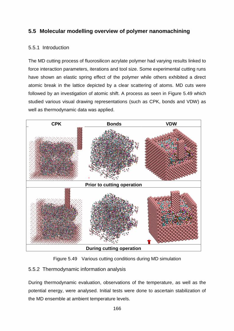
166

5.5 Molecular modelling overview of polymer nanomachining

5.5.1 Introduction

The MD cutting process of fluorosilicon acrylate polymer had varying results linked to

force interaction parameters, iterations and tool size. Some experimental cutting runs

have shown an elastic spring effect of the polymer while others exhibited a direct

atomic break in the lattice depicted by a clear scattering of atoms. MD cuts were

followed by an investigation of atomic shift. A process as seen in Figure 5.49 which

studied various visual drawing representations (such as CPK, bonds and VDW) as

well as thermodynamic data was applied.

CPK Bonds VDW

Prior to cutting operation

During cutting operation

Figure 5.49 Various cutting conditions during MD simulation

5.5.2 Thermodynamic information analysis

During thermodynamic evaluation, observations of the temperature, as well as the

potential energy, were analysed. Initial tests were done to ascertain stabilization of

the MD ensemble at ambient temperature levels.

167

Figure 5.50 MD simulation of (a) temperature

Temperature results as seen in Figure 5.50 had initial spikes to values as high as

800K. This was believed to be associated with early tool entry and eventually these

temperature values eventually stabilised to values about 200K as cutting was in

progress. This condition is allegedly used to represent conditions experienced in an

actual cutting process such as rubbing action of tool and workpiece or molecular

displacement of atoms but reflects a huge loss of heat from boundary atoms.

However, an actual cutting process of the polymer reflected here displays the

recreation of a satisfactory dynamic representation of the process.

Similarly, in the machining of metals, a high proportion of the heat generated is

removed from the cutting area by the chip [1]. Despite the high conductivity present

metallic materials, the huge portion of heat present at the interfacial layer on the

surface of the workpiece plays an important role in heat removal by conduction.

Literature shows [158] that the amount of heat carried away from the primary shear

zone by the chip is as high as 90% for higher cutting speeds. This initial simulation

outcome shows the boundary conditions acting as a high source of heat dissipation

from the interfacial layer of the surface of the workpiece. Also, based on the

constrictions of the size of the simulated workpiece by computational demands, heat

dissipation could be a significant challenge, acting as cutting chips would in metal

machining but reversing realistic temperature levels.

168

Subsequent tests were built on this experiment model. Figure 5.50 and Figure 5.51

show the initial temperature and energy results from MD tests.

Also, results from the potential energy and total energy of these experimental runs

as shown in Figure 5.51, depict the overall loss in energy of the system. Energy loss

in the molecular dynamic system are known to occur (Oluwajobi [84]) but should be

anticipated and adjusted accordingly during simulations. Oluwajobi [84] in his

research found values of ultimate low of -500000eV found during the MD

nanomachining of copper using LJ parameters.

Figure 5.51 MD simulation of energy

Furthermore, for these temperature and energy results, a rubbery reaction was

observed as shown in Figure 5.52. This results from the high interactive forces acting

between workpiece atoms.

In plastic machining, because of their low thermal conductivity, heat generated in the

primary shear zone does not quickly dissipate. This condition is characterised by

concentrated heat generation in the cutting zone, yielding to an increased range in

mobility of the molecular chain of the material and thus improved material ductility.

Parameters such as molecular weight and the glass transition factor are the

determining factors as to which these cutting effects become dominant [158].

169

However, this transition extends from a glassy state to a rubbery state based on

machining conditions. Heat generation is a determining factor in glass transition

states. In actual machining, this heat is generated by the shear in the primary

deformation zone, by friction between the chip and the tool face and between the

workpiece and the tool clearance side.

From the simulation results, the high loss in temperature mentioned above is

assumed to be thus responsible for the resultant higher molecular force interaction

between molecules. The tool in these instances experienced difficulty in rupturing

molecular chains of the polymer leaving an imprint of its shape within the workpiece.

The action induced a form of spring back action from the workpiece. This situation is

reflected by the rapid fall in temperature and the energy trendline further highlights

the elasticity in the material.

Figure 5.52 Hyper-elastic polymer property

Additional experimental runs in simulation had changes in interacting force potential

values to reduce the high elasticity obtained during simulations and allow cutting

action. Comparison of the effect of altering parameters was linked to elasticity and

studied.

5.5.3 Comparison of various potentials between tool and workpiece

Numerous MD tests were run to access the effects of some parameters on MD

results; however this section of the thesis reflects the results of MD test linked to the

170

combined effects from molecular interacting force parameters and speed.

Experimental tests investigated the effects of using only the Lennard-Jones force

potential and also a hybrid force setup of the Lennard-Jones in combination with

Tersoff force potentials. The force potential depicting interactions between the tool

and workpiece was additionally set during MD simulation tests from LAMMPS. A

number of combinations of LJ parameters were tested and these results are shown

in Table 5.27. Variation of the LJ parameters was done following the estimation

based on the chart by Aziz [131] shown in Figure 3.12. The tool in some test had a

smoother cutting effect through the workpiece. This was found to be linked to the

hybrid combination of LJ and Tersoff force potentials which created a more

appropriate representation of force interaction during cutting simulation.

171

Table 5.27 Comparison of various LJ force potentials during MD simulation

VDW view Cutting forces Temperature Potential energy

(a)

LJ

𝝐 = 100

𝝈 = 2.35 i = 3000

v = 95m/s

(b)

LJ

𝝐 = 100

𝝈 = 2.35 i = 3000

v = 95m/s

(c)

LJ 𝝐 = 100

𝝈 = 2.23 i = 3000

v = 65m/s

(d)

LJ

𝝐 = -100

𝝈 = -1.65 i = 5000

v = 65m/s (hybrid forces)

172

Table 5.27 shows variations in simulation observed during tests. The results in Table

5.27(a) show that the tangential force components of cutting forces (fx) varied in the

range from around -4×10-6 N to -5×10-6 N with an average of -1×10-5 N; the potential

energy had a progressive downward slope, falling to low values of about -500000eV,

towards the end of the simulation at 3200 steps. Initial high temperature was

observed but these later stabilised during the simulation run due to optimised cutting

conditions. The phenomenon of ploughing was not observed due to the high

elasticity of the workpiece but an imprint of the tool was seen on the workpiece.

For the subsequent experimental test in Table 5.27(b), an increase in the tool size

from the number of atoms and the structural dimension produced similar results to

other experiments. However, over the same number of experimental iterations,

tangential force further increased to more positive values of -4×10-6 N to 2×10-4 N.

During these tests, high attractive forces between atoms of the tool were also

experienced. These high interactive forces depict an inherent imbalance in force

application of the system on tool atoms. Similar temperature results from initial force

potentials tests in Table 5.27 were observed in this test. A mild build-up at atoms

was observed from the tool imprint.

Further tests in Table 5.27(c), show the varied atomic distance between tool and

workpiece atoms, at reduced cutting speed. As the temperature values stabilised,

the test produced a very soft workpiece with loosely attached atoms. However, the

presence of excessive attractive forces was still present on the tool. This was

identified to be as a result of the inadequate relaxation time for the system. At this

stage evaluation of the cutting force showed positive values with rise from values

ranging between 1×10-2 N to about 3×10-1 N. In this test positive energy value of

1×108 eV over 3200 steps and a stable temperature of 293K was observed. These

results reflected pure cutting action but with plastic deformation. A mild ploughing

phenomenon was identified at this stage with about 2 layers of atoms.

Finally, to improve the relaxation stage of the simulation a higher number of iteration

and LJ parameters (from Table 5.27(d)) were selected. A pure cutting condition was

achieved without plastic deformation. In this test, the atoms behave more like solids

and show cohesiveness. The potential energy and total energy of this experiment

shows a progressive stable rise before 1800 steps with a positively inclined energy

173

value but it has fluctuations towards its end due to compression effect from atomic

pile up with the fixed boundary atoms. The tangential force component started with

1×10-5 N to high values of 3N towards the end of the pass. In this simulation the

atoms behave a lot more like solids with higher attractive forces between them and

more resistance in cutting action. A ploughing phenomenon was observed with a

pile-up of three layers of atoms from the external Van der Wall (VDW) simulation

drawing method. A steady stable temperature value of 293K was observed from the

temperature which indicates stabilisation and heat dissipation within the model. This

is a desired quality for a model and the best cutting condition.

From the results in Table 5.27(d), an additional test run performed at a higher

number of iterations and an introduction of Tersoff force potential between the tool

and the workpiece to achieve stabilisation. This is added due to the suitability of

Tersoff in modelling carbon force interaction with other elements. Simulated results

of these findings are expanded in Table 5.28. A clearer representation of the MD

visualisation with varying colours based on MD component parts is shown in Figure

5.53 for visual inspection. This final test is conducted over 6000 iterations with the

additional hybrid Tersoff potential.

Figure 5.53 MD of simulation model of Roflufocon

174

Table 5.28 Hybrid force simulation with (a) CPK; (b) VDW representation

CPK drawing representation VDW representation

(a)

(b)

(c)

The effect of the number of iterations on the plasticity of the material can be better

observed in this test. It could be postulated that a smaller number of iterations didn’t

provide adequate time for ideal force representation between atoms and thus yielded

plasticity. A higher range in iterations generated a more cohesive solid nature of the

polymer. This is also believed to be linked to the influence that iterations may have

175

on the simulated velocity of cutting. VDW and CPK drawing representation shown in

Table 5.28 show the progressive shift of atoms experienced as the cutting process is

done. Figures in the table seek to infer effects occurring due to shifting of atoms

within the compression and lattice slip zone. Observations show that the effect of an

underlining cushion bed of atoms formed within the workpiece attest to the fact that

the compressive stress zone present in this polymer simulation is greater than that

found by bigger than metals opposites [82] based on the choice of force potentials

and bonds present.

The CPK drawing method shows the more robust internal ploughing phenomenon

experienced in polymers. A build-up of about 4 layers of atoms can be seen from a

closer view. This is attributed to a pure cutting and shift of atoms from the tool atoms.

In the last CPK figure, the atomic layers are seen to overflow from its boundary box

region. Though some elasticity is retained in this simulation, its VDW representation

could be identified as adequately mimicking an ideal polymer cutting process from

the combination of the force potentials acting within the workpiece and with the tool.

5.5.4 Correlation of MD results to machining conditions

Figure 5.54 shows the cutting dynamics complexities in polymers machining. From

the figure a depiction of known dynamic principles guiding orthogonal cutting are

also reflected.

Figure 5.54 Various complexities involved in the cutting of polymers [147]

176

As mentioned in Chapter 2, polymers undergo a transition from a glassy state to a

rubbery state with increase in temperature. From experimental results in previous

sections, the effect of temperature and pressure applied at various cutting

parameters creates a ductile regime cutting characterised by a glass-rubbery effect

and continuous chip flow formation. This condition is also reflected in MD by the

elasticity of the workpiece during tool passes.

Figure 5.55 MD showing atomic movement within the silicon workpiece

The effect of increased feedrates leading to high rubbing experienced at the surface

of the workpiece was shown by the increase in simulated cutting speeds. Similar

reactions with increased cutting velocity influenced simulated temperature output.

High elastoplastic and plastic deformation observed in both simulation and cutting

operation are thus seen to occur in the primary shear zone or high compressive

stress/phase transformation zone (Figure 5.55). Figure 5.55 which shows this atomic

movement within a workpiece gives a better depiction of the movement of atoms

within the material during molecular dynamic simulated conditions. The reaction from

micro-structural cracks which occur along the trailing tensile stress zone are however

difficult to identify from simulated diagrams.

Lattice Slip zone

Compressed

atoms where

phase transition

occurs

Atomic layer

build -up / Chip

Elastic

recovery

process High pressure

transformation

phase

177

Figure 5.56-58 show the observations of the temperature and cutting force

(𝑓𝑥, 𝑓𝑦 and 𝑓𝑧), as well as the potential energy which is also analysed for the hybrid

condition. From the figure, force components as seen in the simulation show an

initial start in the values of 0.02 – 0.1N before rising to values of 0.8N. This is

believed to be as a result of the dimensional constraints of the simulated

environment as the tool approaches the boundary atoms. It can thus be seen that

the outcome of simulated sub-surface machining phenomena correlates with

postulated findings from force and surface experiments in previous sections of the

thesis.

Figure 5.56 Cutting force component of MD simulation of polymer

178

Figure 5.57 Temperature component of MD simulation of polymer

Figure 5.58 Energy observed during MD simulation of polymer

A brief initial stable temperature which indicated a stable thermodynamic system was

seen (Figure 5.57). This was later characterised with a gradual increase in

temperature as the tool atoms are compressed against the fixed boundary atoms.

This condition reflects the effects discussed from the heat generated in the

compressive cutting zone. As the specific heat of polymers is usually greater than

that of metals and its thermal conductivity significantly lower, therefore, temperature

179

rise in the polymer is normally larger and concentrated to a smaller area when a

given quantity of heat is applied to equal volumes of a polymer and a metal. Also

because of the concentration and the scission of molecular chains to form an atomic

build-up layer, heat is believed to be generated. MD simulation however takes into

consideration the overall increase in temperature of the simulated system in the

thesis. In an experimental setup, this also results due to localized heating from

continuous tool rubbing at the machined surface, leading to excessive heating. This

further may create a burning in the machined surface of thermosetting polymers or

the elastoplastic effects experienced in thermoplastic polymers.

Force signal observed had an initial stable start, few oscillations at 1750 steps which

gradually increased to higher energy values (Figure 5.58). This observation may

further display the influence on sub-surface compressive force actions as

responsible for change in material condition during cutting. Higher forces, increased

temperature and energy release explain the importance of the effects of cutting

parameters on sub-surface conditions to determine achievable lens output. Also, an

influence of the post effect of the elastic recovery process as seen in Figure 5.55

may form a combined effect for these results. This could further influence achievable

surface results for materials of high plasticity. Additional conditions such as the

change in the effect of the rubbing action of tool chips found at surface of workpiece

which wasn’t covered in this simulation may also be of importance.

180

5.5.5 Summary

Despite the difficulty in estimating force interaction between elements in a polymer

during machining action, this study was able to reproduce an actual MD investigation

into nanoscale machining of polymers. Results of the force components during initial

simulated cutting reflected similar values as seen in section 4-2. An evaluation into

sub-surface microstructural phenomena during nanometric machining reinforced

known orthogonal theory of sub-surface effects. Potential energy release from the

simulated system provided results which correspond to an increased scission of

molecular chains. This is presumed to be from the generation of a form of tool chip

from the atomic build-up layer. Increased rubbing action between tool and workpiece

could reflect on the high electrostatics addressed in section 4.4. The combined effect

of the compression zone found in polymers, ploughing phenomenon and build-up of

layers of atoms are believed to be conditions associated with high rubbing for static

charging. High elasticity in polymers and close atomic attraction may also contribute

to this. Despite the replication of this cutting process using simulations, it must

however be noted that MD simulations only observe a nano-portion of the cutting

effect which does not proportionally apply to an experimental larger scale

nanomachining process based on force interaction over a larger volume.

181

Conclusion

The objectives of this research work were aimed at investigating postulated facts on

the UHPM of polymers and evaluate the performance of ultra-high precision

manufacturing of contact lens polymers. This was done on the commercially

available contact lens polymer, Roflufocon E, and performed on the Precitech

Nanoform Ultra-grind 250 precision machining.

An extensive literature review, as presented in Chapter 2, discussed in details optical

polymers and the UHPM process in general. It then addressed barriers and current

available evaluation techniques that could be employed in analysing conditions

occurring in polymer cutting.

The reviewed literature revealed the challenges faced in polymer machining from

various wear mechanisms which could drastically influence surface accuracy of the

optical profile attainable; and how current machining parameters employed in the

fabrication of high-end optical polymers have produced Liechenberg cracks on

diamond tools from high static.

The identified knowledge gap in the literature depicts that there exists no report on

an established process scheme for efficient UHPM of polymers. The lack thereof

affects the understanding of the influence of cutting factors in machining. Also,

detailed quantification and understanding of the underlining triboelectric phenomena

between diamond tools and polymers as studied in this thesis does not exist. In

addition, there is no published work on the molecular dynamics simulation of a

contact lens polymer and its nano-machining replication.

The detailed experimental procedures employed were portrayed in this thesis in

Chapter 3. These comprised a detailed overview of a commercially available contact

lens polymer workpiece, specific diamond tooling and state-of-the-art nano-

machining equipment. This chapter further consists of the method employed for the

determination of optical surface quality. This directly considered the effects of

machining parameters such as feed rate, speed and depth of cut. The deductions

from these tests were based on the analysis of machining cuts. Various

combinations of cutting parameters were considered; and selection of the machining

182

final matrix was based on the Box-Behnken RSM modelling method and utilised for

modelling. This methodology permitted prediction within and above selected ranges

of parameters. The selection of the statistical analysis method considered the

number of factors to be evaluated and provided a lower number of experiments for

predictions. It was seen that this response surface technique aided in the selection of

cutting parameters not at the extreme ranges of the Ultra-precision machine based

on its spatial modelling arrangement which aided in predictions.

Other conclusions based on the investigation were on the evaluation of the cutting

parameters effects on relevant condition monitoring practices such as force

monitoring and triboelectricity that best described the influences of cutting factors.

During the evaluation of surface roughness, experimental tests achieved the

minimum surface roughness at 239 rpm speed, 2µm/rev and 25 µm depth of cut.

During modelling, feed rate and depth of cut were identified as significant influential

factors in the determination of surface roughness; however changes in the feed rate

had greater influence than any other factors. This situation was assumed to be due

to a decrease in the distance between cutting passes by the diamond tip, creating a

form of overlapping between cutting grooves. Also, this could be attributed to the

rubbing action originating from tool chip magnetised to the cutting tool from a

triboelectric effects. These chips as the feed gradually increased, increased in width

and caused disturbance during the cutting process. However, as the feed further

increased beyond 7µm/rev a point was achieved where a balance/semi-balance

could be found between increase in the width of chips and chip clearance (due to

size) from the surface of the lens during machining. At this stage a reduced amount

of chip was found at the diamond tip causing a relative improvement in achieved

surface roughness. At a low depth of cut of 10µm, a very rough lens surface of

20.4nm was achieved during machining. This poorer surface finish was presumed to

be attributed to the compounding effect of a reduced chip thickness due to a low

depth of cut.

An overview of the cutting shows that cutting depth influenced the thickness (width)

of the cutting chip. This generated light or thick chips which generated an effect on

continuous and non-continuous chip flow. Also, the feed rate was identified to have a

greater effect on the structural surface of the tool chip. Chips with rough surface and

183

high cracks were obtained at high feeds. This also contributed in chip breaking.

However, it was postulated that the speed led to a variation in chip edges. This

variation ranged from cone-like, fillet-shaped to actual tear. A combination of these

observations on the cutting chip could be used to explain the formation of tool chip at

the tool tip during machining.

During the force evaluation, from the analysis of force at the tool tip, it was

concluded that the effects of sensor positioning along the tool poses an insignificant

effect on the recorded force readings. Furthermore, the effect of the feed rate was

identified as the only significant model term linked to the cutting force. The RSM

model implemented also postulates that negligible or no influence is perceived from

depth of cut and speed during UHPM of polymer. However, the validation of the

model falls below a 10% confidence prediction level needed in general statistics

despite a prior modelling of the exact force at the tool tip. This value indicated an

underlining challenge in the model. This was attributed to challenges in micro-force

acquisition based on the scale of machining. Thus, it was concluded that this model

might not take all factors involved into consideration. It is recommended that more

tests be conducted with a combination of multiple sensors to predict force effects on

cutting parameters.

A careful analysis of the cutting parameters linked to static charging as presented in

Chapter 4, showed a high correlation of feed and speed at higher humidity value and

speed and the depth of cut at lower humidity. UHPM of a contact lens polymers was

here shown to generate tribocharging characteristic under a range of conditions.

However, speed rate which influences the shape of cutting chips and time of a

cutting pass was seen to be the most influential parameter in static formation. This

factor was identified also to be a linked non-continuous chip flow which greatly

reduced chip build-up.

From the triboelectric tests, it was found that at 60% relative humidity increase in the

cutting speeds generates an increased number of negative electrostatic charges at

low feed rates. At the 40% humidity stage, high chip build up around the tool was

frequently observed during machining. This chip build-up also causes a negative rise

in statics up to levels as low as -3.0kV. However, at this humidity stage, it was

concluded that additional experimentation is needed to perfectly model the effect of

184

cutting parameters. This was attributed to wide variations in statics readings based

on loading and offloading of tool chips at the tool tip.

From the last tribo-electric experimental (at 20% humidity), massive static discharge

was observed average cutting conditions. This was believed to be due to the working

on extremely dry workpiece surface. Also it could be explained based on the high

material removal rate possessed at the feed and speed value.

The importance of chipping in the tribo-electric effect could not be undervalued.

Tribo-charging was discovered to be founded derived from a short rubbing action of

tool and workpiece or due to the rubbing action of massive chip formation on the tool

tip. Both of these conditions were causing agents for electric fields formation during

machining and static discharges. It was, however, confirmed that humidity could be

used to control tribocharging.

From the experimental evaluation of triboelectric phenomena, it was found that each

of the cutting parameters influenced chipping, some more than others. Some basic

interactions from cutting parameters contributed most to this condition and had high

electrostatic charging effects. It was concluded that an independent look on

parameter interactions on the tool chip could generate a way to determine possible

electrostatic magnitudes.

In conclusion, the results validated the fact that feed rate had a high influence in

polymer machining surface roughness. As observed from the RSM model, negligible

effect of the cutting speed was experienced during the prediction of surface

roughness. Further experimentation with a wider range of parameters may however,

produce different variations and show underlining interactions with other cutting

parameters. Results of surface roughness measurements indicated a rise in

roughness value with a low depth of cut, and increasing feed. Feed rate was

identified as influential towards high surface accuracy based on significant changes it

has on the cutting tool chip. Conclusively, it could be said that force sensor

positioning had negligible interference in force recordings. However, extensive

amounts of cutting parameter combinations need to be done to adequately model

cutting force influence in diamond machining.

185

In addition, tribocharging is an important factor in polymer machining. This

phenomenon is linked to cutting parameters and relative humidity. It could rise to

magnitudes as high as 22kV and could be the cause for severe wear formation in

diamond tooling. It was concluded that at high humidity, low feeds and high depth of

cuts produced higher static charges while at moderate humidity levels, speed and

depth of cut had greater influence. This was solely attributed to changing conditions

in ion conductivity during machining process. Therefore, it can be concluded that

humidity greatly affects the top surface of the lens and its air-borne discharge rate,

creating a less effective rubbing action at faster speed and feed.

From the MD study a clearer understanding is achieved of sub-structural effects

during nanometric machining. These simulations were able to reproduce an actual

MD investigation into nanoscale machining of polymers. Results of the force

components during initial simulated cutting reflected similar values as seen in section

4-2. An evaluation into sub-surface microstructural phenomena during nanometric

machining reinforced known orthogonal theory of sub-surface effects as caused from

high compressive forces in the cutting zone leading to an increase in temperature

and transition in material state, Potential energy release from the simulated system

also provided results which correspond to an increased scission of molecular chains

presumed to reflect the generation of tool chip. Furthermore, increased rubbing

action between tool and workpiece may reflect on the high electrostatics previously

addressed in Section 4.4.

From all these conclusions, it can be generally concluded that in all experimental

tests to achieve highest quality finish in optical manufacture, the feed rate would be

seen as a vital factor to be considered in a factory-conditioned environment.

186

Recommendation

In spite of an enormous amount of work carried out in this study, there remain some

aspects that would require further investigation. These include:

The need to ascertain level of influence of the feed rate on output quality

within a wider range of cutting parameters;

Further study into the UHPM of polymers should consider a wider range of

polymer types based on their Food and Drug Administration classifications

and area of application within the society;

Further experimentation for an adequate model of cutting force could provide

initial ground for the introduction of an automated force-controlled

manufacturing system;

Analysis of the influence of cutting parameters on temperature occurring

during polymer machining on the tool flank;

A classification of polymers into triboelectric magnitude generated during

polymer machining could greatly improve costs in general polymer cutting and

save tool cost.

These in addition to the work completed in this study would constitute a

comprehensive study on the ultra-high precision machining of contact lens polymers.

This research as mentioned earlier could provide a ground for the establishing of a

customised design contact lens based on racial specifications for the African

populace. Therefore, the need to design an optical equation based on racial profiles

and manufacturing based on the research specifications given in this study would

create both a local and an affordable solution to the creation of an African contact

lens.

187

References

1. Refojo MF, editor Polymers and devices in ophthalmology. Biomedical

Engineering Conference; 1995 7-9 Apr 1995; Shreveport, Louisiana: IEEE.

2. Gupta H, Aqil M. Contact lenses in ocular therapeutics. Drug discovery today.

May 2012;17(9-10):522-7.

3. Heinrich M, Wildsmith C, editors. Need for precision engineering in astigmatic

contact lenses. Proceedings of the ASPE Topical Meeting on Freeform

Optics; 2004.

4. Mamalis AG, Lavrynenko SN. On the precision single-point diamond

machining of polymeric materials. J Mater Process Tech. 2007 Jan 1;181(1-

3):203-5. PubMed PMID: ISI:000241963900041. English.

5. Taniguchi N, editor On the basic concept of nanotechnology. Proceedings of

the International Conference of Production Engineering 1974; Tokyo, Part II:

Japan Society of Precision Engineering.

6. Pawade KJR, Balasubramaniam R, editors. Some investigations on surface

characteristics in precision turning of nylon and polypropylene. 1st

International Conference on Recent Trends in Engineering & Technology, ;

2012 March Special Issue of International Journal of electronics,

Communication & Soft Computing Science & Engineering.

7. Saini V, Sharma D, Kalla S, Chouhan T. Optimisation of process parameter in

ultra-precision diamond turning of polycarbonate material. International

Conference on Manufacturing Excellence, MANFEX 2012; 29-30 March,

2012; Noida, India2012.

8. Venkatesh VC. Precision manufacture of spherical and aspheric surfaces on

plastics, glass, silicon and germanium. Curr Sci India. 2003 May

10;84(9):1211-9. PubMed PMID: ISI:000183086000021. English.

9. Gubbels GPH. Diamond turning of glassy polymers [Doctoral thesis]:

Technische Universiteit Eindhoven; 2006.

10. Barr J, MS F. Contact Lens Spectrum's annual report of major corporate and

product developments and events in the contact lens industry in 2004, as well

as predictions for 2005 [article on the Internet cited on 2006 March 3] 2005.

188

11. Nichols JJ. Annal report: Contact lenses 2011. Contact Lens Spectrum.

2012;27 (January 2012):20 - 5.

12. Brinksmeier E, Glaebe R, Osmer J. Surface integrity demands of high

precision optical molds and realization by a new process chain. Procedia

Engineering. 2011;19:40-3.

13. Oluwajobi AO. Nanomachining technology development [Doctorate thesis]:

University of Huddersfield; 2012.

14. Ramsden J, Allen D, Stephenson D, Alcock J, Peggs G, Fuller G, et al. The

design and manufacture of biomedical surfaces. CIRP Annals-Manufacturing

Technology. 2007;56(2):687-711.

15. Apple DJ, Ram J, Foster A, Peng Q. Evolution of cataract surgery and

intraocular lenses (IOLs): IOL quality. Survey of Ophthalmology. 2000;45,

Supplement 1(0):S53-S69.

16. Nicolson PC, Vogt J. Soft contact lens polymers: an evolution. Biomaterials.

2001 Dec;22(24):3273-83. PubMed PMID: ISI:000171759500008. English.

17. Lloyd AW, Faragher RGA, Denyer SP. Ocular biomaterials and implants.

Biomaterials. 2001 April;22(8):769-85. PubMed PMID: ISI:000167120000003.

English.

18. Efron N. Contact lens practice. Second ed: Elsevier Health Sciences; 2010.

19. Hough D. Contact lens standards. Contact Lens and Anterior Eye.

1998;21(Supplement 1):S41-S5.

20. Rattier BD, Hoffman AS, Schoen FJ, Lemons JE. Biomaterials science: an

introduction to materials in medicine. Journal of Clinical Engineering.

1997;22(1):26.

21. Maldonado-Codina C, Efron N. Hydrogel lenses-material and manufacture: A

review. Optometry in Practice. 2003;4:101-15.

22. Brievogel S. A primer on contact lens polymer. Eyewitness Second quarter -

A publication of the Contact lens Society of America. 2002:32-5.

23. Snyder C. A primer on contact lens materials. Contact Lens Spectrum.

2004;19(2):34-9.

24. Giedd B. Understanding the nuances of contact lens materials. Contact lens

Spectrum. 1999;14:23-8.

25. Optical Filters: ADC cast optical sheet: Optical Polymer International; 2009.

Available from: http://alcat.typepad.com/opi/display--readout-windows----

http://alcat.typepad.com/opi/display--readout-windows----optical--filters-----adc-cast-optical-sheet-display-applications----the--continual-adv.html

189

optical--filters-----adc-cast-optical-sheet-display-applications----the--continual-

adv.html.

26. Cavagnaro JM. Polymer optics: Progress in plastic optics follows advances in

materials and manufacturing2011. Available from:

http://www.laserfocusworld.com/articles/print/volume-47/issue-

9/features/polymer-optics-progress-in-plastic-optics-follows-advances-in-

materials-and-manufacturing.html.

27. Heinrich M, Wildsmith C, editors. Need for precision engineering in astigmatic

contact lenses2004.

28. Bennett ES, Weissman BA. Clinical contact lens practice: Lippincott Williams

& Wilkins; 2005.

29. Selby AP. Nanoindentation of soft contact lens materials [Doctorate thesis]:

The University of Manchester; 2012.

30. Dick L, Risse S, Tünnermann A. Injection molded high precision freeform

optics for high volume applications. Advanced Optical Technologies.

2012;1(1):39-50.

31. Chunning Huang MS. Investigation of injection molding process for high

precision polymer lens manufacturing [Doctorate Thesis]. Ohio: The Ohio

State University; 2008.

32. Chiu W, Lee W. Development of ultra-precision machining technology. Fifth

International Conference on FACTORY 2000 - The Technology Exploitation

Process; 2-4 April 1997; Cambridge, UK 1997. p. 486 – 90.

33. Hsu A. The development of ultra-precision machining technology in ITRC. In:

Center ITR, editor. Presentation. Port-Elizabeth: National Applied Research

Laboratories; 2013.

34. Riemer O, editor Advances in ultraprecision manufacturing. Proceedings of

Japan Society of Precision Engineers; 2011.

35. Chapman G. Ultra-precision machining systems; an enabling technology for

perfect surfaces. Moore Nanotechnology Systems. 2004.

36. Bylinsky G. Closing In on perfection: Ultraprecision machine tools are putting

manufacturers within nanometers of absolute accuracy 2003 28th January,

2014. Available from:

http://money.cnn.com/magazines/fortune/fortune_archive/2003/06/23/344598/

.



http://www.laserfocusworld.com/articles/print/volume-47/issue-9/features/polymer-optics-progress-in-plastic-optics-follows-advances-in-materials-and-manufacturing.html





190

37. Freedonia.Market.Research. World Machine Tools to 2014: Alacra Store; Apr

01, 2011 [Feb 19, 2014]. Available from:

http://www.alacrastore.com/storecontent/Freedonia-Market-Research/World-

Machine-Tools-to-2014-2039-427.

38. Franse J. Manufacturing techniques for complex shapes with submicron

accuracy. Reports on Progress in Physics. 1990;53(8):1049.

39. Davies MA, Evans CJ, Vohra RR, Bergner BC, Patterson SR, editors.

Application of precision diamond machining to the manufacture of

microphotonics components. Optical Science and Technology, SPIE's 48th

Annual Meeting; 2003: International Society for Optics and Photonics.

40. Contour Fine Tooling. Diamond tools for contact lenses and IOL’s2008.

Available from: http://www.contour-diamonds.com/en/about-us/brochures/.

41. Gauthier C, Lafaye S, Schirrer R. Elastic recovery of a scratch in a polymeric

surface: experiments and analysis. Tribology International. 2001;34(7):469-

79.

42. Friedrich K, Sue H, Liu P, Almajid A. Scratch resistance of high performance

polymers. Tribology International. 2011;44(9):1032-46.

43. Lane B, Dow T, Scattergood R. Thermo-chemical wear model and worn tool

shapes for single-crystal diamond tools cutting steel. Journal of Wear.

2013;300(1):216-24.

44. Abou-El-Hossein K, Olufayo O, Mkoko Z. Diamond tool wear during ultra-high

precision machining of rapidly solidified aluminium RSA 905. Journal of Wear.

2013 Apr-May;302(1-2):1105-12. PubMed PMID: ISI:000322682800032.

English.

45. Gubbels GPH, van der Beek GJFT, Hoep AL, Delbressine FLM, van Halewijn

H. Diamond tool wear when cutting amorphous polymers. Cirp Annals-

Manufacturing Technology. 2004;53(1):447-50. PubMed PMID:

ISI:000222519700106. English.

46. Shi M. Thermo-chemical tool wear in orthogonal diamond cutting steel and

stainless steel [Master's dissertation]: North Carolina State University; 2010.

47. Jasinevicius RG, Duduch JG, Porto AJ. Investigation on diamond turning of

silicon crystal-generation mechanism of surface cut with worn tool. Journal of

the Brazilian Society of Mechanical Sciences. 2001;23(2):241-52.

http://www.alacrastore.com/storecontent/Freedonia-Market-Research/World-Machine-Tools-to-2014-2039-427

http://www.alacrastore.com/storecontent/Freedonia-Market-Research/World-Machine-Tools-to-2014-2039-427

http://www.contour-diamonds.com/en/about-us/brochures/

191

48. Abdel-Aal HA, Smith ST, Patten JA. On the development of surface

temperatures in precision single-point diamond abrasion of semiconductors.

International Communications in Heat and Mass Transfer. 1997;24(8):1131-

40.

49. Hurt H, Decker D, editors. Tribological considerations of the diamond single-

point tool. 28th Annual Technical Symposium; 1984: International Society for

Optics and Photonics.

50. Shin I. Cutting-temperature measurement by means of photodiodes in

diamond turning of hard alloys. Measurement Techniques. 1984;27(10):899-

901.

51. Ueda T, Sato M, Nakayama K. The temperature of a single crystal diamond

tool in turning. Cirp Annals-Manufacturing Technology. 1998;47(1):41-4.

52. Overcash JL, Cuttino JF. In-process modeling of dynamic tool-tip

temperatures of a tunable vibration turning device operating at ultrasonic

frequencies. Precision Engineering. 2009;33(4):505-15.

53. Goel S, Luo X, Reuben RL. Wear mechanism of diamond tools against single

crystal silicon in single point diamond turning process. Tribology International.

2013;57:272-81.

54. Gubbels G, Van Der Beek G, Hoep A, Delbressine F, Van Halewijn H.

Diamond tool wear when cutting amorphous polymers. CIRP Annals-

Manufacturing Technology. 2004;53(1):447-50.

55. Olufayo OA, Abou-El-Hossein K, editors. Preliminary Investigation of surface

finish of a contact lens polymer in ultra-precision diamond turning. 6th

Robotics and Mechatronics Conference (RobMech); 2013; Durban, South

Africa, October 30-31, 2013.

56. Contour Fine Tooling. Diamond tool wear during cutting of plastics 2008.

Available from:

http://www.zimmerman.com.tw/download2.asp?file=uploads/07_cuttingplastic.

pdf.

57. Zhou M, Ngoi B, Yusoff M, Wang X. Tool wear and surface finish in diamond

cutting of optical glass. J Mater Process Tech. 2006;174(1):29-33.

58. Rhorer RL, Evans CJ. Fabrication of optics by diamond turning. Handbook of

Optics. 1995:41.1-.13.

http://www.zimmerman.com.tw/download2.asp?file=uploads/07_cuttingplastic.pdf

http://www.zimmerman.com.tw/download2.asp?file=uploads/07_cuttingplastic.pdf

192

59. Olufayo O, Abou-El-Hossein K, Kadernani M. Tribo-electric Charging in the

Ultra-high Precision Machining of Contact Lens Polymers. Procedia Materials

Science. 2014;6:194-201.

60. Kaplan A, McReynolds B, Selvaduray G. Dielectric characteristics of

materials-electrostatic discharge. Experimental Methods In Materials

Engineering. November 2002.

61. Williams MW, editor Mechanisms of triboelectric charging of insulators, a

coherent scenario. Proceedings of ESA Annual Meeting on Electrostatics

2011 June 14-16, 2011; Case Western Reserve University, Cleveland OH:

Electrostatic Society of America.

62. Liu L, Seyam AM, Oxenham W. Frictional electrification on polymeric flat

surfaces. Journal of Engineered Fibers and Fabrics. 2013;8(1):126 -36.

63. Jasti VK. Electrostatic charge generation and dissipation on woven fabrics

treated with antistatic and hydrophilic surface finishes [Doctorate thesis]:

North Carolina State University; 2012.

64. Williams MW. Triboelectric charging of insulating polymers–some new

perspectives. AIP Advances. 2012;2(1):-.

65. Asuni N. Introduction to static electricity: An introduction to ESD Technick.net

- Electronic Hardware Information, Guides and Tools1998 [15th November,

2013]. Available from:

http://www.technick.net/public/code/cp_dpage.php?aiocp_dp=guide_esd_001.

66. Gubbels G, van der Beek G, Delbressine F, Schellekens P, editors.

Electrostatic tool wear in diamond turning of amorphous polymers. Euspen

international conference; 2004; Glasgow, Scotland, UK: European Society of

Precision Engineers.

67. Mason GW, Griffen DT, Merrill JJ, Thorne JM. Physical science concepts

Brigham Young University Print Services; 1997.

68. Diaz A, Felix-Navarro R. A semi-quantitative tribo-electric series for polymeric

materials: the influence of chemical structure and properties. Journal of

Electrostatics. 2004;62(4):277-90.

69. Xie L, Han K. Influence of relative humidity on the aeolian electric field.

Aeolian Research. 2012;7:45-50.

70. Carr JW, Feger C. Ultraprecision machining of polymers. Journal of Precision

Engineering. 1993;15(4):221-37.

http://www.technick.net/public/code/cp_dpage.php?aiocp_dp=guide_esd_001

193

71. Khan GS. Characterization of surface roughness and shape deviations of

aspheric surfaces [Doctoral Thesis]: Friedrich-Alexander-Universität Erlangen-

Nürnberg; 2008.

72. Gubbels GP, Delbressine F, Govaert L, Schellekens PH, editors. Precision

cutting of glassy polymers: influence of aging on the cutting process. Optical

Systems Design; 2004: International Society for Optics and Photonics.

73. Roblee J. Factors affecting surface finish in diamond turning: Precitech, Inc;

2007. Available from: http://www.precitech.com/about/white_papers.html.

74. Ghosh R, Knopf JA, Gibson DJ, Mebrahtu T, Currie G, editors. Cryogenic

machining of polymeric biomaterials: An intraocular lens case study. Medical

Device Materials IV: Proceedings of the Materials & Processes for Medical

Devices Conference 2007, September 23-27, 2007, Palm Desert, California,

USA; 2008: ASM International.

75. CSM. Atomic Force Microscope (AFM): CSM instruments; 2013 [cited 2013

8th May]. Available from: http://www.csm-instruments.com/en/Atomic-Force-

Microscope.

76. Li L. Investigation of the optical effects of single point diamond machined

surfaces and the applications of micro machining [Doctorate thesis]: The Ohio

State University; 2009.

77. Whitehouse DJ. Handbook of surface metrology: CRC Press; 1994.

78. Dandekar CR, Shin YC. Modeling of machining of composite materials: a

review. International Journal of Machine Tools and Manufacture.

2012;57:102-21.

79. Dandekar CR, Shin YC. Multiphase finite element modeling of machining

unidirectional composites: prediction of debonding and fiber damage. Journal

of Manufacturing Science and Engineering. 2008;130(5):051016.

80. Goggins DA. Response surface methods applied to submarine concept

exploration [Master's dissertation]: Massachusetts Institute of Technology;

2001.

81. Minbo C. Study of nanoscale ductile mode cutting of silicon using molecular

dynamics simulation [Doctorate thesis]: National university of Singapore;

2008.

82. Olufayo OA, Abou-El-Hossein K. Molecular dynamics modeling of nanoscale

machining of silicon. Procedia CIRP. 2013;8:503-8.

http://www.precitech.com/about/white_papers.html

http://www.csm-instruments.com/en/Atomic-Force-Microscope

http://www.csm-instruments.com/en/Atomic-Force-Microscope

194

83. Oluwajobi A, Chen X. The effect of interatomic potentials on the molecular

dynamics simulation of nanometric machining. International Journal of

Automation and Computing. 2011;8(3):326-32.

84. Oluwajobi A. Molecular dynamics simulation of nanoscale machining. In:

Wang PL, editor. Molecular dynamics - Studies of synthetic and biological

macromolecules: InTech Publishers; 2012.

85. Oluwajobi AO, Chen X, editors. The effect of depth of cut on the molecular

dynamics (MD) simulation of multi-pass nanometric machining. 17th

International Conference on Automation and Computing (ICAC); 2011: IEEE.

86. Oluwajobi AO, Chen X, editors. The effect of interatomic potentials on

nanometric abrasive machining. Proceedings of the 16th International

Conference on Automation & Computing; 2010; University of Birmingham,

Birmingham: Chinese Automation and Computing Society in the UK.

87. Aly MF, Eugene N, Veldhuis SC. Cutting force prediction using molecular

du\ynamics assisted finite element simulation model. 19th Annual meeting of

American Society for precision Engineers (ASPE); Orlando, Florida: American

Society for precision Engineers (ASPE); 2004.

88. De Chiffre L, Kunzmann H, Peggs G, Lucca D. Surfaces in precision

engineering, microengineering and nanotechnology. Cirp Annals-


89. Cai MB, Li XP, Rahman M. Study of the mechanism of nanoscale ductile

mode cutting of silicon using molecular dynamics simulation. International

Journal of Machine Tools and Manufacture. 2007;47(1):75-80.

90. Chang W-Y, Fang T-H, Lin S-J, Huang J-J. Nanoindentation response of

nickel surface using molecular dynamics simulation. Molecular Simulation.

2010;36(11):815-22.

91. Sushko G, Verkhovtsev A, Yakubovich A, Solov'yov A, editors. Molecular

dynamics simulation of nanoindentation of nickel-titanium crystal. Journal of

Physics: Conference Series; 2013: IOP Publishing.

92. Lai M, Zhang X, Fang F, Wang Y, Feng M, Tian W. Study on nanometric

cutting of germanium by molecular dynamics simulation. Nanoscale Research

Letters. 2013;8(1):1-10.

93. Zhu P, Fang F. Molecular dynamics simulations of nanoindentation of

monocrystalline germanium. Applied Physics A. 2012;108(2):415-21.

195

94. Chen YH, Fang FZ, Zhang XD, Hu XT. Molecular dynamics investigation of

cutting force in nanometric cutting of monocrystalline silicon. American

Journal of Nanotechnology. 2010;1(2):62-7.

95. Komanduri R, Chandrasekaran N, Raff LM. Effect of tool geometry in

nanometric cutting: a molecular dynamics simulation approach. Journal of

Wear. 1998;219(1):84-97.

96. Goel S, Luo X, Reuben RL, Rashid WB. Atomistic aspects of ductile

responses of cubic silicon carbide during nanometric cutting. Nanoscale

Research Letters. 2011;6(1):1-9.

97. Arefin S, Li X, Cai M, Rahman M, Liu K, Tay A. The effect of the cutting edge

radius on a machined surface in the nanoscale ductile mode cutting of silicon

wafer. Proceedings of the Institution of Mechanical Engineers, Part B: Journal

of Engineering Manufacture. 2007;221(2):213-20.

98. Fang T-H, Wu J-H. Molecular dynamics simulations on nanoindentation

mechanisms of multilayered films. Computational Materials Science.

2008;43(4):785-90.

99. Harmandaris VA. Atomistic molecular dynamics simulations of polymer melt

viscoelasticity [Doctorate thesis]: University of Patras; 2001.

100. Rocha JR, Yang KZ, Hilbig T, Brostow W, Simoes R. Polymer indentation with

mesoscopic molecular dynamics. Journal of Materials Research.

2013;28(21):3043-52.

101. Starr FW, Schrøder TB, Glotzer SC. Molecular dynamics simulation of a

polymer melt with a nanoscopic particle. Macromolecules. 2002;35(11):4481-

92.

102. Chen Y-C, Nomura K-i, Kalia RK, Nakano A, Vashishta P. Molecular

dynamics nanoindentation simulation of an energetic material. Applied

Physics Letters. 2008;93(17):171908.

103. Promyoo R. Molecular dynamics simulation of nanometric machining under

realistic cutting conditions using LAMMPS: Purdue University; 2008.

104. Plimpton S. LAMMPS user’s manual. Sandia National Laboratory. 2005.

105. Allen MP. Introduction to molecular dynamics simulation. Computational Soft

Matter: From Synthetic Polymers to Proteins. 2004;23:1-28.

196

106. Rasmussen WLC. Novel carbazole based methacrylates, acrylates, and

dimethacrylates to produce high refractive index polymers [Doctorate thesis]:

Virginia Polytechnic Institute and State University; 2001.

107. Brar A, Singh G, Shankar R. Structural investigations of poly (methyl

methacrylate) by two-dimensional NMR. Journal of Molecular Structure.

2004;703(1):69-81.

108. Souto-Maior R, Tavares M, Monteiro E. Solid State 13C NMR study of methyl

methacrylate-methacrylic acid Copolymers. Ann Magn Reson 2005 4(3):69-

72.

109. Uhlig F, Marsmann HC. 29 Si NMR some practical aspects. Available from:

http://www.pascal-man.com/periodic-table/29Si.pdf.

110. Shimada S, Ikawa N. Molecular dynamics analysis as compared with

experimental results of micromachining. CIRP Annals-Manufacturing

Technology. 1992;41(1):117-20.

111. Rentsch R, Inasaki I. Molecular dynamics simulation for abrasive processes.

CIRP Annals-Manufacturing Technology. 1994;43(1):327-30.

112. Komanduri R, Chandrasekaran N, Raff L. Some aspects of machining with

negative-rake tools simulating grinding: a molecular dynamics simulation

approach. Philosophical Magazine B. 1999;79(7):955-68.

113. Shimada S, Tanaka H, Ikawa N, editors. Atomistic mechanism of surface

generation in micromachining of monocrystalline silicon. Proceedings of 1st

International Conference of the European Society for Precision Engineering

and Nanotechnology 1999; Bremen, Germany: European Society for

Precision Engineering (euspen).

114. Han X, Lin B, Yu S, Wang S. Investigation of tool geometry in nanometric

cutting by molecular dynamics simulation. J Mater Process Tech.

2002;129(1):105-8.

115. Ye Y, Biswas R, Morris J, Bastawros A, Chandra A, editors. Simulation of

nanoscale polishing of copper with molecular dynamics. MRS Proceedings;

2002; San Francisco, California: Cambridge Univ Press.

116. Lin B, Yu S, Wang S. An experimental study on molecular dynamics

simulation in nanometer grinding. J Mater Process Tech. 2003;138(1):484-8.

117. Cheng K, Luo X, Ward R, Holt R. Modeling and simulation of the tool wear in

nanometric cutting. Journal of Wear. 2003;255(7):1427-32.

http://www.pascal-man.com/periodic-table/29Si.pdf

197

118. Rentsch R, Inasaki I. Effects of fluids on the surface generation in material

removal processes:–molecular dynamics simulation–. CIRP Annals-


119. Shimizu J, Zhou L, Eda H. Molecular dynamics simulation of vibration-

assisted cutting: influences of vibration, acceleration and velocity.

International Journal of Nanomanufacturing. 2006;1(1):105-16.

120. Pei Q, Lu C, Fang F, Wu H. Nanometric cutting of copper: a molecular

dynamics study. Computational Materials Science. 2006;37(4):434-41.

121. Cai MB, Li XP, Rahman M. Characteristics of "dynamic hard particles" in

nanoscale ductile mode cutting of monocrystalline silicon with diamond tools

in relation to tool groove wear. Journal of Wear. 2007 Sep 10;263:1459-66.

PubMed PMID: ISI:000249754500077. English.

122. Shimizu J, Zhou L, Eda H. Molecular dynamics simulation of effect of grinding

wheel stiffness on nanogrinding process. International Journal of Abrasive

Technology. 2008;1(3):316-26.

123. Noreyan A, Amar J. Molecular dynamics simulations of nanoscratching of 3C

SiC. Journal of Wear. 2008;265(7):956-62.

124. Du K, Tang Y, Zhang J, Xu F, Yan Y, Sun T. Velocity-dependent

nanoscratching of amorphous polystyrene. Current Nanoscience.

2013;9(1):153-8.

125. Sun J, Fang L, Han J, Han Y, Chen H, Sun K. Abrasive wear of nanoscale

single crystal silicon. Journal of Wear. 2013;307(1):119-26.

126. Schlick T. Molecular Modeling and Simulation: An Interdisciplinary Guide: An

Interdisciplinary Guide: Springer Science & Business Media; 2010.

127. Bicerano J. Computational modeling of polymers: CRC press; 1992.

128. Arab B, Shokuhfar A. Molecular dynamics simulation of cross-linked epoxy

polymers: the effect of force field on the estimation of properties. Journal of

Nano-& Electronic Physics. 2013;5(1).

129. Komanduri R, Raff L. A review on the molecular dynamics simulation of

machining at the atomic scale. Proceedings of the Institution of Mechanical

Engineers, Part B: Journal of Engineering Manufacture. 2001;215(12):1639-

72.

130. Han XS, Hu YZ, Yu S. Molecular dynamics analysis micro-mechanism of

ductile machining single crystal silicon by means of nanometric cutting

198

technology. Eur Phys J-Appl Phys. 2008 Jun;42(3):255-62. PubMed PMID:

ISI:000257337500012. English.

131. Aziz RA. A highly accurate interatomic potential for argon. The Journal of

Chemical Physics. 1993;99(6):4518-25.

132. Rzepa HS. The theory of conformational analysis 2010 [cited 2014 13th

June]. Available from:

http://www.ch.ic.ac.uk/local/organic/conf/c1_theory.html#a1.

133. Fang T-H, Chang W-J. Effects of AFM-based nanomachining process on

aluminum surface. Journal of Physics and chemistry of Solids.

2003;64(6):913-8.

134. Risbood KA, Dixit US, Sahasrabudhe AD. Prediction of surface roughness

and dimensional deviation by measuring cutting forces and vibrations in

turning process. J Mater Process Tech. 2003 1/10/;132(1–3):203-14.

135. de Agustina B, Rubio E, Sebastián M. Surface roughness model based on

force sensors for the prediction of the tool wear. Sensors. 2014;14(4):6393-

408. PubMed PMID: doi:10.3390/s140406393.

136. Molinari A, Moufki A. The merchant's model of orthogonal cutting revisited: A

new insight into the modeling of chip formation. International Journal of

Mechanical Sciences. 2008;50(2):124-31.

137. Xiao K, Zhang L. The role of viscous deformation in the machining of

polymers. International journal of mechanical sciences. 2002;44(11):2317-36.

138. Luo X, Cheng K, Holt R, Liu X. Modeling flank wear of carbide tool insert in

metal cutting. Journal of Wear. 2005;259(7):1235-40.

139. SMC. Electrostatic sensor monitor Series IZD10 user manual. 2013.

140. Cheung C, Lee W. Study of factors affecting the surface quality in ultra-

precision diamond turning. Materials and Manufacturing Processes.

2000;15(4):481-502.

141. Jasinevicius R, De Campos G, Montanari L, Tsukamoto R, Garcia J, Camargo

R, et al. Influence of the mechanical and metallurgical state of an Al-Mg alloy

on the surface integrity in ultraprecision machining. Journal of the Brazilian

Society of Mechanical Sciences and Engineering. 2003;25(3):222-8.

142. Hwang T-W, Zhang G. Analysis of elastoplastic deformation observed on

machined surfaces. 1993.

http://www.ch.ic.ac.uk/local/organic/conf/c1_theory.html#a1

199

143. Qu J, Shih AJ. Analytical surface roughness parameters of a theoretical

profile consisting of elliptical arcs. Machining science and technology.

2003;7(2):281-94.

144. Toenshoff HK, Denkena B. Basics of cutting and abrasive processes:

Springer; 2013.

145. Zhang G, To S. A novel surface quality evaluation method in ultra-precision

raster milling using cutting chips. J Mater Process Tech. 2014.

146. Sheikh-Ahmad JY. Machining of polymer composites: Springer; 2009.

147. Goel S, Luo X, Agrawal A, Reuben RL. Diamond machining of silicon: A

review of advances in molecular dynamics simulation. International Journal of

Machine Tools and Manufacture. 2015;88:131-64.

148. Nakasuji T, Kodera S, Hara S, Matsunaga H, Ikawa N, Shimada S. Diamond

turning of brittle materials for optical components. CIRP Annals-Manufacturing

Technology. 1990;39(1):89-92.

149. Cai M, Li X, Rahman M, Tay A. Crack initiation in relation to the tool edge

radius and cutting conditions in nanoscale cutting of silicon. International

Journal of Machine Tools and Manufacture. 2007;47(3):562-9.

150. Schneider F, Lohkamp R, Sousa F, Müller R, Aurich J. Analysis of the Surface

Integrity in Ultra-precision Cutting of Cp-titanium by Investigating the Chip

Formation. Procedia CIRP. 2014;13:55-60.

151. Cristino V, Rosa P, Martins P. Cutting under active and inert gas shields: A

contribution to the mechanics of chip flow. International Journal of Machine

Tools and Manufacture. 2010;50(10):892-900.

152. Jawahir I, Van Luttervelt C. Recent developments in chip control research and

applications. CIRP Annals-Manufacturing Technology. 1993;42(2):659-93.

153. Salem SB, Bayraktar E, Boujelbene M, Katundi D. Effect of cutting

parameters on chip formation in orthogonal cutting. Journal of Achievements

in Materials and manufacturing Engineering. 2012;50(1):7-17.

154. Komanduri R, Brown R. On the mechanics of chip segmentation in machining.

Journal of Manufacturing Science and Engineering. 1981;103(1):33-51.

155. Fetecau C, Stan F. Study of cutting force and surface roughness in the turning

of polytetrafluoroethylene composites with a polycrystalline diamond tool.

Measurement. 2012;45(6):1367-79.

200

156. Lin WS, Lee BY, Wu CL. Modeling the surface roughness and cutting force for

turning. J Mater Process Tech. 2001;108(3):286-93.

157. Özel T, Hsu T-K, Zeren E. Effects of cutting edge geometry, workpiece

hardness, feed rate and cutting speed on surface roughness and forces in

finish turning of hardened AISI H13 steel. Int J Adv Manuf Technol. 2005

2005/02/01;25(3-4):262-9. English.

158. Sheikh-Ahmad J, McKenzie W, editors. Measurement of tool wear and dulling

in the machining of particleboard. Proceedings of the 13th International Wood

Machining Seminar, Vancouver, Canada; 1997.

201

Publications

1. O.A. Olufayo, K. Abou-El-Hossein, Molecular dynamics modelling of

nanoscale machining of silicon, Procedia CIRP, Volume 8, 2013, Pages 504-509,

ISSN 2212-8271, http://dx.doi.org/10.1016/j.procir.2013.06.141.

(http://www.sciencedirect.com/science/article/pii/S2212827113004186)

2. Olufayo, O.A; Abou-El-Hossein, K., "Preliminary investigation of surface finish

of a contact lens polymer in ultra-high precision diamond turning," Robotics and

Mechatronics Conference (RobMech) , Durban South-Africa, 2013 6th , vol., no.,

pp.117,122, 30-31 Oct. 2013,

http://dx.doi.org/10.1109/RoboMech.2013.6685502http://ieeexplore.ieee.org/stamp/st

amp.jsp?tp=&arnumber=6685502&isnumber=6685470

3. O.A. Olufayo, K. Abou-El-Hossein, M.M. Kadernani, Tribo-electric Charging in

the Ultra-high Precision Machining of Contact Lens Polymers, Procedia Materials

Science, Volume 6, 2014, Pages 194-201, ISSN 2211-8128,

http://dx.doi.org/10.1016/j.mspro.2014.07.024.


4. Yuan-Chieh Cheng; Wei-Yao Hsu; Khaled Abou-El-Hossein; O.A. Olufayo;

Timothy Otieno, Investigation of diamond turning: of rapidly-solidified aluminium

alloys, Proceedings. SPIE 9192, Vol. 9192: Current Developments in Lens Design

and Optical Engineering X, Current Developments in Lens Design and Optical

Engineering XV, 919214; http://dx.doi.org/10.1117/12.2060176

5. K. Abou-El-Hossein, O.A. Olufayo, Z. Mkoko, Performance of diamond

inserts in ultra-high precision turning of Cu3Cr3Zr alloy, Wear, Volume 302, Issues

1–2, April–May, 2013, Pages 1098-1104, ISSN 0043-1648,

http://dx.doi.org/10.1016/j.wear.2013.01.062.


6. K. Abou-El-Hossein, O.A. Olufayo, Z. Mkoko, Diamond tool wear during ultra-

high precision machining of rapidly solidified aluminium RSA 905, Wear, Volume

302, Issues 1–2, April–May 2013, Pages 1105-1112, ISSN 0043-1648,

http://dx.doi.org/10.1016/j.wear.2012.12.060.


7. K. Abou-El-Hossein, O.A. Olufayo, Diamond Machining of Rapidly Solidified

Aluminium for Optical Mould Inserts, Procedia Materials Science, Volume 6, 2014,

Pages 1077-1082, ISSN 2211-8128,

http://dx.doi.org/10.1016/j.mspro.2014.07.178.(http://www.sciencedirect.com/science

/article/pii/S2211812814005434)

http://dx.doi.org/10.1016/j.procir.2013.06.141

http://www.sciencedirect.com/science/article/pii/S2212827113004186

http://dx.doi.org/10.1109/RoboMech.2013.6685502


http://ieeexplore.ieee.org/stamp/stamp.jsp?tp=&arnumber=6685502&isnumber=6685470

http://dx.doi.org/10.1016/j.mspro.2014.07.024


http://dx.doi.org/10.1117/12.2060176

http://dx.doi.org/10.1016/j.wear.2013.01.062


http://dx.doi.org/10.1016/j.wear.2012.12.060


http://dx.doi.org/10.1016/j.mspro.2014.07.178



202

8. Ayomoh, M.K.O.; Abou-El-Hossein, K.A; Olufayo, O.A, "Cutting force

prediction for single point diamond tool-tip," Robotics and Mechatronics Conference

(RobMech), Durban South-Africa, 2013 6th , vol., no., pp.123,128, 30-31 Oct. 2013,

http://dx.doi.org/10.1109/RoboMech.2013.6685503http://ieeexplore.ieee.org/stamp/st

amp.jsp?tp=&arnumber=6685503&isnumber=6685470

9. O. A. Olufayo, K. Abou-El-Hossein, Predictive modelling of cutting force and

its influence on surface accuracy in Ultra-high precision machining of contact lenses,

15th CIRP Conference On Modelling Of Machining Operations, Karlsruhe, Germany

11 – 12 June 2015 (Published to be linked online)


10. O. A. Olufayo, K. Abou-El-Hossein, Evolution of high precision contact lens

manufacturing and its application of light metals,7th Light Metals Technology (LMT)

conference - 27 July, 2015 . DOI: 10.4028/www.scientific.net/MSF.828-829.374



http://ieeexplore.ieee.org/stamp/stamp.jsp?tp=&arnumber=6685503&isnumber=6685470


203

Appendix A: Ultra-precision G-code

;DIFFSYS Version 3.92 jobfile:

;Technical Support : contact [email protected]

;DSF file : [unsaved]

;Created : Monday, April 29, 2013 12:58

;Units : mm

;Z Offset : 0.00000 mm

;Reference Point : Front-most point

;Tool Radius : 0.5 mm

;Rake Angle : 0.000 degrees

;Tilt Angle : 15.000 degrees

;Orientation : 0.000 degrees

;X-axis direction : Edge to Center

;Spindle direction : Clockwise X coordinates are +ve

;Design type : 2D Flat

;

;P1 = depth of cut

;P2 = no of cycles

;P43 = offset of cut depths

;P44 = pass counter

;

P1=0.040

P2=100

;

;watch:p44=pass counter

;watch:p2=# of cycles

;

;----- PART INFO DATA -----------------------------------------

;CUSTOM DESIGN

;--------------------------------------------------------------

;

;PROLOG data:

G01

G71

G90

T1

G18

M3S200

P44=0

WHILE(P44<P2)

P43=P43-P1

G59Z(P43)

GOSUB1000

204

P44=P44+1

ENDWHILE

M5

EXIT

N1000

X9Z2F200

;End of PROLOG data

;

X10.00000Z0.000000 ; 7.000000, 0.000000

F2

X6.900000Z-0.000000 ; 6.900000, 0.000000

X6.800000Z-0.000000 ; 6.800000, 0.000000

X6.700000Z-0.000000 ; 6.700000, 0.000000

X6.600000Z-0.000000 ; 6.600000, 0.000000

X6.500000Z-0.000000 ; 6.500000, 0.000000

X6.400000Z-0.000000 ; 6.400000, 0.000000

X6.300000Z-0.000000 ; 6.300000, 0.000000

X6.200000Z-0.000000 ; 6.200000, 0.000000

X6.100000Z-0.000000 ; 6.100000, 0.000000

X6.000000Z-0.000000 ; 6.000000, 0.000000

X5.900000Z-0.000000 ; 5.900000, 0.000000

X5.800000Z-0.000000 ; 5.800000, 0.000000

X5.700000Z-0.000000 ; 5.700000, 0.000000

X5.600000Z-0.000000 ; 5.600000, 0.000000

X5.500000Z-0.000000 ; 5.500000, 0.000000

X5.400000Z-0.000000 ; 5.400000, 0.000000

X5.300000Z-0.000000 ; 5.300000, 0.000000

X5.200000Z-0.000000 ; 5.200000, 0.000000

X5.100000Z-0.000000 ; 5.100000, 0.000000

X5.000000Z-0.000000 ; 5.000000, 0.000000

X4.900000Z-0.000000 ; 4.900000, 0.000000

X4.800000Z-0.000000 ; 4.800000, 0.000000

X4.700000Z-0.000000 ; 4.700000, 0.000000

X4.600000Z-0.000000 ; 4.600000, 0.000000

X4.500000Z-0.000000 ; 4.500000, 0.000000

X4.400000Z-0.000000 ; 4.400000, 0.000000

X4.300000Z-0.000000 ; 4.300000, 0.000000

X4.200000Z-0.000000 ; 4.200000, 0.000000

X4.100000Z-0.000000 ; 4.100000, 0.000000

X4.000000Z-0.000000 ; 4.000000, 0.000000

X3.900000Z-0.000000 ; 3.900000, 0.000000

X3.800000Z-0.000000 ; 3.800000, 0.000000

X3.700000Z-0.000000 ; 3.700000, 0.000000

X3.600000Z-0.000000 ; 3.600000, 0.000000

205

X3.500000Z-0.000000 ; 3.500000, 0.000000

X3.400000Z-0.000000 ; 3.400000, 0.000000

X3.300000Z-0.000000 ; 3.300000, 0.000000

X3.200000Z-0.000000 ; 3.200000, 0.000000

X3.100000Z-0.000000 ; 3.100000, 0.000000

X3.000000Z-0.000000 ; 3.000000, 0.000000

X2.900000Z-0.000000 ; 2.900000, 0.000000

X2.800000Z-0.000000 ; 2.800000, 0.000000

X2.700000Z-0.000000 ; 2.700000, 0.000000

X2.600000Z-0.000000 ; 2.600000, 0.000000

X2.500000Z-0.000000 ; 2.500000, 0.000000

X2.400000Z-0.000000 ; 2.400000, 0.000000

X2.300000Z-0.000000 ; 2.300000, 0.000000

X2.200000Z-0.000000 ; 2.200000, 0.000000

X2.100000Z-0.000000 ; 2.100000, 0.000000

X2.000000Z-0.000000 ; 2.000000, 0.000000

X1.900000Z-0.000000 ; 1.900000, 0.000000

X1.800000Z-0.000000 ; 1.800000, 0.000000

X1.700000Z-0.000000 ; 1.700000, 0.000000

X1.600000Z-0.000000 ; 1.600000, 0.000000

X1.500000Z-0.000000 ; 1.500000, 0.000000

X1.400000Z-0.000000 ; 1.400000, 0.000000

X1.300000Z-0.000000 ; 1.300000, 0.000000

X1.200000Z-0.000000 ; 1.200000, 0.000000

X1.100000Z-0.000000 ; 1.100000, 0.000000

X1.000000Z-0.000000 ; 1.000000, 0.000000

X0.900000Z-0.000000 ; 0.900000, 0.000000

X0.800000Z-0.000000 ; 0.800000, 0.000000

X0.700000Z-0.000000 ; 0.700000, 0.000000

X0.600000Z-0.000000 ; 0.600000, 0.000000

X0.500000Z-0.000000 ; 0.500000, 0.000000

X0.400000Z-0.000000 ; 0.400000, 0.000000

X0.300000Z-0.000000 ; 0.300000, 0.000000

X0.200000Z-0.000000 ; 0.200000, 0.000000

X0.100000Z-0.000000 ; 0.100000, 0.000000

X-0.000000Z-0.000000 ; 0.000000, 0.000000

;

;EPILOG data:

G01

Z0.5

F100Z10M7

X12F200

;End of EPILOG data

ret

;

206

Appendix B: Polymer USAN worksheet

STATEMENT ON A NONPROPRIETARY NAME ADOPTED BY THE USAN

COUNCIL

USAN ROFLUFOCON E

PRONUNCIATION roe floo foe' kon

INGREDIENT FUNCTION contact lens material (hydrophobic)

CHEMICAL NAMES

1) 2-propenoic acid, 2-methyl-, polymer with 2-hydroxyethyl 2-methyl-2-propenoate,

methyl 2-methyl-2-propenoate, 2,2,2-trifluoro-1-(trifluoromethyl)ethyl 2-methyl-2-

propenoate and 3-[3,3,3-trimethyl-1,1-bis[(trimethylsilyl)oxy]disiloxanyl]propyl 2-

methyl-2-propenoate

2) 2-methylprop-2-enoic acid polymer with 2-hydroxyethyl 2-methylprop-2-enoate,

methyl 2-methylprop-2-enoate, 2,2,2-trifluoro-1-(trifluoromethyl)ethyl 2-methylprop-2-

enoate and 3-[3,3,3-trimethyl-1,1-bis[(trimethylsilanyl)oxy]disiloxanyl]propyl 2-

methylprop-2-enoate

MOLECULAR FORMULA (C4H6O2)v(C6H10O3)w(C5H8O2)x

(C7H6F6O2)y(C16H38O5Si4)z

TRADEMARK Contaperm

MANUFACTURER Contamac Ltd. (England)

WATER CONTENT <1.0%

(at ambient temperature (23±2°C)

OXYGEN PERMEABILITY 130±2 x 10-11(cm2/sec)(ml O2/mlxmm Hg)

at 35°C (Dk Value)

CAS REGISTRY NUMBER 583883-80-1

207

Appendix C: LAMMPS

# in.roflufocon # ---------- Initialize Simulation --------------------- clear units metal dimension 3 boundary p p p atom_style full bond_style class2 angle_style class2 dihedral_style class2 improper_style class2

pair_style hybrid lj/class2/coul/cut 10.0 tersoff #echo both

# ---------- Create Atoms ---------------------

read_data data1.Roflu

#~~~~~~~~~~~~~~~~~~~~~~~~~~~~~~~~~~~~~~~~~~~~~~~~~~~~~~~~~ # New section for boundary concept

region bott block -4 13 -3 -1 -1 15 region left block -4 -1 -3 14 -1 15 region back block -4 13 -3 14 -1 1 region right block -4 13 13 15 -1 15 region front block -4 4 -3 14 13 15

region exc union 5 left bott right back front # atoms that won't

move group mobi union hydrogen carbon oxygen fluorine Silicon

group exc region exc group mob subtract mobi exc # moveable copper atoms

#group pin region pin # indenter

group bott region bott # bottom layer group right region right # right layer group back region back # bck layer group left region left # left layer group front region front # side layer

lattice diamond 3.57 create_atoms 16 region exc

#~~~~~~~~~~~~~~~~~~~~~~~~~~~~~~~~~~~~~~~~~~~~~~~~~~~~~~~~~

pair_coeff * * tersoff ../lammps-16Aug12/potentials/SiC.tersoff NULL C C

NULL NULL NULL C NULL NULL NULL C NULL NULL C C C

pair_coeff 1 1 lj/class2/coul/cut 0.0200000000 2.9950000000 pair_coeff 2 2 lj/class2/coul/cut 0.0540000000 4.0100000000 pair_coeff 3 3 lj/class2/coul/cut 0.0540000000 4.0100000000

208

pair_coeff 4 4 lj/class2/coul/cut 0.1200000000 3.8100000000 pair_coeff 5 5 lj/class2/coul/cut 0.2400000000 3.4200000000 pair_coeff 6 6 lj/class2/coul/cut 0.2670000000 3.3000000000 pair_coeff 7 7 lj/class2/coul/cut 0.0540000000 4.0100000000 pair_coeff 8 8 lj/class2/coul/cut 0.0130000000 1.1100000000 pair_coeff 9 9 lj/class2/coul/cut 0.2400000000 3.5350000000 pair_coeff 10 10 lj/class2/coul/cut 0.0130000000 1.0980000000 pair_coeff 11 11 lj/class2/coul/cut 0.0540000000 4.0100000000 pair_coeff 12 12 lj/class2/coul/cut 0.0598000000 3.2000000000 pair_coeff 13 13 lj/class2/coul/cut 0.0700000000 4.2840000000 pair_coeff 14 14 lj/class2/coul/cut 0.2400000000 3.3500000000 pair_coeff 16 16 lj/class2/coul/cut 0.0000000000 0.0000000000

pair_coeff 1 2 lj/class2/coul/cut 0.032863353 3.465537476 pair_coeff 1 3 lj/class2/coul/cut 0.032863353 3.465537476 pair_coeff 1 4 lj/class2/coul/cut 0.048989794 3.378009769 pair_coeff 1 5 lj/class2/coul/cut 0.0692820323 3.200453093 pair_coeff 1 6 lj/class2/coul/cut 0.0730753036 3.143803429 pair_coeff 1 7 lj/class2/coul/cut 0.032863353 3.465537476 pair_coeff 1 8 lj/class2/coul/cut 0.0161245154 1.823307434 pair_coeff 1 9 lj/class2/coul/cut 0.0692820323 3.253816989 pair_coeff 1 10 lj/class2/coul/cut 0.01612451549 1.813424936 pair_coeff 1 11 lj/class2/coul/cut 0.032863353 3.465537476 pair_coeff 1 12 lj/class2/coul/cut 0.0345832329 3.095803611 pair_coeff 1 13 lj/class2/coul/cut 0.0374165738 3.581979899 pair_coeff 1 14 lj/class2/coul/cut 0.06928203230 3.167530584 pair_coeff 1 15 lj/class2/coul/cut 0.2400000000 3.3500000000 pair_coeff 1 16 lj/class2/coul/cut 0.2400000000 3.3500000000

pair_coeff 2 3 lj/class2/coul/cut 0.0540000000 4.0100000000 pair_coeff 2 4 lj/class2/coul/cut 0.080498447 3.908721018 pair_coeff 2 5 lj/class2/coul/cut 0.113841996 3.703268826 pair_coeff 2 6 lj/class2/coul/cut 0.120074977 3.637719066 pair_coeff 2 7 lj/class2/coul/cut 0.0540000000 4.0100000000 pair_coeff 2 8 lj/class2/coul/cut 0.026495283 2.10976302 pair_coeff 2 9 lj/class2/coul/cut 0.113841996 3.7650166 pair_coeff 2 10 lj/class2/coul/cut 0.026495283 2.098327906 pair_coeff 2 11 lj/class2/coul/cut 0.0540000000 4.0100000000 pair_coeff 2 12 lj/class2/coul/cut 0.05682605 3.582178108 pair_coeff 2 13 lj/class2/coul/cut 0.061481705 4.144736421 pair_coeff 2 14 lj/class2/coul/cut 0.113841996 3.665173939 pair_coeff 2 15 lj/class2/coul/cut 0.113841996 3.665173939 pair_coeff 2 16 lj/class2/coul/cut 0.2400000000 3.3500000000

pair_coeff 3 4 lj/class2/coul/cut 0.080498447 3.908721018 pair_coeff 3 5 lj/class2/coul/cut 0.113841996 3.703268826 pair_coeff 3 6 lj/class2/coul/cut 0.120074977 3.637719066 pair_coeff 3 7 lj/class2/coul/cut 0.0540000000 4.0100000000 pair_coeff 3 8 lj/class2/coul/cut 0.026495283 2.10976302 pair_coeff 3 9 lj/class2/coul/cut 0.113841996 3.7650166 pair_coeff 3 10 lj/class2/coul/cut 0.026495283 2.098327906 pair_coeff 3 11 lj/class2/coul/cut 0.0540000000 4.0100000000 pair_coeff 3 12 lj/class2/coul/cut 0.05682605 3.582178108 pair_coeff 3 13 lj/class2/coul/cut 0.061481705 4.144736421 pair_coeff 3 14 lj/class2/coul/cut 0.113841996 3.665173939 pair_coeff 3 15 lj/class2/coul/cut 0.113841996 3.665173939 pair_coeff 3 16 lj/class2/coul/cut 0.2400000000 3.3500000000

pair_coeff 4 5 lj/class2/coul/cut 0.169705627 3.609736833 pair_coeff 4 6 lj/class2/coul/cut 0.178997207 3.545842636

209

pair_coeff 4 7 lj/class2/coul/cut 0.080498447 3.908721018 pair_coeff 4 8 lj/class2/coul/cut 0.039496835 2.056477571 pair_coeff 4 9 lj/class2/coul/cut 0.169705627 3.669925067 pair_coeff 4 10 lj/class2/coul/cut 0.039496835 2.045331269 pair_coeff 4 11 lj/class2/coul/cut 0.080498447 3.908721018 pair_coeff 4 12 lj/class2/coul/cut 0.084711274 3.491704455 pair_coeff 4 13 lj/class2/coul/cut 0.091651514 4.040054455 pair_coeff 4 14 lj/class2/coul/cut 0.169705627 3.572604092 pair_coeff 4 15 lj/class2/coul/cut 0.169705627 3.572604092 pair_coeff 4 16 lj/class2/coul/cut 0.2400000000 3.3500000000

pair_coeff 5 6 lj/class2/coul/cut 0.253140277 3.359464243 pair_coeff 5 7 lj/class2/coul/cut 0.113841996 3.703268826 pair_coeff 5 8 lj/class2/coul/cut 0.05585696 1.948383946 pair_coeff 5 9 lj/class2/coul/cut 0.240000000 3.47702459 pair_coeff 5 10 lj/class2/coul/cut 0.05585696 1.937823521 pair_coeff 5 11 lj/class2/coul/cut 0.113841996 3.703268826 pair_coeff 5 12 lj/class2/coul/cut 0.119799833 3.308171701 pair_coeff 5 13 lj/class2/coul/cut 0.129614814 3.827699048 pair_coeff 5 14 lj/class2/coul/cut 0.240000000 3.38481905 pair_coeff 5 15 lj/class2/coul/cut 0.240000000 3.38481905 pair_coeff 5 16 lj/class2/coul/cut 0.113841996 2.411223756

pair_coeff 6 7 lj/class2/coul/cut 0.120074977 3.637719066 pair_coeff 6 8 lj/class2/coul/cut 0.058915193 1.913896549 pair_coeff 6 9 lj/class2/coul/cut 0.253140277 3.415479469 pair_coeff 6 10 lj/class2/coul/cut 0.058915193 1.90352305 pair_coeff 6 11 lj/class2/coul/cut 0.120074977 3.637719066 pair_coeff 6 12 lj/class2/coul/cut 0.126359012 3.249615362 pair_coeff 6 13 lj/class2/coul/cut 0.136711375 3.759946808 pair_coeff 6 14 lj/class2/coul/cut 0.253140277 3.324906014 pair_coeff 6 15 lj/class2/coul/cut 0.253140277 3.324906014 pair_coeff 6 16 lj/class2/coul/cut 0.2400000000 3.3500000000

pair_coeff 7 8 lj/class2/coul/cut 0.026495283 2.10976302 pair_coeff 7 9 lj/class2/coul/cut 0.113841996 3.7650166 pair_coeff 7 10 lj/class2/coul/cut 0.026495283 2.098327906 pair_coeff 7 11 lj/class2/coul/cut 0.0540000000 4.0100000000 pair_coeff 7 12 lj/class2/coul/cut 0.05682605 3.582178108 pair_coeff 7 13 lj/class2/coul/cut 0.061481705 4.144736421 pair_coeff 7 14 lj/class2/coul/cut 0.113841996 3.665173939 pair_coeff 7 15 lj/class2/coul/cut 0.113841996 3.665173939 pair_coeff 7 16 lj/class2/coul/cut 0.2400000000 3.3500000000

pair_coeff 8 9 lj/class2/coul/cut 0.05585696 1.980871021 pair_coeff 8 10 lj/class2/coul/cut 0.013 1.103983696 pair_coeff 8 11 lj/class2/coul/cut 0.026495283 2.10976302 pair_coeff 8 12 lj/class2/coul/cut 0.027881894 1.884675038 pair_coeff 8 13 lj/class2/coul/cut 0.030166206 2.180651279 pair_coeff 8 14 lj/class2/coul/cut 0.05585696 1.928341256 pair_coeff 8 15 lj/class2/coul/cut 0.05585696 1.928341256 pair_coeff 8 16 lj/class2/coul/cut 0.2400000000 3.3500000000

ULTRA-HIGH PRECISION MACHINING OF CONTACT LENS ...

Documents

Transcript of ULTRA-HIGH PRECISION MACHINING OF CONTACT LENS ...