
Empirical Characterization of Induced Seismicity in Alberta ...
Upload
khangminh22Category
view
4download
0
Final Report on: “WP2 - Impacts of Seismicity: Transmission to People, Property and Well Integrity”
A Technical Report commissioned by the Oil and Gas Authority (OGA)
PROJECT: OGA Scientific and Engineering Analysis of the Preston New Road 1z (PNR-1z) Data—Updated to Account for PNR-2 Data
Benjamin Edwards PhD FHEA FGS ( Ltd.)
Helen Crowley PhD (Independent Consultant)Rui Pinho PhD (Independent Consultant)
Independent Expert ReviewJulian Bommer PhD CEng FICE (Bommer Consulting Ltd.)
Report Number: ISEIS-HC-RP-JJB-OGA_WP2-8 22-07-2020
Version History
Version Date Author(s) Reviewer(s)8 (PNR-2 Final) 22-07-2020 Edwards, Crowley, Pinho OGA, Bommer7 (PNR-2 Submitted) 01-06-2020 Edwards, Crowley, Pinho Bommer6 (PNR-2 Draft) 23-05-2020 Edwards, Crowley, Pinho Bommer5 (PNR-2 Early Draft) 15-05-2020 Edwards, Crowley, Pinho4 (Revised) 29-10-2019 Edwards, Crowley, Pinho OGA, Bommer3 (Submitted) 26-09-2019 Edwards, Crowley, Pinho Bommer2 (Final Draft) 23-09-2019 Edwards, Crowley, Pinho Bommer1 (Draft) 27-08-2019 Edwards, Crowley, Pinho Bommer0 (Early Draft) 19-08-2019 Edwards, Crowley, Pinho

[Blank Page]

ISEIS-HC-RP-JJB-OGA_WP2 WP2 - Impacts of Seismicity: Transmissionto People, Property and Well Integrity
Foreword to the PNR-2 UpdateThe current version of this report is an update to Version 4 (29-10-2019), which was publicly released by the Oil and Gas Authority (OGA) in November, 2019. Version 4 was presented alongside reports from four other work-packages in the project and an interim summary report by the OGA. It focussed on ground motion data collected during hydraulic fracturing of the first well (PNR-1z) at Preston New Road. The PNR-1z dataset included a series of earthquake events up to ML. 1.5, one unit above the ‘red-light’ threshold of ML 0.5, that occurred before hydraulic fracturing was temporarily suspended.
Operations resumed at Preston New Road in summer 2019, and led to the largest recorded hydraulic fracturing earthquake in the UK, a Ml 2.9 event on 26th August. The Ml 2.9 earthquake was felt widely by the local population and was accompanied by reports of minor cosmetic damage, such as cracked plasterwork. In early January 2020, the OGA requested that the analyses undertaken on the PNR-1z ground motion dataset be extended to account for the new, larger magnitude earthquake data from PNR-2. This revised report addresses that request, using data from both PNR-1z and PNR-2, and making direct comparison between the reported effects and modelled damage for the largest event.
Executive SummaryCuadrilla Resources began hydraulic fracturing at Preston North Road (PNR), Lancashire, in October 2018. By the end of the operation in December 2018 the British Geological Survey (BGS) had detected 57 seismic events on a dense network of seismometers at the surface. The magnitude of these detected events was small (-0.8 ≤ ML ≤ 1.5), with the largest two (ML 1.1 and 1.5) reported by the BGS as European Macroseismic Intensity (EMS-98) II (scarcely felt: felt only by very few people at rest in houses). On completion of the operations at PNR-1z, the Oil and Gas Authority (the regulator) initially commissioned a series of scientific and engineering studies on the data collected. The work scope was later expanded to account for new data from a subsequent well, PNR-2, adjacent to the first. During this second operational phase, a further 135 events (-1.7 ≤ ML ≤ 2.9) were detected by the BGS. The largest ML 2.9 event was assigned EMS-98 intensity VI by the BGS, with reports of minor cosmetic damage to structures.
This report documents the investigations for Work Package 2 of the analyses commissioned by the OGA and aims to investigate the induced seismicity at PNR and potential impacts of hypothetical future events. The report comprises four main sections. Section 2 provides readers with an overview of several important topics that are of relevance to induced seismicity at PNR and the analysis documented later in this report. Section 3 documents site characterisation work undertaken in the surrounding region and later used for interpretation of recorded ground motion data and for development of scenario calculations. Section 4 provides an analysis of the recordings of the 57 detected earthquake events during hydraulic fracturing of well PNR-1z and a further 135 earthquakes detected during hydraulic fracturing of well PNR-2, focussing in particular on the performance of predictive models. The combined datasets are then used to calibrate a predictive model, providing a unique PNR-specific ground motion prediction
1

WP2 - Impacts of Seismicity: Transmissionto People, Property and Well Integrity
ISEIS-HC-RP-JJB-OGA_WP2
equation (GMPE). Section 5 then uses these predictive models to determine hypothetical earthquake scenarios at PNR in terms of ground shaking and macroseismic intensity. A Ml 2.9 scenario is compared directly with the reported effects of the 26th August event. Finally, using these scenario calculations a risk analysis is undertaken, determining the exposure of people and impact on buildings at the surface in addition to the well itself.
Site Characterisation and Ground Motion AmplificationThe shear-wave velocity of near surface geological deposits is a reliable proxy for ‘site-amplification’ effects. These amplification effects can lead to significant spatial differences in the levels of shaking from one earthquake and are often correlated with regions of high macroseismic intensity and damage due to large earthquakes. Through multi-channel analysis of surface wave (MASW) experiments our site investigation work shows that the region around PNR is characterised by sediments of low shear-wave velocity (as low as
180 m/s at the surface increasing, in some cases, to 400 m/s at depths of about 30 m). Three main geological regions were classified, those with superficial deposits of (i) blown-sand, (ii) till and (iii) alluvium. The blown sand deposits, which extend over much of the coastal areas of Blackpool and Lytham St. Annes, lead to the lowest velocity sites, with a measured 30 m average shear-wave velocity (Vs30) of around 200 m/s. The site characterised by till deposits showed the highest measured Vs30, at around 260 m/s. The site with alluvial and peat deposits had measured Vs30 = 240 m/s. These values are all indicative of very low velocity and potentially strongly amplifying sediments. For reference,
Vs30 values tend to lie between 180 - 360 m/s (soils), 380 - 760 m/s (very dense soil and ‘soft’ rock) and > 760 m/s (rock). The site conditions in the region around PNR therefore lead to significantly higher motions (e. g., up to 2 - 3 times higher for peak ground velocity, PGV, or more at the site’s fundamental resonance frequency) than would be experienced for the same earthquake on rock sites. Fortunately, the nature of these soils means that we also expect significant non-linear effects at high strain levels. As a result, for large magnitude earthquakes the soils do not behave linearly, which generally leads to lower amplification levels during strong shaking.
In order to extend the measurements, horizontal to vertical spectral ratios (HVSR) have been calculated for each of the 26 surface seismic monitoring sites in the PNR region. HVSR offer an insight into the local amplification of seismic waves at these sites. In particular the fundamental resonance frequency of sites can be determined, and this in turn can be used to estimate Vs30. We find that sites characterised by surface deposits of alluvium or blown sand consistently show low Vs30, with an average of 190 m/s (consistent with the measured value of 200 m/s at site L009) and limited variability. Sites located on surface peat deposits show the highest average Vs30 (although still low) of around 250 m/s, which is consistent with the measured value of 240 m/s at site L003. Finally, sites located on till show a wide variety of fundamental resonance frequencies, and therefore estimated Vs30. Nevertheless, the average, 230 m/s, is not significantly different to that measured at site L001 (260 m/s). Based on these observations we present a gridded Vs30 map for use in the ground motion predictions and subsequent risk calculations.
ii
WP2 - Impacts of Seismicity: Transmissionto People, Property and Well Integrity
ISEIS-HC-RP-JJB-OGA_WP2
Recorded Ground Motion Data and Predictive Model PerformanceThe recorded ground motion data from 57 earthquakes detected during hydraulic fracturing at PNR-lz and 135 events at PNR-2 have been processed, visually inspected and compared to predictions from two GMPEs developed specifically for induced seismicity (Atkinson, 2015 and Douglas et al., 2013). In general, GMPEs require moment magnitude as input, and these models are no exception. To determine moment magnitude for the PNR events we tested two models that convert the available local magnitudes to moment magnitudes: an empirical model developed for European earthquakes (Grünthal et al., 2009), which has been shown to perform well against UK tectonic earthquakes (Rietbrock and Edwards, 2019); and an empirical-theoretical model developed for induced seismic events in St. Gallen, Switzerland (Edwards et al., 2015). We found that the combination of the Atkinson (2015) ground motion prediction equation (GMPE) and the Edwards et al. (2015) magnitude conversion led to better predictions, apart from an under-prediction at very short epicentral distances (Repi < 3 km) and for the smallest (ML < 0) earthquakes. Cuadrilla Resources published an empirical magnitude conversion equation based on the PNR-1z data that was almost identical to that of Edwards et al. (2015), confirming it as a good choice in this case. Based on the fit to the data and other considerations, we proposed a transition between the induced earthquake magnitude conversion (valid for ML ≤ 1.5) and that of Grünthal et al. (2009) for ML > 2.5.
In order to improve the predictive ground motion model, we develop a PNR-specific adjustment to the Atkinson (2015) GMPE using a mixed-effects regression technique applied to the recorded seismic data. This is achieved through calibration of the existing model’s coefficients, while retaining its functional form. The calibrated model leads to unbiased predictions for the recorded data throughout the range of distance and magnitude of interest, while retaining the original model’s predictions for ML ≥ 4.5. A smooth transition between the ‘data-controlled’ calibrated GMPE for ML ≤ 3.0 and the original ‘model-controlled’ GMPE for ML ≥ 4.5 is enforced to avoid jumps in predictions between the different model regimes.
Scenarios for Risk CalculationsWe propose hypothetical earthquake scenarios that are used in the remaining analyses, which aim to better understand the potential effects from larger induced earthquakes at the PNR site. These scenarios were proposed prior to the ML 2.9 event that occurred in August 2019, but this fact nevertheless does not alter the logic behind their choice. Five scenarios are hypothesised: ML 2.5, 3.0, 3.5, 4.0 and 4.5. Based on events that have already occurred at PNR and Preese Hall, in addition to general considerations of UK seismicity, we define the events on a sliding qualitative scale from ‘likely to happen’ (ML 2.5), to ‘may happen’ (Ml 3.5) and ‘unlikely to happen’ (ML 4.5). It is important to note that no probabilities are assigned to these scenarios and they are purely representative of qualitative scenarios (‘likely’ through to ‘unlikely’). For instance, while we consider it unlikely that a ML 4.5 event occurs at PNR, there is international precedent for hydraulic fracturing to lead to events of this magnitude (even if at a vanishingly small percentage of hydraulically fractured wells), and similar magnitude (and shallow) UK tectonic events have occurred in the past. It is, therefore, not possible to rule out the ML 4.5 scenario. Given the seismicity at PNR-2 in 2019 and with the
iii
WP2 - Impacts of Seismicity: Transmissionto People, Property and Well Integrity
ISEIS-HC-RP-JJB-OGA_WP2
aim of direct comparison with the observed effects of these events, in the current version of the report we present a further two scenarios, based on the largest event magnitudes observed: ML2.1 and 2.9.
Using the PNR-specific adjustment of the Atkinson (2015) GMPE along with the Boore et al. (2014) non-linear site amplification model and the superficial geology based Vs30 map we predict PGV, peak ground acceleration (PGA) and spectral accelerations (SA) at ten oscillator periods (0.03 to 5 s) for the earthquake scenarios. In an initial analysis we use the PGV predictions to calculate the expected macroseismic intensity across the region. Using the median PGV predictions, we find median epicentral intensities reach IV for the
ML 3.5 scenario and extend for roughly 5 km. In terms of the 84th-percentile PGV predictions (only 16% of motions are expected to exceed this level), we find that intensity V is reached at the epicentre (within approximately 1 — 2 km). In this case, PGV exceeds 1.5 cm/s, which is a rough threshold at which localised cosmetic (non-structural) damage may occur. For the largest scenario, ML 4.5, we predict median intensities of VI extending out to around 3 - 4 km from PNR. At the 84th-percentile PGV predictions (which, again, may only occur in isolated pockets, not over the whole region) we find that intensities of VII (EMS-98 scale: damaging) may occur out to about 1 km.
Uncertainties in converting PGV to intensity are high, with roughly ± 1 unit at one standard deviation. In terms of providing a regional picture (median PGV) and potential localised effects (84th-percentile PGV) of the effect of induced seismicity these scenarios provide a useful insight. However, instead of providing intensity measures, a more thorough approach is to perform a risk analysis, considering the input ground motion and calculating the effect of this on buildings. For this purpose, 500 ground motion fields have been calculated for each earthquake scenario. Each of the ground motion fields is sampled from the full statistical model (as opposed to only using the median predictions or 84th-percentiles) and considers a spatially correlated ground motion field (nearby locations experience similarly higher- or lower-than- average motions). The result is a non-homogeneous distribution of predicted ground motions with statistical characteristics defined by the GMPEs. This means that in any one of the 500 realisations for one earthquake magnitude, a particular location could experience median, or ±1, 2 and up to 3 standard deviations from the median.
Risk CalculationsBased on the various scenarios defined above, risk calculations are performed in a semi-probabilistic framework. For each of the earthquake scenarios, the 500 randomly generated ground motion fields are used. Each is compared with probabilistic fragility curves for an inventory of structures in a 16 x 15 km region surrounding PNR. The resulting damage in terms of damage state (DS) levels (1-4, from minor/cosmetic through to heavy structural damage, respectively) and additionally chimney collapse is then calculated. Statistics are then calculated over the 500 realisations, and a mean and median level (in terms of the number and percentage of structures at each damage state) is calculated (Table E1). The difference between mean and median predictions gives an indication of the influence of outliers (i.e., particularly
iv

WP2 - Impacts of Seismicity: Transmissionto People, Property and Well Integrity
ISEIS-HC-RP-JJB-OGA_WP2
high motions, well in excess of the median PGV) on the resulting damage. This could be indicative, for example, of a small built-up area being hit by particularly high (e.g., 95th-percentile motions) for one or more of the 500 random ground motion realisations.
We reflect on these results in light of the PNR-2 induced seismic events that occurred in August 2019, with the largest reaching ML 2.9. The larger event lies between the ‘likely to happen’ (ML 2.5) to ‘may-happen’ (ML 3.5) qualitative descriptors used in this report. Median predicted PGV for an ML = 2.9 at the epicentre is 0.4 cm/s, which is just below the threshold of intensity IV (0.54 cm/s) according to Caprio et al. (2015). BGS assigned the event as intensity VI due, in part at least, to some reports of minor cosmetic damage (DS1). This intensity is unusual for an event of this magnitude (see, for instance, Section 4.1). The risk analyses performed here showed a median prediction (which has a 50% probability of not being exceeded) of 8 buildings with DS1 in this case. Nevertheless, variability in ground motion (which is taken into account in our analyses) means that a range of outcomes are possible for one magnitude scenario. Due to this, and the contribution of outlier events, a mean (which, as noted earlier, is more sensitive to outlier motions) of 52 of buildings at DS1 was calculated. This is consistent with reports made to the BGS. It is noted, however, that these ‘did-you-feel-it?’ reports are self-submitted online and therefore unverified.
Finally, the impact of ground motions on the well itself are calculated. We find that the well can accommodate significant loading without the occurrence of damage. Two cases are looked at: (i) deformations induced by motions from a nearby earthquake and (ii) bending and shear stresses due to a fault traversing the well. In terms of induced ground strains, we find that the level of motion expected due to a ML 4.5 event would be unlikely to induce failure. Specifically, 98.6% of realised motions from such an event would be lower than the threshold for damage. In terms of fault shearing, assuming a movement of 17 mm during the largest considered earthquake
(Ml 4.5), we find that there is a critical length less than 0.075% of the production well length that is sensitive to this slip; the fault would have to cut through this precise region in order for the bending moment to overcome the well’s elastic flexural capacity, which again constitutes the threshold for damage, not necessarily failure, to occur.
Table El. Mean and median number of buildings at each damage state within a 16 x 15 km grid around PNR for scenario events. See Section 2.6 for a description of damage states (DS) 1-4.
Scenario (ML)
DS1 DS2 DS3 DS4 Chimney failure
Mean Median Mean Median Mean Median Mean Median Mean Median
2.1 0 0 0 0 0 0 0 0 0 02.5 4 0 0 0 0 0 0 0 0 02.9 52 8 5 0 1 0 0 0 <1 03 112 23 15 0 4 0 <1 0 2 0
3.5 740 405 181 29 58 1 16 0 31 44 2752 1996 1166 446 513 85 272 11 297 63
4.5 5541 5139 3043 2097 1660 733 1088 193 1003 393
v
WP2 - Impacts of Seismicity: Transmissionto People, Property and Well Integrity
ISEIS-HC-RP-JJB-OGA_WP2
Contents1. Introduction and Structure of Work Package 1.........................................................................
2. Overview of Ground Motions and their Impact 13....................................................................
2.1 Summary of Ground-Motion Characteristics 13................................................................
2.1.1 Peak Displacement, Velocity, Acceleration and Response Spectra 14......................
2.1.2 Significant Shaking Duration 16......................................................................................
2.1.3 Frequency Content 16........................................................................................................
2.1.4 Variability 17......................................................................................................................
2.1.5 Spatial Correlation 18.........................................................................................................
2.2 Factors Influencing Ground Motions 19
2.2.1 Earthquake Magnitude 19
2.2.2 Attenuation 21
2.2.3 Site Characteristics 22
2.2.4 Earthquake Stress Drop 24
2.3 Prediction of Ground Motions 25
2.4 Relationship between Ground Motions and Macroseismic Intensity 30
2.4.1 Macroseismic Intensity 30
2.4.2 Ground Motion to Intensity Conversion Equations 31
2.5 Impact of Ground Motion Levels on People 32
2.6 Impact of Ground Motion Levels on the Built Environment 35
3. Ground Characterisation at PNR 39
3.1 Site Characterisation Measurements Undertaken at PNR 39
3.1.1 Site L001 40
3.1.2 Site L003 45
3.1.3 Site L009 47
3.2 Shear-Wave Velocity Model for Selected PNR sites 49
3.2.1 Till deposit sites (L001) 49
3.2.2 Peat/Alluvium Deposit Sites (L003) 51
3.2.3 Blown sand deposit sites (L009) 54
3.3 Vs30 for PNR sites 56
4. Induced Events and Ground Motions Observed at PNR 64
4.1 Macroseismic Data for the Events 65
4.2 Surface Ground Motion Recordings from PNR Events 69
..............................................................................
vi
.................................................................................................
....................................................................................................................
.......................................................................................................
...............................................................................................
........................................................................................
.........................
................................................................................................
..................................................
.................................................................
......................................
.............................................................................................
...........................................
........................................................................................................................
........................................................................................................................
........................................................................................................................
..................................................
...............................................................................................
..........................................................................
................................................................................
.............................................................................................................
......................................................
..................................................................................
................................................
WP2 - Impacts of Seismicity: Transmissionto People, Property and Well Integrity
ISEIS-HC-RP-JJB-OGA_WP2
4.3 Assessment of Predictive Models for PNR Ground Motions 71
4.3.1 Atkinson (2015) GMPE using Grünthal et al. (2009) M 73
4.3.1 Atkinson (2015) GMPE using Edwards et al. (2015) M 75
4.3.2 Douglas et al. (2013) GMPE using Grünthal et al. (2009) M 77
4.3.3 Douglas et al. (2013) GMPE using Edwards et al. (2015) M 79
4.3.4 Summary of Comparison 81
4.4 Comparison of Observed Motions with Anthropogenic Sources of Vibration 82
4.5 Calibration of a PNR-specific GMPE 85
5. Assessment of Potential Impact of Future Scenarios 93
5.1 Proposal of Potential Induced Earthquake Scenarios 93
5.2 Assessment of Potential Shaking Levels 93
5.2.1 ML = 2.9 Scenario 94........................................................................................................
.....................................
.............................................
........................................
....................................
.............................................................................................
........
............................................................................
............................................................
...................................................
........................................................................
5.2.2 ML = 3.5 Scenario 95........................................................................................................
5.2.3 ML = 4.5 Scenario 97........................................................................................................
5.2.4 Scenario Ground Motion Variability 98.........................................................................
5.3 Inventory of Exposed Structures and Population 99.......................................................
5.3.1 Extent of Exposure Model 99..........................................................................................
5.3.2 Datasets 100........................................................................................................................
5.3.3 Field Trip (9th June 2019) 103..........................................................................................
5.3.4 Mapping Scheme 105........................................................................................................
5.3.5 Exposure Maps 106............................................................................................................
5.4 Assessment of Potential Impact on the Local Community 108.........................................
5.5 Assessment of Potential Impact on the Built Environment 109
5.5.1 Fragility Functions - Chimneys 109
5.5.2 Fragility Functions - Buildings 110
5.5.3 Scenario Damage Assessment 114
5.5.4 Comparison with Damage Data and Intensity Maps 118
5.5.5 Sanity Checks of Results 124
5.6 Assessment of Potential Impact on Well Integrity 124
5.6.1 Well Integrity due to Fault Slip 128
5.6.2 Well Integrity due to Wave-Induced Ground Strain 130
6. Conclusions 131..............................................................................................................................
.......................................
................................................................................
.................................................................................
..................................................................................
..............................................
...........................................................................................
...................................................
................................................................................
..............................................
7. Summary Discussion and Recommendations 132.......................................................................
vii

WP2 - Impacts of Seismicity: Transmissionto People, Property and Well Integrity
ISEIS-HC-RP-JJB-OGA_WP2
8. Acknowledgements 133..................................................................................................................
9. References 134.................................................................................................................................
viii

ISEIS-HC-RP-JJB-OGA_WP2 WP2 - Impacts of Seismicity: Transmissionto People, Property and Well Integrity
1. Introduction and Structure of Work PackageOn 25 February 2019 the Oil and Gas Authority (OGA) announced that:
“Cuadrilla recently completed hydraulic fracturing operations at Preston New Road [PNR]. As part of our normal responsibilities as one of the regulators of this industry, the OGA now plans to carry out a scientific analysis of the data gathered during these operations. It is not a review of the traffic light system. As is usual in these circumstances, the OGA will work with recognised and independent geologists and scientists with expertise in hydraulic fracturing operations to assess these data and will provide updates on our website as appropriate.”
This report documents Work Package 2 (WP2) of this assessment, which aims to address the impacts of seismicity, including transmission to people and property, and impacts on well integrity. This includes assessment of ground motions that have been recorded at PNR during both hydraulic fracturing phases (PNR-1z in 2018 and PNR-2 in 2019) and that could occur under potential future induced earthquake scenarios.
The report is split into four main sections. Section 2 introduces earthquake ground motions and their impacts, including a summary of their ground motion characteristics, and factors that influence these. An overview of how earthquake ground motions are predicted is then provided, followed by a review of how these ground motions can be related to macroseismic (felt) intensities. Section 2 ends by summarising the impact of ground motions on people and the built environment. Section 3 introduces the effect of subsurface site conditions on recorded ground motions and documents the in situ measurements and interpretation undertaken to characterise the ground conditions in the vicinity of the PNR site. Section 4 presents an analysis of data recorded during hydraulic fracturing at Preston New Road, including macroseismic observations and surface seismometer recordings. The performance of predictive models is then assessed in relation to these data and a PNR-specific adjustment is made to provide unbiased predictions. Section 5 looks into the impacts of hypothetical earthquake events at PNR. Potential earthquake scenarios are proposed for use in this section based on previous UK seismic events and the seismicity observed at PNR to the end of 2018 (i.e., completion of PNR-1z). An assessment of the shaking levels predicted for these events is then undertaken, and based on this, their impact on the built environment and well integrity is determined. In addition, the model is used to predict damage expected for the ML 2.1 and 2.9 events observed during hydraulic fracturing of PNR-2. Direct comparisons are made with the reported intensities of the largest event. As part of this, an inventory of exposed structures near to the PNR site is developed.
The first Preston New Road shale gas well (PNR-1z) was fracked over a 3-week period between 15th October and 17th December 2018, with an extended period of inactivity during November due to operational issues. As part of their licence, Cuadrilla Resources operated within a ‘Traffic Light System’ (TLS, Bommer el al. 2006). The TLS has been set by the UK government, based on a review after Preese Hall (Green et al., 2012), as a means to control induced seismicity.
ISEIS-HC-RP-JJB-OGA_WP2 WP2 — Impacts of Seismicity: Transmissionto People, Property and Well Integrity
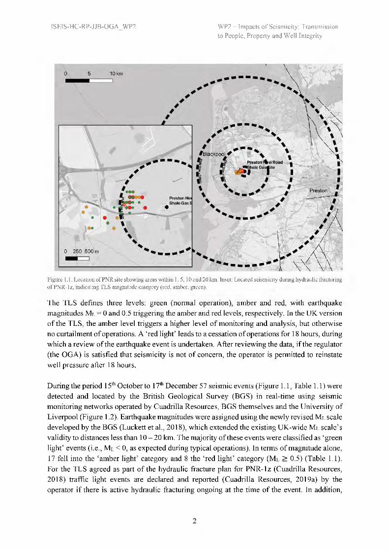
Figure 1.1. Location of PNR site showing areas within 1,5,10 and 20 km. Inset: Located seismicity during hydraulic fracturing of PNR-1z. indicating TLS magnitude category (red, amber, green).
The TLS defines three levels: green (normal operation), amber and red, with earthquake magnitudes ML = 0 and 0.5 triggering the amber and red levels, respectively. In the UK version of the TLS, the amber level triggers a higher level of monitoring and analysis, but otherwise no curtailment of operations. A ‘red light’ leads to a cessation of operations for 18 hours, during which a review of the earthquake event is undertaken. After reviewing the data, if the regulator (the OGA) is satisfied that seismicity is not of concern, the operator is permitted to reinstate well pressure after 18 hours.
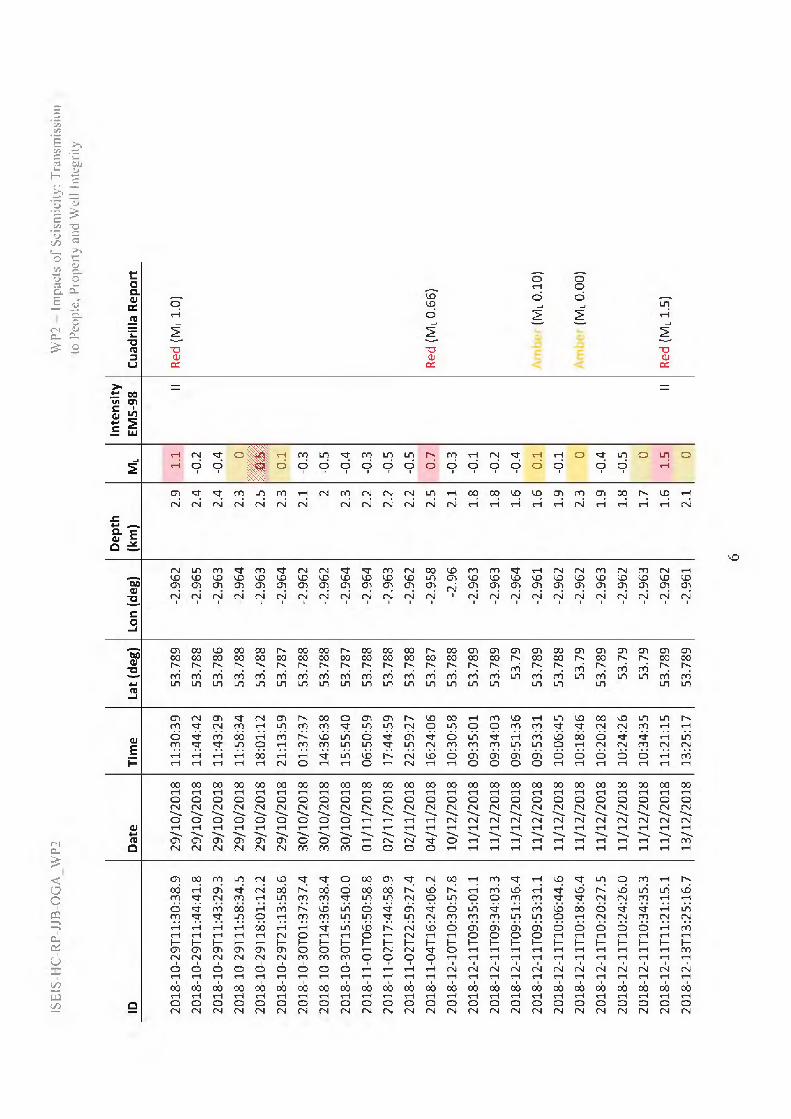
During the period 15th October to 17th December 57 seismic events (Figure 1.1, Table 1.1) were detected and located by the British Geological Survey (BGS) in real-time using seismic monitoring networks operated by Cuadrilla Resources, BGS themselves and the University of Liverpool (Figure 1.2). Earthquake magnitudes were assigned using the newly revised ML scale developed by the BGS (Luckett et al., 2018), which extended the existing UK-wide ML scale’s validity to distances less than 10-20 km. The majority of these events were classified as ‘green light’ events (i.e., ML < 0, as expected during typical operations). In terms of magnitude alone, 17 fell into the ‘amber light’ category and 8 the ‘red light’ category (Ml > 0.5) (Table 1.1). For the TLS agreed as part of the hydraulic fracture plan for PNR-1z (Cuadrilla Resources, 2018) traffic light events are declared and reported (Cuadrilla Resources, 2019a) by the operator if there is active hydraulic fracturing ongoing at the time of the event. In addition,
ISEIS-HC-RP-JJB-OGA_WP2 WP2 — Impacts of Seismicity: Transmissionto People, Property and Well Integrity
significant trailing events (i.e., those falling in to the TLS ‘red light’ category are reported). The reason being that mitigating action can then be taken (pers. comm. OGA, 2019). Of the 17 events detected by the BGS and falling into the range of ‘amber’ and ‘red light’ magnitudes, only six were during active injection, and therefore declared by the operator (Cuadrilla Resources, 2019a) as ‘pumping’ TLS events (3 ‘red light’ and 3 ‘amber light’). In addition, three further ‘red light’ events were declared as ‘trailing’ events, where seismicity occurs after injection has stopped. These were events on:
• 27/10/2018 11:55:25 (ML 0.78)• 04/11/2018 16:24:06 (ML 0.66)• 11/12/2018 11:21:15 (ML 1.5)
Two events (one on 2018-10-24 at 13:02:29.3 and another on 2018-10-29 at 18:01:12.2) that exceed the ‘red light’ TLS magnitude threshold according to BGS assigned ML were not reported by the operator in the HFP report (Cuadrilla Resources, 2019a). This is due to rounding choice (pers. comm. OGA, 2019), with BGS using standard practice of single decimal place magnitude values (which may push a 0.45 event to 0.5). With magnitudes in the ‘amber light’ category (to two decimal places), these ‘non-pumping’ events did not require reporting.
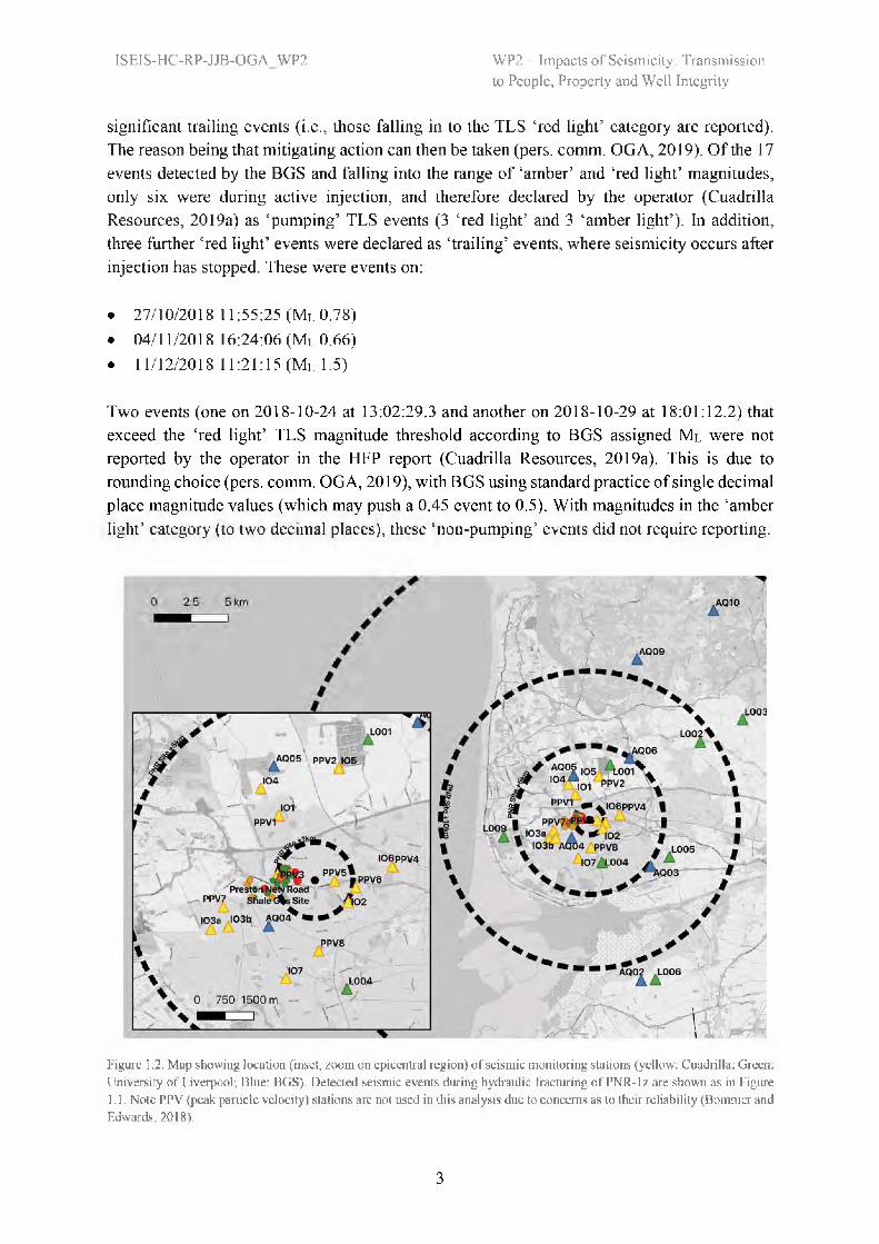
Figure 1.2. Map showing location (inset, zoom on epicentral region) of seismic monitoring stations (yellow: Cuadrilla; Green: University of Liverpool; Blue: BGS). Detected seismic events during hydraulic fracturing of PNR-1z are shown as in Figure 1.1. Note PPV (peak particle velocity) stations are not used in this analysis due to concerns as to their reliability (Bommer and Edwards, 2018).
3
ISEIS-HC-RP-JJB-OGA_WP2 WP2 — Impacts of Seismicity: Transmissionto People, Property and Well Integrity
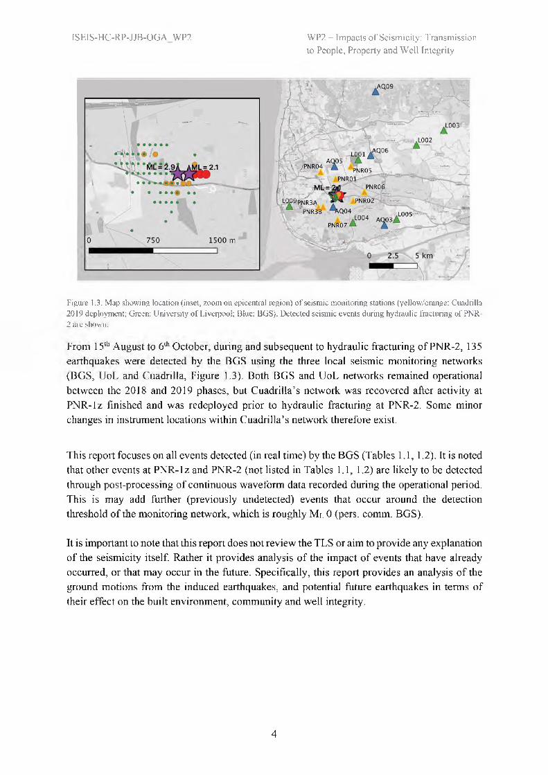
Figure 1.3. Map showing location (inset, zoom on epicentral region) of seismic monitoring stations (yellow/orange: Cuadrilla 2019 deployment; Green: University of Liverpool; Blue: BGS). Detected seismic events during hydraulic fracturing of PNR-2 are shown.
From 15th August to 6th October, during and subsequent to hydraulic fracturing of PNR-2, 135 earthquakes were detected by the BGS using the three local seismic monitoring networks (BGS, UoL and Cuadrilla, Figure 1.3). Both BGS and UoL networks remained operational between the 2018 and 2019 phases, but Cuadrilla’s network was recovered after activity at PNR-1z finished and was redeployed prior to hydraulic fracturing at PNR-2. Some minor changes in instrument locations within Cuadrilla’s network therefore exist.
This report focuses on all events detected (in real time) by the BGS (Tables 1.1,1.2). It is noted that other events at PNR-1z and PNR-2 (not listed in Tables 1.1,1.2) are likely to be detected through post-processing of continuous waveform data recorded during the operational period. This is may add further (previously undetected) events that occur around the detection threshold of the monitoring network, which is roughly ML 0 (pers. comm. BGS).
It is important to note that this report does not review the TLS or aim to provide any explanation of the seismicity itself. Rather it provides analysis of the impact of events that have already occurred, or that may occur in the future. Specifically, this report provides an analysis of the ground motions from the induced earthquakes, and potential future earthquakes in terms of their effect on the built environment, community and well integrity.
4

WP2
- I
mpa
cts
of S
eism
icity
: Tra
nsm
issi
onto
Peo
ple, P
rope
rty a
nd W
ell
Inte
grity
ISEI
S-H
C-R
P-JJ
B-O
GA
_WP2
Tabl
e 1.
1. B
GS
loca
ted
even
ts d
urin
g th
e op
erat
iona
l per
iod
for P
NR
-1z.
Not
e M
L com
pute
d by
BG
S to
one
dec
imal
pla
ce. C
uadr
illa
repo
rt to
two
deci
mal
pla
ces
whi
ch m
ay re
sult
in d
iscr
epan
cy
betw
een
TLS
clas
sific
atio
n. S
olid
bac
kgro
unds
indi
cate
dec
lare
d ev
ents
(i.e
., du
ring
pum
ping
or
sign
ifica
nt tr
ailin
g ev
ents
). H
atch
ed b
ackg
roun
ds in
dica
te T
LS m
agni
tude
cla
ssifi
catio
n, b
ut n
ot
decl
ared
due
to n
o ac
tive
inje
ctio
n. N
ote
in C
uadr
illa
Res
ourc
es (2
019b
) tim
es a
re re
porte
d as
loca
l tim
e (B
ST th
en s
ubse
quen
tly G
MT)
. Tim
es h
ere
are
all G
MT.
IDD
ate
Tim
eLa
t (d
eg)
Lon
(deg
)D
epth
(k
m)
ML
Inte
nsity
EM
S-98
Cuad
rilla
Rep
ort
2018
-10-
18T1
5:48
:53.
618
/10/
2018
15:4
8:54
53,7
85-2
.975
3.2
-0.2
2018
-10-
18T2
2:54
:46.
818
/10/
2018
22:5
4:47
53.7
83-2
.975
3.6
-0.8
2018
-10-
18T2
3:44
:41.
918
/10/
2018
23:4
4:42
53.7
86-2
.978
2.8
-0.3
2018
-10-
19T1
3:20
:48.
519
/10/
2018
13:2
0:48
53.7
83-2
.976
3.7
0.3
2018
-10-
20T0
3:44
:01.
420
/10/
2018
03:4
4:01
53.7
86-2
.978
3.1
0
2018
-10-
23T1
4:45
:32.
523
/10/
2018
14:4
5:32
53.7
87-2
.977
30.
4Am
ber (
ML
0.40
)
2018
-10-
24T1
3:02
:29.
324
/10/
2018
13:0
2:29
53.7
85-2
.971
3.5
0.5
2018
-10-
24T1
3:26
:26.
524
/10/
2018
13:2
6:26
53.7
84-2
.97
3.4
0.4
2018
-10-
24T1
3:51
:31.
524
/10/
2018
13:5
1:32
53.7
84-2
.97
2.9
-0.1
2018
-10-
24T1
4:38
:30.
324
/10/
2018
14:3
8:30
53.7
85-2
.967
3.5
0.1
2018
-10-
24T2
3:56
:12.
924
/10/
2018
23:5
6:13
53.7
83-2
.968
3.8
0
2018
-10-
25T1
4:59
:27.
125
/10/
2018
14:5
9:27
53.7
88-2
.965
2.4
0.3
2018
-10-
25T1
7:00
:33.
825
/10/
2018
17:0
0:34
53.7
87-2
.968
2.3
-0.1
2018
-10-
25T1
7:04
:13.
325
/10/
2018
17:0
4:13
53.7
86-2
.963
2.2
-0.6
2018
-10-
26T0
2:13
:01.
626
/10/
2018
02:1
3:02
53.7
87-2
.966
2.3
-0.2
2018
-10-
26T1
1:26
:44.
626
/10/
2018
11:2
6:45
53.7
88-2
.964
2.2
0.2
2018
-10-
26T1
1:36
:58.
426
/10/
2018
11:3
6:58
53.7
87-2
.963
2.9
0.8
Red
(ML 0
.76)
2018
-10-
26T2
0:39
:22.
726
/10/
2018
20:3
9:23
53.7
86-2
.966
2.3
-0.1
2018
-10-
27T1
0:47
:37.
427
/10/
2018
10:4
7:37
53.7
87-2
.962
2.2
-0.3
2018
-10-
27T1
0:55
:25.
227
/10/
2018
10:5
5:25
53.7
89-2
.963
2.5
0.8
Red
(Ml 0
.78)
2018
-10-
27T1
1:07
:16.
627
/10/
2018
11:0
7:17
53.7
87-2
.964
2.2
-0.2
2018
-10-
27T1
1:44
:31.
127
/10/
2018
11:4
4:31
53.7
88-2
.963
2.4
0
2018
-10-
27T1
3:12
:34.
727
/10/
2018
13:1
2:35
53.7
87-2
.964
2.2
-0.4
5
WP2
- I
mpa
cts
of S
eism
icity
: Tra
nsm
issi
onto
Peo
ple, P
rope
rty a
nd W
ell
Inte
grity
ISEI
S-H
C-R
P-JJ
B-O
GA
_WP2
IDDa
teTi
me
Lat (
deg)
Lon
(deg
)De
pth
(km
)M
LIn
tens
ityEM
S-98
Cuad
rilla
Rep
ort
2018
-10-
29T1
1:30
:38.
929
/10/
2018
11:3
0:39
53.7
89-2
.962
2.9
1.1
IIRe
d (M
L 1.0
)20
18-1
0-29
T11:
44:4
1.8
29/1
0/20
1811
:44:
4253
.788
-2.9
652.
4-0
.220
18-1
0-29
T11:
43:2
9.3
29/1
0/20
1811
:43:
2953
.786
-2.9
632.
4-0
.420
18-1
0-29
T11:
58:3
4.5
29/1
0/20
1811
:58:
3453
.788
-2.9
642.
30
2018
-10-
29T1
8:01
:12.
229
/10/
2018
18:0
1:12
53.7
88-2
.963
2.5
0.5
2018
-10-
29T2
1:13
:58.
629
/10/
2018
21:1
3:59
53.7
87-2
.964
2.3
0.1
2018
-10-
30T0
1:37
:37.
430
/10/
2018
01:3
7:37
53.7
88-2
.962
2.1
-0.3
2018
-10-
30T1
4:36
:38.
430
/10/
2018
14:3
6:38
53.7
88-2
.962
2-0
.520
18-1
0-30
T15:
55:4
0.0
30/1
0/20
1815
:55:
4053
.787
-2.9
642.
3-0
.420
18-1
1-01
T06:
50:5
8.8
01/1
1/20
1806
:50:
5953
.788
-2.9
642.
2-0
.320
18-1
1-02
T17:
44:5
8.9
02/1
1/20
1817
:44:
5953
.788
-2.9
632.
2-0
.520
18-1
1-02
T22:
59:2
7.4
02/1
1/20
1822
:59:
2753
.788
-2.9
622.
2-0
.520
18-1
1-04
T16:
24:0
6.2
04/1
1/20
1816
:24:
0653
.787
-2.9
582.
50.
7Re
d (M
L 0.6
6)20
18-1
2-10
T10:
30:5
7.8
10/1
2/20
1810
:30:
5853
.788
-2.9
62.
1-0
.320
18-1
2-11
T09:
35:0
1.1
11/1
2/20
1809
:35:
0153
.789
-2.9
631.
8-0
.120
18-1
2-11
T09:
34:0
3.3
11/1
2/20
1809
:34:
0353
.789
-2.9
631.
8-0
.220
18-1
2-11
T09:
51:3
6.4
11/1
2/20
1809
:51:
3653
.79
-2.9
641.
6-0
.420
18-1
2-11
TO9:
53:3
1.1
11/1
2/20
1809
:53:
3153
.789
-2.9
611.
60.
1Am
ber
(M
L 0.1
0)20
18-1
2-11
T10:
06:4
4.6
11/1
2/20
1810
:06:
4553
.788
-2.9
621.
9-0
.120
18-1
2-11
T10:
18:4
6.4
11/1
2/20
1810
:18:
4653
.79
-2.9
622.
30
Ambe
r (M
L 0.
00)
2018
-12-
11T1
0:20
:27.
511
/12/
2018
10:2
0:28
53.7
89-2
.963
1.9
-0.4
2018
-12-
11T1
0:24
:26.
011
/12/
2018
10:2
4:26
53.7
9-2
.962
1.8
-0.5
2018
-12-
11T1
0:34
:35.
311
/12/
2018
10:3
4:35
53.7
9-2
.963
1.7
020
18-1
2-11
T11:
21:1
5.1
11/1
2/20
1811
:21:
1553
.789
-2.9
621.
61.
5II
Red
(ML 1
.5)
2018
-12-
13T1
3:25
:16.
713
/12/
2018
13:2
5:17
53.7
89-2
.961
2.1
0
6

WP2
- I
mpa
cts
of S
eism
icity
: Tra
nsm
issi
onto
Peo
ple, P
rope
rty a
nd W
ell
Inte
grity
ISEI
S-H
C-R
P-JJ
B-O
GA
_WP2
IDD
ate
Tim
eLa
t (d
eg)
Lon
(deg
)D
epth
(k
m)
Ml
Inte
nsit
yEM
S-98
Cuad
rilla
Rep
ort
2018
-12-
14T1
3:06
:05.
314
/12/
2018
13:0
6:05
53.7
89-2
.962
1.7
-0.2
2018
-12-
14T1
3:05
:50.
314
/12/
2018
13:0
5:50
53.7
89-2
.963
1.8
-0.6
2018
-12-
14T1
3:06
:36.
814
/12/
2018
13:0
6:37
53.7
89-2
.962
1.8
-0.5
2018
-12-
14T1
3:09
:51.
414
/12/
2018
13:0
9:51
53.7
89-2
.96
1.7
0.1
2018
-12-
14T1
3:18
:30.
314
/12/
2018
13:1
8:30
53.7
89-2
.962
1.8
-0.1
2018
-12-
14T1
3:34
:42.
214
/12/
2018
13:3
4:42
53.7
89-2
.962
1.8
-0.3
2018
-12-
14T1
3:35
:50.
114
/12/
2018
13:3
5:50
53.7
9-2
.963
1.9
-0.5
2018
-12-
14T1
3:41
:05.
514
/12/
2018
13:4
1:05
53.7
89-2
.959
2.2
0.9
Red
(ML 0
.86)
2018
-12-
14T1
4:51
:56.
514
/12/
2018
14:5
1:57
53.7
89-2
.961
2.1
0.1
Tabl
e 1.
2. B
GS
loca
ted
even
ts d
urin
g th
e op
erat
iona
l per
iod
for P
NR
-2. N
ote
ML c
ompu
ted
by B
GS
to o
ne d
ecim
al p
lace
. Cua
drill
a re
port
to tw
o de
cim
al p
lace
s w
hich
may
resu
lt in
dis
crep
ancy
be
twee
n TL
S cl
assi
ficat
ion.
IDDa
teTi
me
Lat
(deg
)Lo
n (d
eg)
Dep
th
(km
)M
LIn
tens
ity
2019
-08-
15T1
2:15
:02.
615
/08/
2019
12:1
5:03
53.7
87-2
.971
2.3
-0.2
2019
-08-
16T0
9:03
:44.
316
/08/
2019
09:0
3:44
53.7
89-2
.971
1.7
-0.7
2019
-08-
16T0
9:08
:47.
016
/08/
2019
09:0
8:47
53.7
81-2
.972
2.7
-0.6
2019
-08-
16T0
9:09
:39.
516
/08/
2019
09:0
9:39
53.7
87-2
.973
2.3
-0.4
2019
-08-
16T0
9:41
:40.
616
/08/
2019
09:4
1:41
53.7
86-2
.968
2.1
-0.8
2019
-08-
16T0
9:51
:40.
216
/08/
2019
09:5
1:40
53.7
87-2
.968
2.1
-0.6
2019
-08-
16T0
9:52
:01.
616
/08/
2019
09:5
2:02
53.7
88-2
.969
1.8
-0.6
2019
-08-
16T1
0:01
:33.
716
/08/
2019
10:0
1:34
53.7
9-2
.966
1.7
-0.8
2019
-08-
16T1
0:05
:45.
216
/08/
2019
10:0
5:45
53.7
9-2
.968
1.7
-0.7
2019
-08-
16T1
0:09
:41.
116
/08/
2019
10:0
9:41
53.7
88-2
.975
2.2
-0.6
2019
-08-
16T1
0:26
:51.
316
/08/
2019
10:2
6:51
53.7
88-2
.972
2.3
-0.5
7

WP2
- I
mpa
cts
of S
eism
icity
: Tra
nsm
issi
onto
Peo
ple, P
rope
rty a
nd W
ell
Inte
grity
ISEI
S-H
C-R
P-JJ
B-O
GA
_WP2
IDDa
teTi
me
Lat (
deg)
Lon
(deg
)D
epth
(k
m)
ML
Inte
nsity
2019
-08-
16T1
1:08
:49.
216
/08/
2019
11:0
8:49
53.7
88 -2
.972
2-0
.6 20
19-0
8-17
T10:
36:0
2.5
17
/08/
2019
10:3
6:03
53
.788
-2.9
72 2.
1 -0
.8 20
19-0
8-17
T10:
39:0
7.7
17
/08/
2019
10:3
9:08
53
.789
-2.9
71 1.
7 -0
.5 20
19-0
8-17
T11:
25:2
3.1
17
/08/
2019
11:2
5:23
53
.789
-2.9
7 1.
7 -0
.6 20
19-0
8-17
T11:
24:4
4.1
17
/08/
2019
11:2
4:44
53
.79
-2.9
7 1.
6 -1
.1 20
19-0
8-19
T09:
35:5
0.5
19
/08/
2019
09:3
5:50
53
.789
-2.9
7 1.
9 0
2019
-08-
19T0
9:40
:50.
0
19/0
8/20
1909
:40:
50
53.7
89 -2
.971
1.9
-0.7
2019
-08-
19T0
9:50
:59.
3
19/0
8/20
1909
:50:
59
53.7
89 -2
.968
2.1
-0.3
2019
-08-
19T1
0:06
:14.
2
19/0
8/20
1910
:06:
14
53.7
89 -2
.968
1.6
020
19-0
8-19
T10:
09:2
4.2
19
/08/
2019
10:0
9:24
53
.789
-2.9
71 1.
8 -0
.6 20
19-0
8-19
T10:
18:1
2.0
19
/08/
2019
10:1
8:12
53
.79
-2.9
71 2
-0.5
2019
-08-
19T1
0:20
:41.
7
19/0
8/20
1910
:20:
42
53.7
89 -2
.97
1.8
-0.5
2019
-08-
20T0
9:06
:26.
1
20/0
8/20
1909
:06:
26
53.7
89 -2
.972
2-0
.6 20
19-0
8-20
T09:
13:5
6.5
20
/08/
2019
09:1
3:56
53
.787
-2.9
64 2.
7 0
2019
-08-
20T0
9:14
:12.
9
20/0
8/20
1909
:14:
13
53.7
86 -2
.964
2.7
-0.1
2019
-08-
20T0
9:16
:54.
4
20/0
8/20
1909
:16:
54
53.7
88 -2
.973
1.9
-0.8
2019
-08-
20T0
9:24
:04.
6
20/0
8/20
1909
:24:
05
53.7
87 -2
.972
2.1
-1.2
2019
-08-
20T0
9:23
:48.
4
20/0
8/20
1909
:23:
48
53.7
88 -2
.968
2.8
-0.7
2019
-08-
20T0
9:33
:37.
8
20/0
8/20
1909
:33:
38
53.7
85 -2
.969
2.1
-0.7
2019
-08-
20T0
9:37
:48.
7
20/0
8/20
1909
:37:
49
53.7
87 -2
.968
1.5
-120
19-0
8-20
T09:
38:2
4.7
20
/08/
2019
09:3
8:25
53
.787
-2.9
73 2.
2 -0
.7 20
19-0
8-20
T09:
41:1
1.5
20
/08/
2019
09:4
1:11
53
.787
-2.9
71 2.
1 -0
.5 20
19-0
8-20
T09:
43:2
7.7
20
/08/
2019
09:4
3:28
53
.787
-2.9
7 2
-0.5
2019
-08-
20T1
0:04
:12.
3
20/0
8/20
1910
:04:
12
53.7
87 -2
.969
1.9
-0.9
2019
-08-
20T1
0:16
:42.
2
20/0
8/20
1910
:16:
42
53.7
87 -2
.969
2.2
-0.3
8

WP2
- I
mpa
cts
of S
eism
icity
: Tra
nsm
issi
onto
Peo
ple, P
rope
rty a
nd W
ell
Inte
grity
ISEI
S-II
C-R
P-JJ
B-O
GA
WP2
IDDa
teTi
me
Lat (
deg)
Lon
(deg
)D
epth
(k
m)
Inte
nsity
2019
-08-
20T1
0:48
:40.
920
/08/
2019
10:4
8:41
53.7
88-2
.973
2.1
-0.5
2019
-08-
20T1
5:24
:47.
7
20/0
8/20
1915
:24:
48
53.7
88 -2
.973
2.2
-0.8
2019
-08-
20T1
6:02
:03.
6
20/0
8/20
1916
:02:
04
53.7
87 -2
.972
2.3
-0.8
2019
-08-
20T1
7:02
:51.
6
20/0
8/20
1917
:02:
52
53.7
86 -2
.971
2.2
-0.9
2019
-08-
20T1
8:49
:45.
9
20/0
8/20
1918
:49:
46
53.7
89 -2
.972
2.2
-0.7
2019
-08-
20T2
0:07
:58.
9
20/0
8/20
1920
:07:
59
53.7
89 -2
.971
2.2
-120
19-0
8-20
T22:
11:
54.0
20
/08/
2019
22:1
1:54
53
.786
-2.9
7 2.
2 -0
.9 20
19-0
8-20
T22:
35:5
9.1
20
/08/
2019
22:3
5:59
53
.788
-2.9
74 2.
2 -1
.3 20
19-0
8-20
T23:
15:4
8.8
20
/08/
2019
23:1
5:49
53
.789
-2.9
73 2.
2 -1
.3 20
19-0
8-20
T23:
35:3
0.1
20
/08/
2019
23:3
5:30
53
.785
-2.9
72 2.
4 -1
.4 20
19-0
8-20
T23:
46:3
3.9
20
/08/
2019
23:4
6:34
53
.788
-2.9
69 2.
3 -1
2019
-08-
21T0
9:45
:54.
3
21/0
8/20
1909
:45:
54
53.7
88 -2
.971
2.1
-0.7
2019
-08-
21T0
9:57
:32.
8
21/0
8/20
1909
:57:
33
53.7
88 -2
.969
2.1
-0.3
2019
-08-
21T0
9:59
:22.
0
21/0
8/20
1909
:59:
22
53.7
86 -2
.967
2.2
-0.7
2019
-08-
21T1
0:02
:20.
9
21/0
8/20
1910
:02:
21
53.7
88 -2
.964
2.3
-0.1
2019
-08-
21T1
0:12
:10.
0
21/0
8/20
1910
:12:
10
53.7
87 -2
.971
2.2
-0.6
2019
-08-
21T1
4:44
:02.
8
21/0
8/20
1914
:44:
03
53.7
88 -2
.966
2.2
-0.8
2019
-08-
21T1
4:46
:01.
5
21/0
8/20
1914
:46:
01
53.7
89 -2
.974
2-0
.8 20
19-0
8-21
T15:
05:2
2.4
21
/08/
2019
15:0
5:22
53
.787
-2.9
7 2.
1 -0
.9 20
19-0
8-21
T15:
12:4
5.2
21
/08/
2019
15:1
2:45
53
.783
-2.9
65 1.
3 -1
2019
-08-
21T1
5:16
:58.
9
21/0
8/20
1915
:16:
59
53.7
88 -2
.966
2-0
.3 20
19-0
8-21
T15:
23:2
5.7
21
/08/
2019
15:2
3:26
53
.787
-2.9
69 2.
1 -0
.8 20
19-0
8-21
T15:
25:1
0.1
21
/08/
2019
15:2
5:10
53
.79
-2.9
67 2.
3 -0
.6 20
19-0
8-21
T15:
38:0
4.4
21
/08/
2019
15:3
8:04
53
.788
-2.9
69 2.
3 -0
.3 20
19-0
8-21
T15:
38:4
6.6
21
/08/
2019
15:3
8:47
53
.787
-2.9
69 2.
2 -0
.7
9
WP2
- I
mpa
cts
of S
eism
icity
: Tra
nsm
issi
onto
Peo
ple, P
rope
rty a
nd W
ell
Inte
grity
ISEI
S-H
C-R
P-JJ
B-O
GA
_W
P2
IDDa
teTi
me
Lat (
deg)
Lon
(deg
)D
epth
(k
m)
ML
Inte
nsity
2019
-08-
21T1
5:42
:32.
221
/08/
2019
15:4
2:32
53.7
88-2
.969
2.1
-0.3
2019
-08-
21T1
5:57
:12.
5
21/0
8/20
1915
:57:
12
53.7
87 -2
.972
2.2
-0.8
2019
-08-
21T1
6:00
:36.
3
21/0
8/20
1916
:00:
36
53.7
88 -2
.967
2.7
-0.4
2019
-08-
21T1
6:03
:15.
9
21/0
8/20
1916
:03:
16
53.7
88 -2
.969
2.3
-0.2
2019
-08-
21T1
7:03
:45.
5
21/0
8/20
1917
:03:
45
53.7
89 -2
.961
2.7
-0.5
2019
-08-
21T1
9:39
:46.
6
21/0
8/20
1919
:39:
47
53.7
87 -2
.968
2.1
-120
19-0
8-21
T19:
46:3
3.3
21
/08/
2019
19:4
6:33
53
.787
-2.9
61 2.
8 1.
6 3
2019
-08-
21T1
9:55
:45.
4
21/0
8/20
1919
:55:
45
53.7
87 -2
.965
2.2
-0.3
2019
-08-
21T2
0:08
:21.
7
21/0
8/20
1920
:08:
22
53.7
86 -2
.964
2.6
-0.3
2019
-08-
21T2
0:21
:35.
9
21/0
8/20
1920
:21:
36
53.7
89 -2
.975
2.2
-0.9
2019
-08-
21T2
1:42
:00.
3
21/0
8/20
1921
:42:
00
53.7
87 -2
.962
2.4
0.9
2019
-08-
21T2
3:04
:43.
5
21/0
8/20
1923
:04:
43
53.7
89 -2
.97
2.3
-1.1
2019
-08-
21T2
3:15
:12.
4
21/0
8/20
1923
:15:
12
53.7
9 -2
.969
2.3
-0.5
2019
-08-
22T0
2:52
:43.
9
22/0
8/20
1902
:52:
44
53.7
86 -2
.965
2.5
0.1
2019
-08-
22T0
6:46
:30.
2
22/0
8/20
1906
:46:
30
53.7
87 -2
.959
2.2
0.3
2019
-08-
22T1
3:59
:51.
7
22/0
8/20
1913
:59:
52
53.7
86 -2
.968
2.1
-0.5
2019
-08-
22T1
5:10
:42.
7
22/0
8/20
1915
:10:
43
53.7
85 -2
.966
2-0
.5 20
19-0
8-22
T15:
23:3
3.9
22
/08/
2019
15:2
3:34
53
.787
-2.9
61 2.
3 1
2
2019
-08-
22T2
0:34
:07.
5
22/0
8/20
1920
:34:
08
53.7
83 -2
.965
2.2
-1.3
2019
-08-
22T2
3:44
:44.
6
22/0
8/20
1923
:44:
45
53.7
86 -2
.963
2.2
-0.3
2019
-08-
23T0
1:22
:20.
7
23/0
8/20
1901
:22:
21
53.7
86 -2
.969
2.4
-0.6
2019
-08-
23T0
2:35
:54.
9
23/0
8/20
1902
:35:
55
53.7
86 -2
.964
2.2
-0.5
2019
-08-
23T0
3:26
:09.
3
23/0
8/20
1903
:26:
09
53.7
84 -2
.964
2.2
-1.2
2019
-08-
23T0
4:33
:36.
1
23/0
8/20
1904
:33:
36
53.7
87 -2
.962
2.4
0.4
2019
-08-
23T0
5:13
:58.
2
23/0
8/20
1905
:13:
58
53.7
84 -2
.966
2.2
-1.4
10
WP2
- I
mpa
cts
of S
eism
icity
: Tra
nsm
issi
onto
Peo
ple, P
rope
rty a
nd W
ell
Inte
grity
ISEI
S-H
C-R
P-JJ
B-O
GA
_W
P2
IDDa
teTi
me
Lat (
deg)
Lon
(deg
)D
epth
(k
m)
ML
Inte
nsity
2019
-08-
23T0
6:51
:17.
223
/08/
2019
06:5
1:17
53.7
88-2
.968
2.1
-0.7
2019
-08-
23T1
3:16
:45.
123
/08/
2019
13:1
6:45
53.7
87-2
.971
2.3
-0.5
2019
-08-
23T1
3:22
:07.
6
23/0
8/20
1913
:22:
08
53.7
87 -2
.971
2.2
-0.6
2019
-08-
23T1
5:26
:09.
0
23/0
8/20
1915
:26:
09
53.7
88 -2
.97
2.2
-0.9
2019
-08-
23T1
7:48
:56.
3
23/0
8/20
1917
:48:
56
53.7
85 -2
.962
2.4
-0.1
2019
-08-
23T1
9:05
:59.
0
23/0
8/20
1919
:05:
59
53.7
86 -2
.965
2-0
.6 20
19-0
8-23
T19:
39:1
5.1
23
/08/
2019
19:3
9:15
53
.787
-2.9
64 2
-0.7
2019
-08-
23T2
1:17
:44.
3
23/0
8/20
1921
:17:
44
53.7
86 -2
.964
2.2
-1.2
2019
-08-
23T2
1:25
:21.
2
23/0
8/20
1921
:25:
21
53.7
85 -2
.966
2-1
2019
-08-
23T2
1:25
:18.
0
23/0
8/20
1921
:25:
18
53.7
85 -2
.965
2-0
.9 20
19-0
8-23
T21:
41:2
1.4
23
/08/
2019
21:4
1:21
53
.786
-2.9
62 2.
3 0.
2 20
19-0
8-23
T22:
22:0
8.6
23
/08/
2019
22:2
2:09
53
.787
-2.9
64 2.
8 1.
1 20
19-0
8-23
T23:
06:0
8.9
23
/08/
2019
23:0
6:09
53
.784
-2.9
61 2.
3 -1
2019
-08-
24T0
2:06
:32.
5
24/0
8/20
1902
:06:
33
53.7
87 -2
.965
1.8
-1.7
2019
-08-
24T0
2:06
:32.
6
24/0
8/20
1902
:06:
33
53.7
85 -2
.964
1.9
-1.6
2019
-08-
24T0
4:01
:07.
7
24/0
8/20
1904
:01:
08
53.7
87 -2
.961
2.5
0.5
2019
-08-
24T0
5:17
:52.
3
24/0
8/20
1905
:17:
52
53.7
84 -2
.964
2.1
-1.6
2019
-08-
24T0
8:24
:26.
2
24/0
8/20
1908
:24:
26
53.7
86 -2
.968
2-1
.1 20
19-0
8-24
T22:
01:3
5.1
24
/08/
2019
22:0
1:35
53
.787
-2.9
62 2.
5 2.
1 4
2019
-08-
25T2
0:10
:04.
7
25/0
8/20
1920
:10:
05
53.7
86 -2
.968
2-1
2019
-08-
25T2
3:20
:24.
9
25/0
8/20
1923
:20:
25
53.7
85 -2
.966
2-1
.6 20
19-0
8-26
T01:
33:3
9.0
26
/08/
2019
01:3
3:39
53
.784
-2.9
68 2.
1 -1
.4 20
19-0
8-26
T03:
39:2
2.8
26
/08/
2019
03:3
9:23
53
.785
-2.9
61 2.
1 -1
.3 20
19-0
8-26
T07:
30:4
7.0
26
/08/
2019
07:3
0:47
53
.787
-2.9
64 2.
5 2.
9 6
2019
-08-
26T0
7:49
:24.
2
26/0
8/20
1907
:49:
24
53.7
84 -2
.967
2.1
-1.3
11

WP2
- I
mpa
cts
of S
eism
icity
: Tra
nsm
issi
onto
Peo
ple, P
rope
rly a
nd W
ell
Inte
grity
ISEI
S-H
C-R
P-JJ
B-O
GA
_WP2
IDDa
teTi
me
Lat
(deg
)Lo
n (d
eg)
Dep
th
(km
)M
LIn
tens
ity
2019
-08-
26T0
9:28
:21.
126
/08/
2019
09:2
8:21
53.7
87-2
.966
1.8
-120
19-0
8-26
T09:
55:5
7.1
26
/08/
2019
09:5
5:57
53
.786
-2.9
64 2
-120
19-0
8-26
T13:
51:5
9.3
26
/08/
2019
13:5
1:59
53
.786
-2.9
65 2.
2 -0
.2 20
19-0
8-26
T13:
51:2
8.7
26
/08/
2019
13:5
1:29
53
.782
-2.9
66 2
-1.4
2019
-08-
26T2
1:18
:29.
2
26/0
8/20
1921
:18:
29
53.7
87 -2
.96
2.7
12
2019
-08-
27T0
4:06
:39.
8
27/0
8/20
1904
:06:
40
53.7
86 -2
.965
2.2
-0.8
2019
-08-
27T0
6:55
:12.
7
27/0
8/20
1906
:55:
13
53.7
87 -2
.959
2.2
0.5
2
2019
-08-
27T0
7:07
:50.
0
27/0
8/20
1907
:07:
50
53.7
87 -2
.967
2-0
.6 20
19-0
8-27
T08:
52:0
9.9
27
/08/
2019
08:5
2:10
53
.785
-2.9
64 2.
1 0.
2 20
19-0
8-27
T11:
47:5
3.2
27
/08/
2019
11:4
7:53
53
.787
-2.9
65 1.
8 -0
.8 20
19-0
8-27
T14:
54:2
0.0
27
/08/
2019
14:5
4:20
53
.785
-2.9
67 2.
7 -0
.7 20
19-0
8-28
T20:
44:1
6.7
28
/08/
2019
20:4
4:17
53
.786
-2.9
65 1.
9 -1
.2 20
19-0
8-29
T01:
23:5
0.7
29
/08/
2019
01:2
3:51
53
.784
-2.9
65 1.
9 -1
.5 20
19-0
8-29
T07:
00:0
5.6
29
/08/
2019
07:0
0:06
53
.784
-2.9
64 1.
8 -1
2019
-09-
01T1
8:42
:07.
7
01/0
9/20
1918
:42:
08
53.7
85 -2
.965
2.2
-0.9
2019
-09-
02T0
3:12
:37.
3
02/0
9/20
1903
:12:
37
53.7
86 -2
.963
2.4
0.2
2019
-09-
02T0
3:12
:21.
3
02/0
9/20
1903
:12:
21
53.7
86 -2
.966
2.4
020
19-0
9-02
T05:
33:0
7.3
02
/09/
2019
05:3
3:07
53
.785
-2.9
64 2.
2 -1
2019
-09-
08T1
6:12
:31.
3
08/0
9/20
1916
:12:
31
53.7
84 -2
.964
2-1
.3 20
19-0
9-10
T02:
52:0
0.3
10
/09/
2019
02:5
2:00
53
.787
-2.9
68 2
-120
19-0
9-12
T05:
31:2
3.2
12
/09/
2019
05:3
1:23
53
.788
-2.9
61 2.
2 0
2019
-09-
14T1
9:50
:16.
5
14/0
9/20
1919
:50:
16
53.7
86 -2
.966
2.2
-0.7
2019
-09-
28T1
8:28
:22.
8
28/0
9/20
1918
:28:
23
53.7
85 -2
.966
2-1
.3 20
19-1
0-06
T00:
26:4
6.5
06
/10/
2019
00:2
6:46
53
.787
-2.9
65 2
-0.6
12
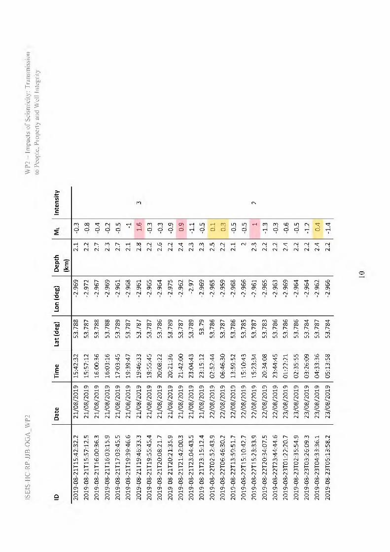
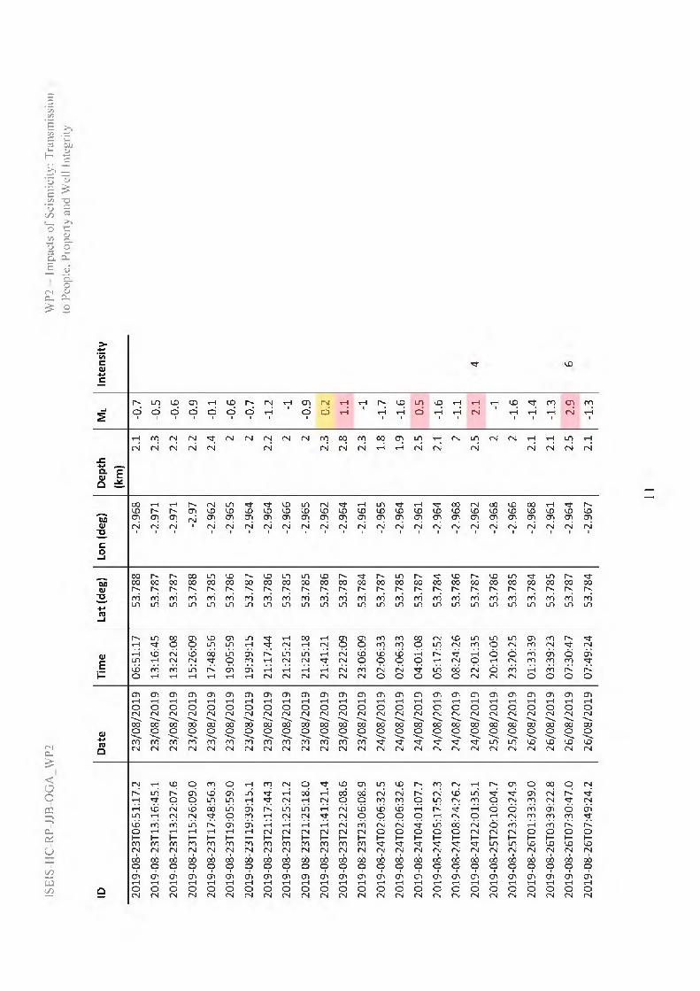
ISEIS-HC-RP-JJB-OGA_WP2 WP2 — Impacts of Seismicity: Transmissionto People, Property and Well Integrity
2. Overview of Ground Motions and their ImpactThe ground motions resulting from earthquakes are complex natural phenomena, the physics of which is, in parts, poorly understood. The earthquake ground motion field (the shaking at some reference horizon, typically the surface) is of primary interest in seismic hazard analysis. It is this motion that applies loading to structures and, in the worst case, leads to damage or failure. The ground motion field itself is a result of several processes, some of which work against one another, and which can therefore lead to significantly different ground motion fields from earthquake to earthquake. In the following section, the parameters used to characterise the complexity of the ground motion field are summarised, in addition to the phenomena that may influence these. We then provide an overview of the relationship between ‘instrumental’ ground motions (i.e., those that are recorded by seismometers or accelerometers) and macroseismic intensity, which reflects a qualitative description of shaking effects (from human perception, through to various damage states). We finally review the effects of ground motion levels on structures and people and through examples relevant to induced seismicity.
2.1 Summary of Ground-Motion CharacteristicsGround motions from earthquake events are transient movements of the surface as seismic waves radiated by an earthquake pass by. At any point at the surface (or to an extent, the subsurface) these movements can be recorded using an accelerometer (recording acceleration) or seismometer or geophone (recording velocity). These instruments typically record continuously in three orthogonal directions (vertical and two horizontal) at sample rates at or above 100 samples per second (although lower sample rates are sometimes utilised). For modem, high-quality instrumentation, signals recorded on either type can be integrated or differentiated to provide any of the three measures of motion (displacement, velocity or acceleration). After an earthquake, the radiated P (primary) and S (secondary, or shear) waves are recorded along with their multiples and coda (waves scattered due to subsurface heterogeneity). In some cases, other waves are also observed, such as surface waves - usually evident for shallow earthquakes and/or distant recordings.
Earthquake ground motions are characterised in various ways. For a given location the characteristics of shaking can broadly be split into: (i) point measures such as peak displacement, velocity and acceleration; (ii) duration of shaking; and (iii) frequency content. Variability of ground motions is also an important characteristic to consider. This variability is described in term of (iv) event-to-event and (v) site-to-site variations around the median. In terms of ground motion fields (i.e., motions over a surface area), the ground motions may also be characterised in terms of their (vi) spatial correlation. These topics are addressed in the following.
13

ISEIS-HC-R-JJB-OGA_WP2 WP2 — Impacts of Seismicity: Transmissionto People, Property and Well Integrity
Figure 2.1. Example earthquake (2018-12-11. ML = 1.5) record at PNR site IO1 east-west direction. Top to bottom: (i) counts as recorded by datalogger (proportional to velocity); (ii) ground velocity (in mm/s); (iii) ground acceleration (in mm/s2) through differentiation of the recorded signal; (iv) ground displacement (mm) through integration and finally, (v) displacement (mm) simulated on a Wood-Anderson seismometer (for local magnitude calculation). PGA, PGV and PGD are indicated for this single horizontal component.
2.1.1 Peak Displacement, Velocity, Acceleration and Response SpectraIn terms of assessing impact on the built environment, the most common ground motion characteristic used by engineers is peak ground acceleration (PGA). For instance, building codes (which specify the design response over various oscillation periods) are often defined using PGA. For a single orientation (e.g., east-west), PGA, and similarly peak ground velocity (PGV) and displacement (PGD) are simply the maxima of the absolute values of acceleration, velocity and displacement, respectively, recorded at a given site (Figure 2.1). For induced seismicity PGV (often also termed peak particle velocity, PPV) is an important parameter, since it is used to define norms and standards within which acceptable motions are permitted (e.g., BS6472-2: BSI, 2008).
Typically, peak values are defined per recording rather than per orientation. Since recordings of ground motion are 3-component there are various ways of defining the record PGA (and equivalently PGV, PGD). The most common is the geometric mean (equivalent to the
14
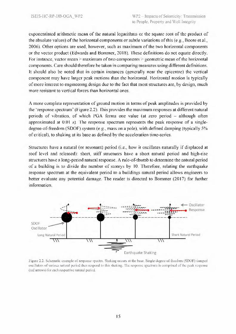
ISEIS-HC-RP-JJB-0GA WP2 WP2 — Impacts of Seismicity: Transmissionto People, Property and Well Integrity
exponentiated arithmetic mean of the natural logarithms or the square root of the product of the absolute values) of the horizontal components or subtle variations of this (e.g., Boore et al., 2006). Other options are used, however, such as maximum of the two horizontal components or the vector product (Edwards and Bommer, 2018). These definitions do not equate directly. For instance, vector mean > maximum of two components > geometric mean of the horizontal components. Care should therefore be taken in comparing measures using different definitions. It should also be noted that in certain instances (generally near the epicentre) the vertical component may have larger peak motions than the horizontal. Horizontal motion is typically of more interest to engineering design due to the fact that most structures are, by design, much more resistant to vertical forces than horizontal ones.
A more complete representation of ground motion in terms of peak amplitudes is provided by the ‘response spectrum’ (Figure 2.2). This provides the maximum responses at different natural periods of vibration, of which PGA forms one value (at zero period - although often approximated at 0.01 s). The response spectrum represents the peak response of a single-degree-of-freedom (SDOF) system (e.g., mass on a pole), with defined damping (typically 5% of critical), to shaking at its base as defined by the acceleration time-series.
Structures have a natural (or resonant) period (i.e., how it oscillates naturally if displaced at roof level and released): short, stiff structures have a short natural period and high-rise structures have a long-period natural response. A rule-of-thumb to determine the natural period of a building is to divide the number of storeys by 10. Therefore, relating the earthquake response spectrum at the equivalent period to a buildings natural period allows engineers to better evaluate any potential damage. The reader is directed to Bommer (2017) for further information.
Figure 2.2. Schematic example of response spectra. Shaking occurs at the base. Single-degree-of-freedom (SDOF) damped oscillators of various natural period then respond to this shaking. The response spectrum is comprised of the peak response (red arrows) for each respective natural period.
15

ISEIS-HC-RP-JJB-OGA_WP2 WP2 — Impacts of Seismicity: Transmissionto People, Property and Well Integrity
2.1.2 Significant Shaking DurationWhile peak motions are important in terms of structural response, high values alone do not necessarily lead to potential damage. For instance, a high PGA associated with a very short signal is associated to negligible displacement since displacement is a double integration (effectively a cumulative sum, twice) of acceleration over time. Similarly, high PGD could be related to a very long duration, which imposes negligible force [for example due to so-called slow earthquakes that often occur at subduction zones (Miller et al., 2002) and take place over hours or days]. It is therefore critical to account for duration of shaking in the assessment of seismic risk (Crowley et al., 2017).
Significant duration of shaking is defined in various ways. Typically, the Arias intensity (AI) (cumulative sum of squared acceleration over time) is determined, which can be thought of as a proxy of the energy in a record. Plotting the cumulative value of AI with respect to time, the duration between various intervals with respect to the total Al is then measured (e.g., 5 - 95% or 5 - 75%). Generally, earthquakes follow a predictable pattern in terms of the expected significant duration with a function of magnitude, distance (larger in both cases leads to longer duration) and, to a limited extent, site class or average shear-wave velocity in the upper 30 m (Vs30). Empirical models exist that provide predictions for various measures of duration (e.g., Kempton and Stewart, 2006; Bommer et al., 2009), however, these tend to be for tectonic events with magnitudes greater than 3. For the very near-source and small magnitude events associated with induced seismicity it may be sufficient to consider the expected source duration itself, as given by simple models of earthquakes (Brune, 1970, 1971; Madariaga, 1976). These models relate the earthquake stress drop (see Section 2.2.4) to their source comer frequency and consequently signal duration.
2.1.3 Frequency ContentThe frequency content of earthquake ground motions has an important bearing on their effect on structures. As noted previously, all structures have a natural period (the reciprocal of natural frequency) and are therefore sensitive to motions at these frequencies. Earthquake signals have a characteristic frequency amplitude spectrum (FAS: the distribution of amplitudes at various frequencies). The shape of an earthquake acceleration record FAS is a approximated by a trapeze, with amplitudes increasing up to a first corner proportional to frequency squared, then flat, followed by an exponential decay at high frequencies (Figure 2.3). The spectral shape is, in general, defined by the first corner frequency, which is proportional to magnitude (Brune, 1970) (Figure 2.3, right) and the rate of high-frequency decay, known as k (Anderson and Hough, 1984), which is proportional to distance (Figure 2.3, left), k is also influenced by site type, with low Vs30 sites (e.g., thick sedientary deposits) leading to strongly damped signals and therefore a high rate of spectral decay. The combination of small magnitudes for induced seismicity and potentially high k at low Vs30 sites means that the characteristic spectral shape of these events is almost identical, only scaled in amplitude by magnitude.
16

ISEIS-HC-RP-JJB-OGA_WP2 WP2 — Impacts of Seismicity: Transmissionto People, Properly and Well Integrity
Figure 2.3. Schematic example of frequency content of earthquake records with (left) increasing distance for one event; (right) various magnitude events at the same distance. Note that this example (right) does not consider the effect of strong local damping (e.g., due to thick low velocity sediments), which may lead to a constant apparent f0 independent of earthquake magnitude.
While the ideal spectral shape is fairly simple, in reality the frequency content is more complex and may be influenced by other factors, such as site resonance and earthquake stress drop. The frequency content of earthquake ground motions is inherently included in ground motion prediction equations (see Section 2.3). Any systematic difference in the frequency content of records (e.g., due to particular site resonance effects, or to particularly high or low earthquake stress drop) at a particular location may lead to systematic over- or under-prediction of ground motion amplitudes. This is discussed further in Section 2.2.
2.1.4 VariabilityEarthquake ground motions are highly variable due to the complexities of fault rupture, and wave propagation through the heterogeneous subsurface (e.g., Edwards et al., 2019). The variability in ground motion due to this complexity is not captured in median predictions from GMPEs, which are designed to robustly determine ground motions given a set of limited predictor variables (magnitude, M, depth, H, distance to site, R, 30m average shear-wave velocity of site, Vs30, etc.). Instead GMPEs capture random variability through standard deviations on their predictions. The determination of these standard deviations (aleatory variability) is as important as the median values themselves. The aleatory variability of a GMPE is commonly assumed to be lognormally distributed and split into two parts: between event (with standard deviation, τ), and within event (φ), such that the logarithm of an arbitrary ground motion intensity is given by:
log Y = f(M, R, H, Vs30 ... ) + B (τ) + W (φ). (1)
For a given intensity measure, e.g., PGV, a single between-event term, B(t ), is sampled from a zero-mean Guassian distribution with standard deviation t (accounting for the average difference of an event’s ground motions with respect to the median predictions). Within-event
17
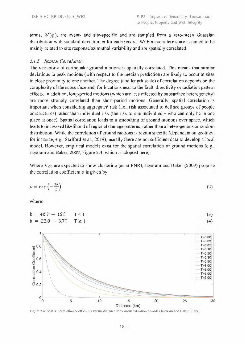
ISEIS-HC-RP-JJB-OGA_WP2 WP2 — Impacts of Seismicity: Transmissionto People, Property and Well Integrity
terms, W(φ), are event- and site-specific and are sampled from a zero-mean Guassian distribution with standard deviation φ for each record. Within event terms are assumed to be mainly related to site response/azimuthal variability and are spatially correlated.
2.1.5 Spatial CorrelationThe variability of earthquake ground motions is spatially correlated. This means that similar deviations in peak motions (with respect to the median prediction) are likely to occur at sites in close proximity to one another. The degree (and length scale) of correlation depends on the complexity of the subsurface and, for locations near to the fault, directivity or radiation pattern effects. In addition, long-period motions (which are less effected by subsurface heterogeneity) are more strongly correlated than short-period motions. Generally, spatial correlation is important when considering aggregated risk (i.e., risk associated to defined groups of people or structures) rather than individual risk (the risk to one individual - who can only be in one place at once). Spatial correlation leads to a smoothing of ground motions over space, which leads to increased likelihood of regional damage patterns, rather than a heterogenous or random distribution. While the correlation of ground motions is region specific (dependent on geology, for instance, e. g., Stafford et al., 2019), usually there are not sufficient data to develop a local model. However, empirical models exist for the spatial correlation of ground motions (e.g., Jayaram and Baker, 2009, Figure 2.4, which is adopted here).
Where Vs30 are expected to show clustering (as at PNR), Jayaram and Baker (2009) propose the correlation coefficient p is given by:
p = exp(—y)
(2)
where:
b = 40.7 - 15T T< 1 (3)b = 22.0 - 3.7T T ≥ 1 (4)
Figure 2.4. Spatial correlation coefficients versus distance for various vibration periods (Jayaram and Baker. 2009).
18

ISEIS-HC-RP-JJB-OGA_WP2 WP2 — Impacts of Seismicity: Transmissionto People, Property and Well Integrity
They propose that for application of their model, one should: 1. Obtain median ground-motion values at the sites of interest using a ground motion
prediction equation (GMPE); 2. Probabilistically generate the GMPE inter-event term which follows a zero-mean
univariate normal distribution; 3. Simulate the location-specific intra-event terms using the standard deviations from the
ground-motion models and the respective correlation coefficients (Equation 1); 4. Combine the three terms generated in Steps 1-3 to obtain correlated ground-motions at the
sites of interest.
2.2 Factors Influencing Ground MotionsThe main contributors to the strength of earthquake ground motions are: 1. Earthquake magnitude; 2. Distance of site from earthquake source (attenuation); 3. The site’s geology, specifically its shear-wave velocity profile; 4. Earthquake rupture properties (e. g., stress drop); 5. Wave propagation effects (e. g., focussing).
2.2.1 Earthquake MagnitudeEarthquake magnitude can be considered the most direct factor influencing earthquake ground motion. An earthquake’s magnitude describes its ‘size’ and works on a logarithmic scale. However, as with any size characterisation, there are a variety of ways that this is performed. Some measures (e.g., moment magnitude, denoted M or Mw; Hanks and Kanamori, 1979) relate to physical characteristics of the fault (crack) that generated seismic waves (and the resulting surface shaking). Other magnitudes (e.g., local magnitude, ML; Richter, 1935) effectively describe the surface effects (such as the peak ground displacement) normalized to a common reference distance, without consideration of the physical source itself.
ML is calculated for all located UK earthquakes by the BGS. Recently, the BGS has published an updated ML model (Luckett et al., 2018), which is also valid at the very short distances typical for records of induced seismicity. ML is based on the ‘Wood-Anderson’ amplitude, which is the displacement on a (simulated) Wood-Anderson seismograph (see Figure 2.1). Since the majority of GMPEs are based on moment magnitude, M, these values must be converted.
Different earthquake magnitude scales (Ml , M) are usually calibrated (over a limited range) to be consistent with one another. However, there is no guarantee that they are similar throughout—particularly at the low end (Ml < 2) typical in induced seismicity (Edwards and Douglas, 2013; Dost et al., 2018, 2019). For instance, moment magnitude of induced earthquakes (Ml < 2) is systematically higher than the local magnitude for a given event. The model of Grünthal et al. (2009) converts between ML and M over a wide magnitude range (down to ML -0.8 , although with limited data below ML 1). At the low magnitude end the
19

WP2 — Impacts of Seismicity: Transmissionto People, Property and Well Integrity
ISEIS-HC-RP-JJB-OGA_WP2
gradient between ML and M approaches 0.67. Numerous studies have shown consistency with this model (Dost et al., 2018, 2019), although small (< 0.1 unit) region-specific offsets are sometimes apparent (e.g., Edwards et al., 2015). In the ML < 1 range, Deichmann (2017) showed that M µ 2/3 ML for ML << 2, confirming the empirical observations.
To convert the ML values of the PNR dataset, we therefore assume:
M = 0.0376M2L + 0.646ML + 0.53 (Ml > 2.5) (Grünthal et al., 2009) (5a)
and
M = 2/3Ml + 0.833
(Ml < 1.5) (Edwards et al., 2015) (5b)
with linear transition in the range 1.5 ≤ ML ≤ 2.5.
In July 2019 Cuadrilla Resources published their hydraulic fracture plan for PNR-2, this included an analysis of ML and M for the PNR-1z data. They found, in the range -0.8 < Ml <1.5 that:
M = 0.655ML + 0.897 (-0.8 ≤ ML ≤ 1.5) (Cuadrilla Resources, 2019b). (5c)
The PNR-1z empirical model (Equation 5c) is remarkably similar to the empirical-theoretical model proposed by Edwards et al. (2015) (based on Deichmann, 2017) and adopted for this work (Figure 2.5) and therefore justifies the use of Equation 5b in the small magnitude range.
Figure 2.5. Local to moment magnitude conversions.
20
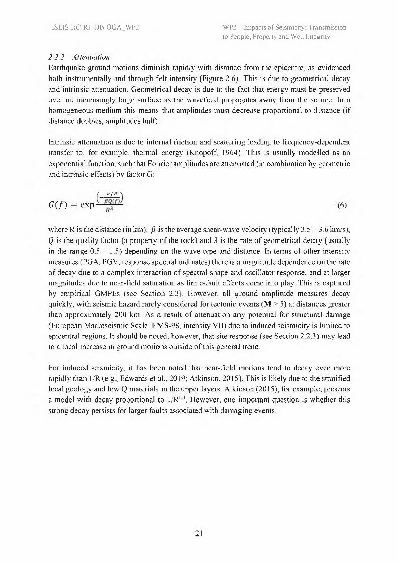
WP2 — Impacts of Seismicity: Transmissionto People, Property and Well Integrity
ISEIS-HC-RP-JJB-OGA_WP2
2.2.2 AttenuationEarthquake ground motions diminish rapidly with distance from the epicentre, as evidenced both instrumentally and through felt intensity (Figure 2.6). This is due to geometrical decay and intrinsic attenuation. Geometrical decay is due to the fact that energy must be preserved over an increasingly large surface as the wavefield propagates away from the source. In a homogeneous medium this means that amplitudes must decrease proportional to distance (if distance doubles, amplitudes half).
Intrinsic attenuation is due to internal friction and scattering leading to frequency-dependent transfer to, for example, thermal energy (Knopoff, 1964). This is usually modelled as an exponential function, such that Fourier amplitudes are attenuated (in combination by geometric and intrinsic effects) by factor G:
f nfR \G(ft = exp)((-nfR) (6)
where R is the distance (in km), β is the average shear-wave velocity (typically 3.5 - 3.6 km/s), Q is the quality factor (a property of the rock) and A is the rate of geometrical decay (usually in the range 0.5 - 1.5) depending on the wave type and distance. In terms of other intensity measures (PGA, PGV, response spectral ordinates) there is a magnitude dependence on the rate of decay due to a complex interaction of spectral shape and oscillator response, and at larger magnitudes due to near-field saturation as finite-fault effects come into play. This is captured by empirical GMPEs (see Section 2.3). However, all ground amplitude measures decay quickly, with seismic hazard rarely considered for tectonic events (M > 5) at distances greater than approximately 200 km. As a result of attenuation any potential for structural damage (European Macroseismic Scale, EMS-98, intensity VII) due to induced seismicity is limited to epicentral regions. It should be noted, however, that site response (see Section 2.2.3) may lead to a local increase in ground motions outside of this general trend.
For induced seismicity, it has been noted that near-field motions tend to decay even more rapidly than 1/R (e.g., Edwards et al., 2019; Atkinson, 2015). This is likely due to the stratified local geology and low Q materials in the upper layers. Atkinson (2015), for example, presents a model with decay proportional to 1/R1.3. However, one important question is whether this strong decay persists for larger faults associated with damaging events.
21
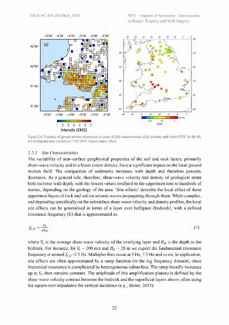
WP2 — Impacts of Seismicity: Transmissionto People, Property and Well Integrity
ISEIS-HC-RP-JJB-OGA_WP2
Figure 2.6. Example of ground motion attenuation in terms of (left) macroseismic (felt) intensity and (right) PGV for the ML 4.6 earthquake near Cardiff on 17/02/2018. Figure source: BGS.
2.2.3 Site CharacteristicsThe variability of near-surface geophysical properties of the soil and rock layers, primarily shear-wave velocity and to a lesser extent density, have a significant impact on the local ground motion field. The compaction of sediments increases with depth and therefore porosity decreases. As a general rule, therefore, shear-wave velocity and density of geological strata both increase with depth, with the lowest values confined to the uppermost tens to hundreds of metres, depending on the geology of the area. ‘Site effects’ describe the local effect of these uppermost layers of rock and soil on seismic waves propagating through them. While complex, and depending specifically on the subsurface shear-wave velocity and density profiles, the local site effects can be generalised in terms of a layer over halfspace (bedrock), with a defined resonance frequency (f0) that is approximated as:
f = -Vs'r‘0 4HB (7)
where Vs is the average shear-wave velocity of the overlying layer and HB is the depth to the bedrock. For instance, for Vs = 200 m/s and HB = 20 m we expect the fundamental resonance frequency at around fr,0=2.5 Hz. Multiples then occur at 5 Hz, 7.5 Hz and so on. In application, site effects are often approximated by a ramp function (in the log frequency domain), since theoretical resonance is complicated by heterogeneous subsurface. The ramp broadly increases up to f0, then remains constant. The amplitude of this amplification plateau is defined by the shear-wave velocity contrast between the bedrock and the superficial layers above, often using the square-root impedance for vertical incidence (e.g., Boore, 2013):
22

WP2 — Impacts of Seismicity: Transmissionto People, Property and Well Integrity
ISEIS-HC-RP-JJB-OGA_WP2
A(f)=fe)0.5 (8)
with the impedance given by the product of average density, ρ, and shear-wave velocity in the layers above (subscript s) and below (subscript b) a frequency-dependent reference depth. This depth is defined (Joyner et al., 1981) as the quarter-wavelength depth, similar to Equation 7, such that the reference depth above/below which to calculate the averages is defined as:
Hs(f)=Vs 4f (9)
This implies that for a site with bedrock Vs of 2000 m/s and near-surface Vs of around 200 m/s (density tends to be a minor influence), amplification of the ground-motion field reaches a factor of around 3 on average, although this is usually exceeded locally at frequencies near f0 for sites with simple layered stratigraphy (Boore, 2013).
In addition to the amplification effect of decreasing seismic velocity toward the surface, a counteractive effect of damping, D(f), applies at high frequency (Anderson and Hough, 1984):
D(f) = exp (-πfKo) (10)
where κ0 is a site specific damping term, related to Q (a property defining seismic attenuation per wave cycle). Near surface materials have low Q, which leads to strong damping of high-frequency motions as they propagate through the upper layers. Lower velocity materials (sediments, soil) lead to stronger damping. The combination of the amplification described above (e.g., Equations 8, 9) and damping effects (Equation 10) lead to an overall site effect approximated by an initial ramp, followed by exponential decay at high frequency. For low- velocity sites we observe strong amplification followed by strong attenuation as frequency increases. For high-velocity sites, we observe limited amplification but also only weak attenuation of amplitude at high frequency.
As a further generalisation for response spectra the upper 30 m average shear-wave velocity has been shown to correlate very well to averages over various depths Vsx and therefore amplification (Boore et al., 2011). As such modern GMPEs are normally constructed using Vs30 as a predictor variable, with lower values (in general) leading to stronger predicted motions.
The site amplification discussed above concern what are referred to as linear effects—those independent of the input motion. As such, an amplification factor always applies, regardless of the scenario. In reality we observe that for strong motions on low velocity sites, amplification is typically reduced due to the non-linearity of soil response to shaking (e.g., Sandikkaya et al., 2013). As a result of this, low-velocity soils (Vs30 < 300 m/s) may lead to weaker amplification (or even de-amplification) for near-source moderate to large magnitude events than higher- velocity soil (the opposite to linear response, described previously). Non-linear effects are
23
ISEIS-HC-RP-JJB-OGA_WP2 WP2 — Impacts of Seismicity: Transmissionto People, Property and Well Integrity
typically included in modern GMPEs and are considered in the analysis presented later in this report.
2.2.4 Earthquake Stress DropEarthquakes are typically characterised in terms of their moment magnitude (M), a logarithmic scale that describes the seismic moment (Mo) of an event [M log(M0) — = (2/3) 6.03, in SI units]. Seismic moment itself is defined by the product of average slip, fault area and the shear modulus (the latter being broadly constant within the crust). Therefore, M is a static measure and independent of the kinematic or dynamic characteristics of the earthquake itself. For example, an earthquake with rupture area 60 x 15 km, average slip of 1.2m (and shear modulus of 32 GPa for the crust) will always be defined as M 7. However, in terms of ‘end-member’ possibilities M 7 events (or equally any large magnitude earthquake) can then be either potentially devastating when slip occurs over seconds to minutes (as ‘earthquake’ is typically understood), or practically unnoticed when a fault (with identical geometric properties) slips over hours or days (as observed for ‘slow’ earthquakes, Miller et al., 2002).
The dynamic stress drop (Act , the tectonic driving stress minus the dynamic frictional stress) helps us to further characterise a seismic event beyond its moment magnitude, and can be considered a proxy for energy release. The dynamic stress drop during a seismic event has a significant impact on the radiated wavefield. Returning to the previous example we observe
Δσ ~ 1 to 10 MPa for normal (potentially damaging) earthquakes, whereas for ‘slow’ earthquakes (with limited high-frequency energy released) we observe Δσ ~ 0.01 to 0.1 MPa, two orders of magnitude smaller.
There are various ways of defining stress drop ( or stress parameter), but as used in engineering seismology stress parameter effectively it defines the proportion of high-frequency radiated energy for a given magnitude, with higher stress drop events radiating more high-frequency energy (Figure 2.7, left). For increasing magnitude events, for a given stress parameter, the source corner frequency
(fc), decreases (Figure 2.7, right), but magnitude dependent changes in stress parameter may give rise to a change in the reduction of fc as magnitude increases.
In terms of response spectral ordinates, increase in stress parameter leads to stronger mid (e.g., PGV) to short period (e.g., PGA) ordinates. Potential regional variations in stress parameter may mean that GMPEs developed in other settings do not correctly predict median motions. Of particular relevance in induced seismicity, it is thought that earthquake stress drop is depth-dependent, with deeper earthquakes leading to higher stress drop. Some recent GMPEs account for this in their predictions (e.g., Chiou et al, 2014), but many do not. Since GMPEs are usually developed using predominantly deep tectonic events, this may lead to an overestimate when applied to shallow induced seismicity.
24

WP2 — Impacts of Seismicity: Transmissionto People, Property and Well Integrity
ISEIS-HC-RP-JJB-OGA_WP2
Figure 2.7. Schematic representation of the impact of stress drop (parameter) on Fourier spectral amplitudes.
2.3 Prediction of Ground MotionsGround motions are predicted through ground motion models (GMMs). In its simplest form a GMM is a ground motion prediction equation (GMPE). GMPEs provide a statistical estimate of the expected median ground motion and its standard deviation due to a given earthquake scenario. GMPEs are developed for various ground motion intensity measures. For instance, 5% damped pseudo-spectral acceleration (PSA), which is given by the product of the squared angular frequency (ω1 2) and the absolute spectral displacement (SD) of a simple harmonic oscillator, damped to 5% of critical, SD itself, pseudo-spectral velocity (PSV = ωSD), peak ground acceleration (PGA) or peak ground velocity (PGV). Each ground motion measure has its own advantages and is selected depending on application.
The form of GMPEs is typically:
log Y — Fsource + Fpath + Fsite + B (τ ) + W(φ) (11)
where Y is a ground motion intensity, predicted in terms of its natural or base-10 logarithm (since ground motion residuals are observed to be log-normally distributed). Units of ground motion provided by GMPEs are not standardized and may be in terms of SI units (m, m/s, m/s2), CGS units (cm, cm/s, cm/s2 or gal) or in units of gravity. A set of recommendations regarding selection of GMPEs (e.g., on functional form) are made by Bommer et al. (2010) and Cotton et al. (2006). Bommer et al. (2010) proposed to exclude GMPEs from probabilistic seismic hazard analyses if:
1. The model is derived for an inappropriate tectonic environment.2. The model is not published in a Thomson Reuters ISI-listed peer reviewed journal
(although an exception can be made for an update to a model that did meet this criterion).
25

ISEIS-HC-RP-JJB-OGA_WP2 WP2 — Impacts of Seismicity: Transmissionto People, Property and Well Integrity
3. The dataset used to derive the model is not presented in a table listing the earthquakes and their characteristics, together with the number of records from each event.
4. The model has been superseded by a more recent publication.5. The model does not provide spectral predictions for an adequate range of response periods.6. The functional form lacks either non-linear magnitude dependence or magnitude-
dependent decay with distance.7. The coefficients of the model were not determined with a method that accounts for inter-
event and intra-event components of variability; in other words, models must be derived using one- or two-stage maximum likelihood approaches or the random effects approach.
8. Model uses inappropriate definitions for explanatory variables or models site effects without consideration of site characterization, such as Vs30.
9. The range of applicability of the model is too small to be useful for any relevant extrapolations.
10. Model constrained with insufficiently large dataset: fewer than 10 earthquakes per unit of magnitude or fewer than 100 records per 100 km of distance.
However, it should be noted that some of these considerations are not as relevant for induced seismicity. A comprehensive resource of available GMPEs is maintained by Dr John Douglas (University of Strathclyde) and is available online at gmpe.org.uk (last accessed 08/2019).
As noted by Bommer and Edwards (2018) there are several important considerations when selecting GMPEs specifically for induced seismicity, summarised here:
• Magnitude: due to close proximity to population centres, induced seismicity is typically considered as a risk at smaller magnitude than considered for tectonic seismicity (for the latter generally M > 4.5). As a result, many GMPEs are not developed with a suitable range of magnitude and are therefore not technically applicable for induced seismicity. In fact there are very few models valid without adjustment at M < 3. Several studies have shown that the extrapolation (without adjustment of coefficients and/or functional form) of GMPEs to smaller magnitudes will generally lead to gross over-estimation of the predicted amplitudes (Bommer et al., 2007; Atkinson and Morrison, 2009; Chiou et al., 2010). Magnitude type also has an important impact on the predictions, particularly in the range M < 3 where M is not equivalent, but proportional to 0.67 ML (Dost et al., 2017). This difference in magnitude type may lead to incorrect conclusions where GMPEs apparently match at low M when wrongly assuming equivalence.
• Depth: induced seismicity tends to occur at shallow depths - at PNR around 2 to 3 km. On the other hand tectonic earthquakes (which the majority of GMPEs are developed with) typically occur at greater depths (around 10 km). Two considerations are necessary here:(i) due to their proximity to the surface they may lead to higher ground motions than for an equivalent tectonic event at greater depth; but counteracting this (ii) due to their shallow depth (and lower confining stress), their stress drop may be lower, leading to lower ground motions than for a deeper event of the same magnitude;
26
WP2 — Impacts of Seismicity: Transmissionto People, Property and Well Integrity
ISEIS-HC-RP-JJB-OGA_WP2
• Distance: hazards due to induced seismicity are focussed in the very-near epicentral region, a region where very little empirical data exists. As for magnitude (above) this means that many GMPEs are not technically applicable and must be extrapolated and/or adjusted beyond their valid range. Accounting for the importance of near-field prediction and the shallow depth sources, it is important to use a distance measure that reflects this such as hypocentral or rupture distance;
• Near source saturation: a common feature of many modem GMPEs is the phenomenon of near-source saturation, which is essentially a flattening of the attenuation curves at short distances. Since this is related to the dimensions of the earthquake source (i.e., fault rupture) the distance saturation is dependent on magnitude, with the flattened part of the attenuation curve extending over greater distances from the source for larger earthquakes. The magnitude dependence of the near-source distance saturation persists for moderate-magnitude earthquakes and it is important that the adopted GMPE is able to correctly model this feature in the magnitude range of applicability for induced seismicity (e.g., Yenier and Atkinson, 2014; Yenier et al., 2016).
• Site classification: GMPEs are typically developed either for a reference site or with a predictor variable that allows different site types to be considered. It is important that the GMPE selected is suitable for the Vs30 in the region, since this can lead to significant differences in predictions.
• Other predictor variables: factors such as source mechanism are not considered as important as those above (since they generally lead to relatively minor changes in prediction) and may need to be assumed. It is therefore better to have a simple model form that can be easily adjusted at a later point.
There exist several hundred GMPEs in the literature, with many differences in parameterisation and model form. Based on a study conducted by Arup (Arup, 2014), the ground-motion prediction equation (GMPE) adopted for application at Preston New Road by the operator was the European model of Akkar et al. (2014). Shortcomings with this selection were, however, noted by Bommer and Edwards (2018) and the model is therefore not considered here. Instead, we focus on two GMPEs which are commonly used for predicting ground motions due to induced seismicity: Atkinson (2015) and Douglas et al. (2013). Their parameterisation, model form and consideration of uncertainty is discussed in the following. For more general review of development of GMPEs, the reader is referred to Douglas and Edwards (2016).
The GMPE of Atkinson (2015) was specifically developed for instances of induced seismicity. The model is developed using a high-quality earthquake ground motion database (NGA-West2, Anchetta et al., 2014) comprised of records from tectonic events (M 3 to 6 at distances up to 40 km) worldwide. However, the majority of events for the smaller magnitudes are from tectonic (and not exclusively shallow) Californian earthquakes. The model has the form:
logY = c0 + C1M + c 2M2 + c3logR + B(τ ) + W(φ) (12)
27

WP2 — Impacts of Seismicity: Transmissionto People, Property and Well Integrity
ISEIS-HC-RP-JJB-OGA_WP2
with Y the ground motion intensity (PGA, PGV, PSA at given period), M is the moment magnitude (not necessarily equivalent to local magnitude) and R is the distance in km, given by:
R = R2hyp + h2eff
(13)
where Rhyp is the distance to the earthquake hypocentre and heff accounts for near-epicentre saturation of motions. Atkinson proposed two alternatives: heff = max(1, 10-1.72+0.43M) and heff = max(1, 10-0.28+0.19M). The latter formulation is suggested by Bommer and Edwards
(2018), and is used here. Logarithms are base 10 and the ground motion intensities are in cm/s2 for PGA, PSA, or cm/s for PGV. B(t ) and W(φ) are samples from the log-normal distributions describing the within-event and between-event variability, respectively. The predictions are made for a reference Vs30 = 760 m/s. Predictions of other site types (Vs30 values) is achieved using the site response model of Boore et al. (2014) and the appropriate reference rock Vs30 (760m/s for Atkinson, 2015, and 1100 m/s for Douglas et al., 2013). We note that the model of Atkinson (2015) is specifically designed for use with the amplification model of Boore et al. (2014), whereas for the model of Douglas et al. (2013) we are making the assumption that the different reference rock condition can be adjusted through the use of appropriate reference rock Vs30.
Tables of coefficients (c0-3) and standard deviations (τ and φ) are provided by Atkinson (2015) based on regression to the dataset used in their study for several ground motion intensity values (PGV, PGA and PSA at selected periods). This GMPE follows a simple functional form, with reference motions implicitly defined at M = 0 and R = 1 km as c0. Quadratic magnitude scaling accounts for the increase of ground shaking with magnitude (the relative increase of motions from one magnitude to the next decreases for increasingly large events due to finite fault size effects).
c3logR accounts for the attenuation of ground motions with increasing distance, and is roughly equivalent to geometrical decay (see Section 2.2.2), with strong decay proportional to R-1.4 at long-periods. It is noted that this decay also includes the effect of the oscillator response and duration at short periods, however, which leads to increased rates of decay. Intrinsic attenuation is not directly considered in this model due to the near-source distances that it is focussed on (Rhyp < 40 km). Variability in this model follows the standard form described in Section 2.1.4.
The GMPE of Douglas et al. (2013) is based on a ground motion dataset of shallow induced events (although some related to natural processes). The dataset included events with M 1 to 4 at distances up to 20 km. The authors produced a homogenised catalogue, with M calculated consistently for all events. We use Model 1 of their work (two other models were produced to show the sensitivity of various assumptions). One model was produced without correction for site effects, and one with sites corrected to a reference rock with Vs30 = 1100 m/s. We present the latter, which can, as for Atkinson (2015), be used for various Vs30 sites by using the Boore
28
WP2 — Impacts of Seismicity: Transmissionto People, Property and Well Integrity
ISEIS-HC-RP-JJB-OGA_WP2
et al. (2014) site response model (with Vref = 1100 m/s). The Douglas et al. (2013) model has the form:
ln Y = a + bM + c ln R + dRhyp + B(t ) + W(φ). (14)
In their model, ground motion units are SI (i.e., m/s2 for PGA, PSA or m/s for PGV). They also use natural logarithms rather than base-10. The main difference in this model to Atkinson’s is the lack of M2 term. This is because it is based on data below the value where the term has an impact (M > 4). They use the same distance metric (Equation 13), although the heff term is period dependent in their model. Douglas et al. (2013) also define an ‘intrinsic decay’ term (d), although at these short distances it is not clear how well resolved this is. Their model uses the standard within- and between-event variability. The values presented are much higher than Atkinson’s however. This may be due to the various sources of data used, and potentially poor metadata for site characteristics and small magnitude events.
The above GMPEs are both directly applicable only to rock sites, specifically sites with Vs30 = 760 (Atkinson, 2015) or Vs30 =1100 m/s (Douglas et al., 2013). In order to apply the GMPEs to sites with arbitrary site condition we use the site amplification model of Boore et al. (2014), which is additive to ln Y (hence conversion of Equation 13 is required from base-10 logarithms). The linear site term (see Section 2.2.3) is:
ln(FS,lin) = clin ln(min(Vs30,Vc/Vref)
(15)
where Vs30 is a property of the site under investigation (in m/s), clin and Vc are period dependent coefficients (see Boore et al., 2014) and Vref is the reference velocity of the GMPE. At high ground motions, ground motion amplification is reduced by non-linearity of the soil, this is described by:
ln(Fs,.nl) = f1 + Aln(££^)
(16)
with:
f2 = f4[exp{f5(min(Vs30,760) - 360)} - exp{/5(760 - 360)}] (17)
where f1-2 and f4-5 are period dependent coefficients defined in Boore et al. (2014) and PGAr is the PGA value predicted for the relevant scenario (M, R, etc.) for a site with Vref = 760 m/s.
Notable here is that the GMPE of Atkinson (2015) is developed using M > 3 events and therefore not directly applicable to the seismicity at PNR. The Douglas et al. (2013) model is based on M > 1 data, so closer to the magnitude range of interest, but it is based on a mixture of various data sources with potentially poor quality metadata leading to high model variability.
29

WP2 — Impacts of Seismicity: Transmissionto People, Property and Well Integrity
ISEIS-HC-RP-JJB-OGA_WP2
The Atkinson (2015) model does not account for potentially lower stress drop events at shallow depth (being based on tectonic events at greater depth) and may therefore overestimate motions. The Douglas et al. (2013) model is based on shallow seismicity, so should implicitly account for this effect, however, its applicability at M > 4 is limited by the lack of M2 term in the functional form and the fact that it did not use data in this range during development.
2.4 Relationship between Ground Motions and Macroseismic IntensityInstrumental ground motions (such as PGV, PGA, etc) and macroseismic intensity (which is a measure of quantifiable effects on people and structures) are inherently linked. Very broadly, one cannot increase macroseismic effects without increasing the underlying ground motions. Models exist which equate ground motions with macroseismic intensity and are referred to as ground motion to intensity conversion equations (GMICE).
2.4.1 Macroseismic IntensityMacroseismic intensity defines the effects of an earthquake on people and the built environment. The European Macroseismic Scale (EMS-98) defines a homogenised intensity scale used across Europe (Table 2.1). It is, however, broadly equivalent to macroseismic scale used in the US (Modified Mercalli Intensity, MMI).
The United States Geological Survey (USGS) uses ShakeMap (Wald et al., 2005; García et al., 2012) to visualise the spatial extent of felt effects (Figure 2.8). ‘Weak’ shaking (intensity II- III) is rarely reported by the public following a detected event. Light shaking (intensity IV, no damage) may be reported and corresponds to velocities exceeding 14 mm/s (Worden et al., 2012). Damage is predicted for moderate shaking (intensity V) and above, with velocities exceeding 47 mm/s.
Linking ground motion and macroseismic intensity at low intensities is complicated by the fact that felt intensity is typically biased upwards (people less often report not feeling a seismic event). Some ambiguity is also present in the definition of macroseismic intensity, with for instance, the Italian MCS scale typically leading to higher assigned values.
PERCEIVED SHAKING Not felt Weak Light Moderate Strong Very strong Severe Violent Extreme
POTENTIAL DAMAGE none none none Very light Light Moderate Mod./Heavy Heavy Very Heavy
PEAK ACC.(%g) <0.05 0.3 2.8 6.2 12 22 40 75 >139
PEAK VEL.(cm/s> <0.02 0.1 1.4 4.7 9.6 20 41 86 >178INSTRUMENTAL
INTENSITY I Il-Ill IV V VI VII VIII IX X+
Figure 2.8. USGS ShakeMap legend indicating shaking levels, Modified Mercalli Intensity (labelled instrumental intensity), and peak motions based on Worden et al. (2012). Note that intensity and corresponding PGA and PGV values differ to those adopted later in this report (see Caprio et al., 2015)
30

WP2 — Impacts of Seismicity: Transmissionto People, Property and Well Integrity
ISEIS-HC-RP-JJB-OGA_WP2
Table 2.1. Abbreviated European Macroseismic Scale (EMS-98)
EMS intensity Definition Description of typical observed effects (abstracted)
I Not felt Not felt.
II Scarcely felt Felt only by very few individual people at rest in houses.
III Weak Felt indoors by a few people. People at rest feel a swaying or light trembling.
IV Largely observed Felt indoors by many people, outdoors by very few. A few people are awakened. Windows, doors and dishes rattle.
V Strong Felt indoors by most, outdoors by few. Many sleeping people awake. A few are frightened. Buildings tremble throughout. Hanging objects swing considerably. Small objects are shifted. Doors and windows swing open or shut.
VI Slightly damaging Many people are frightened and run outdoors. Some objects fall. Many houses suffer slight non-structural damage like hair-line cracks and fall of small pieces of plaster.
VII Damaging Most people are frightened and run outdoors. Furniture is shifted and objects fall from shelves in large numbers. Many well built ordinary buildings suffer moderate damage: small cracks in walls, fall of plaster, parts of chimneys fall down; older buildings may show large cracks in walls and failure of fill-in walls.
VIII Heavily damaging Many people find it difficult to stand. Many houses have large cracks in walls. A few well built ordinary buildings show serious failure of walls, while weak older structures may collapse.
IX Destructive General panic. Many weak constructions collapse. Even well built ordinary buildings show very heavy damage: serious failure of walls and partial structural failure.
X Very destructive Many ordinary well built buildings collapse.
XI Devastating Most ordinary well built buildings collapse, even some with good earthquake resistant design are destroyed.
XII Completely devastating Almost all buildings are destroyed.
2.4.2 Ground Motion to Intensity Conversion EquationsIn order to convert between instrumental ground motion and macroseismic intensity we use GMICE. Due to the significant variability and scatter in both ground motion and macroseismic intensity data, the development of median models is not straightforward. The most common GMICE used in the US is Worden et al. (2012), which predicts MMI. Other recent European models include the Italian based model of Faenza and Michelini (2010). However, the latter use MCS intensity, which—while by definition broadly comparable with EMS-98 and MMI—has been shown to consistently lead to higher intensities assignments than other scales Musson et al. (2010).
31

WP2 — Impacts of Seismicity: Transmissionto People, Property and Well Integrity
ISEIS-HC-RP-JJB-OGA_WP2
Recent work by Caprio et al. (2015) has compiled various datasets (EMS-98, MMI and MCS) based on both expert assignments and from the ‘did-you-feel-it?’ public questionnaires and defined a regional and global GMICE. This model is reversible due to consideration of errors in both ground motion and intensity, with a generic (scale independent, EMS-98 equivalent) intensity defined as:
I = a1 + b1 log10 PGM log10 PGM < tPGM I = a2 + b2 log10 PGM log10 PGM > tPGM
(18)
where PGM is peak ground motion (largest of two horizontal components of either acceleration or velocity, PGA, PGV, respectively). The coefficients for Equation 18 are in Table 2.2.
Table 2.2. Coefficients for the global GMICE of Caprio et al. (2015), Equation 18
PGM a1 b1 a2 b2 tPGM
PGA (cms-2) 2.270 1.647 -1.361 3.822 1.6PGV (cms-1) 4.424 1.589 4.018 2.671 0.3
Since no UK-specific GMICE exists, we adopt the global model of Caprio et al. (2015) for the analyses later in this report. Macroseismic intensity (estimated from GMICE) provides a useful first order estimate of potential effects of scenario earthquakes. However, it is no replacement for a full investigation in terms of building stock and its vulnerability (see Section 2.6).
2.5 Impact of Ground Motion Levels on PeopleGround motions can cause a nuisance to people even if they do not affect structures themselves. Here we consider these low-level ‘nuisance’ ground motions, while stronger motions are considered in the subsequent section. While ground motions that do not cause damage to buildings could be considered relatively benign, it is well known that continuous or repeated levels of vibration can cause a nuisance to the local populations and are actively avoided in various industries. A convenient way to assess the impact of induced seismicity on people’s wellbeing is to compare vibration levels to existing British Standards (which define acceptable levels for industry) and other anthropogenic sources (such as road traffic, construction, etc).
British Standard ISO 4866 (BSI, 2010) provides “extreme” examples of typical vibration sources (Table 2.3). It is noted that the values “refer to the response of structures and structural elements to a particular type of excitation and are indicative only”. Furthermore, while the source of these vibrations, in most cases, releases less energy than that released by an earthquake, the felt vibration (the amplitude of shaking) at the surface can be equated. The key difference is that earthquakes at depth disperse energy over a wide area—subjecting a large volume (and surface area) to vibration—while many other sources of vibration are more localised.
British Standard 5228-2 (BSI, 2014) states that the threshold of human perception is typically in the PGV range of 0.14 mm/s to 0.3 mm/s, well below any damage levels. However, we note
32
WP2 — Impacts of Seismicity: Transmissionto People, Property and Well Integrity
ISEIS-HC-RP-JJB-OGA_WP2
that this is below the levels typically associated to felt seismicity (e.g., Bommer et al., 2006). This may be due to the definition of perceived, where the activity being undertaken by the person will have an impact. We therefore presume the threshold in BS 5228-2 applies for a person in a quiet environment with no other noise disturbances. For instance, typical traffic induced vibrations are within this range [around 0.2 mm/s according to Edwards et al. (2018), or even higher according to British Standard 4866 (BSI, 2010)], and are not something that we would consider perceivable within the context of a person going about their day-to-day life.
Other impacts on people may be related to the impact of ‘sight and sound’ as well as vibration, with larger seismic events often being reported as ‘loud bangs’ or ‘crashes’. For instance, a recent ML 2.2 event in Cornwall (8th August 2019) was reported as a “sonic boom” or a “loud bang from beneath” according to news reports. The USGS (https://earthquake.usgs.gov/leam/topics/booms.php. last accessed 08/2019) note that “small shallow earthquakes sometimes produce rumbling sounds or booms that can be heard by people who are very close to them. High-frequency vibrations from the shallow earthquake generate the booming sound; when earthquakes are deeper, those vibrations never reach the surface. Sometimes the earthquakes create booming sounds even when no vibrations are felt.” Due to the shallow depth of induced seismicity (and generally higher frequency content due to their small magnitude—see Section 2.1.3), these events are therefore more likely to produce audible sound waves that can be heard at the surface.
The combination of possible felt (but non-damaging) and heard effects of induced seismicity certainly are cause for concern to the local population. Residents may be frightened by such effects and may be particularly concerned about the possibility of future, stronger events.
33

WP2 — Impacts of Seismicity: Transmissionto People, Property and Well Integrity
ISEIS-HC-RP-JJB-OGA_WP2
Table 2.3. Typical frequency, amplitude, velocity and acceleration levels as listed in BS ISO 4866:2010 (BSI, 2010). The lower and upper (corresponding to the amplitude range) equivalent local magnitudes (for vibrations at the epicentre with event depth at 2.5 km) has been calculated according to the updated (Luckett et al., 2018) BGS ML, scale used for the TLS.
Frequency range Hz
Amplitude range pm
Particle velocity mm/s
Particle acceleration m/s^2
Magnitude
ML (low)
Magnitude
ML (high)Traffic (road, rail)
1 to 100 1 to 200 0.2 to 50 0,02 to 1 0.7 3.0
Blasting vibration
1 to 300 100 to 2 500
0.2 to 100 0.02 to 50 2.7 4.1
Air over pressure
1 to 40 1 to 30 0.2 to 3 0.02 to 0.5 0.7 3.0
Pile driving 1 to 100 10 to 50 0.2 to 100 0.02 to 2 1.7 2.4
Machinery outside
1 to 100 10 to 1 000
0.2 to 100 0.02 to 1 1.7 3.7
Machinery inside
1 to 300 1 to 100 0.2 to 30 0.02 to 1 0.7 2.7
Human activities inside
0.1 to 30 5 to 500 0.2 to 20 0.02 to 0.2 0.7 3.4
34
WP2 — Impacts of Seismicity: Transmissionto People, Property and Well Integrity
ISEIS-HC-RP-JJB-OGA_WP2
2.6 Impact of Ground Motion Levels on the Built EnvironmentThis Section provides a summary of the impact of past events (induced and tectonic) with a magnitude of up to 4.8 (which is slightly higher than the largest scenario considered in Section 6), and with relatively similar building stock and socio-economic settings to those found in the United Kingdom (see Section 5.3). This summary has been taken from a report describing 21 case studies of damaging low to moderate magnitude events by Nievas et al. (2019) which was developed as part of the extensive studies into the impact of gas production in the Groningen field in the northern Netherlands. Readers are thus referred to that report for more detailed information on the events that are presented herein.
The damage states mentioned in the following and in the table below refer to the EMS-98 damage scale (Grünthal, 1998) which describes 5 damage states for unreinforced masonry (URM) buildings (see Figure 2.9), where the first damage grade (damage state 1, DS1) refers to no structural damage and slight non-structural damage which is manifested through hairline cracks in walls and damage to plaster. The second damage grade (DS2) describes the initiation of structural damage, with cracks in many walls, many pieces of plaster falling and some partial collapse of chimneys. The third damage grade (DS3) corresponds to moderate structural damage wherein most walls have large and extensive cracks, roof tiles may detach, chimneys fracture at the roof line, and non-structural elements such as partition walls of gable walls may fail. Damage grade 4 (DS4) occurs when very heavy structural damage is present, with serious failure of walls, and partial structural failure of roofs and floors. Finally, at damage grade 5 (DS5) total or near total collapse of the building is experienced.
The following events with magnitude less than 4.8 have been selected from the study by Nievas et al. (2019):
• M3.2 Basel earthquake, Switzerland• M3.5 Huizinge earthquake, the Netherlands• M3.6 Darmstadt earthquakes, Germany• M3.9 Ischia earthquake, Italy• M4.0 Folkestone earthquake, United Kingdom• M4.8 Guy-Greenbrier (Arkansas) earthquake, USA• M4.8 Liège earthquake, Belgium• M4.8 Épagny-Annecy earthquake, France• M4.8 Tbilisi earthquake, Georgia
35
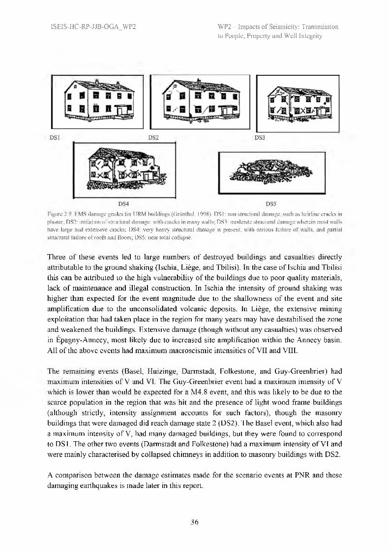
WP2 — Impacts of Seismicity: Transmissionto People, Property and Well Integrity
ISEIS-HC-RP-JJB-OGA_WP2
Figure 2.9. EMS damage grades for URM buildings (Grϋnthal, 1998). DS1: non structural damage, such as hairline cracks in plaster; DS2: initiation of structural damage, with cracks in many walls; DS3: moderate structural damage wherein most walls have large and extensive cracks; DS4: very heavy structural damage is present, with serious failure of walls, and partial structural failure of roofs and floors; DS5: near total collapse.
Three of these events led to large numbers of destroyed buildings and casualties directly attributable to the ground shaking (Ischia, Liège, and Tbilisi). In the case of Ischia and Tbilisi this can be attributed to the high vulnerability of the buildings due to poor quality materials, lack of maintenance and illegal construction. In Ischia the intensity of ground shaking was higher than expected for the event magnitude due to the shallowness of the event and site amplification due to the unconsolidated volcanic deposits. In Liège, the extensive mining exploitation that had taken place in the region for many years may have destabilised the zone and weakened the buildings. Extensive damage (though without any casualties) was observed in Épagny-Annecy, most likely due to increased site amplification within the Annecy basin. All of the above events had maximum macroseismic intensities of VII and VIII.
The remaining events (Basel, Huizinge, Darmstadt, Folkestone, and Guy-Greenbrier) had maximum intensities of V and VI. The Guy-Greenbrier event had a maximum intensity of V which is lower than would be expected for a M4.8 event, and this was likely to be due to the scarce population in the region that was hit and the presence of light wood frame buildings (although strictly, intensity assignment accounts for such factors), though the masonry buildings that were damaged did reach damage state 2 (DS2). The Basel event, which also had a maximum intensity of V, had many damaged buildings, but they were found to correspond to DS1. The other two events (Darmstadt and Folkestone) had a maximum intensity of VI and were mainly characterised by collapsed chimneys in addition to masonry buildings with DS2.
A comparison between the damage estimates made for the scenario events at PNR and these damaging earthquakes is made later in this report.
36

ISEI
S-H
C-R
P-JJ
B-O
GA
_W
P2W
P2 -
Im
pact
s of
Sei
smic
ity: T
rans
mis
sion
to P
eopl
e an
d Pr
oper
ty a
nd W
ell
Inte
grity
Dat
e an
d T
ime
(UT
C)
Plac
eM
Dep
th
(km
)M
axim
um
Inte
nsity
Indu
ced
/ te
cton
ic
Dea
ths
(due
to
shak
ing)
Inju
red
(due
to
shak
ing)
Bui
ldin
gs
dam
aged
Bui
ldin
gs
dest
roye
dL
osse
s (1
06 U
SD)
Com
men
ts
08/1
2/20
0616
:48
Bas
el,
Switz
erla
nd3.
25.
0V (E
MS-
98)
Indu
ced
(wat
er
inje
ctio
n)0
0
40 -
200
0 (b
ased
on
dam
age
clai
ms)
06.
5 -
8.3
Cre
akin
g of w
oodw
ork
and
rattl
ing
of
door
s an
d w
indo
ws
alar
med
the
popu
latio
n.
Mos
t da
mag
e w
as
crac
ked
plas
terw
ork
of b
rick
mas
onry b
uild
ings
(D
S1)
12/0
8/20
12H
uizi
nge,
th
e N
ethe
rland
s3.
53.
0VI
(E
MS-
98)
Indu
ced
(gas
ex
tract
ion)
00
2000
(b
ased
on
dam
age
clai
ms)
0N
ot
avai
labl
e
Maj
ority
of
dam
age
was
crac
ked
plas
tew
ork
of b
rick
mas
onry
build
ings
(D
S1),
mai
nly
in
olde
r fa
rmho
use
build
ings
. D
amag
e nu
mbe
rs
base
d on
cl
aim
s ra
ther
than
eval
uatio
n of
the
dam
age
(whi
ch m
ay a
lso
have
bee
n du
e to
se
ttlem
ent d
ue to
sof
t soi
ls).
17/0
5/20
14
16:4
6D
arm
stad
t, G
erm
any
3.6
5.0
VI
(EM
S-98
)Te
cton
ic0
015
40
1.36
Dis
lodg
ed,
crac
ked
or
parti
ally
colla
psed
ch
imne
ys
(36)
, di
slod
ged
roof
tiles
, cr
acke
d pl
aste
rwor
k (a
bout
27%
with
DS1
an
d 7%
with
DS2
).
21/0
8/20
17
18:5
7
Isch
ia
(Nap
oli),
Ita
ly3.
91.
7V
III
(EM
S-98
)Te
cton
ic2
39-4
234
9 - 1
000
688
8 - 1
40
Ver
y sh
allo
w e
vent w
ith l
ocal
ised h
igh
inte
nsity
in
a hi
lly
area
with
un
cons
olid
ated v
olca
nic
depo
sits l
eadi
ng
to h
igh
ampl
ifica
tion
of gr
ound
mot
ions
. A
hand
ful
of
colla
psed
(DS5
) bu
ildin
gs
(lead
ing
to 1 d
eath
) an
d m
any
build
ings
w
ith
sign
ifica
nt
diag
onal
crac
king
and
chim
ney
failu
re (
DS3
). Th
e ot
her
deat
h w
as d
ue t
o fa
lling
cor
nice o
f a
chur
ch.
Bui
ldin
g st
ock
repo
rted
to h
ave
had
man
y ill
egal
exte
nsio
ns
and
poor
-qua
lity
mat
eria
ls.
28/0
4/20
07
07:1
8
Folk
esto
ne.
Uni
ted
Kin
gdom
4.0
5.3
VI
(EM
S-98
)Te
cton
ic0
180
7 - 1
300
060
Min
or h
ead
inju
ry d
ue to
fal
ling
mas
onry
. D
islo
dged
, cr
acke
d or
colla
psed
ch
imne
ys,
disl
odge
d ro
of t
iles
(DS1
-2),
crac
ked
plas
terw
ork
(DS1
). M
any
chim
neys
wer
e in
need
of r
epoi
ntin
g
37

ISEI
S-H
C-R
P-JJ
B-O
GA
_W
P2W
P2 -
Im
pact
s of
Sei
smic
ity: T
rans
mis
sion
to P
eopl
e an
d Pr
oper
ty a
nd W
ell
Inte
grity
Dat
e an
d T
ime
(UT
C)
Plac
eM
Dep
th
(km
)M
axim
umIn
tens
ity'
Indu
ced
/ te
cton
ic
Dea
ths
(due
to
shak
ing)
Inju
red
(due
to
shak
ing)
Bui
ldin
gs
dam
aged
Bui
ldin
gs
dest
roye
dL
osse
s (1
06 U
SD)
Com
men
ts
befo
re t
he e
vent
. Pr
e-ex
istin
g flo
od a
nd
settl
emen
t da
mag
e m
ay a
lso
have b
een
pres
ent.
28/0
2/20
11
05:0
0
Guy
- G
reen
brie
r (A
rkan
sas)
, U
SA
4.8
3.8
V (M
MI)
Indu
ced
(was
tew
ater
in
ject
ion)
00
140
1.0
Scar
cely p
opul
ated a
rea
led
to r
educ
ed
num
ber
of
dam
aged
build
ings
(bric
k m
ason
ry),
crac
ked
wal
ls, d
oorf
ram
es o
ut
of
plum
b (D
S2).
Ligh
t w
ood
fram
e bu
ildin
gs a
re c
omm
on
in
the
build
ing
stoc
k, w
hich
may
als
o ha
ve h
elpe
d re
duce
th
e ex
tent
of d
amag
e.
15/0
7/19
96
00:1
3
Épag
ny-
Ann
ency
, Fr
ance
4.
84.
0V
III
(MSK
64)
Tect
onic
01
11,8
003
70-1
00
Hig
h in
tens
ity
attri
bute
d to
site
am
plifi
catio
n in t
he A
nnec
y ba
sin.
Inju
ry
due
to b
roke
n gl
ass, p
anic
of
loca
ls d
ue to
lo
w
seis
mic
risk
awar
enes
s.
Dis
lodg
ed,
crac
ked
or
colla
psed
bric
k ch
imne
ys
(600
), di
slod
ged
roof
tiles
, cr
acke
d pl
aste
rwor
k (D
S 3-
4).
08/1
1/19
83
00:4
9Li
ège,
B
elgi
um4.
85.
8V
II (E
MS-
98)
Tect
onic
125
-30
13,0
00-
16,0
0025
- 20
550
- 80
In
a re
gion
of
exte
nsiv
e m
inin
g ex
ploi
tatio
n w
hich
may
hav
e de
stab
ilise
d th
e zo
ne a
nd
wea
kene
d th
e bu
ildin
gs.
Dea
th d
ue to
a f
allin
g ce
iling
, inj
urie
s du
e to
falli
ng m
ason
ry e
lem
ents
as
peop
le fl
ed
the
build
ings
. Col
laps
e of
chim
neys
, roo
fs
and
wal
ls (D
S4-5
) of s
ome
olde
r mas
onry
bu
ildin
gs, t
houg
h m
ost e
xper
ienc
ed D
S3.
24/1
1/20
04
22:5
9Tb
ilisi
. G
eorg
ia4.
86.
0V
II-V
III
(EM
S-98
)Te
cton
ic4
30-7
011
,780
-50
,000
2319
-42
0818
0-35
0
Dea
ths
due
to
falli
ng
debr
is
(3)
and
colla
pse
of a
roof
(1).
Exte
nsiv
e da
mag
e to
lo
w-r
ise
bric
k an
d st
one
build
ings (
low
qu
ality
cons
truct
ion
and
lack
of
mai
nten
ance
of
build
ings
obse
rved
). Se
ries
of a
fters
hock
s, c
ontin
uous h
eavy
ra
ins
and
snow
falls
caus
ed
addi
tiona
l da
mag
e.
38
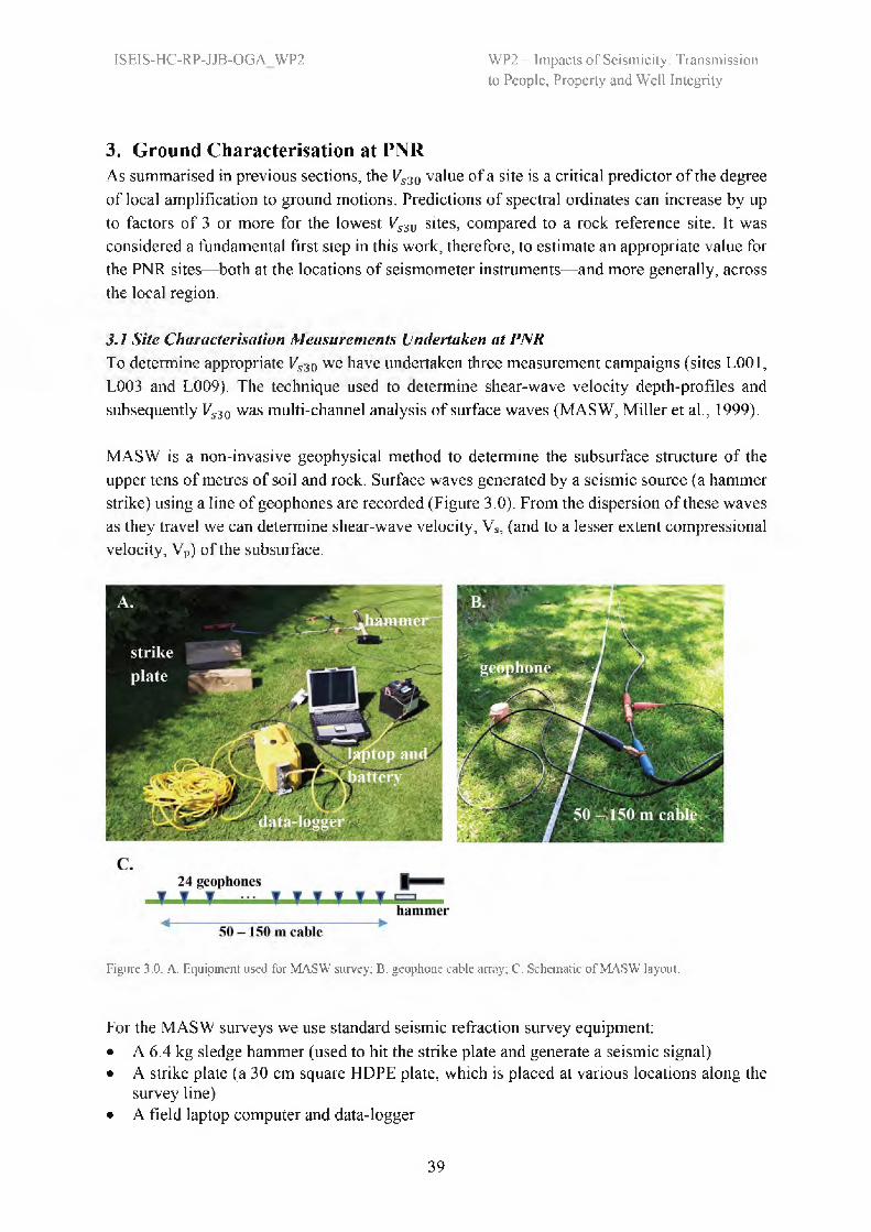
WP2 — Impacts of Seismicity: Transmissionto People, Property and Well Integrity
ISEIS-HC-RP-JJB-OGA_WP2
3. Ground Characterisation at PNRAs summarised in previous sections, the Vs30 value of a site is a critical predictor of the degree of local amplification to ground motions. Predictions of spectral ordinates can increase by up to factors of 3 or more for the lowest Vs30 sites, compared to a rock reference site. It was considered a fundamental first step in this work, therefore, to estimate an appropriate value for the PNR sites—both at the locations of seismometer instruments—and more generally, across the local region.
3.1 Site Characterisation Measurements Undertaken at PNRTo determine appropriate Vs30 we have undertaken three measurement campaigns (sites L001, L003 and L009). The technique used to determine shear-wave velocity depth-profiles and subsequently Vs30 was multi-channel analysis of surface waves (MASW, Miller et al., 1999).
MASW is a non-invasive geophysical method to determine the subsurface structure of the upper tens of metres of soil and rock. Surface waves generated by a seismic source (a hammer strike) using a line of geophones are recorded (Figure 3.0). From the dispersion of these waves as they travel we can determine shear-wave velocity, Vs, (and to a lesser extent compressional velocity, Vp) of the subsurface.
Figure 3.0. A. Equipment used for MASW survey; B. geophone cable array; C. Schematic of MASW layout.
For the MASW surveys we use standard seismic refraction survey equipment:• A 6.4 kg sledge hammer (used to hit the strike plate and generate a seismic signal)• A strike plate (a 30 cm square HDPE plate, which is placed at various locations along the
survey line)• A field laptop computer and data-logger
39

WP2 - Impacts of Seismicity: Transmissionto People, Property and Well Integrity
ISEIS-HC-RP-JJB-OGA_WP2
• 50 - 150 m geophone cable (laid on the ground surface)• 24 vertical 4.5 Hz geophones.
For planning and deployment of the MASW measurements we follow the guidance detailed in Foti et al. (2017). The dispersion of seismic surface waves is determined through cross correlation of the recorded data, as described by Miller et al. (1999). In all cases either 1 or 2 second post-trigger records (at sample intervals of 0.00625 and 0.0125 s respectively) were taken, depending on the record length required to capture the full surface-wave train during the survey. Processing of the collected data for dispersion characteristics is performed in the software package ‘geopsy’ (www.geopsy.org. last accessed 08/2019). A model for the subsurface velocity (VP and Vs) is then generated through inversion that explains the dispersion behaviour of the Rayleigh waves using the software ‘dinver’ (Wathelet, 2008, Wathelet et al., 2004).
The strategy for measurement in the short timeframe available here was to target specific superficial geology that is present in the area. The predominant superficial deposits near to the PNR site are: (i) blown sand; (ii) till; and (iii) peat and alluvium. Space and landowner consent also played a role in the choice of measurement sites. The selected sites cover the appropriate geological zones (i - iii), allowing a certain degree of inference as to the Vs30 for a given superficial geology.
3.1.1 Site L001Site L001 lies on till deposits (Figure 3.1) according to the BGS superficial geology map and is less than 5 km from the PNR site and associated seismicity. Several borehole lithological logs are available within 1 km of this site (Figure 3.2). We use logs 1419 and 18458993 as the nearest open access logs obtained through the BGS single onshore borehole index (SOBI) database. These are shown in Appendix A. SOBI: 1419 indicates till deposits (sand, gravel, clay) to 29 m, overlaying mudstone, while SOBI: 18458993 (although less detailed) also documents clay, sand and gravel deposits to 35 m, overlaying mudstone. Therefore, sites in this area comprise of around 30 m of sand, gravel and clay overlying a more consolidated mudstone.
Data provided by the operator (Figures 3.3, 3.4) from both refraction low velocity later (LVL) analyses and borehole investigations indicates the depth of a first refractor at between 4.5 and 11.9 m. Based on the lithological logs, this is likely to be a transition between clay and sand layers rather than the deeper mudstone. More distant survey points from the same analyses indicate a second refractor resolved at between 17 - 30 m depth, although at most survey locations LVL investigations were unable to resolve to this depth.
40

WP2 — Impacts of Seismicity: Transmissionto People, Property and Well Integrity
ISEIS-HC-RP-JJB-OGA_WP2
Figure 3.1. Location of MASW measurement at L001 (red dashed square). The PNR site along with 3, 5,10 km zones around it are shown (dashed concentric rings). The base-map is the BGS 625k superficial deposit map: green is blown sand; light blue is till; brown is peal and cream is alluvium. Built-up areas are highlighted by cross-hatched regions. Inset: Location of MASW measurement points (circles) and surrounding region.
Two MASW lines were measured: one at 3m geophone spacing (69 m total length, Figure 3.5); and one at 6 m (138 m total length, Figure 3.6). Both lines share the same easternmost point. Various shot offsets were used, with the optimal location being offset 5 m from the first geophone based on visual inspection of the traces and dispersion.
The dispersion for the 5 m offset shot is shown in Figure 3.7. The aim of the longer MASW transect is to resolve lower frequency dispersion and therefore image deeper structure. It appears that the dispersion is indeed resolved below the 5 Hz limit (Figure 3.7, left) seen for the shorter MASW transect, although caution is required in interpreting dispersion much below 5 Hz frequency due to (i) the source not generating sufficiently low frequency waves; (ii) the short duration of the signal; (in) the sensitivity of the geophones (Foti et al., 2017). Nevertheless, using this information, it appears that the dispersion can be observed down to approximately 4 Hz.
41

WP2 — Impacts of Seismicity: Transmissionto People, Property and Well Integrity
ISEIS-HC-RP-JJB-OGA_WP2
Figure 3.2. MASW line at site LOO) (blue: 138 m; yellow: 69 m). Instrument sites IO5 and AQ06 arc also nearby, lite SOBI borehole log locations are indicated with purple circles. Hatched areas indicate populated regions. The background is the BGS superficial geology map. lite highlighted SOBI locations indicate those in the text. Note: the SOBI IDs reveal confidential location information and should not be reproduced.
Figure 3.3. As previous, but showing location of low velocity layer refraction survey (blue) and borehole investigations (red) carried out on behalf of the operator. Depth to refractor 1 (Rl) is indicated.
42

WP2 — Impacts of Seismicity: Transmissionto People, Property and Well Integrity
ISEIS-HC-RP-JJB-OGA_WP2
Figure 3.4. As previous, but showing location of more distant low velocity layer refraction survey (blue) and borehole investigations (red) carried out on behalf of the operator. Survey points with resolved refractor 2 depths (R2) are indicated.
Figure 3.5. 24 geophone records (bottom nearest source), with 3 m spacing at site L001.
43
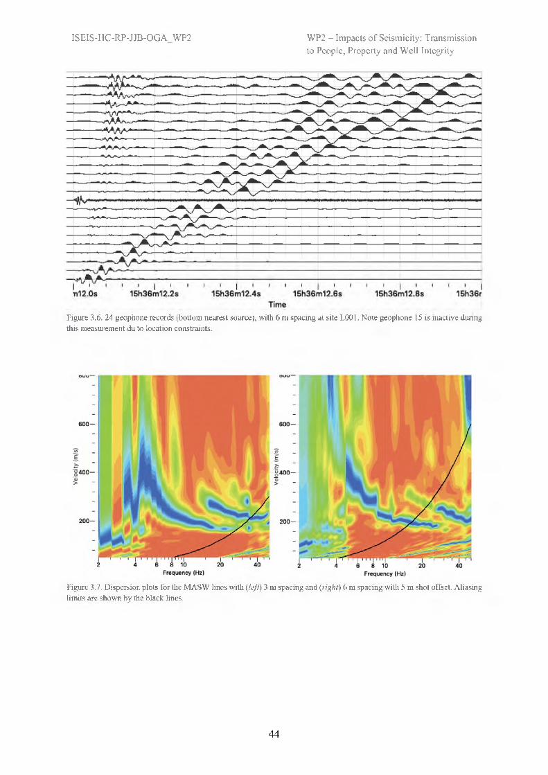
WP2 — Impacts of Seismicity: Transmissionto People, Property and Well Integrity
ISEIS-HC-RP-JJB-OGA_WP2
Figure 3.6. 24 geophone records (bottom nearest source), with 6 m spacing al site L001. Note geophone 15 is inactive during this measurement du to location constraints.
Figure 3.7. Dispersion plots for the MASW lines with (left) 3 m spacing and (right) 6 m spacing with 5 m shot offset. Aliasing limits are shown by the black lines.
44

WP2 — Impacts of Seismicity: Transmissionto People, Property and Well Integrity
ISEIS-HC-RP-JJB-OGA_WP2
3.1.2 Site L003Site L003 lies on peat and alluvial deposits (Figure 3.8, inset) and is around 12 km from the PNR site and associated seismicity. One MASW line was measured with 2 m geophone spacing (46 m total length). Other regions within 5 km of PNR lie on similar geology (Figure 3.8), although the majority of the region is similar to site L001 (i.e., till deposits). As at the previous site, various shot offsets were used, with the optimal location being offset 5 m from the first geophone. Two nearby lithological logs were located in the SOBI (see Appendix A, IDs: 4838, 4495, Figure 3.9). The lithological logs indicate layers of soil followed by sand gravel and clay with increasing hardness down to about 20 m, overlying ‘very hard clay gravel boulder stone’. No LVL or borehole information from the 3D seismic survey campaign was available in this area, however, the general trend over the wider survey of two refractors, the first around 5 to 12 and the second around 17 to 30 m is considered.
Figure 3.8. Location of MASW measurement at L003 (red dashed square). The PNR site along with 3, 5, 10 km zones around it are shown (dashed concentric rings). The base-map is the BGS superficial deposit map: green is blown sand; light blue is till; brown is peat and cream is alluvium. Built-up areas are highlighted by cross-hatched regions. Inset: Location of MASW measurement points (circles) and surrounding region.
45

WP2 — Impacts of Seismicity: Transmissionto People, Property and Well Integrity
ISEIS-HC-RP-JJB-OGA_WP2
Figure 3.9. MASW line at site L003 (red circles mark end points). The SOBI borehole log locations considered in the analyses are indicated with purple circles. The background is the BGS superficial geology map. The highlighted SOBI locations indicate those in the text.
Figure 3.10. 24 geophone records (bottom nearest source), with 2 m spacing at site L003.
46
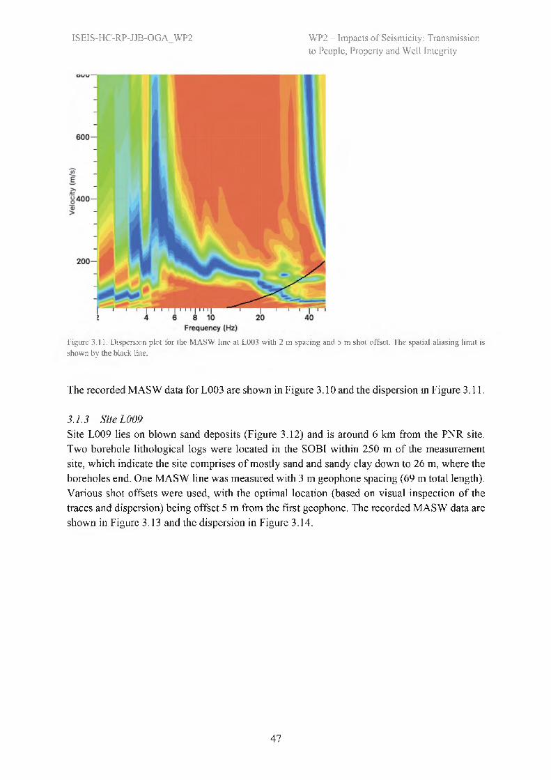
WP2 — Impacts of Seismicity: Transmissionto People, Property and Well Integrity
ISEIS-HC-RP-JJB-OGA_WP2
Figure 3.11. Dispersion plot for the MASW line at L003 with 2 m spacing and 5 m shot offset. The spatial aliasing limit is shown by the black line.
The recorded MASW data for L003 are shown in Figure 3.10 and the dispersion in Figure 3.11.
3.1.3 Site L009Site L009 lies on blown sand deposits (Figure 3.12) and is around 6 km from the PNR site. Two borehole lithological logs were located in the SOBI within 250 m of the measurement site, which indicate the site comprises of mostly sand and sandy clay down to 26 m, where the boreholes end. One MASW line was measured with 3 m geophone spacing (69 m total length). Various shot offsets were used, with the optimal location (based on visual inspection of the traces and dispersion) being offset 5 m from the first geophone. The recorded MASW data are shown in Figure 3.13 and the dispersion in Figure 3.14.
47

WP2 — Impacts of Seismicity: Transmissionto People, Property and Well Integrity
ISEIS-HC-RP-JJB-OGA_WP2
Figure 3.12. Location of MASW measurement al L009 (red dashed square). The PNR site along with 3,5,10 km zones around it are shown (dashed concentric rings). The base-map is the BGS superficial deposit map: green is blown sand; light blue is till; brown is peat and cream is alluvium. Built-up areas are highlighted by cross-hatched regions. Inset: Location of MASW measurement points (circles) and surrounding region.
Figure 3.13. 24 geophone records (bottom nearest source), with 3 m spacing at site L009.
48

WP2 — Impacts of Seismicity: Transmissionto People, Property and Well Integrity
ISEIS-HC-RP-JJB-OGA_WP2
Figure 3.14. Dispersion plot for the MASW line at L009 with 3 in spacing and 5 m shot offset. Aliasing limit is shown by the black line.
3.2 Shear-Wave Velocity Model for Selected PNR sites
3.2.1 Till deposit sites (L001)Using the available lithological logs for site L001, along with the Rayleigh wave dispersion (Figure 3.7, Section 3.1.1) an initial model layering was defined (with tolerance of ±2 m, increasing to ±4 m at depth) for the inverted subsurface profiles. The fundamental mode Rayleigh dispersion was inverted (Figure 3.15) to provide Vs following the approach detailed in Wathelet (2008) and Wathelet et al. (2004). through software ‘dinver’ (part of the geopsy programme package). Poisson’s ratio was allowed to vary between 0.2 and 0.5, Vp was allowed to vary between 80 and 5000 m/s, Vs between 50 and 1500 m/s (i.e., velocity was almost unconstrained) and density was set at 2000 kg/m3 The most sensitive parameter in the inversion of Rayleigh wave dispersion is Vs, with Vp and density poorly resolved. In addition to the lithologically based model, a simple model with 5 m layers is presented (Figure 3.16).
In Figure 3.15 the full suite of inverted dispersion curves is shown. The ‘best fitting’ models encapsulating the observed dispersion (misfit < 0.05) are shown in terms of the corresponding Vs in Figure 3.16. Note the change in colour scale.
49
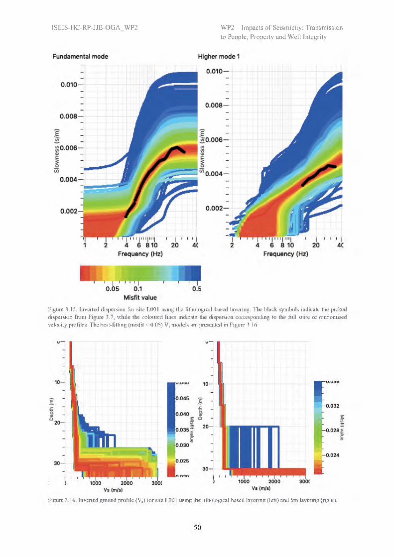
WP2 — Impacts of Seismicity: Transmissionto People, Property and Well Integrity
ISEIS-HC-RP-JJB-OGA_WP2
Figure 3.15. Inverted dispersion for site L001 using the lithological based layering. The black symbols indicate the picked dispersion from Figure 3.7, while the coloured lines indicate the dispersion corresponding to the full suite of randomised velocity profiles. The best-fitting (misfit < 0.05) Vs models are presented in Figure 3.16.
Figure 3.16. Inverted ground profile (Vs) for site L001 using the lithological based layering (left) and 5m layering (right).
50

WP2 - Impacts of Seismicity: Transmissionto People, Property and Well Integrity
ISEIS-HC-RP-JJB-OGA_WP2
This site exhibits slowly increasing velocity with depth (Figure 3.17), from values around 180-200 m/s
at the surface, to 300-400 m/s at or around 30 m. A first possible refractor is evident
at around 5 - 6 m, consistent with the LVL survey data, with a second possible at around 16 m. A clear interface is evident at around 29 - 32 m consistent with the transition from till to mudstone in the lithological logs. The velocity of the mudstone is poorly constrained, but is likely to be above 600 m/s.
Figure 3.17. Mean and standard deviation assuming normal distribution (from all models using the lithological layering with misfit < 0.05, Figure 3.16, black) and the best-fitting single model (red) for site L001. Note that the resolution below 30 m is very poor and therefore Vs unreliable.
3.2.2 Peat/Alluvium Deposit Sites (L003)At L003, only the fundamental mode dispersion was evident and was therefore used as the inversion target. Using the available lithological logs for site L003, along with the Rayleigh wave dispersion (Section 3.1,2) an initial layering was defined (with tolerance of ±2 m, increasing to ±4 m at depth) for the inverted subsurface profiles. As for all sites, Poisson’s ratio was allowed to vary between 0.2 and 0.5, Vp was allowed to vary between 80 and 5000 m/s, Vs between 50 and 1500 m/s (i.e., almost unconstrained) and density was set at 2000 kg/m3 In addition to the lithologically based model, a simple model with 5 m layers is presented.
In Figure 3.18 the full suite of inverted dispersion curves is shown. The ‘best fitting’ models (misfit < 0.07, encapsulating the empirical dispersion curve) are shown in terms of the corresponding Vs in Figure 3.19. Note the change in colour scale.
51

WP2 — Impacts of Seismicity: Transmissionto People, Property and Well Integrity
ISEIS-HC-RP-JJB-OGA_WP2
The profile in this case shows evidence for a small increase in Vs at about 6 m and again at 15 - 17 m (as for the previous site). The deeper 30 m refractor (as obseved at the previous site at around 30 m) is not resolved, however, the uncertatines at increase significantly from about 25 m (Figure 3.20), slightly shallower than at site L001.
Figure 3.18. Inverted dispersion for site L003 using the lithological based layering. The black symbols indicate the picked dispersion from Figure 3.11, while the coloured lines indicate the dispersion corresponding to the fall suite of randomised velocity profiles. The best-fitting (misfit < 0.07) V5 models are presented in Figure 3.19.
52
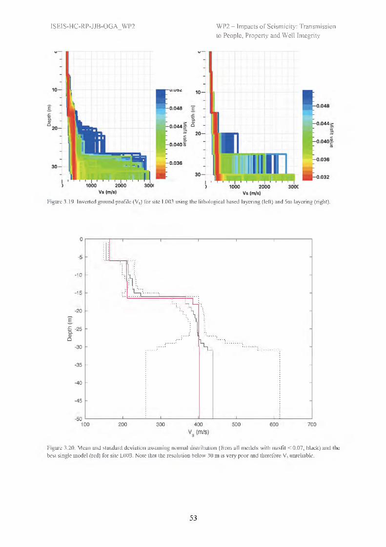
WP2 — Impacts of Seismicity: Transmissionto People, Property and Well Integrity
ISEIS-HC-RP-JJB-OGA_WP2
Figure 3.19. Inverted ground profile (Vs) for site L003 using the lithological based layering (left) and 5m layering (right).
Figure 3.20. Mean and standard deviation assuming normal distribution (from all models with misfit < 0.07, black) and the best single model (red) for site L003. Note that the resolution below 30 m is very poor and therefore Vs unreliable.
53

WP2 — Impacts of Seismicity: Transmissionto People, Property and Well Integrity
ISEIS-HC-RP-JJB-OGA_WP2
3.2.3 Blown sand deposit sites (L009)At site L009 only the fundamental dispersion curve was observed using the MASW. Using the available lithological logs for the site, along with the Rayleigh wave dispersion (Section 3.1.3) an initial layering was defined (with tolerance of ±2 m, increasing to ±4 m at depth) for the inverted subsurface profiles. In this case, since no basement rock was evident in the logs, we allow for a final layer at anywhere below 20 m. Poisson’s ratio was again allowed to vary between 0.2 and 0.5, Vp was allowed to vary between 80 and 5000 m/s, Vs between 50 and 1500 m/s (i.e., almost unconstrained) and density was set at 2000 kg/m3. In addition to the lithologically based model, a simple model with 5 m layers is presented.
In Figure 3.21 the full suite of inverted dispersion curves is shown. The ‘best fitting’ models (misfit < 0.06) are shown in terms of the corresponding Vs in Figure 3.22. Note the change in colour scale. The average model, based on the lithological layering is shown in Figure 3.23 and essentially comprises of two layers with an interface at around 13 m.
Figure 3.21. Inverted dispersion for site L009 using the lithological based layering. The black symbols indicate the picked dispersion from Figure 3.14, while the coloured lines indicate the dispersion corresponding to the full suite of randomised velocity profiles. The best-fitting (misfit < 0.06) Vs models are presented in Figure 3.22.
54

WP2 — Impacts of Seismicity: Transmissionto People, Property and Well Integrity
ISEIS-HC-RP-JJB-OGA_WP2
Figure 3.22. Inverted ground profile (Vs) for site L009 using the lithological based layering (left) and 5m layering (right).
Figure 3.23. Mean and standard deviation assuming normal distribution (from all models with misfit < 0.06, black) and the best single model (red) for site L009. Note that the resolution below 30 m is very poor and therefore Vs unreliable.
55

WP2 - Impacts of Seismicity: Transmissionto People, Property and Well Integrity
ISEIS-HC-RP-JJB-OGA_WP2
3.3 Vs30 for PNR sitesUsing the shear-wave velocity profiles estimated in the previous section we can directly calculate travel time average velocity to depth x using:
"i=ly .
yS,l (19)
where there are N layers, with defined thickness of the ith layer hi, and shear-wave velocity Vs,i. The 30 m shear-wave velocity profile is therefore discretised in to N layers of constant velocity and Vs30 calculated. Since a range of possible models are produced (within a defined misfit) an uncertainty on Vs 30 is obtained in terms of its standard deviation.
An alternative method to estimate Vs30 is based on correlations to the dispersion of Rayleigh wave phase velocity of the 40 - 45 m wavelength signal, Vr ,40-45, approximated by:
VS3O = Vr ,40-45 (20)
(Foti et al., 2017). Generally, VR,40 is more appropriate at sites with shallow groundwater, as expected here. Table 3.1 summarises the Vs30 values using the various approaches detailed above. Covering the range of Vs30 values, we defined three equally spaced values for scenario calculations as 200, 240 and 280 m/s.
Table 3.1. Vs30 values (mean and plus/minus one standard deviation).
Surface Deposit
Lithological Depths
Site Vs 30 fromVR40-45
Vs30 from
Vs(z) (median)
Vs30 fromVs(z)(16th -
percentile)
Vs30 fromVs(z)(84th -
percentile)Till Yes
NoL001 269.0 257.1
249.7251.7 247.6
264.4 252.8
Alluvium/Peat
Yes No
L003 244.3 240.0
234.0
237.3 233.3
244.3
235.7Sand Yes L009 213.3 205.3
195.5203.3 194.1
205.5 196.0
In order to define a spatially variable Vs30 map, extending the MASW-based measurements in Table 3.1, we have determined horizontal-to-vertical (H/V) spectral ratios (HVSR) using ambient seismic noise (Haghshenas et al., 2008) at each of the surface seismometer sites. HSVR are determined (Figures 3.24 - 3.26) by computing the ratio of horizontal and vertical Fourier spectral amplitudes of ambient vibrations (i.e., non-earthquake signals) averaged over many time-periods. Here we use 2 minutes of data between 0230 and 0232, averaged over several days (specifically all days where seismic events were registered by the BGS).
56
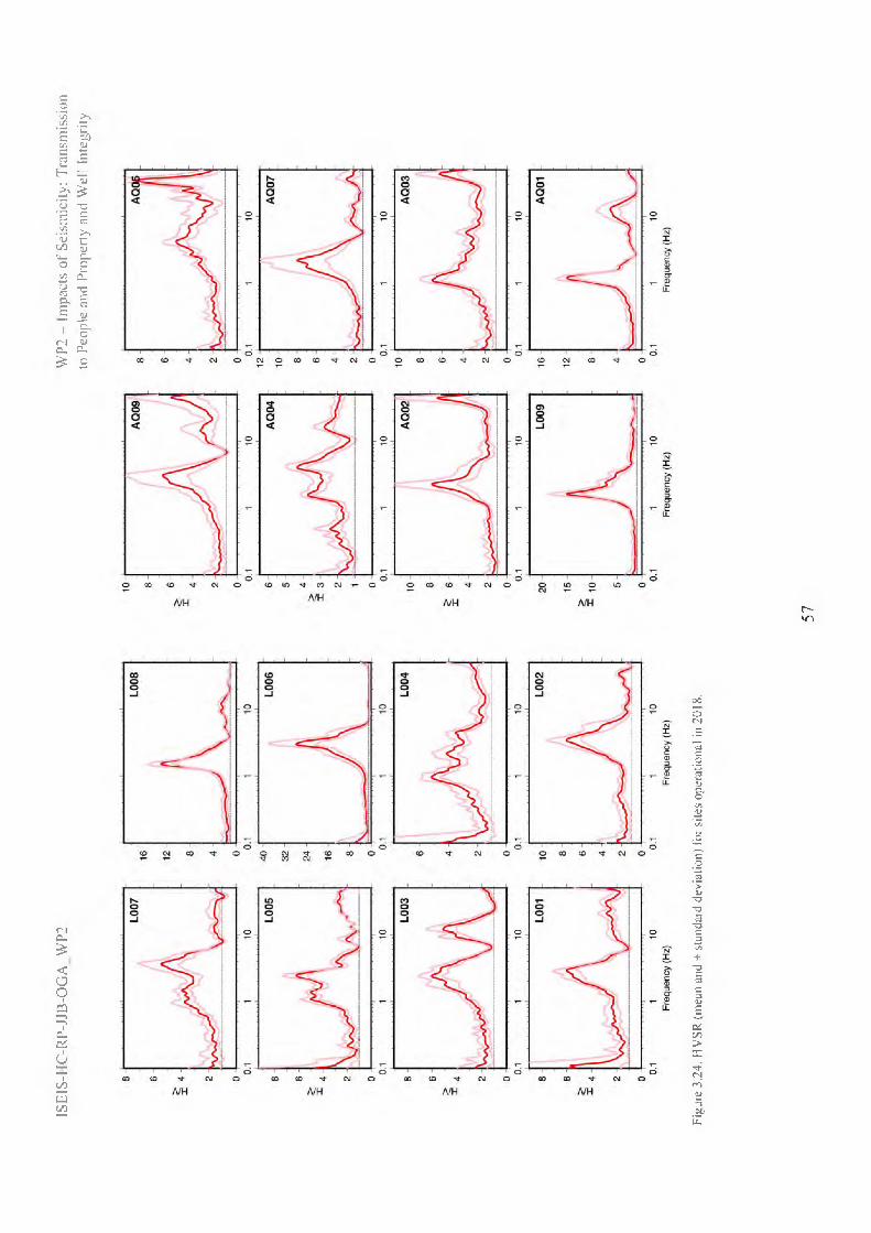
WP2
— I
mpa
cts
of S
eism
icity
: Tra
nsm
issi
onto
Peo
ple
and
Prop
erty
and
Wel
l In
tegr
ityIS
EIS-
HC
-RP-
JJB
-OG
A_
WP2
Figu
re 3
.24.
HV
SR (m
ean
and
± st
anda
rd d
evia
tion)
for
site
s op
erat
iona
l in
201
8.
57
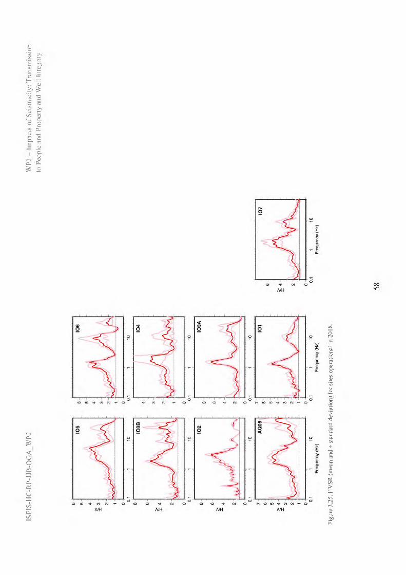
WP2
— I
mpa
cts
of S
eism
icity
: Tra
nsm
issi
onto
Peo
ple
and
Prop
erty
and
Wel
l In
tegr
ityIS
EIS-
HC
-RP-
JJB
-OG
A_W
P2
Figu
re 3
.25.
HV
SR (m
ean
and
± st
anda
rd d
evia
tion)
for
site
s op
erat
iona
l in
201
8.
58

ISE
IS-H
C-R
P-JJ
B-O
GA
_WP2
WP2
- I
mpa
cts
of S
eism
icity
: Tra
nsm
issi
on
to P
eopl
e an
d Pr
oper
ty a
nd W
ell
Inte
grity
Figu
re 3
.26. H
VSR
(mea
n an
d ±
stan
dard
dev
iatio
n) fo
r add
ition
al s
ites
oper
atio
nal
in 2
019.
59
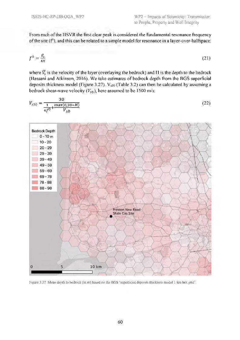
WP2 — Impacts of Seismicity: Transmissionto People, Property and Well Integrity
ISEIS-HC-RP-JJB-OGA_WP2
From each of the HSVR the first clear peak is considered the fundamental resonance frequency of the site (f0), and this can be related to a simple model for resonance in a layer-over-halfspace:
fO =Ä' 4H (21)
where Vs is the velocity of the layer (overlaying the bedrock) and H is the depth to the bedrock (Hassani and Atkinson, 2016). We take estimates of bedrock depth from the BGS superficial deposits thickness model (Figure 3.27). Vs30 (Table 3.2) can then be calculated by assuming a bedrock shear-wave velocity (Vsb), here assumed to be 1500 m/s:
”s30 — i ma30x(0,30-H)
4f° Vsb
(22)
Figure 3.27. Mean depth to bedrock (in m) based on the BGS ‘superficial deposits thickness model 1 km hex grid’.
60
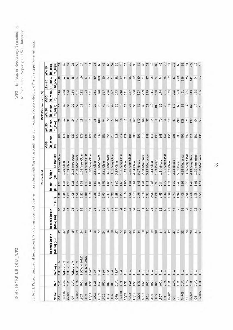
WP2
— I
mpa
cts
of S
eism
icity
: Tra
nsm
issi
onto
Peo
ple
and
Prop
erty
and
Wel
l In
tegr
ityIS
EIS-
HC
-RP-
JJB
-OG
A_W
P2
Tabl
e 3.
2. P
icke
d fu
ndam
enta
l fre
quen
cies
(f0)
incl
udin
g up
per a
nd lo
wer
est
imat
es a
long
with
Vs30
usi
ng c
ombi
natio
ns o
f mea
n/m
ax b
edro
ck d
epth
and
f0 a
nd it
s up
per/l
ower
est
imat
e.
f0 s
elec
ted
Vs30
Est
imat
es (
m/s
)
Nam
eN
etG
eolo
gyBe
droc
k De
pth
[Mea
n] (
m)
Bedr
ock
Dep
th
[Max
] (m
)f0
(Hz)
f0 lo
w(H
z)f0
hig
h (H
z)f0
Qua
lity
Vs30
(H
_mea
n,
f0)
ΔVs3
0 (H
_mea
n,
f0_l
ow)
ΔVs
30
(H_m
ean,
f0 h
igh)
Vs30
(H
_max
, f0
)
Δ Vs
30
(H_m
ax,
f0_l
ow)
ΔVs
30(H
_max
, f0
_hig
h)IO
3aCU
AAL
LUVI
UM
3730
1.55
1.34
1.72
Very
Cle
ar18
625
2118
625
21PN
R3A
CUA
ALLU
VIU
M37
521.
451.
351.
79Cl
ear
174
1240
174
1240
PNR0
4CU
AAL
LUVI
UM
3644
1.62
1.35
1.89
Clea
r19
432
3219
432
32l0
7CU
AAL
LUVI
UM
1923
2.06
1.26
2.28
Mod
erat
e22
784
2123
488
23PN
R07
CUA
ALLU
VIU
M19
231.
581.
472.
08M
oder
ate
177
1252
181
1255
L008
UO
LBL
OW
N S
AND
2432
1.52
1.39
1.66
Very
Cle
ar17
615
1618
216
17L0
09U
OL
BLO
WN S
AND
2930
1.60
1.49
1.74
Very
Cle
ar19
113
1619
313
16AQ
01BG
SPE
AT4
111.
191.
081.
30Ve
ry C
lear
127
1111
131
1111
AQ02
BGS
PEAT
1621
2.26
1.87
2.61
Clea
r24
138
3325
140
36AQ
09BG
SPE
AT22
263.
042.
063.
81M
oder
ate
332
100
7534
810
883
L002
UO
LPE
AT24
253.
452.
833.
91Cl
ear
382
6447
387
6648
L003
UO
LPE
AT16
262.
411.
683.
21M
oder
ate
254
7072
278
8288
L006
UO
LPE
AT18
222.
992.
753.
51Ve
ry C
lear
313
2247
327
2352
l03b
CUA
PEAT
2734
1.85
1.62
2.12
Clea
r21
827
3122
228
32PN
R3B
CUA
PEAT
2734
1.82
1.66
1.96
Very
Cle
ar21
418
1621
819
16AQ
03BG
STI
LL25
291.
101.
001.
32Cl
ear
129
1225
131
1226
AQ04
BGS
TILL
2734
1.56
1.41
1.80
Very
Cle
ar18
417
2818
718
29AQ
05BG
STI
LL33
374.
173.
614.
94Cl
ear
500
6793
500
6793
AQ06
BGS
TILL
3437
2.56
1.48
3.27
Broa
d30
713
085
307
130
85AQ
07BG
STI
LL8
142.
181.
442.
68M
oder
ate
219
6641
229
7145
L001
UO
LTI
LL31
362.
912.
183.
15M
oder
ate
349
8729
349
8729
L004
UO
LTI
LL19
210.
960.
831.
13Cl
ear
111
1419
111
1519
L005
UO
LTI
LL30
321.
080.
981.
99Br
oad
130
1210
913
012
109
L007
UO
LTI
LL24
311.
450.
841.
80Br
oad
168
7039
174
7442
l01
CUA
TILL
3748
1.34
1.22
1.51
Very
Cle
ar16
114
2016
114
20PN
R01
CUA
TILL
3748
1.38
1.24
1.62
Clea
r16
517
2916
517
29l0
4CU
ATI
LL37
481.
711.
322.
68Br
oad
205
4711
720
547
117
l05
CUA
TILL
3336
4.94
2.45
5.51
Broa
d59
329
968
593
299
68PN
R05
CUA
TILL
3336
4.09
2.96
4.56
Mod
erat
e49
113
656
491
136
56l0
2CU
ATI
LL28
332.
962.
753.
30Ve
ry C
lear
347
2439
355
2541
PNR0
2CU
ATI
LL28
332.
661.
484.
13Ve
ry B
road
312
137
168
319
141
177
l06
CUA
TILL
3133
1.55
1.01
1.65
Mod
erat
e18
664
1218
664
12PN
R06
CUA
TILL
3133
1.55
1.11
1.68
Mod
erat
e18
653
1618
653
16
61

WP2 - Impacts of Seismicity: Transmissionto People, Property and Well Integrity
ISEIS-HC-RP-JJB-OGA_WP2
An effective approach to map Vs30 is through the proxy of surface geology (Wills and Clahan, 2006). We compare the Vs30 calculated from f0 and bedrock depth (Table 3.2) with surface geology (Figure 3.28). In addition to the values presented in Table 3.2, we also present values estimated from an empirical f0 proxy presented by Hassani and Atkinson (2016) for sites in eastern and northern North America (legend: ‘Atkinson f0 proxy’). Additionally, to represent the uncertainty in bedrock depth, we also estimate Vs30 assuming that the bedrock is uniformly at 30 m depth, rather than the values taken from the BGS superficial geology model (legend: ‘H=30m’).
Figure 3.28. Estimated and measured Vs30 grouped by superficial geology. Error bars are provided for the empirical Vs 30 f0 proxy (Hassani and Atkinson, 2016) and based on the lower- and higher-estimates of f0 from Table 3.2. The horizontal coloured lines indicate superficial geology and correspond to the geological maps presented earlier — beige: alluvium; green: blown- sand; brown: peat; blue: till.
It is clear from Figure 3.28 that the Vs30 values estimated from f0 are close to those measured (both directly, and through the dispersion proxy) at the three sites (L009, L003 and L001 : see Section 3.2). For sites with superficial geology defined by alluvium or blown sand we observe little variability, and a (log) average Vs30 = 189 m/s. Sites comprised of till or peat superficial deposits show wider variability, in the case of till sites ranging from around 110 to 600 m/s. The average Vs30 for the peat sites was 248 m/s, while for till sites the average was 233 m/s. These average values (approximately 190, 230 and 250 m/s) correspond well to the measured values at the corresponding sites (Table 3.1). Based on the BGS superficial geology map, we have characterised the area into Vs30 zones of 1 km2 (Figure 3.29). While this is coarse (and indeed misses some of the finer geological features) there are two justifications for not using a finer grid. The first is the uncertainty on the Vs30 values based on geology in the case of peat and, in particular, till, is large. Secondly, the grid is then consistent with the risk calculations performed later, as detailed in Section 5.
62

ISEIS-HC-RP-JJB-OGA_WP2 WP2 — Impacts of Seismicity: Transmissionto People, Property and Well Integrity
63
Figure 3.29. Vs30 map at 1 km2 resolution for the PNR region overlying the BGS superficial deposit map.
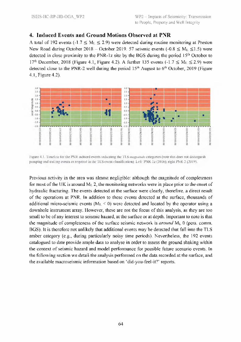
WP2 — Impacts of Seismicity: Transmissionto People, Property and Well Integrity
ISEIS-HC-RP-JJB-OGA_WP2
4. Induced Events and Ground Motions Observed at PNRA total of 192 events (-1.7 ≤ ML ≤ 2.9) were detected during routine monitoring at Preston New Road during October 2018 - October 2019. 57 seismic events (-0.8 ≤ ML ≤1.5) were detected in close proximity to the PNR-1z site by the BGS during the period 15th October to 17th December, 2018 (Figure 4.1, Figure 4.2). A further 135 events (-1.7 ≤ ML ≤ 2.9) were detected close to the PNR-2 well during the period 15th August to 6th October, 2019 (Figure 4.1, Figure 4.2).
Figure 4.1. Timeline for the PNR induced events indicating the TLS magnitude categories (note this does not distinguish pumping and trailing events as required in the TLS event classification). Left: PNR-1z (2018); right PNR-2 (2019).
Previous activity in the area was almost negligible: although the magnitude of completeness for most of the UK is around ML 2, the monitoring networks were in place prior to the onset of hydraulic fracturing. The events detected at the surface were clearly, therefore, a direct result of the operations at PNR. In addition to these events detected at the surface, thousands of additional micro-seismic events (Ml < 0) were detected and located by the operator using a downhole instrument array. However, these are not the focus of this analysis, as they are too small to be of any interest to seismic hazard, at the surface or at depth. Important to note is that the magnitude of completeness of the surface seismic network is around ML 0 (pers. comm. BGS). It is therefore not unlikely that additional events may be detected that fall into the TLS amber category (e.g., during particularly noisy time periods). Nevertheless, the 192 events catalogued to date provide ample data to analyse in order to assess the ground shaking within the context of seismic hazard and model performance for possible future scenario events. In the following section we detail the analysis performed on the data recorded at the surface, and the available macroseismic information based on ‘did-you-feel-it?’ reports.
64

WP2 — Impacts of Seismicity: Transmissionto People, Property and Well Integrity
ISEIS-HC-RP-JJB-OGA_WP2
Figure 4.2. Overview of PNR seismicity (inset figures show PNR-1z and PNR-2 seismicity independently) in addition to the wider region’s historical seismicity and the monitoring networks in place (yellow/orange: Cuadrilla; Green: University of Liverpool; Blue: BGS). Detected seismic events are shown according to their TLS magnitude category, as in Figure 1.1, apart from events ML 2.5 or greater, which are indicated by stars. Note PPV stations are not used in this analysis due to concerns as to their reliability (Bommer and Edwards, 2018).
4.1 Macroseismic Data for the EventsThe British Geological Survey regularly provide macroseismic intensity (see Section 2.4.1) for UK earthquakes. These intensity estimates, which aim to quantify the potential ‘felt effects’ and damage from earthquakes are based on (i) ‘did-you-feel-it?’ web questionnaires submitted to the BGS (www.earthquakes.bgs.ac.uk/questionnaire/EqOuestlntro.html) and sometimes, in the case of larger events, (ii) damage surveys. In addition, macroseismic intensity can be estimated using equations that link recorded motions (GMICE, see Section 2.4.2) or to magnitude (e.g., Musson, 2003).
For the two largest events that occurred during hydraulic fracturing of PNR-1z, macroseismic intensities were assigned by the BGS (Table 1.1). Both events were assigned European macroseismic intensity II, which equates to “Scarcely felt - Felt only by very few individual people at rest in houses”. Five of the largest events (1.0 ≤ Ml ≤ 2.9) from the seismicity at PNR-2 were assigned intensities, along with a ML 0.5 event (Table 1.1, 1.2). Intensity VI
65

WP2 — Impacts of Seismicity: Transmissionto People, Property and Well Integrity
ISEIS-HC-RP-JJB-OGA_WP2
(slightly damaging) was assigned to the ML 2.9 event, with IV being assigned to the second largest, Ml 2.1 earthquake. Of particular interest is the intensity for the Ml 2.9 event, which was widely felt in the epicentral region. Based on data presented by Baptie (2019), the intensity map is shown in Figure 4.3, with the number of contributing reports in Figure 4.4.
Figure 4.3. Macroseismic intensity in a 2 km grid based on ‘did-you-feel-it?’ reports (Baptie, 2019).
Figure 4.4. Number of observations of macroseismic intensity in a 2 km grid based on ‘did-you-feel-it?’ reports (Baptie, 2019).
66

WP2 - Impacts of Seismicity: Transmissionto People, Property and Well Integrity
ISEIS-HC-RP-JJB-OGA_WP2
In order to supplement this data, we have collated all maximum intensity estimates for shallow (depth < 5 km) UK earthquakes from the BGS macroseismic intensity database (Figure 4.5). These data include, for instance the recent Newdigate seismic sequence in 2018 and 2019 that comprised of tightly clustered events at about 2 km depth (Hicks et al., 2019). This shows that previous events in the ML 1 to 1.5 range have been assigned intensities of between II (the lowest that is assigned), and IV+, with ‘+’ indicating a mid-way point between two intensities. Intensity V and VI are considered the threshold of minor cosmetic damage (DS1) in the EMS-98 scale [differentiated partly by the occurrence of DS1 in few and many class A or B structures, respectively (with unreinforced brick structures typical to the UK in the less vulnerable class B)]. It can therefore be generalised that shallow events with ML ≤ 1.5 (the largest event associated with PNR-1z) have not previously been associated with damage. For the larger events of PNR-2 (Ml 2.1 and 2.9), we observe that, apart from one obvious outlier (intensity VIII), only one previous event in this range was assigned VI (both discussed later in this section). Several are assigned V or V+, but these are all at the high end of the range. Looking at deeper events (not plotted here) there are some assigned VI however all of these are historical records, which are significantly more unreliable than modem records.
Figure 4.5. Epicentral intensity for UK events with shallow focal depths (D < 5 km) versus magnitude.
Figure 4.6. Epicentral intensity for UK events with ML 3 to 4 versus depth.
67
WP2 - Impacts of Seismicity: Transmissionto People, Property and Well Integrity
ISEIS-HC-RP-JJB-OGA_WP2
There appears to be no clear depth dependence on the intensity values (Figure 4.5, with decreasing depth to 2 km). This may give some support to the fact that shallow focus earthquakes have lower stress drops than larger events (Hough, 2014), since otherwise we would expect higher intensities for increasingly shallow events. However, looking at intensities for deeper events within a defined magnitude range of 3 to 4 (Figure 4.6), we observe an apparent increase of epicentral intensity for sources with depth less than 5 km. It should be noted again, however, that the highest intensities often correspond to historical events with highly uncertain depths (and intensities), therefore this apparent trend is debatable. Whether depth dependent stress drop for UK events is an issue is therefore not clear. What can be generalised from this data, however, is that for events with ML 3 to 4 we expect higher intensities (generally IV to VI) for shallow induced events, than for tectonic events (which typically occur around 10 km depth). Intensity V and VI would imply strong shaking through to many unreinforced buildings with minor cosmetic damage, respectively. For induced events with ML < 3 macroseismic intensity is unlikely to exceed V+ based on existing data. The assignment of intensity VI to the ML 2.9 event is therefore clearly at the high-tail of the distribution of intensity for previous shallow events of this magnitude and more consistent with larger events.
Outlier observations exist that are of interest in Figures 4.5 and 4.6. The first is an intensity VII event in Figure 4.6. This was a M 3.3 earthquake in Mansfield on 04/04/1924 (Figure 4.7). Its intensity has been assigned through historical documents and reports and may therefore be less reliable than more recent data. Its intensity of VII indicates that it was damaging with “many well built ordinary buildings suffering moderate damage: small cracks in walls, fall of plaster, parts of chimneys fall down; older buildings may show large cracks in walls and failure of fill- in walls.” This event occurred after a similar sized event in the same location the previous month (06/03/1924), which may have weakened some vulnerable structures and led to the higher than expected epicentral intensity. Compounding of reported effects for these closely spaced events may also have led to the appearance of more significant damage for the later event. A M 2.2 event with intensity VIII is also of interest. This event occurred in Barrow-in- Furness on 1865-02-15 and led to heavy damage in the village of Rampside and liquefaction in the tidal area according to Musson (1996). Musson (1996) assigns a magnitude of ML 2.5 to 3.5. This is, however, highly unusual for such as small event (as noted by the author himself), which opens the question as to whether, for instance, the assigned magnitude is too low. In fact, the intensity VIII assignment is highly contentious, with Green and Bommer (2019) recently challenging the interpretation of this event. This led to a robust exchange documented in a response by Musson (2019) and follow up by Green and Bommer (2020). Finally, the M 2.6 event with intensity VI was the 1750-02-08 event that occurred in London. This was a very shallow event (2 km) that occurred in a densely populated area with likely mixed levels of construction quality (although, strictly speaking, this should be accounted for when assigning intensity), which may therefore be attributed to its high intensity.
68

WP2 — Impacts of Seismicity: Transmissionto People, Property and Well Integrity
ISEIS-HC-RP-JJB-OGA_WP2
Figure 4.7 Epicentral intensity for the M 3.3 Mansfield earthquake. Image source: BGS
4.2 Surface Ground Motion Recordings from PNR EventsIn total 26 seismometers were in operation within 25 km of the PNR site. Nine were operated by the BGS, 9 by the University of Liverpool (UoL) and 8 by the operator (Figure 4.2). The instruments were all high-quality broadband sensors with data recorded on high dynamic range digital dataloggers. BGS and UoL operated continuous datalogging at 100 sample per second on 24-bit instruments. The operator recorded at 200 sps, which technically allows higher frequency signals to be observed. However, most of this signal is dominated by noise for surface records. UoL operates Nanometrics 3-component Trillium compact 120 broadband instruments, while BGS use 3-component Guralp broadband sensors. All these sensors can be considered to produce equivalent scientific-quality records. The station distribution is dominated by the operator’s instruments in the nearest 5 km, with BGS and UoL having a more disperse network over a 20 km radius.
Data from the 192 events recorded on 26 seismometers (a total of 4992 3-component records) has been reviewed through visual inspection. In case there was a clear uncorrupted signal the record was retained for further analyses: 758 of the PNR-1z records passed this initial inspection, while 947 of the PNR-2 records passed, a total of 1705 three-component records. The resulting dataset is relatively uniform in terms of distance coverage between local magnitude -0.5 and 2.9 and epicentral distances 1 to 20 km (Figure 4.8). The smallest events (ML < -0.5) tend only to be recorded at very close distances.
While the data is visually acceptable, it is important to define usable frequency ranges for each of the records. This is achieved through signal-to-noise ratio (SNR) analysis, whereby a pre-event portion of the time-series signal is compared to the event waveform in the Fourier
69
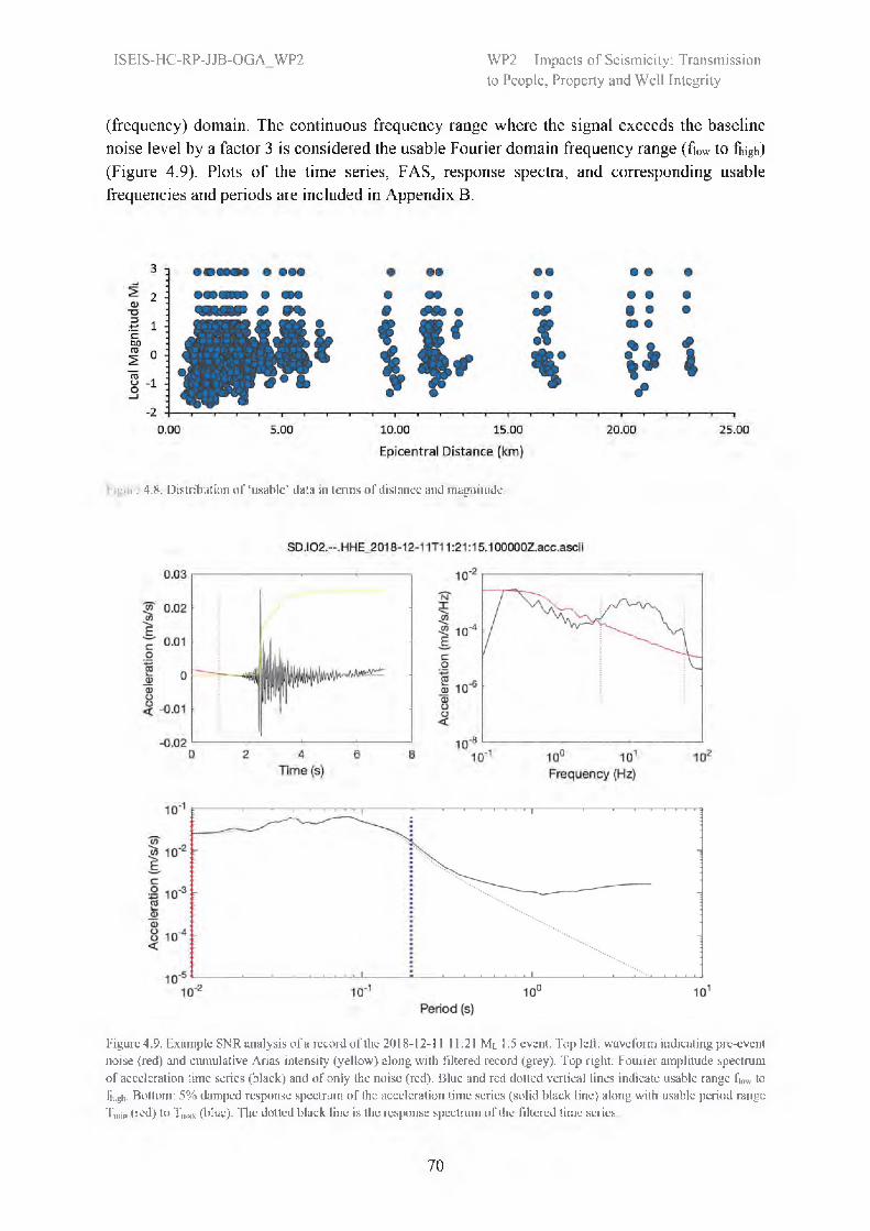
WP2 — Impacts of Seismicity: Transmissionto People, Property and Well Integrity
ISEIS-HC-RP-JJB-OGA_WP2
(frequency) domain. The continuous frequency range where the signal exceeds the baseline noise level by a factor 3 is considered the usable Fourier domain frequency range (flow to fhigh) (Figure 4.9). Plots of the time series, FAS, response spectra, and corresponding usable frequencies and periods are included in Appendix B.
Figure 4.8. Distribution of ‘usable’ data in terms of distance and magnitude.
Figure 4.9. Example SNR analysis of a record of the 2018-12-11 11:21 ML 1.5 event. Top left: waveform indicating pre-event noise (red) and cumulative Arias intensity (yellow) along with filtered record (grey). Top right: Fourier amplitude spectrum of acceleration time series (black) and of only the noise (red). Blue and red dotted vertical lines indicate usable range flow to fhigh. Bottom: 5% damped response spectrum of the acceleration time series (solid black line) along with usable period range Tmin (red) to Tmax (blue). The dotted black line is the response spectrum of the filtered time series
70

WP2 - Impacts of Seismicity: Transmissionto People, Property and Well Integrity
ISEIS-HC-RP-JJB-OGA_WP2
Figure 4.10. Number of usable records at selected oscillator periods.
Based on the SNR analysis, the usable period range for the response spectrum can be defined, which is not equivalent due to the complex interaction of input and oscillator motion (Bora et al., 2016). Based on analyses by Akkar and Bommer (2006) and Boore and Douglas (2011) we define the usable period range as Tmax = 0.8/flow and Tmin = 0.01 s (assumed equivalent to PGA) respectively. Records with fhigh < 10 Hz are discarded. For valid PGV we additionally require Tmax >0.1 and fhigh/flow > 2.
Since the events here are mostly small magnitude (the majority are ML < 1), they are dominated by high-frequency (f > 5 Hz) signals. The usable period range is therefore limited, with no data for T > 2s (Figure 4.10). A table of usable frequency range for each record is included in Electronic Appendix C.
4.3 Assessment of Predictive Models for PNR Ground MotionsAll ground motions (within their usable period limits) have been compared to the predictions from GMPEs of Atkinson (2015) and Douglas et al. (2013) (see Section 2.3.1). Both GMPEs require moment magnitude (M) rather than Ml . as available for the PNR events (see Section 2.2.1). Two conversion equations have been tested: Edwards et al. (2015) (as proposed in Section 2.2.1 for this magnitude range) since it is very similar to the empirical data from PNR- lz presented by Cuadrilla Resources (2019b), and Grünthal et al. (2009), which is based on tectonic European events. An example is shown for the ML 1.5 event in Figure 4.11.
In order to assess the full dataset, residual plots are presented (log-observed minus log-predicted spectral ordinate), using both GMPEs along with the conversion equations from ML to M of Grünthal et al. (2009) and Edwards et al. (2015). In the following only PGA, PGV and 0.3s PSA are presented for brevity. It should be noted that the Atkinson (2015) GMPE was calibrated only down to M = 3. We are therefore relying on a significant extrapolation in predicting motions at PNR. The Douglas et al. (2013) model was calibrated using data down to M = 1, and so relies on less extrapolation, but predictions below M = 1 should still be viewed with caution.
71

WP2 - Impacts of Seismicity: Transmissionto People, Property and Well Integrity
ISEIS-HC-RP-JJB-OGA_WP2
Figure 4.11. Example of recorded geometric mean horizontal PGV data (blue) and the model of Atkinson (2015) (orange, square: median; line: plus/minus one sigma). Assuming a conversion to M from ML using (top) Grünthal et al. (2009) and (bottom) Edwards et al. (2015).
72

WP2 - Impacts of Seismicity: Transmissionto People, Property and Well Integrity
ISEIS-HC-RP-JJB-OGA_WP2
4.3.1 Atkinson (2015) GMPE using Grünthal et al. (2009) MIn general, the Atkinson (2015) GMPE along with the Grünthal et al. (2009) ML to M conversion leads to systematic underprediction of up to a log 10 unit (i.e., factor of 10) for all but the longest periods (T ≥ 0.3 s). The underprediction decreases with increasing magnitude, distance and period, but always leads to biased residuals (Figures 4.12 - 4.14).
Figure 4.12. Residuals (observed - GMPE) for PGA using the Atkinson (2015) GMPE with Grünthal et al. (2009).
73
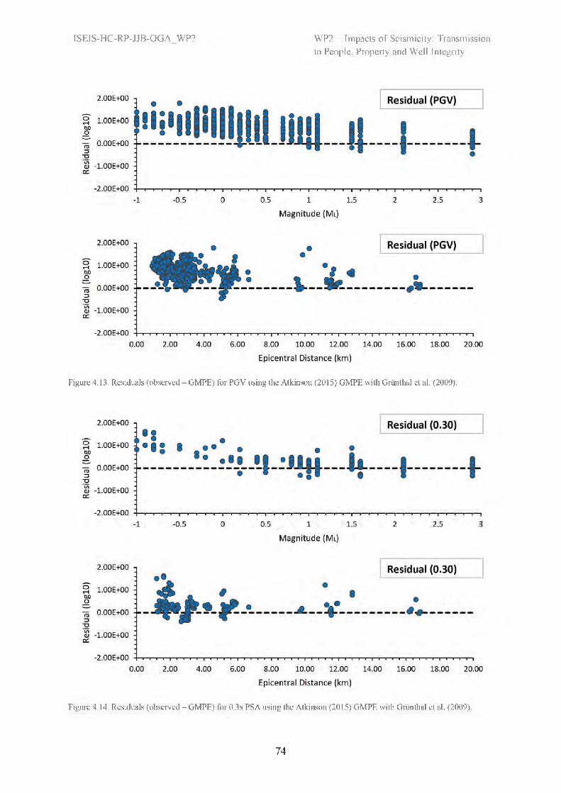
WP2 - Impacts of Seismicity: Transmissionto People, Property and Well Integrity
ISEIS-HC-RP-JJB-OGA_WP2
Figure 4.13. Residuals (observed - GMPE) for PGV using the Atkinson (2015) GMPE with Grünthal et al. (2009).
Figure 4.14. Residuals (observed - GMPE) for 0.3s PSA using the Atkinson (2015) GMPE with Grünthal et al. (2009)
74

WP2 - Impacts of Seismicity: Transmissionto People, Property and Well Integrity
ISEIS-HC-RP-JJB-OGA_WP2
4.3.1 Atkinson (2015) GMPE using Edwards et al. (2015) MUsing the ML to M conversion of Edwards et al (2015) the predictions of the Atkinson (2015) GMPE are closer to the observed values, with residuals broadly centred for distances greater than a few km and ML > 0.5. Mid- to long-period motions (e.g., T = 0.3 s) are somewhat over-predicted across the range of magnitude and distance available in the observed data. Short to mid-period motions (including PGA, PGV) tend to show a rapid decay in the first few kilometres, with these motions tending to be underpredicted by the model (Figures 4.15-4.17). We note significant outliers in Figure 4.15 and 4.16 (almost a factor 100 above the prediction, or around six standard deviations according to Atkinson, 2015). These residuals correspond to two very small events (Ml < -0.2) recorded at a relatively distant station (12 km away) and are likely to be noise contaminated (e.g., due to vibrations from a passing vehicle). Note that these residuals are present in all residual plots for PGA and PGV presented here (some points are off-scale in Figures 4.12 to 4.13).
Figure 4.15. As Figure 4.12, but using the Edwards et al. (2015) ML to M conversion.
75

WP2 - Impacts of Seismicity: Transmissionto People, Property and Well Integrity
ISEIS-HC-RP-JJB-OGA_WP2
Figure 4.16. As Figure 4.13, but using the Edwards et al. (2015) ML to M conversion
Figure 4.17. As Figure 4.14, but using the Edwards et al. (2015) ML to M conversion.
76

WP2 - Impacts of Seismicity: Transmissionto People, Property and Well Integrity
ISEIS-HC-RP-JJB-OGA_WP2
4.3.2 Douglas et al. (2013) GMPE using Grünthal et al. (2009) MThe Douglas et al (2013) GMPE using the Grünthal et al. (2009) based M exhibits the opposite behaviour to Atkinson (2015) for PGV, with significant and systematic overprediction in the magnitude-distance range available. However, for PGA the model is generally unbiased. For the longer period (T = 0.3 s) PSA, the motions tend to be systematically underpredicted.
Figure 4.18. Residuals (observed - GMPE) for PGA using the Douglas et al. (2013) GMPE with Grünthal et al. (2009).
77

WP2 - Impacts of Seismicity: Transmissionto People, Property and Well Integrity
ISEIS-HC-RP-JJB-OGA_WP2
Figure 4.19. Residuals (observed - GMPE) for PGV using the Douglas el al. (2013) GMPE with Grünthal et al. (2009).
Figure 4.20. Residuals (observed- GMPE) for 0.3s PSA using the Douglas et al. (2013) GMPE with Grünthal et al. (2009)
78

WP2 - Impacts of Seismicity: Transmissionto People, Property and Well Integrity
ISEIS-HC-RP-JJB-OGA_WP2
4.3.3 Douglas et al. (2013) GMPE using Edwards et al. (2015) M
Using the Edwards et al. (2015) ML to M conversion leads to worse residuals for PGA and PGV for the Douglas et al. (2013) model (Figures 4.21 - 4.23). However, the predictions at mid- to long-periods (e.g., T = 0.3 s) is in this case are broadly unbiased. A trend in the PGA residuals at very short distance [although weaker than seen using the Atkinson (2015) model] indicates rapid decay of the amplitudes with distance in the near-epicentre region, which is not captured in the models.
Figure 4.21. As Figure 4.18, but using the Edwards et al. (2015) conversion from ML to M.
79
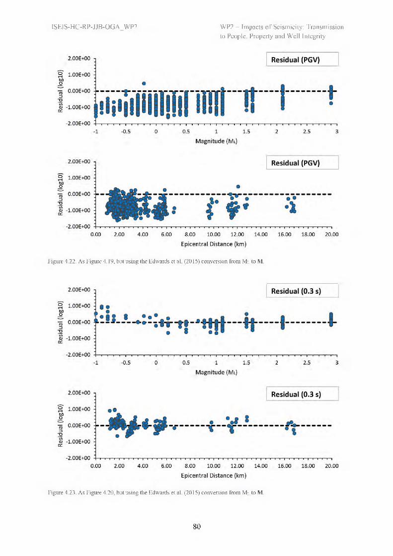
WP2 - Impacts of Seismicity: Transmissionto People, Property and Well Integrity
ISEIS-HC-RP-JJB-OGA_WP2
Figure 4.22. As Figure 4.19, but using the Edwards et al. (2015) conversion from ML to M.
Figure 4.23. As Figure 4.20, but using the Edwards et al. (2015) conversion from ML to M.
80
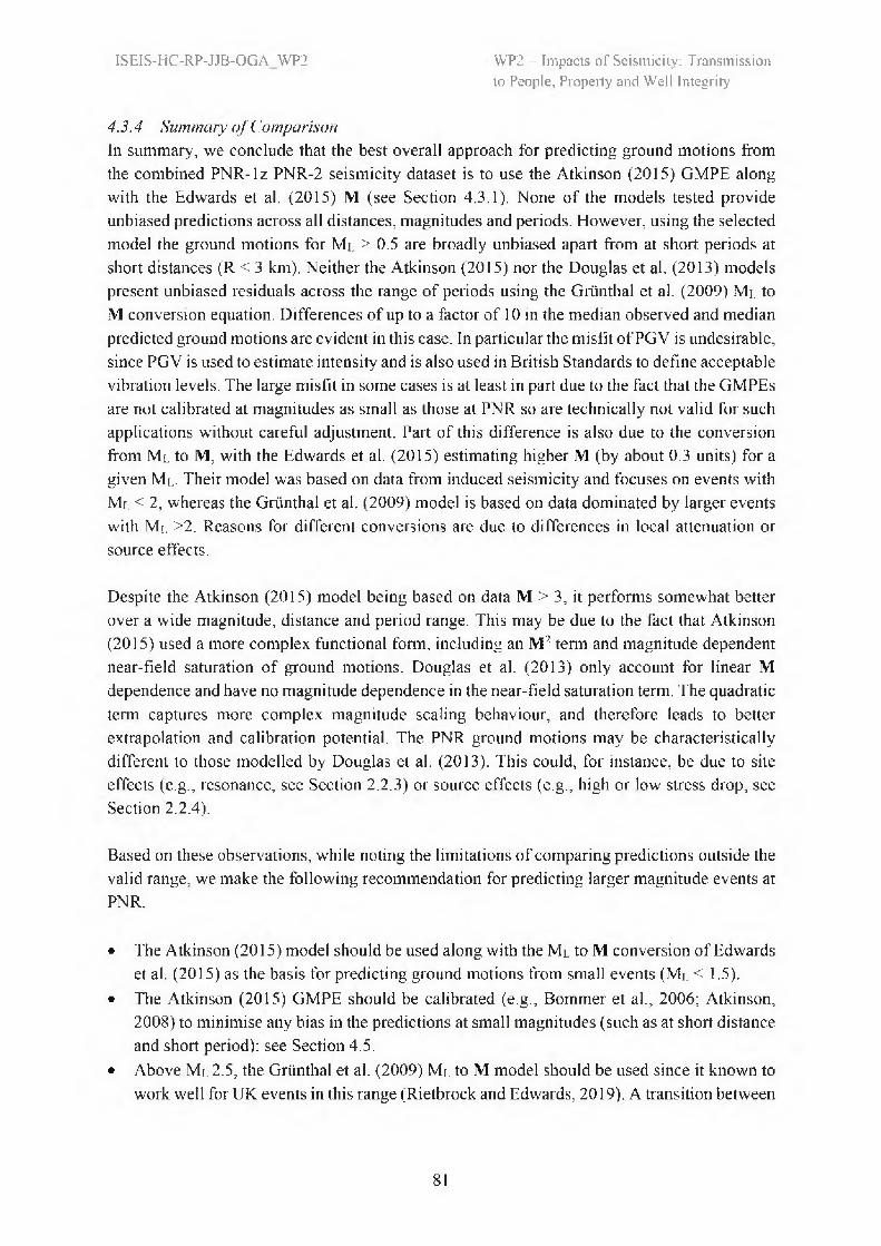
WP2 - Impacts of Seismicity: Transmissionto People, Property and Well Integrity
ISEIS-HC-RP-JJB-OGA_WP2
4.3.4 Summary of ComparisonIn summary, we conclude that the best overall approach for predicting ground motions from the combined PNR-1z PNR-2 seismicity dataset is to use the Atkinson (2015) GMPE along with the Edwards et al, (2015) M (see Section 4.3.1), None of the models tested provide unbiased predictions across all distances, magnitudes and periods. However, using the selected model the ground motions for ML > 0.5 are broadly unbiased apart from at short periods at short distances (R < 3 km). Neither the Atkinson (2015) nor the Douglas et al. (2013) models present unbiased residuals across the range of periods using the Grünthal et al. (2009) ML to M conversion equation. Differences of up to a factor of 10 in the median observed and median predicted ground motions are evident in this case. In particular the misfit of PGV is undesirable, since PGV is used to estimate intensity and is also used in British Standards to define acceptable vibration levels. The large misfit in some cases is at least in part due to the fact that the GMPEs are not calibrated at magnitudes as small as those at PNR so are technically not valid for such applications without careful adjustment. Part of this difference is also due to the conversion from ML to M, with the Edwards et al. (2015) estimating higher M (by about 0.3 units) for a given Ml . Their model was based on data from induced seismicity and focuses on events with ML < 2, whereas the Grünthal et al. (2009) model is based on data dominated by larger events with ML >2. Reasons for different conversions are due to differences in local attenuation or source effects.
Despite the Atkinson (2015) model being based on data M > 3, it performs somewhat better over a wide magnitude, distance and period range. This may be due to the fact that Atkinson (2015) used a more complex functional form, including an M2 term and magnitude dependent near-field saturation of ground motions. Douglas et al. (2013) only account for linear M dependence and have no magnitude dependence in the near-field saturation term. The quadratic term captures more complex magnitude scaling behaviour, and therefore leads to better extrapolation and calibration potential. The PNR ground motions may be characteristically different to those modelled by Douglas et al. (2013). This could, for instance, be due to site effects (e.g., resonance, see Section 2.2.3) or source effects (e.g., high or low stress drop, see Section 2.2.4).
Based on these observations, while noting the limitations of comparing predictions outside the valid range, we make the following recommendation for predicting larger magnitude events at PNR.
• The Atkinson (2015) model should be used along with the ML to M conversion of Edwards et al. (2015) as the basis for predicting ground motions from small events (ML < 1.5).
• The Atkinson (2015) GMPE should be calibrated (e.g., Bommer et al., 2006; Atkinson, 2008) to minimise any bias in the predictions at small magnitudes (such as at short distance and short period): see Section 4.5.
• Above ML 2.5, the Grünthal et al. (2009) Ml to M model should be used since it known to work well for UK events in this range (Rietbrock and Edwards, 2019). A transition between
81

WP2 - Impacts of Seismicity: Transmissionto People, Property and Well Integrity
ISEIS-HC-RP-JJB-OGA_WP2
the conversions in the range Ml 1.5 to 2.5 should be included to avoid a step in the Ml to M conversion relation (Figure 2.5).
The calibration of the Atkinson (2015) model to the PNR data at low magnitude, while retaining its predictions for larger events, is presented in Section 4.5. The approach suggested here will result in predictions for Ml ≤ 2.9 that are unbiased with respect to recorded data at PNR. It also ensures that predictions at Ml > 2.5 are well calibrated to data (albeit natural earthquakes) and use a Ml to M relation that has been shown to be suitable across the UK and Europe in the ML > 2 range. In the case that enough locally recorded events become available in the higher magnitude range (Ml > 1.5) and the data support a revision to the approach above, the transition points between the two conversion relations can simply be revised, whilst maintaining the same rationale.
4.4 Comparison of Observed Motions with Anthropogenic Sources of VibrationGround motions can be compared against other anthropogenic sources of vibration as a means to provide a context for the level of shaking. Construction sites and other industrial activities, for instance, generate vibrations which are limited by thresholds defined in British Standards. In addition, everyday activities, from dropped objects to desk fans and coffee machines, generate vibrations. Figure 4.24 shows a variety of shaking levels for anthropogenic sources, along with those recorded at the PNR site for the more ‘moderate’ ML 1.1 and 1.5 events. Generally, the motions can be considered as almost imperceptible and well below the level of vibration that people experience going about everyday activities.
British Standard 6472 (BSI, 2008) lays out a range of acceptable maximum levels of PGV for blast-type vibrations (no more than three per day), which is appropriate for induced seismicity (Table 4.1). For residential properties a PGV of 6 - 10 mm/s are deemed acceptable during the day, reduced to 2 mm/s at night. A scaling factor is provided to reduce the acceptable levels when more than 3 ‘events’ (i.e., in this case felt earthquakes) per day are expected.
British Standard 7385-2 (BSI, 1993) defines acceptable thresholds for vibration and the levels at which cosmetic damage may occur (Figure 4.25). Finally, BS 7385-2 notes that the probability of damage approaches zero at PGV of 12.5 mm/s, consistent with the ShakeMap intensity IV (light shaking, no damage). British Standard 5228-2 (BSI, 2014) notes that minor damage is possible at vibration amplitudes which are greater than twice the threshold for cosmetic damage, and major damage to a building structure can occur at values greater than four times these values.
82

WP2 — Impacts of Seismicity: Transmissionto People, Property and Well Integrity
ISEIS-HC-RP-JJB-OGA_WP2
Figure 4.24. Examples of thresholds for tolerable motions defined in terms of PGV and the dominant frequency of the shaking due to blasting (left; USAGE, 1972), traffic (middle; Bameich, 1985) and pile-driving (right; Athanasopoulos and Pelekis, 2000) and PGV from the PNR dataset (blue squares). Modified from Bommer et al. (2006).
Definitions of damage categories are presented in British Standard ISO 4866 (BS1, 2010), where:
• Cosmetic: the formation of hairline cracks on drywall surfaces, or the growth of existing cracks in plaster or dry wall surfaces; in addition, the formation of hairline cracks in mortar joints of brick/concrete block construction. This is roughly equivalent to damage state 1 (DS1, see Section 2.6).
• Minor: the formation of large cracks or loosening and falling of plaster or drywall surfaces, or cracks through bricks/concrete blocks. This is roughly equivalent to DS2.
• Major: the damage to structural elements of the structure, cracks in support columns, loosening of joints, splaying of masonry cracks, etc.
83

WP2 — Impacts of Seismicity: Transmissionto People, Property and Well Integrity
ISEIS-HC-RP-JJB-OGA_WP2
Table 4.1. From British Standard 6472-2 (BSI, 2008b). Maximum satisfactory magnitudes of vibration with respect to human response for up to three blast vibration events per day.
Place Time Satisfactory magnitude A) ppv mms-1
ResidentialDay D)Night D)Other times D)
6.0 to 10.0c)2.04.5
Offices B) Any time 14.0
Workshops B) Any time 14.0NOTE 1 This table recommends magnitudes of vibration below which the probability of adverse comment is low (noise caused by any structural vibration is not considered).
NOTE 2 Doubling the suggested vibration magnitudes could result in adverse comment and this will increase significantly if the magnitudes are quadrupled.
NOTE 3 For more than three occurrences of vibrations per day see the further multiplication factor in 5.2.A) The satisfactory magnitudes are the same for the working day and the rest
of the day unless stated otherwise.B) Critical working areas where delicate tasks impose more stringent criteria
than human comfort are outside the scope of this standard.C) Within residential properties people exhibit a wide variation of tolerance to
vibration. Specific values are dependent upon social and cultural factors, psychological attitudes and the expected degree of intrusion. In practice the lower satisfactory magnitude should be used with the higher magnitude being justified on a case-by-case basis.
D) For the purpose of blasting, daytime is considered to be 08h00 to 18h00 Monday to Friday and 08h00 to 13h00 Saturday. Routine blasting would not normally be considered on Sundays or Public Holidays. Other times cover the period outside of the working day but exclude night-time, which is defined as 23h00 to 07h00.
Figure 4.25. British Standard 7385-2:1993 PPV (component) thresholds for cosmetic, minor and major damage
84

WP2 - Impacts of Seismicity: Transmissionto People, Property and Well Integrity
ISEIS-HC-RP-JJB-OGA_WP2
4.5 Calibration of a PNR-specific GMPEWhile the Atkinson (2015, hereinafter A15) GMPE is designed for induced seismicity, and is therefore an obvious choice for the application at PNR, it is nevertheless based on data from potentially very different and diverse geological settings. Furthermore, the magnitude range of this model is M = 3 and above - as dictated by the dataset used in its derivation. Application to events of smaller magnitude relies on extrapolation, which cannot be guaranteed to work well. As shown in the Section 4.3, the model performs reasonably well, despite these limitations. However, systematic differences between the model predictions and the PNR data are apparent. One typical approach when dealing with local seismicity, is to calibrate a base GMPE such that it predicts ground motion data available in the target region with minimum bias, sometimes referred to as the ‘referenced empirical approach’ (Atkinson, 2008). Such adjustment can also take into account the following:
a) Potentially lower stress drop sources for induced (shallow) events (Hough, 2014): the A15 model is designed for induced events (by making use of low M, short R data), but still makes extensive use of deeper tectonic events
b) The more rapid decay of motions in the near-field (distances less than a few km), which may arise due to strong attenuation effects as waves propagate at shallow depths.
The calibration is performed through mixed-effects regression and residual analysis:
1. Determine logarithmic residuals between the recorded data (PGV, PGA, PSA) and the A15 predictions (see Section 4.3). Here we use site-specific Vs30 and compute non-linear amplification factors using the Boore et al. (2014) model, as per the approach suggested by Atkinson (2015). In doing this we assume that the Boore et al. (2014) amplification model is consistent with the site conditions present at PNR
2. Fit the residuals (Figures 4.26,4.27) using a linear mixed-effects regression with parametric form as defined by Atkinson (2015):
X = bc0 + AqM 4- Ac 2M2 + Ac 3 log10 R + Be + VKS. (23)
With X here the (log10) residual for a given spectral ordinate, M the moment magnitude and R, an effective distance, defined as:
R= Itfyp + max(l,10-°-28+019M)2. (24)
Note that this is the ‘alternative’ formulation for R defined by Atkinson (2015), and subsequently recommended by the author for application (Atkinson, 2020). Be are event-specific random effects with a prior belonging to a normal distribution defined by N(0,τ) and Ws are station-specific random effects with prior distribution defined by N(0, φ). In the calibration framework adopted here, a constraint is applied that the adjusted GMPE should converge to the original model for M = 4.5 at Rhyp = 20 km, roughly the mid-point of the dataset used in the derivation of the original model.
85
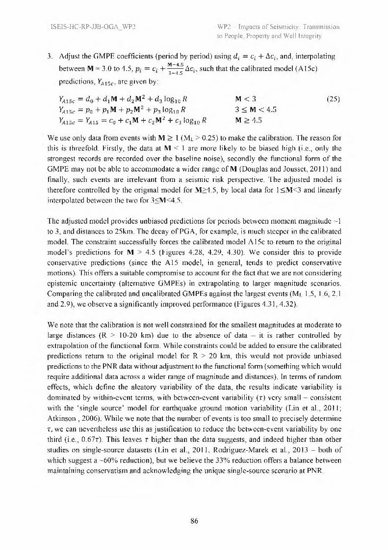
WP2 - Impacts of Seismicity: Transmissionto People, Property and Well Integrity
ISEIS-HC-RP-JJB-OGA_WP2
3. Adjust the GMPE coefficients (period by period) using di = ci + Δci, and, interpolating
between M = 3.0 to 4.5, M—4.5
pi = q -I------ -Ac,3—4.5
, such that the calibrated model (A 15c)
predictions, YA15c, are given by:
Yii5c = d0 + d1M + d2M2 + d3 log10 R M < 3 YA15c = p0 + P1M + p2M2 + p3 log10 R 3 < M < 4.5YA15c = Kus = c0 + cxM + c2M2 + c3 log10 R M > 4.5
(25)
We use only data from events with M ≥ 1 (ML > 0.25) to make the calibration. The reason for this is threefold. Firstly, the data at M < 1 are more likely to be biased high (i.e., only the strongest records are recorded over the baseline noise), secondly the functional form of the GMPE may not be able to accommodate a wider range of M (Douglas and Jousset, 2011) and finally, such events are irrelevant from a seismic risk perspective. The adjusted model is therefore controlled by the original model for M>4.5, by local data for 1<M<3 and linearly interpolated between the two for 3<M<4.5.
The adjusted model provides unbiased predictions for periods between moment magnitude ~1 to 3, and distances to 25km. The decay of PGA, for example, is much steeper in the calibrated model. The constraint successfully forces the calibrated model A 15c to return to the original model’s predictions for M > 4.5 (Figures 4.28, 4.29, 4.30). We consider this to provide conservative predictions (since the A15 model, in general, tends to predict conservative motions). This offers a suitable compromise to account for the fact that we are not considering epistemic uncertainty (alternative GMPEs) in extrapolating to larger magnitude scenarios. Comparing the calibrated and uncalibrated GMPEs against the largest events (Ml 1.5, 1.6, 2.1 and 2.9), we observe a significantly improved performance (Figures 4.31,4.32).
We note that the calibration is not well constrained for the smallest magnitudes at moderate to large distances (R > 10-20 km) due to the absence of data - it is rather controlled by extrapolation of the functional form. While constraints could be added to ensure the calibrated predictions return to the original model for R > 20 km, this would not provide unbiased predictions to the PNR data without adjustment to the functional form (something which would require additional data across a wider range of magnitude and distances). In terms of random effects, which define the aleatory variability of the data, the results indicate variability is dominated by within-event terms, with between-event variability (τ) very small - consistent with the ‘single source’ model for earthquake ground motion variability (Lin et al., 2011; Atkinson , 2006). While we note that the number of events is too small to precisely determine τ, we can nevertheless use this as justification to reduce the between-event variability by one third (i.e., 0.67t ). This leaves τ higher than the data suggests, and indeed higher than other studies on single-source datasets (Lin et al., 2011, Rodriguez-Marek et al., 2013 - both of which suggest a ~60% reduction), but we believe the 33% reduction offers a balance between maintaining conservatism and acknowledging the unique single-source scenario at PNR.
86
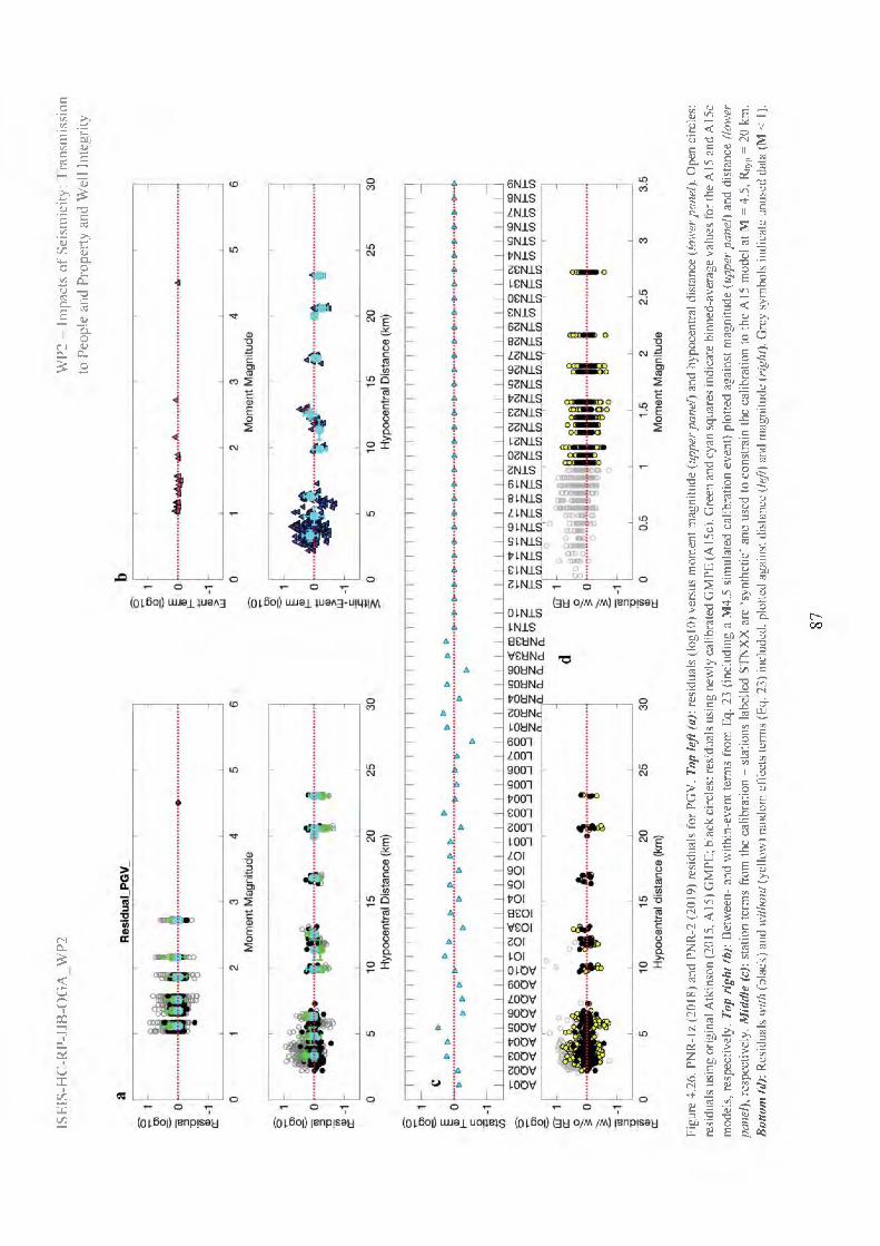
ISEI
S-H
C-R
P-JJ
B-O
GA
_WP2
WP2
- I
mpa
cts
of S
eism
icity
: Tra
nsm
issi
onto
Peo
ple
and
Prop
erty
and
Wel
l In
tegr
ity
Figu
re 4
.26.
PN
R-1
z (2
018)
and
PN
R-2
(201
9) r
esid
uals f
or P
GV
. To
p le
ft (a
): re
sidu
als
(log
10) v
ersu
s m
omen
t mag
nitu
de (
uppe
rpan
el)
and
hypo
cent
ral
dist
ance
(lo
wer
pane
l). O
pen
circ
les:
re
sidu
als
usin
g or
igin
al A
tkin
son
(201
5, A
15) G
MPE
; bla
ck c
ircle
s: re
sidu
als
usin
g ne
wly
cal
ibra
ted
GM
PE (A
15c
). G
reen
and
cya
n sq
uare
s in
dica
te b
inne
d-av
erag
e va
lues
for t
he A
15 a
nd A
l 5c
mod
els,
resp
ectiv
ely. T
op r
ight
(b)
: B
etw
een-
and
with
in-e
vent
term
s fr
om E
q. 2
3 (in
clud
ing
a M
4.5
sim
ulat
ed c
alib
ratio
n ev
ent)
plot
ted
agai
nst m
agni
tude
(up
perp
anel
) an
d di
stan
ce (
low
er
pane
l), r
espe
ctiv
ely. M
iddl
e (c
): st
atio
n te
rms
from t
he c
alib
ratio
n -
stat
ions
lab
elle
d ST
NX
X a
re ‘
synt
hetic
’ and
use
d to
con
stra
in th
e ca
libra
tion
to th
e A
15 m
odel a
t M =
4.5
, Rhy
p =
20 k
m.
Bot
tom
(d):
Res
idua
ls w
ith (b
lack
) and
with
out (
yello
w)
rand
om e
ffec
ts te
rms
(Eq.
23)
incl
uded
, plo
tted
agai
nst d
ista
nce
(left)
and
mag
nitu
de (r
ight
). G
rey
sym
bols
indi
cate
unu
sed
data
(M <
1).
87
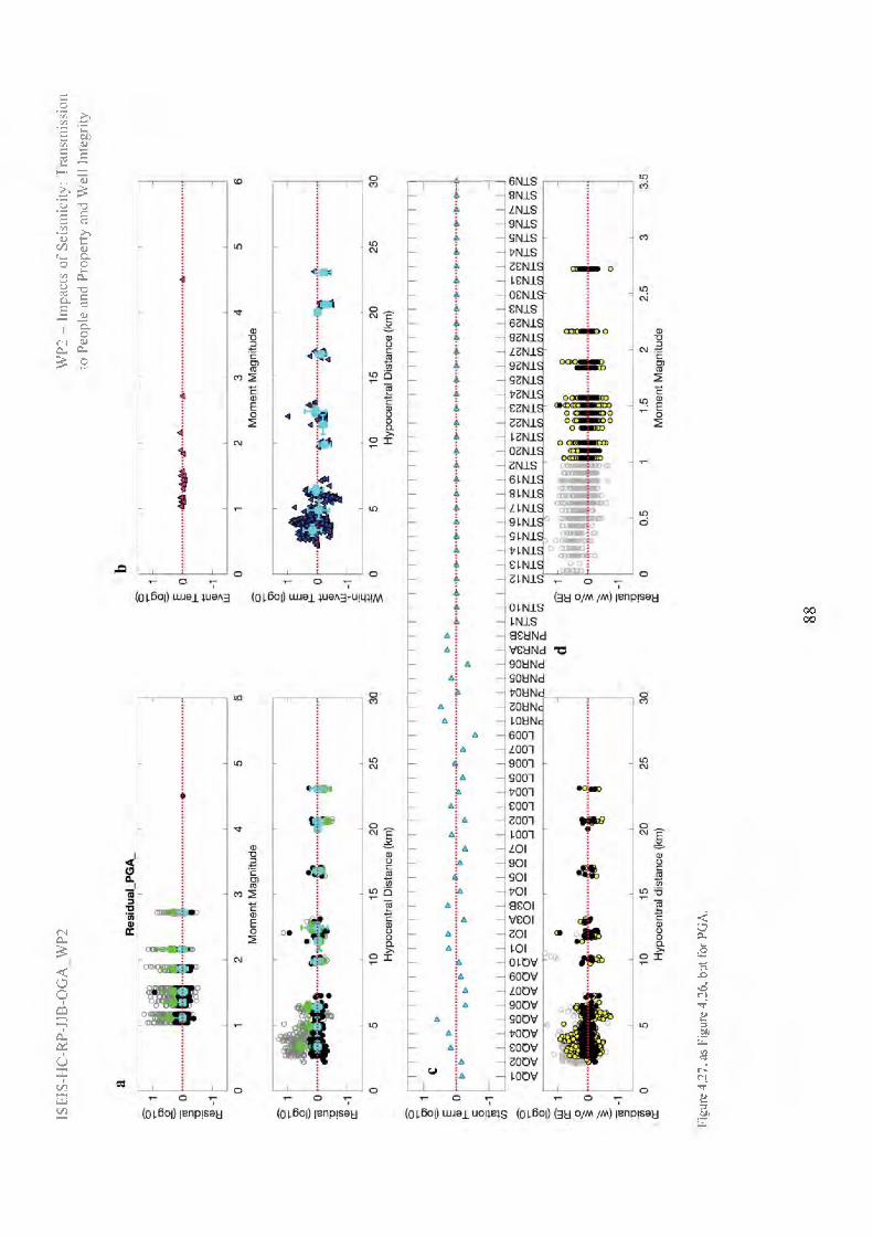
WP2
- I
mpa
cts
of S
eism
icity
: Tr
ansm
issi
onto
Peo
ple
and
Prop
erty
and
Wel
l In
tegr
ityIS
EIS-
HC
-RP-
JJB
-OG
A_W
P2
Figu
re 4
.27.
as
Figu
re 4
.26,
but
for
PG
A.
88

ISEI
S-H
C-R
P-JJ
B-O
GA
_WP2
WP2
— I
mpa
cts
of S
eism
icity
: Tra
nsm
issi
on
to P
eopl
e an
d Pr
oper
ty a
nd W
ell I
nteg
rity
Figu
re 4
.28.
Com
paris
on o
f orig
inal
GM
PE (A
15, d
otte
d lin
es) a
nd th
e ca
libra
ted
mod
el (A
15c,
sol
id li
nes)
for
PGV
. To
p: p
redi
ctio
ns v
ersu
s m
omen
t mag
nitu
de (l
eft)
and
dist
ance
(rig
ht).
Botto
m:
Diff
eren
ce (r
atio
) bet
wee
n or
igin
al a
nd a
djus
ted
GM
PEs
(A15
c/A
15) v
ersu
s m
omen
t mag
nitu
de (l
eft)
and
dist
ance
(rig
ht) -
i.e.
ratio
of s
olid
(A
15c)
and
dot
ted
(A15
) lin
es in
pan
els
abov
e.
89
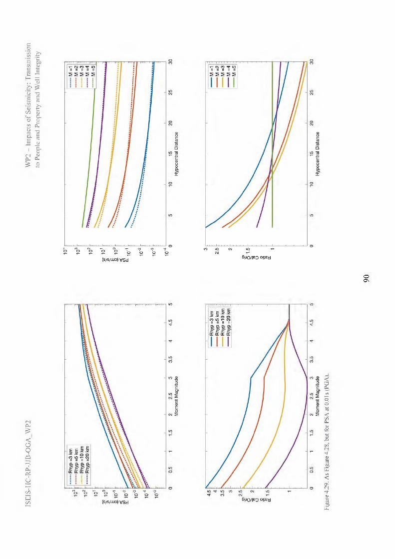
ISEI
S-H
C-R
P-JJ
B-O
GA
_WP2
WP2
— I
mpa
cts
of S
eism
icity
: Tra
nsm
issi
on
to P
eopl
e an
d Pr
oper
ty a
nd W
ell I
nteg
rity
Figu
re 4
.29.
As
Figu
re 4
.28,
but
for P
SA a
t 0.0
1s (P
GA
).
90

WP2 — Impacts of Seismicity: Transmissionto People, Property and Well Integrity
ISEIS-HC-RP-JJB-OGA_WP2
Figure 4.30. Predicted PSA versus period for the A15 (dotted lines) and adjusted A 15c (solid lines) models. Note, predicted PSA is interpolated between the published A15 periods.
Figure 4.31. Example application of the original (A 15, dotted) and calibrated model (A 15c, solid) to the PGV data from the lour largest events (ML = 1.5, 1.6; 2.1 and 2.9).
91

WP2 — Impacts of Seismicity: Transmissionto People, Property and Well Integrity
ISEIS-HC-RP-JJB-OGA_WP2
Figure 4.32. as Figure 4.31, but for PSA at 0.01s (PGA).
Table 4.2. Adjustment coefficients.
PGV PGA T=0.03s T=0.05s T=0.1s T=0.2s T=0.3s T=0.5sΔco 0.4768 0.9835 1.4608 1.1935 0.1346 -0.3445 -0.2713 0.7530ΔC1 -0.2398 -0.2486 -0.2781 -0.2924 -0.0209 -0.0094 -0.1653 -0.5752ΔC2 0.0498 0.0456 0.0522 0.0473 0.0034 0.0176 0.0424 0.1144ΔC3 -0.3113 -0.6062 -0.9729 -0.6437 -0.0800 0.0257 0.1222 -0.3670
92

WP2 - Impacts of Seismicity: Transmissionto People, Property and Well Integrity
ISEIS-HC-RP-JJB-OGA_WP2
5. Assessment of Potential Impact of Future ScenariosThe following section deals with potential future earthquake scenarios and their impact on people and the built environment.
5.1 Proposal of Potential Induced Earthquake ScenariosDefining possible earthquake scenarios, given the available information and state of knowledge about induced seismicity, is difficult and somewhat ambiguous. Nevertheless, we define five illustrative scenarios (with focus on the three of those in terms of intensity prediction) and, in the subsequent sections, describe the effects of those events in terms of building damage and exposure of the local population to shaking. It is worth highlighting that the original proposal of scenarios was completed prior to the operator commencing hydraulic fracturing operations on the second well (PNR-2), and which led to larger magnitude events than at PNR-1z (ML 1.5) and earlier at Preese Hall (ML 2.3). The logic behind our choice of scenarios was not altered by this increased level of seismicity (with the ML2.9 originally considered between ‘likely to happen’ and ‘may happen’ in our scenarios).
The scenarios we consider are ML = 2.5 to 4.5 in 0.5 increments. The ML = 2.5 event is similar to a previous induced event in 2011 that led to a moratorium on hydraulic fracturing in the UK, the Preese Hall ML = 2.3 earthquake. This event therefore represents a scenario that can be considered ‘likely to happen’ (or unsurprising) at PNR, which is only 4 km from the Preese Hall site. Events of ML 3.0 and 3.5 are not appreciably larger than that this so cannot be ruled out in the future and may, for instance, occur as trailing events, despite shut in. For instance, the Basel 2006 ML 3.4 event occurred during shut in after an earlier ML 2.3 event. Since the work for this report was completed a larger ML 2.9 event was recorded at the PNR-2 well, which is close to the ‘maximum magnitude’ of ML 3.1 for that well proposed by the operator (Cuadrilla Resources, 2019b). The largest events we consider are ML 4.0 and 4.5, which are considered unlikely given the UK traffic light threshold and regulatory environment (e.g., with 3D seismic imaging and extensive monitoring) in place. Nevertheless, shallow focus events of similar magnitude have occurred previously in the UK and we cannot therefore rule out that an event of this magnitude could be triggered by fluid injection into a critically stressed fault (particularly small faults with limited throw in the vicinity of the reservoir that may not have been observed by 3D seismics). It is beyond the scope of this report to assign probabilities or quantitative likelihoods to these scenarios and they are provided instead as illustrative examples to aid decision making. Furthermore, in addition to the hypothetical scenarios we include two further events that can be used as direct comparisons with the largest events that occurred at PNR-2: ML 2.1 and 2.9.
5.2 Assessment of Potential Shaking LevelsIn order to estimate the shaking level and associated macrosesimic intensity we use the locally- calibrated version of the Atkinson (2015) GMPE (see Section 4.5) along with the ML to M conversion equation of Grünthal et al. (2009) (since all considered scenarios have M > 2.5, see Section 2.2.1). We use spatially dependent Vs30 values (see Section 3.3) to represent the site conditions across the PNR region. The GMICE of Caprio et al. (2015) (see Section 2.4.2) is
93
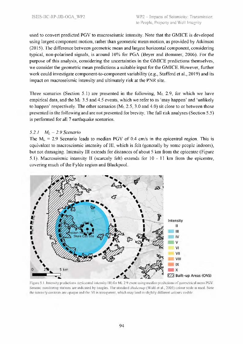
WP2 — Impacts of Seismicity: Transmissionto People, Property and Well Integrity
ISEIS-HC-RP-JJB-OGA_WP2
used to convert predicted PGV to macroseismic intensity. Note that the GMICE is developed using largest component motion, rather than geometric mean motion, as provided by Atkinson (2015). The difference between geometric mean and largest horizontal component, considering typical, non-polarised signals, is around 10% for PGA (Beyer and Bommer, 2006). For the purpose of this analysis, considering the uncertainties in the GMICE predictions themselves, we consider the geometric mean predictions a suitable input for the GMICE. However, further work could investigate component-to-component variability (e.g., Stafford et al., 2019) and its impact on macroseismic intensity and ultimately risk at the PNR site.
Three scenarios (Section 5.1) are presented in the following, ML 2.9, for which we have empirical data, and the ML 3.5 and 4.5 events, which we refer to as ‘may happen’ and ‘unlikely to happen’ respectively. The other scenarios (Ml 2.5, 3.0 and 4.0) sit close to or between those presented in the following and are not presented for brevity. The full risk analyses (Section 5.5) is performed for all 7 earthquake scenarios.
5.2.1 Ml = 2.9 ScenarioThe Ml = 2.9 Scenario leads to median PGV of 0.4 cm/s in the epicentral region. This is equivalent to macroseismic intensity of III, which is felt (generally by some people indoors), but not damaging. Intensity III extends for distances of about 5 km from the epicentre (Figure 5.1). Macroseismic intensity II (scarcely felt) extends for 10-11 km from the epicentre, covering much of the Fylde region and Blackpool.
Figure 5.1. Intensity predictions (epicentral intensity III) for ML 2.9 event using median predictions of geometrical mean PGV. Seismic monitoring stations are indicated by tringles. The standard Shakemap (Wald et al., 2005) colour scale is used. Note the intensity contours are opaque and the fill is transparent, which may lead to slightly different colours visible.
94

WP2 — Impacts of Seismicity: Transmissionto People, Property and Well Integrity
ISEIS-HC-RP-JJB-OGA_WP2
Figure 5.2. Intensity predictions (epicentral intensity IV) for ML 2.9 event using median plus one sigma predictions of geometrical mean PGV The standard Shakemap colour scale is used. Note the intensity contours are opaque and the fill is transparent, which may lead to slightly different colours visible.
The intensity presented in Figure 5.1 (and subsequently in Figures 5.3, 5.5) are for the median intensity from a median PGV prediction. This represents the most likely scenario for a ML 2.9 event (based on the models adopted). However, ground motions are highly variable, both from event to event (for the same magnitude) and from site to site (for one event) (see Section 2.1.4). If we instead look for a low-probability case we can use the PGV model’s standard deviation (sigma) to predict motions that lie on the 84th-percentile (i.e., plus one standard deviation). This implies not only that we have a particularly energetic earthquake, but also a particularly amplifying soil condition. It is obviously unlikely that a uniform condition like this would exist across the region (only 16% of motions for this scenario will exceed the predicted median plus one sigma), however, we may observe pockets of high intensity motion consistent with those predicted. Figure 5.2 therefore represents the intensity possible at this level - but should not be considered a proxy for the region-wide intensity map. For the median plus one sigma prediction of geometrical mean PGV we observe an increase in the epicentral intensity to IV and a significant widening of the intensity III and II regions (Figure 5.2).
5.2.2 Ml -3.5 ScenarioThe ML= 3.5 scenario (Figure 5.3) leads to a significant increase in the extent of felt shaking and an increase in the epicentral intensity in the median PGV case to IV (light shaking, may cause windows and doors to rattle). The maximum median PGV is 1.5 cm/s. Intensity IV is not generally associated with damage. Intensity IV extends for approximately 4-5 km from the epicentre, while intensity III extends for about 11-12 km. While median motions are below the threshold considered potentially damaging in British Standard 7385-2:1993, the significant aleatory variability means that motions may exceed 1.5 cm/s and lead to some cosmetic damage at the epicentre with intensity V expected up to 1 - 2 km from the epicentre (Figure 5.4). Please
95

WP2 — Impacts of Seismicity: Transmissionto People, Property and Well Integrity
ISEIS-HC-RP-JJB-OGA_WP2
see Section 5.2.1 for an explanation of the median plus one sigma predictions, which should not be considered as a likely region-wide prediction, but possible upper-estimates in some localised areas.
Figure 5.3. Intensity predictions (epicentral intensity IV) for ML 3.5 event using median predictions of geometrical mean PGV. Seismic monitoring stations are indicated by tringles. The standard Shakemap colour scale is used. Note the intensity contours are opaque and the fill is transparent, which may lead to slightly different colours visible.
Figure 5.4. Intensity predictions (epicentral intensity V) for ML 3.5 event using median plus one sigma predictions of geometrical mean PGV. The standard Shakemap colour scale is used. Note the intensity contours are opaque and the fill is transparent, which may lead to slightly different colours visible.
96
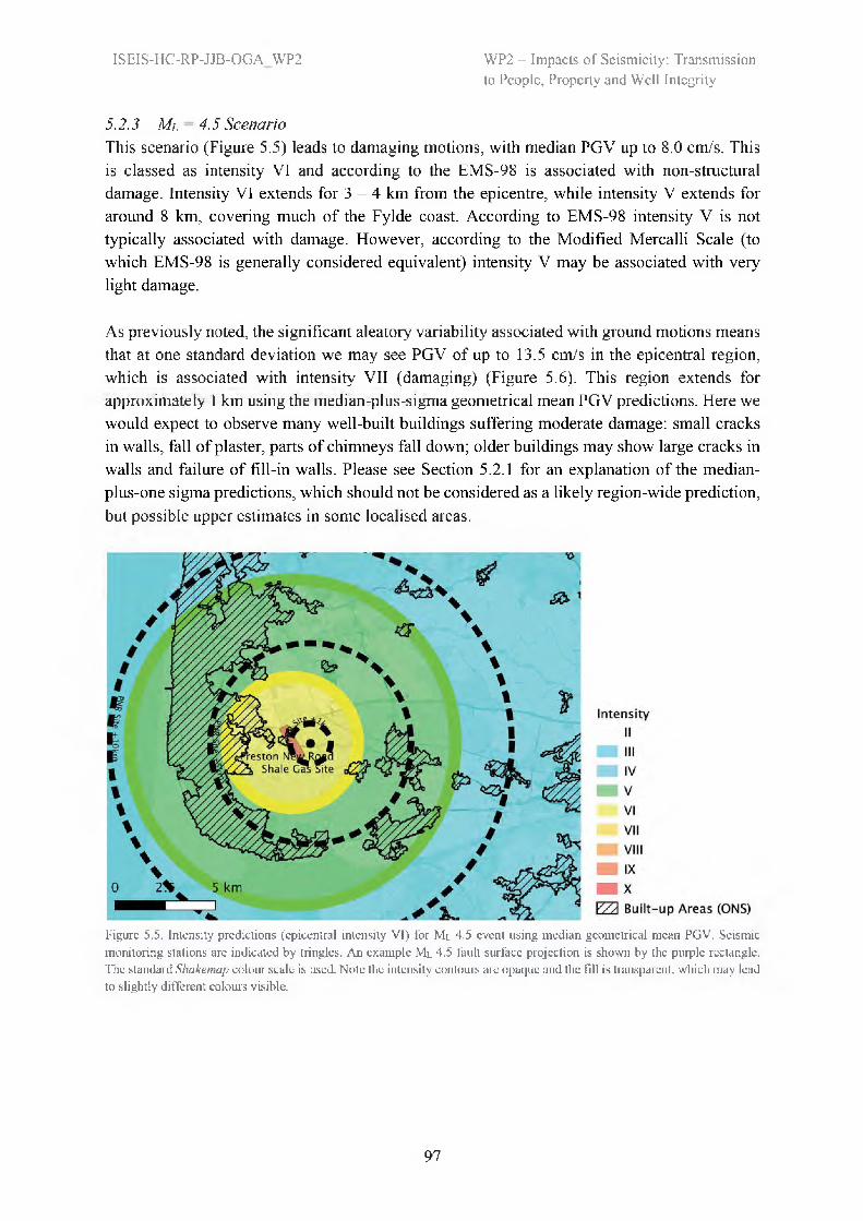
WP2 — Impacts of Seismicity: Transmissionto People, Property and Well Integrity
ISEIS-HC-RP-JJB-OGA_WP2
5.2.3 Ml =4.5 ScenarioThis scenario (Figure 5.5) leads to damaging motions, with median PGV up to 8.0 cm/s. This is classed as intensity VI and according to the EMS-98 is associated with non-structural damage. Intensity VI extends for 3 - 4 km from the epicentre, while intensity V extends for around 8 km, covering much of the Fylde coast. According to EMS-98 intensity V is not typically associated with damage. However, according to the Modified Mercalli Scale (to which EMS-98 is generally considered equivalent) intensity V may be associated with very light damage.
As previously noted, the significant aleatory variability associated with ground motions means that at one standard deviation we may see PGV of up to 13.5 cm/s in the epicentral region, which is associated with intensity VII (damaging) (Figure 5.6). This region extends for approximately 1 km using the median-plus-sigma geometrical mean PGV predictions. Here we would expect to observe many well-built buildings suffering moderate damage: small cracks in walls, fall of plaster, parts of chimneys fall down; older buildings may show large cracks in walls and failure of fill-in walls. Please see Section 5.2.1 for an explanation of the median-plus-one sigma predictions, which should not be considered as a likely region-wide prediction, but possible upper estimates in some localised areas.
Figure 5.5. Intensity predictions (epicentral intensity VI) for Ml 4.5 event using median geometrical mean PGV. Seismic monitoring stations arc indicated by tringles. An example Ml 4.5 fault surface projection is shown by the purple rectangle. The standard Shakemap colour scale is used. Note the intensity contours are opaque and the fill is transparent, which may lead to slightly different colours visible.
97

WP2 — Impacts of Seismicity: Transmissionto People, Property and Well Integrity
ISEIS-HC-RP-JJB-OGA_WP2
Figure 5.6. Intensity predictions (epicentral intensity VII) for ML 4.5 event using median plus one sigma geometrical mean PGV. An example Ml 4.5 fault surface projection is shown by the purple rectangle. The standard Shakemap colour scale is used. Note the intensity contours are opaque and the fill is transparent, which may lead to slightly different colours visible.
5.2.4 Scenario Ground Motion VariabilitySignificant aleatory variability is present in predictions of PGA, PGV and PSA, which leads to differences from site to site and event to event of a factor of up to 2 to 2.6 (depending on ground motion measure) at one standard deviation. Some 99% of the motions are expected to fall within 3 standard deviations of the median, or a factor of 6.1-7.7 for the Atkinson (2015) model, revised to 5.7 - 6.6 for the ‘single-source’ (0.67τ) implementation. For risk calculations presented subsequently, we perform multiple calculations with spatially-correlated variable motions (see Section 2.1.5) with within- and between-event variability defined by the Atkinson (2015) model (using 0.67τ) for geometric mean motions. As for the intensity analysis, we again do not consider and component-to-component variability (Stafford et al., 2019), which may lead to an increase in motions such as PGA. For example, Beyer and Bommer (2006) show a mean increase of 10% in PGA between geometric mean and largest component definitions. This is, however, left open to further work. Each event has a specific between-event term randomly selected (from a lognormal distribution with standard deviation 0.67τ). Single-scenario variability is then applied through random sampling from a lognormal distribution with standard deviation φ, conditioned on the spatial correlation model of Jayaram and Baker (2009). Both τ and φ are taken from the A15 model. Ground motions are determined for a regular grid with 1 km spacing over a 16 by 15 km area centred around the PNR site.
98

WP2 — Impacts of Seismicity: Transmissionto People, Property and Well Integrity
ISEIS-HC-RP-JJB-OGA_WP2
5.3 Inventory of Exposed Structures and PopulationIn order to define the risk posed by the ground motions in the scenarios defined in the previous section, we require an exposure model. This defines the building typology and vulnerability to shaking. The development of an exposure model for the PNR region is detailed in the following.
5.3.1 Extent of Exposure ModelThe Preston New Road site is located at the following coordinate 53.78720N, -2.95103E. A 7 km buffer to the west, 6 km to the south and 9 km to both the north and east of this coordinate has been used to create a grid of 240 cells, each of 1 km2 (see Figure 5.7). This extent, to be used for the exposure model, has been defined based on the boundary of macroseismic intensity V in the maps calculated in the first version of this study (Edwards et al., 2019) together with the built-up area in the region, also shown in Figure 5.7.
Figure 5.7. Extent of the exposure model. The point shows the coordinate of the Preston New Road site and circles indicate ±1, ±5 km and ±10 km. The grid (blue) is 16 x 15 km at 1 km intervals.
99

WP2 — Impacts of Seismicity: Transmissionto People, Property and Well Integrity
ISEIS-HC-RP-JJB-OGA_WP2
5.3.2 DatasetsA number of different open datasets have been obtained and combined to produce an inventory of the exposed structures and population within the region of the Preston New Road site. A brief summary of each dataset is provided below:[1] OpenStreetMap (https://www.Openstreetmap.org) Date accessed: 22/05/2019[2] World Pop (www.worldpop.org - School of Geography and Environmental Science, University of
Southampton; Department of Geography and Geosciences, University of Louisville; Departement de Geographic, Universitc de Namur) and Center for International Earth Science Information Network (CIESIN), Columbia University (2018). Global High Resolution Population Denominators Project. The spatial distribution of population in 2019, United Kingdom of Great Britain & Northern Ireland (https: www.worldpop.org/geodata/summary?id=6057). Date accessed: 08/04/2020
[3] CORINE Land Cover, CLC 2018 (https://land.copemicus.eu/pan-european/corine-land-covcr/clc2018
. Date accessed: 19/07/2019
[4] CDRC Dwelling Age map and dataset (https://maps.cdrc.ac.uk/#/mctrics/dwcllingage/dcfault/BTTTFFT/13.20666666666666/-2,9467/53.7772/). Date accessed: 21/08/2019
OpenStreetMap [1] is a community driven initiative to map open data on roads, trails, railway stations, building footprints and more. A shapefile with the footprints of all the buildings within the grid shown in Figure 5.7 has been downloaded. There are 56,420 footprints in this shapefile. It should be noted that as this dataset relies on voluntary contributions from the general public, it may not always be 100% complete or accurate. From a brief review of the data that has been downloaded for this project, it has been noted that terraced buildings have been delineated as a single building (see Figure 5.8), though this might not be a consistent assumption through the region. It has also been noted that whilst residential static mobile homes are present within the GTS layer (e.g., Carr Bridge residential park), static holiday caravans are not (e.g., those in Haven Marton Mere Holiday Village). With additional time and resources, each building within the exposure model could be checked manually and corrected through the OpenStreetMap portal, but for the purposes of this project the data downloaded on 22/05/2019 has been used without modification to identify the total number of buildings within the region.
Figure 5.8. (a) Google Satellite image of residential area near Lytham and (b) overlay of OpenStreetMap building footprints. Imagery: ©2019 Google, Map data: ©2019 Google, Infoterra Ltd. & Bluesky, Maxar Technologies, The Geoinformation Group
100

ISEIS-HC-RP-JJB-OGA_WP2 WP2 — Impacts of Seismicity: Transmissionto People, Property and Well Integrity
World Pop [2] is a project that provides high resolution, open and contemporary data on global human population distributions. The 2019 population data (Date accessed: 08/04/2020) for the United Kingdom has been downloaded in a Geotiff format at a resolution of 3 arc-seconds (approximately 100 m at the equator) (Figure 5.9) and this has been aggregated to estimate the total population in each grid cell. The total population in the exposure model is found to be 233,044.
Figure 5.9 Worldpop geotiff for the region of interest.
CORINE Land Cover [3] (Figure 5.10) is an inventory of European land cover with 44 different classes. The classes of importance to this project are the following: urban, industrial or commercial, rural (non-irrigated arable land, pastures and broad-leaved forest) and sport and leisure as different building types were observed in each of these classes during the field trip (described further below). By overlaying the OpenStreetMap footprints on the land cover classes (Figure 5.11), an estimate of the percentage of buildings in each land use category in each grid cell has been made. These percentages are then used with the mapping schemes (described further below) to identify the number of buildings of each building class within each grid cell.
101
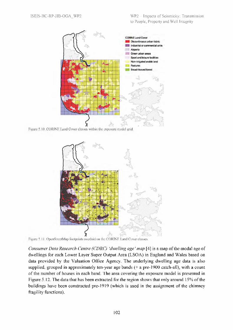
ISEIS-HC-RP-JJB-OGA_WP2 WP2 — Impacts of Seismicity: Transmissionto People, Property and Well Integrity
Figure 5.10. CORINE Land Cover classes within the exposure model grid.
102
Figure 5.11. OpenStreetMap footprints overlaid on the CORINE Land Cover classes.
Consumer Data Research Centre (CDRC) 'dwelling age ’ map [4] is a map of the modal age of dwellings for each Lower Layer Super Output Area (LSOA) in England and Wales based on data provided by the Valuation Office Agency. The underlying dwelling age data is also supplied, grouped in approximately ten-year age bands (+ a pre-1900 catch-all), with a count of the number of houses in each band. The area covering the exposure model is presented in Figure 5.12. The data that has been extracted for the region shows that only around 15% of the buildings have been constructed pre-1919 (which is used in the assignment of the chimney fragility functions).

WP2 — Impacts of Seismicity: Transmissionto People, Property and Well Integrity
ISEIS-HC-RP-JJB-OGA_WP2
Figure 5.12. CDRC dwelling age map.
5.3.3 Field Trip (9th June 2019)On Saturday 9th June, consultants Rui Pinho and Helen Crowley spent the day visiting the rural villages (Little Plumpton, Great Plumpton, Westby), urban zones (Wrea Green, Ribby, Wesham), industrial parks (Whitehalls Business Park and areas in Wesham) and sports and leisure areas (Ribby Hall Village, Carr Bridge residential park) within the region of interest. Some of the main building classes found within each land cover class (i.e., rural, urban, industrial and sports/leisure) are described below. Only visual external inspections of the buildings from street level were carried out during the site trip.
RuralThe predominant building class found within the rural areas comprises older unreinforced brick masonry detached and semi-detached housing with 2 storeys, and typically with tall brick chimneys (see Figure 5.13).
Figure 5.13. Detached two-storey brick masonry buildings with tall brick chimneys.
103

WP2 - Impacts of Seismicity: Transmissionto People, Property and Well Integrity
ISEIS-HC-RP-JJB-OGA_WP2
UrbanWithin the urban residential areas, a predominance of more modern semi-detached, detached and terraced housing was found (Figure 5.14), often with shorter brick or prefabricated metal chimneys. Many of these buildings are likely to have cavity walls, as this became common during the inter-war period and mandatory in 1935.
Figure 5.14. Modern masonry housing (terraced, semi-detached) without tall brick chimneys.
IndustrialThe industrial building stock (of factories and large retail outlets) that was observed during the site visit comprised light steel frame construction, with bracing in the longitudinal direction (and also on the roof) and moment frames in the transverse direction (Figure 5.15).
Figure 5.15. Light steel frame buildings in Whitehalls Business Park.
Sports/LeisureTwo different sports/leisure areas were visited: Ribby Hall Village and Carr Bridge residential park (Figure 5.16). The former was made up of a large number of different small units, some of which resembled static mobile homes and others that resembled detached bungalows and houses. Instead, at Carr Bridge, all of the houses were comprised of static mobile homes.
104
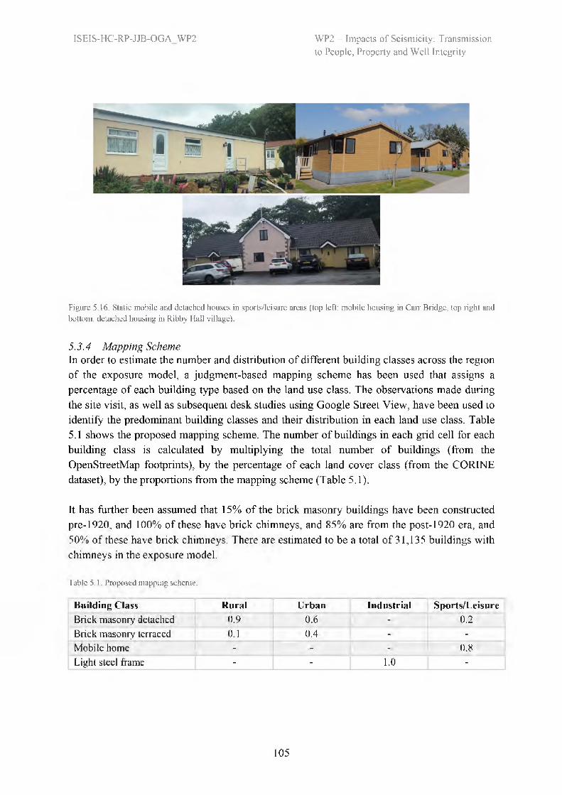
WP2 — Impacts of Seismicity: Transmissionto People, Property and Well Integrity
ISEIS-HC-RP-JJB-OGA_WP2
Figure 5.16. Static mobile and detached houses in sports/leisure areas (top left: mobile housing in Carr Bridge, top right and bottom: detached housing in Ribby Hall village).
5.3.4 Mapping SchemeIn order to estimate the number and distribution of different building classes across the region of the exposure model, a judgment-based mapping scheme has been used that assigns a percentage of each building type based on the land use class. The observations made during the site visit, as well as subsequent desk studies using Google Street View, have been used to identify the predominant building classes and their distribution in each land use class. Table 5.1 shows the proposed mapping scheme. The number of buildings in each grid cell for each building class is calculated by multiplying the total number of buildings (from the OpenStreetMap footprints), by the percentage of each land cover class (from the CORINE dataset), by the proportions from the mapping scheme (Table 5.1).
It has further been assumed that 15% of the brick masonry buildings have been constructed pre-1920, and 100% of these have brick chimneys, and 85% are from the post-1920 era, and 50% of these have brick chimneys. There are estimated to be a total of 31,135 buildings with chimneys in the exposure model.
Table 5.1. Proposed mapping scheme.
Building Class Rural Urban Industrial Sports/Leisure Brick masonry detached 0.9 0.6 - 0.2Brick masonry terraced 0.1 0.4 - -Mobile home - - - 0.8Light steel frame - - 1.0 -
105

WP2 — Impacts of Seismicity: Transmissionto People, Property and Well Integrity
ISEIS-HC-RP-JJB-OGA_WP2
5.3.5 Exposure MapsFigure 5.17 shows the population within the exposure model and Figure 5.18 shows the distribution of buildings (of each class).
Figure 5.17. Distribution of population in the exposure model.
106
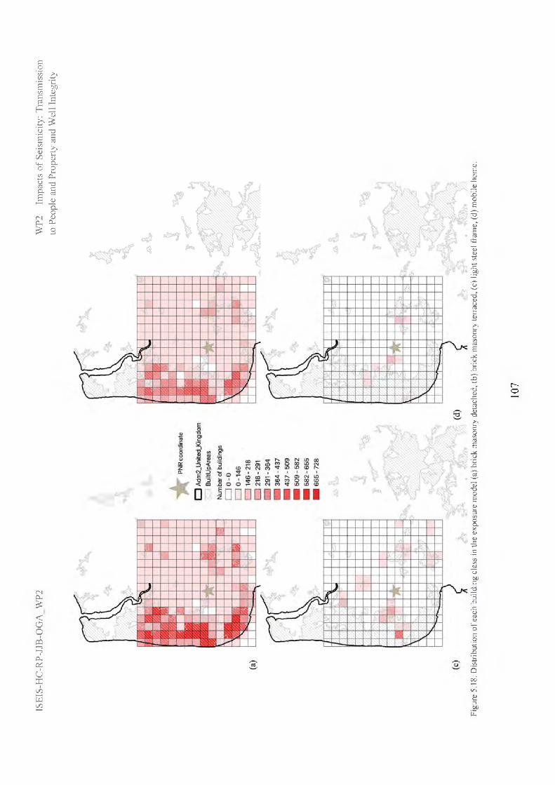
WP2
- Im
pact
s of
Sei
smic
ity: T
rans
mis
sion
to P
eopl
e an
d Pr
oper
ty a
nd W
ell I
nteg
rity
ISE
IS-H
C-R
P-JJ
B-O
GA
WP2
Figu
re 5
.18.
Dis
tribu
tion
of ea
ch b
uild
ing
clas
s in
the
expo
sure
mod
el (
a) b
rick
mas
onry
det
ache
d, (b
) br
ick
mas
onry
terr
aced
, (c)
ligh
t ste
el f
ram
e, (d
) mob
ile h
ome.
107

WP2 — Impacts of Seismicity: Transmissionto People, Property and Well Integrity
ISEIS-HC-RP-JJB-OGA_WP2
5.4 Assessment of Potential Impact on the Local CommunityHere we estimate the exposure of the local population to median levels of PGV and macroseismic intensity for three scenarios M 2.5, 3.5 and 4.5. This is estimated by combining the Worldpop data for population in 2019 (Date accessed: 08/04/2020, Figure 5.17) with the predicted PGV and intensity within each square of the grid. The results are presented in Tables 5.2 and 5.3 in terms of the percentage exposed within the grid.
Figure 5.19. Example of exposed population within the 16 x 15 km study region. The rectangle west of the PNR site shows the surface projection of the ML 4.5 fault, The colour of each of the grid indicates the population within. The colour of the background indicates the macroseismic intensity.
Table 5.2. Average population exposure (% of total within grid) within the 15 x 16 km study area to various median intensity (and corresponding PGV) levels for Ml . 2.5. 3.5 and 4.5 events.
EMS-98 Intensity 2 3 4 5 6 7PGV (cm/s) 0.03 0.13 0.54 2.3 5.5 13.1
2.9 100.0 16.3 0.0 0.0 0.0 0.0M 3.5 100.0 100.0 16.8 0.0 0.0 0.0
4.5 100.0 100.0 100.0 89.1 3.0 0.0
Table 5.3. As Table 5.2, but at the median + sigma PGV level. Note that it is expected that only 16 % of the proportions indicated here will be realised (as defined by the 1 sigma level).
EMS-98 Intensity 2 3 4 5 6 7PGV (cm/s) 0.03 0.13 0.54 2.3 5.5 13.1
2.9 100.0 77.0 0.6 0.0 0.0 0.0M 3.5 100.0 100.0 80.0 0.3 0.0 0.0
4.5 100.0 100.0 100.0 100.0 69.7 0.1
108
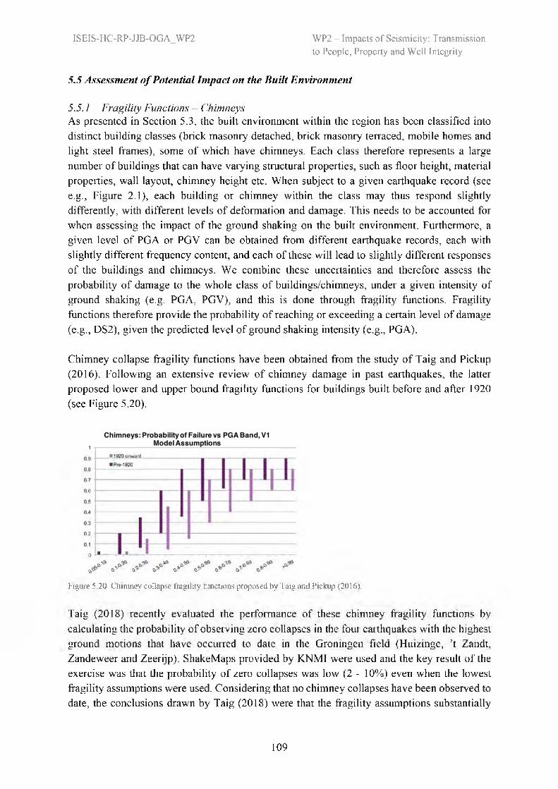
WP2 — Impacts of Seismicity: Transmissionto People, Property and Well Integrity
ISEIS-HC-RP-JJB-OGA_WP2
5.5 Assessment of Potential Impact on the Built Environment
5.5.1 Fragility Functions - ChimneysAs presented in Section 5.3, the built environment within the region has been classified into distinct building classes (brick masonry detached, brick masonry terraced, mobile homes and light steel frames), some of which have chimneys. Each class therefore represents a large number of buildings that can have varying structural properties, such as floor height, material properties, wall layout, chimney height etc. When subject to a given earthquake record (see e.g., Figure 2.1), each building or chimney within the class may thus respond slightly differently, with different levels of deformation and damage. This needs to be accounted for when assessing the impact of the ground shaking on the built environment. Furthermore, a given level of PGA or PGV can be obtained from different earthquake records, each with slightly different frequency content, and each of these will lead to slightly different responses of the buildings and chimneys. We combine these uncertainties and therefore assess the probability of damage to the whole class of buildings/chimneys, under a given intensity of ground shaking (e.g. PGA, PGV), and this is done through fragility functions. Fragility functions therefore provide the probability of reaching or exceeding a certain level of damage (e.g., DS2), given the predicted level of ground shaking intensity (e.g., PGA).
Chimney collapse fragility functions have been obtained from the study of Taig and Pickup (2016). Following an extensive review of chimney damage in past earthquakes, the latter proposed lower and upper bound fragility functions for buildings built before and after 1920 (see Figure 5.20).
Figure 5.20 Chimney collapse fragility functions proposed by Taig and Pickup (2016).
Taig (2018) recently evaluated the performance of these chimney fragility functions by calculating the probability of observing zero collapses in the four earthquakes with the highest ground motions that have occurred to date in the Groningen field (Huizinge, ’t Zandt, Zandeweer and Zeerijp). ShakeMaps provided by KNMI were used and the key result of the exercise was that the probability of zero collapses was low (2 - 10%) even when the lowest fragility assumptions were used. Considering that no chimney collapses have been observed to date, the conclusions drawn by Taig (2018) were that the fragility assumptions substantially
109
WP2 - Impacts of Seismicity: Transmissionto People, Property and Well Integrity
ISEIS-HC-RP-JJB-OGA_WP2
overstated the likelihood of failures at low levels of PGA. Considering these findings, the lower bound values presented in Figure 5.20 are taken as the best estimate for the chimney fragility functions, and a lognormal distribution has been fit to the data points of PGA versus probability of failure. The median and dispersion of these functions are shown in Table 5.4. One thing worth noting is that a minimum level of PGA before chimney collapse has now been implemented, and this value has been taken as 0.08 g given that this is the highest level of ground shaking measured in the vicinity of the PNR site and no chimneys have collapsed to date in the region.
Table 5.4. Parameters of the lognormal chimney fragility functions.
Chimney type Median PGA (g) DispersionPre-1920 masonry buildings 0.585 0.62Post-1920 masonry buildings 0.765 0.52
5.5.2 Fragility Functions - BuildingsFor the detached and terraced masonry houses and the light steel frame buildings, numerical models from studies being carried out as part of the probabilistic risk assessment in the Groningen gas field (van Elk et al., 2019) have been employed (see Figure 5.21a), given the similarity of these buildings in the Netherlands and the UK. These numerical models are described in detail in Arup (2017; 2019) and Mosayk (2017).
Capacity curves provide a description of the lateral strength and ductility capacity of a single- degree-of-freedom (SDOF) system (Figure 2.2) that has the first mode of vibration properties of the original multi-degree-of-freedom (MDOF) structure (see Figure 5.21b). The capacity curves for the three aforementioned building classes have been taken from the numerical models used in the Groningen field study. The capacity curve for mobile homes has been obtained from HAZUS (FEM A, 2004) as this class of building is not found in the Groningen field.
To develop fragility functions, the capacity curves of the SDOF systems are subjected to nonlinear dynamic analysis, and the peak displacement response of each analysis is obtained. When developing fragility functions for the Groningen gas field, Crowley et al. (2019) used ground motions that were consistent with the levels of hazard with between 500 to 100,000 years return periods, as the focus was on collapse fragility and fatality risk assessment. As the focus of the present study is on damage assessment (given the low magnitude range of the scenarios considered), ground motions with lower intensities (matching the hazard in Groningen with a return period of 50 years) were added to the pool of recordings used for the development of the fragility functions.
110

WP2 — Impacts of Seismicity: Transmissionto People, Property and Well Integrity
ISEIS-HC-RP-JJB-OGA_WP2
Figure 5.21. (a) Numerical models for detached (top left), terraced (top right) and light steel frame buildings, (b) Capacity curve (shown on the right) of a SDOF equivalent linear systems (middle figure) from the nonlinear analysis of MDOF structures (from Bal et al., 2010), where F is the lateral force and A is the displacement response.
With additional time and resources, one would ideally undertake a probabilistic seismic hazard analysis (PSHA) at the PNR site and then select records that are consistent with this hazard (following disaggregation of the hazard to understand the magnitude, distance, epsilon and duration of the events contributing most to the hazard at different levels of intensity) following, for example, the methods outlined in Bradley (2010) and Baker and Lee (2018). However, as this has not been possible within the timeframe of this project, the same records being used to develop fragility functions for the buildings in the Groningen gas field have been employed. It is noted that the duration of these records is likely to be longer than expected for the magnitude of the events considered herein and there may be differences in the frequency content, and this may lead to higher estimations of damage than actually expected.
Nonlinear dynamic analyses of SDOF models for each building class have been undertaken and the peak displacement response of each analysis has been recorded. This response is plotted
111

WP2 - Impacts of Seismicity: Transmissionto People, Property and Well Integrity
ISEIS-HC-RP-JJB-OGA_WP2
against a measure of intensity of each accelerogram (e.g., peak ground acceleration, SA[T=0.01s]) and then piecewise linear regression of the displacement response has been carried out to obtain a bilinear relationship between the intensity measure and the response (see Figure 5.22). Piecewise linear regression has been employed as there is clearly a marked change in slope of the response displacements over the range of intensities considered (from linear to nonlinear response - shown in the capacity curve in Figure 5.21b), in particular for the brick masonry buildings.
Each spectral ordinate in the GMPE of Atkinson (2015) has been considered for the development of the fragility functions (from peak ground acceleration up to spectral accelerations at higher periods of vibration), and the final intensity measure selected for each building class is given by that which leads to the lowest dispersion in the response (i.e., the lowest scatter in the plots in Figure 5.22).
Figure 5.22. Response analyses (input spectral acceleration, SA vs. spectral displacement, SD, response) for SDOF models and piecewise linear regression (a) detached, (b) terraced, (c) mobile home and (d) light steel frame.
112

WP2 — Impacts of Seismicity: Transmissionto People, Property and Well Integrity
ISEIS-HC-RP-JJB-OGA_WP2
Figure 5.23. Building fragility functions (input spectral acceleration versus probability of exceeding damage state) for (a) detached, (b) terraced, (c) mobile home and (d) light steel frame for various damage states (DS, see Section 2.6). Indicative PGV values are provided, where possible and with minimal extrapolation, as equivalent motions (for a given SA) according to Atkinson (2015). These values were determined by comparing predictions of SA and PGV over a range of magnitudes (4 < M < 6, i.e., extending well above scenarios under consideration) at short distances < 10 km and for Vs30 = 240 m/s.
For a given damage state, a displacement threshold is identified (as shown by the vertical lines in the capacity curve shown in Figure 5.21b). Once this threshold of displacement is exceeded, the damage state is reached or exceeded. The displacement thresholds for each damage state have been obtained from experimental testing campaigns for the masonry buildings (Graziotti et al. 2019; Borzi et al., 2018) and from HAZUS (FEMA, 2004) for the light steel frames and mobile homes. In order to calculate the fragility function, it is thus necessary to calculate the probability of reaching or exceeding these levels of displacement. This can be undertaken using the equation describing the displacement response (given by the blue lines in Figure 5.22) together with the aleatory variability (defined by the scatter in the plots in Figure 5.22), and assuming a lognormal distribution. For each level of ground shaking intensity, the probability of reaching or exceeding each damage state is calculated and plotted, as shown in Figure 5.23. Interested readers are referred to Crowley et al. (2017; 2018) for a more detailed description, and complete presentation of the equations used to develop the fragility functions.
113
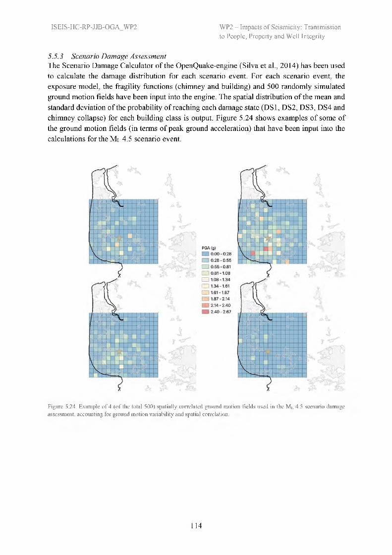
WP2 — Impacts of Seismicity: Transmissionto People, Property and Well Integrity
ISEIS-HC-RP-JJB-OGA_WP2
5.5.3 Scenario Damage AssessmentThe Scenario Damage Calculator of the OpenQuake-engine (Silva et al., 2014) has been used to calculate the damage distribution for each scenario event. For each scenario event, the exposure model, the fragility functions (chimney and building) and 500 randomly simulated ground motion fields have been input into the engine. The spatial distribution of the mean and standard deviation of the probability of reaching each damage state (DS1, DS2, DS3, DS4 and chimney collapse) for each building class is output. Figure 5.24 shows examples of some of the ground motion fields (in terms of peak ground acceleration) that have been input into the calculations for the Ml 4.5 scenario event.
Figure 5.24. Example of 4 (of the total 500) spatially correlated ground motion fields used in the ML 4.5 scenario damage assessment, accounting for ground motion variability and spatial correlation.
114
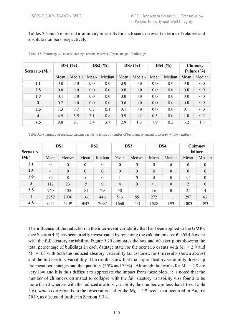
WP2 - Impacts of Seismicity: Transmissionto People, Property and Well Integrity
ISEIS-HC-RP-JJB-OGA_WP2
Tables 5.5 and 5.6 present a summary of results for each scenario event in terms of relative and absolute numbers, respectively.
Table 5.5. Summary of scenario damage results in terms of percentage of buildings.
Scenario (ML)DS1 (%) DS2 (%) DS3 (%) DS4 (%) Chimney
failure (%)Mean Median Mean Median Mean Median Mean Median Mean Median
2.1 0.0 0.0 0.0 0.0 0.0 0.0 0.0 0.0 0.0 0.0
2.5 0.0 0.0 0.0 0.0 0.0 0.0 0.0 0.0 0.0 0.02.9 0.1 0.0 0.0 0.0 0.0 0.0 0.0 0.0 0.0 0.0
3 0.2 0.0 0.0 0.0 0.0 0.0 0.0 0.0 0.0 0.0
3.5 1.3 0.7 0.3 0.1 0.1 0.0 0.0 0.0 0.1 0.04 4.9 3.5 2.1 0.8 0.9 0.2 0.5 0.0 1.0 0.2
4.5 9.8 9.1 5.4 3.7 2.9 1.3 1.9 0.3 3.2 1.3
Table 5.6 Summary of scenario damage results in terms of number of buildings (rounded to nearest whole number).
Scenario (ML)
DS1 DS2 DS3 DS4 Chimney failure
Mean Median Mean Median Mean Median Mean Median Mean Median
2.1 0 0 0 0 0 0 0 0 0 02.5 4 0 0 0 0 0 0 0 0 02.9 52 8 5 0 1 0 0 0 <1 03 112 23 15 0 4 0 <1 0 2 0
3.5 740 405 181 29 58 1 16 0 31 44 2752 1996 1166 446 513 85 272 11 297 63
4.5 5541 5139 3043 2097 1660 733 1088 193 1003 393
The influence of the reduction in the inter-event variability that has been applied to the GMPE (see Section 4.5) has been briefly investigated by repeating the calculations for the M 4.5 event with the full aleatory variability. Figure 5.25 compares the box and whisker plots showing the total percentage of buildings in each damage state for the scenario events with Ml = 2.9 and Ml = 4.5 with both the reduced aleatory variability (as assumed for the results shown above) and the full aleatory variability. The results show that the larger aleatory variability drives up the mean percentages and the quantiles (25% and 75%). Although the results for Ml = 2.9 are very low and it is thus difficult to appreciate the impact from these plots, it is noted that the number of chimneys estimated to collapse with the full aleatory variability was found to be more than 2 whereas with the reduced aleatory variability the number was less than 1 (see Table 5.6), which corresponds to the observations after the Ml = 2.9 event that occurred in August 2019, as discussed further in Section 5.3.4.
115

WP2 — Impacts of Seismicity: Transmissionto People, Property and Well Integrity
ISEIS-HC-RP-JJB-OGA_WP2
Figure 5.25. Box and whisker plot showing the total percentage of buildings in each damage state for scenario event (a) ML= 2.9 with reduced total aleatory variability from the Atkinson GMPE, (b) Ml = 2.9 with full aleatory variability (c) Ml = 4.5 reduced variability and (d) Ml - 4.5 with full variability. The diamond indicates the mean, the box represents the lower to upper quartiles and the whisker indicates the total range (lowest to highest value). The median (50th percentile) is indicated by the red horizontal line.
Figure 5.26. Spatial distribution of the mean number of buildings in DS1 for the scenario event Ml = 2.9. Note that every grid cell has a number of buildings < 1 for all other damage states and chimney collapse.
116

WP2 — Impacts of Seismicity: Transmissionto People, Property and Well Integrity
ISEIS-HC-RP-JJB-OGA_WP2
Figure 5.27. Spatial distribution of the mean percentage of buildings in each damage state for the scenario event Ml = 4.5 and VS30 = 240 m/s (a) DSI, (b) DS2, (c) DS3, (d) DS4, (e) chimney collapse.
Maps showing the distribution of the mean percentage of damaged buildings in each damage state and percentage of buildings with collapsed chimneys for the ML 2.9 and 4.5 scenario events are shown in Figures 5.26 and 5.27, respectively. It is noted that only the \ results are shown for ML 2.9 as all grid cells had a value of <1 building for the other damage states.
117
WP2 - Impacts of Seismicity: Transmissionto People, Property and Well Integrity
ISEIS-HC-RP-JJB-OGA_WP2
5.5.4 Comparison with Damage Data and Intensity Maps
The only damage data that is currently available for the ML 2.9 event comes from BGS ‘did- you-feel-it?’ data (Baptie, 2019), which consists of self-reported damage from the occupants of buildings within the PNR region. The following fields from the ‘did-you-feel-it?’ dataset provided by the BGS are related to the damage of the buildings:
• buildingsDamage• plasterSmallCracks• plasterLargeCracks• plasterFellSmall• plasterFellLarge• stones Fell• wallsCollapsed• wallsLargeCracks• chimneyCollapsed• houseWallsCollapsed
For each field the following options are available: ‘yes’, ‘no’, ‘no information’ and ‘don’t know’. A total of 2266 questionnaires have been submitted for this event. The damage reports are not provided by structural engineers and thus cannot be considered to be highly reliable. Furthermore, for these specific induced seismicity events in the PNR region it is clear that there are heightened emotions that can influence the verity of the provided data (many of the respondents to the questionnaire noted their personal negative feelings towards ‘fracking’ and their desire for it to stop). In addition, there is also the possibility that more than one member of a household have completed the survey, thus creating multiple damage entries for the same structure. Nevertheless, it is currently the only data that is available to ‘history check’ the risk model presented herein and so an attempt has been made to compare the damage data from these ‘did-you-feel-it?’ reports with the estimated damage presented in the previous section.
The damage data for each building has been mapped to DS0, DS1 and DS2 using the EMS-98 damage scale (Grünthal et al., 1998) for unreinforced masonry buildings (which make up the majority of buildings for which ‘did-you-feel-it?’ data has been supplied), as presented Figure 5.28. DS1 has been selected if ‘yes’ was supplied for any of the following fields: plasterSmallCracks, plasterFellSmall, stonesFell, whereas DS2 has been selected for ‘yes’ in any of the following fields: plasterLargeCracks, plasterFellLarge and wallsLargeCracks. It is noted that this mapping of these damage descriptions to the EMS-98 damage state does not account for the extent of the damage and thus they are likely to provide conservative (i.e. higher) estimates of the damage state.
118

WP2 — Impacts of Seismicity: Transmissionto People, Property and Well Integrity
ISEIS-HC-RP-JJB-OGA_WP2
Figure 5.28. EMS-98 Damage scale for unreinforced masonry buildings (Grünthal et al., 1998)
It is worth noting here that one report of ‘wallsCollapsed’ and another of ‘houseWallsCollapsed’ were provided, but from the accompanying damage descriptions it was clear that these were not wall collapses (in one case due to lack of any other reported damage, and in the other case due to the description being that the “floor has come away by the garage”).
The total number of damaged buildings with DSI has been found to be 97, and there are 50 buildings with DS2. Further, no chimneys were reported to have collapsed. These numbers can be compared with the 51 buildings with DSI, 5 buildings with DS2 and <1 building with chimney collapse presented previously in Table 5.6. The modelled damage is thus lower, which could be both due to the unreliable self-reporting of damage (and possible duplications per building, as discussed above) and the conservative mapping to the EMS-98 damage scale, but the total number of damaged buildings is nevertheless of a similar order of magnitude.
These results have also been aggregated to number of buildings at the level of postal code districts and are mapped in Figures 5.29 and 5.30.
119

WP2 — Impacts of Seismicity: Transmissionto People, Property and Well Integrity
ISEIS-HC-RP-JJB-OGA_WP2
Figure 5.29. Number of buildings in each postal district with DS1 according to the FMS-98 damage scale, as reported by ‘did- you-feel-it?’ data for the ML 2.9 event (Baptie, 2019).
Figure 5.30. Number of buildings in each postal district with DS2 according to the EMS-98 damage scale, as reported by ‘did- you-feel-it?’ data for the ML 2.9 event (Baptie, 2019).
Similar maps have been produced using the modelled results presented in Section 5.3.3. The number of buildings with DS1 and DS2 have been aggregated at the same postal code districts and the resulting maps are presented in Figures 5.31 and 5.32. A comparison of these maps with those presented from the ‘did-you-feel-it?’ data shows that the modelled damage is more concentrated in the built-up areas west of the PNR site whereas the ‘did-you-feel-it?’ data indicates highest damage in the postal district to the south of the PNR site. The concentration of damage in the south cannot be explained by site effects, with similar Vs30 and HVSR in this region to other districts.
120

WP2 — Impacts of Seismicity: Transmissionto People, Property and Well Integrity
ISEIS-HC-RP-JJB-OGA_WP2
Figure 5.31. Number of buildings in each postal district with DSI according to the EMS-98 damage scale, as estimated using the risk model presented herein
Figure 5.32. Number of buildings in each postal district with DS2 according to the EMS-98 damage scale, as estimated using the risk model presented herein
BGS have used the aforementioned ‘did-you-feel-it?’ data, which also includes reports on the effects on people and objects, in order to assign macroseismic intensity data (as presented previously in Section 4.1 and Figure 4.3), Whilst macroseismic intensity should not be assigned purely from building damage data, it is an important ‘sensor’ for identifying and distinguishing the higher levels of intensity (above V). Hence, an attempt has been made to use the modelled damage data to assign intensity levels for comparison with the intensity map presented in Figure 4.3.
121

WP2 — Impacts of Seismicity: Transmissionto People, Property and Well Integrity
ISEIS-HC-RP-JJB-OGA_WP2
The percentage of buildings with DS1 an DS2 in each cell of the grid used for the intensity map has been calculated using the results from the analyses presented in the previous section (see Figures 5.33 and 5.34). In order to map these damage results to intensity, the definition of intensity from EMS-98 (Grünthal et al., 1998) has been used. In the EMS-98 scale, damage to buildings occurs at intensity levels of V and greater. Intensity level V is defined as occurring when there is “Damage of grade 1 to a few buildings of vulnerability class A and B”. Intensity level VI is defined as occurring when “Damage of grade 1 is sustained by many buildings of vulnerability class A and B; a few of class A and B suffer damage of grade 2; a few of class C suffer damage of grade 1”. Vulnerability class A refers mainly to highly vulnerable buildings, such as adobe and rubble stone structures, which are not present in the region. Vulnerability class B refers mainly to older unreinforced masonry buildings which make up a large proportion of the exposure model. Vulnerability class C refers to newer unreinforced masonry buildings with concrete floors, which are also present in the exposure model.
If it is assumed that the majority of the buildings are vulnerability class B then we would need a “few” buildings with DS1 to assign intensity V and both a “few” buildings with DS1 and “many” buildings with DS2 to assign intensity VI. The definition of “few” and “many”, as provided in EMS 98, is shown in Figure 5.35; it is not clear from this figure if there is a minimum threshold for the definition of “few”, so anything above 0% has been assumed as “few”. However, this may be conservative depending on the assumed definition.
Figure 5.35. Quantitative definition of qualitative terms in EMS-98 (Grünthal et al., 1998)
122
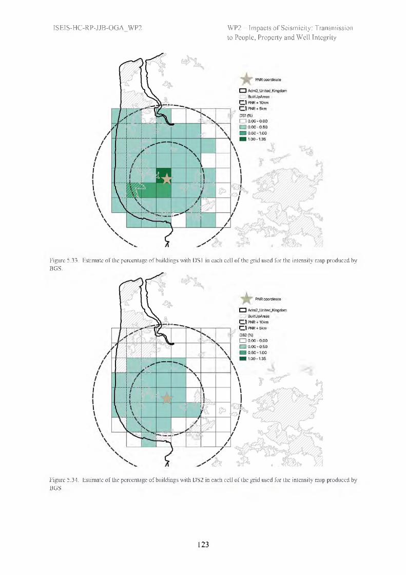
ISEIS-HC-RP-JJB-OGA_WP2 WP2 — Impacts of Seismicity: Transmissionto People, Property and Well Integrity
Figure 5.33. Estimate of the percentage of buildings with DS1 in each cell of the grid used for the intensity map produced by BGS.
Figure 5.34. Estimate of the percentage of buildings with DS2 in each cell of the grid used for the intensity map produced by BGS.
123
WP2 - Impacts of Seismicity: Transmissionto People, Property and Well Integrity
ISEIS-HC-RP-JJB-OGA_WP2
Any of the coloured cells in Figure 5.33 could be defined as having a “few” buildings with DS 1 and could thus be assigned intensity V. None of the cells would be defined as having “many” buildings with DS1, though some of the cells could have a “few” buildings with DS2 (see Figure 5.34). Given these results, it would be difficult to justify assigning an intensity greater than V based on the modelled damage for the ML2.9 event. The macroseismic intensity map presented in Figure 4.3 had some cells with intensity VI which could be due to the higher levels of reported damage, as presented previously in Figures 5.29 and 5.30. However, it is not clear how the macroseismic intensity was assigned from these damage estimates given that the percentage of damaged buildings cannot be reliably estimated, since ‘did-you-feel-it?’ reports do not come from a random samples of buildings within each post code district; on the contrary, data contributors who deem their building to have been damaged by the event are more likely to have compiled the ‘did-you-feel-it?’ questionnaire than those who instead do not have damage to report.
5.5.5 Sanity Checks of Results
In addition to the history check included in the previous section, the modelled scenario damage results presented herein can also be compared with the damage observed in past events with magnitudes of the same range, shallow depths and with similar characteristics, vulnerability and density of the building stock (i.e., Basel, Huizinge, Darmstadt, and Folkestone, as presented in Section 2.6).
The Basel (M3.2, depth 5 km) and Huizinge (M3.5, depth 3 km) events both led to a much larger number of buildings with DS1 (around 2000) than predicted herein for events of this magnitude, but these numbers are based on damage claims rather than inspections of damage made by structural engineers. It is highly likely that a large proportion of these buildings already had DS1 damage due to lack of maintenance and settlement of the foundations (see e.g. Bommer et al., 2015).
On the other hand, the damage caused by the Darmstadt event (M3.6, depth 5km) had reported levels of DS 1-2 damage and chimney collapse which are slightly lower than the estimates made here for the ML 3.5 scenario (i.e., a few hundred damaged buildings and tens of collapsed chimneys).
The Folkestone (M4.0, depth 5.3 km) led to around 1000 damaged buildings (DS 1-2) and a number of collapsed chimneys, though the exact number is unknown. A larger number of damaged buildings has been estimated for the ML 4.0 event, but this is likely to be due to the higher exposure given the proximity of the PNR site to the city of Blackpool.
5.6 Assessment of Potential Impact on Well IntegrityThe following text from API (2009) explains the basic concept of well integrity in relation to hydrocarbon extraction through hydraulic fracturing:
124

WP2 - Impacts of Seismicity: Transmissionto People, Property and Well Integrity
ISEIS-HC-RP-JJB-OGA_WP2
“The primary method used for protecting groundwater during drilling operations consists of drilling the wellbore through the groundwater aquifers, immediately installing a steel pipe (called casing), and cementing this steel pipe into place The steel casing protects the zones from material inside the wellbore during subsequent drilling operations and, in combination with other steel casing and cement sheaths that are subsequently installed, protects the groundwater with multiple layers of protection for the life of the well.
The subsurface zone or formation containing hydrocarbons produces into the well, and that production is contained within the well alt the way to the surface. This containment is what is meant by the term “well integrity. ” Moreover, regular monitoring takes place during drilling and production operations to ensure that these operations proceed within established parameters and in accordance with the well design, well plan, and permit requirements. Finally, the integrity of well construction is periodically tested to ensure its integrity is maintained.”
Figure 5.36 shows a schematic of the Bowland Shale wells being used at Preston New Road. For the purposes of this study, well integrity is assumed to be compromised when either the yield flexural capacity, the yield strain or the shear stress capacity of the steel production casing (see Figure 5.36) is exceeded due to earthquake effects. It is noted that the exceedance of these capacities would not necessarily result in immediate exchange between the hydrocarbons or fracking fluid in the well and the surrounding groundwater, and these are thus conservative thresholds with which to assess the integrity of the well following seismic action.
125

WP2 - Impacts of Seismicity: Transmissionto People, Property and Well Integrity
ISEIS-HC-RP-JJB-OGA_WP2
Figure 5.36. Schematic of Bowland Shale well (not to scale) (Regeneris, 2011).
126

WP2 - Impacts of Seismicity: Transmissionto People, Property and Well Integrity
ISEIS-HC-RP-JJB-OGA_WP2
Figure 5.37. Structural model of the Bowland Shale Well.
In a vertical structural assembly subjected to lateral deformation, the highest strains and stresses are typically found in locations of the structure that are adjacent/interfacing with a very stiff body. For instance, in bridge piers, airport towers, lamp posts, etc., the highest strain/stress concentrations are observed at the base of the structures, where they are connected to the necessarily much stiffer foundation elements. In the case of the well structure being studied herein, the location where the sharpest variation of stiffness occurs is found in the production casing at the point where the intermediate casing ends, given how much stiffer the (cemented) upper sections of the well are with respect to the smaller non-cemented production casing. This (expected) structural behavior was also observed in preliminary structural analyses that not only showed the portion of the production casing below the intermediate casing deflecting much more than its upper counterparts when the well is subjected to lateral displacements (see Figure 5.37), but also confirmed that the largest strains and stresses were indeed located in the production casing at the point where the intermediate casing is interrupted; we henceforth term this location as the critical section of the well.
As discussed in Bommer (2018), buried structures may experience relative displacements due to one of three causes: (a) slip on a geological fault that the structure traverses; (b) liquefaction of the surrounding ground; (c) the passage of the seismic waves along the structure or
127

WP2 - Impacts of Seismicity: Transmissionto People, Property and Well Integrity
ISEIS-HC-RP-JJB-OGA_WP2
component. Only the first and the third causes have been considered herein, given that liquefaction would require moment magnitudes above at least 4.5 in order to be triggered (Green and Bommer, 2019). The potential impact of (a) and (c) on the aforementioned critical section of the well is therefore analysed herein (see sub-sections 5.6.1 and 5.6.2, respectively).
The material properties’ of the steel casing used in Preston New Road were not available at the time of producing this report, and so typical values have been taken from the literature. Based on a nominal diameter of 5.5 inches (139.7 mm), as shown in Figure 5.36, a wall thickness of 10 mm has been taken from the common production casing sizes table reported in Renpu (2011) and steel class S355 has been assumed. The design properties for a S355 steel class Circular Hollow Section (CHS) with diameter of 139.7 mm and wall thickness of 10 mm are as reported in Table 5.8.
Table 5.8. Assumed mechanical properties of the (steel) production casing.
Parameter Value UnitsSecond moment of area (I) 8.619x 10⁶ nun4Elasticity Modulus (E) 2x 10s kN/m1 1 2Elastic bending moment capacity (Mmax) 43.8 kNmPlastic shear force capacity 532 kNShear area 2594 mm2Yield strain 0.0018 -
5.6.1 Well Integrity due to Fault SlipFor a well drilled vertically, fault slip would pose a very serious hazard if the well directly traversed the fault plane (Bommer, 2018), as schematically represented in Figure 5.38. The amount of fault slip expected for a given magnitude can be estimated with the empirical relationship of Wells and Coppersmith (1994). For a M 4.5 event, fault displacement would be 17 mm, though it is noted that this relationship is derived from field observations and is not calibrated for events below M 5.2. Two mechanisms of failure are investigated: exceedance of maximum (i) bending capacity; and (ii) shear capacity.
1 It is reiterated that given the critical section discussion above, concrete properties needed not to be assumed, given that neither cracking of the cement nor separation of the cement from the steel casing had to be considered.
128

WP2 - Impacts of Seismicity: Transmissionto People, Property and Well Integrity
ISEIS-HC-RP-JJB-OGA_WP2
Figure 5.38. Sketch of the production casing and the parameters used to estimate well integrity due to fault slip.
As discussed already (and shown in Figure 5.37 above), when subjected to lateral loading the well behaves as an inverted cantilever with flexural bending of structural relevance developing downwards from the critical section, which is also the location at which largest values of bending moment are generated. Starting from the classical formulae to calculate the horizontal tip deflection (δ) of a cantilever for a given moment at its base (M), it is then possible to estimate the critical length (Lcritical) below which the elastic bending moment capacity of the production casing (M max ) is exceeded:
M ■ L2 ___ ¡3E/ ■ 88 = „ ^’critical ~
3£7 yj Mmax
(26)
where E is the elasticity modulus and I is the second moment of area of the structural section.
Using the production casing mechanical properties given in Table 5.8, the critical length (at which a lateral deformation of 17 mm makes the well reach its bending capacity, beyond which damage to the casing would occur) is found to be just under 1.5 m. This means that for the well integrity to be compromised through exceedance of its bending capacity under a magnitude 4.5 event, the fault would have to pass within the length of 1.5 m below the depth at which the intermediate casing is interrupted. Given that the total depth of the production casing is over 2 km, this critical length is less than 0.075 % of the total length of the well. There is thus a very small probability that a fault would actually pass within the critical length.
Furthermore, it is noted that the above calculations are very conservative (i.e., the critical length would in reality be much lower than the 0.075% value reported above), given that:
129

WP2 - Impacts of Seismicity: Transmissionto People, Property and Well Integrity
ISEIS-HC-RP-JJB-OGA_WP2
• the well is actually embedded in the ground (ignored in the above calculations), and this will reduce the deformability of the well;
• the horizontal component of the displacement is likely to be less than the fault displacement, given the dip of the fault (see Figure 5.38);
• in the calculations above the elastic bending moment capacity (Mmax) at the critical section has been adopted as resistance threshold, however, whilst exceedance of this value could cause some damage to the production casing, it would not necessarily result in immediate exchange between the hydrocarbons or fracking fluid in the well and the surrounding groundwater;
• the additional plastic flexural capacity of the steel casing has not been considered.
As mentioned above, in additional to the flexural bending capacity of the production casing, the shear capacity also needs to be considered, given that, again, if shear forces above such value would develop in the well then the casing would experience damage. The shear stress capacity of the assumed steel section is given by the design plastic shear force resistance divided by the shear area, both of which are quantified in Table 5.8 (for the production casing considered in this study), thus leading to a shear stress capacity of approximately 205 MPa, which safely exceeds expected shear stresses in local faults. For instance, Fellgett et al. (2017) provide a comprehensive overview of the information available on the state of stress in the UK; based on analysis of available borehole data across Cheshire and Lancashire (including Preese Hall) they show that vertical stress gradients vary between 25 and 26 MPa/km, while the pore pressure gradient for this region is 10.8 MPa/km, or broadly hydrostatic (10 MPa/km). Maximum horizontal stress tends to follow 28 MPa/km, with no measured or calculated value exceeding 75 MPa down to 2.6 km depth.
5.6.2 Well Integrity due to Wave-Induced Ground StrainAs discussed in Bommer (2018), it is generally assumed that near the ground surface, seismic waves propagate vertically upwards. Therefore, a vertical well will be exposed to longitudinal strain from the passage of P-waves and lateral strain due to the passage of S-waves. The ground strain can be estimated from the ratio of PGV to the propagation velocity; since S-waves generally carry greater energy and propagate more slowly than P-waves, the lateral strain is likely to be greater.
The maximum strain that the production casing may sustain without damage (i.e., the so-called ‘yield strain’ for steel material structures) is given in Table 5.8 as equal to 0.18 %. Considering that peak strain is given by the ratio between PGV and Vs, and assuming a Vs of 240 m/s close to the surface, a PGV of 43 cm/s would be required to induce this level of strain. As discussed in Section 5.2.3, even under the largest magnitude 4.5 scenario, median values of PGV only up to 8.95 cm/s are estimated in the epicentral region. At least 2.2 standard deviations (with reduced aleatory variability) above the median would be needed to reach a PGV of 43 cm/s. This corresponds to the 98.6th percentile—a level of motion that for the given scenario has a
130
WP2 - Impacts of Seismicity: Transmissionto People, Property and Well Integrity
ISEIS-HC-RP-JJB-OGA_WP2
1.4% chance of being exceeded. Thus, there is an extremely low probability that the well could be damaged due to wave-induced ground strain for the largest event considered herein.
6. ConclusionsThis work aimed to improve our understanding of induced seismicity at PNR and potential future events in terms of its impact on people, the built environment and well integrity. For a summary of the work, we refer the reader to the Executive Summary at the start of this report. In the following we make our concluding remarks.
• The induced seismicity at Preston New Road during October and December 2018, with maximum magnitude of ML 1.5, led to ground motions that were practically imperceptible to people at the surface. Anthropogenic sources of vibration far exceed those caused by even the largest earthquake during that period and typical structures were not, therefore, at any risk whatsoever from these motions.
• The seismicity at PNR-2 led to larger events that were widely felt (both in terms of predicted intensity and evidence from ‘did-you-feel-it?’ reports). Damage in terms of plaster cracks, falling plaster, falling stones and wall cracks has been reported by the local population for the largest ML 2.9 event.
• Moment magnitude is predicted from local magnitude using a theoretically based conversion (Deichmann, 2017), calibrated against data from a Swiss geothermal site in St. Gallen (Edwards et al., 2015). The European conversion equation of Grünthal et al. (2009) underpredicted moment magnitude for the small induced events.
• The ground motion prediction equation (GMPE) of Atkinson (2015) performed reasonably over a range of magnitudes, distances and periods, when compared to the recorded data at PNR-1z and PNR-2. For short to moderate periods at short distances (Repi < 3 km), the model tended to underpredict motions somewhat due to a fast decay of ground motion amplitudes.
• To ensure unbiased predictions where data are available, we have calibrated the Atkinson (2015) model such that for magnitudes 1 < M < 3 it predicts observed PNR motions with minimal bias. In order to ensure conservatism, the original model predictions are reverted to in the case of events with M > 4.5, with a smooth transition between these data-driven and model-driven end members.
• The model calibration has led to slightly higher median epicentral motions (and to some extent, intensity). However, these higher amplitudes decay more rapidly, resulting in a reduced exposure to the urban residential areas to the west (Blackpool) and south (Lytham St Annes). In addition, a reduction in ground motion within-event variability means that intensities based on 84th percentile PGV are reduced.
• The measured 30 m average shear-wave velocity (Vs30) of sites around PNR was low (190- 270 m/s). In particular, areas characterised by blown sand deposits had the lowest velocity. Sites around PNR will therefore amplify ground motions significantly with respect to a (theoretical) site located on a rock outcrop.
• Using ambient noise HVSR measurements at the seismic monitoring sites across the PNR region, site fundamental resonance frequencies were determined. These in turn were used
131

WP2 - Impacts of Seismicity: Transmissionto People, Property and Well Integrity
ISEIS-HC-RP-JJB-OGA_WP2
to estimate Vs30 and construct a Vs30 map based on geological proxies. The variability of mapped Vs30 was limited however (spanning only 190 - 250 m/s), and only minor variability in predicted ground motions (and intensities) result from its implementation.
• Intensity predictions were presented for scenario events (Ml 2.9, 3.5 and 4.5) at PNR. These showed that median field-wide epicentral-intensities would reach III (weak), IV (largely observed) and VI (slightly damaging) respectively.
• For the Ml 3.5 and 4.5 scenarios at the 84th-percentile prediction of PGV, we estimate that intensities could rise to V (strong) and VII (damaging) respectively, in limited pockets close to the epicenter.
• An inventory model has been developed for a 16 x 15 km grid around the PNR site for the purpose of probabilistic risk assessment. This includes a mapped building typology and population exposure, along with associated fragility functions.
• Risk analyses have been performed by simulating 500 random and spatially correlated ground motion fields (consistent with those used for the intensity models) and, for each randomization, calculating the number and type of damage to structures based on the regional building inventory and the fragility functions assigned to each type.
• We find that in terms of median risk (of which there is a 50% chance of not exceeding) the onset of non-structural building damage (DS1) is around Ml 2.9. DS2 (minor structural damage) may occur at Ml 3.5, DS3 and DS4 (major structural damage) may occur at ML 4.0 and 4.5. In terms of mean risk (which is more sensitive to the outlier predictions, e.g., high ground motions coinciding with more vulnerable structures in a particular location), we see onset of damage (for each state) at 0.5 magnitude units lower.
• Well integrity is very unlikely to be affected by strain due to seismic waves from a nearby earthquakes (up to ML 4.5). The chance of damage, let alone failure, due to fault ruptures (with slip up to 17 mm) transecting the well is also very low due to the fact that a fault must transect a critical portion of the well (around 0.075 % of its length) to exceed its elastic bending capacity. Finally, the shear strength of the well itself is well in excess of the assumed fault stresses at reservoir depths.
7. Summary Discussion and RecommendationsThe comprehensive analysis of recorded ground motions, development of a structural inventory and site investigation at PNR has allowed us to model the macroseismic intensity and expected damage (if any) for a range of feasible and experienced earthquake scenarios. Initial work prior to PNR-2 focused on purely theoretical scenarios. However, the Ml 2.9, with associated intensity map and damage reports, has allowed us to ‘ground truth’ these models. In terms of damage, the predicted and reported levels are seen to be consistent, with both showing similar orders of magnitude of buildings at DS1.
An important disparity observed during this investigation is the macroseismic intensity of the ML 2.9 event, which the was originally assigned as VI based on ‘did-you-feel-it?’ reports. Based on PGV predictions (which are calibrated to the locally observed PGV data and therefore broadly unbiased), epicentral intensities of III to IV are expected for an event of this size. This
132
WP2 - Impacts of Seismicity: Transmissionto People, Property and Well Integrity
ISEIS-HC-RP-JJB-OGA_WP2
is consistent with the range of intensities assigned to previous shallow Ml 2.9 events in the UK (III to V). In fact, according to the model of Caprio et al. (2015) PGV values of 0.54, 2.3 and 5.5 cm/s are expected for intensity IV, V and VI, respectively. The largest recorded motion at PNR was 0.9 cm/s - which falls into the IV category (as indicated by our median plus sigma PGV based predictions, Figure 5.2). Furthermore, Caprio et al. (2015) propose roughly one- unit for the standard deviation on their predicted intensities, which means that there is a small but non-zero likelihood that intensities of V (plus 2 sigma) or VI (plus three sigma) being possible (i.e., ~2.2 and 0.1 % likelihoods, respectively), based in the median PGV predicted.
Intensity estimated from PGV is supported by the modelled damage: around 1 % buildings within 1 km of the epicenter were assigned DS1 damage, far below the EMS-98 definition of
‘many’ buildings required to assign intensity VI. Instead, intensity V seems appropriate, if damage is verified. Intensity V, while not immediately apparent in the ‘summary descriptions’ of intensity (Table 2.1), includes ‘few’ (up to ~ 10-20 %) buildings with minor cosmetic damage (Grünthal et al., 1998). This highlights the disadvantage of intensity assignment based on ‘did-you-feel-it?’ reports alone. They are inherently positively biased: the public are far more likely to report ‘felt’ effects than not, and this is exacerbated as the ‘significance’ of the felt event increases.
Concluding this investigation has allowed us to consider what could be improved for future projects. We therefore make recommendations based on how predictions of risk can be improved:
• Site Investigation. Site amplification plays an important role in seismic hazard. Our analyses have shown that the low Vs30 at PNR increases seismic hazard and, consequently, risk. We have made use of 3 direct measurements of Vs30 and proxy estimates of Vs30 obtained from site fundamental frequencies using HVSR analysis. The latter showed that in areas of till superficial deposits, significant variability was present in the site response (and Vs30). This could not be mapped via geological proxies alone since this indicated uniform conditions. Non-invasive site investigation is not particularly expensive (relative to invasive techniques), but can be time consuming. Extensive MASW and HVSR analysis in advance of a seismic risk study being undertaken would allow a reduction in the uncertainty, and may be useful in making decisions on siting of wells away from regions of very low Vs30/strong site amplification.
• Seismic monitoring. Ground motion records, including those far below the level perceptible by humans, have proved invaluable in testing and calibrating GMPEs. The ground motion dataset used herein is of high quality and covers a useful range of magnitude and distance—however a significant amount of data was recorded by the BGS and University of Liverpool, particularly at greater distances. While earthquake detection and localization (which is an obvious requirement of the operator and regulator) requires a dense network near to and around the earthquake epicenters, calibrating GMPEs requires the consideration of ground motion attenuation to distances exceeding 10 or 20 km. Therefore, a level of seismic monitoring outside the epicentral zone is important for future
133

WP2 - Impacts of Seismicity: Transmissionto People, Property and Well Integrity
ISEIS-HC-RP-JJB-OGA_WP2
projects. The use of a dense network within 5 km of the expected epicenters, becoming less dense with increasing distance (as at PNR) can be considered an optimal configuration.
• Earthquake Magnitude. It is essential that robust earthquake magnitudes are determined, and, ideally, these should not only be Ml (using the authoritative BGS definition) as used in the TLS, but also M (moment magnitude). The latter is more difficult to robustly determine and maintain consistency since factors such as subsurface velocity, density, geometrical decay and amplification must all be defined and, furthermore, may vary between sites. Ensuring transparency of the calculation process (such as equations, assumptions, and constants used) is therefore important.
• Intensity and Damage. Information from felt events is very useful to ‘ground truth’ model predictions. Detailed inventories (through reconnaissance and available data) are crucial to understanding spatially variable seismic risk. It is important to make any data available (including data that is obtained during operations) in a transparent and accessible way so that it can be used efficiently to test and, if necessary, update models (which can only ever be as good as the data on which they are based).
8. AcknowledgementsWe thank the Oil and Gas Authority for initiating this study and providing or facilitating the provision of various datasets used herein. We extend our thanks to the British Geological Survey, in particular Richard Luckett and Brian Baptie, who provided data for the surface seismometers operated by both the BGS themselves and those operated by Cuadrilla Resources. Map data copyrighted OpenStreetMap contributors and available from https://www.openstreetmap.org.
9. ReferencesAkkar, S. and Bommer, J.J., 2006. Influence of long-period filter cut-off on elastic spectral displacements. Earthquake Engineering and Structural Dynamics, 35(9), pp. 1 145-1165.
Akkar, S., Sandikkaya, M.A. and Bommer, J.J., 2014. Empirical ground-motion models for point-and extended-source crustal earthquake scenarios in Europe and the Middle East. Bulletin of Earthquake Engineering, 72(1), pp.359-387.
Anderson, J.G. and Hough, S.E., 1984. A model for the shape of the Fourier amplitude spectrum of acceleration at high frequencies. Bulletin of the Seismological Society of America, 74(5), pp. 1969-1993.
Ancheta, T.D., Darragh, R.B., Stewart, J.P., Seyhan, E., Silva, W.J., Chiou, B.S.J., Wooddell, K.E., Graves, R.W., Kottke, A.R., Boore, D.M. and Kishida, T., 2014. NGA-West2 database. Earthquake Spectra, 30(3), pp.989-1005.
API, 2009. Hydraulic Fracturing Operations—Well Construction and Integrity Guidelines. API Guidance Document HE I, First Edition, October, American Petroleum Institute, Washington DC.
134
ISEIS-HC-RP-JJB-OGA_WP2 WP2 - Impacts of Seismicity: Transmissionto People, Property and Well Integrity
Arup, 2014. Environmental Statement: Appendix L - Induced Seismicity. Temporary Shale Gas Exploration: Preston New Road, Lancashire. Cuadrilla Bowland Ltd., May, 140 pp.
Arup, 2017. Typology modelling: Analysis results in support of fragility functions - 2017 batch results, Technical report: 229746_031.0_REP2005, November 2017.
Amp, 2019. Typology modelling: Analysis results in support of fragility functions - 2018-2019 batch results, June 2019.
Athanasopoulos, G.A. and Pelekis,, P.C., 2000. Ground vibrations from sheetpile driving in urban environment: measurements, analysis and effects on buildings and occupants. Soil Dynamics and Earthquake Engineering, 19(5), 371-387.
Atkinson, G.M., 2006. Single-station sigma. Bulletin of the Seismological Society of America, 96(2), pp.446-455.
Atkinson, G.M., 2008. Ground-motion prediction equations for eastern North America from a referenced empirical approach: Implications for epistemic uncertainty. Bulletin of the Seismological Society of America, 98(3), pp. 1304-1318.
Atkinson, G.M. and Morrison, M., 2009. Observations on regional variability in ground-motion amplitudes for small-to-moderate earthquakes in North America. Bulletin of the Seismological Society of America, 99(4), pp.2393-2409.
Atkinson, G.M., 2015. Ground-motion prediction equation for small-to-moderate events at short hypocentral distances, with application to induced-seismicity hazards. Bulletin of the Seismological Society of America, 105(2 A.), pp.981-992.
Atkinson, G.M., 2020. The Intensity of Ground Motions from Induced Earthquakes with Implications for Damage Potential. Bulletin of the Seismological Society of America (in press), doi:1 0.1785/0120190166.
Baker J.W. and Lee C., 2018. An improved algorithm for selecting ground motions to match a conditional spectrum, Journal of Earthquake Engineering, 22(4), pp.708-723.
Baptie, B., 2019. Seismicity induced by hydraulic fracturing operations at Preston New Road, Lancashire, 2018, a public presentation at the Society for Earthquake and Civil Engineering Dynamics, 25 September, 2019, London.
Barneich, J.A., 1985. Vibration problems in geotechnical engineering-vehicle induced ground motion. In proceedings of a symposium sponsored by the geotechnical engineering division in conjunction with the ASCE convention in Detroit, 187-202.
135

WP2 - Impacts of Seismicity: Transmissionto People, Property and Well Integrity
ISEIS-HC-RP-JJB-OGA_WP2
Beyer, K. and Bommer, J.J., 2006. Relationships between median values and between aleatory variabilities for different definitions of the horizontal component of motion. Bulletin of the Seismological Society of America, 96(4A), pp. 1512-1522.
Bommer, J.J., Oates, S., Cepeda, J.M., Lindholm, C., Bird, J., Torres, R., Marroquin, G. and Rivas, J., 2006. Control of hazard due to seismicity induced by a hot fractured rock geothermal project. Engineering Geology, 83(4), pp.287-306.
Bommer, J.J., Stafford, P.J., Alarcon, J.E. and Akkar, S., 2007. The influence of magnitude range on empirical ground-motion prediction. Bulletin of the Seismological Society of America, 97(6), pp.2152-2170.
Bommer, J.J., Stafford, P.J. and Alarcon, J.E., 2009. Empirical equations for the prediction of the significant, bracketed, and uniform duration of earthquake ground motion. Bulletin of the Seismological Society of America, 99(6), pp.3217-3233.
Bommer, J.J., Douglas, J., Scherbaum, F., Cotton, F., Bungum, H. and Fäh, D., 2010. On the selection of ground-motion prediction equations for seismic hazard analysis. Seismological Research Letters, 81(5), pp.783-793.
Bommer, J.J., Crowley, H. and Pinho, R., 2015. A risk-mitigation approach to the management of induced seismicity. Journal of Seismology, 19(2), pp.623-646.
Bommer, J.J., 2017. Predicting and Monitoring Ground Motions Induced by Hydraulic Fracturing. Technical report prepared for the Oil and Gas Authority, 23 pp. Online (last accessed 09/2019): https://www.ogauthority.co.uk/media/3693/pgv-thresholds-for-control-of-induced-seismic-hazard v5.pdf
Bommer J.J., 2018. Integrity of Hydraulic Fracturing Wells During Earthquakes, Technical report for the Oil and Gas Authority, 12 April 2017, https://www.ogauthority.co.uk/media/5156/5-julian-bommer-well-integrity-during-earthquakes.pdf
Bommer J.J. and Edwards, B., 2018. Evaluation of PPV Prediction and Monitoring for the Preston New Road TLS. A technical report prepared for the Oil and Gas Authority, 26 pp.
Boore, D.M., Watson-Lamprey, J. and Abrahamson, N.A., 2006. Orientation-independent measures of ground motion. Bulletin of the seismological Society of America, 96(4A), pp. 1502- 1511.
Boore, D.M., Thompson, E.M. and Cadet, H., 2011. Regional correlations of VS 30 and velocities averaged over depths less than and greater than 30 meters. Bulletin of the Seismological Society of America, 101(6), pp.3046-3059.
Boore, D.M., 2013. The uses and limitations of the square-root-impedance method for computing site amplification. Bulletin of the Seismological Society of America, 103(4), pp.2356-2368.
136
WP2 - Impacts of Seismicity: Transmissionto People, Property and Well Integrity
ISEIS-HC-RP-JJB-OGA_WP2
Boore, D.M., Stewart, J.P., Seyhan, E. and Atkinson, G.M., 2014. NGA-West2 equations for predicting PGA, PGV, and 5% damped PSA for shallow crustal earthquakes. Earthquake Spectra, 30(3), pp. 1057-1085.
Bora, S.S., Scherbaum, F., Kuehn, N. and Stafford, P., 2016. On the relationship between Fourier and response spectra: Implications for the adjustment of empirical ground-motion prediction equations (GMPEs). Bulletin of the Seismological Society of America, 106(3), pp.1235-1253.
Borzi B., Crowley H. and Pinho R., 2008. Simplified pushover-based earthquake loss assessment (SP-BELA) method for masonry buildings, International Journal of Architectural Heritage, 2:4, 353-376.
Bradley, B.A., 2010. A generalized conditional intensity measure approach and holistic ground-motion selection. Earthquake Engineering & Structural Dynamics, 39(12), pp. 1321 - 1342.
British Standards Institute (BSI), 2008. Guide to evaluation of human exposure to vibration in buildings, Part 2: Blast-induced vibration. BS 6472-2:2008.
British Standards Institute (BSI), 2010. Mechanical vibration and shock — Vibration of fixed structures - Guidelines for the measurement of vibrations and evaluation of their effects on structures. BS ISO 4866:2010.
British Standards Institute (BSI), 2014. Code of practice for noise and vibration control on construction and open sites - Part 2: Vibration. BS 5228-2:2009+A1 :2014.
Brune, J.N., 1970. Tectonic stress and the spectra of seismic shear waves from earthquakes. Journal of Geophysical Research, 75(26), pp.4997-5009.
Brune, J.N., 1971. Correction to tectonic stress and the spectra of seismic shear waves from earthquakes. Journal of Geophysical Research, 76(20), p.5002.
Caprio, M., Tarigan, B., Worden, C.B., Wiemer, S. and Wald, D.J., 2015. Ground motion to intensity conversion equations (GMICEs): A global relationship and evaluation of regional dependency. Bulletin of the Seismological Society of America, 105(3), pp. 1476-1490.
Chiou, B., Youngs, R., Abrahamson, N. and Addo, K., 2010. Ground-motion attenuation model for small-to-moderate shallow crustal earthquakes in California and its implications on regionalization of ground-motion prediction models. Earthquake Spectra, 26(4), pp.907-926.
Chiou, B.S.J. and Youngs, R.R., 2014. Update of the Chiou and Youngs NGA model for the average horizontal component of peak ground motion and response spectra. Earthquake Spectra, 30(3), pp.1117-1153.
137
WP2 - Impacts of Seismicity: Transmissionto People, Property and Well Integrity
ISEIS-HC-RP-JJB-OGA_WP2
Crowley, H., Polidoro, B., Pinho, R., and van Elk, J., 2017. Framework for developing fragility and consequence models for local personal risk, Earthquake Spectra, 33 (4) 1325- 1345.
Crowley, H., Pinho, R., van Elk, J. and Uilenreef, J., 2019. Probabilistic damage assessment of buildings due to induced seismicity. Bulletin of Earthquake Engineering, 17(8), pp.4495-4516.
Crowley H., Pinho R., Cavalieri F., 2019. Report on the v6 Fragility and Consequence Models for the Groningen Field, NAM Platform, March 2019.
Cotton, F., Scherbaum, F., Bommer, JJ. and Bungum, H., 2006. Criteria for selecting and adjusting ground-motion models for specific target regions: Application to central Europe and rock sites. Journal of Seismology, 10(2), p. 137.
Cuadrilla Resources, 2018. Preston New Road lz Hydraulic Fracture Plan, Technical Report PNR1zHFP, 8 pp.
Cuadrilla Resources, 2019a. Preston New Road-lz HFP Report, Technical Report PNR1z-HFP- Report-001,25 pp.
Cuadrilla Resources, 2019b. Hydraulic Fracture Plan PNR 2, Technical Report CORP-HSE- RPT-003, 24 pp.
Deichmann, N., 2017. Theoretical basis for the observed break in ML/Mw scaling between small and large earthquakes. Bulletin of the Seismological Society of America, 107(2), pp.505-520.
Dost, B., Edwards, B. and Bommer, J.J., 2018. The relationship between M and ML: a review and application to induced seismicity in the Groningen Gas Field, The Netherlands. Seismological Research Letters, 89(3), pp. 1062-1074.
Dost, B., Edwards, B. and Bommer, J.J., 2019. Erratum: The relationship between M and ML: a review and application to induced seismicity in the Groningen Gas Field, The Netherlands. Seismological Research Letters, 90 (4), pp. 1660-1662.
Douglas, J. and Boore, DM., 2011. High-frequency filtering of strong-motion records. Bulletin of Earthquake Engineering, 9(2), pp.395-409.
Douglas, J. and Jousset, P., 2011. Modeling the difference in ground-motion magnitude-scaling in small and large earthquakes, Seismological Research Letters 82(4), pp.504-508.
Douglas, J., Edwards, B., Convertito, V., Sharma, N., Tramelli, A., Kraaijpoel, D., Cabrera, B.M., Maercklin, N. and Troise, C., 2013. Predicting ground motion from induced earthquakes in geothermal areas. Bulletin of the Seismological Society of America, 103(3), pp. 1875-1897.
Douglas, J. and Edwards, B., 2016. Recent and future developments in earthquake ground motion estimation. Earth-Science Reviews, 160, pp.203-219.
138

ISEIS-HC-RP-JJB-OGA_WP2 WP2 - Impacts of Seismicity: Transmissionto People, Property and Well Integrity
Edwards, B. and Douglas, J., 2013. Selecting ground-motion models developed for induced seismicity in geothermal areas. Geophysical Journal International, 195(2), pp. 1314-1322.
Edwards, B., Kraft, T., Cauzzi, C., Kástli, P. and Wiemer, S., 2015. Seismic monitoring and analysis of deep geothermal projects in St Gallen and Basel, Switzerland. Geophysical Journal International, 201(2), pp. 1022-1039.
Edwards, B. and Bommer, J.J., 2018. Communicating the Effects of Surface Vibrations due to Induced Seismicity. A technical report prepared for the Oil and Gas Authority. 20 pp.
Edwards, B., Delvoye, A. and Brotherson, L., 2018. Seismic Context Measurements for Induced Seismicity. Technical report for the Department of Business, Energy and Industrial Strategy. 43 pp.
Edwards, B., Zurek, B., van Dedem, E., Stafford, P.J., Oates, S., van Elk, J., deMartin, B. and Bommer, J.J., 2019. Simulations for the development of a ground motion model for induced seismicity in the Groningen gas field, The Netherlands. Bulletin of Earthquake Engineering, 17(8), pp.4441-4456.Edwards, B. Crowley, H., Pinho, R. (2019). Final Report on: “WP2 - Impacts of Seismicity: Transmission to People, Property and Well Integrity”. Technical report for the Oil and Gas Authority, ISEIS-HC-RP-JJB-OGAWP2 (Version 4), 111 pp.
Faenza, L. and Michelini, A., 2010. Regression analysis of MCS intensity and ground motion parameters in Italy and its application in ShakeMap. Geophysical Journal International, 180(3), pp. 1138-1152.
Fellgett, M.W., Kingdon, A., Williams, J.D.O. and Gent C.M.A. State of stress across UK Regions, BGS Open Report OR/17/048, 64 pp.
FEMA, 2004. HAZUS-MH Technical Manual, Federal Emergency Management Agency, Washington D.C.
Foti, S., Hollender, S., Garofalo, F., Albarello, D., Asten, M., Bard, P.-Y., Comina, C., Cornou, C., Cox, B., Di Giulio, G., Forbriger, T., Hayashi, K., Lunedei, E., Martin, A., Mercerat, D., Ohmberger, M., Poggi, V., Renalier, F., Sicilia, D., Socco, L.V., 2017. Guidelines for the good practice of surface wave analysis: a product of the InterPACIFIC project. Bulletin of Earthquake Engineering, 16(6), pp.2367-2420.
García, D., Mah, R.T., Johnson, K.L., Hearne, M.G., Marano, K.D., Lin, K.W., Wald, D.J., Worden, C.B. and So, E., 2012. ShakeMap Atlas 2.0: An improved suite of recent historical earthquake ShakeMaps for global hazard analyses and loss model calibration. In Proceedings of the World Conference on Earthquake Engineering, September 2012.
Graziotti F., Tomassetti U., Penna A., Magenes M., 2019. Tests on URM clay and calcium-silicate masonry structures: identification of damage states, Eucentre Foundation, Pavia, Italy, May 2019.
139

ISEIS-HC-RP-JJB-OGA_WP2 WP2 - Impacts of Seismicity: Transmissionto People, Property and Well Integrity
Green, C.A., Styles, P. and Baptie, B.J., 2012. Preese Hall shale gas fracturing review and recommendations for induced seismic mitigation. Department of Energy and Climate Change, London, 26 pp.
Green, R.A. and Bommer, J.J., 2019. What is the Smallest Earthquake Magnitude that Needs to be Considered in Assessing Liquefaction Hazard? Earthquake Spectra, 35(3), pp.1441- 1464.
Grünthal, G., 1998. European Macroseismic Scale 1998 (EMS-98). Cahiers du Centre Européen de Géodynamique et de Séismologie 15, Centre Européen de Géodynamique et de Séismologie, Luxembourg, 99 pp.
Grünthal, G., Wahlström, R. and Stromeyer, D., 2009. The unified catalogue of earthquakes in central, northern, and northwestern Europe (CENEC)—updated and expanded to the last millennium. Journal of Seismology’, 13(4), pp.517-541.
Haghshenas, E., Bard, P.Y., Theodulidis, N. and Sesame WP04 Team, 2008. Empirical evaluation of microtremor H/V spectral ratio. Bulletin of Earthquake Engineering, 6(1), pp.75- 108.
Hanks, T.C. and Kanamori, H., 1979. A moment magnitude scale. Journal of Geophysical Research: Solid Earth, 84(^5), pp.2348-2350.
Hassani, B. and Atkinson, G.M., 2016. Applicability of the site fundamental frequency as a Vs30 proxy for central and eastern North America. Bulletin of the Seismological Society of America, 106 (2), pp.653-664.
Hicks, S.P., Verdon, J., Baptie, B., Luckett, R., Mildon, Z.K. and Gernon, T., 2019. A Shallow Earthquake Swarm Close to Hydrocarbon Activities: Discriminating between Natural and Induced Causes for the 2018-2019 Surrey, United Kingdom, Earthquake Sequence. Seismological Research Letters. DOI : 10.1785/0220190125.
Hough, S.E., 2014. Shaking from injection-induced earthquakes in the central and eastern United States. Bulletin of the Seismological Society of America, 104(5), pp.2619-2626.
Jayaram, N. and Baker, J.W., 2009. Correlation model for spatially distributed ground-motion intensities. Earthquake Engineering and Structural Dynamics, 38( 15), pp. 1687-1708.
Joyner, W.B., Warrick, R E. and Fumai, T.E., 1981. The effect of Quaternary alluvium on strong ground motion in the Coyote Lake, California, earthquake of 1979. Bulletin of the Seismological Society of America, 71(4), pp. 1333-1349.
Kempton, J.J. and Stewart, J.P., 2006. Prediction equations for significant duration of earthquake ground motions considering site and near-source effects. Earthquake spectra, 22(4), pp.985-1013.
Knopoff, L., 1964. Q, Reviews of Geophysics, 2(4), pp.625-660.
140

WP2 - Impacts of Seismicity: Transmissionto People, Property and Well Integrity
ISEIS-HC-RP-JJB-OGA_WP2
Lin, P.S., Chiou, B., Abrahamson, N., Walling, M., Lee, C.T. and Cheng, C.T., 2011. Repeatable source, site, and path effects on the standard deviation for empirical ground-motion prediction models. Bulletin of the Seismological Society of America, 101(5), pp.2281 -2295.
Luckett, R., Ottemoller, L., Butcher, A. and Baptie, B., 2018. Extending local magnitude ML to short distances. Geophysical Journal International, 216(2), pp.l 145-1156.
Madariaga, R., 1976. Dynamics of an expanding circular fault. Bulletin of the Seismological Society of America, 66(3), pp.639-666.
Miller, M.M., Melbourne, T., Johnson, D.J. and Sumner, W.Q., 2002. Periodic slow earthquakes from the Cascadia subduction zone. Science, 295(5564), 2423-2423.
Miller; R. D. Park, C. B. and Xia, J., 1999. Multichannel analysis of surface waves. Geophysics, 64, 800-808.
Mosayk, 2017. Nonlinear dynamic analysis of index buildings for v5 fragility and consequence models, October 2017.
Musson, R.M.W., 1998. The Barrow-in-Furness earthquake of 15 February 1865: liquefaction from a very small magnitude event. Pure and Applied Geophysics, 152(4), pp.733-745.
Musson, R.M.W., 2003. Updated intensity attenuation for the UK. A British Geological Survey Tchnical Report. Earth Hazards and Systems Programme Open Report OR/13/029, 19 pp.
Musson, R.M.W., Grünthal, G. and Stucchi, M., 2010. The comparison of macroseismic intensity scales. Journal of Seismology, !4(2), pp.413-428.
Nievas C. I., Ntinalexis M., Kazantzidou-Firinidou D., Borozan J., Sangirardi M., Crowley H., Bommer J.J. (2019) “A Database of Damaging Earthquakes of Moment Magnitude from 4.0 to 5.5 (Part 2)” March 2019, Available at NAM Platform: https://nam-onderzoeksrapporten.data-app.nl/reports/download/groningen/en/bb24d606-lc5d-40dc-a9af-968edl82c400
Regeneris (2011). Economic Impact of Shale Gas Exploration and Production in Lancashire and the UK, Cuadrilla Resources.
Renpu W. (2011). Advanced Well Completion Engineering. Chapter 5 - Production Casing and Cementing, Elsevier Publishing, DOI: 10.1016/C2010-0-66820-9.
Richter, C.F., 1935. An instrumental earthquake magnitude scale. Bulletin of the Seismological Society of America, 25( 1), pp. 1 -32.
Rietbrock, A. and Edwards, B., 2019. Update of the UK stochastic ground motion model using a decade of broadband data. Proceedings of the SECED conference, 9-10th September 2019, Greenwich, London.
141

ISEIS-HC-RP-JJB-OGA_WP2 WP2 - Impacts of Seismicity: Transmissionto People, Property and Well Integrity
Rodriguez-Marek, A., Cotton, F., Abrahamson, N.A., Akkar, S., Al Atik, L., Edwards, B., Montalva, G.A. and Dawood, H.M., 2013. A model for single-station standard deviation using data from various tectonic regions. Bulletin of the seismological society of America, 103(6), pp.3149-3163.Sandtkkaya, M.A., Akkar, S. and Bard, P.Y., 2013. A nonlinear site-amplification model for the next pan-European ground-motion prediction equations. Bulletin of the Seismological Society of America, 103( 1), pp. 19-32.
Silva, V., Crowley, H., Pagani, M., Monelli, D., Pinho, R., 2013. Development of the OpenQuake engine, the Global Earthquake Model’s open-source software for seismic risk assessment. Natural Hazards, 72(3), pp.1409-1427.
Stafford, P.J., Zurek, B.D., Ntinalexis, M. and Bommer, J.J., 2019. Extensions to the Groningen ground-motion model for seismic risk calculations: component-to-component variability and spatial correlation. Bulletin of Earthquake Engineering, 17(8), pp.4417-4439.
Taig A.R. and Pickup F.E., 2016. Risk Assessment of Falling Hazards in Earthquakes in the Groningen region, Arup Report 229746 032.0 REP1008.
Taig T., 2018. Groningen Region Falling Hazard Risk Assessments: An update, October 2018.
USACE, 1972. Army Corps of Engineers, Engineering and Design Systematic Drilling and Blasting for Surface Excavations. Chapter 2. Mechanics of Blasting.
van Elk J., Bourne S.J., Oates S., Bommer J.J., Pinho R. and Crowley H., 2019. A probabilistic model to evaluate options for mitigating induced seismic risk Earthquake Spectra, 35(2), pp. 537-564.
Wald, D.J., Worden, B.C., Quitoriano, V. and Pankow, K.L., 2005. ShakeMap manual: technical manual, user's guide, and software guide (No. 12-A1).
Wathelet, M., 2008. An improved neighborhood algorithm: parameter conditions and dynamic scaling, Geophysical Research Letters, 35, L09301, DOI: 10.1029/2008GL033256.
Wathelet, M., D. Jongmans, and Ohrnberger, M., 2004. Surface wave inversion using a direct search algorithm and its application to ambient vibration measurements, Neur Surface Geophysics 2, pp.211 -221.
Wills, C.J. and Clahan, K.B., 2006. Developing a map of geologically defined site-condition categories for California, Bulletin of the Seismological Society of America 96(4A), pp.1483- 1501.
142

WP2 - Impacts of Seismicity: Transmissionto People, Property and Well Integrity
ISEIS-HC-RP-JJB-OGA_WP2
Worden, C. B., Gerstenberger, M. C., Rhoades, D. A. and Wald, D. J., 2012. Probabilistic relationships between ground-motion parameters and modified Mercalli intensity in California. Bulletin of the Seismological Society of America, 102( 1 ), pp. 204-221.
Yenier, E. and Atkinson, G. M., 2015. Regionally adjustable generic ground-motion prediction equation based on equivalent point-source simulations: Application to central and eastern North America. Bulletin of the Seismological Society of America, 105(4), pp. 1989-2009.
Yenier, E., Atkinson, G. M. and Sumy, D. F., 2016. Ground motions for induced earthquakes in Oklahoma. Bulletin of the Seismological Society of America, 107(1), pp. 198-215.
143
Copyright © 2022 FDOKUMEN