ORIGINAL ARTICLE

Recent seismicity in Northeast India and its adjoining region

Kiran Kumar Singh Thingbaijam &

Sankar Kumar Nath & Abhimanyu Yadav &

Abhishek Raj & M. Yanger Walling &

William Kumar Mohanty

Received: 11 May 2007 /Accepted: 12 November 2007 / Published online: 13 December 2007# Springer Science + Business Media B.V. 2007

Abstract Recent seismicity in the northeast India andits adjoining region exhibits different earthquakemechanisms – predominantly thrust faulting on theeastern boundary, normal faulting in the upperHimalaya, and strike slip in the remaining areas. Ahomogenized catalogue in moment magnitude, MW,covering a period from 1906 to 2006 is derived fromInternational Seismological Center (ISC) catalogue,and Global Centroid Moment Tensor (GCMT) data-base. Owing to significant and stable earthquakerecordings as seen from 1964 onwards, the seismicityin the region is analyzed for the period with spatialdistribution of magnitude of completeness mt, b value,a value, and correlation fractal dimension DC. Theestimated value of mt is found to vary between 4.0and 4.8. The a value is seen to vary from 4.47 to 8.59while b value ranges from 0.61 to 1.36. Thrust zonesare seen to exhibit predominantly lower b valuedistribution while strike-slip and normal faultingregimes are associated with moderate to higher bvalue distribution. DC is found to vary from 0.70 to1.66. Although the correlation between spatial distri-bution of b value and DC is seen predominantlynegative, positive correlations can also be observed in

some parts of this territory. A major observation is thestrikingly negative correlation with low b value in theeastern boundary thrust region implying a possiblecase of extending asperity. Incidentally, application ofbox counting method on fault segments of the studyregion indicates comparatively higher fractal dimen-sion, D, suggesting an inclination towards a planargeometrical coverage in the 2D spatial extent. Finally,four broad seismic source zones are demarcated basedon the estimated spatial seismicity patterns in collab-oration with the underlying active fault networks. Thepresent work appraises the seismicity scenario infulfillment of a basic groundwork for seismic hazardassessment in this earthquake province of the country.

Keywords b value . a value .

Correlation fractal dimension . Northeast India .

Seismicity

1 Introduction

The northeast Indian region has been placed in zoneV, the highest level of seismic hazard potential,according to the seismic zonation map of India (BIS2002). As such there have been incidents of two greatearthquakes – 1897 Shillong Earthquake, and 1950Assam Earthquake in the region. The Global SeismicHazard Assessment Programme (GSHAP) also clas-sifies the region in the zone of high seismic risk with

J Seismol (2008) 12:107–123DOI 10.1007/s10950-007-9074-y

K. K. S. Thingbaijam : S. K. Nath (*) :A. Yadav :A. Raj :M. Y. Walling :W. K. MohantyDepartment of Geology and Geophysics,Indian Institute of Technology,Kharagpur, Indiae-mail: nath@gg.iitkgp.ernet.in

peak ground acceleration rising to the tune of 0.35–0.4g (Bhatia et al. 1999). Moreover, rapid urbaniza-tion in the region have provided a higher level ofman-made constructions deviating from the typicalAssam-type houses to multistoried structures and asignificant population outburst as compared to thetime of occurrence of great earthquakes, therebyimplicating increased vulnerability to earthquakedisasters.

In the present study, contemporary perspectives onseismicity and seismotectonic setting of the study regionare examined. Region specific earthquake magnitudescaling relations correlating different magnitude scalesare achieved to develop a homogenous catalogue inmoment magnitude, MW, for the region. The differentaspects of spatial seismicity are quantified throughspatial distribution of seismicity parameters – magnitudeof completeness or threshold magnitude mt, a and bvalues, and correlation fractal dimension DC of theepicenters. Thereafter, the seismotectonic disparities inthe region are correlated with the spatial variation ofseismicity parameters. The predominant fault segmentsin the region are also examined by box counting fractaldimension, D. The results of the spatial seismicityanalysis in conjunction with the organization of activefault networks are employed to classify broad seismicsource zones.

2 Regional tectonic background

The northeast Indian region presents a complextectonic province displaying juxtaposition of twomobile belts, the E–W trending Himalaya and the N–S trending Arakan Yoma belt developed as a conse-quence of collision between the Indian and theEurasian plates, and the underthrusting of the Indianplate below theMyanmar plate, respectively (Dasguptaet al. 2000). The major background tectonic setup canbe divided into the eastern (or upper) Himalayastructures, the Mishmi massif, the Indo Myanmararc, the Brahmaputra valley, and the Shillong plateau(Nandy 2001).

The Himalayan structures comprise of thrustplanes namely Main Central Thrust (MCT), MainBoundary thrust (MBT), Main Frontal Thrust (MFT),and their subsidiary thrusts. The Mishmi regiontraversed by Mishmi thrust, Lohit thrust, Po Chufault, and Tidding suture forms a prominent tectonic

intricacy. The major structures also include theTsangpo suture, Tuting and Bame faults. A conjugateset of faults is also found in the zone namely, rightlateral NW–SE trending Po Chu Fault and a leftlateral NE–SW trending fault parallel to the Bamefault. The Shillong plateau is characterized by anumber of faults, shear and lineaments – the majorones being the N–S trending Dhansiri and Kulsifaults, N–E trending Barapani Shear Zone, andseveral NE–SW and N–S trending lineaments. Otherfeatures include Mikir Hills, Dhubri, Sylhet andDuaki faults, and Dudhnai and Kulsi faults. TheMikir hill is detached from the Shillong plateau by theNW–SE trending Kopili and on the north by Dhansirifault. The Assam valley zone or the Brahmaputrabasin lies on the northern territory edged by the NE–SW trending Naga thrust on the southeastern flank.The Kopili fault is etched on the middle of theBrahmaputra basin followed by Bomdila lineamenton the northwest. Disang thrust is seen southeast tothe Kopili fault and adjacent to the Naga thrust. Onthe southern part of the study region, structurespredominant are the regional antiforms and synformswith the N–S trending axes, and the N–E and N–Wtrending conjugate fault/lineament system developedas a result of E–W compression. The N–S trendingTripura-Cachar fold belt constitutes a different tec-tonic domain. The Indo Myanmar arc, sidelined byPatkoi–Naga–Manipur–Chin hills, is manifested bythe Arakan Yoma range to form the Eastern BoundaryThrust (EBT). An oblique subduction is said to occurin the arc. EBT zone is demarcated on the east by theShan Sagaing fault. High angle reverse fault parallelto the regional N–S folds dominates in the easternpart of the outer arc ridge in the zone. The ArakanYoma range has been observed with fault planesolutions of deep focus earthquakes in Indo-Myanmararc indicating thrust mechanisms.

A few notable earthquakes in the region as listed inTable 1 present the seismotectonic implications of theregion. The Cachar earthquake of 1869 is believed tohave occurred on the Kopili fault. Bilham andEngland (2001) associates the Great Earthquake of1897 with the ‘pop-up’ tectonics between the Daukifault and the Oldham fault in the Shillong plateau.The Great Earthquake of 1950 is believed to haveoriginated from right lateral shear movement alongthe Po Chu fault (Ben-Menahem et al. 1974). TheSrimangal Earthquake is associated with the Sylhet

108 J Seismol (2008) 12:107–123

and N–W trending Mat faults, and the Dhubriearthquake of 1930 with the Dhubri fault while theManipur Earthquake of 1988 occurred on the IndoMyanmar Arc.

3 Earthquake database

Recent study by Scordilis (2006) exhibited that on aglobal scale, earthquake magnitudes estimated byNational Earthquake Information Center (NEIC;http://neic.usgs.gov/neis/epic/) and International Seis-mological Center (ISC) catalogues are practicallyequivalent. The ISC catalogue has been accreditedwith higher annual earthquake volume compared toany other global catalogues (Willemann and Storchak2001). Therefore, the preliminary data catalogueintended for the present analysis is derived from theISC catalogue accessible at http://www.isc.ac.uk/bull(last accessed February 2007; ISC 2007) covering aperiod 1906–2006, and the entire study region and thevicinity bounded within the latitude–longitude: 19°N85°E and 32°N 101°E.

A major issue with earthquake catalogues is the useof different magnitude scales. As such the size ofearthquakes is usually defined by magnitudes. Differenttypes of magnitude scales exist mostly due to numerouscombinations of wave types and recording instruments.Local magnitude, ML, was defined by Richter (1935)on the basis of the trace amplitudes of earthquakes byWood–Anderson seismographs. On the other hand, thebody-wave magnitude, mb, is based on the groundamplitude of body waves with a period of about 1srecorded at long distances and the surface wavemagnitude, MS, is based on the ground amplitude ofsurface waves with a period of about 20s at distancesbetween 15° and 130° (Gutenberg 1945a, b). The rela-tionship between MS and ML as given by Gutenbergand Richter (1956) is

MS¼ 1:27 ML � 1ð Þ � 0:016M2L: ð1Þ

ML, MS and mb scales saturate at different levelsfor large earthquakes, and do not behave uniformlyfor all magnitude ranges often resulting in incorrectestimation of earthquake magnitude. These limitationsare overcome with the moment magnitude, MW,which is based on the scalar seismic moment, M0

(Kanamori 1977). Theoretically, the reliability of thescale is ascribed by the fault size and the dislocationassociated with the seismic moment. MW is definedby Hanks and Kanamori (1979) as

MW ¼ 2

3log10M0 � 6:05 ð2Þ

where M0 is the scalar seismic moment in Nm. Thehomogenization of earthquake catalogue involvesexpressing the earthquake magnitudes in one commonscale. Practical problems, such as seismic hazardassessment, necessitate use of homogenized catalogue.As such a consistent magnitude should be used forinvestigating the frequency magnitude distribution(FMD). Pertinently, MW is preferred because of itsapplicability for all ranges of earthquakes; large orsmall, far or near, shallow or deep focused.

Several magnitude scales are used in the ISCcatalogue of which the body wave magnitude mb,ISC,the surface wave magnitude MS,ISC and local magni-tude ML,ISC are predominant. Acronym specifying thedata source is added as an additional subscript to theusual definition of the magnitude scales for ease ofidentification.

Table 1 List of some notable earthquakes in the northeastIndian region

Place Date Magnitude Description

Cachar Jan 10, 1869 MW 7.4 Damage of Buildings,land fissures,liquefactionand sand venting

Shillong Jun 12, 1897 MW 8.1 Devastation ofShillong, more than1600 fatalities

Assam Aug 15, 1950 MW 8.6a,MW 8.7b

Wide spreaddevastations in theregion. Fatalitiesreported about 1,526

Srimangal Jul 08, 1918 MS 7.6 Damage of buildingsDhubri Jul 02, 1930 MS 7.1 Damage to old

constructions,however no loss oflife reported

Manipur Aug 06, 1988 Mw 7.2 The entire regionshook

a Kanamori (1977)b The present study

J Seismol (2008) 12:107–123 109

Global Centroid Moment Tensor (GCMT) databaseat http://www.globalcmt.org (last accessed February2007) formerly known as the Harvard CMT catalogueprovides earthquake data in scalar seismic moment.Kagan (2003) places the accuracy of moment magni-tude in the database with an uncertainty in the orderof 0.05–0.09, depending on the focal depth, time andmagnitude. The database is found to have 130 entriescovering the region for the period from 1976 to 2006.However, only three events designated by MW,ISC

could be connected to the database.A homogenous catalogue in MW can be con-

structed using the empirical relationships betweenMW, MS, mb and ML established by correlating theentries for the same earthquakes in the cataloguesderived from the ISC catalogue as well as theGCMT database for the region (e.g. Bormann et al.2007; Stromeyer et al. 2004). Orthogonal regression(OR) rather than the conventionally followed stan-dard linear least square method has been demon-strated to be more appropriate for magnitude scaleregressions (Castellaro et al. 2006). Accordingly,generalized orthogonal regression (GOR) is per-formed in the present analysis. GOR employs anerror variance ratio, denoted by ‘η’, between theerror variances of the linearly related variables onvertical and horizontal axis, respectively. Assuminga case of η = 1 may not be practical sinceconsiderable disparity is found in the accuracies ofmagnitudes reported by different catalogues (Kagan2003). In the present analysis, the comparative

standard deviation associated with different magni-tude scales is placed to be 0.15, 0.20 and 0.25 forMW,GCMT, MS,ISC and mb,ISC, respectively. Thesevalues are roughly estimated from the standarddeviations of the magnitude differences betweensame entries in both the data sources for therespective magnitude scales, and are also more orless comparable with those estimated by Castellaroet al. (2006) for the events recorded in Italy.

The correlation of MW,GCMT and MS,ISC from 121entries as depicted in Fig. 1 is seen to follow therelation,

MW;GCMT ¼ 0:7042 �0:0356ð ÞMS;ISC

þ1:8197 �0:1896ð Þ;for MS;ISC < 7:5; n ¼ 121

ð3Þ

Similarly, the regression between MW,GCMT and mb,ISC

as presented in Fig. 2 yield the following relation,

MW;GCMT ¼ 1:3691 �0:211ð Þmb:ISC

� 1:7742 �1:139ð Þ ;for MW;GCMT> 4:4; mb;ISC< 6:7; n ¼ 30

ð4ÞEquation 2 is seen to have significant dispersions, andhence is not preferred in the present analysis. As suchnon-linearity is often found in the correlation betweenMW and mb that implicates high conversion errors

Fig. 1 Correlation of MW,GCMT with MS,ISC from 121 events inthe study region

Fig. 2 Correlation between MW,GCMT and mb,ISC for 130earthquakes that occurred in the study region during 1976 to2006 in the study region

110 J Seismol (2008) 12:107–123

(Castellaro et al. 2006). Furthermore, the correlationof mb,ISC with MS,ISC from 469 entries as depicted inFig. 3 is found to follow the relation,

MS;ISC ¼ 1:4511 �0:0419ð Þmb;ISC

� 2:4101 �0:1851ð Þ; for mb;ISC< 6:3; n ¼ 469

ð5ÞThe number of points correlating mb,ISC and MS,ISC

is seen to be scanty at the higher magnitudes, whichconforms to the saturation of the body wave magnitudescale at higher magnitude (mb > 6; Kanamori 1983).

However, the data to correlate MW,GCMT and ML,

ISC is found to be scanty, and largely scattered rulingout a suitable model fit. In a previous study by Heatonet al. (1986), ML and MW were shown to be roughlyequivalent up to magnitude 6.0. Deichmann (2006)also pointed out theoretically that ML and MW areequivalent over the entire range for which ML can bedetermined. Furthermore, Ristau et al. (2005) reportedthat in the western Canadian region, the continentalcrust events (as is the case with the present study)indicated MW = ML for earthquakes with ML ≥ 3.6.From these considerations and observations, ML isassumed almost equivalent to MW in the presentanalysis. Nevertheless, it should be noted that theprocedure to determine ML depends on the recordingseismographs, which imply observational differencesin different cases and hence implicates that the ap-propriate region specific relationships be derived byanalyzing relevant waveform data (e.g. Braunmiller etal. 2005) in a future study.

Equation 1 is employed to obtain MW equivalentfor the MS entries extending up to MW 7.6. On theother hand, the mb entries in the catalogue have beenscaled to MS and subsequently to MW through Eqs. 1and 2. Furthermore, those entries not under theprovision of the given relationships are taken care ofby connecting to entries in other catalogues on one-to-one correspondence. The maximum magnitudesreported in the catalogue is 6.6 in mb,ISC, 5.0 in ML,

ISC, and 8.7 in MS,ISC. Four entries in the cataloguehave mb,ISC values >6.2 as listed in Table 2, for whichscaling by Eq. 3 is not applicable. For the events ofthe years 1988 and 1995, the corresponding MW

values are obtained from GCMT database. The 1970event is assigned MW 6.8 correlating with that of theevent on August 20, 1988. The largest earthquakereported in the catalogue is the Great AssamEarthquake of 1950, MS 8.6. Kanamori (1977) placedit as MW 8.6. Brune and Engen (1969) assigned aseismic moment of 4.31 × 1021Nm to this earthquake.However, later workers associated high value ofseismic moment to the tune of 21.0 × 1021Nm (Ben-Menahem et al. 1974) and 9.5 × 1021Nm (Chen andMolnar 1977). The average magnitude computed withthe later values from the seismic moment magnituderelation (Hanks and Kanamori 1979) would be MW

8.715 implicating a value of MW 8.7 to the earthquakein this study. The Great Nepal-Bihar Earthquake of1934 in the central Himalaya with MS 8.3 lies on thewestern margin of the region, and is beyond thespatial scope of the present study since our focus is onthe eastern and northeastern Himalaya. The earth-quake of 1951 with MS 8.0 is connected with MW 7.8correlating with the one in the Chinese catalogue(Rong 2002). Three shallow earthquakes (MS > 7.6)reported in the ISC catalogue and not connected toany equivalent value in MW–1912/05/23 MS 8.0,1946/09/12 MS 7.8, and 1947/07/29 MS 7.7 areassumed practically equivalent to MW values.

A time series of the number of events againsteach year is shown in Fig. 4. Number of eventsagainst hour of the day plot as depicted in Fig. 5adoes not indicate any significant extraneous record-ings that could occur due to contamination fromexplosions. On the other hand, the depth distributionfrom the catalogue as shown in Fig. 5b exhibitsextraneously higher number at 33km depth implyingthat those depth records are not reliable for theearthquake depth analysis. Furthermore, depths

Fig. 3 Correlation of mb, ISC with MS, ISC from 469 events inthe study region

J Seismol (2008) 12:107–123 111

reported ≥250km are associated with rather highstandard deviations. The entries indicate that shallowearthquakes (<70km) are dominant in the region.However, intermediate depth earthquakes (70–300 km) are mostly concentrated in the Arakan Yomarange in the Eastern Boundary Thrust region, albeitsparsely distributed over the remaining region. Aseismotectonic map prepared with the data catalogueis presented in Fig. 6.

4 Seismicity analysis

A quantitative approach to seismicity analysis can becarried out with the assessment of seismicity param-eters: a and b value, and correlation fractal dimension,DC. The first two parameters are obtained from FMDgiven by Gutenberg-Richter (GR) relation. Therelation as given by Gutenberg and Richter (1944) is,

log10N ¼ a� bm; ð6Þwhere N is the cumulative frequency of occurrence ofmagnitude m in a given earthquake database. Theintercept and slope, a and b value, respectively,

signify the background seismicity level, and themagnitude size distribution.

5 The b value and correlation fractal dimension

In several studies, b value has been found to vary bothspatially and temporally, and has often been employedas one parameter approach for seismicity analysis. Alow b value implies that majority of earthquakes are

Table 2 The list of earthquake with mb, ISC >6.2 in the catalogue during 1964 to 2006 with the corresponding MW

Date Time Lat (°N) Lon (°E) Depth (km) mb,ISC MW

1970/07/29 10:16:20.40 26.0200 95.3700 68.0 6.4 6.81988/08/06 00:36:25.54 25.1297 95.1493 100.1 6.6 7.21988/08/20 23:09:10.14 26.7198 86.6261 64.6 6.4 6.81995/05/06 01:59:07.04 24.9605 95.2949 117.6 6.3 6.4

Fig. 4 A time series of events in the catalogue indicatessignificant and stable recording from 1964 onwards. Howeverthe recording of events with magnitude >5.6 is seen to bereasonably stable from 1924 onwards

Fig. 5 a Number of events against hour of the day plot showsoverall consistency of number of events from a low of 129 tohigh of 192, but mostly between 150 and 175 indicating nosignificant extraneous recording. b Depth distribution from thecatalogue shows extraneously high number at around 33 kmdepth; most likely due to software used for depth calculationthat constrains the lower limit to 33 km

112 J Seismol (2008) 12:107–123

of higher magnitude, and a high b value implies that themajority of earthquakes are of lower magnitude. Thevariation of b value has been seen to be inversely relatedto stress distribution (Mogi 1962; Wesnouski et al.1983; Schorlemmer et al. 2005). Furthermore, largematerial heterogeneities have been reported with higherb values (Scholz 1968). Aftershocks have been reportedto have high b values while foreshocks have beenassociated with low b values (Suyehiro et al. 1964;Nuannin et al. 2005). In spatial analysis, low b value canbe inferred as growing stress regime unleashing largermagnitude earthquakes while high b value indicates lowstress buildup with continued stress release throughnumerous smaller magnitude earthquakes.

The estimation of b value is generally performedby maximum-likelihood method (Aki 1965; Bender1983; Utsu 1999) given as,

b ¼ log10 eð Þmmean � mt � Δm

2

� �� � ; ð7Þ

where mmean is the average magnitude and Δm is themagnitude bin size. Schorlemmer et al. (2003)

suggests a bootstrap method (Chernick 1999) toestimate the associated standard deviation, δb, of bvalue. The approach involves computation of b valuerepeatedly for a number of times, each time employingdifferent replacement events drawn from the associatedcatalogue wherein any event can be selected more thanonce. The error is, then, estimated as the standarddeviation associated with the computed values.

Another commonly used seismicity parameter isthe fractal correlation dimension of earthquakes, DC.The parameter is implied as a power law exponentrelating distance and the number of pair of points ofeither epicenters or foci within the distance (Kagan2007). The temporal variations in the fractal dimen-sion can enable assessment of seismic processes(Kagan and Knopoff 1980). A lower DC valueindicates higher clustering while a higher DC valueimplies uniform or random spatial distribution. DC

has been implicated as a quantifier of crustaldeformation in time and space (Turcotte 1986).However, the variation of fractal dimension indifferent seismic zones has also been attributed tothe Geological diversity (Aviles et al. 1987). Anestimation of DC can be achieved through correlation

Fig. 6 A seismotectonic map of northeast India and itsadjoining region prepared with the earthquakes from the datacatalogue of the present study. The tectonic features are adapted

from Dasgupta et al. (2000) while the beach balls are takenfrom GCMT database for the earthquakes of MW>5.4 coveringa period from 1976 to 2006

J Seismol (2008) 12:107–123 113

integral method (Grassberger and Procaccia 1983).The fractal correlation dimension is given as,

DC ¼ limr!0

log10 C N ; rð Þlog10 rð Þ ð8Þ

where

C N ; rð Þ ¼ 2

N N � 1ð ÞXN

i¼1

XN

j¼iþ1

H r � yi � yj�� ��� �

: ð9Þ

C(N, r) is referred to as the correlation integral.H(x) is Heaviside step function, whose value is 0 ifx < 0, otherwise 1. N is the total number of points inthe query. The coordinates of the location of pointsare given by yi and yj. Essentially, C(N, r) accountsfor the number of points that are at a distance ≤r withrespect to the total number of pairs of all the points.

A plot of log10(C(N, r)) against log10(r) is used toestimate DC as the slope of the curve in its linearbound for a specific range of r. In case of an infinitetwo-dimensional distribution of epicenters, the plot isa straight line. But practically for larger values of r astate of saturation is attained thereby decreasing thegradient. For smaller values of r, an increase in thegradient is induced indicating a state of depopulation(Narenberg and Essex 1990). The specific range of ris, therefore, projected from the bounds of saturationand depopulation limits.

The two parameters, b value and DC have beenemployed together in several studies. The results ofHirata (1989a), Henderson et al. (1992), and Barton etal. (1999) indicated that the two parameters tend tocorrelate negatively. Oncel and Wilson (2002) alsoreported the correlations to be generally negative,although both positive and negative correlations couldbe transiently observed. The correlations are seen tobe dependent on the modes of failure within the activefault complex. Wyss et al. (2004) purposed thatheterogeneity of seismogenic volumes leads to varia-tions in DC and b values, and indicated a positivecorrelation between the two parameters dominant inregions of creeping and locked patches as well.Nonetheless, conclusively DC and b value togetherform a composite indicator of the underlying dynam-ics of the region. The spatial correlations can beinterpreted from individual inferences of the varia-tions of DC and b value. Low values indicateclustering of mainly large earthquakes identifyingregions of high stress concentrations. High values

suggest random occurrence of mainly smaller earth-quakes indicating low stress buildup. Low DC andhigh b value indicates clustering of mainly smallerearthquakes that may be implicated with creepingparts of the fault zones. High DC and low b valueindicates random occurrence of mostly larger earth-quakes suggesting formation of asperities across theunderlying faults (Oncel and Wyss 2000). The spatialvariations of both parameters in conjunction can berelated to the tectonic dynamics across a region.

6 Methodology

The deployment of seismographs besides the techniquesof analysis usually progresses with time leading todecrease of the minimum magnitude of completeness,mt. Therefore, two important aspects in the cataloguebased analysis, besides the data homogeneity, are thestarting time of good quality records, and mt. The valueof mt varies with time and space mainly owing tospatial and temporal irregularities of seismic recordingnetworks. In the present study, the recordings of eventsare seen to be stable and significant from 1964onwards as shown in Fig. 4. Hence, a sub-cataloguecovering the period from 1964 to 2006 with a reducedspatial bounds of 86°N to 100°N longitudes and 19°Eto 31°E latitudes is employed for the analysis.

The constraining parameter, mt is estimated withthe methodology described by Wiemer and Wyss(2000) that assumes power law fit as best fit for FMDat 90% confidence level. The b and a values areestimated as a function of minimum magnitudethrough Eqs. 7 and 6, respectively, considering onlythose events with m ≥ mi where mi is a contender formt. The bootstrap method is employed to evaluate thestandard deviation of b value, wherein for each casethe b values are computed 1,000 times. Thereafter, apredicted distribution of magnitudes is calculated foreach b and a values. Subsequently, residual percent-age is obtained from the following,

%residual ¼

PMmax

mi

Nobsi � Npred

i

������

PiNobsi

� 100; ð10Þ

where Nobsi and N pred

i are the observed and predictedcumulative number of events in each magnitude bin.

114 J Seismol (2008) 12:107–123

The mt is defined as the point at which the GR lawcan model the FMD with residuals under 10%. Theentire sub-catalogue is considered to provide anillustration. Figure 7 shows variation of b value withthe minimum magnitude as well as the % residual,which goes under 10 at MW 4.5. A FMD plot for thesub-catalogue, shown in Fig. 8, also indicates adeviation from the linear fit at MW 4.5 on the lowermagnitude range. The associated a and b value arefound to be 7.47 and 0.97(±0.017), respectively.

The spatial coverage in the estimation of seismicityparameters is achieved by rolling a square windowcovering the entire region with a slide of 0.5 degreeevery time. The b value and DC are estimated from theevents encapsulated by the window only if at least 50events within the mt can be employed. The 50 events’criterion is important to achieve a meaningful statis-tical analysis (Utsu 1965). The estimates are thereafterassigned to the centroid of the window. Adequatespatial coverage is found achievable through a 3° × 3°window, and hence, is adopted for the spatial analysis.Great circle distances between the epicenter positionsare used in the estimation of DC. An estimation of DC

at 87.5°E, 29.5°N is presented in Fig. 9.

7 The spatial distributions of seismicityparameters

Spatial analyses essentially capture average character-istics of seismicity parameters over a stipulated timespan. The windowing technique employed in thepresent study highlights the disparity of the estimatedparameters across the study region, although con-straints by mt as well as on the number of eventsintroduce considerable spatial gaps in the estimationprocess. The process accomplished in the present

Fig. 7 The variation of b value estimated from GR law fit onthe frequency magnitude distribution with minimum magnitudeis depicted. The goodness of fit is examined with percentresidual estimated by percentage of the residual (i.e. absolutedifference of observed and predicted values) over the observedvalue. The value of mt is seen to be MW 4.5 corresponding to bvalue of 0.97 at % residual ≤10

Fig. 8 FMD plot for the entire sub-catalogue shows departurefrom the linearity on the lower magnitude at MW 4.5

Fig. 9 The estimation of DC corresponding to the 3°×3°square window with centroid at 87.5°E, 29.5°N from the slopeof best fit line on the plot of log10(C(N, r)) against log10(r). Thescale ‘r’ is measured in degrees

J Seismol (2008) 12:107–123 115

analyses relegates to spatial recording patterns andadequate seismicity adhered to the GR law.

The magnitude of completeness, mt, is seen to varyfrom MW 4.0 to 4.8 across the region as depicted inFig. 10. Most parts of the region are predominantlyassociated with mt∼ MW 4.4–4.5 except in the Shil-long plateau region, areas of MBT and MCT, andLohit thrust zone in the north of EBT where highervalues are observed. However, the lower values areattached to Tripura-Cachar fold belt region, and tosoutheast of the study region.

Spatial distribution of a value goes from a low of4.47 to as high as 8.59 as shown in Fig. 11. Highervalues (≥6.87) are seen in the Shillong plateau area,Mishmi region, northern flank of the eastern Hima-laya, and the southern area of EBT. The remainingareas of the study region are observed with moderateto lower values, especially low in the Tripura-Cacharfold belt zone, and southeast of the study region.

The b value distribution as depicted in Fig. 12ranges from 0.61 to 1.36. The values <1.05 are seen inmost of the parts of the study region. The Naga thrustzone, northern EBT, Tripura-Cachar fold belt zone aswell as eastern part of the study region are seen with bvalue <0.9. Higher values, on the other hand, areobserved predominantly in the regions of easternHimalaya, Mishmi, and southern EBT. The spatial

variation of δb as depicted in Fig. 13 exhibits a rangefrom 0.032 to 0.146 and is seen mostly positivelycorrelated to the b value distribution. However, theranges of δb are comparatively low in the southernportion of EBT, and in upper Himalaya vis-à-vis high bvalues, confirming the observed higher b values. To alarge extent, the spatial distributions of mt, a and bvalue are seen to follow similar trends.

The fractal correlation dimension, DC, is found tovary from 0.70 to 1.66 as shown in Fig. 14. By andlarge, higher values of DC dominate the study region,indicating that the earthquake epicenters are mostlyscattered within their relevant spatial bounds. Fur-thermore, an overall negative correlation with b valuedistribution is implicated. The stress build-up isapparently indicated with low b value in the Nagathrust area, northern EBT zone, and the eastern flankof the study region. The correlation of b value and DC

in the regions suggests a case of widening asperityacross the underlying faults with scattered highermagnitude earthquakes. However, a trend of positivecorrelations is emphasized towards the southern EBTwith high b values. Similarly, tendency towards thenorth in the Mishmi region is that of positivecorrelations with high b values, indicating dispersedseismicity with mostly low magnitude earthquakes.Nevertheless, a slight tendency of negative correlation

Fig. 10 The spatial distri-bution of estimated magni-tude of completeness or thethreshold magnitude, mt onthe backdrop of seismicitywith MW ≥4.0 from the sub-catalogue covering a re-cording period from 1964 to2006

116 J Seismol (2008) 12:107–123

is observed to the east of the region with decrease in bvalues. Lower values (DC <1.2) are observed in thezones of Shillong plateau, MBT and MCT, easternHimalaya, Tripura-Cachar fold belt and some areas ofMishmi block to the east suggesting clustering of

epicenters of higher magnitude earthquakes exhibitingnegative correlation. Whereas the trend on thesouthern flank of Shillong Plateau is of positivecorrelations – high DC and high b values suggestingscattered low magnitude seismicity. A demarcation

Fig. 11 The spatial distri-bution of computed a valueon the backdrop of seismic-ity with MW ≥4.0 from thesub-catalogue covering arecording period from 1964to 2006

Fig. 12 The spatial distri-bution of computed b valueon the backdrop of seismic-ity with MW ≥4.0 from thesub-catalogue covering arecording period from 1964to 2006

J Seismol (2008) 12:107–123 117

can thus be observed in the Mat fault zone adjacentto EBT, which indicates scattered low magnitudeseismicity to the southeast while areas to the west ofthe fault in the Tripura-Cachar fold belt is indicatedwith likely asperity progress related to clustering of

higher magnitude earthquakes. On the other hand, inthe upper Himalaya, mostly on the northwest of thestudy region, the clustering phenomenon and themagnitude distributions are observed to be followingpredominantly positive associations.

Fig. 13 The spatial distri-bution of standard deviationof b value (δb) on thebackdrop of seismicitywith MW ≥4.0 from the sub-catalogue covering a re-cording period from 1964 to2006

Fig. 14 The spatial distri-bution of correlation fractaldimension, DC on the back-drop of seismicity withMW ≥4.0 from the sub-catalogue covering therecording period from1964 to 2006

118 J Seismol (2008) 12:107–123

The zonation of seismicity parameters identifiesmost of the study region as highly seismic withfrequency magnitude distribution indicating domi-nance of higher magnitude earthquakes, and thespatial occurrence mostly scattered across the region.

8 Fractal dimension of fault segments

The seismicity of a region is mostly rendered by theunderlying active fault network as the earthquakesgenerally nucleate from within the faults. A quantita-tive study of the fault system is, therefore, importantto appreciate the underlying geodynamic regime ofthe earthquake occurrence. Fracturing or the fractalgeometry of the fault system can be quantified throughbox counting estimated fractal dimension (Hirata1989b). The fractal dimension of a fault segment, Dis computed by dividing the square area of length Renclosing the system into regular square grid of boxesof length r. If the fault system has a self similaritystructure, then

N rð Þ � r�D ð11Þ

where N(r) is the number of boxes that the fault lineenters and D is a fractal dimension or morespecifically a capacity dimension (Mandelbrot 1983).D is referred to as box-counting estimated fractaldimension, and is assessed from the slope of the linearfit on the plot between log10N(r) and log10 r. Equation11 may be seen valid only for certain range of scales,i.e. range of values of r, within which the self-similarity structure exists.

In the present study, the box counting method isemployed to examine the segments of active faultnetwork in the study region. The data employed is afault map on a digital raster monochrome imagecovering an area of 87°E to 99°E and 22°N to 30°Nas exported from GIS. The image is split into thirtysquare images, each either enclosing a part or none ofthe fault system. Thereafter, the box counting algo-rithm is employed to each image containing the faultstructures to compute the pertaining fractal dimensionD, which is estimated as the slope of the linear fit onthe plot between log10 N(r) against log10 r, where N(r)is the number of boxes entered by the fault structure,and r is the number of boxes scaled on one side of theimage as shown in Fig. 15. The estimated fractal

dimensions represent measure of geometry of the faultsystems as the employed fault segments predominant-ly pertains to major faults active in the region.

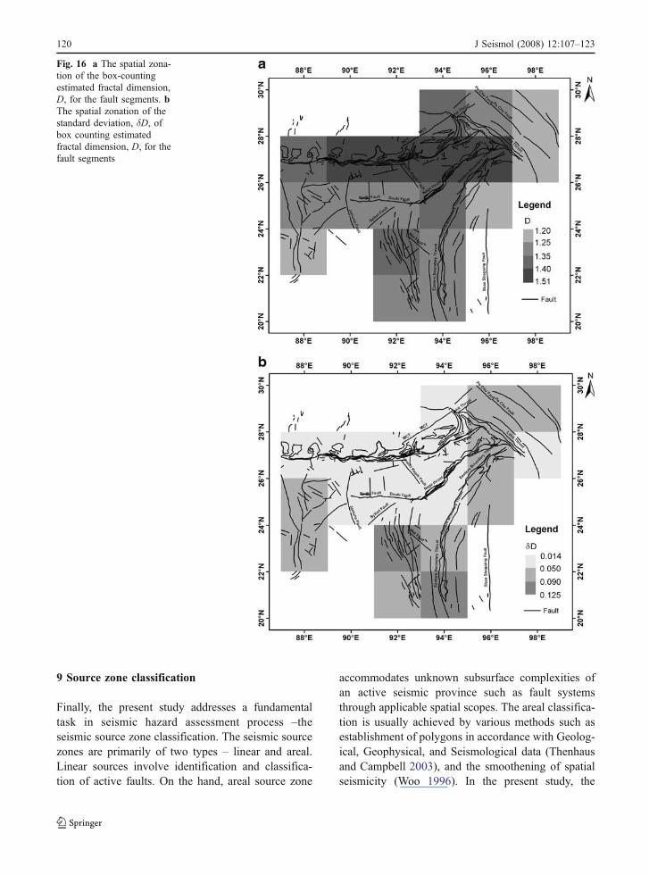
The estimated D is found to vary from 1.20 to1.51. Figures 16a and b depict the estimated D and itsestimated standard deviation δD, respectively, foreach corresponding segment. A value close to 2suggests that it is a plane that is being filled up,while a value close to 1 implies that line sources arepredominant (Aki 1981). The results corroborate thefindings to upper limit of 1.6 as indicated by Hirata(1989b). The Himalayan structures are seen withhigher values towards 1.51. The zones of Naga thrust,Lohit thrust, the EBT and that of Mat fault and thesouth western to it are similarly seen with high Dvalues. The moderate values are observed across theShillong plateau region and the southern EBT. Thestandard deviations associated with the estimatedfractal dimension of the segments imply that there isno much statistically significant difference in theestimated values over narrow ranges in most of thecase. However, low standard deviations as observedwith high D values associated with the segmentscontaining the Himalayan structures sustain theestimated high values.

Fig. 15 The estimation of fractal dimension D for the faultsegment with the centroid at longitude 88°E and latitude 23°Nfrom the slope of the best fit line on the plot of log10(C(N, r))against log10(r). The scale ‘r’ is the number of square boxes onone side of the entire box

J Seismol (2008) 12:107–123 119

9 Source zone classification

Finally, the present study addresses a fundamentaltask in seismic hazard assessment process –theseismic source zone classification. The seismic sourcezones are primarily of two types – linear and areal.Linear sources involve identification and classifica-tion of active faults. On the hand, areal source zone

accommodates unknown subsurface complexities ofan active seismic province such as fault systemsthrough applicable spatial scopes. The areal classifica-tion is usually achieved by various methods such asestablishment of polygons in accordance with Geolog-ical, Geophysical, and Seismological data (Thenhausand Campbell 2003), and the smoothening of spatialseismicity (Woo 1996). In the present study, the

Fig. 16 a The spatial zona-tion of the box-countingestimated fractal dimension,D, for the fault segments. bThe spatial zonation of thestandard deviation, δD, ofbox counting estimatedfractal dimension, D, for thefault segments

120 J Seismol (2008) 12:107–123

spatial pattern of seismicity quantified by b value andDC are employed along with the underlying tectonicnetwork. The method involves segregation of varyingcorrelations of b value and DC in accordance with thefault patterns. Thus, the northeast Indian region isbroadly classified into four seismic source zones –Eastern Himalayan Zone (EHZ), Mishmi Block Zone(MBZ), Eastern boundary Zone (EBZ), and ShillongZone (SHZ) as shown in Fig. 17.

The seismotectonics of the region as displayed inFig. 6 indicates activities due to thrust, normal andstrike slip motions across the region. The beach ballspresenting oblique reverse focal mechanism impli-cates thrusting and is seen to dominate in the northernEBT where earthquake foci are mostly in theintermediate depth (70 < km < 300). However, thesouthern part of EBT shows significantly strike slipmechanism. The observed trend of focal mechanismsin the zone relates to oblique thrusting in the territory.The strike slip mechanism is also seen on the Mishmizone of Lohit thrust and Po Chu fault. The zones ofDauki fault and that of Dhansiri Kopila fault in theShillong Plateau region exhibits strike slip focalmechanisms. On the other hand, the earthquakemechanisms are predominantly normal in the east-ern/upper Himalayan region. Accordingly, the EHZ is

associated with predominantly normal faulting mech-anism with significantly shallow occurring earth-quakes. MBZ and SHZ have dominantly strike slipfocal mechanism with shallow earthquakes. EBZ onthe other hand has predominantly oblique reversefocal mechanism – with the occurrence of intermedi-ate depth earthquakes.

10 Discussion and conclusions

Region specific magnitude scaling relations have beenestablished for the study region, which facilitated thegeneration of a homogenous earthquake catalogue forthe present analysis. The seismicity analysis in theregion has been performed with a sub-catalogue(1964–2006), considering the stability and improvedearthquake recordings from 1964, which is likely dueto the advent of World-Wide Standard SeismographicNetwork (WWSSN). The analysis highlighted varia-tions of seismicity in the study region, althoughsignificant spatial gaps have been found due to eitherlack of valid minimum magnitude of completeness orinadequate number of events. The spatial patterns ofseismicity parameters – mt, a and b value exhibited byand large positive correlations in the study region.

Fig. 17 The classifiedsource zones demarcatedby the polygons

J Seismol (2008) 12:107–123 121

The spatial distribution of δb also follows positivecorrelations with the estimated b values in most of thecases, wherein low b values are seen with lowstandard deviation indicating an overall tendency oflow b values across the study region. To this effect,the lower b values are seen predominant in the thrustzones and moderate to higher values in the zonesexhibiting strike slip and normal focal mechanism.The results of the present study are comparable withthose of recent works (Scholemmer et al. 2005; Wysset al. 2004; Oncel and Wilson 2002). Mostly highvalues of DC have been seen across the region thatexhibits high the box-counting fractal dimension, D,of the underlying predominant fault segments. Nega-tive correlation is quite dominant in the northern EBTand Tripura-Cachar fold belt with low b value, whileother regions tend to differ. The trend of moderatelyhigh b values on the north and high on the south seemto corroborate oblique reverse faulting mechanism inthe northern EBT. However, in Shillong plateau area,the mechanisms of earthquake occurrence are consid-erably different with higher b values but low DC. Inthe eastern Himalaya with predominantly normal fault-ing mechanisms, positive correlations are exhibited withhigh b values. Similarly positive correlations are alsoobserved in the Mishmi massif region of Po Chu faultand Lohit thrust exhibiting high b values. Lastly, theestablished spatial seismicity patterns of b value andDC with the consideration of underlying active faultnetworks have been applied to demarcate four broadseismic source zones, designated as EHZ, MBZ, EBZ,and SHZ, in the study region. The analysis of therecent seismicity in the northeast Indian regionperformed thus accomplishes a basic groundworktowards seismic hazard assessment of this earthquake-prone country of India.

Acknowledgment The critical review and constructive sug-gestions of the anonymous referee greatly helped in signifi-cantly improving the manuscript with enhanced scientificexposition.

References

Aki K (1965) Maximum likelihood estimate of b in the formulalog N=a-bM and its confidence limits. Bull Earthq ResInst Univ Tokyo 43:237–239

Aki K (1981) A probabilistic synthesis of precursor phenom-ena. In: Simpson DW, Richards PG (eds) EarthquakePrediction, Maurice Ewing Series 4, AGU 566–574

Aviles CA, Scholz CH, Boatwright J (1987) Fractal analysisapplied to characteristic segments of the San Andreasfault. J Geophys Res 92:331–344

Barton DJ, Foulger GR, Henderson JR, Julian BR (1999)Frequency-magnitude statistics and spatial correlationdimensions of earthquakes at Long Valley caldera.California. Geophys J Int 138:563–570

Bender B (1983) Maximum likelihood estimation of b values formagnitude grouped data. Bull Seism Soc Am 73:831–851

Ben-Menahem A, Aboodi E, Schild R (1974) The source of thegreat Assam earthquake–an interplate wedge motion. PhysEarth and Planet Int 9:265–289

Bhatia SC, Ravi Kumar M, Gupta HK (1999) A probabilisticseismic hazard map of India and adjoining regions. Ann diGeofis 42:1153–1166

Bilham R, England P (2001) Plateau ‘ pop up’ in the great 1897Assam earthquake. Nature 410:806–809

BIS (2002) IS 1893–2002 (Part 1): Indian standard criteria forearthquake resistant design of structures, part 1–generalprovisions and buildings. Bureau of Indian Standards,New Delhi

Bormann P, Liu R, Ren X, Gutdeutsch R, Kaiser D, CastellaroS (2007) Chinese national network magnitudes, theirrelation to NEIC magnitudes, and recommendations fornew IASPEI magnitude standards. Bull Seism Soc Am97:114–127

Braunmiller J, Deichmann N, Giardini D, Wiemer S (2005)Homogeneous moment-magnitude calibration in Switzer-land. Bull Seism Soc Am 95:58–74

Brune J, Engen G (1969) Excitation of mantle love waves anddefinition of mantle wave magnitude. Bull Seism Soc Am57:1355–1365

Castellaro S, Mulargia F, Kagan YY (2006) Regressionproblems for magnitudes. Geophys J Int 165:913–930

Chen W, Molnar P (1977) Seismic moments of major earth-quakes and average rate of slip in Central Asia. J GeophyRes 82:2945–2969

Chernick MR (1999) Bootstrap methods: a practitioner’s guide,Wiley Series in Probability and Statistics. Wiley, NewYork

Dasgupta S, Pande P, Ganguly D, Iqbal Z, Sanyal K, VenaktramanNV, Dasgupta S, Sural B, Harendranath L, Mazumadar K,Sanyal S, Roy A, Das LK, Misra PS, Gupta H (2000)Seismotectonic Atlas of India and its Environs. GeologicalSurvey of India, Calcutta, India

Deichmann N (2006) Local magnitude, a moment revisited.Bull Seism Soc Am 96:1267–1277

Grassberger P, Procaccia I (1983) Measuring the strangeness ofstrange attractors. Physica D 9:189–208

Gutenberg B (1945a) Amplitudes of surface waves andmagnitudes of shallow earthquakes. Bull Seism Soc Am35:3–12

Gutenberg B (1945b) Magnitude determination for deep-focusearthquakes. Bull Seism Soc Am 35:117–130

Gutenberg B, Richter CF (1944) Frequency of earthquakes inCalifornia. Bull Seism Soc Am 34:185–188

Gutenberg B, Richter CF (1956) Magnitude and energy ofearthquakes. Ann Geofis 9:1–15

Hanks TC, Kanamori H (1979) A moment magnitude scales. JGeophysis Res 84:2348–2350

122 J Seismol (2008) 12:107–123

Heaton TH, Tajima F, Mori AW (1986) Estimating groundmotion using recorded accelerograms. Surv Geophys8:25–83

Henderson JR, Main IG, Pearce RG, Takeya M (1992)Seismicity in North eastern Brazil: fractal clustering andthe evolution of the b value. Geophys J Int 116:217–226

Hirata T (1989a) A correlation between the b value and thefractal dimension of earthquake. J Geophys Res 94:7507–7514

Hirata T (1989b) Fractal dimension of fault systems in Japan:fractal structure in rock fracture geometry at variousscales. Pageoph 131:157–170

ISC (2007) On-line Bulletin, http://www.isc.ac.uk/Bull, Inter-natl. Seis. Cent., Thatcham, United Kingdom

Kagan YY (2003) Accuracy of modern global earthquakecatalogs. Phys Earth Planet Inter 135:173–209

Kagan YY (2007) Earthquake spatial distribution: the correla-tion dimension. Geophys J Int 168:1175–1194

Kagan YY, Knopoff L (1980) Spatial distribution of earth-quakes: the two point correlation function. Geophys JRAstr Soc 62:303–320

Kanamori H (1977) The energy release in Great Earthquakes. JGeophy Res 82:2981–2987

Kanamori H (1983) Magnitude scale and quantification ofearthquakes. Tectonophys 93:185–199

Mandelbrot BB (1983) The fractal geometry of nature.Freeman, New York

Mogi K (1962) Magnitude-frequency relationship for elasticshocks accompanying the fractures of various materialsand some related problems in earthquakes. Bull EarthqRes Inst Univ Tokyo 40:831–883

Nandy DR (2001) Geodynamics of north eastern India and theadjoining region, 1st edn. ACB publications, Kolkata

Narenberg MAA, Essex C (1990) Correlation dimension andsystematic geometric effects. Phys Rev A 42:7065–7074

Nuannin P, Kulhanek O, Persson L (2005) Spatial and temporalb value anomalies preceding the devastating off coast ofNW Sumatra earthquake of December 26, 2004. GeophysRes Lett 32:L11307 DOI 10.1029/2005GL022679

Oncel AO, Wilson TH (2002) Space-time correlations ofseismotectonic parameters: example from Japan and fromTurkey preceding the Izmith earthquake. Bull Seism SocAm 92:339–349

Oncel AO, Wyss M (2000) The major asperities of the 1999 M7.4 Izmit earthquake, defined by the microseismicity of thetwo decades before it. Geophys J Int 143:501–506

Richter CF (1935) An instrumental earthquake magnitude scale.Bull Seis Soc Am 25:1–31

Ristau J, Rogers GC, Cassidy JF (2005) Moment magnitude–local magnitude calibration for earthquakes in westerncanada. Bull Seism Soc Am 95:1994–2000

Rong Y (2002) Evaluation of Earthquake Potential in China,PhD. Dissertation, Geophysics and Space Physics, Universityof California, Los Angeles

Schorlemmer D, Neri G, Wiemer S, Mostaccio A (2003)Stability and significance tests for b value anomalies:example from the Tyrrhenian Sea. Geophys Res Lett30:1835 DOI 10.1029/2003GL017335

Scholemmer D, Wiemer S, Wyss M (2005) Variations inearthquake-size distribution across different stress regimes.Nature 437:539–542

Scholz CH (1968) The frequency-magnitude relation of micro-fracturing in rock and its relation to earthquakes. BullSeism Soc Am 58:399–415

Scordilis EM (2006) Empirical global relations converting MS

and mb to moment magnitude. J Seis 10:225–236Stromeyer D, Grünthal G, Wahlström R (2004) Chi-square

regression for seismic strength parameter relations, andtheir uncertainties, with applications to an Mw basedearthquake catalogue for central, northern and northwest-ern Europe. J Seis 8:143–153

Suyehiro S, Asada T, Ohtake M (1964) Foreshocks andaftershocks accompanying a perceptible earthquake incentral Japan: on the peculiar nature of foreshocks. PapMeteorol Geophys 19:427–435

Thenhaus PC, Campbell W (2003) Seismic hazard analysis. In:Chen WF, Scawthorn C (eds) Earthquake engineeringhandbook. CRC Press, Boca Raton, pp 1–43

Turcotte DL (1986) A fractal model for crustal deformation.Tectonophysics 132:261–269

Utsu T (1965) A method for determining the value of b in theformula log N=a-bM showing the magnitude–frequencyrelation for the earthquakes. Geophys Bull Hokkaido Univ13:99–103

Utsu T (1999) Representation and analysis of the earthquakesize distribution: a historical review and some newapproaches. Pageoph 155:509–535

Wesnouski SG, Scholz CH, Shimazaki K, Matsuda T (1983)Earthquake frequency distribution and the mechanics offaulting. J Geophys Res 88:9331–9340

Wiemer S, Wyss M (2000) Minimum magnitude of completereporting in earthquake catalogs: examples from Alaska,the Western United States, and Japan. Bull Seism Soc Am90:859–869

Willemann RJ, Storchak DA (2001) Data collection at theinternational seismological centre. Seis Res Lett 72:440–453

Woo G (1996) Kernel estimation methods for seismic hazardarea source modeling. Bull Seism Soc Am 86:353–362

Wyss M, Sammis CG, Nadeau RM, Wiemer S (2004) Fractaldimension and b value on creeping and locked patches ofthe San Andreas Fault near Parkfield, California. BullSeism Soc Am 94:410–421

J Seismol (2008) 12:107–123 123