Empirical Characterization of Induced Seismicity in Alberta ...

Western University Western University

Scholarship@Western Scholarship@Western

Electronic Thesis and Dissertation Repository

11-15-2018 2:30 PM

Empirical Characterization of Induced Seismicity in Alberta and Empirical Characterization of Induced Seismicity in Alberta and

Oklahoma Oklahoma

Mark Novakovic The University of Western Ontario

Supervisor

Atkinson, Gail M.

The University of Western Ontario

Graduate Program in Geophysics

A thesis submitted in partial fulfillment of the requirements for the degree in Doctor of

Philosophy

© Mark Novakovic 2018

Follow this and additional works at: https://ir.lib.uwo.ca/etd

Part of the Geophysics and Seismology Commons

Recommended Citation Recommended Citation Novakovic, Mark, "Empirical Characterization of Induced Seismicity in Alberta and Oklahoma" (2018). Electronic Thesis and Dissertation Repository. 5961. https://ir.lib.uwo.ca/etd/5961

This Dissertation/Thesis is brought to you for free and open access by Scholarship@Western. It has been accepted for inclusion in Electronic Thesis and Dissertation Repository by an authorized administrator of Scholarship@Western. For more information, please contact [email protected].

https://ir.lib.uwo.ca/

https://ir.lib.uwo.ca/etd

https://ir.lib.uwo.ca/etd?utm_source=ir.lib.uwo.ca%2Fetd%2F5961&utm_medium=PDF&utm_campaign=PDFCoverPages

http://network.bepress.com/hgg/discipline/158?utm_source=ir.lib.uwo.ca%2Fetd%2F5961&utm_medium=PDF&utm_campaign=PDFCoverPages

https://ir.lib.uwo.ca/etd/5961?utm_source=ir.lib.uwo.ca%2Fetd%2F5961&utm_medium=PDF&utm_campaign=PDFCoverPages

mailto:[email protected]

i

Abstract

This thesis characterizes ground motions from induced seismic events in Alberta and

Oklahoma, following an overall methodology that uses ground-motion recordings to calibrate

the parameters of a seismological model. This body of work is carried out in three related

studies.

In the first study, we perform a preliminary evaluation of ground motions in Alberta using

thousands of observations of natural, induced and blast events of magnitude 1 to 4, recorded

on a newly-deployed regional seismograph array. We evaluate the applicability of a moment

magnitude (M) estimation algorithm for the events and compare the observed ground

motions with expectations based on regional ground motion prediction equations (GMPEs).

Ground motions for earthquakes are similar to those predicted by the small-M GMPE of

Atkinson (2015), if one assumes that the predominant site condition in Alberta is a generic

soft soil (Vs30 < 400 m/s).

In the second study, ground motion observations from induced seismic events in Oklahoma

are used to perform a generalized inversion to solve for regional source, attenuation and

station site responses within the context of an equivalent point-source model following the

method of Atkinson et al. (2015) and Yenier and Atkinson (2015b). The resolved parameters

fully specify a regionally calibrated GMPE that can be used to describe median amplitudes

from induced earthquakes in the central United States. Overall, the ground motions for soft

rock (B/C) site conditions for induced events in Oklahoma are of similar amplitude to those

predicted by the GMPEs of Yenier and Atkinson (2015b) and Atkinson et al. (2015) at close

distances, for events of M 4 to 5. For larger events the Oklahoma motions are larger,

especially at high frequencies. The Oklahoma motions follow a pronounced trilinear

amplitude decay function at regional distances.

In the third study, we follow a similar procedure to develop a GMPE that fully specifies

regional source, attenuation and station site responses for induced seismic events in Alberta.

Ground motions in Alberta follow a pronounced trilinear amplitude decay function at

regional distances. We account for observations of lower amplitude ground motions at high

ii

frequencies in Alberta when compared to those observed in Oklahoma by adapting the near

surface attenuation kappa effect (κ) model from Hassani and Atkinson (2018). Overall

ground motions in Alberta are consistent with those expected for very shallow (depth < 10

km) natural events in central and eastern North America.

Keywords

Ground motion prediction equation, induced seismicity, moment magnitude, attenuation,

stress parameter, engineering seismology.

iii

Co-Authorship Statement

This integrated-article format thesis includes the following manuscripts written by Mark

Novakovic and the co-authors. Mark is the first author on studies investigating the

applicability of moment magnitude estimation algorithm for induced seismic events in

Alberta, and the development of ground motion prediction equations for induced seismicity

in Alberta and Oklahoma. Chapters 2, 3, and 4 have been previously published or submitted

for publication to the peer reviewed journals Seismological Research Letters and the Bulletin

of the Seismological Society of America. This thesis contains only the original results of

research conducted by the candidate under the supervision of Dr. Gail M. Atkinson. Mark

performed the analyses described in this thesis and authored these reports with assistance

from Dr. Gail M. Atkinson. Ground motion data (Pseudo Spectral Accelerations and Peak

Ground Motions) were computed and tabulated by Dr. Karen Assatourians. Continuous

waveform data were provided from the Canadian Rockies and Alberta Network (CRANE) by

Dr. Jeff Gu.

1) Novakovic M., Atkinson G. M. (2015). Preliminary Evaluation of Ground Motions from

Earthquakes in Alberta. Seismol. Res. Lett., 86(4): 1086-1095.

2) Novakovic M., Atkinson G. M., Assatourians K. (2018). Empirically Calibrated Ground-

Motion Prediction Equation for Oklahoma. Bull. Seismol. Soc. Am. DOI:

10.1785/0120170331

3) Novakovic M., Atkinson G. M., Assatourians K., Gu Y. (2018). Empirically Calibrated

Ground-Motion Prediction Equation for Alberta. Bull. Seismol. Soc. Am. DOI: (Submitted to

the Bulletin of the Seismological Society of America, 31/08/2018)

The composed articles and thesis were completed under the supervision of Dr. Gail M.

Atkinson.

iv

Acknowledgements

To my supervisor Dr. Gail Marie Atkinson, I would like to express my sincerest gratitude for

all of the guidance, support, patience, encouragement and opportunity you have provided

throughout my time at Western. I have been incredibly fortunate to have had a mentor with

such expansive knowledge and deep roots in the engineering seismology field and

community, for which I will be eternally grateful.

I would like to thank Karen Assatourians for his friendship, support and tireless effort to

provide high quality ground motion data sets for our analysis.

I would like to thank Justin Rubinstein, Thomas Pratt and our other anonymous paper

reviewers for their constructive feedback which strengthened the manuscripts presented here.

I would like to thank my PhD committee members, Dr. Robert Scherbakov and Dr. Sheri

Molnar; and my thesis examiners, Dr. Chris Cramer, Dr. Hadi Ghofrani, Dr. Katsu Goda, and

Dr. Hesham El Naggar.

I would like to thank Behzad Hassani, Emrah Yenier, and Joseph Farrugia for our discussions

of seismological principles and practices, which always concluded with a better

understanding of the topic at hand.

I would like to kindly thank Andrew Reynen and Andrew Law from Nanometrics for

providing earthquake meta-data tables for the TransAlta Network.

I would like to thank Tegan, Carson, Micah, Krista, Joanna, Sam, Azedeh, Sheri, Bernie,

Arpit, Sebastian, Mingzhou, Freddie, Shaun, Sjors, Derek, Emma, Soushyant, Joelle, Sid,

Surej, and the 3rd Rocks for your friendship and support.

I would like to thank my parents, Ray and Donna, for all they have done to help me get

where I am today. I would like to thank my brothers Robi and Stefan for their love and

support. Finally, I would like to thank Holly Mussell, my rock, for your unwavering love,

support, encouragement and understanding throughout the completion of my studies.

v

Table of Contents

Abstract ................................................................................................................................ i

Co-Authorship Statement................................................................................................... iii

Acknowledgements ............................................................................................................ iv

Table of Contents ................................................................................................................ v

List of Tables ................................................................................................................... viii

List of Figures .................................................................................................................... ix

List of Electronic Supplements ....................................................................................... xvii

Chapter 1 ............................................................................................................................. 1

1 Introduction .................................................................................................................... 1

1.1 Organization of Thesis ............................................................................................ 1

1.2 Motivation ............................................................................................................... 1

1.3 Response Spectra .................................................................................................... 3

1.4 Moment Magnitude Estimation .............................................................................. 4

1.5 Ground Motion Prediction Equations ..................................................................... 7

1.6 References ............................................................................................................... 9

Chapter 2 ........................................................................................................................... 15

2 Preliminary Evaluation of Ground Motions from Earthquakes in Alberta .................. 15

2.1 Introduction ........................................................................................................... 15

2.2 Magnitude Evaluations ......................................................................................... 18

2.3 Evaluation of Ground Motions ............................................................................. 21

2.4 Conclusions ........................................................................................................... 32

2.5 Acknowledgements ............................................................................................... 32

2.6 References ............................................................................................................. 32

Chapter 3 ........................................................................................................................... 35

vi

3 Empirically Calibrated Ground Motion Prediction Equation for Oklahoma ............... 35

3.1 Introduction ........................................................................................................... 35

3.2 Database ................................................................................................................ 36

3.3 Estimation of Moment Magnitude ........................................................................ 39

3.4 Ground-Motion Model .......................................................................................... 41

3.5 Application to Induced Events in Oklahoma ........................................................ 47

3.6 Conclusions ........................................................................................................... 63

3.7 Data and Resources ............................................................................................... 64

3.8 Acknowledgements ............................................................................................... 64

3.9 References ............................................................................................................. 65

Chapter 4 ........................................................................................................................... 68

4 Empirically-Calibrated Ground Motion Prediction Equation for Alberta ................... 68

4.1 Introduction ........................................................................................................... 68

4.2 Database ................................................................................................................ 69

4.3 Estimation of Moment Magnitude ........................................................................ 72

4.4 Ground Motion Model .......................................................................................... 74

4.5 Application to Induced Events in Alberta ............................................................. 81

4.6 Conclusion ............................................................................................................ 99

4.7 Data and Resources ............................................................................................. 100

4.8 Acknowledgements ............................................................................................. 100

4.9 References ........................................................................................................... 100

Chapter 5 ......................................................................................................................... 105

5 Conclusions and Future Studies ................................................................................. 105

5.1 Summary, Discussion and Conclusions .............................................................. 105

5.2 Recommendations for Future Studies ................................................................. 107

5.3 References ........................................................................................................... 108

vii

Appendices ...................................................................................................................... 110

Curriculum Vitae ............................................................................................................ 115

viii

List of Tables

Table 2.1: WNA anelastic attenuation and empirical calibration terms for 1.00 Hz and 3.33

Hz frequencies ........................................................................................................................ 19

Table A3.1: Tabulation of magnitude estimation model parameters. Where MCF is the

calibration factor for each frequency that aims to match the level that has been modified from

Novakovic and Atkinson (2015) for Oklahoma. γF, low (Eastern), γF, mod (moderate), and γF, high

(Western) are the anelastic attenuation coefficients designed to remove distance dependent

trends………………………………………………………………………………..……..110

Table A3.2: Summary table of stress parameter values from inversion for events of M ≥ 4.2

in Oklahoma……………………………………………………………………………….110

Table A3.3: Summary of Oklahoma model coefficients and the anelastic attenuation function

γOK, calibration factor COK, within event variability η, and in-between event variability ε as

determined by the inversion…………………………………………………………….. 102

Table A4.1: Tabulation of magnitude estimation model parameters. MCF is the magnitude

calibration factor for each frequency. γF, low (Eastern), γF, mod (moderate), and γF, high (Western)

are the anelastic attenuation coefficients………………………………………………...... 113

Table A4.2: Summary of Alberta model coefficients, the anelastic attenuation function γAB,

calibration factor CAB, within event variability η, and in-between event variability ε as

determined by the inversion…………………………….………………………………. 113

Table A4.3: Table of stress parameter values from inversion for all events in Alberta.......114

ix

List of Figures

Figure 1.1: Fourier displacement source spectrum where the solid line shows stress-drop

values of 100 bars and dashed line show stress-drop values of 500 bars. Corner frequencies

are shown as circles, and black vertical lines highlight the 1.00 Hz and 3.33 Hz frequencies.

Reprinted from “Estimation of Moment Magnitude (M) for Small Events (M<4) on Local

Networks”, G. M. Atkinson (2014), Seismological Research Letters, 85(5): 1116-1124…….6

Figure 2.1: Map of stations and study events in Alberta. Events which are considered to be

blasts are designated by an x. The deformation front that marks the boundary of the Rocky

Mountains is distinguishable by topography. ......................................................................... 16

Figure 2.2: Estimated M versus ML (excluding events designated as blasts). Standard error

of M estimates are also shown (horizontal bars, with verticals to denote edges). .................. 20

Figure 2.3: Distribution of events (blasts excluded) in M and distance. ............................... 21

Figure 2.4: PSA amplitudes (all components) at 1.00 Hz for events of M = 3.0 ±0.3, as a

function of hypocentral distance, compared to the relations of AGY14 (vertical component)

and A15 (horizontal component, B/C conditions). ................................................................. 22


function of hypocentral distance, compared to the relations of AGY14 (vertical component)

and A15 (horizontal component, B/C conditions). ................................................................. 23

Figure 2.6: PSA residuals for M ≥ 2.6 for PSA at 1.00 Hz (top), 3.33 Hz (middle) and 10.0

Hz (lower), for horizontal (left) and vertical (right) components (blasts removed). .............. 25

Figure 2.7 Mean and standard error of PSA residuals for M ≥ 2.6 at 1.00 Hz (top), 3.33 Hz

(middle) and 10.0 Hz (lower), binned by log distance, for horizontal and vertical components

(no error bar plotted if the number of observations in the bin is <3). Slight offset from bin

center used for plotting clarity (to distinguish horizontal from vertical). ............................... 26

Figure 2.8: Scaling of source terms with magnitude, in comparison to empirical (A15) and

simulation-based (Yenier and Atkinson, 2015a) models ........................................................ 28

file:///C:/Users/MarkNovakovic/Documents/UWO/Thesis/Thesis_Manuscirpt_v2-1.docx%23_Toc523404560















x

Figure 2.9: Average PSA residuals versus frequency in distance ranges 10-120 km, 120-250

km, 250-400 km (left=vertical, right=horizontal). Average including all distances is also

shown (heavy line). Dashed line on right panel shows the average horizontal residual minus

the average vertical residual, which is similar to an average site response function. ............. 29

Figure 2.10: Average station residuals for vertical and horizontal components of selected

frequencies, for events with M > 2.6 (blasts excluded). ......................................................... 31

Figure 3.1: Study earthquakes (circles) and recording stations (light triangles). Stations

chosen as B/C reference sites are highlighted (dark triangles). .............................................. 37

Figure 3.2: The magnitude distance distribution of the database, containing 7278 records

from 194 earthquakes (M 3.5 – 5.8) recorded at 101 seismograph stations. We consider

records within logarithmically spaced bins with a cut-off distance that increases from 120 km

for M = 3.5 to 500 km for M ≥ 4.0 events. The moment magnitude values (MNA15) are

determined as described in Figure 3.3. ................................................................................... 38

Figure 3.3: The logic tree used to decide which frequency is used to estimate moment

magnitude (M) of the event. We compute M based on PSA at 0.30 Hz, 1.00 Hz and 3.33 Hz.

The M estimate from 3.33 Hz PSA is used for events of M < 3, 1.00 Hz estimate for M 3 - 4,

and 0.30 Hz for M ≥ 4. For each event, the anelastic attenuation coefficient that minimizes

the residuals is chosen, where three values are considered: low (CENA value), high

(California value) or moderate (average of the two). ............................................................. 40

Figure 3.4: Comparison of MNA15 magnitude estimates with USGS/OGS reported M as

obtained from regional or global moment tensors. Squares show average estimated M for

events in 0.1 magnitude unit bins, along with standard deviation (dashed lines). Mean

deviation from other estimates is about -0.1 units. ................................................................. 41

Figure 3.5: Observed normalized amplitudes (circles) after correction for magnitude

dependence (FM, Eqn 3.4) and CENA anelastic attenuation (Eqn 3.8); squares show median

normalized amplitudes in distance bins. Solid lines show the adopted trilinear geometric

spreading function (which has magnitude dependence as in YA15), for a range of

magnitudes, assuming a 100-bar stress parameter; only the shape is important, as the level is







xi

determined by inversion. A constant is added to all ground motions to adjust the level of the

geometric spreading function for better visualization.. .......................................................... 45

Figure 3.6: Regional anelastic attenuation term for Oklahoma with standard deviation, in

comparison to previous results of Yenier and Atkinson (2015b) for California and CENA.. 48

Figure 3.7: Site amplification (ln units) for the assigned reference B/C stations, resulting

from the inversion OK005 sits on shale with VS30 of 613 m/s, OK029 sits on sandstone, while

both OK030 and OK031 sit on shale. VS30 for OK029, OK030 and OK031 is believed to be

close to B/C based on horizontal-to-vertical component ratios. ............................................. 49

Figure 3.8: Typical site amplifications (ln units) for stations resulting from the inversion.

WHAR is a sandstone station with VS30 of 1403 m/s. WMOK is a station sitting on granite

with VS30 of 1859 m/s. OK009 is a station sitting on a conglomerate with VS30 of 322 m/s.

No VS30 information is available for WLAR, OK032, KAN10 and HHAR; however

according to surficial lithology maps, these stations sit on sandstone, alluvium, gravel and

limestone respectively. ............................................................................................................ 50

Figure 3.9: All station terms. The lines depict the site response relative to B/C condition for

all stations used in the study in natural log units. Squares depict the mean site term for each

frequency, with their standard deviations in dashed lines.. .................................................... 51

Figure 3.10: Determination of stress parameter, for M5.8 Pawnee event. Left) ∆LF (low-

frequency offset) is determined as the offset of the average of observed spectral displacement

(SD) on the seismic moment end of the specturm (1.00 Hz) relative to predicted SD from

YA15 (corrected for site and attenuation effects to a reference distance of 20 km). Right)

∆HF (high-frequency offset) is determined from the level of the 10.0 Hz PSA, after shifting

spectrum by ∆LF. Note that the spectra in this figure have been converted from units of g to

cm/s2.. ...................................................................................................................................... 52

Figure 3.11: Stress parameters for individual events (circles), compared with a with simple

bilinear fit to the stress parameter versus magnitude (upper as a dashed line) and a simple fit

to the stress parameter with respect to focal depth (lower as a solid line). ............................. 53

xii

Figure 3.12: Stress parameters determined by inversion for each event (Figure 3.8) (circles)

as a function of moment magnitude (MNA15) and depth (larger circles denote greater depth).

Solid lines show models that capture the observed trends in the Oklahoma data, in

comparison to YA15 CENA model (dashed lines) for several values of focal depth. ........... 54

Figure 3.13: Calibration factor (COK) obtained from inversion (squares) and its standard

deviation (jagged lines). The solid line shows suggested model function for COK, the Yenier

and Atkinson (2015b) calibration factor for CENA is shown as a dot-dashed line, and its

modeled form is shown as a dashed line. . ............................................................................. 56

Figure 3.14: The Oklahoma calibration factor (gray line) and its inverse (black line), in

comparison to the site amplification functions of Seyhan and Stewart (2014; SS14) for

California, for a range of VS30 values (lines with symbols). It should be noted that the site

amplification function is at a constant level for Vs30 greater than 1500 m/s. .......................... 58

Figure 3.15: Between-event residuals η, where dark (pink) circles show M < 4, light circles

(green) show M ≥ 4, and squares show the depth bin mean ± σ…………………………..…59

Figure 3.16: Within event residuals with respect to the final GMPE for PSA at 1.01 Hz.

Black squares depict the mean residual and its standard deviation in logarithmically spaced

distance bins. ........................................................................................................................... 60



distance bins. ........................................................................................................................... 61

Figure 3.18: : Within event residuals with respect to the final GMPE for PSA at 10.2 Hz.


distance bins. ........................................................................................................................... 61

Figure 3.19: Within event residuals with respect to the final GMPE for PGA. Black squares

depict the mean residual and its standard deviation in logarithmically spaced distance bins. 62

Figure 3.20: Final GMPE overlaying site corrected observations at 5.12 Hz. Lines depict the

GMPE evaluated every 0.2 magnitude units from M = 4.1 to M = 5.9 at linearly-increasing

xiii

depths ranging from 3 to 8 km, respectively. Circles vary in diameter where larger circles

represent larger magnitude observations and smaller circles denote smaller magnitude event

observations. ........................................................................................................................... 62

Figure 3.21: GMPE for Oklahoma as determined in this study (solid lines) in comparison to

the YA15 GMPE for CENA (dashed lines); both GMPEs are evaluated for focal depths of 5,

6 and 8 km for M = 4, 5, and 6 respectively. The GMPE of Atkinson (2015), as determined

from moderate California earthquakes with mean depth of 9 km, is also indicated (dotted

lines), for distances < 50 km. All models are for NEHERP B/C reference site conditions. .. 63

Figure 4.1: Earthquakes (circles) and stations (inverted triangles) used in this study. Stations

chosen as B/C reference sites are highlighted (diamonds). .................................................... 69

Figure 4.2: The magnitude-distance distribution of the database, containing 884 records

from 37 earthquakes (M 3 – 4.3) recorded at 75 seismograph stations. We consider records

within logarithmically spaced bins with a cut-off distance that increases from 200 km for M

= 3 to 600 km for M ≥ 4 events. The moment magnitude values (M) are determined as

described in Figure 4.3. ........................................................................................................... 70

Figure 4.3: A logic tree to decide which frequency is used to estimate moment magnitude

(M) of the event. We compute M based on PSA at 1.00 Hz and 3.33 Hz. The M estimate

from 3.33 Hz PSA is used for events of M < 3, 1.00 Hz estimate for M ≥ 3, and the mean of

the two values for M ~= 3. For each event, the anelastic attenuation coefficient that

minimizes the residuals is chosen, where three values are considered: low (CENA value),

high (California value) or moderate (average of the two). ..................................................... 73

Figure 4.4: Comparison of moment magnitude estimates based on PSA with the local

magnitudes as reported by the Alberta Geological Survey. The two scales agree quite well

for M > 2.6; ground motion response amplitudes scale weakly with ML at lower magnitudes.

................................................................................................................................................. 74


dependence (FM, Eqn 4.4), Oklahoma stress parameter model and anelastic attenuation (Eqn

4.5 & 4.13); squares show median normalized amplitudes in distance bins. Solid lines show

the adopted trilinear geometric spreading function (which has magnitude dependence as in






















xiv

YA15), for a range of magnitudes, assuming a 100-bar stress parameter; only the shape is

important, as the level is determined by inversion. A constant is added to all ground motions

to adjust the level of the geometric spreading function for better visualization. Large scatter

at near distances reflects variability in source amplitudes. ...... Error! Bookmark not defined.

Figure 4.6: Regional anelastic attenuation function obtained from the inversion (Alberta) in

comparison to previous results of Novakovic et al. (2018) for Oklahoma, Yenier and

Atkinson (2015b) for California and Central and Eastern North America. ............................ 82

Figure 4.7: Site amplification (ln units) for the assigned reference B/C stations as obtained

from the inversion. The average over the five reference stations is 0 ln units by definition.

The selected reference stations are all post-hole seismometers that provide well behaved

horizontal-to-vertical component ratios and B/C like responses. ........................................... 83

Figure 4.8: Typical site amplification (ln units) for stations resulting from the inversion.

Pronounced peaked amplification is observed at many stations suggesting that site conditions

are on average softer across the province than those chosen as B/C-like reference stations. . 84

Figure 4.9: All station terms. The lines depict the site response relative to B/C condition for

all stations used in the study in natural log units. Squares depict the mean site term for each

frequency with their standard deviation in dashed lines. ........................................................ 84

Figure 4.10: (Left) stress parameters determined by inversion for each event as a function of

M (triangles). Solid lines show the stress parameter model for Oklahoma evaluated over a

range of depths. Lines with symbols depict YA15 stress parameter models for CENA over a

range of depths. (Right) Composition of stress parameter computations in this study with

suspected induced events in Oklahoma from other studies.. .................................................. 87

Figure 4.11: (Left) the dashed line shows the event source term; thin solid lines show the

evaluated source term for linearly spaced κ values and best fit stress parameter value pair;

thick solid line depicts best spectral matched κ for an events modeled stress parameter value.

(Right) shows goodness of κ-Δσ pair fits in the 90th, 95th and 97.5th percentiles. .................. 89































xv


(Right) shows goodness of κ-Δσ pair fits in the 90th, 95th and 97.5th percentiles.. ................. 90




(Right) shows goodness of κ-Δσ pair fits in the 90th, 95th and 97.5th percentiles. .................. 90

Figure 4.14: Kappa value that minimizes the residuals between the observed event term and

predicted source term when the stress parameter is assigned based on Eqn (4.16). . ............ 91

Figure 4.15: Calibration factor (CAB) obtained from inversion (squares) and its standard

deviation (error bars). Heavy line shows suggested model function for CAB. Corresponding

calibration factors for other regions are shown for comparison (lines with symbols;

circles=Oklahoma; triangle=CENA; diamond=California).. .................................................. 93

Figure 4.16: The Alberta calibration factor (light line) and its inverse (black line), in

comparison to the site amplification functions of Seyhan and Stewart (2014; SS14) for

California, for a range of VS30 values (lines with symbols) .................................................... 94


Black squares and error bars depict the mean residual and its standard deviation in

logarithmically spaced distance bins ...................................................................................... 95



logarithmically spaced distance bins. ..................................................................................... 96

Figure 4.19: Between-event residuals as a function of moment magnitude at 0.5 Hz, 1.0 Hz,

5.1 Hz and 10.2 Hz. ................................................................................................................ 96

Figure 4.20: Between-event residuals as a function of stress parameter (bar) at 0.5 Hz, 1.00

Hz, 5.0 Hz and 10.0 Hz.. ......................................................................................................... 97

Figure 4.21: 20 Final GMPE overlaying site corrected observations at 1.0 Hz. Lines depict

the GMPE evaluated every 0.2 magnitude units from M = 2.9 to M = 4.5. Circles vary in




























xvi

diameter where larger circles represent higher magnitude observations and smaller circles

denote lower magnitude event observations.. ......................................................................... 98

Figure 4.22: . The GMPE for Alberta as determined in this study (solid lines) in comparison

to the NAA18 GMPE for Oklahoma (circles) is evaluated at the typical focal depth for events

in Oklahoma of 5 km. YA15 GMPE for CENA (dashed lines) is evaluated for focal depths of

6 and 8 km for M4 and M6 respectively. The GMPE of Atkinson (2015), as determined from

moderate California earthquakes with mean depth of 9 km, is also indicated (dotted lines), for

distances < 50 km. All models are for NEHRP B/C reference site conditions. ............... Error!

Bookmark not defined.









xvii

List of Electronic Supplements

Table S3.1: Site Amplification Functions. Site amplification functions for all stations used

in the Oklahoma study. Records are relative to the B/C site condition and are reported in

natural logarithmic units.

Table S3.2: Event Specific Information and Stress Parameter. Event by event determined

stress parameter, magnitude M, date, time, location and reported depth (km).

Table S3.3: Model Parameters. Coefficients at 30 logarithmically spaced frequencies, PGA

and PGV for all models used in the study as well as inversion resulting anelastic attenuation

coefficient (γOK), regional calibration factor for Oklahoma (COK), within event variability (η),

and inter event variability (ε).

Table S4.1: Model Parameters. Coefficients at 30 logarithmically spaced frequencies, PGA

and PGV for all models used in the study as well as inversion resulting anelastic attenuation

coefficient (γOK), regional calibration factor for Oklahoma (COK), within event variability (η),

and inter event variability (ε). This table includes an evaluated form of the GMPE for Alberta

derived in this paper, as well as the Novakovic et al. Oklahoma GMPE (2018).

Table S4.2: Site Amplification Functions. Site amplification functions for all stations used

in the Alberta study. Records are relative to the B/C site condition and are reported in natural

logarithmic units.

1

Chapter 1

1 Introduction

1.1 Organization of Thesis

This thesis is presented in 5 chapters. Chapter 1 introduces the motivation of the study as

well as background materials relevant to response spectra, the estimation of moment

magnitude from commonly used ground motion parameters and ground motion prediction

equations. Chapter 2 presents an adopted moment magnitude estimation equation

(Atkinson et al., 2014) and its applicability to induced seismic events in Alberta. In

Chapter 3, a regionally adjustable ground motion prediction equation framework (Yenier

and Atkinson, 2015b) is empirically calibrated for use with induced seismic events in

Oklahoma. Chapter 4 explores the empirical calibration of the regionally adjustable

ground motion prediction equation (Yenier and Atkinson, 2015b) for induced seismicity

observed in Alberta as well as the adaptation of a near surface attenuation correction term

(Hassani and Atkinson, 2018) that accounts for region specific differences between

observed ground motions and simulations. Chapter 5 contains a summary, concluding

remarks, and recommendations for future studies.

1.2 Motivation

Induced seismic activity attributed to hydraulic fracturing and waste water injection

operations has become more prevalent over the last decade (Ellsworth, 2013; Keranen et

al., 2014; Schultz et al., 2015; Atkinson et al., 2016; Petersen et al., 2016). A pressing

issue is the potential hazard to infrastructure due to ground motions from induced

earthquakes (Atkinson, 2017). Thus, it is important to characterize ground motions from

such events. Recent monitoring programs launched by Universities (Western University,

University of Alberta, and University of Calgary, in partnership with Nanometrics, Inc.),

and by the Alberta Geological Survey, as well as the Geological Survey of Canada (with

GeoScience British Columbia) have resulted in densification of the seismographic

network, and improved the availability of ground-motion datasets for induced events in

the Western Canada Sedimentary Basin (WCSB, in western Alberta and eastern B.C.).

2

Nevertheless, the ground-motion data in the WCSB is sparse in comparison to those

available in other regions, such as California and Oklahoma. Therefore, we can extend

our understanding of motions in the WCSB by comparing them to those in more data-rich

regions. Understanding of ground motions is fundamental to hazard assessment.

Seismic hazard for ordinary structures is considered in provisions of the National

Building Code of Canada (NBCC). Generally, seismic hazard is evaluated using a

probabilistic approach for engineering design practice such that structures are designed to

withstand potential ground shaking that could occur (Cornell, 1968; McGuire, 1977;

Basham et al., 1982, 1985). Seismic hazard analysis is composed of four main

components: definition of seismic source zones, magnitude-recurrence relationships for

each source, selection of ground motion prediction equations (GMPE), and the

computation of ground shaking intensity versus probability of exceedance (the hazard

curve). Seismic source zones are defined by grouping associated seismicity which is in

close proximity to a known fault system or simply by a geographic area. Magnitude-

recurrence relationships express by the frequency of occurrence versus the magnitude as

developed by the Gutenberg and Richter (1944) recurrence law. Applicable ground

motion prediction equations are selected to define each event type in each source zone,

typically expressed as a suite of weighted GMPEs. The hazard contributions are

integrated over all distances and magnitudes for all source zones according to the total

probability theorem (Adams and Atkinson, 2003). The probability of exceeding a

specified intensity of ground shaking, at various frequencies over a given period of time

expresses the hazard. The reliability of the input GMPEs to specify the expected median

or peak ground motion amplitude as a function of distance, magnitude and other

variables, as well as the rate of occurrence of events, are particularly important to the

reliability of the final hazard model (Adams and Atkinson, 2003; Atkinson and Adams

2013).

The NBCC is periodically updated with regional seismic hazard maps that reflect

evolving seismic hazard models. Currently the NBCC national seismic hazard maps do

not consider the contributions of induced seismicity to hazard. In the United States

induced seismicity is not considered directly in the hazard maps either, however, yearly

3

seismic hazard forecasts for the Central and Eastern United States were generated by

Petersen et al. (2016, 2017, and 2018). Areas located within the stable craton that are

distant from zones with tectonically-active structures are generally associated with

relatively low hazard. An issue arises when regions with historically low seismicity rates

and low probabilities of exceeding damaging ground motions become exposed to induced

seismicity.

Introducing induced seismicity to previously low-rate seismic zones may completely

change the hazard assessment of the region. This becomes increasingly important as

operations are conducted in close proximity to critical infrastructure. Mitigation

strategies, such as traffic light protocols, have been introduced to reduce the probability

of increased exposure to strong ground motions after an initial induced event occurs (e.g.

UKOOG, 2013). Such protocols may provide procedures for shut-down and flow back of

hydraulic fracture treatments based on the magnitude and location of an induced event,

and the ground motion level (e.g. AER, 2015, BCOGC, 2017). The rapid and reliable

determination of local (ML) and moment magnitude (M) after a seismic event occurs is

important for operators of wells and nearby critical infrastructure, in order to initiate

response plans and mitigation strategies to reduce the exposure and impact of an induced

event. ML is a common scale used in catalogs because it is relatively simple to compute,

whilst M is the measure preferred for many seismological applications because it is a

better measure of earthquake size and energy release (Hanks and Kanamori, 1982). The

results of this thesis aim to improve our knowledge of ground-motion effects of induced

seismic events, reduce their impact on surrounding stakeholders, and help facilitate the

inclusion of such hazards into future building code editions.

1.3 Response Spectra

Ground shaking should be specified in a format that is relevant for engineered structures.

Building design is based on a spectrum that specifies the level of displacement (or

seismic design force) as a function of the natural period of vibration of that structure with

some level of damping (Consortium of Universities for Research in Earthquake

Engineering (CUREE), 1997); the spectrum is specified for a target probability of

exceedance, typically 2% in 50 years for building-code applications. It is useful to

4

represent peak values of seismic response (displacement, velocity, or acceleration) of a

single degree of freedom system, versus the natural period of vibration, for a given

viscous critical damping ratio of 5% (Trifunac, 1971). Earthquake input ground-motions

may then be modelled as a response spectrum which specifies the maximum or median

shaking response of several oscillators with varying natural frequencies; a common

response spectral measure is the pseudo-spectral accelerations (PSA) with 5% damping.

By the superposition of different modes of response, spectrum techniques can be applied

to the design and analysis of complex structures such as buildings or dams. Response

spectra were first introduced by Biot (1941) and Housner (1941), using a direct

mechanical analog, and later by Housner and McCann (1949) using electric analog

techniques. The growing number of strong-motion instrumentation in seismically active

regions of the world facilitated the need for a rapid and automated spectrum calculation

procedures. Nigam and Jennings (1969) introduced a numerical method for the

calculation of response spectra from strong-motion earthquake accelerograms. The

methodology to calculate spectra is based on obtaining the exact solution to the

governing differential equation for the successive linear segments of the excitation, then

using this solution to compute the response at discrete time intervals in a purely

arithmetical way (Hudson, 1962; Iwan, 1960). To construct the response spectra, one

calculates the displacement for that period. The pseudo-velocity and pseudo-acceleration

values are determined by multiplying the spectral displacement by the factor of ω or ω2,

respectively, where ω is the angular frequency. For earthquake design, the horizontal

component is generally of most interest as it is more damaging because structures have a

greater inherent capacity to resist vertical loads.

1.4 Moment Magnitude Estimation

For moderate to large events (M>4.5), M is routinely obtained by exercising standard

seismological methods (e.g. seismic moment tensor solutions) with regional or global

data. The robust determination of M for small events using conventional techniques is

particularly challenging however, as the signal may only be recorded above the noise

floor at close distances. This becomes an important problem when developing

magnitude-recurrence relations for regions that merge small-event and large-event

5

seismicity catalogs together. This is also important for induced seismicity applications in

which a reliable assessment of moment magnitude is necessary for traffic light protocols

and triggering of mitigation strategies in response to events that may exceed damaging

ground-motion thresholds. Reliable estimation of M for moderate events in North

America (M 3-5) was developed by Atkinson and Babaie Mahani (2013), utilizing

regional recordings of PSA) at 1.00 Hz, a standard ShakeMap parameter that is

commonly used in engineering seismology (Wald et al., 1999). This ground-motion

parameter closely correlates with seismic moment and allows for a regional calibration of

M using moderate events with known moment magnitudes. Due to the lack of events

with known moment for M < 3, and an insufficient signal to noise ratio at 1.00 Hz at

regional distances, this technique is not directly useful for induced-seismicity

applications.

Atkinson et al. (2014) tackled the problem by developing a method of estimating M from

PSA at 1.00 Hz or 3.33 Hz from local network data that focuses on short-to-regional

distances, utilizing a stochastic point-source model to provide a physically- based scaling

of the relationship down to small magnitudes. The source spectrum in this model is

represented by a Brune model of the shear radiation.

The Brune (1970, 1971) model represents the spectral shape of earthquake ground

motions at the source, which scales with the corner frequency and seismic moment

expressed as

Ω(ω) = 𝑀𝑜

1 + (𝜔𝜔𝑜)2 (1.1)

where Ω is the Fourier displacement spectrum amplitude, Mo is the seismic moment, ω is

the angular frequency, and ω𝑜 is the angular corner frequency (Madariaga, 2006). The

flat low-frequency end of a standard Brune (1970, 1971) model displacement spectrum,

in which the amplitude is directly proportional to seismic moment, will scale practically

independently of stress drop. PSA at 1.00 Hz and PSA at 3.33 Hz fall on the low-

frequency end of the spectrum over a wide range of stress-drop values for sufficiently-

small events (M < 3) and are less susceptible to noise contamination at these magnitudes

6

than PSA at 1.00 Hz. Figure 1.1 shows source spectrum evaluated at 100 bars and 500

bars at RHypo = 1 km for M 1, 2, 3 and 4 (Atkinson et al., 2014) to demonstrate the

frequency selection that represents the moment end of the spectrum for small magnitude

events. By simulating time series for events of M 0-4 using the stochastic point-source

algorithm Stochastic-Method SIM-ulation (SMSIM; Boore, 2000), the authors ensure that

the equation will scale correctly to small magnitudes. Finally, seismologically informed

regressions produce a relationship between hypocentral distance (Rhypo), moment

magnitude (M) and the vertically oriented PSA at 1.00 Hz and 3.33 Hz as equation (1.2):

𝑴 = log10𝑃𝑆𝐴𝐹−𝑀𝐶𝐹+log10 𝑍(𝑅)+𝛾𝐹𝑅𝐻𝑦𝑝𝑜

1.45 (1.2)

where 𝑃𝑆𝐴𝐹 is the vertical channel PSA at frequency F, MCF is the magnitude calibration

factor, Z(R) is the geometric spreading term and 𝛾𝐹 is an anelastic attenuation term. The

vertical component is selected because in general the PSA will be similar to an

unamplified horizontal-component PSA which will minimize the influence of site

Figure 1.1: Fourier displacement source spectrum where the solid line shows stress-drop

values of 100 bars and dashed line show stress-drop values of 500 bars. Corner frequencies

are shown as circles, and black vertical lines highlight the 1.00 Hz and 3.33 Hz frequencies.

Reprinted from “Estimation of Moment Magnitude (M) for Small Events (M<4) on Local

Networks”, Atkinson et al. (2014), Seismological Research Letters, 85(5): 1116-1124.

7

response and is applicable to a range of sites (Lermo and Chavez Garcia 1993; Siddiqqi

and Atkinson, 2002; Atkinson and Boore, 2006). The formulation of this model is

particularly useful as its derivation method is transparent, robust, and based on simple

and well-known seismological scaling principles. As more detailed empirical

information on the overall amplitude level and attenuation is acquired, the model can be

refined on a regional basis. The method produced unbiased estimates of moment

magnitudes in both Eastern and Western North America for records within 120 km for M

≤ 2.6, 300 km for 2.6 < M ≤ 4.0, and up to 500 km for M > 4.0.

1.5 Ground Motion Prediction Equations

Observed ground motion attributes are often expressed for hazard assessment and

ShakeMap applications using empirical ground-motion prediction equations (GMPEs).

In data-rich regions (e.g. Western North America, WNA) these can be directly derived

using regression techniques (e.g., NGA-WEST, Boore and Atkinson 2008, Boore et al.,

2013). Deriving a GMPE in data-poor regions can be achieved using several approaches.

Based on a seismological model, a GMPE may be developed by generating synthetic

ground motions over a wide magnitude and distance range. The seismological model

describes the source, path and site effects and relies upon available empirical data in the

region to calibrate model parameters.

The stochastic method is a simple and powerful method for simulating ground motions.

The widely adopted method is based on the work of Hanks and McGuire who combined

the notion that high-frequency motions are basically random with seismological models

of the spectral amplitude of ground motion (Hanks, 1979, McGuire and Hanks, 1980,

Hanks and McGuire, 1981). It is assumed that ground motions can be expressed as band-

limited, finite-duration, Guassian noise. The source spectra is described by a single

corner-frequency model whose corner frequency depends on the earthquake size

according to the Brune (1970, 1971) model; the source spectrum is attenuated with

distance based on an empirical function. Their work has been generalized to allow for

arbitrarily complex models, the extension to the simulation of time series and the

consideration of many measures of ground motions (Boore, 1983). Commonly,

parametric or functional descriptions of the ground motion’s amplitude spectrum are

8

combined with a random phase spectrum that is modified such that the motion is

distributed over a duration related to the earthquake magnitude and to the distance from

the source (Boore 2003). Simple stochastic point-source methods or more sophisticated

finite-source broadband techniques may be used to perform simulations (e.g., Atkinson

and Boore, 1995, 2006; Silva et al., 2002; Somerville et al., 2001, 2009; Frankel, 2009;

Toro et al., 1997).

The hybrid empirical method is another common approach to deriving GMPEs

(Campbell, 2002, 2003). Data-rich host regions are used to calibrate an empirically well

constrained GMPE by determining adjustment factors obtained from response-spectral

ratios of stochastic simulations in the host and target regions (e.g., Campbell, 2002, 2003;

Scherbaum et al., 2005; Pezeshk et al., 2011). Atkinson (2008) describes a referenced

empirical approach. This method is similar to the hybrid empirical method; however,

adjustment factors are determined empirically using ratios of observed ground motions in

the target region to predictions of an empirical GMPE in the host region (e.g., Atkinson,

2008, 2010; Atkinson and Boore, 2011; Atkinson and Motazedian, 2013; Hassani and

Atkinson, 2015). Key concepts from both the hybrid empirical and referenced empirical

approaches are utilized of by Yenier and Atkinson (2015a) to develop a robust

simulation-based generic GMPE. The overarching philosophy behind the generic GMPE

methodology is that the magnitude-scaling terms are fixed by previous detailed

simulation studies, while a select few parameters, specifically the anelastic attenuation

and calibration constant, are fine-tuned for the region of interest. Calibration of a well-

behaved and validated generic model for a specific region of interest can be achieved

using limited amplitude and attenuation data. The source, path, and site models in the

generic GMPE framework are decoupled allowing for flexibility and adjustments when

necessary to capture the characteristics of ground motions in a region.

First a well-calibrated simulation based GMPE for active tectonic regions using the

NGA-West2 database (Ancheta et al., 2014) is developed. Basic source and attenuation

parameter effects, including magnitude, distance, stress parameter, geometrical spreading

rates and anelastic attenuation coefficients on peak ground motions and response spectra

are isolated and parameterized. Minimal regional data are then required to calibrate the

9

predictive model. An empirical calibration factor that accounts for residual effects that

are missing in simulations when compared to empirical data is also considered. Atkinson

et al. (2015) describe the adjustment approach of this generic GMPE to the Southern

Ontario Seismic Network. Chapters 3 and 4 describe the approach in detail and we apply

this method to ground motion observations from Oklahoma and Alberta respectively.

1.6 References

Adams, J., and Atkinson, G. M. (2003). Development of seismic hazard maps for the

proposed 2005 edition of the National Building Code of Canada, Canadian

Journal of Civil Engineering, 30, 255-271.

Alberta Energy Regulator (2015). Subsurface Order No. 2,

https://aer.ca/documents/orders/subsurface-orders/SO2.pdf (last accessed

August 22, 2018).

Ancheta, T., Darragh, R., Stewart, J., Seyhan, E., Silva, W., Chiou, B., Wooddel, K.,

Graves, R., Kottke, A., Boore, D., et al. (2014). PEER NGAWest2 Database,

Earthquake Spectra 30, 989-1006.

Atkinson, G. M. (2008). Ground motion prediction equations for Eastern North America

from a referenced empirical approach: Implications for epistemic uncertainty.

Bull. Seismol. Soc. Am. 98, 1304-1318.

Atkinson, G. M. (2010). Ground-motion prediction equations for Hawaii from a

referenced empirical approach. Bull. Seismol. Soc. Am. 100 (2), 751-761.

Atkinson, G. M. (2015). Ground-motion prediction equation for small to-moderate events

at short hypocentral distances, with application to induced seismicity hazards,

Bull. Seismol. Soc. Am. 105, 2A, doi: 10.1785/0120140142

Atkinson, G. M. (2017). Strategies to prevent damage to critical infrastructure from

induced seismicity. FACETS, Science Application Forum, doi: 10.1139/facets-

2017-0013

Atkinson, G. M., and Adams, J. (2013). Ground motion prediction equations for

application to the 2015 Canadian national seismic hazard maps, Canadian

Journal of Civil Engineering, 40, 988-998.

Atkinson, G. M., and Boore, D. M. (1995). Ground-motion relations for eastern North

America. Bull. Seismol. Soc. Am. 85, 17-30.

Atkinson, G. M., and Boore. D. M. (2006). Ground motion prediction equations for

earthquakes in Eastern North America. Bull. Seismol. Soc. Am. 103, 107-116.

10

Atkinson, G. M., and Boore, D. M. (2011). Modifications to existing ground-motion

prediction equations in light of new data. Bull. Seismol. Soc. Am, 101: 1121-

1135.

Atkinson, G., Eaton, D., Ghofrani, H., Walker, D., Cheadle, B., Schultz, R.,

Shcherbakov, R., Tiampo, K., Gu, J., Harrington, R., Liu, Y., van der Baan,

M., and Kao, H. (2016). Hydraulic fracturing and seismicity in the Western

Canada Sedimentary Basin, Seismological Research Letters 87, no. 3, doi:

10.1785/0220150263.

Atkinson, G. M., Greig, W., and Yenier, E. (2014). Estimation of Moment Magnitude

(M) for Small Events (M<4) on Local Networks. Seismological Research

Letters, 85 (5): 1116-1124.

Atkinson, G. M., Hassani, B., Singh, A., Yenier, E., Assatourians, K. (2015). Estimation

of Moment Magnitude and Stress Parameter from ShakeMap Ground-Motion

Parameters. Bull. Seismol. Soc. Am. DOI: 10.1785/0120150119.

Atkinson, G. M. and Mahani A. B. (2013). Estimation of moment magnitude from

ground motions at regional distances. Bull. Seismol. Soc. Am. 103, 2604–

2620.

Atkinson, G. M., and Motazedian, D. (2013). Ground-motion amplitudes for earthquakes

in Puerto Rico. Bull. Seismol. Soc. Am. 103, 1846-1859.

Basham, P., Weichert, D., Anglin, F., and Berry, M. (1982). New probabilistic strong

seismic ground motion maps of Canada – a compilation of earthquake source

zones, methods and results, Energy, Mines and Resources Canada, Earth

Physics Branch, Open-file Report 82-33.

BC Oil and Gas Commission (BCOGC). (2017). Guidance for Ground Motion

Monitoring and Submission, https://www.bcogc.ca/node/13256/download (last

accessed August 22, 2018).

Biot, M. A. (1941). A mechanical analyzer for the prediction of earthquake stresses, Bull.

Seismol. Soc. Am. 31, 151-171.

Boore, D. M. (1983). Stochastic Simulation of High Frequency Ground Motions Based

on Seismological models of the Radiated Spectra, Bull. Seismol. Soc. Am. 83,

1064-1080.

Boore, D. M. (2000). SMSIM – Fortran programs for simulating ground motions from

earthquakes: Version 2.0. – A revision of OFR 96-80-A. USGS OFR 2000-

509. doi: 10.3133/ofr00509.

Boore, D. M. (2003). Simulation of Ground Motion Using the Stochastic Method. Pure

Appl. Geophys. 160, 635-676

11

Boore, M. D., and Atkinson, G. M. (2006). Earthquake Ground-Motion Prediction

Equations for Eastern North America. Bull. Seismol. Soc. Am. 96 (6): 2181-

2205.

Boore, M. D., and Atkinson, G. M. (2008). Ground-Motion Prediction Equations for the

Average Horizontal Component of PGA, PGV, and 5%-Damped PSA at

Spectral Periods between 0.01 s and 10.0 s, Earthquake Spectra, 24(1): 99-138.

Boore, D. M., Stewart, J. P., Seyhan, E., Atkinson, G. M. (2013). NGA-West2 Equations

for Predicting Response Spectral Accelerations for Shallow Crustal

Earthquakes

Brune, J. N. (1970). Tectonic stress and the spectra of seismic shear waves from

earthquakes. J. Geophysics. Res. 75, 26, 4997-5009.

Brune, J. N. (1971). Correction: Tectonic stress and the spectra of seismic shear waves, J.

Geophysics. Res. 76, 20, 5002.

Campbell, K. W. (2002). Development of semi-empirical attenuation relationships for the

CEUS, Report to U.S. Geological Survey, NEHRP Award No.01HQGR0011.

Campbell, K. W. (2003). Prediction of strong ground motion using the hybrid empirical

method and its use in the development of ground-motion (attenuation) relations

in eastern North America, Bull. Seismol. Soc. Am. 93, 1012–1033.

Consortium of Universities for Research in Earthquake Engineering (1997). Historic

Developments in the Evolution of Earthquake Engineering.

Cornell, C. (1968). Engineering Seismic Risk Analysis. Bull. Seismol. Soc. Am. 58,

1583-1606.

Ellsworth, W. (2013). Injection-Induced Earthquakes, Science 341, 1225942.

Frankel, A. (2009). A constant stress-drop model for producing broadband synthetic

seismograms: Comparison with the Next Generation Attenuation relations,


Gutenberg, R. and Richter, C.F. (1944). Frequency of earthquakes in California, Bulletin

of the Seismological Society of America, 34, 185-188.

Hanks, T. C. (1979). b Values and ω-γ Seismic Source Models: Implications for Tectonic

Stress Variations Along Active Crustal Fault Zones and the Estimation of

High-Frequency Strong Ground Motion, J. Geophys. Res. 84, 2235-2242.

Hanks, T. C., McGuire, R. K. (1981). The Character of High-Frequency Strong Ground

Motion, Bull. Seismol. Soc. Am. 71, 2071-2095.

12

Hanks, T. C., and Kanamori, H. (1979). A moment magnitude scale. Journal of

Geophysics Research. 84, 2348-2350.

Hassani, B., and Atkinson, G. M. (2015). Referenced empirical ground-motion model for

Eastern North America, Seismol. Res. Lett. 86(2A), 477-491.

Hassani B., and Atkinson G. M. (2018). Adjustable Generic Ground-Motion Prediction

Equation Based on Equivalent Point-Source Simulations: Accounting for

Kappa Effects. Bull. Seismol. Soc. Am. 108(2), 913-928.

Housner, G. W. (1941). Calculation of the response of an oscillator to arbitrary ground

motion. Bull. Seismol. Soc. Am. 31, 143-149.

Housner, G. W., and McCann (1949). The analysis of strong-motion earthquake records

with electric analog computer, Bull. Seismol. Soc. Of Am. 39, 47-56.

Hudson, D. E. (1962). Some problems in the application of spectrum techniques to

strong-motion earthquake analysis. Bull. Seismol. Soc. Am. 39, 47-56.

Iwan, W. D. (1960). Digital Calculation of Response Spectra and Fourier Spectra,

Unpublished Note, Calif. Inst. Of Tech., Pasadena.

Keranen, K., Weingarten, M., Abers, G., Bekins, B., and Ge, S. (2014). Sharp Increase in

Central Oklahoma Seismicity Since 2008 Induced by Massive Wastewater

Injection, Science 345, 448-451.

Lermo, J. and Chavez Garcia, F. (1993). Site effect evaluation using spectral ratios with

only one station. Bull. Seismol. Soc. Am. 83, 1574-1594.

Madariaga, R. (2006). Seismic source theory, chapter 2 in volume 4 Earthquake

Seismology, Treatise on Geophysics (H. Kanamori ed.).

McGuire, R. (1977). Seismic design spectra and mapping procedures using hazard

analysis based directly on oscillator response, International Journal of

Earthquake Engineering and Structural Dynamics, 5, 211-234.

McGuire, R. K. and Hanks, T. C. (1980). RMS Accelerations and Spectral Amplitudes

of Strong Ground Motion During the San Fernando, California, Earthquake,


Nigam & Jennings (1969), Calculation of Response Spectra from Strong-Motion

Earthquake Records, Bulletin of the Seismological Society of America 59(2),

909-922.

Petersen, et al. (2016). USGS Open-File Report 2016-1035,

https://pubs.er.usgs.gov/publication/70182572 (Last accessed November

2016).

13

Petersen, et al. (2017). 2017 One-Year Seismic-Hazard Forecast for the Central and

Eastern United States from Induced and Natural Earthquakes. Seismological

Research Letters. 83 (3): 772-783.

Petersen, et al. (2018). 2018 One-Year Seismic Hazard Forecast for the Central and

Eastern United States from Induced and Natural Earthquakes. Seismological

Research Letters. 89 (3): 1049-1061.

Pezeshk, S., Zandieh, A., and Tavakoli, B. (2011). Hybrid empirical ground-motion

prediction equations for eastern North America using NGA models and

updated seismological parameters, Bull. Seismol. Soc. Am. 101, 1859–1870.

Scherbaum, F., Bommer, J. J., Bungum, H., Cotton, F., and Abrahamson, N. A. (2005).

Composite ground motion models and logic trees: Methodology, sensitivities,

and uncertainties, Bull. Seismol. Soc. Am. 95, 1575–1593.

Schultz, R., Stern, V., Novakovic, M., Atkinson, G. M., Gu, Y. (2015). Hydraulic

Fracturing and the Crooked Lake Sequences: Insights Gleaned from Regional

Seismic Networks. Geophysical Research Letters.

Doi:10.1002/2015GL063455.

Siddiqqi J., and Atkinson G. M. (2002). Ground motion amplification at rock sites across

Canada, as determined from the horizontal-to-vertical component ratio. Bull.

Seismol. Soc. Am. 89, 888-902.

Silva, W. J., Gregor, N.J., and Darragh, R. (2002). Development of Regional Hard Rock

Attenuation Relations for Central and Eastern North America, Technical

Report, Pacific Engineering and Analysis, El Cerrito, CA.

www.pacificengineering.org.

Somerville, P., Collins, N., Abrahamson, N., Graves, R., Saikia, C. (2001). Ground

motion attenuation relations for the central and eastern united states, Report to

U.S. Geological Survey, NEHRP Award Number 99HQGR0098, 38 pp.

Somerville, P., Graves, R., Collins, N., Song, S. G., Ni, S., and Cummings, P. (2009).

Source and ground motion models of Australian Earthquakes, Proc. Of the

2009 Annual Conference of the Australian Earthquake Engineering Society,

Newcastle, Australia, December 2009.

Toro, G. R., Abrahamson, N. A., Schneider, J. F. (1997). A model for strong Ground

Motions from Earthquakes in Central and Eastern North America: Best

Estimates and Uncertainties. Seismological Research Letters, 68 (1), 41-57.

Trifunac, M. D. (1971). Response envelope spectrum and interpretation of strong

earthquake ground motion. Bull. Seismol. Soc. Am. 61 (2), 343-356.

14

United Kingdom Onshore Oil and Gas (UKOOG) (2013).

http://www.ukoog.org.uk/knowledge-base/seismicity-kb/what-is-the-industry-

doing-to-mitigate-induced-seismicity. (last accessed November 24, 2014).

Yenier, E., and Atkinson, G. M. (2015a). An Equivalent Point-Source Model for

Stochastic Simulation of Earthquake Ground Motions in California. Bull.

Seismol. Soc. Am. 105(3), 1435-1455.

Yenier, E., and Atkinson, G. M. (2015b). Regionally-Adjustable Generic Ground-Motion

Prediction Equation based on Equivalent Point-Source Simulations:

Application to Central and Eastern North America. Bull. Seismol. Soc. Am.

105(4), 1989-2009.

Wald, D.J., V. Quitoriano, T.H. Heaton, H. Kanamori, C.W. Scrivner, and C.B. Worden

(1999). TriNet “ShakeMaps”: Rapid Generation of Peak Ground-motion and

Intensity Maps for Earthquakes in Southern California, Earthquake Spectra

15(3), 537-556.

15

Chapter 2

2 Preliminary Evaluation of Ground Motions from Earthquakes in Alberta

2.1 Introduction

Between September 9, 2013 and January 22, 2015 more than 900 seismic events in the

local magnitude (ML) range from 1 to 4 were detected and located in near-real-time by

the new TransAlta/Nanometrics network in Western Alberta, which commenced

operation in the fall of 2013. The network is comprised of 27 three-component

broadband seismograph stations, located as shown in Figure 2.1, which act in cooperation

with other real-time seismograph stations operated by the Alberta Geological Survey

(AGS) (Stern et al., 2011) and the Geological Survey of Canada (GSC). There are

additional campaign-mode stations in the Canadian Rockies and Alberta Network

(CRANE) operated by the University of Alberta (Gu et al., 2011).

In this study, we compile and analyze a ground-motion database of 5%-damped pseudo-

acceleration response spectra (PSA) from the signals recorded on the

TransAlta/Nanometrics stations, to gain an initial understanding of overall ground-motion

source, attenuation and site characteristics in the region. A catalog of events is provided

on www.inducedseismicity.ca; the locations and initial magnitudes of events were

obtained from the Athena website operated by Nanometrics on behalf of the project. We

processed the recorded time series as described in Assatourians and Atkinson (2010).

Briefly, the velocity time series are corrected for glitches and trends, then filtered and

corrected for instrument response in the frequency domain. Differentiation to generate

acceleration time series is done in the frequency domain before conversion back to the

time domain. Horizontal and vertical peak ground velocity (PGV) and peak ground

acceleration (PGA) values are computed from peak amplitudes of instrument-corrected

time series, and 5% damped pseudo spectral accelerations are calculated from the

corrected acceleration time series following the Nigam and Jennings (1969) formulation

for the computation of response spectra. The results of the processing procedures were

16

Figure 2.1 Map of stations and study events in Alberta. Events which are considered to be

blasts are designated by an x. Note that the deformation front that marks the boundary of

the Rocky Mountains is distinguishable by topography.

validated against other standard processing software, as described in Assatourians and

Atkinson (2010).

The TransAlta/Nanometrics data will be supplemented in the future with recordings from

the AGS, GSC and CRANE networks, but these networks require significant additional

compilation and processing effort to obtain reliable ground-motion amplitudes. In

particular, we have encountered quality-control issues in the instrument response

information in some cases, which has made it difficult to utilize all stations from all

networks. Therefore, in our initial evaluation, we focus on the high-quality standard for

the exchange of earthquake data (SEED) datafiles provided by the TransAlta (operated by

17

Nanometrics) network, which can be most readily analyzed.

An issue encountered in the database compilation is that many of the seismic events listed

in the catalog are suspected to be blasts from mining or quarry operations, which are

difficult to distinguish automatically from earthquakes (either natural or induced) in near-

real-time operations. A manual review of waveforms from all events across the province

is beyond the scope or resources of the analysis team (such reviews are conducted only

for events in areas of particular interest to the client). For this study we are relying on a

blast discrimination technique developed by Fereidouni et al. (2015), which is based on

the ratio of the vertical component PSA over the horizontal component PSA at a

frequency of 10.0 Hz (PSAH(10.0)/PSAV(10.0)). Fereidouni et al. (2015) have shown

that PSAH(10.0)/PSAV(10.0) is much greater for blasts than for earthquakes, for

observations recorded within 100 km of the event. This technique is only applicable for

some of the areas of our database, since it requires the existence of stations within 100

km. Our discrimination of blasts, as shown in Figure 2.1, is thus preliminary. For

example, we suspect that many of the events in the area near Jasper National Park are

also blasts, but we are not yet able to automatically distinguish blasts from earthquakes in

this region. Therefore, we have retained the earthquake designation for these events at

present.

Another important issue in the database evaluation that is not yet resolved is the

discrimination of natural events from those that suspected to be induced. Approximately

80% of the events in our database occur in distinct clusters in time and space that are

characteristics of induced events. The locations of most of these clusters coincide with

areas suspected to be induced-seismicity sources, on the basis on other studies. For

example, events in the Crooked Lake region are strongly related in temporally and

spatially to hydraulic fracturing in horizontal wells in the Duvernay formation (Schultz et

al., 2015). Events in the Brazeau River region (south of Crooked Lake and west of

Edmonton) are strongly correlated with activities at a disposal well in the area (Shultz et

al., 2014), while events in the Rocky Mountain House area (west of Red Deer) have been

related to gas extraction activities (Baranova et al., 1999). In this study, we do not

attempt to distinguish natural from induced seismicity on an event-by-event basis, as this

18

would be beyond the present scope. However, as noted above, due to the location and

timing of events we believe that the great majority of them (~80%) are potentially

induced.

2.2 Magnitude Evaluations

For each event in the database, we have estimated the moment magnitude (M) using the

PSA-based algorithm of Atkinson, Greig and Yenier (2014, denoted AGY14):

𝐌 =(𝑙𝑜𝑔10(𝑃𝑆𝐴𝐹)−𝑀𝐶𝐹+𝑍(𝑅𝐻𝑦𝑝𝑜)+ γF)

1.45 (2.1)

where RHypo is hypocentral distance and Z(RHypo) is a geometric spreading model:

Z(R) = 1.3log10(RHypo) for RHypo ≤ 50 km (2.2a)

Z(RHypo) = 1.3log10(50) + 0.5log10(RHypo /50) for R > 50 km (2.2b)

PSAF is the PSA value of the vertical component at frequency F, MCF is an empirical

calibration term, γF is the anelastic attenuation term at frequency F. As recommended by

AGY14, we set the focal depth (h) to 5 km to enable a rapid and robust determination of

R, even if the depth is not well known. It is noted that the computed value of R is not

sensitive to h, with the exception of the rare observations that are made very close to the

source. Our preliminary evaluation of attenuation (as shown later in this paper) suggests

that the Western North American (WNA) crustal attenuation model is appropriate for the

study events in this region, regardless of whether the events are east or west of the

deformation front that marks the edge of the Rocky Mountains (visible in Figure 2.1).

For WNA, AGY14 gives recommended values for γF and MCF as noted in Table 2.1,

which we adopt for use in magnitude determination. We use Equation 2.1 to calculate M

for each observation, based on the observed vertical PSA (PSAV) and RHypo. AGY14

suggest that M be calculated from at least three records from the 1.00 Hz PSAv in

general, but that for events of M<3 it is preferable to use the 3.33 Hz PSAv due to noise

issues that inflate the 1.00-Hz amplitudes. The question then arises as to which ground-

motion measure to use for events that are close to M 3, as slightly different values will

19

result based upon this choice. Moreover, the estimated value will also depend somewhat

on the distance constraints applied, as noise issues become more prevalent at more distant

Table 2.1: WNA anelastic attenuation and empirical calibration terms for 1.00 Hz and

3.33 Hz frequencies

1.00 Hz 3.33 Hz

MCF -4.25 -3.15

γF 0.0035 0.004

stations. Based on our preliminary evaluation of the ground-motion data and its

attenuation and noise behavior with distance, we have restricted the distance range of

stations used in magnitude determination as follows: we use all stations with R<150 km

for events of M ≤ 2.6, and all stations with R<300 km for events with M > 2.6. We

exclude any station whose value of M exceeds ± 2σ of the event average, where σ is the

standard deviation, as a quality-control measure. The average M for each event is

recalculated after this initial screening, using both the 1.00 Hz and 3.33 Hz definitions

(denoted M(1.00 Hz) and M(3.33 Hz)). The final M assigned to an event is determined

based on the following criteria:

(i) if M(1.00 Hz)<3 and M(3.33 Hz)<3, then M=M(3.33 Hz); or

(ii) if M(1.00 Hz)≥3 and M(3.33 Hz)≥3, then M=M(1.00 Hz); otherwise

(iii) M=(M(1.00 Hz) + M(3.33 Hz))/2

In other words, we use the 3.33Hz measure when M is clearly below 3, the 1.00 Hz

measure when M is clearly above 3, or an average of the two when the measures are

ambiguous. The estimated value of M is plotted against the local magnitude (ML) values,

as computed by Nanometrics, in Figure 2.2. In general, the calculated value of M tracks

the 1:1 line against ML well for events of M>2.6; for such events, the average value of

20

Figure 2.2: Estimated M versus ML (excluding events designated as blasts).

Standard error of M estimates are also shown (horizontal bars, with verticals to

denote edges).

M-ML = -0.17 ± 0.06. We note there is a cluster of events of high ML relative to the

overall trend. The ML of these events may tend to be overestimated because they

occurred in the Fox Creek area (outlined by the dashed box in figure 2.1) where the

network coverage of the TransAlta/Nanometrics network is poor. The inclusion of

distant noisy stations may have biased the magnitude estimates for these events. The

low-magnitude range on Figure 2.2 is also affected by noise issues, as indicated by the

departure of the ML versus M trend from the 1:1 line. For very weak motions, the

response of an oscillator is driven by low-frequency noise, even at higher frequencies.

The ideal solution would be to have quieter sites, but this would require expensive

borehole installations. A more practical short-term alternative is to devise an appropriate

correction for the noise to reduce the bias in the determined values of M. By inspection

of Figure 2.2, we suggest that such a correction for the stations of the

TransAlta/Nanometrics network in Western Alberta is given by the line:

Mcorr = 2M – 2.6 for M<2.6 (2.3)

where Mcorr is the noise-corrected estimate of the moment magnitude, based on the

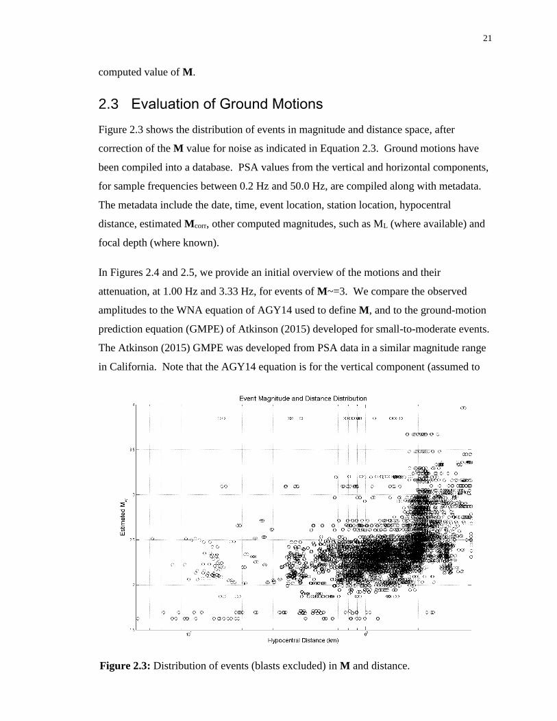
21

computed value of M.

2.3 Evaluation of Ground Motions

Figure 2.3 shows the distribution of events in magnitude and distance space, after

correction of the M value for noise as indicated in Equation 2.3. Ground motions have

been compiled into a database. PSA values from the vertical and horizontal components,

for sample frequencies between 0.2 Hz and 50.0 Hz, are compiled along with metadata.

The metadata include the date, time, event location, station location, hypocentral

distance, estimated Mcorr, other computed magnitudes, such as ML (where available) and

focal depth (where known).

In Figures 2.4 and 2.5, we provide an initial overview of the motions and their

attenuation, at 1.00 Hz and 3.33 Hz, for events of M~=3. We compare the observed

amplitudes to the WNA equation of AGY14 used to define M, and to the ground-motion

prediction equation (GMPE) of Atkinson (2015) developed for small-to-moderate events.

The Atkinson (2015) GMPE was developed from PSA data in a similar magnitude range

in California. Note that the AGY14 equation is for the vertical component (assumed to

Figure 2.3: Distribution of events (blasts excluded) in M and distance.

22

have negligible site response), while A15 is for the geometric mean of the horizontal

components, for B/C site conditions (near-surface shear-wave velocity of 760 m/s); all

three observed components are plotted. Overall, the motions are in qualitative agreement

with the expected amplitude and attenuation trends suggesting that overall the western

attenuation model is a reasonable first approximation. This is perhaps surprising, as we

might have expected a mixture of eastern and western attenuation types in this region, as

it is close to the deformation front. It could be that crustal complexity extends several

hundred kilometers east of the deformation front, such that the entire region is more

western than eastern in tectonic setting. We examine our first impressions in more detail

in the following.

Figure 2.4: PSA amplitudes (all components) at 1.00 Hz for events of M = 3.0 ±0.3,

as a function of hypocentral distance, compared to the relations of AGY14 (vertical

component) and A15 (horizontal component, B/C conditions).

23


function of hypocentral distance, compared to the relations of AGY14 (vertical

component) and A15 (horizontal component, B/C conditions).

To gain insight into the attenuation and magnitude-scaling features of the ground-motion

data, it is useful to evaluate the residuals relative to a reference prediction equation

(where the residual for an observation is defined as log10(PSAobs) – log10(PSApred)).

Trends in the differences between observations and predictions plotted versus distance

allow us to refine our model of attenuation with distance, whereas trends in magnitude

are informative for source scaling. A constant offset may reflect a combination of effects

including differences in source level (i.e., stress parameter) and site amplification. For

the predicted values, we use the A15 small-M empirical GMPE developed for California,

including the recommended additional c4 term to extend the GMPE to regional distances.

Thus, the reference prediction GMPE is given by (Atkinson, 2015):

𝑙𝑜𝑔(𝑃𝑆𝐴) = 𝑐0 + 𝑐1𝑴+ 𝑐2𝑴2 + 𝑐3 log(𝑅𝑒𝑓𝑓) + 𝑐4𝑅𝑒𝑓𝑓 (2.4)

24

where Reff is an effective point-source distance that includes near-source distance-

saturation effects using an effective depth parameter (Yenier and Atkinson, 2014):

𝑅𝑒𝑓𝑓 = √𝑅𝐻𝑦𝑝𝑜2 + ℎ𝑒𝑓𝑓

2 (2.5)

R is hypocentral distance and:

ℎ𝑒𝑓𝑓 = max (1, 10−1.72+0.43𝑴) (2.6)

Note that a minimum value of heff=1 km is specified; this is the value taken by Equation

(2.6) when M=4. This ensures the scaling of ground motions near the source approaches

a constant as the hypocenter (or fault plane) is approached. Figure 2.6 plots the PSA

residuals with respect to the A15 model, where the event magnitude is as calculated by

the AGY14 M estimation model described in the foregoing. To focus on higher-quality

data, we consider only events of M≥2.6. The site conditions are not well known and are

currently under investigation. However, all sites have posthole seismometers driven into

the surficial soil layer. The instruments are thus founded at the level of resistance for a

posthole auger. It is possible that this results in a relatively common site condition

among the stations, if the regional near-surface geology is not highly variable in nature.

If so, this would be a significant benefit to this installation method. In this study, we do

not attempt to subtract site effects from the observations, as they are so poorly known.

Rather, we use the comparisons between observations and prediction equations to infer

what site response terms might account for the observed residuals and evaluate whether

these are reasonable. For example, residuals for the vertical-component observations

with respect to A15 might be expected to be minimal, under the assumption that the

vertical component is a proxy for the unamplified horizontal-component motions (e.g.,

Lermo and Chavez Garcia, 1993; Ghofrani and Atkinson, 2014). By contrast, we might

expect significant positive residuals for the horizontal components as the instruments are

located within the soil layer (not on firmer B/C site conditions). What we see in Figure

2.6 is generally consistent with those expectations, with some exceptions. Overall, there

is no compelling evidence for significant deviations of the attenuation model from the

trends given in the A15 model. However, there are some deviations from a flat trend in

25

the attenuation residuals. Specifically, the 3.33Hz vertical-component PSA values have

Figure 2.6: PSA Residuals for M ≥2.6 for PSA at 1.00 Hz (top), 3.33 Hz (middle) and 10.0

Hz (lower), for horizontal (left) and vertical (right) components (blasts removed).

26

near-zero average residuals with respect to A15 at R>150 km but have negative residuals

at closer distances. By contrast, at 1.00 Hz the vertical-component residuals are near-

zero at R<150 km, but negative at larger distances. The 1.00 Hz horizontal PSA

residuals are generally positive, suggesting significant site amplification; the 3.33 Hz

horizontal PSA residuals are also largely positive, but more ambiguous at closer

distances. At 10.0 Hz, the residuals are negative at R<150 km on both components, but

positive on both components at R>150 km. This suggests that there may be significant

effects of noise on the spectral response and/or that a more complex attenuation model

may be warranted (perhaps a bilinear model with a change in geometric spreading at

R<100 km). These overall trends are shown more clearly in Figure 2.7, which plots the

mean and standard error of the residual data of Figure 2.6 binned by distance at 0.2 log10

units in width. Due to the paucity of near-distance data, the only truly compelling trends

Figure 2.7 Mean and standard error of PSA residuals for M ≥2.6 at 1.00 Hz (top), 3.33 Hz

(middle) and 10.0 Hz (lower), binned by log distance, for horizontal and vertical components

(no error bar plotted if the number of observations in the bin is <3). Slight offset from bin

center used for plotting clarity (to distinguish horizontal from vertical).

27

are the positive residuals at R>150 km on the horizontal component at 3.33 Hz, and on

both components at 10.0 Hz. The attenuation model will be refined as more observations

at close distances are obtained, enabling the trends to be more accurately defined.

If we subtract the terms in c3 and c4 of Equation 2.4 from the observed PSA for each

station, we can determine average source terms for each event; these are the amplitudes

that would be observed at near-source distances. Figure 2.8 plots these source terms

relative to the empirical A15 model. The expected magnitude scaling based on the point-

source simulation model of Yenier and Atkinson (2015a) for California is also shown

(shifted by the appropriate calibration constant so that it matches the level of A15 in the

M3 to 6 range where both are applicable); this model provides the expected scaling for a

Brune source model with a stress parameter of 100 bars. It is important to recognize that

both the Yenier and Atkinson (2015a) and A15 scaling were defined for events of M>3,

and thus both represent significant extrapolations to lower magnitudes on Figure 2.8. At

M>3, the empirical and point-source scaling are very close to each other, while the

extrapolated scaling at lower magnitudes shows some deviation between the two models.

Overall, the magnitude scaling of the source terms is very similar to that expected for a

100-bar point-source model. It should be acknowledged that for the 1.00 Hz scaling, it is

expected that it follows the point-source scaling of Yenier and Atkinson (2015a) for

events of M>3, as the event magnitudes have been determined from a similar point-

source model and thus there is some circularity. However, the scaling in the A15 model

is entirely empirical as derived from a different database (the NGA-West2 database).

Moreover, as frequency increases, the scaling will not be controlled by the estimated

moment magnitude but becomes more dependent on the stress parameter. At 3.33 Hz we

observe larger PSA in the horizontal channels than in the vertical channels suggesting a

common site response amongst the stations. At 10.0 Hz, the attenuation-corrected

ground motions are significantly higher than predicted equivalently in the horizontal and

vertical components. However, because of the attenuation trends noted at R<150 km

(Figures 2.6 and 2.7), it would be premature to draw conclusions regarding the overall

stress parameter from this observation. The scaling behavior with magnitude requires

further investigation after sufficient data is obtained to define the attenuation at closer

distances , allowing more robust source characterization.

28

Figure 2.8: Scaling of source terms with magnitude, in comparison to empirical (A15) and

simulation-based (Yenier and Atkinson, 2015a) models

In considering the source characteristics of the events, it should be noted that at

frequencies of 1.00 Hz and lower, PSA amplitudes are insensitive to stress parameter in

the magnitude range covered in this study. However, stress parameter becomes important

with increasing frequency, which is at least part of the reason why the scatter is broader

at 10.0 Hz in Figure 2.8 than at 1.00 Hz. It has been suggested that stress parameter may

be smaller for induced events than for natural events, leading to weaker ground motions

(Hough, 2014). This may be primarily a focal depth effect, as Yenier and Atkinson

(2015a, b) have shown that stress parameter increases with focal depth in both WNA and

Central and Eastern North America (CENA). Specifically, Yenier and Atkinson

(2015a,b) have found that average stress parameters for shallow events (<5 km) of M 3 to

5 are about 10 bars on average for WNA, and about 30 bars on average for CENA,

although there is much inter-event variability (factor>2). For events with depths of 10

km or greater, the average stress parameters are about 10 times higher than those for very

shallow events, in both regions. Thus, the focal depth effect on stress parameter may

29

overwhelm any differences due to an eastern or western tectonic setting. Furthermore, it

may be difficult to distinguish between focal depth effects and event type effects (natural

vs. induced) on stress parameter. Further studies with events covering a broader distance

range will be required to determine the average stress parameters in this region and to

resolve the influence that competing factors such as faulting mechanism, depth effects,

and near surface attenuation effects (κo) may have upon the stress parameter of events.

In Figure 2.9, we examine the average residual versus frequency in selected distance

ranges, for frequencies of 0.50 Hz and greater (noise issues are too severe at lower

frequencies). We can interpret Figure 2.9 as an average site response curve for the

stations, relative to the reference B/C condition of A15. However, it should be

Figure 2.9: Average PSA residuals versus frequency in distance ranges 10-120km, 120-250km,

250-400 km (left=vertical, right=horizontal). Average including all distances is also shown

(heavy line). Dashed line on right panel shows the average horizontal residual minus the average

vertical residual, which is similar to an average site response function.

30

acknowledged that this term also includes any net bias, whether or not it is attributable to

site conditions or other factors, such as overall source effects, noise issues, etc.

Specifically, it is likely that the large positive term at frequencies < 1.00 Hz and

frequencies > 10.0 Hz is largely driven by noise. Specifically, the PSA at frequencies f <

1.00 Hz is largely attributable to the oscillator response at the prominent 0.30 Hz

microseismic noise peak. Noise may also be responsible for the distance-dependence of

the average residual term, as it has a relatively larger contribution to amplitudes for the

weak motions observed on distant stations. Overall, it appears that the site response is

about 0.2 log10 units greater on the horizontal than the vertical component (factor of 1.6).

Moreover, there is a noticeable peak in the horizontal response curve at a frequency near

2 Hz that is not present on the vertical component. Finally, the trend to larger amplitudes

at high frequencies, relative to the predictions of A15, could reflect a combination of

noise and/or lesser near-surface attenuation (e.g. smaller value of the kappa parameter of

Anderson and Hough, 1984) relative to California sites.

To remove the influence of noise on the overall site response term in Figure 2.9, which

should be common on the vertical and horizontal components, we subtract the average

vertical-component response curve from the average horizontal-component response

curve. The resulting line (plotted in the right panel of Figure 2.9) is similar to an average

H/V ratio plot over all records. It suggests that the dominant feature of the response of

these sites is a peak in the frequency range from 2.00-5.00 Hz. This is in agreement with

preliminary results of H/V studies for sites in the region (Farrugia et al., 2015). The H/V

ratio is a well-known method for estimating the total amount of amplification a site will

experience during a seismic event, and in particular for determining the fundamental

frequency at that site (Lermo and Chavez Garcia, 1993; Ghofrani and Atkinson, 2014).

Preliminary H/V studies (Farraguia et al, 2015) suggest that the TransAlta network

stations all have very similar site responses, with a pronounced amplification in the 2 – 5

Hz frequency band on most stations that is consistent with expectations for relatively

shallow soft soil sites underlain by hard rock.

If we interpret the differences of residuals as site-response terms, we can infer the

amplification relative to the A15 reference condition of B/C by computing the average

31

residual at each station. As shown in Figure 2.10, the inferred site terms are relatively

consistent from one station to the next (consistent with the results of Farrugia et al. 2015).

This suggests that an overall typical site amplification curve, as given in Figure 2.9

(dashed line), may be a reasonable way to model site effects at the stations.

As more ground-motion observations are collected, we will be able to further resolve the

competing influences of source, attenuation and site factors on the observed ground

motions in this region. Ground motions observations at close distances, R<50 km, will

be particularly valuable, as will a larger number of events. A larger number of events

would facilitate the distinction between natural and induced events, and illuminate any

geographical effects related to the tectonic setting (location relative to the deformation

front). This will provide a baseline for evaluating whether the ground-motion attributes

of induced events differ significantly from those of natural earthquakes, and whether

these differences can be entirely attributed to focal depth effects.

Figure 2.10: Average station residuals for vertical and horizontal components of selected

frequencies, for events with M > 2.6 (blasts excluded).

32

2.4 Conclusions

This preliminary evaluation of ground motions in Alberta has determined that:

(i) The ground motions for small events in Alberta are generally consistent with

those for similar-sized events in California (as characterized by the AGY14 and A15

GMPEs) in terms of overall amplitude level and attenuation, but there are region-specific

features in the residuals that require further investigation with additional ground-motion

data;

(ii) The scaling characteristics of the Alberta events are generally consistent with

expectations based on both empirical (A15) and point-source simulation models (Yenier

and Atkinson, 2015a);

(iii) There appears to be significant site response on the horizontal component in the

2.00 to 5.00 Hz frequency range, which is relatively consistent among stations,

suggesting a common site response model for stations in Western Alberta.

2.5 Acknowledgements

This study was financially supported by the Natural Sciences and Engineering Research

Council of Canada and TransAlta. The constructive comments of Justin Rubinstein and

two anonymous referees are gratefully acknowledged.

2.6 References

Anderson, J. G., and Hough S. E. (1984). A model for the shape of the Fourier amplitude

spectrum of acceleration at high frequencies, Bull. Seismol. Soc. Am. 74, 1969

– 1993.

Assatourians, K., and Atkinson, G. M. (2010). Database of processed time series and

response spectra for Canada: An example application to study of the 2005 MN

5.4 Riviere du Loup, Quebec earthquake, Seismol. Res. Lett. 81, no. 6, 1013–

1031.

Atkinson G. M., (2015). Ground-motion prediction equation for small-to-moderate events

at short hypocentral distances, with application to induced seismicity hazards.

Bull. Seism. Soc. Am., 105(2A), 981-992. DOI: 10.1785/0120140142.

33


(M) for Small Events (M<4) on Local Networks. Seismol. Res. Lett., 85, 1116-

1124.

Baranova, V., Mustaqeem, A., and Bell, S. (1999). A model for induced seismicity

caused by hydrocarbon production in the western Canada sedimentary basin.

Can. J. Earth Sci., 36, 47-64.

Farrugia J. and G. M. Atkinson (2015). A Preliminary Evaluation of Site Amplification in

Alberta. Undergraduate Thesis, Western University, London Ontario, Canada.

Fereidoni, A. and G. M. Atkinson (2015). Identifying quarry blast events in seismicity

catalogs based on ground motion parameters. Canadian Geophysical Union

(CGU) Annual Meeting, Montreal, Canada, 3-7 May 2015.

Ghofrani, H. and G. M. Atkinson (2014). Site condition evaluation using horizontal-to-

vertical spectral ratios of earthquakes in the NGA-West2 and Japanese

databases. J. Soil Dyn. And Earthq. Eng., 67, 30-43.

Lermo J. and F. Chavez-Garcia (1993). Site effect evaluation using spectral ratios with

only one station. Bull. Seism. Soc. Am., 84, 1350-1364.

Gu, Y., A. Okeler, L. Shen and S. Contenti (2011). The Canadian Rockies and Alberta

Network (CRANE): New constraints on the Rockies and western Canada

sedimentary basin. Seism. Res. L., 82, 575-588.

Hough, S. (2014). Shaking from injection-induced earthquakes in the central and eastern

United States. Bull. Seism. Soc. Am., 104(5): 2619–2626

Doi:10.1785/0120140099.


Earthquake Records, Bulletin of the Seismological Society of America 59(2),

909-922.

Schultz, R., V. Stern and Y.Gu (2014). An investigation of seismicity clustered near the

Cordel Field, west central Alberta, and its relation to a nearby disposal well. J.

Geophys. Res., Solid Earth, 119, 3410-3423.

Schultz, R., V. Stern, M. Novakovic, G. M. Atkinson and Y. Gu (2015). Hydraulic

fracturing and the Crooked Lake sequences: Insights gleaned from regional

seismic networks. Geophys. Res. L., doi 10.1002/2015GL063455.

Stern, V., R. Schultz and G. Jean (2011). Alberta microseismicity project, Phase 1: Site

assessments for the ATSN semipermanent stations and the PSEIP Strachan

temporary seismic array. Energy Resources Conservation Board, ERCB/AGS

Open File Rpt. 2011-15, 75pp.

34

Yenier, E. and G. M. Atkinson (2015a). An Equivalent Point-Source Model for

Stochastic Simulation of Earthquake Ground Motions in California. Bull. Seism.

Soc. Am., 105(3), 1435-1455.

Yenier, E. and G. M. Atkinson (2015b). Regionally-adjustable generic Ground‐Motion

Prediction Equationbased on stochastic point-source simulations: Application to

Central and Eastern North America. Bull. Seism. Soc. Am., 105 (4): 1989-2009.

DOI: 10.1785/0120140332

35

Chapter 3

3 Empirically Calibrated Ground Motion Prediction Equation for Oklahoma

3.1 Introduction

More than 13,000 seismic events in the moment magnitude (M) range from 1 to 5.8 were

detected and located across the state of Oklahoma from January 1, 2010 to December 1,

2016. Prior to 2009, an annual average of 21 earthquakes of M≥3 was observed. Annual

seismicity rates of such events increased to ~100/year from 2009 to 2013, and by 2015

the annual rate had risen to ~1000 M≥3 (Peterson et al, 2016; see Data and Resources).

Most events are considered to have been induced by waste water injection, but it is not

within the scope of this study to attempt an event-by-event classification. Hundreds of

the events have been strongly felt, whilst the largest two earthquakes, the M5.7 Prague

and M5.8 Pawnee events, had reports of damage to infrastructure in nearby cities (e.g.

Ellsworth, 2013). A pre-requisite for assessing and mitigating the hazard posed by

induced earthquakes in Oklahoma is an understanding of the ground motions that they

produce. Ground-motion prediction equations (GMPEs), expressing peak ground motion

and response spectral amplitudes as functions of magnitude, distance and site condition,

are a valuable tool for characterizing ground motion in a format that is useful for seismic

hazard analysis (e.g. McGuire, 2004) and near-real-time ShakeMaps (e.g. Wald et al.,

1999).

In this study, a region-specific GMPE for Oklahoma (median horizontal component) is

developed using a compiled database of ~7278 ground motion observations, including

188 events of magnitude 3.5 to 5.8, over the hypocentral distance range from 2 km to 500

km. A generalized inversion is used to solve for regional source and attenuation

parameters and station site responses, within the context of an equivalent point-source

model, following the method of Atkinson et al. (2015) and Yenier and Atkinson

(2015a,b). The resolved parameters include the regional geometric spreading and

anelastic attenuation, source parameters for each event (e.g. moment magnitude and

stress parameter for a Brune point-source model), and site response terms for each station

36

relative to a reference site condition of NEHRP (Natural Earthquake Hazards Reduction

Program) B/C site class boundary (time-averaged shear-wave velocity in the upper 30 m,

VS30, of 760 m/s). The parameters fully specify a regionally-calibrated GMPE that can

be used to describe median horizontal-component amplitudes across the region for hazard

and ShakeMap applications, and to aid in the development of traffic light protocols and

other risk-mitigation tools. This GMPE is based on more ground-motion data than any

previous GMPEs for induced events in North America, and utilizes a methodology

designed to ensure appropriate scaling of motions over a wide range of magnitudes and

distances.

3.2 Database

Digital ground-motion records from thousands of events recorded on ~1200 regional

three-component broadband seismograph and accelerometer stations were obtained from

IRIS (Incorporated Research Institutes for Seismology), from publicly accessible

networks across Oklahoma, Texas, Arkansas, Colorado, Missouri and New Mexico (see

Data and Resources). The downloaded records were processed and compiled to produce

a ground-motion database of peak ground acceleration (PGA), peak ground velocity

(PGV), and 5%-damped pseudo-acceleration response spectra (PSA); PSA are sampled at

30 log-spaced frequencies from 0.20 to 50.0 Hz. For this study, we analyzed events of

M≥3.5 at hypocentral distances (Rhypo) from 2 km to 500 km; Figure 3.1 is a map of the

selected events and stations. The GMPE is based on the geometric mean of the

horizontal component ground-motion amplitudes, consistent with previous studies (e.g.

Yenier and Atkinson, 2015b). We note that the geometric mean is very similar to the

orientation-independent horizontal-component measure used in the Next Generation

Attenuation database (Boore, 2010), but more practical to calculate when doing batch

processing of large numbers of records.

The compilation and processing of the database from which the records were drawn

follows standard time-series analysis procedures. In brief, the records were windowed,

glitches and trends were removed, the time series were filtered from 0.10 to 50.0 Hz (4th

order Butterworth filter) and corrected for instrument response; the processing was done

using an updated version of the ICORRECT algorithm of Assatourians and Atkinson

37

(2010). The signal window of 300 seconds, from which response spectra are computed,

includes the P-wave, S-waves and strongest portions of the coda. This window length is

typical of that used to compute response spectra for earthquakes in the range of M 3.5 to

6 at regional distances (e.g. Assatourians and Atkinson, 2010). The length of the window

ensures that the entire signal is captured at all stations with automated batch processing.

Moreover, we verified that the response spectral amplitudes are not sensitive to the

selected window length, provided that the entire signal is captured. Acceleration time

series are generated from broadband seismograph records by differentiation in the

frequency domain prior to conversion back to the time domain. For the accelerometer

records, the digital time series are already correctly scaled in acceleration and can be

integrated to calculate velocity. The window length is long enough that it is possible that

more than one event may be captured during processing. This becomes increasingly

problematic when a large event is contained within the same ground motion window as a

smaller event. We filter our catalog by discarding smaller events that occur within 5

minutes of a large event. Due to the large number of records processed (~6,000,000 in

Figure 3.1 Study earthquakes (circles) and recording stations (light triangles).

Stations chosen as B/C reference sites are highlighted (dark triangles).

38

total), there was no visual inspection of records. Thus, it is inherent that contributions

from low-frequency microseismic noise within the selected passband will contribute to

some degree to the spectral amplitudes, especially for small magnitudes at larger

distances. However, as this ambient vibration is a real component of the signal, the PSA

amplitudes accurately reflect the corresponding oscillator response to the motions.

Moreover, we have limited the impact of such noise contributions through our record

selection criteria. Specifically, for events of M 3.5 we impose a cut-off distance of 150

km, with this cut-off distance growing steadily to 500 km for M ≥ 4. Figure 3.2 shows

the distribution of the selected database in magnitude and distance. PGA and PGV

values are computed from the absolute maximum amplitude of the corresponding time

Figure 3.2 The magnitude distance distribution of the database, containing 7278 records

from 194 earthquakes (M 3-5.8) recorded on 101 seismograph stations. We consider

records within logarithmically spaced bins with a cut-off distance that increases from 150

km for M = 3.5 to 500 km for M ≥ 4.0 events. The moment magnitude values (MNA15)

are determined as described in Figure 3.3.

39

series, whilst PSA amplitudes for the selected 30 frequencies from 0.20 Hz to 50.0 Hz are

calculated from the corrected acceleration time series using the Nigam and Jennings

(1969) algorithm. The selected database for analysis includes 188 events at 101 stations,

for a total of 7278 records.

3.3 Estimation of Moment Magnitude

We estimate moment magnitude for each event using a slight modification of the method

outlined in Novakovic and Atkinson (2015), which is based on spectral amplitude for the

low-frequency end of the spectrum:

where Equation (3.1) is evaluated using PSAF at three frequencies: 0.3, 1.00, and 3.33

Hz. The calibration factor MCF levels the equation whilst the anelastic attenuation

coefficient γF removes regional attenuation trends with distance. These parameters and

their values are adjusted for the Oklahoma region and are as listed in Table A3.1.

Density of network coverage in Oklahoma allows for the magnitude estimate to be

reliably computed from the recorded PSA at the five closest stations (distances < 50 km

in Oklahoma). The algorithm is based on the amplitudes recorded by the vertical-

component to minimize the effects of site response (Novakovic and Atkinson, 2015).

There are two modifications to the Novakovic and Atkinson (2015) algorithm. The first

is that we use an event-adjusted attenuation model to ensure that there will be no

significant distance dependence in the residuals, testing three alternative values for γF to

consider: low (e.g. Central and Eastern North America (CENA)), high (e.g. California) or

intermediate anelastic attenuation rates. The CENA and California values of the

attenuation coefficient are as given in Novakovic and Atkinson (2015), whilst the

intermediate model is the geometric mean of the two values. The attenuation rate that

minimizes the standard deviation of the residuals is selected for each event. CF is a fixed

frequency-dependent constant that matches the level of amplitudes and is not influenced

by the choice of attenuation rate. The second modification is that we calculate M at each

𝐌 =log10(PSAF)+MCF+1.3log10(Rℎ𝑦𝑝𝑜)+γFRℎ𝑦𝑝𝑜

1.45 (3.1)

40

of three frequencies (0.30 Hz, 1.00 Hz, and 3.33 Hz), allowing improved accuracy of

estimation according to the magnitude of the event. This is a matter of balancing the

opposing considerations of noise and corner frequency. Specifically, we need to use a

frequency that is low enough to be below the corner frequency for the event magnitude,

so that we are measuring the low-frequency end of the spectrum. On the other hand, low

frequencies are increasingly contaminated by microseismic noise, which is an important

consideration for small events.

Considering these factors, PSA at 0.30 Hz provides the best estimate for larger events

(M>4), whilst PSA at 3.33 Hz is a good choice for small events (M<3). For events of

intermediate magnitude, PSA at 1.00 Hz is the optimal choice. We take the estimated

magnitude from 3.33 Hz, 1.00 Hz, and 0.30 Hz PSA observations and use these values to

determine the best magnitude estimate according to magnitude range, as illustrated in

Initial Magnitude Estimates:M0.30Hz, M1.00Hz, M3.33Hz

for γLow, γMod, and γHigh

MF = min([std(MF,γLow ); std(MF,γMod); std(MF,γHigh)])

M1.00Hz < 3

M3.33Hz < 3

MEvent = M3.33Hz

3 ≤ M1.00Hz < 4

M3.33Hz ≥ 3 & M0.30Hz < 4

𝑴𝑬𝒗𝒆𝒏𝒕 = 𝑀1.00𝐻𝑧

M3.33Hz < 3 & M0.30Hz < 4

𝑴𝑬𝒗𝒆𝒏𝒕 =𝑴1.00𝐻𝑧 +𝑴3.33𝐻𝑧

𝟐

M3.33Hz ≥ 3 & M0.30Hz ≥ 4


𝟐

M1.00Hz ≥ 4

M0.30Hz ≥ 4

MEvent = M0.30Hz

Figure 3.3: The decision tree used to decide which frequency is used to estimate

moment magnitude (M) of the event. We compute MF based on PSA at 0.30 Hz, 1.00

Hz and 3.33 Hz. The M estimate from 3.33 Hz PSA is used for events of M < 3, 1.00

Hz estimate for M 3 - 4, and 0.30 Hz for M ≥ 4. For each event, the anelastic

attenuation coefficient that minimizes the residuals is chosen, where three values are

considered: low (CENA value), high (California value) or moderate (average of the

two).

41

Figure 3.4 (see also Novakovic and Atkinson, 2015). For example, if both M3.33 Hz < 3

and M1.00 Hz < 3, then this is a small event and we accept M3.33 Hz as the event magnitude.

If not, we proceed sequentially to consider the lower-frequency estimates of magnitude.

If M3.33 Hz < 3 and M1.00 Hz ≥3, we take the mean of these two calculations as the event

magnitude. If not, we check if M3.33 Hz ≥ 3, M1.00 Hz ≥ 3, and M0.30 Hz < 4, and so on as

shown in the decision tree of Figure 3.3. The resulting values of M are in close

agreement, being on average about 0.1 magnitude units less than those determined using

regional moment tensor solutions, as illustrated in Figure 3.4. We do not think this

discrepancy is significant, but readers should make note that the GMPE is based on

MNA15.

3.4 Ground-Motion Model

The descriptive variables for the GMPE are moment magnitude, hypocentral distance

(Rhypo), and station-specific site response. Following the approach of Atkinson et al.

(2015) we use a generalized inversion (Andrews, 1986) to solve for site response,

regional source and attenuation parameters of the generic form:

Figure 3.4: Comparison of MNA15 magnitude estimates with USGS/OGS reported

M as obtained from regional or global moment tensors. Squares show average

estimated M for events in 0.1 magnitude unit bins, along with standard deviation

(dashed lines). Mean deviation from other estimates is about -0.1 units.

42

ln(Y) = FE + Fz + Fs + Fγ + C (3.2)

where ln(Y) is the natural logarithm of PSA at a selected frequency. FE, Fz, Fs, and Fγ

are the earthquake source term, geometric spreading function, site response term, and the

anelastic attenuation term, respectively. Residual differences between simulations and

empirical data are accounted for by the empirical calibration factor, C. The terms are

each based on the generic GMPE of Yenier and Atkinson (2015b) and express the

components of a stochastic equivalent point-source model (e.g. Boore, 2003). The idea

of this formulation is that the basic scaling of the model in magnitude, distance and

frequency content is constrained to follow seismological scaling principles, but the

parameter values representing the Brune (1970, 1971) stress, attenuation and site

response are calibrated by regional observations. The components are summarized in the

following; see Yenier and Atkinson (2015b) for more details.

The effects of magnitude and stress parameter on ground-motion amplitudes are

described by the earthquake source function FE, adopted from the reference model

developed by Yenier and Atkinson (2015a), which was based on equivalent point-source

simulations calibrated to the Next Generation Attenuation (NGA)-East and NGA-West 2

databases. The implicit assumption is that the general magnitude-scaling characteristics

of ground motions are not region specific (e.g. Ambraseys & Douglas, 2004; Atkinson

and Morrison, 2009); this is a benefit to using this GMPE approach, as it ensures that a

model calibrated using data from moderate magnitudes will scale appropriately to larger

magnitudes. The source function is given as:

FE = FΔσ + FM (3.3)

For a specified reference stress (Δσ=100 bar), near-surface attenuation (κo=0.025), and

site condition (B/C), FM represents the magnitude effect on ground motion amplitudes

that would be observed at the source if there were no near-distance saturation effects.

The FM term is a hinged quadratic function of moment magnitude

𝐹𝑀 = {𝑒𝑜 + 𝑒1(𝑴−𝑀𝐻) + 𝑒2(𝑴 −𝑀𝐻)

2 𝑴 ≤ 𝑀𝐻

𝑒𝑜 + 𝑒3(𝑴 −𝑀𝐻) 𝑴 > 𝑀𝐻 (3.4)

43

where frequency dependent coefficients, e0 to e3, and the hinge magnitude MH were

determined by Yenier and Atkinson (2015b) using stochastic equivalent point-source

simulations. The stress adjustment term FΔσ is needed when Δσ is different than 100 bars

and is defined as

FΔσ = eΔσln(Δσ/100) (3.5)

where the rate of ground motion scaling with Δσ is described by eΔσ. Equation 3.5

provides the relationship between stress parameter and response spectral amplitudes

allowing the determination of Δσ from PSA observations. Its form is given by:

𝑒Δ𝜎 = {𝑠𝑜 + 𝑠1𝑴+ 𝑠2𝑴

2 + 𝑠3𝑴3 + 𝑠4𝑴

4 Δ𝜎 ≤ 100 𝑏𝑎𝑟

𝑠5 + 𝑠6𝑴+ 𝑠7𝑴2 + 𝑠8𝑴

3 + 𝑠9𝑴4 Δ𝜎 < 100 𝑏𝑎𝑟

(3.6)

where s0 to s9 are frequency dependent coefficients.

We use a trilinear geometric spreading function FZ. This is a modification to the bilinear

form used by Yenier and Atkinson (2015a,b) and Yenier et al. (2017). The modification

is made to accommodate a flat transition zone from direct-wave to surface-wave

spreading. The trilinear function better reflects the strong influence of the Moho

(Mohorivicic) bounce effects (Burger et al., 1987) that are observed in the region. The

Mohorivicic discontinuity varies in depth from 32 to 42 km in the northeastern and

central parts of Oklahoma and is as deep as 50 km towards the southwest (Taves, 2013).

Spatial variations of Moho depth in the region can explain the broad range over which

these bounce effects are observed; this will be seen clearly in the subsequent analyses and

figures. FZ is a function of Rhypo, M, and transition distances Rt:

𝑭𝒁 = ln(𝑍) + (𝑏3 + 𝑏4 ∗ 𝑴) ln (𝑅

𝑅𝑟𝑒𝑓) (3.7)

44

𝑅 = √𝑅ℎ𝑦𝑝𝑜2 + ℎ𝑒𝑓𝑓

2 ,

ℎ𝑒𝑓𝑓 = 10(−0.405+0.235𝑴),

𝑅𝑟𝑒𝑓 = √12 + ℎ𝑒𝑓𝑓2

𝒁 =

{

𝑅−1.3 𝑓𝑜𝑟 𝑅 ≤ 𝑅𝑡1

𝑅𝑡1−1.3 (

𝑅

𝑅𝑡1)−0.05

𝑓𝑜𝑟 𝑅𝑡1 < 𝑅 ≤ 𝑅𝑡2

𝑅𝑡1−1.3 (

𝑅𝑡2𝑅𝑡1)

−0.05

(𝑅

𝑅𝑡2)

−0.5

𝑓𝑜𝑟 𝑅𝑡2 < 𝑅

We assume Rhypo is equal to the closest distance to the fault rupture for the small to

moderate events of this study. The coefficient heff is the magnitude-dependent pseudo-

depth term introduced to account for close-distance saturation effects due to finite-fault

effects. An implicit assumption is that finite-fault effects in all regions will influence

near-distance saturation effects in a similar way (Yenier and Atkinson, 2014). The finite-

source model is employed to allow predictions from point-source models to mimic finite-

fault effects by placing the point at an equivalent overall distance, such that the closest

distance motions saturate appropriately (Atkinson and Silva, 2000; Boore, 2009; Yenier

and Atkinson, 2014). The saturation effect is a function of magnitude ensuring the

appropriate scaling of moderate to larger earthquakes (M3-7.5) near the source (Yenier

and Atkinson 2015). The coefficients b3 and b4 account for the change in apparent

attenuation that occurs when ground motions are modeled in the response spectral

domain rather than the Fourier domain (Yenier and Atkinson, 2015a).

To define the shape of the trilinear form, we first removed the estimated anelastic

attenuation coefficients for CENA, and the magnitude scaling assuming a stress

parameter of 100 bars, all as given in Yenier and Atkinson (2015b). At each frequency

45

we plotted the residual ground motion trends against hypocentral distance. We then

chose the model parameters that broadly match the shape across all frequencies. This

suggested that a trilinear geometric spreading function was required, with slopes -1.3, -

0.05 and - 0.5, and transition distances of 45 km and 200 km for Rt1 and Rt2, respectively.

Figure 3.5 depicts the adopted trilinear model shape in comparison to normalized PSA

values, where the PSA values are normalized by removing the magnitude scaling and

anelastic attenuation terms (e.g. Eqns 3.4 and 3.8). A value of 100 bars is assumed in

calculation of the magnitude-scaling term for the normalization. We have adopted a

frequency-independent geometric spreading model, with all frequency-dependent effects


dependence (FM, Eqn 3.4) and CENA anelastic attenuation (Eqn 3.8); squares show

median normalized amplitudes in distance bins. Solid lines show the adopted trilinear

geometric spreading function (which has magnitude dependence as in YA15), for a

range of magnitudes, assuming a 100-bar stress parameter; only the shape is important,

as the level is determined by inversion. A constant is added to all ground motions to

adjust the level of the geometric spreading function for better visualization.

46

being carried by the anelastic attenuation coefficients. This modeling choice is consistent

with nearly all previous stochastic models of ground motion (e.g. see Yenier and

Atkinson, 2015a/b; Boore, 2003; Atkinson and Boore, 2006). We acknowledge that this

conceptually-simple model may not be entirely accurate, but it strikes a reasonable

balance between modeling the most important effects whilst maintaining simplicity and

appears to allow a reasonable approximation to the observed shapes of the amplitude

decay function as seen on Figure 3.5.

With the geometric spreading model constrained, all remaining coefficients can be

determined by inversion, as in Atkinson et al. (2015). We determine the regional

anelastic attenuation function Fγ in the inversion process:

Fγ = γRhypo (3.8)

where γ is a frequency-dependent anelastic attenuation coefficient. Yenier and Atkinson

(2015b) determined γ values for CENA and for California using the NGA-East and

NGA-West 2 databases, respectively. In this study, we determine the anelastic

coefficient for each frequency from the Oklahoma database in the inversion.

The station terms FS are expressed relative to a reference NEHRP site condition. Stations

location on B/C sites with time-averaged shear-wave velocity in the top 30 m (Vs30) of

~760 m/s are chosen as the reference sites, with respect to which all other site responses

will be determined. Four stations on sandstone or shale with Vs30 ~ 760 m/s are selected

as reference sites: OK029, OK030, OK031, and OK005 (highlighted on Figure 3.1).

Their selection was guided by a combination of surficial geology information (USGS

National Geologic Map Database) and Vs30 studies (EPRI, 2013a, see Data and

Resources). The reference sites have well-behaved horizontal-to-vertical component

ratios that are broadly similar to each other and consistent with those expected for B/C

sites based on other studies (e.g. Ghofrani and Atkinson, 2014). We assume that the

average site amplification over these stations at each frequency is zero. This constraint,

when applied in the inversion, calibrates the GMPE for an average B/C site condition,

provided these are typical B/C sites. Thus, all site terms will be relative to the average

47

site amplification for the six reference sites. Note that any differences between the actual

amplification of the six sites (on average) and that assumed for B/C sites in the

underlying generic GMPE of Yenier and Atkinson (2015b), will be cast into the

calibration constant (C) by the inversion.

3.5 Application to Induced Events in Oklahoma

The database for the inversion to Equation (3.2) contains 7278 records from 188 M ≥ 3.5

events at 101 stations, as shown in Figure 3.2. The record set was further filtered to

ensure that each analyzed event is recorded on at least five stations, and that each station

records at least 15 events. This allows robust determination of source, site and event

terms. We take the geometric mean of the two horizontal-component PSA values in units

of g, for 30 logarithmically spaced frequencies from 0.20 Hz to 50.0 Hz, PGA, and PGV.

To facilitate inversion, the fixed geometric spreading function and magnitude

scaling terms from Equation (3.2) are subtracted from the observed ground motion

values:

ln(Yij) – FM,i – FZ,i j = Ei + FS,j + γRhypo ij (3.9)

where Yi,j is the ground-motion parameter for event i and station j. FM,i, FZ,i j, are the

magnitude scaling term and geometric spreading term for event i and station j , as

calculated given the known M and distance Rhypo ij. Note that the stress parameter

function (FΔσ) and the empirical calibration factor (C) are implicitly included in the event

term, Ei. FS,j is the site amplification term relative to the reference B/C site condition at

station j. γ is the regional anelastic attenuation term.

The unknown terms in Equation (3.9) are obtained, for PSA values at 30 equally

logarithmically spaced frequencies from 0.20 Hz to 50.0 Hz, PGA, and PGV, using the

generalized inversion scheme of Andrews (1986). Figure 3.6 shows the resulting

anelastic attenuation term as a function of frequency. These values indicate weaker

attenuation in comparison to previous studies for CENA at frequencies greater than 2.00

48

Hz; at lower frequencies the attenuation in Oklahoma appears to be stronger than what is

typically observed in CENA, but less than that observed in California.

The site amplification term (FS,j) is obtained for each of the 101 stations, relative to the

assumed reference site condition of B/C, as represented by the average over the six

selected reference sites. These site amplification terms can be subtracted from the

observations to level all records to the same reference site condition. The site

amplification terms for all stations are given in Table S3.1, available in the electronic

supplement. Figure 3.7 shows the site amplification functions for the reference stations.

Note that by definition the average of these six functions is zero (in ln units) as a

condition applied as an inversion constraint. Figure 3.8 plots a sample of typical site

response functions for non-reference stations, most of which are softer than B/C. As

expected, the peak amplifications for softer sites are significantly larger than those for the

reference sites, often exceeding a factor of four at some frequencies. Figure 3.9 plots all

site response functions retrieved from the inversion along with their mean and standard

deviation. It is interesting that the average over all sites is near zero, as this is not

necessarily expected. The regression is constrained such that the mean amplification of

the reference B/C stations should be zero, but there is no such constraint on the average

Figure 3.6: Regional anelastic attenuation term for Oklahoma with standard deviation,

in comparison to previous results of Yenier and Atkinson (2015b) for California and

CENA.

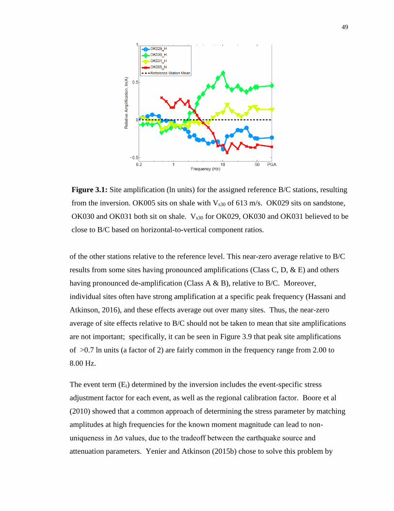
49

of the other stations relative to the reference level. This near-zero average relative to B/C

results from some sites having pronounced amplifications (Class C, D, & E) and others

having pronounced de-amplification (Class A & B), relative to B/C. Moreover,

individual sites often have strong amplification at a specific peak frequency (Hassani and

Atkinson, 2016), and these effects average out over many sites. Thus, the near-zero

average of site effects relative to B/C should not be taken to mean that site amplifications

are not important; specifically, it can be seen in Figure 3.9 that peak site amplifications

of >0.7 ln units (a factor of 2) are fairly common in the frequency range from 2.00 to

8.00 Hz.

The event term (Ei) determined by the inversion includes the event-specific stress

adjustment factor for each event, as well as the regional calibration factor. Boore et al

(2010) showed that a common approach of determining the stress parameter by matching

amplitudes at high frequencies for the known moment magnitude can lead to non-

uniqueness in Δσ values, due to the tradeoff between the earthquake source and

attenuation parameters. Yenier and Atkinson (2015b) chose to solve this problem by

Figure 3.1: Site amplification (ln units) for the assigned reference B/C stations, resulting

from the inversion. OK005 sits on shale with Vs30 of 613 m/s. OK029 sits on sandstone,

OK030 and OK031 both sit on shale. Vs30 for OK029, OK030 and OK031 believed to be

close to B/C based on horizontal-to-vertical component ratios.

50

basing the stress parameter value on the corner frequency (spectral shape), and by using a

calibration constant to reconcile the overall spectral amplitude levels. In this study, we

took an approach that is similar to that of Yenier and Atkinson (2015b), but results in a

more stable determination of the stress parameter for cases where the source spectrum

does not nicely follow the ideal Brune-model spectral shape. We base the determination

of the stress parameter on the event’s average high-frequency spectral level, as

represented by PSA at 10.0 Hz, relative to that expected based on the seismic moment

(implicitly including any offset in amplitude level at the moment-end of the spectrum).

To avoid complications of near-distance saturation effects, the event spectrum for this

purpose is evaluated at a reference distance of 20 km, using the attenuation function from

the inversion to correct observations to the reference distance of 20 km (and then

averaging over all stations for each event). Figure 3.10 is a graphical illustration of the

Figure 3.2: Typical site amplifications (ln units) for stations resulting from the

inversion. WHAR is a sandstone station with Vs30 of 1403 m/s. WMOK is a station

sitting on granite with Vs30 1859 m/s. OK009 is a station sitting on conglomerate with

Vs30 of 322 m/s. No Vs30 information is available for WLAR, OK032, KAN10 and

HHAR; however according to surficial lithology maps, these stations sit on sandstone,

alluvium, gravel and limestone respectively

51

approach taken. We use the average event spectrum at 20 km to first find the offset of

the long-period SD (spectral displacement) level at 1.00 Hz from that expected for the

given seismic moment for the event, in ln units (∆LF), for an ideal 100-bar Brune model

spectrum, as defined by Yenier and Atkinson (2015b). We remove the ∆LF offset from

the average event spectrum, so that it now matches the level for an ideal Brune spectrum

of that moment magnitude, at low frequencies. The amount by which the 10.0 Hz-PSA

value of this amplitude-corrected spectrum differs from that expected for a 100-bar

Brune-model spectrum is taken as a measure of the stress parameter. Higher values of

stress result in larger values of 10.0 Hz-PSA, relative to the 100-bar model, whereas

lower stress results in lower 10.0 Hz-PSA values. Note this is similar to the shape-based

approach of Yenier and Atkinson (2015b) but focuses on the high-frequency spectral

level relative to the low-frequency level, instead of focusing on the corner frequency.

Figure 3.3 All station terms. The lines depict the site response relative to B/C

condition for all stations used in the study in natural log units. Squares depict the

mean site term for each frequency, with their standard deviations in dashed lines.

52

Figure 3.4: Determination of stress parameter, for M5.8 Pawnee event. Left) ∆LF (low-

frequency offset) is determined as the offset of the average of observed spectral

displacement (SD) on the seismic moment end of the specturm (1.00 Hz) relative to

predicted SD from YA15 (corrected for site and attenuation effects to a reference

distance of 20 km). Right) ∆HF (high-frequency offset) is determined from the level of

the 10.0 Hz PSA, after shifting spectrum by ∆LF. Note that the spectra in this figure

have been converted from units of g to cm/s2.

For ease of application in implementing this approach, the generic GMPE of Yenier and

Atkinson (2015b) was evaluated at 20 km for multiple combinations of magnitude and

stress parameter, and used to define the relationship between 10.0 Hz PSA and stress

parameter:

𝑙𝑜𝑔10( ∆𝜎) = 2.024 + 1.52(log10 ( 𝑃𝑆𝐴10 𝐻𝑧,𝑒𝑣𝑒𝑛𝑡) − (𝑙𝑜𝑔10(𝑃𝑆𝐴10 𝐻𝑧,100𝑏𝑎𝑟) +

∆𝐿𝐹 )) ∗ max (1,1.3 (3.5

𝑴)) (3.10)

53

where PSA10 Hz,event is the average 10.0 Hz PSA value for the event, adjusting for site and

path effects to the reference distance of 20 km, and PSA10Hz,100bar is the corresponding

10.0 Hz PSA that is predicted for a Brune stress parameter of 100 bar at 20 km. This

parameterization makes it easy to back-calculate the stress parameter from the 10 Hz

value of the event spectrum at 20 km. The basic idea is that we are using the high-

frequency spectral level to infer the corner frequency, instead of using the corner

frequency to infer the high frequency level (as was done in Yenier and Atkinson 2015b).

We took this approach because we determined it was more stable, leading to a lower

standard deviation of determined stress parameters.

Figure 3.5: Stress parameters for individual events (circles), compared with a with

simple bilinear fit to the stress parameter versus magnitude (upper as a dashed line) and a

simple fit to the stress parameter with respect to focal depth (lower as a solid line).

54

Stress parameter values for all events are given in Table S3.2 of the electronic

supplement; a summary of stress parameters for events of M > 4.2 is provided in Table

A3.2. The stress parameter increases with magnitude for small shallow events, as

observed in previous studies for CENA events, and their values fall within the expected

range (Yenier and Atkinson 2015b). Stress parameter values typically range from 40 to

500 bars and are observed for events of M>4. We note that the catalog depths for the

events (Table S3.2) are predominantly in the range from 3 to 8 km; this table reflects

updated location and depth estimates from the double-difference relocation results from

Schoenball and Ellsworth (2017) where available. More than 140 events in this study

had depths that were double difference relocated and have uncertainties from 0.3 to 1 km

in the vertical direction (Schoenball and Ellsworth, 2017). We plot stress parameter as a

function of magnitude and depth in Figure 3.11; it is apparent that trends in both variables

are present, though the trends in depth are not well-resolved due to the

Figure 3.6 Stress parameters determined by inversion for each event (Figure 3.8)

(circles) as a function of moment magnitude (MNA15) and depth (larger circles denote

greater depth). Solid lines show models that capture the observed trends in the Oklahoma

data, in comparison to YA15 CENA model (dashed lines) for several values of focal

depth.

55

limited depth range of the data. A multivariable regression is performed to develop a

regional stress model as a function of magnitude and depth using relocated events only.

Figure 3.12 shows the proposed stress parameter model for induced events in this region:

ln (∆σ) = 5.65 + min[0, 0.097(d - 10)] + min[0, 1.329(M –5.1)] (3.11)

It has been suggested that stress increases with focal depth, and that this is the primary

reason why induced events typically have a lower stress parameter than do natural

tectonic earthquakes (e.g. Yenier and Atkinson, 2015b; Atkinson and Assatourians,

2017). The depth trends observed in Oklahoma appear to be weak but are not well-

resolved because all events are relatively shallow; by contrast, there is a strong magnitude

scaling, resulting from large high-frequency spectral amplitudes for the largest Oklahoma

events. It has also been suggested that events in Central North America may have lower

stress than those in Eastern North America, due to differences in focal mechanism

(Huang et al., 2017; Cramer, 2017).

The regional calibration factor (C) can be determined as the average residual mismatch

between the observations and the model (after considering the stress parameter for each

event, the site term for each station, and the regional geometric spreading and anelastic

attenuation functions). As discussed in Yenier and Atkinson (2015a) the calibration factor

reflects the average differences between the observations and the simulations, including

any systematic factors that are not accurate or not included in the modeling approach.

Examples of such factors include any residual regional site amplification effects relative

to the assumed amplification model for B/C that was included in the Yenier and Atkinson

(2015b) formulation, and any surface wave or other contributions to the motion that were

not included in the Brune source model. Removing the resolved parameters from the

inversion from the ground motion observations, Equation 3.9 becomes

ln(Yi j) – FM,i – FZ,i j – γABRi j – FΔσ – FS,j = COK + ηi + εi j (3.12)

where COK is the regional calibration factor for Oklahoma, ηi is the between-event error,

and εij is the within-event error. Following Abrahamson and Youngs (1992), we use a

mixed effects regression of residuals to solve Equation 3.12. An iterative regression is

56

performed to maximize the likelihood of the model and estimate the regional calibration

factor (COK). The residual error of the observations with respect to the model is separated

into its between-event and within event components (ηi and εij). The regional calibration

factor for Oklahoma is shown in Figure 3.13 and is summarized in Table A3.3 along with

the determined error components. A full list of model parameters, calibration factor, and

error components at all frequencies are given in Table S3.3 of the electronic supplement.

At frequencies < 1.2 Hz we observe a positive average residual of 0.43 ln units. This

might be explained by inherent limitations of stochastic methods at low frequencies,

which do not allow surface wave phases or coherent pulses to be properly modeled.

Figure 3.7: Calibration factor (COK) obtained from inversion (squares) and its standard

deviation (jagged lines). The solid line shows suggested model function for COK, the

Yenier and Atkinson (2015b) calibration factor for CENA is shown as a dot-dashed line,

and its modeled form is shown as a dashed line.

57

The calibration factor dips to -0.5 ln units between 1.2 Hz and 10.0 Hz then recovers to a

near-zero value at high frequencies. The calibration factor follows the average trends

given by:

𝐶𝑂𝐾 = {

0.45 𝑓𝑜𝑟 𝑓 < 0.7 𝐻𝑧

1.54(log10(𝑓))2 − 1.69(log10(𝑓)) + 0.15 𝑓𝑜𝑟 0.7 𝐻𝑧 ≤ 𝑓 < 11.3 𝐻𝑧

0.08 𝑓𝑜𝑟 𝑓 ≥ 11.3 𝐻𝑧 (3.13)

The shape of the calibration function at intermediate frequencies reflect deviations from

the regional site response model assumed for the reference B/C condition. The generic

GMPE form upon which this study is based has embedded within it a prescribed average

amplification function for B/C conditions, which was derived from an assumed model

(Atkinson and Boore, 2006). Any differences between the average amplification factors

for B/C sites in Oklahoma and those in the assumed embedded model will map into the

calibration factor. As shown in Figure 3.14, we can interpret the inverse of the

calibration factor as the amplification of the six reference sites (on average), relative to

the assumed amplification function for B/C (Seyhan et al., 2014). By this logic, we may

infer that the reference sites have an amplification that is slightly larger than that assumed

by Yenier and Atkinson (2015b) for B/C sites, and more peaked at intermediate

frequencies. An alternative explanation for the dip in the calibration constant at

intermediate frequencies could be that the shape of the assumed Brune source model is

not well-followed on average.

The final Oklahoma GMPE includes the assumed magnitude scaling, geometric

spreading functions and anelastic attenuation terms, the derived model for the stress

parameter, the site amplification terms, and the empirical calibration factor, and is

described as:

ln(Yij) = FM + FΔσ,OK + FZ + Fγ + FS + COK (3.14)

58

where the coefficients for all terms are summarized in Table A3.3 and fully listed in

Table S3.3 of the electronic supplement. The error terms (ηi and εij) are normally

distributed in natural logarithmic units and have standard deviations of τ and φ

respectively. The combined ground motion variability resulting from event-specific

factors, such as the randomness in the source process, that have not been included in the

predictive model can be expressed by the between-event variability, τ. Record specific

factors such as the randomness in the site amplification for a given site class, or

azimuthal directivity effects that are not considered are mapped into the within event

variability, φ. The between-event and within-event variability have similar levels, though

the between-event variability is generally lower; which is a common feature of empirical

Figure 3.8 The Oklahoma calibration factor (gray line) and its inverse (black line),

in comparison to the site amplification functions of Seyhan and Stewart (2014;

SS14) for California, for a range of VS30 values (lines with symbols). It should be

noted that the site amplification function is at a constant level for Vs30 greater than

1500 m/s.

59

GMPE derivation (Strasser et al., 2009). The total standard deviation (σ) of equation

3.14 can be described as

𝜎 = √𝜏2 + 𝜑2 (3.15)

where the value of sigma is typically in the range of 0.57 to 0.69 natural logarithmic

units. Figure 3.15 shows between event residuals as a function of depth binned by

magnitude. In Figures 3.16 through 3.19 we plot the within-event residuals (Residual =

ln(PSAObseration) - ln(PSAPredicted)) for the horizontal-component (geometric mean) PSA at

1.01 Hz, 5.12 Hz, 10.2 Hz, and PGA as a function of hypocentral distance, binned by

magnitude. There are no significant trends in the residuals in magnitude or distance for

hypocentral distances greater than 10 km; at closer distances, there is a tendency towards

slightly positive residuals at some frequencies, and slightly negative at others. Figure

3.20 demonstrates the final GMPE (for PSA at 5 Hz), overlaying site-corrected

observations. As expected from the residual plots, observations fit well to the GMPE.

Figure 3.15: Between-event residuals η, where dark (pink) circles show M < 4, light

circles (green) show M ≥ 4, and squares show the depth bin mean ± σ.

60

In Figure 3.21, we compare the GMPE for induced events in Oklahoma, at selected

frequencies, to the CENA GMPE of Yenier and Atkinson (2015b) for earthquakes at

shallow depths of 5, 6, and 8 km (the typical earthquake depths in Oklahoma), for events

of M 4, 5, and 6, respectively. The GMPE of Atkinson (2015), which was derived from

moderate events with an average depth of 9 km in California (NGA-West2 database), but

postulated to apply for induced events in CENA, is also shown. The trilinear geometric

spreading function used in this study results in higher predicted ground motions at larger

hypocentral distances in comparison to the Yenier and Atkinson (2015b) or Atkinson

(2015) model. At high frequencies (f > 3 Hz), the amplitudes for relatively small events

(M~=4) in the GMPE from this study are similar to those of previous studies (e.g. Yenier

and Atkinson, 2015b). At lower frequencies, Oklahoma amplitudes tend to be higher,

likely reflecting amplification effects due to regional geology. For events of M 5 to 6,

Oklahoma amplitudes tend to be larger than those in the Yenier and Atkinson (2015b)

model, reflecting the differences in magnitude and depth dependence of the stress

parameter.

Figure 3.9 Within event residuals with respect to the final GMPE for PSA at 1.01 Hz.

Black squares depict the mean residual and its standard deviation in logarithmically

spaced distance bins.

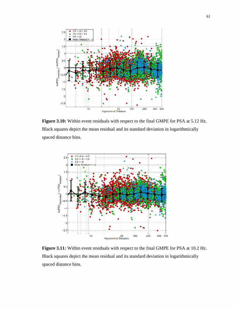
61







62

Figure 3.12: Within event residuals with respect to the final GMPE for PGA. Black

squares depict the mean residual and its standard deviation in logarithmically spaced

distance bins.

Figure 3.20: Final GMPE overlaying site corrected observations at 5.12 Hz. Lines depict

the GMPE evaluated every 0.2 magnitude units from M = 4.1 to M = 5.9 at linearly-

increasing depths ranging from 3 to 8 km, respectively. Circles vary in diameter where

larger circles represent larger magnitude observations and smaller circles denote smaller

magnitude event observations.

63

Figure 3.13 The GMPE for Oklahoma as determined in this study (solid lines) in

comparison to the YA15 GMPE for CENA (dashed lines); both GMPEs are evaluated for

focal depths of 5, 6, and 8 km for M = 4, 5, and 6, respectively. The GMPE of Atkinson

(2015), as determined from moderate California earthquakes with mean depth of 9 km, is

also indicated (dotted lines), and is extrapolated for distances > 50 km. All models are

for NEHERP B/C reference site conditions.

3.6 Conclusions

We derived a regionally-adjusted GMPE for induced events in Oklahoma (geometric

mean of horizontal components), for a reference site condition of B/C. We used the

generic GMPE framework of Yenier and Atkinson (2015b) to ensure stable scaling of

motions over all magnitudes and distances. The generic GMPE was calibrated by

determining an anelastic attenuation function, site amplification models, regional stress

parameter model, and calibration factor from >7000 ground motion observations from

64

Oklahoma events of M ≥ 3.5 at hypocentral distances from 2 to 500 km. The derived

GMPE is useful for hazard assessments and ShakeMap applications and may also be

useful for ground motion-based alerting systems and traffic light protocols.

3.7 Data and Resources

Shear wave velocities, Vs30, used to determine B/C reference stations from the EPRI

Ground-Motion Model Review Project: Shear Wave Velocity Measurements at Seismic

Recording Stations (2013a) was accessed from

https://www.epri.com/#/pages/product/3002000719/ (accessed November 2016).

Surficial geology also used as a proxy method to select B/C reference stations were found

in the USGS National Geologic Map Database at https://mrdata.usgs.gov/geology/state/

(accessed November 2016). Statistics of seismicity rate increases in Oklahoma from the

one-year seismic hazard forecast for the Central and Eastern United States from induced

and natural earthquakes, Peterson et al 2016, USGS Open-File Report 2016-1035, from

https://pubs.er.usgs.gov/publication/70182572 (accessed November 2016). The facilities

of Incorporated Research Institutes for Seismology (IRIS, www.iris.edu, last accessed

Oct. 2017) Data Services, and specifically the IRIS Data Management Center, were used

for access to waveforms, related metadata, and/or derived products used in this study.

IRIS Data Services are funded through the Seismological Facilities for the Advancement

of Geoscience and EarthScope (SAGE) Proposal of the National Science Foundation

under Cooperative Agreement EAR-1261681. Ground motion data were downloaded

from IRIS then were processed and compiled using an updated version of the

ICORRECT algorithm, as described in Assatourians and Atkinson (2017). Careful

consideration is being taken as we decide how to partition and organize the near 6.8

million record ground motion database in a useful and meaningful way. The database of

processed ground motion observations, event/station metadata, and M estimates for each

event will become fully available online in the near future.


This study was funded by the Natural Sciences and Engineering Research Council of

Canada and TransAlta. Funding was also received from the U.S. Geological Survey

65

under Grant G16AP00107. We thank Behzad Hassani for his valuable input on the

regression procedure. We thank our anonymous reviewers and Dr. Thomas Pratt for their

constructive comments.

3.9 References

Abrahamson, N. A., and R. R. Youngs. (1992). A stable algorithm for regression analysis

using the random effects model, Bull. Seismol. Soc. Am. 82(1), 505–510.

Ambraseys, N. N., & Douglas, J. (2004). Magnitude calibration of north Indian

earthquakes. Geophysical Journal International, 159(1), 165-206. DOI:

10.1111/j.1365-246X.2004.02323.x

Andrews, J. (1986). Objective determination of source parameters and similarity of

earthquakes of different size, Earthquake Source Mechanics, American

Geophysical Union, Geophysical Monograph, Vol. 37, 259-267.



5.4 Riviere du Loup, Quebec earthquake, Seismol. Res. Lett. 81, no. 6, 1013–

1031.

Assatourians, K., and Atkinson, G. M. (2017). Are Ground-Motion Models Derived from

Natural Events Applicable to the Estimation of Expected Motions for Induced

Earthquakes? Seism. Res. Lett. DOI: 10.1785/0220160153.

Atkinson, G. M. and Boore, D. M. (2006). Earthquake ground-motion prediction

equations for eastern North America, Bull. Seism. Soc. Am. 85, 17-30.

Atkinson, G. M., Hassani, B., Singh, A., Yenier, E. and Assatourians, K. (2015).

Estimation of Moment Magnitude and Stress Parameter from ShakeMap

Ground-Motion Parameters. Bull. Seismol. Soc. Am.105(5), 2572-2588.

Atkinson, G. M., and Morrison, M. (2009). Regional variability in ground motion

amplitudes along the west coast of North America, Bull. Seismol. Soc. Am.,

99, 2393–2409.

Atkinson, G. M., and Silva, W. (2000). Stochastic modeling of California ground

motions. Bull. Seismol. Soc. Am. 90, 255-274.

Boore, D. M. (2003). Simulation of ground motion using the stochastic method, Pure and

Applied Geophysics 160, 635-675.

Boore, D. M. (2009). Comparing stochastic point-source and finite-source ground motion

simulations: SMSIM and EXSIM. Bull. Seismol. Soc. Am. 99, 3202-3216.

66

Boore, D. M. (2010). Orientation-Independent, Nongeometric-Mean Measures of Seismic

Intensity from Two Horizontal Components of Motion. Bull. Seism. Soc. Am.

100, 1830-1835.

Boore, D. M., Campbell, K. W., and Atkinson, G. M. (2010). Determination of stress

parameters for eight well-recorded earthquakes in eastern North America.

Bull. Seism. Soc. Am. 100, 1632-1645.


earthquakes. J. Geophysics. Res. 75(26), 4997-5009.

Brune, J. N. (1971). Correction: Tectonic stress and the spectra of seismic shear waves,

J. Geophysics. Res. 76(20), 5002.

Burger, R. W., P.G. Somerville, J.S. Barker, R.B. Herrmann, and D.V. Helmberger

(1987). The effect of Crustal structure on strong ground motion attenuation

relations in eastern North America. Bull. Seisin. Soc. Am. 77, 420-439, 1987.

Cramer, C. (2017). Brune Stress Parameter Estimates for the 2016 Mw Pawnee and Other

Oklahoma Earthquakes. Seismological Research Letters, 88(4):1005-1016.

Ellsworth, W. L. (2013). Injection-induced earthquakes. Science. 341(6142), 7.

doi:10.1126/science.1225942

Ghofrani, H. and Atkinson G. M. (2014). Site Condition Evaluation Using Horizontal-to-

Vertical Response Spectral Ratios of Earthquakes in the NGA-West2 and

Japanese Databases. Soil Dynamics and Earthquake Engineering.67, 30-43.


Eastern North America, Seismol. Res. Lett. 86(2A), 477-491.

Hassani, B. and Atkinson, G. M. (2016). Site-effects model for central and eastern North

America based on peak frequency. Bull. Seism. Soc. Am., 106, 2197-2213.

Huang, Y., Ellsworth, W. L., and Beroza, G. C. (2017). Stress drops of induced and

tectonic earthquakes in the central United States are indistinguishable. Science

Advances 3(8), e1700772.

McGuire, R. K. (2004). Seismic Hazard and Risk Analysis, Earthquake Engineering

Research Institute. Aug 1, 2004.


Earthquake Records, Bulletin of the Seismological Society of America. 59(2),

909-922.

67

Novakovic & Atkinson (2015), Preliminary Evaluation of Ground Motions from

Earthquakes in Alberta. Seismol. Res. Lett., 86(4), 1086-1095.

Petersen, et al. (2016). USGS Open-File Report 2016-1035,

https://pubs.er.usgs.gov/publication/70182572 (Last accessed November

2016).

Schoenball, M., Ellsworth, W.L., (2017). Waveform relocated earthquake catalog for 4

Oklahoma and Southern Kansas illuminates the regional fault network.

Seismological Research Letters, 88(5), 1252-1258.

Seyhan, E. and Stewart, J. (2014). Semi-Empirical Nonlinear Site Amplification from

NGA-West2 Data and Simulations. Earthq. Spectra. 30(3), 1241-1256.

Strasser, F. O., Abrahamson, N. A., and Bommer, J. J., (2009), Sigma: Issues, Insights,

and Challenges. Seismological Research Letters 80 (1): 40-56.

Taves, M. A. (2013). Imaging of the crust and Moho beneath Oklahoma using receiver

functions and Pn tomography; With emphasis on the Southern Oklahoma

aulacogen. Texas Tech University, 2013. https://ttu-ir.tdl.org/ttu-

ir/bitstream/handle/2346/48853/TAVE-

THESIS.pdf?sequence=1&isAllowed=y, accessed March 15, 2018.

Wald, D. J., Quitoriano V., Heaton T. H., Kanamori H., Scrivner C. W., Worden C. B.

(1999). TriNet ShakeMaps: Rapid generation of peak ground motion and

intensity maps for earthquakes in southern California. Earthq. Spectra. 15(3),

537-555.

Yenier, E., and G. M. Atkinson (2014). Equivalent point-source modeling of moderate to

large magnitude earthquakes and associated ground-motion saturation effects.


Yenier, E., and G. M. Atkinson (2015a). An Equivalent Point-Source Model for


Seismol. Soc. Am. 105(3), 1435-1455.

Yenier, E., and G. M. Atkinson (2015b). Regionally-Adjustable Generic Ground-Motion



DOI: 10.1785/0120140332

Yenier, E., Atkinson, G. M., Sumy, D. F. (2017), Ground Motions for Induced

Earthquakes in Oklahoma, Bull. Seismol. Soc. Am. 107(1), 198-215

68

Chapter 4

4 Empirically-Calibrated Ground Motion Prediction Equation for Alberta

4.1 Introduction

Approximately 1000 seismic events believed to be related to oil and gas activity, in the

moment magnitude (M) range of 1 to 4.3, were detected and located across Alberta,

Canada, from September 2013 to September 2017. Understanding the ground motions

produced by induced seismicity is a prerequisite for assessing and mitigating hazard.

Ground-motion prediction equations (GMPEs) expressing peak ground motion and

median response spectral amplitudes as functions of magnitude, distance and site

condition, are useful for seismic hazard analysis (e.g. McGuire, 2004) and near-real-time

ShakeMaps (e.g. Wald et al., 1999).

A region-specific GMPE for Alberta (median horizontal component) is developed using a

compiled database of 880 ground motion observations including 37 events of moment

magnitude 3 to 4.3, over the hypocentral distance (Rhypo) range from 2 to 600 km. We

perform a generalized inversion to solve for regional source, attenuation and site

responses following the method of Atkinson et al. (2015) within the context of an

equivalent-point-source model. The resolved parameters include the regional geometric

spreading and anelastic attenuation, source parameters for each event (magnitude scaling

and stress parameter for a Brune point-source model), and site response terms for each

station, referenced relative to the NEHRP (Natural Earthquakes Hazards Reduction

Program) B/C site class boundary (time-averaged shear-wave velocity in the upper 30 m

of 760 m/s). These parameters fully specify a regionally calibrated GMPE that can be

used to describe median horizontal-component amplitudes across the region for hazard

and ShakeMap applications, and to aid in the development of traffic light protocols and

other risk-mitigation tools. Alberta ground motions are placed into context by comparing

the resulting GMPE with one derived for Oklahoma induced seismicity by Novakovic et

al. (2018, denoted as NAA18); NAA18 was calibrated using a larger ground-motion

dataset than any previous GMPE study for induced events in North America.

69

Further comparisons of GMPEs derived from waste-water injection and hydraulic-

fracture induced seismic events with GMPEs determined from natural events in CENA

and California are made.

4.2 Database

Publicly accessible networks across Alberta, British Columbia, Montana, and

Washington (TD, CN, RV, MB, UW, US) were queried through IRIS (Incorporated

Research Institute for Seismology) to obtain digital time series for thousands of events as

recorded on over 400 three-component broadband seismograph and accelerometer

stations. The Canadian Rockies and Alberta Network (CRANE, Gu et al, 2011), operated

by the University of Alberta, has also contributed several months of continuous

waveform data from 20 active stations in 2013-2014. Waveforms were processed and

compiled to produce a ground motion database of 5%-damped pseudo spectral

acceleration (PSA), peak ground acceleration (PGA), and peak ground velocity (PGV).

Figure 4.1: Earthquakes (circles) and stations (inverted triangles) used in this study.

Stations chosen as B/C reference sites are highlighted (diamonds).

70

PGA and PGV are computed from the absolute maximum amplitude of the corresponding

time series. PSAs are calculated from the corrected time series using the Nigam and

Jennings (1969) algorithm, sampled at 30 log-spaced frequencies from 0.20 Hz to 50.0

Hz. Events of M ≥ 3 at Rhypo from 2 km to 575 km are analyzed in this study and are

shown in map view in Figure 4.1. Consistent with previous studies (e.g. Yenier and

Atkinson, 2015b; NAA18), the GMPE is based on the geometric mean of the horizontal

component ground-motion amplitudes. The geometric mean is very similar to the

orientation-independent horizontal component measure used in the Next Generation

Attenuation database (Boore, 2010), but is more practical to calculate for batch

processing large numbers of ground motion records.

Figure 4.2: The magnitude-distance distribution of the database, containing 884 records

from 37 earthquakes (M 3 – 4.3) recorded on 75 seismograph stations. We consider

records within logarithmically spaced bins with a cut-off distance that increases from 200

km for M = 3 to 575 km for M ≥ 4 events. The moment magnitude values (M) are

determined as described in Figure 4.3.

71

Standard time-series analysis procedures were applied during the compilation and

processing of the ground motion database using an updated version of the ICORRECT

algorithm of Assatourians and Atkinson (2010). Records were windowed, glitches and

trends were removed, the time series were filtered from 0.10 Hz to 50.5 Hz (4th order

Butterworth filter) and corrected for instrument response. We select a signal window

length of 300 seconds to ensure the P-wave, S-wave and strongest portions of the coda

are captured across all magnitude and distance ranges. This choice in window length is

typical of that used to compute response spectra for earthquakes in the range of M = 3 to

6 at regional distances (e.g. Assatourians and Atkinson, 2010; NAA18). We checked that

there is no sensitivity in the compute PSA to the selected window length, provided that

the entire signal is captured. Broadband seismograph records are differentiated in the

frequency domain prior to conversion back to the time domain to generate acceleration

time series. The digital time series of accelerometer records are already correctly scaled

in acceleration and can be integrated to calculate velocity. No individual visual

inspection of the seismograph records was performed during batch processing as it would

be impractical to perform on the large database (~400,000 records in total). Low-

frequency microseismic noise within the selected passband will inherently contribute, to

some degree, to the spectral amplitudes, especially for small magnitudes at larger

distances. However, it should be noted that the PSA amplitudes accurately reflect the

corresponding oscillator response to the motions, as this ambient vibration is a real

component of the signal. Through our record selection criteria, we have attempted to

limit the impact of such noise contributions. Striking a balance between limiting noise

contributions and preserving enough records for regression, we impose a cut-off distance

of 200 km for M 3.0, with this cut-off distance growing steadily to 575 km for M ≥ 4.

Figure 4.2 shows the magnitude and distance distribution of the selected database. A

total of 884 ground motions recorded at 75 seismic stations from 37 earthquakes of M 3

to 4.3 are selected for this study.

72

4.3 Estimation of Moment Magnitude

Moment magnitude (M) is estimated for each event from the spectral amplitude of the

low-frequency end of the spectrum using a slightly modified version of the method

outlined in Novakovic and Atkinson (2015):

where Equation (4.1) is evaluated using PSAF at two frequencies: 1.00 and 3.33 Hz. The

level of the equation is matched by the magnitude calibration factor MCF, whilst the

anelastic attenuation coefficient γF removes regional attenuation trends with distance.

These parameters and their values are listed in Table A4.1. The magnitude estimate is

based on the recorded PSA at the five closest stations (to minimize the impact of

attenuation and noise) using the vertical-component amplitude (to minimize the effects of

site response) (Novakovic and Atkinson, 2015).

The Novakovic and Atkinson (2015) algorithm is modified for this study by using an

event-adjusted attenuation model to ensure that there will be no significant distance

dependence in the residuals. The modified algorithm tests three alternative values for γF

to consider low (e.g. Central and Eastern North America (CENA), γLow), high (e.g.

California, γHigh) or moderate (γMod) anelastic attenuation rates. Coefficients for CENA

and California attenuation are given in Novakovic and Atkinson (2015); these are the

values used for the low and high attenuation models, respectively, whilst the intermediate

model is the geometric mean of the two values. We select the attenuation rate that

minimizes the standard deviation of the residuals for each event. Initial values of M are

calculated from both 1.00 Hz and 3.33 Hz ground motions to balance the opposing

considerations of noise and corner frequency. Specifically, it is necessary to use a

frequency that is low enough to be below the corner frequency for the event magnitude so

that we are measuring the low-frequency end of the spectrum. However, we also wish to

minimize the contributions of noise, which become important at low frequencies for

small events.

𝐌 =log10(PSAF)+MCF+1.3log10(Rℎ𝑦𝑝𝑜)+γFRℎ𝑦𝑝𝑜

1.45 (4.1)

73

Moment magnitude for larger magnitude events in Alberta (M > 3) are best estimated by

the 1.00 Hz PSA, whilst PSA at 3.33 Hz is a good choice for smaller events, M < 3. It

should be noted that in NAA18, Oklahoma events of M ≥ 4 are computed using PSA at

0.30 Hz, although the M estimates obtained from PSA at 1.0 Hz do not saturate until M >

4.5. The paucity of M > 4 events in Alberta made this refinement unnecessary;

moreover, we noted that the M estimates we obtained from PSA at 1.0 Hz agree well

with those from moment tensor solutions (e.g. Wang et al. 2015; 2017; Schultz et al.,

2017). The best magnitude estimate is selected according to the magnitude range, as

illustrated in Figure 4.3 (see also Novakovic and Atkinson, 2015; NAA18). MF is the

magnitude computed from PSA at frequency F. If both M3.33 Hz < 3 and M1.00 Hz < 3, then

this is a small event and we accept M3.33 Hz as the event magnitude. If not, we proceed

sequentially to consider the lower-frequency estimates of magnitude. If M3.33 Hz < 3 and

M1.00 Hz ≥3, we take the mean of these two calculations as the event magnitude. If not,

we check if both M3.33 Hz ≥ 3, and M1.00 Hz ≥ 3; if true, then this is a large event and we

accept that M1.00 Hz is the event magnitude.

Initial Magnitude Estimates:M1.00Hz, M3.33Hz

for γLow, γMod, and γHigh

MF = min([std(MF,γLow ); std(MF,γMod); std(MF,γHigh)])

M1.00Hz < 3

M3.33Hz < 3

MEvent = M3.33Hz

3 ≤ M1.00Hz

M3.33Hz ≥ 3

𝑴𝑬𝒗𝒆𝒏𝒕 = 𝑀1.00𝐻𝑧

M3.33Hz < 3


𝟐

Figure 4.3. The decision tree to decide which frequency is used to estimate moment

magnitude (M) of the event. We compute M based on PSA at 1.00 Hz and 3.33 Hz. The

M estimate from 3.33 Hz PSA is used for events of M < 3, 1.00 Hz estimate for M ≥ 3,

and the mean of the two values for M ~= 3. For each event, the anelastic attenuation

coefficient that minimizes the residuals is chosen, where three values are considered: low

(CENA value), high (California value) or moderate (average of the two).

74

The resulting values of M are in good agreement with Alberta Geological Survey

calculations of local magnitude in the region, for ML > 2.6, as shown in Figure 4.4 (Stern

et al., 2018).

4.4 Ground Motion Model

GMPEs are described by the M, hypocentral distance (Rhypo), and a station-specific site

response. We use a generalized inversion (Andrews, 1986) to solve for anelastic

attenuation, site response and regional source parameters of the generic GMPE form:

ln(Y) = FE+ F𝜅 + Fz + Fγ + Fs + C (4.2)

Figure 4.4. Comparison of moment magnitude estimates based on PSA with Alberta

Geological Survey reported Local magnitudes (MLAGS). The two scales agree quite well

for M > 2.6; ground motion response amplitudes scale weakly with ML at lower

magnitudes.

75

where ln(Y) is the natural logarithm of PSA at a selected frequency. FE, Fz, Fγ, and Fs are

the earthquake source term, geometric spreading model, anelastic attenuation function,

and site response term, respectively. The empirical calibration factor C captures residual

differences between simulations and empirical data. These model terms express the

components of a stochastic equivalent point-source model (e.g. Boore, 2003) and are

based on the generic GMPE of Yenier and Atkinson (2015b). The near-surface high-

frequency attenuation function, F𝜅 , is adapted from Hassani and Atkinson (2018). Basic

scaling of the model in magnitude, distance, and frequency content is constrained to

follow seismological scaling principles, but the parameter values representing the Brune

(1970, 1971) stress, attenuation and site responses are calibrated by regional

observations. A summary of these components is given in the following; see Yenier and

Atkinson (2015b) for more details.

Magnitude and stress parameter effects on ground motion amplitudes are described by the

earthquake source function FE, adopted from the reference model developed by Yenier

and Atkinson (2015a), which was based on equivalent point-source simulations calibrated

to the NGA-East and NGA-West 2 databases. The implicit assumption is that the general

magnitude-scaling characteristics of ground motions are not region specific (e.g.

Ambraseys and Douglas, 2004; Atkinson and Morrison, 2009); this form ensures that a

model calibrated using data from moderate magnitudes will scale appropriately to larger

magnitudes. The source function is given as:

FE = FM + FΔσ (4.3)

FM represents the magnitude effect on ground motion amplitudes that would be observed

at the source if there were no near-distance saturation effects for a specified reference

stress (Δσ=100 bar), near-surface attenuation (κo=0.025 s), and site condition (B/C). The

FM term is a hinged quadratic function of M:

FM = {𝑒𝑜 + 𝑒1(𝐌 −𝑀𝐻) + 𝑒2(𝐌 −𝑀𝐻)

2 𝐌 ≤ 𝑀𝐻

𝑒𝑜 + 𝑒3(𝐌 −𝑀𝐻) 𝐌 > 𝑀𝐻 (4.4)

76

where frequency dependent coefficients, e0 to e3 and the hinge magnitude MH were

determined by Yenier and Atkinson (2015b) using stochastic equivalent point-source

simulations. The stress adjustment term FΔσ is needed when Δσ is different than 100 bars

and is defined as:

FΔσ = eΔσln(Δσ/100) (4.5)

where the rate of ground motion scaling with Δσ is described by eΔσ. Equation 4.5

provides the relationship between stress parameter and response spectral amplitudes

allowing the determination of Δσ from PSA observations. Its form is given by:

𝑒Δ𝜎 = {𝑠𝑜 + 𝑠1𝑴+ 𝑠2𝑴

2 + 𝑠3𝑴3 + 𝑠4𝑴

4 Δ𝜎 ≤ 100 𝑏𝑎𝑟

𝑠5 + 𝑠6𝑴+ 𝑠7𝑴2 + 𝑠8𝑴

3 + 𝑠9𝑴4 Δ𝜎 < 100 𝑏𝑎𝑟

(4.6)

where s0 to s9 are frequency dependent coefficients.

A trade-off exists in ground-motion modeling between stress parameter and the near-

surface high-frequency attenuation slope, kappa (𝜅0) (Anderson and Hough, 1984).

Yenier and Atkinson (2015) used a fixed kappa and site condition to constrain this trade-

off. Hassani and Atkinson (2018) extended their model to allow variable site conditions

and kappa combinations, by introducing a kappa term (𝐹𝜅) and site response term (FS) in

the response spectral domain (e.g. Equation 4.2). The kappa term is defined by the

following polynomial (Hassani and Atkinson, 2018):

𝐹𝜅0 =∑𝑒𝑘0,𝑖[log10(𝜅0)]𝑖

4

𝑖=0

(4.7)

where 𝑒𝑘0,𝑖 are magnitude-dependent coefficients. Because the kappa term is 0 for the

reference value of 𝜅0 = 0.001 s, it is required that

𝑒𝜅0,0 = 3𝑒𝜅0,1 − 9𝑒𝜅0,2 + 27𝑒𝜅0,3 − 81𝑒𝜅0,4. (4.8)

The magnitude-dependent coefficients for each of the i = 1-4 of the 𝐹𝜅0 functional form

can then be expressed as

77

𝑒𝜅0,𝑖 =∑𝑃𝑖,𝑗[log10(𝑴)]𝑗

3

𝑗=0

(4.9)

and stress-parameter-dependent coefficients of 𝑒𝜅0,𝑖, 𝑃𝑖,𝑗 can be written as

𝑃𝑖,𝑗 = ∑𝑑𝑖,𝑗,𝑛[log10(𝛥𝜎)]𝑛

2

𝑛=0

(4.10)

in which 𝑑𝑖,𝑗,𝑛 are the coefficients of 𝑃𝑖,𝑗 for each oscillator frequency, i= 1-4, j = 0-3,

and n = 0-2. The Yenier and Atkinson (2015b) model implicitly applies to 𝜅0 = 0.025 s,

so we chose to reference the kappa term (𝐹𝜅) from equation 4.2 to this value as:

𝐹𝜅 = 𝐹𝜅𝐴𝐵 − 𝐹𝜅0.025 (4.11)

where 𝐹𝜅𝐴𝐵 is the 𝐹𝜅𝑜 function evaluated for the kappa term determined for Alberta, and

𝐹𝜅0.025 is the 𝐹𝜅𝑜 function evaluated for the reference kappa of 0.025s. The kappa function

is evaluated for the frequencies which coefficients are provided in Hassani and Atkinson

(2018), then interpolated to the frequencies used in this study for both the regional kappa

term determined for Alberta and the reference kappa term.

A trilinear geometric spreading functional form is adopted instead of the bilinear form

used in Yenier and Atkinson (2015a, b) and Yenier et al. (2017) in order to accommodate

a flat transition zone from direct-wave to surface-wave spreading. Strong influences of

Moho bounce effects (Burger et al., 1987) observed in this region are better reflected in

the trilinear form. Generally, the Mohorivicic discontinuity is ~ 35 km deep in the

northern Western Canadian Sedimentary Basin and dips to depths of ~ 50 km under the

Rocky Mountains that borders BC and Alberta, reaching depths of as much as 58 km

towards the south of the province (e.g. Gu et al, 2011; Bouzidi et al, 2002). Moho depth

variations across the region can explain the broad range over which these bounce effects

are observed; these effects will be seen clearly in the subsequent analysis and figures. FZ

is a function of Rhypo, M, and transition distances Rt:

78

𝑭𝒁 = ln(𝑍) + (𝑏3 + 𝑏4𝑴) ln (𝑅

𝑅𝑟𝑒𝑓) (4.12)

𝑅 = √𝑅ℎ𝑦𝑝𝑜2 + ℎ𝑒𝑓𝑓

2 ,

ℎ𝑒𝑓𝑓 = 10(−0.405+0.235𝑴),

𝑅𝑟𝑒𝑓 = √12 + ℎ𝑒𝑓𝑓2

𝒁 =

{

𝑅−1.3 𝑓𝑜𝑟 𝑅 ≤ 𝑅𝑡1

𝑅𝑡1−1.3 (

𝑅

𝑅𝑡1)1.3

𝑓𝑜𝑟 𝑅𝑡1 < 𝑅 ≤ 𝑅𝑡2

𝑅𝑡1−1.3 (

𝑅𝑡2𝑅𝑡1)

1.3

(𝑅

𝑅𝑡2)

−0.5

𝑓𝑜𝑟 𝑅𝑡2 < 𝑅

We assume Rhypo is equal to the closest distance to the fault rupture for the small to

moderate events of this study. To account for close-distance saturation effects due to

finite-fault effects, we introduce the magnitude-dependent pseudo-depth term, heff. An

implicit assumption is that finite-fault effects in all regions will influence near-distance

saturation effects in a similar way; further discussion of the saturation term is given by

Yenier and Atkinson (2014). The coefficients b3 and b4 account for the change in

apparent attenuation that occurs when ground motions are modeled in the response

spectral domain rather than the Fourier domain (Yenier and Atkinson, 2015a).

We adopt a frequency-independent geometric spreading model allowing frequency-

dependent effects to be carried by the anelastic attenuation coefficient; this is consistent

with nearly all previous stochastic models of ground motion (e.g. Yenier and Atkinson,

2015a/b; Boore, 2003; Atkinson and Boore, 2016; NAA18). To define the shape of the

trilinear form, we first assume that the anelastic attenuation and stress parameter models

derived in NAA18 are valid in Alberta and remove the magnitude scaling and anelastic

attenuation functions. Residual ground motion trends are plotted against Rhypo at each

frequency. Model parameters are chosen that broadly match the shape across all

frequencies, suggesting that a trilinear geometric spreading function with transition

79

distances of 90 km and 160 km and slopes of -1.3, 1.3, and -0.5 is appropriate for the

region. Yenier (2017) developed a local magnitude relation for the Western Canadian

Sedimentary Basin (WCSB) that introduced a trilinear distance correction model to

correct for the decay in Wood-Anderson amplitudes, which features a steep transition

zone that agrees well with that found in this study. Figure 4.5 depicts the adopted

trilinear model shape in comparison to PSA values that have been normalized in

amplitude (except for the geometric spreading effects) by removing the magnitude

scaling and anelastic attenuation terms. Figure 4.5 suggests that the adopted geometric

spreading model, though not perfect at all frequencies, provides a reasonable balance

between modeling the most important decay trends whilst maintaining simplicity.

With the geometric spreading model constrained, all remaining coefficients can be

Figure 4.5. Observed normalized amplitudes (circles) after correction for magnitude

dependence (FM, Equation 4.4), Oklahoma stress parameter model and anelastic

attenuation (Equations 4.5 & 4.13); squares show median normalized amplitudes in

distance bins. Solid lines show the adopted trilinear geometric spreading function (which

has magnitude dependence as in YA15), for a range of magnitudes, assuming a 100-bar

stress parameter; only the shape is important, as the level is determined by inversion. A

constant is added to all ground motions to adjust the level of the geometric spreading

function for better visualization. Large scatter, shown by the standard deviation (black

dashed lines),at near distances reflects variability in source amplitudes.

80

determined by inversion, as in Atkinson et al. (2015). We determine the regional

anelastic attenuation function Fγ in the inversion process:

Fγ = γRhypo (4.13)

where γ is a frequency-dependent anelastic attenuation coefficient. Yenier and Atkinson

(2015b) determined γ values for CENA and for California using the Next Generation

Attenuation (NGA) East and NGA-West 2 databases, respectively. NAA18 determined

the anelastic attenuation coefficient for Oklahoma, finding it to be stronger than typically

observed in CENA for low frequencies, but weaker than comparable values in California.

At frequencies greater than 2.00 Hz, Oklahoma anelastic attenuation appears to be weak

even in comparison to values in CENA. In this study, we determine the anelastic

coefficient from the Alberta database in the inversion, frequency by frequency, and

compare with attenuation rates from other studies (Novakovic and Atkinson, 2015;

Atkinson et al., 2014).

Station terms Fs are expressed relative to a reference NEHRP site condition.

Seismograph stations thought to be located on sites with time-averaged shear-wave

velocities in the top 30 m (Vs30) of ~760 m/s are chosen as reference sites, with respect to

which all other site responses will be determined. Farrugia et al. (2017) suggest that

generally the site condition in Alberta is C-D, based on a combination of H/V ratio

analysis and results from site-specific studies. H/V ratios are used as an initial guide to

selection of sites likely to be suitable reference sites as shown in the electronic

supplement of Farrugia et al. (2017). We select five reference sites, which are post-hole

installations thought to be coupled near bedrock and have well-behaved horizontal to

vertical component ratios that are broadly similar to each other and consistent with those

expected for near B/C sites based on other studies (e.g. Ghofrani and Atkinson, 2014).

Moreover, we restrict our reference station selection to the stiffest sites available, as

determined by Farrugia et al. (2017) using surface ambient noise vibration. The

inversion constraint applied is that the average site amplification over these selected

reference stations at each frequency is zero. This constraint will calibrate the GMPE to

be applicable for an average B/C site condition, provided that the reference sites represent

81

typical responses for B/C sites. All site terms are thus relative to the average site

amplification for the reference sites, by definition. Any differences between the actual

amplification of the five sites (on average) and that assumed for B/C sites in the

underlying generic GMPE of Yenier and Atkinson (2015b), will be cast into the

calibration constant (C) by the inversion. A summary table of the model coefficients is

provided in Table A4.2. A full table, including the evaluated GMPE, are given in Table

S4.1.

4.5 Application to Induced Events in Alberta

The record set was further filtered to ensure that each analyzed event is recorded on at

least five stations, and that each station records at least 5 events to allow for robust

determination of source, site, and event terms. The database for the inversion of

Equation 4.2 contains 884 records from 37 events of M ≥ 3.0 events at 75 stations, as

shown in Figure 4.2. We take the geometric mean of the two horizontal-component PSA

values in units of g, for 30 logarithmically spaced frequencies from 0.20 Hz to 50.0 Hz,

PGA, and PGV.

To facilitate inversion, the fixed geometric spreading function and magnitude scaling

terms from Equation 4.2 are subtracted from the observed ground motion values:

ln(Yij) – FM,i – FZ,i j = Ei + FS,j + γRhypo ij (4.14)

where Yij is the ground-motion parameter for event i and station j. FM,i and FZ,i j, are the

magnitude scaling term and geometric spreading term for event i and station j, as

calculated given the known M and distance Rhypo ij. Note that the stress parameter

function (FΔσ), near-surface high-frequency attenuation parameter (𝐹𝜅) and the empirical

calibration factor (C) are implicitly included in the event term, Ei. FS,j is the site

amplification term relative to the reference B/C site condition at station j. γ is the

regional anelastic attenuation term.

82

The unknown terms in Equation 4.14 are obtained for each ground-motion frequency

using the generalized inversion scheme of Andrews (1986). Figure 4.6 shows the

resulting anelastic attenuation term for Alberta as a function of frequency with its

standard deviation, as well as the anelastic attenuation determined for Oklahoma from

Novakovic et al. (2018), the CENA and California models from Yenier and Atkinson

(2015b), and the Q-converted anelastic attenuation for Oklahoma from Cramer (2017).

Generally, we observe similar attenuation to that for CENA at frequencies greater than

8.00 Hz, with slightly stronger (moderate) attenuation for frequencies less than 5.00 Hz.

At frequencies from 2.00 Hz to 20.0 Hz, anelastic attenuation in Alberta is stronger than

that observed in Oklahoma (Cramer, 2017; Novakovic et al., 2018).

The site amplification term (Fs,j) is obtained for each of the 75 stations, relative to the

assumed reference site condition of B/C, as represented by the average over the five

selected reference sites. The selected reference stations are all post-hole seismometers

Figure 4.6: Regional anelastic attenuation function obtained from the inversion

(Alberta), in comparison to previous results of Novakovic et al. (2018) for Oklahoma,

Cramer (2017) Q-converted anelastic attenuation for Oklahoma, Yenier and Atkinson

(2015b) for California and Central and Eastern North America.

83

that provide well behaved horizontal-to-vertical component ratios and B/C like responses.

We note that these site amplification terms can be subtracted from the observations to

level all records to the same reference site condition. The site amplification terms for

each station (in ln units) are given in Table S4.2, available in the electronic supplement.

Figure 4.7 shows the site amplification functions for the reference stations. Although the

inversion is constrained by defining that the average site response over the five reference

stations is zero (in ln units), the mean of all station terms is not expected to be zero,

because most sites are softer than B/C. Figure 4.8 plots a sample of typical site response

functions for non-reference stations. As expected, the peak amplifications for many sites

are significant, in some cases exceeding a factor of five at specific frequencies. Figure

4.9 plots all site response functions retrieved from the inversion along with their mean

and standard deviation. The mean response across all stations increases steadily from a

factor of 1 at 0.20 Hz to a factor of 2 at 10.0 Hz. This average response is consistent with

our understanding that the sites range from NEHRP class C to E (e.g. Farrugia et al.,

2017).

Figure 4.7: Site amplification (ln units) for the assigned reference B/C stations as

obtained from the inversion. The average over the five reference stations is 0 by

definition.

84

Figure 4.8: Typical site amplification (ln units) for non-reference stations

Figure 4.9: All station terms. The lines depict the site response relative to B/C

condition for all stations used in the study in natural log units. Squares depict the mean

site term for each frequency with their standard deviation in dashed lines.

85

The event term (Ei) determined by the inversion implicitly includes the event-specific

stress adjustment factor for each event, average near-surface site effects for the reference

sites, and the regional calibration factor. Boore et al. (2010) showed that a common

approach of determining the stress parameter by matching amplitudes at high frequencies

for a known moment magnitude can lead to strong non-uniqueness in Δσ values, due to

the tradeoff between the earthquake source and amplitude decay parameters. Yenier and

Atkinson (2015b) chose to solve this problem by basing the stress parameter value on the

corner frequency (spectral shape), and by using a calibration constant to reconcile the

overall spectral amplitude levels relative to those expected for the specified seismic

moment. In this study, we follow the approach taken in Novakovic et al. (2018) that is

similar to that of Yenier and Atkinson (2015b), but results in a more stable determination

of the stress parameter for cases where the source spectrum does not nicely follow the

ideal Brune-model spectral shape. In Novakovic et al. (2018), determination of the stress

parameter is based on the event’s average high-frequency spectral level, as represented

by PSA at 10 Hz, relative to that expected based on the seismic moment, accounting for

any offset in amplitude level at the moment-end of the spectrum. For event terms in

Alberta, we observed that high-frequency level tends to be best expressed in the

frequency range from 6.00 to 8.00 Hz (Note: this can be seen in Figures 4.11-4.13). We

used the event term as evaluated at 6.30 Hz to represent the high-frequency level for each

event. We use the attenuation function from the inversion to correct observations to the

reference distance of 20 km, taking the average of attenuation-corrected spectra over all

stations for each event. The average event spectrum at 20 km is used to first find the

offset of the long-period PSD (pseudo spectral displacement) level at 1.00 Hz from that

expected for the given moment for the event, in ln units (∆𝐿𝐹), for an ideal 100-bar

Brune model spectrum, as defined by Yenier and Atkinson (2015b). The offset given by

∆𝐿𝐹 is removed from the average event spectrum, so that it now matches the level for an

ideal Brune spectrum of that moment magnitude, at low frequencies. The amount by

which the 10-Hz PSA value of this amplitude-corrected spectrum differs from that

expected for a 100-bar Brune-model spectrum is taken as a measure of the stress

parameter. Higher values of stress result in larger values of 6.30-Hz PSA, relative to the

100-bar model, whereas lower stress results in lower 6.30-Hz PSA values. Note this is

86

similar to the shape-based approach of Yenier and Atkinson (2015b) but focuses on the

high-frequency spectral level relative to the low-frequency level, instead of focusing on

the corner frequency.

For ease of application in implementing this approach, the generic GMPE of Yenier and

Atkinson (2015b) was evaluated at 20 km for multiple combinations of magnitude and

stress parameter, then is used to define the relationship between 6.30 Hz PSA and stress

parameter:

𝑙𝑜𝑔10( ∆𝜎) = 2.024 + 1.52(log10 ( 𝑃𝑆𝐴6.3𝐻𝑧,𝑒𝑣𝑒𝑛𝑡) − (𝑙𝑜𝑔10(𝑃𝑆𝐴6.3𝐻𝑧,100𝑏𝑎𝑟) +

∆𝐿𝐹 )) ∗ max (1,1.3 (3.5

𝑴)) (4.15)

where PSA6.30 Hz,event is the average 6.3 Hz PSA value for the event, adjusting for site and

path effects to the reference distance of 20 km, and PSA6.30 Hz,100bar is the corresponding

6.30 Hz PSA that is predicted for a Brune stress parameter of 100-bar at 20 km. This

parameterization makes it easy to back-calculate the stress parameter from the 6.30 Hz

value of the event spectrum at 20 km. The basic idea is that we are using the high-

frequency spectral level to infer the corner frequency, instead of using the corner

frequency to infer the high frequency level (as was done in Yenier and Atkinson, 2015b).

This approach was found to be more stable by Novakovic et al. (2018), leading to a lower

standard deviation of determined stress parameters.

Stress parameter values for all study events are given in Appendix Table A4.2 of the

electronic supplement. The stress parameter increases with magnitude for small events

and the values fall within the range that would be expected (Yenier & Atkinson, 2015b;

NAA18). A wide range of stress parameter values, typically from 10 to 200 bars, are

observed for events of M > 3. It has been suggested that stress increases with focal

depth, and that this is the primary reason why induced events typically have a lower

stress parameter than do natural tectonic earthquakes (e.g. Yenier and Atkinson, 2015b;

Atkinson and Assatourians, 2017; Novakovic et al. 2018). Catalog depths for the events

(Table A4.2) fall predominantly in the range from 1 to 10 km, however the errors in

depth calculations are often larger than the measurement itself, precluding any

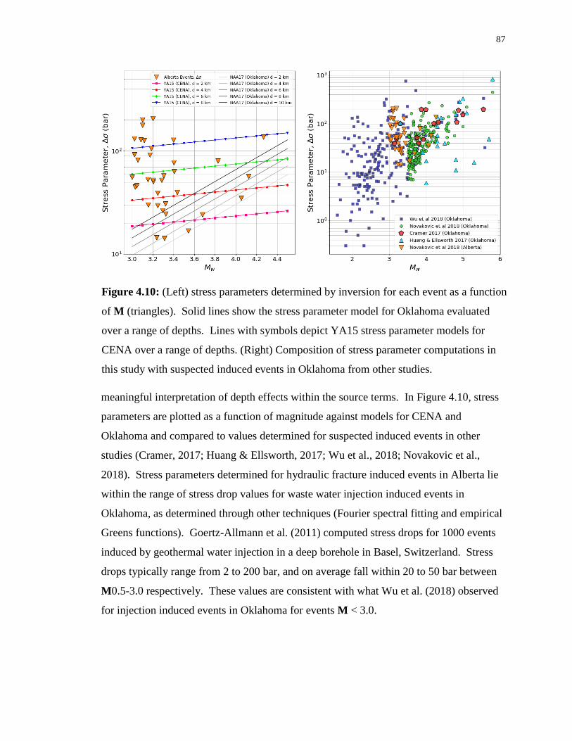
87

meaningful interpretation of depth effects within the source terms. In Figure 4.10, stress

parameters are plotted as a function of magnitude against models for CENA and

Oklahoma and compared to values determined for suspected induced events in other

studies (Cramer, 2017; Huang & Ellsworth, 2017; Wu et al., 2018; Novakovic et al.,

2018). Stress parameters determined for hydraulic fracture induced events in Alberta lie

within the range of stress drop values for waste water injection induced events in

Oklahoma, as determined through other techniques (Fourier spectral fitting and empirical

Greens functions). Goertz-Allmann et al. (2011) computed stress drops for 1000 events

induced by geothermal water injection in a deep borehole in Basel, Switzerland. Stress

drops typically range from 2 to 200 bar, and on average fall within 20 to 50 bar between

M0.5-3.0 respectively. These values are consistent with what Wu et al. (2018) observed

for injection induced events in Oklahoma for events M < 3.0.

Figure 4.10: (Left) stress parameters determined by inversion for each event as a function

of M (triangles). Solid lines show the stress parameter model for Oklahoma evaluated

over a range of depths. Lines with symbols depict YA15 stress parameter models for

CENA over a range of depths. (Right) Composition of stress parameter computations in

this study with suspected induced events in Oklahoma from other studies.

88

On average the stress parameter from Alberta events follow the YA15 CENA models

events having a depth of about 6 km. For this depth the stress dependence on magnitude

is given by YA15 as:

ln (∆σ) = 4.544 + min[0, 0.229(M –5.0)]. (4.16)

We determine the best near-surface attenuation parameter (𝜅0) for Alberta through an

iterative grid-search process. For each event we evaluate the magnitude scaling term;

remove the reference 𝜅 term by subtracting the 𝐹𝜅 function evaluated at 0.025 s (𝐹𝜅0.025);

then evaluate the stress parameter function for a suite of logarithmically-spaced stress

parameter values; and evaluate the 𝜅 function for linearly-spaced kappa terms, using:

𝐸𝑝𝑟𝑒𝑑𝑖,𝑗 = 𝐹𝑀 + 𝐹𝛥𝜎,𝑖 + 𝐹𝜅𝑗 − 𝐹𝜅0.025 𝑠 (4.17)

By comparing the spectrum predicted by the event term 𝐸𝑝𝑟𝑒𝑑𝑖,𝑗 for each stress-kappa pair

against the value determined for the event by the inversion, for frequencies from 0.90 Hz

to 24.0 Hz, we determine the best fit stress-kappa pair for each event, as well as all pairs

that fit above the 97.5th, 95th and 90th percentiles. This allows us to observe the

acceptable range of stress-kappa pairs for each event and evaluate the trade-off between

these two parameters. These two terms have a proportional relationship such that if one

parameter is increased, the other follows. This is demonstrated in Figures 4.11-4.13. We

next fix the stress parameter values for each event to match the model given by Equation

4.16 and grid search for the best mean kappa term. For the stress parameter values given

in Equation 4.16, the corresponding 𝜅0 that best matches the observed event term to the

model generally lies between 0.05 s and 0.07 s, as shown in Figure 4.14. Based on these

analyses, we select a mean value of 0.06 s as the average regional kappa term for soil

sites in Alberta.

There is a classic non-uniqueness issue in the resolution of Δσ and κ. Our mean kappa of

0.06 is dependent on the assumed model of Equation (4.16) for the stress parameter. The

stress parameter is ultimately a shape term that aims to bridge the offset between spectral

amplitudes at low frequencies with those at high frequencies; however, the value of

kappa also plays a critical role in this regard, as does any frequency-dependence in the

89

calibration factor. It is important to recognize that different self-consistent parameter sets

exist (i.e. different combination of stress, kappa, and calibration factor) that would also

satisfy the observational constraints and result in similar final GMPEs. As observed in

Figures 11-13, there is a wide range of κ - Δσ pairs that will provide a similar goodness

of fit for each event. We attempted to provide some constraint on the problem by

assuming the stress model of Yenier and Atkinson (2015b) as a basis for the kappa

determination. However, if we were to circle back and re-compute the stress parameter

values for each event after applying a kappa adjustment term for κ = 0.06s to the Yenier

and Atkinson source spectra, prior to taking the HF-LF measure, we would obtain higher

corresponding stresses-and a more negative calibration constant. We performed this

exercise, finding that it brings the stress parameter values up to those of the Yenier and

Atkinson (2015b) stress parameter model for CENA evaluated at a focal depth of 8 km,

and also results in a lower (more negative) calibration factor at high frequencies by about

0.13 natural logarithmic units; the resulting overall GMPE does not change significantly.



thick solid line depicts best spectral matched κ for an events modeled stress parameter

value. (Right) shows goodness of κ-Δσ pair fits in the 90th, 95th and 97.5th percentiles.

90



thick solid line depicts best spectral matched κ for an events modeled stress parameter

value. (Right) shows goodness of κ-Δσ pair fits in the 90th, 95th and 97.5th percentiles.

Figure 4.13: I(Left) the dashed line shows the event source term; thin solid lines show

the evaluated source term for linearly spaced κ values and best fit stress parameter value

pair; thick solid line depicts best spectral matched κ for an events modeled stress

parameter value. (Right) shows goodness of κ-Δσ pair fits in the 90th, 95th and 97.5th

percentiles.

91

We chose not to implement a higher stress model, as we believe that the Yenier and

Atkinson (2015b) stress parameter model is better constrained than what we can

determine from these data. Moreover, it is known that the events are typically shallow,

and the selected stress model should reflect this.

The regional calibration factor (C) is determined as the residual mismatch between the

observations and the model (after considering the modeled stress parameter for each

event, the site term for each station, and the regional kappa, geometric spreading and

anelastic attenuation functions). As discussed in Yenier and Atkinson (2015a), the

calibration factor reflects the average differences between the observations and the

simulations, including any systematic factors that are not accurate or not included in the

modeling approach. Examples of such factors include any residual regional site

amplification effects relative to the assumed amplification model for B/C that was

included in the Yenier and Atkinson (2015b) formulation, and any surface wave or other

contributions to the motion that were not included in the Brune source model. Removing

Figure 4.8: Kappa value that minimizes the residuals between the observed event term

and predicted source term when the stress parameter is assigned based on Eqn (4.16).

92

the resolved parameters from the inversion from the ground motion observations,

Equation 4.2 becomes

ln(Yi j) – FM,i – FZ,i j – γABRi j – FΔσ – FS,j – 𝐹𝜅0= CAB + ηi + εi j (4.18)

where CAB is the regional calibration factor for Alberta, ηi is the between-event error, and

εij is the within-event error. Following Abrahamson and Youngs (1992), we use a mixed

effects regression of residuals to solve Equation 4.18. An iterative regression is

performed to maximize the likelihood of the model and estimate the regional calibration

factor (CAB). The residual error of the observations with respect to the model is separated

into its between-event and within event components (ηi and εij). The regional calibration

factor for Alberta is shown in Figure 4.15 and is summarized in Appendix Table A4.2

along with the determined error components. A full list of model parameters, calibration

factor and error components at all frequencies is given in Table S4.1 of the electronic

supplement. At frequencies < 0.30 Hz we observe a positive residual of up to 0.5 ln units

at 0.20 Hz. This is explained by microseismic contributions and inherent limitations of

stochastic methods at low frequencies, which do not allow surface wave phases or

coherent pulses to be properly modeled. We suggest using a constant value of 0 at f < 0.2

Hz to prevent mapping the micro seismic peak at low frequencies to larger magnitudes.

The calibration factor dips steadily from 0 to -0.5 ln units between 0.2 Hz to 2.23 Hz

where it remains relatively constant to 50.0 Hz. A suggested calibration factor model for

Alberta is given by:

𝐶𝐴𝐵 =

{

0 𝑓𝑜𝑟 𝑓 < 0.3 𝐻𝑧 −0.69𝑙𝑜𝑔10(𝑓) − 0.36 𝑓𝑜𝑟 0.2 𝐻𝑧 ≤ 𝑓 < 1.59 𝐻𝑧 −0.50 𝑓𝑜𝑟 𝑓 ≥ 1.59 𝐻𝑧 −0.39 𝑓𝑜𝑟 𝑃𝐺𝑉 −0.36 𝑓𝑜𝑟 𝑃𝐺𝐴

(4.19)

The shape of the calibration function at intermediate frequencies might reflect deviations

from the regional site response model assumed for the reference B/C condition. The

generic GMPE form upon which this study is based has embedded within it a prescribed

average crustal amplification function for B/C conditions, which was derived from an

assumed model (Atkinson and Boore, 2006).

93

Any differences between the average amplification factors for selected B/C reference

sites in Alberta and those in the assumed embedded model will map into the calibration

factor. As shown in Figure 4.16, we may interpret the inverse of the calibration factor as

the amplification of the reference sites (on average), relative to the assumed amplification

function for B/C. By this logic, we may infer that the reference sites might have an

amplification that is larger than that assumed by Yenier and Atkinson (2015b) for B/C

sites, and more peaked at intermediate frequencies. We also note that Alberta ground

motions present relatively low amplitudes at high frequencies, which could reflect

deviations from the assumed crustal amplification model used in the base model

simulations of Yenier and Atkinson (2015b).

Figure 4.9: Calibration factor (CAB) obtained from inversion (squares) and its standard

deviation (error bars). Heavy line shows suggested model function for CAB.

Corresponding calibration factors for other regions are shown for comparison (lines with

symbols; circles=Oklahoma; triangle=CENA; diamond=California).

94

The trilinear geometric spreading function developed in this study agrees with that

developed for an improved local magnitude equation from a private ground motion

database in the Western Canadian Sedimentary Basin (Yenier, 2017). The differences in

geometric spreading functions from the bilinear equations previously used in magnitude

relationships in the region suggests an updated study should be undertaken to adjust the

moment magnitude estimation equations to incorporate these attenuation effects.

Alternatively, moment magnitudes could be estimated from stations within 50 km to

minimize the effects of attenuation.

Figure 4.10: The Alberta calibration factor (light line) and its inverse (black

line), in comparison to the site amplification functions of Seyhan and Stewart

(2014; SS14) for California, for a range of VS30 values (lines with symbols).

95

The final GMPE for Alberta includes the assumed magnitude scaling and geometric

spreading functions, the derived model for the anelastic attenuation terms, stress

parameter, site amplification terms, and the empirical calibration factor, and is described

as:

ln(Yij) = FM + FΔσ,AB + FZ + Fγ + FS + 𝐹𝜅0+ CAB (4.20)

where the coefficients for all terms are summarized in Appendix Table A4.3 and fully

listed in Table S4.1 of the electronic supplement. The electronic supplement also

provides a spreadsheet for evaluating the function. In Figures 4.17 and 4.18 we plot the

within-event residuals (ε = ln(observed) – ln(predicted)) for the horizontal-component

(geometric mean) PSA at 1.01 Hz and 10.17 Hz. There are no significant trends in the

residuals in magnitude or distance, for hypocentral distances greater than 50 km; at closer

distances, there is a tendency towards slightly positive residuals at some frequencies, and

slightly negative at others. In figure 4.19 the between event residuals (η) are plotted as a

Figure 4.11. Within event residuals with respect to the final GMPE for PSA at 1.01 Hz.


logarithmically spaced distance bins.

96

Figure 4.12. Within event residuals with respect to the final GMPE for PSA at 10.17 Hz.


logarithmically spaced distance bins.

Figure 4.19: Between-event residuals as a function of moment magnitude at 0.5 Hz, 1.0

Hz, 5.1 Hz and 10.2 Hz.

97

function of magnitude and do not display any meaningful trend with magnitude, though,

there is a tendency towards greater variability at high frequencies. Figure 4.20 shows the

between-event residual as a function of stress parameter. At high frequency ground

motion is controlled by the stress parameter. The adopted stress parameter model under

predicted stress for some study events in the ranges of M 3-3.2 and over predicted for

some events of M 3.2-3.4. As a result, we observe a strong trend in the between-event

variability as a function of stress parameter, which is expected due to the limitations of

predictive power in the adopted stress parameter model.

Figure 4.21 demonstrates the final GMPE (for PSA at 1.0 Hz), overlaying site-corrected

observations. As expected from the residual plots, observations follow the GMPE well.

In Figure 4.22, we compare the GMPE for induced events in Alberta, at selected

frequencies, to: the Oklahoma GMPE of NAA18 evaluated at the mean focal depth of

induced events in Oklahoma of 5 km; the CENA GMPE of Yenier and Atkinson (2015b)

for earthquakes at depths of 2 and 5 km, for events of M3 and M5, respectively; and the

GMPE of Atkinson (2015), which was derived from moderate events with an average

depth of 9 km in California (NGA-West2 database), but postulated to apply for induced

events, is also shown.

Figure 4.20: Between-event residuals as a function of stress parameter (bar) at 0.5 Hz,

1.00 Hz, 5.0 Hz and 10.0 Hz.

98

For low-to-intermediate frequencies the tri-linear geometric spreading function generally

traces the level of YA15 and Atkinson (2015) where the GMPE predicts slightly lower

amplitudes near the first transition and slightly higher near the second transition zone. At

higher frequencies the GMPE derived for Alberta is generally low for near to

intermediate distances (<150 km) and matches the level at far distances when compared

to YA15 and Atkinson (2015). Alberta ground motion amplitudes are generally lower

than those observed in Oklahoma, especially at high frequencies (> 10 Hz). Differences

of amplitude in the Alberta and Oklahoma GMPEs reflect the differences in stress

parameter models. Alberta events appear to follow the CENA model of YA15 evaluated

at 6 km depth, whereas in Oklahoma the derived model (involving both depth and

magnitude) features higher stress parameters. This could reflect generally greater depths

for induced events in Oklahoma, or some other differences attributable to source

processes. Differences in average regional crustal amplification may also contribute to

the difference in observations as these will map into the source terms.

Figure 4.21 Final GMPE overlaying site corrected observations at 1.0 Hz. Lines depict

the GMPE evaluated every 0.2 magnitude units from M = 2.9 to M = 4.5. Circles vary in

diameter where larger circles represent higher magnitude observations and smaller circles

denote lower magnitude event observations.

99

Figure 4.22. The GMPE for Alberta as determined in this study (solid lines) in

comparison to the NAA18 GMPE for Oklahoma (circles) is evaluated at the typical focal

depth for events in Oklahoma of 5 km. YA15 GMPE for CENA (dashed lines) is

evaluated for focal depths of 6 and 8 km for M4 and M6 respectively. The GMPE of

Atkinson (2015), as determined from moderate California earthquakes with mean depth

of 9 km, is also indicated (dotted lines), for distances < 50 km. All models are for

NEHRP B/C reference site conditions.

4.6 Conclusion

A regionally-adjusted GMPE for induced events in Alberta is developed that describes

the geometric mean of horizontal component PSA, PGV, and PGA ground motions for a

100

reference condition of B/C. The generic GMPE framework of Yenier and Atkinson

(2015b) is used to ensure stable scaling of motions over all magnitudes and distances.

We calibrate the generic GMPE by determining site amplification models, anelastic

attenuation function, regional stress parameter model, regional near surface high

frequency attenuation term (adapted from Hassani and Atkinson 2018), and calibration

factor from > 880 ground-motion observations from Alberta events of M ≥ 3 at

hypocentral distances from 20 to 575 km. The derived GMPE is useful for ShakeMap

applications, hazard assessments and may also be useful for ground-motion-based

alerting systems and traffic light protocols.

4.7 Data and Resources

Events were detected and located for TransAlta by Nanometrics. Ground motion data

were downloaded from the Incorporated Research Institutes for Seismology

(www.iris.edu, last accessed Oct. 2017), processed, and compiled using an updated

version of the ICORRECT algorithm, as described in Assatourians and Atkinson (2017).

A ground motion database paper composed of processed ground motion observations,

event/station metadata and M estimates for each event will become available online in

the near future.


This study was funded by the Natural Sciences and Engineering Research Council of

Canada and TransAlta. We thank Joseph Farrugia for his valuable input and

interpretation of site classifications. We thank Emrah Yenier for his suggestions which

strengthened the manuscript. We thank our reviewers for their constructive feedback.

4.9 References

Abrahamson, N. A., and R. R. Youngs (1992). A stable Algorithm for regression analysis

using the random effects model, Bull. Seismol. Soc. Am. 82(1), 505–510.

Ambraseys, N. N., and Douglas, J. (2004). Magnitude calibration of north Indian

earthquakes. Geophysical Journal International, 159(1), 165-206. DOI:

10.1111/j.1365-246X.2004.02323.x

101

Anderson, J. G., and Hough S. E. (1984). A model for the shape of the Fourier amplitude

spectrum of acceleration at high frequencies, Bull. Seismol. Soc. Am. 74, 1969 –

1993.

Andrews, J. (1986). Objective determination of source parameters and similarity of

earthquakes of different size, Earthquake Source Mechanics, American

Geophysical Union, Geophysical Monograph, 37, 259-267.



5.4 Riviere du Loup, Quebec earthquake, Seismol. Res. Lett. 81(6), 1013–1031.

Assatourians, K., and Atkinson, G. M. (2017). Are Ground-Motion Models Derived from

Natural Events Applicable to the Estimation of Expected Motions for Induced

Earthquakes? Seism. Res. Lett. DOI: 10.1785/0220160153.

Atkinson, G. M. and Boore D. M. (2006). Earthquake ground-motion prediction

equations for eastern North America, Bull. Seism. Soc. Am. 85, 17-30.


(M) for Small Events (M<4) on Local Networks. Seismological Research

Letters, 85, 1116-1124.

Atkinson, G. M., Hassani, B., Singh, A., Yenier, E. and Assatourians, K. (2015).

Estimation of Moment Magnitude and Stress Parameter from ShakeMap

Ground-Motion Parameters. Bull. Seismol. Soc. Am. 105(5), 2572-2588.

Atkinson, G. M., and Morrison, M. (2009). Regional variability in ground motion

amplitudes along the west coast of North America, Bull. Seismol. Soc. Am., 99,

2393–2409.

Boore, D. M. (2003). Simulation of ground motion using the stochastic method, Pure and

Applied Geophysics 160, 635-675.

Boore, D. M. (2010). Orientation-Independent, Nongeometric-Mean Measures of Seismic

Intensity from Two Horizontal Components of Motion. Bull. Seismol. Soc. Am.

100, 1830-1835.

Boore, D. M., Campbell, K. W., and Atkinson, G. M. (2010). Determination of stress

parameters for eight well-recorded earthquakes in eastern North America. Bull.

Seismol. Soc. Am. 100, 1632-1645.

Bouzidi Y., Schmitt D. R., Burwash R. A., Kanasewich E. R. (2002). Variations in

Crustal Thickness in Alberta from Depth-Migrated Seismic Reflection Profiles,

Can. J. Earth. Sci., 39, 311-350.

102


earthquakes. J. Geophysics. Res. 75(26), 4997-5009.

Brune, J. N. (1971). Correction: Tectonic stress and the spectra of seismic shear waves, J.

Geophysics. Res. 76(20), 5002.

Burger, R. W., Somerville, P. G., Barker, J. S., Herrmann, R.B., and Helmberger, D.V.

(1987). The effect of Crustal structure on strong ground motion attenuation

relations in eastern North America. Bull. Seismol. Soc. Am. 77, 420-439, 1987.

Cramer, C. (2017). Brune Stress Parameter Estimates for the 2016 Mw Pawnee and Other

Oklahoma Earthquakes. Seismological Research Letters, 88(4):1005-1016.

Cramer, C. (2017). Gulf Coast Regional Q and Boundaries from USArray Data. Bull.

Seismol. Soc. Am. 108(1), 437-449

Ellsworth, W. L. (2013). Injection-induced earthquakes. Science. 341 (6142): 7.

DOI:10.1126/science.1225942

Farrugia, J. J., Atkinson, G. M., Molnar, S. (2017). Validation of 1D Earthquake Site

Characterization Methods with Observed Earthquake Site Amplification in

Alberta, Canada. Bull. Seismol. Soc. Am. 108 (1): 291-308.

Fereidoni A., Atkinson G.M. (2017), Discriminating Earthquakes from Quarry Blasts

Based on ShakeMap Ground-Motion Parameters, Bull. Seismol. Soc. Am.,

DOI:10.1785/0120160308.

Ghofrani H. and Atkinson G. M. (2014). Site Condition Evaluation Using Horizontal-to-

Vertical Response Spectral Ratios of Earthquakes in the NGA-West2 and

Japanese Databases. Soil Dynamics and Earthquake Engineering. 67, 30-43.

Goertz-Allmann, B. P., Goertz, A., Wiemer, S. (2011). Stress drop variations of induced

earthquakes at the Basel geothermal site. Geophysical Research Letters, 38,

L09308, doi:10.1029/2011GL047498

Gu Y., Okeler A., Shen L., Contenti S. (2011). The Canadian Rockies and Alberta

Network (CRANE): New Constraints on the Rockies and Western Canadian

Sedimentary Basin. Seismological Research Letters 82(4), 575-588.


Eastern North America. Seismological Research Letters 86(2A), 477-491. Hassani, B. and Atkinson, G. M. (2016). Site-effects model for central and eastern North

America based on peak frequency. Bull. Seism. Soc. Am., 106, 2197-2213.

103

Hassani, B., and Atkinson G. M. (2018). Adjustable Generic Ground-Motion Prediction

Equation Based on Equivalent Point-Source Simulations: Accounting for Kappa

Effects. Bull. Seismol. Soc. Am. 108(2), 913-928.

Huang, Y., Ellsworth, W. L., and Beroza, G. C. (2017). Stress drops of induced and

tectonic earthquakes in the central United States are indistinguishable. Science

Advances 3(8), e1700772.

McGuire, R. K. (2004). Seismic Hazard and Risk Analysis, Earthquake Engineering

Research Institute. Aug 1, 2004.

Nigam, N. C. and Jennings, P. C. (1969). Calculation of Response Spectra from Strong-

Motion Earthquake Records, Bull. Seismol. Soc. Am. 59(2), 909-922.

Novakovic M., Atkinson G. M. (2015). Preliminary Evaluation of Ground Motions from

Earthquakes in Alberta. Seismol. Res. Lett., 86(4), 1086-1095.

Novakovic M., Atkinson G. M., Assatourians K. (2018). Empirically Calibrated Ground-


10.1785/0120170331

Schultz, R., Wang, R., Gu, Y., Haug, K., Atkinson, G.M. (2017) A Seismological

Overview of the Induced Earthquakes in the Duvernay Play Near Fox Creek,

Alberta. Journal of Geophysical Research: Solid Earth, 122(1), 492-505.

Seyhan, E. and Stewart, J. (2014). Semi-Empirical Nonlinear Site Amplification from

NGA-West2 Data and Simulations. Earthquake Spectra, 30(3), 1241-1256.

Stern, V. H., Schultz, R. J., Shen, L., Gu, Y. J. and Eaton, D. W. (2018): Alberta

earthquake catalogue, version 6.0 (GIS data, point features); Alberta Energy

Regulator, AER/AGS Digital Dataset 2013-0017.

Wald D. J., Quitoriano V., Heaton T. H., Kanamori H., Scrivner C. W., Worden C. B.

(1999). TriNet ShakeMaps: Rapid generation of peak ground motion and

intensity maps for earthquakes in southern California. Earthq. Spectra. 15(3),

537-555.

Wang, R., Gu., Y, Schultz, R., Kim A., Atkinson, G. M. (2015), Source Analysis of a

Potential Hydraulic-Fracturing-Induced Earthquake Near Fox Creek, Alberta.

Geophysical Research Letters, DOI: 10.1002/2015GL066917.

Wang, R., Gu, Y. J., Schultz, R., Zhang, M., and Kim, A. (2017). Source characteristics

and geological implications of the January 2016 induced earthquake swarm near

Crooked Lake, Alberta. Geophysical Journal International, 210(2), 979-988.

Wu, Q., Chapman, M., Chen, X. (2018). Stress-Drop Variations of Induced Earthquakes

in Oklahoma. Bull. Seismol. Soc. Am. 108 (3A), 1107-1123.

104

Yenier, E., and Atkinson, G. M. (2014). Equivalent point-source modeling of moderate

to large magnitude earthquakes and associated ground-motion saturation

effects. Bull. Seismol. Soc. Am. 104, 1458-1478.



Seismol. Soc. Am. 105(3), 1435-1455.


Prediction Equation based on Equivalent Point-Source Simulations: Application

to Central and Eastern North America. Bull. Seismol. Soc. Am. DOI:

10.1785/0120140332

Yenier, E., Atkinson G. M., Sumy D. F. (2017). Ground Motions for Induced

Earthquakes in Oklahoma, Bull. Seismol. Soc. Am. 107(1), 198-215

Yenier, E. (2017). A Local Magnitude Relation for Earthquakes in the Western Canadian

Sedimentary Basin, Bull. Seismol. Soc. Am. DOI: 10.1785/0120160275

105

Chapter 5

5 Conclusions and Future Studies

5.1 Summary, Discussion and Conclusions

In this thesis we characterized ground motions from induced earthquakes in Oklahoma,

USA and Alberta, Canada.

In Chapter 2 we estimate the moment magnitude of events in Alberta using the PSA-

based algorithm of Atkinson et al. (2014). We found that the attenuation and amplitude

calibration parameters for WNA provide a consistent agreement with local magnitude

calculations for events M > 2.6. The deviation of moment magnitude and local

magnitude for M < 2.6 was initially postulated as a noise effect, and a noise correction

was suggested. Since that study was conducted, the relationship between local magnitude

and moment magnitude has become better understood, and it is now believed that this

correction factor should be discarded (Ross et al., 2016; Yenier, 2017). The Wood-

Anderson filter that is applied to seismograms in determining local magnitude can

explain the observed deviation (Bakun, 1984; Hanks and Boore, 1984). Amplitudes of

larger events are artificially lowered more than those of smaller events as the Wood-

Anderson filter has a corner frequency of roughly 1.00 Hz. There exists a discontinuity

between M estimated from PSA at 1.00 Hz and M estimated at 3.33 Hz, that can be

bridged by taking the mean of these two values if each parameter lies on opposite sides of

M=3. Ground motions are compared to a reference model of Atkinson (2015) and are

found to be generally consistent with those for similar-size events in California in terms

of overall amplitude level and attenuation. We observed features in this comparison that

were unresolvable with the sparse available data, which will require further investigation

with additional ground-motion records. Ground motion scaling characteristics of Alberta

events are generally consistent with expectations based on both empirical (Atkinson,

2015) and point-source simulation models (Yenier and Atkinson, 2015a). We observe a

significant site response on the horizontal component in the 2 to 5 Hz frequency range,

106

which is relatively consistent among all stations. This suggests a relatively common site

response model could be appropriate for all stations in Western Alberta.

In Chapter 3, we derived a regionally-adjusted GMPE for induced events in Oklahoma

(geometric mean of horizontal components), for a reference condition of B/C. We used

the generic GMPE framework of Yenier and Atkinson (2015b) to ensure stable scaling of

motions over all magnitudes and distances. Observations of ground motion amplification

at regional distances due to the summation of direct rays and the first post critically

refracted waves off of the Mohorivicic discontinuity dictated the need for the

development of a tri-linear geometric spread model. Yenier and Atkinson (2015b) base

the stress parameter value on the corner frequency by matching the attenuation-corrected

spectral shape to that of an ideal Brune spectra. On average the Oklahoma source spectra

do not nicely follow the ideal Brune-model spectral shape, so an alternative approach was

considered in this study that bases the determination of the stress parameter on the

event’s mean high-frequency spectral level (10 Hz level) relative to that expected based

on the low-frequency level (1 Hz level). This approach was found to result in more

stable determination of the stress parameter. The generic GMPE was calibrated by

determining an anelastic attenuation function, site amplification models, regional stress

parameter model, and calibration factor. The derived GMPE presents higher ground

motions at high frequencies than those observed in CENA (for the same magnitude and

distance), which reflect differences in magnitude and depth dependence of the stress

parameter. At low frequencies the amplitudes in Oklahoma tend to be higher than those

for corresponding events in CENA, suggesting differences in the crustal amplification

effects due to regional geology. The derived GMPE is useful for hazard assessments and

ShakeMap applications and may also be useful for ground-motion-based alerting systems

and traffic light protocols.

In Chapter 4, we empirically calibrated the regionally adjustable GMPE (Yenier and

Atkinson, 2015b) for induced events in Alberta. Similar to Oklahoma, we observed

strong influences of Mohorivicic bounce effects and model ground motion attenuation at

regional distances with a trilinear geometric spreading function. We discovered that the

spectral shape of attenuation corrected event spectra has significantly lower amplitudes at

107

high frequency than those expected for an ideal Brune source. We attribute this to a

combination of differing crustal amplification in the region as well as differing near-

surface attenuation effects (commonly expressed as the kappa effect, κo) relative to those

assumed in the simulations of the reference model. Yenier and Atkinson (2015b)

assumed a kappa value of 0.025 s in the simulations upon which their model was based.

Hassani and Atkinson (2018) showed how this model could be adjusted for alternative

values of kappa. We adapt the functional form of the kappa effect from Hassani and

Atkinson (2018) and develop a referenced kappa adjustment factor. We perform grid

search analysis to determine that the best choice in kappa for Alberta is 0.06 s, as a

regional average for the seismographic recording sites. If the source scaling of the events

can be constrained, this would reduce the trade-offs between stress and kappa, and allow

a less-ambiguous definition of the ground-motion model parameters. Overall, the ground

motions for B/C site conditions for induced events in Alberta are of similar amplitude at

low frequencies to those predicted by the GMPEs of Yenier and Atkinson (2015b) and

Atkinson et al (2015), for events of M 3 to 4.5. Alberta motions present lower

amplitudes at high frequencies than those observed in Oklahoma but are fairly consistent

with the model of Yenier and Atkinson (2015b) for very shallow events in CENA.

Through the process of these studies we concluded that it is not entirely straight forward

to calibrate the generic GMPE to a regional database in a unique and unambiguous way.

5.2 Recommendations for Future Studies

Based on the requirement of a trilinear geometric spreading function in Chapter 4, the

moment magnitude estimation equation should be revisited to incorporate the updated

function shape. Re-evaluation of the frequency-dependent magnitude calibration factor

should be adjusted in agreement with available moment tensor solutions in the region.

This would facilitate routine, rapid and accurate estimation of moment magnitude for all

events in CENA of M>2.5, and would be helpful for real-time hazard assessment,

alerting and traffic-light applications.

In our generic ground-motion model, disparities between assumed seismological models

and the true physical characteristics are cast into a frequency-dependent calibration

108

factor. The fact that this calibration factor is not close to zero at all frequencies suggests

the need for additional in-depth studies to refine the underlying geological and

geophysical model parameters. One such parameter is the crustal amplification model,

which to date has been based on a gradient model. The crustal structure in areas

containing sedimentary basins might be better expressed as a ‘layer cake’ model. The

effects of alternative crustal amplifications based on more realistic earth models should

be explored in further studies. The interplay between amplification effects through the

crustal structure and near-surface velocity profile, and near-surface damping (as

expressed by kappa) also requires further study. It appears that such effects may be quite

different in the Western Canadian Sedimentary Basin in comparison to those in

Oklahoma or in CENA. Finally, the scaling of source attributes for induced events

relative to those of natural earthquakes is a fruitful area for further detailed investigations.

5.3 References

Atkinson, G. M. (2015). Ground-Motion Prediction Equation for Small-to-Moderate

Events at Short Hypocentral Distances, with Application to Induced-Seismicity

Hazards. Bull. Seismol. Soc. Am. 105. 10.1785/0120140142.


(M) for Small Events (M<4) on Local Networks. Seismol. Res. Lett., 85, 1116-

1124.

Bakun, W.H. (1984). Seismic Moments, Local Magnitudes, and Coda-duration

Prospects. Bull. Seismol. Soc. Am. 74, 439-458.

Hanks, T.C. and Boore, D.M. (1984). Moment-magnitude Relations in Theory and

Practice. J. Geophys. Res., 89, 6229-6235.

Hassani B., and Atkinson G. M. (2018). Adjustable Generic Ground-Motion Prediction

Equation Based on Equivalent Point-Source Simulations: Accounting for Kappa

Effects. Bull. Seismol. Soc. Am. 108(2), 913-928.

Ross, Z.E., and Ben-Zion, Y. (2016). Towards Reliable Automated Estimates of

Earthquake Source Parameters from Body Wave Spectra. J. Geophys. Res.,

121, doi:10.1002/2016JB013003.



Seismol. Soc. Am. 105(3), 1435-1455.

109




DOI: 10.1785/0120140332

Yenier, E. (2017). A Local Magnitude Relation for Earthquakes in the Western Canada

Sedimentary Basin. Bull. Seismol. Soc. Am. 107. 10.1785/0120160275.

110

Appendices

Table A3.1: Tabulation of magnitude estimation model parameters where MCF is the

calibration factor for each frequency that aims to match the level that has been modified

from Novakovic and Atkinson (2015) for Oklahoma. γF, low (Eastern), γF, mod (moderate),

and γF, high (Western) are the anelastic attenuation coefficients designed to remove

distance dependent trends.

3.33 Hz 1.00 Hz 0.30 Hz

MCF -3.3 -4.5 -5.45

γF, low 0.0015 0.0007 0.0011

γF, mod 0.0033 0.0021 0.0017

γF, high 0.0050 0.0035 0.0027

Table A3.2: Summary table of stress parameter values from inversion for events of M ≥

4.2 in Oklahoma.

Event

Number

Date

(mm/dd/yyyy)

Time

(hh:mm:ss)

UTC

Longitude Latitude Depth

(km)

Magnitude,

M

Stress

Parameter,

Δσ (bar)

7 2/28/2011 05:00:50 -92.344 35.265 3.8 4.2 64.0

12 11/5/2011 07:12:45 -96.781 35.538 3.4 4.6 99.0

13 11/8/2011 02:46:57 -96.786 35.518 4.81 4.6 103.6

16 12/7/2013 18:08:06 -97.383 35.609 6.5 4.2 90.8

17 12/7/2013 18:10:25 -97.386 35.607 8.44 4.3 110.2

36 6/16/2014 10:47:36 -97.397 35.593 5 4.2 71.5

46 7/29/2014 02:46:36 -98.045 36.756 5.29 4.2 93.2

48 8/19/2014 12:41:36 -97.468 35.773 4.51 4.2 57.0

57 10/2/2014 18:01:24 -97.955 37.245 5 4.5 78.7

58 10/2/2014 18:02:55 -97.967 37.233 5 4.2 44.4

64 11/12/2014 21:37:11 -97.602 36.648 5.37 4.6 52.0

65 11/12/2014 21:40:01 -97.621 37.271 4.03 4.8 56.6

100 4/4/2015 13:21:17 -97.572 36.118 5.05 4.2 67.6

117 6/5/2015 23:12:41 -97.968 37.219 5.11 4.2 40.3

118 6/5/2015 23:12:47 -97.921 37.265 2.35 4.3 49.1

133 7/20/2015 20:19:04 -98.257 36.843 4.08 4.6 92.9

111

138 7/27/2015 18:08:39 -98.791 36.472 5 4.4 235.2

139 7/27/2015 18:12:15 -97.572 35.989 5 4.5 128.5

146 9/16/2015 02:30:02 -96.795 35.978 4.02 4.2 52.6

151 10/10/2015 09:20:43 -97.931 36.719 5.63 4.6 139.9

161 11/20/2015 22:40:40 -97.828 36.948 5 4.3 102.1

164 11/23/2015 21:17:47 -98.276 36.838 5.03 4.6 39.9

166 11/30/2015 09:49:13 -98.056 36.751 5.63 4.8 173.4

171 1/1/2016 11:39:40 -97.406 35.669 5.83 4.3 42.9

172 1/7/2016 04:27:28 -98.741 36.486 7.09 4.6 70.5

173 1/7/2016 04:27:58 -98.725 36.496 4.06 4.6 69.6

182 2/13/2016 17:06:04 -98.72 36.46 4.54 4.6 81.8

183 2/13/2016 17:07:06 -98.726 36.485 8.27 5.1 220.5

185 9/3/2016 12:02:44 -96.931 36.431 4.5 5.8 448.9

186 11/7/2016 01:44:24 -96.803 35.991 4.4 5.0 87.5

112

Table A3.3: Summary of Oklahoma model coefficients and the anelastic attenuation

function γOK and γCENA, calibration factor COK and Ce,CENA, within event variability η, and

in-between event variability ε as determined by the inversion.

f (Hz) 0.19 0.3 0.51 1.01 2 3.3 5.12 10.17 15.26 20.21 50 PGV PGA

Mh 6.8927 6.7271 6.6563 6.4642 6.2509 5.8482 5.4307 5.4332 5.625 5.3764 5.9006 5.9 5.85

e0 -0.0689 0.4494 1.2828 2.0102 2.5469 2.6187 2.5414 2.7636 2.889 2.5728 2.3793 5.9604 2.2156

e1 1.9793 1.9171 1.7362 1.3242 0.8848 0.8513 0.818 0.7155 0.7003 0.7181 0.6997 1.03 0.6859

e2 -0.061 -0.084 -0.134 -0.2472 -0.3483 -0.3634 -0.3859 -0.2604 -0.1696 -0.1604 -0.1067 -0.1651 -0.1393

e3 1.5919 1.4521 1.1836 0.9798 0.9178 0.8798 0.8423 0.7935 0.7602 0.7536 0.7489 1.0789 0.7656

b3 -0.5823 -0.5278 -0.4321 -0.2957 -0.2078 -0.2146 -0.2908 -0.3807 -0.4634 -0.5115 -0.6376 -0.5785 -0.6187

b4 0.0793 0.0702 0.053 0.0273 0.0085 0.0059 0.0143 0.0252 0.0361 0.043 0.0625 0.0574 0.0603

s0 -6.1625 -7.6498 -6.5491 1.116 3.9137 -0.2401 -2.8318 -4.0209 -2.3368 -0.9678 -1.1697 -2.2458 -2.1315

s1 4.8839 6.3092 5.697 -0.5002 -3.2548 -0.1858 1.8381 3.0878 2.0173 0.9945 1.2816 1.9508 1.937

s2 -1.3179 -1.8048 -1.7236 0.0514 0.9791 0.1799 -0.3622 -0.761 -0.5053 -0.2209 -0.3364 -0.5181 -0.504

s3 0.149 0.2188 0.2222 0.0085 -0.1185 -0.0293 0.0321 0.0833 0.0563 0.0217 0.0394 0.0614 0.0582

s4 -0.0059 -0.0095 -0.0102 -0.001 0.0051 0.0014 -0.0011 -0.0034 -0.0023 -0.0008 -0.0017 -0.0027 -0.0025

s5 -1.2368 -3.5814 -6.0007 -4.3861 0.8735 2.1854 0.7143 -2.5045 -3.8552 -4.1732 -1.2719 -1.7584 -1.4442

s6 0.7939 2.7948 4.984 3.9802 -0.4705 -1.9496 -1.0055 1.6147 2.8013 3.2534 1.2532 1.3793 1.2353

s7 -0.1084 -0.7224 -1.4353 -1.2537 0.0707 0.6164 0.4204 -0.3024 -0.6513 -0.8208 -0.3167 -0.3256 -0.2851

s8 -0.0028 0.0771 0.1753 0.1685 0.0044 -0.075 -0.0591 0.0246 0.0673 0.0917 0.0362 0.035 0.0302

s9 0.0009 -0.0028 -0.0076 -0.008 -0.0008 0.0032 0.0028 -0.0007 -0.0026 -0.0038 -0.0015 -0.0014 -0.0012

γCENA -0.0009 -0.0011 -0.001 -0.0013 -0.002 -0.0032 -0.0043 -0.0057 -0.0057 -0.0055 -0.0047 -0.0047 -0.0028

Ce,CENA 0.0783 -0.0325 -0.3011 -0.3734 -0.3654 -0.233 -0.1027 -0.1737 -0.2819 -0.4892 -0.1823 -0.0196 -0.21

γOK -0.0017 -0.0022 -0.0021 -0.0020 -0.0017 -0.0018 -0.0018 -0.0031 -0.0044 -0.0026 -0.0010 -0.0026 -0.0017

Cok

(ln units) 0.4537 0.6724 0.2519 0.2959 -0.2234 -0.2809 -0.4081 0.0813 0.1704 -0.0273 0.1191 0.0733 0.4537

η

(ln units) 0.4948 0.4972 0.4908 0.4931 0.5309 0.5089 0.4936 0.4412 0.4096 0.4394 0.5278 0.5090 0.4948

ε

(ln units) 0.4676 0.4787 0.4271 0.3786 0.4118 0.4430 0.4457 0.4547 0.4114 0.4131 0.4300 0.4226 0.4676

113

Table A4.1: Tabulation of Magnitude Estimation Model Parameters. MCF is the

magnitude calibration factor for each frequency. γF, low (Eastern), γF, mod (moderate), and

γF, high (Western) are the anelastic attenuation coefficients.

3.33 Hz 1.00 Hz

MCF -3.3 -4.5

γF, low 0.0015 0.0007

γF, mod 0.0033 0.0021

γF, high 0.0050 0.0035

Table A4.2: Summary of Alberta model coefficients, the anelastic attenuation function

γAB, calibration factor CAB, within event variability η, and in-between event variability ε

as determined by the inversion.

f (Hz) 0.19 0.3 0.51 1.01 2 3.3 5.12 10.17 15.26 20.21 50 PGV PGA

Mh 6.8927 6.7271 6.6563 6.4642 6.2509 5.8482 5.4307 5.4332 5.625 5.3764 5.9006 5.9 5.85

e0 -0.0689 0.4494 1.2828 2.0102 2.5469 2.6187 2.5414 2.7636 2.889 2.5728 2.3793 5.9604 2.2156

e1 1.9793 1.9171 1.7362 1.3242 0.8848 0.8513 0.818 0.7155 0.7003 0.7181 0.6997 1.03 0.6859

e2 -0.061 -0.084 -0.134 -0.2472 -0.3483 -0.3634 -0.3859 -0.2604 -0.1696 -0.1604 -0.1067 -0.1651 -0.1393

e3 1.5919 1.4521 1.1836 0.9798 0.9178 0.8798 0.8423 0.7935 0.7602 0.7536 0.7489 1.0789 0.7656

b3 -0.5823 -0.5278 -0.4321 -0.2957 -0.2078 -0.2146 -0.2908 -0.3807 -0.4634 -0.5115 -0.6376 -0.5785 -0.6187

b4 0.0793 0.0702 0.053 0.0273 0.0085 0.0059 0.0143 0.0252 0.0361 0.043 0.0625 0.0574 0.0603

s0 -6.1625 -7.6498 -6.5491 1.116 3.9137 -0.2401 -2.8318 -4.0209 -2.3368 -0.9678 -1.1697 -2.2458 -2.1315

s1 4.8839 6.3092 5.697 -0.5002 -3.2548 -0.1858 1.8381 3.0878 2.0173 0.9945 1.2816 1.9508 1.937

s2 -1.3179 -1.8048 -1.7236 0.0514 0.9791 0.1799 -0.3622 -0.761 -0.5053 -0.2209 -0.3364 -0.5181 -0.504

s3 0.149 0.2188 0.2222 0.0085 -0.1185 -0.0293 0.0321 0.0833 0.0563 0.0217 0.0394 0.0614 0.0582

s4 -0.0059 -0.0095 -0.0102 -0.001 0.0051 0.0014 -0.0011 -0.0034 -0.0023 -0.0008 -0.0017 -0.0027 -0.0025

s5 -1.2368 -3.5814 -6.0007 -4.3861 0.8735 2.1854 0.7143 -2.5045 -3.8552 -4.1732 -1.2719 -1.7584 -1.4442

s6 0.7939 2.7948 4.984 3.9802 -0.4705 -1.9496 -1.0055 1.6147 2.8013 3.2534 1.2532 1.3793 1.2353

s7 -0.1084 -0.7224 -1.4353 -1.2537 0.0707 0.6164 0.4204 -0.3024 -0.6513 -0.8208 -0.3167 -0.3256 -0.2851

s8 -0.0028 0.0771 0.1753 0.1685 0.0044 -0.075 -0.0591 0.0246 0.0673 0.0917 0.0362 0.035 0.0302

s9 0.0009 -0.0028 -0.0076 -0.008 -0.0008 0.0032 0.0028 -0.0007 -0.0026 -0.0038 -0.0015 -0.0014 -0.0012

γCENA -0.0009 -0.0011 -0.001 -0.0013 -0.002 -0.0032 -0.0043 -0.0057 -0.0057 -0.0055 -0.0047 -0.0047 -0.0028

Ce,

CENA 0.0783 -0.0325 -0.3011 -0.3734 -0.3654 -0.233 -0.1027 -0.1737 -0.2819 -0.4892 -0.1823 -0.0196 -0.21

γAB -5.03E-

04

-2.29E-

03

-2.86E-

03

-2.46E-

03

-2.58E-

03

-3.43E-

03

-4.16E-

03

-5.07E-

03

-5.59E-

03

-5.24E-

03

-4.10E-

03

-3.04E-

03

-4.21E-

03

CAB (ln units) 0.54 0.24 -0.20 -0.37 -0.62 -0.65 -0.45 -0.48 -0.52 -0.51 -0.29 -0.39 -0.36

CAB

model(l

n units) 0.00 0.00 -0.16 -0.36 -0.50 -0.50 -0.50 -0.50 -0.50 -0.50 -0.50 -0.39 -0.36

η (ln units) 0.495 0.497 0.491 0.493 0.531 0.509 0.494 0.441 0.411 0.410 0.439 0.528 0.509

ε (ln

units) 0.468 0.479 0.427 0.379 0.412 0.443 0.446 0.455 0.425 0.411 0.413 0.430 0.423

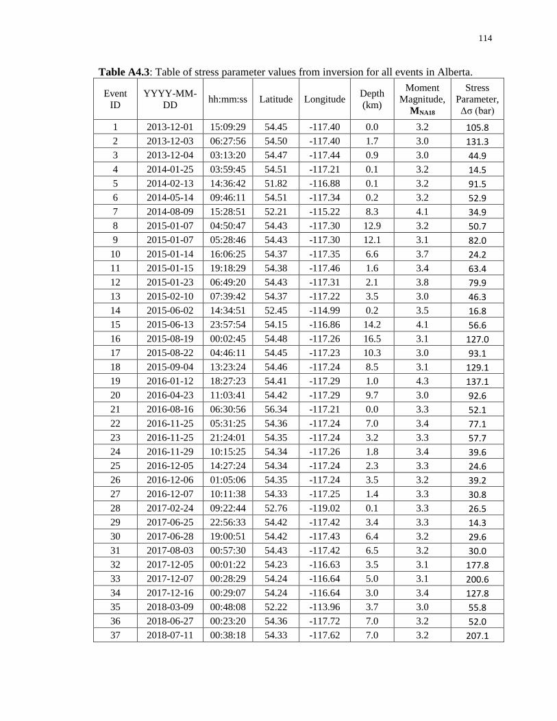
114

Table A4.3: Table of stress parameter values from inversion for all events in Alberta.

Event

ID

YYYY-MM-

DD hh:mm:ss Latitude Longitude

Depth

(km)

Moment

Magnitude,

MNA18

Stress

Parameter,

Δσ (bar)

1 2013-12-01 15:09:29 54.45 -117.40 0.0 3.2 105.8

2 2013-12-03 06:27:56 54.50 -117.40 1.7 3.0 131.3

3 2013-12-04 03:13:20 54.47 -117.44 0.9 3.0 44.9

4 2014-01-25 03:59:45 54.51 -117.21 0.1 3.2 14.5

5 2014-02-13 14:36:42 51.82 -116.88 0.1 3.2 91.5

6 2014-05-14 09:46:11 54.51 -117.34 0.2 3.2 52.9

7 2014-08-09 15:28:51 52.21 -115.22 8.3 4.1 34.9

8 2015-01-07 04:50:47 54.43 -117.30 12.9 3.2 50.7

9 2015-01-07 05:28:46 54.43 -117.30 12.1 3.1 82.0

10 2015-01-14 16:06:25 54.37 -117.35 6.6 3.7 24.2

11 2015-01-15 19:18:29 54.38 -117.46 1.6 3.4 63.4

12 2015-01-23 06:49:20 54.43 -117.31 2.1 3.8 79.9

13 2015-02-10 07:39:42 54.37 -117.22 3.5 3.0 46.3

14 2015-06-02 14:34:51 52.45 -114.99 0.2 3.5 16.8

15 2015-06-13 23:57:54 54.15 -116.86 14.2 4.1 56.6

16 2015-08-19 00:02:45 54.48 -117.26 16.5 3.1 127.0

17 2015-08-22 04:46:11 54.45 -117.23 10.3 3.0 93.1

18 2015-09-04 13:23:24 54.46 -117.24 8.5 3.1 129.1

19 2016-01-12 18:27:23 54.41 -117.29 1.0 4.3 137.1

20 2016-04-23 11:03:41 54.42 -117.29 9.7 3.0 92.6

21 2016-08-16 06:30:56 56.34 -117.21 0.0 3.3 52.1

22 2016-11-25 05:31:25 54.36 -117.24 7.0 3.4 77.1

23 2016-11-25 21:24:01 54.35 -117.24 3.2 3.3 57.7

24 2016-11-29 10:15:25 54.34 -117.26 1.8 3.4 39.6

25 2016-12-05 14:27:24 54.34 -117.24 2.3 3.3 24.6

26 2016-12-06 01:05:06 54.35 -117.24 3.5 3.2 39.2

27 2016-12-07 10:11:38 54.33 -117.25 1.4 3.3 30.8

28 2017-02-24 09:22:44 52.76 -119.02 0.1 3.3 26.5

29 2017-06-25 22:56:33 54.42 -117.42 3.4 3.3 14.3

30 2017-06-28 19:00:51 54.42 -117.43 6.4 3.2 29.6

31 2017-08-03 00:57:30 54.43 -117.42 6.5 3.2 30.0

32 2017-12-05 00:01:22 54.23 -116.63 3.5 3.1 177.8

33 2017-12-07 00:28:29 54.24 -116.64 5.0 3.1 200.6

34 2017-12-16 00:29:07 54.24 -116.64 3.0 3.4 127.8

35 2018-03-09 00:48:08 52.22 -113.96 3.7 3.0 55.8

36 2018-06-27 00:23:20 54.36 -117.72 7.0 3.2 52.0

37 2018-07-11 00:38:18 54.33 -117.62 7.0 3.2 207.1

115

Curriculum Vitae

Name: Mark Novakovic

Post-secondary The University of Western Ontario

Education and London, Ontario, Canada

Degrees: 2014-present Ph.D. Engineering Seismology

University of Alberta

Edmonton, Alberta, Canada

2008-2013 B.Sc. with Specialization Geophysics

Honors and Queen Elizabeth II Graduate Scholarship in Science and

Awards: Technology

2016-2017

Western University Earth science Travel Grant

2015, 2017

Western Graduate Research Scholarship

2014-2018

University of Alberta Academic Excellence Scholarship

2009

Related Work Post-Doctoral Engineering Seismologist

Experience Nanometrics

2018 -- Present

Teaching Assistant

The University of Western Ontario

2014 – 2017

Rocky Physics Research Professional

The University of Alberta

2013-2014

Teaching Assistant

The University of Alberta

2013-2014

116

Publications:


Motion Prediction Equation for Alberta. Bull. Seismol. Soc. Am. (submitted, in

review)



10.1785/0120170331

Schultz R., Stern V., Novakovic M., Atkinson G. M., Gu Y., (2015). Hydraulic

Fracturing and the Crooked Lake Sequences: Insights Gleaned from Regional

Seismic Networks. Geophysical Research Letters, DOI: 10.1002/2015GL063455.

Novakovic M., Atkinson G. M. (2015). Preliminary Evaluation of Ground Motions from

Earthquakes in Alberta. Seismol. Res. Lett. 86(4), 1086-1095.

Conference Proceedings:

Banff Induced Seismicity Workshop 2018, Novakovic M, Atkinson G. M., Assatourians

K., Gu Y., Empirical Ground Motion Characterization of Induced Seismicity in

Alberta and Oklahoma.

CGU Niagara Falls 2018, Novakovic M., Atkinson G. M., Assatourians K., Gu Y.,

Empirical Ground Motion Characterization of Induced Seismicity in Alberta and

Oklahoma.

CGU Niagara Falls 2018 Conference Session Chair Induced Seismicity in Canada and

the USA: Lessons Learned and Recommendations for Partnerships and Potential

Directions.

AGU New Orleans 2017 Conference Oral Session Chair Seismological Contributions:

Earthquake Ground Motions and Engineering Seismology.

AGU New Orleans 2017, Novakovic M., Atkinson G. M., Assatourians K., Empirical

Ground Motion Characterization of Induced Seismicity in Alberta and

Oklahoma, Poster Presentation.

SSA Denver 2017, Novakovic M., Atkinson G. M., Assatourians K., Empirical

Characterization of Source, Site and Attenuation Parameters from Ground

Motion Observations for Induced Seismicity in Oklahoma, Poster presentation.

117

SSA Reno 2016, Kropivnitskaya Y. Y., Tiampo K., Validation and Calibration of

Predictive Relationships between Earthquake Intensity and Tweets Rate for

Improving Real-Time Estimation Intensity, Presenter SRL issue 87:2B, Pg. 551.

AGU San Francisco 2015, Novakovic M., Atkinson G. M., Estimation of Source and

Attenuation parameters from Ground Motion Observations for Induced

Seismicity in Alberta, Poster S43B-2798.

Geoconvention Induced Seismicity Workshop Calgary 2015, Novakovic, M., Source and

Attenuation Parameters for Induced Seismicity in the Crooked Lake Region of

Alberta. Oral Presentation.

Canadian Geophysical Union Joint Assembly, Montreal 2015, Novakovic M., Atkinson

G. M., Source and Attenuation Parameters for Induced seismicity in the Crooked

Lake Region of Alberta. Oral presentation.

Canadian Geophysical Union Joint Assembly, Banff 2014, Novakovic, M., Atkinson G.

M., Cheadle B., Investigation of Observed Seismicity in the Crooked Lake

Region of Alberta. Oral Presentation.

Empirical Characterization of Induced Seismicity in Alberta ...

Documents

Transcript of Empirical Characterization of Induced Seismicity in Alberta ...