Mechanical Modeling of Natural and Anthropogenic Fluid-Rock Interactions: Volcano

Deformation and Induced Seismicity

by

Guang Zhai

A Dissertation Presented in Partial Fulfillment of the Requirements for the Degree

Doctor of Philosophy

Approved July 2018 by the Graduate Supervisory Committee:

Manoochehr Shirzaei, Chair

Edward Garnero Amanda Clarke James Tyburczy

Mingming Li

ARIZONA STATE UNIVERSITY

December 2018

i

ABSTRACT

The dynamic Earth involves feedbacks between the solid crust and both natural and

anthropogenic fluid flows. Fluid-rock interactions drive many Earth phenomena, including

volcanic unrest, seismic activities, and hydrological responses. Mitigating the hazards

associated with these activities requires fundamental understanding of the underlying

physical processes. Therefore, geophysical monitoring in combination with modeling

provides valuable tools, suitable for hazard mitigation and risk management efforts.

Magmatic activities and induced seismicity linked to fluid injection are two natural and

anthropogenic processes discussed in this dissertation.

Successful forecasting of the timing, style, and intensity of a volcanic eruption is made

possible by improved understanding of the volcano life cycle as well as building quantitative

models incorporating the processes that govern rock melting, melt ascending, magma

storage, eruption initiation, and interaction between magma and surrounding host rocks at

different spatial extent and time scale. One key part of such models is the shallow magma

chamber, which is generally directly linked to volcano’s eruptive behaviors. However, its

actual shape, size, and temporal evolution are often not entirely known. To address this

issue, I use space-based geodetic data with high spatiotemporal resolution to measure surface

deformation at Kilauea volcano. The obtained maps of InSAR (Interferometric Synthetic

Aperture Radar) deformation time series are exploited with two novel modeling schemes to

investigate Kilauea’s shallow magmatic system. Both models can explain the same

observation, leading to a new compartment model of magma chamber. Such models

significantly advance the understanding of the physical processes associated with Kilauea’s

summit plumbing system with potential applications for volcanoes around the world.

ii

The unprecedented increase in the number of earthquakes in the Central and Eastern

United States since 2008 is attributed to massive deep subsurface injection of saltwater. The

elevated chance of moderate-large damaging earthquakes stemming from increased

seismicity rate causes broad societal concerns among industry, regulators, and the public.

Thus, quantifying the time-dependent seismic hazard associated with the fluid injection is of

great importance. To this end, I investigate the large-scale seismic, hydrogeologic, and

injection data in northern Texas for period of 2007-2015 and in northern-central Oklahoma

for period of 1995-2017. An effective induced earthquake forecasting model is developed,

considering a complex relationship between injection operations and consequent seismicity.

I find that the timing and magnitude of regional induced earthquakes are fully controlled by

the process of fluid diffusion in a poroelastic medium and thus can be successfully

forecasted. The obtained time-dependent seismic hazard model is spatiotemporally

heterogeneous and decreasing injection rates does not immediately reduce the probability of

an earthquake. The presented framework can be used for operational induced earthquake

forecasting. Information about the associated fundamental processes, inducing conditions,

and probabilistic seismic hazards has broad benefits to the society.

iii

To my mother, my uncle and aunt, and my wife for their enduring love and support.

献给我的母亲骆桂芬女士，我的舅舅骆哲先生舅妈陈涛女士，以及我的妻子宋宁忆女士，感谢他们长久以来的爱与支持。

iv

ACKNOWLEDGMENTS

First of all, I deeply and sincerely appreciate my supervisor, Prof. Manoochehr Shirzaei,

for his invaluable guidance, support, and encouragement. This dissertation is made possible

because he has always believed in me and continuously supported me over the years. I feel

very honored to have the opportunity to work with and learn from him, who has been

extremely open to and always ready for what I want to discuss. He guided and encouraged

me to touch different topics (volcano and earthquake), and he was never out of reach

whenever I came into difficulties in my research.

I would like to give my great thanks to my current dissertation committee members Dr.

Edward Garnero, Dr. Amanda Clarke, Dr. James Tyburczy, and Dr. Mingming Li as well as

previous exam/dissertation committee members Dr. Allen McNamara and Dr. Stanley

Williams for their insightful discussions and constructive suggestions along with my path

toward completing this dissertation. The diverse lectures they provided in the past years are

extremely helpful with my research that not only significantly broaden my scope but also

teach me critical thinking.

My graduate study in RaTLab (Remote Sensing & Tectonic Geodesy Lab) has been a

very pleasant journey. I had a great time and office #745 was a great place over the years

because of so many wonderful officemates, Dr. Megan Miller, Dr. Jennifer Weston, Mostafa

Khoshmanesh, Zac Yung-Chun Liu, Dr. Chandrakanta Ojha, Grace Carlson, and Sonam

Sherpa. I also want to give my thanks to Prof. Susanna Werth.

Special thanks go to Mingming Li when I came to ASU in 2013 when he was a senior

PhD student. He helped me a lot in my everyday life especially during the stressful first two

years. I still remember the time when he picked me up from the airport and hosted me the

v

first week before I moved to a new apartment. Also, great thanks to Xinming Chen who

always drives me everywhere, without which my life would be tough.

There are many other people that I would like to acknowledge, staffs and faculties from

SESE and across the University, friends in my everyday life, and far beyond.

Finally, I want to thank all my families for their endless loves, supports,

encouragements, and patience, without which I would never make it and complete this

dissertation. I also give my deep thanks to my beloved wife who always supports and

believes in me. My heartfelt gratitude is extended to my uncle and aunt who are so unselfish

to support me both financially and spiritually.

vi

TABLE OF CONTENTS

Page LIST OF TABLES .............................................................................................................................. x

LIST OF FIGURES ........................................................................................................................... xi

CHAPTER

1 INTRODUCTION .................................................................................................................. 1

Part I Volcano Deformation

2 SPATIOTEMPORAL MODEL OF KĪLAUEA’S SUMMIT MAGMATIC SYSTEM

INFERRED FROM INSAR TIME SERIES AND GEOMETRY-FREE TIME-

DEPENDENT SOURCE INVERSION ..................................................................................... 12

2.1 Abstract ........................................................................................................................... 12

2.2 Introduction .................................................................................................................... 13

2.3 Methods ........................................................................................................................... 18

2.3.1 Multitrack Wavelet-Based InSAR ............................................................... 18

2.3.2 Time-Dependent Geometry-Free Source Modeling ................................ 19

2.3.3 Principal Component Analysis .................................................................... 24

2.4 Surface Deformation Data............................................................................................ 25

2.4.1 GPS Data ........................................................................................................ 25

2.4.2 InSAR Deformation Time Series ................................................................ 26

2.5 Model Results ................................................................................................................. 29

2.6 Discussion ....................................................................................................................... 39

2.6.1 Distributed PCD Inversion.......................................................................... 39

2.6.2 Model Implications for Magma Storage .................................................... 40

2.6.3 Model Implications for Magma Supply and Transport ........................... 42

vii

CHAPTER Page

2.6.4 Other Implications ........................................................................................ 47

2.7 Conclusions ..................................................................................................................... 50

3 3-D MODELING OF IRREGULAR VOLCANIC SOURCES USING SPARSITY-

PROMOTING INVERSIONS OF GEODETIC DATA AND BOUNDARY ELEMENT

METHOD .......................................................................................................................................... 51

3.1 Abstract ........................................................................................................................... 51

3.2 Introduction .................................................................................................................... 52

3.3 Method............................................................................................................................. 56

3.3.1 Distributed PCDs as Volcanic Deformation Source ............................... 56

3.3.2 Magmatic Deformation Source Modeling ................................................. 61

3.4 Algorithm Learning and Synthetic Test ...................................................................... 70

3.5 Application to Kilauea Volcano ................................................................................... 74

3.5.1 Data Sets ......................................................................................................... 76

3.5.2 Inversion Parameter Setup ........................................................................... 77

3.5.3 Model Result .................................................................................................. 79

3.6 Discussion ....................................................................................................................... 82

3.6.1 Advances and Limitations of Two-Step Modeling ................................... 83

3.6.2 Implications for Volcanic Source Volume Change .................................. 84

3.6.3 Implications for Reservoir Storage Change ............................................... 87

3.6.4 Implications for Evolution of Kilauea Magma Chamber ........................ 89

3.7 Conclusion ...................................................................................................................... 91

Part II Induced Seismicity

viii

CHAPTER Page

4 FLUID INJECTION AND TIME-DEPENDENT SEISMIC HAZARD IN THE

BARNETT SHALE, TEXAS .......................................................................................................... 94

4.1 Abstract ........................................................................................................................... 94

4.2 Introduction .................................................................................................................... 95

4.3 Seismic and Injection Data Sets ................................................................................... 97

4.4 Method............................................................................................................................. 99

4.5 Hydrogeological Background and Model Setup ...................................................... 102

4.6 Result ............................................................................................................................. 103

4.7 Discussion and Summary ............................................................................................ 108

5 PHYSICS-BASED INDUCED EARTHQUAKE FORECASTING IN

OKLAHOMA .................................................................................................................................. 112

5.1 Abstract ......................................................................................................................... 112

5.2 Introduction .................................................................................................................. 112

5.3 Data ................................................................................................................................ 114

5.3.1 Well Injections ............................................................................................. 114

5.3.2 Seismicity ...................................................................................................... 116

5.4 Method........................................................................................................................... 116

5.4.1 Declustering the Seismic Catalog .............................................................. 116

5.4.2 Poroelastic Modeling .................................................................................. 117

5.4.3 Seismicity Rate Modeling ........................................................................... 120

5.5 Result and Discussion ................................................................................................. 122

5.6 Conclusion .................................................................................................................... 128

6 SUMMARIES AND CONCLUSIONS............................................................................ 129

ix

Page

REFERENCES ................................................................................................................................ 132

APPENDIX

A SUPPLEMENTARY INFORMATION FOR CHAPTER 2 ...................................... 150

B SUPPLEMENTARY INFORMATION FOR CHAPTER 3 ...................................... 165

C SUPPLEMENTARY INFORMATION FOR CHAPTER 4 ...................................... 174

D SUPPLEMENTARY INFORMATION FOR CHAPTER 5 ..................................... 200

E APPENDIX REFERENCES............................................................................................ 218

x

LIST OF TABLES

Table Page

2.1 Summary of the cluster analysis results .................................................................................... 38

C.1 Parameters for modeling of coulomb stress, seismicity rate and probability ................... 191

C.2 List of injection wells ................................................................................................................ 192

C.3 Earthquake catalog from ComCat .......................................................................................... 194

C.4 Earthquake catalog from publication ..................................................................................... 198

xi

LIST OF FIGURES

Figure Page

2.1. Map view of Kilauea’s summit and rift zones ........................................................................ 14

2.2. InSAR surface LOS deformation ............................................................................................. 26

2.3. LOS displacement for nine episodes ....................................................................................... 28

2.4. Three-dimensional checkerboard test ...................................................................................... 31

2.5. Inverted 3-D distribution of volume change rate .................................................................. 33

2.6. Episodic plane view of zones of major volume change rate ................................................ 35

2.7. PCA results of the time-dependent source model ................................................................. 37

2.8. Time series of magma storage rate for PCA clusters ............................................................ 42

2.9. Schematics showing magma storage and transport ............................................................... 44

2.10. Time series of LOS displacement at summit and ERZ ...................................................... 45

2.11. Relation between summit volume change and ERZ normal stress .................................. 48

2.12. Modeled coulomb stress change distribution ....................................................................... 49

3.1. Schematics of simple inflationary and deflationary volcanic systems ................................. 54

3.2. Benchmark tests for oblate and prolate spheroid sources .................................................... 60

3.3. Comparison of different regularization schemes ................................................................... 63

3.4. Workflow chart for implementing sparsity-promoting inversion ....................................... 72

3.5. Algorithm learning using synthetic tests.................................................................................. 73

3.6. Synthetic test considering data noise ....................................................................................... 74

3.7. InSAR LOS velocity map and time series at Kilauea summit .............................................. 77

3.8. Calibration test using spherical source ................................................................................... 78

3.9. Sparse volume change models of uplift and subsidence periods ....................................... 80

3.10. Tensile slip models using BEM for inflation and deflation periods ................................. 81

xii

Figure Page

3.11. Schematic of source volume change as enclosed tensile crack .......................................... 84

4.1. The Barnett Shale injection and seismic date ......................................................................... 98

4.2. Snapshots of the distribution of the modeled cumulative pore pressure, poroelastic

stress, total coulomb stress, and seismicity rate ................................................................... 104

4.3. Time series of spatially average parameters in Figure 4.2 ................................................... 105

4.4. Annual earthquake magnitude exceedance probability in Barnett..................................... 107

5.1. Fluid injection and seismicity in Oklahoma .......................................................................... 115

5.2. Time series of coulomb stressing rate and seismicity rate .................................................. 123

5.3. Observed and predicted M3+ earthquakes ........................................................................... 125

5.4. Annual earthquake magnitude exceedance probability in Oklahoma ............................... 127

A.1 InSAR LOS displacement after correcting decollement slip .............................................. 153

A.2 Variance-covariance analysis of inverted volume change ................................................... 154

A.3 Standard deviation of inverted volume change using bootstrapping ................................ 155

A.4 Data fitting of LOS time series at summit and SWRZ ....................................................... 156

A.5 Model misfit RMS of all time steps ........................................................................................ 157

A.6 Observed LOS displacement distribution ............................................................................. 158

A.7 Modeled LOS displacement distribution .............................................................................. 159

A.8 Model misfit of residual distribution...................................................................................... 160

A.9 Integrated volume change in three directions ...................................................................... 161

A.10 Correlation analysis of all PCA clusters............................................................................... 162

A.11 Same as Figure A.9 but with lower PCD resolution.......................................................... 163

A.12 Schematic of implementing 3-D Laplacian smoothing ..................................................... 164

B.1 Data fitting of synthetic tests without considering data noise............................................ 167

xiii

Figure Page

B.2 Data fitting of synthetic tests considering data noise .......................................................... 168

B.3 Simulated descending LOS deformation for calibration ..................................................... 169

B.4 Data fit for the sparsity-promoting inversion for the uplift period ................................... 170

B.5 Data fit for the sparsity-promoting inversion for the subsidence period ......................... 171

B.6 Data fit for the BEM modeling for the uplift period .......................................................... 172

B.7 Data fit for the BEM modeling for the subsidence period ................................................. 173

C.1 Time series of total annual injection volume versus earthquake count ............................ 177

C.2 Poroelastic model setup ........................................................................................................... 178

C.3 Yearly snapshots of modeled parameters .............................................................................. 179

C.4 Yearly snapshots of relative earthquake probability ............................................................ 180

C.5 Same as Figure C.3 using different hydraulic diffusivity of 0.7 m2/s ................................ 181

C.6 Annual exceedance probabilities for hydraulic diffusivity of 0.7 m2/s ............................. 182

C.7 Production well locations at Azle ........................................................................................... 183

C.8 Yearly snapshots of total CFS due to fluid production at Azle ......................................... 184

C.9 Yearly snapshots of total CFS due to both injection and production at Azle ................. 185

C.10 Yearly snapshots of seismicity rate due to both injection and production at Azle ....... 186

C.11 Time series of modeled parameters due to both injection and production at Azle ...... 187

C.12 Annual earthquake magnitude exceedance probabilities due to both injection and

production at Azle ................................................................................................................ 188

C.13 Cumulative number of earthquakes ..................................................................................... 189

C.14 Sensitivity test for frictional parameter and background stressing rate .......................... 190

D.1 Monthly injection volume and histogram of observed seismicity in Oklahoma ............ 203

D.2 Spatial locations of seismicity before and after declustering .............................................. 204

xiv

Figure Page

D.3 Histograms of M3+ events before and after declustering ................................................. 205

D.4 Subsurface stratigraphic information in Oklahoma ............................................................ 206

D.5 Basement depth and injection well depth ............................................................................. 207

D.6 The fitted surface of basement interface .............................................................................. 208

D.7 Well bottom to basement relative distance........................................................................... 209

D.8 Profile of layered poroelastic model ...................................................................................... 210

D.9 Mechanical parameters of each layer ..................................................................................... 211

D.10 Snapshots of poroelastic modeling result and seismicity rate in CO.............................. 212

D.11 Snapshots of poroelastic modeling result and seismicity rate in WO ............................ 213

D.12 Comparison of relative seismicity rates using different fault geometries ....................... 214

D.13 Background seismicity prior to 2008 in Oklahoma ........................................................... 215

D.14 Gutenberg-Richter relationship for CO.............................................................................. 216

D.15 Cumulative background earthquake number for CO and WO ....................................... 217

1

CHAPTER 1

INTRODUCTION

1.1 Overview

Earth is a dynamic system with mutual interaction between solid and liquid materials

[Hefferan and O'Brien, 2010]. The interaction between shallow fluids (both natural and man-

made) and rocks changes the stress state in the brittle lithosphere. Driven by this mechanical

interaction, many Earth phenomena are widely observed, including volcanic unrest, seismic

activities, and hydrological responses [Dzurisin, 2007; Manga and Wang, 2015]. The hazards

associated with these activities generally evolves over different spatial and temporal scales,

requiring better understanding of the associated physical processes to improve forecasting

capacity. Geophysical observations combined with numerical modeling can provide insights

into the fundamentals of the dynamics associated with the fluid-rock interaction processes.

In this dissertation, I focus on volcanic and seismic processes involving natural and

anthropogenic fluid interactions with the solid crust, respectively. The presented work here

enhances the understanding of physical processes of both volcanic plumbing system and

induced seismicity with broad goals of helping to reduce the associated risks.

1.1.1 Volcano Deformation

Volcanoes are one of the most important components of the Earth system. They act to

deliver materials in the Earth’s interior to the surface and continue to recycle earth materials

[Francis and Oppenheimer, 2004]. This process is partially manifested as volcanic eruptions.

Worldwide, millions of people live in volcanically active areas and are exposed to great

dangers and economic loses.

2

Volcanoes are linked to the thermal processes in the deep earth and thus their

formation and location are controlled by plate tectonics and mantle dynamics [Francis and

Oppenheimer, 2004; Parfitt and Wilson, 2008]. Various eruption styles and volcano structures

reflect the complex internal physiochemical processes that govern magma generation,

transport, storage, and eruption. The general working mechanism of a volcano is as follows:

magmatic melt is generated in the mantle and moves upward due to buoyance. This rising

magma can ascend to surface directly or is stored in a shallow crust forming magma

chamber. The shallow magma chamber is the source feeding distinct surface eruptions.

Thus, understanding how volcanos form and erupt is dependent on the understanding of

how magma is generated, stored, transported, accumulated, and erupted.

Successful forecasting of the timing, style, and intensity of an eruption is made possible

by improved understanding of the volcano life cycle as well as building quantitative models

incorporating the processes that govern rock melting, melt ascending, magma storage,

eruption initiation, and interaction between magma and surrounding host rocks at different

scales of time and space. One key part of such model is the shallow magma chamber which

is generally directly linked to eruption behaviors at Earth’s surface [Francis and Oppenheimer,

2004; Parfitt and Wilson, 2008]. A magma chamber is formed due to repeated magma

intrusions and emplacements and expressed as a connected network of magma bodies [Fiske

and Kinoshita, 1969]. The chamber shape evolves gradually through internal physical and

chemical reactions and interactions with crust rocks [Gudmundsson, 1990]. Although the shape

of a shallow magma chamber cannot be highly irregular based on thermal and mechanical

stability considerations [Gudmundsson, 1990], its actual shape, size, and temporal evolution are

not entirely known [Marsh, 2015].

3

Magmatic processes associated with shallow magma chambers are generally studied

indirectly through seismic and geodetic imaging [Dzurisin, 2007; Lees, 2007]. Seismic imaging

uses seismic tomography to estimate the anomalies of physical properties of crustal rocks to

infer magma distribution. However, such method used for shallow magmatic system is

limited because of low spatial resolution which stems from low seismic ray coverage. In

addition, this method cannot be used to constrain the pressure condition of a magma

chamber. In contrast, geodetic measurement of surface deformation with high spatial

resolution can provide crucial information on the geometrical and physical parameters of

magma chamber and the associated magmatic processes.

Due to inaccessibility of the magmatic units at depth, mathematic models provide the

link between surface deformation and source at subsurface [Dzurisin, 2007]. These models

belong to a wide class of inhomogeneous inclusion problems in elasticity [Davis and

Selvadurai, 1996; Mura, 2013]. In general, these models assume that the magma inside the

chamber is entirely molten (behaving like fluid) with uniform excess pressure. The volume

change in the magma chamber causing the change in excess pressure elastically deforms the

crust and results in deformation at the Earth’s surface. Despite the significant improvement

in the monitoring capacity of geodetic techniques at various spatiotemporal scales, the

models and methods to interpret these observations remain very simple. Following the first

application of a Mogi-type source to interpret surface deformation at Kilauea, many other

analytical models with predefined source geometries have been proposed to explain spatial

and temporal observations of surface deformation at volcanos. They often fail to explain the

fine details of observed surface deformation as a result of their over simplification of

chamber geometries.

4

In the first part of this dissertation, I focus on the well-studied Kilauea volcano. I

explore a large set of SAR images to map the evolution of surface deformation during the

time period from 2003 to 2011 at Kilauea. Two different modeling and inversion methods

are proposed to investigate the magmatic source responsible for surface deformation: (1) a

time-dependent, geometry-free kinematic chamber model and (2) a mechanical irregularly-

shaped chamber model. The results significantly improve the understanding of Kilauea’s

shallow magmatic system with potential extended application to volcanoes around the world.

The advanced magma chamber model is helpful for building forecasting models to mitigate

volcanic hazards.

1.1.2 Induced Seismicity

The interaction between fluid and faults has been widely documented in historical

observations for thousands of years [Manga and Wang, 2015]. Specifically, earthquakes can

change ground water levels, streamflow and spring discharges, as well as causing rapid well

level fluctuations. These records show that earthquakes can modify the hydrological systems.

However, fluid can also perturb the fault system leading to the generation of earthquakes

since fluid can mechanically modify the stress condition in the crust where most earthquakes

occur [Hubbert and Rubey, 1959].

Many fluid-related anthropogenic activities can induce earthquakes, including fluid

injection, fluid extraction, and water impoundment. The first documented fluid induced

earthquake dates back to 1920 due to subsurface water withdrawal [Pratt and Johnson, 1926].

The significant advancements in the understanding of fluid induced earthquakes arose from

two case studies of fluid injection and earthquakes in Colorado in the 1960s. The first was

the Denver earthquakes triggered by water disposal at the Rocky Mountain Arsenal in 1962

5

[Healy et al., 1968] and the second was the earthquake control experiment in the Rangely oil

field, Colorado in 1969 [Raleigh et al., 1976]. These early studies suggested a causal link

between fluid injection and earthquake triggering, supported by the strong temporal

correlation between seismicity frequency and injection amount.

The understanding of how seismicity is induced by injection requires integrating fluid

processes into the framework of earthquake physics [Segall and Lu, 2015]. The basic

mechanism of induced seismicity is the reduction of frictional strength on pre-existing faults

due to fluid injection. Fluid is injected into the targeted subsurface formations and then

diffuses away, which can mechanically alter the stress condition in the medium or on the

faults. These changes include the direct pore pressure and poroelastic stress changes due to

fluid diffusion, stress changes from induced seismic or aseismic slips, stress change due to

thermoelastic response caused by temperature difference of injected fluid and host rocks,

and change of frictional properties due to increased pore pressure and geochemical alteration

of fracture surfaces.

Although the mechanism of induced seismicity is well known, discrimination of them

from natural earthquakes is still a great challenge [Ellsworth, 2013]. A statistical approach for

induced seismicity based on temporal and spatial correlation between injection and seismicity

may fail under certain circumstances, such as the region defined for analysis being not large

enough. A seismological method for distinguishing induced seismicity is not currently

available because no evidence shows that induced earthquakes are inherently different from

natural earthquakes. As the pattern of induced seismicity is directly controlled by subsurface

mechanical changes [Segall and Lu, 2015], one promising way is to study precursory signals of

such changes, such as geodetic observation of deformation (e.g., InSAR [Shirzaei et al.,

2016]). However, observations show that such precursory signals do not routinely exist,

6

making it difficult for further application. Hydrogeological models, resulting in the

quantitative evaluation of subsurface mechanical changes, provide the most reliable

approach to determine the likelihood of fluid injection induced seismicity (e.g., [Keranen et al.,

2014]), although in some cases it is complicated by the poor constraints on local

hydrogeology, the background stress field, and the initial pore pressure [Ellsworth, 2013].

Most studies addressing the correlation between injection and seismicity quantify the

pore pressure change in the subsurface using uncoupled groundwater flow equations

[Hornbach et al., 2015; Keranen et al., 2014]. Recent studies consider coupling between pore

pressure and matrix deformation to investigate the relationship between injection and

earthquakes since poroelastic stress can also contribute to the triggering of earthquakes

[Segall and Lu, 2015]. The theory of poroelasticity is widely used for this purpose, accounting

for the coupling between deformation of the porous medium and evolution of the pore fluid

pressure [Cheng, 2016]. This means a change of pore pressure can deform rocks and vice

versa.

The unprecedented increase in the number of earthquakes in the Central and Eastern

United States since 2008 is attributed to massive deep subsurface injection of saltwater

[Ellsworth, 2013; Frohlich, 2012; Keranen et al., 2014; Weingarten et al., 2015], which is mostly

coproduced from unconventional oil and gas production. Many of those events show

spatiotemporal correlation with high-volume injection operation based on statistical analysis

[Frohlich, 2012; Horton, 2012; Kim, 2013; Rubinstein et al., 2014]. The elevated chance of

moderate-large damaging earthquakes stemming from increased seismicity rate, as observed

in Oklahoma, Texas, Colorado, Kansas, and Arkansas, causes broad societal concerns

among industry, regulators, and the public [Ellsworth, 2013], creating the need to understand

the associated seismic hazard due to fluid injection.

7

In the second part of this dissertation, I focus on Texas and Oklahoma that

experienced intensive deep waste fluid injections and seismicity increases. I investigate the

large-scale seismic, hydrogeologic, and injection data spanning period 2007-2015 for

northern Texas and 1995-2017 for northern-central Oklahoma. I develop an effective

induced earthquake forecasting model, considering a complex relationship between injection

operations and consequent seismicity. This model incorporates the underlying physics of the

process governing fluid diffusion in a poroelastic medium and earthquake nucleation. The

results significantly advance the understanding of the time-dependent seismic hazard

associated with waste fluid injection. This time-dependent hazard model can be used for

operational induced-earthquake forecasting.

8

1.2 Dissertation Objectives and Contributions

In this dissertation, I investigate two different sets of fluid-related geo-problems. The

first one is geophysical application of geodetic data (InSAR) to image active magmatic

systems. The current models for magmatic deformation source remain highly simplistic,

incapable for complex source geometries. I developed two different modeling schemes to

invert surface deformation to study complex magmatic sources. The focus is Kilauea

volcano with a summit shallow magmatic system which remains elusive. The second one is

investigating the waste fluid injection and its link to recent surges of seismicity in the central

and eastern United States. I devise an induced earthquake forecasting method to investigate

the time-dependent induced seismic hazard and focus on induced seismicity in Texas and

Oklahoma. More specifically, I summarize the dissertation contributions as following.

Part one:

(1) I use advanced multitemporal InSAR technique to illuminate surface deformation at

high spatial and temporal resolutions.

(2) I develop a kinematic volcanic source modeling scheme using geometry-free, time-

dependent source inversion and linear Kalman filtering.

(3) I develop a physics-based volcanic source modeling using sparsity-promoting

inversion and boundary element method.

(4) I apply the modeling methods to Kilauea volcano and propose a new magma

chamber model.

Part two:

(5) I propose an induced earthquake forecasting model considering the physics of fluid

diffusion and earthquake nucleation.

9

(6) I use a poroelastic model to simulate the evolution of pore pressure and poroelastic

stresses as well as coulomb stress change in the medium.

(7) I use a seismicity rate model and probabilistic earthquake model to estimate time-

dependent seismic hazards.

(8) I apply the method to Texas and Oklahoma and provide time-dependent earthquake

probabilities in both areas.

10

1.3 Dissertation Roadmap

The first part of this dissertation contains Chapters 2 and 3 and the second part of this

dissertation contains Chapters 4 and 5. Each of these chapters is written based on an

independent manuscript that has been either published in or submitted to a scientific journal.

Chapter 2 proposes a time-dependent, geometry-free kinematic modeling scheme,

which implements a static geometry-free inversion and a linear Kalman filtering. This

method is applied to Kilauea volcano to image the summit shallow magmatic reservoir using

high spatiotemporal InSAR time series. Then principal component analysis is used to

decompose the obtained 4-D source model. This chapter has been published as Zhai and

Shirzaei [2016] in Journal of Geophysical Research.

Chapter 3 devises a mechanical 3-D modeling method of irregular volcanic sources,

which employs a sparsity-promoting inversion and a boundary element method. This

approach is applied to two periods of rapid deformation of uplift and subsidence at Kilauea.

This chapter has been published as Zhai and Shirzaei [2017] in Journal of Geophysical Research.

Chapter 4 focuses on the time-dependent seismic hazard in the Texas using a newly

proposed physics-based induced earthquake forecasting model, which incorporates the

physics of the processes governing fluid diffusion in poroelastic medium and earthquake

nucleation. This chapter has been published as Zhai and Shirzaei [2018] in Geophysical Research

Letter.

Chapter 5 focuses on induced seismicity in Oklahoma where the issue of injection

induced earthquakes is far more severe. The physics-based method is applied to large-scale

injection, seismic, and hydrogeological data. This chapter has been submitted to Science

Advances.

Chapter 6 provides a summary of this dissertation.

11

Part I

Volcano Deformation

12

CHAPTER 2

SPATIOTEMPORAL MODEL OF KĪLAUEA’S SUMMIT MAGMATIC SYSTEM

INFERRED FROM INSAR TIME SERIES AND GEOMETRY-FREE TIME-

DEPENDENT SOURCE INVERSION

The work presented in this chapter has been published as: Zhai, G., and Shirzaei, M. (2016),

Spatiotemporal model of Kīlauea's summit magmatic system inferred from InSAR time

series and geometry-free time-dependent source inversion. Journal of Geophysical Research: Solid

Earth 121, 5425-5446, doi: 10.1002/2016JB012953.

2.1 Abstract

Kīlauea volcano, Hawaiʻi Island, has a complex magmatic system including summit

reservoirs and rift zones. Kinematic models of the summit reservoir have so far been limited

to first-order analytical solutions with predetermined geometry. To explore the complex

geometry and kinematics of the summit reservoir, a multitrack wavelet-based InSAR

(interferometric synthetic aperture radar) algorithm and a novel geometry-free time-

dependent modeling scheme are applied. To map spatiotemporally distributed surface

deformation signals over Kīlauea’s summit, synthetic aperture radar data sets from two

overlapping tracks of the Envisat satellite, including 100 images during the period 2003–

2010 are processed. Following validation against Global Positioning System data, the surface

deformation time series are inverted to constrain the spatiotemporal evolution of the

magmatic system without any prior knowledge of the source geometry. The optimum model

is characterized by a spheroidal and a tube-like zone of volume change beneath the summit

and the southwest rift zone at 2–3 km depth, respectively. To reduce the model dimension, a

13

principal component analysis scheme, which allows for the identification of independent

reservoirs, is applied. The first three PCs, explaining 99% (63.8%, 28.5%, and 6.6%,

respectively) of the model, include six independent reservoirs with a complex interaction

suggested by temporal analysis. The data and model presented here, in agreement with earlier

studies, improve the understanding of Kīlauea’s plumbing system through enhancing the

knowledge of temporally variable magma supply, storage, and transport beneath the summit,

and verify the link between summit magmatic activity, seismicity and rift intrusions.

2.2 Introduction

Kīlauea volcano, one of the world’s most active volcanoes, is located on Hawaiʻi Island

(Figure 2.1). Its volcanic system includes a summit caldera and two rift zones—the

southwest rift zone (SWRZ) and east rift zone (ERZ)—which are regarded as the boundaries

of the northern stable sector of Kīlauea’s edifice and the southern mobile flank, as inferred

from modeling of rift zone opening [Cayol et al., 2000; Lundgren et al., 2013]. The southern

flank is situated on a subhorizontal fault system or decollement, which is located close to the

base of the volcanic edifice at a depth of about 7–11 km [Borgia et al., 2000; Brooks et al., 2008;

Delaney and Denlinger, 1999; Denlinger and Okubo, 1995; Eaton, 1962; Got et al., 1994; Owen et al.,

1995]. Due to the gravitational instability of the south flank, shallow episodic intrusions, and

possible steady magma accumulation in the deep rift zone [Swanson et al., 1976], the whole

south flank experiences seaward sliding at an average velocity of 8–10 cm/year [Owen et al.,

1995; Owen et al., 2000a; Poland et al., 2014]. Deep long-period seismicity and tremors at a

depth of about 30 km beneath Kīlauea’s SWRZ suggest a horizontal melt zone as a deep

source feeding Kīlauea volcano [Gonnermann et al., 2012; Wright and Klein, 2006]. Magma rising

from the deep melt zone through a central conduit is believed to be stored in a shallow

14

magma reservoir at ~2–4 km depth [Baker and Amelung, 2012; Cervelli and Miklius, 2003;

Delaney et al., 1990; Owen et al., 2000a; Yang et al., 1992]. This shallow magma reservoir feeds

the ERZ and SWRZ through laterally stretched dikes [Duffield et al., 1982; Lundgren et al.,

2013; Montgomery-Brown et al., 2010] and sustains the summit eruption [Carbone and Poland,

2012; Carbone et al., 2013; Johnson et al., 2010]. The temporally variable pressure in the magma

reservoir causes changes in the stress field, which is the driving force for active dike

intrusions and propagation in the ERZ [Lundgren et al., 2013; Montgomery-Brown et al., 2011;

Montgomery-Brown et al., 2010].

Figure 2.1. Map view of Kilauea’s summit and rift zones showing major tectonics and volcanic features with topography as background reference. Cyan rectangle defines the horizontal extent of Kilauea’s summit used for source modeling in this study. Red diamonds show the locations of GPS stations spanning the time period of InSAR time series and being used for this study. Black lines represent the geological settings (fault traces, craters, calderas, and so on). Inset indicates the relative location of the study area (cyan rectangle) in this paper and the red rectangles represent the frames of two descending SAR tracks (Track 200 and Track 429) explored in this research.

15

The Puʻu ʻŌʻō–Kupaianaha vents on the ERZ have experienced almost continuous

eruptive activities since 1983 and produced nearly half of the lava erupted from Kīlauea in

the past 160 years [Heliker and Brantley, 2004]. Subsidence is the predominantly observed

deformation pattern at the summit area of Kīlauea, with the exception of three brief

inflationary periods associated with vent geometry changes at Puʻu ʻŌʻō during the first 20

years of its eruption history. After late 2003, summit deformation switched from deflation to

inflation [Miklius et al., 2005], strongly suggesting a new surge of magma supply into the

shallow magma plumbing system [Poland et al., 2012]. Summit inflation culminated in 2007

and was followed by a small fissure eruption in the ERZ, called the Father’s Day event

[Poland et al., 2008]. Following this event, the summit deflated until mid-2010.

The south flank of Kīlauea undergoes secular seaward movement, with accompanying

quasi-periodic slow slip events on the basal decollement [Brooks et al., 2006; Montgomery-Brown

et al., 2009]. On the ERZ, occasional surface deformation occurs due to diking [Cervelli et al.,

2002; Montgomery-Brown et al., 2010; Owen et al., 2000b], which is caused by intermittent

magmatic activities and long-term seaward movement of Kīlauea’s south flank [Owen et al.,

2000a]. The SWRZ has undergone almost continuous subsidence since 1983 with the

exception of an inflationary period at the upper part of the SWRZ in 2006 [Myer et al., 2008].

Previous geodetic studies have been focused on the inflation and deflation periods

associated with the summit magma reservoir, seaward motion of the south flank, and the

ERZ dike intrusions [Baker and Amelung, 2012; Cervelli and Miklius, 2003; Dvorak et al., 1983;

Fiske and Kinoshita, 1969; Johnson, 1992; Lockwood et al., 1999; Lundgren et al., 2013; Montgomery-

Brown et al., 2010; Owen et al., 1995; Owen et al., 2000b; Poland et al., 2009b; Segall et al., 2006].

The advent of space-based geodetic technologies, such as Interferometric Synthetic Aperture

Radar (InSAR) and Global Positioning System (GPS), has significantly enhanced spatial and

16

temporal resolution of the surface deformation data relevant to the volcanic activity and the

associated deformation models used to explain the kinematics of the magmatic systems. To

investigate the source geometry and volume change associated with the observed surface

deformation data at Kīlauea volcano, various analytical source models have been used

[McTigue, 1987; Mogi, 1958; Okada, 1985; Yang et al., 1988]. Cervelli and Miklius [2003] modeled

the shallow magma reservoir as a single-point source located no deeper than 3.5 km below

the surface, which was constrained by GPS observations. Although this simple model could

interpret most of the observed deformation signal, the residual shows another concentrated

deformation pattern which is not absorbed in the point source, indicating a more complex

magmatic plumbing system underneath the summit. By utilizing InSAR and GPS data, Baker

and Amelung [2012] investigated the second-order details of the summit magma chamber,

characterized by four separate deformation sources forming an interconnected, top-down,

inflation-deflation system. Dike intrusion is another typical active magma process that

occasionally happens along the ERZ. The modes of rift intrusion could be passive, due to

secular seaward south flank movement or extensional failure of the upper ERZ [Cervelli et al.,

2002; Owen et al., 2000b; Shirzaei et al., 2013], or active, marked by increased stress on the

ERZ caused by source inflation of Kīlauea’s summit [Montgomery-Brown et al., 2010]. To

constrain the temporal evolution of the Kīlauea system, including summit magma chamber

and rift zones, as well as its coupling with the Mauna Loa system, Shirzaei et al. [2013] applied

a time-dependent modeling scheme using a combination of the spherical pressurized and

rectangular dislocation sources.

Petrological studies also show the geometric complexity of Kīlauea’s magmatic

plumbing system. Isotopic ratio variation over time for historical lavas erupted at Kīlauea’s

summit and the coherence between major and trace element whole-rock data indicate a

17

single spherical magma reservoir beneath Kīlauea’s summit [Pietruszka and Garcia, 1999a],

with an estimated size of ~2–3 km3 [Pietruszka and Garcia, 1999b]. However, recent lava

chemistry analysis [Pietruszka et al., 2015] refined this view of a single magma reservoir. Using

Pb isotope ratio analysis, they demonstrated that two magma bodies are beneath the summit,

with sizes of ~0.06–0.2 km3 and ~0.1–0.3 km3 for shallow (< 2 km) and deep (2–4 km) ones

respectively.

Earlier works on the Kīlauea system allow only for constraints to the first-order

geometry, strength, interaction, and temporal evolution of the magmatic systems. Therefore,

more advanced models of the Kīlauea system need to be provided that can resolve complex

magmatic source geometries and their spatiotemporal evolution and interactions. Availability

of large sets of space-based surface deformation data at unprecedented spatiotemporal

resolution allows for the investigation of the signal associated with subtle magmatic activities

at various spatial and temporal scales. Here synthetic aperture radar (SAR) data sets acquired

in two overlapping tracks of the Envisat satellite during the period from January 2003 to

October 2010 are explored. In order to investigate the source of the summit deformation

field, a geometry-free time-dependent inversion, which allows resolving complex magmatic

volume changes as well as their spatiotemporal evolutions, is used. In conjunction with

seismic and gas data sets, the obtained time-dependent model of volume change distribution

is used to investigate the temporally variable relationship between the shallow and deep

reservoirs and their connection to the rift zone via stress transferring.

This article is structured as follows: section 2.3 details the methods used in this

research, including InSAR time series generation, the time-dependent geometry-free

modeling scheme, and principal component analysis (PCA). The data sets and validation are

presented in section 2.4, which are followed by modeling results in section 2.5. Applying this

18

novel time dependent model in the real context of Kīlauea volcano for further discussion is

shown in section 2.6. In the last section 2.7, the conclusions inferred from this research will

be given.

2.3 Methods

To identify the active magmatic reservoirs and their spatiotemporal evolution beneath

Kīlauea’s summit, following approach is applied: (1) The multitrack wavelet-based InSAR

algorithm is used to generate high spatiotemporal resolution maps of the surface

deformation, (2) a time-dependent, geometry-free inversion algorithm is used to investigate

the 4-D source of the observed multitemporal surface deformation, and (3) PCA is used to

identify the independent components of the deformation source.

2.3.1 Multitrack Wavelet-Based InSAR

To measure the time-dependent surface deformation across Kīlauea’s summit, the

Wavelet-Based InSAR (WabInSAR) algorithm, a multitemporal SAR interferometric

approach [Shirzaei, 2013, 2015; Shirzaei and Bürgmann, 2013], is used. This approach is detailed

and comprehensively validated in earlier publications [Shirzaei, 2013, 2015]; however, for the

sake of completeness, it is briefly discussed in this section. A large set of SAR images

acquired from similar radar-viewing geometries are precisely coregistered to the same master

image. WabInSAR generates a large set of interferograms with respect to maximum

perpendicular and temporal baselines. The flat earth effect and topography are removed

using a reference digital elevation model and satellite ephemeris data [Franceschetti and Lanari,

1999]. The algorithm then estimates complex phase noise using wavelet analysis of the

interferometric data set. The time series of complex phase noises at each pixel is a

19

statistically random variable, and a chi-square test is applied to identify elite pixels, i.e., those

with less noise [Shirzaei, 2013]. The pixels that pass the test are selected as elite pixels.

WabInSAR then implements a variety of wavelet-based filters for correcting the effects of

topography, correlated atmospheric delay [Shirzaei and Bürgmann, 2012], and orbital errors

[Shirzaei and Walter, 2011]. Through a reweighted least square approach, WabInSAR inverts

the interferometric data set and generates a uniform time series of the line-of-sight (LOS)

surface deformation. The effect of temporally uncorrelated atmospheric delay is then

removed using a high-pass filter. Maximum spatial and temporal baselines of 500 m and 3

years are chosen to make sure that enough interferograms were generated with acceptable

spatial and temporal coherence. To flatten interferograms, a 30 m resolution digital elevation

model (DEM) produced by the Shuttle Radar Topography Mission (SRTM) was used. In

order to improve the signal-to-noise ratio and enhance phase unwrapping, a multilooking

operator to obtain an average pixel size of 40 m is applied. Once two time series of two

independent tracks were generated, the multitrack WabInSAR algorithm [Shirzaei, 2015] is

used to combine them into a seamless time series of surface deformation over Kīlauea’s

summit.

2.3.2 Time-Dependent Geometry-Free Source Modeling

The InSAR time series of the surface deformation are used within a time-dependent

modeling scheme [Shirzaei and Walter, 2010] to solve for the 4-D distribution of the

magmatic volume changes beneath Kīlauea’s summit. This modeling scheme contains two

major steps: (1) A static inversion using regularized, reweighted least squares at every time

step as a minimum spatial mean square error estimator; (2) a linear Kalman filter [Grewal and

Andrews, 2001] to generate a time series of source volume change as a minimum temporal

20

mean square error estimator. These two steps are implemented iteratively to obtain the

optimum time-dependent source model.

2.3.2.1 Static Source Inversion Using Distributed Point Center of Dilatations

Characterizing the magmatic source volume change distribution responsible for the

observed surface deformation at each time step, an inversion scheme, comprised of a 3-D

distribution of point center of dilatations (PCD) buried in a homogeneous elastic half-space

[Segall, 2010], is employed. A similar method was first used by Vasco et al. [1988] for the

inversion of leveling data at Long Valley Caldera to estimate the distribution of the source

volume changes without any assumption on the initial source geometry. In their approach,

surface deformation data are inverted to solve for the distribution of three diagonal

components of the strain tensor at depth. Mossop and Segall [1999] applied a similar approach

to estimate the volumetric strain at the Geysers geothermal field. Masterlark and Lu [2004]

used an array of point sources to solve for the 3-D distribution of the pressure changes

underneath volcanoes on the Seguam Island, Alaska. Camacho et al. [2011] presented a

geometry-free modeling scheme that jointly inverts the surface deformation and gravity data

to solve for the distribution of pressure changes in a volcanic source zone. Recently, D'Auria

et al. [2012] used surface InSAR deformation data following Vasco et al. [2002] to constrain

spatiotemporal distribution of the volumetric strain underneath Campi Flegrei caldera, Italy.

Here the volume change distribution of PCDs is solved for. Pressurized spherical sources

are not used, because the pressure change in the vicinity of each pressurized source is

affected by the stress imparted by the other sources [Pascal et al., 2014] and thus its

interpretation “is not well motivated on physical grounds” [Segall, 2010]. However,

estimating the volume change distribution as is done here is correct. PCDs are composed of

21

three orthogonal force couples and they can be superimposed once linear elastic rheology is

employed [Segall, 2010]. The presented framework here provides only an analogy to the true

physical source. The actual physical process involves more complicated mechanisms,

affected by material heterogeneities, nonlinear strain, and magma composition.

To solve for the distribution of the volume changes due to shallow magma activities at

Kīlauea, a 3-D array of PCDs at locations {𝑋𝑋𝑖𝑖 ,𝑌𝑌𝑖𝑖,𝑍𝑍𝑖𝑖} with assigned volume changes 𝑑𝑑𝑑𝑑𝑖𝑖 (𝑖𝑖 =

1, 2, … , 𝑚𝑚) is employed. To invert the volume change distribution from LOS surface

deformation 𝐿𝐿𝑗𝑗 (𝑗𝑗 = 1, 2, … ,𝑛𝑛) and assuming 𝐺𝐺𝑗𝑗𝑖𝑖 is the Green’s function and 𝑟𝑟𝑗𝑗 is the

observation residual, following equation holds:

⎣⎢⎢⎢⎡𝐿𝐿1...𝐿𝐿𝑛𝑛⎦⎥⎥⎥⎤

= �𝐺𝐺11 ⋯ 𝐺𝐺1𝑚𝑚⋮ ⋱ ⋮𝐺𝐺𝑛𝑛1 ⋯ 𝐺𝐺𝑛𝑛𝑚𝑚

�

⎣⎢⎢⎢⎡𝑑𝑑𝑑𝑑1

.

.

.𝑑𝑑𝑑𝑑𝑚𝑚⎦

⎥⎥⎥⎤

+

⎣⎢⎢⎢⎡𝑟𝑟1...𝑟𝑟𝑛𝑛⎦⎥⎥⎥⎤, 𝑃𝑃 = 𝑆𝑆02𝐷𝐷𝐿𝐿𝐿𝐿−1

𝑙𝑙𝑏𝑏𝑖𝑖 < 𝑑𝑑𝑑𝑑𝑖𝑖 < 𝑢𝑢𝑏𝑏𝑖𝑖

(2.1)

where 𝑚𝑚 and 𝑛𝑛 are the number of PCDs and observations, respectively. 𝐺𝐺𝑗𝑗𝑖𝑖 is Green’s

function and relates the volume change at ith PCD to the LOS displacement at the location

of jth observation point. The Green’s function of a PCD is explained in the appendix (Text

A.1). 𝑃𝑃 is the diagonal matrix of observation weight which is inversely proportional to the

observation variance–covariance matrix (𝐷𝐷𝐿𝐿𝐿𝐿) with primary variance factor 𝑆𝑆02. 𝑙𝑙𝑏𝑏 and 𝑢𝑢𝑏𝑏 are

lower and upper bounds on the unknowns. Set 𝐿𝐿 = [𝐿𝐿1 ⋯ 𝐿𝐿𝑛𝑛]𝑇𝑇, 𝐺𝐺 = �𝐺𝐺11 ⋯ 𝐺𝐺1𝑚𝑚⋮ ⋱ ⋮𝐺𝐺𝑛𝑛1 ⋯ 𝐺𝐺𝑛𝑛𝑚𝑚

�,

𝒅𝒅𝒅𝒅 = [𝑑𝑑𝑑𝑑1 ⋯ 𝑑𝑑𝑑𝑑𝑛𝑛]𝑇𝑇 , and 𝑟𝑟 = [𝑟𝑟1 ⋯ 𝑟𝑟𝑛𝑛]𝑇𝑇, and then equation (2.1) is simplified as

𝐿𝐿 = 𝐺𝐺𝒅𝒅𝒅𝒅 + 𝑟𝑟 (2.2)

and parameter variance–covariance (𝑄𝑄𝑑𝑑𝑑𝑑𝑑𝑑𝑑𝑑) is given by

22

𝑄𝑄𝑑𝑑𝑑𝑑𝑑𝑑𝑑𝑑 = (𝐺𝐺𝑇𝑇𝑃𝑃𝐺𝐺)−1 (2.3)

In order to reduce the roughness of the estimated distribution of volume change in the

crust and avoid unrealistic stress heterogeneities, the second-order derivative of the PCD

volume changes in 3-D space [Harris and Segall, 1987] is minimized:

λ𝐷𝐷𝒅𝒅𝒅𝒅 = 0 (2.4)

where λ is the smoothing factor controlling the roughness of parameters and 𝐷𝐷 is the

Laplacian operator (Text A.2). A smoothing factor that balances the roughness of parameter

space and the misfit between observed and modeled deformation [Harris and Segall, 1987] is

chosen. Additionally, a ramp removing the possible remaining effect due to residual orbital

error and reference point selection is solved for jointly.

Here linear elastic rheology is considered, which is a first-order assumption for a

magma chamber with a complex rheology [Johnson et al., 2000]. Despite this simplification,

such model assumptions still explain deformation data well, though the estimated magma

flux might be uncertain. A Poisson’s ratio of 0.25 is used for volume change inversion and a

Young’s modulus of 30 GPa is utilized to estimate stress change in the crust, consistent with

the range of 20–75 GPa suggested by earlier works [e.g., Baker and Amelung, 2012; Cayol et al.,

2000; Delaney and Denlinger, 1999]. Surface topography is not considered in the inversion,

which is justified given the gentle surface relief at Kīlauea. Moreover, inversion of InSAR

data alone is not affected significantly by the topography [Wicks et al., 2002].

This inversion framework will be applied separately to each time step of the InSAR

time series to generate a time series of deformation source parameters that is optimized in

the sense of minimum spatial root-mean-square error.

23

2.3.2.2 Linear Kalman Filtering

To reduce the temporal noise associated with the source model obtained in the

previous step, a Linear Kalman Filter (LKF) in an iterative manner [Grewal and Andrews,

2001; Kalman, 1960; Shirzaei and Walter, 2010] is applied. The Kalman filter implements a

predictor–corrector type estimator to minimize the estimated observation variance–

covariance. Implementing LKF assures an optimal estimate of the volume changes at the

acquisition times of the SAR images. The general expression is governed by linear dynamics

and observation equations:

𝑥𝑥𝑡𝑡 = 𝐴𝐴𝑡𝑡−1𝑥𝑥𝑡𝑡−1 + 𝑤𝑤𝑡𝑡−1, 𝑝𝑝(𝑤𝑤𝑡𝑡)~𝑁𝑁(0,𝑄𝑄𝑡𝑡)

𝑧𝑧𝑡𝑡 = 𝐵𝐵𝑡𝑡𝑥𝑥𝑡𝑡 + 𝑑𝑑𝑡𝑡, 𝑝𝑝(𝑑𝑑𝑡𝑡)~𝑁𝑁(0,𝑅𝑅𝑡𝑡), t = 1, 2, 3 … (2.5)

where 𝐴𝐴𝑡𝑡 is the dynamics equation coefficient relating the state of previous time step to the

state of current step, 𝑤𝑤𝑡𝑡 and 𝑑𝑑𝑡𝑡 are the process and measurement noise, with Gaussian

distribution, respectively, 𝑄𝑄𝑡𝑡 and 𝑅𝑅𝑡𝑡 are the process and measurement noise variances and

are estimated as diagonal elements of the parameter variance–covariance matrix (equation

(2.3)). 𝐵𝐵𝑡𝑡 is the measurement equation coefficient relating the current state to the estimated

volume change, and 𝑧𝑧𝑡𝑡 is the measurement vector. The iterative solution for discrete LKF is

given by Grewal and Andrews [2001]. This iterative procedure is conducted to predict the

optimal parameters of the current time step from that of the previous time step. Then

observations at the current step are used to refine the predicted parameters for the current

time step. This procedure reduces the temporal noise of the estimated parameters and is

then applied to reduce temporal noise of the volume change time series for every inverted

PCD.

24

2.3.3 Principal Component Analysis

PCA is a classic technique in data analysis for cluster analysis, discriminant analysis, and

multiple linear regression [Jolliffe, 2005]. It is used to simplify the data set by reducing its

dimensionality but retaining most of the significant information of the original variables in

the data. PCA employs a mathematical procedure to transform a set of correlated variables

into another set of uncorrelated variables called principal components, which is conducted

through minimizing mean root squares to find mutually orthogonal directions in the data

with maximum variances. This procedure is mathematically expressed by orthogonal

transformations to explain the variance–covariance structure of a high-dimensionality

random vector through a few linear combinations of the original component variables.

Consider p original variables (p-dimensional random vector) α = �𝛼𝛼1,𝛼𝛼2, … ,𝛼𝛼𝑝𝑝�, and

k (k ≤ p) principal components of α are random variables M = (𝑚𝑚1,𝑚𝑚2, … ,𝑚𝑚𝑘𝑘), so

𝑚𝑚1 = 𝑛𝑛11𝛼𝛼1 + 𝑛𝑛12𝛼𝛼2 + ⋯+ 𝑛𝑛1𝑝𝑝𝛼𝛼𝑝𝑝𝑚𝑚2 = 𝑛𝑛21𝛼𝛼1 + 𝑛𝑛22𝛼𝛼2 + ⋯+ 𝑛𝑛2𝑝𝑝𝛼𝛼𝑝𝑝

⋮ ⋮ ⋮ ⋮𝑚𝑚𝑘𝑘 = 𝑛𝑛𝑘𝑘1𝛼𝛼1 + 𝑛𝑛𝑘𝑘2𝛼𝛼2 + ⋯+ 𝑛𝑛𝑘𝑘𝑝𝑝𝛼𝛼𝑝𝑝

(2.6)

The criteria used to choose coefficients 𝑛𝑛𝑖𝑖𝑗𝑗 are (a) ‖𝑛𝑛𝑖𝑖‖ = 1, and 𝑉𝑉𝑉𝑉𝑟𝑟(𝑚𝑚𝑖𝑖) is the

maximum value, where 𝑛𝑛𝑖𝑖 is the ith row of 𝑛𝑛𝑖𝑖𝑗𝑗 ; (b) Cov�𝑚𝑚𝑞𝑞,𝑚𝑚𝑟𝑟� = 0 for all q < r. Var and

Cov mean the variance and covariance of a vector, respectively. This means that the

principal components are linear combinations of the original variables, which maximize the

variance of the linear combinations and have minimal covariance (correlation) with the

previous principal components. Typically, the first few combinations explain most of the

variance in the original data. Instead of working with all original variables, PCA is first

performed and then only the first few principal components are used in subsequent analysis.

In addition, the solution is conformed to find the eigenvalues (or singular values), so in most

25

cases, singular value decomposition is applied to decompose the original variable vector α.

The ratio of different eigenvalues (or singular values) represents the relative importance of

corresponding components. To identify the clusters of PCDs that experience similar

spatiotemporal volume changes, PCA is applied and the results are presented in section 2.5.

2.4 Surface Deformation Data

InSAR time series in conjunction with GPS data are utilized to explore the surface

deformation at Kīlauea’s summit during the period from January 2003 to October 2010. The

GPS data are mainly used to validate the InSAR time series and estimate the effect of the

decollement slip underneath Kīlauea. Then the thoroughly tested and validated InSAR time

series is used to model the 4-D maps of the magmatic system beneath Kīlauea’s summit.

2.4.1 GPS Data

Thanks to the Hawaiian Volcano Observatory, Stanford University, and the University

of Hawaiʻi, a dense continuous GPS observation network has been established at Kīlauea

with more than 70 stations. The GPS data are made available through University NAVSTAR

Consortium and 39 stations recorded continuous data during the same period as the SAR

acquisitions. Only GPS stations for InSAR time series validation, modeling slip on the

decollement, and variance–covariance analysis of inversion results are shown in Figure 2.2a.

The daily GPS solutions were calculated using the GIPSY/OASIS Ⅱ software developed at

Jet Propulsion Laboratory [Stephen et al., 1996; Zumberge et al., 1997] with a processing strategy

of undifferenced ionosphere-free observation in the IGS08 reference frame. The coordinate

system for GPS measurement is Earth centric and Earth fixed, which is different than the

coordinate system used in InSAR processing. This difference is addressed by correcting the

26

GPS observations with respect to a stable GPS station on Hawaiʻi Island (MKEA), which

records 3-D Pacific plate movement.

Figure 2.2. (a) The long-term LOS surface displacement velocity (cm/yr) calculated from the processed InSAR time series. The convention used in this paper is that positive LOS corresponds to uplift. The time period spans from January 2003 to October 2010. The velocity map is overlaid on a shaded relief image. Red diamonds indicate GPS stations used for InSAR time series validation and black triangles are those used for decollement slip inversion. (b, c) Deformation for all time steps along profiles AA’ and BB’. (d) InSAR time series validation. The InSAR (blue stars) and GPS (yellow triangles) displacement time series in Envisat descending LOS direction. Constant velocity of the Pacific Plate movement is removed from GPS data.

2.4.2 InSAR Deformation Time Series

The Envisat advanced SAR images provided by European Space Agency are explored

in this paper to constrain the spatiotemporal evolution of Kīlauea’s magmatic system. SAR

data sets spanning the period from 2003 to 2010 are acquired in descending tracks 200 and

27

429 (incidence angle = 23o and heading angle = 192o) and include 54 and 46 images,

respectively, with an average sampling rate of 28 days. 650 and 440 interferograms are

generated in tracks 200 and 429, respectively, and 180,264 elite pixels collocated in both data

sets are identified. Treating these data sets as two independent but temporally overlapping

data sets [Shirzaei, 2015], an InSAR time series with high spatiotemporal resolution and

accuracy is obtained.

Figure 2.2a shows the obtained long-term LOS velocities. The LOS velocity map

displays multiple deformation patterns at Kīlauea’s summit. Long-term subsidence is the

predominant deformation pattern at Kīlauea’s summit caldera and in the middle–upper

SWRZ. LOS displacement time series along two profiles are shown in Figures 2.2b and 2.2c.

However, the subsidence in the SWRZ is broader and weaker than that of the summit. The

ERZ is characterized by a strong signal of uplift along LOS due to rift intrusion south of

Makaopuhi Crater and the whole south flank moves seaward as indicated by GPS stations

PGF3 and PGF5. Figure 2.2d shows examples of the generated InSAR time series and

comparison with GPS observations, which are projected onto the Envisat LOS direction.

The InSAR data are in good agreement with GPS data, for both linear and transient signals

of surface motion.

The spatiotemporal evolution of the surface deformation on Kīlauea’s south flank

shows more complicated features. Figure 2.3 shows the spatial distribution of the cumulative

LOS displacement during nine different periods from January 2003 to October 2010. The

first period 2003/01/27–2004/07/21 (Figure 2.3a) is characterized by weak surface

subsidence in the upper SWRZ, uplift east of Halemaʻumaʻu, and seaward motion of the

south flank near the Hilina Fault Zone. During the next period 2004/07/21–2005/11/23

28

Figure 2.3. InSAR time series for LOS displacement during nine periods from 2003/01/27 through 2010/10/13, showing the spatiotemporal evolution of the deformation patterns during this time. Red means surface moves toward satellite (uplift) and blue means movement away from satellite (subsidence). The corresponding time period for each map is labeled.

(Figure 2.3b) subsidence dominates in the SWRZ father away from the caldera and south of

Halema’uman’u experiences uplift. In the following period 2005/11/23–2006/07/26 (Figure

2.3c), widely distributed uplift south of the summit caldera becomes the major deformation

feature, and subsidence ceases in the upper SWRZ. From 2006/07/26–2007/05/21 (Figure

2.3d), uplift occurred in the upper SWRZ outside Halemaʻumaʻu Crater. The period

2007/05/21–2007/07/30 (Figure 2.3e) is characterized by subsidence east of Halemaʻumaʻu

Crater inside the summit caldera and strong rift extension in the ERZ near Makaopuhi

Crater following the Father’s Day event. During the period 2007/07/30–2007/12/17

29

(Figure 2.3f), subsidence inside the caldera strengthened and spread with deformation

centered on the south rim of the caldera. During the period 2007/12/17–2008/03/31

(Figure 2.3g), subsidence affected the south rim of the caldera. The south rim pattern

remained consistent during 2008/03/31–2009/02/09 (Figure 2.3h), except that it became

stronger and broader at the south rim of the caldera. During the last period 2009/02/09–

2009/10/13 (Figure 2.3i), subsidence decreased in magnitude and area with its center moved

slightly southwestward. To understand the causes of these variations, a sophisticated time-

dependent modeling scheme is applied, and the results are discussed in the following section

2.5.

2.5 Model Results

The modeling scheme presented in section 2.3.2 is implemented and the surface

deformation time series that is validated in section 2.4.2 are used to investigate the

spatiotemporal evolution of Kīlauea’s magmatic system. Prior to inverting the surface

deformation data and solving for the volume change distributions as described below, the

effects of other sources of deformation, such as slip on the decollement, are removed to

isolate the contributions due to localized magmatic activities at the summit. The long-term

rate of slip on the decollement is relatively steady at 11±1 cm/year (for details, see appendix

Text A.3). This estimate is consistent with that obtained in earlier works [Owen et al., 1995;

Owen et al., 2000a]. Then the contribution of the decollement is removed from the LOS

deformation time series observed at Kīlauea’s summit (Figure A.1). The corrected InSAR

surface deformation data are used to apply the time-dependent modeling scheme and

investigate the spatiotemporal evolution of the volume changes beneath the caldera. To this

end, the model domain is set to be a cuboid, with dimensions of 10 km in the east–west

30

direction, 16 km in the north–south direction, and 6 km in depth. This cuboid is chosen

such that its plane view encompasses deformation at the summit, but it is not affected by the

large signal due to the 2007 dike intrusion in the ERZ (Figure 2.1). Given that the summit

deformation signal is localized over a few kilometers (Figure 2.2a), it is safe to consider a

constraint of zero volume changes at the cuboid edges during the source inversion. In total,

26,697 elite pixels within model domain are used for following inversion. The model domain

is discretized into 4095 PCDs, with horizontal spacing of 0.75 km × 0.75 km and vertical

separation of 0.5 km.

Before using this model set up to solve for the distribution of volume changes beneath

the summit area, following aspects on the modeling method are investigated: (1) the model

resolution through a 3-D checkerboard test (checkered in three directions), (2) the effect of

additional observations, such as GPS, on the uncertainty of model parameters through

variance–covariance analysis, and (3) the influence of the observation noise on the model

results through bootstrapping.

The 3-D checkerboard test allows analyzing the model resolution, as well as the effect

of data gaps, on the model results. Using the model setup detailed above, three scenarios

with different source distribution patterns (Figure 2.4) are devised. To this end, PCDs are

grouped to form zones of 0 and 1000 m3 volume change with dimensions of n × n × n

PCDs (n = 2, 3, 4) (Figure 2.4). Through forward modeling, the surface LOS deformation

associated with each scenario is calculated at the location of the elite pixels identified in

section 2.3.1. These scenarios allow evaluating the model and data resolution for resolving

various deforming bodies at different depths. The simulated surface LOS deformation is

then inverted for the distribution of volume changes associated with each scenario and

bounded least squares with regularization is applied to stabilize the matrix inversion (see

31

section

2.3.2.1). In all

cases, the

model

resolution

decreases with

depth. The

overall

conclusion is

that distinct

zones of

deformation

with

dimension of

~1 km or

larger can be resolved accurately at a depth range of 0.5–3.5 km. For sources with larger

dimension (~ 3 km), the model resolution is still satisfactory at depths greater than 3.5 km.

Next investigation is whether adding sparse GPS observations causes a significant

reduction in the variance of inverted volume change distribution. Within the study area, only

four GPS stations (i.e., AHUP, UWEV, KOSM, and MANE) provide continuous

observations that spans the InSAR observation period. Thus, these GPS stations are used

together with InSAR data sets for variance–covariance analysis. Given the linearity of the

problem (equation (2.2)), only the locations of the InSAR pixels and GPS stations are

Figure 2.4. Tree-dimensional checkerboard test, examining the model resolution and the effect of data gaps on the inverted volume change distribution. Three different model resolutions are investigated using different sizes of checkered grids including (a) 1.5 × 1 km, (b) 2.25 × 1.5 km, and (c) 3 × 2 km (horizontal × vertical). Figure 4 (left column) is synthetic models, and Figure 4 (right column) is recovered models.

32

needed. Since there are many more InSAR pixels compared to four GPS stations, the first

task is to estimate the relative weight of GPS data (𝛼𝛼) using the following relation:

𝑄𝑄𝑑𝑑𝑑𝑑𝑑𝑑𝑑𝑑 = (𝐺𝐺𝐼𝐼𝑇𝑇𝑃𝑃𝐼𝐼𝐺𝐺𝐼𝐼 + 𝛼𝛼𝐺𝐺𝐺𝐺𝑇𝑇𝑃𝑃𝐺𝐺𝐺𝐺𝐺𝐺)−1 (2.7)

where 𝐺𝐺𝐼𝐼 and 𝐺𝐺𝐺𝐺 are design matrices for InSAR and GPS data following equation (2.2) and

optimum 𝛼𝛼 is the one that minimized the trace of 𝑄𝑄𝑑𝑑𝑑𝑑𝑑𝑑𝑑𝑑 , namely yielding the least variance–

covariance for the volume change distribution. Adding GPS data causes very little reduction

in variance at every given 𝛼𝛼 (Figure A.2a). This is better shown in the 3-D view of the

variance distribution for the case of the InSAR only inversion, InSAR and GPS inversion,

and their difference (Figures A.2b–A.2d). Using 𝛼𝛼 = 2200 which indicates GPS and InSAR

data have same relative weight during inversion (Figure A.2c), the improvement is negligible.

Therefore, in the presented inversion scheme, the GPS data do not provide a noticeable

improvement. To avoid the complexities such as relative data weighting and variable

temporal errors, GPS data are not used for the magmatic source inversion.

The sensitivity of the model results to the observation noise and gap is explored using a

bootstrapping approach. The bootstrapping is done using the LOS surface displacement

measured between the first and last time steps of the InSAR time series. The inversion is

repeated 200 times, and in each iteration a random noise with standard deviation of 5 mm

(based on the estimated uncertainty for the InSAR time series) is added to the observations.

Sufficiently large numbers of iterations allows generating an ensemble of model parameters

that is used for estimating standard deviations of the volume change distribution. The

estimated distribution of standard deviations (Figure A.3) indicates that the shallow PCDs

are more sensitive to the data gap and noise. Also, given the linearity of the equations, the

average uncertainty of the volume change rate is estimated to be ~ 50 m3/year (uncertainty

of LOS velocity map is ~1 mm/year).

33

The smoothing factor introduced in equation (2.4) needs to be estimated before

applying the time-dependent modeling. In general, the smoothing factor is a function of the

number of surface displacement observations and their variance–covariance. Therefore, it

may vary from

one time step to

another. To

reduce the

computational

load, one

smoothing factor

is used

throughout the

inversion for all

time steps. This

value is

estimated

through the

examination of

the total surface

deformation measured between the first and last time step. The optimal smoothing factor

was determined using the trade-off curve method [Jónsson et al., 2002], which shows the

relation between model misfit and parameter roughness. The trade-off curve is shown in

Figure 2.5a and the optimum smoothing factor of 0.26 is obtained where curvature is at a

maximum.

Figure 2.5. (a) Trade-off curve. The smoothing factor λ = 0.26, indicating the largest curvature on the trade-off curve, is used for the time-dependent inversion. (b) Rate of residuals averaged over all time steps of inversions. (c) Plan view of the inverted long-term volume change rate at 2.4 km depth. The values of the two isosurfaces are –3000 m3/yr (inner one) and –540 m3/yr (outer one), respectively. (d, e) The 3-D views of the long-term volume change rate. The isosurfaces are the same as that of Figure 5c. Two vertical profiles are used to show more details of the 3-D volume change distribution. Color bars of Figure 5d and 5e are the same as that in Figure 5c. UTM coordinate system is used for visualization.

34

The time-dependent distribution of volume changes underneath Kīlauea’s summit from

January 2003 through October 2010 is estimated. Figure 2.5b shows the average rate of the

model misfit, which is calculated from model misfits of all time steps (Figure A.5). Overall

residuals are smaller than 2 mm/year, except inside the caldera where residuals are larger at

some time steps. These larger residuals are possibly due to modification of the SRTM DEM

during occasional caldera rim collapses at Halemaʻumaʻu, shallow hydrothermal activities or

magmatic activities that are not mapped into the model. Temporal data fittings at the Caldera

and SWRZ (Figure A.4) as well as spatial data fittings (Figures A.6–A.8) for nine consecutive

periods discussed in section 2.4.2 further confirm that the model well explains the observed

LOS displacement at the surface both in time and space.

In the following discussion on the model results, the notion “long-term” means the

entire time span of this study (2003–2011), “intermediate-term” is periods with length of

about half of the entire time span of this study, and “short-term” is six-month time span. In

Figures 2.5c–2.5e the 3-D distribution of the long-term volume change rates at Kīlauea’s

summit is shown from different perspectives with two isosurfaces of 3000 m3/year and 540

m3/year, equivalent to ~ 60% and 10% of the largest volume change rate. The red color is

associated with an increase in volume (inflation), while the blue color corresponds with a

decrease in volume (deflation). In Figure 2.5c, a major zone of deflation is identified at a rate

> 3000 m3/year underneath and southwest of the Kīlauea caldera. This zone of deflation

fades toward the SWRZ, identifying the volume change distribution within the rift zone. The

zone of deflation beneath Kīlauea’s summit, to first order, can be approximated using a

sphere with radius of 1 km at 2–3 km depth.

Given the non-linear surface deformation, temporally variable behavior is expected in

Kīlauea’s magmatic system. Figure 2.6 shows the rate of volume change distributions in the

35

Figure 2.6. (a–i) Plane views of the zones of major volume change rate and their spatial evolution at nine consecutive periods. Every zone is characterized by an isosurface that is labeled with its value of volume change rate (m3/yr). The choice of isosurface allows for maintaining a similar size for zones of major volume changes throughout the observation period. Negative values indicate volume loss, while positive values correspond with zones of volume gain. Purple dots are the locations of microearthquakes.

form of isosurface plots during nine shorter periods that are identified in Figure 2.3. In each

panel, the value of the isosurface is chosen so the zones of major volume change have a

relatively similar spatial extent throughout the study period. The first period 2003/01/27–

2004/07/21 (Figure 2.6a) is characterized by a zone of deflation in the upper SWRZ at a

depth of 2.4 km, and an inflation zone east of Halemaʻumaʻu Crater at 2.4 km depth. During

the next period 2004/07/21–2005/11/23 (Figure 2.6b) the volume change of the zone of

inflation (2.2 km depth) increases southwestward near Halemaʻumaʻu Crater, whereas the

36

zone of deflation (2.4 km depth) is farther away from the caldera along the SWRZ. While the

zone of deflation disappears, the zone of inflation (2.5 km depth) continues to grow through

the next period 2005/11/23–2006/07/26 (Figure 2.6c), and moves toward the SWRZ. For

2006/07/26–2007/05/21 (Figure 2.6d), the volume change of the inflation zone decreases

and splits into two small and connected inflating bodies, with one in the upper SWRZ

(centered at 2.6 km depth) and another southeast of Kīlauea caldera (centered at 2.3 km

depth). This period leads up to a major rift intrusion in the ERZ, starting on June 17, 2007.

During the following period 2007/05/21–2007/07/30 (Figure 2.6e), volume change patterns

change from inflation to deflation at Kīlauea caldera, likely in response to the ERZ

intrusions. Also within this period, the major zone of deflation is located at the south rim of

Kīlauea caldera, at a depth of 2.2 km. Throughout the next periods (2007/07/30–

2010/10/13) the zone of deflation persists with slight variations in horizontal location and

center depth of 2.2–2.5 km (Figures 2.6f–2.6i).

In order to identify clusters of PCDs that act together and form a quasi-independent

magmatic body, the principal component analysis presented in section 2.3.3 is applied.

Following PCA and sorting the PCs from greatest to least importance based on the ratio of

associated eigenvalues, first three PCs explain about 99% (63.8%, 28.5%, and 6.6%,

respectively) of the time-dependent volume change model. Then these PCs are used to

decompose the obtained volume changes into three sets of independent clusters. Table 2.1

summarizes the results of this analysis, and Figure 2.7 shows the spatial location and the

temporal evolution of the volume changes associated with these clusters. In each panel the

isosurfaces and their associated values represent 3-D zones with >~50% of the

corresponding largest volume change rate. The first PC represents the spatial and temporal

37

Figure 2.7. PCA results of the time-dependent source model of Kilauea’s summit plumbing system. In each panel the isosurfaces and their associated values indicates the 3-D zone with >~50% of the largest volume change rate. (a) A deflationary PCD cluster identified from the first PC. (b) A deflationary PCD cluster and two inflationary PCD clusters obtained from the second PC. (c) A deflationary and an inflationary PCD cluster identified from the third PC. Figure 7 (first column) shows the 3-D view of each identified clusters; Figure 7 (second column) is the plane view; and Figure 7 (third column) shows the time series of volume change for each cluster, and the vertical lines indicate the Father’s Day event. ISO (isosurface) value (m3/yr) indicates the value of volume change rate on the enclosing envelope of each cluster.

distribution of the estimated volume change to first order (Figure 2.7a). The isosurface plot

of the first PC includes a cluster of deflating PCDs with volume change rates > 2500

m3/year, which are located at the south rim of Kīlauea caldera at ~2.4 km depth. The second

and third PCs (Figures 2.7b and 2.7c) represent the spatiotemporal deviations of the volume

change distribution from that of the first PC. The second PC identifies a cluster of deflating

PCDs as well as two inflating ones. The deflationary cluster is located northeast of the

38

Halemaʻumaʻu Crater with a depth of 1.6 km, and the associated isosurface has a volume

change rate >1100 m3/year. The two inflationary clusters are located beneath the east rim of

Kīlauea’s caldera and the upper SWRZ, at depths of 1.9 km and 2.3 km, respectively, and the

given isosurface indicates clusters with volume change rates >1100 m3/year. The third PC

marks inflationary and deflationary clusters. The inflationary cluster is located under the

SWRZ with a volume change rate >400 m3/year on the isosurface, while the deflationary

cluster is located east of Halemaʻumaʻu Crater with volume change rate >700 m3/year on

the isosurface.

Table 2.1 Summary of the cluster analysis results PC # Cluster # Cluster Depth (km) Explained

Percentage 1 1 2.4 63.8%

2 2 1.6

28.5% 3 1.9 4 2.3

3 5 2.0 6.6% 6 2.4

Figure 2.7 (third column) shows the temporal evolution of the volume changes

associated with each cluster. Cluster #1 (southeast of Halemaʻumaʻu) experiences slow

volume gain prior to 2006, which turns into rapid inflation beginning in 2006 until mid-2007

when the Father’s Day event occurred in the ERZ. Afterward, it deflated and only this

cluster regained volume in mid-2010 (Figure 2.7a). Clusters #3 and #4 show similar

temporal behavior characterized by volume gain until mid-2007 followed by a slow decay

toward the end of the observation period. Cluster #2 located at 1.6 km shows an almost

opposite trend to Clusters #3 and #4 (Figure 2.7b). Cluster #5 gains volume until 2006,

followed by an episode of volume loss that is reversed immediately after the Father’s Day

event. Cluster #6 shows behavior that is opposite to that of Cluster #5. These observations

39

indicate a complex interaction between components of Kīlauea’s summit magmatic system

that is different than the simple top-down relationship suggested in earlier works [e.g., Baker

and Amelung, 2012].

2.6 Discussion

A geometry-free, time-dependent inverse modeling approach, which implements

regularized least squares optimization and a linear Kalman filter (LKF), is employed. The

usefulness of such a method for constraining the spatiotemporal evolution of deformation

sources with complex geometries at Kīlauea is shown. In this section 2.6, some aspects of

the presented data, method, and model results are discussed.

2.6.1 Distributed PCD Inversion

PCDs consist of three mutually orthogonal double-couple forces and inverting the

surface deformation data to solve for these three forces allows for the estimation of the

volume change at the center of each PCD. Therefore, their effect can be superimposed

analogous to the case of solving for coseismic slip distribution on a fault using a 2-D array of

rectangular dislocations. Using a distribution of the PCDs, the volume change inside magma

bodies with irregular shapes [Shirzaei et al., 2015] can be solved for. Note that interpreting

individual PCDs and their equivalent pressure changes are not physically meaningful and

rather the volume change associated with a zone or cluster should be discussed, as presented

here.

40

2.6.2 Model Implications for Magma Storage

Understanding the summit reservoir at Kīlauea is of great importance. The magma

supplied to Kīlauea first enters the summit reservoirs before subsequent upward and lateral

movement to feed the summit and rift eruptions. The time-dependent source model (Figure

2.6) and PCA (Figure 2.7) allow clearly identifying several spatially and temporally

independent reservoirs beneath the summit and constrain their dynamics. The summit

magmatic system consists of six connected reservoirs with depths between 1 and 3 km

where the densities of the surrounding rocks are comparable to that of rising hot magma

[Ryan, 1987b]. Both seismic and surface deformation data suggest that the preferable magma

storage zone is located in the range of 1–6 km beneath Kīlauea’s summit. Recent works

show that magma could be stored at depths less than 2 km as part of Kīlauea’s summit

feeding system for the ERZ eruptions [Cervelli and Miklius, 2003; Lundgren et al., 2013].

In the model, the largest reservoir is located south of the caldera, and several other

smaller ones are scattered at various locations and depths (Figure 2.7 and Table 2.1). In

general, the results agree with many other studies, suggesting that Kīlauea’s summit reservoir

comprises multiple active sources with depths varying between 1 and 4 km. Using tilt data,

Fiske and Kinoshita [1969] identified an inflation sequence near the summit caldera leading to

the 1967–1968 eruption. This sequence is divided into three clusters with depths of 2–3 km,

whose locations are northeast of the Halemaʻumaʻu Crater (HMM source), south of the

summit caldera, and by the intersection of the SWRZ and Kīlauea caldera. The magmatic

source south of the caldera was also identified in earlier studies [Cervelli and Miklius, 2003;

Dvorak et al., 1983; Eaton, 1959, 1962; Shirzaei et al., 2013; Yang et al., 1992], all of which

suggest a magmatic source comparable in size and location to Cluster #1 obtained from

PCA (Table 2.1). A shallow source consistent with Cluster #2 beneath HMM is also

41

suggested based on modeling of subsidence caused by magma withdrawal to feed rift

intrusions and eruptions [Cervelli and Miklius, 2003; Lundgren et al., 2013; Poland et al., 2009b].

The inversion indicates that the HMM source is located at a depth of ~1.6 km, which falls in

the depth range of 1–2 km suggested by Anderson et al. [2015] using large number of

deflation-inflation (DI) events. Cervelli and Miklius [2003] estimated a depth of 350 m for

HMM source; however, a deeper source depth is favored by the higher-resolution data and

more sophisticated inversion scheme. Cluster #3 is located northeast of Keanakākoʻi Crater

at a depth of 1.9 km. To constrain the Keanakākoʻi reservoir, Battaglia et al. [2003] placed

relocated long-period earthquake clusters at the depth of 4 km beneath the summit caldera,

and Poland et al. [2014] estimate a depth range of 2.0–4.9 km using surface deformation data

collected during 2004–2005. Cluster #3 can be interpreted as the reservoir for Keanakākoʻi,

but due to the horizontal shift and shallower depth, it can also be considered as a previously

unknown reservoir. The resolution test suggested that the estimated depth of 1.9 km for this

cluster is robust. Cluster #4 is similar to the magmatic source found by Fiske and Kinoshita

[1969] using cluster analysis based on migrating inflation centers and that identified by Baker

and Amelung [2012] based on InSAR data. However, the estimated depth of 2.3 km is

shallower than the 2.9–4.2 km reported by Baker and Amelung [2012]. Cluster #5 marks a

reservoir east of Halemaʻumaʻu at a depth of 2 km. Though it overlaps with Cluster #2, its

temporal evolution and depth are independent. Thus, it marks a new reservoir, which might

have gone unidentified because of its proximity to the HMM reservoir. Myer et al. [2008]

suggested a shallow magmatic reservoir under the upper SWRZ which is similar to the

identified Cluster #6. The estimated depth (2.4 km) of Cluster #6 here falls outside of the

depth range (1–2 km) suggested by Myer et al. [2008].

42

2.6.3 Model Implications for Magma Supply and Transport

At a given volcano,

the eruptive activity, rate

of gas emissions, and

seismicity are

determined by the rate at

which magma ascends

from depth and supplies

the volcano [Dvorak and

Dzurisin, 1993].

Estimates of the magma

supply rate are a

function of two

parameters: (1) the

volume change beneath

the volcano and (2) the

long-term volume

eruption rate. The

discharge rate can be

determined using high-

resolution DEMs and field mapping [e.g., Poland, 2014] and is an accurate indicator of the

supply rate when there is little surface deformation observed at the volcano. Otherwise, the

volume changes associated with surface deformation need to be taken into account. Based

on different studies, the long-term supply rate to Kīlauea is estimated to be ~0.09 km3/year,

Figure 2.8. Estimated magma storage rate (MSR) time series associated with each PCA cluster shown in Figure 7. The rate is calculated using a moving time window of 3 months from the volume change time series. Red and green mark 6 months leading up to and following the Father’s Day event, respectively.

43

while its short-, intermediate- and long-term variations range from 0.02 to 0.18 km3/year

[Dvorak and Dzurisin, 1993; Poland et al., 2014]. The time-dependent model provides a unique

opportunity to investigate short- and intermediate-term variations in the magma storage rate

(MSR) due to the temporally variable MSR at Kīlauea’s shallow reservoirs. Figure 2.8 shows

the estimated short-term MSR time series associated with each PCA cluster. The rates are

estimated as the local slope of the volume change time series shown in Figure 2.7. Cluster

#1 shows the largest MSR of up to 0.005 km3/year, dominating Kīlauea’s shallow reservoir.

The MSR is steady near zero prior to mid-2005 followed by a sudden increase in the

following year, indicating a new batch of magma has been supplied to the summit reservoir

[Poland et al., 2012; Shirzaei et al., 2013]. This period of increased MSR is accompanied by

elevated gas emissions, seismicity, and heightened eruption rates at the Pu‘u ‘Ō‘ō, which also

indicates an increased magma supply from the mantle to Kīlauea. A 12-month window

spanning the Father’s Day event is explored. The beginning and end of this window are

roughly marked by the rapid changes in the surface deformation and MSR that occur

immediately preceding and following the Father’s Day event. Following the rapid increase in

MSR at Cluster #1 until beginning 2006, MSR declines until the Father’s Day event in June

2007. This apparent decline can be due to migration of magma to other clusters and the rift

zone, as well as reconfiguration of the magma body under gravity. Degassing and

solidification processes can also contribute to the observed MSR reduction. Nearly 6 months

after the event, Cluster #1 starts gaining volume at a rate that is initially high, but the

corresponding MSR declines exponentially. Though an order of magnitude smaller, the MSR

of other clusters shows a more complicated temporal pattern. In particular, comparing the 6

months leading to and following the Father’s Day event, which are marked in red and green,

respectively, shows interesting patterns of MSR. Prior to the Father’s Day event, Clusters #2

44

and #5 show a decline in MSR similar to that of Cluster #1. In contrast, Clusters #3, #4,

and #6, located outside the Halemaʻumaʻu area, show an increased MSR. During the ~6

months following the Father’s Day event, when Cluster #1 shows a steady decrease in MSR,

Clusters #2 and #5 experience an elevated MSR, while Clusters #3, #4, and #6 decline in

their MSR. These observations are sketched in Figure 2.9. As seen prior to the rift eruption,

there is a top-down relationship between reservoirs beneath the caldera, together with lateral

interaction with off-Halemaʻumaʻu reservoirs and rifts. Following an event, the relations are

reversed and the fluid flow follows a bottom-up-type relationship beneath HMM. Moreover,

the off-Halemaʻumaʻu reservoirs lose volume and likely feed the rifts and other reservoirs.

Figure 2.9. Sketch showing Kilauea’s magma storage system and mechanism of magma transport and supply (a) prior to and (b) following a major rift intrusion in June 2007. Approximate location of the reservoir (PCA clusters in Figure 7) and the possible direction of the magma transport are shown.

The spatiotemporal link between the magma reservoirs beneath Kīlauea’s summit is

discussed in previous studies, mostly based on the episodic deformation pattern. Cervelli and

Miklius [2003] proposed a Γ-shaped model that indicates a single conduit from the south

crater reservoir to the Halemaʻumaʻu reservoir to the Puʻu ʻŌʻō Crater. A “blocked pipe”

between the south crater reservoir and Halemaʻumaʻu reservoir was suggested to explain the

episodic DI events that happened in the Halemaʻumaʻu reservoir. This blockage in magma

flow was supported by a hypothesis [Poland et al., 2009a] that involves a process of small-

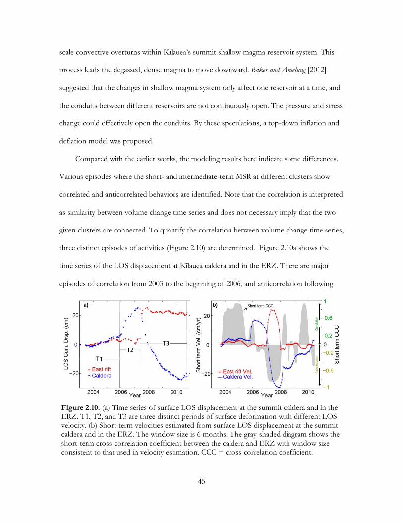
45

scale convective overturns within Kīlauea’s summit shallow magma reservoir system. This

process leads the degassed, dense magma to move downward. Baker and Amelung [2012]

suggested that the changes in shallow magma system only affect one reservoir at a time, and

the conduits between different reservoirs are not continuously open. The pressure and stress

change could effectively open the conduits. By these speculations, a top-down inflation and

deflation model was proposed.

Compared with the earlier works, the modeling results here indicate some differences.

Various episodes where the short- and intermediate-term MSR at different clusters show

correlated and anticorrelated behaviors are identified. Note that the correlation is interpreted

as similarity between volume change time series and does not necessary imply that the two

given clusters are connected. To quantify the correlation between volume change time series,

three distinct episodes of activities (Figure 2.10) are determined. Figure 2.10a shows the

time series of the LOS displacement at Kīlauea caldera and in the ERZ. There are major

episodes of correlation from 2003 to the beginning of 2006, and anticorrelation following

Figure 2.10. (a) Time series of surface LOS displacement at the summit caldera and in the ERZ. T1, T2, and T3 are three distinct periods of surface deformation with different LOS velocity. (b) Short-term velocities estimated from surface LOS displacement at the summit caldera and in the ERZ. The window size is 6 months. The gray-shaded diagram shows the short-term cross-correlation coefficient between the caldera and ERZ with window size consistent to that used in velocity estimation. CCC = cross-correlation coefficient.

46

the Father’s Day event. Prior to the Father’s Day event, Kīlauea’s summit uplifts and shows

a positive correlation to the ERZ. Following the Father’s Day event, the zones were

anticorrelated and rapid rift extension coincided with a rapid collapse of the summit.

Afterward, Kīlauea’s summit continued to subside until mid-2010 with negligible

deformation in the ERZ. However, there are subtler transient periods of correlated behavior.

Figure 2.10b shows the short-term linear velocities estimated within a moving 6 month time

window, as well as the cross-correlation coefficients between the caldera and rift zone within

this moving window. The short-term correlation indicates various episodes of correlated and

anticorrelated deformation between the summit and ERZ. Based on Figure 2.10, the time

series of the volume changes at all clusters are divided into three periods. Then in each

period the intermediate-term correlation coefficient between every two time series and the

standard deviation of the short-term correlation (Figure A.10) are calculated. The

intermediate-term correlation indicates a similarity between two clusters over a relatively

long period of time, and the standard deviation determines how it temporally varies. During

the first period (2003/01/27–2005/11/23), Clusters #2 and #6 are correlated with each

other. The rest of the clusters correlate mutually and are anticorrelated with Clusters #2 and

#6. The most significant standard deviation is observed between Cluster #1 and all others,

suggesting that other clusters experience a more temporally variable volume change

compared to that of Cluster #1. During the second (2005/11/23–2007/05/21) and third

(2007/05/21–2010/10/13) periods, Clusters #2 and #5 are correlated but are anticorrelated

with the rest. The standard deviation of short-term correlation between Cluster #1 and

Clusters #5 & #6 are higher during the second period, suggesting a more transient behavior

of volume changes for clusters #5 & #6. However, during the third period, the standard

deviations between Cluster #1 and Clusters #2, #3, & #4 are much smaller than that

47

between Cluster #1 and Clusters #5 & #6, indicating that Clusters #2, #3, & #4 undergo

very tiny transient volume changes over this period. Clusters #1, #3, & #4 are mutually

correlated and are anticorrelated with Cluster #2 throughout all three time periods. For the

first period, Cluster #2 correlates with Cluster #6 and anticorrelates with Cluster #5. For the

following two periods this relation reverses, meaning that Cluster #2 correlates with Cluster

#5 and anticorrelates with Cluster #6. This correlation analysis suggests that different

clusters are spatially connected, as shown in Figure 2.9.

2.6.4 Other Implications

Earlier works established links between magmatic activity at Kīlauea’s summit and

seismicity and rift eruptions. The time-dependent source model of Kīlauea’s summit

presented here can be used to further explain the rift intrusions and seismicity along them.

To this end, the concept of stress transferring is used. The normal stress change in the ERZ

is calculated using a compression negative convention due to the volume change within the

summit reservoir. The distribution of the normal stress rate in the ERZ is shown in Figures

2.11a–2.11c for three time periods, as identified in Figure 2.10a. During the first period

(2003/01/27–2005/11/23), when Kīlauea caldera is characterized by a slow rate of volume

change (Figure 2.11a), the imparted normal stress in the ERZ is minor. During the second

period (2005/11/23–2007/05/21), the maximum inflation rate occurs beneath the caldera

(Figure 2.11b), and the normal stress increases significantly across the rift zone, unclamping

the ERZ. The increased normal stress culminates during the Father’s Day event in June 2007

and then begins to diminish toward end of the observation period. During the third period

(2007/05/21–2010/10/13), the rate of volume change beneath the caldera is negative

(Figure 2.11c). Consequently, the imparted normal stress is negative, and thus it helps to

48

clamp the rift zone and possibly stop the intrusion. Figure 2.11d shows the temporal

evolution of normal stress history on the ERZ as well as the cumulative volume change

beneath Kīlauea caldera where positive values of stress indicate unclamping of the rift zone.

During the process of magma intrusion to rift zones, elevated number of

microearthquakes is observed along the path of magma flow. The model suggests the link

Figure 2.11. (a–c) Volume change rate distribution and associated normal stress rate distribution on the ERZ for three time periods (T1, T2, and T3 as seen in Figure 10a). For volume change rate: blue, deflation; red, inflation. For stress rate distribution: blue, clamping; red, unclamping. (d) The time series of source volume change and normal stress on the ERZ.

between seismicity and magmatic activity at the summit reservoir. The catalog of relocated

earthquakes at Kīlauea used here is provided by Lin et al. [2014], spanning a period of from

1992 to 2009 and including 25,705 events. The earthquakes that occurred near the summit

49

during the period covered by the InSAR observations are selected. Two distinct periods of

inflation (2003/01/27–2007/05/21) and deflation (2007/05/21–2010/10/13) are

considered according to the surface deformation data and the ERZ and SWRZ geometries

are used as receiver faults. The Coulomb failure stress change (∆𝐶𝐶𝐶𝐶𝑆𝑆) [King et al., 1994] in

the crust is estimated using the estimated volume change distribution at each time step.

∆𝐶𝐶𝐶𝐶𝑆𝑆 = ∆𝜏𝜏 − 𝜇𝜇∆𝜎𝜎𝑛𝑛, where ∆𝜏𝜏 is the shear stress change, 𝜇𝜇 is the frictional coefficient, and

∆𝜎𝜎𝑛𝑛 is the normal stress change. A friction coefficient of 0.4 is used. The estimated ∆𝐶𝐶𝐶𝐶𝑆𝑆

and the distribution of earthquakes are shown in Figure 2.12. For the inflation period

(Figures 2.12a and 2.12b), most earthquakes along the SWRZ and ERZ receive

Figure 2.12. Coulomb stress change rate distributions for two preferred fault geometries, during two periods. (a) Inflation period and SWRZ receiver. (b) Inflation period and ERZ receiver. (c) Deflation period and SWRZ receiver. (d) Deflation period and ERZ receiver. Dips for both receiver faults are set to be 90 °. Black dots are microearthquakes.

50

positive ∆𝐶𝐶𝐶𝐶𝑆𝑆, suggesting that magmatic activity enhanced the occurrence of earthquakes.

However, during the deflation period (Figures 2.12c and 2.12d), most earthquakes were

located within zones of negative ∆𝐶𝐶𝐶𝐶𝑆𝑆, which suggests they are not triggered by magmatic

activities. These earthquakes are located within a narrow zone near Halemaʻumaʻu, at a

depth range from 0 to 2 km and occurred during 2008–2009 (Figure 2.6h). These

earthquakes are likely to be associated with the summit eruption. One possible explanation is

that volume loss at the reservoir following the Father’s Day event resulted in magma

degassing, which in turn opened the Halemaʻumaʻu Crater in 2008, causing the summit

eruption.

2.7 Conclusions

A novel geometry-free time-dependent modeling scheme is proposed to invert InSAR

deformation data for the magmatic source beneath Kīlauea’s summit during 2003–2010. The

modeling scheme considers a 3-D array of PCDs and solves for the time series of the

distributed volume change at the center of PCDs. Application of principal component

analysis to this time-dependent model identifies six independent zones of magmatic

activities. Temporal analysis of the volume changes for these reservoirs indicates a more

complex relation throughout Kīlauea’s summit reservoir. The data and model results

enhance the understanding of magma storage, transport, and supply at Kīlauea’s summit and

quantify the relation between magmatic activities at the summit to the rift eruption and

seismicity.

51

CHAPTER 3

3-D MODELING OF IRREGULAR VOLCANIC SOURCES USING SPARSITY-

PROMOTING INVERSIONS OF GEODETIC DATA AND BOUNDARY ELEMENT

METHOD

The work presented in this chapter has been published as: Zhai, G., and Shirzaei, M. (2017),

3‐D Modeling of Irregular Volcanic Sources Using Sparsity‐Promoting Inversions of

Geodetic Data and Boundary Element Method. Journal of Geophysical Research: Solid Earth 122,

10,515-10,537, doi: 10.1002/2017JB014991.

3.1 Abstract

Geodetic observations of surface deformation associated with volcanic activities can be

used to constrain volcanic source parameters and their kinematics. Simple analytical models,

such as point and spherical sources, are widely used to model deformation data. The

inherent nature of oversimplified model geometries makes them unable to explain fine

details of surface deformation. Current nonparametric, geometry-free inversion approaches

resolve the distributed volume change, assuming it varies smoothly in space, which may

detect artificial volume change outside magmatic source regions. To obtain a physically

meaningful representation of an irregular volcanic source, a new sparsity-promoting

modeling scheme is devised assuming active magma bodies are well-localized melt

accumulations, namely, outliers in the background crust. First, surface deformation data are

inverted using a hybrid L1- and L2-norm regularization scheme to solve for sparse volume

change distributions. Next, a boundary element method is implemented to solve for the

displacement discontinuity distribution of the reservoir, which satisfies a uniform pressure

52

boundary condition. The inversion approach is thoroughly validated using benchmark and

synthetic tests, of which the results show that source dimension, depth, and shape can be

recovered appropriately. This modeling scheme is applied to deformation observed at

Kilauea summit for periods of uplift and subsidence leading to and following the 2007

Father’s Day event. The magmatic source geometries for these periods are statistically

distinct, which may be an indicator that magma is released from isolated compartments due

to large differential pressure leading to the rift intrusion.

3.2 Introduction

Repeated intrusions and emplacements of magma underneath active volcanoes lead to

the formation of a magma chamber [Fiske and Kinoshita, 1969]. Acting as a melt repository, its

shape evolves gradually through internal mechanical–chemical processes and interactions

with crustal host rocks [Dufek et al., 2013; Gudmundsson, 1990]. Although the shape of a

shallow magma chamber cannot be highly irregular based on thermal and mechanical

stability considerations [Gudmundsson, 1990], its actual shape, size, and temporal evolution are

not entirely known [Marsh, 2015]. Except for small lens-shaped magma chambers that are

mostly molten during their early stages, the majority of magma chambers is partially molten

with low melt fractions and composed mostly of crystal-rich mushes in a suprasolidus state

[Marsh, 1981]. The widely used analytical models of the magma chamber, however, assume

that the chamber is entirely molten with uniform internal pressure [e.g., Davis, 1986; Mogi,

1958; Yang et al., 1988]. Moreover, the excess pressure in magmatic bodies inferred from

these analytical models can be orders of magnitude larger than the solid host rock tensile

strength of <10 MPa even when the source dimension is well constrained independently

[Beauducel et al., 2004; Gudmundsson, 2008]. Owing to their symmetric shape and uniform

53

internal pressure, such models predict a symmetric stress field, in contrast to indirect

observations of a heterogeneous stress field adjacent to magma chambers from surface

fissure orientations and fracture patterns [Chadwick and Dieterich, 1995; Gudmundsson, 2008].

Therefore, the ability to constrain a realistic shape of a magma chamber and its evolution in

time and space improves the estimates of the stress field. This leads to better forecast

models predicting the time and location of chamber rupture, dike intrusions, volcanic

eruptions, and caldera formations [Gudmundsson, 2008].

Most processes associated with magma chambers can only be studied indirectly using

geodetic and geophysical methods. While seismic tomography has been widely used to

measure heterogeneous properties of magmatic plumbing systems, due to low spatial

resolution [e.g., ray coverage; Lees, 2007], its application for studying shallow magma

chambers is limited. Moreover, seismic imaging does not constrain excess pressure of the

magma chamber. On the other hand, geodetic measurements of surface deformation with

high spatiotemporal resolution may provide crucial information to illuminate the geometries

and internal processes of shallow magmatic systems.

Figure 3.1 sketches a simple magmatic system that deforms as a result of inflation and

deflation of a magmatic reservoir. Due to the scarcity of direct observations of volcanic

processes responsible for surface deformation at depth, mathematical models provide the

linkage between surface deformation and the inaccessible source [Lisowski, 2007]. Following

the first application of a point dilatational source to interpret surface deformation at Kilauea

[Mogi, 1958], many other analytical models have been proposed to explain observations of

spatial and temporal surface deformation at volcanos [Bonaccorso and Davis, 1999; Davis, 1983,

1986; Fialko et al., 2001; McTigue, 1987; Okada, 1992; Yang and Davis, 1986; Yang et al., 1988].

Typical analytical models can often explain the first-order surface deformation pattern and

54

allow for constraining the average depth of the magma chamber. These models fail to

explain the high-order complexities of surface deformation, primarily due to

oversimplification of the model geometry. Numerical modeling approaches, such as finite

element methods (FEMs), are capable of accounting for arbitrary chamber shape and size

[Ronchin et al., 2013]. These models consider 3-D heterogeneous medium properties and

irregular surface relief [Trasatti et al., 2003], but in most current applications, they assume a

fixed geometry provided by prior simple analytical solutions [Bonaccorso et al., 2005; Masterlark

et al., 2012; Trasatti et al., 2005]. In addition, using FEM to invert for model geometry is

computationally expensive, as it requires iteratively remeshing the model space and

numerically evaluating stress tensors [Masterlark et al., 2012]. This limitation could be

resolved by incorporating a mesh-independent deformation source into FEM [Charco and del

Sastre, 2014], yet this method relies on a priori source shape to resolve source geometrical

parameters and strength.

Figure 3.1. Schematics showing a simple volcanic system with (left) inflation and (right) deflation behaviors.

Magma chambers also contain chemically distinct, partially molten melts or crystal

mushes, which leads to the formation of porous rocks and isolated magma compartments

with nonuniform pressure distribution [De Natale and Pingue, 1992, 1996; De Natale et al.,

1991; Gudmundsson, 2012]. Yet again, analytical models do not account for these complexities.

55

To overcome these limitations, some researchers consider a combination of elementary

sources to model deformation data to account for chamber heterogeneities as well as

investigate chamber shape irregularity without assuming a priori source geometry. Vasco et al.

[1988] divided the source region into three-dimensional cells and used a linear inversion of

surface deformation data at Long Valley to model the 3-D distribution of volumetric strain.

They identified zones of high volumetric strain consistent with results from seismic imaging.

Mossop and Segall [1999] used a similar approach to explain leveling and GPS data at the

Geyser geothermal field in northern California. Masterlark and Lu [2004] extended the

concept of the three-dimensional source array and attempted to identify source clusters for

Seguam Island. D'Auria et al. [2012] investigated 4-D volcanic source beneath Campi Flegrei

caldera through inversion of InSAR to map volumetric strain distribution. Zhai and Shirzaei

[2016] investigated the Kilauea volcano magmatic system using a time-dependent modeling

scheme combined with volume change distribution inversion. The strategy of combining 3-

D source array inversion with FEM-based numerical models is a challenge to acquire an

amorphous source distribution due to the significant computing load required for remeshing

the medium for each source. However, remeshing can be avoided by using an array of cubic

elements as a static, unchangeable mesh [Ronchin, 2015; Trasatti et al., 2008].

Although geometry-free modeling schemes are successful at constraining distributed

volumetric strain and illuminating zones of deformation, these models fail to (1) resolve the

actual shape and size of the source, (2) constrain the average excess pressure of the

magmatic source, and (3) fulfill the uniform pressure boundary condition [Segall, 2010].

Here a nonparametric, geometry-free kinematic inverse modeling scheme is proposed.

The deformation source comprises distributed point centers of dilatations (PCDs; see

section 3.3.1). A nonparametric modeling method relates surface deformation to model

56

parameters through superposition of elementary sources. A sparsity-promoting inversion

scheme is used to image the magmatic source’s irregular geometry. For such models of the

magmatic body to also fulfill the uniform pressure boundary condition, distributed force

dipoles are needed. Otherwise, the resolved excess pressure is nonphysical. Thus, to fulfill

the required boundary conditions, the source geometry fixed by implementing the sparsity-

promoting inversion is used and a boundary element method (BEM) is applied. The

displacement discontinuity distribution on the surface of the chamber and its internal excess

pressure are solved for, considering no shear traction on the surface of the chamber and that

tensile stress is equal to the excess pressure. This method is validated through benchmark

and synthetic tests and then applied to two episodes of deformation at Kilauea volcano,

including the uplift period from December 2005 to May 2007 and the subsidence period

from May 2007 to May 2010.

3.3 Method

3.3.1 Distributed PCDs as Volcanic Deformation Source

In this section, the formula of the forward model, which relates volcanic surface

deformation to its source that comprises distributed PCDs characterized by volume changes,

is first derived. This forward model is benchmarked through comparison with independent

volcanic deformation models.

3.3.1.1 Surface Deformation Due to Volume Change Distribution

Relating the volume change at depth to the surface deformation, a volume integral

derived from Volterra’s formula [Vasco et al., 1988] is used. Assuming linear elasticity and

finite volume of fluid source, the relationship between stress-free volumetric strain θ𝑇𝑇(𝛏𝛏) at

57

3-D location 𝛏𝛏 inside a finite source with volume of V and surface deformation 𝑢𝑢𝑖𝑖(𝒙𝒙) in the

𝑖𝑖th direction at surface location 𝒙𝒙 is given by

𝑢𝑢𝑖𝑖(𝒙𝒙) = � θ𝑇𝑇(𝛏𝛏)𝑘𝑘𝑖𝑖(𝒙𝒙,𝛏𝛏) 𝑑𝑑𝑉𝑉, 𝑖𝑖 = 1, 2, 3

𝑉𝑉 (𝛏𝛏∈V) (3.1)

where 𝑘𝑘𝑖𝑖(𝒙𝒙, 𝛏𝛏) is the directional Green’s function in half space [Maruyama, 1964; Vasco et al.,

1988]:

𝑘𝑘𝑖𝑖(𝒙𝒙, 𝛏𝛏) = 1 + 𝜐𝜐

3𝜋𝜋 𝑆𝑆

𝑆𝑆 =𝑥𝑥𝑖𝑖 − ξ𝑖𝑖

((𝑥𝑥1 − ξ1)2 + (𝑥𝑥2 − ξ2)2 + (𝑥𝑥3 − ξ3)2)32

(3.2)

where 𝜐𝜐 is Poisson’s ratio. Note that this Green’s function is under stress-free condition and

a scale factor is needed to describe volumetric strain under stressed condition (e.g.,

confinement from surroundings). The scale factor can be determined using the relation

between stress-free (𝜖𝜖𝑇𝑇) versus stressed (𝜖𝜖) dilatational strains of the finite source [Eshelby,

1957]. This relationship is given by Rudnicki [2002] under the condition that the diameter of

reservoir is much smaller than its depth;

𝜖𝜖(𝑿𝑿) = −1

4𝜋𝜋 1 + 𝜐𝜐

3(1− 𝜐𝜐) 𝜖𝜖𝑇𝑇 Δ𝑞𝑞

𝑞𝑞 = �1𝑟𝑟 𝑑𝑑𝑉𝑉

𝑉𝑉

(3.3)

where Δ is a Laplacian operator, 𝑞𝑞 is the ordinary Newtonian potential for unit density filling

the finite source volume, and 𝑟𝑟 is the distance between observation point 𝑿𝑿 in medium and

differential volume 𝑑𝑑𝑉𝑉. Here 𝑿𝑿 should be located inside 𝑉𝑉 if one wants to calculate the

strain state of the finite source, then Δ𝑞𝑞 = −4𝜋𝜋 based on Poisson’s equation [Hofmann-

Wellenhof and Moritz, 2005]. Thus,

58

𝜖𝜖𝜖𝜖𝑇𝑇 =

1 + 𝜐𝜐3(1 − 𝜐𝜐) (3.4)

This factor is shape-independent when the diameter of the reservoir is much smaller

than its depth, which means the reservoir is equivalent to an isotropic point source.

Combining equations (3.1) and (3.4), stress-free volumetric strain is replaced with the

stressed version (θ):

𝑢𝑢𝑖𝑖(𝒙𝒙) = � θ(𝛏𝛏)𝐾𝐾𝑖𝑖(𝒙𝒙, 𝛏𝛏) 𝑑𝑑𝑉𝑉

𝑉𝑉 (𝛏𝛏∈V) (3.5)

where 𝐾𝐾𝑖𝑖(𝒙𝒙, 𝛏𝛏) = 𝑘𝑘𝑖𝑖(𝒙𝒙, 𝛏𝛏) 3(1−𝜐𝜐)1+𝜐𝜐

= 1−𝜐𝜐𝜋𝜋𝑆𝑆. This Green’s function under stressed conditions

is identical to that of Mossop and Segall [1999]. Equation (3.5) indicates that the surface

deformation due to an arbitrary-shaped source is an integration of volumetric strain scaled

with stressed Green’s function over the volume of the finite source. The stressed condition

can be accounted for by applying a similar type of scaling factor to the Green’s function

presented in other studies, which can also be used for calculating source volume change

without altering source shape [Lu et al., 2002; Masterlark and Lu, 2004; Vasco et al., 2007; Vasco

et al., 2002].

Next step is to divide 𝑉𝑉 into n volume cells 𝑉𝑉𝑚𝑚 (m = 1, 2, … , n). Assuming uniform

volumetric strain θ𝑚𝑚 within each volume cell, equation (3.5) can be rewritten as

𝑢𝑢𝑖𝑖(𝒙𝒙) = � θ𝑚𝑚 � 𝐾𝐾𝑖𝑖(𝒙𝒙, 𝛏𝛏) 𝑑𝑑𝑉𝑉𝑚𝑚

𝑉𝑉𝑚𝑚 (𝛏𝛏∈𝑉𝑉𝑚𝑚)

𝑛𝑛

𝑚𝑚=1

= ∑ θ𝑚𝑚𝐾𝐾𝑖𝑖(𝒙𝒙, 𝛏𝛏𝑚𝑚) 𝑉𝑉𝑚𝑚𝑛𝑛𝑚𝑚=1

= ∑ Δ𝑉𝑉𝑚𝑚 𝐾𝐾𝑖𝑖(𝒙𝒙, 𝛏𝛏𝑚𝑚)𝑛𝑛𝑚𝑚=1

(3.6)

59

where ∫ 𝐾𝐾𝑖𝑖(𝒙𝒙, 𝛏𝛏) 𝑑𝑑𝑉𝑉𝑚𝑚 𝑉𝑉𝑚𝑚 (𝛏𝛏∈𝑉𝑉𝑚𝑚) = 𝐾𝐾𝑖𝑖(𝒙𝒙, 𝛏𝛏𝑚𝑚) 𝑉𝑉𝑚𝑚 and 𝛏𝛏𝑚𝑚 is the center location of the mth

cell. This is justified considering that every cell is small enough and equivalent to an isotropic

point source. Also, using a FEM simulation, Ronchin [2015] showed that a cell half the size of

its depth is equivalent to an isotropic point source at the cell center with error ~2% in

predicted InSAR line of sight (LOS) displacement. Δ𝑉𝑉𝑚𝑚 = θ𝑚𝑚𝑉𝑉𝑚𝑚 is the volume change of

the mth source cell under stressed conditions. Equation (3.6) indicates that a finite reservoir

with an arbitrary shape can be approximated by a superposition of spatially distributed

PCDs. Note that equation (3.6) neither requires a constant pressure boundary condition on

the surface of a chamber nor satisfies this condition [Segall, 2010].

3.3.1.2 Benchmark Test

To numerically test the validity and applicability of the proposed forward model

(equation (3.6)), several benchmark tests are implemented as a reference, considering

solution of pressurized prolate spheroid [Yang et al., 1988] widely used for modeling volcanic

deformation [e.g., Lundgren et al., 2015; Tiampo et al., 2000] and numerical solution of

pressurized oblate spheroid obtained from BEM. Four different prolate spheroids are tested

with fixed vertical semiaxes of 3 km and horizontal semiaxis of 0.5 km, 1 km, 1.5 km, and 3

km, and two different oblate spheroids with fixed horizontal semiaxis of 3 km and vertical

semiaxis of 1.5 km and 0.5 km. The uniform pressure on the surface of each spheroid is 8

MPa, and the depth to the center of each spheroid is 6 km. The shear modulus and Poisson

ratio of the elastic half-space medium are 20 GPa and 0.25, respectively. For the purpose of

comparison, the total (stress-free) volume change associated with the spheroid and the

equivalent distribution of PCDs are identical. The volume change of a prolate spheroid is

calculated using transformation strain after Eshelby [1957] and volume–pressure relationship

60

[Segall, 2010]. Due to the inherent nonuniqueness of the volume change distribution

estimated using PCD arrays, the PCD distribution that best fits the prolate spheroid results

in terms of least-squares is considered to be the optimal representation of the prolate

spheroid. For the case of an elongated spheroid with an aspect ratio of 6 (Figure 3.2a), the

agreement between surface displacement associated reference model and that of PCDs is

Figure 3.2. Benchmark tests for prolate and oblate spheroid sources. (a–d) Comparison between displacements associated with a prolate spheroid [Yang et al., 1988] with aspect ratios of (a) 6.0, (b) 3.0, (c) 1.5, (d) 1.0, and the equivalent model comprising distributed PCDs. (e, f) Comparison between displacements associated with an oblate spheroid obtained from BEM with aspect ratios of (e) 2.0 and (f) 6.0, and the equivalent model comprising distributed PCDs. All prolate and oblate spheroids have a fixed depth of 6 km and uniform pressure of 8 MPa.

fair, although the distributed PCDs overestimate vertical and underestimate horizontal

displacements in the near field. As for the prolate with aspect ratios of 1–3 (Figures 3.2b–

3.2d) and oblate spheroids with aspect ratios of 2 and 6 (Figures 3.2e and 3.2f), the

agreement between results from distributed PCDs and that of the reference model is

satisfactory. The benchmark tests indicate that the smaller the aspect ratio of the volcanic

source, the better the performance of distributed PCDs to represent surface displacement

61

field. It also highlights that this modeling approach shall not be used for interpreting

deformation associated with conduits.

3.3.2 Magmatic Deformation Source Modeling

Although distributed point sources show great success in modeling volcanic processes

[D'Auria et al., 2012; Masterlark and Lu, 2004; Mossop and Segall, 1999; Ronchin, 2015; Trasatti et

al., 2008; Vasco et al., 2007; Vasco et al., 1988; Vasco et al., 2002; Zhai and Shirzaei, 2016], they

provide very limited information about the physics of a magma chamber as a finite body

with an irregular shape. For instance, the volume change associated with distributed point

sources does not correspond to a uniform pressure boundary condition, which is required

for a finite source [Segall, 2010]. To overcome this limitation and obtain a finite source with

irregular shape that satisfies the boundary conditions, a modeling scheme that consists of

two main steps is proposed: (1) Constrain the geometry of the magmatic source through a

sparsity-promoting inversion of surface deformation data and (2) apply BEM to estimate the

displacement discontinuity distribution and associated pressure change on a closed surface

approximating the circumference of the model geometry fixed in the previous stage.

3.3.2.1 Sparsity-Promoting Inversion for Source Geometry

3.3.2.1.1 Formulating Problem with Sparse Constraint

Following Zhai and Shirzaei [2016] and discretizing the 3-D medium into cubical cells

with center coordinates of {𝑋𝑋𝑖𝑖,𝑌𝑌𝑖𝑖 ,𝑍𝑍𝑖𝑖}, PCDs are assigned with volume changes of

𝒅𝒅𝒅𝒅 = [𝑑𝑑𝑑𝑑1, … , 𝑑𝑑𝑑𝑑𝑖𝑖, … , 𝑑𝑑𝑑𝑑𝑚𝑚]𝑇𝑇 , 𝑖𝑖 = 1, … ,𝑚𝑚 to each cell center, where 𝑚𝑚 is the number of

parameters. The relation between volume change distribution 𝒅𝒅𝒅𝒅 and surface LOS

deformation 𝐿𝐿 = �𝐿𝐿1 ⋯ 𝐿𝐿𝑗𝑗 ⋯ 𝐿𝐿𝑙𝑙�𝑇𝑇

, 𝑗𝑗 = 1, … , 𝑙𝑙 is formularized as

62

𝐿𝐿 = 𝐺𝐺𝒅𝒅𝒅𝒅 + 𝑒𝑒 (3.7)

where 𝑙𝑙 is the number of observations and 𝑒𝑒 is the vector of observation residuals. Within 𝐺𝐺,

the matrix of Green’s function, also commonly called the design matrix, each component on

row i and column j relates the ith source cell to the corresponding LOS deformation at the

jth observation point on surface and is computed using equation (3.6) and a unit range

vector of the SAR satellite.

Equation (3.7) is often solved by minimizing ‖𝐿𝐿 − 𝐺𝐺𝒅𝒅𝒅𝒅‖22, which requires a full ranked

design matrix 𝐺𝐺. Given that such design matrices are often poorly conditioned, namely, rank

is less than the number of unknowns [Bjerhammar, 1973], to obtain a unique and robust

solution, a penalty term 𝑝𝑝(𝒅𝒅𝒅𝒅) is introduced, which makes the solution feasible [Smith and

Coit, 1997]. Thus, the revised form of the objective function is

arg min 𝒅𝒅𝒅𝒅

‖𝐿𝐿 − 𝐺𝐺𝒅𝒅𝒅𝒅‖22 + 𝑝𝑝(𝒅𝒅𝒅𝒅) (3.8)

Tikhonov regularization presented by 𝜆𝜆2‖Γ𝒅𝒅𝒅𝒅‖22 is a popular penalty term [Tikhonov and

Arsenin, 1977]. 𝜆𝜆2 controls amount of penalty. Depending on the purpose of regularization,

Γ can be an identity matrix, gradient operator, or Laplacian operator, respectively, to acquire

minimally perturbed, flat (or zero gradient), and smooth solutions. An efficient way to solve

Tikhonov regularization is through the data augmentation approach [Golub and Van Loan,

2012]. Incorporating the penalty term, equation (3.8) is equivalent to solving the following

least-squares problem:

𝐿𝐿𝑎𝑎 = 𝐺𝐺𝑎𝑎𝒅𝒅𝒅𝒅 + 𝐸𝐸 (3.9)

where 𝐿𝐿𝑎𝑎 = [𝐿𝐿 , 0]𝑇𝑇 and 𝐺𝐺𝑎𝑎 = [𝐺𝐺 , 𝜆𝜆Γ]𝑇𝑇 are the augmented observation vector and the

design matrix, respectively, and 𝐸𝐸 = [𝑒𝑒 , 0]𝑇𝑇 is the observation residuals. The regularized

63

solution of equation (3.9) is given by (𝐺𝐺𝑎𝑎𝑇𝑇𝐺𝐺𝑎𝑎)−1𝐺𝐺𝑎𝑎𝑇𝑇𝐿𝐿𝑎𝑎. As shown in Figure 3.3a, all

components in the solution are nonzero for L2-norm penalty problem.

Figure 3.3. (a–c) Comparison of L2-, L1-, and L0-norm minimization in the two-dimensional (x, y) plane. The solid gray areas are the constraint regions. The blue ellipses are the contours of the residual sum of squares function. The constrained solution is defined by the red square (�̂�𝛽) at the intersection of the blue ellipse and the gray area. The black point depicts the least squares solution without constraint. The L1-norm minimization generally produces a sparse solution similar to L0-norm minimization. In this 2-D case, one of the components is exactly zero. (d, e) The (e) elastic-net ball with λ2/α = 0. 5, compared to the (d) L-1 ball. The curved surface (Figure 3e) encourages a grouping effect on strongly correlated variables.

In addition to the L2-norm penalty term, some other norms can be used to serve

particular purposes. For instance, at active volcanos, the zone of molten rock is often well

localized, and the geometrical and physical properties are distinct compared with host rock.

Thus, it is reasonable to seek an optimum solution to equation (3.7) that fulfills some

64

sparsity criterion, namely, only a small fraction of parameter vector is nonzero. One effective

penalty term to obtain a sparse solution is 𝑝𝑝(𝒅𝒅𝒅𝒅) = 𝛼𝛼‖𝒅𝒅𝒅𝒅‖0, where 𝛼𝛼 is the penalty factor

controlling the degree of sparsity. An L0-norm optimization problem (Figure 3.3c) is

nonconvex and is computationally expensive by an order 2𝑚𝑚, which is impractical when the

number of unknowns is large (e.g., 𝑚𝑚 > 20). Alternatively, one can use an L1-norm penalty

term (Figure 3.3b) [Figueiredo et al., 2007], which approximates properties of the L0 solutions

[Donoho, 2006a; Donoho, 2006b]. The broad applications of L1-norm based sparsity-

promoting optimization include data compression [Candes and Tao, 2006], digital image

processing for object recognition [Mutch and Lowe, 2006], digital signal processing for source

localization with sensor array [Malioutov et al., 2005], medical imaging [Lustig et al., 2007;

Winters et al., 2010], and geophysical inversions [Charléty et al., 2013; Evans et al., 2015; Evans

and Meade, 2012; Gholami and Siahkoohi, 2010; Yao et al., 2011; Yao et al., 2013]. The penalty

term associated with L1-norm regularization is of the form 𝑝𝑝(𝒅𝒅𝒅𝒅) = 𝛼𝛼‖𝒅𝒅𝒅𝒅‖1; thus, the

objective function in equation (3.8) is revised as

arg min 𝒅𝒅𝒅𝒅

‖𝐿𝐿 − 𝐺𝐺𝒅𝒅𝒅𝒅‖22 + 𝛼𝛼‖𝒅𝒅𝒅𝒅‖1 (3.10)

Minimization using an L1 penalty term is successfully used to recover sparse solutions;

however, when parameters are strongly correlated, it may fail to find the optimum sparse

solution, namely, the solution may become overly sparse [Zou and Hastie, 2005]. Figures 3.3b

and 3.3d show that for an L1 penalty problem, the optimal model has only one nonzero

component in the vector of model variables. This is because minimization with the L1

penalty always seeks the sparsest solution. To overcome this limitation, a combination of L1

and L2 penalty terms, so-called elastic net [Zou and Hastie, 2005], is commonly used:

arg min 𝒅𝒅𝒅𝒅

‖𝐿𝐿 − 𝐺𝐺𝒅𝒅𝒅𝒅‖22 + 𝜆𝜆2‖Γ𝒅𝒅𝒅𝒅‖22 + 𝛼𝛼‖𝒅𝒅𝒅𝒅‖1 (3.11)

65

where Γ is defined as Laplacian operator that is calculated using the finite-difference

approximation [Zhai and Shirzaei, 2016]. The great advantage of minimization with mixed

penalty regularization is that (1) the solution space is strictly convex, in contrast to that of

minimization using only an L1 penalty term and (2) it encourages a grouping effect, where

strongly correlated variables tend to be in or out of the model together. The elastic net

allows for selecting groups of correlated variables (Figure 3.3e), required by the L2-norm

penalty term while remaining sparse as dictated by the L1-norm penalty term. It can be

transformed to an equivalent minimization problem using L1 penalty term using the

notation of equation (3.9):

arg min 𝒅𝒅𝒅𝒅

‖𝐿𝐿𝑎𝑎 − 𝐺𝐺𝑎𝑎𝒅𝒅𝒅𝒅‖22 + 𝛼𝛼‖𝒅𝒅𝒅𝒅‖1 (3.12)

The objective function in equation (3.12) is known as Least Absolute Shrinkage and

Selection Operator and is also presented in the following form [Tibshirani, 1996]:

arg min 𝒅𝒅𝒅𝒅

‖𝐿𝐿𝑎𝑎 − 𝐺𝐺𝑎𝑎𝒅𝒅𝒅𝒅‖22 , 𝑠𝑠𝑢𝑢𝑠𝑠𝑗𝑗𝑒𝑒𝑠𝑠𝑠𝑠 𝑠𝑠𝑡𝑡 ‖𝒅𝒅𝒅𝒅‖1 ≤ 𝜏𝜏 (3.13)

Equations (3.12) and (3.13) are equivalent and the solutions coincide when parameters 𝛼𝛼 and

𝜏𝜏 are appropriately chosen [Van Den Berg and Friedlander, 2008]; however, implementing

equation (3.13) is more straightforward [Evans and Meade, 2012; Van Den Berg and Friedlander,

2008].

In equation (3.13), the tuning parameter 𝜏𝜏 can be approximated based on observed

surface deformation data. Assuming an elastic medium, the total volume change underneath

the surface is not model-dependent and is only a function of surface deformation [D'Auria et

al., 2012]. Geertsma [1973] uses nuclei theory to show that total volume change observed at

the Earth’s surface is 2(1− υ) times the volume change in a subsurface reservoir, which is

consistent to more recent results [Walsh, 2002]. The expression of total volume change

66

beneath the surface based on InSAR observation is given by Shirzaei et al. [2015]. Assuming

monotonic surface deformation, the only meaningful solutions are those of which volume

changes are pervasively positive or negative [De Natale and Pingue, 1992]. Thus, the total

volume change can be estimated by

‖𝒅𝒅𝒅𝒅‖1 = �� 𝑑𝑑𝑑𝑑𝑖𝑖𝑚𝑚

𝑖𝑖=1� = 𝑉𝑉𝑐𝑐 ,𝑉𝑉𝑐𝑐 = �

∬ 𝐿𝐿 𝑑𝑑𝑥𝑥𝑑𝑑𝑑𝑑 𝑅𝑅2

2(1− 𝜐𝜐)𝑠𝑠𝑧𝑧� (3.14)

where 𝐿𝐿 is LOS displacement, 𝜐𝜐 is the Poisson’s ratio with value set to be 0.25, and 𝑠𝑠𝑧𝑧 is the

vertical component of the unit range vector of the SAR satellite (~0.92 for Envisat). Due to

incompleteness of observed surface deformation and data noise, the calculated 𝑉𝑉𝑐𝑐 from

equation (3.14) may not be accurate, yet it serves an excellent starting point. Thus, using a

Pareto curve [Hennenfent et al., 2008; Van Den Berg and Friedlander, 2008] to find the best 𝜏𝜏

yielding optimal solution of equation (3.13), the possible value of 𝜏𝜏 within the following

range is systematically examined:

(1− ε)𝑉𝑉𝑐𝑐 ≤ 𝜏𝜏 ≤ (1 + ε) 𝑉𝑉𝑐𝑐 (3.15)

where ε is a value between 0 and 1. The tests indicate that this range is wide enough to

identify optimum 𝜏𝜏 in most cases.

3.3.2.1.2 Refining the Source Sparsity

Although by including an L2-norm penalty factor, a grouping effect is produced,

namely, it eliminates oversparse solutions, various selections of 𝜆𝜆 may result in artifacts

(small but nonzero values) in the sparse solution [Zou and Hastie, 2005]. To mitigate this

effect, a statistical framework is implemented to eliminate insignificant elements of the

solution vector, enhancing model sparsity while still explaining the observed surface

67

deformation. Assuming 𝒅𝒅𝒅𝒅� is the vector of optimum volume change distribution obtained

from equation (3.13), then

𝐿𝐿� = 𝐺𝐺𝒅𝒅𝒅𝒅� (3.16)

where 𝐿𝐿� is the predicted surface LOS displacement. By removing insignificant elements (i.e.,

setting them to be zero) in 𝒅𝒅𝒅𝒅� , the updated vector of volume changes 𝒅𝒅𝒅𝒅�′ and associated

predicted observation 𝐿𝐿�′ are obtained. Defining the residual vector 𝑟𝑟 = 𝐿𝐿� − 𝐿𝐿�′ and assuming

a normally distributed error, the variables 𝑟𝑟𝑖𝑖𝜎𝜎

, 𝑖𝑖 = 1, … ,𝑚𝑚, follow a standard normal

distribution 𝑁𝑁(0,1), where σ is the standard deviation of residuals, a function of observation

error and distribution and model setup. 𝑟𝑟𝑇𝑇𝑟𝑟𝜎𝜎2

follows a chi-square distribution (𝜒𝜒2) with 𝑛𝑛 −

𝑚𝑚 degrees of freedom. By specifying a significance level of 𝜗𝜗, the confidence interval of 𝑟𝑟𝑇𝑇𝑟𝑟

is given by

0 < 𝑟𝑟𝑇𝑇𝑟𝑟 < 𝜎𝜎2 𝜒𝜒𝑛𝑛−𝑚𝑚, 1−𝜗𝜗2 (3.17)

The elements in vector 𝑑𝑑𝑑𝑑� with absolute value close to zero are likely to be artifacts and thus

are set to zero. The goal is to eliminate as many as possible insignificant elements, while

maintaining that the residual vector satisfies equation (3.17).

Implementing this statistical framework to identify insignificant PCDs may introduce

some errors because the solution 𝒅𝒅𝒅𝒅� is an approximation of the optimum solution without

knowing the true sparse model. Therefore, an approach that iterates between estimating 𝒅𝒅𝒅𝒅�

through penalized least squares and refining the model sparsity through a statistical test is

proposed. Thus, the algorithm with 𝑘𝑘 iterations is designed as follows:

1. When 𝑘𝑘 = 0, obtain the initial solution 𝒅𝒅𝒅𝒅� (𝒌𝒌) using equation (3.13) and identify subset of

insignificant elements, 𝑺𝑺𝒅𝒅𝒅𝒅(𝒌𝒌) , using the statistical test provided in equation (3.17).

68

2. When 𝑘𝑘 > 0, solve the sparsity-constrained subject to

𝒅𝒅𝒅𝒅� (𝒌𝒌) = arg min 𝒅𝒅𝒅𝒅

‖𝐿𝐿𝑎𝑎 − 𝐺𝐺𝑎𝑎𝒅𝒅𝒅𝒅‖22 , 𝑠𝑠𝑢𝑢𝑠𝑠𝑗𝑗𝑒𝑒𝑠𝑠𝑠𝑠 𝑠𝑠𝑡𝑡 ‖𝒅𝒅𝒅𝒅‖1 ≤ 𝜏𝜏, 𝑺𝑺𝒅𝒅𝒅𝒅(𝒌𝒌−𝟏𝟏) = 0 (3.18)

The iterations stop once 𝑺𝑺𝒅𝒅𝒅𝒅 reaches the steady state, namely, the number of insignificant

PCDs remains constant with an increasing number of iterations, or 𝑘𝑘 reaches a specified

maximum number of iterations 𝑘𝑘𝑚𝑚𝑎𝑎𝑚𝑚 .

3.3.2.2 Solving for Source Strength and Displacement Discontinuity Distribution

A hybrid L1- and L2-norm regularization approach for inverting deformation data

allows for constraining a sparse model composed of the 3-D location, size, and irregular

geometry of the volcanic source. The irregular surface surrounding this sparse model can

also be used to develop a mesh with triangular elements [Beauducel et al., 2004; Maerten et al.,

2005]. This mesh represents the magma chamber as a closed surface, which can be used to

solve for the displacement discontinuity distribution to investigate the associated chamber

evolution assuming that the chamber surface is only affected by tensile tractions. The

triangular patches are assumed to be embedded in an elastic, isotropic, and homogeneous

half-space medium with zero tractions on the free surface and shear modulus and Poisson’s

ratio of 20 GPa and 0.25, respectively. To solve for the displacement discontinuity

distribution on the surface of the magma chamber, a BEM, which relates displacement

discontinuities to the boundary conditions on the surface of the magma chamber through

the coefficient matrix 𝐴𝐴 [Liu et al., 2011; Thomas, 1993], is implemented. More extensive

readings on this topic are referred to Gaul et al. [2003] and Liu [2009]. The coefficient matrix

is a function of source geometry and mechanical properties of the medium. The boundary

conditions include tensile traction equals a uniform pressure 𝑝𝑝 and shear tractions vanish on

69

each triangular patch. Thus, the primary unknown is 𝑝𝑝. However, due to approximation

errors, the source geometry determined in sparsity-promoting inversion may not be accurate

enough. Therefore, a scaling factor 𝛿𝛿 and three rigid shift parameters 𝑥𝑥𝑜𝑜, 𝑑𝑑0, and, 𝑧𝑧0, which

allow expanding/shrinking and translating the magmatic body, are additionally considered.

Given the triangular mesh 𝛤𝛤, the system of equations to be solved is

𝑇𝑇(𝑝𝑝) = 𝐴𝐴(𝛤𝛤, 𝜇𝜇, 𝜐𝜐, 𝛿𝛿,𝑥𝑥𝑜𝑜 ,𝑑𝑑0, 𝑧𝑧0)𝒔𝒔 (3.19)

where 𝒔𝒔 is the vector of displacement discontinuities including the tensile, strike, and dip

components of all triangles. 𝑇𝑇 is the traction vector containing only tensile tractions at each

triangle, which equals to pressure change 𝑝𝑝. 𝜇𝜇 and 𝜐𝜐 are shear modulus and Poisson’s ratio,

respectively.

In addition, to relate the displacement discontinuities to surface deformation, a solution

of triangular dislocations [Nikkhoo and Walter, 2015] is applied:

𝐿𝐿 = 𝐵𝐵(𝛤𝛤, 𝜐𝜐, 𝛿𝛿, 𝑥𝑥𝑜𝑜 ,𝑑𝑑0, 𝑧𝑧0)𝒔𝒔 (3.20)

where 𝐵𝐵 is the design matrix containing Green’s functions, which relates displacement

discontinuities on triangular patches to surface deformation projected onto the SAR satellite

LOS direction using a unit range vector. 𝐿𝐿 is the observed LOS surface displacement.

Equations (3.19) and (3.20) together form a system of nonlinear inverse problem with

five unknowns of 𝛿𝛿, 𝑥𝑥𝑜𝑜 ,𝑑𝑑0, 𝑧𝑧0, and 𝑝𝑝, which can be solved using a nonlinear optimization

method [Shirzaei and Walter, 2009]. To account for residual errors due to satellite orbit and

clock inaccuracy, the best-fitting plane is also solved for.

70

3.4 Algorithm Learning and Synthetic Test

Here the robustness of the presented approach for modeling irregular volcanic sources

is investigated. Given the difficulty of linearizing a sparsity-constrained inversion problem,

an analytical solution is unavailable, and using a conventional resolution matrix to assess

posterior errors is not feasible [Franklin, 1970; Menke, 1984]. Therefore, several synthetic

tests are performed. The checkerboard test is a widely used synthetic model to test the

performance of an inversion method, which is highly dependent on the pattern of the model

expected to retrieve [Lévěque et al., 1993]. Given that the presented inversion scheme is

designed to recover sparse models, the synthetic sources for simulating observation should

be sparse. Therefore, several complex sparse volcanic sources are simulated, and through

forward modeling, the associated surface deformation is calculated. This synthetic surface

deformation will then be inverted to solve for simulated volcanic sources.

Five synthetic sources with 3-D geometries are considered, including a sphere,

prolate ellipsoid, torus, and vertical and horizontal L shaped chambers (Figure 3.5), and

generate the associated LOS deformation fields at a resolution of 50 m. To invert the

simulated observations and recover the synthetic sources using the approach presented in

section 3.3.2.1, the model medium is discretized into cubic cells of 0.1 km dimension with a

PCD at the center of the cell. Moreover, before implementing the inversion, the parameters

of the inversion approach, which includes a smoothing factor 𝜆𝜆, tuning parameter 𝜏𝜏,

standard deviation σ, and iteration number 𝑘𝑘, need to be set up. To this end, the inversion

problem can be viewed as a mapping operator that projects observation L onto the

parameter space 𝒅𝒅𝒅𝒅 [Alpaydin, 2014]. This mapping operator, f(∙), returns the optimum

solution of the regularized inversion and has a generalized form of

71

𝒅𝒅𝒅𝒅 = f(L|𝜆𝜆, 𝜏𝜏, σ,𝑘𝑘) (3.21)

where the tuning parameter 𝜏𝜏 can be determined using a Pareto curve [Hennenfent et al., 2008;

Van Den Berg and Friedlander, 2008]. Considering the purpose of a synthetic test, the value of

𝜏𝜏 is initialized with the absolute value of volume change associated with each synthetic

model. The Laplacian operator, Γ, designed in the presented approach is used to stabilize the

inversion and enforce the grouping effect on model variables, and smoothing factor 𝜆𝜆 is

selected from an interval [0, 1]. To refine the model sparsity, a confidence level of 5% for 𝜗𝜗

is considered. The standard deviation of residuals, σ, can be estimated through rigorous

analysis of error variance–covariance propagation at each iteration 𝑘𝑘. However, a value

between 1 and 10% of the largest surface deformation yields reasonable results based on

many tests.

Here an iterative algorithm is implemented to identify optimum values of the

hyperparameters (so-called algorithm learning in Figure 3.4a). However, to reduce the

computation time, these parameters for one source is estimated and then investigation is

made to explore if these parameters can be directly used to recover other synthetic sources.

To this end, a spherical source is used as the reference and a standard Monte Carlo search

algorithm is applied to systematically examine the different combinations of

hyperparameters. It is found that 𝜆𝜆 = 10−4, 𝑘𝑘𝑚𝑚𝑉𝑉𝑥𝑥 = 5, and σ being 5% of the largest

surface deformation provide the best estimates of the reference source (Figure 3.5a). In the

following steps, the same hyperparameters are used to recover deformation sources

associated with a prolate ellipsoid, vertical L shape, horizontal L shape, and torus. There is

good agreement between synthetic and recovered sources (Figures 3.5b–3.5e), and the model

fit to simulated observations is reasonable (Figure B.1 in the appendix).

72

Figure 3.4. Workflow chart. Three modules are designed to implement the sparsity-promoting algorithm. Module (a): Using synthetic sources to learn the algorithm and show the performance of the inversion method. Module (b): Using a synthetic source referred to the real geographical location to calibrate the hyperparameters associated in the algorithm for inversion of the real data set. Module (c): Applying the calibrated hyperparameters and inversion method to real data.

To further investigate the effect of data noise on inversion results, the synthetic tests

are repeated using the sphere and vertical L shaped geometries, which were the most

challenging in previous tests, and 5% colored noise is added to the corresponding simulated

InSAR LOS deformation. Considering real case studies of InSAR observation (discussed

later) and the precision of multitemporal processing (~ 5 mm for displacement; Shirzaei et al.,

2015), 5% colored noise is chosen here to serve as lower bound to evaluate the performance

of the inversion method. The optimal hyperparameters 𝜆𝜆, 𝑘𝑘𝑚𝑚𝑉𝑉𝑥𝑥, and σ are found to be 0.3,

73

6, and 5% of largest deformation, respectively. Despite noisy observations, the source sizes

and shapes are well recovered

compared with the synthetic

geometries (Figure 3.6), and the

model fit to simulated data is

satisfactory (Figure B.2). Based on

these synthetic tests, it is

concluded that hyperparameters

are geometry-independent, as long

as the model resolution remains

similar and the same

hyperparameters can be used to

recover sources of different

geometries. Also, observation

noise affects the results, yet the

effect remains in the acceptable

range, as long as the majority of

systematic errors are removed

through proper filtering

techniques.

Figure 3.5. Algorithm learning using synthetic tests with five different shapes: (a) sphere, (b) prolate ellipsoid, (c) vertical L shape, (d) horizontal L shape, and (e) torus. (left panel) Zones of uniform volumetric strain. (right panel) Inverted volume change distribution. The model domain has dimensions of (–1, 1) km in east, (–1, 1) km in north, and (0.2, 1.6) km in depth. White lines mark the cross sections. Black circles and polygons show corresponding spatial extensions of synthetic

74

Figure 3.6. Synthetic tests considering data noise in the simulated LOS deformation using a sphere and vertical L shape in Figure 4. (a) Inverted volume change distributions for sphere. (b) Inverted volume change distributions for vertical L shape. White lines mark the cross sections. Black circles and polygons show corresponding spatial extensions of the synthetic sphere and vertical L shape sources.

3.5 Application to Kilauea Volcano

Kilauea on Hawaii Island is one of the most active volcanoes around the world, acting

as a natural laboratory for investigating subsurface volcanic processes associated with

basaltic magmatism due to its high frequency of magmatic intrusions and eruptions. The

volcanic tectonics of Kilauea are characterized by a 5 km wide summit caldera from which

two rifts originate to the southwest and east, forming narrow boundaries between the

northern stable sector of the Kilauea edifice and the mobile southern flank situated on a

subhorizontal fault system [Cayol et al., 2000]. Magma rising from a deep source [Gonnermann

et al., 2012; Wright and Klein, 2006] is thought to be stored in a shallow magma reservoir

[Baker and Amelung, 2012; Cervelli and Miklius, 2003; Delaney et al., 1990]. The shallow magma

reservoir is a key element of Kilauea’s plumbing system [Eaton and Murata, 1960], which acts

as a waypoint to feed rift zone intrusions [Montgomery-Brown et al., 2010] and sustain summit

eruptions [Carbone et al., 2013].

75

Kilauea hosts a long history of documented unrest. Eruptive activity was concentrated

at the summit caldera until 1955 when eruptions became more common in the east rift zone.

Notable eruptive episodes did occur from 1972 to 1974 [Lockwood et al., 1999] and from 1981

to 1983 [Klein et al., 1987] at the summit caldera. For the next 20 years, subsidence was the

predominantly observed deformation pattern at the summit area of Kilauea. Simultaneously,

the Pu’u O’o–Kupaianaha vents on the east rift zone experienced almost continuous

eruptive activities. Starting in late 2003, the summit deformation mode switched from

deflation to inflation [Miklius et al., 2005] due to a new surge of magma supply into shallow

magma plumbing system [Poland et al., 2012]. The summit inflation culminated in 2007,

followed immediately by a small fissure eruption on the east rift zone (called the Father’s

Day event) and by a summit eruption in Halemaumau crater in 2008 [Patrick et al., 2013].

After the inflation period, the summit deflated from 2007 until mid-2010, followed by

reinflation [Lundgren et al., 2013].

Previous geophysical and geochemical investigations including ground deformation,

seismicity, gravity, and isotopes mainly focused on different centers of inflation and deflation

associated with the Kilauea summit shallow reservoir [Baker and Amelung, 2012; Battaglia et al.,

2003; Cervelli and Miklius, 2003; Fiske and Kinoshita, 1969; Johnson et al., 2010; Lundgren et al.,

2013; Pietruszka et al., 2015; Yang et al., 1992]. The diversity of the source locations from

those results likely suggests complex magmatic reservoirs with irregular geometry beneath

Kilauea summit, given that different parts of a magma reservoir are active during distinct

time periods [Gudmundsson, 2012]. In order to investigate the source geometry, the presented

sparsity-promoting inversion approach is applied to InSAR LOS deformation observed at

Kilauea’s summit for two periods: 2005–2007 and 2007–2010. After determining source

geometry, the surface deformation is inverted to solve for the tensile displacement

76

discontinuity distribution on the periphery of the constrained source to examine the details

of the kinematics of the magma chamber. The results from this modeling method provide

additional insights into the dynamics of Kilauea’s summit reservoir.

3.5.1 Data Sets

The time series of surface deformation at the Kilauea volcano is generated using an

advanced multitemporal InSAR algorithm [Shirzaei, 2013; Shirzaei and Bürgmann, 2013; Shirzaei

et al., 2013] for the period 2003–2010. The SAR data set includes 100 images and 38 images

acquired in descending (track 200 and 429) and ascending (track 93) orbit of the Envisat

satellite. The details of processing and validation are provided in [Zhai and Shirzaei, 2016].

The effect of mobile southern flank on the surface deformation of both viewing geometries

is corrected using a long-term decollement slip model. The LOS velocity map and the time

series of the displacement field at a selected point inside the summit area for descending

orbit are shown in Figure 3.7. To implement the modeling scheme, two periods with rapid

changes in the pattern of observed surface deformation are selected (Figure 3.7b), including

the inflation period from December 2005 to May 2007 leading to the Father’s Day eastern

rift intrusion in July 2007 and the deflation period from May 2007 to May 2010 following the

event. The inflation period accumulated up to 25 cm and 23 cm of uplift in descending and

ascending viewing geometries, respectively, south of the Kilauea caldera (Figure B.4),

whereas during the deflation period, the location of maximum subsidence of 43 cm and 46

cm in descending and ascending viewing geometries, respectively, is at the southern rim of

the caldera (Figure B.5). The different patterns of deformation distribution may reflect

source geometrical complexities during the corresponding periods.

77

Figure 3.7. Descending InSAR processing result at Kilauea. (a) Velocity map of surface deformation along the LOS direction at the summit area. The effect of slip on decollement is removed from the InSAR time series. (b) Time series of LOS deformation for a selected point at the summit area. Rapid inflation and deflation periods are investigated.

3.5.2 Inversion Parameter Setup

To apply the presented inversion scheme to Kilauea deformation data, hyperparameters

𝜆𝜆, σ, and 𝑘𝑘 (Figure 3.4b) are first needed to be calibrated. As noted earlier, hyperparameters

are a function of the model resolution and observation quality but not a function of source

geometry. Therefore, a synthetic model is used to estimate optimal hyperparameters based

upon the actual model setup and observation locations at Kilauea. The model domain is set

to be a cuboid, with dimensions of ~14 km in east, ~17 km in north, and 6 km in depth,

which is discretized into 6,615 PCDs, with spacing of 0.8 km, 0.8 km, and 0.4 km in

respective directions. The effect of data gaps is considered and the actual distribution of

InSAR surface deformation data in descending orbit, as shown in Figure 3.7a, are used.

Using this model domain and observation locations, surface deformation (Figure 3.8a)

associated with a spherical zone of uniform volumetric strain with radius of 1.2 km and

center depth of 3 km (informed based upon previous studies) is simulated. To mimic a

realistic scenario, a colored noise with a standard deviation of 5 mm (Figure B.3), obtained

78

from comparing InSAR time series with independent observations [Shirzaei, 2015], is added.

Implementing the iterated approach shown in Figure 3.4a, different combinations of

hyperparameters are examined with variations of 𝜆𝜆 between 0 and 1, σ between 1% and 10%

of largest deformation, and 𝑘𝑘 between 1 and 20. The optimum parameters of 𝜆𝜆, σ, and 𝑘𝑘 are

0.2, 5%, and 8, respectively. Using these hyperparameters, the synthetic surface deformation

is inverted to solve for distribution of volume change (Figure 3.8b). Model prediction and

residuals are shown in Figures 3.8c and 3.8d. The other complex source geometries are also

successfully constrained using these hyperparameters, given the same model resolution,

observation distribution, and data noise at Kilauea. Therefore, these optimum values will be

used to inform the optimization algorithm (Figure 3.4c) for inverting actual surface

deformation observations during both uplift and subsidence periods at Kilauea.

Figure 3.8. Result of calibration test referred to Kilauea summit area using a synthetic spherical zone of uniform volumetric strain as the deformation source with a center depth of 3 km and radius of 1.2 km. (a) Simulated surface deformation from the synthetic spherical source. Colored noise is considered. (b) The inverted volume change distribution. (c) The predicted surface deformation from the inverted sparse model in Figure 8b. (d) Misfit of surface deformation (Figure 8a–8c).

79

3.5.3 Model Result

Using the optimized 𝜆𝜆, σ, and k, the initial value of tuning parameter 𝜏𝜏 for uplift and

subsidence periods is set up using equation (3.14), which is optimized with a Pareto curve

[Charléty et al., 2013; Hennenfent et al., 2008; Van Den Berg and Friedlander, 2008]. A Pareto curve

relates chi-square of misfit to the L1-norm of parameters, and the optimum value of 𝜏𝜏

corresponds to the location of maximum curvature on it. The Pareto curve is constructed by

investigating values adjacent to those obtained from equation (3.14), controlled by the

nondimensional parameter ε in equation (3.15). The choice of ε depends on the

characteristics of surface deformation, such as data noise, coverage, gaps, and spatial

resolution. For the case study, ε = 0.3 is an appropriate choice to acquire a typical Pareto

curve, as discussed below.

3.5.3.1 Uplift Period

Figure 3.9a shows the Pareto curve and the optimum value of 1.17 × 107 m3 for tuning

parameter 𝜏𝜏. Using the optimum hyperparameters, the inversion algorithm is implemented

to find the sparse model of an inflating magmatic source constrained by uplift data. Figure

3.9b shows the pattern of inverted sparse volume change distribution along three profiles.

The optimum model includes a concentrated zone of volume distribution south of the

summit caldera. The plan view shows that the body is pear-shaped with a tail stretching to

the upper seismic southwest rift zone. The observed and predicted LOS displacements for

both descending and ascending viewing geometries indicate good fits to the data (Figure

B.4). A slightly larger residual for the ascending data set can be due to the orbit of satellite

being perpendicular to the southwest rift zone, which degrades sensitivity of ascending

measurements to the rift-perpendicular displacements. Once the geometry and location of

80

Figure 3.9. Sparse models of volume change distribution from sparsity-promoting inversion for uplift and subsidence periods. The left panel shows the corresponding Pareto curves to identify the optimal tuning parameter 𝜏𝜏, and the right panel shows the inverted sparse volume change distributions in view of cross sections. (a) Pareto curve for uplift period. (b) Sparse model of uplift period. (c) Pareto curve for subsidence period. (d) Sparse model of subsidence period.

the magmatic source are constrained, it can be approximated as an enclosed triangular mesh

[Beauducel et al., 2004; Maerten et al., 2005], which has a volume of ~29.1 km3. Then the

displacement discontinuity distribution and pressure change are solved for using the BEM

modeling scheme discussed in section 3.3.2.2, which provides a more physical representation

of an inflating magma chamber under uniform pressure boundary conditions. The model fit

is shown in Figure B.6. The best fitting model has a Root Mean Square Error (RMSE) of 1.9

81

cm and 2.1 cm for descending and ascending data sets, respectively. The optimum pressure

change is 4.6 MPa inside the magmatic body. The magnitude of strike and dip components

are average less than 10% of the tensile component and are not discussed further. The

obtained tensile displacement discontinuity distribution on the triangular mesh is shown in

Figure 3.10a. It indicates that the magma body expands vertically at the top and bottom with

negligible expansion on its sides. The greatest openings happen at the top of the magma

body.

Figure 3.10. Tensile slip models from BEM modeling for (a) inflation and (b) deflation periods in side views. The shapes are generated to approximate the inverted sparse distribution of volume change associated with each time period. Blue triangles are seismicity during the corresponding time periods.

3.5.3.2 Subsidence Period

For the subsidence period, the Pareto curve (Figure 3.9c) indicates an optimal tuning

parameter of 1.44 × 107 m3. The inversion result of the volume change distribution is shown

in Figure 3.9d, which comprises a magmatic body of ~37.3 km3 volume. The data fit shown

in Figure B.5 presents a satisfactory agreement between observed and modeled displacement

fields. Profiles show that the constrained body is a NE–SW oriented, horizontal, prolate

ellipsoid extending from inside the caldera to the upper seismic southwest rift zone. The

82

tensile displacement discontinuity distribution from BEM modeling is shown in Figure 3.10b

and the optimum pressure change is –3.9 MPa. The optimal model has a RMSE of 2.7 cm

and 3.1 cm for descending and ascending data sets, respectively (Figure B.7). The tensile

displacement discontinuity model shows that closings happen at top and bottom of the body

with weak behavior along the sides.

3.6 Discussion

A two-step volcanic source modeling scheme that allows imposing a realistic pressure

boundary condition on an irregularly shaped magmatic body constrained based on the

geodetic observations is proposed. The first optional step is to apply an iterative sparsity-

promoting inversion approach to image irregular volcanic reservoirs based on ground

deformation data. This step is optional as one can instead use the source geometry

constrained using any other methods such as seismic tomography. Applying the method, the

algorithm hyperparameters are optimized using synthetic tests through an algorithm learning

procedure. The majority of hyperparameters including the smoothing factor, residuals

standard deviation, and iteration number are geometry-independent and only depend on

model resolution and distribution of surface deformation data. This allows for optimizing

hyperparameters through a limited number of synthetic tests and then using them for a wide

range of modeling exercises, as long as the model setup and observation distribution remain

unchanged. Once the irregular geometry of the magmatic source is constrained in the first

step (or obtained using other methods), in the second step a boundary element method is

applied to impose physical boundary conditions and solve for the uniform pressure inside

the reservoir. The entire procedure is thoroughly validated using several synthetic examples

and then applied to two episodes of rapid inflation and follow up deflation at Kilauea

83

volcano. To investigate real data sets, a similar concept is used and an additional calibration

step is applied to identify hyperparameters relevant to the model set up (dimension and

resolution) and distribution of deformation data.

3.6.1 Advances and Limitations of Two-Step Modeling

The presented inversion method can resolve the shape, size, and location of the

magmatic source associated with zones of volume change underneath volcanoes. However,

like other inversion methods its success depends on the quality and coverage of the surface

deformation data as well as the resolution that is allowed by the model for solving details of

the source geometry. The synthetic tests and real case studies, however, indicate several

advantages of the proposed method compared to other volcanic source inversion

techniques. For example, a source like a torus (or magma tube) is extremely hard to be

resolved using conventional inversion approaches. While the inversion method can

successfully resolve such geometries (Figure 3.5e). A major limitation of the PCD inversion

is its inability to reconstruct deformation associated with a dike. That is because a magma

overpressure within a dike can be approximated by a distribution of force couples

perpendicular to the dike surface, while PCD includes three mutually orthogonal double

forces. Although sill (horizontal dike) also consists of single double force, since the majority

of the signal is vertical, the reconstruction of the associated signal using PCD is satisfactory,

provided that the sill radius-to-depth ratio is sufficiently small. However, in most cases, dike

sources can be identified by their distinct surface deformation pattern, and thus, the

geometry can be constrained using a standard inversion technique, which can be used as an

input to the next inversion step. Once the geometry is constrained, a BEM approach is

applied to impose a realistic pressure condition and solve for uniform pressure inside the

84

magmatic body. Thus, in contrast to the analytical models [e.g., Davis, 1986; McTigue, 1987;

Mogi, 1958], the presented approach allows for constraining the actual shape and dimension

of the source.

Recently, major advances were made in investigating the physics of volcanic sources

[Anderson and Poland, 2016; Anderson and Segall, 2011]. Yet one major disadvantage of these

physics-based volcano source modeling techniques is the reliance on simple analytical

models. This limitation can be overcome by combining the physics-based inversion methods

with the approach presented here.

Figure 3.11. Schematic of magmatic source volume change represented as an enclosed tensile crack. The dashed line indicates the surface of the magma chamber. The inner wall of the crack moves from S to Sin. The outer wall of the crack moves from S to Sout. The volume change of crack ΔVcr is the sum of volume change caused by the inner wall and outer wall movements. The magma chamber volume change ΔVch is caused by the movement of the outer wall.

3.6.2 Implications for Volcanic Source Volume Change

Volume change within a magma body is regarded as the cause of surface deformation

and seismic signals. First order analytical models of magma chamber with simple geometries

[e.g., Davis, 1986; McTigue, 1987; Mogi, 1958] are widely applied to investigate surface

deformation at volcanoes and constrain the subsurface volume change. However, for more

complex source geometries, closed mathematical expressions are not available. An alternative

85

method was presented to model irregular volcanic sources through a two-step procedure,

which has the ability to constrain the irregular source geometry as an enclosed crack of

dislocation satisfying a uniform pressure boundary condition. The source volume change can

be estimated using a distribution of tensile crack openings and the surface area of the source.

Although the surface observation is well explained, interpreting the estimated volume change

is not trivial. Müller [2001] notices two different formulas for calculating seismic moment (M)

of an isotropic spherical/point source, 𝑀𝑀 = (λ + 2μ)∆𝑉𝑉𝑐𝑐ℎ and 𝑀𝑀 = (λ + 2μ/3)∆𝑉𝑉𝑐𝑐𝑟𝑟 ,

where λ and μ are the Lamé parameters and ∆𝑉𝑉 is volume change. The volume change, ∆𝑉𝑉,

in each formulation has different physical meanings, representing either the chamber

mechanical volume change (∆𝑉𝑉𝑐𝑐ℎ) or crack volume change (∆𝑉𝑉𝑐𝑐𝑟𝑟), respectively (Figure 3.11).

Crack volume change ∆𝑉𝑉𝑐𝑐𝑟𝑟 is the total volume change that resulted from a crack surface

moving inward and outward. Volume change defined using a crack dislocation model

corresponds to stress-free volume change [Eshelby, 1957] and provides the exact source

moment [Müller, 2001]. However, mechanical chamber volume change ∆𝑉𝑉𝑐𝑐ℎ, namely, the

actual change in the source volume under confining pressure, is defined by the chamber

surface moving outward, which is smaller than the crack volume change. This is due to the

fact that filling a crack requires no additional moment to push away surrounding medium

when the crack is thin [Wielandt, 2003]. The transformation from ∆𝑉𝑉𝑐𝑐𝑟𝑟 to ∆𝑉𝑉𝑐𝑐ℎ is dependent

on the shape of magma body. For isotropic sources, such as point source (the dimension is

small enough) and spherical source, the relation between ∆𝑉𝑉𝑐𝑐𝑟𝑟 and ∆𝑉𝑉𝑠𝑠𝑝𝑝ℎ is identical to

equation (3.4):

∆𝑉𝑉𝑐𝑐𝑟𝑟∆𝑉𝑉𝑠𝑠𝑝𝑝ℎ

=𝜆𝜆 + 2𝜇𝜇𝜆𝜆 + 2𝜇𝜇/3 =

3(1− 𝜐𝜐)1 + 𝜐𝜐 (3.22)

86

where 𝜆𝜆 and 𝜇𝜇 are Lamé constants. ∆𝑉𝑉𝑠𝑠𝑝𝑝ℎ is the volume change of a spherical chamber. For

a source with the geometry of a prolate ellipsoid, the chamber volume change ∆𝑉𝑉𝑝𝑝𝑟𝑟𝑜𝑜 lies

between ∆𝑉𝑉𝑐𝑐𝑟𝑟 and ∆𝑉𝑉𝑠𝑠𝑝𝑝ℎ , but closer to ∆𝑉𝑉𝑠𝑠𝑝𝑝ℎ , as concluded by Müller [2001] using a cylinder

approximation of a prolate ellipsoid. Thus, for a geometry-free volcanic source, the actual

chamber volume change (∆𝑉𝑉𝑐𝑐ℎ) is within the range determined by ∆𝑉𝑉𝑐𝑐𝑟𝑟 as the upper bound

and the equivalent volume change of a best approximating sphere as the lower bound

[Amoruso and Crescentini, 2009]. In practical applications, if the source shape is close neither to

a crack with tensile components nor to an isotropic inflation/deflation source, a range of

volume changes should be estimated. The lower limit ∆𝑉𝑉𝑠𝑠𝑝𝑝ℎ is readily calculated using upper

limit ∆𝑉𝑉𝑐𝑐𝑟𝑟 (equation (3.22)), then following inequality holds:

∆𝑉𝑉𝑐𝑐𝑟𝑟1 + 𝜐𝜐

3(1− 𝜐𝜐) ≤ ∆𝑉𝑉𝑐𝑐ℎ ≤ ∆𝑉𝑉𝑐𝑐𝑟𝑟 (3.23)

On the other hand and given the magma chamber compressibility, 𝛽𝛽𝑐𝑐ℎ, which is dependent

on shape and depth of magma chamber and host rock rigidity (𝛽𝛽ℎ𝑟𝑟 ; Amoruso and Crescentini,

2009; Rivalta and Segall, 2008; Segall et al., 2001), the exact value of ∆𝑉𝑉𝑐𝑐ℎ can be calculated

(Text B.1):

∆𝑉𝑉𝑐𝑐ℎ =∆𝑉𝑉𝑐𝑐𝑟𝑟

(1 + 𝛽𝛽ℎ𝑟𝑟/𝛽𝛽𝑐𝑐ℎ) (3.24)

The compressibility of a chamber with a complex geometry can be numerically computed

using a finite element method [Anderson and Segall, 2011]. However, the chamber

compressibility can be constrained by applying its definition when pressure change 𝑝𝑝 is

known:

∆𝑉𝑉𝑐𝑐ℎ𝑉𝑉 = 𝑝𝑝𝛽𝛽𝑐𝑐ℎ (3.25)

87

where 𝑉𝑉 is the source volume. Combining equations (3.24) and (3.25), then

𝛽𝛽𝑐𝑐ℎ =∆𝑉𝑉𝑐𝑐𝑟𝑟𝑉𝑉𝑃𝑃 − 𝛽𝛽ℎ𝑟𝑟 (3.26)

∆𝑉𝑉𝑐𝑐ℎ = ∆𝑉𝑉𝑐𝑐𝑟𝑟 − 𝑉𝑉𝑝𝑝𝛽𝛽ℎ𝑟𝑟 (3.27)

At Kilauea, the appropriate value of shear modulus for the host rock is 5–25 GPa

[Johnson et al., 2000]. Here a value of 20 GPa is used, which is consistent with laboratory

experiments using intact samples [Ryan, 1987a]. In the case studies, the crack volume

changes are 1.29 × 107 𝑚𝑚3 and 1.76 × 107 𝑚𝑚3 for the uplift and subsidence periods,

respectively. From equation (3.23), the chamber volume change for the uplift period is

between 0.72 × 107 𝑚𝑚3 and 1.29 × 107 𝑚𝑚3, while the range of chamber volume change

for the subsidence period is between 0.98 × 107 𝑚𝑚3 and 1.76 × 107 𝑚𝑚3. Moreover, given

equations (3.26) and (3.27), the exact values of estimated chamber volume changes for both

periods are 0.89 × 107 𝑚𝑚3 and 1.32 × 107 𝑚𝑚3, respectively. The chamber compressibilities

for both periods are 0.66 × 10−10 𝑃𝑃𝑉𝑉−1 and 0.91 × 10−10 𝑃𝑃𝑉𝑉−1, respectively.

3.6.3 Implications for Reservoir Storage Change

In complex volcanic settings, such as Kilauea, where the magma chamber is coupled

with the rift system [Segall et al., 2001], the typical movement of magma to the rift zone is

accompanied by dike intrusion [e.g., Lundgren et al., 2013; Montgomery-Brown et al., 2010].

Investigating the link between reservoir and rift requires implementing mass balance analysis,

constraining magma volume rather than chamber or crack volume. Thus, realistic estimates

of reservoir magma storage change are of great importance.

For volcanoes storing large amounts of magma in a reservoir, magma compression due

to slight pressure variations in the chamber from magma intrusions can amount to a

88

significant net volume change of stored magma. A parcel of magma (∆𝑉𝑉𝑚𝑚𝑎𝑎𝑚𝑚𝑚𝑚𝑎𝑎) intruded

into a chamber is accommodated by both expansion of magma chamber (∆𝑉𝑉𝑐𝑐ℎ) and

compression of stored magma (∆𝑉𝑉𝑐𝑐𝑜𝑜𝑚𝑚𝑝𝑝𝑟𝑟𝑐𝑐𝑠𝑠𝑠𝑠𝑖𝑖𝑜𝑜𝑛𝑛 ; Johnson et al., 2000):

∆𝑉𝑉𝑚𝑚𝑎𝑎𝑚𝑚𝑚𝑚𝑎𝑎 = ∆𝑉𝑉𝑐𝑐ℎ + ∆𝑉𝑉𝑐𝑐𝑜𝑜𝑚𝑚𝑝𝑝𝑟𝑟𝑐𝑐𝑠𝑠𝑠𝑠𝑖𝑖𝑜𝑜𝑛𝑛 (3.28)

∆𝑉𝑉𝑐𝑐𝑜𝑜𝑚𝑚𝑝𝑝𝑟𝑟𝑐𝑐𝑠𝑠𝑠𝑠𝑖𝑖𝑜𝑜𝑛𝑛 is a function of chamber volume 𝑉𝑉, compressibility of magma 𝛽𝛽𝑚𝑚𝑎𝑎𝑚𝑚𝑚𝑚𝑎𝑎 , and

chamber pressure change 𝑝𝑝:

∆𝑉𝑉𝑐𝑐𝑜𝑜𝑚𝑚𝑝𝑝𝑟𝑟𝑐𝑐𝑠𝑠𝑠𝑠𝑖𝑖𝑜𝑜𝑛𝑛

𝑉𝑉 = 𝑝𝑝𝛽𝛽𝑚𝑚𝑎𝑎𝑚𝑚𝑚𝑚𝑎𝑎 (3.29)

Then, considering equations (3.24), (3.25), (3.28), and (3.29), following equation is derived:

∆𝑉𝑉𝑚𝑚𝑎𝑎𝑚𝑚𝑚𝑚𝑎𝑎 = ∆𝑉𝑉𝑐𝑐ℎ(1 + 𝛽𝛽𝑚𝑚𝑎𝑎𝑚𝑚𝑚𝑚𝑎𝑎/𝛽𝛽𝑐𝑐ℎ) = ∆𝑉𝑉𝑐𝑐𝑟𝑟1 + 𝛽𝛽𝑚𝑚𝑎𝑎𝑚𝑚𝑚𝑚𝑎𝑎/𝛽𝛽𝑐𝑐ℎ

1 + 𝛽𝛽ℎ𝑟𝑟/𝛽𝛽𝑐𝑐ℎ (3.30)

Applying equations (3.26) and (3.27), then

∆𝑉𝑉𝑚𝑚𝑎𝑎𝑚𝑚𝑚𝑚𝑎𝑎 = ∆𝑉𝑉𝑐𝑐𝑟𝑟 + 𝑉𝑉𝑝𝑝(𝛽𝛽𝑚𝑚𝑎𝑎𝑚𝑚𝑚𝑚𝑎𝑎 − 𝛽𝛽ℎ𝑟𝑟) (3.31)

Compressibility of degassed basalt at crustal depths is 0.4− 2 × 10−10 𝑃𝑃𝑉𝑉−1 and the

acceptable value for Kilauea basalt is 0.59− 0.87 × 10−10 𝑃𝑃𝑉𝑉−1 based on measurements

of magma bulk modulus for gas-poor Kilauea olivine tholeitte [Fujii and Kushiro, 1977]. Then

the magma volume change can be estimated using equation (3.31). For uplift and subsidence

periods, the ranges of magma volume change are 1.68 − 2.05 × 107 𝑚𝑚3 and 2.18 −

2.59 × 107 𝑚𝑚3, respectively. Note that the calculated magma volume change is at the depth

of the magmatic reservoir. The effect of the depth difference on the estimation of magma

volume change should be accounted for to transform it to a different depth level [Rivalta and

Segall, 2008].

89

3.6.4 Implications for Evolution of Kilauea Magma Chamber

The presented modeling approach is used to investigate the source of the rapid uplift

period leading to the 2007 Father’s Day east rift intrusion and the following subsidence

period at Kilauea volcano. The resolved complex model geometries and concurrent

seismicity [Lin et al., 2014] are presented in Figure 3.10. The volume of the source associated

with the ~1.5-year uplift period is ~29.1 km3, while that of the ~3-year subsidence period is

~37.3 km3. The source of the subsidence episode is also slightly shallower, extending roughly

from 1 km to 4 km depth. Visual inspection suggests that the source geometry of the

subsidence period is different from that of the uplift period. Note that data uncertainties and

model deficiencies may have a significant impact on model results. For instance, the effect of

surface topography and heterogeneities of the elastic medium [Montgomery-Brown et al., 2009],

which can bias the inversion results and lead to the inaccurate distribution of PCDs, are not

accounted for. Yet, such errors are systematic in nature with the direction of bias remaining

identical for both episodes. Therefore, the medium heterogeneities and surface topography

cannot be a reason for the apparent difference between geometries, unless they also vary

from one episode to another, which is implausible. Thus, the difference might be due to

observation error, which is random in nature, namely, it changes from one episode to

another. There are several standard statistical tests to investigate the impact of observation

errors [Meyer, 1970]. Here, to investigate if the apparent difference is statistically significant,

the model geometry of the uplift period is used as input for the BEM modeling of

deformation data during the subsidence period and the displacement discontinuity

distribution and associated pressure change are solved for. In this case, the optimal pressure

change is –7.4 MPa and RMSEs of the model fits to the observed descending and ascending

deformation are 4.5 cm and 4.5 cm, which are 66% and 45% worse, respectively. An F test

90

indicates that at 99% confidence level, the complex geometries resolved for the uplift and

subsidence periods are distinct. Note that although the difference is significant and beyond

the observation error, it is not to suggest that two independent source models are present,

but the evidence suggests that during these periods, different parts of the same magmatic

body were activated.

Geodetic observations and models suggest that during the 2007 Kilauea east rift

intrusion, magma is transported directly from the reservoir beneath the caldera to the rift

zone [Montgomery-Brown et al., 2011]. During this eruption, magma is likely mobilized from

crystal mush toward the rift zone, where magma has higher melt fraction. Moreover, during

large eruptions, like the 2007 Father’s Day event, due to a rapid drop in differential pressure,

magma is likely transported to the dike from isolated compartments [Gudmundsson, 2012,

2016]. Compartments with different pore fluid pressures are well known in many

hydrocarbon reservoirs [Deming, 2002; Economides and Nolte, 2000; Satter et al., 2008]. Although

their origin and role in the volcanic process have been debated, it is suggested that the

observed change in source shape from uplift to the subsidence episode is due to transported

magma to the rift zone from isolated compartments under significant differential pressure.

These compartments are linked to structural boundaries (e.g., faults) and pressure seals

[Deming, 2002] and are possibly one of the reasons why the composition of the material

varies during eruptions [Gudmundsson, 2012]. At Kilauea, however, the composition of

erupted materials and thus the style of eruption are linked to the geochemistry of the primary

melts formed far below the volcano in the mantle [Sides et al., 2014], and the existence and

role of the magma chamber compartment at Kilauea are yet to be investigated.

The difference between source geometries from uplift to subsidence period can also be

explained by alteration of the local stress field due to rift intrusion. The shape of the magma

91

chamber is a function of tectonic stress, magmatic pressure, surrounding rock properties and

long-term equilibrium conditions [e.g., Gudmundsson, 2012; Marsh, 1989]. Rift opening and

dike intrusions are capable of altering local stress at the summit magma reservoir, which in

turn controls the shape of the magma chamber.

3.7 Conclusion

A finite reservoir with an arbitrary shape as the deformation source can be

approximated by a superposition of spatially distributed PCDs. A new sparsity-promoting

inversion scheme is proposed to image complex volcanic source geometries using geodetic

observations such as InSAR deformation data. This inversion method applies hybrid L1- and

L2-norm regularization on volume change distribution in an iterative manner. The main

assumption is that the model sought is sparse, namely, only small numbers of model

parameters are nonzero. Through synthetic tests, it is shown that this inversion method is

able to recover the shape, location, and depth of a zone of volume change with complex

geometry and sharp edges. Representing the complex source geometry using a triangular

mesh of dislocations, a BEM modeling scheme is applied to solve for the distributed

displacement discontinuities on the surface of the finite magma chamber and associated

pressure change under uniform pressure boundary conditions.

Results of applying this method to InSAR surface deformation observed at Kilauea for

rapid uplift and subsidence indicate that the geometries and depths of the summit magma

reservoir vary from one period to another, implying short-term (a timescale less than several

years) evolution of the magma chamber. The models of displacement discontinuities reveal

that inflation and deflation mainly occur at the top and bottom of the magma chamber with

negligible expansion on the sides. The magnitudes of pressure changes for the two periods

92

are comparable. This new model revises kinematics of the Kilauea summit plumbing system

and is valuable for understanding associated physical processes.

93

Part II Induced Seismicity

94

CHAPTER 4

FLUID INJECTION AND TIME-DEPENDENT SEISMIC HAZARD IN THE

BARNETT SHALE, TEXAS

The work presented in this chapter has been published as: Zhai, G., and Shirzaei, M.

(2018). Fluid injection and time‐dependent seismic hazard in the Barnett Shale,

Texas. Geophysical Research Letters, 45. https://doi.org/10.1029/2018GL077696.

4.1 Abstract

The Barnett Shale in Texas has experienced an increase in seismicity since 2008,

coinciding with high-volume deep fluid injection. Despite the spatial proximity, the lack of a

first-order correlation between seismic records and the total volume of injected fluid requires

more comprehensive geomechanical analysis, which accounts for local hydrogeology. Using

time-varying injections at 96 wells and employing a coupled linear poroelastic model, the

spatiotemporal evolution of pore pressure and poroelastic stresses during 2007–2015 is

simulated. The overall contribution of poroelastic stresses to Coulomb failure stress change

is ~10% of that of pore pressure; however, both can explain the spatiotemporal distribution

of earthquakes. A seismicity rate model is used to calculate earthquake magnitude

exceedance probability due to stress changes. The obtained time-dependent seismic hazard is

heterogeneous in space and time. Decreasing injection rates does not necessarily reduce

probabilities immediately.

95

4.2 Introduction

A variety of human activities, such as water impoundment, underground mining,

geological carbon sequestration, hydraulic stimulation of enhanced geothermal system, and

fluid injection/extraction associated with oil and gas exploitation, can induce earthquakes

[Ellsworth, 2013; Grigoli et al., 2017; Rubinstein and Mahani, 2015]. The recent increase of

seismicity in the central and eastern United States is suggested to be induced by deep

injection of coproduced brine into the subsurface [Ellsworth, 2013]. Most of the increased

seismic events are found in the proximity of injection wells preceded by high-volume

injections [e.g., Frohlich, 2012; Horton, 2012; Keranen et al., 2013; Kim, 2013; Rubinstein et al.,

2014]. The process of inducing seismicity through injection is well known since the Denver

earthquakes triggered at the Rocky Mountain Arsenal [Healy et al., 1968] and the experiments

in Rangely earthquake control [Raleigh et al., 1976]. However, distinguishing them from

natural earthquakes is not straightforward due to poor constraints on local hydrogeology, the

background stress field, and the initial pore pressure [Ellsworth, 2013; Grigoli et al., 2017],

which can be resolved using structural geology analysis [Magnani et al., 2017].

There are numerous mechanisms impacting the process of injection-induced seismicity,

including direct increase of pore pressure reducing effective normal stress through fluid

diffusion [Healy et al., 1968; Hubbert and Rubey, 1959], stress perturbation in the medium due

to poroelastic stress changes [Barbour et al., 2017; Deng et al., 2016; Segall and Lu, 2015],

interaction with induced seismic [Sumy et al., 2014] or aseismic [Guglielmi et al., 2015] slips,

thermoelastic response caused by temperature difference of injected fluid and host rocks

[Majer et al., 2007], modifying velocity-strengthening frictional properties into velocity-neutral

due to increased pore pressure [Scuderi and Collettini, 2016], and reducing rock frictional

strength due to geochemical alteration of fracture surfaces [Majer et al., 2007]. Most studies

96

addressing the correlation between injection and nearby seismicity either are qualitative [Ake

et al., 2005; Frohlich, 2012] or quantify pore pressure using uncoupled groundwater flow

equations [Hornbach et al., 2015; Keranen et al., 2014]. Recent studies consider coupling

between pore pressure and matrix deformation to investigate the relationship between

injection and earthquakes [Deng et al., 2016; Fan et al., 2016; Segall and Lu, 2015; Shirzaei et al.,

2016]. This relationship is a function of injection rate, local hydrogeology, initial pore

pressure and background stress state, fault orientation and permeability, and frictional

properties [Chang and Segall, 2016; Fan et al., 2016]. Moreover, a delay of months to years is

often observed between injection and seismicity, which stems from a low initial pore

pressure [Keranen et al., 2013], low rate of fluid diffusion [Keranen et al., 2014], transient fluid

flow [Norbeck and Horne, 2016], unsuitable fault orientation, and low background stress. Also,

varying injection rates can result in transient and possibly large changes in poroelastic stress

and pore pressure rate [Barbour et al., 2017; Segall and Lu, 2015].

The seismic hazard associated with fluid injection is estimated using a reconstructed

Gutenberg-Richter law adapted for induced events [Shapiro et al., 2013]. This law predicts a

probability decrease for large earthquakes immediately after an injection rate decline

[Langenbruch and Zoback, 2016], which is in contrast with the not uncommon observation of

large earthquakes occurring after injection shut-in [Horton, 2012; Kim, 2013]. This is likely

because the reconstructed Gutenberg-Richter law is obtained assuming nondecreasing

injection rates and is applicable for earthquake magnitudes less than 2.0 [Shapiro, 2015],

ignoring time-dependent fluid diffusion and mechanisms of earthquake nucleation. Thus, a

comprehensive analysis requires incorporating the rate-and-state friction law into

geomechanical modeling [Dieterich et al., 2015; McClure and Horne, 2011; Segall and Lu, 2015].

In this approach, the seismicity rate is expressed as a function of space and time,

97

hydrogeological properties, fault geometries, and injection rates. Furthermore, the seismicity

rate model acts as an input for the calculation of spatiotemporal earthquake probability,

which is important for seismic hazard forecasting.

The Barnett Shale in Texas experienced a dramatic increase in seismicity since 2008,

when large-volume coproduced waste fluid was injected into the subsurface. Three major

earthquake sequences (Dallas-Fort Worth [DFW] Airport earthquakes, Cleburne

earthquakes, and Azle earthquakes) occurred in this area suggesting a causal link between

injection and increased seismicity [Frohlich et al., 2011; Hornbach et al., 2015; Justinic et al.,

2013]. A coupled poroelastic model is used to simulate the spatiotemporal evolution of pore

pressure and poroelastic stresses at the basin-wide scale considering high-volume time-

varying injections. The model results combined with geomechanical analysis and seismicity

rate theory are used for the evaluation of potential fault activation and estimation of time-

dependent seismic hazard.

4.3 Seismic and Injection Data Sets

The seismic data are obtained from the Advanced National Seismic System composite

earthquake catalog (ComCat), which contains 203 M≥ 2.0 earthquakes from 2008 to 2015

(Figure 4.1 and Table C.3). It is notable that only three earthquakes are recorded in the study

area during 1990–2007. Most of the earthquakes are located 5 km deep in the Precambrian

crystalline basement overlaid by the Ellenburger formation. In addition, 67 earthquakes

located by Frohlich [2012] from 2009 through 2011 are compiled (Table C.4). Many of these

events are absent from ComCat owing to the recording from a local monitoring network

used by Frohlich [2012]. These events have also a fixed 5 km depths. Cumulative numbers of

earthquakes for both ComCat and Frohlich catalogues are shown in Figure C.13.

98

Injection data are

provided by Texas

Railroad Commission

for 96 injection wells

within the Barnett

Shale for the period

2007–2015, given

injection shut-in in

December 2015

(Figure 4.1 and Table

C.2). The annual total

injection volume

increases from ~1.8 ×

107 m3/year to ~3.6 ×

107 m3/year during

2007–2011 and then

decreases to ~1.7 ×

107 m3/year in 2015

(Figure C.1). The

injection rate for

individual wells has

strong temporal variability (Figures 4.1b and 4.1c). Most wells inject into the Ellenburger

formation, except a few that dispose into shallower zones (Table C.2). Each well has an

Figure 4.1. The Barnett Shale injection and seismic data for the period 2007–2015. (a) Spatial distribution of 96 injection wells (filled triangles) and earthquakes including earthquakes compiled by Frohlich [2012] in blue filled circles and that from ComCat in black filled circles. Major regional subsurface faults (black lines) and earthquake focal mechanisms are provided by from Hornbach et al. [2015] and U.S. Geological Survey National Earthquake Information Center. The inset shows the study area, and three red dots are center locations of three earthquake sequences at DFW airport, Cleburne, and Azle. Two shaded areas within inset are the Fort Worth basin (grey) and Barnett Shale (blue). (b) Examples of monthly injection rate time series for eight selected wells, whose locations are shown in panel (a). (c) Time series of total injection rate aggregated over all 96 wells.

99

upper limit on the daily injection volume based on the well’s individual permit. The

maximum upper limit is 35,000 BBLS/day (~ 5565 m3/day; Table C.2). Although these wells

are injecting into an area adjacent to seismic faults (Figure 4.1), the overall correlation

between the total volume or rate of injected fluid and seismicity rate is poor (Figure C.1).

This suggests a higher-order relationship between injection and seismicity, enhanced by

heterogeneous background stress and local hydrogeology of the relatively large study area.

4.4 Method

A coupled poroelastic model is employed to calculate the spatial and temporal

evolution of poroelastic stresses and pore pressure due to fluid injections in the Barnett

Shale. Note that the pore pressure estimate through poroelastic modeling is different from

wellhead pressure. The wellhead pressure is the pressure at which fluid is injected into the

formation matrix, while the term “pore pressure” refers to the change in formation pressure

due to the process of fluid diffusion. The governing equations relating the deformation field

𝒖𝒖 and pore pressure 𝑝𝑝, both of which are a function of location 𝒙𝒙 and time 𝑠𝑠, are given

[Cheng, 2016; Wang and Kümpel, 2003]

𝐺𝐺∇ ∙ ∇𝒖𝒖 +𝐺𝐺

1 − 2𝜐𝜐 ∇(∇ ∙ 𝒖𝒖) − 𝛼𝛼∇𝑝𝑝 = 𝒇𝒇(𝒙𝒙, 𝑠𝑠) (4.1)

1𝑄𝑄𝜕𝜕𝑝𝑝𝜕𝜕𝑠𝑠 + 𝛼𝛼

𝜕𝜕(∇ ∙ 𝒖𝒖)𝜕𝜕𝑠𝑠 − ∇ ∙ (𝜒𝜒∇𝑝𝑝) = 𝑞𝑞(𝒙𝒙, 𝑠𝑠) (4.2)

where ∇ is the gradient operator and ∇ ∙ is the divergence operator, 𝐺𝐺 is the shear modulus,

𝜐𝜐 is the drained Poisson ratio, 𝛼𝛼 is the Biot effective stress coefficient (the change in fluid

volume per unit volumetric change in medium under drained condition), 𝑄𝑄 is the Biot

modulus, 𝜒𝜒 is the mobility coefficient defined by the ratio of intrinsic permeability and

dynamic fluid viscosity, 𝒇𝒇 is the body force per unit bulk volume acting on solid medium,

100

and 𝑞𝑞 is the volumetric fluid injection rate per unit bulk volume. To characterize a linear

poroelastic medium, five independent parameters are needed, including 𝐺𝐺, 𝜐𝜐, undrained

Poisson ratio 𝜐𝜐𝑢𝑢, hydraulic diffusivity 𝐷𝐷 (the ratio of hydraulic conductivity and specific

storage), and Skempton coefficient 𝐵𝐵 (the change in pore pressure per unit change in

confining pressure under undrained conditions). Parameters 𝛼𝛼, 𝜒𝜒, and 𝑄𝑄 can be uniquely

determined using these five parameters [Wang and Kümpel, 2003]. Equations (4.1) and (4.2)

are solved by imposing boundary conditions of zero traction and excess pore pressure at the

half-space surface [Fan et al., 2016].

The poroelastic model informed by injection and hydrogeological data provides the

spatiotemporal distribution of elastic stress tensor derived from 𝒖𝒖, ∆𝑺𝑺(𝒙𝒙, 𝑠𝑠) and pore

pressure change, ∆𝑝𝑝(𝒙𝒙, 𝑠𝑠). Defining the fault orientations and the coefficient of friction 𝜇𝜇,

the shear stress ∆𝜏𝜏𝑠𝑠(𝒙𝒙, 𝑠𝑠) and normal stress ∆𝜎𝜎(𝒙𝒙, 𝑠𝑠) (positive for unclamping) are

calculated; thus, the Coulomb failure stress (CFS) change ∆𝜏𝜏(𝒙𝒙, 𝑠𝑠) is given by

∆𝜏𝜏 = ∆𝜏𝜏𝑠𝑠 + 𝜇𝜇(∆𝜎𝜎 + ∆𝑝𝑝) = (∆𝜏𝜏𝑠𝑠 + 𝜇𝜇∆𝜎𝜎) + 𝜇𝜇∆𝑝𝑝 (4.3)

Dieterich [1994] developed a framework describing the evolution of seismicity rate as a

function of background seismicity rate and CFS change. A simplified version was given by

Segall and Lu [2015] relating the relative seismicity rate 𝑅𝑅(𝒙𝒙, 𝑠𝑠) (rate of seismicity relative to

the background seismicity rate) to the Coulomb stressing rate �̇�𝜏(𝒙𝒙, 𝑠𝑠):

𝑑𝑑𝑅𝑅(𝒙𝒙, 𝑠𝑠)𝑑𝑑𝑠𝑠 =

𝑅𝑅(𝒙𝒙, 𝑠𝑠)�̇�𝜏0𝐴𝐴𝜎𝜎� (

�̇�𝜏(𝒙𝒙, 𝑠𝑠)�̇�𝜏0

− 𝑅𝑅(𝒙𝒙, 𝑠𝑠)) (4.4)

where �̇�𝜏0 is the background stressing rate, 𝐴𝐴 is a constitutive parameter in the rate-and-state

friction law, 𝜎𝜎� is the background effective normal stress, and 𝐴𝐴𝜎𝜎��̇�𝜏0

is the characteristic

relaxation time. Table C.1 gives the typical values for 𝐴𝐴 [Segall and Lu, 2015]. The value of

101

10–5 MPa/year is used for background stressing rate �̇�𝜏0, which is obtained based on a

geodetic study of the strain rate of the Northern American plate [Calais et al., 2006]. 𝜎𝜎� is 35

MPa at the bottom of the Ellenburger formation, considering a normal stress gradient of 10

MPa/km along depth for high-dip angle faults.

Assuming an inhomogeneous Poisson process for earthquake occurrence, the

probability of at least one event larger than 𝑀𝑀 in time interval [𝑠𝑠1 𝑠𝑠2] at location 𝒙𝒙 is

𝑃𝑃≥𝑀𝑀(𝑠𝑠1, 𝑠𝑠2,𝒙𝒙) = 1 − exp [−𝑁𝑁≥𝑀𝑀(𝑠𝑠1, 𝑠𝑠2,𝒙𝒙)] (4.5)

where 𝑁𝑁≥𝑀𝑀(𝑠𝑠1, 𝑠𝑠2,𝒙𝒙) is the expected number of ≥ 𝑀𝑀 earthquakes during [𝑠𝑠1 𝑠𝑠2] at 𝒙𝒙. From

equation (4.4) and assuming a constant background seismicity rate, 𝑟𝑟≥𝑀𝑀(𝒙𝒙) at 𝒙𝒙, the number

of earthquakes is

𝑁𝑁≥𝑀𝑀(𝑠𝑠1, 𝑠𝑠2, 𝒙𝒙) = � 𝑟𝑟≥𝑀𝑀(𝒙𝒙)𝑅𝑅(𝒙𝒙, 𝑠𝑠)𝑑𝑑𝑠𝑠𝑡𝑡2

𝑡𝑡1 (4.6)

where 𝑟𝑟≥𝑀𝑀(𝒙𝒙) ∗ 𝑅𝑅(𝒙𝒙, 𝑠𝑠) defines the earthquake rate after stress perturbation for earthquake

magnitude larger than 𝑀𝑀 at location 𝒙𝒙 and time 𝑠𝑠. 𝑟𝑟≥𝑀𝑀(𝒙𝒙) is given using Gutenberg-Richter

frequency-magnitude relationship and is scaled with grid size s(𝒙𝒙) at 𝒙𝒙:

𝑟𝑟≥𝑀𝑀(𝒙𝒙) = s(𝒙𝒙)𝑆𝑆 𝑘𝑘10−𝑏𝑏𝑀𝑀 (4.7)

where 𝑘𝑘 is the background earthquake rate of magnitude ≥ 0, describing the productivity

level in the whole study region with size 𝑆𝑆. 𝑠𝑠 is the slope of frequency-magnitude

relationship, characterizing the earthquake size distribution. Considering the spatial

proximity of the study area to Oklahoma, the b-value determined using Oklahoma catalog is

taken as a reference (Table C.1) [Langenbruch and Zoback, 2016]. Also, using the historical

earthquakes of M > 2.0 within the study area [Table C.3; Frohlich et al., 2016; Gono, 2015], 𝑘𝑘

value roughly equals to 101.3/year (Table C.1). The absolute values of seismicity rate and

102

earthquake probability are sensitive to 𝑘𝑘 and 𝑠𝑠, while the relative values are weakly

dependent on them.

4.5 Hydrogeological Background and Model Setup

The availability of hydrogeological data following Hornbach et al. [2016] (Text C.1 and

Figure C.2A) and the depths of injected fluid allow identifying five layers (Figure C.2B),

characterizing the geomechanical properties of the poroelastic medium (Text C.2 and Figure

C.2C). The main injection layer of the dolomitic Ellenburger formation has a basin-wide

depth range of 2,200–3,500 m with an average thickness of 1,300 m in the model [Montgomery

et al., 2005; Pollastro et al., 2007; Zhao et al., 2007]. The 100-m-thick Barnett Shale formation

acts as a sealing layer atop the Ellenburger formation. The granite basement below 3.5 km is

thought to be fractured and hydraulically connected to the Ellenburger formation [Ewing,

1990], hosting most of the observed seismicity. The Ellenburger formation is believed to

comprise very low permeability rocks [Gale and Gomez, 2007]. The overall stress state in the

Barnett Shale is consistent with normal faulting regime [Snee and Zoback, 2016] where high-

dip-angle faults are oriented along the northeast (Figure 4.1). The Cleburne and Azle

earthquake sequences involve dip-slip focal mechanism. The focal mechanism of the DFW

Airport sequence is not determined but is perceived to be similar to that of the Cleburne and

Azle sequences [Frohlich et al., 2011]. The optimal receiver fault geometry used for calculating

CFS change is summarized in Table C.1 [Hornbach et al., 2015; Scales et al., 2017; Snee and

Zoback, 2016].

103

4.6 Result

Using time-varying injected volumes at 96 wells with injection shut-in in December

2015, the evolution of pore pressure and poroelastic stresses is simulated in the study area

(Text C.3 and Figure C.3). Figure 4.2 shows snapshots of the temporal evolution of pore

pressure scaled by the frictional coefficient with a value of 0.6, as well as CFS change due to

poroelastic stresses at the bottom of the Ellenburger formation (3.5 km). Note that Figure

4.2 is divided into two blocks, demonstrating the evolution of parameters prior to and after

the assumed injection shut-in in December 2015. Therefore, all model validations are

performed only using the block associated with the preshut-in period. The overall effect of

pore pressure (maximum of 3.5 MPa) is an order of magnitude larger than that of poroelastic

stresses, which is consistent with Chang and Segall [2016].

Visual inspection suggests that the location and timing of the seismicity correspond to

zones of increased pore pressure, poroelastic stress, and total CFS change, although the

values for DFW Airport sequence appear to be small (Figure 4.2). The calculated pore

pressure following injection shut-in shows a slow decay, consistent with Shirzaei et al. [2016].

Also, simulated time-dependent seismicity rates correlate with the location and timing of

observed seismicity, but the values for the DFW Airport sequence also appear to be small

(Figure 4.2). Interestingly, although the simulated seismicity rate adjacent to the wells has

already dropped following injection shut-in, at further distances, the seismicity rate remains

high and then gradually decays.

Given the spatiotemporally variable injections, the patterns and values of CFS change,

stressing rate, and time-dependent seismicity rate are different at the locations of seismic

swarms (Figures 4.3a–4.3c). Three regions of 20-km radial distance from a swarm center are

104

Figure 4.2. Comprises two blocks associated with preinjection and postinjection shut-in on December 2015 and shown are snapshots of the distribution of the modeled cumulative 𝜇𝜇∆𝑝𝑝, ∆𝜏𝜏𝑠𝑠 + 𝜇𝜇∆𝜎𝜎, (∆𝜏𝜏𝑠𝑠 + 𝜇𝜇∆𝜎𝜎) + 𝜇𝜇∆𝑝𝑝, and 𝐿𝐿𝑡𝑡𝐿𝐿10(𝑅𝑅) at different times, corresponding with the end of each earthquake sequences, the end of injection operation, and two postinjection epochs. Incremental occurrences of earthquakes from Frohlich [2012] (blue dots) and ComCat (black dots) catalogues are shown for the preinjection shut-in period. Note the different magnitudes of pore pressure and poroelastic stress. Zones defined for earthquake sequences of DFW Airport, Cleburne, and Azle are marked by black circles. Here 𝜇𝜇∆𝑝𝑝 is the CFS change due to pore pressure change, scaled by the coefficient of friction; ∆𝜏𝜏𝑠𝑠 + 𝜇𝜇∆𝜎𝜎 is the CFS change due to poroelastic stress change; (∆𝜏𝜏𝑠𝑠 + 𝜇𝜇∆𝜎𝜎) +𝜇𝜇∆𝑝𝑝 is the total CFS change; and 𝐿𝐿𝑡𝑡𝐿𝐿10(𝑅𝑅) is the logarithm of seismicity rate.

defined to identify areas affected by the earthquake sequences (Figure 4.2). For each area, the

time series of CFS change, stressing rate, and seismicity rate are spatially averaged (Figure

105

4.3). For DFW Airport, both CFS change and seismicity rate increase with time and they

continue to increase beyond injection shut-in. The seismicity rate at Cleburne increases until

2011, then decays to the background level, although the CFS change only gradually decreases

after 2015. At Azle, both values increase until 2015, after which the CFS change reaches a

persistent high value, while the seismicity rate decreases toward the background value. Figure

4.3d shows similar parameters as shown in Figures 4.3a–4.3c, but now calculation is done for

Figure 4.3. Modeled time series of spatially average total CFS change (blue), Coulomb stressing rate (black), and relative seismicity rate (green) for zones of (a) DFW Airport, (b) Cleburne, (c) Azle, and (d) the whole study area. The vertical dashed lines show the timing of injection shut-in. The Coulomb stressing rate is smoothed using six-month moving average window.

the whole study area. During period 2011–2015, the average CFS change increases and the

seismicity rate reaches a steady state. Afterward, the seismicity rate gradually drops, but the

average CFS change remains almost constant near its high value. The impact of various A

values and background stressing rates on the estimated seismicity rate is further tested for

the whole study area (Figure C.14). As seen, various combinations result in very different

seismicity rate pattern. However, the preferred set of parameters (Table C.1) yields an

106

earthquake magnitude exceedance probability (discussed below) that is most consistent with

the observed seismicity. Nevertheless, due to the poor quality of seismic data and

incompleteness of catalog, performing comprehensive quantitative validation of seismicity

rate model is not possible.

The simulated earthquake magnitude exceedance probability is a function of time and

location (equation (4.5)). The local earthquake probability is sensitive to the seismicity rate

(or Coulomb stressing rate), as indicated by the relative earthquake probability distribution

(Figures 4.2 and C.4). Through spatial integration, the annual magnitude exceedance

probability is estimated for different zones (Figure 4.4) same as those investigated in Figure

4.3. In the vicinity of the DFW Airport sequence, the exceedance probability continues to

increase over time (Figure 4.4a), as does the seismicity rate (Figure 4.3a). However, the

magnitude of probability increase is less than 6% for magnitude ≥ 2.0. For Cleburne, the

annual exceedance probability culminates during years 2011–2014 with a maximum of ~40%

for magnitude ≥ 4.0 and then decreases. The probability for magnitude ≥ 4.0 is ~30% in

Cleburne in 2015 when the Venus magnitude 4.0 event occurred. In contrast, Azle peaks in

2015, followed by a decaying period. During 2015, the exceedance probability for magnitude

≥ 4.0 is ~8%. The magnitude exceedance probability is also evaluated for the whole study

area (Figure 4.4d). Three distinct episodes for the annual probability change are identified

including an increasing period from 2007 to 2011, a steady episode of 2011–2015, and a

decaying period following 2015. The steady episode has a yearly probability of ~60% for

magnitude ≥ 4.0.

107

Figure 4.4. Annual earthquake magnitude exceedance probabilities for (a) DFW Airport, (b) Cleburne, (c) Azle, and (d) the whole study area for different years. The vertical dashed lines indicate the largest magnitudes of earthquakes occurred in Cleburne and Azle, color-coded with the associated year.

108

4.7 Discussion and Summary

The linear poroelastic model is characterized by five layers in half space, and each layer

is assumed to be homogeneous, isotropic, and porous. However, this is an idealized

description of an inherently complex medium. In the Barnett Shale, the Ellenburger

formation and underlying basement are fractured [Ewing, 1990], enhancing permeability. The

existence of paleokarst may also increase permeability. Using the upper value of 0.7 m2/s for

hydraulic diffusivity [Hornbach et al., 2015], new poroelastic, seismicity rate, and earthquake

probability models are obtained (Figures C.5 and C.6). As seen, increasing the hydraulic

diffusivity results in pore pressure and seismicity rates with broader spatial distribution,

although the maximum magnitudes are reduced (Figures C.3 and C.5). This leads to the

reduction of annual exceedance probability for M ≥ 4.0 earthquakes from 60% to 40% for

the whole area. It also modifies the temporal pattern of annual earthquake probabilities

(Figures 4.4d and C.6). Moreover, well logs and seismic imaging show that subsurface

architectures are not perfect layers with equal thicknesses, which can alter fluid diffusion.

Investigating such effect on earthquake probability is a subject of future studies. The

interaction between permeability and pore pressure may alter the estimated stress changes

because permeability is pressure dependent, but this effect likely has a secondary impact on

the results compared with other model uncertainties.

Although most earthquakes occur in zones of increased CFS change or predicted high

seismicity rates, there are zones subject to elevated CFS change lacking elevated seismicity.

This may be attributed to heterogeneous background tectonic stresses or initial pore

pressures, the absence of faults, and/or heterogeneous fault orientations. Due to the low

permeability of the injection layer, the prediction of CFS change after injection shut-in

exhibits a slowly decaying pattern (Figures 4.2 and 4.3). The large postinjection CFS change

109

may expedite earthquake occurrence (e.g., clock advance in the context of the earthquake

cycle), which could have a longer-lasting effect on earthquake probability. However, the

calculation of this effect requires detailed knowledge of the earthquake cycle for a preexisting

fault, which is unavailable. Also, the seismicity rate model presented here (equation (4.4))

only predicts rupture nucleation rate and does not account for the effect of interactions

between adjacent ruptures [Segall and Lu, 2015]. Future work needs to be done to overcome

this limitation.

The model depicts an outward propagating seismicity front after injection shut-in

following December 2015 (Figures 4.2 and C.3), where fluid continues to propagate and

transiently changes the stress state [Segall and Lu, 2015]. Following shut-in, the seismicity rate

within the zone of high-rate injections (near-field) drops faster than that of outside (far-

field). During injection, both pore pressure and poroelastic stresses contribute to the CFS

change. After injection shut-in, the pore pressure in the near-field decreases faster; however,

due to the process of fluid diffusion, the pore pressure declining rate decreases in the far-

field. Also, note that following injection shut-in, poroelastic stresses decrease but their

contribution to the total CFS change is too small to make a noticeable impact.

The maps of CFS change indicate that different amounts of stress change are needed to

trigger an earthquake sequence at different locations (Figures 4.3a–4.3c and C.13). For DFW

Airport, the earthquake sequence starts almost at the beginning of injection with CFS

increase of ~0.005 MPa. This indicates either the faults in this area were critically stressed

prior to injection, the isotropic poroelastic model is overly simplified, or a combination of

both. Also, the possibility that the DFW Airport sequence is of natural origin cannot be

ruled out. At Cleburne and Azle, the required CFS change for the first events to occur is

0.35–0.4 MPa. In late 2015 another earthquake sequence occurred near DFW Airport,

110

accompanied by a continuous increase of CFS change (Figures 4.2 and 4.3a). The timing of

the earthquake sequences shows that they occur once CFS change increases by 0.05 MPa.

Examining the spatiotemporal evolution of earthquakes recorded by ComCat, two other

earthquake sequences occurred in the Cleburne zone [e.g., Gono, 2015], which are noted as

sharp increases in cumulative earthquake count (Figure C.13). This suggests a recurring

pattern for seismic swarms following CFS change of 0.45–0.5 MPa (Figure 4.3b). However,

the Azle earthquake record is too sparse to allow such an examination.

Regional estimates of time-dependent earthquake probability caused by stress field

perturbation due to fluid injection are obtained. The results highlight the importance of the

stressing rate for earthquake probability change, which can be orders of magnitude above the

background probability (Figure C.4). The key to probability calculation is predicting the

seismicity rate dependent on the injection-induced stress history (Figures 4.3 and 4.4). The

average CFS change increases linearly from 2011–2015, corresponding with a steady

stressing rate (Figure 4.3d). Accordingly, the annual magnitude exceedance probability

almost remains unchanged during the same period (Figure 4.4d). After 2015, the average

CFS change reaches a steady state accompanied by a period of decaying seismicity rate and

decreasing annual magnitude exceedance probability (Figures 4.3d and 4.4d). This implies

that after injection shut-in, the earthquake probability reduces due to a rapid decrease of CFS

change. However, during a period of decreasing injection rate from 2011 through 2015

(Figure 4.1c), the stressing rate and earthquake probability do not decrease immediately. This

is because the time-dependent poroelastic process positively contributes to the stressing rate.

This is opposite to the direct effect of a declining injection rate on the CFS change. These

results demonstrate that the change in injection-induced earthquake probability is highly

111

time-dependent because of the temporally variable nature of the poroelastic process and

injection rate.

In addition to fluid injection, brine is possibly produced, especially at Azle, from the

Ellenburger formation along with hydraulic fracturing [Hornbach et al., 2015]. This volume of

extracted fluid may change the pore pressure within the formation, revising the total CFS

change. To investigate this effect, the data from Hornbach et al. [2015] for 120 production

wells at Azle are used (Figure C.7) and the associated CFS change due to production volume

is evaluated (Text C.4 and Figures C.8–C.12). The impacts of brine production on stress

change and seismicity rate at Azle are negligible. However, the data set of production wells is

not complete, and the true impact of fluid extraction may be much larger. This highlights the

need for new regulations to require operators to release production data in a timely fashion.

112

CHAPTER 5

PHYSICS-BASED INDUCED EARTHQUAKE FORECASTING IN OKLAHOMA

The work presented in this chapter has been submitted to a journal for publication.

5.1 Abstract

Models that unequivocally link probability of induced earthquakes with volume of

wastewater injection are scarce. Here, it is shown that physics-based models of fluid

diffusion and seismicity rate are capable of predicting the time and magnitude of the induced

earthquakes. Using reported injection data and a poroelastic model combined with a

rate/state-friction law, the changes in crustal stress and seismicity rate in Oklahoma were

computed. The magnitude-time distribution of the observed M3+ earthquakes for the

period 2008 – 2017 is accurately reproducible. Also, the injection rate reduction in 2016

mitigates the exceedance probability of M5.0 by 22% in Western Oklahoma, but it does not

affect that of Central Oklahoma. After injection shut-in in April 2017, the earthquake

exceedance probability will approach its historical background level by 2025. The increased

fluid pressure at pre-stressed faults is the main driver of the induced earthquakes in

Oklahoma.

5.2 Introduction

The recent increase in the number of earthquakes in the central and eastern United

States since 2008 is attributed to massive deep subsurface injection of saltwater [Ellsworth,

2013; Keranen et al., 2014; Shirzaei et al., 2016; Weingarten et al., 2015]. The spatial proximity of

the seismicity to the injection wells and the fact that many of these events are preceded by

113

months to years of high volume fluid injection suggest a link between the observed

seismicity and injection [Frohlich, 2012; Horton, 2012; Kim, 2013; Rubinstein et al., 2014]. The

elevated rate of seismicity and chance of damaging earthquakes cause broad societal

concerns among the public and regulators [Ellsworth, 2013]. Despite significant efforts in

improving the monitoring capability for detecting induced seismicity [Frohlich, 2012] and

understanding the underlying mechanism [Healy et al., 1968; Majer et al., 2007; Segall and Lu,

2015; Shirzaei et al., 2016], there have been very limited efforts with modest success to

quantify the associated time-varying seismic hazard [Langenbruch and Zoback, 2016; Norbeck

and Rubinstein, 2018; Petersen et al., 2016].

Since 2008, central and northern Oklahoma have experienced a 900-fold increase in

seismicity (Figures 5.1 and D.1), including four major events of 2011-11-09 Mw5.7 Prague,

2016-02-13 Mw5.1 Fairview, 2016-09-03 Mw5.8 Pawnee, and 2016-11-07 Mw 5.0 Cushing

[Yeck et al., 2017]. In response to the seismicity surge during 2015 and to mitigate hazards,

regulators reduced the total volume of disposed brine within areas of elevated seismicity in

2016 to less than 40% of the 2014 total volume [OCC, 2016]. In spite of injection reduction,

seismic moment release soared within the injection regulation zones, culminating in several

major events in late 2016 such as the Pawnee and Cushing earthquakes. This indicates the

relation between fluid injection and associated induced seismic hazard is complex, a likely

reason for the limited success of current induced earthquake forecasting models [Langenbruch

and Zoback, 2016].

Overall earthquake hazard is proportional to seismicity rate [Petersen et al., 2016], which

is determined by changes in crustal stress field [Dieterich, 1994]. As fluid is injected into the

target formations and diffuses away, the stress field is perturbed [Cheng, 2016; Segall and Lu,

2015], reducing the shear strength of pre-stressed faults and promoting their slip [Fan et al.,

114

2016; Shirzaei et al., 2016]. Moreover, the maximum magnitude of injection-induced events is

controlled by several factors including total injected volume, regional tectonics, and local

hydrogeology [Holland, 2013; McGarr, 2014; Pei et al., 2018; van der Elst et al., 2016]. The total

seismic moment is correlated with both injection volume and basement depth [Hincks et al.,

2018]. We also suggest that the occurrence of moderate to large magnitude induced

earthquakes is determined by background tectonic stress and basement fault structures [Pei et

al., 2018]. This body of evidence highlights that a successful forecasting model requires full

integration of the physics governing the processes of fluid diffusion in a poroelastic medium

and induced earthquake nucleation [Zhai and Shirzaei, 2018].

5.3 Data

5.3.1 Well Injections

The monthly injection volumes at 867 high-volume wells spanning from January-1995

to April-2017 were obtained from the Oklahoma Corporation Commission (Figure 5.1).

Most of the active wells are located in the seismically active north-central zone [Langenbruch

and Zoback, 2016]. The analysis was restricted to the wells injecting into the Arbuckle

formation. The information (e.g., coordinates, depth, and injection records) associated with

each well were also visually inspected and those with incorrect or unreasonable (e.g.,

extremely large monthly injection volume) values were discarded. This provides us with 715

wells within north-central Oklahoma, and their records are reliable. Shown in Figure D.1, the

total monthly injection time series is comparable with published work [Langenbruch and

Zoback, 2016].

115

Figure 5.1. Fluid injection and seismicity in Oklahoma from 1995-2017. (A) Map showing the locations of M3+ earthquakes after declustering and Arbuckle wastewater disposal wells. Blue circles are recent earthquakes during 2008-2017 and black circles indicate the historical earthquakes before 2008. Red triangles represent the injection wells colored and scaled according to average monthly injection rate. The four M5+ earthquakes are shown as black stars. Black lines are mapped faults [Marsh and Holland, 2016]. Black dashed line is the Nemaha Fault Zone and Uplift dividing CO (red rectangle) and WO (blue rectangle). The inset shows the location of the study region (black dashed rectangle). (B) Time series of total monthly injection volume (red) and a histogram of all recorded seismicity (black) after declustering in CO. (C) Time series of total monthly injection volume (blue) and a histogram of all recorded seismicity (black) after declustering in WO.

116

5.3.2 Seismicity

The Oklahoma Geological Survey compiled the earthquake catalog used here. The

seismic moment released in both central Oklahoma (CO) and west Oklahoma (WO) was

dominated by the M3+ earthquakes that mostly nucleated either within the Arbuckle group

or the upper few kilometers of the crystalline basement [Keranen et al., 2014; Langenbruch and

Zoback, 2016]. In CO, although the fluid injection commenced in 1995 and increased over

time, the seismicity began only in 2008 and peaked in 2015 (Figure 5.1B). In WO, injection

began in 2005, but the sharp increase in seismicity occurred in 2013, coinciding with a rapid

rise of fluid injection rate (Figure 5.1C).

5.4 Method

5.4.1 Declustering the Seismic Catalog

Generally, recorded seismicity catalogs consist of earthquakes that are independent and

earthquakes that interact with and depend on others, such as foreshocks and aftershocks. To

remove the foreshocks and aftershocks, the declustering algorithm of Reasenberg [1985] is

used. This approach is widely used to eliminate the dependent earthquakes that form

earthquake clusters. It relies on the definition of spatial and temporal interaction zones. The

spatial radial extent of interaction zone is defined by 𝑑𝑑 (𝑘𝑘𝑚𝑚) = 100.4𝑀𝑀0−1.943+𝑘𝑘 , where 𝑀𝑀0

is the earthquake magnitude; 𝑘𝑘 = 1 for the distance to the largest earthquake and 𝑘𝑘 = 0 for

the distance to the last event. The temporal extension of the interaction zone is defined

based on Omori’s law. All linked events form a cluster and the largest earthquake is defined

as the mainshock.

To decluster the seismicity catalog, the parameters associated with the algorithm

[Reasenberg, 1985] should be set up. Since the successful application of this method to detect

117

foreshocks and aftershocks [Reasenberg, 1985], it is a common exercise to utilize the standard

parameters values obtained by Schorlemmer and Gerstenberger [2007] through a Monte Carlo

simulation. However, among those parameters, attention should be paid to 𝜏𝜏𝑚𝑚𝑖𝑖𝑛𝑛 and 𝜏𝜏𝑚𝑚𝑎𝑎𝑚𝑚 ,

the minimum and maximum look-ahead time of observing the next earthquake at a certain

probability 𝑝𝑝, because the behavior of Omori’s law is related to the site-dependent tectonic

setting [Dieterich, 1994]. In Oklahoma, 𝜏𝜏𝑚𝑚𝑖𝑖𝑛𝑛 and 𝜏𝜏𝑚𝑚𝑎𝑎𝑚𝑚 can be estimated through earthquake

sequence analysis from four M5+ earthquakes (2011-11-09 Mw 5.7 Prague Earthquake,

2016-02-13 Mw 5.1 Fairview Earthquake, 2016-09-03 Mw 5.8 Pawnee Earthquake, 2016-11-

07 Mw 5.0 Cushing Earthquake), which provide a value of 1 day for 𝜏𝜏𝑚𝑚𝑖𝑖𝑛𝑛 and 30 days for

𝜏𝜏𝑚𝑚𝑎𝑎𝑚𝑚 [Yeck et al., 2017]. For probability 𝑝𝑝, the standard value of 95% is used. Moreover, an

average location uncertainty of 1.5 km for earthquake epicenter and 2.0 km for earthquake

depth is obtained based on the seismic catalog. Focusing on the mainshocks, the dependent

earthquakes were removed and the events directly linked to deep fluid injection were

identified using the declustering scheme. Finally, the number of M3+ earthquakes was

reduced by 60% (Figures D.2 and D.3).

5.4.2 Poroelastic Modeling

A coupled poroelastic model is employed to calculate the spatial and temporal

evolution of poroelastic stresses and pore pressure due to fluid injections. The theory of

poroelasticity accounts for the coupling between deformation of the porous medium and

evolution of the pore fluid pressure. This means a change of pore pressure can deform rocks

and vice versa. The full governing equations of linear poroelasticity contain the Navier-

Cauchy equation which is derived by substituting poroelastic constitutional equations into

the equilibrium equation and the diffusion equation which is obtained by combining Darcy’s

118

law and the Continuity equation [Cheng, 2016]. More details are reported in Zhai and Shirzaei

[2018].

The subsurface geological structure in Oklahoma is complex, owing to its long and

complex magmatic and tectonic history [Johnson, 2008]. The central seismically active

Oklahoma (CO) is located between the south-north trending Nemaha fault system and the

eastern Wilzetta fault system. The Nemaha uplift acts as a boundary separating the western

seismically active Oklahoma (WO) from CO (Figure 5.1). Most of the industry co-produced

saltwater was injected into deep un-pressured and permeable carbonate/sandstone Arbuckle

formation, which overlies the Precambrian crystalline granite basement [Faith et al., 2010].

The average thickness of the Arbuckle formation is ~ 1000 m [Keranen et al., 2013]. Resting

on the Arbuckle formation, there are formations including the Post-Simpson Mississippian

shale, the Devonian shale, and the Upper Ordovician shale. Atop the Mississippian shales

are Pennsylvania and Permian sandstones. The stratigraphic columns are summarized in

Figure D.4.

A recent study shows that induced seismicity is strongly correlated with the relative

distance (𝐷𝐷𝑟𝑟𝑐𝑐𝑙𝑙𝑎𝑎) between injection depth and basement depth [Hincks et al., 2018]. Based on

penetrating-basement well log information, the top of the granite basement is not a planar

surface. The basement depth increases from east to west with a range of 1000 – 3000 m.

Injection well depth also reflects this trend, suggesting that the injection bottoms in the

Arbuckle formation are very close to the basement (Figure D.5). Using the records of wells

drilled into the crystalline basement [Campbell and Weber, 2006], the basement depth was

estimated using a polynomial curve fitting (Figure D.6), which is then used to approximate

𝐷𝐷𝑟𝑟𝑐𝑐𝑙𝑙𝑎𝑎 at the locations of injection wells (Figure D.7). The lithostratigraphic columns were

simplified by considering four horizontal layers shown in Figure D.8.

119

To characterize the poroelastic medium, the shear modulus 𝐺𝐺, Poisson ratio 𝜐𝜐,

undrained Poisson ratio 𝜐𝜐𝑢𝑢, hydraulic diffusivity 𝐷𝐷, and Skempton coefficient 𝐵𝐵 are needed.

The Poisson ratio can be determined using the ratio of P and S wave velocities [Christensen,

1996]:

𝜐𝜐 = 12 (1−

1(𝑑𝑑𝑝𝑝 𝑑𝑑𝑠𝑠⁄ )2 − 1) (5.1)

Tomographic imaging shows that the average values of 𝑑𝑑𝑝𝑝 𝑑𝑑𝑠𝑠⁄ at different depths (< 15 km)

are in the range of 1.71 - 1.74 [Chen, 2016], which corresponds to a value roughly equal to

0.25 for Poisson ratio. Another important hydrogeological parameter is the hydraulic

diffusivity 𝐷𝐷 within Arbuckle formation. Analysis of seismicity migration pattern and local

hydrogeology provide a diffusivity range of 0.5 – 4.5 m2/s [Goebel et al., 2017; Keranen et al.,

2014]. Distinct geological signatures indicate obvious differences between hydrogeology in

WO and CO [Shah and Keller, 2017]. Also, the Earth tide strain analysis at several different

saltwater disposal wells suggests larger hydraulic diffusivity in WO and smaller hydraulic

diffusivity in CO [Perilla-Castillo, 2017]. Earthquake migration towards Kansas as far as 90

km away from the initial swarm locations near high-volume injections within WO is an

indicator for relatively large hydraulic diffusivity of the formation in WO [Peterie et al., 2018].

Accounting for these hydrogeological differences, different diffusivity values of 1.5 m2/s and

4.0 m2/s for CO and WO, respectively, were used. As seen in Figure 5.3 (discussed later), the

model setup using these values provides the best fit to the observations in CO and WO.

Figure D.9 lists the optimal values of the model parameters. Other values of hydraulic

diffusivity were further tested, including 1.0 m2/s and 2.0 m2/s for CO, and 2.0 m2/s and 6.0

m2/s for WO and found that fit to the data did not improve and got worse in some cases.

120

The hydraulic diffusivities of basement and shale formations were assumed to be several

orders of magnitude smaller than that of the Arbuckle formation [Hornbach et al., 2016].

Once the Earth model is obtained, the method of Wang and Kümpel [2003] is applied to

simulate the spatial and temporal evolution of poroelastic stresses and pore pressure due to

time series of monthly injected volumes in a layered poroelastic half-space. This method uses

a spectral element method and calculates time-dependent axisymmetric pore pressure and

poroelastic strain tensor in a 3D cylindrical coordinate system. For each well, a radial domain

of 100 km with 50 radial samples and a time span of 35 years between 1995 and 2030 with

280 temporal samples were defined for simulating the output. To reduce the computation

load, only the results at the bottom of Arbuckle formation were output. Then a tensor

transformation was applied to compute the strain tensor in a Cartesian coordinate system.

Afterward, the pore pressure and transformed poroelastic strain associated with each well

were resampled on a grid of 5.5 by 3.5 degrees with a cell size of 0.025 by 0.025 degrees in

longitude and latitude directions, respectively.

5.4.3 Seismicity Rate Modeling

The poroelastic model provides the spatiotemporal distribution of the elastic stress

tensor (∆𝑺𝑺) derived from 𝒖𝒖, and pore pressure change (∆𝑝𝑝). This information allows us to

calculate the spatial and temporal distribution of the Coulomb Failure Stress (CFS) change

∆𝜏𝜏(𝒙𝒙, 𝑠𝑠), which is obtained from contributions of pore pressure and poroelastic stresses

once the fault geometry and frictional coefficient are defined [Zhai and Shirzaei, 2018].

Both laboratory experiments and rate-and-state friction laws predict that a small change

in shear or normal stresses may cause a large change in fault slip rate. Dieterich [1994]

developed a framework describing the evolution of seismicity rate as a function of

121

background seismicity rate and CFS change. A simplified version was given by Segall and Lu

[2015] relating the relative seismicity rate 𝑅𝑅(𝒙𝒙, 𝑠𝑠) (rate of seismicity relative to the

background seismicity rate) to the Coulomb Failure Stress rate �̇�𝜏(𝒙𝒙, 𝑠𝑠). However, the

inherent assumption associated with the Dieterich [1994] model is that the background stress

is sufficiently high relative to the shear resistance and a nonzero background stressing rate

leads to a nonzero background seismicity rate. Given that the Arbuckle formation is

naturally under-pressured [Keranen et al., 2013; Murray and Holland, 2014], an amount of fluid

is initially needed to compensate the pressure deficit before the seismicity rate increases.

Thus, to solve for the seismicity rate associated with the imparted Coulomb Failure Stress

rate, a critical time 𝑠𝑠𝑐𝑐𝑟𝑟𝑖𝑖𝑡𝑡 (when the seismicity rate starts to deviate from its background value)

is considered:

𝑑𝑑𝑅𝑅(𝒙𝒙, 𝑠𝑠)𝑑𝑑𝑠𝑠 =

𝑅𝑅(𝒙𝒙, 𝑠𝑠)�̇�𝜏0𝐴𝐴𝜎𝜎� (

�̇�𝜏(𝒙𝒙, 𝑠𝑠)�̇�𝜏0

− 𝑅𝑅(𝒙𝒙, 𝑠𝑠)), 𝑠𝑠 ≥ 𝑠𝑠𝑐𝑐𝑟𝑟𝑖𝑖𝑡𝑡

𝑑𝑑𝑅𝑅(𝒙𝒙, 𝑠𝑠)𝑑𝑑𝑠𝑠 =

𝑅𝑅(𝒙𝒙, 𝑠𝑠)�̇�𝜏0𝐴𝐴𝜎𝜎� (1 − 𝑅𝑅(𝒙𝒙, 𝑠𝑠)), 𝑠𝑠 < 𝑠𝑠𝑐𝑐𝑟𝑟𝑖𝑖𝑡𝑡

(5.2)

where, �̇�𝜏0 is the background stressing rate, 𝐴𝐴 is a constitutive parameter in the rate-and-state

friction law, 𝜎𝜎� is the background effective normal stress, 𝐴𝐴𝜎𝜎��̇�𝜏0

is the characteristic relaxation

time.

Calculating CFS change, the geometry of receiver faults should be determined. In Situ

stress analysis shows that the stress directions are remarkably uniform in north-central

Oklahoma with maximum horizontal stress oriented to 85°±5° (referred to North direction),

which predicts northeast and southeast trending strike-slip faults, consistent with mapped

active fault geometries [Alt and Zoback, 2016]. Statistical analysis of earthquake focal

mechanisms indicates two optimal fault strikes of 40°-60° and 130°-150°, with most

122

earthquakes occurring on faults elongated in the northeast direction [Holland, 2013]. Thus,

the geometrical parameters of an optimal receiver fault were set to be a strike of 50°, a dip of

90°, and a rake of 180°.

To solve for seismicity rate evolution using equation (5.2), the critical time 𝑠𝑠𝑐𝑐𝑟𝑟𝑖𝑖𝑡𝑡 for CO

and WO zones are identified first. Figures 5.1B and 5.1C show the time series of total

monthly injection volume versus earthquake histogram for both zones, suggesting a critical

time of 2008 for CO and 2013 for WO. To set up the seismicity rate model parameters, a

typical value of 0.003 for 𝐴𝐴 was used [Segall and Lu, 2015]. A value of 10-5 MPa/year is

considered for the background stressing rate �̇�𝜏0, which was obtained based on geodetic

studies of the strain rate across the Northern American plate [Calais et al., 2006]. 𝜎𝜎� was 22

MPa at the bottom of the Arbuckle formation, considering a normal stress gradient of 10

MPa/km along depth.

5.5 Result and Discussion

Using the Earth model and time series of injected fluid volume, the spatiotemporal

evolution of the pore pressure and poroelastic stresses in the crust were solved for [Shirzaei et

al., 2016; Zhai and Shirzaei, 2018] (Figures D.10 and D.11). Based on the resolved

spatiotemporal distribution of pressure and stress changes, the Coulomb Failure Stress (CFS)

was calculated on a fault with the strike, dip and rate angles of 50°, 90°, and 180°,

respectively, assuming a frictional coefficient of 0.6 (Figures 5.2, D.10 and D.11). Changes in

pore pressure control the spatial and temporal patterns of CFS change. The temporal

evolutions of averaged CFS rates for both CO and WO regions have a nonlinear pattern.

Two peaks characterize the time series of CFS rate at the end of 2008 and 2014 in CO

region and an extended period of elevation occurs during 2013 – 2015 in the WO area

123

Figure 5.2. Simulated time series of average coulomb stressing rate and seismicity rate in (A) CO and (B) WO. Blue and red curves are the time series of average coulomb stressing rate and seismicity rate, respectively. Two snapshots of spatial distributions of CFS change rate and logarithmic seismicity rate are also shown for each study area. Black circles are the incremental M3+ seismicity either from the beginning of the observation period in 1995 or the timing of the previous snapshot.

124

(Figure 5.2), consistent with the temporally variable injected volumes (Figures 5.1B, C).

Following injection shut-in, the predicted pore pressure, poroelastic stress, and CFS change

have decaying patterns (Figures 5.2, D.10 and D.11).

Assuming a background stressing rate of 10-5 MPa/year [Calais et al., 2006], a rate- and

state-dependent seismicity rate model [Dieterich, 1994; Segall and Lu, 2015; Zhai and Shirzaei,

2018] was applied to simulate the change in earthquake count relative to the background

seismicity, as a result of imparted CFS change. Such model is applicable if fault systems are

critically stressed before injection. It is perceived that Arbuckle group, where most injection

occurred, is naturally under-pressured throughout most of the midcontinent [Keranen et al.,

2013; Murray and Holland, 2014]. Thus, at the early stage of injection, the fluid was used to

compensate the pressure deficit, and only when a state of pressure equilibrium reached the

excess pressure might propagate into the basement, triggering the seismicity. This hypothesis

is consistent with the observations that elevated seismicity in CO and WO regions began

~13 and ~8 years after injection commencement, respectively (Figures 5.1B, C). Accounting

for these delays and informed by the time series of CFS rate, the temporal evolution of

relative seismicity rates in CO and WO were solved for (Figure 5.2, D.10 and D.11). In 2015,

both time series of seismicity rates are characterized by a major peak, while that of CO

shows an additional smaller peak in 2010. The snapshots of the spatial distribution of

modeled seismicity rate show outward propagating seismicity fronts after injection shut-in at

some high-volume wells. This is consistent with the notion that fluid diffuses until pressure

equilibrium is reached and until then it transiently changes the stress state in the medium and

induces earthquakes. Notably, the locations of observed seismicity are either collocated with

the zones of predicted increased seismicity rate or close to its front. The sensitivity tests also

125

show that seismicity rate weakly depends on the assumed orientation of fault system in

Oklahoma (Figure D.12).

Figure 5.3. Observed and predicted M3+ earthquakes in CO and WO through the physics-based approach. (A, B) Observed (left) and simulated (right) earthquake magnitude-time distribution (blue dot) and the associated earthquake count density (black and red) for M3+ earthquakes in CO. (C, D) Observed (left) and simulated (right) earthquake magnitude-time distribution (blue dots) and the associated earthquake count density (black and red) for M3+ earthquakes in WO.

Next the Gutenberg-Richter (GR) frequency-magnitude relationship for the recorded

seismicity before seismicity increase was evaluated in CO and WO regions (Text D.1 and

Figures D.13-D.15). The background seismicity rate of 𝑀𝑀 ≥ 0 (so-called 𝑘𝑘-value) are ~102.71

and ~101.7 for the two regions, respectively, with the same 𝑠𝑠-value of 1.09. Availability of

GR parameters that characterize the seismicity rate before injection and the relative

seismicity rate change obtained through poroelastic modeling allow estimating the

probability density function of absolute seismicity rate change as a function of earthquake

126

magnitude and time (Text D.2). Estimating the probability density function of given

earthquake magnitudes (e.g., M3+) at any time interval, the magnitude-time space can be

discretized and randomly sampled through iterations (Text D.2 and Figure 5.3). In CO, two

peaks of increased seismicity rate and earthquake magnitude are accurately recovered in 2010

and 2015. In WO, both predicted and observed earthquake magnitude-time distribution are

characterized by a single peak in 2015. In both zones, the predicted numbers of M3+

earthquakes are comparable to that of observed seismicity. However, In CO the largest

predicted event is slightly smaller than that observed, suggesting some of the largest events

may not be purely induced. The annual earthquake magnitude exceedance probabilities in

CO and WO were further estimated (Text D.3 and Figure 5.4). The annual probability for

exceeding M5 increases with time till 2015, from <1% in 2008 to 43% in 2015 for CO and

from <1% in 2012 to 45% in 2015 for WO. Due to the mandated injected volume reduction

in 2016, the model predicts a significant decrease in the probability of exceeding M5 (down

to 23%) in WO. However, the decrease of probability is negligible in 2016 for CO. The

reason for different responses to injected volume reduction is that the earthquake

exceedance probability is highly time-dependent because of the temporally variable nature of

diffusion process. In WO, the injection volume reduction is more significant than that of

CO. Also, the Earth model in WO is characterized by a larger hydraulic diffusivity, which

results in a more rapid diffusion of fluid and decrease in seismicity rate and exceedance

probability.

The model predicts a probability of ~10% to exceed M5.8 during 2016 in CO where an

M5.8 Pawnee earthquake occurred in September 2016. Injection-induced seismicity follows

GR relationship which generally holds for the distributed events. The major limitation in

applying this law is estimating the maximum earthquake that can be hosted by the local faults

127

because the linear relationship associated with GR law may not capture the background

magnitude statistics of the rare large-size earthquakes. However, the model provides a lower

bound on the probability to exceed M5.8, consistent with the suggestion that following

injection operations b-value decreases [Bachmann et al., 2011].

Figure 5.4. Annual earthquake magnitude exceedance probabilities in (A) CO and (B) WO.

128

Assuming a hypothetical injection shut-in in 2017 April, the probabilities within both

CO and WO continue to decrease, as expected from postinjection decaying patterns of both

pore pressure and seismicity rate, and approach to background tectonic level only in 2025.

This indicates that the probability of large earthquakes may not decrease immediately

following injection shut-in, primarily due to time-dependent nature of fluid diffusion, which

takes some time to reach the earthquake epicenters [Barbour et al., 2017; Keranen et al., 2013;

Norbeck and Horne, 2016; Shirzaei et al., 2016]. Factors affecting the delay include injection

rate, background stress condition, and local hydrogeology.

5.6 Conclusion

Assessing the time-varying seismic hazard due to fluid injection is critically important.

Successful effort to forecast fault activation requires accurate quantification of the physics

governing the evolution of crustal stresses and seismicity rate [Ellsworth, 2013; McClure and

Horne, 2011; Zhai and Shirzaei, 2018]. Despite the improvements in seismic monitoring

capacity and the resulting decrease in the magnitude detection threshold [Deichmann and

Giardini, 2009; Kim, 2013], estimates of induced earthquake probability remain elusive due to

insufficient models incapable of accounting for the complexities of the physical mechanisms.

This work highlights the critical role of fluid diffusion in a poroelastic medium to understand

the temporal evolution of induced seismic hazard. Also, continuously updated information

about the probability of a future earthquake is essential for successful operational earthquake

forecasting. Thus, the ability to link the evolution of pore fluid pressure change to seismicity

rate change presents a proactive approach to quantifying the seismic hazard associated with

fluid injection [Segall and Lu, 2015] and developing frameworks for operational induced

earthquake forecasting [Jordan et al., 2011].

129

CHAPTER 6

SUMMARIES AND CONCLUSIONS

In this dissertation, I investigate problems on volcanic and earthquake processes using

different observations and developing various methods. Both problems involve mechanical

interactions of fluid with solid crust, which are typical processes in the dynamic earth.

In the first part of this dissertation, I develop two different modeling approaches to

investigate Kilauea’s shallow magmatic reservoir.

First, a novel geometry-free time-dependent modeling scheme is used to invert InSAR

deformation data for the magmatic source beneath Kīlauea’s summit during 2003–2010. The

modeling scheme considers a 3-D array of PCDs and solves for the time series of the

distributed volume change at the center of PCDs. Application of principal component

analysis to this time-dependent model identifies six independent zones of magmatic

activities. Temporal analysis of the volume changes for these reservoirs indicates a more

complex relation throughout Kīlauea’s summit reservoir. The data and model results

improve the understanding of magma storage, transport, and supply at Kīlauea’s summit and

quantify the relation between magmatic activities at the summit to the rift eruption and

seismicity.

Second, a new sparsity-promoting inversion scheme is used to image complex volcanic

source geometries using geodetic observations such as InSAR deformation data. Benchmark

and synthesis tests show that the shape, location, and depth of a zone of volume change

with complex geometry can be recovered appropriately. To impose a physically meaningful

uniform pressure boundary condition, the boundary element method is applied to solve for

the distributed displacement discontinuities on the surface of the finite magma chamber and

130

associated pressure change. I apply this modeling scheme to InSAR deformation observed at

Kilauea summit for periods of rapid uplift and subsidence leading to and following the 2007

Father’s Day event. Results indicate that the geometries and depths of the summit magma

reservoir vary from one period to another, implying short-term (a timescale less than several

years) evolution of the magma chamber. The shallow reservoir inflation and deflation mainly

occur at its top and bottom with negligible expansion on its sides. The magnitudes of

pressure changes for the two periods are comparable. This new model revises kinematics of

the Kilauea summit plumbing system and is valuable for understanding associated physical

processes.

Third, for the same Kilauea summit magmatic reservoir, two different sets of models

can explain the observations. Time-dependent kinematic modeling allows to identify several

deformation centers. A physics-based approach can constrain the shape of zones of irregular

magmatic bodies. The deformation centers spatially overlap the resolved irregular magma

bodies and thus I propose a new model of the magma chamber that consists of isolated

compartments. Although the origin and role of compartments are still in debate, the possible

mechanism involves the fact that chambers contain magmas of different compositions with

different thermal and mechanical properties. The magmas in a chamber are generally at

various stages of solidification and thus at a different temperature and viscosity. Low

permeability and different mechanical properties may act as barrier to fluid movement and

contribute to the formation of compartments.

In the second part of this dissertation, I use hydrogeological modeling to investigate

fluid injection induced seismicity.

I suggest an effective induced earthquake forecasting model, considering a more

complex relationship between injection operations and consequent seismicity than other

131

existing models. To this end, I develop a new physics-based framework to evaluate time-

dependent seismic hazard due to fluid injection. In the model, I integrate the mechanisms of

earthquake nucleation within a poroelastic medium affected by ambient stress. Firstly, I

implement a coupled flow and poroelastic model to simulate the evolution of pore pressure

and poroelastic stresses in time and space. Secondly, I use local geology and maps of existing

faults to calculate the rate of Coulomb failure stress change. Thirdly, I import the maps of

Coulomb stress change rate into a seismicity rate model derived from the rate-and-state

friction law. Finally, the estimated seismicity rate changes are used within a probabilistic

model to evaluate the time-dependent seismic hazard for each given fault.

I apply this method to the time-varying injections at 96 Ellenberger wells in the Barnett

Shale during 2007-2015 and 855 Arbuckle wells in Oklahoma during 1995-2017. In both

study areas, earthquake locations correlate well with pore pressure and poroelastic stress,

although poroelastic stress is smaller by up to one order of magnitude than pore pressure.

Given the good quality of earthquake catalog in Oklahoma, the predicted earthquake

magnitude-time distribution based on the modeling results shows excellent fit to

observations. These case studies show that the regional induced earthquake timing and

magnitude are fully controlled by the process of fluid diffusion in a poroelastic medium and

thus it can be successfully forecasted. The obtained time-dependent seismic hazard is

spatiotemporally heterogeneous and decreasing the injection rates does not necessarily

reduce probabilities immediately, highlighting the important role of hydrological parameters

in assessing seismic hazard. The presented framework can be used for operational induced

earthquake forecasting and information about the fundamental process understanding,

inducing conditions, and probabilistic seismic hazard assessment have tremendous value to

the broad society.

132

REFERENCES

Ake, J., K. Mahrer, D. O’Connell, and L. Block (2005), Deep-injection and closely monitored induced seismicity at Paradox Valley, Colorado, Bulletin of the Seismological Society of America, 95(2), 664-683.

Alpaydin, E. (2014), Introduction to machine learning, MIT press.

Alt, R. C., and M. D. Zoback (2016), In situ stress and active faulting in Oklahoma, Bulletin of the Seismological Society of America, 107(1), 216-228.

Amoruso, A., and L. Crescentini (2009), Shape and volume change of pressurized ellipsoidal cavities from deformation and seismic data, Journal of Geophysical Research: Solid Earth, 114(B2).

Anderson, K., and M. P. Poland (2016), Bayesian estimation of magma supply, storage, and eruption rates using a multiphysical volcano model: Kīlauea Volcano, 2000–2012, Earth and Planetary Science Letters, 447, 161-171, doi:10.1016/j.epsl.2016.04.029.

Anderson, K., and P. Segall (2011), Physics-based models of ground deformation and extrusion rate at effusively erupting volcanoes, Journal of Geophysical Research-Solid Earth, 116, doi:10.1029/2010jb007939.

Anderson, K. R., M. P. Poland, J. H. Johnson, and A. Miklius (2015), Episodic Deflation–Inflation Events at Kılauea Volcano and Implications for the Shallow Magma System, Hawaiian Volcanoes: From Source to Surface, 208, 229.

Bachmann, C. E., S. Wiemer, J. Woessner, and S. Hainzl (2011), Statistical analysis of the induced Basel 2006 earthquake sequence: introducing a probability-based monitoring approach for Enhanced Geothermal Systems, Geophysical Journal International, 186(2), 793-807, doi:10.1111/j.1365-246X.2011.05068.x.

Baker, S., and F. Amelung (2012), Top-down inflation and deflation at the summit of Kīlauea Volcano, Hawai‘i observed with InSAR, Journal of Geophysical Research, 117(B12), doi:10.1029/2011jb009123.

Barbour, A. J., J. H. Norbeck, and J. L. Rubinstein (2017), The Effects of Varying Injection Rates in Osage County, Oklahoma, on the 2016 Mw 5.8 Pawnee Earthquake, Seismological Research Letters.

Battaglia, J., J. L. Got, and P. Okubo (2003), Location of long‐period events below Kilauea Volcano using seismic amplitudes and accurate relative relocation, Journal of Geophysical Research: Solid Earth (1978–2012), 108(B12).

Beauducel, F., G. De_Natale, F. Obrizzo, and F. Pingue (2004), 3-D modelling of Campi Flegrei ground deformations: Role of caldera boundary discontinuities, Pure and Applied Geophysics, 161(7), 1305-1327, doi:doi: 10.1007/s00024-004-2506-5.

Bjerhammar, A. (1973), Theory of errors and generalized matrix inverse, 127-128 pp., Elsevier publishing company, Amsterdam.

133

Bonaccorso, A., S. Cianetti, C. Giunchi, E. Trasatti, M. Bonafede, and E. Boschi (2005), Analytical and 3-D numerical modelling of Mt. Etna (Italy) volcano inflation, Geophys. J. Int., 163(2), 852-862, doi:doi: 10.1111/j.1365-246X.2005.02777.x.

Bonaccorso, A., and P. M. Davis (1999), Models of ground deformation from vertical volcanic conduits with application to eruptions of Mount St. Helens and Mount Etna, Journal of Geophysical Research, 104(B5), 10,531-510,542.

Borgia, A., P. T. Delaney, and R. P. Denlinger (2000), Spreading volcanoes, Annual Review of Earth and Planetary Sciences, 28, 539–570.

Brooks, B. A., J. Foster, D. Sandwell, C. J. Wolfe, P. Okubo, M. Poland, and D. Myer (2008), Magmatically Triggered Slow Slip at Kilauea Volcano, Hawaii, Science, 321(5893), 1177.

Brooks, B. A., J. H. Foster, M. Bevis, L. N. Frazer, C. J. Wolfe, and M. Behn (2006), Periodic slow earthquakes on the flank of Kīlauea volcano, Hawaii, Earth Planet. Sci. Lett., 246, 207–216.

Calais, E., J. Y. Han, C. DeMets, and J. M. Nocquet (2006), Deformation of the North American plate interior from a decade of continuous GPS measurements, Journal of Geophysical Research-Solid Earth, 111(B6), doi:10.1029/2005jb004253.

Camacho, A. G., P. J. González, J. Fernández, and G. Berrino (2011), Simultaneous inversion of surface deformation and gravity changes by means of extended bodies with a free geometry: Application to deforming calderas, Journal of Geophysical Research: Solid Earth (1978–2012), 116(B10).

Campbell, J. A., and J. L. Weber (2006), Wells drilled to basement in Oklahoma.

Candes, E. J., and T. Tao (2006), Near-optimal signal recovery from random projections: Universal encoding strategies?, IEEE transactions on information theory, 52(12), 5406-5425.

Carbone, D., and M. P. Poland (2012), Gravity fluctuations induced by magma convection at Kilauea Volcano, Hawai'i, Geology, 40(9), 803-806, doi:10.1130/g33060.1.

Carbone, D., M. P. Poland, M. R. Patrick, and T. R. Orr (2013), Continuous gravity measurements reveal a low-density lava lake at Kilauea Volcano, Hawai'i, Earth and Planetary Science Letters, 376, 178-185, doi:10.1016/j.epsl.2013.06.024.

Cayol, V., J. H. Dieterich, A. T. Okamura, and A. Miklius (2000), High Magma Storage Rates Before the 1983 Eruption of Kilauea, Hawaii, Science, 288(2343).

Cervelli, P., and A. Miklius (2003), The shallow magmatic system of Kïlauea Volcano, USGS Professional Paper 1676, 149–164.

Cervelli, P., P. Segall, F. Amelung, H. Garbeil, C. Meertens, S. Owen, A. Miklius, and M. Lisowski (2002), The 12 September 1999 Upper East Rift Zone dike intrusion at Kilauea Volcano, Hawaii, Journal of Geophysical Research-Solid Earth, 107(B7), doi:10.1029/2001jb000602.

Chadwick, W. W., Jr., and J. H. Dieterich (1995), Mechanical modeling of circumferential and radial dike intrusion on Galapagos volcanoes, J. Volc. Geotherm. Res., 66, 37-52.

134

Chang, K. W., and P. Segall (2016), Injection-induced seismicity on basement faults including poroelastic stressing, Journal of Geophysical Research-Solid Earth, 121(4), 2708-2726, doi:10.1002/2015jb012561.

Charco, M., and P. G. del Sastre (2014), Efficient inversion of three-dimensional finite element models of volcano deformation, Geophysical Journal International, 196(3), 1441-1454.

Charléty, J., S. Voronin, G. Nolet, I. Loris, F. J. Simons, K. Sigloch, and I. C. Daubechies (2013), Global seismic tomography with sparsity constraints: Comparison with smoothing and damping regularization, Journal of Geophysical Research: Solid Earth, 118(9), 4887-4899.

Chen, C. (2016), Comprehensive analysis of Oklahoma earthquakes: From earthquake monitoring to 3D tomography and relocation.

Cheng, A. H.-D. (2016), Poroelasticity, Springer.

Christensen, N. I. (1996), Poisson's ratio and crustal seismology, J. Geophys. Res., 101, 3139-3156.

D'Auria, L., F. Giudicepietro, M. Martini, and R. Lanari (2012), The 4D imaging of the source of ground deformation at Campi Flegrei caldera (southern Italy), Journal of Geophysical Research: Solid Earth (1978–2012), 117(B8).

Davis, P. M. (1983), Surface deformation associated with a dipping hydrofracture, J. Geophys. Res., 88, 5826-5834.

Davis, P. M. (1986), Surface deformation due to inflation of an arbitrarily oriented triaxial ellipsoidal cavity in an elastic half-space, with reference to Kilauea volcano, Hawaii, J. Geophys. Res., 91, 7429-7438.

Davis, R. O., and A. P. Selvadurai (1996), Elasticity and Geomechanics, Cambridge Univ. Press, Cambridge, xi+201 pp.

De Natale, G., and F. Pingue (1992), Seismological and geodetic data at Campi Flegrei (Southern Italy): Constraints on volcanological models, in Volcanic seismology, edited, pp. 484-502, Springer.

De Natale, G., and F. Pingue (1996), Ground deformation modeling in volcanic areas, in Monitoring and Mitigation of Volcano Hazards, edited, pp. 365-388, Springer.

De Natale, G., F. Pingue, P. Allard, and A. Zollo (1991), Geophysical and geochemical modelling of the 1982–1984 unrest phenomena at Campi Flegrei caldera (southern Italy), Journal of Volcanology and Geothermal Research, 48(1), 199-222.

Deichmann, N., and D. Giardini (2009), Earthquakes Induced by the Stimulation of an Enhanced Geothermal System below Basel (Switzerland), Seismological Research Letters, 80(5), 784-798, doi:10.1785/gssrl.80.5.784.

Delaney, P. T., and R. P. Denlinger (1999), Stabilization of volcanic flanks by dike intrusion: an example from Kilauea, Bulletin of Volcanology, 61(6), 356-362, doi:10.1007/s004450050278.

135

Delaney, P. T., R. S. Fiske, A. Miklius, A. T. Okamura, and M. K. Sako (1990), Deep Magma Body beneath the Summit and Rift Zones of Kilauea Volcano, Hawaii, Science, 247(4948), 1311-1316, doi:DOI 10.1126/science.247.4948.1311.

Deming, D. (2002), Introduction to hydrogeology, McGraw-Hill College, New York.

Deng, K., Y. Liu, and R. M. Harrington (2016), Poroelastic stress triggering of the December 2013 Crooked Lake, Alberta, induced seismicity sequence, Geophysical Research Letters, 43(16), 8482-8491.

Denlinger, R. P., and P. Okubo (1995), Structure of the mobile south flank of Kilauea, Volcano, Hawaii, J. Geophys Res.(100), 24,499-424,507.

Dieterich, J. H. (1994), A constitutive law for rate of earthquake production and its application to earthquake clustering, J. Geophys. Res., 99, 2601-2618.

Dieterich, J. H., K. B. Richards-Dinger, and K. A. Kroll (2015), Modeling Injection-Induced Seismicity with the Physics-Based Earthquake Simulator RSQSim, Seismological Research Letters, 86(4), 1102-1109, doi:10.1785/0220150057.

Donoho, D. L. (2006a), Compressed sensing, IEEE Transactions on information theory, 52(4), 1289-1306.

Donoho, D. L. (2006b), For most large underdetermined systems of equations, the minimal L1-norm near-solution approximates the sparsest near-solution, Communications on Pure and Applied Mathematics, 59(7), 907-934.

Dufek, J., C. Huber, and L. Karlstrom (2013), Magma chamber dynamics and thermodynamics, in Modeling Volcanic Processes: The Physics and Mathematics of Volcanism, edited by S. A. Fagents, T. K. P. Gregg and R. M. C. Lopes, pp. 5-31, Cambridge University Press, Cambridge, doi:10.1017/CBO9781139021562.002.

Duffield, W. A., R. L. Christiansen, R. Y. Koyanagi, and D. W. Peterson (1982), Storage, Migration, and Eruption of Magma at Kilauea Volcano, Hawaii, 1971-1972, Journal of Volcanology and Geothermal Research, 13(3-4), 273-307, doi:Doi 10.1016/0377-0273(82)90054-3.

Dvorak, J., A. Okamura, and J. H. Dieterich (1983), Analysis of surface deformation data, Kilauea Volcano, Hawaii, October 1966 to September 1970, J. Geophys. Res., 88, 9295-9304.

Dvorak, J. J., and D. Dzurisin (1993), Variations in magma supply rate at Kilauea volcano, Hawaii, Journal of Geophysical Research: Solid Earth (1978–2012), 98(B12), 22255-22268.

Dzurisin, D. (2007), Volcano Deformation - New Geodetic Monitoring Techniques, 476 pp., Springer.

Eaton, J. P. (1959), A portable water-tube tiltmeter, Bulletin of the Seismological Society of America, 49(4), 301-316.

Eaton, J. P. (1962), Crustal structure and volcanism in Hawaii, Wiley Online Library.

Eaton, J. P., and K. J. Murata (1960), How volcanos grow, Science, 132, 925-938.

Economides, M. J., and K. G. Nolte (2000), Reservoir stimulation, Wiley New York.

136

Ellsworth, W. L. (2013), Injection-Induced Earthquakes, Science, 341, doi:10.1126/science.1225942.

Eshelby, J. D. (1957), The determination of the elastic field of an ellipsoidal inclusion, and related problems, Proc. R. Soc. London, 241, 376-396.

Evans, E. L., J. P. Loveless, and B. J. Meade (2015), Total variation regularization of geodetically and geologically constrained block models for the Western United States, Geophysical Journal International, 202(2), 713-727.

Evans, E. L., and B. J. Meade (2012), Geodetic imaging of coseismic slip and postseismic afterslip: Sparsity promoting methods applied to the great Tohoku earthquake, Geophysical Research Letters, 39, doi:10.1029/2012gl051990.

Ewing, T. E. (1990), Tectonic map of Texas, Bureau of Economic Geology, University of Texas at Austin.

Faith, J. R., C. D. Blome, M. P. Pantea, J. O. Puckette, T. Halihan, N. Osborn, S. Christenson, and S. Pack (2010), Three-dimensional geologic model of the Arbuckle-Simpson Aquifer, south-central OklahomaRep. 2331-1258, US Geological Survey.

Fan, Z., P. Eichhubl, and J. F. Gale (2016), Geomechanical analysis of fluid injection and seismic fault slip for the Mw 4. 8 Timpson, Texas, earthquake sequence, Journal of Geophysical Research: Solid Earth, 121(4), 2798-2812.

Fialko, Y., Y. Khazan, and M. Simons (2001), Deformation due to a pressurized horizontal circular crack in an elastic half-space, with applications to volcano geodesy, Geophysical Journal International, 146(1), 181-190, doi:10.1046/j.1365-246X.2001.00452.x.

Figueiredo, M. A., J. M. Bioucas-Dias, and R. D. Nowak (2007), Majorization–minimization algorithms for wavelet-based image restoration, IEEE Transactions on Image processing, 16(12), 2980-2991.

Fiske, R. S., and W. T. Kinoshita (1969), Inflation of kilauea volcano prior to its 1967-1968 eruption, Science, 165(3891), 341-349, doi:10.1126/science.165.3891.341.

Franceschetti, G., and R. Lanari (1999), Synthetic aperture radar processing, 324 pp., CRC Press, Boca Raton, Florida.

Francis, P., and C. Oppenheimer (2004), Volcanoes (2nd Edition), edited, Oxford University Press, New York, Oxford.

Franklin, J. N. (1970), Well-posed stochastic extensions of ill-posed linear problems, J. Math. Anal. Appl., 31, 682-716.

Frohlich, C. (2012), Two-year survey comparing earthquake activity and injection-well locations in the Barnett Shale, Texas, Proceedings of the National Academy of Sciences, 109(35), 13934-13938.

Frohlich, C., C. Hayward, B. Stump, and E. Potter (2011), The Dallas-Fort Worth Earthquake Sequence: October 2008 through May 2009, Bulletin of the Seismological Society of America, 101(1), 327-340, doi:10.1785/0120100131.

137

Frohlich, C., J. I. Walter, H. DeShon, B. Stump, C. Hayward, and M. Hornbach (2016), A Historical Review of Induced Earthquakes in Texas, Seismological Research Letters, 87(4), 1022-1038, doi:10.1785/0220160016.

Fujii, T., and I. Kushiro (1977), Density, viscosity, and compressibility of basaltic liquid at high pressures, in Annual Report of the Director 1976-1977Rep., 419-424 pp, Geophysical Laboratory, Carnegie Institution, Washington, D. C.

Gale, J. F., and L. A. Gomez (2007), Late opening-mode fractures in karst-brecciated dolostones of the Lower Ordovician Ellenburger Group, west Texas: recognition, characterization, and implications for fluid flow, AAPG bulletin, 91(7), 1005-1023.

Gaul, L., M. Kögl, and M. Wagner (2003), Boundary element methods for engineers and scientists: an introductory course with advanced topics, Springer-Verlag Berlin Heidelberg, New York.

Geertsma, J. (1973), A basic theory of subsidence due to reservoir compaction: the homogeneous case, Verhandelingen Kon. Ned. Geol. Mijnbouwk. Gen, 28, 43-62.

Gholami, A., and H. Siahkoohi (2010), Regularization of linear and non-linear geophysical ill-posed problems with joint sparsity constraints, Geophysical Journal International, 180(2), 871-882.

Goebel, T. H. W., M. Weingarten, X. Chen, J. Haffener, and E. E. Brodsky (2017), The 2016 Mw5.1 Fairview, Oklahoma earthquakes: Evidence for long-range poroelastic triggering at > 40 km from fluid disposal wells, Earth and Planetary Science Letters, 472, 50-61, doi:10.1016/j.epsl.2017.05.011.

Golub, G. H., and C. F. Van Loan (2012), Matrix computations, JHU Press.

Gonnermann, H. M., J. H. Foster, M. Poland, C. J. Wolfe, B. A. Brooks, and A. Miklius (2012), Coupling at Mauna Loa and Kilauea by stress transfer in an asthenospheric melt layer, Nature Geoscience, 5(11), 826-829, doi:10.1038/ngeo1612.

Gono, V. (2015), On shaky ground: understanding the correlation between induced seismicity and wastewater injection in the Fort Worth basin, Master thesis, The University of Texas at Austin.

Got, J. L., J. Fréchet, and F. W. Klein (1994), Deep fault plane geometry inferred from multiplet relative relocation beneath the south flank of Kilauea, J. Geophys Res., 99(B8), 15375-15386.

Grewal, M. S., and A. P. Andrews (2001), Kalman Filtering : Theory and Practice Using MATLAB, 416 pp., John Wiley & Sons, New York, N.Y.

Grigoli, F., S. Cesca, E. Priolo, A. P. Rinaldi, J. F. Clinton, T. A. Stabile, B. Dost, M. G. Fernandez, S. Wiemer, and T. Dahm (2017), Current challenges in monitoring, discrimination, and management of induced seismicity related to underground industrial activities: A European perspective, Reviews of Geophysics.

Gudmundsson, A. (1990), Emplacement of dikes, sills and crustal magma chambers at divergent plate boundaries, Tectonophys., 176(3-4), 257-275.

Gudmundsson, A. (2008), Magma-Chamber Geometry, Fluid Transport, Local Stresses and Rock Behaviour During Collapse Caldera Formation, in Caldera Volcanism: Analysis,

138

Modelling and Response, edited by G. Joachim, M. Joan and iacute, pp. 313-349, Elsevier.

Gudmundsson, A. (2012), Magma chambers: formation, local stresses, excess pressures, and compartments, Journal of Volcanology and Geothermal Research, 237, 19-41.

Gudmundsson, A. (2016), The mechanics of large volcanic eruptions, Earth-Science Reviews, 163, 72-93.

Guglielmi, Y., F. Cappa, J. P. Avouac, P. Henry, and D. Elsworth (2015), Seismicity triggered by fluid injection-induced aseismic slip, Science, 348(6240), 1224-1226, doi:10.1126/science.aab0476.

Harris, R., and P. Segall (1987), Detection of a locked zone at depth on the Parkfield, California segment of the San Andreas fault, J. Geophys. Res., 92, 7945-7962.

Healy, J. H., W. W. Rubey, D. T. Griggs, and C. B. Raleigh (1968), The Denver earthquakes, Science, 161, 1301-1310.

Hefferan, K., and J. O'Brien (2010), Earth materials, John Wiley & Sons.

Heliker, C., and S. Brantley (2004), The Ongoing Pu ‘u ‘O’o-Kupaianaha Eruption of Kilauea Volcano, Hawaii, US Geological Survey Fact Sheet, 3085(2).

Hennenfent, G., E. v. d. Berg, M. P. Friedlander, and F. J. Herrmann (2008), New insights into one-norm solvers from the Pareto curve, Geophysics, 73(4), A23-A26.

Hincks, T., W. Aspinall, R. Cooke, and T. Gernon (2018), Oklahoma’s induced seismicity strongly linked to wastewater injection depth, Science, eaap7911.

Hofmann-Wellenhof, B., and H. Moritz (2005), Physical Geodesy, Springer.

Holland, A. A. (2013), Optimal Fault Orientations within Oklahoma, Seismological Research Letters, 84(5), 876-890, doi:10.1785/0220120153.

Hornbach, M. J., H. R. DeShon, W. L. Ellsworth, B. W. Stump, C. Hayward, C. Frohlich, H. R. Oldham, J. E. Olson, M. B. Magnani, and C. Brokaw (2015), Causal factors for seismicity near Azle, Texas, Nature communications, 6.

Hornbach, M. J., M. Jones, M. Scales, H. R. DeShon, M. B. Magnani, C. Frohlich, B. Stump, C. Hayward, and M. Layton (2016), Ellenburger wastewater injection and seismicity in North Texas, Physics of the Earth and Planetary Interiors, 261, 54-68, doi:10.1016/j.pepi.2016.06.012.

Horton, S. (2012), Disposal of Hydrofracking Waste Fluid by Injection into Subsurface Aquifers Triggers Earthquake Swarm in Central Arkansas with Potential for Damaging Earthquake, Seismological Research Letters, 83(2), 250-260, doi:10.1785/gssrl.83.2.250.

Hubbert, M. K., and W. W. Rubey (1959), Role of fluid pressure in mechanics of overthrust faulting, Geol. Soc. Am. Bull., 70, 11-166.

Johnson, D. J. (1992), Dynamics of Magma Storage in the Summit Reservoir of Kilauea Volcano, Hawaii, J. Geophys. Res., 97(B2), 1807–1820.

139

Johnson, D. J., A. A. Eggers, M. Bagnardi, M. Battaglia, M. P. Poland, and A. Miklius (2010), Shallow magma accumulation at Kilauea Volcano, Hawai'i, revealed by microgravity surveys, Geology, 38(12), 1139-1142, doi:Doi 10.1130/G31323.1.

Johnson, D. J., F. Sigmundsson, and P. T. Delaney (2000), Comment on" Volume of magma accumulation or withdrawal estimated from surface uplift or subsidence, with application to the 1960 collapse of Kīlauea volcano" by PT Delaney and DF McTigue, Bulletin of Volcanology, 61(7), 491-493.

Johnson, K. S. (2008), Geologic history of Oklahoma, Earth sciences and mineral resources of Oklahoma: Oklahoma Geological Survey Educational Publication, 9, 3-5.

Jolliffe, I. (2005), Principal Component Analysis, in Encyclopedia of Statistics in Behavioral Science, edited by B. S. Everitt and D. C. Howell, pp. 1580-1584, John Wiley & Sons, Chichester, England.

Jónsson, S., H. Zebker, P. Segall, and F. Amelung (2002), Fault Slip Distribution of the 1999 Mw7.1 Hector Mine Earthquake, California, estimated from Satellite Radar and GPS Measurements, Bull. Seismol. Soc. Am., 92, 1377-1389.

Jordan, T. H., Y.-T. Chen, P. Gasparini, R. Madariaga, I. Main, W. Marzocchi, G. Papadopoulos, G. Sobolev, K. Yamaoka, and J. Zschau (2011), Operational Earthquake Forecasting: State of Knowledge and Guidelines for Utilization, Annals of Geophysics, 54(4), 315-391.

Justinic, A. H., B. Stump, C. Hayward, and C. Frohlich (2013), Analysis of the Cleburne, Texas, Earthquake Sequence from June 2009 to June 2010, Bulletin of the Seismological Society of America, 103(6), 3083-3093, doi:10.1785/0120120336.

Kalman, R. E. (1960), A New Approach to Linear Filtering and Prediction Problems, ASME–Journal of Basic Engineering, 82, 35-45.

Keranen, K. M., H. M. Savage, G. A. Abers, and E. S. Cochran (2013), Potentially induced earthquakes in Oklahoma, USA: Links between wastewater injection and the 2011 Mw 5.7 earthquake sequence, Geology, 41(6), 699-702, doi:10.1130/g34045.1.

Keranen, K. M., M. Weingarten, G. A. Abers, B. A. Bekins, and S. Ge (2014), Sharp increase in central Oklahoma seismicity since 2008 induced by massive wastewater injection, Science, 345(6195), 448-451.

Kim, W.-Y. (2013), Induced seismicity associated with fluid injection into a deep well in Youngstown, Ohio, Journal of Geophysical Research: Solid Earth, 118(7), 3506-3518, doi:10.1002/jgrb.50247.

King, G. C. P., R. S. Stein, and J. Lin (1994), Static stress changes and the triggering of earthquakes, Bull. Seism. Soc. Am., 84, 935-953.

Klein, F. W., R. Y. Koyanagi, J. S. Nakata, and W. R. Tanigawa (1987), The seismicity of Kilauea's magma system, US Geol. Surv. Prof. Pap, 1350(2), 1019-1185.

Langenbruch, C., and M. D. Zoback (2016), How will induced seismicity in Oklahoma respond to decreased saltwater injection rates?, Science Advances, 2(11), doi:10.1126/sciadv.1601542.

140

Lees, J. M. (2007), Seismic tomography of magmatic systems, Journal of Volcanology and Geothermal Research, 167(1), 37-56.

Lévěque, J. J., L. Rivera, and G. Wittlinger (1993), On the use of the checker‐board test to assess the resolution of tomographic inversions, Geophysical Journal International, 115(1), 313-318.

Lin, G., P. M. Shearer, R. S. Matoza, P. G. Okubo, and F. Amelung (2014), Three-dimensional seismic velocity structure of Mauna Loa and Kilauea volcanoes in Hawaii from local seismic tomography, Journal of Geophysical Research-Solid Earth, 119(5), 4377-4392, doi:10.1002/2013jb010820.

Lisowski, M. (2007), Analytical volcano deformation source models, in Volcano Deformation, edited, pp. 279-304, Springer.

Liu, Y. (2009), Fast multipole boundary element method: theory and applications in engineering, Cambridge university press.

Liu, Y., S. Mukherjee, N. Nishimura, M. Schanz, W. Ye, A. Sutradhar, E. Pan, N. A. Dumont, A. Frangi, and A. Saez (2011), Recent advances and emerging applications of the boundary element method, Applied Mechanics Reviews, 64(3), 030802.

Lockwood, J. P., R. I. Tilling, R. T. Holcomb, F. Klein, A. T. Okamura, and D. W. Peterson (1999), Magma migration and resupply during the 1974 summit eruptions of Kilauea Volcano, Hawaii, US Government Printing Office.

Lu, Z., T. Masterlark, J. Power, D. Dzurisin, and C. Wicks (2002), Subsidence at Kiska volcano, western Aleutians, detected by satellite radar interferometry, Geophysical Research Letters, 29(18).

Lundgren, P., et al. (2013), Evolution of dike opening during the March 2011 Kamoamoa fissure eruption, Kilauea Volcano, Hawai'i, Journal of Geophysical Research-Solid Earth, 118(3), 897-914, doi:10.1002/jgrb.50108.

Lundgren, P., S. V. Samsonov, C. M. López Velez, and M. Ordoñez (2015), Deep source model for Nevado del Ruiz Volcano, Colombia, constrained by interferometric synthetic aperture radar observations, Geophysical Research Letters, 42(12), 4816-4823.

Lustig, M., D. Donoho, and J. M. Pauly (2007), Sparse MRI: The application of compressed sensing for rapid MR imaging, Magnetic resonance in medicine, 58(6), 1182-1195.

Maerten, F., P. Resor, D. Pollard, and L. Maerten (2005), Inverting for slip on three-dimensional fault surfaces using angular dislocations, Bulletin of the Seismological Society of America, 95(5), 1654-1665, doi:doi: 10.1785/0120030181.

Magnani, M. B., M. L. Blanpied, H. R. DeShon, and M. J. Hornbach (2017), Discriminating between natural versus induced seismicity from long-term deformation history of intraplate faults, Science advances, 3(11), e1701593.

Majer, E. L., R. Baria, M. Stark, S. Oates, J. Bommer, B. Smith, and H. Asanuma (2007), Induced seismicity associated with enhanced geothermal systems, Geothermics, 36(3), 185-222, doi:10.1016/j.geothermics.2007.03.003.

141

Malioutov, D., M. Çetin, and A. S. Willsky (2005), A sparse signal reconstruction perspective for source localization with sensor arrays, IEEE Transactions on Signal Processing, 53(8), 3010-3022.

Manga, M., and C. Wang (2015), 4.12. Earthquake hydrology, Treatise on Geophysics, second edition. Elsevier, Oxford, 305-328.

Marsh, B. (1981), On the crystallinity, probability of occurrence, and rheology of lava and magma, Contributions to Mineralogy and Petrology, 78(1), 85-98.

Marsh, B. D. (1989), Magma Chambers, Annual Review of Earth and Planetary Sciences, 17(1), 439-472, doi:doi:10.1146/annurev.ea.17.050189.002255.

Marsh, B. D. (2015), Magma Chambers in The Encyclopedia of Volcanoes (Second Edition), edited by H. Sigurdsson, B. Houghton, S. McNutt, H. Rymer and J. Stix, pp. 185-201, Academic Press, Amsterdam.

Marsh, S., and A. Holland (2016), Comprehensive fault database and interpretive fault map of Oklahoma, Oklahoma Geol. Surv. Open‐File Rept., 15.

Maruyama, T. (1964), Statical elastic dislocations in an infinite and semi-infinite medium, Bull. Earthq. Res. Inst., 42, 289-368.

Masterlark, T., K. L. Feigl, M. Haney, J. Stone, C. Thurber, and E. Ronchin (2012), Nonlinear estimation of geometric parameters in FEMs of volcano deformation: Integrating tomography models and geodetic data for Okmok volcano, Alaska, Journal of Geophysical Research: Solid Earth, 117(B2).

Masterlark, T., and Z. Lu (2004), Transient volcano deformation sources imaged with interferometric synthetic aperture radar: Application to Seguam Island, Alaska, J. Geophys. Res., 109(B1), doi:doi: 10.1029/2003JB002568.

McClure, M. W., and R. N. Horne (2011), Investigation of injection-induced seismicity using a coupled fluid flow and rate/state friction model, Geophysics, 76(6), WC181-WC198, doi:10.1190/geo2011-0064.1.

McGarr, A. (2014), Maximum magnitude earthquakes induced by fluid injection, Journal of Geophysical Research-Solid Earth, 119(2), 1008-1019, doi:10.1002/2013jb010597.

McTigue, D. F. (1987), Elastic stress and deformation near a finite spherical magma body: resolution of the point source paradox, J. Geophys. Res., 92, 12931–12940.

Menke, W. (1984), Geophysical Data Analysis: Discrete Inverse Theory, Academic Press, Orlando, 260 pp.

Meyer, P. L. (1970), Introductory Probability and Statistical Applications, second edition ed., 367 pp., oxford & IBH

Miklius, A., P. Cervelli, M. Sako, M. Lisowski, S. Owen, P. Segal, J. Foster, K. Kamibayashi, and B. Brooks (2005), Global positioning system measurements on the Island of Hawai'i: 1997 through 2004, Rep. 2005–1425, 48 pp, U.S. Geological Survey.

Mogi, K. (1958), Relations between the eruptions of various volcanoes and the deformations of the ground surfaces around them, Bull. Earthq. Res. Inst. (Tokyo), 36, 99-134.

142

Montgomery-Brown, E. K., P. Segall, and A. Miklius (2009), Kilauea slow slip events: Identification, source inversions, and relation to seismicity, Journal of Geophysical Research-Solid Earth, 114, , B00A03, doi:10.1029/2008JB006074.

Montgomery-Brown, E. K., D. K. Sinnett, K. M. Larson, M. P. Poland, P. Segall, and A. Miklius (2011), Spatiotemporal evolution of dike opening and decollement slip at Kilauea Volcano, Hawai'i, Journal of Geophysical Research-Solid Earth, 116, doi:10.1029/2010jb007762.

Montgomery-Brown, E. K., D. K. Sinnett, M. Poland, P. Segall, T. Orr, H. Zebker, and A. Miklius (2010), Geodetic evidence for en echelon dike emplacement and concurrent slow slip during the June 2007 intrusion and eruption at Kilauea volcano, Hawaii, Journal of Geophysical Research-Solid Earth, 115, doi:10.1029/2009jb006658.

Montgomery, S. L., D. M. Jarvie, K. A. Bowker, and R. M. Pollastro (2005), Mississippian Barnett Shale, Fort Worth basin, north-central texas: Gas-shale play with multi-trillion cubic foot potential, Aapg Bulletin, 89(2), 155-175, doi:10.1306/09170404042.

Mossop, A., and P. Segall (1999), Volume strain within The Geysers geothermal field, Journal of Geophysical Research-Solid Earth, 104(B12), 29113-29131, doi:Doi 10.1029/1999jb900284.

Müller, G. (2001), Volume change of seismic sources from moment tensors, Bull. Seism. Soc. Am., 91(4), 880-884.

Mura, T. (2013), Micromechanics of defects in solids, Springer Science & Business Media.

Murray, K. E., and A. A. Holland (2014), Inventory of class II underground injection control volumes in the midcontinent.

Mutch, J., and D. G. Lowe (2006), Multiclass object recognition with sparse, localized features, paper presented at 2006 IEEE Computer Society Conference on Computer Vision and Pattern Recognition (CVPR'06), IEEE.

Myer, D., D. Sandwell, B. Brooks, J. Foster, and M. Shimada (2008), Inflation along Kilauea's Southwest Rift Zone in 2006, Journal of Volcanology and Geothermal Research, 177(2), 418-424.

Nikkhoo, M., and T. R. Walter (2015), Triangular dislocation: an analytical, artefact-free solution, Geophysical Journal International, 201(2), 1117-1139.

Norbeck, J., and J. Rubinstein (2018), Hydromechanical earthquake nucleation model forecasts onset, peak, and falling rates of induced seismicity in Oklahoma and Kansas, Geophysical Research Letters, 45(7), 2963-2975.

Norbeck, J. H., and R. N. Horne (2016), Evidence for a transient hydromechanical and frictional faulting response during the 2011 Mw 5.6 Prague, Oklahoma earthquake sequence, Journal of Geophysical Research-Solid Earth, 121(12), 8688-8705, doi:10.1002/2016jb013148.

OCC (2016), Media advisory—Regional earthquake response plan for central Oklahoma and expansion of the area of interest.

143

Okada, Y. (1985), Surface deformation due to shear and tensile faults in a half-space, Bull. Seism. Soc. Am., 75, 1135-1154.

Okada, Y. (1992), Internal deformation due to shear and tensile faults in a half-space, Bull. Seism. Soc. Am., 82, 1018-1040.

Owen, S., P. Segall, J. Freymueller, A. Miklius, R. Denlinger, T. Arnadottir, M. Sako, and R. Burgmann (1995), Rapid Deformation of the South Flank of Kilauea Volcano, Hawaii, Science, 267(5202), 1328-1332, doi:10.1126/science.267.5202.1328.

Owen, S., P. Segall, M. Lisowski, A. Miklius, R. Denlinger, and M. Sako (2000a), Rapid deformation of Kilauea Volcano: Global Positioning System measurements between 1990 and 1996, J. Geophys. Res., 105(B8), 18,983–918,998.

Owen, S., P. Segall, M. Lisowski, A. Miklius, M. Murray, M. Bevis, and J. Foster (2000b), January 30, 1997 eruptive event on Kilauea Volcano, Hawaii, as monitored by continuous GPS, Geophysical Research Letters, 27(17), 2757-2760, doi:Doi 10.1029/1999gl008454.

Parfitt, E. A., and L. Wilson (2008), Fundamentals of Physical Volcanology, edited, Blackwell Publishing Ltd, Oxford, UK.

Pascal, K., J. Neuberg, and E. Rivalta (2014), On precisely modelling surface deformation due to interacting magma chambers and dykes, Geophysical Journal International, 196(1), 253-278, doi:10.1093/gji/ggt343.

Patrick, M. R., T. Orr, A. J. Sutton, E. Tamar, and D. Swanson (2013), The first five years of Kīlauea’s summit eruption in Halema ‘uma ‘u Crater, 2008–2013, US Geol. Surv. Fact Sh, 3116(4).

Pei, S., Z. Peng, and X. Chen (2018), Locations of Injection‐Induced Earthquakes in Oklahoma Controlled by Crustal Structures, Journal of Geophysical Research: Solid Earth, 0(0), doi:doi:10.1002/2017JB014983.

Perilla-Castillo, P. (2017), Rock properties derived from analysis of earth tide strain observed in continuous pressure monitoring of the Arbuckle Group of Oklahoma.

Peterie, S. L., R. D. Miller, J. W. Intfen, and J. B. Gonzales (2018), Earthquakes in Kansas induced by extremely far‐field pressure diffusion, Geophysical Research Letters.

Petersen, M. D., C. S. Mueller, M. P. Moschetti, S. M. Hoover, A. L. Llenos, W. L. Ellsworth, A. J. Michael, J. L. Rubinstein, A. F. McGarr, and K. S. Rukstales (2016), 2016 one-year seismic hazard forecast for the Central and Eastern United States from induced and natural earthquakesRep. 2331-1258, US Geological Survey.

Pietruszka, A. J., and M. O. Garcia (1999a), A rapid fluctuation in the mantle source and melting history of Kilauea Volcano inferred from the geochemistry of its historical summit lavas (1790–1982), Journal of Petrology, 40(8), 1321-1342.

Pietruszka, A. J., and M. O. Garcia (1999b), The size and shape of Kilauea Volcano's summit magma storage reservoir: a geochemical probe, Earth and Planetary Science Letters, 167(3), 311-320.

144

Pietruszka, A. J., D. E. Heaton, J. P. Marske, and M. O. Garcia (2015), Two magma bodies beneath the summit of Kīlauea Volcano unveiled by isotopically distinct melt deliveries from the mantle, Earth and Planetary Science Letters, 413(0), 90-100, doi:http://dx.doi.org/10.1016/j.epsl.2014.12.040.

Poland, M., T. Huth, and A. Miklius (2009a), Source processes of short-term, transient tilt events at Kilauea Volcano, Hawaii, paper presented at AGU Fall Meeting Abstracts.

Poland, M., A. Miklius, and E. Montgomery‐Brown (2014), Magma supply, storage, and transport at shield-stage Hawaiian volcanoes, in Characteristics of Hawaiian Volcanoes, edited by M. Poland, T. Takahashi and C. Landowski, pp. 179-234, U.S. Geological Survey, Reston, Virginia.

Poland, M., A. Miklius, T. Orr, J. Sutton, C. Thornber, and D. Wilson (2008), New episodes of volcanism at Kilauea Volcano, Hawaii, Eos, Transactions American Geophysical Union, 89(5), 37-38.

Poland, M. P. (2014), Time-averaged discharge rate of subaerial lava at Kilauea Volcano, Hawai'i, measured from TanDEM-X interferometry: Implications for magma supply and storage during 2011-2013, Journal of Geophysical Research-Solid Earth, 119(7), 5464-5481, doi:10.1002/2014jb011132.

Poland, M. P., A. Miklius, A. J. Sutton, and C. R. Thornber (2012), A mantle-driven surge in magma supply to Kilauea Volcano during 2003-2007, Nature Geoscience, 5(4), 295-U297, doi:10.1038/Ngeo1426.

Poland, M. P., A. J. Sutton, and T. M. Gerlach (2009b), Magma degassing triggered by static decompression at Kilauea Volcano, Hawai'i, Geophysical Research Letters, 36, doi:10.1029/2009gl039214.

Pollastro, R. M., D. M. Jarvie, R. J. Hill, and C. W. Adams (2007), Geologic framework of the Mississippian Barnett Shale, Barnett-Paleozoic total petroleum system, bend arch-Fort Worth Basin, Texas, Aapg Bulletin, 91(4), 405-436, doi:10.1306/10300606008.

Pratt, W. E., and D. W. Johnson (1926), Local subsidence of the Goose Creek oil field, The Journal of Geology, 34(7, Part 1), 577-590.

Raleigh, C. B., J. H. Healy, and J. D. Bredehoeft (1976), An Experiment in Earthquake Control at Rangely, Colorado, 191(4233), 1230-1237 doi:DOI: 10.1126/science.191.4233.1230.

Reasenberg, P. (1985), Second‐order moment of central California seismicity, 1969–1982, Journal of Geophysical Research: Solid Earth, 90(B7), 5479-5495.

Rivalta, E., and P. Segall (2008), Magma compressibility and the missing source for some dike intrusions, Geophysical Research Letters, 35(4), doi:10.1029/2007gl032521.

Ronchin, E. (2015), Finite Element Models of Volcano Deformational Systems Having Structural Complexity, Ph.D thesis, 231 pp, Universitat de Barcelona.

Ronchin, E., T. Masterlark, J. M. Molist, S. Saunders, and W. Tao (2013), Solid modeling techniques to build 3D finite element models of volcanic systems: an example from the Rabaul Caldera system, Papua New Guinea, Computers & Geosciences, 52, 325-333.

145

Rubinstein, J. L., W. L. Ellsworth, A. McGarr, and H. M. Benz (2014), The 2001-Present Induced Earthquake Sequence in the Raton Basin of Northern New Mexico and Southern Colorado, Bulletin of the Seismological Society of America, 104(5), 2162-2181, doi:10.1785/0120140009.

Rubinstein, J. L., and A. B. Mahani (2015), Myths and facts on wastewater injection, hydraulic fracturing, enhanced oil recovery, and induced seismicity, Seismological Research Letters.

Rudnicki, J. (2002), Eshelby transformations, pore pressure and fluid mass changes, and subsidence, paper presented at Second Biot Conference on Poromechanics (Poromechanics II), Grenoble, France, August.

Ryan, M. P. (1987a), Elasticity and contractancy of Hawaiian olivine tholeiite and its role in the stability and structural evolution of subcaldera magma reservoirs and rift systems, Volcanism in Hawaii, 2, 1395-1447.

Ryan, M. P. (1987b), Neutral buoyancy and the mechanical evolution of magmatic systems, in Magmatic Processes: Physicochemical Principles, edited, pp. 259-287, Geochem. Soc. University Park, PA.

Satter, A., G. M. Iqbal, and J. L. Buchwalter (2008), Practical enhanced reservoir engineering: assisted with simulation software, Pennwell Books, Tulsa.

Scales, M. M., H. R. DeShon, M. B. Magnani, J. I. Walter, L. Quinones, T. L. Pratt, and M. J. Hornbach (2017), A Decade of Induced Slip on the Causative Fault of the 2015 Mw 4.0 Venus Earthquake, Northeast Johnson County, Texas, Journal of Geophysical Research: Solid Earth.

Schorlemmer, D., and M. Gerstenberger (2007), RELM testing center, Seismological Research Letters, 78(1), 30-36.

Scuderi, M. M., and C. Collettini (2016), The role of fluid pressure in induced vs. triggered seismicity: Insights from rock deformation experiments on carbonates, Scientific reports, 6, 24852.

Segall, P. (2010), Earthquake and volcano deformation, 432 pp., Princeton University Press, Princeton, New Jersey.

Segall, P., P. Cervelli, S. Owen, M. Lisowski, and A. Miklius (2001), Constraints on dike propagation from continuous GPS measurements, J. Geophys. Res., 106, 19,301-319,318.

Segall, P., E. K. Desmarais, D. Shelly, A. Miklius, and P. Cervelli (2006), Earthquakes triggered by silent slip events on Kilauea volcano, Hawaii, Nature, 442(7098), 71-74, doi:10.1038/Nature04938.

Segall, P., and S. Lu (2015), Injection-induced seismicity: Poroelastic and earthquake nucleation effects, Journal of Geophysical Research-Solid Earth, 120(7), 5082-5103, doi:10.1002/2015jb012060.

Shah, A. K., and G. R. Keller (2017), Geologic influence on induced seismicity: Constraints from potential field data in Oklahoma, Geophysical Research Letters, 44(1), 152-161.

146

Shapiro, S. A. (2015), Fluid-induced seismicity, Cambridge University Press.

Shapiro, S. A., O. S. Kruger, and C. Dinske (2013), Probability of inducing given-magnitude earthquakes by perturbing finite volumes of rocks, Journal of Geophysical Research-Solid Earth, 118(7), 3557-3575, doi:10.1002/jgrb.50264.

Shirzaei, M. (2013), A Wavelet-Based Multitemporal DInSAR Algorithm for Monitoring Ground Surface Motion, Ieee Geoscience and Remote Sensing Letters, 10(3), 456-460, doi:Doi 10.1109/Lgrs.2012.2208935.

Shirzaei, M. (2015), A seamless multitrack multitemporal InSAR algorithm, Geochemistry Geophysics Geosystems, 16(5), 1656-1669, doi:Doi 10.1002/2015gc005759.

Shirzaei, M., and R. Bürgmann (2012), Topography correlated atmospheric delay correction in radar interferometry using wavelet transforms, Geophysical Research Letters, 39(1), doi: 10.1029/2011GL049971.

Shirzaei, M., and R. Bürgmann (2013), Time-dependent model of creep on Hayward fault inferred from joint inversion of 18 years InSAR time series and surface creep data, J. Geophys. Res. Solid Earth, 118( 1733–1746), doi:10.1002/jgrb.50149.

Shirzaei, M., W. L. Ellsworth, K. F. Tiampo, P. J. González, and M. Manga (2016), Surface uplift and time-dependent seismic hazard due to fluid injection in eastern Texas, Science, 353(6306), 1416-1419.

Shirzaei, M., M. L. Rudolph, and M. Manga (2015), Deep and shallow sources for the Lusi mud eruption revealed by surface deformation, Geophysical Research Letters.

Shirzaei, M., and T. R. Walter (2009), Randomly iterated search and statistical competency as powerful inversion tools for deformation source modeling: Application to volcano interferometric synthetic aperture radar data, Journal of Geophysical Research-Solid Earth, 114, doi:Doi 10.1029/2008jb006071.

Shirzaei, M., and T. R. Walter (2010), Time-dependent volcano source monitoring using interferometric synthetic aperture radar time series: A combined genetic algorithm and Kalman filter approach, Journal of Geophysical Research-Solid Earth, 115, doi:Doi 10.1029/2010jb007476.

Shirzaei, M., and T. R. Walter (2011), Estimating the Effect of Satellite Orbital Error Using Wavelet-Based Robust Regression Applied to InSAR Deformation Data, Ieee Transactions on Geoscience and Remote Sensing, 49(11), 4600-4605, doi:Doi 10.1109/Tgrs.2011.2143419.

Shirzaei, M., T. R. Walter, and R. Bürgmann (2013), Coupling of Hawaiian volcanoes only during overpressure condition, Geophysical Research Letters, doi:10.1002/grl.50470.

Sides, I. R., M. Edmonds, J. Maclennan, D. A. Swanson, and B. F. Houghton (2014), Eruption style at Kilauea Volcano in Hawai'i linked to primary melt composition, Nature Geosci, 7(6), 464-469, doi:10.1038/ngeo2140.

Smith, A. E., and D. W. Coit (1997), Constraint-Handling Techniques - Penalty Functions, in Handbook of Evolutionary Computation, edited by T. Bäck, D. Fogel and Z. Michalewicz, Institute of Physics Publishing and Oxford University Press, Bristol, U.K., Chapter C5.2.

147

Snee, J. E. L., and M. D. Zoback (2016), State of stress in Texas: Implications for induced seismicity, Geophysical Research Letters, 43(19), 10208-10214, doi:10.1002/2016gl070974.

Stephen, M., Y. Sever, W. Bertiger, M. Heflin, K. Hurst, R. Muellerschoen, S. Wu, T. Yunk, and J. Zumberge (1996), GIPSY-OASIS II: a high precision GPS data processing system and general satellite orbit analysis tool, Jet Propulsion Laboratory, California Institute of Technology, Pasadena, CA.

Sumy, D. F., E. S. Cochran, K. M. Keranen, M. Wei, and G. A. Abers (2014), Observations of static Coulomb stress triggering of the November 2011 M5.7 Oklahoma earthquake sequence, Journal of Geophysical Research-Solid Earth, 119(3), 1904-1923, doi:10.1002/2013jb010612.

Swanson, D. A., W. A. Duffield, and R. S. Fiske (1976), Displacement of the south flank of Kilauea Volcano: The result of forceful intrusion of magma into the rift zones, Profess. Paper 936 Rep., 1-39 pp, U. S. Geol. Surv.

Thomas, A. L. (1993), Poly 3 D: a three-dimensional, polygonal element, displacement discontinuity boundary element computer program with applications to fractures, faults, and cavities in the Earth's crust, to the Department of Geology.Stanford University.

Tiampo, K. F., J. B. Rundle, J. Fernández, and J. O. Langbein (2000), Spherical and ellipsoidal volcanic sources at Long Valley caldera, California, using a genetic algorithm inversion technique, J. Volcanology Geothermal Res., 102, 189-206.

Tibshirani, R. (1996), Regression shrinkage and selection via the lasso, Journal of the Royal Statistical Society. Series B (Methodological), 267-288.

Tikhonov, A. N., and V. Y. Arsenin (1977), Solutions of Ill-Posed Problems, V. H. Winston & Sons, Washington D.C.

Trasatti, E., C. Giunchi, and N. P. Agostinetti (2008), Numerical inversion of deformation caused by pressure sources: application to Mount Etna (Italy), Geophysical Journal International, 172(2), 873-884.

Trasatti, E., C. Giunchi, and M. Bonafede (2003), Effects of topography and rheological layering on ground deformation in volcanic regions, J. Volcanology Geothermal Res., 122(1-2), 89-110.

Trasatti, E., C. Giunchi, and M. Bonafede (2005), Structural and rheological constraints on source depth and overpressure estimates at the Campi Flegrei caldera, Italy, Journal of volcanology and geothermal research, 144(1), 105-118.

Van Den Berg, E., and M. P. Friedlander (2008), Probing the Pareto frontier for basis pursuit solutions, SIAM Journal on Scientific Computing, 31(2), 890-912.

van der Elst, N. J., M. T. Page, D. A. Weiser, T. H. W. Goebel, and S. M. Hosseini (2016), Induced earthquake magnitudes are as large as (statistically) expected, Journal of Geophysical Research-Solid Earth, 121(6), 4575-4590, doi:10.1002/2016jb012818.

148

Vasco, D., C. Puskas, R. Smith, and C. Meertens (2007), Crustal deformation and source models of the Yellowstone volcanic field from geodetic data, Journal of Geophysical Research: Solid Earth, 112(B7).

Vasco, D. W., L. R. Johnson, and N. E. Goldstein (1988), Using surface displacement and strain observations to determine deformation at depth, with an application to Long Valley Caldera, California, Journal of Geophysical Research-Solid Earth and Planets, 93(B4), 3232-3242, doi:10.1029/JB093iB04p03232.

Vasco, D. W., C. Wicks, K. Karasaki, O. Marques, and J. B. Hulen (2002), Geodetic imaging: reservoir monitoring using satellite interferometry, Geophysical Journal International, 149(3), 555-571, doi:DOI 10.1046/j.1365-246X.2002.01569.x.

Walsh, J. (2002), Subsidence above a planar reservoir, Journal of Geophysical Research: Solid Earth, 107(B9).

Wang, R. J., and H. J. Kümpel (2003), Poroelasticity: Efficient modeling of strongly coupled, slow deformation processes in a multilayered half-space, Geophysics, 68(2), 705-717, doi:10.1190/1.1567241.

Weingarten, M., S. Ge, J. W. Godt, B. A. Bekins, and J. L. Rubinstein (2015), High-rate injection is associated with the increase in US mid-continent seismicity, Science, 348(6241), 1336-1340, doi:10.1126/science.aab1345.

Wicks, C. W., D. Dzurisin, S. Ingebritsen, W. Thatcher, Z. Lu, and J. Iverson (2002), Magmatic activity beneath the quiescent Three Sisters volcanic center, central Oregon Cascade Range, USA, Geophysical Research Letters, 29(7), doi:Doi 10.1029/2001gl014205.

Wielandt, E. (2003), On the relationship between seismic moment and source volume, Inst. of Geophys., Stuttgart Univ., Germany.[Available at http://www.geophys.uni-stuttgart.de/~erhard/skripte/ew/isomoment/, accessed on May 30 2003.].

Winters, D. W., B. D. Van Veen, and S. C. Hagness (2010), A sparsity regularization approach to the electromagnetic inverse scattering problem, IEEE transactions on antennas and propagation, 58(1), 145-154.

Wright, T. L., and F. W. Klein (2006), Deep magma transport at Kilauea volcano, Hawaii, Lithos, 87(1-2), 50-79.

Yang, X.-m., and P. M. Davis (1986), Deformation due to a rectangular tension crack in an elastic half-space, Bull. Seism. Soc. Am., 76, 865-881.

Yang, X. M., P. M. Davis, P. T. Delaney, and A. T. Okamura (1992), Geodetic analysis of dike intrusion and motion of the magma reservoir beneath the summit of Kilauea Volcano, Hawaii: 1970-1985, J. Geophys. Res., 97, 3305-3324.

Yang, X. M., P. M. Davis, and J. H. Dieterich (1988), Deformation from Inflation of a Dipping Finite Prolate Spheroid in an Elastic Half-Space as a Model for Volcanic Stressing, Journal of Geophysical Research-Solid Earth and Planets, 93(B5), 4249-4257, doi:Doi 10.1029/Jb093ib05p04249.

149

Yao, H., P. Gerstoft, P. M. Shearer, and C. Mecklenbräuker (2011), Compressive sensing of the Tohoku-Oki Mw 9.0 earthquake: Frequency-dependent rupture modes, Geophysical Research Letters, 38(20), n/a-n/a, doi:10.1029/2011gl049223.

Yao, H., P. M. Shearer, and P. Gerstoft (2013), Compressive sensing of frequency-dependent seismic radiation from subduction zone megathrust ruptures, Proceedings of the National Academy of Sciences, 110(12), 4512-4517.

Yeck, W., G. Hayes, D. E. McNamara, J. L. Rubinstein, W. Barnhart, P. Earle, and H. M. Benz (2017), Oklahoma experiences largest earthquake during ongoing regional wastewater injection hazard mitigation efforts, Geophysical Research Letters, 44(2), 711-717.

Zhai, G., and M. Shirzaei (2016), Spatiotemporal model of Kīlauea's summit magmatic system inferred from InSAR time series and geometry-free time-dependent source inversion, Journal of Geophysical Research: Solid Earth, 121(7), 5425-5446, doi:10.1002/2016JB012953.

Zhai, G., and M. Shirzaei (2017), 3‐D Modeling of Irregular Volcanic Sources Using Sparsity‐Promoting Inversions of Geodetic Data and Boundary Element Method, Journal of Geophysical Research: Solid Earth, 122(12), 10,515-510,537, doi:doi:10.1002/2017JB014991.

Zhai, G., and M. Shirzaei (2018), Fluid Injection and Time‐Dependent Seismic Hazard in the Barnett Shale, Texas, Geophysical Research Letters, 45(10), 4743-4753, doi:10.1029/2018GL077696.

Zhao, H., N. B. Givens, and B. Curtis (2007), Thermal maturity of the Barnett Shale determined from well-log analysis, AAPG bulletin, 91(4), 535-549.

Zou, H., and T. Hastie (2005), Regularization and variable selection via the elastic net, Journal of the Royal Statistical Society: Series B (Statistical Methodology), 67(2), 301-320.

Zumberge, J. F., M. B. Heflin, D. C. Jefferson, M. M. Watkins, and F. H. Webb (1997), Precise point positioning for the efficient and robust analysis of GPS data from large networks, Journal of Geophysical Research: Solid Earth, 102(B3), 5005-5017, doi:10.1029/96JB03860.

150

APPENDIX A

SUPPLEMENTARY INFORMATION FOR CHAPTER 2

151

Text A.1 Definition of Green’s Function of PCD Assuming a homogenous and isotropic elastic half space, the displacement at point 𝑥𝑥 on the free surface, due to dilatational point source at location 𝑥𝑥′, takes the form [Lu et al., 2002],

𝑢𝑢𝑖𝑖(𝑥𝑥1,𝑥𝑥2,𝑥𝑥3 = 0) = 𝐶𝐶 ∗ 𝑆𝑆𝑖𝑖

𝑆𝑆𝑖𝑖 = 𝑥𝑥𝑖𝑖 − 𝑥𝑥′𝑖𝑖

[(𝑥𝑥1 − 𝑥𝑥′1)2 + (𝑥𝑥2 − 𝑥𝑥′2)2 + (𝑥𝑥3 − 𝑥𝑥′3)2]3/2 , 𝑖𝑖 = 1, 2, 3. (A.1)

Equation (A.1) shows that the displacement at the free surface is a linear function of source strength, 𝐶𝐶. 𝐶𝐶 is proportional to the volume change or pressure change in a reservoir, as well as pressure change inside a confined aquifer and the thermoelastic deformation change produced by distributed temperature changes at depth. Here, the volume change distribution is solved for [Segall, 2010], and 𝐶𝐶 in equation (A.1) is replaced with

𝐶𝐶 =1 − 𝜗𝜗𝜋𝜋 𝑑𝑑𝑑𝑑 (A.2)

where is Poisson’s ratio and 𝑑𝑑𝑑𝑑 is the volume change. Text A.2 Construction of Laplacian Smoothing Matrix Equation (2.2) does not provide a robust and unique solution due to the design matrix being “ill-conditioned” [Bjerhammar, 1973]. This issue can be resolved through regularization [Tikhonov and Arsenin, 1977], which considers an additional constraint, such as the second derivative of parameters, to stabilize the solution of equation (2.2). This regularization function is quantified through Laplacian smoothing operator D, as shown in equation (2.4). Laplacian operator can be computed using a simple numerical finite-difference approximation. Figure A.12 illustrates how the Laplacian smoothing operator for the array of PCD is constructed. Using 3-D Delaunay triangulation, all the neighbors, i.e. surrounding PCDs with volume change Vj (j = 1, 2, …, m), are identified to ith PCD with volume change Vi. All second-order derivatives are averaged with respect to a fixed neighbor PCD, shown as V1. Thus, the Laplacian smoothing operator of ith PCD is defined as

∇2𝑉𝑉𝑖𝑖 =1

𝑚𝑚− 1�

𝑉𝑉𝑗𝑗 − 𝑉𝑉𝑖𝑖𝐻𝐻𝑖𝑖𝑗𝑗

− 𝑉𝑉𝑖𝑖 − 𝑉𝑉1𝐻𝐻𝑖𝑖1

𝐻𝐻𝑗𝑗1

𝑚𝑚

𝑗𝑗=2

(A.3)

where Hij is the spatial distance between ith PCD and its jth neighbor. Hj1 is the spatial distance between the first and jth neighbor. Hi1 is the spatial distance between ith PCD and its first neighbor. The spatial distances are calculated using 3-D coordinates of PCDs. Text A.3 Solving Slip History on the Decollement The deformation signal due to slip on the decollement is characterized by long wavelengths and is more in the north–south direction compared to that of the magmatic activities at Kilauea’s summit [Shirzaei et al., 2013]. Given the distinct characteristics of the signals affecting Kilauea’s south flank, a 𝐿𝐿1-norm minimization approach can be used to invert GPS data and solve for the depth and slip history of the decollement. 𝐿𝐿1-norm is chosen here because it is less sensitive to outliers [Marshall and Bethel, 1996], which are signals due to magmatic activity at Kilauea’s summit. Through this step, it is to investigate whether the slip rate varies on the decollement during the observation period. To model the slip on the decollement, a subhorizontal rectangular dislocation model [Okada, 1985] with uniform seaward motion is used. This model is constrained using only GPS stations near the

ϑ

152

shoreline (black triangles and station PGF3 and PGF5 in Figure 2.2a) that also span the time period of InSAR time series. The observed displacement at these stations is mostly caused by slip on the decollement. To optimize the slip at each time step, a Genetic Algorithm (GA) is applied, which is a nonlinear optimization algorithm [Shirzaei and Walter, 2009]. It minimizes the 𝐿𝐿1-norm of the difference between observed and modeled surface deformation. This inversion is run for each time step, which provides a time series of slip on the decollement. The long-term rate of slip on the decollement is relatively steady at 11±1 cm/year. This slip rate is estimated using linear regression based on the solved slip history. Variance–covariance analysis is used to estimate the uncertainty of slip rate.

153

Figure A.1. (a) The observed InSAR LOS velocity at the Kilauea south flank. (b) The corrected InSAR LOS velocity after the effect of long-term slip on the decollement is removed. (c) The difference between panel A and B.

154

Figure A.2. Distribution of the standard deviations associated with volume change inversion obtained through variance–covariance analysis. (a) Mean standard deviation of the volume change as a function of GPS relative weight. The value at which GPS and InSAR have same relative weight is shown using the vertical black line. 3-D distribution of the standard deviations are shown considering (b) only InSAR, (c) both InSAR and GPS with equal weight, and (d) difference between Figure A.2b and Figure A.2c.

155

Figure A.3. Distribution of the standard deviations associated with the inverted volume change distribution obtained through bootstrapping as a result of data gap and observation noise. The data used for bootstrapping is InSAR LOS displacement between first and last time steps. The noise added is 5 mm based on InSAR time series analysis.

156

Figure A.4. (a) Observed LOS velocity for Kilauea summit area. (b, c) LOS displacement time series and predicted LOS displacement time series using the inverted volume change at the summit caldera and SWRZ, respectively.

157

Figure A.5. Model misfit Root Mean Square (RMS) for all time steps, obtained by inverting for the rate of volume change at each time step.

158

Figure A.6. Observed LOS displacement for the nine consecutive periods shown also in Figure 2.3.

159

Figure A.7. Modeled surface LOS displacement for the nine consecutive periods shown in Figure A.6.

160

Figure A.8. Misfit (observed – modeled) for nine consecutive periods shown in Figures A.6 and A.7.

161

Figure A.9. Integrated major volume change rates in three directions for nine consecutive periods shown in Figures 2.3 and A.6. Y–X plane: integrated volume change in depth direction; Z–X plane: integration in north–south direction; Z–Y plane: integration in east–west direction. The color bar scales vary for different time period to highlight the temporally variable pattern of volume change rate distribution.

162

Figure A.10. Estimated intermediate-term correlation coefficient and standard deviation of the short-term correlation between time series of volume changes of every two clusters for the three identified time periods.

163

Figure A.11. Same as Figure A.9, except that the spacing between PCDs is doubled.

164

Figure A.12. Schematic view of implemented finite-difference approach to calculate the Laplacian smoothing operator.

165

APPENDIX B

SUPPLEMENTARY INFORMATION FOR CHAPTER 3

166

Text B.1 Mathematical Relationship Between ∆𝑉𝑉𝑐𝑐𝑟𝑟 and ∆𝑉𝑉𝑐𝑐ℎ Considering a finite source with an irregular shape subjected to uniform internal pressure and assuming an isotropic, homogeneous, Poisson-solid half-space, the relationship between crack volume change and mechanical chamber volume change can be derived. The constitutional equation of linear elasticity with strain 𝜖𝜖𝑖𝑖𝑗𝑗 and stress 𝜎𝜎𝑖𝑖𝑗𝑗 is

𝜎𝜎𝑖𝑖𝑗𝑗 = 𝜆𝜆𝜖𝜖𝑘𝑘𝑘𝑘𝛿𝛿𝑖𝑖𝑗𝑗 + 2𝜇𝜇𝜖𝜖𝑖𝑖𝑗𝑗 (B.1) where 𝛿𝛿𝑖𝑖𝑗𝑗 is Kronecker delta, 𝜆𝜆 and 𝜇𝜇 are Lamé constants. Then

𝜎𝜎𝑘𝑘𝑘𝑘 = 3𝜆𝜆𝜖𝜖𝑘𝑘𝑘𝑘 + 2𝜇𝜇𝜖𝜖𝑘𝑘𝑘𝑘 = 3𝜅𝜅𝜖𝜖𝑘𝑘𝑘𝑘 (B.2) where the host rock bulk modulus κ = 𝜆𝜆 + 2𝜇𝜇

3. Using the method of Eshelby [1957], 𝜖𝜖𝑖𝑖𝑗𝑗𝑇𝑇 is

the stress-free strain that the inclusion would undergo in the absence of the matrix, and 𝜖𝜖𝑖𝑖𝑗𝑗𝐶𝐶 is the constrained strain in the inclusion when it is embedded in the matrix. The stress inside the inclusion is 𝜎𝜎𝑖𝑖𝑗𝑗𝐼𝐼 :

𝜎𝜎𝑖𝑖𝑗𝑗𝐼𝐼 = 𝜆𝜆(𝜖𝜖𝑘𝑘𝑘𝑘𝐶𝐶 − 𝜖𝜖𝑘𝑘𝑘𝑘𝑇𝑇 )𝛿𝛿𝑖𝑖𝑗𝑗 + 2𝜇𝜇(𝜖𝜖𝑖𝑖𝑗𝑗𝐶𝐶 − 𝜖𝜖𝑖𝑖𝑗𝑗𝑇𝑇 ) (B.3) So,

𝜎𝜎𝑘𝑘𝑘𝑘𝐼𝐼 = 3𝜅𝜅(𝜖𝜖𝑘𝑘𝑘𝑘𝐶𝐶 − 𝜖𝜖𝑘𝑘𝑘𝑘𝑇𝑇 ) (B.4) The internal pressure is defined as 𝑃𝑃 = −𝜎𝜎𝑘𝑘𝑘𝑘𝐼𝐼 /3, then

𝑃𝑃 = 𝜅𝜅(𝜖𝜖𝑘𝑘𝑘𝑘𝑇𝑇 − 𝜖𝜖𝑘𝑘𝑘𝑘𝐶𝐶 ) (B.5) Generally, a finite inclusion is taken as reference, so 𝑃𝑃 is replaced with pressure change ∆𝑃𝑃 and thus

∆𝑃𝑃 = 𝜅𝜅(𝜖𝜖𝑘𝑘𝑘𝑘𝑇𝑇 − 𝜖𝜖𝑘𝑘𝑘𝑘𝐶𝐶 ) (B.6) Following the definition of magma chamber compressibility, 𝛽𝛽𝑐𝑐ℎ [Segall, 2010; Segall et al., 2001], then

𝛽𝛽𝑐𝑐ℎ =∆𝑉𝑉𝑐𝑐ℎ𝑉𝑉 ∗

1∆𝑃𝑃 (B.7)

Where 𝑉𝑉 is volume of cavity (inclusion) and ∆𝑉𝑉𝑐𝑐ℎ is mechanical chamber volume change. Traction-free volume change ∆𝑉𝑉𝑇𝑇 is equivalent to crack volume change ∆𝑉𝑉𝑐𝑐𝑟𝑟 of a magma chamber [Müller, 2001; Wielandt, 2003], and constrained volume change of inclusion ∆𝑉𝑉𝐶𝐶 corresponds to mechanical chamber volume change ∆𝑉𝑉𝑐𝑐ℎ, here

𝜖𝜖𝑘𝑘𝑘𝑘𝑇𝑇 =∆𝑉𝑉𝑇𝑇

𝑉𝑉 = ∆𝑉𝑉𝑐𝑐𝑟𝑟𝑉𝑉 (B.8)

𝜖𝜖𝑘𝑘𝑘𝑘𝐶𝐶 =∆𝑉𝑉𝐶𝐶

𝑉𝑉 =∆𝑉𝑉𝑐𝑐ℎ𝑉𝑉 (B.9)

Combine equations (B.6–B.9), and define host rock compressibility 𝛽𝛽ℎ𝑟𝑟 = 1𝜅𝜅, then

∆𝑉𝑉𝑐𝑐ℎ =∆𝑉𝑉𝑐𝑐𝑟𝑟

(1 + 𝛽𝛽ℎ𝑟𝑟/𝛽𝛽𝑐𝑐ℎ) (B.10)

167

Figure B.1. Data fit for the synthetic tests shown in Figure 3.4 without considering observation noise.

168

Figure B.2. Data fit for synthetic tests shown in Figure 3.5 considering 5% colored noise added to simulated observations.

169

Figure B.3. Simulated surface deformation in descending viewing geometry associated with synthetic spherical source used for calibration. (a) Surface LOS deformation calculated from forward modeling referred to Kilauea summit area. (b) Simulated color noise for InSAR data. (c) The addition of Figures B.3a and B.3b.

170

Figure B.4. Data fit for the sparsity-promoting inversion for the uplift period. (a, b) Results for descending and ascending measurements, respectively. In each row, the 1st column is observed surface LOS displacement, the 2nd column is predicted surface LOS displacement, and the 3rd column is the model misfit.

171

Figure B.5. Data fit for the sparsity-promoting inversion for the subsidence period. (a, b) Results for descending and ascending measurements, respectively. In each row, the 1st column is observed surface LOS displacement, the 2nd column is predicted surface LOS displacement, and the 3rd column is the model misfit.

172

Figure B.6. Data fit for the BEM modeling for the uplift period. (a, b) Results for descending and ascending measurements, respectively. In each row, the 1st column is observed surface LOS displacement, the 2nd column is predicted surface LOS displacement, and the 3rd column is the model misfit.

173

Figure B.7. Data fit for the BEM modeling for the subsidence period. (a, b) results for descending and ascending measurements, respectively. In each row, the 1st column is observed surface LOS displacement, the 2nd column is predicted surface LOS displacement, and the 3rd column is the model misfit.

174

APPENDIX C

SUPPLEMENTARY INFORMATION FOR CHAPTER 4

175

Text C.1 Lithostratigraphy The Fort Worth Basin locates between the northeast-trending Ouachita fold belt and Bend arch along the southern North American continental margin [Ewing, 1990]. The main oil and gas production sites are in the northern part of the Fort Worth Basin. Within the basin, the Mississippian Barnett Shale sits directly on the Ordovician Viola Limestone or Ellenburger Limestone which overlie Precambrian crystalline granite basement [Pollastro et al., 2007]. Resting on the Barnett Shale, there are formations including the Pennsylvanian Canyon Group, Strawn sandstone, Atoka sandstone, Bend, and Marble Falls Limestone. Atop the Canyon Group is the Permian Cisco Group, which is overlaid by the Cretaceous undifferentiated layer. Figure C.2A shows the stratigraphic columns. The average thickness of the Barnett shale is ~ 100 m and that of the Ellenburger formation is ~ 1000–1500 m based on well logs in the Fort Worth basin [Montgomery et al., 2005; Pollastro et al., 2007]. The isopach shows that the average depth of the bottom of the Barnett Shale formation (or the top of the Ellenburger formation) is ~ 2.2 km within the study area [Pollastro et al., 2007; Zhao et al., 2007]. The lithostratigraphy is simplified by considering five horizontal layers as shown in Figure C.2B. Text C.2 Parameter Determination A layered linear poroelastic model is used to constrain the spatiotemporal evolution of poroelastic stresses and pore pressure. Each layer is characterized by five parameters, including shear modulus, drained and undrained Poisson ratio, Skempton’s pore pressure coefficient, and hydraulic diffusivity. The choices of shear modulus, Poisson ratios, and Skempton’s coefficient in the study area are referred to Shirzaei et al. [2016]. The hydraulic diffusivity is constrained using local hydrogeological information and can be determined using hydraulic conductivity 𝐾𝐾 and specific storage 𝑆𝑆𝑠𝑠:

𝐷𝐷 =𝐾𝐾𝑆𝑆𝑠𝑠

(C.1)

The hydraulic conductivity can be expressed using intrinsic permeability 𝐾𝐾𝑖𝑖 :

𝐾𝐾 =𝐾𝐾𝑖𝑖𝜌𝜌𝑓𝑓𝐿𝐿𝜂𝜂 (C.2)

where, 𝜌𝜌𝑓𝑓 is the fluid density; 𝐿𝐿 is the gravitational constant; 𝜂𝜂 is the dynamic viscosity of fluid. Also, the specific storage is given by following expression:

𝑆𝑆𝑠𝑠 = 𝜌𝜌𝑓𝑓𝐿𝐿(𝛽𝛽𝑠𝑠 + 𝑛𝑛𝛽𝛽𝑓𝑓) (C.3) where 𝛽𝛽𝑠𝑠 and 𝛽𝛽𝑓𝑓 are the compressibilities of solid medium and fluid; 𝑛𝑛 is the porosity. Substituting equations (C.2) and (C.3) into equation (C.1), then

𝐷𝐷 =𝐾𝐾𝑖𝑖

𝜂𝜂(𝛽𝛽𝑠𝑠 + 𝑛𝑛𝛽𝛽𝑓𝑓) (C.4)

The values of compressibility and porosity for different layers in the model are acquired based on geological information compiled by Hornbach et al. [2016]. If a layer contains different geological formations, the average value is calculated as model input. The hydraulic diffusivity is estimated assuming a compressibility of 4.6 × 10−10𝑃𝑃𝑉𝑉−1 for brine fluid and an average matrix compressibility of 7.0 × 10−10𝑃𝑃𝑉𝑉−1 for dolomitic limestone [Hornbach et al., 2015]. A value of 1.1 × 10−3 𝑃𝑃𝑉𝑉 ∙ 𝑠𝑠 is used for fluid viscosity 𝜂𝜂. The final list of the hydrogeological parameters is given in Figure C.2C.

176

Text C.3 Implementation of Numerical Simulations The formulation provided by Wang and Kümpel [2003] is used to simulate the spatial and temporal evolution of poroelastic stresses and pore pressure due to monthly time series of injected volumes (Figure 4.1) in a layered poroelastic half space (Figure C.2). This method solves equations (4.1) and (4.2) using a spectral element method and calculates time-dependent axisymmetric pore pressure and poroelastic strain tensor in a 3-D cylindrically coordinate system. For each well, a radial domain of 200 km with 50 radial samples and a time span of 18 years between 2007 and 2025 with 150 temporal samples are defined. To reduce the computation load, only the results at the depth of 3.5 km are output. Then a tensor transformation is applied to compute strain tensor in a Cartesian coordinate system (see equation (7) of Fan et al. [2016]). Afterward, the pore pressure and transformed poroelastic strain associated with each well are resampled on a grid of 2.0 by 1.6 degrees (Figure 4.2) with a cell size of 0.05 by 0.04 degrees in longitude and latitude directions, respectively. The stress tensor is estimated using the constitutive equations of linear elasticity and the elastic parameters in Figure C.2. Given the geometry of receiver fault and its coefficient of friction (Table C.1), the Coulomb failure stress can be computed using USGS package Coulomb 3.3. Seismicity rate R (rate of seismicity relative to the background seismicity rate) is evaluated using equation (4.4). Using the set of parameters provided in Table C.1 and the stressing rate obtained from the time-dependent coulomb stress change, the MATLAB function ode45 is applied to solve the differential equation and estimate R between 2007 and 2025 with 1000 samples. To estimate time-dependent earthquake probability due to total Coulomb failure stress change, equation (4.5) is applied to all grid cells of the poroelastic model, which allows calculating the magnitude exceedance probability as a function of time and location. The background seismicity rate (equation (4.7)) is calculated using the set of parameters given in Table C.1. Text C.4 Modeling of Fluid Production at Azle The records of fluid production at 120 wells are obtained in Azle area, as mentioned by Hornbach et al. [2015] (Figure C.7). The data are originally reported in G-10 forms by RRC and contain one value of flowback volume at each well per year. Here, it is assumed that production at each well maintains a constant annual rate during the study period of 2007–2015. To evaluate the associated pressure and poroelastic stresses, a similar modeling procedure is implemented as that used with injection data. The modeling results are shown in Figures C.8–C.12.

177

Figure C.1. Time series of the annual total volume of injected fluid versus number of earthquakes. Grey shadings indicate periods of anticorrelation between injected volume and earthquake counts. Earthquakes are compiled from ComCat.

178

Figure C.2. (A) Subsurface lithostratigraphic information associated with the Barnett Shale. (B) East–west cross section showing the simplified five-layer model characterizing the study area. Vertical yellow lines indicate the depth extent of injection wells. (C) Geomechanical parameters used to characterize each layer.

179

Figure C.3. Yearly Snapshots (end of each year) show distribution of modeled cumulative 𝜇𝜇∆𝑝𝑝, ∆𝜏𝜏𝑠𝑠 + 𝜇𝜇∆𝜎𝜎, (∆𝜏𝜏𝑠𝑠 + 𝜇𝜇∆𝜎𝜎) + 𝜇𝜇∆𝑝𝑝, and 𝐿𝐿𝑡𝑡𝐿𝐿10(𝑅𝑅). 𝜇𝜇∆𝑝𝑝 is the coulomb failure stress change due to pore pressure change, scaled with the coefficient of friction; ∆𝜏𝜏𝑠𝑠 + 𝜇𝜇∆𝜎𝜎 is the coulomb failure stress change due to poroelastic stress change; (∆𝜏𝜏𝑠𝑠 + 𝜇𝜇∆𝜎𝜎) + 𝜇𝜇∆𝑝𝑝 is the total coulomb failure stress change; 𝐿𝐿𝑡𝑡𝐿𝐿10(𝑅𝑅) is the logarithm of seismicity rate.

180

Figure C.4. Yearly snapshots (end of each year) of relative earthquake exceedance probability of magnitude larger than 4.0 (M>=4.0), which is defined by the ratio between probability due to injection and reference probability. Note that the plots show the log10 of relative probability.

181

Figure C.5. Similar plot as Figure C.3 for hydraulic diffusivity of 0.7 m2/s.

182

Figure C.6. Annual earthquake magnitude exceedance probabilities for the whole study area, assuming a hydraulic diffusivity of 0.7 m2/s to Ellenburger formation consistent with the end-member compressibility of rock matrix pore space as provided by Hornbach et al. [2015].

183

Figure C.7. Production well locations at Azle, as used by Hornbach et al. [2015].

184

Figure C.8. Yearly snapshots (end of each year) of total coulomb stress change due to fluid production at Azle.

185

Figure C.9. Yearly snapshots (end of each year) of total coulomb stress change due to both injection and production at Azle.

186

Figure C.10. Yearly snapshots (end of each year) of seismicity rate due to both injection and production at Azle.

187

Figure C.11. Time series of total Coulomb failure stress change, Coulomb stressing rate, and relative seismicity rate due to combined effect of injection and production at Azle.

188

Figure C.12. Annual earthquake magnitude exceedance probabilities due to both injection and production at Azle, which can be compared with Figure 4.4c, where only the exceedance probabilities due to injection are provided.

189

Figure C.13. Cumulative number of earthquakes compiled from ComCat (green) and Frohlich [2012] (blue) catalogues. Vertical color bars indicate the durations of earthquake sequences occurred in DFW Airport (purple), Cleburne (yellow), and Azle (orange).

190

Figure C.14. Time series of average seismicity rate over the whole study area using different combinations of frictional parameter A and background stressing rate τ0. The middle panel corresponds to the preferred parameters used in this study and provided in Table C.1.

191

Table C.1 The set of parameters used for modeling the Coulomb failure stress change, seismicity rate, and earthquake magnitude exceedance probability.

Receiver Fault Geometry Strike 220°

Dip 65° Rake –90°

μ 0.6 Parameters for Seismicity Rate Modeling

�̇�𝜏0 10–5 MPa/year 𝜎𝜎� 35 MPa 𝐴𝐴 0.003

Parameters of Gutenberg–Richter law for Background Seismicity Rate in Barnett Shale

𝑘𝑘 101.3/year

𝑠𝑠 1.09

192

Table C.2 Parameters of injection wells. bpd = BBLS/day, E = Ellenburger, S = Shallow injection. Data are compiled from Railroad Commission of Texas.

UIC# API# Max Vol.

(bpd)

Max Pres. (psig)

Inject. Dep. (ft)

Latitude Longitude County Injection layer

96543 12132868 3500 2000 9025 33.074458 -97.185708 Denton E 97701 12132954 25000 3500 10675 33.154601 -97.260306 Denton E 94754 22130983 25000 3100 7789 32.339149 -97.662307 Hood E 94942 22100019 10000 2550 5816 32.518664 -98.012928 Hood E 95424 22131029 10000 2550 5816 32.518672 -98.012279 Hood E 95664 22131054 30000 2763 6776 32.339908 -97.885999 Hood E 95808 22131048 25000 2000 7900 32.323077 -97.873181 Hood E 96415 22131109 25000 3300 8325 32.318405 -97.856356 Hood E 96673 22131113 25000 2900 7375 32.333426 -97.682529 Hood E 96785 22131206 30000 3250 8000 32.5081 -97.64855 Hood E 98847 22131584 25000 3575 7327 32.528838 -97.797734 Hood E 98889 22131585 30000 3560 6849 32.364587 -97.714078 Hood E 98944 22131364 25000 2900 7873 32.457515 -97.648201 Hood E 97038 22131173 20000 3100 6850 32.539093 -97.774521 Hood E 94929 25130249 35000 3500 8050 32.374266 -97.543196 Johnson E 94931 25130219 20000 3708 8468 32.395508 -97.400416 Johnson E 95462 25131020 37000 4300 10050 32.440134 -97.252898 Johnson E 95581 25130481 25000 3800 9408 32.336824 -97.314534 Johnson E 96091 25130696 10000 4832 9747 32.311911 -97.516865 Johnson E 96184 25130509 5000 3400 8600 32.314799 -97.520873 Johnson E 96321 25130815 20000 3800 9800 32.384985 -97.368873 Johnson E 96368 25130834 25000 4000 10400 32.449607 -97.130839 Johnson E 96487 25130895 30000 3500 8605 32.274189 -97.467896 Johnson E 96488 25130897 30000 3500 8925 32.379499 -97.375507 Johnson E 96597 25130385 25000 3500 8752 32.520656 -97.604511 Johnson E 97039 25130953 25000 4000 10200 32.286167 -97.178823 Johnson E 97089 25131305 30000 4000 11000 32.517649 -97.107017 Johnson E 97113 25131266 15000 2300 9575 32.307925 -97.380068 Johnson E 97813 25131443 25000 3000 7820 32.190891 -97.583517 Johnson E 98399 25132059 25000 3600 9000 32.534126 -97.426356 Johnson E 98425 25132327 30000 2500 10247 32.446472 -97.252357 Johnson E 98632 25132450 25000 4200 10813 32.423145 -97.154627 Johnson E 98954 25132402 30000 5500 11850 32.518889 -97.102547 Johnson E 99562 25133189 25000 3000 8100 32.374574 -97.534147 Johnson E 99676 25134121 N/A N/A 11516 32.51211 -97.174789 Johnson E 99950 25133335 30000 2500 9107 32.514192 -97.437592 Johnson E 93369 25130127 9000 2900 8307 32.404077 -97.419281 Johnson E 94930 25130299 15000 2900 8558 32.325958 -97.380685 Johnson E 96725 25131021 25000 3500 9875 32.376273 -97.20734 Johnson E 95078 25130489 30000 3750 8750 32.522049 -97.603382 Johnson E 95502 25130428 20000 3000 8750 32.518058 -97.577462 Johnson E 8096 36730852 175 1000 1548 32.925629 -97.928569 parker S 60651 36732202 N/A N/A 5229 32.994756 -98.053152 parker E 62594 36732996 N/A N/A 1100 32.854673 -97.850907 parker S 72444 36733071 130 350 925 32.872013 -97.755851 parker S 77529 36733002 400 445 1619 32.990867 -97.957528 parker S 96159 36734430 20000 3475 8985 32.728775 -97.611551 parker E 96233 36733920 30000 3300 8300 32.88026 -97.741798 parker E

193

96496 36734054 25000 3420 7590 32.619429 -97.690614 parker E 96568 36733992 20000 3800 9050 32.678804 -97.57094 parker E 96729 36734072 30000 3267 8268 32.912066 -98.030216 parker S 97827 36733999 25000 3400 8400 32.941547 -97.693803 parker E 97860 36734555 25000 3000 7250 32.708734 -97.941833 parker E 98090 36734467 25000 3400 9075 32.586134 -97.680318 parker E 99421 36734709 25000 2500 9250 32.780163 -97.890161 parker E 100265 36734693 25000 2600 8697 32.977895 -97.575961 parker E 100495 36734251 20000 2400 8114 32.701533 -97.948643 parker E 96606 36733859 25000 2000 8400 32.9792 -97.732716 Parker E 95809 36733790 25000 2000 7900 32.596564 -97.686955 parker E 96561 36734085 25000 3400 8400 32.590938 -97.684641 parker E 95124 43931228 25000 3500 9400 32.983263 -97.428339 Tarrant E 96924 43931801 30000 3600 10250 32.717895 -97.534446 Tarrant E 97422 43932114 10000 3750 8250 32.768395 -97.262923 Tarrant E 97642 43932003 25000 4400 11175 32.946644 -97.033312 Tarrant E 97865 43932466 25000 2500 9099 32.69247 -97.523727 Tarrant E 98070 43932779 25000 3400 8400 32.787702 -97.498444 Tarrant E 100852 43934128 25000 4000 9750 32.973828 -97.296287 Tarrant E 98402 43932673 25000 5023 12211 32.852997 -97.050932 Tarrant E 29944 49700730 N/A N/A 2905 33.317443 -97.650566 Wise S 41166 49700741 200 500 1596 33.176365 -97.886005 Wise S 84862 49733986 3000 1050 2280 33.313839 -97.792492 Wise S 92294 49735024 4000 680 2000 33.217429 -97.794798 Wise S 92686 49735063 4500 668 1427 33.225988 -97.759523 Wise S 92809 49735119 10000 900 2260 33.322912 -97.795280 Wise S 93165 49735241 3000 575 1300 33.193744 -97.809590 Wise S 93178 49735209 4000 500 1991 33.296776 -97.750228 Wise S 93251 49735252 6624 680 1734 33.227052 -97.760982 Wise S 93533 49735433 4000 1000 2250 33.317361 -97.799711 Wise S 95065 49735723 5000 750 2725 33.420295 -97.443924 Wise S 95129 49735807 20000 3600 8880 33.182446 -97.727675 Wise E 95391 49736875 10000 3670 9120 33.001791 -97.545337 Wise E 95423 49735858 N/A N/A 2706 33.003186 -97.843204 Wise S 97741 49736296 25000 3600 8200 33.293548 -97.750235 Wise E 98309 49736317 25000 3400 9550 33.191176 -97.633855 Wise E 99840 49736872 N/A N/A 10200 33.03043 -97.447156 Wise E 94263 49735690 10000 1125 2800 33.037893 -97.449885 Wise S 100492 49737190 N/A N/A 3400 33.39655 -97.811043 Wise E 95745 49735925 5000 1300 2900 33.404475 -97.796325 Wise S 96768 42530115 25000 2000 7900 32.263529 -97.702682 Somervell E 97071 42530132 25000 2000 6384 32.272181 -97.673432 Somervell E 96898 42530122 20000 3150 8100 32.292548 -97.624002 Somervell E 100281 42530200 25000 3042 7792 32.289321 -97.629718 Somervell E 95567 33732039 5000 1425 3105 33.455816 -97.776894 Montague S 95519 33733760 20000 1450 3450 33.477969 -97.798551 Montague S 95950 33733781 20000 1275 3200 33.503733 -97.797757 Montague S 98868 9734005 15000 1600 2550 33.451025 -97.295232 Cooke S

194

Table C.3 Earthquake catalog obtained from ComCat.

Date Latitude Longitude Depth Magnitude RMS 5/31/1997 33.182 -95.966 5 3.4 0.72 1/25/2002 34 -97.53 5 2.6 0 4/7/2003 33.892 -97.695 5 2.9 1.08

10/31/2008 32.8 -97.016 5 2.6 0.63 10/31/2008 32.836 -97.029 5 3 0.67 10/31/2008 32.871 -96.971 5 2.6 0.22 10/31/2008 32.755 -97.017 5 2.5 1.08 10/31/2008 32.799 -97.045 5 2.6 0.69 10/31/2008 32.832 -97.012 5 2.9 0.56 10/31/2008 32.831 -97.028 5 2.9 1.32 10/31/2008 32.788 -97.028 5 2.9 0.8 11/1/2008 32.766 -97.035 5 2.5 1.02 11/1/2008 32.874 -96.968 5 2.7 0.61 5/16/2009 32.795 -97.016 8.7 3.3 0.84 5/16/2009 32.85 -97.095 5 3 1.18 5/16/2009 32.77 -97.117 5 2.7 1.43 5/16/2009 32.795 -97.016 5 2.6 0 6/2/2009 32.352 -97.403 5 2.8 0 6/7/2009 32.285 -97.345 5 2.6 0.4 6/8/2009 32.35 -97.4 5 2.4 0 6/9/2009 32.266 -97.402 5 2.3 0.27 6/9/2009 32.35 -97.4 5 2 0 6/27/2009 32.297 -97.451 5 2.4 0.64 7/10/2009 32.35 -97.32 5 2 0 9/30/2009 32.356 -97.406 5 2.4 0.91 10/1/2009 32.318 -97.243 5 2.3 0.47 12/5/2009 32.412 -97.004 5 2.9 0.87 11/8/2010 32.26 -97.39 5 2.5 0.53 11/12/2010 32.361 -97.249 5 2.1 1.2 6/12/2011 32.236 -97.002 5 2.7 1.46 6/25/2011 32.37 -97.049 5 2.5 0.74 7/17/2011 32.424 -97.084 5 3 0.44 8/1/2011 32.913 -96.929 5 2.2 1.4 8/7/2011 32.832 -97.037 5 2.6 0.63 9/23/2011 32.648 -97.135 5 2.4 1.25 12/7/2011 32.418 -97.106 5 2.7 0.95 1/6/2012 32.782 -96.685 5 2.1 0.98 1/18/2012 32.372 -97.487 5 3.3 0.79 6/4/2012 32.36 -97.344 5 2.3 0.97 6/15/2012 32.462 -97.273 5 3.3 0.79 6/23/2012 32.401 -97.246 5 2.1 0.14 6/24/2012 32.474 -97.289 5 3.5 1.04 6/25/2012 32.443 -97.272 5 2.3 0.65 6/26/2012 32.357 -97.232 5 2.5 1.04 6/29/2012 32.367 -97.311 5 2.3 0.82 7/6/2012 32.43 -97.276 5 2.7 0.45 7/10/2012 32.476 -97.266 5 2.4 1.18 7/10/2012 32.445 -97.291 5 2.8 0.5 7/11/2012 32.438 -97.237 5 2.1 0.46 7/13/2012 32.499 -97.323 5 2.7 0.78 7/28/2012 32.363 -97.376 6.4 2.2 0.87

195

9/30/2012 32.842 -96.976 5 3.4 0.68 9/30/2012 32.815 -96.962 5 3.1 0.72 10/1/2012 32.841 -96.93 5 2.3 1.13 10/17/2012 32.557 -97.019 6 2.7 1.02 11/20/2012 32.622 -97.157 5 2.3 1.02 2/24/2013 32.462 -96.912 5 2.5 1.21 2/24/2013 32.527 -96.911 5 2.6 0.73 2/24/2013 32.446 -96.987 5.1 2.7 1.63 3/10/2013 32.503 -97.499 4.3 2.7 0.53 3/17/2013 32.491 -96.85 2.4 2.6 0.64 4/18/2013 31.817 -97.088 0 2.1 0.98 9/21/2013 33.957 -97.136 6.6 2.8 1.04 9/22/2013 33.984 -97.162 5 2.6 0.63 9/23/2013 33.9544 -97.1107 8.93 3.2 1.15 9/23/2013 33.946 -97.161 5 3.4 1.17 10/16/2013 32.5272 -96.9032 5 2.4 0.39 11/1/2013 32.8213 -97.2095 5 2.1 0.72 11/2/2013 32.4647 -97.1154 5 2 0.9 11/6/2013 32.9194 -97.5175 5 2.6 0.58 11/6/2013 32.8884 -97.6784 5 2.6 0.83 11/8/2013 32.9556 -97.6719 5 2.8 0.56 11/9/2013 32.8873 -97.618 5 2.3 1.18 11/9/2013 32.9197 -97.6665 5 3 0.91 11/11/2013 32.9923 -97.5436 5 2.8 0.8 11/13/2013 32.9574 -97.5029 5 2.6 0.49 11/19/2013 32.9328 -97.6024 5 2.4 0.71 11/19/2013 32.9101 -97.5845 5 2.8 0.76 11/20/2013 32.9116 -97.5509 5 3.6 0.71 11/21/2013 32.9232 -97.578 5 2.1 0.46 11/23/2013 32.9152 -97.5983 5 2.9 0.63 11/25/2013 32.8968 -97.6281 5 3.3 0.93 11/26/2013 32.9479 -97.5353 5 2.8 0.59 11/26/2013 32.8882 -97.5299 5 3 0.95 11/26/2013 32.9692 -97.6237 3.36 2.8 1 11/28/2013 32.9553 -98.1312 4.96 3.6 0.51 11/28/2013 33.0204 -98.2091 4.98 2.8 0.53 11/29/2013 32.9118 -97.5251 5 3.1 1.34 12/3/2013 32.9387 -97.5545 5 2.7 0.63 12/8/2013 32.9144 -97.5817 4.99 3.6 0.53 12/9/2013 32.9576 -98.0594 5 3.7 0.85 12/10/2013 32.8951 -97.5437 5 2.7 0.85 12/11/2013 33.6998 -96.7133 5 2.7 0.33 12/13/2013 33.7031 -96.6921 5 2.6 1.1 12/14/2013 33.7122 -96.8048 4.69 2.7 0.51 12/15/2013 32.9379 -97.6196 5.05 2.9 0.9 12/17/2013 32.9543 -97.5546 5 2.1 0.69 12/22/2013 32.9619 -97.5552 5 3.3 0.58 12/23/2013 32.9284 -97.5789 6.39 3.3 0.44 1/11/2014 32.8802 -97.4895 5 2.2 1.13 1/13/2014 32.9391 -97.576 2 3.1 0.4 1/28/2014 32.9454 -97.5328 5 3 0.58 2/2/2014 32.6451 -97.4354 4.99 2.4 0.62 4/17/2014 32.869 -96.8991 5 2.5 0.61 7/20/2014 32.8386 -96.8669 3.23 2.2 0.81 9/7/2014 32.7397 -97.1132 4.12 2.4 0.53

196

9/11/2014 32.8153 -96.9178 5 2.8 0.93 9/12/2014 32.7335 -97.1299 5 2.5 0.68 10/1/2014 32.8499 -96.9824 6.56 2.1 0.45 10/28/2014 32.8431 -96.9058 5 2.4 0.74 11/10/2014 32.8183 -96.8902 5 2.3 1.1 11/15/2014 32.8481 -96.9576 5 2.6 0.53 11/23/2014 32.8346 -96.8932 3.96 3.3 0.46 11/23/2014 32.8449 -96.9343 8.01 2.5 0.5 11/24/2014 32.846 -96.8955 5 2.4 0.15 11/25/2014 32.8481 -96.9013 5 2.2 0.55 11/25/2014 32.8404 -96.8922 2.58 2.7 0.88 11/30/2014 32.5035 -97.1328 5 3.4 0.41 12/2/2014 32.836 -96.893 5 2.7 1.23 12/10/2014 32.8621 -96.9338 5 2 0.5 12/12/2014 32.8501 -96.8902 3.02 2.7 0.63 12/15/2014 32.8412 -96.9009 4.16 2.7 0.52 12/17/2014 32.8507 -96.9193 5 2.6 0.41 12/19/2014 32.8245 -96.9317 8.13 2.4 1.26 12/20/2014 32.8304 -96.9188 3.18 2.4 0.48 12/30/2014 32.8372 -96.9132 3.09 2.7 0.57 1/2/2015 32.8438 -96.9034 2.25 2.4 0.45 1/6/2015 32.8487 -96.8883 5 2.3 0.33 1/6/2015 32.835 -96.9027 5.93 3.5 0.19 1/7/2015 32.847 -96.8922 5 3.6 0.52 1/7/2015 32.8085 -96.8962 8.24 2.9 0.55 1/7/2015 32.8485 -96.9375 5 2.7 0.2 1/7/2015 32.8564 -96.8819 5 1.7 0.5 1/7/2015 32.8588 -96.9174 5 2.4 0.56 1/7/2015 32.8512 -96.8844 5 1.6 0.16 1/7/2015 32.8417 -96.9131 5 3.1 0.72 1/7/2015 32.8473 -96.8896 4.27 2.3 0.27 1/7/2015 32.8367 -96.9063 5 2.7 1.19 1/7/2015 32.8464 -96.9171 7.24 2.7 0.36 1/8/2015 32.8375 -96.9 5 1.9 0.46 1/8/2015 32.8282 -96.9008 5 2.3 0.34 1/8/2015 33.968 -97.299 8.3 2.5 0.49 1/8/2015 32.4778 -97.0944 5 2.6 1.15 1/9/2015 32.8418 -96.8936 5.03 2.4 0.49 1/12/2015 32.8175 -96.8769 5 2.4 0.54 1/14/2015 32.8396 -96.8998 5 1.9 0.5 1/18/2015 32.852 -96.9378 5 2.2 0.55 1/20/2015 32.8492 -96.9152 9.83 2.3 0.17 1/20/2015 32.8615 -96.9093 8.77 2.6 0.44 1/20/2015 32.8257 -96.9011 8.96 3 0.68 1/20/2015 32.8526 -96.9265 8.32 2.5 0.43 1/23/2015 32.8904 -96.8967 8.74 2.2 0.43 2/27/2015 32.8254 -96.8928 5 3.1 0.78 3/8/2015 32.8364 -96.9026 5 2.2 0.61 3/12/2015 32.8775 -96.9129 8.17 2.4 0.22 3/12/2015 32.8839 -96.9075 5 2 0.37 3/14/2015 32.8565 -96.9251 5 2.7 0.63 3/25/2015 32.4646 -97.1445 6.62 2.6 0.55 4/2/2015 32.8543 -96.9392 5 2.7 0.52 4/2/2015 32.8579 -96.9345 7.86 3.3 0.46 4/3/2015 32.8575 -96.9117 5 2.5 0.72

197

4/3/2015 32.8678 -96.934 5.74 2.3 0.49 4/3/2015 32.8826 -96.8772 5 2.2 0.28 5/3/2015 32.8511 -96.9514 5 3.2 0.56 5/3/2015 32.8561 -96.891 5 2.5 0.7 5/4/2015 32.8589 -96.852 5 2.1 0.84 5/4/2015 32.8613 -96.8716 5 2.7 0.78 5/7/2015 32.4817 -97.1006 2.54 4 0.79 5/9/2015 32.854 -96.8903 5 2.7 0.68 5/10/2015 32.5005 -97.0942 4.94 2.4 0.85 5/18/2015 32.8675 -96.9566 5 3.3 0.73 6/13/2015 32.8726 -96.9038 5 2.3 0.93 6/15/2015 32.5299 -97.101 5 2.4 0.87 6/27/2015 32.8723 -96.907 5 2.3 0.82 6/28/2015 32.8505 -97.0002 5 2.1 0.52 7/13/2015 32.8351 -96.939 5 2.4 0.89 7/16/2015 32.8533 -96.9417 5 1.8 0.57 8/12/2015 32.8465 -96.9122 9.78 2.7 0.3 8/25/2015 32.8363 -96.9467 5 2.1 0.47 8/25/2015 32.8552 -96.9412 5 2.2 0.65 8/31/2015 32.8463 -96.9359 5 1.8 0.53 9/12/2015 32.8427 -96.9185 5 2.5 0.56 9/12/2015 32.8281 -96.933 5 2.2 0.95 9/14/2015 32.8785 -96.901 5 2 0.59 9/16/2015 32.8411 -96.9448 5 2.1 0.52 9/22/2015 32.8838 -96.9187 5 2.4 0.4 10/1/2015 32.8119 -96.922 5 2.7 0.58 10/4/2015 32.8633 -96.9174 5 2.1 0.81 10/18/2015 32.8733 -96.9165 6.53 2.4 0.34 10/19/2015 32.8755 -96.9134 5 2.7 0.61 10/19/2015 32.8659 -96.9394 5 2.3 0.44 10/23/2015 32.4889 -97.1324 7.57 2.1 0.08 10/23/2015 32.4429 -97.1262 5.13 2.6 0.39 10/27/2015 32.8725 -96.924 5 2.3 0.39 10/28/2015 32.8608 -96.9495 5 2.2 0.51 10/29/2015 32.8435 -96.9109 8.67 2.5 0.36 11/3/2015 32.8566 -96.9525 5 2.2 0.5 11/15/2015 32.8476 -96.9288 8.72 2 0.24 11/16/2015 32.8702 -96.9488 5 2.4 0.92 12/3/2015 32.8576 -96.9236 5 2.8 0.6 12/4/2015 32.8655 -96.9028 5.66 2.6 0.3 12/4/2015 32.8648 -96.9196 5 2.1 0.44 12/6/2015 32.8752 -96.921 5.7 2.1 0.39 12/7/2015 32.8186 -96.9185 5 2.8 0.49 12/17/2015 32.8465 -96.9682 5 2.1 0.29 12/17/2015 32.965 -97.3421 5 3 0.55

198

Table C.4 Earthquake catalog obtained from Frohlich [2012].

Date Latitude Longitude Depth Magnitude RMS 2009/12/05 32.368 -97.082 5 2.9 0.62 2009/12/22 32.454 -97.193 5 N/A 0.80 2009/12/30 32.263 -97.161 5 N/A 0.24 2010/01/01 32.416 -97.222 5 N/A 0.97 2010/01/02 32.474 -97.164 5 2.1 0.42 2010/01/27 32.614 -97.161 5 1.9 0.46 2010/02/06 32.552 -97.128 5 N/A 0.53 2010/05/25 32.531 -97.121 5 2.1 0.46 2010/05/26 32.858 -97.038 5 N/A 0.70 2010/06/17 32.270 -97.279 5 N/A 0.47 2010/07/11 32.966 -97.505 5 N/A 1.46 2010/07/30 33.416 -97.787 5 N/A 0.69 2010/08/16 32.263 -97.218 5 N/A 0.45 2010/09/30 32.288 -97.372 5 N/A 0.26 2010/10/01 32.259 -97.213 5 N/A 0.47 2010/10/03 32.270 -97.220 5 N/A 0.43 2010/10/15 32.511 -97.148 5 N/A 0.61 2010/11/01 32.822 -97.042 5 N/A 0.51 2010/11/08 32.293 -97.372 5 2.5 0.28 2010/11/08 32.290 -97.374 5 N/A 0.30 2010/11/12 32.290 -97.374 5 2.1 0.34 2010/11/20 33.158 -97.242 5 2.3 0.34 2010/11/21 33.155 -97.252 5 2.1 0.58 2010/11/23 32.334 -97.895 5 N/A 0.09 2010/11/23 32.848 -97.018 5 2.4 0.80 2010/11/24 33.156 -97.264 5 N/A 0.57 2010/11/26 33.159 -97.252 5 N/A 0.53 2010/12/11 33.160 -97.251 5 2.3 0.58 2010/12/13 32.855 -97.064 5 2.5 0.32 2010/12/13 33.167 -97.262 5 N/A 0.51 2010/12/14 33.198 -97.256 5 N/A 0.44 2010/12/29 33.463 -97.525 5 N/A 0.41 2010/12/29 33.471 -97.514 5 N/A 0.43 2011/01/04 33.162 -97.259 5 N/A 0.48 2011/03/25 32.540 -97.209 5 N/A 0.45 2011/05/23 32.469 -97.020 5 N/A 0.72 2011/06/01 32.292 -97.368 5 N/A 0.37 2011/06/03 32.425 -97.401 5 N/A 0.24 2011/06/03 32.274 -97.187 5 N/A 0.49 2011/06/06 32.271 -97.443 5 N/A 1.30 2011/06/06 32.462 -97.187 5 N/A 0.26 2011/06/06 32.513 -97.146 5 N/A 0.63 2011/06/07 32.491 -97.145 5 2.2 0.66

199

2011/06/07 32.582 -97.195 5 N/A 0.45 2011/06/07 32.470 -97.178 5 2.2 0.60 2011/06/07 32.465 -97.187 5 N/A 0.78 2011/06/07 32.484 -97.157 5 N/A 0.62 2011/06/07 32.454 -97.289 5 N/A 1.03 2011/06/07 32.496 -97.130 5 2.2 0.71 2011/06/07 32.504 -97.143 5 2.4 0.56 2011/06/07 32.547 -97.127 5 N/A 0.47 2011/06/07 32.502 -97.149 5 N/A 0.62 2011/06/07 32.511 -97.140 5 N/A 0.61 2011/06/07 32.493 -97.145 5 2.4 0.66 2011/06/09 32.500 -97.146 5 N/A 0.60 2011/06/10 32.828 -97.455 5 N/A 0.73 2011/06/12 32.495 -97.151 5 2.7 0.58 2011/06/25 32.480 -97.151 5 2.4 0.71 2011/07/09 32.483 -97.149 5 N/A 0.29 2011/07/13 32.520 -97.029 5 N/A 1.05 2011/07/17 32.488 -97.171 5 3.0 0.63 2011/07/17 32.494 -97.161 5 N/A 0.61 2011/07/17 32.593 -97.147 5 N/A 0.22 2011/08/01 32.865 -97.049 5 2.2 0.24 2011/08/07 32.864 -97.050 5 2.6 0.27 2011/08/12 32.728 -97.382 5 N/A 1.17 2011/08/14 32.483 -97.215 5 N/A 1.21

200

APPENDIX D

SUPPLEMENTARY INFORMATION FOR CHAPTER 5

201

Text D.1 Background Seismicity The parameters characterizing the seismicity before the increase in earthquakes are explored separately in CO and WO (Figure D.13). The Gutenberg-Richter frequency-magnitude relationship was constructed using a maximum likelihood estimation method and found a 𝑘𝑘-value of 102.71 within an area size of ~25,000 km2and a 𝑠𝑠-value of 1.09 for CO (Figure D.14). The seismicity data within WO did not allow such an estimation since the number of earthquakes is too few to construct a frequency-magnitude curve. Nonetheless, the estimated 𝑠𝑠-value for the combined region of CO and WO is consistent with that obtained for CO [Langenbruch and Zoback, 2016], thus the same 𝑠𝑠-value of 1.09 was assumed for WO. The background seismic productivity levels in CO and WO are different (Figure D.15). The seismic productivity in WO is obtained by scaling that of CO with a factor equal to the ratio between annual seismicity rate in WO and CO zones, giving a 𝑘𝑘 value of ~101.7 within an area size of ~12,000 km2 for WO. Text D.2 Earthquake Magnitude-Time Simulation For a region of size 𝑆𝑆, assuming the background earthquake magnitude-frequency relationship remains homogeneous in both space and time, the absolute seismicity rate as a function of stress changes due to fluid injection can be given by scaling the background seismicity with relative seismicity rate. Thus, the earthquake count per unit area per unit time per unit magnitude is given by

𝑅𝑅(𝒙𝒙, 𝑠𝑠,𝑀𝑀) =ln (10)𝑘𝑘𝑠𝑠10−𝑏𝑏𝑀𝑀

𝑆𝑆0𝑅𝑅(𝒙𝒙, 𝑠𝑠) (D.1)

where 𝑘𝑘 is the background seismicity rate of magnitude ≥ 0, describing the productivity level within the measurable region 𝑆𝑆0, 𝑠𝑠 is the slope of frequency-magnitude relationship, characterizing the earthquake size distribution. The total number of earthquakes per unit time per unit magnitude for specific region 𝑆𝑆 is given by integration over the entire area

𝑅𝑅(𝑠𝑠,𝑀𝑀) = � 𝑅𝑅(𝒙𝒙, 𝑠𝑠,𝑀𝑀)𝑑𝑑𝒙𝒙𝑆𝑆

=ln (10)𝑘𝑘𝑠𝑠10−𝑏𝑏𝑀𝑀

𝑆𝑆0� 𝑅𝑅(𝒙𝒙, 𝑠𝑠)𝑑𝑑𝒙𝒙𝑆𝑆

(D.2)

To simulate magnitude-time distribution that is governed by the function of 𝑅𝑅(𝑠𝑠,𝑀𝑀), time 𝑠𝑠 is discretized into 𝑁𝑁𝑡𝑡 evenly spaced time samples [𝑠𝑠1, 𝑠𝑠2, … , 𝑠𝑠𝑖𝑖 , … , 𝑠𝑠𝑁𝑁𝑡𝑡] with time interval length of ∆𝑠𝑠 = 𝑠𝑠𝑖𝑖+1 − 𝑠𝑠𝑖𝑖 and define the minimum magnitude 𝑀𝑀𝑚𝑚𝑖𝑖𝑛𝑛 and maximum magnitude 𝑀𝑀𝑚𝑚𝑎𝑎𝑚𝑚 for the purpose of mimicking probability distribution. Firstly, for the time interval [𝑠𝑠𝑖𝑖 𝑠𝑠𝑖𝑖+1], the total number of earthquakes from 𝑀𝑀𝑚𝑚𝑖𝑖𝑛𝑛 to 𝑀𝑀𝑚𝑚𝑎𝑎𝑚𝑚 is calculated:

N(𝑠𝑠𝑖𝑖) = � � 𝑅𝑅(𝑠𝑠,𝑀𝑀)𝑑𝑑𝑠𝑠𝑑𝑑𝑀𝑀𝑡𝑡𝑖𝑖+1

𝑡𝑡𝑖𝑖

𝑀𝑀𝑚𝑚𝑚𝑚𝑚𝑚

𝑀𝑀𝑚𝑚𝑖𝑖𝑚𝑚

(D.3)

Secondly, for the same time interval [𝑠𝑠𝑖𝑖 𝑠𝑠𝑖𝑖+1], the cumulative probability distribution is defnined as a function of earthquake magnitude 𝑀𝑀:

P(𝑀𝑀; 𝑠𝑠𝑖𝑖) = 1 −∫ ∫ 𝑅𝑅(𝑡𝑡,𝑀𝑀)𝑑𝑑𝑡𝑡𝑑𝑑𝑀𝑀𝑡𝑡𝑖𝑖+1

𝑡𝑡𝑖𝑖𝑀𝑀𝑚𝑚𝑚𝑚𝑚𝑚M

∫ ∫ 𝑅𝑅(𝑡𝑡,𝑀𝑀)𝑑𝑑𝑡𝑡𝑑𝑑𝑀𝑀𝑡𝑡𝑖𝑖+1𝑡𝑡𝑖𝑖

𝑀𝑀𝑚𝑚𝑚𝑚𝑚𝑚𝑀𝑀𝑚𝑚𝑖𝑖𝑚𝑚

(D.4)

Based on the number of earthquakes N(𝑠𝑠𝑖𝑖) and probability distribution function P(𝑀𝑀; 𝑠𝑠𝑖𝑖) for time interval [𝑠𝑠𝑖𝑖 𝑠𝑠𝑖𝑖+1], the magnitudes of the N(𝑠𝑠𝑖𝑖) events can be determined using a random sampling method [Meyer, 1970]. Similarly, the associated event times of the N(𝑠𝑠𝑖𝑖) earthquakes are randomly sampled from the time interval [𝑠𝑠𝑖𝑖 𝑠𝑠𝑖𝑖+1]. This procedure is

202

iteratively applied to all the defined time intervals to obtain a united magnitude-time distribution. Text D.3 Time-dependent Earthquake Magnitude Exceedance Probability Assuming a nonhomogeneous Poisson process for earthquake occurrence, the probability of at least one event larger than 𝑀𝑀 in time interval [𝑠𝑠1 𝑠𝑠2] over region 𝑆𝑆 is

𝑃𝑃≥𝑀𝑀(𝑠𝑠1, 𝑠𝑠2, 𝑆𝑆) = 1 − exp [−𝑁𝑁≥𝑀𝑀(𝑠𝑠1, 𝑠𝑠2,𝑆𝑆)] (D.5) where, 𝑁𝑁≥𝑀𝑀(𝑠𝑠1, 𝑠𝑠2,𝑆𝑆) is the expected number of ≥ 𝑀𝑀 earthquakes during [𝑠𝑠1, 𝑠𝑠2] over region 𝑆𝑆, which is given by integration over space and time:

𝑁𝑁≥𝑀𝑀(𝑠𝑠1, 𝑠𝑠2, 𝑆𝑆) = � �𝑘𝑘10−𝑏𝑏𝑀𝑀

𝑆𝑆0𝑅𝑅(𝒙𝒙, 𝑠𝑠)

𝑆𝑆

𝑡𝑡2

𝑡𝑡1𝑑𝑑𝒙𝒙𝑑𝑑𝑠𝑠 (D.6)

203

Figure D.1. Monthly injection volume and histogram of observed seismicity during 1995-2017. Time series of total monthly injection rate within north-central Oklahoma is obtained by summation of Arbuckle disposal well injection data from Oklahoma Corporation Commission, comparable to previous studies [Langenbruch and Zoback, 2016]. Seismicity catalog is compiled from Oklahoma Geological Survey. M0+ earthquakes without declustering are shown in the histogram.

204

Figure D.2. Earthquake declustering. Red dots show all the recorded M3+ earthquakes. Declustered M3+ earthquakes are shown as blue dots. Black lines are mapped faults. Declustering is implemented using a maximum look-ahead time of 30 days and using an average location uncertainty of 1.5 km for epicenter and 2.0 km for depth.

205

Figure D.3. Histograms of M3+ earthquakes. (a) Histogram of recorded M3+ earthquakes before declustering. (b) Histogram of declustered M3+ earthquakes.

206

Figure D.4. Subsurface stratigraphic information in Oklahoma. Shown are time-stratigraphic, rock-stratigraphic, geologic, and model stratigraphic units.

207

Figure D.5. Basement depth and injection well depth. (a) 3-D distribution of depth samples of basement interface. (b) 3-D distribution of injection depth of Arbuckle wells.

208

Figure D.6. The fitted surface of basement interface. The polynomial curve is applied to fit a curved surface to the samples of basement interface.

209

Figure D.7. Well bottom to basement relative distance. The relative distance between the well injection depth to the fitted basement interface. The x-axis shows longitude of the injection well.

210

Figure D.8. Profile of layered model. Four-layer hydrogeological model characterized by shallow aquifer, impermeable shale, high-permeability carbonate Arbuckle group, and granite basement.

211

Figure D.9. Mechanical parameters of the layered hydrogeological model. Each layer is characterized by the shear modulus, drained Poisson ratio, undrained Poisson, Skempton coefficient, and hydraulic diffusivity.

212

Figure D.10. Snapshots of poroelastic modeling result and seismicity rate in CO. Snapshots are at three epochs-2010 January (a), 2013 January (b), and 2016 June (c)-before injection shut-in, one epoch-2017 April (d)-at injection shut-in, and two epochs-2010 December (e) and 2025 December (f) after injection shut-in. Four columns are pore pressure scaled with friction coefficient (first column), CFS due to poroelastic stresses (second column), total CFS (third column), and relative seismicity rate (fourth column), respectively. Blue dots are the locations of incremental occurrence of M3+ earthquakes. Hydraulic diffusivity of 1.5 m2/s is used for poroelastic model output in CO. CFS is calculated using northeast trending optimal fault geometry with a frictional coefficient of 0.6. Relative seismicity rate is simulated assuming a background stressing rate of 10-5 MPa/year based on geodetic studies [Calais et al., 2006].

213

Figure D.11. Snapshots of poroelastic modeling result and seismicity rate in WO. Same figure as Figure D.10 but for WO. Hydraulic diffusivity of 4.0 m2/s is used for poroelastic model output in WO.

214

Figure D.12. Comparison of relative seismicity rate using different fault geometry. Normalized seismicity rate in the Pawnee region using northeast and southeast trending fault geometries.

215

Figure D.13. Background seismicity prior to 2008. Two regions are defined to calculate the background a-value scaled with area and b-value of Gutenberg-Richter law in CO and WO. Blue dots are the background seismicity.

216

Figure D.14. Gutenberg-Richter law for CO. Background seismicity prior to 2008 in CO is used to implement the linear fitting.

217

Figure D.15. Cumulative background earthquake number. (a) Cumulative earthquake number before 2008 (critical time of CO) corresponding to the central polygon in Figure D.13. (b) Cumulative earthquake number before 2013 (critical time of WO) corresponding to the western polygon in Figure D.13.

218

APPENDIX E

APPENDIX REFERENCES

219

Bjerhammar, A. (1973), Theory of errors and generalized matrix inverse, 127-128 pp., Elsevier publishing company, Amsterdam.

Calais, E., J. Y. Han, C. DeMets, and J. M. Nocquet (2006), Deformation of the North American plate interior from a decade of continuous GPS measurements, Journal of Geophysical Research-Solid Earth, 111(B6), doi:10.1029/2005jb004253.

Eshelby, J. D. (1957), The determination of the elastic field of an ellipsoidal inclusion, and related problems, Proc. R. Soc. London, 241, 376-396.

Ewing, T. E. (1990), Tectonic map of Texas, Bureau of Economic Geology, University of Texas at Austin.

Fan, Z., P. Eichhubl, and J. F. Gale (2016), Geomechanical analysis of fluid injection and seismic fault slip for the Mw 4. 8 Timpson, Texas, earthquake sequence, Journal of Geophysical Research: Solid Earth, 121(4), 2798-2812.

Frohlich, C. (2012), Two-year survey comparing earthquake activity and injection-well locations in the Barnett Shale, Texas, Proceedings of the National Academy of Sciences, 109(35), 13934-13938.

Hornbach, M. J., H. R. DeShon, W. L. Ellsworth, B. W. Stump, C. Hayward, C. Frohlich, H. R. Oldham, J. E. Olson, M. B. Magnani, and C. Brokaw (2015), Causal factors for seismicity near Azle, Texas, Nature communications, 6.

Hornbach, M. J., M. Jones, M. Scales, H. R. DeShon, M. B. Magnani, C. Frohlich, B. Stump, C. Hayward, and M. Layton (2016), Ellenburger wastewater injection and seismicity in North Texas, Physics of the Earth and Planetary Interiors, 261, 54-68, doi:10.1016/j.pepi.2016.06.012.

Langenbruch, C., and M. D. Zoback (2016), How will induced seismicity in Oklahoma respond to decreased saltwater injection rates?, Science Advances, 2(11), doi:10.1126/sciadv.1601542.

Lu, Z., T. Masterlark, J. Power, D. Dzurisin, and C. Wicks (2002), Subsidence at Kiska volcano, western Aleutians, detected by satellite radar interferometry, Geophysical Research Letters, 29(18).

Marshall, J., and J. Bethel (1996), Basic concepts of L 1 norm minimization for surveying applications, Journal of surveying engineering, 122(4), 168-179.

Meyer, P. L. (1970), Introductory Probability and Statistical Applications, second edition ed., 367 pp., oxford & IBH

Montgomery, S. L., D. M. Jarvie, K. A. Bowker, and R. M. Pollastro (2005), Mississippian Barnett Shale, Fort Worth basin, north-central texas: Gas-shale play with multi-trillion cubic foot potential, Aapg Bulletin, 89(2), 155-175, doi:10.1306/09170404042.

Müller, G. (2001), Volume change of seismic sources from moment tensors, Bull. Seism. Soc. Am., 91(4), 880-884.

Okada, Y. (1985), Surface deformation due to shear and tensile faults in a half-space, Bull. Seism. Soc. Am., 75, 1135-1154.

220

Pollastro, R. M., D. M. Jarvie, R. J. Hill, and C. W. Adams (2007), Geologic framework of the Mississippian Barnett Shale, Barnett-Paleozoic total petroleum system, bend arch-Fort Worth Basin, Texas, Aapg Bulletin, 91(4), 405-436, doi:10.1306/10300606008.

Segall, P. (2010), Earthquake and volcano deformation, 432 pp., Princeton University Press, Princeton, New Jersey.

Segall, P., P. Cervelli, S. Owen, M. Lisowski, and A. Miklius (2001), Constraints on dike propagation from continuous GPS measurements, J. Geophys. Res., 106, 19,301-319,318.

Shirzaei, M., W. L. Ellsworth, K. F. Tiampo, P. J. González, and M. Manga (2016), Surface uplift and time-dependent seismic hazard due to fluid injection in eastern Texas, Science, 353(6306), 1416-1419.

Shirzaei, M., and T. R. Walter (2009), Randomly iterated search and statistical competency as powerful inversion tools for deformation source modeling: Application to volcano interferometric synthetic aperture radar data, Journal of Geophysical Research-Solid Earth, 114, doi:Doi 10.1029/2008jb006071.

Shirzaei, M., T. R. Walter, and R. Bürgmann (2013), Coupling of Hawaiian volcanoes only during overpressure condition, Geophysical Research Letters, doi:10.1002/grl.50470.

Tikhonov, A. N., and V. Y. Arsenin (1977), Solutions of Ill-Posed Problems, V. H. Winston & Sons, Washington D.C.

Wang, R. J., and H. J. Kümpel (2003), Poroelasticity: Efficient modeling of strongly coupled, slow deformation processes in a multilayered half-space, Geophysics, 68(2), 705-717, doi:10.1190/1.1567241.

Wielandt, E. (2003), On the relationship between seismic moment and source volume, Inst. of Geophys., Stuttgart Univ., Germany.[Available at http://www.geophys.uni-stuttgart.de/~erhard/skripte/ew/isomoment/, accessed on May 30 2003.].

Zhao, H., N. B. Givens, and B. Curtis (2007), Thermal maturity of the Barnett Shale determined from well-log analysis, AAPG bulletin, 91(4), 535-549.