
Fabrication and Scale-up of Polybenzimidazole (PBI ...
315
Final Technical Report • June 2012 Fabrication and Scale-up of Polybenzimidazole (PBI) Membrane Based System for Precombustion- Based Capture of Carbon Dioxide Final Technical Report Reporting Period: April 1, 2007 through March 30, 2012 SRI Project P17789 Cooperative Agreement No.: DE-FC26-07NT43090 Prepared by: Gopala N. Krishnan, Indira Jayaweera, and Angel Sanjrujo SRI International 333 Ravenswood Avenue Menlo Park, CA 94025 Contibutors: Kevin O’Brien, energy Commercialization, Inc. Richard Callahan, Enrefex, Inc Kathryn Berchtold, Los Almaos National Laboratory, Daryl-Lynn Roberts, and Will Johnson, Visage Energy Project Partners: SRI International, Los Alamos National Laboratory, Whitefox Technologies, Visage Energy, Enerfex Inc, BP Alternative Energy, Southern Co. Project Manager: Mr. Robie Lewis Prepared for: U.S. Department of Energy National Energy Technology Laboratory 3600 Collins Ferry Road Morgantown, WV 26505
-
Upload
khangminh22 -
Category
Documents
-
view
2 -
download
0
Transcript of Fabrication and Scale-up of Polybenzimidazole (PBI ...

Final Technical Report • June 2012
Fabrication and Scale-up of Polybenzimidazole
(PBI) Membrane Based System for
Precombustion- Based Capture of Carbon
Dioxide
Final Technical Report
Reporting Period: April 1, 2007 through March 30, 2012
SRI Project P17789
Cooperative Agreement No.: DE-FC26-07NT43090
Prepared by:
Gopala N. Krishnan, Indira Jayaweera, and Angel Sanjrujo
SRI International
333 Ravenswood Avenue
Menlo Park, CA 94025
Contibutors:
Kevin O’Brien, energy Commercialization, Inc.
Richard Callahan, Enrefex, Inc
Kathryn Berchtold, Los Almaos National Laboratory,
Daryl-Lynn Roberts, and Will Johnson, Visage Energy
Project Partners:
SRI International, Los Alamos National Laboratory, Whitefox Technologies, Visage
Energy, Enerfex Inc, BP Alternative Energy, Southern Co.
Project Manager:
Mr. Robie Lewis
Prepared for:
U.S. Department of Energy
National Energy Technology Laboratory
3600 Collins Ferry Road
Morgantown, WV 26505

1
DISCLAIMER

2
Objectives .................................................................................................................... 26
Benefits ........................................................................................................................ 26
Tasks Performed ......................................................................................................... 27
Initial Work with Whitefox Technology Membranes .................................................. 29
PBI Hollow-Fiber Fabrication at SRI .......................................................................... 41
Membrane Module (50 Kwth) Fabrication and Testing .............................................. 58
III. MEMBRANE PERFORMANCE SIMULATION AND ECONONOMIC
ANALYSIS .................................................................................................................. 66
Comparison of Porous PBI Substrate vs Metal Substrate ........................................... 66
Simulation of Hollow Fiber Membrane Systems ........................................................ 67
Process Modeling and Cost of CO2 Capture ................................................................ 70
IV. STRATEGIC PLAN DEVELOPMENT ..................................................................... 108
Future of Coal Gasification Technology ..................................................................... 109
Financial, Insurance, Regulatory, and Legal Issues .................................................... 111
Pre-commercialization Pathway Schedule ................................................................... 114
V. CONCLUSIONS AND RECOMMENDATIONS ...................................................... 121
VI. REFERENCES ............................................................................................................ 122
APPENDIX A: INITIAL HOLLOW FIBER DEVELOPMENT ......................................... A-1
APPENDIX B: POTTING MATERIAL DEVELOPMENT ................................................. B-1
APPENDIX C: STRATEGIC DEVELOPMENT PLAN ..................................................... C-1
APPENDIX D: MEMBRANE SIMULATION CALCULATIONS ..................................... D-1

3
E.1 Project team ............................................................................................................... 9
E.2 Summary of economic estimates by scenario ........................................................... 19
E.3 Summary of economic estimates with process improvements .................................. 20
E.4 Risks to the Implementation of the Commercialization Pathway and Actions to
Mitigate Risks ............................................................................................................ 21
1.1 Comparison of Dry and Wet LANL Data at ~ 250°C ............................................... 25
II-1 H2 permeability and H2/CO2 selectivity of the WF-MB-102208 PBI fibers ............. 34
II-2 H2 permeance and H2/CO2 selectivity of the fibers at 250˚C .................................... 39
II-3 Hollow fiber spinning parameters .............................................................................. 44
II-4 Relationship between process parameters and fiber properties ................................. 45
II-5 Parameters affecting macro-voids and their associated levels to be tested ............... 47
II-6 Module specification for 0.6 mm O.D. fiber with a 0.45 µm thick dense layer ........ 59
II-7 The simulation of a membrane module with for a 50 kWth system .......................... 59
II-8 Gas flow rates in feed, retentate and permeate streams for a 50 KWth System ........ 60
III-1 PBI hollow fiber vs PBI coated on a metal substrate................................................. 67
III-2 LANL PBI data extrapolated to 170ºC and 215ºC..................................................... 68
III-3 Hollow fiber membrane performance at 98% H2 recovery at different temperatures
and permeate pressures .............................................................................................. 68
III-4 LANL permeation data for gas mixtures ................................................................... 69
III-5 Extrapolated LANL Data for a separation layer of 0.5 µm ....................................... 70
III-6 Simulation projection of a membrane with 0.5 m separation layer ......................... 70
III-7 Effect of N2 permeate sweep gas ............................................................................... 71
III-8 Effect of H2O on percent N2 permeate sweep gas ..................................................... 72
III-9 Energy balance based on “Plot To Enerfex From LANL” data ................................. 72
III-10 Energy balance based on “Plot To Enerfex From LANL” data for a low CH4
concentration .............................................................................................................. 73
III-11 Membrane performance at 750 psia and 1,015 psia feed pressure ............................ 73

4
III-12 LANL empirical data ................................................................................................. 73
III-13 SRI Empirical data for asymmetric hollow fiber 24b-4 ............................................. 73
III-14 Characteristics of temperatures, pressures, and gas flows for Scenario 1 ................. 77
III-15 Characteristics of temperatures, pressures, and gas flows for Scenario 2 ................. 82
III-16 Characteristics of temperatures, pressures, and gas flows for Scenario 3 ................. 87
III-17 Characteristics of temperatures, pressures, and gas flows for Scenario 4 ................. 91
III-18 Characteristics of temperatures, pressures, and gas flows for Scenario 5 ................. 96
III-19 Summary of plant performance for various scenarios ............................................... 100
III-20 Comparison of No-CO2 capture IGCC plants ............................................................ 101
III-21 Comparison of Selexol CO2 capture IGCC plants ..................................................... 102
III-22 Comparison of Scenario 2 (NETL Selexol) with NETL and SRI Selexol CO2
capture IGCC plants ................................................................................................... 103
III-23 Summary of preliminary economic estimates for various scenarios ......................... 105
III-24 Sensitivity analysis of the CO2 capture ...................................................................... 106
III-25 Cost of CO2 capture with removal and non-removal of H2S ..................................... 107
IV-1 PBI team stakeholder classification ........................................................................... 108
IV-2 Typical stages of maturation for energy technologies ................................................. 115
IV-3 Potential commercialization pathway schedule ........................................................... 117
IV-4 Risks to the implementation of the commercialization pathway and actions to
mitigate risks ................................................................................................................ 118

5
E-1 The measured permeance of H2 in GPU and H2/CO2 selectivity of selected WFX-
PBI hollow fiber at 250˚C .......................................................................................... 11
E-2 Image of a bundle of PBI-based, asymmetric hollow fibers made at SRI ................. 12
E-3 High magnification photographs of cross-sections near shell and lumen sides of SRI
Series A fiber ............................................................................................................. 12
E-4 Relationship between selectivity for H2/CO2 and H2 permeance at 250°C for SRI-
fabricated fibers ......................................................................................................... 13
E-5 Comparison of H2/CO2 selectivity and H2 permeability in polymers ........................ 14
E-6 Measured selectivity for H2/CO2 and H2 permeance at 225°C measured over 1000 h 14
E-7 A photograph of 3-in diameter x1-ft long HF element for insertion in the pressure
vessel .......................................................................................................................... 15
I-1 Chemical structure of polybenzimidazole ................................................................. 23
I-2 Tradeoff plot between H2 permeability and H2/CO2 selectivity in polymers ............ 24
I-3 Permeance of PBI on metallic substrate as a function of time at 250 C ................... 25
I-3 SEMs of PBI-based multi-bore hollow fibers with varied outer diameters and bore
diameters .................................................................................................................... 30
II-1 Porous structure leading to a non-optimized “dense” layer at the inner (lumen)
surface of the multi-bore fiber ................................................................................... 30
II-3 The cross section of PBI fiber WF-MB-102208 ........................................................ 31
II-4 The cross section of the PBI fiber illustrating the porous walls ............................... 32
II-5 High magnification image of the interior walls of the membrane ............................. 32
II-6 The surface of a membrane at a magnification of 100,000X ..................................... 33
II-7 Cross section of the WFX-07a membrane with a 0.60 mm-substrate + lumen-side
selective layer (Set 1) ................................................................................................. 35
II-8 The measured permeance for H2, N2 and CO2 as a function of pressure difference at
250˚C of WFX-07 membrane .................................................................................... 35
II-9 The measured permeance of H2 in GPU and H2/CO2 selectivity of selected WFX-
PBI hollow fiber set 2 at 250˚C ................................................................................. 36
II-10 SEM images of the lumen surfaces of the previous (WFX-3b) and new (WFX-00)
porous substrate fiber ................................................................................................. 37

6
II-11 SEM image of the cross section of the porous substrate fiber at low and high
magnifications ............................................................................................................ 38
II-12 The measured permeance of H2 in GPU and H2/CO2 selectivity of selected WFX-
PBI hollow fiber at 250˚C .......................................................................................... 38
II-13 The measured permeance of H2 in GPU and H2/CO2 selectivity of selected WFX-
PBI hollow fiber at 250˚C .......................................................................................... 40
II-14 Schematic of the SRI bench Scale spinning line ...................................................... 41
II-15 SRI bench Scale spinning line .................................................................................. 42
II-16 A photograph of PBI hollow fiber bundles fabricated at SRI .................................... 42
II-17 Processing steps in fabricating hollow fiber modules ................................................ 43
II-18 Fiber spinning process factors and responses flow chart ........................................... 44
II-19 A photograph of a cross section of an asymmetric PBI hollow fiber membrane ...... 46
II-19a Photographs of the cross section of bulk porous sections of PBI fibers drawn from
four different coagulation solvent combinations ....................................................... 47
II-20 Photographs of a fiber without macro-defects and the cross section illustrating the
porous substrate ......................................................................................................... 48
II-21 A cross section of the PBI asymmetric hollow fiber made at SRI with no finger
voids ........................................................................................................................... 49
II-22 Image of a bundle of PBI-based, asymmetric hollow fibers made at SRI ................. 49
II-23 Photograph of coils of 0.6mm diameter PBI hollow fibers fabricated at SRI ........... 50
II-24 High magnification photographs of cross-sections near shell and lumen sides of SRI
Series A fiber ............................................................................................................. 50
II-25 Fiber bundle potted with PBI sealant ......................................................................... 51
II-26 Potted hollow fiber membrane elements, 1-in x 14-in size ....................................... 52
II-27 Potted Fiber bundles assembled with varying packing densities to assess the potting
performance ............................................................................................................... 52
II-28 Measured permeance values for H2 and CO2 at 150° to 225°C as a function of
applied pressure difference across the hollow fiber membrane ................................. 53
II-29 Measured selectivity for H2/CO2 as a function of H2 permeance in GPU units at
temperatures from 150° to 250°C .............................................................................. 54
II-30 Measured selectivity for H2/CO2 and H2 permeance at 225°C measured over 1000 h 55

7
II-31 Relationship between selectivity for H2/CO2 and H2 permeance at 250°C as a
function of the dense layer thickness ......................................................................... 56
II-32 Comparison of H2/CO2 selectivity and H2 permeability in polymers ........................ 56
II-32a A photograph of assembled sub-scale 1-in module with SRI PBI hollow fiber
membrane ................................................................................................................... 58
II-33 Performance data for large hollow fiber membrane module at 200°C ...................... 22
II-34 A block diagram showing mass balances for the test skid with a feed gas processing
capacity of 50 kWth .................................................................................................... 60
II-35 Schematic diagram of the nominal 4 inch shell side feed test module ...................... 61
II-36 The skid containing two pressure vessels in as-fabricated stage ............................... 62
II-37 Gas flow diagram for the test skid ............................................................................. 62
II-38 A photograph of 3-in dia. x1-ft long HF element in a pressure vessel ...................... 63
II-39 A photograph showing the installed skid with instrumentation................................. 64
II-40 The selectivity of H2/CO2 and H2 permeance of fibers at 225°C measured for 120 h 65
III-1 Plot of LANL PBI H2/CO2 selectivity vs. H2 permeability at two temperatures ....... 67
III-2 Block flow diagram for Scenario 1 ............................................................................ 76
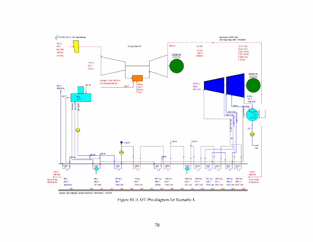
III-3 GT-Pro diagram for Scenario 1 .................................................................................. 78
III-4 Block flow diagram for Scenario 2 ............................................................................ 81
III-5 GT-Pro diagram for Scenario 2 .................................................................................. 83
III-6 Block flow diagram for Scenario 3 ............................................................................ 86
III-7 GT-Pro diagram for Scenario 3 .................................................................................. 88
III-8 Block flow diagram for Scenario 4 ............................................................................ 90
III-9 GT-Pro diagram for Scenario 4 .................................................................................. 92
III-10 Block flow diagram for Scenario 5 ............................................................................ 95
III-11 GT-Pro diagram for Scenario 5 .................................................................................. 97
IV-1 Past capacity announcements vs. actual..................................................................... 110
IV-2 Global IGCC project pipeline .................................................................................... 112

8

9

10
Figure E-1. The measured permeance of H2 in GPU and H2/CO2 selectivity of selected
WFX-PBI hollow fiber at 250˚C.
0
10
20
30
40
50
0 250 500 750 1000
H2 Permeance (GPU)
Se
lec
tiv
ity
(H
2/C
O2)
H2 Permeance Data at 250o C
1.0 mm OD Fiber
WFX Coated Asymmetric Fiber)
0.6 mm OD Fiber
WFX Coated Porous Substrate Fiber

11
Figure E-2. Image of a bundle of PBI-based, asymmetric hollow fibers made at SRI.
Figure E-3. High magnification photographs of cross-sections near shell and lumen sides
of SRI Series A fiber.

12
Figure E-4. Relationship between selectivity for H2/CO2 and H2 permeance at 250°C for
SRI fabricated fibers.
0
10
20
30
40
50
60
0 250 500 750 1000
H2 Permeance (GPU)
Se
lec
tiv
ity
(H
2/C
O2)
0.6 mm OD Fiber, 0.5 m Dense Layer
SRI Asymmetric Fiber at 225oC
Predicted
0.1 m Dense Layer
SRI Asymmetric Fiber at 225oC

13
Figure E-5. Comparison of H2/CO2 selectivity and H2 permeability in polymers.
Figure E-6. Measured selectivity for H2/CO2 and H2 permeance at 225°C measured over
1000 h.

14
Figure E-7. A photograph of 3-in diameter x1-ft long HF element for insertion in the
pressure vessel.
PBI Hollow Fibers

15
Scenario 1: Base case IGCC plant with no CO2 capture: In this base case scenario,
the gas stream from the gasifier is cooled, and NH3 and Hg vapor are removed before
H2S is removed using Selexol solvent. The clean fuel gas stream is sent to the gas
turbine.
Scenario 2: Selexol units are used to separate CO2 and H2S from H2. Most of the
steam is condensed out during the cool-down of the gas to the operating temperature
of the Selexol unit.
Scenario 3: The PBI membrane is used to separate the H2 and steam from the CO2.
The H2S is in the retentate stream, separated from the CO2 using Selexol and sent to a
Claus unit for S recovery.
Scenario 4: The PBI membrane is used to separate the H2 and steam from the CO2.
The H2S in the retentate stream and is not separated from the CO2
Scenario 5: The PBI membrane is used to separate the H2 and steam from the CO2.
The H2S permeates with the H2 and is separated with Selexol and sent to a Claus unit.

16

17
Upstream factors such as gasifier type and characteristics of fuel source may
cause variation in the performance of capture systems.
Non-technical factors such as regulatory changes and public opinion could
impact timelines for pilot, demonstration, and deployment of new capture
systems.
Commercialization of PBI capture systems will impact supply chains such
as the global supply of PBI hollow fibers and PBI polymer.
Mitigating these risks was important in order to rapidly transition PBI
capture systems from pilot to demonstration to deployment.

18
No Capture Selexol Capture No Capture
Selexol
Capture
PBI Capture,
H2S removal
from CO2
PBI Capture,
No H2S
removal from
CO2
PBI Capture,
H2S removal
from H2
Units NETL Case 1 NETL Case 2 Scenario 1 Scenario 2 Scenario 3 Scenario 4 Scenario 5
Power Production @ 100% Capacity GWh/yr 5609 4868 5,455 4,460 4,566 4,755 4,519
Power Plant Capital c/kWh 4.53 5.97 4.50 6.19 6.24 5.43 6.35
Power Plant Fuel c/kWh 1.94 2.28 1.90 2.47 2.68 2.54 2.73
Variable Plant O&M c/kWh 0.75 0.94 0.78 1.00 0.98 0.95 0.99
Fixed Plant O&M c/kWh 0.58 0.72 0.60 0.79 0.77 0.74 0.78
Cost of Electricity (COE)* c/kWh 7.80 9.91 7.78 10.44 10.67 9.66 10.85
Cost of Electricity (COE) c/kWh 7.80 10.33 7.78 10.86 11.09 10.06 11.27
Increase in COE* % n/a 27.3% n/a 34.2% 37.1% 24.1% 39.3%
Increase in COE % n/a 32.7% n/a 39.5% 42.5% 29.2% 44.8%
* Exludes transportation, storage, and monitering costs
Project Cases (Conservative Estimates)

19
PBI Capture,
H2S removal
from CO2
PBI Capture,
No H2S
removal from
CO2
PBI Capture,
H2S removal
from H2
Units Scenario 3 Scenario 4 Scenario 5
Power Production @ 100% Capacity GWh/yr 4,980 5,152 4,944
Power Plant Capital c/kWh 5.39 4.75 5.45
Power Plant Fuel c/kWh 2.30 2.22 2.31
Variable Plant O&M c/kWh 0.91 0.89 0.92
Fixed Plant O&M c/kWh 0.71 0.68 0.71
Cost of Electricity (COE)* c/kWh 9.30 8.54 9.39
Cost of Electricity (COE) c/kWh 9.68 8.90 9.77
Increase in COE* % 19.5% 9.7% 20.6%
Increase in COE % 24.4% 14.4% 25.5%
* Exludes transportation, storage, and monitering costs
Project Cases (Aggressive Estimates)

20
Table E-4. Risks to the Implementation of the Commercialization Pathway and Actions to
Mitigate Risks
Risk Mitigation
Limited worldwide PBI production
capacity requires new PBI production
plants
PBI supplier becomes member of
development team and provides input on
commercialization pathway. PBI supplier
provides plan to support pathway.
PBI hollow fiber production capacity
requires significant increase in capacity
PBI hollow fiber supplier is currently team
member. Supplier provides feedback on
pathway and plan for capacity increase to
support pathway.
Geographic variations in fuel supply result
in large variations in system performance.
Parallel pilot testing and a Design of
Experiment Approach provide a means to
quickly identify sources of variation and
potential solutions. International
cooperation provides the intellectual capital
to solve issues.
Regulatory requirements and/or public
opinion extend approval times and hence
project time lines
Parallel testing in a variety of international
markets with a range of regulatory and
public opinion processes increases
probability that projects move forward in at
least one region.
Variation in gasifier types creates variation
in system performance
Design of Experiment Approach and
parallel evaluations provide a means to
identify and resolve issues.
Increase in worldwide demand for ancillary
membrane equipment drives up capital
costs
Increase in production capacity of PBI
polymer and hollow fiber should help
reduce cost of fiber and provide some
offset to other potential cost increases.
Competition from other technologies will
also limit increases in costs to the end-user.

21

22

23
Figure I-1. Chemical structure of polybenzimidazole.
N
NN
N
n
H
H

24

25
Figure I-3.Permeance of PBI on metallic substrate as a function of time at 250 C.
Temperature,°C Trans-Membrane
Pressure, psi H2/CO2 Selectivity
LANL - Dry 235 35.5 43.0
GTI - Dry 255 37.9 40.3
GTI - Wet 258 35.6 41.4

26

27

28

29

30
Figure II-1. SEMs of PBI-based multi-bore hollow fibers with varied outer diameters and bore
diameters: (a) 7-bore, O.D. 2 mm (b) 7-bore, O.D. 4.2 mm.
Figure II-2. Porous structure leading to a nonoptimized “dense” layer at the inner (lumen)
surface of the multibore fiber.
(a) (b)(a) (b)(a) (b)
LANL

31
Figure II-3.The cross section of PBI fiber WF-MB-102208.

32
Figure II-4. The cross section of the PBI fiber illustrating the porous walls.
Figure II-5. High magnification image of the interior walls of the membrane.

33
Figure II-6. The surface of a membrane at a magnification of 100,000X.

34
Table II-1. H2 Permeability and H2/CO2 Selectivity of the WF-MB-102208 PBI Fibers

35
Figure II-7. Cross section of the WFX-07a membrane with a 0.60 mm-substrate + lumen-side
selective layer (set 1).
Figure II-8. The measured permeance for H2, N2 and CO2 as a function of pressure difference at
250˚C of WFX-07 membrane.
0.0
10
20
30
40
50
0 20 40 60 80 100
WFX-7a (34 cm fiber) at 250 C
H2 Permeance CO2 Permeance N2 Permeance
Pressure Difference (psi)
H2
Selectivity H2/CO2 = 13
Selectivity H2/N2 = 18
N2CO2

36
Figure II-9. The measured permeance of H2 in GPU and H2/CO2 selectivity of selected WFX-
PBI hollow fiber set 2 at 250˚C.
0
5
10
15
20
25
30
35
40
45
0 25 50 75 100 125 150 175 200
Permeance (GPU)
Sele
cti
vit
y (
H2/C
O2)
WFX-9
WFX-8
WFX-10
WFX-16
WFX-28
WFX-27
WFX-23

37
Figure II-10. SEM images of the lumen surfaces of the previous (WFX-3b) and new (WFX-00)
porous substrate fiber.

38
Figure II-11. SEM image of the cross section of the porous substrate fiber at low and high
magnifications.
Figure II-12. The measured permeance of H2 in GPU and H2/CO2 selectivity of selected WFX-
PBI hollow fiber at 250˚C.
WFX-34
WFX-37a and WFX-35
WFX-35-long term
0
5
10
15
20
25
30
35
40
45
0 250 500 750 1000
Sele
cti
vit
y (H
2/C
O2)
H2 Permeance (GPU)
H2 Permeance Data at 250 C
1 mm OD Fiber
0.6 mm OD Fiber

39
Table II-2. H2 permeance and H2/CO2 selectivity of the fibers at 250˚C.
In asymmetric membranes, the porosity changes from one
Fiber ID Testing Reriod H2 Permeance Selectivity No. of Coatings Treatment
(GPU) (H2/CO2)
WFX-35 8 hr testing 424 9 single No Pretreatment
WFX-35 36 hr testing 587 8 single No Pretreatment
WFX-36 8 hr testing 420 5 single No Pretreatment
WFX-34 8 hr testing 545 6 single No Pretreatment
WFX-37a 8 hr testing 408 9 single No Pretreatment
WFX-38 8 hr testing 257 14 single No Pretreatment
WFX-39 8 hr testing 500 6 single No Pretreatment
WFX-40 36 hr testing 517 5 single No Pretreatment
WFX-41 8 hr testing 68 8 single No Pretreatment
WFX-44 36 hr testing 211 11 single Pre-treated
WFX-45 8 hr testing 183 38 double Pre-treated
WFX-45 36 hr testing 160 23 double Pre-treated
WFX-46 36 hr testing 214 10 double Pre-treated
WFX-50 36 hr testing 148 8 double Pre-treated
WFX-49 4 hr testing 277 4 double Pre-treated
WFX-43b 4 hr testing 333 19 No Coating pre-treated

40
surface of the membrane to the other, with the highest density part being the functional
separation layer. In the WFX membranes, the separation layer was not sufficiently uniform
decrease the H2/CO2 selectivity. Applying a dense PBI layer minimized the defective regions
and increased the selectivity. But the extra-thick dense layer decreased the H2 permeance. In
coated porous substrates, the gas separation function is provided by the applied secondary dense
layer coating. The porous substrate provides the mechanical support with negligible gas transport
resistance as in the asymmetric fiber.
Figure II-13. The measured permeance of H2 in GPU and H2/CO2 selectivity of selected WFX-
PBI hollow fiber at 250˚C.

41
Figure II-14. Schematic of the SRI bench Scale spinning line.

42
Figure II-15. SRI bench Scale spinning line.
Figure II-16. A photograph of PBI hollow fiber bundles fabricated at SRI series B fiber.

43
Figure II-17. Processing steps in fabricating hollow fiber modules.

44
Figure II-18. Fiber spinning process factors and responses flow chart.
Table II-3. Hollow Fiber Spinning Parameters
Parameter Notes
Controllable parameters 1. Spinneret Design 2. Dope solution (composition, flow rate, and
temperature) 3. Bore solution (flow rate, composition and
temperature) 4. Coagulant ( flow rate, composition and
temperature ) 5. Additives
-Spinneret design is fixed
Output Response 1. Bulk pore size distribution
2. Shell side dense layer thickness and defects
3. Lumen side pore structure
4. H2 Permeance
5. Macro-voids
6. Mechanical strength (Mandrill test)
- Key screening parameters are density of macro-voids, dense layer thickness and the H2 permeance
Uncontrollable input factors
HF SpinningControllable input
factors
Response/ Output measures

45
Table II-4. Relationship Between Process Parameters and Fiber Properties
Macroscopic Properties
Parameter Fiber OD Finer ID Diameter
Variance, DV
Ovality, OV Irregular Bores ,
IB
Spinneret
Design, SD
Second order to
DR
Second order
to FD
Dope Flow
Rate, FD
OD decrease
with decrease in
FD at a constant
draw rate
Fiber breaks as FD
increases when Dr
is held constant due
to dope elasticity
Draw Ratio, DR
OD decreases as
DR increases
ID is
controlled by
FB once OD is
fixed with
constant DR
and FD
Highly dope
specific
Air Gap Height,
AG
DV depends on
AG, but highly
dope specific
Second order to
VK in the quench
bath
Bore Flow Rate,
FB
Second order to
DR
ID decreases
as FB
decreases
OV tends to
decrease as FB
increases since
increasing OD/ID
increases VK
Solvent
Concentration
in Bore
Solution, SC
IB decreases as SC
increases. Low SC
can increase fiber
break
Vitrification
Kinetics, VK
Fiber shrinkage
is second order
to DR
Second order
to FB
Highly dope
specific, DV
decrease as VK
increase
OV decreases as
VK increases
IB decreases as VK
at fiber ID decreases
(e.g., increase SC)

46
Figure II-19. A photograph of a cross section of an asymmetric PBI hollow fiber membrane.

47
Table II-5. Parameters Affecting Macro-Voids and their Associated Levels to be tested
Name Lower Level Upper Level
1. Bore fluid solvent concentration (wt%)
2. Non solvent in dope (wt%) 3. Non-solvent diffusion rate
5
0 Slow diffusing
coagulant
50
25 Highly diffusive coagulant
Figure II-19a. Photographs of the cross section of bulk porous sections of PBI fibers drawn from
four different coagulation solvent combinations.
Coagulant 1 Coagulant 2
Coagulant 4Coagulant 3

48
Figure II-20. Photographs of a fiber without macro-defects and the cross section illustrating the
porous substrate.
In both cases, the exterior of the hollow fibers were dense
with an extremely porous inner layer. The dense layer provides the separation between the
highly permeating H2 and low-permeating CO2 whereas the porous layer provides mechanical
strength with low pressure drop for the passage of the permeating gas. Based on the initial tests,
Series A fibers were found to be superior and further development focused only on Series A.

49
Figure II-21. A cross section of the PBI asymmetric hollow fiber made at SRI with no finger
voids.
Figure II-22. Image of a bundle of PBI-based, asymmetric hollow fibers made at SRI.
Selective Layer

50
Figure II-23. Photograph of coils of 0.6mm diameter PBI hollow fibers fabricated at SRI.
Figure II-24. High magnification photographs of cross-sections near shell and lumen sides of
SRI Series A fiber.

51
Figure II-25. Fiber bundle potted with PBI sealant.

52
Figure II-26. Potted hollow fiber membrane elements, 1-in x 14-in size
Figure II-27. Potted Fiber bundles assembled with varying packing densities to assess the
potting performance

53
Figure II-28. Measured permeance values for H2 and CO2 at 150° to 225°C as a function of
applied pressure difference across the hollow fiber membrane.

54
Figure II-29. Measured selectivity for H2/CO2 as a function of H2 permeance in GPU units at
temperatures from 150° to 250°C.

55
Figure II-30. Measured selectivity for H2/CO2 and H2 permeance at 225°C measured over
1000 h.

56
Figure II-31. Relationship between selectivity for H2/CO2 and H2 permeance at 250°C as a
function of the dense layer thickness.

57
Figure II-32. Comparison of H2/CO2 selectivity and H2 permeability in polymers.
Figure II-32a. A photograph of assembled sub-scale 1-in module with SRI PBI hollow fiber
membrane.

58
Figure II-33. Performance data for large hollow fiber membrane module at 200°C.

59
Table II-6. Module Specification for 0.6 mm O.D. fiber with a 0.45 µm Thick Dense Layer
Table II-7. The Simulation of a Membrane Module with for a 50 kWth System
Stream Feed Retentate Sweep Permeate
CO2, fraction 0.388 0.8524 0 0.0344
CO, fraction 0.0114 0.0272 0 0.0002
CH4,fraction 0.0008 0.0019 0 0.00001
N2, fraction 0.015 0.0363 1 0.4785
H2, fraction 0.542 0.0659 0 0.4548
H2S, fraction 0.0058 0.0141 0 0.00001
H2O, fraction 0.037 0.0022 0 0.0319
CO2, recovery - 90.00% - -
H2, recovery - - - 95.00%
scfh 931.3 381.4 504.6 549.9
LPM 440 180 238 260
pressure, psia 215 200 15 15
Btu/cf LHV 153.4 28.9 0 125
Btu/h LHV 142,847 11,008 0 131,839
kWth 41.866 3.226 0 38.64
kWe 25.12 1.936 0 23.184
3.0” × 12” Fiber Element
Fiber O.D/I.D. 600µm / 450µm
Fiber packing 50 - 60%
Total fiber length per element, km 1.86
Number of fibers per element 5,586
Module membrane area, m2 3
Module membrane area, ft2 32.3
Element Volume, m3 0.00139
Specific membrane area, m2/m
3 2,159
kWth (feed)/element 25
H2 recovery 95.0%
CO2 recovery 90.0%

60
Table II-8. Gas Flow Rates in Feed, Retentate and Permeate streams for a 50 KWth System
Figure II-34. A block diagram showing mass balances for the test skid with a feed gas processing
capacity of 50 kWth.
Stream Feed Retentate Permeate
SLPM SLPM SLPM
CO2, fraction 171 153 17
CO, fraction 5 5 0
CH4, fraction 0 0 0
N2, fraction 7 7 238
H2, fraction 238 12 226
H2S, fraction 3 3 0
H2O, fraction 16 0 16
N2,Sweep 238

61
Figure II-35. Schematic diagram of the nominal 4 inch shell side feed test module

62
Figure II-36. The skid containing two pressure vessels in as-fabricated stage.
Figure II-37. Gas flow diagram for the test skid

63
Figure II-38. A photograph of 3-in diameter x1-ft long HF element for insertion in the pressure
vessel.
PBI Hollow Fibers

64
Figure II-39. A photograph showing the installed skid with instrumentation.
Heated Membrane Module Vessels
Temperature Controllers
CO2 Analyzer
Feed Flow Controllers
Pressure Transmitter
Flow Indicator

65
Figure 11-40. The selectivity of H2/CO2 and H2 permeance of fibers at 225°C measured over a
period of 120 h.

66

67
Parameter
0. 12 µm Layer on 0.64
cm OD Porous Metal tube
0.5 µm. layer on 0.05 cm
O.D. PBI hollow fiber
Membrane Area, m2 1,759,317 73,232
Membrane Volume, m3 1,675,750 5,492
Membrane Bundle
Volume, m3* 2,234,333 7,323
* 75% membrane volumetric packing density 1Membrane area and volume for a 600 MW power plant
Figure III-1. Plot of LANL PBI H2/CO2 selectivity vs. H2 permeability at two temperatures.
PBI (400ºC)
PBI (250ºC)

68
Feed H2O,
%
Sat. H2O,
% T, ºC αH2/CO2
H2 permeance,
Barrer
23 75 250 43 88
23 41 215* 60 50
16 16 170* 90 20
*Extrapolated
1 Separation layer thickness: 0.5 mm,N2 sweep: 42%;
2Extrapolated data
Feed rate.
Feed pressure.
Permeate pressure.
N2 permeate sweep.
Membrane separation layer thickness.

69
Separation Layer = 12 µm
Mixed Gas GPU
10-6
cm3/s/cm
2/cm Hg H2 α Barrer
H2 7.30 1.00 8.76E-09
CO2 0.17 42.94 2.04E-10
CO 0.06 121.67 7.20E-11
N2 0.020 365.00 2.40E-11
CH4 0.030 243.33 3.60E-11
H2S 0.004 1825.00 4.80E-12

70
Separation Layer = 0.5 µm
Mixed Gas GPU
10-6
cm3/s/cm
2/cm Hg H2 α Barrer
H2 175.20
1.00 8.76E-09
CO2 4.08 42.94 2.04E-10
CO 1.44 121.67 7.20E-11
N2 0.48 365.00 2.40E-11
CH4 0.72 243.33 3.60E-11
H2S 0.10 1825.00 4.80E-12
The gas permeation unit (GPU) varies inversely with the separation layer thickness (i.e.,
12.0/0.5 × 7.3 = 175.2.) The permeability values are the intrinsic permeation property of the
membrane. Permeability values may be somewhat different because of changes in polymer
morphology or mixed gas effects in a thinner membrane at higher pressure. Nonetheless, for a
first approximation, we performed a simulation at the targeted thickness of a 0.5 µm separation
layer and a 750 psia feed pressure with a gas composition representative of the gas downstream
of the WGSRs. The results for a 600 MW power plant are summarized in Table III-6.
Feed
Pressure
Permeate
Pressure
Membrane
Layer N2 Sweep Permeate
CO2
Recovery
Membrane
Area
4 in. ×5 ft
elements
psia psia μm % Btu/ft3 % m
2 Number
750 250 0.5 61.5 115.5 88.6 70,906 1,156
Note: 90% H2 recovery.
μ μ

71
Raffinate Permeate Raffinate Sweep N2 Feed
flux
Membrane
area
Permeate
Fuel CO2
Recovery H2 purity
CO2
purity % ft
3/ft
2-h ft
2/MW Btu/ft
3
58.9% 76.0% 81.1% 0% 6.0 5,364 251.7
88.6% 35.4% 85.6% 61.5% 25.3 1,274 115.3
198% H2 recovery, Feed at 750 psia, Permeate at 250 psia, and 0.5 µm separation layer thickness.
198% H2 recovery, Feed at 750 psia, Permeate at 250 psia, and 0.5 µm separation layer thickness.
Sweep N2
Feed
flux Permeate Raffinate Raffinate
Membrane
Area
Permeate
Fuel
% ft
3/ft
2-h
H2 purity
CO2
purity
CO2
recovery ft
2/MW Btu/ft
3
61.5% 29.5 35.7% 83.9%* 90.0% 1,093 116.2
42.0% 33.8 35.7% 80.4%* 90.0% 1,251 115.6

72
Energy balance Btu/hr Btu/scf % MWg MWe
Permeate fuel gas 5,656,550 115.21 82.82 1.66 0.99
Raffinate capture gas 1,173,055 87.77 17.18 0.34 0.21
Feed gas 6,829,605 211.76 100.00 2.00 1.20
CH4 production in the
gasifier must be minimized to maximize energy recovery in the permeate fuel and to minimize
energy loss in the raffinate capture gas.
Energy balance Btu/hr Btu/cf % MWg MWe
Permeate fuel gas 5,851,496 115.23 95.64 1.71 1.03
Raffinate capture gas 267,051 21.21 4.36 0.08 0.05
Feed gas 6,118,547 190.28 100.00 1.79 1.08 * For comparison because the “Plot to Enerfex from LANL” data were on a dry basis.
Effect of Gasifier Pressure and Consequently of Membrane Feed Pressure on
Membrane Area – Gasifier outlet pressure in the current Aspen model is 815 psia.
Consequently, the WGSR outlet pressure, which is also the membrane feed pressure, is 777 psia.
BP’s experience with quench-style gasifiers puts the operating pressure higher, providing 977
psia downstream of the syngas scrubbers. The membrane feed pressures in our simulation
analyses have ranged from 715 to 1,015 psia. Table III-11 illustrates the difference in membrane
area between 750 and 1,015 psia feed pressure. Membrane area decreases with increasing feed
pressure because the pressure difference across a membrane increases permeation flux while
actual gas volume is reduced. Increasing membrane feed pressure from 750 to 1,015 psia reduces
the membrane area by 39% while maintaining CO2 recovery at approximately 90%.

73
Feed, psia Permeate,
psia
Permeate,
Btu/cf
CO2 recovery
%
Membrane area/
MWe, m2
1,015 250 115.2 90.5 72.5
750 250 115.5 88.6 118.2
0.5 µm separation layer and 98% H2 recovery
Single Gas GPU Units Single Gas Barrer Units
Gas 10-6
cm3/s/cm
2/cm Hg H2 α 10
-10cm
3×cm/s/cm
2/cm Hg
H2 5.20 1.00 62.4
CO2 0.12 43.33 1.44
Note: 12 µm shell side dense separation layer; Feed presssure = 260 cm Hg; Permeate pressure =
76 cm Hg; Temperature = 250ºC; Pall Accusep™ tube = 0.5 in. O.D
Single Gas GPU Units Single Gas Barrer Units
Gas 10-6
cm3/s/cm
2/cm Hg H2 α 10
-10cm
3×cm/s/cm
2/cm Hg
H2 115 1.00 57.5
CO2 2.67 43 1.38
Note: Feed Pressure = 260 cm Hg; Permeate pressure = 76 cm Hg; Temperature = 250ºC;
Asymmetric hollow fiber = 0.6 mm OD; separation layer thickness = 0.5 µm

74
Scenario 1: Base case IGCC plant with no CO2 capture: In this base case scenario, the gas
stream from the gasifier is cooled, and NH3 and Hg vapor are removed before H2S is
removed using Selexol solvent. The clean fuel gas stream is sent to the gas turbine.
Scenario 2: Selexol units are used to separate CO2 and H2S from H2. Most of the steam is
condensed out during the cool-down of the gas to the operating temperature of the Selexol
unit.
Scenario 3: The PBI membrane is used to separate the H2 and steam from the CO2. The
H2S is in the retentate stream, separated from the CO2 using Selexol and sent to a Claus
unit for S recovery.
Scenario 4: The PBI membrane is used to separate the H2 and steam from the CO2. The
H2S in the retentate stream and is not separated from the CO2
Scenario 5: The PBI membrane is used to separate the H2 and steam from the CO2. The
H2S permeates with the H2 and is separated with Selexol and sent to a Claus unit.

75

76
Figure III-2. Block flow diagram for Scenario 1.

77
Gasifier In Gasifier Out COS-Rxtr In COS-Rxtr Out Selexol In To Comb To Claus Comb In Comb Out To HRSG
Temperature C 1113 1316 210 204 37 38 49 361 1377 560
Pressure psia 980 815 798 788 738 667 31 235 212 15
Vapor Frac 1 1 1 1 1 1 1 1 1 1
Mole Flow scfm 244900 318503 404693 404693 276979 273859 10077 1603371 1497989 1882929
Mass Flow lb/hr 719728 1024852 1269434 1269434 934472 904000 61286 6938118.04 6938118.04 8694000
Volume Flow cuft/hr 1072180 1896936 748620 720759 355224 389901 324967 13196806 35665050 314398937
Dew Temp C 226 175 209 208 38 4 35 50 104 39
Mass Flow lb/hr
H2O 265883 140092 386270 386111 895 134 761 33545 340820 352672
AR 15616 15616 15616 15616 15942 15942 0 83985 83985 106829
CO2 0 344779 343293 343681 389837 347805 42032 350032 1077111 1077901
O2 403686 0 0 0 0 0 0 1146251 607686 1011943
N2 13422 12268 12268 12268 20477 44327 6965 4828513 4828513 6144652
O2S 0 0 0 0 0 0 0 0 3 3
CH4 0 707 707 707 1352 1352 0 1352 0 0
CO 0 463197 463197 463197 460441 460395 46 460395 0 0
COS 0 533 533 3 5 0 5 0 0 0
H2 21121 34047 34047 34047 34047 34044 3 34044 0 0
H2S 0 12208 12110 12411 11227 1 11225 1 0 0
NH3 0 1404 1392 1392 248 0 248 0 0 0
Mole Frac
H2O 0.3811 0.1544 0.3351 0.3350 0.0011 0.0002 0.0265 0.0073 0.0799 0.0658
AR 0.0101 0.0078 0.0061 0.0061 0.0091 0.0092 0.0000 0.0083 0.0089 0.0090
CO2 0.0000 0.1556 0.1219 0.1220 0.2023 0.1825 0.5994 0.0314 0.1033 0.0823
O2 0.3258 0.0000 0.0000 0.0000 0.0000 0.0000 0.0000 0.1413 0.0802 0.1062
N2 0.0124 0.0087 0.0068 0.0068 0.0167 0.0365 0.1561 0.6799 0.7277 0.7368
O2S 0.0000 0.0000 0.0000 0.0000 0.0000 0.0000 0.0000 0.0000 0.0000 0.0000
CH4 0.0000 0.0009 0.0007 0.0007 0.0019 0.0019 0.0000 0.0003 0.0000 0.0000
CO 0.0000 0.3284 0.2584 0.2584 0.3754 0.3796 0.0010 0.0648 0.0000 0.0000
COS 0.0000 0.0002 0.0001 0.0000 0.0000 0.0000 0.0000 0.0000 0.0000 0.0000
H2 0.2706 0.3354 0.2640 0.2640 0.3857 0.3900 0.0011 0.0666 0.0000 0.0000
H2S 0.0000 0.0071 0.0056 0.0057 0.0075 0.0000 0.2067 0.0000 0.0000 0.0000
NH3 0.0000 0.0016 0.0013 0.0013 0.0003 0.0000 0.0092 0.0000 0.0000 0.0000
78

79

80

81

82
Gasifier In Gasifier Out WGSR Feed WGSR Exit Selexol In To Claus To CO2 Comp To Gas Turb To HRSG
Temperature C 1128 1316 229 270 36 43 10 27 567
Pressure psia 980 815 798 777 727 25 17 695 15
Vapor Frac 1 1 1 1 1 1 1 1 1
Mole Flow scfm 254904 332812 507801 507801 409517 20706 149463 239349 1941483
Mass Flow lb/hr 749525 1072618 1570228 1570228 1365699 139344.973 1023937 202417 8438000
Volume Flow cuft/hr 1113196 1982160 976954 1084332 532707 810279 7739767 315352 326904708
Enthalpy MMBtu/hr -889 -1992 -5801 -6048 -4867 -503 -4017 -360 -2100
Dew Temp F 436 344 434 375 103 59 -27 80 123
Mass Flow lb/hr
H2O 268958 140141 639191 332467 1233 586 154 493 668537
AR 16535 16535 16535 16535 16878 0 0 16878 112732
CO2 0 354486 353150 1102449 1229830 126673 1020759 82399 117481
O2 427455 0 0 0 0 0 0 0 1070185
N2 14213 12999 12999 12999 14305 0 286 14019 6469035
O2S 0 0 0 0 0 0 0 0 29
CH4 0 792 792 792 1111 0 0 1111 0
CO 0 497137 497137 20488 20393 0 2039 18354 0
COS 0 580 580 46 49 25 0 25 0
H2 22365 35554 35554 69858 69836 0 698 69137 0
H2S 0 12919 12826 13129 11768 11767 0 2 0
NH3 0 1476 1465 1465 296 296 0 0 0
Mole Frac
H2O 0.3704 0.1478 0.4419 0.2299 0.0011 0.0099 0.0004 0.0007 0.1209
AR 0.0103 0.0079 0.0052 0.0052 0.0065 0.0000 0.0000 0.0112 0.0092
CO2 0.0000 0.1531 0.0999 0.3120 0.4316 0.8792 0.9815 0.0495 0.0087
O2 0.3314 0.0000 0.0000 0.0000 0.0000 0.0000 0.0000 0.0000 0.1089
N2 0.0126 0.0088 0.0058 0.0058 0.0079 0.0000 0.0004 0.0132 0.7523
O2S 0.0000 0.0000 0.0000 0.0000 0.0000 0.0000 0.0000 0.0000 0.0000
CH4 0.0000 0.0009 0.0006 0.0006 0.0011 0.0000 0.0000 0.0018 0.0000
CO 0.0000 0.3373 0.2211 0.0091 0.0112 0.0000 0.0031 0.0173 0.0000
COS 0.0000 0.0002 0.0001 0.0000 0.0000 0.0001 0.0000 0.0000 0.0000
H2 0.2753 0.3352 0.2197 0.4316 0.5350 0.0000 0.0147 0.9063 0.0000
H2S 0.0000 0.0072 0.0047 0.0048 0.0053 0.1055 0.0000 0.0000 0.0000
NH3 0.0000 0.0016 0.0011 0.0011 0.0003 0.0053 0.0000 0.0000 0.0000

83

84

85

86

87
WGSR Feed WGSR Exit Membrane In Retentate Permeate To Selexol To Claus To CO2 Comp To HRSG
Temperature C 230 271 232 232 246 36 38 38 568
Pressure psia 798 777 777 757 250 707 31 667 15
Vapor Frac 1 1 1 1 1 1 1 1 1
Mole Flow scfm 565764 565764 565764 203043 630320 201372 10041 191331 1989406
Mass Flow lb/hr 1749330 1749330 1749330 1206556 1730101 1232199 65511 1166688 8438003
Volume Flow cuft/hr 1089697 1208803 1124313 635637 3727296 268896 312621 272403 335126883
Enthalpy MMBtu/hr -6344 -6620 -6673 -4362 -2242 -4484 -205 -4278 -4130
Dew Temp F 434 375 375 102 71 30 138
Mass Flow lb/hr
H2O 717891 373312 373312 25796 347516 418 355 63 1027389
AR 18379 18379 18379 18128 4161 18451 0 18451 91431
CO2 383912 1225689 1225689 1102752 122937 1154596 51957 1102639 127354
O2 0 0 0 0 7169 0 0 0 987410
N2 14457 14457 14457 14259 1176445 15396 0 15396 6204420
O2S 0 0 0 0 0 0 0 0 0
CH4 917 917 917 890 27 1343 0 1343 0
CO 558133 22661 22661 21818 843 21741 0 21741 0
COS 658 50 50 50 0 53 0 53 0
H2 39104 77642 77642 6638 71003 6655 0 6655 0
H2S 14260 14604 14604 14604 0 13202 13199 3 0
NH3 1620 1620 1620 1620 0 346 0 346 0
Mole Frac
H2O 0.4455 0.2316 0.2316 0.0446 0.1936 0.0007 0.0124 0.0001 0.1813
AR 0.0051 0.0051 0.0051 0.0141 0.0010 0.0145 0.0000 0.0153 0.0073
CO2 0.0975 0.3113 0.3113 0.7805 0.0280 0.8240 0.7436 0.8282 0.0092
O2 0.0000 0.0000 0.0000 0.0000 0.0022 0.0000 0.0000 0.0000 0.0981
N2 0.0058 0.0058 0.0058 0.0159 0.4214 0.0173 0.0000 0.0182 0.7041
O2S 0.0000 0.0000 0.0000 0.0000 0.0000 0.0000 0.0000 0.0000 0.0000
CH4 0.0006 0.0006 0.0006 0.0017 0.0000 0.0026 0.0000 0.0028 0.0000
CO 0.2228 0.0090 0.0090 0.0243 0.0003 0.0244 0.0000 0.0257 0.0000
COS 0.0001 0.0000 0.0000 0.0000 0.0000 0.0000 0.0000 0.0000 0.0000
H2 0.2168 0.4306 0.4306 0.1026 0.3534 0.1037 0.0000 0.1091 0.0000
H2S 0.0047 0.0048 0.0048 0.0133 0.0000 0.0122 0.2439 0.0000 0.0000
NH3 0.0011 0.0011 0.0011 0.0030 0.0000 0.0006 0.0000 0.0007 0.0000

88

89

90

91
Gasifier In Gasifier Out WGSR Feed WGSR Exit Membrane In Retentate Permeate To CO2 Comp To HRSG
Temperature C 1123 1316 231 271 232 232 246 41 567
Pressure psia 980 815 798 777 777 750 250 650 15
Vapor Frac 1 1 1 1 1 1 1 1 1
Mole Flow scfm 272846 358469 561039 561039 561039 200998 628162 192123 1988446
Mass Flow lb/hr 802970 1158287 1734614 1734614 1734614 1.19E+06 1730134 1169540 8438000
Volume Flow cuft/hr 1186791 2134969 1081903 1199555 1114924 629236 3715257 238638 334725805
Enthalpy MMBtu/hr -882 -2072 -6305 -6579 -6632 -4337 -2236 -4257 -4094
Dew Temp F 432 338 435 376 376 32 138
Mass Flow lb/hr
H2O 274473 140496 718000 373049 373049 25778 347271 0 1020286
AR 18184 18184 18184 18184 18184 17936 4193 17936 91462
CO2 0 371279 370192 1212879 1212879 1091215 121664 1092302 126066
O2 470088 0 0 0 0 0 7233 0 993560
N2 15630 14312 14312 14312 14312 14117 1178678 14117 6206627
O2S 0 0 0 0 0 0 0 0 0
CH4 0 950 950 950 950 922 28 922 0
CO 0 558382 558382 22334 22334 21503 832 21503 0
COS 0 665 665 50 50 50 0 50 0
H2 24595 38224 38224 76803 76803 6567 70236 6567 0
H2S 0 14191 14111 14460 14460 14460 0 14541 0
NH3 0 1603 1593 1593 1593 1593 0 1603 0
Mole Frac
H2O 0.3532 0.1376 0.4493 0.2334 0.2334 0.0450 0.1941 0.0000 0.1801
AR 0.0106 0.0080 0.0051 0.0051 0.0051 0.0141 0.0011 0.0148 0.0073
CO2 0.0000 0.1488 0.0948 0.3107 0.3107 0.7802 0.0278 0.8171 0.0091
O2 0.3405 0.0000 0.0000 0.0000 0.0000 0.0000 0.0023 0.0000 0.0988
N2 0.0129 0.0090 0.0058 0.0058 0.0058 0.0159 0.4236 0.0166 0.7047
O2S 0.0000 0.0000 0.0000 0.0000 0.0000 0.0000 0.0000 0.0000 0.0000
CH4 0.0000 0.0010 0.0007 0.0007 0.0007 0.0018 0.0000 0.0019 0.0000
CO 0.0000 0.3517 0.2247 0.0090 0.0090 0.0242 0.0003 0.0253 0.0000
COS 0.0000 0.0002 0.0001 0.0000 0.0000 0.0000 0.0000 0.0000 0.0000
H2 0.2828 0.3345 0.2138 0.4295 0.4295 0.1025 0.3508 0.1072 0.0000
H2S 0.0000 0.0073 0.0047 0.0048 0.0048 0.0134 0.0000 0.0140 0.0000
NH3 0.0000 0.0017 0.0011 0.0011 0.0011 0.0029 0.0000 0.0031 0.0000

92

93

94

95

96
WGSR Feed WGSR Exit Membrane In Retentate To CO2 Comp Permeate To Selexol To Claus To Turbine To HRSG
Temperature C 231 271 232 232 40 232 40 38 241 567
Pressure psia 798 777 777 757 707 250 465 31 450 15
Vapor Frac 1 1 1 1 1 1 1 1 1 1
Mole Flow scfm 572530 572530 572530 202328 192527 370203 516670 6920 509750 1943550
Mass Flow lb/hr 1770071 1770071 1770071 1203531 1175604 566540 1414409 24499 1389910 8437965
Volume Flow cuft/hr 1104602 1224390 1137759 633397 215925 2110648 1061215 188112 1777267 327298730
Enthalpy MMBtu/hr -6395 -6674 -6728 -4396 -4332 -2401 -509 -46 -258 -2210
Dew Temp F 436 376 376 36 107 160 49 124
Mass Flow lb/hr
H2O 735190 382011 382011 26397 0 355614 3576 3039 536 682809
AR 18537 18537 18537 18283 18204 253 4839 0 4839 96534
CO2 373744 1236530 1236530 1113124 1113124 123406 129301 5819 123483 129183
O2 0 0 0 0 0 0 7169 0 7169 1064808
N2 14593 14593 14593 14394 14340 199 1181684 0 1181684 6464624
O2S 0 0 0 0 0 0 0 0 0 6
CH4 985 985 985 956 947 29 437 0 437 0
CO 571541 22709 22709 21864 21778 845 846 0 846 0
COS 684 51 51 51 51 0 0 0 0 0
H2 38791 78290 78290 6694 6692 71596 71628 716 70912 0
H2S 14386 14745 14745 147 130 14598 14928 14925 3 0
NH3 1620 1620 1620 1620 338 0 0 0 0 0
Mole Frac
H2O 0.4508 0.2342 0.2342 0.0458 0.0000 0.3372 0.0024 0.1542 0.0004 0.1233
AR 0.0051 0.0051 0.0051 0.0143 0.0150 0.0001 0.0015 0.0000 0.0015 0.0079
CO2 0.0938 0.3104 0.3104 0.7906 0.8309 0.0479 0.0360 0.1208 0.0348 0.0096
O2 0.0000 0.0000 0.0000 0.0000 0.0000 0.0000 0.0027 0.0000 0.0028 0.1083
N2 0.0058 0.0058 0.0058 0.0161 0.0168 0.0001 0.5164 0.0000 0.5234 0.7510
O2S 0.0000 0.0000 0.0000 0.0000 0.0000 0.0000 0.0000 0.0000 0.0000 0.0000
CH4 0.0007 0.0007 0.0007 0.0019 0.0019 0.0000 0.0003 0.0000 0.0003 0.0000
CO 0.2254 0.0090 0.0090 0.0244 0.0255 0.0005 0.0004 0.0000 0.0004 0.0000
COS 0.0001 0.0000 0.0000 0.0000 0.0000 0.0000 0.0000 0.0000 0.0000 0.0000
H2 0.2126 0.4290 0.4290 0.1038 0.1090 0.6068 0.4350 0.3247 0.4364 0.0000
H2S 0.0047 0.0048 0.0048 0.0001 0.0001 0.0073 0.0054 0.4002 0.0000 0.0000
NH3 0.0011 0.0011 0.0011 0.0030 0.0007 0.0000 0.0000 0.0000 0.0000 0.0000

97

98
The plant performance summary data are shown in Table III-19. Both the NETL Case 1
and Scenario 1 correspond to IGCC plants with no CO2 capture. NETL Case 2 and Scenario
2 are both IGCC plants with CO2 capture using Selexol.

99

100
Plant Performance NETL Case 1 NETL Case 2 Scenario 1 Scenario 2 Scenario 3 Scenario 4 Scenario 5
Gas Turbine Gross Power kWe 464,300 464,010 464,000 464,000 464,000 464,000 464,000
Sweet Gas Expander Gross PowerkWe 7,130 6,260 6,600 6,440 0 0 0
Steam Turbine Gross Power kWe 298,920 274,690 302,855 276,977 271,796 273,126 260,282
Gross Power Total kWe 770,350 744,960 773,455 747,417 735,796 737,126 724,282
Auxiliary Load kWe 130,100 189,285 144,193 231,766 214,603 194,327 208,459
Net Plant Power kWe 640,250 555,675 629,262 515,651 521,193 542,799 515,823
Net Plant Efficiency (HHV) 38.2% 32.5% 39.2% 30.3% 27.6% 29.0% 27.1%
Net Plant Heat Rate (HHV) Btu/kWhr 8,922 10,505 8,707 11,251 12,372 11,754 12,608
Coal Feed Flowrate lb/hr 489,634 500,379 469,630 497,286 552,757 546,883 557,495
Thermal Input kWth 1,674,044 1,710,780 1,605,650 1,700,204 1,889,857 1,869,776 1,906,056
Oxygen Flowrate lb/hr 418,795 425,751 400,438 423,938 469,915 457,774 480,010
CO2 Captured lb/hr 0 1,033,930 0 1,023,964 1,136,804 1,126,092 1,147,346
CO2 Removal 0% 90% 0% 90% 90% 90% 90%

101
Gross Plant Power Output Scenario 1 NETL Case 1
Gas Turbine Gross Power kWe 464,000 464,300
Sweet Gas Expander Gross Power kWe 6,600 7,130
Steam Turbine Gross Power kWe - 298,920
GT-PRO Steam Turbine Gross Power kWe 302,855 -
Total Gross Power kWe 773,455 770,350
Auxiliary Load
Coal Handling kWe 432 450
Coal Milling kWe 2,187 2,280
Coal Slurry Pumps kWe 713 740
Slag Handling and Dewatering kWe 1,126 1,170
Air Separation Unit Auxiliaries kWe 1,000 1,000
ASU Main Air Compressor kWe 68,180 60,070
Oxygen Compressor kWe 10,810 11,270
Nitrogen Compressor kWe 31,897 30,560
Tail Gas Recycle Compressor kWe 2,350 1,230
Boiler Feedwater Pumps kWe - 4,590
Condensate Pumps kWe - 250
Flash Bottoms Pump kWe 200 200
Circulating Water Pump kWe - 3,710
Cooling Tower Fans kWe - 1,910
Scrubber Pumps kWe 420 300
Selexol Unit Auxiliaries kWe 2,896 3,420
Gas Turbine Auxiliaries kWe - 1,000
GT-PRO Auxillaries kWe 18,782 -
Steam Turbine Auxiliaries kWe - 100
Claus Plant Auxiliaries kWe 200 200
Miscellaneous Balance-of-Plant kWe 3,000 3,000
Transformer Losses kWe - 2,650
Total Auxiliaries kWe 144,193 130,100
Net Plant Power kWe 629,262 640,250
Net Plant Efficiency (HHV) 39.2% 38.2%
Net Plant Heat Rate (HHV) Btu/kWhr 8,707 8,922
Coal Feed lb/hr 469,630 489,634
Thermal Input kWt 1,605,650 1,674,044

102
Gross Plant Power Output Scenario 2 NETL Case 2
Gas Turbine Gross Power kWe 464,000 464,010
Sweet Gas Expander Gross Power kWe 6,440 6,260
Steam Turbine Gross Power kWe - 274,690
GT-PRO Steam Turbine Gross Power kWe 276,977 -
Total Gross Power kWe 747,417 744,960
Auxiliary Load
Coal Handling kWe 457 460
Coal Milling kWe 2,316 2,330
Coal Slurry Pumps kWe 755 760
Slag Handling and Dewatering kWe 1,193 1,200
Air Separation Unit Auxiliaries kWe 1,000 1,000
ASU Main Air Compressor kWe 72,190 72,480
Oxygen Compressor kWe 11,440 11,520
Nitrogen Compressor kWe 34,271 35,870
Tail Gas Recycle Compressor kWe 5,490 990
CO2 Compressor kWe 32,484 27,400
Boiler Feedwater Pumps kWe - 4,580
Condensate Pumps kWe - 265
Flash Bottoms Pump kWe 200 200
Circulating Water Pump kWe - 3,580
Cooling Tower Fans kWe - 1,850
Scrubber Pumps kWe 420 420
Double Stage Selexol Unit Auxiliaries kWe 47,339 17,320
Gas Turbine Auxiliaries kWe - 1,000
GT-PRO Auxiliaries kWe 18,686 -
Steam Turbine Auxiliaries kWe - 100
Claus Plant Auxiliaries kWe 200 200
Miscellaneous Balance-of-Plant kWe 3,000 3,000
Transformer Losses kWe - 2,760
Total Auxiliaries kWe 231,440 189,285
Net Plant Power kWe 515,977 555,675
Net Plant Efficiency (HHV) 30.3% 32.5%
Net Plant Heat Rate (HHV) Btu/kWhr 11,243 10,505
Coal Feed Flowrate lb/hr 497,286 500,379
Thermal Input1 kWe 1,700,204 1,710,780

103
Gross Plant Power Output Scenario 2 (NETL Selexol) NETL Case 2
Gas Turbine Gross Power kWe 464,000 464,010
Sweet Gas Expander Gross Power kWe 6,432 6,260
Steam Turbine Gross Power kWe - 274,690
GT-PRO Steam Turbine Gross Power kWe 277,212 -
Total Gross Power kWe 747,644 744,960
Auxiliary Load
Coal Handling kWe 451 460
Coal Milling kWe 2,286 2,330
Coal Slurry Pumps kWe 746 760
Slag Handling and Dewatering kWe 1,177 1,200
Air Separation Unit Auxiliaries kWe 1,000 1,000
ASU Main Air Compressor kWe 71,130 72,480
Oxygen Compressor kWe 11,300 11,520
Nitrogen Compressor kWe 34,531 35,870
Tail Gas Recycle Compressor kWe 1,310 990
CO2 Compressor kWe 30,593 27,400
Boiler Feedwater Pumps kWe - 4,580
Condensate Pumps kWe - 265
Flash Bottoms Pump kWe 200 200
Circulating Water Pump kWe - 3,580
Cooling Tower Fans kWe - 1,850
Scrubber Pumps kWe 420 420
Double Stage Selexol Unit Auxiliaries kWe 17,430 17,320
Gas Turbine Auxiliaries kWe - 1,000
GT-PRO Auxiliaries kWe 18,859 -
Steam Turbine Auxiliaries kWe - 100
Claus Plant Auxiliaries kWe 200 200
Miscellaneous Balance-of-Plant kWe 3,000 3,000
Transformer Losses kWe - 2,760
Total Auxiliaries kWe 194,634 189,285
Net Plant Power kWe 553,010 555,675
Net Plant Efficiency (HHV) 32.9% 32.5%
Net Plant Heat Rate (HHV) Btu/kWhr 10,358 10,505
Coal Feed Flowrate lb/hr 490,983 500,379
Thermal Input kWe 1,678,654 1,710,780

104

105
No Capture Selexol Capture No Capture
Selexol
Capture
PBI Capture,
H2S removal
from CO2
PBI Capture,
No H2S
removal from
CO2
PBI Capture,
H2S removal
from H2
Units NETL Case 1 NETL Case 2 Scenario 1 Scenario 2 Scenario 3 Scenario 4 Scenario 5
Power Production @ 100% Capacity GWh/yr 5609 4868 5,455 4,460 4,566 4,755 4,519
Power Plant Capital c/kWh 4.53 5.97 4.50 6.19 6.24 5.43 6.35
Power Plant Fuel c/kWh 1.94 2.28 1.90 2.47 2.68 2.54 2.73
Variable Plant O&M c/kWh 0.75 0.94 0.78 1.00 0.98 0.95 0.99
Fixed Plant O&M c/kWh 0.58 0.72 0.60 0.79 0.77 0.74 0.78
Cost of Electricity (COE)* c/kWh 7.80 9.91 7.78 10.44 10.67 9.66 10.85
Cost of Electricity (COE) c/kWh 7.80 10.33 7.78 10.86 11.09 10.06 11.27
Increase in COE* % n/a 27.3% n/a 34.2% 37.1% 24.1% 39.3%
Increase in COE % n/a 32.7% n/a 39.5% 42.5% 29.2% 44.8%
* Exludes transportation, storage, and monitering costs
Project Cases (Conservative Estimates)

106
Units Base Case
Module
Cost
Module
Cost
Membrane
Thickness
GT Fuel
Pressure
Module
Temperature
No H2S
removal
Temperature,
Thickness, Pressure
Membrane Temperature C 250 250 250 250 250 170 250 170
Separation Layer Thickness μm 0.5 0.5 0.5 0.1 0.5 0.5 0.5 0.1
Gas Turbine Fuel Pressure psia 450 450 450 450 290 450 450 290
Membrane Permeate Pressure psia 250 250 250 250 250 290 250 290
H2S Capture Yes Yes Yes Yes Yes Yes No Yes
Membrane Module Cost $/ft2 15 30 10 15 15 15 15 15
Hydrogen Recovery % 91.4 91.4 91.4 90.8 91.4 98.6 91.4 98.6
Membrane Area 1000m2 93.6 94 94 19 94 708 94 137
Power Production @ 100% Capacity GWh/yr 4,642 4,642 4,642 4,596 4,902 4,847 4,735 4,980
Power Plant Capital c/kWh 6.12 6.19 6.10 6.14 5.80 5.95 5.45 5.39
Power Plant Fuel c/kWh 2.62 2.62 2.62 2.67 2.48 2.32 2.55 2.30
Variable Plant O&M c/kWh 0.97 0.97 0.97 0.97 0.93 0.93 0.95 0.91
Fixed Plant O&M c/kWh 0.76 0.76 0.76 0.77 0.72 0.72 0.74 0.71
Cost of Electricity (COE)* c/kWh 10.47 10.54 10.44 10.55 9.92 9.92 9.70 9.30
Cost of Electricity (COE) c/kWh 10.87 10.95 10.85 10.96 10.31 10.30 10.10 9.68
Increase in COE* % 34.2% 35.4% 34.2% 35.2% 27.5% 27.2% 24.6% 19.5%
Increase in COE % 39.7% 40.6% 39.4% 40.6% 32.5% 32.1% 29.8% 24.4%

107
Table III-25. Cost of CO2 Capture with Removal and Non-Removal of H2S
PBI Capture,
H2S removal
from CO2
PBI Capture,
No H2S
removal from
CO2
PBI Capture,
H2S removal
from H2
Units Scenario 3 Scenario 4 Scenario 5
Power Production @ 100% Capacity GWh/yr 4,980 5,152 4,944
Power Plant Capital c/kWh 5.39 4.75 5.45
Power Plant Fuel c/kWh 2.30 2.22 2.31
Variable Plant O&M c/kWh 0.91 0.89 0.92
Fixed Plant O&M c/kWh 0.71 0.68 0.71
Cost of Electricity (COE)* c/kWh 9.30 8.54 9.39
Cost of Electricity (COE) c/kWh 9.68 8.90 9.77
Increase in COE* % 19.5% 9.7% 20.6%
Increase in COE % 24.4% 14.4% 25.5%
* Exludes transportation, storage, and monitering costs
Project Cases (Aggressive Estimates)

108
PBI Project Team Member Stakeholder Classification
SRI International Technology Developer
Los Alamos National Laboratory Technology Developer
Whitefox Technologies OEM & Suppliers
Enerfex OEM & Suppliers
BP Alternative Energy Utilities
Southern Company Utilities
Visage Energy Business/Financial
US DOE National Energy Technology
Laboratory
Government
This commercialization effort was designed to meet the following objectives:

109
Validate the potential of the technologies under development to meet the
Sequestration Program Capture focus area goals, which are:
Capture at least 90% of the carbon dioxide from the effluent gas of a power
generation plant.
Cost less than a 10% increase in the cost of electricity.
Considerably increase the likelihood of commercializing the polybenzimidazole-
based (PBI-based) membrane technology for pre-combustion carbon dioxide
capture.
Expedite the development of the technical and commercial potential of the
technology.
Upstream factors such as gasifier type and characteristics of fuel source may
cause variation in the performance of capture systems
Non-technical factors such as regulatory changes and public opinion could impact
timelines for pilot, demonstration, and deployment of new capture systems
Commercialization of PBI capture systems will impact supply chains such as the
global supply of PBI hollow fibers and PBI polymer
Mitigating these risks was important in order to rapidly transition PBI capture
systems from pilot to demonstration to deployment

110
Figure IV-1. Past capacity announcements vs. actual [Ventys 2007]

111
The US is leading the commercialization efforts of IGCC
globally with 26 projects at some stage of development in 17 states with a
combined capacity of 15,000 MW.
Australia is next, given strong state and federal policies targeting clean
coal technologies while Canada is driven primarily by early EOR
opportunities.
China’s interest is growing due to air quality regulations becoming a
greater threat to economic development. On a worldwide basis, the main
activity on coal gasification is centered in China due to strong support
from the central government.
In contrast, Europe is expected to see rather slow development of IGCC, at
least until 2015 according to EER’s study.

112
Figure IV-2. Global IGCC project pipeline [Emerging Energy Research]
business

113
Long-term indemnification of storage has yet to be resolved.
Need clarity on property rights associated with CO2 including
access rights and pore space ownership.
Ambiguities must be resolved regarding pore space ownership and the
relation between the surface and mineral estate. A process for owners and
project developers to transfer/lease the necessary subsurface pore space
property rights for a CCS project is also an issue.
The long-term ownership of and liability for the stored CO2 also are
potential barriers for CCS which may be addressed by
transferring liability to the state or by federal or private indemnification
schemes.
a price on carbon, investor interest in CCS worldwide has been
limited to outside niche applications. Policies that place a price on GHG
emissions, such as a cap and trade, would discourage investments in

114
traditional fossil-fuel use and spur investments in a range of clean energy
technologies, including CCS.
Funding for Initial CCS Projects: To foster the initial, large-scale CCS
projects needed to fully demonstrate the technology, the government can
offer financial incentives for CCS. For example, the government could
create a trust fund that could competitively award money to CCS projects
to help them overcome financing hurdles. [Pena and Rubin 2008] A study
prepared for the Pew Center found that coal power plant owners would
require between $300 million and $650 million in funds to cover the
investments in equipment and lost capacity necessary for the initial
commercial-scale deployments of CCS, depending on the plant type and
whether plants are newly built with CCS or retrofit.
Mandating GHG Emission Rates: Policymakers could rely on
performance standards to drive CCS deployment by enacting new
regulations that require CCS via a new source performance standard for
power plants or a low-carbon performance standard.

115
Table IV-2. Typical Stages of Maturation for Energy Technologies
Technology Development Maturation Stages
Proof-of-Concept
(Fundamental) Research
Post Proof-of-Concept
Research
(Current PBI Stage)
Pilot-scale
Demonstration
Type of Work
performed
Bench scale batch-type
experimentation and
conceptual studies at the
fundamental science level
Bench/Laboratory Scale
Field testing
Construction of a to
scale carbon control
plant
Study Size No working model 0.01 - 0.1 MW 1 - 5 MW 100 - 250 MW
Required
Funding
$0.3 - $1 MM
$1 - $5 MM
$15 - $40 MM
+$100 MM
Funding
Period
6 - 7 years
3 - 5 years
3 - 4 years
3 - 7 years

116
.

117
China P P D
e
D
e
D
py
D
py
D
py
D
py
D
py
Europe P P D
e
D
e
D
e
D
py
D
py
D
py
Australia P P D
e
D
e
D
e
D
py
D
py
D
py
Canada P P D
e
D
e
D
e
D
py
D
py
D
py
US P P D
e
D
e
D
e
D
py
D
py
D
py
D
py
2
2011
2
2012
2
2013
2
2014
2
2015
2
2016
2
2017
2
2018
2
2019
2
2020
Year
P=Pilot, De=Demo, Dpy=Deployment

118
Table IV-4. Risks to the Implementation of the Commercialization Pathway and Actions to
Mitigate Risks
Risk Mitigation
Limited worldwide PBI production
capacity requires new PBI production
plants
PBI supplier becomes member of
development team and provides input on
commercialization pathway. PBI supplier
provides plan to support pathway.
PBI hollow fiber production capacity
requires significant increase in capacity
PBI hollow fiber supplier is currently team
member. Supplier provides feedback on
pathway and plan for capacity increase to
support pathway.
Geographic variations in fuel supply result
in large variations in system performance.
Parallel pilot testing and a Design of
Experiment Approach provide a means to
quickly identify sources of variation and
potential solutions. International
cooperation provides the intellectual capital
to solve issues.
Regulatory requirements and/or public
opinion extend approval times and hence
project time lines
Parallel testing in a variety of international
markets with a range of regulatory and
public opinion processes increases
probability that projects move forward in at
least one region.
Variation in gasifier types creates variation
in system performance
Design of Experiment Approach and
parallel evaluations provide a means to
identify and resolve issues.
Increase in worldwide demand for ancillary
membrane equipment drives up capital
costs
Increase in production capacity of PBI
polymer and hollow fiber should help
reduce cost of fiber and provide some
offset to other potential cost increases.
Competition from other technologies will
also limit increases in costs to the end-user.
.

119

120

121

122
Anand, M.; Langsam, M.; Rao, M. B.; Sircar, S., Journal of Membrane Science 1997, 123, 17-25.
Armor, J. N., Journal of Membrane Science 1998, 147, 217-233.
B.D. Freeman, Macromolecules 1999, 32(2), 375-380.
Berchtold, K.A.; J.S. Young; K.W. Dudeck; J. Acquaviva; F. Onorato; S.D. Hopkins, Novel Polymeric-
Metallic Composite Membranes for CO2 Separations at Elevated Temperatures, Fifth Annual Conference
on Carbon Capture & Sequestration, May 2006.
Carbon capture journal web edition
http://www.carboncapturejournal.com/displaynews.php?NewsID=263&PHPSESSID=hn7lh6bj98jl7ktcjd
1lpavn06
Chiou , J.S, J.W. Barlow, D.R. Paul, Journal of Applied Polymer Science 1985, 30, 2633-2642.
Ciferno, Jared; Howard McIIverid, Gary Stiegel, Carbon Sequestration Systems Analysis Technical Note,
No. 5, National Energy Technology Laboratory, July 2005.
D.W. Breck, Zeolite Molecular Sieves: Structure, Chemistry, and Use; John Wiley and Sons: New York,
1974; pp 593-724.
Emerging Energy Research Gasification Market Analysis
Greenberg, A.R., S. Brahmandam, K.A. Berchtold, J.S. Young; et al., “Mechanical and Transport
Behavior of Polybenzimidazole (PBI) Dense Films Used for Elevated-Temperature Gas Separation,”
Proceedings of the 5th Annual Carbon Sequestration Meeting, NETL (2006).
H2-IGCC website www.h2-igcc.eu/Pdf/ICEPAG-Final.pdf
Hagg, M.-B., Separation and Purification Methods 1998, 27, 51-168.
Hydrogen energy website http://www.hydrogenenergycalifornia.com/
Khare, Vivek P. and Alan R. Greenberg, North American Membrane Society Annual Meeting
Proceedings 2004.
Kita, H.; Inada, T.; Tanaka, K.; Okamoto, K., Journal of Membrane Science 1994, 87, 139-147
Klara, Julianne, et al. Cost and Performance Baseline for Fossil Energy Plants, DOE/NETL-2007/1281.
Koros, W. J.; Fleming, G. K., Journal of Membrane Science 1993, 83, 1-80.
Koros, W. J.; Mahajan, R., Journal of Membrane Science 2000, 175, 181-196.
L.M. Robeson, W.F. Burgoyne, M. Langsam, A.C. Savoca, C.F. Tien, Polymer 1994, 35(23), 4970-4978.
Larbot, A.; Fabre, J. P.; Guizard, C.; Cot, L., Journal of Membrane Science 1988, 39, 203-212.
Lawson, K.W., M.S. Hall, D.R. Lloyd, Journal of Membrane Science 1995, 101, 99-108.
Lee, D., Journal of Membrane Science 2002, 210, 291.
Lin, Y. S., Separation and Purification Technology 2001, 25, 39-55.
Liu, Y.; Pan, C.; Ding, M.; Xu, J., European Polymer Journal 1999, 35, 1739-1741.
Mahajan, R.; Koros, W. J., Polymer Engineering and Science 2002, 42, 1420-143
Manta website http://www.manta.com/c/mm750v6/pbi-performance-produst-inc

123
Marano, John; Jared Ciferno, Membrane Selection and Placement for Optimal CO2 Capture from IGCC
Power Plants, Fifth Annual Conference on Carbon Capture & Sequestration, May 2006.
MHI website http://www.mhi.co.jp/en/news/story/090622english.html
National Carbon Capture website http://www.nationalcarboncapturecenter.com/
Pena, N. and E. Rubin. A Trust Fund Approach to Accelerating Deployment of CCS: Options and Considerations.
Prepared for the Pew Center on Global Climate Change, 2008
Prabhu, A.; Oyama, S., Journal of Membrane Science 2000, 176, 233-248.
R. Engleman, Geological Carbon Dioxide Sequestration: Insurance and Legal Perspectives on Liability,
September 2004
R.C. Reid, J.M. Prausnitz, B.E. Poling, The Properties of Gases and Liquids, 4th ed.; McGraw-Hill: New
York, 1987; pp 29-73, 656-732.
Rao, M. B.; Sircar, S., Gas Separation and Purification 1993, 7.
Rao, M. B.; Sircar, S., Journal of Membrane Science 1993, 85, 253-264.
Reliable plant website http://www.reliableplant.com/Read/19145/ge-energy-proposes-world-leading-igcc-plant-
for-australia
Rezac, M. E.; Koros, W. J., Journal of Applied Polymer Science 1992, 46, 1927-1938.
Robeson, L. M., Journal of Membrane Science 1991, 62, 165-185.
Staudt-Bickel, C.; Koros, W. J., Journal of Membrane Science 1999, 155, 145-154.
Tuan, V. A.; Falconer, J. L.; Noble, R. D., Microporous and Mesoporous Materials 2000, 41, 269-280.
Undeerc website http://www.undeerc.org/
Ventyx- Velocity Suite and 2002-2005 data- Previous NETL Tracking New Coal-Fired Power Plants
Reports2007 & 2009 data
Vu, D. Q.; Koros, W. J., Industrial and Engineering Chemistry Research 2002, 41, 367-380.
Wang, Sam, Alberta Research Council, Report to Asia Pacific Economic Cooperation)
West Virginia website www.nrcce.wvu.edu/cleanenergy/docs/20-Xiao.pdf

A-1
APPENDIX A
INITIAL PBI HOLLOW FIBER DEVELOPMENT
Hollow Fiber Development at WhiteFox Technologies
Morphology and Permeation Characterization at Los Alamos National Laboratories
Morphology and Permeation Characterization at SRI International

A-2

A-3
(a) (b)
Figure A-1. SEM of early stage fiber morphologies.
Figure A-2. SEM of examples of early substrate “homogeneity” issues.

A-4
Figure A-3. SEMs of PBI-based multi-bore hollow fibers with varied outer diameters and bore
diameters: (A) 7-bore, OD: 2 mm (B) 7-bore, OD: 4.2 mm.
Figure A-4. SEM (A) and 3D x-ray-computed micro-tomography (B)cross-sections of inter-
lumen walls.
(a) (b)(a) (b)(a) (b)
(a) (b)
0.6 mm
LANL
(a) (b)
0.6 mm
LANL

A-5
Figure A-5. Porous structure leading to a non-optimized “dense” layer at the inner (lumen)
surface of the multi-bore fiber.
LANL

A-6
Figure A-6. The cross section of PBI multi-bore fiber WF-MB-102208.
Figure A-7. The cross section of the PBI fiber illustrating the porous walls.

A-7
Figure A-8. The cross section of a PBI fiber illustrating porous walls and external skin layer.
Figure A-9. High magnification image of the interior walls of the membrane.

A-8
Figure A-10. The surface of a membrane at a magnification of 500X.
Figure A-11. The surface of a membrane at a magnification of 100,000X.

A-9

A-10
Figure A-12. The size distribution of meso-pores in the PBI membrane.
0
2 10-5
4 10-5
6 10-5
8 10-5
0.0001
1 10 100 1000
Dif
fere
nti
al
Po
re V
olu
me
(c
c/g
.A)
Pore Diameter (nm)
Desorption
Adsorption

A-11
Figure A-13. The Flow rate of H2 and CO2 as a function of pressure difference at 25 C.
0
0.2
0.4
0.6
0.8
1
1.2
1.4
1.6
1.8
0 10 20 30 40 50 60 70
Pressure Differential (psi)
Gas F
low
Rate
(cc/m
in) H2
CO2

A-12
Figure A-14. The permeance of membrane for H2 as a function of temperature and pressure.
Figure A-15. The permeance of membrane for CO2 as a function of temperature and pressure.
0.00
5.00
10.00
15.00
20.00
25.00
0 20 40 60 80 100
Pressure Difference (psi)
Perm
ean
ce (
GP
U)
25 C
250 C
150 C
200 C
Hydrogen
GPU= 1x 10⁻⁶
cc/(s.cm2.cm Hg))
0.00
5.00
10.00
15.00
20.00
25.00
0 10 20 30 40 50 60 70 80 90 100
Pressure Differential (psi)
Perm
ean
ce (
GP
U)
25 C
150 C
200 C
250 C
Carbon Dioxide
GPU= 1x 10⁻⁶ cc/(s.cm2.cm Hg))

A-13
Table A-2. H2 Permeability and H2 /CO2 Selectivity of the WF-MB-102208 PBI Fibers

A-14

A-15
Figure A-16. The activation energy for transport of H2 through the membrane.
-12
-11.8
-11.6
-11.4
-11.2
-11
-10.8
-10.6
-10.4
-10.2
-10
0 0.0005 0.001 0.0015 0.002 0.0025 0.003 0.0035 0.004
Inverse Temperature (1/K)
Ln
Perm
ean
ce
E = 8.8 kJ/mole
E = 3.2 kJ/mole

A-16
Figure A-17. Permeance of membrane 1Fx (x=1..4) for CO2 and H2 as a function of temperature,
at P = 65 psi.
0.0
10
20
30
40
50
0 50 100 150 200 250 300 350
Fibers from batch WF-MB-010609
1F1-CO2 1F2-CO2 1F3-CO2 1F4-CO2
1f1-H2 1F2-H2 1F3-H2 1F4-H2
Temperature (oC )

A-17
Table A-4. Permeation Characteristics of 7-Bore Fiber (PBI 1F3) in Binary Gas Mixtures
Gas, Rolume
Ratio
Volume
ratio
FP, H2
(ml/min)
FP, CO2
(ml/min)
QH2
(GPU)
QCO2
(GPU)
SH2/CO
2
H2/CO2 61:39 12.5 1.3 27 1.5 18
P = 65 psi, T = 250 °C.
Table A-5. Permeation Characteristics of 7-bore Fiber (PBI 1F4) in Multi-Gas Mixtures
Gas, volume
Ratio
Volume
Ratio
FP, H2
(ml/min)
FP, CO2
(ml/min)
QH2
(GPU)
QCO2
(GPU) SH2/CO2
H2/CO2 65:35 4.2 0.8 8.5 2.6 3.2
H2/CO2 65:35 4.5 0.6 9 1.8 5
H2/CO2 65:35 (*)
5.4 0.6 7.2 1.2 6
H2/CO2/H2O 50:27:23 7.2 0.8 19.3 2.4 8 P = 65 psi, T = 250 °C. (*)
P = 97 psi.

A-18
Figure A-18. A macroscopic image of the porous fiber substrate.

A-19
Figure A-19. SEM image of the cross section of the porous substrate fiber at a low
magnification.
Figure A-20. SEM image of the cross section of the porous substrate fiber at a high
magnification.

A-20
Figure A-21. SEM image of the cross section of the porous substrate fiber neat the outer edge.
Figure A-22. SEM image of the cross section of the porous substrate fiber neat the inner edge.

A-21
Figure A-23. The measured permeation rate of H2, CO2, and N2 through the porous substrate at
25 C.
0
10
20
30
40
50
60
70
80
0 5 10 15 20 25 30 35 40 45 50
Pressure Difference (psi)
Pe
rme
ati
on
Ra
te (
cc
/min
)
H2
CO2
N2

A-22
Figure A-24. The calculated permeance of H2, CO2, and N2 through the porous substrate at 25 C.
0
200
400
600
800
1000
1200
1400
1600
1800
2000
0 5 10 15 20 25 30 35 40 45 50
Pressure Difference (psi)
Pe
rme
an
ce
(G
PU
)H2
CO2
N2

A-23
Figure A-25. SEM of a single bore fiber. Bulk morphology of the open cellular PBI-based
porous support structure.
Figure A-26. Graded porous structure leading to a non optimized “dense” layer at the inner
(lumen) surface of the fiber.
LANL

A-24
Figure A-27. Non-optimized “dense” layer at the inner (lumen) surface of the fiber with a view
of the graded porous structure cross section.
Figure A-28. Hydrogen and carbon dioxide permeance through a PBI coated PBI hollow fiber as
a function of temperature.
LANL
0
1
2
3
4
5
6
7
1.5 1.7 1.9 2.1 2.3 2.5 2.7 2.9
GP
U
1000/T (K-1)
H2
CO2

A-25
Figure A-29. Hydrogen/carbon dioxide selectivity as a function of temperature and thermal
history/preconditioning for PBI coated PBI hollow fibers
0
5
10
15
20
25
30
35
40
1.6 1.8 2 2.2 2.4 2.6 2.8 3 3.2 3.4
Se
lec
tivit
y
1000/T (K-1)
H2/CO2 Selectivity
1st Pass up in Temperature
(solid)
2nd Pass up in Temperature after Pre-conditioning
(open)

A-26
Table A-64. Performance of the Coated 1st Generation Single Bore Hollow Fibers
Temp,
°C
Trans-
Membrane
Pressure, psi
H2/CO2
Selectivity
Permeance,
GPU
Polymer-Metallic
PBI Membrane 235 45 43.0 5.2
Coated SB
Hollow Fibers,
1.2mm OD
248 45 37.4 6.2
Figure A-30. Trade-off plot between H2 permeability and H2/CO2 selectivity in polymers.
LANL PBI_A (400 °C)
LANL PBI_A (250 °C)
Gen1 PBI_HF (250 °C)

A-27
1 1 GPU: 10
-6 cm
3/sec of gas flow (STP) per cm
2 membrane area per cm of Hg pressure drop.

A-28
°
Figure A-31. Cross section of a 0.60 mm substrate layer (WFX-03a) with homogeneous
microporous characteristics.
Figure A-32. The measured permeance of CO2, N2 and H2 of WFX-3a PBI hollow fiber as a
function of pressure difference at 30˚, 150˚, and 200˚C.
0
500
1000
1500
2000
2500
3000
3500
0 5 10 15 20 25 30 35 40
WFX-3a-SB-052109, 0.6 mm, 30, 150, 200 C
CO2 (30 C)
N2 (30 C)
H2 (30 C)
CO2 (150 C)
H2 (150 C)
CO2 (200 C)
H2 (200 C)
P (psi)
300C
1500C
2000C
2000C
1500C
300C
S H2/CO2
at 200 C
= 4.4
300C

A-29
Figure A-33. The measured permeance of CO2, N2 and H2 of WFX-3b PBI hollow fiber as a
function of pressure difference at 30˚, 150˚, and 200˚C.
Figure A-34. Progress in the permeation characteristics of the Whitefox membrane substrate-
layer section.
0
500
1000
1500
2000
2500
3000
0 5 10 15 20 25 30 35 40
CO2 (30 C)
N2 (30 C)
H2(30 C)
CO2 (150 C)
N2 (150 C)
H2 (150 C)
CO2 (200 C)
N2 (200 C)
H2 (200 C)
P (psi)
30 C
150 C
200 C
S H2/CO2 at 200 C
= 4
WFX-3b-SB-052109, 0.7mm, 30, 150, 200 C
30 C
150 C
200 C
Pe
rme
ance
(G
PU
)
Membrane prototype number (1=WFX-01, 2=WFX-03b, 3=WFX-03a)
Permeance progress trend at membrane (substrate layer, T = 150 °C)
Permeance H2 Permeance CO2

A-30
Figure A-35. Cross section of the WFX-07a membrane with a 0.60 mm-substrate + lumen-side
selective layer.
Figure A-36. The measured permeance for H2, N2 and CO2 as a function of pressure difference at
250˚C.
0.0
10
20
30
40
50
0 20 40 60 80 100
WFX-7a (34 cm fiber) at 250 C
H2 Permeance CO2 Permeance N2 Permeance
Pressure Difference (psi)
H2
Selectivity H2/CO2 = 13
Selectivity H2/N2 = 18
N2CO2

A-31

A-32
Figure A-37. Micro x-ray tomography of the cross section of the WFX-3b fiber. Note: Each
picture represents a slice through the fiber. Data was taken using a 4X objective
where ~0.6 cm of fiber length comprises 1000 slices.

A-33
Figure A-38. Micro x-ray tomography along the length of the WFX-3b fiber. Note: Low
resolution image of a fiber section illustrative of the varied wall thickness over the
fiber length and circumference.
Figure A-39. SEM picture of the cross section of the WFX-3b fiber.
1000 µm

A-34
Figure A-40. SEM of the WFX-3b fiber lumen surface.

A-35
Figure A-41. SEM images of the cross section of the porous substrate fiber with selective layer
near the inner edge and the inner surface of the fibers WFX-27 and WFX-9.
Figure A-42. SEM images of the inner surfaces of the porous substrate fiber of the fiber
identified as WFX-9 and WFX-27.

A-36
Figure A-43. The measured permeance of H2 in GPU and H2/CO2 selectivity of selected WFX-
PBI hollow fiber set 2 at 250˚C.
0
5
10
15
20
25
30
35
40
45
0 25 50 75 100 125 150 175 200
Permeance (GPU)
Sele
cti
vit
y (
H2/C
O2)
WFX-9
WFX-8
WFX-10
WFX-16
WFX-28
WFX-27
WFX-23

A-37
Figure A-44. Trade-off plot between H2 permeability and H2/CO2 selectivity in polymers.
LANL PBI_A (400 °C)
LANL PBI_A (250 °C)
Gen1 PBI_HF (250 °C)
WFX-PBI (250 C)

A-38
Figure A-45. SEM images of the lumen surfaces of the previous (WFX-3b) and new (WFX-00)
porous substrate fiber.
Figure A-46. SEM image of the cross section of the porous substrate fiber at low and high
magnifications.

A-39
Figure A-47. SEM images of the inner surfaces of the porous substrate and coated fibers.
Note: The left and right images correspond to substrate (WFX-00) and the coated
fiber (WFX-35).

A-40
Figure A-48. SEM images of the cross section and lumen surface of coated fibers.
WFX-35 WFX-38WFX-37
Cross section images
Lumen Surface images
WFX-35 WFX-38WFX-37WFX-35 WFX-38WFX-37WFX-35 WFX-38WFX-37
Cross section images
Lumen Surface images

A-41
The measured permeation data for coated fibers WFX-34, WFX-35, WFX-36, WFX-
37 and WFX-38 are depicted in Figures A-49 and A-50. In these plots, both measured H2
and CO2 permeances at 250°C are presented as a function of the pressure difference
between lumen and the shell side of the fiber. In these tests, pressure was applied from
the shell side. The observed H2 permeance values for coated fibers were in the range 250
to 600 GPU and the corresponding H2/CO2 selectivities were in the range 5 to 14 (Table
A-7). These PBI hollow fibers showed H2/CO2 selectivity higher than that can be
achieved by molecular flow permeation. The moderate selectivity in these fibers and the
relatively high H2 permeance are due to the fact that the ultra-thin dense selective layer
(0.1 to 0.2 m) is not as dense as it needs to be. However, the data indicate that in these
ultra-thin layer coatings, small changes in the coating thickness can have a profound
effect on both selectivity and permeability.
Figure A-49. The measured permeance of H2 and CO2 of WFX-34, WFX-35, WFX-36
and WFX -37 at 250˚C.
0
100
200
300
400
500
600
700
0 10 20 30 40 50
Pe
rme
ance
(GP
U)
Delta P (psi)
WFX-34 H2
WFX-35 H2
WFX-36 H2
WFX-37a H2
WFX-34 CO2
WFX-37a CO2
WFX-35 CO2
WFX-35,-36, -37a
WFX-34
CO2
H2
H2

A-42
Figure A-50. Comparison of the measured permeance of H2 and CO2 of WFX-37 and
WFX-38 at 250˚C.
Table A-7. The H2 permeance and H2/CO2 selectivity of the WFX fibers at 250˚C.
Fiber ID Coating Thickness H2 Permeance Selectivity
( m) (GPU) (H2/CO2)
WFX-00 (Substrate) No Coating 2200 4
WFX-34 <0.1 554 6
WFX-35 ~0.2 425 9
WFX-36 ~0.2 420 5
WFX-37a ~0.2 408 9
WFX-38 ~0.3 259 14
0
50
100
150
200
250
300
350
400
450
0 10 20 30 40 50 60
Pe
rme
ance
(GP
U)
Delta P (psi)
WFX-37a H2
wfx-37a co2
WFX-38 H2
WFX-38 CO2
WFX-35 H2
WFX-35 CO2
H2
CO2
H2WFX-38
WFX-37a
WFX-35

A-43
Figure A-51. The measured permeance of H2 in GPU and H2/CO2 selectivity of selected
WFX-PBI hollow fiber at 250˚C.
WFX-34
WFX-37a and WFX-35
WFX-35-long term
0
5
10
15
20
25
30
35
40
45
0 250 500 750 1000
Sele
cti
vit
y (H
2/C
O2)
H2 Permeance (GPU)
H2 Permeance Data at 250 C
1 mm OD Fiber
0.6 mm OD Fiber

A-44
Figure A-52. SEM image of the lumen surface of the porous substrate fiber (WFX-00) at
low and high magnifications.

A-45
Figure A-53. SEM images of the cross section near the inner surfaces of the treated
porous substrate (WFX-43b).
Figure A-54. SEM images of the inner surfaces of the treated porous substrate (WFX-43b).

A-46
Cross-section lumen Cross-section lumen
Figure A-55. SEM images of the cross section of WFX-45 (coated fiber).
Lumen surface Lumen surface
Figure A-56. SEM images of the lumen surface of WFX-45 (coated fiber).

A-47

A-48
Table A-8. The H2 permeance and H2/CO2 selectivity of the fibers at 250˚C.
\
Figure A-57. Comparison of the measured permeance of H2 and CO2 of WFX-44 (single
coating) and WFX-45 (double coating) at 250˚C.
Fiber ID Testing Reriod H2 Permeance Selectivity No. of Coatings Treatment
(GPU) (H2/CO2)
WFX-35 8 hr testing 424 9 single No Pretreatment
WFX-35 36 hr testing 587 8 single No Pretreatment
WFX-36 8 hr testing 420 5 single No Pretreatment
WFX-34 8 hr testing 545 6 single No Pretreatment
WFX-37a 8 hr testing 408 9 single No Pretreatment
WFX-38 8 hr testing 257 14 single No Pretreatment
WFX-39 8 hr testing 500 6 single No Pretreatment
WFX-40 36 hr testing 517 5 single No Pretreatment
WFX-41 8 hr testing 68 8 single No Pretreatment
WFX-44 36 hr testing 211 11 single Pre-treated
WFX-45 8 hr testing 183 38 double Pre-treated
WFX-45 36 hr testing 160 23 double Pre-treated
WFX-46 36 hr testing 214 10 double Pre-treated
WFX-50 36 hr testing 148 8 double Pre-treated
WFX-49 4 hr testing 277 4 double Pre-treated
WFX-43b 4 hr testing 333 19 No Coating pre-treated
0
50
100
150
200
250
0 20 40 60 80
H2
Pe
rme
ance
(GP
U)
Delta P (psi)
WFX-44 CO2
WFX-44 H2
WFX-45 H2
WFX-45 CO2
WFX-45
WFX-45

A-49
Figure A-58. The measured permeance of H2 in GPU and H2/CO2 selectivity of selected
WFX-PBI hollow fiber at 250˚C.
In asymmetric
membranes, the porosity changes from one surface of the membrane to the other, with the
highest density part being the functional separation layer. In the WFX membranes, the
separation layer was not sufficiently uniform decrease the H2/CO2 selectivity. Applying
a dense PBI layer minimized the defective regions and increased the selectivity. But the
extra-thick dense layer decreased the H2 permeance. In coated porous substrates, the gas
separation function is provided by the applied secondary dense layer coating. The porous
substrate provides the mechanical support with negligible gas transport resistance as in
the asymmetric fiber.
0
10
20
30
40
50
0 100 200 300 400 500 600 700
Sele
ctiv
ity
(H2/
CO
2)
H2 Permeance (GPU)
Un treated
Pre-Treated
H2 Permeance Data at 250 oC
WFX-45
WFX-44

A-50
Figure A-59. H2 permeation results for coated asymmetric and porous substrate fibers.
Figure A-60. High magnification pictures of coated asymmetric fiber (ID = 1 mm)
0
5
10
15
20
25
30
35
40
45
0 250 500 750 1000
Se
lec
tivit
y (H
2/C
O2)
H2 Permeance (GPU)
H2 Permeance Data at 250 C1 mm OD Fiber (coated asymmetric Fiber)
0.6 mm OD Fiber (coated porous substrate fiber)
Cross Section Coated Lumen Surface

A-51
Figure A-62. High magnification pictures of coated porous substrate fiber (ID = 0.6 mm)
Figure A-63. Example of potted PBI-based hollow fibers.
Coating
Cross Section Coated Lumen Surface

A-52
Figure A-64. A schematic diagram of the Whitefox Big Pen Module Design.

A-53
Figure A-65. Photograph of a disassembled Big Pen Fiber cartridge. (Note that the
fibers shown are not PBI-based)
Figure A-66. Photograph of a Whitefox Big Pen Module Housing

B-1
APPENDIX B
POTTING MATERIAL DEVELOPMENT
Thermal Stability of Adhesives Evaluated at Los Alamos National Laboratories

B-2
The thermal stabilities of a wide variety of adhesives as candidate potting materials
for the PBI hollow fiber membranes were investigated. The goals of these investigations
are twofold. Over the long term, we aim to identify a material that would be appropriate
for use in a high temperature, syngas environment on an industrial scale. In the short
term, however, we need a material that is thermally and mechanically stable under less
demanding laboratory conditions (i.e., temperatures of 250 – 350 °C). This short-term
solution will allow us to test the fibers as Whitefox’s production of them evolves and
improves. To that end, several of materials classes are being explored as potential potting
material candidates. The materials classes under primary investigation include high
temperature epoxies, filled epoxies, silicones, filled silicones, filled silicates, PBI-based
materials, and filled PBI based materials.
Thermogravimetric Analysis (TGA)
A TA Instruments Q500 TGA was used to evaluate the thermal stability of each
candidate potting material. Three types of experiments were performed, in which the
sample weight was measured as a function of temperature and / or time:
(1) Temperature Ramps - Temperature ramp from 25 – 500 °C at
2 °C/min under a nitrogen atmosphere
(2) Isothermal Holds - Isothermal holds at temperatures ranging from 200
to 450 °C under a nitrogen atmosphere
(3) Curing Profiles - Curing of the adhesives under nitrogen, using the
curing profile recommended by the manufacturer for high temperature
application
Temperature Ramps: Silicone materials were investigated as one class of likely
candidate materials for fiber potting. Silicone materials are commonly used as potting
agents in low temperature applications and generally have high thermal stabilities. In
spite of the known high permeabilities of this material class, we believed these materials
could still prove useful, given the long path lengths that could be used to encase the
hollow fiber ends. Table B-1 summarizes the TGA results for two silicones and
compares them to PBI. The WFX silicone shows no weight loss up to 400 °C, and the
Sylgard 184 (Dow Corning) loses little weight over the same temperature range. While
these data appear promising, the mechanical stability of the WFX silicone begins to
diminish around 185 °C, i.e., the material begins to flow. Clearly, this material does not
meet our needs as a potting agent, even under our milder laboratory test conditions. The
Sylgard 184 fares better, in that softening does not begin until ~300 °C.

B-3
Table 1. Thermal And Mechanical Stability Of Silicone Samples And PBI
As seen in Table B-1, PBI maintains mechanical stability up to its degradation
temperature, ca. 500 °C. Potentially, it could be used to pot the hollow fibers. For such
an application, a cross-linked PBI may also be of interest. Table B-2 includes TGA
results for 4 PBI materials with varying levels of a sulfolane based cross-linking agent (0
– 15%). Each of these maintains thermal and mechanical stability through at least 350°C.
PBI without an added cross-linking agent is thermally stable to much higher
temperatures, i.e., until it degrades at ~ 500°C.
The use of commercial “high temperature” adhesives is also being investigated.
These materials include: commercial grade JB Weld, Cotronics Duralco materials, and
several Loctite materials. TGA results for a number of these materials are summarized in
Table B-2. Of these, the Duralco epoxy based materials, 4460 & 4700, exhibit thermal
stabilities adequate for laboratory tests up to 300° C, while the Loctite samples appear
stable up to 350° C (598 Black, filled silicone) and 400°C (2000 Putty, filled silicate and
5920 Copper, filled silicone). Figure B-1 compares the Duralco samples and clearly
shows that significant degradation begins just above 300° C. The Loctite data is given in
Figure B-2 and shows the onset of degradation occurring at ~370 and ~420° C for the
598 Black and 5920 Copper, respectively. The 2000 Putty shows no sign of significant
degradation even at temperatures in excess of 500° C.
Table B-2. TGA Results of candidate potting materials
Mechanical stability limit
250 °C 300 °C 350 °C 400 °C Flow temperature
WFX silicone 100% 100% 100% 100% ~ 185 °C
Sylgard 184 99% 98% 96% 93% > 300 °C
PBI 100% 99% 97% 95% > Td ~ 500 °C (no flow)
Weight Retention in N2
Adhesive
250 °C 300 °C 350 °C 400 °C
WFX silicone 100% 100% 100% 100%
Sylgard 184 99% 98% 96% 93%
PBI 100% 99% 97% 95%
PBI w/ 1% Crosslinker 100% 99% 96% 91%
PBI w/ 3% Crosslinker 100% 99% 96% 92%
PBI w/ 15% Crosslinker 100% 99% 95% 90%
JB Weld Industrial 97% 93% 76% 70%
Duralco 4460 100% 100% 94% 51%
Duralco 4700 100% 100% 92% 83%
Duralco 4701 98% 95% 83% 63%
Loctite 2000 Putty 98% 98% 98% 97%
Loctite 5920 Copper 98% 97% 97% 95%
Loctite 598 Black 99% 98% 97% 86%
Adhesive
Weight Retention in N2

B-4
Figure B-1. TGA results for the three Cotronics Duralco epoxy samples.
Figure B-2. TGA results for the three Loctite samples.
Duralco Samples: Temperature Ramps
20
30
40
50
60
70
80
90
100
110
0 100 200 300 400 500
Temperature (C)
% W
eig
ht
Duralco 4460
Duralco 4700
Duralco 4701
Loctite Samples: Temperature Ramps
20
30
40
50
60
70
80
90
100
110
0 100 200 300 400 500
Temperature (C)
% W
eig
ht
LT 2000 Putty
LT 5920 Cu
LT 598 Black

B-5
Isothermal Holds: We investigated the thermal stability of some of the materials
discussed above as a function of time for two reasons. First, both the end-use syngas
environment and our laboratory test conditions require elevated temperatures for long
periods of time. In addition, some adhesives may require a “break-in” period, during
which weight loss occurs and after which the material is stable. Table 12 summarizes the
TGA results of these experiments. The JB Weld sample experienced minimal weight loss
when held at 200° C, but degradation increased upon holding at 250° C. The Loctite
5920 Copper shows promising results at 300 C, with minimal weight loss (0.7%)
occurring over a 2-hour period. When this same sample was cooled to ambient, reheated
to 300° C and held for another 2 hours, only an additional 0.3% weight was lost. Further,
another cycle of cooling to ambient, heating to 300° C and holding for 2 hours resulted in
only 0.1 wt% loss. Figure B-3 plots the % weight vs. time data for all 3 isothermal holds
of this sample. The PBI samples with varying levels of a sulfolane based cross-linking
agent were tested sequentially at 350, 400, and 450 °C. Each of these experienced the
greatest weight loss at 350° C, but none lost more than 4.6% at any of the temperatures
tested. For pure PBI, the weight loss experienced during each of these isothermal holds
is likely due to water and or solvent evaporation. This is likely also a source of weight
loss for the cross-linked PBI materials, though degradation of the crosslinks may also
begin to occur at the higher test temperatures.
Table B-3. Summary Of TGA Isothermal Hold Experiments.
Adhesive
Hold
Temperature
(°C)
Hold Time
(hr)
Weight Loss
During Hold
JB Weld 200 1 0.3%
JB Weld 250 2 2.4%
Loctite 5920 Copper 300 2 0.7%
PBI 350 2 1.7%
PBI w/ 1% Crosslinker 350 2 4.6%
PBI w/ 3% Crosslinker 350 2 3.3%
PBI w/ 15% Crosslinker 350 2 3.1%
PBI 400 2 0.4%
PBI w/ 1% Crosslinker 400 2 0.6%
PBI w/ 3% Crosslinker 400 2 0.7%
PBI w/ 15% Crosslinker 400 2 2.7%
PBI 450 2 0.1%
PBI w/ 1% Crosslinker 450 2 0.7%
PBI w/ 3% Crosslinker 450 2 0.4%
PBI w/ 15% Crosslinker 450 2 1.2%

B-6
Figure B-3. TGA results for Loctite 5920 Copper during 3 isothermal holds at 300 °C.
Curing Profiles: An excessive weight loss during cure could be detrimental for this
potting application; therefore, we examined sample weight as a function of temperature
and time for those materials whose curing conditions require elevated temperatures.
Table B-4 gives the total weight loss during cure and a description of the cure conditions
for the Duralco and Loctite materials. The Duralco epoxies all lose ~10% during cure,
while the Loctite 2000 Putty loses a much larger amount, 30%. Figures B-4 and B-5
show the weight loss as a function of time for the Duralco samples and the Loctite 2000
Putty, respectively. Except for the Duralco 4701, the weight loss appears to plateau well
before the end of the cure profile.
Loctite 5920 Copper: Isothermal Holds
90
92
94
96
98
100
102
0 200 400 600 800 1000
Time (min)
% W
eig
ht
Heat to 300 C
Hold @ 300 C
Cool to 30 C

B-7
Table B-4. Cure conditions for Duralco and Loctite samples.
Figure B-4. TGA results for Duralco samples during cure.
AdhesiveWeight Loss During
Cure in N2Cure Conditions*
Duralco 4460 10%
(1) 120 C, 4 hrs (2)
175 C, 2 hrs (3) 230
C, 16 hrs
Duralco 4700 12%
(1) 120 C, 4 hrs (2)
175 C, 2 hrs (3) 230
C, 16 hrs
Duralco 4701 8%(1) 135 C, 2 hrs (2)
175 C, 2 hrs
Loctite 2000 Putty 30% 93 C, 3 hrs
Loctite 5920 Copper not measured ambient air, 24 hrs
Loctite 598 Black not measured ambient air, 24 hrs
Duralco Cure Profiles
86
88
90
92
94
96
98
100
102
0 500 1000 1500
Time (min)
% W
eig
ht
Duralco 4460 Cure
Duralco 4700 Cure
Duralco 4701 Cure

B-8
Figure B-5. TGA results for Loctite 2000 Putty during cure.
In summary, both commercial and non-commercial materials are being explored for
their application as high temperature potting materials. These materials must ultimately
demonstrate thermal, chemical, and mechanical stability and durability in the challenging
syngas environments of an IGCC and must create a durable and non-permeable seal
between the membrane fibers and the module cartridge/housing materials. Several
candidate potting/adhesive materials and material classes have been identified. Several
materials have been identified and demonstrated as suitable for use at temperatures up to
ca. 300°C. The Loctite 2000 Putty and 5920 Copper have demonstrated promise as
potential sealants over a broader temperature range that is more conducive to extensive
fiber evaluation at the laboratory scale. Not surprisingly, several PBI-based and filled
PBI-based materials have also shown promise and are also likely candidates for larger
pilot and industrial scale application.
Loctite 2000 Putty Cure Profile
60
65
70
75
80
85
90
95
100
105
0 50 100 150 200
Time (min)
% W
eig
ht

C-1
APPENDIX C
STRATEGIC DEVELOPMENT PLAN
Visage Energy, Inc.
Energy Commercialization
SRI International
Enerfex, Inc.
Los Alamos National Laboratory

Strategic Development Plan • May 2010
C-2
Strategic Development Plan Report:
Fabrication and Scale-up of Polybenzimidazole (PBI) Membrane Based System for
Pre-Combustion Based Capture of Carbon Dioxide
Cooperative Agreement No.: DE-FC26-07NE43090
Prepared by:
Gopala Krishnan and Indira Jayaweera, SRI International
Richard Callahan, Enerfex
Kathryn Berchtold, LANL
Will Johnson, Visage Energy
Kevin O’Brien, Energy Commercialization, LLC
Prepared for:
U.S. Department of Energy
National Energy Technology Laboratory
626 Cochran Mill Road
Pittsburgh, PA 15236

Strategic Development Plan • May 2010
C-3
DISCLAIMER
This report was prepared as an account of work sponsored by an agency of the United
States Government. Neither the United States Government nor any agency thereof, nor any of
their employees, make any warranty, express or implied, or assumes any legal liability or
responsibility for the accuracy, completeness, or usefulness of any information, apparatus,
product, or process disclosed, or represents that its use would not infringe privately owned
rights. Reference herein to any specific commercial product, process, or service by trade
name, trademark, manufacturer, or otherwise does not necessarily constitute or imply
endorsement, recommendation, or favoring by the United States Government or any agency
thereof. The views and opinions of authors expressed herein do not necessarily state or reflect
those of the United States Government or any agency thereof.

Strategic Development Plan • May 2010
C-4
TABLE OF CONTENTS
TABLE OF CONTENTS ........................................................................................................................................ 4
1 EXECUTIVE SUMMARY............................................................................................................................ 7
2 INTRODUCTION.......................................................................................................................................... 9
3 CARBON CAPTURE AND STORAGE MARKET ANALYSIS ............................................................ 12
3.1 ENERGY MARKET OVERVIEW .................................................................................................................... 12 3.2 SNAPSHOT OF GASIFICATION MARKET ...................................................................................................... 14
3.2.1 Integrated Gasification Combine Cycle market............................................................................... 15 3.2.2 Value-Added Chemicals and Transportation Fuels ......................................................................... 16
3.3 MARKET GROWTH FORECAST .................................................................................................................... 18 3.4 TECHNOLOGY COMPETITIVE LANDSCAPE .................................................................................................. 21
3.4.1 Purchase Credits in a Cap and Trade Scheme ................................................................................ 21 3.4.2 Technology Substitutes .................................................................................................................... 21
3.4.2.1 Renewable Energy....................................................................................................................................... 22 3.4.2.2 Energy Efficiency ........................................................................................................................................ 22 3.4.2.3 Nuclear Energy ............................................................................................................................................ 22 3.4.2.4 Fuel Switching ............................................................................................................................................ 23
3.4.3 Capture Technology Competitors .................................................................................................... 24 3.4.3.1 Post-combustion .......................................................................................................................................... 24 3.4.3.2 Pre-combustion ........................................................................................................................................... 25 3.4.3.3 Oxy-combustion .......................................................................................................................................... 26
3.5 BARRIERS TO ENTRY .................................................................................................................................. 28 3.5.1 Market Barriers ............................................................................................................................... 28
3.5.1.1 Technology Transfer Analysis .................................................................................................................... 29 3.5.2 Compilation of Financial Issues ...................................................................................................... 30 3.5.3 Compilation of Insurance Issues...................................................................................................... 31 3.5.4 Compilation of Regulatory and Legal Issues ................................................................................... 33
3.6 STATUS OF COMMERCIALIZATION EFFORT ................................................................................................ 33 3.6.1 Identification of Stakeholders (Frame-Setters and Enablers) ......................................................... 33 3.6.2 Update on Stakeholder Outreach Efforts ......................................................................................... 35
4 PBI TECHNOLOGY COMMERCIALIZATION PLAN ........................................................................ 39
4.1 BACKGROUND OF PBI TECHNOLOGY ......................................................................................................... 39 4.2 STATUS OF PBI TECHNOLOGY ................................................................................................................... 41 4.3 PBI COMMERCIALIZATION PATHWAY SCHEDULE ...................................................................................... 45
4.3.1 Risk Mitigation for Commercialization Pathway............................................................................. 48 4.4 PROJECTION OF PBI TECHNOLOGY MARKET ENTRY ................................................................................. 49
5. CONCLUSIONS ................................................................................................................................................ 54

Strategic Development Plan • May 2010
C-5
LIST OF FIGURES
Figure 1. “Business Ecosystem” Pro Forma ............................................................................. 10 Figure 2. World Energy Consumption (1980-2030) ................................................................ 12 Figure 3. World Electricity Generation by Fuel, 2006-2030 ................................................... 13
Figure 4. Gasification Process ................................................................................................ 14 Figure 5. Global Syngas Output by Feedstock ....................................................................... 16 Figure 6. Past Capacity Announcements vs. Actual ............................................................... 18 Figure 7. Global IGCC Project Pipeline ................................................................................. 19 Figure 8. Potential for decarbonizing the U.S. electric sector - the full portfolio .................. 21
Figure 9. World Renewable Electricity Generation by Source, 2006-2030 ............................ 22
Figure 10. World Nuclear Generating Capacity by Region ...................................................... 23
Figure 11. NETL Fossil Energy CO2 Capture Solutions Commercialization .......................... 27
Figure 12. Technology Transfer Pathways ............................................................................... 29 Figure 13. Technology Commercialization Process ................................................................. 35 Figure 14. Symbiotic Relationship Between Energy Importing and Exporting States ............. 37 Figure 15. Trade-Off Plot between H2 Permeability and H2/CO2 Selectivity in Polymers ....... 39 Figure 16. Role of Membrane and Process Simulation ............................................................ 40 Figure 17. SEM Images of the Cross Section Near the Inner Surfaces of the Porous Substrate
at Low and High Magnifications ............................................................................................... 42 Figure 18. The Measured Permeance of H2 In GPU and H2/CO2 Selectivity at 250˚C for PBI
Membrane Samples Processed Using Different Conditions. The WFX-45 Sample Exhibited
Properties Close to the Target Values ........................................................................................ 43
Figure 19. SEM Images of the Cross Section of the Lumen Of WFX-45 (Coated Fiber)........ 43 Figure 20. PBI Test Module...................................................................................................... 44
Figure 21. Schematic of Skid Used for Testing PBI Modules .................................................. 45 Figure 22. Projected Mws from Which CO2 is Captured Using the PBI System Based on
Commercialization Pathway Schedule ...................................................................................... 50
Figure 23. Number of Modules as a Function of Time Based on Commercialization Pathway
Schedule ..................................................................................................................................... 51
Figure 24. Pounds of PBI Polymer Required as a Function of Time Based on
Commercialization Pathway Schedule ...................................................................................... 52 Figure 25. Kilometers of PBI Hollow Fiber Projected as a Function of Time Based on
Commercialization Pathway Schedule ...................................................................................... 53

Strategic Development Plan • May 2010
C-6
TABLE OF TABLES
Table 1: PBI Team Stakeholder Classification ........................................................................... 7 Table 3: General IGCC SWOT Analysis ................................................................................... 28 Table 4. Preliminary Process Economics Analysis Using Simulation ..................................... 41 Table 5: Typical Stages of Maturation for Energy Technologies ............................................. 45 Table 6. Potential Commercialization Pathway Schedule ...................................................... 47
Table 7. Risks to the Implementation of the Commercialization Pathway and Actions to
Mitigate Risks ............................................................................................................................ 48

Strategic Development Plan • May 2010
C-7
1 Executive Summary
This report describes activities conducted to support the Department of Energy (DOE)
National Energy Technology Laboratory (NETL) Carbon Sequestration Program’s financial
assistance for a research and development cooperative agreement, DE-FC26-07NE43090, to
fabricate and scale-up polybenzimidazole (PBI)-based polymer membranes for the pre-
combustion capture of carbon dioxide (CO2). This CO2 separation and capture technology
directly supports the DOE-NETL Carbon Sequestration Program goal of identification of two
capture technologies that are ready for pilot-scale testing by 2012 by validating the scale-up of
the PBI-based membranes to commercial size. To support this overall program goal, the
project team is implementing a commercialization approach to infuse the business perspective
and acumen into the technology development process to ensure that the needs and requirements
of stakeholders with a vested interest in the success of the technology are taken into account
during the research and development phase.
The PBI project team, comprised of the following members and their associated
stakeholder identifications, ensures that the research is focused on the actual needs of the end-
user while meeting the requirements of the regulatory and business stakeholders.
Table 1: PBI Team Stakeholder Classification
PBI Project Team Member Stakeholder Classification
SRI International Technology Developer
Los Alamos National Laboratory Technology Developer
Whitefox Technologies OEM & Suppliers
Enerfex OEM & Suppliers
BP Alternative Energy Utilities
Southern Company Utilities
Visage Energy Business/Financial
US DOE National Energy Technology
Laboratory
Government
This commercialization effort was designed to meet three NETL objectives:
Validate the potential of the technologies under development to meet the
Sequestration Program Capture focus area goals, which are:
o Capture at least 90% of the carbon dioxide from the effluent gas
of a power generation plant.
o Cost less than a 10% increase in the cost of electricity.
Considerably increase the likelihood of commercializing the
polybenzimidazole-based (PBI-based) membrane technology for pre-
combustion carbon dioxide capture.

Strategic Development Plan • May 2010
C-8
Expedite the development of the technical and commercial potential of
the technology.
Accelerated deployment of CCS technologies hinges not only on the economics of the
process, but also on the ability to create a regulatory environment that encourages investment
in these technologies and rewards early technology adopters. The CCS technology learning
curve could be decreased by the timely and coordinated deployment of utility-scale state-of-
the-art technologies enabling the sharing of best practices concerning the permitting process,
design, construction, startup, and operation of power generation facilities with CCS within
each of the different technology pathways.
The Visage Energy/SRI Partnership commercialization effort for the PBI project is
designed to establish commercialization pathway(s) for novel technologies by aligning multi-
organizational teams and focusing on end-user needs within the context of the Statement of
Project Objectives (SOPO). This is often challenging when multiple organizations are
involved.
A commercialization pathway schedule was developed based on the on the technical
progress and expected time line for availability of modules for pilot testing. There were a
number of considerations when establishing this schedule:
Upstream factors such as gasifier type and characteristics of fuel source
may cause variation in the performance of capture systems
Non-technical factors such as regulatory changes and public opinion
could impact timelines for pilot, demonstration, and deployment of new
capture systems
Commercialization of PBI capture systems will impact supply chains
such as the global supply of PBI hollow fibers and PBI polymer
Mitigating these risks was important in order to rapidly transition PBI
capture systems from pilot to demonstration to deployment

Strategic Development Plan • May 2010
C-9
2 INTRODUCTION
The management of Greenhouse Gas emissions, in particular CO2, produced during the
course of energy generation from coal is a critical factor to ensure that sufficient clean energy
is available to continue to promote economic growth in the United States. This requires new
investments in not only capital equipment, but also in research, development, and
demonstration of new technologies to manage CO2 emissions [i.e., Carbon Capture and Storage
(CCS) technologies]. Successful deployment of CCS technologies hinges not only on the
economics of the process but also on the ability to create a regulatory environment that
encourages investment in technologies and rewards early adopters of the technologies.
NETL is developing a technology portfolio of cost-effective, commercial-scale carbon
capture, storage, and mitigation technologies through the Carbon Sequestration Program. The
overall goal of this project is to develop a PBI-based capture system that is capable of
operation under a broad range of conditions relevant to the power industry, while meeting the
Carbon Sequestration Program goals (90% CO2 capture at less than a 10% increase in the cost
of energy services). The RD&D that this project team is pursuing is aligned directly with these
capture goals and utilizes a pre-combustion CO2 separation technology and capture system
focused on the integration of high-temperature polymer-based membranes into an advanced
IGCC process. Thus, one of the key milestones for the project will be to construct a capture
system in a 3-year timeframe that can be field tested, in the next phase of development, at an
end-user’s facility.
Previous work has demonstrated that polybenzimidazole (PBI) shows promise as a
membrane material for pre-combustion-based capture of CO2. The primary goals of this
project are to demonstrate the performance and fabrication of a technically and economically
viable pre-combustion-based CO2 capture system based on PBI. In addition, the optimization
of that PBI-based capture system for integration into an IGCC plant will be addressed. To that
end, larger scale/larger throughput membrane-based separation modules will be designed,
fabricated, and evaluated during the course of the project. The project intends to develop a
commercialization plan that addresses technical issues (e.g., a roadmap for the scale-up of
production of PBI membrane modules) and business issues (e.g., identification and
incorporation of multiple-stakeholder needs and requirements for a CO2 Capture technology
and project management) to outline a clear path for technology transfer of the PBI membrane
technology.
The commercialization effort for the PBI project, shown in Figure 1, is designed to
establish pathway(s) for novel technologies by aligning the aforementioned multi-
organizational teams to focus on end-user needs within the context of the Statement of Project
Objectives (SOPO). As a result, the commercialization effort, which embodies macro and
micro level perspectives to research and development projects like the PBI project, was
included in the original application to NETL and is delineated in the current project’s SOPO.
The commercialization effort goal is to substantially reduce the technology development
timeline and ensure seamless deployment of the technology by the end-user. Specifically, the
commercialization process intends to:
Infuse business perspective and acumen into technology development
processes.
Expedite development of the technical AND commercial potential of the
technology.
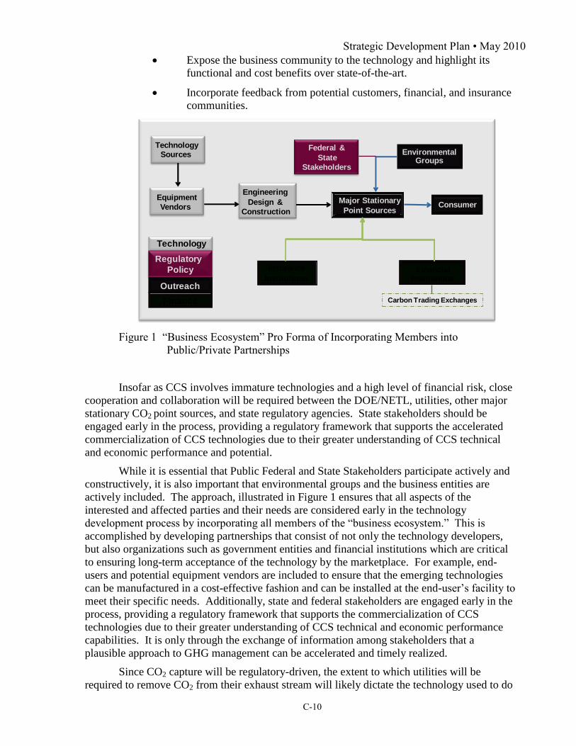
Strategic Development Plan • May 2010
C-10
Expose the business community to the technology and highlight its
functional and cost benefits over state-of-the-art.
Incorporate feedback from potential customers, financial, and insurance
communities.
Federal &
State
Stakeholders
TechnologySources
Equipment
Vendors
Engineering
Design &
Construction
Major Stationary
Point SourcesConsumer
Environmental Groups
FinancialInstitutions
Insurance
Technology
Finance
Regulatory
Policy
OutreachInstitutions
Carbon Trading Exchanges
Figure 1 “Business Ecosystem” Pro Forma of Incorporating Members into
Public/Private Partnerships
Insofar as CCS involves immature technologies and a high level of financial risk, close
cooperation and collaboration will be required between the DOE/NETL, utilities, other major
stationary CO2 point sources, and state regulatory agencies. State stakeholders should be
engaged early in the process, providing a regulatory framework that supports the accelerated
commercialization of CCS technologies due to their greater understanding of CCS technical
and economic performance and potential.
While it is essential that Public Federal and State Stakeholders participate actively and
constructively, it is also important that environmental groups and the business entities are
actively included. The approach, illustrated in Figure 1 ensures that all aspects of the
interested and affected parties and their needs are considered early in the technology
development process by incorporating all members of the “business ecosystem.” This is
accomplished by developing partnerships that consist of not only the technology developers,
but also organizations such as government entities and financial institutions which are critical
to ensuring long-term acceptance of the technology by the marketplace. For example, end-
users and potential equipment vendors are included to ensure that the emerging technologies
can be manufactured in a cost-effective fashion and can be installed at the end-user’s facility to
meet their specific needs. Additionally, state and federal stakeholders are engaged early in the
process, providing a regulatory framework that supports the commercialization of CCS
technologies due to their greater understanding of CCS technical and economic performance
capabilities. It is only through the exchange of information among stakeholders that a
plausible approach to GHG management can be accelerated and timely realized.
Since CO2 capture will be regulatory-driven, the extent to which utilities will be
required to remove CO2 from their exhaust stream will likely dictate the technology used to do

Strategic Development Plan • May 2010
C-11
so. There may also be liability risk associated with sequestered CO2. These issues hamper the
ability to finance pilot, demonstration, and full-scale projects. Insurance risks can also add to
this issue in the form of uncertainty around ownership of the captured CO2.
The team determined that one of the key methods to mitigate these risks was to educate
financial and insurance entities during the early development process and make them aware of
progress of the project over time. It was also determined that future financial risks at the pilot,
demonstration, and deployment phase could be mitigated through state incentives and financial
backing from larger companies. The team also suggested that regulatory bodies, such as public
utility commissions, be made aware of the project and briefed on its progress. This would
mitigate the risk that the team might inadvertently design a system that would not comply with
regulatory statutes.

Strategic Development Plan • May 2010
C-12
3 Carbon Capture and Storage Market Analysis
3.1 Energy Market Overview
In the International Energy Outlook 2009 projections, total world consumption of
energy is projected to increase by 44 percent from 2006 to 2030.1 The largest projected
increase in energy demand is for the non-Organization for Economic Co-operation and
Development (OECD) economies. The current economic downturn dramatically impacted
world demand for energy in the near term, as manufacturing and consumer demand for goods
and services slowed. IEO-2009’s forecast is that the majority of nations will begin to return to
trend growth within the next 12 to 24 months (Figure 2).
Figure 2. World Energy Consumption (1980-2030)2
In 2009, US energy markets continued to be impacted by the economic downturn that
began in late 2007. Power-sector investment is expected to be severely affected by financing
difficulties, as well as by weak demand (i.e., availability of capital).3 In response, many
ongoing energy projects have been delayed and others have been canceled all together.
Specifically, electricity generation declined 1 percent in 2008 and an additional 3 percent in
2009,4 which was notably the first annual contraction since the end of the Second World War. The Energy Information Administration (EIA) presumes that in the short term, the key factors
influencing worldwide energy markets will be the pace of the economic recovery, impact on
capital-intensive energy projects from the turmoil in financial markets, and the potential
enactment of legislation related to energy and the environment.5 Thus, EIA predicts moderate
energy consumption growth with energy intensity falling by 1.9 percent per year from 2008 to
2035.
It is unclear whether the full energy investment needed in the longer term to meet
growing energy needs can be made available. The capital required to meet the projected
1 World Energy Outlook 2009 Fact Sheet, the impact of the financial crisis
2 International Energy Annual 2006 (June-December 2008), EIA World Energy Projections Plus (2009)
3 Ibid
4 US Energy Information Administration Annual Energy Outlook 2010 5 Ibid

Strategic Development Plan • May 2010
C-13
energy demand through to 2030 is $26 trillion (in year-2008 dollars) — equal to $1.1 trillion
(or 1.4% of global GDP) per year on average6. It is projected that financing energy
investments will, in most cases, be more difficult and costly than prior to the crisis.
The highest growth in electricity generation is projected for the non-OECD countries
where there is a forecasted increase of 3.5 percent per year in the reference case with the
increase of standards of living.7 In the OECD countries, much slower growth in generation is
expected, averaging 1.2 percent per year from 2006 to 2030, given the well-established
infrastructures and slower population growth.
It is anticipated that fossil fuels will continue to provide the majority of energy
consumed in the US and worldwide over the next 25 years. Specifically, natural gas and coal
combined account for the largest share of total world electricity generation, at more than 60
percent of global electricity supply. They will remain the world’s most important sources of
supply in 2030, with a 64 percent share of total generation (Figure 3). Additionally, it is
anticipated that coal will continue to be a major fuel source for electricity generation over the
next few decades. Moreover in non-OECD countries such as Asia and India, coal resources are
ample and higher prices for oil and natural gas make coal a more economical source of energy
for electricity generation.8
However, EIA anticipates that the percentage of overall energy generated from fossil
fuels will decline from 84 percent in 2008 to 78 percent in 2035. At the same time, renewable
electricity generation is expected to grow exponentially as can be seen in Figure 3. However in
the short term, investment in renewable-based power generation fell proportionately more than
that in other types of generating capacity. Without the stimulus provided by government fiscal
packages, it would have fallen by almost 30%.
Figure 3. World Electricity Generation by Fuel, 2006-20309
6 Ibid
7 Ibid
8 Ibid 9 International Energy Annual 2006 (June-December 2008), EIA World Energy Projections Plus (2009)

Strategic Development Plan • May 2010
C-14
3.2 Snapshot of Gasification Market
Gasification has been used commercially around the world for more than 50 years by
the chemical, refining, and fertilizer industries and for more than 35 years by the electric power
industry. The gasification process, which was originally developed for and is widely deployed
today in the production of chemical feedstock, is a partial oxidation reaction carried out in a
continuous, high pressure reactor, in a reducing environment.10 A key advantage of the
gasification process is the ability to convert undesirable, low value fuels (high in sulfur, heavy
metals) to a clean burning synthesis gas. Subsequently, the fuel is then used in advanced
technology combined cycle combustion turbines, as well as a feedstock for chemicals
production.
Advantages of CO2 capture from pre-combustion gases include:
(1) The gas stream is at high pressure and high temperature providing a high reactivity
for CO2, H2S, and other contaminants which leads to equipment with small foot
prints
(2) The absence of combustion air keeps the volume of gas treated about 4 times less
than that of post-combustion flue gas stream, and
(3) The CO2 gas can be retained at high pressures resulting in reduced electrical energy
need for compressing that gas for pipe-line pressures.
Figure 4. Gasification Process11
10 IGCC gathers pace, PowerGen Worldwide 11 Gasification Redefining Clean Energy, Gasification Technology Council

Strategic Development Plan • May 2010
C-15
3.2.1 Integrated Gasification Combine Cycle market
Integrated Gasification Combined Cycle (IGCC) power generation allows the continued
use of coal without equivalent high level air emissions associated with conventional coal
combustion. In gasification power plants, the pollutants in the syngas are removed prior to
combustion in the turbines.12 In contrast, conventional coal combustion technologies capture
the pollutants after the exhaust gas has passed through the boiler or steam generator.
Specifically plants have been commercialized over the past two decades demonstrating
the technology’s capability to meet stringent air emission standards. The first commercial
scale IGCC projects were clean coal technology demonstrations in both the USA and Europe.
Beginning in the mid 1980s, these included the Cool Water and TECO projects (using Texaco
technology) and the Wabash River generating station (Dynergy/Destec technology) in the
USA. European demonstrations of IGCC have included the Demkolec project in the
Netherlands (Shell technology), and the Puertollano project in Spain (Prenflo/Uhde
technology).13
Commercial and near commercial sized plants using IGCC technologies have now
accumulated several years of operating experience. Additional IGCC cost savings, resulting
from technology advancements and improved construction techniques, have further reduced
power generation costs and improved refiners' operating margins.
Faced with the reality of increasing global competition, excess capacity, and tightening
environmental regulations, the refiners are taking new approaches to increase profitability
including installation of independent power production (IPP). Many oil refineries have
recognized that IGCC allows them to convert these unmarketable residues into valuable
products. Using IGCC, the refineries are able to increase their overall profitability and
improve their relative competitive position by:14
Permitting more extensive upgrading of heavy materials to produce
yields of lighter products and eliminating the need to dispose of
increasingly unmarketable bottom products.
Increasing the economic value of the produced residues through
upgrading them to electric power and other products.
Superior environmental performance, potentially reducing overall
emissions for the refinery and eliminating or reducing the need for
additional pollution control equipment.
Destruction of refinery waste streams, eliminating tipping costs
associated with their disposal, as well as deriving maximum fuel value
from them.
Easy integration with existing refinery equipment and infrastructure.
The main challenges with regard to the widespread adoption of this technology are:
Demonstration of high availability equivalent to Pulverized Coal (PC) plants,
Capital cost reduction to compete with state-of-the-art PC plants.
12 Ibid
13 Ibid 14 Holt, N., Wheeldon, J., Operating Experience, Risk, and Market Assessment of Clean Coal Technologies: 2006, EPRI

Strategic Development Plan • May 2010
C-16
Specifically, the commercial deployment of IGCC technology has been inhibited over
the last decade given the absence of a single entity responsibility for the supply of the IGCC
technology from coal to kilowatts. Thus, within the industry there are no integrated IGCC
power developers currently, but instead there are multiple “technology supporters”.
These technology supporters include:15
Air separation equipment technology and manufacturer firms.
Gasification technology suppliers.
Turbine technology and equipment manufacturers.
Engineering, procurement, and construction (EPC) firms.
The main challenges with regard to the widespread adoption of this technology are:
Unlike the NGCC industry, in which an investor deals mainly with the turbine and EPC firms,
an IGCC investor must manage at least four constituencies, making the investment much more
complex. In particular, the absence of an IGCC power developer increases the obstacles of
achieving performance guarantee wraps and limiting liquidated damages. In response, three
commercial teams were formed in 2004-2005 to offer reference turnkey IGCC plant designs to
the US power industry with price, schedule, performance and emission guarantees.16 The
Gasification Technologies Council, a non-profit organization promoting technological
advances and surveying the market, expects a further dynamic growth in gasification, reaching
a worldwide equivalent thermal capacity of 73 GWth by 2010 based upon planned projects.17
3.2.2 Value-Added Chemicals and Transportation Fuels
In addition to generating power, the IGCC process can be modified to produce value-
added chemicals or transportation fuels from coal. For example, the Tennessee Eastman
facility gasifies coal to produce chemicals.
Figure 5. Global Syngas Output by Feedstock18
15 Coal-based IGCC: Market Penetration Recommendations and Strategies, Booz Allen Hamilton 16 Holt, N., Wheeldon, J., Operating Experience, Risk, and Market Assessment of Clean Coal Technologies: 2006, EPRI
17 Gasification Redefining Clean Energy, Gasification Technology Council 18 Ibid

Strategic Development Plan • May 2010
C-17
It may be that the near-term market niche for IGCC lies not only in the production of
electricity, but also in the generation of multiple products, where electricity, steam, and
chemicals are economically bundled as products from a fully integrated complex. An IGCC
poly-generation facility produces power and other products that conceivably could be varied in
ratio depending on the market price and plant turndown ratio. In addition, poly-generation
could provide energy storage potential, as plants produce electricity at peak demands and store
synthetic fuel or other products at off-peak times19
.
Forecasts from the International Fertilizer Industry Association suggest that demand
should increase 4% in 2010 after falling nearly 7% in 2009.20 High commodity prices
experienced over recent years led to increased production and correspondingly greater fertilizer
consumption as reflected in tight markets and higher fertilizer prices at the start of the outlook
period.21
The use of gasification technology for biomass and waste has become an application of
interest with their use as partial feedstock to larger coal or petroleum coke based IGCC
plants.22
Biomass/waste atmospheric gasifiers are also used adjacent to existing PC boilers
supplying a raw gas to the boiler furnace. Gasification is also being developed for use in the
forest products industry.
19 Coal-based IGCC: Market Penetration Recommendations and Strategies, Booz Allen Hamilton
20 Chemical News & Intelligence, OUTLOOK 10: Fertilizer market back on track for growth 21 Current world fertilizer trends and outlook to 2011/12, FOOD AND AGRICULTURE ORGANIZATION OF THE
UNITED NATIONS 22 Gasification Technology Status, Electric Power Research Institute

Strategic Development Plan • May 2010
C-18
3.3 Market Growth Forecast
Indications are that many new domestic gasification projects will be refinery-based,
utilizing petroleum coke and other low-cost refinery by-products to produce power, steam,
hydrogen, and chemicals for the refinery and additional power for internal use or export.23
The maturation of gasification technologies through completion of several large-scale
demonstration projects has made this technology a popular and viable alternative to
conventional combustion technologies. There is significant market potential for coal
gasification worldwide, as the technology allows generation of fuels for virtually all
applications, i.e., transport, chemical products, and heat and power production. Escalating
prices and limited availability of natural gas in regional consumer markets are driving factors
for investments in gasification technology.
According to the Gasification Technologies Council, in 2007 there were 144
gasification plants and 427 gasifiers in operation worldwide, with a thermal capacity of some
56 GWth. Specifically, coal gasification accounted for approximately 31 GWth of that amount
with the remainder from petroleum, gas, pet coke, biomass, and waste.24 China has become the
global test case for large-scale coal conversion activities. In 2008, China held licenses for the
installation of 18 coal gasification plants; among these, 11 commercial size coal gasification
plants were already in operation, most of them for the industrial production of methanol or
ammonia.
Project momentum slowed dramatically since 2007 according to a new study by
Emerging Energy Research with considerable delays and cancellations of several prominent
IGCC projects in the past two years. The primary cause of the decline is the difficult market
environment facing all new coal builds outside of China and India.
Figure 6. Past Capacity Announcements vs. Actual25
23 US Department of Energy National Energy Technology Laboratory, Wabash Report
24Gasification Market Analysis, Emerging Energy Research 25 2007 & 2009 data Ventyx- Velocity Suite and 2002-2005 data- Previous NETL Tracking New Coal-Fired Power Plants
Reports

Strategic Development Plan • May 2010
C-19
However, as a testament to the IGCC market and proof that overall confidence in
IGCC, as a commercial technology has improved, there are still a considerable number of
plants in the development pipeline as can be seen by the green line on the graph. Visage
Energy also analyzed the potential advantages of a Capture Ready approach from a finance and
insurance perspective.
Within the global IGCC market, there are projects under development in 10 countries
with the overwhelming concentration within the US, accounting for 60% of current coal and/or
pet coke IGCC plants under consideration.
The US is currently leading the commercialization efforts of IGCC globally with 26
projects at some stage of development in 17 states with a combined capacity of
15,000 MW.
Australia is next, given strong state and federal policies targeting clean coal
technologies while Canada is driven primarily by early EOR opportunities.
China’s interest is growing due to air quality regulations becoming a greater threat
to economic development. On a worldwide basis, the main activity on coal
gasification is centered in China due to strong support from the central government.
In contrast, Europe is expected to see rather slow development of IGCC, at least
until 2015 according to EER’s study.
Figure 7. Global IGCC Project Pipeline26
There are a number of potential market penetration options:27
i. Greenfield IGCC: building a new IGCC facility.
26 Gasification Market Analysis, Emerging Energy Research 27 Coal-based IGCC: Market Penetration Recommendations and Strategies, Booz Allen Hamilton

Strategic Development Plan • May 2010
C-20
a. Advantage: Option most widely accepted in the market
b. Disadvantage: Lack of IGCC integrator and performance
wrappers
ii. IGCC with Poly-generation: Building a Greenfield IGCC facility that also
makes chemicals, synthetic gases, or synthetic fuels.
a. Advantage: Product diversification and flexible operating
structure
b. Disadvantage: Added complexity of integrating a power facility
with a chemical facility
iii. PC Repowering: Replacing existing PC facilities that are extremely inefficient
or do not meet clean air requirements with IGCC.
a. Advantage: Owner capital cost resulting from pre-existing coal
handling facility and steam turbines; existing
permits and long-term contracts
b. Disadvantage: Disruptions to facility and added regulatory
complexity
iv. NG Refueling with Syngas: Adding a gasification island in front of idle NGCC
assets.
a. Advantage: Minimal disruption to facility; capability to
withstand natural gas price volatility
b. Disadvantage: More capital intensive than a NGCC plant; plant
loses its peaking capability
v. Brownfield Add-on: Adding an IGCC facility in parallel to an existing PC
facility
a. Advantage: Reduced emissions per combined output; existing
permits and long-term contracts
b. Disadvantage: Potential disruptions to facility; potential for
physical siting constraints

Strategic Development Plan • May 2010
C-21
3.4 Technology Competitive Landscape
There are a number of carbon management strategies in development to address the
growing concern that anthropogenic CO2 emissions are contributing to global climate changes.
As indicated in Figure 8 to achieve emissions reduction targets the deployment of all
technology options will be necessary.
Figure 8. Potential for decarbonizing the U.S. electric sector - the full portfolio28
3.4.1 Purchase Credits in a Cap and Trade Scheme
One possible option to meet future regulations on carbon emission is emissions trading.
The limit or cap is allocated or sold to firms in the form of emission permits representing the
right to emit a specific volume of CO2. Firms are required to hold a number of credits
equivalent to their emissions. Firms that need to increase their emission permits must buy
permits from those who require fewer permits.29 In essence, the buyer is paying a charge for
polluting, while the seller is being rewarded for having reduced emissions.
3.4.2 Technology Substitutes
There are various options that can serve as substitutes to the deployment of CCS
technologies. Specifically, an emitter can operate fossil fuel plants more efficiently, switch to
CO2-free technologies such as nuclear and Renewables, or reduce electricity demanded by
customers.
28 James, R., “The Power to Reduce CO2Emissions: the Full Portfolio” December 2008
29 Stavins, R.N., "Experience with Market-Based Environmental Policy Instruments" November 2001

Strategic Development Plan • May 2010
C-22
3.4.2.1 Renewable Energy
The role of renewable energy sources in the world energy generation landscape could
become more substantial with the extension of current renewable energy policies. For
example, in the IEA’s reference case, there is the assumption that the Production Tax Credit
(PTC) available for electricity generation from Renewables sunsets in 2012 (wind) or 2013
(other technologies) as specified in current law; however, in the past, this incentive has been
renewed. IEA forecast that renewable generation will account for 45 percent of the increase in
total generation from 2008 to 2035. In alternative cases assuming the PTC for renewable
generation is extended through 2035, the share of growth in total generation accounted for by
Renewables is between 61 and 65 percent.
Figure 9. World Renewable Electricity Generation by Source, 2006-203030
3.4.2.2 Energy Efficiency
Energy efficiency is defined as utilizing less energy to provide the same level of energy
service. Improvements in energy efficiency can reduce the need for investment in energy
infrastructure, cut fuel costs, increase competitiveness, and improve consumer welfare. Energy
security can also profit from improved energy efficiency by decreasing the reliance on
imported fossil fuels.31 Such measures could reduce the world's energy needs in 2050 by one
third, and help control global emissions of greenhouse gases, according to the International
Energy Agency (IEA). Energy efficiency and renewable energy have been defined as the
pillars of sustainable energy policy.
3.4.2.3 Nuclear Energy
EIA forecast that electricity generation from nuclear power worldwide increases from
2.7 trillion kilowatt-hours in 2006 to 3.0 trillion kilowatt-hours in 2015 and 3.8 trillion
kilowatt-hours in 2030 in the IEO2009 reference case. An increase in new nuclear generating
30 Energy Information Administration, International Energy Outlook 2009 31 The economics of transition in the power sector, International Energy Agency

Strategic Development Plan • May 2010
C-23
capacity has been prompted by worldwide concerns with rising fossil fuel prices, energy
security, and carbon emissions. Moreover, higher capacity utilization rates have been reported
for many existing nuclear facilities, and it is expected that most of the existing facilities will be
granted extensions to their operating lives.
However, there still exists considerable uncertainty about the future of nuclear powers
such as plant safety, radioactive waste disposal, and the proliferation of nuclear weapons.
Nevertheless, the IEO2009 projection for world nuclear electricity generation in 2025 is 25
percent higher than the projection in IEO2004. Most of the expansion of installed nuclear
power capacity is expected in non-OECD countries. China, India, and Russia account for
almost two-thirds of the projected net increment in world nuclear power capacity between 2006
and 2030 (Figure 9).
Figure 10. World Nuclear Generating Capacity by Region32
3.4.2.4 Fuel Switching
In the absence of a clear path forward for coal plants, US power companies are using
natural gas combustion turbines and combined cycles to fill the power supply gap that cannot
be satisfied by renewable energy, conservation, and end-use efficiency improvements. Natural
gas remains an important fuel for electricity generation worldwide, given that it is more
efficient and less carbon-intensive than other fossil fuels. In the IEO2009 reference case, total
natural gas consumption increases by 1.6 percent per year on average, from 104 trillion cubic
feet in 2006 to 153 trillion cubic feet in 2030, and its use in the electric power sector increases
by 2.1 percent per year. With world oil prices assumed to rebound and rise through 2030,
consumers are expected to choose less expensive natural gas to meet their energy needs
whenever possible. For example, in the industrial sector, newly constructed petrochemical
plants are expected to rely more heavily on natural gas as a feedstock. Until the wide-scale
deployment of CCS, the US and other OECD countries will become increasingly dependent on
larger amounts of imported natural gas.
32 Energy Information Administration, International Energy Outlook 2009

Strategic Development Plan • May 2010
C-24
3.4.3 Capture Technology Competitors
A key observation is that the growth of the pre-combustion capture technology market
is typically contingent on the growth of the coal gasification market. In order to market the
PBI membrane technology effectively, it is critical that technology developers see the benefits
of coal gasification compared to the more developed coal combustion power system.
Several technological avenues for CCS are currently being explored. For power
generation, these include pre-combustion, post-combustion, and oxy-fuel combustion.
3.4.3.1 Post-combustion
Flue gas typically contains up to 14% CO2 that needs to be separated. For CO2
capture, chemical absorption with amines, such as mono-ethanolamine (MEA), is currently
the state-of-art option. Post-combustion systems are positioned as a carbon mitigation
solution for the existing fleet of coal-fired power plants. However, retrofitting a capture
system to a power station requires major technical modifications. These alterations are quite
costly and are accompanied by substantial decreases in generating efficiency (i.e., 33
percent reduction of net plant power output).33
Post Combustion Emerging Technology Classes
Advanced Amines - Improvement to amine-based solutions include modified
tower packing to reduce pressure drops and increased contacting, increased heat integration
to reduce energy requirements, additives to reduce corrosion, and allow higher amine
concentrations, and improved regeneration procedures.
Carbonated-based systems - Are based on the ability of a soluble carbonate to
react with CO2 to form a bicarbonate that, when heated, releases CO2 and
reverts to a carbonate.
o Advantages: Analysis indicates that the energy requirement is
approximately 5 percent lower with a higher loading capacity of 40
percent compared to 30 percent for MEA.34
Aqueous Ammonia - Works similar to amine-based systems.35
o Advantages: Significantly lowers heat of reaction, potential for high
CO2 capacity, lack of degradation during absorption/regeneration,
potential for regeneration at high pressure.
o Disadvantages: Hi Higher volatility of ammonia requires additional
equipment to recover and recycle ammonia.
Membranes - Developing a variety of options for using membranes to recover
CO2 from flue gas.
33 Figueroa, J.D., Carbon dioxide capture and sequestration potential and issues in US,
34 Rochelle G., Solvent and process enhancements for CO2,
35 Resnik, K.P. , Aqua ammonia process for simultaneous removal of CO2,

Strategic Development Plan • May 2010
C-25
o Options: Flue gas is passed through a bundle of membrane tubes, as an
amine solution flows through the shell side of the bundle. Novel thin-
film composite polymer membranes.36
CO2 capture sorbents - Reaction of a solid with CO2 to form stable and then, at
another set of conditions, allow for regeneration to liberate the absorbed CO2.
o Advantage: A number of solids can be used to perform the separation.
o Disadvantage: Solids are inherently more difficult to work with than
liquids, and no solid sorbent system for large scale recovery of CO2 from
flue gas has yet been commercialized.37
Metal organic frameworks - Are a class of hybrid material built from metal
ions well-defined coordination geometry.
o Advantage: High storage capacity and minimal heat required for
recovery.
o Disadvantage: Very early laboratory scale research; manufacturing
costs can be very high because of the high complexity. Unclear the
effects of impurities at flue gas temperature and pressure and long-term
stability. 38
Ionic liquids - Broad category of salts, containing organic cations and inorganic
or organic anions.
o Advantage: Favorable temperature stability and little heat required for
regeneration.
o Disadvantage: Most suitable ionic liquids are not commercially
available. 39
Enzyme-based membranes - Achieves CO2 capture and release by mimicking
the mechanism of the mammalian respiratory system.
o Advantage: Shown to have a very low heat of absorption that reduces
the energy penalty of absorption processes.
o Disadvantage: Limitations include pore wetting, surface fouling, loss of
enzyme activity, long-term operation, and scale-up. 40
3.4.3.2 Pre-combustion
Removal of CO2 is prior to combustion. Before combustion, the syngas is reacted with
steam to produce CO2 that is subsequently scrubbed from the gas stream, usually by a physical
absorption process. Acid gas removal processes that use physical solvents, such as Selexol and
Rectisol, have such properties, but are energy intensive. Commercial applicability is more
36 Falk Pederson, O., Gas treating using membrane gas/liquid contactors. 37 Nelson T.O., Production of concentrated CO2 from flue gas using dry regenerable carbonate sorbents in a thermal-swing
process,
38 Willis, R.R.Annual Report DE-FG26-04NT42121 National Energy Technology Laboratory,
39 Anderson, J.L., Measurement of SO2 solubility in ionic liquids, 40 Yang, W.C., Ciferno, J.Assessment of Carbozyme Enzyme-Based Membrane Technology for CO2 Capture

Strategic Development Plan • May 2010
C-26
near-term until replaced with other technologies with higher performance and improved
economics.41
Pre-Combustion Emerging Technology Classes
Other Membranes - Supported liquid membrane; dense metal alloy
with high hydrogen permeability.
Pre-combustion sorbents- Lithium silicate-based sorbent
o Advantage: Ideal for high temperature environment and has
shown excellent regeneration ability and attrition resistance in
thermal cycling tests.
o Disadvantage: Solids are inherently more difficult to work with
than liquids, and no solid sorbent system for large-scale recovery
of CO2 has yet been commercialized.42
Chemical looping gasification - Multiple solid particle loops are
utilized to provide the oxygen necessary for gasification and carbon
capture.
o Advantage: Provide greater driving force for water gas shift
reaction and minimal increase in cost of electricity.
o Disadvantage: Early stages of development and handling of
multiple solid streams.43
3.4.3.3 Oxy-combustion
Oxy-combustion burns fossil fuels in 95 percent pure oxygen instead of air. This
results in a flue gas with high CO2 concentrations (greater than 80 percent) that can be
condensed and compressed for transport and storage. This method of CO2 capture is still in the
demonstration phase and the key to commercialization is reduction in cost of oxygen
production.
Oxygen production: The cryogenic air separation technology is current
the only commercial option.
o Other Options: Ion transport membrane where oxygen diffuses
through membrane as an oxygen ion, for use in O2/N2 separation.
Oxygen transport membrane utilization in the boiler.44
Ceramic
auto-thermal recovery uses perovskites to adsorb oxygen from
41 Figueroa, J., Plasynski, S., 2007Advances in CO2 capture technology- The US DOE’s Carbon Sequestration Program
42 Li, W. , Gangwal, S.K. 2005Development of fluidizable lithium silicate-based sorbents for high temperature CO2 removal
43 Lyngfelt, A., Kronberger, B., Development of oxygen carrier particles for chemical looping combustion, Seventh
International Conference on GHG, Vancouver 44Acharya, D., Krishnamurthy, K.R., Development of a high temperature oxygen generation process, 22nd Annual
International Pittsburgh Coal Conference, Pittsburgh, PA.

Strategic Development Plan • May 2010
C-27
air and then release the adsorbed oxygen into recycled flue gas to
be vented.45
Time to Commercialization
Advanced physical solvents
Advanced chemical solvents
Ammonia
Amine solvents
Physical solvents
Cryogenic oxygen
Chemical looping
OTM boiler
Biological processes
Ionic liquids
Metal organic frameworks
Enzymatic membranes
Co
st
Re
du
cti
on
Be
ne
fit
PBI membranes
Solid sorbents
Membrane systems
ITMs
Biomass co-firing
Post-combustion (existing, new PC)
Pre-combustion (IGCC)
Oxy-combustion (new PC)
202020152010
OTM – O2 Transport Membrane (PC)
ITM – O2 Ion Transport Membrane (PC or IGCC)
CO2 Capture Targets:
• 90% CO2 Capture
• <10% increase in COE (IGCC)
• <30% increase in COE (PC)
Figure 11. NETL Fossil Energy CO2 Capture Solutions Commercialization46
45 Shah, M., van Hassel, B., CO2 capture by membrane based oxy-fuel boiler, Proceedings of the 2006 Conference on CCS
Alexandria, VA 46 National Energy Technology Laboratory Presentation – Reference Data

Strategic Development Plan • May 2010
C-28
3.5 Barriers to Entry
The most significant barrier to market penetration is pending CO2 capture and
sequestration legislature. Specifically, many states are creating incentives for utility companies
to invest in Renewable Energy Projects but have given no direction to the investment in the
broader category of clean energy technologies generated by fossil fuel with near zero
emissions. Thus, part of the commercialization effort has involved educating regulatory bodies
on the role of CCS technologies as a complement to Renewable Energy technologies providing
a portfolio of solutions to lower GHG emissions.
3.5.1 Market Barriers
The most significant barrier is the capital cost commitment needed for an IGCC plant.
Even though an 850 to 1000 MW plant is the most economical, current risk-averse financial
markets are hesitant towards funding such a large investment, especially as power needs are
trending towards incremental growth. The second main barrier to entry is investor perception
that IGCC investments are novel and overly risky in a saturated market. Table 3 depicts a
Strengths, Weaknesses, Opportunities, and Threats analysis for the IGCC market.
Table 2: General IGCC SWOT Analysis47
Strengths Weaknesses Economies of scale
A more proven technology format as
compared to other entry strategies
In short term, suppliers are in a weaker pricing
position
Most easily optimized of all options
Most easily replicated of all options
Future polygeneration potential
Adversely viewed by investors because of
financial size
Regulatory handling of IGCC facilities
relative to NGCC
Reluctance to enter into long-term contracts
because of uncertainty over future demand,
natural gas prices, and regulatory framework
Opportunities Threats Coal states that support IGCC as BACT Anticipated technology advancements do not
occur in ASU and Gasification islands
NGCC capital costs decrease at a faster rate
Permitting/siting difficult because of
environmental concerns and NIMBY
Utilities/End-user Stakeholders Issues
Require the ability to receive rate-base treatment for investment
Need for long-term stable carbon policies
Complexities in construction and operation of IGCC facilities
State Stakeholders Issues
Renewables and natural gas generation preferred over coal + CCS
Some question viability of CCS as a climate-change mitigation tool
47 Coal-based Integrated Coal Gasification Combined Cycle: Market Penetration Recommendations and Strategies, Booz
Allen Hamilton

Strategic Development Plan • May 2010
C-29
Escalating construction costs and parasitic load associated with CCS
3.5.1.1 Technology Transfer Analysis
In subtask 9.2, Visage Energy was charged with evaluating the technology transfer
opportunities associated with the PBI technology and, specifically, considering a broad
spectrum of technology transfer options available for the technology. There are a number of
possible options for technology transfer for the PBI technology. Each option was based on
market conditions and the market potential addressed in Task 8.0. It is anticipated that the PBI
technology will proceed from research and development, to deployment, to finally wide-scale
adoption by the domestic market and the international market. Although it is possible for the
spread of a technology to occur more rapidly to other countries, it does not appear that this will
be the case with the PBI technology given the CCS leadership role that the United States has
taken. Additionally, the transfer of technology outside of the US is generally more expensive
given the export expenses and the higher barriers to penetration into those international
markets.48 However, technology transfer domestically and abroad can occur simultaneously
depending on the technology demand.
In general, there are five main opportunities for transferring technology into the
marketplace: (1) Sale of Intellectual Property Rights, (2) Licensing technology to an end-user,
(3) External Incubator, (4) Establishing a joint venture with an established company that has a
channel to market and an established client base, and (5) the New Venture formation. The
options are ordered with respect to least financial commitment to highest financial commitment
required from the PBI technology development team.
Figure 12. Technology Transfer Pathways49
Figure 11 presents another framework of the technology transfer pathways where there
are three different variations on the licensing model option (Non Exclusive Licenses, Limited
48 Methodological and Technological issues in Technology Transfer, Intergovernmental Panel on Climate Change 49 Keith Belinko, “A Technology Transfer Decision Framework for Publicly Funded Research Organizations” May 2004

Strategic Development Plan • May 2010
C-30
Exclusive Licenses, and Exclusive Licenses). Technology transfer does not occur at one single
period, but instead is more of a continuum of activities leading to the application of a
commercial technology. The optimal technology transfer pathway for the PBI technology will
be based on the information available at the time of deployment. This decision will need to
address not only the PBI technical specifications, but also the regulatory, legislative, market
competition, and financial environments at that point in time. Given the decision’s dependence
on a number of technical and business issues, it is clear that the optimal technology pathway
may change along the life of the technology development lifecycle. Thus, a snapshot is taken
at a certain point to determine how best to transfer a particular technology. If another snapshot
is taken along the technology transfer continuum as the technology evolves, more information
may become available that could influence the outcome. For example, new applications for the
technology may be found, market competition may increase, and new players may become
involved.50 Currently, it appears that the PBI technology most likely should follow the Non
Exclusive License technology transfer pathway. However, Visage Energy will continue to
analyze the possible technology transfer options available as the PBI technology progresses.
3.5.2 Compilation of Financial Issues
Financial institutions are reticent to invest in these facilities given the dependence of
profitability on increasingly risky and uncertain long-term yields. Historically, the financial
community has not invested resources in the environmental control technologies because they
viewed legal compliance as being sufficient. The two most substantial barriers to project
financing are utility industry inertia in novel technology deployment and the lack of sufficient
business incentives to cover the cost of CCS. Thus, it is becoming clear to regulators that there
will need to be substantial government and industrial financial support to encourage wide-scale
deployment of CCS. There are a number of financing methods being proposed and developed
such as technology mandates, utility mandates, electricity regulator approval of higher cost,
and the creation of a dedicated CCS Trust Fund. In the past, governments assumed that the
vehicle of public/private partnerships would effectively finance the early stage deployment
necessary; however, in the last year numerous projects have been canceled due to a lack of
sufficient resources to cover escalating costs.
Financial Stakeholders Concerns:
Concerned with the current lack of sufficient business incentives but
encouraged by strong indication of an imminent carbon policy.
CCS Financing Options: Emissions trading, Mandating CCS, Energy
regulatory approval of the higher cost, and CCS Trust Fund.
Adoption of Carbon Principles: More stringent requirements for
investment in coal-based generating facilities. Provides a procedure to
analyze the dispatch order of this additional coal-fired power generation
and its economic performance under various scenarios.
50 Ibid

Strategic Development Plan • May 2010
C-31
Approval of CCS project methodology under Clean Development
Mechanism will be important.
Project Financing has been difficult for many project developers to obtain for coal
projects and even IGCC projects because financiers are concerned with the carbon policy
uncertainty. Many fear that without some form of additional support for CCS, a cap and trade
policy will not be sufficient to cover cost. Many in the finance community feel that it is a
missed opportunity that CCS is not included in the CDM and once it is included there will be a
dramatic increase in projects in developing countries.
Due to the uncertainty of escalating cost associated with construction of new coal-fired
plants, Public Utility Commissions are refusing to allow utility companies to recover the cost
of new builds in their rate-base. At this time the majority of CCS projects in development are
Enhanced Oil Recovery projects in which the CO2 originates from an industrial source
typically not requiring deployment of a capture system. The major ramification of this delay in
early deployment of CCS projects is that this experience needs to ultimately guide subsequent
future commercial demonstrations in an effort to foster the learning necessary to proliferate
CCS throughout the power generation and industrial sectors.
Thus, the financial community is looking to regulators to enact appropriate public
policy to initially encourage the development of CCS pilots and later public support around
capital cost and operating cost associated CCS. Currently, in the environmental community,
there is a division on this issue and this will continue to be a major uncertainty for the financial
community.
The IEA has urged the world’s governments to invest $20 billion in near-term, full-
scale carbon capture and storage demonstrations. The organization argues that current
spending is far from the level needed to achieve the necessary emissions reductions set forward
by the G8. The IEA recommendation, which was endorsed at the 2008 Hokkaido Toyako
summit, encourages the deployment of 20 CCS fully operational plants by 2020. 51
“The
technology must be proven within the next decade,” IEA Executive Director Nobuo Tanaka
was quoted as saying at a press conference in Paris.52
McKinsey & Co., in a study published in September of 2008, called for near-term
investment in CCS demonstrations of $14.7 billion, but concluded that after 2030, industry
could cover its own capture and sequestration costs.53 Interestingly, the report also states one
of the less-mentioned drawbacks of CCS is that it will increase the amount of coal needed to
produce a given electrical output given the decrease in plant efficiency.
3.5.3 Compilation of Insurance Issues
Although international governments have made some progress in developing suitable
CCS policy frameworks in an effort to promote early demonstration of CCS projects, there are
still many issues that need to be fully addressed prior to wide-scale deployment of the CCS in
the power generation and industrial sectors. On the transportation front, CO2 pipeline
51 International Energy Agency, CO2 CAPTURE AND STORAGE: A key carbon abatement option, October 2008 52 Eduard Gismatullin, Bloomberg, Carbon-Capture Costs Delay Projects, Hamper CO2 Goals (Update1), October 20, 2008
http://www.bloomberg.com/apps/news?pid=20601072&sid=aHbRYbAnIuMA&refer=energy
Earth2Tech, October 20, 2008 http://earth2tech.com/2008/10/20/iea-carbon-capture-needs-20b-now/#more-12731

Strategic Development Plan • May 2010
C-32
regulations will be required to increase coordination across state and national borders to
eliminate the barrier of inconsistencies in pipeline access and CO2 purity requirements.
Another deployment barrier is the lack of clarity of the property rights associated with CO2
storage, particularly including access rights and ownership of storage reservoirs.
Insurance Stakeholders:
Long-term indemnification of storage liability has yet to be resolved.
Need clarity on property rights associated with CO2 storage including access rights
and pore space ownership.
The largest impediment is the indemnification of the long-term sequestration risk. The
third-party and self-insurance instruments are best suited to the injection closure and post-
closure periods because the risk profile of the project is clear while the site is active and the
developer is best able to leverage the funds necessary to finance the instrument. Thus, the
relative cost associated with closure and post-closure activities are reasonably quantifiable. On
the other hand, long-term storage is much more difficult to estimate and the long-term risk
profiles result in an uncertain probability of risk exposure making it difficult to define the cost
of any necessary remediation activities. It is difficult to identify and monetize the damages
that could result from long-term leakage. Public/Private pooling structure will be necessary
given the inability to assign an upper limit of financial liability. Most insurance companies are
waiting until some of the major impediments are handled.
Currently traditional insurance companies are not offering coverage in the event of
storage catastrophe. The key issue with using traditional insurance products is the long-term
position that would potentially be required. Insurance companies are unable to fix a long-term
premium at the outset of a project given the lack of available data, such as an unexpected
catastrophic loss of a carbon dioxide reservoir which could immediately impact the operating
expenditures of all geological sequestration projects.54
However, without this critical issue
resolved, the majority of the utility companies with whom Visage Energy has had extensive
discussions are extremely reticent to become involved in large pilot projects deploying capture
technologies.
Ambiguities must be resolved regarding pore space ownership and the relation
between the surface and mineral estate. A process for owners and project
developers to transfer/lease the necessary subsurface pore space property rights for
a CCS project is also an issue.
The long-term ownership of and liability for the stored CO2 also are potential
barriers for CCS development which may be addressed by transferring liability to
the state or by federal or private indemnification schemes.
At the federal level, a bill has been introduced and referred to committee that would
establish a carbon-storage-stewardship trust fund funded by fees from operators to ensure
compensation for potential damages relating to the geologic storage of CO2. One private
insurer is making short-term insurance policies available.
54 R. Engleman, Geological Carbon Dioxide Sequestration: Insurance and Legal Perspectives on Liability, September 2004

Strategic Development Plan • May 2010
C-33
3.5.4 Compilation of Regulatory and Legal Issues
Successful deployment of CCS technologies hinges not only on the economics of the
process but also on the ability to create a regulatory environment that encourages investment in
technologies and rewards early adopters of the technologies. Visage Energy would assert that
the technology development is not a major impediment to the wide-scale deployment of CCS
in California.
Without a price on carbon, investor interest in CCS worldwide has been limited
to outside niche applications. Policies that place a price on GHG emissions,
such as a cap and trade, would discourage investments in traditional fossil-fuel
use and spur investments in a range of clean energy technologies, including
CCS.
Example: Allocation of cap-and-trade allowances for carbon reductions
from CCS deployment and potentially bonus allowances to early movers for the
first selected number of gigawatts (GW) of CCS capacity. At the federal level,
the House legislation would allow EPA to issue the bonus allowances to early
movers for the first six gigawatts (GW) of CCS capacity and, in a second phase,
to distribute additional allowances for additional CCS deployment. The second
phase would also be capped at 6 GW. The Senate bill, as introduced, would
provide bonus allowances for up to 10 GW of CCS in the initial phase, and
another 10 GW in a second phase
Funding for Initial CCS Projects: To foster the initial, large-scale CCS
projects needed to fully demonstrate the technology, the government can
offer financial incentives for CCS. For example, the government could create
a trust fund that could competitively award money to CCS projects to help
them overcome financing hurdles.55
A study prepared for the Pew Center
found that coal power plant owners would require between $300 million and
$650 million in funds to cover the investments in equipment and lost capacity
necessary for the initial commercial-scale deployments of CCS, depending on
the plant type and whether plants are newly built with CCS or retrofit.
Mandating GHG Emission Rates: Policymakers could rely on performance
standards to drive CCS deployment by enacting new regulations that require
CCS via a new source performance standard for power plants or a low-carbon
performance standard.
3.6 Status of Commercialization Effort
3.6.1 Identification of Stakeholders (Frame-Setters and Enablers)
The Visage Energy/SRI Partnership commercialization effort for the PBI project is
designed to establish a commercialization pathway(s) for novel technologies by aligning multi-
organizational teams and focusing on end-user needs within the context of the Statement of
Project Objectives (SOPO). This is often challenging when multiple organizations are
55 Pena, N. and E. Rubin. A Trust Fund Approach to Accelerating Deployment of CCS: Options and Considerations. Prepared
for the Pew Center on Global Climate Change, 2008.

Strategic Development Plan • May 2010
C-34
involved. A component of the Visage Energy/SRI commercialization effort is to create this
alignment through the use of SRI’s Disciplines of Innovation (DOI) approach, which is
embedded throughout the performance of the research project (Figure 12). Visage initially
identified the PBI technology stakeholders that would be involved in the entire value chain for
that project, not only in the research area, but in all areas, straight through to
commercialization. There are seven key stakeholders which will need to be brought into
alignment to accelerate the demonstration and commercialization of CCS technologies:
Federal Stakeholders
Technology Developers
State Stakeholders
End-users,
Environmental Groups
Insurance Companies
Financial Institutions
The end goal of successfully financing CCS projects cannot occur on a wide-scale level
if any one of these seven stakeholders is unaligned or excluded. For example, Financial
Institutions will be unwilling to finance CCS projects which have uninsurable and unlimited
project risk. Insofar as traditional turn-key financing may not be available for decades, new
and innovative financing methods will be required for the accelerated development and
deployment of these facilities. Insurance companies will be unwilling to provide insurance
coverage for CCS projects until state and federal regulators bound the liability by providing
some form of federal backstop protection to assist in quantifying the risk associated with
carbon sequestration.56
Visage Energy analyzed the market requirements of each of the stakeholders in an
effort to begin incorporating those requirements into the technology-development process to
target the design and development to those specifications. This step is critical and iterative, as
the feedback gathered needs to be incorporated back into the technology process early. This
should encourage seamless deployment of the PBI technology into the marketplace.
56 COMMERCIALIZATION OF CARBON CAPTURE AND STORAGE TECHNOLOGY THROUGH PUBLIC-PRIVATE
PARTNERSHIPS, Kevin O’Brien, Will Johnson, Daryl-Lynn Roberts 2007

Strategic Development Plan • May 2010
C-35
Figure 13. Technology Commercialization Process
In Task 8.0, Visage Energy performed a market analysis to further understand the
market environment that the PBI technology will face upon completion. The anti-coal
regulatory environment has somewhat hindered the growth of the IGCC market in the last 2
years. Many environmental groups have argued that the concept of “cleaning up coal” is a
false notion that the power generation and coal industry have fabricated to enable the continued
use of this fossil fuel. Additionally, many see investing in this industry as a distraction from
the investment that is necessary in Renewable Energy and Energy Efficiency Initiatives. It is
clear that additional education is necessary to demonstrate the true potential of CCS
technologies as well as a demonstration of how CCS complements Renewable and Energy
Efficiency Initiatives. Consequently, the success of Carbon Sequestration Partnership Projects
will serve as critical examples of the viability of CCS.
3.6.2 Update on Stakeholder Outreach Efforts
The Executive Stakeholders’ Collaborative (ESC) Initiative objective is to provide a
forum to educate senior-level state regulators and end-users about the benefits of CCS
technologies and their commercial viability. The Collaborative Initiative intends to work
closely with the Carbon Sequestration Regional Partnerships to foster an environment that
encourages and continues to accelerate the deployment of CCS as a carbon-management tool.
Insofar as CCS involves immature technologies and a high level of financial risk, close
cooperation and collaboration will be required between the DOE/FE/NETL, utilities, and other
major stationary CO2 point sources, and state regulatory agencies. State stakeholders should be
engaged early in the process, providing a regulatory framework that supports the accelerated
commercialization of CCS technologies due to the stakeholders’ greater understanding of CCS
technical and economic performance and potential.
The CCS/ESC Initiative will seek to foster Public/Private partnerships in an effort to
develop a regulatory framework that encourages sharing deployment costs among electric-
importing states and electric-exporting states within a region. Given the unique regulatory
environment of each state, the CCS/ESC Initiative will combine a local-state approach and a
regional approach to achieve the goal of accelerating the commercialization of CCS nationally.
Expansion Strategy for CCS Executive Stakeholders’ Collaborative Initiative
1) Develop and apply a screening methodology to identify target states to initially
serve as the focal point within each region using the following criteria:
Total carbon footprint (including electric generation plants, cement
manufactures, refineries, chemical manufactures, etc.).
Availability of suitable sequestration resources.
Active participation in RCSPs.
Favorable carbon management regulatory environment .
Collaborate with RCSPs to ensure that executive stakeholder outreach
efforts are closely coordinated with the RCSPs’ other public outreach
efforts.

Strategic Development Plan • May 2010
C-36
2) Formulate a CCS/ESC Action Plan unique to each target state:
Determine which state regulatory agency should be approached first as
the host state agency executive stakeholder (most influential and/or most
willing to be engaged).
Determine subset of major stationary CO2 point sources that are prime
candidates to join the CCS/ESC.
3) Implement the plan by establishing a CCS/ESC in each target state which will
include the DOE/FE/NETL, state-agency principals, CEOs, and senior
management of major stationary CO2 point sources. The composition of a
target state CCS/ESC will expand with the inclusion of each relevant
stakeholder and will evolve into a Regional CCS/ESC.
Initiate and coordinate outreach forums to engage relevant executive
stakeholders within each target state in an effort to expose and educate
the regulatory community about the viability of CCS as a Carbon
Mitigation Strategy and encourage its acceptance among the regulatory
community.
Coordinate a two-day visit to NETL to provide a primer on Carbon
Capture and Storage and NETL’s role in the development of CCS
technologies for each target state.
Additional regulatory agencies were invited to join each state’s
CCS/ESC.
Relevant state agencies in each state may vary. Examples may
include: Public Utilities Commission, Energy Commission, Air
Resource Board, Department of Conservation, Department of
Fish and Game, etc.
Conduct follow-up meetings with Commissioners, staff, and utility
company management to ensure that all questions/concerns have been
adequately addressed and to solicit feedback to incorporate into
upcoming forums.
4) Expand the target state’s CCS/ESC to neighboring states:
Cooperation and coordination is needed between the electric-importing
and electric-exporting states in order to provide the proper environment
for the acceleration of the deployment of CCS technologies.
Specifically, electric exporting states will likely be unwilling to approve
the construction of CCS projects without support from the electric
importing states by sharing in the total financing costs and risks
associated with an accelerated deployment approach.
Examples of regulatory activities that could foster interactions between
electric-importing and electric-exporting states would include (Figure
13):
Support of construction of new or retrofit of existing plants with
CCS including out-of-state projects with assets dedicated to
supplying electricity to importing states.
Provide state regulatory support for ratepayer funds to be utilized
for cost share in CCS technology projects.

Strategic Development Plan • May 2010
C-37
Encourage closer cooperation between major stationary CO2
point sources, financial and insurance entities, and technology
sources focused on CCS development.
Construction subsidies and suspension of coal severance tax for
initial CCS projects.
Joint guarantee from Public/Private partnerships provided by
energy-importing states and energy-exporting states for
indemnification of insurance liability in order to bound risk of
CO2 sequestration for the first few projects, as currently there is
no such indemnification available for CO2 sequestration
(exception in the case of the indemnification of the FutureGen
Alliance if FutureGen is sited in Texas or Illinois).
RD&D & Construction
Funds
Energy Importing
States
Energy Exporting
States
Low carbon energy
with credits
Figure 14. Symbiotic Relationship Between Energy Importing and Exporting States
5) Focus the existing CCS information source and database to assist all relevant
executive stakeholders in gaining an understanding of the regional requirements
for siting and permitting of CCS facilities, and technology procurement.
The RCSPs are currently collecting and developing reports that address
these key issues. Thus these libraries of information will be sourced to
provide relevant decision-makers with executive-level synopses.
Specifically, best practices concerning the permitting process, design,
construction, startup, and operation of power generation facilities with
CCS within each of the different technologies should be shared with
executive stakeholders.
CCS Executive Stakeholders’ Collaborative Forums
Each forum will include an educational session (i.e., presentations from NETL or other
industry experts), a roundtable discussion session, and a next-steps session.
1) Industry experts from NETL, Regional Sequestration Partnerships, CCS Reg
project, and project and technology developers will conduct sessions addressing
issues such as capture technology status, sequestration potential, including
opportunities for Enhanced Oil Recovery (EOR), status of current and pending

Strategic Development Plan • May 2010
C-38
projects in development, and state-specific regulatory and legal barriers to
deployment.
2) The roundtable discussion session is the most valuable part of the forum as it
provides an opportunity for executive stakeholders to engage in further
discussion regarding the benefits and opportunity of CCS as a Carbon
Management tool.
3) Additional Examples of Roundtable Discussion Topics:
The role of CCS technology in meeting the state’s energy needs and
carbon reduction goals.
The development of a comprehensive approach for a legal/regulatory
framework for permitting proposed CCS projects that is consistent with
the target state’s energy and environmental policy objectives.
Develop and support current and emerging CCS opportunities within
that region and address existing project development, legal, and
regulatory barriers.
The roles of the target state agencies in the permitting and siting of CCS
projects.
Coordinate and leverage current DOE CCS RD&D activities within the
target state to ensure that effective avenues of communication exist
between researchers, decision-makers, and other executive stakeholders.
Complementary nature of CCS in providing low-carbon base-load
generation to manage the intermittency of renewable energy.
4) Meeting frequency within each CCS/ESC is anticipated to be once per quarter
for each target state. As the Collaborative expands to include surrounding
states, meeting frequency will increase accordingly. A meeting summary and
next-steps report will be provided to stakeholders following each meeting.

Strategic Development Plan • May 2010
C-39
4 PBI Technology Commercialization Plan
4.1 Background of PBI Technology
Polybenzimidazole (PBI) is a unique amorphous thermoplastic reported to have the
highest Tg (427° C) and Heat Deformation Temperature (435° C at 264 psi) of any
thermoplastic. It withstands brief exposure up to 760° C and also retains its properties down to
-196° C. PBI does not burn and produces little or no smoke or off-gases at 1000 F. It is highly
resistant to acids, bases, and chemicals. At 58,000 psi, it boasts the highest compressive
strength of any thermoplastic or thermoset57
. The ground breaking research results at Los
Alamos National Laboratory (LANL), shown in Figure 14, demonstrated that PBI exhibited H2
permeabilities and H2/CO2 selectivities far superior to other polymeric materials. This
combination of excellent transport, thermal, and mechanical properties resulted in LANL
fabricating membrane modules based on PBI for pre-combustion CO2 capture.
PBI (400°C)
PBI (250°C)
= “wet” = “dry” (1 barrer = 10-10
cm3-cm/s-cm
2-cmHg)
Figure 15. Trade-Off Plot between H2 Permeability and H2/CO2 Selectivity in Polymers
LANL’s initial research focused on coating commercially available metallic substrates
with a PBI selective layer. While the performance characteristics highlighted in Figure 14 met
pre-combustion requirements, the projected process economics of the scaled-up metallic
membrane system fell short of the Department of Energy’s goal of less than 10% increase in
cost of electricity. As a result, membrane systems based on a PBI selective layer on polymeric
hollow fiber membranes were examined. Research indicated that the combination of a PBI
selective layer onto a microporous PBI substrate (referred to now as the PBI Membrane)
combined attractive process economics with the gas transport, thermal, and physical properties
required for pre-combustion capture of CO2
58.
57 Plastics Technology, “Extreme Plastics New Contenders Push Limits of Heat & Chemical Resistance”,
http://www.ptonline.com/articles/article_print1.cfm .
58 O’Brien, K.C.; G. Krishnan; K. Berchtold; S. Blum; R. Callahan; W. Johnson; D. Byard; T. Wu; J. Figueroa,
“Towards a Pilot-Scale Membrane System for Pre-Combustion CO2 Separation”, GHGT-9, November 2008.

Strategic Development Plan • May 2010
C-40
It was also important to establish a robust simulation to be able to model capture on an
IGCC based system. This simulation was constructed using Aspen and GT-Pro and validated
by comparison to results previously reported by NETL59. The membrane separation unit
simulation portion was especially critical since it was used to establish performance targets for
the PBI Membrane module as outlined in Figure 16.
Membrane Separation Unit
Simulation
> 90% CO2 Capture
Aspen Process Simulation &
GT Pro Simulation
Economic Analysis
< 10% increase in COE
Develop Membrane
Performance Targets
Benchmarked against
simulations used by
membrane manufacturers
& field operational data
Benchmarked against
NETL simulations
Impacts Membrane and
Process Development Strategy
Metric of success in
meeting program goals
Figure 16. Role of Membrane and Process Simulation
The simulation was used to evaluate a number of different scenarios including a
baseline with no capture, capture with Selexol, and capture with a PBI Membrane. The results,
shown in Table 3, demonstrate that the PBI membrane-based capture system exhibits process
economics that approach the DOE Program goal of less than 10% increase in COE.
59 Cost and Performance Baseline for Fossil Energy Plants, DOE/NETL 2007/1281

Strategic Development Plan • May 2010
C-41
Table 3. Preliminary Process Economics Analysis Using Simulation
Project Cases
Units
No
Capture
CO2 and
H2S
Capture
w/Selexol
CO2
Capture
w/PBI &
H2S
w/Selexol
CO2
Capture
w/PBI no
H2S
removal
Power Production @100% Capacity GWh/yr 5,455 4,461 4,943 5,035
Power Plant Capacity cents / kWh 4.50 6.19 5.49 5.02
Power Plant Fuel cents / kWh 1.90 2.47 2.31 2.26
Variable Plant O&M cents / kWh 0.78 1.00 0.92 0.91
Fixed Plant O&M cents / kWh 0.60 0.79 0.71 0.70
Power Plant Total cents / kWh 7.78 10.45 9.43 8.89
Cost of Electricity* (COE) cents / kWh 7.78 10.45 9.43 8.89
Increase in COE (over no capture) % n/a 34% 21% 14%
* Separation and Capture Only
Plant operating life: 30 years; Capacity Factor: 80%; Capital charge factor: 17.5%
CO2 capture: 3.3 Million tonnes/yr.
4.2 Status of PBI Technology
The PBI Membrane hollow fiber is composed of two components: a substrate and the
selective layer. The substrate needs to be microporous in nature and provide physical and
mechanical stability. The selective layer needs to be continuous and defect free. During the
course of the project it was determined that the best design was a PBI based selective layer
applied over a PBI based substrate.60
Based on the previous work at LANL, combined with the
simulation work, the target performance specifications for the PBI Membrane were set at
H2/CO2 selectivities in the range of 25 to 40 with H2 permeance (i.e., throughput) of 200 GPU
at 250°C.
The PBI Membrane manufacturer, Whitefox Technologies, has been systematically
adjusting the membrane fabrication process in order to achieve fibers that meet or exceed these
target specifications. Whitefox Technologies has made a significant effort to produce fibers
within this range and also to enhance process controls in order to improve uniformity between
batches of fibers. One of the first achievements was establishing a substrate which was
consistent in nature and exhibited the proper microporous structure. Figure 17 depicts a
Scanning Electron Microscope (SEM) image of the fiber at both low and high magnifications.
60 Continuation application for : “Fabrication and Scale-up of Polybenzimidazole (PBI) Membrane Based
System for Precombustion Based Capture of Carbon Dioxide”, December 2008.

Strategic Development Plan • May 2010
C-42
Figure 17. SEM Images of the Cross Section Near the Inner Surfaces of the
Porous Substrate at Low and High Magnifications
A variety of samples were produced with PBI selective layers of different thicknesses,
different outside diameters of fibers, and with different post-coating treatment conditions. The
results are summarized in Figure 18. The batch labeled WFX-45 exhibited performance close
to the target performance specifications. SEM images of the cross section of the lumen for
these samples are shown in Figure 19.

Strategic Development Plan • May 2010
C-43
Figure 18. The Measured Permeance of H2 In GPU and H2/CO2 Selectivity at 250˚C
for PBI Membrane Samples Processed Using Different Conditions. The WFX-45
Sample Exhibited Properties Close to the Target Values
Figure 19. SEM Images of the Cross Section of the Lumen Of WFX-45 (Coated Fiber)
The latest results from the evaluation of PBI Membrane hollow fibers were used to
develop preliminary design considerations for the membrane module and test skid. The test
skid module will have a membrane fiber element similar in size to a commercial Air Products

Strategic Development Plan • May 2010
C-44
PA3010 Prism membrane separator module. The PA3010 module has about 70 ft2 of effective
membrane area contained in a nominal 3 inch diameter by a 1 foot long fiber element
containing ~0.575 mm OD hollow fibers with about 63% fiber packing density. For this
preliminary design analysis, we assumed that the PBI test module will have the same nominal
element dimensions and fiber packing density as the PA3010 module. The test module
housing mechanical hardware is shown in Figure 20. The test module will be fabricated from
ANSI stainless steel pipe and flanges with all welded construction. All materials of
construction will meet the specified test site pressure and temperature process conditions. All
accessible high temperature surfaces will be adequately insulated and otherwise shielded to
maintain personnel safety and to maintain the optimum membrane operating temperatures.
Spring Seal: Ni/Co Alloy Spring in
Glass Molybdenum Filled TFE Jacket( 2)
PBI Hollow Fiber Membrane
Ansi B16.5 Class 400 LB
3 inch Blind Flange (2)
Ansi B16.5 Class 400 LB
3 inch Weld Neck Flange (2)
Weld Bead
Ansi B36.19 Stainless Steel Pipe
3 inch Sch. 40 Welded & Seamless (1)
I.D. = 3.068 inch; O.D. = 3.5 inch
Ansi B16.5 Class 400 LB
1/2 inch Weld Neck Flange (4)
Ansi B36.19 Stainless Steel Pipe
1/2 inch Sch.40 Welded & Seamless (4)
PBI Pot (2)
Pot Diameter = 3.061 in.
Grove Diameter = 2.818 in.
Grove Width= 0.188 in.
Grove Radius= 0.010-0.025 in.
Diametral Clearance max.= 0.007in.
Stailess Steeel Support Tube (1)
Annular Element Support (1)
Enerfex, Inc
Tit le: Test Module Separator
Scale: none
Date: May 20, 2009
Drawn by: R. Callahan
Revisson: 0
Feed Inlet
Permeate+ Sweep Outlet
Nitrogen sweep inlet
Retentate Outlet
High tempearure high
presure gasket (2)
Element lifting lug
0.007 in.3.068 in.
0.188 in.
2.818 in.
Preliminary Concept
Not To Scale
8.25 in.
31.5 in.
Figure 20. PBI Test Module
The PBI test module will be mounted in a test skid. The schematic for this skid is
shown in Figure 21. The design and controls are similar to skids previously designed and
constructed by Enerfex for pilot-scale testing. A separate control panel, not shown, will have
switches to operate the butter-fly valves, labeled gauges or a display screen for all pressures,
temperature indicators, turbine meters, and sample tubes connected to the appropriate ports.
Appropriate safety designs will be included, such as insulation and shielding of all hot
surfaces.

Strategic Development Plan • May 2010
C-45
Figure 21. Schematic of Skid Used for Testing PBI Modules
4.3 PBI Commercialization Pathway Schedule
The maturation of new technologies for energy applications is different than the process
for other technologies, i.e., software. Energy-related technologies are required to be highly
reliable. They have traditionally transitioned through a series of discrete steps as depicted in
Table 4.
Table 4. Typical Stages of Maturation for Energy Technologies
Technology Development Maturation Stages
Proof-of-Concept
(Fundamental) Research
Post Proof-of-Concept
Research
(Current PBI Stage)
Pilot-scale
Demonstration
Type of Work
performed
Bench scale batch-type
experimentation and
conceptual studies at the
fundamental science level
Bench/Laboratory Scale
Field testing
Construction of a to
scale carbon control
plant
Study Size No working model 0.01 - 0.1 MW 1 - 5 MW 100 - 250 MW
Required
Funding
$0.3 - $1 MM
$1 - $5 MM
$15 - $40 MM
+$100 MM
Funding
Period
6 - 7 years
3 - 5 years
3 - 4 years
3 - 7 years

Strategic Development Plan • May 2010
C-46
This development process is crucial since often heat, thermal, and mass transport
considerations can change dramatically during scale-up of the unit. Pilot-scale testing is a
crucial step since it is the first time the system is exposed to an actual power-plant
environment.
It is important that researchers consider the needs of end-users early in the development
process, e.g., Proof-of-Concept Stage, since many designs made at this early phase could
impact the ability of the system to operate successfully in a power plant environment (Pilot-
scale and beyond). This project has specifically included representatives from utilities and
other end-users (e.g., Southern Company and BP) in order to ensure that their needs are
included in the design of the PBI Membrane, module, and skid. This should facilitate and
hasten the transition of the technology to Pilot-scale and beyond.
The PBI project is currently in the Proof-of-Concept (Applied) Research Stage. During
this stage the PBI module and skid will be tested in a simulated syngas environment on-site at
SRI. Successful completion of this stage will enable the module and skid to be ready for pilot
testing.
The National Carbon Capture Center61
(NCCC) has been targeted as a potential site for
pilot-scale testing. Southern Company is the contractor for this DOE center and is a member
of the PBI research team. The test would focus only on the capture of CO2 (i.e., no storage or
use for enhanced oil recovery) and would use a slipstream for input into the module. It is
especially important that the NCCC has the capability to utilize a variety of fuel sources, e.g.,
biomass and bituminous, subbituminous, and lignite coals. It is anticipated that multiple
modules would be produced in order to evaluate in parallel a variety of different types of coal,
i.e., bituminous, subbituminous, and lignite coal.
Because of their expertise and geographic location relative to bituminous sources, NETL and
its university partners (University of West Virginia, University of Pittsburgh, Carnegie Mellon
University, University of Virginia, and Penn State University) would be included in the pilot-
scale evaluation. The University of Montana and the Energy and Environmental Research
Center62
would be engaged in the evaluation of subbituminous and lignite coals. Of special
interest would be subbituminous coal sourced from the Powder River Basin. Petroleum coke
(“Pet Coke”) would also be tested since it is one of the fuel sources BP has expressed interest
in evaluating. Pet Coke is one of the fuel sources for the Hydrogen Energy Project in
California.63
It is also critical that PBI systems be evaluated internationally as well. These tests
should also be conducted in parallel with tests in the US. Some candidate sites are in Canada,
Australia, China, and Europe. The province of Alberta would be an important test site due to
the near-zero emission plant being designed by EPCOR and Siemens.64
The Alberta Energy
Research Institute and National Resources Canada would be research partners for this effort.
The Wandoan Project is a joint effort between Queensland and GE is planned to be an IGCC
plant equipped with 90% carbon capture.65
In addition, the ZeroGen project offers another
61
http://www.nationalcarboncapturecenter.com/ 62 http://www.undeerc.org/
63 http://www.hydrogenenergycalifornia.com/
64 http://www.carboncapturejournal.com/displaynews.php?NewsID=263&PHPSESSID=hn7lh6bj98jl7ktcjd1lpavn06 65 http://www.reliableplant.com/Read/19145/ge-energy-proposes-world-leading-igcc-plant-for-australia

Strategic Development Plan • May 2010
C-47
IGCC capture plant in Australia66
. CSIRO could be a research partner to evaluate a PBI
system in conjunction with this effort. The existing cooperation between NETL, PNNL, and
the Chinese Academy of Sciences could form a platform for a pilot-scale evaluation at the
Research Center for Energy and Power at Lianyungang.67 Potential sites in Europe include the
Hatfield Plant in Stainforth, UK. This plant, being developed by Powerfuel Power, UK, has
been selected as a CCS demonstration plant for funding under the EU Energy Recovery
Programme.68
Table 5. Potential Commercialization Pathway Schedule
P=Pilot, De=Demo, Dpy=Deployment
China P P D
e
D
e
D
py
D
py
D
py
D
py
D
py
Europe P P D
e
D
e
D
e
D
py
D
py
D
py
Australia P P D
e
D
e
D
e
D
py
D
py
D
py
Canada P P D
e
D
e
D
e
D
py
D
py
D
py
US P P D
e
D
e
D
e
D
py
D
py
D
py
D
py
2
011
2
012
2
013
2
014
2
015
2
016
2
017
2
018
2
019
2
020
Year
This parallel approach at the pilot-scale leads to the ability to rapidly create a
worldwide knowledge base for the PBI technology and should hasten the transition from Pilot
to Demonstration (Demo), to Deployment. One potential schedule is depicted in Table 5. Pilot
studies begin in the US. The information from this initial study enables the implementation of
a series of simultaneous pilots in all the major markets. As part of this international effort, A
Design of Experiments Approach is developed in 2011 to ensure that the information collected
can be shared and statistically evaluated. Existing international relationships developed by the
Department of Energy and NETL facilitate the international cooperation.
The results from the multivariable study are evaluated in 2013 and enable the initiation
of a demonstration study in both the US and China in 2014. Demonstration studies are again
coordinated on an international basis and designed so that performance and statistics can be
shared and analyzed. The experience gained in the US and China enable the initiation of
demonstrations in the other regions by 2015. Full deployment of the technology begins in
2016 in China, 2017 in the US. By 2018 the PBI technology has been deployed global for CO2
capture from IGCC plants.
66 http://www.mhi.co.jp/en/news/story/090622english.html 67 www.nrcce.wvu.edu/cleanenergy/docs/20-Xiao.pdf
68 www.h2-igcc.eu/Pdf/ICEPAG-Final.pdf

Strategic Development Plan • May 2010
C-48
4.3.1 Risk Mitigation for Commercialization Pathway
There are a number of risks technical/business risks that could impact the aggressive
commercialization pathway outlined in Table 5. The risks and actions taken to mitigate these
risks are outlined in Table 7.
Table 6. Risks to the Implementation of the Commercialization Pathway and Actions
to Mitigate Risks
Risk Mitigation
Limited worldwide PBI production
capacity requires new PBI production
plants
PBI supplier becomes member of
development team and provides input on
commercialization pathway. PBI supplier
provides plan to support pathway.
PBI hollow fiber production capacity
requires significant increase in capacity
PBI hollow fiber supplier is currently team
member. Supplier provides feedback on
pathway and plan for capacity increase to
support pathway.
Geographic variations in fuel supply result
in large variations in system performance.
Parallel pilot testing and a Design of
Experiment Approach provide a means to
quickly identify sources of variation and
potential solutions. International
cooperation provides the intellectual capital
to solve issues.
Regulatory requirements and/or public
opinion extend approval times and hence
project time lines
Parallel testing in a variety of international
markets with a range of regulatory and
public opinion processes increases
probability that projects move forward in at
least one region.
Variation in gasifier types creates variation
in system performance
Design of Experiment Approach and
parallel evaluations provide a means to
identify and resolve issues.
Increase in worldwide demand for ancillary
membrane equipment drives up capital
costs
Increase in production capacity of PBI
polymer and hollow fiber should help
reduce cost of fiber and provide some
offset to other potential cost increases.
Competition from other technologies will
also limit increases in costs to the end-user.
PBI was invented in late 1940’s and is manufactured for the last 30 years. The initial
patents have expired. One of the risks of a large-scale demand for the PBI capture system is
the limited worldwide supply of the PBI polymer. PBI polymer is currently produced in any
significant commercial quantities by one supplier--PBI Performance Products. PBI
Performance Products is located in Charlotte, North Carolina and reported to have 70

Strategic Development Plan • May 2010
C-49
employees and have annual sales of approximately $9,400,000.69
Using the targeted
performance (GPU and selectivity) and current design for the membrane module, it is
estimated that for a 250 MW IGCC plant approximately 1,440 modules would be required.
Fabrication of these modules would require nearly 54,000 pounds of PBI polymer.
This amount of polymer, while insignificant for most polymers, is estimated to
represent 30% of the current production capacity. Despite this fact, the polymer industry
typically constructs plants that can produce in excess of 1 million pounds per year. Therefore,
it is predicted that the required increase in capacity of polymer production as the PBI system
transitions through the commercialization pathway is possible. With this increase in PBI
demand, it is reasonable to deduce that many companies would be interested in entering the
PBI production industry. It does highlight the importance of coordinating the
commercialization pathway and timeline with the polymer supplier so that they plan capacity
increases in order to meet the projected increases in demand.
A similar risk involves the supply of PBI hollow fiber. There is one supplier of PBI
hollow fiber--Whitefox Technologies. Using the targeted performance (GPU and selectivity)
and current design for the membrane module, it is estimated that for a 250 MW IGCC plant,
approximately 29,000 km of fiber would be required (1440 modules). This requires a
significant scale-up in capacity for the supplier. Whitefox Technologies is currently a member
of the team and is engaged in the planning for the commercialization of the PBI membrane
system.
It is expected that the fuel source will vary based on the geographic location of the
plant. In other systems, process performance has been shown to be impacted by variations in
the fuel source. Similarly differences in gasifier design may also impact the capture process.
In order to mitigate these risks, a Design of Experiments Approach should facilitate identifying
any variations in performances that could be due to fuel source. Statistic analysis, pooling of
data, and international cooperation will assist in identifying and resolving issues.
Other factors that could impact the timeline are regulatory and political in nature. For
example, delays in permitting or changes in public opinion could impede the progression of
projects. This risk is mitigated due to the fact that the regulatory environment and the stance
and impact of public opinion vary across these regions.
Rapidly deployment could also result in a rapid rise in the cost of ancillary equipment.
Compressors, fittings, valves, and other related items could rise in cost due to increased
demand. It is expected that this rise would be transitory in nature and would be limited by the
fact that other technology options would still be available to the designer. It is expected that
some of these increases might at least be partially offset by a reduction in cost of the raw
polymer and hollow fibers as volume increases.
4.4 Projection of PBI Technology Market Entry
The commercialization pathway schedule outlined in Table 5 can be used to estimate
the total number of modules, pounds of PBI polymer, and kilometers of PBI hollow fiber
required as a function of time. The basis for these calculations will be the number of MW for
which the PBI system is utilized for CO2 capture. Each pilot-scale test was assumed to be 1
69 http://www.manta.com/c/mm750v6/pbi-performance-produst-inc

Strategic Development Plan • May 2010
C-50
MW, each demonstration test was assumed to be 100 MW, while each deployment was
estimated to be 500 MW. It was assumed that there would be a minimum of three pilot-scale
tests per region (e.g., in the US at least three pilot-scale tests). In comparison, demonstration
tests would be two per region. The first deployment is assumed to occur in 2015. The number
of deployments increases incrementally with each subsequent year (e.g., two deployments in
2016, three deployments in 2017, etc.).
The number of modules per MW, pounds of polymer of PBI per module, and
kilometers of PBI hollow fiber per module were then used to project requirements as a function
of time. These results are shown in Figures 21-24.
Figure 22. Projected Mws from Which CO2 is Captured Using the PBI System
Based on Commercialization Pathway Schedule
Figure 22 illustrates the number of MWs from which CO2 is captured using the PBI
system as a function of time. These calculations are based on the commercialization pathway
schedule described in Table 5. It is useful to compare these values to the MW of new IGCC
projects outlined earlier in this document Figure 6. The MWs predicted in Figure 7 correspond
to overall market penetration rates of 0.1%, 0.2%, 1.6%, and 2.1% in the 2011 to 2014 time
frame. This demonstrates that the commercialization pathway projections are conservative and
reasonable.
The number of modules, pounds of polymer, and kilometers of PBI hollow fiber were
then projected for the 2011 to 2020 time frame. These results are shown in Figures 22-24.

Strategic Development Plan • May 2010
C-51
Figure 23. Number of Modules as a Function of Time Based on Commercialization
Pathway Schedule

Strategic Development Plan • May 2010
C-52
Figure 24. Pounds of PBI Polymer Required as a Function of Time Based on
Commercialization Pathway Schedule

Strategic Development Plan • May 2010
C-53
0
50,000
100,000
150,000
200,000
250,000
300,000
350,000
400,000
2011 2012 2013 2014 2015 2016 2017 2018 2019 2020
Kil
om
ete
rs o
f P
BI
Ho
llo
w F
ibe
r
Year
Figure 25. Kilometers of PBI Hollow Fiber Projected as a Function of Time Based on
Commercialization Pathway Schedule
The significance of Figures 21-24 is that they demonstrate that successful transition of
the PBI capture system from the pilot to demonstration to deployments will catalyze the
growth of the PBI polymer production industry--an industry currently located in the southeast
section of the US. Based on the current number of employees at the supplier of PBI polymer,
the projected growth in the industry should create in excess of 400 new jobs by 2020 in order
to support the increase in capacity of the industry. It will also create a huge PBI fiber industry
and stimulate job growth for EDC firms. Many of the EDC firms that could provide this
service have installations in the Gulf Coast. Growth of the PBI industry could also generate
jobs in a region of the country that has suffered severe economic impacts.

Strategic Development Plan • May 2010
C-54
5. Conclusions
The technical progress in the development of the substrate and selective layer has
resulted in hollow fibers that have performance (GPU and selectivity) close to the target goals.
The process simulation has demonstrated that achieving the target membrane performance
goals enables the overall process economics to approach the DOE target of less than 10%
increase in COE. Engineering work has begun to outline the membrane module configuration,
skid, and control system.
A commercialization pathway schedule was developed based on the on the technical
progress and expected time line for availability of modules for pilot testing. There were a
number of considerations when establishing this schedule:
Upstream factors such as gasifier type and characteristics of fuel source may
cause variation in the performance of capture systems
Non-technical factors such as regulatory changes and public opinion could
impact timelines for pilot, demonstration, and deployment of new capture
systems
Commercialization of PBI capture systems will impact supply chains such as
the global supply of PBI hollow fibers, and PBI polymer
Mitigating these risks was important in order to rapidly transition PBI capture
systems from pilot to demonstration to deployment
The global nature of carbon capture coupled with the international relationships
developed by the Department of Energy and NETL have created an environment that facilitates
international cooperation. This enables pilot and demonstration projects to be performed in
parallel. Pre-planning on a global scale between research institutes coupled with experimental
design and data sharing should accelerate the commercialization process. This approach
mitigates the risks listed below and enables an efficient and effective method to enable PBI
capture systems to be transitioned into full deployment.
Job creation and increased regional economic development will also be additional
advantages of the deployment of PBI capture systems. The PBI polymer production industry,
located in the southeastern US, is predicted to undergo explosive growth with the need to
increase its capacity by over 7x by 2020. This growth could result in nearly 400 new jobs
being created. PBI hollow fiber production will also undergo a similar expansion. In addition,
the Gulf Coast region of the US should be positively impacted due to the need for EDC firms
to fabricate and install PBI membrane modules and control systems.

D - 1
APPENDIX D
MEMBRANE SIMULATION CALCULATIONS
Enerfex, Inc.

D - 2
Enerfex Inc., located in Williston, Vermont, designs and evaluates membrane
processes that separate and capture gases to reduce pollution and save energy. In
collaboration with Dresser Rand, Enerfex Inc. designed a system based on conventional
membranes to capture CO2 for Statoil’s natural gas platforms in the North Sea. The
company has also designed systems for onsite industrial gas CO2 recovery, natural gas
nitrogen reduction, and industrial refrigeration NH3 recycle. Enerfex has a proprietary
model to simulate the performance of a membrane module. The model has been
validated using the data from industrial processes. The model was used to simulate the
performance of PBI hollow fiber membrane modules. Details of these calculations were
provided by Enerfex as Memorandums and they are attached below.

D - 3
D-1. PBI MEMBRANE SEPARATOR UNIT SIMULATION
A first step is to initiate the PBI simulation model using available membrane separation
data. Separation data was provided to Enerfex by LANL on November 27, 2007 in a
single Excel chart entitled “Plot to Enerfex from LANL” shown below annotated in blue
notation by Enerfex.
For the present simulation input data can be generated only if a binary mixture is
assumed since purity and recovery values are given only for H2 and CO2. A mixture of
55% H2 and 45% CO2 shall be assumed. Thus as first approximations for the initial
simulation it is assumed that CO and CO2 permeate similarly, that CH4, N2 and H2S are
100% recovered in the residue and that the H2O is 100% recovered in the permeate.Based
on these assumptions the four chosen data points in the chart above give the following
feed, residue and permeate mass balance:
residue permeate
feed XR,1 XR,2 XP,1 XP,2
scfh H2 rec. CO2 rec. H2 H2% CO2 CO2% total H2 H2% CO2 CO2% total
H2 55 98% 90% 1.1 2.64% 40.5 97.36% 41.6 53.9 92.29% 4.5 7.71% 58.4
CO2 45 80% 96% 11 20.30% 43.2 79.70% 54.2 44 96.07% 1.8 3.93% 45.8
100 50% 98% 27.5 38.41% 44.1 61.59% 71.6 27.5 96.83% 0.9 3.17% 28.4
28% 99% 39.6 47.06% 44.55 52.94% 84.15 15.4 97.16% 0.45 2.84% 15.85
and,
feed
XF,1 XF,2
H2 H2% CO2 CO2% total
55 55.00% 45 45.00% 100
PBI Membrane
0
10
20
30
40
50
60
70
80
90
100
1E-06 30 60 81 84 87 90 91.5 93 94.5 95.8 97 98.2 99.2 99.8
Percent of CO2 recovered from the Feed
Pe
rcn
et
of
H2 R
eco
vere
d f
rom
th
e F
ee
d
0
500
1000
1500
2000
2500
3000
3500
Are
a R
eq
uir
ed
pe
r 1
0,0
00
SC
FH
of
Fe
ed
Ft2
/10,0
00 S
CF
H
90%
of C
O2 reco
vered
from
the feed
in resid
ue stream
98%
of H
2 recovered
from
the feed
in p
ermeate stream
Resid
ue co
nsists o
f 90
% C
O2 , p
ermeate co
nsists o
f 92
% H
2
~2
85
ft 2 requ
ired p
er 10
,000
scfh
Feed Composition and Conditions
55% H2, 1% CO, 41% CO2 1% H2O, 1% N2, CH4 & H2S
250ºC, 700 psig
Assumed Dense layer Effective Thickness: 0.5 μ
Component Permeance, GPU
H2 180
CO 2.1 CO2 4.5
H2O 789
CH4, N2, H2S 0.3
Area required
ft2 per 10,000 scfh
Percent H2 recovered

D - 4
The H2 and CO2 permeate fluxes for each of the four chosen data points given in the table
below are based on the corresponding feed fluxes indicated in the LANL chart above:
feed residue perm. perm. perm.
flux flux flux VH2 VCO2
ft3/ft
2-h ft
3/ft
2-h ft
3/ft
2-h ft
3/ft
2-h ft
3/ft
2-h
35.09 14.60 20.49 18.91 1.58
71.43 38.71 32.71 31.43 1.29
125.00 89.50 35.50 34.38 1.13
200.00 168.30 31.70 30.80 0.90
If feed pressure = pF = 714.7 psia
and permeate pressure = pP = 71.5 psia
then the pressure ratio = pF/pP = 0.1 (equation 1)
And if,
GPU = P/L =V/(pF –pP) (equation 2) where:
V – Gas component flux (flow volume per unit area per unit volume)
L – Membrane thickness
P – Permeability equal to gas component flux normalized for pressure difference across the
membrane and membrane thickness
pF – Gas component partial pressure in the higher pressure feed to retentate side of the
membrane
pP – Gas component partial pressure in the lower pressure permeate side of the membrane
Then H2 and CO2 GPU in the present case are given by,
PH2/L = VH2 / [pF×(XF,1 + XR,1)/2 - pP×XP,1] (equation 2a)
PCO2/L = VCO2 / [pF×(XF,2 + XR,2)/2 - pP×XP,2] (equation 2b)
and therefore the H2 over CO2 selectivity αH2/CO2 in the present case is given by,
αH2/CO2 = (PH2/L)/(PCO2/L) = [Xp,1×((XF,2 + XR,2)/2 - 0.1×XP,2)] / [XP,2×((XF,1 +XR,1)/2 - 0.1×XP,1)] (equation 3)
Using the data in the tables at the bottom of page 1, calculates the following H2 GPU,
CO2 GPU, αH2/CO2 and relative H2 to CO2 partial pressure ratio in the feed to residue side of the
membrane:

D - 5
equation 2a equation 2b equation 3
PH2/L PCO2/L selectivity avg. H2/CO2
ft3/ft
2/h/psia ft
3/ft
2/h/psia αH2/CO2 rel. press
0.135086681 0.003137819 43.05 0.40
0.156846847 0.002903453 54.02 0.60
0.12993336 0.002971986 43.72 0.88
0.104322906 0.002586483 40.33 1.04
Converting the GPU units to cm3/cm
2-s-cmHg×10
-6 and to permeability in Barrer for the
given membrane thickness of 0.5 μ gives the following:
"Plot to Enerfex from LANL" November 27, 2007:
PH2/L ×10-6
PCO2/L ×10-6
selectivty avg.
H2/CO2
cm3/cm
2/s/cmHg cm
3/cm
2/s/cmHg αH2/CO2 rel. press
561.93 13.05 43.04 0.40
652.45 12.08 54.01 0.60
540.49 12.36 43.73 0.88
433.96 10.76 40.33 1.04
"Plot to Enerfex from LANL" November 27, 2007:
PH2* PCO2
*
Barrer Barrer
280.96 6.53
326.22 6.04
270.25 6.18
216.98 5.38
*L = 0.5×10⁻⁴
cm
A plot of selectivity αH2/CO2 versus average H2 / CO2 partial pressure in the feed to residue
side of the membrane is given in the following chart:

D - 6
The difference between the GPU values listed in the “Plot to Enerfex from LANL” and
those calculated in the table on the previous page were discussed by R. Callahan and K.
Berchtold. The conclusion is that the plot and data listed was generated with Pall
modeling data and the discrepancy in the listed GPU data and the plotted data is not
understood. In the present simulation the calculated permeability data shown in the table
on the previous page will be used. A subsequent Memorandum II will cover a simulation
using estimated projected performance data provided by LANL on January 18, 2008 and
shown in the table below:
Projection Performance :
PH2/L ×10-6
PCO2/L ×10-6
selectivty avg. H2/CO2
cm3/cm
2/s/cmHg cm
3/cm
2/s/cmHg αH2/CO2 rel. press
100.00 2.32 43.04 0.40
116.11 2.15 54.01 0.60
96.19 2.20 43.73 0.88
77.23 1.91 40.33 1.04
PH2* PCO2
*
Barrer Barrer
700.00 16.26
812.76 15.05
673.30 15.40
540.59 13.40
*L = 7.0×10⁻⁴
cm
Selectivity correlation
0
10
20
30
40
50
60
0 0.2 0.4 0.6 0.8 1 1.2
Avg H2/CO2 relative feed to residue pressure
Sele
cti
vit
y H
2/C
O2
PBI

D - 7
The non-linear trend of αH2/CO2 versus average H2 / CO2 partial pressure shown in the chart
at the bottom of page three is not understood. It is not clear that the data accurately
represents what would happen in a PBI membrane at the conditions given. It has been
Enerfex’s experience with commercial membranes materials such as polyimide,
polysulfone and cellulose acetate in the range of 40º-50ºC and the same range of relative
partial pressure not to exhibit a maximum inflection but instead to have a directly
proportional linear trend between selectivity and average partial pressure ratio.
Four single stage simulations for each of the four data points in the LANL Chart are
presented in the table below. In order for the simulations to converge to the LANL Chart
membrane area it was necessary to adjust the membrane thickness to 1.28 μ in each case.
permeate residue permeate residue permeate residue
LANL Chart LANL Chart LANL Chart * LANL Chart * Simulation Simulation
H2 Rec. CO2 Rec. H2 purity CO2 purity H2 purity CO2 purity
98.00% 90.00% 92.29% 97.36% 91.30% 90.00%
80.00% 96.00% 96.07% 79.70% 94.70% 73.60%
50.00% 98.00% 96.83% 61.59% 95.30% 56.50%
28.00% 99.00% 97.16% 52.94% 95.60% 48.40%
* Calculated binary mixture
The simulation result for 98% H2 recovery based in the binary mixture mass balance
generated permeability values are fairly close to the LANL Chart, i.e., 285 ft2 of
membrane area per 10,000 scfh of feed, 90% CO2 recovery and 91.3% H2 purity. The
relatively high GPU and selectivity shows the membrane is able to achieve substantially
high recovery and purity of H2 and CO2 at a substantially high feed and permeation flux.
This would be a productive membrane with high separation efficiency.
The simulation on page 10 for the 98% H2 recovery case shows that with a small
adjustment to H2 and CO2 permeability values gives a simulation that matches the LANL
Chart data, i.e., H2 permeability = 285.96 Barrer instead of 280.96 Barrer, CO2
permeability = 6.2 Barrer instead of 6.53 Barrer, and selectivity = 46.1 instead of 43
gives 285 ft2 of membrane area per 10,000 scfh of feed, 90% CO2 recovery, 90% CO2
purity and 92% H2 purity.

D - 8
D-2. PBI MEMBRANE SIMULATION: EFFECT OF PROCESS VARIABLES
A PBI simulation model was done using data provided to Enerfex by LANL on
November 27, 2007 in an Excel chart entitled “Plot to Enerfex from LANL” and is shown
below annotated in blue by Enerfex.
The LANL GPU data and performance provided are re-presented in the two tables below.
Corresponding Barrer permeability values for 0.5 μ are added:
LANL GPU DATA LANL PERFORMANCE Assumed dense layer effective thickness: 0.5 μ
Component GPU Barrer
H2 180 90
CO 2.1 1.05
CO2 4.5 2.25
H2O 789 394.5
CH4, N2, H2S 0.3 0.15
The LANL GPU DATA was simulated and compared to the LANL PERFORMANCE.
The simulated membrane area needed to recover 98% H2 in the permeate is 347 ft2
per
10,000 scfh of feed which is 21.8% more than the reported 285 ft2. The residue CO2
purity is the same at 90% with marginally lower recovery at 89.2%. The permeate H2
purity is marginally lower at 90.9%. See four SIMULATED LANL DATA (sheets 1 to
PBI Membrane
0
10
20
30
40
50
60
70
80
90
100
1E-06 30 60 81 84 87 90 91.5 93 94.5 95.8 97 98.2 99.2 99.8
Percent of CO2 recovered from the Feed
Pe
rcn
et
of
H2 R
eco
vere
d f
rom
th
e F
ee
d
0
500
1000
1500
2000
2500
3000
3500
Are
a R
eq
uir
ed
pe
r 1
0,0
00
SC
FH
of
Fe
ed
Ft2
/10,0
00 S
CF
H
purity recovery
permeate H2 92% 98%
residue CO2 90% 90%
ft2/10k scfh feed ~285
90%
of C
O2 reco
vered
from
the feed
in resid
ue stream
98%
of H
2 recovered
from
the feed
in p
ermeate stream
Resid
ue co
nsists o
f 90
% C
O2 , p
ermeate co
nsists o
f 92
% H
2
~2
85
ft2 req
uired
per 1
0,0
00
scfh
Feed Composition and Conditions
55% H2, 1% CO, 41% CO2 1% H2O, 1% N2, CH4 & H2S
250ºC, 700 psig
Assumed Dense layer Effective Thickness: 0.5 μ
Component Permeance, GPU
H2 180
CO 2.1 CO2 4.5
H2O 789
CH4, N2, H2S 0.3
Area required
ft2 per 10,000 scfh Percent H2 r
ecovered
285.6 139.8 80.1 50.1
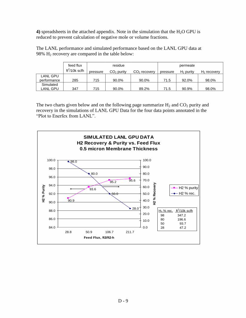
D - 9
4) spreadsheets in the attached appendix. Note in the simulation that the H2O GPU is
reduced to prevent calculation of negative mole or volume fractions.
The LANL performance and simulated performance based on the LANL GPU data at
98% H2 recovery are compared in the table below:
feed flux residue permeate
ft2/10k scfh pressure CO2 purity CO2 recovery pressure H2 purity H2 recovery
LANL GPU performance 285 715 90.0% 90.0% 71.5 92.0% 98.0%
Simulated LANL GPU 347 715 90.0% 89.2% 71.5 90.9% 98.0%
The two charts given below and on the following page summarize H2 and CO2 purity and
recovery in the simulations of LANL GPU Data for the four data points annotated in the
“Plot to Enerfex from LANL”.
SIMULATED LANL GPU DATA
H2 Recovery & Purity vs. Feed Flux
0.5 micron Membrane Thickness
95.6
93.6
90.9
95.2
98.0
80.0
50.0
28.0
84.0
86.0
88.0
90.0
92.0
94.0
96.0
98.0
100.0
28.8 50.9 106.7 211.7
Feed Flux, ft3/ft2-h
H2 %
Pu
rity
0.0
10.0
20.0
30.0
40.0
50.0
60.0
70.0
80.0
90.0
100.0
H2 %
Reco
very
H2 % purity
H2 % rec.
H2 % rec. ft2/10k scfh
98 347.2
80 196.6
50 93.7
28 47.2

D - 10
A simulation was done to calculate GPU parameters that yield a match to the LANL
PERFORMANCE. The GPU parameters for 98% H2 recovery are shown in the table
below along with corresponding Barrer permeability for 0.5 μ and 1.28 μ membrane
thickness. See the four SIMULATED LANL PERFORMANCE (sheets 5 to 8)
spreadsheets in the attached appendix. Note in the simulation that the H2O GPU is
reduced to prevent calculation of negative mole or volume fractions.
Simulated GPU values to match LANL performance
0.5 μ 1.28 μ
Component GPU Barrer Barrer
H2 219.5 109.75 280.96
CO 2.1 1.05 2.687
CO2 5.1 2.55 6.523
H2O 789 394.5 1009.92
CH4, N2, H2S 0.4 0.2 0.512
SIMULATED LANL GPU DATA
CO2 Recovery & Purity vs. Feed Flux
0.5 micron Membrane Thickness
56.4
90.0
73.3
48.4
89.2
99.097.8
94.7
40.0
50.0
60.0
70.0
80.0
90.0
100.0
28.8 50.9 106.7 211.7
Feed Flux, ft3/ft2-h
CO
2 %
Pu
rity
84.0
86.0
88.0
90.0
92.0
94.0
96.0
98.0
100.0
CO
2 %
Reco
very
CO2 % purity
CO2 % rec.
CO2 % rec. ft2/10k scfh
89.2 347.2
94.7 196.6
97.8 93.7
99.0 47.2

D - 11
The LANL performance and simulated LANL performance at 98% H2 recovery are
compared in the table below:
feed flux residue permeate
ft
2/10k
scfh pressure CO2 purity CO2 recovery pressure H2 purity H2 recovery
LANL GPU performance 285 715 90.0% 90.0% 71.5 92.0% 98.0%
Simulated GPU performance 285.6 715 90.0% 90.0% 71.5 91.4% 98.0%
The simulations of LANL performance for the four data points in the “Plot to Enerfex
from LANL” for H2 and CO2 purity and recovery are summarized in the two charts
below.
SIMULATED LANL PERFORMANCE
H2 Recovery & Purity vs. Feed Flux
0.5 micron Membrane Thickness
95.4
91.4
94.895.6
98.0
80.0
50.0
28.0
84.0
86.0
88.0
90.0
92.0
94.0
96.0
98.0
100.0
35.0 71.5 124.8 199.5
Feed Flux, ft3/ft2-h
H2 %
Pu
rity
0.0
10.0
20.0
30.0
40.0
50.0
60.0
70.0
80.0
90.0
100.0
H2 %
Reco
very
H2 % purity
H2 % rec.
H2 % rec. ft2/10k scfh
98 285.6
80 139.8
50 80.1
28 50.1

D - 12
A plot of selectivity αH2/CO2 versus average H2 / CO2 partial pressure in the feed to residue
side of the membrane for the four SIMULATED LANL PERFORMANCE
spreadsheets is given in the chart below. The non-linear trend shown in the chart is
unexpected. Typically commercial membranes such as polyimide, polysulfone and
cellulose acetate with feed to residue mixtures of CO2 and N2 or CH4 with a temperature
range of 40º-50ºC and within the same partial pressure ratio range do not exhibit a
maximum inflection but instead show a proportional linear trend of α CO2/ N2 selectivity
increasing directly with average CO2/N2 partial pressure ratio.
The table below summarizes the simulated LANL performance.
H2/CO2 avg. press. ratio 0.40 0.60 0.88 1.04
% H2 recovery 98% 80% 50% 28%
% CO2 recovery 90% 96% 98% 99%
ft2/10,000 scfh of feed 285.6 139.8 80.1 50.1
H2 GPU 219.5 254.9 211.1 169.5
CO2 GPU 5.1 4.7 4.8 4.2
α H2/CO2 43.0 54.2 44.0 40.4
SIMULATED LANL PERFORMANCE
CO2 Recovery & Purity vs. Feed Flux
0.5 micron Membrane Thickness
48.4
73.5
90.0
56.5
90.0
96.0
99.0
98.0
40.0
50.0
60.0
70.0
80.0
90.0
100.0
35.0 71.5 124.8 199.5
Feed Flux, ft3/ft2-h
CO
2 %
Pu
rity
84.0
86.0
88.0
90.0
92.0
94.0
96.0
98.0
100.0
CO
2 %
Rec
ove
ry
CO2 % purity
CO2 % rec.
CO2 % rec. ft2/10k scfh
90.0 285.6
95.0 139.8
98.0 80.1
99.0 50.1

D - 13
Selectivity correlation
0
10
20
30
40
50
60
0 0.2 0.4 0.6 0.8 1 1.2
Avg H2/CO2 relative feed to residue pressure
Sele
cti
vit
y H
2/C
O2
PBI

D - 14
D-3. PBI MEMBRANE SIMULATION – EFFECT OF SWEEP GAS
LANL provided Projected PBI membrane data in addition to the LANL Performance
simulated in Memorandums I and II. The Projected data are more conservative than the
LANL Performance. The LANL Projected PBI membrane data is presented in Table 1
below.
Table 1
LANL Projected Data :
PH2/L ×10-6
PCO2/L ×10-6
selectivity avg. H2/CO2 PH2* PCO2
*
cm3/cm
2/s/cmHg cm
3/cm
2/s/cmHg αH2/CO2 relative press Barrer Barrer
100.00 2.32 43.04 0.40 700.00 16.26
116.11 2.15 54.01 0.60 812.76 15.05
96.19 2.20 43.73 0.88 673.30 15.40
77.23 1.91 40.33 1.04 540.59 13.40
*L = 7.0×10⁻⁴
cm
Projected membrane thickness is increased from 0.5μ to 7μ and Projected H2 GPU is
reduced from 219 to 100. The Projected data assumes the H2 GPU relative to the other
components’ GPU will be the same as the LANL Performance and, accordingly, the
selectivity’s will be the same. The respective residue and permeate component purities,
recoveries and heating values will therefore be identical to the LANL Performance.
However, membrane areas per 10,000 scfh of feed, which are compared in Table 2 below
with the previously simulated LANL Performance, are about 2.2 times higher in each
simulation case.
Table 2 – LANL Performance & Projected Performance simulation permeate residue permeate residue performance projected
# H2 rec. CO2 rec. H2 purity CO2 purity ft
2/10k scfh feed.
ft2/10k scfh feed.
1 98% 90% 91.4% 87.8% 285.6 627.1
2 80% 96% 94.8% 71.7% 139.8 307.1
3 50% 98% 95.3% 55.1% 80.1 175.8
4 28% 99% 95.6% 47.2% 50.1 110.0
Therefore, the only change in performance is the increase in membrane area requirement.
LANL Projected Performance Simulation spreadsheets titled “Simulated LANL
Projected” numbered 1 to 4 are attached in the Appendix.
Sweep Gas Simulations:
It is generally understood that the H2 rich permeate fuel gas in order to fuel a gas turbine
will need to be reduced in Btu/ft3 heating value. The reduction can be accomplished by
dilution with N2 which will be available from an ASU associated with an IGCC power
plant. The exact lower heating value needed is not known. The dilution can be
conveniently accomplished by means of a N2 sweep gas on the permeate side of the

D - 15
membrane which will at the same time reduce the membrane area requirement for the
same degree of H2 and CO2 purity and recovery. Sweep Gas simulations for LANL
Performance at sweep gas fractions of 0%, 25%, 50% and 75% with 98% H2 recovery are
summarized in Table 3 below.
Table 3 - LANL Performance With N2 Permeate Sweep Gas At 98% H2 Recovery
simulation residue permeate residue sweep fraction
feed flux
membrane area
permeate fuel
# CO2 rec. H2 purity CO2 purity % ft3/ft
2-h ft
2/ MW* Btu/ ft
3
5 90.0% 91.4% 87.7% 0% 35.0 921.7 313.6
6 90.9% 69.0% 87.8% 25% 39.0 827.8 236.7
7 91.7% 46.3% 88.0% 50% 42.7 751.1 158.7
8 92.4% 23.3% 88.0% 75% 47.0 685.4 79.9
* One MW at 44% thermal efficiency equals 32,250 scfh of feed
A plot of the sweep gas effect on heating value and membrane requirement in LANL
Performance over a range of Sweep gas fractions is illustrated in Chart 1 below.
Chart 1 – LANL Performance Area and Heating Value vs. Sweep Gas Fraction
Sweep Gas simulations for LANL Projected at sweep gas fractions of 0%, 25%, 50% and
75% with 98% H2 recovery are summarized in Table 4 below.
LANL Performance With N2 Permeate Sweep
At 98% H2 Recovery
827.8
921.7
751.1
685.4
313.6
236.7
158.7
79.9
500
550
600
650
700
750
800
850
900
950
0% 25% 50% 75%
N2 Permeate Sweep Fraction, %
Me
mb
ran
e A
rea
, ft
2/ M
W
0
50
100
150
200
250
300
350
Pe
rme
ate
Fu
e/, B
tu/ ft
3
membrane area ft2/ MW
permeate fuel Btu/ ft3

D - 16
Table 4 - LANL Projected With N2 Permeate Sweep At 98% H2 Recovery
simulation residue permeate residue sweep fraction
feed flux
membrane area
permeate fuel
# CO2 rec. H2 purity CO2 purity % ft3/ft
2-h ft
2/ MW* Btu/ ft
3
9 90.0% 91.4% 87.7% 0% 15.9 2022.3 313.4
10 90.9% 69.0% 87.9% 25% 17.7 1817.0 236.6
11 91.8% 46.2% 87.9% 50% 19.6 1646.1 158.4
12 92.4% 23.3% 88.0% 75% 21.4 1504.4 79.9
* One MW at 44% thermal efficiency equals 32,250 scfh of feed
A plot of the sweep gas effect on heating value and membrane requirement in LANL
Projected over a range of sweep gas fractions is illustrated in Chart 2 below.
Chart 2 – LANL Projected Area and Heating Value vs. Sweep Gas Fraction
Tables 3 and 4 and Charts 1 and 2 above, show that progressively increasing the sweep
gas fraction reduces both heating value and membrane area requirement while increasing
CO2 recovery and purity by a small amount. LANL Performance simulation spreadsheets
titled “Simulated LANL Performance with Sweep Gas” numbered 5 to 8 and LANL
Projected simulation spreadsheets titled “Simulated LANL Projected Performance with
Sweep Gas” numbered 9 to 12 are attached in the Appendix.
The lower H2 GPU and thicker effective membrane thickness in the LANL Projected data
across the range of sweep gas fractions increases the membrane requirement compared to
LANL Projected With N2 Permeate Sweep
At 98% H2 Recovery
1504.4
2022.3
1646.1
1817.0
313.4
236.6
158.4
79.9
1400
1450
1500
1550
1600
1650
1700
1750
1800
1850
1900
1950
2000
2050
2100
0% 25% 50% 75%
N2 Permeate Sweep Fraction, %
Me
mb
ran
e A
rea
, ft
2/ M
W
0
50
100
150
200
250
300
350
Pe
rme
ate
Fu
el, B
tu/ ft
3
membrane area ft2/ MW
permeate fuel Btu/ ft3

D - 17
LANL Performance by a factor of about 2.2. Accordingly, the design goal for the PBI
membrane should be an effective membrane thickness as close to as possible to the
LANL Performance effective thickness of 0.5μ without a loss of operating membrane
robustness or reduction in acceptable membrane economic life.

D - 18
D-4. PBI SIMULATIONS WITH N2 PERMEATE SWEEP AND AN INCREASED
PERMEATE PRESSURE OF 250 PSIA
Simulations of LANL performance at 71.5 psia permeate pressure presented in
Memorandum III are reviewed in Table 1. The green highlighted data was added after
receiving information from BP that the heating value requirement of the gas turbine is
115 Btu/ft3.
Table 1 - N2 Permeate Sweep Gas At 98% H2 Recovery, 715 psia Feed
& 71.5 psia Permeate
residue permeate residue sweep fraction
feed flux
membrane area
permeate fuel
CO2 rec. H2 purity CO2 purity % ft3/ft
2-h ft
2/ MW* Btu/ ft
3
90.0% 91.4% 87.7% 0% 35.0 921.7 313.6
90.9% 69.0% 87.8% 25% 39.0 827.8 236.7
91.7% 46.3% 88.0% 50% 42.7 751.1 158.7
92.2% 33.7% 87.9% 63.7% 45.2 712.8 115.5
92.4% 23.3% 88.0% 75% 47.0 685.4 79.9 *One MW at 44% thermal efficiency equals 32,250 scfh of feed
Increasing the N2 sweep fraction at 715 psia feed pressure and 71.5 psia permeate
pressure lowered the membrane requirement with little or no effect on H2 and CO2
recovery. The sweep fraction and therefore the membrane requirement is now specified
by the 115 Btu/ft3 permeate fuel heating value. However, 71.5 psia permeate pressure is
not high enough pressure to fuel a gas turbine and will need to be increased to 250 psia.
Accordingly, a set of five simulations with a feed pressure of 715 psia, permeate pressure
at 250 psia and nitrogen sweep fractions of 0%, 50%, 60%, 62.9%1 and 70% were
completed. A sweep gas fraction of 62.9% gives a permeate fuel heating value of 115
Btu/ft3. The results are summarized in Table 2 below.
Table 2 - N2 Permeate Sweep Gas At 98% H2 Recovery, 715 psia Feed
& 250 psia Permeate
simulation residue permeate residue sweep fraction
feed flux
membrane area
permeate fuel
# CO2 rec. H2 purity CO2 purity % ft3/ft
2-h ft
2/ MW* Btu/ ft
3
1 56.1% 73.9% 82.5% 0% 6.7 4,811.2 253.6
2 85.6% 44.4% 87.2% 50% 23.9 1,348.3 152.1
3 87.9% 36.0% 87.6% 60% 28.8 1,119.1 123.6
4 88.5% 33.6% 87.6% 62.9% 30.4 1,059.8 115.3
5 89.8% 27.3% 87.7% 70% 34.3 940.8 93.7
* One MW at 44% thermal efficiency equals 32,250 scfh of feed
1 Subsequently added

D - 19
At 50% sweep fraction, 715 psia feed and an increased permeate pressure of 250 psia,
CO2 recovery and H2 purity are marginally reduced while membrane area is substantially
increased. The data in Table 2 is plotted in Figures 1 and 2 below.
Figure 1 – Membrane Area and Permeate Fuel vs. Sweep Fraction
Figure 2 – Membrane Area and CO2 recovery vs. Sweep Fraction
LANL With N2 Permeate Sweep
98% H2 Recovery, 715 psia Feed & 250 psia Permeate
940.81119.1
1348.3
4811.2
93.2
123.6
152.1
253.6
8001,1001,4001,7002,0002,3002,6002,9003,2003,5003,8004,1004,4004,7005,000
0% 50% 60% 70%
N2 permeate Sweep Fraction, %
Mem
bra
ne
Are
a, ft
2 /MW
50
100
150
200
250
300
Per
mea
te F
uel
, Btu
.ft3
membrane area ft2/ MW
permeate fuel Btu/ ft3
LANL Performance With N2 Permeate Sweep
98% H2 Recovery, 715 psia Feed & 250 psia Permeate
940.81119.1
1348.3
4811.2
89.887.9
85.6
56.1
8001,1001,4001,7002,0002,3002,6002,9003,2003,5003,8004,1004,4004,7005,000
0% 50% 60% 70%
N2 Permeate Sweep Fraction, %
Me
mb
ran
e A
rea
, ft2 /M
W
50
55
60
65
70
75
80
85
90
95
CO
2 R
ec
ov
ery
, %
membrane area ft2/ MW
CO2 recovery %

D - 20
Also completed were five simulations with feed pressure at 1,015 psia, permeate pressure
at 250 psia and nitrogen sweep fractions of 0%, 50%, 60%, 63.5%2 and 70%. Based on
information from BP, 63.5% sweep gas at these pressures gives the desired fuel heating
value of 115 Btu/ft3. The results are summarized in Table 3 below.
Table 3 - N2 Permeate Sweep Gas At 98% H2 Recovery, 1,015 psia Feed
& 250 psia Permeate
simulation residue permeate residue sweep fraction
feed flux
membrane area
permeate fuel
# CO2 rec. H2 purity CO2 purity % ft3/ft
2-h ft
2/ MW* Btu/ ft
3
6 77.6% 84.0% 86.3% 0% 21.0 1,531.5 288.2
7 88.8% 45.3% 87.6% 50% 44.6 723.3 155.5
8 90.0% 36.7% 87.7% 60% 50.0 644.8 125.7
9 90.4% 33.5% 87.8% 63.5% 51.9 620.9 115.1
10 91.0% 27.6% 87.9% 70% 55.5 580.6 94.7
* One MW at 44% thermal efficiency equals 32,250 scfh of feed
Comparing the 715 psia feed and 71.5 psia permeate case at 50% sweep gas fraction, to
the increased feed pressure of 1,015 psia with 250 psia permeate pressure, shows a
substantially improved performance, converging all operating parameters to within 2-3%,
including membrane area. The performance at 63.5% sweep fraction and 115.1 Btu/ft3,
is even better in all respects, almost equaling the performance at 71.5 psia permeate
pressure at 50% sweep gas fraction and exceeds the NETL specified CO2 capture rate of
90%. The membrane area of 620.9 ft2/ MW is substantially less than the 715 psia feed
case and would be about the size of a standard commercial 4” × 5’ hollow fiber bundle.
The data in Table 3 is plotted in Figures 3 and 4 below.
2 Subsequently added
LANL Performance With N2 Permeate Sweep
98% H2 Recovery, 1,015 psia Feed & 250 psia Permeate
580.6644.8
723.3
1531.5
94.7
125.7
155.5
288.2
540
640
740
840
940
1,040
1,140
1,240
1,340
1,440
1,540
1,640
0% 50% 60% 70%
N2 Permeate Sweep Fraction, %
Mem
bra
ne
Are
a, ft
2 /MW
80
110
140
170
200
230
260
290
Per
mea
te fu
el, B
tu/ft
3
membrane area ft2/ MW
permeate fuel Btu/ ft3

D - 21
Figure 3 – Membrane Area and Permeate Fuel vs. Sweep Fraction
Figure 4 – Membrane Area and CO2 recovery vs. Sweep Fraction
LANL Performance With N2 Permeate Sweep
98% H2 Recovery, 1,015 psia Feed & 250 psia Permeate
1531.5
580.6644.8
723.377.6
91.090.0
88.8
400
500
600
700
800
900
1,000
1,100
1,200
1,300
1,400
1,500
1,600
0% 50% 60% 70%
N2 Permeate Sweep Fraction, %
Me
mb
ran
e A
rea
, ft2 /M
W
70
75
80
85
90
95
CO
2 R
ec
ov
ery
, %
membrane area ft2/ MW
CO2 recovery %

D - 22
D-5. PBI MEMBRANE SIMULATION – EFFECT OF MEMBRANE THICKNESS
LANL provided empirical PBI membrane GPU data and consequently empirical PBI
single and mixed gas permeability parameters. Baseline operating performance at LANL
test conditions was simulated. Projected goal performance based on a thinner membrane
separation layer than the test membrane and higher feed pressure than the test pressure
were simulated. The empirical results establish a baseline comparison upon which future
goal membrane performance can be judged.
The LANL empirical GPU and permeability data is presented in Table 1 below:
Table 1 - LANL Empirical Data
Feed Press. = 260 cm Hg; Permeate Press. = 76 cm Hg
Separation Layer 0.0012 cm
Single Gas GPU Mixed Gas GPU
10-6cm
3/s/cm
2/cm Hg H2 α Barrer 10
-6cm
3/s/cm
2/cm Hg H2 α Barrer
H2 5.20 1.00 6.24E-09 7.30 1.00 8.76E-09
CO2 0.12 43.33 1.44E-10 0.17 42.94 2.04E-10
CO 0.25 20.80 3.00E-10 0.06 121.67 7.20E-11
N2 0.020 260.00 2.40E-11 0.020 365.00 2.40E-11
CH4 0.010 520.00 1.20E-11 0.030 243.33 3.60E-11
H2S 0.004 1300.00 4.80E-12 0.004 1825.00 4.80E-12
The tested effective membrane separation layer is 0.0012 cm or 12 μm. This is a
relatively large thickness compared to commercial gas membrane separation layers which
are typically about 0.1 μm. The test feed pressure and trans-membrane pressure (TMP)
difference is significantly less than what will be available with an IGCC shift gas.
Simulations 1, 2, 3, and 4 are presented in the Appendix and summarized in Table 2
below. Simulations 1 and 2 are based on the LANL empirical permeability data at the test
pressure and the test membrane thickness. Simulations 3 and 4 are based on the LANL
empirical permeability data at the expected higher shift gas pressure and the test
membrane thickness.
Table 2 –Simulations at LANL Test Pressure, IGCC Shift Gas Pressure and 98% H2 Recovery
600 MW
Sim. Data Feed Permeate Membrane N2
Sweep Permeate CO2 Rec. Mbr. Area
4"×5' elements
# Source P, cm Hg P, cm Hg Layer, μm % Btu/Ft3 % m
2 #
1 LANL Single Gas 260 76 12 63.8 115.1 89.8 31,935,278 520,642
2 LANL Mixed Gas 260 76 12 63.9 115.0 89.8 22,738,681 370,709
3 LANL Single Gas 1,015 250 12 64.0 115.1 90.6 1,463,662 23,862
4 LANL Mixed Gas 1,015 250 12 64.1 115.0 90.5 1,042,709 16,999
In simulations 1 and 2, based upon both the test membrane thickness and the test feed
pressure, permeation fluxes are extraordinarily low and consequently membrane areas are

D - 23
extraordinarily high. It is clear that the test GPUs give an extreme lower performance
boundary. The test conditions of 12 μm thickness and 260 cm Hg feed pressure were not
meant to realize acceptable economic performance. Even though Simulations 3 and 4 at
the test membrane thickness and the much higher IGCC shift gas operating feed pressure
of 1,015 psia reduce membrane area by about 95% respectively, they are also
unacceptably high. It is noted that marginally higher Mixed Gas test GPU’s in each case
simulated additional membrane area reductions of about 30% compared to the single gas
data.
The main challenge in designing and fabricating an economic PBI hollow fiber
membrane will be the attainment of a substantial reduction in membrane separation layer
thickness. Less than 1.0 μm separation layer will be necessary if a commercial PBI
membrane is to have an acceptable economic membrane area in a 600 MW IGCC power
plant. The LANL empirical data has established quite good single and mixed gas PBI
permeability and selectivity parameters. The task now is a typical membrane fabrication
problem: produce a sufficiently thin, defect free and durable membrane separation layer
that enables economic productivity based upon the measured mixed gas permeability and
selectivity parameters.
Notwithstanding potential deviations, if any, from the empirical data caused by changes
in polymer morphology or an effect on permeability and selectivity in a thinner
membrane separation layer operating at higher pressure, it is still helpful to simulate
projected membrane area reductions based on LANL empirical permeability data
assuming a projected 0.5 μm thick separation layer. A 0.5 μm thickness is a realistic
approach to the commercial gas separation membrane’s 0.1 μm thickness. Given PBI’s
high glass transition temperature of 400 - 450ºC, assuming the same permeability and
selectivity performance in a thinner separation layer operating at higher pressure with 5
times the thickness of a commercial membrane is reasonable. Projected GPUs based on
the LANL’s empirical PBI mixed gas permeability and selectivity data assuming a
membrane separation layer thickness of 0.00005 cm are presented in Table 3 below.
Table 3 - LANL Empirical Data Projected
Separation Layer 0.00005 cm
Single Gas GPU Mixed Gas GPU
10-6cm
3/s/cm
2/cm Hg H2 α Barrer 10
-6cm
3/s/cm
2/cm Hg H2 α Barrer
H2 124.80 1.00 6.24E-09 175.20 1.00 8.76E-09
CO2 2.88 43.33 1.44E-10 4.08 42.94 2.04E-10
CO 6.00 20.80 3.00E-10 1.44 121.67 7.20E-11
N2 0.48 260.00 2.40E-11 0.48 365.00 2.40E-11
CH4 0.24 520.00 1.20E-11 0.72 243.33 3.60E-11
H2S 0.10 1300.00 4.80E-12 0.10 1825.00 4.80E-12

D - 24
Simulations 5 and 6 based on the LANL empirical single gas and mixed gas permeability
data, calculated GPU projections assuming a separation layer of 0.5 μm and the expected
pressure in an IGCC shift gas are presented in the Appendix and summarized in Table 4
below.
Table 4 - Simulations at LANL Test Data, 0.5 μm Separation Layer, IGCC Shift Gas Pressure and 98% H2 Recovery
600 MW
Sim. Data Feed Permeate Membrane N2
Sweep Permeate CO2 Rec. Mbr. Area
4"×5' elements
# Source P, cm Hg P, cm Hg Layer, μm % Btu/Ft3 % m
2 #
5 LANL Single Gas 1,015 250 0.5 64.0 115.2 90.5 61,016 995
6 LANL Mixed Gas 1,015 250 0.5 64.0 115.2 90.5 43,471 709
In comparing Tables 2 and 4, the only difference between simulations 4 and 6 is the
separation layer thickness: 12 µm compared to 0.5 µm, respectively. Since membrane
area and element count vary directly with separation layer thickness (0.5/12 = 1/24) the
element count in simulation 6 would be expected to be 1/24th of the membrane area and
element count in simulation 4, as it is, i.e., 1/24 × 1,042,709 ≈ 43,471 and 1/24 × 16,999
≈ 709, respectively.
Earlier Pall simulated a PBI membrane performance projection calculating GPUs
assuming 0.5 μm separation layer thickness and based upon the same LANL permeability
data presented in Table 1. The results were given in the “Plot to Enerfex from LANL”
which was included in Simulation Memorandum II and is presented again below.
PBI Membrane
0
10
20
30
40
50
60
70
80
90
100
1E-06 30 60 81 84 87 90 91.5 93 94.5 95.8 97 98.2 99.2 99.8
Percent of CO2 recovered from the Feed
Pe
rcn
et
of
H2 R
eco
vere
d f
rom
th
e F
ee
d
0
500
1000
1500
2000
2500
3000
3500
Are
a R
eq
uir
ed
pe
r 1
0,0
00
SC
FH
of
Fe
ed
Ft2
/10,0
00 S
CF
H
90%
of C
O2 reco
vered
from
the feed
in resid
ue stream
98%
of H
2 recovered
from
the feed
in p
ermeate stream
Resid
ue co
nsists o
f 90
% C
O2 , p
ermeate co
nsists o
f 92
% H
2
~2
85
ft2 req
uired
per 1
0,0
00
scfh
Feed Composition and Conditions 55% H2, 1% CO, 41% CO2
1% H2O, 1% N2, CH4 & H2S 250ºC, 700 psig
Assumed Dense layer
Effective Thickness: 0.5 μ
Component Permeance, GPU H2 180
CO 2.1
CO2 4.5 H2O 789
CH4, N2, H2S 0.3
Area required ft2 per 10,000 scfh
Percent H2 r
ecovered

D - 25
As expected the Pall GPU values are approximately the same as the mixed gas GPU
values presented in Table 3 above. Simulation 7, based on the Pall GPU values
calculated with a separation layer of 0.5 μm and the expected pressure in an IGCC shift
gas, is presented in the Appendix and summarized in Table 5 below.
Table 5 - Simulation of Pall GPUs, 0.5 μm Separation Layer, IGCC Shift Gas Pressure and 98% H2 Recovery
600 MW
Sim. Data Feed Permeate Membrane N2
Sweep Permeate CO2 Rec. Mbr. Area
4"×5' elements
# Source P, cm Hg P, cm Hg Layer, μm % Btu/Ft3 % m
2 #
7 PALL GPU3 1,015 250 0.5 63.8 115.3 89.8 42,299 690
LANL has established baseline single and mixed gas permeability values for the
identified shift gas mixture constituents. They have measured GPUs at a 12 µm
separation layer thickness and 2600 torr feed pressure. Pall and Enerfex have calculated
GPUs for a projected 0.5 µm separation layer membrane and simulated at IGCC shift gas
pressure approximately the same PBI membrane performance, i.e., 235 ft2 of membrane
area per 10,000 scfh of feed and 242 ft2 area of membrane area per 10,000 scfh of feed,
respectively, at 98% H2 recovery and 90% CO2 recovery. Both results also approximate
the order of magnitude performance presented as simulation 9 in Simulation
Memorandum IV which was misnamed “Performance”.
A 0.5 µm separation layer in a membrane having the LANL demonstrated mixed gas
permeability is projected to require the equivalent of about ±700, 4 inch diameter by 5
feet long hollow fiber membrane elements for a 600 MW plant. A separator module
design could be an arrangement of 9 elements connected on the hollow fiber bore side to
common feed and residue headers within a single separator module pressure vessel. The
separator module vessel would be sized appropriately to handle the required nitrogen
permeate sweep gas volume flow on the shell side of the hollow fiber. Hence a total of
±80 separator modules containing 9 elements each might be required for 600 MW plant.
3 Pall GPU calculated based on LANL empirical permeability and assumed 0.5 µm thick separation layer.

D - 26
D-6. EFFECT OF GASIFIER PRESSURE AND CONSEQUENTLY MEMBRANE
FEED PRESSURE ON MEMBRANE PERFORMANCE
The gasifier outlet pressure in Scenario # 4b of the ASPEN model is given on page 32,
Figure 13, of the April to June 2008 Progress Report at about 800 psia. In the same
figure, the water Gas Shift Reactor (WGSR) outlet pressure, which provides the
membrane feed pressure, is given at about 750 psia. The membrane feed pressure basis
in prior memoranda ranged from 715 psia to 1,015 psia. Table 1 below illustrates the
performance differences between 750 psia and 1,015 psia feed pressure in prior dry basis
feed simulations. As the feed pressure increases, membrane area decreases in
approximate proportion and CO2 recovery increases marginally. Reducing feed pressure
from 1,015 psia to 750 psia increases membrane area by 63% and reduces CO2 recovery
from 90.5% to 88.6%.
Table 1 – Membrane Performance Based on LANL Test Data, 0.5 μm Separation Layer and 98% H2 Recovery at 750 psia and 1,015 psia Feed Pressure.
In NETL’s “Cost and Performance Baseline for Fossil Energy Plants: Bituminous Coal
and Natural Gas to Electricity Final Report” IGCC case, a GE gasifier at 815 psia is
integrated with a GE F class turbine. In an article by Texaco, GE and Praxiar titled “A
Less Expensive Route to IGCC Power Generation” several examples of an advanced H
system turbine integrated with a GE gasifier operating as high as 1,230 psia are
described. Increasing membrane feed pressure would substantially reduce membrane
capital cost.
Effect of Methane Percentage in the Shift Gas on Membrane Energy Balance – The
heating value in the membrane feed is split between the permeate fuel gas and the
raffinate capture gas according to the selectivity of the respective gases over CO2.
Methane and carbon monoxide have heating values of 1,012 Btu/scf and 320 Btu/scf
respectively and each has a negative selectivity over CO2, i.e., CO2 is marginally
selective over CH4 and CO. Accordingly both gases have 97.8% and 95.7% recovery
rates respectively in the raffinate capture gas, substantially higher than the 88.6% CO2
recovery rate.
Table 2 below presents a material and energy balance for 3% methane in the feed based
on the feed composition provided in the “Plot To Enerfex From LANL”. In this case
82.82% of the feed heating value is recovered in the permeate fuel and 17.18% is in the
raffinate capture gas. Of the 1,173,055 Btu/hr in the raffinate capture gas 81.7% is due to
methane, 9.9% to hydrogen and 8.4% to carbon monoxide. Table 3 shows the MW
balance for the 3% methane case.
600 MW
Feed Permeate Membrane N2
Sweep Permeate CO2 Rec.
Mbr. Area
4"×5' elements
P, psia P, psia Layer, μm % Btu/Ft3 % m
2 #
1,015 250 0.5 64.0 115.2 90.5 43,471 709
750 250 0.5 61.5 115.5 88.6 70,906 1,156

D - 27
Table 2 – Material and Energy Balance for 3% Methane in Membrane Feed
MIXED GAS DATA AND DRY BASIS FEED FROM "PLOT TO ENERFEX FROM LANL"
750 FEED PSIA 250 PERMEATE PSIA
cm press. CO2 CO CH4 N2 H2
N2 sweep
Flux STP H2 Rec
0.00005 cm Hg fract fract fract fract fract fract cm3/s-cm
2 fract
Feed=F1 3878 0.4000 0.0100 0.0300 0.0100 0.5500 0.2149 1.0000
Raffinate=R1 3878 0.8555 0.0231 0.0708 0.0238 0.0269 0.0890 0.0203
Permeate=P1 1293 0.0299 0.0003 0.0004 0.0001 0.3540 0.6150 0.3271 0.9797
Btu/cf CO2 CO CH4 N2 H2 N2 sweep scfh Btu/hr %
P1 scfh 115.21 1,467 14 21 5 17,379 30,194 49,095.8 5,656,550 82.82%
R1 scfh 87.77 11,434 309 946 318 359 13,365.3 1,173,055 17.18%
F1 scfh 211.76 12,901 323 968 323 17,738 32,251.6 6,829,605 100.00%
Table 3 – MW Balance for Membrane Feed Based on “Plot To Enerfex From LANL
MW Balance Btu/hr % MWg MWe
permeate fuel gas 5,656,550 82.82% 1.66 0.99
Raffinate capture gas 1,173,055 17.18% 0.34 0.21
Feed F1 6,829,605 100.00% 2.00 1.20
Table 4 below presents a material and energy balance at a substantially lower methane
feed percentage which, for comparison purposes, is based on a dry basis feed
composition of the Scenario #4b. In this case 95.64% of the feed heating value is
recovered in the permeate fuel and 4.36% is in the raffinate capture gas. Of the 267,051
Btu/hr in the raffinate capture gas 13.1% is due to methane, 43.8% to hydrogen and
43.1% to carbon monoxide. Table 5 shows the MW balance for the low methane
percentage case.
Table 4 – Methane Percentage in Feed Based on Dry Basis ASPEN Scenario #4b
MIXED GAS DATA AND DRY BASIS FEED FROM SCENARIO #4b
750 FEED PSIA 250 PERMEATE PSIA
cm press. CO2 CO CH4 N2 H2
N2 sweep
Flux STP H2 Rec
0.00005 cm Hg fract fract fract fract fract fract cm3/s-cm
2 fract
Feed=F1 3878 0.4012 0.0117 0.0011 0.0137 0.5723 0.2204 1.0000
Raffinate=R1 3878 0.9066 0.0286 0.0027 0.0345 0.0287 0.0863 0.0196
Permeate=P1 1293 0.0293 0.0003 0.0000 0.0001 0.3553 0.6150 0.3481 0.9804
Btu/cf CO2 CO CH4 N2 H2 N2 sweep scfh Btu/hr %
P1 scfh 115.23 1,487 16 1 7 18,042 31,230 50,780.6 5,851,496 95.64%
R1 scfh 21.21 11,414 360 35 434 361 12,590.1 267,051 4.36%
F1 scfh 190.28 12,901 376 35 441 18,402 32,155.1 6,118,547 100.00%
Table 5 – MW Balance for Feed Based on Dry Basis ASPEN Scenario # 4b
MW Balance Btu/cf % MWg MWe
permeate fuel gas 115.23 95.64% 1.71 1.03
Raffinate capture gas 21.21 4.36% 0.08 0.05
Feed F1 190.28 100.00% 1.79 1.08

D - 28
A content 3% methane in the membrane feed gas resulting in a high recovery rate of
methane in the raffinate capture gas lowers net energy recovery in the permeate fuel gas.
Lowering the level of methane in the feed gas to about a 0.1%, as in Scenario #4b,
increases energy recovery in the permeate fuel gas by about 18.5%. The methane content
in Scenario #4b appears to be more representative of what would be expected from a GE
gasifier.
Effect of Water and Hydrogen Sulfide on Membrane Performance - Tables 6 and 7
below present a one MW simulation mass and energy balance based on the Scenario # 4b
feed composition, which includes H2S and H2O. H2S permeability is taken from the
LANL mixed gas data presented in Memorandum V. The permeability H2O is
considered to be higher than H2 based on the relative H2O and H2 permeability in found
in polyimide and is assumed to be 10% more than the LANL H2 mixed gas permeability
presented in Memorandum V. The presence of water in the permeate lowers the
permeate N2 sweep fraction to 41% needed to yield the 115 Btu./cf fuel heating value
design basis. This is opportune since it has been determined that the nitrogen sweep
available is limited to the ASU which is sized to provide a required amount of O2 to the
gasifier and Claus units. The energy balance in Table 7 again is typical of the lower CH4
feed percentage.
Table 6 - Methane Percentage in Feed Based on ASPEN Scenario #4b
MIXED GAS DATA AND FEED FROM SCENARIO #4b
750 FEED PSIA 250 PERMEATE PSIA
PBI
cm press. CO2 CO CH4 N2 H2 H2S H2O N2 Flux STP H2 Rec
0.00005 cm Hg fract fract fract fract fract fract fract fract cm3/s-cm
2 fract
Feed=F1 3,878 0.3054 0.0089 0.0008 0.0104 0.4355 0.0047 0.2343 0.1817 1.0000
Raffinate=R1 3,878 0.8805 0.0288 0.0027 0.0351 0.0295 0.0162 0.0073 0.0526 0.0196
Permeate=P1 1293 0.0419 0.0005 0.0000 0.0002 0.3549 0.0000 0.1930 0.4100 0.2185 0.9804
Btu/cf CO2 CO CH4 N2 H2 H2S H2O N2 H2 rec.
P1 scfh 115.17 2,130 24 1 10 18,035 0.4226 9,808 20,834 50,814.8 98.0%
R1 scfh 21.45 10,770 352 33 429 360 198 89 12,231.3 CO2 rec.
F1 scfh 144.76 12,900 376 34 439 18,395 199 9,897 42,239.7 83.5%
Table 7 – Energy Balance for Feed Based on ASPEN Scenario # 4b
MW Balance Btu/cf scfh Btu/hr % MWg MWe
permeate fuel 115.17 50,814.8 5,852,250 95.71% 1.72 1.03
Raffinate gas capture 21.45 12,231.3 262,350 4.29% 0.08 0.05
Feed F1 144.76 42,239.7 6,114,600 100.00% 1.79 1.08

D - 29
Effect of Higher Feed pressure with Scenario #4b Feed Composition – Table 8 below
shows that increasing feed pressure from 750 psia to 1,015 psia substantially reduces
membrane area and marginally increases CO2 recovery. However, at both feed pressures
the membrane area is larger than earlier dry basis simulations at the same feed pressure
shown in Table 1 above. The reason for this is the lower CO2 feed concentration in the
Scenario #4b feed and the consequently higher enrichment ratio to the CO2 concentration
in the rafinate. The CO2 enrichment ratio in the dry basis case is about 2/3 that of the
ratio in the Scenario #4b case. Membrane area generally varies directly with enrichment
ratio. In addition with the Scenario #4b feed, the membrane is now also a H2O / CO2
membrane recovering 99% of the feed H2O at a mass flow equal to half the mass flow of
the H2.
Table 8 – Membrane Performance Based Scenario #4b, 0.5 μm Separation Layer and 98% H2 Recovery at 750 psia and 1,015 psia Feed Pressure.
600 MW
Feed Permeate Membrane N2 Sweep Permeate CO2 Rec. Mbr. Area 4"×5' elements
P, psia P, psia Layer, μm % Btu/Ft3 % m
2 #
1,015 250 0.5 41.5 115.42 86.8 64,120 1,045
750 250 0.5 41.0 115.17 83.5 109,760 1,789

D - 30
D-7. MEMBRANE UNIT SIZE REDUCTION WITH AN PBI HOLLOW FIBER
MEMBRANE VS. A PALL PBI COATED S/S TUBE
The initial PBI membrane tested was a 12µ thick dense PBI separation layer coated on a
Pall Corporation sintered S/S 0.25 inch diameter tube. Normalized permeability values in
Barrer units were calculated from the empirical Pall Tube membrane data and then used
to simulate projected performance of an asymmetric hollow fiber PBI membrane having a
0.5µ thick dense PBI separation layer. An asymmetric PBI hollow fiber is made totally
from PBI polymer and comprises a micro-porous supporting hollow fiber having a thin
dense separating layer formed in situ on either the inside bore or the outside shell of the
porous hollow fiber wall. A typical hollow fiber membrane will have an outside diameter
of 500 µ, a dense separating layer thickness of 0.1µ to 0.5µ and a supporting micro-
porous substrate wall thickness of about 100µ. Sample PBI hollow fibers produced have
these same dimensions. Compared to the Pall Tube support system, the asymmetric
hollow fiber configuration can achieve a substantially thinner 0.1µ to 0.5 µ separation
layer and a much higher area per volume. The area and volume reductions possible with a
hollow fiber membrane recommend it as the membrane design of choice. A size
comparison of a hollow fiber and a tubular design is presented in Table 1 below. In both
cases CO2 capture is 90% with a feed temperature of 250ºC, a feed pressure of 750 psia
and a permeate pressure of 250 psia.
Table 1 - Pall Tube vs. a Hollow Fiber
Basis: Membrane area and volume per 600 MW power plant
0.25" O.D.12µ layer s/s tube 500µ O.D. 0.5µ layer Hollow Fiber
Membrane Area, m2 1,759,317 73,232
Membrane Volume, m3 1,675,750 5,492
Membrane Bundle Volume, m3* 2,234,333 7,323
* 75% membrane volumetric packing density
For the same size CO2 capture plant, the Pall tube design requires 24 times more
membrane area and 305 times more membrane volume. Note the substantially better area
to volume ratio with a hollow fiber.
Increase H2 and CO2 Recovery with Higher H2 Selectivity by Lowering Membrane
Feed Temperature –LANL PBI H2/CO2 selectivity and. H2 permeability at 400ºC and
250ºC shows that selectivity increases and permeability decreases as the feed temperature
is lowered. All membrane simulations so far have been based on the 250ºC data. In an
effort to simulate increased H2 and CO2 recovery with higher selectivity, the data in
Figure 1 was extrapolated to 215ºC and 170ºC to estimate the selectivity and permeability
values shown in Table 2 below.
Table 2 – LANL PBI data extrapolated to 170ºC and 215ºC
Feed H2O % Sat. H2O, % T, ºC αH2/CO2 H2 perm., Barrer
23 75 250 43 88
23 41 215* 60 50
16 16 170* 90 20
*Extrapolated

D - 31
The estimated selectivity and permeability values extrapolated in the plot in Figure 1
were simulated to yield 98% H2 recovery in all cases at 250 psia and 450 psia permeate
pressure. For comparison the 250ºC selectivity and permeability data was also simulated
to yield 98% H2 recovery. The results are summarized in Table 3 below.
Table 3 - 0.5µ Hollow Fiber Membrane performance at 98% H2 Recovery
at Different Temperatures and Permeate Pressures with 42% N2 Permeate Sweep
Feed Temp., ºC
Permeate, psia
H2/CO2 selectivity
CO2 recovery CO2 purity membrane, m
2
250 250 43 83.8% 88.1% 107,446
250 450 43 63.0% 84.4% 271,904
215* 250 60 88.0% 88.5% 193,091
170* 250 90 91.8% 89.1% 478,543
215* 450 60 68.5% 85.5% 555,138
170* 450 90 72.0% 86.5% 1,785,293
* Extrapolated data
The best performance was at 170ºC and 250 psia permeate pressure where CO2 recovery
exceeded the NETL goal of 90% while recovering 98% of the H2. The extrapolated
values are preliminary and should be considered only as a fair accuracy of how selectivity
would increase as feed temperature is decreased. The PBI hollow fiber will have to be
tested at lower temperatures to measure the exact increase in selectivity.
Two Simulations were done to illustrate reduced membrane area using the extrapolated
permeability and selectivity at 170˚C, 250 psia permeate pressure and a membrane
separation layer thickness of 0.1µ. Set parameters were 98% H2 recovery in one
simulation and 90% CO2 in the other. The results are presented in Table 4 below.
Table 4 - 0.1µ Hollow Fiber Membrane performance at 98% H2 and 90% CO2
Recovery at 170˚C and 250 psia Permeate Pressure with 42% N2 Permeate Sweep
H2/CO2 selectivity H2 recovery H2 purity CO2 recovery CO2 purity membrane, m2
90 98.0% 47.8% 91.8% 89.0% 95,340
90 100.0% 41.0% 90.4% 92.4% 110,040
The standard separation layer in commercial hollow fiber glassy polymer membranes is
0.1µ and therefore an assumption of achieving a 0.1µ in a PBI hollow fiber membrane is
an acceptable technical challenge.

D - 32
D-8. SPECIFIC MEMBRANE AREA OF A SEVEN-LUMEN HOLLOW FIBER
MEMBRANE (HFM) COMPARED WITH A SINGLE-LUMEN HFM
A single-lumen shell side separation layer HFM will provide substantially greater
specific membrane area (m2/m
3) than a multiple-lumen shell side or lumen side
separation layer HFM.
SRI’s preliminary evaluation of a seven-lumen HFM sample provided by White Fox has
been reported. The average cross sectional dimensions of the sample are shown in a
pictorial representation of a one meter unit length HFM in Figure 1.
Figure 1 – A one meter long unit seven-lumen lumen side separation layer HFM, having
the average cross sectional dimensions of the White Fox sample WF-MB-102208.
Assuming a thin dense defect free separation layer is on the inside surface of each lumen,
then the specific separation layer area m2/m
3 is:
1.0 m ×7 × π × 0.25 mm / 1,000 mm/m = 5,495 × 10-6
m2 of separation layer area,
divided by 1.0 m ×π × (1.5 mm /2/1000 mm/m) 2
= 1.766 × 10⁻⁶
m3 of HFM volume =
3,111 m2/m
3.
If instead, it the separation layer is on the shell side of the seven-lumen HFM and each
lumen’s inside surface is porous, then the specific separation layer area in m2/m
3 is:
1.0 m × π × 1.5 mm / 1,000 mm/m = 4,710 × 10-6
m2 of membrane area, divided by
1.0 m ×π × (1.5 mm /2/1000 mm/m) 2 = 1.766 × 10
-6 m
3 of HFM volume = 2,667 m
2/m
3.
Therefore, a seven-lumen HFM having separation layers on the inside of each lumen has
17% more specific separation layer area than a similar diameter HFM having a separation
layer on the outside of the HFM.
1.5 mm
0.25 mm
1,000
mm
Seven-Lumen HFM
Lumen Side Separation
Layer

D - 33
A one meter unit length single-lumen lumen side separation layer HFM having the same
lumen diameter as the seven-lumen HFM and a wall thickness of 0.075 mm equal to half
the average distance between lumens in the seven-lumen HFM is shown in Figure 2.
Figure 2 - A one meter long unit single-lumen lumen side separation layer HFM, having
the same average lumen diameter as the White Fox sample, WF-MB-102208.
If a separation layer is on the lumen side of the single-lumen HFM, then the total
separation layer area for seven single-lumen HFMs would be the same as the seven-
lumen HFM or 5,495 × 10-6
m2. The volume of seven single-lumen HFMs in Figure 2 is:
7 ×1.0 m ×π × (0.4 mm /2/1000 mm/m) 2 = 0.8792 × 10
-6 m
3 of HFM volume, and
the specific membrane area for seven single-lumen HFM is 6,250 m2/m
3.
Seven single-lumen HFMs having a separation layer on the lumen side, a 0.075 mm wall
thickness and a 0.25 mm lumen diameter, has about double the specific membrane area of
the seven-lumen HFM.
A one meter unit length single-lumen lumen side separation layer HFM having the same
lumen diameter as the seven-lumen HFM, and a wall thickness of 0.15 mm equal to the
average distance between lumens in the seven-lumen HFM, is shown in Figure 3.
Figure 3 - A one meter long unit single-lumen lumen side HFM, having the same average
lumen diameter as the White Fox sample WF-MB-102208.
0.40 mm
0.075 mm
1,000 mm
Single-Lumen HFM
Lumen Side Separation Layer
0.55 mm
0.15 mm
1,000
mm
Single-Lumen HFM
Lumen Side Separation
Layer

D - 34
For the 0.15 mm wall thickness in Figure 3, the total volume of seven single-lumen
HFMs is 7 ×1.0 m ×π × (0.55 mm /2/1000 mm/m) 2
= 1.662 × 10⁻⁶
m3, and the specific
membrane area for seven single-lumen HFMs is 3,306 m2/m
3 or about the same specific
membrane area as the seven-lumen HFM.
SEM pictures of the White Fox seven-lumen HFM, and a single-lumen polysulfone and a
single-lumen polyimide HFM, shown in Figures 4 and 5 respectively, have wall
thicknesses that vary from a minimum of about 0.040 mm to a maximum of about 0.100
mm.
Figure – 4 White Fox seven-lumen HFM
Figure – 5 (a) Asymmetric polysulfone single-lumen HFM; (b) Composite single-lumen
HFM polyimide separation layer on porous polysulfone.
(a)
(b)

D - 35
Specific Membrane Area of a Seven-Lumen Lumen Side Separation Layer HFM
Compared with a Single-Lumen Shell Side Separation Layer HFM – A one meter unit
length single-lumen shell side separation layer HFM, having the same lumen diameter as
the seven-lumen HFM, and a wall thickness of 0.075 mm, equal to half the average
distance between lumens in the seven-lumen HFM, is shown in Figure 6.
Figure 6 - A one meter long unit single-lumen shell side separation layer HFM, having
the same lumen diameter as the White Fox sample WF-MB-102208.
Since the separation layer is situated on the shell side of the single-lumen HFM, the
specific separation layer area in m2/m
3 is:
1.0 m × π × 0.40 mm / 1,000 mm/m = 1,256 × 10-6
m2 of membrane area, divided by
1.0 m ×π × (0.40 mm /2/1000 mm/m) 2 = 0.1256 × 10
-6 m
3 of HFM volume = 10,000
m2/m
3, which is 321% greater than the seven-lumen side HFM.
A one meter unit length single-lumen shell side separation layer HFM, having the same
lumen diameter as the seven-lumen HFM, and a wall thickness of 0.15 mm equal to the
average distance between lumens in the seven-lumen HFM, is shown in Figure 7.
.
Figure 7 - A one meter long unit single-lumen shell side separation layer HFM, having
the same lumen diameter as the White Fox sample WF-MB-102208.
0.40 mm
0.075 mm
1,000 mm
Single-Lumen HFM
Shell Side Separation Layer
0.55 mm
0.15 mm
1,000 mm
Single-Lumen HFM
Shell Side Separation Layer

D - 36
Since the separation layer is situated on the shell side of the single-lumen HFM, the
specific separation layer area in m2/m
3 is:
1.0 m × π × 0.55 mm / 1,000 mm/m = 1,727 × 10-6
m2 of membrane area, divided by
1.0 m ×π × (0.55 mm /2/1000 mm/m) 2 = 0.2375 × 10
-6 m
3 of HFM volume = 7,723
m2/m
3, which is 234% greater than the seven-lumen side HFM.
A summary of relative specific membrane areas for seven and single-lumen HFMs
discussed above is given in Table 1.
Table 1 – Summary of Relative Separation Layer Specific Membrane Area, m2/m
3
Separation layer HFM dia. Wall thickness Lumen dia. Sp. Mbr. Area,
m2/m
3 Sp. Mbr. area
Seven lumen HFM shell side 1.50 mm 0.150 mm 0.250 mm 2,667 1.00
Seven lumen HFM lumen side 1.50 mm 0.150 mm 0.250 mm 3,111 1.17
Single lumen HFM lumen side 0.55 mm 0.150 mm 0.250 mm 3,306 1.24
Single lumen HFM lumen side 0.40 mm 0.075 mm 0.250 mm 6,250 2.34
Single lumen HFM shell side 0.55 mm 0.150 mm 0.250 mm 7,273 2.73
Single lumen HFM shell side 0.40 mm 0.075 mm 0.250 mm 10,000 3.75
Depending on wall thickness, a single-lumen HFM with a 0.25 mm lumen diameter,
having a lumen side or shell side separation layer, will have greater than two or three
times the membrane area per unit HFM volume, respectively, compared to a seven-lumen
HFM with either a lumen side or shell side separation layer.
Commercial gas separating HFMs are typically a single-lumen HFM having a shell side
separation layer. An example of a commercial module containing a 4”×5’ fiber bundle or
HFM element, a 0.600 mm O.D. HFM and a separation layer area of 61.3 m2, has a
specific membrane area of 6,667 m2/m
3. An HFM packing density of 65% gives an
effective specific HFM element area of 4,333 m2/m
3.

D - 37
D-9. A SIMULATED IGCC/PBI HOLLOW FIBER MEMBRANE (HFM)
PROCESS MASS BALANCE
A Simulated IGCC/PBI Hollow Fiber Membrane (HFM) Process Mass Balance Shows
That A Lumen-side Feed Will be Needed to Minimize Pressure Drops In Both The Feed
Side And The Permeate Side Of A Membrane Separation Layer (MSL) – Table 1 below
is the simulated membrane process mass balance for a 1.0 MW IGCC / PBI CO2 capture
plant.
Table 1 – 1.0 MW PBI membrane process mass balance Btu/scf CO2 CO CH4 N2 H2 H2S H2O N2 Total
Fraction of Feed
Permeate, scfh 137 1,295 30 1 6 17,766 0 5,203 17,815 42,116 111.9%
Retentate, scfh 26 11,605 762 27 461 243 204 24 13,326 35.4%
Feed, scfh 162 12,900 792 28 467 18,009 204 5,227 37,627 100.0%
The volumetric feed rate decreases by permeation through the MSL to become a retentate
volumetric flow of 13,326 scfh, which is 35.4% of the incoming feed. The combined
permeate and sweep gas volumetric flow rate is 42,116 scfh or 111.9% of the incoming
feed. Of the feed flow, 64.6% or 24,301 scfh permeates through the MSL, where it is
mixed and diluted with 17,815 scfh of N2 sweep gas on the permeate side of the MSL.
Optimization of an IGCC/PBI membrane process, in addition to minimizing total
membrane area and maximizing specific membrane area, also must minimize feed to
retentate pressure drop to maintain the highest possible captured CO2 pressure, and
permeate pressure drop, to maintain a specified gas turbine fuel pressure of 290 psia.
Process optimization in this case requires a lumen-side feed and a shell-side permeate to
minimize pressure drops by taking advantage of the decreased retentate flow and to
accommodate the high permeate flow.
For lumen-side feed in a seven lumen HFM in Figure 1 below, the sweep gas effect is
reduced because the permeate side of the MSL is imbedded within the porous substrate
which blocks the N2 sweep from effectively mixing on the permeate side of the MSL.

D - 38
Figure 1 – Seven Lumen Lumen-side Separation layer
For lumen-side feed in a seven lumen HFM in Figure 2 below, the MSL is on the shell-
side which allows N2 sweep gas to directly sweep the permeate side of the MSL
unimpeded by a porous substrate. However, the lumen surface area is not close to the
feed side of the MSL, which lowers H2 partial pressure difference and H2 permeation
driving force at the MSL.
Figure 2 – Seven Lumen Shell-side Separation layer
The lumen-side feed single lumen HFM with a shell-side MSL, as shown in Figure 3
below, in addition to having much greater specific membrane area than a seven lumen
HFM (see PBI Simulation Memorandum VIII), provides for a direct N2 sweep gas on the
permeate side of the MSL. Also, all of the lumen surface area is close to the MSL,
maximizing H2 partial pressure difference and H2 permeation driving force.
Feed: 37,627 scfh
Seven Lumen HFM
Lumen-side Separation Layer
1.0 MW Lumen-Side Feed
Permeate + Sweep: 42,116
Retentate: 13,326 scfh
N2 Sweep: 17,815 scfh
Feed: 37,627 scfh
Permeate + Sweep: 42,116
Seven Lumen HFM
Shell-side Separation Layer
1.0 MW Lumen-Side Feed
N2 Sweep: 17,815 scfh
Retentate: 13,326 scfh
N2 Sweep: 17,815 scfh

D - 39
Figure 3 – Single Lumen Shell-side Separation layer
The high permeate volume flow in the IGCC / PBI case requires a shell-side permeate to
minimize pressure drop to maintain a specified gas turbine fuel pressure of 290 psia. The
large decrease in feed to retentate volume flow enables a minimum lumen-side feed to
retentate pressure drop to maintain a higher captured CO2 pressure.
Fabricating a Single Lumen Lumen-side Feed HFM with a trans-membrane
pressure Difference of 490 psi – Prism Membranes recently provided a comment on the
possibility of a single lumen HFM having a lumen-side feed pressure of 777 psia, a
permeate side pressure of 290 psia. They believe “it is certainly possible to operate with
a 490 psia differential between the lumen-side and shell-side” if a HFM design considers
PBI material strength, final OD and ID dimensions, and “the way the fiber is spun to
generate wall structure (strength)”.
Benefits of a single lumen lumen-side feed and shell-side separation layer compared
to Multi-lumen HFM – 1. Lower pressure drop with lumen-side feed and shell-side permeate
2. Up to 10,000 m2/m
3 specific membrane area.
3. Lower substrate pressure drop with the lumen closer to the MSL.
4. Greater sweep gas effect.
5. Commercial membrane design standard.
Table 2 below shows an element area comparison between a seven lumen HFM and a
single lumen HFM for a 4”× 5’ HFM element per. Since both HFM assume a shell-side
MSL, permeate pressure drop would be low and N2 sweep gas effect would be good. The
MSL areas / 4”× 5’ for each HFM are in the same ratio as the ratio of their respective
specific membrane areas given in Table 1 above.
Table 2 – HFM performance and MSL area per element comparison
MSL area/4"×5' *
MSL HFM O.D. m2
Seven lumen HFM shell side 1.50 mm 21.4
Single lumen HFM shell side 0.55 mm 58.4
Single Lumen HFM
Shell Side Separation Layer
Feed: 37,627 scfh
Permeate + Sweep: 42,116
Retentate: 13,326 scfh

D - 40
* 65% HFM packing efficiency / 4"×5' element
Conclusions from Memoranda VIII and IX:
1. The single lumen HFM provides substantially higher specific membrane area
necessary for gas separation.
2. The single lumen HFM provides lower substrate pressure drop where lumen-side
flow is needed to lower permeate and sweep gas flow pressure drop.

D - 41
D-10. SELECTIVE RUBBERY MEMBRANE TO SEPARATE H2S FROM THE
PBI CO2 RETENTATE
Poly (ether urethane) designated as PU3, a rubbery material, was suggested as a H2S
selective membrane to remove H2S from the CO2 retentate stream from a PBI membrane
CO2 capture process. Among rubbery membranes, PU3 has a relatively high H2S/CO2
selectivity compared to a common rubbery membrane material such as
polymethyldisiloxane (PDMS), and could be high enough to be useful in effectively
separating H2S from CO2. Rubbery membranes in general are selective for more
condensable gases such as H2S (-60.7 ºC normal b. p.) compared to CO2 (-78.3 normal
sublimation point). PBI, a glassy membrane, on the other hand has the reverse
selectivity, being more selective by size difference for CO2 (3.30Ǻ kinetic diameter)
compared to H2S (3.52 Ǻ kinetic diameter). Permeability and selectivity of PU3, PDMS
and PBI are given in Table 1.
Table 1 - Permeability and selectivity of polyetherurethane (PU3) and polymethydisiloxane (PMDS)
Polymer Gas Composition (mol%) Permeability, P×10-10
Selectivity
(CH4/CO2/H2S) CH4 CO2 H2S H2S/CH4 H2S/CO2 CO2/H2S
PU3* (70.8/27.9/1.3) 4.7 58.8 271 57.7 4.6 0.22
PMDS Single Gas Data 800 2700 8400 10.5 3.1 0.32
PBI (1/41/1) 0.360 2.040 0.048 0.133 0.024 42.5
* Poly(ether urethane) and Poly(ether urethane urea) Membranes with High H2S/CH4 Selectivity;
G. Chatterjee 1, A.A. Houde, S.A. Stern; Department of Chemical Engineering and
Materials Science, Syracuse University, Syracuse, NY 13244-1190
The reference paper cited in Table 1 proposed a PU3 membrane to separate H2S from
CH4 because of its relatively high selectivity of 57.7, and to be used in two step series
combination with a glassy membrane like cellulose acetate, which is typically used to
separate CO2 from CH4 having a relatively high CO2/H2S selectivity of 22.1. Although
PU3 H2S/CO2 selectivity at 4.6 is 48% higher than PDMS, it is still low compared to a
PBI selectivity of 42.5 for CO2 over H2S.
Two simulations were done for membrane processes separating H2S from CO2 using as
single PU3 membrane process and a two step PBI / PU3 membrane process. The logical
location for a PU3 membrane, which must operate at a relatively low temperature
compared to the PBI membrane separating CO2 and H2, would be before CO2
sequestration compression, where the gas stream has been cooled to about 100ºF. The
first step PBI membrane would still operate with hot gas feed.
Simulation results of the single step PU3 membrane process and the two step PBI/PU3
membrane process, both having 99% H2S recovery, is graphically illustrated in Figure 1.

D - 42
Figure 1 – CO2 recovery at different permeate pressures when H2S recovery is 99%
The results in Figure 1 show that a PU3 H2S/CO2 selectivity of 4.6, in either a single PU3
membrane process, or a two step PU3/PBI membrane process, is not high enough to
achieve 99% H2S removal and still provide even near 90% CO2 capture. In an extreme
case of zero PU3 membrane permeate pressure, the highest CO2 capture is only 73% in
the PBI/PU3 two step membrane process.
Simulations were done to determine H2S recovery when CO2 recovery is 90%. Results of
a two step PBI /PU3 membrane processes with 90% CO2 recovery are graphically
illustrated in Figure 2. Simulations of a single PU3 membrane could not reach 90% CO2
capture with any H2S recovery, and furthermore, CO2 capture rates of any significance
had only low of H2S recovery.
CO2 % Recovery At 99% H2S Recovery As A Function Of Permeate Pressure
53%
49%
40%
14%
1%
73%
69%
63%
44%
36%
0%
10%
20%
30%
40%
50%
60%
70%
80%
0 5 15 50 100
Permeate Pressure, psia
CO2 % Recovery
1st PBI Step Membrane +
2nd PU3 Step Membrane**
Single PU3
Membrane
** Compressor power - 0.005MW/MW

D - 43
Figure 2 – H2S recovery at different permeate pressures when CO2 recovery is 90%
The results in Figure 2 shows that a PU3 H2S/CO2 selectivity of 4.6, in a two step
membrane process with a PBI membrane as the first step, is not high enough to achieve
99% H2S removal when CO2 recovery is 90%. In an extreme case of zero PU3
membrane permeate pressure in the second PU3 step of a two step process, the highest
achievable H2S recovery is 54%.
H2S % Recovery At 90% CO2 Recovery As A Function Of Permeate Pressure
51%
42%
29%
20%
54%
0%
5%
10%
15%
20%
25%
30%
35%
40%
45%
50%
55%
60%
0 5 15 50 100
Permeate Pressure, psia
H2S % Recovery
** Compressor power - 0.005MW/MW
1st PBI Step Membrane +
2nd PU3 Step Membrane**

D - 44
D-11. PRELIMINARY DESIGN CONSIDERATIONS FOR A TEST SKID PBI
MEMBRANE MODULE–
The test skid module will have a membrane fiber element similar in size to a commercial
Air Products PA3010 Prism membrane separator module which was previously discussed
and reported on. The PA3010 module has about 70 ft2 of effective membrane area
contained in a nominal 3 inch diameter by a 1 foot long fiber element containing hollow
fibers of about 575µm O.D. with about 63% fiber packing density. The PBI test module
with the same nominal element dimensions and fiber packing density will have hollow
fibers of about 1,100µm O.D. providing about 36.6 ft2 of effective membrane area per
test module. The larger PBI fiber O.D. is necessary to maintain a lumen side pressure
drops of ≤15 psi. Two PBI test modules will be fabricated and placed in parallel in the
test skid giving about 73.2 ft2 total effective membrane area. The test PBI hollow fiber
specifications are given in Table 1.
Table - 1 PBI Test Module: 3” × 1’ Element
Fiber O.D/I.D. 1100µm / 750µm
Lumen side/shell side vol. ratio 0.79
Element volume, m3 0.00148
Fiber volume, m3 0.00094
Fiber packing 63.0%
Total fiber length per element, m 985
Number of fibers per element 3,232
Module membrane area, m2 3.4
Module membrane area, ft2 36.6
Specific membrane area, m2/m
3 2,292*
* Based on a shell side MSL. In the case of a Lumen side MSL, module
membrane area = 24.9 ft2 with a specific membrane area = 1,562 m
2/m
3
The PBI test module performance is based on two design cases:
1. A conservative case using 250ºC performance data, and
2. An aggressive case using 170ºC performance data.
The conservative case provides a good H2 GPU and H2/CO2 selectivity. The
aggressive case provides a lower H2 GPU and a higher H2/CO2 selectivity.
The membrane design criteria for each design case are:
1. 36.6 ft2 of membrane area per module
2. 125 Btu/scf LHV in the permeate fuel
3. 1.0µm thickness membrane separation layer MSL
4. 90% CO2 capture rate

D - 45
Criteria 2 and 4 are set by NETL. Criterion 3 is chosen as a reasonably best case for a
first generation White Fox hollow fiber membrane. However it is possible that the first
generation White Fox hollow fiber MSL may be 2µm – 3µm thick.
The design cases determine:
1. H2 GPU
2. H2 /CO2 selectivity
The design criteria determine:
1. H2 recovery
2. Power separation efficiency
3. Parasitic compression power*
4. Permeate kWe/ ft2 or membrane power density
5. Permeate kWe
* Includes retentate compression to 1,000 psia
A summary of the simulation results for the two design cases are presented in
Table 2.
Table - 2 Summary results for 73.2 ft2 membrane area, 125 Btu/scf LHV permeate, 1.0 µm MSL and 90% CO2 capture
Conservative 250ºC case Aggressive 170ºC case
H2 GPU* 87.6 20.0
H2/CO2 selectivity* 42.90 90.00
H2 recovery 82.0% 96.6%
Power separation efficiency 79.4% 93.8%
Parasitic compression power 6.0% 7.0%
Power density, kWe/ ft2 0.236 0.039
Permeate KWe 17.25 2.88
*Values are determined by the respective design case temperatures
With the given design criteria, only the aggressive case has sufficient selectivity to
achieve 96.6% H2 recovery and 90% CO2 capture. However, as expected due to the
inverse relationship between selectivity and permeability and GPU, higher selectivity
also comes with substantially lower productivity as shown by lower membrane power
density and permeate kWe. Reducing the MSL to 0.165µm in a later generation hollow
fiber, a thickness typical of today’s commercial gas separation membranes, would raise
productivity of the aggressive case to that of the conservative case.
PBI Test Module Optimization and Later PBI Membrane Optimization -
In PBI Simulation Memorandum XIII a conservative design case and an
aggressive design case were presented based on 1.0 µm MSL (membrane separation
layer), 125 Btu/scf LHV permeate and 90% CO2 capture and a design modification of
each case. The two cases and their two modifications presented in Figures 1, 2, 3 and 4 in

D - 46
the Memorandum, are summarized in Figure – 2a below. Figure – 1 achieves a power
density of 0.236 kWe/ft2 and 90% CO2 capture but has 82.0% H2 recovery due to
insufficient H2/CO2 selectivity. Figure – 3 achieves a H2 recovery of 96.6% and 90% CO2
capture but has a lower power density of 0.039 kWe/ft2 due to low H2 GPU.
Figure – 2 modifies Figure – 1 by lowering CO2 capture to 75.3% in order to raise
H2 recovery to 96.6%, although also lowering power density by about a 45%, from 0.236
kWe/ft2 to 0.130 kWe/ft
2, and lowering permeate LHV by 5%, from 125 Btu/scf to 118.7
Btu/scf. Figure – 4 modifies Figure – 3 by reducing the MSL from 1.0 µm to 0.165 µm
to increase H2 GPU from 20 to 121.2 which raises power density from 0.039 kWe/ft2 to
0.238 kWe/ft2.
Based on achieved MSL thicknesses in sample fibers to date, it appears a best case
scenario for a test module in the next twelve months is to be optimized with an MSL of
1.0 µm or somewhat thicker. Accordingly it will be necessary to operate the test module
at the conservative 250ºC design case to maintain sufficiently high H2 GPU and a
reasonably high membrane power density of 0.130 kWe/ft2. The relatively thick 1.0 µm
MSL should also prevent defects that will likely be present from penetrating the MSL
with consequent selectivity loss. However because of insufficient selectivity at 250ºC,
CO2 capture will be reduced from 90% to 75.3% to increase H2 recovery from 82.0% to
96.6%. The later optimization fiber in Figure – 4, with a thinner and a defect free MSL,
which is more characteristic of state of the art gas separation membranes, will enable
90% CO2 capture, 96.6% H2 recovery and a 0.238 kWe/ft2 membrane power density.
Membrane Module Fabrication from ANSI Pipe and Flanges –
Commercial membrane module housings used in high pressure CO2 removal service are
typically fabricated from high pressure and temperature rated pipes and flanges per ANSI
standards. An example of a Cynara commercial membrane module is shown in Figures 1
below.
Table – 2a
Test Module
Optimized Test Module Test Module
Later Optimization
Figure - 1 Conservative 250ºC case
Figure - 2 Conservative 250ºC case
Figure - 3 Aggressive 170ºC case
Figure - 4 Aggressive 170ºC case
MSL 1.0 µm 1.0 µm 1.0 µm>>>>>>> >>>>>>0.165 µm
H2 GPU 87.6 87.6 20.0>>>>>>>> >>>>>>121.2
H2/CO2 selectivity 42.9 42.9 90.0 90.0
CO2 capture 90.0%>>>>>>> >>>>>>>75.3% 90.0% 90.0%
H2 recovery 82.0%>>>>>>> >>>>>>>96.6% 96.6% 96.6%
Power separation efficiency 79.4%>>>>>>> >>>>>>>93.7% 93.8% 93.8%
Parasitic compr. power 6.0% 6.0% 7.0% 7.0%
Permeate LHV, Btu/scf 125.0>>>>>>>> >>>>>>>118.7 125.0 125.0
Power density, kWe/ ft2 0.236>>>>>>>> >>>>>>>0.130 0.039>>>>>>> >>>>>>0.238

D - 47
Figure – 1 Commercial CO2 removal element, pipe and flange housing assembly.
Figure – 2 below is a schematic of a PBI pipe and flange module separating CO2 and H2
from shift gas feed.
Figure – 2 PBI membrane module.
Standard ANSI class pipes and flanges are available from ½ inch pipe size up to 24 inch
pipe size. The mechanical design of the proposed 3.5 inch O. D. test module presented in
PBI Simulation Memorandum XIII is based on standard ANSI pipe and flanges and will
therefore be readily scaleable to a larger module diameter. Furthermore, experience has
demonstrated that membrane performance in a small test module closely predicts
performance in larger modules under similar operating conditions.

D - 48
The specified ANSI B36.19 s/s schedule 40 pipe for the module housing is service rated
to 1,196 psig at 500ºF (260ºC) and 1,084 psig at 700ºF (371ºC). The specified ANSI
B16.5 600 lb class s/s schedule 40 pipe size flange is service rated to 1,200 psig at 500ºF
(260ºC) and 1,065 psig at 700ºF (371ºC).

D - 49
D-12. PBI TEST MODULE AND SKID SPECIFICATIONS
Test Module Membrane Specifications – A proposed test module operating
specification was presented in Simulation Memorandum XIII, Addendum 1, Table 2a,
under Test Module Figure – 3, the aggressive 170ºC case, and presented here again in
Table 1 below. The table also illustrates the affects of a thinner membrane separation
layer (MSL) in the Figure – 3 case such as a proportional increase in H2 GPU and
membrane area power density.
Membrane Element Specifications – The PBI test module is based on a nominal 3 inch
diameter by 1 foot long membrane element having hollow fibers of about 1,100µm O.D.
with a 63% fiber packing density yielding 36.6 ft2 of effective shell side membrane area.
Two PBI test separator modules will be fabricated housing two membrane elements and
placed in parallel in the test skid providing 73.2 ft2 of total effective membrane area. The
membrane element specifications based on a shell side MSL are presented in Table 2
below.
Table – 1 Test Module Test Module Test Module
Figure - 3 Aggressive 170ºC case
Figure – 3’ Aggressive 170ºC case
Figure – 3’’ Aggressive 170ºC case
MSL 1.0 µm>>>>>>> >>>>>>0.5 µm >>>>>>0.165 µm
H2 GPU 20.0>>>>>>>> >>>>>>40.0 >>>>>>121.2
H2/CO2 selectivity 90.0 90.0 90.0
CO2 capture 90.0% 90.0% 90.0%
H2 recovery (LHV) 96.6% 96.6% 96.6%
Power separation efficiency 93.8% 93.8% 93.8%
Parasitic compressor power 7.0% 7.0% 7.0%
Permeate LHV, Btu/scf 125.0 125.0 125.0
Power density, kWe/ ft2 0.039>>>>>>> >>>>>>0.078 >>>>>>0.238
Table - 2 Test Module: 3” × 1’ Element
Fiber O.D/I.D. 1100µm / 750µm
Lumen side/shell side vol. ratio 0.79
Element volume, m3 0.00148
Fiber volume, m3 0.00094
Fiber packing 63.0%
Total fiber length per element, m 985
Number of fibers per element 3,232
Module membrane area, m2 3.4
Module membrane area, ft2 36.6
Specific membrane area, m2/m
3 2,292

D - 50
Mechanical Specifications – The test module housing hardware mechanicals are shown
in Figure 1 below.
Figure – 1 PBI test module mechanicals.
The test module will be fabricated from ANSI stainless steel pipe and flanges with all
welded construction. All materials of construction will meet the specified test site
pressure and temperature process conditions. All accessible high temperature surfaces
will be adequately insulated and otherwise shielded to maintain personnel safety and to
maintain the optimum membrane operating temperatures.
8.25 in
31.50 in
3.75 in
12.00 in
2.81 in
Ansi B16.5 Class 600 lb
3 inch Blind F lange (2)
Ansi B16.5 Class 600 lb
3 inch Weld Neck F lange (2)
Ansi B36.19 Stainless Steel P ipe
3 inch Sch. 40 Welded & Seamless (1)
I .D .= 3 . 068 in c h ; O. D . = 3 .5 in c h
Ansi B16.5 Class 400 lb
1/2 inch Weld Neck Flange (4)
Ansi B36.19 Stainless Steel P ipe
1/2 inch Sch. 40 Welded & Seamless (4)
I .D .= 0 . 6 2 2 inc h ; O. D . = 0 .8 40 inc h
3.068 in

D - 51
Test Skid Process Flow Diagram (PFD) – A test skid process flow diagram is presented
in Figure 2 below. The mass and energy balance in the drawing table is based on the
Figure – 3, 1.0 µm case given in Table 1 having a membrane element specified in Table
2. The stream compositions, CO2 retentate capture rate, H2 permeate recovery and mass
and energy flows are controlled by control valves RTCV in retentate stream 2 CO2CAP
and control valve PMCV in stream 4 permeate H2FL.
Figure 2 – Test skid process flow diagram
Test Skid Process and Instrument Diagram (PID) – The test skid PID is presented in
Figure 3. The PID shows two test modules fitted in parallel with manually operated
sweep
N2SWP
permeate
H2FL
feed
WGSGAS
retentate
CO2CAP
Area: 36.6 ft2MSL: 0.001 mm
Temp.: 170C
Area: 36.6 ft2MSL: 0.001 mm
Temp.: 170C
1
2
3
4
Fiber:
O.D. = 1.100 mm I.D. = 0.750 mm
Fiber:O.D. = 1.100 mm
I.D. = 0.750 mm
Enerfex, Inc. Revisions: 1
Date: October 30, 2009 Date: 12/15/09
Tit le: PBI Test Skid PFD
Scale: none
Drawn by: R. Callahan
*Note: The mass and energy balance data in the table is
taken from the Figure 3 simulation presented in Simulation
Memorandum XIII Addendum 1. All data points are at the
membrane entrances and exits.
1 2 3 4
Stream* feed retentate sweep permeate
CO2, fraction 0.347 0.865 0.000 0.03494
CO, fraction 0.010 0.027 0.000 0.00039
CH4, fraction 0.001 0.002 0.000 0.00001
N2, fraction 0.013 0.037 1.000 0.35667
H2, fraction 0.485 0.045 0.000 0.47180
H2S, fraction 0.005 0.014 0.000 0.00000
H2O, fraction 0.139 0.010 0.000 0.13619
scfh 131.8 47.6 46.7 130.9
temperature, ºC 170.0 170.0 155.0 165.0
pressure, psia 776.7 761.7 290.0 289.0
Btu/cf LHV 132.3 22.8 0.0 125.0
Btu/h LHV 17,441 1,085 0.0 16,356
KWe 3.07 0.19 0.0 2.88
RTCVPMCV

D - 52
isolation valves, remotely operated butter-fly quick shutdown valves, blow down pressure
relief valve PR1/2BF, mass turbine flow meters, sample ports, and pressure and
temperature indicators.
Figure 3 – Test Skid PID diagram
PBI Test Skid start-up and shut-down Protocols -
1. Start-up
a. Open membrane shut-off vales (sov) (8):
i. WGSGAS ½” sov (2)
ii. CO2CAP ½” sov (2)
iii. H2FL ½” sov (2)
iv. N2SWP ½” sov (2)
b. Open membrane butterfly valves:
i. WGSGAS ½” BF (1)
ii. CO2CAP ½” BF (1)
iii. H2FL ½” BF (1)
iv. N2SWP ½” BF (1)
c. Set permeate pressure control valve PMCV ½” to establish 274.3 psig
(289.0 psia) in H2FL permeate stream. Set retentate pressure control valve
RTCV ½” to establish 747.0 psig (761.7 psia) in CO2CAP retentate
stream.
N2SWP
1/2" sov
CO2CAP
1/2" sov
H2FL
1/2" sov
WGSGAS
1/2" sov
WGSGAS
1/2" BFCO2CAP
1/ 2" BF
P/T
P/T
P/T
feed
permeate sweep
retentate
permeate
feed
sweep
retentateWGSGAS1/4" sample
CO2CAP1/4" sample
vent
RTCV
Enerfex, Inc. Revisions: 1
Date: September 30, 2009 Date: 10/13/09
Title: PBI Test Skid PID
Scale: none
Drawn by: R. Callahan
H2FL
1/2" sov
N2SWP
1/2" sov
WGSGAS
1/2" sovCO2CAP
1/2" sov
1/2"
H2FL
1/2" BF PMCV
H2FL1/4" sample
1/2"
1/2"
1/2"
1/2"
1/2"
1/2"
1/2"
1/2"
1/2"
N2SWP
1/2" BF
1/2"
1/2" 1/2"
1/2"1/2"
vent1/2"
CO2CAPPR
1/ 2" BF
flow meter
flow meter
flow meter
flow meter
flow meter
flow meter
flow meter flow meter

D - 53
d. Record pressures, temperatures and flows:
i. Feed – WGSGAS P/T and turbine meter M indicators
ii. Retentate – CO2CAP P/T and turbine meter M indicators
iii. Permeate – H2FL P/T and turbine meter M indicators
iv. Sweep – N2SWP P/T and turbine meter M indicators
e. Take gas samples at WGSGAS ¼”, CO2CAP ¼” and H2FL ¼”
2. Scheduled shut-down
a. Close butterfly valves WGSGAS ½” BF, H2FL ½” BF and CO2CAP ½”
BF and open blow down relief valve CO2CAP PR ½” BF
b. After a predetermined number of minutes purging the membrane close
butterfly valve N2SWP ½” BF
c. Close blow down relief valve CO2CAP PR ½” BF when all P indicators
reach 0.0 psig
d. Close all membrane isolation valves (SOV) (8)
3. Emergency shut-down:
a. Closes membrane butterfly valves:
i. WGSGAS ½” BF
ii. H2FL ½” BF
iii. CO2CAP ½” BF
iv. N2SWP ½” BF
4. Post operation membrane purge confirmation:
a. Open relief blow down CO2CAP PR ½” BF and then open N2SWP ½”
BF for a predetermined number of minutes
b. Close N2SWP ½” BF
c. Close relief blow down CO2CAP PR ½” BF when pressure indicators are
0.0 psig
Preliminary Test Module Skid Elevations and Plan Drawings –

D - 54
Figure 4 – Front elevation view
80.00 in
P /T
W GS GA S
1/4" sam p le
flow meter
6.25 in
flow meter
P /T
1/4" sampleH2FL
50.00 in
flow meter
P /T
flow meter
P /T
CO2CAP
1/4" sample
PMCV1/2"
RTCV
H2FL1/2" BF
H2FL1/2" sov
N2SWP1/2" sov
N2SWP1/2" BF
CO2CAP1/2" BF
1/2"CO2CAP1/2" sov
WSGGAS1/2" sov
WSGGAS1/2" BF

D - 55
Figure 5 – Top plan view
80.00 in
60.00 in
P /T
P /T
flow meter
flow meter flow meter P /T
flow meter
N2SWP1/2" BF
1/4" sampleH2FL
H2FL1/2" BF
1/2"PMCV
H2FL1/2" sov
H2FL1/2" sov
N2SWP1/2" sov
CO2CAP1/2" sov
CO2CAP1/2" BF
1/2"RTCV
1/4" sampleCO2CAP
P /T
WSGGAS1/2" sov
N2SWP1/2" sov
1/4" sample
WSGGAS
WSGGAS1/2" BF

D - 56
Figure 6 – Right side elevation view
60.00 in
Flow Meter
Flow Meter
CO2CAP1/2" sov
CO2CAP
N2SWP
6.25 in
50.00 inFront

D - 57
Figure 7 – Left side elevation view
Figures 4, 5, 6 and 7 show preliminary layout drawings of the two test modules and
associated valves, piping and fittings set in an existing Enerfex pilot skid frame having
the overall given dimensions. A separate control panel, not shown, will have switches to
operate the butter-fly valves, labeled gauges or a display screen for all pressure and
temperature indicators and turbine meters readings and sample tubes connected to all
sample ports. Not shown is insulation and shielding of all hot surfaces to prevent
personnel injuries and to maintain the proper membrane operating temperature.
Effect on Test Module Performance by Changing Hollow Fiber Dimensions– A
change in dimensions in the hollow fiber O.D. and I.D. will affect the test module
performance in some respects and not in others. If a 600 µm O.D. by a 400 µm I.D. fiber
is packaged in the test module as described above for the 1100 O.D. fiber, i.e., having a
nominal 3 inch diameter by 1 foot long membrane element with 63% fiber packing
density, then the shell side membrane area is 67 ft2 and 134 ft
2 for two modules in parallel
in the test skid. The membrane element specifications for such a fiber based on a shell
side MSL are presented in Table 3 below.
Flow Meter
Flow Meter
60.00 in
WSGGAS1/2" sov
H2FL
WGSGAS
6.25 in
50.00 inBack

D - 58
The 600 µm O.D. fiber with the same percent packing density occupies the same fiber
volume as the 1100 µm O.D, fiber. However the smaller O.D. fiber yields about 11 times
the number of fibers and about 1.8 times more membrane surface area and specific
membrane area. Assuming the same viscous free flow through the porous support layer
and the same membrane separation layer thickness, H2 GPU and membrane power
density (kWe/ft2)
would be the same for both fibers. Commercial Separator modules
using the smaller O.D. fiber would need 45% fewer separator units per MW.
Table - 3 Test Module: 3” × 1’ Element
Fiber O.D/I.D. 600µm / 400µm
Lumen side/shell side vol. ratio 0.79
Element volume, m3 0.00148
Fiber volume, m3 0.00094
Fiber packing 63.0%
Total fiber length per element, m 3,308
Number of fibers per element 10,854
Module membrane area, m2 6.2
Module membrane area, ft2 67
Specific membrane area, m2/m
3 4,200

D - 59
D-13. SINGLE STAGE OPTIMIZATION FOR LOWER H2/CO2 SELECTIVITY
H2 Recovery Optimization with Lower Permeability and Higher Selectivity at 170ºC
– Previous PBI Simulation Memoranda have shown that with design parameters of 778.7
psia feed pressure, 290 psia permeate pressure, and 125 LHV Btu/ft3 permeate, the LANL
measured H2/CO2 selectivity of 42.9 at 250ºC could not achieve both the 96+% H2
recovery and 90% CO2 capture targets. See PBI Simulation Memoranda VI and VII. The
LANL H2/CO2 mixed gas selectivity data was presented in PBI Simulation Memorandum
V. With the given design parameters higher H2/CO2 selectivity is required to achieve the
performance targets.
Therefore to achieve both H2 recovery and CO2 capture targets an aggressive case was
proposed based on an extrapolation of membrane performance to 170ºC from two LANL
permeability and selectivity data points at 250ºC and 400ºC, thereby decreasing H2
permeability from 87.6 Barrer at 250ºC to 20 Barrer at 170ºC with a consequent increase
in H2/CO2 selectivity from 42.9 to 90.0. See PBI Simulation Memorandum VII.
Table 1 compares two PBI single stage membrane performance cases: one at 250ºC and a
H2/CO2 selectivity of 42.9 and the other, the so called aggressive case, extrapolated to
170ºC and a H2/CO2 selectivity of 90.0.
Table 1 – Single stage higher selectivity and lower permeability performance for
778.7 psia feed pressure, 90% CO2 capture, and 125 LHV Btu/cf permeate
perm. retent. MSL Sweep gas
compression Net Net MBR. acfh/ H2 H2
Case psia psia temp. αH2/CO2 µm MW/MWe
MWe kWe/ft
2 m
2/MWe
element rec. GPU
1 290 761.7 250ºC 42.9 1.334 0.0283 0.863 0.207 437 281 85.8% 65.7
2 290 761.7 170Cº 90.0 0.165 0.0288 0.971 0.231 402 279 96.6% 121.2
In Case 1 the lower selectivity of 42.9 at 250ºC only achieves 85.8% H2 recovery with a
feed pressure of 778.7 psia, a permeate pressure of 290 psia, a 90% CO2 capture rate and
a permeate LHV of 125 Btu/cf. In Case 2, the aggressive case, the H2 recovery is
substantially higher at 96.6%.
Due to mechanical volume constraints in the module housing and membrane fiber
element design, the maximum actual volumetric feed flow is limited to about ±280 acfh
per element. In order not to exceed the actual volumetric feed flow limit, membrane
thickness changes inversely with H2 GPU. The higher the H2 GPU the lower the
membrane thickness that is needed to maximize the module unit’s feed flow to the
limiting feed flow. In all cases in Table 1 and Table 2 the average of membrane energy

D - 60
density in kWe/ft2 and of specific membrane area in m
2/MWe vary within a narrow range
of ±10.6% and ±8.7% respectively.
H2 Recovery Optimization with higher permeability and Lower Selectivity at 250ºC
– A way to optimize higher H2 recovery and CO2 capture in single stage membrane is to
lower permeate back pressure. In Case 3 in Table 2, with a selectivity of 42.9, permeate
pressure is reduced from 290 psia to 135 psia which increases H2 recovery from 85.8% to
96.1% while maintaining 90% CO2 capture. Although power is needed to compress the
permeate to 290 psia, net MWe in Case 3 increases to 0.911 compared to 0.863 in Case 1.
The 0.911 net MWe in Case 3 is 93.2% of the 0.977 net MWe achieved in the aggressive
Case 2 at 170ºC in Table 1. In Case 4 Table 2, lowering the permeate pressure further to
70 psia increases H2 recovery to 99.5% although with a greater reduction in net MWe to
0.876 when the permeate is recompressed from 70 psia to 290 psia. If an energy
conversion means having 60% efficiency equivalent to a combined cycle efficiency was
available and able to utilize 70 psia permeate, thus obviating the need to compress the
permeate from 70 psia to 290 psia, then the net MWe would be 1.028 not 0.876.
Table 2 – Single stage lower permeate pressure for 778.7 psia feed pressure, 90%
CO2 capture, and 125 LHV Btu/cf permeate
permeate
+
perm. retent. MSL swp.
compr. Net Net MBR. acfh/ H2 H2
Case psia psia temp. αH2/CO2 µm MW/MWe
MWe kWe/ft
2 m
2/MWe
element rec. GPU
3 135 761.7 250ºC 42.9 1.519 0.0902 0.911 0.218 392 280 96.1% 57.7
4 70 761.7 250ºC 42.9 1.595 0.1736 0.876 0.211 376 282 99.5% 54.9
5 135 761.7 250ºC 25.0 2.305 0.0850 0.804 0.191 448 279 84.4% 38.0
6 70 761.7 250ºC 25.0 2.402 0.1619 0.784 0.187 428 279 88.2% 36.5
In cases 5 and 6 a H2/CO2 selectivity of 25.0 at the reduced permeate pressures yields
unacceptably low net MWe and H2 recovery.
Case 3 Table 2 appears to be the optimum Case with a H2/CO2 selectivity of 42.7 and a
permeate pressure of 135 to yield 96.1% H2 recovery and a net MWe of 0.911 which
93.2% of the aggressive case’s net MWe. Lowering the permeate pressure further as in
case 4 Table 2 to 70 psia increases H2 recovery 99.5% however due the higher permeate
compression ratio of 290/70, net MWe is reduced to 0.876. The membrane power
density in Cases 3 and 4 is 0.218 kWe/ft2 and 0.211 kWe/ft
2 respectively, which is 94.4%
and 91.3% of the aggressive case membrane power density respectively.

D - 61
Mechanical design constraints in the module and membrane element, which limit the
maximum actual volumetric flow, requires a relatively thicker dense layer of 1.5 µm in
Case 3 which is about ten times that of the aggressive case. Having a thicker composite
dense layer should be a significant enabling factor in eliminating the micro-hole defects
which have been the main challenge in perfecting performance of hollow fiber PBI
membranes samples produced to date.
Optimum Case 3 Performance Relative to SRI Test Results of Produced Hollow
Fiber WFX-45 – In Figure 1 it appears that the data point for the optimum Case 3
simulation result presented in Table 2 with a selectivity of 42.9 and a H2 GPU of 57.7 is
proximate to the higher test data point for WFX-45. A future produced hollow fiber
having about a 1.5 µm dense layer thickness and somewhat higher selectivity than WFX-
45 would match the performance of the optimum Case 3 simulation.
Figure-1 SRI White Fox hollow fiber test results
Optimum Case 3 simulation

D - 62
There are Two Common Types of 2-Stage Configuration –
1. A series configuration where the first stage retentate is fed to the second stage and
the second stage permeate is compressed and recycled to the first stage feed, and,
2. A cascade configuration where the first stage permeate is compressed and fed to
the second stage and the second stage retentate is recycled to the first stage feed.
Figure 1 shows a flow diagram of each configuration.
Figure 1 – Typical 2-stage configurations.
In general the first stage of the series configuration and the second stage of the cascade
configuration are usually the smaller membrane area stage. In these stages, at typical
industrial operating temperature and pressure such as CO2 removal from natural gas for
example, the more permeable component, usually the more condensable solubility limited
gas like CO2, has higher mixed gas selectivity over a less condensable diffusivity limited
gas like CH4. This mixed gas effect is caused by operating the smaller stage at low
recovery of the higher permeability gas on the permeate side of the membrane and as a
consequence having higher partial pressure of the more permeable gas in the feed to
retentate side of the membrane. The higher partial pressure on the feed side of the
membrane causes the fractional free volume in the membrane material, through which all
the gas molecules must permeate, to become saturated with dissolved more permeable
gas molecules, thus lowering the mixed gas permeability of the diffusivity limited gas
like CH4 by impeding its transport through the fractional free volume. Under these
operating conditions the recovery of the diffusivity limited gas in the second stage
recycle, P2 in the series configuration and R2 in cascade configuration, ranges from 33%
to 37% and 96% to 99% respectively. The purity of the more permeable gas in permeate
P1 of the series configuration and permeate P2 of the cascade configuration is Typically
F0 F1 P1
R1 & F2
P2 R2
Series Configuration
F0 F1
R1
P1 & F2
P2 R2
Cascade Configuration

D - 63
93% to 96% and recovery 81% to 95% depending on the feed concentration of the more
permeable gas in F0.
In general the second stage of the series configuration and the first stage of the cascade
configuration have the larger membrane area. In these stages the recovery of the more
permeable gas in the permeate is higher. The consequent lower partial pressure of the
more permeable gas on the feed to retentate side of the membrane results in a lower
mixed gas selectivity of the more permeable gas over the less permeable gas because the
permeation of the less permeable diffusivity limited gas is not impeded by a partial
pressure driven abundance of the more condensable molecules dissolved in the
membrane fractional free volume. Under these operating conditions the purity and
recovery of the less permeable diffusivity limited gas in the retentate R2 of the series
configuration and retentate R1 of the cascade configuration can be up to 98% and 97% to
99% respectively.
2-Stage PBI Membrane Series Configuration - As a general rule the series
configuration is used when the concentration of the more permeable gas in feed F0 is
40% or higher and the cascade configuration when the concentration of the more
permeable component is less than 40%. Since the PBI membrane feed F0 contains about
49% H2, 35% CO2, 14% H2O and a combined 2% of N2, CO, H2S and CH4 and the
concentration of H2, the next most permeable gas after H2O, is greater than 40%, a series
configuration is a logical choice. At 250ºC, the PBI membrane operating temperature is
substantially higher than the dew point of the most condensable gases in the feed F0 and
therefore there is no expectation of selectivity differences between the stages due to
solubility induced mixed gas effects. For simplification an initial 2-stage simulation of a
four component feed F0 containing 50% H2, 35% CO2, 14% H2O and 1% of N2 is
assumed. Initially, a mixed gas H2/CO2 selectivity of 42.9 is assumed in both stages.
However, a difference in stage selectivity can also exist due to differences in membrane
morphology such that the fractional free in one membrane is reduced or increased
compared to the other, thus increasing or decreasing the stage selectivity respectively.
Accordingly a 2-stage system with selectivity of 42.9 and 25.0 is also simulated. The
smaller fractional free volume membrane stage would have higher selectivity for smaller
gas molecules.
A series configuration simulation result, where both stages have a H2/CO2 selectivity of
42.9, is shown in Appendix 1 – “Series Configuration 42.9/42.9”. As can be seen in the
summary in Table 1 below, the performance of the 2-stage series configuration has
virtually the same result as the 1-stage Case 3 presented in Memorandum XV Part 1.
However an unrealistically high second stage feed flow rate of 1,587 acfh/element is
necessary, consequently requiring an unrealistically low recycle flow to stage feed ratio
of 3.33%. The first stage CO2 retentate recovery is 90.3% making the need for a second
the need for a second stage unnecessary. Compared to 1-stage Case 3, the two stage
configuration has a diminished H2 recovery of 95.4% %.

D - 64
Table 1 – 1-stage Case 3 and 2-stage series 429./42.9 at lower permeate pressure
with 778.7 psia feed pressure, 90% CO2 capture, and 125 LHV Btu/cf permeate
permeate +
perm. retent. MSL swp. compr. Net Net MBR. acfh/ H2 H2
psia psia temp. αH2/CO2 µm MW/MWe MWe kWe/ft2 m
2/MWe element rec. GPU
1-stage
Case 3 135 761.7 250ºC 42.9 1.519 0.0901 0.911 0.218 392 280 96.1% 57.7
2-stage
series 135 746.7 250ºC 42.9/42.9 1.519 0.0903 0.921 0.213 400 293/1587 95.4% 57.7
A series configuration simulation having a first stage H2/CO2 selectivity of 42.9 and a
second stage H2/CO2 selectivity of 25.0 is shown in Appendix 1 – “Series Configuration
42.9/25.0”. The results summarized in Table 2 shows the second stage has substantially
poorer performance that the 1-stage Case 3. Though the acfh/element feed flow rate is
acceptable in each stage, compared to 1-stage Case 3 the membrane power density per
unit area is about 43.6% lower and the membrane area per MWe is about 76.5% higher.
The first stage CO2 recovery in the retentate at 90.3% makes the need for a second stage
unnecessary. H2 recovery of 92.2% with a CO2 capture of 90% is less than the 95.4% H2
recovery in the 2-stage with the same selectivity in each stage and worse compared to the
96.1% H2 recovery in 1- stage Case 3.
Table 2 – 1-stage Case 3 and 2-stage series 42.9/25.0 at lower permeate pressure
with 778.7 psia feed pressure, 90% CO2 capture, and 125 LHV Btu/cf permeate
permeate +
perm. retent. MSL swp. compr. Net Net MBR. acfh/ H2 H2
psia psia temp. αH2/CO2 µm MW/MWe MWe kWe/ft2 m
2/MWe element rec. GPU
1-stage
Case 3 135 761.7 250ºC 42.9 1.519 0.0943 0.911 0.218 392 280 96.1% 57.7
2-stage
series 135 746.7 250ºC 42.9/25.0 1.519 0.0903 0.889 0.123 692 339/196 92.2% 57.7
A 1-stage Case 3a and 2-stage series configuration simulation results wherein all stages
are assumed to have a H2/CO2 selectivity of 25.0 is presented in Appendix 1 –“1-Stage
Configuration 25.0” and “Series Configuration 25.0/25.0”. It can be seen in the results
summarized in Table 3 below that the performance of the 1-stage Case 3a with a
selectivity of 25.0 does not perform nearly as well as the 1-stage case 3 with a selectivity
of 42.9. Critical parameters such as H2 recovery and therefore feed gas energy recovery
are substantially below our performance targets. The 2-stage series configuration 25.0
once again, as in the in previous higher selectivity 1-stage and series configuration
comparison cases, has virtually the same performance as the 1-stage Case 3a. As in the
previous series configuration 42.9/42.9 case an unachievable second stage feed flow rate
of 1,541 acfh/element and a consequently unrealistically low recycle flow to feed stage
ratio of 3.75% is required. The first stage CO2 retentate recovery is 90.3% making the
need for a second the need for a second stage unnecessary. Compared to 1-stage Case 3a,
the two stage configuration 25.0 performs like the 1-stage 3a process but with diminished
H2 recovery of 83.9% compared to 84.9%

D - 65
Table 3 – 1-stage Case 3a and 2-stage series 25.0/25.0 at lower permeate pressure
with 778.7 psia feed pressure, 90% CO2 capture, and 125 LHV Btu/cf permeate
permeate +
perm. retent. MSL swp. compr. Net Net MBR. acfh/ H2 H2
psia psia temp. αH2/CO2 µm MW/MWe MWe kWe/ft2 m
2/MWe element rec. GPU
1-stage
Case 3 135 761.7 250ºC 42.9 1.519 0.0902 0.911 0.218 392 280 96.1% 57.7
1-stage
Case 3a 135 761.7 250ºC 25.0 1.519 0.0911 0.753 0.285 299 412 84.9% 57.7
2-stage
series 135 746.7 250ºC 25.0/25.0 1.519 0.0900 0.809 0.274 321 440/1541 83.9% 57.7
Conclusions – In all industrial cases, a 2-stage system of either configuration will give
higher recovery and purity in both the retentate and permeate output compared to a 1-
stage system. In a typical industrial 2-stage application one stage has increased mixed
gas selectivity and lower permeate recovery and the other decreased mixed gas selectivity
and higher permeate recovery. In the present PBI case the high H2/CO2 selectivity and
the H2 concentration of 42.9 and 49% respectively, enables a 1-stage membrane to get
high purity and recovery in both permeate and the retentate without the need to go to a 2-
stage system.
Because of the high H2 F0 feed concentration a 2-stage configuration with a lower
selectivity in the second series stage does not improve performance. The feed gas
mixture in this case has a high enough H2 partial pressure and selectivity to yield desired
performance in 1-stage by simply lowering the permeate pressure from 290 psia to 135
psia. Specific Recompression power is about the same in the 1-stage with reduced
permeate pressure and 2-stage case.
The Optimized Single Stage Case 3 Simulated Performance Converging
With an Expected WFX-45 Fiber Performance with a Thicker Dense Layer
Optimized Single Case 3 Performance and WFX-45 Test Data -The plot in
Figure 1 above shows the optimized single stage Case 3 simulated performance,
which is close to the best predicted performances of the so called Aggressive
Case previously reported, converging to the SRI test results for White Fox fiber
WFX-45 . Case 3 recovers 96.1% of the feed H2 and captures 90% of the feed
CO2 while achieving 93.2% of the energy recovery, 94.4% of the membrane
area power density and 99.5% of the H2 recovery of the Aggressive Case which
was based on extrapolated LANL temperature data at 170ºC. See Table 1 below
comparing the Single stage Case 3 and Aggressive Case simulation results.

D - 66
Figure-1 SRI test results for WFX-45 presented in the March 24, 2010 Webex
meeting with the Optimum Case 3 simulation result inserted.
The significance of the Case 3 simulation is it achieves this performance based
on un-extrapolated data at 250ºC by reducing permeate pressure from 290 psia
to 135 psia causing a modest compression power demand of 0.083 MW per
MW produced. Furthermore it has a dense layer thickness of 1.5 µm, a H2 GPU
of 57.5 and a H2/CO2 selectivity of 42.9. This selectivity is close to the test
selectivity of 38 measured for the short term WFX-45 data point which had a
higher H2 GPU of 183 due to WFX-45’s substantially thinner dense layer of
about 0.05 µm estimated from an SRI SEM of the fiber. After a period of
exposure to 250ºC the selectivity was reduced to 23 and the H2 GPU to 160.
The WFX-45 fiber dense layer thickness is 1/30th
of the Case 3 simulated
membrane dense layer thickness. A substantially thicker dense layer as in the
simulated Case 3 may be a factor for maintaining initial selectivity or
minimizing initial selectivity reduction during long term exposure to high
temperature and pressure conditions.
Optimum Case 3 simulation

D - 67
Table 1 – Case 3 single stage lower permeate pressure and the aggressive case for
778.7 psia feed pressure, 90% CO2 capture, and 125 LHV Btu/cf permeate
Conclusion – The optimized Single Stage Case 3 simulation predicts a respectable PBI
test module performance could result with a White Fox WFX-45 fiber having a thicker
dense layer. Applying a thicker dense layer of ~1.5 µm in the manufacture of the fiber
could be more easily realized than ~0.1 µm. Furthermore, a substantially thicker dense
layer should eliminate micro-hole defects common in the ~0.1 µm thin dense layer fibers
produced and tested to date, and may offer stable long term selectivity and robustness
under expected high temperature and pressure conditions.
permeate +
perm. retent. MSL
swp. compr. Net Net MBR. acfh/ H2 H2
Case psia psia temp. αH2/CO2 µm MW/MW
MWe kWe/ft2 m
2/MWe element rec. GPU
3 135 761.7 250ºC 42.9 1.519 0.0830 0.911 0.218 392 280 96.1% 57.7
Aggressive 290 761.7 170Cº 90.0 0.165 0.0288 0.971 0.231 402 279 96.6% 121.2

D - 68
D-14. FIBER LENGTH AS A FUNCTION OF H2 GPU
Two simulations sets were done at different H2 GPU’s to show the variation in fiber
length and number of test modules as a function of H2 GPU. Both sets assumed a 50
kWth feed rate having 3.7% H2O content, a fiber dimension of 600 µm O.D. × 400 with
shell side dense layer (MSL). The number of required test modules is based on a 1”×1’
test module element having 367 m of fiber and a 63% fiber packing density.
The first simulation set has the following membrane performance:
H2/CO2 selectivity = 42.9
Permeate pressure = 135 psia
H2 recovery = 98.3%
The first simulation set results are presented in Table 1 below.
Table 1
MSL, µm H2 GPU Fiber length, m No. of 1"×1" modules feed factor*
0.50 175 1,730 4.7 4.2
0.75 117 2,600 7.1 2.8
1.00 88 3,450 9.4 2.1
1.50 58 5,250 14.3 1.4
2.00 44 6,930 18.9 1.1
*acfh feed per module divided by maximum commercial module acfh feed
As expected both the fiber length and the number of test modules decreases as the H2
GPU increases. In theory then the lowest fiber length and lowest number of modules is
only limited by the minimum practical MSL thickness. However there is another
limitation of maximum practical feed flow rate on the feed side of the membrane. A
module’s mechanical design determines the maximum feed flow it is capable of
processing. Based on a known maximum feed flow rate of a known commercial
membrane module, it appears that the practical H2 GPU upper limit may be about 88
assuming the membrane performance parameters listed above. This gives a minimum
fiber length range between 3,450 and 5,250 m and a minimum number of test modules
ranging between 9.4 and 14.3.
The second simulation set has the following membrane performance:
H2/CO2 selectivity = 28.6
Permeate pressure = 15 psia
H2 recovery = 95.7%
The second simulation set is meant to show the effect of a lower H2/CO2 but at the same
H2 GPU as the first simulation set. To maintain a H2 recovery of about 96.0% it is
necessary to reduce the permeate pressure to 15 psia. The upside of the lower permeate
pressure is a substantially lower fiber length and a lower number of test modules for any
given H2 GPU. The downside is a substantial increase in permeate compression power to
achieve the specified combustion turbine fuel injection pressure.

D - 69
The results of the second simulation set are presented in Table 2 below.
Table 2
MSL, µm H2 GPU Fiber length, m No. of 1"×1" modules feed factor*
0.50 175 1,175 3.2 6.2
0.75 117 1,765 4.8 4.1
1.00 88 2,360 6.4 3.1
1.50 58 3,530 9.6 2.1
2.00 44 4,690 12.8 1.6
*acfh feed per module divided by maximum commercial module acfh feed
In the second simulation set it appears that the practical module feed flow rate limits the
H2 GPU upper limit to about 58. This gives a minimum fiber length range between 3,530
and 4,690 m and a minimum number of test modules ranging between 9.6 and 12.3.

D - 70
D-15. ELEMENT AND PERFORMANCE SPECIFICATIONS CHANGING THE
SIZE PBI TEST MODULE
Simulation Memorandum XIV presented a proposed nominal 3” diameter × 1’ long test
element as optimum for a test PBI membrane module. The 3” × 1 foot module fiber
element Specifications are presented in Table 1 below.
After discussions among the project team with respect to some of the engineering
challenges of building a PBI multi-fiber test module, particularly with respect to an
effective fiber potting and element seal, i.e., sealing the feed to retentate side of the
membrane from the permeate side of the membrane, at the high temperature and pressure
conditions of operation, it was decided that a functional 1” diameter × 1’ long a PBI test
module would be easier to fabricate within the project schedule. The 1” × 1’ element
specifications are presented in Table 2 below.
Table – 1 3” × 1’ Test Module Fiber Element
Fiber O.D/I.D. 1100µm / 750µm
Lumen side/shell side vol. ratio 0.79
Element volume, m3 0.00148
Fiber volume, m3 0.00094
Fiber packing 63.0%
Total fiber length per element, m 985
Number of fibers per element 3,232
Module membrane area, m2 3.4
Module membrane area, ft2 36.6
Specific membrane area, m2/m
3 2,292
Table – 2 1” × 1’ Test Module fiber Element
Fiber O.D/I.D. 600µm / 400µm
Lumen side/shell side vol. ratio 0.76
Element volume, m3 0.00016
Fiber volume, m3 0.00010
Fiber packing 63.0%
Total fiber length per element, m 367
Number of fibers per element 1,205
Module membrane area, m2 0.69
Module membrane area, ft2 7.4
Specific membrane area, m2/m
3 4,200

D - 71
Significantly the 1” × 1’ test element provides 1.8 times more specific membrane area, i.e.,
m2 of membrane area per m
3 of element volume, with only 37.4% of the number of fibers
of the 3” × 1’ test module and essentially no change in the lumen side to shell side
volume ratio.
Comparing Earlier and Current Test Module Performance Specifications – The 3” ×
1’ test element performance was based on extrapolated permeability and selectivity of the
Aggressive Case at 170ºC, a 1.0 µm thick membrane separation layer (MSL) and a
permeate back pressure of 290 psia. The 1” × 1’ test module performance is based on
measured permeability and selectivity at 250ºC, a 1.5 µm thick MSL and a permeate back
pressure of 135 psia. A performance comparison of the two test elements is presented in
Table 3 below.
Table - 3 Test module comparative performance at 125 Btu/scf LHV permeate & 90% CO2 capture
Test element 1” × 1’ 3” × 1’
Operating temperature, ºC 250 170
H2 GPU, cm3/cm
2/sec/cm Hg×10
-6 57.7 20.0
H2/CO2 selectivity 42.90 90.00
H2 recovery 96.1% 96.6%
Power separation efficiency 93.3% 93.8%
Membrane separation layer, µm 1.5 1.0
Permeate operating pressure, psia 135 290
Parasitic compression power 7.2% 2.8%
Net MWe/MWe 0.928 0.972
Net Area power density, kWe/ ft2 0.220 0.039
m2/net MWe 422 2,433
Net permeate KWe / element 1.63 1.40
m3/ net MWe 0.10 1.06
The current 1” × 1’ test element configuration operating at the Case 3 simulated
performance given in Simulation Memorandum XV – Part 1 Addendum 1, Table 2, at a
permeate pressure of 135 psia and a temperature of 250ºC, shows substantially better
performance than the earlier 3” × 1’ test element configuration operating at the Figure – 3
simulated performance given in Simulation Memorandum XIV, Table 1, at a permeate
pressure of 290 psia and a temperature of 170ºC. Lowering the permeate pressure and
raising the membrane operating temperature enables 96.1% H2 recovery approaching the
96.6% H2 recovery of the Aggressive Case at 170ºC.
As a result of the higher GPU at 250ºC and the higher trans-membrane pressure drop with
135 psia permeate back pressure, membrane power density in the current element is 5.6
times higher enabling an 82.7% reduction in m2/net MWe. Net MWe/MWe is 95.5% of
the Aggressive Case. Significantly this performance will be achieved with an MSL of 1.5
µm which will provide a more robust and durable membrane compared to typical gas

D - 72
separation membrane MSLs of about 0.1µm thickness which operate at much lower
temperatures of 38ºC to 60ºC.
Reducing the fiber dimensions from 1100µm O.D. by 750µm I.D. to 600µm O.D. by
400µm I.D. increases the specific membrane area 1.8 times which gives a 90.5%
reduction in m3/net MWe.

D - 73
D-16. PBI ASYMMETRIC MEMBRANE PERFORMANCE
Till now all engineering membrane performance simulations and designs have used
empirical performance data provided by LANL. See PBI Simulation Memorandum V.
LANL single gas data for H2 and CO2 from testing using a 12 µm dense PBI layer coated
onto a 0.5 inch O.D. Pall Accusep™ s/s porous tube are presented in Table 1 below.
Table 1 - LANL Empirical Data
Feed Press. = 260 cm Hg; Permeate Press. = 76 cm Hg; Temp. = 250ºC; Pall Accusep™ tube = 0.5 in. O.D.
Shell Side Dense Separation Layer = 0.0012 cm
Single Gas GPU Single Gas Barrer
10-6cm
3/s/cm
2/cm Hg H2 α 10
-10cm
3×cm/s/cm
2/cm Hg
H2 5.20 1.00 62.4
CO2 0.12 43.33 1.44
SRI’s PBI asymmetric hollow fiber 24b-4 which was tested at 250°C had a measured H2
GPU of about 115 and a H2/CO2 selectivity of about 43. The average effective dense
separation layer thickness observed by SEM is estimated to be about 0.5µm after heat
treatment. As of this date the performance has been sustained at test conditions for 500
hours. The SRI test data is presented in Table 2 below.
Table 2 – SRI Empirical Data for Fiber 24b-4
Feed Press. = 260 cm Hg; Permeate Press. = 76 cm Hg; Temp. = 250ºC; Asymmetric Hollow Fiber = 0.6 mm O.D.
Shell Side Dense Separation Layer = 0.00005 cm
Single Gas GPU Single Gas Barrer
10-6cm
3/s/cm
2/cm Hg H2 α 10
-10cm
3×cm/s/cm
2/cm Hg
H2 115 1.00 57.5
CO2 2.67 43 1.38
Significantly and what was hoped for was that intrinsic PBI permeation properties in
Barrer at the same test conditions would be about the same for both a PBI hollow fiber
membrane and the LANL Accusep™ tube membrane. In other words, the best case
outcome was to confirm the same intrinsic permeation properties in a thin PBI dense
layer hollow fiber as achieved in a much thicker PBI dense layer on a 0.5 in diameter
O.D. porous steel tube. SRI has achieved this with single gases and it is expected that
similar results will follow for mixed gas feeds.

D - 74
D-17. COMPARISON OF HOLLOW-FIBER AND SPIRAL-WOUND FLAT
SHEET MEMBRANE PERFORMACE
The MTR Proteous pre-combustion membrane was presented to NETL on November 13,
2009 in a presentation titled “Novel Polymer Membrane Process For Pre-Combustion
CO2 Capture From Coal-Fired Syngas.” Permeance and selectivity data for the MTR
Proteous membrane is presented in slide 15 of the MTR presentation in Figure 1. From
Appendix I it can be seen that the Proteous membrane at about 200°C has a H2
permeance of about 240 GPU and H2/CO2 selectivity of about 15.
SRI has developed an asymmetric hollow fiber PBI pre-combustion CO2 capture
membrane made from polybenzimidazole (PBI). Permanence and selectivity data for the
SRI PBI membrane for fiber 24b-4 is presented in Figure 2. From Figure 2, it can be
seen that the PBI membrane at about 200°C has a H2 permeance of about 175 GPU and
H2/CO2 selectivity of about 43.
Single stage membrane performance using the given permeance and selectivity data was
simulated for 90% CO2 capture for both membranes. The feed and permeate pressure
used was that given in the MTR presentation Slide 16 shown in Appendix III. Membrane
thickness was set at 0.50 µm. A N2 permeate sweep equal to 48% of the total permeate
flow was assumed. Feed composition was set at a typical shifted coal-fired syngas: H2 =
54.2%, CO2 = 38.8%, H2O = 3.7%, N2 = 1.5%, CO = 1.1%, H2S = 0.6% and CH4 = 0.1%.
The comparative performance results are presented in Table 1 below.
Table 1 -Single Stage Performance Comparison of an
MTR Proteous membrane and an SRI PBI membrane
Membrane H2 recovery, % kWth recovery, %
MTR Proteous 68.7% 66.7%
SRI PBI 98.3% 95.5%
The SRI PBI membrane recovers 43% more feed H2 and correspondingly 43% more
thermal energy from the feed than the MTR Proteous membrane. The SRI PBI membrane
achieves its goals of 98.3% H2 recovery and 90% CO2 capture without requiring multiple
stages, multiple recycle streams, and multiple rotating machinery with substantial
parasitic power.
In order for the MTR Proteous Membrane to achieve 98.7% H2 recovery and 90.4% CO2
capture, as calculated from the data in Slide 16 of the MTR presentation, a process
including four membrane stages, three recycle streams, and two compressors and a
refrigeration plant, together drawing 7% of a power plant’s power, is required.(Figure 3).
The SRI PBI single stage membrane process enables substantially better performance
because it meets H2 recovery and CO2 capture goals without the power draining
machinery necessary for the multiple membrane stages and distillation column as in the
MTR membrane process.

D - 75
Figure 1. MTR membrane data.
Figure 2. SRI data with asymmetric PBI hollow fiber
APPENDIX I Mixed-Gas Performance of
MTR Proteus Membrane
Permeance Selectivity
H2/CO2 selectivity increases with increasing temperature presumably because CO2 selectivity decreases rapidly at elevated temperature.
15
0
5
10
15
20
25
30
35
40
45
50
0 250 500 750 1000
H2 Permeance (GPU)
Se
lec
tiv
ity
(H
2/C
O2)
H2 Permeance Data at 250 C
1 mm OD Fiber (coated asymmetric Fiber)
0.6 mm OD
Fiber (coated
SRI-24b-4, uncoated

D - 76
A POSSIBLE MEMBRANE PROCESS DESIGN
7% of plant power
Figure 3. MTR process flow sheet