Experimental study of wave-induced flow in a porous structure

ELSEVIER Coastal Engineering 26 ( 1995) 77-98

COASTAL ENGINEERING

Experimental study of wave-induced flow in a porous structure

I.J. Losada, M.A. Losada, F.L. Martin Oceun & Coastal Research Group, University of Cantabria, Dpto. de Ciencias y Tknicas de1 Agua y de1 Media

Ambiente, E.T.S.I. de Caminos, Canales y Puertos, Avda. de 10s Castros s/n, Santander 39005, Spain

Received 7 September 1994; accepted 22 May 1995

Abstract

The kinematics and dynamics of oscillatory flow in porous media are experimentally studied in an idealized porous structure. The concept of seepage velocity, extensively used in literature for the study of porous media, is analyzed. Spatial and temporal fluctuations due to irregularities in the porous structure are evaluated; it is shown that, quantitatively, spatial fluctuations are always more important. Measurements of the velocity, pressure field and wave height inside the structure reveal that the flow behaviour changes, resulting in two characteristic regions: transition and transmission regions. The relative width of the structure, B/L, associated with the formation of a standing wave and resonant conditions inside the structure, was found to be an important parameter to establish the location of the two regions. The transition region is characterized by very irregular records with secondary peaks, little or no dissipation and important higher harmonics in the velocity spectra. Dissipation is the most important factor in the transmission region where the flow tends to become more regular. The porous structure works as a filter, filtering out the higher frequencies as the oscillation propagates towards the leeside of the structure.

1. Introduction

In the last few years, the role played by the flow induced by gravity waves over and inside porous media has been pointed out to be an important aspect in beach morphodynamics and in the stability and functionality of rubble-mound structures. A wave train through a porous medium, irrespectively of its regular or random nature, is reflected, transmitted and dissi- pated. Inside the structure, it oscillates, propagates through and induces pore pressures within the porous structure. All these processes induce severe changes in the kinematics and dynamics of the flow.

The mathematical treatment of water wave interactions with porous media has been performed by several investigators. The computation of wave attenuation over porous

0378-3839/95/$09.50 0 1995 Elsevier Science B.V. All rights reserved SSDIO378-3839( 95)00013-5

bottoms (sandy and rocky beds) and through porous structures (reefs, bars, breakwaters), together with the reflection and transmission induced by those porous structures, has been extensively present in literature.

Based on Sollitt and Cross ( 1972, 1976), nonlinear, porous models several researchers have worked out solutions for wave interaction with porous structures, mainly rubble mounds.

Sollitt and Cross ( 1972, 1976) presented an analytical approach beginning with the unsteady equations of motion for flow in the pores of a coarse granular medium. The theory is based on the decomposition of the instantaneous flow variables and the spatial and temporal average of the equations. These equations may be transformed into an analytically solvable system if the convective acceleration associated with the seepage velocity is ignored and the friction term is linearized. However, the hypothesis and assumptions formulated in this analytical approach have not yet been checked experimentally. This theory has been used ever since as a basis for the modelling of various important coastal problems. Water wave interactions with porous seabeds of granular material were investigated experimentally and theoretically by Gu and Wang ( 199 I), extending Sollitt and Cross ( 1972). Dalrymple et al. ( 199 1) extended Sollitt and Cross’s ( 1972) theory to the case of an oblique incident wave train impinging on a porous medium. Wave propagation on crown breakwaters was analyzed by Losada et al. ( 1993), concentrating on the influence of the angle of incidence on reflection, transmission and pressure distributions. Recently, wave-induced oscillation in a semi-circular harbor with porous breakwaters has been studied by Yu and Chwang ( 1994) on the basis of the linearized solution in Sollitt and Cross ( 1972) and newly derived boundary conditions for the breakwaters. Finally, Sulisz ( 1994) developed a numerical model to analyze the stability of a multi-layered rubble foundation.

In this paper the kinematics and dynamics of oscillatory flow in porous media are revisited, especially the theory of Sollitt and Cross ( 1972) which serves as a basis for most of the work done in this field. The hypothesis and simplifications introduced to develop this theoretical approach are experimentally checked on an idealized porous structure.

2. Equations of motion and linear solution

The resistance of porous media consisting of coarse granular material is dependent upon many parameters such as shape, location, surface roughness, porosity and orientation of individual particles. Many of them cannot be controlled even in the laboratory.

Defining q’” (u,, 0,) as the actual, instantaneous Eulerian velocity vector at any point and p * as the corresponding pressure field, the Navier-Stokes equations of motion are given as:

Di* - -&p* + yz) + vv*q-*

Dt P

where yand p are the fluid weight and fluid mass density respectively, v is the fluid kinematic viscosity,D( )/Df= (a( )/at) + u(a( )/3x) + [~(a( )/a~) + w(a( )/a~) andV.( ) = ?(a( )I&) + j-((a( )/$) + ;(a( )/dz).

Conservation of mass is expressed as.

I.J. Lmada et al. /Coastal Engineering 26 (1995) 77-98 79

v.q”“=o (2)

The seepage velocity concept has been extensively used by many researchers to study flow through porous media. Using this macroscopic approach, based on averaging over a small but finite volume, perturbations in the flow field due to the presence of individual particles and pore irregularities can be ignored. Furthermore, the randomly-placed and - shaped particles structure can be analyzed as a medium with hydraulic and flow-resistance properties uniformly distributed throughout it.

To replace the actual velocity with the seepage velocity, Sollitt and Cross ( 1972) resolved the local instantaneous velocity field, $* ( uir ui), into three components:

4_*(4,Oi) =s'C"3u) +Gs,("stOs) +Gtt("t,ut) (3)

where 4’ is the seepage velocity, that is, “the average velocity within small but finite and uniformly distributed void spaces; & is the spatial perturbation accounting for local velocity components due to pore irregularities or boundary layers; and Gt is the time perturbation accounting for local transient eddy fluctuations within the pores.” (Sollitt and Cross, 1972). Likewise, the pressure field may be split up into analogous components. These decompo- sitions defined by Sollitt and Cross (1972) are merely theoretical and have not been experimentally checked.

The effect of the transient and spatial perturbations on the mean flow in the pore can be determined by substituting these definitions in the Navier-Stokes equations.

Expanding the total derivative in the Navier-Stokes equation, substituting Eq. (3) and the analogous expression for the pressure field in this equation and performing the averaging in time for a period much smaller than the time scale of macroscopic unsteadiness yields:

where the overbar denotes time average. Proceeding in the same way with the continuity equation leads to:

v.(s’+&) =o (5)

Integrating the equations of motion over a small but finite volume, the effect of spatial fluctuations within the pore may be isolated.

Finally, the space-averaged Navier-Stokes equation becomes:

where ( ) denotes spatial average. Due to the nonlinearity related to the convective accelerations, the spatial and temporal fluctuation terms, (&. Vq’,) and (4;. Vq;) remain in the equations after the averaging process in space and time. This approach is analogous to that of turbulence and the fluctuations terms may be interpreted as stresses with respect to the mean motion.

In order to simplify the solution of the problem, Sollitt and Cross ( 1976) made a scaling analysis and stated that for problems of any practical importance, the wave length is always much greater than the pore diameter and assumed that,

80 I.J. Lmada et al. /Constal Engineering 26 (1995) 77-98

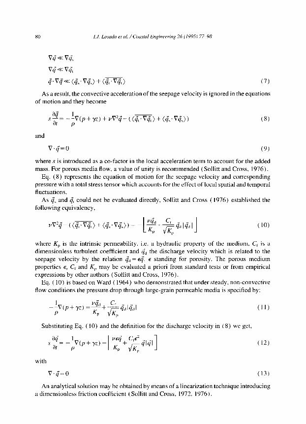
As a result, the convective acceleration of the seepage velocity is ignored in the equations of motion and they become

a$ i sat= -;Q(p+ yz) + uQ 2~-((~~.Q~~)+(4:.Q~~,))

and

Q.$=O (9)

where s is introduced as a co-factor in the local acceleration term to account for the added mass. For porous media flow, a value of unity is recommended (Sollitt and Cross, 1976).

Eq. (8) represents the equation of motion for the seepage velocity and corresponding pressure with a total stress tensor which accounts for the effect of local spatial and temporal fluctuations.

As i< and $t could not be evaluated directly, Sollitt and Cross ( 1976) established the following equivalency,

( 10)

where KP is the intrinsic permeability, i.e. a hydraulic property of the medium, C, is a dimensionless turbulent coefficient and 4’ the discharge velocity which is related to the seepage velocity by the relation td= ~4, E standing for porosity. The porous medium properties E, Cr and K, may be evaluated a priori from standard tests or from empirical expressions by other authors (Sollitt and Cross, 1976).

Eq. ( 10) is based on Ward ( 1964) who demonstrated that under steady, non-convective flow conditions the pressure drop through large-grain permeable media is specified by:

Substituting Eq. ( 10) and the definition for the discharge velocity in (8) we get,

(11)

(12)

with

Q.$=O (13)

An analytical solution may be obtained by means of a linearization technique introducing a dimensionless friction coefficient ( Sollitt and Cross, 1972, 1976).


3. Experimental procedure

3.1. Experimental set-up

Wave experiments were conducted at the College of Civil Engineering Ocean Lab at the University of Cantabria. The wave flume is 69 m long and of a rectangular cross section, 2 m wide and 2 m high with glass walls.

The idealized porous structure used in the experiments was made in order to make the measurements of the velocity field inside the structure possible. It is a vertical-lattice type porous medium made of rectangular wooden sticks nailed together vertically and horizontally to produce 0.04 mX 0.04 mX0.04 m uniform pores within the structure, see Fig. 1 and Fig. 2.

The structure presents some special characteristics that have to be pointed out. The structure is homogeneous but not isotropic. For a pore in a given vertical plane along the structure, the motion is not confined vertically, allowing the column of water to oscillate almost freely in this direction. However, the horizontal motion is confined allowing only tortuous oscillations. This kind of structure presents the possibility of analyzing two a priori, different flow behaviours.

This test section, located 44 m from the wave generator, is 1.56 m long, 0.96 m wide and 0.68 m deep. Regular sinusoidal waves with heights up to H = 0.033 m and periods up to T= 2.5 s were generated by a piston-type wavemaker, driven by an hydraulic piston. Tests main characteristics are presented in Table 1.

The water particle velocities were measured with a Laser Doppler Velocimeter (LDV) . This LDV system is a two-component system based on a backward scatter mode. After some starting tests, it was decided to sample at a rate of 100 samples per second.

Fig. 1. Idealized porous structure

I.J. Losada et al. /Coastal Engineering 26 (I 995) 77-98

0.08

0.08

PORE

Hll HlZ Ii1

back column (T)

/ middle cylumn (M)

I I

I front column (D)

Fig. 2. Idealized porous structure. Location of the velocity measurements.

Nine pores were selected to take the velocity measurements (Fig. 2). They were located at three verticals, three pores each. The front (D), middle (M) and back (T) columns are located 0.14 m, 0.70 m, 1.26 m from the front face of the structure respectively. The lower (I), middle (M) and upper (S) rows are located 0.22 m, 0.30 m and 0.38 m from the horizontal bottom, respectively. Measurements were taken in nine points of each pore (Fig.

Table 1

Main test parameters

Period (s) I 2.5

h Cm) 0.50 0.50 L(m) 1.51 5.24 hlL 0.33 0.095 H(m) 0.033 0.0324

Ur o.s9 7.1 I

I./. Losada et al. /Coastal Engineering 26 (1995) 77-98 83

2). Velocity measurements were also taken at the same heights seawards (0.60 m from the structure) and at the leeward side (0.45 m from the structure) of the structure. Because velocity measurements need to be taken at several locations in the flow, the test had to be repeated 8 1 times for each depth and period in order to obtain the velocity record for each point in the structure.

The free surface was measured at 23 locations using 19 locations inside the structure (each of the columns), using three gauges to measure reflection in front of the structure and one gauge to evaluate wave transmission. The gauges outside the structure were measuring the free surface throughout all the velocity tests in order to measure the incident wave height. These measurements were used in order to check the repeatability of the experiments. Experiments were discarded when differences in measured wave heights were larger than 0.5% between two repetitions of an experiment. Free surface measurements, taken simultaneously at several positions, were used to calculate the phase shift between the different columns.

Four pressure transducers were located inside the structure in order to determine the pressure variations inside the structure. The pressure transducers were located at the following pores: DM, MM, TM, MS and MI, where the first letter stands for the horizontal position of the pore and the second one for the vertical position in the structure. (i.e. DM: front column, middle row). The pressure transducers were introduced into the structure from the top. The pressure transducer nose was located in the center of each of the pores (HO). Pressure at DM, MM and TM was measured simultaneously.

3.2. Velocity measurements

Introduction One of the the goals of the study was to measure velocities inside porous structures and

to decompose the velocity field following Eq. (3)) that is, determining the importance of the velocity components representing the spatial and temporal fluctuations. Measuring with a Laser Doppler Anemometer (LDA) has the advantage that point velocity measurements are possible without physical intrusion into the flow channel. If the velocity is measured at a point in a pore, the total velocity 9 * can be measured at any instant. However, if the total velocity is measured at a point for some small interval, At, and the average velocity within the time interval is determined, the resulting quantity is the sum of the seepage velocity 4 plus the spatial fluctuation qb, associated with that location in the pore, qt = q* - ;?“. At this point, the qt at 9 points in each of the pores are known.

Finally, knowing the same temporal average simultaneously at the nine points in a pore, the spatial average in a pore of all temporal averages is simply the mean velocity, q, in the pore at any instant. This quantity is also known as seepage velocity. A similar procedure can be used to split the pressure field into, p* =p +ps +p,.

Measurements and results

In this section the measurements and results of the porous flow kinematics in the time and frequency domains are presented.

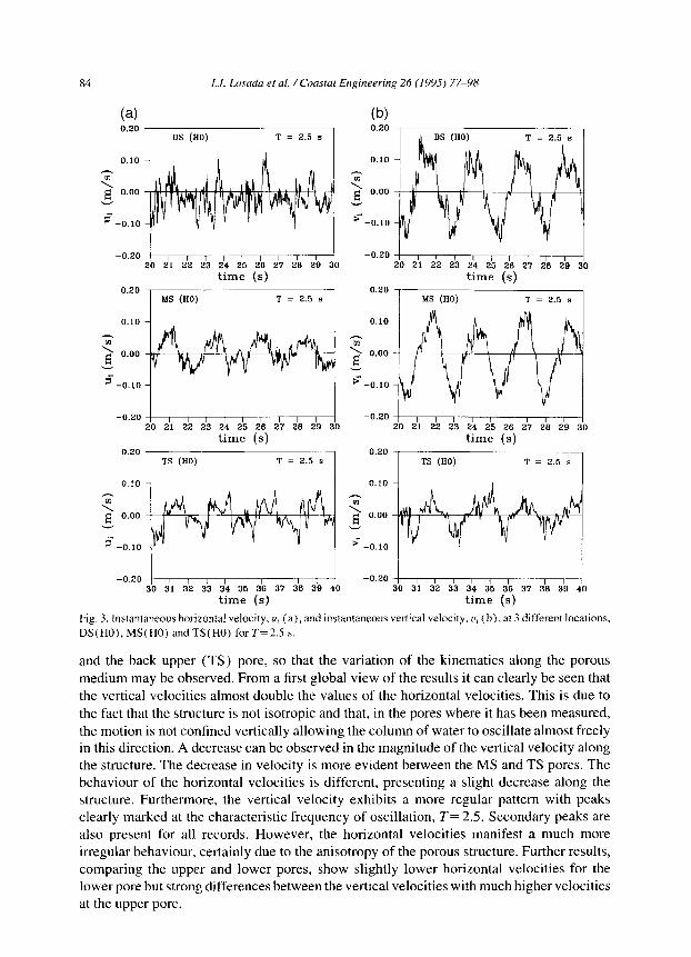
Fig. 3 presents the instantaneous horizontal and vertical velocities q* ( ui,ui). for T= 2.5 s, at the center point (HO) of three pores, the front upper (DS), the middle upper (MS)

84 I.J. Losuda et al. / Ckz.~ai Engimerirzg 26 (I 995) 77-98

(4 0.20

0.10

F l O.OO ’ -0.10

-0.20

0.20

0.10

';;

2 O.OO

2 -0.10

-0.20

0.20

0.10

';;

1 0.00

' -0.10

(b) 0.20

0.10

T 2 O.OO ._ 2 -0.10

-0.20

0.20

0.10

z

2 0'0°

2 -0.10

-0.20

0.20

0.10

T

2 0.00

+ -0.10

-0.20 -1 -0.20 1111111/II/ 30 31 32 33 34 35 36 37 36 39 40 30 31 32 33 34 35 36 37 36 39 40

time (s) time (s)

Fig. 3. Instantaneous horizontal velocity, II, (a). and instantaneous vertical velocity, r, (b), at 3 different locations.

DS(HO),MS(HO) andTS(H0) forT=2.5s.

and the back upper (TS) pore, so that the variation of the kinematics along the porous medium may be observed. From a first global view of the results it can clearly be seen that the vertical velocities almost double the values of the horizontal velocities. This is due to the fact that the structure is not isotropic and that, in the pores where it has been measured, the motion is not confined vertically allowing the column of water to oscillate almost freely in this direction. A decrease can be observed in the magnitude of the vertical velocity along the structure. The decrease in velocity is more evident between the MS and TS pores. The behaviour of the horizontal velocities is different, presenting a slight decrease along the structure. Furthermore, the vertical velocity exhibits a more regular pattern with peaks clearly marked at the characteristic frequency of oscillation, T= 2.5. Secondary peaks are also present for all records. However, the horizontal velocities manifest a much more irregular behaviour, certainly due to the anisotropy of the porous structure. Further results, comparing the upper and lower pores, show slightly lower horizontal velocities for the lower pore but strong differences between the vertical velocities with much higher velocities at the upper pore.

I.J. Losada et al. /Coastal Engineering 26 (1995) 77-98 85

-0.20 -1 -0.20 II 20 21 22 23 24 25 26 27 28 20 30 20 21 22 23 24 25 26 27 26 29 30

time time 0.15

(s) 0.15

(5)

DS = = s 0.10 (HO) T 2.5 8 0.10 DS (HO) T 2.5

20 21 22 23 24 25 26 27 28 29 30 20 21 22 23 24 25 26 27 26 29 30

0.15

0.10

3-i;

5 -0.10

time (s) time 0.15 (s)

0.10

B --0.05 VI 0.05 0.00

$ -0.10

-0.15 -1 -0.15 jI 20 21 22 23 24 25 26 27 26 29 30 20 21 22 23 24 25 26 27 26 29 30

0.15

h 0.10

< 0.05

2 0.00

p -0.05

-0.10

-0.15 -1 -0.15 AI 30 31 32 33 34 35 36 37 36 39 40 30 31 32 33 34 35 36 37 36 39 40

time (s) time (s)

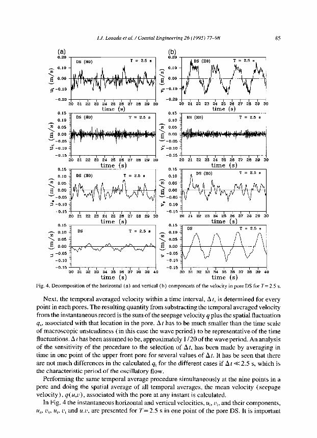
Fig. 4. Decomposition of the horizontal (a) and vertical (b) components of the velocity in pore DS for 7’= 2.5 s.

Next, the temporal averaged velocity within a time interval, At, is determined for every point in each pores. The resulting quantity from substracting the temporal averaged velocity from the instantaneous record is the sum of the seepage velocity 4 plus the spatial fluctuation qs, associated with that location in the pore. At has to be much smaller than the time scale of macroscopic unsteadiness (in this case the wave period) to be representative of the time fluctuations. At has been assumed to be, approximately 1 I20 of the wave period. An analysis of the sensitivity of the procedure to the selection of At, has been made by averaging in time in one point of the upper front pore for several values of At. It has be seen that there are not much differences in the calculated qt for the different cases if At +=K 2.5 s, which is the characteristic period of the oscillatory flow.

Performing the same temporal average procedure simultaneously at the nine points in a pore and doing the spatial average of all temporal averages, the mean velocity (seepage velocity), q( up), associated with the pore at any instant is calculated.

In Fig. 4 the instantaneous horizontal and vertical velocities, ui, c:,, and their components, u,, u,, u,, U, and U,U, are presented for T= 2.5 s in one point of the pore DS. It is important

86 1. J. Losada et al. /Coastal Eqineering 26 (1995) 77-98

to point out that the seepage velocities ( u,L!) are representative of the pore. From these figures the following conclusions can be drawn: 1. The q1 component presents a high frequency signal. Comparing the vertical and horizontal

components, it can be seen that both components are of the same order of magnitude. The magnitude of this fluctuation is very small (approx. 10%) compared to the instantaneous record.

2. Comparing the qs( us, os) components, it can be seen that the spatial variation presents an oscillatory behaviour with peaks at the characteristic period T=2.5 s and smaller peaks at other frequencies. Generally, the fluctuations for the vertical velocity are a little bit higher than for the horizontal component at the same point.

3. The results for the seepage velocity q clearly show the anisotropy of the structure, presenting a nice oscillatory behaviour for the vertical component of the velocity and a much more irregular behaviour for the horizontal velocity. This is due to the fact that the motion is not confined vertically, allowing the column of water to oscillate almost freely in this direction. This also explains the higher vertical velocities measured compared to the horizontal component. The vertical component presents values a 30% smaller than the instantaneous velocity at HO and secondary peaks almost disappear. This is due to the averaging process. The instantaneous record and the seepage velocity look very much alike. The horizontal component presents an oscillatory behavior with important peaks every 2.5 s. However, secondary peaks are very important, too. Comparing the horizontal velocity magnitudes, it can be seen that the seepage velocity is approximately 10% of the instantaneous velocity in DS.

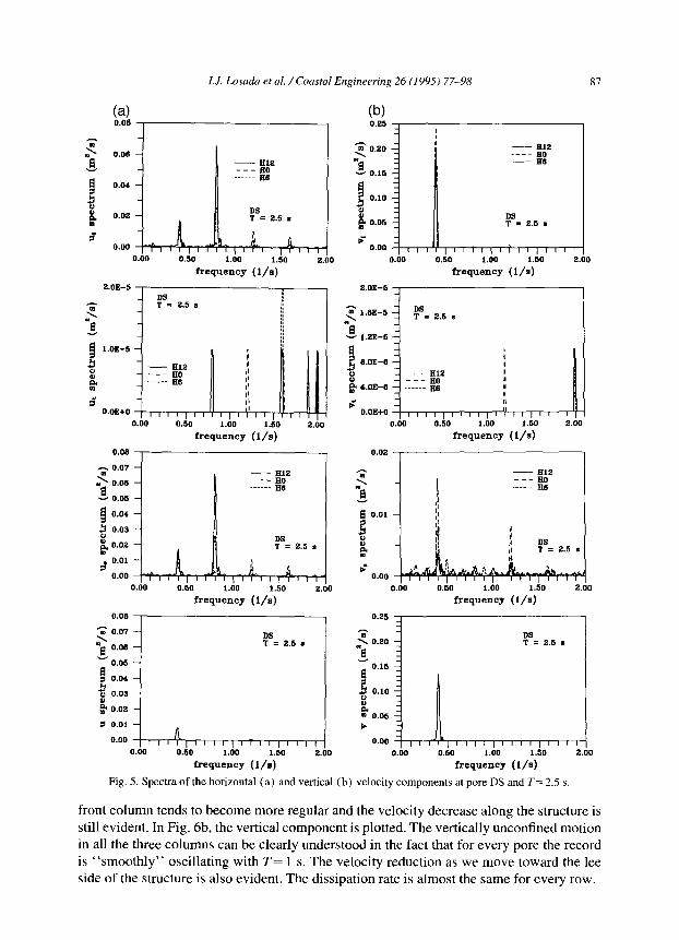
Further information can be obtained performing a spectral analysis. Fig. 5 shows the spectra for each of the instantaneous velocities and its components for T= 2.5 s in pore DS for three different positions on a vertical (H 12, HO, H6). The results for the horizontal velocity differ from those corresponding to the vertical velocities. ~1, shows three additional harmonics to the characteristic frequency. In all three positions the second harmonic is even more important than the first. The 11, spectra, is composed of several harmonics but all of them for frequencies higher than the characteristic frequency, 0.4 Hz. Finally, the last component, u,, also presents higher harmonics with the second harmonic being the most important one. However, the seepage velocity spectrum does not present any higher harmonics and only a very small peak for the characteristic frequency.

The instantaneous vertical velocity is characterized by a very important peak at 0.4 Hz. Smaller peaks can hardly be seen at higher frequencies. For L’, small peaks appear at 1.2 and 2 Hz but not in all three points. 11, presents peaks at higher harmonics but the overall contribution from the I!, spectrum is very small. Finally, the vertical seepage velocity spectrum has a peak at the characteristic frequency and a very small peak at the second harmonic.

The next set of figures show the velocity field inside the porous structure at a macroscopic level by presenting the evolution of the seepage velocity, q( u,u). In Fig. 6a, the horizontal velocity component evolution along the structure is presented for T= 1 s. In DS the velocity presents a very irregular pattern with high peaks. However, as we move toward the end of the structure (MS and TS) two important phenomena occur: (1) velocity decreases, as expected, due to dissipation and (2) the signal becomes very regular with peaks at the oscillatory frequency only. As we move down to other rows, the irregular behaviour in the

I.J. L.osada et al. /Coastal Engineering 26 (1995) 77-98 87

6 0.00 f 11 11 I i ( 1 [ i 11 1, 11 I

0.00 0.50 1.00 1.50 2.00 0.00 0.50 1.00 1.50 2.

frequency (l/s)

2.OE-5

z

TDs= 2.5 II i II

"2

::

ij

i 1.0E-5 -

:I II

I i

ii - Ix ;y II

P ..____ B5

II

5 11 11

O.OB+O , , , , , , , , , '11 , 1 , , , ,

0.00 0.50 1.00 1.50 2.00

frequency (i/s)

0.08

o.io l.dO l.iO

frequency (l/s)

1 LOO

0.08

3 0.07 -

: ;,,- _ F= 2.6 s

0 0.02 -

$ 0.02 -

1 0.01 -

0.00 1 I I ) , I,, , i,, , , ,,

0.00 0.50 1.00 1.50 2.00

frequency (l/s)

frequency (l/s)

2.0E-5 Y -= 1.22-5 - ,’ _ ?= 2.5 s

w 1.2E-5 -

; B.OE-6 : ; 1

0 _ XI ;:2 1

,a 4.OE-6 - ------ ~2 s ,I

pr II

O.OE+O , , , , , , , , , , ,'I , , , , , , , ,

0.00 0.50 1.00 1.50 2.00

frequency (l/s)

0.02

I

E’ ;"= 2.5 m

1.00 1.50

frequency (l/a)

0.25

c -1 0.20 - ?"= 2.5 I

3 -

i 0.15 0.10 I -

P

g 0.05 -

P

0.00 , , , ,Jlb, , , , , , , , , , , , , , , 0.00 0.50 1.00 1.50 2

frequency (l/s)

Fig. 5. Spectra of the horizontal (a) and vertical (b) velocity components at pore DS and T= 2.5 s.

front column tends to become more regular and the velocity decrease along the structure is still evident. In Fig. 6b, the vertical component is plotted. The vertically unconfined motion in all the three columns can be clearly understood in the fact that for every pore the record is “smoothly” oscillating with T= 1 s. The velocity reduction as we move toward the lee side of the structure is also evident. The dissipation rate is almost the same for every row.

I.J. Losada et al. /Coastal Engineering 26 (1998) 77-98

T=ls

, I -o.04+t 1 i’, , , , , , I,

0.00 5.00 10.00 15.00 20

time (s)

(b) 0.20

- DS --- UP T=ls

-0.20 * ) 0.00 5.00 10.00 15.00 20

time (s)

0.04

2 0.02

2 0.00

=I

-0.02

-0.04 C

I( 0 II ,I I I I ,I I / I

5.00 10.00 15.00 2c

time (s)

time (s) 0.10

~ D1 ____ MI T=ls

0 -O.lOOM

time (s)

Fig. 6. Evolution of (a) the horizontal component of the seepage velocity, u. and (b) the vertical component of

the seepage velocity, 11, along the structure for 7’= I 5.

The evolution of the seepage components over the depth has been also analyzed; however, figures have not been included. At the first column (pores DS, DM, DI), the signal is completely irregular, mainly for DS. As we move to the middle (M) and back columns (T), the record becomes more regular. The pores in the upper row present higher velocities but equally important horizontal velocities have been recorded in pores DM and MM. The vertical velocities show a very regular pattern and a reduction in the velocity magnitude as

we move down and to the back of the structure. The same kind of analysis has been done for T= 2.5 s; however, a few differences exist.

For the horizontal velocity, the main period is not clearly marked in the records because of the many secondary peaks. There is not much velocity reduction as we move horizontally along the structure. Furthermore, the vertical component shows higher values at the middle column than for the front column, Fig. 7. This behavior is clearly different from what was

observed for T= 1 s.


-0.15 abo time (s)

0.15

__ III T = 2.5 s ---MI

20 22 ZFme (7) 28 30

Fig. 7. Evolution of the vertical component of the seepage velocity, u, along the structure for 7’= 1 s.

Furthermore, a thorough analysis of the spectral evolution of the seepage velocity spectra into the structure has been done. Due to the lack of space figures showing the results have not been included, however the following conclusions can be pointed out:

The vertical component of the seepage velocity does not present secondary peaks in any pore for any of the two studied periods. The horizontal component of the seepage velocity presents higher harmonics for both periods but for T= 1 s those peaks are only present for the measurements done in the front column (D) . As we move to the rear part of the structure the higher harmonics become insignificant. In any case, the values of the higher harmonic peaks are always much smaller than the peak of the main frequency. In all the cases, the dissipation process induced by the porous medium is indicated by the decrease in the magnitude of the peaks associated with the principal harmonic as we move to the rear side of the structure. For T= 2.5 s, the horizontal component of the seepage velocity presents secondary peaks in the first (D) and second (M) rows of the structure. In the third column, the second harmonics are no longer present.

90 I.J. Lnsudu et al. /Coastal Engineering 26 (1995) 77-98

l For both cases, T= 1 s and T= 2.5 s, the higher harmonics are smoothed progressively as we move down to lower rows. From these first results, it can be concluded that the kinematics of flow in porous media,

even at a macroscopic averaged level, is very much affected by the wave period.

Relative importance of the convective terms

In order to evaluate the assumption made by Sollitt and Cross (1976) and expressed in Eq. (7) the horizontal component and the energy spectra of the horizontal and vertical components of 4’. Vq’and ($?. V<,) + <m> are plotted in Fig. 8 in the center pore (MM), for T= 1 s and T= 2.5 s. The derivatives a/&r and a/ay have been calculated using three point formulas. It has been observed that for all the cases the convective terms due to the temporal fluctuations are much smaller than those due to the spatial fluctuations. From the graphs it can be drawn out that for both periods, the horizontal component of the convective term is much smaller than the term due to the Auctuations, satisfying the inequality (7)

1.5E-4

e- T = 1.0 q vertical component m

frequency (l/s)

sertic* component

T = 9.5 s

-.-....-.- q..sra*.q. + qt.grs.3.q, - q.pa*.q

1.00 2.00 3.00 frequency (l/S)

Fig. 8. Horizontal and vertical components of the spatial and temporal fluctuation and comparison with the

convective acceleration at pore MM for (a) T= I s and (b) T= 2.5 s.


established by Sollitt and Cross ( 1976). However, this inequality is not so evidently satisfied for the vertical components of the velocity. The corresponding spectra show that the vertical velocities present an important peak at the second harmonic frequency representing a 50% of the energy which corresponds to the fluctuations summation at the principal frequency. Furthermore, second order harmonics induced by the fluctuations should only be considered for the horizontal component for both periods and can be neglected for the vertical motion. Therefore, it can be concluded that flows through very tortuous porous media induce the generation of second order harmonics due to the convective terms of fluctuations that may become even more important than the first order harmonics.

Furthermore, convective accelerations induced by seepage velocities seem to play an important role in the modelling of wave propagation in porous media with predominant directions of flow and therefore it can be concluded, that the hypothesis stated in Eq. (7) seems to be violated mainly for the cases in which predominant flow directions exist; in this case, for the vertical direction.

In addition, the sum of the spatially derived component and the transient eddy component which may be interpreted as stresses with respect to the mean motion, averaged in time, is negative for T= 1 s and positive for T= 2.5 s. To be considered as stresses they have to be transposed to the right-hand side of the equation with the subsequent change in sign. Therefore, for T= 2.5 s the total fluctuation results in a net stress at the center pore opposing the motion of the flow. However, the net fluctuation for T= 1 s is positive and favours the how in the direction of wave propagation.

Relative importance of the inertia forces To determine the nature of the fluid motion in a porous medium based on the importance

of the resistance forces (laminar, inertial and turbulent) present in Sollitt and Cross’s ( 1972) model, two different Reynolds numbers may be defined following Gu and Wang ( 1991).

R

f v

Ri=-e=5;.2, V

(14)

where v is the kinematic viscosity of the fluid, d, is the characteristic particle size of the porous material and 4’ stands for a characteristic velocity. Both Reynolds numbers give the relative importance of the inertial forces to the viscous forces; however in R, the inertia is of convective nature and resistance is due to velocity changes in space, whereas in Ri the resistance force arise locally due to the change of velocity at a specific location of the porous structure. Table 2 and Table 3 include the values of the horizontal and vertical root mean square seepage velocities and the corresponding Reynolds numbers in every pore for each of the studied periods, d, has taken to be the pore diameter.

From the analysis of the Reynolds numbers and using Fig. 1 in Gu and Wang ( 1991), Fig. 9, the varying degree of importance of the three resistance forces (laminar,A, inertial, f; and turbulent,f,) can be established. For the cases studied, the results are located in the region where all three forces are of equal importance. The size and velocity ranges which, after Gu and Wang ( 1991), correspond to this region, coincide with the pore size of the model and the velocity measured and are characteristic of Bow in porous media made of pebbles or small gravel. Experimental values obtained by Smith (1991) and Van Gent ( 1994) are also included in Fig. 9.

92 I. J. Losada et al. / Coastal Engineering 26 (I 995) 77-98

Table 2 Horizontal and vertical root mean square seepage velocities and corresponding Reynolds numbers in every pore

for Z’= 1 s. R, = 10053. Velocities in m/s

Pore U,,, x lo-’ V,“,,X lomZ R,(u) R,(v)

DS 1.189

DM 0.957

DI 0.87 I MS 0.547

MM 0.432

MI 0.319

TS 0.416

TM 0.241

TI 0.098

1.786 475.1 3 I 14.6

4.486 383.7 1194.5 2.827 348.7 1130.9 3.529 218.8 1411.8 2.294 173.1 916.9

1.362 127.8 544.7 2.119 166.4 847.9

1.05 I 98.4 420.4 0.598 39.5 239.3

3.3. Free sueace measurements

Twenty-three wave gauges were used to calculate reflection and transmission due to wave-structure interaction and to obtain the free surface variation inside the porous medium. Furthermore, for every velocity measurement four gauges were used to measure the reflection and transmission coefficients associated with each of the velocity tests. Free surface measurements are analyzed in time and frequency domains.

The normalized total wave height evolution is shown in Fig. 10 for both wave periods. For T= 1 s, the wave height decreases from the front face to the rear face showing a strong dissipation.

However, this feature is not the same for T= 2.5 s, where there is no dissipation between Pl and P 10. Dissipation is only important between positions 10 and 19 with a 50% decrease in surface elevation. These results agree with the experiments done by Kondo ( 1972) who stated that values of B/L influence the wave height distribution greatly. A spectral analysis of the free surface measurements has been done, however figures have not been included for lack of space.

For T=2.5 s, the spectra corresponding to the free surface displacement in different positions of the porous structure present a single peak at the frequency associated with the

Table 3 Horizontal and vertical root mean square seepage velocities and corresponding Reynolds numbers in every pore

for T=2.5 s. R, =4021. Velocities in m/s

Pore u,,,,, x 10 2 v,,,,, x lo-’ RF(u) R,(v)

DS 1.739 5.885 695.6 2353.9 DM I .262 4.231 504.7 1694.8 DI 1.286 3.398 5 14.5 1359.5 MS 0.719 6.817 287.7 2726.7 MM 0.809 5.253 323.9 2101.4 MI 0.706 3.803 282.5 1521.1

TS 1.404 4.075 561.5 1630.0 TM 0.790 3.144 283.7 1257.6 Tl 0.675 2.145 270. I 858.8


sand

fl > 10 fi fl > 10 f, L Region

fi > 10 fl f, > 10 f, I Region

-10 -10 -10 -10 -zlo -’ 1 10 10 * 10 s 10 a 10 s 10

Ri

’

Fig. 9. Relative importance of the resistance forces (after Gu and Wang, 1991)

characteristic wave period, and show the wave energy variation through the porous structure but without the presence of secondary harmonics for any of the wave periods.

The spectra associated with T= 1 s present a secondary harmonic for the frequencyf= 2 Hz at the gauges 1 to 5. However, this harmonic is not very important as the energy associated with it is approximately 5% of the energy corresponding to the main frequency. As we move to the back of the structure higher harmonics are no longer present.

1.80

1.60

1.40

1.20 -\

1.00 - -,._ ,”

q 0.60 - . ..\ . .._ . . .

2 0.60 - T 2.5 ‘?--. X

(s)

0.40 - 1.56 1.56 ;@) 0.033 0.0324“~,~

0.297 1.033 ___--____ . . 0.20 - *.--____

1 10 ““*9 O~OO-*****t*************

I I I I I I I I I 0.0 0.1 0.2 0.3 0.4 0.5 0.6 0.7 0.6 0.9 1

x/B 1

Fig. IO. Normalized wave height evolution, H,,, /H,, along the porous structure for T= I s and T= 2.5 s

94 I.J. Losada et cd. / Coastai Engineering 26 (1995) 77-98

G-2.oo ii 0 1 2 3 4 5 6 7 a 9 10

time (s)

- E 2.00

2 1.00

ti o 0.00

.g -1.00

h-2.00 a

-3.00 T = 2.5 s

__-

I I I I I I I I I 20 21 22 23 24 25 26 27 28 29 :

time (s) cl

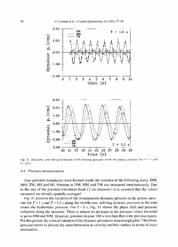
Fig. I I. Horizontal and vertical evolution of the dynamic pressure inside the porous structure for T= I s and T=2.5 s.

3.4. Pressure measurements

Four pressure transducers were located inside the structure at the following pores: DM: MM, TM, MS and MI. Pressure at DM, MM and TM was measured simultaneously. Due to the size of the pressure transducer head (2 cm diameter) it is assumed that the values measured are already spatially averaged.

Fig. 11 presents the variation of the instantaneous dynamic pressure in the porous structure for T= 1 s and 7’= 2.5 s along the middle row, defining dynamic pressure as the total minus the hydrostatic pressure. For T= 1 s, Fig. 11 shows the phase shift and pressure reduction along the structure. There is almost no decrease in the pressure values recorded in pores DM and MM. However, pressure in pore TM is less than that in the previous pores. For this period, the vertical variation of the dynamic pressure is almost neglegible. Therefore, pressure seems to present the same behaviour as velocity and free surface in terms of wave attenuation.


(a) 4.OE-2

T=ls Pore MM

FLOE-2 1

O.OE+O

E 9 10 11 12 13 14 15 18 17

time (5) 9

------- calculated

-4.OE-2 I I I / I I I I I 8 9 10 11 12 13 14 15 16 17 18

time (s)

2 (W ,I 4.OE-2 ,a C!? T = 2.5 8 Pore MM

0 2.OE-2

:

2 8 O.OE+O

!i

z ~ measured 'i: ~~----~- calculated

g -4.OE-2 , , , , , , , I , , , , , , 35 40 45

time (5)

+ -4.OE-2 / T = 2.5 s ’

I I I , , , I I I , I I I 35 40 45

time (s)

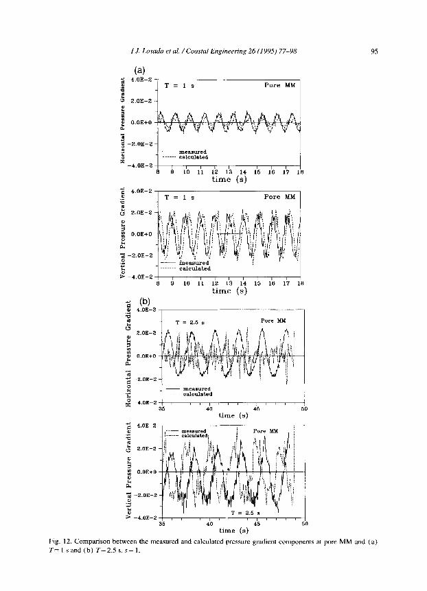
Fig. 12. Comparison between the measured and calculated pressure gradient components at pore MM and (a) T=lsand(b)T=2.5s.s=1.

96 I.J. Lmada et al. /Coastal Engineering 26 (I9953 77-98

In order to check the validity of the measurements, Eq. (6)) with s = 1, has been used to compare the measured pressure gradients with those calculated out of the velocity measurements. Fig. 12 presents the horizontal and vertical pressure gradients at the center pore (MM) for T= 1 s and T= 2.5 s. Phase shift in the figures has been artificially included in order to provide a better comparison.

For T= 1 s, the agreement is very good for both the horizontal and vertical pressure gradients which confirms the validity of the experiments and the Navier-Stokes equation in terms of the seepage velocity. However, for T= 2.5 s results are not that satisfactory. The vertical pressure gradient presents a good agreement between directly measured and calculated values, with slightly higher peaks for the gradients calculated out of the velocity measurements. However, there is no correlation between the horizontal pressure gradients. The calculated signals do not even show the main oscillation but the peak values are of the same order of magnitude.

3.5. Results global analysis and comparison with actual rubble structures

Measurements of the velocity, pressure field and wave height inside the structure reveal that the flow behaviour changes depending on the wave period and associated wave length for a given structure, resulting in two characteristic regions: transition and transmission regions. The relative width of the structure, B/L, associated with the formation of a standing wave and resonant conditions inside the structure, is found to be an important parameter to establish the location of the two regions which changes depending on the wave period.

For T= 1 s, the transition region is very short including only a few columns of the structure. However, for T= 2.5 s, the reflection region includes the middle column (M). This can be explained assuming that reflection does not take place in the front face of the structure but in a plane inside the structure whose location depends on B/L. Most of the reflection process takes part in the upper row for T= 1 s but for T= 2.5 s it also affects lower pores in the first row (D) .

Furthermore, the comparison of the measured pressure gradients with those calculated out of the velocity measurements at pore MM show a good agreement for T= 1 s but no correlation for T= 2.5. This behaviour could be associated to the location of pore MM in the transition region and implies that Sollitt and Cross ( 1972), does not seem to model the flow in this region properly.

The importance of the transition region can be pointed out considering that most of the built breakwaters are in depths of the order of 8 m and under the incidence of waves with wave lengths of order of 100 m. Assuming a breakwater width of 25-30 m, that means Bl L = 0.3 m and therefore, the transition region represents half of the breakwater width and particularly the main layer.

4. Conclusions

( 1) In general, the seepage velocity ignores perturbations in the flow field due to pore irregularities.


(2) The kinematics in the unconfined vertical direction is completely different from the behavior of the horizontal velocity field. Instantaneous fluctuations are usually more important than convective accelerations due to the seepage velocity. This might change when the porous structure presents some dominant directions of propagation.

(3) Spatial fluctuations, accounting for local velocity components due to pore irregularities or boundary layers, are always more important than temporal fluctuations. Convective accelerations should be considered when modelling wave propagation in porous media and when velocities are important.

(4) The ratio (structure length) / (wave length) is an important parameter in the hydro- dynamics of wave propagation in a porous medium, defining a transition and transmission region. The transition region is characterized by irregular records with secondary peaks, little or no dissipation (free surface, velocity field, pressure field) and the presence of important higher harmonics in the velocity spectra.

(5) Secondary harmonics are always present for the instantaneous velocities and fluctuations ( qs,qt) . However, seepage velocity secondary harmonics exist but they are neglegible compared to the seepage principal frequency and to the fluctuation and instantaneous harmonics. Secondary harmonics become neglegible when moving to the rear and bottom of the structure. That means, dissipation tends to eliminate secondary harmonics in the velocity field. The free surface presents higher harmonics for the shorter period but only in the first gauges.

(6) Due to dissipation and anisotropy of the porous structure, different resistant forces can be dominant in different parts of the same structure. This should be considered to improve the modelling of the flow.

(7) The main goal of this work was to evaluate the hypothesis which has been the basis of a theory used by many authors to study the wave-structure interaction. The hypothesis seems not to be valid for flow in very porous structures or at least at the main layers of rubble-mound breakwaters.

Further research should provide a better modelling of the transition region as Sollitt and Cross ( 1972) does not model this region properly. New experiments should be carried out to determine the location of the reflection process in actual breakwaters and therefore establish the limit between the transition and transmission region.

Acknowledgements

This paper is part of the “Reflection of natural and man-made coastal structure” research project, which is funded by the Commission of the European Communities in the framework of the Marine Science and Technology Programme (MAST), under contract No. MAS2- CT92-0030.

References

Dalrymple, R.A., Losada, M.A. and Martin, P., 1991. Reflection and Transmission from porous structures under oblique wave attack. J. Fluid Mech., 224: 6255644.

98 1. J. Losada et al. / Coastal Engineering 26 (I 995) 77-98

Gu, Z. and Wang, H., 1991. Gravity waves over porous bottoms. Coastal Eng., 15: 497-524. Kondo, H., 1972. Reflection and transmission for a porous structure. In: Proc. 13th Coastal Engineering Conference,

Vancouver. ASCE, New York, pp. 1847-1865. Losada, I.J., Dalrymple, R.A. and Losada, M.A., 1993. Water waves on crown breakwaters, J. Waterway Port

Coastal Ocean Eng. ASCE, I19(4): 3677380. Smith, G.M., 1991. Comparison of Stationary and Oscillatory Flow through Porous Media. MSc. Thesis, Queen’s

University, Kingston, Ont., 198 pp. Sollitt, C.K. and Cross, R.H., 1972. Wave transmission through permeable breakwaters. In: Proc. 13th Coastal

Engineering Conference, Vancouver. ASCE, New York, pp. 1827-1846.

Sollitt, C.K. and Cross, R.H., 1976. Wave reflection and transmission at permeable breakwaters. Technical Paper

No. 76-8, CERC.

Sulisz, W., 1994. Stability analysis for multilayered rubble bases. J. Waterway Port Coastal Ocean Eng., ASCE,

120( 3): 269-282.

Van Gent, M.R.A., 1994. Permeability measurements for the modelling of wave action on and in porous structures.

In: Proc. Coastal Dynamics ‘94, Barcelona. ASCE, New York, pp. 671-685.

Ward, J.C., 1964. Turbulent flow in porous media. J. Hydraul. Div. ASCE, 90(HY5): 1-12. Yu, X. and Chwang, A.T., 1994. Wave-induced oscillation in harbor with porous breakwaters. J. Waterway Port

Coastal Ocean Eng. ASCE, 120(2): 125-144.

Experimental study of wave-induced flow in a porous structure

Documents

Transcript of Experimental study of wave-induced flow in a porous structure