28th Symposium on Naval HydrodynamicsPasadena, CA, USA, 12 – 17 September 2010

A comparison of model-scale experimental measurementsand computational predictions for a large transom-stern

waveDavid A. Drazen1, Anne M. Fullerton1, and Thomas C. Fu1

Kristine L.C. Beale2, Thomas T. O’Shea2, Kyle A. Brucker2,Douglas G. Dommermuth2, and Donald C. Wyatt2

Shanti Bhushan3, Pablo M. Carrica3, and Fred Stern3

1Naval Surface Warfare Center - Carderock, USA2Science Applications International Corporation, USA

3University of Iowa, USA

ABSTRACT

The flow field generated by a transom stern hullformis a complex, broad-banded, three-dimensional systemmarked by a large breaking wave. This unsteady mul-tiphase turbulent flow feature is difficult to study ex-perimentally and simulate numerically. Recent model-scale experimental measurements and numerical predic-tions of the wave-elevation topology behind a transom-sterned hullform, Model 5673, are compared and as-sessed in this paper. The mean height, surface roughness(RMS), and spectra of the breaking stern-waves weremeasured by Light Detection And Ranging (LiDAR) andQuantitative Visualization (QViz) sensors over a rangeof model speeds covering both wet- and dry-transom op-erating conditions. Numerical predictions for this dataset from two Office of Naval Research (ONR) supportednaval-design codes, Numerical Flow Analysis (NFA) andCFDship-Iowa-V.4, have been performed. Comparisonsof experimental data, including LiDAR and QViz mea-surements, to the numerical predictions for wet-transomand dry transom conditions are presented and demon-strate the current state of the art in the simulation of shipgenerated breaking waves. This work is part of an on-going collaborative effort as part of the ONR Ship WaveBreaking and Bubble Wake program, to assess, validate,and improve the capability of Computational Fluid Dy-namics (CFD).

INTRODUCTION

The flow field generated by a transom stern hullform is acomplex system dependent upon a number of variables,including the transom height and shape, buttock slope,the wave system generated upstream, the boundary layerflow around the hull, etc., and has been the subject of anumber of studies. While earlier work has focused on the

surface wave profile (Maki, Doctors & Beck 2007, forexample), detailed laboratory scale measurements of theflow field have been performed by Lasheras (Rodrıguez-Rodrıguez, Marugan-Cruz, Aliseda & Lasheras 2008),who focused on identifying the general flow topology.More recently, the development of advanced instrumen-tation has allowed for measurement of the breaking tran-som wave of a full-scale ship to be made (Fu, Fullerton,Terrill & Lada 2006a). In an associated effort, numer-ical predictions of the full-scale stern wake and com-parisons of the mean height, surface roughness (RMS),and spectra of the breaking stern-waves were made(Wyatt, Fu, Taylor, Terrill, Xing, Bhushan, O’Shea &Dommermuth 2008). Although these initial comparisonsof the numerical predictions and full-scale measurementsshowed generally good agreement, differences remainedthat were difficult to associate with the underlying phe-nomenology due to the complexities of in-situ collection.

To obtain quantitative breaking wave data from alarge-scale transom stern hull form, measurements ofthe free-surface elevation in stern region of a large tran-som model were made in June of 2007 (Fu, Fullerton,Ratcliffe, Minnick, Walker, Pence & Anderson 2009b)and October/November of 2008 (Fu, Fullerton, Drazen,Minnick, Walker, Ratcliffe, Russell & Capitain 2010).This large-scale laboratory experiment provides a morecanonical transom wave for study, removing the effectsof the propellers, appendages, and ambient conditions.For this experiment a large, specially designed transomstern model was developed and tested in the Naval Sys-tems Warfare Center - Carderock (NSWCCD) Carriage2 Towing Tank. The hullform used, Model 5673, waspurpose-built for these experiments. It was designedto provide a minimal bow-wave disturbance and maxi-mum stern-wave disturbance. Its dimensions were deter-mined by the maximum practical size allowable in theCarriage 2 facility. Her hull construction was fiberglass.A schematic of Model 5673 is shown in Figure 1, and the

arX

iv:1

410.

1872

v1 [

phys

ics.

flu-

dyn]

7 O

ct 2

014

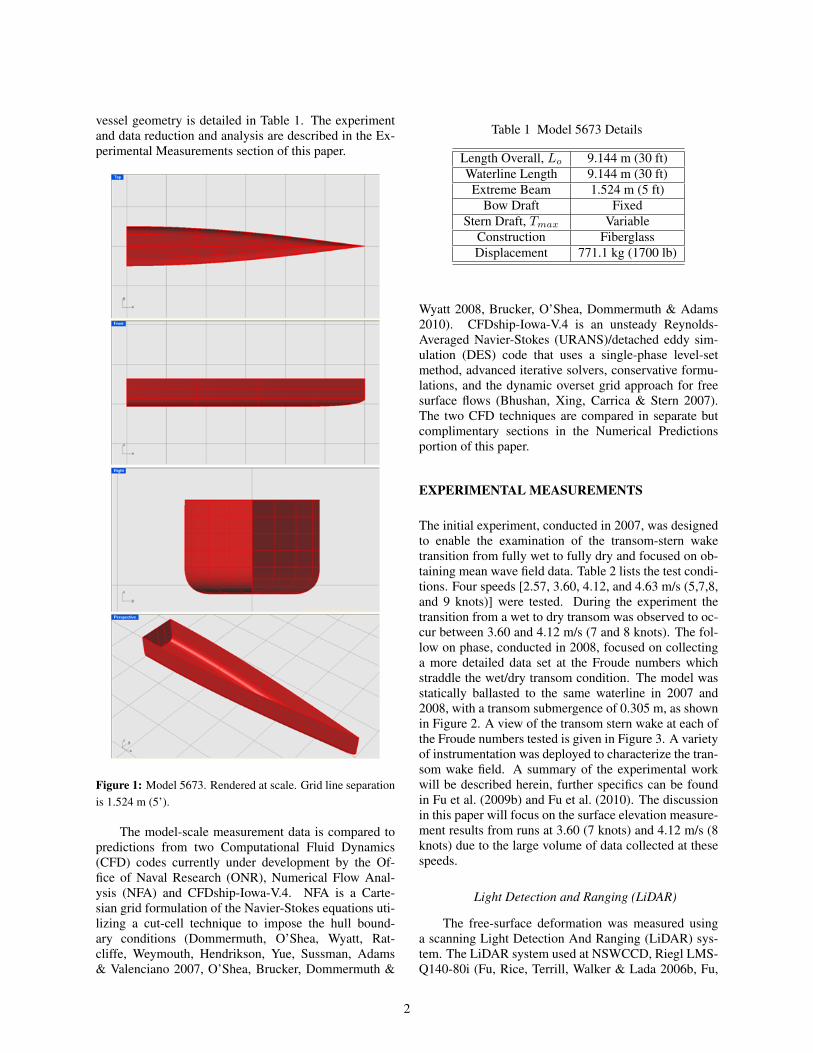
vessel geometry is detailed in Table 1. The experimentand data reduction and analysis are described in the Ex-perimental Measurements section of this paper.

Figure 1: Model 5673. Rendered at scale. Grid line separationis 1.524 m (5’).

The model-scale measurement data is compared topredictions from two Computational Fluid Dynamics(CFD) codes currently under development by the Of-fice of Naval Research (ONR), Numerical Flow Anal-ysis (NFA) and CFDship-Iowa-V.4. NFA is a Carte-sian grid formulation of the Navier-Stokes equations uti-lizing a cut-cell technique to impose the hull bound-ary conditions (Dommermuth, O’Shea, Wyatt, Rat-cliffe, Weymouth, Hendrikson, Yue, Sussman, Adams& Valenciano 2007, O’Shea, Brucker, Dommermuth &

Table 1 Model 5673 Details

Length Overall, Lo 9.144 m (30 ft)Waterline Length 9.144 m (30 ft)Extreme Beam 1.524 m (5 ft)

Bow Draft FixedStern Draft, Tmax Variable

Construction FiberglassDisplacement 771.1 kg (1700 lb)

Wyatt 2008, Brucker, O’Shea, Dommermuth & Adams2010). CFDship-Iowa-V.4 is an unsteady Reynolds-Averaged Navier-Stokes (URANS)/detached eddy sim-ulation (DES) code that uses a single-phase level-setmethod, advanced iterative solvers, conservative formu-lations, and the dynamic overset grid approach for freesurface flows (Bhushan, Xing, Carrica & Stern 2007).The two CFD techniques are compared in separate butcomplimentary sections in the Numerical Predictionsportion of this paper.

EXPERIMENTAL MEASUREMENTS

The initial experiment, conducted in 2007, was designedto enable the examination of the transom-stern waketransition from fully wet to fully dry and focused on ob-taining mean wave field data. Table 2 lists the test condi-tions. Four speeds [2.57, 3.60, 4.12, and 4.63 m/s (5,7,8,and 9 knots)] were tested. During the experiment thetransition from a wet to dry transom was observed to oc-cur between 3.60 and 4.12 m/s (7 and 8 knots). The fol-low on phase, conducted in 2008, focused on collectinga more detailed data set at the Froude numbers whichstraddle the wet/dry transom condition. The model wasstatically ballasted to the same waterline in 2007 and2008, with a transom submergence of 0.305 m, as shownin Figure 2. A view of the transom stern wake at each ofthe Froude numbers tested is given in Figure 3. A varietyof instrumentation was deployed to characterize the tran-som wake field. A summary of the experimental workwill be described herein, further specifics can be foundin Fu et al. (2009b) and Fu et al. (2010). The discussionin this paper will focus on the surface elevation measure-ment results from runs at 3.60 (7 knots) and 4.12 m/s (8knots) due to the large volume of data collected at thesespeeds.

Light Detection and Ranging (LiDAR)

The free-surface deformation was measured usinga scanning Light Detection And Ranging (LiDAR) sys-tem. The LiDAR system used at NSWCCD, Riegl LMS-Q140-80i (Fu, Rice, Terrill, Walker & Lada 2006b, Fu,

2

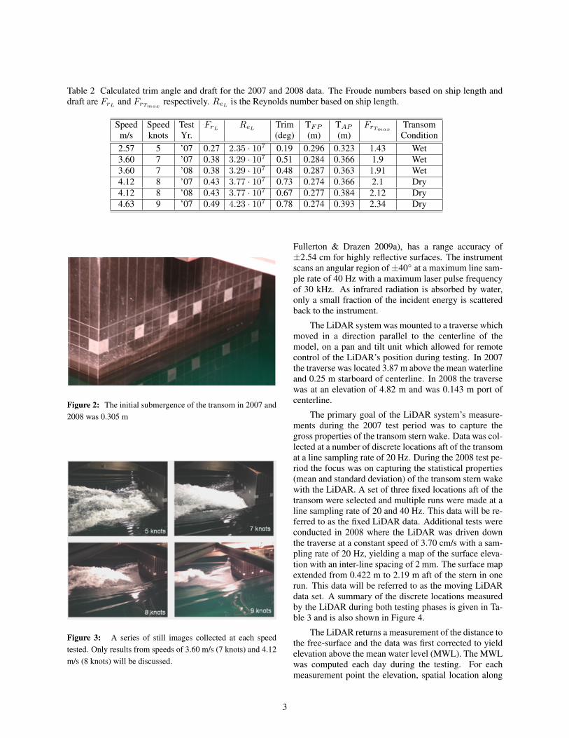
Table 2 Calculated trim angle and draft for the 2007 and 2008 data. The Froude numbers based on ship length anddraft are FrL and FrTmax

respectively. ReL is the Reynolds number based on ship length.

Speed Speed Test FrL ReL Trim TFP TAP FrTmaxTransom

m/s knots Yr. (deg) (m) (m) Condition2.57 5 ’07 0.27 2.35 · 107 0.19 0.296 0.323 1.43 Wet3.60 7 ’07 0.38 3.29 · 107 0.51 0.284 0.366 1.9 Wet3.60 7 ’08 0.38 3.29 · 107 0.48 0.287 0.363 1.91 Wet4.12 8 ’07 0.43 3.77 · 107 0.73 0.274 0.366 2.1 Dry4.12 8 ’08 0.43 3.77 · 107 0.67 0.277 0.384 2.12 Dry4.63 9 ’07 0.49 4.23 · 107 0.78 0.274 0.393 2.34 Dry

Figure 2: The initial submergence of the transom in 2007 and2008 was 0.305 m

Figure 3: A series of still images collected at each speedtested. Only results from speeds of 3.60 m/s (7 knots) and 4.12m/s (8 knots) will be discussed.

Fullerton & Drazen 2009a), has a range accuracy of±2.54 cm for highly reflective surfaces. The instrumentscans an angular region of±40◦ at a maximum line sam-ple rate of 40 Hz with a maximum laser pulse frequencyof 30 kHz. As infrared radiation is absorbed by water,only a small fraction of the incident energy is scatteredback to the instrument.

The LiDAR system was mounted to a traverse whichmoved in a direction parallel to the centerline of themodel, on a pan and tilt unit which allowed for remotecontrol of the LiDAR’s position during testing. In 2007the traverse was located 3.87 m above the mean waterlineand 0.25 m starboard of centerline. In 2008 the traversewas at an elevation of 4.82 m and was 0.143 m port ofcenterline.

The primary goal of the LiDAR system’s measure-ments during the 2007 test period was to capture thegross properties of the transom stern wake. Data was col-lected at a number of discrete locations aft of the transomat a line sampling rate of 20 Hz. During the 2008 test pe-riod the focus was on capturing the statistical properties(mean and standard deviation) of the transom stern wakewith the LiDAR. A set of three fixed locations aft of thetransom were selected and multiple runs were made at aline sampling rate of 20 and 40 Hz. This data will be re-ferred to as the fixed LiDAR data. Additional tests wereconducted in 2008 where the LiDAR was driven downthe traverse at a constant speed of 3.70 cm/s with a sam-pling rate of 20 Hz, yielding a map of the surface eleva-tion with an inter-line spacing of 2 mm. The surface mapextended from 0.422 m to 2.19 m aft of the stern in onerun. This data will be referred to as the moving LiDARdata set. A summary of the discrete locations measuredby the LiDAR during both testing phases is given in Ta-ble 3 and is also shown in Figure 4.

The LiDAR returns a measurement of the distance tothe free-surface and the data was first corrected to yieldelevation above the mean water level (MWL). The MWLwas computed each day during the testing. For eachmeasurement point the elevation, spatial location along

3

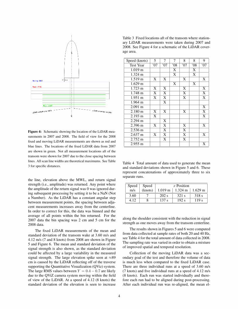
Figure 4: Schematic showing the location of the LiDAR mea-surements in 2007 and 2008. The field of view for the 2008fixed and moving LiDAR measurements are shown as red andblue lines. The locations of the fixed LiDAR data from 2007are shown in green. Not all measurement locations aft of thetransom were shown for 2007 due to the close spacing betweenlines. All scan line widths are theoretical maximums. See Table3 for specific distances.

the line, elevation above the MWL, and return signalstrength (i.e., amplitude) was returned. Any point wherethe amplitude of the return signal was 0 was ignored dur-ing subsequent processing by setting it to be a NaN (Nota Number). As the LiDAR has a constant angular stepbetween measurement points, the spacing between adja-cent measurements increases away from the centerline.In order to correct for this, the data was binned and theaverage of all points within the bin returned. For the2007 data the bin spacing was 2 cm and 5 cm for the2008 data.

The fixed LiDAR measurements of the mean andstandard deviation of the transom wake at 3.60 m/s and4.12 m/s (7 and 8 knots) from 2008 are shown in Figure5 and Figure 6. The mean and standard deviation of thesignal strength is also shown, as the standard deviationcould be affected by a large variability in the measuredsignal strength. The large elevation spike seen at ≈89cm is caused by the LiDAR reflecting off of the traversesupporting the Quantitative Visualization (QViz) system.The large RMS values between Y = 0.4− 0.7 are likelydue to the QViZ camera system moving within the fieldof view of the LiDAR. At a speed of 4.12 (8 knots) thestandard deviation of the elevation is seen to increase

Table 3 Fixed locations aft of the transom where station-ary LiDAR measurements were taken during 2007 and2008. See Figure 4 for a schematic of the LiDAR cover-age area.

Speed (knots) 5 7 7 8 8 9Test Year ’07 ’07 ’08 ’07 ’08 ’071.019 m X X1.324 m X X1.519 m X X X X1.629 m X X1.723 m X X X X1.748 m X X X X1.951 m X X X X1.964 m X2.091 m X2.180 m X X X X2.193 m X X2.294 m X2.396 m X X X X2.536 m X X2.637 m X X X X2.752 m X X2.955 m X

Table 4 Total amount of data used to generate the meanand standard deviations shown in Figure 5 and 6. Theserepresent concatenations of approximately three to sixseparate runs.

Speed Speed x Positionm/s (knots) 1.019 m 1.324 m 1.629 m3.60 7 202 s 321 s 318 s4.12 8 137 s 192 s 119 s

along the shoulder consistent with the reduction in signalstrength as one moves away from the transom centerline.

The results shown in Figures 5 and 6 were computedfrom data collected at sample rates of both 20 and 40 Hz,see Table 4 for the total amount of data collected in 2008.The sampling rate was varied in order to obtain a mixtureof improved spatial and temporal resolution.

Collection of the moving LiDAR data was a sec-ondary goal of the test and therefore the volume of datais much less when compared to the fixed LiDAR case.There are three individual runs at a speed of 3.60 m/s(7 knots) and five individual runs at a speed of 4.12 m/s(8 knots). Each run was started individually and there-fore each run had to be aligned during post-processing.After each individual run was re-aligned, the mean el-

4

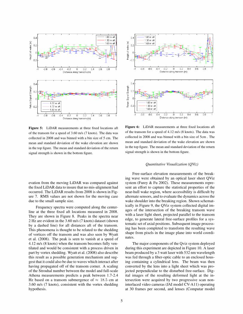
Figure 5: LiDAR measurements at three fixed locations aftof the transom for a speed of 3.60 m/s (7 knots). The data wascollected in 2008 and was binned with a bin size of 5 cm. Themean and standard deviation of the wake elevation are shownin the top figure. The mean and standard deviation of the returnsignal strength is shown in the bottom figure.

evation from the moving LiDAR was compared againstthe fixed LiDAR data to insure that no mis-alignment hadoccurred. The LiDAR results from 2008 is shown in Fig-ure 7. RMS values are not shown for the moving casedue to the small sample size.

Frequency spectra were computed along the center-line at the three fixed aft locations measured in 2008.They are shown in Figure 8. Peaks in the spectra near2 Hz are evident in the 3.60 m/s (7 knots) dataset (shownby a dashed line) for all distances aft of the transom.This phenomena is thought to be related to the sheddingof vortices off the transom and was also seen by Wyattet al. (2008). The peak is seen to vanish at a speed of4.12 m/s (8 knots) when the transom becomes fully ven-tilated and would be consistent with a process driven inpart by vortex shedding. Wyatt et al. (2008) also describethis result as a possible generation mechanism and sug-gest that it could also be due to waves which interact afterhaving propagated off of the transom corner. A scalingof the Strouhal number between the model and full-scaleAthena measurements predicts a peak between 1.7-2.4Hz based on a transom submergence of ≈ 18.5 cm at3.60 m/s (7 knots), consistent with the vortex sheddinghypothesis.

Figure 6: LiDAR measurements at three fixed locations aftof the transom for a speed of 4.12 m/s (8 knots). The data wascollected in 2008 and was binned with a bin size of 5cm . Themean and standard deviation of the wake elevation are shownin the top figure. The mean and standard deviation of the returnsignal strength is shown in the bottom figure.

Quantitative Visualization (QViz)

Free-surface elevation measurements of the break-ing wave were obtained by an optical laser sheet QVizsystem (Furey & Fu 2002). These measurements repre-sent an effort to capture the statistical properties of thenear-hull wake region, where accessibility is difficult byalternate sensors, and to evaluate the dynamics across thewake shoulder into the breaking region. Shown schemat-ically in Figure 9, the QViz system collected digital im-ages of the intersection of the breaking transom wavewith a laser light sheet, projected parallel to the transomedge, to generate lateral free-surface profiles for a sys-tematic set of axial positions. Subsequent image process-ing has been completed to transform the resulting waveshape from pixels in the image plane into world coordi-nates.

The major components of the Qviz system deployedduring this experiment are depicted in Figure 10. A laserbeam produced by a 3 watt laser with 532 nm wavelengthwas fed through a fiber-optic cable to an enclosed hous-ing containing a cylindrical lens. The beam was thenconverted by the lens into a light sheet which was pro-jected perpendicular to the disturbed free-surface. Dig-ital images of the resulting deformed light at the in-tersection were acquired by two progressive scan non-interlaced video cameras (JAI model CV-A11) operatingat 30 frames per second, and lenses (Computar model

5

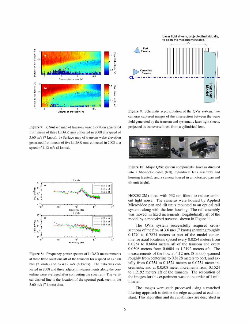
Figure 7: a) Surface map of transom wake elevation generatedfrom mean of three LiDAR runs collected in 2008 at a speed of3.60 m/s (7 knots). b) Surface map of transom wake elevationgenerated from mean of five LiDAR runs collected in 2008 at aspeed of 4.12 m/s (8 knots).

Figure 8: Frequency power spectra of LiDAR measurementsat three fixed locations aft of the transom for a speed of a) 3.60m/s (7 knots) and b) 4.12 m/s (8 knots). The data was col-lected in 2008 and three adjacent measurements along the cen-terline were averaged after computing the spectrum. The verti-cal dashed line is the location of the spectral peak seen in the3.60 m/s (7 knots) data.

Figure 9: Schematic representation of the QViz system: twocameras captured images of the intersection between the wavefield generated by the transom and systematic laser light sheets,projected as transverse lines, from a cylindrical lens.

Figure 10: Major QViz system components: laser as directedinto a fiber-optic cable (left), cylindrical lens assembly andhousing (center), and a camera housed in a motorized pan andtilt unit (right).

H6Z0812M) fitted with 532 nm filters to reduce ambi-ent light noise. The cameras were housed by AppliedMicrovideo pan and tilt units mounted to an optical railsystem, along with the lens housing. The rail assemblywas moved, in fixed increments, longitudinally aft of themodel by a motorized traverse, shown in Figure 11.

The QViz system successfully acquired cross-sections of the flow at 3.6 m/s (7 knots) spanning roughly0.1270 to 0.7874 meters to port of the model center-line for axial locations spaced every 0.0254 meters from0.0254 to 0.6604 meters aft of the transom and every0.0508 meters from 0.6604 to 1.2192 meters aft. Themeasurements of the flow at 4.12 m/s (8 knots) spannedroughly from centerline to 0.8128 meters to port, and ax-ially from 0.0254 to 0.1524 meters at 0.0254 meter in-crements, and at 0.0508 meter increments from 0.1524to 1.2192 meters aft of the transom. The resolution ofthe images for this experiment was on the order of 1 mil-limeter.

The images were each processed using a matchedfiltering approach to define the edge acquired at each in-stant. This algorithm and its capabilities are described in

6

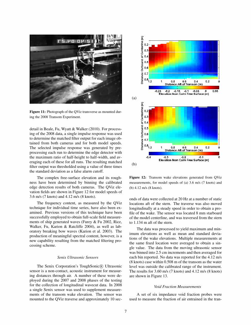
Figure 11: Photograph of the QViz transverse as mounted dur-ing the 2008 Transom Experiment.

detail in Beale, Fu, Wyatt & Walker (2010). For process-ing of the 2008 data, a single impulse response was usedto determine the matched filter output for each image ob-tained from both cameras and for both model speeds.The selected impulse response was generated by pre-processing each run to determine the edge detector withthe maximum ratio of half-height to half-width, and av-eraging each of these for all runs. The resulting matchedfilter output was thresholded using a value of three timesthe standard deviation as a false alarm cutoff.

The complex free-surface elevation and its rough-ness have been determined by binning the calibratededge detection results of both cameras. The QViz ele-vation fields are shown in Figure 12 for model speeds of3.6 m/s (7 knots) and 4.12 m/s (8 knots).

The frequency content, as measured by the QViztechnique for individual time series, have also been ex-amined. Previous versions of this technique have beensuccessfully employed to obtain full-scale field measure-ments of ship generated waves (Furey & Fu 2002, Rice,Walker, Fu, Karion & Ratcliffe 2004), as well as lab-oratory breaking bow waves (Karion et al. 2003). Theproduction of meaningful spectral content, however, is anew capability resulting from the matched filtering pro-cessing scheme.

Senix Ultrasonic Sensors

The Senix Corporation’s ToughSonic R© Ultrasonicsensor is a non-contact, acoustic instrument for measur-ing distances through air. A number of these were de-ployed during the 2007 and 2008 phases of the testingfor the collection of longitudinal wavecut data. In 2008a single Senix sensor was used to supplement measure-ments of the transom wake elevation. The sensor wasmounted to the QViz traverse and approximately 10 sec-

(a)

(b)

Figure 12: Transom wake elevations generated from QVizmeasurements, for model speeds of (a) 3.6 m/s (7 knots) and(b) 4.12 m/s (8 knots).

onds of data were collected at 20 Hz at a number of staticlocations aft of the stern. The traverse was also movedlongitudinally at a steady speed in order to obtain a pro-file of the wake. The sensor was located 8 mm starboardof the model centerline, and was traversed from the sternto 1.134 m aft of the stern.

The data was processed to yield maximum and min-imum elevations as well as mean and standard devia-tions of the wake elevations. Multiple measurements atthe same fixed location were averaged to obtain a sin-gle value. The data from the moving ultrasonic sensorwas binned into 2.5 cm increments and then averaged foreach bin reported. No data was reported for the 4.12 m/s(8 knots) case within 0.508 m of the transom as the waterlevel was outside the calibrated range of the instrument.The results for 3.60 m/s (7 knots) and 4.12 m/s (8 knots)are shown in Figure 13.

Void Fraction Measurements

A set of six impedance void fraction probes wereused to measure the fraction of air entrained in the tran-

7

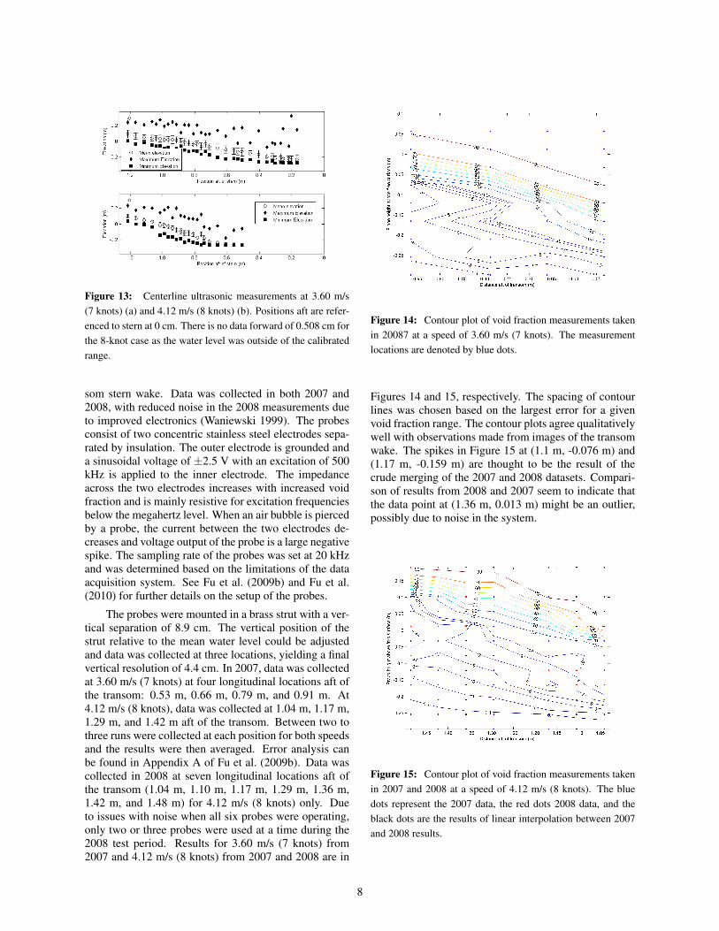
Figure 13: Centerline ultrasonic measurements at 3.60 m/s(7 knots) (a) and 4.12 m/s (8 knots) (b). Positions aft are refer-enced to stern at 0 cm. There is no data forward of 0.508 cm forthe 8-knot case as the water level was outside of the calibratedrange.

som stern wake. Data was collected in both 2007 and2008, with reduced noise in the 2008 measurements dueto improved electronics (Waniewski 1999). The probesconsist of two concentric stainless steel electrodes sepa-rated by insulation. The outer electrode is grounded anda sinusoidal voltage of ±2.5 V with an excitation of 500kHz is applied to the inner electrode. The impedanceacross the two electrodes increases with increased voidfraction and is mainly resistive for excitation frequenciesbelow the megahertz level. When an air bubble is piercedby a probe, the current between the two electrodes de-creases and voltage output of the probe is a large negativespike. The sampling rate of the probes was set at 20 kHzand was determined based on the limitations of the dataacquisition system. See Fu et al. (2009b) and Fu et al.(2010) for further details on the setup of the probes.

The probes were mounted in a brass strut with a ver-tical separation of 8.9 cm. The vertical position of thestrut relative to the mean water level could be adjustedand data was collected at three locations, yielding a finalvertical resolution of 4.4 cm. In 2007, data was collectedat 3.60 m/s (7 knots) at four longitudinal locations aft ofthe transom: 0.53 m, 0.66 m, 0.79 m, and 0.91 m. At4.12 m/s (8 knots), data was collected at 1.04 m, 1.17 m,1.29 m, and 1.42 m aft of the transom. Between two tothree runs were collected at each position for both speedsand the results were then averaged. Error analysis canbe found in Appendix A of Fu et al. (2009b). Data wascollected in 2008 at seven longitudinal locations aft ofthe transom (1.04 m, 1.10 m, 1.17 m, 1.29 m, 1.36 m,1.42 m, and 1.48 m) for 4.12 m/s (8 knots) only. Dueto issues with noise when all six probes were operating,only two or three probes were used at a time during the2008 test period. Results for 3.60 m/s (7 knots) from2007 and 4.12 m/s (8 knots) from 2007 and 2008 are in

Figure 14: Contour plot of void fraction measurements takenin 20087 at a speed of 3.60 m/s (7 knots). The measurementlocations are denoted by blue dots.

Figures 14 and 15, respectively. The spacing of contourlines was chosen based on the largest error for a givenvoid fraction range. The contour plots agree qualitativelywell with observations made from images of the transomwake. The spikes in Figure 15 at (1.1 m, -0.076 m) and(1.17 m, -0.159 m) are thought to be the result of thecrude merging of the 2007 and 2008 datasets. Compari-son of results from 2008 and 2007 seem to indicate thatthe data point at (1.36 m, 0.013 m) might be an outlier,possibly due to noise in the system.

Figure 15: Contour plot of void fraction measurements takenin 2007 and 2008 at a speed of 4.12 m/s (8 knots). The bluedots represent the 2007 data, the red dots 2008 data, and theblack dots are the results of linear interpolation between 2007and 2008 results.

8

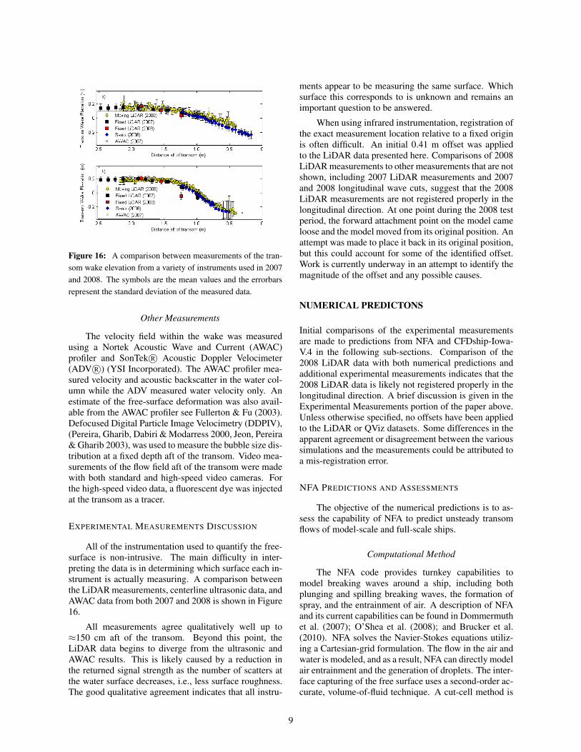
Figure 16: A comparison between measurements of the tran-som wake elevation from a variety of instruments used in 2007and 2008. The symbols are the mean values and the errorbarsrepresent the standard deviation of the measured data.

Other Measurements

The velocity field within the wake was measuredusing a Nortek Acoustic Wave and Current (AWAC)profiler and SonTek R© Acoustic Doppler Velocimeter(ADV R©) (YSI Incorporated). The AWAC profiler mea-sured velocity and acoustic backscatter in the water col-umn while the ADV measured water velocity only. Anestimate of the free-surface deformation was also avail-able from the AWAC profiler see Fullerton & Fu (2003).Defocused Digital Particle Image Velocimetry (DDPIV),(Pereira, Gharib, Dabiri & Modarress 2000, Jeon, Pereira& Gharib 2003), was used to measure the bubble size dis-tribution at a fixed depth aft of the transom. Video mea-surements of the flow field aft of the transom were madewith both standard and high-speed video cameras. Forthe high-speed video data, a fluorescent dye was injectedat the transom as a tracer.

EXPERIMENTAL MEASUREMENTS DISCUSSION

All of the instrumentation used to quantify the free-surface is non-intrusive. The main difficulty in inter-preting the data is in determining which surface each in-strument is actually measuring. A comparison betweenthe LiDAR measurements, centerline ultrasonic data, andAWAC data from both 2007 and 2008 is shown in Figure16.

All measurements agree qualitatively well up to≈150 cm aft of the transom. Beyond this point, theLiDAR data begins to diverge from the ultrasonic andAWAC results. This is likely caused by a reduction inthe returned signal strength as the number of scatters atthe water surface decreases, i.e., less surface roughness.The good qualitative agreement indicates that all instru-

ments appear to be measuring the same surface. Whichsurface this corresponds to is unknown and remains animportant question to be answered.

When using infrared instrumentation, registration ofthe exact measurement location relative to a fixed originis often difficult. An initial 0.41 m offset was appliedto the LiDAR data presented here. Comparisons of 2008LiDAR measurements to other measurements that are notshown, including 2007 LiDAR measurements and 2007and 2008 longitudinal wave cuts, suggest that the 2008LiDAR measurements are not registered properly in thelongitudinal direction. At one point during the 2008 testperiod, the forward attachment point on the model cameloose and the model moved from its original position. Anattempt was made to place it back in its original position,but this could account for some of the identified offset.Work is currently underway in an attempt to identify themagnitude of the offset and any possible causes.

NUMERICAL PREDICTONS

Initial comparisons of the experimental measurementsare made to predictions from NFA and CFDship-Iowa-V.4 in the following sub-sections. Comparison of the2008 LiDAR data with both numerical predictions andadditional experimental measurements indicates that the2008 LiDAR data is likely not registered properly in thelongitudinal direction. A brief discussion is given in theExperimental Measurements portion of the paper above.Unless otherwise specified, no offsets have been appliedto the LiDAR or QViz datasets. Some differences in theapparent agreement or disagreement between the varioussimulations and the measurements could be attributed toa mis-registration error.

NFA PREDICTIONS AND ASSESSMENTS

The objective of the numerical predictions is to as-sess the capability of NFA to predict unsteady transomflows of model-scale and full-scale ships.

Computational Method

The NFA code provides turnkey capabilities tomodel breaking waves around a ship, including bothplunging and spilling breaking waves, the formation ofspray, and the entrainment of air. A description of NFAand its current capabilities can be found in Dommermuthet al. (2007); O’Shea et al. (2008); and Brucker et al.(2010). NFA solves the Navier-Stokes equations utiliz-ing a Cartesian-grid formulation. The flow in the air andwater is modeled, and as a result, NFA can directly modelair entrainment and the generation of droplets. The inter-face capturing of the free surface uses a second-order ac-curate, volume-of-fluid technique. A cut-cell method is

9

Grid Cells Sub domainsNx ×Ny ×Nz ni × nj × nk

832× 384× 192 = 61, 341, 696 13× 6× 6 = 4681664× 786× 384 = 490, 733, 568 13× 6× 6 = 468

2688× 1024× 384 = 1, 056, 964, 608 21× 8× 6 = 1008

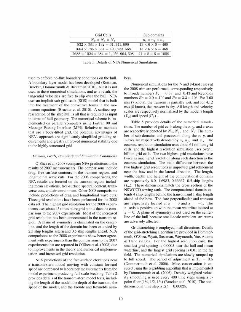
Table 5 Details of NFA Numerical Simulations.

used to enforce no-flux boundary conditions on the hull.A boundary-layer model has been developed (Rottman,Brucker, Dommermuth & Broutman 2010), but it is notused in these numerical simulations, and as a result, thetangential velocities are free to slip over the hull. NFAuses an implicit sub-grid scale (SGS) model that is builtinto the treatment of the convective terms in the mo-menum equations (Brucker et al. 2010). A surface rep-resentation of the ship hull is all that is required as inputin terms of hull geometry. The numerical scheme is im-plemented on parallel computers using Fortran 90 andMessage Passing Interface (MPI). Relative to methodsthat use a body-fitted grid, the potential advantages ofNFA’s approach are significantly simplified gridding re-quirements and greatly improved numerical stability dueto the highly structured grid.

Domain, Grids, Boundary and Simulation Conditions

O’Shea et al. (2008) compare NFA predictions to theresults of 2007 measurements. The comparisons includedrag, free-surface contours in the transom region, andlongitudinal wave cuts. For the 2008 comparisons, theNFA results are focused on the transom region, includ-ing mean elevations, free-surface spectral content, trans-verse cuts, and air entrainment. Other 2008 comparisonsinclude predictions of drag and longitudinal wave cuts.Three grid resolutions have been performed for the 2008data set. The highest grid resolution for the 2008 experi-ments uses about 45 times more grid points than the com-parisons to the 2007 experiments. Most of the increasedgrid resolution has been concentrated in the transom re-gion. A plane of symmetry is eliminated on the center-line, and the length of the domain has been extended by2.5 ship lengths astern and 0.5 ship lengths ahead. NFAcomparisons to the 2008 experiments show better agree-ment with experiments than the comparisons to the 2007experiments that are reported in O’Shea et al. (2008) dueto improvements in the theory and numerical implemen-tation, and increased grid resolution.

NFA predictions of the free-surface elevations neara transom-stern model moving with constant forwardspeed are compared to laboratory measurements from themodel experiment producing full-scale breaking. Table 2provides details of the transom-stern model tests, includ-ing the length of the model, the depth of the transom, thespeed of the model, and the Froude and Reynolds num-

bers.

Numerical simulations for the 7- and 8-knot cases atthe 2008 trim are performed, corresponding respectivelyto Froude numbers Fr = 0.38 and 0.43 and Reynoldsnumbers Re = 2.9× 107 and Re = 3.3× 107. For 3.60m/s (7 knots), the transom is partially wet, and for 4.12m/s (8 knots), the transom is dry. All length and velocityscales are respectively normalized by the model’s length(Lo) and speed (Uo) .

Table 5 provides details of the numerical simula-tions. The number of grid cells along the x, y, and z-axesare respectively denoted by Nx, Ny, and Nz . The num-ber of sub-domains and processors along the x, y, andz-axes are respectively denoted by ni, nj , and nk. Thecoarsest resolution simulation uses about 61 million gridcells, and the highest resolution simulation uses over 1billion grid cells. The two highest grid resolutions havetwice as much grid resolution along each direction as thecoarsest simulation. The main difference between thetwo highest grid resolutions is improved grid refinementnear the bow and in the lateral direction. The length,width, depth, and height of the computational domainsare respectively 6.0, 1.6983, 0.66667, 0.5 ship lengths(Lo). These dimensions match the cross section of theNSWCCD towing tank. The computational domain ex-tends 4 ship lengths behind the transom and 1 ship lengthahead of the bow. The fore perpendicular and transomare respectively located at x = 0 and x = −1. Thez−axis is positive up with the mean waterline located atz = 0. A plane of symmetry is not used on the center-line of the hull because small-scale turbulent structuresare adversely affected.

Grid stretching is employed in all directions. Detailsof the grid-stretching algorithm are provided in Dommer-muth, O’Shea, Wyatt, Sussman, Weymouth, Yue, Adams& Hand (2006). For the highest resolution case, thesmallest grid spacing is 0.0005 near the hull and meanwaterline, and the largest grid spacing is 0.01 in the farfield. The numerical simulations are slowly ramped upto full speed. The period of adjustment is To = 0.5(Dommermuth et al. 2006). Mass conservation is en-sured using the regridding algorithm that is implementedby Dommermuth et al. (2006). Density-weighted veloc-ity smoothing is used every 400 time steps using a 3-point filter (1/4, 1/2, 1/4) (Brucker et al. 2010). The non-dimensional time step is ∆t = 0.00025.

10

The simulations are run for 30,000 time steps, corre-sponding to 7.5 ship lengths, on the SGI R© Altix R© ICE(Silicon Graphics, Inc.) at the U.S. Army Engineer Re-search and Development Center (ERDC). The data setsare so large that only time steps 20,0000 through 30,000are saved every 40 time steps for the purposes of postprocessing. The 1.06 billion cell simulation takes about90 hours of wall-clock time to run 30,000 time steps us-ing 1008 processors. The wall-clock time can be cut inhalf by doubling the number of processors because NFAscales linearly. Alternatively, increasing the number ofprocessors to over 8,000 will enable numerical simula-tions of breaking ship waves and tsunamis with over 10billion grid cells within the next year.

Prediction Assessments

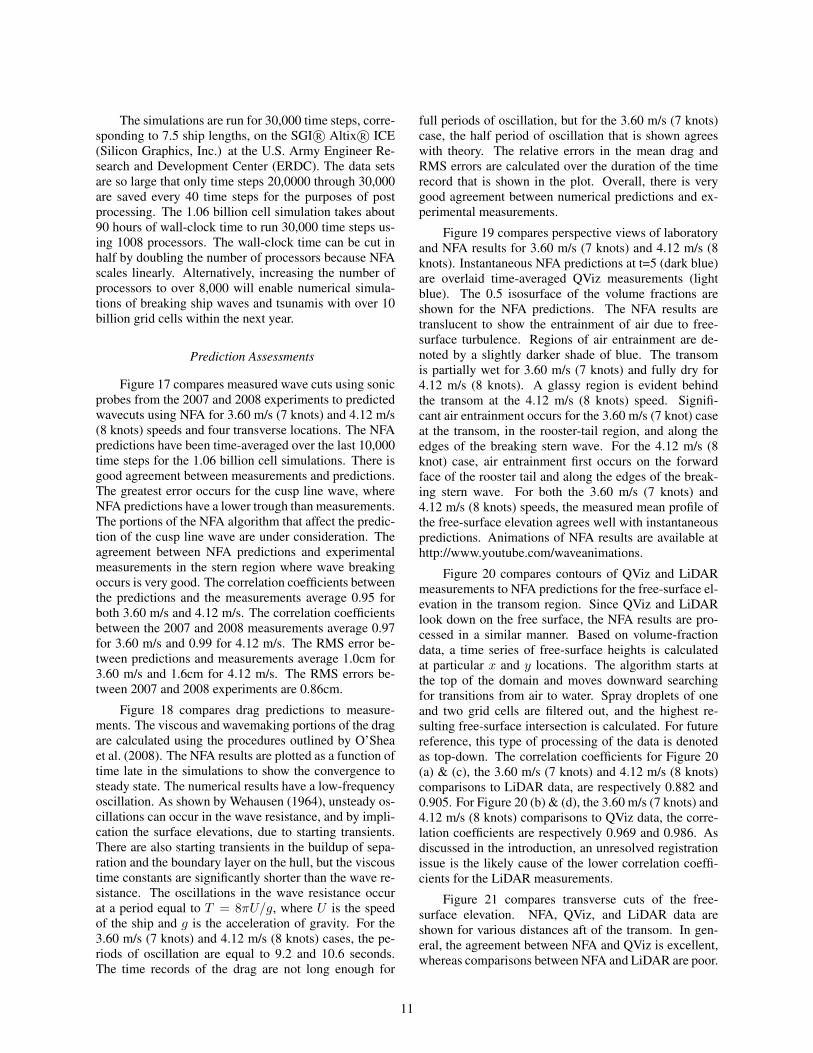
Figure 17 compares measured wave cuts using sonicprobes from the 2007 and 2008 experiments to predictedwavecuts using NFA for 3.60 m/s (7 knots) and 4.12 m/s(8 knots) speeds and four transverse locations. The NFApredictions have been time-averaged over the last 10,000time steps for the 1.06 billion cell simulations. There isgood agreement between measurements and predictions.The greatest error occurs for the cusp line wave, whereNFA predictions have a lower trough than measurements.The portions of the NFA algorithm that affect the predic-tion of the cusp line wave are under consideration. Theagreement between NFA predictions and experimentalmeasurements in the stern region where wave breakingoccurs is very good. The correlation coefficients betweenthe predictions and the measurements average 0.95 forboth 3.60 m/s and 4.12 m/s. The correlation coefficientsbetween the 2007 and 2008 measurements average 0.97for 3.60 m/s and 0.99 for 4.12 m/s. The RMS error be-tween predictions and measurements average 1.0cm for3.60 m/s and 1.6cm for 4.12 m/s. The RMS errors be-tween 2007 and 2008 experiments are 0.86cm.

Figure 18 compares drag predictions to measure-ments. The viscous and wavemaking portions of the dragare calculated using the procedures outlined by O’Sheaet al. (2008). The NFA results are plotted as a function oftime late in the simulations to show the convergence tosteady state. The numerical results have a low-frequencyoscillation. As shown by Wehausen (1964), unsteady os-cillations can occur in the wave resistance, and by impli-cation the surface elevations, due to starting transients.There are also starting transients in the buildup of sepa-ration and the boundary layer on the hull, but the viscoustime constants are significantly shorter than the wave re-sistance. The oscillations in the wave resistance occurat a period equal to T = 8πU/g, where U is the speedof the ship and g is the acceleration of gravity. For the3.60 m/s (7 knots) and 4.12 m/s (8 knots) cases, the pe-riods of oscillation are equal to 9.2 and 10.6 seconds.The time records of the drag are not long enough for

full periods of oscillation, but for the 3.60 m/s (7 knots)case, the half period of oscillation that is shown agreeswith theory. The relative errors in the mean drag andRMS errors are calculated over the duration of the timerecord that is shown in the plot. Overall, there is verygood agreement between numerical predictions and ex-perimental measurements.

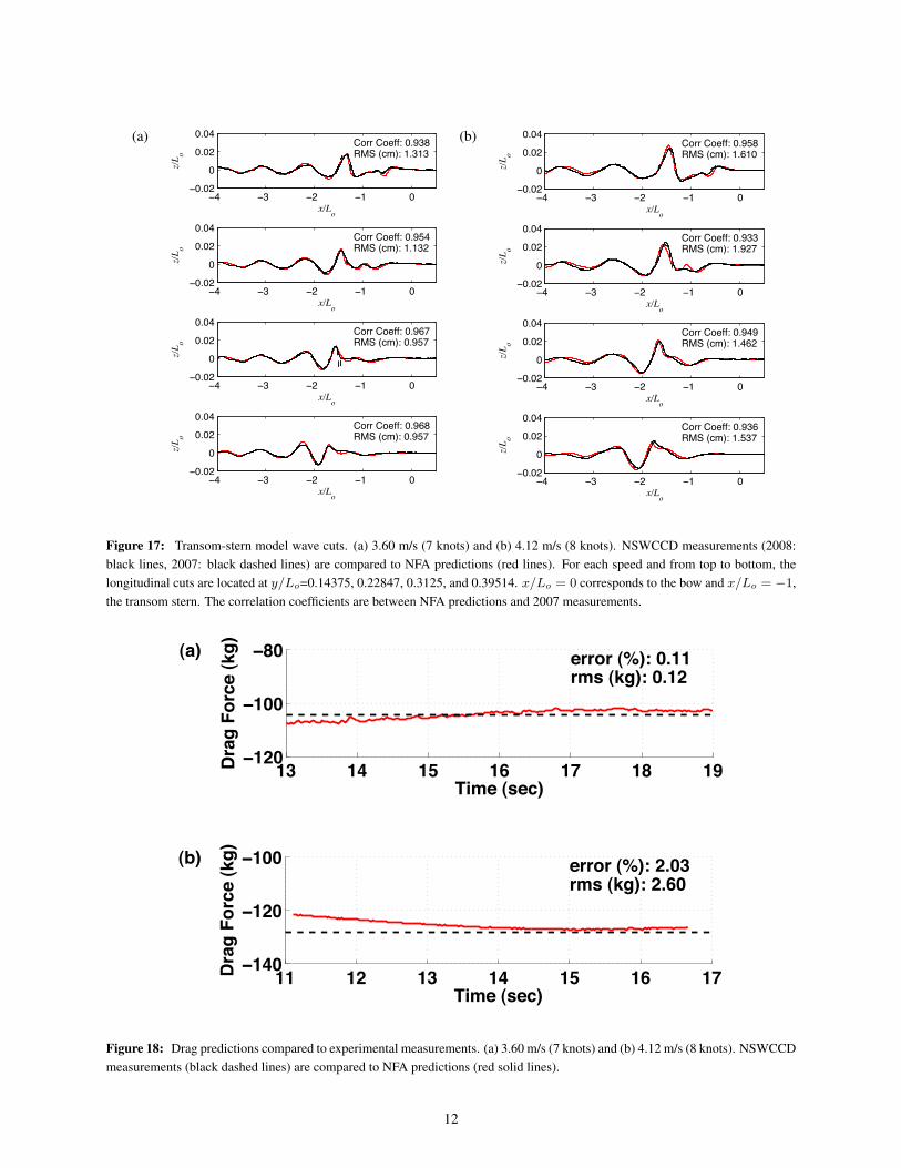
Figure 19 compares perspective views of laboratoryand NFA results for 3.60 m/s (7 knots) and 4.12 m/s (8knots). Instantaneous NFA predictions at t=5 (dark blue)are overlaid time-averaged QViz measurements (lightblue). The 0.5 isosurface of the volume fractions areshown for the NFA predictions. The NFA results aretranslucent to show the entrainment of air due to free-surface turbulence. Regions of air entrainment are de-noted by a slightly darker shade of blue. The transomis partially wet for 3.60 m/s (7 knots) and fully dry for4.12 m/s (8 knots). A glassy region is evident behindthe transom at the 4.12 m/s (8 knots) speed. Signifi-cant air entrainment occurs for the 3.60 m/s (7 knot) caseat the transom, in the rooster-tail region, and along theedges of the breaking stern wave. For the 4.12 m/s (8knot) case, air entrainment first occurs on the forwardface of the rooster tail and along the edges of the break-ing stern wave. For both the 3.60 m/s (7 knots) and4.12 m/s (8 knots) speeds, the measured mean profile ofthe free-surface elevation agrees well with instantaneouspredictions. Animations of NFA results are available athttp://www.youtube.com/waveanimations.

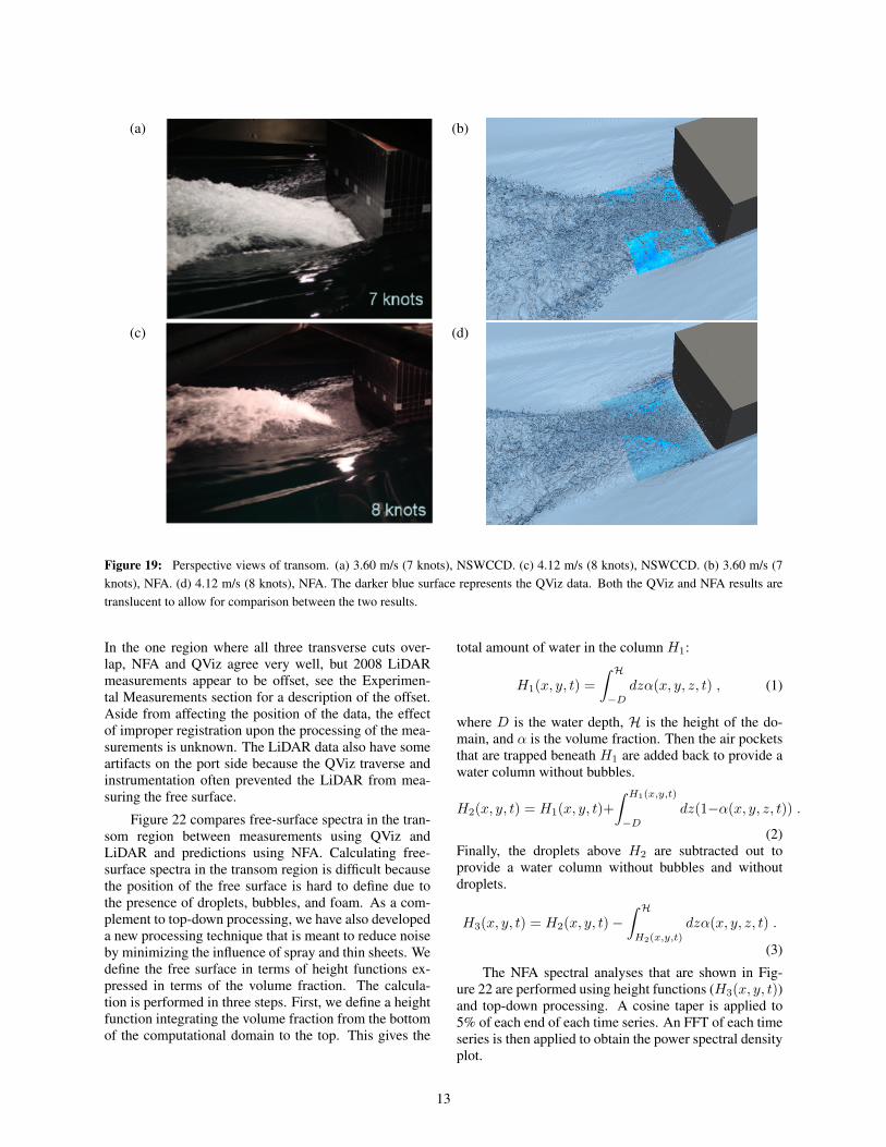
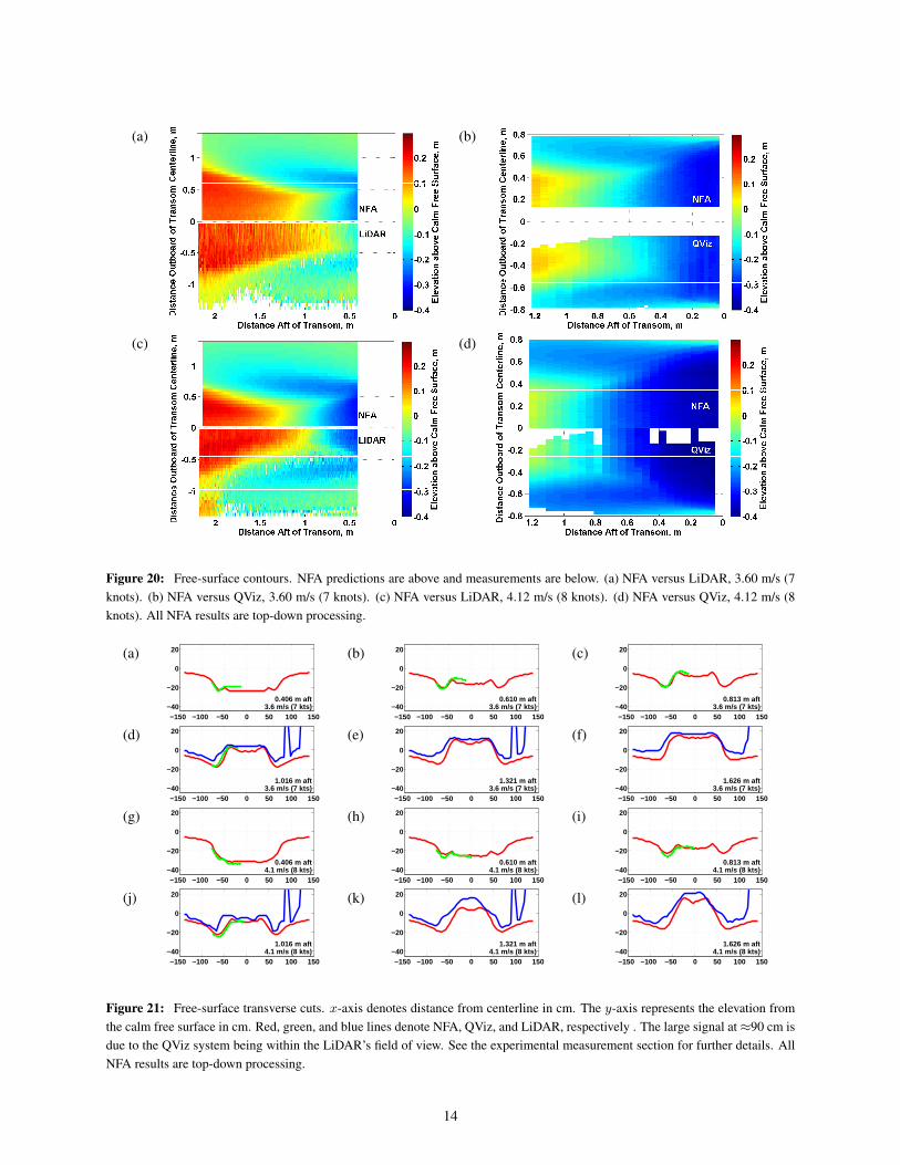
Figure 20 compares contours of QViz and LiDARmeasurements to NFA predictions for the free-surface el-evation in the transom region. Since QViz and LiDARlook down on the free surface, the NFA results are pro-cessed in a similar manner. Based on volume-fractiondata, a time series of free-surface heights is calculatedat particular x and y locations. The algorithm starts atthe top of the domain and moves downward searchingfor transitions from air to water. Spray droplets of oneand two grid cells are filtered out, and the highest re-sulting free-surface intersection is calculated. For futurereference, this type of processing of the data is denotedas top-down. The correlation coefficients for Figure 20(a) & (c), the 3.60 m/s (7 knots) and 4.12 m/s (8 knots)comparisons to LiDAR data, are respectively 0.882 and0.905. For Figure 20 (b) & (d), the 3.60 m/s (7 knots) and4.12 m/s (8 knots) comparisons to QViz data, the corre-lation coefficients are respectively 0.969 and 0.986. Asdiscussed in the introduction, an unresolved registrationissue is the likely cause of the lower correlation coeffi-cients for the LiDAR measurements.

Figure 21 compares transverse cuts of the free-surface elevation. NFA, QViz, and LiDAR data areshown for various distances aft of the transom. In gen-eral, the agreement between NFA and QViz is excellent,whereas comparisons between NFA and LiDAR are poor.

11

(a) (b)

−4 −3 −2 −1 0−0.02

0

0.02

0.04

z/L o

x/Lo

Corr Coeff: 0.938RMS (cm): 1.313

−4 −3 −2 −1 0−0.02

0

0.02

0.04

z/L o

x/Lo

Corr Coeff: 0.954RMS (cm): 1.132

−4 −3 −2 −1 0−0.02

0

0.02

0.04

z/L o

x/Lo

Corr Coeff: 0.967RMS (cm): 0.957

−4 −3 −2 −1 0−0.02

0

0.02

0.04

z/L o

x/Lo

Corr Coeff: 0.968RMS (cm): 0.957

−4 −3 −2 −1 0−0.02

0

0.02

0.04

z/L o

x/Lo

Corr Coeff: 0.958RMS (cm): 1.610

−4 −3 −2 −1 0−0.02

0

0.02

0.04

z/L o

x/Lo

Corr Coeff: 0.933RMS (cm): 1.927

−4 −3 −2 −1 0−0.02

0

0.02

0.04

z/L o

x/Lo

Corr Coeff: 0.949RMS (cm): 1.462

−4 −3 −2 −1 0−0.02

0

0.02

0.04

z/L o

x/Lo

Corr Coeff: 0.936RMS (cm): 1.537

Figure 17: Transom-stern model wave cuts. (a) 3.60 m/s (7 knots) and (b) 4.12 m/s (8 knots). NSWCCD measurements (2008:black lines, 2007: black dashed lines) are compared to NFA predictions (red lines). For each speed and from top to bottom, thelongitudinal cuts are located at y/Lo=0.14375, 0.22847, 0.3125, and 0.39514. x/Lo = 0 corresponds to the bow and x/Lo = −1,the transom stern. The correlation coefficients are between NFA predictions and 2007 measurements.

13 14 15 16 17 18 19−120

−100

−80

Time (sec)

Drag

For

ce (k

g) error (%): 0.11rms (kg): 0.12

(a)

11 12 13 14 15 16 17−140

−120

−100

Time (sec)

Drag

For

ce (k

g) error (%): 2.03rms (kg): 2.60

(b)

Figure 18: Drag predictions compared to experimental measurements. (a) 3.60 m/s (7 knots) and (b) 4.12 m/s (8 knots). NSWCCDmeasurements (black dashed lines) are compared to NFA predictions (red solid lines).

12

(a) (b)

(c) (d)

Figure 19: Perspective views of transom. (a) 3.60 m/s (7 knots), NSWCCD. (c) 4.12 m/s (8 knots), NSWCCD. (b) 3.60 m/s (7knots), NFA. (d) 4.12 m/s (8 knots), NFA. The darker blue surface represents the QViz data. Both the QViz and NFA results aretranslucent to allow for comparison between the two results.

In the one region where all three transverse cuts over-lap, NFA and QViz agree very well, but 2008 LiDARmeasurements appear to be offset, see the Experimen-tal Measurements section for a description of the offset.Aside from affecting the position of the data, the effectof improper registration upon the processing of the mea-surements is unknown. The LiDAR data also have someartifacts on the port side because the QViz traverse andinstrumentation often prevented the LiDAR from mea-suring the free surface.

Figure 22 compares free-surface spectra in the tran-som region between measurements using QViz andLiDAR and predictions using NFA. Calculating free-surface spectra in the transom region is difficult becausethe position of the free surface is hard to define due tothe presence of droplets, bubbles, and foam. As a com-plement to top-down processing, we have also developeda new processing technique that is meant to reduce noiseby minimizing the influence of spray and thin sheets. Wedefine the free surface in terms of height functions ex-pressed in terms of the volume fraction. The calcula-tion is performed in three steps. First, we define a heightfunction integrating the volume fraction from the bottomof the computational domain to the top. This gives the

total amount of water in the column H1:

H1(x, y, t) =

∫ H−D

dzα(x, y, z, t) , (1)

where D is the water depth, H is the height of the do-main, and α is the volume fraction. Then the air pocketsthat are trapped beneath H1 are added back to provide awater column without bubbles.

H2(x, y, t) = H1(x, y, t)+

∫ H1(x,y,t)

−Ddz(1−α(x, y, z, t)) .

(2)Finally, the droplets above H2 are subtracted out toprovide a water column without bubbles and withoutdroplets.

H3(x, y, t) = H2(x, y, t)−∫ HH2(x,y,t)

dzα(x, y, z, t) .

(3)

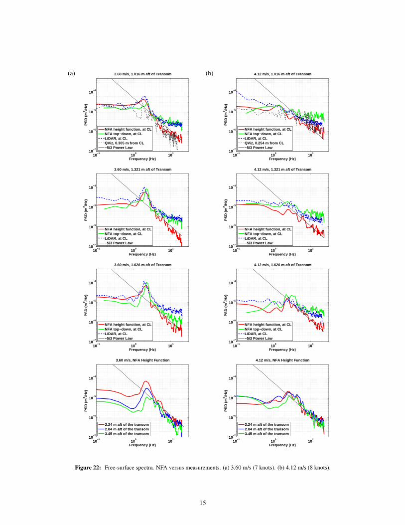
The NFA spectral analyses that are shown in Fig-ure 22 are performed using height functions (H3(x, y, t))and top-down processing. A cosine taper is applied to5% of each end of each time series. An FFT of each timeseries is then applied to obtain the power spectral densityplot.

13

(a) (b)

(c) (d)

Figure 20: Free-surface contours. NFA predictions are above and measurements are below. (a) NFA versus LiDAR, 3.60 m/s (7knots). (b) NFA versus QViz, 3.60 m/s (7 knots). (c) NFA versus LiDAR, 4.12 m/s (8 knots). (d) NFA versus QViz, 4.12 m/s (8knots). All NFA results are top-down processing.

(a) (b) (c)

−150 −100 −50 0 50 100 150−40

−20

0

20

3.6 m/s (7 kts)0.406 m aft

−150 −100 −50 0 50 100 150−40

−20

0

20

3.6 m/s (7 kts)0.610 m aft

−150 −100 −50 0 50 100 150−40

−20

0

20

3.6 m/s (7 kts)0.813 m aft

(d) (e) (f)

−150 −100 −50 0 50 100 150−40

−20

0

20

3.6 m/s (7 kts)1.016 m aft

−150 −100 −50 0 50 100 150−40

−20

0

20

3.6 m/s (7 kts)1.321 m aft

−150 −100 −50 0 50 100 150−40

−20

0

20

3.6 m/s (7 kts)1.626 m aft

(g) (h) (i)

−150 −100 −50 0 50 100 150−40

−20

0

20

4.1 m/s (8 kts)0.406 m aft

−150 −100 −50 0 50 100 150−40

−20

0

20

4.1 m/s (8 kts)0.610 m aft

−150 −100 −50 0 50 100 150−40

−20

0

20

4.1 m/s (8 kts)0.813 m aft

(j) (k) (l)

−150 −100 −50 0 50 100 150−40

−20

0

20

4.1 m/s (8 kts)1.016 m aft

−150 −100 −50 0 50 100 150−40

−20

0

20

4.1 m/s (8 kts)1.321 m aft

−150 −100 −50 0 50 100 150−40

−20

0

20

4.1 m/s (8 kts)1.626 m aft

Figure 21: Free-surface transverse cuts. x-axis denotes distance from centerline in cm. The y-axis represents the elevation fromthe calm free surface in cm. Red, green, and blue lines denote NFA, QViz, and LiDAR, respectively . The large signal at ≈90 cm isdue to the QViz system being within the LiDAR’s field of view. See the experimental measurement section for further details. AllNFA results are top-down processing.

14

(a) (b)

10−1

100

101

10−7

10−6

10−5

10−4

Frequency (Hz)

PS

D (

m2 /H

z)

3.60 m/s, 1.016 m aft of Transom

NFA height function, at CLNFA top−down, at CLLiDAR, at CLQViz, 0.305 m from CL−5/3 Power Law

10−1

100

101

10−7

10−6

10−5

10−4

Frequency (Hz)

PS

D (

m2 /H

z)

4.12 m/s, 1.016 m aft of Transom

NFA height function, at CLNFA top−down, at CLLiDAR, at CLQViz, 0.254 m from CL−5/3 Power Law

10−1

100

101

10−7

10−6

10−5

10−4

Frequency (Hz)

PS

D (

m2 /H

z)

3.60 m/s, 1.321 m aft of Transom

NFA height function, at CLNFA top−down, at CLLiDAR, at CL−5/3 Power Law

10−1

100

101

10−7

10−6

10−5

10−4

Frequency (Hz)

PS

D (

m2 /H

z)

4.12 m/s, 1.321 m aft of Transom

NFA height function, at CLNFA top−down, at CLLiDAR, at CL−5/3 Power Law

10−1

100

101

10−7

10−6

10−5

10−4

Frequency (Hz)

PS

D (

m2 /H

z)

3.60 m/s, 1.626 m aft of Transom

NFA height function, at CLNFA top−down, at CLLiDAR, at CL−5/3 Power Law

10−1

100

101

10−7

10−6

10−5

10−4

Frequency (Hz)

PS

D (

m2 /H

z)

4.12 m/s, 1.626 m aft of Transom

NFA height function, at CLNFA top−down, at CLLiDAR, at CL−5/3 Power Law

10−1

100

101

10−7

10−6

10−5

10−4

Frequency (Hz)

PS

D (

m2 /H

z)

3.60 m/s, NFA Height Function

2.24 m aft of the transom2.84 m aft of the transom3.45 m aft of the transom

10−1

100

101

10−7

10−6

10−5

10−4

Frequency (Hz)

PS

D (

m2 /H

z)

4.12 m/s, NFA Height Function

2.24 m aft of the transom2.84 m aft of the transom3.45 m aft of the transom

Figure 22: Free-surface spectra. NFA versus measurements. (a) 3.60 m/s (7 knots). (b) 4.12 m/s (8 knots).

15

(a) (b)

(c) (d)

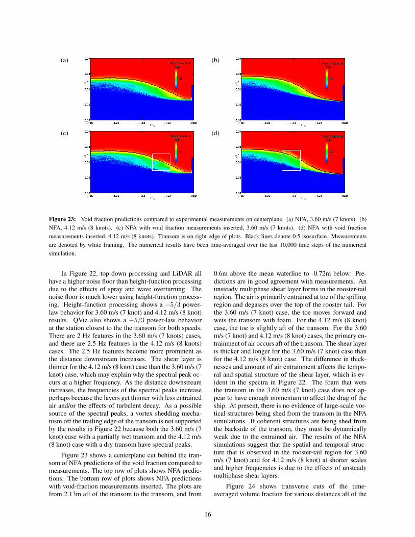
Figure 23: Void fraction predictions compared to experimental measurements on centerplane. (a) NFA, 3.60 m/s (7 knots). (b)NFA, 4.12 m/s (8 knots). (c) NFA with void fraction measurements inserted, 3.60 m/s (7 knots). (d) NFA with void fractionmeasurements inserted, 4.12 m/s (8 knots). Transom is on right edge of plots. Black lines denote 0.5 isosurface. Measurementsare denoted by white framing. The numerical results have been time-averaged over the last 10,000 time steps of the numericalsimulation.

In Figure 22, top-down processing and LiDAR allhave a higher noise floor than height-function processingdue to the effects of spray and wave overturning. Thenoise floor is much lower using height-function process-ing. Height-function processing shows a −5/3 power-law behavior for 3.60 m/s (7 knot) and 4.12 m/s (8 knot)results. QViz also shows a −5/3 power-law behaviorat the station closest to the the transom for both speeds.There are 2 Hz features in the 3.60 m/s (7 knots) cases,and there are 2.5 Hz features in the 4.12 m/s (8 knots)cases. The 2.5 Hz features become more prominent asthe distance downstream increases. The shear layer isthinner for the 4.12 m/s (8 knot) case than the 3.60 m/s (7knot) case, which may explain why the spectral peak oc-curs at a higher frequency. As the distance downstreamincreases, the frequencies of the spectral peaks increaseperhaps because the layers get thinner with less entrainedair and/or the effects of turbulent decay. As a possiblesource of the spectral peaks, a vortex shedding mecha-nism off the trailing edge of the transom is not supportedby the results in Figure 22 because both the 3.60 m/s (7knot) case with a partially wet transom and the 4.12 m/s(8 knot) case with a dry transom have spectral peaks.

Figure 23 shows a centerplane cut behind the tran-som of NFA predictions of the void fraction compared tomeasurements. The top row of plots shows NFA predic-tions. The bottom row of plots shows NFA predictionswith void-fraction measurements inserted. The plots arefrom 2.13m aft of the transom to the transom, and from

0.6m above the mean waterline to -0.72m below. Pre-dictions are in good agreement with measurements. Anunsteady multiphase shear layer forms in the rooster-tailregion. The air is primarily entrained at toe of the spillingregion and degasses over the top of the rooster tail. Forthe 3.60 m/s (7 knot) case, the toe moves forward andwets the transom with foam. For the 4.12 m/s (8 knot)case, the toe is slightly aft of the transom. For the 3.60m/s (7 knot) and 4.12 m/s (8 knot) cases, the primary en-trainment of air occurs aft of the transom. The shear layeris thicker and longer for the 3.60 m/s (7 knot) case thanfor the 4.12 m/s (8 knot) case. The difference in thick-nesses and amount of air entrainment affects the tempo-ral and spatial structure of the shear layer, which is ev-ident in the spectra in Figure 22. The foam that wetsthe transom in the 3.60 m/s (7 knot) case does not ap-pear to have enough momentum to affect the drag of theship. At present, there is no evidence of large-scale vor-tical structures being shed from the transom in the NFAsimulations. If coherent structures are being shed fromthe backside of the transom, they must be dynamicallyweak due to the entrained air. The results of the NFAsimulations suggest that the spatial and temporal struc-ture that is observed in the rooster-tail region for 3.60m/s (7 knot) and for 4.12 m/s (8 knot) at shorter scalesand higher frequencies is due to the effects of unsteadymultiphase shear layers.

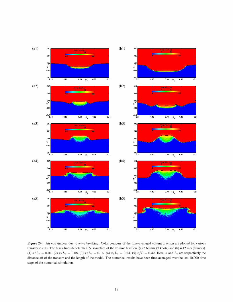
Figure 24 shows transverse cuts of the time-averaged volume fraction for various distances aft of the

16

(a1) (b1)

(a2) (b2)

(a3) (b3)

(a4) (b4)

(a5) (b5)

Figure 24: Air entrainment due to wave breaking. Color contours of the time-averaged volume fraction are plotted for varioustransverse cuts. The black lines denote the 0.5 isosurface of the volume fraction. (a) 3.60 m/s (7 knots) and (b) 4.12 m/s (8 knots).(1) x/Lo = 0.04. (2) x/Lo = 0.08, (3) x/Lo = 0.16. (4) x/Lo = 0.24. (5) x/L = 0.32. Here, x and Lo are respectively thedistance aft of the transom and the length of the model. The numerical results have been time-averaged over the last 10,000 timesteps of the numerical simulation.

17

transom. The 3.60 m/s (7 knot) plots extend from -1mto 1m in transverse direction and from -.62m to .64m inthe vertical. The 4.12 m/s (8 knot) plots extend from -1.9m to 1.9m in transverse direction and from -1.14m to1.14m in the vertical. Most of the air entrainment oc-curs in the rooster-tail region and along the edges of thestern breaking wave. The structure of the void fractionwake has three dominant structures corresponding to thecenterline entrainment in the rooster-tail region and thespilling-breaking entrainment that occurs along the cuspline.

CFDSHIP-IOWA PREDICTIONS AND ASSESSMENTS

CFDShip-Iowa V4 mean and unsteady wave eleva-tion predictions using detached eddy simulation (DES)for the transom stern model for a wet (Fr = 0.38) and adry (Fr = 0.43) transom is assessed using experimentaldata, and the dominant wetted transom flow frequency isexplained as a Karman-like vortex shedding.

Computational Method

The simulations are performed using a singlephase solver in absolute inertial earth-fixed coordinates(Carrica, Wilson & Stern 2007). The turbulence model-ing is performed using DES and the interface modelingusing level-set methods. A multi-block overset grid ap-proach is used to allow grid refinement in the regionsof interest. The governing equations are discretized us-ing cell-centered finite difference schemes on body-fittedcurvilinear grids and solved using a predictor-correctormethod. The time marching is done using the 2nd orderbackward difference scheme. The convection terms andlevel-set equations are discretized using a hybrid 2nd/4th

order Total Variation Diminishing (TVD) scheme. Thepressure Poisson equation is solved using the PortableExtensible Toolkit for Scientific computing (PETSc) us-ing a projection algorithm to satisfy continuity. MPI-based domain decomposition is used, where each decom-posed block is mapped to a single processor.

Domain, Grids, Boundary and Simulation Conditions

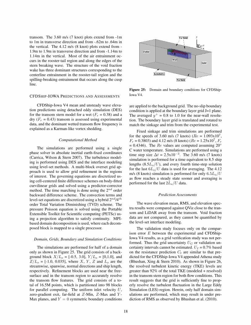
The simulations are performed for half of a domainonly as shown in Figure 25. The grid consists of a back-ground block X/Lo = [-0.5, 3.0], Y/Lo = [0,1.0], andZ/Lo = [-1.0, 0.035], where X , Y , Z and Lo are thestreamwise, spanwise, normal directions and ship length,respectively. Refinement blocks are used near the free-surface and in the transom region to accurately resolvethe transom flow features. The grid consists of a to-tal of 16.5M points, which is partitioned into 98 blocksfor parallel computing. The uniform inlet velocity U ,zero-gradient exit, far-field at Z-Min, Z-Max and Y -Max planes, and Y = 0 symmetric boundary conditions

Figure 25: Domain and boundary conditions for CFDShip-Iowa V4.

are applied to the background grid. The no-slip boundarycondition is applied at the boundary layer grid J=1 plane.The averaged y+ = 0.8 to 1.0 for the near-wall resolu-tion. The boundary layer grid is translated and rotated tomatch the sinkage and trim from the experimental test.

Fixed sinkage and trim simulations are performedfor the speeds of 3.60 m/s (7 knots) (Re = 1.093x107,Fr = 0.3803) and 4.12 m/s (8 knots) (Re = 1.25x107, Fr

= 0.4346). The Re values are computed assuming 20◦

C water temperature. Simulations are performed using atime step size ∆t = 2.5x10−3. The 3.60 m/s (7 knots)simulation is performed for a time equivalent to 8.5 shiplengths (8.5Lo/U ), and every fourth time-step solutionfor the last 6Lo/U data is used for averaging. The 4.12m/s (8 knots) simulation is performed for only 6.5Lo/Uas flow reaches a steady state sooner and averaging isperformed for the last 2Lo/U data.

Prediction Assessments

The wave elevation mean, RMS, and elevation spec-tra results were compared against QViz close to the tran-som and LiDAR away from the transom. Void fractiondata are not compared, as they cannot be quantified bythe level-set interface modeling.

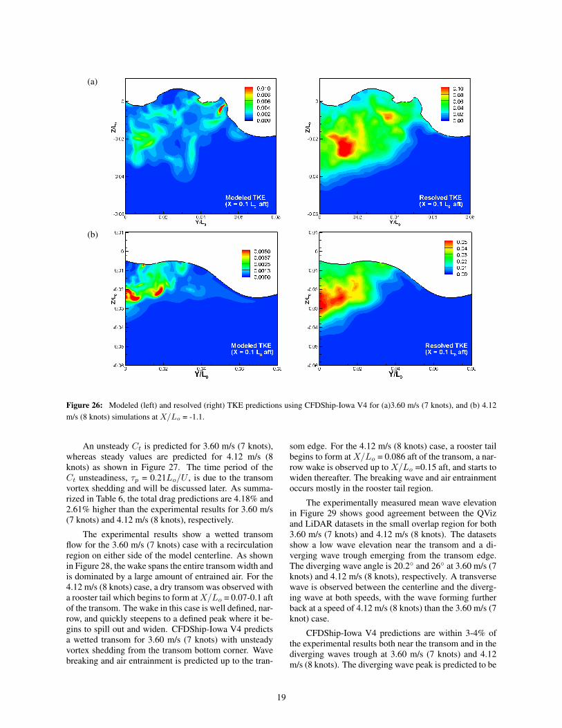
The validation study focuses only on the compar-ison error E between the experimental and CFDShip-Iowa V4 results, as a grid verification study was not per-formed. Thus the grid uncertainty UG or validation un-certainty intervals cannot be estimated. UI = 0.7% basedon the resistance prediction Ct are similar to that pre-dicted for the CFDShip-Iowa V4 appended Athena study(Bhushan, Xing & Stern 2010). As shown in Figure 26,the resolved turbulent kinetic energy (TKE) levels aregreater than 92% of the total TKE (modeled + resolved)in the transom stern region for both flow conditions. Thisresult suggests that the grid is sufficiently fine to prop-erly resolve the turbulent fluctuation in the Large EddySimulation (LES) region. Herein, only half domain sim-ulations are performed, which may result in under pre-diction of RMS as observed by Bhushan et al. (2010).

18

(a)

(b)

Figure 26: Modeled (left) and resolved (right) TKE predictions using CFDShip-Iowa V4 for (a)3.60 m/s (7 knots), and (b) 4.12m/s (8 knots) simulations at X/Lo = -1.1.

An unsteady Ct is predicted for 3.60 m/s (7 knots),whereas steady values are predicted for 4.12 m/s (8knots) as shown in Figure 27. The time period of theCt unsteadiness, τp = 0.21Lo/U , is due to the transomvortex shedding and will be discussed later. As summa-rized in Table 6, the total drag predictions are 4.18% and2.61% higher than the experimental results for 3.60 m/s(7 knots) and 4.12 m/s (8 knots), respectively.

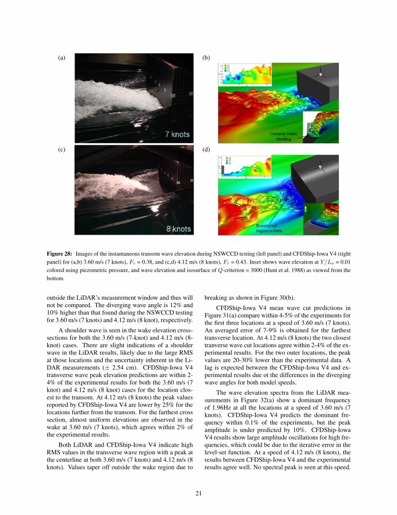
The experimental results show a wetted transomflow for the 3.60 m/s (7 knots) case with a recirculationregion on either side of the model centerline. As shownin Figure 28, the wake spans the entire transom width andis dominated by a large amount of entrained air. For the4.12 m/s (8 knots) case, a dry transom was observed witha rooster tail which begins to form atX/Lo = 0.07-0.1 aftof the transom. The wake in this case is well defined, nar-row, and quickly steepens to a defined peak where it be-gins to spill out and widen. CFDShip-Iowa V4 predictsa wetted transom for 3.60 m/s (7 knots) with unsteadyvortex shedding from the transom bottom corner. Wavebreaking and air entrainment is predicted up to the tran-

som edge. For the 4.12 m/s (8 knots) case, a rooster tailbegins to form atX/Lo = 0.086 aft of the transom, a nar-row wake is observed up to X/Lo =0.15 aft, and starts towiden thereafter. The breaking wave and air entrainmentoccurs mostly in the rooster tail region.

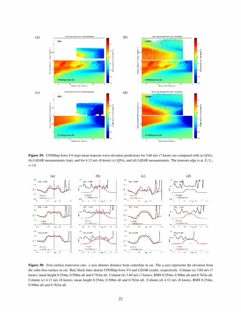
The experimentally measured mean wave elevationin Figure 29 shows good agreement between the QVizand LiDAR datasets in the small overlap region for both3.60 m/s (7 knots) and 4.12 m/s (8 knots). The datasetsshow a low wave elevation near the transom and a di-verging wave trough emerging from the transom edge.The diverging wave angle is 20.2◦ and 26◦ at 3.60 m/s (7knots) and 4.12 m/s (8 knots), respectively. A transversewave is observed between the centerline and the diverg-ing wave at both speeds, with the wave forming furtherback at a speed of 4.12 m/s (8 knots) than the 3.60 m/s (7knot) case.

CFDShip-Iowa V4 predictions are within 3-4% ofthe experimental results both near the transom and in thediverging waves trough at 3.60 m/s (7 knots) and 4.12m/s (8 knots). The diverging wave peak is predicted to be

19

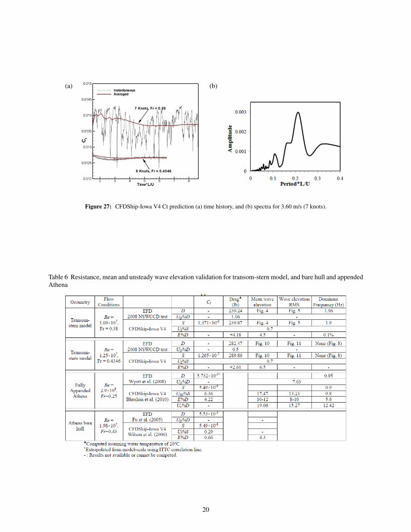
(a) (b)

Figure 27: CFDShip-Iowa V4 Ct prediction (a) time history, and (b) spectra for 3.60 m/s (7 knots).

Table 6 Resistance, mean and unsteady wave elevation validation for transom-stern model, and bare hull and appendedAthena

20

(a) (b)

(c) (d)

Figure 28: Images of the instantaneous transom wave elevation during NSWCCD testing (left panel) and CFDShip-Iowa V4 (rightpanel) for (a,b) 3.60 m/s (7 knots), Fr = 0.38, and (c,d) 4.12 m/s (8 knots), Fr = 0.43. Inset shows wave elevation at Y/Lo = 0.01colored using piezometric pressure, and wave elevation and isosurface of Q-criterion = 3000 (Hunt et al. 1988) as viewed from thebottom

outside the LiDAR’s measurement window and thus willnot be compared. The diverging wave angle is 12% and10% higher than that found during the NSWCCD testingfor 3.60 m/s (7 knots) and 4.12 m/s (8 knot), respectively.

A shoulder wave is seen in the wake elevation cross-sections for both the 3.60 m/s (7-knot) and 4.12 m/s (8-knot) cases. There are slight indications of a shoulderwave in the LiDAR results, likely due to the large RMSat those locations and the uncertainty inherent in the Li-DAR measurements (± 2.54 cm). CFDShip-Iowa V4transverse wave peak elevation predictions are within 2-4% of the experimental results for both the 3.60 m/s (7knot) and 4.12 m/s (8 knot) cases for the location clos-est to the transom. At 4.12 m/s (8 knots) the peak valuesreported by CFDShip-Iowa V4 are lower by 25% for thelocations further from the transom. For the farthest crosssection, almost uniform elevations are observed in thewake at 3.60 m/s (7 knots), which agrees within 2% ofthe experimental results.

Both LiDAR and CFDShip-Iowa V4 indicate highRMS values in the transverse wave region with a peak atthe centerline at both 3.60 m/s (7 knots) and 4.12 m/s (8knots). Values taper off outside the wake region due to

breaking as shown in Figure 30(b).

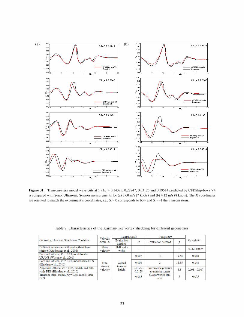
CFDShip-Iowa V4 mean wave cut predictions inFigure 31(a) compare within 4-5% of the experiments forthe first three locations at a speed of 3.60 m/s (7 knots).An averaged error of 7-9% is obtained for the farthesttransverse location. At 4.12 m/s (8 knots) the two closesttranverse wave cut locations agree within 2-4% of the ex-perimental results. For the two outer locations, the peakvalues are 20-30% lower than the experimental data. Alag is expected between the CFDShip-Iowa V4 and ex-perimental results due ot the differences in the divergingwave angles for both model speeds.

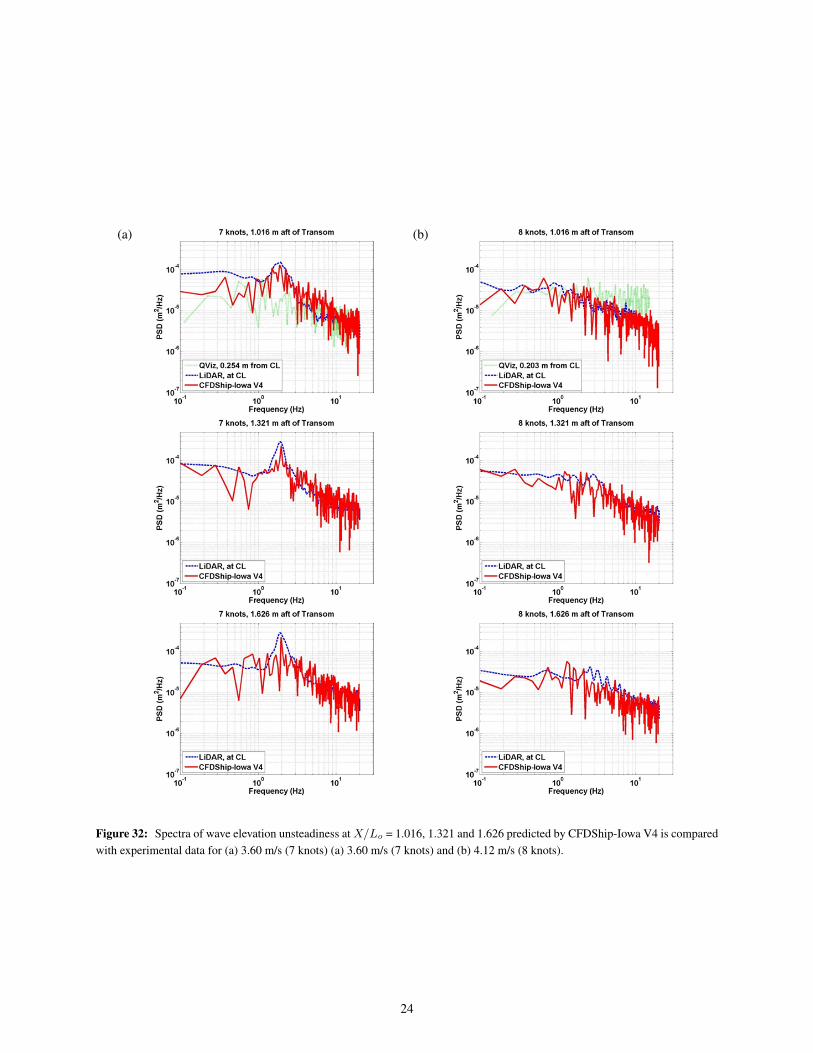
The wave elevation spectra from the LiDAR mea-surements in Figure 32(a) show a dominant frequencyof 1.96Hz at all the locations at a speed of 3.60 m/s (7knots). CFDShip-Iowa V4 predicts the dominant fre-quency within 0.1% of the experiments, but the peakamplitude is under predicted by 10%. CFDShip-IowaV4 results show large amplitude oscillations for high fre-quencies, which could be due to the iterative error in thelevel-set function. At a speed of 4.12 m/s (8 knots), theresults between CFDShip-Iowa V4 and the experimentalresults agree well. No spectral peak is seen at this speed.

21

(a) (b)

(c) (d)

Figure 29: CFDShip-Iowa V4 (top) mean transom wave elevation predictions for 3.60 m/s (7 knots) are compared with (a) QViz,(b) LiDAR measurements (top), and for 4.12 m/s (8 knots) (c) QViz, and (d) LiDAR measurements. The transom edge is at X/Lo

= 1.0.

(a) (b) (c) (d)

Figure 30: Free-surface transverse cuts. x-axis denotes distance from centerline in cm. The y-axis represents the elevation fromthe calm free-surface in cm. Red, black lines denote CFDShip-Iowa V4 and LiDAR results, respectively. Column (a) 3.60 m/s (7knots), mean height 0.254m, 0.508m aft and 0.762m aft. Column (b) 3.60 m/s (7 knots), RMS 0.254m, 0.508m aft and 0.762m aft.Column (c) 4.12 m/s (8 knots), mean height 0.254m, 0.508m aft and 0.762m aft. Column (d) 4.12 m/s (8 knots), RMS 0.254m,0.508m aft and 0.762m aft.

22

(a) (b)

Figure 31: Transom-stern model wave cuts at Y/Lo = 0.14375, 0.22847, 0.03125 and 0.39514 predicted by CFDShip-Iowa V4is compared with Senix Ultrasonic Sensors measurements for (a) 3.60 m/s (7 knots) and (b) 4.12 m/s (8 knots). The X coordinatesare oriented to match the experiment’s coordinates, i.e., X = 0 corresponds to bow and X = -1 the transom stern.

Table 7 Characteristics of the Karman-like vortex shedding for different geometries

23

(a) (b)

Figure 32: Spectra of wave elevation unsteadiness at X/Lo = 1.016, 1.321 and 1.626 predicted by CFDShip-Iowa V4 is comparedwith experimental data for (a) 3.60 m/s (7 knots) (a) 3.60 m/s (7 knots) and (b) 4.12 m/s (8 knots).

24

The flow streamlines exit parallel to the hull bottom forthis case, and vortical structures are not predicted nearthe transom region. Any remaining unsteadiness is likelydue to wave breaking.

Overall, the experimental datasets are reasonablygood for the drag, mean wave elevation and wave-cuts.RMS datasets do not show any coherent pattern, butthe spectra do show a dominant frequency at 3.60 m/s(7 knots) and the dominant frequency compares within0.1% of the experiments. CFDShip-Iowa V4 drag pre-dictions are 4.18% higher than the experimental mea-surements at 3.60 m/s (7 knots) and 2.61% higher at 4.12m/s (8 knots). CFDShip-Iowa V4 predictions show apeak in the transom wave elevation cross-section closeto the transom in the shoulder region, which was not ob-served in the LiDAR data. The mean wave elevation andwave-cut predictions are 4% higher when compared tothe experimental results at 3.60 m/s (7 knots) and 7%higher at 4.12 m/s (8 knots). The limited validation heresupports the credibility of CFDShip-Iowa V4 simulationresults.

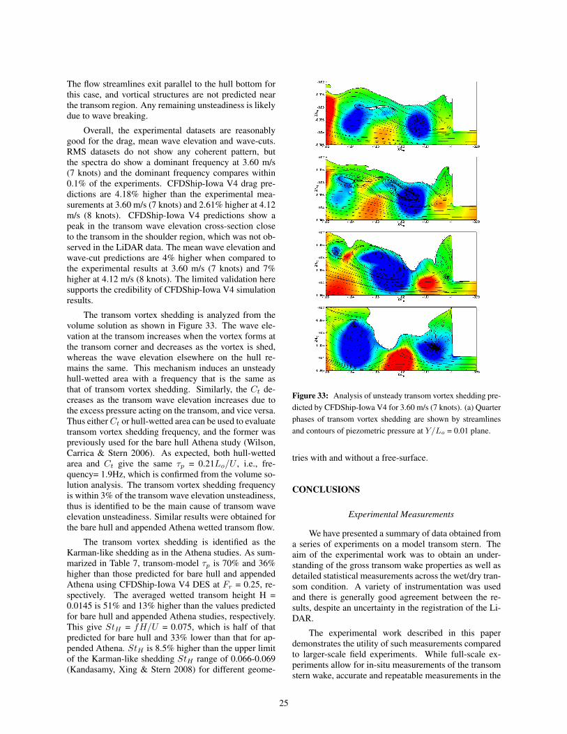
The transom vortex shedding is analyzed from thevolume solution as shown in Figure 33. The wave ele-vation at the transom increases when the vortex forms atthe transom corner and decreases as the vortex is shed,whereas the wave elevation elsewhere on the hull re-mains the same. This mechanism induces an unsteadyhull-wetted area with a frequency that is the same asthat of transom vortex shedding. Similarly, the Ct de-creases as the transom wave elevation increases due tothe excess pressure acting on the transom, and vice versa.Thus eitherCt or hull-wetted area can be used to evaluatetransom vortex shedding frequency, and the former waspreviously used for the bare hull Athena study (Wilson,Carrica & Stern 2006). As expected, both hull-wettedarea and Ct give the same τp = 0.21Lo/U , i.e., fre-quency= 1.9Hz, which is confirmed from the volume so-lution analysis. The transom vortex shedding frequencyis within 3% of the transom wave elevation unsteadiness,thus is identified to be the main cause of transom waveelevation unsteadiness. Similar results were obtained forthe bare hull and appended Athena wetted transom flow.

The transom vortex shedding is identified as theKarman-like shedding as in the Athena studies. As sum-marized in Table 7, transom-model τp is 70% and 36%higher than those predicted for bare hull and appendedAthena using CFDShip-Iowa V4 DES at Fr = 0.25, re-spectively. The averaged wetted transom height H =0.0145 is 51% and 13% higher than the values predictedfor bare hull and appended Athena studies, respectively.This give StH = fH/U = 0.075, which is half of thatpredicted for bare hull and 33% lower than that for ap-pended Athena. StH is 8.5% higher than the upper limitof the Karman-like shedding StH range of 0.066-0.069(Kandasamy, Xing & Stern 2008) for different geome-

Figure 33: Analysis of unsteady transom vortex shedding pre-dicted by CFDShip-Iowa V4 for 3.60 m/s (7 knots). (a) Quarterphases of transom vortex shedding are shown by streamlinesand contours of piezometric pressure at Y/Lo = 0.01 plane.

tries with and without a free-surface.

CONCLUSIONS

Experimental Measurements

We have presented a summary of data obtained froma series of experiments on a model transom stern. Theaim of the experimental work was to obtain an under-standing of the gross transom wake properties as well asdetailed statistical measurements across the wet/dry tran-som condition. A variety of instrumentation was usedand there is generally good agreement between the re-sults, despite an uncertainty in the registration of the Li-DAR.

The experimental work described in this paperdemonstrates the utility of such measurements comparedto larger-scale field experiments. While full-scale ex-periments allow for in-situ measurements of the transomstern wake, accurate and repeatable measurements in the

25

field are difficult to make. Laboratory experiments allowfor more detailed measurements on specific aspects ofthe flow that would not be possible in the field. The abil-ity to obtain highly repeatable wake elevation measure-ments from instruments such as the LiDAR are essentialto our understanding of the full-scale breaking transomwake as well as providing validation for numerical tools.

NFA

The agreement between NFA predictions and lab-oratory measurements is good. Since NFA uses free-slip conditions on the hull, the good agreement suggeststhat the wall boundary layer does not affect wave break-ing and air entrainment in the transom region when theReynolds number is sufficiently high. Analysis of the airentrainment suggests that the peaks that are observed inthe spectra of the free-surface elevation in the transomregion are due to the effects of a multi-phase shear layerthat forms beneath the rooster tail and continues into thestern breaking wave. In terms of processing data, oneadvantage of the numerical simulations over laboratorymeasurements is that all of the data is readily available.NFA predictions of drag, free-surface elevations, and airentrainment are all within experimental error. Withoutthe experiments, there is no basis to validate the numeri-cal simulations, and the development of computer codessuch as NFA would not be possible. NFA’s ease of use,numerical stability, rapid turn around, and high accu-racy provide a robust framework for simulating complexflows around naval combatants. Future improvements tothe NFA algorithm are only possible under the guidanceof high-fidelity laboratory and field experiments such asthose reported in this paper.

CFDShip-Iowa V4

CFDShip-Iowa V4 mean and unsteady wave eleva-tion predictions using DES are validated for a transom-stern model for 3.60 m/s (7 knots), Fr=0.38 and 4.12 m/s(8 knots), Fr=0.43. The drag predictions are within 4.2%of the experimental results for both flow conditions. Thegrids are found to be sufficiently fine to properly activateLES in the transom region as resolved turbulent kineticenergy is greater than 92% of the total. The transom flowpattern compares well with those from the experiments,i.e., a wetted transom is predicted for 3.60 m/s (7 knots)with wide wake dominated by wave breaking up to thetransom. The 4.12 m/s (8 knot) simulation predicts adry transom with well-defined narrow wake that formsa rooster tail with breaking waves.

Comparison with the experimental results are rea-sonably good for the drag, mean wave elevation, wave-cuts and FFT, but coherent patterns are not observedfor the RMS. CFDShip-Iowa V4 mean wave elevationand wave-cut predictions are within 4.5% and 6.5% of

the experimental results for the wetted and dry transomcase, respectively. The larger errors for the dry transomcase were due to the 18% under prediction of the diverg-ing wave angle. CFDShip-Iowa V4 predictions showa shoulder wave close to the transom for both speeds,which are not observed in the LiDAR wave elevationcross-sectional profiles. The transom wave elevationdominant frequency for the wetted transom is predictedwithin 0.1% of that found from the experimental work,whereas neither results predict any dominant frequencyfor the dry transom. The comparison errors are reason-able and supports the credibility of CFDShip-Iowa V4simulations.

The dominant wetted transom flow frequency is ex-plained as a Karman-like vortex shedding from the tran-som bottom corner, as the frequencies are within 3%.The Karman-like shedding Strouhal number, St= 0.075,is 33% lower than that for appended Athena and 8.5%higher than the upper limit of the Karman-like sheddingrange based on the Strouhal number, St= 0.066-0.069.

ACKNOWLEDGEMENTS

The Office of Naval Research supports this researchunder multiple Office of Naval Research contract ve-hicles as directed by Dr. L. Patrick Purtell (ONRCode 331), program manager. The authors would liketo acknowledge the efforts of Susan Brewton, Con-nor Bruns, Michael Capitain, Lisa Minnick, Toby Rat-cliffe, James Rice, Lauren Russell, and Don Walkerfrom NSWCCD - Code 50, the NSWCCD Media Lab,Eric Terrill and Genivieve Lada from the Scrips Insti-tute of Oceanography, UCSD, and David Jeon, Dae-gyoum Kim and Mory Gharib from the California In-stitute of Technology. The support of the Data Anal-ysis and Assessment Center (DAAC) is gratefully ac-knowledged. DAAC members include Dr. MichaelStephens, Randall Hand, Paul Adams, Miguel Valen-ciano, Kevin George, Tom Biddlecome, and RichardWalters. Animations of NFA simulations are available athttp://www.youtube.com/waveanimations. Science Ap-plications International Corporation IR&D supported re-cent upgrades to the NFA algorithm. NFA predictions aresupported in part by a grant of computer time from theDepartment of Defense High Performance ComputingModernization Program (http://www.hpcmo.hpc.mil/).NFA simulations have been performed on the SGI AltixICE at the U.S. Army Engineering Research and Devel-opment Center (ERDC).

References

Beale, K., Fu, T., Wyatt, D., & Walker, D., “Free surfacemeasurements of breaking waves using Quantitative

26

Visualization (QViz),” Proceedings of the 29th AmericanTowing Tank Conference, Annapolis, Maryland, 2010.

Bhushan, S., Xing, T., Carrica, P., & Stern, F., “Model andfull-scale URANS/DES simulations for R/V Athenaresistance, powering and motions,” Proceedings of the9th International Conference on Numerical ShipHydrodynamics, Ann Arbor, Michigan, 2007.

Bhushan, S., Xing, T., & Stern, F., “Vortical structures andinstability analysis for Athena wetted transom flow withfull-scale validation,” J. Fluid Eng., in preparation forpublication.

Brucker, K. A., O’Shea, T. T., Dommermuth, D. G., & Adams,P., “Numerical simulations of breaking waves – weakspilling to strong plunging,” Proceedings of the 28thSymposium on Naval Hydrodynamics, Pasadena,California, USA, 2010, to appear.

Carrica, P., Wilson, R., & Stern, F., “An unsteady single-phaseLevel Set method for viscous free surface flows,” Int. J.Numer. Meth. Fluids, Vol. 53 (2), 2007, pp. 229–256.

Dommermuth, D. G., O’Shea, T. T., Wyatt, D. C., Ratcliffe, T.,Weymouth, G. D., Hendrikson, K. L., Yue, D. K.,Sussman, M., Adams, P., & Valenciano, M., “Anapplication of Cartesian-grid and volume-of-fluidmethods to numerical ship hydrodynamics,” Proceedingsof the 9th International Conference on Numerical ShipHydrodynamics, Ann Arbor, Michigan, 2007.

Dommermuth, D. G., O’Shea, T. T., Wyatt, D. C., Sussman, M.,Weymouth, G. D., Yue, D. K., Adams, P., & Hand, R.,“The numerical simulation of ship waves usingCartesian-grid and volume-of-fluid methods,”Proceedings of the 26th Symposium on NavalHydrodynamics, Rome, Italy, 2006.

Fu, T., Fullerton, A., & Drazen, D., “Free-surfacemeasurements in a tow tank using LiDAR,” ASME 2009Fluids Engineering summer meeting (FEDSM2009)forum on fluid measurements and instrumentation, Vol.FEDSM2009-78464, Vail, Colorado, 2009a.

Fu, T., Fullerton, A., Drazen, D., Minnick, L., Walker, D.,Ratcliffe, T., Russell, L., & Capitain, M., A DetailedStudy of Transom Breaking waves: Part II, TechnicalReport NSWCCD-50-TR-2010/003, Naval SurfaceWarfare Center, Carderock, 2010.

Fu, T., Fullerton, A., Ratcliffe, T., Minnick, L., Walker, D.,Pence, M., & Anderson, K., A Detailed Study ofTransom Breaking Waves, Technical ReportNSWCCD-50-TR-2009/025, Naval Surface WarfareCenter, Carderock, 2009b.

Fu, T., Fullerton, A., Terrill, E., & Lada, G., “Measurements ofthe wave field around the R/V Athena I,” Proceedings ofthe 26th Symposium on Naval Hydrodynamics, Rome,

Italy, 2006a.

Fu, T., Rice, J., Terrill, E., Walker, D., & Lada, G.,“Measurement and characterization of full-scale shipwaves,” Ships and Ship Systems (S3) Tech. Symposium,Carderock, MD, USA, 2006b.

Fullerton, A. & Fu, T., “Acoustic doppler current profiler (adcp)measurements of breaking waves,” ASME 2008 FluidsEngineering summer meeting (FEDSM2008) forum onfluid measurements and instrumentation, Vol.FEDSM2008-55313, Jacksonville, FL, 2003.

Furey, D. & Fu, T., “Quantitative Visualization (QViz)Hydrodynamic measurement technique of multiphaseunsteady surfaces,” Proceedings of the 24th Symposiumon Naval Hydrodynamics, Fukuoka, Japan, 2002.

Hunt, J., Wray, A., & Moin, P., Eddies, stream, and convergencezones in turbulent flows, Technical Report CTR-S88,Center for Turbulence Research, 1988.

Jeon, D., Pereira, F., & Gharib, M., “Applications of defocusingDPIV to bubbly flow measurement,” Particle & ParticleSys. Char., Vol. 20, no. 3, 2003, pp. 193–198.

Kandasamy, M., Xing, T., & Stern, F., “Unsteady free-surfacewave-induced separation: vortical structures andinstabilities,” J. Fluids and Structures, Vol. 25(2), 2008,pp. 343–363.

Karion, A., Waniewski-Sur, T., Fu, T., Furey, D., Rice, J., &Walker, D., “Experimental study of the bow wave of alarge towed wedge,” Proceedings of the 8th InternationalConference on Numerical Ship Hydrodynamics, Busan,Korea, 2003.

Maki, K., Doctors, L., & Beck, R., “On the profile of the flowbehind a transom stern,” 9th Int. Conf. on Num. ShipHydrodynamics, Ann Arbor, Michigan, 2007.

O’Shea, T. T., Brucker, K. A., Dommermuth, D. G., & Wyatt,D. C., “A numerical formulation for simulatingfree-surface hydrodynamics,” Proceedings of the 27thSymposium on Naval Hydrodynamics, Seoul, Korea,2008.

Pereira, F., Gharib, M., Dabiri, D., & Modarress, D.,“Defocusing DPIV: A 3-component 3-D DPIVmeasurement technique,” Exp. Fluids [Suppl. S], Vol. 29,2000, pp. S78–S84.

Rice, J., Walker, D., Fu, T., Karion, A., & Ratcliffe, T.,“Quantitative characterization of the free-surface aroundsurface ships,” Proceedings of the 25th Symposium onNaval Hydrodynamics, St. John’s, Newfoundland andLabrador, Canada, 2004.

Rodrıguez-Rodrıguez, J., Marugan-Cruz, C., Aliseda, A., &Lasheras, J., “Dynamics of large turbulent structures in ahydrualic jump,” J. Fluid Mech., submitted.

Rottman, J. W., Brucker, K. A., Dommermuth, D. G., &

27

Broutman, D., “Parameterization of the internal-wavefield generated by a submarine and its turbulent wake ina uniformly stratified fluid,” Proceedings of the 28thSymposium on Naval Hydrodynamics, Pasadena,California, USA, 2010, to appear.

Waniewski, T., Air entrainment by bow waves, Ph.D. thesis,California Institute of Technology, 1999.

Wehausen, J., “Effect of the initial acceleration upon the waveresistance of ship models,” J. Ship Research, Vol. 7(3),1964, pp. 38–50.

Wilson, R., Carrica, P., & Stern, F., “URANS simulation for ahigh-speed transom-stern ship with breaking waves,” Int.J. CFD, Vol. 20(2), 2006, pp. 105–125.

Wyatt, D., Fu, T., Taylor, G., Terrill, E., Xing, T., Bhushan, S.,O’Shea, T., & Dommermuth, D., “Comparison offull-scale experimental measurements and computationalpredictions of the transom-stern wave of the R/V AthenaI,” Proceedings of the 27th Symposium on NavalHydrodynamics, Seoul, Korea, 2008.

28