Experimental Implementation of Iterative Learning Control for Processeswith Stochastic Disturbances

Zhonglun Cai, Douglas A. Bristow, Eric Rogers and Chris T. Freeman

Abstract— A number of iterative learning control algorithmshave been developed in a stochastic setting in recent years.The results currently available are in the form of algorithmderivation and the derivation of fundamental systems theoreticproperties. This paper gives the results of an optimal iteration-varying stochastic ILC algorithm on a gantry robot system,which confirm that this algorithm is capable of delivering goodperformance in the experimental domain and can outperforma heuristic filter in the later learning stage when noise startsto dominate the signal.

I. INTRODUCTION

Iterative learning control (ILC) is a technique for con-trolling systems operating in a repetitive, or trial-to-trial,mode with the requirement that a reference trajectory r(t)defined over a finite interval 0 ≤ t ≤ T , where T denotesthe trial length, is followed to a high precision. Examples ofsuch systems include robotic manipulators that are requiredto repeat a given task to high precision, chemical batchprocesses or, more generally, the class of tracking systems.

Since the original work [1], the general area of ILChas been the subject of intense research effort. An initialsource for the literature here are the survey papers [2], [3].Application areas include robotics, automated manufacturingplants and food processing.

A standard assumption in much of the current ILC lit-erature is that the input signals are free of noise, althoughin many physical implementations measurement signals aresubject to random noise and the system may be affected byrandom disturbances. A number of specialized algorithmshave been developed for systems with stochastic distur-bances [4], [5], [6]. The learning algorithms developed in thisprevious work provide asymptotic noise and non-repeatingdisturbance insensitivity but use a trial-varying, also termediteration-varying, learning filter. This is in contrast to themany cases where iteration-invariant filters are employed.

Recent work [7] has developed algorithms for iteration-invariant learning filters for mixed deterministic and stochas-tic disturbances for single-input single-output (SISO) sys-tems with linear time-invariant dynamics, but as yet therehas been no experimental verification. This paper givessubstantial new results in this area which is an essential pre-cursor to industrial take-up.

Zhonglun Cai, Eric Rogers and Chris T. Freeman are with School ofElectronics and Computer Science, University of Southampton, Southamp-ton, SO17 1BJ, UK zc@ecs.soton.ac.uk, Douglas Bristow is withDepartment of Mechanical and Aerospace Engineering, Missouri Universityof Science and Technology, Rolla, MO dbristow@mst.edu

II. BACKGROUND

The work in [7] is frequency domain based and it isassumed that the plant dynamics are modeled in discrete-time by

ek(t) =−G(z)uk(t)+d(t)+wk(t) (1)

where t = 0,1, · · · is the time index, k = 0,1, · · · is theiteration index, z is the forward time-shift operator zx(t) =x(t + 1), z−1 is the backward time-shift operator u is thecontrol input, e is the error, d is a deterministic signal, w isa stationary random disturbance, and G is a stable system.Moreover, d(t) captures iteration-invariant disturbances [8]and initial conditions [9].

Consider also the application of a standard first orderiteration-varying ILC law of the form

uk+1(t) = Q(z)[uk(t)+L(z)ek(t)] (2)

where ek(t) is the noise corrupted error measurement mod-eled as

ek(t) = ek(t)+ vk(t) (3)

and vk(t) is stationary random noise. Figure 1 showshow the learning update loop, learning filter Lk(z) androbust filter Q(z) are combined to form the overall con-trol scheme, with the following assumptions: i) u0(t) =0, ii) |d(t)| < M, iii) E[w j1(t1),w j2(t2)] = 0, for allj1, j2, t1, t2, iv) E[w j1(t1),w j2(t2)] = 0, E[v j1(t1),v j2(t2)] = 0,E[w j1(t1),d(t2)] = 0, E[v j1(t1),d(t2)] = 0, for all j1 6= j2 andall t1, t2, and v) G(z) is a rational function with relativedegree 0. If the relative degree is greater than zero then theanalysis is easily modified as detailed in Section II of [7].Finally, the spectrum of a signal, say r(γ), as

Φr(ω) =∞

∑−∞

Rr(τ)e−ıωτ

where Rr(τ) is the autocorrelation function.

G(z)

L(z)Q(z)

…

d(t) wk(t)

ek(t)

uk+1(t)

uk(t)

vk(t)

- + ++

+

+ILC Alrgorithm

yk(t)

Fig. 1. Diagram of the ILC control structure

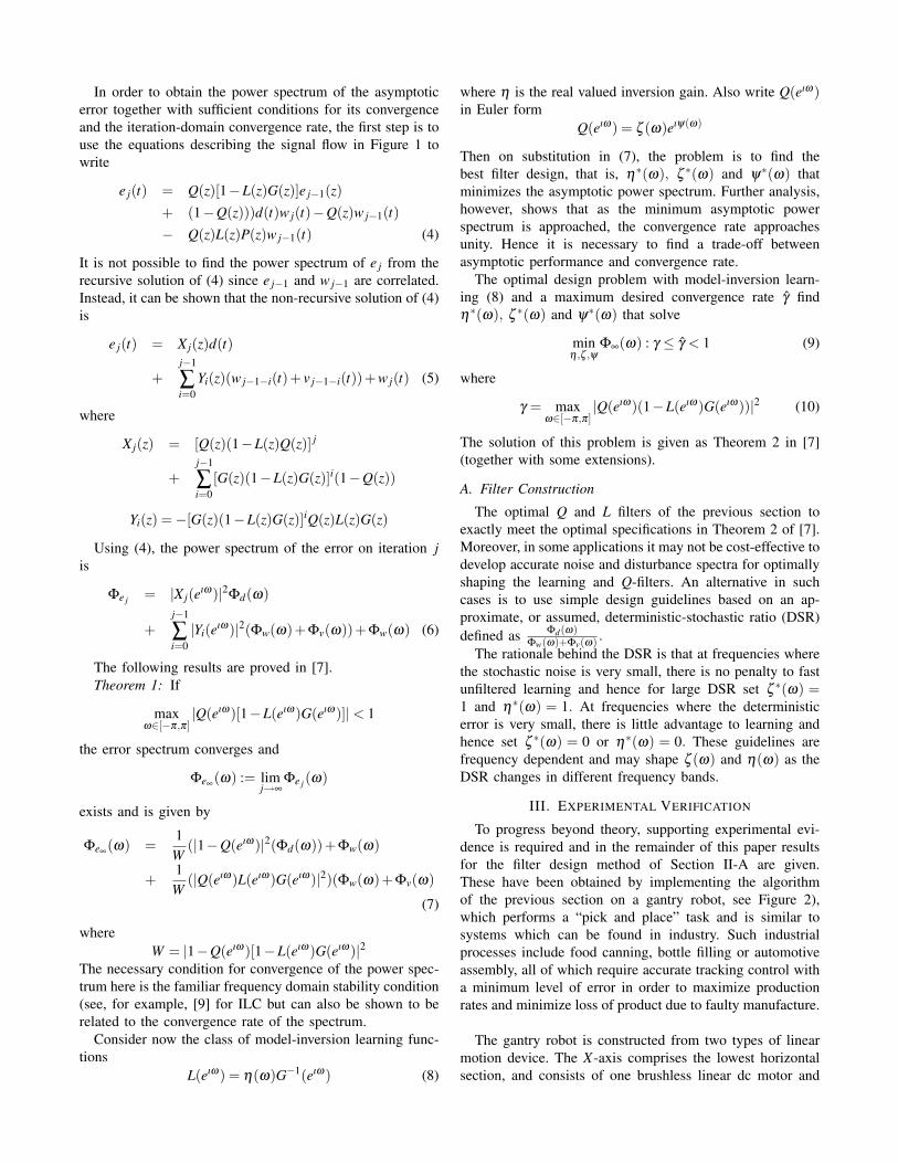
In order to obtain the power spectrum of the asymptoticerror together with sufficient conditions for its convergenceand the iteration-domain convergence rate, the first step is touse the equations describing the signal flow in Figure 1 towrite

e j(t) = Q(z)[1−L(z)G(z)]e j−1(z)+ (1−Q(z)))d(t)w j(t)−Q(z)w j−1(t)− Q(z)L(z)P(z)w j−1(t) (4)

It is not possible to find the power spectrum of e j from therecursive solution of (4) since e j−1 and w j−1 are correlated.Instead, it can be shown that the non-recursive solution of (4)is

e j(t) = X j(z)d(t)

+j−1

∑i=0

Yi(z)(w j−1−i(t)+ v j−1−i(t))+w j(t) (5)

where

X j(z) = [Q(z)(1−L(z)Q(z)] j

+j−1

∑i=0

[G(z)(1−L(z)G(z)]i(1−Q(z))

Yi(z) =−[G(z)(1−L(z)G(z)]iQ(z)L(z)G(z)

Using (4), the power spectrum of the error on iteration jis

Φe j = |X j(eıω)|2Φd(ω)

+j−1

∑i=0|Yi(eıω)|2(Φw(ω)+Φv(ω))+Φw(ω) (6)

The following results are proved in [7].Theorem 1: If

maxω∈[−π,π]

|Q(eıω)[1−L(eıω)G(eıω)]|< 1

the error spectrum converges and

Φe∞(ω) := lim

j→∞Φe j(ω)

exists and is given by

Φe∞(ω) =

1W

(|1−Q(eıω)|2(Φd(ω))+Φw(ω)

+1

W(|Q(eıω)L(eıω)G(eıω)|2)(Φw(ω)+Φv(ω)

(7)

whereW = |1−Q(eıω)[1−L(eıω)G(eıω)|2

The necessary condition for convergence of the power spec-trum here is the familiar frequency domain stability condition(see, for example, [9] for ILC but can also be shown to berelated to the convergence rate of the spectrum.

Consider now the class of model-inversion learning func-tions

L(eıω) = η(ω)G−1(eıω) (8)

where η is the real valued inversion gain. Also write Q(eıω)in Euler form

Q(eıω) = ζ (ω)eıψ(ω)

Then on substitution in (7), the problem is to find thebest filter design, that is, η∗(ω), ζ ∗(ω) and ψ∗(ω) thatminimizes the asymptotic power spectrum. Further analysis,however, shows that as the minimum asymptotic powerspectrum is approached, the convergence rate approachesunity. Hence it is necessary to find a trade-off betweenasymptotic performance and convergence rate.

The optimal design problem with model-inversion learn-ing (8) and a maximum desired convergence rate γ findη∗(ω), ζ ∗(ω) and ψ∗(ω) that solve

minη ,ζ ,ψ

Φ∞(ω) : γ ≤ γ < 1 (9)

where

γ = maxω∈[−π,π]

|Q(eıω)(1−L(eıω)G(eıω))|2 (10)

The solution of this problem is given as Theorem 2 in [7](together with some extensions).

A. Filter Construction

The optimal Q and L filters of the previous section toexactly meet the optimal specifications in Theorem 2 of [7].Moreover, in some applications it may not be cost-effective todevelop accurate noise and disturbance spectra for optimallyshaping the learning and Q-filters. An alternative in suchcases is to use simple design guidelines based on an ap-proximate, or assumed, deterministic-stochastic ratio (DSR)defined as Φd(ω)

Φw(ω)+Φv(ω) .The rationale behind the DSR is that at frequencies where

the stochastic noise is very small, there is no penalty to fastunfiltered learning and hence for large DSR set ζ ∗(ω) =1 and η∗(ω) = 1. At frequencies where the deterministicerror is very small, there is little advantage to learning andhence set ζ ∗(ω) = 0 or η∗(ω) = 0. These guidelines arefrequency dependent and may shape ζ (ω) and η(ω) as theDSR changes in different frequency bands.

III. EXPERIMENTAL VERIFICATION

To progress beyond theory, supporting experimental evi-dence is required and in the remainder of this paper resultsfor the filter design method of Section II-A are given.These have been obtained by implementing the algorithmof the previous section on a gantry robot, see Figure 2),which performs a “pick and place” task and is similar tosystems which can be found in industry. Such industrialprocesses include food canning, bottle filling or automotiveassembly, all of which require accurate tracking control witha minimum level of error in order to maximize productionrates and minimize loss of product due to faulty manufacture.

The gantry robot is constructed from two types of linearmotion device. The X-axis comprises the lowest horizontalsection, and consists of one brushless linear dc motor and

Fig. 2. The multi-axes gantry robot.

a parallel free running slide. The Y -axis lies directly abovethis, is perpendicular to the X-axis, and has one end attachedto the linear motor and the other end to the slide. The Y -axis comprises a single brushless linear dc motor. The Xand Y -axes are 1.02m and 0.91m long respectively. Finally,the vertical Z-axis comprises a short 0.10m travel linearball-screw stage driven by a rotary brushless dc motor. Allaxes are powered by matched brushless motor dc amplifiersand axis motion is detected and recorded with appropriateoptical encoder systems. Each axis has been modeled usingthe velocity control mode of operation, in which the amplifierreceives the encoder data as well as the computer, thereforeproviding an inner closed loop and an integrating action tothe system. The axes dynamics have been determined byperforming a series of open loop frequency response tests.

10−1

100

101

102

103

−80

−60

−40

−20

Mag

nitu

de (

dB)

X−axis Frequency Response

10−1

100

101

102

103

−180

−135

−90

Frequency (rad/s)

Pha

se (

degr

ee)

Experiment 1

Experiment 2

Fitted model

Fig. 3. X-axis Bode gain plot.

From the resulting measurements, linear approximations ofthe transfer function for each axis were determined andthen refined using a non-linear optimization technique. The

frequency response obtained for the X-axis is shown inFigure 3 (the responses of the other axes are similar).

The X-axis dynamics are approximated by the 7th ordertransfer-function

GX (z) =0.00051745(z+0.5823)(z−0.3014)(z−1)(z2−0.07057z+0.009459)

(z2−0.09718z+0.008969)(z2−0.2046z+0.7846)(z2 +0.3149z+0.1024)(z2−0.7757z+0.5403)

(11)

where G−1(z) will be implemented using the matrix Gdefined using the Markov parameters as

G =

CB 0 0 · · · 0

CAB CB 0 · · · 0CA2B CAB CB · · · 0

......

.... . .

...CAN−1B CAN−2B · · · · · · CB

(12)

The required state-space model for the X-axis is

Ax =

2.41 −0.86 0.85 −0.59 0.30 −0.19 0.324.00 0 0 0 0 0 0

0 1.00 0 0 0 0 00 0 1.00 0 0 0 00 0 0 1.00 0 0 00 0 0 0 0.50 0 00 0 0 0 0 0.25 0

Bx = [ 0.0313 0 0 0 0 0 0 ]T

Cx = [ 0.0095 −0.0023 0.0048 −0.0027 0.0029

−0.0011 0.0029 ]

The trial duration for the “pick and place” operation is 2seconds, which is equivalent to 30 units per minute (UPM).Figure 4 shows the reference trajectory. The stoppage timebetween each trial is to compute the control vector for thesubsequent trial. The gantry axes are homed to a predefinedpoint before each iteration begins with an accuracy of ±30microns in order to minimize the effects of initial state error.A sampling time of Ts = 0.01s has been used in all tests. Hereonly X-axis has been used for initial investigation, for whichthe reference trajectory is given in Figure 5. This facility hasbeen widely used to test other (deterministic) ILC controlalgorithms, see, for example, [10], [11].

To obtain the disturbance model from the experiment rig,a number of zero input signals have been fed into the systemand the output and error signals are measured. When inputapplied to(1) is zero, ek(t) = d(t)+wk(t) and when a numberof zero input signals are used

N

∑k=1

ek(t) =N

∑k=1

d(t)+N

∑k=1

wk(t)

where N→ ∞, ∑Nk=1 wk(t) = 0, and hence

N

∑k=1

ek(t)≈ Nd(t)

d(t)≈ 1N

N

∑k=1

ek(t) (13)

00.05

0.10.15

0.2

0

0.01

0.02

0.03

0.04

0

0.002

0.004

0.006

0.008

0.01

y−axis (m)

Reference trajectory

x−axis (m)

z−ax

is (

m)

pick

place

Fig. 4. 3D Reference Trajectory.

0 20 40 60 80 100 120 140 160 180 2000

0.005

0.01

0.015

0.02

0.025

0.03

0.035

0.04

Sample Number

Dis

plac

emen

t (m

)

Fig. 5. X-axis component of the 3D Reference Trajectory.

Hence on each iteration

wk(t)≈ ek(t)−d(t); (14)

and the spectra can be computed using

Φw(ω)≈ 1N

N

∑k=1|FFT[wk(t)]|2 (15)

Hence a transfer function, or even a constant for simplicity,can be fitted to Φd(ω) and Φw(ω). Also in implementationthe random noise term Φv(ω) can be assumed to be zero ora very small constant offset.

Figure 6 gives the Bode gain plots of Φd(ω) and Φw(ω)obtained by application of the procedure described above.The filters that approximate the optimal η∗ and ψ∗ musthave zero-phase and this is emulated here by applying theMATLAB filtfilt technique) to a fourth order low-pass filterto form the iteration-varying optimal filter

H(z) =0.0002+0.0007z−1 +0.0011z−2

1−3.5328z−1 +4.7819z−2 · · ·

+0.0007z−3 +0.0002z−4

−2.9328z−3 +0.6868z−4 (16)

Figure 7 shows the Bode gain plots for the learning filterson trial 0 (the initial filter), 5,10,15 and 20 respectively. Theheuristic filter [12]:

Lk(z) =1

k +1·G−1(z) (17)

101

102

−800

−700

−600

−500

−400

−300

−200

−100

Frequency (1/samples)

Mag

nitu

de (

dB)

Φ

w(ω)

Φd(ω)

Fig. 6. DSR and the deterministic and stochastic spectra.

−80

−60

−40

−20

0

20

Mag

nitu

de (d

B)

102

Iteration−varying optimal filter

Frequency (rad/sec)

Iteration 0Iteration 5Iteration 10Iteration 15Iteration 20

Fig. 7. Frequency responses of optimal filters for iterations 0, 5, 10, 15and 20.

has similar gain at low frequency but at higher frequencythe optimal filters can minimize the effect of amplifying thenoise.

A. Experimental Results

Experiments have been carried out on the gantry robotusing both the optimal and heuristic filters. In the first setof tests, the ILC algorithms were applied directly to therobot and in a further set they were applied to the closed-loop system resulting from application of a Proportional-plusIntegral plus Derivative (PID) controller, as often arises insome applications, that is, the need to pre-stabilize the plantmodel or deal with undesired along the iteration dynamics.Figure 8 shows the mean squared error of both optimaland heuristic filters for the first set of experiments. As theiteration number increases, the tracking error is reduced andthe noise starts to dominate the signal, and the performanceof optimal filters is better. Figure 9 gives the results whenthe PID controller is used, In this case the noise starts todominate from the very early stage of learning progress andthe iteration-varying optimal filters again clearly outperform

Fig. 10. The overall learning process

Fig. 11. The overall learning process with PID controller

the heuristic filter. Figures 10 and 11 show the input, output

0 20 40 60 80 100 120 140 160 180 20010−1

100

101

102

103

Iteration

Mea

n S

quar

ed E

rror

(mm

2 )

Optimal filterHeuristic filter

Fig. 8. Mean squared error plots without PID controller.

and error signals for each set for the filters designed in thispaper and confirm that excellent performance is achieved.

0 2 4 6 8 10 12 14 16 18 2010−3

10−2

10−1

100

101

102

Iteration

Mea

n S

quar

ed E

rror

(mm

2 )

Optimal FilterHeuristic Filter

Fig. 9. Mean squared error plots with PID controller.

IV. CONCLUSIONS

An ILC algorithm for systems with stochastic disturbanceshas been implemented on a multi-axis gantry robot and theperformance assessed. The performance of the ILC controller

has been examined for the cases when a pre-conditioningPID feedback controller has been applied and when thisis excluded and the ILC applied directly to the robot. Inboth cases, the performance obtained with the filters of thispaper outperform heuristic filters previously proposed in theliterature.

These results are for one case only but provide evidenceto support further development of the filters consideredin [7]. In due course it will also be necessary to compareperformance against other model based stochastic based ILCalgorithms. Aspects of this wide problem area are currentlyunder investigation.

REFERENCES

[1] S. Arimoto, S. Kawamura, and F. Miyazaki, “Bettering operations ofrobots by learning,” Journal of Robotic Systems, vol. 1, pp. 123–140,1984.

[2] D. A. Bristow, M. Tharayil, and A. G. Alleyne, “A survey of iter-ative learning control a learning-based method for high-performancetracking control,” IEEE Control Systems Magazine, vol. 26, no. 3, pp.96–114, 2006.

[3] H.-S. Ahn, Y. Chen, and K. L. Moore, “Iterative learning control: briefsurvey and categorization 1998–2004,” IEEE Transactions on SystemsMan and Cybernetics Part C, vol. 37, no. 6, pp. 1099–1121, November2007.

[4] S. S. Saab, “A discrete-time stochastic learning control algorithm,”IEEE Transactions On Automatic Control, vol. 46, no. 6, pp. 877–887, June 2001.

[5] ——, “Stochastic P-type/D-type iterative learning control algorithms,”International Journal of Control, vol. 76, no. 2, pp. 139–148, 2003.

[6] ——, “Optimal selection of the forgetting matrix into an iterativelearning control algorithm,” IEEE Transactions On Automatic Control,vol. 50, no. 12, pp. 2039–2043, December 2005.

[7] D. A. Bristow, “Optimal iteraton-varying iterative learning control forsystems with stochastic disturbances,” in Proceedings of the AmericanControl Conference, Baltimore, MD, USA, June 2010, pp. 1296–1301.

[8] M. Norrlof and S. Gunnarsson, “Time and frequency domain conver-gence properties in iterative learning control,” International Journalof Control, vol. 75, no. 14, pp. 1114–1126, 2002.

[9] R. W. Longman, “Iterative learning control and repetitive control forengineering practice,” International Journal of Control, vol. 73, pp.930–954, 2000.

[10] J. D. Ratcliffe, P. L. Lewin, E. Rogers, J. J. Hatonen, and D. H. Owens,“Norm-optimal iterative learning control applied to gantry robots forautomation applications,” IEEE Transactions On Robotics, vol. 22,no. 6, pp. 1303–1307, December 2006.

[11] L. Hladowski, Z. Cai, K. Galkowski, E. Rogers, C. T. Freeman,and P. L. Lewin, “Using 2D systems theory to design output signalbased iterative learning control laws with experimental verification,”in Proceddings of 47th IEEE Conference on Decision and Control,Cancun, Mexico, December 2008, pp. 3026–3031.

[12] M. Butcher, A. Karimi, and R. Longchamp, “A statistical analysis ofcertain iterative learning control algorithms,” International Journal ofControl, vol. 81, no. 1, pp. 156–166, 2008.