Experimental Design for Parameter Estimation of GeneRegulatory NetworksBernhard Steiert1,2,3*., Andreas Raue1,2., Jens Timmer1,2,3,4,5, Clemens Kreutz1,2.

1 Institute for Physics, University of Freiburg, Freiburg, Germany, 2 Freiburg Center for Systems Biology, University of Freiburg, Freiburg, Germany, 3 Freiburg Institute for

Advanced Studies, University of Freiburg, Freiburg, Germany, 4 BIOSS Centre for Biological Signalling Studies, University of Freiburg, Freiburg, Germany, 5 Department of

Clinical and Experimental Medicine, Linkoping University, Linkoping, Sweden

Abstract

Systems biology aims for building quantitative models to address unresolved issues in molecular biology. In order todescribe the behavior of biological cells adequately, gene regulatory networks (GRNs) are intensively investigated. As thevalidity of models built for GRNs depends crucially on the kinetic rates, various methods have been developed to estimatethese parameters from experimental data. For this purpose, it is favorable to choose the experimental conditions yieldingmaximal information. However, existing experimental design principles often rely on unfulfilled mathematical assumptionsor become computationally demanding with growing model complexity. To solve this problem, we combined advancedmethods for parameter and uncertainty estimation with experimental design considerations. As a showcase, we optimizedthree simulated GRNs in one of the challenges from the Dialogue for Reverse Engineering Assessment and Methods(DREAM). This article presents our approach, which was awarded the best performing procedure at the DREAM6 Estimation ofModel Parameters challenge. For fast and reliable parameter estimation, local deterministic optimization of the likelihoodwas applied. We analyzed identifiability and precision of the estimates by calculating the profile likelihood. Furthermore, theprofiles provided a way to uncover a selection of most informative experiments, from which the optimal one was chosenusing additional criteria at every step of the design process. In conclusion, we provide a strategy for optimal experimentaldesign and show its successful application on three highly nonlinear dynamic models. Although presented in the context ofthe GRNs to be inferred for the DREAM6 challenge, the approach is generic and applicable to most types of quantitativemodels in systems biology and other disciplines.

Citation: Steiert B, Raue A, Timmer J, Kreutz C (2012) Experimental Design for Parameter Estimation of Gene Regulatory Networks. PLoS ONE 7(7): e40052.doi:10.1371/journal.pone.0040052

Editor: Avi Ma’ayan, Mount Sinai School of Medicine, United States of America

Received February 8, 2012; Accepted May 30, 2012; Published July 16, 2012

Copyright: � 2012 Steiert et al. This is an open-access article distributed under the terms of the Creative Commons Attribution License, which permitsunrestricted use, distribution, and reproduction in any medium, provided the original author and source are credited.

Funding: The authors acknowledge financial support by the grants [0315766-VirtualLiver] (http://www.virtual-liver.de/) and [0313921-FRISYS] (http://www.frisys.biologie.uni-freiburg.de/) provided by the German Federal Ministry of Education and Research, as well as the FP7 EU project CancerSys [HEALTH-F4-2008-223188](http://www.ifado.de/cancersys/index.html). The funders had no role in study design, data collection and analysis, decision to publish, or preparation of themanuscript.

Competing Interests: The authors have declared that no competing interests exist.

* E-mail: bernhard.steiert@frias.uni-freiburg.de

. These authors contributed equally to this work.

Introduction

In a deterministic framework, the kinetics of gene regulatory

networks (GRNs) can be described by ordinary differential

equations (ODEs). The kinetic constants as well as the initial

concentrations are usually unknown and have to be estimated

from experiments. Furthermore, precise predictions of the systems’

behavior under perturbed conditions confirm the model reliability.

To identify informative measurements out of all feasible experi-

ments, parameter estimation and experimental design have to be

applied iteratively to calibrate the model efficiently [1]. In this

article, we present our methods and results that received the best

performer award at the DREAM6 Estimation of Model Parameters

challenge [2,3]. The main aspects are the calculation of maximum

likelihood estimates for parameters, determining confidence

intervals by exploiting the profile likelihood [4], and performing

experimental design to reduce the leading uncertainties of

parameters and predictions.

Methods

Problem DefinitionFinding the most informative experimental conditions is a

highly nontrivial process. In general, it has to be decided at which

time points the measurements are performed, what quantities are

observed, and under which perturbations the data are obtained.

The first step is to define an objective function specifying the

purpose of the experimental design, e.g. the expected accuracy of

estimated parameters and/or the expected accuracy of predictions

of the model. Once this goal is fixed, different experimental

designs can be scored.

In the DREAM6 Estimation of Model Parameters challenge, the

goal was to perform experimental design considerations for

spending a virtual budget to estimate parameters of the gene

regulatory networks and to be able to extrapolate the systems

aJTM behavior, i.e. to predict the dynamics under a perturbed

condition. The model parameters of three GRNs (M1, M2 and

PLoS ONE | www.plosone.org 1 July 2012 | Volume 7 | Issue 7 | e40052

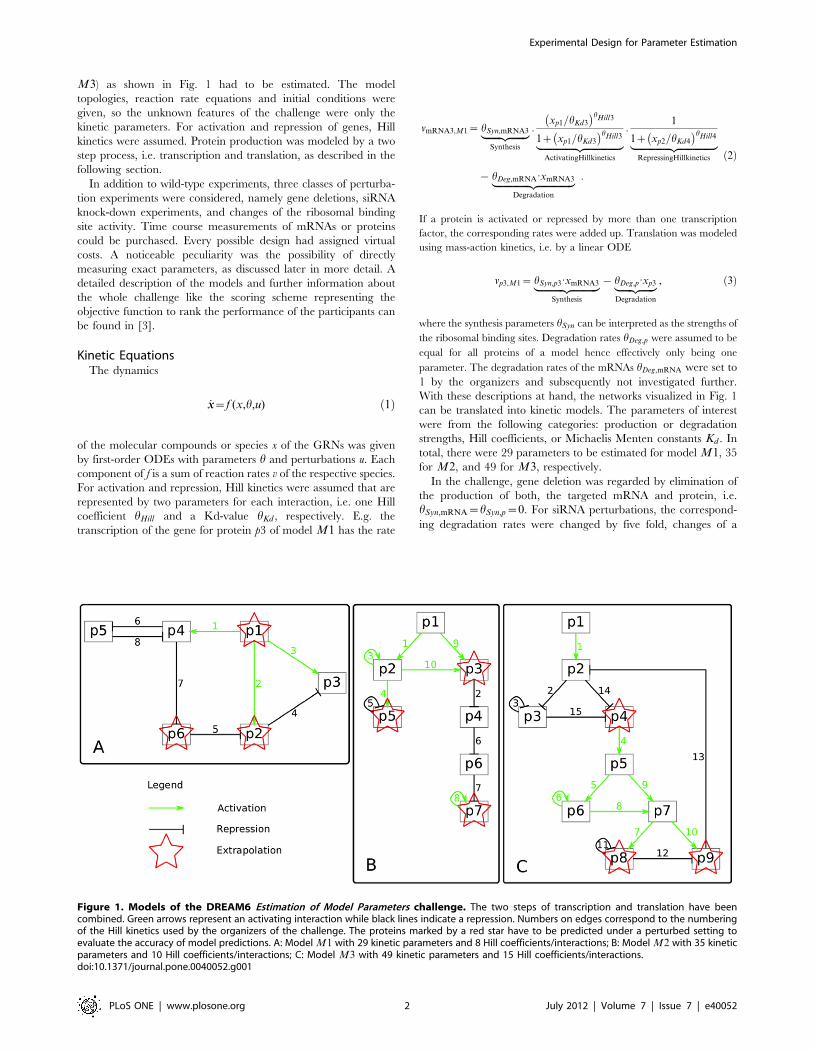
M3) as shown in Fig. 1 had to be estimated. The model

topologies, reaction rate equations and initial conditions were

given, so the unknown features of the challenge were only the

kinetic parameters. For activation and repression of genes, Hill

kinetics were assumed. Protein production was modeled by a two

step process, i.e. transcription and translation, as described in the

following section.

In addition to wild-type experiments, three classes of perturba-

tion experiments were considered, namely gene deletions, siRNA

knock-down experiments, and changes of the ribosomal binding

site activity. Time course measurements of mRNAs or proteins

could be purchased. Every possible design had assigned virtual

costs. A noticeable peculiarity was the possibility of directly

measuring exact parameters, as discussed later in more detail. A

detailed description of the models and further information about

the whole challenge like the scoring scheme representing the

objective function to rank the performance of the participants can

be found in [3].

Kinetic EquationsThe dynamics

_xx~f (x,h,u) ð1Þ

of the molecular compounds or species x of the GRNs was given

by first-order ODEs with parameters h and perturbations u. Each

component of f is a sum of reaction rates v of the respective species.

For activation and repression, Hill kinetics were assumed that are

represented by two parameters for each interaction, i.e. one Hill

coefficient hHill and a Kd-value hKd , respectively. E.g. the

transcription of the gene for protein p3 of model M1 has the rate

vmRNA3,M1~ hSyn,mRNA3|fflfflfflfflfflfflffl{zfflfflfflfflfflfflffl}Synthesis

:xp1=hKd3

� �hHill3

1z xp1=hKd3

� �hHill3|fflfflfflfflfflfflfflfflfflfflfflfflfflfflffl{zfflfflfflfflfflfflfflfflfflfflfflfflfflfflffl}ActivatingHillkinetics

:1

1z xp2=hKd4

� �hHill4|fflfflfflfflfflfflfflfflfflfflfflfflfflfflffl{zfflfflfflfflfflfflfflfflfflfflfflfflfflfflffl}RepressingHillkinetics

{ hDeg,mRNA:xmRNA3|fflfflfflfflfflfflfflfflfflfflfflfflfflfflffl{zfflfflfflfflfflfflfflfflfflfflfflfflfflfflffl}

Degradation

:

ð2Þ

If a protein is activated or repressed by more than one transcription

factor, the corresponding rates were added up. Translation was modeled

using mass-action kinetics, i.e. by a linear ODE

vp3,M1~ hSyn,p3:xmRNA3|fflfflfflfflfflfflfflfflfflfflffl{zfflfflfflfflfflfflfflfflfflfflffl}

Synthesis

{ hDeg,p:xp3|fflfflfflfflfflffl{zfflfflfflfflfflffl}

Degradation

, ð3Þ

where the synthesis parameters hSyn can be interpreted as the strengths of

the ribosomal binding sites. Degradation rates hDeg,p were assumed to be

equal for all proteins of a model hence effectively only being one

parameter. The degradation rates of the mRNAs hDeg,mRNA were set to

1 by the organizers and subsequently not investigated further.

With these descriptions at hand, the networks visualized in Fig. 1

can be translated into kinetic models. The parameters of interest

were from the following categories: production or degradation

strengths, Hill coefficients, or Michaelis Menten constants Kd . In

total, there were 29 parameters to be estimated for model M1, 35

for M2, and 49 for M3, respectively.

In the challenge, gene deletion was regarded by elimination of

the production of both, the targeted mRNA and protein, i.e.

hSyn,mRNA~hSyn,p~0. For siRNA perturbations, the correspond-

ing degradation rates were changed by five fold, changes of a

Figure 1. Models of the DREAM6 Estimation of Model Parameters challenge. The two steps of transcription and translation have beencombined. Green arrows represent an activating interaction while black lines indicate a repression. Numbers on edges correspond to the numberingof the Hill kinetics used by the organizers of the challenge. The proteins marked by a red star have to be predicted under a perturbed setting toevaluate the accuracy of model predictions. A: Model M1 with 29 kinetic parameters and 8 Hill coefficients/interactions; B: Model M2 with 35 kineticparameters and 10 Hill coefficients/interactions; C: Model M3 with 49 kinetic parameters and 15 Hill coefficients/interactions.doi:10.1371/journal.pone.0040052.g001

Experimental Design for Parameter Estimation

PLoS ONE | www.plosone.org 2 July 2012 | Volume 7 | Issue 7 | e40052

ribosomal binding site activity was incorporated by increasing

hSyn,p by a factor of two.

Parameter EstimationThe parameters h, i.e. the kinetic rates, have been estimated by

maximum likelihood. The likelihood

L(yjh)~Pi,j

r(yi(tj)jh) ð4Þ

is the joint probability of independently distributed measurements

y of compound i at time point tj with each data-point distributed

according to r. Each measurement is simulated using the error

model

y~ max½0,xzeabszerel(x)� , ð5Þ

where the absolute error eabs*N(0,s2abs) and the relative error

erel(x)*N(0,srel(x)2) are Gaussian random variables with stan-

dard deviations sabs~0:1 and srel(x)~0:2:x. This error model

represented by the parameters sabs and 0.2 in the formula for

srel(x) was provided by the organizers at the time the challenge

was initiated.

The following considerations were done by the authors. In

general, a sum etotal~eabszerel of two independent Gaussian

random variables eabs and erel is again normally distributed

etotal*N(0,s2total) with variance

s2total(x)~s2

abszs2rel(x) : ð6Þ

Therefore, the likelihood if no clipping of negative values to zero

is present is

L(yjh)~Pi,j

1ffiffiffiffiffiffi2pp

stotal

e{

yi (tj ){xi (tj ,h)� �2

2 s2total ð7Þ

with stotal~stotal(xi(tj ,h)).

According to (5), negative data realizations were clipped to zero

which was accounted for in the likelihood by

Lcut(yjh)~ Pi,jjyijw0

r(yij jh) : Pi,jjyij:0

ð0

{?

1ffiffiffiffiffiffi2pp

stotal

e{

yij0{xij

� �2

2 s2total dyij

0 : ð8Þ

where r(yij Dh) denotes the contribution of a single data point to the

likelihood according to (7). The integral corresponds to the probability of

negative data realizations for given xij(h).

Due to the effort that would have been needed to incorporate (8)

into our existing fast C-algorithm of the optimization routine, we

used (7) in the experimental design stage and implemented (8) in a

more flexible MATLAB-code only for the final parameter

estimation step, i.e. after the whole budget was spent. The

likelihood (8) is correct for the challenge, as it is in accordance with

the error model (5) that was used for the simulation of

measurements. However, for real biological data, other error

models are usually more appropriate which is briefly explained in

the discussion. For numerical reasons, the likelihood was log-

transformed and the log-likelihood is denoted as LL in the

following. Since the DREAM6 scoring metric penalizes the

deviation of the estimated parameters hh from the underlying

truth, confidence intervals of the estimates were calculated to

Figure 2. Experimental design procedure based on profile likelihood. The left panel shows the profile likelihood of a practically non-identifiable parameter. To resolve the corresponding uncertainty of the parameter estimate, a set of parameter vectors along its profile is chosen,represented by the dashes on the x-axis. The parameters are subsequently modified according to two designs, a highly informative experiment in theupper branch and a weakly informative experiment in the lower branch. Model predictions are simulated for the chosen parameter vectors,represented by the time courses in the middle column. A wide spread of the simulated time courses indicates an informative experiment. The impactof data purchasing is shown in the most right subplots by the blue curves, where the acquisition of informative data narrows the parameter down toa small variance, in contrast to a poor experiment with nearly no improvement of the estimate.doi:10.1371/journal.pone.0040052.g002

(8)

Experimental Design for Parameter Estimation

PLoS ONE | www.plosone.org 3 July 2012 | Volume 7 | Issue 7 | e40052

assess the accuracy of our estimates. For this purpose, the profile

likelihood

PL(hi)~ maxhj=i

LL(yDh) ð9Þ

for a parameter hi given the data y is utilized [4]. In (9), the

optimization is performed for all parameters except hi. Confidence

intervals for the estimation of a single parameter are then given by

CIa(hi Dy)~ hi D {2PL(hi)ƒ {2LL(y)�zicdf (x21,�a)|fflfflfflfflfflfflfflfflfflfflfflfflfflfflfflfflfflfflfflffl{zfflfflfflfflfflfflfflfflfflfflfflfflfflfflfflfflfflfflfflffl}

~:D

8<:

9=; : ð10Þ

Here, a is the confidence level and icdf (x21,a) denotes the a

quantile of the chi-square distribution with one degree of freedom

which is given by the respective inverse cumulative density

function. LL� is the maximum of the log-likelihood function after

all parameters are optimized. Every point on a profile PL(hi)represents a corresponding parameter vector

hh(hi)~ argmaxhj=i

LL(yDh) , ð11Þ

containing the subsequently optimized remaining parameters. The

profile likelihoods of all parameters imply a set

Htotal~[

i

hh(hi)Dhi[CIa(hi Dy)n o

ð12Þ

of parameter vectors along all profiles and below the threshold D,

which are used for experimental planning. To identify experi-

mental conditions, i.e. perturbations, for which the parameter

uncertainties propagate into discriminable time-courses, a repre-

sentative finite subset H5Htotal was chosen and the trajectories

were simulated for every parameter vector h[H. The perturba-

tions were accounted for by adapting the respective parameter

components of h[H appropriately. A wide spread of the resulting

trajectories indicated an informative experiment, promising a

reduction of the uncertainty of the parameter values [5]. To

measure the spread of the predictions, we calculated the rank

R(D)~X

k

maxtj

maxi

xk(tj Dhh(hi)){ mini

xk(tj Dhh(hi))

sk(tj Dhh(hi))ð13Þ

of potential designs D, comprising measurements of species fxkgat finite time points ftjg given by the experimental time resolution.

Further possibilities for assessing the spread of predictions are

given for example by the estimation of the variance on each time

point or by substituting the maximization over time points by a

summation in formula (13). However, other possible metrics to

measure the spread yielded comparable results. The investigated

ODE system yields non-linear solutions with respect to the

parameters in general. Experimental design iteratively restricts the

parameter space that is in agreement with the data. In an

‘asymptotic setting’, data quality and amount is sufficient to

change the likelihood shape into a multivariate normal distribu-

tion. This is equivalent to the observation, that the trajectories

fxi(tj)g in LL have an almost linear dependency with respect to

the parameters, yielding quadratic shaped LL and PL. The

solution of the non-linear ODE system is therefore behaving

locally linear in the parameter region where it is in statistical

agreement with the data. Then, uncertainty can be translated in

terms of standard errors or Fisher information. However, in non-

asymptotic settings the non-linearity requires numerical heuristics

for propagating uncertainties of parameter estimates to predic-

tions.

The discussed experimental design procedure is visualized in

Fig. 2. Here, the profile in the leftmost panel represents a practical

non-identifiability, as its upper boundary is only given by the

border of the parameter space. Two designs are evaluated by

applying a perturbation, visualized in the upper and lower

branches. To predict whether experiments are informative for

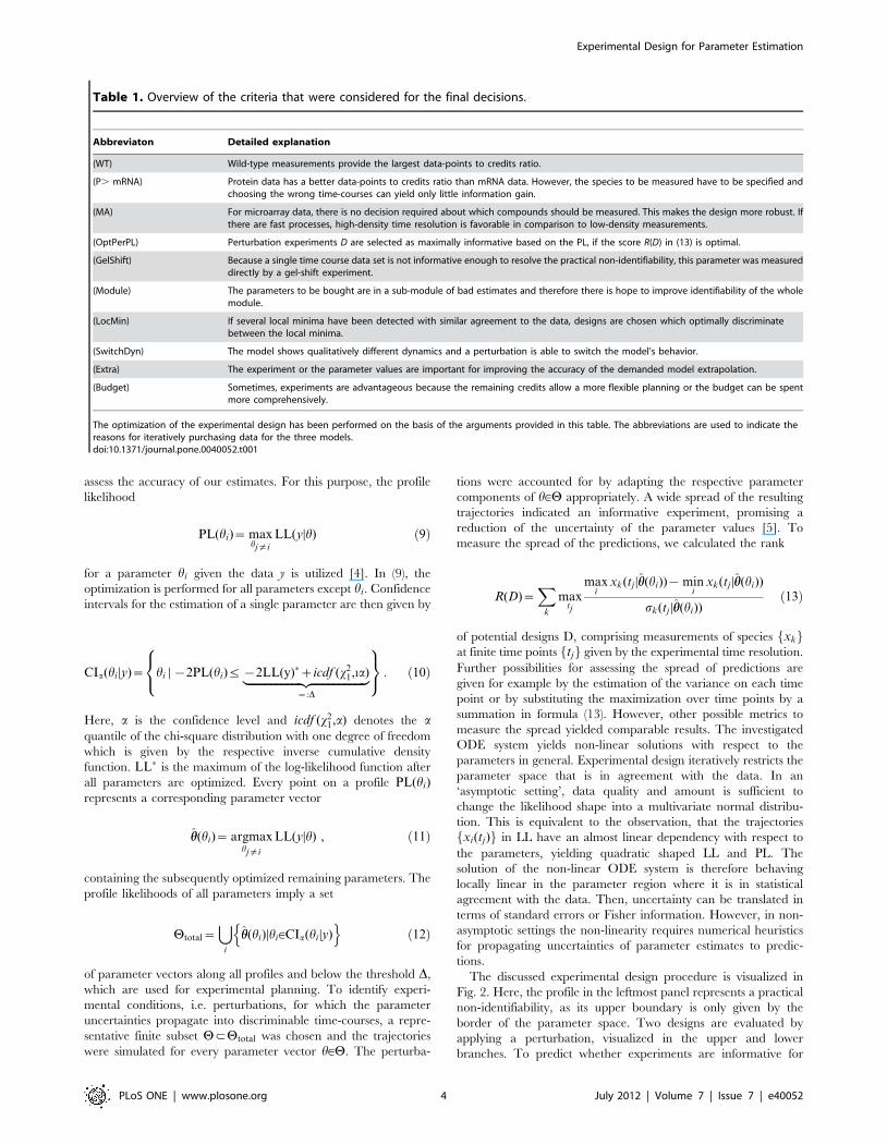
Table 1. Overview of the criteria that were considered for the final decisions.

Abbreviaton Detailed explanation

(WT) Wild-type measurements provide the largest data-points to credits ratio.

(P. mRNA) Protein data has a better data-points to credits ratio than mRNA data. However, the species to be measured have to be specified andchoosing the wrong time-courses can yield only little information gain.

(MA) For microarray data, there is no decision required about which compounds should be measured. This makes the design more robust. Ifthere are fast processes, high-density time resolution is favorable in comparison to low-density measurements.

(OptPerPL) Perturbation experiments D are selected as maximally informative based on the PL, if the score R(D) in (13) is optimal.

(GelShift) Because a single time course data set is not informative enough to resolve the practical non-identifiability, this parameter was measureddirectly by a gel-shift experiment.

(Module) The parameters to be bought are in a sub-module of bad estimates and therefore there is hope to improve identifiability of the wholemodule.

(LocMin) If several local minima have been detected with similar agreement to the data, designs are chosen which optimally discriminatebetween the local minima.

(SwitchDyn) The model shows qualitatively different dynamics and a perturbation is able to switch the model’s behavior.

(Extra) The experiment or the parameter values are important for improving the accuracy of the demanded model extrapolation.

(Budget) Sometimes, experiments are advantageous because the remaining credits allow a more flexible planning or the budget can be spentmore comprehensively.

The optimization of the experimental design has been performed on the basis of the arguments provided in this table. The abbreviations are used to indicate thereasons for iteratively purchasing data for the three models.doi:10.1371/journal.pone.0040052.t001

Experimental Design for Parameter Estimation

PLoS ONE | www.plosone.org 4 July 2012 | Volume 7 | Issue 7 | e40052

identifying parameters, time courses are simulated for specific

species under the given condition. An informative experiment

results in a wide spread of predictions and the underlying sampling

of PL(hi) can be discriminated by acquiring the corresponding

data, as can be seen in the upper branch of Fig. 2. In contrast, a

weakly informative experiment is not able to resolve the non-

identifiability, as shown in the lower branch. Here, the profile is

still unrestricted to higher values and the uncertainty of the

estimate remains large.

The scoring metric to evaluate the performance of the

participating groups at the DREAM6 Estimation of Model Parameters

challenge consisted of two parts. The first was measuring the

deviation of the estimated parameters from the underlying truth

and the corresponding formula will be introduced in (14). The

approach that was explained above and visualized in Fig. 2

optimized the expectation of this part of the score. The second

part of the scoring metric penalized the deviation of extrapolated

trajectories under certain given perturbations that were not

accessible by experiments. In an analogous manner to the

discussed selection of experiments, the influence of parameter

uncertainties on the extrapolations has been studied by simulating

the dynamics under the given prediction setting separately for each

parameter along a finite subset of its profile, which yielded a set of

extrapolations. Large variances of these predictions indicated

parameter uncertainties with large impact on the desired

extrapolations. Accordingly, the uncertainties of those parameters

were analyzed with higher priority as discussed, i.e. finding the

perturbations that maximized the spread of the experimental

outcomes. In case of several experiments with similar perfor-

mance, additional criteria were utilized which are discussed later.

OptimizationFor numerical optimization of the log-likelihood, the trust-

region method [6] implemented in the MATLAB function

LSQNONLIN was applied. The ODE system was solved by the

CVODES algorithm [7]. For efficiency, local gradient and

curvature information was considered. The calculation of deriv-

atives of the LL with respect to the parameters is performed using

the chain rule of differentiation. The sensitivitiesLx

Lhemerge as

inner derivatives. For ODE systems, finite differences are not

appropriate to approximate sensitivities [8]. Therefore, gradients

are calculated from first order sensitivities obtained by integrating

the sensitivity equations simultaneously to the ODEs for the

dynamic variables [9]. We discovered numerical issues in solving

the ODEs and sensitivity equations for model M3 for initial

conditions equals to zero and therefore we set the initial values of

these compounds to 10{16.

To ensure that optimization yields global minima, multiple fits

with latin hypercube sampling [10] of the initial guesses of the

parameters have been performed. This means, that for Nlhs

samples, the domain of each parameter component is subdivided

into Nlhs equally-sized intervals on the logarithmic scale. The

vector samples are drawn so that each interval for each component

is chosen exactly once. Within the intervals, the parameter

components are drawn uniformly distributed. This procedure

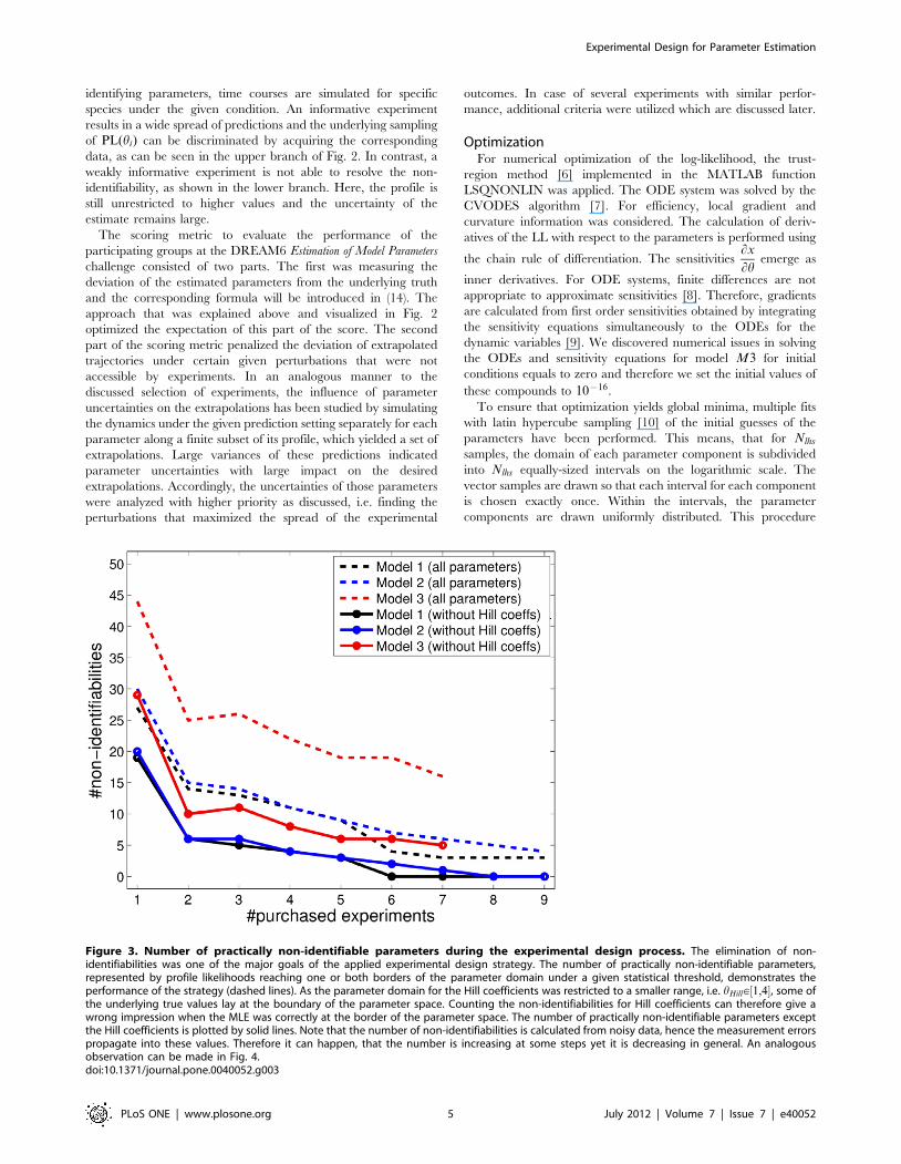
Figure 3. Number of practically non-identifiable parameters during the experimental design process. The elimination of non-identifiabilities was one of the major goals of the applied experimental design strategy. The number of practically non-identifiable parameters,represented by profile likelihoods reaching one or both borders of the parameter domain under a given statistical threshold, demonstrates theperformance of the strategy (dashed lines). As the parameter domain for the Hill coefficients was restricted to a smaller range, i.e. hHill[½1,4�, some ofthe underlying true values lay at the boundary of the parameter space. Counting the non-identifiabilities for Hill coefficients can therefore give awrong impression when the MLE was correctly at the border of the parameter space. The number of practically non-identifiable parameters exceptthe Hill coefficients is plotted by solid lines. Note that the number of non-identifiabilities is calculated from noisy data, hence the measurement errorspropagate into these values. Therefore it can happen, that the number is increasing at some steps yet it is decreasing in general. An analogousobservation can be made in Fig. 4.doi:10.1371/journal.pone.0040052.g003

Experimental Design for Parameter Estimation

PLoS ONE | www.plosone.org 5 July 2012 | Volume 7 | Issue 7 | e40052

prevents the randomly drawn initial guesses to be accidentally

close to each other.

To decide whether several local minima sufficiently agree with

the data, we used a threshold given by the log-likelihood of the best

fit plus the 95%-quantile of the x2-distribution with degrees of

freedom equal to the number of parameters. This corresponds to a

threshold utilized to calculate joint confidence intervals for all

parameters. At the beginning of the experimental design process

for all three models, we found roughly half of 1000 initial

parameter combinations converging into the same optimum. The

others either did not converge, since the initial values were in a

region of the parameter space where the integrator failed to reach

the demanded accuracy, or the optimizer converged in another

local optimum. These needed to be discriminated during the

design process. In the final stage of the experimental design setup,

there was no second optimum below the statistical threshold, i.e.

all further local optima yielded a highly improbable value of the

objective function. This demonstrates that deterministic optimi-

zation combined with randomization of the initial values yields a

good performance for global optimization in this application.

Final DecisionsIf the profile likelihood approach did not yield unambiguous

suggestions, further criteria were taken into account for the final

selection of each data acquisition. Table 1 provides a summary of

such aspects.

Wild-type (WT) measurements for the mRNAs were provided

in the start-up dataset, that was received by all participants. In

general, WT data provided a quite large number of data points for

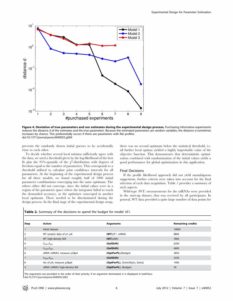
Figure 4. Deviation of true parameters and our estimates during the experimental design process. Purchasing informative experimentsreduces the distance d of the estimates and the true parameters. Because the estimated parameters are random variables, the distance d sometimesincreases by chance. This preferentially occurs if there are parameters with flat profiles.doi:10.1371/journal.pone.0040052.g004

Table 2. Summary of the decisions to spend the budget for model M1.

Step Action Arguments Remaining credits

1 Initial dataset 10000

2 WT protein data of p1–p6 (WT),(P. mRNA) 8800

3 WT high-density MA (WT),(MA) 7800

4 hHill1,hKd1 (GelShift) 6200

5 hHill3,hKd3 (GelShift) 4600

6 siRNA mRNA5, measure p2&p4 (OptPerPL),(Budget) 3850

7 hHill2,hKd2 (GelShift) 2250

8 rbs of p4, measure p2&p6 (OptPerPL), (SwitchDyn), (Extra) 1400

9 siRNA mRNA5 high-density MA (OptPerPL), (Budget) 50

The arguments are provided in the order of their priority. If an argument dominated, it is displayed in bold-face.doi:10.1371/journal.pone.0040052.t002

Experimental Design for Parameter Estimation

PLoS ONE | www.plosone.org 6 July 2012 | Volume 7 | Issue 7 | e40052

less credits. Since it is advantageous to have measurements for all

dynamic variables, we purchased WT measurements for all

proteins as an initial step. This reduced non-identifiability issues

and provided a minimal amount of information about the

parameters allowing more detailed experimental design consider-

ations.

The measurement of two proteins provided 80 data points for

400 credits, a high-density microarray experiments charged 1000

credits and yielded 20:nmRNA data points, i.e. 120, 140, and 180

for the three models. The ratio of the number of data points per

credits was 0.2 for proteins and f0:12,0:14,0:18g for RNA/

microarray data for models M1, M2, and M3. However, the

larger the models, the more informative are microarray experi-

ments in comparison to the information provided by the

measurement of two proteins. Moreover, there is no decision

required about which compounds should be measured. This

makes the design more robust. If there are fast processes, high-

density time resolution is favorable in comparison to low-density

measurements.

To identify informative perturbation experiments, an objective

function that ranks the information gain has to be introduced and

to be maximized. We directly used the score (13) as objective

function. At some steps, we performed a Monte-Carlo evaluation

of a perturbation to confirm our guess. Practically non-identifiable

parameters hHill and hKd could also be measured directly by gel-

shift experiments in contrast to the estimation from time-course

data.

If considered parameters were in a sub-module of bad estimates,

there was hope to improve identifiability of the whole module.

Moreover, if several local minima were detected with similar

agreement to the data, designs were chosen which optimally

discriminate between the local minima. On the other hand, if the

model showed qualitatively different dynamics, a perturbation is

potentially able to switch the model’s behavior. For instance,

oscillations can be diminished by influencing a negative feedback.

For improving the accuracy of the demanded model extrapola-

tions, the parameters influencing these predictions at most were

calculated along the profiles and scored using (13). The

uncertainty of the parameters that propagate into the extrapola-

tions were then reduced in the discussed manner, as visualized in

Fig. 2.

Sometimes, experiments were advantageous because the

remaining credits allowed a more flexible planning or the budget

could be spent in a way that enabled the authors to understand the

model more comprehensively. E.g. siRNA experiments were the

cheapest perturbations and provided often qualitatively the same

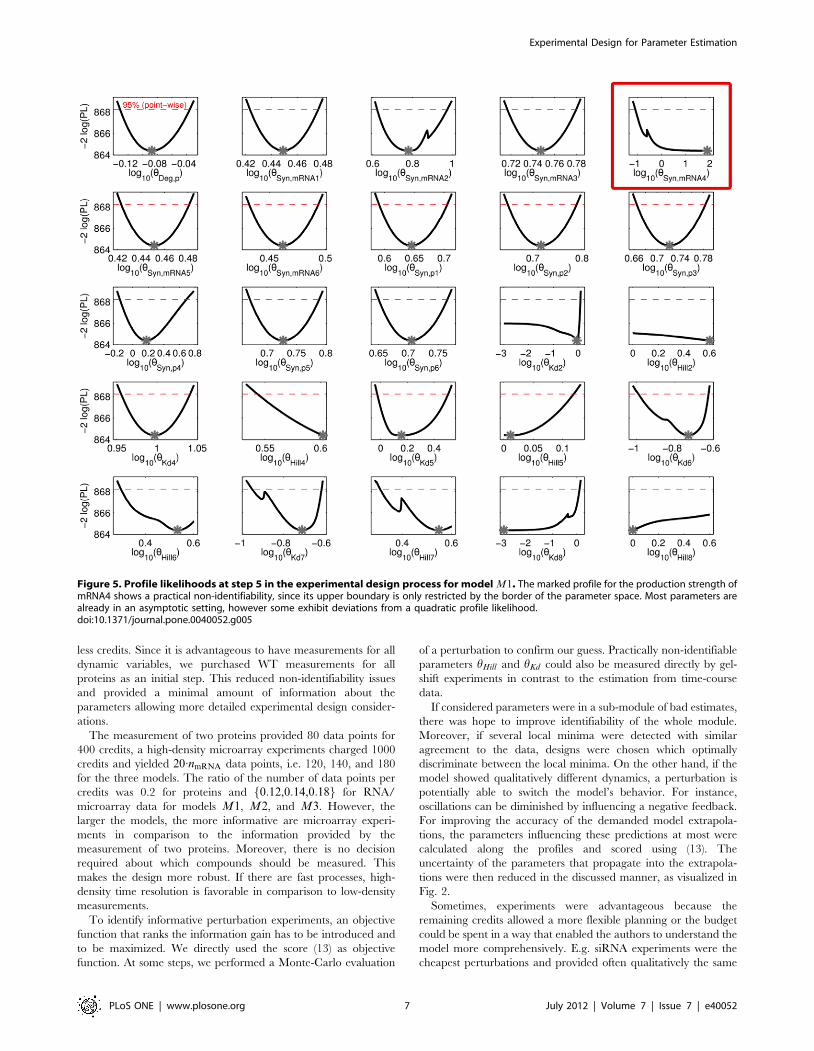
Figure 5. Profile likelihoods at step 5 in the experimental design process for model M1. The marked profile for the production strength ofmRNA4 shows a practical non-identifiability, since its upper boundary is only restricted by the border of the parameter space. Most parameters arealready in an asymptotic setting, however some exhibit deviations from a quadratic profile likelihood.doi:10.1371/journal.pone.0040052.g005

Experimental Design for Parameter Estimation

PLoS ONE | www.plosone.org 7 July 2012 | Volume 7 | Issue 7 | e40052

information as a knockout. The saved credits could therefore be

used to purchase further experiments under additional informative

perturbations. For an objective argumentation, the cost of

experiments could also be integrated (besides the score) to the

objective function. As the cheapest perturbation experiment data-

set charged 750 of the 10 k credits available for each model, we

were also trying to optimize the eventually remaining credits to a

low value. In practice, we tried to choose the experiments such

that after the complete design process there were at most 200

credits left.

Results

To account for strictly positive parameter values, all analyses

have been performed in a logarithmic parameter space. Moreover,

this accounts for the fact that changes of parameter values usually

contribute multiplicatively rather than additively, i.e. changing a

parameter by a factor a or 1/a has a similar impact, but adding a

constant a has mostly a qualitatively different effect than the

corresponding subtraction.

In our initial analyses, we restricted the parameter space to

h[½10{5,105�. After some steps, we reduced this domain for

numerical reasons, as most estimates were in agreement with

hHill[½1,10� for the Hill coefficients and h=[Hill[½10{2,102� for the

other parameters. However, this restriction was weakened again

because the parameter estimation yielded values at the boundary

of the parameter space and the profile likelihood indicated minima

outside the parameter domain. For the final analyses, we used a

continuous parameter domain of [1,4] for Hill coefficients and

½10{3,102� for other parameters. We were able to constrain the

range for Hill coefficients more than for other parameters, which

was first motivated from directly measured parameters by the gel-

shift experiments. Additionally, the profiles supported this

restriction, as they were either flat or in agreement with the

interval [1,4] for Hill coefficients.

The number of kinetic parameters were {29,35,49} for the

three models. Keeping in mind the size of the parameter space,

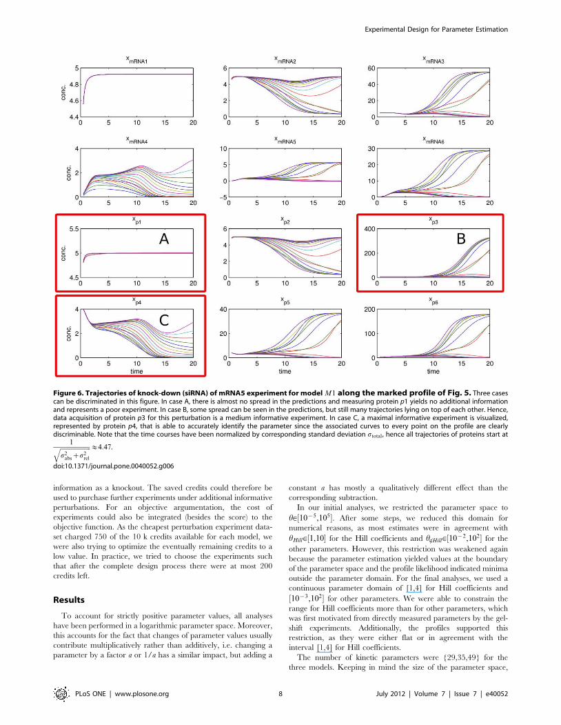
Figure 6. Trajectories of knock-down (siRNA) of mRNA5 experiment for model M1 along the marked profile of Fig. 5. Three casescan be discriminated in this figure. In case A, there is almost no spread in the predictions and measuring protein p1 yields no additional informationand represents a poor experiment. In case B, some spread can be seen in the predictions, but still many trajectories lying on top of each other. Hence,data acquisition of protein p3 for this perturbation is a medium informative experiment. In case C, a maximal informative experiment is visualized,represented by protein p4, that is able to accurately identify the parameter since the associated curves to every point on the profile are clearlydiscriminable. Note that the time courses have been normalized by corresponding standard deviation stotal, hence all trajectories of proteins start at

1ffiffiffiffiffiffiffiffiffiffiffiffiffiffiffiffiffiffiffiffis2

abszs2rel

q &4:47.

doi:10.1371/journal.pone.0040052.g006

Experimental Design for Parameter Estimation

PLoS ONE | www.plosone.org 8 July 2012 | Volume 7 | Issue 7 | e40052

comprising roughly 5 orders of magnitude for each parameter, our

final estimates were very close to the underlying truth that was

provided by the organizers after the challenge: After the

experimental design process, the mean deviation of the estimated

parameters to the true values was 1.7% for M1, 5.2% for M2, and

27.2% for M3.

Successive Refinement of ScoresDuring the iterative experimental design process, we minimized

the uncertainties of parameter estimates and model extrapolations.

Non- or poorly identifiable parameters were tracked down to an

asymptotic setting indicated by an almost quadratic profile

likelihood. This is crucial, since not only the score of the final

parameters and predictions could be optimized, but also the

corresponding uncertainty. A non-identifiable parameter can be

represented by a profile hitting one or both boundaries of the

parameter space beneath the statistical threshold. As the major

goal of the experimental design process is the estimation of model

parameters and therefore the elimination of non-identifiabilities,

the number of non-identifiable parameters demonstrates the

performance of the applied strategy. This is shown in Fig. 3 by

the dashed lines. The boundaries of the Hill coefficients were more

restricted than for the other parameters, as discussed earlier. In

this case, the underlying truth may equal a value at the boundary,

hence creating a minimum of the corresponding profile at the

border that represents an artificial non-identifiability. By neglect-

ing the Hill coefficients, this number can be corrected, as

visualized by the solid lines in Fig. 3. Our experimental design

approach iteratively decreased the number of non-identifiabilities.

An alternative indication of the performance is given by the sum

of the distances

d~1

Nh

XNh

i

loghtrue

i

hhi

� �� 2

ð14Þ

of the maximum likelihood estimate (MLE) hh to the underlying

parameters htrue, as can be seen in Fig. 4. The MLE can by chance

be near the truth at an earlier stage of the design process, while still

having large confidence intervals. The distance therefore does not

have to be monotonously decreasing. In a real world application,

this distance is not accessible in contrast to the shape of the profiles

yielding a conclusion about the number of non-identifiabilities, as

given in Fig. 3. Evaluating those distances is one of the advantages

of simulated data, as given in the DREAM6 challenge.

An overview on the steps leading to our result on model M1 can

be found in Table 2. To demonstrate the application of profile

likelihoods on experimental design, one of the steps that were

performed is discussed in detail here. Featuring many aspects of

the experimental planning process, we chose step 5 to be

examined.

As can be seen from the profiles in Fig. 5, the major non-

identifiabilities represented by flat profiles have already been

resolved. Nearly quadratic shaped profiles indicate the system to

be in an almost asymptotic setting. However, e.g. the production

strength of the mRNA4 showed a practical non-identifiability with

a CI of approximately 3 orders of magnitude within the

boundaries of the parameter space. The experimental design

strategy based on profiles is demonstrated, using parameter sets

fhh(hi)g5Htotal along the profiles for predictions of each

hypothetical experiments. The designs were ranked according to

(13) and the best design is discussed in the following. Fig. 6

visualizes the time-course predictions of mRNAs and proteins for

Figure 7. Comparison of all possible experiments at step 5 of the experimental design process of model M1. This figure demonstratesthe information gain that could be obtained by purchasing time-course data. All possible experiments were taken into account. The smaller thedistance (x-axis) after adding the data, the closer are the maximum likelihood estimates compared to the underlying truth. The purchased experimentwas among the most informative. Moreover this particular experiment was cheaper than the other similarly informative experiments.doi:10.1371/journal.pone.0040052.g007

Experimental Design for Parameter Estimation

PLoS ONE | www.plosone.org 9 July 2012 | Volume 7 | Issue 7 | e40052

this perturbation, i.e. for the knock-down of mRNA5 by setting the

parameter of the corresponding degradation rate hDeg,mRNA5~5.

Three cases can be discriminated, representing weakly, medium

and maximal informative compounds for this particular pertur-

bation. The same procedure was applied for each combination of

perturbations and species.

To show the influence of the choice of buying a particular

experiment, we were able to compare all experiments after the

underlying parameter values were provided. The influence of each

data-set on the distance (14) is quantified in the following. Using

model M1 and the measurements available at step 5, a

comparison of the performance of all possible decisions was

implemented. As the assessment of parameter estimates depends

on the noise realization, we simulated the experiments without

error using the true parameters released after the challenge. To

avoid the distortion of data weighting, the error model (6) was

applied to the hypothetical measurements. After incorporating the

additional experiments, the model was fitted to evaluate the

improvement of the MLE. The distance given by (14), comparing

the MLE with the underlying truth is calculated and visualized in

the histogram in Fig. 7. In the leftmost bin, there are 9 highly

informative experiments comprising our choice. Since the goal of

this step was not only to improve the MLE, but also to resolve non-

identifiabilites and to optimize the extrapolations while not using

too many credits, our decision can be considered optimal.

The DREAM6 challenge asked not only for the parameter

estimates, but as well for model extrapolations under experimen-

tally not accessible perturbations. By plotting the extrapolations

along the profiles, the sensitivity of the predictions on the

parameters and their uncertainties was accessible. This was

incorporated in the experimental design process by focusing on

the parameters that had a dominating influence on the extrapo-

lations. However, an unsatisfying spread in extrapolations always

was related to non-identifiabilities. Therefore, no desperate

emphasis on the predictions was necessary and resolving the

identifiability issue subsequently reduced the extrapolation uncer-

tainty. This supports our strategy to focus more on the estimation

of model parameters, as presented in this article.

Discussion

In this article, we summarized the experimental design strategy

which was awarded the best performer at the DREAM6 Estimation of

Model Parameters challenge. Optimally informative experiments had

to be selected out of a set of feasible measurements. Our approach

was based on the profile likelihood, which not only provides

insights in parameter identifiability, but is as well useful for

designing experiments. The uncertainty of the parameters was

translated into uncertainty of the model predictions for the feasible

experiments by forward evaluations of the ODEs. In this

challenge, we had to chose between {331,516,1079} possible

experiments for the three models. In general, forward evaluation

of the model is much less time consuming than parameter

estimation or other maximization procedures like optimization of

design variables requiring ODE integration at each iteration.

Therefore, the computational time of our approach is primarily

given by the efforts of the profile likelihood calculation. The

assessment of an experimental condition is quite efficient and

therefore our approach is also feasible for more complex design

issues which can occur for continuous design variables, e.g. for

dose-response experiments. However, in reality there is also only a

limited number of options possible in experiments, resulting in

finite design variables. If the profile likelihood-based approach did

not indicate the optimal experiment unambiguously, other

arguments were incorporated for the optimal decisions. Although

presented in the context of parameter estimation for GRNs, the

approach is generic and applicable to most types of quantitative

models in systems biology, e.g. signaling or metabolic networks.

The error model (5) that was used by the organizers to generate

the data for this challenge assures non-negative values. Data being

positive defined holds true for measurements of intensities, e.g.

western blotting [11] or microarray [12] techniques. However, as

shown in [13], a more realistic error model for these kinds of

experiments is given by the log-normal distribution. After log-

transformation of all trajectories and data, the errors are Gaussian

distributed and negative values are allowed, as they are positive

again after back-transforming via the exponential function. We

therefore would not suggest to use the error model (5) for real

applications.

In comparison to the simulated data and measurements of the

challenge, further issues arise in a real world application. Usually

not all molecular compounds in a network can be measured or

only combinations of different species are accessible experimen-

tally due to the specificity of antibodies. The ODEs then need to

be extended by observation functions that represent those

combinations. As total molecule numbers are often unknown,

nuisance parameters that account for scaling of concentrations

have to be introduced as well. For the challenge, gel-shift

experiments corresponded to measurements without noise and

the comparison of noisy time course data and exact parameter

values was difficult. In practice however, direct parameter

measurements exhibit uncertainty. Even though not accessible

during the challenge, the presented strategies can be readily

extended to different possibilities of measurement time points,

which is a common question an experimentalist would ask.

For ODE models, calculating the uncertainty of model

predictions always requires a sampling strategy of the parameter

space. In this manuscript, the set of evaluated parameters was

taken from the profile likelihood calculation. Alternative strategies

comprise the prediction profile likelihood [14], as well as Markov

chain Monte Carlo (MCMC) methods [15] and core predictions

[16]. The efficiency of such sampling strategies in general strongly

depends on the dimension and size of the parameter space. For a

given dimension, i.e. number of parameters, the size of the space is

specified by the admissible range of the individual parameters. In

high-dimensional spaces, small changes of the admissible ranges

have huge impact on the overall size. As an example, if the range is

doubled for each parameter, the parameter space is enlarged by a

factor of 5:4:108 for model M1, 3:4:1010 for model M2, and

5:6:1014 for model M3. Therefore, a suitable choice of the

parameter range can be decisive for the performance of the

experimental planning. At the beginning of the challenge we

allowed quite large ranges for the parameter values which had to

be modified twice. In most cases, the likelihood profiles as well as

the parameters we obtained by the gel-shift experiments indicated

reasonable choices of the boundaries. Nevertheless, the choice can

seriously impact the performance of experimental design strategies

and therefore having some prior knowledge about the boundaries

of the parameter space can be essential, especially if the

performance of several approaches is intended to be compared.

Compared to the idealized situation in the DREAM6 Estimation

of Model Parameters challenge, experimental possibilities in real

world applications are much more limited. Consequently,

experimental design becomes even more important for parameter

estimation and for resolving non-identifiabilities in real applica-

tions. The experimental design approaches presented here were

already applied successfully for the modeling of cellular signaling

where they facilitated reliable parameter estimates and quantita-

Experimental Design for Parameter Estimation

PLoS ONE | www.plosone.org 10 July 2012 | Volume 7 | Issue 7 | e40052

tive analysis of systems dynamics [17,18]. However, the DREAM6

Estimation of Model Parameters challenge provided a very useful

objective benchmark for judging and comparing the performance

of parameter estimation and experimental design techniques. We

could thereby demonstrate the performance of the methods we

developed for systems biology applications.

Acknowledgments

We would like to thank the organizers for their commitment and look

forward to follow-up DREAM challenges on parameter estimation.

Author Contributions

Analyzed the data: BS CK AR JT. Wrote the paper: BS CK AR JT.

References

1. Kreutz C, Timmer J (2009) Systems biology: experimental design. FEBS Journal276: 923–942.

2. The dream project website. Available: http://www.the-dream-project.org/.Accessed 2012 Jun 6.

3. DREAM6 estimation of model parameters challenge website. Available: http://www.the-dream-project.org/challenges/dream6-estimation-model-parameters-

challenge. Accessed 2012 June 6.

4. Raue A, Kreutz C, Maiwald T, Bachmann J, Schilling M, et al. (2009) Structuraland practical identifiability analysis of partially observed dynamical models by

exploiting the profile likelihood. Bioinformatics 25: 1923–1929.5. Raue A, Becker V, Klingmuller U, Timmer J (2010) Identifiability and

observability analysis for experimental design in non-linear dynamical models.

Chaos 20: 045105.6. Coleman T, Li Y (1996) An interior, trust region approach for nonlinear

minimization subject to bounds. SIAM Journal on Optimization 6: 418–445.7. Hindmarsh A, Brown P, Grant K, Woodward C (2005) SUNDIALS: Suite of

nonlinear and differential/algebraic equation solvers. ACM Transactions onMathematical Software 31: 363–396.

8. Conn A, Scheinberg K, Vicente L (2009) Introduction to derivative-free

optimization. MPS-SIAM series on optimization. Society for Industrial andApplied Mathematics/Mathematical Programming Society.

9. Leis J, Kramer M (1988) The simultaneous solution and sensitivity analysis ofsystems described by ordinary differential equations. ACM T Math Software 14:

45–60.

10. McKay M, Beckman R, Conover W (1979) A comparison of three methods forselecting values of input variables in the analysis of output from a computer

code. Technometrics 21: 239–245.11. Kurien BT, Scofield RH (2006) Western blotting. Methods 38: 283–293.

12. Miller MB, Tang YW (October 2009) Basic concepts of microarrays andpotential applications in clinical microbiology. Clinical Microbiology Reviews

22: 611–633.

13. Kreutz C, Rodriguez MB, Maiwald T, Seidl M, Blum H, et al. (2007) An errormodel for protein quantification. Bioinformatics 23: 2747–2753.

14. Kreutz C, Raue A, Timmer J (2011) Likelihood based observability analysis andconfidence intervals for predictions of dynamic models. ArXiv e-prints:

1107.0013.

15. Robert C, Casella G (2004) Monte Carlo Statistical Methods. New York:Springer-Verlag, 2nd edition.

16. Brannmark C, Palmer R, Glad ST, Cedersund G, Stralfors P (2010) Mass andinformation feedbacks through receptor endocytosis govern insulin signaling as

revealed using a parameter-free modeling framework. J Biol Chem 285: 20171–20179.

17. Becker V, Schilling M, Bachmann J, Baumann U, Raue A, et al. (2010)

Covering a broad dynamic range: information processing at the erythropoietinreceptor. Science 328: 1404–1408.

18. Bachmann J, Raue A, Schilling M, Timmer J, Klingmuller U (2011) Division oflabor by dual feedback regulators controls JAK2/STAT5 signaling over broad

ligand range. Molecular Systems Biology 7: 516.

Experimental Design for Parameter Estimation

PLoS ONE | www.plosone.org 11 July 2012 | Volume 7 | Issue 7 | e40052