Experimental and Theoretical Studies of

Ultrasound Computed Tomography

by

J R Jago, BSc, MSc

Thesis submitted in part fulfilment of the requirements

for the Degree of Doctor of Philosophy in the Faculty

of Medicine, University of Newcastle upon Tyne

September 1993

ABSTRACT

The poor lateral resolution and qualitative nature of conventional real-time B-scanning has

prompted interest in techniques in which a wide aperture is synthesised by measuring ultrasound over

180 or 360 degrees. This thesis investigates one group of such techniques known as Ultrasound

Computed Tomography (UCT).

After a brief introduction to conventional ultrasound imaging and the principles of Computed

Tomography, a comprehensive review of the literature on UCT is presented. Consideration is made

of the assumptions and limitations inherent in these techniques and the consequences for their practical

application. It is concluded that combined reflection and transmission UCT offers the best promise

for the realisation of high quality images of soft tissue.

The potential resolution of conventional B-scanning is compared, theoretically, with that of

UCT by consideration of point spread functions derived from linear imaging models. The

assumptions required for the derivation of these models, and the consequences for other aspects of

image quality of their failure, are explored in detail.

The design and construction is described of a prototype system to perform reflection UCT

using a commercial linear array rotated in a water bath. Results are presented of studies on phantoms

and on soft tissues. The limitations of this system are analyzed, and ways of improving the images,

with consequences for the development of another system, discussed.

The use of acoustic speed images, obtained from transmission UCT, to compensate for

artifacts in the equivalent reflection UCT images is explored theoretically. The design and

construction of a system for combined reflection and transmission UCT imaging, again based on

linear arrays, is described. Results are presented of acoustic speed images, and of acoustic speed

compensation of reflection images, of phantoms and in-vitro targets.

Using conclusions drawn from the two systems already investigated, suggestions are made

for the design of an optimum clinically acceptable system for UCT imaging of suitably accessible soft

tissues such as the breast.

ACKNOWLEDGEMENTS

I would like to thank the many members of the Northern Regional Medical Physics

Department who have assisted and encouraged me in this work. In particular I would like to thank

my supervisor Dr TA Whittingham for his support and guidance, Mr E Horsefleld for the mechanical

construction of both UCT systems and other equipment, Dr P Lowe for advice on the design of the

UCT systems, and Mr J Panchen, Mr I Palmer, Mr I Wallace and Mr G Mitchell for their assistance

in the construction of some of the electronics.

Many thanks also to Paul Rutherford, Lionel Whitham and Frank Burns at Batwatch for

reproducing the grey scale images.

I am pleased to acknowledge that part of this work was supported by a grant from the

Regional Research Committee of the Northern Regional Health Authority.

Finally I would especially like to thank my wife, Jill, without whose continual support and

encouragement this thesis would not have been completed.

CONTENTS

1 Background and Aims . 1

1.1 Introduction ........................................... 1

1.2 Conventional ultrasonic imaging ............................... 2

1.3 Compound scanning ...................................... 4

1.4 Ultrasound computed tomography .............................. 5,

1.5 Aims ................................................. 8

2 Principles of Computed Tomography ................................. 9

2.1 Introduction ........................................... 9

2.2 Geometry and data acquisition ................................ 9

2.3 Image reconstruction from projections ........................... 11

2.3.1 Fourier domain methods .............................. 11

2.3.2 Transform methods ................................. 13

2.3.3 Iterative methods .................................. 18

2.4 Sampling requirements for computed tomography .................... 19

3 Literature Review .............................................22

3.1 Introduction ...........................................22

3.2 Reflection-mode ultrasound computed tomography ....................23

3.2.1 Broad-beam methods ................................23

3.2.2 Narrow-beam methods ...............................26

3.2.3 Reflection UCT with acoustic speed compensation .............29

3.2.4 Reflection UCT with RF data ..........................30

3.3 Transmission-mode ultrasound computed tomography ..................31

3.3.1 Measurement requirements for attenuation CT ................34

3.3.2 Measurement requirements for acoustic speed CT ..............37

3.3.3 Alternative reconstruction algorithms ......................39

3.3.4 Applications and clinical trials ..........................41

3.4 Diffraction tomography ....................................

3.4.1 Narrow band methods ...............................45

3.4.2 Broad band methods ................................49

3.4.3 Experimental results ................................51

3.5 A comparison of ultrasound CT methods ..........................53

4 A Theoretical Analysis of Ultrasound Computed Tomography ................ 57

4 .1 Introduction ........................................... 57

4.2 Ultrasound propagation in soft tissue ............................ 58

4.3 Derivation of point spread functions ............................62

4.3.1 B-scan point spread function ...........................62

4.3.1.1 Introduction ...............................62

4.3.1.2 Linear model for B-scan imaging ..................62

4.3.1.3 Validity of the assumptions of the mode...............66

4.3.2 Reflection UCT point spread function .....................69

4.3.2.1 Introduction ...............................69

4.3.2.2 Linear model for reflection UCT ..................70

4.3.2.3 Validity of the assumptions .....................73

4.3.3 Transmission UCT point spread function ...................74

4.3.3.1 Introduction ...............................74

4.3.3.2 Linear model for transmission UCT ................74

4.3.3.3 Validity of the assumptions of the model .............78

4.3.3.4 Reconstruction of an acoustic speed image ............79

4.4 A comparison of B-scan and UCT point spread functions ...............82

4.4.1 Introduction .....................................82

4.4.2 B-scan psf ......................................82

4.4.3 Reflection UCT psf .................................83

4.4.3.1 Broad-beam method ..........................83

4.4.3.2 Narrow-beam method .........................84

4.4.3.3 Comparison of broad and narrow-beam methods ........85

4.4.4 Transmission UCT psf ...............................86

4.5 Other factors influencing B-scan and reflection UCT image quality .........88

4.5.1 Specular reflection .................................88

4.5.2 Speckle and contrast resolution .........................88

4.6 Conclusions ............................................90

5 Development of a system for reflection UCT ............................91

5.1 Introduction ...........................................91

5.2 General requirements ......................................92

5.3 Detailed requirements and specifications ..........................94

5.3.1 Ultrasound generation and detection ......................94

5.3.2 Digitisation, data transfer and sampling requirements ............102

5.3.2.1 Digitisation rates and dynamic range . 102

5 .3.2.2 Sampling requirements ........................103

5 .3.3 Mechanical scanning system ...........................105

5.3.4 Motor drive system .................................108

5 .3.5 Software .......................................110

5.4 Acquisition of a reflection-mode UCT image .......................111

5.4.1 Introduction .....................................111

5.4.2 Measurement of the centre of rotation ......................112

5.4.3 Definition of the acquisition parameters ....................114

5.4.4 Performing the scan ................................115

5.4.5 Reconstruction of the reflection UCT image .................116

5.4.5.1 Scan conversion ............................116

5 .4.5.2 Backprojection .............................116

5.4.5.3 Post-processing .............................117

5.4.6 Displaying the image ................................117

5.5 Results from the vertical plane reflection-only system ..................119

5.5.1 Introduction .....................................119

5.5.2 Measurement of system point spread function ................120

5.5.2.1 B-scan point spread function .....................120

5.5.2.2 Reflection UCT point spread function ...............122

5.5.3 Potential resolution of reflection UCT and B-scanning ...........122

5.5.3.1 Spatial resolution ............................124

5.5.3.2 Contrast resolution ...........................128

5.5.4.1, Introduction ...............................130

5.5.4.2 High contrast targets ..........................130

5.5.4.3 Low contrast targets ..........................134

5.5.5 Investigations of artifacts in reflection-mode UCT images .........134

5.5.5.1 Artifacts due to attenuation ......................134

5.5.5.2 Artifacts due to speed of sound variations .............136

5.5.6 Images of animal tissue in-vitro .........................141

5 .5.7 Images of human organs in-vivo .........................141

5.6 Discussion of reflection-only system ............................144

6 Development of a system for combined acoustic speed and reflection UCT ........147

6.1 Introduction ...........................................147

6.2 Theoretical basis of acoustic speed compensation ....................149

6.2.1 Relative magnitudes of axial and lateral displacement errors ...... . 150

6.2.2 Methods of compensating for displacement errors ..............152

6.3 Requirements and specifications for acoustic speed CT ................. 157

6.3.1 General requirements ............................... 157 /

6.3.2 Ultrasound generation and detection .......................157

6.3.3 Digitisation and data transfer ...........................164

6.3.4 Mechanical scanning system ...........................167

6.3.5 Motor drive system .................................170

6.4 Acquisition of the data for an acoustic speed image ...................172

6.4.1 Introduction .....................................172

6.4.2 Measurement of the centre of rotation .....................172

6.4.3 Definition of the acquisition parameters ....................172

6.4.4 Performing the scan ................................174

6.4.5 Reconstruction of the acoustic speed image ..................174

6.4.5.1 Pre-filtering ...............................174

6.4.5.2 Calculation of time of flight profiles ................174

6.4.5.3 Backprojection .............................175

6.4.6 Displaying the acoustic speed image ......................176

6.5 Results of acoustic speed imaging ..............................178

6.5.1 Introduction .....................................178

6.5.2 Simulated projection data .............................178

6.5.3 A comparison of two methods for calculating TOF profiles ........179

6.5.4 Images of a simple phantom - an evaluation of acquisition and

processingoptions .................................183

6.5.4.1 Number of reference projections required .............184

6.5.4.2 Use of median filters to remove 'glitches' in profiles ......184

6.5.4.3 Use of Shepp-Logan filters ......................186

6.5.5 Image of a more complicated phantom .....................186

6.5.6 Image artifacts from a phantom having large acoustic speed

variations......................................188

6.5.7 Images of animal organs in-vitro ........................190

6.6 Results for acoustic speed compensation of reflection UCT images .........193

6.6.1 Introduction .....................................193

6.6.2 A practical implementation of acoustic speed compensation . 193

6.6.3 Simple wire and cyst phantoms .........................194

6.6.4 More complex sponge phantoms .........................196

6.6.5 Animal organs in-vitro ...............................197

6 .6.6 In-vitro human breast ...............................197

6.7 Discussion of combined acoustic speed and reflection UCT ..............201

7 ConcLusions and future developments .................................204

7.1 Introduction ...........................................204

7.2 Main experimental findings of this study ..........................204

7.3 Limitations of the present systems for clinical applications ............... 205

7.3.1 Scan times and movement artifacts ........................ 205

7.3.2 Patient acceptability ................................207

7.3.3 Refraction artifacts .................................207

7.4 Alternative data acquisition systems .............................209

7.4.1 Totally enclosing arrays ..............................209

7.4.2 Acoustic speed imaging using side scatter measurements ..........213

8 References ..................................................215

9 Appendices ..................................................226

IThe Wiener Inverse Filter ...................................226

IIThe Production of Phantoms ..................................228

1

1 Background and Aims

1.1 Introduction

The work described in this thesis involves a theoretical and practical investigation into the use

of ultrasonic imaging techniques which have developed from the established concepts of Computed

Tomography. Ultrasound is defined as sound waves whose frequency is greater than the human audio

range of about 20 to 20,000 Hertz. In medical imaging the frequencies normally used are in the

range 1MHz to 10Mh1z, although more recent applications (such as intra-luminal imaging and the

imaging of the skin) may use higher frequencies of up to 50MHz. Since it was first used in the

1950's in cardiology, ultrasound has found increasingly widespread applications in the medical field,

both for diagnosis and treatment. Ultrasound is now routinely used in obstetrics, paediatrics,

cardiology, the abdomen, the breast, the eye and virtually the entire vascular system. The main

reasons for the success of ultrasound as a diagnostic tool are: (1) it is generally considered to be safe

for the patient and operator - to date there has been no confirmed evidence of harmful effects from

ultrasound at diagnostic power levels, (2) the equipment is relatively cheap when compared to some

other diagnostic imaging modalities - depending on the application, prices range from a few thousand

pounds to about one hundred thousand, (3) ultrasound can provide information about both structure

and function. Examples are real-time B-scanning for imaging of the texture and structure of organs,

M-mode scanning for the visualisation of rapidly moving structures such as the heart valves, Colour

Doppler Imaging for qualitative mapping of blood flow, and continuous-wave and pulsed Doppler for

quantitative measurements of blood flow. This thesis is concerned solely with imaging, the most

widely used technique of which is known as real-time B-scanning.

In general the use of ultrasound is limited to soft tissues not obscured by gas or bone. Real-

time B-scanning also has some additional limitations of its own, essentially relating to the quality of

the images produced and the degree of operator interaction required (see 1.2). As a result ultrasound

has probably still not realised its full potential for medical imaging. The possibility of developing

new techniques or improving existing ones which will overcome some of these limitations is the main

justification for this work. It may thus be possible to solve some of the clinical problems which have

already been identified, such as the need for more quantitative information for improved

characterisation of tissues and better resolution for earlier detection of tumours, and also to generate

new clinical applications not yet realised.

2

One class of techniques which shows considerable theoretical promise is that of Ultrasound

Computerised Tomography (UCT), and the study of these techniques forms the subject of this thesis.

Strictly speaking, the term Ultrasound Computed Tomography refers to any technique in which

ultrasonic information is used to generate a single slice, or tomogram, of a target using computational

methods. Conventional real-time B-scan imaging, which is inherently tomographic, is therefore,

encompassed by this general definition. In the context of this thesis, ultrasound CT refers only to

those techniques in which ultrasonic information is acquired over a large range of directions about

a constant centre of rotation.

This first chapter offers a brief introduction to the conventional methods of ultrasonic imaging

mentioned above, and a discussion of their principles and limitations. This is followed by an

introduction to the techniques of UCT, and a general statement of the aims of this study.

1.2 Conventional ultrasonic imaging

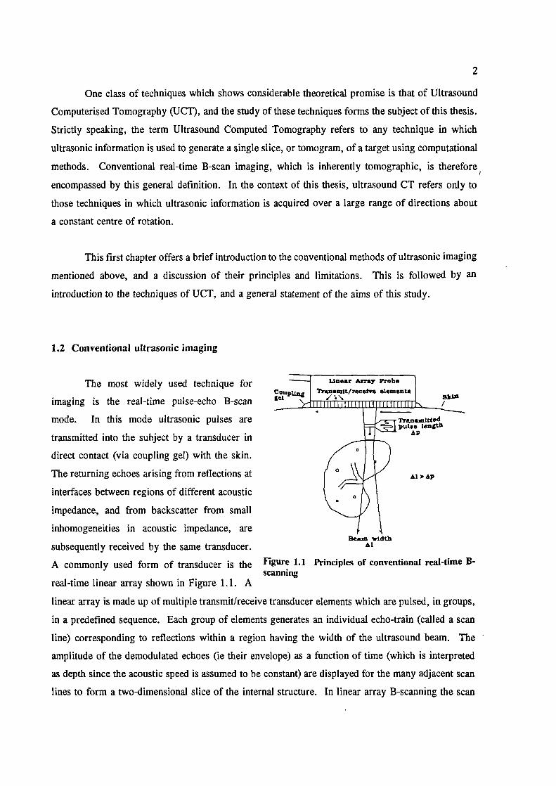
The most widely used technique for

imaging is the real-time pulse-echo B-scan

mode. In this mode ultrasonic pulses are

transmitted into the subject by a transducer in

direct contact (via coupling gel) with the skin.

The returning echoes arising from reflections at

-1 Uear Ax? Probe I

?ran.iuIt/reeelvs eluneiit.

itttedpul.e length

0

0

Al AP

interfaces between regions of different acoustic \ '

impedance, and from backscatter from small

inhomogeneities in acoustic impedance, areScAm width

subsequently received by the same transducer. Al

A commonly used form of transducer is the Figure 1.1 Principles of conventional real-time B-Scanning

real-time linear array shown in Figure 1.1. A

linear array is made up of multiple transmit/receive transducer elements which are pulsed, in groups,

in a predefined sequence. Each group of elements generates an individual echo-train (called a scan

line) corresponding to reflections within a region having the width of the ultrasound beam. The

amplitude of the demodulated echoes (ie their envelope) as a function of time (which is interpreted

as depth since the acoustic speed is assumed to be constant) are displayed for the many adjacent scan

lines to form a two-dimensional slice of the internal structure. In linear array B-scanning the scan

3

lines are parallel. Hence B-scan images are intrinsically tomographic without the need for additional

computer processing. The operator can move the transducer to obtain different slices though the

tissue, or hold the transducer stationary to obtain sequential images in real-time and hence display

moving structures.

However, in addition to its many attractive features conventional pulse-echo B-scanning

possesses the following limitations:- -

a. The interactive nature of the scanning procedure requires that the operator should be

sufficiently experienced to both produce the images and to interpret them at the time of the

scan.

b. The images have poor resolution, in comparison with those from X-ray devices for example.

In particular, image resolution lateral to the scanning direction is limited by the ultrasound

beam width (typically 3 to 4 mm for a 3 MHz probe). Axial resolution, limited by the length

of the ultrasound pulse (typically 1 mm at 3 MHz), is much better.

c. The images possess significant artifacts. For example:

Many interfaces between tissues behave as specular reflectors of ultrasound, and can

be properly visualised only when they are perpendicular to the scanning beam.

ii. The images possess a spatially random noise component known as speckle, due to the

partially-coherent nature of the imaging process, which can obscure small details.

iii. The ultrasound beam is assumed to propagate in a straight line at constant speed. In

practice any changes in acoustic speed between different tissues will lead to image

degradation and reduced resolution.

d. The images describe the structure of tissue interfaces and indicate the texture of tissues but

do not directly yield quantitative information about bulk tissue.

These limitations have restricted the range of applications available to ultrasonic imaging.

The lack of quantitative information about tissue characteristics, and the artifactual appearance of

ultrasonic images sometimes make it difficult to be totally objective about clinical fmdings.

Consequently operators require long training in order to gain an acceptable level of confidence. The

resolution of ultrasonic imaging at the frequencies generally used in the abdomen and breast (3 to 5

MHz) is not sufficient to unambiguously resolve small lesions or calcifications (of less than 2 to 3 mm

diameter). These factors have generally made ultrasonic imaging unsuitable as a mass screening

modality for the early detection of cancer, particularly in the breast where acoustic speed related

artifacts are most troublesome.

4

1.3 Compound scanning

Many of the limitations of real-time B-scanning discussed.above arise because measurements

of backscattered ultrasound are obtained only over a relatively narrow angle defined by the size of

the receiving aperture. The use of a limited aperture restricts both the potential resolution of the

imaging technique and, in the case of specularly reflecting interfaces, the ability to visualise the

interface at all. A technique which allows backscatter measurements to be obtained over an

effectively much greater angle (and equivalently a wider aperture) has been around from the early

days of ultrasonic imaging, and is known as compound scanning. This is a method in which a single

element transducer is used to manually scan the target region from a large number of directions in

the same scan plane (Figure 1.2), a technique now referred to as "static" B-scanning.

A large range of view directions

is achieved by both rocking the transducer

and moving it across the skin surface, the

spatial position and angle of the

transducer being monitored at all times by

the scanner hardware. The scan line echo

data from each direction is added to form

a compound image, using the positional

information to define the direction and

position of each scan line on the image

Rand guided Transducer moved manuallytransducer-.. - - - - - cos - - S

eody surfaceRocking

\ ôI

plane. Since all targets within the object Figure 1.2 'rinciples of compound scanning

are viewed from multiple directions,

specularly reflecting interfaces are more fully visualised. Speckle is also reduced because the echoes

obtained from different directions possess largely independent speckle information which is summed

incoherently, thus tending to "average out" the contributions due to speckle.

One major disadvantage of compounding is that the potential for real-time imaging is lost.

Also many of the limitations of all B-mode scanning techniques still hold. For example, artifacts

arising due to any departures from the assumption of a constant speed of sound are likely to be more

prominent in compound scans than in conventional B-scans. This is because echoes arising from any

particular point in the target will traverse many different regions of the target before reaching the

5

receiver, and will not superimpose correctly if the acoustic speed is variable. In addition, any

movement of the patient during the relatively long time required to perform the scan will also result

in mis-registration of echoes. These factors together mean that the improvement in resolution that

might occur from compounding is frequently not achieved in practice.

1.4 Ultrasound computed tomography

Many approaches to ultrasound CT have been developed over the past twenty years, but most

of them may be grouped into three categories depending on the type of measurements made and the

assumptions used to reconstruct the images. These techniques will be discussed in detail in Chapter

3, but are introduced briefly here.

The requirement, common to all ultrasound CT techniques, for an ultrasonic transducer to

rotate freely about the object (ideally through 360 degrees) in a water-bath, obviously restricts the

techniques to the imaging of superficial or easily accessible targets such as the breast in particular,

but also potentially the neck, scrotum, limbs, neonate and infant. Most of the in-vivo work to date

has concentrated on imaging of the female breast, in view of the lack of bone or gas barriers to

ultrasound and its potential for breast cancer screening.

1.4.1 Reflection-mode ultrasound computed tomography

A scanning technique closely related to manual compound scanning is one in which the

transducer is rotated automatically around the target, in a water-bath, and about a constant centre of

rotation. All the advantages of compound scanning are preserved, while in addition the individual

lines of backscattered echo data bear a simple geometric relationship to each other and computer

processing may therefore be applied efficiently. Furthermore the automatic nature of the scanning

procedure means that it is independent of the operator and allows retrospective reporting of scans.

It was first noted by Johnson and co-workers (Johnson et al 1977), and later by others, that this

procedure for acquiring ultrasonic backscatter (or reflectivity) data is similar to the procedure used

in X-ray computed tomography for acquiring X-ray attenuation data. Consequently it was realised

that similar processing algorithms might be used to reconstruct the ultrasonic data into a high quality

image, and this technique came to be known as reflection-mode ultrasound computed tomography (or

6

reflection-mode UCT).

1.4.2 Transmission-mode ultrasound computed tomography

Another technique which applies the principles of CT to ultrasonic imaging was already

established when reflection tJCT was first proposed. As the name implies, transmission-mode UCT

is involved with measurements of ultrasonic pulses which have been transmitted through an object and

as such is more directly analogous to X-ray CT than is reflection UCT. Interest in the technique

arose from the desire for more quantitative information about bulk tissue than was available from

pulse-echo imaging.

In transmission-mode UCT two transducers are required, one to transmit the ultrasonic pulses

and another on the opposite side of the object to receive them. Measurements on the transmitted

pulses are made at many lateral positions with respect to the object by laterally translating both

transducers in unison, thus forming one projection. Many projections are obtained at angular

increments by rotating the whole scanning gantry around the object. There are essentially two kinds

of measurement that can be made on these pulses. One possibility is to compare the amplitude of the

pulses when they leave the transmitter to their amplitude when they are received, and then use CT

methods (e.g. Greenleaf et al, 1974) to reconstruct an image representing the distribution of ultrasonic

attenuation coefficient. The other possibility is to measure the time it takes for the pulses to travel

between the transmitter and receiver. These time-of-flight (TOF) measurements can then be used

(e.g. Greenleaf er a!, 1975) to reconstruct an image of acoustic speed distribution within the object.

1.4.3 Diffraction tomography

The simplifying assumptions inherent in conventional IJCT techniques, in particular the

neglect of diffraction effects, result in the images possessing considerably poorer resolution than the

theoretical diffraction limit. In an effort to achieve the ultimate 'diffraction limited' resolution some

workers (e.g. Mueller et al, 1978) have attempted to model more accurately the physical mechanisms

of image formation. They generally start by solving approximately the wave-equation for an acoustic

wave in a medium of varying compressibility, density, or both. Most methods assume that the object

is insonated with continuous plane waves, the scattered waves being detected by a transducer scanning

a plane located beyond the object. An image is reconstructed by measuring the phase and amplitude

of the scattered waves at each point on the receiver plane for many frequencies and/or directions of

insonification, and inverting the equations to solve for the spatially varying acoustic parameters.

From these parameters acoustic speed and attenuation distributions can usually be derived. These

methods have come to be known as Diffraction Tomography or Inverse Scattering Tomography.

8

1.5 Aims

Although much research has been carried out concerning the application of computed

tomography techniques to ultrasonic imaging, this research has not had a large impact on clinical

scanning and it was felt that further effort was justified to realise the full potential of the techniques.

Consequently this work has been undertaken to study, both in theory and by experiment, these

techniques with a view to developing practical systems based on relatively simple and cheap

equipment. The main aims of this research can therefore be summarised as follows:-

1) To perform a comprehensive review of the literature on all methods of ultrasound computed

tomography.

2) To carry out a theoretical comparison of the methods which appear to offer the most potential

for high quality imaging of soft tissue. This comparison should consider the assumptions

required for the validity of the methods, the practical limitations imposed by the assumptions,

and the consequences of failure of the assumptions for image quality.

3) To develop practical systems to investigate further the UCT methods described previously.

4) To report the results of these investigations from images of phantoms, in-vitro tissues and in-

vivo subjects, and discuss any advantages of the UCT techniques over conventional scanning

techniques as well as any limitations.

9

2 Principles of Computed Tomography

2.1 Introduction

Although this thesis is not the place for a comprehensive description of the techniques of

Computed Tomography, in order to understand the principles of ultrasound CT and its limitations an

overview of the essential aspects of CT in its more familiar application with X-rays is required. For

more in-depth discussion into CT and more rigorous mathematical proofs, see for example Gordon

and Herman (1974).

Tomographic imaging may be described as a procedure which produces 2-dimensional images

of some 3-dimensional quantity from sets of 1-dimensional measurements. Computed Tomography,

being the application of computers to tomographic reconstruction, is a relatively recent development.

The basic principles of tomographic imaging have been known for a considerable time, with some

of the earliest implementations, dating back to the early 1920s, relying on photographic methods of

reconstruction. These early methods suffered from several limitations. A particularly severe one was

that the desired image slice always suffered some contamination from adjacent slices. With the

development of digital computers "true" tomographic imaging became possible, and the technique

soon found application in many diverse areas including electron microscopy, radio astronomy, and

medical imaging. The first commercial X-ray CT scanner became available in 1971, and X-ray CT

has since become a valuable diagnostic tool.

2.2 Geometry and data acquisition

As suggested in the previous section, an ideal tomogram is simply an image of a thin (ideally

infinitely thin) slice through an object, where no information from out of the plane of the slice is

included in the image. In X-ray CT, a tomogram is produced by using a narrow beam of X-rays to

irradiate a thin slice of an object from many directions in the plane of the slice. The simplest

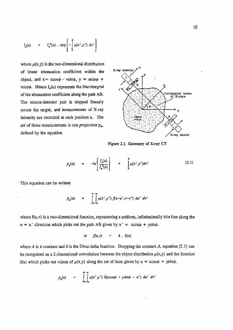
arrangement for X-ray CT (Figure 2.1) involves a single finely collimated X-ray source on one side

of the object, and a collimated detector on the other side which measures the X-ray intensity

transmitted through the object. Assuming that the X-ray beam is infinitely thin and travels in a

straight line between the source and the detector (a valid assumption for X-rays within the body), then

the intensity I(u), measured at position u, is related to the intensity I°(u) at the source by the

equation

X-ray detec/ U

X-ray source

Figure 2.1 Geometry of X-ray CT

10

J(u) I°(u) exP[_JiL(x I Y') dvIJ

where i(x,y) is the two-dimensional distribution

of linear attenuation coefficient within the

object, and x= ucos4 - vsin, y = usin ^vcos. Hence I(u) represents the line-integral

of the attenuation coefficient along the path AB.

The source-detector pair is stepped linearly

across the target, and measurements of X-ray

intensity are recorded at each position u. The

set of these measurements is one projection p,

defined by the equation

p,(u) =

This equation can be written

p,(u) =

_in 1 ) = Ji(x',y')dv'

{ 10(U)

J A

-

JJ(x 1 Y')fu_u'v_v 1) du' dv'

(2.1)

where f(u,v) is a two-dimensional function, representing a uniform, infinitesimally thin line along the

u = u' direction which picks out the path AB given by u' = xcos4 + ysin4.

ie flu,v) = A . ô(u)

where A is a constant and ô is the Dirac-delta function. Dropping the constant A, equation (2.1) can

be recognised as a 2-dimensional convolution between the object distribution J.L(x,y) and the function

ô(u) which picks out values of (x,y) along the set of lines given by u = xcos4 + ysin.

p,(u) = JJ1L(x'Y') ô(xcos + ysin - u') du' dv'

11

or

pQ(u) = a(x,y) * * .5(u) (2.2)

where denotes a 2-dimensional convolution.

Many projections at different angles are acquired by rotating the gantry around the target,

until projections have been acquired over at least 180 degrees. Equation (2.2) expresses the linear

relationship between the target function /2(x,y) and the measured projection data p. The

reconstruction problem is to unscramble the projection information, ie to invert equation (2.1), and

present the solutions as quantitative values of attenuation coefficient for each element (or pixel) in a

two-dimensional array. This array of pixels is then the reconstructed image of the object slice.

2.3 Image reconstruction from projections

An analytical solution to the reconstruction problem was originally discovered in 1917 by

Radon. Equation (2.2) expressed in a slightly different form is often known as Radon's transform.

He proved that any two-dimensional object can be reconstructed uniquely from an infinite set of its

projections (for details of the solution see Herman and Rowland, 1973). The practical problems

associated with applying Radon's analytical solution directly are that (i) only a finite number of

projections can be measured, (ii) real measurements are not exact line-integrals since they are

contaminated by the beam width, scatter, electronic noise, etc, and (iii) Radon's analytical formula

does not generate an efficient algorithm for implementation on a computer.

Various algorithms for the reconstruction of an object from its projections have been

developed which are more amenable to implementation on a computer. These methods can be divided

into essentially three distinct groups; Fourier domain methods, transform methods and iterative

methods.

2.3.1 Fourier domain methods

The first practical use of a Fourier domain solution to the reconstruction problem was

reported by De Rosier and Kiug (1968), who obtained 3-D reconstructions of bacteria from 2-D

electron micrographs. A good mathematical description of the method has been given by Crowther

et al (1970).

12

The basis of the method is the so called central section theorem. This states that the 1-D

Fourier Transform of a projection of an object, obtained at an angle 4), is identical to a line at an

angle 4) through the origin of the 2-D Fourier Transform of the object. To appreciate this, consider

a projection p0(u) obtained at an angle 4) = 0 (ie u = x, v = y),

ie p0(x)

JJIL(x'Y') ô(x-x') dx' dy'

p0(x) =

J4a(x,y') ay'

(2.3)

The 1-D Fourier Transform of the projection is given by

P0(X) = J p0(x) exp(-i2TXx) dx

where X is the spatial frequency component equivalent to x. Hence from (2.3)

P0(X) = J J j(x,y) exp( -i2irX,) dx dy (2.4)

The 2-1) Fourier Transform of the object distribution (in this case X-ray attenuation coefficients) is

M(X,) J J (x,y) exp[-i2ir(Xz + Yy)] dx dy

Comparing this equation to (2.4) it can be seen that P 0() is equivalent to a line Y = 0 through the

origin of M(X,Y), ie along the X-axis.

ie P0(X) = M(X,O)

Expressed in poiar co-ordinates with the radial frequency component R, we have at 4) = 0

P0(R) = M(R,O)

This result can be generalised for a projection at any angle 4), since the choice of reference axes is

arbitrary

ie P0(R) = M(R,4i) (2.5)

This is shown graphically in Figure 2.2.

Clearly, given an infinite set of projections

covering angles of from 0 to 180 degrees, the

2-D Fourier Transform M(R,) of the object

function will be completely determined for all

(R,), the object itself then being given exactly

by its inverse polar Fourier Transform (r,q).

In practice only a finite set of noisy projections

will be available and M(R,q), and hence JL(r,),

will not be obtained exactly. Moreover the

maximum frequency content in the image will

be limited by the finite width w of the X-ray

beam (ie the width of the X-ray detector) to

some value R,

ie M(R,çi) = 0 for I RI > R

where R, 11w

13

P,(u)U

A) Space Doma1nc( Incident

X-rays

Y

b) Frequency Domain

Figure 2.2 Principles of central-section theoremSampling theory then dictates that only

a finite set of projections is required to completely determine the image to a limited resolution (of

w/2). The sampling requirements for CT will be dealt with further in section 2.4.

There remains a problem with the practical implementation of the Fourier method. Polar co-

ordinate Fourier Transforms are extremely time consuming compared to the fast algorithms which

have been developed for cartesian co-ordinate transforms. It would also be preferable to obtain values

of the object function (x,y) in cartesian co-ordinates, for example for display purposes. Hence

values for M(X,Y) must be interpolated from the values of M(R,ç). Much research effort has been

directed towards finding efficient algorithms to perform this interpolation (see for example Crowther

et al, 1970), but generally the algorithms which introduce minimal errors into the reconstruction also

require considerable computation time.

2.3.2 Transform methods

These methods are an attempt to approximate a discrete version of the inverse Radon

14

transform. There are two possible approaches which are essentially equivalent but differ in their

implementation.

Back-projection with post-filtering

This is probably the easiest reconstruction method to understand, and consequently was one

of the first to be applied (Kuhi DE and Edwards RQ, 1963). In this method, also known as the

'summation method', the value of (x,y) at any point (x,y) is estimated by summing all the line-

integrals of the rays that have passed through that point in the object. Alternatively, one can imagine

each projection being 'dragged' across the image matrix in the same direction along which the

projection was obtained. This is shown in

Figure 2.3 for four projections of two point

targets. The back-projection operation may be

expressed mathematically by A

r

dcb (2.6)

where B(X,Y) represents the image obtained by

back-projecting an infinite number of

projections. In practice there will only be a .Figure 2.3 Pnnciples of back-projection

finite set of projections and hence the

integration of (2.6) should be replaced by a discrete summation. However, the continued use of

integrals does not affect the generality of the solutions, provided that sufficient projections are

obtained to satisfy the sampling requirements (see Section 2.4).

Combining equations (2.2) and (2.6) gives,

= [j(x,y) * * ô(u)J dcb

j. 8(x,y) = ju(x,y) * * ô(u) dçó

since p(x,y) is not a function of q. But f ô(u) dqS is simply the rotation of the line, xcos4 + ysin

15

= 0, about the origin, ie

rô(u)db = 1

8(x,y) = (x,y) * * [.J

(2.7)

where r is the distance from the origin. Hence the image B (x,y) formed by simple back-projection

is the object i(x,y) convolved with the function hr. This effect can be seen in Figure 2.3, where

point targets in the object appear as "stars" in the back-projected image.

Using the convolution theorem equation (2.7) may be expressed in the frequency domain as

MB(X,Y)

= M(X,Y). G(R)

where G(R) is the Fourier Transform of (1/r)

1ie G(R) = -

IRI

Hence, in principle, it should be possible (e.g. Cho et al, 1974) to reconstruct an image M(X,Y) of

the 'true' object spectrum M(X,Y) by multiplying the back-projected spectrum by an inverse filter

F(R) of the form

1F(R) = = fRiG(R)

ie M'(X,Y) MB(X,Y) . fRJ

The reconstructed image (x,y) is then given by the inverse Fourier Transform of M(X,Y).

Unfortunately, even though the projection data will be zero outside some limits related to the size of

the object, the back-projected image IB will never reach zero within finite limits because (l/r) is non-

zero everywhere. Hence taking a Fourier Transform on a finite grid will inevitably result in

truncation and hence distortion in the reconstruction. In the limit r - co then - 0, so that a finite

grid could be used outside which B would be negligible. However, the additional computational

expense of calculating a 2-D Fourier Transform on a grid considerably larger than the required

(2.8)

16

reconstruction size makes this approach unattractive.

Filtered back-projection

An alternative approach to filtering the image after back-projection is to filter each projection

before back-projection (Bracewell and Riddle, 1967). Consider the object function /L(x,y) expressed

in terms of its polar Fourier Transform M(R,S)

(x,y) = fM(R) IRI exp[i27rR(xcosçb + ysinq)1 dR dqS

Let p(u)= J

M(R,q5) IRI expQ2irRu) dR (2.9)

where u = xcosq + ysin, as before

rThen j2(x,y) = p'(u) d4' (2.10)

Equation (2.10) is recognisable as the back-projection operation of (2.6), except this time it is p '(u)

being back-projected instead of p(u). Now consider equation (2.9). Taking the inverse Fourier

Transform of both sides, and using the convolution theorem, it can be shown that

(u) exp(i2irRu) du = P (R) = M(R,) . R

But from the central-slice theorem (equation (2.4)), the Fourier Transform of the projection, P(R),

is a line through the origin of M(R,) at an angle ,

ie M(R,) = P(R)

.. P(R) = P(R) . (2.11)

Hence p '(u) can be thought of as a filtered version of p(u). This filtering can be carried out either

in the frequency domain by multiplying P(R) by RI as in equation (2.11), or in the space domain

17

by convolving p(u) with the Fourier Transform p(u) of R

ie p(u)

p(u) * p(u)

where p(u) =

JR I exp (i2irRu) du

To reconstruct the final image, all that now needs to be done is to backproject the filtered projections

as in (2.10).

Since the projection data is band-limited by the measuring system both in the space and

frequency domains (see section 2.4), the function RI may be truncated above some value R.,. In

fact this is essential otherwise noise in the projections, which will dominate the signal at high

frequencies, will be amplified by the large value of I R. Various truncated versions F(R) of the

function R have been suggested. One possibility is a sharp truncation

ie F(R) = I RI for I R

I

F(R) = 0 for IRI ^R

as in Figure 2.4a. Its Fourier transformA) Frequency Domain B) Space Domain

generates the well known space domain filter of

Bracewell and Riddle (1967) shown in Figure

2.4b. The filter has a considerable spread in

the space domain, and hence the discrete form

(Ramachandran and Lakshminarayanan, 1971) -R RJ R

requires a large array which makes the Figure 2.4 Filter of RainachandranLakshminarayanan (1971)

and

convolution very time consuming. Also, the

sharp truncation in the frequency domain tends to introduce 'ringing' artifacts into the reconstructed

image. The discrete filter of Shepp and Logan (1974), defined in the frequency domain by

=I I 2R 1 . R Rsin1____ 1 SiflC[2RjIt J i2J

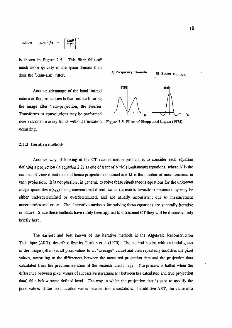
18

I sinO 2

where sinc2(0) = [rJ

is shown in Figure 2.5. This filter falls-off

much more quickly in the space domain than

does the 'Ram-Lak' filter.

Another advantage of the band-limited

nature of the projections is that, unlike filtering

the image after back-projection, the Fourier

Transforms or convolutions may be performed

Frequency Domain B) Space Domain

over reasonable array limits without truncation Figure 2.5 Filter of Shepp and Logan (1974)

occurring.

2.3.3 Iterative methods

Another way of looking at the CT reconstruction problem is to consider each equation

defining a projection (ie equation 2.2) as one of a set of N*M simultaneous equations, where N is the

number of view directions and hence projections obtained and M is the number of measurements in

each projection. It is not possible, in general, to solve these simultaneous equations for the unknown

image quantities u(x,y) using conventional direct means (ie matrix inversion) because they may be

either underdetermined or overdeterniined, and are usually inconsistent due to measurement

uncertainties and noise. The alternative methods for solving these equations are generally iterative

in nature. Since these methods have rarely been applied to ultrasound CT they will be discussed only

briefly here.

The earliest and best known of the iterative methods is the Algebraic Reconstruction

Technique (ART), described first by Gordon et al (1970). The method begins with an initial guess

of the image (often set all pixel values to an "average" value) and then repeatedly modifies the pixel

values, according to the differences between the measured projection data and the projection data

calculated from the previous iteration of the reconstructed image. The process is halted when the

difference between pixel values of successive iterations (or between the calculated and true projection

data) falls below some defined level. The way in which the projection data is used to modify the

pixel values of the next iteration varies between implementations. In additive ART, the value of a

19

pixel L(i,j) in the qth iteration is changed from its value in the previous iteration according to the

formula

=+ p(u) - pr'(u)

N(u)

where p(u) is the measured projection at angle and p'(u) is the equivalent projection calculated

from the q.lth iteration. N(u) is the number of pixels lying along the path u = xcosq + ysinq5. For

multiplicative ART the formula is

I p(u) 114 = I

[p'(u) J

These operations are repeated for every projection to complete one iteration. Other iterative

methods exist which change the pixel values at each iteration using data from all the projections

simultaneously. One such method (Gilbert 1972) is appropriately called the Simultaneous Iterative

Reconstruction Technique (SIRT).

The main advantage of these iterative methods over Fourier based methods is that it is

possible to introduce additional information about the object into the reconstruction process. For

example, the reconstructed values may be constrained after each iteration to be positive since a

negative X-ray attenuation coefficient is physically meaningless. Despite these potential advantages

these methods are now rarely used in X-ray CT because they tend to require a great deal of

processing time. However, they have been shown (Gordan and Herman, 1974) to be useful in

situations where the projection data is particularly noisy or inconsistent, or when the data is under-

determined (e.g. if there are insufficient projections to satisfy the ideal sampling requirements, see

next section).

2.4 Sampling requirements for computed tomography

In computed tomography, as in all sampled systems, the measured data must be sampled

sufficiently finely to allow all frequency components in the data to be represented unambiguously, ie

to prevent aliasing. The Shannon sampling theorem states that, for a band-limited function with a

maximum frequency component f, aliasing will not occur if the sampling interval (s) satisfies the

condition s ^ 1/(2.f). This also has consequences for the number N of projections required to

20

reconstruct an image.

Assuming that the X-ray detector width is w, then the maximum spatial frequency that can

be present in the projections, and hence in the reconstructed image, is given approximately by

1= - (2.12)w

Hence the sampling interval, or distance between each detector position, along a profile should satisfy

wS ^ -

2

For an object diameter of D, the number of samples per projection will be

N=2S

N, ^ (2.13)

It would make sense to choose the size of the pixels Lp in the reconstructed image to equal the

potential resolution, such that

= S =

It is helpful to now consider the situation in the frequency domain. Figure 2.6 represents the

2-dimensional Fourier Transform (F.T.) of object space. As mentioned in 2.3.1, it can be shown that

the 1-D F.T. of the projection of an object, obtained at an angle 0, is identical to a line at 0 through

the origin of the 2-D F.T. of the object. This line extends from -f to +f as given by equation

(2.12). The frequency resolution M within this line is the reciprocal of the distance over which

projection data has been obtained,

ie f =

As already stated, many projections are required to fully reconstruct the object, each

projection providing a unique line in frequency space. These lines should be spaced so that the

Y

21

.pe

x

maximum distance between them in frequency

space does not exceed the frequency resolution

of the projections M. This results in an angle

between projections, M, given by

= 1Df

wD

It can be seen from Figure 2.6 that,

theoretically, projections need only be obtainedFigure 2.6 CT sampling requirements

over a total angle of 1800 (or pi radians) to fully

reconstruct the object. This implies a total number of projections N of

N=

= = (2.14)w

22

Literature Review

3.1 Introduction

Ultrasound CT should strictly refer to any technique where ultrasonic information from many

directions is combined into a single image via computational means, but has largely come to refer

only to techniques where algorithms similar or identical to those used in X-ray Computed

Tomography have been applied. Ultrasound CT techniques may be further sub-divided, according

to the kind of measurements and/or assumptions that are made, into reflection, transmission or

diffraction UCT. A great deal of research into ultrasound CT has been carried out over the last 18

years. An attempt to describe all this work in detail would not be appropriate, and hence this

literature review will concentrate only on research which has presented significant advances or

typified particular techniques.

Although reflection UCT was not the earliest application of CT to ultrasonic imaging

(although similar in concept, compound scanning is not really a CT technique because no fixed

geometry is imposed and in general no computer processing is applied), this technique will be

discussed first because it is the one for which it is easiest to see the connection with conventional

ultrasonic imaging. Subsequently the various UCT techniques involving measurements of transmitted

ultrasound will be discussed. The two quantities most usually reconstructed from these transmission

measurements are the acoustic speed and attenuation distributions. No attempt has been made to

implement a practical diffraction tomography system in the work described in this presentation.

However, it was considered worthwhile to present a brief review of the published research into this

technique because an understanding of why diffraction tomography has so far failed to generate

impressive images of real tissue is necessary in order to justif' its exclusion from this research

project.

Since the objective of this literature review is to determine which of the various IJCT

techniques were most appropriate for further investigation in this study, this chapter will conclude by

summarising the relative advantages and disadvantages of these techniques.

B)

Backpn

A

23

3.2 Reflection-mode ultrasound computed tomography

As suggested in chapter 1, the techniques of reflection ultrasound CT developed out of the

need to overcome some of the limitations and artifacts inherent to the conventional and already well

established reflectivity imaging technique known as real-time B-scanning. Although an introduction

to the basic concepts of reflection-mode IJCT will be given here, a detailed theoretical analysis will

be presented in Chapter 4.

3.2.1 Broad-beam methods

B

Probably the simplest approach

conceptually to reflection-mode UCT, adopted

first by Wade et al (1978), assumes that a wide

aperture (greater than the object's largest

dimension) transducer acts as transmitter and

receiver of a short acoustic pulse (Figure 3. la).

As in conventional pulse-echo imaging, echoes

return to the transducer from interfaces and

scatterers within the object. Assuming that

plane waves are incident on the object and the

acoustic speed is constant, echoes from

scatterers at a given range will arrive at the

same time at the receiver and their sum will

appear as the output voltage. This sum can then

be considered as the integral of the object

reflectivity at that particular range and across

the whole width of the target, unlike B-scanning

A) - - Tranaduccr

- poatlion B

.'nsducer / /

Itinn A/ /

/

Echo amplitude[tA

A A

C

where only a small portion of the target isFigure 3.1 Broad-beam reflection UCT using

interrogated by each scan line beam. wide single-element transducers (Wade 1978).

Consequently the output signal as a function of

time following transmission can be considered as a 1-D projection of the object reflectivity as a

function of range. Thus one difference to X-ray CT is that the projection of the object is parallel to

the direction of propagation of the ultrasound beam, rather than perpendicular as is the case in X-ray

CT.

24

Wade et at proposed that by rotating the transducer around the object to obtain projections

at many angles, and backprojecting the projection data across image space according to the techniques

of Computed Tomography (Figure 3.lb), it should be possible to reconstruct a 2-dimensional image

of the object reflectivity showing ideally isotropic resolution determined by the length of the ultrasonic

pulse. Since the standard CT process of backprojection has an inherent blurring (or low-pass

filtering) effect on the reconstructed image (see 2.3.2), similar filters to those used in X-ray CT (eg

a Shepp-Logan filter) must be applied to the data in order to achieve the best possible resolution.

Wade and co-workers suggested that departures from this simple model of reflectivity image

formation, caused for example by attenuation of the pulses as they propagate to and from the

scatterers within the object, might not be too serious because of the averaging affect of the multiple

projections. In their experimental set-up a large diameter transducer, designed to produce a nearly

uniform beam, was rotated around brass cylinders in water. Images were reconstructed using Shepp-

Logan filtered backprojection. Various artifacts were observed in the images, such as incomplete

cylinder boundaries and boundary distortion, largely due to the high reflectivity of brass in water.

This caused shadowing of the back half of each cylinder by the front half, and in some projections

the shadowing of parts of cylinders by other cylinders - effects not accounted for in their model.

The concepts of reflection UCT were developed further by Norton and Linzer (1979) who

derived a theoretical method for reconstructing 2-D reflectivity images obtained with a circular array

of point transducers completely surrounding the object to be imaged (Figure 3.2a). Each transducer

is excited independently one after the other. They assumed that (a) the object can be modelled as a

collection of isotropic weakly scattering point targets, so that the energy propagating through the

object is much greater than the backscattered energy (this is known as the Born approximation and

is discussed more fully in section 3.4); (b) the acoustic speed is constant; and (c) attenuation can be

compensated for. Accepting these assumptions they showed that the reflectivity reconstruction

problem reduces, for every transducer in the array, to backprojection along concentric circular arcs

centred on each transducer of the raw (ie not envelope detected) rf signal recorded by that transducer

(Figure 3.2b). The backprojection is along circular rather than straight paths (as was the case for a

wide transducer generating plane-waves) because the small transducers generate a divergent spherical

wave. They also showed that the system point spread function (PSF) is limited only by the

bandwidth, and does not depend on the size of the array since the imaging aperture is always 36(Y

and there is effectively no far-field requirement. However no experimental results were presented.

25

Note that any variation in the object orA) Diverging wave front

in the ultrasound field in the directionPoint transducer

perpendicular to the scan plane has been ignored

in all the methods discussed so far. In other

words, all methods have assumed that the object

may be considered as a 2-dimensional

distribution of reflectivity (or backscatter)

coefficient. In a later paper (Norton and Linzer

1981) extended their theory to three dimensions,B)

and drew more closely the similarity betweenEcho amplitudetheir approach to reflection UCT and the at one

arguably more fundamental approach of

diffraction tomography (see 3.4). They

proposed that the fundamental acoustic

parameter actually reconstructed from rf

backscatter measurements is a simple function Back-projection

of the compressibility and density of the

medium, although there is some disagreement as

to whether specular reflection is encompassed Figure 3.2 Reflection UCT using a circularby this model. array of transducers (Norton and Linzer 1979).

It has already been noted that compensation for the attenuation losses of the ultrasound pulses

as they propagate through the object is necessary for an accurate reconstruction of acoustic

reflectivity. This compensation has normally been achieved using a time (and therefore depth)

dependent amplification of the received echoes called time-gain compensation (TGC). The problem

with TGC is that in its conventional application it assumes that the attenuation varies identically with

depth for all possible acoustic pulse-echo paths through the object. A method for correcting the

attenuation losses more accurately than can be achieved by TGC was proposed by Duck and Hill

(1979). Their method relies on the possibility of reconstructing, using CT techniques, both the

attenuation and reflectivity distributions of an object section solely from measurements of

backscattered ultrasound. By assuming that attenuation and scattering are independent and isotropic,

and neglecting the frequency dependence of attenuation, they derived an iterative solution to this

problem that was similar to the Arithmetic Reconstruction Techniques (ART) used in transmission

CT. Results were presented for simulated circular targets of uniform scattering but varying

26

attenuation, which showed good accuracy in the reconstructed attenuation after six iterations. Results

from a lamb kidney in-vitro using a laterally scanned 5MHz transducer, with 10 scans obtained at 36°

intervals, were less encouraging. Some structure was apparent in the backscatter image, but very

little in the attenuation image.

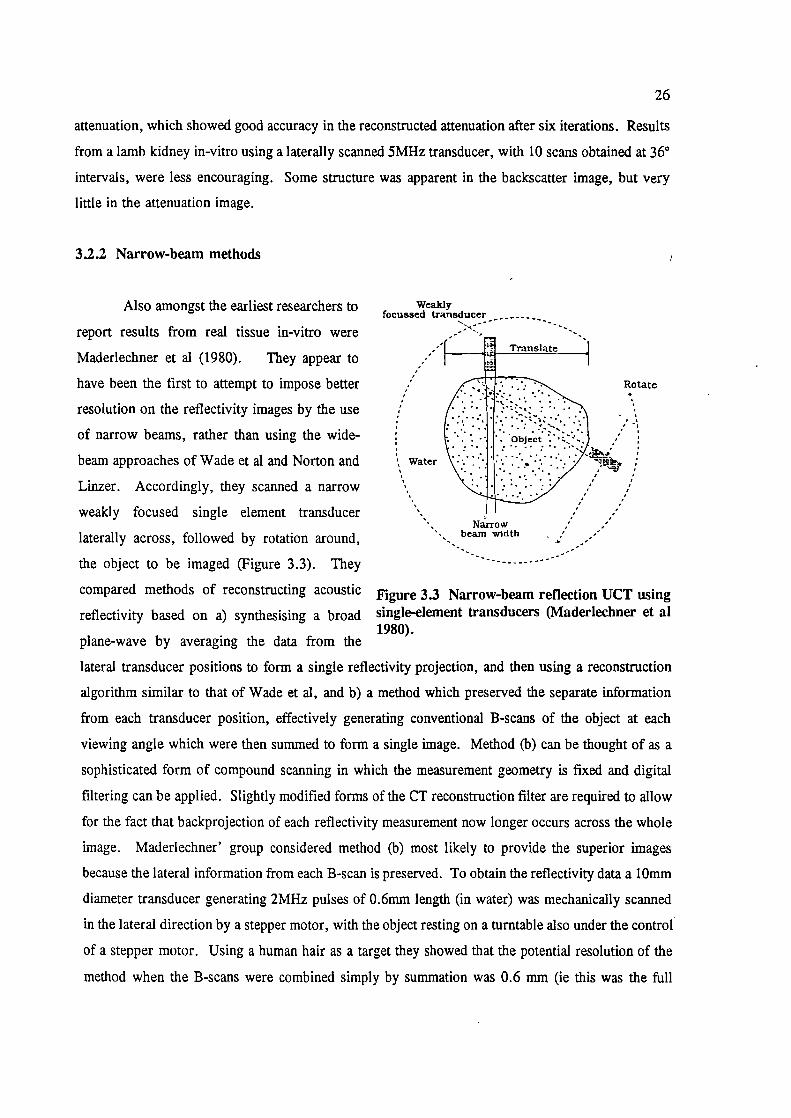
3.2.2 Narrow-beam methods

Also amongst the earliest researchers to

report results from real tissue in-vitro were

Maderlechner et al (1980). They appear to

have been the first to attempt to impose better

resolution on the reflectivity images by the use

of narrow beams, rather than using the wide-

beam approaches of Wade et a! and Norton and

Linzer. Accordingly, they scanned a narrow

weakly focused single element transducer

laterally across, followed by rotation around,

the object to be imaged (Figure 3.3). They

compared methods of reconstructing acoustic

reflectivity based on a) synthesising a broad

plane-wave by averaging the data from the

Weaklyfocussed transducer

I Translate IRotate

• •.

• Object •.•

Water . •. : :. :

Narrowbeam width

Figure 3.3 Narrow-beam reflection UCT usingsingle-element transducers (Maderlechner et al1980).

lateral transducer positions to form a single reflectivity projection, and then using a reconstruction

algorithm similar to that of Wade et al, and b) a method which preserved the separate information

from each transducer position, effectively generating conventional B-scans of the object at each

viewing angle which were then summed to form a single image. Method (b) can be thought of as a

sophisticated form of compound scanning in which the measurement geometry is fixed and digital

filtering can be applied. Slightly modified forms of the CT reconstruction filter are required to allow

for the fact that backprojection of each reflectivity measurement now longer occurs across the whole

image. Maderlechner' group considered method (b) most likely to provide the superior images

because the lateral information from each B-scan is preserved. To obtain the reflectivity data a 10mm

diameter transducer generating 2MHz pulses of 0.6mm length (in water) was mechanically scanned

in the lateral direction by a stepper motor, with the object resting on a turntable also under the control

of a stepper motor. Using a human hair as a target they showed that the potential resolution of the

method when the B-scans were combined simply by summation was 0.6 mm (ie this was the full

Water

Rotate probe

27

width at half max of the image of the hair). When Shepp-Logan filtering was applied before

summation the FWHM was reduced to 0.3mm. They also obtained reconstructions of acoustic

reflectivity in a sponge phantom and an in-vitro pig heart, and demonstrated relatively good isotropic

resolution and reduced artifact in these images compared to conventional B-mode images.

One of the problems of using a mechanically scanned single element transducer to generate /

the reflectivity projections is the time taken to acquire the data. Hiller and Ermert (1980, 1982) were

the first to attempt to reduce scan times by the use of a linear array (Figure 3.4) where the lateral

scanning is achieved electronically without the need for any mechanical movement, but because of

limitations in their mechanical rotation system they could still only achieve a minimum acquisition

time (for 120 projections) of two minutes. in common with Maderlechner et a! they also compared

alternative methods of reconstructing the pulse-echo data based on either (a) discarding or (b)

preserving the lateral information available from each B-scan. They pointed Out that method (b) is

less dependent on the assumptions, such as isotropic scattering and compensateable attenuation,

required for reflection CT and has a higher immunity to measurement errors. They also suggested

that fewer angular transducer positions would be required using method (b) compared to method (a)

(ie 45 compared to 120), because of the greater amount of information obtained at each angle.

Lat&aliy,canned

The experimental apparatus of Hiller

and Ermert consisted of one or two Linear

array

commercially available 2.3MHz 54-element probe

linear arrays mounted on a turntable, and

submerged in a water tank. Only the central 32

elements of the array were used, thus allowing

32 lateral positions (or scan lines) for eachFigure 3.4 Narrow-beam reflection UCT using

angular position. Reconstructions, using both linear arrays (Hiller and Ermert 1980).methods (a) and (b) with a modified Shepp-

Logan filter, were obtained of a ring of 0.6mm diameter steel needles. Both UCT methods

demonstrated considerable improvement over an individual B-scan, with an isotropic resolution of

better than 2mm. Another target consisting of an irregularly shaped piece of PVC, to provide

specularly reflecting surfaces, demonstrated more clearly differences between conventional B-scanning

and the two IJCT methods. In the individual B-scan only a very small portion of the PVC surface

was visible, ie that part of the surface that was perpendicular to the scanning beam, whereas in both

UCT images the surface was complete. However 'streak' artifacts were much more evident in the

28

image obtained by method (a) because the specular reflections violate the assumption of isotropic

scattering, whereas method (b) was much less sensitive to this assumption.

Hiller and Ermert also appear to have been the first to present in-vivo results for reflection

UCT, initially of the human foreman (Hiller and Ermert 1980) but later in the female breast (Hiller

and Ermert 1982), although Carson et al (1981) had already presented reflection images of the breast,

in-vivo (although not incorporating CT filtering) along with transmission UCT images, and had shown

that the two UCT techniques give unique and almost independent information on tissue structure (see

3.3.4). Hiller and Ermert (1982) also presented results of transmission UCT measurements, but using

linear arrays for both reflection and transmission measurements rather than single element transducers.

Reflection, attenuation and acoustic speed images were shown of a dog testicle in-vitro, and of a

human testicle and breast in-vivo.

Friedrich et a! (1982) investigated some of the factors likely to influence the quality of

reflection UCT images. They investigated the affects of the choice of the particular tomographic filter

and the scanning geometry (number of scan angles and total scan angles) used, and considered the

affects of pulse-length, beam-width and registration accuracy. It had already been established by

other workers that the resolution of reflection UCT images was limited by the pulse length.

However, Friedrich and co-workers pointed out that beam width is also important in so much as it

determines the thickness of the scan plane. Registration and refraction errors due to the assumptions

of a known and constant acoustic speed, and consequently straight-path propagation, were thought to

be the most likely causes of image degradation. Mis-registration due to mechanical inaccuracies in

the scanning apparatus was also recognised as a possible problem. They suggested that mis-

registration problems could be minimised by limiting the information used from each B-scan to that

corresponding to the half of the object nearest the transducer. This approach was possible because

they had also shown that a 180° total scan was sufficient and that scanning through 3600 achieved no

significant improvement in image quality. Although some quite good images of in-vitro breasts were

presented, in common with all previous studies the scan times were unacceptably long for a clinical

system.

Limited angle reflection UCT was also considered by Roehrlein and Ermert (1985) and

Ermert and Roehrlein (1986), with the intention of applying the technique to targets for which 360°

access is not possible, such as the neck (ie thyroid) and upper legs. They realised that for scan angles

of less than 180° the reflection image PSF no longer has rotational symmetry, i.e. the resolution is

29

not isotropic. However they showed that isotropic resolution can be achieved by post-processing with

appropriate 2-dimensional inverse filtering. For in-vivo experimental investigations a special

applicator was built to hold either a 3.5MHz linear array (for thyroids, legs and breast), or a 5MHz

linear array (for testicles). A study of 70 patients, using scan angles of 155°, suggested that limited

angle reflection UCT is feasible, particularly for thyroids.

Roehrlein and Ermert (1986) also considered the appearance of speckle in reflection UCT

images. They showed that for reflection UCT images obtained by simple summation (ie no filtering)

of totally uncorrelated B-scans, the mean speckle amplitude (expressed as the ratio between the

standard deviation of the B-scan amplitude and its mean value throughout the image) is reduced by

the square root of the number of B-scans in the summation. The speckle size of the summation image

was found to lie between the axial and lateral components of the speckle size of an individual B-scan.

Tomographic filtering of the summation images, which is normally performed to improve resolution

in line with the conventional CT approach, was found to reduce the speckle size down to the axial

component of the B-scan speckle, but only at the expense of an increase in the mean speckle

amplitude up to that found originally in the B-scan.

3.2.3 Reflection UCT with acoustic speed compensation

It has already been suggested that mis-registration of the superimposed B-scans, due to

acoustic speed variations within the object, may be the main cause of artifact and limitation on

resolution in reflection UCT images. Although many workers have suggested combining simultaneous

acquisition of reflection and transmission data (eg Carson et a! 1981 and Hiller and Ermert 1982, see

above), others have also proposed using reconstructions of acoustic speed distributions to correct

registration errors in reflection images. As early as 1973 Jellins and Kossoff (1973) had shown

improvements in basic compound B-scan images of the breast using very simple acoustic speed

corrections based on a trial-and-error approach. Greenleaf et al (1975) were apparently the first to

propose the use of transmission UCT generated acoustic speed images to improve unfiltered reflection

UCT images. They used a single element 5MHz transducer which was mechanically scanned in a

fan beam for both reflection and transmission data (Greenleaf et a! 1977). They scanned a phantom

consisting of a string held rigidly near to a rubber finger cot filled with saline having an acoustic

speed 5% higher than the surrounding water. The uncorrected reflection images showed blurring of

the string towards the finger cot, whereas in the acoustic speed corrected reflection image the string

was in much sharper focus.

30

The first to apply acoustic speed correction to more demanding targets were Kim et al (1984),

who demonstrated some improvement in Shepp-Logan filtered reflection UCT images of dog hearts

in-vitro using mechanically scanned 2.25MHz transducers. However, as had been the case with

Greenleaf et al (1977) straight-path propagation was assumed and hence no correction was made for

lateral registration errors due to refraction of the ultrasound beam. Bartelt (1988) developed a method

for reconstructing independent images of reflectivity, acoustic speed, attenuation and scattering

directivity from measurements of reflected ultrasound alone. Six 3.5MHz linear arrays were arranged

in a ring to reduce scan times, and the whole ring was rotated (up to 60 degrees) around the object

to be imaged. Directivity estimates were obtained by selecting, for every point in the object, the two

azimuthaly adjacent scans which encompassed the peak backscattered signal from that point, and

calculating the rate of change of the backscattered signal with angle. Acoustic speed and attenuation

estimates were made by comparing overlapping A-scan lines obtained from opposite directions. For

acoustic speed the A-scans were cross-correlated, the maximum of the cross-correlation function

providing an estimate of the average acoustic speed along the line of the A-scans. The acoustic speed

values obtained along many lines and from many directions were then reconstructed into an image

of acoustic speed using conventional CT algorithms. The main problem was attenuation of the echoes

in the A-scan signals which reduced the accuracy of the cross-correlation function and tended to bias

the acoustic speed estimates. For attenuation imaging they calculated the average amplitude difference

of opposite A-scans. However, this provided only a qualitative estimate of attenuation. Reflection

UCT images of a phantom structure, having regions of different acoustic speed, and of a human

forearm were subjected to acoustic speed correction. Probably because of the relatively poor quality

of the acoustic speed images only small improvements in resolution were evident in the corrected

reflection images.

3.2.4 Reflection UCT with RF data

The only researchers, apart from the early work of Norton and Linzer (1979), to have used

the raw rf echo signal in their reconstruction of reflection UCT images have been Herment et al

(1989a and 1989b). Others workers have generally considered only demodulated (ie envelope

detected) signals. Demodulation is a non-linear operation and thus strictly invalidates the concept of

linear summation inherently assumed in CT techniques (see 4.3.1.3). Herment et al compared various

methods of reflection UCT in terms of resolution, signal-to-noise (or signal-to-speckle) ratio and

computing time. They consider both a broad beam method (Herment et al 1989a) and a narrow beam

method using a mechanically scanned single element transducer (Herment et al 1989b). For both

31

methods, they considered the affects of varying the order in which the following stages of image

reconstruction were applied:- (i) deconvolution of the rf point spread function to widen the signal

band-width, (ii) envelope detection to conform to the conventional mode of presentation of B-scan

images, (iii) backprojection for CT image reconstruction, and (iv) tomographic filtering to restore the

high spatial frequencies attenuated by the backprojection process.

They found that the conventional CT method (envelope detection followed by backprojection

and tomographic filtering, with no deconvolution stage) resulted in a factor of 4 improvement in

resolution compared to the lateral resolution of a simple B-scan. Including a deconvolution stage

resulted in a further factor of 3 improvement in resolution over the conventional CT method.

Resolution was even better when both deconvolution and tomographic filtering were performed before

envelope detection. However deconvolution was found to degrade the signal-to-noise ratio compared

to conventional CT, although this effect was not quantified. In terms of computing time, all methods

were found to be very similar. Herment et al also pointed out that the ultimate resolution is only

achievable when the acoustic speed is absolutely constant throughout the object - a situation unlikely

to occur in practice. They thus proposed that their method may be best suited to the study of

superficial structures, such as the carotid arteries, where there is likely to be less opportunity for

acoustic speed variations to degrade the echo data.

A further practical disadvantage of using rf data for reconstruction is that it requires high

geometrical accuracy in the measurement apparatus (better than wavelength/b, or 50 jzm for 3MHz

ultrasound), and hence the technique is probably restricted to data acquisition configurations where

no mechanical movement of the transducers is required, such as is the case for a circular array.

3.3 Transmission-mode ultrasound computed tomography

The earliest published research into transmission UCT was performed in the early 70s by

Greenleaf and co-workers at the Mayo Foundation in Rochester, USA. They were the first to suggest

the possibility of applying the by then well known techniques of Computed Tomography to the

reconstruction of acoustic attenuation (Greenleaf et al 1974) from measurements of the amplitude of

transmitted pulses. Their scanning apparatus consisted of two (one to transmit and one to receive)

5 MHz single element transducers arranged on opposite sides of the target being scanned (Figure

3.5a). The transmitting transducer was pulsed, and the total transmitted energy was calculated as the

32

log of the squared and integrated pulse from the

receiver. The application of CT techniques is

valid if it can be assumed that the transmitted

energy, measured at many lateral positions in a

fixed direction (ie a projection, Figure 3.5b) by

mechanically translating both transducers, is

simply and linearly related to the 2-dimensional

distribution of attenuation coefficient within the

object (see also 2.2). Although they realised

that this assumption was not strictly valid for

ultrasound in human tissues because of

reflection and refraction, they still felt that the

approach was worth attempting. Images of the

acoustic attenuation distribution were

reconstructed onto a 64*64 matrix using a

standard CT technique known as the Arithmetic

Reconstruction Technique (see 2.3.3). Results

were presented for simple phantoms and a

canine heart in-vitro. The images showed

Transmitting a) Geometrytransducer, A

/I

/

4

4

"I

1 /Receiving

transducer, A r

b) A Projection

Figure 3.5 Principles of transmission UCT

recognisable structure, but with thickened boundaries between structures and poor quantitative

accuracy. Despite these artifacts, which they decided were probably due to refraction, they felt that

the technique showed some promise.

Later, the same group (Greenleaf et al 1975) also suggested reconstructing acoustic speed

distributions from measurements of the time of flight of acoustic pulses through tissue. They used

basically the same equipment used for attenuation imaging to reconstruct acoustic speed distributions

for various tissues in-vitro. Pulse time-of-flight (TOF) was measured by detecting the point when the

pulse first rises above the noise level in the signals. Images of acoustic speed distribution were

obtained from excised canine hearts, and comparisons with photographs of the sliced heart were quite

encouraging. Images obtained from post-mastectomy breasts showed more artifacts, but it was still

possible to distinguish between areas of fatty (low acoustic speed) and connective (high acoustic

speed) tissue. By comparing images of acoustic speed and attenuation obtained from the same target,

they showed that these images represent nearly independent parameters.

33

Greenleaf's group argued that the major cause of the artifacts in both their attenuation and

acoustic speed reconstructions was due to refraction. Refraction of the ultrasound beam results in

violation of the assumption that the ultrasound travels in a straight line between transmitter and

receiver, an assumption inherent in the standard CT reconstruction technique. This may result in

either under- or over-estimation of the parameter being measured for the projection data, with

consequent inconsistencies in the projection data and "streak" artifacts in the reconstructed image, as /

well as violation of the basic CT principle that the measured projection is linearly related to the true

geometrical projection of the object. Attempts have been made by several researchers to develop

reconstruction algorithms which do not rely so strongly upon the assumption of straight line

propagation. These approaches will be discussed in a later section (3.3.3), but for now the

consequences of violation of this assumption within the standard straight line reconstruction technique

will be discussed, both in terms of measurement requirements and image artifacts.

In a later paper Greenleaf et al (1978) identified theoretically the underlying assumptions

required for straight line propagation when the ultrasound wave may be modelled by the time-

independent Helmholtz equation. They argued that when diffraction may be ignored (ie X -> 0), and

the relative refractive index varies by less than 10% (ie acoustic speed everywhere in target is similar

to acoustic speed in surrounding medium so that refraction is relatively minimal), then the projection

measurements required for attenuation CT and acoustic speed CT can be based simply on the

amplitude ratios and phase differences respectively of incident and transmitted waves (note that rather

than measuring incident waves it is more usual in practise to measure waves transmitted with, and

without, the target present). Whether these conditions hold sufficiently in soft tissues is an important

question that will be discussed in Chapter 4.

Greenleaf et al pointed out that, not only does refraction violate the straight line assumption

of the reconstruction algorithm, but in the case of attenuation measurements may also result in some

of the ultrasound energy missing the receiver and hence the attenuation being overestimated. Since

attenuation will also be overestimated if any of the ultrasound is reflected from interfaces within or

at the boundaries of the target, they concluded that attenuation images produced from transmission

UCT measurements are more likely to be prone to artifacts and also less quantitative than acoustic

speed images. The main reason for this is that the basic measurements required for acoustic speed

CT are of the times of flight çI'OF) of the ultrasonic pulses propagating across the target. As pointed

out by Greenleaf et a! (1975) and later by Glover and Sharp (1977) pulse TOF, unlike pulse

amplitude, should be largely unaffected by reflection of some of the energy within the pulse.

34

Since the requirements differ for the measurement of basic projection data for attenuation and

acoustic speed reconstructions, the problems associated with these measurements and the affects on

image artifacts will be discussed separately. For a good review of the early work in transmission

ultrasound CT, see for example Wade (1979).

3.3.1 Measurement requirements for attenuation CT

Greenleaf and co-workers (Greenleaf et a! 1978) and other groups (eg Carson and

Scherzinger 1979, Miller et al 1979) have recognised that the undesirable contributions to attenuation

from parameters that are independent of frequency, such as specular reflection and to a lesser extent

refraction, may be minimised by reconstructing the frequency dependence of attenuation rather than

the attenuation coefficient itself. This approach is only valid if the frequency dependence of

attenuation may be assumed to be linear, an assumption that appears to be roughly true in most soft

tissues at the frequencies used (Duck 1990). This technique obviously requires measurements at a

range of frequencies, either by multiple experiments at different frequencies, or more usually by

measurements on broad band pulses.

In another approach, the Carson group (Carson and Scherzinger 1979) showed experimentally

that large receivers (19mm) give better results for attenuation measurements on female breasts in-vivo

because there is less chance of a refracted beam missing the receiver. However, one disadvantage

of using large receivers for breast imaging is that it becomes difficult to image sections close to the

chest wall.

The Carson group also identified another source of error in attenuation measurements, that

is phase cancellation at the receiver. The phenomenon results from the fact that conventional piezo-

electric transducers are sensitive to the instantaneous amplitude (and hence phase) of the incident

ultrasound pressure wave. If the ultrasound wave front becomes distorted as it propagates through

the target, either by refraction or diffraction or more likely both, then phase cancellation will occur

across the receiver aperture resulting in an overestimation of attenuation. Another way of looking

at this is to recognise that conventional transducers have a very peaked directivity pattern, so that they

are only sensitive to waves that impinge upon them at angles close to the perpendicular. This

problem is particularly severe for the large aperture transducers favoured for attenuation

measurements. The Carson group suggested a method to overcome this problem by using a large

array of small transducer elements as a receiver. Being considerably smaller than the total aperture

35

size, each element has quite a broad directivity pattern. By rectifying the signal from each element

before summation and so eliminating the possibility of cancellation, the array is sensitive to wave

components impinging at glancing angles, such as those waves which have been bent by refraction.

In a later paper (Chenevert et al 1984) the same group showed significant improvements in attenuation

images of a breast phantom using a scanned O.25nim hydrophone to synthesise a 5cm diameter 40-

element array, compared to a 19mm diameter single element receiver. However, some expected loss

of resolution which is itself due to the broadened directivity pattern was also observed.

Another way of overcoming the problem of phase cancellation at the receiver is to use a

transducer that is inherently insensitive to phase. Such an approach, using an acoustoelectric

transducer, was proposed by Miller and co-workers (Miller et al 1979). These transducers are

sensitive to the instantaneous intensity of the ultrasound wave, and have a broad directivity pattern.

They compared acoustoelectric receivers with conventional piezoelectric receivers for attenuation

imaging of dog myocardium in-vitro. The images obtained using the acoustoelectric receivers

appeared to be more consistent, with less artifact at the edges of the targets where refraction is

greatest. The same transducer was used for imaging the frequency dependence of attenuation in dog

kidneys in-vitro, with even better results. The inevitable consequence of using such a transducer is

again that some reduction in potential resolution must be accepted.

In a later paper (Kiepper et a! 1981), the same group went further by exploring theoretically

the likely magnitudes of the affects of phase cancellation, refraction, and also the variation of beam

width with frequency (ie diffraction) on attenuation measurements. They proposed a method of

correcting for the beam width variations of the transmitting transducer by measuring its directivity

pattern for various frequencies, and then applying appropriate filters to the measured attenuation data.

They also discussed another potential cause of artifacts in attenuation images that had not previously

been identified. It is well known that some tissues, such as muscle fibre, exhibit an attenuation

coefficient that itself has some angle dependence. This anisotropy is not allowed for in the CT

reconstruction process and hence these tissues will be reconstructed with an "average" attenuation

coefficient. From experimental results in dog myocardium they show that the affects of anisotropy

are significant. They also found that although high attenuation correlates well with infarct in the heart

muscle, the attenuation values were not good quantitatively even when using acoustoelectric receivers

and beam width correction, probably because of anisotropy. Brandenburger et al (1981) performed

a more detailed theoretical analysis of anisotropy. They showed that anisotropy can be intrinsic (eg

muscle fibres) or extrinsic (refraction and reflection are both angle dependent), and concluded from

36

a simulation study that anisotropy can be a major cause of inaccuracy in attenuation reconstructions.

Farrell (1981) argued that one problem with using the frequency dependence of attenuation

as the reconstructed parameter was that, because a range of frequencies was required (the larger the

range the better the accuracy), the technique would be limited to targets of relatively low attenuation

since high frequencies would be attenuated too strongly. He proposed an alternative method for /

reducing refraction and phase cancellation effects which required knowledge of the acoustic speed

distribution of the target. Initially TOF measurements are used to reconstruct the acoustic speed

distribution as in conventional acoustic speed CT. This distribution is then used to calculate simulated

amplitude projections by ray tracing. These projections represent the amplitude measurements that

would be obtained for a target with this acoustic speed distribution but with no attenuation, so that

any amplitude losses are due solely to refraction and phase cancellation affects. These calculated

projections are then used to correct the actual measured projections before reconstruction of the

attenuation image. Good results were obtained with simulated data from circularly symmetrical

targets, but the quality of the images is clearly very dependent on the ability to obtain accurate

acoustic speed images. In addition, the method takes no account of reflection or diffraction losses

unlike the frequency dependence methods.

The basic attenuation measurements made by the majority of the researchers discussed up to

now was of the ratios of the peak amplitude or total energy of pulses transmitted with and without

the target present. Dines and Kak (1979) proposed an alternative method of measuring the integrated

attenuation that should be less affected by refraction and reflection. They showed theoretically that

assuming the ultrasonic pulses may be represented by Gaussian functions, that non-linear propagation

may be neglected, and that the frequency dependence of attenuation in soft tissue is approximately

linear, then the integrated attenuation along the path between the transmitter and receiver is

proportional to the difference in centre frequency between the with target and the without target

pulses. Since it is the spectrum of the transmitted pulse that determines the measured attenuation

value, and not the absolute amplitude of the pulse, the method should still provide a reasonable

estimate of integrated attenuation even if some of the energy of the pulse fails to reach the receiver

because of refraction or reflection. Some improvements in image quality over the conventional peak

amplitude method were demonstrated for excised dog hearts.

Crawford and Kak (1982) showed through computer simulation that, irrespective of the

measurement technique used (ie frequency shift or amplitude ratio), the attenuation images are

37

degraded partly by what they call "multipath". Multipath refers to the multiple ray paths which

connect the transmitter to the receiver in any complex target. The interference of these multiple

pulses at the receiver causes a scalloping of the received power spectrum (equivalent to speckle in B-

mode images). They proposed two methods to reduce the affects of multipath; homorphic signal

processing of the received spectrum to estimate the integrated attenuation for just one of the rays, or

median filtering of the measured projections to remove the glitches caused by multipath. They found

that both methods were successful in improving attenuation images of an ATS labs Tissue Equivalent

phantom, and of a breast phantom.

3.3.2 Measurement requirements for acoustic speed CT

The projection data required for the reconstruction of an acoustic speed image are usually

calculated by subtracting the reference "water-path" time-of-flight (TOF) measured with the target

absent to the TOF measured with the target in place. Most of the early researchers into acoustic

speed CT (eg Greenleaf's group, Glover's group, and Carson's group) measured TOF using the so

called leading-edge or earliest-arrival-time method. As the name of this method implies, the pulse

is assumed to have arrived when its leading edge rises above some (usually fixed) threshold level.

Because of refraction, there will be many possible paths linking the transmitter to the receiver

(Crawford and Kak 1982). However, when the refractive index varies by less than 10% the first

pulse to arrive is likely (Greenleaf et al 1978) to be the pulse that has travelled the shortest (ie

straightest) path, which is also the path assumed by the standard reconstruction algorithm. Hence

when using this detection method, refraction will also tend to have less affect on acoustic speed

reconstructions than on attenuation ones. Using this method, Glover and Sharp (1977) demonstrated

high quantitative and geometrical accuracy for an acoustic speed image of four fingers of a rubber

glove filled with fluids of known acoustic speeds, where the maximum deviation in acoustic speed of

any of the fluids from the surrounding medium (water) was less than 7%.

Despite its apparent success in the reconstruction of simple targets with small acoustic speed

variations, some problems with the use of the earliest arrival time method have been recognised.

Greenleaf et al (1978) noted that small regions of low acoustic speed imbedded within regions of

higher speed may not be detected or their size may be underestimated since, because of the finite

beam width, pulses traversing such regions may appear after pulses traversing the surrounding areas.

Similarly the size of regions with a higher speed of sound than their surroundings will tend to be

overestimated since the region will be detected even if it intersects only a small portion of the

38

ultrasonic beam. This affect could be minimised by using as small a receiving transducer as possible

in order to reduce the number of possible paths, and accepting the consequent reduction in sensitivity.

Note that the requirement for a small receiver is opposite to that found in attenuation CT.

Carson and Scherzinger (1979) also commented on the importance of using a small receiver

transducer since they had observed that this helped generate a fast rise time, which can also be

understood in terms of a reduction in the range of paths and hence arrival tinies of pulses. They also

observed that the measured TOF appears to be artificially high when the pulse is strongly attenuated,

because the received signal crosses the fixed threshold slightly later. This phenomenon was also

described by Crawford and Kak (1982) who called it "time-walk". Crawford and Kak also identified

another possibility, which they called "time-hop", when the attenuation is so severe that the first cycle

of the received pulse (or half-cycle for rectified pulses) fails to cross the fixed threshold. In this case

the TOF will be overestimated by one or more wave periods, depending upon the degree of

attenuation. These problems can be partly overcome by allowing the received pulses to heavily

saturate the receiver amplifier, or by having some form of automatic gain on the amplifier.

A rather more serious limitation of the earliest arrival time method was pointed out by

McKinnon and Bates (1980). They showed theoretically that in most media regions exist which will

never be crossed, because of refraction, by pulses which have propagated for the shortest time

between transmitter and receiver, irrespective of the size or position of the transmitter and receiver.

Hence attempting to use a very small receiver may simply result in no ultrasonic energy reaching the

receiver, a situation which had already been observed in attenuation CT (see 2.3.1).

The effects of both refraction and diffraction on ultrasonic time-of-flight measurements were

investigated experimentally by Greenleaf et al (1981). Simple objects, consisting of finger cots filled

with various liquids of differing acoustic speeds, were insonated with a near plane wave pulse from

a large area transmitter. The transmitted pulse was measured by a linearly scanned 2mm receiver.

They observed that the edges of the finger cot give rise to a diffracted wave, the divergence of which

depends only on the geometry of the situation and not on the acoustic speed of the liquid in the fmger

cot. The degree of refraction however is, as expected, strongly affected by the acoustic speed within

the finger cot. These results also demonstrated clearly why the size of objects, with higher or lower

acoustic speeds than their surroundings, are over or under estimated respectively when using the

earliest arrival time method for CT reconstruction.

39

In an attempt to overcome some of the problems of the earliest arrival time method for

measuring TOF projections, some researchers have proposed alternative methods. Chenevert et at

(1984) suggested a method based on calculation of the cross-correlation between the reference water-

path pulse and the target propagated pulses. Conceptually, the cross-correlation process uses the

reference pulse as a template whose TOF is adjusted until it best matches the target propagated pulse.

Even when there are multiple paths through the target between transmitter and receiver, the cross- /

correlation TOF is determined by the largest component in the received signal fitting the shape of the

template. Hence the sizes of high and low speed regions should be reconstructed more accurately

than when using the earliest arrival time method. Chenevert et al showed considerable qualitative

improvements in acoustic speed images of a breast phantom and a breast in-vivo, but the average

acoustic speed in the breast phantom was still different from the "true" value by nearly 1 %. They

postulated that this was due to frequency dependent attenuation, and interference between multiple

propagation paths, which distorted the shape of the target propagated pulses so that they were no

longer able to match accurately with the reference pulse.

3.3.3 Alternative reconstruction algorithms

It has already been mentioned that probably the main cause of artifacts in both attenuation and

acoustic speed images obtained from transmission ultrasound CT is refraction of the ultrasound pulse

from the straight line path between transmitter and receiver. In the previous two sections some

techniques have been described which attempt to minimise the consequences of refraction by

constraining or processing the measurements themselves - ie such that only the energy that has

travelled as closely as possible to the straight line path is recorded - and then reconstructing the image

assuming ideal straight line propagation. In a slightly different approach Norton and Linzer (1982)

derived 2" order corrections for refraction that were calculated from an acoustic speed image

reconstructed using a conventional straight path method. These corrections were applied to the TOF

measurements, which were then used for a subsequent improved straight path reconstruction of the

acoustic speed. They also derived perturbation corrections for phase cancelation and beam

displacement errors in attenuation imaging. When compared to conventional straight path

reconstructions of simulated circularly symmetric targets, these methods showed considerable

improvements in geometrical and quantitative accuracy.

Other researchers have adopted a different approach in which they have attempted to

reconstruct an image by calculating the curved paths that the refracted ultrasonic pulses had actually

40

travelled. As early as 1975, Greenleaf et a! (1975) suggested that the problem of refraction artifacts

in acoustic speed images might be overcome by an iterative reconstruction algorithm which takes an

acoustic speed image reconstructed assuming straight line propagation as a first iteration, and then

obtains subsequent improved acoustic speed images by calculating the refracted (ie curved) ray-paths

from the previous iteration. Apparently the first to implement such a method was Schomberg (1978),

who developed an extension of the conventional iterative Arithmetic Reconstruction Technique (ART)

by combination with the principles of geometric optics. The method was tested with computer

simulated data of a female breast. A reconstruction of the acoustic speed distribution obtained with

the new method appeared to be superior when compared with a reconstruction obtained with a

conventional straight line technique.

One of the problems with the method of Schomberg is the need to calculate the curved ray

paths in a medium encompassing both discrete interfaces and continuously varying acoustic speed,

the values of which are only known at discrete intervals on a matrix so that the direct application of

Snell's Law is not possible. This problem has been considered by, amongst others, Smith et al (1980)

who showed that the differential form of Snell's Law can be applied when the acoustic speed image

has been smoothed. The technique was tested with three different types of acoustic speed image for

which theoretical ray paths were known for comparison. They found that there was a trade-off

between lateral displacement error, which increased with greater smoothing, and angular displacement

error which were reduced with smoothing.

It was not until 1990 that an iterative ray tracing approach to refraction correction was

implemented with experimentally acquired projection data. Andersen (1990) applied ray tracing with

a Simultaneous Algebraic Reconstruction Technique (SART) to experimental time of flight data from

an ATS gelatine phantom. The TOF was measured using the first arrival method. Reconstructions

of the acoustic speed distribution of the phantom using their technique showed finer resolution and

more accurate representation of the sizes of regions compared to reconstructions obtained with a

conventional straight line technique. The authors pointed out however that their technique still relied

on the assumption that only a single propagation path links the transmitter and receiver, ie the path

of the first pulse to arrive. Multiple paths, and the consequent interference of the multiple pulses at

the receiver, were not accounted for.

41

3.3.4 Applications and clinical trials

One of the main requirements for transmission UCT is that it must be possible to access the

target of interest over a full 3600 angle. This obviously limits the range of soft tissues to which the

technique may practically be applied. One of the most promising applications of the technique was

thought by many workers to be the female breast, because it is an accessible soft tissue with complex

structure for which a viable non-invasive alternative, or adjunct, to X-ray examination would be

useful. The first acoustic speed images of breasts in-vivo were presented by Glover (1977), who

reported results from 5 asymptomatic volunteers and 15 patients with known gross breast pathologies.

Despite the limitation of long scan times (about 10 mm per slice), which resulted in inevitable

movement and 'streak' artifacts in the images, some encouraging results were obtained. He showed

that, for the normals, the young firm breasts exhibited much higher average acoustic speed than older

fatty breasts. Malignant lesions in the generally older symptomatic patients also presented a higher

acoustic speed than the surrounding tissue, although there was considerable overlap between these

values and the parenchyma and mammary tissue of the young normal breasts. The malignant and

benign lesions were differentiable in all cases, although it was accepted that the number of patients

studied was too small to make firm conclusions.

The first attenuation reconstructions of breasts in-vivo were presented by Carson and

Scherzinger (1979). Image slices were shown of the breast of a women with palpable fibrocystic

disease. The known position of the cystic region appeared to correlate well with regions of low

attenuation in the images. Attenuation and acoustic speed images of the breast of a women with a

papillary carcinoma (confirmed post-mastectomy) were presented for comparison. The carcinoma

appeared to exhibit both higher attenuation and higher speed of sound than the surrounding normal

tissue. When they compared transmission UCT images of another breast with images from a

conventional pulse-echo real time scanner, they found that the acoustic speed images appeared to

demonstrate the distributions of major tissue type better than did the attenuation images.

In a later paper (Carson et al 1981) the same group obtained simultaneously both transmission

UCT (attenuation and acoustic speed) and reflection UCT images of in-vivo breasts, using

mechanically scanned single-element 3.5MHz transducers. They argued that the two techniques

provide essentially unique information about tissue structure and composition, and therefore have

complementary roles. They found that, whilst the reflection images were of a high quality from

young dense breasts, they were much poorer in fatty breasts where the acoustic speed images

42

appeared to provide the better diagnostic information.

The potential role for transmission ultrasound CT in routine breast examination was elaborated

by Greenleaf et a! (1980). They identified four situations for which ultrasound CT might be

indicated; 1) in young women in whom X-ray mammography is contraindicated, 2) for pre-

mammographic screening of all women, 3) in women in whom the results of X-ray mammograms are

ambiguous, and 4) for temporal surveillance of lesions in patients in whom multiple X-ray

examinations is contraindicated. They showed examples of some early breast acoustic speed images

obtained with their system. They also showed some results of applying automatic pattern recognition

methods to the acoustic speed images which correlated quite well with lesions identified by histology

and X-ray mammography.

The first extensive clinical trial of transmission UCT was carried out by Greenleaf and Bahn

(1981) who obtained over 1000 images of acoustic speed and attenuation from approximately 150

patients, of whom 30 had biopsy proven cancer. From these results they were able to identify various

characteristics of the images which appeared to correlate well with particular tissue type or pathology.

Normal young breasts were characterised by a relatively homogeneous zone of low speed (1400-

1450ms') and low attenuation just beneath the skin, with the parenchyma showing a reticulated

pattern with intermediate acoustic speed and attenuation. Cysts showed relatively low attenuation,

and speed (1500-1520ms') within the range of water at body temperature. The attenuation of solid

lesions was not a good indicator, since this could be low relative to surrounding tissue in young dense

breasts, but relatively increased in older fatty breasts. However solid lesions generally showed high

absolute speed (> 1465ms') as well as relatively increased speed compared to the surrounding tissue.

Thus it was concluded that acoustic speed was better than attenuation as an indicator of malignant

lesions.

In a more recent study the same group (Schreiman et al 1984) looked at 78 patients with

palpable and/or mammographically evident lesions. Since the absolute values of acoustic speed and

attenuation for normal tissues had been shown by previous studies to vary considerably between

women, they decided to concentrate on relative values, ie the difference in speed or attenuation

between normal and suspicious areas within a given breast. Their apparatus consisted of four pairs

of single element transducers, allowing the simultaneous acquisition of data for four adjacent coronal

slices of the breast. Typically 8 slices were obtained, requiring 5 minutes in total. As well as visual

analysis of the images based on criteria already partially established in earlier studies, computer-aided

43

analysis was performed. For each patient, the image slice or slices that were most likely to contain

the lesion were selected manually. The computer algorithm then calculated the average and standard

deviation of the acoustic speed and attenuation within the boundaries of the breast. Then an area of

3 x 3 pixels with the highest average acoustic speed was located, and the average and standard

deviation of the speed and attenuation within this "suspicious" region was calculated. Equivalent

values of these 8 parameters were also calculated for a "control" slice, usually from the contralateral

breast. These 16 parameters were then used, in conjunction with the pathological diagnoses, to derive

discriminant functions for the prediction of carcinoma. The purely visual analysis was found to be

quite unreliable, showing in particular a rather low sensitivity of 62.5%, with a specificity of 63.2%

(c.f. 92.5% and 34.2% respectively for X-ray mammography with the same patient group).

Computer-aided analysis of the UCT images improved the sensitivity to 82.5% (with a specificity of

60.5%), which although encouraging was still significantly below the value for mammography.

Similar results were obtained by Scherzinger et al (1989), who applied quantitative

discriminant analysis techniques to acoustic speed and attenuation data from 40 patients with

unequivocal clinical diagnoses. They also found that relative acoustic speed and attenuation values

gave the best results, achieving a sensitivity of 83% and specificity of 86% in discriminating between

cancer and solid benign lesions or cysts. However, they found that their results were not so good in

young breasts, where the average acoustic speed is higher. They concluded that transmission UCT

in its present form is unlikely to assume a major role in breast cancer detection and diagnosis.

However UCT has been shown to add additional information to that obtainable from pulse echo

ultrasound, and they proposed that a combined UCT and pulse echo scanner might be the best way

forward if one could be constructed that was sufficiently convenient in patient scanning and of

sufficiently low cost.

Other potential in-vivo targets other than the breast have been investigated by a limited

number of workers. Carson and Scherzinger (1979) were the first to demonstrate that attenuation

UCT was possible in sections containing bone when they showed images of an admittedly limited

quality of a leg of lamb. Dines et al (1981) looked at the feasibility of using UCT for the diagnosis

of intracranial abnormalities. They scanned an infant cadaver head with 5 MHz ultrasound and an

adult cadaver head with 750 kHz ultrasound. Initially both acoustic speed and attenuation

reconstructions were attempted, but they found that pulse distortion and multipath interference,

especially at the skull-brain interfaces, had a particularly severe affect on the time of flight

measurements. The attenuation images obtained showed some correlation of general anatomical

44

features with X-ray CT images, especially in the infant head, which they felt warranted further

investigation. They noted however more severe artifacts on slices obtained close to the base of the

skull, or its vertex, because of the increased amount of bone and its curvature within the scan plane.

3.4 Diffraction tomography

Most of the published work in ultrasound CT, as described in the preceding sections, has been

based upon algorithms that had been developed initially for X-ray CT. As such these algorithms are

based on assumptions that are valid for X-rays, such as the wavelength of the interrogating radiation

being much less than the minimum scatterer size (hence no diffraction) and negligible refraction, with

the result that the measured transmitted quantity (ie X-ray intensity) can be considered as a simple

geometric projection of the object. As will be discussed fully in a later section (4.2), these

assumptions are far less applicable to ultrasonic imaging where the wavelengths are much longer

(typically 0.5mm to 1mm) and the acoustic speed may vary by up to 10% in soft tissue alone. The

presence of significant diffraction and refraction in the interaction of ultrasound with soft tissue has

been shown to cause significant artifacts to arise in UCT images reconstructed using conventional CT

algorithms. Although some workers have attempted to overcome the problems of refraction by

iterative curved-path algorithms (see 3.3.3), these algorithms assume that the curved paths may be

calculated using the principles of geometric optics, and hence still ignore diffraction.

Various researchers have attempted to develop methods for ultrasound CT that include

diffraction effects, some of which are described here under the general term of diffraction

tomography. The methods generally involve the derivation of analytical solutions to the (usually

simplified) wave equation for an incident ultrasonic wave propagating in a scattering medium. The

scattering medium is often modelled as small fluctuations about a mean value of one or more acoustic

parameters, such as acoustic speed or refractive index (or more fundamentally, compressibility and

density). Thus these methods take a quite different approach to reflection and transmission UCT, in

that they attempt to model the processes by which the scattered waves are produced from interaction

between the incident waves and the object, rather than to model the image forming process itself.

The problem in diffraction CT is to reconstruct, by inversion of the wave equation, the distribution

of the acoustic parameter from sufficient measurements of the scattered waves, typically with a

recording aperture located beyond the scattering medium. Sufficient measurements are obtained by

varying the direction of illumination (or equivalently the orientation of the object) and/or its

A) Space I

ãnclder

Scattered fieldamplitude and phase

Measurementline. L

B) Frequency Domain

45

frequency. Unfortunately the wave equation cannot normally be inverted without resorting to various

simplifying assumptions, and it is the constraints imposed on the experimental method by these

assumptions that ultimately limits the usefulness of diffraction CT and probably explains why so few

experimental results have been presented.

Probably the first to apply inverse scattering solutions to the problem of ultrasonic imaging

were Mueller et al (1978) and Johnson et al (1978). Two quite different approaches were taken by

these two groups, in particular Mueller's group used a narrow-band (ie single frequency) approach

while Johnson's used broad-band illumination. Subsequent to the publication of this work, other

researchers have tended to adopt one or other of these approaches and these will therefore be

reviewed separately.

3.4.1 Narrow band methods

Mueller et al (1978) modelled the

unknown object as a continuous distribution of

varying refractive index. They used a single

frequency (ie continuous wave) derivation of the

Helmholtz wave equation, and solved the

inverse problem of determining the refractive

index distribution from measurements of the

scattered wave with the assumptions: (1) that

the refractive index variations are small thus

allowing a first order perturbation (Born)

approximation, (2) plane waves are incident on

the object, and (3) density variation and

attenuation may be neglected. They showed

that the 1D FT of the scattered field, measured—F.T. of L

at points along a line at a given angle with

respect to the object (Figure 3.6a), represents anFigure 3.6 Principles of diffraction tomography

arc (at the same angle) of the 2D FT of the

object distribution (Figure 3.6b). Note that this is somewhat different to the standard CT formulation

where the 1-D FT of the projection represents a straight line in the frequency space of the object.

By measuring the scattered field at many angles with respect to the object (either by rotating the

46

object or the direction of the incident field), they showed that it was possible to reconstruct the object

in the frequency domain by interpolation. A 2-dimensional inverse FT then provided the object

distribution. However reconstructions of simulated cylindrical inhomogeneities demonstrated that the

perturbation approximation breaks down when the refractive index variation is too large.

In a later paper (Mueller et at 1979) they compared the relative merits of the Born

approximation and another, similar, first order approximation known as Rytov's approximation. They

argued that both are probably equally valid within the constraints they had assumed for the object.

They also showed that the Rytov approximation formally reduces to the ray-tracing (ie geometric

optics) approach of transmission UCT for the case of a severely band-limited object - ie one for which

1 / (ultrasonic wavelength) is much greater than maximum spatial frequency present, or in other

words when the wavelength is much less than the minimum scale of the scatterers. Ball et al (1980)

also used the Rytov approximation to derive inverse solutions for both a plane wave source and a

spherical wave source, but in this case no results were presented.

Vezzetti and Aks (1979) drew a distinction between the problem of determining the scattered

field when the scatterer and incident wave is known - which they called the direct problem, and the

problem of determining the scatterer when the incident and scattered fields are known - the inverse

problem. They argued that, while the direct problem may have a unique solution under very general

conditions, the inverse problem only has a unique solution under quite restrictive conditions which

may be impossible to achieve in practice. Inevitably, in order to obtain a practical inverse solution

the direct problem must be simplified. The Born approximation is one such example of a

simplification of the direct problem that has a simple inverse solution. They explored the conditions

for validity of the Born approximation. Theoretically, in order to apply the Born approximation to

the Helmholtz equation the following assumptions must be made: weak reflection; weak scattering and

absorption; weak refraction; the phase of the assumed scattered wave must not differ from phase of

the true wave by more than wavelength/2 - this is likely to be violated at high frequencies. Using

simulated data for simple targets (such as a sphere) which possess an exact analytical solution for

comparison, they determined the accuracy of the Born approximation for objects of various degrees

of refractive index contrast. They showed that, as expected, the approximation breaks down at high

spatial frequencies, particularly for high contrast objects. They also looked at the effects of scattering

angle on the accuracy of the reconstructions, and found that the best results were obtained for angles

other than near 180° (backscatter) or near 0° (forward scatter) - the scattering angles most commonly

used for diffraction tomography experiments. To overcome some of the problems of the Born

47

approximation due to the restrictive assumptions required, they proposed an iterative procedure

whereby an initial reconstruction of the refractive index is obtained by the standard Born method,

while subsequent reconstructions are obtained by approximating the field inside the scatterer by the

incident field whose phase has been modified by the local refractive index (obtained from the previous

reconstruction). Using this method they demonstrated improved reconstructions of a simulated

spherical target.

Modifications to the simple Helmholtz equation to allow for density (as well as

compressibility) fluctuations were introduced as early as 1980 by Mueller (1980). He used a

perturbation method to derive an inhomogeneous wave equation, under both Born and Rytov

approximations, but an inverse solution was not presented. Much later Robinson and Greenleaf

(1986) demonstrated by simulation and experiment that density fluctuations can probably be justifiably

neglected in soft tissues. In this paper they also explored the general validity of the time-independent

Helmholtz equation itself - le the direct problem for ultrasound diffraction tomography. They argued

that the following assumptions must be made for the wave equation to be valid; (1) wave propagation

must be linear, (ii) scattering must be isotropic, (iii) absorption per wavelength must be small enough

to allow its effects to be assigned solely to the imaginary part of the refractive index, and (iv) the

scattering object must be unable to support shear stress. They proposed that (iii) and (iv) are

probably valid in soft tissue, but that non-linear propagation and anisotropy have been clearly

demonstrated (see also 3.3.1). To test their arguments the scattered fields from cylinders with various

scattering properties were determined both by simulation and from actual experimental measurements.

Cylinders were chosen because, within the assumptions discussed above, an exact solution for the

scattered wave is known to exist. The experimental conditions were such that non-linear propagation

and anisotropy could be neglected. It was observed, as previously by Anderson and Adams (1982),

that the main problem with the experimental requirements was obtaining a plane incident wave.

Simulation and experiment were shown to agree closely, hence validating the assumptions required

for solution of the direct problem.

Having established that the scattered field calculated from the homogeneous Helmholtz

equation agreed well with measured data, Robinson and Greenleaf used this simulated (ie noise free)

data from cylinders to test reconstruction algorithms based on either the Born or Rytov

approximations. The real part of the reconstructed refractive index was assumed to represent the

distribution of acoustic speed, and the imaginary part the distribution of acoustic absorption. They

showed that both the Born and the Rytov methods produce more accurate reconstructions than a

48

conventional "straight path" CT algorithm applied to the same data, although they pointed Out that

one would normally use localised (ie narrow) beams for UCT rather than plane waves. The Rytov

reconstructions appeared to offer the best geometrical and quantitative accuracy (except at the cylinder

boundary), particularly in objects where the acoustic speed variations were large. The Born

reconstructions in this case tended to show considerable cross-talk between real (speed) and imaginary

(absorption) parts. However problems did arise with the Rytov approximation when the object

exhibited high absorption (10 dB/cm at 1 MHz). In this case the reconstructed values of speed and

absorption fluctuated wildly, while the Born reconstruction was marginally more recognisable. It was

suggested that this might be because the phase unwrapping, required for the Rytov method, was

performed incorrectly. They concluded that the future of diffraction tomography may lie with

alternative higher order iterative techniques.

Devaney (1982) developed a space domain approach for the reconstruction of an object

distribution. They pointed out that with the conventional method (eg Mueller et al 1978, see above)

the image must first be formed in the spatial frequency domain by interpolation of the measured data

(representing arcs in frequency space) onto the square grid required for the inverse 2-D FFT, a

process which is inherently prone to noise and also requires extreme accuracy in the registration of

data from different angles. They proposed an alternative algorithm which they called filtered

backpropagation, based on the Born or Rytov approximations and plane-wave insonification but not

requiring any frequency domain representation. Backpropagation essentially involves assigning

secondary sources to the measurement plane according to the amplitude of the measured scattered

wave and its normal gradient. Waves from these secondary sources are then computationally

propagated back through image space while being modified by a depth dependent filter. They showed

that their filtered backpropagation algorithm is completely analogous to the filtered backprojection

algorithm of conventional transmission UCT, and that it reduces exactly to the filtered backprojection

algorithm when the wavelength is allowed to approach zero. In a later paper (Devaney and Beylkin

1984) the theory was extended to include reconstruction algorithms for transmitters and/or receivers

positioned on arbitrary surfaces enclosing the object. Rouseff et al (1988) proposed a modified form

of the plane wave backpropagation algorithm that did not require the time consuming step of

calculating the backpropagated field from every view direction for every point in the image. They

showed that provided the ultrasound wavelength is significantly smaller than the minimum spatial

scale of the object, then the backpropagated field is a simple geometric projection of the scatterer in

the plane normal to the plane wave illumination. Hence the object can be reconstructed from the field

calculated at this plane by standard filtered backprojection techniques.

49

In an attempt to overcome the practical problem of mechanical accuracy in transducer

positioning Witten et al (1988) discussed a conceptual diffraction tomography system which utilised

a fixed, circular configuration of transmitters and receivers. This approach would also allow the

problems of phase jitter due to movement induced vibrations in the transducers to be eliminated, and

scan times to be reduced hence minimising patient movement artifacts. The reconstruction algorithm

was based on the typical single frequency, constant density and Born approximation approach, with

solutions derived especially for the circular geometry. The algorithm was tested using synthetically

generated data from discs possessing different acoustic speeds imbedded in a larger disc. They also

proposed a method for generating separate images of compressibility and density by collecting data

at two different frequencies. They appear, as yet, not to have published results from a practical

implementation of the circular array system described.

3.4.2 Broad band methods

One probable advantage of using broad-band illumination instead of narrow-band (or CW)

sources is that the time dependence of the measured scattered waves should provide additional

information to that obtained by simply varying the spatial position of the measurements. Also, broad-

band pulses are easier to generate than CW illumination because of problems with reverberation and

multiple-scattering effects. Having realised these potential advantages, several researchers have

derived solutions to the inverse scattering problem for the case of broad-band illumination.

Johnson et al (1978) assumed that the object could be represented by an unknown distribution

of independent, isotropic point scatterers. The value of the ultrasound field at each scatterer was

assumed to be given by the unperturbed incident field - the essence of the Born approximation.

Making these assumptions for the interaction of the incident wave with the object, the problem of

finding the locations of the point scatterers from measurements of scattered waves at many angles

(ideally over a full 3600) has an exact analytical solution. Equivalent results are obtained if the

scattered waves are measured at many angles about a fixed object, or if the object is rotated within

a fixed measurement geometry. The solution of the equivalent discrete form by an iterative matrix

inversion technique (similar to ART in conventional CT) was shown to be easier when the incident

wave was taken to be an impulse (ie a very broad bandwidth pulse). A solution was also found for

the case where the model was extended to include attenuation. The algorithm was tested with a

simulated noise-free distribution of 6 point scatterers, and assuming that the sources and receivers

were coincident - ie only backscattered waves were considered. Thus the data is identical to that

50

acquired in broad-beam reflection UCT, and they compared their results to a backprojection

reconstruction method (described in 3.2) which they called synthetic focusing. They suggested that

the iterative ART-like method may be more suitable than backprojection when non-enclosing (ie less

than 360°) apertures must be used.

Norton and Linzer (1981) obtained a 3-dimensional solution for the distribution of ultrasonic

reflectivity from measurements of backscattered waves only. The incident waves were generated by

broad-band spherical wave (ie point) sources distributed on a 2-dimensional (plane, spherical or

cylindrical) surface. They showed that as long as the scattering is weak enough for the Born

approximation to apply, absorption is neglected, and only backscattering is considered, then the

mathematics of the inverse scattering problem are greatly simplified and solutions can be obtained that

do not rely on the measurements being made in the far-field. This represented a great advantage over

many previous methods, since the far-field requirement implies large imaging distances which may

be impractical in a clinically acceptable system.

The solutions derived by Norton and Linzer make use of the fact that measurements made (as

a function of time) at each source-receiver may be regarded, assuming a constant (to first order, ie

Born approx.) acoustic speed for the scattering medium, as equivalent to surface integrals of the

reflectivity of the medium over concentric spherical surfaces (with radius varying as a linear function

of time) centred at the source-receiver point. Note that this formulation is very similar to that

assumed by Norton and Linzer, and others, for reflection UCT (see 3.2), where the 2-dimensional

reflectivity distribution is reconstructed by filtered backprojection and summation along circular arcs.

Norton and Linzer showed that the 3-dimensional reflectivity distribution can also be reconstructed

by backprojection and summation, but this time over spherical surfaces and without the need for

additional filtering. The (hr)2 filtering normally required for 3-dimensional CT reconstruction (c.f.

hr filtering for 2-D CT) is not required in this case because it is already provided by the (frequency)2

dependence of scattering obtained with the Born approximation. The main limitation of the method

is that no allowance is made for variation of the acoustic speed within the object. Any such variations

would mean that the integration could no longer be assumed to be over perfectly spherical surfaces.

In a later paper Norton (1983) showed theoretically that the use of broad-band plane-wave

insonification allowed separate images of density and compressibility to be obtained. Two large area

rectangular transducers were required, one to provide the incident plane waves and to measure the

backscattered waves, and another placed at a fixed angle (typically 90°) with respect to the source to

51

act solely as a receiver for waves scattered through this angle. To obtain sufficient measurements for

reconstruction, both transducers are rotated together through 1800 about the scattering object. The

basic principle of their reconstruction method is that far-field scattering from an infinitesimal density

variation is known to be dipole-like, whereas scattering from a compressibility variation is monopole-

like. Using large area transducers allows the measurements to be obtained in the near-field because

wave components that have only been scattered through a known angle can be selected. For example,

assuming weak (ie Born) scattering and no absorption, measurements at a scattering angle of 911 will

not include any contributions from density scatterers, whereas measurements of backscattered waves

will include equal contributions from density and compressibility scatterers. Combination of these

two measurements allows the contributions to be separated. The method again assumes that the

incident plane wave is not significantly distorted by acoustic speed variations within the scattering

medium, and unfortunately no experimental results were presented.

3.4.3 Experimental results

Of the few early researchers into diffraction CT to present experimental results from real

targets were Adams and Anderson (1980). Their method was based on measurements of

backscattered continuous waves at points along a line in the Fresnel region of the object, where the

object was modelled as a 2-dimensional collection of independent, isotropic point scatterers.

Derivation of the reconstruction algorithm followed a different line to that of Mueller's group, the

main differences being due to the spherical wave insonification and near-field measurements of Adams

and Anderson. Also, the reconstruction was performed directly in the space-domain by

backpropagation and deconvolution in a method similar to that of Devaney (1982). Images of limited

quality obtained with 1 MHz insonification were presented of an object consisting of four metal rods

in water.

Rather more encouraging results were obtained by the same group (Anderson and Adams

1982) using a more conventional approach with forward scatter measurements. The object was

modelled this time by a 3-dimensional distribution of varying compressibility, with as usual constant

density and negligible attenuation assumed. Measurements of the scattered waves were made over

a (ideally infinite) plane located beyond the scattering object. A reconstruction algorithm was

developed, based on the Born approximation and implemented in the space domain by

backpropagation and deconvolution. Similarly to most of the diffraction CT techniques, plane wave

insonification was assumed. This is difficult to achieve experimentally, and so the actual incident

52

wave was measured first without the object present and the measured scattered data normalised

according. Quite impressive images were presented of 1mm wires in water using 5 MHz ultrasound,

were a resolution of about 2mm was apparently achieved. A block of reticulated polyurethane foam

containing imbedded holes and wires was also imaged, this time with 1 MHz ultrasound to reduce

attenuation. Separate images reconstructed from amplitude and phase measurements demonstrated

considerable structure, and they suggested that the phase image may represent the attenuation /

distribution of the object (ie assuming a complex compressibility).

Sponheim and Johansen (1991) used a fixed, 4 MHz, 20 cm wide rectangular source

transducer, and rotated the object. The receiving hydrophone, located beyond the object, was scanned

laterally at a distance of 78 mm from the centre of the object. All measurements were corrected, for

differences between the actual illuminating field and the plane wave assumed by the reconstruction

algorithm, by measuring the field without the object present. The signal from the hydrophone was

separated into real and imaginary parts to allow separate reconstructions of acoustic speed and

attenuation. Image reconstruction was by backpropagation as described by Devaney (1982). Images

obtained of acrylic and brass rods and rubber tubes were not very impressive, especially in terms of

the quantitative accuracy of the acoustic speed images. It was suggested that the main problems were

due to the scattering being too strong (due to failure of the Born approximation), and the requirement

that the mechanical apparatus should be accurate to fractions of a wavelength (ie tens of pm).

Several groups have compared reconstructions obtained with diffraction tomography methods

to those obtained with the conventional "straight-path" transmission UCT methods. Jones and Meng

(1988) constructed a gelatine phantom containing regions in which the acoustic speed was known a

priori to an accuracy of ± 2 ms t . They compared the quantitative accuracy of acoustic speed

reconstructions obtained using the following methods; standard transmission UCT using straight-path

backprojection, UCT with iterative ray-tracing (see 3.3.3), and a backpropagation method of

diffraction tomography using the Rytov approximation. The ray-tracing approach appeared to give

the most accurate results, the average error in acoustic speed being just less than 0.15% compared

to about 0.20% for both of the other methods, but also took approximately five times as long to

compute.

Robinson and Greenleaf (1989) used a tissue mimicking breast phantom and compared a

Fourier-domain (Born) diffraction method to straight path UCT (both attenuation and acoustic speed),

taking particular care to avoid experimental measurement errors such as mechanical mis-registration

53

and imperfections in the transmitting and receiving transducers. Despite the fact that the Born

approximation was clearly violated, evidenced by measured phase shifts in the incident wave of more

than pi radians, the real and imaginary parts of the diffraction tomogram appeared to show better

resolution and less artifact than either of the UCT images. However, because of the violation of the

Born approximation and the consequent "cross-talk" between the real and imaginary parts of the

diffraction image, no quantitative information about speed or absorption was available front the

diffraction reconstructions. -

3.5 A comparison of ultrasound CT methods

It is clear from this review that a great deal of research has already been conducted into

ultrasound CT, and that there are many possible approaches requiring different measurement

apparatus and providing different information about soft tissue. In order to establish which of these

techniques would benefit most from further investigation, it is useful to summarise this review by

comparing the techniques in terms of their main advantages and disadvantages.

1) Reflection UCT

Advantages

* The technique is similar in principle to the well established technique of compounding and

is thus relatively easy to understand.

* Various approaches are possible which require different assumptions and different

measurement apparatus, but in general the requirements for a practical system are not

insurmountable and in most cases conventional B-scan imaging equipment can be used.

* The technique is based on backscatter (pulse-echo) measurements where the potential

resolution is limited mainly by the ultrasound pulse length. Since the pulse length is typically

a third or a quarter of the beam width, the potential resolution is better than for the

transmission UCT methods.

Disadvantages

Reflection UCT, based as it is upon pulse-echo measurements, suffers from some of the

limitations of conventional B-scan imaging, although they generally have a less serious affect on

image quality. These limitations are:-

54

* The images are not inherently quantitative because of attenuation and non-linear processing

of the back-scattered data.

* The technique takes no account of diffraction, so that the images are degraded by speckle (see

next chapter).

* Specular reflection is also not accounted for but, particularly in the case of the narrow-beam

methods, this may not detract severely from image quality since all interfaces should be

visualised.

* The acoustic speed within the target is assumed to be known and constant. The effects of any

failure of this assumption are even more serious for reflection UCT images than they are for

B-scan images.

2) Transmission CT

Advantages

* This is very similar in principle to X-ray CT so the same or similar reconstruction algorithms

can be used.

* The assumptions required do not place particularly severe constraints on the design of

practical systems.

* The image quality obtained is not so dependent on the validity of the assumptions as it is for

diffraction CT, mainly because some resolution is effectively imposed on the images by the

use of narrow interrogating ultrasound beams (ie similar to collimation in X-ray and

radioisotope imaging). More fundamentally, transmission (and reflection) UCT uses

relatively large transmitter and receiver apertures and focusing to impose directivity, whereas

diffraction CT uses broad plane waves and point receivers with no inherent directivity.

* In appropriate situations (eg low attenuation and acoustic speed variations) the images,

particularly of acoustic speed, can show reasonably good quantitative accuracy.

Disadvantages

* The image quality does deteriorate markedly in the presence of significant refraction, due to

the failure of the straight path assumption.

* The technique takes no account of diffraction. This assumption is particularly limiting for

attenuation imaging.

* The resolution is ultimately limited by the width of the ultrasound beams, which is in general

55

several times the pulse length and an order of magnitude larger than the wavelength.

3) Diffraction CT

Advantages

* Diffraction CT can be considered the most "fundamental" approach in that it is based upon

a theoretical model that makes the fewest assumptions about the interaction of ultrasound with

tissue.

* In principle, diffraction limited resolution (ie limited only by the wavelength) can be achieved

since diffraction is accounted for.

* The technique is also potentially quantitative, with the possibility of imaging truly

fundamental tissue properties such as density and compressibility.

Disadvantages

* The image quality in diffraction CT is very sensitive to the accuracy of the few assumptions

that are made, due mainly to the necessity of using the exact phase of scattered waves in the

reconstruction. Some of these assumptions may not be valid even in soft tissues, resulting

in phase distortion of the waves. For example the Born approximation, which underlies

virtually all of the techniques, assumes low scattering which will not be valid in the presence

of any specular reflectors, and in most approaches attenuation is ignored which is clearly not

valid.

* These techniques also place the most stringent requirements on the measurement apparatus

since plane-wave assumptions are usually inherent in the model and very accurate recording

of phase information is required.* Even when reasonable experimental results for soft tissue structure have been achieved (eg

Robinson and Greenleaf 1989), the images are not quantitative due to violation of the

assumptions.* Further theoretical work is still required to establish the most suitable model for the

interaction of ultrasound with soft tissue.

In conclusion, previous research has shown that, of the UCT techniques, reflection UCT can

generate images of soft tissue which show the best resolution and fewest artifacts. However variations

in the acoustic speed in the target have been shown to seriously reduce image quality. Transmission

56

UCT has potential, but will probably never achieve the accuracy and precision required for diagnosis.

Although diffraction CT has the potential for the best resolution of all, the techniques developed so

far place virtually impossible demands on the apparatus and practical results have in general been

disappointing. Consequently it was decided that this project would concentrate on developing systems

for reflection and transmission UCT to investigate whether these techniques can be improved.

58

4.2 Ultrasound propagation in soft tissue

Ultrasonic imaging, whether it be pulse-echo B-scanning or the various forms of ultrasound

CT, represents an attempt to form a map of some property of a medium from measurements of

ultrasonic waves which have propagated through and interacted with that medium. Thus to discover

which properties of the medium can be imaged, an understanding of the ways that an ultrasound wave

interacts with the medium and equations to describe this interaction are required.

Various assumptions are generally made to obtain a tractable solution for an ultrasound wave

propagating in a soft tissue medium. The most important of these are the following:-

(a) It is normally assumed that shear waves may be neglected, an assumption that is probable

valid since at diagnostic frequencies shear waves are known to be very strongly attenuated

by soft tissue (Duck 1990).

(b) Absorption affects may be separated and propagation considered to be lossless, at least

initially. Such an assumption is acceptable when deriving equations for the scattering of

ultrasound provided that the absorption per wavelength is negligible, because the effects of

absorption can then be assigned solely to the imaginary part of the refractive index (Robinson

and Greerileaf 1986). Since the wavelength of 3MHz ultrasound in soft tissue is about 0.5mm

with an absorption over this distance of typically less than 1.5%, this assumption appears to

be valid. Absorption can then be introduced later as a simple modification to the equations.

(c) The neglect of absorption, and the additional assumption of small amplitude waves, also

allows for the derivation of linear equations. Justifying this assumption is a little more

difficult, since for example non-linear affects are known to occur in water due to the different

propagation speeds of the compression and rarefaction phases of the wave. This effect causes

a 'steepening' of the wave front, with energy being transferred into higher frequency

harmonics of the wave. Fortunately the frequency dependence of attenuation in soft tissues

serves to inhibit non-linear propagation, so that this assumption can probably be retained in

most practical situations with which we will be concerned.

With these assumption in mind it is possible (Morse and Ingard 1968) to derive an expression

for an ultrasound wave PQ) propagating in a medium of uniform density Po and compressibility ice,

imbedded in which is an inhomogeneity R of density pLr) and compressibility icQ) which will act as

a source of scattered waves (Figure 4.1). The following equation is valid both inside and outside R

2)Po .K0)

,/

59

1 8P(z) - Y K CZ) 3P(z) + V.[y(i) .VP(I)]___ - ___ ___

c02 at 2 at2

(4.1)

where 'y,, and y1 are the fractional changes in density and compressibility between the inhomogeneity

and the surrounding medium,

- i (i) p0IC (Z) K0

' y , C) - 7C) = _______p 0 IC0

and c = l/p0x0 is the propagation speed of the wave in the surrounding medium.

Incident, waveP1 (r)

wave

Figure 4.1 Scattering from an inhomogeneity

This equation can be further simplified by the additional assumption that the density variations

may be ignored or are negligible. This assumption has been investigated by Robinson and Greenleaf

(1986) who found that in most soft tissues compressibility variations are much more significant than

density variations and therefore dominate scattering. In this case equation 4.1 simplifies to

'i() 32P(r)V2P(r) -

32P(r) =

c02 8t2

Consider a single frequency (continuous wave) solution.

ie P(r,t) = P(.r)

60

V2P(f + k02P® = - Ic02 'Y E(b P® (4.2)

where k =

As shown in Figure 4.1, the total pressure field P(r) at any point . is the sum of the incident field

P 1(t) and the scattered field P(L)

ie P® = P1® + P3® 4.3)

Since the incident field P, must satisfy the homogeneous Helmholtz equation

+ k02 P1® = 0

equation (4.2) becomes

V2P® + JCO2P® = - k y® [P® + P®]

This equation can be converted into integral form using (Morse and Ingard 1968) the Green's function

for free space, with the result

- Ic02

F{P1cri +P,cr_.)1l 'L) e r-I dv' (4.4)- ____

S

I—LL

If it is further assumed that the scattering is weak (the well known Born approximation) so

that the field within the scatterer is dominated by the incident field

le P® P1®

then equation (4.4) may be simplified to

I r-r'. 1p1 e ° -- dv' (4.5)= _____47r I

This single frequency solution shows that, when irradiated by an incident field PI(I), each

inhomogeneity gives rise to a scattered wave which radiates spherically outward with a field amplitude

proportional to lç2P1-y. The total scattered field is then just the coherent sum of the scattered waves

from all the irthomogeneities within the object. Multiple frequency (le pulsed field) solutions can also

61

be derived by linear summation of the single frequency solutions. This basic equation wilL now be

used in deriving image formation models and point spread functions for each of the ultrasonic imaging

techniques of interest here.

62

4.3 Derivation of point spread functions

Using equation (4.5) as a starting point, linear image formation processes will be derived for

B-scanning and for UCT which will eventually lead to linear equations for their respective point

spread functions.

4.3.1 B-scan point spread function

4.3.1.1 Introduction

The first stage in deriving a point spread function for conventional B-scan imaging is to

construct a suitable model for how such an image is formed. For the point spread function to have

meaning, the model must obey the principles of linear superposition - ie it must be a linear model.

It will be shown that, within certain limits, such a model can be derived for B-scanning.

4.3.1.2 Linear model for B-scan imaging

All 2-dimensional B-scan images, whether formed by a linear array or a mechanically moved

single-element transducer, are composed of a set of lines of ultrasonic echo data known as scan lines.

In the particular case of linear arrays these scan lines are parallel. Each scan line represents a plot

of echo (ie back-scatter) amplitude against the go-return time of the pulse for one particular location

of the transmitting-receiving transducer aperture. Assuming a constant known acoustic speed in the

target, the scan line data may be considered to be a plot of echo amplitude against range from the

transducer. Thus in order to characterise a B-scan image, the relationship between a scan line

measured from a particular target and the target itself must be defined.

Equation (4.5) showed that the scattered wave from a region of varying compressibility is

given simply by a linear summation of scattered waves, the scattered wave amplitude being

proportional to the incident pressure field PQ). In B-scan imaging the incident pressure wave is

typically a short pulse generated by an ultrasound transducer, with the same transducer receiving the

backscattered waves (or echoes) and converting the integrated pressure across the surface into an

electrical signal A(t). To derive a linear expression relating the received signal to the object, several

assumptions, additional to those made in section 4.2, will be made concerning both the transducer and

the target (justifications for these will be discussed later in 4.3.1.3):-

e)

0

00

63

a) The compressibility distribution may be represented (as in Figure 4.2) by a 2-dimensional

distribution of independent isotropic point scatterers s(x,y). This is known as the discrete

scatterer model (Dickinson 1986), and is equivalent to representing each compressibility

inhomogeneity (R in Figure 4.1) by a delta function. In this case equation (4.5) represents

a linear convolution between the incident field and the scatterer distribution s(x,y). For a B-

scan image in which only backscattered waves are detected, s(x,y) can be thought of (Bamber

and Dickinson 1980) as the 2-D distribution of acoustic reflectivity.

b) The problem is purely 2-dimensional, ie the ultrasonic beam and target have zero extent Out

of the x-y plane.

c) Multiple scattering is negligible.

d) Only plane waves are incident on the target distribution, so that all scatterers at the same

range from the transducer receive the pulse at the same time. This can he effectively

achieved if the targets are all in the far-field (or focal region) of the transducer. This also

ensures that the echo wave-fronts from the scatterers are effectively plane waves by the time

they are received by the transducer.

The intervening medium between the

transducer and the scatterers has a

uniform speed of sound at all ranges

and across the full width of the

ultrasonic beam, so that no distortion of

the transmitted or echo wave-fronts

occurs.

No non-linear processing has been

applied to the echo data.

Attenuation can be neglected.

Consider the situation represented in

Figure 4.2. This shows a wide aperture

transducer emitting a short ultrasonic pulse of

length (st), and receiving echoes from a region

of the scattering distribution s(x,y) lying

between x and x+.x, where x c.t/2, and c

ys(x,y)

s1(x)

A(x)

Figure 4.2 The formation of a scan line

and t are the acoustic speed and the go-return time of flight respectively. Note that since the incident

field is a plane wave with no variation in the pressure field in the y-direction (ie across the beam),

64

the 2-D object distribution s(x,y) can be represented by its lateral sum (or projection)

given by

s1(x) = f s(x,y) dy

(4.6)

If assumptions (a) to (g) hold, and assuming that any modification of the backscattered ultrasound

pulse by the electro-mechanical properties of the transducer is also linear, then using equation (4.5)

it can be shown (see for example Fatemi and Kak, 1980) that the rf echo signal as a function of range

A(x) can be represented by a linear convolution between the if echo h(x) from a single point scatterer

and the function s(x,y).

ie

A(x)

= Js1(x') . h(x-x') dx'

or using (4.6)

A(x)

(Js(x'Y) dy) h(x-x') dx'

(4.7)

The function h2(x) takes account of the scaling terms (e.g. k2 and 1/r) in equation (4.5) as well as the

electro-mechanical properties of the transducer, while its extent is determined primarily by the

ultrasound pulse length. Although it may be possible to derive an expression for this function (Fatemi

and Kak 1980), such an expression is not needed here because h2(x) can be measured experimentally

(see Chapter 5).

Consider now a more realistic situation where the ultrasound beam is not uniform, but rather

is represented by the function h 1(y). Equation (4.7) now becomes

A(x) = J {Js(x',y) . h1 ) dy} ha(XX') dx'

In practice the extent of h(y) (ie the beam width) is determined by the aperture width D and by the

degree of focusing imposed in both transmission and reception. An if B-scan image b(x,y) (Figure

4.3) is simply composed of a set of scan lines obtained at adjacent lateral positions (ie along y). In

a linear array these scan lines are obtained by electronic switching of an active sub-group (width D)

65

y,

A1A2

Linear

array

probe Target s(x.yl

A

y

xImage b(x,y)

A

Figure 4.3 The formation of a B-scan image from scan lines

A1A2A3

66

of transducer elements. Assuming that the beam steps are infinitesimally small (in practice sampling

considerations would stipulate that a beam stepping of less than half the beam width is sufficient),

then b(x,y) is given by

b(x,y) = JJs(x'Y')•hi(y_Y').ha(X_X') dy'dxJ

Defining the function h(x,y)

h(x,y) = h0(x) . h1(y) (4.8)

leaves

b(x,y)=

J fs(x'y').h(x-x'y-y') dx'dy' (4.9)

The function h(x,y) may be thought of as the rf B-scan psf, ie the rf image obtained from a

single point scatterer. The functions h2(x) and h(y) are then the axial and lateral components

respectively of the psf. Thus it has been shown that an rf B-scan may be represented by a simple 2-

dimensional linear convolution between the object function s(x,y) and the if B-scan psf h(x,y).

ie b(x,y) = s(x,y) * * h(x,y)

A similar expression can be defmed for the spatial frequency domain which relates the frequency

content of the image B(X,Y) to the frequency content of the object S(X,Y)

B(X,Y) = S(X,Y) . H(X,Y)

where H(X,Y) is called the optical transfer function (OTF) and is given by the Fourier Transform of

the point spread function.

4.3.1.3 Validity of the assumptions of the model

Using linear imaging theory, a model has been derived for the formation of a B-scan image

which is based on various assumptions. The validity of these assumptions will now be examined for

a realistic imaging situation.

67

a) Object can be represented by point scatterers

This assumption has been explored by various researchers (e.g. Fatemi and Kak 1980,

Bamber and Dickinson 1980), who have generated theoretical and computer models of tissue as a

collection of randomly positioned independent isotropic point scatterers. The simulated B-scan images

thus obtained have shown strong similarities to real B-scan images of human tissue. However these /

models do not account very well for interfaces between media of different acoustic impedance where

the extent of the interface is considerably greater than the wavelength of the interrogating ultrasound.

Such interfaces will give rise to specular reflections for which the laws of geometric optics apply -

ie the angle of reflection equals the angle of incidence. Hence the scattering is far from isotropic and

only those interfaces that are nearly perpendicular to the ultrasound beam will be detected on a B-

scan.

b) No ultrasonic beam Out of x-y plane

All practical transducers generate a 3-dimensional field, and hence a B-scan image inevitably

contains echo information from targets outside of the x-y plane of the scan. This will of course limit

the resolution of targets within the scan plane, and is particularly a problem if very strong scatterers

or reflectors (such as bone) are located just outside the scan plane. The problem is not so severe if

the target contains few strong scatterers (such as a breast), and if the target varies only slowly within

the slice thickness (typically 3-4mm) in the direction perpendicular to the scan plane.

c) Multiple scattering

Very little theoretical or experimental work has been done on the importance or otherwise of

multiple scattering, but it is thought by most researchers (e.g. Vezzetti and Aks, 1980) to be

unimportant because of the relatively weak scattering that is already assumed within the Born

approximation.

d) Plane wave insonification

This assumption can only be justified if the target is placed in the distant far-field of an

unfocused transducer, or at the focus of a focused transducer. This is not always practical, although

with the dynamic focusing available on most modern B-scanners the length of the focal zone may be

quite significant. The main consequence of a departure from plane wave insonification is that the

lateral beam profile h 1(y) will not be constant with range (x). Hence equation (4.9), which assumes

a space-invariant h 1(y), no longer strictly applies although h 1(y) can usually be assumed to change only

68

slowly near the focal region of a focused transducer.

e) Uniform speed of sound

For any realistic tissue target, the speed of sound will not be completely uniform over the

extent of the transducer's ultrasonic field. Indeed variations in the acoustic speed within soft tissue

from the generally assumed value of 1540 m/s are one of the main causes of artifacts in B-scan

images. A varying acoustic speed along the beam axis will mean that the axial component of the psf

h2(x) will be range dependent, because x = c.t/2, and may result in targets being misplaced in the

B-scan image from their true positions. A varying acoustic speed across the beam will cause

distortion of both the transmitted and received ultrasonic wave-fronts, resulting in refraction and

further mis-registration as well as de-focussing of the beam. The likely magnitudes of such geometric

distortions will be examined in detail in section 6.2.

The distorted wave-fronts will also cause phase cancellation at the receiver, which will

manifest itself in the B-scan image as 'speckle-like' fluctuations in echo amplitude (see Abbott and

Thurstone 1979 or O'Donnell 1982). The magnitude of these effects, and whether they influence

significantly the assumptions of a linear system with a space-invariant psf, obviously depends on the

magnitude of the acoustic speed variations. The effects of different degrees of acoustic speed

inhomogeneity will be investigated experimentally later in this Thesis (in Chapters 5 and 6).

1) Non-linear processing

The theory put forward so far has assumed that no processing has been applied to the rf scan-

line data. In conventional B-scan imaging, a considerable amount of processing is typically applied

before the scan-line signals are combined into a B-scan image. In particular, the rf signal is usually

envelope detected (or demodulated) to reduce the required digitisation rates and to facilitate display

of the image. The signal may also be logarithmically compressed to fit the wide dynamic range of

the received echoes into the limited dynamic range of the display device. Both these operations are

non-linear, the consequence being that the B-scan image can no longer be represented exactly by a

linear superposition of echoes from independent point scatterers. Hence the apparently random

fluctuations in echo amplitude, which occur as a result of coherent destructive and constructive

interference between the ri echoes of scatterers at slightly different ranges within the pulse envelope,

can no longer be modelled by a linear convolution of the scatterers with the psf (as in 4.9).

Consequently a demodulated B-scan can not be considered as truly quantitative since the scatterer

distribution can not be deconvolved from the backscattered data.

69

The fluctuations in echo amplitude take on the appearance of a spatially varying "noise"

component in the B-scan image, and have become known as speckle. Hence despite the apparent

violation of the linear model for B-scan imaging, this model can still be usefully applied provided that

speckle is accepted as a noise component which determines the maximum contrast (or dynamic range)

of the images with a second-order influence on the resolution.

g) Negligible attenuation

Attenuation can certainly not be neglected in the majority of situations. However, it is

common practice in conventional B-scanning for the operator to apply range dependant amplification

to the scans, in an attempt to compensate for attenuation. This compensation could be performed

more effectively if information were known a-priori about the 2-dimensional distribution of attenuation

coefficient within the scan plane.

4.3.2 Reflection UCT point spread function

4.3.2.1 Introduction

The basic concepts of reflection UCT have already been introduced in section 3.2. It was

stated there that the pulse-echo signal from a wide-aperture transducer can be thought of as a

projection of the reflectivity distribution of the insonified object, the projection being in a direction

perpendicular to the direction of propagation of the ultrasonic pulse. This technique will be called

the "broad beam" method. The form of the data acquired with this method is analogous to X-ray CT,

so that by acquiring projections from many angles it should be possible to reconstruct the object

distribution using conventional CT reconstruction techniques. As discussed in Chapter 3, other

techniques exist which allow some lateral information, ie perpendicular to the direction of the

projection, to be incorporated into the reconstruction. This can be done by laterally scanning a

narrow single element transducer, or by using a wide field linear array. These methods will be called

the "narrow beam" methods.

It was shown in section 4.3.1 that, within certain limitations, conventional B-scan imaging

can be modelled using linear imaging theory. Since reflection UCT simply involves combining scan

lines or whole B-scan images from many directions, linear imaging theory can be used for reflection

UCT as long as it is remembered that the same assumptions and limitations of the B-scan model still

apply.

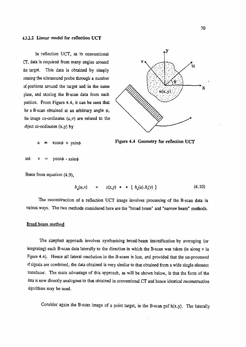
V

x

70

4.3.2.2 Linear mode) for reflection UCT

In reflection UCT, as in conventional

CT, data is required from many angles around

the target. This data is obtained by simply

rotating the ultrasound probe through a number

of positions around the target and in the same

plane, and storing the B-scan data from each

position. From Figure 4.4, it can be seen that

for a B-scan obtained at an arbitrary angle ,

the image co-ordinates (u,v) are related to the

object co-ordinates (x,y) by

u = xcos + ysinc Figure 4.4 Geometry for reflection UCT

and v = ycos - xsin4

Hence from equation (4.9),

b,(u,v) = s(x,y) * * ( ha(U)•hi(V) } (4.10)

The reconstruction of a reflection UCT image involves processing of the B-scan data in

various ways. The two methods considered here are the "broad beam" and "narrow beam" methods.

Broad beam method

The simplest approach involves synthesising broad-beam insonification by averaging (or

integrating) each B-scan data laterally to the direction in which the B-scan was taken (ie along v in

Figure 4.4). Hence all lateral resolution in the B-scans is lost, and provided that the un-processed

if signals are combined, the data obtained is very similar to that obtained from a wide single element

transducer. The main advantage of this approach, as will be shown below, is that the form of the

data is now directly analogous to that obtained in conventional CT and hence identical reconstruction

algorithms may be used.

Consider again the B-scan image of a point target, ie the B-scan psf h(x,y). The laterally

71

averaged psf h(x,y) can be represented as

h(u,v)= J

h(u,v) dv

and using (4.8)

h(u,v) = h(u) . J

h1(v) dv

Assuming a normalised Gaussian function for the lateral beam profile

h1(v) = exp [ a2

where a is a constant proportional to the beam width. Clearly

Jex[' dv = a

Hence the laterally averaged B-scan psf may be represented solely by the axial point response

multiplied by a constant scaling factor,

h(u,v) = a . ha(U) (4.11)

Similarly the laterally averaged B-scan OTF is simply the axial component H() of the B-scan OTF.

To show that image reconstruction in broad beam reflection UCT is directly equivalent to X-

ray CT, assume temporarily that the axial B-scan point response h a(U) can be represented by a delta-

function (u), ie a very short pulse (this is equivalent to the initial assumption of an infinitely narrow

X-ray beam in 2.2). Then the laterally averaged B-scan psf will be given, from equation (4.11), by

h(u,v) = a . ô(u)

and from (4.10) the laterally averaged B-scan b is now

b (u) s(x,y) * * ö(u)

72

Comparing this equation with equation (2.2) it is clear that b(u) can be thought of as a l-D

projection of the object reflectivity s(x,y) along the direction u, where the resolution of the projections

in this case is limited by the axial component of the B-scan psf, or h a(U). Hence in principle any of

the algorithms presented in section 2.3 may be used to reconstruct an image from many projections

b at different angles 4,.

Using a simple back-projection approach results in a broad beam reflection UCT image

s(x,y) given by equation (2.6), ie

s1,,(x,y) = b' (u) dçb = s(x,y) * * h(u) d4,

and thus a back-projected (but unfiltered) broad beam reflection UCT psf given by

h(x,y) = h(U) d4,

(4.12)

Hence the image s(x,y) formed by simple summation (ie no filtering) of laterally averaged B-scans

is the object s(x,y) convolved with a rotated and summed axial B-scan psf, hbb(x,y). Equation (4.12)

can be expressed in the frequency domain as

= S(X,Y) . H1,6(X,Y)

where

H,(X,Y) =

Narrow beam method

It is also possible to derive reconstruction algorithms which allow the lateral information in

the B-scans to be preserved. This method has various advantages over the broad-beam method, the

details of which will be discussed in section 4.4.3.3. The first step in reconstruction is to sum the

B-scan images from all directions to form a summation image s(x,y). In the limit of an infinite

number of B-scans, this is equivalent to an integration with respect to 4,,

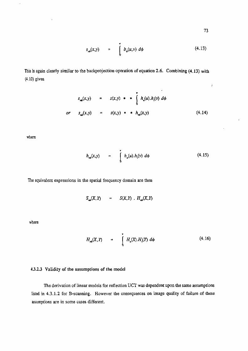
73

s, ,(x,y) = b0(u,v) d4

(4.13)

This is again clearly similar to the backprojection operation of equation 2.6. Combining (4.13) with

(4.10) gives

s,(x,y) = s(x,y) * h(U).h1(V) d

or s(x,y) = s(x,y) * * h(x,y)

(4.14)

where

h(x,y) = h().h1() dc (4.15)

The equivalent expressions in the spatial frequency domain are then

S,Ib(X, F) = S(X,Y) . H,1 ,(X, F)

where

H,,(X,Y) H(X)H1(Y) d4

(4.16)

4.3.2.3 Validity of the assumptions of the model

The derivation of linear models for reflection UCT was dependent upon the same assumptions

listed in 4.3.1.2 for B-scanning. However the consequences on image quality of failure of these

assumptions are in some cases different.

74

(a) Use of demodulated data

Most researchers who have used this technique have, for various reasons discussed in detail

in section 5.3.1, combined demodulated scan lines rather then the raw rf echo data. Hence speckle

cannot be accounted for within this model, just as for conventional B-scanning, and must be

considered as an image artifact. However there is good reason (see section 4.5) to expect that speckle

will be less of a problem for reflection UCT than it is for B-scanning. The consequences of using /

demodulated data for the broad beam method specifically are more compliáated, because in this case

the laterally averaged echo data is not strictly identical to the data that would be obtained from a

single element transducer.

b) Constant acoustic speed

Reflection UCT images are likely to be even more adversely affected by acoustic speed

variations, as shown by previous studies (see 3.2.3). This is because the technique relies on correct

registration (summation) of echoes from all directions through the target. If there are any acoustic

speed variations anywhere within the target, the opportunity is greater in reflection UCT for mis-

registration and consequent loss of resolution to occur.

4.3.3 Transmission UCT point spread function

4.3.3.1 Introduction

The purpose of this section is to derive a linear theory for transmission UCT using the same

formalism and equations as used to describe the backscatter imaging techniques of B-scanning and

reflection UCT. Although this analysis will reveal the principles underlying both acoustic speed and

attenuation CT, only acoustic speed CT will be explored in any detail because, for the reasons

discussed below, only acoustic speed CT has been attempted experimentally in this work.

4.3.3.2 Linear model for transmission UCT

Restating, in differential form, the inhomogeneous Helmholtz equation (4.5) for a field

P ftJ .&' propagating in a uniform medium containing a compressibility inhomogeneity

V2PQj + k02P(rJ = -k ','Q) P

where

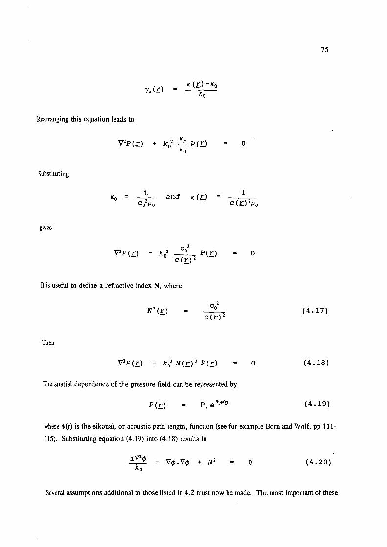
75

- ____

-y,(r ) - ___- IC0

Rearranging this equation leads to

V2P(r) + k02 p(r) = 0K0

Substituting

= ____ and ,c() = 1

c0 p 0 c(r)2p0

gives

Co2V2P(r) + k02 P(r) = 0

c (r)2

It is useful to define a refractive index N, where

c02N 2 (r) = ( 4.17)

c(r)2

Then

V2P(r) + k02 N(r) 2 P(r) = 0 (4.18)

The spatial dependence of the pressure field can be represented by

P(r) = p0 (4.19)

where (r) is the elkonal, or acoustic path length, function (see for example Born and Wolf, pp 111-

115). Substituting equation (4.19) into (4.18) results in

____ - Vp.Vcp + N2 = 0 (4.20)

Several assumptions additional to those listed in 4.2 must now be made. The most important of these

76

is the assumption that diffraction may be neglected. This is equivalent to allowing the ultrasound

wavelength X to approach zero

ie as X - 0, so k 0 = - -

Therefore, by neglecting diffraction, equation (4.20) can be approximated by /

Vc.V4) = N2 (4.21)

Recalling from section 4.2 that the total field equals the incident (ie unperturbed) field plus the

scattered (or perturbed) field, then

4) = + 4)1

where 4 and 4 are the solutions of (4.21) in the unperturbed and perturbed media respectively.

Also let

N = N0+N1

where N0 is the refractive index in the unperturbed medium (ie N 0 = 1) and N 1 is given by

N1 (r) = N(r) - N0= c0 —1

= c0—c(r)

c(r) c(r)

Hence equation (4.21) becomes

V (

+ cp 1) . V (° + ) = (N0 + N1)2

+ 2V4)0 .V4) 1 = N + N12 + 2N0N1 (4.22)

From (4.21) the solution for 4 in the unperturbed medium is given by

V4)0 .V4)0 = N 1

Therefore

= k0.r

where lc is a unit vector in the direction of the incident wave. The solution for the incident field is

77

then

P0(!) = P0e 1k .r

This conforms with the initial assumption of a plane wave propagating along the direction 1cc.

Substituting these results into equation (4.22), and assuming also that the refractive index

perturbations are small, ie N 1 << N0 and hence terms in N 12 and V4i.V4, 1 are negligible, gives a /

solution for the perturbed field

V40.V41 = N0N1

and hence

= N1()

(4.23)

Integrating this equation along a path, which must be parallel to k0, between any two points a and b

gives

41(b) - 1 (a) =

J N1(rJ ds (4.24)

where ds is the element of length along the path a to b.

If the perturbing medium is attenuating the acoustic speed c(t), and hence the refractive index N1(L)

and the eikonal 4), will be complex. It is clear from equation (4.19) that the imaginary part of the

eikonal () is given by

=

Hence the imaginary parts of 4 and N 1 in equation (4.24) give a solution for the integrated

attenuation between a and b as follows

b

1n11 -k0 J

N(j ds (4.25)

Similarly, dividing the real parts of equation (4.24) by the acoustic speed c 0 in the unperturbed

4,(b) - (a)

Co

o(b =

= Jn(rJds

1 _1cfrj C0

(4.26)TOF1a-b] = J

dt =

where

78

medium, gives (Born and Wolf p.1 15) the relationship between the time of flight of the ultrasound

wave between a and b and the relative refractive index ifl)

Equations (4.25) and (4.26) form the basis of ultrasound attenuation and acoustic speed CT.

The principle assumptions made in deriving these equations will now be reviewed and discussed.

4.3.3.3 Validity of the assumptions of the model

Several new assumptions were made in deriving equation (4.26) from equation (4.5). These

were:-

a) That diffraction may be ignored (ie X - 0). This is acceptable if the ultrasonic source, and

all objects within the target, have dimensions which are much greater than the ultrasound

wavelength. This assumption is definitely not valid within soft tissue targets which have

many structures (such as cells, vessels and muscle fibres) of dimensions near to or less than

the wavelength. The consequences of the failure of this assumption are particularly severe

for attenuation imaging, where diffraction effects cause loss of signal at the receiver which

is interpreted as attenuation. This results in inconsistencies in the projection data and causes

loss of accuracy and artifacts in the reconstructed image. The affects on the measurement of

pulse TOF, and hence on acoustic speed imaging, are likely to be less severe but will depend

critically on the method chosen for determining pulse arrival. An experimental investigation

into various methods of measuring pulse TOF has been conducted and will be reported in

section 6.5.3.

b) That both incident and transmitted waves are plane waves. Although difficult to achieve

exactly, a fair approximation to plane wave insonification can be achieved by placing the

target in the focal zone of a weekly focused transducer.

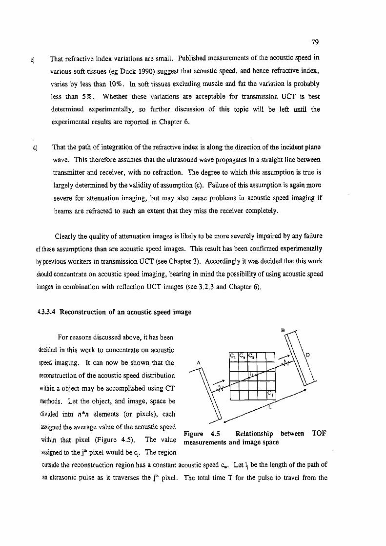
79

c) That refractive index variations are small. Published measurements of the acoustic speed in

various soft tissues (eg Duck 1990) suggest that acoustic speed, and hence refractive index,

varies by less than 10%. In soft tissues excluding muscle and fat the variation is probably

less than 5%. Whether these variations are acceptable for transmission UCT is best

determined experimentally, so further discussion of this topic will be left until the

experimental results are reported in Chapter 6.

d) That the path of integration of the refractive index is along the direction of the incident plane

wave. This therefore assumes that the ultrasound wave propagates in a straight line between

transmitter and receiver, with no refraction. The degree to which this assumption is true is

largely determined by the validity of assumption (c). Failure of this assumption is again more

severe for attenuation imaging, but may also cause problems in acoustic speed imaging if

beams are refracted to such an extent that they miss the receiver completely.

Clearly the quality of attenuation images is likely to be more severely impaired by any failure

of these assumptions than are acoustic speed images. This result has been confirmed experimentally

by previous workers in transmission UCT (see Chapter 3). Accordingly it was decided that this work

should concentrate on acoustic speed imaging, bearing in mind the possibility of using acoustic speed

images in combination with reflection UCT images (see 3.2.3 and Chapter 6).

4.3.3.4 Reconstruction of an acoustic speed image

For reasons discussed above, it has been

decided in this work to concentrate on acoustic

speed imaging. It can now be shown that the

reconstruction of the acoustic speed distribution

within a object may be accomplished using CT

methods. Let the object, and image, space be

divided into nn elements (or pixels), each

assigned the average value of the acoustic speedFigure 4.5 Relationship between TOF

within that pixel (Figure 4.5). The value measurements and image space

assigned to the th pixel would be c. The region

outside the reconstruction region has a constant acoustic speed c. Let l be the length of the path of

an ultrasonic pulse as it traverses the jth pixel. The total time T for the pulse to travel from the

T—T,,

T - T,, (4.27)

80

transmitter (A) to the receiver (B) is given by

T = >.L + i

j cicw

This equation is not yet in a form that can be solved by CT methods, because the parameter

to be reconstructed must be zero outside the reconstruction region. To obtain such a parameter it is

necessary to measure the time T for the pulse to travel the same path with no object present, or in

other words, just through the water.

Lze T = -w

where = i__I

cic

is the relative refractive index of the jU1 pixel.

Equation (4.27) is consistent with the more rigorously derived equation (4.26), and meets the

criteria for CT reconstruction in that (i) it defines a measurable quantity (1' - T) that is given by the

linear summation of the parameter to be reconstructed (m) multiplied by a function of length, and (ii)

the reconstructed parameter is zero everywhere outside the reconstruction region. Also, note the

similarity to the equivalent expression for the ratio of received to transmitted X-ray intensities well

81

known from X-ray CT.

—ia!

=

'0

By measuring T - T for many parallel rays across the target, a TOF projection (P 0) of the

object is formed. By obtaining many projections at different angles enough information can be /

acquired to reconstruct, using any of the algorithms discussed in Chapter 2, the value of i for every

pixel in the image. Using a simple back-projection approach results in an acoustic speed image (x,y)

given by equation (2.6), ie

(x,y) = P(u) dcb

(4.28)

Note that the resolution of the projection is determined by the ultrasound beam width, ie by h1(u).

Thus the back-projected (but unfiltered) acoustic speed image psf is given by

h(x,y) = h1(u) d4

(4.29)

Although the quantity that is actually reconstructed is , if c, is known it easy to convert these values

into the acoustic speed c3.

82

4.4 A comparison of B-scan and UCT point spread functions

4.4.1 Introduction

Having shown that the image formation processes leading to conventional B-scan and UCT

images may be considered as approximately linear (and accepting that violations of this assumption

cause image artifacts), it is now possible to compare the potential spatial resolution of conventional

B-scanning, reflection UCT and transmission UCT by considering their respective point spread

functions.

4.4.2 B-scan psf

Equation (4.9) defined the B-scan imaging process as a linear convolution between the

scatterer distribution s(x,y) and a point spread function h(x,y),

b(x,y) = s(x,y) * * h(x,y)

Equation (4.9) has an equivalent expression in the spatial frequency domain given by

B(X,Y) = S(X,Y) - H(X,Y) (4.30)

where B(X,Y), S(X,Y) and H(X,Y) are the Fourier transforms of b(x,y), s(x,y) and h(x,y)

respectively. The B-scan psf can be measured fairly easily by obtaining a B-scan of a very thin wire

target orientated perpendicularly to the scan plane (see Chapter 5).

The axial resolution (along the beam axis) of a B-scan image is given by ha(x) and hence is

determined by the length of the transmitted ultrasound pulse. Neglecting the electro-mechanical

properties of the transducer in receive and the limited bandwidth of the receiver amplifiers, h a(x) may

be approximated by half the transmitted pulse length since the range x is a function of c.t12, where

is the go-return time of the pulse.

The lateral resolution is given by h(y) which is determined by the ultrasound beam-width.

In fact it is the pulse-echo beam width that is required, again because of the two-way passage of the

acoustic pulse. Since the minimum possible (ie with focusing) beam width at a given point is

determined fundamentally by the angle subtended by the transmit-receive aperture at that point, good

lateral resolution in B-scan images requires large or enclosing transducer apertures. Unfortunately

83

in real-time B-scanning it is often not beneficial to increase aperture lengths beyond a few centimetres,

because in many of the sites of the human body where the technique is applied the superficial areas

free of bone or gas (often called acoustic "windows") are relatively small.

It is instructive to consider the situation in the spatial frequency domain. Equation 4.30 shows

that the frequency content of the object distribution will be modified by the frequency content of the

OTF. Since the OTF is inevitably band-limited by the pulse length, the beam width and by the

limited bandwidth of the receiver amplifiers, the B-scan image will not be an accurate representation

of the object. Typically, the axial component Ha(X) will have a wider band-width than the lateral

component H 1 (Y), because the axial pulse length is typically 3 to 4 times shorter than the lateral beam-

width. Hence the resolution of a B-scan image is limited primarily by the lateral component of the

OTF, which is itself determined by the pulse-echo beam generated by the transducer aperture.

4.4.3 Reflection UCT psf

It has been shown that the resolution of a B-scan image is limited mainly by the lateral

component of the OTF, the axial component typically have a much wider band-width. This is why

computed tomography techniques involve obtaining data from many directions about an object

because, by rotating the B-scan psf, the maximum band-width available (in this case the axial band-

width) can be made to extend in all directions. Part of the CT reconstruction process can be thought

of as an attempt to restore, as closely as possible, the frequency content of the original object from

knowledge of the OTF.

4.4.3.1 Broad-beam method

The broad beam reflection UCT psf was given by equation (4.12) as the axial component ha(u)

of the B-scan psf rotated and summed over 180°,

h 1,,(x,y) = h0(u) d4

Note that, unlike the B-scan psf, hbb(x ,y) (or its Fourier Transform Hbb(X,Y)) will have rotational

symmetry (see Figure 4.6).

ie H1,,(X,Y) = HL,,,(R)

Y

x

84

where R = ( (X)2 + (Y)2 }112

Mso, Hbb(R) will have a maximum frequency

L equal to the maximum frequency in the

axial component H2(U) of the B-scan OTF.

Hence the image s,(x,y) should be an

improvement on an individual B-scan image

b(x,y) since it will have a wider overall

bandwidth, although it's frequency content will

still have been modified from that in the object

because, in general, Hbb(R) will not have a \: >' /'

constant value inside the circle with radius R,,. '(/'.>-" ,"

In fact the H bb(R) approaches the exact (1IR) - - - - - - - -. " H.(R)

function predicted by CT theory as the axial B- Figure 4.6 OTF for broad-beam reflection UCTscan psf h(u) approaches a delta function.

Hence it may be possible to use CT reconstruction filters (such as the Shepp-Logan filter discussed

in Section 2.3.2) to de-convolve the (lIr) blurring and reduce the reflection UCT psf to closer to the

axial B-scan psf.

4.4.3.2 Narrow-beam method

The narrow beam reflection UCT psf was given by equation 4.15 as

h(x,y)

h(zs).h1() d4

and the OTF by

H,,,(X,Y)

H(X).H1(Y) d

A possible narrow beam OTF is shown in Figure 4.7. Both the narrow beam psf and the

OTF will again have rotational symmetry, and H(R) will again have a maximum frequency R,,,,

equal to the maximum frequency in the axial component H(U) of the B-scan OTF. However hb(r)

is of more limited extent than the broad beam psfh bb(r), because the incorporation of lateral resolution

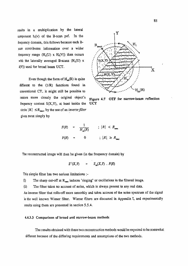
. ..•_.7

'S.

85

results in a multiplication by the lateral

component h 1(v) of the B-scan psf. In the

frequency domain, this follows because each B-

scan contributes information over a wider

frequency range (Ha(U) x H 1 (V)) than occurs

with the laterally averaged B-scans (H(U) x

(V)) used for broad beam UCT.

Even though the form of Hth(R) is quite

different to the (1IR) functions found in

conventional CT, it might still be possible to

restore more closely the original object's

frequency content S(X,Y), at least inside the

circle R ^R,,, by the use of an inverse filter

given most simply by

Y

I,,,!

-

- - - - - -- - I(R)

Figure 4.7 OTF for narrow-beam reflectionUCT

x

F(R) = ____

<R

F(R) = 0

;IR I ^R

The reconstructed image will then be given (in the frequency domain) by

S' (X, Y) = I') . F(R)

This simple filter has two serious limitations

(i) The sharp cut-off at R,,,, induces 'ringing' or oscillations in the filtered image.

(ii) The filter takes no account of noise, which is always present in any real data.

An inverse filter that rolls-off more smoothly and takes account of the noise spectrum of the signal

is the well known Wiener filter. Wiener filters are discussed in Appendix I, and experimentally

results using them are presented in section 5.5.4.

4.4.3.3 Comparison of broad and narrow-beam methods

The results obtained with these two reconstruction methods would be expected to be somewhat

different because of the differing requirements and assumptions of the two methods.

86

i. Resolution and inverse filtering

It has been shown that the unfiltered narrow beam psf is narrower than the broad beam psf,

because the incorporation of lateral resolution restricts the total extent of the psf to that of the lateral

B-scan psf. Hence any inverse filtering performed to restore more closely the object's frequency

content is likely to be more successful for the narrow beam method, because its OTF falls-off into

noise less quickly.

ii. Number of view directions required

It was shown in Section 2.4 that, in order to satisfy sampling requirements, the number of

projections (or view directions) N required over 180 degrees is given by

N= jrD

(4.31)

where D is the diameter of the reconstruction region (ie the length of the projection) and p is the

resolution of the projection, which for reflection UCT is the axial resolution given by half the

transmitted pulse length.

In a wide-field linear array probe the scanned ultrasound field is typically about 30 times

wider than the width of an individual ultrasound beam. For the broad-beam method the projections

are across the full width (D) of the ultrasonic field, whereas for the narrow beam method the

projections are only across the null-null width of the beam. This suggests that the broad beam method

would require about 30 times more view directions than the narrow beam method to satisfy the

sampling requirements. This argument is demonstrated graphically by comparing the OTF of a B-

scan (Figure 4.7) with the OTF of a laterally averaged B-scan (Figure 4.6). This confirms that many

fewer views would be required to adequately sample the object's frequency space using the narrow

beam method than using the broad beam method.

4.4.4 Transmission UCT psf

The psf of an acoustic speed image obtained from transmission measurements was given by

equation (4.29) as

h(x,y) = h1(u) d

87

Thus the theoretical psf is similar to that obtained for broad-beam reflection UCT (equation 4.12),

except that for acoustic speed imaging it is the lateral component of the B-scan psf that determines

the limits of the psf instead of the much shorter axial component. Hence the resolution of an acoustic

speed image, even after filtering, will inevitably be poorer than for a reflection UCT image.

The number of TOF projection required to reconstruct an acoustic speed image is again given

by equation (4.31). The diameter of the reconstruction region is again the width of the ultrasound

field D, while the resolution of the projections (zp in 4.31) is now given by the 6dB beam width (w).

88

4.5 Other factors influencing B-scan and reflection UCT image quality

In the previous sections it has been shown theoretically that, when compared in terms of their

respective point spread functions, reflection UCT images should show better overall spatial resolution

than conventional B-scans.

However many assumptions had to be made about the linearity of ultrasound imaging in order

that a theory could be derived relating reflection UCT and B-scan psfs. It was shown in sections

4.3.2.3 and 4.3.3.3 that some of these assumptions do not strictly hold, resulting in the appearance

of certain artifacts and other characteristic features in the images. Examples of these affects are

speckle and specular reflection. It will be argued below that, although both reflection UCT

techniques are less severely affected by these artifacts than conventional B-scans, the broad beam

method is likely to be more severely affected than is the narrow beam method.

4.5.1 Specular reflection

The appearance of specularly reflecting surfaces is one of the main features of a B-scan

image, a typical example being the boundary of an organ such as a kidney. It is observed that the

organ boundary is only seen when it is virtually perpendicular to the scanning ultrasound beam axis.

Since in a B-scan system ultrasound beams are directed into the target over only a very limited range

of angles, determined by the solid angle subtended by the transmitting-receiving aperture, visualisation

of organ boundaries is incomplete and this makes interpretation of ultrasound images more difficult.

The reflection UCT techniques involve combining backscatter data from all angles around a

target. Hence specularly reflecting surfaces should contribute echoes to at least one view direction

and hence should always be visualised on the resultant image. For the broad beam method, a strong

echo at one probe direction from a local ised surface will 'spread' its contribution across the full width

of the image because of the operation of averaging across the field width. With the narrow beam

method, however, the contribution will be localised to a single beam width and hence will not

significantly contaminate other parts of the image, resulting in better signal to noise.

4.5.2 Speckle and contrast resolution

Speckle arises as a consequence of applying non-linear processing to the echo data. The effect

89

of demodulation is that the interference between scatterers within the same sample volume (ie the

pulse length * beam width) can no longer be accounted for, resulting in speckle. In conventional B-

scan images speckle actually appears as a roughening or granularisation of what might be expected

to be homogeneous areas of an image. It is normally considered as undesirable noise since it can

obscure small structural details and hence leads to reduced spatial resolution. Speckle noise also

masks the underlying mean backscatter level of the tissues, resulting in a relatively poor signal to

noise ratio and hence poor contrast resolution.

The 'granules' or speckle patches have a characteristic size related to the resolution (and

hence sample volume) of the scanning system - the better the resolution, the smaller are the speckle

patches. On B-scans obtained from very different view angles the conditions for interference between

scatterers and hence the speckle patterns observed will be completely different, with the correlation

between speckle patterns gradually increasing as the angle between the B-scans gets smaller.

Reflection UCT techniques aim to take advantage of the fact that data obtained from different

view angles should have independent speckle components. When the data is combined into a single

image the speckle sums randomly, whereas echoes from strong scatterers which are less corrupted

by speckle sum linearly, resulting in an effective reduction of the relative mean speckle level and an

improved "signal to noise" ratio. A reduction in the speckle noise level should also result in

improved contrast resolution.

Clearly the effectiveness of this speckle reduction will depend on the size of the speckle

"patches" in the original data. For the broad beam method the effective sample volume is much

larger than in the narrow beam method, because the 'beam' now has the full width of the ultrasonic

field, making the speckle patches much larger and the reduction in speckle level obtained by

summation less significant.

90

4.6 Conclusions

It has been shown it this section that linear models can be used to describe the processes of

image formation for B-scanning, reflection UCT and transmission UCT, and consequently that point

spread functions can be derived and subsequently used to compare their potential resolution. However

certain characteristic features of the images (such as speckle in B-scans and reflection UCT images),

which result from processes for which linear theory is violated (for example the non-linear process

of demodulation in B-scanning and reflection UCT), will not be totally accounted for by the psf and

must therefore be accepted as second order perturbations or artifacts.

Comparing these techniques on the basis of their predicted point spread functions (or their

optical transfer functions) shows that better resolution is expected from reflection UCT than from B-

scanning. Reflection UCT methods should also be less affected by most of the artifacts which appear

in B-scan images, and in particular they should have a lower mean speckle level and hence better

contrast resolution. Of the two reflection UCT methods considered here, the narrow-beam method

should have the best resolution and should be the least affected by any residual image artifacts.

Acoustic speed imaging should have fewer artifacts than attenuation imaging because it is less

affected by refraction, but even without artifacts the resolution is only likely to be as good as the

lateral resolution of a B-scan image.

91

5 Development of a system for reflection UCT

5.1 Introduction

The results obtained by other researchers into ultrasound CT (Chapter 3), and the theoretical

comparison of ultrasound CT techniques undertaken as part of this work (Chapter 4), both suggested

that reflection-mode UCT was the technique that was most likely to be able to achieve one of the main

objectives of this work - namely to develop a practical scanning system able to produce high quality

images of soft tissue, preferably in-vivo. Due to the anticipated technical difficulties of constructing

a water-bath scanning system suitable for in-vivo studies, it was decided that a practical investigation

into reflection UCT should start with the development of a relatively simple system which would

allow initially the imaging of phantoms and in-vitro targets only. Hence in the development of this

system the desire for short scanning times, which would be one of the main requirements of a clinical

system, has in general been sacrificed in favour of high positional accuracy and thus optimum image

quality.

This chapter will describe the main considerations involved in the design and construction of

a practical reflection CT system for the study of in-vitro targets. The first stage in this process is to

define the requirements of an "ideal" system, arid then to establish specifications for a practical

system, in terms of its mechanical, electronic and software components, which are realistically

achievable within the cost and time constraints. The construction of this system will be described,

along with the sequence of events involved in acquiring the experimental data and reconstructing an

image.

Various experiments will then be described, which attempt to establish whether the

improvements in image quality predicted theoretically (in Chapter 4) are achieved in practice. This

chapter will then conclude with a general discussion of the relative advantages and limitations of this

reflection-only UCT system, and suggestions for the development of an improved system.

92

52 General requirements

Since this system was intended mainly as a test bed for reflection UCT and not as a clinical

scanner, it was possible to design a system which could be built relatively quickly and cheaply, and

mostly with materials and expertise already available in the Medical Physics department.

The basic requirement of a system to perform reflection UCT is that pulse-echo information /

must be obtainable from many directions about a target, with each direction defined by a constant

centre of rotation. The need for a constant centre of rotation prohibits direct contact of the ultrasound

source with the target, so that the scanning must be performed in a fluid coupling medium such as

water. It was decided that this reflection UCT system would be designed to scan in a vertical plane

because a prototype scanning tank had already been constructed along these lines, and because it was

felt that a vertical plane system would be easier to build. The choice of a vertical scan plane limits

the maximum scanning angle to about 180 degrees for any practical target (ie one that can be

submerged by only a few centimetres in water), but may allow easier access for some potential in-

vivo targets such as the neonatal head.

For reasons discussed fully in section 4.4.3.3, it was decided that a narrow beam approach

to reflection UCT would be implemented. Thus an ultrasound transducer was required for the

transmission and reception of ultrasound pulses along a narrow beam, with the beam being scanned

in a lateral direction to allow pulse-echo measurements to be made at many positions across the full

extent of the target. The transducer must also be able to rotate through 180' around the target and

about a constant centre of rotation. It should also be possible to move the position of the transducer

in a direction perpendicular to the plane of rotation, ie to allow multiple parallel slices to be acquired.

This movement however need not be under the control of the computer and can be done manually.

An alternative to rotating the transducer around the target is to rotate the target itself. This approach

has the side benefit of allowing greater than 180° scanning of the target even with a vertical plane

system. However, it was decided that the difficulty of preventing deformation of a soft tissue target

rotating rapidly in water and the impracticality of ever scanning in-vivo with this approach outweighed

the potential advantages.

A high speed digitiser is required with sufficient memory to store the data required for a

single reconstruction. Software is required to control scanning movement, data acquisition, data

storage, image reconstruction and image display. A computer is required that is powerful enough to

93

reconstruct the reflection UCT images in a reasonable time. The computer must also be able to

display the images to a resolution that as least as good as the inherent resolution of the images.

Probe/

Motoi :dr'system.ntrasound generation

and detecUon.

94

3 Detailed requirements and specifications

The basic requirements outlined above will now be examined in detail, in terms of what would

constitute an "ideal" system and in terms of what has been achieved in practice.

For the purposes of ease of specification and design, the scanning system was broken down

into several sub-systems (shown schematically in Figure 5.1) which could be designed and constructed

separately. These will be described in the following sections.

Mechanical Scanning System

Encoder

Positional dataControl

Control• Dlgftisation and• data: transfer:

Ultrasonic

:9ftyarc:. : : : ControlUltrasonic data

Figure 5.1

Schematic diagram of the reflection-only system.

5.3.1 Ultrasound generation and detection

In order to limit development time and costs, the system for ultrasonic generation and

detection was based around a commercial Hitachi EUB-24 linear array scanner (Figure 5.2) which

was no longer required for other clinical imaging. The scanner consists of a linear array probe

(Figure 5.3) with a nominal 3 MHz centre frequency, plus electronics for ultrasonic signal detection

and display. Despite its age (built in 1977), this scanner had the advantage of possessing a wide-field

width (10.5 cm) linear array probe. The use of a linear array allows the lateral scanning requirement

of narrow beam reflection UCT (see 4.3.2.2) to be performed electronically rather than mechanically,

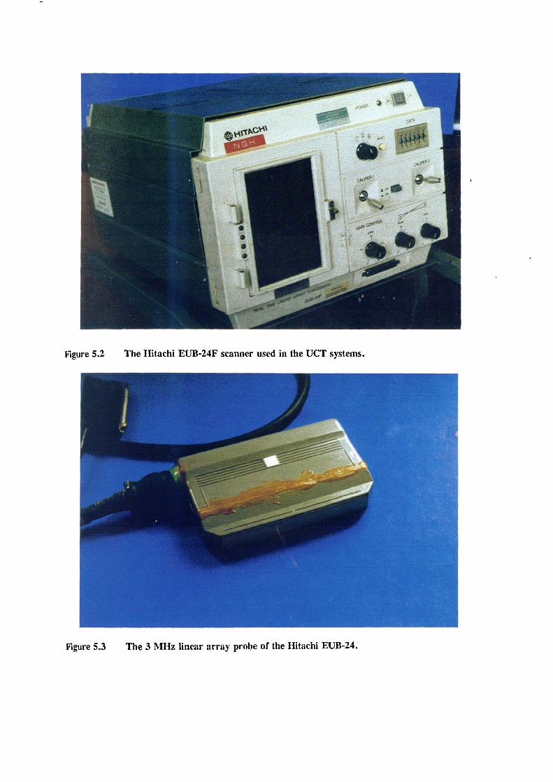
2

1

Figure 5.2

The Hitachi EUB-24F scanner used in the UCT systems.

Figure 5.3 The 3 MHz linear array probe of the Hitachi EUB-24.

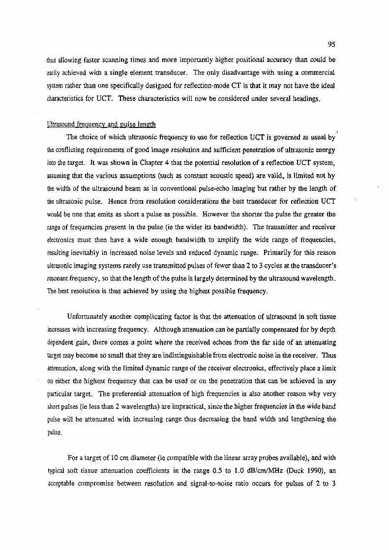
95

thus allowing faster scanning times and more importantly higher positional accuracy than could be

easily achieved with a single element transducer. The only disadvantage with using a commercial

system rather than one specifically designed for reflection-mode CT is that it may not have the ideal

characteristics for UCT. These characteristics will now be considered under several headings.

Ultrasound frequency and pulse length

The choice of which ultrasonic frequency to use for reflection UCT is governed as usual by'

the conflicting requirements of good image resolution and sufficient penetration of ultrasonic energy

into the target. It was shown in Chapter 4 that the potential resolution of a reflection UCT system,

assuming that the various assumptions (such as constant acoustic speed) are valid, is limited not by

the width of the ultrasound beam as in conventional pulse-echo imaging but rather by the length of

the ultrasonic pulse. Hence from resolution considerations the best transducer for reflection UCT

would be one that emits as short a pulse as possible. However the shorter the pulse the greater the

range of frequencies present in the pulse (ie the wider its bandwidth). The transmitter and receiver

electronics must then have a wide enough bandwidth to amplify the wide range of frequencies,

resulting inevitably in increased noise levels and reduced dynamic range. Primarily for this reason

ultrasonic imaging systems rarely use transmitted pulses of fewer than 2 to 3 cycles at the transducer's

resonant frequency, so that the length of the pulse is largely determined by the ultrasound wavelength.

The best resolution is thus achieved by using the highest possible frequency.

Unfortunately another complicating factor is that the attenuation of ultrasound in soft tissue

increases with increasing frequency. Although attenuation can be partially compensated for by depth

dependent gain, there comes a point where the received echoes from the far side of an attenuating

target may become so small that they are indistinguishable from electronic noise in the receiver. Thus

attenuation, along with the limited dynamic range of the receiver electronics, effectively place a limit

on either the highest frequency that can be used or on the penetration that can be achieved in any

particular target. The preferential attenuation of high frequencies is also another reason why very

short pulses (ie less than 2 wavelengths) are impractical, since the higher frequencies in the wide band

pulse will be attenuated with increasing range thus decreasing the band width and lengthening the

pulse.

For a target of 10 cm diameter (ie compatible with the linear array probes available), and with

typical soft tissue attenuation coefficients in the range 0.5 to 1.0 dBIcmIMHz (Duck 1990), an

acceptable compromise between resolution and signal-to-noise ratio occurs for pulses of 2 to 3

96

wavelengths with a resonant frequency in the range from 2 to 3 MHz. In terms of resolution, a 3

MHz pulse of 3 cycles length would imply a total pulse length of 1.5 mm (and a potential pulse-echo

resolution of about 0.75 mm) in soft tissue.

The transmitted pulse from the Hitachi's 3 MHz linear array was measured in water using a

PVDF hydrophone with an 0.5 mm diameter active element. The pulse obtained approximately at

the focus, and its spectrum, are shown in Figures 5.4a and 5.4b respectively. The pulse shows /

minimal affects from non-linear propagation, probably due to the relatively low transmitted peak

negative pulse amplitude of 0.35 MPa at the focus, as measured by the Department's output

measurement system (Martin 1986). The pulse has a centre frequency of 3.0 MHz, and a 6dB

bandwidth of 1.7 MHz, which is within the range specified above as suitable for breast imaging. The

pulse length is also acceptable, being about 1.5 mm and thus giving an axial pulse-echo resolution

of approximately 0.75 mm.

Ultrasound beam width

Under ideal circumstances the width of the ultrasound beam should have no affect on the

resolution or quality of reflection UCT images. However, as argued in section 4.5.1, the assumptions

inherent to the reflection UCT method, such as the neglect of specular reflection, become more

unreliable and result in worsening artifacts as the beam width increases. Hence a transducer used for

reflection UCT should ideally have as narrow a beam as possible. Narrow beams are traditionally

obtained by strong focusing, which results in a narrow beam around the focal range but with wide

beam widths both before and after the focus. In the case of reflection UCT a uniformally narrow

beam is required ideally throughout the extent of the target. Note that for reflectivity imaging it is

the pulse-echo beam width and not simply the transmitted beam width which is relevant. In modern

ultrasound systems the pulse-echo beam width is kept narrow by techniques such as dynamic focusing

on receive, in which the position of the focal zone is varied dynamically to coincide with the sources

of echoes as they arrive at the transducer from greater and greater depths.

A fundamental requirement of CT imaging in general is that each image plane is assumed to

be effectively independent from other parallel planes. In ultrasound imaging this is only possible if

the width of the ultrasound beam in the direction perpendicular to the scan plane (often called the slice

thickness) is infinitely thin, or at least in practice as thin as possible.

a) 0.6

0.4

8-i0.2

Cl)Cl)'a)8.4

Cl)0.0

U,'a.)C)

—0.2

0.5 1.0 1.5 2.0Range (mm)

—0.40.0

97

b) 1.0

0.75

0.5

0.25

0.00 2 4 6 8 10

Frequency (MHz)

Figure 5.4 Transmitted (a) pulse and (b) spectrum from the Hitachi EUB 24's 3Mhz lineararray probe.

98

A pulse-echo beam profile for the Hitachi EUB-24's 3 MHz probe, measured in water using

the Department's beam plotting system, is shown in Figure 5.5a. The beam has a pulse-echo focus

at about 58 mm from the transducer. In the near-field the beam width converges from a 6 dB

beamwidth of 10.0 mm at 2cm from the transducer face to 3.6 mm at the focus. Beyond the focus

the beam diverges at an angle of about 1.5 degrees, reaching a 6 dB width of 6.2 mm at a range of

12 cm. Clearly it would be impossible with this probe to maintain a constant beam width over a /

typical target dimension of about 10 cm (see below), mainly because the Hitachi EUB-24 does not

perform dynamic focusing. This consequences of this limitation will become evident in later sections.

Figure 5.5b shows a pulse-echo beam plot obtained with the Hitachi EUB-24's probe rotated

through 90 degrees, and hence shows the beam profile perpendicular to the scan plane. The out of

plane focus is at about 36 mm, with a minimum 6 dB slice thickness of 4.6 mm and up to 13 mm at

12 cm. Although this slice thickness performance is typical for a linear array of this type, it should

be realised that in any image produced with this probe there may be significant contamination from

targets located above or below the image plane.

Scanned field width and beam spacing

One of the basic requirements of reflection UCT using narrow beams is that the

transmitting/receiving transducer aperture must be scanned laterally across the whole width of the

target, with pulse-echo measurements obtained at regular precisely known intervals. From sampling

requirements (see 2.4) the interval between measurement positions should be no more than half the

6 dB beam width. The accuracy at which the position of the aperture must be known will be

discussed in section 5.3.4.

For this probe the field-width is 10.5 cm, which thus restricts the maximum target diameter

to about 10 cm. This target diameter is less than ideal, but since very few commercial linear arrays

are available which offer a wider field width, it was decided that this limit would be acceptable for

a prototype system. The array is composed of 80 elements at 1.5 mm intervals, and fired in batches

of 10 giving an active aperture width of 15 mm and a total of 70 lines per B-scan frame (ie 1.5 mm

beam spacing). Thus the beam spacing of 1.5 mm meets the requirements of sampling theory in that

it is less than half the beam width at any range. The line period is 278 microseconds, giving a

maximum possible imaging range of about 20 cm in water. The field period is 21 .Smsec, which is

therefore the absolute minimum time taken to acquire the pulse-echo data for one B-scan.

V.,

•.

-

a)

b)

Figure 5.5 Pulse-echo beam plots of the 3 MHz linear array; a) parallel to the scan plane,and b) perpendicular to the scan plane. Each grey level represents a 6 dBchange in echo amplitude.

100

Signal processing

An ideal system for reflection UCT would involve no non-linear processes in the measurement

system since, as emphasised in Chapter 4, the principles of CT reconstruction are based on linearity

and superposition. Hence signal demodulation and non-linear amplification are both undesirable

features.

In principle signal demodulation could be avoided by using the raw RF data, but this is often

impractical because of:-

a) The high digitisation rates required (ideally > 20 MHz for a 3 MHz pulse with a 1.2 MHz

bandwidth).

b) The large amount of storage required because of the high digitisation rates.

c) The very high accuracy required in the positional system to prevent incorrect phase

cancelation of signals combined from different transducer angles or positions. To prevent

phase cancellation a positional accuracy of better than the ultrasonic wavelength/lU is

required, which for 3 MHz implies a positional accuracy of better than 0.05 mm.

Factors b) and c) above have limited the work presented in this thesis to the processing of

demodulated signals, although it is hoped that it may be possible to use RF signals at a later date.

Strictly speaking, this limitation invalidates the use of the linear equations derived in section 4.3 and

4.4 for B-scan and reflection UCT image formation. However, as argued in section 4.3.1.3 these

equations may still be used, provided that we accept that speckle will not be accounted for and that

the resolution of the system can never be less than half the pulse length. In practice speckle is much

less of a problem in reflection UCT images than in conventional B-scan images, because of the fact

that UCT images are composed of many separate B-scans obtained from different angles. Since the

B-scans contain essentially independent speckle patterns, the mean speckle level in the combined

image will increase byv'n, where n is the number of B-scans, whereas the echo level of any strong

scatterers will, assuming correct registration, increase by a.

In a conventional B-mode pulse-echo system, the RF echo signal is demodulated (or envelope

detected) before display. However the demodulated signal from the Hitachi EUB-24 was found to

be noisy and a poor representation of the true signal envelope. In addition the EUB-24 performs

various other non-linear processing operations on the RF signal, such as automatic gain control (AGC)

and edge-enhancement. Consequently it was decided that the RE signal would be extracted from the

4.7m

56OII Imil

IOK}IH

I)2N3904

--

I v'I'1H

I I III

2N29 13

-12 V

5.6m uFull wave rectifier(Diasonograph NE41020)

560 1

Chebyshev low-pass filter

5.6 12.511 9.111

ITFf- 2i : 1500[470T700T500[E]

1.6K 162 1.6K I-I--------------------------------------

Figure 5.6 Circuit for signal demodulation, incorporating a full-wave rectifier from aDiasonogaph NE4IO2A.

EUB-24 before the demodulation stage and fed into a separate circuit designed specifically to perform

low noise demodulation. The full-wave rectifier part of this circuit is a modification to one used in

a Diasonograph NE4IO2A B-mode scanner. The low-pass filter is a 9-pole Chebyshev with a high

frequency roll-off at 1.25 MHz, and was designed specifically for this UCT work. The circuit layout

is shown in Figure 5.6.

Logarithmic compression is another non-linear processing stage usually present in

conventional B-scanning. It will now be shown how this stage can be usefully retained for reflection

UCT even though it violates the assumption of linearity. The main reason for performing logarithmic

compression on the received signal is that the dynamic range (ie the ratio of the largest to the smallest

signal) of the echoes from soft tissue and tissue interfaces may be as high as 50 dB, whereas the

dynamic range of a typical 6-bit digitiser used in conventional scan-converters is only 36 dB. Much

of the structural information of most interest is contained in the lower level echoes which because of

the limited dynamic range of the digitiser can be represented by only a relatively small number of

digitised levels. Conversely the echoes from tissue interfaces are relatively large and need not be

represented by very many digitised levels to preserve their information. Hence appropriate

logarithmic compression of the echo signal is applied to allow the echoes of most interest to be better

matched to the available dynamic range of the digitiser.

102

For this work an 8-bit digitiser (dynamic range is 28 or 48 dB) has been used (see below).

This obviously reduces the problem, but it is still useful to have as many digitised levels as possible

available for the lower level echoes. The problem of non-linearity has been alleviated by restoring

the linearity of the digitised data in the computer. This was done by first converting the data into 16-

bit numbers to allow a higher dynamic range (96 dB), and then scaling the data with the inverse of

the logarithmic compression function.

5.3.2 Digitisation, data transfer and sampling requirements

5.3.2.1 Digitisation rates and dynamic range

The digitisation rates required depend on the maximum frequency content of the signal being

digitised. The Nyquist sampling criterion requires that the digitisation rate should t,e at least twice

the highest frequency present in the signal. Since all real signals are inevitably contaminated to some

extent by wide band noise, in practice the rate should be higher than this to ensure that all signal

frequencies are reproduced with the correct amplitude. It has been decided here to sample at twice

the Nyquist frequency, ie at four times the highest frequency in the signal. For demodulated echoes

from the 3 MHz probe there should be no significant signal above 1.5 MHz, and so ideally a

digitisation rate of at least 6 MHz should be used.

Any digitised signal has a limited dynamic range determined by the number of binary digits

(bits) assigned to each digitised sample. As discussed in the previous section, an 8-bit (48 dB)

digitiser should be adequate provided that the dynamic range of the echo signal has been

logarithmically compressed before digitisation.

The total amount of data required for the reconstruction of a complete reflection UCT image

of a single plane will depend on the following factors:-

(1) The number (Np) of B-scan positions around the target.

(2) The number (I) of beam positions making up each B-scan.

(3) The total pulse-echo time required at each beam position which depends on the diameter (d)

of the target being scanned and the average acoustic speed (c) of the target.

(4) The digitisation rate (R).

(5) The dynamic range (D) of the digitiser in bytes (1 byte = 8 bits) per sample.

103

The formula for the total amount of data required (in bytes) is

Number of bytes =

(5.1)

C

5.3.2.2 Sampling requirements

It was shown in section 4.6.3.3 that, to obtain an adequately sampled reconstruction using the

narrow beam method, the number of B-scans required within a total angle of 180° is given by

Nrw

P 24

where w is the minimum null to null pulse-echo beam width and 4 is half the transmitted

pulse length. Hence for this system

N = in I 151 ...7 mm1

1.5 mm]

(5.2)

It is preferable that the data is acquired and stored as quickly as possible in order to minimise

the possibility of target movement during the scan. Hence an ideal system would allow all of the data

for one reflection UCT image to be stored in very fast access memory, since the relatively slow

transfer of data onto computer disc (for example) would extend the acquisition time.

A Le-Croy 200-MHz 8-bit transient recorder and buffer was used for digitisation of the

demodulated pulse-echo signals. The Le-Croy is a fully programmable system with 1 MByte of data

storage. Assuming a digitisation rate R of 6.25 MHz, and substituting values for 1, d, c and D of 70,

0.105 m, 1540 m/s and 1 respectively, results from (5.1) in a total amount of data for a single

reflection UCT image of 893,750 bytes. Hence all of the data for one reconstruction can be stored

in the transient recorder's buffer storage.

The transient recorder is interfaced to the computer for control and data transfer via an IEEE

high-speed bus. Many features of the system are programmable, including choice of digitisation

rates, definition of digitisation windows, choice of pre- and post-trigger samples and selection of

amplifier gains and offsets. Criteria for the selection of these parameters will be discussed in section

5.4.3.

CLR

D

7474

C

PRST

104

READY (from computer)

STOP

(to computer)

Fr\±I

D Qi

FRAME SYNCH 7474

C

(from EUB24) PRSTTRIGGER

digitiser)

LINE SYNCH (from Hitachi EUB24)

READY

FRAME SYNCH

LINE SYNCH

TRIGGER

T

t

STOP

Figure 5.7 Logic circuit and signals for the synchronisation of data capture.

HItachi EUB24with

linear array probe

Line & frame ComputerComputer

synchs synchs

105

Synchronisation of data capture with the start of one B-scan frame of the linear array, and

triggering of the Transient Recorder for digitisation of individual lines within a frame, was achieved

via an electronic logic circuit shown in Figure 5.7.

RF Echodata

Data Data

synchronisation &

- circuit n

.----•- Demodulator trigger LeCroy

- - circuit input transient recorderi

Figure 5.8 Schematic diagram of the data acquisition system.

This utilises frame and line synchronisation signals from the EUB-24, and a control signal from the

computer, to generate the signals necessary for synchronisation and triggering. The electronic

connections between the various components of the complete data acquisition system are shown

schematically in Figure 5.8.

5.3.3 Mechanical scanning system

The movements required of the transducer aperture for reflection UCT may be separated into

lateral and rotational components. Both lateral and rotational movements should ideally be under the

control of a computer for maximum flexibility.

106

a) Lateral scanning

It has already been mentioned that the transducer aperture must be scanned laterally across

the whole width of the target, with pulse-echo measurements being obtained at regular precisely

known intervals to generate one B-scan from a given direction. For the positioning system not to be

a limiting factor on the potential resolution (ie half the pulse length), it was decided that the position

of the aperture during each measurement should be known to an accuracy of better than one-fifth of

the pulse length (ie better than 0.3 mm).

Using a linear array probe for reflection UCT greatly simplifies the problem of accurate

lateral scanning of the transducer aperture, since in a linear array this scanning is performed

electronically by dynamic selection of an active group of transducer elements. The inter-element

spacing for this array is 1.5 mm, which can be reasonably expected to be accurate to better than 0.3

nun. Hence the lateral beam positioning should be accurate to better than 0.3 mm. Since no

mechanical movement with the inevitable backlash and vibration is required, the time taken to "move"

the ultrasound beam to the next position is negligible compared to the time spent at each position (ie

the pulse-echo time of the ultrasound pulse).

b) Rotational scanning

Since the lateral B-scans must also be obtained from many directions around the target,

obviously a rotational movement of the transducer aperture is required. The positional accuracy of

the rotational movement must at least as good as that in the lateral direction, ie better than 0.3 mm,

for errors in probe positioning not to compromise the resolution of the reflection UCT image.

Thus a mechanical system was needed to rigidly support the linear array probe, with the

freedom to move in a circular arc through 180 degrees in a suitable scanning tank. The full

specification for the mechanical components of the system was as follows:-

The centre of rotation of the probe must be constant to better than 0.3 mm.

ii The probe, once positioned, must remain fixed with a precision of less than 0.3 mm.

iii The system should have as little inertia as possible, consistent with sufficient rigidity, to allow

rapid movement of the probe and hence short scanning times.

IV The probe mounting should be as streamlined as possible to minimise any turbulence in the

water.

With these specifications in mind, a preliminary design of a probe support was made based

- Pivot points

Hollow aluminiumcylinder

Aluminium plate

Figure 5.9 Probe support arm.

107

on a simple cylindrical arm pivoted at both ends

via flat plates and subsequently used in a

detailed analysis of stress and strain. This

analysis included consideration of a range of

realistic scanning sequences (ie number of

angular positions, time to complete scan,

acceleration and deceleration profiles, etc), so

that the expected torques and forces could be

calculated. Decisions on materials and material

thicknesses could then be made. A diagram of

the probe support arm is shown in Figure 5.9.

c) Scanning tank

The scanning tank needed to be large enough to accommodate the full range of probe

movement. Since the width of the scanned field was 10.5 cm (see 5.3.1), which defines the upper

limit on the size of target that can be imaged, it was decided that a scan diameter of up to 20 cm

would be more than adequate for all targets. Allowing for the depth of the probe and support arm

(about 15cm), the dimensions of the rectangular scanning tank were set at 70 cm long by 60 cm wide

by 40 cm high. The rigidity of the pivot points for the probe support arm was maintained by a strong

iron framework outside the tank. Hence the polypropylene walls of the tank only needed to be thick

enough to contain the water, and were not required to aid mechanical rigidity. Waterproofing of the

probe was achieved by placing the probe, and part of its cable, in a large latex sheath obtained from

a commercial supplier. These sheaths are designed specifically for covering ultrasound probes (e.g.

transrectal and transvaginal probes) and as such cause minimum perturbation of the ultrasonic beam

when used with an ultrasound coupling gel.

The scanning tank was filled with a water/alcohol solution to provide acoustical coupling

between the probe and the target. The ethyl alcohol is included to raise the normal speed of sound

in the water (about 1480 rn/sec at room temperature) to nearer the average speed of sound in soft

tissue (1540 m/sec), so as to minimise artifacts which would arise from a difference in acoustic speed

between the water and the target. This requires a concentration of about 10% alcohol.

The design of the mechanical system was submitted to the Department's Bioengineering

Section for comments and approval. All of the construction of the system, apart from the

108

polypropylene water-tank which was commissioned from a commercial manufacturer according to

specifications, was carried out in the Department's Mechanical Workshop.

5.3.4 Motor drive system

A drive system was required to move the probe in a circular arc and position it, quickly and

accurately, under the control of a computer. The following specification was produced:-

i To move the probe to any position in a 180 degree arc with a resolution of 0.1 degrees

(equivalent to 0.3 mm for a scan radius of 10 cm).

ii To achieve the movement in the minimum time consistent with reasonable cost.

iii To allow full control of the drive profile (ie acceleration rates, deceleration rates, peak speed,

etc) from a computer.

Based on the design of the mechanical scanning system (see Section 5.3.4), an analysis was

performed of the torque, rotor inertia and maximum speed requirements for a motor, assuming the

same scan sequences as considered previously.

Two types of drive system were

considered, a) an open-loop stepper-motor

system, and b) a closed-loop dc servo-motor

system. The main problem with an open-loop

system is that it is possible under heavy load to

'loose track" of position, ie miss a step, and

there is no way of knowing if this has occurred.

In a closed-loop system where the position of

the load is constantly monitored, any inevitable

flexibility or backlash between the drive and the

Shaft

Scanning tank

and

obc support ai

Drive IITacho belt II

L_r_J20 : i Gearbox

Command I I

Motor RS 232load can be accommodated. Hence a closed-

loop servo motor system which met the

specifications was purchased from a commercial

supplier. The components of this system and Figure 5.10 Schematic diagram of the motordrive system.

their inter-relations are shown in Figure 5.10.

To provide sufficient torque at the load with a servo-motor of reasonable size and cost, a gear

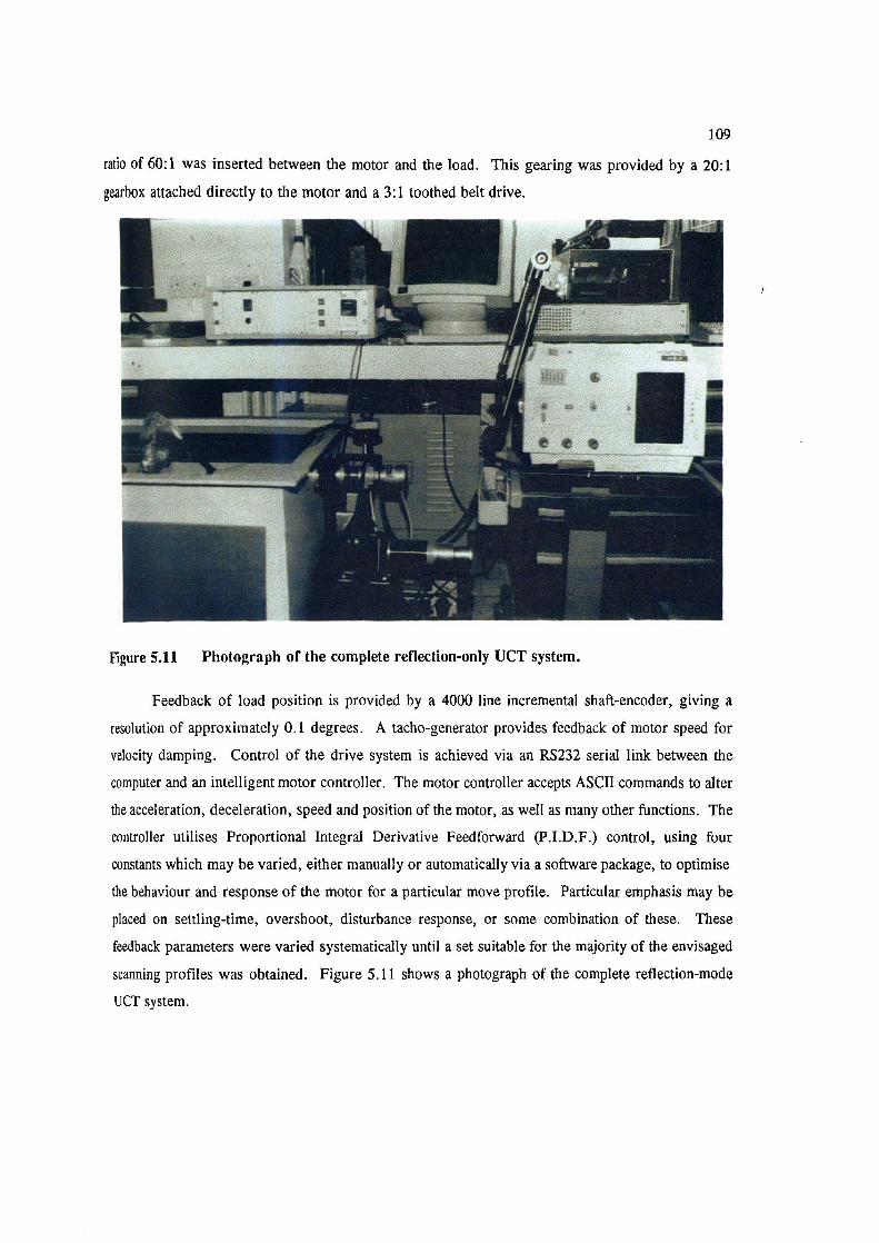
109

ratio of 60:1 was inserted between the motor and the load. This gearing was provided by a 20:1

gearbox attached directly to the motor and a 3:1 toothed belt drive.

Figure 5.11 Photograph of the complete reflection-only UCT system.

Feedback of load position is provided by a 4000 line incremental shaft-encoder, giving a

resolution of approximately 0.1 degrees. A tacho-generator provides feedback of motor speed for

velocity damping. Control of the drive system is achieved via an RS232 serial link between the

computer and an intelligent motor controller. The motor controller accepts ASCII commands to alter

the acceleration, deceleration, speed and position of the motor, as well as many other functions. The

controller utilises Proportional Integral Derivative Feedforward (P.I.D.F.) control, using four

constants which may be varied, either manually or automatically via a software package, to optimise

the behaviour and response of the motor for a particular move profile. Particular emphasis may be

placed on settling-time, overshoot, disturbance response, or some combination of these. These

feedback parameters were varied systematically until a set suitable for the majority of the envisaged

scanning profiles was obtained. Figure 5.11 shows a photograph of the complete reflection-mode

UCT system.

110

5.3.5 Software

The software to perform reflection UCT was initially written on a Sage IV micro-computer

running the CPM-68K operating system, although this computer was later replaced by a more

advanced SUN 386i. Pascal was chosen as the language for the majority of the software, and for the

user-interface in particular, because it is modular and hence aids structured design and programming,

and it is well supported and thus fairly portable. Some low-level routines that needed to run

particularly fast, or needed access to the computer's operating system or peripherals, have been

written in 'C' or assembler. The modular nature of both Pascal and 'C' has enabled the software

routines to be separated into discrete modules, where all routines within a module share a common

purpose. This modular design has been essential in allowing the software development for such a

large project (over 6000 lines of code have been generated for this reflection-only UCT system alone)

to be efficiently managed. The main modules are:-

'UCT_MOTOR":

Contains routines for defining a scanning sequence and programming the motor controller.

'ucT_AcQuIsmoN":

Contains routines for data acquisition, including control of data capture, transfer, and storage,

and calculation of the centre of rotation of the system (see Section 5.4.2 for details).

'UCT RECONSTRUCT":

Contains routines for converting the raw scan data to B-scan image format, routines for

displaying B-scan images, and routines for reconstructing and displaying reflection UCT

images.

"UCT PROCESS":

Contains routines for reflection UCT image processing, including image rotation, adding,

multiplying, scaling, linear translation, log and anti-log transforms, histograms, 1-D and 2-D

convolutions and Fast Fourier Transforms, and many others.

With the basic tools outlined above any of the reconstruction techniques discussed in Section

2.3 can be implemented. Some of these techniques, and others, will be explored in the following

sections.

111

5.4 Acquisition of a reflection-mode UCT image

5.4.1 Introduction

The main components of the hardware and software developed to perform reflection UCT in

a vertical plane have now been described. The sequence of procedures involved in actually acquiring

and reconstructing a reflection CT image are summarised in Figure 5.12. These are:.

a) Measure the centre of rotation of the system. This stage may be omitted if the probe has not

been moved since the centre of rotation was last measured.

b) Enter the parameters defining the acquisition of the ultrasonic data, such as number of B-

scans, total time for scan, etc.

c) Perform the scan.

d) Reconstruct the reflection UCT image.

e) Display the image.

Find Centre of Rotation0

Acquire scan ofwire phantom

x2

Find centres

Rotate probethrough l8cP

1>

Calculate and storecentre of rotation

0= Optional

Acquire Data

4,Define scanacquisitionparameters

Move probeby angle 0

x

Dig! Use scan (n)

1

Store scan (n)onto disc

Reconstruct Image

Read scan (n)off disc

'4'0

Apply l-Dfilter to scan (n)

Lx

Rotate scan (n)by n x 0

Add scan tofinal Image

.4, -,-0

Apply 2-Dfilter to image

'4,

Display 1ma1

Figure 5.12 Procedures involved in acquiring and reconstructing a reflection UCT imageS

These procedures will now be described in detail.

112

5,4.2 Measurement of the centre of rotation

An essential requirement for any imaging system that involves acquisition of data from many

directions around a target, such as reflection UCT, is that the centre of rotation of the system can be

determined to an accuracy which is considerably better than the required resolution of the image, and

that this centre of rotation remains fixed (to the required accuracy) throughout the full range of

movement. For this system, knowledge of the centre of rotation (c.o.r.) is required so that the

reflectivity data from each of the B-scans that have been acquired at different angular positions may

be correctly rotated and superimposed in the computer. Hence the accuracy of the estimation of the

c.o.r. will inevitably limit the ultimate resolution of the reflection UCT image, irrespective of the

efficacy of any reconstruction algorithm used. Consequently considerable effort has gone towards

ensuring that the c.o.r. can be measured accurately.

There are essentially two distinct approaches by which the c.o.r. can be estimated. One

possible method is to estimate the position of the c.o.r. by careful measurements on the mechanical

scanning system itself. It was felt that this would be very difficult to achieve to the required accuracy

of 0.2 mm, and also very time consuming if the c.o.r. was likely to change between scans, and

particularly after removing and replacing the probe. An alternative method involves looking at the

images actually produced by the system, using a suitable test object, and attempting to choose a c.o.r.

that in some way optimises the image. A method such as this can be implemented in software and

hence made to operate automatically, thus allowing the c.o.r. to be re-calculated easily at any time.

A method based on this latter approach has been developed and is described below.

Referring to Figure 5.13, consider the B-scan image of a point target P(x,y) in water/alcohol

obtained with the probe pointing along the negative y-axis. The distance of the point target from the

front face of the probe is x 1 , while the distance to one edge of the probe's ultrasonic field is y1.

These distances can be measured quite easily from the B-scan image itself, since both the speed of

sound in the water/alcohol and the line spacing of the probe are known. If the probe is rotated by

180 degrees about the unknown centre of rotation (x,y3, so that it now points along the positive y-

axis, the equivalent distances become x 2 and Y2 respectively. The centre of rotation, in terms of the

axial distance from the probe face and the lateral distance from one end of the probe, may now be

estimated from the average (ie effectively the Centre of Gravity) of the co-ordinates (x1,y1;x2,y2).

The accuracy of this estimate will depend on how accurately the distances (x1 ,y 1 ;x2 ,y2) can

113

be measured, in other words on how accurately

the centre of an echo image from a point target

can be determined. This accuracy will be of the

order of half the pulse length along x (ie about

0.75 mm), and about half the beam width along

y (about 2.0 mm). However a second target in

the image would give another estimate of the

c.o.r., and, assuming that the measurement

errors are random, N targets would give N

independent estimates which could be averaged

to give a more accurate result (accuracy of

average using N independent estimates is 1/..JN

better than accuracy from a single estimate).

As many targets can be used as are necessary to

achieve the required accuracy in the estimate of

the c.o.r., as long as their echoes do not

overlap.

A test-object for measurement of the

c.o.r. has been constructed (Figure 5.14). It

consists of 50 thin (0.2 mm dia.) nylon wires

arranged in a rigid lattice. These wires were

found, after experiments, to give the shortest

echoes consistent with sufficient tensile strength

in the wire. Software has been written to

automatically search for the centres of the

echoes in the two opposite B-scans, and

subsequently calculate the c.o.r. The complete

process of setting up and measuring the centre

of rotation takes about 3 to 5 minutes.

I

Probe I 'Combined Images'I I

) '2 Iyl

I

______________________________ I—I

•1 I

I I +1---->,

I lx1 I Yc, ix1

I I I I

X C I I. 1x2 , .4\Point I

,I Target I

I p(x.y) I , I

Centre of Images of

Rotation point target

0 I 0)

xc = X 1 +

2

Probe rotated = "1 + Y3

through 180° : 2

Figure 5.13 Principle of the method formeasuring the centre of rotation.

0 000

7

o

0o I I I

0 0 0 0 /No 0 ® 0 a"

F140mm

'spex

50 mm

The repeatability of the method has been Figure 5.14 Test-object for measuring thetested by taking a series of separate centre of rotation.

measurements of the c.o.r., with the test-object

phaselration Deceleration

phaseCreep phase

T/S Zr/3 TTime

VP

U0V

a

C.(

V

0

StartI0 T/3 2T/3

Time

Figure 5.15 Angular displacement profile forprobe movement.

Finish

C0

'S00.

a

C

114

being removed and then replaced in a slightly different position between each measurement. The

experiment showed that the measurement is repeatable to less than 0.3 mm, which just about meets

the requirements set out in section 5.3.4.

5.4.3 Definition of the acquisition parameters

Once the centre of rotation of the system has been obtained, the operator must defme several

parameters which will determine how the ultrasonic data will be acquired.

a) Scan parameters:

The operator must first define the scanning geometry in terms of

1. The total scan angle (up to a maximum of 180 degrees).

11. The number of angular positions of the probe (ie the number of B-scans) required.

II'. The total time for the scan to be completed.

The program written for reflection UCT

then calculates the time available to move the

probe between positions and, based on the

angular displacement profile shown in Figure

5.15 and the known inertias of the complete

system, calculates whether the motor can deliver

the necessary torque to achieve this. The

displacement profile incorporates a 'creep'

phase to minimise the possibility of ringing or

overshoot in the probe positioning. If there is

insufficient torque to deliver the requested

move, the operator is asked to re-enter the

parameters and to allow a longer time for the

move. Although it may seem sensible to always

select the shortest possible scan time, this may

not be advisable for some targets where

turbulence generated in the water by the rapidly

moving probe might cause the target to move during the scan. When an acceptable move has been

115

defined, the software then programs the motor controller with the appropriate acceleration, maximum

speed and deceleration information.

b) Data acquisition parameters:

The operator must now choose the parameters which determine how the ultrasonic data will

be acquired. These are:-

j. The distance along a scan line where digitisation will start and end, ie defining the target

region. This values are converted to the equivalent ultrasonic times-of-flight, assuming that

the speed of sound in the water/alcohol solution is known, which are then used to set the

digitisation window of the transient recorder.

ii. The digitisation rate, which for demodulated signals is 6.25 MHz.

iii. The maximum amplitude of the received signal. This ensures that the full dynamic range of

the digitiser (ie 8 bits = 48 dB) is utilised.

The software will then program the transient recorder accordingly.

c) Receiver gain:

It has already been mentioned in section 5.3.1 that the ultrasonic pulses suffer exponential

attenuation as they propagate through the target, thus reducing the amplitude of echoes received from

increasing ranges. This attenuation can be at least partially compensated for by a logarithmic receiver

gain which varies with time-of-flight and hence range. This feature is often called time gain

compensation (TGC) or swept gain. Since a real (ie tissue) target will normally exhibit a spatially

varying attenuation coefficient, TGC can only compensate for the "average" attenuation of a target.

Also, different targets will present different average degrees of attenuation so that a way of varying

the slope of the logarithmic gain is required. Such a control already exists on the Hitachi EUB-24

and so no additional electronics were necessary. This control is adjusted, before acquisition of the

reflection UCT data, until the strongest echoes displayed in the real-time B-scan image from the EUB-

24 appear to be just below saturation level at all ranges within the target.

5.4.4 Performing the scan

Some care is required in positioning the target within the scan plane. The target should

116

ideally be centred as closely as possible to the centre of rotation of the scanning system. This ensures

that outer parts of the target do riot extend outside the field of view of the linear array for some probe

positions. The target should also be constrained so that any turbulence set up in the water by the

rotating probe do not cause appreciable movement. If this is not possible, as for example with an in-

vivo subject, the scan is best performed as quickly as the program will allow to minimise involuntary

movements of the subject.

Having defined the scan geometry and the data acquisition parameters, the scan acquisition

sequence can be initiated. As soon as the data from all the B-scan positions has been digitised and

stored by the transient recorder, the data is immediately transferred to the computer and stored onto

hard disc. Acquisition of a 15-view scan (ie 15 B-scans) takes a minimum of about 10 seconds.

5.4.5 Reconstruction of the reflection UCT image

The theoretical basis of reconstructing a reflection UCT image has already been discussed in

detail in section 4.4.2. Hence this section will merely outline the practical implementation of the

main stages.

5.4.5.1 Scan conversion

The first stage of image reconstruction is to convert the ultrasonic data acquired in B-scan

format, ie 70 lines of digitised echo data, into the 256 by 256 pixel-image format. For this work this

has been accomplished by a software implementation of the linear-array scan-converters used in

commercial scanners. In this program linear interpolation, both along and between scan lines, has

been used to derive the echo value to be assigned to a given pixel.

5.4.5.2 Backprojection

The process of backprojection involves summing, for each and every pixel in the

reconstructed image, the echo amplitudes from corresponding points in each (filtered or un-filtered)

B-scan defined by the pixel's location in image space. In practice it is faster to deal with all the data

for each B-scan in sequence, which then involves calculating which pixel or pixels should receive data

from each digitised sample in the B-scan.

117

5.4.5.3 Post-processing

As described in Section 4.4.3, knowledge of the point spread function (psf) of the imaging

system can be used to further improve the resolution of the simple summation image. There are two

possible approaches (see Section 2.3.2):-

a)Summation with post-filtering:

The B-scans are rotated and summed to form the simple summation image, and then a 2-

dimensional filter is applied to the final image.

b) Filtered summation:

Each scan-line of every B-scan is filtered with an appropriate 1-dimensional filter function

before rotation and summation.

Method (a) has been implemented in this work because it is much faster then method (b) when

more than about 4 B-scans are involved. The only potential advantage of method b) is that the

filtering may be made depth dependent to account for a depth dependent psf (eg because of varying

beam width). However, since there is not, as yet, sufficient information available about the nature

of the psf within tissue, and particularly about how it varies with depth, it was not considered

worthwhile to implement a depth dependent filter.

The filtering may be performed equivalently in either the space or spatial frequency (ie

Fourier) domains, but for an image array size of 256*256 experience has shown that Fourier domain

filtering is quicker. Details of the filters used and the results obtained for various targets will be

presented in section 5.5.

5.4.6 Displaying the image

The reconstructed images are displayed at 256 by 256 resolution with a 256 level grey-scale

look-up table. For the maximum target diameter of 10.5 cm this gives a pixel size of about 0.4 mm,

which is about half the axial resolution of a B-scan and hence also about half the potential resolution

of a reflection UCT image. Although the raw data in each B-scan is digitised to 256 levels, the

processed reflection UCT images typically possess a wider dynamic range than this because they are

composed from many summed B-scans and are accordingly represented by 16-bit numbers. Hence

routines have been written to re-compress the image data using a selection of linear or logarithmic

grey-scale transfer curves, so that the information in the images is better matched to the to the

118

dynamic ranges of the display device and the human visual system. Logarithmic compression is

particularly useful for emphasising low-echo regions in the images obtained from real tissues (ie

equivalent to the log compression available as standard on conventional B-scanners).

119

5.5 Results from the vertical plane reflection-only system

5.5.1 Introduction

The primary aim of this practical investigation into reflection UCT was to highlight any

advantages, or disadvantages, that reflection UCT has compared to conventional real-time B-scanning.

Accordingly reflection UCT images obtained from various different kinds of target will be compared

to single B-scan images obtained from the same target, and using the same linear array scanner for

data acquisition (ie the Hitachi EUB-24F). This scanner is over 15 years old and has relatively poor

dynamic range and penetration, and consequently the B-scan images presented will not be as good as

could be obtained from a more modern machine. However, since the same raw ultrasonic data is

used to reconstruct both the UCT image and the B-scan image, it seems justifiable to compare the two

imaging methods directly. It should be true that any advantages that can be demonstrated for UCT

over B-scanning would still apply if more sophisticated equipment (e.g. with a shorter ultrasonic pulse

length and better dynamic range and penetration) was used for the data acquisition.

All the UCT images presented here have been acquired with the following conditions:-

i. Only demodulated echo data has been used.

ii. Data has been acquired over a total angle of 180 degrees.

iii. Fifteen views (ie 15 separate B-scans) have been acquired, at angles of 12 degrees between

each view, in accordance with the sampling requirements discussed in Section 5.3.2.2.

Various factors must be considered when deciding which targets to scan. It might appear that

the best way to compare two imaging techniques is to choose a target whose characteristics (ie

geometry, scatterer density, etc) are known exactly. In this way the ability of the imaging techniques

to represent the true structure of the target can be compared unambiguously. For ultrasonic imaging,

the only targets whose characteristics are likely to be known exactly are those which have been

constructed especially for this purpose, ie phantoms. In this study simple arrangements of thin wires

in water have been used for the measurement of point spread functions (5.5.2) and to establish the

high contrast resolution of the techniques (5.5.3 and 5.5.4). More complicated phantoms of varying

scatterer density have been used to assess contrast resolution (5.5.3 and 5.5.4), while phantoms

showing varying acoustic speed and attenuation have been used (5.5.5) to assess the presence of

imaging artifacts.

120

The disadvantage of using phantoms to compare imaging techniques, at least those techniques

intended ultimately for the imaging of soft tissue in-vivo, is that it is very difficult to construct

phantoms which exhibit the complexity and range of structures found in real soft tissues. Since this

reflection UCT system was not constructed to be particularly suitable for in-vivo imaging, an

acceptable alternative is to image soft tissues in-vitro. Hence results for reflection UCT and B-scan

imaging of some animal tissues in-vitro will be presented in section 5.5.6.

It could be argued that the only really worthwhile comparison of two in-vivo imaging

techniques is with images obtained in-vivo. Some examples of in-vivo images are presented in section

5.5.7

5.5.2 Measurement of system point spread function

As discussed in Section 4.1, the simplest way of characterising a linear imaging system is

through the system's point spread function (pst), or its Fourier Transform the system point transfer

function (OTF). Although conventional B-scanning and reflection UCT can only be considered as

linear imaging processes within certain restrictions (see 4.3 and 4.4), their respective psfs and OTFs

can still show a great deal about the potential spatial resolution of the techniques. In the spatial

frequency domain, the OTF shows how the spatial frequency content of the original object will be

transformed by the imaging system into the spatial frequency content of the image. In particular, the

maximum frequencies present (above noise) in the OTF will reveal what level of detail there will be

in the image (ie the effective resolution of the image). Hence measuring the psfs, and then calculating

the equivalent OTFs, is one useful way of comparing conventional B-scannIng with reflection UCT.

The psf of an imaging system can most simply be measured by obtaining an image of a high

contrast point target, ie a single target which is much smaller than the likely resolution of the system.

In practice it is usually easier to use a line target orientated perpendicularly to the plane of the scan.

Clearly, using such a target tells us nothing about the ability of the imaging system to resolve targets

in the direction perpendicular to the scan plane, ie its ability to separate parallel image planes.

5.5.2.1 B-scan point spread function

The B-scan psf was measured by suspending a copper wire of diameter 0.22 mm (ie much

less than half the pulse length) in a water bath, with the axis of the wire perpendicular to the scan

121

b)

-0.8

Figure 5.16 Measured B-scan (a) psf and (b) OTF.

122

plane so that it appears as essentially a point target. The wire was placed as close as possible to the

centre of rotation of the reflection UCT system, at a distance of about 65 mm from the front face of

the probe, ie near to the pulse-echo focus. To show the extent of the B-scan psf, a 3-D contour plot

of the wire image has been plotted in Figure 5.16a. The axial component of the psf (ie ha(x) in

section 4.3.2.2) has a full width at half maximum (FWHM) of about 1.0 mm, and this will

correspond to the axial resolution of the B-scan. As expected, this is considerably better than the

lateral component, h 1(y), of the psf (ie lateral resolution) with a FWHMof about 2.8 mm. The B-

scan OTF, obtained by Fourier transforming the psf, is shown in Figure 5. 16b. It is actually

displayed here as the modulus of the OTF (le the spectrum). This clearly shows the wider bandwidth

available in the axial as compared to the lateral direction.

5.5.2.2 Reflection UCT point spread function

To measure the psf of the reflection UCT system (ie h,,(x,y) in Section 4.3.3.2), the same

wire target was scanned from 15 directions over 180 degrees. The B-scans were combined using

simple, un-filtered summation to form a single image. A contour plot of this image (ie the reflection

UCT psf) is shown in Figure 5.17a. Notice that the psf is now approximately symmetrical, as

expected, indicating nearly isotropic resolution. The FWHM is about 1.6 mm. This value lies

between the FWHM of the axial component and the FWHM of the lateral component of the B-scan

psf, which is to be expected since, as shown in section 4.4, the reflection UCT psf is basically a

rotated version of the B-scan psf. 1-lence the resolution of an unfiltered UCT image will be a little

poorer than the axial resolution of a B-scan image but considerably better than its lateral resolution.

The calculated OTF is shown in Figure 5.17b. The OTF is also nearly symmetrical, and again

appears to extend to some way between the axial and lateral components of the B-scan OTF.

5.5.3 Potential resolution of reflection UCT and B-scanning

The resolution of an imaging system depends on many factors in addition to the point spread

function. In particular, spatial resolution (the ability to discriminate between high contrast targets)

and contrast resolution (the ability to discriminate targets of similar contrast) are inter-dependent, and

both are affected by the level of noise in the image.

One useful way of representing both spatial and contrast resolution is in a contrast-detail

diagram (e.g. Hill et al 1991), which plots the threshold for detectability of targets showing increasing

0.8

123

hi

-0.8

Figure 5.17 Reflection UCT (a) psi and (b) OTE.

124

size along one axis and increasing contrast (compared to the background noise level) along the other

axis. To construct such a diagram requires measurements on a phantom having a wide range of

targets of varying size and contrast. Such phantoms have been made for ultrasound (Smith and Lopez

1981), although a recent study (Lopez et al, 1990) suggests that errors associated with their use in

comparing the performance of imaging systems are quite high. Another problem is that commercially

available versions of this phantom are not suitable for the wide range of scanning angles necessary

for reflection UCT. Although some attempts were made to construct a contrast-detail phantom

suitable for reflection UCT, severe problems in obtaining predictable contrast levels were encountered

and no results are presented here.

Studies using the phantom of Smith and Lopez have established that there are two regions in

the contrast-detail relationship for B-scanning; (a) a high contrast region where target detection is

primarily determined by the B-scan psf and is relatively insensitive to the contrast, and (b) a low

contrast region where detectability is strongly dependent on target contrast. Following this principle,

the assessment of comparative resolution for reflection UCT and B-scanning has been divided into

high and low contrast situations.

High contrast spatial resolution has been assessed quantitatively using wire targets in water

and in tissue equivalent materials. Due to the difficulty in making phantoms (reliably) having regions

with small contrast variations, contrast resolution has been assessed qualitatively using a single low-

scatter insert in a tissue equivalent material. Despite the limitations of this phantom, it is still useful

for a simple comparison of reflection UCT and B-scanning.

Clearly, the construction of a phantom suitable for obtaining a full contrast-detail assessment

of reflection UCT would be a useful area for further work.

5.5.3.1 Spatial resolution

On the basis of their measured psfs, reflection UCT would be expected to show improvements

compared to B-scaiming in the ability to resolve closely spaced targets, at least in the direction

perpendicular to the B-scan beam axis. Various experiments have been performed to establish if this

is true in practice.

125

Wires in water

It is instructive to compare conventional B-scanning with reflection UCT imaging in terms

of their ability to resolve high contrast targets such as wires in water. Two B-scans were obtained,

one with the axis of the beam along the line of the wires (Figure 5.18a) and one with the axis of the

beam perpendicular to the wires (Figure 5.18b). The wire spacings are 1 mm, 2 mm, 5 mm, 10 mm

and 20 mm respectively. As expected, the axial resolution (about 1 mm) is considerably better than

the lateral resolution (between 2 and 5 mm). Figure 5.18c shows the un-filtered reflection UCT

image of the wires. Here all but the 1mm separation wires are resolved.

Wires in tissue equivalent material

A more realistic indication of the potential resolution in real tissue is to look at targets

imbedded in a medium which exhibits some of the features of real tissues, such as speckle. Hence

a tissue equivalent material (FEM) phantom was made, using a mixture of agar, propanol and graphite

powder (see Appendix II and Burlew MM et al, 1980), and having an acoustic speed close to that of

the surrounding medium (ie 1540 mIs). This generates a B-scan with a general appearance that is

very similar to that obtained from real soft tissues. A set of wires was then imbedded in this

phantom. The B-scan image is shown in Figure 5. 19a. Note the coarse pattern of bright and dark

patches in the scattering background. These patches, which are commonly known as speckle, arise

from the coherent nature of ultrasonic imaging and cannot be attributed to actual scattering centres

in the object (see 4.3.2.3).

The unfiltered reflection UCT image (FigureS. 19b) is a considerable improvement. Note that

the mean echo level of the speckle is reduced and the pattern is finer, a result that was predicted

theoretically (4.4.3) and is also consistent with results obtained by, amongst others, Roehrlein and

Ermert (1986). The reduction in the speckle level also contributes to the significant reduction in the

size of the echoes from the wires and hence in potential spatial resolution.

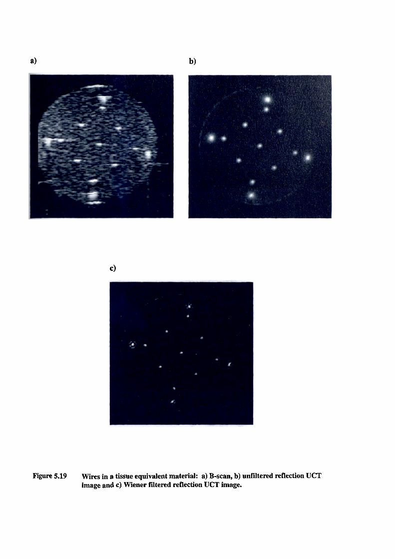
128

5.5.3.2 Contrast resolution

The targets that have been imaged so far are still not very realistic, for example one doesn't

often find copper wires in soft tissues! To assess the comparative performance of reflection UCT and

B-scanning in a target showing a more realistic level of contrast, a phantom consisting of a region of

low scatter amplitude (a hole filled with a water/alcohol solution) embedded in a region of moderate

scatter amplitude (the same TEM material as was used in the wire phantom) was constructed. This

phantom can be thought of as similar to a fluid filled cyst in the liver, for example. Figure 5.20a

shows a single B-scan of such a phantom, again with the ultrasound probe on the left. Note that the

boundary of the "cyst" only appears when it is perpendicular to the ultrasound beam axis. In the

unfiltered reflection UCT image, shown in Figure 5.20b, the boundary of the cyst is complete,

making interpretation of the image easier. The speckle pattern is again much finer and less obtrusive,

thus improving the potential contrast resolution when compared to the B-scan.

ie F(R) - RI

It is also important to note that inverse

filtering using such a filter is only strictly valid

when the psf used to derive it does not depend

on position. This filter has been applied to

various targets to establish whether this

130

5,5.4 Affects of inverse filtering on reflection UCT images

5.5.4.1 Introduction

The reflection UCT OTF extends, although at reduced amplitudes, right out to the maximum

frequencies present in the axial component of the B-scan OTF. By applying a filter such as those

discussed in section 4.4.3.2 to the UCT image, the potential appears to be there to achieve the

axialresolution of a B-scan image in all directions. A suitable filter would be the Wiener inverse filter

described in Appendix I.

The purpose of filtering in CT is to restore in the image the frequency content of the original

object as closely as possible, up to the maximum frequency (R,) present in the OTF. Wiener

inverse filtering was introduced in section 4.4.3.2 as an alternative to the conventional tomographic

filtering of CT images (see 2.3.2), which allows the high frequency roll-off of the filter to be

optimised for the particular signal-to-noise characteristics of the O1'F of the imaging system. A

Wiener inverse filter appropriate to reflection UCT has been calculated from the reflection UCT OTF

and is shown in Figure 5.21. It is interesting to see that, at low frequencies, the filter bears a strong

resemblance to the filters predicted from CT theory (shown in Figure 2.4).

assumption is justified, and whether inverse Figure 5.21filtering in reflection UCT in general is

worthwhile.

5.5.4.2 High contrast targets

ixate wire in water

Wiener filter derived fromreflection UCT psf.

The simplest test of a Wiener filter is to apply itto the UCT image of a single wire, ie to the

psf used originally to derive it. The filtered image is shown in Figures 5.22a and the spectrum in

131

0

figure 5.22 Wiener filtered image (a) of a single wire, and (b) its spectrum.

132

Figure 5.22b. Clearly the FWHM of the image of the point target has been significantly reduced (to

about 1mm). In the frequency domain, the spectrum appears broader and more uniform compared

to the un-filtered spectrum (Figure 5. 17b).

Multiple wires in water

Figure 5.23a shows a B-scan of a set of six copper wires, where the direction of the scan is

from above. The four very bright echoes are from steel rods used in the framework and should be

ignored. An important point demonstrated in Figure 5.23a is that, contrary to the assumption of a

position invariant psf, the beam width and hence the B-scan psf clearly changes with distance from

the probe. Figure 5.23b shows the unfiltered reflection UCT image of the same target. The purpose

of this target was originally to derive six separate inverse filters, ie one from each of the wire images,

in order to take account of the varying beam width. However, it was found that the inverse filters

so derived were almost identical, irrespective of the position of the wire in the field of view. This

is almost certainly because the pulse length, which is independent of depth (at least to first order),

is the dominant factor in the resolution and hence the psf of reflection UCT images. These results

indicate that the inverse filter derived above from a single centrally placed wire should be sufficient

to deconvolve any set of wire targets. This is borne out by the result, shown in Figure 5.23c, of

applying this filter to the original reflection UCT image of the multiple wires.

Figure 5. 18d shows the reflection UCT image of the resolution test wires after filtering with

the Wiener filter. Now even the 1mm wires are resolved. Clearly for images of wires at least, the

resolution of reflection UCT images, already markedly better than the lateral resolution of B-scan

images, is significantly improved by inverse Wiener filtering.

Wires in tissue equivalent material

The Wiener filtered image of the wires in the TEM (Figure 5.19) is shown in Figure 5.19c.

Although the resolution of the wires is further improved as before, some enhancement of the

background speclde can also be seen. It can be postulated that this speckle reinforcement arises

because speckle is not accounted for in the linear imaging model, since wave front distortion and non-

linear processing imply a space-variant psf and a non-linear system respectively. Inverse filters

effectively act as high-pass filters to restore, up to the maximum spatial frequency in the psf, the

frequencies present in the original object that have been attenuated by the imaging system. Since the

speckle in the reflection UCT image has a wider bandwidth than in a single B-scan, inverse filtering

134

will preferentially boost the high frequency components of the speckle and hence increase the mean

speckle level.

5.5.4.3 Low contrast targets

Speckle enhancement as a result of inverse filtering is even more evident on more realistic

targets showing less contrast. The Wiener filtered reflection UCT image of the cyst phantom of

Figure 5.20 is shown in Figure 5.20c. Although the boundaries of the cyst are now sharper, the

speckle has been markedly enhanced. This problem is now more obvious than with the image of the

wires imbedded in the TE material because of the much lower contrast between the "cyst" and the

TEM, compared to the wires, which are very highly scattering, and the TEM. Speckle enhancement

leading to reduced contrast resolution is the main disadvantage of using inverse filtering on reflection

UCT images of anything but the simplest targets, and consequently inverse filtering has not been

applied to any of the images to be shown subsequently.

5.5.5 Investigations of artifacts in reflection-mode UCT images

It has been established that unfiltered reflection UCT can overcome many of the limitations

of B-scanning, showing improved and isotropic resolution, better delineation of specular reflectors

and reduced speckle, for relatively simple and "undemanding" targets. However, real tissues may

posses regions with high attenuation and varying acoustic speed which could degrade the quality of

the reflection UCT images. The likely effects of attenuation and acoustic speed variations on the

quality of the reflection UCT images has thus been studied with various phantoms.

5.5.5.1 Artifacts due to attenuation

To investigate how the presence of a relatively small highly attenuating region in a target

affects the quality of a reflection UCT image, such a region was inserted into a cyst phantom (Figure

5.24a) by increasing the proportion of graphite scatterer in the attenuating region to produce an

attenuation coefficient of approximately 4.5 dB/cm at 3 MIIz (ie similar to skeletal muscle, Duck

1990). The single B-scan (Figure 5.24b), with the probe at the top, demonstrates the typical

shadowing that this region causes. The cyst at the centre of the phantom is now barely visible. The

reflection UCT image of this target (Figure 5.24c) shows a much reduced artifact, presumably

because the region in shadow in the single B-scan has received sufficient interrogation from some of

136

the other B-scan positions contributing to the reflection UCT image. This result is consistent with

the observations of other workers (e.g. Freidrich et 1982, and Roehrlein and Ermert 1985), who

showed that scanning angles of slightly less than 1800 can produce reflection UCT images showing

only marginally reduced quality. This suggests that relatively small strongly attenuating regions will

not be a major problem in reflection UCT, provided that there is sufficient penetration, at a

sufficiently wide range of angles, into all parts of the target.

5.5.5.2 Artifacts due to speed of sound variations

Another possible cause of artifacts in reflection UCT is when the acoustic speed of the target

is significantly different from that of the coupling medium. It has already been mentioned that ethyl

alcohol is added to the water in the scanning tank so that the speed of sound in the water is close to

that in the target being scanned, assuming that the average acoustic speed in the target is about 1540

mis. However, there is quite a range of average acoustic speed to be found in different types of

human tissue (e.g. from about 1430 rn/s for a fatty breast, to about 1570 m/s for a dense breast, Duck

1990). It is not easy to reduce the acoustic speed in the water after the chosen quantity of alcohol

has been added, since this would require discarding a portion of the water/alcohol solution which is

expensive and impractical. Hence the acoustic speed of the water/alcohol is left fixed at 1540 rn/sec

regardless of the target being scanned. Another potential problem is that the acoustic speed within

any particular target may also vary considerably, possibly by 5% or more in breasts (Greenleaf and

Bahn, 1981). These two situations will be considered separately.

a) Target With Average Acoustic Speed Different to Coupling Medium

To investigate the consequences for reflection UCT image quality of scanning a target having

a uniform but significantly different acoustic speed to that of the coupling medium, a graphite/gel

phantom was made without adding propanol. The acoustic speed of this phantom should thus be

(Burlew MM et al, 1980) about 1500 m/s. A set of copper wires was inserted into this phantom to

act as recognisable scattering targets. The reflection UCT image of this phantom (Figure 5.26a),

reconstructed assuming an acoustic speed of 1540 m/s, shows each wire as a crescent instead of the

expected point. It can be argued theoretically that these artifacts are due to displacement of echoes,

both laterally and axially, in the component B-scan images. To appreciate why this is so refer to

Figure 5.25, which shows a point target in a medium of acoustic speed (c i) being viewed, from many

directions, with a probe in a coupling medium of speed (c1). The information actually obtained from

137

True distance to target = d 1 + d 2 = t] C 1 + t2c2

Reconstructed distance = ( t 1 + t2 ) c1

Axial displacement error, d a = d 2 (c 1 - c2)C2

Figure 5.25 Blurring artifact caused by a different acoustic speed in target and surroundingmedium.

a B-scan is the time of flight to the target, rather than the actual distance. Hence to display the B-

scan image as distances (x) the time of flight (t) must be converted using the relation ( x = t.c12).

The speed of sound used will normally be that in the coupling medium, ie c 1 , because this can be

measured very accurately before-hand. However, if c 1 ^ c2 (say c 1 > cJ, then the following effects

will occur:-

I) The images of the point target will be placed further along the scan lines than they should be,

as shown in Figure 5.25. This can be thought of as the axial component (ie along the scan

line) of the acoustic speed artifact. When the B-scans are combined into a single image, the

echoes from the point target will fail to overlap, ie mis-registration will occur, and the image

of the point will be blurred to form the characteristic crescent shape.

2) If the interface between the object and the water is not at right angles to the ultrasonic beam,

then refraction of the beam will also occur (this is not shown in Figure 5.25). This will

result in the echoes being displaced laterally on the B-scan images, again causing blurring in

the combined UCT image.

139

b) Target Showin g Si gnificant Acoustic Speed Variation

It has been shown that a simple correction for the difference in average acoustic speed

between the target and the coupling medium can have quite a dramatic affect on the quality of the

reflection UCT images. However, the algorithm described cannot take account of speed of sound

variations within the object itself, or of any refraction effects. To investigate if speed of sound

variations within the target would significantly affect the images, a "cyst" phantom was made (Figure

5.27a) with one region having an acoustic speed of approximately 1640 mIs, with the rest of the

phantom at about 1540 mIs. In the reflection UCT image (Figure 5.27b), this high acoustic speed

region is in the top left corner. Note that the boundaries of the cyst, and the edges of the phantom

itself, are very blurred. This is because of incorrect registration of echoes from ultrasound beams

which have passed through the high acoustic speed region.

It seems likely that the high acoustic speed region has to be quite large before it has a

significant effect on the images. This is because the amount of blurring at any particular point in the

reflection UCT image depends on what proportion of beams in the total 180' coverage, reaching the

equivalent point in the object, have passed through the high speed region. This is borne out by the

phantom shown in Figure 5.28a, where a set of three wires have been inserted at different distances

from a high speed region. Note that in the reflection UCT image (Figure 5.28b) only the nearest wire

has been significantly blurred, because the angle subtended at the other wires by the edges of the high

speed region is quite small.

The only way that the blurring in these images could be removed would be to have some prior

knowledge of the distribution of acoustic speed values within the same target sections. This

information could then be used to correct the raw data used in the reconstruction of the reflection

UCT image. It has already been shown in Section 4.3.3 that this information can in principle be

obtained from transmission mode UCT. A system designed to perform combined reflection and

transmission UCT for this purpose will be described in Chapter 6.

141

5,5.6 Images of animal tissue in-vitro

The next step is to compare images obtained from real tissue. For this purpose, a fresh

bovine kidney was obtained from an abattoir, and placed in a thin plastic bag filled with 6% NaC1

in water (speed of sound = 1540 m/sec) so as to prevent contamination of the water in the scanning

tank. The B-scan image is shown in Figure 5.29a, where the scan has been obtained from the right.

Some features can be recognised, in particular the strongly scattering calyces. However note the poor

resolution laterally, specular reflectors such as the organ walls only visible when they are

perpendicular to the beam, and shadowing of deep regions by highly attenuating tissues such as the

calyces.

Figure 5.29b shows the 180° reflection UCT image of the same target, reconstructed assuming

an average acoustic speed in the kidney of 1560 m/s. The organ boundary is now visible from all

directions, at least in the lower portion of the kidney. Resolution is much improved and speckle

reduced making interpretation of the image much easier, ducts and tubules in the kidney being clearly

discernable. However the limited 180 degree coverage with this particular system results in a poor

image quality in the upper portion of the kidney. This is probably due to two affects. The most

serious is that the ultrasound from some directions cannot penetrate, due to attenuation, to the depths

required to reach this region. Hence this region of the image does not contain information over a

sufficient fraction of the 180 degrees required for a good reconstruction. The other problem is that

the upper region of the kidney is always beyond the focus of the ultrasound beams where the beam

width is wider. Hence the resolution, although still dominated by the pulse length, is likely to be

slightly poorer than in the lower portion of the kidney.

5.5.7 Images of human organs in-vivo

Although obviously the most realistic situation, obtaining images from tissues in-vivo may

be less informative than images of in-vitro tissue or phantoms because it is not possible to establish

exactly the internal structure of the target. Also the present vertical plane system, although potentially

suitable for a wide range of in-vivo targets such as the breast and the neonatal head, has somewhat

limited accessibility as a water-bath system. There are also problems with immobilising the target

for the 10 seconds required to complete the scan. Possible solutions to these problems will be

considered in Chapter 7.

142

One possibility that has been investigated experimentally is the human forearm. This is also

a good target for reflection UCT because it contains plenty of structure; such as muscle, blood

vessels, tendons, ligaments and subcutaneous fat, although the presence of bone is likely to cause

some problems. The B-scan image of a male forearm is shown in Figure 5.30a. It appears to contain

a great deal of structure, but all of this is again very hard to interpret and there is considerable

shadowing from the bones. The reflection UCT image (Figure 5.30b), reconstructed assuming an

acoustic speed of 1590 mIs throughout the target, demonstrates clearly all of the advantages of

reflection UCT that have been discussed previously. The outlines of the ulna and radius can be seen,

as well as muscle fascia, probable blood vessels, and the skin and sub-cutaneous fat layer. The bones

are less of a problem than expected because they are small enough to allow visualisation of

surrounding structures from sufficient view directions. There is again, however, a problem with

insufficient penetration into the top half of the target.

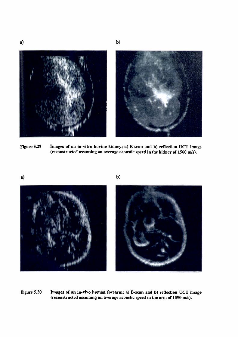
144

5.6 Discussion of reflection-only system

This chapter has described the design, construction and operation of an ultrasound CT system

for narrow beam reflection imaging in a vertical scan plane. This system incorporates a linear array

for rapid and precise positioning, as well as algorithms for very accurate calculation of the system's

centre of rotation.

Reflection UCT images of phantoms, in-vitro and in-vitro organs have been presented and

compared to B-scans of the same targets. These results have been encouraging, the reflection UCT

images appearing to show considerably improved spatial and contrast resolution compared to

conventional B-scans. High contrast spatial resolution was compared by measuring point spread

functions. Unfiltered reflection UCT images were shown to have a psf which, as predicted by the

theory presented in Chapter 4, lies between the axial and lateral components of the B-scan psf. This

is borne out by images from high contrast targets (wires in water) which show that the resolution of

a reflection UCT image (about 1.6mm) lies between the axial resolution (1mm) and the lateral

resolution (3mm) of a B-scan image. Resolution in a "real" soft tissue target is harder to quantify

because it depends on the contrast of the resolved target compared to its surroundings, ie on the

relative scattering strengths. However in real tissue the resolution of a reflection UCT image would

be expected to be considerably better than that for a B-scan image due to the higher signal-to-speckle

ratio (and hence contrast resolution) of the UCT images.

A Wiener inverse filter derived from a measured reflection UCT point spread function was

shown to be effective in improving still further the resolution (to less than 1 mm) of reflection UCT

images of high contrast targets. However in more realistic targets, such as TEM phantoms and soft

tissues, inverse filtering caused an amplification of the speckle component. This speckle amplification

almost certainly arises from the high-pass nature of the inverse filtering operation. Thus for images

of real tissue (ie containing speckle), Wiener inverse filtering still improves the spatial resolution for

high contrast targets but only at the expense of contrast resolution. It may be possible in the future,

with the benefit of higher precision positioning systems and higher data storage capacity, to use the

raw RF echo signal rather than the demodulated signal in the reconstruction. Although the

contributions to speckle from wavefront distortion will still be present (see 4.3.1.3), speckle in RE

images should be much less apparent and hence it may be possible to apply inverse filtering

techniques beneficially.

145

Reflection UCT images also show improvements compared to B-scans in terms of more

subjective criteria such as the ease of interpretation of the images, due mainly to the improved

delineation of tissue boundaries and reduced speckle. Although the B-scan images presented are from

an old scanner and are thus not representative of images obtainable from state-of-the-art equipment,

it is expected that the improvements demonstrated by reflection UCT over conventional B-scanning

would be preserved when using data from more advanced equipment.

An investigation into the likely causes of artifacts in reflection UCT images has shown that

small, highly attenuating structures, known to cause shadowing in conventional B-scans, are not a

major problem in reflection UCT images because of the multiple angles of view. Significant image

degradation was shown to arise, however, from a difference in average acoustic speed between the

target and the coupling medium. A simple adaption to the reconstruction algorithm, to allow different

values of the average acoustic speed to be assigned to the water and the target respectively, was

shown to be effective in considerably reducing the axial mis-registration component of the acoustic

speed artifact in these cases.

The reflection UCT images from some targets still possess significant artifacts, however. In

particular acoustic speed variations within the target itself, and refraction arising from a difference

in acoustic speed between the coupling medium and the target, can cause artifacts in the reflection

UCT images which cannot be corrected by adjusting the average acoustic speed for the whole target.

Correction of these artifacts would require detailed knowledge of the acoustic speed distribution within

the target, information which can be provided in principle by a transmission-mode UCT system. In

addition, attenuation of the ultrasound from some scan directions for thick or highly attenuating

targets can cause some parts of a target to be poorly visualised. One way of overcoming this problem

would be to scan the target over a complete 360°, thus ensuring that all parts of the target receive

ultrasound over at least 180° even if the ultrasound can only penetrate half-way through the target.

In conclusion, a 180° reflection only UCT system without compensation for acoustic speed

variations is capable of producing images of some targets that are superior to conventional real-time

B-scans, but is unlikely to show worthwhile advantages in tissues showing considerable attenuation

and acoustic speed variations, such as the human breast. It may be possible to overcome some of the

problems of 180° scanning using techniques for estimating acoustic speed which do not rely on

transmission measurements. Some possibilities along these lines will be discussed in Chapter 7. The

alternative is to develop a UCT system for combined reflection and transmission imaging that can

146

scan through 360 degrees in a horizontal plane. Such a system has been built and will be described

in the next Chapter.

147

6 Development of a system for combined acoustic speed and reflection UCT

6.1 Introduction

One of the main conclusions of the study into reflection UCT, reported in Chapter 5, was that

the quality of the images is limited when there are significant (> 5%) acoustic speed variations within

the target. The reason for this loss of quality is that the acoustic speed variations cause mis-

registration of the echoes when reconstructing the reflection UCT image. It seems reasonable to

assume that if knowledge of the acoustic speed distribution within a target section were available, the

quality of a reflection UCT image of the same target could be improved by some appropriate

processing of the reflectivity data. Indeed this approach has been suggested by other researchers into

ultrasound CT (see section 3.2), although only a few have attempted it experimentally (Kim et al

1984, Bartelt 1988). These attempts were also limited, mainly by the poor quantitative or geometrical

accuracy of the acoustic speed images produced. Specifically, Bartelt used a pulse-echo method for

the reconstruction of acoustic speed images, the quality of which were very dependent on accurate

time-gain compensation. Kim et al used the established transmission UCT technique to obtain

acoustic speed images (see section 3.3.2), but both their reflection and transmission measurements

were made using stepped single element transducers which inevitably introduced mechanical

inaccuracies.

Considering the encouraging results obtained with the linear array based reflection-only

system described in Chapter 5, it was hoped that a system incorporating linear arrays with their

inherently greater mechanical accuracy, for both reflection and transmission measurements, would

be capable of producing reflectivity and acoustic speed images of sufficient quality to make

compensation for the affects of varying acoustic speed in the reflection images worthwhile.

Consequently a second scanning system based on linear arrays and intended for both reflection and

transmission UCT was developed and is described in this chapter.

The chapter will start by introducing the principles of acoustic speed compensation of

reflection UCT images (6.2). This will include a discussion of the relative importance of the axial

and lateral components of refraction in contributing to artifacts in reflection UCT images, and ways

in which these effects can be compensated for. Then the design and construction of a practical

combined reflection and transmission UCT system will be described (6.3 and 6.4). Since the

technical requirements for reflection UCT have already been discussed in connection with the

148

Teflection only vertical scan-plane system, this chapter will emphasise only the additional technical

tequirements pertaining to transmission UCT and specifically acoustic speed imaging. Various

niethods for acoustic speed reconstruction will be discussed and compared (6.5). Finally, results of

a practical implementation of acoustic speed compensation of reflection UCT images will be given

(6.6).

149

6.2 Theoretical basis of acoustic speed compensation

The basic aim of acoustic speed compensation is to attempt to eliminate, or reduce, those

artifacts in reflection UCT images caused by the assumption of a single acoustic speed for an object

having an unknown and spatially varying acoustic speed. These artifacts may be considered as

consisting of two separable components; (i) displacement of echoes axially, ie along the assumed

straight line propagation path of an ultrasound pulse, due to an incorrect acoustic speed being assumed

in calculating the position of the target, and (ii) displacement of echoes laterally due to the ultrasound

beam being refracted away from the assumed straight path. The purpose of this section is to examine

the relative importance and magnitude of these two affects in determining the quality of a reflection

IJCT image, and to discuss various means of compensating for them.

The simplest case of acoustic speed

artifacts in pulse-echo imaging occurs when an

ultrasound beam crosses a discrete boundary

between two media with different acoustic

speeds. Figure 6.1 shows how an echo from a

point target can be displacement both axially

and laterally due to a change an acoustic speed

across a boundary. In many real soft tissues

acoustic speed is also likely to vary in a

continuous way. However by considering only

finite elements of distance and TOF (Smith at al

1980), such a continuous model can be

approximated by the discrete interface model

discussed below.

trget'-j I

-- V-..

Image oftarget

Figure 6.1 AxiaL and lateral mis-registrationdue to a change in acousticspeed across a boundary.

150

6,2.1 Relative magnitudes of axial and lateral displacement errors

The axial range (d) of an echo on a B-scan image is given by the measured TOF ('F) of a

pulse to and from the scatterer giving rise to the echo and the assumed acoustic speed in the

intervening medium. If the acoustic speed (c,J in the target is assumed (by the reconstruction

algorithm) to be equal to the acoustic speed (c 1) in the coupling medium between the transducer and

the target, then

2

where T is the actual measured TOF given by

T = _+_-C 1 C2

Hence

c d2d = d1 + ____

C2

The axial displacement error (€) is the difference between the calculated range (d) and the true range

(d1+d..

- c1d2- - d2a

C2

= d2 (c1 - c2) (6.1)

C2

Hence the axial displacement error is due solely to the fractional change in acoustic speed across the

boundary and the distance of the target from the boundary.

The lateral displacement error (e ') is governed by the distance of the target from the boundary

and the angles of incidence (0) and refraction (O r) of the ultrasound beam.

450

030

15°

151

10. - On= 2d2sin112 j

Since the angles of incidence and refraction are related by Snell's Law, this equation becomes

0,S]fl_O'

= 2 d2 sin _- ________2

1(6.2)

° 6.0

5.0

,0'4-

3.0

2.0

1.0

7.0

)

0.00.0

1.0 2.0 3.0 4.0 5.0

Change In acoustic speed across boundary (%)

Figure 6.2 Axial and lateral displacement errors as a function of acoustic speed contrast andangle of incidence.

Since there is no simple equation relating e to ç, it is more informative to plot these two

quantities against percentage change in acoustic speed, assuming an acoustic speed in the coupling

medium (c 1) of 1500 ms, for various incident angles (Figure 6.2). This graph shows that the axial

displacement error will always exceed the lateral displacement error for incident angles up to about

450, while for larger incident angles the lateral displacement error is always highest. The relative

importance of axial and lateral displacement errors in any real situation will therefore depend on the

152

exact shape and orientation of the boundary. Considering that any segment of an arbitrary boundary

may have an arbitrary orientation, the incident angles of beams backscattered from a point scatterer

on the other side of the boundary may vary from (Y' to ± 90°. This implies that the "average"

incident angle for all possible boundaries between the ultrasound source and a scatterer will be 45°.

Thus for a target containing many boundaries at different orientations (such as a breast), and where

all scatterers within the target are insonified with ultrasound beams over a large range of angles (as

in UCT), the average incident angle for all scatterers will be around 45° and the average axial and

lateral displacement errors are likely to be similar to each other.

6.2.2 Methods of compensating for displacement errors

Most methods of correcting or compensating for reflection UCT image artifacts due to

acoustic speed variations naturally rely on knowledge of the acoustic speed distribution. However

some attempts have been made to "focus" images which have been distorted by unknown acoustic

speed variations using a technique sometimes called 'wavefront reconstruction' (Hirama et a! 1982,

Zhao and Trahey 1992). This technique originated from the astronomical field (Muller and

Buffington, 1974), where images of distant stars obtained by ground based telescopes are distorted

by refraction (lateral displacement) and phase retardation (axial displacement) of light by the

atmosphere. The technique however relies on the fact that the star or stars are known to be

incoherent point sources, and hence the technique is not in general suitable for ultrasonic imaging

where echoes from multiple scatterers interfere coherently. The exception is the situation where the

tissue contains a recognisable target, such as a fluid filled vessel, which can be used to focus on

(Chen et al, 1987). Since this situation can not always be anticipated in the human breast, knowledge

of the acoustic speed distribution is required. One fairly well established technique for obtaining

acoustic speed distributions in-vivo is transmission UCT (see 3.3). This is the technique pursued in

this thesis.

Axial Displacement Errors

Correction for the axial component of the displacement errors is relatively easy in principle

Since the targets are assumed to lie along the straight line path of the incident ultrasound beams.

Information about the acoustic speed distribution along the path of each ultrasound beam of a

reflection image is used to calculate all the axial displacement errors for that beam. This information

is then used to correctly register the echoes returned by each beam (ie for each scan line of a

153

reflection image).

For the incorporation of acoustic speed information into the reconstruction of a reflection

UCT image to be worthwhile, the estimates of axial displacement derived from the acoustic speed

image should be considerably more accurate than the anticipated final resolution of the reflection

images (ie better than 0.75 mm). Hence a figure of 0.4mm for the required accuracy in the esti,mate

of the displacement error would be reasonable. Equation 6.1 shows that inaccuracies in the axial

displacement estimates will arise from two components of the acoustic speed image: errors in d2 (ie

geometric accuracy) and errors in c (ie quantitative accuracy). The relative importance of geometric

and quantitative accuracy in determining the error (.e) in the estimate of the axial displacement is

given from 6.1 by partial differentiation, so that

M2 (c1 - c2)= ___________

C2

= &2 d2 c1Ac6

for Ac20

for M2 0

(6.3)

(6.4)

Hence the geometric accuracy of the acoustic speed image required to achieve a given

accuracy in €a depends on the fractional change in acoustic speed across the boundary. If the

maximum likely (ie worst case) change in acoustic speed at a soft tissue boundary is 10% (e.g. Duck

1990), then d2 must be known to an accuracy of 4 mm to achieve an accuracy of 0.4 mm in the

estimate of Ea.

The quantitative accuracy required depends on d2 and on the absolute values of acoustic speeds

on each side of the boundary. For an object with a maximum diameter of 105mm (ie the field width

of the ultrasound probe used in Chapter 5), and assuming the acoustic speed in the coupling medium

c 1 to be about 1500 ms 4 with a change in acoustic speed across the boundary of -10% (ie c 2 = 1364

rns t), the accuracy required in c2 to achieve an accuracy of 0.4 mm in €a is 4.7 ms'.

Although geometric accuracies of ±4 mm and quantitative accuracies of ± 5 ms' are

theoretically achievable in acoustic speed imaging (see 4.3.3 and later in 6.3.3), whether they will

be achievable in practice will depend on the degree of artifacts appearing in acoustic speed images

of real targets (section 6.5). Note also that for the majority of acoustic paths within a soft tissue

target, the acoustic speed change across a boundary will be less than 10% and the relevant target will

154

be closer than 105 mm to the boundary, under which circumstances the accuracies required of d2 and

c, may be considerably less than those quoted above.

Lateral Displacement Errors

Correction for the lateral component of the displacement error is rather more difficult because

it requires, from equation 6.2, knowledge of the refraction angles of the ultrasound beams.

Calculation of these refraction angles requires accurate information about the orientation of the

boundaries (or vectors in the case of continuous transitions) between regions of different acoustic

speed as well as the acoustic speed values themselves. If such information was available, corrections

to reflection UCT images could in principle be implemented using the ray-tracing or perturbation

methods which have been used by various workers for refraction correction in transmission UCT (see

3.3.3). As was the case for the axial corrections, the value or otherwise of lateral corrections will

depend on how accurate, in terms of both geometric and quantitative accuracy, the acoustic speed

image needs to be.

Since equation 6.2 is not easy to differentiate analytically, it is more informative to assess the

affects of geometric accuracy (ie in d2) and quantitative accuracy (in c) graphically. Figure 6.2

suggests that, for an average incident angle of about 45°, the accuracy of the lateral displacement

estimates will have a dependence on the accuracy of d2 and c2 which is similar to the dependence of

the axial displacement estimate on these quantities. Thus, under worst case conditions, d2 should be

known to an accuracy of about 4 mm and C2 should be known to an accuracy of about 5 ms'.

Unfortunately there is an additional geometric factor that must be considered when estimating the

lateral displacement error. This factor is the angle of incidence of the acoustic beam at the boundary,

and it will be postulated below that it is the accuracy required of this factor that provides the main

limitation to lateral displacement correction.

Any complex boundary can be considered as a set of short (ie considerably less than the

beamwidth) linear segments, the orientations of which are required to calculate the incident and

refracted angles of an ultrasound beam incident on the boundary. Figure 6.2 showed that the lateral

displacement error varies rapidly with incident angle, particularly if the acoustic speed change across

the boundary is high. Figure 6.3 shows this dependence explicitly by plotting equation 6.2 for the

worst case conditions of an acoustic speed change across a boundary of 10% (c2 = 1364ms') and a

path difference (d2) between target and boundary of 105 mm. By fitting a 4th order polynomial to this

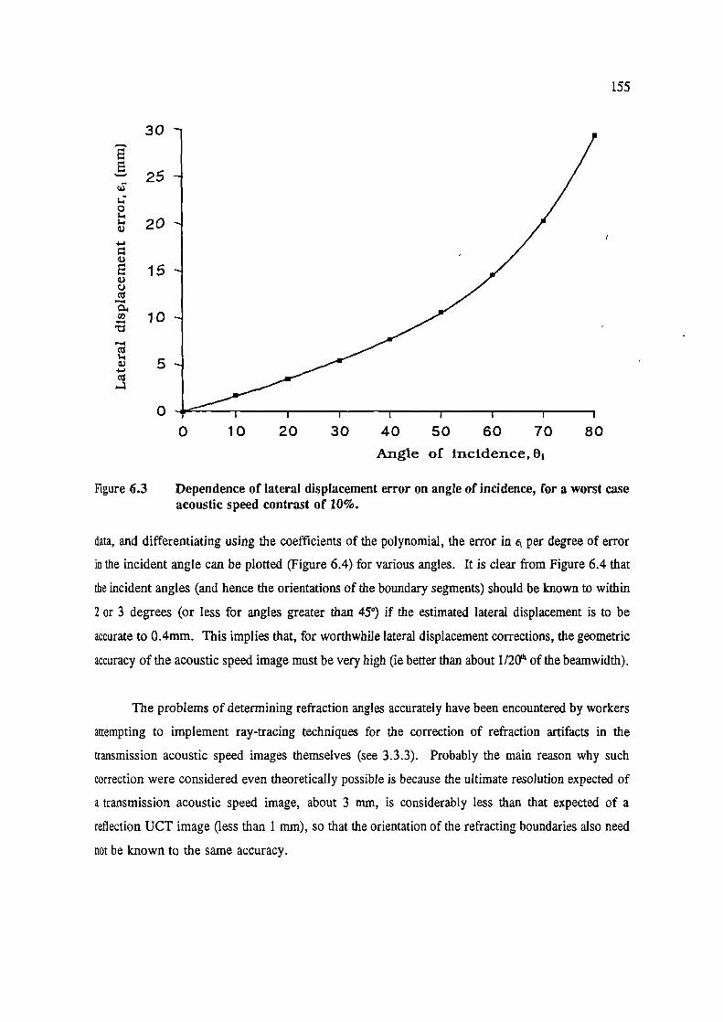
E

l..i0

V

V

V0

Co

1-4I.)

4-I

155

30

25

20

15

10

5

00 10 20 30 40 50 60 70 80

Angle of incidence, O

Figure 6.3 Dependence of lateral displacement error on angle of incidence, for a worst caseacoustic speed contrast of 10%.

data, and differentiating using the coefficients of the polynomial, the error in e1 per degree of error

in the incident angle can be plotted (Figure 6.4) for various angles. It is clear from Figure 6.4 that

the incident angles (and hence the orientations of the boundary segments) should be known to within

2 or 3 degrees (or less for angles greater than 45°) if the estimated lateral displacement is to be

accurate to 0.4mm. This implies that, for worthwhile lateral displacement corrections, the geometric

accuracy of the acoustic speed image must be very high (ie better than about 1/2çfh of the beamwidth).

The problems of determining refraction angles accurately have been encountered by workers

attempting to implement ray-tracing techniques for the correction of refraction artifacts in the

transmission acoustic speed images themselves (see 3.3.3). Probably the main reason why such

correction were considered even theoretically possible is because the ultimate resolution expected of

a transmission acoustic speed image, about 3 mm, is considerably less than that expected of a

reflection UCT image (less than 1 mm), so that the orientation of the refracting boundaries also need

not be known to the same accuracy.

VV

V

E

4)

U,U

4)

4)C)

U,

U,1..4)

U,

0

1.2

1.0

0.8

0.6

0.4

0.2

0

156

0 10 20 30 40 50 60 70 80Angle of incidence, 0,

ligure 6.4 Error in the estimate of lateral displacement caused by a one degree error in theangle of incidence, as a function of incident angle.

Even if acoustic speed images could be produced that were totally free of artifacts, images

produced by transmission UCT (the technique used here) have a resolution that is limited by the

acoustic beam width (typically 6-7 times the wavelength). Hence the acoustic speed images at best

Tepresent a heavily smoothed version of the "true" acoustic speed distribution, with a resolution that

is unlikely to be sufficient for worthwhile lateral displacement corrections. For this reason, only axial

displacement corrections will be implemented in this study, with the consequence that the reflection

UCT images will rarely be totally free of acoustic speed artifacts. Whether axial corrections alone

will show a worthwhile improvement to the resolution of reflection UCT images can only be

established by experiment (see section 6.6). The algorithm for performing the axial displacement

corrections will be discussed in detail in section 6.6.2.

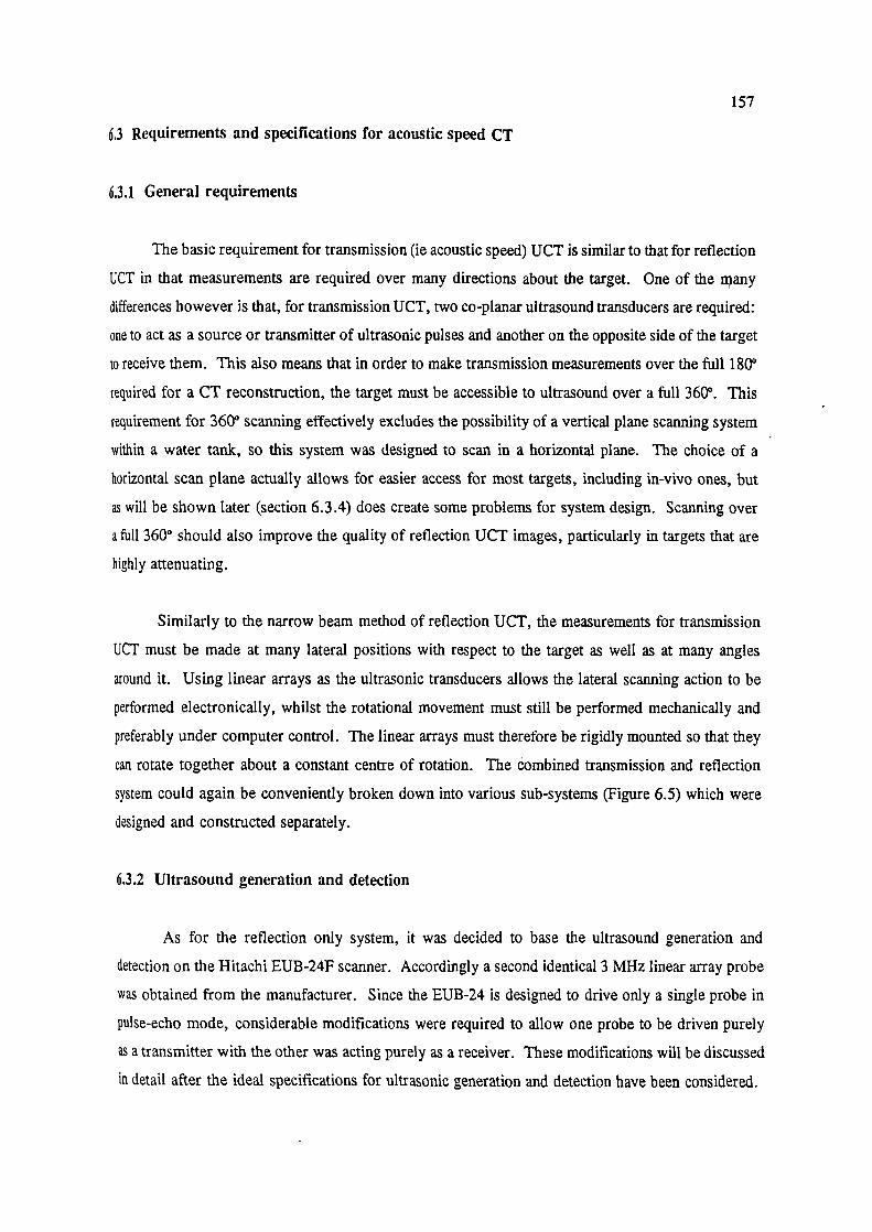
157

6.3 Requirements and specifications for acoustic speed CT

6,3.1 General requirements

The basic requirement for transmission (ie acoustic speed) UCT is similar to that for reflection

UCT in that measurements are required over many directions about the target. One of the nany

differences however is that, for transmission UCT, two co-planar ultrasound transducers are required:

one to act as a source or transmitter of ultrasonic pulses and another on the opposite side of the target

to receive them. This also means that in order to make transmission measurements over the full 180°

required for a CT reconstruction, the target must be accessible to ultrasound over a full 360°. This

requirement for 360° scanning effectively excludes the possibility of a vertical plane scanning system

within a water tank, so this system was designed to scan in a horizontal plane. The choice of a

horizontal scan plane actually allows for easier access for most targets, including in-vivo ones, but

as will be shown later (section 6.3.4) does create some problems for system design. Scanning over

a full 360° should also improve the quality of reflection UCT images, particularly in targets that are

highly attenuating.

Similarly to the narrow beam method of reflection UCT, the measurements for transmission

UCT must be made at many lateral positions with respect to the target as well as at many angles

around it. Using linear arrays as the ultrasonic transducers allows the lateral scanning action to be

performed electronically, whilst the rotational movement must still be performed mechanically and

preferably under computer control. The linear arrays must therefore be rigidly mounted so that they

can rotate together about a constant centre of rotation. The combined transmission and reflection

system could again be conveniently broken down into various sub-systems (Figure 6.5) which were

designed and constructed separately.

6.3.2 Ultrasound generation and detection

As for the reflection only system, it was decided to base the ultrasound generation and

detection on the Hitachi EUB-24F scanner. Accordingly a second identical 3 MHz linear array probe

was obtained from the manufacturer. Since the ETJB-24 is designed to drive only a single probe in

pulse-echo mode, considerable modifications were required to allow one probe to be driven purely

as a transmitter with the other was acting purely as a receiver. These modifications will be discussed

in detail after the ideal specifications for ultrasonic generation and detection have been considered.

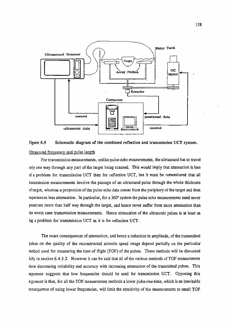
Ultrasound Scanner

Target zi

Array Probes DCMotor

control

ultrasonic data

158

Tank

L1J Encoder

Computer

LIuFigure 6.5 Schematic diagram of the combined reflection and transmission UCT system.

Ultrasound frequency and pulse length

For transmission measurements, unlike pulse-echo measurements, the ultrasound has to travel

only one way through any part of the target being scanned. This would imply that attenuation is less

of a problem for transmission UCT than for reflection UCT, but it must be remembered that all

transmission measurements involve the passage of an ultrasound pulse through the whole thickness

of target, whereas a proportion of the pulse echo data comes from the periphery of the target and thus

experiences less attenuation. In particular, for a 3600 system the pulse echo measurements need never

penetrate more than half way through the target, and hence never suffer from more attenuation than

the worst case transmission measurements. Hence attenuation of the ultrasonic pulses is at least as

big a problem for transmission UCT as it is for reflection UCT.

The exact consequences of attenuation, and hence a reduction in amplitude, of the transmitted

pulses on the quality of the reconstructed acoustic speed image depend partially on the particular

method used for measuring the time of flight (TOF) of the pulses. These methods will be discussed

fully in section 6.4.5.2. However it can be said that all of the various methods of TOF measurement

show decreasing reliability and accuracy with increasing attenuation of the transmitted pulses. This

argument suggests that low frequencies should be used for transmission UCT. Opposing this

argument is that, for all the TOF measurement methods a lower pulse rise-time, which is an inevitable

consequence of using lower frequencies, will limit the sensitivity of the measurements to small TOP

159

differences and hence to small acoustic speed differences. Another justification for higher frequencies

is that they allow shorter wavelengths and hence narrower beams, which has important consequences

for the spatial resolution of the acoustic speed images (as shown theoretically in 4.4.4).

Weighing up these conflicting requirements, a frequency of around 2 MHz would probably

represent the best compromise for the targets of interest. Hence the EUB 24's frequency of 3 MJiz,

although a little higher than the ideal, was considered acceptable.

The factors dictating the ideal pulse length are much more straight forward. The ultrasound

pulse should not be too short, in other words it should not have too wide a bandwidth, since

frequency dependent attenuation will distort the pulse shape and make the TOF measurements less

accurate. The only upper limit on the ideal length of the pulses is that standing wave affects (ie

reverberation), which will only be appreciable for very long pulses, are very undesirable. With these

points in mind the EUB 24, with a pulse length of about 3 cycles (or 1.5mm, see Figure 5.4), appears

to have rather a wide bandwidth for transmission UCT. The consequences of these limitations of the

EUB 24 will become evident when the results of acoustic speed imaging are presented in section 6.5.

Ultrasound beam width

As shown in section 4.4.4, for transmission UCT it is the width of the ultrasound beam that

provides the fundamental limit on the potential resolution of the images. Hence for an ideal system

the ultrasound beam should be as narrow as possible over as great a range as possible. Unlike

reflection UCT where the pulse-echo nature of the measurements allows dynamic focusing to be used

(if available) to minimise the beam width over a large range, in a transmission system only one focal

zone per transmitted pulse is possible. The obvious way of achieving a narrow beam in the focal

zone is to use a large aperture transducer that is strongly focused, but this is undesirable because

strong focusing implies a short focal zone with wide beams both before and after it. These factors

imply that the transducer should be weakly focused, with the centre of focal zone located as closely

as possible to the centre of the target. For targets up to 10 cm in diameter, this implies a focal length

of about 7 cm when allowing for a 2 cm standoff between the transducer and the surface of the target.

A transmitted beam plot for the EUB 24 linear array probe, measured in water using a PZT

needle hydrophone, is shown in Figure 6.6. The focus is about 60 mm from the probe face, with a

6dB beam width at the focus of 3.6 mm. The 6dB widths of the beam at 2 cm and 12 cm from the

probe face (ie at the approximate limits of the largest target) are 10 mm and 4.5 mm respectively.

160

Hence the potential resolution of the acoustic speed image will lie somewhere between about 3 mm

and 10 mm. Given these beam width characteristics this probe fits the requirements for transmission

UCr quite well.

Figure 6.6 Transmission beam plot of the 3 MHz linear array. Each grey level representsa 6 dB change in peak negative acoustic pressure.

Scanned field width and beam spacing

As was the case for reflection UCT, the width of the linear array probe (10.5 cm for the EUB

24) limits the maximum dimension of a target to be scanned to about 10 cm. The distance between

beam positions in the lateral scan is determined by the inherent resolution of the measured projections,

which for transmission UCT is the beam width itself. Thus sampling theory dictates that the beam

spacing should be less than half the minimum 6 dB beam width, as was the case for reflection UCT

(section 5.3.1).

For the EUB 24, the distance between effective aperture positions, and hence samples of the

projection, is 1.5mm. This is, as required, less than the half the minimum 6dB transmission beam

width of 3.6 mm. The number of aperture positions is 70, giving 70 samples per projection.

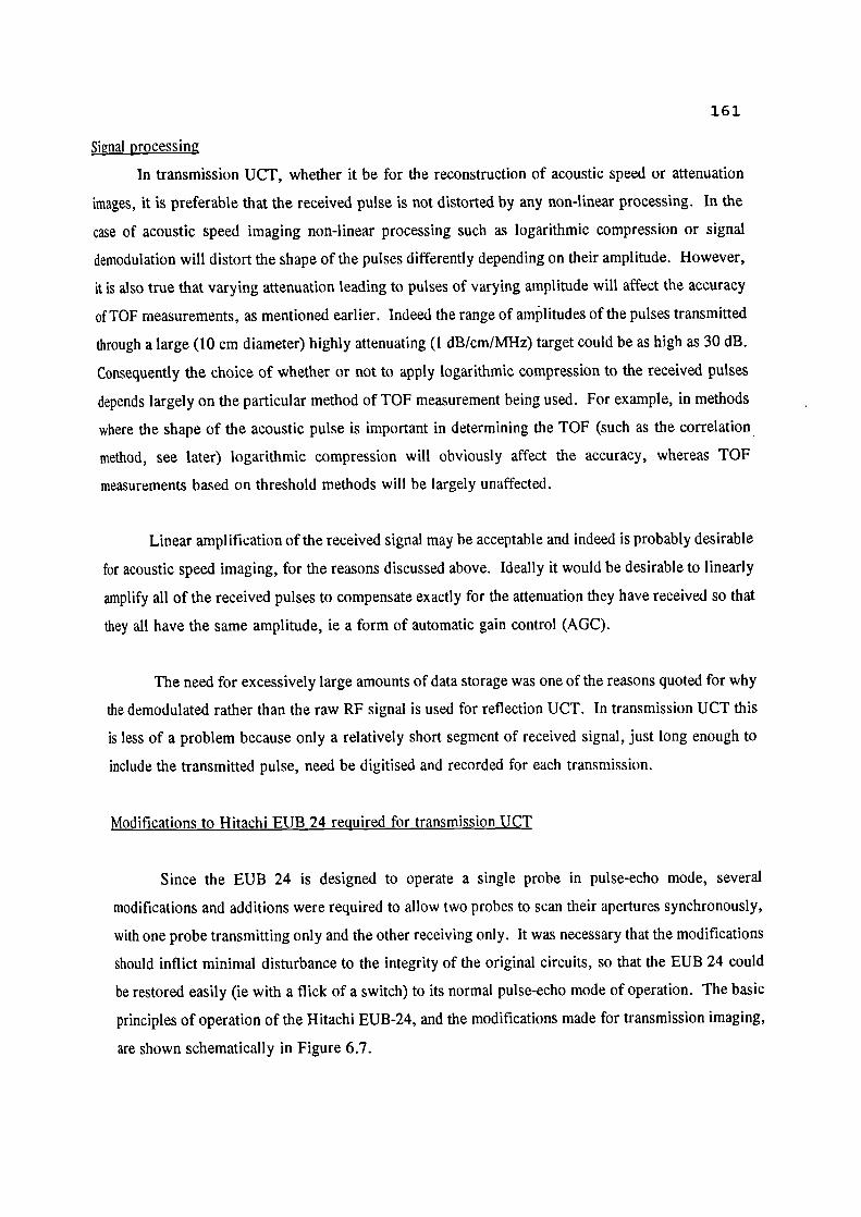
161

$jgnal processing

In transmission UCT, whether it be for the reconstruction of acoustic speed or attenuation

images, it is preferable that the received pulse is not distorted by any non-linear processing. In the

case of acoustic speed imaging non-linear processing such as logarithmic compression or signal

demodulation will distort the shape of the pulses differently depending on their amplitude. However,

it is also true that varying attenuation leading to pulses of varying amplitude will affect the accuracy

of TOF measurements, as mentioned earlier. Indeed the range of amIitudes of the pulses transmitted

through a large (10 cm diameter) highly attenuating (1 dBIcmIMHz) target could be as high as 30 dB.

Consequently the choice of whether or not to apply logarithmic compression to the received pulses

depends largely on the particular method of TOF measurement being used. For example, in methods

where the shape of the acoustic pulse is important in determining the TOF (such as the correlation

method, see later) logarithmic compression will obviously affect the accuracy, whereas TOF

measurements based on threshold methods will be largely unaffected.

Linear amplification of the received signal may be acceptable and indeed is probably desirable

for acoustic speed imaging, for the reasons discussed above. Ideally it would be desirable to linearly

amplify all of the received pulses to compensate exactly for the attenuation they have received so that

they all have the same amplitude, ie a form of automatic gain control (AGC).

The need for excessively large amounts of data storage was one of the reasons quoted for why

the demodulated rather than the raw RF signal is used for reflection UCT. In transmission UCT this

is less of a problem because only a relatively short segment of received signal, just long enough to

include the transmitted pulse, need be digitised and recorded for each transmission.

Modifications to Hitachi EUB 24 required for transmission UCT

Since the EUB 24 is designed to operate a single probe in pulse-echo mode, several

modifications and additions were required to allow two probes to scan their apertures synchronously,

with one probe transmitting only and the other receiving only. It was necessary that the modifications

should inflict minimal disturbance to the integrity of the original circuits, so that the EUB 24 could

be restored easily (ie with a flick of a switch) to its normal pulse-echo mode of operation. The basic

principles of operation of the Hitachi EUB-24, and the modifications made for transmission imaging,

are shown schematically in Figure 6.7.

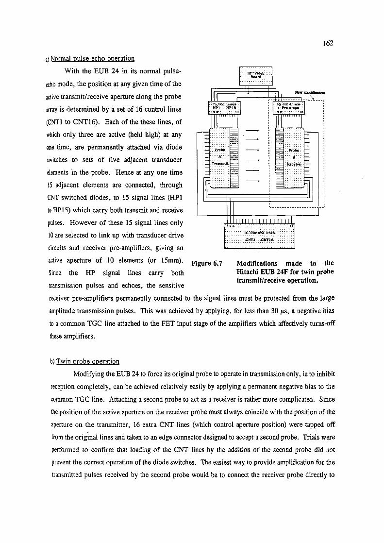
:i New

:5 RX.LI,...+: ftc-amps.:23" 15

II

TX/Re. LinesHP2: .HPTh23' 1

?xpbc::

:":

TrajirnIL

162

a) Normal pulse-echo operation

With the EUB 24 in its normal pulse- • 'RF Vtdco:

echo mode, the position at any given time of the

active transmit/receive aperture along the probe

array is determined by a set of 16 control lines

(CNT1 to CNT16). Each of the these lines, of

which only three are active (held high) at any

one time, are permanently attached via diode

switches to sets of five adjacent transducer

elements in the probe. Hence at any one time

15 adjacent elements are connected, through

CNT switched diodes, to 15 signal lines (HP1

to HP 15) which carry both transmit and receive

pulses. However of these 15 signal lines only

10 are selected to link up with transducer drive 16:contii:unei:::::::::

circuits and receiver pre-amplifiers, giving an

active aperture of 10 elements (or 15mm). Figure 6.7

Modifications made to theSince the HP signal lines carry both

Hitachi EUB 24F for twin probe

transmission pulses and echoes, the sensitive transmit/receive operation.

receiver pre-amplifiers permanently connected to the signal lines must be protected from the large

amplitude transmission pulses. This was achieved by applying, for less than 30 ps, a negative bias

to a common TGC line attached to the FET input stage of the amplifiers which affectively turns-off

these amplifiers.

b) Twin probe operation

Modifying the EUB 24 to force its original probe to operate in transmission only, ie to inhibit

reception completely, can be achieved relatively easily by applying a permanent negative bias to the

common TGC line. Attaching a second probe to act as a receiver is rather more complicated. Since

the position of the active aperture on the receiver probe must always coincide with the position of the

aperture on the transmitter, 16 extra CNT lines (which control aperture position) were tapped off

from the original lines and taken to an edge connector designed to accept a second probe. Trials were

performed to confirm that loading of the CNT lines by the addition of the second probe did not

prevent the correct operation of the diode switches. The easiest way to provide amplification for the

transmitted pulses received by the second probe would be to connect the receiver probe directly to

2201

163

+5V

-5V

Figure 6.8 RF pre-amplifier circuit for the received signals.

the HP signal lines in the EUB 24. Unfortunately this was not possible because a) the EUB 24's

receiver pre-amplifiers are already inhibited to prevent the transmitter probe receiving, and b) there

would be no way to prevent transmission pulses being sent to the receiver probe. Consequently a

batch of 15 identical pre-amplifler circuits (Figure 6.8), designed to have the same input impedance,

gain and bandwidth characteristics as the EUB 24's pre-amplifiers, were built by the Electronics

Department to provide amplification of the pulses received by the second probe. The outputs of these

amplifiers were then connected to the outputs of the corresponding pre-amplifler circuits of the EUB

24.

The modifications required to allow the raw RF signal to be extracted from the EUB 24 after

the pre-amplifiers and summing circuits, had already been made for the reflection only system. This

RF signal receives some amplification within the EUB 24 via its TGC and overall gain controls, but

does not receive automatic gain (AGC) at this stage. Additional amplification, if required, can be

provided by the input amplifier of the LeCroy transient recorder, but since no attempt has been made

to implement AGC all the signals receive the same amplification.

164

6.3.3 Digitisation and data transfer

Digitisation rates and implications for contrast-detail resolution

The transmitted pulse (Figure 5.4) from the EUB 24F's linear array possesses no significant

signal, in water, above about 6 MHz. Allowing for some wideband noise in the signal, sampling

requirements would suggest a digitisation rate of about 24 MHz. In practice, the digitisation rate

should be as high as possible for transmission UCT since the sampling interval represents the best

possible precision in the measurement of pulse TOF. The precision of the TOF measurement directly

determines the potential contrast-detail resolution of the reconstructed acoustic speed image. To

appreciate this, consider a small region of diameter d 1 and acoustic speed c 1 imbedded in a uniform

background region of acoustic speed c0. The difference (st) in TOF between a pulse traversing the

centre of the imbedded region and one just missing it will be given by (see also 4.3.3.4),

11 11= d I_-_i

IC 1 coJ

Defining the acoustic speed contrast (C) as a percentage

c = * (c0-c1)

Cl

implies that the product of the contrast and size of the imbedded region is given by

C.d1 = 100*c0*&

Now the product C.d 1 will be minimised by the smallest value for t, which is simply the precision

in the measurement of pulse TOF or the inverse of the digitisation rate (R).

ie Mm [C . d1 ] = 100 * (6.5)R

This hyperbola is plotted in Figure 6.9 for various values of the digitisation rate, and assuming an

acoustic speed (c0) in the background medium of 1500 mIs. The minimum potential resolution of an

acoustic speed image, as defined by the 6dB beam width, is about 3 mm. Hence at a digitisation rate

of 25 MHz a target of this size would need to have an acoustic speed contrast of at least 2% (or 30

rn/s different to its surroundings) to be detected. At 50 MHz the same target need only show a

165

6

E

Potential resolution of acoustic speed image

ti)

25MHz

50MHz

100MHz200MHz

0

0

1 2 3 4

5

Acoustic speed contrast (%)

Figure 6.9

Theoretical contrast-detail diagrams for acoustic speed imaging, for variousdigitisation rates.

contrast of 1% (15 mIs). Perhaps more revealing is that for a target of 1% contrast to be detected

with a digitisation rate of 25 MHz, it must be at least 6 mm across.

The arguments put forward in section 6.2.1.2 indicated that, for an acoustic speed image to

accurate enough to provide worthwhile acoustic speed compensation, the boundary of a region having

an acoustic speed contrast of 10% should be represented on the acoustic speed image to an accuracy

of better than 4 mni. This geometric accuracy is thus theoretically achievable with a transmission

UCT technique. The required quantitative accuracy was ±5 rn/s for a circular region of contrast 10%

and diameter 105 nmi. With a digitisation rate of 50 MHz the theoretical contrast resolution (from

equation 6.5) is 0.03%, which is equivalent to a potential accuracy in estimation of the acoustic speed

in the region of 0.5 mIs.

In practice many other factors further limit the contrast/detail resolution, but the sampling rate

defines its lower boundary. Clearly a digitisation rate of 50 MHz would be desirable to achieve

166

excellent potential contrast/detail resolution. The upper limit on the digitisation rate is ultimately

defined by the speed of the digitiser, but in practice also by the problems of data storage (see below).

Dynamic range

The dynamic range of the digitiser (ie the number of bits) must be able to cope with the

possible 30 dB range of pulse amplitudes to be digitised. This implies that a minimum of 5 bits is

required. The effect of the number of additional digitisation bits on the accuracy of TOF

measurements really depends on the particular method of TOF measurement used. For threshold

based methods, where the rapidly rising leading edge of the received pulse is used, the precession in

the vertical (ie amplitude) axis is not as critical as that in the horizontal (ie time) axis, and a relatively

small number of bits would suffice. In the TOF measurement methods that use all the information

in the transmitted pulse, and especially when AGC and logarithmic amplification is not provided to

reduce the range of pulse amplitudes, amplitude measurement precession is more critical and more

digitisation bits are required for good accuracy. The LeCroy digitiser has a dynamic range of 48 dB

(8 bits), which is probably only just sufficient for good accuracy in TOF measurements.

Amount of data

The total amount of data required for the reconstruction of a complete acoustic speed image

of a single plane will depend on the following factors:-

(1) The number (Np) of TOF projections (ie the number of probe positions around the target.

(2) The number (I) of beam positions making up a projection.

(3) The time (dt) for which the digitiser must be sampling in order to guarantee that the

transmitted pulse has been digitised (ie the digitisation 'window').

(4) The digitisation rate (R).

(5) The dynamic range (Nb) of the digitiser in bytes (1 byte = 8 bits) per sample.

Amount of data required (bytes) N * 1 dt * R * Nb (6.6)

It was shown in section 4.4.4 that, to obtain an adequately sampled transmission UCT

reconstruction, the number of projections required within a total angle of 18(Y' is given by

N=2w

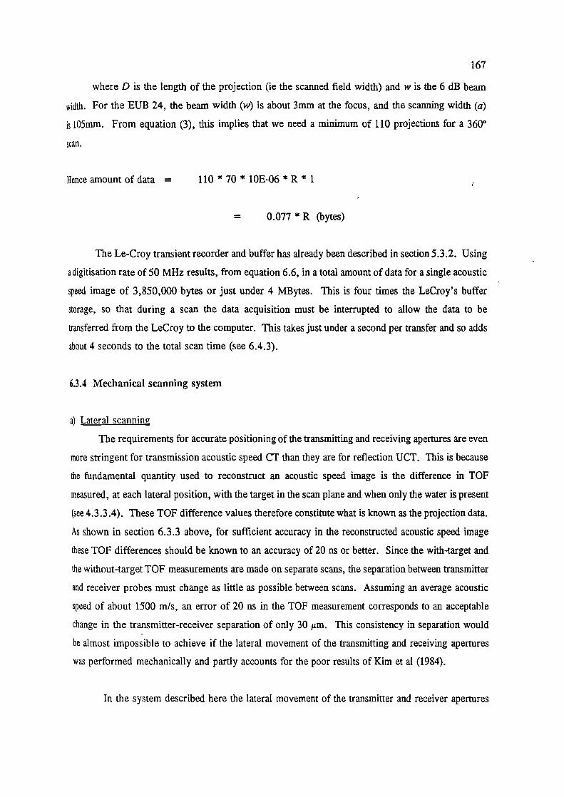
167

where D is the length of the projection (ie the scanned field width) and w is the 6 dB beam

width. For the EUB 24, the beam width (w) is about 3mm at the focus, and the scanning width (a)

s 105mm. From equation (3), this implies that we need a minimum of 110 projections for a 3600

scan.

Henceamountofdata = 110 *70 * 1OE-06 *R* 1

= 0.077 * R (1.y)

The Le-Croy transient recorder and buffer has already been described in section 5.3.2. Using

a digitisation rate of 50 MHz results, from equation 6.6, in a total amount of data for a single acoustic

speed image of 3,850,000 bytes or just under 4 MBytes. This is four times the LeCroy's buffer

storage, so that during a scan the data acquisition must be interrupted to allow the data to be

transferred from the LeCroy to the computer. This takes just under a second per transfer and so adds

about 4 seconds to the total scan time (see 6.4.3).

6.3.4 Mechanical scanning system

a) Lateral scanning

The requirements for accurate positioning of the transmitting and receiving apertures are even

more stringent for transmission acoustic speed CT than they are for reflection UCT. This is because

the fundamental quantity used to reconstruct an acoustic speed image is the difference in TOF

measured, at each lateral position, with the target in the scan plane and when only the water is present

(see 4.3.3.4). These TOF difference values therefore constitute what is known as the projection data.

As shown in section 6.3.3 above, for sufficient accuracy in the reconstructed acoustic speed image

these TOF differences should be known to an accuracy of 20 ns or better. Since the with-target and

the without-target TOF measurements are made on separate scans, the separation between transmitter

and receiver probes must change as little as possible between scans. Assuming an average acoustic

speed of about 1500 m/s, an error of 20 ns in the TOF measurement corresponds to an acceptable

change in the transmitter-receiver separation of only 30 tim. This consistency in separation would

be almost impossible to achieve if the lateral movement of the transmitting and receiving apertures

was performed mechanically and partly accounts for the poor results of Kim et al (1984).

In the system described here the lateral movement of the transmitter and receiver apertures

168

is performed electronically as part of the normal scanning operation of a multi-element probe. Since

the probes are rigid there is no opportunity for the probe separation, at any particular scan angle, to

change significantly between scans.

b) Rotational scanning

For this combined transmission and reflection UCT system an angular positional accuracy of

better than 0.1 degrees (equivalent to 0.2 mm) is still required, being determined by the potential

resolution of a reflection UCT image since this is better than the potential resolution of a transmission

UCT image. The requirement for minimum mechanical inertia in the probe support structure,

consistent with sufficient rigidity to maintain positional accuracy, also still applies.

Despite these similar requirements, the design considerations for the combined transmission

and reflection UCT system are in many ways different from those for the reflection only system. The

nain reasons for these differences are (i) the need for two diametrically opposed probes and (ii) the

decision to scan in a horizontal plane. The vertical scan plane, chosen for the reflection only system,

suggested a relatively simple probe support structure based on a horizontal bar which was pivoted at

both ends via flat end-plates. This is an inherently strong and stable structure with a centre of

rotation defined by the common axis of the pivot points. For a transmission system two bars would

be needed, one to support each probe. Also, because a horizontal plane system would need to be

accessible from above, each bar could only be pivoted at one end (ie at a common centre of rotation

for both). Hence these bars, and their corresponding end-plates, would have to be very strong to

provide sufficient rigidity to maintain a constant circle to better than 0.2 mm runout.

Rather than attempting to define a circular motion by rotation around a fixed pivot, it was

decided that a more reliable and practical solution in this case would be to base the system around

an inherently rigid circular structure with known tolerances. A commercially available system with

which there was already some experience within the Department, called the Hepco Slide System, was

found to meet the requirements. The Hepco system consists of linear and circular precision steel

slideways, with sealed low-friction journals and lightweight carriages, all of various sizes, that can

be used as building blocks to construct very complex systems.

The main component of the system purchased for the UCT scanner is a 0.35 m diameter

stainless steel slide ring (shown schematically in Figure 6.10) which defines, to a precision of better

than 0.1mm, the plane and axis of rotation. One option that was considered, in consultation with the

169

Figure 6.10 Schematic diagram of the mechanical parts of the combined transmission andreflection system.

Bioengineering Department, was to attach the ultrasound probes to Hepco carriages which could

simply run along the ring. The main problem with this approach is that, since the carriages must be

driven together but on opposite sides of the ring, they must be connected in some way across centre

of ring. This connection would have to be very strong to maintain the required accuracy and would

restricts access.

A potentially better solution is to rigidly mount the probes onto opposite sides of the ring and

rotate the ring itself, guided by 5 fixed journals, as in Figure 6.10. The main disadvantage now is

that there is considerably more mass to move than with the alternative approach (because the ring is

quite heavy), but with the advantage of much greater inherent rigidity. This effectively means that

better positional accuracy can be obtained at the expensive of scanning speed. Since it had already

been decided that minimising scan times was not a major requirement, this second approach was

adopted.

Hepco linear slideways have been used to provide the other planes of movement required -

170

namely a) to move the probes in and out in order to change the radius of the scan, and b) to move

the probes up and down (on a screw thread for sub-millimetre accuracy) to alter the height of the scan

plane.

The main problem with the general approach of a submerged steel ring rotating within

precession journals is corrosion of the moving parts - particularly those parts which affect the

positional accuracy, namely the edge of the ring and the journals themselves. This problem was

minimised by using stainless steel parts, the exposed surfaces of which had also been coated

commercially with a thin layer of very hard chrome. Additionally, the tank was emptied and all parts

dried and sprayed with water-repellent oil when the system was not going to be in use for more than

a few days.

Ti_,

.:

Figure 6.11 Photograph of the combined reflection and transmission UCT system.

c) Scanning tank

Due to the very different requirements of a horizontal plane scanner, it was decided that for

the combined transmission and reflection system a cylindrical scanning tank would be more

appropriate than a rectangular one. To again allow for a scan diameter of up to 20 cm, with 30 cm

allowed for the two probes, a polypropylene tank of diameter 60 cm and height 60 cm was

171

commissioned from a local manufacturer. The positions of the five journals were adjusted until they

were all in contact with the ring, and then bolted securely onto a metal plate directly beneath the tank.

Hence the rigidity of the system was again made to be independent of the strength of the tank itself.

A Photograph of the complete mechanical system is shown in Figure 6.11.

6.3.5 Motor drive system

The positioning requirements of a drive system for the combined transmission and reflection

scanner are essentially similar to those for the reflection-only scanner, specifically being able to

position the probes with an angular resolution of 0.1 degrees, but over a full 360 degrees instead of

180. Since the servo-motor, tacho and control system used in the other system had been very

successful, it was decided to duplicate this system. However because of the considerably greater

inertia of the load (ie the slideways and probes) in the combined scanner (0.8 kg m2 compared to 0.08

kg m2 for the reflection-only system), a gearing ratio of 150:1 was required to achieve adequate

torque at the load. This increase in gearing was provided by using a 50:1 gearbox instead of the 20:1

gearbox.

172

6.4 Acquisition of the data for an acoustic speed image

6,4.1 Introduction

The sequence of procedures involved in acquiring transmission time of flight data and

reconstructing an acoustic speed image will now be described.

6.4.2 Measurement of the centre of rotation

For this system it was again necessary to accurately determine the common centre of rotation

of the two probes so that information acquired from different directions may be combined correctly.

The same test-object that was developed for the reflection-only system (see 5.4.2) can be used to give

the centre of rotation in terms of axial and lateral distances with respect to each probe independently.

The lateral distance information can also be used to ensure that the two probes are aligned correctly,

ie so that the central axis of both probes lie as close as possible (to within 1/4 of the beam width or

0.8mm) to the centre of rotation.

The axial distance or range information can be used to calculate the separation of probes.

Although this information is not actually needed for transmission UCT, it is useful in helping to

decide when to start digitising the receiver signal as described in the next section.

6.4.3 Definition of the acquisition parameters

a) Scan parameters:

The scan acquisition parameters define the number of angular positions in the scan and the

time allowed for the scan. Since TOF measurements are required both with and without the target

present, these parameters must be defined for both circumstances, ie separately for the reference

"water" scan and for the "target" scan.

If it were possible to set up the transmitter and receiver probes to be exactly parallel, then

clearly only a single measurement of pulse TOF in water would be required and all the TOF

measurements obtained with the target could be compared to this constant value. However a deviation

in the probe separation of only 0.2 mm would result in a TOF error of about 0.13 s, which is

173

equivalent (see equation 6.5) to the increase in TOF experienced by a pulse passing through a 10 mm

wide region having an acoustic speed 2% higher than the background. For this reason the reference

TOF measurements are obtained, in water, across the whole length of the probes (ie utilising all 70

pulse transmissions), and the "target" measurements are compared only to the reference measurement

obtained at the corresponding position on the probes.

Following a similar argument, the possibility that the probe separation might change slightly

(by < 0.1 mm) as the probes rotate implies that the reference TOF measurements must also be

obtained at the same probe positions as are acquired for the target measurements. In practice an

experimental investigation, the results of which are presented in section 6.5.4.1, has demonstrated

that ten probe positions within the full 180 degrees are usually sufficient for the reference

neasurements. During reconstruction, the TOF measurements from each probe position in the target

scan are compared to those from the nearest available probe position in the reference scan.

b) Data acquisition parameters:

The parameters defining the data acquisition procedure are necessarily somewhat different to

those for the reflection-only system. These parameters are the following:-

i. The time delays after each pulse initiation to start and to stop digitising the signals at the

receiver, ie the digitisation window, must be defined. The pulse initiation is assumed to

coincide with the leading edge of the line sync signals from the EUB 24, which are used to

trigger the LeCroy digitiser. Knowing the separation of the probes from the centre of

rotation measurements, and the acoustic speed in the coupling medium (e.g. water at a

measured temperature), it is then possible to calculate the time after its initiation that a pulse

is expected to arrive at the receiver probe with no target present. A ten microsecond

digitisation window is then calculated, starting 5 s before and ending 5 s after the expected

arrival time. This length of window is expected to be adequate to catch pulses transmitted

through most potential targets. Note that it is not essential for the reconstruction of accurate

acoustic speed images that pulse initiation coincides exactly with the line sync signal, since

it is the difference in TOF measured with and without the target which is used in the

reconstruction. It is essential however that the line sync signals do have a constant time

relationship to pulse initiation, which of course they must have for the EUB 24 scanner to

operate correctly.

on a threshold approach and the other on a

pulse shape approach, have been investigated in

detail.

The simplest method to understand, and

to implement, is the so-called 'threshold

method' (Figure 6.13a). As the name implies,

a fixed threshold is set just above the signal

noise level and a pulse is assumed to have

arrived when the rectified signal first crosses

this threshold. To calculate T - T, this

measurement must be made both for pulses

which have travelled through water only, and

hence have experienced only minimal

attenuation, and for pulses which have become

attenuated after travelling through the target.

175

Retrieve TOFdata through target

at angle 0.

liP band passfilter to

reduce noise

Retrieve ro I Calculate TOP

data through L-. projection

water. T p•

Convolve withS p-Logan filter

PS -> Pi

SackproJccL i,onto Image

at angle 0

Display Image

onto 64x64 matrix

RqeaiIswN proJ

Since the threshold method relies on detecting Figure 6.12 Stages in the reconstruction of

the leading edge of the transmitted pulses it an acoustic speed image.

would be expected to work best when all the

transmitted pulses (target or water only) are saturated. This was confirmed by preliminary

experiments and hence when using this method the amplifier gain was set high.

The other method investigated in detail was the so-called 'correlation method' (Figure 6.13b).

In this case a cross-correlation is performed between the reference signal and the signal obtained with

the target present. l'he maximum value of this cross-correlation function then automatically yields

I - T,. The correlation method works best when the transmitted pulses show minimal distortion, and

hence saturation of the receiver amplifiers is undesirable.

An experimental comparison of these two methods is presented in section 6.5.3.

6.4.5.3 Backprojection

It was shown in section 2.3 that various methods exist for reconstructing an object from the

set of its projections. Of these, the filtered backprojection method (Ramachandran and

176

A)

B)TARGET ABSENT

TARGET ABSENT

TARGET PRESENT

1-lw-

I_lw

I

IS I II t'S

TARGET PRESENT

CROSS-CORRELATION

FIgure 6.13 Two methods for measuring pulse TOF: a) threshold method and b) correlationmethod.

Lakshminarayanan 1971) has been chosen because it is relatively simple to implement, gives

reasonably short processing times, and allows some flexibility in the reconstruction (e.g. for

optimisation of resolution or signal/noise) via the choice of the projection filter. The process of

backprojection simply involves taking a TOF projection and 'dragging' each value across image space

in the same direction along which the projection was obtained. By repeating this operation for every

projection, an image is obtained which turns out to be a blurred version of the original object. This

blurring can be prevented by first convolving each projection with an appropriate filter before

backprojection. Various forms of the well known Shepp-Logan filter (Shepp and Logan 1974) have

been used in this system. The particular form of the Shepp-Logan filter determines the resolution of

the final acoustic speed image. The filter may be modified, effectively by 'smoothing' it, to generate

images showing reduced resolution but also less noise. An investigation of this approach is presented

in section 6.5.4.3.

6.4.6 Displaying the acoustic speed image

The reconstructed acoustic speed images are displayed on a 64 by 64 matrix with a linear 256

177

level grey-scale look-up table. For an object of 10.5 cm diameter this gives a pixel size of 1.6 mm.

These pixels are larger than those used for the reflection images (0.4 mm in a 256 by 256 matrix)

because of the inherently lower resolution of the acoustic speed images, limited as they are by the

ultrasound beam width to about 3 mm.

178

6.5 Results of acoustic speed imaging

6.5.1 Introduction

When assessing the accuracy of acoustic speed imaging there are essentially two characteristics

of the images that must be considered: (i) the geometric or structural accuracy (as in reflection

imaging), and (ii) the quantitative accuracy (ie how accurate are the acoustic speed values for a

particular region). Hence to adequately test these characteristics phantoms and test objects are

required for which both the structure and acoustic speed distributions are known as accurately as

possible.

The reconstruction algorithm itself can be tested separately from the rest of the system by

using 'perfect' noise-free projection data calculated from a computer simulated object (section 6.5.2).

Then the complete system, ie including the acquisition stage, can be tested by measuring projection

data from a very simple object having a simple structure and very accurately known acoustic speed

variations (sections 6.5.3 and 6.5.4).

Targets showing more complicated structure and greater acoustic speed variations can be

provided by phantoms (6.5.5 and 6.5.6) and in-vitro tissues (6.5.7). In order to assess the

geometrical accuracy of the acoustic speed images of these targets, information is required about their

internal structure. This structural information can be provided by reflection UCT since this has

already been shown to be capable of providing acceptable images of the internal structure of such

targets. Hence reflection UCT images, obtained using the combined reflection and transmission

system described in this chapter, will often be shown alongside the acoustic speed images to aid in

their interpretation.

Finally, compensation for acoustic speed artifacts in 360° reflection UCT images generated

by this system will be assessed using both phantoms and soft tissues (section 6.6).

6.5.2 Simulated projection data

The objective of this experiment was to test the operation of the filtered backprojection

algorithm, ie to check that it generated a 'perfect' acoustic speed image when provided with exact

noise-free data. This data was obtained by calculating 110 TOF profiles from the simulated target

179

shown in Figure 6. 14a. This target contains four circular regions of different sizes, two having

higher acoustic speed and two lower acoustic speed than the background. In calculating the TOF data

straight-path propagation has been assumed, ie refraction is ignored.

Figure 6. 14b shows the image reconstructed using simple backprojection, ie without prior

filtering of the projections. Clearly the image is a reasonable representation of the target, except that

the edges of the regions are blurred and the acoustic speed values are totally incorrect. This is

because without the appropriate filtering the backprojected image suffers from 'l/r' blurring and is

not correctly normalised. Figure 6. 14c shows the image reconstructed using a standard Shepp and

Logan projection filter as described in 2.3.2. The regions are now the correct size with accurate

values for the acoustic speed. Note the "pixelation" effect, due to the relatively large pixel size of•

these acoustic speed images.

6.5.3 A comparison of two methods for calculating TOF profiles

Having established the correct operation of the reconstruction algorithm, the next stage was

to test various methods for the calculation of TOF profiles using real measured data. To test TOF

measurement adequately a target was needed for which the true TOF values could be calculated.

Thus the acoustic speed and thickness of this target had to be known to a high accuracy.

An rectangular block of lexan plastic was chosen as an appropriate target. The thickness (D)

of the lexan was measured by digital calipers to be 9.1 ± 0.1 mm. The time of flight of an

ultrasound pulse through the block, minus the TOF through the same thickness of water, is given by

T -T = DI!- 11[Cl cWJ

According to Selfridge (1985) the acoustic speed in texan is 2300 ± 10 m/s, while the acoustic speed

in water at 25°C (the temperature of the water when the data was acquired) is 1498 mIs. Therefore

the difference in TOP between the two probes when the lexan is present and when it is not should

be2.12 ± 0.06 zs.

To check this result for two methods of TOF calculation, pulses that had propagated between

the probes in water (ie the reference data) were digitised at 50 MHz and stored in the computer.

Then the lexan block was placed approximately mid-way between the probes and parallel to the probe

a)

6 mm

1470

50mm .

12 mm6mm

1560 rr

1530 ms .

15

1440 ,.-

12mm

b) c)

u'Ilpipa'

•1

..__, .Figure 6.14 Tests of the reconstruction algorithm; a) simulated data, and images

reconstructed using b) unfiltered backprojection (white =1640 mIs and black =1250 mIs) and c) Shepp-Logan filtered backprojection (white = 1560 mIs, black=1440m1s).

181

faces (ie perpendicular to the ultrasound beam). When correct alignment had been confirmed by

careful inspection of the pulse-echo image of the lexan surface, the transmitted pulses were digitised

and stored. Two methods of calculating the TOF difference from this data were then investigated.

a)Threshold method

Experiments where performed in which one or both of the amplifier gain and threshold level

were adjusted. These experiments have shown that the main problems with the threshold method

arise from the choice of the threshold level itself. A level set too high risks missing the first half-

cycle of the pulse, particularly for attenuated pulses, resulting in an overestimate of the TOF of about

160 ns. A level set too low risks triggering on noise and possibly drastically underestimating the

TOF. Figure 6.15a shows a plot of T - 1's,. against scan-line number (or lateral position) for the.

optimum combination of gain and threshold level. The 'correct' value of T - T, and the lateral

extent of the lexan block (about 73 mm), are shown by dotted lines. The first half cycle of the

through target pulses appears to have been missed on lines 42-44 of Figure 6. iSa, resulting in an

over-estimate of TOF and hence an under-estimation in T - T. Another problem with this method,

evident in Figure 6. 15a from the significant values of T-T in lines 9-11 and lines 61-63, is that there

is a tendency to overestimate the size of regions, such as the lexan block, with a higher speed of

sound than their surroundings. This is because the method always detects the first pulse to arrive,

so that a high speed region will be detected even if it intersects only a small portion of the ultrasonic

beam. Similarly, the size of a low speed region will be underestimated or may not be detected at all

if it is narrower than the beam width, since pulses traversing such regions may appear after the arrival

of energy traversing surrounding areas.

b) Correlation method

The results for the correlation method (Figure 6. 15b) with this target show better accuracy

and consistency than results from the threshold method. The correlation method also has the

advantage that, because it tends to 'lock' onto the largest amplitude pulse when multiple pulses have

been received, the sizes of high and low speed regions should be correctly represented. This is borne

out by Figure 6. 15b which shows that the size of the lexan block has been reconstructed correctly.

The main problem with the correlation method is that it is likely to become unreliable when the

amplitudes of the two signals being correlated is very different, for example after attenuation by the

target, or when the pulse shapes become significantly distorted. Pulse shape distortion can occur as

a result of attenuation, non-linear propagation in water, non-linear processing such as log-

compression, or phase cancellation at the receiver arising from refraction of the beam. In these

1.6

1.5

1.4

182

circumstances the method can be in error by one or more pulse cycles (ie > 330 ns). Since the lexan

block is thin and hence not particularly highly attenuating, and has parallel sides which are

perpendicular to the beam, these problems are not so evident in Figure 6. 15b. However, experiments

in which the amplitudes of the through target pulses have been artificially reduced in the computer

show (Figure 6. 15c) that these problems do occur.

a) /2.3

2.2 -1Range of expected

2.1 1---------- value of T-Tw

2.0

1.9 V

1.8

1.7Limits of lexan block

1.6

1.5

1.45 10 15 20 25 30 35 40 45 50 55 60 65 70

Line No.

b)2.3

2.2Range of expected

Limits of lexan block

510152025303540455055606570

Line No.

Figure 6.15 TOF measurements from a lexan block: a) threshold method, b) correlation

method and c) correlation method with attenuated signals.

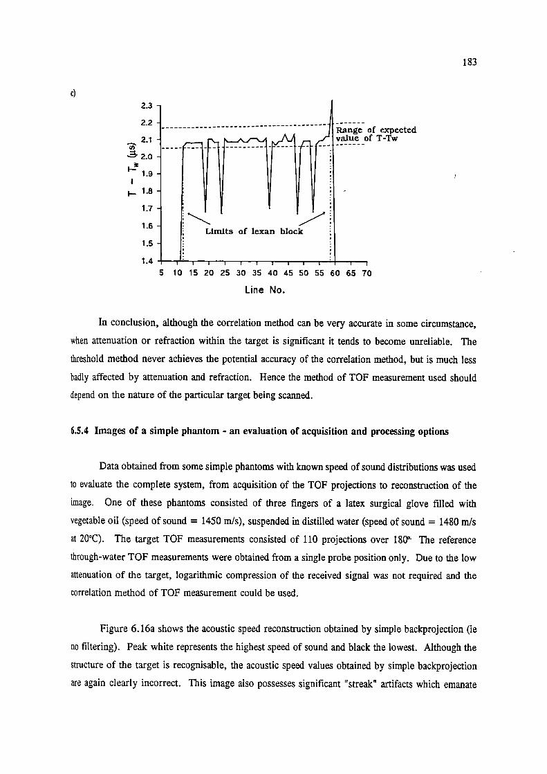
VY:Limits of lexan block

5 10 15 20 25 30 35 40 45 50 55 60 65 70

Line No.

183

c)

2.3

2.1(0

2.0F;?i.9

1.8

1.7

2.2 -j------------------------------------------

1.6

1.5

1.4

Range of expectedvueof T-Tw

In conclusion, although the correlation method can be very accurate in some circumstance,

when attenuation or refraction within the target is significant it tends to become unreliable. The

threshold method never achieves the potential accuracy of the correlation method, but is much less

badly affected by attenuation and refraction. Hence the method of TOF measurement used should

depend on the nature of the particular target being scanned.

6.5.4 Images of a simple phantom - an evaluation of acquisition and processing options

Data obtained from some simple phantoms with known speed of sound distributions was used

to evaluate the complete system, from acquisition of the TOF projections to reconstruction of the

image. One of these phantoms consisted of three fingers of a latex surgical glove filled with

vegetable oil (speed of sound = 1450 mIs), suspended in distilled water (speed of sound = 1480 m/s

at 20°C). The target TOF measurements consisted of 110 projections over 18(Y The reference

through-water TOF measurements were obtained from a single probe position only. Due to the low

attenuation of the target, logarithmic compression of the received signal was not required and the

correlation method of TOP measurement could be used.

Figure 6. 16a shows the acoustic speed reconstruction obtained by simple backprojection (ie

no filtering). Peak white represents the highest speed of sound and black the lowest. Although the

structure of the target is recognisable, the acoustic speed values obtained by simple backprojection

are again clearly incorrect. This image also possesses significant "streak" artifacts which emanate

184

from the edges of the fingers. These are probably due to inconsistencies in the TOF projections

caused by errors in the reference TOF data, or by refraction of the acoustic beam for the target data.

Several procedures were investigated to see if this image could be improved upon.

6.5.4.1 Number of reference projections required

It was felt that changes in the distance between the probes for different probe positions might

be contributing to errors in the TOF projections. One solution to this problem would be to obtain

reference TOF data, ie without the target present, for more than one probe position. By varying the

number of reference probe positions and observing the affects on the images, it was discovered that

little improvement was obtained by having more than 10 reference positions (ie one every 18° for a.

1800 scan). The acoustic speed image obtained using 10 positions (Figure 6.16b) clearly shows a

significant reduction in streak artifacts.

6.5.4.2 Use of median filters to remove 'glitches' in profiles

Refraction is probably the other main

cause of streak artifact. This problem is

demonstrated in Figure 6.17. When the beam

is near to the edge of a region with a different

speed of sound than it's surroundings, it will -

inevitably be refracted to some extent Thiso

will result in less energy (and hence a lower

amplitude pulse) reaching the receiver. All the

TOF measurement methods will tend to •2:-..Y..i- -overestimate the TOF when the pulse amplitude Refracted beam ' -. . •. -..is low, causing a positive spike in the T - T0,

/

projection. This so-called 'glitch' noise is not T -

amenable to linear smoothing filters because of

it's wide band-width. However, a non-linear

filtering operation known as median filtering

can be effective in reducing glitch noise Figure 6.17 Refraction as a cause of glitch

(Crawford and Kak, 1982). A 3-point median noise in TOF profiles.

filter would operate as follows. For each point in

the projection, compare it's value to the points on either side and find the point with the median

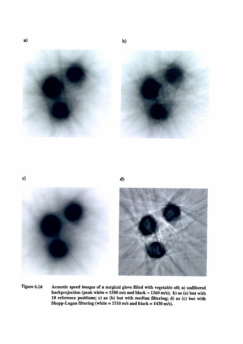
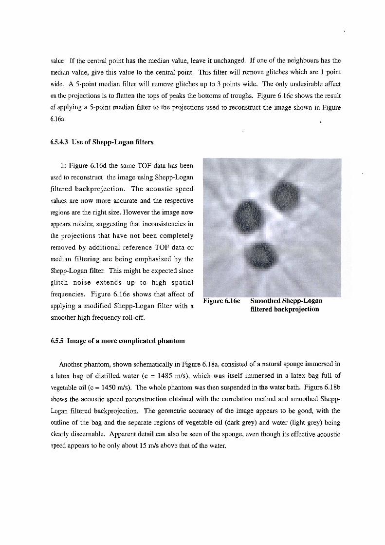
Figure 6.lbe Smoothed Shepp-Loganfiltered backprojection

value If the central point has the median value, leave it unchanged. If one of the neighbours has the

median value, give this value to the central point. This filter will remove glitches which are 1 point

wide. A 5-point median filter will remove glitches up to 3 points wide. The only undesirable affect

on the projections is to flatten the tops of peaks the bottoms of troughs. Figure 6.16c shows the result

of applying a 5-point median filter to the projections used to reconstruct the image shown in Figure

6.16a.

6.5.4.3 Use of Shepp-Logan filters

In Figure 6.16d the same TOF data has been

used to reconstruct the image using Shepp-Logan

filtered backprojection. The acoustic speed

values are now more accurate and the respective

regions are the right size. However the image now

appears noisier, suggesting that inconsistencies in

the projections that have not been completely

removed by additional reference TOF data or

median filtering are being emphasised by the

Shepp-Logan filter. This might be expected since

glitch noise extends up to high spatial

frequencies. Figure 6.16e shows that affect of

applying a modified Shepp-Logan filter with a

smoother high frequency roll-off.

6.5.5 Image of a more complicated phantom

Another phantom, shown schematically in Figure 6.18a, consisted of a natural sponge immersed in

a latex bag of distilled water (c 1485 mIs), which was itself immersed in a latex bag full of

vegetable oil (c = 1450 mIs). The whole phantom was then suspended in the water bath. Figure 6.1 8b

shows the acoustic speed reconstruction obtained with the correlation method and smoothed Shepp-

Logan filtered backprojection. The geometric accuracy of the image appears to be good, with the

outline of the bag and the separate regions of vegetable oil (dark grey) and water (light grey) being

clearly discernable. Apparent detail can also be seen of the sponge, even though its effective acoustic

speed appears to be only about 15 mIs above that of the water.

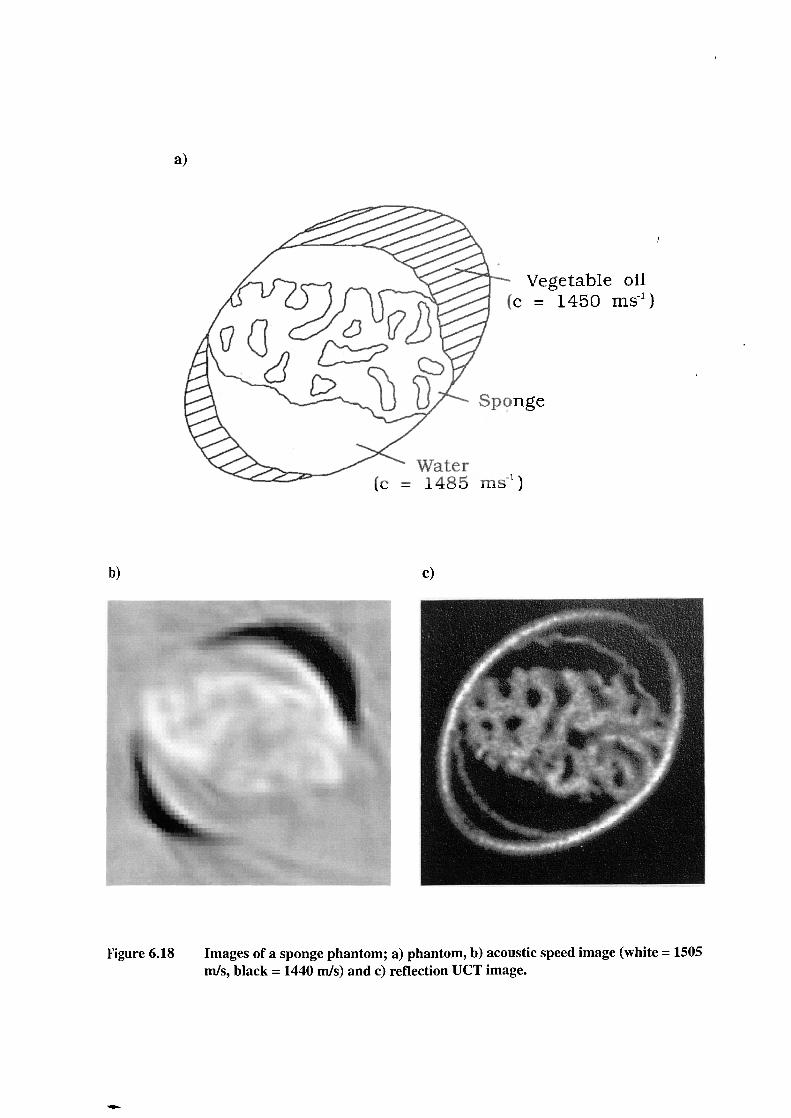
!' • • I

a)

Vegetable oil(c = 1450 ms1)

Sponge

Water(c = 1485 ms1)

b)

c)

Figure 6.18 Images of a sponge phantom; a) phantom, b) acoustic speed image (white 1505

mis, black = 1440 mis) and c) reflection UCT image.

188

A reflection mode UCT image was also obtained, and reconstructed assuming a constant

acoustic speed in the target of 1485 rn/s (Figure 6. 18c). As expected the resolution of the reflection

UCT image is superior, since it is governed by the ultrasonic pulse length rather than the beam width

as is the case with the acoustic speed image. However there is much identifiable structure in

common, and the reflection image generally confirms that the detail in the acoustic speed image is

not artifactual. Note also that, since the acoustic speed variation in this target is only about 3%,

distortion of the reflection UCT image is minimal.

The quantitative accuracy of the acoustic speed image must also be assessed. This was done

by calculating the average value of acoustic speed for all the pixels within a particular region, the

boundaries of which were defined by the reflection image. The portion of the image representing

vegetable oil was calculated at 1451 ± 6 mIs. The average value of acoustic speed in the water was

1484 ± 2 m/s. Hence the average reconstructed values of acoustic speed within these regions agree

with the known acoustic speeds to an accuracy of better than 0.4%.

6.5.6 Image artifacts from a phantom having large acoustic speed variations

It is possible that such good results were obtained for the phantom discussed in the previous

section because the range of acoustic speed within the phantom was only about 3%. The degree of

refraction within this target is likely to have been quite low, and probably lower than that encountered

in a typical breast. A phantom similar to this but showing the larger acoustic speed variations more

typical of a breast is shown in Figure 6. 19a. This phantom consisted of a natural sponge inside a bag

containing a solution of water and ethyl alcohol, giving a speed of sound of 1540 m/s. This bag was

itself inserted into another bag containing vegetable oil (c 1450 m/s), giving a total range of

acoustic speed of 6%.

The acoustic speed image of this phantom, obtained using the correlation method of TOF

measurement, is shown in Figure 6. 19b. By comparing this image with the equivalent reflection UCT

image shown in Figure 6. 19c (reconstructed assuming an acoustic speed of 1485 mIs), it can be seen

that the structural detail in the acoustic speed image is poorer and it contains more artifacts than the

image of Figure 6. 18b. This loss in geometric accuracy may be accounted for by increased refraction

causing the paths of some ultrasonic beams through the target to be significantly different to the

straight-path assumed in reconstruction. Using the threshold method of TOF measurement results in

a better image (Figure 6. 19d), although artifacts are still present. These persistent artifacts are

presumably due to the extreme cases of refraction where some transmitted pulses may miss the

receiver completely, creating 'gaps' in the TOF projection data. Although these gaps can be "filled

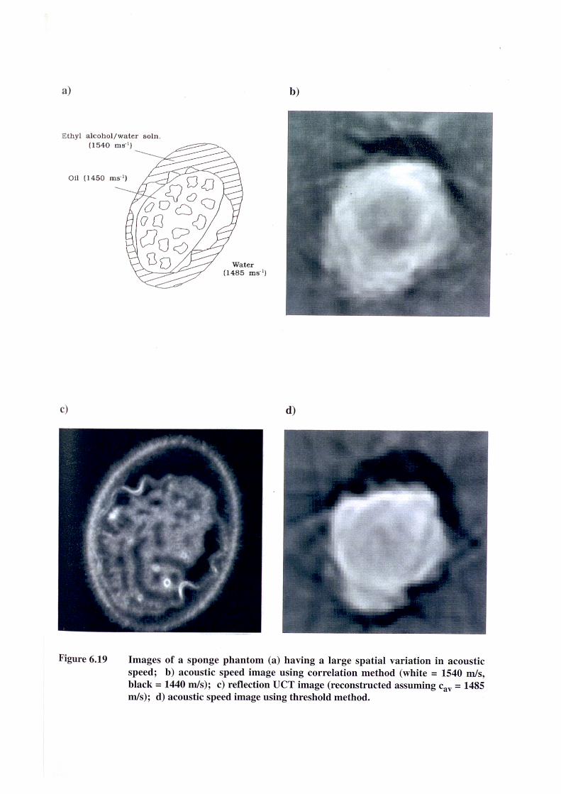
190

in by median filtering, all knowledge of the true acoustic speed along that path is lost.

Refraction is also likely to affect the quantitative accuracy of the images, particularly at the

boundaries between regions of different acoustic speed. However an analysis of the average acoustic

speed values in the water (1483 ± 4 mIs) and in the vegetable oil (1455 ± 6 mIs) has revealed that

the quantitative accuracy of the bulk regions is not significantly poorer than for the previous phantom.

The reconstructed speed in the water/ethyl alcohol solution (1511 ± 12 mIs) is rather lower than

expected, but this may be due to the sponge which has a lower acoustic speed than the solution. Thus

these results are encouraging, bearing in mind that the quantitative accuracy required (see section

6.2.2) for effective compensation of reflection images depends on the size of the regions, and for

large regions should be better than 5 m/s, whilst the geometric accuracy need only be ± 4mm.

The affects of acoustic speed variations on the reflection UCT image (Figure 6. 19c) are very

evident for this target, as revealed by the double boundaries of the bag and by tiny air bubbles within

the sponge appearing as circles instead of points. Hence this confirms observations made by previous

workers (see 3.2), that acoustic speed variations of greater than 5% have a significant effect on the

quality of reflection UCT images reconstructed assuming a constant acoustic speed within the target.

6.5.7 Images of animal organs in-vitro

In order to test the ability of this UCT system to produce acoustic speed images of real tissue,

several animal organs were obtained from a local abattoir. One such in-vitro target was a sheep's

kidney, which was placed inside a bag of saline having an acoustic speed of 1540 mIs. The acoustic

speed image (threshold method) and reflection UCT image (1540 mIs) of this target are shown in

Figures 6.20a and b respectively. Although acoustic speed artifacts are apparent in the double

membranes and general blurring, this reflection IJCT image clearly shows the advantage of 360° over

1800 scanning (c.f. Figure 5.31), since the resolution and general image quality is now roughly

uniform over the whole image.

The acoustic speed image shows similar gross structure to the reflection image, although as

usual at considerably reduced resolution. Note for example that the fatty areas in the central pelvis

of the kidney have a lower acoustic speed (average 1495 m/s) than the surrounding medulla (average

speed 1568 mIs). The quality of the acoustic speed image is again not as high as obtained from some

of the phantoms because of the combined affects of considerable attenuation and acoustic speed

variations. However the average acoustic speed values are consistent with those reported for fat and

for kidney tissue (Duck 1990).

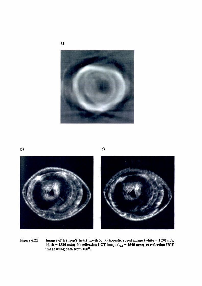
193

6.6 Results for acoustic speed compensation of reflection UCT images

6.6.1 Introduction

It has been shown in the previous section that a transmission UCT system, based on linear

arrays, can produce accurate acoustic speed images under certain circumstances. The quality of these

images, and especially their geometric accuracy, deteriorates when the acoustic speed variations are

large or when the attenuation is high. Since the acoustic speed images were not in general felt to

have sufficient geometric accuracy for worthwhile lateral displacement (refraction) corrections, only

axial displacement correction has been attempted in this study.

It will now be investigated whether these images are sufficiently accurate to provide

worthwhile axial displacement corrections of reflection UCT images obtained from the same target

sections. As before simple phantoms will be considered before moving onto animal and human

tissues in-vitro.

6.6.2 A practical implementation of acoustic speed compensation

The transmission data for the acoustic speed image was obtained first, and then immediately

afterwards (ie before reconstruction of the acoustic speed image) the data for the reflection image was

obtained. In this way movement of the target between scans was kept to a minimum.

After reconstruction of the acoustic speed image, reflection UCT images were reconstructed:

a) assuming a single acoustic speed in the target (the "uncompensated" image) and b) incorporating

information from the acoustic speed image (the "compensated" image). The algorithm for axial

displacement corrections operates as follows:-

1) Each scan line of each B-scan comprising the reflection UCT data is taken in turn. Starting from

a sample point in the scan line known to lie before the target (ie in the surrounding water), this first

sample value is written to the reflection UCT image matrix at a position calculated using the known

centre of rotation of the probes.

2) The point at the equivalent position on the acoustic speed image (ie at the known distance from

the centre of rotation) is then also identified.

3) The next and subsequent scan line values are then written to the reflection UCT image matrix at

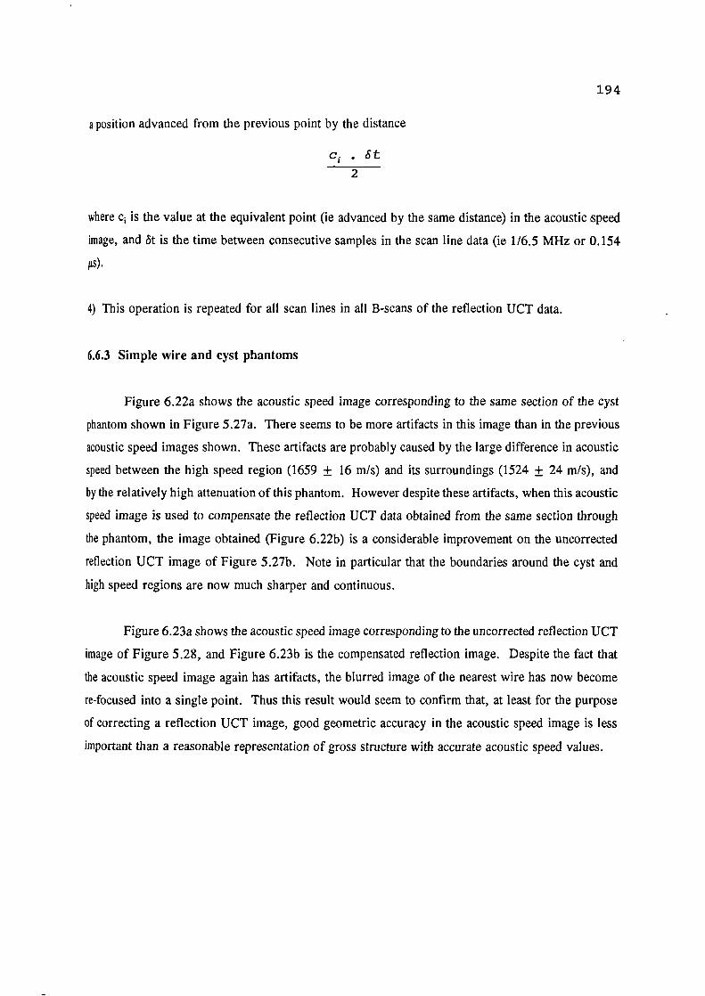
:1.94

a position advanced from the previous point by the distance

ci . St

2

where c 1 is the value at the equivalent point (ie advanced by the same distance) in the acoustic speed

image, and ôt is the time between consecutive samples in the scan line data (ie 1/6.5 MHz or 0.154

ps).

4) This operation is repeated for all scan lines in all B-scans of the reflection UCT data.

6.6.3 Simple wire and cyst phantoms

Figure 6.22a shows the acoustic speed image corresponding to the same section of the cyst

phantom shown in Figure 5.27a. There seems to be more artifacts in this image than in the previous

acoustic speed images shown. These artifacts are probably caused by the large difference in acoustic

speed between the high speed region (1659 ± 16 m/s) and its surroundings (1524 ± 24 mIs), and

by the relatively high attenuation of this phantom. However despite these artifacts, when this acoustic

speed image is used to compensate the reflection UCT data obtained from the same section through

the phantom, the image obtained (Figure 6.22b) is a considerable improvement on the uncorrected

reflection UCT image of Figure 5.27b. Note in particular that the boundaries around the cyst and

high speed regions are now much sharper and continuous.

Figure 6.23a shows the acoustic speed image corresponding to the uncorrected reflection UCT

image of Figure 5.28, and Figure 6.23b is the compensated reflection image. Despite the fact that

the acoustic speed image again has artifacts, the blurred image of the nearest wire has now become

re-focused into a single point. Thus this result would seem to confirm that, at least for the purpose

of correcting a reflection UCT image, good geometric accuracy in the acoustic speed image is less

important than a reasonable representation of gross structure with accurate acoustic speed values.

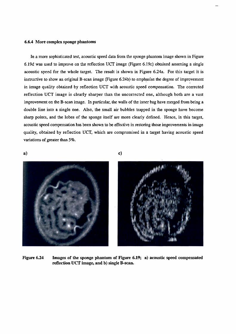
197

6.6.5 Animal organs in-vitro

The acoustic speed images of the in-vitro animal organs shown in 6.5.7 were also used to

compensate for acoustic speed artifacts in the equivalent reflection images. Figure 6.25b shows a

single B-scan, with the probe viewing from the left, of the sheep's kidney. The acoustic speed and

uncorrected reflection UCT images of this target were shown in Figures 6.20a and b respectively.

A reflection UCT image reconstructed using values from the acoustic speed image is shown in Figure

6.25a. Specularly reflecting boundaries are now complete, speckle is virtually eliminated and

resolution is much improved and isotropic. There is very little evidence of the multiple or dispersed

registration of targets seen in Figure 6.20b. All these factors lead to much easier interpretation of

the structure. Note for example the radial fibres now visible in the cortical tissue in the compensated

reflection UCT image, and which are virtually undetectable in the B-scan image.

Figure 6.26b shows a B-scan of the sheep's heart. Figure 6.21a shows the acoustic speed

image and Figure 6.2 lb the uncompensated reflection UCT image. Despite the apparently poor

geometric accuracy of the acoustic speed image, the reflection UCT image reconstructed using these

acoustic speed values (Figure 6.26a) is still a considerable improvement on the uncorrected reflection

UCT image. For example the left and right ventricles are now clearly defined, whereas in the B-scan

the right ventricle is barely visible at all because of the attenuation of the ultrasound signal.

6.6.6 In-vitro human breast

Some studies have also been performed with in-vitro human tissues. A post mastectomy

breast, known to possess a cancerous tumour, was obtained from Pathology and placed in a latex bag

with isotonic saline (c = 1500 mIs). Figures 6.27a to 6.27d show the B-scan, acoustic speed,

uncompensated and compensated reflection UCT images respectively.

This set of images probably demonstrate most dramatically the vast improvement in image

quality obtained with reflection UCT compared to conventional B-scanning, and are an indication of

the possibilities of combined acoustic and reflection UCT for breast imaging. The main problem with

B-scanning in the breast is the large number of interfaces and fibres which permeate typical breast

tissue, most of which cannot be seen from a single view direction making interpretation of the B-scans

very difficult. In the reflection UCT image all of the fibrous structure is visible and the encapsulated

kidney-shaped structure at 4 o'clock, identified by the pathologist as the tumour, is now easily

identified. Indeed a section obtained through the tumour showed a remarkable resemblance to the

reflection UCT image.

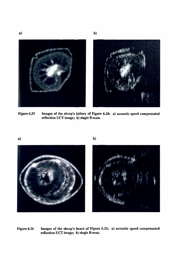
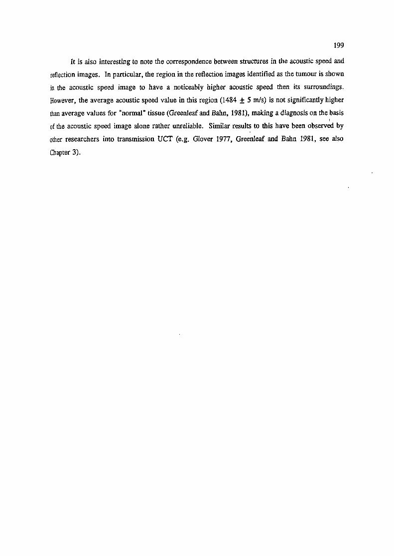
199

It is also interesting to note the correspondence between structures in the acoustic speed and

reflection images. In particular, the region in the reflection images identified as the tumour is shown

in the acoustic speed image to have a noticeably higher acoustic speed then its surroundings.

However, the average acoustic speed value in this region (1484 ± 5 mIs) is not significantly higher

than average values for "normal" tissue (Greenleaf and Balm, 198!), making a diagnosis on the basis

of the acoustic speed image alone rather unreliable. Similar results to this have been observed by

other researchers into transmission UCT (e.g. (lover 1977, Greenleaf and Bahn 198!, see also

Chapter 3).

20].

6.1 Discussion of combined acoustic speed and reflection UCT

This chapter has described the construction of and results from a combined reflection and

transmission UCT system. The system is based on conventional linear arrays and scans through 360°

in a horizontal plane.

The ability to scan though a complete 360° has, as expected, resulted in the reflection UCT

images showing fewer artifacts due to attenuation and far field beam divergence than images obtained

from the 180° reflection UCT system described in Chapter 5. Although these advantages are

worthwhile, the main reason for developing this system was to attempt to reduce the artifacts in

reflection UCT images caused by a varying acoustic speed. Compensating for these artifacts requires

knowledge of the spatial distribution of acoustic speeds within the target. Previous workers have

shown that images of acoustic speed distributions can be obtained using a transmission UCT system,

so this system was constructed to allow transmission measurements to be obtained using the same

basic equipment as used for the reflection UCT measurements.

Acoustic speed images of targets having relatively low attenuation and acoustic speed

variations, have been reconstructed using a correlation method for time of flight (TOF) measurement

and a straight-path CT reconstruction algorithm. The images obtained from these phantoms appear

to show very good geometric and quantitative accuracy. One reason for the quality of these images,

which appears to be comparable to or better than that obtained by previous workers, may be the use

in this system of linear arrays for the transmission measurements. It has been argued here that, to

obtain accurate acoustic speed images, the distance between the transmitter and receiver apertures

should remain very constant (ideally to within 30 m) during lateral scanning of the apertures. This

constant separation is much easier to achieve using a mechanically fixed electronically stepped system

than with the mechanically stepped systems used by all previous workers.

In targets showing relatively high attenuation or acoustic speed variations (e.g. > 5%), such

as might be expected in real breast tissue, the geometric accuracy of the images is significantly

reduced while the quantitative accuracy seems to be relatively uneffected. The affect of high

attenuation is to change the shape and reduce the amplitude of the transmitted acoustic pulse reaching

the receiver, resulting in a poorer accuracy in the estimate of the pulse time of flight. It is possible

to at least partially overcome this problem by using methods for calculating TOF which are not so

dependent on preserving the shape of the pulse envelope, such as threshold methods. Unfortunately

these threshold methods tend to introduce there own geometric distortions: specifically the size of

regions of low acoustic speed is underestimated whereas the size of regions of high acoustic speed

202

is overestimated. Another possibility, not investigated in this work, would be to use a correlation

method while applying some form of automatic gain to the received pulses (or even better to the

transmitted pulses) to reduce the variations in pulse amplitude. It might also be possible to send

specialised pulse sequences, such as "chirps", designed to optimise the "peakyness" of the cross-

correlation function. However, bearing in mind that the linear arrays used in this system generate

pulses with a peak amplitude that is about one tenth that generated by modern arrays, probably the

simplest solution to the attenuation problem would be to use linear arrays with a higher acoustic

output.

The main affect of large acoustic speed variations is probably to cause significant refraction

of the transmitted acoustic beam. As well as violating the assumption of straight path propagation

inherent in the CT reconstruction algorithm, refraction will also cause less energy to reach the

receiver aperture resulting in a pulse of reduced amplitude and poorer accuracy in the estimate of

TOF. Although the effect of pulse amplitude loss can again be minimised by using appropriate

methods for TOF measurement (see below), it is likely to be much more difficult to correct for the

violation of the assumption of straight-path propagation. As discussed in Chapter 3 (Section 3.3),

some workers have investigated reconstruction algorithms for transmission UCT that do not rely upon

the assumption of straight-path propagation. The most successful of these techniques applied ray-

tracing to calculate the curved acoustic paths, combined with an iterative reconstruction algorithm

(e.g. Anderson 1990). Although some improvements in image quality were reported for phantoms,

few results have been presented from real tissues. However there may be some scope in using similar

techniques to improve the acoustic speed images obtained from this system.

It has been shown here that by using a threshold method for calculating the pulse TOF, the

error in the TOF measurement due to attenuation or refraction is minimised even if the pulses have

not taken the assumed straight path through the target. This may explain why the acoustic speed

images show better quantitative accuracy, which depends mainly on the accuracy of the TOF

estimates, than they do geometric accuracy which depends mainly on the degree of deviation from

a straight line of the pulse's paths.

In this work no serious attempt has been made to establish whether the acoustic speed images

are of sufficient quality to provide diagnostic information in there own right. This is because the

main reason for obtaining these images was to establish whether they could be used to provide

worthwhile compensation for the artifacts in reflection UCT images caused by a varying acoustic

speed in the target. It was argued in section 6.2.2 that the resolution of the acoustic speed images,

limited as they are in a transmission tJCT system by the ultrasound beam width, is insufficient to

203

correct for the lateral displacement component of these artifacts. Possible ways of producing acoustic

speed images with the required accuracy will be discussed in Chapter 7.

Since no attempt has been made to correct for the lateral component of the reflection UCT

artifacts, the existence of geometric distortion in the acoustic speed images is only of importance if

it affects the ability to compensate for the axial component of these artifacts. Previous results'from

Chapter 5 have suggested that only large regions, with a relatively high acoustic speed difference

between themselves and their surroundings, cause significant artifacts in reflection UCT images.

Theoretical arguments (section 6.2.1) suggest that in these cases the quantitative accuracy of the

acoustic speed image is more important than the geometric accuracy. This prediction seems to have

been borne out by the results of this study, since even acoustic speed images showing considerable

geometric distortion have been used to provide worthwhile compensation for axial displacement

artifacts in reflection UCT images obtained from the same targets.

To conclude, the results of this study have shown that images of tissue structure at high

resolution, and quantitative images of tissue acoustic speed at lower resolution, can be obtained by

combining the principles of reflection and transmission UCT within a single system. This system uses

linear arrays for both reflection and transmission measurements and thus restricts the mechanical

movement required during data acquisition to a rotational movement only. The elimination of the

lateral movement (required when using single element transducers for transmission measurements)

is particularly important in improving the quality of acoustic speed images. The main limitations of

this combined reflection and transmission system are the remaining rotational movement of the

probes, which increases the data acquisition times and consequent subject movement, and the need

for the targets and the probes to be entirely immersed in a water bath. These limitations have

restricted the practical application of this prototype system mainly to in-vitro targets.

Although some in-vivo studies of the female breast have been performed, the results have

been disappointing and have not been reported here. While movement of the subject during data

acquisition has been a factor, probably the main reason for these disappointing results in-vivo has

been due to excessive attenuation of the ultrasound signals, both in reflection and transmission, due

to the large size and relatively high attenuation of the breasts studied. This problem is being

addressed by modifying the system to accept more modern linear arrays with a considerably higher

acoustic output. The problems of subject movement and general patient acceptability are more

difficult to solve, requiring the construction of systems designed specifically for the particular clinical

application. Some possible approaches to clinically viable systems will be discussed in chapter 7.

204

7 Conclusions and future developments

7.1 Introduction

The purpose of this chapter is to summarise the main results and conclusions of the previous

chapters, and in the light of these findings to consider possibilities for the future development of

ultrasound CT techniques. Of particular importance in this consideration is the need to develop

systems with which these techniques can be applied effectively to patients in-vivo.

7.2 Main experimental findings of this study

These may be summarised as follows:-

1) It was shown in Chapter 5 that, by simply combining reflectivity (or backscatter) data from

many directions and assuming a constant acoustic speed for the whole target, images can be

generated that show considerably better resolution (approximately 1mm) and fewer artifacts

than conventional B-scan images generated with the same equipment, provided that acoustic

speed variations within the target do not exceed about 5%. An important requirement for

achieving such good resolution is high mechanical accuracy in the scanning system. This has

been achieved by the use of a) a linear array for lateral scanning, b) a very rigid rotational

scanning arrangement and c) an accurate and automatic method of calculating the centre of

rotation of the system.

2) In situations where the acoustic speed variations are greater than 5%, such as is likely to

occur in many female breasts, it has been shown that the quality of reflection UCT images

is significantly reduced due to incorrect registration of echoes in the composite B-scan

images. It has been suggested by previous workers that this problem could be alleviated by

using the "true° acoustic speed distribution in the reconstruction of the reflection UCT image.

3) It has already been shown by several workers (see Chapter 3) that acoustic speed distributions

can be obtained by the technique of transmission UCT. Since a transmission UCT technique

requires 360° scanning, a 180° reflection-only system (as described in Chapter 5) is not

suitable for transmission measurements. Hence such a system is likely to find clinical

applications only in targets having relatively low acoustic speed inhomogeneity (the neck or

lower limb may be possibilities), unless non-transmission methods of acoustic speed imaging

can be developed (see 7.4.2).

205

4) The 360° system described in Chapter 6 has demonstrated that both reflection and transmission

UCT can be implemented using identical linear arrays in a single system. Use of linear arrays

allows for much greater positional accuracy than is possible with mechanically scanned

systems. This appears to be the first system to be described that uses linear arrays for

transmission measurements, which may explain why the acoustic speed compensated reflection

UCT images obtained from this system appear to be superior than others reported to date.

5) The acoustic speed compensated reflection images of in-vitro targets produced by this system

are also superior to those available from conventional "state-of-the-art" real-time ultrasonic

imaging systems, despite the fact that this system uses linear arrays which are about 13 years

old.

6) The low acoustic output of these linear arrays does cause problems when imaging large or

highly attenuating targets. It is expected that these problems will be reduced or eliminated by

using more modern arrays with higher outputs.

7.3 Limitations of the present systems for clinical applications

Possibly the main potential clinical application of these systems is in breast cancer screening,

due to the accessibility of breast tissue, the absence of bone or gas and the need for alternative tests

using non-ionising radiation. Although conventional ultrasound has already found widespread use in

breast cancer diagnosis, particularly for differentiating between tumours and cysts, it is not generally

considered to be suitable for mass screening for many of the reasons discussed in Chapter 1 (eg poor

lateral resolution and high operator dependence). However it has been shown in this work that

techniques involving reflection ultrasound CT combined with acoustic speed imaging can overcome

mast of these problems. In addition ultrasound has some significant advantages over X-ray

mammography such as the low risk to patients and the fact that the procedure is painless.

With the application to breast cancer screening in mind, the main limitations of the systems

described in this thesis will be discussed and suggestions for ways of overcoming these limitations

considered.

7.3.1 Scan times and movement artifacts

Very few in-vivo studies have been performed as part of this study. One of the main reasons

206

for this is the long scan times required (about 30 seconds for a single reflection UCT slice and about

2 minutes for transmission UCT), resulting in inevitable subject movement and movement induced

artifacts. If this subject movement could be eliminated then images obtained in-vivo should be as

good as those that have been obtained in-vitro. However since it is unrealistic to expect the subject

to remain completely immobilised (ie prevent breathing) for more than about 20 to 30 seconds, the

only way to minimise movement induced artifacts is to reduce the scan times.

In the present system the fraction of the scan time spent transmitting and receiving ultrasonic

data is small compared to the time spent mechanically moving the probes and in transferring data

between the digitiser and the computer's hard disc. In fact, the data for a single reflection image (15

frames by 70 pulse-echo scan lines) could in theory be obtained in about 0.2 seconds, while that for

a transmission acoustic speed image (110 frames by 70 transmission lines) would require about 0.8

seconds, giving a total scan time (per slice) of approximately 1 second. If reflection and transmission

data could be collected simultaneously the total scan time for both would only be about 0.8 seconds.

The time spent moving the probes around the target, which in the present system is by far the

major component of the scan time, could in principle be eliminated completely. This could be

achieved by using a mechanically fixed system which acquires data around the target by electronic

switching of active transducer elements, analogous to the way in which the linear arrays perform a

lateral scan of the target. Various possible configurations are shown in Figure 7.1. These will be

discussed more fully in section 7.4

The time required to transfer and store the ultrasonic data depends on various aspects of the

transient recorder, computer and their interface. In the present system there is insufficient memory

in the transient recorder to store all of the data for a transmission UCT image, so some of that data

must be transferred to the computer for storage onto disc and this is relatively time consuming.

However, the cost of computer memory is decreasing rapidly and it is not difficult to imagine a

digitiser with a 5 MByte buffer which would be able to store all of the data (reflection and

transmission) for one slice. In this case the data for a single slice could be transferred to the

computer for longer term storage while the system was being prepared for the acquisition of

subsequent slices. A small amount of subject movement between slices is likely to be more acceptable

than movement occurring during acquisition of a slice.

The times required for reconstructing the images from the measured data are of less

importance. For this system the reconstruction times are about 30 minutes for an acoustic speed

compensated reflection UCT image, and about two hours for an acoustic speed image. However,

207

little attempt has been made to optimise the software for speed, and the computer used is considerably

slower than more modern systems or a dedicated processor would be. It is not unrealistic to

anticipate total reconstruction times of less than 2 minutes per slice for relatively little additional cost.

7.3.2 Patient acceptability

Another disadvantage of these systems, especially for any in-vivo clinical studies, is the

relatively poor patient acceptability of water-bath scanning. The main problem is the necessity for

total emersion of the target being scanned because of the requirement of transmission UCT for 360°

access. The method adopted here for in-vivo studies of the breast has been to make a 15 cm diameter

hole in an adjustable height couch, with the breast protruding through the hole and into the water.

Although relatively comfortable for the subject, this approach is only suitable for sagittal sections of

the breast and there are difficulties in obtaining sections close to the chest wall. Coronal and

transverse sections, which would give information close to the chest wall, only allow scanning over

at most 180° and are thus unsuitable for transmission UCT. This problem would be eliminated if

acoustic speed information could be obtained using methods that do not require transmission

measurements. This possibility will be considered further in section 7.4.2.

If the requirement for the mechanical movement of the probes can be eliminated, it is possible

to envisage systems which do not require total emersion in a water bath. One possibility is a fixed

ring of transducers in direct contact with the skin. Other possibilities are discussed in section 7.4.

As well as being more convenient for the patient, these approaches should allow sections close to the

chest wall to be obtained more easily.

7.3.3 Refraction artifacts

Acoustic speed images, and reflection UCT images with acoustic speed compensation, both

suffer from the affects of ultrasound beam refraction. To achieve the full potential resolution of

reflection UCT, refraction must be compensated for in both the reflection and acoustic speed images.

If such compensation were possible it may also then be worthwhile using RF data for the

reconstruction of the reflection UCT images, with a potential resolution of less than the ultrasound

wavelength (eg less than 0.5mm at 3MHz).

To account for refraction requires more sophisticated reconstruction algorithms than have been

used in this study. As discussed in section 6.2.2, one of the problems with incorporating refraction

into the reconstruction of acoustic speed images, for example by ray-tracing methods, is that the

208

images have inherently insufficient resolution to calculate refraction angles accurately. One possibility

that appears not to have been explored previously would be to use the corresponding reflection UCT

image, which shows interfaces between discrete regions of different acoustic speed at inherently

greater resolution, to define the refraction angles in the reconstruction of the acoustic speed image.

This reconstruction approach could proceed in four stages:-

(1) First reconstruct an acoustic speed image using a conventional straight-path algorithm.

(2) Then reconstruct a reflection UCT image with axial acoustic speed compensation but not

refraction correction. Hence steps (1) and (2) are already performed in the system described

in Chapter 6.

(3) Use a ray-tracing technique with data from the acoustic speed image, and with refraction

angles defined by the reflection UCT image, to map the acoustic beam paths through the

target and hence reconstruct an improved acoustic speed image.

(4) Reconstruct an improved reflection image using ray-tracing on the previous reflection image

and acoustic speed information from the latest acoustic speed image.

Stages (3) and (4) could be iterated as necessary, although a thorough mathematical analysis, which

is beyond the scope of this thesis, would be required to establish whether such an iteration would

converge.

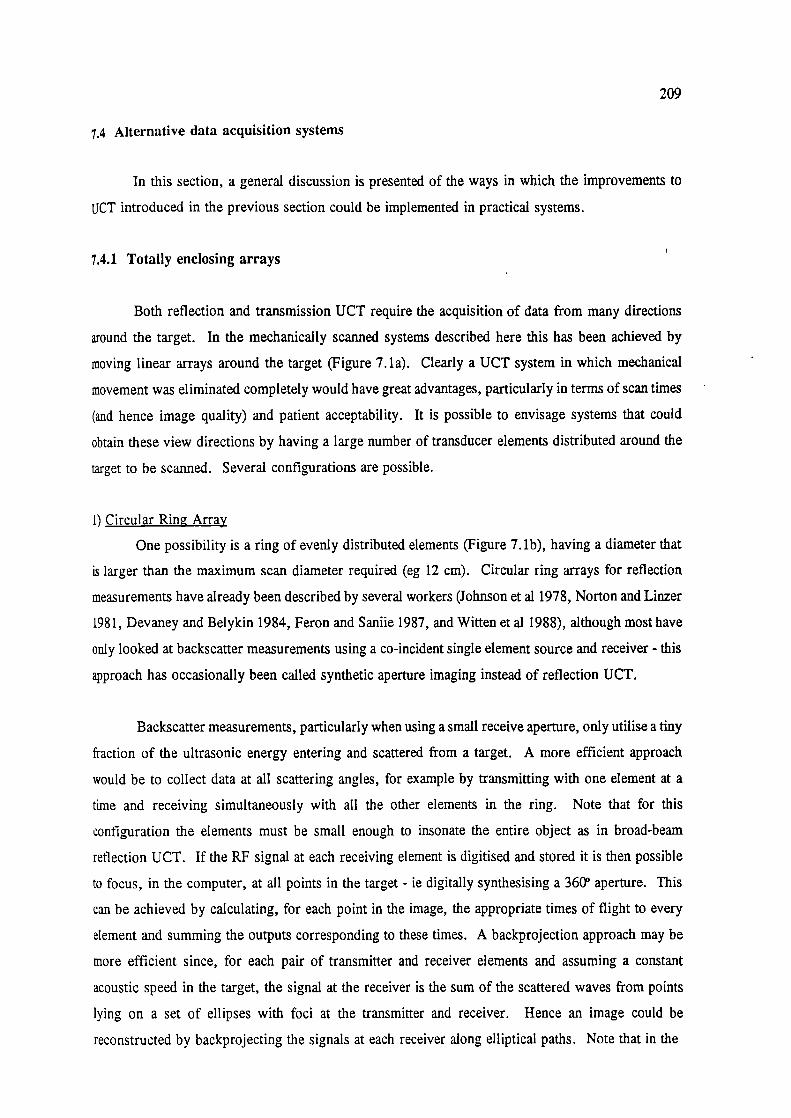
209

7.4 Alternative data acquisition systems

In this section, a general discussion is presented of the ways in which the improvements to

UCT introduced in the previous section could be implemented in practical systems.

7.4.1 Totally enclosing arrays

Both reflection and transmission UCT require the acquisition of data from many directions

around the target. In the mechanically scanned systems described here this has been achieved by

moving linear arrays around the target (Figure 7.la). Clearly a UCT system in which mechanical

movement was eliminated completely would have great advantages, particularly in terms of scan times

(and hence image quality) and patient acceptability. It is possible to envisage systems that could

obtain these view directions by having a large number of transducer elements distributed around the

target to be scanned. Several configurations are possible.

1) Circular Rin g Array

One possibility is a ring of evenly distributed elements (Figure 7. ib), having a diameter that

is larger than the maximum scan diameter required (eg 12 cm). Circular ring arrays for reflection

measurements have already been described by several workers (Johnson et al 1978, Norton and Linzer

1981, Devaney and Belykin 1984, Feron and Saniie 1987, and Witten et al 1988), although most have

only looked at backscatter measurements using a co-incident single element source and receiver - this

approach has occasionally been called synthetic aperture imaging instead of reflection UCT.

Backscatter measurements, particularly when using a small receive aperture, only utiise a tiny

fraction of the ultrasonic energy entering and scattered from a target. A more efficient approach

would be to collect data at all scattering angles, for example by transmitting with one element at a

time and receiving simultaneously with all the other elements in the ring. Note that for this

configuration the elements must be small enough to insonate the entire object as in broad-beam

reflection UCT. If the RF signal at each receiving element is digitised and stored it is then possible

to focus, in the computer, at all points in the target - ie digitally synthesising a 360' aperture. This

can be achieved by calculating, for each point in the image, the appropriate times of flight to every

element and summing the outputs corresponding to these times. A backprojection approach may be

more efficient since, for each pair of transmitter and receiver elements and assuming a constant

acoustic speed in the target, the signal at the receiver is the sum of the scattered waves from points

lying on a set of ellipses with foci at the transmitter and receiver. Hence an image could be

reconstructed by backprojecting the signals at each receiver along elliptical paths. Note that in the

c)cOD0 DQ00

I '

0

d)

"7

0

210

a)

b) >Q000 00000

: Ii I

Figure 7.1 Various possible configurations for ultrasound CT: a) mechanically rotated lineararrays; b) Thed circular ring array; c) ring array with sub-grouping intransmission; d) fixed phased arrays.

case of a co-incident transmitter and receiver the ellipses simplify to concentric circles, as observed

by Norton (1979). In common with other backprojection techniques the image would be degraded

by a blurring function, although it should be possible to de-convolve this. Although the blurring

function in this case would not be given simply by (lIr), if data from a sufficiently large number of

element is used the function should be very close to (lIr) in the near vicinity of an image point.

Regardless of which reconstruction method is used, to enable focusing at points near the edge

of the target and to avoid grating lobes in receive, the element spacing p must be chosen such that

(Whittingham 1991)

x2sinO,

(7.1)

211

where O is the angle between the line joining an element to the centre of the array and a line

tangential to the maximum target diameter. Consider an array of diameter 16cm with elements having

a beam divergence angle of 90°, thus giving a maximum target diameter of 11.3cm. From equation

6.1 the maximum element pitch should be 0.35mm, giving a minimum of 1422 elements in the array

which would be rather expensive. This should be compared to the theoretical requirement for CT of

rl/dl elements, which for a pulse length of 1mm is only about 350 elements. By using short acoustic

pulses it may be possible to avoid grating lobes and hence have a larger element pitch and fewer

elements, but the elements would still need to be small enough to give 90° irradiation (ie less than

0.8mm wide).

An interesting point is that these multi-angle scattering measurements are likely to result in

images showing less emphasis on specular reflectors than do images obtained solely from backscatter

measurements, since these would only be detected by relatively few elements at each transmission,

whereas isotropic scatterers would be detected by all elements. Also note that the data acquisition

time for such a system (350 transmissions) would be less than 0.1 seconds per slice, thus opening up

the possibility of nearly real-time data acquisition. Whether the images could be reconstructed quickly

enough to achieve near real time frame rates is less certain.

Clearly the problem of varying acoustic speed can not be ignored, any more than it could be

for reflection UCT using linear arrays. Hence a method for obtaining acoustic speed images is

essential. Bearing in mind that all the elements are receiving simultaneously in this system, the

information for a transmission UCT approach to acoustic speed imaging should already be available.

To a first approximation, the minimum time taken for acoustic energy to arrive at any one element

after transmission from another element should represent the minimum path (ie a straight path)

between the two elements. Assuming a beam divergence angle of 90°, each element can only transmit

directly to one half of the array. In this case the number of independent straight-line transmission

paths linking N transmitters and receivers is given by

N N- 1+-2 2

which for 350 elements gives 30,800 lines of transmission data. Comparing this to the 7,700 lines

used to reconstruct an acoustic speed image for the system described in Chapter 6 shows that this

approach is potentially viable. Note that the reconstruction of an acoustic speed image from this data

would require a fan-beam algorithm - these have already been developed for X-ray CT.

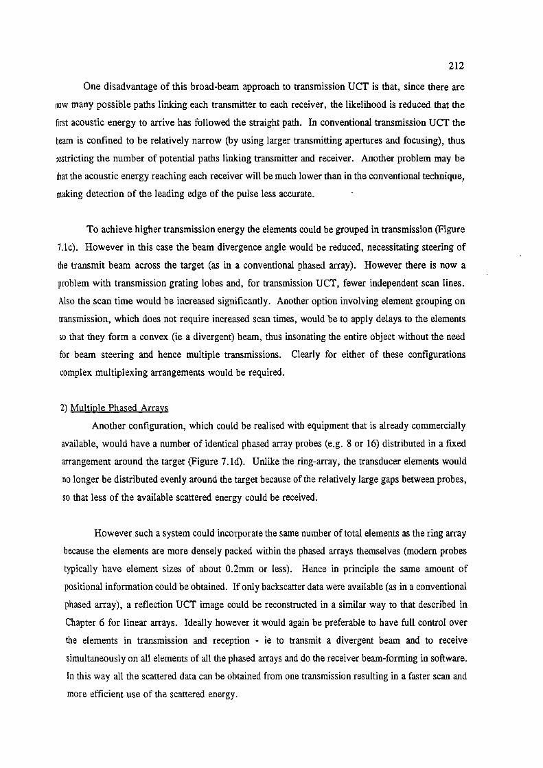
212

One disadvantage of this broad-beam approach to transmission UCT is that, since there are

now many possible paths linking each transmitter to each receiver, the likelihood is reduced that the

first acoustic energy to arrive has followed the straight path. In conventional transmission UCT the

beam is confined to be relatively narrow (by using larger transmitting apertures and focusing), thus

restricting the number of potential paths linking transmitter and receiver. Another problem may be

that the acoustic energy reaching each receiver will be much lower than in the conventional technique

making detection of the leading edge of the pulse less accurate.

To achieve higher transmission energy the elements could be grouped in transmission (Figure

7.lc). However in this case the beam divergence angle would be reduced, necessitating steering of

the transmit beam across the target (as in a conventional phased array). However there is now a

problem with transmission grating lobes and, for transmission UCT, fewer independent scan lines.

Also the scan time would be increased significantly. Another option involving element grouping on

transmission, which does not require increased scan times, would be to apply delays to the elements

so that they form a convex (ie a divergent) beam, thus insonating the entire object without the need

for beam steering and hence multiple transmissions. Clearly for either of these configurations

complex multiplexing arrangements would be required.

2) Multiple Phased Arrays

Another configuration, which could be realised with equipment that is already commercially

available, would have a number of identical phased array probes (e.g. 8 or 16) distributed in a fixed

arrangement around the target (Figure 7. id). Unlike the ring-array, the transducer elements would

no longer be distributed evenly around the target because of the relatively large gaps between probes,

so that less of the available scattered energy could be received.

However such a system could incorporate the same number of total elements as the ring array

because the elements are more densely packed within the phased arrays themselves (modern probes

typically have element sizes of about 0.2mm or less). Hence in principle the same amount of

positional information could be obtained. If only backscatter data were available (as in a conventional

phased array), a reflection UCT image could be reconstructed in a similar way to that described in

Chapter 6 for linear arrays. Ideally however it would again be preferable to have full control over

the elements in transmission and reception - in to transmit a divergent beam and to receive

simultaneously on all elements of all the phased arrays and do the receiver beam-forming in software.

In this way all the scattered data can be obtained from one transmission resulting in a faster scan and

more efficient use of the scattered energy.

dx

Receivingprobe

-H-.J

Principle of the beam-trackingmethod for the in-vivomeasurement of acoustic speed(Ophir 1986).

213

The main problem with the use of phased arrays in the configuration of Figure 7.le is that,

when using a transmission UCT method for acoustic speed imaging, there would now be an

insufficient number of possible paths joining any two probes for the reconstruction of a useful image.

l{ence to make this approach viable for breast scanning, a method is required for acoustic speed

imaging that does not rely on transmission measurements.

7.4.2 Acoustic speed imaging using side scatter measurements

The ability to measure ultrasound which has been scattered at angles other than 0°

(transmission imaging) and 180° (reflection imaging) opens up possibilities for alternative methods

of acoustic speed imaging. Several such techniques have already been investigated by other workers.

Robinson et al (1982) suggested a method involving cross-correlation of overlapping regions from two

sector scans obtained from different transducer positions. The maximum of the cross-correlation

function (ie the mean spatial shift in the image) is then related to the average acoustic speed in the

region. Experiments on liver tissue in-vivo suggested a repeatability of +I 15 ms' (about 1%) in

the estimate of acoustic speed, although this was in a rather large region of interest (at least 3 cm in

diameter) so the technique as described is probably not suitable for imaging.

Another technique that has attracted

some interest in recent years is the beam-

tracking method (or the similar crossed-beam

method), first proposed by Ophir (1986). In

this method two co-planar transducers (oneTransmitting

transmitting and one receiving) are arranged so probe

that their beam axes intersect at right angles Jjj(Figure 7.2). The TOF between the transmitter

and the receiver, via side scatter in the cross-

over region, is the total path length divided by

the average acoustic speed along the path. By

moving the receiving transducer a small distance Figure 7.2

(dx) laterally, the average acoustic speed (c)

along a short segment of the transmission path

is related to the difference in TOF (dt) obtained

at the two receiver positions (ie c=dx/dt). Clearly this estimate will be contaminated if the TOF from

the cross-over region to the receiver is different at the two positions, ie because of a difference in

acoustic speed along these paths. However a more accurate estimate of average acoustic speed can

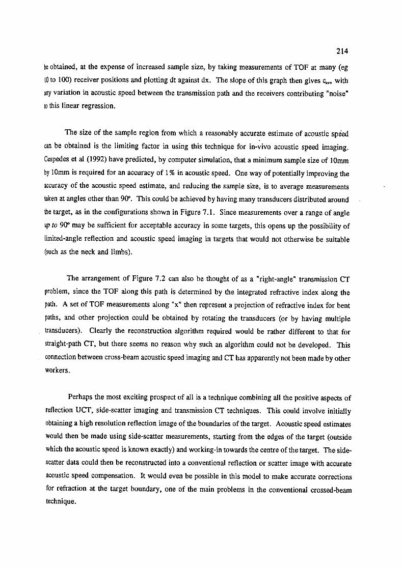
214

be obtained, at the expense of increased sample size, by taking measurements of TOF at many (eg

10 to 100) receiver positions and plotting dt against dx. The slope of this graph then gives c,,, with

any variation in acoustic speed between the transmission path and the receivers contributing "noise"

to this linear regression.

The size of the sample region from which a reasonably accurate estimate of acoustic sped

can be obtained is the limiting factor in using this technique for in-vivo acoustic speed imaging.

Cespedes et al (1992) have predicted, by computer simulation, that a minimum sample size of 10mm

by 10mm is required for an accuracy of 1 % in acoustic speed. One way of potentially improving the

accuracy of the acoustic speed estimate, and reducing the sample size, is to average measurements

taken at angles other than 90°. This could be achieved by having many transducers distributed around

the target, as in the configurations shown in Figure 7.1. Since measurements over a range of angle

up to 90° may be sufficient for acceptable accuracy in some targets, this opens up the possibility of

limited-angle reflection and acoustic speed imaging in targets that would not otherwise be suitable

(such as the neck and limbs).

The arrangement of Figure 7.2 can also be thought of as a "right-angle" transmission CT

problem, since the TOF along this path is determined by the integrated refractive index along the

path. A set of TOF measurements along "x" then represent a projection of refractive index for bent

paths, and other projection could be obtained by rotating the transducers (or by having multiple

transducers). Clearly the reconstruction algorithm required would be rather different to that for

straight-path CT, but there seems no reason why such an algorithm could not be developed. This

connection between cross-beam acoustic speed imaging and CT has apparently not been made by other

workers.

Perhaps the most exciting prospect of all is a technique combining all the positive aspects of

reflection UCT, side-scatter imaging and transmission CT techniques. This could involve initially

obtaining a high resolution reflection image of the boundaries of the target. Acoustic speed estimates

would then be made using side-scatter measurements, starting from the edges of the target (outside

which the acoustic speed is known exactly) and working-in towards the centre of the target. The side-

scatter data could then be reconstructed into a conventional reflection or scatter image with accurate

acoustic speed compensation. It would even be possible in this model to make accurate corrections

for refraction at the target boundary, one of the main problems in the conventional crossed-beam

technique.

215

8 ReferenCes

Abbott JG and Thurstone FL 1979 Acoustic speckle: Theory and experimental analysis

Ultrasonic Imaging 1, 303-324

Adams MF and Anderson AP 1980 Tomography from multiview ultrasonic diffraction data:

Comparison with image reconsti-uction from projections

Acoustical Imaging 10, 365-380

Anderson AH 1990 A ray tracing approach to restoration and resolution enhancement in experimental

ultrasound tomography

Ultrasonic Imaging 12, 268-29 1

Anderson AP and Adams MF 1982 Synthetic aperture tomographic imaging for ultrasonic diagnostics

Acoustical Imaging 12, 565-578

Ball J, Johnson SA and Stenger F 1980 Explicit inversion of the Helmholtz equation for ultra-sound

insonification and spherical detection

Acoustical Imaging 8, 451-461

Bamber JC and Dickinson RI 1980 Ultrasonic B-scanning: A computer simulation

Phys. Med. Biol. 25, 463479

Bartelt H 1988 Computation of local directivity, speed of sound and attenuation from ultrasonic

reflection tomography data

Ultrasonic Imaging 10(2), 110-120

Born M and Wolf E Principles of Optics

Fifth Edition, Pergamon Press, 1975

Bracewell RN and Riddle AC 1967 Inversion of radioisotope scans in radio astronomy

Astrophys. J. 150(2), 427434

216

Brandenburger GH, Klepper JR, Miller JB and Synder DL 1981 Effects of anisotropy in the

ultrasonic attenuation of tissue on computed tomography

Ultrasonic Imaging 3, 113-143

Burlew MM, Madsen EL, Zagzebski JA, Banjavic RA and Sum SW 1980 A new ultrasound tissue-

equivalent material

Radiology 134(2), 517-520

Carson PL, Meyer CR, Scherzinger AL and Oughton TV 1981 Breast imaging in coronal planes with

simultaneous pulse echo and transmission ultrasound

Science 214, 1141-1143

Carson PL, Scherzinger AL, Meyer CR, Moore GE, Jobe W and

Samuels B 1988 Lesion detectability in ultrasonic computed tomography in symptomatic breast

patients.

Invest. Radio!. 23, 421-427

Carson PL and Scherzinger A L 1979 Ultrasonic computed tomography

in New Tachniques and Instrumentation in Ultrasonography, pp 144-166

Cespedes I, Ophir J and Huang Y 1992 On the feasibility of pulse-echo speed of sound estimation in

small regions: simulation studies

Ultrasound Med. Biol. 18(3), 283-29 1

Chen CF, Robinson DE, Wilson LS, Griffiths KA, Manoharan A and Doust BD 1987 Clinical sound

speed measurement in liver and spleen in vivo

Ultrasonic Imaging 9, 22 1-235

Chenevert TL, Byiski DI, Carson PL, Meyer CR, Bland PH, Adler DD and Schmitt RM 1984

Ultrasonic computed tomography of the breast

Radiology 152, 155-159

Crawford CR and Kak AC 1982 Multipath artifact corrections in ultrasonic transmission tomography

Ultrasonic Imaging 4, 234-266

217

Crowther RA, De Rosier DJ and Klug A 1970 The reconstruction of a three-dimensional structure

from projections and its application to electron microscopy

Proc. Roy. Soc. Lond. A. 317, 319-340

De Rosier DJ and Kiug A 1968 Reconstruction of three dimensional structures from electron

micrographs

Nature 217, 130-134

Devaney AJ 1982 A filtered backpropagation algorithm for diffraction tomography

Ultrasonic Imaging 4, 336-350

Devaney AJ and Beylkin G 1984 Diffraction tomography using arbitary transmitter and receiver

surfaces

Ultrasonic Imaging 6, 181-193

Dickinson RJ 1986 Reflection and scattering

in Physical Principles of Medical Ultrasonics, Ed. CR Hill, Ellis Horwood Ltd., Chichester, England

Dines KA and Kak AC 1979 Ultrasonic attenuation tomography in soft tissues

Ultrasonic Imaging 1(1), 18-33

Dines KA, Fry FJ, Patrick JT and Gilmor RL 1981 Computerised ultrasound tomography of the

human head: experimental results

Ultrasonic Imaging 3, 342-351

Duck F, Johnson S, Greenleaf J and Samayoa W 1977 Digital image focussing in the near field of

a sampled acoustic aperture

Ultrasonics 15, 83-88

Duck FA and Hill CR 1979 Acoustic attenuation reconstruction from back-scattered ultrasound

in Computer Aided Tomography and Ultrasonics in Medicine, Ed. Raviv et al. pp 137-148 (North

Holland Publishing Company).

Duck FA 1990 Physical Properties of Tissue

Academic Press, London, England

218

Ermert H and Roehrlein G 1986 Ultrasound reflection-mode computerised tomography for in-vivo

imaging of small organs

1986 IEEE Ultrasonics Symposium Proceedings, IEEE Cat. No. 86, pp 825-828

Farrell EJ 1981 Tomographic imaging of attenuation with simulation correction for refraction

Ultrasonic Imaging 3, 144-163

Fatemi M and Kak AC 1980 Ultrasonic B-scan imaging: Theory of image formation and a technique

for restoration

Ultrasonic Imaging 2, 1-47

Feron ML and Saniie J 1987 Diffraction tomography using the total scattered field

Acoustical Imaging 16, 237-248

Friedrich M, Hundt E and Maderlechner G 1982 Computerised ultrasound echo tomography of the

breast

Eur. J. Radiol. 2, 78-87

Gilbert P 1972 Iterative methods for the three-dimensional reconstruction of an object from

projections

J. Theor. Biol. 36, 105-117

Glover GH and Sharp JC 1977 Reconstruction of ultrasound propogation speed distributions in soft

tissue: time of flight tomography

IEEE Trans. Sonics & Ultrason. 24, 229-334

Glover GH 1977 Computerised time-of-flight ultrasonic tomography for breast examination

Ultrasound Med. Biol. 3, 117-127

Gordon R, Bender R and Herman GT 1970 Algebraic reconstruction techniques (ART) for three-

dimensional electron microscopy and X-ray photography

J. Theor. Biol. 29, 471-481

Gordon R and Herman GT 1974 Three-dimensional reconstruction from projections: A review of

algorithms

Int. Rev. Cytol. 38, 111-151

219

Greenleaf JF, Johnson SA, Lee SL, Herman GT and Wood EH 1974 Algebraic reconstruction of

spatial distributions of acoustic absorption with tissues from their two-dimensional acoustic projections

Acoustical Holography 5, 591-603

Greenleaf JF, Johnson SA, Samayoa, WF and Duck FA 1975 Algebraic reconstruction of spatial

distributions of acoustic velocities in tissue from their time-of-flight profiles

Acoustical Holography 6, 7 1-90

Greenleaf JF, Johnson SA, Sainayoa WF and Hansen CR 1977 Refractive index by reconstruction:

use to improve compound B-scan resolution

Acoustical Holography 7, 263-273

Greenleaf JF, Johnson SA and Lent AH 1978 Measurement of spatial distribution of refractive index

in tissues by ultrasonic computer assisted tomography

Ultrasound Med. Biol. 3, 327-339

Greenleaf JF, Johnson SA, Bahn RC, Rajagopalan B and Kenue S 1979 Introduction to computed

ultrasound tomography

in Computer Aided Tomography and Ultrasonics in Medicine (ed Raviv et al) pp 151-164 (North-

Holland Publishing Co.)

Greenleaf JF, Surender KK, Rajagopalan B, Bahn RC and Johnson SA 1980 Breast imaging by

ultrasonic computer-assisted tomography

Acoustical Imaging 8, 599-614

Greenleaf JF and Bahn RC 1981 Clinical imaging with transmission ultrasonic computerised

tomography

IEEE Trans. Biomed. Eng. 28(2), 177-185

Greenleaf JF, Thomas PJ and Rajagopalan B 1981 Effects of diffraction on ultrasonic computer-

assisted tomography

Acoustical Imaging 11, 351-362

Herman GT and Rowland S 1973 Three methods for reconstructing objects from X-rays: A

comparative study

Comput. Graphics Image Process. 2,, 15 1-178

220

Herment A, Guglielmi JP, Peronneau P and Dumee Ph 1989a High-resolution, reflection mode

tomographic imaging. Part I : Principles and methods

Ultrasonic Imaging 11, 1-21

Herment A, Guglielmi JP, Peronneau P and Dumee Ph 1989b High-resolution, reflection mode

tomographic imaging. Part II: Application to echography

Ultrasonic Imaging 11, 22-41

Hill CR, Bamber JC, Crawford DC, Lowe HJ and Webb S 1991 What might echography learn from

image science?

Ultrasound Med. Blot. 17(6), 559-575

Hitler D and Ermert H 1980 Tomographic reconstruction of B-scan images

Acoustical Imaging 10, 347-364

Hiller D and Ermert H 1982 Ultrasound computerised tomography using transmission and reflection

mode: application to medical diagnosis

Acoustical Imaging 12, 553-564

Hitler D and Ermert H 1984 System analysis of ultrasound reflection mode computerised tomography

IEEE Trans. Sonics & Ultrason. 3 1(4), 240-250

Hirama M, Ikedo 0 and Sato T 1982 Adaptive ultrasonic array imaging system through an

inhomogeneous layer

J. Acoust. Soc. Amer. 71, 100-109

Jellins J and Kossoff G 1973 Velocity compensation in water-coupled breast echography

Ultrasonics 11, 223-226

Johnson SA, Greenleaf JF, Samayoa WF, Duck FA and Sjostrand JD 1975 Reconstruction of three-

dimensional velocity fields and other parameters by acoustic ray tracing

1975 Ultrasonic Symposium Proceedings, IEEE Cat. No. 75, CHP994-1SU

Johnson SA, Greenleaf JF, Tunaka M, Rajagopolan, R and Bahn RC 1977 Reflection and

transmission techniques for high resolution quantitative synthesis of ultrasound parameter images

IEEE Ultrasonic Symposium Proceedings, IEEE Cat. No. 77 CH1264-1SU

221

Johnson SA, Greenleaf JF, Rajagopalan B and Tanaka M 1978 Algebraic and analytic inversion of

acoustic data from partially or fully enclosing apertures

Acoustical Imaging 8, 577-598

Jones HW and Meng JS 1988 Algorithm comparison and parameter consideration in tof tomography

Acoustical Imaging 17, 639-646

Kim JH, Park SB and Johnson SA 1984 Tomographic imaging of ultrasonic reflectivity with

correction for acoustic speed variations

Ultrasonic Imaging 6, 304-312

Kiepper JR, Brandenburger GH, Mimbs, JW, Sobel BE and Miller JG 1981 Application of phase-

insensitive detection and frequency-dependent measurements to computed ultrasonic attenuation

tomography

IEEE Trans. Biomed. Eng. 28(2), 186-200

Kondo M, Takamizawa K, Hirama M, Okazaki K, linuma K and Takehara Y 1990 An evaluation of

an in-vivo local sound speed estimation technique by the crossed beam method

Ultrasound Med. Biol. 16(1), 65-72

Kuhl DE and Edwards RQ 1963 Image separation radioisotope scanning.

Radiology 80(4), 653-662

Lopez H, Loew MH, Butler PF, Hill MC and Ailman RM 1990 A clinical evaluation of contrast-

detail analysis for ultrasound images

Med. Phys. 17(1), 48-57

Maderlechner G, Hundt E, Kronmuller E and Trautenberg E 1980 Experimental results of

computerised ultrasound echo tomography

Acoustical Imaging 10, 415-425

Madsen EL, Zagzebski JA and Banjavic RA 1978 Tissue mimicking materials for ultrasound

phantoms

Med. Phys. 5, 39 1-394

222

Martin K 1986 Portable equipment and techniques for measurement of ultrasonic power and intensity

In Physics in Medical Ultrasound, IPSM Report No. 47 (ed J A Evans), pp 20-29

McKinnon GC and Bates RHT 1980 A limitation of ultrasonic transmission tomography

Ultrasonic Imaging 2, 291-301

Miller JG, Kiepper JR, Brandenburger GH, Busse LI, O'Donnell M and Mimbs JW 1979

Reconstructive tomography based on ultrasonic attenuation

in Computer Aided Tomography and Ultrasonics in Medicine (ed Raviv et al) pp 151-164 (North-

Holland Publishing Co.)

Morse PM and Ingard KU 1968 Theoretical Acoustics

McGraw-Hill Book Company, New York

Mueller RK, Kaveh M and Iverson RD 1978 A new approach to acoustic tomography using

diffraction techniques

Acoustical Imaging 8, 615-628

Mueller RK, Kaveh M and Wade G 1979 Reconstructive tomography and applications to ultrasonics

Proceedings of the IEEE, 67(4), 567-587

Mueller RK 1980 Diffraction tomography I: The wave equation

Ultrasonic Imaging 2, 2 13-222

Muller RA and Buffington A 1974 Real-time correction of atmospherically degraded telescope images

through image sharpening

J. Opt. Soc. Amer. 64(9), 1200-1209

Norton SJ and Linzer M 1979 Ultrasonic reflectivity tomography: reconstruction with circular

transducer arrays

Ultrasonic Imaging 1, 154-184

Norton SJ and Linzer M 1981 Ultrasonic reflectivity imaging in three dimensions: exact inverse

scattering solutions for plane, cylindrical and spherical apertures

IEEE Trans. Biomed. Eng. 28(2), 202-220

223

Norton SJ and Linzer M 1982 Correcting for ray refraction in velocity and attenuation tomography:

a perturbation approach

Ultrasonic Imaging 4, 201-233

Norton SJ 1983 Generation of separate density and compressibility images in tissue

Ultrasonic Imaging 5, 240-252 (1983)

O'Donnell M 1982 Phase-insensitive pulse-echo imaging

Ultrasonic Imaging 4, 32 1-335

Ophir J 1986 Estimation of the speed of ultrasound propagation in biological tissues: A beam-tracking

method

IEEE Trans. Ultrason. Ferro. Freq. 33(4), 359-368

Ramachandran GN and Lakshminarayanan AV 1971 Three-dimensional reconstructions from

radiographs and electron micrographs: Application of convolutions instead of Fourier Transforms

Proc. Nat. Acad. Sci. USA, 68(9), 2236-2240

Robinson DE, Chen F and Wilson LS 1982 Measurement of velocity of propagation from ultrasonic

pulse-echo data

Ultrasound Med. Bid. 8(4), 413-420

Robinson B5 and Greenieaf JF 1986 The scattering of ultrasound by cylinders: Implications for

diffraction tomography

J. Acoust. Soc. Am. 80(1), 40-49

Robinson BS and Greenleaf IF 1989 An experimental study of diffraction tomography under the Born

approximation

Acoustical Imaging 18, 392-400

Roehrlein G and Ermert H 1985 Limited angle reflection mode computerised tomography

Acoustical Imaging 14, 413-424

Roehrlein G and Ermert H 1986 Speckle in ultrasound computerised reflection mode tomography

Acoustical Imaging 15, 341-357

224

Rosenfeld A and Kak AC 1976 Digital Picture Processing

Academic Press, New York

Rouseff D, Tsang L and Porter RP 1988 Diffraction tomography by a method of image projections

Ultrasonic Imaging 10, 204-219

Scherzinger AL, Belgam RA, Carson PL, Meyer CR, Sutherland JV, Bookstein FL and Silver TM

1989 Assessment of ultrasonic computed tomography in symptomatic breast patients by discriminant

analysis

Ultrasound in Med. Biol. 15(1), 21-28

Schomberg H 1978 An improved approach to reconstructive ultrasound tomography

J. Phys. D: Appi. Phys. 11, 181-185

Schreiman JS, Gisvold JJ, Greenleaf JF and Bahn RC 1984 Ultrasound transmission computed

tomography of the breast

Radiology 150, 523-530

Shepp LA and Logan BF 1974 The Fourier reconstruction of a head section

IEEE Trans. Nuci. Sci. NS-21, 21-43

Smith AM, Goldberg M and Liu ESK 1980 Numerical ray tracing in media involving continuous and

discrete refractive boundaries

Ultrasonic Imaging 2, 291-301

Smith SW and Lopez H 1981 A contrast-detail analysis of diagnostic ultrasound imaging

Med. Phys. 9(1), 4-12

Sportheim N and Johansen I 1991 Experimental results in ultrasonic tomography using a filtered

backpropagation algorithm

Ultrasonic Imaging 13, 56-70

Vezzetti DJ and Aks SO 1979 Reconstructions from scattering data: analysis and improvements of

the inverse Born approximation

Ultrasonic Imaging 1, 333-345

225

Vezzetti DJ and Aks SO 1980 Ultrasonic scattering theory II: Scattering from composites

Ultrasonic Imaging 2, 195-2 12

Wade G, Elliot S, Khogeer I, Flesher G, Eisler J, Mensa D, Ramesh NS and Heidbreder G 1978

Acoustic echo computer tomography

Acoustical Imaging 8, 565-576

Wade G 1979 A survey of techniques for ultrasonic tomography

in Computer Aided Tomography and Ultrasonics in Medicine, Ed. Raviv et al, pp 165-2 15 (North

Holland Publishing Company)

Whittingham TA 1991 Resolution and information limitations from transducer arrays

Phys. Med. Biol. 36(11), 1503-1514

Witten A, Tuggle J and Waag RC 1988 A practical approach to ultrasonic imaging using diffraction

tomography

J. Acoust. Soc. Am. 83(4), 1645-1652

Zhao D and Trahey GE 1992 A statistical analysis of phase aberration correction using image quality

factors in coherent imaging systems

IEEE Trans. Med. Imag. 11(3), 446-452

226

9 Appendices

I: The Wiener Inverse Filter

For a linear imaging system the relationship between the image s (x,y) and the original object

s(x,y) can be given by

s'(x,y) = s(x,y) * h(x,y) + n(x,y)

where h(x,y) is the system point spread function and n(x,y) is the noise generated in the image (from

whatever source). The equivalent expression in the spatial frequency domain is

S' (X, Y) = S(X, Y) . H(X, ) + N(X, 1)

In order to generate a faithful (ie unbiurred) image of the original object, it is necessary to

process the image with a filter derived by inverting this equation. In the case of a noise-free image

where n(x,y) (and N(X,Y)) is zero this filter takes the simple form

F(X,Y) = S'(X,Y)H(X, 1)

Hence, provided that H(X,Y) is known and that it has no zeros, the original object can be restored

from the blurred image by multiplying S (X,Y) by F(X,Y), or equivalently by convolving s '(x,y)

with the filter's Fourier Transform, f(x,y).

In almost any real image some noise will be present, and its amplitude will typically fall-off

less quickly in the frequency domain than will the signal in S '(X,Y) determined by the OTF, H(X,Y).

Hence this filter runs into problems at higher frequencies when H(X,Y) becomes small, because

F(X,Y) becomes large leading to amplification of high frequency noise.

A filter which overcomes these limitations is the well known Wiener filter (see e.g. Rosenfeld

and Kak, 1976). This filter seeks the least-squares estimate of S '(X,Y), and allows F(X,Y) to fall

smoothly to zero for spatial frequencies where H(X,Y) is not significantly above the noise level. It

is defined as

H(X,Y)F(X,Y) = ____________H(X,l')1 2 +

where * denotes a complex conjugate and 4' is a measure of the noise-to-signal ratio (explicitly N21S2)

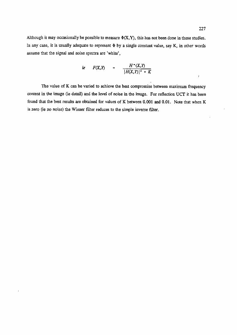
227

Although it may occasionally be possible to measure (X,Y), this has not been done in these studies.

In any case, it is usually adequate to represent by a single constant value, say K, in other words

assume that the signal and noise spectra are 'white',

ie F(X,Y) = H'(X,Y)

H(X,Y)! 2 + K

The value of K can be varied to achieve the best compromise between maximum frequency

content in the image (ie detail) and the level of noise in the image. For reflection UCT it has been

found that the best results are obtained for values of K between 0.001 and 0.01. Note that when K

is zero (ie no noise) the Wiener filter reduces to the simple inverse filter.

228

II: The Production of Phantoms

Material requirements

To adequately compare the image quality of B-scanning, reflection UCT and transmision

UCT, phantoms were required which had predictable bulk acoustic speed, attenuation and scattering

properties that were closely equivalent to those found in soft tissues. A predictable internal and

external structure was also desirable.

Gelatine based phantoms: Various materials for mimicking soft tissue (called tissue mimicking TM

or tissue equivalent TE materials) have been proposed over the years. The most commonly used

material has probably been a gelatine and distilled water base with variable quantities of graphite

powder added to provide scattering (Madsen et al 1978). Varying quantities of alcohol may also

added to modify the acoustic speed of the material from approx 1500 m/s (no alcohol) to approx 1600

rn/s (20% alcohol). To make the material, water is heated to near boiling point and gelatine added

and thoroughly melted. Graphite powder and alcohol are then added as the material cools but before

it starts to set.

Although phantoms for this project were initially made with gelatine, these phantoms had a

tendency to rot over a period of weeks and when higher quantities of alcohol were added they tended

to be rather soft.

Agar based phantoms: Phantoms which use agar instead of gelatine (Burlew et al, 1980) as the base

materials have advantages because (1) agar contains no nitrogen and hence is less prone to bacterial

invasion, and (2) the phantoms produced seem to be inherently stiffer than gelatine based ones.

Hence all of the results from TEM phantoms presented in this thesis are from agar based phantoms.

Structural recluirements

The TEM phantoms had to meet the following requirements for UCT imaging:-

(a) They needed to be submergible in water.

(b) They had to be accessible from 360°.

(c) They had to be relatively long lasting (ie useable for a few months).

In addition it was found that the phantom material could not be left in direct contact with

229

water, because this caused leeching of the alcohol out of phantom. Also the material could not be

exposed to air for long periods because it tended to dry out. Hence it was decided to make the

phantoms inside air-tight polythene bags. The polythene was thin enough to not significantly attenuate

the ultrasound entering the phantom.

A mould in which to make phantom was also needed to give it some convenient extrnal

shape. Accordingly plastic jars of diameter 9.2 cm were used. These were first coated with grease

before being lined with a polythene bag. The molten agar was then poured in and allowed to set.

Once set, a nylon cap was placed on top of the phantom, within the polythene bag, into which was

screwed a plastic rod for securing the phantom in a fixed position for scanning. The open top of the

polythene bag was then wrapped securely around the rod, and the bag with agar material inside

carefully removed from the plastic jar.

Phantom inserts (ie for introducing regions of different acoustic speed or attenuation) where

made by inserting greased and heated metal rods of various sizes into the previously set phantom.

After a few minutes, ie long enough for the phantom to partially re-set around the rods, the rods were

carefully removed. The material for the insert was then poured into the holes. If the insert material

was another TE material, this was allowed to cool such that it was just about to set before being

poured into the holes.