theoretical and experimental study of - CORE

THEORETICAL AND EXPERIMENTAL STUDY OF

CONCENTRATED PHOTOVOLTAIC (CPV)

SYSTEM WITH HYDROGEN PRODUCTION AS

ENERGY STORAGE

MUHAMMAD BURHAN

(BSc Eng, UET Lahore, Pakistan)

A THESIS SUBMITTED

FOR THE DEGREE OF DOCTOR OF PHILOSOPHY

DEPARTMENT OF MECHANICAL ENGINEERING

NATIONAL UNIVERSITY OF SINGAPORE

2015

DECLARATION

I hereby declare that the thesis is my original work and it has been written by

me in its entirety. I have duly acknowledged all the sources of information

which have been used in the thesis.

This thesis has also not been submitted for any degree in any university

previously.

____________________

Muhammad Burhan

25 December 2015

Acknowledgements

ii

ACKNOWLEDGEMENTS

Bismillah Hir Rahman Nir Raheem (In the name of ALLAH, the most

Gracious, the most Merciful). First of all, I am grateful to ALLAH, the God

Almighty, for His blessing and strength that made me able to complete this

thesis.

I would like to convey my heartiest and deepest gratitude to my supervisor,

Prof. Ng Kim Choon who believed in me and gave me opportunity to work on

this project. I am truly thankful to him for his guidance, time and ideas with

encouragement and motivation throughout the project and providing me

funding to complete this project. I would like to extend my gratitude to Prof.

Chua Kian Jon Ernest for his support, advice and guidance in my research.

I am thankful to Dr. Oh Seung Jin for his kind help and efforts throughout my

project and without which, it was difficult for me to finish this project. I am

greatly thankful to my closet lab mates Dr. Muhammad Wakil Shahzad, Dr. Li

Ang and Dr. Azhar Bin Ismail for providing me motivation and

encouragement during my entire PhD and helping me during hard times. I am

also thankful to Dr. Kyaw Thu, Dr. M. Kumja and Dr. Loh Wai Soong for

their inspiration as seniors during my PhD. I would also like to express my

appreciation for Mr. Scadevan Raghvan for his technical and moral help

during my project. I would like to thank to my lab fellows Chen Qien and Lin

Jie for memorable moments and time.

Most importantly, I am truly grateful to my beloved and respected parents, my

father, Muhammad Muazzam and my mother, Naila Nighat, for their prayers,

motivation and support. My parents are my life and all of my happiness and

Acknowledgements

iii

achievements belong to them. I would also like to thank my beloved sisters,

Aisha Shoaib and Zunaira Awais, for their love and support. I dedicate my

thesis to my family.

Muhammad Burhan

25 December 2015

List of Publications

iv


Journal Publications

1. Muhammad Burhan, Chua Kian Jon Ernest, Ng Kim Choon. Sunlight to

hydrogen conversion: Design optimization and energy management of

concentrated photovoltaic (CPV-Hydrogen) system using micro genetic

algorithm. Energy 2016, 99, 115-128.

2. Muhammad Burhan, Chua Kian Jon Ernest, Ng Kim Choon. Simulation and

development of a multi-leg homogeniser concentrating assembly for concentrated

photovoltaic (CPV) system with electrical rating analysis. Energy Conversion and

Management 2016, 116, 58-71.

3. Muhammad Burhan, Oh Seung Jin, Chun Wongee, Chua Kian Jon Ernest, Ng

Kim Choon. Development of Compact and Low Cost Two axis Solar Tracker

using Master Slave Configuration for CPV Applications. Solar Energy 2016.

(accepted)

4. Muhammad Burhan, Chua Kian Jon Ernest, Ng Kim Choon. Electrical rating of

concentrated photovoltaic (CPV) systems: long-term performance analysis and

comparison to conventional PV systems. International Journal of Technology

2016, 7(2), 189-196.

5. Muhammad Burhan, Oh SJ, Ng KC, Chun W. Experimental investigation of

Multijunction Solar Cell using Two Axis Solar Tracker. Applied Mechanics and

Materials 2016, 819, 536-540.


v

6. S. J. Oh, Muhammad Burhan, K.C. Ng, Y. Kim, W. Chun. Development and

performance analysis of a two‐axis solar tracker for concentrated

photovoltaics. International Journal of Energy Research 2015. 39(7), 965-976.

7. Muhammad Burhan, Chua Kian Jon Ernest, Ng Kim Choon. Long Term

Electrical Rating of Concentrated Photovoltaic (CPV) Systems in Singapore.

Applied Energy 2015. (under review)

8. Muhammad Burhan, Chua Kian Jon Ernest, Ng Kim Choon. Long Term

Hydrogen Production Potential of CPV System in Tropical Weather of Singapore.

International Journal of Hydrogen Energy 2015. (under review)

9. Muhammad Burhan, Chua Kian Jon Ernest, Ng Kim Choon. Performance

Comparison of Conventional Concentrated Photovoltaic (CPV) Systems with Ray

Tracing Simulation and Experimentation. Renewable and Sustainable Energy

Reviews 2015. (Manuscript under Preparation)

10. Muhammad Burhan, Chua Kian Jon Ernest, Ng Kim Choon. Energy Output of

Concentrated Photovoltaic: Performance Simulation Model and Field

Experimentation. Energy Conversion and Management 2015. (Manuscript under

Preparation)

Conference Publications

1. Muhammad Burhan, Chua Kian Jon Ernest, Ng Kim Choon. Electrical Rating of

Concentrated Photovoltaic (CPV) Systems: Long Term Performance Analysis and

Comparison with Conventional PV Systems. The 8th International Meeting on

Advanced Thermofluids (IMAT) 2015, Jakarta, Indonesia.


vi

2. Muhammad Burhan, Chua Kian Jon Ernest, Oh Seung Jin, Muhammad Wakil

Shahzad, Ng Kim Choon. Electrical Rating Analysis for Long Term Performance

of Concentrated Photovoltaic (CPV) System. First Pacific Rim Thermal

Engineering Conference (PRTEC) 2016, Hawaii, USA.

3. Muhammad Burhan, Oh Seung Jin, Muhammad Wakil Shahzad and Kim Choon

Ng, Electrical Rating of Concentrated Photovoltaic (CPV) Systems for Long Term

Performance. The 6th International Symposium on Physics of Fluids (ISPF6) 2015,

Xining, China.

4. Muhammad Burhan, Oh SJ, Shahzad MW, Kim YD, Ng KC, Chun W.

Prediction of Annual Performance of CPV Systems using Multi-Junction Solar

Cells, The 7th International Meeting on Advanced Thermofluids (IMAT) 2014,

Kuala Lumpur, Malaysia.


Multijunction Solar Cell using Two Axis Solar Tracker. International Conference

on Energy and Thermal Science (ICETS) 2014, Skudai, Malaysia.

6. Muhammad Burhan, S. J. Oh, K. C. Ng. Analysis of Concentrated Photovoltaic

System with Two Axis Solar Tracker For Hydrogen Production. The 6th

International Symposium on Microchemistry and Microsystems (ISMM) 2014,

Singapore.


Multijunction Solar Cell using Two Axis Solar Tracker. The 6th International

Meeting on Advanced Thermofluids (IMAT) 2013, Singapore.

Table of Contents

vii

Table of Contents

Declaration.....................................................................................................i

Acknowledgement.......................................................................................ii

List of Publications....................................................................................iv

Journal Publications..........................................................................................iv

Conference Publications.....................................................................................v

Table of Contents......................................................................................vii

Summary......................................................................................................xii

List of Tables...............................................................................................xv

List of Figures............................................................................................xvi

Nomenclature...........................................................................................xxvi

Chapter 1: Introduction...........................................................................1

1.1 Objectives.....................................................................................................4

1.2 Thesis Outline..............................................................................................6

Chapter 2: Literature Review................................................................9

2.1 World Energy Scenario and CO2 Emissions................................................9

2.2 Solar Resource Potential............................................................................13

2.3 Solar Photovoltaic......................................................................................16

2.3.1 Multi-Junction Solar cell (MJC).................................................17

2.4 Concentrated Photovoltaic and Two axis Solar Tracker............................21

2.5 Hydrogen Energy Storage..........................................................................28

2.5.1 Water Electrolysis Theory...........................................................31

2.5.2 Alkaline Electrolyser...................................................................34

2.5.3 Proton Exchange Membrane (PEM) Electrolyser......................36

2.6 Standalone Systems and Design Optimization...........................................37

Chapter 3: Development of Two Axis Solar Tracker with

Master Slave Configuration for CPV Field.....................................41

3.1 Introduction................................................................................................41

Table of Contents

viii

3.2 Development of Solar Tracking Technique...............................................42

3.2.1 Astronomical Tracking................................................................43

3.2.2 Active Tracking...........................................................................47

3.2.3.1 Development of Double Lens Collimating Solar

Feedback Sensor...........................................................53

3.3 Development of Tracking System for CPV Field- Master and Slave

Configuration............................................................................................58

3.4 Solar Tracker Hardware Development.......................................................61

3.4.1 Electrical Circuit Development...................................................61

3.4.2 Mechanical Structure and Driving Assembly.............................65

3.5 Tracking Algorithm Development.............................................................67

3.6 Tracking Accuracy.....................................................................................73

3.7 Summary....................................................................................................77

Chapter 4: Design and Ray Tracing Simulation of

Concentrating Assembly for CPV.......................................................79

4.1 Introduction................................................................................................79

4.2 Mini Dish-CPC Concentrating Assembly..................................................80

4.2.1 Mini Parabolic Dish Design........................................................82

4.2.2 Dielectric Filled Compound Parabolic Concentrator (CPC)

Design.........................................................................................83

4.2.3 Experimental Performance Investigation of CPV System with

Mini Dish-CPC Concentrating Assembly..................................87

4.2.4 Mini Dish - CPC Assembly Limitations.....................................89

4.3 Mini Dish Cassegrain Arrangement Concentrating Assembly

Design........................................................................................................91

4.3.1 Primary Reflector - Mini Parabolic Dish....................................93

4.3.2 Homogeniser...............................................................................93

4.3.3 Secondary Reflector - Hyperbolic Dish......................................93

4.3.4 Ray Tracing Simulation of Mini Dish Cassegrain Concentrating

Assembly.....................................................................................96

Table of Contents

ix

4.3.5 Design of Mini Dish CPV System..............................................98

4.4 Fresnel Lens-Glass Homogeniser Concentrating Assembly....................100

4.4.1 Glass Homogeniser...................................................................101

4.4.2 Fresnel Lens Design..................................................................101

4.4.3 Ray Tracing Simulation of Fresnel Lens-Glass Homogeniser

Concentrating Assembly........................................................105

4.4.4 Design of Fresnel Lens-Glass Homogeniser CPV System.......107

4.5 Fresnel Lens-Reflective Homogeniser Concentrating Assembly............109

4.5.1 Ray Tracing Simulation of Fresnel Lens-Reflective Homogeniser

Concentrating Assembly........................................................110

4.5.2 Design of Fresnel Lens-Reflective Homogeniser CPV System112

4.6 Summary..................................................................................................113

Chapter 5: Experimental Investigation of Concentrated

Photovoltaic (CPV) System and CPV-Hydrogen System.........115

5.1 Introduction..............................................................................................115

5.2 CPV Experimental Setup Description......................................................116

5.3 Mini Dish Cassegrain CPV System.........................................................120

5.3.1 Experimental Investigation of Mini Dish Cassegrain CPV

System.......................................................................................123

5.4 Fresnel Lens-Glass Homogeniser CPV System.......................................129

5.4.1 Experimental Investigation of Fresnel Lens-Glass Homogeniser

CPV System..............................................................................130

5.5 Fresnel Lens-Reflective Homogeniser CPV System................................135

5.5.1 Experimental Investigation of Fresnel Lens - Reflective

Homogeniser CPV System........................................................136

5.6 Discussion on Performance Comparison of Developed CPV Systems....141

5.7 CPV-Hydrogen System Description........................................................143

5.8 Results and Discussion for CPV-Hydrogen System................................149

5.9 Summary..................................................................................................153

Table of Contents

x

Chapter 6: Long Term Electrical Rating of Concentrated

Photovoltaic (CPV) Systems................................................................156

6.1 Introduction..............................................................................................156

6.2 Electrical Rating Methodology................................................................158

6.2.1 CPV System Description under Investigation...........................159

6.2.2 Electrical Rating Parameters.....................................................160

6.2.3 Maximum Performance Characteristics of Systems under

Investigation..............................................................................163

6.3 Results and Discussion.............................................................................166

6.4 Summary..................................................................................................178

Chapter 7: Development of a Multi-leg Homogeniser

Concentrating Assembly for Concentrated Photovoltaic (CPV)

System..........................................................................................................180

7.1 Introduction..............................................................................................180

7.2 Design of Multi-leg Homogeniser Concentrating Assembly...................182

7.3 Development of Experimental Setup of Multi-leg Homogeniser CPV

System.....................................................................................................192


7.5 Summary..................................................................................................206

Chapter 8: Design Optimization and Energy Management of

Concentrated Photovoltaic (CPV-Hydrogen) System using

micro Genetic Algorithm for Standalone Operation..................208

8.1 Introduction..............................................................................................208

8.2 CPV-Hydrogen System Description........................................................211

8.3 Development of Performance Model for CPV-Hydrogen System...........213

8.3.1 Direct Normal Irradiance (DNI) Weather Data.........................214

8.3.2 Electrical Load Profile...............................................................215

8.3.3 Concentrated Photovoltaic (CPV) System................................216

8.3.4 Electrolyser................................................................................221

8.3.5 Fuel Cell....................................................................................224

8.3.6 Hydrogen Compressor...............................................................225

Table of Contents

xi

8.3.7 Hydrogen Storage Tank............................................................226

8.4 Objective Function and Optimization Criteria.........................................227

8.5 Optimization Method and the Implementation of micro Genetic

Algorithm................................................................................................231


8.7 Summary..................................................................................................241

Chapter 9: Conclusion...........................................................................244

References..................................................................................................247

Appendices.................................................................................................271

Appendix A: Parts of Tracker Control Box....................................................271

Appendix B: Hydrogen Compression Unit Layout and Components

Description................................................................................279

Appendix C: MJC Characteristics..................................................................285

Summary

xii

Summary

Owing to concerns over the increasing global warming issues from the

extensive use of fossil fuels, the use of solar energy especially photovoltaic

system has gained escalating interest as a sustainable energy source to meet

the global energy demand. This is due to their capability to directly convert

solar energy into electricity with simple configuration. The concentrated

photovoltaic (CPV) system is emerging as a highly efficient photovoltaic

technology. The aim of this thesis is to conduct extensive theoretical and

experimental study of the concentrated photovoltaic system for development

of a compact and cost effective system design, with the hydrogen production

as energy storage to handle solar intermittency. The compact system design

with cost effective approach, will eliminate the installation limitations related

to conventional CPV system. Furthermore, the CPV-Hydrogen study will

show the real CPV hydrogen production potential and will introduce the

design methodology for steady operation of CPV.

A CPV field based upon the compact concentrated photovoltaic (CPV)

systems is developed, utilizing the cost effective master slave configuration

through wireless control communication. The developed system performance

is investigated for long term outdoor operation at the rooftop of Engineering

building (EA). In master slave configuration, the required tracking information

from expensive devices is transmitted wirelessly through one master tracker.

While, the rest of the slave trackers are only equipped with minimum

hardware and operate according to the tracking information received from

master tracker. The compact, smart but highly accurate and sensitive two axis

Summary

xiii

solar trackers are designed and developed utilizing hybrid tracking algorithm.

All the trackers are equipped with novel and low cost solar feedback tracking

sensor utilizing double lens collimator and photo-sensor array, with tracking

accuracy of 0.1o. The accuracy of the tracker is verified for long term field

operation.

The developed CPV field based upon four prototypes of compact CPV

systems; three of them are based upon the conventional concentrating

assemblies designs and utilizing mini parabolic dish in cassegrain arrangement

and Fresnel lens with glass and reflective homogeniser. While the fourth CPV

system is based upon the novel design of multi-leg homogeniser concentrating

assembly which unlike conventional design, concentrates solar radiations on

four solar cells with a single set of concentrator. The detailed design model

and the selection criteria for the concentrating assemblies is proposed and

verified through ray tracing simulation in TracePro. The simulated and

experimental performance of the developed CPV systems is verified and

compared for short term and long term operation.

An electrical rating methodology is proposed to rate the real field potential of

the photovoltaic systems and the highest long term electrical rating of 240.21

kWh/m2.year is recorded for CPV systems, which is 2-3 folds higher than the

conventional PV even in tropical weather conditions of Singapore.

To handle solar intermittency and to operate CPV for steady power

production, the potential of the CPV system is first experimentally analyzed

for hydrogen production. A hydrogen production system based upon PEM

electrolysers and a hydrogen storage system based upon the mechanical

Summary

xiv

compressor, are designed and developed. The CPV-Hydrogen system showed

solar to hydrogen maximum efficiency of 18-19% and average efficiency of

15-16% for whole day operation. In addition, for standalone operation of CPV,

a detailed performance model and design optimization strategy is first time

developed and verified for CPV system with hydrogen production as energy

storage. Using micro-GA, the techno-economic optimization of the CPV-

Hydrogen system is carried out for uninterrupted power supply at minimum

system cost, according to the proposed energy management and control

strategy. The developed model can also be used to estimate the long term

performance of any component of CPV-Hydrogen system for design purpose,

which is already verified for the long term CPV performance. In addition, the

proposed model and strategy can be integrated into the commercial analyzing

tools, to enhance their analyzing capability for CPV.

List of Tables

xv

List of Tables

Table 4.1: Aspheric Coefficients of Optimized Aspheric Lens

Table 5.1: Summary of Performance of Developed CPV systems

Table 5.2: Daily Average Performance of CPV-Hydrogen System

Table 6.1: Maximum Performance Rating of Multi-Junction Solar Cell

and Developed CPVs

Table 6.2: Performance Characteristics of Conventional PV systems at

CITI (BCA), Singapore

Table 6.3: Summary of Long Term Weather Data

Table 6.4: Summary of Long-Term (12 months) Performance Data of

CPV Systems

Table 7.1: Design parameters for Primary Reflector

Table 7.2: Daily Performance Data for Developed CPV System

Table 8.1: Comparison Summary of Renewable Energy System

Simulation and Optimization

Table 8.2: Parameters for Diode model for Solar Cell Under

Concentration

Table 8.3: Parameters for Concentrated Photovoltaic (CPV) System

Table 8.4: Performance Parameters for Electrolyser Model

Table 8.5: Parameters for Faraday Efficiency of Electrolyser

Table 8.6: Performance Parameters for Fuel Cell Model


Table 8.8: Cost Parameters for Individual Components of CPV-Hydrogen

System

Table 8.9: Optimization Summary for Proposed CPV-Hydrogen System

List of Figures

xvi

List of Figures

Figure 2.1: World Population and Energy Demand

Figure 2.2: Global Energy Mix

Figure 2.3: Primary Energy Supply Consumption by Sector

Figure 2.4: CO2 Emission Trend by Fossil Fuels

Figure 2.5: World CO2 Emissions by Sector

Figure 2.6: Global Technical Potential of Energy Sources (log scale,

1018

J/year)

Figure 2.7: Total Energy Resources

Figure 2.8: Scattering of Solar Radiation by Atmosphere

Figure 2.9: Solar Spectrum

Figure 2.10: Three Generations of Solar Cell

Figure 2.11: Part of Solar Spectrum Absorbed by (a) Si Solar Cells and

(b) Multi-Junction Solar Cells

Figure 2.12: Best Research-Cell Efficiencies

Figure 2.13: CPV System arrangement using Lens Concentrator

Figure 2.14: CPV System arrangement using (a) Single Dish and (b) Double

Dish, Cassegrain

Figure 2.15: CPV System arrangement with Fresnel Lens and Homogeniser

Figure 2.16: CPV System arrangement with (a) Single Dish, (b) Double

Dish and Homogeniser

Figure 2.17: Sketch of Electrolyser

Figure 2.18: Unipolar Electrolyser

Figure 2.19: Bipolar Electrolyser

Figure 2.20: Sketch of PEM Electrolyser

Figure 2.21: Simple Schematic of Standalone Solar Energy System with

Hydrogen Production as Energy Storage

Figure 3.1: Plan View Showing Azimuth and Zenith Angles

List of Figures

xvii

Figure 3.2: Active Tracking Sun Position Sensing Schematic

Figure 3.3: Active Tracking Algorithm

Figure 3.4: Rod Type Solar Feedback Sensor (a) Design (b) Prototype

Figure 3.5: The Effect of Angular Offset on the Height of Shadow Column

Figure 3.6: Schematic of Single Lens Solar Feedback Sensor

Figure 3.7: Ray Tracing Simulation of Single Lens Solar Feedback Sensor

Figure 3.8: The Angular Deviation of Incident Rays through Single Lens

Solar Feedback Sensor

Figure 3.9: The Response of Single Lens Feedback Sensor for Different

Focal Length against Angular Deviation Of Incident Rays

Figure 3.10: Schematic of Double Lens Solar Feedback Sensor

Figure 3.11: The Ray Tracing Simulation Results of Double Lens Feedback

Sensor with Parallel Ray Grid Source

Figure 3.12: The Angular Deviation of Incident Rays through Double Lens


Figure 3.13: The Response of Double Lens Feedback Sensor for Different

Lens-Sensor Plate Distance against Angular Deviation of

Incident Rays

Figure 3.14: Collimating Beam Position for Tracking Error (a) 0o (b) 0.3

o

Figure 3.15: Developed Prototype of Double Lens Solar Feedback Sensor

Figure 3.16: Electrical Connection arrangement for Photo-Sensors Array

Figure 3.17: Master and Slave Network arrangement using ZigBee

Figure 3.18: Master and Slave arrangement of Developed CPV Field

Figure 3.19: Block Diagram of Electrical Circuit of Two Axis Solar

Tracking System

Figure 3.20: Control Box for (a) Master Tracker (b) Slave Tracker

Figure 3.21: The Power Supply Box for Developed CPV System

Figure 3.22: Two Axis Solar Tracker Mechanical Components

Figure 3.23: Isometric View of Designed Tracker Model

List of Figures

xviii

Figure 3.24: Solar Tracking Variables

Figure 3.25: Master Tracker Tracking Control Algorithm

Figure 3.26: Slave Tracker Tracking Control Algorithm

Figure 3.27: Breakout of GPS GPRMC Format String

Figure 3.28: Solar Tracker Trajectory During Operation

Figure 3.29: Comparison of Calculated and Actual (a) Azimuth (b) Zenith

Angles

Figure 3.30: Colour Tracking Sensor (CTS) Camera and BAADER Film

Assembly to Determine Solar Position

Figure 3.31: CTS Control Software and Determination of Solar Position

Figure 3.32: CTS Sensor Measured Angular Deviation for (a) Zenith (b)

Azimuth

Figure 4.1: Schematic of Mini Dish-CPC Concentrating Assembly

Figure 4.2: Mini Dish Parabolic Concentrator Coordinates

Figure 4.3: Representation of Polar Coordinates of Parabola

Figure 4.4: Design Schematic of Dielectric Filled Compound Parabolic

Concentrator (CPC)

Figure 4.5: Ray Propagation in Dielectric Filled Compound Parabolic

Concentrator (CPC)

Figure 4.6: Experimental Setup of Mini Dish-CPC CPV System

Figure 4.7: System Efficiency Curve for Mini Dish-CPC CPV System

Figure 4.8: DNI Received During Mini Dish-CPC CPV System Operation

Figure 4.9: Developed Model of Mini Dish-CPC Concentrating Assembly

in TracePro

Figure 4.10: Ray Tracing Simulation of CPV Concentrating Assembly

Figure 4.11: Ray Tracing Simulation of CPV Concentrating Assembly (a)

with Angle Less than Acceptance Angle of Homogeniser (b)

Effective Radius of Parabolic Dish

List of Figures

xix

Figure 4.12: Design Schematic of Mini Dish Cassegrain Arrangement

Concentrating Assembly

Figure 4.13: Coordinates of Secondary Hyperbolic Reflector

Figure 4.14: Mini Dish Cassegrain Concentrating Assembly Model in

TracePro

Figure 4.15: Ray Tracing Simulation of Mini Dish Cassegrain Concentrating

Assembly

Figure 4.16: Irradiance Map at (a) Inlet and (b) Outlet of Homogeniser of

Mini Dish Concentrating Assembly

Figure 4.17: Normalized Power Curve for Mini Dish Cassegrain


Figure 4.18: Design of Mini Dish CPV System

Figure 4.19: Design Model of Mini Dish Cassegrain Concentrating

Assembly

Figure 4.20: Design Schematic of Fresnel Lens-Glass Homogeniser


Figure 4.21: Design Schematic for Aspheric Fresnel Lens

Figure 4.22: Optimized Aspheric Plano-Convex Lens in 2D Interactive

Optimizer of TracePro

Figure 4.23: Ray Tracing Simulation of Aspheric Lens (a) Simulation Result

(b) Irradiance map

Figure 4.24: Fresnel Lens-Glass Homogeniser Concentrating Assembly

Model in TracePro

Figure 4.25: Ray Tracing Simulation of Fresnel Lens-Glass Homogeniser



Fresnel Lens Concentrating Assembly

Figure 4.27: Normalized Power Curve for Fresnel Lens-Glass Homogeniser


List of Figures

xx

Figure 4.28: Design Model of Fresnel Lens-Glass Homogeniser CPV

System

Figure 4.29: Design Model of Fresnel Lens-Glass Homogeniser


Figure 4.30: Schematic of Fresnel Lens-Reflective Homogeniser


Figure 4.31: Fresnel Lens-Reflective Homogeniser Concentrating Assembly

Model in TracePro

Figure 4.32: Ray Tracing Simulation of Fresnel Lens-Reflective

Homogeniser Concentrating Assembly

Figure 4.33: Normalized Power Curve for Fresnel Lens-Reflective


Figure 4.34: Design Model of Fresnel Lens-Reflective Homogeniser CPV

System

Figure 4.35: Design Model of Fresnel Lens-Reflective Homogeniser


Figure 5.1: Design Model of CPV Systems Experimental Setup

Figure 5.2: Schematic of Control Circuit and System Arrangement for CPV

Experimental Setup

Figure 5.3: Front View of Developed CPV Experimental Setup

Figure 5.4: Rear View of Developed CPV Experimental Setup

Figure 5.5: Developed CPV System on Mini Dish Cassegrain Design

Figure 5.6: Optical Reflectance for Aluminium and Silver

Figure 5.7: Silver Coating Problems on Mini Parabolic Dish

Figure 5.8: Maximum Performance Potential of Mini Dish Cassegrain CPV

System (a) in Morning (b) at Noon

Figure 5.9: Performance Characteristics of Mini Dish Cassegrain CPV for

whole Day Operation

Figure 5.10: Total Voltage, Current and Power output from Mini Dish

List of Figures

xxi

Cassegrain CPV

Figure 5.11: System Efficiency against DNI and Heat Sink Temperature for

Mini Dish Cassegrain CPV for Experiment Set-2



Figure 5.13: Experimental and Simulated Normalized Power Output Curve

for Mini Dish Cassegrain CPV

Figure 5.14: Developed CPV System on Fresnel Lens-Glass Homogeniser

Design

Figure 5.15: Maximum Performance Potential of Fresnel Lens-Glass

Homogeniser CPV System (a) in Morning (b) at Noon

Figure 5.16: Performance Characteristics of Fresnel Lens-Glass

Homogeniser CPV for whole Day Operation

Figure 5.17: Total Voltage, Current and Power output from Fresnel Lens-

Glass Homogeniser CPV


Fresnel Lens-Glass Homogeniser CPV for Experiment Set-2




for Fresnel Lens-Glass Homogeniser CPV

Figure 5.21: Developed CPV System on Fresnel Lens-Reflective

Homogeniser Design

Figure 5.22: Maximum Performance Potential of Fresnel Lens-Reflective


Figure 5.23: Performance Characteristics of Fresnel Lens-Reflective



List of Figures

xxii

Reflective Homogeniser CPV


Fresnel Lens-Reflective Homogeniser CPV for Experiment Set-

2


Fresnel Lens-Reflective Homogeniser CPV for Experiment Set-

3


for Mini Dish Cassegrain CPV

Figure 5.28: Comparison of Experimental and Simulated Normalized Power

Output Curve for Developed CPV Systems

Figure 5.29: Schematic of Control Circuit and System Arrangement for

CPV-Hydrogen Experimental Setup

Figure 5.30: CPV-Hydrogen Experimental Setup

Figure 5.31: Hydrogen Compression System

Figure 5.32: Hydrogen Purity Analyzer (a) Before Hydrogen Supply (b)

After Hydrogen Supply

Figure 5.33: PEM Electrolyser Characteristics (a) IV-Curve (b) Production

rate and Faraday Efficiency

Figure 5.34: Solar to Hydrogen Conversion Efficiency and CPV Efficiency

against DNI

Figure 5.35: Electrolyser Efficiency, Voltage and Current Consumed per

Cell of Electrolyser Stack for Whole Day Operation.

Figure 5.36: Daily Average Electrolyser Efficiency against the Solar Energy

Input Received for Whole Day

Figure 5.37: The Effect of Variation of Electrolyser Efficiency on Hydrogen

Production

Figure 6.1: Experimental Setup description of CPV System

Figure 6.2: Fresnel Lens-Glass Homogeniser CPV System Performance

List of Figures

xxiii

(a)Test 1(b)Test 2

Figure 6.3: Fresnel Lens-Reflective Homogeniser CPV System

Performance (a) Test 1 (b) Test 2

Figure 6.4: Mini Dish Cassegrain CPV System Performance (a) Test 1 (b)

Test 2

Figure 6.15: Conventional Mono-Crystalline, Poly-Crystalline and Thin

Film (CIS) PV Systems at CITI (BCA), Singapore

Figure 6.6: Monthly Average Values of Solar Irradiance (Global and DNI)

and Sunshine Duration Data per Day

Figure 6.7: Monthly Electrical Rating and Monthly average Efficiency of

CPV systems with the DNI Received

Figure 6.8: CPV Systems and conventional PVs and their CO2 Savings

comparison

Figure 6.9: Overall Average GHI Efficiency

Figure 6.10: Total Power Delivered by assorted PV Systems against DNI

and Global Irradiance

Figure 7.1: Schematic of Multi-leg Concentrating Assembly for CPV

Figure 7.2: Design of Multi-Leg Homogeniser Concentrating Assembly

Figure 7.3: Distribution of Rays in Multi-Leg Homogeniser Concentrating

Assembly

Figure 7.4: Schematic for Size Calculations for Primary Reflector

Figure 7.5: Coordinates of the Primary Reflector

Figure 7.6: Schematic of Multi-leg Homogeniser Design

Figure 7.7: Acceptance Angle Calculation through Schematic of Multi-Leg


Figure 7.8: Design Model of Multi-leg Homogeniser Concentrating

Assembly

Figure 7.9: Experimental Setup of Multi-leg Homogeniser CPV System

Figure 7.10: Oxidation of Silver Coating

List of Figures

xxiv

Figure 7.11: Development of Multi-leg Homogeniser Concentrating

Assembly

Figure 7.12: Development of Multi-Leg Homogeniser

Figure 7.13: TracePro Model of Multi-leg Homogeniser Concentrating

Assembly

Figure 7.14: Ray Tracing Simulation of Multi-leg Homogeniser

Concentrating Assembly with Parallel Rays

Figure 7.15: Ray Tracing Simulation of Multi-leg Homogeniser

Concentrating Assembly with Solar Ray Angle

Figure 7.20: Normalized Power Output Curves for Multi-leg Homogeniser

CPV System

Figure 7.21: Simulated Irradiance Map at Each Cell Outlet of Multi-leg

Homogeniser at Different Parallel Ray Deviation Angles

Figure 7.22: Electrical Rating of Developed CPV System against Total

Available DNI

Figure 8.1: Schematic of CPV-Hydrogen System for Standalone Operation

Figure 8.2: Energy Management Flow Chart for Proposed CPV-Hydrogen

System

Figure 8.3: Summary of Monthly Solar Energy Received by Singapore

Figure 8.4: Part of Electrical Load Profile of Singapore with 30 minutes

internal Energy System Simulation and Optimization

Figure 8.5: Variation of Cell Open Circuit Voltage (VOC) with

Concentration and Temperature

Figure 8.6: Variation of Cell Short Circuit Current (ISC) with Concentration

and Temperature

Figure 8.7: Multi-junction Cell (a) Short Circuit Current (b) Open Circuit

Voltage Versus Concentration at 25oC

Figure 8.8: Temperature Coefficients of Multi-junction Cell (MJC) against

Concentration (a) Short Circuit Current (b) Open Circuit

List of Figures

xxv

Voltage

Figure 8.9: MJC efficiency Experimentally Measure and Simulated

Figure 8.10: Compressibility Factor for Hydrogen Storage

Figure 8.11: Proposed Optimization Strategy for CPV-Hydrogen System for

Stand Alone Operation

Figure 8.12: Optimization Curve against micro Genetic Algorithm (micro-

GA) Generations

Figure 8.13: Cost Breakup for Optimized CPV-Hydrogen System

Figure 8.14: The State of Hydrogen and Oxygen Storage Tanks over Period

of Operation

Figure 8.15: Percentage Share of Load Contributed by Fuel Cell on Monthly

and Daily Basis

Figure 8.16: The Monthly Total Hydrogen Production with Corresponding

Production Rating

Figure 8.17: Simulated Performance of CPV System in form of Monthly

Electrical Rating

Figure 8.18: Comparison of Simulated and Experimental Electrical Rating

Nomenclature

xxvi

Nomenclature

Symbol Description Units

EOT Equation of time min

Lst Standard longitude of local time zone deg

Lloc Longitude of local observer position deg

ω Hour angle deg

δ Declination Angle deg

θz Zenith Angle deg

θaz Azimuth Angle deg

φ Latitude of local observer position deg

TSR/ TSS Sun rise/sun set time hour

α Right ascension angle deg

n Number of day -

SD Sensor dimension mm

θa Angular offset in the position of the sun or Angular deg

deviation of solar rays from concentrator axis

CH Column Height for Shadow Purpose mm

d Distance between photo-sensors mm

fcx Focal length of convex lens mm

fcn Focal length of concave lens mm

Dcx Convex lens diameter mm

S Distance between collimating lenses mm

bt Collimated beam thickness mm

h Distance between collimating lens assembly and mm

photo-sensor array

Lm Maximum Depth of ZigBee Network -

Rm Maximum number of routing cable children -

Cm Maximum number of non-routing cable children -

fpr Focal length of mini parabolic dish mm

Nomenclature

xxvii


θr Rim angle deg

Dpr Diameter of mini parabolic dish mm

dpr Diameter of centre hole of mini parabolic dish mm

tpr Parabolic Curvature depth of mini parabolic dish mm

td Thickness of mini parabolic dish mm

CRg Geometric concentration ratio -

Acon Effective area of primary concentrator m2

AC Area of solar cell (MJC) m2

θa_CPC Acceptance angle of CPC deg

nCPC Refractive index of CPC material -

L Overall length of CPC mm

a Half of inter aperture size of CPC mm

a' Half of outlet aperture size of CPC mm

θe Tracking error of angular deviation of parallel rays deg

from concentrator axis

Dhp Diameter of mini hyper dish mm

f1hp First focal length of mini hyperbolic dish mm

f2hp Second focal length of mini hyperbolic dish mm

Mt MJC thickness mm

fFL Focal length of Fresnel lens mm

CL Curvature of conical surface of lens mm

RFL Radius of curvature of Fresnel lens mm

k Conical surface constant -

Ai Aspheric coefficients -

ZL Lens dimension variable towards lens sag direction mm

rL Lens dimension variable towards lens radial direction mm

DFL Diameter of Fresnel Lens mm

SFL Fresnel lens rings height mm

Nomenclature

xxviii


tFL Fresnel lens thickness mm

LFL Linear side dimension of square Fresnel lens mm

nFL Refractive index of Fresnel lens material -

PCPV Power output of CPV W

VCPV Voltage output of CPV V

ICPV Current output of CPV A

DNI Direct Normal Irradiance W/m2

ηCPV Efficiency of CPV system %

nE,H2 Rate of Hydrogen production mol/s

ηEF Faraday Efficiency of Electrolyser %

NEC Total number of Electrolyser cells -

IE Electrolyser current A

UE Electrolyser voltage V

nE No. of electrons required for electrolysis -

F Faraday Constant A.s/mol

ηEL Electrolyser Efficiency %

ηCPV_H2 Overall solar to hydrogen conversion efficiency %

Re,m Monthly electrical rating kWh/m2.year

Re Overall electrical rating kWh/m2.year

m Maximum number of days in month -

q Total number of experimental days -

E Daily total energy yield of CPV kWh/m2

Dm Daily total solar energy received kWh/m2

GHI Global Horizontal Irradiance W/m2

d1 Dimension of square primary reflector of mm

multi-leg homogeniser concentrating assembly

d2 Dimension of square secondary reflector of multi-leg mm

homogeniser concentrating assembly

Nomenclature

xxix


f1 Focal length of primary reflector of multi-leg homogeniser mm

concentrating assembly

f2 Focal length of secondary reflector of multi-leg mm


t1 Depth of primary reflector of multi-leg homogeniser mm


t2 Depth of secondary reflector of multi-leg homogeniser mm


AHO Area of centre hole in primary reflector of multi-leg m2


D1 Corresponding diameter of primary reflector of mm

multi-leg homogeniser concentrating assembly

θC Critical angle of optical material deg

IC Solar cell current A

CC Solar concentration at solar cell area Suns

VC Solar cell voltage V

NCM Number of solar cells in one panel -

NPCPV Number of CPV panels -

ISC Solar cell short circuit current A

ELC Electrical load demand of consumer W

VOC Solar cell open circuit voltage V

TC Solar cell temperature oC

Imppt Solar cell maximum power point current A

Vmppt Solar cell maximum power point voltage V

PC Solar cell power W

Pmppt Solar cell maximum power point power W

PLoad Total load demand W

Pexcess Excess available power from CPV W

Nomenclature

xxx


PTr Solar tracker power requirement W

Pcom Hydrogen compressor power W

PMJC,max MJC maximum rated power W

NE,O2 Oxygen production flow rate from electrolyser mol/s

TE Electrolyser Temperature oC

AE Electrolyser Cell Area m2

VEC,max Electrolyser Cell Maximum Voltage V

IEC,max Electrolyser Cell Maximum Current A

PEL,max Electrolyser Cell Maximum Power W

Lmin Minimum Electrical Load Requirement W

Urev Reversible Voltage of Electrolysis V

nF,H2 Hydrogen Consumption Flow Rate from Fuel Cell mol/s

nF,O2 Oxygen Consumption Flow Rate from Fuel Cell mol/s

IF Fuel Cell Current mA

AF Cell Area of Fuel Cell cm2

UF Cell Voltage of Fuel Cell mV

NFC Number of Cells of Fuel Cell -

PFC,max Cell Maximum Power of Fuel Cell W

Lmax Maximum Electrical Load Requirement W

Preq Electrical Power Deficiency not supplied by the CPV W

Uo Reversible Voltage of Fuel Cell mV

STH2 State of Hydrogen Storage kg

STO2 State of Oxygen Storage kg

STW State of Water Storage kg

STMH2 Maximum Hydrogen Storage Capacity kg

STMO2 Maximum Oxygen Storage Capacity kg

ηOP Optical Efficiency of Concentrating Assembly %

ηmppt Efficiency of Maximum Power Point Tracking Device %

Nomenclature

xxxi


ηDC/AC Efficiency of DC to AC Converter %

ηEF Faraday Efficiency of Electrolyser %

ηCDC Efficiency of DC to DC Converter %

ηFF Faraday Efficiency of Fuel Cell %

ηcom Efficiency of Compressor %

Pta Instantaneous Pressure of Hydrogen Tank Pa

PE Pressure of Hydrogen Production from Electrolyser Pa

MH2 Molar Mass of Hydrogen g/mol

CPH Specific Heat Capacity of Hydrogen J/kg.K

Tcom Hydrogen Compressor Temperature K

Tta Temperature of Hydrogen Storage Tank K

nta Instantaneous Number of Moles of Hydrogen Gas in mol

Storage Tank

r Isentropic Exponent of Hydrogen -

R Universal Gas Constant J/mol.K

ZH Compressibility Factor of Hydrogen -

V Volume of Storage Tank of Hydrogen m3

nH Number of Hydrogen Stage Tank -

PH Pressure of Hydrogen Storage Tank Pa

L1 Minimum Limit for Cyclic Hydrogen Storage kg

L2 Maximum Limit for Cyclic Hydrogen Storage kg

tPF Time for Power Failure sec

PSFT Power Supply Failure Time Factor sec

CC Capital Cost $

CAT Total Annual System Cost $

CCPV CPV Total Cost $

CEL Electrolyser Total Cost $

CFC Fuel Cell Total Cost $

Nomenclature

xxxii


CSTH2 Hydrogen Storage Total Cost $

CSTO2 Oxygen Storage Total Cost $

Ccom Hydrogen Compressor Total Cost $

OMC Operation and Maintenance Cost $

RC Replacement Cost $

CRF Capital Recovery Factor -

SPPW Single Payment Present Worth -

y Payment Duration years

i Compound Interest Rate %

w Lifetime Period of System years

Subscript

SR Sun rise

SS Sunset

(H) Angle Value in hours units

cx Convex

cn Concave

pr Parabolic

hp Hyperbolic

FL Fresnel Lens

L Lens

E Electrolyser

F Fuel Cell

ta Tank

com Compressor

H Hydrogen

H2 Hydrogen Gas

O2 Oxygen Gas

Nomenclature

xxxiii

Abbreviation

CPV Concentrated Photovoltaic

MJC Multi-junction Solar Cell

BOS Balance of System

GMT Greenwich Mean Time

C Coordinator

R Router

ED End Device

USART Universal Synchronous/Asynchronous Receiver/Transmitter

RTC Real Time Clock

ISP In System Programming

ADC Analogue to Digital Converter

CTS Colour Tracking Sensor

CPC Compound Parabolic Concentrator

MPPT Maximum Power Point Tracking

TIR Total Internal Reflection

DNI Direct Normal Irradiance

STC Standard Testing Conditions

NOCT Nominal Operating Cell Temperature

AM Air Mass

LTER Long Term Electrical Rating

GHI Global Horizontal Irradiance

MHCA Multi-leg Homogeniser Concentrating Assembly

PSFT Power Supply Failure Time

PEM Proton Exchange Membrane

Chapter 1

Page | 1

Chapter 1: Introduction

Energy is a resource needed for the survival of human beings and its

importance permeates all human activities. The world's current energy

consumption is about 12.477 GTOE and its demand is expected to increase by

41% when the world population hits 8.7 billion in 2035 [1,2]. Of this total

primary energy consumption, the generation of electricity and heating have the

highest share of 42% [3]. It has been reported that about 82% of the world's

energy consumption is derived from the fossil fuels, namely oil, natural gas

and coal. Consequently, the burning of these fuels has led to high emission of

CO2 into the atmosphere causing the drastic effects of global warming [4].

From environmental sustainability, only by switching to renewable energy

resources as primary energy supply can mitigate the effects from global

warming situation. Among all renewable energy resources, solar energy has

the highest potential to meet our energy demand [5] as the daily irradiance

received is 10,000 times more than the global energy consumption [6].

The main advantage for solar energy systems is their energy conversion

efficiency yet at relatively low cost with simple system configuration. The

photovoltaic system or solar cell provides the simple, elegant and direct

method of electricity production from solar energy [7-9]. The current installed

capacity of photovoltaic systems in the world has reached 183GWP [10].

Despite the increase in the total installed capacity of photovoltaic systems, it

ranks third in the renewable energy utilization share, after hydro and wind

energy resources [11,12]. The current photovoltaic market is almost fully

dominated by the single junction crystalline silicon cells and thin film solar

Chapter 1

Page | 2

cells, which offer low efficiencies at the cell level of 20-25% and 19-20%

respectively, and under the single flash test conditions [13]. The single

junction solar cell absorbs only a certain portion of the solar spectrum while

the remaining portion is dissipated as heat loss, thereby offering lower

efficiency [14]. Multi-junction solar cell, on the other hand, offers the highest

efficiency up to 46% due to having cell materials that are responsive to a

wider solar spectrum [16]. However, due to the high cost of multi-junction

solar cells, cost effective concentrated photovoltaic (CPV) concept is used in

which low cost concentrators are used to concentrate solar radiations onto a

small area of solar cell material, thus reducing the use of expensive solar cell

material [17-18].

Solar concentrators operate for parallel rays or beam solar radiation and

require solar tracking to face the sun at all times. Therefore, the two axis solar

tracker is a key component of the CPV system. The conventional CPV

systems are designed as big units containing multiple CPV modules mounted

onto a two axis solar tracker. These gigantic CPV systems are only suitable to

be installed in open fields especially desert areas with clear sky conditions and

high beam radiations availability. It must be noted here that the rooftop

installed PV panels, on the residential or commercial buildings and housing

units, make a very large share of the global PV capacity and most of the

countries are aiming for a share of 40-50% [19]. However, the current large

CPV system design is not suitable for installation as a rooftop unit and the

development of small and compact units for rooftop, was not considered with

an intention of low power production due to low solar beam radiations

availability in the urban region. Therefore, beside higher conversion

Chapter 1

Page | 3

efficiency, the CPV system could not get much customers and popularity like

the conventional PV systems.

Solar energy, while having the highest energy potential, is intermittent in

nature due to changing weather conditions throughout the day [20]. In

addition, there is no solar radiation during the night. An important requirement

of the electricity industry is to provide continuous power supply and meet any

demand load [21]. This feature of steady power supply gives the leading edge

to conventional power plants running on fossil fuel. Therefore, beside solar

energy utilization, energy storage is mandatory for steady and standalone

operation of the solar energy systems, to eliminate to the solar intermittency.

In the literature, there are many studies based upon the stand-alone operation

of the photovoltaic systems, but considering the conventional PV system [22-

24]. However, besides highest conversion efficiency, studies are lacking for

the consideration of CPV system for standalone operation along with its

design modelling, optimization tools and strategy. Solar energy systems are

designed to operate for long term operation with a lifespan of 20-25 years

[25]. Therefore, for long term operation, hydrogen production from water

electrolysis provides a sustainable, clean and reliable energy storage solution

in comparison with the conventional electrochemical electricity storage

options i.e. battery which is only reliable for short term operation [26].

The main motive of this research is to conduct extensive theoretical and

experimental study for the development of concentrated photovoltaic system,

to eliminate the design and performance related concerns and to operate it as a

steady power source.

Chapter 1

Page | 4

1.1 Objectives

The dissertation aims, firstly, to develop compact and cost effective design of

concentrated photovoltaic (CPV) systems with theoretical and outdoor testing

over a long period of operation. Secondly, to experimentally analyze the

potential of CPV for hydrogen production, serving as energy storage, with

development of theoretical design model for steady power operation of CPV.

The main objectives of this thesis are:

1. To design and develop a compact and smart two-axis solar tracker for CPV

applications. A tracking algorithm is developed using hybrid technique of

astronomical and optical tracking methods. It also includes a novel and

low cost solar tracking sensor utilizing double lens collimator with an

array of photo-sensors, having sensitivity of ±0.1o. The performance of

two axis solar tracker is tested and verified outdoor on the rooftop of

Engineering building (EA).

2. To develop a CPV field of compact solar trackers based upon the Master

Slave control configuration. In a CPV field of many tracking units, only

one master unit is equipped with expensive electronic modules and do the

key computation. The required tracking information is then transmitted

wirelessly to the slave units, containing less expensive hardware thereby

reducing overall system cost.

3. To model, design and analyze the performance of the CPV concentrating

assemblies using ray tracing simulation. Three concentrating assemblies,

one is based upon mini parabolic dish in cassegrain arrangement and the

other two are based upon the Fresnel lens (aspheric surface) with glass

Chapter 1

Page | 5

homogeniser and with reflective homogeniser, are designed according to

the small MJC concentration requirement of x500. The performance of the

designed concentrating assemblies is analyzed and compared through ray

tracing simulation in TracePro.

4. To investigate the experimental performance of CPV field, comprising in-

house built CPV systems with designed mini dish and Fresnel lenses. The

experimental and simulated performance of the CPV systems are

compared and analyzed.

5. To develop and analyze the CPV-Hydrogen system to investigate the

performance of the CPV system for hydrogen production. A hydrogen

production system, based upon PEM electrolyser and a hydrogen

compression system with the storage, are designed and fabricated. The

CPV-Hydrogen system is investigated for instantaneous and average

performance to analyze the real potential of the CPV-Hydrogen production

in outdoor weather conditions of Singapore.

6. To analyze the long term electrical rating of the concentrated photovoltaic

(CPV) systems. The proposed electrical rating methodology is used to

investigate the long term power output of the developed CPV systems for

one year field operation and the performance is compared with the

conventional PV systems.

7. To design, develop and analyze the novel multi-leg homogeniser

concentrating assembly (MHCA) for CPV system. The proposed

concentrating assembly can concentrate solar radiations onto four MJCs

using single set of concentrators.

Chapter 1

Page | 6

8. To develop the performance model of CPV system with design

optimization and energy management strategy for stand-alone operation of

CPV system with hydrogen production as energy storage. An optimization

code based upon CPV-Hydrogen system performance model is developed

in FORTRAN with micro-GA. The multi-variable and the multi-objective

techno-economic optimization of CPV-Hydrogen system is conducted for

uninterrupted power supply and minimum overall system cost.

1.2 Thesis Outline

This thesis consists of nine chapters to the conduct theoretical and

experimental study of concentrated photovoltaic (CPV) system with hydrogen

production as energy storage. The contents of each chapter are summarized as

follows.

In Chapter 1, as opening chapter, the aims and objectives of this research are

outlined according to the main motivation of this study as described in the

introduction section. The thesis outline is also presented in this chapter.

In Chapter 2, a detailed literature review is provided to highlight the scope of

existing studies and the gaps that are needed to be addressed. First, the need of

CPV system with its significance and impact on the energy demand is

highlighted, followed by the limitations of the existing CPV systems designs.

The gaps needed to be filled by current research are then highlighted in

theoretical and experimental framework to make CPV system a reliable and

steady power source without any application restrictions.

In Chapter 3, a compact two axis solar tracker is developed based upon a

hybrid tracking algorithm using a novel, cheap and highly accurate in-house

built solar tracking sensor. Using the solar tracker, a tracking system for CPV

Chapter 1

Page | 7

field is proposed and developed based upon the master slave control

configuration.

In Chapter 4, the detailed design modelling and the ray tracing simulation of

the concentrating assemblies of developed CPV systems are discussed. Based

upon the verified design using the ray tracing simulation, the performance of

each of the CPV design is compared and analyzed.

In Chapter 5, the main focus is the development and the experimental

investigation of the CPV and CPV-Hydrogen system. The design and

development of three CPV systems are discussed, followed by a performance

investigation of the systems in outdoor weather conditions. In the second part

of the chapter, the design and the development of the CPV-Hydrogen system

are discussed with maximum and average performance for hydrogen

production in outdoor weather conditions.

In Chapter 6, the long term performance of the three developed CPV systems

is analyzed using proposed electrical rating methodology. The long term

electrical rating (LTER) is presented for tropical weather conditions of

Singapore.

In Chapter 7, a novel design of the CPV system is proposed based upon the

multi-leg homogeniser concentrating assembly (MHCA). The proposed

MHCA is designed and developed, which can concentrate solar radiations on

the four MJCs using single set of concentrators. The performance of

developed CPV system is analyzed through ray tracing simulation and outdoor

field experimentation.

In Chapter 8, an energy management and multi-objective techno-economic

optimization methodology for standalone operation of CPV system with

Chapter 1

Page | 8

hydrogen production as energy storage is developed, analyzed and verified.

The CPV performance model is developed and the CPV-Hydrogen system

design is optimized using micro-GA for uninterrupted power supply at

minimum cost. The developed performance model can also be used to evaluate

the long term performance of the CPV-Hydrogen system.

In Chapter 9, the conclusion and the major findings of the study are presented

with future recommendations.

Chapter 2

Page | 9

Chapter 2: Literature Review

2.1 World Energy Scenario and CO2 Emissions

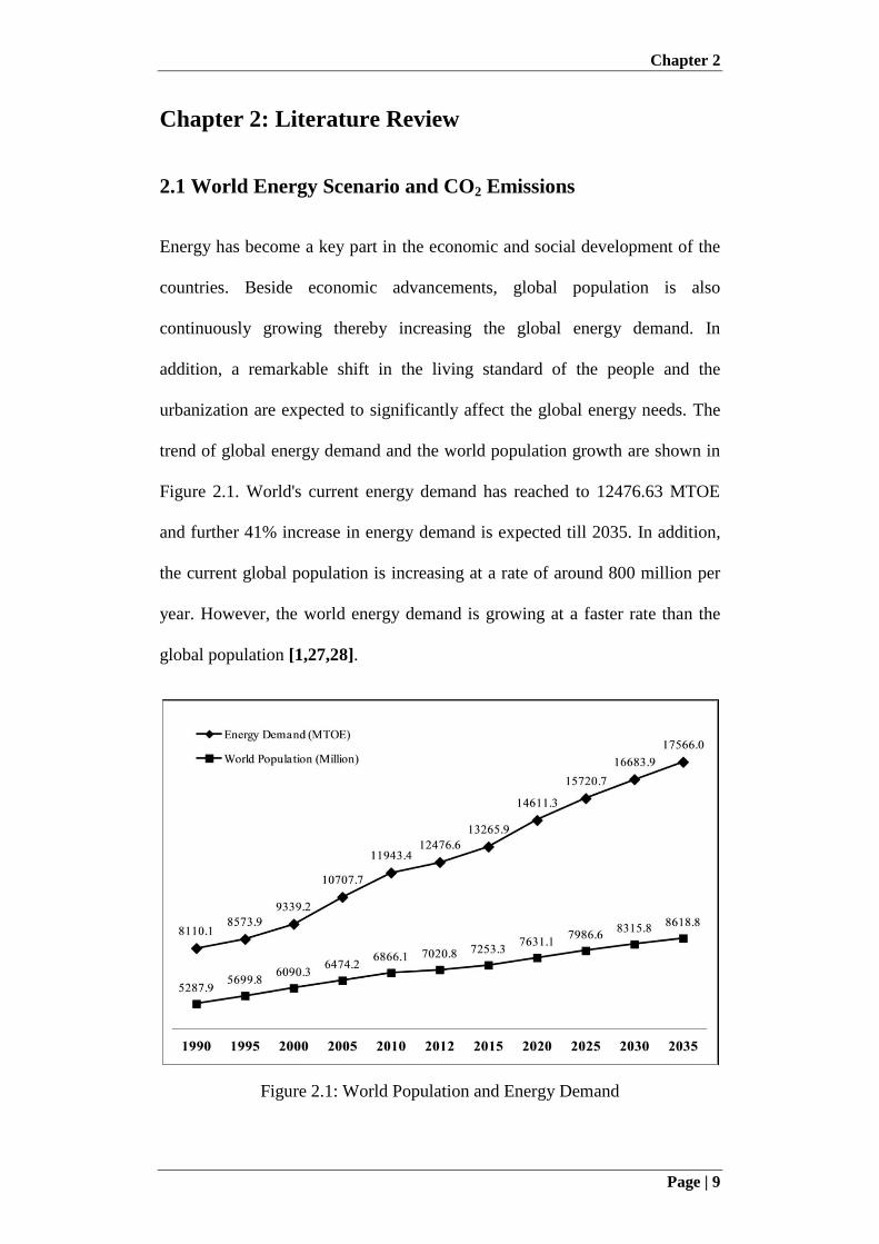
Energy has become a key part in the economic and social development of the

countries. Beside economic advancements, global population is also

continuously growing thereby increasing the global energy demand. In

addition, a remarkable shift in the living standard of the people and the

urbanization are expected to significantly affect the global energy needs. The

trend of global energy demand and the world population growth are shown in

Figure 2.1. World's current energy demand has reached to 12476.63 MTOE

and further 41% increase in energy demand is expected till 2035. In addition,

the current global population is increasing at a rate of around 800 million per

year. However, the world energy demand is growing at a faster rate than the

global population [1,27,28].

Figure 2.1: World Population and Energy Demand

Chapter 2

Page | 10

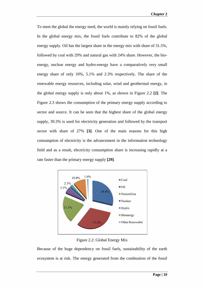
To meet the global the energy need, the world is mainly relying on fossil fuels.

In the global energy mix, the fossil fuels contribute to 82% of the global

energy supply. Oil has the largest share in the energy mix with share of 31.5%,

followed by coal with 29% and natural gas with 24% share. However, the bio-

energy, nuclear energy and hydro-energy have a comparatively very small

energy share of only 10%, 5.1% and 2.3% respectively. The share of the

renewable energy resources, including solar, wind and geothermal energy, in

the global energy supply is only about 1%, as shown in Figure 2.2 [2]. The

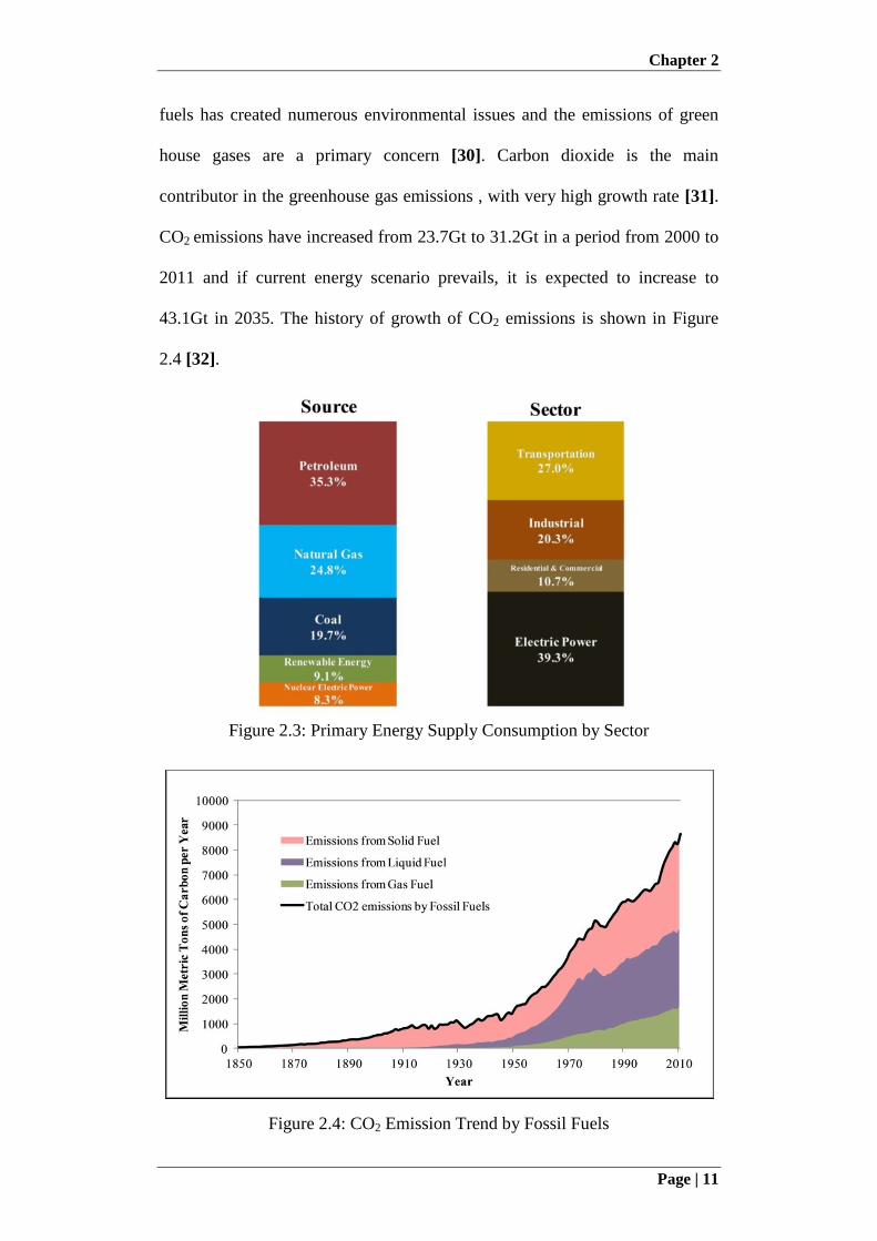
Figure 2.3 shows the consumption of the primary energy supply according to

sector and source. It can be seen that the highest share of the global energy

supply, 39.3% is used for electricity generation and followed by the transport

sector with share of 27% [3]. One of the main reasons for this high

consumption of electricity is the advancement in the information technology

field and as a result, electricity consumption share is increasing rapidly at a

rate faster than the primary energy supply [29].

Figure 2.2: Global Energy Mix

Because of the huge dependency on fossil fuels, sustainability of the earth

ecosystem is at risk. The energy generated from the combustion of the fossil

Chapter 2

Page | 11

fuels has created numerous environmental issues and the emissions of green

house gases are a primary concern [30]. Carbon dioxide is the main

contributor in the greenhouse gas emissions , with very high growth rate [31].

CO2 emissions have increased from 23.7Gt to 31.2Gt in a period from 2000 to

2011 and if current energy scenario prevails, it is expected to increase to

43.1Gt in 2035. The history of growth of CO2 emissions is shown in Figure

2.4 [32].

Figure 2.3: Primary Energy Supply Consumption by Sector

Figure 2.4: CO2 Emission Trend by Fossil Fuels

Chapter 2

Page | 12

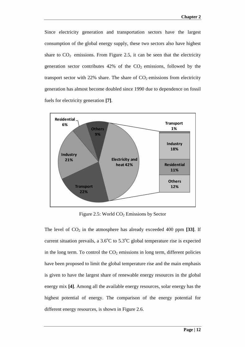
Since electricity generation and transportation sectors have the largest

consumption of the global energy supply, these two sectors also have highest

share to CO2 emissions. From Figure 2.5, it can be seen that the electricity

generation sector contributes 42% of the CO2 emissions, followed by the

transport sector with 22% share. The share of CO2 emissions from electricity

generation has almost become doubled since 1990 due to dependence on fossil

fuels for electricity generation [7].

Figure 2.5: World CO2 Emissions by Sector

The level of CO2 in the atmosphere has already exceeded 400 ppm [33]. If

current situation prevails, a 3.6oC to 5.3

oC global temperature rise is expected

in the long term. To control the CO2 emissions in long term, different policies

have been proposed to limit the global temperature rise and the main emphasis

is given to have the largest share of renewable energy resources in the global

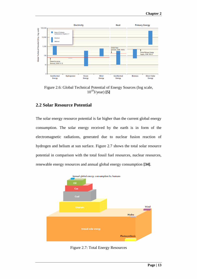
energy mix [4]. Among all the available energy resources, solar energy has the

highest potential of energy. The comparison of the energy potential for

different energy resources, is shown in Figure 2.6.

Chapter 2

Page | 13

Figure 2.6: Global Technical Potential of Energy Sources (log scale,

1018

J/year) [5]

2.2 Solar Resource Potential

The solar energy resource potential is far higher than the current global energy

consumption. The solar energy received by the earth is in form of the

electromagnetic radiations, generated due to nuclear fusion reaction of

hydrogen and helium at sun surface. Figure 2.7 shows the total solar resource

potential in comparison with the total fossil fuel resources, nuclear resources,

renewable energy resources and annual global energy consumption [34].

Figure 2.7: Total Energy Resources

Chapter 2

Page | 14

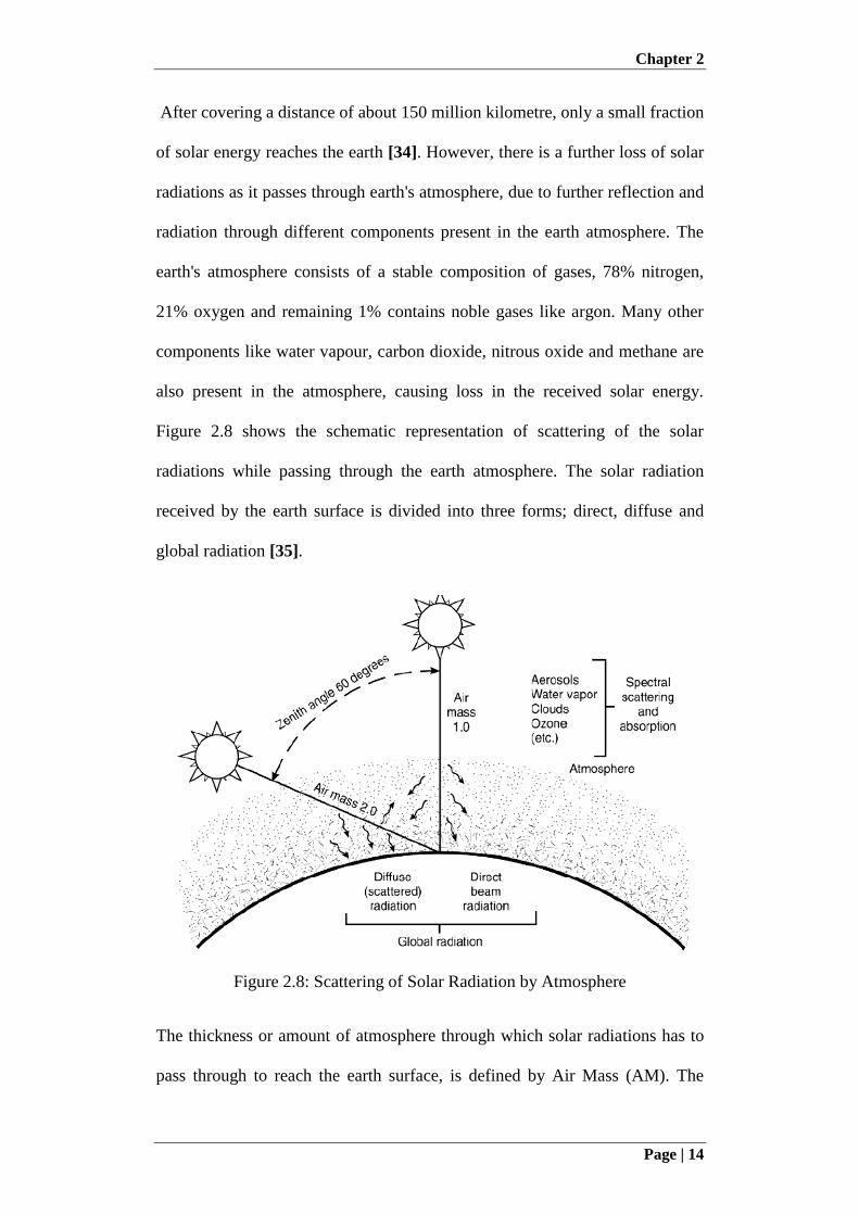
After covering a distance of about 150 million kilometre, only a small fraction

of solar energy reaches the earth [34]. However, there is a further loss of solar

radiations as it passes through earth's atmosphere, due to further reflection and

radiation through different components present in the earth atmosphere. The

earth's atmosphere consists of a stable composition of gases, 78% nitrogen,

21% oxygen and remaining 1% contains noble gases like argon. Many other

components like water vapour, carbon dioxide, nitrous oxide and methane are

also present in the atmosphere, causing loss in the received solar energy.

Figure 2.8 shows the schematic representation of scattering of the solar

radiations while passing through the earth atmosphere. The solar radiation

received by the earth surface is divided into three forms; direct, diffuse and

global radiation [35].

Figure 2.8: Scattering of Solar Radiation by Atmosphere

The thickness or amount of atmosphere through which solar radiations has to

pass through to reach the earth surface, is defined by Air Mass (AM). The

Chapter 2

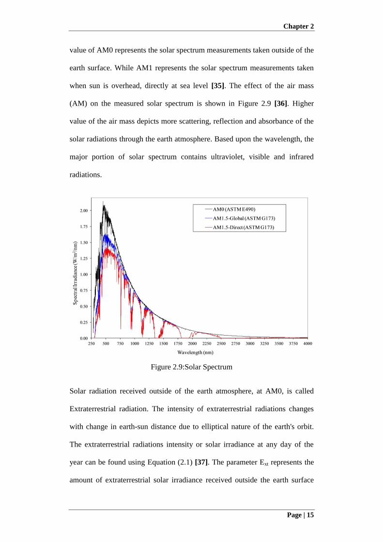
Page | 15

value of AM0 represents the solar spectrum measurements taken outside of the

earth surface. While AM1 represents the solar spectrum measurements taken

when sun is overhead, directly at sea level [35]. The effect of the air mass

(AM) on the measured solar spectrum is shown in Figure 2.9 [36]. Higher

value of the air mass depicts more scattering, reflection and absorbance of the

solar radiations through the earth atmosphere. Based upon the wavelength, the

major portion of solar spectrum contains ultraviolet, visible and infrared

radiations.

Figure 2.9:Solar Spectrum

Solar radiation received outside of the earth atmosphere, at AM0, is called

Extraterrestrial radiation. The intensity of extraterrestrial radiations changes

with change in earth-sun distance due to elliptical nature of the earth's orbit.

The extraterrestrial radiations intensity or solar irradiance at any day of the

year can be found using Equation (2.1) [37]. The parameter Ext represents the

amount of extraterrestrial solar irradiance received outside the earth surface

Chapter 2

Page | 16

and 'n' is the day number starting from 1st of January. The is the solar constant

which is equal to solar irradiance received outside of the earth atmosphere

when distance between earth and sun is 1AU (Astronomical Unit =

149,597,870,700 km). Various scientists have undertaken studies to calculate

the value of the solar constant. NASA and ASTM have accepted solar constant

value of 1353 W/m2 proposed by Thekaekara [38]. However, World

Radiation Centre (WRC) is adopting value of 1357 W/m2

for solar constant.

(2.1)

2.3 Solar Photovoltaic

Solar photovoltaic systems utilize solar cells which convert solar energy

directly into the electricity through photo-reaction. Solar cells are made of

semiconductor material and under the solar radiations, electron-hole pairs are

generated which are separated by the internal electric field around the

junction. In the presence of external load across the solar cell, it can provide

current and voltage through internal electric field. Multiple solar cells can be

easily combined in form of solar modules to generate hundred of watts.

Photovoltaic systems can be used for a wide variety of applications with any

power requirement and with excellent weather resistance. However, one of the

main reason of the huge gap between solar energy potential and its use is the

very low energy conversion efficiencies of most of the commercial

photovoltaic systems.

Based upon the semiconductor material and the manufacturing method, the

solar cell are divided into three generations, as shown in Figure 2.10. First

Chapter 2

Page | 17

generation of the solar cells is based upon silicon wafer based photovoltaic

systems which currently dominate 85% of the photovoltaic market. Single-

crystalline and multi-crystalline wafers, both types of the solar cells are in

commercial use and so far highest efficiencies of 25.6% and 20.4% are

obtained at laboratory scale for single crystalline and multi-crystalline silicone

based solar cells [13]. Second generation solar cells are based upon the

deposits of the thin film of semiconductor material. This manufacturing

technique provides very cost effective photovoltaic systems with reduced cost

per watt of the electrical energy produced, which dominate rest of the

photovoltaic market. However, the conversion efficiency offered by the

second generation photovoltaic systems is lower than the first generation

silicon based solar cells, with highest efficiencies of 20.5% for CIGS and

19.6% for CdTe thin film solar cell at laboratory scale [13].

Currently, most of the research is based upon the third generation solar cells,

to achieve high conversion efficiency while maintaining low cost feature of

the second generation solar cells. Third generation solar cell includes hot

carrier solar cell, multi-junction solar cell, organic polymer-based solar cell,

Gratzel solar cell, multiband and thermo photovoltaic solar cell [14].

However, in this study multi-junction solar cells are considered in form of

concentrated photovoltaic systems for high efficiency power system with low

cost.

2.3.1 Multi-Junction Solar cell (MJC)

The conventional solar cells of both first and second generations are based

upon the single junction of the semiconductor material that responds to only a

Chapter 2

Page | 18

certain portion of the solar spectrum for electricity production, while

remaining portion of solar energy is dissipated as heat. In order to have higher

efficiency, solar cell respond to maximum of the solar spectrum with

minimum lost.

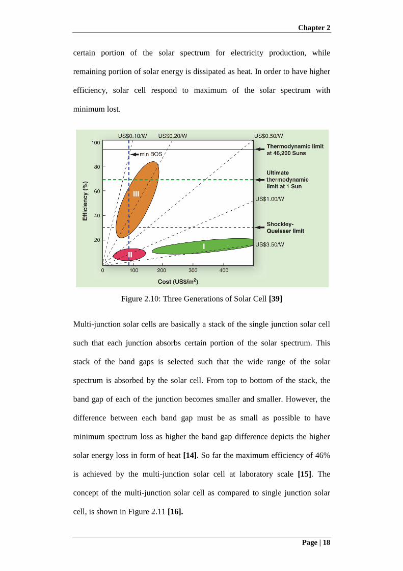
Figure 2.10: Three Generations of Solar Cell [39]

Multi-junction solar cells are basically a stack of the single junction solar cell

such that each junction absorbs certain portion of the solar spectrum. This

stack of the band gaps is selected such that the wide range of the solar

spectrum is absorbed by the solar cell. From top to bottom of the stack, the

band gap of each of the junction becomes smaller and smaller. However, the

difference between each band gap must be as small as possible to have

minimum spectrum loss as higher the band gap difference depicts the higher

solar energy loss in form of heat [14]. So far the maximum efficiency of 46%

is achieved by the multi-junction solar cell at laboratory scale [15]. The

concept of the multi-junction solar cell as compared to single junction solar

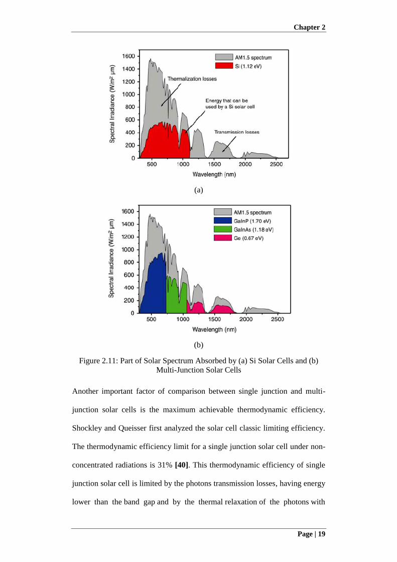
cell, is shown in Figure 2.11 [16].

Chapter 2

Page | 19

(a)

(b)

Figure 2.11: Part of Solar Spectrum Absorbed by (a) Si Solar Cells and (b)

Multi-Junction Solar Cells

Another important factor of comparison between single junction and multi-

junction solar cells is the maximum achievable thermodynamic efficiency.

Shockley and Queisser first analyzed the solar cell classic limiting efficiency.

The thermodynamic efficiency limit for a single junction solar cell under non-

concentrated radiations is 31% [40]. This thermodynamic efficiency of single

junction solar cell is limited by the photons transmission losses, having energy

lower than the band gap and by the thermal relaxation of the photons with

Chapter 2

Page | 20

Figure 2.12: Best Research-Cell Efficiencies

Chapter 2

Page | 21

energy higher than the band gap created carriers. While for the multi-junction

solar cells, this limiting efficiency depends upon the number of the junctions

in the stack. For the four junctions solar cell, the maximum achievable

thermodynamic efficiency limit is 68.5%. However, this limit can be increased

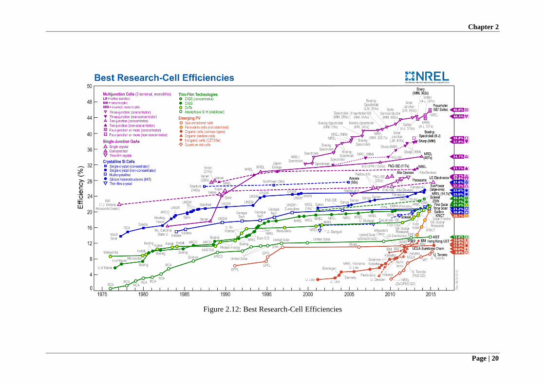
to 81% under concentrated solar radiations of intensity x10,000 [41]. Figure

2.12 shows the chart for the best efficiencies of different solar cell materials

and technologies obtained at laboratory scale and the multi-junction solar cells

can be seen at the top of the chart with highest efficiency among all the solar

cells [42].

2.4 Concentrated Photovoltaic and Two axis Solar Tracker

Besides highest conversion efficiency, the multi-junction solar cells are

expensive to fabricate for large scale applications. In order to make them cost

effective, concentrated photovoltaic concept is used in which low cost solar

concentrators are used to concentrate the sunlight onto a small area of the solar

cell, thereby reducing the use of the expensive semiconductor material [43].

Refractive optics like Fresnel Lens or reflective optics comprising of reflective

mirrors, either flat or curved, are used to concentrate sunlight on the solar cell

to intensity from 200 to 1000 suns; which allows 200 to 1000 times less use of

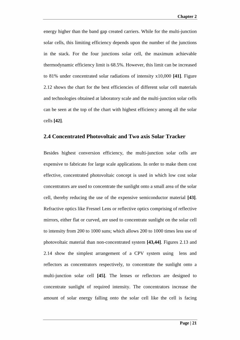
photovoltaic material than non-concentrated system [43,44]. Figures 2.13 and

2.14 show the simplest arrangement of a CPV system using lens and

reflectors as concentrators respectively, to concentrate the sunlight onto a

multi-junction solar cell [45]. The lenses or reflectors are designed to

concentrate sunlight of required intensity. The concentrators increase the

amount of solar energy falling onto the solar cell like the cell is facing

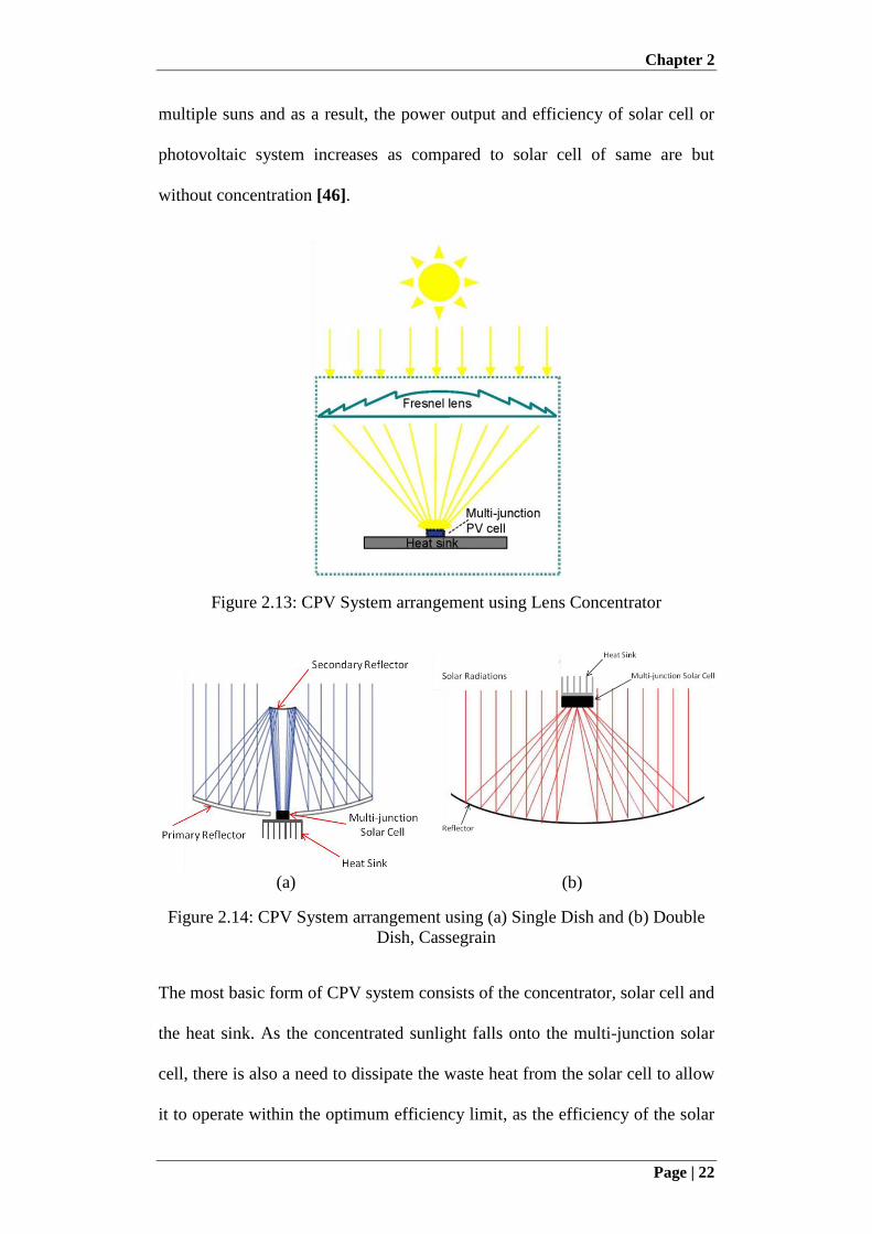
Chapter 2

Page | 22

multiple suns and as a result, the power output and efficiency of solar cell or

photovoltaic system increases as compared to solar cell of same are but

without concentration [46].

Figure 2.13: CPV System arrangement using Lens Concentrator

(a) (b)

Figure 2.14: CPV System arrangement using (a) Single Dish and (b) Double

Dish, Cassegrain

The most basic form of CPV system consists of the concentrator, solar cell and

the heat sink. As the concentrated sunlight falls onto the multi-junction solar

cell, there is also a need to dissipate the waste heat from the solar cell to allow

it to operate within the optimum efficiency limit, as the efficiency of the solar

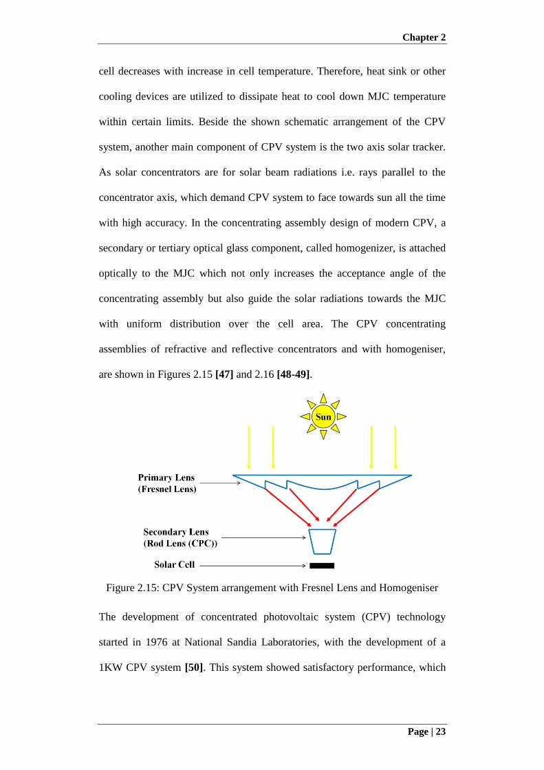
Chapter 2

Page | 23

cell decreases with increase in cell temperature. Therefore, heat sink or other

cooling devices are utilized to dissipate heat to cool down MJC temperature

within certain limits. Beside the shown schematic arrangement of the CPV

system, another main component of CPV system is the two axis solar tracker.

As solar concentrators are for solar beam radiations i.e. rays parallel to the

concentrator axis, which demand CPV system to face towards sun all the time

with high accuracy. In the concentrating assembly design of modern CPV, a

secondary or tertiary optical glass component, called homogenizer, is attached

optically to the MJC which not only increases the acceptance angle of the

concentrating assembly but also guide the solar radiations towards the MJC

with uniform distribution over the cell area. The CPV concentrating

assemblies of refractive and reflective concentrators and with homogeniser,

are shown in Figures 2.15 [47] and 2.16 [48-49].

Figure 2.15: CPV System arrangement with Fresnel Lens and Homogeniser

The development of concentrated photovoltaic system (CPV) technology

started in 1976 at National Sandia Laboratories, with the development of a

1KW CPV system [50]. This system showed satisfactory performance, which

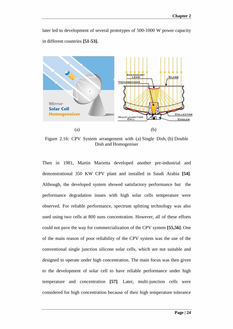
Chapter 2

Page | 24

later led to development of several prototypes of 500-1000 W power capacity

in different countries [51-53].

(a) (b)

Figure 2.16: CPV System arrangement with (a) Single Dish, (b) Double

Dish and Homogeniser

Then in 1981, Martin Marietta developed another pre-industrial and

demonstrational 350 KW CPV plant and installed in Saudi Arabia [54].

Although, the developed system showed satisfactory performance but the

performance degradation issues with high solar cells temperature were

observed. For reliable performance, spectrum splitting technology was also

used using two cells at 800 suns concentration. However, all of these efforts

could not pave the way for commercialization of the CPV system [55,56]. One

of the main reason of poor reliability of the CPV system was the use of the

conventional single junction silicone solar cells, which are not suitable and

designed to operate under high concentration. The main focus was then given

to the development of solar cell to have reliable performance under high

temperature and concentration [57]. Later, multi-junction cells were

considered for high concentration because of their high temperature tolerance

Chapter 2

Page | 25

and response to broader spectrum of solar radiations that resulted in to achieve

higher efficiency and field reliability.

With the reliable and mature solar cell development, now the main focus is on

the development of concentrating assembly and overall system design.

Initially, large reflective concentrating dishes were used for the CPV system

[58,59]. Some CPV systems were also developed for linear concentration

using parabolic trough and linear Fresnel lens, instead of point concentration

[60,61]. In addition, some researchers also proposed the design of the CPV

field using multiple flat reflectors focussing at single common receiver of the

solar cell [62-66]. The first concern with these initial designs of CPV systems

is the use of large reflective concentrators, which are difficulty to

manufacture. Secondly, because of high heat flux at the cell areas and larger

size of the solar cell, the heat rejection from the cell becomes another issue,

which requires liquid based active cooling to keep MJC temperature within

efficient operating limit. To reduce the manufacturing cost and cooling issues,

CPV systems were then developed with relatively small size of refractive

concentrators i.e. Fresnel lenses [67,68]. As mentioned before, concentrators

are designed for parallel or beam radiations, so they are always pointed

towards the sun by using two axis solar tracker. For the CPV system, tracking

is very important, If the solar radiations are not properly focussed then the

power output drops to zero. Although for non-concentrating PV, the solar

tracker can increase the power output of the system. However, for CPV

system, it is the essential part, which also consumes the power. Some designs

of the concentrating assembly were developed then to reduce the tracking

requirements with acceptance angle of concentrating assemblies ±5o and 80-

Chapter 2

Page | 26

85% optical efficiency [69]. Lens-based concentrators mostly have higher

focal length to accommodate homogeniser or secondary optics. This overall

height of the lens based CPV system increases the instability and the shipping

cost of the system. Different designs of the homogenises and concentrators are

also developed to reduce the overall concentrator height and the acceptance

angle [70-72]. Due to advantages of mini lens based concentrators designs,

there is also a CPV design developed based upon the miniaturization of the

dish concentrators with secondary reflector as a flat mirror to reduce the

overall height of concentrator assembly [73]. However, all of these studies and

designs finally led to the current commercial CPV system designs, which are

based upon the single stage concentration using small Fresnel lenses and the

double stage concentration using mini parabolic and hyperbolic reflectors in

the cassegrain arrangement [74-76]. So far, all of the CPV concentrating

assemblies are designed with a dedicated concentrator for each of the solar

cell, which requires a large number of concentrators in case of the mini-

concentrator CPV system design . Thus, there is a need to reduce the number

of mini dishes, with concentrating assembly that can concentrate solar

radiations onto multiple solar cells with single set of concentrator without

increasing the cell size and temperature issues, as proposed in this thesis.

Beside concentrating assembly, one of the most important concern related to

these CPV systems is that they are designed as big units with too many CPV

modules installed on a large two axis solar tracker, which are only suitable to

be installed in open desert like regions with high DNI availability [77]. The

CPV appeared to be some of those technologies that few people bought, with

less market and customers. It must be noted that the rooftop installations of

Chapter 2

Page | 27

conventional flat plate PV make a significant share of the total PV installed

capacity. For most the countries, the rooftop PV installation on commercial

and residential buildings, is aimed to contribute to 40-50% of the total PV

installations [19]. On the other side, the commercial CPV systems are not so

far designed to be installed on the rooftop, which gives motivation for the

development of our new CPV field design based upon the master and slave

configuration of the compact, smart, small and highly accurate two axis solar

trackers which can be easily installed on the rooftop. As the trackers are

proposed to be small and compact, large number of trackers will be required.

However, with the proposed master and slave configuration, minimum

hardware will be required by the slave trackers as they will receive required

tracking information from the master tracker. The expensive sensors and

devices will be supplied to the master tracker which will further distribute the

information to the slave trackers. It is also worthy to mention here that the

solar trackers required for the CPV system are different than the PV systems,

as CPV need very high accuracy. The high accuracy of the tracking is ensure

through hybrid tracking technique, utilizing optical tracking sensor. Most of

the optical sensors developed for the solar tracking systems, does not offer

tracking according to the required accuracy of the CPV. These sensors use

classical approach of the shadow, tilt surface and the collimating tube, with an

array of the photo-sensors. From the closed control loop and the comparison

of the output signal of the photo-sensors, the position of the sun is determined.

Due to requirement of the large shadow device or collimating tube for high

accuracy, these conventional sensors are not suitable for the CPV applications

[78]. However, the optical tracking sensor based upon the position sensitive

Chapter 2

Page | 28

diode (PSD) is used for most of the current commercial large CPV trackers

[79,80]. However, these PSD based tracking sensors are not suitable for the

small systems due to their high cost for many small tracking units. Therefore,

a cheap but highly accurate optical tracking sensor is also needed for proposed

cheap CPV tracking system.

It is a conception that highly efficient CPV systems are suitable for desert

regions with high DNI availability as the CPV systems only respond to beam

radiations (DNI). That is why big units of CPV systems are designed for desert

regions [77]. However, conventional PV system can operate in beam and

diffuse radiations but with lower efficiency. Ultimately, the consumer is

interested in true total long-term power produced by the photovoltaic system.

Therefore, a methodology is also needed that can rate the system based upon

its long-term power output, instead of the maximum conversion efficiency. In

this thesis, an electrical rating methodology is also proposed and the

developed CPV systems performance is evaluated for long-term operation and

compared with the conventional PV systems, installed in the tropical weather

of the Singapore. This study will also help to analyze the CPV system

performance in low DNI regions, which may help to remove the conception

that CPV systems are only suitable in desert regions.

2.5 Hydrogen Energy Storage

Owing to the alarming level of the green-house gas emissions and their drastic

effect on the global environment, renewable energy resources are proved to be

viable option under current global warming condition. Most of the renewable

energy resources are proved to have the potential more than the global energy

Chapter 2

Page | 29

demand. The major global energy need is in form of electrical energy and the

main attractiveness of most of the popular renewable energy systems,

especially solar, wind and hydro energy, is that the electricity can be produced

easily through simple system configuration using these renewable energy

resources. However, one of the core requirement of the electricity or power

production system is the continuous supply of the electricity to the consumer

without any interruption. The availability and the potential of all of the above

mentioned renewable energy systems, varies largely from region to region

especially for wind and hydro energy. However, solar energy is easily

available and accessible around most of the regions and the photovoltaic

system provides simplest way for electricity production directly from the solar

energy [7-9]. As discussed before, solar energy has the highest energy

potential among all energy resources and it can alone supply 10,000 times

more energy than current global energy demand [5,6]. Like many other

renewable energy systems [20], solar energy is not available all the time and at

a constant rate. Beside higher energy potential, in order to be proved to be a

practical power production system, a steady supply of the power at a constant

rate is required [21]. Solar energy is only available during diurnal period but

not all the time and at constant rate due to cloud cover and weather changes.

Moreover, the continuous motion of the sun also results in the variable solar

intensity during different periods of time in a day, due to changing Air Mass

(AM). Therefore, due to intermittent nature of the solar energy, an energy

storage system is needed such that the energy during the time of excess power

production is stored and then supplied back to the system during the time of

low or no power production.

Chapter 2

Page | 30

The common energy storage method employed for most of the photovoltaic

systems, is the electrochemical storage using batteries. The battery bank

provides convenient energy storage option for the systems with small capacity

and short-term energy storage requirements due to convenience in charging

and discharging and high round trip efficiency [81-83]. For most of the solar

energy systems, the design is based upon the long term operation of 20-25

years lifetime period [25]. For long term storage, the batteries do not provide

technically and economically feasible option especially for medium to large

capacity systems [26], due to their self-discharging, low energy density and

the leakage problems. Some other energy storage techniques of compressed

air, pumped hydro, thermal storage and super-capacitors also provide the

storage for the short term operation of only few day, hours or seconds [84].

Moreover, the application of these energy storage techniques is also not

proved to be reliable especially for photovoltaic systems. Therefore, for the

utilization of intermittent energy resources like solar energy, hydrogen

production provides reliable and most-suitable energy storage option for

medium to long term storage.

Hydrogen is considered as the promising alternate fuel of the future due to its

sustainable nature and capability to store high quality energy; electricity from

the fuel cell or heat from the direct combustion. Beside energy storage,

hydrogen can also be used as energy carrier in form of the independent energy

source as it can be easily transmitted anywhere with convenience [85]. In this

scenario, hydrogen is believed to be considered as feasible option for

sustainable and reliable operation of the energy systems. There are many

methods for the production of the hydrogen using solar energy in form of

Chapter 2

Page | 31

thermal energy, electrical energy, bio-energy and photon energy. Different

process are developed for the production of hydrogen from above mentioned

energy types [86]. However, the cheapest and widely used method for

production of hydrogen for industrial need is the steam reforming of the fossil

fuels especially methane or natural gas, followed by the oil and coal as

hydrogen is one of the main constituent of the fossil fuels. This method

contributes to the 96% of the total global hydrogen production [87]. Beside the

production of hydrogen, greenhouse gases like CO and CO2 are also produced

through steam reforming of fossil fuels thereby making it not suitable option

to be used for sustainable energy system. Another popular and simple process,

that shares remaining 4% of the total global hydrogen production, is the

electrolysis of water that uses electricity to split the water molecules for

generation of hydrogen, with oxygen as by-product [88]. However,

electrolysis provides viable and sustainable option for the production of

hydrogen if the electricity is generated through renewable energy resources

and the photovoltaic systems provide simple and convenient production of the

electricity directly from the solar energy.

2.5.1 Water Electrolysis Theory

Water electrolysis is a simplest and popular process to split up the water

molecule to produce hydrogen and oxygen. The main component of the

electrolysis unit is the electrochemical cell, called as the electrolyser, as shown

in Figure 2.17. In electrolyser, electrodes are separated by the electrolyte

either liquid based or solid based, and connected to the external electrical

power source. When a voltage higher than a certain minimum value is applied

across the electrodes, the electrolysis process starts and hydrogen starts

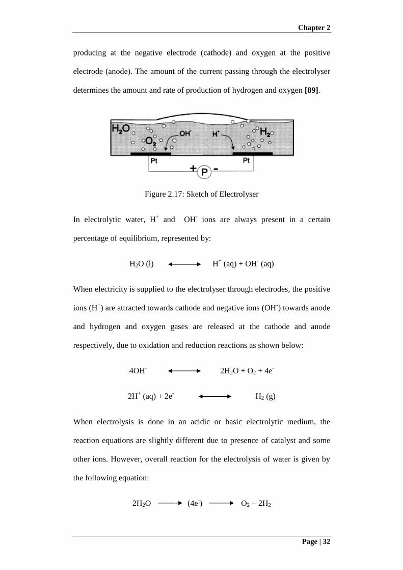
Chapter 2

Page | 32

producing at the negative electrode (cathode) and oxygen at the positive

electrode (anode). The amount of the current passing through the electrolyser

determines the amount and rate of production of hydrogen and oxygen [89].

Figure 2.17: Sketch of Electrolyser

In electrolytic water, H+ and OH

- ions are always present in a certain

percentage of equilibrium, represented by:

H2O (l) H+ (aq) + OH

- (aq)

When electricity is supplied to the electrolyser through electrodes, the positive

ions (H+) are attracted towards cathode and negative ions (OH

-) towards anode

and hydrogen and oxygen gases are released at the cathode and anode

respectively, due to oxidation and reduction reactions as shown below:

4OH- 2H2O + O2 + 4e

-

2H+ (aq) + 2e

- H2 (g)

When electrolysis is done in an acidic or basic electrolytic medium, the

reaction equations are slightly different due to presence of catalyst and some

other ions. However, overall reaction for the electrolysis of water is given by

the following equation:

2H2O (4e-) O2 + 2H2

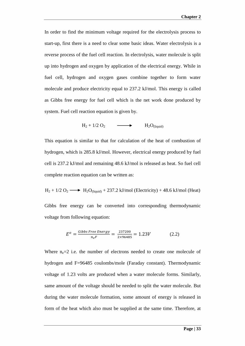
Chapter 2

Page | 33

In order to find the minimum voltage required for the electrolysis process to

start-up, first there is a need to clear some basic ideas. Water electrolysis is a

reverse process of the fuel cell reaction. In electrolysis, water molecule is split

up into hydrogen and oxygen by application of the electrical energy. While in

fuel cell, hydrogen and oxygen gases combine together to form water

molecule and produce electricity equal to 237.2 kJ/mol. This energy is called

as Gibbs free energy for fuel cell which is the net work done produced by

system. Fuel cell reaction equation is given by.

H2 + 1/2 O2 H2O(liquid)

This equation is similar to that for calculation of the heat of combustion of

hydrogen, which is 285.8 kJ/mol. However, electrical energy produced by fuel

cell is 237.2 kJ/mol and remaining 48.6 kJ/mol is released as heat. So fuel cell

complete reaction equation can be written as:

H2 + 1/2 O2 H2O(liquid) + 237.2 kJ/mol (Electricity) + 48.6 kJ/mol (Heat)

Gibbs free energy can be converted into corresponding thermodynamic

voltage from following equation:

(2.2)

Where ne=2 i.e. the number of electrons needed to create one molecule of

hydrogen and F=96485 coulombs/mole (Faraday constant). Thermodynamic

voltage of 1.23 volts are produced when a water molecule forms. Similarly,

same amount of the voltage should be needed to split the water molecule. But

during the water molecule formation, some amount of energy is released in

form of the heat which also must be supplied at the same time. Therefore, at

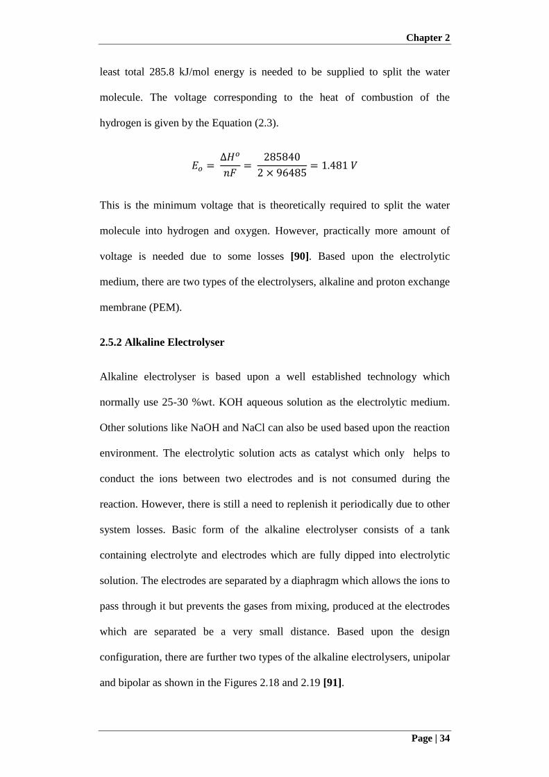
Chapter 2

Page | 34

least total 285.8 kJ/mol energy is needed to be supplied to split the water

molecule. The voltage corresponding to the heat of combustion of the

hydrogen is given by the Equation (2.3).

This is the minimum voltage that is theoretically required to split the water

molecule into hydrogen and oxygen. However, practically more amount of

voltage is needed due to some losses [90]. Based upon the electrolytic

medium, there are two types of the electrolysers, alkaline and proton exchange

membrane (PEM).

2.5.2 Alkaline Electrolyser

Alkaline electrolyser is based upon a well established technology which

normally use 25-30 %wt. KOH aqueous solution as the electrolytic medium.

Other solutions like NaOH and NaCl can also be used based upon the reaction

environment. The electrolytic solution acts as catalyst which only helps to

conduct the ions between two electrodes and is not consumed during the

reaction. However, there is still a need to replenish it periodically due to other

system losses. Basic form of the alkaline electrolyser consists of a tank

containing electrolyte and electrodes which are fully dipped into electrolytic

solution. The electrodes are separated by a diaphragm which allows the ions to

pass through it but prevents the gases from mixing, produced at the electrodes

which are separated be a very small distance. Based upon the design

configuration, there are further two types of the alkaline electrolysers, unipolar

and bipolar as shown in the Figures 2.18 and 2.19 [91].

Chapter 2

Page | 35

Figure 2.18: Unipolar Electrolyser

Figure 2.19: Bipolar Electrolyser

Each of the design configurations has its own significance. Unipolar

electrolyser design requires very few parts with simple construction and easy

maintenance as each the electrode pair is working independently and

electrodes can be easily replaced while the others are still in operation. Bipolar

design consists of alternate layers of the electrodes with diaphragm for the

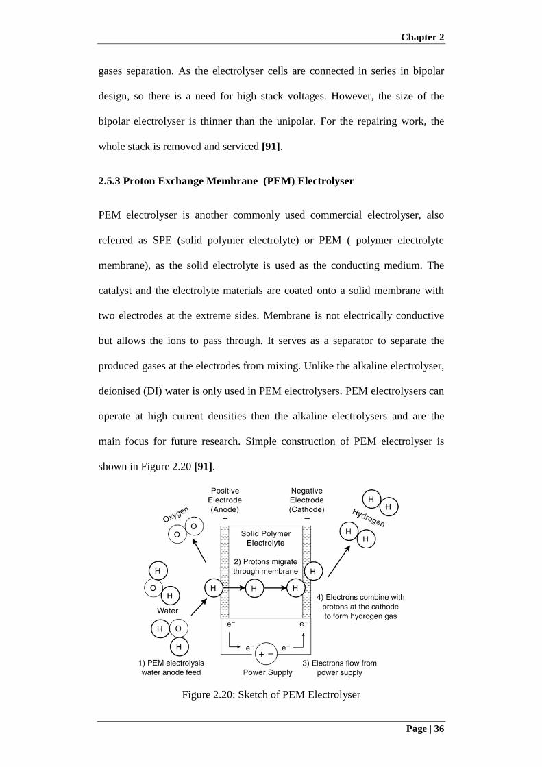
Chapter 2

Page | 36

gases separation. As the electrolyser cells are connected in series in bipolar

design, so there is a need for high stack voltages. However, the size of the

bipolar electrolyser is thinner than the unipolar. For the repairing work, the

whole stack is removed and serviced [91].

2.5.3 Proton Exchange Membrane (PEM) Electrolyser

PEM electrolyser is another commonly used commercial electrolyser, also

referred as SPE (solid polymer electrolyte) or PEM ( polymer electrolyte

membrane), as the solid electrolyte is used as the conducting medium. The

catalyst and the electrolyte materials are coated onto a solid membrane with

two electrodes at the extreme sides. Membrane is not electrically conductive

but allows the ions to pass through. It serves as a separator to separate the

produced gases at the electrodes from mixing. Unlike the alkaline electrolyser,

deionised (DI) water is only used in PEM electrolysers. PEM electrolysers can

operate at high current densities then the alkaline electrolysers and are the

main focus for future research. Simple construction of PEM electrolyser is

shown in Figure 2.20 [91].

Figure 2.20: Sketch of PEM Electrolyser

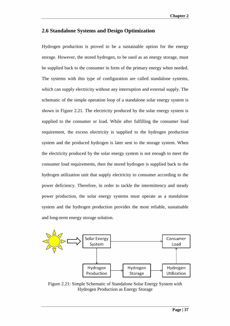
Chapter 2

Page | 37

2.6 Standalone Systems and Design Optimization

Hydrogen production is proved to be a sustainable option for the energy

storage. However, the stored hydrogen, to be used as an energy storage, must

be supplied back to the consumer in form of the primary energy when needed.

The systems with this type of configuration are called standalone systems,

which can supply electricity without any interruption and external supply. The

schematic of the simple operation loop of a standalone solar energy system is

shown in Figure 2.21. The electricity produced by the solar energy system is

supplied to the consumer or load. While after fulfilling the consumer load

requirement, the excess electricity is supplied to the hydrogen production

system and the produced hydrogen is later sent to the storage system. When

the electricity produced by the solar energy system is not enough to meet the

consumer load requirements, then the stored hydrogen is supplied back to the

hydrogen utilization unit that supply electricity to consumer according to the

power deficiency. Therefore, in order to tackle the intermittency and steady

power production, the solar energy systems must operate as a standalone

system and the hydrogen production provides the most reliable, sustainable

and long-term energy storage solution.

Figure 2.21: Simple Schematic of Standalone Solar Energy System with

Hydrogen Production as Energy Storage

Chapter 2

Page | 38

As the solar energy system provides electricity to the consumer, so the

hydrogen production system in the shown schematic of standalone system is

the electrolyser that converts water into hydrogen and oxygen. Similarly, the

energy from the storage is also needed in form of the electricity. Therefore, the

hydrogen utilization system is based upon the fuel cell that converts stored

hydrogen and oxygen into electricity with water production as by-product.

Another important aspect of standalone energy systems is the storage of

hydrogen. The most common methods of hydrogen storage are liquefaction of

hydrogen, high pressure compression storage, adsorption storage and metal

hydride storage [92]. Among all the storage techniques, the compression

storage of the hydrogen at high pressure provides simple and the convenient

option such that hydrogen is readily available without any pre-processing [93].

The only concern raised for the compressed hydrogen storage is the

volumetric capacity [94] at conventional storage pressure of 200-350 bar.

However, the volume is not considered as the constraint for standalone system

especially based upon solar energy. Beside volumetric capacity, another very

important factor that is needed to be considered is the storage capacity

(Gravimetric Capacity) corresponding to the overall mass and size of the

system. The volumetric capacity can be increased to competent level if storage

pressure is increased to 700 bar, but the gravimetric capacity may slightly

reduce [95]. The volumetric capacity can be increased through liquefaction of

the hydrogen. However, due to very low temperature requirement, this method

is not very efficient and boiling of the hydrogen (above 20K) is also another

issue [96]. The adsorption and metal hydride storage techniques provide high

volumetric capacity and solution related to the high pressure storage problems.

Chapter 2

Page | 39

In comparison, the adsorption storage technique offers comparatively low

gravimetric capacity than the metal hydrides [97]. Although the metal

hydrides offer storage at low pressure, but the main issue is also the

gravimetric density offered by them. At very low pressure and temperature,

metal hydrides offer very low gravimetric capacity of about 1% or less, which

can be increased to 2.5-3% at pressure of 350bar [98]. This means, in order to

have storage of 50kg of hydrogen, 2000-2500 kg of storage material is needed

for gravimetric capacity of 2-2.5%. In the literature, very high gravimetric

capacity of above 10% is reported for metal hydrides [99,100], but at very

high pressure and temperature. However, this demands extra work of

compression and extra thermal energy input, along with the big and complex

configuration of the system with regeneration requirement. Therefore, the

compressed hydrogen storage at high pressure in the storage tanks provides

the simple, most convenient and reliable long-term energy storage option.

The main aspect of the standalone energy system development is the design

optimization, which includes the size optimization of each of the component

of the standalone system along with energy management and control

strategies. The system size is optimized such that it has enough capability to

fulfil the energy requirements of the consumer load along with the enough

energy storage to handle the power interruptions for long-term operation. The

system performance is simulated based upon the long term weather data to

optimize the system size for uninterrupted power with enough energy storage

to meet the load requirements. There are many studies in the literature

regarding the standalone energy system optimization with hydrogen

production, based upon the size [101], techno-economic optimization with

Chapter 2

Page | 40

optimum efficiency and control strategy of each of component of the system

[102,103]. In order to handle small power ripples with better system

management and control, PV-hydrogen system was hybridized. The purpose

of the techno-economic optimization is to get the optimum system size while

keeping the overall system cost minimum. However, the cost and the size of

the system can be reduced by capturing most of the available renewable

energy and converting into electricity. In the literature, all of the studies are

based upon the photovoltaic systems considering the conventional PV system,

which offers very low energy conversion efficiency. Many researchers have

considered to adopt the hybridized system of PV and wind turbine with

hydrogen production [104-106] or along with the small capacity battery

storage [107-109] to reduce the overall system cost and the size of the system.

Some authors also proposed and analyzed the PV system in hybridization with

the diesel generator system to significantly reduce the overall system cost and

the energy storage [110,111], but the main concern of green house gas

emission is still there. Despite of highest solar energy conversion efficiency,

the literature is lacking for study related to standalone system with CPV which

can reduce the overall size of the system. In this thesis, the optimization

algorithm and energy management technique for standalone operation of CPV

are also developed with hydrogen production as energy storage.

Therefore, based upon the literature, it is found that a compact and cheap

design of the CPV is needed with the development of complete theoretical and

experimental framework for consideration of CPV as reliable steady power

system or stand alone system, for which hydrogen production provides

sustainable energy storage option.

Chapter 3

Page | 41

Chapter 3: Development of Two Axis Solar Tracker

with Master Slave Configuration for CPV Field

3.1 Introduction

The two-axis solar tracker is one of the key components of a concentrating

photovoltaic (CPV) system. The solar concentrators can only respond to solar

beam radiations and that is why CPV systems need two axis solar tracking

system to face towards the sun during their operation. Therefore, the

performance of the CPV system, to some extent, is dependent on the accuracy

and precision of the solar tracking system as very high tracking accuracy is

required for CPV system operation and poor or inaccurate solar tracking may

lead to 100% power loss.

Most of the commercial CPV units are available in large size with

corresponding larger tracking units, designed for open fields in desert areas

but not suitable for urban or residential areas or rooftops of residential

buildings, unlike conventional PV systems. In this chapter, a novel master and

slave configuration of the CPV field tracking system is proposed with small,

compact and smart but cheap two-axis hybrid solar trackers, which are

designed, developed and experimentally tested. The developed two-axis solar

tracker is based upon the hybrid tracking algorithm, utilizing both active and

passive tracking methods. By following the passive technique as main

tracking algorithm, the tracking accuracy is ensured through active tracking

algorithm. The passive tracking follows predefined solar geometry and active

tracking utilizes photo-sensors for solar position feedback. Due to expensive

Chapter 3

Page | 42

design of conventional solar feedback sensor, a novel and cheap but highly

accurate solar feedback sensor design is also discussed in this chapter with

tracking accuracy of ±0.1o. In addition, a microcontroller based tracker control

box is developed for tracker operation and is tested for long term operation.

For tracking system of CPV field, the overall tracking algorithm is based upon

master slave control in which all the slave trackers receive tracking

information from master tracker thereby eliminating the need of expensive

modules for each tracker. The tracking code is developed using C-

programming language such that the solar tracker can operate at any location

by using coordinates obtained through GPS module.

3.2 Development of Solar Tracking Technique

The two-axis solar tracker is developed based upon hybrid algorithm of

passive and active tracking techniques as each tracking technique has certain

limitations and if relied only on one method, accurate solar tracking is difficult

to achieve. Passive tracking, also called as astronomical tracking, follows the

predefined solar movement path using solar geometry equations and the

tracker is rotated according to calculated solar angles, defined from certain

reference point. However, the mechanical driving assemblies are prone to

backlash or wear and tear, which can cause tracking error as

passive/astronomical tracking works on open loop, without any feedback. In

order to ensure the accurate tracking, the feedback is necessary.

The active tracking, also called as optical tracking, uses photo-sensors and the

solar position is determined according to feedback from photo-sensors.

However, in case of cloud cover, the optical tracking doesn't work as there is

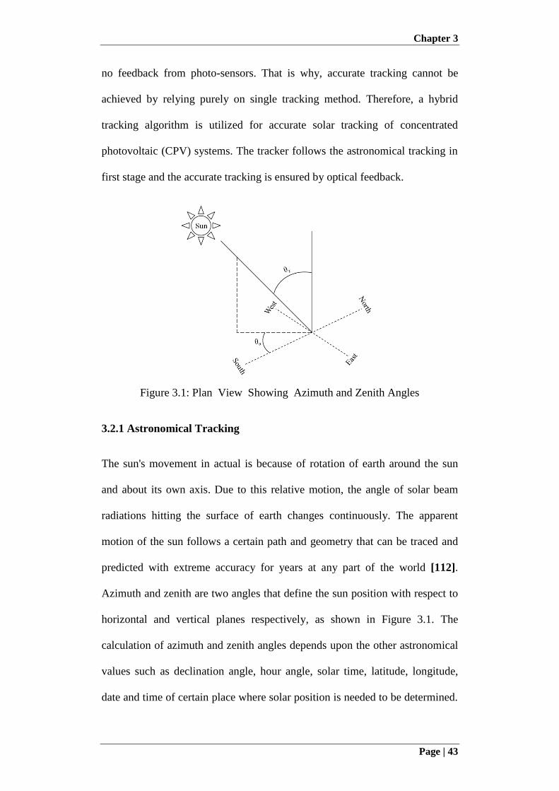
Chapter 3

Page | 43

no feedback from photo-sensors. That is why, accurate tracking cannot be

achieved by relying purely on single tracking method. Therefore, a hybrid

tracking algorithm is utilized for accurate solar tracking of concentrated

photovoltaic (CPV) systems. The tracker follows the astronomical tracking in

first stage and the accurate tracking is ensured by optical feedback.

Figure 3.1: Plan View Showing Azimuth and Zenith Angles

3.2.1 Astronomical Tracking

The sun's movement in actual is because of rotation of earth around the sun

and about its own axis. Due to this relative motion, the angle of solar beam

radiations hitting the surface of earth changes continuously. The apparent

motion of the sun follows a certain path and geometry that can be traced and

predicted with extreme accuracy for years at any part of the world [112].

Azimuth and zenith are two angles that define the sun position with respect to

horizontal and vertical planes respectively, as shown in Figure 3.1. The

calculation of azimuth and zenith angles depends upon the other astronomical

values such as declination angle, hour angle, solar time, latitude, longitude,

date and time of certain place where solar position is needed to be determined.

Chapter 3

Page | 44

Solar time is like 24-hour clock where 12:00 is called as solar noon when sun

is at the meridian of the observer. The solar time is different from local time

and depends upon the longitude of local position. Therefore, the conversion of

local time into solar time is of high importance and needs two corrections.

First correction is based upon a constant depending upon the longitude

difference of the standard meridian, at which local time is based, and the

meridian of observer. For Singapore, local time is based upon GMT+8. As it

takes 1 hour for sun to rotate 15o

(4 min/degree), so longitude for standard

meridian is 120o. Second correction for the solar time is based upon the

difference between mean solar time, which is average solar time because of

elliptical earth's orbit and apparent solar time or real solar time, and is given

by error of time (EOT) equation. The relation between solar time and local

time (in minutes) is given by Equation (3.1).

EOTLL Time Local Time Solar locst )(4 (3.1)

Wherre Lst is standard longitude of local time zone and Lloc is longitude of

local observer position. However, reference for longitudes is west in degrees.

Error of time (EOT) in minutes is given by Equation (3.2).

BB

BBEOT

2sin04089.02cos14615.0

sin032077.0cos001868.0000075.0(2.229

(3.2)

where factor B depends upon the corresponding day of the year:

365

360)1(

nB (3.3)

The angular displacement of the sun with respect to local meridian east or

west due to rotation of earth, is given by hour-angle (ω) in Equation (3.4).

Chapter 3

Page | 45

There is change of 15o/hour in hour-angle. At solar noon or at the lowest value

of zenith angle, the hour angle is zero and is considered negative before solar

noon and positive after solar noon.

)12(24

360

time Solar (3.4)

At solar noon, the angular position of sun with respect to equator is defined by

declination angle (δ) and depends upon factor B, given by Equation (3.5) [37].

BBB

BBB

3sin00148.03cos002679.02sin000907.0

2cos006758.0sin070257.0cos399912.0006918.0

(3.5)

Now, the zenith angle, which is the angle between the direction of solar

radiations and the vertical of local observer, is given by Equation (3.6). During

day time, the zenith angle varies from 0o to 90

o. For a zenith angle greater than

80o, there is a difference of 0.834

o in the apparent position of the sun due to

refraction of solar rays through atmosphere. However, for engineering

application, this difference can be neglected for low latitudes.

coscoscossinsincos z (3.6)

Where ϕ is latitude of local position. The other tracking angle needed to

describe solar position is the azimuth angle, which can be found using

Equations (3.7) or (3.8) depending upon the hour angle.

If ω>0,

cos)90cos(

sin)90sin(sin90360cos

z

zaz (3.7)

Chapter 3

Page | 46

If ω<0,

cos)90cos(

sin)90sin(sin90cos

z

zaz

(3.7)

Where the value '90' is to change the reference plane from north to south.

Another important parameter in solar tracking is the time at which the tracker

must start or stop solar operation and it should be the sunrise and sunset

timings at that particular location, given by Equations (3.9A) and (3.9B) [113].

622.6)06571.0( SRSR tT (3.9A)

622.6)06571.0( SSSS tT (3.9B)

Where α is the sun right ascension and the values of factors tSR and tSS are

given by the Equations (3.10) and (3.11) for sunrise and sunset respectively.

24

)6( )(Hloc

SR

Lnt (3.10)

24

)18( )(Hloc

SS

Lnt (3.11)

The Lloc(H) is the local longitude considered in the form of hours (15o=1 hour).

The significance of the above mentioned tracking method is that it can be

easily applied with high accuracy and simple programming. However, care

must be taken during initialization from reference planes. As explained before,

due to backlash problems of the mechanical assembly, tracking error can occur

for astronomical tracking, which can be corrected through active or optical

tracking method, as explained in the next section.

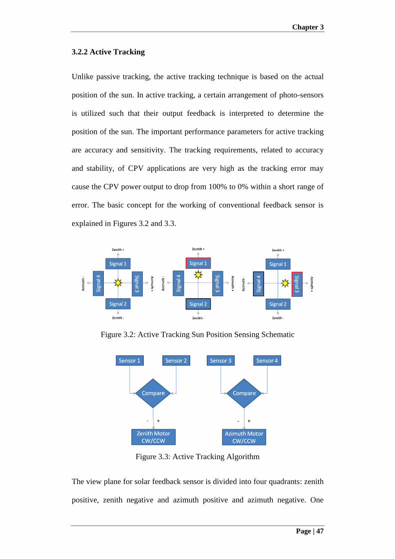
Chapter 3

Page | 47

3.2.2 Active Tracking

Unlike passive tracking, the active tracking technique is based on the actual

position of the sun. In active tracking, a certain arrangement of photo-sensors

is utilized such that their output feedback is interpreted to determine the

position of the sun. The important performance parameters for active tracking

are accuracy and sensitivity. The tracking requirements, related to accuracy

and stability, of CPV applications are very high as the tracking error may

cause the CPV power output to drop from 100% to 0% within a short range of

error. The basic concept for the working of conventional feedback sensor is

explained in Figures 3.2 and 3.3.

Figure 3.2: Active Tracking Sun Position Sensing Schematic

Figure 3.3: Active Tracking Algorithm

The view plane for solar feedback sensor is divided into four quadrants: zenith

positive, zenith negative and azimuth positive and azimuth negative. One

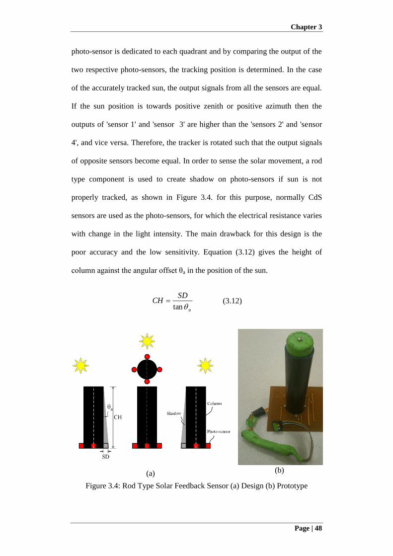
Chapter 3

Page | 48

photo-sensor is dedicated to each quadrant and by comparing the output of the

two respective photo-sensors, the tracking position is determined. In the case

of the accurately tracked sun, the output signals from all the sensors are equal.

If the sun position is towards positive zenith or positive azimuth then the

outputs of 'sensor 1' and 'sensor 3' are higher than the 'sensors 2' and 'sensor

4', and vice versa. Therefore, the tracker is rotated such that the output signals

of opposite sensors become equal. In order to sense the solar movement, a rod

type component is used to create shadow on photo-sensors if sun is not

properly tracked, as shown in Figure 3.4. for this purpose, normally CdS

sensors are used as the photo-sensors, for which the electrical resistance varies

with change in the light intensity. The main drawback for this design is the

poor accuracy and the low sensitivity. Equation (3.12) gives the height of

column against the angular offset θa in the position of the sun.

a

SDCH

tan (3.12)

(a) (b)

Figure 3.4: Rod Type Solar Feedback Sensor (a) Design (b) Prototype

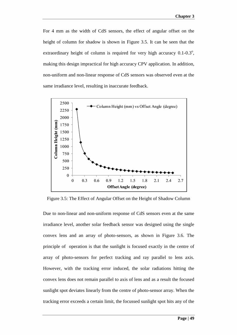
Chapter 3

Page | 49

For 4 mm as the width of CdS sensors, the effect of angular offset on the

height of column for shadow is shown in Figure 3.5. It can be seen that the

extraordinary height of column is required for very high accuracy 0.1-0.3o,

making this design impractical for high accuracy CPV application. In addition,

non-uniform and non-linear response of CdS sensors was observed even at the

same irradiance level, resulting in inaccurate feedback.

Figure 3.5: The Effect of Angular Offset on the Height of Shadow Column

Due to non-linear and non-uniform response of CdS sensors even at the same

irradiance level, another solar feedback sensor was designed using the single

convex lens and an array of photo-sensors, as shown in Figure 3.6. The

principle of operation is that the sunlight is focused exactly in the centre of

array of photo-sensors for perfect tracking and ray parallel to lens axis.

However, with the tracking error induced, the solar radiations hitting the

convex lens does not remain parallel to axis of lens and as a result the focused

sunlight spot deviates linearly from the centre of photo-sensor array. When the

tracking error exceeds a certain limit, the focussed sunlight spot hits any of the

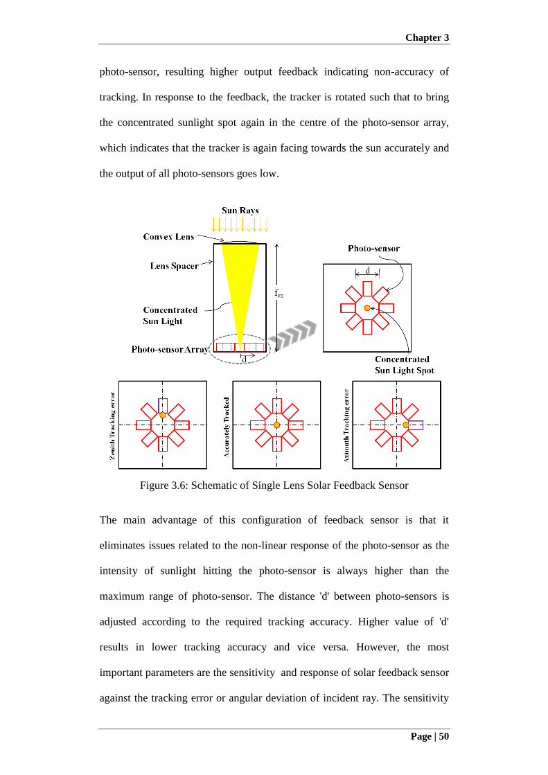
Chapter 3

Page | 50

photo-sensor, resulting higher output feedback indicating non-accuracy of

tracking. In response to the feedback, the tracker is rotated such that to bring

the concentrated sunlight spot again in the centre of the photo-sensor array,

which indicates that the tracker is again facing towards the sun accurately and

the output of all photo-sensors goes low.

Figure 3.6: Schematic of Single Lens Solar Feedback Sensor

The main advantage of this configuration of feedback sensor is that it

eliminates issues related to the non-linear response of the photo-sensor as the

intensity of sunlight hitting the photo-sensor is always higher than the

maximum range of photo-sensor. The distance 'd' between photo-sensors is

adjusted according to the required tracking accuracy. Higher value of 'd'

results in lower tracking accuracy and vice versa. However, the most

important parameters are the sensitivity and response of solar feedback sensor

against the tracking error or angular deviation of incident ray. The sensitivity

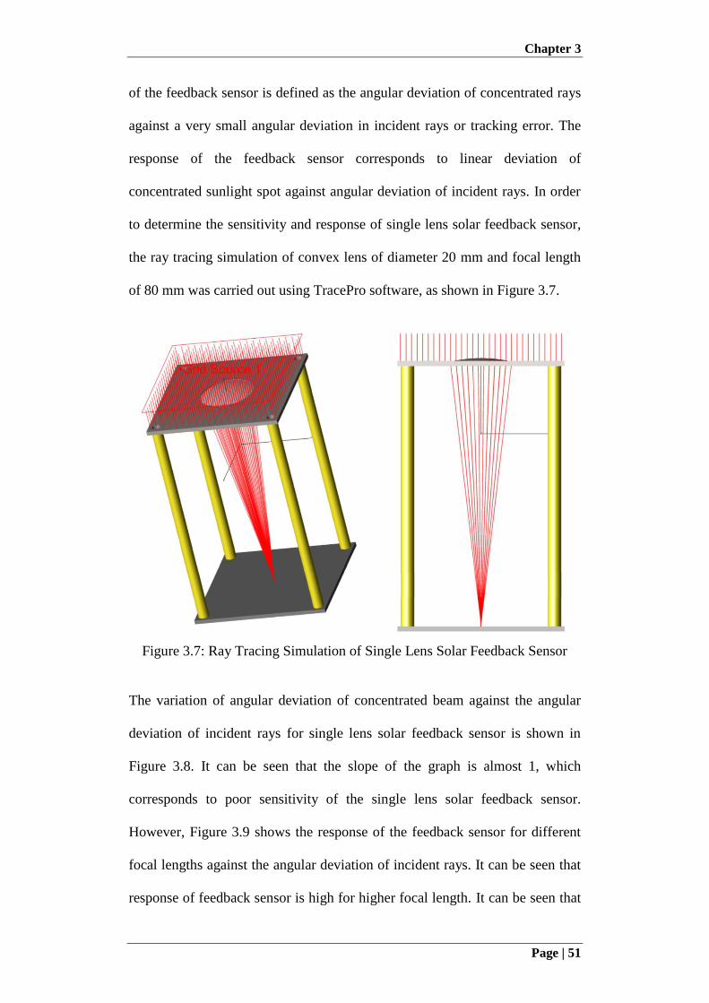
Chapter 3

Page | 51

of the feedback sensor is defined as the angular deviation of concentrated rays

against a very small angular deviation in incident rays or tracking error. The

response of the feedback sensor corresponds to linear deviation of

concentrated sunlight spot against angular deviation of incident rays. In order

to determine the sensitivity and response of single lens solar feedback sensor,

the ray tracing simulation of convex lens of diameter 20 mm and focal length

of 80 mm was carried out using TracePro software, as shown in Figure 3.7.

Figure 3.7: Ray Tracing Simulation of Single Lens Solar Feedback Sensor

The variation of angular deviation of concentrated beam against the angular

deviation of incident rays for single lens solar feedback sensor is shown in

Figure 3.8. It can be seen that the slope of the graph is almost 1, which

corresponds to poor sensitivity of the single lens solar feedback sensor.

However, Figure 3.9 shows the response of the feedback sensor for different

focal lengths against the angular deviation of incident rays. It can be seen that

response of feedback sensor is high for higher focal length. It can be seen that

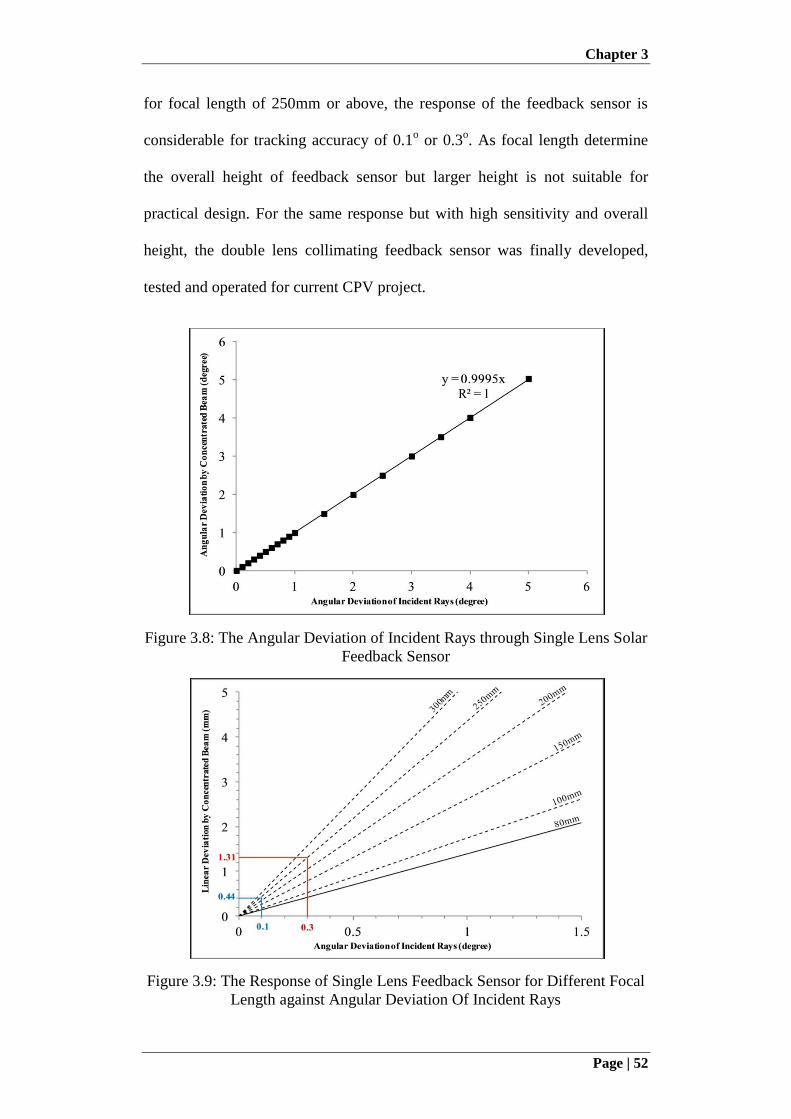
Chapter 3

Page | 52

for focal length of 250mm or above, the response of the feedback sensor is

considerable for tracking accuracy of 0.1o or 0.3

o. As focal length determine

the overall height of feedback sensor but larger height is not suitable for

practical design. For the same response but with high sensitivity and overall

height, the double lens collimating feedback sensor was finally developed,

tested and operated for current CPV project.

Figure 3.8: The Angular Deviation of Incident Rays through Single Lens Solar

Feedback Sensor

Figure 3.9: The Response of Single Lens Feedback Sensor for Different Focal

Length against Angular Deviation Of Incident Rays

Chapter 3

Page | 53

3.2.3.1 Development of Double Lens Collimating Solar Feedback Sensor

In order to have higher sensitivity and accuracy of optical feedback tracking, a

solar feedback sensor was developed based upon double lens collimator

design. The operating principle of double lens collimating solar feedback

sensor, as shown in Figure 3.10, is same as described for single lens solar

feedback sensor. However, the certain arrangement of convex and concave

lenses gives collimated concentrated beam. The converging rays from the

convex lens become parallel again with the concave lens placed on the way.

As far as the collimated beam remains in the middle of photo-sensors array,

the sun is considered to be tracked accurately; otherwise it is adjusted

accordingly against feedback. If Dcx is the diameter of the convex lens with

focal length fcx and focal length of concave lens is fcn, then Equations (3.13)

and (3.14) give the distance between two lenses S and the thickness of the

collimated beam bt after the concave lens, respectively.

)( cncx ffS (3.13)

cn

cx

cx

t ff

Db (3.14)

The Equation (3.14) is derived from corresponding right angle triangle, made

by converging beam within the lens spacing 'S'. Based upon convex lens of

20mm diameter with 80 mm focal length and concave lens of 12 mm diameter

and 12 mm focal length, the current solar feedback sensor was developed. By

using Equations (3.13) and (3.14), the distance between lenses and thickness

of collimated beam were calculated to be 68 mm and 3mm, respectively.

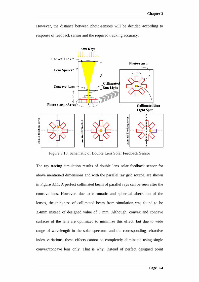
Chapter 3

Page | 54

However, the distance between photo-sensors will be decided according to

response of feedback sensor and the required tracking accuracy.

Figure 3.10: Schematic of Double Lens Solar Feedback Sensor

The ray tracing simulation results of double lens solar feedback sensor for

above mentioned dimensions and with the parallel ray grid source, are shown

in Figure 3.11. A perfect collimated beam of parallel rays can be seen after the

concave lens. However, due to chromatic and spherical aberration of the

lenses, the thickness of collimated beam from simulation was found to be

3.4mm instead of designed value of 3 mm. Although, convex and concave

surfaces of the lens are optimized to minimize this effect, but due to wide

range of wavelength in the solar spectrum and the corresponding refractive

index variations, these effects cannot be completely eliminated using single

convex/concave lens only. That is why, instead of perfect designed point

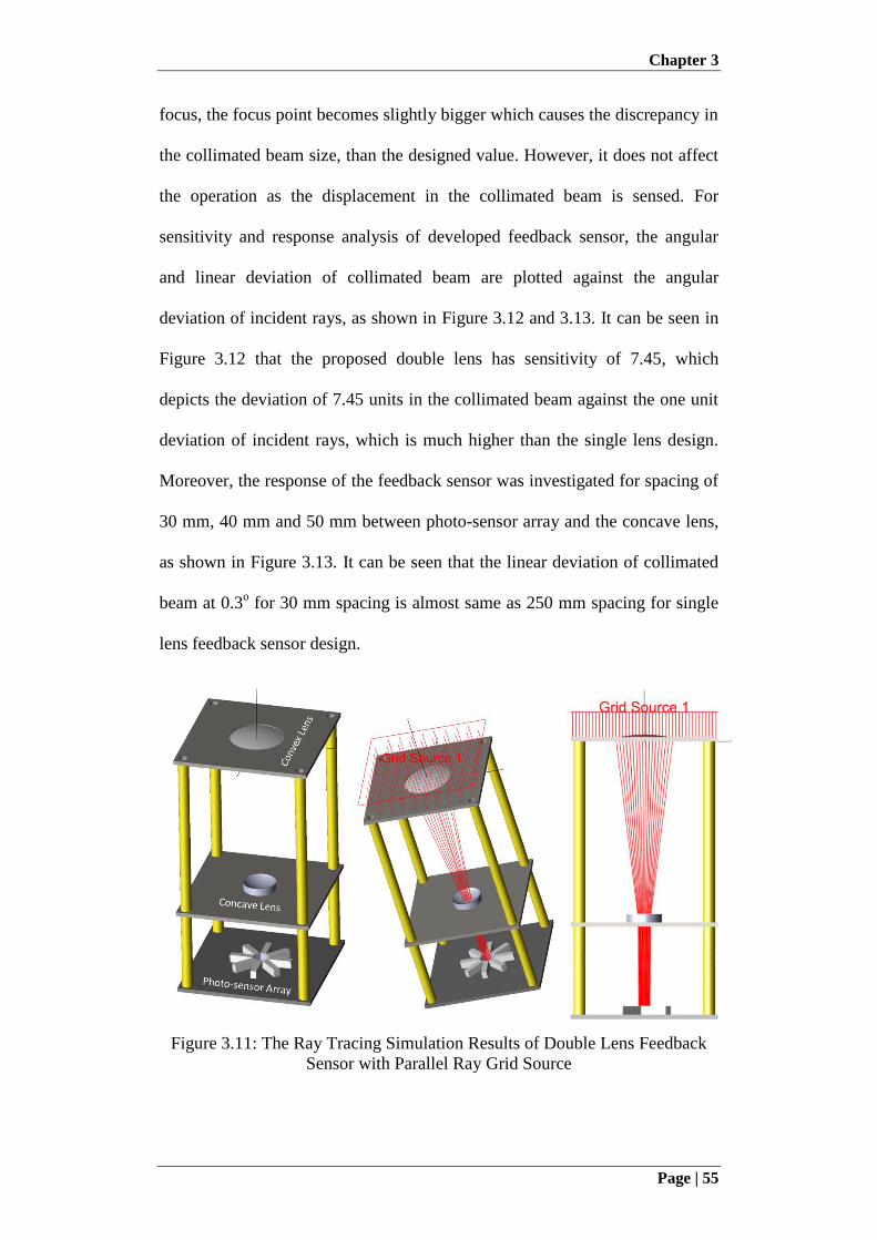
Chapter 3

Page | 55

focus, the focus point becomes slightly bigger which causes the discrepancy in

the collimated beam size, than the designed value. However, it does not affect

the operation as the displacement in the collimated beam is sensed. For

sensitivity and response analysis of developed feedback sensor, the angular

and linear deviation of collimated beam are plotted against the angular

deviation of incident rays, as shown in Figure 3.12 and 3.13. It can be seen in

Figure 3.12 that the proposed double lens has sensitivity of 7.45, which

depicts the deviation of 7.45 units in the collimated beam against the one unit

deviation of incident rays, which is much higher than the single lens design.

Moreover, the response of the feedback sensor was investigated for spacing of

30 mm, 40 mm and 50 mm between photo-sensor array and the concave lens,

as shown in Figure 3.13. It can be seen that the linear deviation of collimated

beam at 0.3o for 30 mm spacing is almost same as 250 mm spacing for single

lens feedback sensor design.

Figure 3.11: The Ray Tracing Simulation Results of Double Lens Feedback

Sensor with Parallel Ray Grid Source

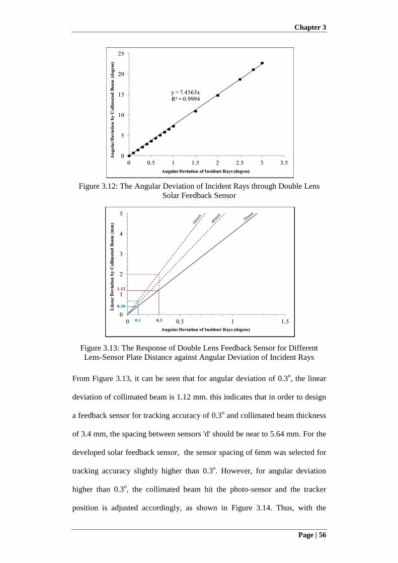
Chapter 3

Page | 56

Figure 3.12: The Angular Deviation of Incident Rays through Double Lens


Figure 3.13: The Response of Double Lens Feedback Sensor for Different

Lens-Sensor Plate Distance against Angular Deviation of Incident Rays

From Figure 3.13, it can be seen that for angular deviation of 0.3o, the linear

deviation of collimated beam is 1.12 mm. this indicates that in order to design

a feedback sensor for tracking accuracy of 0.3o and collimated beam thickness

of 3.4 mm, the spacing between sensors 'd' should be near to 5.64 mm. For the

developed solar feedback sensor, the sensor spacing of 6mm was selected for

tracking accuracy slightly higher than 0.3o. However, for angular deviation

higher than 0.3o, the collimated beam hit the photo-sensor and the tracker

position is adjusted accordingly, as shown in Figure 3.14. Thus, with the

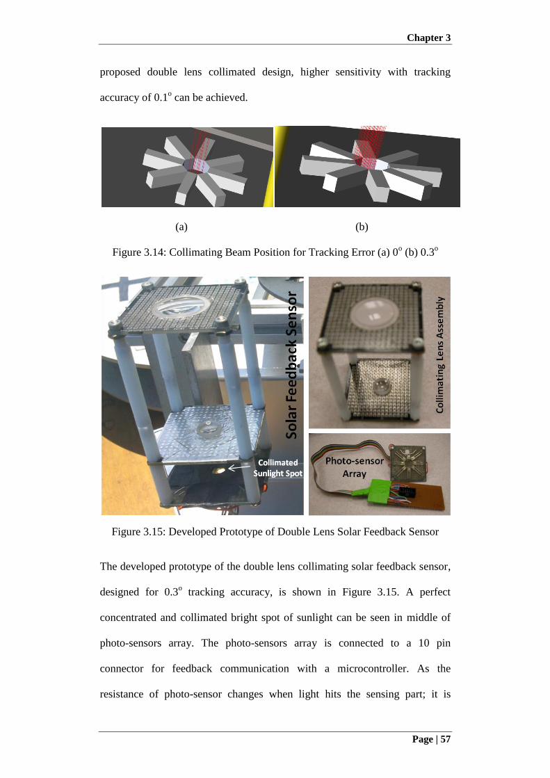
Chapter 3

Page | 57

proposed double lens collimated design, higher sensitivity with tracking

accuracy of 0.1o can be achieved.

(a) (b)

Figure 3.14: Collimating Beam Position for Tracking Error (a) 0o (b) 0.3

o

Figure 3.15: Developed Prototype of Double Lens Solar Feedback Sensor

The developed prototype of the double lens collimating solar feedback sensor,

designed for 0.3o tracking accuracy, is shown in Figure 3.15. A perfect

concentrated and collimated bright spot of sunlight can be seen in middle of

photo-sensors array. The photo-sensors array is connected to a 10 pin

connector for feedback communication with a microcontroller. As the

resistance of photo-sensor changes when light hits the sensing part; it is

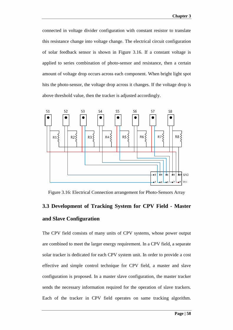
Chapter 3

Page | 58

connected in voltage divider configuration with constant resistor to translate

this resistance change into voltage change. The electrical circuit configuration

of solar feedback sensor is shown in Figure 3.16. If a constant voltage is

applied to series combination of photo-sensor and resistance, then a certain

amount of voltage drop occurs across each component. When bright light spot

hits the photo-sensor, the voltage drop across it changes. If the voltage drop is

above threshold value, then the tracker is adjusted accordingly.

Figure 3.16: Electrical Connection arrangement for Photo-Sensors Array

3.3 Development of Tracking System for CPV Field - Master

and Slave Configuration

The CPV field consists of many units of CPV systems, whose power output

are combined to meet the larger energy requirement. In a CPV field, a separate

solar tracker is dedicated for each CPV system unit. In order to provide a cost

effective and simple control technique for CPV field, a master and slave

configuration is proposed. In a master slave configuration, the master tracker

sends the necessary information required for the operation of slave trackers.

Each of the tracker in CPV field operates on same tracking algorithm.

Chapter 3

Page | 59

However, only the master tracker is equipped with sophisticated and

expensive modules and the required tracking data, which after receiving and

sorting, is transmitted wirelessly to slave trackers in the field. Therefore,

instead of equipping each tracker with the expensive devices, these are

replace with a wireless transceiver.

Figure 3.17: Master and Slave Network arrangement using ZigBee

A wireless control technique using ZigBee protocol, is proposed for master

slave configuration as ZigBee offers low cost communication technique using

radio frequency based upon IEEE 802.15.4 physical radio specification. In

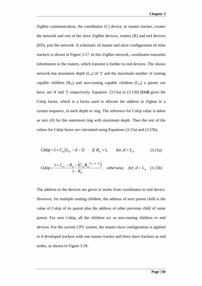
Chapter 3

Page | 60

ZigBee communication, the coordinator (C) device, in master tracker, creates

the network and rest of the slave ZigBee devices, routers (R) and end devices

(ED), join the network. A schematic of master and slave configuration of solar

trackers is shown in Figure 3.17. In this ZigBee network, coordinator transmits

information to the routers, which transmit it further to end devices. The shown

network has maximum depth (Lm) of '2' and the maximum number of routing

capable children (Rm) and non-routing capable children (Cm) a parent can

have, are '4' and '3' respectively. Equation (3.15a) or (3.15b) [114] gives the

Cskip factor, which is a factor used to allocate the address to Zigbee in a

certain sequence, in each depth or ring. The reference for Cskip value is taken

as zero (0) for the outermost ring with maximum depth. Then the rest of the

values for Cskip factor are calculated using Equations (3.15a) and (3.15b).

mmmm LdforRifdLCCskip ,,111 (3.15a)

m

m

dL

mmmm LdforotherwiseR

RCRCCskip

m

,,,1

11

(3.15b)

The address to the devices are given in series from coordinator to end device.

However, for multiple routing children, the address of next parent child is the

value of Cskip of its parent plus the address of other previous child of same

parent. For zero Cskip, all the children act as non-routing children or end

devices. For the current CPV system, the master slave configuration is applied

to 4 developed trackers with one master tracker and three slave trackers as end

nodes, as shown in Figure 3.18.

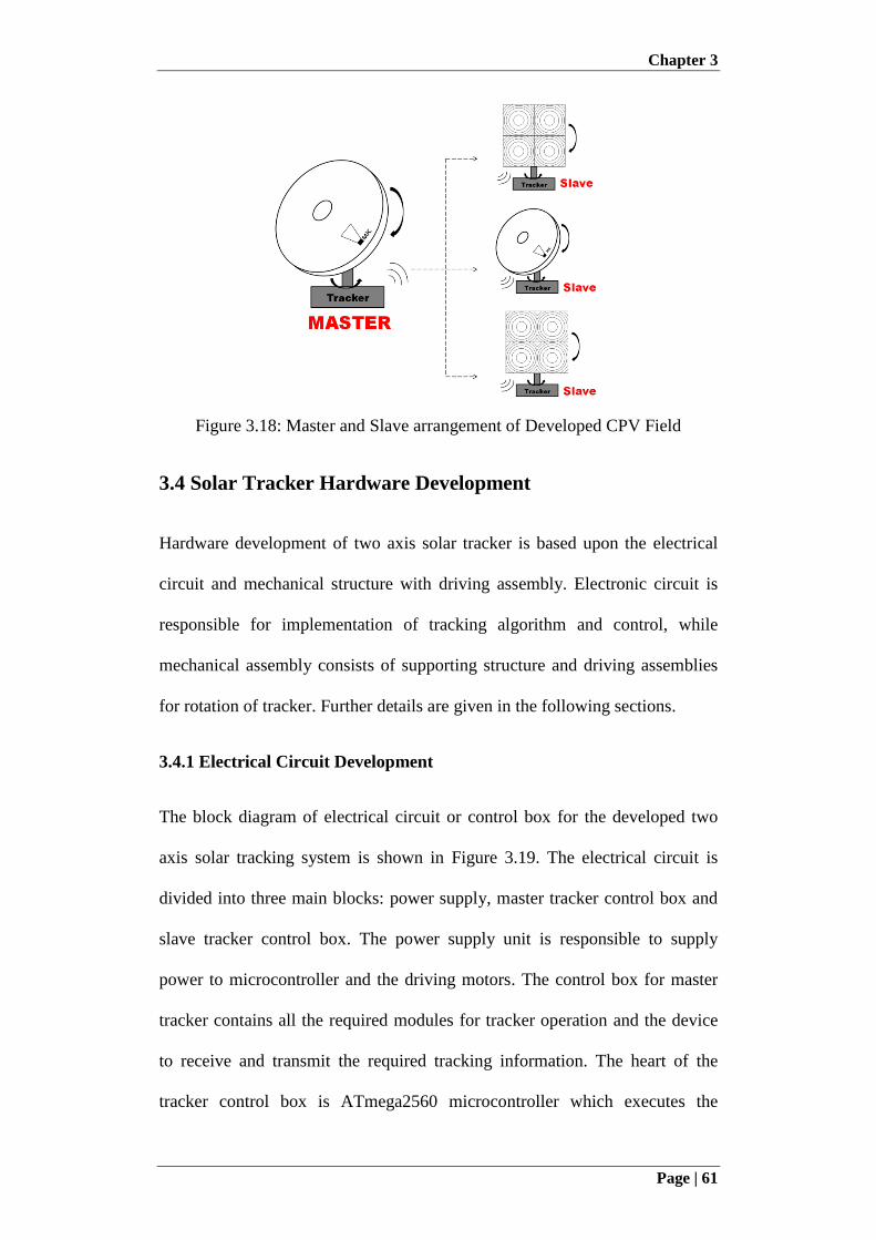
Chapter 3

Page | 61

Figure 3.18: Master and Slave arrangement of Developed CPV Field

3.4 Solar Tracker Hardware Development

Hardware development of two axis solar tracker is based upon the electrical

circuit and mechanical structure with driving assembly. Electronic circuit is

responsible for implementation of tracking algorithm and control, while

mechanical assembly consists of supporting structure and driving assemblies

for rotation of tracker. Further details are given in the following sections.

3.4.1 Electrical Circuit Development

The block diagram of electrical circuit or control box for the developed two

axis solar tracking system is shown in Figure 3.19. The electrical circuit is

divided into three main blocks: power supply, master tracker control box and

slave tracker control box. The power supply unit is responsible to supply

power to microcontroller and the driving motors. The control box for master

tracker contains all the required modules for tracker operation and the device

to receive and transmit the required tracking information. The heart of the

tracker control box is ATmega2560 microcontroller which executes the

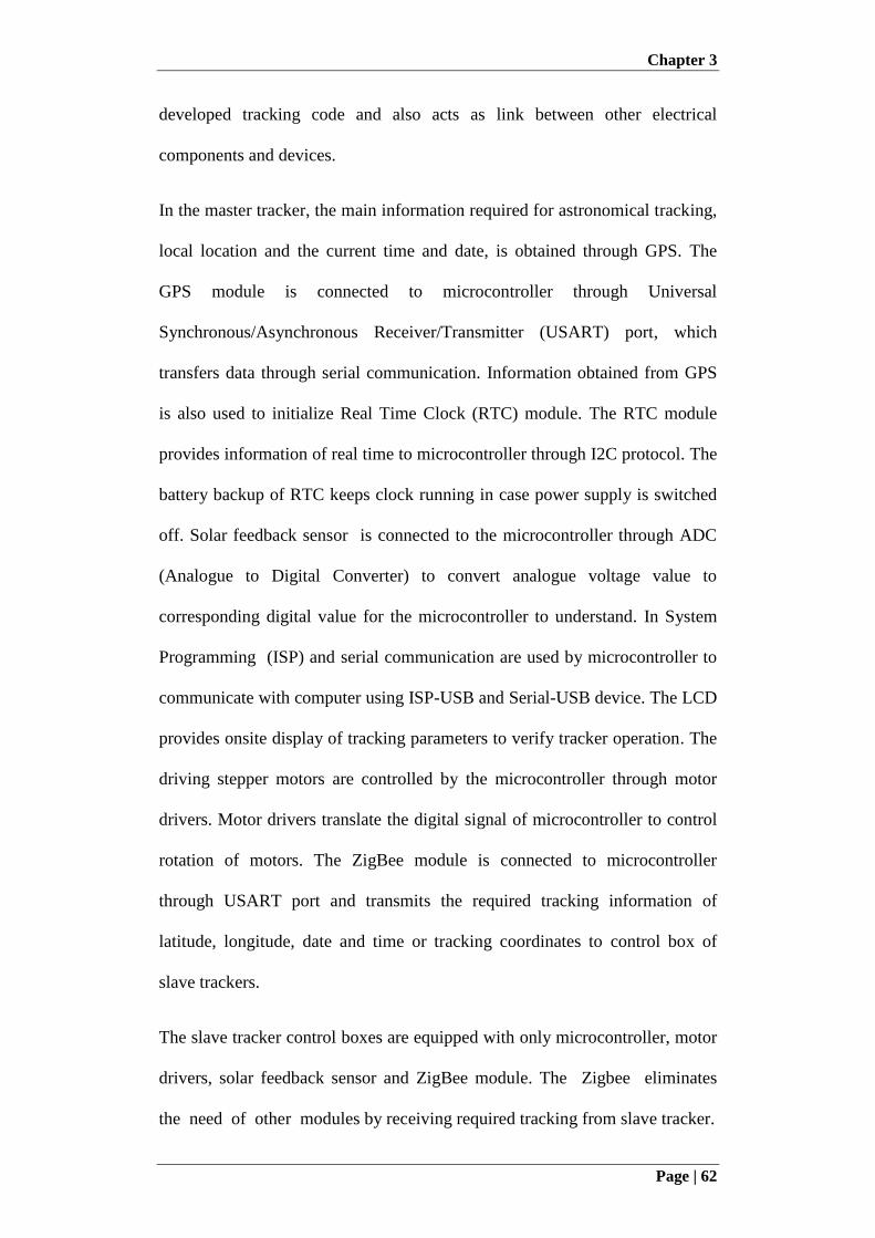
Chapter 3

Page | 62

developed tracking code and also acts as link between other electrical

components and devices.

In the master tracker, the main information required for astronomical tracking,

local location and the current time and date, is obtained through GPS. The

GPS module is connected to microcontroller through Universal

Synchronous/Asynchronous Receiver/Transmitter (USART) port, which

transfers data through serial communication. Information obtained from GPS

is also used to initialize Real Time Clock (RTC) module. The RTC module

provides information of real time to microcontroller through I2C protocol. The

battery backup of RTC keeps clock running in case power supply is switched

off. Solar feedback sensor is connected to the microcontroller through ADC

(Analogue to Digital Converter) to convert analogue voltage value to

corresponding digital value for the microcontroller to understand. In System

Programming (ISP) and serial communication are used by microcontroller to

communicate with computer using ISP-USB and Serial-USB device. The LCD

provides onsite display of tracking parameters to verify tracker operation. The

driving stepper motors are controlled by the microcontroller through motor

drivers. Motor drivers translate the digital signal of microcontroller to control

rotation of motors. The ZigBee module is connected to microcontroller

through USART port and transmits the required tracking information of

latitude, longitude, date and time or tracking coordinates to control box of

slave trackers.

The slave tracker control boxes are equipped with only microcontroller, motor

drivers, solar feedback sensor and ZigBee module. The Zigbee eliminates

the need of other modules by receiving required tracking from slave tracker.

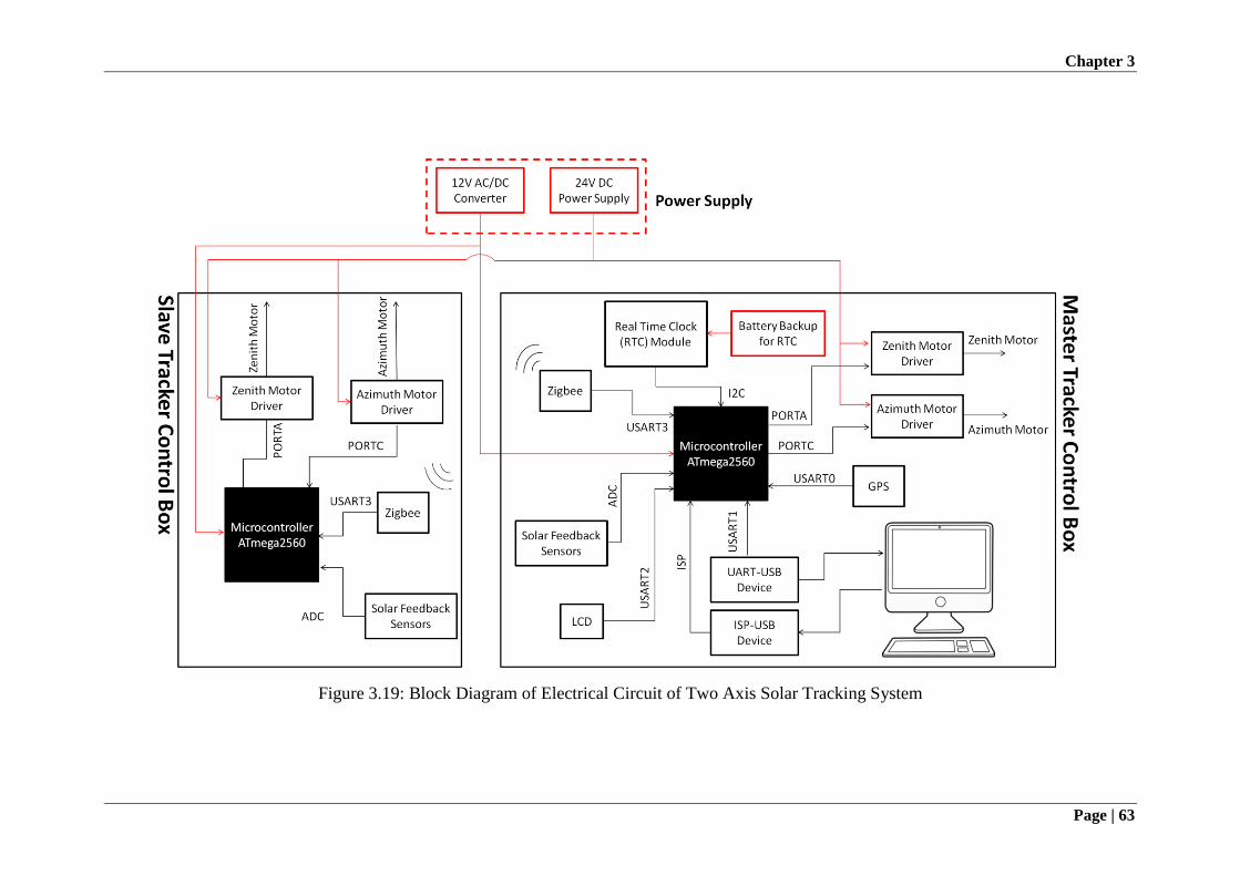
Chapter 3

Page | 63

Figure 3.19: Block Diagram of Electrical Circuit of Two Axis Solar Tracking System

Chapter 3

Page | 64

(a)

(b)

Figure 3.20: Control Box for (a) Master Tracker (b) Slave Tracker

As a result, a simplified control box does the same tracking job without the

need of other electronic modules. The developed control boxes for master and

slave trackers are shown in Figure 3.20. Most of the components like LCD,

ISP-USB and UART-USB converters are optional and do not require for

operation. Only one time use of ISP-USB is required to load the tracking

Chapter 3

Page | 65

program in microcontroller. In addition, a small microcontroller like

atmega128 can be used for slave trackers. The use of atmega2560 and other

optional modules is to have additional feedback regarding system

performance, that is developed as a test rig. The developed power supply unit

is shown in Figure 3.21, containing 24V DC switching power supply for

driving motors and 12V AC/DC converters to power four microcontrollers of

each solar tracker.

Figure 3.21: The Power Supply Box for Developed CPV System

3.4.2 Mechanical Structure and Driving Assembly

The mechanical assembly of solar tracker consists of support structure and

driving assemblies. Driving assemblies utilize stepper motor with worm gear

and wheel for tracker rotation. The mechanical structure provides rigid support

to driving assemblies and provides platform for the installation of CPV

modules. Figure 3.22 shows the labelled 3D model of developed two axis solar

tracker. The isometric view of tracker is also shown in Figure 3.23. Each of

the tracker has two driving assemblies; the lower driving assembly is

responsible for azimuth rotation and the upper driving assembly follows zenith

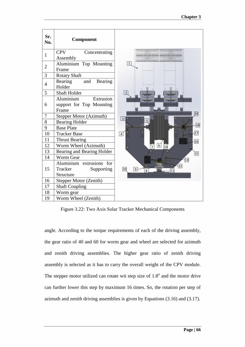
Chapter 3

Page | 66

Sr.

No. Component

1 CPV Concentrating

Assembly

2 Aluminium Top Mounting

Frame

3 Rotary Shaft

4 Bearing and Bearing

Holder

5 Shaft Holder

6

Aluminium Extrusion

support for Top Mounting

Frame

7 Stepper Motor (Azimuth)

8 Bearing Holder

9 Base Plate

10 Tracker Base

11 Thrust Bearing

12 Worm Wheel (Azimuth)

13 Bearing and Bearing Holder

14 Worm Gear

15

Aluminium extrusions for

Tracker Supporting

Structure

16 Stepper Motor (Zenith)

17 Shaft Coupling

18 Worm gear

19 Worm Wheel (Zenith)

Figure 3.22: Two Axis Solar Tracker Mechanical Components

angle. According to the torque requirements of each of the driving assembly,

the gear ratio of 40 and 60 for worm gear and wheel are selected for azimuth

and zenith driving assemblies. The higher gear ratio of zenith driving

assembly is selected as it has to carry the overall weight of the CPV module.

The stepper motor utilized can rotate wit step size of 1.8o and the motor drive

can further lower this step by maximum 16 times. So, the rotation per step of

azimuth and zenith driving assemblies is given by Equations (3.16) and (3.17).

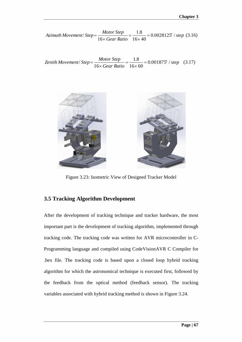
Chapter 3

Page | 67

stepRatioGear

StepMotorStepMovementAzimuth o /0028125.0

4016

8.1

16/

(3.16)

stepRatioGear

StepMotorStepMovementZenith o /001875.0

6016

8.1

16/

(3.17)

Figure 3.23: Isometric View of Designed Tracker Model

3.5 Tracking Algorithm Development

After the development of tracking technique and tracker hardware, the most

important part is the development of tracking algorithm, implemented through

tracking code. The tracking code was written for AVR microcontroller in C-

Programming language and compiled using CodeVisionAVR C Compiler for

.hex file. The tracking code is based upon a closed loop hybrid tracking

algorithm for which the astronomical technique is executed first, followed by

the feedback from the optical method (feedback sensor). The tracking

variables associated with hybrid tracking method is shown in Figure 3.24.

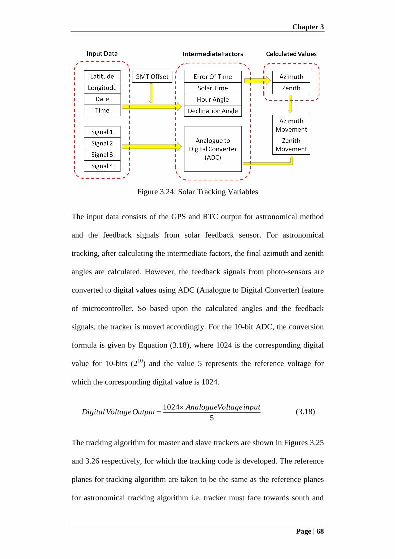
Chapter 3

Page | 68

Figure 3.24: Solar Tracking Variables

The input data consists of the GPS and RTC output for astronomical method

and the feedback signals from solar feedback sensor. For astronomical

tracking, after calculating the intermediate factors, the final azimuth and zenith

angles are calculated. However, the feedback signals from photo-sensors are

converted to digital values using ADC (Analogue to Digital Converter) feature

of microcontroller. So based upon the calculated angles and the feedback

signals, the tracker is moved accordingly. For the 10-bit ADC, the conversion

formula is given by Equation (3.18), where 1024 is the corresponding digital

value for 10-bits (210

) and the value 5 represents the reference voltage for

which the corresponding digital value is 1024.

5

1024 input Voltage AnalogueOutputVoltageDigital

(3.18)

The tracking algorithm for master and slave trackers are shown in Figures 3.25

and 3.26 respectively, for which the tracking code is developed. The reference

planes for tracking algorithm are taken to be the same as the reference planes

for astronomical tracking algorithm i.e. tracker must face towards south and

Chapter 3

Page | 69

the top mounting frame must be horizontal. For the master tracker, first the

GPS data based upon NMEA protocol is received during initialization, as

given below:

$GPGGA,020133.440,3723.3040,N,12656.3569,E,1,06,1.2,43.8,M,21.4,M,,00

00*6F

$GPGSA,A,3,05,08,10,24,29,21,,,,,,,3.2,1.2,2.9*39

$GPGSV,2,1,06,05,49,079,51,21,30,321,42,08,22,045,35,10,22,093,48*70

$GPGSV,2,2,06,29,21,244,29,24,18,317,43*73

$GPRMC,020133.440,A,3723.3040,N,12656.3569,E,0.000.0,009.7,280410,,,

A*61

$GPVTG,009.7,T,M,000.0,N,000.0,K,A*03

The received data is filtered for $GPRMC format and then sorted out to

extract latitude, longitude, date and time information. Figure 3.27 shows the

breakout of GPS data string in $GPRMC format and its conversion into

required information. First column shows the time string, in which first two

digits represent hours value, next two digits represent minutes value and the

remaining digits represent seconds value. The second and third columns show

latitude string and its reference as North, respectively. In latitude string, the

first two digits represent the latitude value in degrees (hours) and the

remaining digits represent latitude value in minutes, which is needed to be

divided by 60 to convert it into degree. The actual converted value of the

latitude is given at the bottom of second column. Similar procedure is

followed for longitude in fourth and fifth columns. The last column shows the

time string, in which the first two digits represent date, the next two digits

represent month and the last two digits represent year. The date and time

extracted from the GPS data initializes the RTC module.

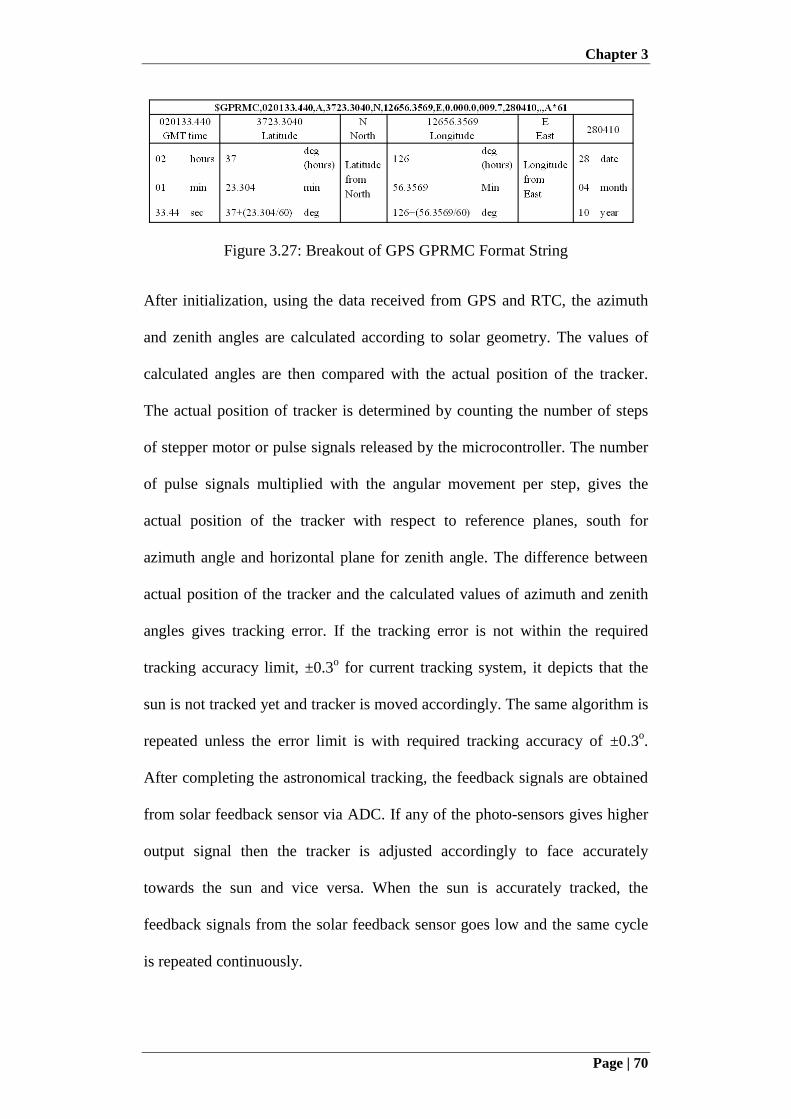
Chapter 3

Page | 70

Figure 3.27: Breakout of GPS GPRMC Format String

After initialization, using the data received from GPS and RTC, the azimuth

and zenith angles are calculated according to solar geometry. The values of

calculated angles are then compared with the actual position of the tracker.

The actual position of tracker is determined by counting the number of steps

of stepper motor or pulse signals released by the microcontroller. The number

of pulse signals multiplied with the angular movement per step, gives the

actual position of the tracker with respect to reference planes, south for

azimuth angle and horizontal plane for zenith angle. The difference between

actual position of the tracker and the calculated values of azimuth and zenith

angles gives tracking error. If the tracking error is not within the required

tracking accuracy limit, ±0.3o for current tracking system, it depicts that the

sun is not tracked yet and tracker is moved accordingly. The same algorithm is

repeated unless the error limit is with required tracking accuracy of ±0.3o.

After completing the astronomical tracking, the feedback signals are obtained

from solar feedback sensor via ADC. If any of the photo-sensors gives higher

output signal then the tracker is adjusted accordingly to face accurately

towards the sun and vice versa. When the sun is accurately tracked, the

feedback signals from the solar feedback sensor goes low and the same cycle

is repeated continuously.

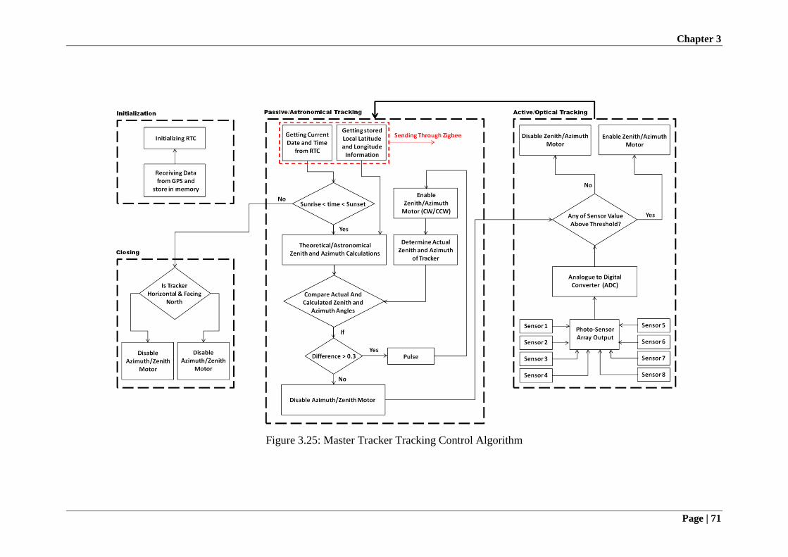
Chapter 3

Page | 71

Figure 3.25: Master Tracker Tracking Control Algorithm

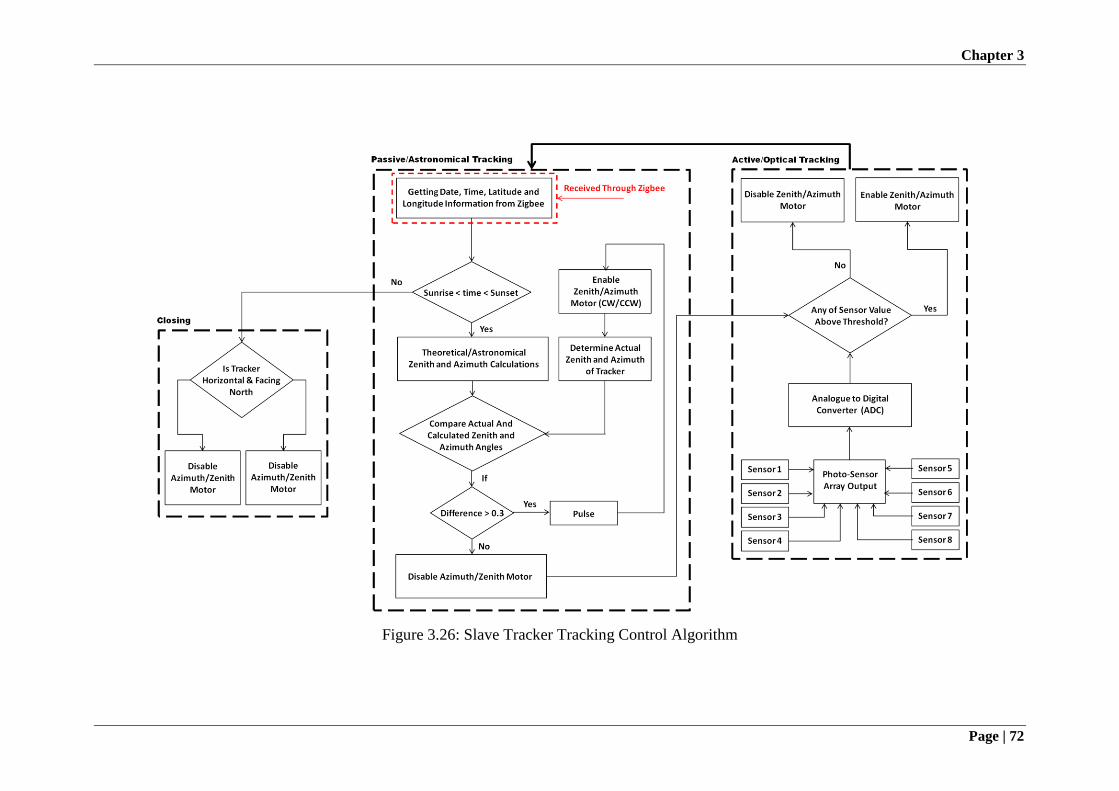
Chapter 3

Page | 72

Figure 3.26: Slave Tracker Tracking Control Algorithm

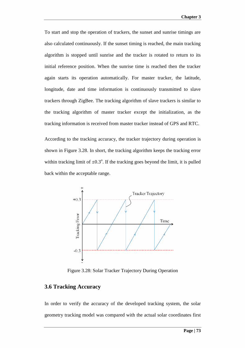
Chapter 3

Page | 73

To start and stop the operation of trackers, the sunset and sunrise timings are

also calculated continuously. If the sunset timing is reached, the main tracking

algorithm is stopped until sunrise and the tracker is rotated to return to its

initial reference position. When the sunrise time is reached then the tracker

again starts its operation automatically. For master tracker, the latitude,

longitude, date and time information is continuously transmitted to slave

trackers through ZigBee. The tracking algorithm of slave trackers is similar to

the tracking algorithm of master tracker except the initialization, as the

tracking information is received from master tracker instead of GPS and RTC.

According to the tracking accuracy, the tracker trajectory during operation is

shown in Figure 3.28. In short, the tracking algorithm keeps the tracking error

within tracking limit of ±0.3o. If the tracking goes beyond the limit, it is pulled

back within the acceptable range.

Figure 3.28: Solar Tracker Trajectory During Operation

3.6 Tracking Accuracy

In order to verify the accuracy of the developed tracking system, the solar

geometry tracking model was compared with the actual solar coordinates first

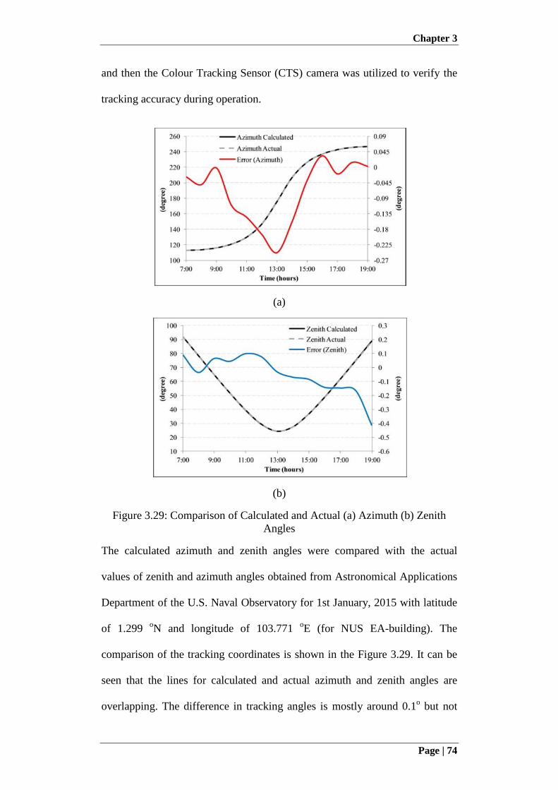
Chapter 3

Page | 74

and then the Colour Tracking Sensor (CTS) camera was utilized to verify the

tracking accuracy during operation.

(a)

(b)

Figure 3.29: Comparison of Calculated and Actual (a) Azimuth (b) Zenith

Angles

The calculated azimuth and zenith angles were compared with the actual

values of zenith and azimuth angles obtained from Astronomical Applications

Department of the U.S. Naval Observatory for 1st January, 2015 with latitude

of 1.299 oN and longitude of 103.771

oE (for NUS EA-building). The

comparison of the tracking coordinates is shown in the Figure 3.29. It can be

seen that the lines for calculated and actual azimuth and zenith angles are

overlapping. The difference in tracking angles is mostly around 0.1o but not

Chapter 3

Page | 75

more than -0.25o and -0.4

o for azimuth and zenith angle respectively, just for

instance. However, it can be handled through solar feedback sensor.

In order to determine the actual position of the sun and its comparison with the

actual tracked position, a colour tracking sensor (CTS) camera was utilized to

get solar position using sun images captured during tracker operation. An

assembly of CTS camera and BAADER safety film was developed as shown

in the Figure 3.30. The CTS camera can detect the position of any colour

within its view angle. The BAADER solar safety film was placed in front of

the CTS which can block 90-95% of the solar radiations along with the rays

from surrounding objects. Therefore, CTS camera only captures the image of

sun appearing as the bright spot. Figure 3.31 shows the control software 'CTS

Studio' to program the camera and to show the captured image. It can be seen

that the captured image contains a bright spot, representing the sun. The solar

position through captured image is provided using bright pixel in a 240x180

pixels array. The CTS sensor has a view angle of 90o, which shows sensitivity

of 0.375o/pixel in x-direction and 0.5

o/pixel in y-direction.

Figure 3.30: Colour Tracking Sensor (CTS) Camera and BAADER Film

Assembly to Determine Solar Position

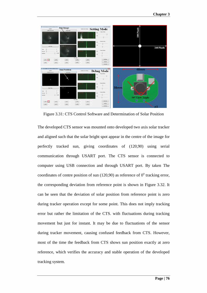
Chapter 3

Page | 76

Figure 3.31: CTS Control Software and Determination of Solar Position

The developed CTS sensor was mounted onto developed two axis solar tracker

and aligned such that the solar bright spot appear in the centre of the image for

perfectly tracked sun, giving coordinates of (120,90) using serial

communication through USART port. The CTS sensor is connected to

computer using USB connection and through USART port. By taken The

coordinates of centre position of sun (120,90) as reference of 0o tracking error,

the corresponding deviation from reference point is shown in Figure 3.32. It

can be seen that the deviation of solar position from reference point is zero

during tracker operation except for some point. This does not imply tracking

error but rather the limitation of the CTS. with fluctuations during tracking

movement but just for instant. It may be due to fluctuations of the sensor

during tracker movement, causing confused feedback from CTS. However,

most of the time the feedback from CTS shows sun position exactly at zero

reference, which verifies the accuracy and stable operation of the developed

tracking system.

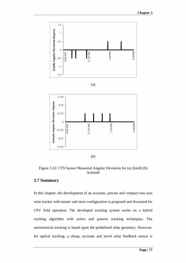
Chapter 3

Page | 77

(a)

(b)

Figure 3.32: CTS Sensor Measured Angular Deviation for (a) Zenith (b)

Azimuth

3.7 Summary

In this chapter, the development of an accurate, precise and compact two axis

solar tracker with master and slave configuration is proposed and discussed for

CPV field operation. The developed tracking system works on a hybrid

tracking algorithm with active and passive tracking techniques. The

astronomical tracking is based upon the predefined solar geometry. However,

for optical tracking, a cheap, accurate and novel solar feedback sensor is

Chapter 3

Page | 78

designed, developed and tested with tracking accuracy of up to 0.1o. For cost

effective control of a field of CPV solar trackers, a master and slave technique

is proposed, designed and implemented using wireless communication through

cheap ZigBee modules. In the proposed master and slave configuration, one

tracker acts as master with all required tracking modules and transmits the

required tracking information to other slave trackers in the field.

A prototype of the CPV trackers field is developed consisting of four trackers,

one master and three slave trackers. The mechanical structure of the trackers is

built with aluminium extrusions for rigid and light weight assembly, while the

driving assembly is based upon worm gear and worm wheel arrangement. The

tracker control box is using microcontroller, GPS, RTC and motor drivers. The

driving assemblies have rotation with step size of 0.0028125o/step for azimuth

and 0.001875o/step for zenith angle. The developed tracker is programmed to

operate with tracking accuracy of 0.3o. In order to verify the accuracy of the

tracker, first the solar geometry model was compared with actual solar

coordinates obtained from Astronomical Applications Department of the U.S.

Naval Observatory. Then the tracker movement was compared with actual

solar position recorded using color tracking sensor (CTS).

After the development of tracking system, the design and ray tracing

simulation of the concentrating assemblies are discussed in next chapter.

Chapter 4

Page | 79

Chapter 4: Design and Ray Tracing Simulation of

Concentrating Assembly for CPV

4.1 Introduction

With the development of accurate, precise and compact two-axis solar tracker

in the previous chapter, the design and development of CPV concentrating

assembly is discussed in this chapter. The design of concentrating assembly is

of high importance in the development of concentrated photovoltaic (CPV)

system. The concentrating assembly guides and concentrates solar radiations

effectively onto small area of multi-junction solar cell (MJC) with uniform ray

distribution at minimal loss. The main parameter to evaluate the performance

of concentrating assembly is its response to tracking error i.e. minimal ray loss

for response of large tracking error. This response against tracking error

defines the tracking accuracy requirement; better response can accept low

tracking accuracy with less energy consumption by tracker.

The CPV concentrating assembly comprises concentrators as primary optics

and a homogeniser as secondary or tertiary optics. Solar concentrators can be

of either reflective type reflectors or refractive type lenses. However, each

concentrator design has its own significance and limitations. Similarly,

homogeniser design can also be reflective and refractive, depending upon the

need. In this chapter, different types of the CPV concentrating assemblies are

designed and evaluated through ray tracing simulation using TracePro

software. For the primary concentrator, parabolic dish and Fresnel lens are

considered for current design and analysis. Moreover, for the homogeniser,

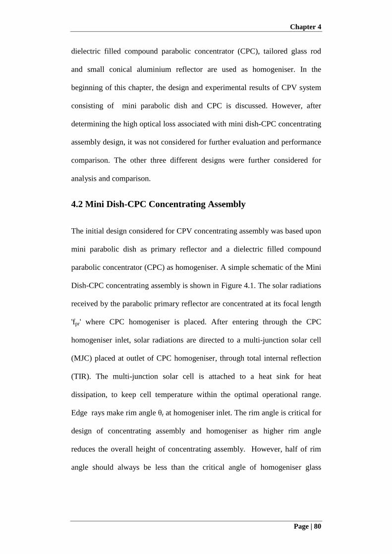
Chapter 4

Page | 80

dielectric filled compound parabolic concentrator (CPC), tailored glass rod

and small conical aluminium reflector are used as homogeniser. In the

beginning of this chapter, the design and experimental results of CPV system

consisting of mini parabolic dish and CPC is discussed. However, after

determining the high optical loss associated with mini dish-CPC concentrating

assembly design, it was not considered for further evaluation and performance

comparison. The other three different designs were further considered for

analysis and comparison.

4.2 Mini Dish-CPC Concentrating Assembly

The initial design considered for CPV concentrating assembly was based upon

mini parabolic dish as primary reflector and a dielectric filled compound

parabolic concentrator (CPC) as homogeniser. A simple schematic of the Mini

Dish-CPC concentrating assembly is shown in Figure 4.1. The solar radiations

received by the parabolic primary reflector are concentrated at its focal length

'fpr' where CPC homogeniser is placed. After entering through the CPC

homogeniser inlet, solar radiations are directed to a multi-junction solar cell

(MJC) placed at outlet of CPC homogeniser, through total internal reflection

(TIR). The multi-junction solar cell is attached to a heat sink for heat

dissipation, to keep cell temperature within the optimal operational range.

Edge rays make rim angle θr at homogeniser inlet. The rim angle is critical for

design of concentrating assembly and homogeniser as higher rim angle

reduces the overall height of concentrating assembly. However, half of rim

angle should always be less than the critical angle of homogeniser glass

Chapter 4

Page | 81

material, otherwise the solar radiations will be reflected back from the

homogeniser inlet.

It is known that the solar radiation incident on the earth's surface is not exactly

parallel to concentrator axis due to solar subtended angle of 0.53o. It depicts

that perfect point focussed concentration of sun light cannot be achieved but

instead, the concentration over a small area is achieved. In addition, due to

movement of the two-axis solar tracker in steps, the rays hitting the primary

reflector cannot be always parallel to axis of concentrating assembly. This

causes the focus point of concentrated solar radiation to deviate from the

centre of the homogeniser and this deviation depends upon the degree of

deviation of incident rays from concentrator axis.

Figure 4.1: Schematic of Mini Dish-CPC Concentrating Assembly

Chapter 4

Page | 82

One important parameter in designing the concentrating assembly is the

acceptance angle, defined as the maximum angular deviation of the incident

rays that can be accepted with minimum losses. The concentrator and

homogeniser are designed such that as long as the concentrated rays are falling

onto the homogeniser inlet, they are directed towards the MJC. The size of the

primary concentrator Dpr is selected according to the concentration ratio

desired at the solar cell area. The centre hole of dimension dpr is for mounting

purpose. The geometric concentration ratio, defined as the ratio of primary

concentrator net area to solar cell area, is given by the Equation (4.1).

C

cong

A

ACR (4.1)

Where Acon is the net effective area of primary concentrator and AC is the area

of solar cell. For current research work, multi-junction solar cell from Arima

Photovoltaic & Co. is used with a cell size of 5.5 mm x 5.5 mm and operating

solar concentration of x500. According to the MJC size and centre hole of

dpr=2.5 cm, the diameter of primary reflector was selected as 15cm with

thickness of td=1cm and concentration ratio of x566. However, the actual

concentration at MJC will be less than x500 due to optical losses caused by

reflectance and absorbance loss of concentrating assembly. The next section

discusses the design of primary parabolic concentrator.

4.2.1 Mini Parabolic Dish Design

The profile of the mini parabolic dish is based upon the simple equation of

parabola, given by Equation (4.2).

prf

xy

4

2

(4.2)

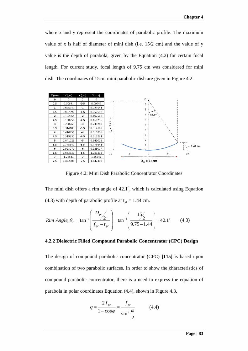
Chapter 4

Page | 83

where x and y represent the coordinates of parabolic profile. The maximum

value of x is half of diameter of mini dish (i.e. 15/2 cm) and the value of y

value is the depth of parabola, given by the Equation (4.2) for certain focal

length. For current study, focal length of 9.75 cm was considered for mini

dish. The coordinates of 15cm mini parabolic dish are given in Figure 4.2.

Figure 4.2: Mini Dish Parabolic Concentrator Coordinates

The mini dish offers a rim angle of 42.1o, which is calculated using Equation

(4.3) with depth of parabolic profile at tpr = 1.44 cm.

o

prpr

pr

rtf

D

AngleRim 1.4244.175.9

215

tan2tan, 11

(4.3)

4.2.2 Dielectric Filled Compound Parabolic Concentrator (CPC) Design

The design of compound parabolic concentrator (CPC) [115] is based upon

combination of two parabolic surfaces. In order to show the characteristics of

compound parabolic concentrator, there is a need to express the equation of

parabola in polar coordinates Equation (4.4), shown in Figure 4.3.

2sin

cos1

2

2

prpr ffq

(4.4)

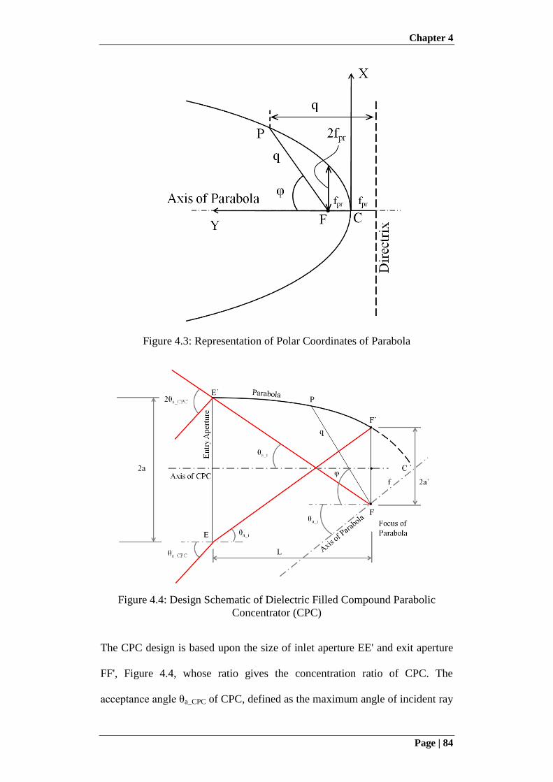
Chapter 4

Page | 84

Figure 4.3: Representation of Polar Coordinates of Parabola

Figure 4.4: Design Schematic of Dielectric Filled Compound Parabolic

Concentrator (CPC)

The CPC design is based upon the size of inlet aperture EE' and exit aperture

FF', Figure 4.4, whose ratio gives the concentration ratio of CPC. The

acceptance angle θa_CPC of CPC, defined as the maximum angle of incident ray

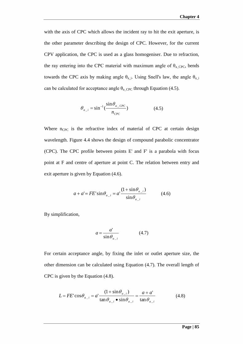
Chapter 4

Page | 85

with the axis of CPC which allows the incident ray to hit the exit aperture, is

the other parameter describing the design of CPC. However, for the current

CPV application, the CPC is used as a glass homogeniser. Due to refraction,

the ray entering into the CPC material with maximum angle of θa_CPC, bends

towards the CPC axis by making angle θa_i. Using Snell's law, the angle θa_i

can be calculated for acceptance angle θa_CPC through Equation (4.5).

)sin

(sin_1

_

CPC

CPCa

ian

(4.5)

Where nCPC is the refractive index of material of CPC at certain design

wavelength. Figure 4.4 shows the design of compound parabolic concentrator

(CPC). The CPC profile between points E' and F' is a parabola with focus

point at F and centre of aperture at point C. The relation between entry and

exit aperture is given by Equation (4.6).

ia

ia

ia aFEaa_

_

_sin

)sin1('sin''

(4.6)

By simplification,

ia

aa

_sin

'

(4.7)

For certain acceptance angle, by fixing the inlet or outlet aperture size, the

other dimension can be calculated using Equation (4.7). The overall length of

CPC is given by the Equation (4.8).

iaiaia

ia

ia

aaaFEL

___

_

_tan

'

sintan

)sin1('cos'

(4.8)

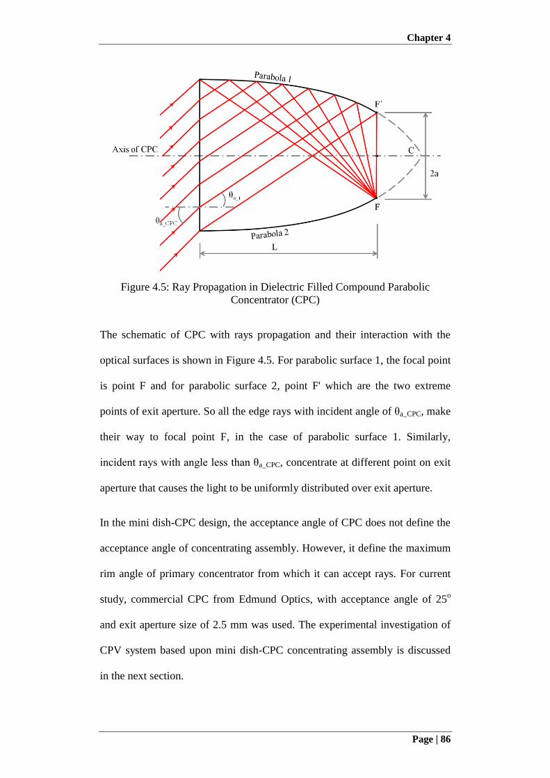
Chapter 4

Page | 86

Figure 4.5: Ray Propagation in Dielectric Filled Compound Parabolic

Concentrator (CPC)

The schematic of CPC with rays propagation and their interaction with the

optical surfaces is shown in Figure 4.5. For parabolic surface 1, the focal point

is point F and for parabolic surface 2, point F' which are the two extreme

points of exit aperture. So all the edge rays with incident angle of θa_CPC, make

their way to focal point F, in the case of parabolic surface 1. Similarly,

incident rays with angle less than θa_CPC, concentrate at different point on exit

aperture that causes the light to be uniformly distributed over exit aperture.

In the mini dish-CPC design, the acceptance angle of CPC does not define the

acceptance angle of concentrating assembly. However, it define the maximum

rim angle of primary concentrator from which it can accept rays. For current

study, commercial CPC from Edmund Optics, with acceptance angle of 25o

and exit aperture size of 2.5 mm was used. The experimental investigation of

CPV system based upon mini dish-CPC concentrating assembly is discussed

in the next section.

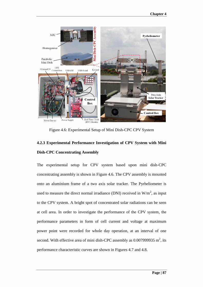
Chapter 4

Page | 87

Figure 4.6: Experimental Setup of Mini Dish-CPC CPV System

4.2.3 Experimental Performance Investigation of CPV System with Mini

Dish-CPC Concentrating Assembly

The experimental setup for CPV system based upon mini dish-CPC

concentrating assembly is shown in Figure 4.6. The CPV assembly is mounted

onto an aluminium frame of a two axis solar tracker. The Pyrheliometer is

used to measure the direct normal irradiance (DNI) received in W/m2, as input

to the CPV system. A bright spot of concentrated solar radiations can be seen

at cell area. In order to investigate the performance of the CPV system, the

performance parameters in form of cell current and voltage at maximum

power point were recorded for whole day operation, at an interval of one

second. With effective area of mini dish-CPC assembly as 0.007999935 m2, its

performance characteristic curves are shown in Figures 4.7 and 4.8.

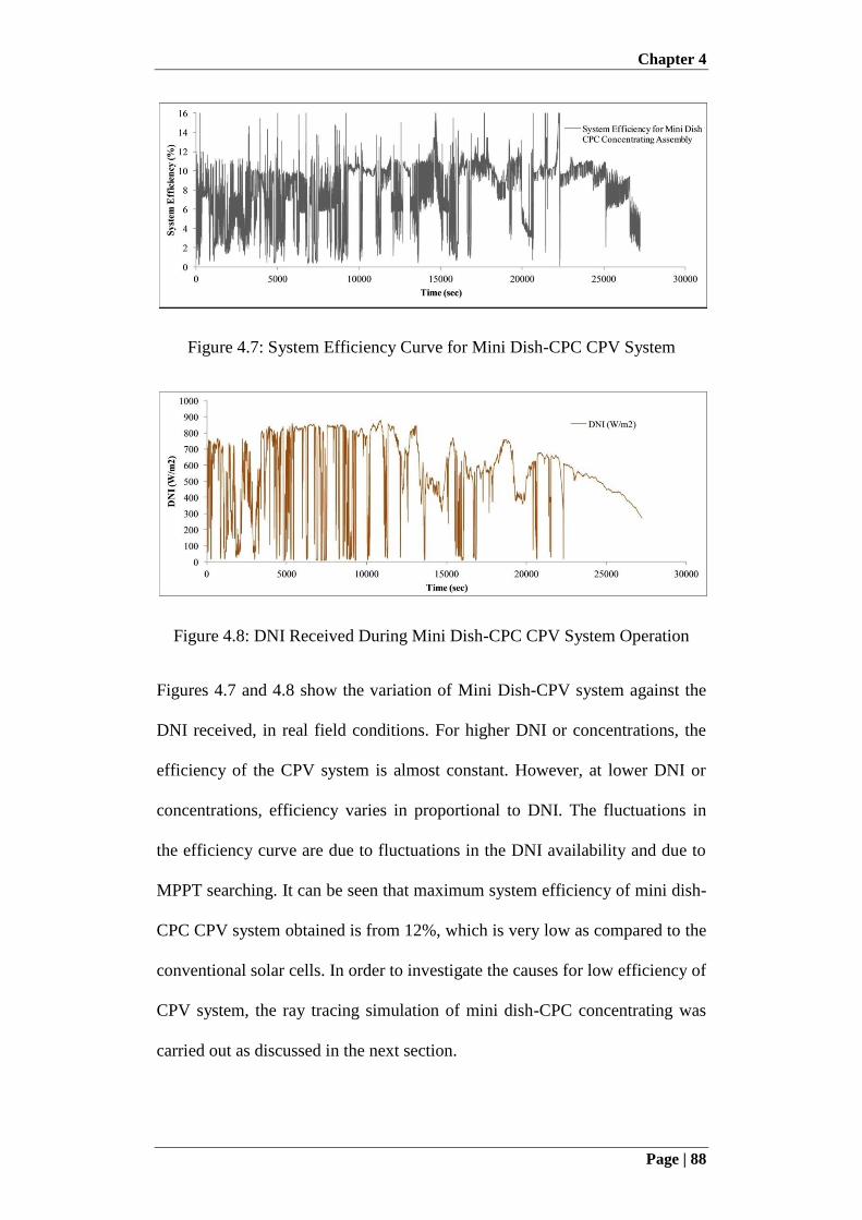
Chapter 4

Page | 88

Figure 4.7: System Efficiency Curve for Mini Dish-CPC CPV System

Figure 4.8: DNI Received During Mini Dish-CPC CPV System Operation

Figures 4.7 and 4.8 show the variation of Mini Dish-CPV system against the

DNI received, in real field conditions. For higher DNI or concentrations, the

efficiency of the CPV system is almost constant. However, at lower DNI or

concentrations, efficiency varies in proportional to DNI. The fluctuations in

the efficiency curve are due to fluctuations in the DNI availability and due to

MPPT searching. It can be seen that maximum system efficiency of mini dish-

CPC CPV system obtained is from 12%, which is very low as compared to the

conventional solar cells. In order to investigate the causes for low efficiency of

CPV system, the ray tracing simulation of mini dish-CPC concentrating was

carried out as discussed in the next section.

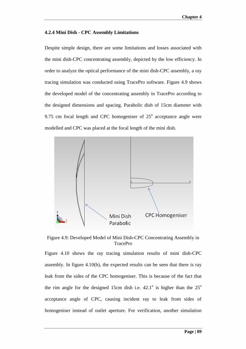
Chapter 4

Page | 89

4.2.4 Mini Dish - CPC Assembly Limitations

Despite simple design, there are some limitations and losses associated with

the mini dish-CPC concentrating assembly, depicted by the low efficiency. In

order to analyze the optical performance of the mini dish-CPC assembly, a ray

tracing simulation was conducted using TracePro software. Figure 4.9 shows

the developed model of the concentrating assembly in TracePro according to

the designed dimensions and spacing. Parabolic dish of 15cm diameter with

9.75 cm focal length and CPC homogeniser of 25o acceptance angle were

modelled and CPC was placed at the focal length of the mini dish.

Figure 4.9: Developed Model of Mini Dish-CPC Concentrating Assembly in

TracePro

Figure 4.10 shows the ray tracing simulation results of mini dish-CPC

assembly. In figure 4.10(b), the expected results can be seen that there is ray

leak from the sides of the CPC homogeniser. This is because of the fact that

the rim angle for the designed 15cm dish i.e. 42.1o is higher than the 25

o

acceptance angle of CPC, causing incident ray to leak from sides of

homogeniser instead of outlet aperture. For verification, another simulation

Chapter 4

Page | 90

was conducted by considering only that area of dish for which the rim angle is

25o, as shown in Figure 4.11. It can be seen that all of the incident rays are

making it towards outlet aperture of CPC.

(a)

(b)

Figure 4.10: Ray Tracing Simulation of CPV Concentrating Assembly

(a) (b)

Figure 4.11: Ray Tracing Simulation of CPV Concentrating Assembly (a)

with Angle Less than Acceptance Angle of Homogeniser (b) Effective

Radius of Parabolic Dish

Chapter 4

Page | 91

The optical loss discussed above is associated with the design limitations.

However, there is another inherent optical loss associated with the design of

dielectric filled CPC, which occurs even if the incident ray angle is within the

acceptance angle of CPC. From Figures 4.10(b) and 4.11(a), it can be seen that

some of the rays are reflected back from CPC outlet aperture. This is due to

TIR at outlet aperture as the striking ray angle is greater than the critical angle

of glass material. The rays hitting near to outlet aperture make angle always

greater than the critical angle of CPC material and are reflected back at outlet

aperture due to TIR. This rays loss is always associated with dielectric filled

CPC design. The effective radius of parabolic dish with rim angle of 25o is

shown in Figure 4.11(b). In order to have smaller incident ray angle at

homogeniser inlet and to avoid TIR at outlet of homogeniser, the

concentrating assembly is redesigned in cassegrain arrangement as explained

in the next section.

4.3 Mini Dish Cassegrain Arrangement Concentrating

Assembly Design

A schematic of the mini dish cassegrain arrangement concentrating assembly

is shown in Figure 4.12. The cassegrain concentrating assembly is a double-

stage concentrator where primary concentrator is a parabolic reflector with

focal length fpr, while secondary concentrator is a small hyperbolic reflector

with two focal points f1hp and f2hp. Parallel or beam rays after being reflected

from primary reflector try to converge at focal point fpr. However, the

secondary hyperbolic reflector, placed in the path of converging rays such that

focal points of both primary and secondary reflectors fpr and f1 coincides,

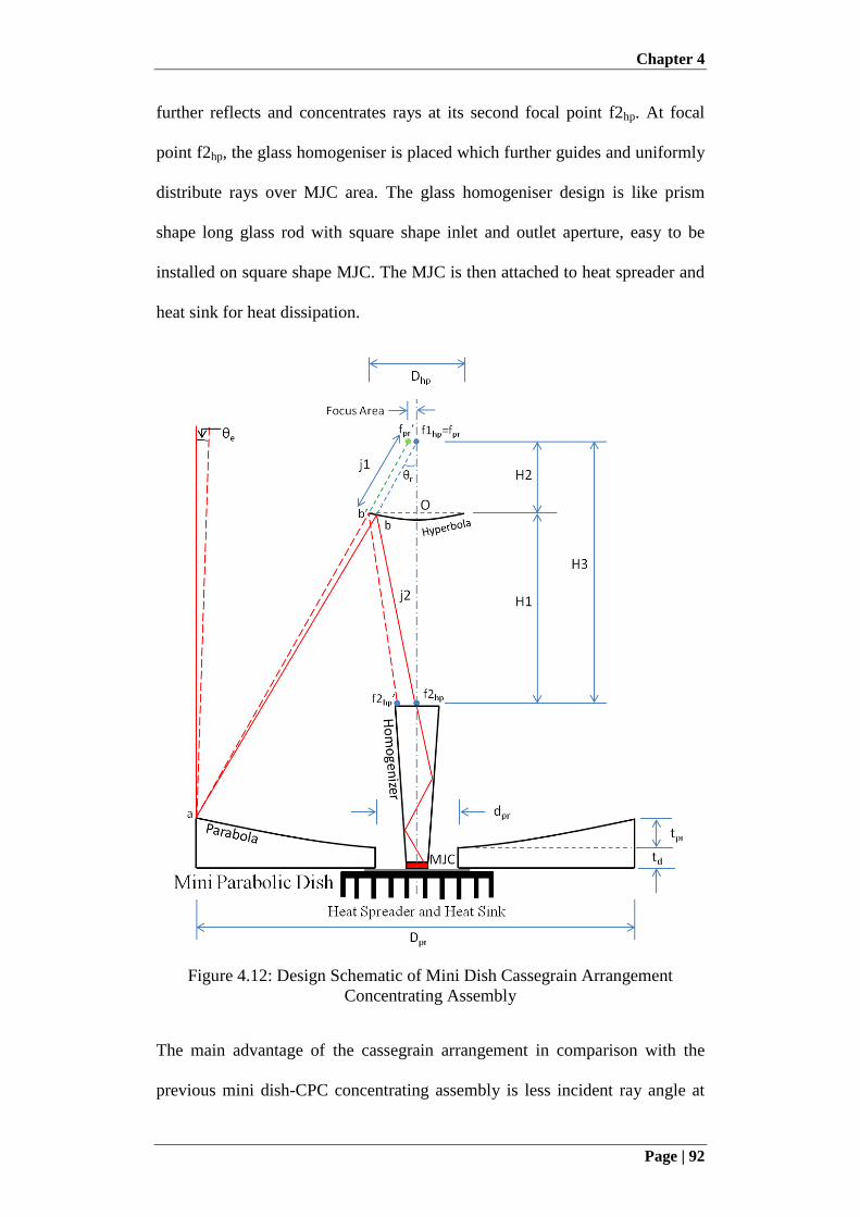
Chapter 4

Page | 92

further reflects and concentrates rays at its second focal point f2hp. At focal

point f2hp, the glass homogeniser is placed which further guides and uniformly

distribute rays over MJC area. The glass homogeniser design is like prism

shape long glass rod with square shape inlet and outlet aperture, easy to be

installed on square shape MJC. The MJC is then attached to heat spreader and

heat sink for heat dissipation.

Figure 4.12: Design Schematic of Mini Dish Cassegrain Arrangement


The main advantage of the cassegrain arrangement in comparison with the

previous mini dish-CPC concentrating assembly is less incident ray angle at

Chapter 4

Page | 93

homogeniser inlet which reduces chance for ray loss at homogeniser outlet due

to TIR and it can be designed for any size of primary reflector regardless of

rim angle limitation. The size calculation of each component of the cassegrain

concentrating assembly, according to space constraints and design

requirements are discussed in next sections.

4.3.1 Primary Reflector - Mini Parabolic Dish

The mini dish parabolic reflector used in this design as discussed in the

previous design, with 15 cm diameter, 9.75 cm focal length fpr and centre hole

dpr of size 2.5 cm which provides space for homogeniser mounting.

4.3.2 Homogeniser

The TECHSPEC tapered light pipe homogenising rod was used as

homogeniser for current concentrating assembly with inlet aperture size of 12

mm x 12 mm, outlet aperture size of 4mm x 4mm and total length of 50 mm.

4.3.3 Secondary Reflector - Hyperbolic Dish

The size of the secondary reflector is of great importance, which is designed

according to the dimensions of primary reflector and homogeniser. Hyperbolic

reflector has two focal points, f1hp and f2hp. Focal point f1hp should coincide

with the focal point of primary reflector However, the position of its second

focal point f2hp is the main design input requirement of hyperbolic reflector.

Moreover, size of the reflector should be as small as possible due to the fact

that smaller size of secondary reflector results in lower ray angle at

homogeniser inlet and less shadow at primary reflector. However, too small

reflector can cause difficulty in fabrication and more ray loss can be

Chapter 4

Page | 94

experienced with even small error in tracking. The hyperbolic reflector is not

only designed for parallel rays but should also accommodate tracking error

with rays not parallel to axis of concentrator. For non-parallel rays, focal point

of primary reflector shifts from fpr to fpr' and focal point f2hp shifts to f2hp'.

Therefore, to accommodate non-parallel rays, size of secondary reflector Ob'

is taken as 3 cm (Dhp). However, in design calculations, the size of the

secondary reflector Ob is taken as 2.5 cm for parallel rays. Moreover, as MJC

is planned to be placed at the bottom end of mini parabolic dish, thus if

thickness of MJC (Mt) is taken as 0.5 mm then the distance between two foci

can be found using Equation (4.9) using 50 mm as length of homogeniser L,

9.75 cm focal length fpr of primary reflector and 1cm as thickness of dish td.

tdpr MLtfH 3 (4.9)

As the rim angle of primary reflector θr is 42.1o, the parameters j1 and H1 can

be found using Equations (4.10) and (4.11) respectively.

r

Ob

jsin

21 (4.10)

r

Ob

Htan

21 (4.11)

So

132 HHH (4.12)

By using the Pythagoras theorem, j2 is given by Equation (4.13).

2

2

222

ObHj (4.13)

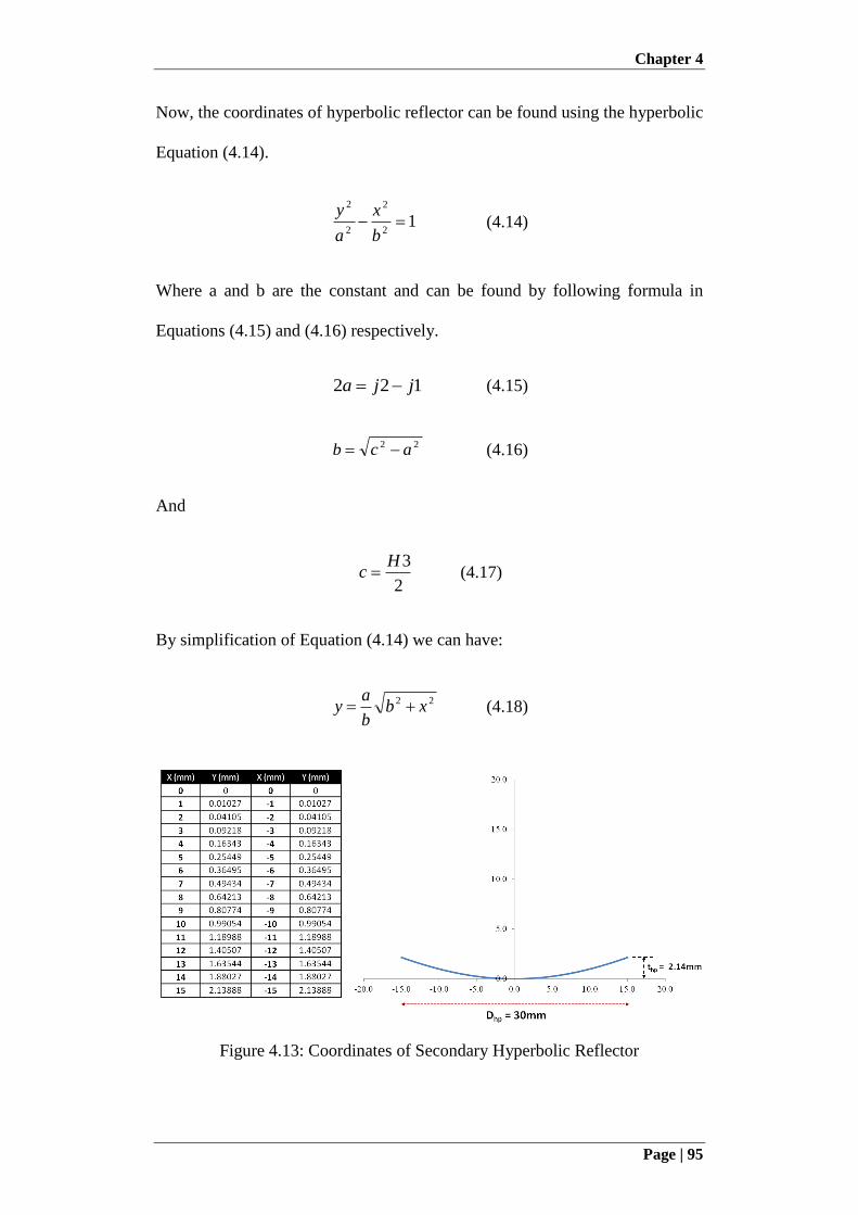
Chapter 4

Page | 95

Now, the coordinates of hyperbolic reflector can be found using the hyperbolic

Equation (4.14).

12

2

2

2

b

x

a

y (4.14)

Where a and b are the constant and can be found by following formula in

Equations (4.15) and (4.16) respectively.

122 jja (4.15)

22 acb (4.16)

And

2

3Hc (4.17)

By simplification of Equation (4.14) we can have:

22 xbb

ay (4.18)

Figure 4.13: Coordinates of Secondary Hyperbolic Reflector

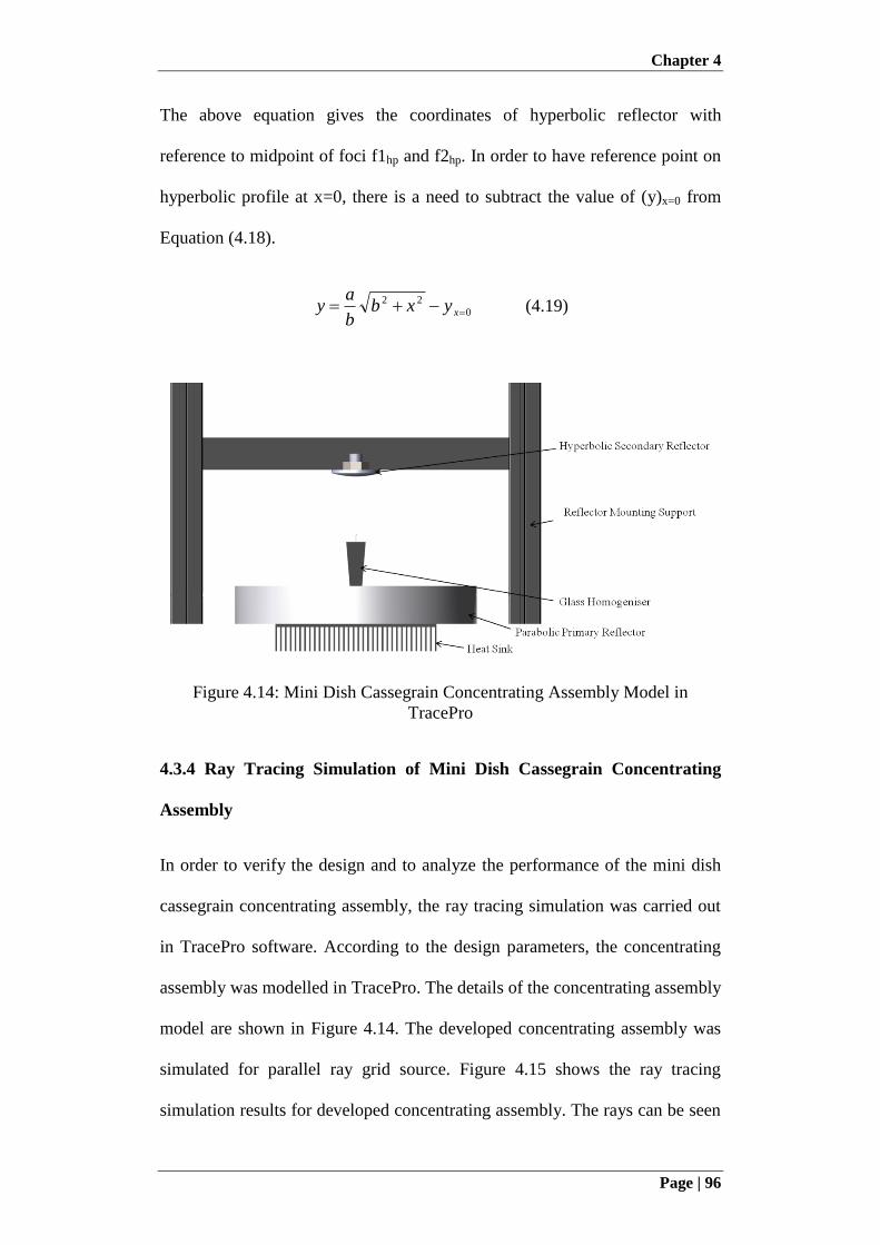
Chapter 4

Page | 96

The above equation gives the coordinates of hyperbolic reflector with

reference to midpoint of foci f1hp and f2hp. In order to have reference point on

hyperbolic profile at x=0, there is a need to subtract the value of (y)x=0 from

Equation (4.18).

0

22

xyxbb

ay (4.19)

Figure 4.14: Mini Dish Cassegrain Concentrating Assembly Model in

TracePro

4.3.4 Ray Tracing Simulation of Mini Dish Cassegrain Concentrating

Assembly

In order to verify the design and to analyze the performance of the mini dish

cassegrain concentrating assembly, the ray tracing simulation was carried out

in TracePro software. According to the design parameters, the concentrating

assembly was modelled in TracePro. The details of the concentrating assembly

model are shown in Figure 4.14. The developed concentrating assembly was

simulated for parallel ray grid source. Figure 4.15 shows the ray tracing

simulation results for developed concentrating assembly. The rays can be seen

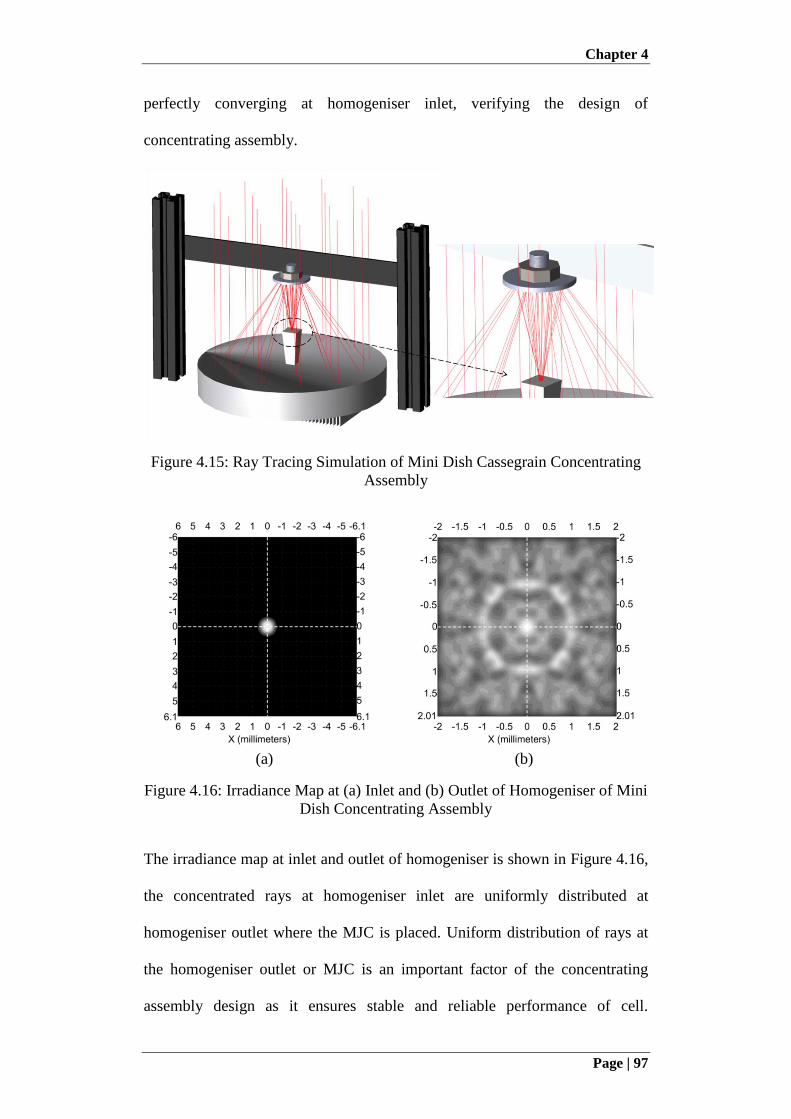
Chapter 4

Page | 97

perfectly converging at homogeniser inlet, verifying the design of

concentrating assembly.

Figure 4.15: Ray Tracing Simulation of Mini Dish Cassegrain Concentrating

Assembly

(a) (b)

Figure 4.16: Irradiance Map at (a) Inlet and (b) Outlet of Homogeniser of Mini

Dish Concentrating Assembly

The irradiance map at inlet and outlet of homogeniser is shown in Figure 4.16,

the concentrated rays at homogeniser inlet are uniformly distributed at

homogeniser outlet where the MJC is placed. Uniform distribution of rays at

the homogeniser outlet or MJC is an important factor of the concentrating

assembly design as it ensures stable and reliable performance of cell.

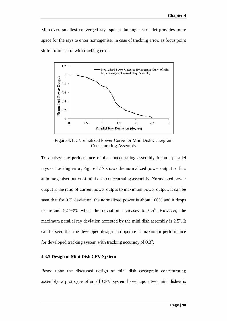
Chapter 4

Page | 98

Moreover, smallest converged rays spot at homogeniser inlet provides more

space for the rays to enter homogeniser in case of tracking error, as focus point

shifts from centre with tracking error.

Figure 4.17: Normalized Power Curve for Mini Dish Cassegrain


To analyze the performance of the concentrating assembly for non-parallel

rays or tracking error, Figure 4.17 shows the normalized power output or flux

at homogeniser outlet of mini dish concentrating assembly. Normalized power

output is the ratio of current power output to maximum power output. It can be

seen that for 0.3o deviation, the normalized power is about 100% and it drops

to around 92-93% when the deviation increases to 0.5o. However, the

maximum parallel ray deviation accepted by the mini dish assembly is 2.5o. It

can be seen that the developed design can operate at maximum performance

for developed tracking system with tracking accuracy of 0.3o.

4.3.5 Design of Mini Dish CPV System

Based upon the discussed design of mini dish cassegrain concentrating

assembly, a prototype of small CPV system based upon two mini dishes is

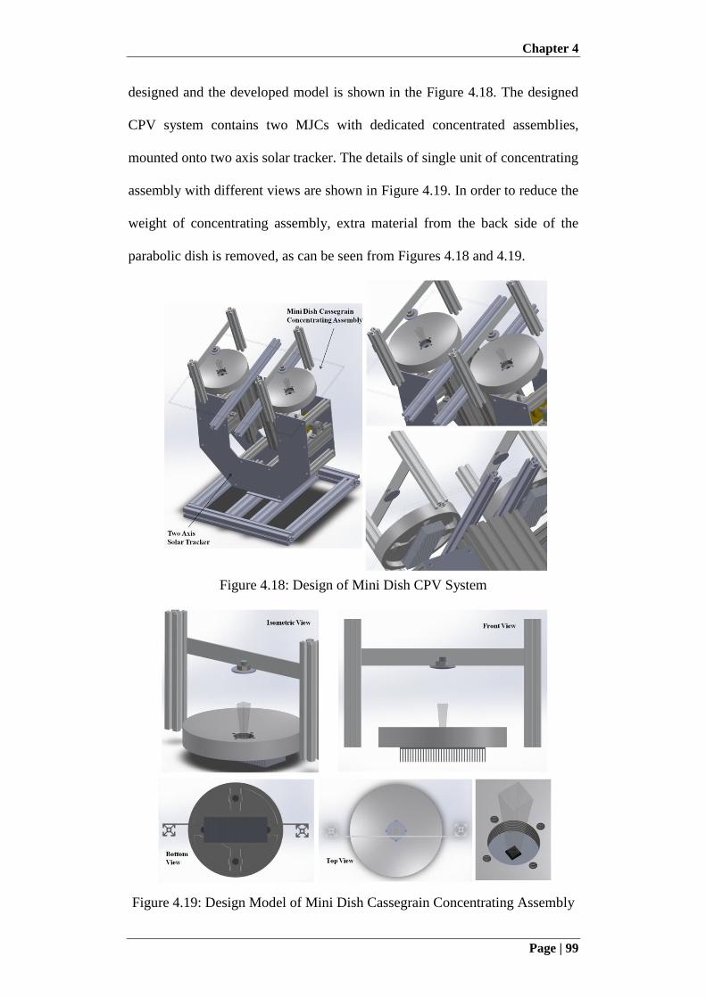
Chapter 4

Page | 99

designed and the developed model is shown in the Figure 4.18. The designed

CPV system contains two MJCs with dedicated concentrated assemblies,

mounted onto two axis solar tracker. The details of single unit of concentrating

assembly with different views are shown in Figure 4.19. In order to reduce the

weight of concentrating assembly, extra material from the back side of the

parabolic dish is removed, as can be seen from Figures 4.18 and 4.19.

Figure 4.18: Design of Mini Dish CPV System

Figure 4.19: Design Model of Mini Dish Cassegrain Concentrating Assembly

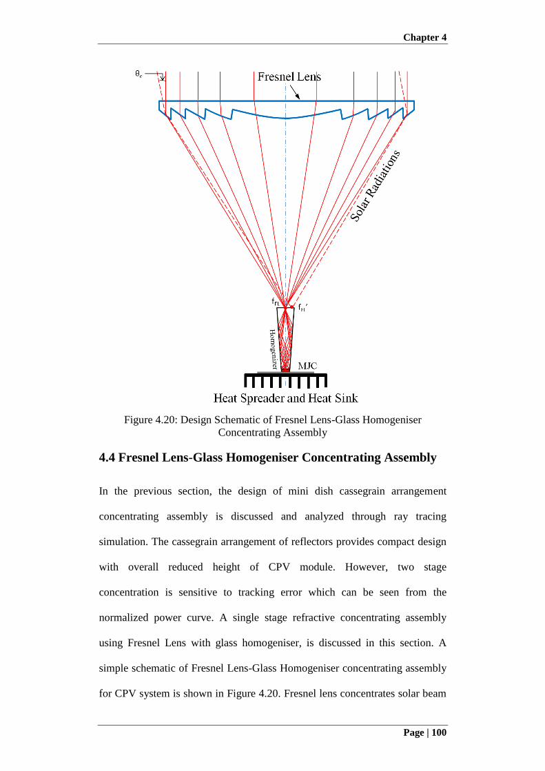
Chapter 4

Page | 100

Figure 4.20: Design Schematic of Fresnel Lens-Glass Homogeniser


4.4 Fresnel Lens-Glass Homogeniser Concentrating Assembly

In the previous section, the design of mini dish cassegrain arrangement

concentrating assembly is discussed and analyzed through ray tracing

simulation. The cassegrain arrangement of reflectors provides compact design

with overall reduced height of CPV module. However, two stage

concentration is sensitive to tracking error which can be seen from the

normalized power curve. A single stage refractive concentrating assembly

using Fresnel Lens with glass homogeniser, is discussed in this section. A

simple schematic of Fresnel Lens-Glass Homogeniser concentrating assembly

for CPV system is shown in Figure 4.20. Fresnel lens concentrates solar beam

Chapter 4

Page | 101

radiation at its focal point fFL where glass homogeniser is placed, which

further guides and uniformly distributes rays onto MJC. Heat Spreader and

heat sink are attached to MJC for heat dissipation.

The main advantage of the Fresnel lens over cassegrain arrangement is the

simple design with less sensitivity to tracking error due to single stage

concentration. However, it has some inherent optical loss at the lens rings. The

detailed design for each of the component of Fresnel Lens-Glass Homogeniser

concentrating assembly for concentration ratio of x476 is discussed as follows.

4.4.1 Glass Homogeniser

For the current design of the Fresnel Lens-Glass Homogeniser concentrating

assembly, optical rod is used as homogeniser with 12 mm x 12 mm inlet

aperture and 5.5 mm x 5.5 mm outlet aperture, same as size of MJC. The

height of the homogeniser is 30 mm.

4.4.2 Fresnel Lens Design

Fresnel lens is a form of plano-convex lens with reduced overall height and

optical material for almost same performance. The lens surface is based upon

aspheric profile as the spherical profile has spherical aberration. The aspheric

profile of current Fresnel lens design is optimized from spherical surface. The

detailed design of Fresnel lens is shown in Figure 4.21. The general sag

equation for lens surface is given by Equation (4.20) [116].

i

L

i

i

LL

LL

L rArCk

rCZ

1

22

2

111 (4.20)

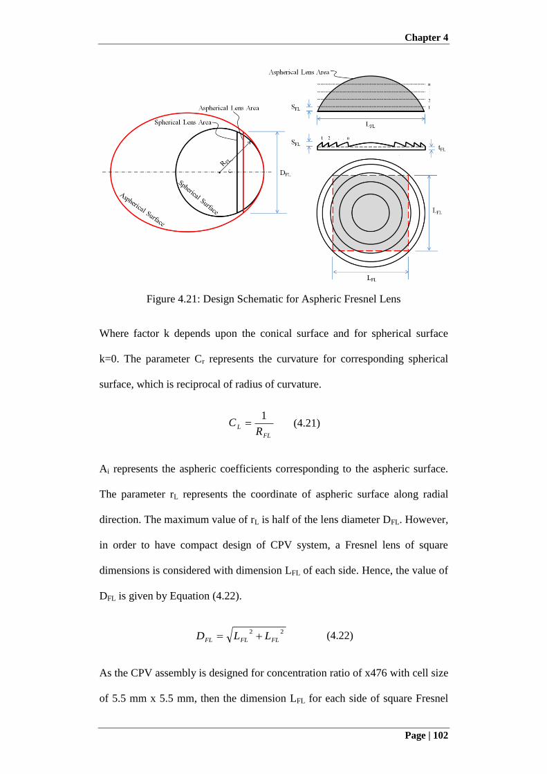
Chapter 4

Page | 102

Figure 4.21: Design Schematic for Aspheric Fresnel Lens

Where factor k depends upon the conical surface and for spherical surface

k=0. The parameter Cr represents the curvature for corresponding spherical

surface, which is reciprocal of radius of curvature.

FL

LR

C1

(4.21)

Ai represents the aspheric coefficients corresponding to the aspheric surface.

The parameter rL represents the coordinate of aspheric surface along radial

direction. The maximum value of rL is half of the lens diameter DFL. However,

in order to have compact design of CPV system, a Fresnel lens of square

dimensions is considered with dimension LFL of each side. Hence, the value of

DFL is given by Equation (4.22).

22

FLFLFL LLD (4.22)

As the CPV assembly is designed for concentration ratio of x476 with cell size

of 5.5 mm x 5.5 mm, then the dimension LFL for each side of square Fresnel

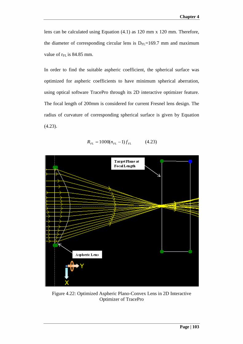
Chapter 4

Page | 103

lens can be calculated using Equation (4.1) as 120 mm x 120 mm. Therefore,

the diameter of corresponding circular lens is DFL=169.7 mm and maximum

value of rFL is 84.85 mm.

In order to find the suitable aspheric coefficient, the spherical surface was

optimized for aspheric coefficients to have minimum spherical aberration,

using optical software TracePro through its 2D interactive optimizer feature.

The focal length of 200mm is considered for current Fresnel lens design. The

radius of curvature of corresponding spherical surface is given by Equation

(4.23).

FLFLFL fnR )1(1000 (4.23)

Figure 4.22: Optimized Aspheric Plano-Convex Lens in 2D Interactive

Optimizer of TracePro

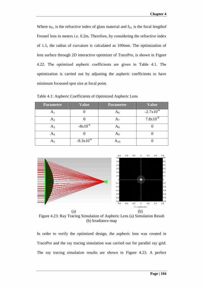
Chapter 4

Page | 104

Where nFL is the refractive index of glass material and fFL is the focal lengthof

Fresnel lens in meters i.e. 0.2m. Therefore, by considering the refractive index

of 1.5, the radius of curvature is calculated as 100mm. The optimization of

lens surface through 2D interactive optimizer of TracePro, is shown in Figure

4.22. The optimized aspheric coefficients are given in Table 4.1. The

optimization is carried out by adjusting the aspheric coefficients to have

minimum focussed spot size at focal point.

Table 4.1: Aspheric Coefficients of Optimized Aspheric Lens

Parameter Value Parameter Value

A1 0 A6 -2.7x10-6

A2 0 A7 7.8x10-8

A3 -8x10-4

A8 0

A4 0 A9 0

A5 -9.3x10-6

A10 0

(a) (b)

Figure 4.23: Ray Tracing Simulation of Aspheric Lens (a) Simulation Result

(b) Irradiance map

In order to verify the optimized design, the aspheric lens was created in

TracePro and the ray tracing simulation was carried out for parallel ray grid.

The ray tracing simulation results are shown in Figure 4.23. A perfect

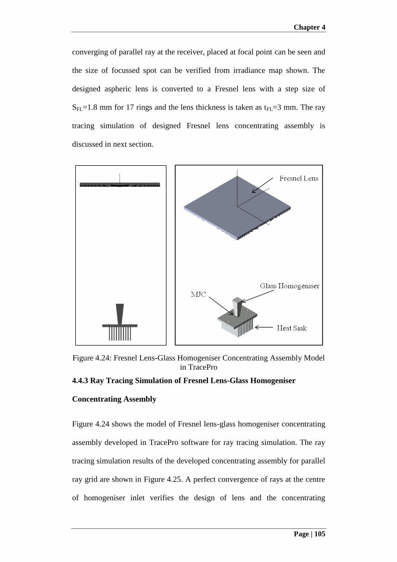
Chapter 4

Page | 105

converging of parallel ray at the receiver, placed at focal point can be seen and

the size of focussed spot can be verified from irradiance map shown. The

designed aspheric lens is converted to a Fresnel lens with a step size of

SFL=1.8 mm for 17 rings and the lens thickness is taken as tFL=3 mm. The ray

tracing simulation of designed Fresnel lens concentrating assembly is

discussed in next section.

Figure 4.24: Fresnel Lens-Glass Homogeniser Concentrating Assembly Model

in TracePro

4.4.3 Ray Tracing Simulation of Fresnel Lens-Glass Homogeniser


Figure 4.24 shows the model of Fresnel lens-glass homogeniser concentrating

assembly developed in TracePro software for ray tracing simulation. The ray

tracing simulation results of the developed concentrating assembly for parallel

ray grid are shown in Figure 4.25. A perfect convergence of rays at the centre

of homogeniser inlet verifies the design of lens and the concentrating

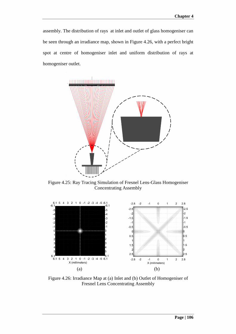
Chapter 4

Page | 106

assembly. The distribution of rays at inlet and outlet of glass homogeniser can

be seen through an irradiance map, shown in Figure 4.26, with a perfect bright

spot at centre of homogeniser inlet and uniform distribution of rays at

homogeniser outlet.

Figure 4.25: Ray Tracing Simulation of Fresnel Lens-Glass Homogeniser


(a) (b)


Fresnel Lens Concentrating Assembly

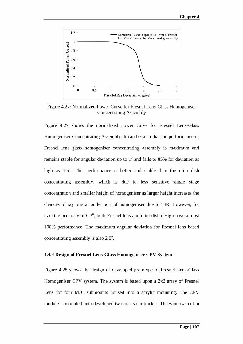
Chapter 4

Page | 107

Figure 4.27: Normalized Power Curve for Fresnel Lens-Glass Homogeniser


Figure 4.27 shows the normalized power curve for Fresnel Lens-Glass

Homogeniser Concentrating Assembly. It can be seen that the performance of

Fresnel lens glass homogeniser concentrating assembly is maximum and

remains stable for angular deviation up to 1o and falls to 85% for deviation as

high as 1.5o. This performance is better and stable than the mini dish

concentrating assembly, which is due to less sensitive single stage

concentration and smaller height of homogeniser as larger height increases the

chances of ray loss at outlet port of homogeniser due to TIR. However, for

tracking accuracy of 0.3o, both Fresnel lens and mini dish design have almost

100% performance. The maximum angular deviation for Fresnel lens based

concentrating assembly is also 2.5o.

4.4.4 Design of Fresnel Lens-Glass Homogeniser CPV System

Figure 4.28 shows the design of developed prototype of Fresnel Lens-Glass

Homogeniser CPV system. The system is based upon a 2x2 array of Fresnel

Lens for four MJC submounts housed into a acrylic mounting. The CPV

module is mounted onto developed two axis solar tracker. The windows cut in

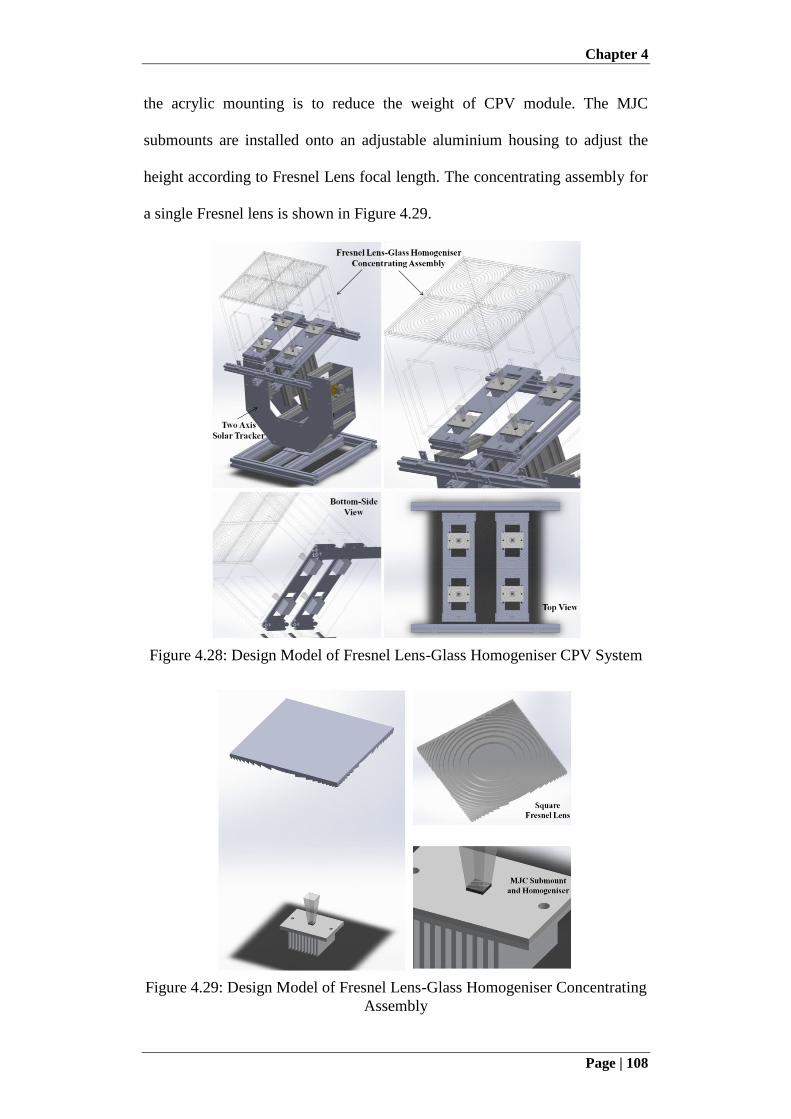
Chapter 4

Page | 108

the acrylic mounting is to reduce the weight of CPV module. The MJC

submounts are installed onto an adjustable aluminium housing to adjust the

height according to Fresnel Lens focal length. The concentrating assembly for

a single Fresnel lens is shown in Figure 4.29.

Figure 4.28: Design Model of Fresnel Lens-Glass Homogeniser CPV System

Figure 4.29: Design Model of Fresnel Lens-Glass Homogeniser Concentrating

Assembly

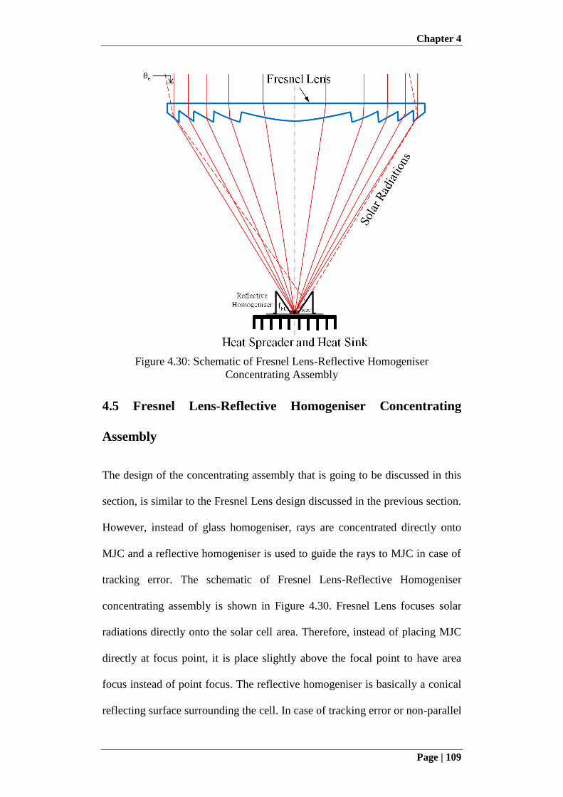
Chapter 4

Page | 109

Figure 4.30: Schematic of Fresnel Lens-Reflective Homogeniser


4.5 Fresnel Lens-Reflective Homogeniser Concentrating

Assembly

The design of the concentrating assembly that is going to be discussed in this

section, is similar to the Fresnel Lens design discussed in the previous section.

However, instead of glass homogeniser, rays are concentrated directly onto

MJC and a reflective homogeniser is used to guide the rays to MJC in case of

tracking error. The schematic of Fresnel Lens-Reflective Homogeniser

concentrating assembly is shown in Figure 4.30. Fresnel Lens focuses solar

radiations directly onto the solar cell area. Therefore, instead of placing MJC

directly at focus point, it is place slightly above the focal point to have area

focus instead of point focus. The reflective homogeniser is basically a conical

reflecting surface surrounding the cell. In case of tracking error or non-parallel

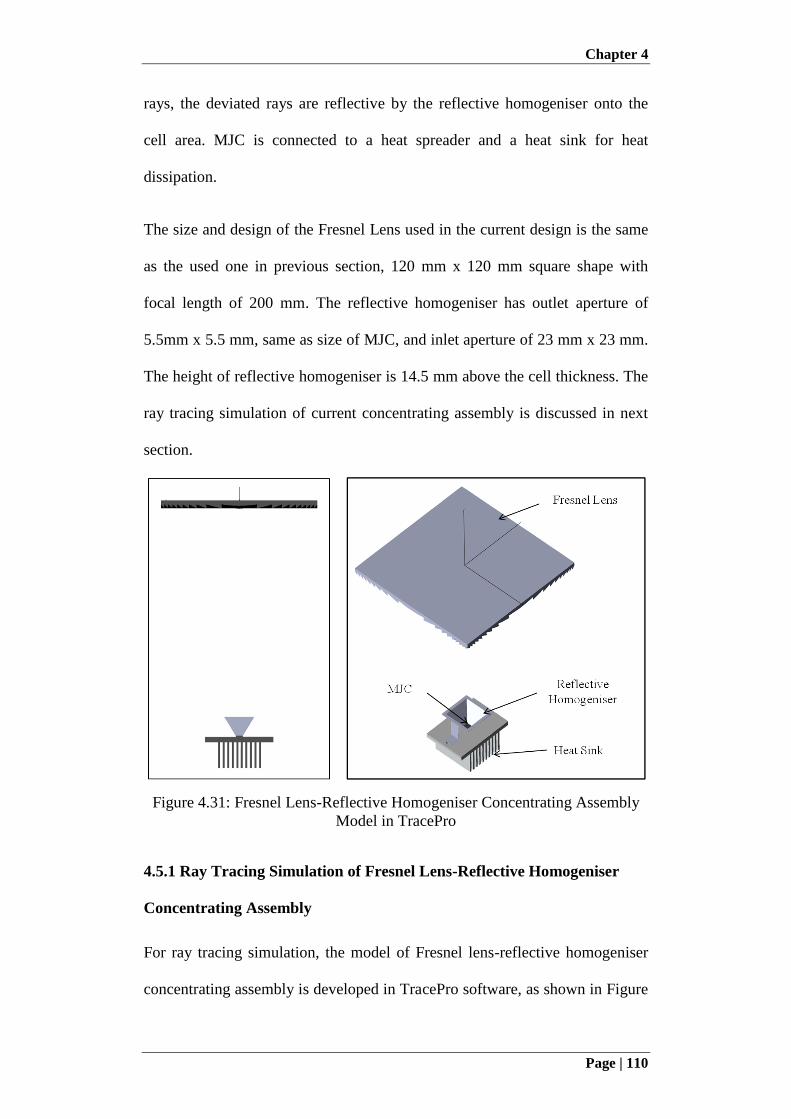
Chapter 4

Page | 110

rays, the deviated rays are reflective by the reflective homogeniser onto the

cell area. MJC is connected to a heat spreader and a heat sink for heat

dissipation.

The size and design of the Fresnel Lens used in the current design is the same

as the used one in previous section, 120 mm x 120 mm square shape with

focal length of 200 mm. The reflective homogeniser has outlet aperture of

5.5mm x 5.5 mm, same as size of MJC, and inlet aperture of 23 mm x 23 mm.

The height of reflective homogeniser is 14.5 mm above the cell thickness. The

ray tracing simulation of current concentrating assembly is discussed in next

section.

Figure 4.31: Fresnel Lens-Reflective Homogeniser Concentrating Assembly

Model in TracePro

4.5.1 Ray Tracing Simulation of Fresnel Lens-Reflective Homogeniser


For ray tracing simulation, the model of Fresnel lens-reflective homogeniser

concentrating assembly is developed in TracePro software, as shown in Figure

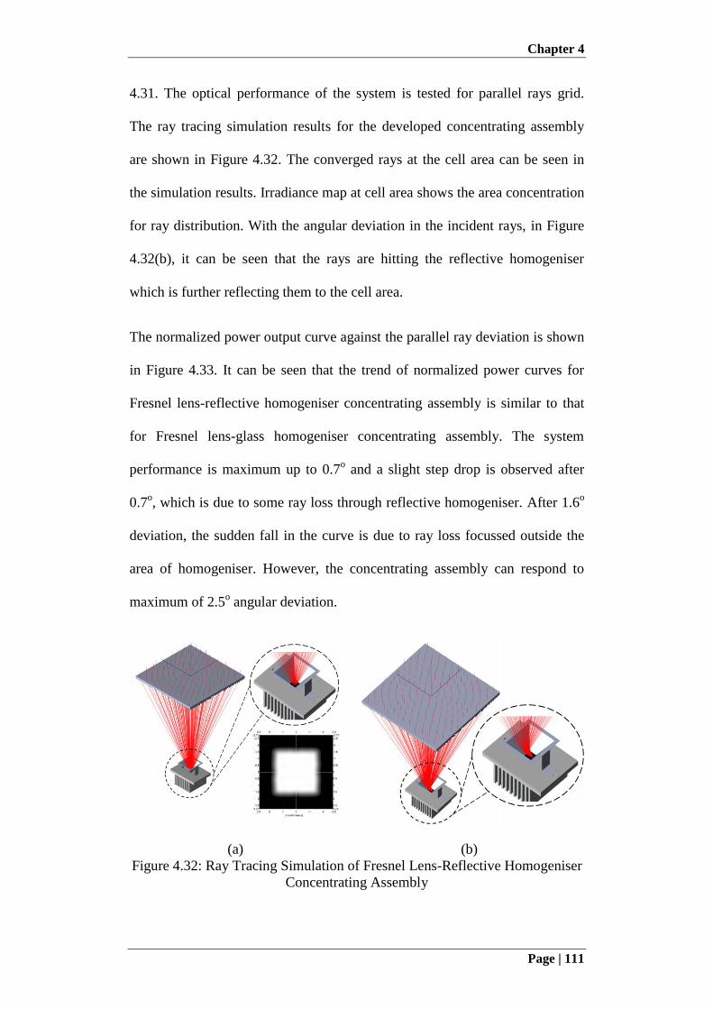
Chapter 4

Page | 111

4.31. The optical performance of the system is tested for parallel rays grid.

The ray tracing simulation results for the developed concentrating assembly

are shown in Figure 4.32. The converged rays at the cell area can be seen in

the simulation results. Irradiance map at cell area shows the area concentration

for ray distribution. With the angular deviation in the incident rays, in Figure

4.32(b), it can be seen that the rays are hitting the reflective homogeniser

which is further reflecting them to the cell area.

The normalized power output curve against the parallel ray deviation is shown

in Figure 4.33. It can be seen that the trend of normalized power curves for

Fresnel lens-reflective homogeniser concentrating assembly is similar to that

for Fresnel lens-glass homogeniser concentrating assembly. The system

performance is maximum up to 0.7o and a slight step drop is observed after

0.7o, which is due to some ray loss through reflective homogeniser. After 1.6

o

deviation, the sudden fall in the curve is due to ray loss focussed outside the

area of homogeniser. However, the concentrating assembly can respond to

maximum of 2.5o angular deviation.

(a) (b)

Figure 4.32: Ray Tracing Simulation of Fresnel Lens-Reflective Homogeniser


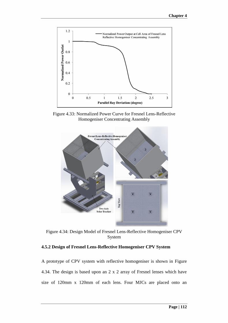
Chapter 4

Page | 112

Figure 4.33: Normalized Power Curve for Fresnel Lens-Reflective


Figure 4.34: Design Model of Fresnel Lens-Reflective Homogeniser CPV

System

4.5.2 Design of Fresnel Lens-Reflective Homogeniser CPV System

A prototype of CPV system with reflective homogeniser is shown in Figure

4.34. The design is based upon an 2 x 2 array of Fresnel lenses which have

size of 120mm x 120mm of each lens. Four MJCs are placed onto an

Chapter 4

Page | 113

aluminium base which provides mounting support and acts as heat spreader

and heat sink. Reflective homogenisers are then placed on each of MJC

submount. This whole assembly is housed into an aluminium frame and

mounted onto a developed two axis solar tracker. The arrangement of the

single lens MJC assembly is also shown in Figure 4.35.

Figure 4.35: Design Model of Fresnel Lens-Reflective Homogeniser


4.6 Summary

In this chapter, the different designs of the concentrating assemblies for CPV

system are introduced and discussed with their performance analysis using ray

tracing simulation. The concentrating assemblies are comprising of reflective

concentrator using mini parabolic dish and refractive concentrator using

Fresnel lens. The analysis was first carried out on a single stage concentrating

assembly with mini parabolic dish as reflective concentrator and compound

parabolic concentrator (CPC) as homogeniser. Due to inherent optical loss of

concentrating assembly at outlet aperture of homogeniser, the low efficiency

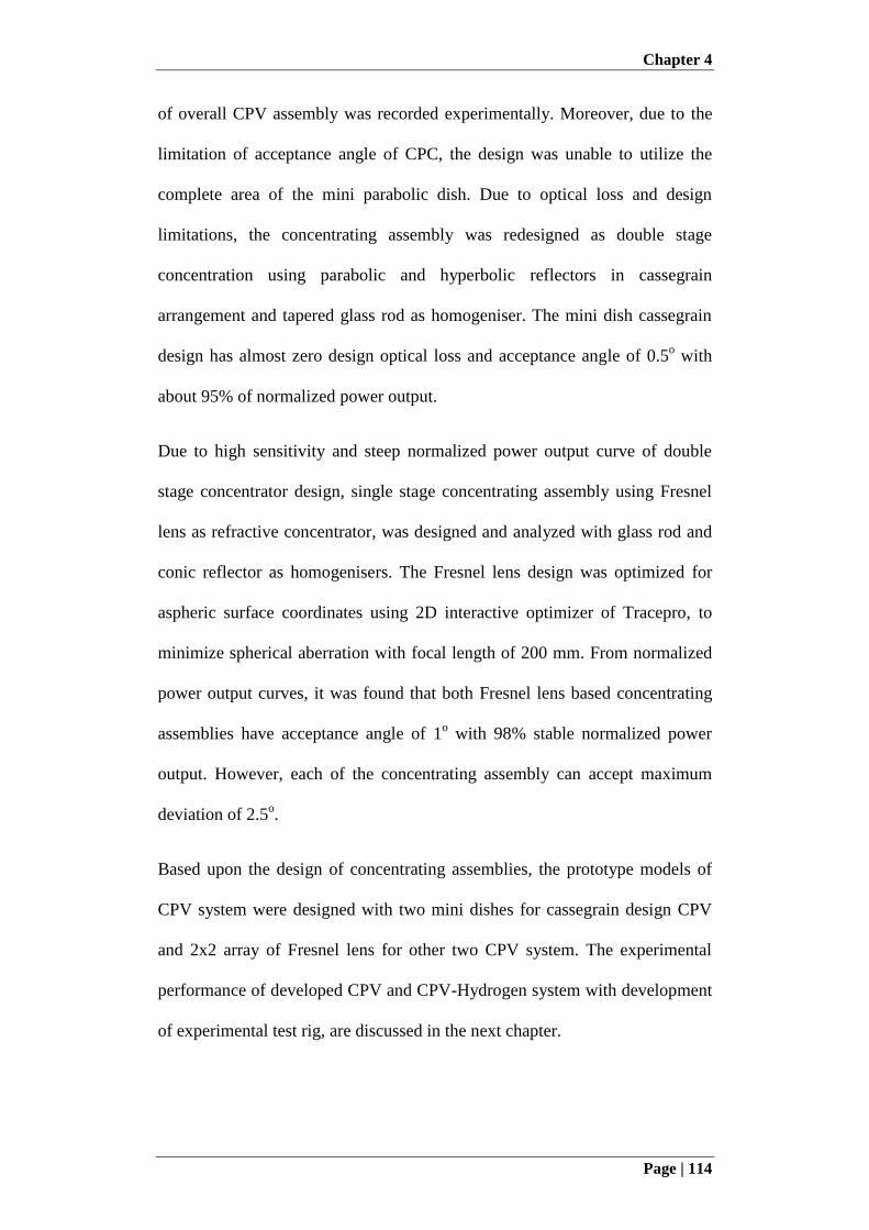
Chapter 4

Page | 114

of overall CPV assembly was recorded experimentally. Moreover, due to the

limitation of acceptance angle of CPC, the design was unable to utilize the

complete area of the mini parabolic dish. Due to optical loss and design

limitations, the concentrating assembly was redesigned as double stage

concentration using parabolic and hyperbolic reflectors in cassegrain

arrangement and tapered glass rod as homogeniser. The mini dish cassegrain

design has almost zero design optical loss and acceptance angle of 0.5o with

about 95% of normalized power output.

Due to high sensitivity and steep normalized power output curve of double

stage concentrator design, single stage concentrating assembly using Fresnel

lens as refractive concentrator, was designed and analyzed with glass rod and

conic reflector as homogenisers. The Fresnel lens design was optimized for

aspheric surface coordinates using 2D interactive optimizer of Tracepro, to

minimize spherical aberration with focal length of 200 mm. From normalized

power output curves, it was found that both Fresnel lens based concentrating

assemblies have acceptance angle of 1o with 98% stable normalized power

output. However, each of the concentrating assembly can accept maximum

deviation of 2.5o.

Based upon the design of concentrating assemblies, the prototype models of

CPV system were designed with two mini dishes for cassegrain design CPV

and 2x2 array of Fresnel lens for other two CPV system. The experimental

performance of developed CPV and CPV-Hydrogen system with development

of experimental test rig, are discussed in the next chapter.

Chapter 5

Page | 115

Chapter 5: Experimental Investigation of Concentrated

Photovoltaic (CPV) System and CPV-Hydrogen System

5.1 Introduction

In the previous chapters, firstly the development of the two axis solar tracking

system is discussed with required CPV tracking accuracy. Secondly, the

concentrating assemblies with mini parabolic dish and the Fresnel lens were

designed and analyzed using ray tracing simulation. Based upon the designed

parameters of the concentrating assemblies, the prototypes of the CPV system

were then designed and modelled. The main focus of this chapter is to analyze

the real field experimental performance of the developed CPV and CPV-

Hydrogen systems..

Besides the ray tracing simulation, the experimental investigation of the CPV

system is very important as the concentrating assembly of the CPV system is

designed for rays parallel to the concentrator axis. However, the solar

radiations hitting the surface are not parallel as the sun subtends an angle on

the earth because of the finite distance and diameter. Moreover, the material of

the concentrator and its surface quality also define performance of the CPV

system, which cannot be simulated through the ray tracing simulation.

Furthermore, the performance of the multi-junction solar cell also depends

upon different parameters like cell temperature and concentration. The

temperature of cell and the solar concentration change during the whole day as

it depends upon direct normal irradiance (DNI), which doesn't remain constant

in actual field conditions. Due to these performance affecting parameters, its

Chapter 5

Page | 116

experimental investigation CPV is of prime importance in the system

development.

Similarly, as the hydrogen production through electrolysis is claimed to be the

suitable option for the energy storage, so the field performance of the CPV

system for the production of hydrogen is important to investigate the real

potential of the CPV-Hydrogen system. In addition, the performance of the

electrolyser depends upon the power supplied by the CPV system, which

changes continuously throughout the day. Therefore, the maximum and the

average experimental performance of the CPV-Hydrogen system is analyzed

which can be expected under different climate conditions

In this chapter, first the design of the test rig developed for control and

operation of CPV system is discussed, followed by the fabrication and the real

field testing of each of the developed CPV system. The simulated and

experimental performances of all the CPV systems are then compared. After

performance investigation of the CPV system, the design and development of

the CPV-Hydrogen system with the hydrogen compression unit is discussed.

Through the CPV-Hydrogen experimentation, the real hydrogen production

potential is analyzed under different weather conditions.

5.2 CPV Experimental Setup Description

Figure 5.1 shows the design model of the experimental setup, developed to

investigate the performance of CPV system. All the four CPV systems are

placed together onto a frame built through aluminium extrusion. All the

control boxes along with the power supply system and other electronic

components are placed in an enclosed compartment at bottom of the frame.

Chapter 5

Page | 117

The four CPV trackers are placed onto top aluminium base which is protected

through sliding covers. The sliding covers are used to protect the trackers in

case of rain and non-operational time.

The covers are mounted onto sliders which moves into guide rails. The design

of three CPV systems, Mini Dish Cassegrain CPV, Fresnel Lens-Glass

Homogeniser CPV and Fresnel Lens-Reflective Homogeniser CPV, is

discussed in the previous chapter. However, the design of fourth CPV system,

Multi-Leg Homogeniser CPV is based upon novel design of multi-leg

homogenise, which will be discussed and analyzed in chapter 7. In order to

record the performance parameters of the CPV, the schematic of the control

circuit for developed CPV experimental setup is shown in Figure 5.2. As

discussed in previous chapters, one of the tracker acts as master and other

three tracker operate as slave trackers.

Figure 5.1:Design Model of CPV Systems Experimental Setup

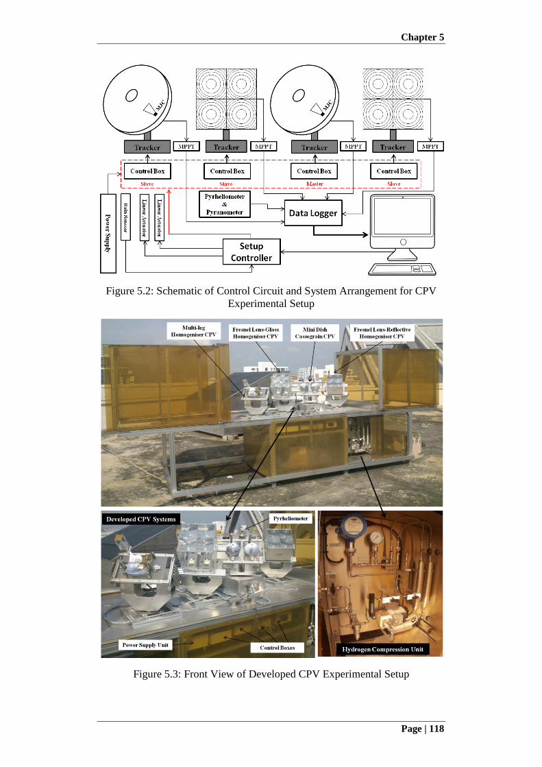
Chapter 5

Page | 118

Figure 5.2: Schematic of Control Circuit and System Arrangement for CPV

Experimental Setup

Figure 5.3: Front View of Developed CPV Experimental Setup

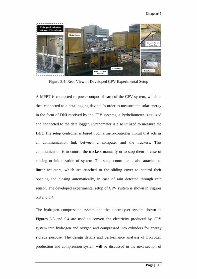
Chapter 5

Page | 119

Figure 5.4: Rear View of Developed CPV Experimental Setup

A MPPT is connected to power output of each of the CPV system, which is

then connected to a data logging device. In order to measure the solar energy

in the form of DNI received by the CPV systems, a Pyrheliometer is utilized

and connected to the data logger. Pyranometer is also utilized to measure the

DHI. The setup controller is based upon a microcontroller circuit that acts as

an communication link between a computer and the trackers. This

communication is to control the trackers manually or to stop them in case of

closing or initialization of system. The setup controller is also attached to

linear actuators, which are attached to the sliding cover to control their

opening and closing automatically, in case of rain detected through rain

sensor. The developed experimental setup of CPV system is shown in Figures

5.3 and 5.4.

The hydrogen compression system and the electrolyser system shown in

Figures 5.3 and 5.4 are used to convert the electricity produced by CPV

system into hydrogen and oxygen and compressed into cylinders for energy

storage purpose. The design details and performance analysis of hydrogen

production and compression system will be discussed in the next section of

Chapter 5

Page | 120

this chapter. The Pyrheliometer is installed on the master tracker which needs

to track the sun for its operation. The Pyranometer is placed horizontally on

top of aluminium base. In order to log and analyze the CPV performance data,

a control and analysis program is developed in LabVIEW software.

The LabVIEW program is developed to perform different tasks; it

communicates and extracts the CPV performance data from data logger and it

also controls the trackers for manual operation with control of linear actuators.

Both data logger and setup controller communicate with the LabVIEW

through serial communication. The CPV performance data received is based

upon the total current and voltage output from the CPV systems. The data is

then analyzed to compute the total system power output and system efficiency,

which are plotted on real time and saved as a spreadsheet file. The power

output PCPV and system efficiency ηCPV of CPV are computed by Equations

(5.1) and (5.2).

CPVCPVCPV IVP (5.1)

con

CPV

CPVADNI

P

(5.2)

Where VCPV and ICPV are the total voltage and current output from the CPV

system, respectively. The DNI is the beam irradiance received from

pyrheliometer and Acon is the total effective area of the concentrator. The

description and performance analysis of individual systems are discussed in

the following sections.

5.3 Mini Dish Cassegrain CPV System

Figure 5.5 shows the developed prototype of Mini Dish Cassegrain CPV

system according to design as discussed in the previous chapters. The glass

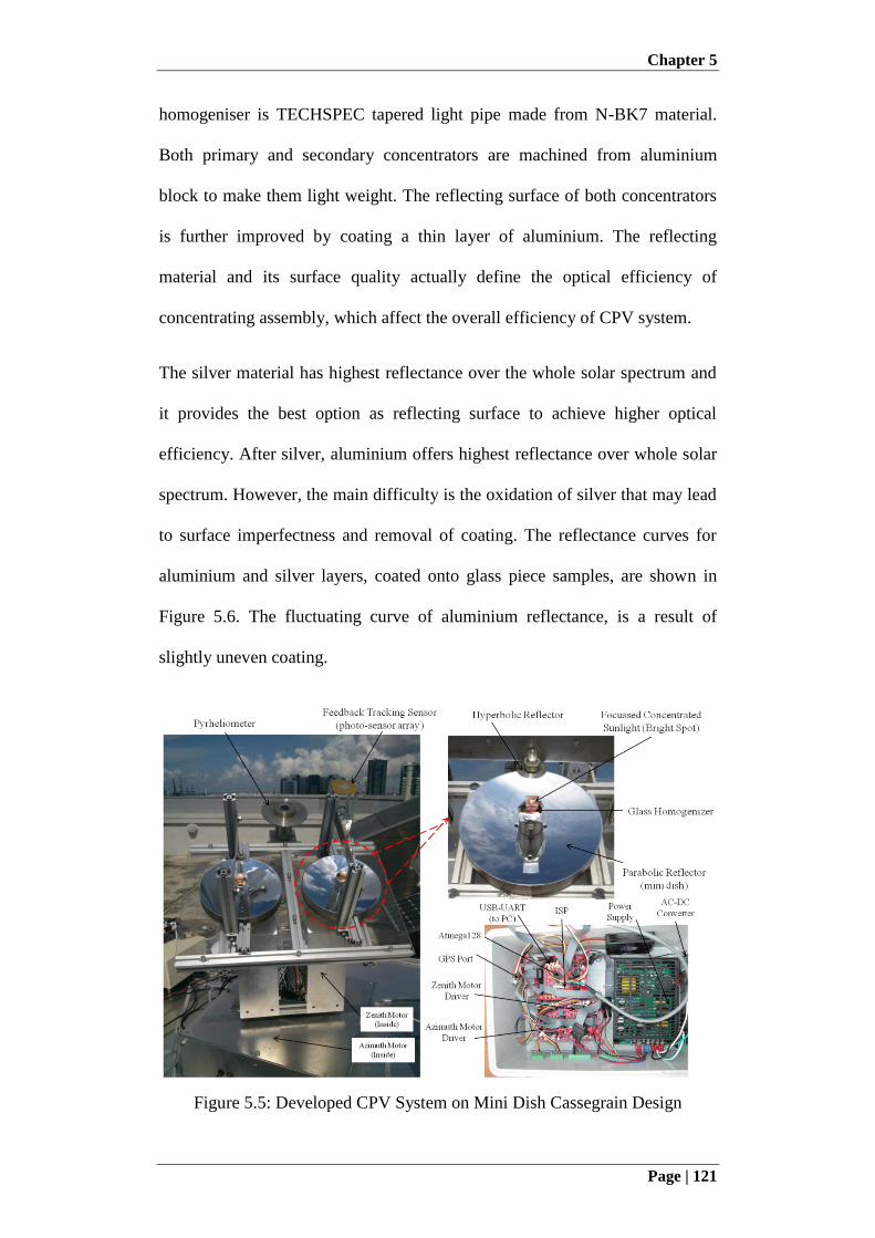
Chapter 5

Page | 121

homogeniser is TECHSPEC tapered light pipe made from N-BK7 material.

Both primary and secondary concentrators are machined from aluminium

block to make them light weight. The reflecting surface of both concentrators

is further improved by coating a thin layer of aluminium. The reflecting

material and its surface quality actually define the optical efficiency of

concentrating assembly, which affect the overall efficiency of CPV system.

The silver material has highest reflectance over the whole solar spectrum and

it provides the best option as reflecting surface to achieve higher optical

efficiency. After silver, aluminium offers highest reflectance over whole solar

spectrum. However, the main difficulty is the oxidation of silver that may lead

to surface imperfectness and removal of coating. The reflectance curves for

aluminium and silver layers, coated onto glass piece samples, are shown in

Figure 5.6. The fluctuating curve of aluminium reflectance, is a result of

slightly uneven coating.

Figure 5.5: Developed CPV System on Mini Dish Cassegrain Design

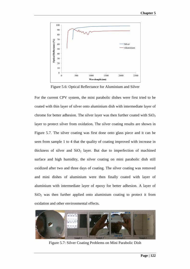
Chapter 5

Page | 122

Figure 5.6: Optical Reflectance for Aluminium and Silver

For the current CPV system, the mini parabolic dishes were first tried to be

coated with thin layer of silver onto aluminium dish with intermediate layer of

chrome for better adhesion. The silver layer was then further coated with SiO2

layer to protect silver from oxidation. The silver coating results are shown in

Figure 5.7. The silver coating was first done onto glass piece and it can be

seen from sample 1 to 4 that the quality of coating improved with increase in

thickness of silver and SiO2 layer. But due to imperfection of machined

surface and high humidity, the silver coating on mini parabolic dish still

oxidized after two and three days of coating. The silver coating was removed

and mini dishes of aluminium were then finally coated with layer of

aluminium with intermediate layer of epoxy for better adhesion. A layer of

SiO2 was then further applied onto aluminium coating to protect it from

oxidation and other environmental effects.

Figure 5.7: Silver Coating Problems on Mini Parabolic Dish

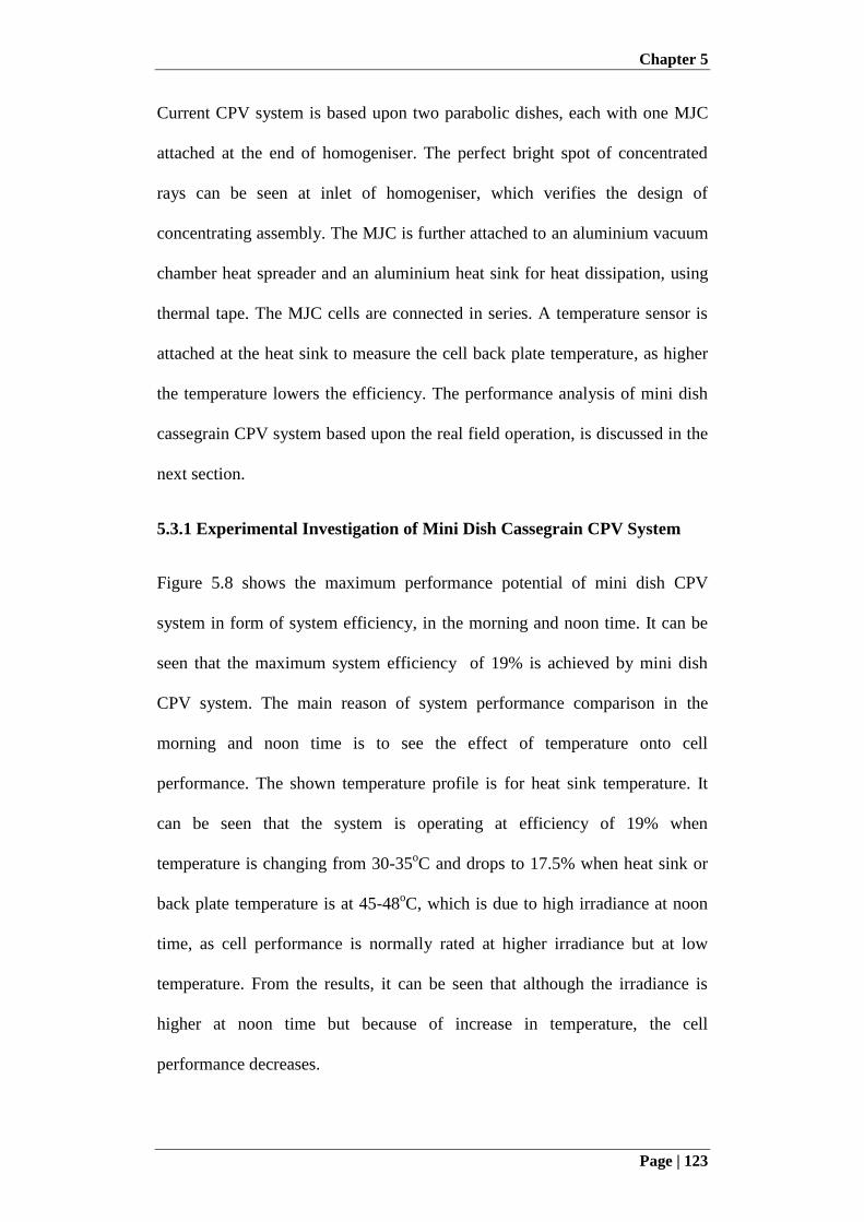
Chapter 5

Page | 123

Current CPV system is based upon two parabolic dishes, each with one MJC

attached at the end of homogeniser. The perfect bright spot of concentrated

rays can be seen at inlet of homogeniser, which verifies the design of

concentrating assembly. The MJC is further attached to an aluminium vacuum

chamber heat spreader and an aluminium heat sink for heat dissipation, using

thermal tape. The MJC cells are connected in series. A temperature sensor is

attached at the heat sink to measure the cell back plate temperature, as higher

the temperature lowers the efficiency. The performance analysis of mini dish

cassegrain CPV system based upon the real field operation, is discussed in the

next section.

5.3.1 Experimental Investigation of Mini Dish Cassegrain CPV System

Figure 5.8 shows the maximum performance potential of mini dish CPV

system in form of system efficiency, in the morning and noon time. It can be

seen that the maximum system efficiency of 19% is achieved by mini dish

CPV system. The main reason of system performance comparison in the

morning and noon time is to see the effect of temperature onto cell

performance. The shown temperature profile is for heat sink temperature. It

can be seen that the system is operating at efficiency of 19% when

temperature is changing from 30-35oC and drops to 17.5% when heat sink or

back plate temperature is at 45-48oC, which is due to high irradiance at noon

time, as cell performance is normally rated at higher irradiance but at low

temperature. From the results, it can be seen that although the irradiance is

higher at noon time but because of increase in temperature, the cell

performance decreases.

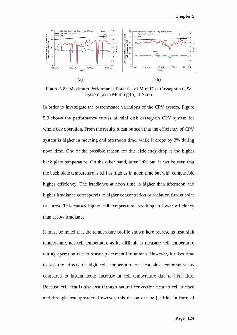
Chapter 5

Page | 124

(a) (b)

Figure 5.8: Maximum Performance Potential of Mini Dish Cassegrain CPV

System (a) in Morning (b) at Noon

In order to investigate the performance variations of the CPV system, Figure

5.9 shows the performance curves of mini dish cassegrain CPV system for

whole day operation. From the results it can be seen that the efficiency of CPV

system is higher in morning and afternoon time, while it drops by 3% during

noon time. One of the possible reason for this efficiency drop is the higher

back plate temperature. On the other hand, after 3:00 pm, it can be seen that

the back plate temperature is still as high as in noon time but with comparable

higher efficiency. The irradiance at noon time is higher than afternoon and

higher irradiance corresponds to higher concentration or radiation flux at solar

cell area. This causes higher cell temperature, resulting in lower efficiency

than at low irradiance.

It must be noted that the temperature profile shown here represents heat sink

temperature, not cell temperature as its difficult to measure cell temperature

during operation due to sensor placement limitations. However, it takes time

to see the effects of high cell temperature on heat sink temperature, as

compared to instantaneous increase in cell temperature due to high flux.

Because cell heat is also lost through natural convection near to cell surface

and through heat spreader. However, this reason can be justified in form of

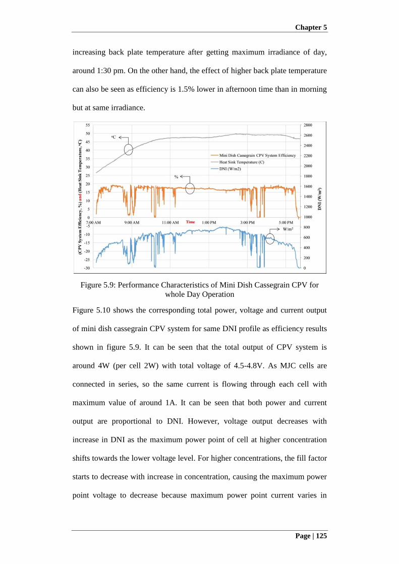
Chapter 5

Page | 125

increasing back plate temperature after getting maximum irradiance of day,

around 1:30 pm. On the other hand, the effect of higher back plate temperature

can also be seen as efficiency is 1.5% lower in afternoon time than in morning

but at same irradiance.

Figure 5.9: Performance Characteristics of Mini Dish Cassegrain CPV for

whole Day Operation

Figure 5.10 shows the corresponding total power, voltage and current output

of mini dish cassegrain CPV system for same DNI profile as efficiency results

shown in figure 5.9. It can be seen that the total output of CPV system is

around 4W (per cell 2W) with total voltage of 4.5-4.8V. As MJC cells are

connected in series, so the same current is flowing through each cell with

maximum value of around 1A. It can be seen that both power and current

output are proportional to DNI. However, voltage output decreases with

increase in DNI as the maximum power point of cell at higher concentration

shifts towards the lower voltage level. For higher concentrations, the fill factor

starts to decrease with increase in concentration, causing the maximum power

point voltage to decrease because maximum power point current varies in

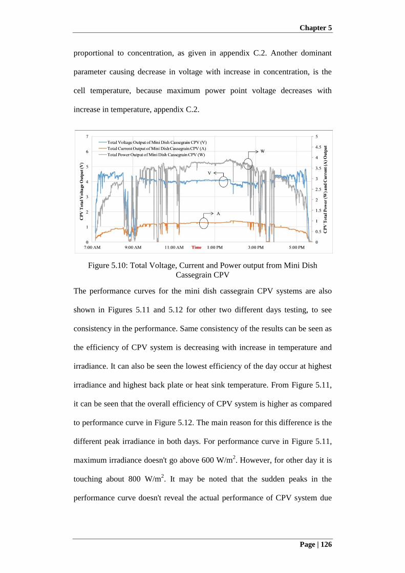
Chapter 5

Page | 126

proportional to concentration, as given in appendix C.2. Another dominant

parameter causing decrease in voltage with increase in concentration, is the

cell temperature, because maximum power point voltage decreases with

increase in temperature, appendix C.2.

Figure 5.10: Total Voltage, Current and Power output from Mini Dish

Cassegrain CPV

The performance curves for the mini dish cassegrain CPV systems are also

shown in Figures 5.11 and 5.12 for other two different days testing, to see

consistency in the performance. Same consistency of the results can be seen as

the efficiency of CPV system is decreasing with increase in temperature and

irradiance. It can also be seen the lowest efficiency of the day occur at highest

irradiance and highest back plate or heat sink temperature. From Figure 5.11,

it can be seen that the overall efficiency of CPV system is higher as compared

to performance curve in Figure 5.12. The main reason for this difference is the

different peak irradiance in both days. For performance curve in Figure 5.11,

maximum irradiance doesn't go above 600 W/m2. However, for other day it is

touching about 800 W/m2. It may be noted that the sudden peaks in the

performance curve doesn't reveal the actual performance of CPV system due

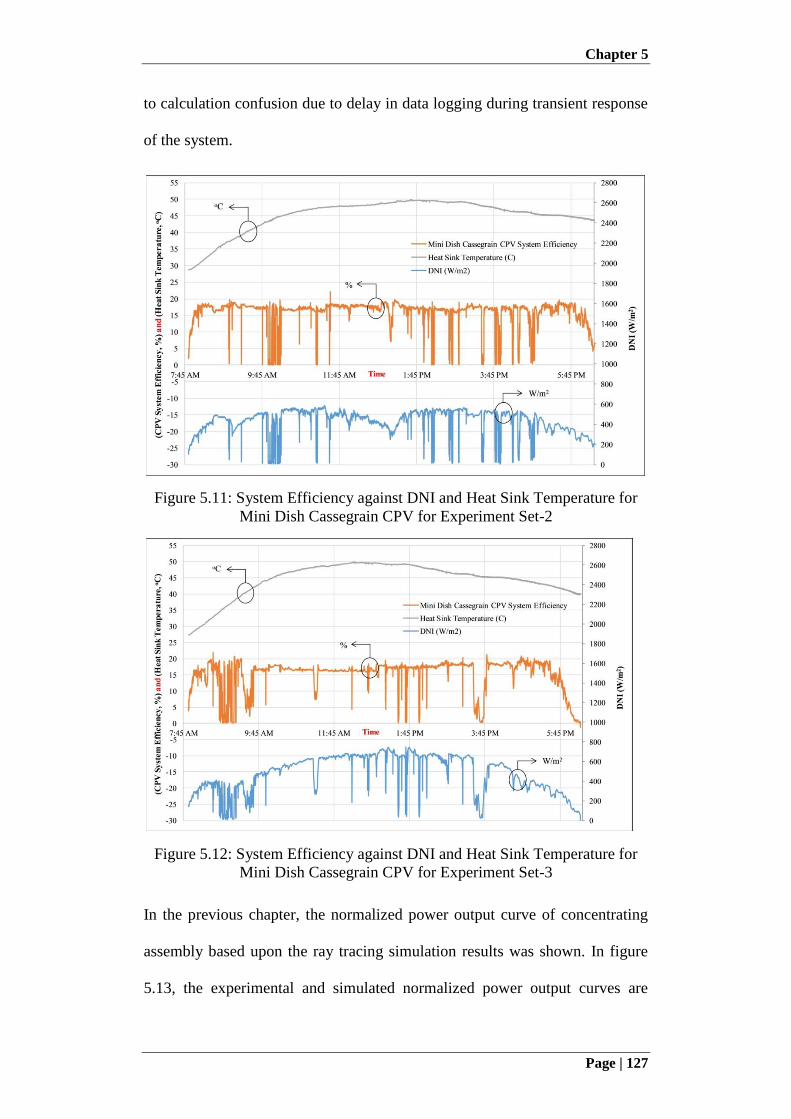
Chapter 5

Page | 127

to calculation confusion due to delay in data logging during transient response

of the system.





In the previous chapter, the normalized power output curve of concentrating

assembly based upon the ray tracing simulation results was shown. In figure

5.13, the experimental and simulated normalized power output curves are

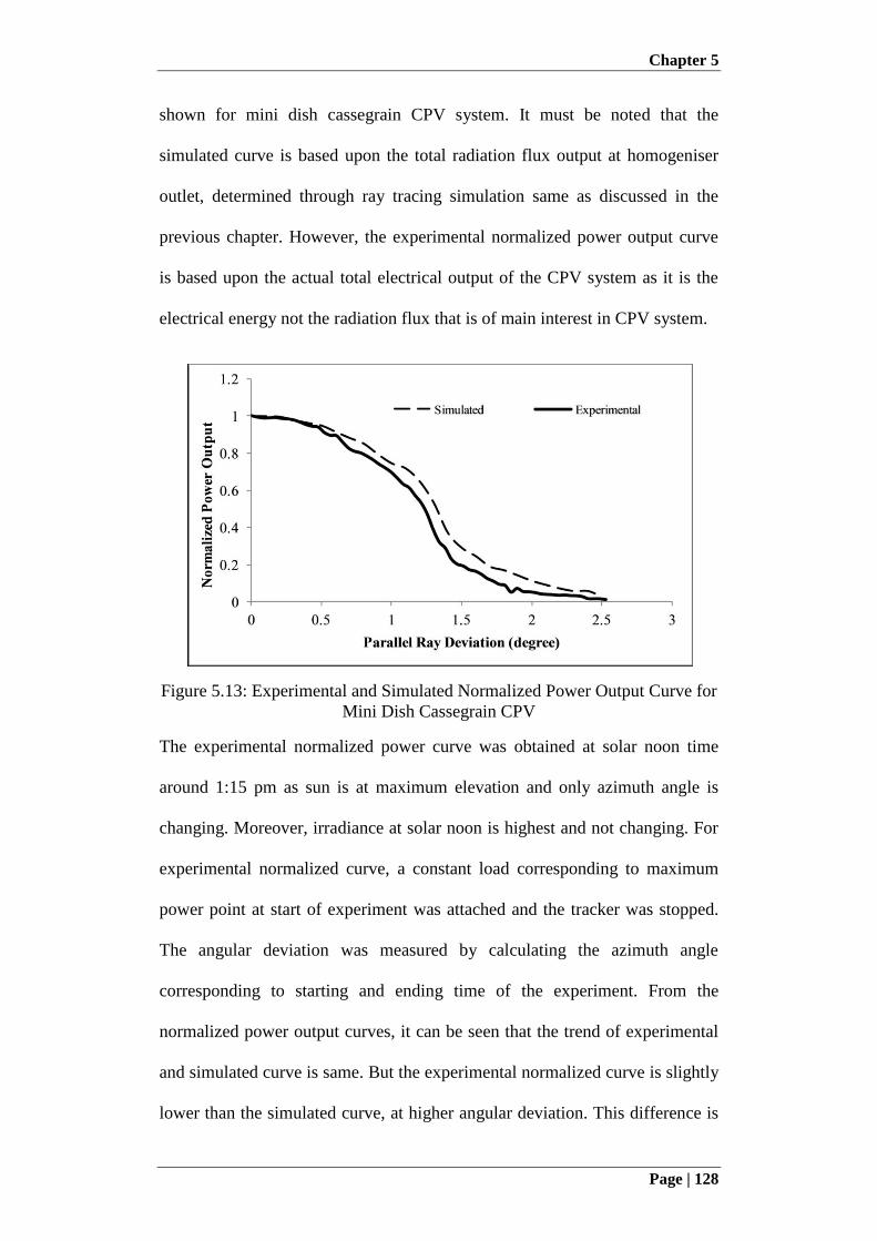
Chapter 5

Page | 128

shown for mini dish cassegrain CPV system. It must be noted that the

simulated curve is based upon the total radiation flux output at homogeniser

outlet, determined through ray tracing simulation same as discussed in the

previous chapter. However, the experimental normalized power output curve

is based upon the actual total electrical output of the CPV system as it is the

electrical energy not the radiation flux that is of main interest in CPV system.

Figure 5.13: Experimental and Simulated Normalized Power Output Curve for

Mini Dish Cassegrain CPV

The experimental normalized power curve was obtained at solar noon time

around 1:15 pm as sun is at maximum elevation and only azimuth angle is

changing. Moreover, irradiance at solar noon is highest and not changing. For

experimental normalized curve, a constant load corresponding to maximum

power point at start of experiment was attached and the tracker was stopped.

The angular deviation was measured by calculating the azimuth angle

corresponding to starting and ending time of the experiment. From the

normalized power output curves, it can be seen that the trend of experimental

and simulated curve is same. But the experimental normalized curve is slightly

lower than the simulated curve, at higher angular deviation. This difference is

Chapter 5

Page | 129

because of the fact that the experimental normalized power curve is based

upon the electrical power output and because of optical loss at higher angular

deviations, the maximum power point of CPV system is shifting as constant

load is applied across cell output, which causes less power production due to

lower operating efficiency. On the other hand, simulated curve is based upon

the radiation flux, which is not affected by the load resistance. For 0.3o angular

deviation, the designed tracking accuracy, the performance of the CPV system

is highest and maximum.

5.4 Fresnel Lens-Glass Homogeniser CPV System

The fabricated Fresnel Lens-Glass Homogeniser CPV system is shown in

Figure 5.14. The developed system consist of a small CPV module with four

MJC cells and an 2 x 2 array of Fresnel Lenses, according to design as

discussed in the previous Chapter 4. The CPV module is mounted onto

aluminium frame of developed two axis solar tracker. The Fresnel lens array is

made of PMMA plastic with optical efficiency of 80%. The glass homogeniser

is tapered glass rod made of quartz material. The glass homogeniser is

attached onto MJC submount with optically graded silicone. Each MJC

submount is attached to heat sink with thermal glue for heat dissipation. A

thermistor type temperature sensor is attached to heat sink to measure cell

back plate temperature. All four MJCs are connected in series and the total

power output is connected to MPPT resistor, which is then logged through

data logger. A perfect bright spot at centre of homogeniser verifies the design

of concentrating assembly. In order to investigate the real field performance of

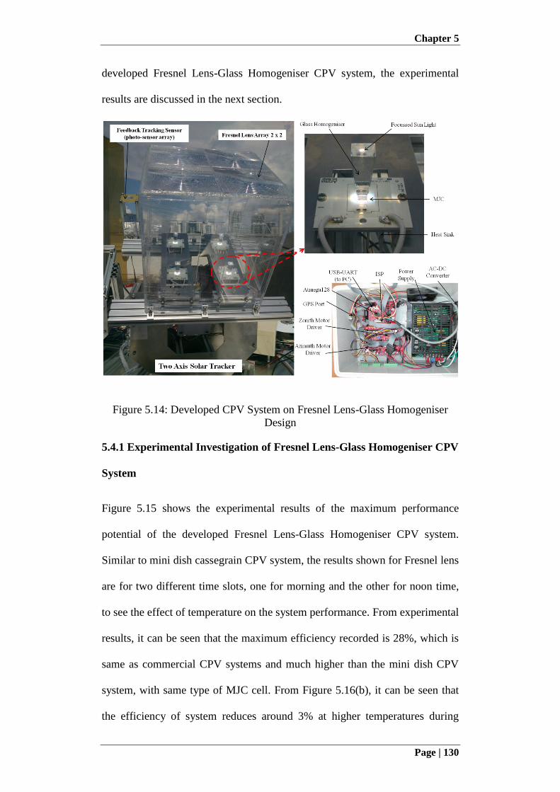
Chapter 5

Page | 130

developed Fresnel Lens-Glass Homogeniser CPV system, the experimental

results are discussed in the next section.

Figure 5.14: Developed CPV System on Fresnel Lens-Glass Homogeniser

Design

5.4.1 Experimental Investigation of Fresnel Lens-Glass Homogeniser CPV

System

Figure 5.15 shows the experimental results of the maximum performance

potential of the developed Fresnel Lens-Glass Homogeniser CPV system.

Similar to mini dish cassegrain CPV system, the results shown for Fresnel lens

are for two different time slots, one for morning and the other for noon time,

to see the effect of temperature on the system performance. From experimental

results, it can be seen that the maximum efficiency recorded is 28%, which is

same as commercial CPV systems and much higher than the mini dish CPV

system, with same type of MJC cell. From Figure 5.16(b), it can be seen that

the efficiency of system reduces around 3% at higher temperatures during

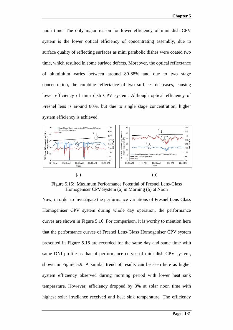
Chapter 5

Page | 131

noon time. The only major reason for lower efficiency of mini dish CPV

system is the lower optical efficiency of concentrating assembly, due to

surface quality of reflecting surfaces as mini parabolic dishes were coated two

time, which resulted in some surface defects. Moreover, the optical reflectance

of aluminium varies between around 80-88% and due to two stage

concentration, the combine reflectance of two surfaces decreases, causing

lower efficiency of mini dish CPV system. Although optical efficiency of

Fresnel lens is around 80%, but due to single stage concentration, higher

system efficiency is achieved.

(a) (b)

Figure 5.15: Maximum Performance Potential of Fresnel Lens-Glass


Now, in order to investigate the performance variations of Fresnel Lens-Glass

Homogeniser CPV system during whole day operation, the performance

curves are shown in Figure 5.16. For comparison, it is worthy to mention here

that the performance curves of Fresnel Lens-Glass Homogeniser CPV system

presented in Figure 5.16 are recorded for the same day and same time with

same DNI profile as that of performance curves of mini dish CPV system,

shown in Figure 5.9. A similar trend of results can be seen here as higher

system efficiency observed during morning period with lower heat sink

temperature. However, efficiency dropped by 3% at solar noon time with

highest solar irradiance received and heat sink temperature. The efficiency

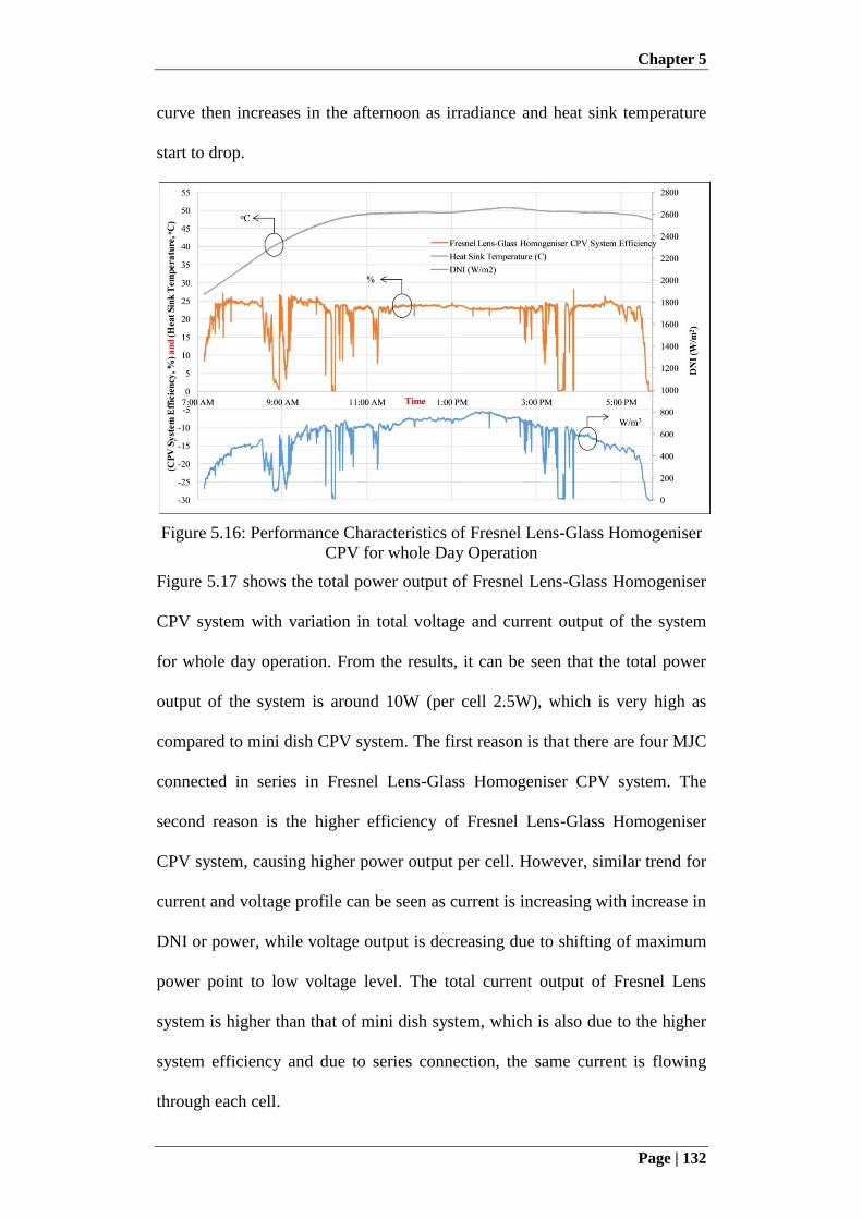
Chapter 5

Page | 132

curve then increases in the afternoon as irradiance and heat sink temperature

start to drop.

Figure 5.16: Performance Characteristics of Fresnel Lens-Glass Homogeniser

CPV for whole Day Operation

Figure 5.17 shows the total power output of Fresnel Lens-Glass Homogeniser

CPV system with variation in total voltage and current output of the system

for whole day operation. From the results, it can be seen that the total power

output of the system is around 10W (per cell 2.5W), which is very high as

compared to mini dish CPV system. The first reason is that there are four MJC

connected in series in Fresnel Lens-Glass Homogeniser CPV system. The

second reason is the higher efficiency of Fresnel Lens-Glass Homogeniser

CPV system, causing higher power output per cell. However, similar trend for

current and voltage profile can be seen as current is increasing with increase in

DNI or power, while voltage output is decreasing due to shifting of maximum

power point to low voltage level. The total current output of Fresnel Lens

system is higher than that of mini dish system, which is also due to the higher

system efficiency and due to series connection, the same current is flowing

through each cell.

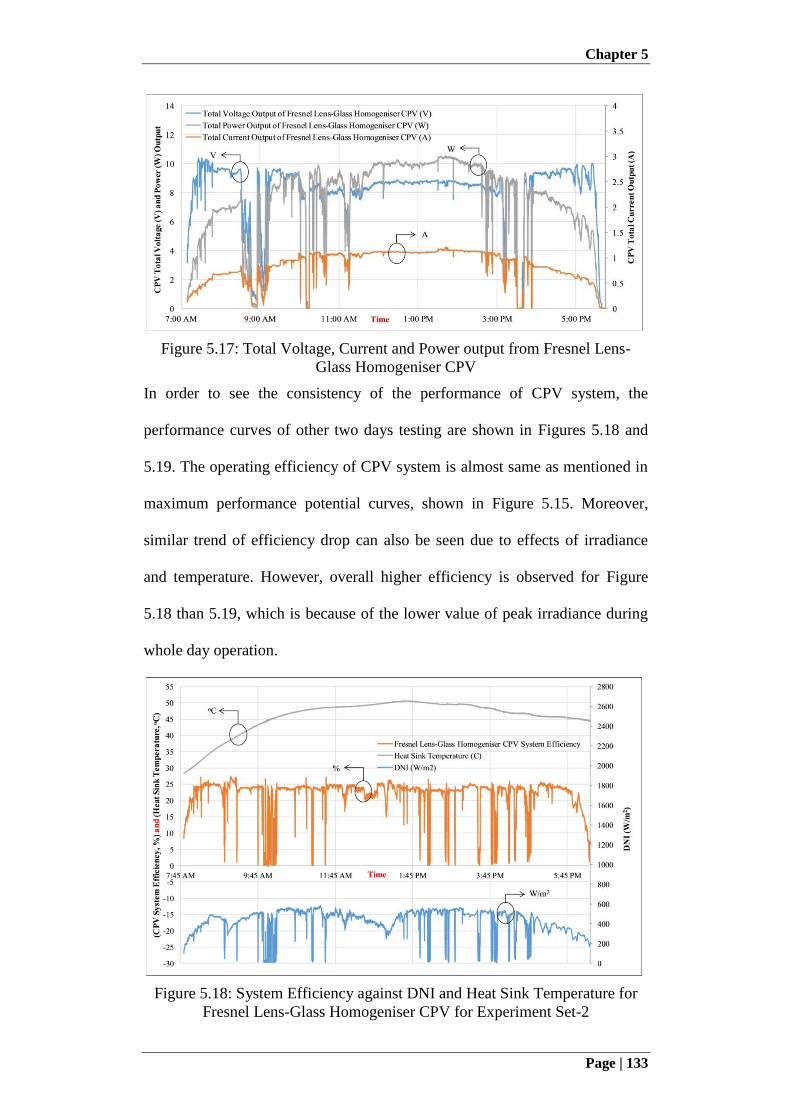
Chapter 5

Page | 133


Glass Homogeniser CPV

In order to see the consistency of the performance of CPV system, the

performance curves of other two days testing are shown in Figures 5.18 and

5.19. The operating efficiency of CPV system is almost same as mentioned in

maximum performance potential curves, shown in Figure 5.15. Moreover,

similar trend of efficiency drop can also be seen due to effects of irradiance

and temperature. However, overall higher efficiency is observed for Figure

5.18 than 5.19, which is because of the lower value of peak irradiance during

whole day operation.



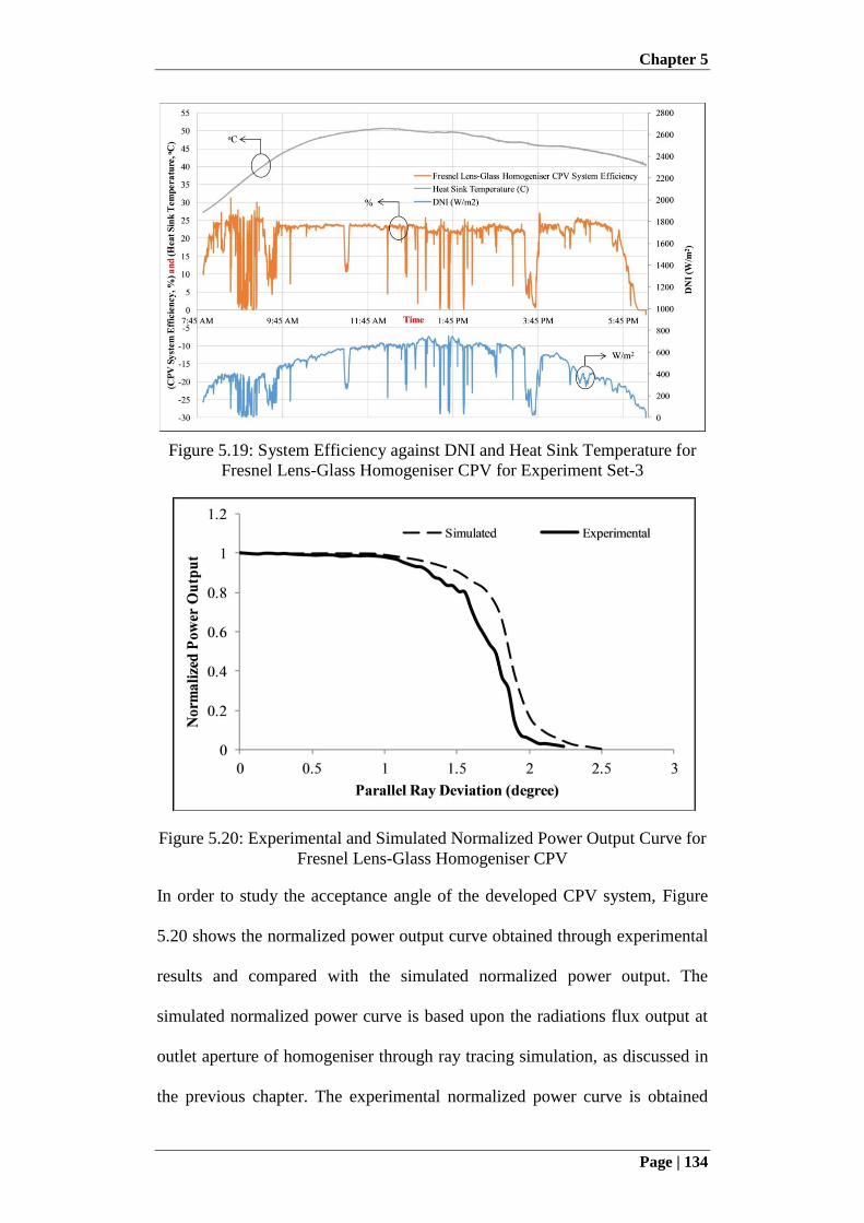
Chapter 5

Page | 134




Fresnel Lens-Glass Homogeniser CPV

In order to study the acceptance angle of the developed CPV system, Figure

5.20 shows the normalized power output curve obtained through experimental

results and compared with the simulated normalized power output. The

simulated normalized power curve is based upon the radiations flux output at

outlet aperture of homogeniser through ray tracing simulation, as discussed in

the previous chapter. The experimental normalized power curve is obtained

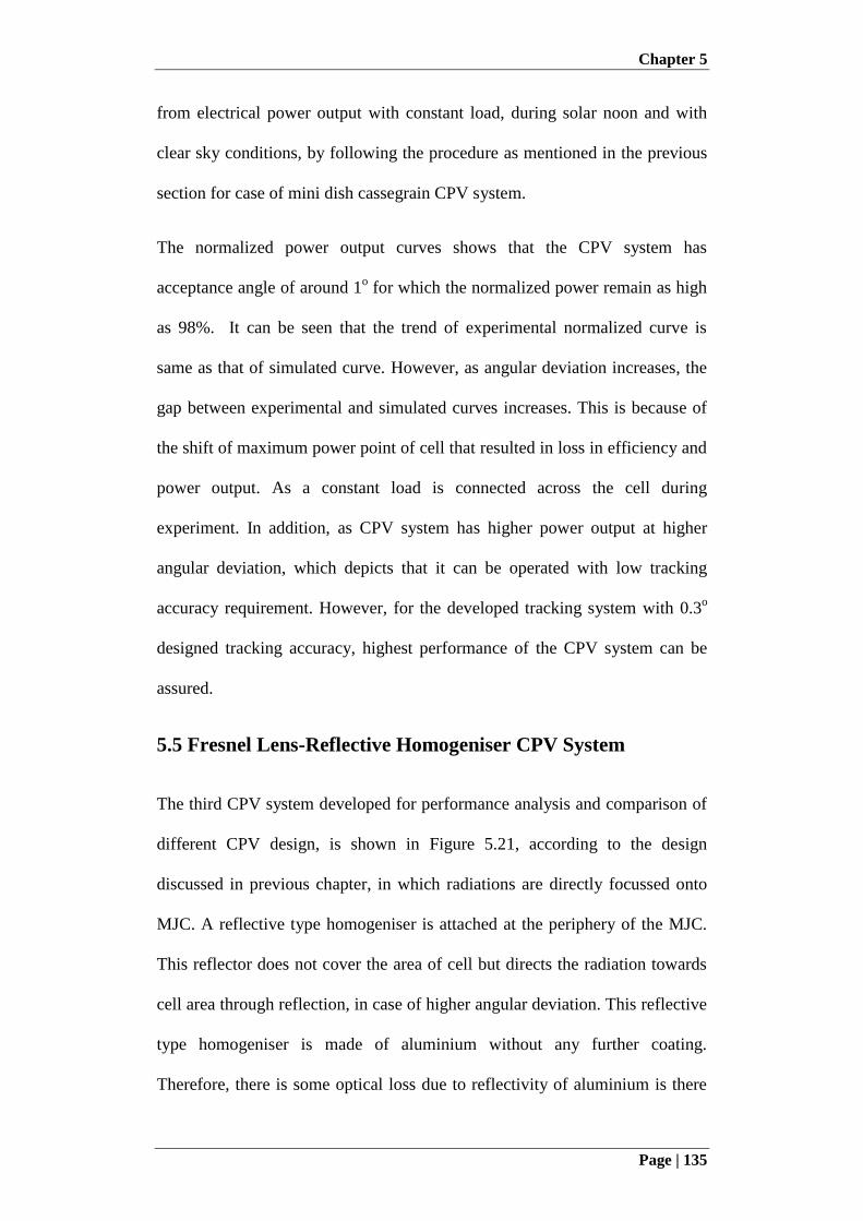
Chapter 5

Page | 135

from electrical power output with constant load, during solar noon and with

clear sky conditions, by following the procedure as mentioned in the previous

section for case of mini dish cassegrain CPV system.

The normalized power output curves shows that the CPV system has

acceptance angle of around 1o for which the normalized power remain as high

as 98%. It can be seen that the trend of experimental normalized curve is

same as that of simulated curve. However, as angular deviation increases, the

gap between experimental and simulated curves increases. This is because of

the shift of maximum power point of cell that resulted in loss in efficiency and

power output. As a constant load is connected across the cell during

experiment. In addition, as CPV system has higher power output at higher

angular deviation, which depicts that it can be operated with low tracking

accuracy requirement. However, for the developed tracking system with 0.3o

designed tracking accuracy, highest performance of the CPV system can be

assured.

5.5 Fresnel Lens-Reflective Homogeniser CPV System

The third CPV system developed for performance analysis and comparison of

different CPV design, is shown in Figure 5.21, according to the design

discussed in previous chapter, in which radiations are directly focussed onto

MJC. A reflective type homogeniser is attached at the periphery of the MJC.

This reflector does not cover the area of cell but directs the radiation towards

cell area through reflection, in case of higher angular deviation. This reflective

type homogeniser is made of aluminium without any further coating.

Therefore, there is some optical loss due to reflectivity of aluminium is there

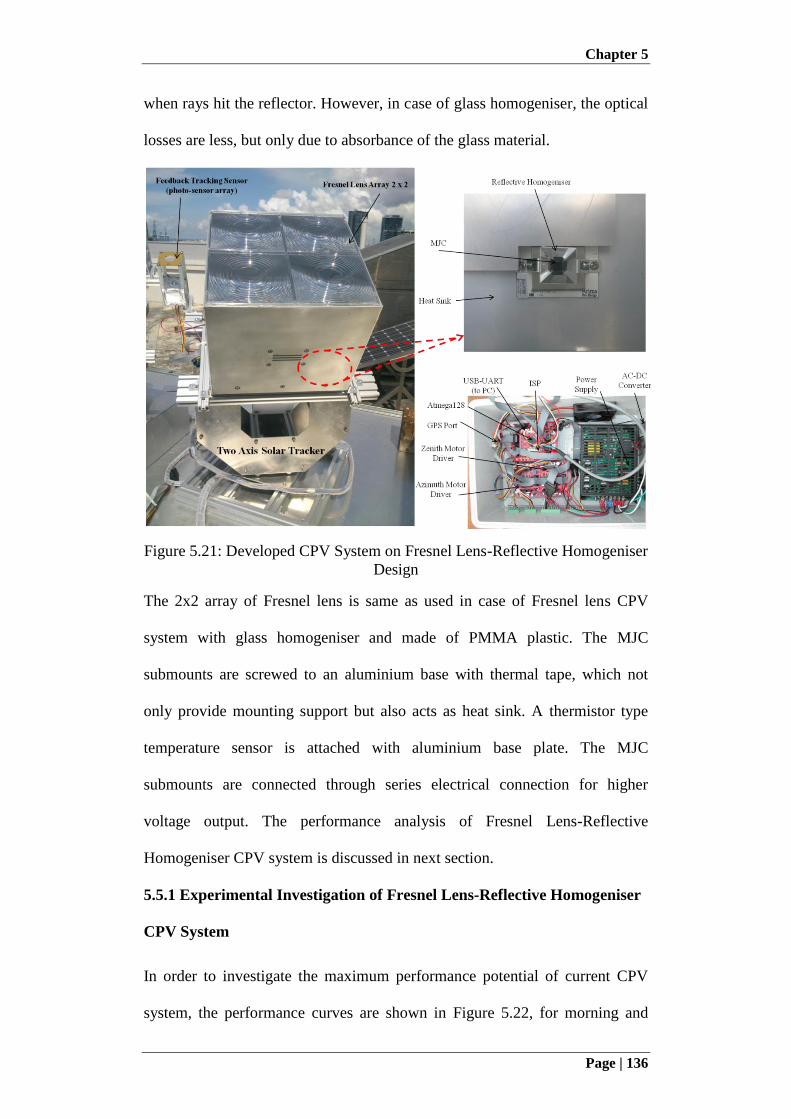
Chapter 5

Page | 136

when rays hit the reflector. However, in case of glass homogeniser, the optical

losses are less, but only due to absorbance of the glass material.

Figure 5.21: Developed CPV System on Fresnel Lens-Reflective Homogeniser

Design

The 2x2 array of Fresnel lens is same as used in case of Fresnel lens CPV

system with glass homogeniser and made of PMMA plastic. The MJC

submounts are screwed to an aluminium base with thermal tape, which not

only provide mounting support but also acts as heat sink. A thermistor type

temperature sensor is attached with aluminium base plate. The MJC

submounts are connected through series electrical connection for higher

voltage output. The performance analysis of Fresnel Lens-Reflective

Homogeniser CPV system is discussed in next section.

5.5.1 Experimental Investigation of Fresnel Lens-Reflective Homogeniser

CPV System

In order to investigate the maximum performance potential of current CPV

system, the performance curves are shown in Figure 5.22, for morning and

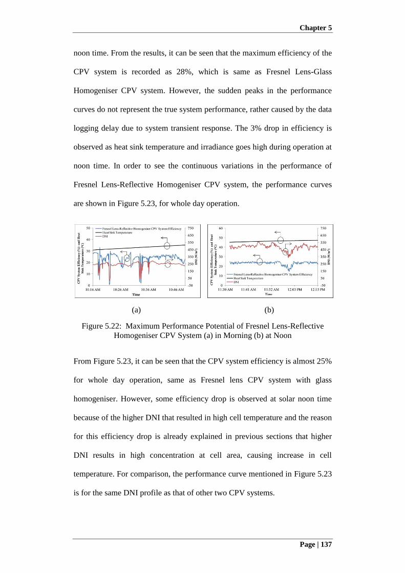
Chapter 5

Page | 137

noon time. From the results, it can be seen that the maximum efficiency of the

CPV system is recorded as 28%, which is same as Fresnel Lens-Glass

Homogeniser CPV system. However, the sudden peaks in the performance

curves do not represent the true system performance, rather caused by the data

logging delay due to system transient response. The 3% drop in efficiency is

observed as heat sink temperature and irradiance goes high during operation at

noon time. In order to see the continuous variations in the performance of

Fresnel Lens-Reflective Homogeniser CPV system, the performance curves

are shown in Figure 5.23, for whole day operation.

(a) (b)

Figure 5.22: Maximum Performance Potential of Fresnel Lens-Reflective


From Figure 5.23, it can be seen that the CPV system efficiency is almost 25%

for whole day operation, same as Fresnel lens CPV system with glass

homogeniser. However, some efficiency drop is observed at solar noon time

because of the higher DNI that resulted in high cell temperature and the reason

for this efficiency drop is already explained in previous sections that higher

DNI results in high concentration at cell area, causing increase in cell

temperature. For comparison, the performance curve mentioned in Figure 5.23

is for the same DNI profile as that of other two CPV systems.

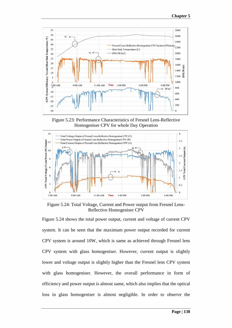
Chapter 5

Page | 138

Figure 5.23: Performance Characteristics of Fresnel Lens-Reflective



Reflective Homogeniser CPV

Figure 5.24 shows the total power output, current and voltage of current CPV

system. It can be seen that the maximum power output recorded for current

CPV system is around 10W, which is same as achieved through Fresnel lens

CPV system with glass homogeniser. However, current output is slightly

lower and voltage output is slightly higher than the Fresnel lens CPV system

with glass homogeniser. However, the overall performance in form of

efficiency and power output is almost same, which also implies that the optical

loss in glass homogeniser is almost negligible. In order to observe the

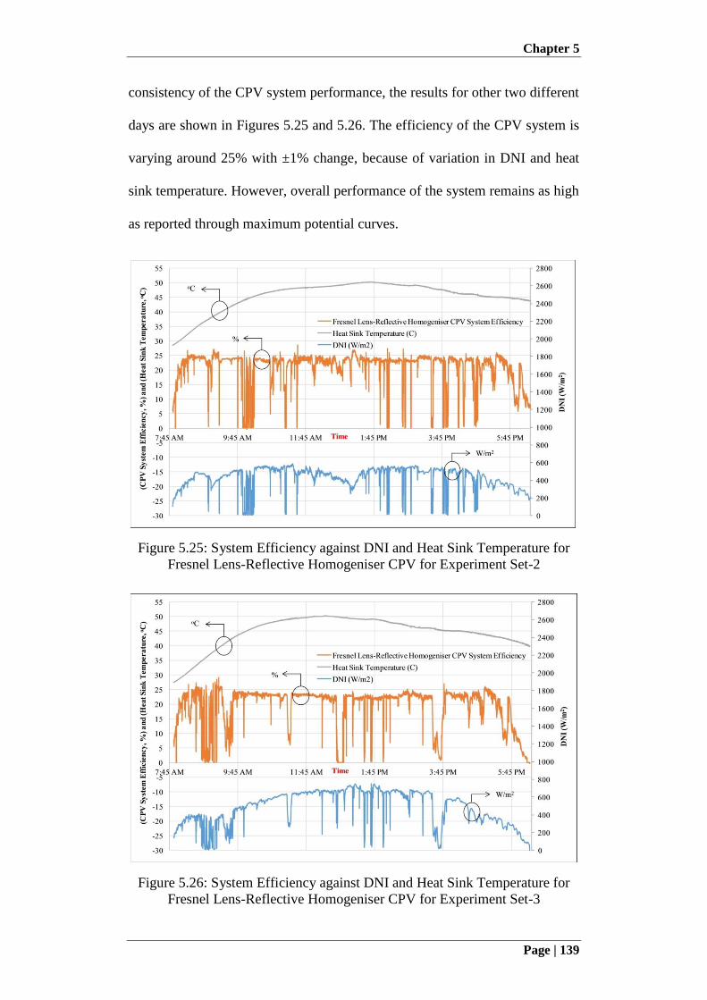
Chapter 5

Page | 139

consistency of the CPV system performance, the results for other two different

days are shown in Figures 5.25 and 5.26. The efficiency of the CPV system is

varying around 25% with ±1% change, because of variation in DNI and heat

sink temperature. However, overall performance of the system remains as high

as reported through maximum potential curves.


Fresnel Lens-Reflective Homogeniser CPV for Experiment Set-2


Fresnel Lens-Reflective Homogeniser CPV for Experiment Set-3

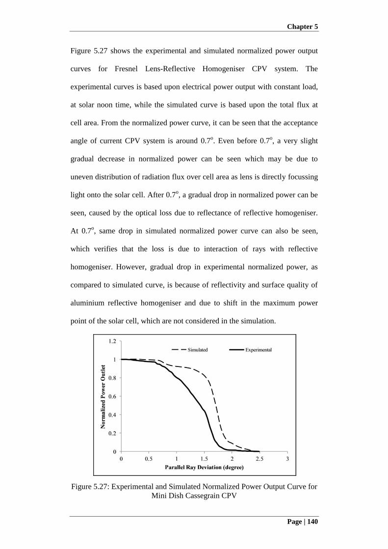
Chapter 5

Page | 140

Figure 5.27 shows the experimental and simulated normalized power output

curves for Fresnel Lens-Reflective Homogeniser CPV system. The

experimental curves is based upon electrical power output with constant load,

at solar noon time, while the simulated curve is based upon the total flux at

cell area. From the normalized power curve, it can be seen that the acceptance

angle of current CPV system is around 0.7o. Even before 0.7

o, a very slight

gradual decrease in normalized power can be seen which may be due to

uneven distribution of radiation flux over cell area as lens is directly focussing

light onto the solar cell. After 0.7o, a gradual drop in normalized power can be

seen, caused by the optical loss due to reflectance of reflective homogeniser.

At 0.7o, same drop in simulated normalized power curve can also be seen,

which verifies that the loss is due to interaction of rays with reflective

homogeniser. However, gradual drop in experimental normalized power, as

compared to simulated curve, is because of reflectivity and surface quality of

aluminium reflective homogeniser and due to shift in the maximum power

point of the solar cell, which are not considered in the simulation.



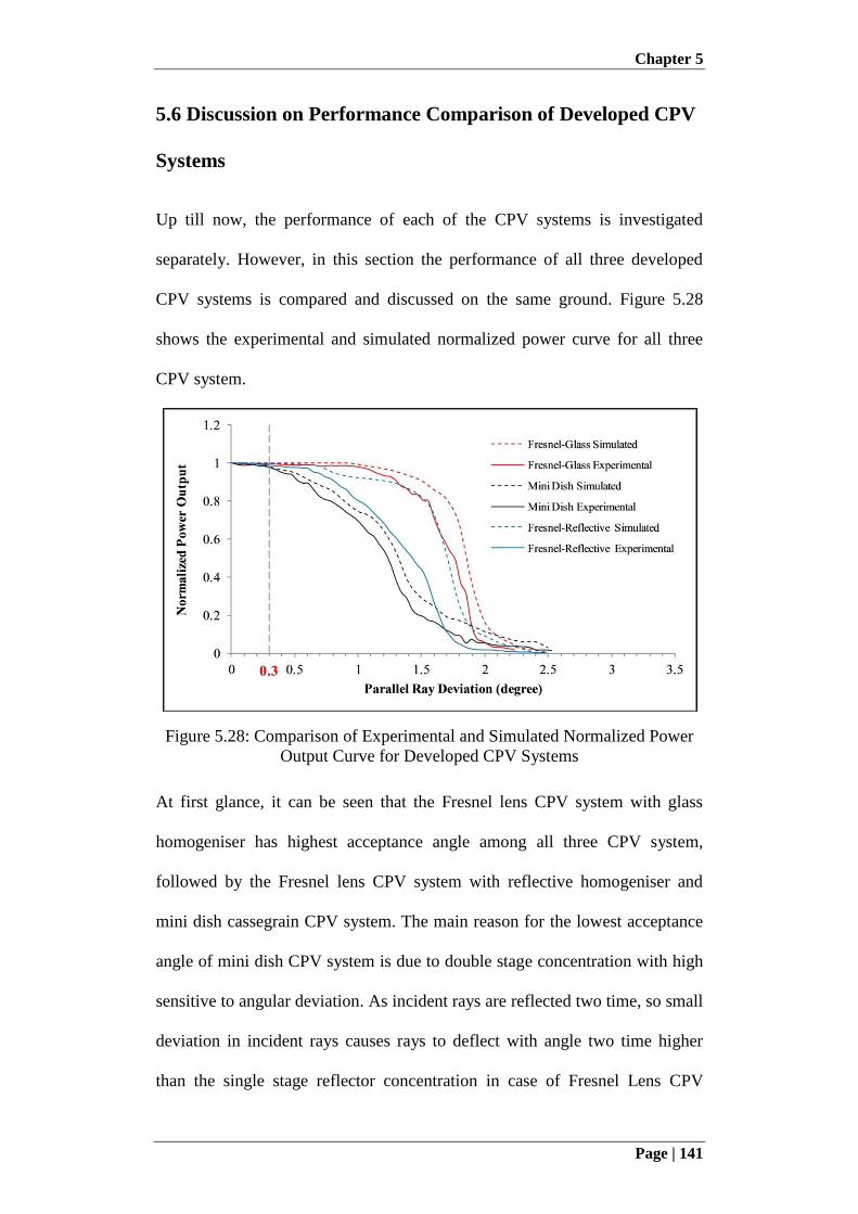
Chapter 5

Page | 141

5.6 Discussion on Performance Comparison of Developed CPV

Systems

Up till now, the performance of each of the CPV systems is investigated

separately. However, in this section the performance of all three developed

CPV systems is compared and discussed on the same ground. Figure 5.28

shows the experimental and simulated normalized power curve for all three

CPV system.

Figure 5.28: Comparison of Experimental and Simulated Normalized Power

Output Curve for Developed CPV Systems

At first glance, it can be seen that the Fresnel lens CPV system with glass

homogeniser has highest acceptance angle among all three CPV system,

followed by the Fresnel lens CPV system with reflective homogeniser and

mini dish cassegrain CPV system. The main reason for the lowest acceptance

angle of mini dish CPV system is due to double stage concentration with high

sensitive to angular deviation. As incident rays are reflected two time, so small

deviation in incident rays causes rays to deflect with angle two time higher

than the single stage reflector concentration in case of Fresnel Lens CPV

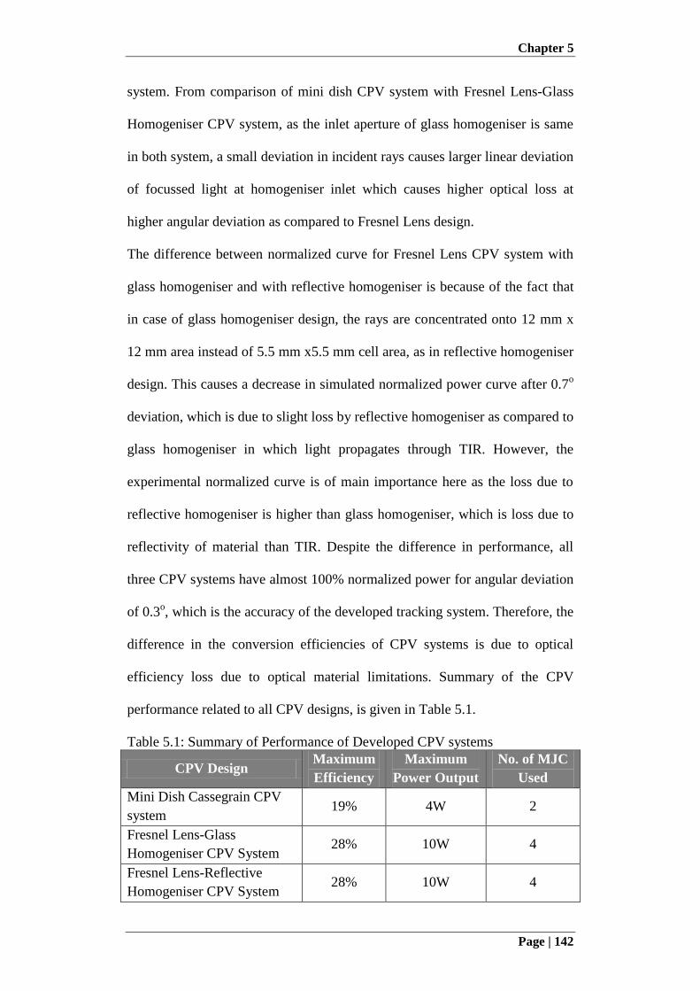
Chapter 5

Page | 142

system. From comparison of mini dish CPV system with Fresnel Lens-Glass

Homogeniser CPV system, as the inlet aperture of glass homogeniser is same

in both system, a small deviation in incident rays causes larger linear deviation

of focussed light at homogeniser inlet which causes higher optical loss at

higher angular deviation as compared to Fresnel Lens design.

The difference between normalized curve for Fresnel Lens CPV system with

glass homogeniser and with reflective homogeniser is because of the fact that

in case of glass homogeniser design, the rays are concentrated onto 12 mm x

12 mm area instead of 5.5 mm x5.5 mm cell area, as in reflective homogeniser

design. This causes a decrease in simulated normalized power curve after 0.7o

deviation, which is due to slight loss by reflective homogeniser as compared to

glass homogeniser in which light propagates through TIR. However, the

experimental normalized curve is of main importance here as the loss due to

reflective homogeniser is higher than glass homogeniser, which is loss due to

reflectivity of material than TIR. Despite the difference in performance, all

three CPV systems have almost 100% normalized power for angular deviation

of 0.3o, which is the accuracy of the developed tracking system. Therefore, the

difference in the conversion efficiencies of CPV systems is due to optical

efficiency loss due to optical material limitations. Summary of the CPV

performance related to all CPV designs, is given in Table 5.1.

Table 5.1: Summary of Performance of Developed CPV systems

CPV Design Maximum

Efficiency

Maximum

Power Output

No. of MJC

Used


system 19% 4W 2

Fresnel Lens-Glass

Homogeniser CPV System 28% 10W 4

Fresnel Lens-Reflective

Homogeniser CPV System 28% 10W 4

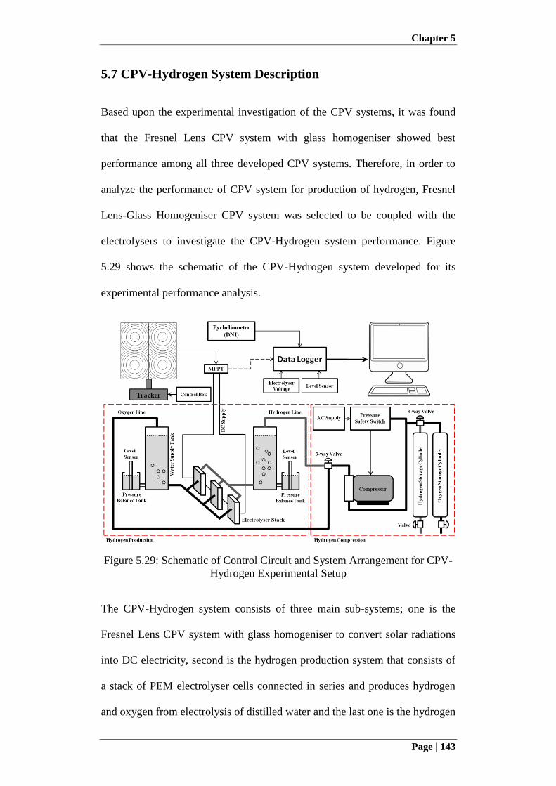
Chapter 5

Page | 143

5.7 CPV-Hydrogen System Description

Based upon the experimental investigation of the CPV systems, it was found

that the Fresnel Lens CPV system with glass homogeniser showed best

performance among all three developed CPV systems. Therefore, in order to

analyze the performance of CPV system for production of hydrogen, Fresnel

Lens-Glass Homogeniser CPV system was selected to be coupled with the

electrolysers to investigate the CPV-Hydrogen system performance. Figure

5.29 shows the schematic of the CPV-Hydrogen system developed for its

experimental performance analysis.

Figure 5.29: Schematic of Control Circuit and System Arrangement for CPV-

Hydrogen Experimental Setup

The CPV-Hydrogen system consists of three main sub-systems; one is the

Fresnel Lens CPV system with glass homogeniser to convert solar radiations

into DC electricity, second is the hydrogen production system that consists of

a stack of PEM electrolyser cells connected in series and produces hydrogen

and oxygen from electrolysis of distilled water and the last one is the hydrogen

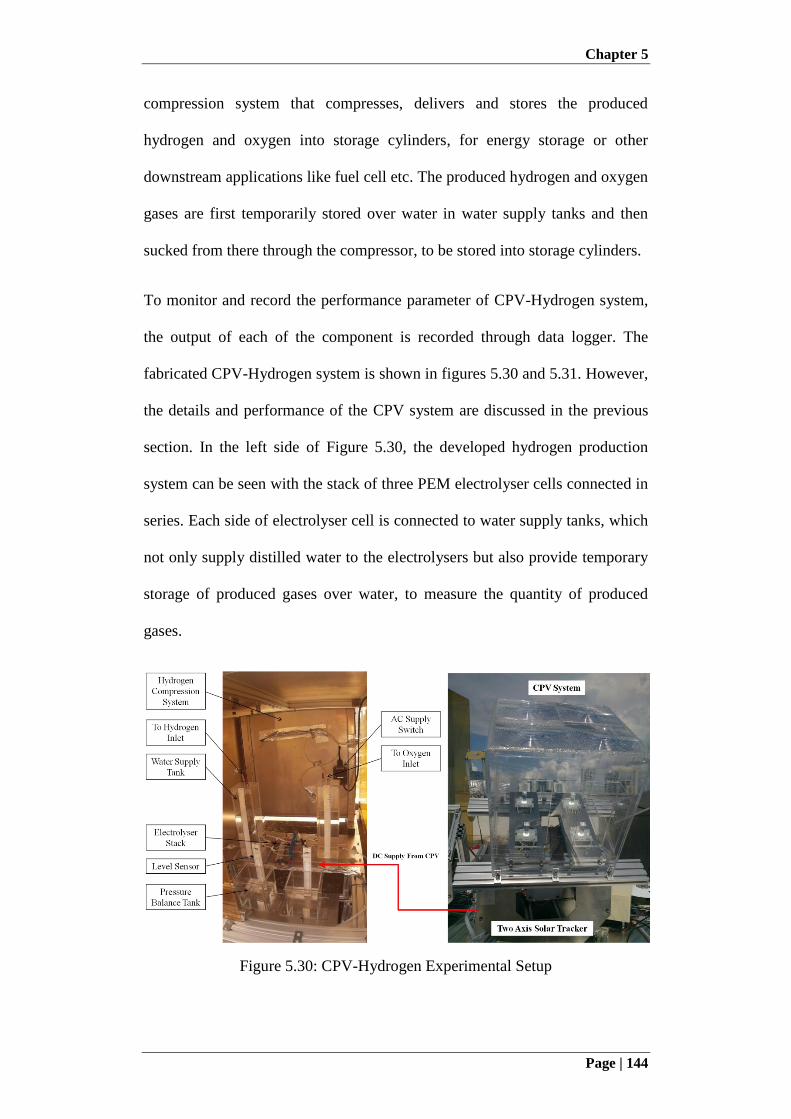
Chapter 5

Page | 144

compression system that compresses, delivers and stores the produced

hydrogen and oxygen into storage cylinders, for energy storage or other

downstream applications like fuel cell etc. The produced hydrogen and oxygen

gases are first temporarily stored over water in water supply tanks and then

sucked from there through the compressor, to be stored into storage cylinders.

To monitor and record the performance parameter of CPV-Hydrogen system,

the output of each of the component is recorded through data logger. The

fabricated CPV-Hydrogen system is shown in figures 5.30 and 5.31. However,

the details and performance of the CPV system are discussed in the previous

section. In the left side of Figure 5.30, the developed hydrogen production

system can be seen with the stack of three PEM electrolyser cells connected in

series. Each side of electrolyser cell is connected to water supply tanks, which

not only supply distilled water to the electrolysers but also provide temporary

storage of produced gases over water, to measure the quantity of produced

gases.

Figure 5.30: CPV-Hydrogen Experimental Setup

Chapter 5

Page | 145

The water supply tank, which is closed to atmosphere, is connected to a

pressure balance tank, which is open to atmosphere. So the water level in the

water supply tank is kept at higher level and the water level in the pressure

balance tank is kept at lower level. The gases are stored in water supply tank

first and as a result, its water level goes down while the water level in pressure

balance tank goes up to keep pressure balance in both tank as atmospheric. A

level sensor is dipped into the pressure balance tank to measure the change in

water level, which gives the amount of gases produced from electrolysis. The

level sensor is a eTape from Milestone Technologies, whose resistance

changes is calibrated in terms of water level change and measured through a

voltage divider. The output of level sensor is also verified by the manual

reading from graduated scale on water supply tank as the volume change in

both tanks is same. When water level in the water supply tank goes to lower

limit, the produced gases are sucked through the compressor and stored into

the storage tanks. The hydrogen compression system is shown in Figure 5.31.

Figure 5.31: Hydrogen Compression System

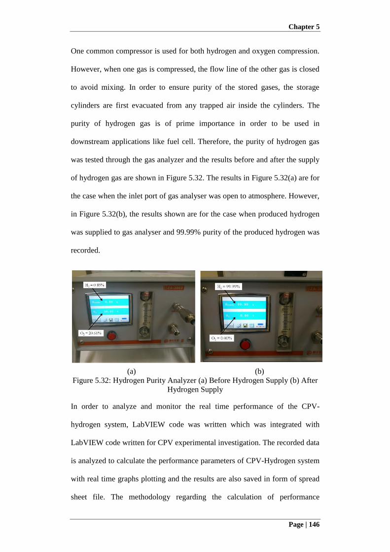
Chapter 5

Page | 146

One common compressor is used for both hydrogen and oxygen compression.

However, when one gas is compressed, the flow line of the other gas is closed

to avoid mixing. In order to ensure purity of the stored gases, the storage

cylinders are first evacuated from any trapped air inside the cylinders. The

purity of hydrogen gas is of prime importance in order to be used in

downstream applications like fuel cell. Therefore, the purity of hydrogen gas

was tested through the gas analyzer and the results before and after the supply

of hydrogen gas are shown in Figure 5.32. The results in Figure 5.32(a) are for

the case when the inlet port of gas analyser was open to atmosphere. However,

in Figure 5.32(b), the results shown are for the case when produced hydrogen

was supplied to gas analyser and 99.99% purity of the produced hydrogen was

recorded.

(a) (b)

Figure 5.32: Hydrogen Purity Analyzer (a) Before Hydrogen Supply (b) After

Hydrogen Supply

In order to analyze and monitor the real time performance of the CPV-

hydrogen system, LabVIEW code was written which was integrated with

LabVIEW code written for CPV experimental investigation. The recorded data

is analyzed to calculate the performance parameters of CPV-Hydrogen system

with real time graphs plotting and the results are also saved in form of spread

sheet file. The methodology regarding the calculation of performance

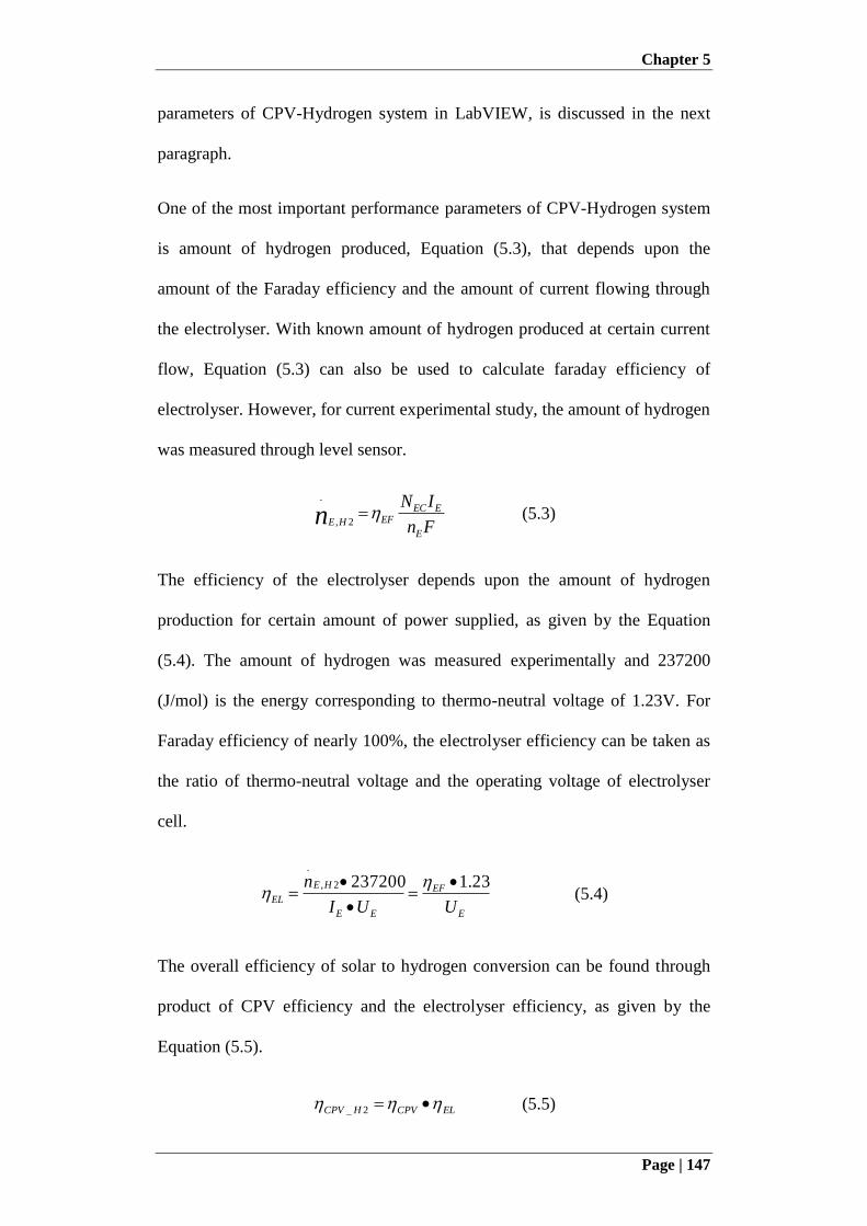
Chapter 5

Page | 147

parameters of CPV-Hydrogen system in LabVIEW, is discussed in the next

paragraph.

One of the most important performance parameters of CPV-Hydrogen system

is amount of hydrogen produced, Equation (5.3), that depends upon the

amount of the Faraday efficiency and the amount of current flowing through

the electrolyser. With known amount of hydrogen produced at certain current

flow, Equation (5.3) can also be used to calculate faraday efficiency of

electrolyser. However, for current experimental study, the amount of hydrogen

was measured through level sensor.

Fn

IN

E

EECEFHEn

2,

.

(5.3)

The efficiency of the electrolyser depends upon the amount of hydrogen

production for certain amount of power supplied, as given by the Equation

(5.4). The amount of hydrogen was measured experimentally and 237200

(J/mol) is the energy corresponding to thermo-neutral voltage of 1.23V. For

Faraday efficiency of nearly 100%, the electrolyser efficiency can be taken as

the ratio of thermo-neutral voltage and the operating voltage of electrolyser

cell.

E

EF

EE

HE

ELUUI

n 23.12372002,

.

(5.4)

The overall efficiency of solar to hydrogen conversion can be found through

product of CPV efficiency and the electrolyser efficiency, as given by the

Equation (5.5).

ELCPVHCPV 2_ (5.5)

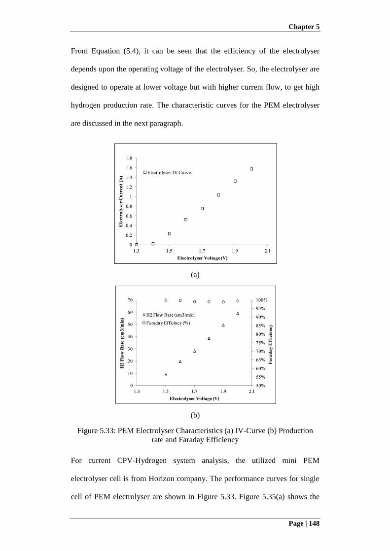
Chapter 5

Page | 148

From Equation (5.4), it can be seen that the efficiency of the electrolyser

depends upon the operating voltage of the electrolyser. So, the electrolyser are

designed to operate at lower voltage but with higher current flow, to get high

hydrogen production rate. The characteristic curves for the PEM electrolyser

are discussed in the next paragraph.

(a)

(b)

Figure 5.33: PEM Electrolyser Characteristics (a) IV-Curve (b) Production

rate and Faraday Efficiency

For current CPV-Hydrogen system analysis, the utilized mini PEM

electrolyser cell is from Horizon company. The performance curves for single

cell of PEM electrolyser are shown in Figure 5.33. Figure 5.35(a) shows the

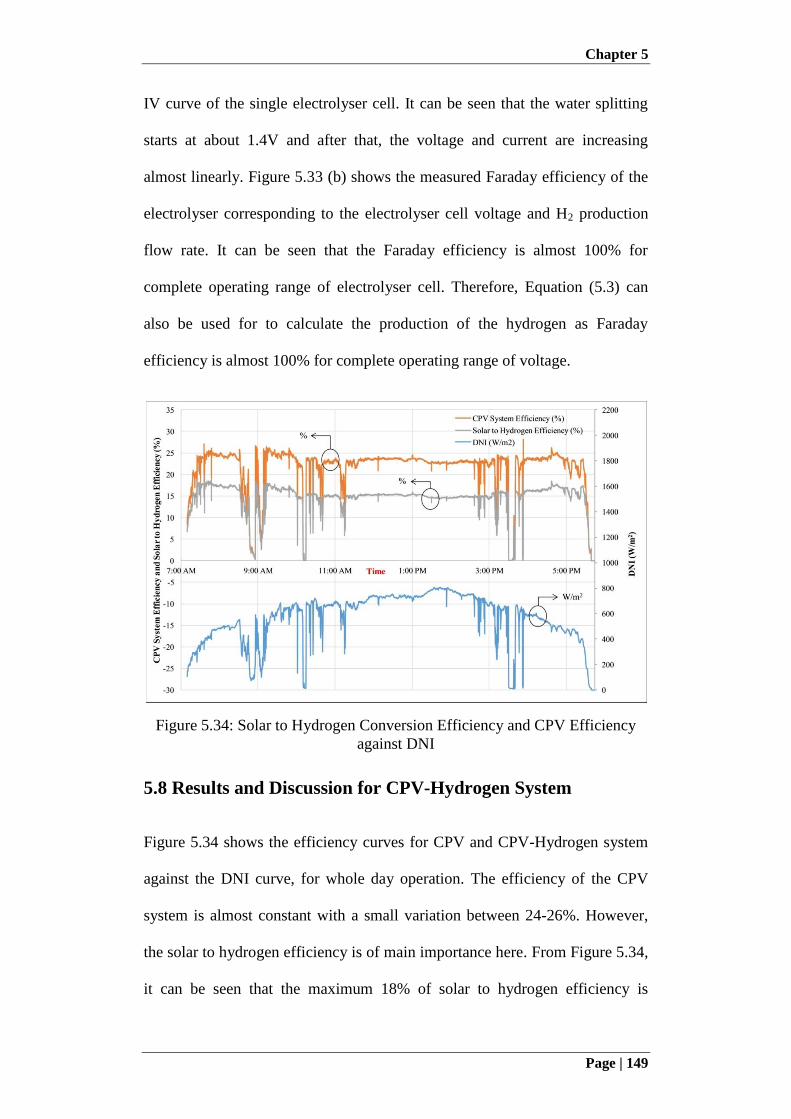
Chapter 5

Page | 149

IV curve of the single electrolyser cell. It can be seen that the water splitting

starts at about 1.4V and after that, the voltage and current are increasing

almost linearly. Figure 5.33 (b) shows the measured Faraday efficiency of the

electrolyser corresponding to the electrolyser cell voltage and H2 production

flow rate. It can be seen that the Faraday efficiency is almost 100% for

complete operating range of electrolyser cell. Therefore, Equation (5.3) can

also be used for to calculate the production of the hydrogen as Faraday

efficiency is almost 100% for complete operating range of voltage.

Figure 5.34: Solar to Hydrogen Conversion Efficiency and CPV Efficiency

against DNI

5.8 Results and Discussion for CPV-Hydrogen System

Figure 5.34 shows the efficiency curves for CPV and CPV-Hydrogen system

against the DNI curve, for whole day operation. The efficiency of the CPV

system is almost constant with a small variation between 24-26%. However,

the solar to hydrogen efficiency is of main importance here. From Figure 5.34,

it can be seen that the maximum 18% of solar to hydrogen efficiency is

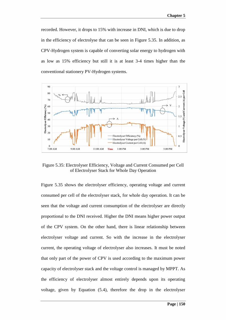
Chapter 5

Page | 150

recorded. However, it drops to 15% with increase in DNI, which is due to drop

in the efficiency of electrolyse that can be seen in Figure 5.35. In addition, as

CPV-Hydrogen system is capable of converting solar energy to hydrogen with

as low as 15% efficiency but still it is at least 3-4 times higher than the

conventional stationery PV-Hydrogen systems.

Figure 5.35: Electrolyser Efficiency, Voltage and Current Consumed per Cell

of Electrolyser Stack for Whole Day Operation

Figure 5.35 shows the electrolyser efficiency, operating voltage and current

consumed per cell of the electrolyser stack, for whole day operation. It can be

seen that the voltage and current consumption of the electrolyser are directly

proportional to the DNI received. Higher the DNI means higher power output

of the CPV system. On the other hand, there is linear relationship between

electrolyser voltage and current. So with the increase in the electrolyser

current, the operating voltage of electrolyser also increases. It must be noted

that only part of the power of CPV is used according to the maximum power

capacity of electrolyser stack and the voltage control is managed by MPPT. As

the efficiency of electrolyser almost entirely depends upon its operating

voltage, given by Equation (5.4), therefore the drop in the electrolyser

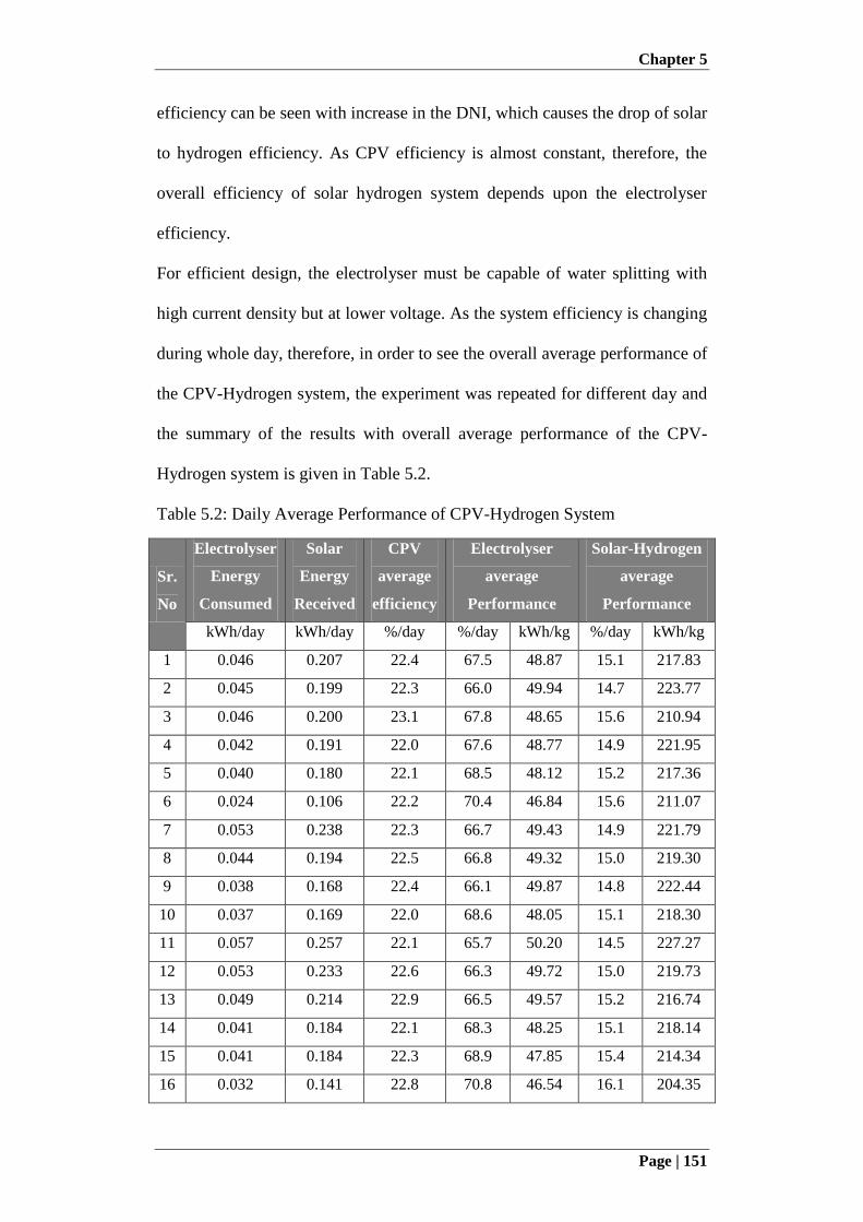
Chapter 5

Page | 151

efficiency can be seen with increase in the DNI, which causes the drop of solar

to hydrogen efficiency. As CPV efficiency is almost constant, therefore, the

overall efficiency of solar hydrogen system depends upon the electrolyser

efficiency.

For efficient design, the electrolyser must be capable of water splitting with

high current density but at lower voltage. As the system efficiency is changing

during whole day, therefore, in order to see the overall average performance of

the CPV-Hydrogen system, the experiment was repeated for different day and

the summary of the results with overall average performance of the CPV-

Hydrogen system is given in Table 5.2.

Table 5.2: Daily Average Performance of CPV-Hydrogen System

Sr.

No

Electrolyser

Energy

Consumed

Solar

Energy

Received

CPV

average

efficiency

Electrolyser

average

Performance

Solar-Hydrogen

average

Performance

kWh/day kWh/day %/day %/day kWh/kg %/day kWh/kg

1 0.046 0.207 22.4 67.5 48.87 15.1 217.83

2 0.045 0.199 22.3 66.0 49.94 14.7 223.77

3 0.046 0.200 23.1 67.8 48.65 15.6 210.94

4 0.042 0.191 22.0 67.6 48.77 14.9 221.95

5 0.040 0.180 22.1 68.5 48.12 15.2 217.36

6 0.024 0.106 22.2 70.4 46.84 15.6 211.07

7 0.053 0.238 22.3 66.7 49.43 14.9 221.79

8 0.044 0.194 22.5 66.8 49.32 15.0 219.30

9 0.038 0.168 22.4 66.1 49.87 14.8 222.44

10 0.037 0.169 22.0 68.6 48.05 15.1 218.30

11 0.057 0.257 22.1 65.7 50.20 14.5 227.27

12 0.053 0.233 22.6 66.3 49.72 15.0 219.73

13 0.049 0.214 22.9 66.5 49.57 15.2 216.74

14 0.041 0.184 22.1 68.3 48.25 15.1 218.14

15 0.041 0.184 22.3 68.9 47.85 15.4 214.34

16 0.032 0.141 22.8 70.8 46.54 16.1 204.35

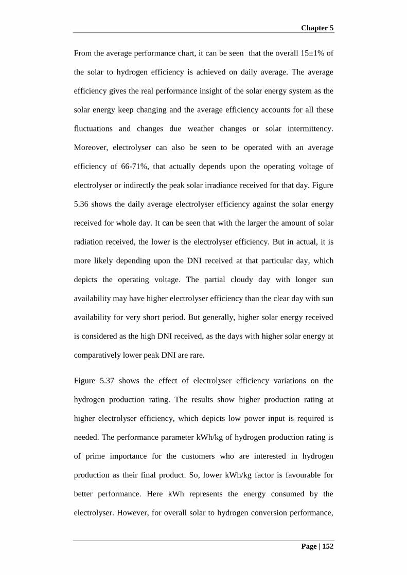
Chapter 5

Page | 152

From the average performance chart, it can be seen that the overall 15±1% of

the solar to hydrogen efficiency is achieved on daily average. The average

efficiency gives the real performance insight of the solar energy system as the

solar energy keep changing and the average efficiency accounts for all these

fluctuations and changes due weather changes or solar intermittency.

Moreover, electrolyser can also be seen to be operated with an average

efficiency of 66-71%, that actually depends upon the operating voltage of

electrolyser or indirectly the peak solar irradiance received for that day. Figure

5.36 shows the daily average electrolyser efficiency against the solar energy

received for whole day. It can be seen that with the larger the amount of solar

radiation received, the lower is the electrolyser efficiency. But in actual, it is

more likely depending upon the DNI received at that particular day, which

depicts the operating voltage. The partial cloudy day with longer sun

availability may have higher electrolyser efficiency than the clear day with sun

availability for very short period. But generally, higher solar energy received

is considered as the high DNI received, as the days with higher solar energy at

comparatively lower peak DNI are rare.

Figure 5.37 shows the effect of electrolyser efficiency variations on the

hydrogen production rating. The results show higher production rating at

higher electrolyser efficiency, which depicts low power input is required is

needed. The performance parameter kWh/kg of hydrogen production rating is

of prime importance for the customers who are interested in hydrogen

production as their final product. So, lower kWh/kg factor is favourable for

better performance. Here kWh represents the energy consumed by the

electrolyser. However, for overall solar to hydrogen conversion performance,

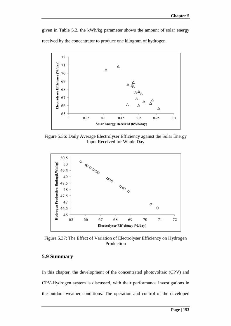
Chapter 5

Page | 153

given in Table 5.2, the kWh/kg parameter shows the amount of solar energy

received by the concentrator to produce one kilogram of hydrogen.

Figure 5.36: Daily Average Electrolyser Efficiency against the Solar Energy

Input Received for Whole Day

Figure 5.37: The Effect of Variation of Electrolyser Efficiency on Hydrogen

Production

5.9 Summary

In this chapter, the development of the concentrated photovoltaic (CPV) and

CPV-Hydrogen system is discussed, with their performance investigations in

the outdoor weather conditions. The operation and control of the developed

Chapter 5

Page | 154

experimental setup of CPV and CPV-Hydrogen system through LabVIEW are

explained. In the first section of the chapter, the development and the

fabrication of all three CPV systems, mini dish cassegrain design, Fresnel

lens-glass homogeniser design and Fresnel lens-reflective homogeniser design,

are discussed. All three CPV systems are fabricated according to the design

criteria discussed in Chapter 4. The mini parabolic and hyperbolic dishes are

fabricated using aluminium material, with further optical coating of aluminium

to get better surface finish. A 2x2 array of PMMA Fresnel lens, according to

optimized design is obtained. All the three fabricated CPV modules are

mounted onto developed two axis solar trackers, which are controlled through

master slave configuration. The performance of the developed CPV systems is

investigated in outdoor weather conditions. The maximum CPV system

efficiencies of 17-18% and 27-28% were recorded for mini dish CPV system

and both Fresnel lens based CPV systems respectively. From the normalized

power curve, the acceptance angles of 0.4o, 0.7

o and 1.2

o were recorded for

mini dish CPV, Fresnel lens-reflective homogeniser CPV and Fresnel lens-

glass homogeniser CPV, respectively. However, all of the three systems

showed highest performance against the developed tracking accuracy of 0.3o.

The lower efficiency for mini dish CPV was due to aluminium coating and

double stage reflection, which also caused lower acceptance angle of the

concentrating assembly.

Based upon the efficiency and the acceptance angle, the Fresnel lens-glass

homogeniser was further considered for performance investigation of CPV-

Hydrogen system. The hydrogen production unit was design and developed

using PEM electrolysers and feed water tanks. The produced hydrogen was

Chapter 5

Page | 155

then compressed and stored into cylinders. The maximum efficiency of solar

to hydrogen conversion was recorded as 18%. However, average efficiency of

15% for solar to hydrogen conversion was recorded for whole day operation.

Moreover, for series of experiments under different weather conditions, the

average performances of 47 kWh/kg and 218 kWh/ kg were measured for

electrolyser and overall solar energy to hydrogen conversion, respectively.

In the next chapter the long term performance of the developed CPV systems

is investigate using proposed electrical rating methodology.

Chapter 6

Page | 156

Chapter 6: Long Term Electrical Rating of

Concentrated Photovoltaic (CPV) Systems

6.1 Introduction

Solar energy has the highest energy potential among all the energy resources,

to meet the global energy needs [5]. In addition, photovoltaic systems offer the

direct conversion of solar energy into electricity, providing simple and elegant

method of solar energy utilization. Due to diversity of the photovoltaic

technology, the existing market is full of different photovoltaic systems

ranging from conventional silicon-based stationary photovoltaic (PV) panels

to two axis tracked concentrated photovoltaic (CPV) systems. Every

photovoltaic system has different performance and working conditions. The

performance of the photovoltaic systems is rated through a flash of light of

1000 W/m2 onto the module, with 25

oC cell temperature under standard

testing conditions (STC) (IEC 60904-3) or 800 W/m2 with 20

oC ambient

temperature and 1m/s flow rate, under standard operating conditions (SOC) or

Nominal Operating Cell Temperature (NOCT) (IEC 61215 and IEC 61646)

[117]. The instantaneous energy conversion efficiency is used as a rating

parameter to analyze the performance potential of the photovoltaic system.

However, the real field conditions are different than the rated conditions, with

temperature much higher than the rated value of 20oC or 25

oC and cell have to

operates for a longer period of time. The intensity of solar radiations is higher

only at the noon time, but not necessarily 1000 W/m2. Beside different

operating conditions, different photovoltaic technologies also need different

working conditions. Although CPV operates at higher efficiency than

Chapter 6

Page | 157

conventional PV [13,118,119] but it can only accept and convert solar beam

radiations into electricity [120]. This depicts that conventional PV can still

have power production in cloudy conditions but not CPV.

Efficiency of the solar cell varies with temperature and spectrum, affecting the

total power output of the system for long term operation than the predicted

value [121] as ultimately the consumer is interested in the total energy yield of

the photovoltaic system. Moreover, dust storms and dust accumulation on the

photovoltaic modules reduces the solar irradiance reaching the solar cell,

thereby reducing its performance. There are many models developed to

estimate the performance of conventional PV systems [122-124]. However,

because of different operating conditions, PV performance models cannot be

used for CPV. Some researchers studied the CPV performance by setting

outdoor parameters for laboratory testing [125]. Some authors used PV power

estimation model but with consideration of yearly average direct normal

irradiance and performance ratio [126]. However, due to intermittency of solar

energy and dynamic nature of meteorological data, DNI data availability and

prediction uncertainties varies from region to region. The CPV performance

depends upon many factors [127] including dust storms [128] that increases

uncertainties in the estimation or simulation approaches and motivating to

propose the long-term electrical rating (LTER) method. The LTER provides

energy planners and designers a simple and quick but accurate methodology to

determine the size of photovoltaic plant, based upon actual power output of

the CPV system from long term field testing data. From LTER, they can

understand the real potential and economic viability of a solar photovoltaic

plant.

Chapter 6

Page | 158

In this chapter, for the first time the long-term electrical rating (LTER) has

been introduced. The LTER of two in house built compact concentrated

photovoltaic (CPV) systems is reported in tropical weather conditions of

Singapore. This is the first ever outdoor field performance data reporting of

any CPV system in Singapore, to investigate its power potential as CPV

systems are recommended only for desert area because of high DNI

availability. The electrical rating in kWh/m2.year, with average system

efficiency, is used to investigate the potential of photovoltaic system in real

field operating conditions. The electrical rating is the total electrical power

output of the system per m2 of the photovoltaic system, normalized for period

of one year. All three developed CPV systems, as discussed in the previous

chapter with maximum efficiencies of 19% and 28%, are evaluated for long

term operation. Experiments were conducted from September, 2014 to August,

2015 and data the regarding electrical power output from CPV systems at the

maximum power point and the direct normal irradiance (DNI) received, was

recorded at an interval of 1sec. The LTER of the developed CPV systems was

compared with the other conventional PV systems installed in Singapore.

6.2 Electrical Rating Methodology

Electrical rating is a method, parameter or tool that is proposed to be used to

investigate the real field potential of any electrical power producing renewable

energy system, utilizing intermittent energy source for its operation like solar

energy or wind energy. From the long term power output measurement of the

system, electrical rating is represented for particular region in normalized

value as kWh/m2.year, in spite of its operating conditions. Instead of using the

Chapter 6

Page | 159

performance data from overwhelming catalogue of the photovoltaic

manufacturers, the motive of the proposed electrical rating methodology is to

provide accurate but simple parameter for consumers and designers to estimate

the size of power plant according to the actual power output data at specific

location, as the availability of the renewable energy resources varies

throughout the year due to their intermittent nature and varies region to region.

In addition, the electrical rating provides a common playing field to analyze

the real potential and economic viability of any renewable energy system,

irrespective of the technology or energy source as the comparison parameter

is the electrical energy output.

Moreover, in electrical rating methodology, the focus is on the long term

average performance of the system rather than the instantaneous efficiency

and rated power. Due to many performance affecting parameters, the CPV

instantaneous changes and fluctuates during operation. However, long term

average efficiency remains stable and provides a reliable parameter to evaluate

the true energy conversion potential of the system. The details of the electrical

rating methodology and the system description are are discussed further in this

section.

6.2.1 CPV System Description under Investigation

The current analysis of the CPV systems is based upon the electrical power

output of the module which is measured in terms of the current and voltage

through maximum power point tracking, connected at the module output. The

performance parameters of the CPV system in form of power output and the

DNI input were recorded for whole day operation, from sunrise to sunset, at an

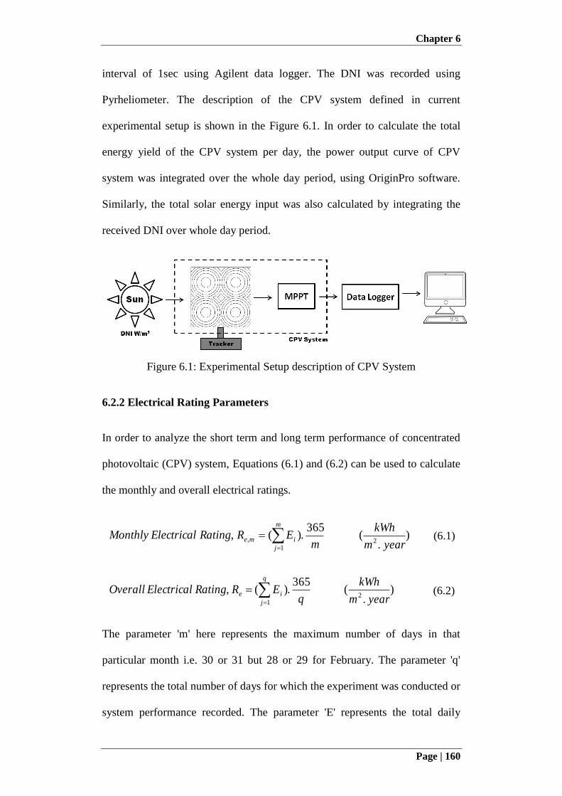
Chapter 6

Page | 160

interval of 1sec using Agilent data logger. The DNI was recorded using

Pyrheliometer. The description of the CPV system defined in current

experimental setup is shown in the Figure 6.1. In order to calculate the total

energy yield of the CPV system per day, the power output curve of CPV

system was integrated over the whole day period, using OriginPro software.

Similarly, the total solar energy input was also calculated by integrating the

received DNI over whole day period.

Figure 6.1: Experimental Setup description of CPV System

6.2.2 Electrical Rating Parameters

In order to analyze the short term and long term performance of concentrated

photovoltaic (CPV) system, Equations (6.1) and (6.2) can be used to calculate

the monthly and overall electrical ratings.

).

(365

.)(,2

1

,yearm

kWh

mERRatingElectricalMonthly

m

j

ime

(6.1)

).

(365

.)(,2

1 yearm

kWh

qERRatingElectricalOverall

q

j

ie

(6.2)

The parameter 'm' here represents the maximum number of days in that

particular month i.e. 30 or 31 but 28 or 29 for February. The parameter 'q'

represents the total number of days for which the experiment was conducted or

system performance recorded. The parameter 'E' represents the total daily

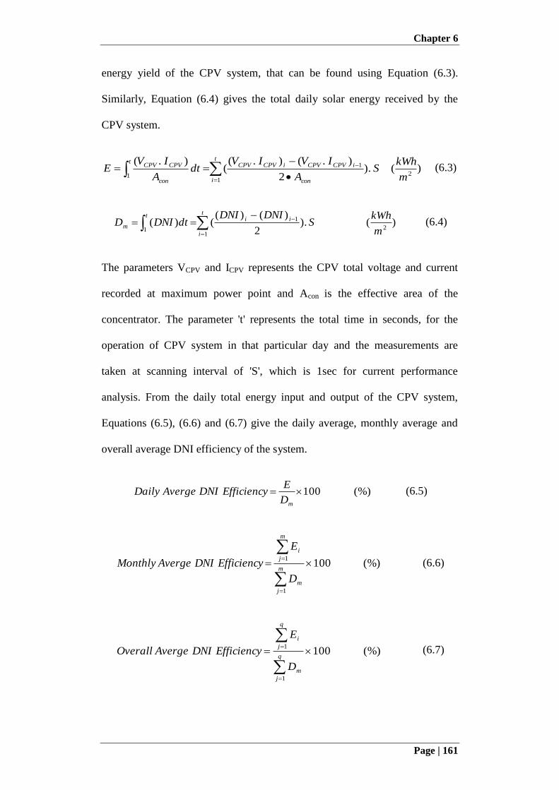
Chapter 6

Page | 161

energy yield of the CPV system, that can be found using Equation (6.3).

Similarly, Equation (6.4) gives the total daily solar energy received by the

CPV system.

t

i con

iCPVCPViCPVCPVt

con

CPVCPV

m

kWhS

A

IVIVdt

A

IVE

12

1

1)().

2

).().((

).( (6.3)

t

i

iit

mm

kWhS

DNIDNIdtDNID

12

1

1)().

2

)()(()( (6.4)

The parameters VCPV and ICPV represents the CPV total voltage and current

recorded at maximum power point and Acon is the effective area of the

concentrator. The parameter 't' represents the total time in seconds, for the

operation of CPV system in that particular day and the measurements are

taken at scanning interval of 'S', which is 1sec for current performance

analysis. From the daily total energy input and output of the CPV system,

Equations (6.5), (6.6) and (6.7) give the daily average, monthly average and

overall average DNI efficiency of the system.

(%)100mD

EEfficiencyDNIAvergeDaily (6.5)

(%)100

1

1

m

j

m

m

j

i

D

E

EfficiencyDNIAvergeMonthly (6.6)

(%)100

1

1

q

j

m

q

j

i

D

E

EfficiencyDNIAvergeOverall (6.7)

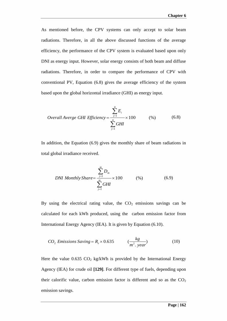
Chapter 6

Page | 162

As mentioned before, the CPV systems can only accept to solar beam

radiations. Therefore, in all the above discussed functions of the average

efficiency, the performance of the CPV system is evaluated based upon only

DNI as energy input. However, solar energy consists of both beam and diffuse

radiations. Therefore, in order to compare the performance of CPV with

conventional PV, Equation (6.8) gives the average efficiency of the system

based upon the global horizontal irradiance (GHI) as energy input.

(%)100

1

1

q

j

q

j

i

GHI

E

EfficiencyGHIAvergeOverall (6.8)

In addition, the Equation (6.9) gives the monthly share of beam radiations in

total global irradiance received.

(%)100

1

1

m

j

m

j

m

GHI

D

ShareMonthlyDNI (6.9)

By using the electrical rating value, the CO2 emissions savings can be

calculated for each kWh produced, using the carbon emission factor from

International Energy Agency (IEA). It is given by Equation (6.10).

).

(635.022

yearm

kgRSavingEmissionsCO e (10)

Here the value 0.635 CO2 kg/kWh is provided by the International Energy

Agency (IEA) for crude oil [129]. For different type of fuels, depending upon

their calorific value, carbon emission factor is different and so as the CO2

emission savings.

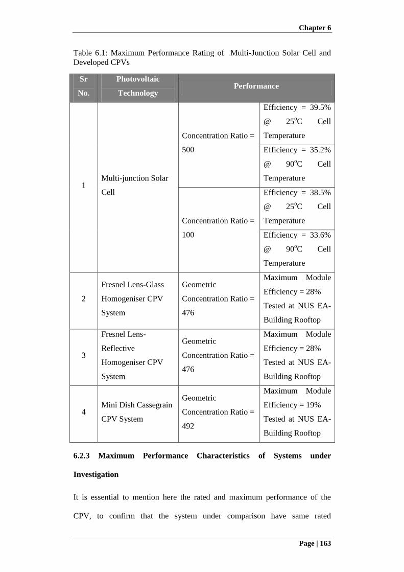
Chapter 6

Page | 163

Table 6.1: Maximum Performance Rating of Multi-Junction Solar Cell and

Developed CPVs

Sr

No.

Photovoltaic

Technology Performance

1 Multi-junction Solar

Cell

Concentration Ratio =

500

Efficiency = 39.5%

@ 25oC Cell

Temperature

Efficiency = 35.2%

@ 90oC Cell

Temperature


100

Efficiency = 38.5%

@ 25oC Cell

Temperature

Efficiency = 33.6%

@ 90oC Cell

Temperature

2

Fresnel Lens-Glass

Homogeniser CPV

System

Geometric


476

Maximum Module

Efficiency = 28%

Tested at NUS EA-

Building Rooftop

3

Fresnel Lens-

Reflective

Homogeniser CPV

System

Geometric


476

Maximum Module

Efficiency = 28%

Tested at NUS EA-

Building Rooftop

4 Mini Dish Cassegrain

CPV System

Geometric


492

Maximum Module

Efficiency = 19%

Tested at NUS EA-

Building Rooftop

6.2.3 Maximum Performance Characteristics of Systems under

Investigation

It is essential to mention here the rated and maximum performance of the

CPV, to confirm that the system under comparison have same rated

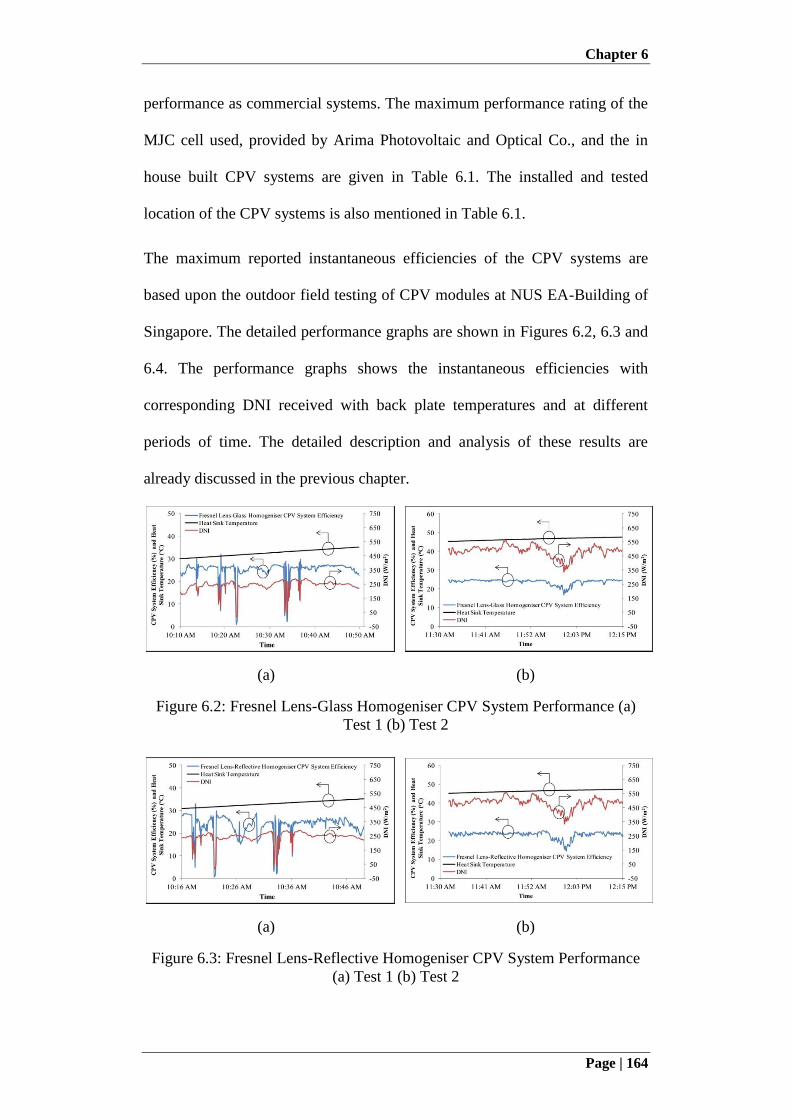
Chapter 6

Page | 164

performance as commercial systems. The maximum performance rating of the

MJC cell used, provided by Arima Photovoltaic and Optical Co., and the in

house built CPV systems are given in Table 6.1. The installed and tested

location of the CPV systems is also mentioned in Table 6.1.

The maximum reported instantaneous efficiencies of the CPV systems are

based upon the outdoor field testing of CPV modules at NUS EA-Building of

Singapore. The detailed performance graphs are shown in Figures 6.2, 6.3 and

6.4. The performance graphs shows the instantaneous efficiencies with

corresponding DNI received with back plate temperatures and at different

periods of time. The detailed description and analysis of these results are

already discussed in the previous chapter.

(a) (b)

Figure 6.2: Fresnel Lens-Glass Homogeniser CPV System Performance (a)

Test 1 (b) Test 2

(a) (b)

Figure 6.3: Fresnel Lens-Reflective Homogeniser CPV System Performance

(a) Test 1 (b) Test 2

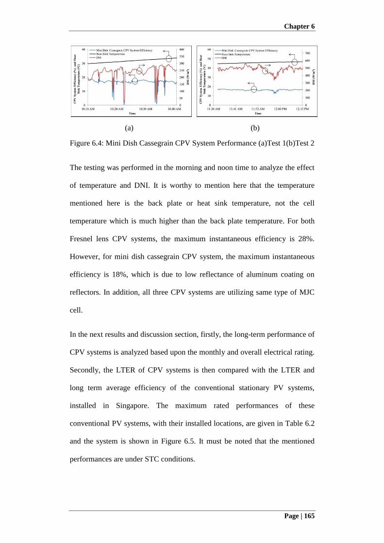
Chapter 6

Page | 165

(a) (b)

Figure 6.4: Mini Dish Cassegrain CPV System Performance (a)Test 1(b)Test 2

The testing was performed in the morning and noon time to analyze the effect

of temperature and DNI. It is worthy to mention here that the temperature

mentioned here is the back plate or heat sink temperature, not the cell

temperature which is much higher than the back plate temperature. For both

Fresnel lens CPV systems, the maximum instantaneous efficiency is 28%.

However, for mini dish cassegrain CPV system, the maximum instantaneous

efficiency is 18%, which is due to low reflectance of aluminum coating on

reflectors. In addition, all three CPV systems are utilizing same type of MJC

cell.

In the next results and discussion section, firstly, the long-term performance of

CPV systems is analyzed based upon the monthly and overall electrical rating.

Secondly, the LTER of CPV systems is then compared with the LTER and

long term average efficiency of the conventional stationary PV systems,

installed in Singapore. The maximum rated performances of these

conventional PV systems, with their installed locations, are given in Table 6.2

and the system is shown in Figure 6.5. It must be noted that the mentioned

performances are under STC conditions.

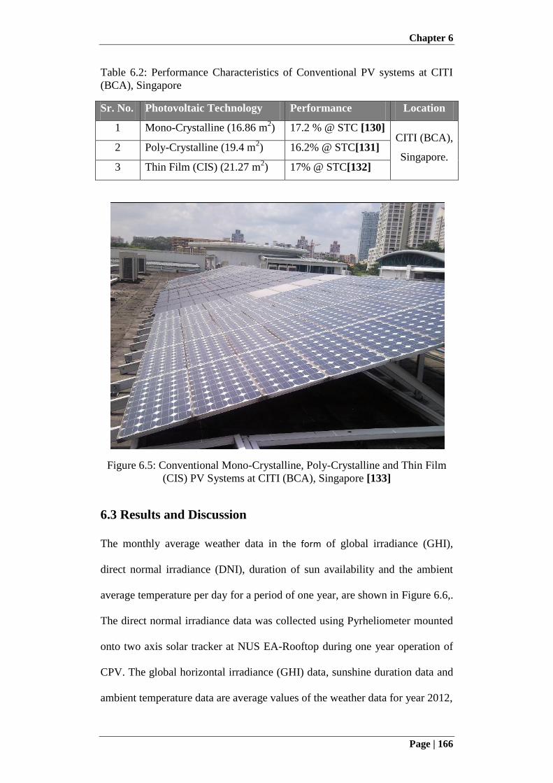
Chapter 6

Page | 166

Table 6.2: Performance Characteristics of Conventional PV systems at CITI

(BCA), Singapore

Sr. No. Photovoltaic Technology Performance Location

1 Mono-Crystalline (16.86 m2) 17.2 % @ STC [130]

CITI (BCA),

Singapore. 2 Poly-Crystalline (19.4 m

2) 16.2% @ STC[131]

3 Thin Film (CIS) (21.27 m2) 17% @ STC[132]

Figure 6.5: Conventional Mono-Crystalline, Poly-Crystalline and Thin Film

(CIS) PV Systems at CITI (BCA), Singapore [133]

6.3 Results and Discussion

The monthly average weather data in the form of global irradiance (GHI),

direct normal irradiance (DNI), duration of sun availability and the ambient

average temperature per day for a period of one year, are shown in Figure 6.6,.

The direct normal irradiance data was collected using Pyrheliometer mounted

onto two axis solar tracker at NUS EA-Rooftop during one year operation of

CPV. The global horizontal irradiance (GHI) data, sunshine duration data and

ambient temperature data are average values of the weather data for year 2012,

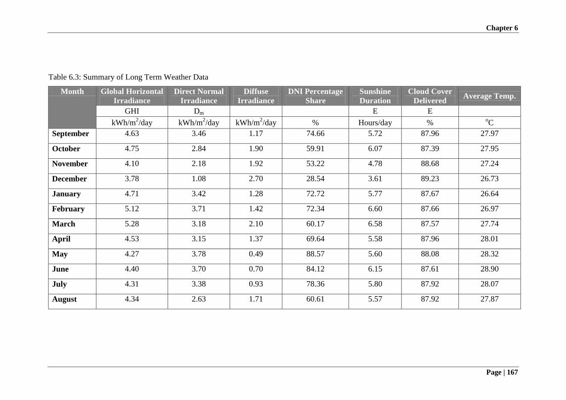
Chapter 6

Page | 167

Table 6.3: Summary of Long Term Weather Data

Month Global Horizontal

Irradiance

Direct Normal

Irradiance

Diffuse

Irradiance

DNI Percentage

Share

Sunshine

Duration

Cloud Cover

Delivered Average Temp.

GHI Dm E E

kWh/m2/day kWh/m

2/day kWh/m

2/day % Hours/day %

oC

September 4.63 3.46 1.17 74.66 5.72 87.96 27.97

October 4.75 2.84 1.90 59.91 6.07 87.39 27.95

November 4.10 2.18 1.92 53.22 4.78 88.68 27.24

December 3.78 1.08 2.70 28.54 3.61 89.23 26.73

January 4.71 3.42 1.28 72.72 5.77 87.67 26.64

February 5.12 3.71 1.42 72.34 6.60 87.66 26.97

March 5.28 3.18 2.10 60.17 6.58 87.57 27.74

April 4.53 3.15 1.37 69.64 5.58 87.96 28.01

May 4.27 3.78 0.49 88.57 5.60 88.08 28.32

June 4.40 3.70 0.70 84.12 6.15 87.61 28.90

July 4.31 3.38 0.93 78.36 5.80 87.92 28.07

August 4.34 2.63 1.71 60.61 5.57 87.92 27.87

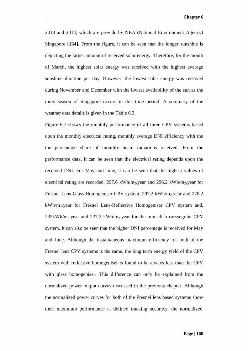
Chapter 6

Page | 168

2013 and 2014, which are provide by NEA (National Environment Agency)

Singapore [134]. From the figure, it can be seen that the longer sunshine is

depicting the larger amount of received solar energy. Therefore, for the month

of March, the highest solar energy was received with the highest average

sunshine duration per day. However, the lowest solar energy was received

during November and December with the lowest availability of the sun as the

rainy season of Singapore occurs in this time period. A summary of the

weather data details is given in the Table 6.3.

Figure 6.7 shows the monthly performance of all three CPV systems based

upon the monthly electrical rating, monthly average DNI efficiency with the

the percentage share of monthly beam radiations received. From the

performance data, it can be seen that the electrical rating depends upon the

received DNI. For May and June, it can be seen that the highest values of

electrical rating are recorded, 297.6 kWh/m2.year and 296.2 kWh/m2.year for

Fresnel Lens-Glass Homogeniser CPV system, 297.2 kWh/m2.year and 278.2

kWh/m2.year for Fresnel Lens-Reflective Homogeniser CPV system and,

235kWh/m2.year and 227.2 kWh/m2.year for the mini dish casssegrain CPV

system. It can also be seen that the higher DNI percentage is received for May

and June. Although the instantaneous maximum efficiency for both of the

Fresnel lens CPV systems is the same, the long term energy yield of the CPV

system with reflective homogeniser is found to be always less than the CPV

with glass homogeniser. This difference can only be explained from the

normalized power output curves discussed in the previous chapter. Although

the normalized power curves for both of the Fresnel lens based systems show

their maximum performance at defined tracking accuracy, the normalized

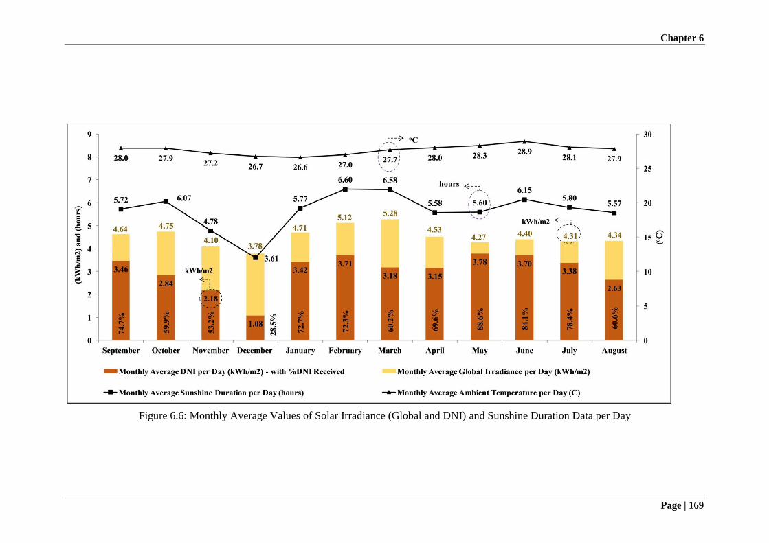
Chapter 6

Page | 169

Figure 6.6: Monthly Average Values of Solar Irradiance (Global and DNI) and Sunshine Duration Data per Day

Chapter 6

Page | 170

power curve for CPV system with reflective homogeniser is lower than the

CPV with glass homogeniser. This is because of the optical loss that occurs

when concentrated light reflects through the reflective homogeniser, which is

made of aluminum having comparatively low reflectance. In short term

performance analysis, this effect of homogeniser is not prominent. However,

through long term performance, the true effect of homogeniser design on the

system performance can be found. For mini dish CPV system, the reason for

low electrical rating is due to comparatively low conversion efficiency.

Beside the best performances, the poor performance of the CPV system was

observed in November and December due to low availability of the DNI.

Figure 6.7 also shows the average DNI efficiency of each of the CPV system

based upon monthly DNI. It can be seen that the average DNI efficiency of

Fresnel Lens-Glass homogeniser CPV system is highest i.e. 22% followed by

the one with the reflective homogeniser design and the mini dish CPV system

with 21.5% and 16% respectively. It can be seen that the average efficiency is

lower than the instantaneous rated efficiency, representing the real potential

of the system. Furthermore, the average efficiency for each of the CPV system

is higher in February. To further explain this trend of higher efficiency, there

is need to reconsider Figure 6.6 as the highest sunshine duration and lowest

ambient temperature recorded for February.

After discussing the monthly variation of electrical rating of CPV systems, the

overall electrical rating for 12-months period of operation is shown in Figure

6.8. For performance comparison purpose, the overall electrical rating of CPV

systems is compared with the conventional PV systems installed at CITI

(BCA), Singapore. The overall electrical rating recorded for Fresnel lens CPV

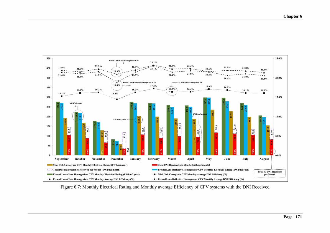
Chapter 6

Page | 171

Figure 6.7: Monthly Electrical Rating and Monthly average Efficiency of CPV systems with the DNI Received

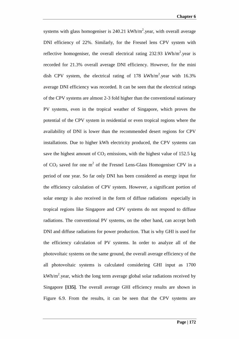
Chapter 6

Page | 172

systems with glass homogeniser is 240.21 kWh/m2.year, with overall average

DNI efficiency of 22%. Similarly, for the Fresnel lens CPV system with

reflective homogeniser, the overall electrical rating 232.93 kWh/m2.year is

recorded for 21.3% overall average DNI efficiency. However, for the mini

dish CPV system, the electrical rating of 178 kWh/m2.year with 16.3%

average DNI efficiency was recorded. It can be seen that the electrical ratings

of the CPV systems are almost 2-3 fold higher than the conventional stationary

PV systems, even in the tropical weather of Singapore, which proves the

potential of the CPV system in residential or even tropical regions where the

availability of DNI is lower than the recommended desert regions for CPV

installations. Due to higher kWh electricity produced, the CPV systems can

save the highest amount of CO2 emissions, with the highest value of 152.5 kg

of CO2 saved for one m2 of the Fresnel Lens-Glass Homogeniser CPV in a

period of one year. So far only DNI has been considered as energy input for

the efficiency calculation of CPV system. However, a significant portion of

solar energy is also received in the form of diffuse radiations especially in

tropical regions like Singapore and CPV systems do not respond to diffuse

radiations. The conventional PV systems, on the other hand, can accept both

DNI and diffuse radiations for power production. That is why GHI is used for

the efficiency calculation of PV systems. In order to analyze all of the

photovoltaic systems on the same ground, the overall average efficiency of the

all photovoltaic systems is calculated considering GHI input as 1700

kWh/m2.year, which the long term average global solar radiations received by

Singapore [135]. The overall average GHI efficiency results are shown in

Figure 6.9. From the results, it can be seen that the CPV systems are

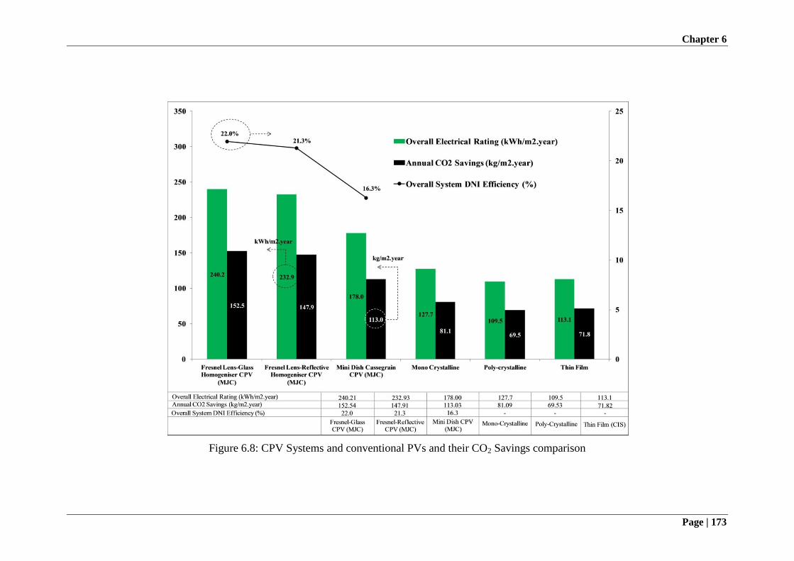
Chapter 6

Page | 173

Figure 6.8: CPV Systems and conventional PVs and their CO2 Savings comparison

Chapter 6

Page | 174

operating at higher efficiency than the conventional PV, as high as 14% long

term efficiency. However, the conventional PV systems showed the

maximum of 7.5% long term efficiency. This graph is of great importance

when the efficiency of the CPV is needed to be compared with the

conventional PV. Due to non-acceptance of diffuse radiations by the CPV

systems, the GHI efficiency shows the overall potential of system by

considering all forms of solar energy as a input.

Figure 6.9: Overall Average GHI Efficiency

An overall summary of the monthly and overall performance of each of three

CPV system is given in Table 6.4. From the data given, it can be seen that the

during one year period of operation, only 66.1% of the total solar energy was

received in the form of the beam radiations and the global radiation received is

close to average solar energy availability of Singapore as 1700 kWh/m2.year.

From the results, it can be seen that the electrical rating is depending upon the

availability of DNI. Therefore, in order to further investigate and quantify

their relation, a graph is plotted between total energy output of the system in

the form of monthly electrical rating and corresponding monthly solar

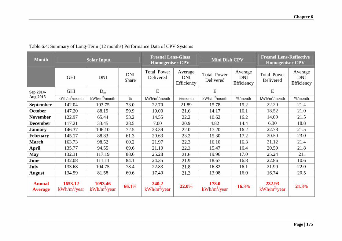
Chapter 6

Page | 175

Table 6.4: Summary of Long-Term (12 months) Performance Data of CPV Systems

Month Solar Input Fresnel Lens-Glass

Homogeniser CPV Mini Dish CPV

Fresnel Lens-Reflective

Homogeniser CPV

GHI DNI DNI

Share

Total Power

Delivered

Average

DNI

Efficiency

Total Power

Delivered

Average

DNI

Efficiency

Total Power

Delivered

Average

DNI

Efficiency

Sep.2014-

Aug.2015 GHI Dm E E E

kWh/m2/month kWh/m

2/month % kWh/m

2/month %/month kWh/m

2/month %/month kWh/m

2/month %/month

September 142.04 103.75 73.0 22.70 21.89 15.78 15.2 22.20 21.4

October 147.20 88.19 59.9 19.00 21.6 14.17 16.1 18.52 21.0

November 122.97 65.44 53.2 14.55 22.2 10.62 16.2 14.09 21.5

December 117.21 33.45 28.5 7.00 20.9 4.82 14.4 6.30 18.8

January 146.37 106.10 72.5 23.39 22.0 17.20 16.2 22.78 21.5

February 145.17 88.83 61.3 20.63 23.2 15.30 17.2 20.50 23.0

March 163.73 98.52 60.2 21.97 22.3 16.10 16.3 21.12 21.4

April 135.77 94.55 69.6 21.10 22.3 15.47 16.4 20.59 21.8

May 132.31 117.19 88.6 25.28 21.6 19.96 17.0 25.24 21.

June 132.08 111.11 84.1 24.35 21.9 18.67 16.8 22.86 10.6

July 133.68 104.75 78.4 22.83 21.8 16.82 16.1 21.99 22.0

August 134.59 81.58 60.6 17.40 21.3 13.08 16.0 16.74 20.5

Annual

Average

1653.12

kWh/m2/year

1093.46

kWh/m2/year

66.1% 240.2

kWh/m2/year

22.0% 178.0

kWh/m2/year

16.3% 232.93

kWh/m2/year

21.3%

Chapter 6

Page | 176

availability but normalized to yearly average solar energy input per m2, as

shown in the Figure 6.10. For the CPV system, the power output is plotted

against the DNI and for the conventional photovoltaic systems i.e. mono

crystalline, poly-crystalline and thin film, the electrical rating is plotted for

DNI that is 66.1% of the long term GHI i.e. 1700 kWh/m2.year as the

performance of stationary PV depends upon the GHI. The plotted data is fitted

through linear regression. It can be seen that the electrical rating and the direct

normal irradiance (DNI) availability are directly proportional to each other

with R2 value of 0.996, 0.9921 and 0.990 for both Fresnel lens based glass and

reflective homogeniser CPVs and the mini dish CPV system, respectively.

However, the main point of interest is that the electrical rating and DNI are

proportional to each other through the long term average efficiency. It can be

seen that the slope of the regressed line is the same as the long term DNI

efficiency of the CPV or PV systems i.e. 22%, 21.3% and 16.3% for CPVs

against DNI and 7.5%, 6.4% and 6.7% for conventional PVs against GHI.

This electrical rating graph has the main importance from the design point of

view of photovoltaic plant. From this graph, it can be seen that if the total

average annual DNI availability is known then by knowing the average

efficiency of the CPV system, not maximum or rated efficiency, a quick

estimate of the total power output of the CPV system can be made at a

particular region. Although the study is based upon the tropical region,

however, if the higher total DNI availability for desert regions like Gulf

countries, is known then the higher electrical rating can be achieved and

estimated from electrical rating graph, if the average efficiency of the CPV

system is known.

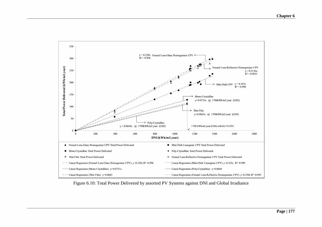
Chapter 6

Page | 177

Figure 6.10: Total Power Delivered by assorted PV Systems against DNI and Global Irradiance

Chapter 6

Page | 178

6.4 Summary

Due to many factors affecting the performance of the photovoltaic system, a

simple and accurate electrical rating methodology is proposed to analyze the

field performance of any photovoltaic system. The conventional rating

methods for photovoltaic system performance analysis employ a certain

constant factor under laboratory conditions. Moreover, the solar cell

temperature is kept either at 25oC according to the standard rating procedures.

However, the real field conditions change continuously, especially solar

irradiance along with variations in cloud cover and ambient temperature.

Another important factor is the dust covering that reduces the system

performance significantly. Even all the models developed to simulate the

performance of the photovoltaic systems, are unable to cover all the

performance which in actual cannot be predicted accurately. Despite operating

conditions, the working conditions of CPVs are different from PVs. The

consumers are ultimately interested in the total electricity yield by the system.

Therefore, an electrical rating methodology provides the actual

performance data of the photovoltaic systems to designers and consumer to

accurately predict the size of a photovoltaic plant, under climate conditions of

a particular region.

The performance of the developed CPV systems: Fresnel lens-Glass

Homogeniser, Fresnel lens-Reflective Homogeniser and mini dish cassegrain,

was evaluated for long term operation of one year (12-months). The

performance parameters of the CPV systems in terms of the voltage and

current output at maximum power point were recorded to measure the system

power output. By integrating the power output curve over whole day period,

Chapter 6

Page | 179

the daily electric energy yield was calculated and by summing up daily energy

yield for each of months, the overall average efficiency and the

monthly/overall electrical ratings of all three systems were obtained. Electrical

ratings of 240.21 kWh/m2.year, 232.93 kWh/m

2.year and 178.00 kWh/m

2.year

were recorded with the overall average efficiency of 22.0%, 21.3% and 16.3%

for the Fresnel lens CPV system with glass homogeniser, reflective

homogeniser and the mini dish cassegrain CPV system respectively. The

recorded electrical ratings are 2-3 folds higher than the conventional PV

systems installed in Singapore. Moreover, the electrical rating chart shows the

proportional relation of electrical against received DNI. From the electrical

rating chart, the total power output of the CPV system can be accurately

predicted if the average efficiency of the system and the annual DNI

availability is known.

In the next chapter, the design, development and testing of novel multi-leg

homogeniser concentrating assembly is discussed for CPV applications.

Chapter 7

Page | 180

Chapter 7: Development of a Multi-leg Homogeniser

Concentrating Assembly for Concentrated

Photovoltaic (CPV) System

7.1 Introduction

Among all the photovoltaic technologies, concentrated photovoltaic (CPV)

system offers the highest efficiency for solar energy to electricity conversion,

as highly efficient multi-junction solar cells (MJC) are utilized. Because of

high production cost of the MJC, it is not cost effective to build them in panels

like conventional silicon based stationary PV modules. Therefore, in CPV

system, low cost solar concentrators are used to concentrate sun rays onto a

small area of MJC and as a result, reducing the use of expensive solar cell

material by replacing it with cheap solar concentrators. In the conventional

design of the CPV concentrating assembly, as discussed in the previous

chapters, a single concentrator is used to concentrate solar radiation onto a

single solar cell. In this chapter, a novel design of the CPV concentrating

assembly is proposed which can concentrate solar radiation onto four MJCs

using a single set of concentrators. The main motive for the development of

this novel concentrating assembly design is to further reduce the cost of CPV

system by reducing the number of concentrators needed for same capacity of

system. As the concept of concentrated photovoltaic makes the use of multi-

junction solar cells cost effective by replacing expensive solar cell material

with the low cost solar concentrators, this novel concept of concentrating

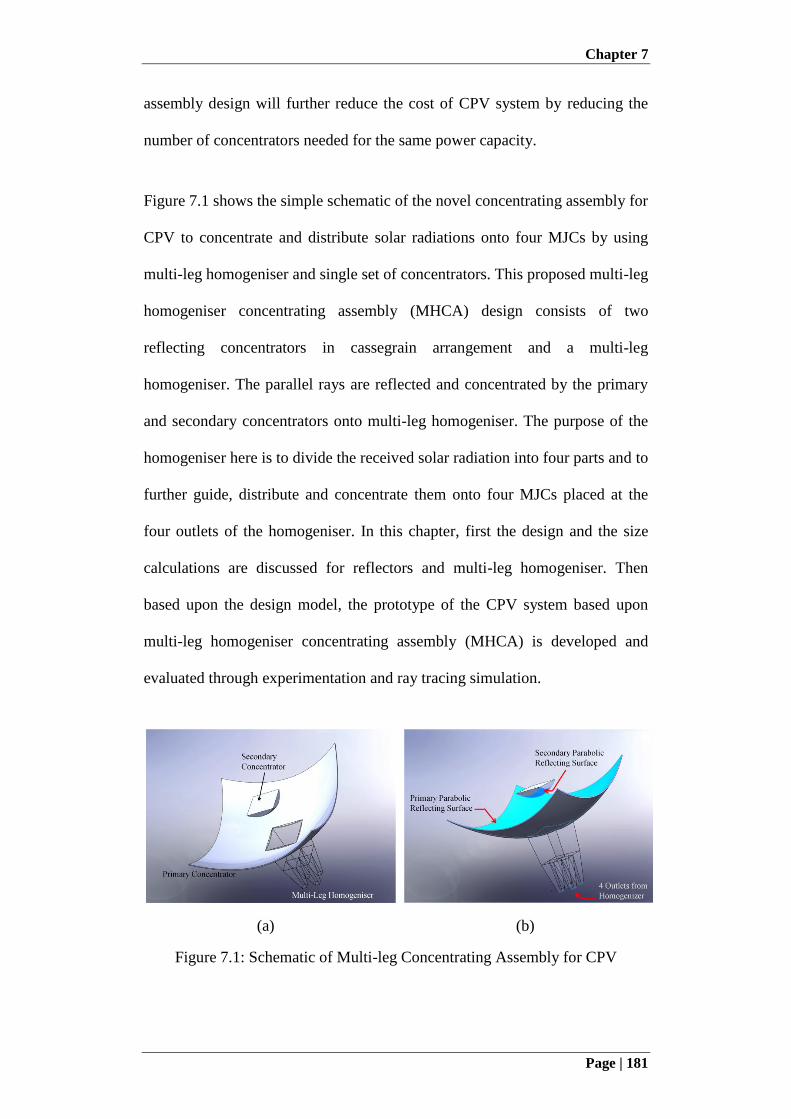
Chapter 7

Page | 181

assembly design will further reduce the cost of CPV system by reducing the

number of concentrators needed for the same power capacity.

Figure 7.1 shows the simple schematic of the novel concentrating assembly for

CPV to concentrate and distribute solar radiations onto four MJCs by using

multi-leg homogeniser and single set of concentrators. This proposed multi-leg

homogeniser concentrating assembly (MHCA) design consists of two

reflecting concentrators in cassegrain arrangement and a multi-leg

homogeniser. The parallel rays are reflected and concentrated by the primary

and secondary concentrators onto multi-leg homogeniser. The purpose of the

homogeniser here is to divide the received solar radiation into four parts and to

further guide, distribute and concentrate them onto four MJCs placed at the

four outlets of the homogeniser. In this chapter, first the design and the size

calculations are discussed for reflectors and multi-leg homogeniser. Then

based upon the design model, the prototype of the CPV system based upon

multi-leg homogeniser concentrating assembly (MHCA) is developed and

evaluated through experimentation and ray tracing simulation.

(a) (b)

Figure 7.1: Schematic of Multi-leg Concentrating Assembly for CPV

Chapter 7

Page | 182

7.2 Design of Multi-leg Homogeniser Concentrating Assembly

The design schematic of the CPV concentrating assembly based upon multi-

leg homogeniser is shown in Figure 7.2. Unlike the conventional design of the

mini dish cassegrain concentrating assembly, as discussed in the previous

chapters, the current design is based upon the two parabolic reflectors and as a

result, area concentration is achieved instead of point concentration. Both of

the reflectors of concentrating assembly are arranged such that the foci of both

of the reflectors, primary and secondary, coincide with each other. The parallel

rays, after being reflected by the primary parabolic reflector, are concentrated

at its focal point. The secondary parabolic reflector is placed in the way of the

converging rays such that its focal point coincides with the focal point of

primary reflector. The converging solar radiations after being reflected by the

secondary reflector, become parallel again as both of the reflectors have

parabolic curvature, and the radiations then enter the multi-leg homogeniser.

In order to design the concentrating assembly, the targeted ray path is

designed such that the edge ray of primary reflector at point 'a' must hit

secondary reflector surface at point 'b', which is at the same level as point 'b'

and focal points. The parallel incident ray, after being reflected from point 'b',

becomes parallel again and after entering into the multi-leg homogeniser, it is

reflected at point 'c' due to total internal reflection, towards the outlet aperture

of homogeniser. The point 'c' is at the junction of top and bottom tapered

portion of the homogeniser. So the slope and the height of the bottom tapered

portion is designed such that the ray after being reflected from point 'c', hits

the point 'e' which is at the extreme edge of homogeniser outlet aperture and

Chapter 7

Page | 183

hits the MJC which is placed there. As the edge ray leaves from point 'e' of the

homogeniser outlet, the subsequent rays are then assured to be uniformly

distributed over the entire area of the solar cell, as shown in the Figure 7.3. To

keep the cell temperature within the optimum operating limit, all four MJCs

are attached to heat spreader and heat sink. As the parallel incident rays also

become parallel after the secondary reflector, the concentrated rays at the inlet

aperture of multi-leg homogeniser then take the shape of primary reflect.

However, the size of the secondary reflector determines the size of the

concentrated rays area.

Figure 7.2: Design of Multi-Leg Homogeniser Concentrating Assembly

The design procedure for MHCA is divided into three steps. The first step is

related to the size calculations and the design of primary concentrator. The

second step is the design of the multi-leg homogeniser, followed by the third

step related to the design and size calculations of the secondary concentrator,

as the size of secondary concentrator depends upon the size of inlet aperture of

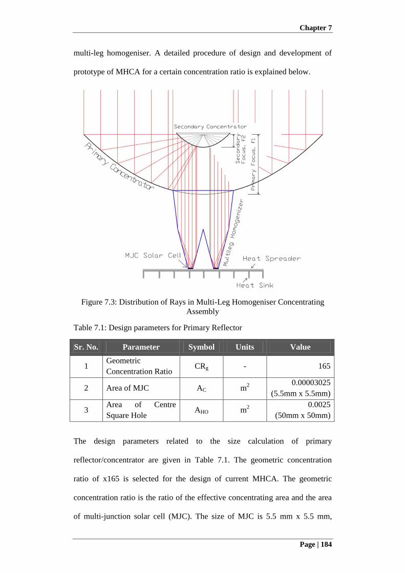
Chapter 7

Page | 184

multi-leg homogeniser. A detailed procedure of design and development of

prototype of MHCA for a certain concentration ratio is explained below.

Figure 7.3: Distribution of Rays in Multi-Leg Homogeniser Concentrating

Assembly

Table 7.1: Design parameters for Primary Reflector

Sr. No. Parameter Symbol Units Value

1 Geometric

Concentration Ratio CRg - 165

2 Area of MJC AC m2 0.00003025

(5.5mm x 5.5mm)

3 Area of Centre

Square Hole AHO m

2

0.0025

(50mm x 50mm)

The design parameters related to the size calculation of primary

reflector/concentrator are given in Table 7.1. The geometric concentration

ratio of x165 is selected for the design of current MHCA. The geometric

concentration ratio is the ratio of the effective concentrating area and the area

of multi-junction solar cell (MJC). The size of MJC is 5.5 mm x 5.5 mm,

Chapter 7

Page | 185

provided by Arima Photovoltaic and Optical Co., as explained in the previous

chapters. The system can be designed for higher concentration ratio. However,

lower concentration ratio is only selected for prototype purpose as higher

concentration ratio needs bigger reflector area that can make system expensive

at testing stage. In order to provide the space for mounting of multi-leg

homogeniser, a 50 mm x 50 mm square hole is cut in the centre of the primary

reflector, as shown in the Figure 7.4. Therefore, the net effective area of

concentrating assembly and the total area of primary reflector are given by

Equations (7.1) and (7.2), respectively.

Effective Area of Concentrating Assembly, 4 Cgcon ACRA (7.1)

Area of Primary Concentrator HOcon AAd 2

1 (7.2)

The parameter d1 gives one of the dimensions of the primary reflector as its

shape is assumed to be square. The square shape of primary reflector is helpful

to obtain the compact arrangement of concentrators in a CPV module. The

value '4' in Equation (7.1) represents the total number of MJCs accommodated

by the MHCA. Therefore, with the concentration ratio of 165, the size of the

primary reflector given by Equation (7.1) is 150 mm x 150 mm. It must be

noted here that the primary reflector is basically a square cut part of the

circular parabolic reflector, as shown in Figure 7.4. The diameter of the

corresponding circular primary reflector is equal to the diagonal of the square

reflector. However, the effective area of the primary reflector is shown by the

white shaded area in Figure 7.4. Equation (7.3) gives the diameter of the

corresponding circular diameter.

2

1

2

1

2

11 2dddD (7.3)

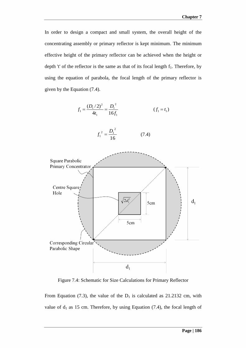
Chapter 7

Page | 186

In order to design a compact and small system, the overall height of the

concentrating assembly or primary reflector is kept minimum. The minimum

effective height of the primary reflector can be achieved when the height or

depth 't' of the reflector is the same as that of its focal length f1. Therefore, by

using the equation of parabola, the focal length of the primary reflector is

given by the Equation (7.4).

)(164

)2/(11

1

2

1

1

2

11 tf

f

D

t

Df

16

2

12

1

Df (7.4)

Figure 7.4: Schematic for Size Calculations for Primary Reflector

From Equation (7.3), the value of the D1 is calculated as 21.2132 cm, with

value of d1 as 15 cm. Therefore, by using Equation (7.4), the focal length of

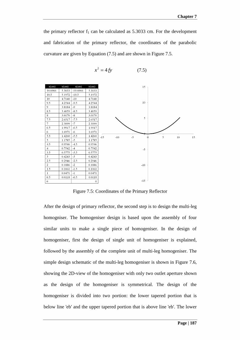
Chapter 7

Page | 187

the primary reflector f1 can be calculated as 5.3033 cm. For the development

and fabrication of the primary reflector, the coordinates of the parabolic

curvature are given by Equation (7.5) and are shown in Figure 7.5.

fyx 42 (7.5)

Figure 7.5: Coordinates of the Primary Reflector

After the design of primary reflector, the second step is to design the multi-leg

homogniser. The homogeniser design is based upon the assembly of four

similar units to make a single piece of homogeniser. In the design of

homogeniser, first the design of single unit of homogeniser is explained,

followed by the assembly of the complete unit of multi-leg homogeniser. The

simple design schematic of the multi-leg homogeniser is shown in Figure 7.6,

showing the 2D-view of the homogeniser with only two outlet aperture shown

as the design of the homogeniser is symmetrical. The design of the

homogeniser is divided into two portion: the lower tapered portion that is

below line 'eb' and the upper tapered portion that is above line 'eb'. The lower

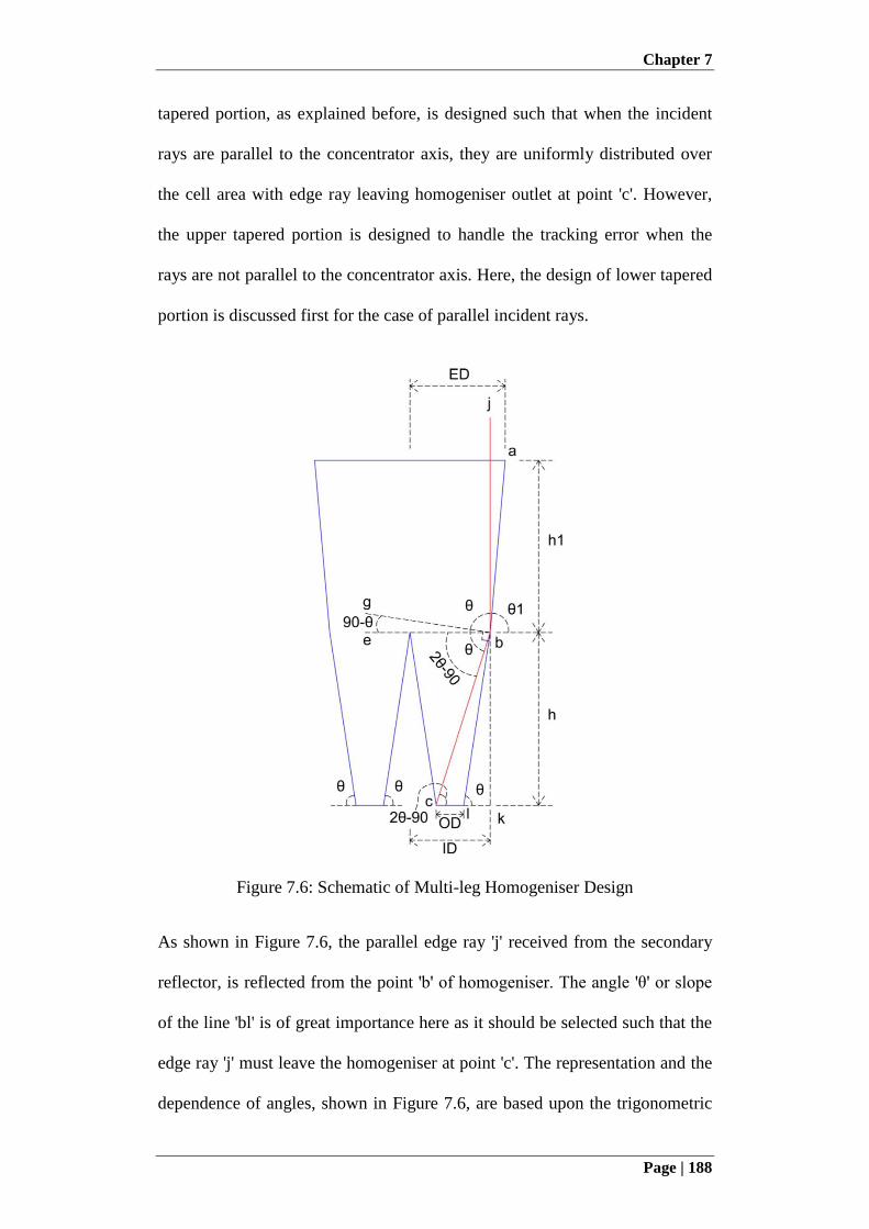
Chapter 7

Page | 188

tapered portion, as explained before, is designed such that when the incident

rays are parallel to the concentrator axis, they are uniformly distributed over

the cell area with edge ray leaving homogeniser outlet at point 'c'. However,

the upper tapered portion is designed to handle the tracking error when the

rays are not parallel to the concentrator axis. Here, the design of lower tapered

portion is discussed first for the case of parallel incident rays.

Figure 7.6: Schematic of Multi-leg Homogeniser Design

As shown in Figure 7.6, the parallel edge ray 'j' received from the secondary

reflector, is reflected from the point 'b' of homogeniser. The angle 'θ' or slope

of the line 'bl' is of great importance here as it should be selected such that the

edge ray 'j' must leave the homogeniser at point 'c'. The representation and the

dependence of angles, shown in Figure 7.6, are based upon the trigonometric

Chapter 7

Page | 189

laws. The line 'bg' is perpendicular to lower tapered side 'bl' and the edge ray

'j', after being reflected by the side 'bl', according to optics law, makes angle 'θ'

with perpendicular 'bg'. Therefore, if right angle triangle ∆ckb is considered,

the height 'h' of the lower tapered portion is given by Equation (7.6).

902tan.2

ODIDODh (7.6)

It can be seen that there are two unknowns 'h' and 'θ' in Equation (7.6).

Therefore, another Equation (7.7) is obtained from the right angle triangle

∆blk.

tan.2

ODIDh (7.7)

By comparing Equations (7.6) and (7.7), the slope 'θ' of lower tapered portion

of homogeniser is given by Equation (7.8).

tan.2

902tan.2

ODIDODIDOD (7.8)

The size of the outlet aperture of homogeniser 'OD' is 5.5mm, same as the size

of MJC. The value of 'ID' is taken as the 16 mm. The value of 'ID' is assumed

according to the convenience of fabrication but not very small and not very

large as it will cast shadow on the reflector. Later, it will be shown that the

value of 'ID' also affects the size of the secondary reflector. Therefore, by

solving Equation (7.8) with hit and trial for the given values of 'ID' and 'OD',

the value of slope 'θ' is calculated as 81.33o. The height 'h' of the lower tapered

portion can now be calculated using Equation (7.7) as 34.43 mm.

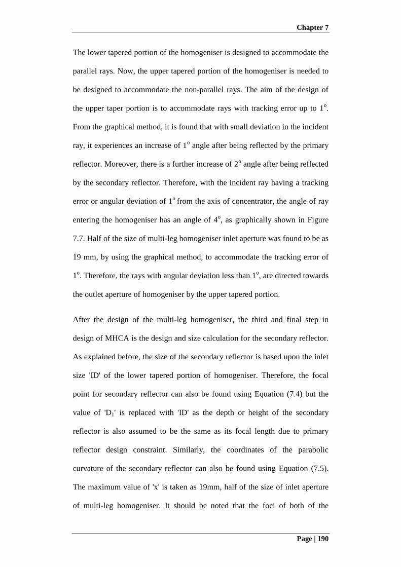
Chapter 7

Page | 190

The lower tapered portion of the homogeniser is designed to accommodate the

parallel rays. Now, the upper tapered portion of the homogeniser is needed to

be designed to accommodate the non-parallel rays. The aim of the design of

the upper taper portion is to accommodate rays with tracking error up to 1o.

From the graphical method, it is found that with small deviation in the incident

ray, it experiences an increase of 1o angle after being reflected by the primary

reflector. Moreover, there is a further increase of 2o angle after being reflected

by the secondary reflector. Therefore, with the incident ray having a tracking

error or angular deviation of 1o

from the axis of concentrator, the angle of ray

entering the homogeniser has an angle of 4o, as graphically shown in Figure

7.7. Half of the size of multi-leg homogeniser inlet aperture was found to be as

19 mm, by using the graphical method, to accommodate the tracking error of

1o. Therefore, the rays with angular deviation less than 1

o, are directed towards

the outlet aperture of homogeniser by the upper tapered portion.

After the design of the multi-leg homogeniser, the third and final step in

design of MHCA is the design and size calculation for the secondary reflector.

As explained before, the size of the secondary reflector is based upon the inlet

size 'ID' of the lower tapered portion of homogeniser. Therefore, the focal

point for secondary reflector can also be found using Equation (7.4) but the

value of 'D1' is replaced with 'ID' as the depth or height of the secondary

reflector is also assumed to be the same as its focal length due to primary

reflector design constraint. Similarly, the coordinates of the parabolic

curvature of the secondary reflector can also be found using Equation (7.5).

The maximum value of 'x' is taken as 19mm, half of the size of inlet aperture

of multi-leg homogeniser. It should be noted that the foci of both of the

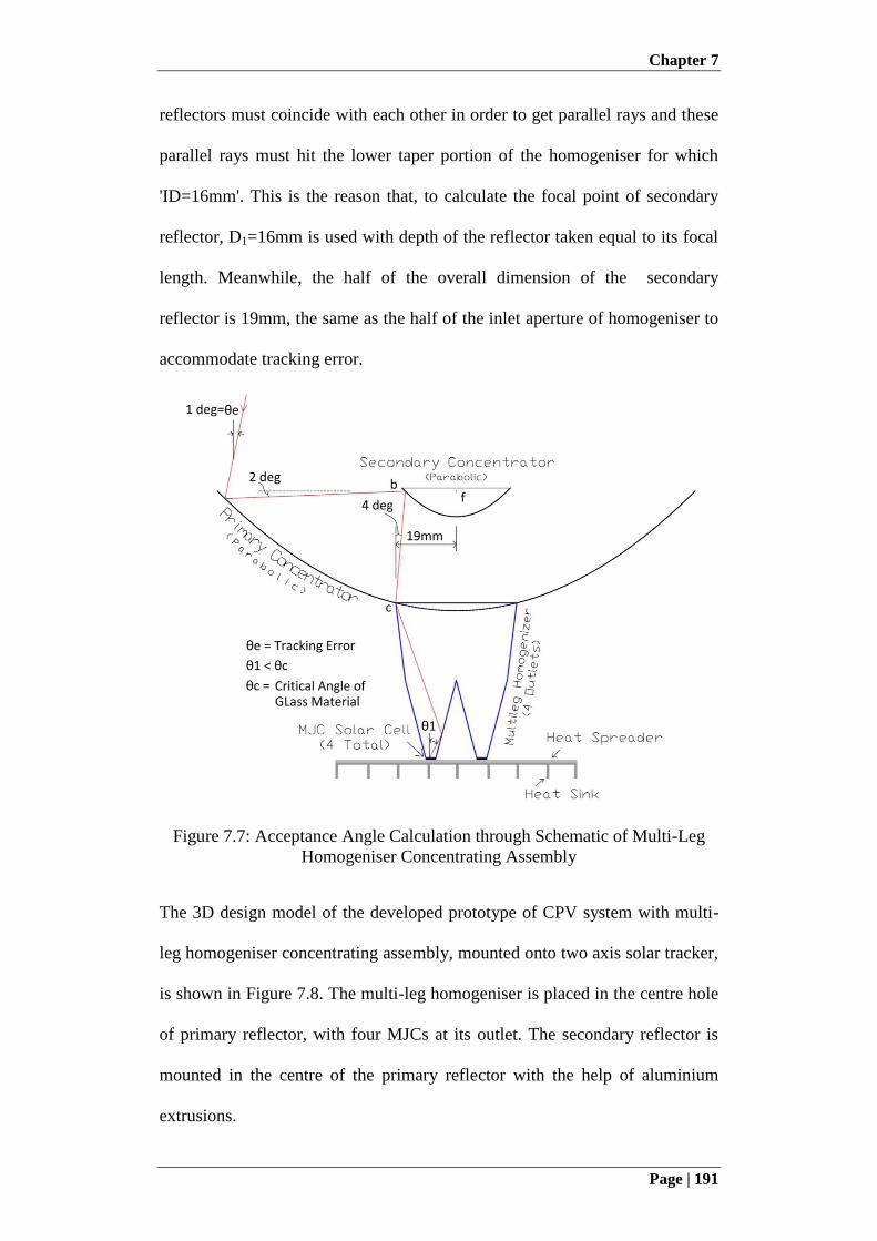
Chapter 7

Page | 191

reflectors must coincide with each other in order to get parallel rays and these

parallel rays must hit the lower taper portion of the homogeniser for which

'ID=16mm'. This is the reason that, to calculate the focal point of secondary

reflector, D1=16mm is used with depth of the reflector taken equal to its focal

length. Meanwhile, the half of the overall dimension of the secondary

reflector is 19mm, the same as the half of the inlet aperture of homogeniser to

accommodate tracking error.

Figure 7.7: Acceptance Angle Calculation through Schematic of Multi-Leg


The 3D design model of the developed prototype of CPV system with multi-

leg homogeniser concentrating assembly, mounted onto two axis solar tracker,

is shown in Figure 7.8. The multi-leg homogeniser is placed in the centre hole

of primary reflector, with four MJCs at its outlet. The secondary reflector is

mounted in the centre of the primary reflector with the help of aluminium

extrusions.

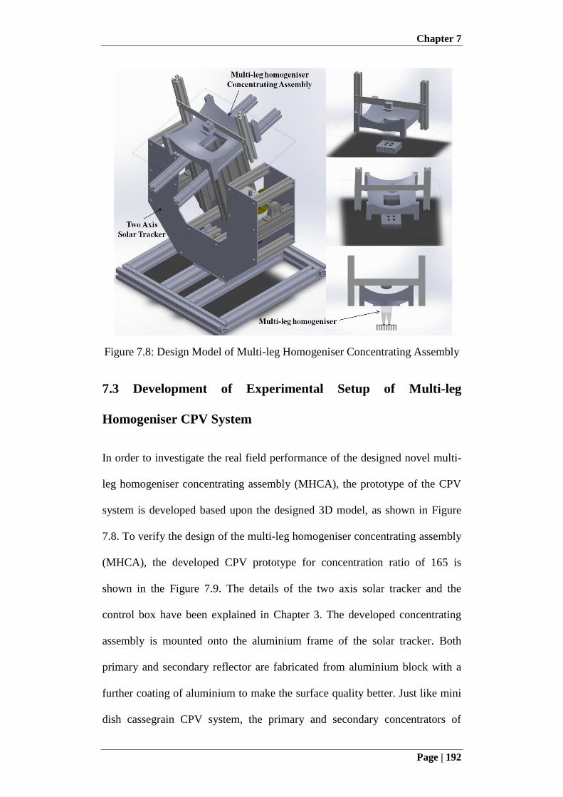
Chapter 7

Page | 192

Figure 7.8: Design Model of Multi-leg Homogeniser Concentrating Assembly

7.3 Development of Experimental Setup of Multi-leg

Homogeniser CPV System

In order to investigate the real field performance of the designed novel multi-

leg homogeniser concentrating assembly (MHCA), the prototype of the CPV

system is developed based upon the designed 3D model, as shown in Figure

7.8. To verify the design of the multi-leg homogeniser concentrating assembly

(MHCA), the developed CPV prototype for concentration ratio of 165 is

shown in the Figure 7.9. The details of the two axis solar tracker and the

control box have been explained in Chapter 3. The developed concentrating

assembly is mounted onto the aluminium frame of the solar tracker. Both

primary and secondary reflector are fabricated from aluminium block with a

further coating of aluminium to make the surface quality better. Just like mini

dish cassegrain CPV system, the primary and secondary concentrators of

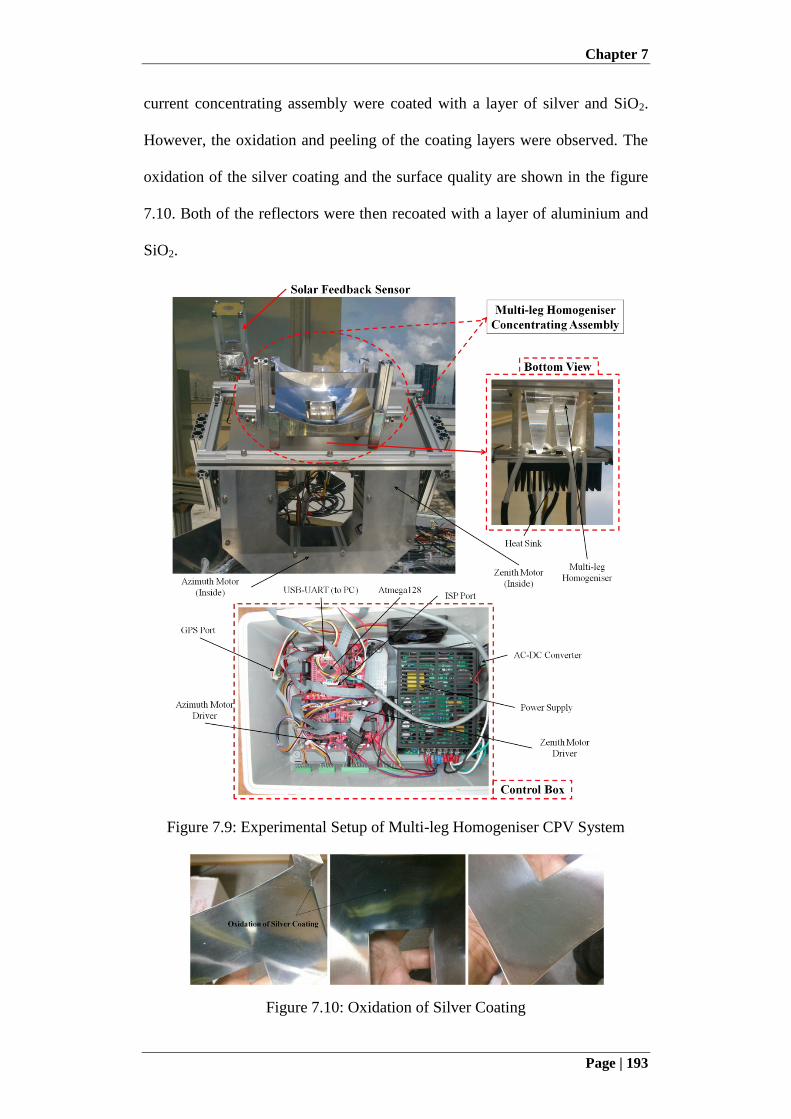
Chapter 7

Page | 193

current concentrating assembly were coated with a layer of silver and SiO2.

However, the oxidation and peeling of the coating layers were observed. The

oxidation of the silver coating and the surface quality are shown in the figure

7.10. Both of the reflectors were then recoated with a layer of aluminium and

SiO2.

Figure 7.9: Experimental Setup of Multi-leg Homogeniser CPV System

Figure 7.10: Oxidation of Silver Coating

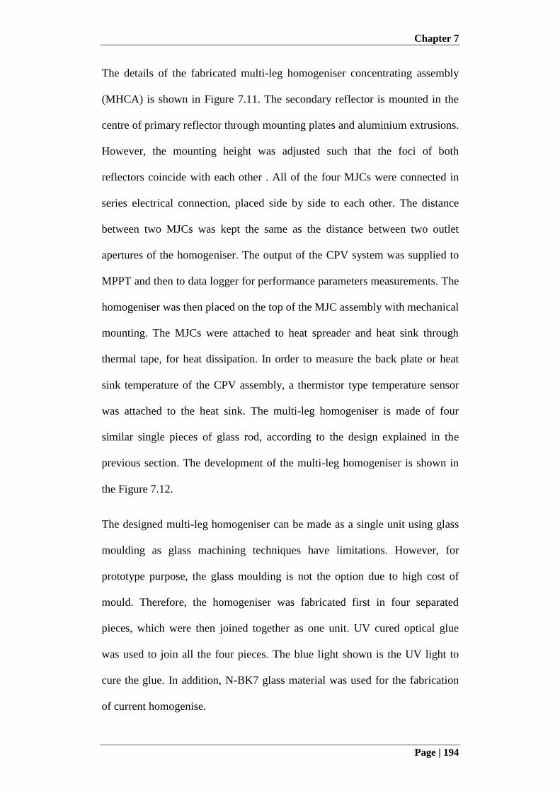
Chapter 7

Page | 194

The details of the fabricated multi-leg homogeniser concentrating assembly

(MHCA) is shown in Figure 7.11. The secondary reflector is mounted in the

centre of primary reflector through mounting plates and aluminium extrusions.

However, the mounting height was adjusted such that the foci of both

reflectors coincide with each other . All of the four MJCs were connected in

series electrical connection, placed side by side to each other. The distance

between two MJCs was kept the same as the distance between two outlet

apertures of the homogeniser. The output of the CPV system was supplied to

MPPT and then to data logger for performance parameters measurements. The

homogeniser was then placed on the top of the MJC assembly with mechanical

mounting. The MJCs were attached to heat spreader and heat sink through

thermal tape, for heat dissipation. In order to measure the back plate or heat

sink temperature of the CPV assembly, a thermistor type temperature sensor

was attached to the heat sink. The multi-leg homogeniser is made of four

similar single pieces of glass rod, according to the design explained in the

previous section. The development of the multi-leg homogeniser is shown in

the Figure 7.12.

The designed multi-leg homogeniser can be made as a single unit using glass

moulding as glass machining techniques have limitations. However, for

prototype purpose, the glass moulding is not the option due to high cost of

mould. Therefore, the homogeniser was fabricated first in four separated

pieces, which were then joined together as one unit. UV cured optical glue

was used to join all the four pieces. The blue light shown is the UV light to

cure the glue. In addition, N-BK7 glass material was used for the fabrication

of current homogenise.

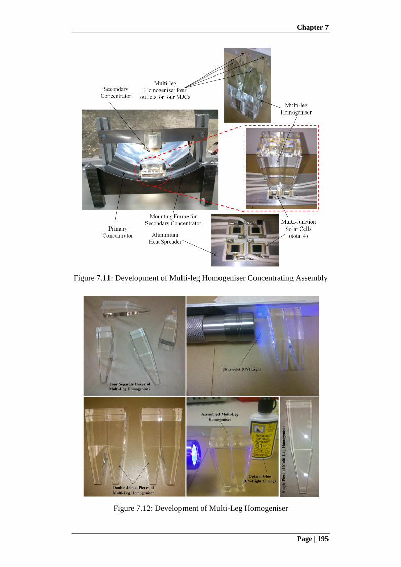
Chapter 7

Page | 195

Figure 7.11: Development of Multi-leg Homogeniser Concentrating Assembly

Figure 7.12: Development of Multi-Leg Homogeniser

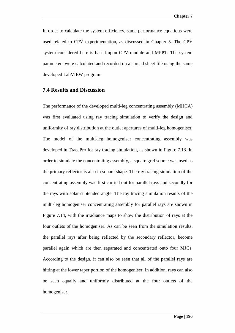
Chapter 7

Page | 196

In order to calculate the system efficiency, same performance equations were

used related to CPV experimentation, as discussed in Chapter 5. The CPV

system considered here is based upon CPV module and MPPT. The system

parameters were calculated and recorded on a spread sheet file using the same

developed LabVIEW program.


The performance of the developed multi-leg concentrating assembly (MHCA)

was first evaluated using ray tracing simulation to verify the design and

uniformity of ray distribution at the outlet apertures of multi-leg homogeniser.

The model of the multi-leg homogeniser concentrating assembly was

developed in TracePro for ray tracing simulation, as shown in Figure 7.13. In

order to simulate the concentrating assembly, a square grid source was used as

the primary reflector is also in square shape. The ray tracing simulation of the

concentrating assembly was first carried out for parallel rays and secondly for

the rays with solar subtended angle. The ray tracing simulation results of the

multi-leg homogeniser concentrating assembly for parallel rays are shown in

Figure 7.14, with the irradiance maps to show the distribution of rays at the

four outlets of the homogeniser. As can be seen from the simulation results,

the parallel rays after being reflected by the secondary reflector, become

parallel again which are then separated and concentrated onto four MJCs.

According to the design, it can also be seen that all of the parallel rays are

hitting at the lower taper portion of the homogeniser. In addition, rays can also

be seen equally and uniformly distributed at the four outlets of the

homogeniser.

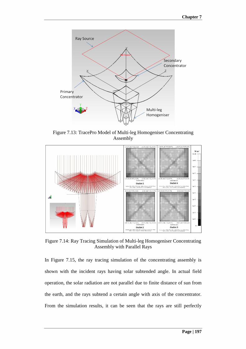
Chapter 7

Page | 197

Figure 7.13: TracePro Model of Multi-leg Homogeniser Concentrating

Assembly

Figure 7.14: Ray Tracing Simulation of Multi-leg Homogeniser Concentrating

Assembly with Parallel Rays

In Figure 7.15, the ray tracing simulation of the concentrating assembly is

shown with the incident rays having solar subtended angle. In actual field

operation, the solar radiation are not parallel due to finite distance of sun from

the earth, and the rays subtend a certain angle with axis of the concentrator.

From the simulation results, it can be seen that the rays are still perfectly

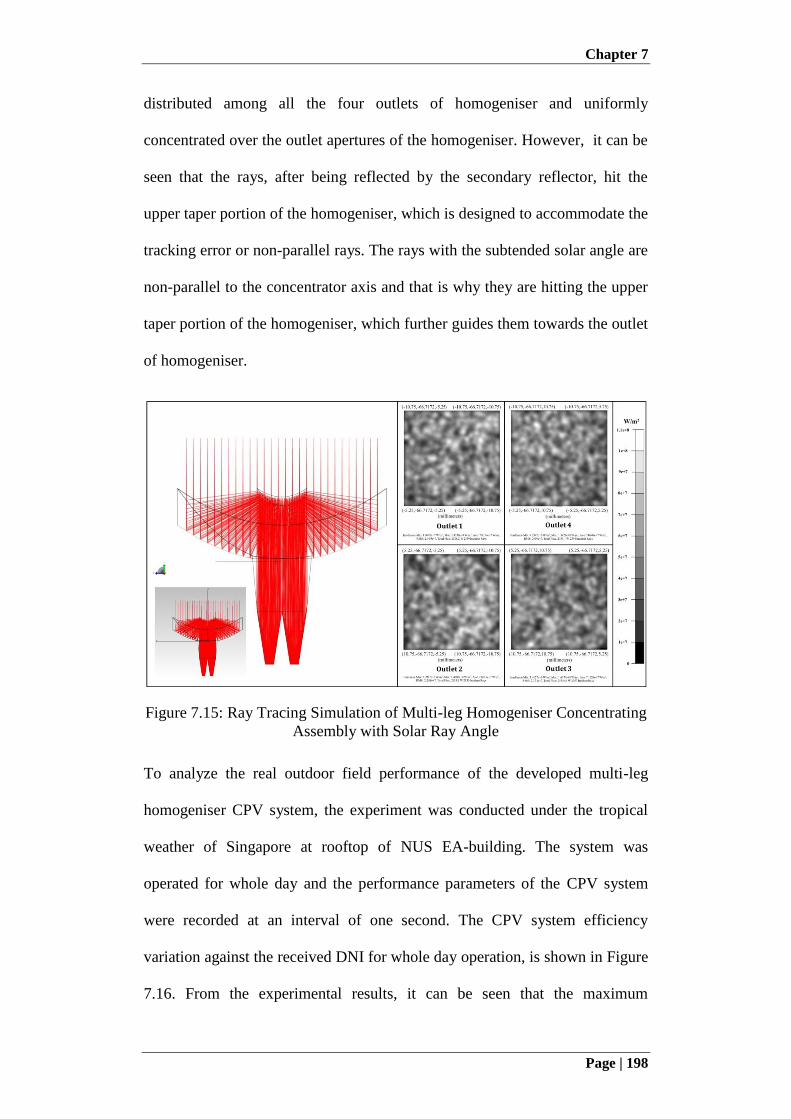
Chapter 7

Page | 198

distributed among all the four outlets of homogeniser and uniformly

concentrated over the outlet apertures of the homogeniser. However, it can be

seen that the rays, after being reflected by the secondary reflector, hit the

upper taper portion of the homogeniser, which is designed to accommodate the

tracking error or non-parallel rays. The rays with the subtended solar angle are

non-parallel to the concentrator axis and that is why they are hitting the upper

taper portion of the homogeniser, which further guides them towards the outlet

of homogeniser.

Figure 7.15: Ray Tracing Simulation of Multi-leg Homogeniser Concentrating

Assembly with Solar Ray Angle

To analyze the real outdoor field performance of the developed multi-leg

homogeniser CPV system, the experiment was conducted under the tropical

weather of Singapore at rooftop of NUS EA-building. The system was

operated for whole day and the performance parameters of the CPV system

were recorded at an interval of one second. The CPV system efficiency

variation against the received DNI for whole day operation, is shown in Figure

7.16. From the experimental results, it can be seen that the maximum

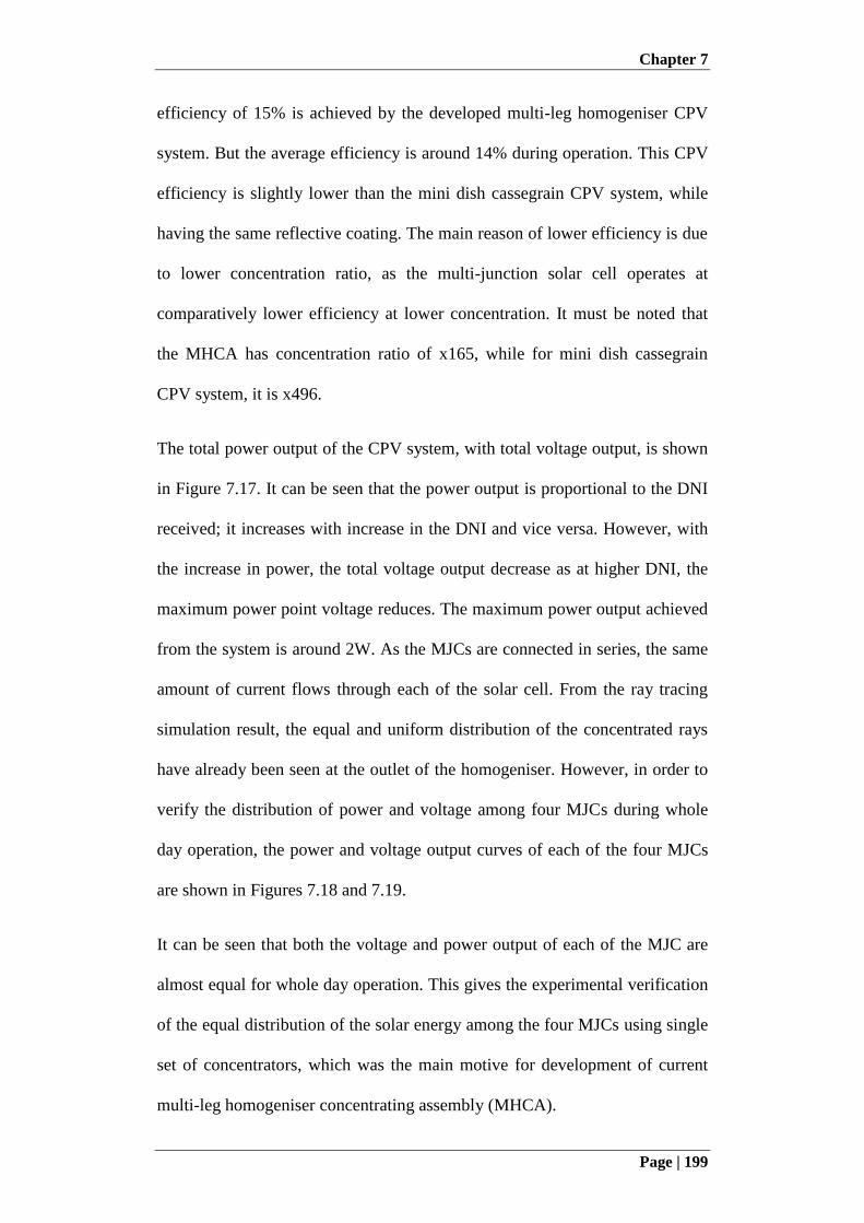
Chapter 7

Page | 199

efficiency of 15% is achieved by the developed multi-leg homogeniser CPV

system. But the average efficiency is around 14% during operation. This CPV

efficiency is slightly lower than the mini dish cassegrain CPV system, while

having the same reflective coating. The main reason of lower efficiency is due

to lower concentration ratio, as the multi-junction solar cell operates at

comparatively lower efficiency at lower concentration. It must be noted that

the MHCA has concentration ratio of x165, while for mini dish cassegrain

CPV system, it is x496.

The total power output of the CPV system, with total voltage output, is shown

in Figure 7.17. It can be seen that the power output is proportional to the DNI

received; it increases with increase in the DNI and vice versa. However, with

the increase in power, the total voltage output decrease as at higher DNI, the

maximum power point voltage reduces. The maximum power output achieved

from the system is around 2W. As the MJCs are connected in series, the same

amount of current flows through each of the solar cell. From the ray tracing

simulation result, the equal and uniform distribution of the concentrated rays

have already been seen at the outlet of the homogeniser. However, in order to

verify the distribution of power and voltage among four MJCs during whole

day operation, the power and voltage output curves of each of the four MJCs

are shown in Figures 7.18 and 7.19.

It can be seen that both the voltage and power output of each of the MJC are

almost equal for whole day operation. This gives the experimental verification

of the equal distribution of the solar energy among the four MJCs using single

set of concentrators, which was the main motive for development of current

multi-leg homogeniser concentrating assembly (MHCA).

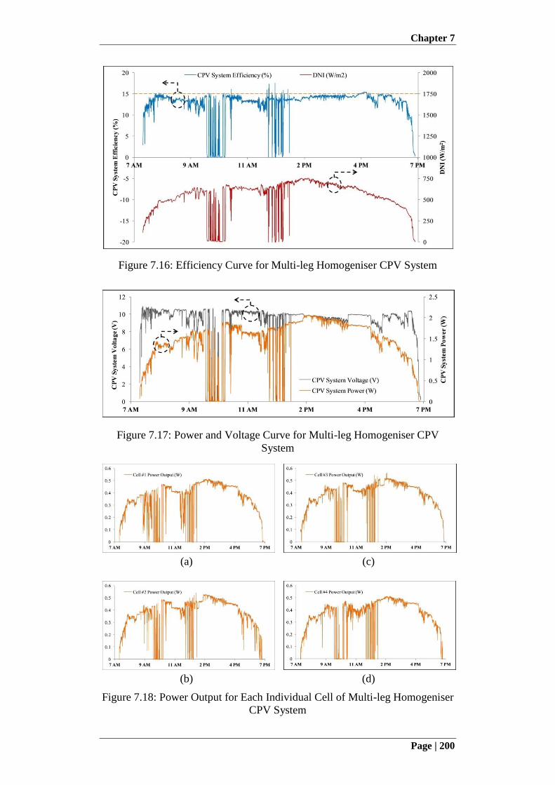
Chapter 7

Page | 200

Figure 7.16: Efficiency Curve for Multi-leg Homogeniser CPV System

Figure 7.17: Power and Voltage Curve for Multi-leg Homogeniser CPV

System

(a) (c)

(b) (d)

Figure 7.18: Power Output for Each Individual Cell of Multi-leg Homogeniser

CPV System

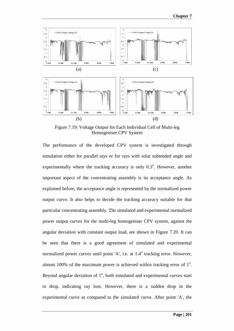
Chapter 7

Page | 201

(a) (c)

(b) (d)

Figure 7.19: Voltage Output for Each Individual Cell of Multi-leg

Homogeniser CPV System

The performance of the developed CPV system is investigated through

simulation either for parallel rays or for rays with solar subtended angle and

experimentally where the tracking accuracy is only 0.3o. However, another

important aspect of the concentrating assembly is its acceptance angle. As

explained before, the acceptance angle is represented by the normalized power

output curve. It also helps to decide the tracking accuracy suitable for that

particular concentrating assembly. The simulated and experimental normalized

power output curves for the multi-leg homogeniser CPV system, against the

angular deviation with constant output load, are shown in Figure 7.20. It can

be seen that there is a good agreement of simulated and experimental

normalized power curves until point 'A', i.e. at 1.4o tracking error. However,

almost 100% of the maximum power is achieved within tracking error of 1o.

Beyond angular deviation of 1o, both simulated and experimental curves start

to drop, indicating ray loss. However, there is a sudden drop in the

experimental curve as compared to the simulated curve. After point 'A', the

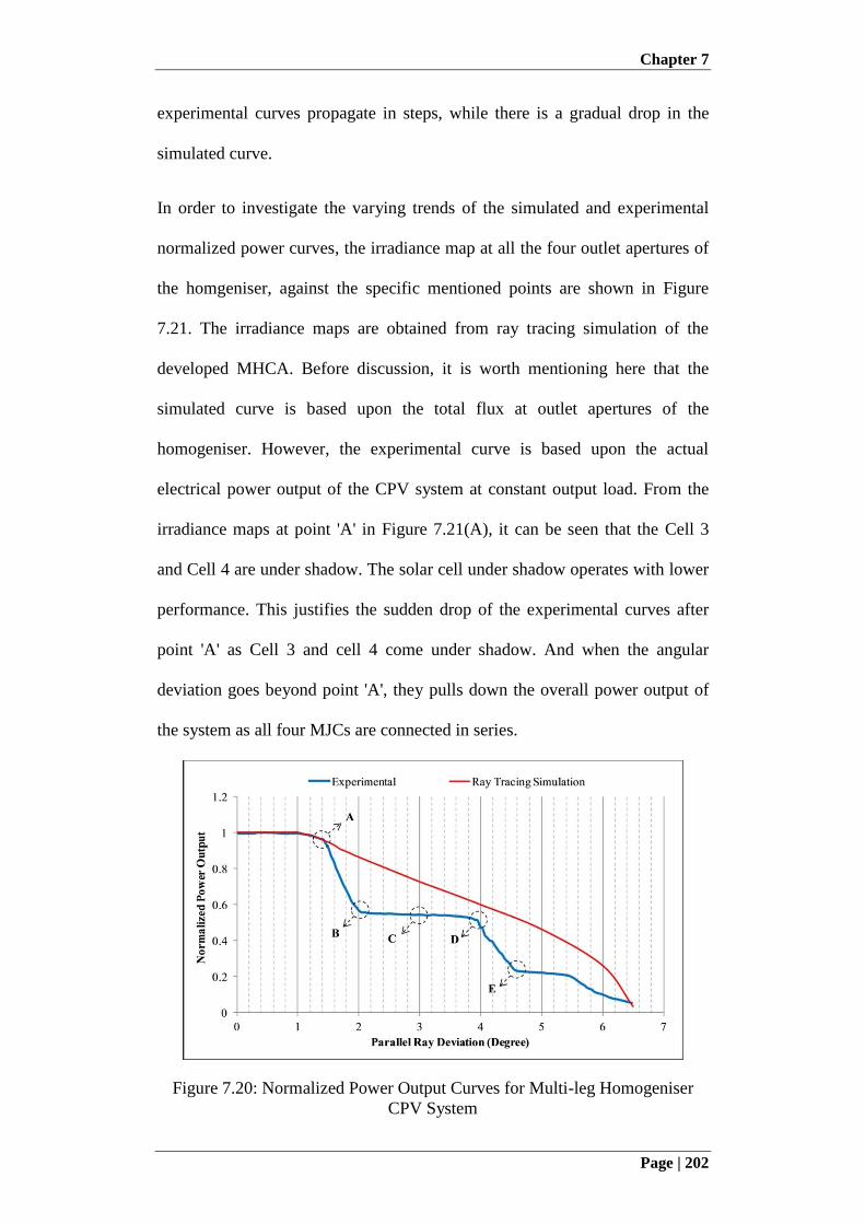
Chapter 7

Page | 202

experimental curves propagate in steps, while there is a gradual drop in the

simulated curve.

In order to investigate the varying trends of the simulated and experimental

normalized power curves, the irradiance map at all the four outlet apertures of

the homgeniser, against the specific mentioned points are shown in Figure

7.21. The irradiance maps are obtained from ray tracing simulation of the

developed MHCA. Before discussion, it is worth mentioning here that the

simulated curve is based upon the total flux at outlet apertures of the

homogeniser. However, the experimental curve is based upon the actual

electrical power output of the CPV system at constant output load. From the

irradiance maps at point 'A' in Figure 7.21(A), it can be seen that the Cell 3

and Cell 4 are under shadow. The solar cell under shadow operates with lower

performance. This justifies the sudden drop of the experimental curves after

point 'A' as Cell 3 and cell 4 come under shadow. And when the angular

deviation goes beyond point 'A', they pulls down the overall power output of

the system as all four MJCs are connected in series.

Figure 7.20: Normalized Power Output Curves for Multi-leg Homogeniser

CPV System

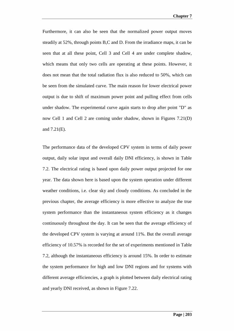
Chapter 7

Page | 203

Furthermore, it can also be seen that the normalized power output moves

steadily at 52%, through points B,C and D. From the irradiance maps, it can be

seen that at all these point, Cell 3 and Cell 4 are under complete shadow,

which means that only two cells are operating at these points. However, it

does not mean that the total radiation flux is also reduced to 50%, which can

be seen from the simulated curve. The main reason for lower electrical power

output is due to shift of maximum power point and pulling effect from cells

under shadow. The experimental curve again starts to drop after point "D" as

now Cell 1 and Cell 2 are coming under shadow, shown in Figures 7.21(D)

and 7.21(E).

The performance data of the developed CPV system in terms of daily power

output, daily solar input and overall daily DNI efficiency, is shown in Table

7.2. The electrical rating is based upon daily power output projected for one

year. The data shown here is based upon the system operation under different

weather conditions, i.e. clear sky and cloudy conditions. As concluded in the

previous chapter, the average efficiency is more effective to analyze the true

system performance than the instantaneous system efficiency as it changes

continuously throughout the day. It can be seen that the average efficiency of

the developed CPV system is varying at around 11%. But the overall average

efficiency of 10.57% is recorded for the set of experiments mentioned in Table

7.2, although the instantaneous efficiency is around 15%. In order to estimate

the system performance for high and low DNI regions and for systems with

different average efficiencies, a graph is plotted between daily electrical rating

and yearly DNI received, as shown in Figure 7.22.

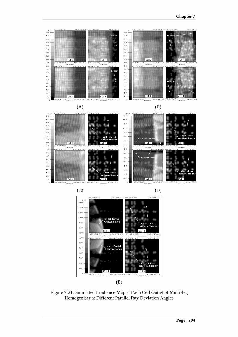
Chapter 7

Page | 204

(A) (B)

(C) (D)

(E)

Figure 7.21: Simulated Irradiance Map at Each Cell Outlet of Multi-leg

Homogeniser at Different Parallel Ray Deviation Angles

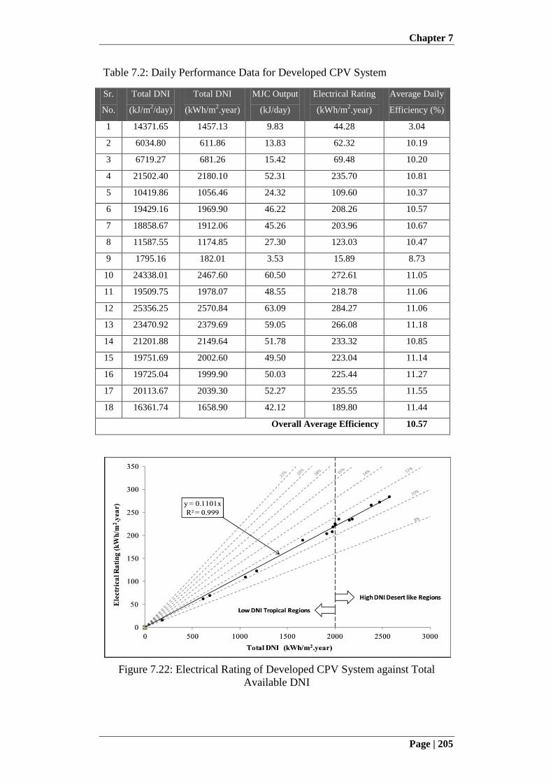
Chapter 7

Page | 205

Table 7.2: Daily Performance Data for Developed CPV System

Sr.

No.

Total DNI

(kJ/m2/day)

Total DNI

(kWh/m2.year)

MJC Output

(kJ/day)

Electrical Rating

(kWh/m2.year)

Average Daily

Efficiency (%)

1 14371.65 1457.13 9.83 44.28 3.04

2 6034.80 611.86 13.83 62.32 10.19

3 6719.27 681.26 15.42 69.48 10.20

4 21502.40 2180.10 52.31 235.70 10.81

5 10419.86 1056.46 24.32 109.60 10.37

6 19429.16 1969.90 46.22 208.26 10.57

7 18858.67 1912.06 45.26 203.96 10.67

8 11587.55 1174.85 27.30 123.03 10.47

9 1795.16 182.01 3.53 15.89 8.73

10 24338.01 2467.60 60.50 272.61 11.05

11 19509.75 1978.07 48.55 218.78 11.06

12 25356.25 2570.84 63.09 284.27 11.06

13 23470.92 2379.69 59.05 266.08 11.18

14 21201.88 2149.64 51.78 233.32 10.85

15 19751.69 2002.60 49.50 223.04 11.14

16 19725.04 1999.90 50.03 225.44 11.27

17 20113.67 2039.30 52.27 235.55 11.55

18 16361.74 1658.90 42.12 189.80 11.44

Overall Average Efficiency 10.57

Figure 7.22: Electrical Rating of Developed CPV System against Total

Available DNI

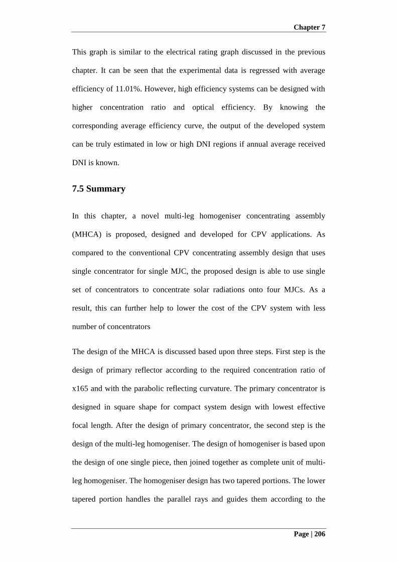
Chapter 7

Page | 206

This graph is similar to the electrical rating graph discussed in the previous

chapter. It can be seen that the experimental data is regressed with average

efficiency of 11.01%. However, high efficiency systems can be designed with

higher concentration ratio and optical efficiency. By knowing the

corresponding average efficiency curve, the output of the developed system

can be truly estimated in low or high DNI regions if annual average received

DNI is known.

7.5 Summary

In this chapter, a novel multi-leg homogeniser concentrating assembly

(MHCA) is proposed, designed and developed for CPV applications. As

compared to the conventional CPV concentrating assembly design that uses

single concentrator for single MJC, the proposed design is able to use single

set of concentrators to concentrate solar radiations onto four MJCs. As a

result, this can further help to lower the cost of the CPV system with less

number of concentrators

The design of the MHCA is discussed based upon three steps. First step is the

design of primary reflector according to the required concentration ratio of

x165 and with the parabolic reflecting curvature. The primary concentrator is

designed in square shape for compact system design with lowest effective

focal length. After the design of primary concentrator, the second step is the

design of the multi-leg homogeniser. The design of homogeniser is based upon

the design of one single piece, then joined together as complete unit of multi-

leg homogeniser. The homogeniser design has two tapered portions. The lower

tapered portion handles the parallel rays and guides them according to the

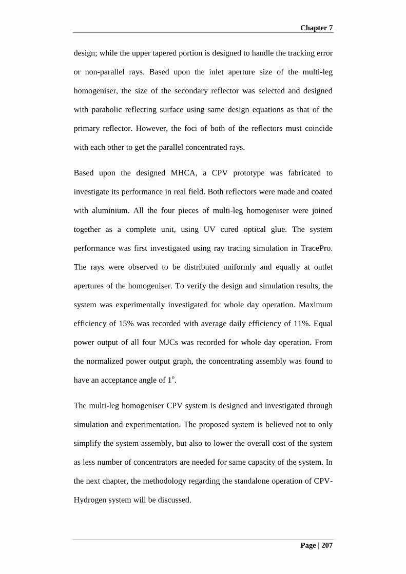
Chapter 7

Page | 207

design; while the upper tapered portion is designed to handle the tracking error

or non-parallel rays. Based upon the inlet aperture size of the multi-leg

homogeniser, the size of the secondary reflector was selected and designed

with parabolic reflecting surface using same design equations as that of the

primary reflector. However, the foci of both of the reflectors must coincide

with each other to get the parallel concentrated rays.

Based upon the designed MHCA, a CPV prototype was fabricated to

investigate its performance in real field. Both reflectors were made and coated

with aluminium. All the four pieces of multi-leg homogeniser were joined

together as a complete unit, using UV cured optical glue. The system

performance was first investigated using ray tracing simulation in TracePro.

The rays were observed to be distributed uniformly and equally at outlet

apertures of the homogeniser. To verify the design and simulation results, the

system was experimentally investigated for whole day operation. Maximum

efficiency of 15% was recorded with average daily efficiency of 11%. Equal

power output of all four MJCs was recorded for whole day operation. From

the normalized power output graph, the concentrating assembly was found to

have an acceptance angle of 1o.

The multi-leg homogeniser CPV system is designed and investigated through

simulation and experimentation. The proposed system is believed not to only

simplify the system assembly, but also to lower the overall cost of the system

as less number of concentrators are needed for same capacity of the system. In

the next chapter, the methodology regarding the standalone operation of CPV-

Hydrogen system will be discussed.

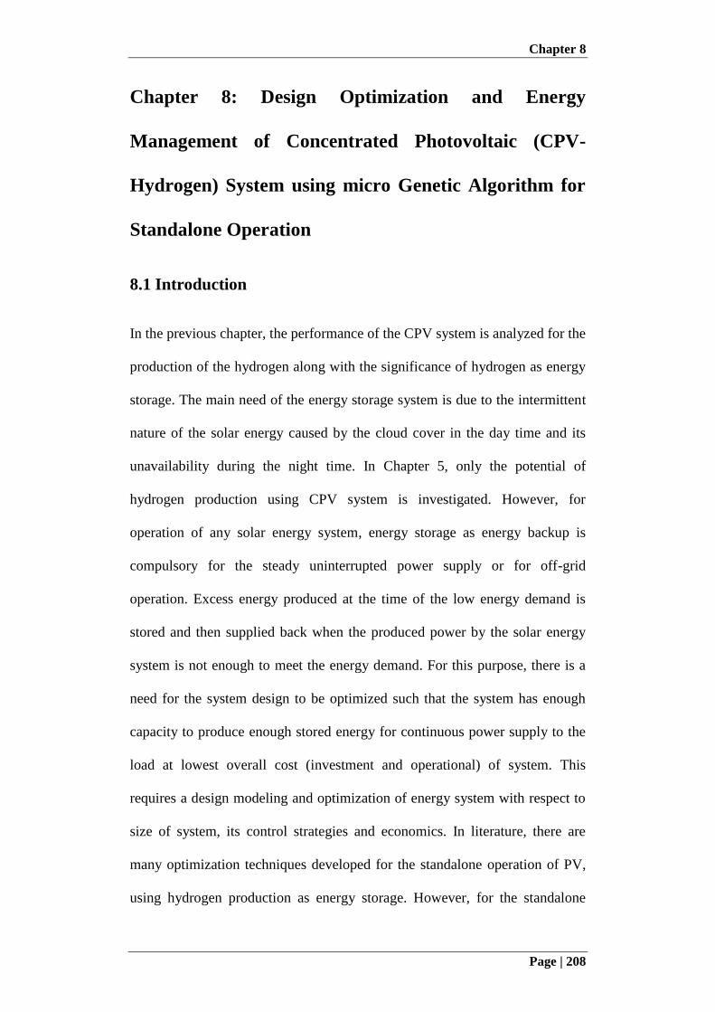
Chapter 8

Page | 208

Chapter 8: Design Optimization and Energy

Management of Concentrated Photovoltaic (CPV-

Hydrogen) System using micro Genetic Algorithm for

Standalone Operation

8.1 Introduction

In the previous chapter, the performance of the CPV system is analyzed for the

production of the hydrogen along with the significance of hydrogen as energy

storage. The main need of the energy storage system is due to the intermittent

nature of the solar energy caused by the cloud cover in the day time and its

unavailability during the night time. In Chapter 5, only the potential of

hydrogen production using CPV system is investigated. However, for

operation of any solar energy system, energy storage as energy backup is

compulsory for the steady uninterrupted power supply or for off-grid

operation. Excess energy produced at the time of the low energy demand is

stored and then supplied back when the produced power by the solar energy

system is not enough to meet the energy demand. For this purpose, there is a

need for the system design to be optimized such that the system has enough

capacity to produce enough stored energy for continuous power supply to the

load at lowest overall cost (investment and operational) of system. This

requires a design modeling and optimization of energy system with respect to

size of system, its control strategies and economics. In literature, there are

many optimization techniques developed for the standalone operation of PV,

using hydrogen production as energy storage. However, for the standalone

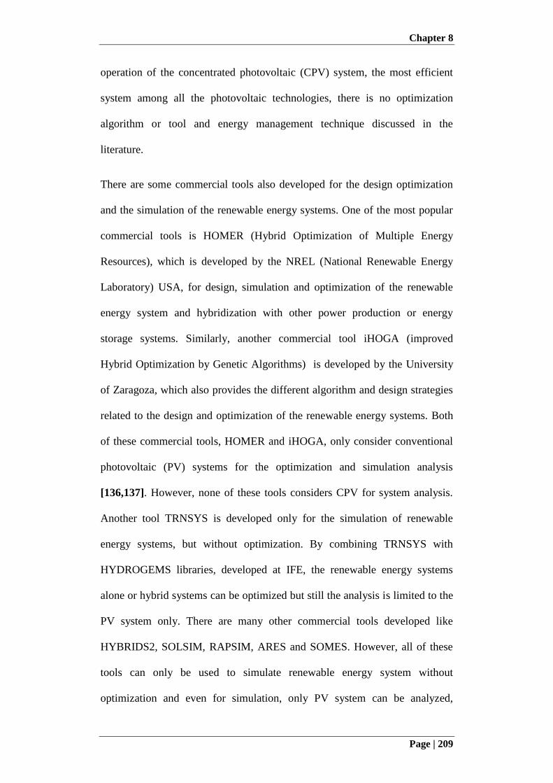
Chapter 8

Page | 209

operation of the concentrated photovoltaic (CPV) system, the most efficient

system among all the photovoltaic technologies, there is no optimization

algorithm or tool and energy management technique discussed in the

literature.

There are some commercial tools also developed for the design optimization

and the simulation of the renewable energy systems. One of the most popular

commercial tools is HOMER (Hybrid Optimization of Multiple Energy

Resources), which is developed by the NREL (National Renewable Energy

Laboratory) USA, for design, simulation and optimization of the renewable

energy system and hybridization with other power production or energy

storage systems. Similarly, another commercial tool iHOGA (improved

Hybrid Optimization by Genetic Algorithms) is developed by the University

of Zaragoza, which also provides the different algorithm and design strategies

related to the design and optimization of the renewable energy systems. Both

of these commercial tools, HOMER and iHOGA, only consider conventional

photovoltaic (PV) systems for the optimization and simulation analysis

[136,137]. However, none of these tools considers CPV for system analysis.

Another tool TRNSYS is developed only for the simulation of renewable

energy systems, but without optimization. By combining TRNSYS with

HYDROGEMS libraries, developed at IFE, the renewable energy systems

alone or hybrid systems can be optimized but still the analysis is limited to the

PV system only. There are many other commercial tools developed like

HYBRIDS2, SOLSIM, RAPSIM, ARES and SOMES. However, all of these

tools can only be used to simulate renewable energy system without

optimization and even for simulation, only PV system can be analyzed,

Chapter 8

Page | 210

without CPV consideration [138]. A summary of the commercial renewable

energy analysis tools is shown in table 8.1.

Table 8.1: Comparison Summary of Renewable Energy System Simulation

and Optimization

Optimization Simulation Hydrogen

Energy Storage

Analyze

CPV?

HOMER[136]

x x x No

iHOGA[137]

x x x No

TRNSYS +

HYDROGEMS[138]

x x x No

HYBRIDS2[138]

x x No

SOLSIM[138]

x No

INSEL[138]

x No

ARES[138]

x No

SOMES[138]

x No

RAPSIM[138]

x No

Because of the highest solar energy conversion efficiency, the concentrated

photovoltaic (CPV) system is of the main interest for the future research. On

the other hand, it can be seen that there is no optimization and design

algorithm discussed in the literature and all commercial tools are also lacking

for CPV system consideration for design and optimization analysis. The main

aim of this chapter is to develop the design model and optimization algorithm

with the control strategies for the standalone operation of the CPV system with

the hydrogen production as energy storage. For the developed technique, the

multi-variable design and multi-objective optimization strategy is proposed

with the techno-economic analysis of the overall CPV-hydrogen system. The

CPV-Hydrogen system is optimized with regards to its size for zero PSFT

(power supply failure time) and optimum state of the energy storage with

Chapter 8

Page | 211

minimum overall system annual cost. As discussed in chapter 6, most of the

CPV performance prediction models are not reliable to be used for

performance prediction considering all details of the system. Therefore, a CPV

performance model is also proposed based upon the CPV system basic

parameters and cell characteristics using the actual weather data and then the

results are verified with the electrical rating discussed in the previous paper.

Besides optimized design, the chapter also discusses the simulated long term

performance of the individual system of the CPV-Hydrogen, using the weather

data of the Singapore.

8.2 CPV-Hydrogen System Description

The schematic of the proposed CPV-Hydrogen system considered for the

optimization of the standalone operation simulation is shown in the Figure 8.1.

The concentrated photovoltaic (CPV) system is consisting of the CPV

modules utilizing multi-junction solar cells (MJCs). The CPV modules are

installed onto the two axis solar trackers, which are one of the main

component of the CPV system as the concentrators need to face towards the

sun all the time. For the analysis, the CPV module of any type can be

considered; It can be either Fresnel lens based refractive type CPV module or

Mini Dish based Casegrain reflector type CPV module. The performance

model of the CPV system only considers the solar concentration at the cell

area, regardless of the type of the concentrator. The output of each of the CPV

system is connected to a MPPT (maximum power point tracking) device to

ensure the CPV operation at maximum power or efficiency point . The DC

output power of each of the CPV system is fed into the main DC line at a

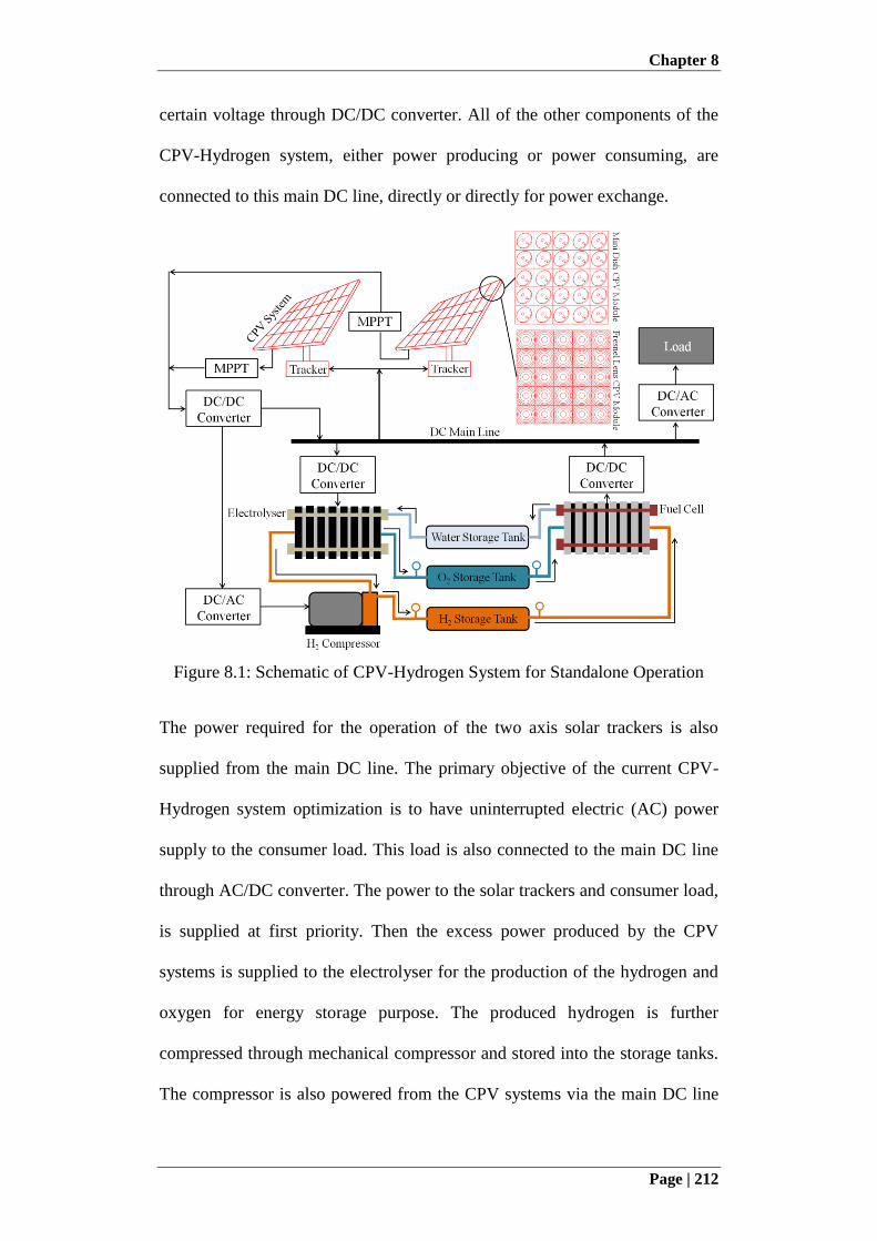
Chapter 8

Page | 212

certain voltage through DC/DC converter. All of the other components of the

CPV-Hydrogen system, either power producing or power consuming, are

connected to this main DC line, directly or directly for power exchange.

Figure 8.1: Schematic of CPV-Hydrogen System for Standalone Operation

The power required for the operation of the two axis solar trackers is also

supplied from the main DC line. The primary objective of the current CPV-

Hydrogen system optimization is to have uninterrupted electric (AC) power

supply to the consumer load. This load is also connected to the main DC line

through AC/DC converter. The power to the solar trackers and consumer load,

is supplied at first priority. Then the excess power produced by the CPV

systems is supplied to the electrolyser for the production of the hydrogen and

oxygen for energy storage purpose. The produced hydrogen is further

compressed through mechanical compressor and stored into the storage tanks.

The compressor is also powered from the CPV systems via the main DC line

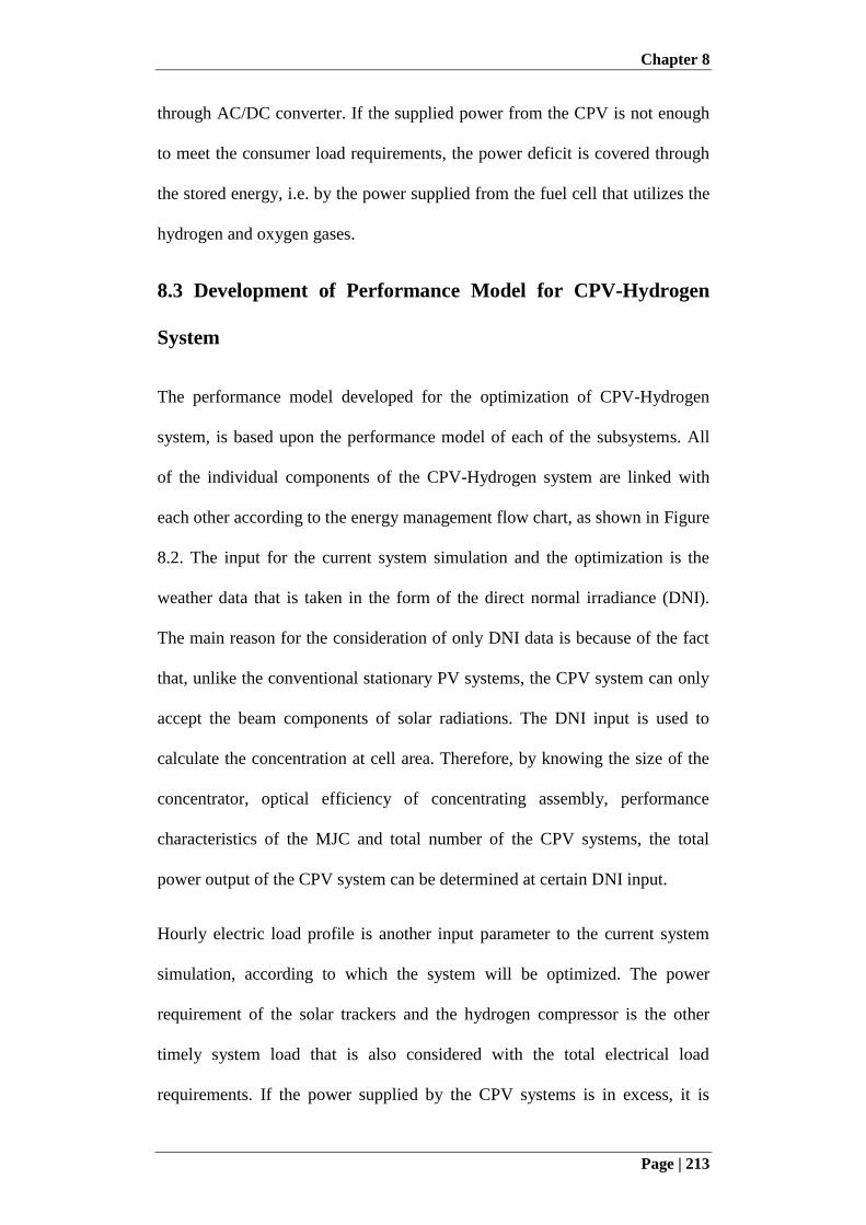
Chapter 8

Page | 213

through AC/DC converter. If the supplied power from the CPV is not enough

to meet the consumer load requirements, the power deficit is covered through

the stored energy, i.e. by the power supplied from the fuel cell that utilizes the

hydrogen and oxygen gases.

8.3 Development of Performance Model for CPV-Hydrogen

System

The performance model developed for the optimization of CPV-Hydrogen

system, is based upon the performance model of each of the subsystems. All

of the individual components of the CPV-Hydrogen system are linked with

each other according to the energy management flow chart, as shown in Figure

8.2. The input for the current system simulation and the optimization is the

weather data that is taken in the form of the direct normal irradiance (DNI).

The main reason for the consideration of only DNI data is because of the fact

that, unlike the conventional stationary PV systems, the CPV system can only

accept the beam components of solar radiations. The DNI input is used to

calculate the concentration at cell area. Therefore, by knowing the size of the

concentrator, optical efficiency of concentrating assembly, performance

characteristics of the MJC and total number of the CPV systems, the total

power output of the CPV system can be determined at certain DNI input.

Hourly electric load profile is another input parameter to the current system

simulation, according to which the system will be optimized. The power

requirement of the solar trackers and the hydrogen compressor is the other

timely system load that is also considered with the total electrical load

requirements. If the power supplied by the CPV systems is in excess, it is

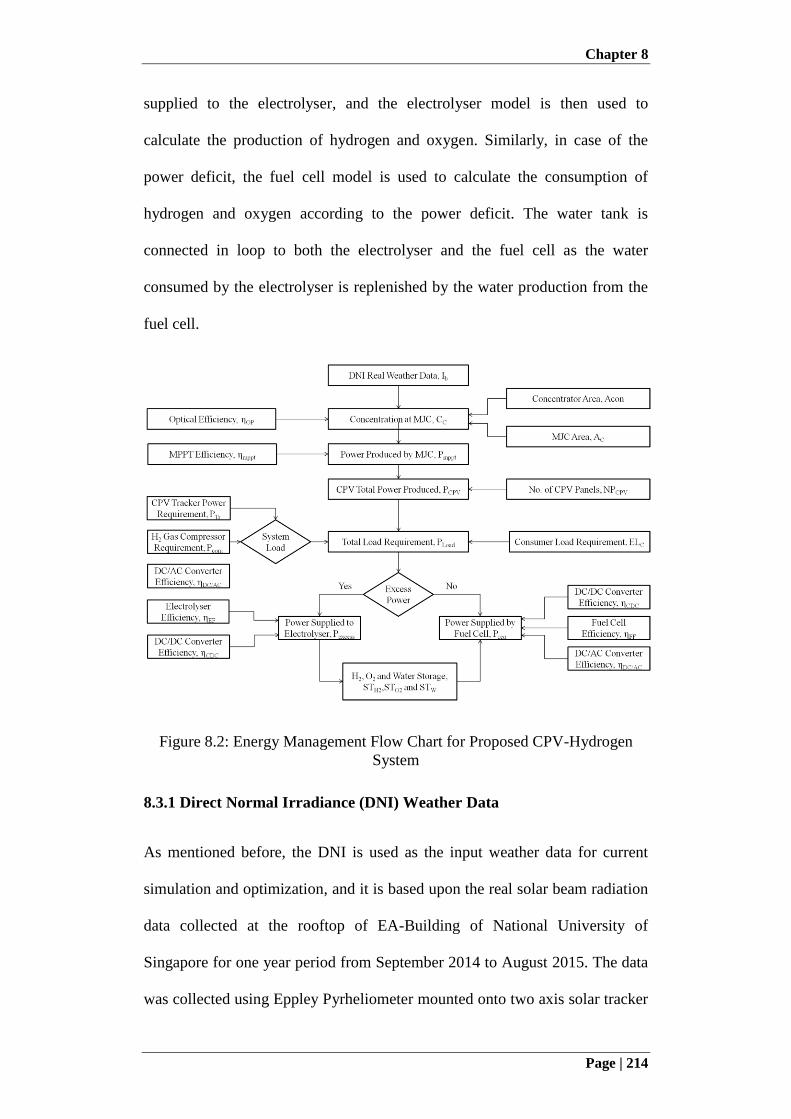
Chapter 8

Page | 214

supplied to the electrolyser, and the electrolyser model is then used to

calculate the production of hydrogen and oxygen. Similarly, in case of the

power deficit, the fuel cell model is used to calculate the consumption of

hydrogen and oxygen according to the power deficit. The water tank is

connected in loop to both the electrolyser and the fuel cell as the water

consumed by the electrolyser is replenished by the water production from the

fuel cell.

Figure 8.2: Energy Management Flow Chart for Proposed CPV-Hydrogen

System

8.3.1 Direct Normal Irradiance (DNI) Weather Data

As mentioned before, the DNI is used as the input weather data for current

simulation and optimization, and it is based upon the real solar beam radiation

data collected at the rooftop of EA-Building of National University of

Singapore for one year period from September 2014 to August 2015. The data

was collected using Eppley Pyrheliometer mounted onto two axis solar tracker

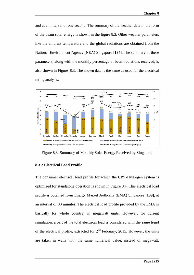
Chapter 8

Page | 215

and at an interval of one second. The summary of the weather data in the form

of the beam solar energy is shown in the figure 8.3. Other weather parameters

like the ambient temperature and the global radiations are obtained from the

National Environment Agency (NEA) Singapore [134]. The summary of these

parameters, along with the monthly percentage of beam radiations received, is

also shown in Figure 8.3. The shown data is the same as used for the electrical

rating analysis.

Figure 8.3: Summary of Monthly Solar Energy Received by Singapore

8.3.2 Electrical Load Profile

The consumer electrical load profile for which the CPV-Hydrogen system is

optimized for standalone operation is shown in Figure 8.4. This electrical load

profile is obtained from Energy Market Authority (EMA) Singapore [139], at

an interval of 30 minutes. The electrical load profile provided by the EMA is

basically for whole country, in megawatt units. However, for current

simulation, a part of the total electrical load is considered with the same trend

of the electrical profile, extracted for 2nd

February, 2015. However, the units

are taken in watts with the same numerical value, instead of megawatt.

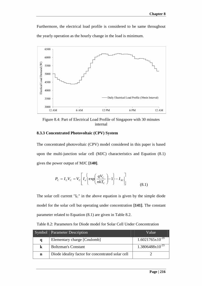
Chapter 8

Page | 216

Furthermore, the electrical load profile is considered to be same throughout

the yearly operation as the hourly change in the load is minimum.

Figure 8.4: Part of Electrical Load Profile of Singapore with 30 minutes

internal

8.3.3 Concentrated Photovoltaic (CPV) System

The concentrated photovoltaic (CPV) model considered in this paper is based

upon the multi-junction solar cell (MJC) characteristics and Equation (8.1)

gives the power output of MJC [140].

SC

C

CoCCCC I

nkT

qVIVVIP 1exp

(8.1)

The solar cell current "IC" in the above equation is given by the simple diode

model for the solar cell but operating under concentration [141]. The constant

parameter related to Equation (8.1) are given in Table 8.2.

Table 8.2: Parameters for Diode model for Solar Cell Under Concentration

Symbol Parameter Description Value

q Elementary charge [Coulomb] 1.6021765x10-19

k Boltzman's Constant 1.3806488x10-23

n Diode ideality factor for concentrated solar cell 2

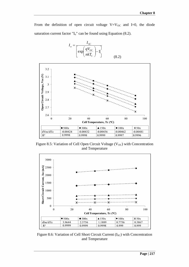
Chapter 8

Page | 217

From the definition of open circuit voltage V=VOC and I=0, the diode

saturation current factor "Io" can be found using Equation (8.2).

1expC

OC

SCo

nkT

qV

II

(8.2)

Figure 8.5: Variation of Cell Open Circuit Voltage (VOC) with Concentration

and Temperature

Figure 8.6: Variation of Cell Short Circuit Current (ISC) with Concentration

and Temperature

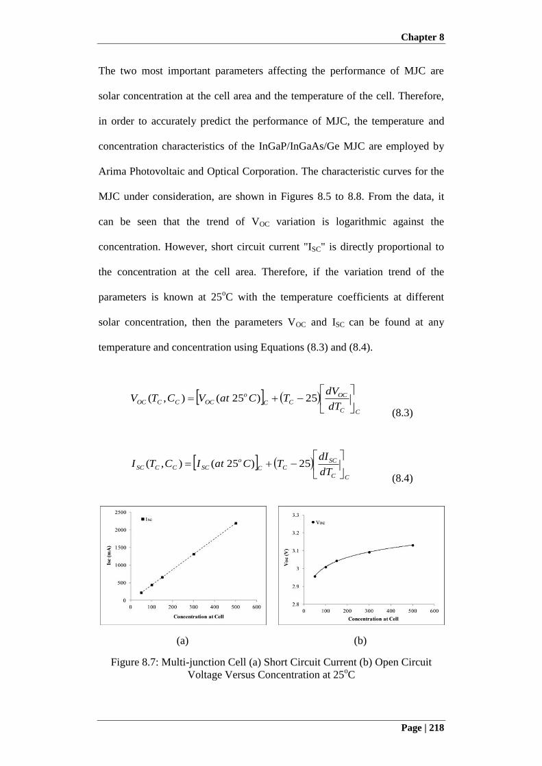
Chapter 8

Page | 218

The two most important parameters affecting the performance of MJC are

solar concentration at the cell area and the temperature of the cell. Therefore,

in order to accurately predict the performance of MJC, the temperature and

concentration characteristics of the InGaP/InGaAs/Ge MJC are employed by

Arima Photovoltaic and Optical Corporation. The characteristic curves for the

MJC under consideration, are shown in Figures 8.5 to 8.8. From the data, it

can be seen that the trend of VOC variation is logarithmic against the

concentration. However, short circuit current "ISC" is directly proportional to

the concentration at the cell area. Therefore, if the variation trend of the

parameters is known at 25oC with the temperature coefficients at different

solar concentration, then the parameters VOC and ISC can be found at any

temperature and concentration using Equations (8.3) and (8.4).

CC

OCCC

o

OCCCOCdT

dVTCatVCTV

25)25(),(

(8.3)

CC

SCCC

o

SCCCSCdT

dITCatICTI

25)25(),(

(8.4)

(a) (b)

Figure 8.7: Multi-junction Cell (a) Short Circuit Current (b) Open Circuit

Voltage Versus Concentration at 25oC

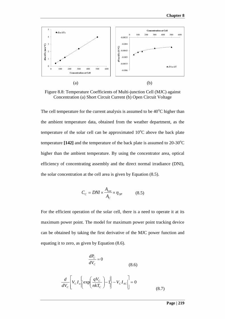
Chapter 8

Page | 219

(a) (b)

Figure 8.8: Temperature Coefficients of Multi-junction Cell (MJC) against

Concentration (a) Short Circuit Current (b) Open Circuit Voltage

The cell temperature for the current analysis is assumed to be 40oC higher than

the ambient temperature data, obtained from the weather department, as the

temperature of the solar cell can be approximated 10oC above the back plate

temperature [142] and the temperature of the back plate is assumed to 20-30oC

higher than the ambient temperature. By using the concentrator area, optical

efficiency of concentrating assembly and the direct normal irradiance (DNI),

the solar concentration at the cell area is given by Equation (8.5).

OP

C

con

CA

ADNIC (8.5)

For the efficient operation of the solar cell, there is a need to operate it at its

maximum power point. The model for maximum power point tracking device

can be obtained by taking the first derivative of the MJC power function and

equating it to zero, as given by Equation (8.6).

0C

C

dV

dP

(8.6)

01exp

SCC

C

C

oC

C

IVnkT

qVIV

dV

d

(8.7)

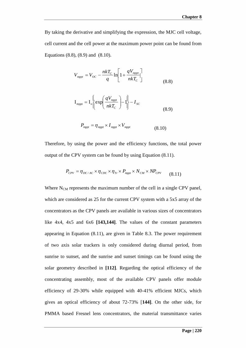
Chapter 8

Page | 220

By taking the derivative and simplifying the expression, the MJC cell voltage,

cell current and the cell power at the maximum power point can be found from

Equations (8.8), (8.9) and (8.10).

C

mpptC

OCmpptnkT

qV

q

nkTVV 1ln

(8.8)

SC

C

mpptI

nkT

qV

1expII omppt

(8.9)

mpptmpptmpptmppt VIP (8.10)

Therefore, by using the power and the efficiency functions, the total power

output of the CPV system can be found by using Equation (8.11).

CPVCMmpptTrCDCACDCCPV NPNPP / (8.11)

Where NCM represents the maximum number of the cell in a single CPV panel,

which are considered as 25 for the current CPV system with a 5x5 array of the

concentrators as the CPV panels are available in various sizes of concentrators

like 4x4, 4x5 and 6x6 [143,144]. The values of the constant parameters

appearing in Equation (8.11), are given in Table 8.3. The power requirement

of two axis solar trackers is only considered during diurnal period, from

sunrise to sunset, and the sunrise and sunset timings can be found using the

solar geometry described in [112]. Regarding the optical efficiency of the

concentrating assembly, most of the available CPV panels offer module

efficiency of 29-30% while equipped with 40-41% efficient MJCs, which

gives an optical efficiency of about 72-73% [144]. On the other side, for

PMMA based Fresnel lens concentrators, the material transmittance varies

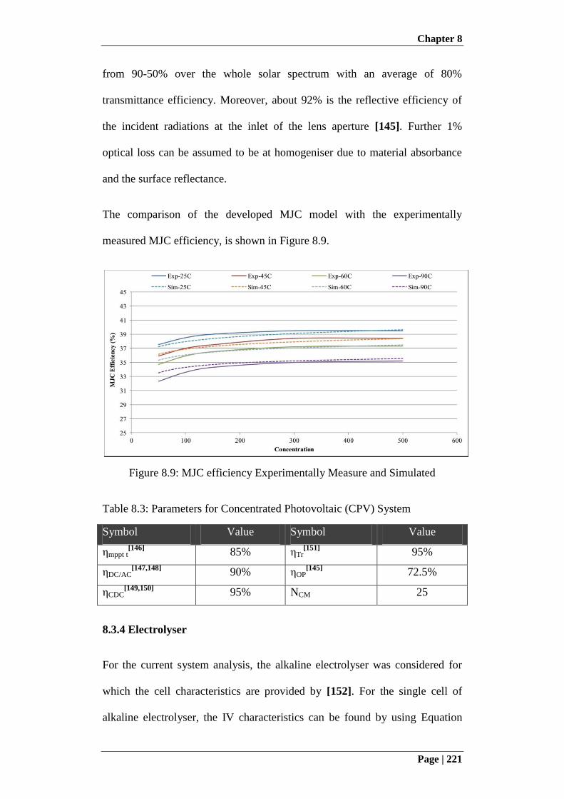
Chapter 8

Page | 221

from 90-50% over the whole solar spectrum with an average of 80%

transmittance efficiency. Moreover, about 92% is the reflective efficiency of

the incident radiations at the inlet of the lens aperture [145]. Further 1%

optical loss can be assumed to be at homogeniser due to material absorbance

and the surface reflectance.

The comparison of the developed MJC model with the experimentally

measured MJC efficiency, is shown in Figure 8.9.

Figure 8.9: MJC efficiency Experimentally Measure and Simulated

Table 8.3: Parameters for Concentrated Photovoltaic (CPV) System

Symbol Value Symbol Value

ηmppt t[146]

85% ηTr[151]

95%

ηDC/AC[147,148]

90% ηOP[145]

72.5%

ηCDC[149,150]

95% NCM 25

8.3.4 Electrolyser

For the current system analysis, the alkaline electrolyser was considered for

which the cell characteristics are provided by [152]. For the single cell of

alkaline electrolyser, the IV characteristics can be found by using Equation

Chapter 8

Page | 222

(8.12). The electrolyser is assumed to be operated at steady thermal condition,

at a temperature of 80oC. The constant parameters related to Equation (8.12)

are provided in Table 8.3.

1log)(

2

321

2

32121

E

E

EE

EEE

E

ErevE I

A

T

t

T

tt

TSTSSIA

TrrUU

(8.12)

Table 8.4: Performance Parameters for Electrolyser Model

Symbol (Units) Values Symbol (Units) Values

Urev (V) 1.229 AE (m2) 0.25

r1 (Ωm2) 7.331x10

-5 S3 (V

oC

-2) -1.606 x10

-5

r2 (Ωm2 oC

-1) -1.107 x10

-7 t1 (m

2 A

-1) 1.599 x10

-2

S1 (V) 1.586 x10-1

t2 (m2 A

-1 oC

-1) -1.302

S2 (V oC

-1) 1.378 x10

-3 t3 (m

2 A

-1 oC

-2) 4.213 x10

2

The amount of the hydrogen and oxygen produced by the electrolyser is based

upon the amount of current flowing through the electrolyser cell and the

Faraday efficiency. As the water molecule contains two atoms of hydrogen

and one atom of oxygen, so the hydrogen production rate is double than the

oxygen production rate. The hydrogen and the oxygen production can be

calculated by using Equations (8.13) and (8.14) and their constant parameters

are given in Table 8.5.

2,2, 2 OE

E

EECEFHE n

Fn

INn

(8.13)

2

2

765

2

4321 exp.

E

E

EE

E

E

EEEF

A

I

TaTaa

A

I

TaTaaa

(8.14)

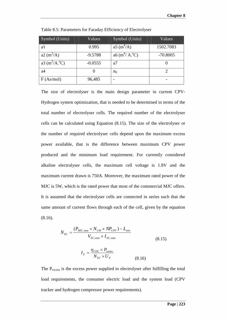
Chapter 8

Page | 223



a1 0.995 a5 (m4/A) 1502.7083

a2 (m2/A) -9.5788 a6 (m

4/ A.

oC) -70.8005

a3 (m2/A.

oC) -0.0555 a7 0

a4 0 nE 2

F (As/mol) 96,485 - -

The size of electrolyser is the main design parameter in current CPV-

Hydrogen system optimization, that is needed to be determined in terms of the

total number of electrolyser cells. The required number of the electrolyser

cells can be calculated using Equation (8.15). The size of the electrolyser or

the number of required electrolyser cells depend upon the maximum excess

power available, that is the difference between maximum CPV power

produced and the minimum load requirement. For currently considered

alkaline electrolyser cells, the maximum cell voltage is 1.8V and the

maximum current drawn is 750A. Moreover, the maximum rated power of the

MJC is 5W, which is the rated power that most of the commercial MJC offers.

It is assumed that the electrolyser cells are connected in series such that the

same amount of current flows through each of the cell, given by the equation

(8.16).

max,max,

minmax, )(

ECEC

CPVCMMJC

ECIV

LNPNPN

(8.15)

EEC

excessCDC

EUN

PI

(8.16)

The Pexcess is the excess power supplied to electrolyser after fulfilling the total

load requirements, the consumer electric load and the system load (CPV

tracker and hydrogen compressor power requirements).

Chapter 8

Page | 224

8.3.5 Fuel Cell

The PEM (Proton Exchange Membrane) fuel cell considered for the current

system analysis is discussed in [152]. The fuel cell consumes the hydrogen

and the oxygen for power production and like the electrolyser, the

consumption of hydrogen is double than the oxygen. The rate of the hydrogen

and the oxygen consumption depends upon the current supplied by the fuel

cell and its faraday efficiency. For current fuel cell system, the faraday

efficiency is assumed to be 0.7. The rate of the hydrogen and oxygen

production can be found by using Equation (8.17)

2,2, 2 OF

E

FFCFFHF n

Fn

INn

(8.17)

Equation (8.18) gives the IV characteristics of the single cell of PEM fuel cell.

The constant parameters for Equation (8.18) are given in Table 8.6. The active

area per single cell of PEM fuel cell is taken as AF = 300 cm2.

F

F

F

FoF

A

IR

A

IbUU log (8.18)

Table 8.6: Performance Parameters for Fuel Cell Model

TF = 70 oC TF = 35

oC


Uo (mV) 1065 Uo (mV) 1049

b (mV/dec) 80 b (mV/dec) 108

R (Ω/cm) 0.438 R (Ω/cm) 0.412

Similar to the design of electrolyser, the size of the fuel cell, in terms of the

number of cells connected in series, is the main design parameter that is

Chapter 8

Page | 225

needed to be optimized for the current system analysis. The number of the

required cells depends upon the maximum load requirement of the system that

is the consumer electric load during the system operation. For PEM fuel cell

under consideration, the maximum power produced by single cell is 114.6W.

Therefore, the total number of cells required to fulfill maximum power deficit

requirements are given by equation (5.19).

max,/

max

FCACDCCDC

FCP

LN

(5.19)

The current flow provided by the fuel cell depends upon the power deficiency,

Preq the power that CPV system is unable to provide to the consumer load and

given by equation (5.20).

FFCACDCCDC

req

FUN

PI

/ (8.20)

8.3.6 Hydrogen Compressor

The excess electrical energy produced by the CPV system is stored in the form

of the hydrogen and oxygen, by using electrolyser. The produced hydrogen is

compressed and stored in storage cylinders as the mechanical compression

provides a reliable and suitable solution. However, the oxygen is stored at its

produced pressure without any compression. The power consumed by the

mechanical compressor depends upon the inlet pressure and the pressure at

compressor outlet i.e. storage tank pressure. The power consumed by the

compressor can be computed using the equation (8.21) [153].

11000

1

/

22,

r

r

E

ta

comACDC

com

HH

HEcomP

PTCP

MnP

(8.21)

Chapter 8

Page | 226

The details of the parameters appearing in the equation (8.21) are provided in

Table 8.6. The flow rate of the hydrogen through the compressor is the same

as the rate of hydrogen production from electrolyser. In addition, the

compressor operating temperature "Tcom" and the electrolyser operating

temperature "TE" are assumed to be the same because the gas being

compressed is coming directly from the electrolyser. The parameters "PE" and

"Pta" are the operating pressure of the electrolyser and pressure of the

hydrogen storage tank, which are pressures at the compressor inlet and outlet

respectively.



MH2 (g/mol) 2.0159

ηDC/AC (%) 90

CPH (J/kg.K) 14304 ηcom (%)[153]

70

Tcom (K) 306 r 1.4

8.3.7 Hydrogen Storage Tank

For storage of hydrogen in the storage tanks, the model is developed using the

ideal gas equation based upon the compressibility factor and is given by

Equation (8.22).

H

ta

tatata Z

V

RTnP

(8.22)

The pressure in the storage tank is directly proportional to the amount of the

gas stored in the tank. The compressibility factor considered for the hydrogen

"ZH", is based upon the real gas pressure data at the constant tank volume of

3.34 m3 and at the constant temperature of 33

oC [154]. Figure 8.8 shows the

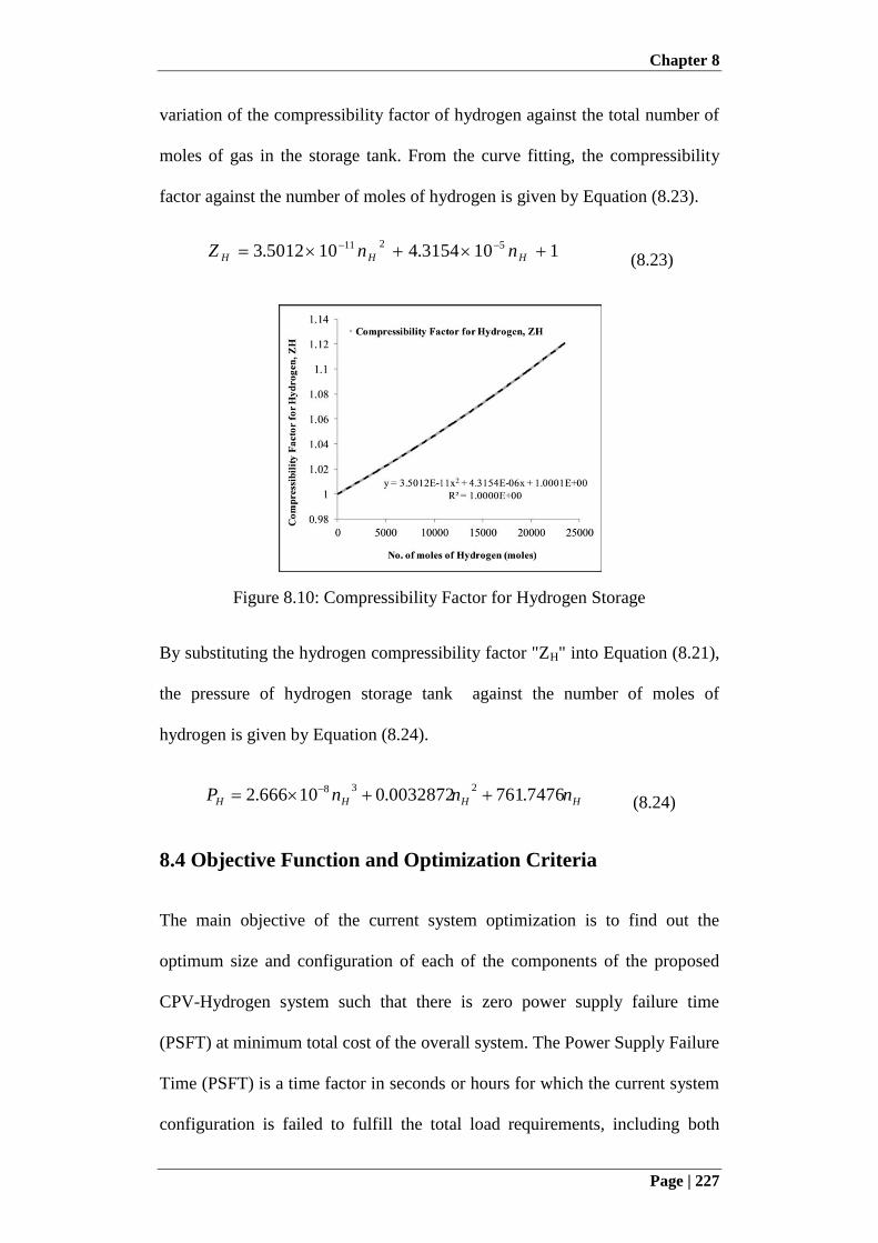
Chapter 8

Page | 227

variation of the compressibility factor of hydrogen against the total number of

moles of gas in the storage tank. From the curve fitting, the compressibility

factor against the number of moles of hydrogen is given by Equation (8.23).

1103154.4105012.3 5211

HHH nnZ (8.23)

Figure 8.10: Compressibility Factor for Hydrogen Storage

By substituting the hydrogen compressibility factor "ZH" into Equation (8.21),

the pressure of hydrogen storage tank against the number of moles of

hydrogen is given by Equation (8.24).

HHHH nnnP 7476.7610032872.010666.2238

(8.24)

8.4 Objective Function and Optimization Criteria

The main objective of the current system optimization is to find out the

optimum size and configuration of each of the components of the proposed

CPV-Hydrogen system such that there is zero power supply failure time

(PSFT) at minimum total cost of the overall system. The Power Supply Failure

Time (PSFT) is a time factor in seconds or hours for which the current system

configuration is failed to fulfill the total load requirements, including both

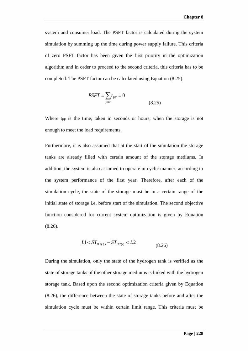
Chapter 8

Page | 228

system and consumer load. The PSFT factor is calculated during the system

simulation by summing up the time during power supply failure. This criteria

of zero PSFT factor has been given the first priority in the optimization

algorithm and in order to proceed to the second criteria, this criteria has to be

completed. The PSFT factor can be calculated using Equation (8.25).

0year

PFtPSFT

(8.25)

Where tPF is the time, taken in seconds or hours, when the storage is not

enough to meet the load requirements.

Furthermore, it is also assumed that at the start of the simulation the storage

tanks are already filled with certain amount of the storage mediums. In

addition, the system is also assumed to operate in cyclic manner, according to

the system performance of the first year. Therefore, after each of the

simulation cycle, the state of the storage must be in a certain range of the

initial state of storage i.e. before start of the simulation. The second objective

function considered for current system optimization is given by Equation

(8.26).

21 )(2)(2 LSTSTL iHfH (8.26)

During the simulation, only the state of the hydrogen tank is verified as the

state of storage tanks of the other storage mediums is linked with the hydrogen

storage tank. Based upon the second optimization criteria given by Equation

(8.26), the difference between the state of storage tanks before and after the

simulation cycle must be within certain limit range. This criteria must be

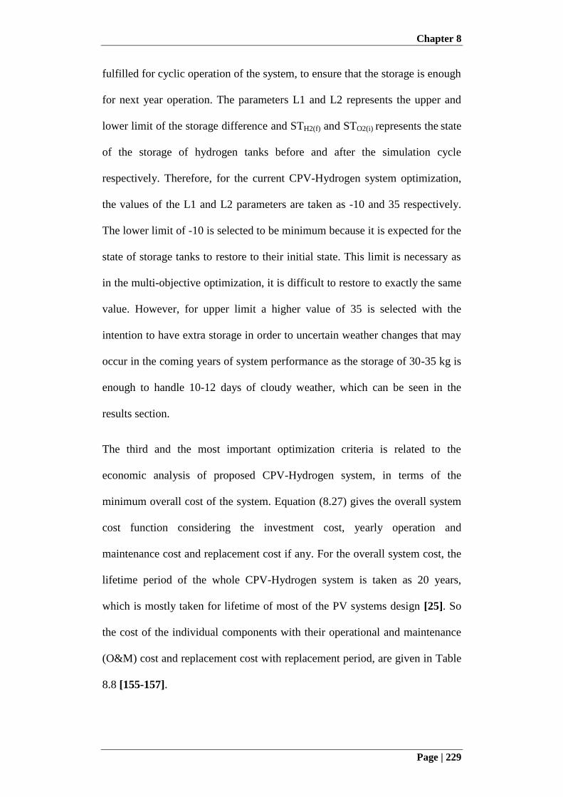
Chapter 8

Page | 229

fulfilled for cyclic operation of the system, to ensure that the storage is enough

for next year operation. The parameters L1 and L2 represents the upper and

lower limit of the storage difference and STH2(f) and STO2(i) represents the state

of the storage of hydrogen tanks before and after the simulation cycle

respectively. Therefore, for the current CPV-Hydrogen system optimization,

the values of the L1 and L2 parameters are taken as -10 and 35 respectively.

The lower limit of -10 is selected to be minimum because it is expected for the

state of storage tanks to restore to their initial state. This limit is necessary as

in the multi-objective optimization, it is difficult to restore to exactly the same

value. However, for upper limit a higher value of 35 is selected with the

intention to have extra storage in order to uncertain weather changes that may

occur in the coming years of system performance as the storage of 30-35 kg is

enough to handle 10-12 days of cloudy weather, which can be seen in the

results section.

The third and the most important optimization criteria is related to the

economic analysis of proposed CPV-Hydrogen system, in terms of the

minimum overall cost of the system. Equation (8.27) gives the overall system

cost function considering the investment cost, yearly operation and

maintenance cost and replacement cost if any. For the overall system cost, the

lifetime period of the whole CPV-Hydrogen system is taken as 20 years,

which is mostly taken for lifetime of most of the PV systems design [25]. So

the cost of the individual components with their operational and maintenance

(O&M) cost and replacement cost with replacement period, are given in Table

8.8 [155-157].

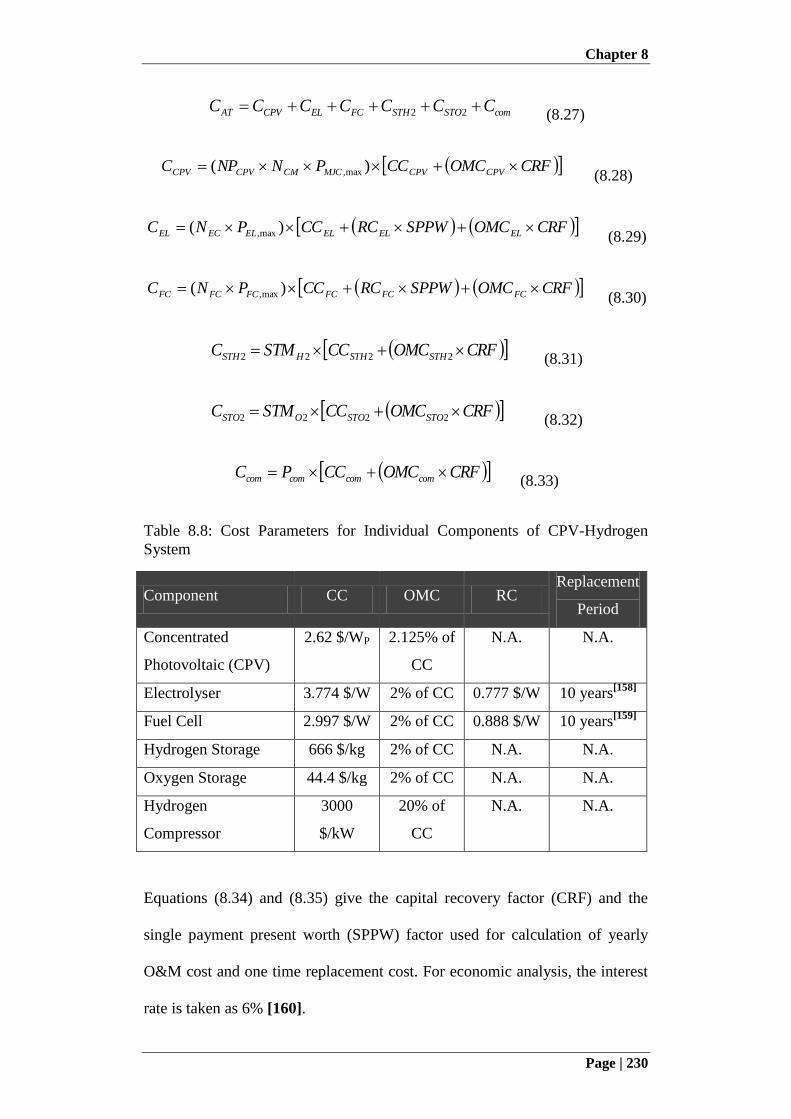
Chapter 8

Page | 230

comSTOSTHFCELCPVAT CCCCCCC 22 (8.27)

CRFOMCCCPNNPC CPVCPVMJCCMCPVCPV )( max, (8.28)

CRFOMCSPPWRCCCPNC ELELELELECEL )( max, (8.29)

CRFOMCSPPWRCCCPNC FCFCFCFCFCFC )( max, (8.30)

CRFOMCCCSTMC STHSTHHSTH 2222 (8.31)

CRFOMCCCSTMC STOSTOOSTO 2222 (8.32)

CRFOMCCCPC comcomcomcom (8.33)

Table 8.8: Cost Parameters for Individual Components of CPV-Hydrogen

System

Component CC OMC RC Replacement

Period

Concentrated

Photovoltaic (CPV)

2.62 $/WP 2.125% of

CC

N.A. N.A.

Electrolyser 3.774 $/W 2% of CC 0.777 $/W 10 years[158]

Fuel Cell 2.997 $/W 2% of CC 0.888 $/W 10 years[159]

Hydrogen Storage 666 $/kg 2% of CC N.A. N.A.

Oxygen Storage 44.4 $/kg 2% of CC N.A. N.A.

Hydrogen

Compressor

3000

$/kW

20% of

CC

N.A. N.A.

Equations (8.34) and (8.35) give the capital recovery factor (CRF) and the

single payment present worth (SPPW) factor used for calculation of yearly

O&M cost and one time replacement cost. For economic analysis, the interest

rate is taken as 6% [160].

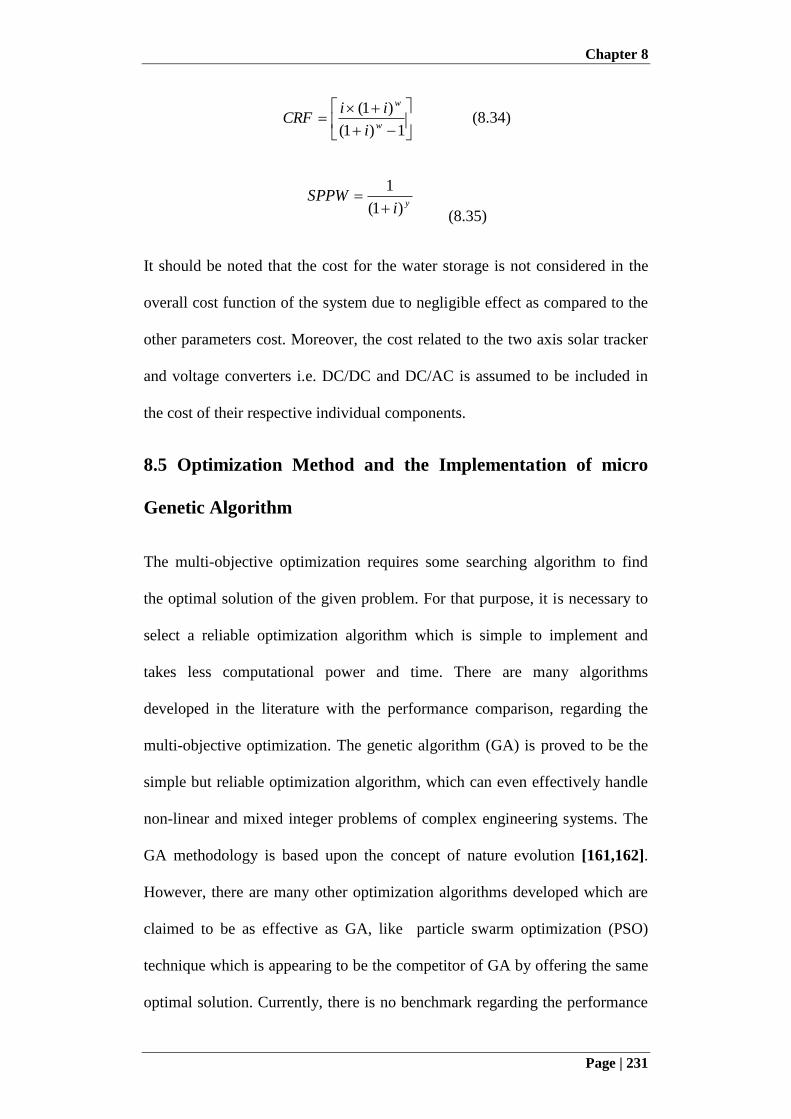
Chapter 8

Page | 231

1)1(

)1(w

w

i

iiCRF (8.34)

yiSPPW

)1(

1

(8.35)

It should be noted that the cost for the water storage is not considered in the

overall cost function of the system due to negligible effect as compared to the

other parameters cost. Moreover, the cost related to the two axis solar tracker

and voltage converters i.e. DC/DC and DC/AC is assumed to be included in

the cost of their respective individual components.

8.5 Optimization Method and the Implementation of micro

Genetic Algorithm

The multi-objective optimization requires some searching algorithm to find

the optimal solution of the given problem. For that purpose, it is necessary to

select a reliable optimization algorithm which is simple to implement and

takes less computational power and time. There are many algorithms

developed in the literature with the performance comparison, regarding the

multi-objective optimization. The genetic algorithm (GA) is proved to be the

simple but reliable optimization algorithm, which can even effectively handle

non-linear and mixed integer problems of complex engineering systems. The

GA methodology is based upon the concept of nature evolution [161,162].

However, there are many other optimization algorithms developed which are

claimed to be as effective as GA, like particle swarm optimization (PSO)

technique which is appearing to be the competitor of GA by offering the same

optimal solution. Currently, there is no benchmark regarding the performance

Chapter 8

Page | 232

comparison and limitations of the PSO against the GA as the searching criteria

for both of the algorithms is different [163,164]. There are some of the studies

claiming to find as efficient solution from PSO as GA but with faster

convergence towards the optimal solution [165,166]. On the other hand, a lot

of studies show that the better performance of the PSO is only under certain

conditions and for certain kind of problems [167-169]. It is also studied that

actually PSO takes overall more time than the GA for the total number of

generations, due to time of the particle communication after each generation

[170]. Some studies also showed clearly the better performance of GA over

PSO [171]. Therefore, the GA is proved to be the most reliable optimization

technique implemented in various case studies. However, this simple and

conventional GA requires more convergence time and the computational

power than the modified GA versions like micro-GA and NSGA-II [172]. The

micro-GA works on the same methodology as of the simple GA, but with

relatively very small population size [173-175]. While the NSGA-II also

follows the same methodology of GA but with difference selection criteria for

the individuals [176,177] and with relatively large population size than the

micro-GA [178]. Both micro-GA and NSGA-II are popular for the multi-

objective optimization problems [179] but in many case, the micro-GA has

shown the better performance than NSGA-II [178] especially in terms of the

computational time which is 8-12 times faster than the NSGA-II and with

better optimal solution and Pareto front [180].

Therefore, after developing the overall performance model of the CPV-

Hydrogen system, the optimization model is developed based upon micro

Genetic Algorithm (micro-GA) due to its less computational power

Chapter 8

Page | 233

requirements and convergence time. The micro-GA optimizes the CPV-

Hydrogen system according to the objective function discussed in the previous

section and the developed optimization strategy as shown in Figure 8.11. The

working of micro-GA algorithm is the same as simple GA but with small

population and re-initialization. During the micro-convergence of the micro-

population, based upon the fitness value, the most fit or best set of the

individuals goes to the next population, while the remaining individuals go

through tournament selection, uniform crossover and the mutation. After the

micro-convergence, the algorithm and the population is reinitialized with the

elitism, by carrying forward the best individual and the rest of the individuals

of the population are selected randomly.

The FORTRAN is used to develop the system optimization model and the

developed model is based upon two sections. One section is based upon the

system optimization model according to the modeling equations of the

individual systems discussed in the previous sections and according to the

energy management flow chart shown in Figure 8.2. The second section of the

developed FORTRAN code is based upon the optimization strategy utilizing

micro-GA that optimizes the system in a certain sequence of objective

functions. During the simulation, at any stage if any of the objective function

does not follow the defined criteria then the simulation loop is terminated and

new simulation cycle is started with new micro GA generations and

optimization parameters, which helps to reduce the computational time. For

current optimization problem in order to obtain high accuracy of the results,

the simulation is based upon an interval of one second as the weather data of

DNI is available in this interval of one second. However, to reduce the

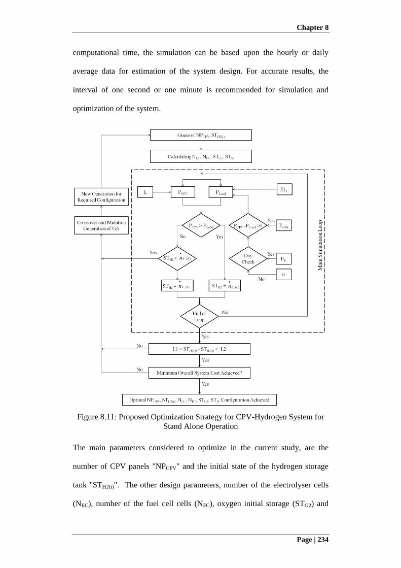
Chapter 8

Page | 234

computational time, the simulation can be based upon the hourly or daily

average data for estimation of the system design. For accurate results, the

interval of one second or one minute is recommended for simulation and

optimization of the system.

Figure 8.11: Proposed Optimization Strategy for CPV-Hydrogen System for

Stand Alone Operation

The main parameters considered to optimize in the current study, are the

number of CPV panels "NPCPV" and the initial state of the hydrogen storage

tank "STH2(i)". The other design parameters, number of the electrolyser cells

(NEC), number of the fuel cell cells (NFC), oxygen initial storage (STO2) and

Chapter 8

Page | 235

the water initial storage, are directly or indirectly linked to NPCPV and STH2(i)

as per the developed performance model. The optimization was carried out

with maximum 300 generations of micro-GA and with population size of 5.

The optimized parameters, optimization results, analysis and the verification

are discussed in the next section.


Figure 8.12 shows the optimization curves for the overall CPV-Hydrogen

system cost, with the PSFT factor curve and the hydrogen storage round

difference curve which defines the second objective function of optimization

i.e. the difference in the states of the hydrogen storage tanks (STH2(f) - STO2(i))

before and after the simulation, . It can be seen that the PSFT factor is zero for

all the selected optimized configurations and the hydrogen storage round

difference curve is also within the required limit of -10 to 35. The limit range

for the hydrogen storage round difference is represented by the dotted lines on

the graph at -10 and 35 values. In addition, it can be seen that the curve for

overall system cost is decreasing in steps according to the change in the

optimization parameters and almost after 51-52 generations, it stabilizes at the

minimum cost which gives the best optimized configuration of CPV-

Hydrogen system. Figure 8.13 shows the breakup for the overall cost of the

CPV-Hydrogen system. From the results, it can be seen that the electrolyser

and the CPV system are the most expensive components in the CPV-

Hydrogen system, responsible for 86% of total system cost. However,

electrolyser is the most expensive among all the components, contributing

51% of the overall cost of the system. The main reason for the high cost of the

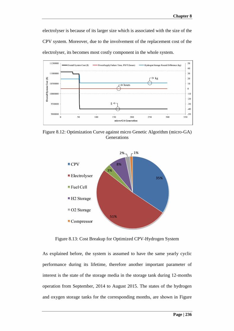
Chapter 8

Page | 236

electrolyser is because of its larger size which is associated with the size of the

CPV system. Moreover, due to the involvement of the replacement cost of the

electrolyser, its becomes most costly component in the whole system.

Figure 8.12: Optimization Curve against micro Genetic Algorithm (micro-GA)

Generations

Figure 8.13: Cost Breakup for Optimized CPV-Hydrogen System

As explained before, the system is assumed to have the same yearly cyclic

performance during its lifetime, therefore another important parameter of

interest is the state of the storage media in the storage tank during 12-months

operation from September, 2014 to August 2015. The states of the hydrogen

and oxygen storage tanks for the corresponding months, are shown in Figure

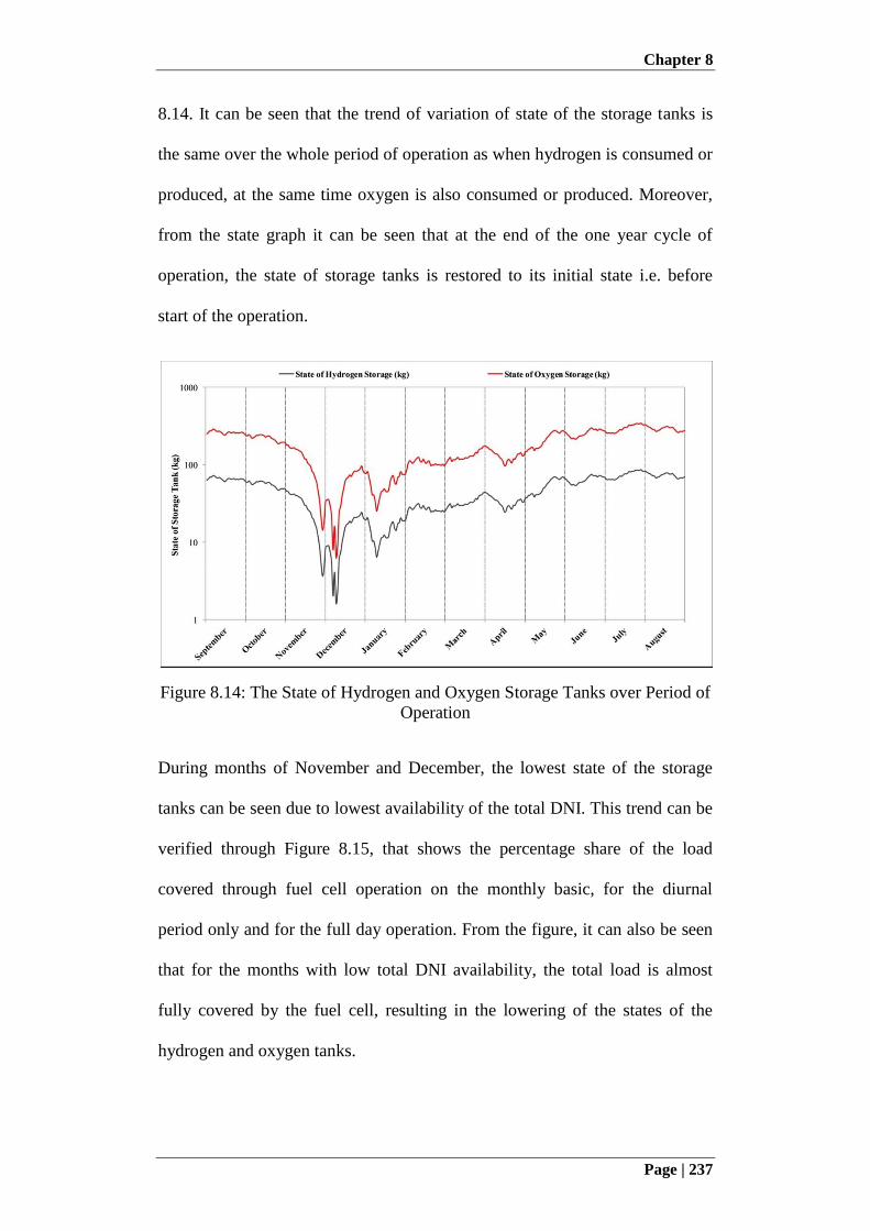
Chapter 8

Page | 237

8.14. It can be seen that the trend of variation of state of the storage tanks is

the same over the whole period of operation as when hydrogen is consumed or

produced, at the same time oxygen is also consumed or produced. Moreover,

from the state graph it can be seen that at the end of the one year cycle of

operation, the state of storage tanks is restored to its initial state i.e. before

start of the operation.

Figure 8.14: The State of Hydrogen and Oxygen Storage Tanks over Period of

Operation

During months of November and December, the lowest state of the storage

tanks can be seen due to lowest availability of the total DNI. This trend can be

verified through Figure 8.15, that shows the percentage share of the load

covered through fuel cell operation on the monthly basic, for the diurnal

period only and for the full day operation. From the figure, it can also be seen

that for the months with low total DNI availability, the total load is almost

fully covered by the fuel cell, resulting in the lowering of the states of the

hydrogen and oxygen tanks.

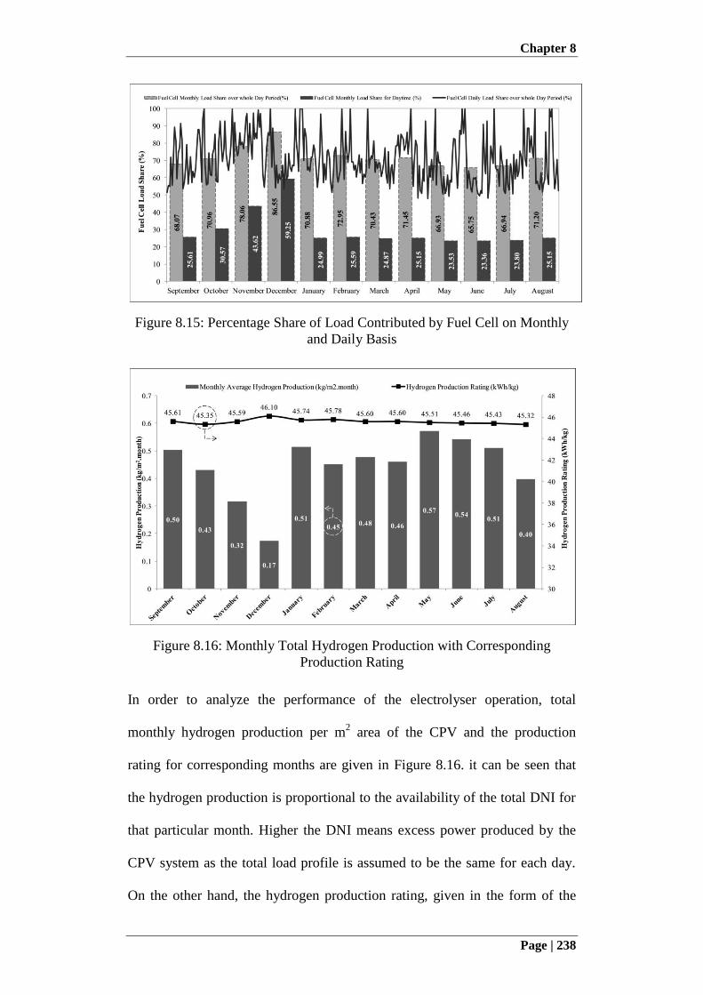
Chapter 8

Page | 238

Figure 8.15: Percentage Share of Load Contributed by Fuel Cell on Monthly

and Daily Basis

Figure 8.16: Monthly Total Hydrogen Production with Corresponding

Production Rating

In order to analyze the performance of the electrolyser operation, total

monthly hydrogen production per m2 area of the CPV and the production

rating for corresponding months are given in Figure 8.16. it can be seen that

the hydrogen production is proportional to the availability of the total DNI for

that particular month. Higher the DNI means excess power produced by the

CPV system as the total load profile is assumed to be the same for each day.

On the other hand, the hydrogen production rating, given in the form of the

Chapter 8

Page | 239

kWh of the CPV energy consumed for one kg production of the hydrogen, is

almost constant for the whole period of operation except for the month of

December, for which the excess power available is far less as compared to the

other months.

Figure 8.17: Simulated Performance of CPV System in form of Monthly

Electrical Rating

The simulated performance of the CPV system in the form of the electrical

rating (kWh/m2.year) for different month of operation is also shown in Figure

8.17. The weather used for the current system simulation and optimization is

the real weather data collected during the long term performance testing of the

CPV system. The simulated electrical rating trend seems to be the same as

discussed in the previous chapter of long term performance testing of the CPV

system. In order to compare the actual and the simulated monthly electrical

rating, both parameters are shown together in Figure 8.18. It can be seen that

the simulated electrical rating is almost equal to experimentally measured

electrical rating. The slight difference in the simulated and experimental

values is due to fluctuations of the power or the measured data, experienced

during the experiment. This verifies the proposed CPV model, which can also

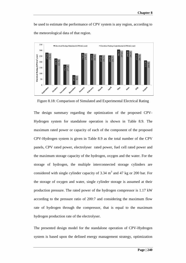
Chapter 8

Page | 240

be used to estimate the performance of CPV system is any region, according to

the meteorological data of that region.

Figure 8.18: Comparison of Simulated and Experimental Electrical Rating

The design summary regarding the optimization of the proposed CPV-

Hydrogen system for standalone operation is shown in Table 8.9. The

maximum rated power or capacity of each of the component of the proposed

CPV-Hydrogen system is given in Table 8.9 as the total number of the CPV

panels, CPV rated power, electrolyser rated power, fuel cell rated power and

the maximum storage capacity of the hydrogen, oxygen and the water. For the

storage of hydrogen, the multiple interconnected storage cylinders are

considered with single cylinder capacity of 3.34 m3 and 47 kg or 200 bar. For

the storage of oxygen and water, single cylinder storage is assumed at their

production pressure. The rated power of the hydrogen compressor is 1.17 kW

according to the pressure ratio of 200:7 and considering the maximum flow

rate of hydrogen through the compressor, that is equal to the maximum

hydrogen production rate of the electrolyser.

The presented design model for the standalone operation of CPV-Hydrogen

system is based upon the defined energy management strategy, optimization

Chapter 8

Page | 241

criteria and the objective functions. In addition, it should also be noted that the

daily electrical load profile is assumed to be constant throughout the period of

operation, for current study. However, seasonal electrical load profile can be

considered if the changes in the load requirements are significant.

Furthermore, the PSFT factor is considered to be zero as one of the

optimization criteria. However, if higher value of PSFT is considered, in case

of any other power backup source, then the number of the CPV panels and

electrolyser size with overall system cost, can be reduced. In addition, the

oxygen storage for the current study is considered to be without compression.

The main reason for this consideration is that the oxygen can be easily

obtained from atmosphere in case of shortage; however, it is not applicable to

the hydrogen.

8.7 Summary

In this chapter, the energy management and the optimization technique for

standalone operation of the CPV-Hydrogen system is proposed, developed and

verified. The multi-objective and muti-variable design and techno-economic

optimization of the CPV-Hydrogen system is successfully conducted using

micro-GA. The performance model of CPV-Hydrogen system is developed by

considering the performance model of each of the individual components of

the system, which are linked together through the proposed energy

management technique. The developed CPV performance mode is based upon

the characteristic model of the MJC and by knowing the concentrator area and

the optical efficiency of the concentrating assembly, the total power output of

the CPV system can be easily calculated according to the total number of the

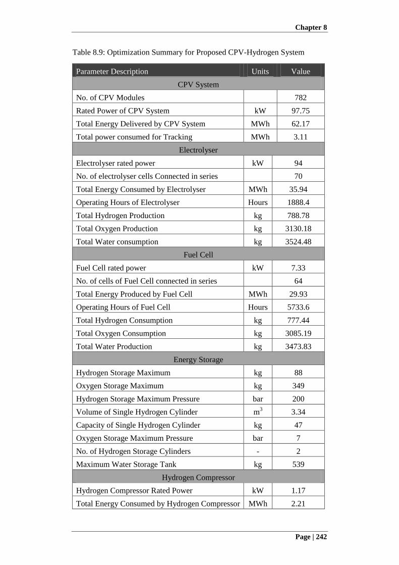
Chapter 8

Page | 242

Table 8.9: Optimization Summary for Proposed CPV-Hydrogen System

Parameter Description Units Value

CPV System

No. of CPV Modules 782

Rated Power of CPV System kW 97.75

Total Energy Delivered by CPV System MWh 62.17

Total power consumed for Tracking MWh 3.11

Electrolyser

Electrolyser rated power kW 94

No. of electrolyser cells Connected in series 70

Total Energy Consumed by Electrolyser MWh 35.94

Operating Hours of Electrolyser Hours 1888.4

Total Hydrogen Production kg 788.78

Total Oxygen Production kg 3130.18

Total Water consumption kg 3524.48

Fuel Cell

Fuel Cell rated power kW 7.33

No. of cells of Fuel Cell connected in series 64

Total Energy Produced by Fuel Cell MWh 29.93

Operating Hours of Fuel Cell Hours 5733.6

Total Hydrogen Consumption kg 777.44

Total Oxygen Consumption kg 3085.19

Total Water Production kg 3473.83

Energy Storage

Hydrogen Storage Maximum kg 88

Oxygen Storage Maximum kg 349

Hydrogen Storage Maximum Pressure bar 200

Volume of Single Hydrogen Cylinder m3 3.34

Capacity of Single Hydrogen Cylinder kg 47

Oxygen Storage Maximum Pressure bar 7

No. of Hydrogen Storage Cylinders - 2

Maximum Water Storage Tank kg 539

Hydrogen Compressor

Hydrogen Compressor Rated Power kW 1.17

Total Energy Consumed by Hydrogen Compressor MWh 2.21

Chapter 8

Page | 243

MJCs in the system. The alkaline electrolyser model and the PEM fuel cell

model are also based upon the single cell characteristics. Their rated power

depends upon the maximum excess power available and the maximum load

requirements, respectively. For the storage purpose, only hydrogen

compression is considered, while oxygen and water are stored at their own

production pressure i.e. without any compression. For the overall system

optimization, three objective functions are defined; zero PSFT factor, the

minimum overall cost of the system and the enough energy storage available

at the start and end of the simulation cycle.

Simulation and optimization code is developed in FORTRAN using micro-GA

algorithm and the system is optimized according to developed optimization

strategy. The parameters considered to be optimized are the number of the

CPV panels and the initial storage of hydrogen. The optimized design is

verified against all the defined objective functions. Such an approach can be

optimally configured in any region or weather condition with high or low solar

irradiance. Moreover, the proposed methodology can be integrated with the

commercially available tools of renewable energy systems simulation, to

enhance their capability to consider CPV for their analysis.

Chapter 9

Page | 244

Chapter 9: Conclusion

In this thesis, a theoretical and experimental study of the concentrated

photovoltaic (CPV) system has been extensively conducted for four

configurations of CPV, employing a compact yet cost effective system design

and with the hydrogen production as energy storage. The major findings of the

current work following the order of presentation in the thesis are:

1. The developed, compact hybrid tracking system incorporated with low

cost tracking sensor and controls providing the sophisticated an accurate

solar tacking methodology at a fraction of the cost of commercially

available solar trackers. The wireless controlled architecture of the tracker

design enables field communication from a master CPV to the arrays of

slave-CPV units that can be located on rooftop of buildings.

2. The ray tracing simulation and field experimentation show that the single

stage concentrator, namely the Fresnel lens based system, provides

suitable CPV design with minimum sensitivity of tracking error, and when

hybridized with glass homogeniser, it shows overall highest long term

rating or efficiency.

3. In addition, the novel multi-leg homogeniser concentrator requires less

number of concentrators needed for same capacity of the CPV system and

as a result, the overall cost of the CPV system and the assembly efforts

will reduce.

4. The study demonstrated that long-term electrical rating methodology gives

the reliable performance data because it captures the efficiencies of

concentrator, MJC cell, the tracking algorithm as well as the

Chapter 9

Page | 245

meteorological irradiance input and the maintenance level. It provides the

real production output of a photovoltaic system for designers and

consumers for actual sizing of the photovoltaic plants. Of all the CPV

systems tested, the Fresnel CPV system has a LTER of 240.21

kWh/m2.year at 22.0% overall efficiency, which is 2 to 3 folds higher than

the conventional silicon based PV systems in the same period of

measurement.

5. In the hybrid CPV-Hydrogen system, the long term rating yields an

efficiency of 15% with a specific hydrogen production of 215-220 kWh/kg

which is of interest for designers of hydrogen plant. However, for steady

power production and standalone but cost effective operation of the CPV

system, the performance model with optimization strategy and energy

management technique have been developed, considering hydrogen as

energy storage. The proposed model can be used by the designers to

simulate and analyze the long term performance of CPV or CPV-

Hydrogen system. In addition, the performance model can be easily

integrated with the commercial optimization and simulation tools to

enhance their capability to consider CPV for system analysis.

6. Such a compact CPV system has been proven to be suitable at the rooftop

of one or more residential or commercial buildings, for reliable long-term

operation of CPV system. By adopting the concept of mini-CPVs, the

lower cost fabrication techniques can be exploited for mass production of

key components of CPV such as small concentrators, homogenisers and

the tracker gearbox and motors.

Chapter 9

Page | 246

For future work, the LTER of the CPV system should be recorded for desert

regions in order to develop a CPV performance database for different climate

conditions. A cost-effective system for dust control has to be developed cost

effectively for the mini-CPVs. A prototype of multi-leg homogeniser CPV

system with high concentration ratio, is also recommended to be fabricated

and tested. In addition, the standalone operation of CPV-Hydrogen system can

be verified experimentally using proposed methodology and this methodology

or performance model can also be integrated into commercial software like

TRNSYS etc.

References

Page | 247

References

[1] BP Energy Outlook 2035, January 2014.

[2] International Energy Agency, World Energy Outlook 2013.

[3] U.S. Energy Information Administration / Annual Energy Review

2011. Energy Consumption by Sector.

[4] International Energy Agency, Redrawing the Energy-Climate Map,

World Energy Outlook Special Report, 10 June 2013.

[5] IPCC, Renewable Energy Sources and Climate Change Mitigation.

Special Report of the Intergovernmental Panel on Climate Change.

2012.

[6] Dincer I, Joshi AS. Solar Based Hydrogen Production Systems,

Springer, 2013.

[7] Sun Y, Wang Y, Zhu L, Yin B, Xiang H, Huang Q. Direct liquid-

immersion cooling of concentrator silicon solar cells in a linear

concentrating photovoltaic receiver. Energy 2014, 65, 264-271.

[8] Chantana J, Ueno S, Ota Y, Nishioka K, Minemoto T. Uniqueness

verification of direct solar spectral index for estimating outdoor

performance of concentrator photovoltaic systems. Renewable Energy

2015, 75, 762-766.

[9] García-Domingo B, Piliougine M, Elizondo D, Aguilera J. CPV

module electric characterisation by artificial neural

networks. Renewable Energy 2015, 78, 173-181.

References

Page | 248

[10] Fraunhofer Institute for Solar Energy Systems, ISE.

PHOTOVOLTAIC REPORT.

https://www.ise.fraunhofer.de/de/downloads/pdf-

files/aktuelles/photovoltaics-report-in-englischer-sprache.pdf. 17

November, 2015.

[11] Ispy Publishing, PV and Solar Market Intelligence Report, Report - 1,

2013.

[12] Schlumberger SBC Energy Institute,

http://www.sbc.slb.com/SBCInstitute/Publications/SolarPhotovoltaic.a

spx. Date Retrieved: 23-03-2014.

[13] Green MA, Emery K, Hishikawa Y, Warta W, Dunlop ED. Solar cell

efficiency tables (Version 45). Progress in photovoltaics: research and

applications 2015, 23(1), 1-9.

[14] Yastrebova NV. High-efficiency multi-junction solar cells: Current

status and future potential. Centre for Research in Photonics,

University of Ottawa, April 2007.

[15] National Renewable Energy Laboratory (NREL).

http://www.nrel.gov/ncpv/images/efficiency_chart.jpg. Date retrieved:

17-11-2015.

[16] Cherucheril G, March S, Verma A. Multijunction Solar Cells.

Department of Electrical Engineering. Iowa State University. 2011.

[17] Mathur SS, Negi BS, Kandpal TC. Geometrical designs and

performance analysis of a linear Fresnel reflector solar concentrator

References

Page | 249

with a flat horizontal absorber. International journal of energy

research 1990, 14(1), 107-124.

[18] Siaw FL, Chong KK, Wong CW. A comprehensive study of dense-

array concentrator photovoltaic system using non-imaging planar

concentrator. Renewable Energy 2014, 62, 542-555.

[19] International Energy Agency (IEA). Trends 2015 in Photovoltaic

Applications, Survey Report of Selected IEA Countries between 1992

and 2014. Report IEA-PVPS T1-27:2015.

[20] Cavallo AJ. Energy storage technologies for utility scale intermittent

renewable energy systems. Journal of solar energy engineering

2001, 123(4), 387-389.

[21] Cook TR, Dogutan DK, Reece SY, Surendranath Y, Teets TS, Nocera

DG. Solar energy supply and storage for the legacy and nonlegacy

worlds. Chemical reviews 2010, 110(11), 6474-6502.

[22] Darras C, Sailler S, Thibault C, Muselli M, Poggi P, Hoguet JC, ...

Fontès G. Sizing of photovoltaic system coupled with

hydrogen/oxygen storage based on the ORIENTE model. International

Journal of Hydrogen Energy 2010, 35(8), 3322-3332.

[23] Lund PD. Optimization of stand-alone photovoltaic systems with

hydrogen storage for total energy self-sufficiency. International

journal of hydrogen energy 1991, 16(11), 735-740.

[24] Zhou K, Ferreira JA, De Haan SWH. Optimal energy management

strategy and system sizing method for stand-alone photovoltaic-

References

Page | 250

hydrogen systems. International journal of hydrogen energy

2008, 33(2), 477-489.

[25] Khan MJ, Iqbal MT. Pre-feasibility study of stand-alone hybrid energy

systems for applications in Newfoundland. Renewable energy

2005, 30(6), 835-854.

[26] Agbossou, K., Kolhe, M., Hamelin, J., & Bose, T. K. (2004).

Performance of a stand-alone renewable energy system based on

energy storage as hydrogen. Energy Conversion, IEEE Transactions

on, 19(3), 633-640.

[27] U.S. Census Bureau, Total Midyear Population for the World: 1950-

2050,

http://www.census.gov/population/international/data/idb/worldpoptotal

.php. Date Retrieved: 24-03-2014.

[28] Worldometer, http://www.worldometers.info/world-population/. Date

Retrieved, 24-03-2014.

[29] World Energy Council, World Energy Resources - 2013 Survey, 2013.

[30] Masjuki HH, Mahlia TMI, Choudhury IA, Saidur R. Potential CO2

reduction by fuel substitution to generate electricity in Malaysia.

Energy Conversion and Management 2002, 43, 763–770.

[31] Ong HC, Mahlia TMI, Masjuki HH. A review on energy scenario and

sustainable energy in Malaysia. Renewable and Sustainable Energy

Reviews 2011, 15, 639–647.

References

Page | 251

[32] Carbon Dioxide Information Analysis Center, CDIAC.

http://cdiac.ornl.gov/trends/emis/glo_2010.html. Date retrieved: 14-11-

2015.

[33] NASA, Global Climate Change.

http://climate.nasa.gov/400ppmquotes/. Date retrieved: 14-11-2015.

[34] International Energy Agency, Solar Energy Perspectives, Renewable

Energy Technologies, 2011.

[35] Myers DR. The Solar Resource. Solar Hydrogen Generation - Towards

a Renewable Energy Future. Springer. 2008.

[36] NREL. http://rredc.nrel.gov/solar/spectra/am1.5/. Date Retrieved: 14-

11-2015.

[37] Duffie JA, Beckman WA. Solar Engineering of Thermal Process, 3rd

ed. John Wiley & Sons, Inc. Hoboken, New Jersey. 2005.

[38] Thekaekara MP. Solar irradiance: total and spectral and its possible

variation. Applied Optics, Vol. 15, No. 4, April 1976.

[39] Lewis NS. Toward cost-effective solar energy use. Science 2007,

315(5813), 798-801.

[40] Shockley W, Queisser HJ. Detailed balance limit of efficiency of p–n

junction solar cells. Journal of Applied Physics 1961, 32(3), 510–519.

[41] Razykov TM, Ferekides CS, Morel D, Stefanakos E, Ullal HS,

Upadhyaya HM. Solar photovoltaic electricity: Current status and

future prospects. Solar Energy 2011, 85, 1580–1608.

References

Page | 252

[42] NREL, National Center for Photovoltaic. Research Cell Efficiency

Records. http://www.nrel.gov/ncpv/. Date Retrieved: 25-11-2015.

[43] Mendelsohn M, Lowder T, Canavan B. Utility-Scale Concentrating

Solar Power and Photovoltaics Projects: A Technology and Market

Overview. NREL/TP-6A20-51137. April 2012.

[44] Garboushian V, Roubideaux D, Yoon S. Integrated high-concentration

PV Near-term alternative for low-cost large-scale solar electric power.

Solar Energy Materials and Solar Cells 1997, 47, 315 323.

[45] Moana L. CPV systems – solar, not cost per view.

http://lamoana.hubpages.com/hub/CPV-systems-solar-not-cost-per-

view#. Date Retrieved: 30-04-2014.

[46] Photovoltaic Efficiency: Concentrated Solar Power.

http://www.teachengineering.org/collection/cub_/lessons/cub_pveff/At

tachments/cub_pveff_lesson04_fundamentalsarticle_v2_dwc.pdf. Date

Retrieved: 27-04-2014.

[47] Chroma Energy Pvt. Ltd.

http://www.chromaenergy.in/enr/index.php?option=com_content&vie

w=article&id=80&Itemid=101. Date Retrieved: 30-04-2014.

[48] InterPV.

http://www.interpv.net/tech/tech_view.asp?idx=109&part_code=0100

30012. Date Retrieved: 22-05-2014.

[49] GPIII Solar. http://www.gpiiisolar.com/gps600. Date Retrieved: 30-

04-2014.

References

Page | 253

[50] Burgess EL, Pritchard DA. Proc 13th Photovoltaic Specialists

Conference (IEEE New York) 1978, 1121.

[51] Sala G, Araújo GL, Luque A, Ruiz J, Coello MA, Lorenzo E, Chenlo

F, Sanz J, Alonso A. Proc ISES International Solar Energy Society

Silver Jubilee Congress (Pergamon, New York) 1979, 1737.

[52] Claverie M, Dupas A, Esteve A. (CNRS, France). Proc 3rd E.C.

Photovoltaic Solar Energy Conference (Reidel, Dordrecht) 1980, 381.

[53] Giuffrida M, Tornielli GP, Pidatella S, Repetto A, Bellafronte E, Zani

PE. Proc. 3rd E.C. Photovoltaic Solar Energy Conference (Reidel,

Dordrecht) 1980, 391.

[54] Salim A, Eugenio N. Solar Cells 1990, 29,1.

[55] Luque A, Miñano JC, Davies PA, Terrón MJ, Tobías I, Sala G, Alonso

J. Proc IEEE PV Specialists Conference (IEEE New York) 1991, 99.

[56] O’Neil Ml, McDanal A, Walters R, J. Perry. Proc 22nd Photovoltaic

Specialists Conference (IEEE, New York) 1991, 523.

[57] Garboushian V, Roubideaux D, Yoon S. Proc 25th Photovoltaic

Specialists Conference (IEEE, New York) 1996, 1373

[58] Bett AW, Burger B, Dimroth F, Siefer G, Lerchenmüller H. High

concentration PV using III-V solar cells. Proc 2006 IEEE 4th World

Conference Photovoltaic Energy Conversion.

References

Page | 254

[59] Tsadka S, Segev R, Migalovich P, Levin O, Tarazi E, Whelan R. Solar

electricity generation system. US Patent application publication; 2009.

p. US2009/0065045.

[60] Singh P, Liburdy JA. A solar concentrator design for uniform flux on a

flat receiver. Energy Conversion and Management 1993, 34, 533–543.

[61] Clemens DD. Photovoltaic concentrator system. US Patent 5,660,644,

1997.

[62] Walter L, John L. Multiple reflector concentrator solar electric power

system. US Patent 5,374,317, 1994.

[63] Chong KK, Siaw FL, Wong CW, Wong GS. Design and construction

of nonimaging planar concentrator for concentrator photovoltaic

system. Renewable Energy 2009, 34, 1364–1370.

[64] Chong KK, Wong CW, Siaw FL, Yew TK. Optical characterization of

nonimaging planar concentrator for the application in concentrator

photovoltaic system. Journal of Solar Energy Engineering 2010,

132(1), 011011.

[65] Ittner III WB. An array of directable mirrors as a photovoltaic solar

concentrator. Solar Energy 1980, 24, 221–234.

[66] Akiba S, Michael E, Amnon Y. Hybrid concentrated photovoltaic and

thermal power conversion at different spectral bands. Solar Energy

2004, 76, 591–601.

References

Page | 255

[67] Diaz V, Alvarez LL, Alonso J, Luque A, Mateos C. Proc European PV

Solar Conference (WIP, Munich) 2004, 2086.

[68] Bett AW, Dimroth F, Gluntz SW et al. Proc 19th European PV Solar

Conference (WIP, Munich) 2004, 2488.

[69] Roland W, Alexander R. Concentrating photovoltaic system using a

Fresnel lens and non-imaging secondary optics. US Patent application

publication, 2008, p.US2008/0245401.

[70] Chen Leon LC. Stationary photovoltaic array module design for solar

electric power generation systems. US Patent 6,653,551, 2003.

[71] Chen Leon LC. Photovoltaic array module design for solar electric

power generator systems. US Patent 6,717,045, 2004.

[72] Andreev VM, Grilikhes VA, Khvostikov VP, Khvostikova OA,

Rumyantsev VD, Sadchikov NA, Shvarts MZ. Concentrator PV

modules and solar cells for TPV systems. Solar energy materials and

solar cells 2004, 84(1), 3-17.

[73] David FK, Patrick MY. Concentrating solar collector with solid optical

element. US Patent application publication, 2006, p. US2006/0231133.

[74] Horne S, Conley G, Gordon J, Fork D, Meada P, Schrader E,

Zimmermann T. A solid 500 sun compound concentrator PV design.

In Photovoltaic Energy Conversion, Conference Record of the 2006

IEEE 4th World Conference on 2006, 1, 694-697.

References

Page | 256

[75] Garboushian V, Stone KW, Slade A. The Amonix High-Concentration

Photovoltaic System. Concentrator Photovoltaics 2007, 130, 253.

[76] David FK, Stephen HJ. Laminated solar concentrating photovoltaic

device. US Patent application publication, 2007, p. US2007/0256726.

[77] McConnell R. A Solar Concentrator Pathway to Low-Cost Electrolytic

Hydrogen. In Solar Hydrogen Generation. Springer New York. 2008,

(pp. 65-86).

[78] Luque-Heredia I, Moreno JM, Magalhaes PH, Cervantes R, Quemere

G, Laurent O. 11 Inspira’s CPV Sun Tracking. Concentrator

Photovoltaics 2007, 130, 232-251.

[79] Luque-Heredia I, Cervantes R, Quemere G. A sun tracking error

monitor for photovoltaic concentrators. In Photovoltaic Energy

Conversion, Conference Record of the 2006 IEEE 4th World

Conference on 2006, 1, 706-709.

[80] Xu G, Zhong Z, Wang B, Guo R, Tian Y. Design of PSD based solar

direction sensor. In Sixth International Symposium on Precision

Mechanical Measurements, International Society for Optics and

Photonics 2013, 89162-89162.

[81] Vosen SR Keller JO. Hybrid energy storage for stand-alone electric

power systems: optimization of system performance and cost through

control strategies. Int. J. Hydrogen Energy 1999, 24, 1139–1156.

References

Page | 257

[82] Agbossou K, Chahine R, Hamelin J, Laurencelle F, Anouar A, St-

Arnaud JM, Bose TK. Renewable energy system based on hydrogen

for remote applications. J. Power Sources 2001, 96, 168–172.

[83] Galli S, Stefanoni M, Havre K, Borg P, Brocke W, Mergel J.

SAPHYS: a JOULE-II E.C. project for solar hydrogen. In 11th World

Hydrogen Energy Conf., Stuttgart, Germany, June 1996.

[84] Barton JP, Infield DG. Energy storage and its use with intermittent

renewable energy. Energy Conversion, IEEE Transactions on 2004,

19(2), 441-448.

[85] Turner JA. Sustainable hydrogen production. Science 2004, 305(5686),

972-974.

[86] J.W. Sheffield and Ç. Sheffield (eds.). Assessment of Hydrogen Energy

for Sustainable Development, 135–146.

[87] Santhanam KSV, Miri MJ, Bailey AV, Takacs GA. Introduction to

hydrogen technology. John Wiley. 2009.

[88] Barbir F. PEM electrolysis for production of hydrogen from renewable

energy sources. Solar energy 2005, 78(5), 661-669.

[89] Zoulias E, Varkaraki E, Lymberopoulos N, Christodoulou CN,

Karagiorgis GN. A Review on Water Electrolysis. Center for

Renewable Energy Sources and Saving.

References

Page | 258

[90] Harrison KW, Remick R, Martin GD. Hydrogen Production:

Fundamentals and Case Study Summaries. 18th World Hydrogen

Energy Conference. NREL/CP-550-47302, January 2010.

[91] Harrison K, Levene JI. Electrolysis of Water. Solar Hydrogen

Generation - Toward a Renewable Energy Future. Springer. 2008.

[92] Durbin DJ, Malardier-Jugroot C. Review of hydrogen storage

techniques for on board vehicle applications. International Journal of

Hydrogen Energy 2013, 38(34), 14595-14617.

[93] Jorgensen SW. Hydrogen storage tanks for vehicles: Recent progress

and current status. Current Opinion in Solid State and Materials

Science 2011, 15 (2), 39–4.

[94] Satyapal S, Petrovic J, Read C, Thomas G, Ordaz G. The U.S.

Department of energy’s national hydrogen storage project: progress

towards meeting hydrogen-powered vehicle requirements. Catalysis

Today 2007, 120(3-4), 246-256.

[95] Hua TQ, Ahluwalia RK, Peng J-K, Kromer M, Lasher S, McKenney

K, et al. Technical assessment of compressed hydrogen storage tank

systems for automotive applications. International Journal of

Hydrogen Energy 2011, 36(4), 3037-3049.

[96] Wolf J. Liquid-hydrogen technology for vehicles. MRS Bulletin 2002,

684-687.

References

Page | 259

[97] Weinberger B, Lamari FD. High pressure cryo-storage of hydrogen by

adsorption at 77 K and up to 50 MPa. International Journal of

Hydrogen Energy 2009, 34, 3058-3064.

[98] Mori D, Haraikawa N, Kobayashi N, Kubo H, Toh K, Tsuzuki M,

et.al. High-pressure metal hydride tank for fuel cell vehicles. In MRS

Proceedings 2005, 884, 6-4).

[99] Umegaki T, Yan JM, Zhang XB, Shioyama H, Kuriyama N, Xu Q.

Boron- and nitrogen-based chemical hydrogen storage materials.

International Journal of Hydrogen Energy 2009, 34(5), 2303-2311.

[100] Sakintuna B, Lamari-Darkrim F, & Hirscher, M. Metal hydride

materials for solid hydrogen storage: a review. International Journal

of Hydrogen Energy 2007, 32(9), 1121-1140.

[101] Darras C, Sailler S, Thibault C, Muselli M, Poggi P, Hoguet JC, ...

Fontès G. Sizing of photovoltaic system coupled with

hydrogen/oxygen storage based on the ORIENTE model. International


[102] Lund PD. Optimization of stand-alone photovoltaic systems with

hydrogen storage for total energy self-sufficiency. International

journal of hydrogen energy 1991, 16(11), 735-740.

[103] Zhou K, Ferreira JA, De Haan SWH. Optimal energy management

strategy and system sizing method for stand-alone photovoltaic-

hydrogen systems. International journal of hydrogen energy

2008, 33(2), 477-489.

References

Page | 260

[104] Dufo-López R, Bernal-Agustín JL, Contreras J. Optimization of

control strategies for stand-alone renewable energy systems with

hydrogen storage. Renewable energy 2007, 32(7), 1102-1126.

[105] Nelson DB, Nehrir MH, Wang C. Unit sizing and cost analysis of

stand-alone hybrid wind/PV/fuel cell power generation

systems. Renewable energy 2006, 31(10), 1641-1656.

[106] Kolhe M, Agbossou K, Hamelin J, Bose TK. Analytical model for

predicting the performance of photovoltaic array coupled with a wind

turbine in a stand-alone renewable energy system based on

hydrogen. Renewable Energy 2003, 28(5), 727-742.

[107] Castañeda M, Cano A, Jurado F, Sánchez H, Fernández LM. Sizing

optimization, dynamic modeling and energy management strategies of

a stand-alone PV/hydrogen/battery-based hybrid system. International


[108] Santarelli M, Pellegrino D. Mathematical optimization of a RES-H 2

plant using a black box algorithm. Renewable Energy 2005, 30(4),

493-510.

[109] Shiroudi A, Taklimi SRH, Mousavifar SA, Taghipour P. Stand-alone

PV-hydrogen energy system in Taleghan-Iran using HOMER

software: optimization and techno-economic analysis. Environment,

development and sustainability 2013, 15(5), 1389-1402.

[110] Karakoulidis K, Mavridis K, Bandekas DV, Adoniadis P, Potolias C,

Vordos N. Techno-economic analysis of a stand-alone hybrid

References

Page | 261

photovoltaic-diesel–battery-fuel cell power system. Renewable Energy

2011, 36(8), 2238-2244.

[111] Rehman S, Alam MM, Meyer JP, Al-Hadhrami LM. Feasibility study

of a wind–pv–diesel hybrid power system for a village. Renewable

Energy 2012, 38(1), 258-268.

[112] Oh SJ, Lee YJ, Chen K, Kim YM, Lim SH, Chun W. Development of

an embedded solar tracker for the enhancement of solar energy

utilization. International Journal of Energy Research 2012, 36(2),

249-258.

[113] Aviation Formulary V1.44 by ED Willams.

http://williams.best.vwh.net/sunrise_sunset_algorithm.htm, Date

retrieved:26-11-2015.

[114] Farahani S. ZigBee wireless networks and transceivers. newnes, 2011.

[115] Winston R, Miñano JC, Benitez PG. Nonimaging optics. Academic

Press. 2005.

[116] Malacara-Hernández D, Malacara-Hernández Z. Handbook of optical

design. CRC Press, 2013.

[117] Arndt R, Puto IR. Basic Understanding of IEC Standard Testing for

Photovoltaic Panels. TUV SUD America Inc.

http://www.tuvamerica.com/services/photovoltaics/articlebasicunderst

andingpv.pdf. Date Retrieved: 21-10-2015.

References

Page | 262

[118] Renzi M, Egidi L, Comodi G. Performance analysis of two 3.5 kWp

CPV systems under real operating conditions. Applied Energy 2015,

160, 687-696.

[119] Pérez-Higueras P, Muñoz E, Almonacid G, Vidal PG. High

Concentrator PhotoVoltaics efficiencies: present status and forecast.

Renewable & Sustainable Energy Reviews 2011, 15, 1810–18155.

[120] Fernández EF, Pérez-Higueras P, Garcia Loureiro AJ, Vidal PG.

Outdoor evaluation of concentrator photovoltaic systems modules

from different manufacturers: First results and steps. Progress in

Photovoltaics: Research and Applications 2013, 21, 693–701.

[121] De Soto W, Klein SA, Beckman WA. Improvement and validation of a

model for photovoltaic array performance. Solar energy 2006, 80(1),

78-88.

[122] Akinyele DO, Rayudu RK, Nair NKC. Development of photovoltaic

power plant for remote residential applications: The socio-technical

and economic perspectives. Applied Energy 2015, 155, 131-149.

[123] Chin VJ, Salam Z, Ishaque K. Cell modelling and model parameters

estimation techniques for photovoltaic simulator application: A

review. Applied Energy 2015, 154, 500-519.

[124] Caamaño E, Lorenzo E, Zilles R. Quality control of wide collections

of PV modules: lessons learned from the IES experience. Progress in

Photovoltaics: Research and Applications 1999, 7, 137–149.

References

Page | 263

[125] García-Domingo B, Aguilera J, de la Casa J, Fuentes M. Modelling the

influence of atmospheric conditions on the outdoor real performance

of a CPV (Concentrated Photovoltaic) module. Energy 2014, 70, 239–

50.

[126] Talavera DL, Pérez-Higueras P, Ruíz-Arias JA, Fernández EF.

Levelised cost of electricity in high concentrated photovoltaic grid

connected systems: Spatial analysis of Spain. Applied Energy

2015, 151, 49-59.

[127] Eccher M, Salemi A, Turrini S, Brusa RS. Measurements of power

transfer efficiency in CPV cell-array models using individual DC–DC

converters. Applied Energy 2015, 142, 396-406.

[128] Said, S. A. M. (1990). Effects of dust accumulation on performances

of thermal and photovoltaic flat-plate collectors. Applied

Energy, 37(1), 73-84.

[129] International Energy Agency, CO2 Emissions from Fuel Combustion

Highlights, 2013.

[130] Yingli Green Energy Holding Co. Ltd., PANDA 60 CELL SERIES 2,

www.yinglisolar.com

[131] Yingli Green Energy Holding Co. Ltd., YGE 48 Cell 40mm SERIES,

www.yinglisolar.com

[132] MiaSolé Hi-Tech Corp., FLEX–02N SERIES CIGS MODULE, www.

miasole.com

References

Page | 264

[133] Burhan M, Oh SJ, Shahzad MW, Ng KC. Electrical Rating of

Concentrated Photovoltaic (CPV) Systems for Long Term

Performance. The 6th

International Symposium on Physics of Fluids

(ISPF6) 2015, Xining, China.

[134] National Environment Agency (NEA) Singapore, www.nea.gov.sg

[135] Shahzad MW, Thu K, Park YC, Chun W, Ng KC. Solar Thermal

Rating: A methodology for evaluating the long term performance of

renewable energy systems. International Meeting on Advanced

Thermofluids 2013.

[136] HOMER (Hybrid Optimization of Multiple Energy Resources).

Available from: http://www.homerenergy.com/software.html

[137] iHOGA (Improved Hybrid Optimization by Genetic Algorithms).

Available from:

http://personal.unizar.es/rdufo/index.php?option=com_content&view=

article&id=2&Itemid=104&lang=en

[138] Bernal-Agustin JL, Dufo-Lopez R. Simulation and optimization of

stand-alone hybrid renewable energy systems. Renewable and

Sustainable Energy Reviews 2009, 13, 2111-2118.

[139] Energy Market Authority (EMA) Singapore, http://www.ema.gov.sg

[140] Nishioka K, Takamoto T, Agui T, Kaneiwa M, Uraoka Y, Fuyuki T.

Annual output extimation of concentrator photovoltaic systems using

high-efficiency InGaP/InGaAs/Ge triple-junction solar cells based on

References

Page | 265

experimental solar cell's characteristics and field-test meteorological

data, Solar Energy Materials & Solar Cells 2006, 90, 57-67.

[141] Cotal H, Sherif R. Temperature Dependence of the IV Parameters

from Triple Junction GaInP/InGaAs/Ge Concentrator Solar Cells,

IEEE 4th World Conference on Photovoltaic Energy Conversion 2006,

1, 845-848.

[142] Calderón M, Calderón AJ, Ramiro A, González JGI, González, I.

Analysis of the performance of the photovoltaic array through the

exergy efficiency. International Conference on Renewable Energy and

Power Quality 2011, 13-15.

[143] Horne S, McDonald M, Hartsoch N, Desy K. (2009). Reflective optics

CPV panels enabling large scale, reliable generation of solar energy

cost competitive with fossil fuels.

[144] ArzonSolar. http://www.arzonsolar.com/wp-

content/uploads/2015/02/uModule-Datasheet.pdf. Date retrieved: 16-

11-2015.

[145] 3M, Renewable Energy Division. Factors Influencing the Optical

Efficiency of Fresnel Lens Concentrators.

http://www.lapptannehill.com/wp-content/uploads/2014/02/3M-

Factors.pdf. Date retrieved: 16-11-2015.

[146] Pan CT, Juan YL. A novel sensorless MPPT controller for a high-

efficiency microscale wind power generation system. Energy

Conversion, IEEE Transactions on 2010, 25(1), 207-216.

References

Page | 266

[147] Chiu HJ, Lin LW. A high-efficiency soft-switched AC/DC converter

with current-doubler synchronous rectification. Industrial Electronics,

IEEE Transactions on 2005, 52(3), 709-718.

[148] Ki SK, Lu DDC. Implementation of an efficient transformerless

single-stage single-switch AC/DC converter. Industrial Electronics,

IEEE Transactions on 2010, 57(12), 4095-4105.

[149] Wang K, Lin CY, Zhu L, Qu D, Lee FC, Lai JS. Bi-directional DC to

DC converters for fuel cell systems. In Power Electronics in

Transportation 1998, 47-51.

[150] Nymand M, Andersen MA. High-efficiency isolated boost DC–DC

converter for high-power low-voltage fuel-cell applications. Industrial

Electronics, IEEE Transactions on 2010, 57(2), 505-514.

[151] Helioslite. http://helioslite.com/site/wp-

content/uploads/2015/06/H%C3%A9liosLite-datasheet-35m2-2014-

12.pdf. Date retrieved: 16-11-2015.

[152] Ulleberg Ø. Stand-Alone Power Systems for the Future: Optimal

Design, Operation & Control of Solar-Hydrogen Energy Systems.

Ph.D. Thesis, Department of Thermal Energy and Hydropower,

Norwegian University of Science and Technology, Trondheim, Norway

1998.

[153] Li CH, Zhu XJ, Cao GY, Sui S, Hu MR. Dynamic modeling and sizing

optimization of stand-alone photovoltaic power systems using hybrid

energy storage technology. Renewable Energy 2009, 34(3), 815-826.

References

Page | 267

[154] REFPROP Reference Fluid Thermodynamic and Transport Properties,

National Institute of Standards and Technology (NIST) Standard

Reference Database 23, Version 8.0, http://www.nist.gov

[155] Guinot B, Champel B, Montignac F, Lemaire E, Vannucci D, Sailler S,

Bultel Y. Techno-economic study of a PV-hydrogen-battery hybrid

system for off-grid power supply: Impact of performances' ageing on

optimal system sizing and competitiveness. International Journal of

Hydrogen Energy 2015, 40, 623-632.

[156] Simbeck D, Chang E. Hydrogen Supply: Cost Estimate for Hydrogen

Pathways - Scoping Analysis. SFA Pacific, Inc. Mountain View,

California, 2002 NREL.

[157] PV Magazine, Concentrated PV solar set to boom. http://www.pv-

magazine.com/news/details/beitrag/concentrated-pv-solar-set-to-

boom_100013699/#axzz3j DrxpxEr. Date Retrieved: 19-08-2015.

[158] Ghosh PC, Emonts B, Janßen H, Mergel J, Stolten D. Ten years of

operational experience with a hydrogen-based renewable energy

supply system. Solar Energy 2003, 75(6), 469-478.

[159] Granovskii M, Dincer I, Rosen MA. Economic and environmental

comparison of conventional, hybrid, electric and hydrogen fuel cell

vehicles. Journal of Power Sources 2006, 159(2), 1186-1193.

[160] Rehman S, Al-Hadhrami LM. Study of a solar PV–diesel–battery

hybrid power system for a remotely located population near Rafha,

Saudi Arabia. Energy 2010, 35(12), 4986-4995.

References

Page | 268

[161] Deb K. Genetic algorithm in search and optimization: the technique

and applications. In Proceedings of International Workshop on Soft

Computing and Intelligent Systems,(ISI, Calcutta, India) 1998, 58-87.

[162] Konak A, Coit DW, Smith AE. Multi-objective optimization using

genetic algorithms: A tutorial. Reliability Engineering & System Safety

2006, 91(9), 992-1007.

[163] Bai Q. Analysis of particle swarm optimization algorithm. Computer

and information science 2010, 3(1), 180.

[164] Aote SS, Raghuwanshi MM, Malik LA. Brief Review on Particle

Swarm Optimization: Limitations & Future Directions. International

Journal of Computer Science Engineering (IJCSE) 2013, 2(5), 196-

200.

[165] Shukla M, Dhaliwal BS. Review of Multi-objective Optimization

using Genetic Algorithm and Particle Swarm Optimization. IP

Multimedia Communications, A Special Issue from IJCA. 72-74.

[166] Rajendra R, Pratihar DK. Particle Swarm Optimization Algorithm vs.

Genetic Algorithm to Solve Multi-Objective Optimization Problem in

Gait Planning of Biped Robot. In Proceedings of the International

Conference on Information Systems Design and Intelligent

Applications 2012 (INDIA 2012) held in Visakhapatnam, India,

January 2012, 563-570). Springer Berlin Heidelberg.

References

Page | 269

[167] Boeringer DW, Werner DH. Particle swarm optimization versus

genetic algorithms for phased array synthesis. Antennas and

Propagation, IEEE Transactions on 2004, 52(3), 771-779.

[168] Rajendra R, Pratihar DK. Particle swarm optimization algorithm vs

genetic algorithm to develop integrated scheme for obtaining optimal

mechanical structure and adaptive controller of a robot. Intelligent

Control and Automation 2011, 2(04), 430.

[169] Hassan R, Cohanim B, De Weck O, Venter G. A comparison of

particle swarm optimization and the genetic algorithm. In Proceedings

of the 1st AIAA multidisciplinary design optimization specialist

conference 2005, 1-13

[170] Panda S, Padhy NP. Comparison of particle swarm optimization and

genetic algorithm for FACTS-based controller design. Applied soft

computing 2008, 8(4), 1418-1427.

[171] Jones KO. Comparison of genetic algorithm and particle swarm

optimization. In Proc. Int. Conf. Computer Systems and

Technologies2005. 1-6.

[172] Yu X, Gen M. Introduction to evolutionary algorithms. Springer

Science & Business Media. 2010.

[173] Senecal PK. Numerical optimization using the GEN4 micro-genetic

algorithm code. University of Wisconsin-Madison. 2000.

References

Page | 270

[174] Abu-Lebdeh G, Benekohal RF. Convergence variability and

population sizing in micro-genetic algorithms. Computer-aided civil

and infrastructure engineering 1999, 14(5), 321-334.

[175] Krishnakumar K. Micro-genetic algorithms for stationary and non-

stationary function optimization. In 1989 Advances in Intelligent

Robotics Systems Conference, International Society for Optics and

Photonics 1990, 289-296.

[176] Srinivas N, Deb K. Muiltiobjective optimization using nondominated

sorting in genetic algorithms. Evolutionary computation 1994, 2(3),

221-248.

[177] Deb K, Pratap A, Agarwal S, Meyarivan TAMT. A fast and elitist

multiobjective genetic algorithm: NSGA-II. Evolutionary

Computation, IEEE Transactions on 2002, 6(2), 182-197.

[178] Choi S. Speedups for Efficient Genetic Algorithms: Design

optimization of low-boom supersonic jet using parallel GA and micro-

GA with external memory. Genetic Algorithms and Genetic

Programming at Stanford 2003, 21-30.

[179] Coello CC, Lamont GB, Van Veldhuizen DA. Evolutionary algorithms

for solving multi-objective problems. Springer Science & Business

Media. 2007.

[180] Coello CC, Pulido GT. Multiobjective structural optimization using a

microgenetic algorithm. Structural and Multidisciplinary Optimization

2005, 30(5), 388-403.

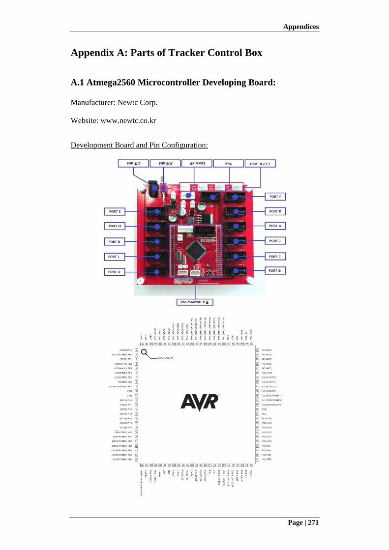
Appendices

Page | 271

Appendix A: Parts of Tracker Control Box

A.1 Atmega2560 Microcontroller Developing Board:

Manufacturer: Newtc Corp.

Website: www.newtc.co.kr

Development Board and Pin Configuration:

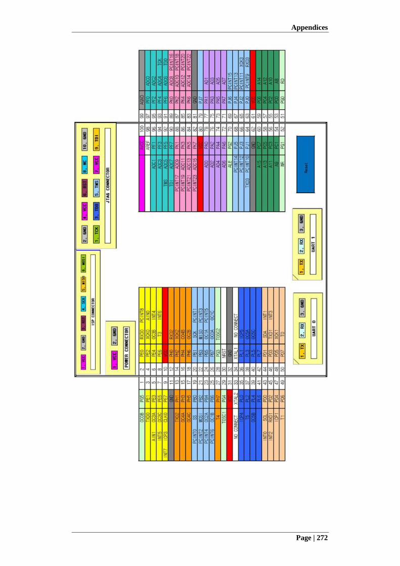
Appendices

Page | 272

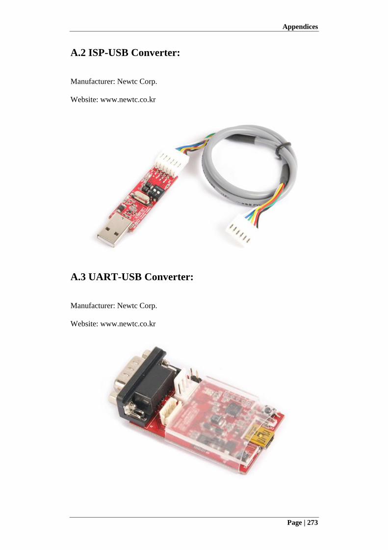
Appendices

Page | 273

A.2 ISP-USB Converter:



A.3 UART-USB Converter:



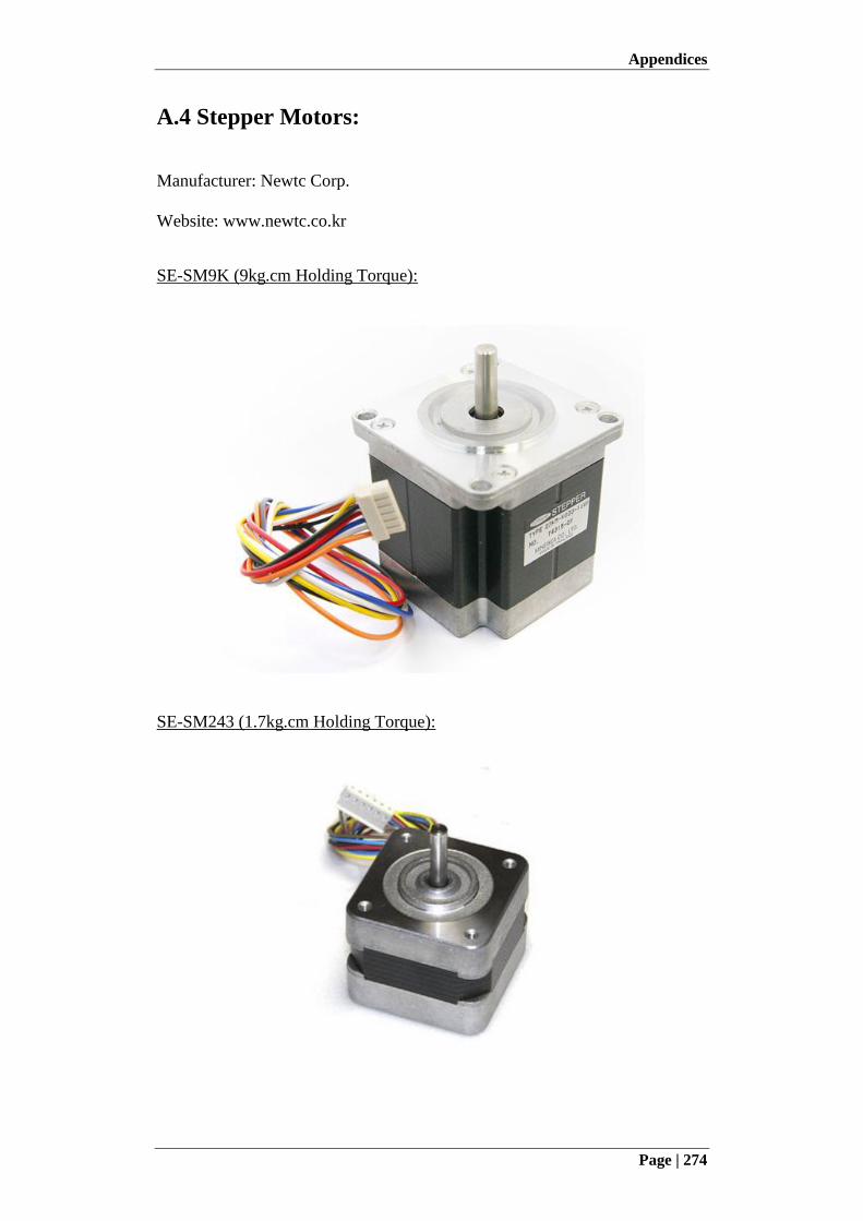
Appendices

Page | 274

A.4 Stepper Motors:



SE-SM9K (9kg.cm Holding Torque):

SE-SM243 (1.7kg.cm Holding Torque):

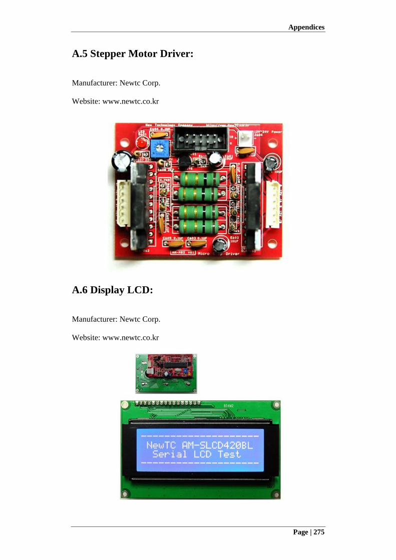
Appendices

Page | 275

A.5 Stepper Motor Driver:



A.6 Display LCD:



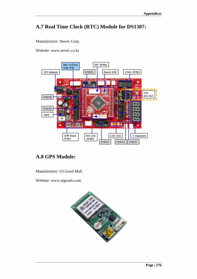
Appendices

Page | 276

A.7 Real Time Clock (RTC) Module for DS1307:



A.8 GPS Module:

Manufacturer: UI Good Mall.

Website: www.uigoods.com

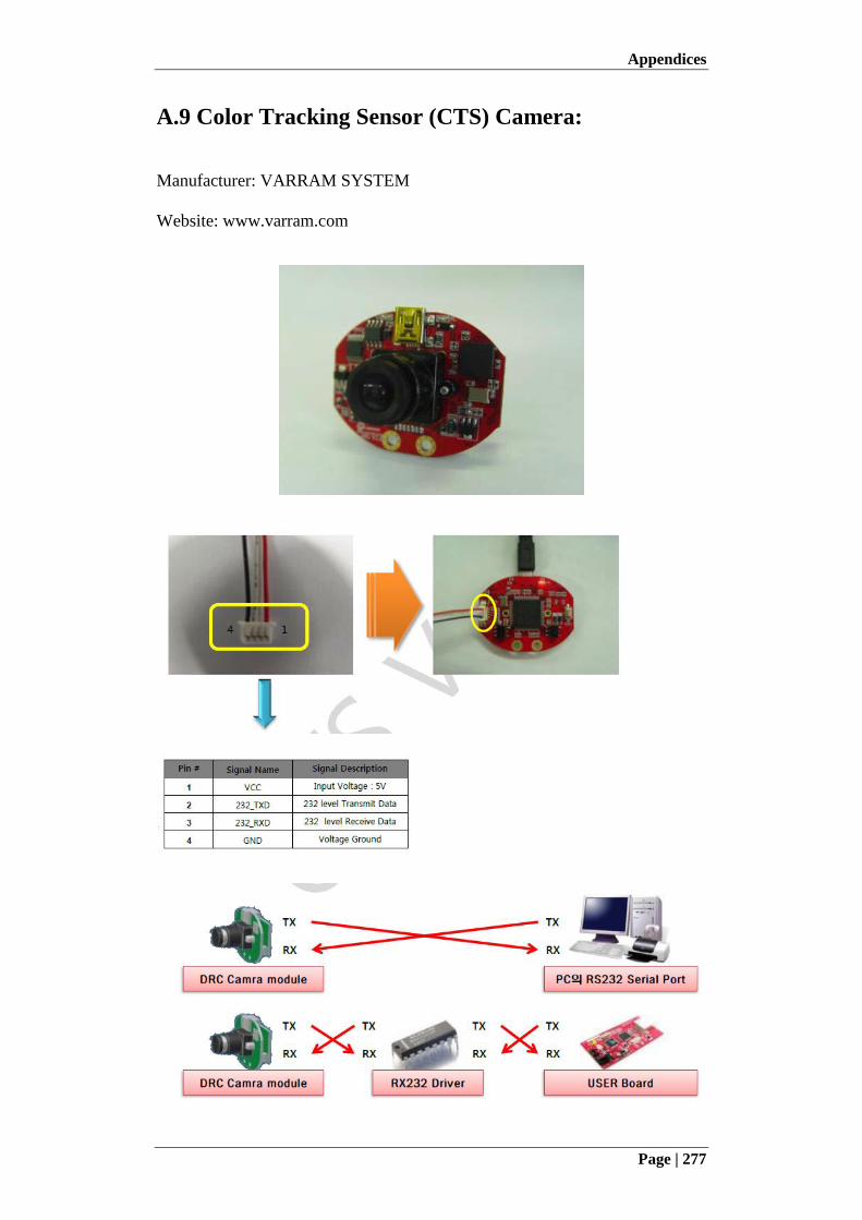
Appendices

Page | 277

A.9 Color Tracking Sensor (CTS) Camera:

Manufacturer: VARRAM SYSTEM

Website: www.varram.com

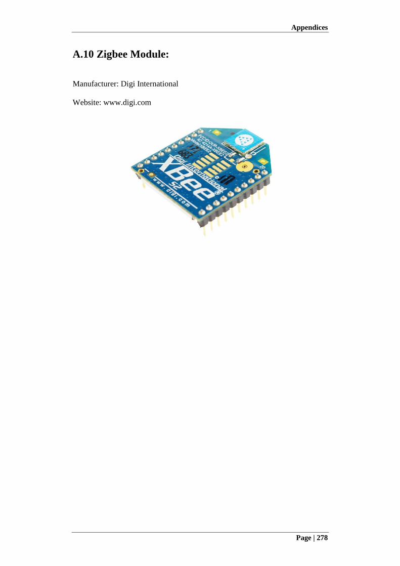
Appendices

Page | 278

A.10 Zigbee Module:

Manufacturer: Digi International

Website: www.digi.com

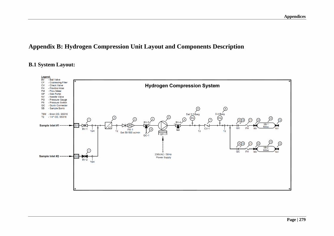
Appendices

Page | 279

Appendix B: Hydrogen Compression Unit Layout and Components Description

B.1 System Layout:

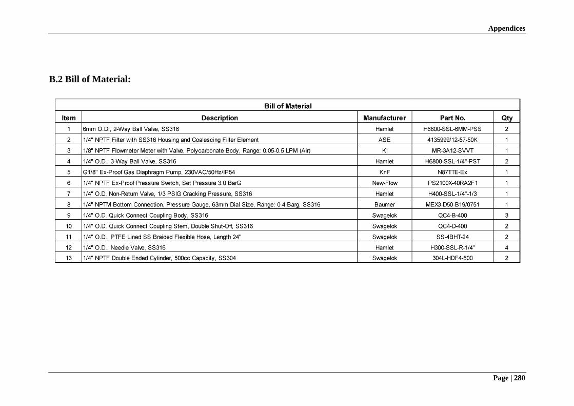
Appendices

Page | 280

B.2 Bill of Material:

Appendices

Page | 281

B.3 Hydrogen Compressor:

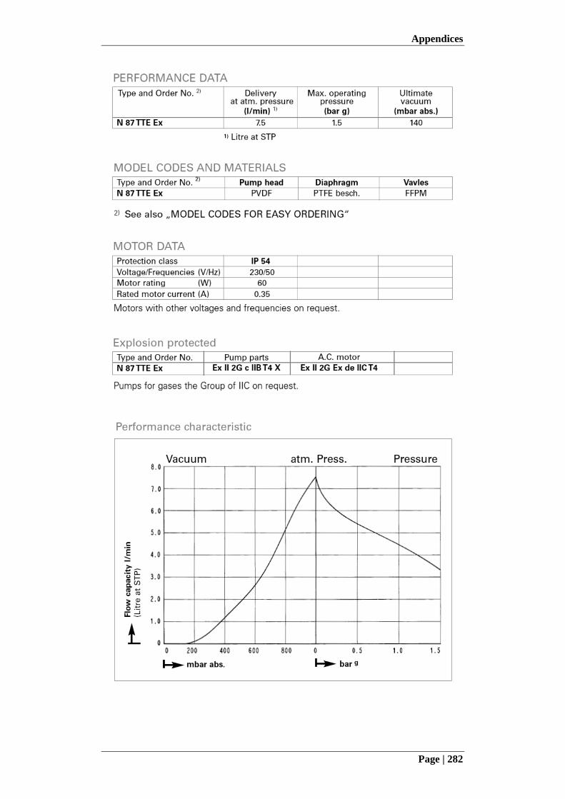
Appendices

Page | 282

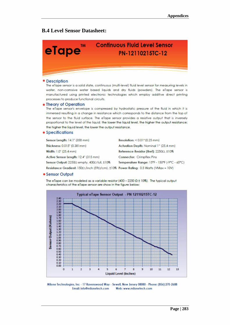
Appendices

Page | 283

B.4 Level Sensor Datasheet:

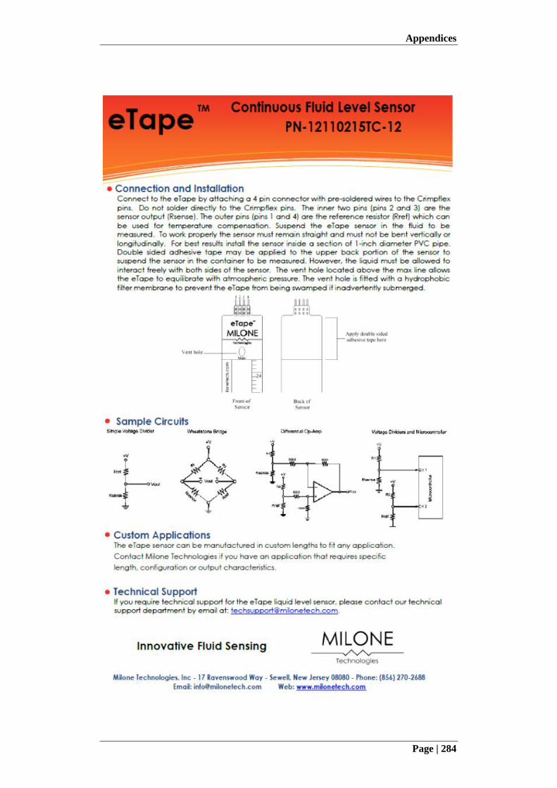
Appendices

Page | 284

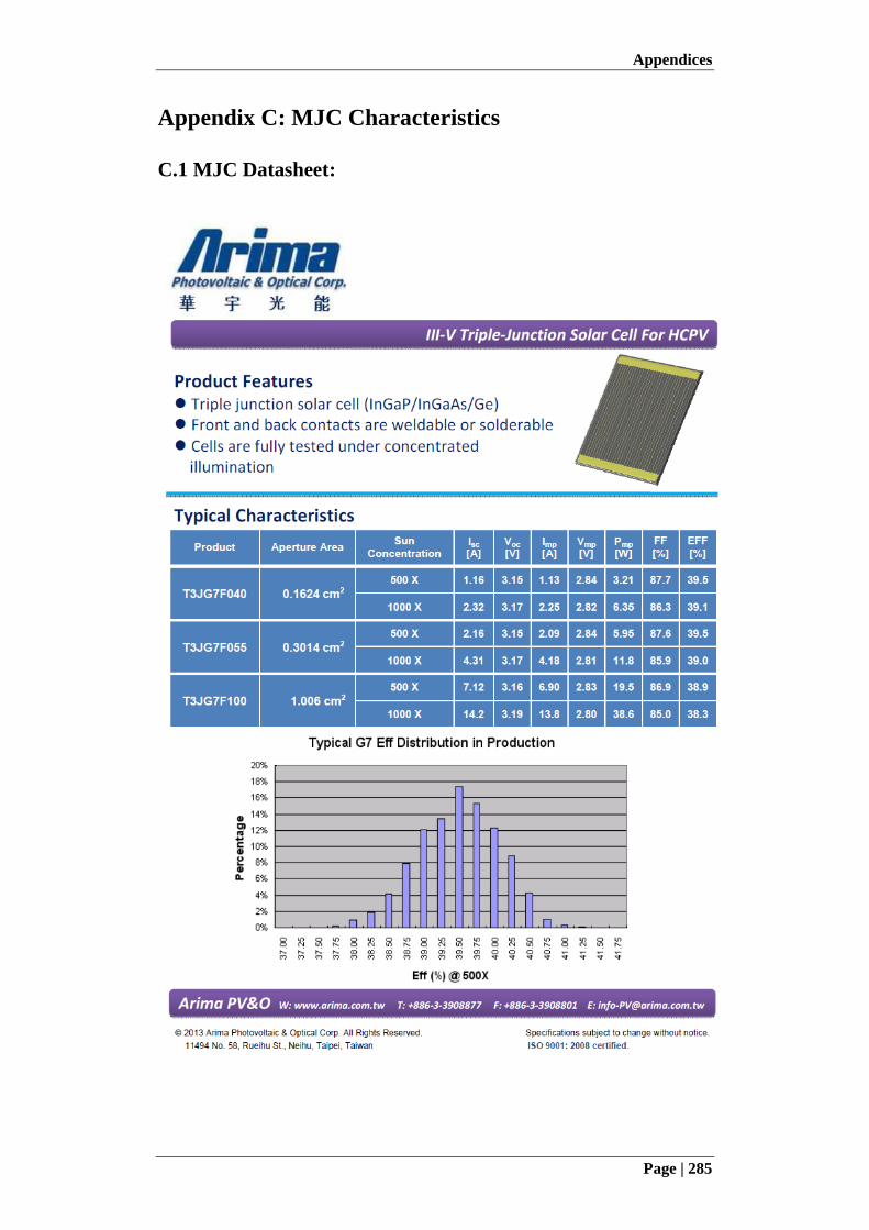
Appendices

Page | 285

Appendix C: MJC Characteristics

C.1 MJC Datasheet:

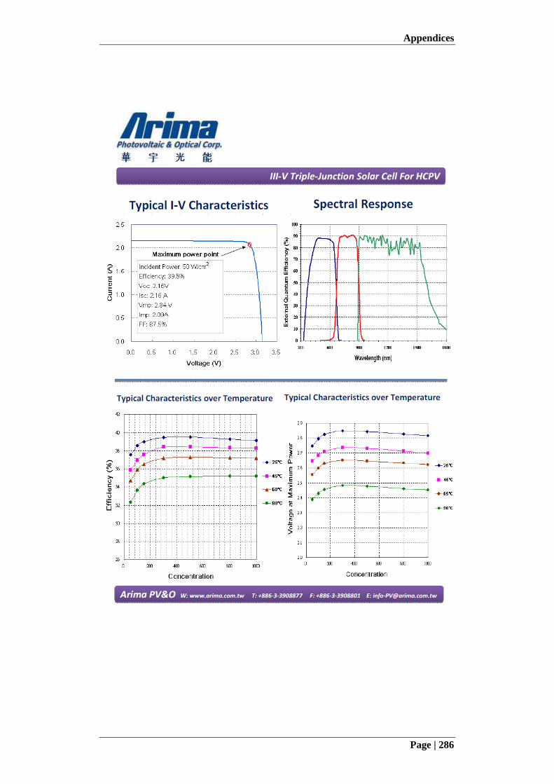
Appendices

Page | 286

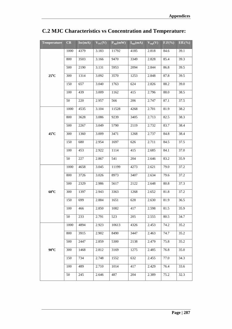
Appendices

Page | 287

C.2 MJC Characteristics vs Concentration and Temperature:

Temperature CR Isc(mA) VOC(V) Pmp(mW) Imp(mA) Vmp(V) F.F(%) Eff.(%)

25oC

1000 4379 3.183 11792 4185 2.818 84.6 39.1

800 3503 3.166 9470 3349 2.828 85.4 39.3

500 2190 3.131 5953 2094 2.844 86.8 39.5

300 1314 3.092 3570 1253 2.848 87.8 39.5

150 657 3.040 1763 624 2.826 88.2 39.0

100 439 3.009 1162 415 2.796 88.0 38.5

50 220 2.957 566 206 2.747 87.1 37.5

45oC

1000 4535 3.104 11528 4268 2.701 81.9 38.2

800 3628 3.086 9239 3405 2.713 82.5 38.3

500 2267 3.049 5790 2119 2.732 83.7 38.4

300 1360 3.009 3471 1268 2.737 84.8 38.4

150 680 2.954 1697 626 2.711 84.5 37.5

100 453 2.922 1114 415 2.685 84.1 37.0

50 227 2.867 541 204 2.646 83.2 35.9

60oC

1000 4658 3.045 11199 4273 2.621 79.0 37.2

800 3726 3.026 8973 3407 2.634 79.6 37.2

500 2329 2.986 5617 2122 2.648 80.8 37.3

300 1397 2.943 3363 1268 2.652 81.8 37.2

150 699 2.884 1651 628 2.630 81.9 36.5

100 466 2.850 1082 417 2.598 81.5 35.9

50 233 2.791 523 205 2.555 80.5 34.7

90oC

1000 4894 2.923 10613 4326 2.453 74.2 35.2

800 3915 2.902 8490 3447 2.463 74.7 35.2

500 2447 2.859 5300 2138 2.479 75.8 35.2

300 1468 2.812 3169 1275 2.485 76.8 35.0

150 734 2.748 1552 632 2.455 77.0 34.3

100 489 2.710 1014 417 2.429 76.4 33.6

50 245 2.646 487 204 2.389 75.2 32.3

theoretical and experimental study of - CORE

Documents

Transcript of theoretical and experimental study of - CORE