Retrospective Theses and Dissertations Iowa State University Capstones, Theses andDissertations

1990

Plan and market(s): a theoretical model of theChinese grain economyDabai ChenIowa State University

Follow this and additional works at: https://lib.dr.iastate.edu/rtd

Part of the Agricultural and Resource Economics Commons, and the Agricultural EconomicsCommons

This Dissertation is brought to you for free and open access by the Iowa State University Capstones, Theses and Dissertations at Iowa State UniversityDigital Repository. It has been accepted for inclusion in Retrospective Theses and Dissertations by an authorized administrator of Iowa State UniversityDigital Repository. For more information, please contact digirep@iastate.edu.

Recommended CitationChen, Dabai, "Plan and market(s): a theoretical model of the Chinese grain economy " (1990). Retrospective Theses and Dissertations.9425.https://lib.dr.iastate.edu/rtd/9425

13 ' ' W '

INFORMATION TO USERS

The most advanced technology has been used to photograph and reproduce this manuscript from the itnicrofilm master. UMI films the text directly from the original or copy submitted. Thus, some thesis and dissertation copies are in typewriter face, while others may be from any type of computer printer.

The quality of this KprodoctlOB If depend** upon the quality of the copy submitted. Broken or indistinct print, colored or poor quality illustrations and photographs, print bleedthrough, substandard margins, and improper alignment can adversely affect reproduction.

In the unlikely event that the author did not send UMI a complete manuscript and there are missing pages, these will be noted. Also, if unauthorized copyright material had to be removed, a note will indicate the deletion.

Oversize materials (e.g., maps, drawings, charts) are reproduced by sectioning the original, beginning at the upper left-hand corner and continuing from left to right in equal sections with small overlaps. Each original is also photographed in one exposure and Is included In reduced form at the back of the book.

Photographs Included in the original manuscript have been reproduced xerographlcally in this copy. Higher quality 6" x 9" black and white photographic prints are available for any photographs or Illustrations appearing In this copy for an additional charge. Contact UMI directly to order.

University Microtiims international A Beii & Howell information Company

300 Noftn Zeeb Road. Ann Arbor, 48106-1346 USA 313 761-4700 800 521-0600

Order Number 0101S86

Plan and market (s): A theoretical model of the Chinese grain economy

Chen, Dabai, Ph.D.

Iowa State University, 1990

Copyright ©1990 by Chen, Dabai. All rights reserved.

U M I SOON.ZeebRd. Ann AAor, MI 48106

Plan and market(s): A theoretical model

of the Chinese grain economy

by

Dabai Chen

A Dissertation Submitted to the

Graduate Faculty in Partial Fulfillment of the

Requirements for the Degree of

DOCTOR OF PHILOSOPHY

Department: Economics Major: Agricultural Economics

Approved :

P r the Major Department

For the Graduate College

Iowa State University Ames, Iowa

1990

Copyright © Dabai Chen, 1990. All rights reserved.

Signature was redacted for privacy.

Signature was redacted for privacy.

Signature was redacted for privacy.

ii

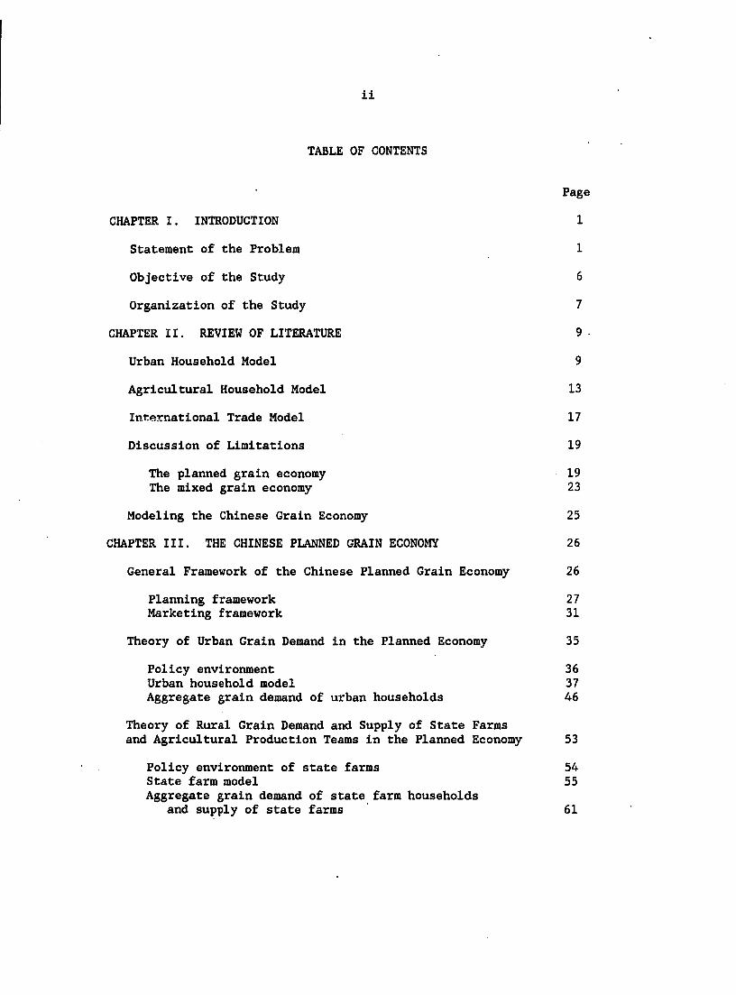
TABLE OF CONTENTS

Page

CHAPTER I. INTRODUCTION 1

Statement of the Problem 1

Objective of the Study 6

Organization of the Study 7

CHAPTER II. REVIEW OF LITERATURE 9

Urban Household Model 9

Agricultural Household Model 13

International Trade Model 17

Discussion of Limitations 19

The planned grain economy 19 The mixed grain economy 23

Modeling the Chinese Grain Economy 25

CHAPTER III. THE CHINESE PLANNED GRAIN ECONOMY 26

General Framework of the Chinese Planned Grain Economy 26

Planning framework 27 Marketing framework 31

Theory of Urban Grain Demand in the Planned Economy 35

Policy environment 36 Urban household model 37 Aggregate grain demand of urban households 46

Theory of Rural Grain Demand and Supply of State Farms and Agricultural Production Teams in the Planned Economy 53

Policy environment of state farms 54 State farm model 55 Aggregate grain demand of state farm households

and supply of state farms 61

ill

Page

Policy environment of agricultural production teams 66 Agricultural production team model 69 Aggregate grain demand and supply of production teams 81 The state market analysis 98

Theory of International Grain Trade in the Planned Economy 122

Policy environment 122 Model of the Ministry of Foreign Trade 125 Aggregate Import grain demand and export grain supply 140 Interactions of plans and markets 146

CHAPTER IV. THE CHINESE MIXED GRAIN ECONOMY 155

General Framework of the Chinese Mixed Grain Economy 156

Planning framework 156 Marketing framework 158

Theory of Urban Grain Demand in the Mixed Economy 162

Policy Environment 163 Urban household model 164 Aggregate grain demand of urban households 183 The state market analysis 190 The free market analysis 195

Theory of Rural Grain Demand and Supply of State Farm (Households) and Agricultural Households in the Mixed Economy 199

Policy environment of state farm (households) 201 State farm (household) model 202 Aggregate grain demand of state farm households

and supply of state farms 209 Policy environment of agricultural households 212 Agricultural household model 214 Aggregate grain demand and supply of agricultural

households 232 The state market analysis 250 The free market analysis 257

Theory of International Grain Trade in the Mixed Economy 277

Policy environment 277 Model of the Ministry of Foreign Trade 280

iv

Page

Aggregate import grain demand and export grain supply 290 Interactions of plans and markets 297

CHAPTER V. MODELING THE CHINESE GRAIN ECONOMY 305

Domestic Grain Demand 306

Food grain demand 306 Feed grain demand 308 Seed grain demand 310 Inventory grain demand 310

Domestic Grain Supply 311

Grain production 311 Grain supply in the state market 312 Grain supply in the own market (and the free market) 312

International Grain Trade 313

Net grain import (export) 313 Domestic quantity balance 314

Government's Grain Price Subsidy 315

Grain price subsidy to the Ministry of Food 315 Grain price subsidy to the Ministry of Foreign Trade 316

A Brief Summary 316

Flexibility of the grain model for China 316 Classification of equations 317 Classification of variables 318

CHAPTER VI. SUMMARY, CONCLUSIONS, AND SUGGESTIONS FOR FURTHER RESEARCH 319

Summary 319

Conclusions 322 Market economy 322 Planned economy 322 Mixed economy 325

Suggestions for Further Research 328

V

Page

BIBLIOGRAPHY 331

ACKNOWLEDGEMENTS 353

APPENDIX 354

A Glossary of Some Economic Terms Used In the Text 354

Agricultural household 354 Bao Gan Dau Hu 354 Bonus 354 Combined market « 355 Dual market 355 Dual market graph 355 Free market 355 Free market analysis 355 Grain 355 Grain price subsidy 356 Household market 356 Household-own market 356 Market mechanism 356 Mixed economy 356 Own market 357 Planned economy 357 Production responsiblity system 357 Production team 357 Ration coupons 357 State farm 358 State farm household 358 State market 358 State market analysis 358 Team market 358 Team-own market 359 Urban household 359 United market 359

vi

LIST OF FIGURES

Page

Figure 3.1. Agricultural planning process in the Chinese planned economy 31

Figure 3.2. Circulation of grain in the Chinese planned economy 32

Figure 3.3. The derivation of urban grain demand of the first type of urban household in the planned economy 44

Figure 3.4. The derivation of urban grain demand of the second type of urban household in the planned economy 45

Figure 3.5. The aggregation of the urban grain demands in the planned economy 52

Figure 3.6. The grain supplies of state farms in the planned economy 61

Figure 3.7. The aggregate grain demand of the state farm households in the planned economy 66

Figure 3.8. The aggregation of grain supplies of the state farms in the planned economy 67

Figure 3.9. The demand and the supply curves in Case 1 79

Figure 3.10, The demand and the supply curves in Case 2 80

Figure 3.11. The demand and the supply curves in Case 4 and Case 5 81

Figure 3.12. Aggregate grain demands and supplies of the first, the second, and the third subtype within the first type of production teams 96

Figure 3.13. Aggregate grain demands and supplies of the first, the second, and the third type of production teams 97

Figure 3.14. Aggregate grain demand and supply of all production teams 98

vii

Page

Figure 3.15. The grain supplies of the first type of production team in the state market 105

Figure 3.16. The j i :t demand and supply of the second and the third type of production team In the state market 106

Figure 3.17. Aggregation of the grain supplies of the first and the second subtype within the first type of production team in the state market 120

Figure 3.18. Aggregate grain demands and supplies of the first, the second and the third type of production teams in the state market 121

Figure 3.19. Aggregate grain demand and supply of all production teams in the state market 121

Figure 3.20. Net import demands of the MOFT 138

Figure 3.21. Net export supplies of the MOFT 139

Figure 3.22. Aggregation of import grain demands in the planned economy 145

Figure 3.23. Aggregation of export grain supplies in the planned economy 146

Figure 3.24. The effects of a change in the ration level in the planned economy 149

Figure 3.25. The effects of a change in the sales quota in the planned economy 151

Figure 3.26. The effects of a change in the state market price in the planned economy 152

Figure 3.27. The effects of a change in the Import quota in the planned economy 154

Figure 4.1. Agricultural planning process in the Chinese mixed economy 158

Figure 4.2. Circulation of grain in the Chinese mixed economy 159

viil

Figure 4.3.

Figure 4.4.

Figure 4.5.

Figure 4.6.

Figure 4.7.

Figure 4.8.

Figure 4.9.

Figure 4.10.

Figure 4.11.

Figure 4.12.

Figure 4.13.

Figure 4.14.

Figure 4.15.

Figure 4.16.

Figure 4.17.

Page

A dual market graph 180

The derivation of grain demand of the first type of urban household in the mixed economy 181

The derivation of grain demand of the second type of urban household in the mixed economy 183

The aggregation of the urban grain demands in the mixed economy 190

Grain supply of state farm in the mixed economy 209

Aggregate grain supply of state farms in the mixed economy 211

Grain demands and supplies of the first type of agricultural household 230

Grain demands and supplies of the second type of agricultural household 231

Grain demands and supplies of the third type of agricultural household 232

Aggregation of grain demands and supplies of two subtypes within the first type of agricultural households 246

Aggregate grain demands and supplies of three subtypes within the second type of agricultural households 247

Aggregate grain demand and supply of the second type of agricultural households 248

Aggregation of grain demands and supplies of the third type of agricultural households 249

Aggregate grain demand and supply of all types of agricultural households 250

Aggregation of grain demands and supplies of the first type of agricultural households in the free market 274

ix

Page

Figure 4.18. Aggregation of grain demands and supplies of the second type of agricultural households in the free market 275

Figure 4.19. Aggregate grain demand and supply of the third type of agricultural households in the free market 276

Figure 4.20. Aggregate grain demand and supply of all agricultural households in the free market 276

Figure 4.21. Aggregation of import grain demands in the mixed economy 296

Figure 4.22. Aggregation of export grain supplies in the mixed economy 296

Figure 4.23. The effects of a change in the ration level in the mixed economy 299

Figure 4.24. The effects of a change in the sales quota in the mixed economy 301

Figure 4.25. The effects of a change in the state market price in the mixed economy 302

Figure 4.26. The effects of a change in exchange rate in the mixed economy 304

Figure 4.27. The effects of a change in the import quota or export quota in the mixed economy 304

1

CHAPTER I. INTRODUCTION

We are facing changing economies in the world. Governments make

policies to influence changes in the economies, or even changes in the

nature of the economies. People are adjusting their behavior in response

to the changes, especially to the structural changes in the economies.

Economists are trying to keep pace with these changes by using economic

principles to get pictures of the changing behavior and structure. To

understand the changes in the economies, one should look at the past

economic structure, at the current economic structure, and even forward

to the structural changes that may occur over time as a consequence of

the current policies or their alternatives. This is a very difficult and

Important task.

Statement of the Problem

A new structure has emerged in socialist economies during the last

25 years. The Soviet Union, the East European countries, and, finally,

China have begun their own economic reforms. Although the manifestations

of these reforms may vary from time to time and from country to country,

the basic measures of the economic reforms can be seen in several ways :

decentralizing management, reducing control of ownership, price reform,

opening free markets, encouraging individual initiative, more concern for

consumer welfare, etc. From the point of view of operational mechanisms

The data used in this chapter are mainly from: Chinese State Statistics Bureau, 1987; Agricultural Yearbook Editing Committee, 1986, 1987; FAO, 1988a, b.

2

in the economy, the transition from a traditional planned economy to a

mixed economy--which combines the dual features of planned and market

economies--is the most meaningful and interesting structural change in

the socialist economies.

The above situation leads to key questions for all economists.

First, what is a planned economy and what is its operational mechanism?

More specifically, what roles are played by the plan and the market, and

what .characterizes the behaviors of the government and the people in a

planned economy? Second, what is a mixed economy and what is its

operational mechanism? Particularly, what roles are played by the plan

and the market(s), respectively; how do the plan and the market(s) relate

and Interact with each other; and what characterizes the behaviors of the

government and the people in a mixed economy? Finally, what is the

difference between basic features of planned and mixed economies ; and

what are the differences between the behaviors of the government and the

people in a planned and a mixed economy?

In attempting to answer the above questions, the author will

concentrate on the Chinese economy. This is because the Chinese economy

is the second largest in socialist countries and because the Chinese

government has applied a series of policies to promote economic reform.

Although China has been engaged in Its economic reform for only ten

years, it has moved further toward a mixed economy than many of the other

socialist countries and has achieved greater success In some respects.

Furthermore, this study will deal with only the grain economy in

Chinese agriculture. One reason is that agriculture plays such an

3

important role in the Chinese economy. China has been predominantly an

agrarian country throughout history. Feeding over one billion people, or

21.7% of the world's population, with only 6.9% of the world's arable

land, China remains one of the largest agricultural economies in the

world. In today's China, about 80% of the population lives in rural

areas, about 50% of the labor force is engaged in the agricultural

sector, and about 33% of the GNF is contributed by the agricultural

sector. On the other hand, agriculture supplies much raw material to

processing Industries, provides considerable savings for sustained

investment in a growing industrial sector, and, generally, earns some

foreign currency for purchasing equipment in international markets. In

this sense, the Chinese government has recognized agriculture as the base

of the national economy.

In addition, agriculture plays an important role in economic reform

in China. Agriculture, as an experimental sector, was chosen by the

Chinese government for a major breakthrough in economic reform, and the

success of agricultural reform led to economic reform in the industrial

sector as well as in other sectors. The depth and breadth of economic

reform in the agricultural sector are far beyond those in other sectors.

The transition from a collective to an individual economy in agriculture

has been almost completed throughout the whole country except for the

ownership of land. Agricultural households can sell their products in

reopened free markets after the government procurement contracts are

satisfied. The improvement of agricultural efficiency and productivity

provides a secure base for further growth of the rest of the economy and

4

a continuously rising standard of living--In short, for further economic

reform.

Within agriculture, the grain economy is the most Important. The

grain sector was recognized as a treasure with which to manage the

country in all past Chinese dynasties. At present, the Chinese govern­

ment still thinks of grain as the base of the base (agriculture) of the

national economy. To encourage grain production, to ensure grain supply,

and to sustain an increasingly huge population seems to be a long-run

goal for the Chinese government. The Importance of the grain economy in

China can be understood from the following three aspects:

1. Consumption aspect.. Grain is the most important commodity in

Chinese consumption. On the average, Chinese spend about 50%

of their income on food consumption, and about 80% of their

caloric intake and 30% of their protein intake comes from food

grain. In addition, China has been the largest consumer of

food grains in the world because it has had the largest

population. For food grain only, the Chinese consumed 270

million metric tons, which was almost 15.3% of the total grain

produced in the world in 1987.

2. Production aspect. Grain is the most important product in the

agricultural sector of China. Generally, about 80% of the

arable land in China is intensively used for annual grain

production. In addition, China is one of the largest producers

of grain In the world. For instance. In 1987, China was the

5

2 largest producer for rice (38.6%) , the largest producer for

wheat (17.0%), the second-largest producer for corn (17.3%),

the third-largest producer for soybeans (12.1%), and the

largest producer for grain generally (20.1%) in the world.

Trade aspect. Grain is the most important good in China's

agricultural trade. To import some grain can help the Chinese

government balance domestic demand and supply, guarantee

political security and improve the standard of living for the

people. To export some grain can help the Chinese government

obtain valuable foreign currency to pay for equipment needed

for industrial modernization. In the international grain

market, China has been very active and played an important

role. For example, in 1987, China's grain import and export in

3 trade volume were ranked third (9,9%) and eighth (2.5%) in the

world, respectively. In the same year, China was the second-

largest buyer for wheat (13.4%); the third-largest buyer (4.6%)

and the fourth-largest seller (9.6%) for rice; the third-

largest buyer (8.1%) and the fourth-largest seller for corn

(6.1%); and the fifth-largest buyer (7.6%) and the third-

largest seller (5.9%) for soybeans.

2 The numbers in the parentheses in this paragraph indicate the

corresponding percentage of volume of the world product.

3 The numbers In the parentheses in this paragraph indicate the

corresponding percentage of volume traded in the world market.

6

Besides, the grain economy represents well the features of planned

and mixed economies. Due to the importance of the grain economy, the

Chinese government applied a series of rigid policies to control grain

consumption and production. From the late 1950s, only the state grain

market had existed in the country. After more than 20 years' experience

with that system, the government eventually shifted under the economic

reform from a planned to a mixed grain economy and opened a free market

for grain as a supplement to the state market. At present, dual markets

for grain, i.e., the state market and the free market, coexist. Conse­

quently, dual prices, i.e., a state market price and a free market price,

coexist. The government even discussed the possibility of a completely

open free market for grains, with only free market price as the signal to

guide grain consumption and production. Thus, studying the Chinese grain

economy can help people learn the features of planned and mixed economies

and, in turn, learn more about the features of the Chinese grain economy

Itself.

To study the Chinese grain economy, a theoretical grain model for

China will be developed. This work can be used by the Chinese government

to appraise policy alternatives, and to make decisions on further

economic reforms in the agricultural sector and, therefore, in the

national economy.

Objective of the Study

The main objective of this study is to conduct theoretical analyses

of the Chinese grain economy, more particularly, to develop a theoretical

7

framework for both planned and mixed economies. The associated specific

objectives are:

1. To construct a theoretical grain model for China, and to

evaluate the interaction between the domestic and International

markets for both planned and mixed economy assumptions.

2. To build a rationing system into the grain modeling framework

and to make theoretical analyses of the rationing effects on

both the domestic and international markets in both planned and

mixed economy scenarios.

3. To build both domestic prices, including state market and free

market prices, and international prices into the grain model­

ling framework to make theoretical analyses of the effects of

these prices on both domestic and international markets in both

planned and mixed economy scenarios.

Organization of the Study

The study is organized as follows:

Chapter II reviews all of the relevant theoretical literature,

discusses controversies and the limitations of the previous studies, and,

finally. Indicates the direction of this study.

Chapter III presents the theoretical framework of a Chinese grain

model for a planned economy by both mathematical and graphical analysis.

The behaviors of urban households (urban consumers) and rural production

teams (rural consumers and producers) In the domestic market are treated

separately. The behavior of the government in the International market

8

is described. The urban demand, the rural demand and supply, and the

import demand (or export supply) for grain are derived. Comparative

statics is used to provide analysis of alternative policies of key

instruments. The roles of the state market and the international market

in the planned economy are stressed and analyzed.

Chapter IV presents the theoretical framework of a grain model for a

mixed economy by using mathematical and graphical analysis. Similarly,

the behaviors of the urban households (urban consumers) and rural

households (rural consumers and producers) in the domestic markets,

including both the state market and the free market, are treated separ­

ately, and the behavior of government in the international market also is

described. The urban demand, the rural demand and supply, and the import

demand (or export supply) for grain are also derived. Comparative

statics also are used to provide analysis of alternative policies. Last,

the roles of the state market, free market and international market in

the mixed economy are discussed and analyzed.

Chapter V constructs a complete grain model of China containing

features of both a planned and a mixed economy. The domestic state

market is controlled by state monopoly power and is assumed in disequi­

librium, whereas the domestic free market is competitive and is assumed

in equilibrium. The international markets are assumed to be competitive

and/or imperfectly competitive.

Chapter VI includes a summary of the analyses, comparison of policy

alternatives, conclusions, and suggestions for further research.

9

CHAPTER II. REVIEW OF LITERATURE

The review of literature in this study is classified into three

sections: the urban household model, the agricultural household model,

and the international trade model. The review is mainly focused on the

theoretical contributions that are related to this study. Following

that, the limitations of the previous studies for both the planned grain

economy and mixed grain economy are discussed.

Urban Household Model

In agreement with early works done by several economists such as

Davenant (1699), Gregory King (1696), and others, Adam Smith wrote in

1776, "Price varies directly as the quantity demanded, which depends on

price."

The foundation of preference theory was built by Daniel Bernoullli

in the 1730s. Later in the eighteenth century, Smith provided the

proposition that the demand curve is downward sloping. Edgeworth (1881)

defined a cardinal utility function and derived the indifference curve.

After that. Fisher (1892) and Pareto (1906) established the modem theory

on the assumption of ordinal utility.

An outstanding contribution of the period was made by Engel in 1857.

He formulated the relationship between income and particular categories

of expenditure. Walras (1874) presented a "theory of demand" and ob­

tained demand as a function of all prices and income from a model of

utility maximization by assuming cardinal utility. In the late nine­

teenth century, Marshall (1890) introduced the concept of the elasticity

I

10

of demand.

Finally, Slutsky (1915) showed that the assumption of ordinal

utility and other restrictions guarantee a utility maximum subject to a

budget constraint. He also obtained a "Slutsky matrix" possessing

symmetry and other characteristics. In 1934, Allen and Hicks redis­

covered the Slutsky model independently.

Hicks gave an example of rationing demand in his famous Value and

Capital in 1939. Several articles were published during World War II in

British Journals. Scitovsky (1942) mentioned primary conditions for

maximum utility under rationing. Nicholson (1942-43) used a two-

dimensional geometric argument to describe the consumers' behavior under

rationing. A general approach to demand under rationing was worked out

by Samuelson (1947) and Graff (1948).

Malmquist (1948) investigated the aggregation problem of demand

under rationing. He derived expressions for collective income, price,

and ration elasticity of demand for a rationed good in terms of in­

dividual demand elasticities. Assuming random differences in indi­

viduals' tastes, Tobin (1952) revisited Malmquist's argument and studied

the relation between the collective and the individual's demand.

Tobin and Houthakker (1951) provided a basic theory of consumer

behavior for straight rationing by using the traditional Lagrangian

method to maximize constrained consumer's utility and did comparative

statics for changes in demand under rationing due to changes in some

demand parameters Including the ration itself. They discussed the effect

of a change in income on demand with rationing and compared it with the

11

effect of a change in income on the same demand but without rationing.

Tobin (1952), In his survey paper, had summarized a series of

theoretical and empirical findings for a rationing demand system from

World War II. Glower (1965) and Barro and Grossman (1971) used general

disequilibrium to approach the consumer's behavior under a rationing

system. Malinvaud (1977) and Muellbauer and Portes (1978) also extended

rationing theory to provide equilibria that depend on properties of the

demand and supply system under rationing.

Follak published his two papers in 1969 and 1971 and applied theory

to the case in which the ration is just binding. Howard (1977) developed

Tobin's rationing framework into a more general case by using the Kuhn-

Tucker conditions and making some acceptable assumptions (such as strict

equalities). He derived different demand functions for a representative

consumer whose rations are not binding except for one and made some

comparative statics. This is a theoretical improvement.

Beaton (1978) expressed a hope that the duality theory can be used

to generate empirically estimable demand functions under both rationing

and nonrationing in the same way. Neary and Roberts (1980) developed a

new approach by minimizing a constrained expenditure function to get a

compensated constrained demand function and then used partial derivatives

based on duality theory to derive elasticities of demand under a ration­

ing system. Hausman (1979) developed a solution procedure that is used

for a unique optimum given the maximization of the function on a convex

budget set. His general principle used in the analysis of piecewise

nonlinear budget sets is to have the consumer choose the most preferred

12

consumption point on each budget segment, determine the corresponding

utility of that consumption, and then consume at his maximum utility

across all segments.

Deaton and Muellbauer (1980) even discussed a modified AIDS (Almost

Ideal Demand System) to project a demand system under rationing. Later,

Deaton also introduced rationing into a modified LES (Linear Expenditure

System).

Not much theoretical work has been done on demand under a rationing

system in a socialist country. In his early work, Market Control and

Planning in Communist China. Perkins (1966) described the movement from a

market economy to a planned economy in China during the 1950s. His

conclusion for scope of market control is that the importance of markets

declined after planned control. He discussed why the government used

(formal) rationing for a number of key commodities such as grain and

cotton textiles. He laid a foundation for further research on the topic,

but he did not give any mathematical expression for the structural change

in this classical book for the Chinese planned economy.

Making the analysis of the Chinese economy. Chow (1985) pointed out

the differences between planned and mixed economies. He also tried to

use demand rationing to explain the planned economy. After comparing

working hours of workers under rationing with those under an alternative

purchase tax system (without rationing), he concluded that the rationing

system discourages the worker from working as much as before. He did not

express the mixed economy mathematically.

Tong-eng Wang (1980) used a graphic analysis to explain the changes

in demand under rationing in China but neglected the difference in the

shape of the demand curves under planned and market economy assumptions.

Terry Sicular (1988) examined interactions between the markets and

the plan in the context of the Chinese agricultural sector. She derived

urban consumers' demand, which is a function of a free market price

vector, wage income plus government transfer, or the benefit consumers

obtain from the dual markets (state and free markets) and dual prices

(state and free market prices). From there, she drew her main conclusion

that the aggregate demand for an agricultural product in a mixed economy

is directly affected only by free market prices and not by state market

prices (planning). Overall, this work is a major theoretical improvement

for the Chinese economy. She did permit urban consumers to have free

choices in both the state market (up to the rationing level) and the free

market in her urban demand model; but as the case stands, her results

always lead to urban consumption in the state market being strictly equal

to the ration. That means, she did force urban consumers to use up their

coupons, by assuming the equilibrium solution. This may not well reflect

the real situation in the urban areas in China during the 1980s.

Agricultural Household Model

The first usage of the word 'supply' as an economic term in English

appeared in 1767. Stewart mentioned that supply is found to be in

proportion to demand. Soon after that, Adam Smith (1776) wrote, "Price

varies directly as the quantity supplied which also depends on price."

14

Walras (1874) was the first to express quantity supplied mathemati­

cally as a function of more than one price. All of his supply functions,

however, were derived from a utility maximization. Marshall (1890) laid

the foundation for a theory of cost and supply. His most important

contribution to the theory of supply was his concept of the time period,

especially the short run and the long run.

Hicks (1939) was the first to derive the output supply function from

a profit maximization, in his Value and Capital. Later, Samuelson

(1947), in his Foundations of Economic Analysis, also discussed the

problem of a profit maximization subject to a production function.

In about the last twenty years, economists developed the so-called

agricultural household model to describe the behavior of rural households

that are both consumers and producers. The important issue is recogniz­

ing the owner's time as a scarce resource.

Becker (1965) provided a new approach with his theory of the

allocation of time. He used utility maximizing subject to constraints of

expenditure (including time spent in consuming) and a production function

to combine both consumption and production activities into a household

model. Although his main interest was focused on labor supply of the

household, he founded a theoretical basis for the household model and,

therefore, the agricultural household model.

After that, Lancaster (1966) studied consumer theory under an

assumption that consumption is an activity in which goods, singly or in

combination, are inputs and in which the output is a collection of

characteristics. He found his model to be richer in explanatory and

15

predictive power than the traditional model. Muth (1966) considered the

hypothesis that commodities purchased on the market by consumers are

inputs into the production of goods within the household.

Hymer and Resnick (1969) concentrated on the necessary condition for

using a household model. They assume that the leisure and labor demand

are not choice variables. Then they found that there are two virtual

prices for labor and goods, respectively. Thus, there are two equali­

ties on supply and demand rather than one. They thought of relaxing the

assumption, in other words, assuming that a labor market may be assumed

to exist, or that the consumption and the production for the household

are dependent on each other. After 1975, World Bank and Stanford Univer­

sity staffs have developed agricultural household models that combine the

consumption and the production with the labor supply of the household.

Some theoretical works have been completed on the rural demand and

supply under rationing and procurement in the Chinese economy. Without

using any mathematical expression, Perkins (1968) also introduced the

transition from the market economy to the planned economy in rural areas

in China during the mid-1950s. He discussed the Interaction of the

market and plan in the late 1950s and early 1960s.

Walker (1984) studied grain procurement and consumption in China.

He provided plenty of data that had been carefully collected from all

possible publications including Journals, news, and other sources. Where

data was missing, his work was very helpful in furthering research on

rural demand and supply, as well as on urban demand.

16

Chow (1985) Illustrated the rationing system in China. He examined

a demand system with rationing for the Chinese economy and discussed

relationships between the rural consumption and production for agricul­

tural households. Later he did distinguish between urban consumption and

rural consumption and tried to explain urban-rural income redistribution

in China. He used an aggregate production function to model Chinese

agriculture.

Wang (1980) used a normal supply curve to graph China's situation

and tried to explain the price policy of the government, but neglected

the difference in the shape of supply curves in both market and planned

economies.

Sicular (1983) first provided an agricultural household model for

the Chinese planned economy. She assumed that the households' behaviors

were represented by a utility maximization subject to a budget, the

production function, and a quota constraint. On a theoretical basis, she

conducted analysis for the team behavior with and without a quota.

Although she tried to use alternative unrestricted utility maximization

with the exact same first-order conditions to replace the restricted

utility maximization, there was a minor mistake in her work so that the

first-order conditions for both the utility maximization problems were

not identical as she wished.

Using her early work, Sicular (1988) published a paper in the

Journal of Political Economy in which the interaction between the markets

and plan in the Chinese mixed economy was examined. At this

time, she applied a modern aggregate agricultural household model to

represent the agricultural sector in the economy. According to her

result, the rural demand function is a function of the free market price,

income plus an extra term that is named a lump-sum transfer and equals

the sum of the quota levels times the difference between the market and

state prices. On the other hand, the rural supply function Is identical

to what would exist in the absence of planning, in other words, the

market economy. As mentioned before it) urban household models in this

chapter, by this kind of aggregation and assumption for equilibrium

condition, she could ensure the results derived. The general rural

demand and supply functions may not be properly specified for the Chinese

mixed economy without allowing for the differences in activities of

agricultural households in the market(s).

International Trade Model

James Mill (1804) was the first to formulate the theory of compara­

tive advantage and explain its practical meaning in terms of cost ratios.

David Rlcardo (1817), in his famous On the Principles of Political

Economy and Taxation, gave an explicit formulation of the theory and

attempted to spell out the implications of trade theory so that the

theory became well known as the Ricardian theory.

Later in the nineteenth century, John S. Mill (1909; the first

edition published in 1848), the son of James Mill, completed the theory

by taking account of the role of reciprocal demands to explain how the

exact international terms of trade would occur between the two closed

I

18

economy equilibrium price ratios of two commodities by means of recipro­

cal demand in each country. Mill described this situation as the

equation of international demand.

To make an attempt to reduce a complex problem to a more manageable

form by isolating one sector of the economy or one (or several) commodi­

ties in the economy, the partial equilibrium model was developed in the

tradition of Alfred Marshall (1890). The partial equilibrium model also

is often vised for the international trade of agricultural commodities.

Not much theoretical work has been done on international agricul­

tural trade in the Chinese economy. Perkins (1967), in his paper, "The

International Impact on Chinese Central Planning," pointed out the basic

strategy of international trade for Chinese planners. He also mentioned

the limited size of trade due to the self-sufficiency of the Chinese

economy and limited availability of foreign currency for the Chinese

government.

Surls (1984) suggested several possible explanatory variables that

affect China's grain trade levels. He identified the factors as the

urban grain demand and supply balance, world grain market prices, the

balance of payments situation, trade policy, and economic priorities. He

even tried to use an econometric model to verify the determinants of

grain trade for China.

The World Bank (1985a, 1985b) publication, Long-Term Development

Issues and Options for China, used a material-balance table to simulate

the trade behavior of the Chinese government. The basic consideration Is

that foreign trade, in particular sectors, is adjusted in each period to

fill the gap between the domestic demand and supply. Other projections,

such as Noh (1983), or Carter and Zhong (1988), followed the same idea to

form a balance sheet to predict grain trade trends for China.

Discussion of Limitations

As just mentioned, the theoretical derivations of grain models for

the Chinese economy so far are unsatisfactory. For the current inves­

tigation on the demand and the supply functions for both planned and

mixed economies, the theory is not well constructed. In particular, the

roles of both state and market price mechanisms in either planned or

mixed economies are not completely clear. Both the theoretical and

empirical results are still open to question. Therefore, it is necessary

to discuss the limitations of previous studies and hence to indicate

further developments required for this study.

The planned grain economy

What is the proper modelling framework for the planned grain economy

in China? More specifically, what is the role of the state price

mechanism for the planned grain economy in China? These questions are

still not resolved. The reasons can be understood from the discussion in

this study.

Behaviors of the urban households and the urban grain demand It

is widely accepted that the domestic demand for food grain in the Chinese

planned economy can be divided into two sections ; urban demand and rural

demand. The former is derived from urban households' behavlor(s), where­

as the latter is mainly derived from behavior(s) of production teams.

still, some technical problems need to be solved. It has been

obvious that the behaviors of urban households are classified into

different types of groups by their situation relative to the ration in

the state market. Allowing for the difference in types among the urban

households, how to aggregate the individual demands into urban grain

demand in the planned economy has not been discussed. Therefore, the

correct specified functional form for the urban grain demand, which has

to Include all proper factors that influence or change the demand, has

not yet been set up. Furthermore, the right shape of the urban grain

demand function in the Chinese economy has not been traced out. Finally,

the role of the state price of grain in the planned economy has not been

clearly described.

To solve these problems, we suggest using the two-stage aggregation

method in this study. First, we have to derive different individual

demand functions by distinguishing different types of urban households'

behaviors, then aggregate the individual demands into the group demand by

assuming that all individuals within the group are identical, and,

finally, into the total urban demand in the planned economy. Working in

this way, the aggregate urban grain demand function contains all of the

proper factors that reflect the real situation correctly and makes its

shape and the role of the state price mechanism much clearer.

Behaviors of the state farms and the agricultural production teams

and the rural grain demand and sunriv It is known that there were two

different kinds of rural enterprises in the Chinese planned economy:

state farms, which were state-owned and production teams, which were

collective. The past theoretical studies on the rural grain demand and

supply concentrated only on behavior of the production teams and not on

the behavior of the state farms. Furthermore, the studies ignored the

different behaviors of the production teams in the state market.

Some theoretical work needs to be done in this study. Funda­

mentally speaking, how do the state farms or production teams relate to

the rural grain demand and supply in the Chinese planned economy? More

directly, what are the behaviors of the state farms or the production

teams in the state market? Is there any difference in relationships to

the state market among the state farms or production teams? The basic

questions are how to derive and aggregate both individual demands and

supplies for the state farms or production teams, allowing for the

differences in their situations under the procurement and rationing

systems, respectively.

Using the two-stage aggregation method and following the similar

assumption; step by step, we can work out the above problems and reach

the correctly specified functional forms for both the rural grain demand

and supply in the Chinese planned economy. These functions will contain

all of the proper factors that influence the market activities and make

the shapes of the rural demand and supply curves apparent. It is

necessary to point out that the role of the state price will be clearly

seen by means of the effective and Ineffective components within the

rural grain demand and/or supply function(s).

Behavior of the Chinese government and international grain trade

The behavior of the Chinese government in international (grain) trade in

22

a planned economy has been described in many previous studies. It is

generally acknowledged that the Chinese government has the monopoly power

to manage its foreign grain trade. For the roles played by both the

domestic and international price in the international market, the past

discussions were mainly qualitative rather than quantitative and empiri­

cal rather than theoretical. Up to now, there has been no theoretical

model that correctly reflects the behavior of the government in the

international grain markets.

The unsolved issues to be considered in this study are how to design

a theoretical model to describe the activities of the Chinese government

in the international grain markets and how to derive an import grain

demand or an export grain supply function for the planned economy. In

particular, are the grain import and the grain export independent of each

other or are there any trade-offs between grain and other agricultural

commodities, such as cotton, and trade-offs between different grains,

such as wheat and rice? What roles in international grain trade are

played by either the domestic or the international prices? The author

will try to create a new economic model to answer these questions.

Combining the domestic market and the international markets to­

gether, what is the equilibrium situation for the Chinese planned grain

economy, how is this equilibrium situation different from a usual

equilibrium condition for the free grain economy, and, finally, how do

the government's grain policy instruments (either domestic or interna­

tional) affect the equilibrium? These questions also will be answered by

making a proper theoretical analysis in this study.

23

The mixed grain economy

The proper modeling framework for the mixed grain economy in China,

more specifically, the roles of the state and the free market price

mechanisms in the Chinese mixed economy, are still questions in need of

answers. The readers can recognize these issues from the next discus­

sion.

Behaviors of the urban houaeholda and the urban grain demand As

studied in the planned grain economy, the demand in the Chinese mixed

grain economy is regularly divided into two sections: the urban demand

and the rural demand. The urban grain demand is still derived from the

behaviors of urban households.

After the shift from a planned economy to a mixed economy, the urban

households have found themselves facing a new environment. The new model

that reflects the change has been created by Byrd (1987) and Slcular

(1988) without considering the difference of the households' situations

related to the state market and the free market.

Still, some technical problems exist in the theoretical derivation.

Given the differences in the individual households' situations in the

state market in the planned economy, what is the change in their be­

haviors to adjust themselves to fit the new economy? More specifically,

changes in the functional forms for the individual and aggregate urban

grain demand(s) that allow for the existence of different types of urban

households in the mixed economy have to be explored and stressed. The

roles of both the state and the free market price in both the state and

free market have to be Illustrated separately and clearly. Last, the

24

shapes of urban demand functions In both the state and the free market

have to be truly traced out.

Behaviors of state farm (households and agricultural households and

rural grain demand and supply Since the institutional change in the

economic reform, the basic unit of rural consumption and production has

become the individual or household, either the state farm household that

belongs to the state farm, or the agricultural household which belonged

to the production team. The previous theoretical studies on the rural

grain demand and supply were focused mainly on the behavior of the agri­

cultural households. Moreover, most of the studies ignored the dif­

ference in the behaviors among the agricultural households in both the

state market and free market.

The same theoretical questions, that were presented for the planned

rural economy need to be settled in the study for the mixed rural

economy. They are: how the state farm (households) or agricultural

households connect with the rural grain demand and supply in the Chinese

mixed economy, in detail, how to derive and aggregate individual demands

and supplies, allowing for different types of state farm (households) or

agricultural households, respectively, and how to evaluate the price

effects (both the state and the free market prices) on these aggregate

rural grain demands and supplies.

Behavior of the Chinese government and International trade The

behavior of the Chinese government in international (grain) trade in a

mixed economy has been discussed in several studies. Although the

25

Chinese government has decentralized the management of foreign trade, It

Is still acknowledged that the central government has the authority to

make the final decision on its foreign grain trade. Unfortunately, there

has been no theoretical model that properly presents the changing

behavior of the government in the international grain markets.

The unsolved problems are similar to those presented in the planned

economy and it is unnecessary to repeat them here; but special attention

will be paid to those changes brought by the structural reform, in other

words, change in the model designing, change in the function form of

Import grain demand/ export grain supply, change in market roles played

by the domestic and the international market prices, and finally, change

in Interactions of government plan and domestic and international market.

Modeling the Chinese Grain Economy

After the theoretical analysis for both the planned and the mixed

grain economy, the empirical analyses can be made on the basis of the

theoretical models and careful comparisons for both the planned and the

mixed grain economies.

It may be possible to build a theoretical model to Include both the

planned economy and the mixed economy by distinguishing different time

periods. Until now, there has been no such econometric model to deal

with projections for the Chinese grain economy and to evaluate policy

alternatives for the structural changes within the economies.

26

CHAPTER III. THE CHINESE PLANNED GRAIN ECONOMY

Central planning is considered by the Chinese government as essen­

tial to the national economy and is set up on the basis of public

ownership of production means including state and collective ownership.

After organizing collectives in the mid-1950s, combining a planning

system with a marketing system, the government centralized control of the

grain economy. To ensure rapid growth of industries and meet basic needs

of the population, the government became involved, through direct and

indirect plans, in almost all agricultural economic activities, such as

resource allocation, investment distribution, production decisions, and,

especially, marketing decisions.

This chapter deals with a theoretical model for the Chinese planned

grain economy. To begin with, a brief overview is presented on the

planning and the marketing frameworks in the economy to help the readers

understand the theoretical work. This is followed by three sections of

theoretical discussion: the behavior of the urban households, the

behaviors of state farms and agricultural production teams, and the

behavior of the Ministry of Foreign Trade (MOFT), These sections develop

an urban household model, a state farm model and an agricultural produc­

tion team model, and a MOFT model, respectively.

General Framework of the Chinese

Planned Grain Economy

Because the Chinese government managed its grain economy by using

the forces of both the plans and the market, it is necessary to introduce

27

the Chinese planned grain economy from both aspects of planning and

marketing processes. The material used In the planning framework Is

mainly borrowed from Tuan and Crook's (1983) excellent report, Planning

and Statistical Systems in China's Agriculture.

Planning framework

In mainland China, the grain economy was planned and managed at two

levels : central and local. The local governments included provincial,

prefecture, and county levels. . The top apparatus of the central govern­

ment is the State Council. Managed by the Premier and several Vice

Premiers, the State Council sets up several various commissions, min­

istries, and other agencies to perform its administrative functions. The

responsibilities of the commissions are to help the State Council to

coordinate its programs. Among these commissions, the State Planning

Commission bears most of the responsibility for central plans, including

agricultural plans. It works with the State Economic Commission, the

State Capital Construction Commission, the State Statistical Bureau, the

People's Bank of China, the economic ministries, and other agencies

subordinate to the State Council to formulate national plans for dif­

ferent periods, such as five years or annually. The annual plans are

actually carried out in practical economic activities. Plans for the

coming year are formed in the fall before the new year so that the

agricultural output for the current year can be known by the planners.

There were 29 provincial, municipal, or autonomous region govern­ments, 220 prefectural and 2300 county governments in China in 1978. Zhongguo nongye nianjian bianji weiyuanhui, 1981.

28

The foundation of an annual plan Is material-balance tables specified In

physical units.

The provincial government Is led by a governor (or head of Provin­

cial Revolution Committee during the Cultural Revolution) who is assisted

by several vice governors. It also sets up various commissions and

departments that correspond to the national commissions and ministries,

respectively. These commissions and departments perform their duties

mainly under the governor's administration and receive guidance from the

corresponding organs at the national level.

The prefectural government is responsible for governing several

counties within a province and delivering documents and reports between

counties and provinces. The county government is controlled by a county

chairperson (or head of County Revolution Committee during the Cultural

Revolution). Both prefectures and counties use the same models as

provincial and national. Different commissions and bureaus in both the

prefectural and the county government also correspond to the commissions

and departments at provincial levels, but on a smaller scale. The

communes were basic governmental and administrative units in the country­

side and were managed by heads of commune (or the head of the Commune

Revolution Committee during the Cultural Revolution).

There were two kinds of rural enterprises in the Chinese planned

economy: state farms and collective farms or the commune system which

was composed of four parts--commune, production brigades, production

There were 2002 state farms in China in 1978. Zhongguo nongye nlanjlan bianjl weiyuanhui, 1981.

29

teams, and agricultural households. The planning process was different

for state farms and collective farms.

State farm planning State farms drew up their own preliminary

plans according to national objectives and previous production, then the

copies were sent to the provincial government. After summarizing and

balancing these preliminary plans, the provincial governments sent a

draft plan to the central government.

The Planning Commission and its subordinate ministry received the

draft plans for state farms and integrated those into the comprehensive

plan for the whole economy by holding an annual planning convention.

After this plan was approved, the relevant local plans were passed down

from the central government to the provincial level and to the state farm

system. This is the direct planning process.

Collective farm planning For collective farms, the planning

process was indirect or semidirect. At the beginning, the central

planners estimated demand and supply for each important and centrally

controlled good, including grain, to form a draft plan. After consider­

ing transfer between the provinces, and possible trade with other coun­

tries, the Planning Commission brought total quantity of grain supplied

and demanded into balance for each province. The initial plans were sent

down to province-level administrations. The corresponding Planning

Commissions in the province broke plans down among their subordinate

There were 52,781 communes in China in 1978; each had an average of 13 brigades and 91 teams and averaged 3279 households, 15,134 persons, and over 1,800 hectares. Zhongguo nongye nianjian bianji weiyuanhui, 1981.

30

prefectures and then their subordinate counties as well as their state

farms. In turn, the county planning commissions would distribute plan

targets for their subordinate communes. Finally, communes allotted goals

to their brigades and then to production teams, the basic production and

accounting units in the countryside.

At each local level, individual units received their target input

allocations and output quantities. Managers, farmers, and accountants

compared the targets with their own projections, then adjusted their

goals and sent revised figures back up through the planning chain. The

central ministries and commissions evaluated the revised targets,

repeated the material balance procedure, and used the results as the

final plan, which was then officially approved by the State Council.

Approved annual plans were formulated at the province level, then

sent through the same process of disaggregation. They eventually became

provincial annual plans. Finally, the provincial planner sent annual

plans to the county, then to commune, brigade, and production team.

Individual units would receive their output quotas and figures for their

resource allocation and organize their production by seasons. The

planning process was finished.

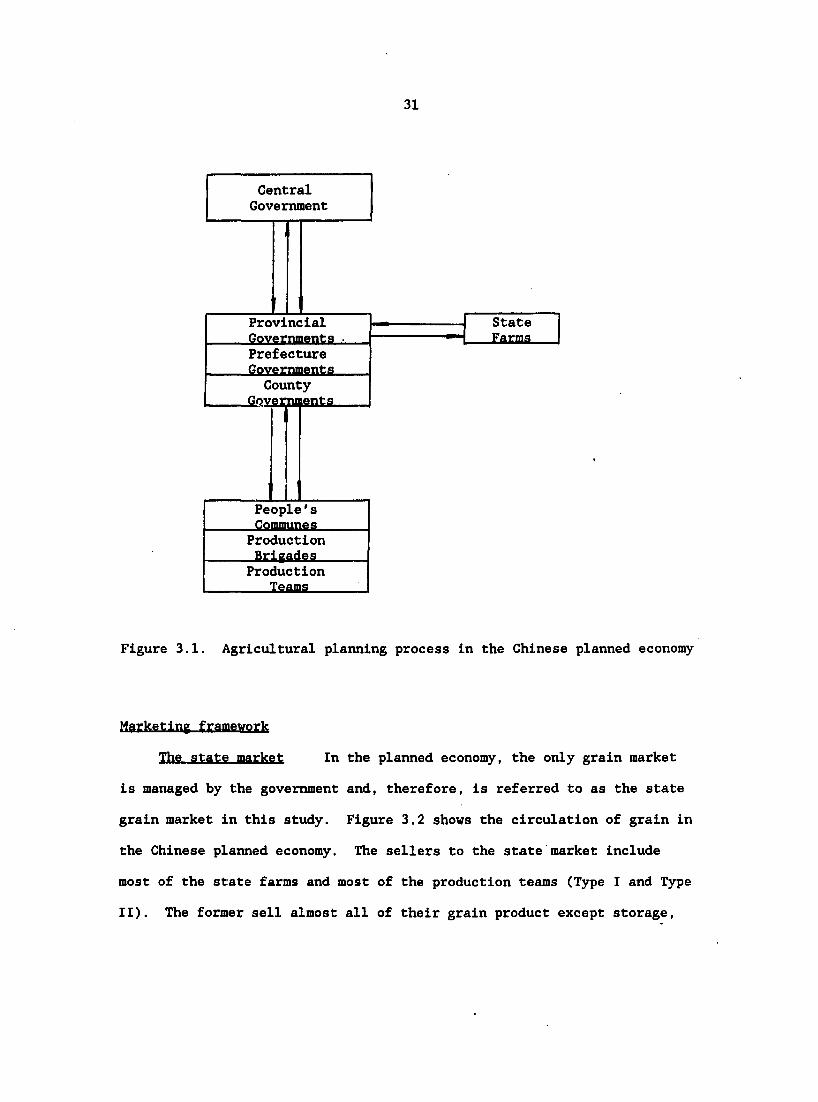
Figure 3.1 briefly describes the agricultural planning process

Just introduced. The arrows in the figure indicate the delivery of the

plans either between the governments at different levels or between the

governments and the enterprises.

31

State Farms

Central Government

People's Communes Production Brigades Production

Xsams

Provincial Governments • Prefecture Governments County

Governments

Figure 3.1. Agricultural planning process in the Chinese planned economy

Marketing framework

The state market In the planned economy, the only grain market

is managed by the government and, therefore, is referred to as the state

grain market in this study. Figure 3.2 shows the circulation of grain in

the Chinese planned economy. The sellers to the state market include

most of the state farms and most of the production teams (Type I and Type

II). The former sell almost all of their grain product except storage,

32

Urban Households

Military Industry

International Grain Market

Direct Plan Control

State Grain Market

Indirect Plan

Control

Production Tegms Type I

Production Teams pe II

\ \ \

Team Households

Team \ Households

Produ Te

Type

ctlon ams III

Team Households

State Stock State Stock State Stock

Farms

State Farm Households

Team Market

Figure 3.2. Circulation of grain in the Chinese planned economy

including seed and feed for next year's production, and the latter

usually sell part of their grain product and keep the remaining part for

their next year's production and internal distribution.

The buyers from the state market consist of all urban households,

all households in the state farms, the military, some industries, and

part of the production teams. The production teams, as the figure shows,

Include Type II and Type III production teams. They are classified by

their activities in the state market. The Type III production teams are

complete buyers or zero sellers for the state market. The Type II

production teams are partial buyers or partial sellers because they also

33

are involved in the partial selling (buying) activities. Last, the

remaining Type I production teams are zero buyers or complete sellers in

the state market.

International trade and the state stock are both used by the

government to adjust and maintain the balance of the demand and supply

for grain in the state market. The functions of the international grain

market will be discussed in more detail later in this chapter. The

functions of the state stock can be summarized: 1) to ensure the needs

between harvests, 2) to protect people against natural disasters and/or

plan mistakes, 3) to have flexibility for fluctuation in the interna­

tional market to avoid unnecessary loss, 4) to overcome time lag diffi­

culties caused by both domestic and International transportation, and 5)

to provide for emergency needs due to some abnormal situations, such as

war or embargo.

For those economic and/or political reasons, by affording high

storage costs, the Chinese government has accumulated a surprisingly

large grain stock. It is estimated that the grain stock in China was at

least 50% to 70% of the annual grain consumption. To simplify our

theoretical model, we assume that the grain stock demand (or supply)

equals zero, and will leave it to be handled in Chapter V.

Team-own market and team market Obviously, a study of the state

market excludes the distribution activities within the production teams.

For convenience, let us call an assumed market in which this distribution

happens the team-own market.

According to the roles set by the government, the team-own market of

34

grain does not open to anybody else except for their own household

members. In this so-called team-own market, the only seller is the team

itself, and the buyers are its own households. The distributions are

generally made according to the work, ages, and sexes of the members

within the households and at the state market prices (or less).

In addition, another assumed market in which all grain distribution

activities in all of team-own markets are added together is called the

team market. The sellers in this market are teams, and the buyers, of

course, are still agricultural households.

Finally, we have a newly assumed combined market, which combines

both the state market and the team market. Thus, in this discussion,

demand and supply usually mean the demand and supply in this combined

market, unless we mark out a specific market.

The dashed line in Figure 3.2 divides the circulation of grain in

the Chinese planned economy into two parts. The right and upper part is

the circulation of grain occurring in the state market and under direct

control of the government plan. The left and lower part is the circula­

tion of grain occurring within the team market and under indirect or

semidirect control of the plan.

In general, the circulation of grain in the state market was a

smaller portion of the total output in the planned economy and the

circulation of grain in the team market occupied a larger portion. For

instance, in 1975, the government purchased 21.4% of the total grain

output and the production teams distributed 78.6% of the total grain

output. In the same year, the urban population comprised 15.7% of the

35

total population whereas the rural population accounted for 84.3%. To a

certain extent, these facts provide a rough proof that the agricultural

households in the Chinese planned grain economy still possessed self-

sufficiency.

Theory of Urban Grain Demand

in the Planned Economy

Because the Chinese government had applied different measures to

distinguish and treat the basic food grain needs for urban and rural

people, it is essential to explore and derive both urban and rural demand

theories for the planned economy separately. To start with, this section

of the chapter focuses on the behavior of urban households in such an

economy.

For convenience, the general assumptions used in demand analysis are

followed through this study. More specifically, there exist utility

functions for households. These utility functions have the usual proper­

ties, in other words, completeness, reflexivity, transitivity, con­

tinuity, nonsatiation, and strict convexity. Finally, the objective of

the urban household is supposed to be to maximize its utility subject to

given constraints.

The discussion of urban grain demand in the planned economy is

divided into the following three parts: policy environment, urban house­

hold model, and aggregate grain demand of urban households. The policy

The data used here are from the State Statistical Bureau, P.R.C., 1987.

36

environment existing for urban households is introduced to make further

theoretical analysis. Immediately after that, the individual urban

household grain demands are derived from utility maximization and

distinguished by different types of households' situations relative to

the rationing system. The aggregate urban grain demand is finally

formulated on the basis of the discussion of these different situations.

Policy environment

Ownership of assets In the Chinese planned economy, almost all

schools, stores, and other enterprises are owned by either the public or

by cooperatives.

Labor Urban labor is hired by the government, public, or coop­

erative enterprises. The government agents set the wage rates for the

working people according to their education, working experience, and

positions. The people usually work a fixed eight hours every day except

Sunday and the public holidays. Labor cannot be mobile between different

enterprises without permission and, in general, neither can they be fired

by their employers.

Plan control To guarantee basic living needs of the urban house­

holds, the government issues ration coupons for food grain as well as

other necessary goods such as vegetable oil, cotton, cloth, meat, and

whatever else the government thinks necessary. The grain coupons are

distributed to members of urban households according to their ages and

occupations. In this way, the government can easily make a plan to

supply comparatively sufficient food grain based on the amount of ration

37

coupons Issued.

Market control Urban households can buy food grain only from

state-owned grain retail stations with both money and the ration coupons

in the amount indicated. Without coupons, people cannot use only money

to buy any food grain; and, in theory, coupons cannot be bought, sold, or

exchanged legally in the market or in private. The government also sets

fixed retail prices for food grain in the state market, although it may

adjust retail prices for some various reasons.

Urban household model

To some extent, any study is considered the continuation and the

development of all previous relevant studies. Our study, of course,

cannot be an exception. Noting that Howard (1977) has written a very

fine article titled "Rationing, Quantity Constraint, and Consumption

Theory," we are going to follow his approach in this part until the

general urban hqusehold demand functions are derived. Working in his

model we will, under the general circumstances in the planned economy,

expand his derivation from a single ration binding to multiple ration

binding and, therefore, deduce more general demand functions for both the

rationed and the unrationed goods.

Under the environment mentioned early in this section, the urban

household in the Chinese planned economy faces a budget line formed by

wage income and expenditure on all goods, given state prices and some

ration constraints for some of the specific goods including food grain.

Suppose an urban household has a utility function

38

u (X ...Xg,

where X ...Xg and X ...X are rationed goods but Xj ...X are not.

Assuming that the rations for commodities X ...X are and

the prices for commodities X .. .X , Xj ...X are , **1 ' ' ' *'n '

respectively, and that a given household's wage Income is M because of

fixed working hours set by the government, we express the Lagranglan

function as: n

L - U(Xj . ..Xg, . -Xjç, Xj . . .X ) + Aj (M - Z P X )

+ S A„.(R. - X.) (3.1) 1-1

The Kuhn-Tucker conditions will be:

aXi" fxj ~ 1 • " 21 ° k (3.2)

fxi" 3X ~ • l i ° n (3.3)

Agi) - 0 1-1 k (3.4)

• 0 1 - 1 n ( 3 . 5 )

1-1, ..., n (3.6)

- M - SP.X, a: 0 1 - 1, .... n (3.7) C7 X 3>

A - A (M - ZP X ) & 0 1 - 1, .... n (3.8)

A > 0 (3.9)

- R, . X. & 0 1 - 1, ..., k (3.10) 2i

1 2L. dx^ i aXj 1 1

1 a L _ dX^ i aXj." i i)

1 & 0

39

21 - Xi' - 0 "

& 0 i - 1 k (3.12)

To simplify the Kuhn-Tucker conditions, it is better to make some

further assumptions :

1) Suppose that the household buys each kind of good, in other

words, instead of (3.6):

> 0 i - 1 n (3.13)

then (3.2) and (3.3) can be replaced by

- V i - h i - " 1 - 1 " ( 3 1 4 )

- V i - " 1 - 1 -

After that, both (3.4) and (3.5) can be dropped out because they are

automatically satisfied.

2) Suppose that

M - SPX - 0 i - 1 n (3.16) i

or the urban household spends all of its income in today's market.

Combining (3.16) with (3.9), (3.8) can be automatically ignored.

3) Suppose that some ration constraints in (3.10), say from h to

k*" , are not strictly binding for this household,

> 0 i - h k (3.17)

immediately according to (3.11), this means that

- 0 i - h, .... k (3.18)

Undoubtedly, (3.17) and (3.18) can both be used for parts of (3.10)

40

and (3.12), respectively.

4) On the other hand, suppose that the remaining ration constraints

are Just binding, or

- 0 i - 1 g (3.19)

from (3.11), this Implies that

Agi a 0 i - 1 g (3.20)

substituting (3.18) and (3.20) into (3.14) separately, and noting that

(3.15) represents (3.14) if (3.18) holds, we obtain (3.21) and (3.22).

- 1?! 21 - 0 i - 1, ..., g (3.21)

~ Vi ° 1 - h n (3.22)

Thus, the simplified Kuhn-Tucker conditions consist of (3.21),

(3.22), (3.16), (3.19), (3.13), (3.9), (3.20), and (3.18).

Assuming that the second-order conditions are satisfied, we can

solve the first-order conditions for the above simplified constrained

utility maximization, given a rationing system. Let R - (R R ),

and P - (P , ..., P ), the household demand functions for (i - 1

n) would be either

\ " i ( 1 Rg, M)

- f (R, P, M) i - h n (3.23)

2: Rj i - h k (3.24)

or

X - R i - 1 g (3.25)

We have extended Howard's results into functional forms in which

multiple rations are binding. From now on we are going to develop our

41

own way by using these results.

Especially for a particular rationed good i (i - 1, ...,g), the

demand function of a specific household may be either

~ f£ « • • •, _ 2 * i+l ' ' " • ' Rg > ' • • • ' I

- f (R', P, M) S (3.26)

or

(3.27)

where R' - (R , ..., R R ^ R ) and P was given before.

These results mean that the household may have either one of the

above two types of demand functions for a particular rationing good. Its

choice may (3.26) or may not (3.25) be directly affected by the ration.

Conversely, a specific ration may or may not affect a household decision

or demand function. In the former case, the household's demand would be

the ration itself; whereas in the latter case, the household's demand

would be a function of prices, income, and all other effective (binding)

rations until it reaches the ration level. Please note the difference

between the ration effect and the rationing system effect. It is true

that a ration effect will lead to a rationing system effect, but it is

not true that a rationing system leads to a specific ration effect. In

fact, the rationing system has an effect on a household demand function

if and only if there is at least one ration that is binding.

Obviously, there are two possible types of urban households if they

face a rationed good, say food grain Xj. For the first type of house­

hold, the demand is not affected by the food grain ration but is by some

other rations:

42

Xj - (R", P, M) 3 Rj (3.28)

where R" is R', but excluding R ; and P is the same as before.

For the second type of household, the demand is only affected by the

official ration on food grain; therefore, it equals the ration,

Xj - RJ (3.29)

The formulas (3.27) and (3.28) imply the planned food grain demand

of an urban household in the planned economy. Because the demand for

food, grain is not more than or equal to the official ration level for

both the first and the second type of household, the task of a central

planner is to make available the ration level of food grain to satisfy

the restricted need of either the first or the second type of household.

Thus, the planned demand for food grain is just the ration level Rj to

any urban household in the planned grain economy.

Comparative statics The comparative statics are made for two

types of urban household.

1. The first type of urban household

The food grain demand function for the first type of household is

Xj - f (R", P, M) 3 RJ

The comparative statics can be obtained as the following:

ax < 0 (i/j) for substitutes within the effective rationed goods

aRj > 0 (i/j) for complements within the effective rationed goods

ax. " 0 for ineffective rationed goods

aRj

ax, < 0

aPj > 0

43

ax, < 0 for Ineffective rationed goods

> 0 for normal Ineffective rationed goods

dM < 0 for.inferior ineffective rationed goods

A brief interpretation of the results is that, for the first type of

household, the grain demand decreases when grain price Increases, it

increases when household's income increases assuming grain as a normal

good, and it does not change if the grain ration Increases.

2. The second type of urban household

The food grain demand function for the second type of household is

The comparative statics are shown as the following:

- 0 (i/j)

ax, ax .Pj - aP, - »

ax - 0

dM

It Is easy to conclude that, for the second type of household, the

grain demand is only influenced by the official ration level but not by

other factors at all.

Graphic analysis The graphic analyses also are made for two

44

types of urban household.

1. The first type of urban household

As Figure 3.3a shows, and Xg are commodities. Xg is a rationed

good--say food grain--but Xj is not. R is the official ration of Xg. AB

is a budget line for an urban household with rationing, and AC is a bud­

get line for that household without rationing.

X. 1

A

C X X, 2 2 R R

(a) (b)

Figure 3,3. The derivation of urban grain demand of the first type of urban household in the planned economy

For the first type of urban household, its indifference curve is

tangent on the budget line AB, either at point D, which is between A and

B, or at point B. Because the ration is not binding, the household need

not constrain its grain consumption at all.

By assuming the normal negative sign for the price effect on the

grain demand function of the first type of household, its demand curve Is

kinked as shown in Figure 3.3b. As usual, the demand curve is sloping

downward and becomes vertical after it meets the ration line R. That is,

under the rationing system, the food grain consumption of the first type

45

of urban household increases as the state market price goes down until

the ration becomes effective.

2. The second type of urban household

Facing the same state market price and official ration R, the second

type of urban household makes a different choice. Its indifference

curve, as Figure 3.4a indicates, would be tangent to the budget line on

AC but beyond B. The ration in this case is effective, so the household

is forced to reduce its grain consumption to the ration level R. This

means a lower indifference curve that would pass through the ration line

at B.

X. 1

A

C X R 2

(a) (b)

Figure 3.4. The derivation of urban grain demand of the second type of urban household in the planned economy

The corresponding demand curve for food grain of the second type of

— S urban household is a vertical line R in (Pg, Xg) space (see Figure 3.4b).

Under the rationing system, the food grain consumption of the second type

46

of urban household is Just the official ration level and is not affected

by any change in the state market price for food grain.

Aggregate grain demand of urban households

According to economic theory, the aggregate urban food grain demand

is the sum of all individual urban households' food grain demands:

UP D - S X, (3.30)

j-1 J

UP where D - aggregated urban food grain demand in the planned economy and

Xj - individual urban food grain demand.

Considering that there are two types of urban households, the

aggregate urban food grain demand is the sum of aggregate urban food

grain demands for both the first type and the second type of urban

households, or

(3.31)

UPI where D - aggregated urban food grain demand for the first type

of urban households in the planned economy

pUPII _ aggregated urban food grain demand for the second type

of urban households in the planned economy.

For the first type of urban households, whose ration coupons are not

used up, we assume that there are n households in this group and all of

them are identical, even facing the same ration restriction, R.. The

UPI aggregate food grain demand, D , would be

J-1 ^

47

ITP " - (R", P, M) 3 n Rj (3.32)

For the second type of urban households, whose ration coupons are

just used up, we assume that there are ng Identical households in this

group, and they face the same ration Rj. Then, their aggregate food

grain demand would be

j,UPII _ J2 UP

J-1 J

- ngRj (3.33)

UP Using the above results, D , the aggregate food grain demand in the

urban area in the planned economy would be

UP "" — — - n Xj (R", P, M) + ngRj 3 (n + n ) R (3.34)

Suppose the total number of urban households in China is n so that

Ry - + ng (3.35)

The total number of urban households is the sum of the numbers of

the first and the second types of urban households. In addition let

îr - fui (3 3*) u

where is the relative frequency of the first type of urban house­

holds. Substituting (3.32) and (3.33) into (3.31) gives

UP — — D - n Xj (R", E, M) + (n - n )Rj

48

- «"• ••• M) + <1 - fui) njj S "Kj

UP — — —" - D"'' (P J, n , Rj, R", P, M) :S nRj (3.37)

Thus, the aggregate urban food grain demand in the planned economy

is theoretically specified as a function of the relative frequency of the

first type of urban households, the total number of urban households, the

official ration level for grain, the ration levels for other rationed

goods, the state market price of food grain and other commodity prices,

and the Individual household's income. Furthermore, suppose both the

first and the second type of household are the same in size and income.

Then, the change in the total number of urban households is consistent

with the change in the total population, and the change in the individual

household's income is agreeable to the change in any representative

household's Income, regardless of whether the ration is binding, or in

total households' income, regardless of the method for aggregation.

UP In analyzing formula (3.36) we notice that D consists of two

UPI UPII components, D and D . This conclusion is different from past

studies. Checking the structure of both components, we find that they

contain some different factors as well as some similar factors. This

fact implies that each component sometimes plays its own role to affect

UP the total urban grain demand, D , because of the difference in the

existing factors. On the other hand, both components sometimes play

UP their roles together to affect the D because of the similarity in the

existing factors.

49

Second, formula (3.37) indicates that the total urban grain demand

is no more than the product of n and Rj, or the planned aggregate urban

grain demand. In order to estimate the urban grain demand roughly, the

central planners need to find out the total number of urban households

and to decide the official ration level for grain. Then they can obtain

the result by performing simple multiplication.

Last, it is useful for the government to consider relaxing the

ration restriction or even the ration system. By the Le Chatelier

principle and observing formula (3.37), we know that the individual urban

grain demand of the second type of urban household cannot be reduced by

relaxing the ration constraint. In other words, the individual urban

grain demand of the second type of urban household without ration

constraint cannot be less than that with the ration constraint. Thus,

the total urban grain demand of the second type of household cannot be

reduced if the government decides to cancel the usage of ration coupons

for grain. On the other hand, if the government relaxes other ration

constraints except for grain, by the same principle and similar in­

ference, we can conclude that the total urban grain demand cannot be

UPI reduced because the Xj and D cannot be reduced. Suppose the govern­

ment relaxes all rationing systems; by the same principle, the total

UP urban grain demand cannot be reduced because both components in D

cannot be reduced. If this is true, the total urban grain demand would

be the same as the total urban grain demand in the market economy despite

the planned state price policy.

Comparative statics By using (3.37), the results of the

50

comparative statics can be calculated

âj£!i ^ ''ui afui

-

- n (X, - Rj) s 0

The total urban grain demand decreases or remains unchanged If the

relative frequency of the first type of urban household Increases.

- 'ul-'j + (I • ""ul) > »

The total urban grain demand Increases as the urban population Increases.

- ao""'

3Rj aSj

- - fui» "u > °

The total urban grain demand Increases If the government Increases

the official ration level. Please note that the ration effect on the

urban grain demand becomes operative because of only one component,

UP • UP within D , rather than all D . In other words, the change In the

offleal ration level affects only part of the urban households (the

second type) but not all. In this sense, we name this kind of ration

effect as the partial ration effect to emphasize the new discovery of the

partial role of the official ration level In the planned grain economy.

51

arff _ açffi

aPj aPj

The total urban grain demand is partly influenced by Pj, the state

price of food grain. If the sign of aXi/9Pj is negative, as the state

price goes up, the total urban grain demand of the first type of urban

households goes down; therefore, the total urban grain demand goes down.

Thus, the slope of the urban grain demand curve is determined by

Wj-

This situation means a partial state price effect in the planned

urban grain economy or the change in the government price policy for food

grain can directly influence grain consumption of only part of the urban

households (the first type). Differing from all previous studies, this

is a new theoretical finding for the planned economies.

aPi ap,

< 0 (1 / j)

• ul"u >0 (1 / j)

Total urban grain demand decreases or Increases if the relative

prices of goods increase. Note that this also is the partial price

effect.

an ' aM

52

dX

" ul"u 3M °

The total urban grain demand Increases when household Income In­

creases, provided that the food grain Is a normal good for the house­

hold. This means that the government income policy for households has

also a partial (income) effect on the grain consumption of a part of the

households (the first type).

Graphic analysis The graphic analyses are made for aggregate

urban grain demands.

Formula (3.32) gives the aggregate urban grain demand of the first

UPI UPI type of urban household, D . Figure 3.5a shows that the D is a

kinked line that consists of two segments, a downward sloping line and a

— c c vertical line passing through - P jn Rj on the Q axis in the (P ,

g Q ) space.

pS oUPI

<UI

.UPII

<UII <u

(a) (b) (c)

Figure 3.5. The aggregation of the urban grain demands in the planned economy

53

From formula (3.33), we obtain the total urban grain demand of the

second type of urban household, As Figure 3.5b Indicates, the

UPII — s D Is a vertical line that crosses Q jj - (1 - o" the Q axis

S s in the (P , Q ) space.

Finally, formula (3.34) indicates that the total urban grain demand,

UP D , is the sum of the total urban grain demand of both the first and the

second type of urban household. Figure 3.5c shows that the shape of the

UP UPI D is similar to that of D , except that (1) the aggregate constant is

S s s now - n Rj on the Q axis in the (P , Q ) space, and (2) the aggregate

UP UPI downward sloping segment in D is steeper than that in D because of

the effect of In addition, by the Le Chatelier principle, we know

UP that the slope in D is much steeper than that in an assumed market

economy because of the rationing system. That is why the elasticity of

the urban grain demand in the planned economy may be very small but is

still greater than zero.

Theory of Rural Grain Demand and Supply

of State Farms and Agricultural Production Teams

in the Planned Economy

As mentioned at the beginning of this chapter, two kinds of basic

rural enterprises existed in the Chinese planned economy: state farms

and agricultural production teams. The behaviors of the state farm and

the production team were different from each other because of different

ownerships of their properties and different policy environments faced by

them. Thus, this section contains two subsections: one is studying the

54

behavior of the state farm in the planned grain economy; the other one is

studying the behavior of the agricultural production team in the planned

economy. Each subsection is divided into three parts: the policy envi­

ronment, the state farm model or the agricultural production team model,

and aggregate grain demand and supply of all state farms or all produc­

tion teams. To begin with, the policy environment presents basic back­

ground materials for state farms or production teams. Assuming the state

farm's physical output maximization or the production team's utility

maximization, we build a state farm model or an agricultural production

team model to derive an individual farm's or team's grain demand and

supply. After that, the aggregate grain demand and supply of the state

farms and the agricultural production teams are formulated from derived

individual farm's or team's demands and supplies in each subsection,

respectively. Finally, the state market analysis is added for exploring

and stressing the roles of the government in the rural state market.

We now start with the first subsection: the theory of grain demand

and supply of state farms in the planned economy.

Policy environment of state farms

The state farm sector consists of a small but significant portion of

Chinese agriculture. According to statistics for 1978, state farms

occupied about 4.5% of the total arable land in mainland China and

produced about 2% of the grain output, which was about 10% of the total

grain commodities purchased by the government.

55

State-owned enterprises As state-owned enterprises, state farms

were completely run under the government's plans. State farms delivered

their agricultural products to the government, and the government

distributed equipment and inputs to the state farms. In case profit was

generated, the state farms turned it over to the government, and the

government gave the state farm financial assistance in case of a loss.

Labor All laborers employed by state farms were paid a fixed

wage, and they were not transferable between farms without permission.

Consumption of food grain Laborers earned wage income and were

free to use it to buy any commodities under the plan control. In the

grain market, they were treated the same as the urban household by the

government.

State farm model

As discussed before, under the government's plan, the state farm

manager made decisions including the labor supply for grain production,

and the individual households within the farm determined their own food

grain consumption. Thus, the state farm model in the planned economy can

be subdivided to deal with consumption and production separately.

Food grain demand of state farm household As individual con­

sumers facing fixed wage income and ration coupons for food grain

consumption, state farm households did not differ from urban households

in the state market. The urban household grain demand functions (3.28)

and (3.29) can be used for the state farm household. Thus, we have

Xjg - Xj(R', P, M) (3.38)

56

or

(3.39)

For the same reasons, the formulas (3.36) and (3.37) represent the

state farm households' different attitudes toward the ration coupons for

food grain In the state market. The comparative statics and graphic

analyses also are the same as before and, therefore, are omitted here.

operation of the state farms was generally not profitable. Most of the

state farms were established for pioneer settlement or land development

In the border areas. There were several targets given by the state

government to the farms. Among these targets, the gross output target

might be the most Important one for a state farm, whereas other targets

might be met or neglected by the farm's manager. Assume that the state

farm's objective had been to maximize Its gross output, subject to the

government's plan. Furthermore, assume that the production functions are

all concave, homogeneous In a particular Input or output, and twice

continuously dlfferentlable. The Lagranglan function Is then

Food grain supply of state farm Before the economic reform, the

n n n

- ,f,Qi(*i

n (3.40)

where - the 1 output produced by the state farm

- the h Input used by the state farm

- the ration on the h Input to the state farm

57

- the h input used for the i output

Qj - the i output target set by the government

n X, - S X. . & 0 is an input allocation constraint imposed by the

i-1

government's plans. That is, the state farm can receive only X amount

of the h input from the government. On the other hand, Qi - Qi & 0

an output target set by the government That means the state farm has

provide no less than amount of the • th i output.

The Kuhn-Tucker conditions would be:

SL—. at. . aXhj aq "2i

f2l_ 3 i

g 0 h - 1, i - 1,

, k , n

(3.41)

h - 1, i - 1,

, k . n

(3.42)

i - 1, . n (3.43)

i - 1, , n (3.44)

It;; - 9i - Si = 0 i - 1, ., n (3.45)

i - 1, , n (3.46)

Xhi a 0 h - 1, ... i - 1, ...

, k , n

(3.47)

Qi & 0 i-1, ... , n (3.48)

li 2i - ° i - 1, ... , n (3.49)

Suppose that Xj , and Agi > 0 (h - 1, ..., k; i - 1. . • • » ^ ) »

then immediately we find out that (3.41) and (3 .45) become

58

ax " " 2i 33 " ° i - li .. . ! n <3.50)

and

- Qi - Qi - 0 i - 1 n (3.51)

Furthermore, if

- 0 i — 1, ..., n (3.52)

then we have

n S

'11 " n-1 - Z & 0 1 - 1 n ( 3 . 5 3 )

In other words, the constants (3.53) are not strictly binding or If

A > 0 1-1 n (3.54)

then

ai - k - X . - S X . . - 0 1 - 1 n ( 3 . 5 5 )

a hl n-1

In other words, the constraints (3.53) are Just binding.

In fact, the constraints (3.43) are generally binding because the

state farm accepted planned allocations from the government, and the

constraints (3.45) must be fulfilled because the output targets presented

the management level for the managers of the farms and are relevant to

their future official positions.

Note that If A ^ - -0(1-1, . .., n) (3.41) becomes

l-li.'.'iin (3 56)

59

That Is, there Is no freedom for the state farm to choose the Inputs

and, therefore, outputs because every target is strictly given by the

control plan. If this is true, solve the first-order conditions.

Provided the second-order conditions are satisfied, we o'lltain the input

demand ' s, which would be functions of and ; in other words, if

both and are just binding then

j i - \) h - 1 k; i - 1 n (3.57)

On the other hand, if - 0 but > 0, the input demand X 's

would be the functions of X itself :

\i " i V h - 1 k; i - 1 n (3.58)

Thus, the corresponding grain supply functions by the state farm

would be either

< «!• V \ VJ

- Qj (Q, i - 1 n; h - 1 k (3.59)

or

- i - 1, .. ., n; h - 1, . . . , k (3.60)

For the state farms, the grain supply functions are functions either

of both the input allocation quotas and the output targets or of only the

input quotas.

60

Comparative statics The comparative statics are shown only for

the two different grain supplies by the state farms here.

1. - Q (Q, Xj )

30. —^ >0 i - 1, ..., n; aq

dQ, — > 0 i - 1 , . . . , n ; h - 1 k

The state farm will probably increase its i grain output if the

government either improves its plan allocation for the h input or

raises its plan target for i grain output to the farm.

2. Q^-Qi(V

ao, _ > 0

The state farm will probably increase its i grain output to

respond to an increase in the h input supply from the government.

These results imply that the grain supply by the state farm, in both

cases, does not change in response to either input or output prices, but

to the relevant plans.

Graphic analysis For both supply functions, the supply curves

are vertical lines in (P®, Q®) space (Figure 3.6a or b). Figure 3.6a

displays a situation in which the output target is binding; Figure 3.6b

displays another situation in which the output target is not binding.

61

Qi < Qi <

(a) (b)

Figure 3.6. The grain supplies of state farms in the planned economy

Aggregate grain demand of state farm households and supply of state farms

The food grain demand and supply by state farms has been derived.

It is time now to derive the aggregate grain demand and supply for state

farms. We first aggregate the grain demand of all state farmers, and

then aggregate the grain supply:

Aggregate grain demand of state farm households Because grain

demands of households in the state farms are the same as those for urban

consumers, it is easy to conclude that the aggregate grain demand of

state farm households is the same as that of urban consumers. Thus, the

aggregate grain demand for. state farm households is;

(3.61)

- f p n pR, + (1 - fue?) n„ , (R', P, M) 'HF*j HFl) "HF*j

- n p, Rj, R', P, M)

where

(3.62)

62

FI FII D , D - aggregate grain demand for the first type or the second

type of households in state farms

HFI " f®l*tlve frequency of first type households in state farms

n p - total number of households in scate farms

Rj - ration of food grain for households in state farms

R' - rations of other commodities except food grain for

households in state farms

P - state prices of all commodities

M - wage income for households in state farms

Aggregate grain supply of state farm households From the

analysis for individual state farms, state farms have food grain supplies

for either

qf - Ql(5, 5%)

or

Q[ - Q (X')

Assuming that all state farms of the same type are identical, that

there are np state farms total, and that the relative frequency of the

first type of state farms is the aggregate grain supply for state

farms is

(3.63)

FFI F i + (1 " FFI )

- S(Pppi. np, Q, X') (3.64)

63

F where S - aggregate grain supply for state farms

FI FII s , s - aggregate grain supply for the first or the second type

state farms

n_ - total number of state farms r

Q - output target set by the government

- input ration that is binding for the first type of state

farm

X' - input rations that are binding for the second type of state

farm

Comparative statics We are conducting comparative statics for

only the aggregate grain supply of the state farms and dropping out com­

parative statics for the aggregate grain demand of the state farm house­

holds because of similarity between the individual grain demands for the

state farm households and urban households. Therefore, the aggregate

grain demand for the state farm households is similar to those for the

urban households. The following are comparative statics for the aggre­

gate grain supply for state farms.

By formulas (3.63) and (3.64)

- sFi + sFi:

• FFI"F< (Q'

aZI. „ qF afpF

"pOi > 0

- 'ppX > »

64

- 'fFI-V < 0 as

That is, the aggregate grain supply by the first type of state farm

increases if the relative frequency of the first type of state farm

within all state farms, or the total number of state farms, or the output

target set for the state farms increases. On the other hand, the

aggregate grain supply by the first type of state farm may increase or

decrease if the input ration increases.

s"' - (1 - fppi) -F Qi (X')

dx' ^ ax' ^ Thus, we finally have

âsL_ _ asfi asFii

^ FFI ^ FFI ^ FFI

- Hp Q[(Q. \) - tip Q[(X') < 0

65

^"FF *"FF ^"FF

aq aq

That Is, the aggregate grain supply by the state farms Is increasing

if the relative frequency of the first type of state farms decreases, or

the total number of state farms or the output target set for the state

farms Increases. If the government raises an input ration, the result in

the aggregate grain supply by the state farms is still unclear.

Note that the output target effect on the aggregate grain supply is

partially through the aggregate grain supply by the first type of state

farms but not the second type. This is a partial output target effect.

In addition, the state grain market price has no effect on the aggregate

grain supply by the state farms.

Graphic analysis The graphic analysis is subdivided into two

1. Aggregate grain demand by state farm households

The shape of aggregate grain demand of the state farm households is

the same (kinked) as that of urban households, but the intercept on the q

parts :

axis has been changed (Figure 3.7).

66

FH P

Q "F*j

Figure 3.7. The aggregate grain demand of state farm households in the planned economy

2. Aggregate grain supply by state farms

The aggregate grain supply by state farms is the sum of the aggre­

gate grain supply by both the first and the second type of state farms.

The former is drawn in Figure 3.8a, the latter is drawn in Figure 3.8b,

and their sum--the aggregate grain supply by state farms--is given in

Figure 3.8c. As Figure 3.8 shows, all of the three curves are vertical

lines in the (Q, P) space and have respective intercepts:

FI " FFl"F i' Qpil " " FFI "F i' F " FI FII"

We have finished discussion of the first subsection. We now move on

to the second subsection: theory of grain demand and supply of agricul­

tural production teams in the planned economy.

Policy environment of agricultural production teams

Collective of agricultural households As a basic unit of

production and distribution in rural areas, a production team made its

own decisions to buy agricultural inputs from the state for use, to

67

<FI

(a)

FII

(b) (c)

Figure 3.8. The aggregation of grain supplies of the state farms in the planned economy

produce agricultural commodities by allocating its resources, to pay the

agricultural taxes to the government, to sell products to the state

market, and, finally, to distribute part of its products and income to

its household members and to keep the necessary stock for its further

reproduction. Thus, given the plan and the market control, the house­

holds' incomes and food grain consumption were mainly determined by their

production teams.

Labor The agricultural laborers were hired by the production

team. Without approval from higher authority, the laborers could not be

mobile even between teams. Usually, production teams set the minimum

working days for laborers according to their ages, sex, and physical

conditions.

The laborers were paid annually by accounting their accumulated

working points, which were determined on the basis of their working

assignments and times, working attitudes and experiences, ages, and sex,

etc. The accumulated working points were used to finance the grain

68

apportionment plus remaining cash income.

Plan control Most of the economic activities of the production

teams were restricted or guided by the government's plans directly or

indirectly. On the production side, the government set some minimum

area quotas for the main crops and rationed purchases of some inputs in

short supply such as chemicals, fertilizer, diesel fuel. On the consump­

tion side, the government set minimum delivery quotas or sales quotas for

the main grain commodities as well as others produced by the team, and a

floor quota as well as a ceiling quota for food grain distribution within

the production team. Finally, the government set stock quotas for the

production teams. All quotas Just mentioned would be determined by local

authorities and varied from place to place and from year to year.

Market control The grain market for rural people was a state

monopolized system in the planned economy. The government reserved for

itself the exclusive right to purchase grain from the producation teams

by using a quota system. Moreover, the government decided the procure­

ment prices of grain in the state market and imposed agricultural taxes

that were normally fixed in grain upon the production teams.

The government procured grain mainly from the majority of production

teams that were totally self-sufficient; they were able to meet their

floor consumption quotas after satisfying the procurement quotas and were

not allowed to buy any food grain from the state market. Thus, those

production teams are called nonbuyers or complete sellers, and they are

classified into the first type in this study.

There was a channel through which rural households could buy food

69

grain from the government. Two additional types, the second and third

types of production teams, had the government's permission to do so.

The second type of production teams are called partial buyers or

partial sellers in the state market. They produced grain and fulfilled

the delivery quotas set by the government, but they could not meet the

floor consumption quotas for their household members because of either

predictable reasons such as normally poor production conditions or

unpredictable reasons such as some accidental disasters. Hence, they

were given the right to buy grain back from the government until their

floor quotas were met.

The third type of production teams are called complete buyers or

nonsellers in this study. According to the government's plan, they did

not produce food grain, but produced other agricultural commodities such

as cash crops, livestock, vegetables, fruits. The government set the

ceiling consumption quotas for those production teams, and they bought

all their food grain from the state market.

Agricultural production team model

For a production team, both production and consumption were managed

by the team leader and guided directly or indirectly by the government's

plans. Suppose the team's objective is to maximize its utility subject

to its budget constraint, as well as several other constraints given by

government's policies. Furthermore, suppose the team's utility function

U(X X ) and production function G(q , ..., q ) have the usual

70

properties mentioned earlier In this chapter as well as In general

mlcroeconomlc theory. To reflect the distribution activities happening

within the production teams, we developed Sicular's model (1983) by

adding two more constraints. In our model, the Lagranglan function for

the production team would be

n L - U(X^ X^) + S (PIAI -

i—1

i—1

+ //4i(*ic - i> + - 4) (3.65) 1—1 i—1

where X - the i commodity consumed by the production team

- the i commodity produced by the production team

- sales quota for the ith commodity

Xj - ceiling consumption quota set for the i commodity

Xj g - floor quota set for the i commodity

S (P q - P X ) & 0 is a budget constraint for the team. That is, i

the team's total income from its production cannot be less than its total

expenditure.

X - X & 0 or X - X p >: 0 is a constraint that represents a ceil­

ing consumption quota or a floor consumption quota set by the government,

in other words, the team's consumption of the i commodity cannot exceed

the ceiling limit or cannot be below the floor limit. Last, q - X -

& 0 is a fixed sales quota imposed by the government. That is, the

71

team's 1 output has to be not less than the sum of the team's consump­

tion and its sales quota.

The Kuhn-Tucker conditions for our model are now:

3X " 8) • ' *31 • *41 • *51 ® "

SL. _ A,P, - A, as - A,, s 0 "11 2 31

" 1 % - "

• '1*1) "

- «'"l "

§5; - s 0

* 3 i § ^ - °

It;; - *1. - *1 = ° *41 "

It;; - *1 - *1? = ° 5i âX ^ - 0

5i

i - 1,

i - 1,

i - 1,

i - 1,

i - 1

i - 1

i - 1

i - 1

i - 1

i - 1

i - 1

i - 1

, n (3.66)

, n (3.67)

n (3.68)

n (3.69)

(3.70)

n (3.71)

n (3.72)

n (3.73)

n (3.74)

n (3.75)

n (3.76)

n (3.77)

n (3.78)

Unlike a usual agricultural household model, our production team

model has three additional constraints: (3.73), (3.75), and (3.77).

72

Thus the results in our model, or the grain demand and supply by the pro­

duction team, would be influenced by the constraint(s) if at least one

constraint is binding or not influenced if no constraint is binding.

The situations for constraint binding can be easily explained. For

instance, if (3.75) or (3.77) is binding, the food grain demand of the

team is fixed at the ceiling level or the floor level. In addition, as

Sicular (1986) pointed out, if (3.73) is binding, that is, - S ,

given the sales quota the grain demand and the grain supply by the

team are dependent on each other, and separability of the model of the

agricultural production team is eliminated by this binding constraint.

Using the same procedures as in the urban demand section; making the

necessary assumptions, such as the positiveness of all demand and

supply q , equality of budget constraint; discussing the combined

situations for these additional constraints; then solving the first order

conditions simultaneously, we obtain the food grain demand function X

and the food grain supply q for three different cases:

Demand Function Supply Function Case 1

(3.77) is binding

1.1. (3.73) is binding

1.2. (3.73) is not binding

Case 2

V*iF (3 79) q -X p + (3.80)

qi-qi(P) (3.81)

both (3.77) and (3.73) are not binding

2.1. (3.75) is binding (3.82)

2.2. (3.75) is not binding Xj -Xj (P) (3.84) (3.83)

73

Case 3

(3.77) is not binding but (3.73) is binding

3.1. (3.75) is binding (3.85) (3.86)

3.2. (3.75) is not binding Xj -Xj (P,Sj )(3.87) qj -X (P,S )+S

-q (P,S ) (3.88)

These results indicate that, under certain circumstances, the grain

demand function by the production team is either fixed X p or X or

varied X (P). In other words, the grain demand Xj is either the floor

quota or the ceiling quota or a function of the consumer and the producer

prices. On the other hand, the grain supply function of the production

team is either fixed Xj p + or varied q (P) or q (P,Sj ). In other

words, the grain supply q is either the sum of the floor quota and the

sales quota for grain or a function of the consumer and producer prices

or of the prices and sales quotas. The corresponding relationship

between the grain demand and the grain supply can be easily checked.

Case 3.2 is an extremely restricted one. By the formula (3.88)

qi(P,Si) equals Xj (P,Sj ) plus a constant S . Thus, both the supply and

the demand curves must have the same positive or negative slopes with

respect to their own price change and must keep an equal horizontal

distance from each other in the (Q, P) space. Assuming nonpositlve-

ness of the slope of the demand curve and nonnegativeness of the slope of

the supply curve, we drop out further discussion about the case In this

study.

It Is obvious that Case 3.1 and all the remaining cases (Case 1 and

Case 2) can be included in the activities of the first type of production

74

teams, which is nonbuyer and complete seller in the state market. In

addition to this type, two more special types of production teams exist;

and therefore, our basic model (3.65) has to be adjusted to fit their

cases.

The second type of production team produced grain that was less than

the sum of the floor consumption quota and sales quota. Thus, instead of

(3.73) we have

qi - J i - Si < 0 i - 1, ..., n (3.89)

for this case in our model. Noting that (3.75) is not binding, solving

the new first order conditions we obtain

Case 4 Demand Function Supply Function

(3.77) is binding _ both (3.75) and (3.89) X.-X.„ (3.90) q.-q,(P) (3.91) are not binding

Another case applies to the third type of production teams, which do

not produce grain by permission, q - 0 then - 0, and their grain

consumption up to the ceiling quota is supplied by the government. In

this case, (3.75) is dropped out of our model. Because of a drain on

their strength and relatively lower ceiling quota as well as price level,

the production team would not buy grain below the ceiling level. Thus,

we have

Demand Function Supply Function Case 5

(3.75) is binding

and S - 0 *i"*ic (3 9%) q .-O (3.93)

(3.77) is not binding

75

In analyzing all of the above realistic demand functions of produc­

tion teams, note the roles played by the government's floor quotas and

ceiling quotas. Indeed, all possible demand functions are not less than

the floor quota and not more than the ceiling quota, that is,

XjF=SXj:èXjc (3.94)

In other words, the floor quota Xjp can be seen as the lower bound

of grain demand by production teams and the ceiling quota Xj can be seen

as the upper bound. The government can easily figure out both the

minimum and the maximum grain demand by any production team. Thus, the

government uses the floor quota and the ceiling quota as the policy

instruments to plan rural grain demand for production teams.

Turning to analyze the corresponding supply functions of production

teams, we find out the role played by the government sales quotas. All

supply functions are not less than the sales quota except for that of

the second and the third type of production teams, that is

Xjp + Sj qj (3.95)

In other words, the sum of the floor quota and the sales quota

Xjp + Sj is the lower bound of grain supply by the first type of produc­

tion teams, which is the majority within production teams. The govern­

ment can easily figure out the minimum grain supply by a usual production

team. Thus, the government uses the floor quota or sales quota as a

policy Instrument to guarantee planned grain supply.

Comparative statics The comparative statics are reported for all

three types of production teams as follows:

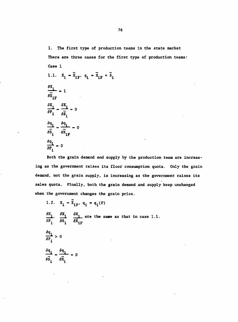
76

1. The first type of production teams in the state market

There are three cases for the first type of production teams:

Case 1

1.1. - X p +

ax. - 1

ax. iF

ax, ax

1

aq, aq. " — 0

Both the grain demand and supply by the production team are increas­

ing as the government raises its floor consumption quota. Only the grain

demand, not the grain supply, is increasing as the government raises its

sales quota. Finally, both the grain demand and supply keep unchanged

when the government changes the grain price.

1 . 2 . X j ^ - X ^ p , q j ^ - q ^ f P )

ax, ax, ax, , i are the same as that in case 1.1.

aPi aSj_ axip

aq.

aq, aq

as ax

77

The grain demand Increases, but the grain supply does not change, If

the government raises the floor consumption quota. On the other hand,

the grain demand does not change, but the grain supply Increases, If the

government raises Its grain price.

Case 2

2 .1 . qj^ - q^fP)

These functions are the same as those In Case 1.2 except the celling

quota X Is used here Instead of the floor quota X p. Thus, we omit

comparative statics for Case 2.1.

2.2. X - X (P), q - qj (P)

ax

ax ax

as *1

S;-aq. âq.

as ax

These are the same as the standard demand and supply functions in a

market economy except that the price here is the state market price.

Case 3

3.1,

These functions are the same as those in case 1.1 except that the

celling quota X here replaces the floor quota X . Thus, we omit

comparative statics for Case 3.1.

78

2. The second type of production teams in the state market

Case 4 - q fP)

ax

aXiF

ax, ax.

3i/ °

aq. aq.

ax p as

The grain demand Is fixed at the floor consumption quota and is

increasing as the floor quota increases. The grain supply is increasing

as the grain price Increases.

3. The third type of production team in the state market

Case 5 X - X , q - 0

ax.

^ ic

ax. ax.

ai,--- 0

aq. aq. aq

ail " aXiP " °

The grain demand is increasing if the ceiling consumption quota

increases. The grain supply is always zero.

Graphic analysis The graphic analysis is made in the combined

market with the state price for all three types of production teams.

79

1. The first type of production teams

Case 1

For Case 1.1, both the grain demand and supply curves are vertical

lines in (P, Q) space (Figure 3.9a). While the grain demand is passing

through on Q axis, the grain supply is passing through on

the Q axis. Thus, the horizontal distance between the two curves is

(a) (b)

Figure 3.9. The demand and the supply curves in Case 1

For Case 1.2, the demand curve is still vertical but the supply

curve is upward sloping, and the horizontal distance between the demand

and the supply is greater than because is not binding (Figure

3.9b).

Case 2

For Case 2.1, the demand curve is a vertical line and the supply

curve is upward sloping, and the horizontal distance between these two

curves is always greater than (Figure 3.10a).

80

X. V /

- - - .

"ic ' iF *ic

(a) (b)

Figure 3.10. The demand and the supply curves in Case 2

For Case 2.2, the demand slopes downward and the supply slopes

upward (Figure 3.10b), and the horizontal distance between the demand and

the supply curve is greater than because X has to be more than X p,

the floor consumption quota, and less than X , the ceiling consumption

quota. The demand curve becomes vertical at X - X p and X - X ^ .

Case 3

The graph for Case 3,1 is the same as that for case 1.1 (Figure

3.9a) except that the intercept X p is replaced by X .

2. The second type of production teams

Case 4

As Figure 3.11a shows, the grain demand X is a vertical line

passing through Xj p on axis, and the grain supply q is upward sloping

and on the left of a vertical line that passes through X p + on

axis. The supply curve q crosses the demand curve X . Given price P,

if q is on the right of X , the team is a net seller in the combined

market. On the other hand, if q is on the left of Xj , the team becomes

81

a net buyer In the combined market.

(a) (b)

Figure 3.11. The demand and supply curves In Case 4 and Case 5

3. The third type of production teams

As Figure 3.11b shows, the demand curve for Case 5 Is a vertical

line that passes through X ^ on the axis.

Aggregate grain demand and supply of production teams

Aggregate grain demand of production teams There are three types

of production teams, according to their activities in the state market,

or, alternatively, their situations relative to the ceiling quota or the

floor quota and the sales quota. Situations are complex for the first

type of production teams. Within the first type of teams, there are

three subtypes that may contain even two different cases. Start with the

first subtype of production teams. Assuming that the total number of all

production teams is n , the relative frequency of the first type and the

first subtype (within the first type) of production teams are and

82

are and P<j<2i< respectively. Furthermore, assuming that all teams of

Til the first subtype are identical, we can obtain D , the aggregate grain

demand by the first subtype of production teams, as follows:

D - TIl "T *iF

Til — - D (PTI' PTII' "T' V (3 96)

TI2 TI3 By using the same method, we can derive D and D , the aggre­

gate grain demand of the second and the third subtype of production

TI2 teams. The only difference for D is that it contains two components

rather than one to reflect Cases 2.1 and 2.2 within the subtype. Thus,

DTI2 _ dTI21 pTI22

" TI TI2 TI21 "T ic TI T12 ' TI21 "T *i ^

" TI TI2 [ TI21 "T *ic + TI21 "T

TI2 — • ( TI' TI2' TI21' "T- *ic' (3 97)

and

TI3 — D - Pçj,j (1 - - Pjj-2) "T *ic

TI3 — - D (Pjj, Pjjj , 12' "T' ic (3.98)

TI Adding (3.96), (3.97) and (3.98) together, we obtain D , aggregate

grain demand by the first type of production teams.

83

- "t *iF TI TI2 [ TI21 "t ic

+ (1 - "T + Ti " TIl " TI2 "t *ic

- P j ( TIl "t *iF TI2 [ TI21 "T *ic

+ (1 - ^ 121 "T + (1 - TIl " TI2 "T *ic

- D ( xi' TIl' TI2' TI21' "t' *iF' *ic' (3.99)

That is, the aggregate grain demand by the first type of production

teams is a function of the relative frequencies P j, TI2'

TI21' total number of production teams, the floor consumption

quotas, the ceiling consumption quotas, and commodity prices.

TII Till Obviously, we can derive D and D , aggregate grain demand by

the second and the third type of production teams in the same way:

TII — D - P jj «Y *iF

TII — - i> ly,, x p) (3.100)

and

Till — D - (1 - PJJ - PÇPJJ) OP

Till — • ° ( TI' TII' "T- Xic) (3.101)

Thus, the aggregate grain demand by the second and the third type of

production teams are a function of the relative frequency P ^ , the total

number of production teams, and the floor quotas, and a function of the

relative frequencies P and P jj. the total number of teams, and the

ceiling quotas.

84

T Finally, D , the aggregate grain demand of all production teams can

be formulated by summing (3.99), (3.100) and (3.101).

(3.102)

- P I N^ ^IF 'TI2 ^ TI21 "T *ic

+ (1 - xi21 "T *i ' TIl " TI2 "T *ic'

TII "t *iF • TI " TII "t *ic

- ( TI' TII' TIl' TI2' TI21' "T' iF' *ic' (3.103)

where

T D - aggregate grain demand by production teams

_TI _TII -Till - aggregate grain demand by the first, second, u f D , D and third type of production teams

TI' TII " relative frequency of the first and the second type

of production teams

Ptii, P,j,j2 " the relative frequency of the first or the second

subtype within the first type of production teams

TI21 " relative frequency of case 2.1 of the first subtype of

production teams

n - the total number of production teams

X j, - the floor quota for production teams

- the ceiling quota for production teams

P - prices of commodities

Formula (3.115) indicates that aggregate grain demand of production

teams is a function of the relative frequencies P , P ^ , P ^ , P ^ ,

85

and JPJJ21' tot*! number of production teams n ,, the floor quota and the

celling quota, and commodity prices.

In addition, observing (3.100) and (3.101) we note that

TT T TI "T *1F < D - TI "T *1c (3.104)

— Till — (1 - - D < (1 - f Yl • TI2 "T Ic (3.105)

That is, the aggregate grain demand by the second type of production

teams is staying on the upper bound n under the government

policy, whereas the aggregate grain demand by the third type of produc­

tion teams is staying on the lower bound (1 - P j - P jj) n,p re­

stricted by the government. Furthermore, looking at (3.96), (3.97) and

(3.98) carefully, we find that

TI TIl "T IF " TIl "T *1c (3.106)

— TI2 — Pti Pji2 "T *iF TI TI2 "T *1c (3.107)

— TT 3 — TI(1' TI1"PTI2 "T*1F • TI ' TI1' TI2 "T 1c (3.108)

The second inequality (3.107) is obtained by adding the following

two inequalities:

— TI21 **• Pti Prj,j2 TI21 "T IF " TI TI2 TI21 "T Ic (3.109)

— TI22 — TI TI2 " TI21 "T*iF TI TI2 " TI21 "T 1c (3.110)

Now, we add (3.106), (3.107) and (3.108) into a new inequality:

TI T IF xi T Ic (3.111)

86

TI That is, D , aggregate grain demand by the first type of production

teams is more than n and less than n Thus, the former

is its lower bound and the latter is its upper bound. Finally, summing

(3.104), (3.105) and (3.111), we immediately have

That means aggregate grain demand by production teams in the planned

economy is between the product of total number of production teams and

the floor quota and the product of total number of production teams and

the ceiling point. In other words, n X p and n are the lower bound

and the upper bound for the aggregate grain demand by production teams,

respectively. In this case, the government can easily plan and manage

the grain demand for production teams.

Aggregate grain supply of production teams By using the same

aggregation method as in the analysis of aggregate grain demand by

production teams, and making appropriate assumptions such as the total

number of production teams, the relative frequencies, and identicalness

of production teams within a certain type or subtype, we can derive

(3.112)

S ,TI (3.113)

where

gTIl _ gllll gTI12

" TI TIl TIll "T + i) + TI TIl ^ " TIll "T 9i(P)

S (P j, P,j,jj , TIll' "t* *iF' i' F) (3.114)

and

87

S - TI21 "T 9i(P)

- (P j, Pjj21' "T' (3.115)

S - P J (1 - P ii - TI21 (*ic

TTl — — - s ('TI' ni' 'nz' *ic' (: IIS)

Substituting (3.114), (3.115), and (3.116) into (3.113) we obtain

TTl "" — s - P J TIl [ TIll "T ( iF •*• i ^ ' TIll "T

+ P j P j2 "T 9i(P) + TI • TIl " TI2 ( ic i

- Pjj (f ii [ TIll "T (*iF ®i "*• (I' TIll) "T

+ P j2 "r 9i(P) + " TIl ' TI2 (*lc S ))

TT — — - s (P J, P J , P J2' TIll' "t' *iF' *ic' i' (3.117)

TII Till By using the same procedures, S and S can be derived.

TII S - P II "t Si/P)

- (P JJ, n , P) (3.118)

and

.Till - 0 (3.119)

Formulas (3.117), (3.118) and (3.119) specify aggregate grain supply

functions by the first, the second, and the third type of production

teams, respectively. Adding (3.117), (3.118) and (3.119) together, we

88

finally get

(3.120)

• TI TIl f TIll "T (*1F "*" i (I' TIll) "T

+ P j2 "T 9i(P) + (1 - Pjii - ^TI2^^*ic + Sj)) + Ppi q^CP)

" ( TI' TII' TIl' TI2' TIll' "t' *iF' *ic' i' (3.121)

where

,T S - aggregate grain supply of production teams

TI TII Till S , S , S - aggregate grain supply of the first, second and

third type of production teams, respectively

Til TI2 TI3 S , S , S - aggregate grain supply of the first, second, and

third subtype within the first type of production

teams

Sj - the sales quota for production teams

TIll " relative frequency of case 1.1 of the first subtype of

production teams

Other factors such as , P jj, P ^ , n , X p, and P are

defined as the same as those used in the aggregate grain demand function.

Formula (3.121) indicates that aggregate grain supply by production

teams is a function of the relative frequencies P j, P ^ , P ^ , P g'

and the total number of production teams, the floor quota, the

ceiling quota, and sales quota, and, finally, commodity prices. Making

the bounds analysis for aggregate grain supply by the third type of

production teams, we can figure out the following inequalities by

89

observing (3.114), (3.115) and (3.116).

PTI F' ,TI1

Til "t + Sj ) < S - TIl [ TIll "t (*iF

+ (1 - P iii) "r qi(P)] (3.122)

— — tt2 Pti Pjii (X p + S ) < - P I Pjj2 "T qi(P) (3.123)

Pti (1 - %i - 'tij) <*if + < s"' -

Pti (1 - tI1' TI2 *1c (3.124)

Thus, summing up (3.122), (3.123) and (3.124) immediately we obtain

Pti nT (X p + S ) < s" (3.125)

That means aggregate grain supply by the third type of production

teams, or the majority of production teams, is more than Pti nT (X p +

S ). In other words, the product of the relative frequency of the first

type of production teams, the total number of teams, and the sum of the

floor quota and the sales quota is the lower bound for aggregate grain

supply by the third type of production team. If this is true, the

government can easily guarantee the minimum grain supply plan for most

production teams.

Comparative statics The comparative statics are made for both

aggregate grain demand and supply of production teams:

1. Aggregate grain demand of production teams

From (3.102) and other relevant formulas we know that

dT _ pTI pTII jjTIII

90

a. D" - + D"'

ai£. icHi ^ âEÎH ^ âiiîf! > 0 a Ti dPjj âPj j ap j

âlZi _ gpTIl gpTIS Q

^ TIl ® TI1 ^ TIl

_ âi£! + âBÎi! < 0 dPji2 ^Pjx2 ^ tI2

TI21 TI21

a£î. âi£fl ^ âi£H, asE! „ ôn an an fliXj,

a^.aaJH^o

aXiF aXiF

_ açIH + > 0 ax c aXic aXic

The aggregate grain demand by the first type of production teams

decreases as the relative frequency or or its own price in­

creases, and it increases as the relative frequency or the

total number of productions teams, the floor quota, or the ceiling quota

increases.

b. - P ij "r iF

- 'in *iF > »

91

aoTII

ax p • TII "T °

The more the relative frequency of the second type of production

teams, or the total number of production teams, or the floor quota is,

the more the aggregate grain demand by the second type of production

teams is.

c. d"" . (1 - P„) - Pjjj

aoTlil

3n - (1 - xi " TII) *ic °

.nTII

- •PTI - XII "x > 0 ic

The aggregate grain demand by the third type of production teams is

increasing if the relative frequency or decreases, the total

number of production teams, or the ceiling quota increases. Thus,

âcL _ acIL 91?"" < 0 SPt i afTI

aiL- _ âûHI + > g 3Ptii ap jj ap jj <

è-Cr-it-iS"

92

TI21 TI21

âuL _ âfiîL + acIH. + ss IR > o aiy, âiVj, 8iy,

aDL_aD!L + mIL> o

aXiF aXiF aXiF

âcL. âiiZL + > 0

aXio *Xic aXic

The aggregate grain demand of production teams Is Increasing If the

relative frequency , the total number of production teams, the floor

quota, or the celling quota Increases. On the other hand, the aggregate

grain demand is decreasing if the relative frequency , or ,

or its own price Increases.

Note that every factor (including P ) except n has only a partial

effect on the aggregate grain demand through only a certain component or

only a certain group of components within the aggregate demand function.

By the previously detailed statics, the government can know exactly how a

policy Instrument is going to affect the aggregate grain demand and how a

certain type of production team is affected by such a policy Instrument.

The government also can pay attention to a change in relative frequency

of a certain type or subtype of production teams to estimate its effect

on the aggregate grain demand.

2, Aggregate grain supply by production teams

From (3.132) and other relevant formulas we have

93

- s" + S?::

a. s" -

asH _ aPii

as":

a'Ti

Cr 45 + afrii

as?"

ap ii

C" âsEi, ^ TI2

as":

**TI2

^ TIll ^ TIll

anr anr as": anr

^ > 0

âs!!.

^ ic

0

âfilf _ isIH: + as"'

aSi ai, asi

anIE .

î°

-„TI3 + f > 0

a?^ aPj d?^

> 0

> 0

The more the relative frequency is, the less the aggregate grain

supply of the first type of production team is. On the other hand, the

more the total number of production teams, the floor quota, the ceiling

quota, the sales quota, or its own price is, the more the aggregate grain

supply of the first type of production team is.

94

b. S?:: - q (P)

ggTII If- - "I > »

a-Tll - 'in "i'" > »

flP - P,„ n, > 0

The aggregate grain supply by the second type of production teams

increases if the relative frequency of the second type of teams, the

total number of production teams, or its own price Increases. Thus,

it-e-Ci-C;-" CrC;'* T TI

âsL. âsiL> 0

^ TI2 ^ TI2

Till ^ TIll

âsL _ âsZi + isEii ^ 3X1^ an + 8n

aXiF aXiF

aXic axic

95

If; - fff ^ Hp > ° The aggregate grain supply by production teams Increases If the

relative frequency or , the total number of production teams, the

floor quota, the celling quota, the sales quota, or its own price

Increases. The aggregate grain supply is uncertain if the relative

frequency xi3 Increases.

Finally, we also need to point out that the effect of any factor

(Including own price) within the aggregate grain supply function is a

partial one because it affects the grain supply through only a certain

component or a certain group of components rather than all components

within the aggregate supply function. This knowledge is useful for the

government to use as a policy instrument to affect part of the aggregate

supply and to predict the different responses from the different types of

production teams.

Graphic analysis The graphic analyses of aggregate grain demands

and supplies of three types of production teams are presented below:

1. The first type of production teams

a. The first subtype of production teams

For the first subtype of the first type of production teams, aggre­

gate demand curve is a vertical line whose intercept on the axis is

Tlla " TI TIl "t IF ( S"re 3.12a). On the other hand, the

96

aggregate supply curve of the first subtype of teams is formed by the sum

of a vertical line that passes through (X p + and

an upward-sloping line (Figure 3.12a). Note that the horizontal dis-

TIl Til Til tance between D and S is always not less than S - P jj n

b. The second subtype of production teams

For the second subtype of production teams, the aggregate grain

TI2 demand curve D is the sum of a vertical line whose intercept on the

axis is Qjj2a " TI TI2 TI21 "t *ic ® downward-sloping line between

TI2b " TI TI2 TI21 "T iF Tl2b 3.12b). On the other

TI2 hand, aggregate supply curve S is an upward-sloping line on the right

of Djj2» and their horizontal distance is more than " xi TI2 "t i

(Figure 3.12b).

.Til

- -S Til

Til i

<TIla

(a)

Tllb 9i

.TI2

-S TI2

,TI2 i

1. TI2b TI2a i

(b)

.TI3 ,TI3

— S TI3

<TI3a TI3b i

(c)

Figure 3.12. Aggregate grain demands and supplies of the first, the second, and the third subtype within the first type of production teams

c. The third subtype of production teams

TI3 Figure 3.12c shows that D , aggregate grain demand by the third

subtype of the first type of production teams, is a vertical line whose

97

TIl " TI2 "T ic' intercept on the axis is - P i (1

TI3 aggregate grain supply S also is a vertical line whose intercept on

the axis is Qpisy " TI ' TIl " TI2 "t *iF + Si)'

TI3 TI3 TI3 horizontal distance between D and S is S - (1 - " 12

— — — Til TI2 TI3 TI "T (%iF + - X g). Adding D , D , and D together we obtain D ,

the aggregate grain demand by the first type of production teams, which

contains two segments: one is a vertical line whose intercept is "

Tlla TI2a TI3a' **°ther one is a downward-sloping line (Figure

TI 3.12a). Similarly, we draw S , aggregate grain supply by the first type

of production teams in Figure 3.12c, which also contains two segments:

TI2 one is a vertical line whose intercept is + Qirj2a +

Qlisb' another one is an upward-sloping line (Figure 3.13a).

,TI

Tla Tlb

(a)

.TII

/ z

/ ,TII

/

TIIb TIIa

(b)

.Till

<TIIIa

(c)

Figure 3.13. Aggregate grain demands and supplies of the first, the second, and the third type of production teams

2. The second type of production teams

As Figure 3.13b shows, aggregate grain demand by the second type of

production teams is a vertical line passing through Aj,

on the axis, and the aggregate grain supply by the second type of

98

production team Is an upward slope In the (P , Q ) space.

3. The third type of production teams

For the third type of production team, aggregate grain demand Is a

vertical line that passes "T *1c 1 (Figure

3.13c).

Now we can complete graphic analysis for the aggregate grain demand

and supply of all types of production teams. By summing , Dçpjj. and

In Figure 3.12 we obtain D , the aggregate grain demand by produc­

tion teams, which consists of two segments. One Is a vertical piece

whose Intercept Is + Qxnia' another one Is a

downward-sioping line (Figure 3.14). Similarly, the aggregate grain

supply curve Is obtained, and It Is an upward sloping line In the same

figure. In general, Is on the right of because the team surplus Is

provided for urban households as well as other uses.

Ta b 1

Figure 3.14. Aggregate grain demand and supply of all production teams

The state market analysts

In the view of central planners, the main Interest In food grain is

the balance between the demand and the supply occurring In the state

99

considering that the role played by a state farm is a nonbuyer or

complete seller in the state market, and the state farm household behaves

in the same way as the urban household does in the state market, there is

no need to repeat the state market analysis for the state farms, but

there is a need to split both the grain demand and the grain supply of

production teams in the combined market into a state market analysis and

a team market analysis.

Derivation of team's grain demand and supply in the state market

At the beginning of the second subsection, we already classified the

production teams into three types according to their activities in the

state market. In order to make the state market analysis, we are

formulating the grain demand and the grain supply functions correspond­

ing to the roles played by these three types of production teams in the

state market.

1. Nonbuyer

As a nonbuyer (complete seller), the production team provides

sufficient grain to the state market as well as its own households by the

government standard. It is not permitted to buy any grain from the state

market; therefore, its grain demand in the state market is

XJ3I - 0 (3.126)

Its grain supply in the state market, q. T, is the difference

between its supply and its demand in the combined market, or

qjsi - Qj - Xj (3.127)

Substitute Xj and qj into (3.127) according to (3.79) through (3.84)

individually, and we have the results for three subtypes of nonbuyer:

100

a. the first subtype of nonbuyer

Sjslll - (3.128)

9jsI12 • 9j(P) - *jF

" jSI12 ( jF* (3.129)

b. the second subtype of nonbuyer

4jsI21 - 4j(P) • *jc

- qj (P, Xjg) (3.130)

9jsl22 • 9j(P) " Xj(P)

- qjsI22 C) (3.131)

c. the third subtype of nonbuyer

jsI3 " 4j(P) • *Jc

• qjSI3 (Xjc' (3.132)

That is, the grain supply by the first type of production team is

the sales quota, or a function of the floor quota and commodity prices,

or a function of the ceiling quota and commodity prices, or a function of

commodity prices, or, finally, a function of the ceiling quota and

commodity prices.

2. Partial buyer

A partial buyer (partial seller) sells its grain to both the state

market and its households and has the right to buy some grain back up to

the floor quota. Obviously, its grain supply in the state market is

qjgll - Sj (3.133)

101

Its grain demand in the state market the difference between

its floor quota and the remainder left after subtracting its state market

supply, from qj, its total grain supply in the combined market, or

Xjall - Xj - (Sj - qjsll) (3 134)

Substituting (3.90), (3.91) and (3.132) into (3.133) we obtain

*jsll " JF "

" *JF • 9j(P)

- XjsII (XjF' (3.135)

Thus, the grain demand by the second type of production team is a

function of the floor quota, the sales quota, and both consumer and pro­

ducer price of grain; and its grain supply is just the sales quota.

3. Complete buyer

For a complete buyer (nonseller) in the state market, the grain

demand function and the supply function are the same as

(3.92) and (3.93),

XjsIII - Xjc (3.136)

and

"jslll - " <3 137)

Comparative statics of teams' grain demand and supply Compara­

tive statics are calculated for all three types of production teams in

the state market;

1. Nonbuyer

For the nonbuyer or complete seller in the state market, the grain

102

demand X. ? - 0, but there are three subtypes of nonbuyer in analyzing jSi

its grain supply:

a. The first subtype of the nonbuyer

» qjsiii -

1 as,

The grain supply in the state market is increasing if the sales

quota increases.

9jsI12 " js (*jF'

sr'-sf >• . .1

The grain supply in the state market increases as the grain price

increases or the floor quota decreases.

b. the second subtype of nonbuyer

9jsI21 " Xjc)

£545121 _ f3i . 0 aPj 3Pj > °

103

fljsm. .1

aXj.

The grain supply in the state market increases if the grain price

Increases; it decreases if the ceiling quota increases.

9jsI22 " 9jsI22 (F)

aq13122 aqufP) *%,(?)

aPj -6Pj -aPj

The grain supply in the state market increases if the grain price

increases.

c. the third subtype of nonbuyer

9jsI3 • 9jsI3 (*jc'

The grain supply is increasing if the grain price increases or the

ceiling quota decreases.

2. Partial buyer

*jsll • XjsII (*jF' Sjsii - Sj

! ^ _ 1

104

Sr-S;-fljaii _ 1

''j

jail _ 0

For the partial buyer in the state market, the grain demand is

increasing if the ceiling quota or sales quota increases, or grain price

decreases, and its grain supply is increasing if the sales quota in­

creases. Thus, the state price has an effect on its grain demand but not

its grain supply in the state market.

3. Complete buyer

XjsIII - Xjc' ^jslll • 0

aXic

For the complete buyer in the state market, the higher the ceiling

quota is, the higher the grain demand is. The state price of grain has

no effect on either the grain demand or the grain supply.

Looking back at all of the above comparative statics, we can con­

clude that all the factors included in both the demand and the supply

function only have an effect on only a partial group of production teams.

For instance, the change in grain price has an effect only on the demand

105

of the partial buyer and the demand and the supply of a part of the

nonbuyers. This finding is important for policy makers to recognize the

roles played by such policy parameters.

Graphic analysis of team's demand and supply Graphic analyses

also are made for all these three types of production teams in the state

markets :

1. Nonbuyer

For nonbuyer or complete seller, the grain supply in the state

market is either a vertical line (Figure 3.15a) or an upward-sloping

line (Figure 3.15b). The former reflects the first case of the first

subtype of nonbuyer, whereas the latter describes the remaining situa­

tions.

jslll

/ / /

SjsIlZ (21,22,3)

/

J (a) (b)

Figure 3.15. The grain supplies of the first type of production team in the state market

2. Partial buyer

Figure 3.16a shows that the grain demand in the state market for

partial buyers is a downward sloping line and becomes vertical at both

*jsll " *jF XjsII X b e c a u s e o f r e s t r i c t i o n o f b o t h t h e f l o o r jc

106

quota and the celling quota. The grain supply for this partial buyer is

a vertical line that passes through Sj.

Ijsll

"jc

(a)

JF

*j32 jsIII

"jc

(b)

Figure 3.16. The grain demand and supply of the second and the third type of production team in the state market

3. Complete buyer

For the complete buyer, the grain demand in the state market is a

vertical line passing through on the Q axis (Figure 3.16b).

Aggregate grain demand of production teams in the state market

TS In the state market, D , aggregate grain demand by all production teams,

Is the sum of aggregate grain demands of all three types of production

teams, that is,

pTS _ „TSI „TSII TSIII (3.138)

Making the similar assumptions and following the similar procedures

in aggregation of grain demand in the combined market using formula

(3.126), (3.135) and (3.136), we can derive aggregate grain demand by the

TSI TSII first, the second, and the third type of production teams, D , D ,

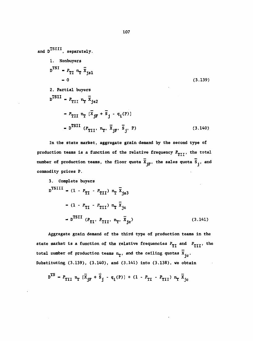
107

TSUI and D , separately.

1. Nonbuyers

- TI "t *jsl

- 0 (3.139)

2. Partial buyers

- TII "T *j=2

• TII "T [XjF + - Si/P)]

- (Pxii. "T' XjF' j' (3.140)

In the state market, aggregate grain demand by the second type of

production teams is a function of the relative frequency , the total

number of production teams, the floor quota X^p, the sales quota Sj, and

commodity prices P.

3. Complete buyers

- (1 - ^TI - ^TIl) "T Xjs3

(1 - - P^jj) Uj, Xjg

TCTT — - D (P^j, P^jj, n^, Xjg) (3.141)

Aggregate grain demand of the third type of production teams in the

state market is a function of the relative frequencies P^j and P^^^, the

total number of production teams n,p, and the ceiling quotas Xj^.

Substituting (3.139), (3.140), and (3.141) into (3.138), we obtain

D - Pçpjj nj, [XjF + Sj - qj^(P)] + (1 - Pçpj - f^Il) "T *jc

108

- (P j, Op, Xjp, Xj , Sj, P) (3.142)

In the state market, aggregate grain demand by production teams is a

function of the relative frequency P^^. and P^^^, the total number of

production teams nj,, the floor quotas Xjp, the ceiling quotas Xj^, the

sales quotas Sj, and commodity prices P. In addition, observing (3.140)

carefully we can figure out the following inequality:

TSTT — — 0 < < Pp; (Xjp + Sj) (3.143)

That is, the aggregate grain demand by partial buyers in the state

TS11 7SIX — market is more than - zero and less than - P^j (Xj^ + Sj).

TSII Thus, zero is the lower bound, and is the upper bound for the

aggregate grain demand in the state market, or the government needs to

TSII provide at most of grain to those partial buyers.

TSITT Since formula (3.141) indicates that D - (1 - P.^^ - Prpjj

TSUI the government needs to set a plan to sell exactly D amount of grain

to those complete buyers. Adding (3.139), (3.141) and (3.143) together

we obtain

— TS — — — (l-i'Ti-^TII^"T*jc ^ ^ TIl"T^^jF'^^j^'^^^"^Tl"^TII^"T^jc (3.144)

Formula (3.144) indicates that aggregate grain demand of production

jc TS —

teams in the state market is between - (1 - P,^^ - P^^^.) X. and

TS — — — VX " TII "T (XjF + - ^TI " ^TIL) "T Xjc' ^he

lower bound and the latter is the upper bound for the total grain demand

in the state market. To satisfy the basic need of food grain to team

109

TS TS households, the government has to provide at least but at most

of grain.

Aggregate grain SUDPIV of production teams In the state market

TS S , aggregate grain supply of production teams In the state market, is

TSI TSII TSUI the sum of S , S , and S , aggregate grain supply of the first,

the second, and the third types of production teams in the state market.

Algebraically,

_ gTsi + s?::: + (3.145)

Using the similar assumptions and methods in the analysis of the

aggregate grain supply of production teams in the combined market and

applying formulas (3.127), (3.128), (3.129), (3.130), (3.131), (3.132),

(3.133) and (3.137), we can induce and individually.

1. Nonbuyers

TSI There are three subtypes of nonbuyers; therefore, S is the

aggregate grain demand of the first, the second, and the third subtypes

of nonbuyers in the state markets.

3TSI . jISIl 5TSI2 5TSI3 (3.146)

where

gTSIl _ gTSIll gTSI12

• TI TIl TIll "T Sjsill ^TI TIl (I'^TIll) "T 4jSI12

- f-rii ^Tiii "T + Ti ^Tii ^^"^Tiii^ "T [qj(P)-%jF]

• TI TIl (^TIll "T Sj + (1 ^TIll^ "T t9j(P) - Xjp])

110

- s (P^J, ^xill' "T' *jF' (3.147)

gTSI2 _ gTSI21 gTSI22

• TI TI2 TI21 "T 9jSI21 ^TI TI2 " TI21^ "T 9jsi22

• *'TI^'TI2^TI2l"T[9j(P)'*jc]+fTr^Tl2(l"^TI2l)"T[9j(F)"%j(F)]

S (^TI' TI2' TI21' *jc' "T' (3.148)

TOT? S - P^J (1 - Ppii - ^TI2^ 4jS13

- P^j (1 - P^jj^ - P^j2^ (4j(P) - Xjcl

TST^ — - S (^TIl' ^TI2' Xjc' (3 149)

Substitute (3.147), (3.148) and (3.149) into (3.146):

TOT — — S - P^J ^TII (^TIll "x Sj + (1 - P^m) "t [qj(P) - Xjp])

•*• ^TI TI2 TI21 "T [9j(P) - Xjc]

+ P.JJ ^ipj2 " ^TI21 ) [9j(P) " Xj(P)]

+ Pjj (1 - P^;! - Pxi2) [9j(P) - Xjc]

TST ^ "* ^ - s (P^J, Pjjj^, ^112> ^TIll ' "t' XjF' *jc' ®j' (3.150)

That is, in the state market, the aggregate grain supply by the

nonbuyers is a function of relative frequencies P^j, P^j^f ^xi2' TIll'

and ^xj21' total number of production teams, the floor quotas, the

Ill

ceiling quotas, the sales quotas, and commodity prices.

2. Partial buyers

For partial buyers, their aggregate grain supply in the state market

TSII S is given as the following:

" TII "T

_ S^SII n^, ij) (3.151)

In the state market, the aggregate grain supply by partial buyers is

a function of relative frequency of , the total number of production

teams, and the sales quotas.

3. Complete buyers

For complete buyers, their aggregate grain supply in the state

TSUI market S is zero, or

S - (1 - f^ll " TII^ "T 4jS3

- 0 (3.152)

Finally, adding (3.150), (3.151) and (3.152) together we obtain

(P, TI Til ^^Tiii "t Sj + (1 - Pçpjj^j^) ly,

^Tl ^TI2 TI21 "T

"*• ^TI ^TI2 " ^TI21^ "T

+ p j (1 - p jj - [qj(P) - + Pjii "r

112

S (•PTl'^TII'^TIl'^TI2'^TIll'^TI21'"T'^JF'*jc'®J'^^ (3.153)

Thus, In the state market, the aggregate grain supply by production

teams is a function of the relative frequencies P^^i, Pji2'

^TIll' ^TI21' total number of production teams, the floor quotas,

the ceiling quotas, the sales quotas, and commodity prices.

Additionally, observing (3.147), (3.148), and (3.149), we note

that

— TQT1 ^TI TIl "T Sj < S (3.154)

— TCTO ^TI 112 "T Sj < S (3.155)

^TI - ^TIl • TI2^ "T Sj < S^SI3 (3.156)

Summing (3.154), (3.155) and (3.156) we get

P^j n,j, S J < S^SI (3.157)

That is, in the state market, the aggregate grain supply by non-

buyers or most of the production teams is always guaranteed to be more

TSI than S^^^ - P^j n^ Sj, which is the lower bound for the aggregate grain

supply by nonbuyers.

TSTT — Formula (3.151) indicates that S is a constant P^^^ n^ Sj, or

the government can keep a fixed procurement of grain from partial buyers.

Combining (3.157) with (3.151) we obtain a new inequality;

TS (Pti + "T Sj < S (3.158)

TS ^ Thus, the government has a guarantee to procure )n^Sj

amount of grain from production teams. In other words, S^^^ is the

113

minimum planned grain supply by production teams.

Lastly, comparing aggregate grain demand with aggregate grain supply

for nonbuyers, partial buyers, and complete buyers in the state market,

respectively. We can figure out the balances between the demand and

supply by these different buyers. Subtracting (3.139) from (3,150) and

noting (3.154) we can get

Pti ^TIl "r Sj < (3.159)

Similarly,

gTSII _ jjTSII _ [q^(P) - Xj^] > 0 (3.160)

gTSIII _ jjTSIII _ .pTSIII _ .(1 . rvp Xjp < 0 (3.161)

TSII TSII In general, S - D might be negative, that is, the government

TSII TSII provides a net amount of grain to partial buyers. Assuming S - D

< 0 and adding (3.159), (3.160) and (3.161) together we get

^TI ^TIl "T " TII "T [XjF '

- (1 - - P^jj) n^ Xj^ < S^® - (3.162)

TS TS Let (S - D )' equal the left of the inequality (3.162). In the

TSII TSTT TS TS case of S -D >0,(S -D )' becomes even bigger, but is still

TS TS less than S - D Thus, regardless of positiveness or negativeness of

TS TS TS TS s - D , the government can have more than (S - D )' amount of grain

for use, excluding that resold to production teams or used by the rural

people themselves. This surplus provides a base for the government to

114

make further plans to consider other uses, which Include urban people's

consumption and Industrial uses as well as the needs of international

grain trade.

Comparative statics of agyreiyate prain demand and supply bv teams

Comparative statics is divided into two parts.

1. Aggregate grain demand of production teams in the state market

From (3.138) and other relevant formulas

• + D^SII + dTSIII

a. Nonbuyers

- 0

b. Partial buyers

TSTI — D - "T [*jF

15-;;- - "T [XjF + :j - SifP)] > 0

aoTSii

an.j. " TII [*jF °

n„ > 0 aXjF aij "I T

aPj Tii X 3Pj

In the state market, the aggregate grain demand by partial buyers is

increasing if the relative frequency the total number of production

teams, or the floor quotas increase, or its own price decreases.

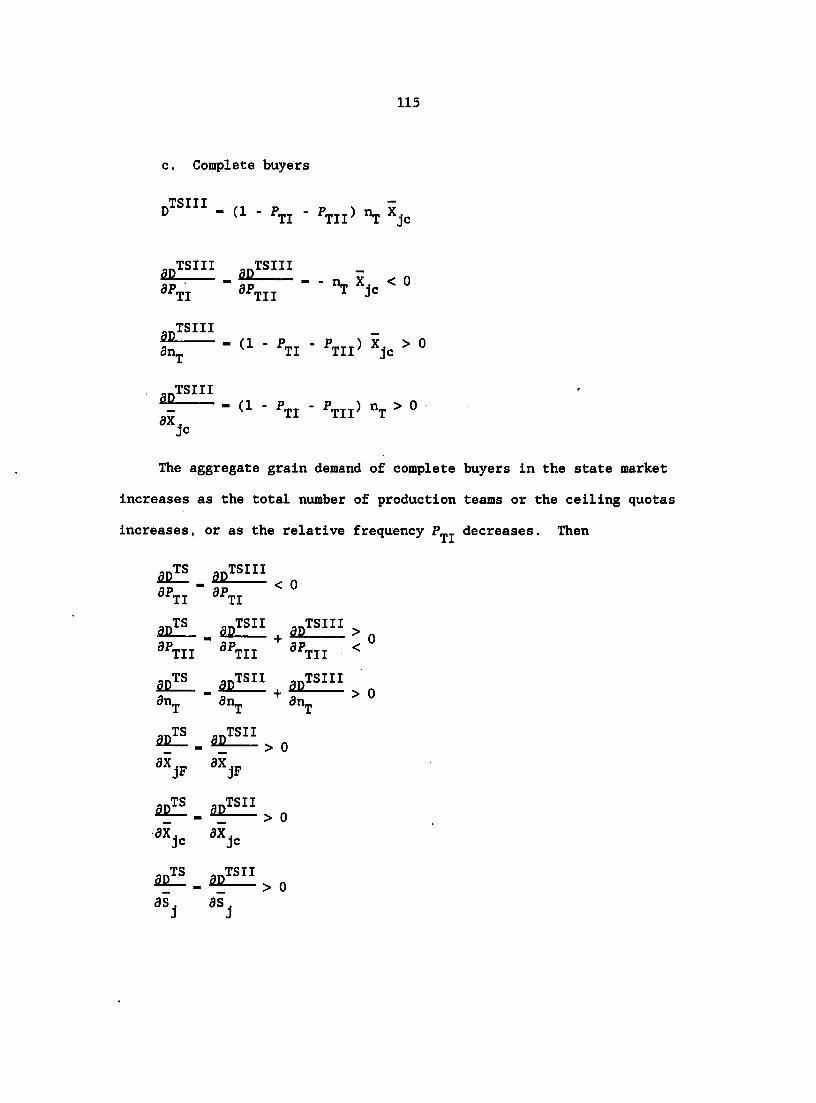
115

c. Complete buyers

TCTTT —

D - (1 - ^TI - ^TII> "T Xjc

aiZîîii _ gpTsiii - ^ g

TI ""TII

.TSUI

aP^T • aP-TTT • " "T jc

8n^ • • TI • TII^ *jc °

TSUI

„n - (1 - Pj i - ^Tii) "T ° **jc

The aggregate grain demand of complete buyers in the state market

increases as the total number of production teams or the ceiling quotas

increases, or as the relative frequency decreases. Then

â£L. > „ aPTii 3^X11 ^^TII

_ 5£!!££, âcZfH 5n^ 8n^ + dn^ > "

aZ!_ 0

aXjF aXjF

â£!_ 0

axjc axjc

0 asj asj

116

i Ç . Ï = < .

Thus, in the same market, the aggregate grain demand by production

teams increases when the total number of production teams, floor quotas,

ceiling quotas, or sales quotas increase. On the other hand, it de­

creases when the relative frequency or its own price increases. In

addition, each of these factors affects the aggregate grain demand in a

partial way through a component or a group of components in the aggregate

demand function; therefore, these factor effects are called partial

effects in this study.

2. Aggregate grain supply of production teams in the state market

From (3.146) and other relevant formulas

gTS _ gTSI + gTSII + gTSIII

a. Nonbuyers

gTSI _ gTSII gTSI2 + gTSl3

where

gTSII _ p p (p TI Ptii (fg,211 Aj Sj + (1 - [qj(P) - Xjp])

TCTO —

S - ^TI21 "t " *jc^

^TI TI2 " ^TI21^ "T [9j(P) -

- 'in - ISj'" - i:j.l

Thus,

117

is2i ..TSIl ,.TSI2 ,,TSI3

ai>Ti SPj, af,: *'11

.^ISI _ ,,TSn ,TS13

^'tii ^'TII "TII *

isZE. âsîflî ssEîL >.„

^^112 ^^TI2 *^712 ^

aaî!L.asHH^>o ""tih ""nil *

â£!L . âsï!!H > 0

^^1121 "TI21 *

asî!i. âslîii âsI!H â£!i! , „ aof aoj ^ aiij * dn^

â£!! . âsZ!ii 0

«V

4. ' .„TSI ..TSIl ^ ^ > 0 asj aSj

âsîfi . asEH, â£!fi 0 3P. 3P, ap,

J J J

In the state market, the aggregate grain supply by nonbuyers is

increasing if the relative frequency , the sales quotas Sj, or its own

price Pj increases. The aggregate grain supply is uncertain if the

relative frequencies ^TI2' ^TIll* ^TI21 ^^e ceiling quotas

increases. Lastly, the aggregate grain supply is decreasing if the floor

quotas increase.

118

b. Partial buyers

- P,„ n, Sj

agTSii ^ - S, > 0 afTTT - *T Sj

a&

TII

,TSII

an? ^TII Sj > °

agTSI

- 'ill "T > ° asj

For partial buyers, the aggregate grain supply in the state market

is increasing if the relative frequency , the total number of

production teams, or the sales quotas increases.

c. Complete buyers

gTS::! _ 0

Thus, we finally have the results:

iè-îfr-âsZ!_ _ asZH > 0 aPiii ^^Tii

isIL - âsEi > 0 3PTI2 ^^tI2

âs!!_

**TI11

asl!_ **TI21

SgTSI >

^^TIll <

>

*^TI21 <

119

asIL _ 5S!!L . an^ dn^ + an, ^ "

aa^_ a^< 0

**JF **jF

âs!!.âs!!i>o

4=

âsîî _ isîîi + > 0

as as as

For production teams, the aggregate grain supply in the state market

increases as the relative frequency or , the total number of

production teams, or the sales quotas increases. The aggregate grain

supply is uncertain as the relative frequency ^TI2' TIll' ^TI21

or celling quotas increases, and it decreases as the floor quotas, or its

own price, increases.

Graphic analysis of aggregate grain demand and supply in the state

market Based on these mathematical analyses, the graphs of the

aggregate grain demand and supply by production teams can be drawn in

three subparts.

1. Nonbuyers

a. The first subtype of nonbuyers

The aggregate grain supply by the first subtype of nonbuyers is the

sum of a vertical line passing through n^ Sj on

the Qj axis and an upward sloping line (Figure 3.17a).

120

TSIlb

(a) (b) (c)

Figure 3.17. Aggregation of the grain supplies of the first and the second subtype within the first type of productions teams in the state market

b. The second and the third subtypes of nonbuyers

For both the second and the third subtypes of nonbuyers, their

aggregate grain supplies in the state market have the same shape (Figure

3.17b and c), although they may have a slight change in their slopes.

Thus, we can figure out the shape of the aggregate grain supply of

nonbuyers in the state market. That is an upward sloping line shown in

Figure 3.18a.

2. Partial buyers

For partial buyers in the state market, the aggregate grain demand

is a downward sloping line on the left of Xj^, and its

aggregate grain supply is a vertical line that passes through -

PTII "X (Figure 3.18a).

3. Complete buyers

For complete buyers in the state market, the aggregate grain demand

is a vertical line that passes through - (1 - ^jc

and its aggregate grain supply is zero (Figure 3.18c). Thus, adding

121

,TSI

<TSIlb

(a)

.TSII \.

,TSII

^TSIIb^TSIIa

(b)

D TSUI

TSIIIa

(c)

Figure 3.18. Aggregate grain demands and supplies of the first, the second and the third type of production teams in the state market

Figure 3.18a, 3.18b and 3.18c together, we obtain the aggregate grain

demand and aggregate grain supply of production teams in the state

market. The former has two segments: one is a downward-sloping line and

the other one is a vertical line passing through - Q-pgjja + silla

on the Qj axis. The latter also has two segments: one is an upward-

sloping line and the other one is a vertical line passing through

^TSb ~ TSIb ^TSIIb Qj (Figure 3.19). The minimum horizon-

TS TS tal distance between D and S is Q^g - - Q-jga' *hich is the

minimum net grain supply of production teams in the state market.

^TSa ^TSb

Figure 3.19. Aggregate grain demand and supply of all production teams in the state market

122

Theory of International Grain Trade

in the Planned Economy

During the period of the Chinese planned economy, the government

built up a state trading system to manage international trade. Thus, the

government had significant power to use trade to achieve not only

economic but also political objectives. For simplicity, this study

focuses on the economic issues rather than the political issues.

The discussion of international grain trade in the Chinese planned

economy contains four major parts: policy environment, the Ministry of

Foreign Trade (MOFT) model, aggregate grain import demand or export

supply, and interactions of plans and markets. Under policy environment,

the existing background for the decision-making process in the MOFT is

introduced so that theoretical work can be pursued. Next, the individual

grain import demands or export supplies are derived from the MOFT model

under the assumption that the MOFT maximizes its utility, subject to its

budget constraint and other constraints due to the planning control.

After that, total import grain demand or export grain supply is aggre­

gated from all individual import demands or export supplies. In the last

part, plan impacts on both the domestic grain market and the interna­

tional grain market are examined and analyzed. The roles of plans and

markets in the planned economy are illustrated and described.

Policy environment

State monopoly of foreign trade After collectivization of the

agricultural sector and the nationalization of the industrial sector in

123

China In the mid-1950s, the state government had the sole responsibility

for the management of foreign trade. Including the foreign grain trade.

This situation was unchanged until 1978.

In practice, under the guidance of the State Planning Commission

(SPC), the Ministry of Foreign Trade (MOFT) made annual, as well as

medium-term, foreign trade plans. The plans were carried out by opera­

tions of several different Foreign Trade Corporations (FTCs) through

their subordinated local Foreign Trade Bureaus (FTBs), and then exchange

activities in the International markets. Among the FTCs, the China

National Cereals, Oils and Foodstuffs Import and Export Corporation

(CNCOFIEC), and its branches in different provinces and cities are

specialized in the trade of grain, as well as in other foodstuffs.

Objective of foreign trade The Chinese government usually thinks

of foreign trade as the engine of socialist development. The main task

of foreign trade is to import relatively advanced plants and equipment

that cannot be produced or cannot be produced in sufficient quantities

inside China. In this way, the new technology would be absorbed and the

modernization of industry would be facilitated and accelerated. The

problem lies in that China's import capacity mainly depends on its export

capacity. To fulfill the main task, the government has to make a great

effort to export goods (such as raw material, agricultural commodities,

and products of light industry) to earn as much hard currency as pos­

sible. On the other hand, the government wants, to the maximum feasible

extent, to rely on China's own production for those basic needs of its

people, such as food and cloth.

124

In the international markets, the MOFT may behave as a special

consumer with a utility function within imported commodity space and may

face a budget constraint, as well as other constraints due to the

planning control. The assumed objective for the MOFT is to maximize its

utility from purchasing commodities in the international markets.

Plan control The MOFT makes Its foreign trade plan, which states

its revenues and expenditures. Imposed import and export quotas, and

expected targets in quantities of goods to be imported and exported.

For the MOFT, one main concern is the external balance, which is the

budget in foreign exchange. To pay for its imports, the Chinese govern­

ment has to collect foreign currency from its export earnings and/or its

foreign exchange reserves and foreign loans because the Chinese currency

is not an internationally convertible currency. In other words, the MOFT

must extend its exports to guarantee its ability to purchase the desired

foreign goods. Comparatively speaking, the Internal balance is not so

important for the MOFT in the planned economy because its profits have to

be turned over to the State Treasurer, and its losses can be covered by

the State Treasurer.

Another concern for the MOFT is the balance of domestic demand and

supply for some Important goods. According to needs in the Chinese

economy, the government Identifies all Important goods that are needed

to keep the balance. For those types of equipment necessary for in-,

dustrial development, the MOFT must fulfill plan requirements. For those

types of goods necessary for the people's livelihood, such as grain, the

MOFT must strictly maintain the planned balance (rather than the real

125

balance) in the domestic state market (rather than the combined market).

Market operation Because the main interest in this section is

focused on the foreign grain trade managed by the MOFT, for simplicity,

we assume that the MOFT is a price taker in all international markets

except the international grain market. The behavior of the MOFT in the

foreign grain markets changes as its position changes. When the MOFT is

a buyer in the foreign grain market, it behaves as either perfectly

competitive or imperfectly competitive. In the former case, it is a

price taker; and in the latter case, it is a price follower because of

its limited export capacity.

Bilateral trade agreement Political factors as well as economic

factors affect the negotiation of package deals for other traded commodi­

ties, and the MOFT makes several bilateral agreements with different

foreign governments. In these agreements, the Chinese government usually

guarantees to buy a minimum amount of a specific commodity such as wheat

from the other country in the following several years. Therefore, during

the period, the MOFT's total purchases are at least the sum of the

amounts stated in all agreements with these countries.

Model of the Ministrv of Foreign Trade

In the Chinese planned economy, the MOFT is assumed to maximize its

utility in the import commodity space subject to given constraints.

Suppose that the MOFT has a utility function U(Xj^j, ..., Xjj,

Xni) where (i - 1 n) is the i*"^ imported good. Furthermore, to

guarantee utility maximization, suppose that U(Xj^j) has all proper

126

properties such as completeness, reflexivity, transivity, continuity,

nonsatiation, and strict convexity. The Lagrangian function is formu­

lated as the following:

L ~ U (X^i' *••» ^kl' •••' nl^

n I _ n J + ( Z P, X,_ + K FR + q FL - Z P, X,?)

1 i iE i_i

+ - Xii) - - C'l i-1

n — pc po + s A3, [(XiB - X,j) - (Si - D, )] i-k

n + S A^i (Xj^j - X,j) i-1

where

(3.163)

"il the i^^ imported commodity (i - 1.

th Xj^g - the export quota for the i commodity (i-1,

X,, -il

i

FR —

FL —

in case there is no potential to export, X^^g - 0

the import quota for the i^^ commodity (i-1,

in case there is no desire to import, X,^ - 0

international price for the i^^ commodity (i-1,

the foreign currency reserves

the foreign loans

planned domestic grain supply in the state market

planned domestic grain demand in the state market

, n)

, n)

, n)

, n)

127

PS th - planned domestic supply of the 1 commodity in the state

market (i - k, ..., n)

planned domestic demand of the i^^ commodity in the state

market (i - k n)

K, T) - fixed proportional coefficient 0 3 % 3 1, Osfysl

The constraints in the Lagrangian function can be classified into

three categories:

1) external balance.

n I _ n S P. X,_ + K FR + % FL - S P. X,T is an external balance con-i-1 ^ i-1 II

straint. It says that ZP^X^^, total expenditure for importing goods,

T— must be covered by ZP^X^g total earnings from possibly exporting goods

plus part of reserves FR and loans FL in foreign currency.

2) balance of the planned domestic demand and supply.

(X^g - X^j.) is a net export for good i if X^g > X^^ or a net import

for good i if X^^g < X^^, and - 5^ ) is a planned surplus for good i

PS PS PS PS if or a planned shortage for good i if . The

— pg pg constraint (X^g - X^^) - (S^^ - ) & 0 means that, for an important

good i, the net export or net import has to be covered by the planned

domestic surplus or has to cover the planned domestic shortage. Grain,

as a composite good, is considered in the balance table by the central

planners, and, therefore, is an exception. An individual variety of

grain is not considered to be a single good, but more importantly, is

128

considered to be part of a composite good. Suppose that the first

J _ (i - 1 j) commodities belong to the grain category, then S (X^g -

i-1

PS PS Xij) - (Sq - Dg ) is a constraint that guarantees the planned balance of

domestic grain demand and grain supply in only the state market by using

international grain markets.

3) Import quota imposed for some commodities.

Due to the central plan, the government may impose import quotas for

some specific commodities. X^^ - X^^ is the import quota constraint,

that is, import of commodity i must be no more than the import quota set

by the government.

The Kuhn-Tucker conditions are:

aXj^j • 8X^2 "'^l^i • 2 " '^4i ^ ° ^ ' J (3.164)

- Ag 3 0 for X^j-0, i - l,...,j (3.165)

-Ag^ -A^i :S 0 for X^^/O, i - k,...,n (3.166) il ""il

ax ax Vi - ^31 a O for X^^-O, i - k n (3.167)

Xii - 0 i-1 n (3.168)

QT ^ T "" ^ T - Z pf X,_ + K FR + q FL - 3 pf X,_ & 0 (3.169)

'' l i-1 i-1

"^1 3A^ " ° i - 1, .... n (3.170)

129

^ • V • ® » (3 I 'l '

(3.172)

^ - (XiE - *ii> • (Si^ - dJ ®) & 0 i - k, .... n (3.173)

ai__

Si ^31 ax " ° i - k, .... n (3.174)

" *il ° for X^j / 0 i - 1 n (3.175)

\i 3A^ " ° for / 0 i-k n (3.176)

^1' Ag, & 0 i - 1 n (3.177)

X3I > 0 i-k n (3.178)

Suppose that the MOFT strictly keeps its budget in foreign currency

at the balance level,

lb - XlE + * P* + s PL - *11 - » 1 i-1 i-1

then both (3.169) and (3.170) can be omitted. Similarly, suppose that

the MOFT keeps grain and other commodities at the planned balance levels,

then

% - - *11' • <=" - "f) - " <3.180)

and

130

^ - (*IE • =^11' • - "R* - » (3 181)

After that, (3.171), (3.172), (3.173), and (3.174) can be dropped

from the model.

Furthermore, suppose that the second-order conditions are satisfied;

solving the first-order conditions, we find three possible situations for

Xii'.

1. - 0 (3.182)

2. - X^j (pl, FR, PL, Xg, Xj, - Dg! - DJ^) (3.183)

and

3. Xj^j - X^j (3.184)

The first formula (3.182) implies a corner solution. That is, the

MOFT does not import any amount of good i. Pormula (3.183) says that

import demand for good i is a function of international commodity prices,

foreign reserves in the country, foreign loans borrowed by the govern­

ment, the export quotas, the planned balance of domestic grain supply and

demand in the state market, and the planned balances of domestic supplies

and demands of other commodities in the state market. The last formula

(3.184) gives imported good i as just its quota.

If X^^ is determined, the corresponding quantities of either net

export supply X^^g or net import demand X^^^ are Immediately determined.

We now discuss the three situations of X^^:

1. Xi, _ 0

131

There are two possible solutions for if - 0.

a. Xj^g - 0

XiNI - XiNE - 0 (3.185)

The HOFT is not buying and selling good i in international markets.

This case will be dropped out of this study because it is meaningless.

b.

*11IE - *1E (3 IBS)

The MOFT exports good i at the quota level only and, therefore, is

called a command exporter for good i.

2. X^; - Xj^j (pl, FR. FL, Xg, Xj,

a. Xj^g - 0, then

XIJJI - XJ^J (PL, FR, FL, XG, XJ. SQ® - DG? (3.187)

Net import demand for good i is a function of international prices

of goods, the foreign reserves, the foreign loans, the export quotas, the

import quotas, the planned balance of domestic grain supply and demand in

the state market, and the planned balances of domestic supply and demand

for other goods in the state market. Therefore, the MOFT is a flexible

importer for good i.

b. Xj^g > 0, then we have

1) ifx,g>x^j

XiNE - hE • Xii (P:. FR, FL, sf - - D^^)

- X^JJG (PL, FR, FL, XG, XJ, SQ® - DG? - D^^) (3.188)

132

2) if < Xi,

*iNI " *il " iE

- (Pl, PR, FL, Xg, Xj, - D ! - ofS ) - Xg

- X i (Pl, FR, FL, Xg, Xj, - D S) (3.189)

These are either net export supply or net import demand of good i,

which is a function of international prices of goods, the foreign

reserves, the foreign loans, the export quotas, the import quotas, the

planned balance of domestic grain supply and demand in the state market,

the planned balances of domestic supply and demand for other goods in the.

state market. Because export quota is effective, the MOFT is called

either a restricted flexible exporter or importer for good i in case (2)

a and b.

3)

*iNI " *iNE " ° (3,190)

either net export supply or net import demand for good i is zero. The

MOFT is a nonexporter and nonimporter. This case is not discussed

further.

3. Xi, . X ,

*iE • °

thus

*iNI " *il (3.191)

The MOFT imports good i at the quota level only and is called a

command importer for good i.

133

b. XiB > 0

1) if > X g

*iNI " *il ' *iE (3.192)

2) if X,j < XiB

X INI X IE X II (3.193)

3) if Xii - XiE

X INI

X iNE

0 (3.194)

Because (3.194) does not make sense, it is dropped from the discus­

sion. Thus, if X g > 0, either net import demand or net export supply

for good i is fixed at the difference of the import quota and the export

quota by the MOFT. The MOFT is both a dual command importer and exporter

in these cases because it is restricted by both the import and the export

quota at the same time.

All of the above results indicate that the MOFT tries to decide all

net imports and net exports for all goods together, although it may pay

prior attention to export quotas in order to collect the foreign currency

needed to purchase goods in the international market.

Comparative statics From the above discussion, we can classify

the MOFT's behavior by its importing and exporting behaviors.

1. Importer

a. Dual command importer

134

*iNIl " *il • *iE

_ 1

3 il

fïim. .1

For dual command Importer, the net import demand increases or de­

creases as the import or the export quota increases.

b. Command importer

*iNI2 " *il

fiW _ 1

Net import demand for the i good is not affected by any factor

except for the import quota.

c. Flexible importer

*i»I3 - f'- *!• - "G' - 0 ')

fïim . fïu - 0 S?l 6FI

fïim _ fîu> 0 aFR 3FR

fîim _ fïu 0 aFL aFL "

. fii < 0 aXiE

fïim _ fil > 0 aXii ax j

135

3(sp- Df ) " 8<sf - Df ) "

Net Import demand for the 1 good Is increasing if the foreign

reserves, the foreign loans, or the import quotas increase. On the other

hand, net import demand for the i good is decreasing if its own price,

the export quota, or its planned balance of domestic supply and demand in

the state market increases.

Especially, for net import demand of a kind of grain (i - 1,

..., J) and net import demand of total grain , where

GNI - (3 195) n-1

then

but

a(3 - ' ° That is, when the balance of domestic grain supply and demand in the

state market decreases, net import demand of total grain increases, but

net import of a specific kind of grain X ^ may increase or decrease

depending on the situations. The reason this happens is explained as

follows. As the balance of domestic grain supply and demand in the state

market decreases, the government must increase the net grain import to

136

satisfy the planned domestic needs because grain Is so Important to

people's lives as well as political stability in the country. But the

increase in net grain import is constrained by the budget balance in

foreign currency. To increase net grain import and keep other imports

and exports unchanged, the government must have additional money to keep

its budget balanced. If the HOFT cannot get more foreign currency from

the State Treasury, it must adjust its net import and/or net export to

compensate its additional expenses from increasing net grain import.

There are two ways for the MOFT to deal with this matter. First, it can

reduce imports and expand exports, and, therefore, reduce net imports or

expand net exports for other goods rather than grain. Alternatively, it

can make adjustments only within the grain trade to avoid financial

difficulty. For example, it can expand net exports for a specific kind

of grain, say rice, whose price is relatively higher in the International

market, and expand net imports for another specific kind of grain, say

wheat, whose price is relatively lower in the international market.

Working in this way, making a trade-off between rice exporting and wheat

importing by utilizing their price difference, the MOFT can easily have

its net grain import expanded without any further financial request

in foreign currency from the State Treasury. In addition, without

changing the aggregate grain demand and supply in the domestic state

market, the government can easily use its play to change or restrict the

proportion of different varieties of grain demanded or supplied in the

state market to guarantee the trade-off in the international market.

137

d. Restricted flexible Importer

XlNI4 - 11 (P'' FL, Xg, Xj. - DfS) - X g

Because X Is fixed, the partial derivatives for restricted flex­

ible Importer are exactly the same as those for the flexible Importer.

2. Exporter

a. Dual command exporter

*1NE1 " *1E " *11

For the dual command exporter, comparative statics Is the same as

that for the dual command Importer but with opposite signs.

b. Command exporter

*1NE2 " *1E

AXIE

Net export supply for the 1 good Is not affected by any factor

except for the export quota.

c. Restricted flexible exporter

XlNE3 - XiE - *11 FR. FL. X ' h' " "'G'

Obviously, any partial derivative for X gg Is the same as that for

a negative X j or a negative X ^ g (see flexible Importer). Thus, It Is

not necessary to continue the discussion of comparative statics here.

. Graphic analysis The graphic analysis also is divided into two

parts by importing and exporting behaviors of the MOFT.

1. Importer

a. Dual command Importer

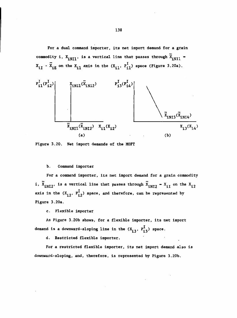
138

For a dual command Importer, its net import demand for a grain

commodity i, is a vertical line that passes through -

— T *il " *iE *ii axis in the (X , space (Figure 3.20a).

*iNIl(*iNI2)

*iNIl *iNI2 *il *i2

(a)

\ x . iNI3 iNI4

Xl,(Xw)

(b)

Figure 3.20. Net import demands of the MOFT

b. Command importer

For a command importer, its net import demand for a grain commodity

i, X Q22' is a vertical line that passes through X ^ g " o" the X g

axis in the (X g, P g) space, and therefore, can be represented by

Figure 3.20a.

c. Flexible importer

As Figure 3.20b shows, for a flexible importer, its net import

demand is a downward-sloping line in the (X g, P g) space.

d. Restricted flexible importer.

For a restricted flexible importer, its net Import demand also is

downward-sloping, and, therefore, is represented by Figure 3.20b.

139

2. Exporter

a. Dual command exporter

For a dual command exporter, Its net export supply is a

— — J vertical line that passes - Xjg - Xjj on the (Xj , Pj ) space

Figure 3.21a).

XjNEl(*jNE2) •J3

Vl<V2' (a)

X

/ JNE3

/ X j3

(b)

Figure 3.21. Net export supplies of the MOFT

b. Command exporter

jNE2' export supply of a grain commodity j for a command

exporter, is the same as that for a dual command exporter, except for

that its intercept on the X g axis is Xj g " rather than Xj ^

(Figure 3.21a).

c. Restricted flexible exporter

As Figure 3.21b shows, when the MOFT behaves as a restricted

flexible exporter, Xj gg, its net export supply for a grain commodity j,

is an upward-sloping line in the (X _, P _) space. jj jj

140

Aggregate Import grain demand and export grain supply

Within the first grain commodities, suppose that the first e

are net importing grain commodities and the remaining are net exporting

grain commodities. In the planned economy, the aggregate import grain

demand D is then

MP *iNIl iNI2 *iNi3 *iNi4 (3.196)

1-e 1-e 1-e 1-e

" (*111 ' *iEl *iI2 1-e 1-e

+ S (Pl, FR, PL, Xg, Xj, 1-e

+ s (X„4 (pl, FR, FL, Xg, Xj, sf - D ? - X ^ l 1-e

- (pl, FR, FL, Xg, Xj, (3.197)

That is, as long as the HOFT behaves as a flexible or a restricted

flexible importer for at least one grain commodity, D , the aggregate

import grain demand, is a function of international prices of commodi­

ties, the foreign reserves, the foreign loans, the export quotas, the

import quotas, the planned balance of domestic grain supply and demand in

the state market, and the planned balances of domestic supplies and

XP demands of other goods in the state market. On the other hand, S , the

aggregate export grain supply in the planned economy is as follows;

XP - f /iNEl + , /iNE2 + , /iNE3 <3,198)

" g y iEl " *ill

141

— T — — pc pc pc pc + S [X g3 - X J3(P\ FR, FL, Xg, Xj, - D" S - D )]

f-J

- (pl, FR, FL, Xg, Xj, Sq® - (3.199)

As long as the MOFT behaves as a restricted flexible exporter for at

least one grain commodity, the aggregate export grain supply Is similar

to the aggregate Import grain demand as a function of International

prices of commodities, foreign reserves, foreign loans, export quotas.

Import quotas, the planned balance of domestic grain supply and demand in

the state market, and the planned balances of domestic demands of other

goods in the state market.

Two important things should be pointed out. First, both the

aggregate import grain demand and the aggregate export grain supply by

the MOFT do contain International price vectors, especially the interna­

tional grain price, but do not contain domestic price vectors, especially

the domestic grain price. This fact Indicates that the MOFT's behavior

in the International grain market is affected by international prices

but not by domestic prices. Second, whether China becomes a net import­

ing grain country or a net exporting grain country depends on the

difference between the aggregate Import grain demand, D , and the

XP MP XP aggregate export grain supply, S . If D > S , the MOFT is a net

grain Importer; otherwise, it is a net grain exporter. Looking back at

the history of Chinese grain trade after the 1950s, we found out that

China was a net importing grain country most of the time, especially In

the planned economy. That means, in general, the aggregate import grain

142

MP XP demand D is greater than the aggregate supply of grain S in China.

If this is true, the net grain import demand, is as follows;

pNMP _ jjMP _ gXP (3.200)

Undoubtedly, is a function that contains all the factors

XP and/or S have/has.

Comparative statics The comparative statics are calculated for

both aggregate import grain demand and export grain supply.

1. Aggregate import grain demand

_ S fïilill + S fim + S **iNI4 > 0

**iNIl *iNIl **iNIl **iNIl

âcîîL-. S s fïim+ s **iNi4 > 0

**iNEl **iNEl **iNEl **ÏNE1

S fîim + s fim + s fïiïïià > 0

aXii2 '"3X 12 aXii2 < ax^j2

As the import quota or the export quota faced by the dual command

importer or the command importer increases, the total effect on the

aggregate grain demand is unclear because the effects on the last two

terms, aggregate import grain demand by the flexible Importers and

restricted flexible importers are unclear.

Based on similar reasoning, we have

_ S + S fïmiâ > 0

3Xii3 3*113 3*113

143

âçî!!_ _ s **inI4 + s fïim > 0

aXii ® ax j

The remaining comparative statics are focused on the behaviors of

flexible and restricted Importers.

_ S **iI3 S **iI4 >0 (i - 1, .... j)

apj apj 3pJ

apMP S'fîm. s **iI4 n

.Pj ap' 1- ap:

afiîîL- _ s fill + s fîilà > 0 aPR 1-e aFR 1-e aPR

iDÎî!_ _ s £ïm + s fiiA > 0 aPL 1-e âPL 1-e aPL "

ms. s mn s fikià 9(3% - DG®) ' a(sf - of) a(sf - of)

The aggregate import grain demand increases when the foreign

reserves or the foreign loans increase. It decreases when its

international price, pj, average grain price, or the balance of domestic

grain supply and demand In the state market increases. Finally, it

becomes uncertain when the international price of one grain commodity

Increases.

2. Aggregate export grain supply

Under the changes of the import quotas or the export quotas, the

final results of comparative statics for aggregate export grain supply

are the same as those for the aggregate import grain demand. Otherwise,

144

the results are given as follows:

âsï!_ _ S îhn > 0 api f-j api <

dpl apj u 1

âsïL_ _ s fîm < 0 aPR f-j 3FR

isïL_. s fîm<0 8FL f-j aPL

âSÎÎ! _ 2 fïiE2 >0

a(SGS . D^S) F-J acs^S - D^®)

These results indicate that, given the above change(s) in the fac-

tor(s), aggregate export grain supply is changing in the opposite direc

tion of changes in the aggregate grain demand.

Graphic analysis Graphic analysis also is presented for both

aggregate grain demand and export grain supply.

1. Aggregate import grain demand

Given the average international grain price, we can aggregate the

import grain demand by graph. As Figure 3.22a shows, the sum of

aggregate import grain demands by dual commanders and commanders, is a

vertical line that intercepts on the Q axis is Q j - Z

— II + S X 22 the (Qq, P ) space. 1-e

145

In Figure 3.22b, aggregate import grain demand by flexible

and restricted flexible importers, is given as a downward-sloping line in

the (Q , Pg) space. Finally, after summing and we obtain

MP aggregate Import grain demand by the MOFT. As Figure 3.22c shows, D

MPI is still a downward-sloping line, but it is much steeper than D in the

(Qg, Pg) space because of the effect of .

.MPI I

(a) (b) (c)

Figure 3.22. Aggregation of Import grain demands in the planned economy

2. Aggregate export grain supply

Similarly, we can figure out aggregate export grain supply in the

I I XPI (QQI PQ) space. In Figure 3.23a, S , the sum of the aggregate export

grain supplies by dual command exporters and command exporters is a

vertical line that passes through - S (*iEl " *iil + 2 o"

I I f-j axis in the (Q , P ) space.

XP Lastly, S , the aggregate export grain supply by the MOFT is

XPI XPII obtained from the sum of S and S , which is the aggregate grain

146

supply by restricted flexible exporters (Figure 3.23b). It is still an

XPII upward-sloping line, but it is steeper than S because of the effect

ypT of (Figure 3.23c).

,XPII

(a) (b) (c)

Figure 3.23. Aggregation of export grain supplies in the planned economy

Interactions of plans and markets

In the Chinese grain economy, the markets, especially the domestic

state markets, are different from markets in the usual sense. Deter­

mined by the government authority and not by the interaction of market

forces, the state market price lacks the mechanism to adjust the market­

ing process automatically and instantaneously. Moreover, through the

planning process, the government almost controls grain consumption and

production. In the state market, the government limits the maximum grain

demand by using ration coupons in urban areas and floor quotas in rural

areas and guarantees the minimum grain supply by applying the output

targets to state farms and the sales quotas and the ceiling quotas to

production teams. That the government has monopoly power in the state

147

market Is not only because it has the authority to decide the prices but

also because it has authority, to a great extent, to decide the quanti­

ties exchanged. Hence, the state market becomes a buyer market when the

government procures grain from state farms and production teams and

becomes a seller market when the government retails grain to the urban

households and sells or resells grain to those production teams per­

mitted. Under such circumstances, in a certain sense, the state grain

market can be seen as an extension of government policies.

In the international grain markets, the Chinese government has no

power to decide prices, but still has full monopoly power to decide the

variety and quantity of grain imported and exported. Thus, the interna­

tional grain markets can be partly seen as extensions of government

policies. The next is the analysis of the policy impacts on the equilib­

rium situations of the domestic as well as the international market.

Market equilibrium situations Generally, one particularly

noticeable feature of the state grain market is its disequilibrium.

Indeed, disequilibrium is an internal part of the Chinese grain economy.

Without perfect information and knowledge, exogenous prices cannot be the

equilibrium prices in the state market. In addition, it is believed by

both the Chinese officials and professional authorities that the grain

price in the state market is well below its equilibrium price. One

reason is that the government wants to set lower prices for agricultural

products but higher prices for industrial products to create a difference

between prices of agricultural and industrial products and to collect

148

funds from the agricultural sector. After economic reform, this hypothe­

sis was partly proved by the much higher free-market prices, whose

average might be considered as the equilibrium price. Obviously, this

too-low price would create an excess grain demand in the state market.

Moreover, usage of the ration coupons imply an existing shortage problem

in quantities of grain in the planned economy. Even under such a

rationing system, restricted excess grain demand still existed throughout

the state market because the Chinese government had adjusted its grain

price within only a narrow range, and China had been a net grain import­

ing country from 1961. Hence, the equilibrium quantities of grain were

reached by means of international trade in the planned economy.

In the international grain markets, there exist equilibrium prices

and quantities. Although the equilibrium prices are mainly determined by

excess grain suppliers of the rest of the world, the equilibrium quan­

tities are mainly determined by the planned excess grain demand, rather

than the real excess grain demand of the MOFT.

Domestic policy instruments In the domestic grain market, as

already analyzed, the policy instruments include ration coupons, sales

quotas, ceiling quotas, floor quotas, and the state market prices. Among

these policy instruments, the ration coupons, the sales quotas and the

state market prices are more important for the central planners because

these three mainly determine a disequilibrium in the state grain market.

The first two of the three policy instruments, needless to say, are

quantity parameters to adjust either the grain demand or the grain supply

in the state market. The last one is regarded as a policy instrument

149

because the state market price is centrally decided and generally is

uniform throughout the country (although there are some local differen­

tials). It is weakly (partly) related to the grain demand and supply in

the state market. Next are comparative studies for these three policy

instruments :

1. Ration coupons

Ration coupons are issued to the urban households plus the house­

holds of state farms. With the rationing system the government can plan

the maximum grain demand in the state market. Suppose the government

raised the amount of ration coupons to the urban people in order to

improve their standard of living. The market impacts of this policy are

illustrated in Figure 3.24.

S P

I P

ES(R)

(a) (b)

Figure 3.24. The effects of a change in ration level in the planned economy

P P On the left, D and S separately represent the aggregate grain

demand and supply in the domestic state market in the planned economy.

150

S D At the given state market price P , the grain demand is and the

S FD PS grain supply is Q . The planned grain demand and supply are and Qg ,

S PD D which are not affected by the state market price Pj . Obviously,

PS S and because the government wants to make sure that the plans

would fully coordinate the balance of real demand and supply in the state

grain market. On the right, the international grain market is partly

separated from the state market because the state market price is

irrelevant to the planned excess demand, but it is partly related to the

state market because the balance of the planned demand and supply is

relevant to the planned excess demand. Suppose that China is an import­

ing grain country. We find out that the planned excess demand is ED,

which is downward-sloping, and the excess supply of the rest of the world

is ES(R), which is a horizontal line because China is assumed to be

either a price taker or a price follower in the international market in

spite of the fact that it is a larger country. The import grain demand

is determined by a cross point under a presumed international grain

price P . All of these descriptions about the beginning situations of

the markets are fitted to discussion of any other policy instruments,

and, therefore, are not repeated in this part.

Because the government increases the amount of ration coupons

distributed, the domestic grain demand in the state market is expanding

from to Q . At the same time, the planned grain demand also is 1 2

PD PD expanding from Q to Q Neither the domestic grain supply nor the

1 2 planned grain supply is changing. Thus, the balance of total grain

151

demand and supply as well as the balance of total planned grain demand

and supply in the state market is increasing. The change in the latter

balance rather than the former balance would cause a rightward shift of

the planned excess demand curve ED in the international market. The

M Import grain demand then increases to Qg.

2. Sales quotas

Sales quotas are set to production teams. Using sales quotas, the

government can plan the minimum grain supply in the state market. Figure

3.25 shows the impacts on both the domestic and the international market

when the government increases sales quotas.

The beginning situations have already been discussed. As the gov­

ernment decides to increase the sales quota S to S in the state market,

S P

,PS rtPS„SrtS «D „PD S

I P

ES(R)

ED ED'

(a) <b)

Figure 3.25. The effects of a change in the sales quota in the planned economy

p the total grain supply line S is shifted to the right, and results in

S s an Increase of both total grain supply from to and planned grain

152

PS PS supply from to Qg . Thus, both the balance of total grain demand and

supply and the balance of total planned grain demand and supply decrease.

Because of a decrease in the balance of total planned grain demand and

supply, the planned excess grain demand line ED is shifted back to ED'.

Immediately, the import grain demand decreases from to Qg.

3. The state market price

The state grain markets are set for both domestic consumers and

producers. By adjusting the state market prices, the government can

partly influence the behaviors of urban households and rural production

teams. Figure 3.26 indicates the effects of a change in the state market

price on both the state and the international markets.

The beginning situations are the same as before. When the govern-

S s ment decides to raise the state market price--say from P to Pg'-to

ES(R)

.M

(a) (b)

Figure 3.26. The effects of a change in the state market price in the planned economy

153

Improve the rationality of the price, immediately in the state market,

the total grain demand decreases and the total grain supply increases,

but both total planned grain demand and supply are unchanged. Hence, the

balance of total grain demand and supply decreases but the balance of

total planned grain demand and supply does not change. There is no

impact on the international market because all factors specified in ED

stay the same as before. Here, we can draw a conclusion that a change in

the state grain market price has an impact only on the domestic market

but not on the international market.

International policy Instruments In the international grain

markets, the main policy instruments used by the Chinese government in

the planned economy are import quotas and export quotas. Comparative

studies of these two policy instruments follow.

1. Import quota

The import quotas are used to restrict import grain demand.

Theoretically, the impacts on an individual import grain demand due to a

change in grain import quotas are not certain. Suppose the import quotas

for all grains increase simultaneously, or suppose the import quota for

total import grain demand increases.

As Figure 3.27 shows, when the import grain quota increases, the

planned excess demand in the international market shifts to the right,

the import grain demand increased from to Qg. There is no change

in the domestic market.

154

P I

ED'

ES(R)

r ED"

Q M

(a) (b)

Figure 3.27. The effects of a change in the import grain qyota in the planned economy

2. Export quota

Export quotas are used to limit the export grain supply. The

impacts on an individual import grain demand due to an increase in the

grain export quota also are not certain. Suppose the export quotas for

all grains increase together, or suppose the export quota for total

export grain supply increases, then the result is in the opposite

direction to the result of an increase in the import grain quota (Figure

3.27b).

155

CHAPTER IV. THE CHINESE MIXED GRAIN ECONOMY

A major aspect of the Chinese mixed economy is the integration of

central planning with the markets' mechanism in spite of the fact that

central planning is still considered as fundamental by the government.

Even though the state market still plays the dominant role, and the free

market is merely an auxiliary means of regulating the economy, current

economic reform has eventually provided a new approach for combining the

state market with the free market to distribute and circulate goods,

especially important goods such as grain. In this sense, the Chinese

grain economy has been transformed in the last decade from being planned

to being mixed. After the collective disappeared earlier in the

economic reforms and the free market reemerged later, the powerful

influence of the government in the grain economy declined significantly.

This chapter deals with a theoretical model for the Chinese mixed

grain economy. The expositional process is similar to that in Chapter

III. At the beginning, a brief overview of the planning and the market­

ing framework in the mixed economy is presented. Following this are

three sections of theoretical discussions; the behavior of urban

households, the behavior of state farm households and agricultural

g households, and the behavior of the MOFT in the mixed grain economy.

These sections generate an urban household model, a state farm (house­

hold) model and an agricultural household model, and, finally, a MOFT

g For convenience, we call the households that belonged to the state

farms state farm households, and the households that belonged to the production teams agricultural households.

156

model.

General Framework of the Chinese

Mixed Grain Economy

Because we have introduced the general framework of the Chinese

planned grain economy, this section is mainly focused on the distinc­

tions, rather than the similarities, between the frameworks of the mixed

and the planned grain economy.

Planning framework

Since the economic reform, the macro aspects of the grain economy

have still been planned and managed by the central and local governments,

but institutional changes have occurred on the micro aspects of the

economy. Among these institutional changes, the most significant and

important for the planning framework is that the rural households,

including both state farm households and agricultural households, have

replaced state farms and production teams, respectively, and become the

fundamental units of management and production in the agricultural sector

with state or collective ownership of land and major fixed assets. The

Production Responsibility System (PRS) consists of contracts that define

the rights and responsibilities of owners (including state, collective,

and private) and managers of assets. The most widely accepted contrac­

tual form is the Bao Gao Dao Hu (BGDH). Under the BGDH, the households

have the right to manage collectively owned land according to their size

or labor force. The households are obligated to pay agricultural taxes,

make contributions to social welfare funds, and provide their share in

157

satisfying state procurement requirements. After that, all remaining

output may be kept and disposed of by the households.

In addition to the replacement of state farms and production teams,

the other institutions in the countryside have been restructured. The

communes have been transformed into the townships, and the brigades have

been renamed as the villages. All these institutional changes have

brought about change in the planning framework. At the central govern­

ment level, there is no big change at all. At the local government

level, however, the channel from county to basic units--agricultural

households through the townships then the villages--has been established

to replace the old channel. There are now two kinds of new rural

enterprises in the Chinese mixed economy: the state farm households and

the agricultural households. The planning processes for state farm

households and agricultural households are almost the same as that for

state farms and production teams before the economic reform, except that

the plan targets and sales quotas that were set for the state farm and

the production team have to be split into the corresponding small shares

to fit the households' sizes and production situations.

Figure 4.1 briefly describes the planning process in the mixed grain

economy. The arrows in the graph indicate the transition of the plans

between the central government and the local governments and between the

local governments and the state farm households and the agricultural

households.

158

State Farm Households

Central Government

Agricultural Households

Townships

Villages

Provincial Governmenta Prefecture govenuBcnta County

Governments

Figure 4.1. Agricultural planing process in the Chinese mixed economy

Marketing framework

In the mixed economy, there are dual grain markets. The state

market is continuously controlled by the government, while the free

market is managed by the government but is opened for private exchange.

Figure 4.2 shows the circulation of grain in the Chinese mixed economy.

159

Agricultural Households fyplllIN

Household Market

State Stock

Free Market

Military Industryy

International Ilarkst

Urban Households

State Farm

Households'

State Grain Market

Agricultural Households Type I

Agricultural Households Type II

Figure 4.2. Circulation of grain in the Chinese mixed economy

The arrows in the graph indicate the flow directions of grain within the

economy. We will discuss the situations in these markets separately.

The state market Sellers in the state grain market include state

farm households and a majority of the agricultural households (Type I and

Type II). The former sell almost all their product to the state market,

and the latter sell part of their product to the state market. Among the

latter, Type I agricultural households are complete sellers or nonbuyers

and Type II are partial sellers in the state markets. On the other hand,

160

buyers in the state grain market include urban households, the military,

industry, state farm households, and a minority of agricultural house­

holds (Type II and Type III). Obviously, the first four buyers purchase

most of their grain from the state market by either ration coupons or the

government's permission. For the last buyers. Type III agricultural

households are complete buyers and Type II are partial buyers in the

state market.

Under the guidance of the government's plans, both the international

market and the state stock still are used to adjust and maintain the

balance of the demand and supply for grain in the state market. Indeed,

the government now may even purchase or sell some grain in the free

market to change the level of the state stock. For simplicity, we

continue to assume that the stock grain demand/supply equals zero and to.

leave it to be dealt with in Chapter V. The relationship between the

international market and the state market in the mixed grain economy is

discussed in the last section of this chapter.

The free market Everybody in the mixed economy can buy goods in

the free market. As the figure shows, buyers in the free market consist

of urban households, industry, state farm households, and a minority of

agricultural households (Type II and Type III). The first three buyers

have the right to buy grain from the state market at the lower prices, so

they may purchase additional amounts of grain from the free market at

generally higher prices to satisfy themselves. The seller in the free

market Is usually a Type I agricultural household, that Is called a

complete seller in the free market.

161

Household-own market and household market The previous analyses

for the state market and the free market clearly eliminate the part of

agricultural households' own grain consumption (Type I and Type II).

Among these households, Type I is a complete self-supplier whereas Type

II is only a partial self-supplier.

For convenience, we call an assumed market in which such a house­

hold's own consumption occurs as the household-own market. Clearly, in

this household-own market, the only seller and buyer is the household

itself, and the trading price can be seen as the free market price. In

addition, we call another assumed market in which, for all involved agri­

cultural households, all the own grain consumptions without circulation

within either the state market or the free market are combined together

the household market. Sellers and buyers in this market are the house­

holds themselves.

Finally, we assume an additional united market that combines both

the free market and the household market in the mixed grain economy. In

these discussions, we mention grain demand and supply with a specifica­

tion for the market.

The dashed line in Figure 4.2 divides the circulation of grain in

the Chinese mixed economy into four parts. The central part is the

circulation of grain occurring in the state market and under direct

control of the government plans. The other three parts, except a rec­

tangle on the left corner, compose the circulation of grain occurring in

the free market and under weakened Indirect plan control. The rectangle

represents the circulation of grain within the so-called household market

162

and is almost out of government control.

Generally, the circulation of grain in both the state market and the

free market hold only a smaller share, whereas the own grain consumption

by most of the agricultural households still holds a larger share of

total grain consumption in the Chinese mixed economy. It is estimated

that the government retailed about 34% of the total grain consumed in

China and the agricultural households sold about 5% of the total grain

9 consumed to the free market in 1985. Thus, in the household market, the

own grain consumption by the agricultural households was roughly figured

out to be about 61% of total grain consumed in the same year. These

figures illustrate that the Chinese mixed grain economy, to a certain

degree, is still self-sufficient but not commercialized.

Theory of Urban Grain Demand

in the Mixed Economy

Even though the free market is now open to everyone without any

restriction from the government, the urban and the rural people still

receive different treatment in the state grain market. Thus, it is still

necessary to explore and develop urban and rural grain demand theories

separately for the mixed economy. Again, behavior of the urban house­

holds in the mixed grain economy will be discussed first.

To insure the correct derivation of the urban grain demand func­

tion, the general assumptions mentioned in Chapter III are consciously

maintained here. Like the corresponding section in Chapter III, the

9 The data used here are from State Statistical Bureau, 1987.

163

study for urban grain demand in the mixed economy contains three similar

parts: policy environment, urban household model, and aggregate grain

demand of urban households. Unlike the corresponding section in Chapter

III, this section has two additional parts: the state market analysis

and the free market analysis. Under the policy environment, the policy

changes due to the economic reform are especially stressed. The indi­

vidual urban households still are classified into different types, and

they maximize their utilities subject to new constraints based on the

policy changes. Then, the aggregate urban grain demand is derived from

the aggregation of grain demands by all different types of individual

urban households. Finally, the exchange activities in both the state

market and the free market are analyzed separately.

Policy environment

Ownership of assets In the Chinese mixed economy, most schools,

stores, and other enterprises still are owned by either the public or the

cooperatives, but some stores and enterprises have emerged under private

or foreign ownership.

Labor Urban laborers who are hired by either public or private

businesses are paid by wages plus bonuses. Those working for the public

cannot change Jobs without their employer's permission, but they may work

in other places in their spare time. Those working for private busi­

nesses are free to take offers from the job market.

Plan control The government still issues ration coupons for food

grain for all urban households. The issuing and distributing method is

164

exactly the same as before.

Market control There is a dual market system. Urban households

still need coupons to buy grain from the state market. Prices in the

state grain market are determined by the government and are usually fixed

for comparatively long time periods. In spite of existence of the state

market, the free market is encouraged by the government and outlets are

scattered in urban areas. The urban households can freely buy grain from

the free market. The prices in the free grain market are determined by

market forces and change from time to time. In general, for food grains,

the free market prices are much higher than the state market prices.

Urban household model

Concentrating on the commodity demand, we simply assume that each

urban household earns a fixed wage income, M, plus a fixed bonus, B, even

though members may work in their spare time. Thus, the urban household

in the mixed economy now faces a new budget, dual markets and dual

prices. Suppose the urban household is buying a good, say food grain

, and let

Xi - *18 + XiF (4.1)

That is, total food grain bought is the sum of X g grain purchased

from the state market and X grain purchased from the free market.

Obviously, X , X g, and X p, > 0.

Furthermore, suppose the price for the state market grain X g is

P g, and the price for the free market grain X p is P . Comparing the

165

state market grain price with the free market grain price, we find all

three possible situations: (1) > P p, (2) Pj g - P p, and (3) P g <

ip-

Sicular (1988) carefully examined these three situations in her

paper. Apparently, the first situation may occur if a surplus of grain

in the free market exists. In the case of P g > P p, the urban house­

holds would buy all of their food grain from the free market at a lower

price; therefore, an increasing demand for food grain would push the free

market price up quickly. On the other hand, the rural households would

try to sell as much food grain as possible to the state market at a

higher price. Some of them might even attempt to buy food grain from the

free market and then resell it to the state market to make a profit.

Thus, both the higher demand and the lower supply in the free market

would cause a quick increase of the free market price, then a reduction

in the price difference between the markets until an end of this situa­

tion.

The second situation may happen only by coincidence. Obviously, if

P g - P p, there is no price difference between the state market and the

free market, and the ration coupons are no longer meaningful for the

urban households because they could buy as much as desired in either

market at the same price. With this case, there is no real reason for

keeping such a dual market system, or the dual markets for those goods

without coupon limits can be treated as a single market. As a result,

the problem has returned to the usual utility maximization problem for

the urban household.

166

The third situation occurs when a shortage of food grain In the free

market exists. Looking at the long-run process, the case of Is

the most likely because the problem of food grain shortage In China has

not yet been solved and might become more serious In the future. In this

case. If we assume all food grain products are homogeneous, the urban

households would buy food grain In the state market first until their

coupons are used up and then consider further purchasing In the free

market.

In theory, the third situation exists continuously, because China

usually faces constant grain shortages In both the state market and the

free market. In practice, according to statistics during the period 1979

to 1986, the state market prices had been much lower than the correspond­

ing free market prices. Similar analyses can be used for the other

goods. Thus, this study Is mainly concentrating on the third situation

with an effective rationing coupon system.

Focusing on the third situation, Byrd (1987) created a model to deal

with the (urban) demand from Industry in the mixed economy. After that,

Slcular (1988) developed her model to handle the urban demand for agri­

cultural goods in the mixed economy. First of all, perhaps for simplic­

ity, she assumed that the urban producer also is a consumer of agricul­

tural commodities. This is true for those urban industries that use

agricultural goods as their Inputs or for those urban households which

open private enterprises; but it is not true for the majority of urban

households which earn fixed wages in the public or cooperative enter­

prises and consume agricultural goods in their own home. Thus, her model

167

may not fit the mixed grain economy very well. Second, perhaps by

accident, she ignored the dependence between the total urban grain demand

(total urban demand for agricultural goodsand the total urban grain

demand in only the state market. In detail, she made the mistake of

choosing both (X g) and X g (i g) the decision variables in the

Lagrangian function for the urban household, but X g is either just X

itself if Xj g :fi (X g - 7j 2 12 included in Xj if Xj g -

(?12 ~ 12 and X p > 0 (X g & 12 • Fortunately, by assuming the equi­

librium conditions and such an aggregate demand function, she had grain

consumption in the state market equal the ration level and avoided the

technical trouble caused by variable choices in her model, but she

totally omitted the possibility of X - X g (X g - - 2 1'l2 " finally,

based on such derivation, Sicular drew her main conclusion that the state

market price has no direct effect on grain demand (the demand for agri­

cultural goods) but only the free market price does.

In fact, this result may not well represent the situation in today's

China. It is known that most of the urban households in China cannot use

up their food grain coupons; they accumulate the coupons at home instead.

Some of them trade illegally with the rural people for agricultural goods

such as eggs, chickens or even for money. In this case, urban households

purchase food grain from the free market not because the total quantity

of grain in the state market is limited but because the qualities .and

%nless otherwise noted, from now on the parentheses in this paragraph indicate the similar item or symbol used by Sicular (1988) in her model.

168

varieties of grain available in the state market are limited. For

instance, in Northern China, sometimes the state market limits the

purchase of some grains such as rice or wheat flour within the ration

level for total grains provided.

Noting Sicular's mistake, considering a multiple-good case instead

of her three-good case, and assuming the situation in which the state

market prices are less than the free market prices, we extend our urban

household model in the planned economy to fit the changes in the mixed

grain economy. Regardless of the rationing system, our decision vari­

ables would be (i - 1, ..., n) and all relevant Lagrangian multi­

pliers. The Lagrangian function for an urban household in the mixed

economy is as follows:

L ~ U[XJ , . . . , (X G + X P) , . • • , XJÇ, X , • • • » X ]

k n

+ AJIM + B . Z (PiAs + PipXiF» - fl*ll i-1 i-1

+ s Aji (Rj - (4.2) 1—1

U[Xj I • • • > (X g + X p) , . . . , X , Xj , . . . , X ]

+ + B ( is + ip) " j ^ i i " ' iS *18

+ Z Agi (Ri - Xig) (4.3) i—1

where the first k goods are rationed and the remaining n-k goods are

unrationed. M + B - S (Pj gX g + is a new budget con­

straint faced by the urban household in the mixed economy. It implies

169

that the total Income of the household, M + B, has to cover the total

expenditure, Including the expenses on the rationed goods in both the

state market and the free market and the unrationed goods. Another

constraint, - X g, means the ration for purchasing goods in the state

market.

The Kuhn-Tucker conditions are:

" ««IS + *1F> ° '•

* 1 ° 1 -

- « H. B . «'isXls + 'iXi

- *

h - h s ^ " 1-

*21 15^ - ° i -

iS' iF ® •

& 0 i -

Ai, A2i a 0 i -

Let us make some assumptions to simplify the Kuhn-Tucker conditions:

(1) Suppose

M + B - S (PigXis + - S P X - 0 (4.14) i-1 i-1

that is, the urban household spends all its money in the market(s). Then

1, . .. , k (4.4)

1. . • • f 11 (4.5)

1, . • • f XI (4.6)

> 0 (4.7)

(4.8)

1, . . . , k (4.9)

1, . . . , k (4.10)

1, . .., k (4.11)

1, . • • f R (4.12)

1, . , . , k (4.13)

170

(4.7) and (4.8) can be dropped out.

(2) Suppose

> 0 i - 1, ..., n (4.15)

the household buys every good in the market(s). Hence, (4.5) equals zero

and becomes (4.5)', and (4.6) can be eliminated.

Looking at the new Kuhn-Tucker conditions carefully, we have trouble

with (4.4), which is expressed as an implicit condition. To obtain an

explicit expression, we need a technique to develop a mathematical AT

transformation for (i - 1, ..., k):

flL_ . âL_ aXi a(Xis + Xip)

+ x,?) dL

5 + 5: dL dL

_L

— + -rf 3L— âL— dXis ax F

5L_

2L— . âL_ (i - 1 k) (4.16) aXis axip

Because X > 0 (i - 1, ..., k) by (4,15), immediately we have

(4 17)

Substituting (4.17) into (4.16) we have

171

aL_ aL_ **is *XiF - 0 (4.18)

2L_ . âL_ aXis aXiF

Consequently, it is necessary to have either

- 0 but 41 - f 0 (4.19) is iF

or

f^-0 but 4L-_ f 0 (4.20) ° iF is

Moreover, in order to avoid the situation of multiple solutions for

X., we need to reduce the ranges for % / 0 in (4.19) and - / 0 in iF is

(4.20). Clearly only two cases in which a unique solution for is

insured can exist and are discussed below:

Case 1. - 0 and — < 0 (4.21)

This is because — < 0 guarantees a corner solution X.„ - 0;

therefore, the situation of multiple solutions for X under concave

constraint sets can be avoided.

The above conditions imply that, to maximize the utility, the urban

household is buying food grain only in the state market; hence,

and

Xis - X g ( ) a (4.22)

X p - 0 (4.23)

Substituting (4.22) and (4.23) into (4.1), we obtain

Xi - Xis ( ) :S (4.24)

where X g ( ) is an implicit function for X g at this time.

172

These results indicate that the ration constraint is not binding.

The urban household seems to satisfy its initial needs in the state grain

market at a lower price and does not need the free market for further

purchases at a higher price. Indeed, if the household's preference has

been unchanged, this case fits well the first type of urban household in

the planned economy. Thus, we conclude that for the first type of urban

households, their preference and, therefore, grain demand function are

not affected by the existence pf the free market in the mixed economy.

Case 2. — > 0 and — - 0 (4.25) ôXis

ar — This is because — > 0 guarantees a corner solution X g - R ;

therefore, it guarantees continuity and a unique solution of X under

nonlinear budget constraints.

These conditions imply that, to maximize utility, the urban house­

hold decides to use both the state market and the free market to purchase

its food grain. Thus,

Xj g - (4.26)

and

XiF - XiF ( ) (4 27)

Substituting (4.26) and (4.27) into (4.1), we get

Xi - Ri + XiF ( ) > (4.28)

where X p ( ) is an implicit function for X ^ at this time.

The results indicate that the ration constraint in the state market

is Just binding. The urban household seems not to satisfy its initial

purchase in the state grain market and is willing to pay a higher price

173

for an additional purchase in the free market. Assuming the household's

preference has been unchanged, this household in the mixed economy

exactly belonged to the second type of urban households in the planned

economy because their attitudes toward the grain coupons in the state

market are exactly the same. The ônly difference is that the household

in the mixed economy needs the free market to purchase additional grain

to make itself better off, whereas the household in the planned economy

had the same need for further purchase but had no way to go (to the free

market).

Now we continue to discuss the Kuhn-Tucker conditions by using the

above results. Within the first k rationed goods, supposing the first g

goods belong to Case 1 and the remaining k-g goods belong to Case 2; we

could obtain a set of explicit conditions for replacing undeveloped

(4.4):

2L_ _ 5L_ aXi

_ âlL . p , dx^ ax^g " is " ^2i

" 33 ' l iS 2i i - 1, ..., g (4.29)

*1 lx[ - XiS Ix;; - 0 1 - 1. •••. g (4:30)

âL_ . âL. ax a(x s + Xip)

_ aL + Xip)

174

âL_ AXIF

. m_ . P

aXi ax p

âîL_ ax " ^l^iF ^ i - h, . ... k (4.31)

*i axT " "*• *1?) âX.p " ° i - h k (4.32) 1 IF

In addition, according to conditions that appeared in Case 1 and

Case 2, we have

It;; - *1 - Xis - 0 1 -t. k (4.33)

a n d - X ^ ^ g > 0 ( 1 - 1 k ) c a n b e o m i t t e d f r o m o u r m o d e l .

We already assumed all X > 0 (1 - 1, ..., n), so that (4.29) and

(4.31) become the equalities (4.29)' and (4.31)', and (4.30) and (4.32)

can be dropped out. Thus, a complete new set of Kuhn-Tucker conditions

consists of (4.29)', (4.31)', (4.5)', (4.14), (4.33), and a set of

positive constraints (4.11), (4.12) and (4.13).

Solving these first-order conditions simultaneously, provided that

the second-order conditions are satisfied, additionally, let

is " IS *•'' '

IF " IF " h, ..., k),

- Pi (1 - 1, .... n),

Rj - (1 - h k),

and M' - M + B.

The implicit demand functions for the urban household in the mixed

175

economy would be

- iS

" *iS (PiS' PiF' Rj. M') a Ri i - 1 g (4.34)

Xi - x s + Xip

- Ri + X p (Pjg, P p, P . R , M') > i - h, ..., k (4.35)

Xi - X (P g, Pjg, P , Rj, M') i - 1 n (4.36)

The following discussion for urban household grain demand in the

mixed economy is similar to that in the planned economy, and, therefore,

will be given briefly. Facing rationed grain in the state market in the

mixed economy, an urban household can have two different choices, hence

two possibly different grain demand functions. All the urban households

in the mixed economy still can be classified into two types by their

choices. Suppose that the preferences of these two types of urban house­

holds have not changed and that their real income and the real price of

grain also have not changed. Immediately, we obtain individual grain

demand functions for those two types of urban households and note that

those two types to which the urban households belong have not changed at

all since the period of the planned economy.

The first type of urban households, whose grain demand was not

affected by the grain ration in the planned economy, are continuously

satisfying their initial purchase in the state grain market. Its demand

function for food grain in the mixed economy is

*JI • *jSI

- Xjgj (P g, P p, P , R , M') S Rj (4.37)

176

Note that P g, Includes Pjg but and exclude and Rj,

respectively. Thus, formula (4.37) implies that the grain demand of the

first type of household in the mixed economy is a function of the state

market price vector P g, including grain price Pjg: the free market

price vector P p, excluding grain price P p, the price vector of

unrationed goods, the ration vector R , excluding grain ration Rj; and,

finally, its wage M plus bonus B.

On the other hand, the second type of urban household, whose grain

demand was the ration itself in the planned economy, is getting better

off by an additional purchase in the free market. Its demand function

for food grain in the mixed economy becomes:

*jll • *jSII XjFII

- Rj + Xjpii (P g, Pfp, R , M") > Rj (4.38)

- XjFII (PiS' PiF' Pi- i' «"> (4.39)

Note that PJg excludes Pjg, but PJ|p and R" include Pjp and Rj,

respectively. Moreover, M" is the difference between M' and expenditure

on Xjg, or

M" - M' - PjgRj (4.40)

Hence, formula (4.39) implies that the grain demand by the second

type of urban household in the mixed economy is a function of the state

market price vector Pjg, excluding grain price Pjg: the free market price

Pg,, including grain price Pjp: the price vector of unrationed goods, the

ration vector R , including grain ration Rj: and its wage and bonus

income.

177

Comparative statics The comparative statics are given for the

above two types of urban households. To save space and time, we con­

centrate on only own price effects, own ration effect, and the Income

effect as well as the bonus effect.

1. The first type of urban household

From formula (4.37), the food grain demand of the first type of

urban household In the mixed economy Is

*jl " *jSI ( IS' IF' 1' 1' M') 3 Rj

The comparative statics can be calculated as the following:

Sï-Sf-

0 aRj 3Rj

> 0 for normal goods

aXji aXjgr - gg-" > 0 for normal goods

The results Indicate that, for the first type of urban household In

the mixed economy. Its food grain demand Is driven by the own state mar­

ket price In the opposite direction and by Its wage and bonus Income In

the same direction, but Is not driven by the own free market price and

the official food grain ration level. Noting that both P g and

vectors appeared In the function form, and checking our results, we can

conclude that the food grain demand by the first type of urban household

178

In the mixed economy is affected by the dual price system but not by the

dual prices of grain.

2. The second type of urban household

By formula (4.38), the food grain demand of the second type of urban

household in the mixed economy is

Xjll - Rj + XjFIl(PiS' PiF' Pi' i'

The comparative statics can be calculated as the following:

fïiii . ÎÏJEU aui- < 0 if film > o gPjg ÔM" aPjg aM"

fill! . fîjui < 0

+ i f^^>.1 aR, dR. aR,

J j j

ax ax gQI - gQi > 0 for normal goods

^ 111 ggJ - ggJ > 0 for normal goods

These results imply that, for the second type of urban household in

the mixed economy, its food grain demand is driven by the own free market

price directly through the price effect, by the own state market price

indirectly through the income effect in the opposite direction, and by

its wage and bonus income in the same direction. The ration effect

consists of two components: one directly impacts on and the other

one indirectly impacts on Xjpjj through the income effect. As the

official grain ration level increases, Xj might increase. Similarly,

179

both P|g and Pj!p vectors are contained in the function form of Xjjj.

Combining this with the previous results, we can draw a conclusion that

the food grain demand by the second type of urban household in the mixed

economy is directly influenced by the dual price system but not by grain

own dual prices.

Graphic analysis In order to make a graphic analysis of the

mixed grain economy, it is necessary to introduce a dual market graph in

this part. As Figure 4.3 shows, the usual (Q, F) space can be divided

F into two subspaces by a vertical line of the free market price P . On

F S S S the left of P is the (Q , P ) subspace, where Q is the quantity

g demanded or supplied in the state market and P is the state market

price. All activities occurring in the state market are represented in

S S F F F F (Q , p ) subspace. On the right of P is the (Q , P ) subspace, where Q

F is quantity demanded or supplied in the free market and P is the free

market price. All activities happening in the free market are reflected

in (Q , P ) subspace. To learn the quantity demanded or supplied in both

the state and the free market in the mixed economy, one should first read

S S S s Q in (Q , P ) subspace according to the given state market price P ,

then read in (Q , P ) subspace according to the given free market

price P , and, finally, add and together to get total quantity

demanded or supplied in the combined market.

This graph is especially useful for a rationed good such as food

grain in the mixed economy. Under rationing, there is a vertical limit

S S s " for the rationed good in (Q , P ) subspace. For example, Qj - Rj is an

180

free market

state market

N

w-

Flgure 4.3. A dual market graph

individual urban grain demand, and Q - is an aggregate urban grain

F demand by a certain type of urban household. Thus, we can move the F

axis to this vertical limit, such as .Rj or ZRj, to combine both the state

market and the free market together (Figure 4.3).

S F Moreover, under the assumption that P < P , or the state market

price is less than the free market price, given the ration level Rj or

—S whatever it is, and the state market price P , as Figure 4.3 shows, the

exchange activity occurring in the state market would be located in the

S S south of (Q , P ) subspace, with the right boundary Rj and the upper

—S boundary P . On the other hand, the exchange activity happening in the

free market would be located in the north of (Q , P ) subspace, with the

left boundary Rj and the lower boundary P . Indeed, Rj and P limit the

S S FF state market (Q , P ) subspace, as well as the free market (Q , P )

subspace. In other words, the government directly controls the state

market by means of two policy instruments: ration coupons and the state

market price. Any change in the ration coupons or the state market price

181

means a change in the state market space, and, therefore, a change in the

free market space. Because of shortages, an expansion or a reduction of

the state market space would cause a reduction or an expansion of the

free market space. In this sense, the free market space can be seen as a

residual space and is indirectly controlled by these government policy

instruments. The following are graphic analyses for two types of urban

households in the mixed economy.

1. The first type of urban household

In Figure 4.4a, both and Xg are goods. Xg is a rationed good-

say food grain--but X is not. R is the official ration level for Xg.

ABC is a kinked budget line for the first type of urban household in the

mixed economy. Assume the income of the household is fixed, and AB is

part of the budget line that reflects the state market price Pg and the

ration R, whereas BC, another part of the budget line, reflects the free

market price Pp. Under the assumption that Pg < Pp, BC is steeper than

AB.

X. 1

rF A

R C *2 state market free market

O 2 state market free market

(a) (b)

Figure 4.4. The derivation of grain demand of the first type of urban household in the mixed economy

182

For the first type of urban household in the mixed economy, its

indifference curve would be tangent to the budget line AB because the

official ration is not binding. The shape of the food grain demand is

the same as that in the planned economy. Figure 4.4b gives a kinked

S s demand in (Q , P ) space for the first type of urban household. The

ration R plus the dotted line separate (Q, P) space into the state market

space (Q , P ) and the free market space (Q , P ). Of course, the

exchange activity participated in by the first type of household is

limited in the state market space only.

2. The second type of urban household

Figure 4.5a shows that another situation exists for the second type

of urban household. Its indifference curve would be tangent on the

budget line BG. Suppose the real prices of goods and Xg in the state

market and the real income of the household have been unchanged since the

period of the planned economy. Consequently, the household's utility in

the mixed economy (at point D) obviously would be higher than that in the

planned economy (at point B) because of opening the free market.

In Figure 4.5b, two pieces of demand line for the second type of

urban household are given. The first piece is a vertical line X g - R,

S s —g which is located in (Q , P ) subspace. Given the state market price P ,

a corresponding point on X g - R should be read as quantity demanded in

the state market. There is no change in this demand at all if the state

market price changes. The second piece is a downward-sloping curve that

FF "" is located in (Q , P ) subspace. Because the official ration R is given

by the government and Pg < P , is provided by the assumption, this piece

183

Xo(Q ) R G Xg State market free market

(a)

state market free market (b)

Figure 4.5. The derivation of grain demand of the second type of urban household in the mixed economy

— —O would be on the right of R and on the north of P . Given the free market

price, a corresponding point on X should be read as quantity demanded in

the free market only. Thus, in general, for dual markets, there are dual

demand lines. Given dual prices in the dual markets, there are always

corresponding dual points on the dual demand lines, respectively.

Finally, because the urban household is always buying its initial food

grain in the state market, the demand in the free market can be called

the residual demand, to correspond to the total grain demand by the urban

household.

Aggregate grain demand of urban households

The aggregate urban food grain demand is the sum of all individual

urban household's food grain demands. In the mixed economy we have

D™. SX :i j

(4.41) j-1

184

where - aggregated urban food grain demand in the mixed economy

Xj - Individual urban household food grain demand in the mixed

economy

Clearly, the aggregate urban food grain demand can be the sum of

aggregate urban households' food grain demands of both the first and the

second types of households. That is,

_ 0%%: + D"M:: (4.42)

where - aggregate urban food grain demand of the first type of

households in the mixed economy

pUMII _ aggregate urban food grain demand of the second type of

households in the mixed economy

For the first type of urban households, who purchase food grain from

only the state market, we assume that the total number of households in

this group is n and all of them are identical and face the same offi­

cial ration Rj. Then their aggregate food grain demand would be

D ™.

j-1

"ui

• jf, XjSI (PiS' PlF' P;' *i'

" "ui ^JSI^^iS' iP' ^i' i' ^ "ui 43)

For the second type of urban households, who purchase food grain

from both the state market and the free market, we assume that there are

n ^ identical households in this group and that they are facing the same

ration Rj. Hence, their aggregate food grain demand would be

185

- À"-... "un _

• + XjFii ('ÎS" PiF' H' "Pl

" "uil j * "uiI jFII iS' IF' "uil j

Substituting (4.43) and (4.44) into (4.42), we obtain

® • "UI ^jsi^^îs' iF' ^i' i'

"uil^j "uiI^jFII (^iS' Ïf' i' i' "P (^-^5)

Let the total number of urban households in China be n , so that

"U - "UI + "UII (4 46)

In addition, let

^ - ''ui <"•">

where P j is the relative frequency of the first type of urban house­

holds. Substituting (4.46) and (4.47) into (4.45) gives

" "UI XjSI iS' iF* Pp P P

("u " "ui^ * ("u "UI^ *jFII (^iS' iF' P P P

" UI "u jSI iS' iF' Pp ^P ^P

+ (l-Pyj)n j + (l- ui 'V'jFII iS' ÏF' Pp P P

UM -- D (Pur "U' PiS' PiF' Pp ^P "P (4.48)

Hence, the aggregate urban food grain demand in the mixed economy is

theoretically specified as a function of the relative frequency of the

first type of urban households, the total number of urban households, the

186

state market prices including the state grain price; the free market

prices including the grain price; the prices of unrationed goods; the

ration levels including the grain ration; and the individual household's

wage plus bonus Income.

Analyzing formula (4.48), we find out that contains two com­

ponents: and This conclusion is different from the previous

studies. Looking at both and we note that they have some

different factors and some similar factors. This fact implies that each

component sometimes plays its own role to affect the total urban grain

demand 0 because of the difference in the existing factors, and

sometimes both components play their roles together to affect because

of the similarity in the existing factors.

Second, comparing (4.48), aggregate urban grain demand in the mixed

economy, with (3.34), aggregate urban grain demand in the planned econ­

omy, we cannot draw any conclusion here because of too many uncertain

factors. However, by assuming and Rj are fixed for both the mixed

economy and the planned economy, and neglecting the differences between

jSI iS' iF' 1' 1' the mixed economy and Xjg(P, R , M') in the

planned economy, the sum of the first two terms in is consistent with

UP D ; consequently, we can have

D™ - D"® + (1 - i>m)n„XjFii (fJs' "iF' 'r "ï> > •>" (t **)

That is, given the assumed conditions above, the aggregate urban

grain demand in the mixed economy would be higher than that in the

planned economy. If this is true, we can conclude that the urban

households are benefited in food grain consumption by the economic

187

reform.

Comparative statics As we did in the study for individual types

of households, the comparative statics in this part are still focused on

the effects of own prices, own ration, the income, and the bonus. Using

(4.48), the comparative statics of the aggregate urban grain demand in

the mixed economy can be calculated:

"u *jSI + "u + "u XjFII °

The total urban grain demand decreases if the relative frequency of

the first type of urban household increases.

" UI *jSI XjFII °

The total urban grain demand increases as the total number of urban

households increases.

'"js " "'js

" ui"ui? r + jS jS

ai2! iclEi

''jP " "if

- " • ''ui' -H; < 0 J'

188

An Increase in either the state grain market price or the free grain

market price can drive the total urban grain demand down. Note that both

the state market price and the free market price have only a partially

direct price effect on the total urban grain demand through corresponding

components in for Pjg and in for Pjp) individually.

This conclusion is different from the previous one (Sicular, 1988) that

the aggregate demand of agricultural goods in the mixed economy is only

directly affected by the free market price but not by the state market

price.

When the official ration level is increased, the total urban grain

demand also increases, but only the second type of urban households want

more food grain. This also is a partial ration effect in the mixed

economy.

Ô M " a M a n

as • as as

" ui"u aB + "u as ^ ®

When the government increases the wage or gives an additional bonus

189

to the urban households, the total urban grain demand increases, provided

that grain is a normal good.

Graphic analysis The graphic analysis is made for two types of

urban households separately.

1. Aggregate grain demand by thé first type of urban households

From (4.48) and (4.43) we know that

" UI "u JSI iS' iF' i' i' UI "u ( -50)

Figure 4.6a indicates that the aggregate food grain demand by the

first type of urban households in the mixed economy would be a kinked

line in (Q®, P ) subspace, and nothing in the'(Q , P ) subspace. The

main piece of is downward sloping with n Rj as its right

boundary and Pg as its upper boundary.

2. Aggregate grain demand by the second type or urban households

By formulas (4.48) and (4.44) we can get

UMII - -D - (1 - Pyj) n Rj + (1 - Pyj) n (P g, P p, . Wp

2: (1 - Py;) Rj (4.51)

In Figure 4.6b, the shape of is the same as that of the graph

for individual urban households within the second type (Figure 4.5b),

S S except that the right bound line for (Q , P ) space has become Q jjj -

"u *j'

Based on furmula (4.48), referring to Figure 4.6a and 4.6b, we can

draw a graph of the aggregate urban grain demand in the mixed economy

(Figure 4.6c). The shape of is similar to that of except

190

(a) (b) (c)

Figure 4.6. The aggregation of the urban grain demands in the mixed economy

S S that (1) the right boundary line for (Q , P ) space is now - n Rj,

and (2) the downward-sloping piece of is much steeper than that of

DUMII

To close this section we present the market analysis, which includes

the state market analysis and the free market analysis. These two parts

can help us to recognize fully the roles of both the state market and the

free market for urban households in the mixed economy.

The state market analysis

Although dual markets exist in the mixed economy, the government

still is paying more attention to the state market. Thus, it is neces­

sary to conduct the state market analysis to explore whether or not there

is a change in the government plans regarding urban grain demand in the

state market.

Grain demand bv urban household in the state market As we know,

there are two types of urban households in the state market, and their

191

behavior in the mixed economy is similar to that in the planned economy.

1. The first type of urban household

XjSI - XjSI (Pis' Pi?' n- 1' «•' = (4 52)

For the first type of urban household, its grain demand in the state

market is a function of the state market price vector P g, the free mar­

ket price vector Pf , the prices of other goods, the state ration levels,

and the money income.

2. The second type of urban household

*jSII " ( -53)

For the second type of urban household, its grain demand in the

state market is just the amount of the ration coupons received.

Comparative statics for the individual ?rain demands Compara­

tive statics are made for individual grain demands of the two types of

urban household in the state market.

*jSI " *jSI ( iS' iF' i' i' jSII "

aRj aRj

aXjcT ax > 0 for normal goods - 0

These results indicate that, for urban housholds in the state

192

market, (1) grain demand by the first type decreases, but demand by the

second type does not change when the state grain market price increases;

(2) grain demands by both the first and the second type do not change

when the free grain market price increases; (3) grain demand by the first

type does not change, but demand by the second type increases when the

government increases the official ration level; and (4) grain demand by

the first type increases, but demand by the second type does not change

when the government raises the income of urban households.

Aggregate grain demand by urban households in the state market

Now we formulate the aggregate urban grain demand in the state

market of the mixed economy, as follows:

D™S - (4.54)

where and are aggregate urban grain demands by the first and

the second type of urban households in the state market of the mixed

economy. From formulas (4.43), (4.44) and (4.48), we know that

IIMRT — —

" UI "u *jSI ( iS' iF' i' i' UI "u ( -55)

UMSII . , , _ _ T jSII D - (1 - Pyj) Hy X

- (1 - Pyj) ny Rj (4.56)

and

D UMS

UI

.UMS

"u *jSI (^iS' ^iF' i ' i' ' UI "u

- D (Pyj, n , P g, P p, P , R(, M') 3 n Rj (4.57)

That is, total grain demand by urban households in the state market

is a function of the relative frequency P j» the total number of urban

households, the state market price vector, the free market price vector,

193

the prices of other goods, the state ration levels, and the money income.

In addition, formula (4.57) implies that the total urban grain

demand in the state market of the mixed economy is not more than the

product of the total number of urban households and the official ration

UHF level, or D , the planned urban grain demand in the mixed economy. In

other words, the government still is using the same method to plan the

aggregate grain demand in the urban area, even though it permits reopen­

ing of the free market. Without any further assumptions, we cannot

compare with the planned urban grain demand in the planned

— UHF economy. If we suppose R. is fixed, however, D is certainly greater

UPP than D because n , the total number of urban households, has certainly

increased in the urban area in mainland China.

Comparative statics for aggregate grain demand The comparative

statics are shown for aggregate grain demands by two types of urban

households in the state market separately.

1. The first type of urban households

" UI "u *jSI (*iS' iF' i'

Because is exactly the same as , it is not necessary to

recalculate the comparative statics for here.

2. The second type of urban households

D SII _ (1 . fy,)

-pUMSII

dP^j. " ' < 0

„dUMSII - (1 - ?,„) R, > 0

an ' UI' "j

194

.-UMSII ..UMSII

.pUMSII (1 • UI> "U > 0

SRj

These results Illustrate that, for the second type of urban house­

holds, the aggregate grain demand in the state market (1) decreases when

the relative frequency increases, (2) does not change when the state

market price or the free market price increases, and (3) increases when

the total number of urban households or the official grain ration in­

creases.

Now we perform comparative statics for aggregate grain demand by all

urban households.in the state market.

„DHS _ pOMSI pDMSII

^

âiff. , 0

îÇ-

8M' " aM' "

For urban households in the mixed economy, the aggregate grain

demand in the state market (1) is uncertain if the relative frequency

195

Increases, (2) decreases If the state grain market price increases, (3)

does not change if the free grain market price increases, and (4)

increases if the state grain ration level or the money income increases.

Based on these results, we can conclude that both the state grain

market price and the state ration level have partial (not total) direct

(not indirect) effects on the aggregate grain demand in the state market

through and respectively. Besides, the free grain market

price has no effect on and , and hence on at all.

Graphic analysis The graphic analyses for either individual or

aggregate grain demands by either individual type or aggregate urban

households in the state market have been completed; readers interested

S s can refer to the (Q , P ) subspace in Figures 4.4b, 4.5b, and 4.6.

The free market analysis

The existence of the free grain market provides a channel through

which urban households can purchase additional grain to satisfy them­

selves. In particular, the free market is not a unique market within the

mixed economy but coexists with the state market so that it is somewhat

different from the free market in a free economy in the common sense.

Thus, it is necessary to make the free market analysis to explore its

operational mechanism in such an environment.

Grain demand bv urban households in the free market There are

two types of urban household in the free market.

1. The first type of urban household

196

Xjpj - 0 (4.58)

For the first type of urban household, the grain demand in the free

market is zero.

2. The second type of urban household

XjFII - Xjril (Pis' PÏP' n- (4 59)

For the second type of urban household, its grain demand in the free

market is a function of the state market price vector P g, the free

market price vector P p, the prices of other goods, the state ration

levels, and the household's income minus its expenditure in the state

grain market.

Comparative statics for the individual grain demand Comparative

statics are made for individual grain demand by two types of urban

household in the free market.

1. The first type of urban household

XjFi - 0

For the first type of urban household, the grain demand in the free

market is always zero and is unaffected by any factor.

2. The second type of urban household

XjFII " XjFII ( iS' iF' i' i'

film _ fjii ân::. 0 > o ap,„ 3M" ap,_ 1= aM" JO JO

St-**jFII _ ML. > n •

197

gQ, > 0 for normal goods

Thus, for the second type of urban household, the grain demand in

the free market (1) decreases if the state grain market price or the free

grain market price increases, (2) is uncertain but possibly Increases if

the state ration level increases, and (3) increases if its income

increases.

Aggregate grain demand of urban households in the free market

Now we derive the aggregate urban grain demand in the free market

of the mixed economy as follows;

pUMF _ jjUMFI + pUMFII (4.60)

where and are the aggregate grain demands by the first and

the second type of urban households in the free market of the mixed

economy. From formulas (4.43), (4.44) and (4.48), we can have

pUMFI _ Q (4.61)

- (1 - "U XjFII

- (1 - Pyj) nu XjFii PiF' ' M")

ITMPTT — - (Pui> "u- Pig. PiF' i' i' M") (4.62)

Thus, substituting (4.61) and (4.62) into (4.60), we obtain

pUMF _ pUMFII

- - "Ul) "U XjFII (PÎS' PiF' i'

- (P j, n , P%g, PJ-p, P , R , M") (4.63)

Consistent with the aggregate grain demand of the second type of

urban households in the free market, is a function of the relative

198

frequency , the total number of urban households, the state market

price vector P g, the free market price vector the prices of other

goods, the state ration levels, and the household's income minus the

expenditure on Xjjjg

Comparative statics for aggregate grain demand The comparative

statics are made for the aggregate grain demand(s) of two types of urban

households as well as of all urban households in the free market.

1. The first type of urban households

_ 0

There is nothing that can change the aggregate grain demand of the

first type of households in the free market.

2. The second type of urban households

D - (1 - Pyj) ny Xjpjj (P g, Pjlp, P , M")

onUMFII

aPyj " • VjFII °

„nUMFII

any - (1 - XjFii > 0 _

J®

199

ÔX.p J aM' " (1 " ^Ul) "U AM' ^ °

For the second type of urban households, the aggregate grain demand

in the free market (1) decreases if the relative frequency , the state

grain market price, or the free grain market price increases, (2) is

uncertain but possibly increases if the grain ration level increases, and

(3) increases if the income of urban households increases.

UMP UMPTT We have D - D from formula (4.63), so that the comparative

UMF UMFII statics for both D and D are exactly the same. Thus, we can

conclude that for the second type, as well as all types of urban house­

holds, both the state grain market price and the state ration level have

indirect effects, but the free market price has a direct effect on the

aggregate grain demand in the free market through the income effect.

Graphic analysis Similarly, the graphic analyses for either

individual or aggregate grain demands of either the individual type or

the aggregate of urban households in the free market have been completed

F F in the (Q , P ) subspace in Figure 4.4b, 4.5b and 4.6 and are not

reprinted here.

Theory of Rural Grain Demand and Supply

of State Farm (Households) and Agricultural Households

in the Mixed Economy

After the institutional changes in the rural area in the recent

economic reforms, there have been two kinds of basic rural enterprises in

the Chinese mixed economy: state farm households and agricultural

households. The state farm households became the basic production units

200

much later than agricultural households did. There are differences be­

tween the behaviors of state farm households and agricultural households

becausee they face different environments, especially the policy about

land ownership utilized by them. Consequently, the first two subsec­

tions in this section are formed separately. One subsection studies the

behavior of the state farm (households) and the other one studies the

behavior of the agricultural households. Each subsection consists of

three parts: the policy environment, the state farm (household) model or

agricultural household model, and the aggregate grain demand and supply

of all state farm (households) or all agricultural households. The pol­

icy environment introduces the basic background materials during the eco­

nomic reform for the state farm (households) or the agricultural house­

holds. The state farm model is developed based on an assumption of its

profit maximization whereas the agricultural household model is built

based on an assumption of its utility maximization. After that, the

aggregate grain demand and supply of the state farm (households) and the

agricultural households are given from the derived state farm (house­

hold's) or agricultural household's grain demand and supply in each

subsection.

To close this section, an additional subsection deals with the

market analysis. This subsection contains two parts; the state market

analysis and the free market analysis. Within these two parts, the

market situations are described, the policy impacts are discussed, and,

finally, the interactions among the state market, the free market, and

the household market in the mixed grain economy are explored and studied.

201

The topic of the first subsection is the theory of rural grain

demand and supply of state farm (households) in the mixed economy. From

the early 1980s, managers in the state farms had changed their behavior

to catch up with the policy changes. Their goal of management had

shifted away from the previous output maximization. The adjustment

brought changes to the state farms. The initiative of state farm

households had been partly stimulated by the bonuses attached to their

wage income. In the mid-1980s, state farms applied the production

responsibility system and turned their households' members into basic

production units. After that, there seems to be no big difference

between the state farm households and the agricultural households except

for their production equipment and explanation of land ownership.

Policy environment of state farm (households)

This part deals with the earlier stage of state farms in the mixed

economy, before the production responsibility system.

State ownership Before the mid-1980s, the state farm was still

run under the government's plans. All properties, including land,

livestock, houses, and equipment, belonged to the state. In the mixed

economy, the state farm delivered all its agricultural products to the

government. The government distributed equipment and material inputs to

the state farm. Although the state compensated the losses of the state

farm, the government permitted the state farm to keep profits for its own

reinvestment and partial benefits of its own households. Thus, under the

state plans, to a great degree, the managers of the state farms made an

202

effort to make as much profit as possible.

Labor All laborers of the state farm household still were not

transferable. Just like the past, they were paid by a fixed wage. In

order to encourage their working initiative, additional bonuses were

provided by the farm manager.

Consumption of food grain The wage income earned by the state

farm households could be spent in the market(s). These households were

given ration coupons and permitted to purchase grain from the state

market. They were treated as the urban households.

Market control Almost all economic activities of the state farms

were limited to the state market. To motivate the state farm to develop

agricultural production, the government set the minimum sales quotas for

each state farm. On the other hand, the government increased the pro­

curement prices for agricultural products including grain. It also set

an above-quota price that was used for the grain delivered above the

quota and was clearly higher than the procurement price. In addition,

the state farm could buy some material inputs from the free market.

State farm household) model

For a state farm, its grain economy possesses dual features. Its

grain production decision was made by the farm manager, but its food

grain consumption decisions were made by its households. Hence, the

state farm model in the mixed economy can be. subdivided to handle grain

consumption and production.

203

Food grain demand of state farm household As an individual

consumption unit, earning fixed wages plus bonuses, receiving grain

coupons from the government, and facing dual grain markets in the mixed

economy, the state farm household does not differ from the urban house­

hold. Thus, the urban household grain demand functions can be used for

the state farm household:

XjsH - "js (%' PiF' 5;. M') S Rj (4-64)

or

XjsH - 3 * Xjp'fis' Pif' 'r H- (4 «5)

Formulas (4.64) and (4.65) represent different attitudes toward the

ration coupons for grain and the dual markets, especially the free

market. The comparative statics and the graphic analysis are also the

same as before and, therefore, are deleted here.

Grain supply of the state farm Since the economic reform, the

state farm had shifted its interest from concentrating on output to

seeking profits for its own needs. Although the output target set by the

government remained the same, the profit goal had become more important

for the managers of the state farms. Assuming that the objective of the

state farm is transformed into maximizing profit, subject to the govern­

ment plans, and that the production functions for the state farm have all

the usual properties, as mentioned in Chapter III, the Lagrangian

function would be

" i (Fis9iS+ *ÏSAQiSA)+i PiQi"j (7jS*jS+ jF jF 'j Tj j

204

+ {G [Q ( • • • > (Q g » • • • Q]j ' ' • • • > Q ] )

+ .V21"" - ^ is' + Asi« s - 'is> i-1 j-1

where

Qj g - the output sold at the quota price (1-1, .. ., k)

Q^g^ - the 1^^ output sold at the above quota price (1-1, ..., k)

- the 1 output without quota (1-1 n)

Q g - the sales quota for the 1 output of the state farm

(1-1, ..., k)

X._ - the Input bought at the state market price (J-1 k) J® •

Xjp - the Input bought at the free market price (j - 1 k)

Xj - the Input without ration (j - 1, ..., m)

X._ - the purchase ration for the j input of the state farm J®

( j - 1 , . k )

Pj g - the quota price for the 1*" output (1-1 k)

P g - the above quota price for the 1 output (1-1, ..,, k)

P - the price for the 1 output (1-1, ..., n)

7.„ - the state market price for the input (j-1, ..., k)

7jp - the free market price for the j input (j - 1 k)

Tj - the price for the j input (j-1 m)

Because the sales quota Q g set by the government must be fulfilled.

we have

"is - "is <"•">

Substitute (4.67) into (4.66), and the Lagrangian function becomes

205

+ 2: AgiCXig - X g) (4.68)

" /iSA i + 2 FiQi- Z (PigA - Pig) Qis ' S TypfXjS Xjp) 1—1 1—1 1-1 j-1

"Â * i /'j" • "js'

+ {G [Qj , .. . , (Q g + iSA ' * ' ' k' 1 ' ' ' ' '

k S j-1

The Kuhn-Tucker conditions are

^ ^ 0 j - 1 k ( 4 . 6 9 )

2 P, 7=1 - ?. + A, 3 ^ 0 j-1 m (4.70) j 1-1 j J 1-1 j

X j _ 0 j - 1 m ( 4 . 7 1 )

SA " ® [ 1 (QlS "*• QlSA?' • • • Qfc' 1 n ~ ° (4 72)

Al It; - ° (4 73)

It;; - â s - Xj, a 0 J-1 k (4 74)

121 It;; - ° J-1 k (4 75)

Xj, A > 0 j - 1, ..., k (4.76)

Agi a 0 1 - 1, .... k (4.77)

Assume that Xj > 0, or that the state farm Is purchasing each

product In the market(s). Obviously, this assumption Implies that (4.69)

and (4.70) equal zero and (4.71) is dropped out. By the same reasons

given in the last section, we let 7jg < 7jp for j-1 m, the

206

state market price for the input is less than the free market price,

and Ignore the situations of 7jg & 7jp. Thus, the state farm always

makes its initial purchase of X._ in the state market until X._ is ful-ja ja

filled. Under the condition of 7jg < 7jp, we now consider the transfor­

mation of (4.69). By the mathematical transformation of (4.16), we

understand that - 0 is equivalent to these two cases:

Case 1. - 0, < 0.

Thus,

âL_ . s p fSi Xjp) _ + 2 !Si A aXjg iSA aXj aXjg js + aXjg 2i

aq, gn 3Q. • iSA ax " TjS+ h aq ax " 2i" ° j-l....,k (4.78)

ja 1 jS

Case 2. > 0, — - 0.

Thus,

â L . s p a(Xjg + Xjy) _ â2.fSi aXjp iSA a(Xjg + Xjp) aXjp + i aq ax p

aq, ac aq

" iSA aXjp • '"jF + 1 2 aq aXjp" ° ( -79)

The Kuhn-Tucker conditions now consist of (4.78), (4.79), (4.72),

(4.73), and (4.74). Furthermore, suppose that > 0, and that the first

h inputs belong to case 1 and the i to the k inputs belong to case

2. Solving the equations simultaneously, provided the second-order

conditions are satisfied, let

*iSA " iSa "

207

- 1. ..., n)

7js ~ ?jg(j "It .•., h)

Tjp " TjpCj " » k)

7j - 7j(j - 1. '••. œ)

Xjg •" Xjg( j ~ 1, .. . , k)

We obtain the Implicit input demand functions of the state farm in

the mixed economy as follows;

Xj - Xjs (PisA' 'r ?js' *is> J - 1 "

Xj - ÏJ3 + Xj,

- *JS + Xjp/PisA' i' TjS- 7jP' Tj' *is> J - ' " <*•'»

Xj - Xj PJ, 7'p, 7-, X'g) j - 1 m (4,82)

Substituting (4.80), (4.81) and (4.82) into the grain supply

function of the state farm, we get

Qjj "" • • • I X , . . . , X , Xj , . . . , X )

" i ' iSA' i' 7jS' 7jF' " J' iS (4.83)

That is, the grain supply of the state farm is a function of the

above quota prices, the prices of other outputs, input prices in the

state market and the free market, prices of other inputs, and, finally,

input rations in the state market. It needs to be pointed out that the

state market grain quota price is excluded from the grain supply func­

tion, or it does not affect the grain supply. Thus, we can conclude that

when two prices exist in the same.state market, the grain supply of the

208

state farm is guided by only the higher price, the above-quota price, and

not by the lower price, the quota price. In our case, after the state

farm fulfills the government's quota requirement, the additional grain

supply depends on only the above-quota price. The case can easily be

extended to where more than two prices exist.

Comparative statics The comparative statics for the grain demand

by state farm households are the same as those by urban households, and

are, hence, not necessary to recalculate here. The comparative statics

for the grain supply by the state farm are focused on the grain own

prices.

Using formula (4.83), we have

The above results imply that the grain supply is increasing if the

above quota price increases, but it remains unchanged if the quota price

increases.

also is made for only grain supply by the state farms. Because the grain

supply function does not contain the quota price but the above-quota

price, the supply curve is kinked in Figure 4.7. The lower piece is a

is upward-sloping and is connected with at the quota price P g.

Graphic analysis Like comparative statics, the graphic analysis

S vertical line whose intercept on the axis is Q g, and the upper piece

209

Figure 4.7. Grain supply of state farm in the mixed economy

Aggregate grain demand of state farm households and supply of state farms

The individual grain demand and supply of the state farm (household)

have been derived. In this part, aggregate grain demand of state farm

households and aggregate grain supply of state farms are derived separ­

ately.

Aggregate grain demand of state farm households Individual grain

demand of the state farm household is similar to that of urban house­

holds, so the aggregate grain demand of the state farm households is no

exception.

Using formulas (4.42) and (4.48), we have

D™ . (4.84)

" FI "F jS ( iS' IF' i' i*

+ (1 - fpi) "F + *jF (fiS' PÏP' Rj' M')]

- D™ (Ppj, np, PJg, Pj-p, P , Rj-, M') (4.85)

where

FM D - the aggregate grain demand of state farm households

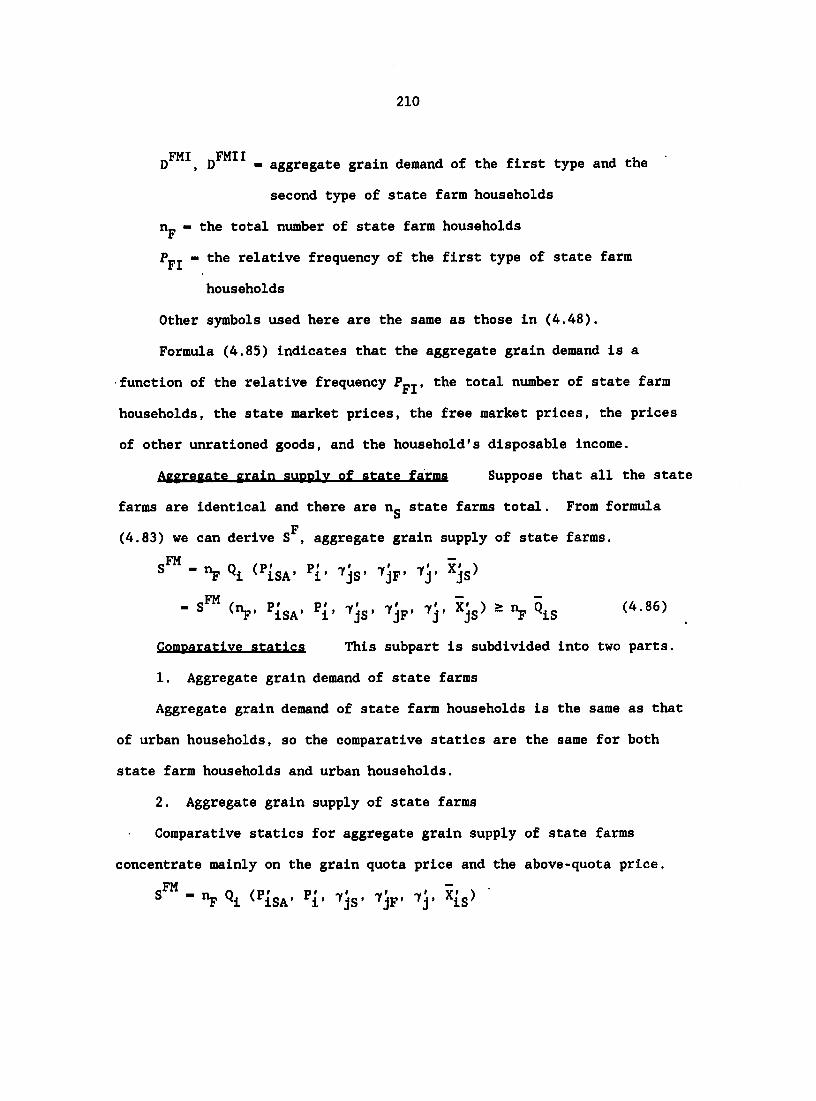
210

- aggregate grain demand of the first type and the

second type of state farm households

np - the total number of state farm households

Ppj - the relative frequency of the first type of state farm

households

Other symbols used here are the same as those in (4.48).

Formula (4.85) indicates that the aggregate grain demand is a

function of the relative frequency Ppj, the total number of state farm

households, the state market prices, the free market prices, the prices

of other unrationed goods, and the household's disposable income.

Aggregate grain supply of state farms Suppose that all the state

farms are identical and there are n state farms total. From formula

F (4.83) we can derive S , aggregate grain supply of state farms.

S - "p Qi (PiSA' ' 7js' 7jF' j'

- S (np, P , 7jg, 7jp. 7j. X g) & Hp Q g (4.86)

Comparative statics This subpart is subdivided into two parts.

1. Aggregate grain demand of state farms

Aggregate grain demand of state farm households is the same as that

of urban households, so the comparative statics are the same for both

state farm households and urban households.

2. Aggregate grain supply of state farms

Comparative statics for aggregate grain supply of state farms

concentrate mainly on the grain quota price and the above-quota price.

FM —

s - "F Qi (^iSA' 7jS' 7jF' j ' iS^

211

SS. FM 3Q,

aPis " a'ls " °

3P.„. "F ap. > 0

ISA ISA

The higher the above quota price is, the higher the aggregate grain

supply by the state farms is.

Graphic analysis The graphic analysis for aggregate grain demand

is presented in Figure 4.6. The graphic analysis here is limited to only

the aggregate grain supply of the state farms. The shape of the aggre­

gate grain supply of the state farms is the same as that of an individual

S " state farm, but the intercept on the Q axis has been changed to n Q g

(Figure 4.8).

•Vis

Figure 4.8. Aggregate grain supply of state farms in the mixed economy

We have finished our study of the first subsection, and we are

starting our work with the second subsection, the topic of which is the

theory of rural grain demand and supply of agricultural households in the

mixed economy.

212

Policy environment of agricultural households

Private agricultural household As a basic unit of production and

consumption in rural areas in the mixed economy, the agricultural

household makes its own decisions in its economic activities. It owns

almost all of the means of production except for the land used. Accord­

ing to contract, it is assigned a specific plot of land to plant within a

specified period.

Labor Agricultural laborers are transferable in the mixed

economy. The agricultural household can hire labor to help its operation

or can have its labor hired by someone else. In either case, the hired

laborer is paid wages.

Plan control The government has loosened its plan control in the

rural areas. First, it reduced the grain quota and agricultural tax in

grain, and tried to use price as a signal to guide the grain delivery to

the state market. Second, in early 1985, the government introduced a

contract system to replace the quota system for grain. According to the

contract, the government negotiates its purchase with agricultural

households before the sowing season. Thus, the households have their own

right to decide whether or not to sign the contract with the government.

In theory, the contracts are voluntary, but in practice, the contracts

become semi-mandatory to a great extent. In a certain sense, this

contract system can be thought of as a new quota system.

Market operation There are dual grain markets in the mixed

economy. The state market is considered to be dominated by the govern­

ment whereas the free market is regarded as a supplement to state

213

commerce. The government made an effort to improve the situation in the

state grain market. It raised the grain quota price about 30% to 50% and

set a higher above quota purchase price for grain delivered above the

quota. The government even tried to use a negotiated purchase price in

response to the free market price. In general, the above quota price is

less than the negotiated purchase price, which may be very close to and

even exceed the free market price. Since 1985, the government abolished

multiple prices in the state market. Instead, it set a uniform contract

price, 30 percent of the quota price plus 70 percent of the above-quota

price. Thus, this contract price seems to be more than the quota price

but less than the above-quota price and, of course, less than the free

market price. Besides, the government maintains the negotiated price,

which may approximate the free market price.

To be consistent with the analysis for the planned economy, we still

classify the agricultural households into three types by their activities

in the state market rather than in the dual markets. The first type is

called nonbuyer or complete seller in the state market because it has to

sign contracts and fulfill their obligations. Among the first type of

agricultural households, a majority generally produce grain to supply

themselves and the state market, even the free market. The minority may

produce other cash crops to make a profit and buy grain from the free

market for their own use and resale to the government. Hence, the

nonbuyer in the state market may be either a nonbuyer or a complete buyer

in the free market.

The second type is a partial buyer or a partial seller in the state

214

market because it has to fulfill its obligation by the contract and can

buy some grain back with the government's permission because of unex­

pected natural disasters. According to their situations in the free

market the second type of agricultural households can be subdivided into

two: one is a nonbuyer who does not need to buy grain from the free

market, the other one is a complete buyer who buys part of the consumed

grain from the free market to satisfy itself fully.

The last type of agricultural household is called a complete buyer

or nonseller in the state market because it does not need to produce and

sell grain by the government's plan. This type also contains two sub­

types: the nonbuyer who does not buy any grain in the free market, and

the complete buyer who buys but does not sell grain in the free market.

The basic situations are the same in the input markets. In brief,

there are also dual markets and dual (multiple) prices for the inputs

used by the agricultural households. Generally, the households purchase

their initial needs up to the official ration level in the state market,

then their additional needs at the higher prices in the free market.

Agricultural household model

For an agricultural household in the mixed economy, both its produc­

tion and consumption are managed by itself and guided by the government's

plan and information from both the state market and the free market.

Suppose that the household's objective is to maximize its utility, sub­

ject to its budget, production function, and other constraints given by

the plan control and that its utility function and production function

215

have the usual properties mentioned In Chapter III as well as in general

mlcroeconomlc theory.

To build a general agricultural household model in the mixed

economy, we have to take into further consideration the changes in the

price policy of the state government. It is known that there were

multiple prices and there are dual prices in the state grain market. In

fact, any multiple (more than two) price system can be seen as an

extension of a dual price system in which a quota price Pg and an above

quota price Pg exist and, of course, Pg > Pg. Considering the rela­

tionship between Pg and the free market price Pp, we ignore the cases

PgA > Pp or PgA - Pp. Readers can refer to the reasons from the discus­

sion about the relationship between Pg (Pg here now) and Pp in the last

section. Now we discuss the case Pg < Pp.

The reasons for an agricultural household to sell its product to the

state market at the lower Pg rather than to the free market at the

higher price Pp may be briefly summarized as follows: 1) lack of the

free market information; 2) consideration of additional transportation

cost; 3) receipt of the government's benefits, for example, receiving

lower cost inputs such as chemical fertilizer or an awarded right to buy

a good in shortage such as a name brand bicycle; or 4) influence of local

authorities. From the point of view of economics, the first reason can

be considered as the value of market information and the second reason

can be treated as sales cost. In fact, both of the reasons are deducting

some value from the free market price Pp. The third reason, actually, is

adding some value to the above-quota price, Pg . All three reasons are

216

reductions in the difference between Pg and Pp, even a change in sign in

case Pg < Pp. For simplicity, we ignore these three situations in our

theoretical model. The last reason is apparently noneconomic and,

therefore, is not discussed in this study.

Overall, there is no real economic reason for an agricultural house­

hold facing a free market to take such a voluntary action unless the gov­

ernment asks it to do so. Furthermore, the negotiated price can be seen

as the approximate free market price and can be ignored in this study

because it plays a role to transfer part of supply in the free market to

the state market. Under these circumstances, we assume a unique and

uniform price Pg that can be considered as either the above-quota price

(in the earlier stage of the mixed economy) or the contract price (in the

later stage of the mixed economy)--the new quota price--in our model.

Under all of these assumptions, we extend Sicular's (1988) model

from a three-good case to a multiple-good case and change her decision

variables from unreasonable and 7 to reasonable X . Our Lagrangian

function for the agricultural household in the Chinese mixed economy is

then as follows;

L - U [X (X g + X p) X , X ]

k k n k k

+ Ag G [Qi'

k

(Qis + Qip) > • • • > Q i I I Qjj]

k (4.87)

where

217

- the commodity consumed by the household (i - 1, ..., n)

- the i commodity consumed by the household in the state

market (i - 1, ..., k)

XiF - the i commodity consumed by the household in the free market

(i - 1 k)

X g - the state market ration for the i commodity (i - 1, .k)

- the i commodity produced by the household (i - 1 n)

Q g - the i commodity sold to the state market (i - 1 k)

Q p - the i commodity accounted at the free market price

(i - 1, ..., k)

- the sales quota to the state market for the i commodity

(i - 1 k)

iS " P.- - the state market price for the i*" commodity (i - 1, . . . , k)

P p - the free market price for the i' commodity (i - 1 k)

P - the price for the i commodity (i - 1, ..., n)

M - other income received by the household

For the household, X g & X g is a rationing constraint and Q g > Q g

is a sales quota constraint in the state market.

The Kuhn-Tucker conditions are;

0 i - 1 k (4.88) i

âL_ m_ îi " ax

aL_

'i

5L_ )i

dX ~ dX ' ^ i - 1, ..., n (4.89)

*i ax" " 0 i - 1 (4.90)

aq 3 0 i - 1 k (4.91)

218

+ Al9i < ° i - 1 n (4.92)

i - 1, ..., n (4.93)

âL__ 3A, --M+S Pij,Q„+s PjQ,-s PisX .s P,pXip.Z P,Xj;

1 1-1 1-1 1-1 1-1 1-1 1-1

0 1 dh

-s P,x,&0 (4.94)

(4.95)

- G [Q (Qig + Qip) Qjç. Q*] & 0 (4.96)

^ 2 I t - "

ax • *is • is °

aL__ _ n 31 ax 31

\s °

aL-, 41

x , Qi 0

*1S' *1F' IS' IF °

1' 2' 31' 41

The second tvne of agricultural household

then (4.94) becomes

k n k 2L__ aA,

(4.97)

k (4.98)

k (4.99)

k (4.100)

k (4.101)

, .... n (4.102)

k (4.103)

k (4.104)

Suppose that > 0,

n ,-S P.X,-0 (4.105) •r-xf, fis-'isf, '•Ar hshsf, fi

1 1-1 1-1 1-1 1-1 1-1 1-1

so that (4.95) can be dropped out. Moreover, suppose A > 0, then we

have

219

- G [Q (Q g + Qip) Q , Q„] - 0 (4.106)

Hence, (4.97) can be omitted. Now we work with (4.88) and (4.91).

Suppose all and (i - 1 n) are positive, that is, the house­

hold consumes and produces each commodity. Then

^ - 0 i - 1 n (4.107)

^ - 0 i - 1 n ( 4 . 1 0 8 )

Immediately applying the mathematical transformation (4.16), assum­

ing the household makes both its initial purchase and sale from and to

the state market rather than the free market, both and > 0, and

considering the possible situations in the mixed economy, both (4.107)

and (4.108) imply only three cases;

Case 1:

™

Case 2:

Case 3:

Furthermore, suppose that for the agricultural household, the first

d^^ within the first k'^ commodities belong to case 1, the e^^ through

the g^^ commodities belong to case 2, and the remaining h*"^ through the

k^^ commodities belong to case 3. We then have

ax, • ax,_ ' •^l^iS ' 3i • ° i-1 d (4.112)

220

1%; - "iPis - "31 > ° ^ »= <4113'

(4 114)

ViF - » 1 - ' " <411:

1 ^ - % ; - • ^ i ^ s • \ i - V 1 - 1 s < 4 1 1 * )

^ ^ • "I'lS * ^41 > ° 1-" •= (4 llf' .

V i F 1 - 1 e < 4 1 1 * )

ViF-" 1-" " <"11"

Finally, consider situations of both constraints (4.98) and (4.100).

Because of a shortage of consumed goods and the price difference between

the state market and the free market, rural households usually use up

their purchase rations. On the other hand, by the contract, the sales

quotas must be fulfilled. Thus, we simply assume that all and >

0 (1 - 1 k), immediately;

- X , - X , - 0 1 - 1 k ( 4 . 1 2 0 ) IS LS

It;; - Sis - Si: - 0 1-1 k (4.121)

Apparently both (4.120) and (4.121) imply deletions of (4.99),

(4.101), (4.112), and (4.116). Consequently, our model is composed of

(4.113) through (4.115), (4.117) through (4.119), part of (4.107) and

(4.108) (1-1, ..., n), and (4.105) through (4.106).

Due to the assumption of positiveness of all Ag^^ and A^^, there are

221

no free choices for the agricultural household in the state market.

After fulfilling the sales quotas and using up purchase rations, the

agricultural household can have free choices in the market. Thus, we let

M' - M + s Pjs «IS - ifis) , (4.122) i-l

M' represents the real disposable income of the agricultural

household before its free choices both in the state market without any

restriction and in the free market.

Provided that the second-order conditions are satisfied, considering

final Kuhn-Tucker conditions simultaneously, and letting

P[p - (1 - h, ..., k) and P^ - P^ (1 - 1 n),

the implicit (If any) grain demand and supply functions for the agricul­

tural household would be

i - 1 d (4.123)

*i " iS "*• ^IF

- X^s + IF (flF' 1' M') > *18 i - e k (4.124)

Xi - X^ (P|p, P[, M') i - 1, ..., n (4.125)

- Qjg i - 1 g (4.126)

^i " iS ^IF

- Qis + Qip ('ÎF' *1' M') > k (4.127)

Qi - Qi (P^p, P(, M') i - 1 n (4.128)

Because we derive the above results by assuming both X^^g and >

0, these results fit the case of the partial buyer or partial seller,

the second type of agricultural household. Thus, we can conclude that

222

the possible combination of grain demand and grain supply functions for

any of the second type of households might be (4.123) and (4.126), or

(4.124) and (4.126), or (4.124) and (4.127). In other words, we have

Xjiii - ïjj (4.129)

*jII2 " *jII3 " *jS "*• *jF (*iF' ^ *jS (4.130)

and

Sjlll • jn2 • jS _ <4 131'

9jII3 - SjS + QjF > Sjs (4 1:2)

These results indicate that, for the second type of agricultural

household, the grain demand is either the grain ration (the first sub­

type) or a function of the free market price vector, the prices of other

goods, and its disposable income (the second and the third subtype),

whereas its grain supply is either the sales quota (the first nd the

second subtype) or a function of the same factors used in its demand

functions plus its grain sales quotas (the third subtype).

To obtain the grain demand and supply functions for the first and

the third types of agricultural households, we can use our basic model

but adjust part of our assumptions to fit their situations.

The first type of agricultural household For the first type of

household, the nonbuyer in the state market, the only thing we need to do

is note that assumption - 0 for 1-1, ..., b has replaced part of

the assumption of > 0 for 1-1 k. Consequently, the change in

the Kuhn-Tucker conditions are that part of (4.114), (4.120) and (4.121)

for 1-1 b drop out, and part of (4.117) for i - 1, ..., b

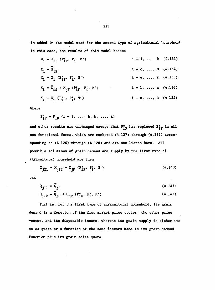
223

Is added in the model used for the second type of agricultural household.

In this case, the results of this model become

- 1 , . X. - XiF (PÏF- Pi' M')

- X, is

-X, (p;,, Pi. M')

-Xis+XjF (P;?, Pi. M')

- \ (PJlF' *1' M')

- c,

- e,

- 1,

- e,

b (4.133)

d (4.134)

k (4.135)

n (4.136)

k (4.135)

where

^iF • iF (1 - •» b| h| . .# k)

and other results are unchanged except that Pj^p has replaced P^p in all

new functional forms, which are numbered (4.137) through (4.139) corre­

sponding to (4.126) through (4.128) and are not listed here. All

possible solutions of grain demand and supply by the first type of

agricultural household are then

and

Xjll - XjI2 - XjF (PÎF' i' M')

Qjii " 9js

QjI2 - Qjs + Qjp (p;p, Pi. M')

(4.140)

(4.141)

(4.142)

That is, for the first type of agricultural household, its grain

demand is a function of the free market price vector, the other price

vector, and its disposable income, whereas its grain supply is either its

sales quota or a function of the same factors used in its grain demand

function plus its grain sales quota.

224

The third type of agricultural household Similarly, for the

third type of households, complete buyers or nonsellers in the state

market, we need to use - 0; therefore, - 0 for i - l,...,b

replaces part of the assumption > 0 and > 0 for i - 1,... ,n.

Furthermore, we cancel part of (4.100) for i - 1, b and add part of

(4.117) for i - 1, ..., b to the model of the second type of household.

All possible solutions of grain demand and supply of the third type of

agricultural household are

Xjllll • *jS (4.143)

XjIII2 - XjS + XjF (PiF' (4.144)

and

Qjlll - 0 (4.145)

These results mean that, for the third type of agricultural house­

hold, its grain demand is either the official ration (the first subtype)

or a function of the free market price vector, the other price vector,

and its disposable income (the second subtype), whereas its grain supply

is always zero.

Comparative statics The comparative statics are shown for the

grain demands and grain supplies of all three types of agricultural

household. To save time and space, we calculate only grain price, grain

ration, and grain quota effects.

1. The first type of agricultural household

a. the first subtype

*jll • *jF (^iF' M')' Qjii • Qjs

225

Thus,

iîj'- S" i!i< • " iif • •

ïr-î;-ax.Ti 3X,„ -Lf. 8X._ aq

ill

s " These results imply that, for the first subtype within the first

type of agricultural households, (1) grain demand decreases but grain

supply does not change if the state market price or the free market price

increases; and (2) grain demand decreases but grain supply increases if

the sales quota increases.

b. the second subtype

XjI2 - XjF (PiF' *1' M')

QjI2 " QjS QjF (^iF' i' **')

Because Xj^g " do not need to discuss the partial deriva­

tives for Xjj2 here. For we have

Sî'-Sï-

If-'*-The results illustrate that, for the second subtype within the first

226

type of agricultural household, grain supply increases when the state

market price, the free market price, or the sales quota increases.

2. The second type of agricultural household

a. the first subtype

*jiii " *js' Qjiii • QjS

fiuii. Hmi _ 0 _ fSmi _ o

aXjs aXjs

_ 0 . 1

The results illustrate that, for the first subtype within the second

type of agricultural household, (1) grain demand and supply do not change

when either the state market price or the free market price increases;

(2) grain demand increases but grain supply does not change when the

grain ration increases; and (3) grain demand does not change but grain

supply increases when the sales quota increases.

b. the second subtype

*jII2 ' *jS *jF (^iF' i' M')' QJII2 " Qjs

Because Qjjj2 " Qjm' partial derivatives for Qjjj2 the

same as those for and, hence, do not need to be repeated and

rediscussed here. For we have

J® . J»

227

film . fïjE ^ „ '"jP "JF

'"js '*JS *XjS

t^jui. f^E an < 0

The results mean that, for the second subtype within the second type

of agricultural household, the grain demand is decreasing if the state

market price, the free market price, or the sales quota increases; and it

increases if the ration level increases.

c. the third subtype

*jII3 " *jS *jF (^iF' i' **')

QjII32 " jS "*• ^JF (*iF' i' **')

Because - Xjjj2' not repeat calculations and discussion

for the partial derivatives of X.,,? here. For Q.-,., we have

ja ja

« S " " axjs aXjs

228

For the third subtype within the second type of agricultural house­

hold, the grain supply increases as the state market price, the free

market price, or the sales quota Increase; and it decreases as the ration

level increases.

3. The third type of agricultural household

a. the first subtype

Using formula (4.143) and (4.145) we have

*jllll • XjS

Qjllll " °

thus,

fiiUIl _ fiiUU _ 0

fiiui _ 1

axjs

For the first subtype within the third type of agricultural house­

hold, its grain demand increases if the official ration increases, and

its grain supply is always zero.

b. the second subtype

From formula (4.144) and (4.145)

*JIII2 " *JS '^iF' ''i' " '

"jiiiz - "

hence

JO ja

229

•JS

JUIZ > 0 if

ax mi2_ 0

We can conclude that, for the second subtype within the third type

of agricultural household, the grain demand (1) decreases if the state

market price or the free market price increases, (2) increases if the

official ration increases, and (3) does not change if the sales quota

increases. On the other hand, its grain supply always remains fixed at

three types of agricultural households in both the state market and the

united market that combines the free market with the household-own

market. Thus, we need to change our previous dual market graph (graph

for the state market and the free market) into a new dual market graph

(graph for the state market and the united market) but use the same

procedures used before.

1. The first type of agricultural household

a. the first subtype

For the first subtype of nonbuyer in the state market, its demand in

the (Q", P" - P^) subspace is a downward-sloping line, and its supply in S s

the (Q ,P ) subspace is a vertical line (Figure 4.9a).

zero.

Graphic analysis The graphic analyses are presented for all

230

,U,

<jll

VjS ^

(a)

Figure 4.9. Grain demands and supplies of the first type of agricultural household

b. the second subtype

For the second subtype of nonbuyer, its only demand in the united

market is a downward sloping line, and its supply consists of one

G C vertical line in the (Q , P ) subspace and one upward-sloping line in the

(Q^, P^) subspace (Figure 4.9b).

2. The second type of agricultural household

a. the first subtype

For the first subtype of partial buyer in the state market, both

S s grain demand and supply are vertical lines in the (Q , P ) subspace

(Figure 4.10a).

b. the second subtype

For the second subtype of partial buyer in the state market, grain

S s demand consists of two segments: one is a vertical line in the (Q , P )

subspace, and the other one is a downward sloping line in the (Q^, P^)

S s subspace. Grain supply is a vertical line in the (Q , P ) subspace

231

(Figure 4.10b),

„U

jiii Qjlll Q"

*js js

(a)

„U

*js QjS

(b)

JII2_ç

.U

jII3

jII3

Xjs QjS

(c)

Figure 4.10. Grain demands and supplies of the second type of agricultural household

c. the third subtype

As Figure 4.10c shows, for the third subtype of partial buyers in

the state market, both demand and supply are composed of two segments.

S s For the former, one is a vertical line in the (Q , F ) subspace, and the

other one is a downward-sloping line in the (Q^, P^) subspace. For the

S s latter, one is a vertical line in the (Q , P ) subspace, and the other

one is an upward-sloping line in the (Q^, P^) space.

3. The third type of agricultural household

a. the first subtype

For the first subtype of complete buyer in the state market the

S s demand curve is only a vertical line in the (Q , P ) subspace (Figure

4.11a).

b. the second subtype

As Figure 4.11b indicates, for the second subtype of complete buyer

232

in the state market, its demand curve is the same as that in Figure

4.10b.

jS

(b)

Figure 4.11. Grain demands and supplies of the third type of agricultural household

Aggregate grain demand and supply of agricultural households

Aggregate grain demand of agricultural households As we pointed

out, agricultural households in the mixed economy can be classified into

three types by their behavior in the state market. To aggregate grain

demand of agricultural households, we start with aggregation of grain

demand of the first type of household. Assuming that the total numbers

of all agricultural households is n^, that the relative frequency of the

first type and the first subtype within the first type of agricultural

households is and , respectively, and that all households of the

first type are identical except for their behavior in the market(s), we

HI can draw D , the aggregate grain demand of the first type of agricul­

tural household, as the following:

(4,146)

233

where

HI l

^ " HI HIl "H Xjll

" HI HIl "H *jF (^IF'

ml - (Pjjj, n , PJp, P . M') (4.147)

HT9

° " HI ^HIl^ "H XjI2

" Hi " ^Hii^ "H *JF (^iF'

- oHIZ (Pj j, rijj, P p. P , M') (4.148)

Consequently,

- 'HI "H V (PÏF' n'

HT " (^Hr "H' PiF' i' "") (4.149)

That is, aggregate grain demand of the first type of agricultural

households is a function of the relative frequency P^^ , the total number

of agricultural households, the free market price vector P^^, the other

prices P^, and the disposable income M'.

HII HIII In the same way, we can get D and D , aggregate grain demand

of the second and the third type of agricultural households. Algebrai­

cally,

D"" - (4.150)

where

_HII1 _ " HII HIIl "H Xjlll

- P, HII ^HIIl "H jS

^ (^HII' HIIl' "H* Xjg) (4.151)

234

HII2 _ HII HII2 "H jII2

" HII HII2 "H [XjS "*• ^jF (^IF' M')]

" (^HII' HII12' "H* *jS' iF' (4.152)

HTI3

^ " HII • HII2^ "H XjII3

" HII " ^HIIl • HII2^ "H [*jS *jF (^IF' ' M')]

UTTO —

" ^HIIl' HII2' "h' *jS' IF' (4.153)

Hence

HTT —

^ " HII HIIl "H *JS ^HII HII2 "H^*jS"'"*jF (*iF'

^HII • HIIl • HII2^ "H [XjS •*• ^jF (^IF' i' M')]

• HII "H jS "*" ^HII • HIIl^ "H jF (^iF"

HII — " (^HII' HIIl' "H* *jS' IF' i' ) (4.154)

Similarly,

(4.155)

where

^ " ^HI ^HII^ ^HIIIl "h jllll

" ^HI • HII^ ^HIIIl "H JS

" ^^HI' HII' HIIIl' "H' *js) (4.156)

^ " HI ^HIl) ' HIIIl^ "h *jIII2

(^'^Hl'^HII^ ^^"^HIIIl^ "H [*jS *jF (^IF' l'

• ^^HI' ^HII' HIIl' "H' *jS' IF' i' (4-157)

235

Thus,

^ ^HII^ "H jS

" ^HI ' " ^HIIIl)"H^^jS "*"

" • HI • HII^ "H jS

"*• " ^HI " ^HIl) " ^HIIIl^ "H *jF (^IF' i'

- D (Pj^j, Pjjjj., ^HIIIl' "H' *jS' IF' ^i' (4.158)

These results Imply that the aggregate grain demand of the second

and third type of agricultural households are functions of the relative

frequencies , P^jj. and the total number of agricultural house­

holds, the free market prices, the prices of other commodities, the

ration limits, and the disposable income M', and a function of the

relative frequencies P^^, P^^^ and •PHUH' total number of agricul­

tural households, the free market prices, the prices of other commodi­

ties, the ration limits, and the disposable income M'.

Finally, adding (4.149), (4.154) and (4.158) together, we obtain D^,

the aggregate grain demand of all agricultural households:

d" - (4.159)

" HI "H jF (^iF' i*

^HII "H jS ^HII ' HIIl) "H jF (^iF' i'

+(1 - Pj^j - Pj^jj) rijj Xjg

' HI ' HII^ ' HIIIl^ "H *jF (^iF' i' ^

236

(1 - Pjjj) iijj Xjg + Pjjj rijj Xjp (PJp. M') + [Pjiji (1 -

" HI " HIl) " ^HIIIl)] "H *jF (^IF'

(1 - Pjjj) Xjg + HI "H *JF (^IF'

+ [1 - Pj^j - Pjjjj ^HIIl " HIIIl ^HI

*jF (^IF' i' ^

- D (Pjjj, Pjjjj, ^HIIIl' "H' *jS' IF' i' (4.160)

where U D - aggregate grain demand of agricultural households

pHI^ pHII ijHIII _ aggregate grain demand of the first, second, or

third type of agricultural households

^HI' relative frequency of the first or the second type

of agricultural households

^HIIl' HIIIl " relative frequency of the first subtype within

the second or third type of agricultural households

n^j - the total number of agricultural households

Other symbols used here, such as X.„, Py„, P.', and M", are the same JO If 1

as those mentioned earlier in this section.

Formula (4.160) indicates that the aggregate grain demand is a

function of the relative frequencies P^^, Pfjjji ^hIII' ^HIIIl'

total number of agricultural households, the ration limits, the free

market prices, the prices of other goods, and the disposable income M".

Aggregate grain SUPDIV bv agricultural households By using the

same aggregation method as that used in the analysis of the aggregate

237

grain demand of agricultural households, and making proper assumptions

about the total number of agricultural households and the relative

frequencies and identicalness of agricultural households within a certain

type or subtype, we can obtain

gHI _ gHIl gHI2 (4.161)

where

® " HI HIl "H Qjii

" HI HIl "H QjS

°HI' ^HIl' "H' HTl —

- (P„-, P_,, n„, Q._) (4.162)

S - Pjjj (1 - njj QJJ2

- Pjjj (1 - Pj jj ) tijj [Qjg + Qjp (PiF' M')]

HTl — " ® ^^HI' ^HIl' "H' 9js' PjLF' (4.163)

Then,

HI — ^ " HI "H jS ^HI " ^HIl^ "H "^JF (^iF' i'

HT — - s (Pj^j, n^, Qjg, PiF' M') (4.164)

Similarly,

gHII _ gHIIl gHII2 gHII3 (4.165)

where

Hill ^ " HII HIIl "H Qjlll

- P, HII ^HIIl "H QjS

" (^HII' HIIl' "H' Ôjg) (4.166)

238

sHII2 . p p no HIT HII2 H jII2

P, HII ^HII2 "H jS

- S (^HII' HII2' "H' Ôjg) (4.167) UTTQ

® " HII " ^HIIl " ^HII2^ "h 9jII3

' ^HII^^ " HIIl " HII2^"H^^jS

" (^HII' HIIl' HII2' "H' Ôjs' ÎF' (4.168)

Thus, substituting (4.166) through (4.168) into (4.165) we obtain

HIT — — ^ " HIl"H^jS •*• ^HII^l • HIIl • HII2^"H^jF^^iF' '^i' ^jS '

HI I — " ® (^HII' HIIl' HII2' "H' QjS' ^iF' i' (4.169)

Finally,

SHIII - gHIIIl + sH:I:2 (4.170)

where

^ - (1 - ^HII • HII^'^HIIII "H Qjllll

- 0 (4.171)

HT T T 9

^ - ^HII " HII^ • HIIIl) "H 9jIII2

- 0 (4.172)

Substituting (4.171) and (4.172) into (4.170) we have

- 0 (4.173)

Adding (4.164), (4.169), and (4.173) together) we have S^, the

aggregate grain supply of all agricultural households:

s" - (4.174)

239

" "H jS "H QjP (^iF' i' "*" ^HII "H jS

•*" ^HII • HIIl " ^HII2^ "H JF (^IF' l' JS'

' (^HI ^HII^ "H jS

+ [Pjjj + Pjjjj (1 - - i'ljjjg)] "H jF ( IF' i' iS'

• ® (^HI' HII' HIIl' HII2' "H' Ôjs' iF' ^ (^-175)

where

H s - aggregate grain supply of agricultural households

gHI^ gHII gHIII _ aggregate grain supply of the first, the second,

or the third type of agricultural households

Other symbols, such as ^HII2' "H* *iF' i* ^jS'

M', are the same as before.

Formula (4.175) shows that the aggregate grain supply of all agri­

cultural households in the mixed economy is a function of the relative

frequencies P^^, Pjjjj. and the total number of agricultural

households, the sales quotas, the free market prices, the prices of other

goods, and the disposable income H', respectively.

Comparative statics Comparative statics are calculated for both

aggregate grain demand and supply by agricultural households.

1. Aggregate grain demand of agricultural households

From (4.159) and other relevant formulas we have

D" - f D"" + D»:::

a. D": _ + D»::

240

⣠. âDilll ^ âEÏIi , „

asE: _ âi£El + acîîE > q an^ atijj 3n, H

âEÏi _ ^ âcîîH ^ „

3Qjs aSjs »Qjs

âEÏL _ acîlii aaïiî „

«fjs "js

âi£i . ap"" + ap"" < „ aPjF aPjF sfjF

The aggregate grain demand of the first type of household increases

if the relative frequency f , or the total number of agricultural house-Hi

holds increases; and it decreases if the sales quota, the state market

price, or the free market price increases.

b ^nil _ pHIIl pHII2 + pHII3

^^HII ^^HII ^^HII ^^HII

**HII1 *^HII1 ^^HIIl ^^HIIl

^^HII2 ^^HII2 ^^HII2 ^^HII2

^"h ^"H ^"H ^"H

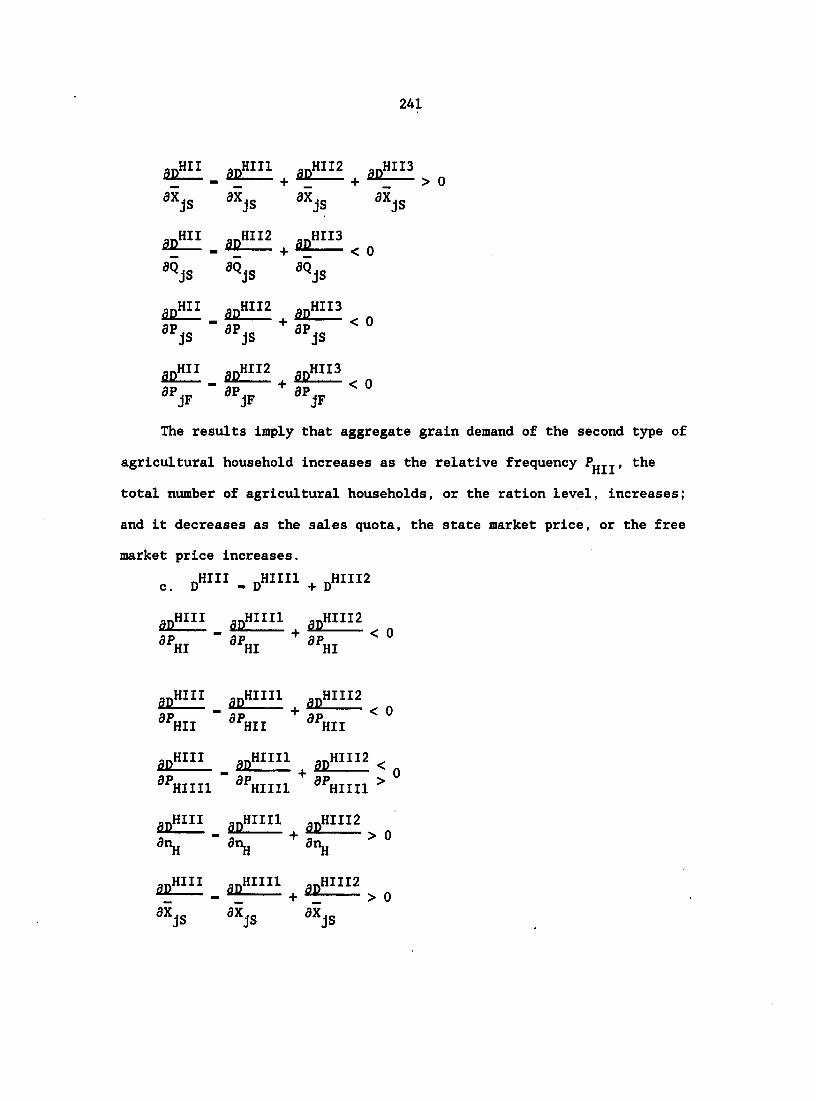
241

axjs «js

'^js »Qjs «Qjs

acH aïïIH ^ âîlî^H , „ »'js "^fjs "js

The results imply that aggregate grain demand of the second type of

agricultural household increases as the relative frequency Pjjjj, the

total number of agricultural households, or the ration level, increases;

and it decreases as the sales quota, the state market price, or the free

market price increases.

o. D""' - d""" + D"""

iliîfîi ,„Hni2

"«''HI

""HII "HII ®''HII

_ apHIIIl an""" <

^^HIIIl ^^HIIIl ^^HIIIl

anHlll apHllll apHlllZ

.pHIII _ apHIIIl ,pHIII2

5Xjs aXjs aXjs

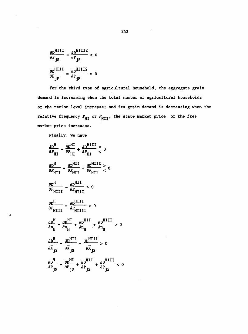
242

,„Hin _

-JP

For the third type of agricultural household, the aggregate grain

demand is increasing when the total number of agricultural households

or the ration level increase; and its grain demand is decreasing when the

relative frequency or , the state market price, or the free

market price increases.

Finally, we have

âCÎL _ âûîï apHiii >

^

gp" _ gp"" âniiiE > 0

^^HII ^^HII ^^HII ^

âDÎÎ ap"" 0

2pÎL_ . D!1££L > 0 ^^HIIl ^^HIIIl

flpL _ âfiiEi ^ âcEfi > Q

axjs aXjs aXjs

a s !L_ a D !!I + ac!Hi + a)!!Hi<o aPjs aPjs aPjs

243

an" an"' an"" an*"''

«V afjP aPjp WPjF

Hence, the aggregate grain demand of agricultural households

Increases If the relative frequency or the total number of

agricultural households, or the state ration Increases; and It decreases

If the state market price, Pjg, or the free market price, Pjp, Increases.

2. Aggregate grain supply of agricultural households

From (4.174) and other relevant formulas we have

s" - s": + s":: +

a. s": _ sHii + s"i2

âsE _ asEi âsîîii «

as"! _ agHii agHiz >

^^HIl *^HI1 ^^HIl

asH _ âsïïl agHiZ ^ Q

aOjs aOjs aOjs

_ âsilfî > 0

The aggregate grain supply of the first type of agricultural

household Increases If the relative frequency P , the total number of HI

agricultural households, the sales quota, the state market price, or the

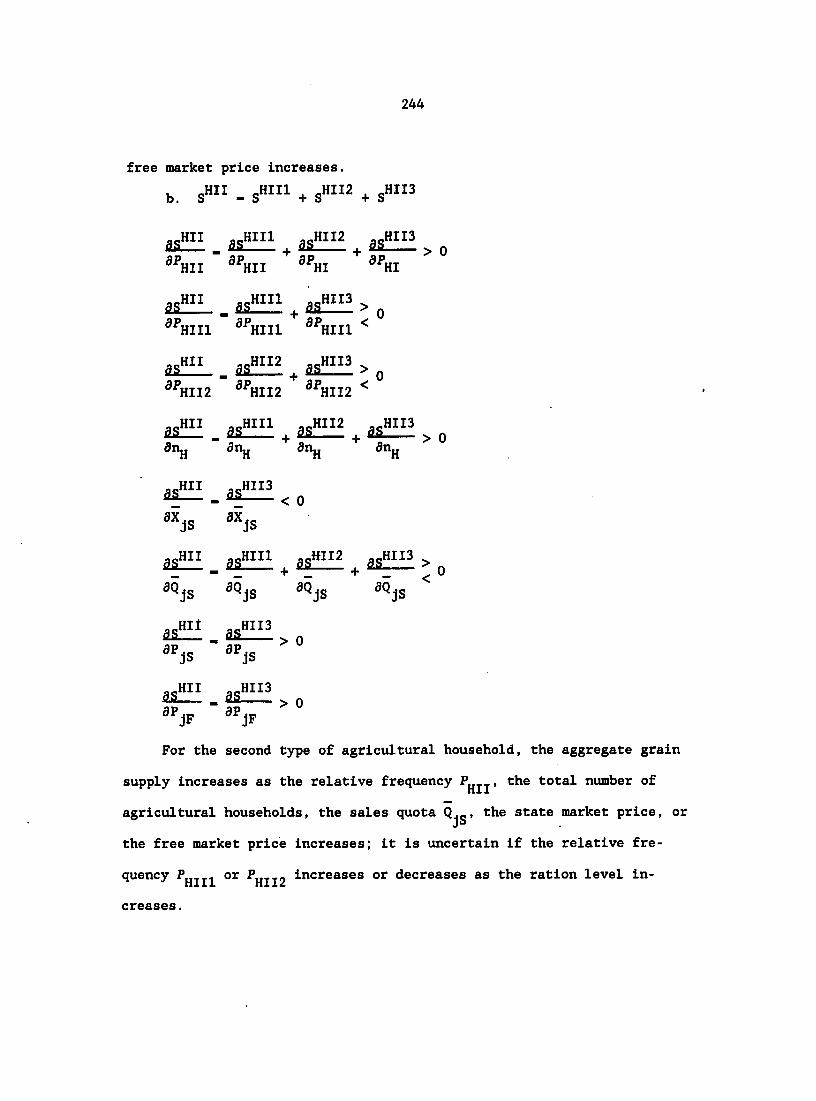
244

free market price Increases.

b. s"" - s""" + s"'" + s""'

âs!E . âsïill asïïffî âsîEi > 0 ^^HII ^^HII

aa!!IL_as!2H + aa!H!>o ^^HIIl ^^HIIl ^^HIIl

âs ï iL .â^ ,âs!Ei>o ^^HII2 ^^HII2 ^^HII2 <

-.HII ..Hill --HII2 HII3 QÂ _ as + flS + flS > 0 anjj gn 3njj dn

a-HII HII3 fiS— _ as < 0

»JS aXjs

asH_a5HH + as!!H! + as!EH>o

sQjs aSjs aSjs ^

ï7-ïr-

*7-*r-For the second type of agricultural household, the aggregate grain

supply increases as the relative frequency , the total number of

agricultural households, the sales quota Q. , the state market price, or

the free market price increases; it is uncertain if the relative fre­

quency or increases or decreases as the ration level in­

creases.

245

c. s"::: - o

Thus, we have

®^HII °^HII

âsH . âslîi + as"" > 0 ÔHH atiH atijj

âsî!_ . âsïlf < 0

*Xjs axjs

âsîL _ asH + gs"" > 0

> 0

aSjs aSjs aSjs

"js

+ 85"" .

4" aPjF "JF > 0

These results indicate that the aggregate grain supply is increasing

if the relative frequency P„_ or P»__, the total number of agricultural HI nil

households, the sales quota, the state market price, or the free market

price increases. It decreases if the ration level Increases.

Graphic analysis Graphic analyses are performed for the aggre­

gate grain demand and supply of all three types of agricultural house­

holds individually.

1. The first type of agricultural household

246

There are two subtypes within the first type of agricultural house-

HXl holds. Aggregate grain demands and supplies of the first subtype (D

HIl HI2 HI2 and S ) and the second subtype (D and S ) of agricultural house­

holds are similar in their curves' shape to those individual agricultural

households within the first subtype and the second subtype. For the

former, the aggregate grain demand is a downward-sioping line in the (Q^,

p") subspace, and the aggregate supply is a vertical line in the (Q^, P^)

subspace with an intercept - Pjjj n^ Qjg (Figure 4.12a). For

the latter, the aggregate grain demand is a downward-sloping line in the

(Q^, P^) subspace, and the aggregate supply is composed of two segments:

one is a vertical line with an intercept - P^j (1 - "h jS

S s s the Q axis in the (Q , P ) subspace. The other is an upward-sloping

line in the (Q", P") subspace (Figure 4.12b).

pU, HI2gHI2 pU,,D": s":

(C)

Figure 4.12. Aggregation of grain demands and supplies of two subtypes within the first type of agricultural households

HI HI Figure 4.12c shows the aggregate grain demand D and supply S of

HI the first type of agricultural households. D is a downward-'si oping

247

line in the (Q^, P^) subspace, and is similar to in shape, but

S " ""F its intercept on the Q axis is now Qjjj^ - Ppjj n^ Qjg. At P , the

equilibrium price of the free market, there is a surplus in the united

market so that the second subtype of the first type of agricultural

households are main suppliers in the free market.

2. The second type of agricultural household

There are three subtypes within the second type of agricultural

households. The aggregate grain demands and supplies for the first

and the second and and the third and

gHII3j subtype are illustrated in Figure 4.13a, b, and c. Both and

gHIIl vertical lines with intercepts on the axis: Qnnia "

^HII^HIIl .Vj£ and Q, Hlllb • HII^HIIl"H^jS' D

HII2 is composed of two

pieces; one is a vertical line with an intercept Qjjjj2a " HII^HII2"H^jS

S s in the (Q , P ) subspace, the other one is a downward-sloping line in

(Q"\ p") subspace. is only a vertical line that has an intercept

— s S HII3 HII3 ^HII2b " (Q , P ) space. Both D and S

consist of two segments. The former has one vertical segment in

,u,

d"" S«" -S

" " q" '

%IIla^HIIlb

(a)

p"l p:

HII2

HII3„HII3

^HII2a^HIl2b Q®

(b)

'^HII3a^HII3b

(c)

Figure 4.13. Aggregate grain demands and supplies of three subtypes within the second type of agricultural households

248

S S the (Q , P ) subspace, with an intercept

n XJG on the axis and one downward-sioping segment in the (Q", P* ) S s

subspace. The latter has one vertical segment in the (Q , F ) subspace

" S with an intercept the Q axis, and

one downward-sloping segment in the (Q", P") subspace.

By summing Figure 4.13a, b, and c, we obtain the aggregate grain

HIT HII demand D and supply S of the second type of agricultural household

HII HII in Figure 4.14. Both D and S contain two segments and are similar

S HII in shape to Figure 4.13c, but the intercept on the Q axis for D is

HII Hlla " %IIla HII2a %II3a ® Hllb " %IIlb

%II2b HII3b'

HII JHII

rS

Hlla Hllb qS

(a)

Figure 4.14. Aggregate grain demand and supply of the second type of agricultural households

3. The third type of agricultural household

There also are two subtypes within the third type of agricultural

household. As Figures 4.15a and b show, the shapes of the aggregate

grain demands and supplies for both the first subtype and

HIII2 HIII2 and the second subtype (D and S ) are similar to those in

249

HIIIl HIII2 Figures 4.11a and b. The Intercepts for D and D now are

Hlllla " ' HI • HII HIIIl "H *jS %III2a " ' HI " HII

(1 HIIIl "H *jS'

„U

DHIIII qU

pU HIII2 pU.

.u

Hllllba qS

(a)

HIII2a qS

(b)

Hllla

Figure 4.15. Aggregation of grain demands and supplies of the third type of agricultural households

The aggregate grain demand and supply of the third

type of agricultural household are drawn in Figure 4.15c. They look like

HIII S those in Figure 4.15b, but the intercept of D on the Q axis is

Hllla " Hlllla HIII2a'

Finally, adding Figure 4.12c, 4.14, and 4.15c together, we obtain

H H the aggregate grain demand, D , and supply, S , of all agricultural

H H H households in Figure 4.16. Both D and S contain two segments. D

S s consists of one vertical line in the (Q , P ) subspace, with an intercept

Qjla " Hla %IIa Hllla Q axis and a downward-sioping line in

the (q",p") subspace. S , on the other hand, consists of one vertical

S s line in the (Q , P ) subspace, with an intercept +

Qniiib o" the axis and an upward-sloping line in the (Q , p") sub-

—p H H space. Given P , obviously S > D so that agricultural households,

250

especially the first type, are main suppliers in the free market.

-S

S

Figure 4.16. Aggregate grain demand and supply of all types of agricultural households

The state market analysis

Because grain demand of the state farm households is the same as

that of the urban households and grain supply of the state farms occurs

in the state market only, it is not necessary to repeat the state market

analysis for the state farm (households) in this part. Instead, the

state market analysis concentrates on grain demand and supply of the

agricultural households in the state market. This part is subdivided

into two parts: one analyzes individual behavior of agricultural

households; the other analyzes aggregate behavior of agricultural

households. Now we work on the first subpart.

Grain demand and supply bv agricultural household in the state

market There are three types of agricultural household in the state

market.

1. Nonbuyer

Xjgj - 0 (4.176)

251

QjSi-Qjs (4.177)

The grain demand of nonbuyer in the state market is zero and the

grain supply of nonbuyer in the state market is fixed at Qjg.

2. Partial buyer

XjSII " jS (4.178)

QjSII • QjS (4.179)

For a partial buyer, both grain demand and supply in the state

market are fixed at X g and Qjg. If Xjg < Qjg, this partial buyer is a

net seller in the state market. Otherwise, he is a net buyer in the

state market.

3. Complete buyer

KjSIII " jS (4.180)

QjSIII - 0 (4.181)

For a complete buyer, the grain demand is fixed at X.„ at the state J®

market and the grain supply is zero.

Comparative statics for the individual grain demands and supplies

Comparative statics are made for individual grain demands and supplies

of these three types of agricultural household.

1. Nonbuyer

XjSI - ° "jsi - QjS

For a nonbuyer in the state market, the grain demand is zero and

252

unaffected by any policy instruments, and its grain supply is only

affected by the sales quota in the same direction.

2. Partial buyer

*jSII • jS QjSII " QjS

_ fibsii , 0 fSisu . fSjsn . 0

aXjs aXjs

0 !Smi_ 1

"Qjs Qjs

For a partial buyer in the state market, grain demand increases if

the ration level increases, and grain supply increases if the sales quota

increases.

3. Complete buyer

*jSIII " jS jSIII " jS

The comparative statics for are the same as that for Xjgjj,

whereas the comparative statics for Qjgjjj are always zero.

Next are analyses of the second subpart.

Aggreeate grain demand of agricultural households in the state

HTS HTTS HTT IS market First, we aggregate D , D and D , grain demands of

the first, the second, and the third type of agricultural households,

HS then add them together to obtain D , aggregate grain demand of all

agricultural households,

- D"" + (4.182)

253

From formulas (4.149), (4.154), and (4.158), we easily conclude that

_ 0 (4.183)

In the state market, aggregate grain demand of nonbuyers is zero.

• HII "H *jS

- (Pjjjj, njj, Xjg) (4.184)

Aggregate grain demand of partial buyers in the state market is a

function of the relative frequency , the total number of agricultural

households, and the ration level.

- (1 - "H jS

- D (Pjjj, Pjjjj, Hjj, Xjg) (4.185)

For complete buyers, aggregate grain demand in the state market is a

function of the relative frequencies and , the total number of

all agricultural households, and the ration level.

Substituting (4.183), (4.184), and (4.185) into (4.182), we have

HS " ~ • " HII "H *jS • HI " HII "H *jS

• "H jS

uc — - (P„J. njj, Xjg) (4.186)

Thus, aggregate grain demand of agricultural households in the state

market is a function of the relative frequency , the total number of

agricultural households, and the ration level X._. J®

Aggregate grain supply of agricultural households in the state

HS market Similarly, we have the following formula for S , aggregate

grain supply of agricultural households in the state market;

254

gHS _ gHIS + gHIIS gHIIIS (4.187)

HIS HIIS HIIXS where S , S , and S are aggregate grain supply for the first,

second, and third types of agricultural households and can be obtained

from formulas (4.164), (4.169), and (4.173):

HIS " "HI "H jS

HIS

S - P.„ Q

( 'hi' "h' Qjs) (4.188)

HIIS " "HII "H ""jS

S - P..„ n Q

UTTC —

- (Pjjjj, njj, Qjg) (4.189)

In the state market, grain supplies of both nonbuyers and partial

buyers are functions of the relative frequency, the total number of

agricultural households, and the sales quota.

_ 0 (4.190)

For complete buyers in the state market, the grain supply is zero.

Adding (4.188), (4.189) and (4.190) we have

HS " — ® " HI "H QjS HII "H QjS

(PHI + Pj jj) tijj Qjg

HS — - S (Pj j, Pjjjj, njj, Qjg) (4.191)

In the state market, aggregate grain supply of all agricultural

households is a function of the relative frequency P and P , the Hi Hll

total number of agricultural households, and the'sales quotas.

Comparative statics for the aggregate grain demands and supplies

Comparative statics are assessed for the aggregate grain demands and

supplies of three types of agricultural households, then for the

255

aggregate grain demand and supply by all agricultural households.

1. Nonbuyers

HIS D - 0 s":s - p.

HI "H QJS

SI HIS dP,

2É

HI

HIS

Vj£ > 0

3n

âS.

H

HIS

aq

" Hl jS °

hi"H ° JS

For the first type of agricultural households in the state market,

aggregate grain demand is always restricted at zero, and aggregate grain

supply increases if the relative frequency P , the total number of

agricultural households, or the sales quotas Increase.

2. Partial buyers

HI I "H JS

m HI IS

ap

m

HI I

HIIS

" "H *JS > 0

s"'" - 'HIT QjS

agHils

ap..,, " "H JS °

dn,

an

H

HIIS

ax

• HII *jS °

" HII "H °

aa

HII

HIIS dn,

âS

H

HIIS

jS ax

- HII QjS > °

" HII "H ° jS

For the second type of agricultural households in the state market,

(1) both aggregate grain demand and supply increase as the relative

frequency Pf|jj. or the total number of agricultural households Increases;

256

(2) aggregate grain demand increases, but aggregate grain supply does not

change, as the ration level increases; and (3) aggregate grain demand

does not change, but aggregate grain supply increases, as the sales quota

increases.

3. Complete buyers

.HIIIS - „HIIIS JS " HI HII "H iS ® °

an " ' HI • HII *jS °

„ HIIS

- - (1 - HI " HII "H ° **jS

For the third type of agricultural household in the state market,

aggregate grain demand decreases if the relative frequency or

increases, or it increases if the total number of agricultural households

or the ration level increases; and the aggregate grain supply is always

zero.

Lastly, we have comparative statics for and where

dHS _ jjHIIS + pHIIIS gHS _ gHIS + gHIIS

Thus,

âcî!! . > 0 is!^_âs!l^>o

ac!!! _ gpHiis gpHiiis Q âs!î! . âsîlii! > 0

257

âfi. an, HS

aa dn,

HI IS HIIIS

dn,

HS as ân,

,HIS HIIS > 0 > 0

H H H H H H

.HIIS .HIIIS

,HIIS

For ail agricultural households in the state market, (1) both

aggregate grain demand and supply Increase if the relative frequency

or the total number of agricultural households increases; (2) aggregate

grain demand does not change, but aggregate grain supply increases, if

the relative frequency or the sales quota increases; and (3)

aggregate grain demand increases, but aggregate grain supply does not

change, if the ration level increases.

Graphic analysis The graphic analyses for either individual or

aggregate grain demands and supplies of either individual type or

aggregate of agricultural households in the state market are available in

S s the (Q , P ) subspace in the dual market graphs. Readers can refer to

Figures 4.9 through 4.11 and Figures 4.12 through 4.16.

The free market analysts

For state farm households, their activities in the free market are

similar to the activities of urban households and hence are deleted here.

We are only studying the behavior of agricultural households in the free

market in this part. Like the state market analysis, this part also is

subdivided into two parts. The first one studies individual behavior of

258

agricultural households. The second one studies aggregate behavior of

agricultural households. We begin with the first subpart.

Grain demand and supply of individual agricultural household in the

free market When making the free market analysis, we depend on the

results obtained from the united market analysis. Generally, grain de­

mand or grain supply in the free market can be derived easily from the

difference between the grain demand and the grain supply in the united

market. In detail, both the grain demand and the gra n supply in the

free market are just the excess grain demand and the excess grain supply

in the united market. To be consistent with the previous studies, we

still Insist on the previous classification of the three agricultural

households by their behavior in the state market.

1. Nonbuyer

There are two subtypes of nonbuyer in the state market. The grain

demand or grain supply in the free market for these two subtype nonbuyers

can be derived from formulas (4.140) and (4.141) or (4.140) and (4.142).

*jFIl • XjUIl " QjUIl

- Xjp (P p, P;, M') (4.192)

For the first subtype of nonbuyer in the state market, the grain

demand in the free market is a function of the free market price vector

P p, the other goods' prices, and disposable income.

*jFI2 " *jUI2 ' jUI2 *jUI2 9jUI2

- XjF (PiF' 1' ' V (PÎF' M')

- XjFI2 (PlF' M') (4.193)

259

or Xjpi2 • QjFi2 " ° XjUI2 " QjUI2

QjFI2 " QjUI2 " *jUI2 *jUI2 9jUI2

- V (PÏF' ?!' M') - XjF (PiF' Pi' M')

• Vl2 (PÏF' M') (4.194)

For the second subtype of nonbuyer in the state market, the grain

demand (supply) in the free market is a function of the free market price

vector, the prices of other goods, and the disposable income; or both its

grain demand and supply in the free market are zero. In fact, the most

frequent case for the nonbuyers in the state market is that they become

nonbuyers in the free market, too. The main grain suppliers in the free

market mainly come from this subtype.

2. Partial buyer

There are three subtypes of partial buyers in the state market.

Their grain demands or supplies in the free market can be calculated from

formulas (4.129) and (4.131), (4.130) and (4.131), and (4.130) and

(4.132).

XjFIIl - "jFIIl - ° (4 195)

There is no grain demand or supply in the free market for the first

subtype of partial buyer.

*jFII2 " *jUII2 " QjUII2

- XjF (?!?' Pi' M')

- XjFII2 (PiF' Pi' M') (4.196)

For the second subtype of partial buyer in the state market, the

grain demand in the free market is a function of the free market price

260

vector, the prices of other goods, and the disposable Income.

*jFII3 " XjUII3 • QjUIIS %jUII3 QjUIIS

- XjF (PiF' 1' «'> - V (PiF'

" *JFII3 ( IF' 1'

*jFII3 " 9jFII3 • ° XjUII3 " 9jUII3

9jFII3 • 9jUII3 " *jUII3 *jUII3 QjUII3

- V (flF' 1' - XjF (PiF' 1'

" QjFII3 ( IF' 1'

For the third subtype of partial buyer In the state market, the

grain demand or supply In the free market Is a function of the free

market price vector, the prices of other goods, and disposable Income;

or, both of them are zero.

3. Complete buyer

There are two subtypes of complete buyer In the state market. Their

grain demands and supply in the free market can be figured out by using

formulas (4.143) and (4.145) or (4.144) and (4.145).

XjFIIIl " SjFIIIl " ° (4.200)

*jFIII2 " jUIII2 ' QjUIII2

- XjF (PlF' *1' *')

" *jFIII2 ( IF' 1' (4.201)

For the first subtype of complete buyer in the state market, both

(4.197)

(4.198)

(4.199)

261

grain demand and supply in the free market are zero. For the second .

subtype of complete buyer in the state market, the grain demand in the

free market is a function of free market prices, the prices of other

goods, and disposable income.

Comparative statics for individual grain demands and supplies

Comparative statics are assessed for individual grain demands and

supplies of all these three types of agricultural households.

1. Nonbuyer

XjFIl - XjF (PiF' n- M')

Comparative statics for X.__. are the same as those for X._. and are Jtli. JiX

omitted here.

By formula (4.193), if

XjFI2 - XjF (PiF' Pi' «'> - QjF (PÎF' i'

aPjs aPjs ' aPjs

_ fSji < 0 PjF *PjF *PjF

_ fiiE . fSjz < Q

aSjs aM' apjg aM' aq g

In case Xj g > jui2' *jFI2 decreasing if the state price or the

market price incre

opposite results for Q.

free market price increases. If Xj g < jui2' cl®*rly, we have the

'jFI2

2. Partial buyer

*jFIIl " SjFIIl " °

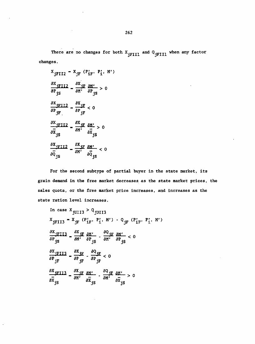
262

There are no changes for both and when any factor

changes.

*jFII2 " *jF ( IF'

fïjEiiz _ fïjE am. > 0 aPjs «"• aPjs

fîiEin . < 0

"JF, « jP

"iFiiz. f!LjE am > 0

-JS -JS

Emiz. Hjf SOL.. „

»Qjs S

For the second subtype of partial buyer in the state market, its

grain demand in the free market decreases as the state market prices, the

sales quota, or the free market price increases, and increases as the

state ration level increases.

In case > Qjuna

*jFII3 " *jF ( iF' i' • QjF iF' i*

fijEm 5jE mL_ fSjE an:-. n

aPjs aPjs - aM' aPjg

_ f5E fSjE 0

**jFII3 , m. f&E ML. 0

ay - - aM' -aXjs aXjg aXjg

263

**jFII3 _ mL. fSjE Ml- . n

For the third subtype of partial buyer in the state market, in case

JUII3 jUII3' grain demand in the free market decreases as the

state market price, the free market price, or the sales quota increases,

and increases as the state ration level increases. In case <

QJUII3> we have opposite results for Qjujj3' Thus, there is no need to

calculate comparative statics for this case.

3. Complete buyer

XjFIIIl " °

*jFIII2 " jF ( iF' i'

**jFIII2 fiiE mi_ . n aPjs aPjs

**jFIII2 _ filE < 0

* jF * jF

**jFIII2 filE mi_ . n

jS **jS

Thus, for the first subtype of complete buyer in the state market,

the grain demand in the free market is unaffected by any factor's change.

For the second subtype of complete buyer, the grain demand in the free

market decreases if the free market price or the state market price

increases, and it increases if the state ration level increases.

The following is the second subpart of the free market analysis.

264

Aggregate demand of agricultural households in the free market

HIP HTIF HITIP First, we aggregate D , D , and D , grain demand of the first,

the second, and the third type of agricultural households in the free

HP market, then add them into D , aggregate grain demand of all agricul­

tural households in the free market:

pHF _ jjHIF pHIIF pHIIIF (4.202)

Using formulas (4.192) through (4.201) and referring to formulas

(4.149), (4.154), (4.158), (4.164), (4.169) and (4.173), we can derive

pHIF, pHIIF pHIIIF individually.

DHIF _ D»:?! + (4.203)

• HI HIl "h XjFIl HX ' HIl HIll "h *jFI2

" HI HIl "H *jF ( iF' i' HI ' HIl HIll "H

[XjF (PÏF' Pi' M') - Qjf (Pip. Pi' M')]

-D (Pjjj, "H' PjLF'. i' ) (4.204)

The aggregate grain demand in the free market for the first type of

agricultural households is a function of the relative frequency P , HI

• HIl' ' HIll' total number of agricultural households, the free market

prices the prices of other goods, and disposable income.

dhiif _ + phiifs (4.205)

" ° HII ''HII2 "h *jFII2

^HII " HIIl " PHII2 PHII31 "H *jFII3

" HII HII2 "H XjF PiF' i'

HII • HIIl " PHII2 HII31 "H

265

[XjF (PÎF' Pi' M') - Qjp (Pip- Pi' M')]

" PHIII' PHII2' HII31' "H' ÏF' P ( -206)

For the second type of agricultural households, the aggregate grain

demand in the free market is a function of the relative frequencies ,

HIIl' PhII2' PHII31' HIIS' o al number of agricultural house­

holds, the free market price P p, the prices of other goods, and

disposable income.

DHIIIF - DHIIIFI + DHIIIF2 (4.207)

- 0 + (1 - Pjji - (1 - rijj XjFiii2

" PHI " PHII ' HIIII "H JF PIF'

- D (Pjjj, Pjjjj, Hjj, Pip, p , M') (4.208)

That is, for the third type of agricultural household, the aggregate

grain demand in the free market is a function of the relative frequencies

Pjji. •Phii» and fpi Ill' total number of agricultural households, the

free market price P p, the prices of other goods, and disposable income.

Lastly, substituting (4.204), (4.206) and (4.208) into (4.202), we

get

HF ® " PHI PHII "H JF PIF' PIS' HI ' HII PHIII "H

[XjF (PiF' Pi' • QjF (PiF' Pi' M')]

PHII HII2 "H JF PIF' P

PHII " PHIII ' PHII2 HIIBI "H

[XjF (PiF' Pi' - QjF (PiF' Pi' M')]

( ' PHI " PHII ( " PHIIII "H JF (PIF' Pi'

266

HF - D (Pjjj, HIIl' HII2' HII31' HIIIl'

"H- PlF' (4.209)

The aggregate grain demand of all agricultural households in the

free market is a function of the relative frequencies P , P ^ .,

HIll' HIIl' HII2' HII31' HIIIl' total number of agricultural

households, the free market prices P p, the prices of other goods, and

disposable income.

Aggregate grain supply of agricultural households in the free market

Similarly, we first aggregate and grain supply of

the first, the second, and the third type of agricultural households in

HF the free market, then combine these together to obtain S , aggregate

grain supply of all agricultural households in the free market:

gHF _ gHIF gHIIF gHIIIF (4,210)

Using formulas (4.192) through (4.201) and referring to formulas

(4.164), (4.169), and (4.171), we obtain

gHIF _ gHIFl gHIF2 (4.211)

- 0 + (1 - Pj jj ) njj Qjp22

- Pj I (1 - Pjjjj ) njj

[QjF (fiF' i- - V M')]

HIF " ( HI' HIl' HIll' HI13' "H' ÏF* ) (4.212)

For the first type of agricultural household, the aggregate grain

supply in the free market is a function of the relative frequencies P , HI

HIl' HIll ' HI13 twhich is (1 - total number

267

of agricultural households, the free market price P p, the prices of

other goods, and disposable income.

SHIIF - gHIIFl + sHIIF2 + gHIIFS (4.213)

- 0 + 0 + Pjjjj (1 - - HII2 "H 9jFII3

" HII " HIIl " HII2 " HII33 "H

[QjF (PÏF' Pi' M") - Xjp (PÏF' Pi' M")]

" ® HIIl' PHII2' PHII31' "H' iF' i' ( -214)

The aggregate grain supply in the free market for the second type of

agricultural households is a function of the relative frequencies Pjjjj.

HIIl' PHII2' HII31' PhII33' total number of agricultural

households, the free market prices, the prices of other goods, and the

disposable Income.

gHIIIF _ gHIIIFl + gHIIIF2 (4.215)

- 0 . (4.216)

The aggregate grain supply in the free market for the third type of

agricultural households is zero. Subsitutlng (4.212), (4.214) and

(4.216) into (4.210) we obtain

" HI HIl) PHI13 "H

[QjF (PiF' Pi' M') - Xjp (P%p, ? [ , M')]

HII " PHIII " PHII2 HII33 "H

[QjF (PiF' Pi' M') - V (*iF' i' M')]

HF • ® HIl' HIll' PHI13' HII' PHIII' HirZ' HII31*

PHII33' "H' PiF' Pi' (4.217)

268

For agricultural households, the aggregate grain supply In the free

market Is a function of the relative frequencies ^HIII' HI13'

HII' HIIl' HII2' HII31' HII33' total number of agricultural

households, the free market price P|p, the prices of other goods, and

disposable Income.

Comparative statics for aggregate grain demands and supplies

Comparative statics are made for three types of agricultural households

separately.

1. Nonbuyers

Using formulas (4.203) and (4.211) we have

sdUL. . âsiii! . âsE!! 0 ''hi ''HI ''HI

4E!E; . sfiïEÎ. âaEfî > „ ' HIl ''hII ''HII ""HIX

âsiEL. âsHi!!, 0 'hiii "'HHI 'HIII

âEÎiZ

% % % %

aa5!.as!!Z! > o GZjS

*'jF

acEL. âoiEi âEÎÎZi „ asEL . as!!Hi „

aôjs 39js aSjs aQjs aPj;

The results indicate that, for the first type of agricultural

269

HIF households in the free market, (1) both the aggregate grain demand, D

HIF and the aggregate grain supply, S , increase if the relative frequency

HIF or the total number of agricultural households increases; (2) D

HIF uncertain, but S decreases, if the relative frequency increases;

HIF HIF (3) D increases, but S decreases, if the relative frequency

HIF HIF increases; and (4) D decreases, but S increases, if the state

is

market price P. , or the free market price P.„, or the sales quote Q Js jF'

increases.

2. Partial buyers

Using formulas (4.205) and (4.213) we have

<jS

aa HIIF aa HIIF2 HIIF3

ap

22

HII

HIIF

3P, HII

3P, > 0

HII

m HIIF3

dP,

ao

Hill

HIIF

3P, < 0

m

Hill

HIIF2

dP. HII2

ap

22 HIIF

ao

HII2

HIIF3

* HII2

ap, HII31

ap. < 0 HII31

ac! HII

HII

ac! HIIF2 ad HIIF3

'"H % > 0

aa an HIIF2 an HIIF3

ap jS

ap

ao ap HII

jF

an ap

js

HIIF2

jF

ap < 0

an ap

js

HIIF3

jF < 0

a& HIIF aa HIIF3 ap

aa

HII

HIIF

ap, > 0

aa

HII

HIIF3

ap.

aa

Hill

HIIF

ap. < 0

aa

Hill

HIIF3

^ HII2 * HII2 < 0

aa HIIF aa HIIF3 ap.

aa

HII31

HIIF

ap < 0

a"H

HIIF

aa

HII31

HIIF3

aa

a"H

HIIF3 aa ap

aa ap

js

HIIF

jF

ap

> 0

> 0

a& ap

js

HIIF3

jF > 0

270

âlEi . âclEE 0

™JS aXjs «*JS » js "js

âEÏif! . âEÏilfî „ as!!IE.as!!H!!>o

aSjs »Qjs "Qjs

The above results show that, for the second type of agricultural

households in the free market, (1) both the aggregate grain demand,

HIIF HIIF D , and the aggregate grain supply, S , increase when the relative

frequency , or the total number of agricultural households increases;

HIIF HIIF (2) both D and S decrease when the relative frequency or

HIIF HIIF HII31' increases; (3) D is uncertain, but S decreases, when the

HIIF HIIF relative frequency decreases; and (4) D decreases, but S

increases, when the state market price Pjg, or the free market price Pjp,

or the ration, or the sales quota increases.

3. Complete buyers

From formulas (4.207) and (4.213) we have

--HIIIF ._.HIIIF2

._HIIIF ._HIIIF2

.-IÎÏXÏF __HIIIF2

§- ?? < 0 HIIIl "HUH

..HIIIF __HIIIF2 ^ - ^ < 0

271

._HIIIF ._HIIIF2

,„HII1F _ ,„HIIIF2

aXjs aXjs

These results Illustrate that, for the third type of agricultural

households in the free market, the aggregate grain demand,

declines if the relative frequency or or the total

number of agricultural households, or the state market price, or the free

market price, or the state ration rises.

Lastly, using formulas (4.209) and (4.217) we have

21 _ âfiîî!! + + 2D!1 > Q

^ HII ^ HII ^ HII ^ HII

o HIl ° HI1

"' HIll '' HIll

^ HII2 ^ HII2

272

mE âcîîHL _ 0

an ap v U * HIIIl HIIIl

acE _ apHiF apHiiF ap"" q

"H "h "H "H

âcîîL- .qHIF „HIIF ,HIIIF

''js " js NS *Pjs

aiE_ae + a^ + aaEH<o * jF *FjF *FjF *PjF

a2!!I_aEH + aie< o

aâjs aXjs ax,;

aig.aig + aigl o

'Qjs ^Qjs ^Qjs

âsî!£. âsîE!> 0

^ HI ^ HI

ifiî!! _ âsH > 0

^ HII ^ HII

asE__as!E_ ^ HIl ^ HIl

^-^>0 * Hill Hill

âsEL- _ 5SÎEL < 0

^ HI13 ^ HI132

273

âsE_ _ isEE 0

ap ap HI13 HI13

isE_,âsEiL,„ ^ HII31 ^ HII31

as!!! âsîEI . âsEI£. 0

% " % %

aqHF a-HIF .-HIIF

-„HF ._HIF flçHIIF

a ^ _ a ^ > o

aXjg 3Xjg

âsî!! _ âsHf! + asïii! > q

'Qjs 'Qjs

These results tell us that, for agricultural households in the free

market, (1) the aggregate grain demand is uncertain, but the aggregate

grain supply decreases if the relative frequency, or in­

creases; (2) decreases, but increases, if the relative frequency

HIl HII31' state market price Pjg, or the free market price Pj ,

or the state ration or the sales quota increases; (3) D increases, but

HF S decreases, if the relative frequency ,P ^ or P , increases; (4) both

HF HF D and S decrease if the relative frequency, or P ^ g'

HF HF creases; or (5) both D and S increase if the total number of

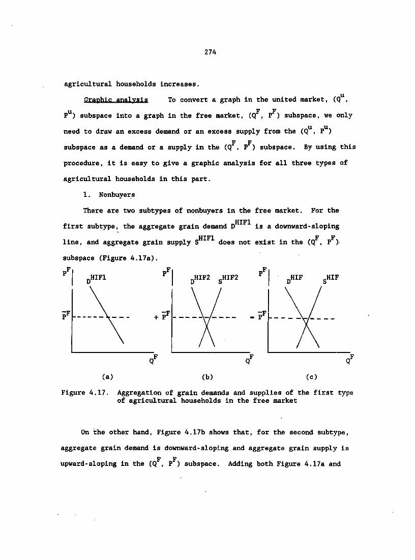
274

agricultural households increases.

Graphic analysis .u

To convert a graph in the united market, (Q ,

p") subspace into a graph in the free market, (Q , P ) subspace, we only

need to draw an excess demand or an excess supply from the (Q , p")

subspace as a demand or a supply in the (Q , P ) subspace. By using this

procedure, it is easy to give a graphic analysis for all three types of

agricultural households in this part.

1. Nonbuyers

There are two subtypes of nonbuyers in the free market. For the

.HIFl first subtype, the aggregate grain demand D is a downward-sloping

HIFX F F line, and aggregate grain supply S does not exist in the (Q , P )

subspace (Figure 4.17a).

.HIFl

—F \ —F P — -J" p

jjHIF2 gHIF2 HIF

-F

HIF

(a) (b) (c)

Figure 4.17. Aggregation of grain demands and supplies of the first type of agricultural households in the free market

On the other hand. Figure 4.17b shows that, for the second subtype,

aggregate grain demand is downward-sloping and aggregate grain supply is

F F upward-sloping in the (Q , P ) subspace. Adding both Figure 4.17a and

275

Figure 4.17b, we obtain Figure 4.17c, which shows a downward-sloping

HIF aggregate grain demand D and an upward-sloping aggregate grain supply

SHIF

2. Partial buyers

There are three subtypes of partial buyers in the free market. For

the first subtype, the aggregate grain demand is zero; but the demands

F F are downward-sloping in the (Q , P ) subspace for both the second and

third subtypes. On the other hand, for both the first and the second

subtype, the aggregate grain supply does not exist; but it is upward-

F F sloping in the (Q , P ) subspace for the third subtype (Figure 4.18a, b).

Figure 4.18c shows the situation for the second type of agricultural

household in the free market.

HIIF2 HIIF3 „HIIF3

-F

F F

,F HIIF HIIF

-F

(a) (b) (c)

Figure 4.18. Aggregation of grain demands and supplies of the second type of agricultural households in the free market

3. Complete buyers

There are two subtypes of complete buyers in the free market. For

the first subtype, both grain demand and supply are zero. For the second

276

F F subtype, grain demand is downward-sloping in the (Q , P ) subspace, and

grain supply is zero (Figure 4.19). Thus, aggregate grain demand and

supply of complete buyers are similar to that shown in Figure 4.19.

HIIIF(2)

Figure 4.19. Aggregate grain demand and supply of the third type of agricultural households in the free market

Lastly, adding Figure 4.17c, Figure 4.18c and Figure 4.19 together,

we obtain Figure 4.20, which shows the normal demand and supply

F F in the (Q , P ) subspace.

Figure 4.20. Aggregate grain demand and supply of all agricultural households in the free market

277

Theory of International Grain Trade

In the Mixed Economy

In the Chinese mixed economy, the state government has applied an

organizational reform to decentralize the state trading system. Without

changing the feature of the state monopoly In foreign trade management,

the government still has significant power to use trade to achieve Its

goals.

The discussion of International grain trade in the Chinese mixed

economy consists of four major parts: policy environment, the Ministry

of Foreign Trade (MOFT) model, aggregate grain Import demand or export

supply, and interactions of plans and markets. Under the discussion of

policy environment, the changed decision environment faced by the MOFT in

the mixed economy is provided so that theoretical work can be further

developed. Later, individual grain import demands and/or export supplies

are derived from the MOFT model in which the MOFT Is assumed to maximize

its utility subject to its constraints due to planning control. The

aggregate grain Import demand or export supply is summed from all

individual grain import demands or export supplies. Lastly, the plan's

Impacts on both the domestic grain market(s) (Including the state market

and the free market) and the international grain market are Inspected and

evaluated.

Pollev environment

State monopolv and decentralization of foreign trade Since the

economic reform, the Chinese government has decentralized foreign trade

278

management in two directions: horizontally to several ministries other

than the HOFT and vertically to local governments. This is an attempt to

provide flexibility and Improve efficiency for the MOFT's planning.

At the ministerial level, several new export and import corporations

(FTCs) have been established under the guidance of some production

ministries to conduct foreign trade directly. Among these corporations,

China National Seeds Import and Export Corporation (CNSIEC) is the only

one relevant to the foreign grain trade. At the local level, the

governments of several provinces and cities have been granted authority

to organize local corporations to direct the operations of local FTC

branches. These branches still need to report their plan and budget

matters to national FTCs and, hence, the HOFT.

Although there is an organizational reform in the state trading

system, individuals still are not allowed to do an import-export business

in the Chinese mixed economy. The bulk of China's foreign trade,

especially foreign grain trade, still is mainly carried out by FTCs and,

hence, the MOFT.

Objective of foreign trade With a more flexible attitude, the

Chinese government still thinks that foreign trade can play a very

important role in China's industrialization. Thus, the main task of

foreign trade in the national economy has not changed fundamentally.

The government tries, to the maximum feasible extent, to export

available goods to earn valuable foreign currency to ensure its import

capacity for industrial plants and equipment. On the other hand, it

tries to encourage China's own production of agricultural and light-

279

industrial commodities to satisfy basic needs in the domestic markets and

needs in the international markets if possible.

In the international market, the MOFT may still behave as a specific

consumer with a utility function within imported commodity space subject

to constraints due to planning controls. The assumed objective for the

MOFT still is to maximize its utility from purchasing commodities in the

international markets.

Plan control The MOFT still makes its trade plan which il­

lustrates its revenues and expenditures, imposes quotas for imports and

exports, and target quantities of goods to be exported and imported.

The MOFT still is concerned with its external balance, which is its

budget in the foreign exchange. In addition, although its loss can still

be covered by the State Treasurer, it now pays considerable attention to

its internal balance, which is its budget in the domestic currency. The

reason the MOFT does this is that the State Council sets the profit

target in the domestic currency to the MOFT and will reward the income

bonus as a money incentive to the staff members of the MOFT if the MOFT

can achieve at least or above the target.

The remaining concern for the MOFT, such as the planned balance

(rather than real balance) of domestic demand and supply in the state

market (rather than the combined market), has not changed from that under

the planned econmomy.

Market operation Because this section concentrates on the

foreign grain trade in the mixed economy only, we simply assume that the

MOFT is a price taker in all international markets except the

I

280

international grain markets. The behavior of the MOFT in the foreign

grain markets in the mixed economy is the same as that in the planned

economy. In detail, the MOFT acts as a price taker when it purchases

grain from the foreign markets and acts as a price follower when it sells

grain to the foreign markets.

Other bilateral trade agreements In the mixed economy, the MOFT

has several bilateral agreements with other countries. In general, the

contents of the agreements may be very similar to those carried out in

the planned economy.

Model of the Ministry of Foreign Trade

In the Chinese mixed economy, the MOFT still is assumed to maximize

its utility in the import commodity space, subject to given constraints.

Suppose the MOFT continuously has a utility function , ..., Xj ,

Xj j, ..., X j) where X j (1-1, ... , n) is the 1 imported good.

Furthermore, to guarantee utility maximization, we still suppose U(X )

has all the proper properties such as completeness, reflexivity, tran-

sivity, continuity, nonsatiatlon, and strict convexity. The new La-

grangian function is formulated as follows:

L "• U(X j, . . . , Xj , X , . . . ,

n I _ T + A-( S P, X,_ + «FR + r)FL - S P, X,_)

1 1 IE i_i i

+ Ajl J (e p: - P») - J (e Pj - pf)

* A3I E - X j) - (S%S -1 — 1

281

— pc pc - ''ll' - -"I'l

1-1

n + s IjlCXil - Xii) (4-218)

1—1

where

Xj, J - the 1 Imported commodity

Xj j - the Import quota for the 1 commodity, In case there is no

desire to import, X j - 0

— til XiE - the export quota for the 1 commodity, in case there is no

potential to export, X g - 0

pj - international price for the 1 commodity

- domestic (the state market) price for the 1 commodity

e - the exchange rate in Yuan/$

JT - the Internal profit target for the MOFT

FR - the foreign currency reserves

FL - the foreign loans

PS Sg - planned domestic grain supply in the state market

PS Dg - planned domestic grain demand in the state market

- planned domestic supply of 1 commodity in the state market

PS (h - planned domestic demand of 1 commodity in the state market

Yuan (1 Yuan - 100 Fen) is the basic unit of the Chinese currency --ReMingBe (RMB), according to the current exchange rate, 1 Yuan - $0.268 or $1 - 3.73 Yuan.

282

K, % - fixed proportional coefficients 0 3 % 5 1, 0 1

The constraints in the Lagranglan function can be classified into

four categories. Three of these four categories are exactly the same as

those listed in the MOFT model In the planned economy, and are not

explained in detail in this section. The remaining one is the newly

added internal balance in the current MOFT model. Now we introduce these

four categories as follows:

n I _ n J 1) External balance. S P. X._ + /cFR + f FL - Z P. X,? is an

1-1 1-1 "

external balance constraint. It requires that total expenditures for

importing goods must be covered by total earnings from exporting goods

plus other possible sources of foreign currency.

n T s. -2) Internal balance. Z (e P - P ) - S (e P - P ) X

1-1 1-1

n

II TT

I g — is an internal balance constraint. It says that S (e P. - P ) X ,

1-1 IB

total earnings converted to domestic currency from importing goods, minus

total expenditures converted to domestic currency for importing goods,

IS — S (e P. - P,)X.y, must reach at least jr, the profit target set by the 1-1

state government.

— DC DC

3) Balance of domestic demand and supply. (X g - X ) - (S - )

- 0 is a planned balance constraint for the domestic demand and supply of

the 1 commodity. It means th#t, for the 1 commodity, the planned

domestic surplus or shortage in the state market must be disposed of or

283

n _ be covered by using the international market. In particular, S (X.„ -

i-1

PS pg Xii) - (Sg - Dg ) is designed for the planned balance of domestic demand

and supply for a composite good--grain.

4) Import quota. - X j is the Import quota constraint imposed

for some commodities. That is, import of the 1 commodity must not

exceed the import quota X .

The Kuhn-Tucker conditions are then:

'A -

• fP + 3 + >51 s 0

for X j / 0, 1-1,

- pp + A3 i 0

for Xj j - 0, i " 1,

for Xj j / 0, 1 - k.

- Pj) + a 0

(4.219)

j (4.220)

(4.221)

''ii "

for Xj j - 0, 1 - k,

1 - 1,

n

n

(4.222)

(4.223)

ft - + 'f* + SPL 1 1 — 1

" I S P% T 0

1-1 ^ (4.224)

âL_ 1 ax. - 0 (4.225)

284

- fl' He • i 0 (4.226)

^ 2 % - - ° ( 4 2 2 ' )

% - j/ iE - *il' • <C • » (4 22:)

h ^ - O (4 229)

3A - (XiE - \j) - (sFS - D S) & 0 i - k n (4.230)

\i Ia"" • ° i - k n (4.231)

(X J - X j) 0 for / 0, i - 1. ..., n (4.232)

Agi - 0 for X^j / 0, i - 1 n (4.233)

1' 2' 3' 5i ~ ® 1 "" 1, • . • I n (4.234)

& 0 i - k, ..., n (4.235)

Suppose the MOFT maintains both its external balance and internal

balance,

AT T— T ^ - S pfx.P + /cFR + fjFL - S PTX.T - 0 (4.236) 1 i-1 i-1

% - • f") &E - ''ll - 0 (4 237)

then, (4.224) through (4.227) can be dropped out.

Similarly, suppose the MOFT maintains grain as well as all other

285

commodities at the planned.balance level, we then have

It - ° (4 23:' 3 i—1

- «IE - *1I> - "i® - "f ' - » i - •= " (4 239)

These results lead to omitting (4.228) through (4.231) from our

model.

Furthermore, suppose the second-order conditions are satisfied;

solving the first-order conditions, we find three possible ways for

1. - 0 (4.240)

2. X j-X j(P , P®, e, FR, PL, n , Xg, Xj, S -D )(4.241)

3. (4.242)

Apparently, the first formula (4.240) Implies a comer solution,

that Is, the MOFT does not Import any amount of good 1. The second

formula (4.241) Illustrates that Import demand for good 1 Is a function

of international commodity prices, domestic commodity prices (in the

state market), the exchange rate, the foreign reserves in the country,

the foreign loans borrowed by the government, the profit target for the

MOFT, the export quotas, the Import quotas, the planned balance of

domestic grain supply and demand in the state market, and the planned

balances of domestic supply and demand of other commodities in the state

market. The last formula (4.242) indicates that Imported good 1 is just

equal to its quota.

Once X Is determined, the corresponding quantities of either net

export supply X g or net Import demand X ^ immediately determined.

286

Comparing our new model (4.218) In the mixed economy with the previous

model (3.163) in the planned economy, we find out that the only dif­

ference is the constraint of internal balance. Furthermore, comparing

the results of (4.240) through (4.242) of our new model with the corre­

sponding results (3.182) through (3.184), we find out that the only

difference is that formula (4.241) for contains three more factors:

g the domestic state market prices P , the exchange rate e, and the profit

target n for the HOFT. Because we use a similar method to solve a

similar new model in this section, we can easily use the results provided

in the previous model with (4.241) to replace corresponding (3.183).

Thus, except for these different formulas, we only list all results of

our new model without detailed explanations.

1 . - 0

a. Xj g - 0 (4.243)

This case is dropped out because it is meaningless.

b. X g >0

*iNE " *iE (4.244)

The MOFT is a command exporter for good 1.

2. X j - X j (pl, P , e, FR, FL, n , X , X , - D ®)

a. X E - 0

INI - X i l (P^ ' ® ' FR ' FL, n, Xg, Xj, (4.245)

Net import demand for good 1 is a function of the international

price vector, the domestic state market price vector, the exchange rate,

foreign reserves, foreign loans, the profit target set for the MOFT,

287

export quotas, Import quotas, the planned balance of domestic grain

supply and demand In the state market, and the planned balance of

domestic supply and demand of other commodities In the state market.

Thus, the MOFT is a flexible Importer for good 1.

b. XiE > 0

1) ifX,g>X,j

XiNE - lE - Xll(P ' FR' FL, X , Xj, S S-D S,

- X gCpI, P®, e, FR, FL, ff, Xg, X , S ®-D ®)(4.246)

2) if < Xii

*1NI " *11 " *iE

- (P\ P . e, FR, FL, n , Xg, Xj, - Xg

- P , e, FR, FL, n , Xg, Xj, S ®-D )(4.247)

These results Indicate that either net export supply or net import

demand for good 1 is a function of international prices, the domestic

state market prices, the exchange rate, foreign reserves, foreign loans,

the profit target for the MOFT, export quotas. Import quotas, the planned

balance of domestic grain supply and demand in the state market, and the

planned balance of domestic supply and demand for other commodities in

the state market. The MOFT is either a restricted flexible exporter or

restricted flexible importer for goods in these cases.

3) ifX^E-^ii

*1NI " *iNE • ° (4.248)

We simply drop this case out.

288

3. \i '

lE - 0

XiNI - (4 249)

The MOFT is a command importer in this case.

"• XlE > 0

The MOFT is a command exporter for good i.

1) if

XlNI - *11 - *1E (4 251)

The MOFT is a dual command importer.

2) 1£ îji < ïij

- ^iE - *11 (4 252)

The MOFT is a dual command exporter.

3) if 11 - XiE

XlNI - &NE - » (4 2::)

We simply neglect this case.

All of these results reflect that the MOFT tries to decide all net

imports and net exports for all goods together, although it may pay prior

attention to export quotas. The MOFT now is concerned with the interna­

tional prices as well as the domestic state market prices.

Comparative statics From the above discussion, we can classify

MOFT's importing or exporting behaviors. We show comparative statics of

S — only the newly added factors P , e, and i r for only flexible Importer and

restricted flexible exporter or importer. For the remaining factors

within the previous three functions and the remaining functions, the

289

readers can refer to the comparative statics for the corresponding part

in Chapter III because of similarity.

1. Importer

a. dual command Importer

*1NI1 " 11 " *1E

b. command Importer

*1NI2 " *11

c. flexible Importer

*1NI3 • Xll(P ' ®' FR, FL. n , Xg, Xj,

ax^^ax

apj d? l

J" ap ap®

de de

< 0

< 0

< 0

. fïu > 0 dn dir ^

Net import demand for the 1 good decreases if the exchange rate in

yuan/dollar, the international price, or the state market price in­

creases, and it is uncertain if the profit target is raised.

Moreover, we have the following results,which are similar to

those in Chapter III.

290

but

=<3 - ' ° d. restricted flexible Importer

XINI4 - P , e, FR, FL, n, Xg, Xj. - X G

The partial derivatives for X ^ are exactly the same as those for

X.„__ and are omitted here. INl J

2. Exporter

a. dual command exporter

*iNEl " *1E ' *11

b. command exporter

*1NE2 " *iE

c. restricted flexible exporter

— T C — — DC pC pC pC XiNE3 - - Xj j (P \ e, FR, FL, n , Xg, Xj, s" -d" , s" -D" )

The partial derivatives for X g are the same as those for X ^ g

but with opposite signs.

Graphic analysis The graphic analysis also is the same as that

in the similar part in Chapter III and, hence, is omitted in this

section.

Aggregate import grain demand and export grain SUPDIV

Within the first j grain commodities, suppose that the first e are

net importing grain commodities and the remaining j-e are net exporting

grain commodities. In the mixed economy, the aggregate import grain

291

demand is then

D ,MM

*iNIl *iNI2 •*• *iNI3 *iNI4 1-e 1-e 1-e l-e (4.254)

S - XiEi) + Z \ i 2 1-e 1-e

+ S Xj j3 (pl, P®, e. FR, FL, n , Xg, Xj, 1-e

+ S [X 4(pl, P , e, FR, FL, n , Xg, Xj, 1-e

iE4

(PL, P , e, FR, FL, JT, Xg, Xj, S -DG , (4.255)

That is, as long as the MOFT behaves as a flexible or a restricted

flexible importer for at least one grain commodity, the aggregate import

grain demand is a function of international prices of commodities, the

domestic state market prices of commodities, the exchange rate, the

foreign reserves, foreign loans, the profit target for the MOFT, export

quotas, import quotas, the planned balance of domestic grain supply and

demand in the state market, and the planned balances of domestic supplies

and demands of other commodities in the state market.

Similarly, we can obtain S , the aggregate export grain supply in

the mixed economy as the following:

(4.256)

(*iEl ' ill) ,*iE2 f-J f-J

292

- S™ (pl, P , e, FR, FL, H, X , Xj, (4.257)

As long as the MOFT behaves as a restricted flexible exporter for at

least one grain commodity, the aggregate export grain supply is similar

to the aggregate grain import demand as a function of international

prices of commodities, the domestic state market prices of commodities,

the exchange rate, the foreign currency reserves, the foreign loans, the

profit target for the MOFT, the export quotas, the import quotas, the

planned balance of domestic grain supply and demand in the state market,

and the planned balances of domestic supplies and demands of other goods

in the state market.

Three important things need to be noted here. First, both the

aggregate Import grain demand and the aggregate export grain supply of

the MOFT do contain both the international price vector, including

international grain prices, and the domestic state market price vectors,

including the state grain market prices. This reflects the fact that the

MOFT's behavior is affected not only by International prices but also by

the domestic state market prices. Thus, there is a certain connection

between prices in the state grain market and prices in the international

grain market in the mixed economy.

Second, both and contain the exchange rate. The exchange

rate plays an important role in the mixed economy to adjust the import

grain demand and export grain supply. Thus, the government can use the

exchange rate as a new policy Instrument to affect the grain economy.

Third, whether China becomes a net importing grain country or a net

293

exporting country still depends on the difference between and S .

In case > S , the MOFT is a net grain importer; otherwise, it is a

net grain exporter. In today's world, both domestic and foreign agricul­

tural economists who specialize in Chinese agricultural development

recognize that a shortage in the domestic grain market will persist in

the long run in the Chinese economy. If this is true, we obtain the net

grain import demand as follows:

pNMM _ pMM _ gXM (4.258)

It is certain that is a function that contains all the factors

and/or have/has.

Comparative statics The comparative statics for both and

MP XP are the same as those for D and S in the corresponding part of

Chapter III except for those relationships that include the domestic

state market prices, the exchange rate, and the profit target for the

MOFT. Thus, we mainly consider only those factors in the comparative

statics in this subpart of Chapter IV.

1. Aggregate import grain demand

_ 2 + s > 0 apj 1-e apj 1-e apj

as _ S îïim+ 2 îïim>0

ap 1-e ap 1-e apj

2 s < 0 ap i-e a?l 1-e a?l

294

S Z < 0 8?l l-e 3?l l-e aP=

i-e l-e

âfiîîl. 2 **iNI3 + 2 fim>0

3»r l-e âTT l-e dn ^

âEÎÎÎ _ 2 **iNI3 + 3 fïmiâ < 0

3(sf - Df ) l-e a(S%S . D S) l-e a(sf -

The above results indicate that the aggregate Import grain demand

(1) is uncertain if the state market price, the International market

price of a grain commodity, the exchange rate in yuan/dollar, or the

profit target for the HOFT increases; and (2) decreases if the average

state grain market price or the average international grain price in­

creases .

2. Aggregate export grain supply

isH _ 2 > 0

apj f-j apj

sÇ. s d? l f-j ap®

ap f-j aPg

âS . g fiBEÎ<0

s?l f-j

295

âsiiîî _ 2 **iNB3 > 0 de " Je < °

âfiï _ g **iNB3 > 0

ajr f-J dit ^

âsi î _ g *XiNE3 > 0

a(sf - of) f-j a(sf - D ®)

The above results Illustrate that (1) the aggregate export grain

supply is uncertain if the state market price, the international market

price of a grain commodity, the exchange rate, or the profit target for

the MOFT increases; (2) the aggregate export grain supply increases if

the average state grain market price increases; and (3) aggregate export

grain supply decreases if the average state grain market price increases.

Graphic analysis The graphic analyses are made for both aggre­

gate import grain demand and aggregate export grain supply.

1. Aggregate import grain demand

Given the average international grain price P , we can draw aggre­

gate import grain demand. As Figure 4.21a shows, the sum of aggre­

gate import grain demands by both dual command importers and command

importers, is a vertical line whose intercept on is QQJ" 23 1-3

+ S X j2 the (Qg, Pg) space. 1-e

Figure 4.21b gives , aggregate import grain demand by flexible

MM and restricted flexible importers. Finally, D , aggregate import grain

demand by the MOFT, is obtained in Figure 4.21c.

296

,MMI

\ \

mil

GI G

(a) (b) <c)

Figure 4.21. Aggregation of Import grain demands In the mixed economy

2. Aggregate export grain supply

Similarly, Figure 4.22 describes the aggregation of export grain

XMI supplies. On the left, S , the sum of aggregate export grain supplies

of both dual command exporters and command exporters Is given as a

vertical line with an Intercept Q g" Z + Z X g o" the f-j f-j

axis. In the middle, aggregate grain supply of restricted

flexible exporters Is given. Lastly, S , aggregate export grain supply

of the MOFT Is drawn as an upward sloping line In the (Q , P ) space on

the right of Figure 4.22.

,XMI ,XMII

/ / /

,XM

GE G G G

(a) (b) (c)

Figure 4.22. Aggregation of export grain supplies In the mixed economy

297

Interactions of clans and markets

In the mixed grain economy, the state market has not been changed

fundamentally. The government sets state market prices by its own

evaluation. Moreover, on the consumption side, the government still uses

ration coupons in the urban area to restrict urban grain demand and

grants permission to the minority of agricultural households to limit the

rural grain demand in the state market. On the production side, the

government sets contracts (somewhat different new quotas) to guarantee

rural grain supply in the state market. Thus, the state government still

controls not only the prices in the state market but also the quantities

exchanged in the state market. In this sense, the state market can still

be seen as an extension of the government policies.

According to the official opinion, the free market, as newly

reopened during the economic reform, is only an adjustment and a supple­

ment to the state market. The price in the free market is determined by

the interaction of market forces. However, the quantity exchanged in the

free grain market is partly determined by price and is partly influenced

by the government policies. It is known that grain demand or supply in

the free market is only a residual grain demand or supply of the sum of

grain demands and supplies in both the household market and the state

market. Thus, the government has the power to use a policy instrument to

change the exchanged quantities in the state market, and, hence, change

the exchanged quantities in the free market indirectly. In this sense,

we should not overestimate the roles played by the free market in such a

mixed economy. In the international grain market, the Chinese government

298

still has no power to decide the prices, but has full monopoly power to

decide the varieties and quantity imported and exported. Thus, interna­

tional grain markets still can be partially seen partly as an extension

of the government policies.

Market equilibrium situations In the mixed economy, the disequi­

librium feature of the state market has not changed. It still is

believed that the grain price in the state market is well below its

equilibrium price and, hence, creates a restricted excess demand under

the rationing coupon system in the state grain market.

Because the exchange activity occurring in the free market must obey

the economic principles, noting that the free market price is well above

the state market price, we may conclude that there is an equilibrium

existing in the free grain market, and that it is decided by interaction

of both demand and supply in the market. The average grain price may be

considered as approximately the equilibrium price.

In the international grain market, there is an equilibrium. Because

China is generally a grain importing country and it behaves as a perfect­

ly competitive or a price follower in the international market, the ex­

change prices are determined by excess grain supplies of the rest of the

world, and the exchange quantity is mainly determined by the excess grain

demand of the MOFT.

Domestic policy instruments In the domestic market of the mixed

economy, the main policy instruments include the ration coupons, the

ration permissions, the sales quotas, and the state market prices.

The mechanism of the ration permissions in the state market is the

299

same as that of the ration coupons, so we are discussing the roles of

only the ration coupons, the sales quotas, and the state market price.

Apparently, the first two are policy instruments for quantity adjustment,

the last one is a policy instrument for price adjustment. Next are

comparative studies for these domestic policy instruments.

1. The ration coupon

Figure 4.23 shows how an increase in the issued ration coupon per

capita in the state market affects both the free market and the interna­

tional market.

,F P

F «F F

,S I P P

ES(R)

ED'

S D-D PD-PD -S M «M I

(a) (b) (c)

Figure 4.23. The effects of a change in the ration level in the mixed economy

We now Illustrate the initial situations in the domestic markets and

International market. To save space, we separate our dual graph and move

the free market to the left. Figure 4.23a shows the situation in the

free market. and are aggregate grain demand and supply in the free

market and cross each other to determine the initial equilibrium price,

F F P , and the equilibrium quantity, . Figure 4.23b gives the situation

in the state market. and represent the aggregate grain demand and

300

supply in the state market in the mixed economy. Given the state market

S F D price P , which is less than P , the grain demand is and grain supply

c D S is Qj . In general, does not need to equal Qj . The planned grain

PD PS demand is and the planned grain supply is . They are not affected

S PD D PS S by the state market price P . Obviously, and - Qj because

the government has to guarantee that planned balance fully covers the

real balance in the state market. Lastly, Figure 4.23c indicates the

situation in the international market. ED and ES(R) are excess grain

demand by the HOFT and excess grain supply by the rest of the world,

respectively. Given an international grain price, pj, we have the

equilibrium grain quantity, Q , in the international market. All of

the previous descriptions about the initial situations of the markets are

continuously used in the remaining discussions of all other policy

instruments but are not illustrated anymore.

Consider that the government raises the ration coupons per capita,

in the state market, grain demand, D , shifts to the right . At the

PD PD same time, the planned grain demand, , shifts to right Qg . Thus, the

balance of total grain demand and supply as well as the planned balance

of total grain demand and supply in the state market is increasing. As a

M F result of shift in D , in the free market, grain demand D shifts back to

p' FF D Immediately, the equilibrium price P goes down to Pg, and the

equilibrium quantity goes down to Qg. In the international market,

because of changes in the planned balance rather than real balance of

grain demand and supply in the domestic state market, excess grain demand

ED shifts back to ED'. The import grain demand is expanded to at the

301

given international grain price pj.

2. The sales quotas.

The sales quotas are set for agricultural households in the mixed

economy. The government uses the sales quota to ensure planned grain

supply in the state market. Figure 4.24 describes the impacts on the

domestic markets and the international market when the government raises

the sales quotas.

I ,S P P'

ES(R)

ED

S S «S Q

,F P'

F «F F

(a) (b) (c)

Figure 4.24. The effects of a change in the sales quota in the mixed economy

The beginning situations are as discussed before. As the government

tries to increase the sales quota to Q g, both the grain supply and

S s planned grain supply in the state market increase from to (Figure

4.24b), Because the grain supply in the state market increases, that

causes a decrease in grain supply in the free market. In Figure 4.24a,

F F' S , grain supply in the free market, shifts to the left S and grain

F ' P demand shifts to left D . Thus, the equilibrium price P is decreasing

302

F F to Pg but the equilibrium quantity, Q , is not certain and possibly de-

g creases. In the International market, an increase in P in the state

I S market and a decrease in P - P may cause a left shift in excess demand

ED. Hence, import grain demand decreased from to Qg (Figure 4.24c).

3. The state market price

The state market prices are set for both domestic consumers and

producers. By adjusting the state market price, the government can

influence the situation in the markets. Figure 4.25 indicates the

effects of a change in the state market price on the domestic markets and

international market.

I S P P

ES(R)

ED' M M „M S

,F P

F F

(a) (b) (c)

Figure 4.25. The effects of a change in the state market price in the mixed economy

The initial situations remain the same. Suppose the government

S S decides to increase the state market price, say from P to P ; as a

result, grain demand decreases from to in the state market (Figure

4.25b). In the free market, D shifts left but shifts right. The

303

equilibrium quantity is not certain, but the equilbrium price increases

I S (Figure 4.25a). Keeping constant as P rises, the price difference

I S ?! - Pj may decrease, and, hence, the MOFT may suffer more loss in

importing grain. If this is true, the excess grain demand ED shifts

back, and the import grain demand decreases from to Qg (Figure 4.25c).

International policy jnefrumenta In the international grain

markets, the main policy instruments used by the Chinese government are

the exchange rate, the import quotas, and the export quotas. Comparative

studies of these three policy instruments are discussed next.

X. Exchange rate

The exchange rate is used to shift excess grain demand in the

international grain market. Because of the bonus, if the government

raises the exchange rate in yuan/dollar, the MOFT may earn more profit

from importing grain, hence more bonus from the State Council. Thus, the

excess grain demand shifts up. On the other hand, an increase in the

exchange rate causes the government to reduce its purchasing interest in

the international market, then shifts ED down, the final results is not

certain. There is no change in either the domestic state market or free

market (Figure 4.26).

2. The import quota

We discuss the impact of all import quotas for the total grain

demand only. As Figure 4.27c shows, if the import quota Q increases,

the excess grain demanded, ED, in the international market shifts to the

right; the import grain demand is increasing from to Q . There is no

304

change in the domestic markets.

ES(R)

ED

QÎ Q™ q» .M

(a) (b) (c)

Figure 4.26. The effects of a change in the exchange rate in the mixed economy

pS D« S«

ES(R)

(a) (b)

Q? Q? Qo Q"

Figure 4.27. The effects of a change in the import quota or export quota in the mixed economy

3. The export quotas

The impact of export quotas is similar to that of the import quotas,

but in the opposite direction. As the government increases all export

quotas for grain together, it results in a left shift in excess grain

demand, ED, and a decrease in import grain demand (Figure 4.27c).

305

CHAPTER V. MODELING THE CHINESE GRAIN ECONOMY

In keeping with the objective of this study to assess the Impacts of

government policy on China's grain trade and domestic grain consumption

and production, and in attempting to develop empirical analyses of the

Chinese grain economy in the future, this chapter will first formulate a

complete grain model for China, covering both periods of planned and

mixed economy. The differences of Individual corresponding equation(s)

between the two periods are Illustrated; and, therefore, the differences

between corresponding submodels for both planned and mixed economy also

are Illustrated. The most important Impact channels in this model are

via the domestic grain prices in both the state market and the free

market, as well as international grain prices. In addition, the other

government policy Instruments, such as ration coupons and sales quotas in

the domestic grain market(s), and import quotas and export quotas in the

international grain market(s), are built into the model so that their

impacts also can be further evaluated by estimating this model.

The grain model for China, CHNGMODI, includes four sections:

domestic grain demand, domestic grain supply, international grain trade,

and government grain price subsidy. The first two sections deal with the

domestic markets. The market equilibrium conditions are given for the

state market and the free market. In the third section, which treats the

international markets, import grain demand/export grain supply are

specified. Finally, the fourth section is used to simulate the govern­

ment grain price subsidy.

306

To close this chapter, a brief summary about the components of the

model is provided. In particular, flexibility of the model GHNGMODI is

discussed first. After that, classifications of the equations and

variables within GHNGMODI are given in this section.

Domestic Grain Demand

The submodel of domestic grain demand in China is divided into four

parts: domestic food grain demand, domestic feed grain demand, domestic

seed grain demand, and, finally, domestic inventory grain demand.

Food grain demand

Because of the differences in the government's grain policy between

the urban and the rural areas in China, the domestic food grain demand

(GFOOD) consists of domestic urban food grain demand (GFOODUB) and

domestic rural food grain demand (GFOODRU);

GFOOD - GFOODUB + GFOODRU (5.1)

Urban food grain demand The urban food grain demand (GFOODUB) is

the sum of the urban food grain demands in the state market and the free

market (GFOODUBSM and GFOODUBFM):

GFOODUB - GFOODUBSM + GFOODUBFM (5.2)

The equations for GFOODUBSM and GFOODUBFM are given by

GFOODUBSM - f(Pgsc' cross' GU' BPOP, UBPM) (5.3)

and

GFOODUBFM - f(PQp, P j gg, Rgy, UBFOP, UBPM, DUM) (5.4)

where P g and P p represent own price of grain to the consumer in the

state market and to the consumer and producer in the free market,

307

respectively, P j- gg represents the prices of other relevant goods,

represents the average annual amount of ration coupons per urban person,

and UBFOF represents the number of the urban population. UBFH represents

income per urban consumer and DUM represents a dummy variable for the

structural change.

Obviously, the difference between the explanations of urban grain

demand in the planned economy and in the mixed economy is formula (5.4).

In particular, there are two new factors, P p and DUM, appearing within

(5.4). The former implies the emergence of the free market after the

economic reform, and the latter is used to distinguish the periods of the

grain economy before and after the reform.

Rural food grain demand Similar to the urban food grain demand,

the rural food grain demand is the sum of the rural food grain demand in

the state market (GFOODRUSM) and rural food grain demand in the own (and

the free) market (GFOODRUOH). By the own market we mean the self-

production and self-consumption of grain by many agricultural households,

as described in Chapters III and IV. Thus, we have

GFOODRU - GFOODRUSM + GFOODRUOM (5.5)

The functional forms of GFOODRUSM and GFOODRUOM are given by

GFOODRUSM - f(Pgsc' GR' POP, WI) (5.6)

and

GFOODRUOM - f/R gC' GF' cross' R PM, DUM) (5.7)

where R j represents the amount of ration per rural person, RUPOP

represents number of rural population, WI represents a weather condition

index, and RUPM represents real income per rural consumer. The other

308

variables, F" P„, P _ and DUM, are the same as described earlier ubL Vf Cross

in this section.

Clearly, there is no change in formula (5.6) in going from the

planned economy to the mixed economy. On the other hand, within formula

(5.7), Pqp and DUM are used to illustrate the difference between the

rural grain demand in the own market and the free market, and, therefore,

the difference between the rural grain demands in the planned economy and

the mixed economy.

Food grain demand in the state market The total food grain

demand in the state market (GFOODSH) is provided by

GFOODSM - GFOODUBSM + GFOODRUSM (5.8)

where GFOODUBSM and GFOODRUSM are previously specified.

Food grain demand in the own market (and free market) The total

food grain demand in the own (and the free) market (GFOODOM) is provided

by

GFOODOM - GFOODUBFM + GFOODRUOM (5.9)

where GFOODUBFM and GFOODRUOM are as previously specified.

Feed grain demand

Importance of feed grain Feed grain is very important within the

Chinese grain economy because China has one of the world's largest year-

end livestock inventories, especially inventories of hogs, which provide

over 90 percent of the meat in China and consume a relatively large

amount of feed grain to compete with human needs. For example, according

to a study by the World Bank (1987), about 87 million tons of grain.

309

Including cereals, tubers, and soybeans, was used to feed livestock in

China in 1984. This was equivalent to about 33 percent of the total

Chinese human grain consumption in the same year.

Circulation of feed grain In general, the government assigns

feed grain rations for the production teams or rural households, but does

not provide feed grain to them from the state stock. The feed grain will

mainly depend upon the collective reserve system or private households.

In case of an emergency, with the government's permission, the household

may buy feed grain from the state market. In the mixed economy, however,

the rural households may purchase additional feed grain from the free

market.

Additionally, the government applies rationing policy to sell feed

grain to those state farms, or collective farms, or individual house­

holds, that are specialized in livestock production and deliver meat

products to the state market.

Feed grain demand Because feed is used as input in livestock

production, the theoretical specification of feed demand follows the

derived demand approach, which has been developed in both the agricul­

tural production team model and the agricultural household model in this

study.

In addition, the feed grain demand (GFEED) is separated into two

subparts: the feed grain demand in the state market (GFEEDSM) and the

feed grain demand in the own (and free) market (GFEEDOM). Thus,

GFEED - GFEEDSM + GFEEDOM (5.10)

Furthermore, GFEEDSM is specified as a function of price of grain in

310

the state market (P gc), price of livestock product (P g), meat consumed

in the urban area (UBMC), per capita income of urban residents (UBPM),

and number of livestock (LN). Thus, the functional form of feed demand

in the state market is

GFEEDSM - f(Pggc, P g, UBMC, UBPM, LN) (5.11)

Similarly, GFEEDOM is specified as a function of grain price in the

state market (P gg), grain price in the free market (Pgp). meat price in

the state market (P g), meat price in the free market (P ), meat

consumed in the rural areas (RUMC), per capita Income in the rural area

(RUPM), number of livestock (LN), and dummy variable (DUM). Thus, the

functional form of feed demand in the free market is

GFEEDOM - f(PQgg, Pgp, Pjjg, Pjjp, RUMC, RUPM, LN, DUM) (5.12)

Needless to say, P p and DUM are factors newly added to formula

(5.12) because of the economic reform.

Seed grain demand

The demand for seed grain (GSEED) is specified as a function of

sown area (GAS) and a time trend (T). The behavioral relationship is

given as

GSEED - f(GAS, T) (5.13)

Inventory grain demand

Total grain inventories in China (GSTOÇK) are further disaggregated

into the state inventory (GSTOCKS) and the rural inventory (GSTOCKRU).

The state inventory managed by the state plan is mainly used for nation­

wide disasters and other unpredictable events such as war. The rural

311

inventory owned and managed by production teams or agricultural house­

holds is mainly used to compensate their losses in bad harvests. Thus,

GSTOCK - GSTOCKS + GSTOCKRU (5.14)

The behavioral relationship for the state stock is specified as

GSTOCKS - f(UBPOP, GSQ, WI) (5.15)

where GSQ is grain sales quota, and the other variables, UBFOP, , and

WI, are the same as in earlier equations.

The behavioral function for the private stock is specified as

GSTOCKRU - f(RUPOP, GPROD, GSQ, WI) (5.16)

where GPROD is grain production and the other variables are remaining the

same as before.

Domestic Grain Supply

The submodel of domestic grain supply in China consists of three

parts; grain production, grain supply in the state market, and grain

supply in the own market (and the free market).

Grain production

The grain production part includes three equations explaining area

sown to grain, grain yield, and grain production, respectively.

Area sown to grain Area sown to grain in China (GAS) is expres­

sed as a function of sown grain area planned by the government (PGAS),

the state grain market price for producer, P gp. the free grain market

price, Pgp, and the structural dummy variable, DUM, in other words,

GAS - f(PGAS, Pggp, Pgp, DUM) (5.17)

The variables P p and DUM are newly added to explain GAS within the

312

mixed economy.

Grain yield Grain yield in China (GY) is expressed as a function

of the state market price Pggp. the free market price P p, input uses X,

the sales quota GSQ, a time trend, T, to represent technical change, a

dummy variable, DUH, to represent structural change, and a weather index,

WI:

GY - fXPggp, Pgp, X. GSQ, T, DUM, WI) (5.18)

Undoubtedly, P p and DUM, of course, are new variables added in

formula (5.18) for GY in the mixed economy.

Grain production China's grain production (GPROD) is expressed

as a product of area sown to grain (GAS) and grain yield (GY):

GPROD - GAS * GY (5.19)

grain supply in the state market

Grain supply in the state market (GSSM) is expressed as the sum of

sales quota (GSQ), and imports (GIM):

GSSM - GSQ + GIM (5.20)

where the sales quota is a function of urban population (UBPOP), rural

population (RUPOP), and grain production (GPROD). Thus,

GSQ - f(UBPOP, RUPOP, GPROD) (5.21)

Grain SUPDIV in the own market (and the free market)

Grain supply in the own (and the free) market (GSOM) is the dif­

ference between grain production and the sales quota. Thus,

GSOM - GPROD - GSQ (5.22)

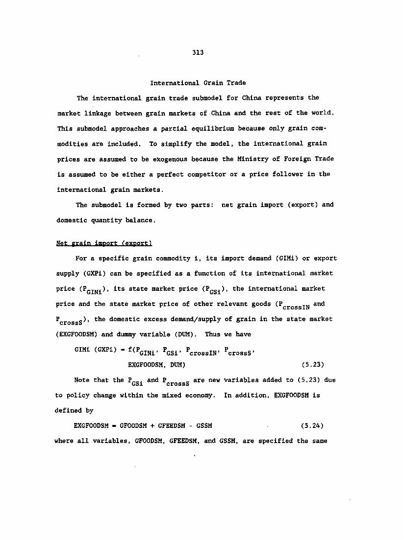
313

International Grain Trade

The international grain trade submodel for China represents the

market linkage between grain markets of China and the rest of the world.

This submodel approaches a partial equilibrium because only grain com­

modities are included. To simplify the model, the international grain

prices are assumed to be exogenous because the Ministry of Foreign Trade

is assumed to be either a perfect competitor or a price follower in the

international grain markets.

The submodel is formed by two parts: net grain import (export) and

domestic quantity balance.

Net grain import (export)

For a specific grain commodity i, its import demand (GlMi) or export

supply (GXPi) can be specified as a function of its international market

price (PgiQi), its state market price (Pggi), the international market

price and the state market price of other relevant goods and cross xiN

PcrossS ' domestic excess demand/supply of grain in the state market

(EXGFOODSM) and dummy variable (DUM). Thus we have

GIMi (GXPi) - PQSJL. crossIN' crossS'

EXGFOODSM, DUM) (5.23)

Note that the P g and PgpQggg are new variables added to (5.23) due

to policy change within the mixed economy. In addition, EXGFOODSM is

defined by

EXGFOODSM - GFOODSM + GFEEDSM - GSSM (5.24)

where all variables, GFOODSM, GFEEDSM, and GSSM, are specified the same

314

as before.

The net grain import (export) NGIM (NGXP) is the sum of all GIMi and

GXPi, i.e.,

NGIM (NGXP) - S (NGIMi - NGXPi) (5.25) i

Domeatic quantity balance

It is known that the domestic state market is usually in disequi­

librium. However, there is a quantity balance for the volume traded in

the state market as well as that in the whole domestic market.

Domestic quantity balance The domestic quantity balance is

expressed by the following equation:

NGIM (NGXP) - GFOOD + GFEED + GSEED + GSTOCK - GPROD (5.26)

It is said that NGIM (NGXP) is the sum of all domestic grain

demands, including GFOOD, GFEED, GSEED and GSTOCK, minus domestic grain

production (GPROD).

Domestic quantity balance in the state market The equation of

domestic quantity balance in the state market is expressed as the

following:

NGIM (NGXP) - GFOODSM + GSTOCKS - GSSM (5.27)

where GFOODS, GSTOCKS, and GSSM are the same as given before.

Domestic quantity balance in the own market (the free market)

The equation of domestic quantity balance in the own market (the free

market) is expressed as the following:

GSOM - GFOODOM + GFEEDOM + GSEED + GSTOCKRU (5.28)

where all the variables are defined the same as before.

315

Government's Grain Price Subsidy

Because the Chinese government wants to keep political stability

within the country, it provides heavy subsidies in the form of a dif­

ference between its purchase price and sale price for grain in the state

market; and, therefore, it is bearing a great pressure to balance its

budget. The government's grain price subsidy can be classified into two

categories: 1) grain price subsidy to the Ministry of Food (MOF) due to

its, grain trade in the domestic state market, and 2) grain price subsidy

to the Ministry of Foreign Trade (MOFT) due to its grain trade in the

international market.

Obviously, the total government's grain price subsidy (GPS) is the

summation of the above two parts of the grain price subsidies:

GPS - GPSMOF + GPSMOFT (5.29)

where GPSMOF is the government's grain price subsidy to the MOF and

GPSMOFT is the government's grain price subsidy to the MOFT.

Grain price subsidy to the Ministry of Food

In the domestic state grain market, the government has to maintain

the lower stable consumer price in order to win the support from the

urban consumers; on the other hand, the government has to increase the

producer price in order to stimulate the rural producers' incentive to

expand their production. The difference in the consumer price and the

producer price in the state grain market has created a financial problem

in the government's budget.

The function explaining the grain price subsidy to the MOF (GPSMOF)

316

is given as

GPSMOF - (Pggp - Pggg) * GSQ (5.30)

where Pggp. P gg and GSQ are the same as before.

Grain price subsidv to the Ministry of Foreign Trade

In the international market, the government has made grain trades

without paying much attention to the domestic state market price,

especially in the planned economy. But the price difference between the

domestic state market and the international market may create a loss (or

an earning) to the HOFT on its internal account. Thus, the MOFT receives

a grain price subsidy, if any, (or has given a grain price credit), to

compensate (or to turn over) its loss (or earning) from the grain trade.

The function explaining grain price subsidy to the MOFT (GPSMOFT) is

given by

GPSMOFT - S (PgiQi - Pggci) * NGIMI, (5.31)

and the function explaining the grain price credit from the MOFT (GPC-

MOFT) is given by

GPCMOFT - S (PciNi - Pcgci) * NGXPi (5.32)

where Pg ^ , P g , NGIMI and NGXPi are the same as before in this model.

A Brief Summary

Flexibility ?£ the grain model for China

The grain model for China, CHNGMODI, is built to include both

periods of the planned economy and the mixed economy by distinguishing

317

different explanatory variables and time dummy variables. Thus, it can

be used to project China's grain demand, grain supply, and foreign grain

trade by using time-series data simulating the structural change within

the economy.

In addition, by taking out all added new variables and equations

mentioned earlier in this chapter, CHNGMODI can be adjusted to become

CHNGHODIA, which can be well fitted to the case of the Chinese planned

grain economy only. For the case of the Chinese mixed grain economy

only, our model CHNGMODI is identical with CHNGMODIB, which can be esti­

mated by using time-series data covering only the period of the mixed

economy.

Classification of equations

CHNGMODI consists of 18 (19) behavioral or technical equations (B-

type) and 14 (15) identities (I-type) that are arranged in the sections

set out next.

No. of relationship Section name B-Type I-Type

Domestic Grain Demand 9 7 Food Grain Demand 4 5 Feed Grain Demand 2 1 Seed Grain Demand 1 0 Inventory Grain Demand 2 1

Domestic Grain Supply 4 2

International Grain Trade 2(3) 4(5)

Government's Grain Price Subsidy 3 1

TOTAL 18(19) 14(15)

318

Classification of variables

CHNGHODI contains 32(34) endogenous variables and 25 exogenous vari­

ables. The variables are classified and listed below:

Endogenous variables The endogenous variables include: GAS,

EXGFOODSM, GFEED, GFEEDOM, GFEEDSM, GFOOD, GFOODOM, GFOODRU, GFOODRUOM,

GFOODRUSM, GFOODSM, GFOODUB, GFOODUBFM, GFOODUBSM, GIM, GIMi, GSOM, GPS,

GPSMOF, GPCMOFT, GPSMOFT, NGIM, (NGXP), GPROD, GSSM, GSEED, GSTOCK,

GSTOCKS, GSTOCKRU, GXP, GXPi, GY, GSQ, and P p.

Exogenous variables The exogenous variables in CHNGMODI include :

GPAS, DUM, LN, Pg oss' crossIN' crossS' GIN' GINi' GSC' GSCi' GSP'

Pggpi, Pjjp, Pjjg, Rqj , Rgy, RUMC, RUPM, RUPOP, T, UBMC, UBPM, UBPOP, WI,

and X.

319

CHAPTER VI. SUMMARY, CONCLUSIONS, AND

SUGGESTIONS FOR FURTHER RESEARCH

Summary

The Chinese grain economy is one of the most important and complex

in the world. The main objective of this study is to develop a theoreti­

cal framework for analyzing the Chinese grain model in both planned and

mixed economy regimes, in order to understand changing relationships

among the government, the firms, and the households, and, furthermore, to

understand the changing features of the operational mechanism of the

socialist economy.

Generally speaking, the Chinese grain economy was/is formed and

operated by the government and by basic economic units--urban households

(as consumers) and rural firms (as producers and consumers). By inspect­

ing the changing organizations of these basic units and exploring the

changing behaviors of the households, the firms, and the government, a

theoretical model was constructed and used to evaluate the impacts of

changing government policies in both the domestic and international

markets. The development of the theoretical model is, in a certain

sense, a breakthrough and is quite successful. By analyzing the separate

parts of the model, we determine the nature of the whole. To reflect and

stress the changes over time due to economic reform, the theoretical

discussions of the Chinese grain economy under two scenarios were sep­

arated into Chapters III and IV. The former focused on the operational

mechanism of the planned grain economy, and the latter emphasized the

320

operational mechanism of the mixed grain economy.

The discussion In each Chapter (III or IV) was naturally divided

Into two sections: the domestic economy and International trade. The

domestic economy was Separated Into urban and rural parts, because of

dual feature of the domestic grain economy. Furthermore, the rural

economy was broken Into two subparts for state farms (state farm house­

holds) and agricultural production teams (agricultural households) due to

the different features of ownerships of production means and resources.

Within the domestic economy, first of all, different types of

behavior of urban consumers, as well as rural producers and consumers,

were analyzed, and different demand/supply functions were derived

according to their activities In the market(s). Second, these Indi­

vidual demand/ supply functions were synthesized to determine the effects

of some government policy Instruments. Particularly, In contrast to

previous studies, the method of two-stage aggregation was used to obtain

the total grain demand and supply functions. That Is, we aggregated

demands or supplies of Individual units Into group demands or supplies by

the behavioral classifications, then those group demands or supplies were

aggregated Into a total grain demand or supply.

In our sections on International trade, the different behaviors of

the MOFT were classified and aggregated Import grain demand/export grain

supply functions were derived for both the planned economy and the mixed

economy.

By using the method described, In the Chinese grain economy, the

roles of key policy Instruments, which mainly Include the ration coupon,

321

the state market price, the sales quota, and the import/export quota,

were fully and clearly recognized.

To complete this theoretical study, in Chapter V, a grain model for

China was formulated by combining the results obtained in Chapters III

and IV. This model has several features that were neglected in previous

studies by others. First, it covers periods of both planned economy and

mixed economy by using a time dummy variable as well as other distinc­

tive variables. Second, it contains the international markets and either

two (planned economy) or three (mixed economy) domestic markets with

different market characteristics. Third, the differences in methods of

determining the domestic market prices (endogenous or exogenous) and

international market price (exogenous) associated with the different

market characteristics are explicitly presented, and, of course, these

three different prices are not necessarily equivalent. Fourth, the model

embodies a structural feature that is very important for the purpose of

assessing the impacts of rationing policy. Overall, this model provides

a theoretical foundation for a full understanding of the Chinese grain

economy and (in principle) empirical measurement of the impacts of

government policy.

For the associated objectives, this study provides a tool to analyze

the interactions of domestic and international markets under both planned

and mixed economy assumptions and to assess the impacts of rationing

systems, domestic prices (including state market prices and free market

prices) and international prices on China's grain trade and domestic

market. The grain model for China incorporates all required instruments

322

and variables; therefore, such impacts can be evaluated theoretically

with the model.

Conclusions

The theoretical understanding and findings gained from the study of

the features of the Chinese economy can be summarized in the following

categories.

The basic features of the market economy may be presented by using

these key words: private ownership, market mechanism, and government's

regulation. Despite some different opinions, in general, economists

think that the price mechanism (the market mechanism) in its micro aspect

leads private firms to the efficient allocation of resources in the

market economy. On the other hand, the government sets policies to deal

with problems of macro stability in the economy. In other words, the

private firms and households have a right to make their own decisions for

their consumption, production, and distribution, whereas the government

uses regulation to influence and change the economy. This is the general

framework of the market economy in today's world.

Planned economv

The basic features of the planned economy may be described by these

key words: state or collective ownership, government's central plan, and

the state market. Yun Chen (1984), a Chinese communist leader and

authority on the planned economy, vividly depicted the planned economy as

323

"the economy of the bird cage." That means, the bird can live within the

cage, but cannot fly out of the cage. In the planned economy, the

government uses the central plan plus the state market, that is, the

cage, through state or collective firms to allocate resources to achieve

its national economic goals. On the micro level, within the cage, either

state or collective firms have a limited freedom to decide what, how, and

how much to produce because the main signals in the economy are not

market prices but the government's plans, and the means of production are

owned by either state or collective firms. The market mechanism plays no

role, or a relatively small one, in such an economy.

Plan and domestic state market The key to understanding the

planned economy is the state market. The state market, controlled and

operated by the state government, is not a market In the usual sense, and

can be seen as an extension of the government's plan. The prices in the

state market are not determined by market forces but by the government's

sole opinion.

For the Important commodities such as grain, cotton, and steel, the

government uses additional policy instruments to guarantee volume traded

in the state market. On the demand side, the government uses rationing

to restrict consumers' demand. On the supply side, the government uses

output targets and sown area plans to lead firms' production and uses

sales quotas to guarantee producers' supply.

Usually, there is a disequilibrium in the state market because of

the exogenous character of the state market price, which cannot drive an

equilibrium in the market. The concept of equilibrium used by communist

324

economists means only equilibrium for quantity but not necessarily for

price.

In the state market, for those Important goods, the government

usually sets a relative low price, which Is believed to be below the

equilibrium price and which will create a shortage problem. In this

sense, some economists call the planned economy a shortage economy.

Additionally, the procurement price may not be equal to the retail

price In the state market. In most cases, the procurement price is

higher than the retail price, because the government faces the pressure

from the producer to raise the former and from the consumer not to raise

the latter. As a result, the government has to cover a large subsidy in

its budget.

The new findings in this section are: (1) either the ration or the

state price has only a partial effect on the consumer demand if the

ration is not fulfilled, (2) the state price has only a partial effect on

the producers' supply.

Plan and the international market(s) In the international

market, the government reserves for itself the exclusive right to

purchase or sell Important goods such as grain. The government makes a

foreign trade plan to set import and export quotas and targets. Given

the plan, assuming the HOFT is either a price taker or a price follower

in the international market, it may adjust the real volume traded

according to the given International prices and other factors such as

balance of foreign currency reserves. An equilibrium exists in the

international market. The equilibrium quantity is determined by the

325

MOFT, whereas the equilibrium price is determined by the rest of the

world.

The new findings in this part are that, (1) the international price,

but not the domestic state market price, can affect the quantity traded

in the international market, (2) the domestic balance in the state market

but not in the united market, can directly affect the quantity of the

foreign trade, and (3) the domestic balance of composite grain commodity,

but not the domestic balance of a single grain commodity, is the main

concern in the foreign grain market. These findings are consistent with

the conjectures in previous studies and are clearly expressed in the

mathematical analysis.

Mixed economy

The basic features of the mixed economy are dual ownership, govern­

ment's central plan, and a dual market (a triple market if the own market

is included). The most remarkable changes in the mixed economy are

emergence of semi-private/private enterprises and the free market.

Although the government now still uses a central plan, plus the state

market through the state, collective, or even semi-private/private

ownership of production means, to allocate resources to achieve its

national goals, the former rigid control over the economy has been

somewhat loosened because of reopening of the free market. From the

micro view, within the cage, the state, collective, and private firms

have more freedom to make their own decisions on their consumption,

production, and distribution, especially in the free market. The

326

activities in the free market are mainly led by the market mechanism.

Obviously, the mixed economy possesses dual features of both planned

and market economy. Hence, it can be seen as transitional between the

planned economy and the market economy. The exact location of mixed

economy between the two, roughly speaking, will mainly depend upon the

proportions of state and private ownership and the relative sizes of the

state market and the free market within the economy. At this moment, the

Chinese mixed economy still belongs to the socialist category because the

central plan, plus the state ownership, still plays a dominant role, and

the free market is only an adjustment and supplement to the state market.

In this sense, the mixed economy can be considered an enlarged "economy

of the bird cage."

Plan and domestic state and free market The coexistence of the

state market and the free market, especially the coexistence of the state

market price and the free market price, has brought some changes in the

government plan and the situation in the state market. Based on politi­

cal considerations, the government has to maintain the price differences

between the state market and free market and to create price differences

between consumers and producers for the necessary goods such as grain in

the state market. Thus, it has to set income subsidy plans to carry this

heavier burden. In addition, some government officials may use their

power to buy goods in the state market then sell goods in the free market

to make their own profits. This may partly damage the government plan in

the state market.

The free market within the mixed economy is somewhat different from

327

the free market in the usual sense. In fact, it is a residual market to

the state market, especially for the most important commodities. The

government can directly influence consumer demand and producer supply in

the state market but not in the free market. However, through the

Interaction of the state market and the free market, the demand and

supply in the free market may be affected indirectly. In addition, the

price difference between the state market and the free market may lead to

flows from the state market to the free market, therefore changing the

situation in the free market.

There is no change from disequilibrium situation in the state

market. However, an equilibrium for both price and quantity may exist in

the free market because of effects of market forces. Although the excess

demands for those important goods still exist in the state market within

the mixed economy, overall, the nationwide shortage situation has been

somewhat improved by the price mechanism of the free market.

The new findings in this section are: (1) the ration level, or the

state price, or the free market price plays only a partial role in

affecting the consumers' demands and (2) the state price has no effect on

the producers' supplies, but the free market price does.

Plan and the International marketfs) The government still has

monopoly power in the international market. The plan procedure and

policy instruments used are basically unchanged. The market situation

also is assumed to be the same as before. Hence, the exchanged quantity

is decided by the government, given the exchange price in the interna­

tional grain markets.

328

The Important new finding for the mixed economy In this section is

that both domestic price and international price can influence the

quantity exchanged in the international market. This is different from

the first corresponding finding in the planned economy and provides

mathematical support for the hypotheses in previous studies. Other new

findings for the mixed economy are the same as the second, and the third

listed for the planned economy.

Suggestions for Further Research

Although the results of this study were theoretically satisfactory

and all the objectives were accomplished, there are still some areas

that can be explored for further research. First, an empirical econo­

metric model can be implemented based on the theoretical model developed

in Chapter V. At present, an empirical model is more important than ever

for the following purposes: (1) to fill in the element missing from the

previous studies with the first econometric model covering both the

planned economy and the mixed economy on a theoretical basis, (2) to be

used statistically to test and examine the validity of the theoretical

model, (3) to explore the relationship between availability of data and

rationality of the empirical model, (4) to evaluate and estimate the

policy instruments impacts on both the domestic and International

market(s), (5) to evaluate policy alternatives for structural changes

within economies, and (6) to estimate and to project China's grain demand

and supply in the domestic market(s) and grain trade in the international

market(s).

329

The empirical work can be done in alternative ways: (1) by con­

structing and estimating a simplified grain model for China, CHNGRMODI,

then developing it into a more detailed grain model for China, CHNGR-

MODII, or (2) constructing and estimating several different grain crop

models such as a wheat model for China, CHNUHHOD, a rice model for China,

CHNRIMOD, etc.; and then combining them to form a grain model for China,

CHNGRMODIII.

Second, within the crop sector, this study can be extended to

Include commercial crops such as cotton. Although we have considered

prices of commercial crops in our model, the roles of commercial crops in

the grain economy were not thoroughly explored. It is acknowledged that

the commercial crops are competitive with grain crops. This is espe­

cially true in China because all cultlvatable lands are extensively sown

each year. In addition, China has been the largest consumer and producer

of cotton in the world since 1982. Thus, it is very important to

construct a cotton submodel to associate with the grain model to evaluate

the Interactions of the cotton model and the grain model in both domestic

market(s) and international market(s).

Third, within the agricultural sector as a whole, this study also

can be extended to include the livestock sector. Even though feed grain

was built into the model, the role of the livestock sector in the grain

economy was not sufficiently investigated in both theoretical and

empirical studies. On the basis of this study, a theoretical livestock

model can be developed to fit the policy environment of the livestock

sector. Furthermore, the empirical livestock model can be merged with

330

our grain model to evaluate their relations and Interactions In the

market(s). By doing this, better estimations and projections of demand,

supply and foreign trade for both feed grain and food grain In the

Chinese grain economy can be obtained.

Fourth, within the national economy as a whole, this study can be

further developed to Include the industrial sector, as well as other

sectors of the economy. Although the agricultural sector as a whole has

been considered, the model is still 4 partial equilibrium model. To

Improve the situation, detailed domestic markets for each Important good

(or composite good) within the country should be constructed, and the

corresponding international markets can be treated in the same way used

in this study. Thus, a computable general equilibrium (CGE) model can be

formulated and estimated so that interactions among the plans, domestic

markets and International markets can be further recognized.

Last, this study should be extended to connect the proposed model

with the world market(s). Although world grain prices have been con­

sidered in the model, the model is still national. To Improve the situa­

tion, a detailed domestic market for each major country or group of

countries should be Included. Import demand/export supply can be formu­

lated by using the. definition of excess demand/excess supply in each

domestic market. In comparison with our national model, such a non-

spatial model provides more realistic information for international trade

and policy analysis.

331

BIBLIOGRAPHY

Abbott, J. G. 1977. Food and Agricultural Marketing in China. Food Policy 2:318-30,

Abouchar, Alan, editor. 1977. The Socialist Price Mechanism. Durham, NC: Duke University Press.

Agricultural Yearbook Editing Committee, 1980-1988. China's Agricultural Yearbook. Beijing: Agricultural Publishing House.

Allen, R. G. D. 1956, Mathematical Economics, London: Macmillan,

Allen, R, G. D., and J. R. Hicks. 1934. A Reconsideration of the Theory of Value. Economica 1:196-219;

Amstutz, Daniel G. 1984, International Impact of U.S. Domestic Farm Policy. American Journal of Agricultural Economics 66:728-734.

An, Xiji. 1982. An Estimation of China's Grain Production and Consumption in 1990. Research paper. Beijing Agricultural Univer­sity. (In Chinese)

An, Xiji. 1989. Prices, Production Costs and Farm Income in Mainland China. Paper presented at AAEA annual meeting. Baton Rouge, LA.

Anderson, J., John Dillon, and Brian Hardaker. 1977. Agricultural Decision Analysis. Ames, lA: Iowa State University Press.

Anderson, K., and R. Tyers. 1987. Economic Growth and Market Liberalization in China: Implications for Agricultural Trade. The Developing Economies 25(2):124-51.

Arrow, K., and M. Intriligator, editors. 1981. Handbook of Mathematical Economics. Vol. 1. Amsterdam: North Holland.

Arrow, K,, and M. Intriligator, editors. 1982. Handbook of Mathematical Economics. Vol. 2. Amsterdam: North Holland.

Arzac, Enrique R., and Maurice Wilkinson. 1979. A Quarterly Econometric Model of United States Livestock and Feed Grain Markets and Some of its Policy Implications, American Journal of Agricultural Economics 61:297-308.

Ball, R. J., editor. 1973. The International Linkage of National Economic Models. Amsterdam: North-Holland.

332

Barker, R., R. W. Herdt, and B. Rose. 1985. The Rice Economy of Asia. Washington, D.G.: Resources for the Future.

Barnett, A. D., editor. 1981. China's Economy In Global Perspective. Washington, D.C.: Brooking Institution.

Barnett, A. D. 1982. China's Food Prospects and Import Needs, pp. 59-68. la Harrison Brown (ed.). China Among the Nations of the Pacific. Boulder, CO: Westvlew Press.

Barnett, A. Doak. 1985. The making of Foreign Policy in China: Structure and Process. Boulder, CO; Westvlew Press.

Bamum, Howard N., and Lyn Squire. 1979. A Model of an Agricultural Household: Theory and Evidence. World Bank Staff Occasional Papers No. 27. Baltimore: The Johns Hopkins University Press.

Barrett, Nancy Smith. 1974. The Theory of Microeconomlc Policy. Lexington, Mass.: D. C. Heath.

Barro, R. J., and H. I. Grossman. 1971. A General Equilibrium Model of Income and Employment. American Economic Review 61:82-93.

Barro, R., and H. Grossman. 1976. Money, Employment and Inflation. New York: Cambridge University Press.

Baxhaum, David C., C. E. Joseph, and P. D. Reynolds. 1982. China Trade, New York: Praeger.

Beattle, Bruce R., and C. Robert Taylor. 1985. The Economics of Production. New York: John Wiley & Sons.

Becker, Gary S. 1965. A Theory of the Allocation of Time. Economic Journal 75:493-517.

Bergson, Abram. 1967. Market Socialism Revisited. Journal of Political Economy 75:663-75.

Bernouilll, Daniel. 1738. Specimen Theoriae Novae de Mensura Sortis. Commentorll Academlae Sclentlarum Imperlalls Petropolltanae. English Translation by L. Sommer, 1954. Exposition of a New Theory on Measurement of Risk. Econometrica 22(l):23-36.

Bhagwati, J. N., editor. 1981. International Trade: Selected Readings. Cambridge, Mass.; The MIT Press.

Bhagwati, J. N., and Srinivasan. 1983. Lectures on International Trade. Cambridge, Mass.; The MIT Press.

333

Bliss, C. J. 1972. Prices, Markets and Planning. Economic Journal 82(325):87-100.

Brandt, Jon A., et al. 1985. Documentation of the CNFAP Hog-Pork Model and Review of Previous Studies. CNFAP Staff Report No. 9-85.

Brennan, M. J. 1958. The Supply of Storage. American Economic Review 48:50-72.

Bressler, R. G., and Richard A. King. 1970. Markets, Prices, and Interregional Trade. New York: John Wiley.

Brown, Stuart S. 1985. "Artificial Pricing" and Market Distribution by Non-Market Economies (U.S.S.R., Eastern Europe, China, Commercial Policy, Dumping). Ph.D. dissertation, Columbia University.

Buck, John L. 1937. Land Utilization in China. Nanking: University of Nanking.

Buck, John L. 1964. Chinese Agriculture. In Albert Feuerwerker (ed.)." Modern China. Englewood Cliffs, NJ: Prentice Hall.

Buck, John Lossing. 1982. Chinese Farm Economy. New York: Garland Publishing.

Buck, John Lossing, Owen L. Dawson, and Yuan-Li Wu. 1966. Food and Agriculture in Communist China. New York: Praeger.

Bunge, Frederica M., and Rinn-Sup Shinn. 1981. China: A Country Study. 3rd ed. Washington, D.C.: GPO.

Byrd, William A. 1987. The Market Mechanism and Economic Reforms in Chinese Industry. Ph.D. dissertation. Harvard University.

Cai, T. 1983. Conventional Practice in Setting Export-Import Prices. Chinese Economic Studies 16(3):85-92.

Carlson, S. A. 1965. A Study on the Pure Theory of Production. New York: Sentry Press.

Carson, R. L. 1973. Comparative Economic Systems. New York: Macmillan.

Carter, Colin A., and Fu-Ning Zhong. 1988. China's Grain Production and Trade: An Economic Analysis. Boulder, CO: Westview Press.

Caves, Richard E., and Ronald W. Jones. 1981. World Trade and Payments: An Introduction. Boston, Mass.: Little Brown and Co.

334

Chachollades, Miltiades. 1978. International Trade Theory and Policy. New York: McGraw-Hill.

Chao, Kang. 1970. Agricultural Production In Communist China 1949-1965. Madison, WI: The University of Wisconsin Press.

Chao, K. 1977. The Development of Cotton Textile Production In China. Cambridge, Mass.: Harvard University Press.

Chao, Kuo-Chun. 1957. Agrarian Policies of Mainland China (1949-1956). Cambridge, Mass.: Harvard University Press.

Chen, Nal-Ruenn. 1967. Chinese Economic Statistics: A Handbook for Mainland China. Chicago, IL: Aldlne Publishing Co.

Chen, Yun. 1954. Bridging the Gap Between Supply and Demand. People's China 22, November 16, 1954, p. 1-10.

Chen, Yun. 1982. Manage Foreign Trade Work Well. Chines Economic Studies 15(3/4):139-43.

Chen, Yun. 1984. Selected Works of Chen Yun, Vol. II, 1949-1956. Beijing: People's Publishing House.

Chen, Yun. 1986. Planning and the Market. Beijing Review 29(29): 157-174.

Cheng, C. Y. 1982. China's Economic Development: Growth and Structural Change. Boulder, CO: Westvlew Press.

Chiang, Alpha C. 1984. Fundamental Methods of Mathematical Economics. 3rd ed. New York: McGraw-Hill Book Company.

China Resource Trade Consultancy Co. Ltd. 1986. Almanac of China's Foreign Economic Relation and Trade. Hong Kong: China Resource Trade Consultancy Co. Ltd.

Chinese State Statistics Bureau. 1987. China's Statistical Yearbook, 1986. Beijing: Statistical Publishing House.

Chlnn, D. L. 1979. Team Cohesion and Collective Labor Supply in Chinese Agriculture. Journal of Comparative Economics 3(4):375-94.

Chlnn, D. L. 1981. A Calorie-Arbitrage Model of Chinese Grain Trade. Journal of Development Studies 17(3):357-70.

Chow, G. C. 1975a. Analysis and Control of Dynamic Systems. New York: Wiley.

335

Chow, G. C. 1975b. Econometric Analysis by Control Methods. New York: Wiley.

Chow, G. C. 1982. Outline of an Econometric Model for Chinese Economic Planning. Journal of Economic Dynamics and Control 4:171-90.

Chow, Gregory C. 1985. The Chinese Economy. New York: Harper & Row Publishers.

Chow, Gregory C. 1987. The Chinese Economy. 2nd ed. Singapore: World Scientific Publishing Co.

Chung, M. P., and A. J. de Boer. 1983. Management Decentralization on China's State Farms. American Journal of Agricultural Economics 65(4):657-66.

Clower, R. W. 1965. The Keyneslan Counter-Revolutlon: A Theoretical Appraisal. In F. H. Hahn and F. R. R. Brechling (eds.). The Theory of Interest Rates. London; Macmlllan.

Crook, Frederick W. 1974. Agriculture In the United States and the People's Republic of China, 1967-1971. Washington, D.C.: Economic Research Service, U. S. Department of Agriculture.

Dawson, Owen L. 1970. Communist China's Agriculture. New York: Praeger Publishers.

Deane, Hugh. 1983. China's Changing Countryside. New York: Far East Reporter.

Deaton, A. S. 1978. Specification and Testing In Applied Demand Analysis. Economic Journal 88:524-36.

Deaton, A. S. 1980. An Almost Ideal Demand System. American Economics Review 70:312-26.

Deaton, Angus. 1981. Theoretical and Empirical Approaches to Consumer Demand Under Rationing. In Angus Deaton (ed.) Essays In the Theory and Measurement of Consumer Behavior. Cambridge: Cambridge University Press.

Deaton, Angus, and John Muellbauer. 1980. Economics and Consumer Behavior. Cambridge: Cambridge University Press.

Deaton, A. S., and J. Muellbauer. 1981. Functional Forms for Labour Supply and Commodity Demands with and without Quantity Constraints. Econometrlca 49(5):1521-32.

336

Deng, Xiaping. 1983. Selected Works of Deng Xiaping (1975-1982). Beijing: People's Publishing House.

Denny, David Ladd. 1972. Rural Policies and the Distribution of Agricultural Products in China: 1950-1959. Ph.D. dissertation. The University of Michigan.

Dernberger, R. F. 1980a, Agricultural Development: The Key Link in China's Four Modernization Program. American Journal of Agricul­tural Economics 62(2):331-38.

Dernberger, R. F. 1980b. China's Development Experience in Comparative Perspective. Cambridge, Mass.: Harvard University Press.

Dillon, John. 1977. The Analysis of Response in Crop and Livestock Production. 2nd ed. Sydney: Pergamon.

Dong, Fureng. 1983. Some Problems Concerning China's Strategy in Foreign Economic Relations. International Social Science Journal 25(3):455-67.

Donnithorne, Andrey. 1970. China's Grain: Output, Procurement, Transfers, and Trade. Hong Kong Economic Research Centre, Chinese University of Hong Kong.

Du, Rensheng. 1984. New Developments in the Contracting System of United Production and the Cooperative Economy in the Countryside. Chinese Economic Studies 17(4):16-39.

Dunkel, F. V. 1982. Grain Storage in South China. Cereal Food World 27:409-14.

Eckstein, Alexander. 1966. Communist China's Economic Growth and Foreign Trade. New York: McGraw-Hill.

Eckstein, A., editor. 1971a. China Trade Prospects and U. S. Policy. New York: Praeger.

Eckstein, A., editor. 1971b. Comparison of Economic Systems. Berkeley, CA: The University of California at Berkeley Press.

Eckstein, Alexander. 1975. China's Economic Development. Ann Arbor, MI : University of Michigan Press.

Eckstein, Alexander. 1977. China's Economic Revolution. New York: Cambridge University Press.

Eckstein, A., editor. 1980. Quantitative Measures of China's Economic Output. Ann Arbor, MI: University of Michigan Press.

337

Eckstein, A., W. Galenson, and Ta-Chung Liu, editors. 1968. Economic Trends in Communist China. Chicago, IL: Aldlne Publishing Co.

Edgeworth, F. Y. 1881. Mathematical Psychics. London: Kegan Paul.

Ellman, Michael. 1979. Socialist Planning. Cambridge: Cambridge University Press.

Enders, W., and H. Lapan. 1987. International Economics: Theory and Policy. Englewood Cliffs, NJ: Prentice-Hall.

Engel, E. 1857. Die Productions and Consumptions Verhâltnisse des Kônigreichs Sâchsen. Zeitschrift des Statischen Bureaus des Kôniglich Sâchischen Hinisterium des Inneren 8 and 9.

PAO. 1977. Learning from China. Rome: PAO.

FAO, Agricultural Services Division. 1982. China: Grain Shortage Structures; Report on a FAO/UNDP Workshop Study Tour in the People's Republic of China, 18 October to 16 November 1979. FAO Agricultural Service Bulletin No. 49. Rome: FAO.

FAO. 1988a. FAO: 1987 Production Yearbook. Rome: FAO.

FAO. 1988b. FAO: 1987 Trade Yearbook. Rome: FAO.

Federal Reserve Bank of Kansas City. 1981. Modeling Agriculture for Policy Analysis in the 1980s. Federal Reserve Bank, Kansas City.

Ferguson, C. E. 1969. The Neoclassical Theory of Production and Distribution. Cambridge, Mass.: Cambridge University Press.

Field, R. M., and J. A. Kilpatrick. 1978. Chinese Grain Production: An Interpretation of the Data. China Quarterly 74:369-84.

Fisher, I. 1892. Mathematical Investigations in the Theory of Value and Prices. Transactions of Connecticut Academy of Arts and Sciences 9. New York: Augustus M. Kelley, 1965.

Foreign Agriculture. 1982. The China Trade. Foreign Agriculture 20(8):4-13.

Fox, Karl A. 1958. Econometric Analysis for Public Policy. Ames, lA: Iowa State University Press.

Friedman, Milton. 1981. Market Mechanisms and Central Economic Planning. Washington, D.C.: American Enterprise Institute for Public Policy Research.

338

Frlsch, R. 1965. Theory of Production. Chicago: Rand McNally.

Fuss, M. A., and D. HcFadden. 1978. Production Ecnomics; A Dual Approach to Theory and Application. Amsterdam: North Holland.

Gardner, B. L. 1979. Optimal Stockpiling of Grain. Lexington, Mass. Lexington Books.

Gardner, B. L. 1988. Economics of Agricultural Policies. New York: Macmillan Publishing Co.

Graff, J. de V. 1948. Towards an Austerity Theory of Value. South African Journal of Economics 16:35-50.

Green, D. W., and Christopher I. Higgins. 1977. SOVMOD I: A Macroeconometric Model of the Soviet Union. New York: Academic Press.

Gregory, P. R., and Robert C. Stuart. 1985. Comparative Economic Systems. 2nd ed. Boston: Houghton Mifflin Company.

Hausman, Jerry A. 1979. The Econometrics of Labor Supply on Convex Budget Sets. Economics Letters 3:171-74.

Hausman, Jerry A. 1985. The Econometrics of Nonlinear Budget Sets. Econometrica 53(6):1255-79.

He, Guiting, et al. 1984. The Economics of Hybrid Rice Production in China. IRRI Research Paper Services, International Rice Research Institute No. 101.

Heady, E. 0. 1952. Economics of Agricultural Production and Resource Use. New York: Prentice Hall.

Heady, E. 0., and J. L. Dillon. 1961. Agricultural Production Functions. Ames, lA: The Iowa State University Press.

Heal, G. 1973. The Theory of Economic Planning. Amsterdam: North Holland.

Helpman, Elhanan, and Paul R. Krugman. 1985. Market Structure and Foreign Trade. Cambridge, Mass.: The MIT Press.

Henderson, J. N., and R. E. Quandt. 1980. Microeconomic Theory, 3rd ed. New York: McGraw-Hill Book Company.

Hicks, J. R. 1939. Value and Capital. Oxford: Clarendon Press.

339

Hillman, J., and A. Schmitz. 1979. International Trade and Agriculture; Theory and Policy. Boulder, CO: Westview Press.

Houthhakker, H. S., and J. Tobin. 1952. Estimates of the Free Demand for Rationed Foodstuffs. The Economic Journal 62:103-118.

Howard, David H. 1977. Rationing, Quantity Constraints, and Consumption Theory. Econometrica 45(2):399-412.

Hsiao, Gene J. 1977. The Foreign Trade of China: Policy, Law, and Practice. Berkeley, CA: University of California Press.

Hsu, Dixin. 1986. The Contemporary Meaning of Das Kapltal. Red Flag, April 1.

Hsu, R. C. 1982. Food for One Billion: China's Agriculture Since 1949. Boulder, CO: Westview Press.

Hsu, R. 1984. Grain Procurement and Distribution in China's Rural Areas: Post-Mao Policy and Problems. Asian Survey 24(12): 1229-46.

Huenemann, R. 1966. Urban Rationing in Communist China. China Quarterly, No. 26.

Hymer, Stephan, and Stephen Resnick. 1969. A Model of an Agrarian Economy with Nonagrlcultural Activities. American Economic Review 59(4):493-506.

Institute of Pacific Relations. 1978. Agrarian China. New York: AMS Press.

International Rice Research Institute. 1978. Rice Research and Production in China: An IRRI Team's View. Los Banos: Philippines, International Rice Research Institute.

Intrlligator, M. 1971. Mathematical Optimization and Economic Theory. Englewood Cliffs, NJ: Prentice Hall.

Intrlligator, M. 1978. Econometric Models, Techniques, and Applications. Englewood Cliffs, NJ: Prentice Hall.

Ishlhara, Kyoichl. 1987. Planning and the Market in China. The Developing Economies 25(4):287-309.

Ishlkawa, S. 1965. Strategy of Foreign Trade Under Planned Economic Development--With Special Reference to China's Experience. Hitot-subashl Journal of Economics 5(2):27-58.

340

Johnson, D. Gale, editor. 1980. The Politics of Food: Producing and Distributing the World's Food Supply. Chicago: Chicago Council on Foreign Relations.

Johnson, D. Gale. 1982. Agriculture in the Centrally Planned Economies. American Journal of Agricultural Economics 64(5):845-53.

Johnson, G. E. 1979. Agriculture, the Base: Rural Development 1949-1979. International Journal 34(4):606-23.

Johnson, Stanley R., Zuhair A. Hassan, and Richard D. Green. 1984. Demand Systems Estimation. Ames, lA: The Iowa State University Press.

Johnson, Todd M. 1984. Nationalization, Price Control, and Rationing of Key Agricultural Goods in China: An Economic History of the Period, 1949-1957. (Centrally Planned Agency Monopoly). Ph.D. dissertation. University of Hawaii, Honolulu.

Johnston, J. 1984. Econometric Methods. 3rd ed. New York: McGraw-Hill .

Judge, G., R. C. Hill, W. Griffiths, H. Lutkepohi, and Tsoung-Chao Lee. 1986. Introduction to the Theory and Practice of Econometrics. 2nd ed. New York: Wiley and Sons.

Judge, G., W. Griffiths, R. C. Hill, and Tsoung-Chao Lee. 1988. The Theory and Practice of Econometrics. 2nd ed. New York: Wiley and Sons.

Kilpatrick, J. A. 1979, The Use of Fertilizer in China's Agricultural Development. Ph.D. dissertation. Michigan University, Ann Arbor.

Kilpatrick, J. A. 1980. Chinese Agriculture: Development, Production, and Trade. American Journal of Agricultural Economics 62(2):359-61.

Kilpatrick, J. A. 1985. Agriculture in Soviet Union and China: Implications for Trade. American Journal of Agricultural Economics 67(5):1044-66.

King, Gregory. 1696. Natural and Political Observations and Conclusions upon the State and Condition of England. In G. E. Bamett (ed.) Two Tracts by Gregory King. Baltimore, MD: Johns Hopkins Press, 1936.

Kostecki, M. M. 1982. Canada's Grain Trade with the Soviet Union and China. Canadian Journal of Agricultural Economics 30(2):223-238.

341

Kueh, Y. Y. 1977. Food Grain Production Instability in China and the World Grain Trade. Food Policy 2.

Kueh, Y. Y. 1984a. A Weather Index for Analyzing Grain Yield Instability in China, 1952-1981. China Quarterly 97:68-83.

Kueh, Y. Y. 1984b. Fertilizer Supplies and Foodgrain Production in China, 1952-82. Food Policy 9(3):219-231.

Kueh, Y. Y. 1984c. China's Food Balance and the World Grain Trade: Projection for 1985, 1990 and 2000. Asian Survey 24(12):1247-74.

Labys, W. C. 1973. Dynamic Commodity Models: Specification, Estimation, and Simulation. Lexington, Mass.: Lexington Books.

Labys, W. C., and P. K. Pollak. 1984. Commodity Models for Forecasting and Policy Analysis. New York: Nichols Publishing Co.

Lancaster, Kelvin. 1966. A New Approach to Consumer Theory. Journal of Political Economy 74:132-57.

Lardy, N. R. 1980. Chinese Agricultural Development, Production and Trade. American Journal of Agricultural Economics 62(2):356-58.

Lardy, Nicholas R. 1983a. Agriculture in China's Modern Economic Development. Cambridge: Cambridge University Press.

Lardy, Nicholas R. 1983b. Agricultural Prices in China. Washington, D.C.: World Bank.

Lardy, Nicholas R. 1987. China's Entry into the World Economy. Lanham, MD: University Press of America, New York Asia Society.

Lardy, N. R., and K. Lieaberthal, editors. 1983. Chen Yun's Strategy for China's Development: A Non-Maoist Alternative. New York: M. E. Sharpe, Inc.

Larsen, Marlon R. 1971. Home Needs Influence China's Pattern of Foreign Agricultural Trade. Foreign Agriculture 9(41):4-7.

Lau, L. J., and P. A. Yotopoulos. 1972. Profit, Supply, and Factor Demand Functions. American Journal of Agricultural Economics 54:11-18.

Leamer, E. E. 1984. Sources of International Comparative Advantages. Cambridge-, Mass.: The MIT Press.

Leamer, E. E., and R. M. Stern. 1970. Quantitative International Economics. Chicago, IL: Aldine Publishing Co.

342

Leeman, Wayne A. 1977. Centralized and Decentralized Economic Systems: The Soviet-Type Economy, Market Socialism and Capitalism. Chicago, IL: Rand HcNally College Publishing Co.

Li, Suezeng, Shengming Yang, and Juhuang He. 1987. The Structure of China's Domestic Consumption. World Bank Staff Working Paper No. 755.

Lin, Justin Yifu. 1988. The Household Responsibility System in China's Agricultural Reform: A Theoretical and Empirical Study. Economic Development and Cultural Change 36(3):199-224.

Linnemann, Hans, J. DeHoogh, M. A. Keyzer, and H. D. J. Van Heemst. 1979. MOIRA: Model of International Relations in Agriculture. Amsterdam: North-Holland.

Ma, Hong, and Zangqing Sun, editors. 1981. Studies of Issues in the Structure of China's Economy. (Zhonguo Jinji Zhekou Wenti Yanjiu.) Beijing: People's Publishing House.

Ma, Shu-Yon. 1986. Recent Changes in China's Pure Trade Theory. China Quarterly 106:291-305.

Mah, Feng-hwa. 1963. Communist China's Foreign Trade: Price Structure and Behavior, 1955-1959. Rand Memo RM-3825-RC. Santa Monica, CA: The Rand Corp.

Malinvaud, E. 1977. The Theory of Unemployment Reconsidered. Oxford: Basil Blackwell.

Malmquist, S. 1948. A Statistical Analysis of the Demand for Liquor in Sweden. Uppsala: Apelbegs Boktryckeriaktiebalag.

Marshall, A. 1890. Principles of Economics. London: Macmillan.

Martin, Lee R., editor. 1977a. A Survey of Agricultural Economics Literature. Vol. 1. Minneapolis, MN: University of Minnesota Press.

Martin, Lee R., editor. 1977b. A Survey of Agricultural Economics Literature. Vol. 2. Minneapolis, MN: University of Minnesota Press.

Maxwell, N., and P. Nolan. 1980. The Procurement of Grain. China Quarterly 82:304-307.

McCalla, A., and T. Josling. 1981. Imperfect Markets in Agricultural Trade. Totowa, NJ: Alanhela, Osmum.

343

McCalla, À. F., and T. E. Josllng. 1985. Agricultural Policies and World Markets. New York: Macmlllan.

Mellor, J. W. 1966. The Economics of Agricultural Development. Ithaca, NY: Cornell University Press.

Mellor, John W. 1978. The New Economics of Growth. Baltimore, MD: Johns Hopkins University Press.

Meyers, William H., W. S Huyser, and M. D. Helmar. 1984. A Performance Comparison of Aggregate and Disaggregate Export Models for the Soybean Sector. Paper presented at the NCR-134 Conference on Applied Commodity Price Analysis and Forecasting, St. Louis, MO.

Michael, R. T., and Gary Becker. 1973. On the New Theory of Consumer Behavior. Swedish Journal of Economics 75(4):378-96.

Mill, John S. 1909 (The first edition published in 1848.). Principles of Political Economy. Edited by W. J. Ashley. London: Longmans Green.

Mittelhammer, R. C., S. C. Matulich, and D. Bushaw. 1981. On Implicit Forms of Multiproduct--Multifactor Production Functions. American Journal of Agricultural Economics 63:164-68.

Mok, Victor. 1964. The Foreign Trade of Communist China, 1949-1960: A Regional and Commodity Analysis. Ph.D. dissertation. Michigan State University, East Lansing.

Muellbauer, J. 1981. Linear Aggregation in Neoclassical Labour Supply. Review of Economic Studies 48:21-36.

Muellbauer, J., and R. Portes. 1978. Macroeconomic Models with Quantity Rationing. Economic Journal 88:788-821.

Muth, Richard F. 1966. Household Production and Consumer Demand Functions. Econometrica 34(3):699-708.

Myers, Ramon Hawley. 1970. The Chinese Peasant Economy. Cambridge, Mass.: Harvard University Press.

Myers, R. H. 1978. Wheat in China--Past, Present and Future. China Quarterly 74:297-333.

Naylor, T. H. 1965. A Kuhn-Tucker Model of the Multi-Product, Multi-Factor Firm. Southern Economics Journal 31:650-58.

Neary, J. P., and K. W. S. Roberts. 1980. The Theory of Household Behavior under Rationing. European Economic Review 13:25-42.

344

Nerlove, Marc. 1958. The Dynamics of Supply: Estimation of Farmers' Response to Price. Baltimore, MD: Johns Hopkins University Press.

Nicholson, J. L. 1942-43. Rationing and Index Numbers. Review of Economic Studies 10:378-97.

Niu, Ruofeng. 1989. China's Agricultural Trade and Perspectives on Foreign Competition. Paper presented at the AAEA annual meeting, Baton Rouge, LA.

Noh, H. M. 1983. Prospects of Grain Production, Consumption and Trade in China. Ph.D. dissertation. Kansas University, Manhattan, Kansas.

Nuttall, John Lawrence. 1978. Predicting China's Industrial and Agricultural Production Jfrom United Nations Trade Statistics. Ph.D. dissertation. University of Illinois at Urbana-Champaign.

OECD. 1985. Agriculture in China. Paris; OECD.

01, Jean C. 1983. State and Peasant in Contemporary China: The Politics of Grain Procurement. Ph.D. dissertation. University of Michigan.

01, Jean C. 1986. Peasant Grain Marketing and State Procurement: China's Grain Contracting System. China Quarterly 106:272-90.

Optimization. 1965. Optimization Methods in Planning Foreign Trade. Economic Planning in Europe, Geneva.

Pareto, V. 1906. Manuale de Economla Politica, con una Introduzione alia Sclenza Sozlale. Milan: Società Editrice Librarla. (English Translation by A. S. Schwier, Manual of Political Economy. New York: Macmillan. 1972)

Perkins, Dwight H. 1966. Market Control and Planning in Communist China. Cambridge, Mass.: Harvard University Press.

Perkins, Dwight H. 1967. The International Impact on Chinese Central Planning. In Alan A. Brown and E. Neuberger (eds.) International Trade and Central Planning. London: Cambridge University Press.

Perkins, D. H. 1969. Agricultural Development in China, 1368-1968. Chicago, IL: Aldine Publishing Co.

Perkins, Dwight H. 1984. Rural Development in China. Baltimore, MD: Johns Hopkins University Press.

345

Phllps, L. 1974. Applied Consumption Analysis. Amsterdam: North Holland.

Piazza, Alan. 1983. Trends in Food and Nutrient Availability in China, 1950-81. World Bank Staff Working Paper No. 607.

Piazza, Alan. 1985. Food Consumption and Nutritional Status in the People's Republic of China. Ph.D. dissertation. Stanford Univer­sity.

Pindyck, R., and D. Rubinfeld. 1981. Econometric Models and Econometric Forecasts. New York: McGraw-Hill.

Pollak, Robert A. 1969. Conditional Demand Functions and Consumption Theory. Quarterly Journal of Economics 83:60-78.

Pollak, R. A. 1971. Conditional Demand Functions and the Implications of Separable Utility. Southern Economic Journal 37:423-33.

Prybyla, Ian S. 1987. Market and Plan under Socialism: The Bird in the Cage. Stanford, CA: Hoover Institution Press.

Pryor, Frederic L. 1963. The Communist Foreign Trade System. Cambridge: The HIT Press.

Putterman, L. 1988. Ration Subsidies and Incentives in the Pre-Reform Chinese Commune. Economica 55(218):235-248.

Rada, E. 1983. Food Policy in China: Recent Efforts to Balance Supplies and Consumption Requirements. Asian Survey 23(4):518-535.

Reynolds, B. L. 1983. Economic Reforms and External Imbalance in China, 1978-81. American Economic Review 73:325-28.

Ricardo, David. 1817. On the Principles of Political Economy and Taxation. In P. Straffa (ed.) The Works and Correspondence of David Ricardo. Cambridge: Cambridge University Press, 1951.

Rock Creek Research, Inc. 1985. Post-Reform China, In Fall 1985 China Projection Report. Rock Creek Research, Inc., Washington, D.C.

Samuelson, P. A. 1947. Foundations of Economic Analysis. Cambridge, Mass.: Harvard University Press.

Schnitzer, M. C., and James W. Nordyke. 1983. Comparative Economic Systems. Cincinnati, OH: South Western Publishing Co.

Schultz, Theodore W. 1964. Transforming Traditional Agriculture. New Haven: Yale University Press.

346

Schultz, Theodore W. 1978. Distortions of Agricultural Incentives. Bloomington, IN: Indiana University Press.

Scitovsky, T. de. 1942. The Political Economy of Consumers' Rationing. Review of Economic Statistics 24:114-24.

Sheahan, John. 1986. Alternative International Economic Strategies and Their Relevance for China. World Bank Staff Working Paper. Washington, B.C.: World Bank.

Sicular, Terry. 1983. Market Restrictions in Chinese Agriculture: A Microeconomic Analysis. Ph.D. dissertation. Yale University, New Haven, CT.

Sicular, Terry. 1985. China's Grain and Meat Economy: Recent Development and Implications for Trade. American Journal of Agricultural Economics 67(5):1055-62.

Sicular, Terry. 1986. Using a Farm-Household Model to Analyze Labor Allocation on a Chinese Collective Farm. I. Singh (ed.) Agricultural Household Models. Baltimore, MD; - Johns Hopkins University Press.

Sicular, Terry. 1988. Plan and Market in China's Agricultural Commerce. Journal of Political Economy 96(2);283-307.

Silberberg, E. 1978. The Structure of Economics: A Mathematical Analysis. New York: McGraw-Hill Book Company.

Singh, Inderjit, Lyn Squire, and John Strauss, editors. 1986. Agricultural Household Models: Extensions, Applications, and Policy. Baltimore, MD; The Johns Hopkins University Press.

Skinner, G. W. 1985. Rural Marketing in China: Repression and Revival. China Quarterly 64(2):9-26.

Slutsky, E. 1915. Sulla Teoria del Bilancio del Consumatore. Giornale degli Economisti 51. (English Translation In G. J. Stigler and K. E. Boulding (eds.) Readings in Price Theory. Chicago, IL: Chicago University Press, 1957).

Smith, Adam. 1776. An Inquiry into the Nature and Causes of the Wealth of Nations. London: W. Strahan and T. Cadell.

State Statistical Bureau, P.R.C. 1987. China Trade and Price Statistics. Hong Kong: New World Press.

347

Stavls, Benedict. 1974. Making.Green Revolution; The Politics of Agricultural Development In China. Ithaca: Cornell University Rural Development Committee.

Stavls, Benedict. 1977. People's Communes and Rural Development In China. Ithaca, NY: Cornell University Rural Development Committee, Center for International Studies.

Stavls, Benedict. 1982. The Chinese Agricultural Economy. Boulder, CO: Westview Press.

Stlefel, Matthias. • 1982. Production, Equality and Participation in Rural China. Geneva: United Nations Research Institute for Social Development, Popular Participation Programme.

Stokey, Edith, and Richard Zeckhauser. 1978. A Primer for Policy Analysis. New York: Norton.

Stone, Bruce. 1985. The Basis for Chinese Agricultural Growth in the 1980s and 1990s: A Comment on Document No. 1,' 1984. China Quar­terly, 101:114-21.

Stone, Bruce. 1988. Relative Price in the People's Republic of China: Rural Taxation Through Public Monopsony, pp. 124-154. In John Mellor and R. Ahmed (eds.) Agricultural Price Policy for Developing Countries. Baltimore, MD: Johns Hopkins University Press.

Surls, Fredric M. 1980. New Directions in China's Agricultural Imports. American Journal of Agricultural Economics 62(2):349-355.

Surls, F. M. 1984. Grain Marketing and Imports in China: Outlook and Situation Report. Washington, D.C.: U.S. Department of Agricul­ture .

Tang, Anthony M. 1980. Food Production in the People's Republic of China. Washington, D.C.: International Food Policy Research Institute.

Tang, A. M. 1982. China as a Factor in the World Food Situation. American Journal of Agricultural Economics 64(2):323-331.

Tang, Chi-yu. 1980. An Economic Study of Chinese Agriculture. New York: Garland Publishing.

Taylor, Jeffrey R., and Karen A. Hardee. 1986. Consumer Demand in China. Boulder, CO: Westview Press.

Theil, H. 1975. Theory and Measurement of Consumer Demand, Vol. 1. Amsterdam: North Holland.

348

Theil, H. 1976. Theory and Measurement of Consumer Demand, Vol. 2. Amsterdam; North Holland.

Thomas, H. J., editor. 1972. The Demand for Food. Manchester, England; Manchester University Press.

Tlmmer, C. P. 1980. Food Policy in China. Development Digest 18(2):31-46.

Tlmmer, C. Peter. 1981. China and the World Food System. In Ray H. Goldberg (ed.) Research in Domestic and International Agribusiness. Grenwich, CT: JAI Press.

Tlmmer, C. P., and Harold Alderman. 1979. Estimating Consumption Parameters for Food Policy Analysis. American Journal of Agricul­tural Economics 61(5);982-87.

Tlmmer, C. Peter, W. Falcon, and S. Pearson. 1984. Food Policy Analysis. Baltimore, MD: The Johns Hopkins University Press.

Tobin, James. 1952. A Survey of the Theory of Rationing. Econometrica 20:521-553

Tobin, James, and H. S. Houthakker. 1951. The Effects of Rationing on Demand Elasticities. Review of Economic Studies 18(47):140-153.

Tomek, W. G., and Kenneth L. Robinson. 1981. Agricultural Product Prices. 2nd ed. Ithaca, NY: Cornell University Press.

Trzeclakowski, Wltold. 1978. Indirect Management in a Centrally Planned Economy. Amsterdam: North Holland.

Tsao, James T. H. 1987. China's Development Strategies and Foreign Trade. Lexington, Mass.: Lexington Books.

Tuan, Francis C. 1984. Agricultural Statistics of the People's Republic of China, 1949-1982. Washington, D.C.: U.S. Department of Agricul­ture, Economic Research Service.

Tuan, F. C. 1987. China's Livestock Sector. Foreign Agricultural Economic Report. No. 226. Washington, D.C.: Economic Research Service, U.S. Department of Agriculture.

Tuan, Francis C., and Frederick W. Crook. 1983. Planning and Statistical Systems in China's Agriculture. Washington, D.C.: U.S. Department of Agriculture, Economic Research Service.

Tweeten, L. G. 1983. Foundations of Farm Policy. 2nd ed. Lincoln, NE: University of Nebraska Press.

349

U.S. Central Intelligence Agency. 1977. China: International Trade. Washington, D.C.: GPO.

U.S. Central Intelligence Agency. 1979a. China: Demand for Foreign Grain. (Research Paper No. ER 79-10073). Washington, D.C.: GPO.

U.S. Central Intelligence Agency. 1979b. China: International Trade Quarterly Review. Washington, D.C.: GPO.

U.S. Congress 90th, 1st session. Joint Economic Committee. 1967. An Economic Profile of Mainland China. Washington, D.C.: GPO.

U.S. Congress 92nd, 2nd session. Joint Economic Committee. 1972. People's Republic of China: An Economic Assessment. Washington, D.C.: GPO.

U.S. Congress 94th, 1st session. Joint Economic Committee. 1975. China: A Reassessment of the Economy. Washington, D.C.: GPO.

U.S. Congress 95th, 2nd session. Joint Economic Committee. 1978. Chinese Economy Post-Mao. Washington, B.C.: GPO.

U.S. Congress 96th, 1st session. (1980). Hearing before subcommittee on Priorities and Economy in Government of the Joint Economic Commit­tee, Executive Session, June 26 and July 9, 1979. Allocation of Resources in the Soviet Union and China. Washington, D.C.: GPO.

U.S. Congress 97th, 2nd session. Joint Economic Committee. 1982. China Under the Four Modernizations. Washington, B.C.: GPO.

U.S. Congress 99th, 2nd session. Joint Economic Committee. 1986. China's Economy Looks Toward the Year 2000. Washington, B.C.: GPO.

Van Der Gaag, Jacques. 1984. Private Household Consumption in China: A Study of Peoples' Livelihood. World Bank Staff Working Paper, No. 701. Washington, D.C.: The World Bank.

Varian, Hal R. 1984. Microeconomic Analysis. 2nd ed. New York: W. W. Norton & Company, Inc.

Waelbroeck, J., editor. 1976. The Models of Project Link. Amsterdam: North Holland.

Walker, Kenneth R. 1965. Planning in Chinese Agriculture. Chicago, IL: Aldine Publishing Co.

Walker, Kenneth R. 1977a. Provincial Grain Output in China. 1952-57. London: Contemporary China Institute. University of London School of Oriental and African Studies.

350

Walker, K. R. 1977b. Grain Self-Sufficiency in North China, 1953-75. China Quarterly 71:555-90.

Walker, K. R. 1982. Interpreting Chinese Grain Consumption Statistics. China Quarterly 92:575-88.

Walker, Kenneth R. 1984. Food Grain Procurement and Consumption in China. New York: Cambridge University Press.

Walras, L. 1874. Eléments d'économie politique pure. Lausanne: Corbaz. Translated by W. Jaffe as Elements of Pure Economics. Homewood, IL: Richard D. Irwin, 1954.

Wang, Pe Sheng. 1962. Communist China's Foreign Trade and Its Relationships to Her National Income and Agricultural Production. Ph.D. dissertation. University of Washington.

Wang, Tong-eng. 1980. Economic Policies and Price Stability in China. Berkeley, CA: Center for Chinese Studies, Institute of East Asian Studies, University of California at Berkeley.

Wang, Tong-eng. 1985. Price Policy and Behavior in the People's Republic of China. Jahrbuch der Wirtschaft Osteuropas 11(1):206-227.

Watson, Andrew. 1988. The Reform of Agricultural Marketing in China Since 1978. China Quarterly 113:1-28.

Weitzmann, M. 1974. Prices Versus Quantities. Review of Economic Studies 41(4):477-91.

Whitaker, Donald P., and Rinn-Sup Shinn. 1972. Area Handbook for the People's Republic of China. Washington, D.C.; GPO.

Wiens, T. B. 1978. Chinese Agriculture: Continued Self-Reliance. American Journal of Agricultural Economics 60(5):872-77.

Wiens, Thomas B. 1982. The Micro-Economics of Peasant Economy. New York: Garland Publishing.

Wiens, T. B. 1983. Price Adjustment, the Responsibility System and Agricultural Productivity. American Economic Review 73(2):319-24.

Wiens, T. B. 1985. Agriculture in the Soviet Union and China: Implications for Trade: Discussion. American Journal of Agricul­tural Economics 67(5):1063-66.

351

Wong, John. 1979. Rice Exports: A New Dimension in China's Economic Relations with Southeast Asia. Journal of Southeast Asian Studies 10(2):451-69.

Wong, John. 1980. China's Wheat Import Programme. Food Policy 5(2):117-131.

Woodward, D. 1982. A New Direction for China's State Farms. Pacific Affairs 55(2):231-51.

World Bank. 1983. China; Socialist Economic Development, Vols. 1-3. Washington, D.C.: World Bank.

World Bank. 1985a. China: Long-Term Development Issues and Options. A World Bank Country Economic Report. Baltimore, MD: The Johns Hopkins University Press.

World Bank. 1985b. China: Agriculture to the Year 2000. Washington, D.C.: World Bank.

World Bank. 1987. China; The Livestock Sector. Washington, D.G.: World Bank.

Wu, Yuan-Li. 1971. Food and Agriculture in Mainland China. Current History 61(361);160-64.

Xu, Muqiao. 1979. Economic Problems in Socialist China. Beijing: People's Publishing House.

Xue, Huqian. 1982. Current Economic Problems in China. (Translation by K. K. Fung.) Boulder, CO: Westview Press.

Yeh, K. C. 1973. Agricultural Policies and Performance in China: A Handbook. (Yuan-li Wu, editor) New York: Praeger.

Yotopoulos, P. A., and L. J. Lau, editors. 1979. Resource Use in Agriculture; Applications of the Profit Function to Selected Countries. Food Research Institute Studies 17(1):1-119.

Zhao, Y. 1983. On Export-Import Procedure. Chinese Economic Studies 16(3);85-92.

Zhao, Ziyang. 1986. Report on the Seventh Five-Year Plan. Xihua News Agency, April 14, 1986.

Zhongguo nongye nianjian bianji weiyuanhui. 1981. Zhongguo nongye nianjian, 1980. Beijing; Nongye Chubanshe.

352

Zhou, Enlal. 1975. Four Modernization Program. China Reconstructions. Beijing: March 1975.

Zhou, Enlai. 1959. Report on the Adjustment of Major Targets in the National Economic Plan for 1959 and Further Develoment of the Campaign for Measuring Production and Practicing Economy. Beijing: March 1975.

353

ACKNOWLEDGEMENTS

The author wishes to express sincere gratitude to his major profes­

sor, Dr. William H. Meyers for his encouragement, guidance, support,

patience, insight, and understanding throughout this study. The author

is also grateful to Dr. Karl A. Fox for his valuable comments, diligent

advice, and thorough reading of a preliminary draft. Special thanks are

extended to other members of the committee: Dr. Hack C. Shelley , Dr.

Robert N. Wisner, and Dr. Helen H. Jensen for their unusual interest and

useful advice in Improving this study.

The author appreciates the opportunity he has had to work in the

Center for Agricultural and Rural Development (CARD) to gain his research

experience. The author is also indebted to CARD, the Ford Foundation,

and the Rockefeller Foundation for their financial support of this study.

Sincere thanks go to Ms. Susan L. Lund for her patience in typing

this thesis, to Dr. Jay D. Atwood for his friendship in making correc­

tions, and to Miss Lois W. Domek for her effort in an excellent editing.

Last, the author would like to express his unlimited love to his

parents, and his heartfelt gratitude to his alma mater, Iowa State

University.

354

APPENDIX

A Glossary of Some Economic Terms

Used In the Text

The following economic terms are either commonly used in China or

defined by the author in this study. The meanings of the terms are

briefly explained in order to familiarize the readers with the text of

this study.

Agricultural household

Agricultural household is defined by the author as a type of rural

household that is a basic unit of production and consumption and belonged

to the agricultural production team before the economic reform.

Bao Can Dau Hu

A form of the responsibility system in agricultural production with

the character of individual operation. By contract, each household uses

land owned by the collective and has to pay the state tax and fulfill the

state procurement quotas in specified crops.

Bonus

A method practiced by social enterprises or administrators to give

workers and staffs material incentive or additional income according to

their work. In general, bonuses are given as rewards to those who

overfulfill their tasks and make special contributions.

355

Combined market

A market that Is assumed to combine both the state market and the

team market in the planned economy.

Dual market

Dual market implies the state market and the free market in the

mixed economy.

Dual market %raDh

Dual market graph is a graph created in this study to describe the

coexistence of dual markets.

Free market

Free market is a form of commodity exchange among indviduals and/or

firms under the state administration. Prices in the free market are

negotiable between buyer and seller.

Free market analysis

A market analysis is used to describe the exchange activities in the

free market only.

SEâln

Grain, as defined by the Chinese State Statistics Bureau, includes

rice, wheat, corn, soybeans, sorghum, millet, sweet potatoes, and other

coarse grains.

356

Grain price subsidy

Grain price subsidy is the subsidy to either the Ministry of Food or

the Ministry of Foreign Trade to compensate their loss in exchanging

grain due to the difference between their purchase price and the sale

price.

Household market

A market that is assumed to have all agricultural households' own

consumption occurring.

Household-own market

A market that is assumed to have an agricultural household's own

consumption occurring.

Market mechanigm

The process by which individuals and firms carry out economic

activities on the basis of information provided by the market. The

market mechanism is capable of balancing supply and demand in the market.

Mixed economy

Mixed economy is a transitional economy between planned economy and

market economy. The basic features of a mixed economy are coexistence of

state/ collective ownership and private ownership and coexistence of the

state market and the free market.

357

Own market

A market that is assumed (in Chapter V) to circulate own-consumed

grain for either production teams or agricultural households without

going through the state market and/or the free market.

Planned economy

Planned economy is/was an economy set in the socialist country. The

basic features of a planned economy are that, the government applies the

central plan through the state market to lead the state firms or collec­

tive firms to allocate resources and to distribute products and incomes

in order to achieve its national goals.

Production responsibility system

A system that links labor management and evaluation, and results in

proper labor payments from collective according to the job or the final

output.

Production team

The production team is generally the basic collective accounting and

production unit in rural areas in the planned economy. The team owns

some collective properties such as land, draft animals, and production

means, and, under the guidance of local government, takes care of its own

operations and distributes income among its members.

Ration coupons

Ration coupons are used by government to limit distrubution of a

certain good(s) such as grain in the state market. According to the

358

government's rule, the residents (or urban resident only) may obtain a

certain amount of coupons, and buy the good In the state market only with

both money (by price and quantity) and coupons (by quantity). The

coupons may not be permitted to exchange In the market.

State farm

A state farm Is an agricultural enterprise under public ownership.

The state owns all means of production on the farm, and controls all the

products. The workers and staffs of the state farm are paid In wages.

State farm household

A state farm household Is defined by the author as a type of rural

household that is a basic unit of production and consumption and belonged

to the state farm before the economic reform.

State market

The state market is a market operated and controlled by the govern­

ment. The prices in the state market are decided by the government's

opinions.

State market analysis

A market analysis is used to describe the exchange activities in the

state market.

Team market

A team market is the market assumed to have all grain distribution

activities in all of the team-own markets be added together.

359

Team-own market

A team-own market Is the market assumed for the distribution

activities within the production teams.

Urban household

Urban household is the household that lives in an urban area by the

government's permission and has the right to share some benefits such as

ration coupons provided by the government.

United market

United market is the market assumed to combine both the free market

and the household market in the mixed economy.