AAllmmaa MMaatteerr SSttuuddiioorruumm –– UUnniivveerrssiittàà ddii BBoollooggnnaa

RESEARCH DOCTORATE IN

Mechanics and Engineering Advanced Sciences - Project n° 2:

“Fluid Machines and Energy Systems Engineering”

Cycle XXV

Affiliation sector: 09/C1

Scientific-disciplinary sector: ING-IND/08

PhD Thesis title

Theoretical and Experimental Analysis

of

micro-CHP Energy Systems

Presented by: Dr. Eng. Roberta Vecci

PhD School Coordinator: Supervisor:

Chiar.mo Prof. Ing. Chiar.mo Prof. Ing.

Vincenzo Parenti Castelli Michele Bianchi

Final exam year 2013

AAllmmaa MMaatteerr SSttuuddiioorruumm –– UUnniivveerrssiittàà ddii BBoollooggnnaa

DOTTORATO DI RICERCA IN

Meccanica e Scienze Avanzate dell'Ingegneria – Progetto n° 2: “Ingegneria delle Macchine e dei Sistemi

Energetici”

Ciclo XXV

Settore Concorsuale di afferenza: 09/C1 Settore Scientifico disciplinare: ING-IND/08

TITOLO TESI

Analisi teorico-sperimentale di

Sistemi Energetici micro-Cogenerativi

Presentata da: Dott.ssa Ing. Roberta Vecci

Coordinatore Dottorato: Relatore: Chiar.mo Prof. Ing. Chiar.mo Prof. Ing. Vincenzo Parenti Castelli Michele Bianchi

Esame finale anno 2013

To my daughter, Alissa

who has endured with patience my choice and

who encourages me to pursue my dreams, every day.

ACKNOWLEDGMENTS

My thanks to my superiors for welcoming me into their group giving me the

opportunity to realize my dream.

My thanks to Professor Giorgio Negri di Montenegro, my professor during the

degree years, for whom I have profound respect.

My thanks are to my supervisor, Professor Michele Bianchi, my guide, for his

precious teachings and advice.

A sincere thanks to Professor Antonio Peretto, for the total trust he has given

me during all these years.

Finally, a thanks are due to laboratory technicians, Mr. Tarì and, especially,

Mr. Stefano Benaglia, for their help and total disponibility.

And above all

My heartfelt thanks go to my parents, and to two special persons who always

walked to my side "for better or for worse" during all these years.

INTRODUCTION

The micro-CHP (Combined Heat and Power) energy systems, using renewable

energy sources are an excellent response to the current issues of environmental

impact. Producing, in combined and efficient mode, electricity and heat at low

temperature directly on-site, using plants of size less than 50 kWel, they, especially

for stationary applications in residential and small industries, represent the

realization the energy Distributed Generation (GD) concept, an important strategy

in the production scenario in the medium term.

Following this idea, the Ph.D. activity has pursued the aim of conceptual

development and subsequent implementation of an Integrated Energy System

(IES), capable of meeting the energy requirements and thermal properties of

specific users, using different types of fuel, with the integration of electric

generators in Renewable Energy Sources (RES), and electric and thermal

accumulation systems, totally controlled by an automatic management control

system.

To this end, in the first doctoral years the study of micro-CHP energy systems

components, such as the combustion chambers of Micro Gas Tturbines (MGT),

reactors, and pyrolyzer for the production of syngas from scrap tires has been

addressed.

Specifically, the thermo-fluid dynamics (CFD) numerical analysis activity of

MGT combustion chambers was carried out, evaluating turbulence and combustion

models, and also by defining chemical kinetics mechanisms valid for the

combustion of syngas, biogas and natural gas. Finally, the validation of the results

obtained through the comparison with the experimental data has been made (De

Pascale, M.Fussi, A.Peretto, R.Vecci, "Numerical investigation of a swirled flame

model combustor fed with pyrolysis gas," ECOS 2011 - The 24th International

Conference on Efficiency, Cost, Optimization, Simulation and Environmental Impact

of Energy Systems, Novi Sad - Serbia, July 4-7, 2011., - M. Fussi, R.Vecci, 'potential' of

renewable fuels "low-Btu" gas turbine "- The search there and you see - Palazzo

D'Accursio-Bologna, 28-29 May 2010, Poster).

The need to environmentally recover scrap tires has led to the study (using

three-dimensional CFD codes), the design and the definition of the control

methods of a pyrolysis pilot plant. The plant is pending patents definition.

Having the availability of a Polymeric Exchange Membrane Fuel Cells (PEMFC),

the coupling of which with an electrochemical storage system was developed and

tested in a previous Ph.D. activity, at the DIN’s (previously DIEM) laboratory, the

research has continued with the implementation of the conceptually conceived

Integrated Energy System (IES).

After having built the system, the attention has been focused on the energy

source of the above system, a 5 kWel PEMFC, on which numerous experimental

campaigns for determining the PEMFC system electrical performance (polarization

curve, powers, efficiencies of the fuel cell system) and CHP performance (thermal

power, optimum cooling system temperatures, heat exchange with users,

efficiencies), under different operating conditions.

Furthermore, the degradation mechanisms of the PEMFC system, in particular

due to the flooding of the anodic side, have been assessed.

The analysis of the effect of the water management of the anodic exhaust at

variable FC loads has been carried out, and the purge process programming logic

was optimized, leading also to the determination of the optimal flooding times by

varying the AC FC power delivered by the cell.

Then, for the analysis of the fuel (hydrogen, H2) utilization factor, an algorithm

for its calculation from the experimental data, able to determine the amount of not-

reacted H2 and, therefore, the causes which produce the loss has been developed.

The algorithm considers the FC like a black box, so it doesn’t need access to its

internal component and can be applied during the normal FC lifecycle. Through

this algorithm the presence of the H2 crossover phenomenon was experimentally

demonstrated.

Therefore, the ageing suffered by the FC system has been analyzed. An

experimental tests campaign, comparing recent data with historical ones, was

carried out to verify the aging suffered by the cell, the components involved and

their main causes.

This thesis is completely dedicated to the detailed description of the latter

investigation, conducted on experimental IES realized. This study, joining together

theoretical and conceptual realization of an idea and its exploration by innovative

mean is, I think, by mechanical engineer "old-fashioned" as I am, the culmination of

personal fulfillment from an engineering standpoint.

ABSTRACT

In the framework of the micro-CHP (Combined Heat and Power) energy

systems and the Distributed Generation (GD) concept, an Integrated Energy

System (IES) able to meet the energy and thermal requirements of specific

users, using different types of fuel to feed several micro-CHP energy sources,

with the integration of electric generators of renewable energy sources

(RES), electrical and thermal storage systems and the control system was

conceived and built. A 5 kWel Polymer Electrolyte Membrane Fuel Cell

(PEMFC) has been studied. Using experimental data obtained from various

measurement campaign, the electrical and CHP PEMFC system performance

have been determinate.

The analysis of the effect of the water management of the anodic exhaust at

variable FC loads has been carried out, and the purge process programming

logic was optimized, leading also to the determination of the optimal flooding

times by varying the AC FC power delivered by the cell.

Furthermore, the degradation mechanisms of the PEMFC system, in

particular due to the flooding of the anodic side, have been assessed using an

algorithm that considers the FC like a black box, and it is able to determine

the amount of not-reacted H2 and, therefore, the causes which produce that.

Using experimental data that cover a two-year time span, the ageing

suffered by the FC system has been tested and analyzed.

Keywords

Micro-CHP, Distributed Generation DG, PEMFC, Integrated Energy System

TABLE OF CONTENTS 

Nomenclature…………………………………………………………………………………….…………...i 

Introduction…………………………………………………………………………………………………vii 

1.  The fuel cell technology ................................................................................................ 1‐1 1.1  The history of the fc technology [1‐12] ................................................... 1‐2 1.2  Description of the FC technology ............................................................ 1‐11 1.3  FCs  tipology ..................................................................................................... 1‐14 

1.3.1  The AFC (Alkaline FC) ................................................................ 1‐15 1.3.2  The DMFC (Direct Methanol FC) ............................................ 1‐17 1.3.3  The PAFC (Phosphoric acid fuel cells) ................................ 1‐19 1.3.4 The MCFC (Molten Carbonate FC) ........................................... 1‐20 1.3.5   SOFC (Solid Oxide FC) ................................................................ 1‐23 1.3.6 The PEM (Proton Exchange Membrane FC) ........................ 1‐25 

1.4  The Proton Exchange Membrane Fuel Cell: PEMFC ....................... 1‐26 1.4.1  PEMFC: principle of operation and components ............ 1‐27 

1.5  The stack ........................................................................................................... 1‐34 1.6  Balance of Plant .............................................................................................. 1‐36 1.7  Thermodynamics ........................................................................................... 1‐37 

1.7.1  Enthalpy of reaction .................................................................... 1‐37 1.7.2  Reversible cell potential ............................................................ 1‐38 1.7.3  Voltage losses ................................................................................. 1‐41 1.7.4  Efficiency of the fuel cell ............................................................ 1‐44 

1.7.5  Operating Condition: ................................................................... 1‐46 1.8  PEMC application and current status .................................................... 1‐49 

References to chapter 1 ............................................................................... 1‐53 

2.  The Integrated Energy System ................................................................................. 2‐1 2.1  The IES test system ......................................................................................... 2‐3 2.2  The components of the Integrated Energy System ......................... 2‐11 

2.2.1  The fuel cell (FC) system ........................................................... 2‐11 2.2.2  The batteries and the bidirectional inverter..................... 2‐24 2.2.3  The photovoltaic (PV) emulator ............................................. 2‐32 2.2.4  The electrical load ........................................................................ 2‐34 2.2.5  The control system ....................................................................... 2‐36 2.2.6  Sensors .............................................................................................. 2‐40 

2.3  The IES operation states ............................................................................. 2‐45 2.4  The FC operation programming logic ................................................... 2‐50 

References of the chapter 2 ....................................................................... 2‐52 

3.  Experimental analysis of thr IES performance .................................................. 3‐1 3.1  The acquired and calculated variables ................................................... 3‐2 3.2  PEMFC performance analysis ..................................................................... 3‐6 

3.2.1  PEMFC electric performance analysis ................................... 3‐6 3.2.2  The FC thermal performance analysis ................................. 3‐28 References to the chapter 3 ....................................................................... 3‐33 

4.  The degradation mechanisms of the PEMFC ...................................................... 4‐1 4.1  The main degradation mechanisms of the PEMFC  

stack components ............................................................................................ 4‐7 4.1.1  Chemical and/or physical effects ............................................. 4‐8 4.1.2  Extreme external factors ........................................................... 4‐15 4.1.3  Poor water management ........................................................... 4‐18 

4.2  Contamination of the PEMFC components ......................................... 4‐25 4.3  Hydrogen crossover ...................................................................................... 4‐26 

References to the chapter 4 ....................................................................... 4‐32 

5.  Anodic exhaust management: analysis and optimization ............................ 5‐1 

5.1  The hydrogen purging: motivation, limit and  optimization strategies .................................................................................. 5‐3 

5.2  Experimental investigation on the effects of purging ....................... 5‐8 5.2.1  Piecewise model of the voltage drop due to flooding ... 5‐12 

5.3  Optimized purging strategy ...................................................................... 5‐14 5.3.1  Application of the optimized strategy ................................. 5‐16 

5.4  Efficiency evaluation of the FC purge programming logic ........... 5‐21 5.5  Analysis of the utilization coefficient .................................................... 5‐27 

5.5.1  Effect of the flooding duration ................................................ 5‐27 5.5.2  Definition of the not‐reacted hydrogen fraction ............. 5‐28 5.5.3  Algorithm for the evaluation of the  

not‐reacted hydrogen fraction ............................................... 5‐30 5.5.4  Analysis of the efficiency using the 

 fractions XDE and XA .................................................................... 5‐35 5.6  Experimental result ...................................................................................... 5‐38 

5.6.1  Results of the 2010 tests  (Old purge programming logic) ............................................. 5‐39 

5.6.2  Results of the 2012 tests  (New purge programming logic) ........................................... 5‐43 

References to the chapter 5 ...................................................................... 5‐56 6.  Ageing of the PEMFC ....................................................................................... 6‐1 6.1  The FC ageing analysis ................................................................................... 6‐3 

References for Chapter 6 ............................................................................ 6‐15  

Conclusions………………………………………………………………………………………………..c‐1 

 

 

 

 

 

 

 

 

 

 

 

 

 

 

 

 

 

 

 

 

 

 

 

 

 

i

Nomenclature Symbols

A active area

cw water specific heat

C capacity of the battery

E0 standard state reversible cell potential

Er reversible cell potential

Er,T actual cell voltage

F Faraday constant, F =96485 [C/mol]

fh heat of formation of a reactant

i current CROSSHI

2current induced by H2 crossed over

CROSSHJ

2 H2 crossover rate

K membrane gas permeability

PEMl membrane thickness

m mass

m& mass flow rate

Mflow volume flow rate

mmol molecular weight

n number of electrons

Ncel number of fuel cells in the stack

p correction factor for grid losses

P electric power a

HP2 anodic side H2 partial pressure

Q thermal power

Qth recovered thermal power

Qav available thermal power

R universal gas constant

ROhm overall cell resi stance

RH Relative Humidity

T temperature

Tfl flooding time

To operating time

ii

Tpu purge time

Uo air utilization factor

Uf fuel utilization factor

v,V voltage

Greeks

α slope of the straight line of the FC voltage

Pα activity of the products

  Rα activity of the reactants

ΔE fuel chemical energy introduced into the FC

  GΔ   Gibbs free-energy change

HΔ   enthalpy change

  SΔ entropy change

∆Tw CHP water temperature difference

aVΔ activation polarization

cVΔ mass transport or concentration losses

OVΔ Ohmic losses

ΔVfl FC voltage drop during the flooding time

ΔVmax maximum allowable FC voltage loss

ΔVp FC voltage drop during the purge time

ΔVrec FC voltage recovery after the OCV opening

PITMδ PITM location

η efficiency

θ electrolyte temperature  

PEMH 2

ψ H2 membrane permeability coefficient

ρ   density  

τ time with FC at constant power

iii

Acronyms and subscripts

a anode

A refers to H2 not-reacted for other causes

AC Alternate Current

AFC Alkaline FC

air of the air

aux of the auxiliaries

B blower

Batt of the battery

BOL Beginnig Of Life

BOP Balance Og Plant

BP Bipolar Plates

c cathode

CCP Combined Cooling and Power

cell refers to fuel cell

CHP Combined Heat and Power

CO / CO2 carbone monoxide /carbone dioxide

DPEM membrane diffusion coefficient

DC Direct Current

DE dead end

DM Diffusion Media

DMFC Direct Methanol Fuel Cell

DSP Digital Signal Processing

DV Directional Valve

el, ref reference value for electric production

EOL End Of Life

FC Fuel Cell

f faradaic

fl flooding

FPGA Field-Programmable Gate Array

GD Distributed Generation

GDL Gas Diffusion Layer

GFC Gas Flow Channel

GGH Gas-Gas Humidifier

H2 (H2) hydrogen

H2O water

HHV Higher Heating Value

iv

HX Heat eXchanger

HT High Temperature

IES Integrated Energy System

in inlet

id ideal

L Liter

LHV Lower Heating Value

LT Low Temperature

M through the FC membrane

MEA Membrane-Electrode Assembly

mot motor

N Normal temperature and pressure conditions

NR No-Reacted

MCFC Molten Carbonate FC

O2 oxigen

OCV Outlet Control Valve

OLTC On-Load Tap-Changer transformer

out outlet

P pump

PAFC Phosphoric Acid FC

PEM Proton Exchange Membrane

PES Primary Energy Saving

PID Proportional-Integral- Derivative controller

PMS Power Management System

PRV Pressure Reducing Valve

Pt platinum

PTFE PolytetraFluoroEthylene

PITM Platinumin-Into-The-Membrane

pu purge

rec recovery

RES renewable energy source

s, (stack) of the stack

S measuring Sensors

SCV Safety Control Valve

SOC State Of Charge of the battery

SOFC Solid Oxide FC

v

tank of the tank

tot total

th, ref reference value for thermal production

vent loss due to the utilization factor

u output of PID controller

w water

vi

vii 

 

INTRODUCTION 

The  electricity  and heat  energy  consumption  of  residential  and  small  businesses units  is  currently satisfied  through  the separate supply of electricity and heat.  In fact,  to  date,  this  requirement  is  satisfied  by  a  traditional  model  in  which  the electricity is generated in large power stations, far from the urban catchment area, and  from  there,  transferred  later  to  individual  users  through  the  complex transmission and distribution network.  

The  thermal  energy,  instead,  is  generated  directly  at  the  single  user  via combustion  systems  for  space  heating.  The  above  model,  although  it  is  well established and tested, is still suffering from multiple disadvantages, in particular a low overall  thermodynamic efficiency, not negligible pollutant  emissions and  the necessary  presence  of  an  electricity  distribution  network,  onerous  in  terms  of operating cost and investment. All of this leads to the end user a quite high cost of energy purchased  

An alternative to the traditional model are networks of district heating (also named  teleheating) which,  fed by cogeneration plants,  involving  the combination of  electrical  energy  production  and  heat  and/or  cold  generation  in  a  centralized manner. These networks,  although  solve most  of  the disadvantages  listed  above, are  still  ineffective  in  terms  of  pollutant  emissions  reduction  but,  most importantly, require a double network of  electricity and thermal distribution and, therefore,  high  costs  anyway.  Recently  is  gradually  emerging  a  new  concept  of energy generation (considered in its three forms: electricity, heat and cold), called " Distributed Generation" (GD), that involves the insertion, in metropolitan areas, of multiple  high‐efficient  micro‐cogenerative  plants,  able  to  satisfy  a  significant portion  of  the  household,  commercial  and  office  buildings  energy  requirements (electrical, heating and air conditioning). 

viii 

 

The outstanding  feature of  the GD  is  the ability  to combine  the well‐known thermodynamic benefits of the cogeneration with high perspective performance of the most promising systems for micro‐Combined Heat and Power (CHP). This fact involves  both  a  more  rational  use  of  the  energy  resources  and  a  significant simplification of the infrastructure required for the energy conveyance. 

In the context of the micro‐CHP energy systems, one of those currently most promising for residential uses are the fuel cells (FCs) ‐ based energy. 

The  fuel  cell  is  an  energy  conversion  device  that  converts  the  chemical energy of  the  fuel  (typically hydrogen) directly  into electrical energy without  the need  to  go  through  a  combustion process.  In  fact,  because  it  uses  a  fuel without carbon  atoms  and  sulfur  emission pollutants  such  as  CO,  CO2, NOx  and  SOx  and particulates and metals are not present. The only product of the FC is the  'water, originating from the oxidation of hydrogen. 

The hydrogen, however, is not present in nature as a single molecule, but it is necessary  to  produce  it.  To  date,  despite  the  promotion  of  the  development  of clean  technologies  for  hydrogen  production  (e.g.  by  algae  or  bacteria  exploiting solar  energy),  unfortunately  the  most  economically  advantageous  industrial systems are  those  that use  fossil  fuels as a  fuel,  in particular methane. Currently, the only alternative used is the electrolysis process, which through the electrolytic cell powered by direct current, allows the water molecule splitting into hydrogen and  oxygen.  Clearly,  this  alternative  is  only  viable  if  the  process  used  for  the production of the electrical energy required for the process comes from renewable sources,  such  as  biomass,  hydropower,  wind  power  and  photovoltaic. Consequently,  the  massive  diffusion  of  hydrogen  will  occur  only  when  these sources will be economically competitive with conventional sources.  

Nevertheless,  nowadays,  all  industrialized  countries  are  promoting  "H2 economy",  that  is,  a  society based on  the use of hydrogen and electricity  seen as clean energy carriers, both derived  from fossil  fuels  in  the  first development and from  renewable  (and  possibly  also  by  nuclear  power)  in  a  later  and  permanent phase. 

 

ix 

 

The  fuel  cell  is  therefore a direct application of  two highly  topical  issues  in industrialized countries,  i.e.  the hydrogen as a potential fuel of the future to cope with the problems of air pollution, in particular the increase in greenhouse gases, and  the scarcity of primary energy sources used up  to now.  In  fact,  although  the extraction technologies and geology techniques for the discovery of new fields are in  continuous  development,  the  developing  countries  energy  demands  and  the world's population are still strongly increasing. It is estimated that the population will amount to 8.5 billion in 2020 and 10 billion in 2050 (http://www.bp.com). 

Therefore is in this context that the fuel cell (FC) energy systems are inserted. In  fact,  they have energy efficiency  significantly higher  than  that of  conventional systems. This property  coupled with  their different  operating principle  lead  to  a significant  reduction  of  the  amount  of  carbon  dioxide  (CO2)  emitted,  on  equal power  and  heat  products.  The  reduced  local  air  pollutants  emissions  are  also coupled to an extremely low noise level (less than 60 dBA at 10 meters), due the absence  of  great  alternative  moving  mechanical  components  like  the  ones  in compressors  and  internal  combustion  engines.  Another  characteristic  that distinguishes  the  FC  systems  is  the  modularity,  which  offers  the  possibility  of increasing  the  installed  power  in  proportion  to  the  growth  of  the  electricity request,  with  considerable  economic  savings  and  considerably  reduced construction times. 

To  maximize  the  benefits  from  distributed  generation  in  terms  of  service continuity  and  participation  to  the  energy  free market,  energy  systems  that  can operate  even  in  stand‐alone mode or when  the network  to which  they belong  is disconnected  from  the  main  national  ones  are  sought.  For  both  traditional  and innovative  type  distributed  generation  systems  such  as  fuel  cells  or  solar photovoltaic  (PV)  panels,  the  island  mode  operation  is  made  possible  by  the presence  of  energy  storage  systems  and  the  development  of  systems  that implement energy management logics. 

It  is  in  this  context  that  the  research  carried  out  in  this  Ph.D.  thesis  is inserted.  The  aim  of  this  work  was  the  study  and  implementation  of  a  micro‐Combined Heat and Power (micro‐CHP) Integrated Energy System (IES) capable of responding  to  the  electric  and  thermal  energy  demands  of  specific  users,  using 

x 

 

different  types  of  fuel,  with  the  integration  of  renewable  energy  sources  (RES) electric generators and electric and thermal storage systems. 

The  system  has  been  realized  in  the  laboratory  of  the  Departement  of Industrial (DIN) and, to date consists of a 5 kWel Polymeral Exchange Membrane (PEM) FC from 5 kWel, as micro‐CHP energy source, powered by hydrogen taken directly from cylinders, from a 100 Ah lead‐acid battery storage system and a 500 W photovlotaic (PV) module emulator, all connected to a 230 V AC bus through the inverters  with  specific  characteristic.Also  electric  active  and  reactive  loads  are present, feed by the common AC bus. 

The developed integrate energy system (IES) is able to operate both in stand‐alone operating conditions, in which the energy system feeds the load and in grid connected operating conditions, in which the energy system is connected with the national distribution network. The passage from one to the other above operating conditions is allowed by the battery bidirectional inverter. 

The key features of the IES are essentially the flexibility and the dynamicity. In  fact  the  system must  be  able  to  operate  to  vary  the  number  and  type  of  the micro‐CHP  sources,  the  available  type  of  fuel  and  any  renewable  energy  source. Furthermore, regardless of  the number and type of components,  the  IES must be able to meet the variable heat demand of the electricity and heat from the users. 

One of the major problems affecting the development of this technology is the lifetime that to date is still excessively short. 

The  research  conducted  and  exposed  in  this  PhD  thesis  has  addressed  this problem by making an innovative contribution that consists in the development of external  indices  by  which  is  possible  monitor  not  only  the  electric  and  CHP performance but also  the degradation of the PEMFC during the useful life  

In fact, particular attention has been focused on the PEMFC, present into the IES,  performance with  a  black  box,  component  of  the  IES, without  analyzing  the individual  sub‐component  (single elementary cells, bipolar plates, electrodes, gas diffusion  layers,  membrane,  etc.)  and  not  with  post‐mortem  inspection  of  its individual components, as generally done until now. 

xi 

 

Specifically, in this Ph.D. thesis: 

‐ Chapter 1 provides a description of the FC technology, with a brief summary of  the  technology  history  and  of  the  different  typological  FC.  In  this  chapter  are alos  described  the  principle  of  operation,  the  characteristics  and  the thermodynamics that govern the FC system, focusing in particular on PEM fuell cell type. 

‐ Chapter 2 describes in detail the developed Integrated Energy System (IES), all its individual components and the principles of operation.  

‐ Chapter 3 shows the experimental test campaigns carried out on the IES in order  to  analyze  the  electric  and  thermal  performance  at  variable  load  of  the PEMFC in study. 

‐ Chapter 4 present a brief description of the main degradation mechanisms that affected the PEMFC tecnology, as reported in the literature. 

‐  Chapter  5  describes  the  experimental  analysis  performed  on  the  PEMFC degradation  mechanisms.  In  particular,  the  investigations  of  the  flooding  at  the anode  side  of  the  stack  and  the  anodic  exhaust  management  optimization developed  have  been  here  illustred.  Furthermore,  the  fuel  utilization  factor analysis and the developed algorithm for calculating the amount of  the hydrogen (H2)  reacted, not‐reacted and expelled  through  the dead‐end valve and of  the H2 

not‐ reacted due to crossover phenomenon are shown. 

‐  Chapter  6  describes  the  analysis  carried  out  on  the  aging  of  the  PEMFC, whereas 50 h of not‐continuous operation, which led to show that the main cause of the to PEMFC performance degradation at low loads is due to the H2 crossover mechanism.    

xii 

 

 

1‐1 

Chapter 1 

1. THE FUEL CELL TECNOLOGY 

Fuel  cells  (FCs)  are  defined  as  electrochemical  device  that  directly  convert chemical energy stored in fuels such as hydrogen to electrical energy.  

Unlike  internal  combustion  engines,  the  fuel  is  not  combusted,  but  the  energy  is released  electrocatalytically.  This  allows  to  FCs  to  be  a  low  emission  energy sources and also to own highly energy efficient, especially if the heat produced by the reaction is also harnessed for space heating, hot water or to drive refrigeration cycles.  In  fact  the  FCs  efficiency  can  reach  as  high  as  60%  in  electrical  energy conversion  and  overall  80%  in  co‐generation  of  electrical  and  thermal  energies with reduction in main pollutants greater than 90% [1].  

 

1‐2 

1.1 THE HISTORY OF THE FC TECHNOLOGY [1­12] 

Although the FC is considered a modern technology, its invention dates back more than  two  centuries  ago.  But  it  was  only  after  the  Second  World  War  that  the technology  began  to  be  seen  as  promising  technological  solution  and  its development was promoted. 

In the 1830s, a Welsh judge and physical scientist, Sir William Grove (1811‐1896) conducted  a  series  of  experiments  on water  electrolysis.  His  device  (Figure  1.1) consisted of two platinum electrodes dipped into water acidified with sulfuric acid. After disconnecting the current, the electrodes, at which hydrogen and oxygen had been evolved earlier as gases, were polarized, that is, a certain potential difference was preserved between them. When in this state they were linked by an external circuit,  a  current  was  found  to  flow  in  this  circuit.  Grove  called  his  invention  a “voltaic battery”. His results were published in 1839 in the Philosophical Magazine. This  date  is  historically  regarded  as  the  beginning  of  fuel  cells,  although  Grove himself  did  not  regard  his  battery  as  a  practical  means  for  producing  electrical energy.  

 

 

Figure 1.1: W. Grove (1811­1896) and the “Grove’s cell” present in the letter “On the Gas Voltaic Battery”. 

 

 

1‐3 

In  1889,  Ludwig  Mond  and  Carl  Langer  conducted  relatively  successful experiments concerning the generation of electric currents using hydrogen‐oxygen cells. They researched fuel cells using coal gas as a fuel.  For the first time, the “fuel cell” term was used. Further attempts to convert coal directly into electricity were made  in  the  early  twentieth  century  but  the  technology  generally  remained obscure. 

In  1894  the  German  physical  chemist  Friedrich  Wilhelm  Ostwald  (1853‐1932, Nobel  Prize  1909)  overcame  the  limitation  of  heat  engines  by  eliminating  the interim stage of  fuel combustion (the  formation of  thermal energy), using single‐step conversion of the fuel’s chemical energy into electrical energy. He proposed to build devices  for  the direct  oxidation of  natural  fuels with  the oxygen of  the  air, using  the  electrochemical  mechanism  occurring  in  ordinary  batteries  (“cold combustion”  of  natural  fuels).  A  device  to  perform  this  direct  conversion  was named “fuel cell”.   

 

 

Figure 1.2: Friedrich Wilhelm Ostwald (1853­1932), Nobel Prize 1909. 

 

 

 

1‐4 

In  the  1920  the  cell  research  is  promoted  in  Germany  leading  the  way  in  the development  cycle  and  carbonate  cells  "solid  oxide  fuel  cells  (SOFC)"  today. Meanwhile is discovered and understood the process of the combustion chamber and the oil begins to spread. 

In  1932,  Cambridge  engineering  professor Francis Thomas Bacon  (1904  –  1992) developed  the  first  AFC  but  it  was  not  until  1959  that  Bacon  demonstrated  a practical 5 kW fuel cell system. At around the same time, Harry Karl Ihrig fitted a modified  15  kW  Bacon  cell  to  an  Allis‐Chalmers  agricultural  tractor.  Allis‐Chalmers, in partnership with the US Air Force, subsequently developed a number of fuel cell powered vehicles including a forklift truck, a golf cart and a submersible vessel. 

 

 

Figure 1.3: Francis Thomas Bacon (1904 – 1992) and his AFC. 

 

Then, only in the late 1950s and early 1960s NASA, in collaboration with industrial partners,  began  developing  fuel  cell  generators  for manned  space missions.  The first  PEMFC  unit was  one  of  the  results  of  those  partnerships  this,  with Willard Thomas Grubb  at  General  Electric  (GE)  credited  with  the  invention.  Another  GE researcher,  Leonard  Niedrach,  refined  Grubb's  PEMFC  by  using  platinum  as  a catalyst on the membranes. The Grubb‐Niedrach fuel cell was further developed in cooperation with NASA,  and was  used  in  the  Gemini  space  program  of  the mid‐1960s. 

1‐5 

Contextually,  International Fuel Cells  (IFC,  later UTC Power) developed a 1.5 kW AFC for use in the Apollo space missions. The fuel cell provided electrical power as well  as  drinking  water  for  the  astronauts  for  the  duration  of  their  mission.  IFC subsequently developed a 12 kW AFC, used to provide onboard power on all space shuttle  flights.  While  research  was  continuing  on  fuel  cells  in  the  West,  in  the Soviet  Union  fuel  cells  were  being  developed  for military  applications,  although much of this early work is still secret. On the other hand, General Motors (GE) had experimented with  its hydrogen  fuel cell powered Electrovan fitted with a Union Carbide  fuel  cell.  Although  the  project was  limited  to  demonstrations,  it marked one  of  the  earliest  road‐going  fuel  cell  electric  vehicles  (FCEV).  From  the  mid‐1960s, Shell was involved with developing DMFC, where the use of liquid fuel was considered to be a great advantage for vehicle applications. 

In  the 1970s  the emergence of air pollution promoted clean air  legislation  in  the United States and Europe. This mandated the reduction of harmful vehicle exhaust gases. At  the same  time,  the OPEC oil  embargo  there was. This  led governments, businesses and consumers  to embrace  the concept of energy efficiency. Clean air and  energy  efficiency  were  to  become  two  of  the  principal  drivers  for  fuel  cell adoption  in  subsequent  decades,  in  addition  to  the more  recent  concerns  about climate change and energy security. Moreover, concerns over oil availability led to the development of a number of one‐off demonstration fuel cell vehicles, including models powered by hydrogen or ammonia, as well as of hydrogen‐fuelled internal combustion engines. Many German, Japanese and US vehicle manufacturers began to  experiment  with  FCEV,  increasing  the  power  density  of  PEMFC  stacks  and developing  hydrogen  fuel  storage  systems.  The,  the  focus  shifted  back  to  pure hydrogen  fuel,  which  generates  zero  harmful  emissions.  Concerns  over  energy shortages and higher oil prices,  also prompted  the PAFC  technology. There were significant  field demonstrations of  large stationary PAFC units  for prime, off‐grid power, including a 1 MW unit developed by IFC. 

Furthermore,  funding  from  the  US  military  and  electrical  utilities  enabled developments in MCFC technology, such as the internal reforming of natural gas to hydrogen. The use of an established natural gas infrastructure was a key advantage in developing fuel cells for large stationary prime power applications. 

1‐6 

Also in the 1980s, technical and commercial development continued in particular for  the PAFCs.  Several  experimental  large  stationary PAFC plants were built,  but saw  little  commercial  traction.  With  subsequent  advancements  in  membrane durability  and  system  performance,  PAFC  were  rolled  out  in  greater  numbers almost two decades later for large‐scale combined heat and power applications. 

US Navy commissioned studies for the use of fuel cells in submarines where highly efficient,  zero‐emission,  near‐silent  running  offered  considerable  operational advantages.  

In 1983 the Canadian company Ballard began research into fuel cells, and was to become a major player in the manufacture of stacks and systems for stationary and transport applications in later years. 

In the 1990s the attention turned to PEMFC and SOFC technology particularly, for small  stationary  applications.  These  were  seen  as  offering  a  more  imminent commercial  possibility,  due  to  the  lower  cost  per  unit  and  greater  number  of potential markets  ‐  for  example backup power  for  telecoms  sites  and  residential micro‐CHP.  In  Germany,  Japan  and  the  UK  began  to  be  significant  government funding devoted to developing PEMFC and SOFC technology for residential micro‐CHP applications. 

Government  policies  to  promote  clean  transport  also  helped  drive  the development of PEMFC for automotive applications. The California Air Resources Board (CARB) introduced the Zero Emission Vehicle (ZEV) Mandate. This was the first vehicle emissions standard  in  the world predicated not on  improvements to the  internal  combustion  engine  (ICE) but  on  the use of  alternative power  trains. Carmakers such as the‐DaimlerChrysler, General Motors, and Toyota, all of which had substantial sales in the US, responded to this by investing in PEMFC research. Companies other than automakers, such as Ballard, continued PEMFC research for automotive and stationary clean power. Ballard went on to supply PEMFC units to Daimler  and  Ford.  The  programmers  initiated  in  the  1990s  still  continue,  albeit with some changes to the strategic focus of some key players. 

1‐7 

Significant  advances  in  DMFC  technology  occurred  around  the  same  time,  as PEMFC  technology  was  adapted  for  direct  methanol  portable  devices.  Early applications included portable soldier‐borne power and power for devices such as laptops and mobile phones.  

MCFC  technology,  first  developed  in  the  1950s,  made  substantial  commercial advances,  in  particular  for  large  stationary  applications  in which  it  was  sold  by companies such as Fuel Cell Energy and MTU.  

SOFC  technology  also  underwent  substantial  developments  in  terms  of  power density and durability for stationary applications. Boosted by general optimism in high‐technology industries, many fuel cell companies listed on stock exchanges in the  late  1990s,  only  for  prices  to  fall  victim  to  the  crash  in  technology  stocks shortly after. 

The 2000s were characterized by increasing concerns on the part of governments, business  and  consumers  over  energy  security,  energy  efficiency,  and  carbon dioxide  (CO2)  emissions.  Attention  has  turned  once  again  to  fuel  cells  as  one  of several  potential  technologies  capable  of  delivering  energy  efficiency  and  CO2 savings while reducing dependence on fossil fuels. 

Government and private  funding  for  fuel cell  research has  increased markedly  in the  last  decade.  There  has  been  a  renewed  focus  on  fundamental  research  to achieve breakthroughs in cost reduction and operational performance to make fuel cells  competitive  with  conventional  technology.  A  good  deal  of  government funding  worldwide  has  also  been  targeted  at  fuel  cell  demonstration  and deployment  projects.  The  European  Union,  Canada,  Japan,  South  Korea,  and  the United States are all engaged  in high‐profile demonstration projects, primarily of stationary and transport fuel cells and their associated fuelling infrastructure. The genuine benefits that fuel cell technology offers over conventional technologies has played a part in promoting adoption.  Several fuel cell buses were deployed in the mid‐2000s  as  part  of  the  HyFleet/CUTE  project  in  Europe,  China  and  Australia. Buses were, and still are, seen as a promising early market application of fuel cells due  to  their  combination of high efficiency,  zero‐emissions and ease of  refueling, and  due  to  the  vehicles  running  on  set  routes  and  being  regularly  refueled with hydrogen at their bases. 

1‐8 

In  the  2007,  fuel  cells  began  to  become  commercial  in  a  variety  of  applications, when  they  started  to  be  sold  to  end‐users  with  written  warranties  and  service capability,  and met  the  codes  and  standards  of  the markets  in which  they were sold. As such, a number of market segments became demand driven,  rather  than being  characterized  by  oversupply  and  overcapacity.  In  particular,  thousands  of PEMFC  and  DMFC  auxiliary  power  units  (APU)  were  commercialized  in  leisure applications, such as boats and campervans, with similarly large numbers of micro fuel  cell  units  being  sold  in  the  portable  sector  in  toys  and  educational  kits. Demand from the military also saw hundreds of DMFC and PEMFC portable power units  put  into  service  for  infantry  soldiers,  where  they  provided  power  to communications  and  surveillance  equipment  and  reduced  the  burden  on  the dismounted solider of carrying heavy battery packs. 

A  large‐scale  residential  CHP  program  in  Japan  helped  stimulate  commercial stationary  PEMFC  shipments.  These  units  began  to  be  installed  in  homes  from 2009 Demonstration programs for backup power systems in the USA gave further impetus  to the stationary sector. This was also driven by practical concerns over the need for reliable backup power for telecoms networks during emergencies and rescue operations. The inadequacy of diesel generators was illustrated during the Gulf of Mexico Hurricane Katrina disaster, when many ran out of  fuel, disrupting the telecoms network and hampering relief efforts. The need for reliable on‐grid or off‐grid stationary power in developing countries also gave a boost to fuel cells.  

Hydrogen and natural gas  fuelled PEMFC units began to be sold  in parts of  India and east Africa to provide primary or backup power to mobile phone masts. The rapidity  of mobile  phone  adoption  in  these  regions means  that  the  conventional grid infrastructure cannot keep pace with new power demands, or is too unreliable for  an  effective mobile  network.  Fuel  cells  provide  a  solution  to  this  previously unmet need. 

In  transport  applications,  the  greatest  commercial  activity  occurred  in  the materials handling segment, where there is a strong business case for their use in place of the incumbent technology, lead acid batteries. Funding for demonstration fleets of fuel cell materials handling vehicles saw increasing numbers deployed in warehouses  across  the  USA,  although  the  overall  numbers  remained  small 

1‐9 

compared with  those  for  stationary  and  portable  fuel  cells.  Fuel  cell  buses  have been commercially available  for several years and their usefulness has been well demonstrated. However  their  cost,  at around  five  times  that of a diesel bus, plus the  cost  of  hydrogen  infrastructure means  that  they  are  only  used where  a  city deems the environmental benefit to be worth the extra investment. Fuel cell cars are currently only available  for  lease;  these vehicles are being made available by manufacturers  to  gain  experience  ahead  of  a  commercial  launch  planned  from 2015. 

In the past decade, PEMFC and DMFC have dominated the total market share in the portable,  stationary  and  transport  sectors.  Their  uptake  by  consumers  has  been facilitated  by  the  development  of  codes,  standards  and  government  policies  to lower the barriers to adoption; such as allowing methanol fuel cartridges on board of aircraft and feed‐in tariffs for fuel cell CHP installations. 

Over the last five years growth in shipments of fuel cells has accelerated rapidly as various  applications  have  become  commercial.  Portable  fuel  cells  saw  the  most rapid rate of growth over the period since 2009 as increasing numbers of fuel cell educational  kits  were  sold  to  consumers.  This  genuine  commercial  market generated much‐needed  revenue  for  several  key  players  and  has  allowed  those companies to invest in research into larger stationary and transport applications. The portable sector has also been boosted by shipments of APU products  for  the leisure market, in particular camping and boating. Shipments in the portable sector were also augmented by the launch of Toshiba's Dynario fuel cell battery charger in  2009.  On  a  limited  production  run  of  3,000,  demand  for  the  Dynario  far outstripped supply. Stationary fuel cell adoption has increased rapidly as the roll‐out of the Japanese Ene‐Farm project took place and fuel cells for uninterruptible power supplies (UPS) were adopted in North America. 

The  supply  chain  has  also  been  steadily  growing  alongside  the  increase  in  the number  of  fuel  cell  system manufacturers.  There  has  been  an  expansion  of  the component supply chain and related services,  from the manufacturers of MEA to fuel  and  infrastructure providers. Manufacturing  capacity has  tended  to  increase more  rapidly  than  output.  This  is  particularly  true  in North  America,  one  of  the leading regions for fuel cell manufacturing. 

1‐10 

The global economic recession of the late 2000s undoubtedly had negative effects for  certain  fuel  cell  companies.  Limited  credit  availability  and  restrictions  in government funding, as well as lack of profitability for organizations that were still mainly R&D focused, caused a number of firms to go out of business. 

The  fuel  cell  industry  has  faced  and  continues  to  face  challenges  as  it  comes through  a  period  of  recession  and  completes  the  transition  from  R&D  to commercialization. On the whole, it has survived extremely difficult circumstances. Although  many  fuel  cell  companies  are  still  far  from  being  profitable,  the opportunities  for growth  in the future are very promising. The success of certain application  segments  in  recent  years  means  that  there  has  been  a  move  to consolidate  particular  technologies  into  a  standard  reference  design  for  a particular type of fuel cell. This has led to fuel cells increasingly being developed as scalable energy solutions capable of serving several different market segments, be they APU or to power devices such as unmanned aerial vehicles (UAV). 

 

 

 

1‐11 

1.2 DESCRIPTION OF THE FC TECHNOLOGY 

As it defined by its inventor Grove, a fuel cell (FC) is a “galvanic cell”, e.g. a device that  generates  electrical  energy  by  converting  the  energy  of  chemical  reactions. Other varieties of electrochemical power sources are the throw‐away batteries for domestic  use  and  storage  batteries,  used  for  example  in  automobiles,  personal computers, cell phones. 

On  the  contrary  of  these  batteries,  in  which  the  chemical  reactions  are  used  to create electricity, and the reacting materials, as well as the reaction products, are typically metals or other solid compounds (oxides, salts, etc.)  In fuel cells both the reactants  and  the  products  are  typically  liquids  or  gases.  This  permits  the continuous  supply  of  reactants  to  the  cells  and  a  continuous  removal  of  the reaction  products.  Thus,  fuel  cells  can  be used  for  power  generation without interruption, as long as the reactants are continuously supplied and the reaction products are removed, without the need to be recharged and/or discharged.  

The FC consists of two porous electrodes separated by an electrolyte which carry out the electrochemical conversion of the energy contained in the fuel introduced to one of the two electrodes. 

Although FCs are classified according to the type of electrolyte, because it changes in  a  decisive  way  the  kinetics  and  the  type  of  chemical  reactions,  they  present anyway  similar  thermodynamic  principles  and  gas  diffusion  mechanisms  to  the electrodes.  In  particular,  a  FC  unit  consists  of  a  stack,  which  is  composed  of  a number of individual cells.  

Each cell (Figure 1.4) within the stack has two electrodes, one positive called the cathode, and one negative, called the anode. The reactions that produce electricity take  place  at  the  electrodes.  Every  fuel  cell  also  has  either  a  solid  or  a  liquid electrolyte,  which  carries  ions  from  one  electrode  to  the  other,  and  a  catalyst, which accelerates the reactions at the electrodes. The electrolyte plays a key role ‐ it must  permit  only  the  appropriate  ions  to  pass  between  the  electrodes.  If  free electrons  or  other  substances  travel  through  the  electrolyte,  they  disrupt  the chemical reaction and lower the efficiency of the cell. 

1‐12 

 

Figure 1.4: Single cell scheme. 

Precisely, the reacting gases, hydrogen and oxygen (typically is air), are supplied to the individual electrodes. The overall reaction is split into two partial reactions. On anode, hydrogen molecules are oxidized, that is, they transfer their electrons to the metallic electrode with  the  formation of positive hydrogen  ions  (protons). At  the other electrode,  the cathode, oxygen molecules are reduced,  that  is, electrons are transferred to them from the metallic electrode. These two partial reactions taken together  yield  the  same  product  as  the  overall  reaction.  Thus,  in  the electrochemical  reaction  scheme,  the  overall  reaction  occurs  as  two  partial reactions  spatially  separated  at  two  different  electrodes  immersed  into  the electrolyte  solution.  During  this  reaction,  the  anode  acquires  electrons  and becomes  negatively  charged,  while  the  cathode  loses  electrons  and  becomes positively  charged.  To  avoid  accidental  contacts  between  anode  and  cathode (producing  an  internal  short  of  the  cell)  and  to  avoid  the  intermixing of  the  fuel and oxygen, an insulating porous separator is often placed in the gap between the two electrodes.  

When  the  two  electrodes  are  connected  outside  the  cell  through  some  electrical device,  the  electrons  flow  from  the  anode  (the  negative  pole  of  the  cell)  to  the cathode (positive pole). Within the cell, the hydrogen ions formed at the anode are 

1‐13 

transferred  to  the  cathode where  they  participate  in  the  electrode  reaction.  The moving  ions  in  the  solution  and  electrons  in  the  metal  together  yield  a  closed electrical circuit. When the circuit is closed through the external device, the partial reactions proceed and the external electric current is maintained continuously, as long  as  the  reacting  gases  are  supplied  to  the  electrodes.  Thus,  some  of  the chemical energy of the overall reaction is converted to electrical energy used in the external  device.  The  remaining  part  of  the  chemical  energy  is  lost  for  practical purposes and it  is dissipated as heat, because extra energy is needed to force the reaction  to  proceed  at  a  finite  rate  (overvoltage).  However,  this  loss  can  be considerable less than the loss occurring in the conventional thermal‐mechanical‐electrical energy conversion systems.  

1‐14 

1.3 FCS  TIPOLOGY  

Fuel  cell  types  are  generally  classified  according  to  the  nature  of  the  electrolyte they  use.  Although  each  type  requires  particular  materials,  fuels,  operation temperature and is suitable for different applications. 

The main FC typologies are seven: − PEM (Proton Exchange Membrane FC)  − AFC (Alkaline FC) − DMFC (Direct Methanol FC)  − PAFC (Phosphoric Acid FC)  − MCFC (Molten Carbonate FC)  − SOFC (Solid Oxide FC)  

The  first  four  types  (AFC,  PEMFC,  and  DMFC)  are  called  low  temperature  FCs, while  the  last  two  (PAFC,  MCFC  and  SOFC)  are  known  as  middle  and  high‐temperature FCs. The characteristics for each type are summarized in Table 1.1. 

 

  PEMFC  PAFC  MCFC  SOFC 

Temperature[°C]  60÷110  190÷200  600÷700  650÷900 

Pressure [atm]  1÷3  1÷8  1÷8  1÷14 

Size 

(Pel) [kW] 

1÷250  100÷1000  250÷10000  1÷10000  

Efficiency 

[%] 

30÷40%  38÷45%  45÷55%  45÷60% 

Power density 

 [mW/cm2] 

700  200  160  200(circular)

500(planar) 

Fuel  H2  H2  H2/CH4/CO  H2/CH4/CO 

Oxidant  O2/Air  O2/Air  O2/Air/CO2  O2/Air 

Impurity 

Tolerance 

CO<10 ppm  CO< 1% 

H2S,COS<50ppm 

H2S,COS<1 ppm  H2S < 1 ppm 

Reforming  Ext. or int.  External  Ext. or int.  Ext. or int. 

Cogenerazione  Water @ 70‐80°C  Water/steam  Steam  Steam 

Table 1.1: The FC properties for each typology 

1‐15 

1.3.1 THE  AFC (ALKALINE FC)  

 

Figure: 1.5: The AFC scheme. 

AFCs  use  an  alkaline  electrolyte  such  as  potassium  hydroxide  in  water  and  are generally  fuelled with pure hydrogen. The first AFCs operated at between 100 °C and 250 °C but typical operating temperatures are now around 70 °C. As a result of the low operating temperature, it is not necessary to employ a platinum catalyst in the system and instead, a variety of non‐precious metals can be used as catalysts to speed  up  the  reactions  occurring  at  the  anode  and  cathode.  Nickel  is  the  most commonly used catalyst in AFC units. 

The reactions that occur to the electrodes are: 

 

cathode

anodeelectrolyte

oxigenhydrogen

Anode:  H2 +2(OH)‐   2H2O + 2e‐   (1.1) 

Cathode:  ½O2 + 2H+ + 2e‐   2(OH)‐    (1.2)

(overall reaction)  H2 + ½O2   H2O   (1.3)

1‐16 

The  oxygen  reduction  reaction  and  hydrogen  oxidation  taking  place  within  the alkaline medium involving hydroxyl ions. The hydroxyl ion formed by the cathodic reduction  of  the  water  migrates  through  the  electrolyte,  to  the  anode,  where, recombining with hydrogen, just oxidized to produce water. 

Due  to  the  rate  at  which  the  chemical  reactions  take  place  these  cells  offer relatively high  fuel  to  electricity  conversion efficiencies,  as  high  as 60%  in  some applications [13]. 

One of the major problems of an AFC is the formation of carbonates., through the oxidation of the carbon support present on the electrode "gas diffusion" (in open circuit condition), it clogs the pores rapidly decreasing the performance of the cell, By  the  recirculation  of  the  solution  of  KOH,  however,  avoids  the  formation  of carbonates. Furthermore,  the carbon dioxide can be  removed  from the hydrogen and  the  air  stream  through  a  system  "iron‐sponge", which  is  similar  to  the  shift reaction which takes place in a reformer, or via the CO2 absorption swing.  

This type of fuel cell was the first to be developed, but due to their sensitivity to the presence of  carbon dioxide have been progressively abandoned  in  favor of other types of cell. Remain very promising if you have pure hydrogen. 

 

 

 

 

 

 

 

 

 

1‐17 

1.3.2 THE DMFC (DIRECT METHANOL FC)  

 

Figure 1.6: The DMFC scheme. 

DMFC  uses  a  polymer  membrane  as  an  electrolyte.  However,  the  platinum‐ruthenium catalyst on  the DMFC anode  is able  to draw the hydrogen  from  liquid methanol, eliminating  the need for a  fuel reformer. Therefore pure methanol can be used as fuel, hence the name. 

The reactions at the electrodes are: 

Methanol offers several advantages as a fuel. It is inexpensive but has a relatively high energy density and can be easily transported and stored. It can be supplied to the  fuel  cell  unit  from  a  liquid  reservoir  which  can  be  kept  topped  up,  or  in cartridges which can be quickly changed out when spent. 

Anode:  CH3OH + H2O   CO2 + 6H+ + 6e‐  (1.4)

Cathode:  3/2O2 + 6H+ + 6e‐   3H2O   (1.5)

(overall reaction)   CH3OH + 3/2O2   CO2+ 2H2O  (1.6)

1‐18 

DMFCs operate in the temperature range from 60 °C to 130 °C and tend to be used in applications with modest power requirements, such as mobile electronic devices or chargers and portable power packs. One particular application for DMFC power units  for  commercial materials  handling  vehicles.  A  number  of  these  units  have been  sold  to  commercial  warehouses,  where  the  forklift  trucks  had  been conventionally  powered  with  battery  packs.  By  switching  to  fuel  cells,  the warehouses can refuel their trucks in a matter of minutes, compared to the hours it would take to charge a battery. The fuel cells also eliminate the need for a battery charging  infrastructure within  the warehouse,  thereby making more  floor  space available for other uses. 

 

 

 

 

 

 

 

1‐19 

1.3.3 THE PAFC (PHOSPHORIC ACID FUEL CELLS)  

 

Figure 1.7: The PAFC scheme. 

 

PAFCs  consist  of  an  anode  and  a  cathode  made  of  a  finely  dispersed  platinum catalyst on carbon and a silicon carbide structure  that holds  the phosphoric acid electrolyte.  

The reactions at the electrodes are: 

   

  They are quite resistant  to poisoning by carbon monoxide but  tend  to have lower efficiency than other fuel cell types in producing electricity. However, these cells  operate  at  moderately  high  temperatures  of  around  180ºC  and  overall efficiency can be over 80% if its process heat is harnessed for cogeneration. 

Anode:  H2   2H+ + 2e‐   (1.7)

Cathode:  ½O2 + 2H+ + 2e‐  H2O   (1.8)

(overall reaction)  H2 + ½O2   H2O   (1.9)

1‐20 

This type of fuel cell is used in stationary power generators, with output in the 100 kW to 400 kW range, to power many commercial premises around the world, and they are also finding application in large vehicles such as buses. Most fuel cell units sold before 2001 used PAFC technology. 

 

 

 

1.3.4 THE MCFC (MOLTEN CARBONATE FC)  

 

Figure 1.8: The MCFC scheme. 

 

Molten  carbonate  fuel  cells  (MCFCs) use  a molten  carbonate  salt  suspended  in  a porous  ceramic  matrix  as  the  electrolyte.  Salts  commonly  used  include  lithium carbonate, potassium carbonate and sodium carbonate. 

 

1‐21 

The reactions at the electrodes are: 

‐ Using hydrogen as fuel: 

 

‐ Using carbone monoxide as fuel: 

 

They operate at high temperature, around 650 °C and there are several advantages associated with this. Firstly, the high operating temperature dramatically improves reaction  kinetics  and  thus  it  is  not  necessary  to  boost  these with  a  noble metal catalyst.  The  higher  temperature  also  makes  the  cell  less  prone  to  carbon monoxide poisoning  than  lower  temperature systems. As a  result, MCFC systems can operate on a variety of different fuels, including coal‐derived fuel gas, methane or natural gas, eliminating the need for external reformers. 

Disadvantages  associated  with  MCFC  units  arise  from  using  a  liquid  electrolyte rather than a solid one and the requirement to inject carbon dioxide at the cathode as  carbonate  ions are  consumed  in  reactions occurring at  the anode. There have also been some issues with high temperature corrosion and the corrosive nature of the electrolyte but these can now be controlled to achieve a practical lifetime. 

Anode:  H2 + ½O2   H2O          (1.10) 

Cathode:  H2 + CO32‐   H2O + CO2 + 2e‐          (1.11) 

(overall reaction)   ½O2 + CO2 + 2e‐   CO32‐          (1.12) 

Anode:  CO + ½O2   CO2          (1.13) 

Cathode:  CO + CO32‐   2CO2 + 2e‐          (1.14) 

(oxidation reaction)  ½O2 + CO2 + 2e‐   CO32‐          (1.15) 

1‐22 

MCFCs are used in large stationary power generation. Most fuel cell power plants of megawatt capacity use MCFCs, as do large combined heat and power (CHP) and combined cooling and power (CCP) plants. These fuel cells can work at up to 60% efficiency  for  fuel  to  electricity  conversion,  and  overall  efficiencies  can  be  over 80% in CHP or CCP applications where the process heat is also utilized. 

 

 

 

 

 

 

 

 

 

 

 

 

 

 

 

 

 

1‐23 

1.3.5 THE SOFC (SOLID OXIDE FC)  

 

 

Figure 1.9: The SOFC scheme. 

 

SOFCs  use  a  solid  ceramic  electrolyte,  such  as  zirconium  oxide  stabilized  with yttrium oxide, instead of a liquid or membrane. Their high operating temperature means that fuels can be reformed within the fuel cell itself, eliminating the need for external reforming and allowing the units to be used with a variety of hydrocarbon fuels. They are  also  relatively  resistant  to  small  quantities of  sulphur  in  the  fuel, compared to other types of fuel cell, and can hence be used with coal gas. 

 

This  FC  typology work  at  very  high  temperatures,  the  highest  of  all  the  fuel  cell types at around 800 °C to 1,000 °C. They can have efficiencies of over 60% when converting  fuel  to  electricity;  if  the  heat  they  produced  is  also  harnessed;  their overall efficiency in converting fuel to energy can be over 80%. 

1‐24 

The reactions at the electrodes are: 

 

A further advantage of the high operating temperature is that the reaction kinetics are  improved,  removing  the  need  for  a metal  catalyst.  There  are  however  some disadvantages  to  the  high  temperature:  these  cells  take  longer  to  start  up  and reach  operating  temperature,  they must  be  constructed  of  robust,  heat‐resistant materials, and they must be shielded to prevent heat loss. 

There are three different SOFC geometries: planar, coplanar and micro‐tubular. In the  planar  design,  components  are  assembled  in  flat  stacks  where  the  air  and hydrogen traditionally flow though the unit via channels built in to the anode and cathode.  In  the  tubular  design,  air  is  supplied  to  the  inside  of  an  extended  solid oxide tube (which is sealed at one end) while  fuel  flows round the outside of the tube. The tube itself forms the cathode and the cell components are constructed in layers around the tube. 

SOFCs are used extensively in large and small stationary power generation: planar types  find  application  in,  for  example,  Bloom  Energy's  100  kW  off‐grid  power generators and SOFCs with output of a few kilowatts are being tested for smaller cogeneration  applications,  such  as  domestic  combined  heat  and  power  (CHP). Micro‐tubular  SOFCs with output  in  the watt  range  are  also being developed  for small portable chargers. 

Anode: 

H2 + O2‐   H2O + 2e‐ 

CO + O2‐     CO2 + 2e‐ 

CH4 + 4 O2‐      2H2O + CO2 + 8e‐ 

(1.16)

(1.17)

 (1.18) 

Cathode:  ½O2 + 2e‐   O2‐  (1.19)

(oxidation reaction)  H2 + ½O2   H2O  (1.20)

1‐25 

1.3.6 THE PEM (PROTON EXCHANGE MEMBRANE FC)  

This typology of the fuel cell will be described in detail in the next paragraph, being the  FC  type  that  has  been  studied  and  implemented  in  the  experimental  plants realized in the PhD years and described in this thesis. 

1‐26 

1.4 THE PROTON EXCHANGE MEMBRANE FUEL CELL: PEMFC  

 

 

Figure 1.10: The PEMFC scheme. 

The  Proton  Exchange  Membrane  fuel  cell  (also  called  Polymer  Electrolyte Membrane  Fuel  Cell),  PEMFC  are  constructed  using  polymer  electrolyte membranes  (notably  Nafion)  as  proton  conductor  and  Platinum  (Pt)‐based materials as catalyst. 

PEMFCs  operate  at  relatively  low  temperatures  (below  100  °C)  and  can  tailor electrical output  to meet dynamic power requirements. Due  to  the relatively  low temperatures  and  the  use  of  precious  metal‐based  electrodes,  these  cells  must operate  on pure hydrogen. Electrons  travel  in  an external  circuit,  generating  the electrical output of the cell. On the cathode side, another precious metal electrode combines  the  protons  and  electrons  with  oxygen  to  produce  water,  which  is expelled as the only waste product; oxygen can be provided in a purified form, or extracted at the electrode directly from the air. 

1‐27 

A variant of the PEMFC which operates at elevated temperatures is known as the high  temperature  PEMFC  (HT  PEMFC).  By  changing  the  electrolyte  from  being water‐based to a mineral acid‐based system, HT PEMFCs can operate up to 200 °C. This overcomes some of the current limitations with regard to fuel purity with HT PEMFCs able to process reformate containing small quantities of Carbon Monoxide (CO).  The  balance  of  plant  can  also  be  simplified  through  elimination  of  the humidifier.  

1.4.1 PEMFC: PRINCIPLE OF OPERATION AND COMPONENTS 

In a single PEMFC cell (Figure 1.10, Figure 1.11) hydrogen fuel is processed at the anode where  electrons  are  separated  from protons  on  the  surface  of  a  Pt‐based catalyst. The protons pass  through  the membrane  to  the  cathode  side of  the  cell while the electrons travel in an external circuit, generating the electrical output of the  cell.  On  the  cathode  side,  another  precious  metal  electrode  combines  the protons and electrons with oxygen to produce water, which is expelled as the only waste  product;  oxygen  can  be  provided  in  a  purified  form,  or  extracted  at  the electrode directly from the air. 

 

 

Figure 1.11: A single PEM fuel cell. 

1‐28 

The reactions at the electrodes are (Fig. 1.12): 

Phenomena  involved  in  PEM  fuel  cell  operation  are  complex;  they  involve  heat transfer,  species  and  charge  transport,  multi‐phase  flows,  and  electrochemical reactions  [14].  In  particular  these multi‐physics,  highly  coupled  and  no‐linear transport and electrochemical reaction. The phenomena take place during fuel cell operation are: 

1) hydrogen gas and air are forced (by pumping) to flow down the anode and cathode gas flow channels (GFCs), respectively;  

2) H2  and  O2  flow  through  the  respective  gas  diffusion  layers  /Micro porous  layers  (GDLs/MPLs)  and  diffuse  into  the  respective  catalyst layers (CLs); 

3) H2  is  oxidized  at  the  anode  catalyst  layer  (CL),  forming  protons  and electrons; 

4) protons migrate and water is transported through the membrane; 5) electrons  are  conducted  via  carbon  support  to  the  anode  current 

collector,  and  then  to  the  cathode  current  collector  via  an  external circuit;  

6) O2  is  reduced with  protons  and  electrons  at  the  cathode  CL  to  form water;  

7) product water  is  transported out of  the cathode CL,  through cathode GDL/MPL, and eventually out of the cathode GFC;  

8) heat is generated due to inefficiencies, mainly in the cathode CL due to the sluggish oxygen reduction reaction and is conducted out of the cell via carbon support and bipolar plates (BPs). 

   

Anode:  −+ +→ eHH 222            (1.21) 

Cathode:  OHeHO 22 2221

→++ −+       (1.22) 

(overall reaction)  OHOH 222 21

→+           (1.23) 

1‐29 

  A single PEMFC (Figure 1.11) is composed by Membrane Electrode Assembly (MEA) consisting of  the Catalyst Layers  (CL) and membrane, Gas Diffusion Layer (GDL) and Micro‐Porous Layer  (MPL) also  called Diffusion Media  (DM),  gas  flow channels (GFCs), and bipolar plates (BP).  

 

MEMBRANE 

Membrane  refers  to  a  thin  layer  of  electrolyte which  conducts  protons  from  the anode  to  the  cathode. Desirable membrane materials  are  those  that  exhibit  high ionic  conductivity,  while  preventing  electron  transport  and  the  cross‐over  of hydrogen fuel  from the anode and oxygen reactant from the cathode. In addition, they  must  be  chemically  stable  in  an  environment  with  HO–  and  HOO  radicals, thermally stable throughout the operating temperatures, and mechanically robust.  

Current  membranes  are  mostly  based  on  the  perfluorosulfonic  acid,  the  most prominent of which, Nafion, was first developed by the DuPont Company in 1960s. Nafion_ has a backbone structure of polytetrafluoroethylene (PTFE, known by the trade  name  Teflon),  which  provides  membrane  with  physical  strength.  The sulfonic acid functional groups in Nafion provide charge sites for proton transport. [14]. 

Additionally,  other  perfluorinated  polymer  materials  such  as  Neosepta‐F™ (Tokuyama), Gore‐Select™ (W.L. Gore and Associates,  Inc.), and Flemion ™ (Asahi Glass Company), Asiplex™ (Asahi Chemical Industry) are also adopted for PEM fuel cell applications [8, 12]. 

The membrane  layer  contains  the  solid  polymer membrane,  liquid water,  water vapor  and  trace  amounts  of  hydrogen, H2,  oxygen,  O2,  or  dioxide  carbonate,  CO2 depending upon the purity of the H2 coming into the system. 

 

 

1‐30 

CATALYST LAYER 

The  catalyst  layer  (CL)  is  where  the  hydrogen  oxidation  reaction  or  oxygen reduction  reaction  takes  place.  CL  is  usually  very  thin  (about  10  μm).  Several phases contained in a CL are key to the electrochemical reaction (Figure 1.12): 

(1) carbon support with Pt catalyst particles dispersed on the carbon surface, 

(2) ionomer, and 

(3) void space.  

 

Figure 1.12: PEMFC components: Catalyst Layers. 

The catalyst plays the critical role of reducing the reaction activation barrier. The reactions in the catalyst layers are exothermic; therefore, heat must be transported out  of  the  cell.  The  heat  can  be  removed  through  the  convection  in  the  flow channels,  and conduction  in  the  solid portion of  the  catalyst  layers,  gas diffusion media and bipolar plates.  

1‐31 

Since  liquid  water  is  produced  by  the  PEM  fuel  cell,  the  condensation  and evaporation  of  water  affects  the  heat  transfer  in  a  PEM  fuel  cell.  Therefore,  the water and heat management in the fuel cell are closely linked. 

The catalyst  layers are usually made of platinum (Pt) or Pt and  its alloys  (Pt–Co, Pt–Ni,  Pt–Fe,  Pt–V,  Pt–Mn  and Pt–Cr).  In  fact Pt  presents  good  catalyst  kinetics... Consequently the CL contributes a significant portion of cost for a fuel cell, thus the Pt loading is an important factor in the CL development. The DOE target is 0.3 and 0.2 mg/cm2  for 2010 and 2015,  respectively. Another  important  issue  related  to CLs  is  their  durability.  The  catalyst  layer  is  susceptible  to  material  degradation during operation. 

 

 

 

  GAS DIFFUSION LAYER 

  Gas Diffusion Layers (GDLs) and Micro‐Porous Layer (MPLs), together called Diffusion Media (DM), (Figure 1.13), play multiple roles [7, 8, 14, 23]: 

1) electronic  connection  between  the  bipolar  plate  with  channel‐land structure and the electrode;  

2) passage for reactant transport and heat/water removal;  3) mechanical support to the membrane electrode assembly (MEA);  4) protection of  the  catalyst  layer  from  corrosion  or  erosion  caused by 

flows or other factors. 

Transport  inside  GDLs,  closely  related  to  the  GDL  structural  feature,  plays  an important role in fuel cell energy conversion. GDLs are usually 100–300 μm thick. A  popular  GDL  material  is  the  carbon  fiber  based  porous  media:  the  fibers  are either  woven  together  to  form  a  cloth,  or  bonded  together  by  resins  to  form  a paper. 

 

1‐32 

 

Figure 1.13: PEMFC components: Gas Diffusion Layers. 

 

Multi‐phase  flow, originated  from  the water production by  the oxygen  reduction reaction,  is  critical  to  fuel  cell  water management  and  it may  refer  the  flooding phenomenon.  To  help  remove  water  from  the  pores  of  the  carbon  paper,  the diffusion layer can be treated with PolyTetraFluoroEthylene (PTFE, a.k.a. DuPont’s Teflon™). 

 

GAS FLOW CHANNEL AND BIPOLAR PLATES  

  Gas  Flow  Channels  (GFCs)  are  important  components  of  PEM  fuel  cell  and they  supply  and  distribute  hydrogen  fuel  and  oxygen  reactant  for  reactions  and remove byproduct water. They are located within the bipolar plates with a typical cross‐section dimension of around 1 mm.  Insufficient supply of reactants will lead to hydrogen/oxygen starvation, reducing cell performance and durability. 

Bipolar Plates (BP) provide mechanical support over DMs and conductive passages for both heat and electron transport. Furthermore, they distribute fuel and oxidant within the cell, separate the individual cells in the stack, collect the current, carry water away from each cell, humidify gases, and keep the cells cool. Bipolar plates also  have  reactant  flow  channels  on  both  sides,  forming  the  anode  and  cathode compartments of the unit cells on the opposing sides of the bipolar plate.  

1‐33 

In  order  to  simultaneously  perform  these  functions,  specific  plate materials  and designs are used. Commonly used designs can include straight, serpentine, parallel, interdigitated or pin‐type flow fields. 

A popular BP material  is the non‐porous graphite, which is chemically stable and highly conductive  to electrons and heat. There are several disadvantages such as its  brittleness  and  costly  manufacturing  associated  with  using  graphite.  Other materials under development are: metals  such as aluminum,  iron,  stainless  steel, titanium, nickel, polymer composites, carbon‐based materials... Metallic alloys can be  ideal  materials  for  BPs  because  they  are  amenable  to  low‐cost/high‐volume manufacturing, offer high  thermal and electrical  conductivities,  and can be made readily in thin sheet or foil form (<1 mm thick) for high fuel cell power densities. 

Fabrication of BPs, together with GFCs, may contribute an important portion of a fuel cell cost [1], so the DOE target on the BP weight is <0.4 kg/kW by 2015. 

1‐34 

1.5 THE STACK 

Typical  fuel  cells  operate  at  a  voltage  ranging  from  0.6  –  0.8  V  and  produce  a current  per  active  area  (current  density)  of  0.2  to  1  A/cm2.  Hence,  a  single  cell cannot be  satisfied  the voltage or  the power request by most applications, many cells are connected in series to make a fuel cell stack (Figure 1.14).  

 

 

Figure 1.14: A single cell, its exploded view and the stack of a PEMFC. 

 

A PEM fuel cell stack is made up of bipolar plates, membrane electrode assemblies (MEA) and end plates (Figure 1.14, Figure 1.15). Two consecutive cells in the stack are separated by flow field plates. Notice that increasing the number of cells in the stack increases the voltage, while increasing the surface area of the cells increases the current.  

1‐35 

 

Figure 1.15: The stack. 

1‐36 

1.6 BALANCE OF PLANT 

Operation,  control,  and monitoring of  the  fuel  cell  stack  require several essential subsystems that as a whole form the Balance Of Plant (BOP). Thus,  in addition to the stack itself, a FC system, are composed of the following subsystems (Fig. 1.16): 

‐ Fuel storage subsystem (e.g. natural fuels such as hydrocarbons, coal); ‐ Hydrogen supply system: (purification, reforming, or gasification);  ‐ Air  supply  oxidant  system  (must  be  supplied  to  the  cathode  at  a  specific 

pressure  and  flow  rate.  Air  compressors,  blowers,  and  filters  are  generally used). 

‐ Water management subsystem (removal of  reaction heat excesses or heating of the stack to the temperature needed for the reaction);  

‐ Thermal management subsystem (stack  temperature must be monitored and controlled  trough  an  active  or  passive  stack  cooling  systems  as  well  as  a separate heat exchanger in the case of an active system).  

‐ Devices for the removal of reaction products;  ‐ Valves, pumps, and all components necessary  for the reactant supply;  ‐ Different regulating and controlling devices;  ‐ ‐Power conditioning devices (meters, converters).  

 

Figure 1.16: Power plant scheme. 

1‐37 

1.7 THERMODYNAMICS 

1.7.1 ENTHALPY OF REACTION  

The  heat  of  reaction  is  the  difference  between  the  heat  of  formation  of  the reactants and products. The equation  for  the reaction of hydrogen and oxygen  is exothermic  (heat  producing),  and  is  the  same  whether  it  proceeds  by electrochemical or thermochemical routes:  

.)(2)(2)(2 21

liqgg OHOH →+  + heat   (1.24) 

The  heat  of  reaction  is  calculated  by  subtracting  the  sum  of  all  the  heats  of formation of the reactants from those of the products:  

( ) ( ) ( )222 2

1OfHfOHf hhhH −−=Δ   (1.25) 

where  fh represents the heat of formation, for each reactant.  

Assuming the reactants and products are both under standard condition (p=1 atm; T = 25 °C) where the product water will be in liquid form, by definition, the heat of formation of any element is zero, while that of liquid water is –285.8 kJ/mol, thus: 

=ΔH  ‐ 285.8 kJ/mol ‐ 0 ‐ 0‐= ‐ 285.8 kJ/mol.                   (1.26) 

The sign convention states that the heat of reaction for all exothermic reactions is negative. The heat of reaction is known as hydrogen’s heating value; the enthalpy of  hydrogen  combustion  is  known  as  the  higher  heating  value  (HHV)  if  liquid product water  is produced trough exact stoichiometric amounts of hydrogen and oxygen.  If  however,  the  oxygen  is  supplied  in  excess,  the  heat  of  combustion  of hydrogen is known as the lower heating value (LHV) with a value of ‐242 kJ/mol.  

 

1‐38 

1.7.2 REVERSIBLE CELL POTENTIAL 

The  Gibbs  free‐energy  change,  GΔ ,  of  a  chemical  reaction  is  a  measure  of  the maximum net work obtainable from the reaction. Only if the entropy change,  SΔ , is zero, the free‐energy change is equal to the enthalpy change,  HΔ , of the reaction, as may be seen from the following equation: 

STHG Δ−Δ=Δ   (1.27) 

If the entropy change is negative, which is the case for the reaction between H2 and O2  to  water  that  occur  in  FC,  the  free‐energy  change  is  less  negative  than  the enthalpy change:  .HG Δ≤Δ  In case of the liquid‐phase reaction between hydrogen and oxygen the respective values are [3], under stationary condition (p=1atm; T= 25 °C): 

.)(2)(2)(2 21

liqgg OHOH →+                                         

GΔ = ‐237.3 kJ/mol;  (1.28) 

HΔ = ‐ 285.8 kJ/mol, as shown above in the eq. 1.26. 

Notice that the Gibbs free‐energy change strongly depends on the temperature and state (liquid or gas)  [15]. 

  In the  ideal conditions,  i.e. when the process  is reversible,  in the fuel cell no  losses  are  present,  so  all  this  Gibbs  free‐energy  change  is  converted  into electrical energy.  

  The  reversible  (or  ideal)  cell  potential,  Er,  is  calculated  from  the  following equation: 

nFG

nFSTHEr

Δ−=

Δ−Δ−=                                      (1.29) 

where:  n  is  the number of  electrons  exchanged  in  the  reaction  (equal  to 2  if  the reaction  of  water  production  occurs  is  from  H2  and  O2)  and  F  is  the  Faraday constant, equal to 96485 C/mol. 

1‐39 

For the half‐cell reactions and the overall reaction between hydrogen and oxygen the following standard ­ state reversible potential, E0, (i.e., the ideal potential when all  reactants  and products  are  in  their  standard  state  (p = 1  atm; T =25°C)  )  are obtained [16]. 

 

  In the case of a hydrogen–oxygen fuel cell under standard‐state conditions: 

Anode:         −+ +→ eHH 222          0AE  = 0.0 V 

Cathode:  OHeHO 22 2221

→++ −+       0CE  = 1.23 V                             (1.30) 

Cell:     OHOH 222 21

→+           0cellE   VV

molCmolmolkJ 23.1229.1

/964852/237

≈=⋅

−−= . 

At  standard  conditions,  this  is  the  highest  voltage  obtainable  from  a  hydrogen–oxygen fuel cell. Thus, to obtain higher voltages, several cells have to be connected together in series. 

The  dependence  of  the  standard  potential  on  the  temperature  is  found  by differentiating Eq. 1.29 with regard to the temperature, T, at constant pressure, p: 

nFS

TG

nFTE

pp

r Δ=⎟

⎠⎞

⎜⎝⎛∂Δ∂

−=⎟⎟⎠

⎞⎜⎜⎝

⎛

∂∂ 10

  (1.31) 

Integrating Eq. 1.5, it has: 

( ) ( ) ( )0000 TTnF

STETE rr −Δ

+=    (1.32) 

since  the  change  in  entropy  is  negative;  the  open  circuit  voltage  output decreases  with  increasing  temperature.  This  means  that  the  fuel  cell  is theoretically more efficient at low temperatures. 

However, mass transport and ionic conduction is faster at higher temperatures and this more than offsets the drop in open circuit voltage [19]. 

1‐40 

For  no‐standard  conditions,  the  reversible  voltage  of  the  fuel  cell  may  be calculated from the energy balance between the reactants and the products [44]. The theoretical potential for an electrochemical reaction can be expressed by the Nernst equation [19]: 

⎟⎟⎟⎟

⎠

⎞

⎜⎜⎜⎜

⎝

⎛

−=∏∏

i

i

vR

vP

rTr nFRTEE

α

αln0

,    (1.33) 

where Er,T is the actual cell voltage,  0rE  is the standard‐state reversible voltage, R is 

the  universal  gas  constant,  T  is  the  absolute  temperature,  n  is  the  number  of electrons  consumed  in  the  reaction,  and  F  is  Faraday’s  constant  (96485  C/mol). The terms  RP αα ,  are the activity of the products and of the reactants, respectively. 

The  Nernst  equation  gives  the  ideal  open  circuit  potential,  and  provides  a relation between  the  ideal standard potential, E0,  for  the cell reaction, and  the ideal  equilibrium  potential,  Er,  at  the  partial  pressures  of  the  reactants  and products. 

For the reaction that occurs in the fuel cell, at standard conditions: 

VmolC

KKmolJVE Tr 219.121.01

1ln)/(964852

)(15.298))/((314.8)(229.12

1, =⎥⎥⎦

⎤

⎢⎢⎣

⎡

⋅⋅⋅⋅

−=  (1. 34) 

is the potential between the two electrodes of the fuel cell, at standard conditions and without current flow.  

Considering  that  the gases are  ideal:  the activities of  the gases are equal  to  their partial  pressures,  and  the  activity  of  the water  phase  is  equal  to  unity,  thus,  the Nernst equation 1.33 can be written as: 

⎥⎥⎦

⎤

⎢⎢⎣

⎡⎟⎟⎠

⎞⎜⎜⎝

⎛−= ∏

iv

i R

iPrTr p

pnFRTEE ,0

, ln  (1.35) 

1‐41 

That is, for the case of H2/O2 reaction: 

⎟⎟⎟

⎠

⎞

⎜⎜⎜

⎝

⎛

⋅⋅−=

21

0,

22

2ln2

OH

OHrTr

pp

pF

RTEE   (1.36) 

where: OHp2  is  the  partial  pressure  of  the  water, 

2Hp is  the  partial  pressure  of hydrogen and 

2Op is the partial pressure of oxygen. 

 

 

1.7.3 VOLTAGE LOSSES 

  Useful  electrical  work  is  obtained  from  a  fuel  cell  only  when  a  reasonably large current is drawn. However, an increase in current leads to a decrease of the actual cell voltage from the reversible cell potential due to irreversible losses in a practical  fuel  cell.  Several  sources  contribute  to  these  irreversible  losses  (also called overpotential or polarization), although they originate primarily from three sources: 

1)‐ activation losses, aVΔ ,  

2)‐ Ohmic losses,  OVΔ ,  

2)‐ mass transport or concentration losses,  cVΔ . 

 

  Activation  losses  results  from  the  control  of  the electrochemical  rate on  the electrode surface by sluggish electrode kinetics. Similar to a chemical reaction the electrochemical reaction has to overcome an activation barrier which depends on the electrode surface (electrocatalyst).  It  is  influenced by processes  involving the adsorption/desorption of reactant species and/or product species, the transfer of electrons through the double layer, and the nature of the electrode surface (rough or smooth surface). Generally, the activation polarization is described by the Tafel 

1‐42 

equation: 

⎟⎟⎠

⎞⎜⎜⎝

⎛=Δ

0

lnii

nFRTV FC

ca α

  (1.37) 

where  FCi  is the cell current density,  0i  is the reaction exchange current density, n is  the number of exchange protons per mole of  reactant, F  is Faraday’s  constant, and  cα   is the charge transfer coefficient used to describe the amount of electrical energy applied to change the rate of the electrochemical reaction [23]. 

  Ohmic  losses  are  caused  by  resistance  to  the  flow  of  ions  within  the  ion conducting  electrolyte  and  resistance  to  the  flow  of  electrons  through  the electrode materials. These losses are expressed by Ohm's law: 

OhmFCO RIV ⋅=Δ   (1.38) 

where  IFC  is  the  cell  current  and  ROhm  the  overall  cell  resistance  (including electronic, ionic, and contact resistances). 

Concentration  losses  are  typically  observed  at  high  reaction  rates  when  the reactants  are  rapidly  consumed and a  concentration gradient  is  formed between the  electrode  surface  and  the  bulk.  Slow  diffusion  of  the  reactants  gases  in  the electrodes is a major contributor to concentration losses, although slow transport through the electrolyte to or from the reaction site also plays a role. If the limiting current density,  Li , is known, the concentration losses are calculated as: 

⎟⎟⎠

⎞⎜⎜⎝

⎛−=Δ

L

FCc i

inFRTV 1ln

  (1.39). 

 

1‐43 

 

Figure 1.17: Typical polarization curve of a PEMFC with the loss voltages. 

 

PEMFC exhibits qualitatively similar voltage/current relationships, as illustrated in Figure 1.17. 

The  semi‐exponential  behavior  at  low  current  densities  is  due  to  the  activation polarization of the oxygen reduction reaction. In the intermediate current density region  the  pseudo‐linear  behavior  is  caused  predominantly  by  Ohmic  losses.  At high  current  densities,  the  cell  potential  decays  rapidly  due  to  mass‐transport limitations.  The  highest  voltage  is  obtained  at  zero  current.  Its  value  should  be given  by  the  standard  potential  of  the  chemical  reaction  (i.e.  1.23  V  at  standard conditions for reaction in equation 1.30).  

However,  under  practical  conditions,  the  open‐circuit  potential  (voltage  at  zero current) settles at values slightly below 1 V This deviation can be explained if the open‐circuit  potential  is  considered  to  be  a  mixed  potential  due  to  the simultaneous occurrence of the four‐electron (direct reduction) and two‐electron (indirect  reduction  via  hydrogen  peroxide  as  an  intermediate)  oxygen  reduction reactions. Impurity oxidation can also contribute to this deviation. 

 

1‐44 

Activation polarization and concentration losses can occur at both electrodes. The effect of polarization is a shift of the electrode potentials to new values. Thus, the anode  (cathode)  voltage  is  described  by  the  reversible  electrode  potential increased (decreased) by electrode polarization [7]: 

)(,)(,)()( CAcCAaCACA VVEV Δ+Δ±=    (1.40) 

The overall cell voltage, VFC , is given by the difference between cathode and anode voltage diminished by the Ohmic losses in the cell [15]: 

OACcell VVVV Δ−−=   (1.41) 

and thus equal to: 

( ) ( ) OAcAaACcCaCcell VVVEVVEV Δ−Δ−Δ−−Δ−Δ−= ,,,,    (1.42). 

 

 

1.7.4 EFFICIENCY OF THE FUEL CELL 

  The thermodynamic efficiency,  idη , is the ideal efficiency, i. e. the efficiency in reversible condition. Thus, for an FC can be defined as the ideal electric work divided by the total energy theoretically released by reaction: 

HG

id ΔΔ

=η   (1.43) 

In  this  case  fuel  cell  working  ideally,  so  the  free‐energy  change  may  be  totally converted into electrical energy.  

Using the Higher Heating Value of hydrogen a maximum efficiency value of 83% is obtained [7]. 

   

1‐45 

The  voltage  efficiency,  celη is  used  to  describe  the  quality  of  a  fuel  cell,  when comparing different cell designs. It is defined as [9]: 

th

cellcellcel E

VHVnF

=Δ⋅−

=η   (1.44) 

where  Eth  is  the  theoretical  standard  electrode  potential  obtained  from  the enthalpy change.  Eth may be refers to the heating value of the fuel, and in the case in which Low Heating Value (LHV) is used it is named VLHV, while it is called VHHV . 

If the Higher Heating Value (HHV) is considered: 

LHV

cellcel V

V=η ,  using LHV;   (1.44’ ) 

HHV

cellcel V

V=η ,   using HHV;    (1.44”) 

Referring to H2/O2 reaction,  VLHV is 1.23 V and  VHHV  is 1.48 V  [3, 10]. 

  The faradaic efficiency,  fη , describes the relationship between the observed current, IFC, and the theoretically expected current, Iid, on the basis of the hydrogen inlet flow, assuming that all hydrogen is consumed [5]: 

idf I

I=η   (1.45) 

The  faradaic  efficiency  may  be  less  than  unity  due  to  low  hydrogen  utilization, parallel electrochemical reactions, and hydrogen crossover [5].  

The  fη   is  expressed also as  fuel  utilization  factor,  i.e.  as  the  ratio  between  fuel (H2)  actually  reacted,  im& ,  i.e.  the hydrogen  that makes up  to  the  electrochemical reactions and the amount of fuel really introduced into the cell,

2Hm& : 

2H

if m

mU&

&=

  (1.46). 

 

1‐46 

The efficiency of the cell may be expressed as a product between them, as: 

fVidcell U⋅⋅= ηηη   (1.47). 

 

 

1.7.5  OPERATING CONDITION 

The main  PEMFCs  operating  parameters  are  the  temperature,  pressure  and  the relative  humidity.  The  range  of  operating  conditions  and  the  optimal  conditions parameter present in literature, are summarized in the Table 1.2 

 

Operating parameter  Range   optimal 

Fuel   Hydrogen, H2  H2 ‐ 99.99995 % 

Oxidant  Oxigen, O2 or air  O2 

Temperature   20°C ‐ 90 °C  60 °C ‐ 80 °C 

Pressure   1 ‐ 3 atm   2 ‐ 3 atm 

Relative Humidity (RH)  50 ‐ 100 %   100 % 

Table 1.2: Operating parameter. 

 

As the table shows, the range of temperatures in the literature are 20 ÷ 90 °C, and it  is well  known  that  higher  temperatures  result  in  better  fuel  cell  performance. The polymer membrane that  is used for  the majority of PEMFCs  limits  the upper temperature to below the glass transition temperature of the polymer. In addition, proton  conductivity  of  the  membrane  is  affected  by  the  water  content  in  the membrane;  therefore,  the  temperature  is  also  limited  by  the  amount  of  liquid water content in the membrane. However, it may not be advantageous for the fuel cell system design to require high operating temperatures.  

1‐47 

The pressure range for most PEMFCs in literature is from 1 ÷ 3 atm. Fuel cells that operate  at  3  atm  require  additional  equipment  to  regulate  and  monitor  the pressure.  Consequently,  it  may  not  be  advantageous  to  run  the  fuel  cell  system above ambient pressure.  

The  relative humidity  should be monitored since  it  changes daily under ambient conditions.  

Also,  the  humidity,  pressure,  temperature,  and  hydrogen  and  oxidant  flow  rates should  all  be monitored  and  controlled  depending  upon  ambient  conditions  and system requirements.  

 

 

Table 1.3: The typical trend of the power density versus current density of a PEMFC. 

 

Furthermore, typically a cell is operated at voltage values comprised between 0.6 ÷ 0.8 V, that is fed in such a way that at full load the current corresponds to voltages of this magnitude. At partial loads is observed an increase in both the cell voltage is the voltage output, while if the current values become too high, which is obtained by  introducing a  larger  amount of  fuel  to  the  anode,  the power  grows more and 

1‐48 

more  slowly up  to when  it  reaches  a maximum, beyond which prevail  losses  for concentration. This effect is visible in the figure 1.46 which shows the trend of the power density as a function of current density. 

 

The operation of the cell at voltage values around 0.7 V is due, therefore, to achieve a  compromise  between  the  two  conflicting  requirements:    to  maintain  the efficiency at high values, avoiding the tensions are too high, and to retain the value of  the  power  density  to  acceptable  levels,  avoiding  tension  are  too  low.  In  the choice of the optimal value of the operation voltage, also, it must be consider that too  low power density  values  cause  excessive overall  dimensions of  the  cell  and too high costs,  caused by  increasing amounts of valuable materials necessary  for the electrolytes, for the electrodes and especially for the catalysts.  

 

A single cell normally produces a current density of 300 ÷800 mA/cm2 .Therefore, to obtain the power and the voltage desired, various cells should be connected in series,  by means  of  bipolar  plates,  and  thereby  form  a  stack,  and  then  assemble them into modules, in order to obtain the required power generators. 

 

1‐49 

1.8 PEMC APPLICATION AND CURRENT STATUS 

PEM  fuel  cells  are  being  applied  in  the  three  areas(Figure  1.18):  transportation, portable power generation and stationary.  

  The major application of PEM  fuel  cells  focuses on  transportation above all because of their potential impact on the environment, e.g. the control of emission of  the  green  house  gases.  Other  applications  include  distributed/stationary  and portable power generation.  Most major motor companies work solely on PEM fuel cells  due  to  their  high  power  density  and  excellent  dynamic  characteristics  as compared  with  other  types  of  fuel  cells.  Fuel‐cell  vehicles  (FCV)  have  been developed  and  demonstrated,  e.g.  GM  Hydrogen  1,  Ford  Demo  IIa  (Focus), DaimlerChrysler NeCar4a, Honda FCX‐V3, Toyota FCHV, Nissan XTERRA FCV, VW Bora HyMotion, and Hyundai Santa Fe FCV  . Auto makers such as Toyota, Honda, Hyudai,  Daimler,  have  announced  that  they will  commercialize  their  vehicles  by 2015 [5].    

 

Figure 1.18: The applications and the fuel for the various FC typologies. 

Back‐up  power  for  banks  and  telecommunication  companies  receives  growing interests  recently  because  of  the  extremely  high  cost  associated  with  power breakdowns. Several units like Plug Power GenSys_ and Ballard FCgen™ 1020 ACS fuel cell systems have been developed.  

1‐50 

A  promising  area  is  portable  power  supply,  considering  that  limited  energy capacity  of  batteries  unlikely  meets  the  fast‐growing  energy  demand  of  the modern  portable  electric  devices  such  as  laptops,  cell  phones  and  military radio/communication devices. Major electronics companies, such as Toshiba, Sony, Motorola, LG, and Samsung, have in‐house R&D units for portable fuel cell. 

Distributed PEM  fuel  cell  power  system  is  primarily  focused on  small  scale  (50–250 kW for decentralized use or <10 kW for households) [6].  The main stationary PEMFC producers are Ballard, Plugpower, Nuvera, ReliOn, Akltergy, and ClearEdge. Early design considered fuel cells for residential power supply, in which the waste heat of fuel cells can be utilized for household usage – this significantly increases the overall efficiency [7]. In fact PEMFC micro‐CHP, for example have an electrical efficiency of 37% and an overall efficiency of 82% in CHP mode. However, the high cost  of  PEM  fuel  cells  remains  a  major  barrier  that  prohibits  their  widespread applications in this area.  

In  particular,  current  stationary  electric  power  is  primarily  generated  by  large central power stations. Large‐scale central power stations have many benefits such as high efficiency, but exhibit  several  inherent disadvantages,  e.g.  the waste heat that  usually  cannot  be  efficiently  utilized  (due  to  the  costly  long‐distance transport)  and  power  loss  during  transmission. Distributed  power  decentralized generation  is  a way  to  resolve  these  disadvantages, which  cogenerates  heat  and power for local usage. 

Furthermore,  fuel  cells  can  be  applied  for  decentralized  small‐scale  stationary power generation. Except cost, fuel cells exhibit several important advantages such as  high  electric  power  conversion  efficiency,  low  noise,  zero  emission,  and  easy scale‐up.  In  this  sector,  distributed  PEM  fuel  cell  systems  can  be  employed  to several areas such as heat‐power co‐generation for household/residential use and uninterruptable power supply. Several units are now available in the market: the GenSys™  Blue  CHP  (combined  heat  and  power)  system  by  Plug  Power  was developed to be compatible with existing home heating systems such as forced air or hot water. 

1‐51 

COMMERCIAL BARRIERS 

The two greatest barriers to PEMFC commercialization are durability and cost [5]. 

In fact, the components of the PEMFC, in particular the MEA (membrane electrode assembly)  [24],  suffer degradation during  long‐term operations. Several research are promoted to  

The  lifetime  required by a  commercial  fuel  cell  is over 5000 operating hours  for light‐weight vehicles and over 40,000 h for stationary power generation with less than 10% performance decay.

At  current,  most  fuel  cells  exhibit  major  performance  decay  after  around  a thousand hours of operation [25,27,28]. The DOE targets are to achieve a life time of  40,000  h  by  2011  with  40%  efficiency  for  distributed  power  and  5000‐h durability by 2015 with 60% efficiency for transportation.  

 

 

Figure 1.19: The breakdown of fuel cell cost [1]. 

 

1‐52 

Figure 1.19 shows the breakdown of fuel cell cost. It may see that in 2009, the cost was  further  bought  down  to  $61/kW  ($34/kW  for  balance  of  plant  including assembly and testing, and $27/kW for stack) and more than 35% reduction in the last  two  years.  One  primary  portion  of  a  fuel  cell  cost  is  due  to  the  MEA  that consists of a Nafion_ membrane and catalyst (usually Pt‐based) layers [29]. The Pt loading has been reduced by two orders of magnitude in the past decade and there is still room for further loading reduction. The 2010 and 2015 DOE targets for the fuel  cell  cost  are  $45/kW  and  $30/kW,  respectively,  for  transportation applications.  

To date, research has promoted its aim to break down these limits as witness this study. 

 

 

Table 1.4: Panel Perspective on Cost and Technical Potential for 1–10 kW CHP Stationary Fuel Cell Systems Operating on Natural Gas (http://www.osti.gov/bridge). 

1‐53 

References to chapter 1 

[1]  Papageorgopoulos  D.  DOE  fuel  cell  technology  program  overview  and 

introduction  to  the 2010  fuel  cell pre‐solicitation workshop  in DOE  fuel  cell 

pre‐solicitation workshop. Department of Energy, Lakewood, Colorado; 2010. 

[2]  Perry and T. F. Fuller A Historical Perspective of Fuel Cell Technology in the 

20th Century, M.L., “Journal of the Electrochemical Society” Vol. 149, pp S59‐

S67, 2002.  

[3]  P. Costamagna and S. Srinivasan Quantum Jumps in the PEMFC Science and 

Technology  from  the  1960s  to  the  Year  2000,  “Journal  of  Power  Sources” 

Vol.102, pp 242‐269, 2001. 

[4]  S. Srinivasan  ,Fuel Cells: From Fundamentals to Applications, Springer, New 

York, 2006.  

[5]  S.  K.  Kamarudin, W.  R. W.  Daud,  A. Md.Som, M.  S.  Takriff,  and  A. W. 

Mohammad,  Technical Design  and  Economic  Evaluation  of  PEM  Fuel  Cell 

Systems, “Journal of Power Sources” Vol. 157, pp 641‐649, 2006.  

[6]  G. Wand, Fuel Cell History Part 1, “Fuel Cell Today”, June 16, 2006.  

[7]  W. Vielstich, A.  Lamm,  and H. Gasteiger  , Wiley,  Chichester,Handbook  of 

Fuel Cells: Fundamentals, Technology, Applications , UK, volume 4, 2003.  

[8]  Polymer  Electrolyte  Fuel  Cells,  S.  Gottesfeld  and  T.  A.  Zawodzinski,  in 

“Advances in Electrochemical Science and Engineering” Vol. 5, pp 195‐301, R. 

C. Alkire, H. Gerischer, D. M. Kolb, and C. W. Tobias  (editors),Wiley‐VCH, 

Weinheim, Germany, 1997. 

[9]  Fuel  Cells  and  Their  Application,  K.  Kordesch  and  G.  Simader,  VCH, 

Weinheim, Germany, 1996. 

[10]  K. Kordesch  ,25 Years of Fuel Cell Development  (1951‐1976), “Journal of  the 

Electrochemical Society” Vol. 125, pp 78C‐91C, 1978.  

[11]  Vladimir S. BagotskyA.N. Frumkin Institute of Electrochemistry and Physical 

ChemistryRussian  Academy  of  Sciences,  Moscow,  Russia  ‐  E‐mail: 

vbag@mail.ru (August, 2009)  

1‐54 

[12]  Ryan  Baker  and  Jiujun  ZhangInstitute  for  Fuel  Cell  InnovationNational 

Research  Council  of  Canada4250  Wesbrook  Mall  ‐Vancouver,  British 

Columbia V6T 1W5, Canada (April, 2011)  

[13]  Carette, L.; Friedirch, A.; Stimming, U.;Chemphyschem. 2000,1,161‐193. 

[14]  Y. Wanga, K.  S. Chen,  J. Mishler,  S. C. Cho  a, X. C. Adroher, A  review  of 

polymer electrolyte membrane fuel cells: Technology, applications, and needs 

on fundamental research, J. of Applied Energy, 88 .(2011), 981–1007. 

[15]  J.  Larminie,  A.  Dicks:  Fuel  Cell  Systems  Explained,  John  Wiley  &  Sons, 

Chichester, 2000 

[16]  Gittleman C, DM, Jorgensen S, Waldecker J, Hirano S, Mehall M. Automotive 

fuel cell R&D needs. In: DOE fuel cell pre‐solicitation workshop. Department 

of Energy, Lakewood, Colorado; 2010. 

[16]  L.  Guzella,  A.  Sciarretta,  Vehicle  propulsion  system  ‐  Introduction  to 

Modeling and Optimization, Seconth Ed., 2007. 

[17]  Garche J, Jorissen L. PEMFC fuel cell. In: Vielstich W, Gasteiger H, Lamm A, 

editors. Handbook  of  fuel  cells:  fundamentals,  technology  and  applications. 

John Wiley & Sons, Ltd.; 2003. 

[18]   Geiger  S, Copper MAJ.  Fuel  cell  small  stationary market  survey.  Fuel Cell 

Today 2003. 

[19]  Bard, A.J. and Faulkner, L.R. (2001) Electrochemical Methods: Fundamentals and 

Applications, 2nd ed., New York: John Wiley & Sons. 

[20]  Ay, M., Midilli, A., and Dincer, I. (2006) Thermodynamic modeling of a proton 

exchange membrane fuel cell. Int. J. Energy, 3: 16‐44. 

[21]  Perry, R.H. and Green, D.W. (1997) Perry’s Chemical Engineers’ Handbook, 7th 

ed., New York: McGraw Hill. 

[22]  Barbir,  F.  (2005).  PEM  Fuel  Cells:  Theory  and  Practice.  1st  ed.,  New  York: 

Elsevier Science 

[23]  Mench, M., Wang, Y., and Tynell, S.T.  (2007). An  Introduction  to Fuel Cells 

and Related Transport Phenomena. Department  of Mechanical  and Nuclear 

Engineering, Pennsylvania  State University. Draft. Retrieved March  4,  2007, 

from http://mtrl1.mne.psu.edu/Document/jtpoverview.pdf. 

1‐55 

[24]  Zhang S et al. A review of accelerated stress tests of MEA durability  in PEM 

fuel cells. Int J Hydrogen Energy 2009;34(1):388–404. 

[25]  Borup R, et al. PEM fuel cell durability. 2008 DOE hydrogen program review 

June 9–13, 2008, 5. 

<http://www.hydrogen.energy.gov/pdfs/review08/fc_26_borup.pdf>. 

[26]  Schmittinger W,  Vahidi  A.  A  review  of  the  main  parameters  influencing 

longterm  performance  and  durability  of  PEM  fuel  cells.  J  Power  Sources 

2008;180(1):1–14. 

[27]  Borup R et al. Scientific aspects of polymer electrolyte fuel cell durability and 

degradation. Chem Rev 2007;107(10):3904–51. 

[28]  Wood DL, Borup RL. In: Buchi MIFN, Schmidt TJ, editors. Polymer electrolyte 

fuel cell durability. New York: Springer; 2009. p. 159. 

[29]  Directed  technologies  I. Mass production  cost estimation  for direct H2 PEM 

fuel cell systems for automotive applications: 2008 update 2009. p. 10. 

    

1‐56 

 

2‐1 

Chapter 2 

2. THE INTEGRATED ENERGY SYSTEM 

In  order  to  meet  the  energy  and  thermal  requirements  of  users  with  different necessity, a system composed by several micro‐CHP (Combined Heat and Power) energy sources, feed with different types of fuel, integrated with renewable energy sources (RES) electric generators, electrical and thermal storage systems and also a  control  system,  an  Integrated Energy System  (IES)  (Figure 2.1), was  conceived and built. 

An  IES  test  rig  can  be  split  into  two  parts:  the  "micro‐cogenerative  energy system"  (Figure  2.1,  red  area),  hereinafter  called  "System”,  and  the  "test  bench" proper (Figure 2.1, blue area). 

The  “System”  is  composed  by  multiple  distributed  sources,  by  an  electric storage system and a thermal storage system. All the measuring sensors, inverters and On‐Load Tap‐Changer (OLTC) transformers are included into the System part. 

"Test bench", instead, refers to the fuel supply system, the renewable energy source  (RES),  the  electrical  load,  the  thermal  load  and  the  automatic  control system. 

2‐2 

 

FUEL1

. .

.

Thermal Storage System

SOURCE n

CONTROLSYSTEM

AC B

US

SOURCE 2

. .

.

ELECTRIC ENERGY

ActiveLoad

&

ReactiveLoad

Electric StorageSystem

SOURCE 1

R.E.S.

Externalgrid

THERMAL ENERGY

FUEL2

FUELn

. .

.Test bench

System

 

Figure 2.1: Conceptual layout of the Integrated Energy System (IES). 

 

Conceptually  the  IES  test  rig  must  be  designed  to  be  able  to  provide  the energy  for  the power  loads  in absence of grid‐connection (island mode or stand‐alone operating condition), but also be capable of grid‐connected operating mode. The  passage  from  grid‐connected  to  stand‐alone  conditions  is  assured  by  the battery inverter. 

2‐3 

2.1 THE IES TEST SYSTEM 

The  test  IES  (Figure  2.2)  has  been  realized  at  the  Department  of  Industrial Engineering (DIN) laboratory of the University of Bologna in collaboration with the Department  of  Electric  Engineering  (DEI),  that  realized  the  embedded  and  real‐time automatic control system.  

 

Figure 2.2: Realized layout of the test Integrated Energy System developed to date. 

Actually, the IES test rig consists of the following power‐related components (Figure 2.2, Figure 2.3): 

• a PEMFC  capable  to provide  a 5  kW electric AC power with  a 80‐cells stack fed with pure hydrogen, connected to a dedicated inverter;  

• an  electrochemical  storage  system  (100 Ah  lead‐acid  batteries) with  a bidirectional inverter; 

• a 500 W photovoltaic module emulator (PV) as renewable energy source (RES), with its inverter; 

• an electric load emulator ( active and reactive load); • an embedded and real‐time automatic control system. 

 

2‐4 

 

Figure 2.3: A photo of the test Integrated Energy System (IES), to date. 

All the sources that make up the distributed energy system produce energy in the form of Direct Current (DC); also the Integrated Energy System is designed to operate in island mode. In these conditions the system must provide the AC power for the utilities even in the absence of connection to the network. 

The  different  energy  sources  can  mutually  be  connected  to  the  AC  grid, following two different approaches: a) adoption of a DC node; b) adoption of an AC node.  The  plant  schemes  that  can  be  realized  for  the  hybrid  configuration  FC  ‐ batteries, are: 

‐ characterized by the parallel of the various sources on a DC node connected in turn to the network via AC inverter (Figure 2.4); 

‐ characterized by  independent connection of  the various sources  to  the AC network via a suitable power electronic converter (Figure 2.5). 

2‐5 

In  any  case  the  electrochemical  storage  system  is  always  connected  to  the network via a bidirectional electronic  converter,  able  to ensure  the possibility of both the charging and the discharging of  the electric accumulation system in any operating  condition,  depending  on  various  no‐balance  conditions  between electricity production and consumption.  

Depending on the configuration for supplying the loads in AC, it is necessary in case a) a single inverter, or in case b) two inverters. 

 

 

  Figure 2.4: Connection of the generating system to the AC grid. Common AC/DC inverter 

layout. 

 

  Figure 2.5: Connection of the generating system to the AC grid. Dedicated AC/DC inverter 

layout. 

For  the  IES,  a  system  diagram  characterized  by  the  connection  of  the  various independent  sources  on  a  single  AC  node  via  dedicated  electronic  power  converters (booster, inverter and charger), has chosen. This choice has allowed to realize the direct coupling  of  electrochemical  sources  that  have  different  V‐I  characteristics  and  also  a standard connection of the components with the external network.  

Moreover, although the chosen layout has an simple design, it is very flexible from the point of view of the interconnection with other sources However, in order to control the system, it is necessary to develop a fully automatic loads management system able to always guarantee optimum operation and to safeguard the life of the FC that is the weak element of the system. 

2‐6 

Finally, although more expensive, this configuration has several advantages; 

 i). a standard interface between the components and the network; 

ii). simplified system design and operation;  

iii). compatibility with existing networks; 

iv). the reduction of system costs;  

 v). a better reliability; 

vi). the possibility to expand the system. 

All of the sources of the developed system are connected to a 230 V AC bus through inverters with specific characteristics. 

The electrochemical storage system (batteries) is connected to the AC bus through a  voltage  set‐bidirectional  electronic  converter.  This  inverter  is  able  to  control  the voltage  and  the  frequency  of  the  AC  bus  when  the  IES  operate  in  island‐mode  and ensures both the charge and the discharge of the batteries in each operating condition depending on the balance between production and consumption of electricity. 

The FC inverter controls the power production taking into account FC limitations and requirements. It needs a set voltage on the AC side, since such energy source comes to work in grid‐connected mode exclusively. 

The  inverter  of  the PV  emulator  tracks  its maximum power  operating point  and reproduces  the  randomness  of  the  generated  energy  due  the  not‐regularity  and  not‐controllability of the light beam intensity that hit the surface of the photovoltaic panel. 

Finally,  the  AC  bus  feeds  electric  active  and  reactive  loads  which  reproduce programmable  profiles  through  separate  On‐Load  Tap‐Changer  (OLTC)  transformers. This  operation  mode  of  the  system  allows  the  energy  flows  balancing  through  the charging and discharging of the battery in different operation conditions. For example, in case of excess of energy (e.g. fuel cell operation, strong solar radiation and low users consumption) power to charge the battery is drawing from the AC node. Instead, in the 

2‐7 

case  of  lack  of  energy  (e.g.  fuel  cell  turned  off, weak  solar  radiation  and  high  utilities consumption) the loads are supplied with the aid of batteries. To achieve these aims, a micro‐controller with monitoring AC node has been implemented in the system. 

The electric scheme of the developed IES is show in Figure 2.6. It consists of three power  branches  (in  addition  to  the  external  network  branch  of  which  there  is  only considered the presence and the possible interfacing): 

1). the fuel cell (FC) branch; 

2). the battery branch; 

3). the photovoltaic (PV) branch.  

 

Figure 2.6: Electrical architecture of the Integrated Energy System. 

Moreover on each branch are  installed  the  thermal magnetic  circuit brakers  and the contactors (Figure 2.6),  that allows the opening or closing of the  lines. The control 

2‐8 

logic of the three contactors positioned on the battery branch, on the FC branch and on the  loads  branch,  respectively,  has  been  designed  to  be  driven  by  the  control  system. This  command  is  absent  only  for  the  network,  for  which  only  a  circuit  breaker  is intended. Therefore, when the system that operates in island mode is connected to the network, it begins to absorb power from the network. 

All  the  branches  are  installed  on  a  common  electric  board,  are  realized  with  a bipolar  cable  (section:  6  mm2,  plus  ground)  and  are  protected  by  a  circuit  breaker "hager" (Table 2.1). Moreover the phase of each branch is passed through a Hall effect transducer for the current flow measurement. 

 

BRANCH  

CIRCUIT BREAKER  CONTACTOR 

Network  

“hager” MY240 4552403 4500 C40 400V  Not present 

Battery  

“hager” MY240 4552403 4500 C40 400V 

“hager” ES240   2392407Ith: 40A   Ui: 400 V 230V 50Hz 8,5kW   AC1   400V 

FC  

“hager” MY232 45523283 4500 C32 400V 

“hager” ES240   2392407Ith: 40A   Ui: 400 V 230V 50Hz 8,5kW   AC1   400V 

Load  

“hager” MB250 4327285 6000 B50 400V 

“hager” ES240   2392407 Ith: 40A   Ui: 400 V 230V 50Hz 8,5kW   AC1   400V 

Active Load  

“hager” MB250 4327285 6000 B50 400V  Not present 

Reactive Load  

“hager” MB250 4327285 6000 B50 400V  Not present 

Table 2.1: Circuit breackers and contactors. 

The built up architecture  is also equipped with measuring sensors (indicate with S)  that are  in  the “electric board” (Figure 2.7).  In particular, a voltage sensor (S1) and current  sensors  (S4,  S5,  S6)  which  allow  characterizing  the  electric  power  flows supplied or absorbed by each component are installed.  

2‐9 

ELECTRIC BOARD

STACK Externalsource

FC Inverter Bidirec. Inv.

BATTERIES

Electric Load

AC bus

On-load tap-changertransformer

S5

S6S1

S4

S3'S8'

 

Figure 2.7: Measuring sensors in the electric board. 

 

The  characteristic  of  the  measuring  sensors  presents  in  the  electric  board  are shown in Table 2.2.  

 

Table 2.2: Measuring sensors of the electric board. 

 

 

ii

2‐10 

The developed IES can operate in three different modes (Figure 2.8): 

‐  stand‐alone mode with  simultaneous operation of FC and battery, when power load  request  is  greater  than  the  FC  power,  the  battery  will  discharge  to  deliver  the missing energy; 

‐  stand‐alone mode with  simultaneous operation of FC and battery, when  the FC power is greater than that required by the load, the battery will charge; 

‐ grid‐connected mode. In this case, the FC is turned off and the national network feeds the entire load and it charges the battery. 

 

 

Figure 2.8: The power branches and the operating modes of the Integrated Energy System. 

 

The “only FC operating mode” is not provided because the fuel cell works at unity power factor. Therefore, the FC is not able to provide the reactive power required by the loads.  The  FC  cannot  work  alone  even  with  purely  resistive  loads  for  two  important reasons: the first concerns the inverter that equipped the cell, which needs the reference data from an external source; the second concerns the FC, not well suited to follows load variations, rather sudden for the required applications. 

2‐11 

2.2 THE COMPONENTS OF THE INTEGRATED ENERGY SYSTEM 

2.2.1 THE FUEL CELL (FC) SYSTEM 

In the developed IES there is only one energy source, a commercial Polymer Electrolyte Membrane  Fuel  Cell  (PEMFC)  system  (Figure  2.9),  called  “Penta  H2”  developed  by ARCOTRONICS FUEL CELL S.r.l. This FC  system  is  a micro‐CHP  (micro‐Combined Heat and Power) system, suitable for stationary application and it is the main study object of this Ph.D. thesis. 

The FC  system,  in parallel  to  the network,  is  able  to provide 5 kW of  electric AC power  (via  an  electronic  converter  with  output  a  single  phase  230  VAC  ‐  50  Hz)  and about 4.8 kW thermal output and it has been designed to operate at low temperatures nearly 65°C at full load. 

 

Figure 2.9: The polymer electrolyte membrane fuel cell (PEMFC) system. 

 

2‐12 

The FC system consists of two compartments(Figure 2.10): in the lower there are the  stack  and  the  thermo‐fluid  dynamics  components;  in  the  upper,  the  electrical auxiliaries. 

 

The FC system (Figure 2.11) is divided into four subsystems: 

‐ the supply circuits of fuel (e.g. hydrogen, H2) (red line); 

‐ the air line (light blue line);  

‐ the FC cooling system (dark blue line); 

‐ the stack and electric auxiliaries (black line). 

 

The anode side is supplied with pure hydrogen draw from a 200 bar pressurized external gas reservoir, the pressure is first reduced with an external pressure reducing to 3 bar, before entering the convey line. 

 

Before entering the stack the hydrogen stream has the pressure again reduced, by means of a second Pressure Reducing Valve (PRV) located into the FC system, to about 1.3 bar and passes through a Safety Control Valve (SCV). 

 

 

2‐13 

 

Figure 2.10: Photo of the FC system. 

2‐14 

STACK

air Outlet

P

PRV

anodecathode

HX

DV

FC Inv

Fan

S7

AC bus

Water Inlet

Water Outlet

air Inlet

H2 Inlet

(3 bar)

H2 Outlet

S9

S13

S2

Aux electric output

S3

S10

S11

OCV

tank

SCV

GGH

F

B

S8

S12

mot

mot

mot

 

H2 line FC int. H2O lineair line FC ext. H2O line

electric line

 

Figure 2.11: The FC system layout. 

   

2‐15 

At the outlet side of the anodic line an Outlet Control Valve (OCV) is installed, this valve operate in dead‐end mode, i.e. accomplishing a periodic purging of the water (FC reaction  product  migrating  in  the  anode  compartment)  and  of  the  accumulating impurities, but also a fraction of not reacted pure hydrogen. 

On  the other hand,  the  required air  is  admitted  at  the  cathode  side of  the FC by means of an air Blower (B), which provides air at a pressure value equal to about 1.2 bar (Table 2.1, Table 2.3). The characteristic curves and the efficiency curves of the blower are shown in Figure 2.12 with continuous and dotted lines, respectively.  

0.0 100

5.0 103

1.0 104

1.5 104

2.0 104

0 20 40 60 80 100

Pres

sure

hea

d (P

a)

V air

(m3/h)

speed 100%

90%

70%

90%

80%

60%

50%

40%

efficiency = 20%

33%

40%

45%

47%

 

Figure 2.12: Blower characteristic and efficiency curves. 

 

 

Variable Rated voltage range 

Frequency  Air volume Speed  Power 

input  Current Noise level 

Max. ambient Temperature 

Approx. weight 

Unit VAC  Hz m3/h  min‐1 W A dBA °C  kg

Value 208‐250 

50/60  70  13000 600 2.6 71 50  3.7

Table 2.3: The main variables of the blower at bach pressure of 103Pa. 

2‐16 

The  air  inlet  stream  is  humidified  before  entering  the  stack  by  exploiting  the humid  air  stream  at  the  cathode  outlet,  through  a  counter  flow  Gas‐Gas  Humidifier (GGH). 

The  DC  electric  power  output  of  the  stack  is  collected  and  converted  into  AC electric power by the Fuel Cell Inverter (FC Inv).  

 

The  FC  cooling  system  (Figure  2.13)  is  divided  into  two  subsystem:  the primary cooling circuit (blue line), and the secondary cooling circuit (green line). 

The  primary  cooling  circuit  is  a  closed  circuit  that  cools  the  stack  using demineralized water (15 l ; quality DI <5 μS/cm.); it include the circulation pump (P), a water  tank  and  a  water‐water  Heat  Exchanger  (HX),  which  conveys  heat  to  the secondary cooling circuit. 

The secondary cooling circuit is an external water stream that can be used for the cogeneratve applications. 

 

The  cooling  system  is  provided  with  a  Directional  Valve  (DV)  to  deviate,  in particular operating conditions, the cooling water coming from the stack either towards the water tank or towards the HX in order to guarantee: 

(i) a fast FC heating up during the system start‐up; 

(ii) a steady value of the stack internal temperature during the FC generating operation. 

2‐17 

 

Figure 2.13: The FC cooling system: the primary cooling circuit (blue line) and the secondary cooling circuit (green line). 

The heart of the FC system is the stack (Figure 2.14) consisting of 80 cells with an active  area  of  275  cm2  each.  The  cells  are  electrically  connected  in  series,  while  the reactant gases and the cooling liquid are fed to the cells in parallel. 

 

 

Figure 2.14: The 80­cells stack of the PEMFC. 

2‐18 

Table  2.4  show  the  nominal  data  of  the  PEMFC  stack.  The  DC  electrical  output capability of  the stack  is 1‐5 kW at voltage  in  the range 50‐70 V and current  intensity variable in the range 1 –118 A. 

 

DATA  Units  Values 

DC stack power   kWe 1‐5 DC voltage   V 50‐70 DC Current    A 10 ‐118 

H2 consumption max  Nm3/h  4.2 

H2 purity (vol.)  %  99.9995 

Anode side pressure bar 1.3 Cathode side pressure  bar 1.2 Internal temperature °C 65 

N. of cells   ‐ 80 AC Power  kWe 4.5 AC Voltage   V 220 mass  kg 200 Noise  dBA@1m  55 

Start up  s 

12 @500 W 

1min @ full load 

Table 2.4: The nominal data of the test stack. 

The  single  cell  (Figure  2.15)  is  composed  by  two  main  parts:  the  Membrane‐Electrodes‐Assemblies (MEA) and the Bipolar Plates (BPs). 

2‐19 

 

Figure 2.15: A single cell of the test PEMFC stack. 

The bipolar plates  consist of  two composite graphite half‐plates which are glued together (Figure 2.15). Each plate of a single cell has a weight of 130 g and a thickness of 0.7 mm (Figure 2.16). 

The  bipolar  plates,  together  with  the  sealing  must  prevent  any  mixing  of  the various fluids, and ensure that none of them leak to the exterior. Moreover, they conduct the current between the cells. 

To distribute air and hydrogen to the MEA each plate show a single channel, with a depth of 5 mm, along all its surface, the channel geometry (Figure 2.16) on the air and on the hydrogen side are identical. The channels for the cooling media are integrated into the  back  of  the  hydrogen  half‐plate.  Hence,  the  cooling  channels  are  situated  in  the partition between anode and cathode after the two half‐plates are glued together. 

2‐20 

 

Figure 2.16: Composite graphite plates for stationary applications, hydrogen side, back view. 

The  Membrane–Electrode  Assembly  (MEA),  built  with  a  mould‐to‐size  process using a graphite‐polymer compound, is composed of two electrodes of porous material, separated by an electrolyte (Figure 2.17), the area between electrode and electrolyte is covered  with  a  catalytic  material,  which  allows  chemical  reactions  to  occur  at  the desired speed. 

 

Figure 2.17: A photo of the Nafion membrane with the catalysts layers glued. 

Air In

Air out

H2O In

H2O out

H2 In

H2 out

2‐21 

The  electrolyte  is  a  commercially  available Polymer Exchange Membrane  (PEM), Nafion DuPont [1]. The Nafion membrane (Figure 2.18) consists of a polymer structure with  pendant  sulfonic  acid  groups  (S03H‐groups).  By  swelling  the  membranes  with water, the S03H‐groups separate into mobile hydrated hydrogen ions (H+) and immobile sulfite ions (S03). Moreover, the sulfonic groups are highly hygroscopic, absorbing about 13  molecules  of  water  per  sulfonic  group  within  the  polymer,  giving  high  ionic conductivity.  The  mobility  of  the  H+  ion  and  thus  the  conductivity  of  the  membrane depend strongly on the water content [2].  

 

Figure 2.18: The polymer electrolyte membrane (Nafion @Du Point) of the FC system. 

 

Therefore, proper water management of the membrane is essential for an efficient and reliable operation of the fuel cell [3]. The humidification of the membrane is, to date, obtained by mixing water steam with the reagents in input to the fuel cell.  

To  accelerate  the  electrochemical  reactions  on  both  sides  of  the  membrane  is deposited a thin layer of platinum (tenths of a milligram per cm2 of surface). 

2‐22 

Nafion  membranes  are  generally  characterized  by  their  equivalent  weight  and their thickness. The equivalent weight describes the dry weight of the polymer per mol sulfonic  acid  group  and  presents  a  measure  for  the mass  based  concentration  of  the S03H  groups.  For  example,  the  first  two  digits  into  the  Nafion  112  name  indicate  an equivalent weight of 1100 g/mol. The thickness of the membrane is characterized by the third digit and amounts to 2/1000 inches in the dry state. 

Compared to other commonly used membranes, such as Nafion 115 or Nafion 117, Nafion  112  is  a  thin  membrane.  Typically,  thinner  membranes  show  a  better performance due to the smaller overall electrolyte resistance. A further advantage is the more  effective water  diffusion,  leading  to  a  better  hydration  of  the  anode,  thus  lower Ohmic losses even at high current densities [1]. 

 

NAFION

GAS DIFFUSION LAYERS

 

Figure 2.19: Card­stock gas diffusion layers. 

The electrodes (Figure 2.19) must be porous to ensure the supply of the reactant gases  to  the  reaction  zone  via  gas  diffusion.  Gas  diffusion  occurs  through  the  backing layer and the carbon support to the catalyst particles. A three‐phase boundary between the  gas  phase,  the  electronic  conductor  (carbon  supported  catalyst  particles)  and  the ionic conductor (solid polymer electrolyte) is prerequisite for the reaction to take place.  

2‐23 

Usually the catalyst is impregnated with some ionomeric solution (such as Nafion solution) before pressing the electrode onto the membrane. This ensures a good contact between catalyst particle and ionomer material, extends the reaction zone and increases the catalyst utilization [4]. 

At the top of the FC system an electronic  inverter (Figure 2.20) provides 230 VAC single‐phase voltage output at 50 Hz (within 1.25 Hz respect to the network frequency). This inverter manages the connection of the cell with the AC bus automatically, adapting both the frequency and the output voltage of the cell to the one generated by the battery inverter. 

 

Figure 2.20: The inverter of the fuel cell system 

The  inverter  output  is  connected  to  two  terminals:  one dedicated  to  feeding  the load on the AC bus together with the battery, the other for the auxiliary power supply. The  auxiliary  components  operate  at  different  voltage  and  power  values.  Therefore, during  the  tests,  it  is  necessary  to  identify  the  distinct  powers  absorbed  by  these components to characterize the performance of each part. 

 

 

2‐24 

2.2.2 THE BATTERIES AND THE BIDIRECTIONAL INVERTER 

The main tasks of the electrical storage system are: • rapidly reproduce variable load profiles to overcome the FC inertia; • provide the reactive power required by the load (the FC is able to deliver only 

active power);  • impose  a  fixed  voltage  at  AC  bus  (the  main  parameter  for  the  correct 

functionality of all other devices interfaced with that branch); • offset  the  difference  between  the  FC  power  and  the  one  absorbed  by  the 

loads. 

The  electrochemical  storage  system  installed  in  the  test  IES  (Figure  2.21)  is composed by four lead‐acid batteries. Each battery has voltage of 12 V and a capacity of 100 Ah [5]. Assembling the four batteries in series a 48 V and 100 Ah storage system has been obtained. 

 

Figure 2.21: The electrochemical storage system of the test IES 

An  insulating  material  panel  (Figure  2.22)  has  been  interposed  between  the batteries to prevent accidental direct contact between the two poles, which would bring the  storage  system  in  short‐circuit  conditions  and,  then,  to  an  incorrect  discharge. Moreover,  in  the middle of  the battery pack  there  is a slot  tha allow the  insertion of a thermocouple to acquire the pack temperature. 

2‐25 

 

Figure 2.22: The batteries pack scheme with the panel and thermocouple. 

The temperature monitoring is important for two reasons: the first is the presence of  this  temperature  in  the algorithm used  to calculate  the state of charge  (SOC) of  the batteries,  under  the  assumption  that  this  temperature  is  similar  to  the  internal temperature of the electrolyte, since the speed of the redox reactions which occur in the batteries  are  directly  proportional  to  the  operating  temperature  of  the  reactants, according  to  the  Arrhenius1  law.  The  second  is  that  the  charge  capacity  of  the  lead batteries,  although  nominally  equal  to  100  Ah,  strongly  depends  on  the  battery temperature.  At  temperatures  below  20°C,  the  charging  voltage  should  be  slightly increased;  with  temperatures  above  20°C,  it  must  be  reduced.  These  attentions  are important to prevent overloads and underloads at all batteries temperatures. 

On the battery branch a Sunny Island 4248 inverter is installed (Figure 2.23). This is a bidirectional power converter designed for use in stand‐alone condition. Using the energy  stored  in  the  batteries,  it  imposes  a  reference  voltage  of  230 V  and  an  output frequency  of  50  Hz,  making  possible  the  stable  operation  of  the  components  that interface on the AC bus, such as the FC inverter, the photovoltaic emulator inverter and the on‐load tap‐changer transformer (OLTC) on the branch loads.  

                                                        

 1 Arrhenius Law:   ,  where: T is the reactants temperature; Ea is the activation energy of the reactions; A 

is the frequence factor and R is the Boltzman costant.. 

2‐26 

 

Figure 2.23: Island 4248, the inverter of the batteries. 

For  regulating,  the  inverter  is  provided  with  suitable  voltage  and  network frequency  control.  Figure  2.24  shows  the  diagram  of  the  regulation  with  statism (proportional  control)  implemented  in  the  inverter,  which  has  no  need  for communication  between  inverters.  The  regulation  with  statism  involves  a  slight modification of the inverter circuit with the insertion of an inductor in AC side. 

 

Figure 2.24: The control with statism. 

2‐27 

The device can provide a nominal power of 4200 W and has two distinct AC ports (Figure 2.25). 

AC BUSwith

flow control

External power source

AC BUSwithout

flow control

AC BUS

 

Figure 2.25: Ports of the bidirectional invert of the batteries. 

 

The  port  connected  to  the  external  network  is  always  bidirectional  but  with  a control of the power flow, implemented for the possible link with the external network (or any other external power source) and it is actually used to charge the batteries. 

 

Instead,  the  port  connected  to  the AC  bus  of  the  system  is  bidirectional without control logic of the power flow [5]. This means that in stand‐alone operating conditions, the batteries absorb the excess AC bus power supplied by the fuel cell and not used by the  loads,  or,  in  the opposite  case,  compensate  for  the missing power  required by  the loads. Hence,  the electrochemical energy storages are not properly  loaded through the charging port, but the effect of the charge is achieved through the mismatch of power on the AC bus. 

2‐28 

Phase Phase Phase

I II III

VoltageCurrent

 

Figure 2.26: Batteries charge control. 

Before each test run the batteries are put through a multiphase load cycle (Figure 2.26),  that  uses  the  grid  connection.  In  the  first  charging  phase  the  current  is  keep constant equal to 10 A, while the voltage increase. When the battery voltage is 60 V the second  phase  begins,  which  keeps  the  voltage  constant  and  begins  a  gradual  current reduction. After a prescribe time is passed, the charging mode switch to the final third phase in which the current is always reducing but at a slightly lower voltage of 54 V. 

The exact time set for the duration of the second phase is autonomously chosen by the  inverter  between  three  different  processes:  Boost  Charge,  Full  Charge  and Equalizing Charge: 

‐  the  Boost  charge  is  the  process  used  principally,  is  designed  to  recharge  the batteries in the fastest time possible; 

‐ the Full Charge is carried out every 14 days or after eight recharges, in order to fully charge the battery or to compensate the effects of insufficient charging; 

‐ the Equalizing Charge is conducted every 60 days. Each battery,  in fact,  is made by 2 V cells, connected in series. The state of charge of the single cells tends to diverge during  the normal  functioning, which  can  lead  to premature  failure,  first  of  individual cells and then of  the entire system. Thus,  this mode allows the charging of  the weaker cell,  by  means  of  targeted  overloaded,  restoring  the  uniform  state  of  charge  of  the battery system. 

2‐29 

The  choice  of  the  FC‐batteries  coupling  and  of  their  active  configuration  was motivated by the following considerations: first, the FC‐batteries coupling allows to take full  advantage  of  the  good  characteristics  in  terms  of  the  FC  energy  density  and  the batteries  power  density.  Second  a  FC‐batteries  hybrid  system  can  distinguish  two configurations  indicated  in  the  literature  as  "active"  or  "passive",  depending  on  the presence or absence of an electronic component in the connection between the fuel cell and the battery, for the flow energy adjustment. 

The voltage‐current characteristics curves, V‐I, of both the fuel cell and the battery are shown in Figure 2.27. 

 

Figure 2.27: The V­I characteristics curves of the fuel cell (continuous line) and the battery (dotted line). 

In the case of passive configuration the voltage at the terminals of the battery and the fuel cell must be similar and compatible, in every operating condition.  

If the FC and the battery are approximately the same size, their V‐I characteristics will usually also characterized by a similar slope. However,  the FC polarization curves shows  a  clear  voltage  reduction  at  low  loads,  which  leads  to  discharge  the  battery, without using the full power of the fuel cell. 

On  the contrary case,  if  the size of  the battery cell  is higher  than  that of cell  this negative  aspect  is  even more  evident,  since  the V‐I  characteristic  of  the  battery  has  a lower slope than that of the cell.  

2‐30 

 

Figure 2.28: Coupling between FC and a battery with 0% SOC. 

Figure  2.28  shows  the  characteristics  for  a  partially  discharged  battery.  The battery can be charged only at very low current values, where the cell voltage exceeds the amount of the battery. So it is possible to recharge the battery only in the case where the load is very low. 

The  problem  is  solved  with  the  active  configuration,  which  provides  the interposition  of  an  electronic  component  between  the  battery  and  the  cell.  The electronic component can be: 

1) a simple voltage limiter that reduces the FC voltage at low load, which allows, both  a  better  distribution  of  the  load  between  cell  and  battery  and  a  faster battery charging (Figure 2.29); 

 

Figure 2.29: A simple voltage limiter. 

2‐31 

2) a limiter with the voltage set equal to the voltage of maximum power of the cell. The voltage is controlled charging of the battery (Figure 2.30); 

 

Figure 2.30: Limiter with voltage set equal to the maximum power voltage of the FC. 

 

3) a  DC/DC  converter,  which  controls  the  voltage  to  the  battery,  limits  the  FC current, for example to a value not exceeding the maximum power value , and that  limits  the battery charging current. For  the connection  to  the network  is proposed the use of a PWM (pulse‐width modulation) cycloconverter according to the scheme shown in Figure 2. 31: 

 

Figure 2.31: Scheme of circuit with a PWM Cycloconverter. 

2‐32 

2.2.3 THE PHOTOVOLTAIC (PV) EMULATOR 

The  photovoltaic  (PV)  branch,  in  which  a  PV‐array  emulator  and  its  inverter  are installed  in  series, has  the  task of  adding a  random power  source. This branch can be active or passive as it is not possible to modulate the amount of power produced by the solar  radiation  on  the PV  panel  surface.  Therefore,  the  amount  of  energy  produced  is random,  only  depending  on  the  irradiation  to  which  the  panel  is  subjected.  The photovoltaic (PV) emulator installed in the plant is the E4360A Solar Array (Figure 2.32). 

 

 

Figure 2.32: The photovoltaic (PV) emulator. 

 

The  emulator  reproduces  the  V‐I  characteristic  of  a  PV  module  using  four parameters: 

‐ the solar array cells open circuit voltage, Voc; 

‐ the solar array cells short circuit current, Isc; 

‐ the current, Imp and the voltage, Vmp, of the solar array cells corresponding to the     maximum power. 

 

2‐33 

The  V‐I  characteristic  is  the  exponential  model  developed  by  Britton  et  al.  [6] (Figure 2.33). 

 

Figure 2.33: The V­I curve of the PV emulator VS the one of the solar array. 

The four parameters can be set manually, directly on the user  interface provided on the emulator or remotely on the control panel of the control system. Furthermore, it is  also  possible  to  give  as  input  a  solar  energy  production  profile  that  simulates  a variable radiation versus time. 

 

Figure 2.34: Windyboy, the PV inverter. 

The  inverter "Windyboy"  (Figure 2.34)  realizes  the  interface between  the AC bus and  the  PV  emulator.  This  device  operates  in  the  grid‐connected  mode;  therefore  it requires  a  reference  voltage  on  AC  bus.  Thanks  to  the  software  implemented,  this inverter is able to implement maximum power point tracking. 

2‐34 

2.2.4 THE ELECTRICAL LOAD 

  The load emulator consists of an active load and a reactive load. 

 

 

Figure 2.35: The electric load emulators:  left) the active load (a resistor); right) the reactive load (an inductive reactance). 

 

The active load (Figure 2.35‐left) was constructed using three resistors connected in parallel achieving a total impedance value of 9 Ω approximately. At nominal voltage of 220 V it absorbs 23 A, then a dissipating active power of about 5 kW. The three resistors were  mounted  on  a  metal  support  equipped  with  a  fan  in  order  to  reduce  the temperature effect on the resistance close to the electric cables sheaths. 

To simulate the reactive load (Figure 2.35‐right), an inductive reactance of 12 mH in  the  linear  region has been used. The maximum voltage power  source of  the  load  is 120 V, nearly corresponding to a reactive power loss of 3650 VAR. Over such limit, the absorbed current would be greater than the OLTC nominal one. 

Each  load  is  powered  by  an  On‐Load  Tap‐Changer  (OLTC)  transformer  (Figure 2.36) which controls the voltage in the range between 0 and 230V. 

 

2‐35 

 

 

 

Figure 2.36: The On­Load Tap­Changer (OLTC) transformers. 

The main characteristics of the OLTC transformers installed in the test bench are shown in Table 2.5. 

 

Nominal data  Units  Values 

Nominal power  VA  7000 

Nominal current  A  32 

Input voltage  V  220 

Output voltage  V  0 ‐ 230 

Table 2.5: The OLTC nominal data. 

In particular, the load control is realized by an hysteresis regulator that adjust the transformer tap changer positions in order to track active and reactive power set points within an hysteresis window of ±100 W or VAR. 

2‐36 

2.2.5 THE CONTROL SYSTEM 

The main tasks of the control system are: 

Monitor the value of the quantities characterizing the system status. In particular, information on  instantaneous power  flows on each branch of  the system are obtained from measures of the AC bus voltage and the AC current of each of the three branches. This allows to evaluate the rates of power delivered by the fuel cell and the battery. 

Acquire  all  the  quantities  directly  measured  or  processed  that  characterize  the system behavior .This data is saved in a text file in the DSP internal memory and can be accessed by a personal computer via a cable connection. This file contains a table with the measured  values which may  be  subsequently  processed  and  plotted  to  study  the behavior of the system in different operating conditions. 

Check  the  contactors  and  the  circuit  breackers  located  on  the  branches  (FC, battery, PV and loads branches), the FC power set‐point. Moreover, through a dedicated card  (card  of  load  control)  DSP  controls  OLTC  transformers  to  vary  the  load  (ohmic‐inductive), allowing you to play different load scenarios. 

Interface with  the  operator,  a  personal  computer  (PC)  allows  the  display  of  the monitored variables and provides a virtual panel for the commands management. 

 

The control system, realized [5] with the help of Department of Electric Energy and Information Engineering (DEI) of the University of Bologna, consist in a microcontroller with  a  Digital  Signal  Processing  (DSP)  data  acquisition  system  and  a  Field‐Programmable Gate Array (FPGA). 

The  FPGA  is  a  digital  interface  programmable  via  software,  able  to  realize  logic functions. 

The DSP  is an embedded and  real‐time microcontroller with a high‐performance chipsets, which is efficient  in performing user‐defined control algorithms [7]. Checking the flow of all data, the microcontroller is therefore the brain of the test bench.  

2‐37 

In particular, the microcontroller inputs are:  

‐ the data required to estimate the battery State Of Charge (SOC), i.e.: the batteries     DC current, the battery DC voltage and the battery temperature; 

‐ the information necessary to monitor the FC stack: the DC voltage and DC current     of the stack ; 

‐ the data related to FC:  the hydrogen mass flow rate, the AC current and AC         voltage of the FC auxiliaries; 

‐ the AC bus data relative to the electric board: the AC bus voltage, the FC AC        current, the load AC current, the battery AC current (usually referred to as current     accumulation, to distinguish it from batteries DC current, upstream of the        bidirectional inverter). 

The microcontroller outputs are: 

‐ the signal for the FC connection status; 

‐ the FC power set point; 

‐ the load shedding signal across the contactors state of the electric board. 

 

Moreover, to the DSP is entrusted with the control of all data and component, with the exception of  the  load setting, which  is performed by a separate board to make the users simulation unit and the energy management unit physically separated. In fact, the load control board has the following outputs: i). the active load set‐point ii). the reactive load set‐point, iii). measuring instruments signals. 

 

In  addition,  the  DSP  must  preserve  the  system  through  the  implementation  of virtual  protections,  such  as  a minimum/maximum voltage  relay  that  intervenes when malfunction  caused  by  voltage  variations  respect  to  its  nominal  value,  occurs,  and  a directional relay that  intervenes, if there is a not provided power flow to the network. 

2‐38 

     

Figure 2.37: Left: The National Instrument CompactRIOTM, on the right a single module. 

The DSP  is a National  Instrument CompactRIOTM  system,  (Figure 2.37),  equipped with the following modules: 

• NI cRIO 9004: the embedded real‐time controller equipped with a 200 MHz Pentium‐class processor and an Ethernet port for network communication. 

• NI  cRIO  9215:  has  four  synchronous  analogic  inputs  (in  the  developed system these are: the network voltage, the AC FC current, DC battery current and AC loads current) and it is able to sample the channels simultaneously. 

• NI  cRIO 9201:  consisting  of  height  multiplexed  analogue  inputs  (currently they are used only two: one for the air mass flow and the other for the water mass flow). 

• NI cRIO 9263: analog output module, consisting of 4 channels (empty now). • NI cRIO 9481:  digital  output module with  four  channels  (called  also  "relay 

module"),  used  to  control  the  circuit  breakers  of  the  load,  battery,  FC  and photovoltaic branch. 

• NI  cRIO 9472:  digital  output module,  consisting  of  height  channels  (empty now). 

• NI cRIO 9215: analogic input module (it has the following inputs: DC FC voltage and DC FC current, AC voltage and AC current of the auxiliary systems). 

• NI cRIO 9215: analog input module with four channels (now, one of which is empty, while  the  other  three  are  used  for  the  hydrogen mass  flow  rate, DC battery voltage and DC battery current, respectively). 

• NI  cRIO 9211:  has  four  analogic  inputs  for  thermocouples  (e.  g.  input  and output cooling water temperature from the FC, the tank temperature and the batteries temperature. 

2‐39 

The control software was written using the LabView programming language then uploaded into the DSP. 

 

 

   

Figure 2.38: Layout of the acquisition and control system. 

 

The  DSP  is  connected  to  the  various  components  of  the  IES  “micro‐grid  via different lines (Figure 2.38): 

• Power line (black line): it is composed of the set of lines that connect different branches  to  the  AC  bus,  the  AC  bus  itself  and  the  load  supply  lines  which depart from OLTC transformers. 

• Sensors  Line  (blue  line):  consisting  of  the  connections  between  the  input   modules of the DSP (both analog and digital) and all sensors installed in the   system. 

2‐40 

 

• Command line (red line): composed by the set of lines connecting the output modules of the DSP with actuators installed in the system. These actuators are stepper  motors  that  change  the  transformation  ratio  of  the  OLTC transformers and contactors wired into the electrical board. 

• Serial communication line (purple line): it connects the FC with DSP through a serial port RS232C. 

• Connection line (green line): a 5 category 5 crossover cable that connects the DSP to the remote real‐time monitoring station. 

 

 

 

 

2.2.6 SENSORS 

  The IES is fully equipped with thermo‐fluid dynamic and electrical sensors (Figure 2.39)  

  The thermo‐fluid dynamic sensors are three flow maters and two thermocouples (Table 2.6): 

• S9: hydrogen flow meter located on the fuel supply circuit inlet, at the anode side of the fuel cell; • S10:  two  K‐series  thermocouples,  positioned  at  the  inlet  and  outlet  of  the secondary cooling circuit. • S11: a J‐series thermocouple, positioned  in the tank of the FC system primary cooling circuit;  • S12: water flow meter placed on the secondary cooling circuit inlet; • S13: air flow meter positioned upstream of the blower, on the air circuit inlet. 

    

2‐41 

 

SENSOR  TYPE   ACCURACY   MEASURED QUANTITY 

S1 

LEM LV25‐P  voltage transducers  

±1.6% of reading (rdg)  

vAC  

S2  Vaux  

S3 ; S3’  VDC  ;  VDC­Batt  

S4 

LEM LA100‐P  current transducers  

±0.45% of rdg  

iAC  

S5  iLoad  

S6  iBatt  

S7  iAux  

S8 ; S8’ LEM LA200‐P  

current transducer  ±0.40% of full 

scale   iDC  ; iDC_Batt 

S9 BRONKHORST H2 El‐Flow thermal flow 

meter 

±0.8% of rdg plus ±0.2% of full 

scale  2_ HflowM

S10  K‐series thermocouple   ±1 °C   ΔTW  

S11  J‐series thermocouple   ±1 °C   Ttank  

S12 McMILLAN FLO‐

SENSORS Turbine flow‐meter 

±0.50% of rdg             OHflowM 2_   

S13 GL gx Turbine flow‐

meter   ±0.5% (linearity)             airflowM _

Table 2.6: Measuring sensors and acquired variables. 

 

2‐42 

Electric Board

Electric LoadBattery

source

Fuel Cell system

Microcontroller CompactRIO

Load profile emulator

AC bus voltageFC current

Load currentBattery current

FC stack DC currentFC stack DC voltage

FC hydrogen flow rate

Electric load set point

FC auxiliaries AC currentFC auxiliaries AC voltage

FC power set point

FC cooling water temperatureFC water tank temperature

Electric board switches status

FC air flow rate

S2S7

S8S3

S9

S6

S10

S5S4S1

S11

S12 S13

FC cooling water flow rate

 

Figure 2.39: The data acquisition system layout. 

 

The electric sensors are (Table 2.6): • S1:  voltage  transducer  placed  on  the  AC  bus,  in  the  node  where  load  is 

connected  to  the  parallel  of  the  FC  and  the  battery  branches,  inside  the electric board;  

• S2:  voltage  transducer  placed  on  the  auxiliary  branch,  downstream  the  FC inverter; 

• S3: voltage transducer placed on the FC branch upstream the inverter; • S4: current transducer placed on the FC branch, inside the electric board; • S5: current transducer placed on the load branch, inside the electric board; • S6: current transducer placed on the battery branch, inside the electric board;  • S7:  current  transducer  placed  on  the  auxiliary  branch,  downstream  the  FC 

inverter; • S8: current transducer placed on the FC branch, upstream the inverter. 

Also a voltage transducer and a current transducer placed directly on the battery terminals (not shown in figures) have been installed to verify the battery state of charge. 

2‐43 

The measured values allow the control system to verify the battery state of charge, SOC (function of  the DC voltage, Current ant  temperature of  the batteries),  to monitor the FC stack and to evaluate the load power required.  

Figure  2.40  shows  the  electric  board  realized  in  the  test  bench:  in  topper  all measuring sensors, contactors, circuit breakers and the AC bus are installed, while in the bottomer the NY‐CompactRio are positioned.  

 

 

Figure 2.40: The electric board. 

The energy fluxes and the produced/lost electric and thermal power contributions are shown in the flow chart reported in Figure 2.41.   

2‐44 

 

Figure 2.41: The chart of the FC system energy fluxes. 

Table  2.7  reports  the  calculated  values  of  the  different  power  contributions measured. 

 

FC DC POWER OUTPUT  DCDCDC ViP ⋅= STACK EFFICIENCY 

FC AC NET POWER OUTPUT  ACACFC ViP ⋅=

FC SYSTEM ELECTRIC EFFICIENCY 

POWER CONSUMED BY THE AUXILIARIES  auxauxaux ViP =

EFFICIENCY OF AUXILIARIES 

 

POWER CONSUMED BY THE INVERTER  auxFCDCinv PPPP −−= INVERTER EFFICIENCY 

BATTERY EXCHANGE POWER 

 

AVAILABLE THERMAL POWER 

HYDROGEN MASS FLOW THROUGH THE  MEMBRANE 

 

RECOVERED THERMAL POWER 

 

FUEL UTILIZATION FACTOR 

 

THERMAL EFFICIENCY 

 

POWER LOSS DUE TO THE UTILIZATION FACTOR 

 

PRIMARY ENERGY SAVING INDEX 

refth

th

refel

FC

p

PES

,,

11

ηη

ηη

+⋅

−=

 

Table 2.7: Calculated parameters. 

2Hi

DCS LHVm

P&

=η

22 HH

FCFC LHVm

P&

=η

auxFC

FCaux PP

P+

=η

DC

invDCinv P

PP −=η

ACBattBatt ViP ⋅= DCDCS

Sav ViQ ⋅

−=

ηη1

FNm

im celmolDCi

H

22⋅

=& wwwth TcmQ Δ= &

2H

if m

mU&

&=

22 HH

thth LHVm

Q⋅

=&

η

( )22 HiHvent LHVmmP && −=

2‐45 

2.3 THE IES OPERATION STATES  

The IES operation is governed by an automatic Power Management System (PMS), based  on  software  implemented  in  Labview,  which  define  different  operating  modes depending on the accurate estimation of the State Of Charge value (SOC).  

The SOC control is important in order to minimize the stress due to the of FC start and shutdowns alternation. In fact, the regulation of the power that the FC has to deliver (the only "controllable” energy source) depends strongly on the battery state of charge. Is  also  necessary  that  the  batteries  voltage  don’t  exceed  the  limits  imposed  by  the inverter, this violation would  lead to the  inverter disconnection and, consequently, the system blackout. 

 

The State of Charge (SOC) of a battery is the discharge capacity of the battery for a fixed current. In other words, the SOC can be defined as the amount of energy available (in  percentage)  compared  to  the  nominal  energy.  In  the  literature,  [10‐13]  several models have been proposed in order to estimate the SOC, such as: the electrolyte specific gravity measurement method, the battery impedance evaluation method, the impedance of the battery open circuit voltage evaluation, the method of current integration. 

 

The  algorithm  for  estimating  the  SOC  value,  implemented  in  the DSP  of  the  IES, developed [10, 11] and validated [12, 13] by a joint effort between the DIN and the DEI, is based on the latter two methods and takes also into account the battery temperature and the battery discharge velocity, two factors that, if neglected, might affect the proper SOC value. 

The microcontroller  acquires  as  input  (Figure 2.42)  the  data  needed  to  estimate the SOC, i.e.: i) .battery DC voltage; ii). battery DC current; iii). battery temperature, then the software has the task of coordinating the FC and batteries activity, in order to satisfy the instantaneous load.  

 

2‐46 

∫t

t

di0

)( ττ∫t

t

di0

)( ττ

),(

)(),()0(0

θ

ττθα

IC

diItCt

t∫⋅−

 

Figure 2.42: SOC estimation algorithm scheme. 

 

The battery SOC is described by the following equation: 

( )

( )θ

θα

,

)(,)(

)( 0

0

IC

dttiItC

tSOC

t

t∫−

=      (2.1) 

where: 

   is the battery capacity at time t0;  is the battery current istantaneous value; 

 is the efficiency coefficient associated with the efficiency of the battery charge or discharge. ,  is the battery capacity at a constant discharge velocity, I and at electrolyte temperature, θ defined as shows in the following equation: 

                 δ

ε

θθ

θ)()1(1

)1(),( *

*0

IIk

CKIC

c

fc

⋅−+

+⋅⋅

=     (2.2) 

       where: 

      C is the battery capacity; 

2‐47 

ϑ  is the electrolyte temperature; I is the battery current during a constant discharging profile; 

fϑ  is the electrolyte solidification; **

0 ,,,, ICK c σε  experimental constants.  

To maximize  the autonomy and  independence of  the experimental  system, when operates in island mode, the battery SOC and limitations of the battery voltage [13, 14] are of paramount relevance. The aim of the SOC control is to maintain this value close to the  optimal  batteries  voltage  value,  SOC*  a  value  that  has  been  determined  as  a compromise of the SOC values that are able to: 

 

• maintain  the  batteries  to  a  such  level  that  they  are  able  to  transfer  energy, when  the power absorbed by  the  load  is greater  than  that generated by  the photovoltaic system and the fuel cell, or vice versa to store it; 

 

• minimize  the  number  of  FC  start  and  shutdowns.  The  PMS  switches  on  the fuel cell only when the SOC value is less or equal to the SOC start value, while switching off the FC when the battery is fully charged.  

 

Under  the  hypothesis  of  fuel  cell  switched  on,  the  PMS  is  able  to  distinguish between different states of operation [8, 9] (Figure 2.43), defined as interval associated with the battery SOC: 

 • State 1:  SOC   SOC*min; • State 2:  SOC*min   SOC   SOC*max; • State3:  SOC*   SOC   SOC*max; • State 4: SOC*max   SOC. 

2‐48 

 

Figure 2.43: The SOC allowable values. 

For each of  the  four operating states  ,the power management system determines the  value  of  PFC‐setpoint,  which  is  the  power  value  that  the  fuel  cell  should  dispense  in order to control and maintain the battery state of charge around the optimal value SOC*. 

The equations implemented in the control software to calculate the Pfc‐setpoint value are the following: 

State 1:  PFC‐setpoint =  PV‐load +( FCmax+  PV‐load)∙(1 umax)                                                 (2.3) 

State 2:  PFC‐setpoint =  PV‐load +( FCmax +  PV‐load) ·   ∙(1 umax)                       (2.4) 

State 3:  PFC‐setpoint =  PV‐load +( FCmin +  PV‐load )·   ∙(1 umin)                     (2.5) 

State 4:  PFC‐setpoint =  PV‐load +( FCmin +  PV‐load)∙(1 umin)                                                 (2.6) 

where: 

FCmax=4.5 kW 

FCmin=0.5 kW; 

PV‐load  is  the difference between the power produced by the photovoltaic system and the power required by the active load. 

umin and umax are the Proportional‐Integral‐ Derivative(PID) controller outputs. 

 

2‐49 

Analyzing the equations that defined the operating states, it observes that in states 1  (eq.  2.3)  and  4  (eq.  2.6),  the  PMS  calculates  the  PFC‐setpoint  modifying  the  SOC  value bringing  it  in  the  range  defined  by  the  limits  SOC*min  and  SOC*max:  this  charge  or discharging  the  battery  rapidly,  the  battery  discharging  and  charging  velocity  also depends on the power required by  the active and reactive  loads. For states 2 (eq. 2.4) and 3 (eq. 2.5), the PFC‐setpoint is defined by adding or subtracting to the PPV‐load, a quantity proportional  to  the  difference  between  the  SOC  and  the  SOC*  normalized  on  the expression (SOC*‐ SOC*min) for the state 2 and on (SOC*max ‐ SOC *) for the state 3. 

Moreover,  the PFC‐setpoint  value  is  limited by  the amount umin and umax,  variables, that  varies  between  0  and  1,  in  order  to  limit  the  value  of  the  power  that  should  be delivered  by  the  fuel  cell.  Each  of  them  is  determined  through  the  realization  of  a Proportional Integral and Derivative (PID) controller: 

 

u(t) =          (2.7) 

 

where e(t) is the input (the error to be controlled), while Kp, Ti and Td parameters are  appointed  proportional  gain,  integral  time  constant  and  derivative  time  constant, respectively [15]. 

The  main  performance  required  to  the  PID  controller  implemented  in  the  IES system are: i) respect the voltage limits, Vbatt‐min and Vbatt‐max , inside the battery inverter in order to avoid the disconnection of this component and, consequently, the blackout of the system; ii) dampen the battery voltage hysteresis;  iii) maintain the battery voltage, Vbatt, values within a range defined by two threshold values: Vbatt‐nom‐min and Vbatt‐nom‐max , greater  than  the  under  voltage  threshold  of  the  inverter,  Vbatt‐min,  and  less  than  the overvoltage Vbatt‐max, respectively. 

This  type of  regulator has  a  fixed  structure  in which  it  is  possible  to  change  the parameters value,  in order  to obtain  the desired performance.  In  the present  case,  for the determination of umin and umax variables were chosen the same values parameters: Kp = 1; Ti = 30 s; Td = 0.06 s. 

2‐50 

2.4 THE FC OPERATION PROGRAMMING LOGIC 

The logic adopted for the PEMFC operation considers the energy delivered by the cell  varies  continuously  as  a  function  of  the  battery  state  of  charge,  SOC,  as  shown  in Figure 2.44. 

 

 

Figure 2.44: FC programming logic: FC power VS battery charge reduction [5]. 

 

 

Specifically  for  this  programming  logic,  the  power  delivered  by  the  cell  (PFC)  is defined so as to be proportional to the energy reduction in the battery, Ei. Only if the cell operates between the load nominal value, P0 (upper limit) and a minimum value (Pmin, set equal to 30% of maximum load). For too low values of Ei the cell is turned off, while for high values work at maximum  load. This  condition on  the  interval  allowed  for  the working power of the cell  is adopted since its efficiency would decrease drastically for load values outside this range. 

 

0%

50%

100%

0 5 10 15 20 25 30 35 40

% F

C p

ower

out

put (

P FC/P

0)

Battery charge reduction [B/P0 (min)]

FC switch-off

PFC

= P0

FC min power (Pmin

=30% P0)

PFC

=Pmin

PFC

= 0 Pmin

< PFC

< P0

FC max power (P0)

2‐51 

Analytically, the power which runs to the fuel cell is chosen as the minimum value between the following ones: 

                           (2.8) 

while the stop condition of the fuel cell, can be indicated with the expression: 

    (2.9) 

where: 

PFCi  FC power delivered in the time interval, i; Δt   duration of the single interval time; Ei    battery energy reduction up to the time interval i Ri    energy request by the users in the ith period. 

 

Precisely,  in the time interval  i  ,  the cell  is disconnected if  the energy supplied at minimum load exceeds the battery energy reduction considering the loads demand. 

By adopting  this programming  logic,  the on‐off system of  the FC  is more regular, the number of starts decrease and the contribution of the cell to meet the utilities load increases [5]. 

⎟⎟⎟

⎠

⎞

⎜⎜⎜

⎝

⎛

Δ⋅⋅>⋅Δ⋅⋅<<Δ⋅⋅Δ⋅⋅Δ⋅

Δ⋅⋅<=+

tPEseEtPEtPsetPtP

tPEseP

ii

i

i

FCi

0

0000

0

1

6.05.06.03.03.0;

3.00min

tPtRE ii Δ⋅<Δ⋅+− min1

2‐52 

References of the chapter 2: 

[1]  DuPont: ʺDupont Nafion PFSA Membranes N‐112, NE‐1135, N‐115,N‐117, NE‐1110 

Product Informationʺ,2003,  http://www.dupont.com 

[2]  T. A. Zawodzinski, J. Davey, J. Valerio, S. Gottesfeld: ʺThe WaterContent of Electro‐

Osmotic  Drag  in  Proton‐Conducting  PolymerElectrolytesʺ,  Electrochimica  Acta, 

Vol.40, No.3, pp. 297‐302, 1995. 

[3]  H. van Bussel, F. Koene, R. Mallant: ʺDynamic Model of solidpolymer fuel cell water 

managementʺ, Journal ofPower Sources, Vol.71, pp. 218‐222, 1998. 

[4]  Carrette,  K.  A.  Friedrich,  U.  Stimming:  ʺFuel  Cells  ‐  Fundamentals  and 

Applicationsʺ, Fuel Cells, Vol. 1, No. 1, pp. 5 ‐ 39, 2001 

[5]  B. Belvedere, M. Bianchi, A. Borghetti, A. De Pascale, M. Di Silvestro, M. Paolone, 

DSP‐Controlled  Test  Set‐up  for  the  Performance Assessment  of  an Autonomous 

Power Unit Equipped with a PEM Fuel Cell, Proc. of  the  International Conference 

on Clean Electrical Power, Capri – Italy, May 21st‐23rd, 2007. 

[6]  Britton, Lunscher, Tanju, A 9 kW high‐Performance Solar Array Simulator, Proc. Of 

the Euoropean Space Power Conference, (1993). 

[7]  CompactRIO™ Reference and Procedures Help (FPGA Interface), 2004–2010 

National Instruments Corporation. http://www.ni.com/dataacquisition/compactrio/. 

[8]  Belvedere  B.,  Bianchi M.,  Borghetti A.,  Paolone M., Design,  Implementation  and 

Testing  of  an Automatic  Power Management  System  for Residential  Stand‐alone 

Microgrids with Hybrid  Power  Supply,The  18th  IFAC World Congress  , Milano 

(Italy) , August 28‐September 2, 2011. 

[9]  Belvedere  B.,  Bianchi  M.,  Borghetti  A.,  Paolone  M.,  A  microcontroller‐based 

automatic scheduling system  for residential microgrids., Proc. of 2009  IEEE Power 

Tech Conference, (2009),  Bucharest. 

[10]  Piller,  S., Perrin, M.,  Jossen, A.  (2001). Methods  for  state‐of‐charge determination 

and their applications, Journal of  Power Sources, 96, 113–120. 

[11]  Pop,  V.,  Bergveld, H.J., Notten,  P.H.L.,  Regtien,  P.P.L.  (2005).  State‐of‐the‐art  of 

battery  state‐of‐charge determination, Measurement Science  and Technology, Vol.  

16, R93‐R110. 

2‐53 

[12]  M. Bagnoli, B. Belvedere, M. Bianchi, A. Borghetti, A. De Pascale, M. Paolone, A 

feasibility study of an auxiliary power unit based on a PEM  fuel cell  for on‐board 

applications, Journal of fuel cell science and Tech., vol.3, no.4, pp 445‐451, 2006. 

[13]  US  department  of  energy,  2004,  Fuel  Cell  Handbook,  7th  ed.,  Eg&G  Services 

Parsons, Inc., Morgantown, WV. 

[14]  G. Hinds, NPL Report DEPC‐MPE 002, 2004, pp. 25–42. 

[15]  Z.  Luo,  D.  Li,  H.  Tang,  M.  Pan,  R.  Ruan,Degradation  behavior  of  membrane‐

electrodeassemblymaterials  in  10‐cell  PEMFC  stack,  Int.  J.Hydrogen  Energy  31 

(2006) 1831‐1837. 

 

 

 

 

 

 

 

 

 

 

 

 

 

 

2‐54 

 

 

 

 

 

 

 

 

 

 

 

 

 

 

 

 

 

3‐1 

Chapter 3 

3. EXPERIMENTAL ANALYSIS OF THE IES PERFORMANCE 

In this chapter the experimental performance analysis of the developed Integrated Energy  System  (IES)  is  described.  Both  electrical  and  CHP  performance  of  the PEMFC in study, “Penta H2”, has been investigated. Different test campaigns were conducted to analyze the behavior of the system at variable loads. The aim of this analysis  is  to determine  the main  factors  characterizing  the FC  system efficiency and, thus, to optimize its performance. 

After  a  definition  of  the  main  variables  necessary  to  processing  the experimental  data,  the  tests  carried  out  to  investigate  the  PEMFC  electrical  and thermal performance at different load conditions are shown. 

In particular, different tests campaigns are conducted in order to investigate the FC electrical properties and thermal ones. 

3‐2 

3.1 THE ACQUIRED AND CALCULATED VARIABLES 

The variables used to processing the experimental data acquired by the sensors [1‐3] and which stored by the microcontroller CompactRIO [1‐4], as described in the previous chapter (Ch. 2 ‐ Tables 2.2 and 2.6), are here defined in detail. 

Denoting with the symbols: V the voltage, [V], i the current, [A], P the power [W] and with  the acronyms DC the Direct Current, and AC the Alternate Current, the variables acquired by the sensor are: 

‐ the voltages [V]: 

vAC  :  the voltage measured with voltage transducers at the AC bus; vaux  :  the  voltage  measured  with  voltage  transducers  at  the  FC 

auxiliaries;  VDC  :  the  voltage  measured  with  voltage  transducers  at  the  FC  DC 

outlet;   

‐ the currents [A]: 

iAC  :  the  current  measured  with  current  transducers  at  the  FC  AC outlet; 

iLoad  :  the  current  measured  with  current  transducers  at  the  load outlet; 

iaux  :  the  current  measured  with  current  transducers  at  the auxiliaries; 

iBatt  :  the  current measured with  current  transducers  at  the battery outlet; 

iDC  :  the  current  measured with  current  transducers  at  the  FC  DC outlet;  

    

3‐3 

 ‐ the flow rates: 

Mflow_H2 [NL/min]:  the  H2  consumption  measured  with  a  thermal                 flow meter;  

Mflow_air [m3/h]   :  the air flow rate supplied to the stack; Mflow_ H2O  [L/min] :  the cogenerative water flow rate measured with a 

        turbine flow meter;   

 ‐ the temperatures [°C]: 

Tw_in  :  the inlet cogenerative water temperature measured with a      K‐series thermocouple; Tw_out  :  the outlet cogenerative water temperature measured with a      K‐series thermocouple; Ttank  :  the temperature of the FC water cooling tank measured with a 

  J‐series thermocouple. 

Obviously, considering that the hydrogen density at normal conditions (p=1 bar; T= °C) is 

2Hρ = 0.0893 kg/m3, note the hydrogen flow rate, Mflow_H2, expressed in NL/min, immediately hydrogen mass flow rate, 

2Hm& , can be calculate in g/s, and vice  versa.  The  same  for  the  air  flow  rate,  Mflow_air,  considering  its  density  at ambient conditions ( airρ =1,204 kg/m3), and for the water flow rate, Mflow_w, ( wρ = 1000 kg/m3) at atmospheric conditions. 

 

The CompactRIO microcontroller  [1‐4]  elaborates  and  stores  the measured quantities used to calculate the performance variables: 

‐ PDC    [W]  : FC DC power output, i.e. the power delivered by the stack; ‐ PFC    [W]  : FC AC power output, i.e. the power fed into the network from the FC; ‐ Paux  [W]  : power absorbed by the auxiliaries; ‐ PBatt [W]  : battery exchange power.   

3‐4 

Notes  these  quantities,  by means of  appropriate  equations,  it  is  possible  to calculate the following indirect variables: 

‐ Pinv  [W]  : power losses by the FC inverter; ‐  im&     [g/s]  : mass flow rate of the actually reacted H2 through the membrane; ‐ ηinv    [‐]  : efficiency of the FC system inverter; ‐ ηaux   [‐]  : efficiency of the FC system auxiliaries (water pump, blower); ‐ ηstack [‐]  : efficiency of the FC stack; ‐ ηFC     [‐]  : efficiency of the FC system;  ‐ ηtot     [‐]  :  total efficiency of the FC system; ‐ Uf      [‐]  :  fuel (H2) utilization factor; ‐ Uo      [‐]  : oxidant (air) utilization factor; ‐ Pvent [W] : power loss due to the fuel utilization factor; ‐ Qav   [W]  : available thermal power; ‐ Qth   [W]  :  recovered thermal power;  ‐ ηth    [‐]  :  thermal efficiency. 

The  analytic  expressions  of  the  above  variables  used  to  analyze  the performance of the IES are summarized in Table 3.1.   

3‐5 

Calculated variable  Analytical expression 

FC DC power output DCDCDC ViP ⋅=  

Power consumed by the auxiliaries auxauxaux viP ⋅=  

FC AC net power output ACACFC ViP ⋅=  

Power consumed by the inverter auxFCDCinv PPPP −−=  

Battery exchange power ACBattBatt ViP ⋅=  

Stack efficiency 2Hi

DCDCS LHVm

iV&

⋅=η

 

Hydrogen mass flow through the membrane F

Nmim celmolDCi

H

22⋅

=& 

Fuel utilization factor 2H

if m

mU&

&=

 

Power loss due to the utilization factor  ( )22 HiHvent LHVmmP && −=  

Inverter efficiency DC

invDCinv P

PP −=η

 

Efficiency of auxiliaries AuxFC

FCaux PP

P+

=η 

FC system efficiency 22 HH

FCFC LHVm

P&

=η 

Available thermal power  DCDCS

Sav ViQ ⋅

−=

ηη1

 

Recovered thermal power wwwth TcmQ Δ= &  

Thermal efficiency 

22 H

thth LHVm

Q

H⋅

=&

η 

Primary Energy Saving index 

refth

th

refel

FC

p

PES

,,

11

ηη

ηη

+⋅

−=

Table 3.1 : Definition and analytic expressions of the calculated variables. 

3‐6 

3.2 PEMFC PERFORMANCE ANALYSIS 

As  described  in  Chapter  2,  the  developed  IES  is  conceived  so  that  both  the  FC output power and  the  load request may vary  independently. For  those operating conditions when the load request is higher than the FC output power, the batteries cover the required extra power otherwise the batteries work in self‐charging mode condition [5, 6].  

Although the system can operate both in grid‐connected and island mode, in the performed tests the surplus power has been stored into the battery, avoiding power exchange with the external grid.  

Furthermore,  it  must  be  noticed  that,  performing  long  run  tests,  special attention  is  required  in  managing  the  power  fluxes,  to  avoid  that  the  batteries reach the over or under voltage conditions, which would lead the entire system to break down. 

To  analyze  the  electrical  and  thermal  performance  of  the  5  kW  PEMFC  in study, at different load conditions, different test campaigns have been carried out, as described more in detail in the following. 

 

3.2.1 PEMFC ELECTRIC PERFORMANCE ANALYSIS 

In order  to  investigate  the electric performance of  the  test PEMFC,  two different test campaigns have been performed: case A and case B.  

The  first  campaign  (case  A)  has  been  executed  with  increasing  FC  power output as reported in Figure 3.1 which shows the FC power, with continuous red line, versus time.  

The second test campaign (case B) has been performed by decreasing the FC power output, as reported in Figure 3.2. 

 

3‐7 

In both  cases  the FC power  set point has been varied proceeding  stepwise, with a discrete delta between two successive values equal to 500 W. Considering that the minimum FC power output is equal to 500 W and the maximum FC power output is 4500 W, nine different operating points have been investigated: 500 W, 1000 W,  1500 W,  2000 W,  2500 W,  3000 W,  3500 W,  4000 W,  4500 W, with  a minimum waiting time between set point change of 40 s. Test were repeated more times in different days and with FC “hot” or “cold”. 

For  each  power  output  set‐point,  the  mean  value  of  all  the  measured variables  (showed  previously,  in  Table  3.16)  has  been  calculated  from  the performed test campaigns referring to the case A and case B. 

 

Figure  3.1  and  Figure  3.2  show  the  measured  DC  power  delivered  by  the stack, Pdc_stack (purple line,), the AC FC power, PFC (red line) and the flow rate of the hydrogen  introduced,  Mflow_H2  (dotted  gray  line),  as  a  function  of  the  time.  It  is possible to note that the stack power is always greater than the FC AC power, for each time instant and in the both tests case carried out. The reason of this behavior is due to the fact that the energy produced by the electrochemical reactions on the stack must be able  to provide  the power required  to  feed  the auxiliaries and  the inverter of the FC system.  

 

By  the  analysis  of  the measured  hydrogen  flow  rate  consumption, Mflow_H2, plotted with dotted gray  line  in  the Figure 3.1 and Figure 3.2,  it can be observed that, during each  time period  in which  the power  is kept  constant,  the hydrogen mass flow rate is not steady and periodic spikes occur. This peculiar hydrogen flow rate  behavior  is  due  to  the  OCV  purging  operating  mode:  each  time  the  valve opening occurs, the mass flow rises due to the consequent leakage of hydrogen and stack pressure drop. During the performed tests the valve operating frequency and the  valve  opening  time  has  been  kept  constant  (equals  to  20  s  and  2.5  s, respectively),  in  order  to  guarantee  the  stack  safety  in  spite  of  the  best  FC performance.  

3‐8 

 

Figure 3.1: Test with increasing FC power output: case A. 

 

 

Figure 3.2: Test with decreasing FC power output:  case B.   

0

10

20

30

40

50

60

70

80

90

100

0

500

1000

1500

2000

2500

3000

3500

4000

4500

5000

5500

6000

6500

0 40 80 120 160 200 240 280 320 360 400 440 480 520 560 600 640 680 720

flow ra

te  [Nl/min]

Power  [W]

Time  [s]

P_fc [W]

Pdc_stack [W]

Mflow_H2 [Nl/min]

0

10

20

30

40

50

60

70

80

90

100

0

500

1000

1500

2000

2500

3000

3500

4000

4500

5000

5500

6000

6500

0 40 80 120 160 200 240 280 320 360 400 440 480 520 560 600 640 680 720

flow ra

te  [Nl/min]

Power   [W

]

Time [s]

P_fc [W]

Pdc_stack [W]

Mflow_H2 [Nl/min]

3‐9 

Figure 3.3 a) and b) show the stack  instantaneous electric performance: FC DC voltage, VDC, (red line) and FC DC current  DCi , (blue line) measured during the test  carried  out with  FC  power  increasing  (case A)  and with  FC  power  decrease (case B), respectively. 

a) 

b) 

Figure 3.3: The measured DC stack voltage (red line) and the DC stack current (blue line), VS time: a) in the case A test; b) in the case B test.    

0

20

40

60

80

100

120

50

55

60

65

70

0 40 80 120 160 200 240 280 320 360 400 440 480 520 560 600 640 680 720

DC

Sta

ck c

urre

nt [A

]

DC

Sta

ck v

olta

ge [V

]

Time [s]

V_DCI_DC

0

20

40

60

80

100

120

50

55

60

65

70

0 40 80 120 160 200 240 280 320 360 400 440 480 520 560 600 640 680 720

DC

Sta

ck c

urre

nt [A

]

DC

Sta

ck v

olta

ge [V

]

Time [s]

V_DCI_DC

3‐10 

The air  flow rate, Mflow_air  (green  line)  introduced  to  the  cathode  side of  the stack through the humidifier, and the power absorbed by the auxiliaries, Paux (blue line), has been plotted on Figure 3.4 a) and b). 

a) 

b) 

Figure 3.4: The measured air mass flow rate (green line) and the auxiliaries power (blue line), VS time: a) in the case A test; b) in the case B test.    

0

100

200

300

400

500

600

700

0

5

10

15

20

25

0 40 80 120 160 200 240 280 320 360 400 440 480 520 560 600 640 680 720

Paux

 [W]

Mflow

_air [m

3 /h]

Time [s]

Mflow_air [m3/hr]

Paux [W]

[m3/h]

0

100

200

300

400

500

600

700

0

5

10

15

20

25

0 40 80 120 160 200 240 280 320 360 400 440 480 520 560 600 640 680 720

Paux

[W]

Mflow

_air [m

3 /h]

Time [s]

Mflow_air [m3/hr]

Paux [W]

[m3/h]

3‐11 

Figure 3.5 shows  the behavior of  the stack electric efficiency,  Sη   (red  line), and of the mass flow rate of the hydrogen reacted through the membrane,  im&  (gray line), as a function of the time in the case A (Figure 3.5‐a) and case B (Figure 3.5‐b). 

 

Specifically, the H2 actually reacted is the hydrogen that has been used by the electrochemical reactions which take place at the electrodes of the stack, through the membrane. The mass flow rate of this H2 amount was calculated, through the acquired stack current, DCi , using the Nernst equation: 

FNm

im cellsmolDCi

H

22⋅

=&  (3.1) 

where: 

DCi   is the DC current generated by the FC stack; 

cellsN   is the number of elementary cells that compose the FC stack (equal to 80 for the stack in study); 

2Hmolm   is  the  H2  molar  mass  i.e.  the  mass  (in  grams)  of  one  hydrogen  mole, equals to 2.02 g/mole; 

ne = 2  represents  the  number  of  electrons  moles  released  on  the  external circuit each time unit. This value is related to the number of moles of the reagent H2 through the oxidant reaction which occurs at the anode:  

  H2 → 2H+ +2 e‐  ; F  is the Faraday constant, which represent the amount of charge per mole 

of electrons (F: = 96 485 C/mole of electrons).           

3‐12 

 

a) 

 

b) 

Figure 3.5 The mass flow rate of the H2 reacted,  im&  (gray line) and the stack electric efficiency,  Sη  (red line), VS time: a) in the case A tests; b) in the case B tests. 

0.5

0.55

0.6

0.65

0.7

0

0.02

0.04

0.06

0.08

0.1

0.12

0 40 80 120 160 200 240 280 320 360 400 440 480 520 560 600 640 680 720

Stack electric efficiency [‐]

reacted H2 mass flo

w rate [g/s]

Time [s]

[g/s]

[‐]

0.5

0.55

0.6

0.65

0.7

0

0.02

0.04

0.06

0.08

0.1

0.12

0 40 80 120 160 200 240 280 320 360 400 440 480 520 560 600 640 680 720

Stack electric efficiency [‐]

reacted H2 mass flo

w rate [g/s]

Time [s]

[g/s]

[‐]Sηim&

im&

Sη

3‐13 

By means  of  the mass  flow  rate  of  the  hydrogen  that  has  reacted, im& ,  it  is 

possible to calculate the electric efficiency of the stack (Eq. 3.2): 

222 Hi

DC

Hi

DCDC

LHV

DCS LHVm

PLHVm

iVVV

H&&

=⋅

==η   (3.2) 

where 2HLHVV is the heating voltage and LHVH2 is the Lower Heating Value of the 

hydrogen, equal to 120000 kJ/kg, being defined as: 

5.992

22

2≈

⋅⋅=

FNmLHV

V cellsmolHLHV

H

H   [V]  (3.3). 

 

Figure 3.6 shows the stack polarization curve for the case A (continuous line) and for the case B (dotted line). 

40

45

50

55

60

65

70

75

0 20 40 60 80 100 120 140

case A

case B

Stac

k vo

ltage

[A]

Stack current [A] 

Figure 3.6: The polarization curves referring to case A (continuous line) and case B (dotted line) tests.   

3‐14 

The  polarization  curves  construction  was  conducted  by  setting  the  nine consecutive FC power values  investigated.  In particular,  the power of  the FC was manually  setted  at  the  desired  level,  then  maintained  constant  for  the  time necessary to acquire a sufficient number of data points, and then manually the fuel cell  at  the  next  power  value  has  been  set.  Then,  in  order  to  determine  the polarization  curve,  it  is  necessary  to  average  the  stack  voltage  (VDC  [V])  and  the stack current (iDC [A]) acquired data, for each FC power level. 

 

It is noticed that on the X‐axis of the polarization curve plot (Figure 3.6) the current  values  and  not  the  current  density  values  are  present.  In  fact,  since  the purpose is not to compare the performance of different fuel cells but of the same cell, the active area does not change over the time. 

 

Furthermore,  it  can  be  observed  that  the  FC  stack  operates  far  from  the regions  where  the  activation  and  the  concentration  losses  take  place  (showing Figure 3.7 in which the regions of the FC polarization losses are illustrated). This is due to the FC inverter that is able to keep the FC voltage values within the linear region  of  the  Ohmic  losses.  In  fact,  the  obtained  polarization  curves  show  the typical linear trend related to the Ohmic losses.  

 

The stack polarization curves (VDC ‐ iDC) obtained in similar tests carried out on seven different days are shown in Figure 3.8. It is possible to note how all the pairs of values (iDC; VDC) determined are comprises between two line (dotted black lines  in  the graph) that represents  the 95% confidence  interval calculated on the basis of the experimental data. 

 

3‐15 

 

Figure 3.7: The theoretical polarization losses for a PEM fuel cell. 

40

45

50

55

60

65

70

75

0 20 40 60 80 100 120 140

Test N.1

Test N.2

Test N.3Test N.4Test N.5

Test N.6

Test N.7confidence line

Stac

k vo

ltage

[V]

Stack current [A] 

Figure 3.8: The polarization curves obtained during seven different tests and relevant 95% confidence limits (dotted black lines).   

Region ofActivation Polarization

(Reaction Rate Loss)

Region ofConcentration Polarization

(Gas Transport Loss) Region ofOhmic Polarization(Resistence Loss)

Theoretical potential

Total Loss

Current density (mA/cm2)

Cel

lpot

entia

l(V

)

3‐16 

From  the  time  resolved acquired data  the power, efficiency, mass  flow rate average  are  calculated  for  each  step,  from  which  have  been  deleted  the  values during the transitory between step.  

Figure  3.9  shows  the  trends  of  the  power  delivered  by  the  stack  (Pdc_stack, purple  lines),  and  the  fuel power  introduced at  the anode side of  the stack  (Pfuel, black lines), the power absorbed by the auxiliaries (Paux, blue lines) and lose by the inverter  (Pinv,  green  lines),  as  a  function of FC AC power,  PFC,  in  the  case A  tests (continuous lines) and in the case B tests (dotted lines). 

 

Figure 3.9: The calculate powers in the case A tests (continues lines) and in the case B tests (dotted lines). 

 

Precisely, the above powers were calculate averaging the necessary acquired values as aforementioned, then using the following equations: 

 ‐  the  AC  power  delivered  by  the  FC  defined  as  the  product  between  the current and the voltage measured after the inverter: 

ACACFC ViP ⋅=   (3.4) 

0

2000

4000

6000

8000

10000

12000

14000

0

100

200

300

400

500

600

700

800

900

1000

0 500 1000 1500 2000 2500 3000 3500 4000 4500 5000

PDC_stack 

&   Pfue

l [W

]

P aux

 &   Pinv

 [W

]

FC  power  [W]

P_aux [W] P_inv [W]

P_aux [W] P_inv [W]

Pdc_stack [W] P_fuel [W]

Pdc_stack [W] P_fuel [W]

3‐17 

 ‐  the DC power delivered by  the  stack defined as  the product between  the current and the voltage of the stack: 

DCDCDC ViP ⋅=   (3.5) 

‐ the power absorbed by the auxiliaries, defined as a product of their current and voltage direct measured by the sensors: 

auxauxaux ViP ⋅=   (3.6) 

Notice  that  the  FC  system  auxiliaries  considered  are  the  blower  and  the water pump. 

‐ the power absorbed by the inverter is calculated by the difference between the DC stack power (here named with the acronim, PDC  or Pdc_stack in the plot), the AC power delivered by the fuel cell, PFC, and the power absorbed by the auxiliaries, Paux: 

auxFCDCinv PPPP −−=   (3.7) 

‐ the power introduced into the fuel cell through the fuel as a product of the H2 mass flow rate introduced at the anode side of the stack and the Lower Heating Value of the hydrogen, 

2HLHV , equal to 120000 kJ/kg: 

22 HHfuel LHVmP &=   (3.8). 

Through using the averaged mass flow rate of the hydrogen introduced into the FC,

2Hm& , and of the H2 actually reacted,  im& ,  it is possible to calculate the fuel utilization factor, Uf , defined as: 

2H

if m

mU

&

&=

  (3.9). 

Through the above calculated power, the efficiency of the all components of the FC system has been determined (Figure 3.10). 

3‐18 

 

Figure 3.10: The calculate efficiencies in the case A tests (continuous lines) and in the case B tests (dotted lines). 

‐ The stack efficiency (red lines, ηdc_stack  in figure 3.10) that  is defined as the ratio between the stack power, PDC, and the power given by the H2 actually reacted:  

2Hi

DCS LHVm

P&

=η  (3.10); 

‐ the auxiliaries’ efficiency (blue lines): 

auxFC

FCaux PP

P+

=η  (3.11) 

defined as the ratio between the AC FC power, PFC  , and the available power output of the inverter, defined from the equation 3.7:  invDCauxFC PPPP −=+ . 

‐  the  efficiency  of  the  inverter  (green  lines)  is  the  ratio  of  the  difference between the stack power output and the inverter power, and the power delivered by the stack: 

DC

invDCinv P

PP −=η

  (3.12); 

0.00

0.10

0.20

0.30

0.40

0.50

0.60

0.70

0.80

0.90

1.00

0 500 1000 1500 2000 2500 3000 3500 4000 4500 5000

Efficien

cy [‐]

power [W]

h_aux h_inv

h_FC h_stack

h_aux h_inv

h_stack h_FC

ηaux

ηFC

ηaux

ηstack

ηinv

ηstack

ηinv

ηFC

3‐19 

‐ the efficiency of the FC system (black lines) defined as the ratio between the AC FC power and the power introduced in the stack through the fuel: 

22 HH

FCFC LHVm

P&

=η  (3.13) 

that is also equal to: 

auxinvsfHH

FCFC U

LHVmP

ηηηη ⋅⋅⋅==22

&  (3.14). 

 

Comparing  the  results obtained  from  the  increase  loads  campaign  (A) with the decrease ones (B) it can be noted that the values almost match. This show that the fuel cell, if correctly managed is free from hysteresis phenomenon. 

More in detail, Figure 3.11 provides the plot of the power, PDC (purple lines) and the efficiency,  Sη (red lines) of the stack by varying the FC power in the case A test (continuous lines) and in the case B test (dotted lines). 

 

Figure 3.11: The power (purple lines) and efficiency (red lines) of the stack VS the FC power, in the case A tests (continuous lines) and in the case B tests (dotted lines). 

   

0.00

0.10

0.20

0.30

0.40

0.50

0.60

0.70

0.80

0

1000

2000

3000

4000

5000

6000

7000

0 500 1000 1500 2000 2500 3000 3500 4000 4500 5000

Efficien

cy [‐]

power  [W]

FC  power  [W]

Pdc_stack [W]

Pdc_stack [W]

h_stack

h_stack

η stack

η stack

3‐20 

The power supplied by the stack, PDC (Figure 3.11) increase with the increase of  the  FC  power  for  both  the  test  campaigns  conducted.  Hence,  the  difference between  the  two  powers  is  not  constant with  increasing  of  the  AC  power  level, because at very high speeds the auxiliaries tend to consume more energy. 

 

Instead, the efficiency of the stack,  Sη  (Figure 3.11), decreases linearly with FC power in each test case analyzed. It assumes maximum value at minimum loads conditions  (0.69)  and  this  is  equal  in  the  two  case  tests.  Instead,  the  minimum value  is  reached  at  full  loads  and  it  is  slightly  different  for  the  two  cases,  being equal to 51.5 % and 53.2 %, respectively.  

The  Sη  difference from the two curves is achieved also at partial loads and is increasing proportional to the FC power increasing. 

 

Figure 3.12 shows the comparison between the powers (blue lines) and the efficiencies (red lines) of the auxiliaries.  

 

Figure 3.12: The auxiliary power (blue lines) and efficiency (red lines) VS FC power, in the case A tests (continuous lines) and in the case B tests (dotted lines). 

0.00

0.10

0.20

0.30

0.40

0.50

0.60

0.70

0.80

0.90

1.00

0

100

200

300

400

500

600

700

0 500 1000 1500 2000 2500 3000 3500 4000 4500 5000

Efficien

cy [‐]

power   [W

]

FC  power  [W]

P_aux [W]

P_aux [W]

h_aux

h_aux

ηaux

ηaux

3‐21 

The  power  absorbed  by  the  auxiliaries,  Paux  (blue  line  in  Figure  3.12), increase with the increase of the FC power. Its value goes from about 230 W at low loads to 585 W at maximum power condition; this is due to the air blower power dependency to the square of the air flow velocity.  

For  maintaining  the  stoichiometry  of  the  reaction  the  increase  of  the  FC power  require  more  hydrogen  and  more  air,  the  latter  impose  the  raise  of  the consumption noted.  

The auxiliary efficiency,  auxη  (red line in Figure 3.12), instead, remains almost constant  in  a  wide  range  of  the  operating  conditions  (nearly  0.88).  Only  at  low loads it decreases assuming the value 0.69.  

Figure 3.13  shows  the power  (green  lines)  and  efficiency  (red  lines)  of  the inverter  versus  the  FC  electric  power.  It  is  possible  to  notice  that  there  is  no differences between the curves obtained in the two different test campaigns, A and B case, analyzed. 

 

Figure 3.13: The inverter power (green lines) and efficiency (red lines) VS FC power, in the case A tests (continuous lines) and in the case B tests (dotted lines). 

 

0.00

0.10

0.20

0.30

0.40

0.50

0.60

0.70

0.80

0.90

1.00

0

100

200

300

400

500

600

700

800

900

1000

0 500 1000 1500 2000 2500 3000 3500 4000 4500 5000

Efficien

cy [‐]

power [W

]

FC  power  [W]

P_inv [W]

P_inv [W]

h_inv

h_inv

ηinv

ηinv

3‐22 

Also for the inverter can be deduced the same consideration exposed above for  the  auxiliaries.  In  fact,  (Figure  3.13)  the  power  of  the  inverter  increases proportionally to the FC power, showing a parabolic trend, assuming the minimum value (170 W) at very low loads (PFC 500 W) and the maximum value equal to 892 W at full load, due to its dependency to the square of the circulating current.  

Again the efficiency of the inverter is constant (nearly 0. 87) at medium and high loads and decrease at minimum load condition to a value equal to 0.82. 

Figure 3.14 provides the plot of the fuel utilization factor, Uf, calculated on the basis  of  the  measured  mean  fuel  consumption  (Eq.  3.8)  and  the  FC  electric efficiency,  FCη  (Eq. 3.13), as a function of the FC power output. 

 

Figure 3.14 : The fuel utilization coefficient, Uf  (red lines) and the FC electric efficiency,  FCη  

(black lines), VS FC electric power, in the case A tests (continuous lines) and in the case B tests (dotted lines). 

The Uf (Figure 3.14) increases with the FC electric power. This   because the OCV operation, with constant opening time and frequency, equal to 2.5 s and 20 s, respectively,  it  is  conceived  to  reach  the  highest  performance  at  the  FC  rated power.  But,  at  part‐load,  the  amount  of  purged  hydrogen  is  more  significant  in comparison with the reacted hydrogen utilized by the stack and, thus, the Uf value drops below 60 %.  

0.00

0.10

0.20

0.30

0.40

0.50

0.60

0.70

0.80

0.90

1.00

0.00

0.10

0.20

0.30

0.40

0.50

0.60

0.70

0.80

0.90

1.00

0 500 1000 1500 2000 2500 3000 3500 4000 4500 5000

Hydrogen utilization

 factor [‐]

Efficien

cy [‐]

FC power [W]

Uf Uf

h_FC h_FCηFC                                           ηFC

3‐23 

The  FCη , in spite of its directly dependence to the Uf, remains almost constant (nearly 0.38) in a wide operating range, showing a penalization at very low power output. 

 

 

Figure 3.15 : Utilization factor, Uf  (red lines), FC electric efficiency,  FCη  (black lines), and 

auxiliary power consumption, Paux (blue lines) referring to case A tests (continuous line) and case B tests (dotted line). 

 

To better understand  the causes of Uf   behaviour,  especially at  low  loads,  it necessary  to  compare  also  the  auxiliary  power  absorption,  Paux.,  versus  the  FC electric power (Figure 3.15).  

It  can be noticed  (Figure 3.15)  that  the power  consumed by  the  auxiliaries (mainly  due  to  the  air  blower  power  consumption,  as  aforementioned)  is  not negligible. In fact it is equal to about 15% of the FC power output, at full load and to about 50% at minimum power condition. 

In order  to minimize  the amount of  the H2 purged and  to maximize  the FC efficiency at different loads, the anodic exhaust management optimization as well as the degradation mechanism analysis has been carried out, as described in detail in the chapter 4. 

0.00

0.10

0.20

0.30

0.40

0.50

0.60

0.70

0.80

0.90

1.00

0

100

200

300

400

500

600

700

0 500 1000 1500 2000 2500 3000 3500 4000 4500 5000

power   [‐]

Efficien

cy [‐]

FC power [W]

P_aux [W]P_aux [W]Ufh_FCUfh_FC

ηFC

ηFC

3‐24 

Note  the  efficiency  of  the  stack,  Sη ,  was  possible  to  calculate  also  the available  thermal  power,  avQ   ,  usable  through  the  cooling  system  (Figure  3.15), defined as: 

DCDCS

Sav ViQ ⋅

−=

ηη1

  (3.15) 

 

Also  the  power  loss  due  to  the  utilization  factor,  Pvent,  (Figure  3.16)  was calculated through the equation: 

( )22 HiHvent LHVmmP ⋅−= &&   (3.16). 

in the case A tests (continuous lines) and in the case B tests (dotted lines). 

 

 

Figure 3.16: The available thermal power, Qav (orange lines), the power loss due to the utilization factor, Pvent (blue lines), the stack power, Pdc_stack  (purple lines) and the power 

introduced through the fuel,Pfuel (black lines), as a function of FC AC power. 

 

0

2000

4000

6000

8000

10000

12000

14000

0 500 1000 1500 2000 2500 3000 3500 4000 4500 5000

power   [W

]

FC  power  [W]

Pdc_stack [W]P_fuel [W]Pdc_stack [W]P_fuel [W]Q_th_av [W]Q_th_av [W]P_H2_vent [W]P_H2_vent [W]

3‐25 

Finally, the air utilization factor, Uo, was provided. The Uo is defined as: 

( )( )

stHair

Hairo mm

mmU

2

2

//&&

&&=

  (3. 17) 

where:  

‐  stHair mm )/(2

&&  is the stoichiometric air‐hydrogen mass flow ratio, equal to 34.78; ‐  airm&   is  the  mass  flow  rate  of  the  air  introduced  calculated  according  to  the 

following equation: 

                    airo

airairmolairflowairflowiarair T

pmMMm

⋅ℜ⋅

⋅=⋅= −__ρ&

  (3.18) 

        in which  airρ is the air density (kg/m3), expressed through the Law of gas state, and  airflowM −  (m3/h) is the volumetric air flow rate (acquired by the sensor) produced by the variable speed blower (Figure 3.17).  

0.0 100

5.0 103

1.0 104

1.5 104

2.0 104

0 20 40 60 80 100

Pres

sure

hea

d (P

a)

V air

(m3/h)

speed 100%

90%

70%

90%

80%

60%

50%

40%

efficiency = 20%

33%

40%

45%

47%

 

Figure 3.17: Characteristic curves of the air blower. 

3‐26 

UO  is  useful  for  a  black  box  model  that  return  the  blower  operating  point using  the  blower  characteristic  curves  (Figure  3.17,  continuous  lines)  and  the hydrogen flow rate data [6]. 

 

Figure 3.18 shows the calculated, Uo (blue lines) and the flow rate of the air, 

airflowM _   (green  lines),  versus  FC  electric  power,  for  both  the  test  campaigns investigated: case A (continuous lines) and case B (dotted lines). 

It  is possible notice (Figure   that the Uo decreases with FC power, assuming values  between  0.27,  at minimum  load  and  0.15,  at  full  load, while  the  air mass flow  rate  increases  proportionally  to  the  power  delivered  by  the  fuel  cell.  This probably due to an not‐optimal choice of the blower.  

 

 

Figure 3.18 The air utilization factor, Uo (blue lines) and the air mass flow rate,  airflowM _  

(green lines), VS FC electric power, in the case A tests (continuous lines) and case B tests (dotted lines). 

   

0.00

0.05

0.10

0.15

0.20

0.25

0.30

0.35

0

5

10

15

20

25

0 500 1000 1500 2000 2500 3000 3500 4000 4500 5000

Air utilization factor [‐]

mass flow rate   [m

3/h]

FC power   [W]

Mflow_air [m3/hr]

Mflow_air [m3/hr]

Uo

Uo

[m3/h]

[m3/h]

3‐27 

UO  and the air flow rate show the great difference between A and B test, thus is  probably  due  to  a  thermal  effect  on  the  air  density  inside  the  system  that depends on the load history. 

The values of the calculated electric variables at full load are summarized in the following tables: Table 3.1 and Table 3.2. 

 Power contribution  [W] 

 @ full load 

Case A 

Value 

Case B 

Value 

Pfuel  12526  12032 

PDC  5989  5944 

Pinv  892  872 

Paux  586  574 

PFC  4512  4498 

avQ  5637  5223 

Pvent  896  861 

Table 3.1: FC power values at design operating conditions. 

 Efficiency  & utilization factor  [%] 

 @ full load 

Case A 

value 

Case B 

value 

fU  92.8  92.8 

Sη  51.5  53.2 

invη  85.1  85.3 

auxη  88.5  88.7 

FCη  36.0  37.4 

Uo  14.8  15.4 

Table 3.2: Efficiency and utilization factor values at design operating conditions. 

3‐28 

3.2.2 THE FC THERMAL PERFORMANCE ANALYSIS 

  Under to evaluate the FC system thermal power production and to acquire its cogenerative  performance,  at  different  load  conditions  a  different  test  campaign has been carried out.  

The tests have been conducted increasing the FC power output from 500 W to the rated power, by varying stepwise the power setpoint with a step of 1000 W.  

Moreover,  each  power  set  point  is  kept  constant  until  the  external  water outlet  temperature  reaches  steady  state.  This was done because when  the mean values of the variables are evaluated considering only the measures which occur in steady  state  conditions,  then  it  can  be  assumed  that  the measurements  are  not longer affected by the heat stored in the FC tank. 

 

The condition to change the power output to a higher set point value consists in a temperature variation equal or lower to 0.2 °C per minute. 

It  is  important  to  note  that  during  the  test  the  external  water  flow  rate, Mflow_H2O,  is maintained  constant  to  about 2  liter per minute  as well  as  the water inlet temperature, Tw_in , is continuously supplied from the laboratory well at about 22 °C. 

 

Figure 3.19 shows the variables acquired during one of the tests. In particular these are: the tank temperature, Ttank (black line), the water inlet temperature, Tw_in (blue  line),  the  external  water  outlet  temperature,  Tw_out  (red  line),  and    the external water flow rate, Mflow_H2O  (green line).  

 

 

3‐29 

 

Figure 3.19: Temperatures behaviour performed during tests for thermal power estimation. 

 

The  results  of  the  test  campaign  executed  to  evaluate  the  thermal performance  are  reported  for  five  operating  points.  These  results  correspond  to the mean values of the variables acquired during the periods in which the steady state conditions of the external water temperature occur. 

 

Figure  3.20  shows  the  thermal  power,  Qth,  and  the  thermal  efficiency,  ηth, versus  the  FC  power  output.  In  particular,  the  thermal  power  was  calculate through the equation: 

 

wwwth TcmQ Δ= &   (3. 19) 

where  wm&  is the external water mass flow rate; cw is the specific heat of water equal to 4.1868 kJ/(kg K) and  wTΔ  is the difference between outlet and inlet water temperature. 

 

0

0.5

1

1.5

2

2.5

3

3.5

0

10

20

30

40

50

60

70

0 200 400 600 800 1000 1200 1400 1600 1800 2000 2200 2400 2600 2800 3000 3200 3400 3600 3800 4000 4200

flow ra

te  [L/min]

Tempe

rature  [°C]

Time  [s]

Temp_H2Oout [°C]

Temp_tank [°C]

Temp_H2Oin [°C]

Mflow_H2O [L/min]

3‐30 

The thermal efficiency was calculated through the equation: 

 

22 HH

thth LHVm

Q⋅

=&

η  (3.20). 

 

As shown in the Figure 3.20, the thermal power, Qth  ,  increases significantly with  the  FC  power  output. Moreover,  in  all  the  considered  operating  points,  the thermal to electric power ratio of the system is close to 1. 

Instead,  the  thermal  efficiency, ηth,  values  remain  almost  constant  equal  to about 0.35 also at very low load conditions. 

 

 

Figure 3.20: The thermal power, Qth (blue line), the thermal efficiency, ηth  (red line), the total efficiency, ηtot (gray line), the FC efficiency, ηFC (black line) and the Primary Energy 

Saving index, PES (green line), versus the FC electric power. 

 

 

‐0.4

‐0.3

‐0.2

‐0.1

0.0

0.1

0.2

0.3

0.4

0.5

0.6

0.7

0.8

0.9

1.0

0

500

1000

1500

2000

2500

3000

3500

4000

4500

5000

0 500 1000 1500 2000 2500 3000 3500 4000 4500 5000

Efficien

cy  [‐]

Power  [W]

FC power  [W]

Qth [W]h_FCh_thh_totPES

ηFC

ηth

ηtot

3‐31 

The  total  efficiency,  ηtot  (gray  line  –  Figure  3.20),  equal  to  the  sum  of  the electric and thermal efficiency, has been also calculated and is provided in Figure 3.20. The obtained results show values ranging between 0.60 and 0.80.  

 

The  experimental  results  show  that  the  thermal  performance  are  strongly affected by the FC cooling system configuration. In fact, it has been observed that the thermal power can be recovered only for FC power set point higher than 3000 W. For this reason, the cooling circuit of the FC system in study could be modified, forcing the water to flow always into the heat exchanger, in order to better exploit the available heat by means of a controlled valve positioned at the external water inlet. When the FC operates at low electric power output a proper management of the valve is required. 

 

Finally,  the Primary Energy Saving (PES)  index has been evaluated. The no‐dimensional PES index represents the ratio between the amount of saved primary energy due to cogeneration and the primary energy consumption of the separated production of electric and thermal energy in reference conditions: 

refth

th

refel

FC

p

PES

,,

11

ηη

ηη

+⋅

−=

  (3.15) 

where  ηel,ref  is  the  reference  electric  efficiency  and  ηth,ref  is  the  reference thermal production efficiency (Table 3.3). 

 

According to [7], the reference electric efficiency, ηel,ref , is here chosen equal to 44.2 %, the reference thermal production efficiency, ηth, ref  , is fixed equal to 89 % and the correction factor for grid losses, p, is equal to 86 %. 

 

3‐32 

Given  the  above  assumptions,  the  PES  of  the  FC  system  in  study  assumes positive values for FC power output higher than 1000 W, as shown in Figure 3.20 (green  line).  The  obtained  experimental  results  highlight  also  that  positive  PES values can be reached starting from above 900 W of FC power output, although the FC stack internal temperature limits the possibility to recover heat for very low FC power conditions. 

 

The results of the thermal calculated variables at full load are included in Table 3.3. 

 Thermal calculated variables 

@ full load 

Acronym  Value 

 

Unit 

Recovered Power  thQ  

4450  [W] 

Efficiency value thη  

35.2  [%] 

Primary Energy Saving index  PES  24.0  [%] 

 ‐ reference electric efficiency  ηel,ref   44.2  [%] 

 ‐ reference thermal production efficiency  ηth, ref  89  [%] 

 ‐ correction factor for grid losses  p  86  [%]  

Table 3.3: The FC system thermal  and cogenerative performance results at full load. 

3‐33 

References to the chapter 3  

[1] M. Bianchi , A. Borghetti, A. De Pascale, U. Mencherini, D. Messori, F. Napolitano, 

C. A. Nucci, A. Peretto, R. Vecci, “Analisi di sistemi energetici basati sull’impiego di 

Fuel Cell per applicazioni stazionarie cogenerative”, Ecomondo 2011‐Rimini.  

[2]  M.  Bianchi,  A.  De  Pascale,  U. Mencherini,  A.  Peretto,  R.  Vecci,  “Banco  prova 

sperimentale per la caratterizzazione di FC per applicazioni microcogenerative”, Giornata 

di Studio Roberto Bettocchi – Macchine Energia e Ambiente, 19 Settembre 2012, 

Cento (FE),  

[3] Italia CompactRIO™ Reference and Procedures Help (FPGA Interface), 2004–2010 

National  Instruments  Corporation. 

http://www.ni.com/dataacquisition/compactrio/ 

[4] M. Bagnoli, B. Belvedere, M. Bianchi, A. Borghetti, A. De Pascale, M. Paolone, “ A 

feasibility study of an auxiliary power unit based on a PEM fuel cell for on‐board 

applications”, Journal of Fuel Cell Science and Tech., vol.3, no.4, pp 445‐451, 20. 

[5] B. Belvedere, M. Bianchi, A. Borghetti, A. De Pascale, M. Di Silvestro, M. Paolone, 

Experimental characterization of an autonomous power unit  equipped with a PEM  fuel 

cell, Proceedings of the 62nd ATI National meeting, 2007, 899‐904.   

[6] B.  Belvedere,  M.  Bianchi,  A.  Borghetti,  A.  De  Pascale, M.  Paolone,  R.  Vecci, 

Experimental  analysis  of  a  PEM  fuel  cell    performance  at  variable  load  with  anodic 

exhaust management optimization, Int. J. of Hydrogen Energy,  (2012) ,1‐9. 

[7] Directive 2004/8/CE of the European Parliament and of the Council. Commission 

Decision, 21 December 2006.  

 

 

 

 

 

 

 

 

3‐34 

 

 

 

 

 

 

 

 

 

 

 

 

 

 

 

 

 

 

 

 

 

 

 

 

 

 

 

4‐1 

Chapter 4 

4. THE DEGRADATION MECHANISMS  OF THE PEMFC 

The  short‐lifetime  of  the  Proton  Exchange Membrane  Fuel  Cells  (PEM‐FCs)  is  a barrier to the deployment and commercialization of this power generation system [1]. FC  lifetime requirements vary significantly,  ranging  from 3000  to 5000 h  for car application, up to 20,000 h for buses and 40,000 h for stationary applications [1‐4]. 

Degradation of PEMFC performance is unavoidable. The rate of degradation of  the  stack  voltage  is  used  as  a  principal  indicator  of  the  health  status  and, consequently, of the durability of a FC. Generally the range of voltage decay rate is of 1‐10 [μV/h] [1‐3], but it can also exceed these values due to harsh and extreme operating  conditions.  The  limits  to  the  degradation  rate  are  usually  based  on Beginning‐Of‐Life  (BOL)  and  End‐Of‐Life  (EOL),  currently  only  few  PEMFC  stack satisfy these targets [5]. Mercedes‐Benz claims a lifetime of above 2000 h without degradation for their stacks installed in test‐vehicles all over the world [6]. 

Table  4.1  gives  an  overview  of  degradation  rates,  determined  in  long‐term durability tests by various authors, it must be noted that most of the tests evaluate 

4‐2 

the stability of cell performance under steady load. When the fuel cell is subjected to more demanding conditions,  such as  fluctuating  loads,  freeze/thaw cycles and shut  down/start  up,  the  observed  degradation  rates  are  significantly  higher.  In fact, Fowler et al. [11] demonstrate that the voltage decay rate of a PEMFC that has been used with 600 h of non‐continuous operation under a variety of conditions, including  stop‐start  cycling,  long  term  storage,  dehydration  and  flooding,  is  120 μV/h. 

4‐3 

Authors  Test duration 

(h) 

Degradation rate 

(μVh−1) 

Sishtla et al. [7] (reformate fuel, 4 thermal cycles over 1200 h) 

5100  6 

Washington [8] (Ballard Mk5R)  4700  6 

Washington [8] (Ballard Mk6000)  8000  2.2 

Nakayama [9]  4000  4.3 

Maeda et al. [10] (on reformate fuel)  5000  6 

Fowler  et  al.  [11]  (non‐continuous  operation,  start‐stop  cycling,  long‐term  storage,  dehydration, flooding) 

600  120 

Endoh et al. [12]  4000  2 

Knights et al. [13]  13,000  0.5 

Scholta et al. [14] (GDL Toray TGP 120, 600mAcm−2, Tstack  =  65–70°C,  H2,  O2  humidified  (short  stack, methane reformate operation, 0.5Acm−2 ) 

2500  20 

Scholta  et  al.  [14]  (GDL  SIGRACET®  SGL‐10BB, 300mAcm−2,  Tstack  =55°C,  H2  =  1.3  bar,  dryO2  = ambient pressure, dry) 

2500  60 

Cheng  et  al.  [15]  (400mAcm−2,  Tcell  =60°C,  H2  O2: RH= 100%, ambient pressure) 

4000  3.1 

Wang et al. [16] ( 1.0Acm−2, 0.64 V)  1000  54 

Lightner  [17,  18]  (first  1000  h  steady  state, degradation 2_Vh−1; then accelerated cyclic testing)  

4000  20 

Borup  et  al.  [19,  20]  (steady‐state,  Tcell  =80°C, RHH2/O2 = 75%, gas pressH2/O2 = 15 psig, flow rate H2/O2 = 1.2/2.0*1.5Acm−2 equiv.) 

1000  12 

Cleghorn  et  al.  [21]  (single  cell,  800mAcm−2,  Tcell =70°C, RH H2, O2 100% 

26,300  4 ‐ 6 

Table 4.1: Results of long­term durability tests under laboratory conditions. 

4‐4 

The FC industry needs to improve the long term performance, to satisfy the market  requirement  in  term  of  service  stability  of  performance  and  reliability. Hence, the aim of the designer is to minimize the rate of degradation. 

 

Component Failure modes  Causes 

Membrane  Chemical attack     Conductivity loss   Delamination from electrode  

Contamination  Non‐uniform distribution of reactants/water/coolant  Mechanical stress  Drying of membrane  Contamination  Thermal/mechanical stress  

Active layer  Loss of activation    Decrease in mass transport  rate of reactants  Loss of reformate tolerance  Decrease  in  control  of  water management  

Sintering of electrocatalyst  Corrosion of electrocatalyst Poisoning  Mechanical stress  Contamination  Dealloying of electrocatalyst Change in hydrophobicity of materials  

Gas Diffusion Layer (GDL)  

Decrease  in  mass  transport rate of reactants  Conductivity loss   Decrease  in  control  of  water management 

Degradation  of  backing material   Mechanical stress  Corrosion  Change in hydrophobicity of materials  

Bipolar plate  Conductivity loss  Fracture/deformation 

Corrosion  Mechanical stress  

Gasket  Mechanical failure   Corrosion  

Mechanical stress  

Table 4.2: The main failure modes in PEMFC [2]. 

If  the  performance  of  FC  at  BOL  is  relatively  understood,  instead,  EOL analysis has been very  few  [2].  Indeed,  all  the deterioration mechanisms of PEM fuel  cells’  components,  that  affect  the performance degradation,  are not  yet  fully understood [1], and are open issues Qualitatively,  the physical mechanisms of FC degradation  are  the  result  of  irreversible  changes  in  the  kinetic  and  transport properties  of  the  cell,  to  well  understanding  these  phenomena  a  post  mortem analysis of components and materials is, usually, required. 

4‐5 

Table  4.2  summarized  the  main  failure  modes  of  the  PEMFC  stack components.  Usually,  the  stack  degradation  is  a  combination  of  many  of  the reported  causes,  such  as  harsh  operating  conditions,  the  inherent  reactivity  of component materials, contamination and poor design/assembly. 

The  most  common  degradation  causes  [2,  3,  4]  are  fuel  and  oxidant starvation, fuel crossover, sintering and corrosion of the electrocatalyst, corrosion of  the  bipolar  plate,  unwanted  chemical  reactions,  membrane  failure,  poisoning and  flooding  of  the  reaction  sites.  Thermal  management  is  also  very  important when  a  FC  is  operated  at  sub‐zero  and  elevated  temperatures  (e.g.  freezing conditions and cold start‐ups) [1, 3]. 

Degradation is most severe when the Membrane Electrode Assembly (MEA) is  highly  stressed,  e.g.  by  rapid  fluctuations  in  load,  by  running  at  high  current densities  for  extended  periods,  or  when  non‐uniform  distribution  of  reactants and/or  temperature  occurs.  Moreover,  the  membrane  pinhole  formation  is catastrophic  for  fuel  cell  operation.  Contamination  of  the  MEA  by  impurities leached  from  the  fuel  cell  components,  usually  due  to  their  corrosion,  or introduced  through  the  reactant  gases  is  a major  cause  of  degradation  [2,  3].  In fact,  the  anode  gas  may  contain  impurities  from  the  reforming  process,  while systems  operating  in  urban  environments  may  be  forced  to  operate  on  air containing pollutants such as NOx, SO2 and dust particles. While membrane failure is  the  major  lifetime  constraint,  the  other  degradation  modes  cause  a  gradual decrease in the output voltage of the stack. 

Another  phenomenon  that  particularly  affects  the  longevity  of  a  PEMFC, contributing  to cell degradation,  is  the quality of water management. Poor water management  can  cause  dehydration  or  flooding.  Operation  under  dehydrated condition could damage the membrane, whereas flooding facilitates the corrosion of  the  electrodes,  of  the  catalyst  layers,  of  the  gas  diffusion medium  and  of  the membrane. 

Furthermore,  inadequate water  content,  either  globally within  the  stack  or locally  at  certain  locations  in  the unit  cell,  results  in  reduced  conductivity  in  the membrane  [22]  and  in  any  ions  present  in  the  catalyst  layer.  This  produces  an increased ohmic losses and a drop of the cell’s voltage [2, 13]. 

4‐6 

St‐Pierre  et  al.  [24]  showed  that  the  life  and  longevity  of  a  FC  is  strongly affected  by  the  quality  of  water  management  in  the  PEM‐FC.  In  fact,  proper management of water within the cell ensures high efficiency and the maintaining of  the  power  density  and  stable  operating  conditions  over  long  periods  of operation  [25].  A  balance  must  be  realized  between  reactants  (hydrogen  and oxygen)  delivery  and  water  supply  and  removal  [23]  to  keep  the  membrane humidified  and  have  a  high  proton  conductivity  which  is  proportional  to  water content,  without  an  excessive  accumulation  of  water  (flooding)  that  may negatively impact on the performance and lifetime of fuel cell. 

4‐7 

4.1 THE MAIN DEGRADATION MECHANISMS OF THE PEMFC STACK COMPONENTS 

The PEMFC short life and performance degradation are principally due to: 

‐  chemical  and/or  physical  effects:  degradation,  corrosion,  chemical reactions,  contamination,  sintering,  poisoning  and  mechanical  failure  of  the  cell components; fuel (H2) crossover. 

‐ extreme external factors: reactant gas (fuel and oxidant) starvation; thermal management (elevate and freezing temperatures). 

‐ poor water management: dehydration of the membrane, and flooding of the reaction sites. 

 

Figure 4.1: Components of a single PEMFC. 

4‐8 

4.1.1 CHEMICAL AND/OR PHYSICAL EFFECTS  

All components of the PEMFC stack (Figure 4.1), e.g. the electrodes/electrocatalyst, the  membrane,  the  Gas  Diffusion  Layer  (GDL)  and  bipolar  plate  (BP)  may  be affected by the corrosion [28]. 

This  decay  strongly  depends  on  the  operating  conditions.  In  general,  the longer the PEMFC stack is operated in transient or cyclic condition, the stronger is the corrosion and therefore the deterioration [29 ‐ 33]. 

ELECTRODES/ELECTROCATALYST 

Generally, the basic structure of the anodic and cathodic electrodes is similar, often exactly  the  same  (see  for example  the electrodes of  the  “Penta H2” PEMFC analyzed in this PhD thesis [1, 27]). Frequently carbon paper or cloth constitutes the  basic  mechanical  structure  of  the  electrode.  Since  the  carbon  paper  also facilitates the diffusion of the reactants onto the catalyst it is known as the GDL [4, 29,  34,  35].  Catalysts  (for  both  anode  and  cathode)  are  usually  made  of  pure platinum  (Pt)  or  Pt  alloy with  nanometer  size  particles    formed  into  very  small particles applied on the carbon surface. 

CATALYST 

The catalyst corrosion strongly reduces the FC performance and the voltage output  and  it  is  one  of  main  barriers  to  their  commercialization.  Corrosion promotes  changes  in  the  structure,  chemistry  and  distribution  of  the electrocatalyst  over  time, which  can  lead  to  an  increase  in  activation  losses  and therefore a decrease  in cell performance. The  factors  that most contribute  to  the corrosion  are  potential  cycling,  number  of  cycles,  cell  temperature  and humidification level (Table 4.3). 

Cell potential cycling is one of the most important factors that contribute to the  platinum  agglomeration  and/or  oxidation  and  hence  to  a  decrease  in Electrochemical Active Surface Area (ECSA) [2, 3, 28, 29]. Borup et al. [29] show a loss  of  the  ECSA  of  around  40%  after  1500  potential  cycles  from  0.1  to  1.0  V. Wilson et al.  [36] have shown that  the number of Pt‐particles smaller  than 3 nm 

4‐9 

was reduced from 40 to 5% at the cathode after operation of a PEMFC for 2200 h (operation  at  maximum  power,  over  humidified  gases,  80°C  cell  temperature). Borup  et  al.  [29]  also  shows  that  the  loss  of  Pt  surface  area  proceeds  through electrodissolution/re‐deposition  and  surface  migration  of  Pt  atoms,  with  the driving force being the minimization of surface energy. 

 

Authors 

Experimental  setup/testing conditions 

Initial ECSA (%) 

Loss  of catalyst 

Comments  

Borup  et al. [7] 

RH 100%, 850 h, 2550 cycles RH  100%,  1500  cycles  (0.1–0.75 V)  RH 100%, 600 cycles (0.1–1.2 V) RH  100%,  1500  cycles  (0.1–1.2 V)  

∼ 90 ∼ 84 ∼ 37 ∼12 

No ‐ 

Borup  et al. [46] 

H2 RH 224%, O2 RH 100%,1500 cycles (0.1–1.2 V) 

∼ 61  No  ECSA  strongly correlates  with number of cycles 

Li et al. [54] 

2500 cycles (0.1.2 V)     2500 cycles (0–1.0 V) Pt  on Vulcan,  2500  cycles  (0–1.2 V)  

∼ 0.3–0.56    ∼  0.68–

0.74∼30 

‐ ECSA decrease  correlated  with carbon  weight  loss, cycling  to high voltages cause  high  ECSA loss   

Wang  et al. [18] 

Cathode:  ∼1.0Acm−2,  0.64  V 1000 h 

(∼0.68)  from  25 to  17m2 g−1 

Partly (diffusion  in other  electrochemically  inactive parts) 

Loss of Pt due to  oxidation and dissolution 

Wilson  et al. [56] 

Over  humidified  gases,  Tcell =80 °C, 2200 h  

Reduction of particles smaller than 3 nm from 40 to 5% 

‐ ‐ 

Table 4.3: Literature overview of the electrocatalyst degradation. 

To maintain a large catalyst surface for a long time, operation of the fuel cell at both constant voltages and low voltage levels is preferred. 

Different  cell  temperatures  during  operation  also  have  an  impact  on  the ECSA.  Generally,  kinetics  goes  up with  increasing  temperature  and  hence  higher temperatures result in faster growth of Pt‐particles [28, 29, 38]. 

4‐10 

St‐Pierre et al [24]demonstrate that the hydration level will have an effect on particle growth  in  the electrocatalyst, moreover  large particles of platinum oxide (~50  μm) were  also  identified  on  the  outside  of  the  cathode GDL.  These  results demonstrate  that  the movement of platinum  is  favored by  the presence of  liquid water [2, 3, 24]. 

With  water  and  especially  at  higher  relative  humidity,  corrosion  of  the electrodes, mainly at the cathode, occurs [28, 29]. The anode catalyst is much less susceptible  to  corrosion  than  the  cathode  catalyst.  In  fact,  the  anode  is  almost unaffected  by  platinum  agglomeration/sintering,  dissolution  and  oxidation, irrespective of  the  conditions  (constant  voltage or  cycling)  at which  the  fuel  cell was operated [3, 29, 39]. 

Only  in  extended  fuel  cell  testing  anode  catalyst  deterioration  can  be observed,  after  long  operation  periods  platinum  agglomeration  does  not  occur, although  the ECSA decreases.  The  reasons might  be:  i)  the  detachment  from  the carbon  layer  and  loss  of  Pt‐particles;  ii)  the  loss  of  ionomer  in  the  catalyst  (Pt‐particles which are not well‐bound to the carbon support move in the ionomer and can be lost easier than well‐bound particles [29, 39]). 

GAS DIFFUSION LAYER (GDL) 

Also  the  GDL  is  affected  by  the  corrosion,  since  the  carbon  paper  or  cloth often  serves as  the  support  for  the  catalyst,  carbon corrosion directly affects  the lifetime of  the  cell  [29]. Principally,  the  losses of  carbon are due  to  the potential cycling,  in  particular  on  a  high  level  and  a  high  constant  voltage  and  to  a  lower relative humidity of  reactant gases, usually  the water management  is handled by the GDL. 

To  date  the  GDLs  are  treated  to  be  hydrophobic  to  facilitate  the  water removal  and  to  improve  gas  diffusion,  so  they  are  optimized  for  high  relative humidity. Over time, they lose the hydrophobicity, which in turn reduces the mass transport rate of the gas. Higher hydrophilicity (thus lower hydrophobicity) means that more water tends to stay in the GDL blocking the pores and hinder transport of reactant gas molecules. This leads to a performance loss [28, 29, 37]. 

4‐11 

There  is  no  experimental  evidence  of  the  influence  of  the  operating temperatures  on  the  GDL  corrosion.  In  fact,  many  experiments  show  that  GDL corrosion has not been affect by temperature [29]. Instead Li et al. [37], monitoring the  carbon  weight  loss  (gas‐phase  corrosion)  of  a  fuel  cell  during  a  steady operation with humidified air  at different  temperatures, has  showed  that  carbon weight loss increase with operating temperature. 

MEMBRANE 

Nowadays, DuPont’s Nafion® and Gore’s Primea® series are two of the mostly used ion exchange membranes and are considered the industrial standard [40].In particular,  Nafion®  consists  of  a  thermoplastic  resin  which,  due  to  its perfluorinated composition, is relatively stable both chemically and thermally [41]. Nafion‐type membranes have proved extremely stable for applications such as ion exchange and electrolysis, with lifetimes of tens of thousands of hours, but they are far more  susceptible  to  degradation when  placed  in  the  harsh  environment  of  a PEMFC  [2,  4].  In  fact,  these  type  membranes  are  more  vulnerable  and  degrade more rapidly, especially in automotive applications during potential cycling, during start‐up and shut‐down phases as well as in freezing periods when exposed to sub‐zero temperatures [2]. 

The  degradation  of  the membrane  is  a  complicated multi‐step mechanism, which  can  lead  to  catastrophic  failure  when  the  fuel  cell  is  operated  for  an extended period of time. In fact, chemical attack of the membrane by contaminants is one of the main sources of reduction PEMFC lifetime.  

These contaminants may originate from corrosion of the bipolar plates [42] or electrodes [43]. Ma et al. [44] postulated that such contaminants disable proton conductivity  sites  in  the  membrane,  leading  to  a  decrease  in  conductivity  over time. 

The  accepted  chemical  degradation  mechanism  for  Nafion  membranes  is peroxide  radical  attack  [45];  the  strongest  evidence  for  this  mechanism  is  the presence of hydrogen peroxide in the product water [2]. Hubner and Roduner [50] observed  that  the  hydrogen  peroxide  radical  attack  is  catalyzed  by  metal  ions derived  from  corroded  components  of  the MEA.  The  steps  of  these  degradation 

4‐12 

mechanism  are:  i)  formation  of  hydroxyl  (OH)  and  peroxyl  (OOH)  radicals stemming  from  hydrogen  peroxide  (H2O2),  which  chemically  attack  the  polymer end groups presented in the membrane [46, 47];. ii) the chemical attack, along with the  transient  operating  conditions  such  as  potential,  temperature  and humidification cycling, causes mechanical degradation and a change in membrane properties [46, 47–49]. 

Hydrogen peroxide can be formed both at the anode and the cathode. At the anode, H2O2 is formed when crossover of oxygen from the cathode occurs [47, 49]. Furthermore,  air  bleed  in  presence  of  carbon  monoxide  (from  the  fuel)  at  the anode can provide the oxygen to form hydrogen peroxide. At the cathode, H2O2 can be formed in the oxygen‐reduction reaction prior to the formation of water [2]. 

The chemical attack causes both membrane degradation and thinning, which lead  to reactant gas crossover due  to  the  loss of membrane material  [28]. Figure 4.2  has  been  reported  as  testimonial  of  the  cracked  membrane/MEA  after  long term operation [51]. 

Since the H2O2 formation occurs at both anode and cathode, mixed potentials can  arise  on both  electrodes, when H2  and O2  travel  through  the membrane  and react  with  the  other  reactant  [53].  Since  this  reaction  is  highly  exothermic,  the released energy may cause hot spots on the membrane surface resulting in pinhole formation. Pinholes, again, make gas crossover easier. Hence, the increasing of gas crossover and pinholes formation gives origin at a membrane destructive cycle.  

These  hot  spots  are  particular  membrane  regions  characterized  by  high reaction  density,  high  current  density  and  also  high  temperature;  consequently, they can also affect the Pt‐catalyst.  In  fact, kinetics and therefore Pt‐sintering are accelerated by high temperature [53]. 

An indicator for the membrane degradation state is also the concentration of lost  fluoride  [46,  47,  54].  In  fact,  when  fluoride, which  is  part  of  the membrane polymer structure, can be found as fluoride ions in the exiting water, this indicates a chemical change in the membrane. 

 

4‐13 

 

Figure 4.2: MEA cross section: a) Delamination phenomenon; b) Cracking phenomenon. c) A cracked membrane/MEA [66]. 

Another important factor in the durability of the membrane is its mechanical strength.  In  fact,  membrane  degradation  is  enhanced  by mechanical  stress  [55], which  is  exacerbated by misalignment of  components and/or unnecessarily high compressive  forces.  Wakizoe  et  al.  [56]  showed  that  a  reinforced  membrane performed better under start‐stop cycling than an unreinforced membrane. Liu et al.  [57]  also  observed  that  mechanically  reinforced  membranes  may  not  suffer from  the  rapid  and unpredictable  failures which  arise  from hydrogen  crossover; instead  the  degradation  process  for  reinforced  membranes  is  gradual,  which  is more  desirable.  Furthemore,  they  illustrate  that  some  mechanical  reinforced membranes  exhibited  a  lifetime  of  an  order  of  magnitude  higher  than  non‐reinforced membranes of the same thickness. 

Hence, to increase the membrane durability it is necessary to achieve higher chemical  and mechanical  stability.  In  particular,  to  have  a more  stable  chemical structure  it  is preferable  to remove the reactive weak endgroups  in the polymer. Curtin et al. [62] showed that a reduction of the reactive polymer endgroups of the 

4‐14 

membrane  is  associated with  a  reduction  of  the  fluoride  ion  release,  a  good  life indicator as mentioned above. 

A  factor  that  can  also  accelerate  the membrane  degradation  is  poor water management.  The  performance  degradations  can  usually  due  to  the  membrane dehydration.  Generally  this  failure  can  recovered  by  humidification,  but  if  the membrane is operating in dehydrated condition for an extended period, failure due to  reactant  crossover  can  occur  [2].  A  combination  of  low  humidification  and uneven distribution of reactant will lead to local hot‐spots, which are very prone to membrane  failure.  Moreover  a  lower  water  content,  due  to  the  loss  of  the membrane  hydrophilicity,  gives  a  lower  conductivity,  subsequentially  the  over time cell performance decrease. 

BIPOLAR PLATES (BP) 

Corrosion  of  bipolar  plates  also  reduces  the  lifetime  of  PEMFC.  This phenomenon has two adverse effects on PEM FC durability: contamination of the fuel cell with corrosion product and an increase in contact resistance [2 ‐ 4]. 

The main degradation mechanism are: i) the dissolution of the bipolar plates material  under  permanent  water  contact,  the  dissolved  material  flush  away  or travels  into  the  membrane;  ii)  the  formation  of  a  resistive  surface  film  on  the plates, which results in a higher ohmic resistance; iii) mechanical stress which can cause deformation and/or fracture of the plates under high compressive pressure [2]. 

Hence,  in  order  to  ensure  a  good  balance  between  cost,  performance  and durability,  bipolar  plate  materials  must  have  good  corrosion  resistance,  low resistivity  (including  contact  resistance),  high  mechanical  strength,  low  density, low reactivity, impermeability to reactant gases and low cost (both in terms of raw material  and  processing).  The  suitability  of  a  variety  of  stainless  steels  was discussed  by Davies  et  al  [58], who  showed  that  the  thickness  and  resistivity  of passive films varies with the type of alloy used. 

4‐15 

GASKETS 

Gasket materials  are  usually  fluorine  caoutchouc,  ethylene‐propylene diene monomer  (EPDM)  rubber  and  silicone.  Poor  sealing  results  in  fuel  losses  and  a reduced  voltage  due  to  the mixed  potential  at  the  electrodes.  Schulze  et  al  [59] analyzed the problem of degradation of sealing materials during fuel cell operation founding traces of silicone in the anode and electrocatalyst layers. They suggested that  the  accumulation  of  silicone  in  these  areas  could  disturb  the  wetting characteristics of  the electrodes,  the water balance of  the cell  and react with  the electrocatalyst  at  the  cathode. A migration of  silicone  into  the  electrode but  also into the membrane has been observed by Ahn et al. [60]. 

4.1.2 EXTREME EXTERNAL FACTORS 

REACTANT GAS STARVATION  

The reactant hydrogen (H2) or oxygen (O2) starvation causes the drop of the cell’s voltage and the global performance decrease of the PEMFC. Generally, fuel or oxidant starvation refers to the FC operation at sub‐stoichioemtric conditions. The reactant  starvation  can  be  caused  by  several  factors,  for  example  a  poor  water management  with  flooding,  or  a  poor  heat  management  during  sub‐zero temperatures and cold start‐ups with ice within the cell that can block the pores of the gas diffusion layers. Moreover, a poor gas feeding management can also lead to non‐uniform distribution of the reactant gases resulting in partial or complete fuel and/or  oxidant  starvation  or  in  sub‐stoichiometric  operation  in  individual  cells. Also, an imperfect stack and cell design with an uneven distribution of mass in the flow fields, a poor stack assembly as well as quick load demands can contribute to the gas starvation [2, 67]. 

Liu  et  al.  [67]  has well  analyzed  the  phenomenon,  showing  that  lower  cell potentials do not negatively  influence durability, but what does  influence a  cell’s durability  is  a  subsequent  cell  reversal  due  to  starvation.  In  fact, measuring  the polarization  curves  of  a  segmented  single  fuel  cell  with  several  subcells  under anode and cathode starvation, Liu et al. observed that during anode starvation, the 

4‐16 

current  density  of  the  subcells  nearest  to  the  outlet  (row  4  of  4)  dropped immediately  to  zero,  followed  by  a  voltage  decrease.  Subsequently  the  current density of row 3 dropped to zero. Apparently,  the subcells of rows 1 and 2 were not impacted.  

Furtheremore,  reactant  gas  starvation  can  also  result  in  generation  of hydrogen  in  the  cathode  or  oxygen  in  the  anode.  For  example,  if  hydrogen starvation  occurs,  the  cell  current  cannot  be  maintained  causing  a  high  anode potential  [67].  Consequently,  the  water  present  at  the  anode  may  split  into hydrogen and oxygen, producing oxygen in the anode and, similarly, during oxygen starvation hydrogen at the cathode [68]. The presence of oxygen at the anode and hydrogen  at  the  cathode  will  lead  to  reversal  of  the  cell  potential,  which  is  a negative potential difference between the anode and the cathode [69]. Cell reversal accelerates  the  corrosion  of  the  carbon  components,  such  as  the  backing  layers with the ensuing electrocatalyst corrosion, and eventually leads to the components damage  [67,  68,  70]. During hydrogen  starvation,  oxygen  at  the  anode  can  react with  the  carbon  present  in  the  gas  diffusion  and  backing  layers  to  form  carbon dioxide [2, 67, 68, 71]. 

THERMAL MANAGEMENT 

Under  extreme  temperature  conditions  such  as  freezing  or  elevated temperatures, thermal managememt of the PEMFC is very important [2, 72, 73]. 

The  repetitive  cycles  of  ice  formation  on  the  membrane  surface  and  its melting into water can delaminate the catalyst layer from both the membrane and the gas diffusion layer [3, 74, 75]. The result of the mechanical damage is a loss of thermal  and  electrical  interfacial  contact.  He  and  Mench  [76]  correlated  the  ice formation on  the membrane  surface with  its  thickness  and  initial water  content. Since the Nafion® membranes have a large compression under freezing condition; the  contained  liquid  water  can  flow  out  of  the  membrane  and  will  freeze immediately on  the  surface and  in  the  catalyst  layer. Thicker  the membrane and the  higher  the  initial water  content  are,  thicker will  be  the  developing  ice  layer. Chang et al. [77] shows that with decreasing temperature of the liquid water in the cell from 80 to 30°C the proton conductivity of a Nafion® membrane can decrease up to 30%, depending on the thickness and the measurement method. 

4‐17 

Another result of  freeze/thaw cycles is cracks in the membrane that  lead to gas crossover and  in turn touncontrolled reaction between hydrogen and oxygen with subsequent pinhole formation damaging the membrane and reducing the life of the cell [75].  

Exposure of a non‐operating PEM fuel cell to freezing temperatures is one of the  issues affecting durability.  In  fact, when  the  fuel  cell  is  subjected  to  sub‐zero temperatures for an extended period of time the residual water contained within the  cell  can  freeze.  This  leads  to  thermal  and  mechanical  stress  and  hence  to mechanical damage of the cell components or may even cause physical breakdown. 

Furtheremore  the start‐up of  the PEMFC at sub‐zero  temperatures  is also a critical issue. If the generated water in the cathode is not removed while the cell is running  at  sub‐zero  temperatures,  ice  will  form  causing  voltage  drop  and  even shuts down  the electrochemical  reaction. This  is more  likely  to happen at higher current densities. Therefore  it  is  important  that before  ice  completely blocks  the catalyst layer the cell temperature reaches above freezing [78, 79]. 

Operation  of  PEMFCs  under  higher  temperatures  (>100  °C)  seems  to  offer some advantages: the electrochemical kinetics and hence the efficiency improves, the tolerance  for contaminants  increases and water management and cooling are enhanced due to a higher temperature difference between the cell and the coolant. Moreover,  waste  heat  can  be  recovered,  CO‐poisoning  is  reduced  and  therefore lower quality hydrogen from reformation can be used. However, the operation of cell  at  high  temperaturs  accelerates  the  degradation  of  cell  components  and  the decrese of longtime performance and durability [73, 80–82]. For example, Song et al. [81] studied the effect of Nafion® content on the electrode and the performance under  different  temperatures.  They  observed  that  at  elevated  temperature  the water  uptake  of  the membrane  can  be  aggravated  and  proton  conductivity may decrease, especially at low relative humidities. This leads to a significant resistive loss lowering the cell performance and efficiency. 

4‐18 

4.1.3 POOR WATER MANAGEMENT 

One  of  the  most  critical  aspects  of  PEMFC  durability  is  the  water management  [63, 69, 83].  In particular,  in order  to ensure stable operation, high efficiency and to maintain the power density of PEM fuel cells in the long run it is necessary  to  keep  the membrane  humidified  and,  at  the  same  time,  to  avoid  its flooding.  The  humidification  of  the  membrane  is  important  for  high  proton conductivity, because the membrane’s conductivity is directly related to its water content [1, 3, 48]. On the other hand, accumulation of too much water also impacts performance and  lifetime of  the  fuel  cell. Excess water  in  fact  can block  the  flow channels and the pores of  the gas diffusion  layer (GDL) and can  instantly  lead  to reactant starvation. Reactant starvation denotes operation of a fuel cell under sub‐stoichiometric  reaction  conditions.  Too  much  water  also  aggravates  other degradation  mechanisms  such  as  corrosion  and  contamination.of  components. Moreover, the degradation is proportional to the time in which the cell is exposed to  excess  water.  Hence,  a  proper  water  balance  between  water  formation  and water  removal  is  required  [75,  76].  The  water  balance  depends  on  the  water carried in or formed inside the cell and the water removed from the cell. Reactant gases, which are pre‐humidified or saturated and the oxygen‐reduction reaction at the cathode generate water within the cell. Water is removed by evaporation into the gas streams, exiting humidified gases and exiting liquid water. 

MEMBRANE DEHYDRATION  

Generally  occurs  at  the  anode  side.  The  main  causes  of  this  phenomenon seems to be a poor water management leading to a shortage of water [2, 63, 86]. In particular, the reasons for membrane dehydration can be three: 

• sufficient  humidification  cannot  be  maintained  when  feeding  the  cell with  low‐humidified  or  dry  reactant  gas  streams.  Water  formation reaction  at  the  cathode  alone  is  not  able  to  compensate  the  lack  of water; 

• evaporation  of water  and  subsequent  vapor  removal  through  the  flow channels, mainly  at  higher  cell  operating  temperatures  can play  a  role [85];  

4‐19 

• electro‐osmosis. In fact, the electro‐osmotic force is strong when a high electric field at high current densities exists. It has been observed that at high current densities the water replenishment by back‐diffusion is not sufficient  to  keep  the  anode  side  of  the membrane wet  [99–101].  For example Wang and Wang  [87]  show  that during a  step  increase of  the current  density  the  electro‐osmotic  force  will  immediately  pull  water molecules from the anode to the cathode. 

The  main  consequence  of  dehydration  is  drying  of  the  proton‐conducting membrane. With decreasing water content the conductivity decreases which leads to  higher  ionic  resistance  and  higher  ohmic  losses  [2,  63,  84].  That  results  in  a substantial drop in cell potential and thus a temporary power loss [63, 84, 87]. 

Although  a  temporary  drop  in  voltage  can  usually  be  recovered  by humidification,  dry  cell  operation  over  a  long  time  can  cause  serious  and irreversible  damage  to  the  membrane.  The  recovery  time  depends  on  the membrane  thickness  and  the water  diffusion  coefficient  [63,  87].  Le  Canut  et  al. [63] exposed a PEMFC  to drying  conditions  for about 12 min, during  this period the  initial  cell voltage of around 0.8 V  (current density = 0.1 A cm−2) dropped  to about  0.75  V.  After  15–20  min  of  rehumidification  the  initial  value  could  be reached again (Figure 4.3). 

 

Figure 4.3: Cell voltage VS time for cell rehydration and re­humidification [63]. 

4‐20 

Anode dehydration is expected to be more serious at the inlet of the cell. That can be explained by the higher water back‐diffusion to the anode at the bottom of the  cell.  Since  the  hydration  state  at  the  exit  of  the  cathode  is  higher,  caused by exiting  water,  the  back‐diffusion  is  higher  as  well  [90].  Moreover,  under  de‐hydrated condition the membrane pores shrink which  leads again to  lower back‐diffusion rates. During operation  this effect can be aggravated by a poor  thermal management  [84].  Huang  et  al.  [91]  demonstred  that  when  membranes  are exposed to dry conditions over a longer time, they can become brittle and develop crazes or cracks. This causes gas crossover and therefore uncontrolled reaction of H2 and O2 which results in formation of hot spots and, thus, of pinholes leading to more  gas  crossover.  Once  this  process  is  initiated  a  “destructive  cycle”  of increasing gas crossover and pinhole production is established [53]. 

THE FLOODING PHENOMENON  

Flooding  is  the  accumulation  of  excess water which  can  occurs  at  both  the anode  and  cathode  side  of  the  membrane.  The  rated  performance  in  terms  of output DC  current  and  voltage  can  be  significantly  diminished  by  the  electrodes flooding  phenomenon.  The  flooding  phenomenon,  whether  it  occurs  in  both electrodes  or  only  in  one,  leads  to  a  sudden  increase  of  concentration  losses (Figure 4.4)  [1]  Indeed, water blocks  the pores of  the  gas diffusion  layers  and  it prevents the reagents to reach the catalysts, causing a sudden voltage drop [1, 23]. An excess of water promotes the corrosion of the electrodes, of the catalyst layers, of  the  bipolar  plates  and  of  the  membrane  [23].  Then,  the  impurities  can  be deposited on  the  catalysts. Hence,  dissolved  catalyst  particles  and  the  impurities can also be transported  in the membrane replacing H+  ions. Consequently, ohmic losses  increase,  the  electrodes  performances  decrease  and  the  conductivity  is reduced over the time, leading to FC failure [1, 23]. 

4‐21 

 

Figure 4.4: FC Impurities concentration (continuous line) and FC stack voltage (dotted line) in absence of purge [1]. 

Furtheremore,  the  gas may  be  forced  to  flow  through  alternative  channels which results in a partial pressure decrease across the backing layers [63, 84, 92]. He  et  al.  [93]  correlated  partial  pressure  directly  to  the  flooding  level  and considered it to be a good indicator for performance. They show that (Figure 4.5) if the  cathode pressure‐drop doubles  from 1.5 kPa  to  around 3 kPa,  the  initial  cell voltage of 0.9 V goes down to around one third of its initial value (cell temperature, 51  °C;  H2  flow  rate,  2.0  A  cm−2  equiv.;  air  flow  rate,  2.8  A  cm−2  equiv.,  ambient pressure;  H2  temperature,  50°C;  air  temperature,  27°C)  [93].  Figure  4.5  shows clearly  that  cathode  flooding  has  a  negative  effect  on  fuel  cell  performance. Especially at higher current densities (above 0.55 A/cm2) the partial‐gas‐pressure‐drop  at  the  cathode  due  to  flooding  increases  significantly  which  results  in  a considerable cell voltage drop [93]. 

Also  Dipierno  and  Fronk  [94]  have  developed  a  method  and  a  device  to monitor the pressure drop across the flow fields to detect and correct flooding of common PEM fuel cells. 

4‐22 

 

Figure 4.5: Effect of cathode flooding on fuel cell performance [93]. 

Weber  et  al.  [95]  developed  a  model  for  determining  the  water  effects  in GDLs  and  coupled  it  to  a  membrane  model.  They  show  that  the  fraction  of hydrophobic pores, fHO (fHO =1−fHI, where fHI is the fraction of hydrophilic pores) of a GDL plays an important role in the maximum power and the limiting (maximum) current in a fuel cell. At low values of fHO (that is high hydrophilicity, hence higher chance  of  excess  water  in  the  GDL)  the  maximum  power  is  limited  due  to  low values of  limiting current, and due to mass transport  limitations of oxygen in the cathode. The optimum value of fHO was determined to be 0.45, where the maximum power  (W cm−2) of  the  cell  could be  reached. Turhan et  al.  [96] and Kowal et  al. [97] demonstrated that  in the case of over‐humidified reactants, the water inside the  cell  increased  with  decreasing  cell  pressure;  the  contrary  was  observed  for under‐humidified inlet conditions. 

At the cathode, the flooding is promoted by three mechanisms: 

• water formation due to the oxygen reduction reaction generates water. More water  is  formed when  the  load or  the current density of  the  fuel cell is increased; 

• electro‐osmosis  under  the  influence  of  an  applied  electric  field  across the  membrane  takes  place.  The  electro‐osmotic  drag  causes  protons moving through the membrane to pull water molecules from the anode 

4‐23 

to  the  cathode.  The  rate  of  transported  water  depends  on  the humidification  level  of  the  membrane  and  increases  with  increasing current density [84]. Ngyuen and White [84] have shown that along 10 cm of a flowchannel, where the membrane hydration level at the inlet is higher  than at  the exit,  the electro‐osmotic drag coefficient at  the  inlet was around 5 times higher than at the exit; 

• saturated  or  over‐humidified  reactant  gases  as  well  as  liquid  water injection. 

Water  removal  mechanisms  are  water  back‐diffusion  to  the  anode, evaporation, water‐vapor diffusion and capillary transport of liquid water through the porous cathode backing layer [93].  

Water back‐diffusion  takes place when  the water  content of  the membrane cathode  side  exceeds  that  of  the  anode  side  [87].  In  comparison  to  other mechanisms,  back‐diffusion does  not  contribute much  to water  removal. Only  at low current densities (0.3 A cm−2) the effect of back‐diffusion can exceed electro‐osmosis  [84]. Water  evaporation  is  facilitated  by  higher  cell  temperatures  and  a higher air flow rate is beneficial to carry water out of the cell. He et al. [93] show that by increasing the cell temperature from 40 to 50°C the cathode pressure can drop  from 3  to 2 kPa and hence the  flooding  level drops within 15 min (air  flow rate, 2.0 A cm−2; H2 flow rate, 2.0 A cm−2; p = ambient pressure; H2, 43 °C; air, 25 °C). At higher temperatures, water evaporation as well as the volumetric air flow rate (if the mass flow rate of air stays the same) will increase. Also, a decrease in surface tension and viscosity of water makes it easier to flush water out of the cell [93]. The capillary transport of water through the porous cathode backing layer to the flow channels also helps reducing the hydration level [28]. 

Although the flooding at the anode occurs less frequently than the cathode [1, 24,  98]  (since  the  cathode  is  naturally  the water  generating  electrode),  it  is  the most hazardous for the correct functionality of the cell. In fact it is able to cause the failure  of  the  fuel  necessary  for  the  realization  of  electrochemical  reactions  and causes corrosion of  the catalyst  layer  [1]. Also, due  to usually  low hydrogen  flow rates, liquid water is more likely to stay in the anode [93]. 

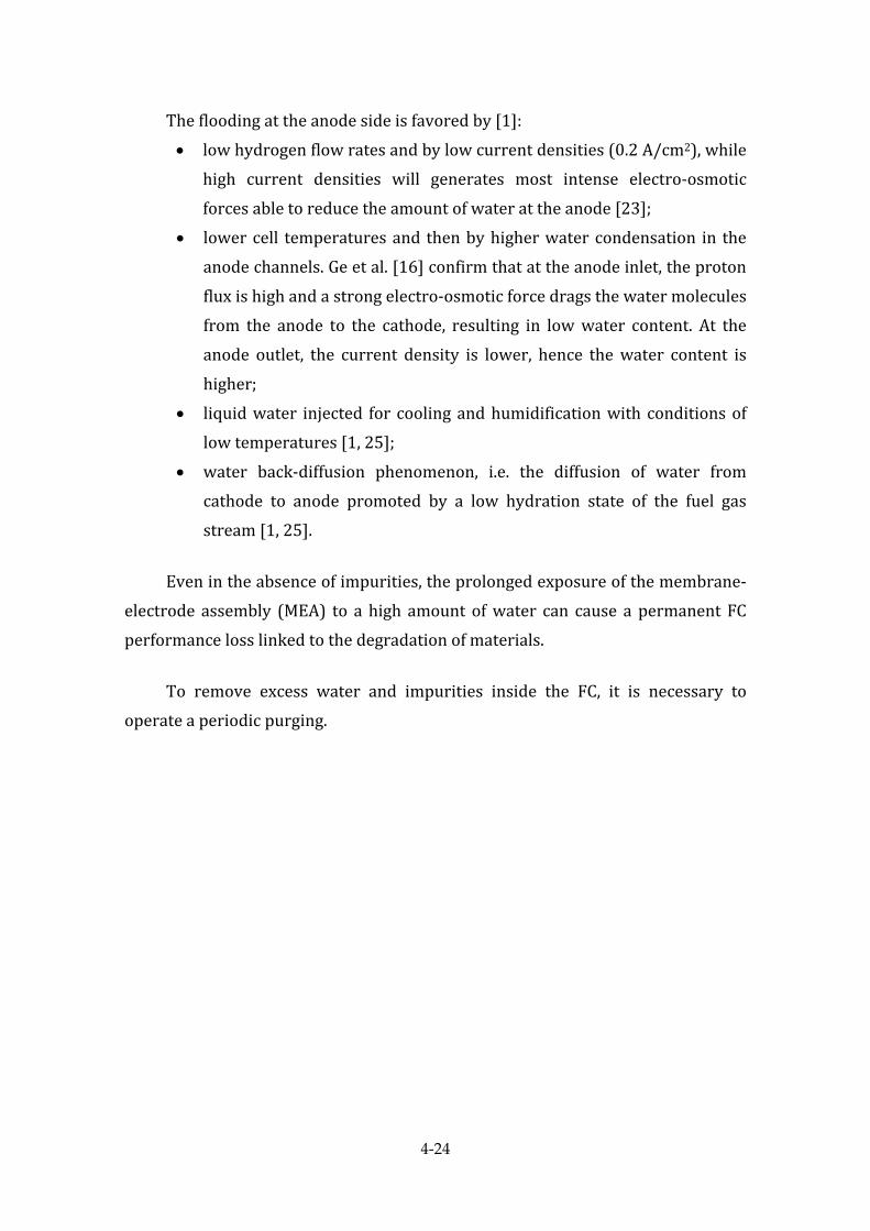
4‐24 

The flooding at the anode side is favored by [1]: • low hydrogen flow rates and by low current densities (0.2 A/cm2), while 

high  current  densities  will  generates  most  intense  electro‐osmotic forces able to reduce the amount of water at the anode [23];  

• lower cell  temperatures and  then by higher water condensation  in  the anode channels. Ge et al. [16] confirm that at the anode inlet, the proton flux is high and a strong electro‐osmotic force drags the water molecules from  the  anode  to  the  cathode,  resulting  in  low water  content.  At  the anode  outlet,  the  current  density  is  lower,  hence  the water  content  is higher; 

• liquid water  injected  for  cooling and humidification with  conditions of low temperatures [1, 25]; 

• water  back‐diffusion  phenomenon,  i.e.  the  diffusion  of  water  from cathode  to  anode  promoted  by  a  low  hydration  state  of  the  fuel  gas stream [1, 25].  

Even in the absence of impurities, the prolonged exposure of the membrane‐electrode  assembly  (MEA)  to  a  high  amount of water  can  cause  a  permanent  FC performance loss linked to the degradation of materials. 

To  remove  excess  water  and  impurities  inside  the  FC,  it  is  necessary  to operate a periodic purging. 

4‐25 

4.2 CONTAMINATION OF THE PEMFC COMPONENTS 

Contamination is the process where impurities pollute and penetrate into the cell’s components  and/or  initiate  chemical  attack  and  slow  down  the  actual  reactions taking  place  in  the  cell.  The  contamination  products  originate  from  components inside the cell or can be transported into the cell by the reactants. Consequentelly, metal, alkaline metal and ammonium ions, silicon and catalyst particles as well as carbon  monoxide  (CO),  nitrogen  oxides  (NOx)  or  sulfur  dioxide  (SO2)  can  be present  in  the  cell.  Even  trace  amounts  of  impurities  result  in  considerable degradation of performance [2, 61, 62]. 

The  CO‐poisoning  is  due  to  the  adsorption  of  the  CO‐molecules  [2]  by  the platinum  that  block  the  hydrogen  from  reaching  the  platinum  particles.  CO‐poisoning can lead to a significant performance loss, but it does not seem to have an influence on lifetime. It was demonsted that even 50 ppm of CO are sufficient to poison  the  anode  reaction  resulting  in  a  lower  cell  potential  output  and  lower energy conversion efficiency [66]. The CO poisoning, occurs only at the anode side, because the CO can be present in the hydrogen stream, when the fuel is obtained by reforming liquid hydrocarbons or alcohol fuels [2‐4, 40, 63, 64, 65]. In order to stop  the  CO‐poisoning  it  is  necessary  to  remove  carbon  monoxide  from  the reactant. For example, Le Canut et al. [63], observed that the voltage could be fully recovered with  injection of air  into  the  fuel stream (air bleed 2%), considering a recovery  time  of  40  min  for  the  low  and  around  10  min  for  the  high  CO concentration. 

Also the membrane can be attacked by cationic contaminants. Alkaline metals and ammonium ammonium ions can in fact penetrate into the membrane resulting in considerable reduction of performance [61, 62]. Kienitz et al.  [61] assume that the reduced performance of a contaminated cell is due to the limited proton flux at the cathode. Protons will be replaced, due to the higher affinity of the cations, with the sulfonic acid endgroups of the membrane, resulting in lower conductivity and water levels and in a higher electro‐osmotic force. This will reduce the maximum current and the exchange current density in the cells. 

4‐26 

4.3 HYDROGEN CROSSOVER 

Hydrogen crossover is an undesirable diffusion of hydrogen from the anode to the cathode through the membrane (Figure 4.6). 

 

Figure 4.6: The H2 crossover phenomenon in a PEMFC. 

Hydrogen  crossover  can  have  at  least  three  effects:  the  fuel  efficiency reduction,  the  cathode  potential  depression  and  the  aggressive  peroxide  radical formation [106]. 

Cheng et al. [107] have demonstrated that the hydrogen which crosses over can directly  react with oxygen at  the  cathode  surface,  resulting  in a  reduction of the cathode potential. 

More  severely,  the  direct  reaction  between  H2  and  O2  at  the  cathode  can produce  peroxide  radicals, which  not  only  attack  the  catalyst  layer,  but  also  the membrane, causing significant catalyst‐layer and membrane degradation [108]. In addition, Yu et al.  [109] confirmed that  the  formation of hot‐points by  the highly exothermal chemical reaction between H2 and O2 can also lead to pin‐holes into the membrane, destroying the MEA and causing safety problems. Therefore, Ianaba et al.  [110]  and Teranishi  et  al.  [111]  demonstred  that  also  hydrogen peroxide  can 

4‐27 

lead  to  pin‐holes  in  the  membrane  causing  the  performance  degradation  of  the PEMFC.  Moreover,  an  accelerated  sintering  of  catalysts  could  be  caused  by  this hydrogen crossover [108]. 

The  measurement  of  hydrogen  crossover  is  of  importance  for  the fundamental  understanding  and  practical mitigation  of  fuel  cell  degradation  and membrane failure [107]. 

Since  H2  crossover  is  a  diffusion  process,  the  PEM  structure  and  fuel  cell operating conditions [110, 112] can greatly influence the crossover process. In fact, Sakai et al [113] investigated the H2 crossover at temperature up to 80 °C, showing that  the  uses  of  thinner  membranes  and  the  operation  of  fuel  cells  at  high temperature and high pressure will facilitate H2 crossover. Also the water content in  the  membrane  [113]  and  gas  pressure  [110]  had  a  great  effect  on  the  H2 crossover. 

Rama  et  al.  [114]  analyzed  the  effects  of  membrane  thickness,  operating pressure  and  temperature  and  current  density  on  H2  crossover  using  a concentrated  solution  membrane  system  containing  four  species:  water, electrolyte membrane,  proton  and  hydrogen.  The  simulated  results  indicate  that the  increase  in  the  H2  crossover  found  when  temperatures  increases  were attributed to the dependence of the H2 diffusion coefficient on temperature. 

The structure and chemistry of PEM are critical in the control of proton and water transport and H2 crossover. The use of Nafion‐based composite membranes could  reduce  H2  crossover  with  a  less  porous  crystalline  structure  provided  by well‐dispersed small additive particles [115], or after heat‐treating at 120 °C [116]. 

The  three‐region model  [117]  and  cluster‐network model  [118]  have  been widely  used  to  describe  the  microstructure  of  perfluorosulfonated  membranes such  as  Nafion‐type  membranes.  However,  there  is  still  no  agreement  as  to whether  the  gas  permeates  through  Nafion  in  the  intermediate  region,  which consists mainly  of  the  flexible  amorphous  part  of  the  perfluorocarbon  backbone [119, 120], or through the hydrated ionic clusters, which contain mainly water and sulfonic  acid  groups  [113].  Brohka  et  al.  [121]  have  suggested  another  solution according to which the gas permeates through both regions. 

4‐28 

In order to improve our understanding of the H2 crossover phenomena, it is necessary to clarify the nature of H2 crossover from the anode to the cathode via the MEA.  

Many studies have been conducted in order to investigate the causes and the effects  of  the  H2  crossover  phenomenon.  For  example,  Yasuda  et  al.  [14]  have studied  the  impacts  of  crossover  hydrogen  on  the  location  of  the  platinum  (Pt) band  formed  in  the membrane  after  Pt  dissolution.  The  Pt  band  or  Platinumin‐Into‐The‐Membrane  (PITM) was  shown  to  be  located  closer  to  the  anode  under lower hydrogen partial pressure conditions [122]. 

Zhang  et  al.  [15]  examined  the  effects  of  hydrogen  and  oxygen  partial pressures on Pt precipitation within the membrane, and developed a simple model to estimate the location of the PITM band defined as: 

2222

22

2 OOHH

PEMHHPITM pKpK

lpK+

=δ   (4.1) 

where:  PITMδ is  the  PITM  location,  PEMl is  the membrane  thickness, K  is  the membrane gas permeability, and p is the gas partial pressure. 

Holby et al. studied the influence of crossover hydrogen on the stability of Pt nanoparticles via a theoretical approach [124]. 

T.  Cheng  et  al.  [125]  have  evaluated  the  crossover  hydrogen  effects  on  Pt degradation and the subsequent impacts on the cathode catalyst layer.  

Precisly,  they  have  investigated  the  effects  of  crossover  hydrogen  on  Pt dissolution and agglomeration in fuel cell stacks under dynamic cycling conditions that simulate fuel cell system start‐ups and shutdowns.  

The experimental results provided that H2 crossover maychemically reducePt oxides  and  subsequently  decreases  the  amount  of  Pt  ions  formed  via  the  oxide pathway. Hence, with less H2 crossover, the concentration of Pt ions in the cathode becomes higher and subsequently leads to more Pt growth and agglomeration,  in agreement  with  the  relative  crystallite  sizes  and  active  surface  area  loss  by  CO stripping. Finally, based on Fick’s Law of diffusion, the higher Pt ion concentration 

4‐29 

may counterbalance the longer Pt ion diffusion path.  

Kocha  et  al.  [123]  have  confirmed  the  dependence  of  H2  crossover  on  the membrane  thickness.  They  compared  the  H2  crossover  currents  measured  in Nafion  112  and  in Nafion  111  in  the  temperature  range  of  25–80  °C,  suggesting that the dominant factor limiting the H2 crossover rate is the membrane diffusion coefficient (DPEM). For Nafion membranes, DPEM has been defined empirically as a function  of  temperature  (T)  [126],  but  also  of  the  backpressure  (P)  and  of  the relative humidity, RH [107]. 

X. Cheng et al. [107] have developed a multilayer diffusion model to describe H2 crossover  through  the MEA (Figure 4.7).This  investigation was carried out  to examine the effects of temperature (T), pressure, and relative humidity (RH) on H2 crossover. They have demonstrated that the H2 crossover strongly depends on T, RH and backpressure (P). 

 

 

Figure 4.7: The H2 crossover trough the MEA in a PEMFC scheme [107]. 

 

4‐30 

In fact, the H2 crossover rate,  crossHJ

2(mol cm‐2 s‐1), can be expressed as: 

)(2

2

2

aH

PEM

PEMHcross

H Pl

J ⎟⎟⎠

⎞⎜⎜⎝

⎛=

ψ  (4.2) 

where: 

PEMH2

ψ  is the permeability coefficient of H2 in the PEM (mol cm‐1 atm‐1 s‐1); 

PEMl  is the PEM thickness; a

HP2 is the H2 partial pressure inside the anode chamber. 

Each  of  these  parameters  is  also  function  of  the  temperature,T, backpressiure, P and relative humidity, HR.  

In particular  the permeability coefficient  PEMH 2

ψ is a  function of T, P, RH and also  of  the  water  content  and  the  nature  of  the  membrane  [127].  It  can  be calculated at various conditions through the current induced by the crossed–over hydrogen,  cross

HI2,  that  is  directly  related  to  the  H2  crossover  rate  through  the 

Faraday’s equation:  

nFAI

JcrossHcross

H2

2=   (4.3) 

Where where n  is  the  electron number of H2  oxidation  (=2), F  the  Faraday constant (A s mol−1), and A is the MEA active area (cm2). 

Instead, the thickness of the membrane,  PEMl does not vary substantially, for a given fuel cell system. For example it is equal to ~50 μm for Nafion 112 and  175 μm for Nafion 117. 

Finally,  the H2 partial pressure, a

HP2can be calculated based on the fuel cell 

anode  inlet  total  pressure  (a

inletP ),  the  H2  partial  pressure  in  the  inlet  stream,  (a

inletHP −2) and the outlet total pressure, backpressure (P).  

 

 

4‐31 

Assuming that the pressure drop along the superfine anode channel is linear, a

HP2is defined by following equation: 

⎟⎟⎠

⎞⎜⎜⎝

⎛ +⎟⎟⎠

⎞⎜⎜⎝

⎛= −

22

2

PPP

PP

ainlet

ainlet

ainletHa

H   (4.4) 

The  magnitude  of  H2  crossover  (eq.  4.2)  goes  up  monotonically  with increases  in  temperature  and  backpressure. However,  the  RH  effect  is more complicated than those of temperature and backpressure [107]. 

More in detail, H2 crossover rate increases with increasing temperature and, since the permeability coefficient,  PEM

H 2ψ  is directly related to the H2 solubility and 

diffusion  coefficients  [123],  any  effect  of  temperature  on  these  two  coefficients could  cause  a  change  of  PEM

H2ψ .  The  increase  of  this  parameter  with  increasing 

temperature  probably  indicates  that  the  effect  of  temperature  on  the  diffusion coefficient is more significant than that on the solubility coefficient. 

According  to  the  Eq.  4.3,  the  H2  crossover  rate  will  be  increased  if  the  H2 partial  pressure,  increases.  In  particular,  X.  Chang  et  al.  [107].have  observed  a monotonic increase in the H2 crossover rate with increasing backpressure Thus it is  understandable  that  an  increase  in  backpressure  will  result  in  a  H2  partial pressure increase, which then creates a larger pressure difference across the PEM.  

The  activation  energies  and  maximum  permeability  coefficients  of  H2 permeation through both Nafion 112 and Nafion 117‐based showed similar values of  these parameters  for both MEAs,  suggesting  that  the membrane  thickness has no significant effect on the H2 permeation mechanism. 

The RH effect on  the H2 crossover  rate  seems  to be more complicated  than those of temperature and backpressure [107]. In fact, fixed the temperature the H2 crossover rate increases as the RH increases, at higher backpressure, while the RH increase reduces the crossover rate, at lower backpressure. 

However,  the  temperature  effect  is  much  larger  than  those  caused  by backpressure and RH. 

4‐32 

References to the chapter 4 

[1]  B. Belvedere, M. Bianchi, A. Borghetti, A. De Pascale, M. Paolone, R. Vecci., 

Experimental  analysis of  a PEM  fuel  cell performance  at variable  load with 

anodic  exhaust  management  optimization,  (Original  Research  Article) 

International  Journal  of Hydrogen  Energy,  Volume  38,  Issue  1,  11  January 

2013, 385‐393. 

[2]  Hinds  G.  Performance  and  Durability  of  PEM  Fuel  Cells:  A  Review. NPL 

Report DEPC‐MPE 002, 2004, pp. 25‐42. 

[3]  Schmittinger W, Vahidi A. A review of the main parameters, influencing long‐

term performance and durability of PEM fuel cell, Journal of  Power Sources, 

2008;180: 1‐14. 

[4]  Fuel Cell Handbook, 7th Edition, US DOE, 2004. 

[5]  http://www.ballard.com/ 

[6]  http://www.mercedes‐benz.de/content/germany/mpc/mpc‐germany 

website/de/home mpc/buses/home/bus world/ 

[7]  C. Sishtla, G.Koncar, R. Platon, S. Gamburzev, J. Power Sources 71 (1998) 249. 

[8]  K. Washington, Proceedings Fuel Cell Seminar 2000, Portland, U.S.A., 2000, p. 

468. 

[9]  U. Pasaogullari, C.Y. Wang, J. Electrochem. Soc. 152 (2) (2005) A380–A390. 

[10]  H.  Maeda,  A.  Yoshimura,  H.  Fukumoto,  Proceedings  Fuel  Cell  Seminar, 

(2000), Portland, U.S.A., p. 379. 

[11]  M. Fowler, J.C. Amphlett, R.F. Mann, B.A. Peppley, P.R. Roberge, J. New Mat. 

Electrochem. Syst. 5 (2002) 255. 

[12]  E.  Endoh,  S.  Terazono,  H.Widjaja,  Abstract  89,  Electrochem.  Soc. Meeting 

Abstracts, Salt Lake City, U.S.A., 2002. 

[13]  S.D. Knights, K.M. Colbow,  J. St‐Pierre, D.P.Wilkinson,  J. Power Sources 127 

(2004) 127–134. 

[14]  J. Scholta, N. Berg, P. Wilde, L. Jorissen, J. Garche, J. Power Sources 127, (2004) 

206–212. 

4‐33 

[15]  X. Cheng, L. Chen, C. Peng, Z. Chen, Y. Zhang, Q. Fan,  J. Electrochem. Soc. 

151 (2004) A48–A52. 

[16]  X. Wang, D. Myers, R. Kumar, Proceedings of  the Fuel Cells Durability,  first 

ed., Washington, DC, 2006, pp. 151–162. 

[17]  V. Lightner, DOE Hydrogen Program, Record 5036, 2006. 

[18]  V. Lightner, DOE Hydrogen Program, Backup Ref. 5036a, 2006. 

[19]  R.  Borup, D.Wood,  J. Davey,  P.Welch,  F. Garzon, DOE Hydrogen  Review, 

Presentation, 2006. 

[20]  R. Borup, D.Wood, J. Davey, P.Welch, F. Garzon, DOE Hydrogen Review, FY 

2006 Annual Progress Report, 2006. 

[21]  S.J.C.  Cleghorn,  D.K.  Mayfield,  D.A.  Moore,  J.C.  Moore,  G.  Rusch,  T.W. 

Sherman, N.T. Sisofo, U. Beuscher, J. Power Sources 158 (2006) 446–454. 

[22]  Zawodzinski  T, Derouin  C,  Radzinski  S,  Sherman  R,  Smith  V,  Springer  T, 

Gottesfeld  S.  Water  Uptake  by  and  Transport  Through  Nation  117 

Membranes, J. Electrochem. Soc. Vol.140, No.4, (1993): pp. 1041‐1047. 

[23]  McKay  DA,  Siegel  JB,  Ott  W,  Stefanopoulou  AG.  Parameterization  and 

prediction of temporal fuel cell voltage behavior during flooding and drying 

conditions, Journal of Power Sources, Volume 178, Issue 1, 15 March 2008, p. 

207‐222. 

[24]  St‐Pierre  J, Wilkinson  DP,  Knights  S,  Bos M.  Relationship  between  water 

management,  contamination  and  lifetime  degradation  in  PEFC,  Journal  of 

New Materials for Electrochemical Systems, 3, 99 ‐106 (2000). 

[25]  Mokmeli A, Asghari S. An  investigation  into  the effect of anode purging on 

the fuel cell performance, International Journal of Hydrogen Energy 35, (2010), 

9276‐9282.  

[26]  B.  Belvedere,  M.  Bianchi  ,  A.  De  Pascale,  Experimental  analysis  of  a 

cogenerative  performance  of  a  PEM  fuel  cell  based  energy  system, 

Proceedings of ICAE 2011, 16‐18 May 2011 ‐ Perugia, Italy. 

4‐34 

[27]  B.  Belvedere, M.  Bianchi,  A.  Borghetti,  A.De  Pascale, M.  Di  Silvestro, M. 

Paolon, DSP‐Controlled  Test  Set‐up  for  the  Performance Assessment  of  an 

Autonomous Power Unit Equipped with a PEM Fuel Cell, Proceedings of the 

2007 International Conference On Clean Electrical Power (ICCEP’07), art. No. 

4272427, pp. 468‐473. 

[28]   R.L. Borup, J.R. Davey, F.H. Garzon, D.L. Wood, M.A. Inbody, Proceedings of 

the Fuel Cells Durability, first ed., Washington, DC, (2006),  21–42.. 

[29]  R.L.  Borup,  J.R.  Davey,  F.H.  Garzon,  D.L. Wood,  M.A.  Inbody,  J.  Power 

Sources 163 (2006) 76–81. 

[30]   P. Meyers, R.M.S. Darling, The Electrochem. Soc. Meeting Abstracts, Abstract 

1212, Paris, France, 2003. 

[31]  S. Motupally, T.D.  Jarvi, The Electrochem. Soc. 208th Meeting, Abstract, Los 

Angeles, CA, 2005. 

[32]  C. Paik, T. Skiba, V. Mittal, S. Motupally, T. D.  Jarvi, The Electrochem. Soc. 

207th Meeting, Abstract 771, Quebec City, Canada, 2005. 

[33]  T. Patterson, Effect of potential cycling on  loss of electrochemical surface rea 

of  platinum  catalyst  in  polymer  electrolyte membrane  fuel  cell,  in:AICHE 

National Conference, New Orleans, LA, 2002. 

[34]  M.S. Wilson, F.H. Garzon, K.E. Sickafus, S. Gottesfeld, J. Electrochem. Soc. 140 

(1993) 2872–2877. 

[35]  P. Ascarelli, V. Contini, R. Giorgi, J. Appl. Phys. 91 (2002). 

[36]  M.S. Wilson, F.H. Garzon, K.E. Sickafus, S. Gottesfeld, J. Electrochem. Soc. 140 

(1993) 2872. 

[37]  W. Li, M. Ruthkosky, M. Balogh, R. Makharia, S. Oh, Proceedings of the Fuel 

Cells Durability, first ed., Washington, DC, 2006, pp. 101–114. 

[38]  Horky,  K.  Beverage,  O.  Polevaya,  Y.  Shi,  Proceedings  of  the  Fuel  Cells 

Durability, first ed., Washington DC, 2006, pp. 133–150. 

[39]  K.L. More, K.S. Reeves, 2005DOEHydrogen Program Review, Arlington, VA, 

2005. 

4‐35 

[40]  K. Duff, Stainless Steel alloys  for Polymer Electrolyte Membrane  (PEM) Fuel 

Cells,  presentation,  2005,  http://www.chemistry.oregonstate.edu/ 

courses/ch407h/CH407Hprojectkeeganfuelcell steels.ppt. 

[41]  Larminie, A. Dicks,  Fuel  Cell  Systems  Explained,  John Wiley &  Sons  Ltd., 

Chichester, England, 2003. 

[42]  M. Li, S. Luo, C. Zeng, J. Shen, H. Lin, C. Cao, Corros. Sci., 46, 1369 (2004).  

[43]  E. Gulzow, M.  Schulze, N. Wagner,  T. Kaz,  R.  Reissner, G.  Steinhilber, A.  

Schneider, J. Power Sources, 86, 352 (2000).  

[44]   L. Ma, S. Warthesen, D.A. Shores,  J. New Mat. Electrochem. Systems, 3, 221  

(2000).  

[45]  G. Hubner, E. Roduner, J. Mater. Chem., 9, 409 (1999). 

[46]  G. Escobedo, K. Schwiebert, K. Raiford, G. Nagarajan, F. Principe, Proceedings 

of the Fuel Cells Durability, first ed., Washington, DC, 2006, 83–100. 

[47]  D.E.  Curtin,  R.D.  Lousenberg,  T.J.  Henry,  P.C.  Tangeman, M.E.  Tisack,  J. 

Power Sources 131 (2004) 41–48. 

[48]  F.  Finsterwalder,  M.  Quintus,  M.  Schaloske,  T.  Guth,  G.  Frank,  The 

Electrochem. Soc. 210th Meeting, Abstract 0485, Cancun, Mexico, 2006. 

[49]  V.O. Mittal, H.R.  Kunz,  J.M.  Fenton,  Abstract  0448,  The  Electrochem.  Soc. 

210th Meeting, Cancun, Mexico, 2006. 

[50]  G. H¨ubner, E. Roduner, J. Mater. Chem. 9 (1999) 409–418. 

[51]   S. Kundu, M.W. Fowler, L.C. Simon, S. Grot, J. Power Sources 157, (2006), 650–

656. 

[52]  V. Ramani, H.R. Kunz, J.M. Fenton, The Electrochem. Soc. Interf. 17–19, (2004), 

45. 

[53]   J. Yu, T. Matsuura, Y. Yoshikawa, M.N.  Islam, M. Hori, Electrochem. Solid‐

State Lett. 8 (2005) ,A156–A158. 

[54]  R. Baldwin, M. Pham, A. Leonida, J. McElroy, T. Nalette, J. Power Sources 29 

(1990) 399–412. 

[55]  S.  Stucki, G.G.  Scherer,  S.  Schagowski,  E.  Fisher,  J. Appl.  Electrochem.,  28, 

1041 (1998).   

4‐36 

[56]  M. Wakizoe, H. Murata, H.  Takei,  Proc.  Fuel  Cell  Seminar  2000,  Portland,  

U.S.A., p. 487. 

[57]   W. Liu, K. Ruth, G. Rusch, J. New Mat. Electrochem. Syst. 4 (2001), 227–231. 

[58]  D.P. Davies,  P.L. Adcock, M. Turpin,  S.J. Rowen,  J.  Power  Sources,  86,  237 

(2000). 

[59]  M.  Schulze,  T. Knori, A.  Schneider,  E. Gulzow,  J.  Power  Sources,  127,  222  

(2004).  

[60]  S.‐Y. Ahn,  S.‐J.  Shin, H.Y. Ha,  S.‐A. Hong, Y.‐C. Lee, T.W. Lim,  I.‐H. Oh,  J. 

Power Sources, 106, 295 (2002). 

[61]  B. Kienitz, H. Baskaran, B. Pivovar, T. Zawodzinski  Jr., ECS Trans. 11  (2007) 

777–788. 

[62]  X. Cheng, Z. Shi, N. Glass, L. Zhang, J. Zhang, D. Song, Z.‐S. Liu, H. Wang, J. 

Shen, J. Power Sources 165 (2007) 739–756. 

[63]  J. Le Canut, R.M. Abouatallah, D.A. Harrington, J. Electrochem. Soc. 153 (2006) 

A857–A864  

[64]  A.  Rodrigues,  J.C.  Amphlett,  R.F.  Mann,  B.A.  Peppley,  P.R.  Roberge, 

Proceedings  of  the  32nd  Intersociety  Energy  Conversion  Engineering 

Conference, IECEC‐97 (1997) 768–773. 

[65]   D.D. Penta, K. Bencherif, Q. Zhang, M. Sorine, Proceedings of  the 2006  IEEE 

Int. Conference on Control Applications, Munich, Germany, 2006. 

[66]   Z. Qi,  Proceedings  of  the  Fuel  Cells Durability,  first  ed., Washington, DC, 

(2006), 163–190. 

[67]  Z. Liu, L. Yang, Z. Maoa,W. Zhuge, Y. Zhang, L.Wang, J. Power Sources 157, 

(2006), 166–176. 

[68]  D.P. Wilkinson,  J.  St‐Pierre,  PEM  fuel  cell  durability,  in: W.  Vielstich,  H. 

Gasteiger,  A.  Lamm  (Eds.),  Handbook  of  Fuel  Cells  –  Fundamentals, 

Technology and Applications, Fuel Cell Technology and Applications, vol. 3, 

John Wiley and Sons, 2003. 

[69]  T. van Nguyen, M.W. Knobbe, J. Power Sources 114 (2003) 70–79. 

4‐37 

[70]  T.W. Patterson, R.M. Darling, Electrochem. Solid‐State Lett. 9,  (2006), A183–

A185. 

[71]  M. Saito, K. Hayamizu, T. Okada, J. Phys. Chem. 109, (2005), 3112– 3119. 

[72]  M. Sundaresan, R.M. Moore, J. Power Sources 145 (2005) 534–545. 

[73]  J. Zhang, Z. Xie, J. Zhang, Y. Tang, C. Song, T. Navessin, Z. Shi, D. Song, H. 

Wang, D.P. Wilkinson, Z.S. Liu, S. Holdcroft, J. Power Sources 160 (2006) 872–

891. 

[74]  E. Cho, J. Ko, H.Y. Ha, S. Hong, K. Lee, T. Lim, I. Oh, J. Electrochem. Soc. 150 

(2003) A1667–A1670. 

[75]  A. Pesaran, G.‐H. Kim,  J. Gonder, Proceedings  of  the  Fuel Cells Durability, 

first ed., Washington, DC, (2006), 205–227. 

[76]  S. He, M.M. Mench, J. Electrochem. Soc. 153 (9) (2006) A1724–A2173. 

[77]  C.H. Lee, H.B. Park, Y.M. Lee, R.D. Lee, Ind. Eng. Chem. Res. 44 (2005) 7617–

7626, Sources 165 (2007) 739–756. 

[78]  R.K. Ahluwalia, X. Wang, J. Power Sources 162 (2006) 502–512. 

[79]   L. Mao, C.‐Y. Wang, J. Electrochem. Soc. 154 (2007) B139–B146. 

[80]  A.S.  Arico,  A.  Stassi,  E.  Modica,  R.  Ornelas,  I.  Gatto,  E.  Passalacqua,  V. 

Antonucci, ECS Trans. 3 (2006) 765–774. 

[81]  Y. Song, H. Xu, Y. Wei, H.R. Kunz, L.J. Bonville, J.M. Fenton, J. Power Sources 

154 (2006) 138–144. 

[82]  W.  Bi,  T.F.  Fuller, Abstract  395,  The  Electrochem.  Soc.,  212th  ECS Meeting, 

Washington, DC, 2007 

[83]  I. Manke, N. Kardjilov, A. Haibel, C. Hartnig, M. Strobl, A. Rack, A. Hilger, J. 

Scholta, W. Lehnert, W. Treimer, S. Zabler, J. Banhart, DGZfPBerichtsband 94‐

CD, 2005. 

[84]  T.V. Nguyen, R.E. White, J. Electrochem. Soc. 140 (1993) 2178–2186. 

[85]  N.E. Vanderborgh, J.R. Huff, J. Hedstrom, IEEE CH2781‐3/89/0000‐163 (1989) 

1637–1640. 

[86]  Y. Sone, P. Ekdunge, D. Simonsson, J. Electrochem. Soc. 143 (1996) 1254. 

4‐38 

[87]  Y. Wang, C.‐Y. Wang, Electrochim. Acta 51 (2006) 3924–3933. 

[88]  S. Kim, M.M. Mench, J. Power Sources 174 (2007) 206–220. 

[89]  F.  Kagami,  F. Ogawa,Y. Hishinuma,  T. Ghikahisa,  Fuel  Cell  Seminar  2002, 

Palm Springs, USA, 2002, p. 239. 

[90]  G. Li, P.G. Pickup, Electrochem. Solid‐State Lett. 9 (2006) A249–A251. 

[91]  X. Huang, R. Solasi, Y. Zou, M. Feshler, K. Reifsnider, D. Condit, S. Burlatsky, 

T. Madden, J. Polym. Sci. Part B Polym. Phys. 44 (16) (2006), 2346–2357. 

[92]  D.A.  McKay,  W.T.  Ott,  A.G.  Stefanopoulou,  Modeling,  parameter 

identification, and validation of reactant water dynamics for a fuel cell stack,  

in:Proceedings  of  the  IMECE,ASMEInt.  Mech.  Eng.  Congress&Exposition, 

2005. 

[93]  W. He, G. Lin, T.V. Nguyen, AICHE J. 49 (2003) 3221–3228. 

[94]  B.A. Dipierno, M.H. Fronk, US Patent 6,103,409 (2000). 

[95]  A.Z. Weber,  R.M. Darling,  J. Newman,  J.  Electrochem.  Soc.  151  (10)  (2004) 

A1715–A1727. 

[96]  A. Turhan, K. Heller,  J.S. Brenizer, M.M. Mench, J. Power Sources 160 (2006) 

1195–1203. 

[97]  J.J. Kowal, A. Turhan, K. Heller,  J.S. Brenizer, M.M. Mench,  J. Electrochem. 

Soc. 153 (2006) A1971–A1978. 

[98]  S. Ge, C.‐Y. Wang, J. Electrochem. Soc. 154 (2007) B998–B1005. 

[99]  T. Nguyen, J. Hedstrom, N. Vanderborgh, in: R.E. White, A.J. Appleby (Eds.), 

The Electrochem. Soc. Softbound Proceedings Series PV 89–14 (1989) 39. 

[100] T.E. Springer,  J. Zawodzinski, S. Gottesfeld,  in: R.E. White, M.W.   erbrugge, 

J.F. Stockel (Eds.), The Electrochem. Soc. Softbound Proceedings Series PV 91–

10 (1991) 209. 

[101] P.J.  Schutz,  in:  R.E.  White,  A.J.  Appleby  (Eds.),  The  Electrochem.  Soc. 

Softbound Proceedings Series PV 89–14 (1989) 87. 

[102] R. Mukundan,Y.S. Kim, T. Rockward, J.R. Davey,B. Pivovar, D.S. Hussey, D.L. 

Jacobson, M. Arif, R. Borup, ECS Trans. 1 (2007) 543–552. 

4‐39 

[103] Y. Hishinuma, T. Chikahisa, F. Kagami, T. Ogawa,  JSME  Int.  J. B 47   2004), 

235–241. 

[104] Gou J, Pei P, Wang Y. The dynamic behavior of pressure during purge process 

in the anode of a PEM fuel cell. J Power Sources 2006;162:1104e14. 

 [105] Strasser k. The dsign of alkaline fuel cells. J Power Sources 1990;29:149e66. 

[106]  J. Zhang,Y. Tang, C. Song, J. Zhang, H.Wang, J. Power Sources 163 (2006)  532. 

[107] X. Cheng,  J. Zhang, Y. Tang, C. Song,  J. Shen, D. Song,  J. Zhang, Hydrogen 

crossover  in high‐temperature PEM  fuel cells,  J. of Power Sources 167  (2007) 

25–31. 

[108] A.  Collier,H.Wang,  X.  ZiYuan,  J.  Zhang,  D.P.Wilkinson,  Int.  J.  Hydrogen 

Energy 31 (2006) 1838. 

[109]  J. Yu, T. Matsuura, Y. Yoshikawa, M.N.  Islam, M. Hori, Electrochem. Solid‐

State Lett. 8 (2005) A156–A158. 

[110] M.  Inaba,  T.  Kinumoto, M.  Kiriake,  R. Umebayashi, A.  Tasaka,  Z. Ogumi, 

Electrochim. Acta 51 (2006) 5746. 

[111] K. Teranishi, K. Kawata, S. Tsushima, S. Hirai, Electrochem. Solid‐State Lett. 9 

(2006) A475–A477. 

[112] Y. Song, J.M. Fenton, H.R. Kunz, L.J. Bonville, M.V. Williams, J. Electrochem. 

Soc. 152 (2005) A539–A544. 

[113] T. Sakai, H. Takenaka, E. Torikai, J. Electrochem. Soc. 133 (1986) 88. 

[114] P. Rama, R. Chen, R. Thring, IMechE Part A: J. Power Energy 220 (2006), 535. 

[115] V. Ramani, H.R. Kunz, J.M. Fenton, J. Membr. Sci. 266 (2005) 110. 

[116] Y. Si, H. Russell Kunz, J.M. Fenton, J. Electrochem. Soc. 151 (2004) A623–A631. 

[117] H.L. Yeager, ACS Symp. Ser. 180 (1982) 41. 

[118] T.D. Gierke, W.Y. Hsu, ACS Symp. Ser. 180 (1982) 283. 

[119] Z. Ogumi, Z. Takehara, S. Yoshizawa, J. Electrochem. Soc. 131 (1984) 769. 

[120] Z. Ogumi, T. Kuroe, Z.‐i. Takehara, J. Electrochem. Soc. 132 (1985) 2601. 

[121] K. Broka, P. Ekdunge, J. Appl. Electrochem. 27 (1997) 117. 

4‐40 

[122] K. Yasuda, A. Taniguchi, T. Akita, T.  Ioroi, Z.  Siroma,  Phys. Chem. Chem. 

Phys. 8 (2006) 746. 

[123] Zhang, B.A. Litteer, W. Gu, H. Liu, H.A. Gasteiger,  J. Electrochem. Soc. 154 

(2007) B1006. 

[124] E.F. Holby, W. Sheng, Y. Shao‐Horn, D. Morgan, Energy Environ. Sci. 2 (2009) 

865. 

[125] T.T. H. Cheng , E. Rogers, A. P. Young, S. Ye, V. Colbow, S. Wessel, Effects of 

crossover hydrogen on platinum dissolution and agglomeration,  J. of Power 

Sources ,96 ,(2011) ,7985‐7988. 

[126] R.S. Yeo, J. McBreen, J. Electrochem. Soc.,126 ,(1979),1682. 

[127] A.Z. Weber, J. Newman, J. Electrochem. Soc. 151 (2004) A311–A325. 

5‐1 

Chapter 5 

5. ANODIC EXHAUST MANAGEMENT: ANALISYS AND OPTIMIZATION 

In  this  chapter  an  investigation  on  the  performance  of  the  commercial  PEMFC, installed in the developed IES, taking into account the anodic exhaust management and its effects on the flooding phenomenon, is described. 

To  address  the  problem  of  flooding,  it  is  necessary  to  run  periodically  the purge process of the FC. Indeed, in this study the periodic anodic purge process in dead‐end mode has been  investigated. This operation  is performed by opening a particular control valve,  the Outlet Control Valve (OCV),  located along  the anodic exhaust line. 

The purge process has been analyzed at different FC power output levels. For each  FC  power  level  the  optimized  behavior  of  the  FC  operation was  found,  by regulating the time of flooding. 

The  aim  of  this  analysis  is  to  optimize  the  purge  process  to  reduce  the amount of hydrogen discharged with water, in order to increase the FC efficiency.  

5‐2 

Furthermore,  an  investigation  on  the  benefits  in  terms  of  fuel  utilization factor and costs, resulting from optimization of the FC purge process, is shown. 

It should be noted that this analysis is based on the assumption that the cell is a “black box”, it is not broken down into its individual components, but it is a real system  in  its  own  right  (the  “FC  ‐system”),  inserted within  the  test  IES  in which acting as energy source. Therefore, it was not possible to investigate the individual components  of  the  cell  (such  as  single  cells  stack  components,  membrane,  GDL, bipolar plates, etc.),  so only "global"  indexes and algorithms, able  to describe the behavior of the PEMFC, seen as an element of the IES system, were determined. 

5‐3 

5.1 THE HYDROGEN PURGING: MOTIVATION, LIMIT AND OPTIMIZATION STRATEGIES 

There are  two different schemes  for supplying hydrogen at  the anode side. First, hydrogen may be supplied in the so‐called dead­end mode. In this mode, hydrogen stoichiometry is equal to 1 or a slightly higher, i.e. hydrogen is supplied at the exact rate as the fuel cell stack needs (Figure 5.1).  

 

Figure 5.1: Dead end mode: layout. 

In  the second scheme, which  is called  flow­through mode, hydrogen may be supplied in excess (Figure 5.2). A recirculation mode may also be used in the case of  pure  hydrogen.  In  this  case  the  unused  gas  is  not  wasted,  but  returned  for consumption back to the stack inlet by means of a pump or an ejector. In this case, the stack may operate at the stoichiometric ratio much higher than 1. 

5‐4 

 

Figure 5.2: Flow­through mode: layout. 

To  prevent  accumulation  of  inert  and  impurities,  which  lead  to  output voltage loss, the purge process should be periodically run in a FC energy system. 

The  purge  process  has  a  fundamental  role  on  the  stability  of  the  power supplied  by  the  FC  [1].  Mokmeli  et  al.  [2]  showed  that  the  amount  and  the concentration of impurities in the FC increases with time in absence of purge. Due to this increasing accumulation of impurities, the stack is characterized by loss of voltage increasing over time. 

To  operate  the  purging,  an  outlet  control  valve  (OCV)  is  usually  installed downstream of the FC stack, both for the dead‐end and flow‐through layout. This valve is keep closed until the purge is required. The purge occurs during the entire OCV opening time window. During this time, in addition to impurities, excess water and inert gas, also a quantity of fuel is discharged and thus it is not used by the FC electrochemical reactions. The amount of not‐reacted fuel varies with the amount of time between two consecutive purges, for given opening time of the OCV. 

The  two main  control  parameters  of  the  periodic  purge process  (as  shown qualitatively in Figure 5.3) are: 

• the  time between two consecutive purges, named here Tfl, equal  to  the time interval in which the OCV is closed and, thus, water accumulates in the FC anodic side, causing flooding; 

• the purge  time, Tpu, during which the OCV  is open and thus  impurities, inert gases and excess water are evacuated from the FC. 

5‐5 

 

Figure 5.3: Characteristic time settings of purge process. 

The  purge  process  setting  typically  consists  in  programming  these  two parameters as  function of the FC voltage or as  function of time [2]. The optimum flooding time  is a compromise between minimum hydrogen waste and minimum voltage loss. 

The  first  approach  suggested  by  Strasser  [3]  is  called  "purge  controlled  by the  current".  It  is  based  on  the  observation  that  the  current  varies when  the  FC accumulates  both  impurities  and  inert  gases  and  the  phenomenon  of  flooding starts [1]. 

In  fact,  in  this  approach,  the  reactants  are  streamed  through  the  stack  in opposite directions in a cascading manner, inert gases are collected in the last step of  the  cascading  system,  a  cell  called  gas‐space  cell.  The  load  current  in  the gas‐space cell changes when the inert gas concentration in the cell increase. A current sensor measure the difference between the gas‐space cell and another one used as reference, when the difference increase over a defined value, an electronic device activates  the  OCV  opening  [3].  This  approach  is  an  intelligent  method  and  the hydrogen waste may be minimized but, the complexity and the structural changes due to the connection configuration are the most disadvantages of this method [2]. 

 

5‐6 

The second purge programming approach is based, instead, on the setting of the OCV characteristic times, independently on the FC operating conditions.  

A  simplified way  to  realize  the purging process using  this  second approach consists  in  assuming  constant  values  for  both Tpu  and Tfl,  so  the  purge  could  be thought  as  a  periodical  process  (Figure  5.4)  [1].  The  values  of  these  two parameters should be chosen as a tradeoff between the minimization of amount of discharged H2  and  of  the  voltage  loss  of  the  FC,  resulting  in  an  improvement  in terms of fuel utilization. 

Finally,  the  purge  can  be  operated  when  the  stack  voltage  equals  a predetermined threshold value, with the aim to protect and preserve the longevity and performance of the FC. The amount of purge time must be such as to allow the recovery of the voltage loss. 

Figure  5.4  shows  the  degradation  of  the  FC  stack  voltage  during  the  time when the OCV is closed (flooding time, Tfl,). The flooding time can be divided into two  parts.  In  the  first,  the  stack  voltage  is  constant  for  a  given  value,  which represents  the  absence  of  liquid water  in  the  gas  diffusion  layers,  and  then  the tension starts to decay. This effect is caused by the increasing water content in the FC, which compromises the correct occurrence of electrochemical reactions. 

 

Figure 5.4: (a) FC stack voltage variation versus operating time; (b) one period of FC voltage variation. 

5‐7 

In addition to the decay of the FC voltage, a fluctuation of H2 pressure within the anode channels,  linked to the dynamic process of purging, occurs.  In  fact,  the purge is a dynamic process which could change the anode side pressure frequently [4].  Pressure  wave  transmission  generated  in  the  flow  channels  during  the dynamic processes may lead to mechanical vibrations of the membrane electrode assembly (MEA) and accelerate its damaging [1].  

Gou et al. [4] have analyzed the dynamic characteristic of pressure during the purge  process  using  one‐dimensional  non‐steady  fluid  simulation  and experiments. They have introduced a new parameter, called pressure swing, which represents  the  top  value  of  pressure  variation  at  certain  point  in  the  channel during  the purge process  and actually  it  represents  the mechanical  attack of  gas flow  to  the MEA  in  this  transient  process  (Figure  5.4),  showing  that  the  shorter purge time results in the lower pressure drop along the anode channel far from the purge valve. Also this causes the pressure drop effect to be sensed in the shorter path of the anode. Moreover, they observed that the long flooding time causes the more voltage loss, while the shorter ones results in more hydrogen waste. 

 

 

5‐8 

5.2 EXPERIMENTAL INVESTIGATION ON THE EFFECTS OF PURGING 

An investigation on the flooding phenomenon and its effects on FC performance at different FC power output levels have been carried out. The stack used into the IES follow  the  dead‐end  layout,  with  the  Outlet  Control  Valve  (OCV)  installed downstream of the FC (Figure 5.5). 

The  aim  of  this  analysis  is  to  optimize  the  purging  process,  to  increase  FC lifetime  (linked  with  the  flooding  occurrence)  and  to  reduce  the  amount  of hydrogen  (H2)  discharged  with  water,  in  order  to  increase  the  fuel  utilization factor  and  FC  efficiency.  The  OCV  control  strategy  provided  by  the  FC manufacturer is a simple logic in which the OCV opening time, Tpu ,and the flooding time, Tfl ,where kept constant, independently on the FC power output. 

DEAD-END VALVE

3

 

Figure 5.5: The OCV valve position in the IES layout. 

 

Different  FC  power  levels  have  been  investigated,  by  analyzing  the  FC performance  depending  on  the  purge  time,  in  order  to  find  the  corresponding optimum purge process time settings. 

 

5‐9 

Figure 5.6 to Figure 5.10 show the experimental value of the FC voltage (blue line)  and  the  H2  mass  flow  rate  (red  line)  versus  time,  during  few  consecutive purges (under the original strategy with constant values of Tpu=2.5 s and Tfl=20 s), for five different FC power values, equal to 500 W, 1500 W, 2500 W, 3500 W, and 4500 W, respectively.  

 

The periodic OCV opening occurrence clearly induces a sudden increase of H2 mass flow, measured at the FC anode inlet stream, which is not integrally absorbed by the electrochemical reactions. Indeed, the shown experimental trend of voltage undergoes a  sudden drop when  the OCV opening occurs. The experimental plots also  show  the  decrease  of  the  voltage  due  to  flooding  in  the  time  period,  Tfl  ,in which the OCV is closed. 

 

 

Figure 5.6: PFC = 500 W; Voltage and H2 mass flow VS time (Tpu = 2.5 s and Tfl = 20 s). 

0

10

20

30

40

50

60

70

80

90

100

66.4

66.5

66.6

66.7

66.8

66.9

67

560 565 570 575 580 585 590 595 600 605 610 615 620 625 630 635 640 645 650 655 660

Consum

ption of H2  [N

L/min]

Stack Voltage

  [V]

Time  [s]

Vdc_stack [V] Mflow_H2 [NL/min]

5‐10 

 

Figure 5.7: PFC = 1500 W; Voltage and H2 mass flow VS time (Tpu = 2.5 s and Tfl =20 s). 

 

 

 

Figure 5.8: PFC = 2500 W; Voltage and H2 mass flow VS time (Tpu = 2.5 s and Tfl =20 s). 

 

0

10

20

30

40

50

60

70

80

90

100

110

120

130

140

150

160

62

62.2

62.4

62.6

62.8

63

63.2

63.4

63.6

63.8

64

1600 1605 1610 1615 1620 1625 1630 1635 1640 1645 1650 1655 1660 1665 1670 1675 1680 1685 1690 1695 1700

Consum

ption of H2  [N

L/min]

Stack Voltage

  [V]

Time  [s]

Vdc_stack [V] Mflow_H2 [NL/min]

0

10

20

30

40

50

60

70

80

90

100

110

120

130

59

59.1

59.2

59.3

59.4

59.5

59.6

59.7

59.8

59.9

60

60.1

60.2

60.3

60.4

60.5

60.6

2445 2450 2455 2460 2465 2470 2475 2480 2485 2490 2495 2500 2505 2510 2515 2520 2525 2530 2535 2540

Consum

ption of H2  [N

L/min]

Stack Voltage

  [V]

Time  [s]

Vdc_stack [V] Mflow_H2 [NL/min]

5‐11 

 

Figure 5.9: PFC = 3500 W; Voltage and H2 mass flow VS time (Tpu = 2.5 s and Tfl = 20 s). 

 

 

 

Figure 5.10: PFC = 4500 W; Voltage and H2 mass flow VS  time (Tpu = 2.5 s and Tfl = 20 s). 

0

10

20

30

40

50

60

70

80

90

100

110

120

130

140

150

160

53

53.5

54

54.5

55

55.5

56

56.5

57

3150 3155 3160 3165 3170 3175 3180 3185 3190 3195 3200 3205 3210 3215 3220 3225 3230 3235

Consum

ption of H2  [N

L/min]

Stack Voltage

  [V]

Time  [s]

Vdc_stack [V] Mflow_H2 [NL/min]

50

60

70

80

90

100

110

120

130

44

45

46

47

48

49

50

3805 3810 3815 3820 3825 3830 3835 3840 3845 3850 3855 3860 3865 3870 3875 3880 3885

Consum

ption of H2  [N

L/min]

Stack Voltage

  [V]

Time  [s]

Vdc_stack [V] Mflow_H2 [NL/min]

5‐12 

5.2.1 PIECEWISE MODEL OF THE VOLTAGE DROP DUE TO FLOODING 

Analyzing the FC voltage behavior during a single operating time, To (Figure 5.11), i.e. the time during which a flooding (Tfl) and its consecutive purge (Tpu) happen, it can identify three different phases: 

1. during  the  flooding  phase,  when  the  OCV  is  closed,  the  FC  voltage decrease due the water accumulation; 

2. at  the  opening  of  the  OCV,  i.e.  at  the  beginning  of  the  purge  time,  the stack  voltage  undergoes  a  sharp  drop.  This  behavior  is  related  to  the occurrence  of  a  pressure  drop  of  the  H2  stream  within  the  stack (approximately decreasing from the value of 1.3 bar down to 1 bar). 

3. finally, the voltage increase again during the recovery phase, due the low water content, and the closing the OCV. 

Observing  that  the voltage versus  time dependency  in each of  these phases can be linearized, a piecewise linear model of the FC voltage trend versus time has been developed (Figure 5.12). 

mH2.

VDC_Stack

recoverypurge

flooding

Tfl TpuTo

 

Figure 5.11: The FC voltage behaviour (blue line) and the H2  flow rate (red line) during a single operating time, To= Tfl +Tpu, when PFC is equals to a constant value. 

5‐13 

 

Figure 5.12: Linearized trend of voltage during a purge period; the flooding phase,ΔVf ( blue line), the pressure drop phase,ΔVp  ( red line) and the recovery phase,(ΔVrec (black line). 

5‐14 

5.3 OPTIMIZED PURGING STRATEGY 

According to the study reported in [5], the purge process is optimized when the  amount  of  voltage  recovered  at  the  time  of  OCV  opening  equals  the  voltage drop occurring between two consecutive purges. Generally, if the purge process is optimized, it can write:  

recpfl VVV Δ=Δ+Δ   (5.1) 

where (Figure 5.12): ΔVfl  is the FC voltage drop during the flooding (blue line);  ΔVp  is  the  sudden  FC  voltage  drop  related  to  the  phenomenon  of  the  OCV 

opening (red line); ΔVrec  is the voltage recovered after the OCV opening, due to the elimination of 

the internally accumulated water (black line).  

To  optimize  the  purge  process  a  new  purge  programming  logic  has  been defined.  In  this  new  logic  the  values  of  purge  parameters  are  not  constant  and assume different value according to the FC power output.  

According the new model, the Tfl is defined imposing a maximum permissible FC voltage drop during flooding, ΔVmax, and keeping the Tpu value constant, equal to 2.5 s, so Tfl change with the FC power level. 

The  calculation  of  the  optimum Tfl  using  the  new  purge  logic  is  performed using  a previously defined piecewise‐linear model  of  the FC  voltage drop versus time. 

Assuming the quantities ΔVp and ΔVrec constant and ΔVfl variable, eq. 5.1 can be rewritten as: 

recpfl VVT Δ=Δ+α   (5.2) 

where α  is the slope of the straight  line modeling the FC voltage behavior during the  flooding; Tfl  is  the  flooding phase time,  i.e.  the  time between two consecutive purges. 

5‐15 

Thus, according  to eq. 5.2,  for each FC power  levels,  the optimized Tfl  value has been obtained by solving the simple equation: 

0=Δ+ maxfl VTα  (5.3) 

The  ΔVmax  value  has  been  fixed  equal  to  the  actual  FC  voltage  drop  during  the flooding phase at FC maximum power (equal to 0.65 V). 

 

Figure 5.13 shows, for a single operating period, To, the comparison between the  actual  behavior  (continuous  lines)  of  the  FC  stack  voltage,  estimated  by piecewise‐linear model  and  the  "optimized"  behavior  (dotted  lines)  obtained  by applying eq. (5.6). In particular, the blue lines indicate the voltage drop during the flooding;  the  red  ones  indicate  the  voltage drop due  to  the pressure drop  at  the OCV opening and the black lines indicate the voltage recovery. 

 

Figure 5.13: Original (continuous lines) and optimized (dotted lines) stack voltage trend during the flooding time (blue line) and the purge time (red and black lines), for a constant 

FC power output value. 

 

5‐16 

5.3.1 APPLICATION OF THE OPTIMIZED STRATEGY 

The  optimized  strategy  algorithm  has  been  used  to  optimize  the  purge process of  five different FC operating points characterized by power output  level equal to: 500 W; 1500 W; 2500 W; 3500 W; 4500 W, respectively. 

Figure 5.14 shows the FC voltage drop behavior versus time, comparing the old with the new strategy. Using the old purge logic (continuous lines) with fixed Tfl, the final voltage drop at the end of the flooding time is constant and completely different from the new one, because the value of α varies with the FC working set point. 

0.0

0.13

0.26

0.39

0.52

0.65

0 50 100 150 200 250 300 350 400

PFC

= 500 WP

FC = 1500 W

PFC

= 2500 W

PFC

= 3500 WP

FC = 4500 W

ΔVo

ltage

[V]

time [s]

Old purge logic New purge logic

α = - 0.0016 (V/s)

α = - 0.0064 [V/s]

α = -0.0325 [V/s]

α = - 0.01 [V/s]

α = - 0.0075 [V/s]

Tfl

= 20 s (Old logic)

 

Figure 5.14: FC voltage drop VS time adopting old purge process settings (continuous lines) and new logic (dashed lines), for the five different FC power set points. 

   

5‐17 

By using  the  new purge  programming  logic  (Figure  5.14,  dashed  lines)  the OCV time setting can be modulated depending on the FC power set point.  

For a given FC power output set point, the optimized Tfl can be read on the x‐axis, where the ΔV value (along the dotted lines, Fig. 5.14) reduces to zero. 

The flooding time (Tfl) for each of the FC power level are compared in Table 5.1. 

FC Power PFC [W] 

 Old purge Tfl [s] 

 Optimized purge 

Tfl+ [s] 

500  

20  406.2 

1500  

20  101.5 

2500  

20  86.6 

3500  

20  65 

4500  

20  20 

Table 5.1: The flooding time (Tfl) versus FC power, old and new optimized purge process settings. 

For  each  investigated  FC  power  level,  the  corresponding  optimum  flooding time settings have been defined. The complete OCV management strategy require also  the  definition  of  the  opening  time;  in  this  case  the  Tpu  time  has  been  kept constant, equal to 2.5 s. 

Figure 5.15  to Figure 5.19 show, over a period T0,  the comparison between the original FC stack voltages not optimized behavior (named “old time” designed with continuous line) with the optimized one (dotted line), for each of the five FC powers evaluated. 

5‐18 

67.94

67.95

67.96

67.97

67.98

67.99

68

68.01

68.02

68.03

68.04

68.05

68.06

68.07

68.08

68.09

0 1 2 3 4 5 6 7 8 9 10 11 12 13 14 15 16 17 18 19 20 21 22 23 24 25 26 27 28 29 30 31 32 33 34 35

Voltage

 of stack [V]

Time [s]

 

Figure 5.15: PFC=500 W, original (continuous lines) and optimized (dotted lines) stack voltage. 

64.66

64.71

64.76

64.81

64.86

64.91

64.96

0 1 2 3 4 5 6 7 8 9 10

11

12

13

14

15

16

17

18

19

20

21

22

23

24

25

26

27

28

29

30

Voltage

 of stack [V]

Time [s]

 

Figure 5.16: PFC=1500 W, original (continuous lines) and optimized (dotted lines) stack voltage. 

5‐19 

59.9

59.95

60

60.05

60.1

60.15

60.2

60.25

60.3

60.35

60.4

0 1 2 3 4 5 6 7 8 9 10 11 12 13 14 15 16 17 18 19 20 21 22 23 24 25 26 27 28 29 30Voltage

 of stack [V]

Time [s]

 

Figure 5.17: PFC=2500 W, original (continuous lines) and optimized (dotted lines) stack voltage. 

56.15

56.25

56.35

56.45

56.55

56.65

56.75

0 1 2 3 4 5 6 7 8 9 10

11

12

13

14

15

16

17

18

19

20

21

22

23

24

25

26

27

28

29

30

Voltage

 of stack [V]

Time [s]

 

Figure: 5.18 PFC=3500 W, original (continuous lines) and optimized (dotted lines) stack voltage. 

5‐20 

51

51.2

51.4

51.6

51.8

52

52.2

52.4

0 1 2 3 4 5 6 7 8 9 10

11

12

13

14

15

16

17

18

19

20

21

22

23

24

25

26

27

28

29

30

Voltage

 of stack [V]

Time [s]

 

Figure 5.19: PFC=4500 W, original (continuous lines) and optimized (dotted lines) stack voltage. 

5‐21 

5.4 EFFICIENCY EVALUATION OF THE FC PURGE PROGRAMMING LOGIC  

The purge process programming logic, currently implemented in the PEM‐FC is a function  of  the  time,  as mentioned  above.  In  particular,  the  original  values  of  Tfl and Tpu were set by the manufacturer and are respectively equal to 20 s and 2.5 s, both  kept  constant  for  each  FC power  output  set  point.  This  purge process  time setting is optimized for the maximum FC power (4.5 kW), but it is very inefficient for  low  and medium  FC  power.  This  is  due  to  considerable  not‐reacted  H2  loss during the opening time of the OCV. 

To reduce the amount of not‐reacted and expelled H2 during the purge and, at the same time, safeguarding the FC internal components, it is necessary to improve the implemented purge logic, by optimizing the purge process time settings. 

The aim of this purge process optimization is to increase the fuel utilization factor, Uf, defined as: 

2H

if m

mU

&

&=   (5.4) 

where: 

im&   mass  flow  rate  of  H2  that  actually  reacted,  as  defined  by  the  Nernst equation; 

2Hm&   mass flow rate of the fuel into the system. 

The  Nernst  equation  defines  the  quantity  of  hydrogen  consumed  by  the electrochemical reaction,  in order to produce a specified current. As seen (Ch.3 – eq. 3.1) it can be written as: 

FNm

im cellsmolDCi

H

22⋅

=&  (5.5) 

where, it remeber: 

DCi   is the DC current generated by the FC stack; 

cellsN   is the number of elementary cells that make up the FC stack (equals to 80 for the stack in study); 

 

5‐22 

2Hmolm   is  the  H2  molar  mass  i.e.  the  mass  (in  grams)  of  one  hydrogen  mole, equals to 2.02 g/mole; 

ne = 2  represents  the  number  of  electrons  moles  released  on  the  external circuit. This value is related to the moles number of the reagent H2 and to the reaction which occurs at the anode: H2 ‐> 2H+ +2 e‐ ; 

F  is the Faraday constant, that represent the amount of charge per mole of electrons (F=96,485 C/mole of electrons). 

2Hm&   is the H2 mass flow rate introduced to the anode side of the PEMFC, it can be  also  defined  from  the  volumetric  flow  rate  according  to 

222 HHH Vm ρ⋅= &&   in  which 2Hρ   is  the  hydrogen  density  in  normal 

conditions, equals to 0.0893 kg/m3.  

The FC efficiency  FCη  can be expressed as  function of  the utilization factor by simple substitution: 

fLHVcells

Stack

HH

FCFC U

VNV

LHVmP

⋅==

22&η   (5.6) 

where: 

FCP   is the power delivered by the FC; 2HLHV   is the lower heating value of hydrogen equals to 120,000 kJ/kg; 

StackV   is  the  FC  voltage,  fundamental  parameter  that  characterizes  the efficiency of the electrochemical process; 

cellsN   is the number of elementary cells that make up the FC stack; LHVV   is the equivalent of the fuel Lower Heating Value, in terms of voltage. 

The synthetic value for the utilization factor, Uf,  and for the FC efficiency, FCη , require the definition of reference value for both the H2 mass flow rate,

2Hm& , and for  the  FC  current, DCi ,  via  the measured  input  power,PM,  those  value  have  been calculated  by  time‐averaging  the  instantaneous  values  over  a  time  window  in which the FC set point was kept constant. This time period was chosen sufficiently long to include a high number of purges. 

To compare the two purge strategy the savings of fuel input energy to the FC has been introduced; this has been evaluated using the following expression: 

5‐23 

⎥⎦

⎤⎢⎣

⎡−=Δ

+

EEE 1

  (5.7) 

where: 

dtLHVmE H ⋅⋅= ∫τ

0 2   (5.8) 

dtLHVmE H ⋅⋅= ∫ ++ τ

0 2    (5.9) 

E  and E+  are  the mean  fuel  input  energy  introduced  into  the FC during  the time,  evaluated  respectively  in  the  old  and  new  purge  logic  (with  the  + superscript). 

Table 5.2 shows the values of PM, 2Hm&  and  FCη  obtained using the old purge 

programming logic and the new one (values with the superscript +), for each of the five FC power set points, respectively. 

FC  power setting 

Old purge logic  New purge logic   ∆E [­] 

 PFC [W] 

PM [W] 

2Hm& 

[kg/s]⋅10‐5 ηFC [‐] 

PM+ [W] 

+2Hm&  

[kg/s]⋅10‐5 ηFC+ [‐] 

500  

2273  1.89  0.22  2942  2.45  0.29  30.0 

1500  

4167  3.47  0.36  4688  3.91  0.40  12.9 

2500  

6579  5.48  0.38  7576  6.31  0.42  7.6 

3500  

8975  7.48  0.39  9210  7.67  0.40  2.9 

4500  

11840  9.87  0.38  11840  9.87  0.38  0.0 

Table 5.2: Comparisons between old and new purge logic in term of average fuel input power, H2 mass flow rate, FC efficiency and energy saving. 

5‐24 

The FC efficiency versus the power setting (Figure 5.20), increases using the optimization of the purge process (dotted red line). This increase occurs over the whole range of the power delivered by the fuel cell (500 ‐ 4500 W), in particular at low and medium FC power, where the original purge  logic was totally  inefficient, as can be noted considering the improvement in fuel energy. 

0.20

0.25

0.30

0.35

0.40

0.45

0 1000 2000 3000 4000 5000

OLD purge logic

NEW purge logic

effic

ienc

y

PFC [W] 

Figure 5.20: FC efficiency versus FC rated power with the original purge programming logic (continuous line) and the optimized one (dotted line). 

5‐25 

The  values  of  the  coefficients  Uf  and  Uf+,  for  each  FC  power  levels  are reported in Table 5.3. 

FC Power PFC [W] 

Fuel utilization coefficient 

Old purge Uf. [­] 

Optimized purge Uf.+ [­] 

500  

0.53  0.69 

1500  

0.77  0.86 

2500  

0.84  0.92 

3500  

0.90  0.93 

4500  

0.93  0.93 

Table 5.3: Values of the fuel utilization coefficient using the old purge logic, Uf , and the new ones, Uf+ , for each FC power levels. 

 

The  optimized  strategy,  regarding  the  Uf,  is  near  optimal  only  for  the medium‐high load. In  fact,  in the range 2000‐4000 W the fuel utilization factor is the same of  the one at  full  load (design point  for  the FC).  Instead,   at  lower  load, even  if  a  substantial  improvement has been obtained,  the value are considerably less (Figure 5.21). 

 

 

 

 

5‐26 

 

0.5

0.6

0.7

0.8

0.9

1

0 1000 2000 3000 4000 5000

OLD purge logic

NEW purge logic

Hyd

roge

n ut

iliza

tion

fact

or, U

f

PFC [W] 

Figure 5.21: Fuel utilization factor versus FC rated power with the original purge programming logic (continuous line) and the optimized one (dotted line). 

 

Further improvements in the fuel utilization factor are difficult to achieve by further modifying  the purge  logic at part  (in  the  range 1500‐3500 W) and  lower load conditions. Moreover,  the maximum Uf  is not near  the maximum theoretical value of 100%. This can be due to some undefined causes that will be explored into the following chapter. 

   

5‐27 

5.5 ANALYSIS OF THE UTILIZATION COEFFICIENT 

5.5.1 EFFECT OF THE FLOODING DURATION 

In order to understand the causes of not‐optimization at low loads obtained with the  application  of  the  new  purge  programming  logic,  an  experimental  campaign was conducted varying the flooding time, for each of the usual FC power level from 20 s up to the optimal value, as determined with the new purge programming logic (Table  5.4).  The  power  for  each  point  was  maintained  constant  for  a  sufficient large number of purges. 

PFC [W]  ΔTfl  [s]  Tfl_opt [s] 

4500  ‐  ‐  ‐  ‐  ‐  20 

3500  20  40  60  ‐  ‐  65 

2500  20  40  60  80  ‐  86.6 

1500  20  40  60  80  100  101.5 

Table 5.4: The Tfl time steps assumed and the optimal ones, for each FC power level analyzed. 

Analyzing the results of the campaign in term of Uf versus the flooding time, Tfl  ,  and  the FC power  (Figure 5.22),  it  can be observed  that,  at medium  loads Uf increases with Tfl  and  assume  the maximum  value  at  the  optimal  flooding  time. Instead, at low loads, the maximum is reached for a Tfl minor of the optimal ones. 

In  order  to  understand  the  causes  of  the  Uf  behavior  at  low  loads,  the quantity of H2 not‐reacted,  NRm&  (i.e. the amount of fuel that does not participate in the electrochemical reactions), must be analyzed. 

The  procedure  for  the  calculation  of  the  fuel  utilization  coefficient,  Uf, described in the previous paragraph, is based on the assumption that the amount of  not‐reacted  fuel  entirely  coincides  with  the  amount  of  H2  ejected  during  the purge time. 

5‐28 

0 .65

0 .70

0 .75

0 .80

0 .85

0 .90

0 .95

0 20 40 60 80 100 120

Fue l u tiliza tion coeffic ient - U f

U f = (m i/m H 2) - 4500 WU f = (m i/m H 2) - 3500 WU f = (m i/m H 2) - 2500 WU f = (m i/m H 2) - 1500 W

Uf =

(mi /

mH

2)

f lo od ing tim e - Tfl [s ]  

Figure 5.22: The fuel utilization factor, Uf , versus the flooding time and the FC power. 

5.5.2 DEFINITION OF THE NOT­REACTED HYDROGEN FRACTION 

Indeed there must be different way to disperse the hydrogen, so the amount of H2 not‐reacted ( NRm& ), can be decomposed into two terms: 

ADENR mmm &&& +=   (5.10) 

where: 

DEm&   quantity  of  H2  not‐  reacted  because  ejected  during  the  opening  of  the “dead‐end” valve, OCV;  

Am&   quantity of H2 not‐reacted for other causes, such as leakage through the membrane,  through  the  seals,  etc.  (hereinafter  referred  to  "other"), present in both the flooding time and the purge time. 

 

5‐29 

Therefore,  according  to  the  above  definitions,  can  be  deduced  immediately that  the quantity of H2 not‐reacted during  the  flooding  (when  the OCV  is  closed) and the purge time, are, respectively, equal to the following amounts: 

⎩⎨⎧

+=

ADE

ANR mm

mm

&&

&&

OCV

fl

TtTt

=

=

,,   (5.11) 

With the terms of eq. 5.10 the fuel utilization factor, Uf can be rewritten as: 

2H

if m

mU

&

&=

2

2

H

NRH

mmm

&

&& −=

2

2)(

H

ADEH

mmmm

&

&&& +−=

22

1H

A

H

DE

mm

mm

&

&

&

&−−=

 

or: 

ADEf xxU −−= 1   (5.12) 

Where the x terms are defined as the ratio between the mass flow rate of the not‐reacted H2 for the specified reason and the mass of fuel which is introduced in FC, more precisely: 

2H

DEDE m

mx&

&=

  (5.13) 

is  the H2 not‐reacted because ejected during  the opening of  the  “dead‐end” valve, OCV;  

2H

AA m

mx&

&=

  (5.14) 

is the H2 not‐reacted fraction due to other causes. 

 

 

5‐30 

5.5.3 ALGORITM FOR THE EVALUATION OF THE NOT­REACTED HYDROGEN 

FRACTION 

In  order  to  determine  the  two  fractions:  XDE  (eq.  5.13)  and  XDA  (eq.  5.14), from the experimental data an algorithm has been developed. 

For  each  operating  condition  characterized  by  the  FC  power,  PFC,  constant and the flooding, Tfl also constant: 

A. The H2  flow rate, 2_ HflowM ,  introduced to  the anode side of  the PEMFC 

(Figure 5.23), and DC current,  DCi , generated in the stack are acquired. 

 

Figure 5.23: Plot of the measured hydrogen flow rate versus time. 

B. Identify  the  discrete  instants  of  time  when  the  OCV  open  and  close, analyzing  the  flow  rate  plot  (Figure  5.24).  This  define  the  discrete intervals time for both the "purge time", Tpu, and the "flooding time", Tfl; 

0

10

20

30

40

50

60

70

4460 4480 4500 4520 4540 4560 4580 4600 4620 4640 4660

hydrog

en flow

 rate [Nl/min]

Time [ms]

5‐31 

 

Figure 5.24: Determination of the real flooding time, Tfl, and the real purge time, Tocv, during a single operating time, To. 

C. Calculate  the  number  of  purges  carried  for  the  fixed  FC  power  output and Tfl. 

D. Evaluates  the  instantaneous  amount  of  reacted  hydrogen  through  the Nernst equation (eq. 5.5); 

E. Calculate  the  values  of  the H2 mass  flow  rate  reacted,  im& (Figure  5.25, green  line)  and  the  values  of  the  H2  mass  flow  rate  introduced, 

2Hm&

(Figure 5.25, blue line) averaging the instantaneous value over the purge and the flooding time‐interval previously determined; 

0

10

20

30

40

50

60

70

4460 4465 4470 4475 4480 4485 4490 4495 4500

flow rate [Nl/min]

Time [ms]

OCV open                 

OCVclose

TOCV Tfl

Mflow_H2 [NL/min]

TO

5‐32 

 

Figure 5.25: Algorithm application: trend of the mass flow rates of the H2 introduced in the FC (blue line), actually reacted (green line) and not­reacted (orange line), versus time. 

F. Calculate  the  not‐reacted H2 mass  flow  rate,  NRm&   (Figure  5.25,  orange line)  as  the  difference  between  the  mass  flow  rate  of  the  hydrogen introduced  into  the  FC  and  the  mass  flow  rate  of  the  hydrogen  that actively makes up in the electrochemical reactions: 

iHNR mmm &&& −=2   (5.15) 

G. Calculate the average mass flow during the flooding time. This quantity obviously  coincide  with  the  amount  of  H2  not‐reacted  due  to  "other" causes,  since during  the  flooding  the amount of H2 purged  through  the OCV is clearly zero. 

)()(_ flNRflAflA TmTmm &&& ==   (5.16) 

H. Determine  the  mass  flow  rate  of  the  not‐reacted  H2  due  to  "other", during  the  purge  time,  )(_ OCVAOCVA Tmm && = ,  as  the  average  of  the mass flow  of  the  purge  under  examination  and  the  one  of  the  previous  one (Figure 5.26, purple line). 

5‐33 

 

Figure 5.26: The mass flow rate of not­reacted H2 because lost for other cause,  Am& , during the time in which the OCV is open (Tocv). 

I. Calculate the mass flow of H2 expelled through the OCV as the difference between  the  amount  of  not‐reacted  H2  and  the  amount  of  H2  lost through "other", during the purge time (Figure 5.27, red line): 

OCVAOCVNRDE mTmm _)( &&& −=   (5.17) 

 

Figure 5.27: Trend of the mass flow rate of the H2 not­reacted,  NRm& , expelled through the OCV, 

DEm&  and lost for other causes,  Am& . 

5‐34 

J. Calculate  the  related masses  simply  by multiplying  the mass  flow  rate for its temporal duration (Figure 5.28): 

( )OCVflHH TTmm +⋅=22

&   (5.18) 

( )OCVflii TTmm +⋅= &   (5.19) 

OCVDEDE Tmm ⋅= &   (5.20) 

flAA Tmm ⋅= &   (5.21) 

 

Figure 5.28: The masses trends: mass of the H2 introduced, m H2 (blue line), mass of H2 actually reacted, mi (green line), mass of the H2 lost for the "other" causes, mA (purple line) 

and mass of the H2 purged, mDE (red line). 

K. Average the masses over the entire test duration to determine an unique value  of mH2, mA, mDE  through which  calculate Uf,  XA  and  XDE  with  the equations 5.18, 5.19, 5.20. 

5‐35 

5.5.4 ANALYSIS OF THE EFFICIENCY USING THE FRACTIONS XDE AND XA 

In  order  to  understand  the  causes  of  the  non‐optimization  at  low  loads  in terms of efficiency and fuel utilization coefficient, the fractions XDE (eq. 5.12) and XA (eq. 5.13) have been analyzed. The two fractions has been determinated using the developed Uf calculation algorithm, previously illustrated. 

Figure 5.29 shows the behavior of  the amount of  the purged H2, XDE, versus the  flooding  time, Tfl, by varying  the FC power  level. The quantity of H2 expelled through the OCV decreases as the flooding time increase, assuming the minimum value at the optimal flooding time, for each FC power level analyzed. In fact, fixed the FC power, PFC, the fraction XDE has a hyperbolic trend. 

0.020

0.040

0.060

0.080

0.10

0.12

0.14

0 20 40 60 80 100 120

Fraction XDE

XDE = (m DE/m H2) - 4500 WXDE = (m DE/m H2) - 3500 WXDE = (m DE/m H2) - 2500 WXDE = (m DE/m H2) - 1500 W

XDE

= (m

DE

/ mH

2)

T fl [s]  

Figure 5.29: The fraction XDE VS flooding time, Tfl and FC power level, PFC. 

Figure 5.30 shows the behavior of the H2 that does not react to other causes, fraction XA, by varying the flooding time, Tfl and the FC power level, PFC. The trend 

5‐36 

of XA is completely not continuous and not‐monotonic to vary both the Tfl and the PFC. This behavior is evident especially at low loads. 

From this analysis it can be deduced that the amount of hydrogen that does not react to other causes is particularly significant, especially at low loads. 

The  literature  survey  conducted  on  the  degradation mechanisms  draw  the attention  to  the  H2  crossover  phenomenon  as  one  of  the  main  causes  of  the membrane‐electrode assembly (MEA). 

This mechanism  consists  in  the  diffusion  of  H2  from  the  anode  side  to  the cathode  side,  through  the membrane.  Thus,  the  fuel  crossover  involves  a  loss  of hydrogen, which  therefore  does  not  participate  in  the  electrochemical  reactions, moreover, over the long term, causes the loss of FC performance.  

0.0

0.050

0.10

0.15

0.20

0 20 40 60 80 100 120

Fraction XA

XA = (maltro/mH2) - 4500 WXA = (maltro/mH2) - 3500 WXA = (maltro/mH2) - 2500 WXA = (maltro/mH2) - 1500 W

XA =

(mA

/ m

H2)

T fl [s]  

Figure 5.30: The fraction XA VS flooding time, Tfl and FC power level, PFC. 

5‐37 

Among the parameters that characterized the H2 crossover phenomenon, the most  significant  are:  the  operating  temperature  and  pressure,  the  relative humidity and to a lesser extend the thickness of the membrane, 

The rate of H2 crossover is defined as [6]: 

)(2

2

2

aH

PEM

PEMHcross

H Pl

J ⎟⎟⎠

⎞⎜⎜⎝

⎛=

ψ

  (5.22) 

where: PEMH2

ψ   H2 membrane permeability coefficient; 

PEMl   membrane thickness; a

HP2  anodic side H2 partial pressure. 

In  virtue  of  what  is  reported  in  the  literature  and  on  the  basis  of  the experimental analysis carried out, as the crossover phenomenon closely related to the H2 partial pressure, then it can be possible to associate the fraction XA to this phenomenon. In fact, considering that the design condition of the PEMFC in study is  that  at  full  load  (4500  W),  is  plausible  to  say  that  the  apparent  loss  of  cell performance at low loads are due to the partial pressure fluctuations at low power levels. 

5‐38 

5.6 EXPERIMENTAL RESULT 

In  this  section  the  results  of  the  fuel  utilization  factor, Uf,  of  the  fraction of not‐reacted  H2  because  lost  for  other  causes,  XA  and  of  the  purged  H2,  XDE  are shown. Those results are obtained using the experimental data acquired during the tests of the 2010 and the 2012. 

The tests of the 2010 were performed by fixing the time of flooding, Tfl equal to 20s and purging time Tpu = 2.5 s and varying the FC power level. 

Instead, the 2012 experimental tests were conducted keeping the purge time constant, ever equal to 2.5 s and changing the flooding time gradually, from 20 s up to the optimal Tfl correlated to that determined FC power (Table ), with a steps of 20  s.  The  power  was  varied,  with  a  steps  of  500 W,  from  the  maximum  value, 4500W  up  to  1500  W.  (Precisely,  after  keeping  a  certain  FC  power  level  for  a significant  time  and,  therefore,  after  acquired  an  adequate  number  of  data  for these FC power level, manually setting the fuel cell at the later power level).  

To quantify Uf, XA and XDE the calculation algorithm developed and described in the previous paragraph has been applied. 

The  first  graph  of  each  page  report  the  various  H2  mass  flow  rate    [g/s] against the time, with the following key: 

• introduced, Mflow_H2 (blue line), • actually reacted, Mi (green line), • not‐reacted, M_NR (orange line), • not‐reacted and purged, M_DE (red line), • not‐reacted for other causes, MA_OCV (purple line). 

The second of each page report the various H2 mass  [g] obtained from the X‐algorithm, with the following key: 

• introduced, m_H2 (blue line), • actually reacted, mi (green line), • not‐reacted for other causes, mA (purple line), • not‐reacted and purged, m_DE (red line) 

5‐39 

5.6.1 RESULTS OF THE 2010 TESTS (OLD PURGE PROGRAMMING LOGIC) 

 

Figure 5.31: Experimental and averaged hydrogen mass flow rate, 2010 data, PFC=4500 W and Tfl=20 s. 

 

Figure 5.32: Computed hydrogen mass rate, 2010 data, PFC=4500 W and Tfl=20 s. 

   

5‐40 

 

Figure 5.33: Experimental and averaged hydrogen mass flow rate, 2010 data, PFC=3500 W and Tfl=20 s. 

 

Figure 5.34: Computed hydrogen mass rate, 2010 data, PFC=3500 W and Tfl=20 s. 

   

5‐41 

 

Figure 5.35: Experimental and averaged hydrogen mass flow rate, 2010 data, PFC=2500 W and Tfl=20 s. 

 

Figure 5.36: Computed hydrogen mass rate, 2010 data, PFC=2500 W and Tfl=20 s. 

   

5‐42 

 

Figure 5.37: Experimental and averaged hydrogen mass flow rate, 2010 data, PFC=1500 W and Tfl=20 s. 

 

Figure 5.38: Computed hydrogen mass rate, 2010 data, PFC=1500 W and Tfl=20 s. 

   

5‐43 

5.6.2 RESULTS OF THE 2012 TESTS (NEW PURGE PROGRAMMING LOGIC) 

 

Figure 5.39: Experimental and averaged hydrogen mass flow rate, 2012 data, PFC=4500 W and Tfl=20 s. 

 

Figure 5.40: Computed hydrogen mass rate, 2012 data, PFC=4500 W and Tfl=20 s. 

5‐44 

 

Figure 5.41: Experimental and averaged hydrogen mass flow rate, 2012 data, PFC=3500 W and Tfl=20 s. 

 

Figure 5.42: Computed hydrogen mass rate, 2012 data, PFC=3500 W and Tfl=20 s. 

5‐45 

 

Figure 5.43: Experimental and averaged hydrogen mass flow rate, 2012 data, PFC=3500 W and Tfl=40 s. 

 

Figure 5.44: Computed hydrogen mass rate, 2012 data, PFC=3500 W and Tfl=40 s. 

   

5‐46 

 

Figure 5.45: Experimental and averaged hydrogen mass flow rate, 2012 data, PFC=3500 W and Tfl=60 s. 

 

Figure 5.46: Computed hydrogen mass rate, 2012 data, PFC=3500 W and Tfl=60 s. 

   

5‐47 

 

Figure 5.47: Experimental and averaged hydrogen mass flow rate, 2012 data, PFC=2500 W and Tfl=20 s. 

 

Figure 5.48: Computed hydrogen mass rate, 2012 data, PFC=2500 W and Tfl=20 s. 

   

5‐48 

 

Figure 5.49: Experimental and averaged hydrogen mass flow rate, 2012 data, PFC=2500 W and Tfl=40 s. 

 

Fig.: 5.50 Computed hydrogen mass rate, 2012 data, PFC=2500 W and Tfl=40 s. 

   

5‐49 

 

Figure 5.51: Experimental and averaged hydrogen mass flow rate, 2012 data, PFC=2500 W and Tfl=60 s. 

 

Figure: 5.52: Computed hydrogen mass rate, 2012 data, PFC=2500 W and Tfl=60 s. 

   

00.250.5

0.751

1.251.5

1.752

2.252.5

2.753

3.253.5

3.754

4.254.5

4.755

mass   [g

] 

purge n°

PFC = 2500 W    ‐ Tfl = 60 s 

m_H2 [g]

mi [g] 

mA [g]

m_DE [g]

1                                      2                                    3                                     4           5                                    6 

5‐50 

 

Figure 5.53: Experimental and averaged hydrogen mass flow rate, 2012 data, PFC=2500 W and Tfl=80 s. 

 

Figure 5.54: Computed hydrogen mass rate, 2012 data, PFC=2500 W and Tfl=80 s. 

   

5‐51 

 

Figure 5.55: Experimental and averaged hydrogen mass flow rate, 2012 data, PFC=1500 W and Tfl=20 s. 

 

Figure 5.56: Computed hydrogen mass rate, 2012 data, PFC=1500 W and Tfl=20 s. 

   

0

0.25

0.5

0.75

1

1.25

1.5

1.75

2

2.25

2.5

2.75

3

3.25

3.5

3.75

mass   [g

]

purge n°

PFC = 1500 W    ‐ Tfl = 20 s 

m_H2 [g]

mi [g] 

mA [g]

m_DE [g]

1                               2                              3                              4                             5 6                               7 

5‐52 

 

Figure 5.57: Experimental and averaged hydrogen mass flow rate, 2012 data, PFC=1500 W and Tfl=40 s. 

 

Figure 5.58: Computed hydrogen mass rate, 2012 data, PFC=1500 W and Tfl=40 s. 

   

0

0.25

0.5

0.75

1

1.25

1.5

1.75

2

2.25

2.5

2.75

3

3.25

3.5

3.75

mass [g]

purge n°

PFC = 1500 W    ‐ Tfl = 40 s 

m_H2 [g]

mi [g] 

mA [g]

m_DE [g]

5‐53 

 

Figure 5.59: Experimental and averaged hydrogen mass flow rate, 2012 data, PFC=1500 W and Tfl=60 s. 

 

Figure 5.60: Computed hydrogen mass rate, 2012 data, PFC=1500 W and Tfl=60 s. 

   

0

0.25

0.5

0.75

1

1.25

1.5

1.75

2

2.25

2.5

2.75

3

3.25

3.5

3.75

mass  [g]

purge n°

PFC = 1500 W     ‐ Tfl = 60 s 

m_H2 [g]

mi [g] 

mA [g]

m_DE [g]

1                                                    2                                                   3                    4                                                   5 

5‐54 

 

Figure 5.61: Experimental and averaged hydrogen mass flow rate, 2012 data, PFC=1500 W and Tfl=80 s. 

 

Figure 5.62: Computed hydrogen mass rate, 2012 data, PFC=1500 W and Tfl=80 s. 

   

5‐55 

 

Figure 5.63: Experimental and averaged hydrogen mass flow rate, 2012 data, PFC=1500 W and Tfl=100 s. 

 

Figure 5.64: Computed hydrogen mass rate, 2012 data, PFC=1500 W and Tfl=100 s. 

 

 

 

5‐56 

References to the chapter 5 

[1]  B. Belvedere, M. Bianchi, A. Borghetti, A. De Pascale, M. Paolone, R. Vecci., 

Experimental  analysis of  a PEM  fuel  cell performance  at variable  load with 

anodic  exhaust  management  optimization,  (Original  Research  Article) 

International  Journal  of Hydrogen  Energy,  Volume  38,  Issue  1,  11  January 

2013, 385‐393. 

[2]  Mokmeli A, Asghari S. An  investigation  into  the effect of anode purging on 

the fuel cell performance, International Journal of Hydrogen Energy 35, (2010), 

9276‐9282.  

[3]  Strasser k. The dsign of alkaline fuel cells. J Power Sources 1990; 29 : 149 e 66. 

[4]  Gou J, Pei P, Wang Y. The dynamic behavior of pressure during purge process 

in the anode of a PEM fuel cell. J Power Sources 2006; 162 :1 104 e 14. 

[5]  B.  Belvedere,  M.  Bianchi  ,  A.  De  Pascale,  Experimental  analysis  of  a 

cogenerative  performance  of  a  PEM  fuel  cell  based  energy  system, 

Proceedings of ICAE 2011, 16‐18 May 2011 ‐ Perugia, Italy. 

[6]  X. Cheng,  J. Zhang, Y. Tang, C. Song,  J. Shen, D. Song,  J. Zhang, Hydrogen 

crossover  in high‐temperature PEM  fuel cells,  J. of Power Sources 167  (2007) 

25–31. 

 

6‐1 

Chapter 6 

6. AGEING OF THE PEMFC  

The  investigation  of  PEMFC  ageing mechanisms  is  fundamental  in  order  to promote  the development of  fuel cell  technology offering high performance and durability to consumers [1, 2]. 

As aforementioned, the durability of proton exchange membrane (PEM) fuel  cells  is  one  of  the  biggest  challenges  and  barriers  for  commercializing this promising technology [2, 3]. The 2015 US Department of Energy (DOE) [3] lifetime requirements for transportation applications range from 5000 h for  cars  to  20,000  h  for  buses,  and  for  stationary  applications  the requirement  is 40,000 h of continuous operation. Currently,  the  lifetimes of fuel cell vehicles and stationary cogeneration systems are around 1700 h and 10,000 h, respectively [1‐3]. 

As  a  result,  numerous  research activities have  investigated  the  failure modes of degradation in order to reduce the wide gap that exists between the ideal and the state‐of the‐art lifetimes of PEM fuel cells [1‐23]. 

6‐2 

Only a relatively small number of studies have investigated degradation across  real  PEM  fuel  cell  lifetimes  due  to  high  costs  and  prolonged  testing periods  required.  However,  various  in  situ  [4]  and  ex  situ  [5]  accelerated tests  have  been  proposed  and  implemented  to  explore  degradation mechanisms of individual components in PEM fuel cells [1, 2]. 

The most well‐known ageing conditions are:  fuel gas starvation  [1, 6], inappropriate hydration of the membrane [7], temperatures at too high levels or  in  cycling  conditions,  operation  at  low  current  densities  [8]  and  even  at open circuit voltage [9, 10], presence of pollutants [11], current cycling [12, 13] as done for transport applications.  Fuel cell degradation induced by one of the above ageing conditions can occur as corrosion phenomena at bipolar plates  [14,  15],  ageing  of  the  inner  FC  components  e.g.  gas  diffusion  layers [16,  17],  electrodes  [8,  18‐20]  or  membranes  [21‐23]  ,  as  well  described previously (chapter 4).  

In  this  chapter  the  ageing analysis  carried out on  the PEM  fuel  cell  in study  is  described. The methodology  and  the  coefficient previously defined (chapter  5)  for  the  optimization  of  the  FC,  in  particular  the  fuel  utilization factor  and  its  fraction  (XDE  and  XA)  behavior,  is  here  applied  to  assess  the PEMFC degradation and the effect of the aging. 

6‐3 

6.1 THE FC AGEING ANALYSIS 

The analysis on the FC ageing is carried out by considering about 50 hours of not‐continuous  operation  of  the  system.  Precisely,  the  FC  performance  has been  analyzed  comparing  the  2010  and  2012  year  tests,  as  shown  in  the following. 

Figure 6.1 shows  the polarization curves referring  to 2010  tests  (blue line) and 2012 test (red line), respectively. An overall aging, for each power level delivered by the fuel cell has been observed.  Furthermore, although full load aging is almost absent, at medium and low loads is well evident. 

50

52

55

57

60

62

65

67

70

0 20 40 60 80 100 120

20102012

Vdc-

stac

k [V

]

Idc-stack [A]  

Figure 6.1: Ageing analysis: The polarization curves referring to 2010 tests (blue line) and 2012 test (red line). 

 

 

6‐4 

In order to verify what the components most affected the performance loss,  the  powers  and  the  efficiencies  of  the  electrical  and  the  mechanical components have been analyzed. Also the FC stack power and efficiency have been investigated. 

The value of the utilization factor (Uf) is proportional to all efficiencies values trough the following equation: 

auxinvsfHH

FCFC U

LHVmP

ηηηη ==22&   (5.1) 

The  value  of  fuel  utilization  factor,  Uf,  is  mainly  due  to  the  stack efficiency,  sη ,  and  to  the  FC  efficiency,  FCη .  Instead,  the  inverter  ( invη )  and auxiliary  ( auxη )  are  less  influential  having  high  efficiency  values,  as  can  be noted from the full load FC performance (Figure 6.1‐Figure 6.4). 

 

Figure 6.2: Ageing of the FC stack: efficiency (red line) and power (blue line) VS FC power level, considering 50 h of operation. (2010 tests (dotted line) VS 2012 tests 

(continuous line)). 

 

0.40

0.45

0.50

0.55

0.60

0.65

0.70

1500

2000

2500

3000

3500

4000

4500

5000

5500

6000

6500

1000 1500 2000 2500 3000 3500 4000 4500 5000

η_stack 

Pdc_stack [W

]

P_fc[W]

Pdc_stack_2010 [W] Pdc_stack_2012[W] η_stack_2010 η_stack_2012

6‐5 

A significant drop of  the stack efficiency, can be shown comparing the 2012 performance (Figure 6.2, red continue line) with the 2010 ones (Figure 6.2, red dotted line). 

Remembering that the stack efficiency is defined as: 

2Hi

DCDCS LHVm

iV&

⋅=η

   (5.2) 

where  DCV and  DCi are  voltage  [V]  and  current  [A]  of  the  stack, respectively, while  im& is  the mass  flow  rate  of  the  actually  reacted H2  and 

2HLHV is the H2 lower heating value (120,000 kJ/kg). 

Thus,  it  is  necessary  to  introduce  to  date  (2012  –  continuous  line)  a greater  amount of H2,  in order  to  ensure  the power  target  (Figure 6.2 blue lines) 

Consequently, in order to evaluate the influence on the FC performance loss  of  the  electrical  and  the  mechanical  components,  their  power  and efficiency  versus  FC  power  level  has  been  investigated,  as  Figure  6.3  and Figure 6.4 shown. 

6‐6 

 

Figure 6.3: Ageing of the inverters: efficiency (red line) and power (blue line) versus FC power level, considering 50 h of operation. (2010 tests (dotted line) VS 2012 tests 

(continuous line)). 

 

Both  inverters  (Figure  6.3)  and  auxiliaries  (Figure  6.4)  performance have been degraded.  In  fact,  comparing  the 2010 data with  the  2012 ones, efficiency  and  also  power  drop  are  present.  However,  these  losses  do  not result in a significant contribution to the system energy balance. 

0.80

0.81

0.82

0.83

0.84

0.85

0.86

0.87

0.88

0.89

0.90

0

100

200

300

400

500

600

700

800

900

1000

1000 1500 2000 2500 3000 3500 4000 4500 5000

η_inv

P_INV      [W

]

P_fc [W]

P_INV_2010 [W]  P_INV_2012 [W]  η_inv_2010 η_inv_2012

6‐7 

 

Figure 6.4: Ageing of the auxiliaries: efficiency (red line) and power (blue line) VS FC power level. 

 

Using the developed Uf calculation algorithm (chapter 5), the mass flow rates of  the H2  introduced at  the anode side,  reacted  in  the electrochemical reactions and not‐reacted, with the corresponding mass has been calculated (Figure 6.8 to Figure 6.15) for different power level 1500 W to 4500 W, with a step of 1000 W. For the comparison between the 2010 data and 2012 ones, a flooding time of 20 s and a purge time of 2.5 s as the purge programming logic have been assumed. 

The  significant  contribution  to  aging  is  given  by  the  fuel  utilization coefficient, Uf. As shown in Figure 6.5, Uf, have a very high drop at both low and medium loads. 

0.83

0.84

0.85

0.86

0.87

0.88

0.89

0.90

0

100

200

300

400

500

600

700

1000 1500 2000 2500 3000 3500 4000 4500 5000

η_au

x 

P_au

x [W

]

P_fc [W] 

P_aux_2010 [W] P_aux_2012 [W] η_aux_2010 η_aux_2012

6‐8 

 

Figure 6.5: Ageing of the PEMFC: the fuel utilization factor, Uf  versus FC power level, considering 50 h of operation. (2010 tests (blue line) VS 2012 tests (red line)). 

 

Furthermore,  the  two  fractions of  the not‐reacted H2 due  the purging, XDE,  (Figure  6.6),  and  to  the  crossover  phenomenon,  XA,  (Figure  6.7),  have been analyzed. 

 

0.65

0.70

0.75

0.80

0.85

0.90

0.95

1000 1500 2000 2500 3000 3500 4000 4500 5000

Uf -2010Uf - 2012

Uf =

mi /

mH

2

PFC [W]

6‐9 

 

Figure 6.6: Ageing of the PEMFC: the amount of H2 expelled through the OCV, XDE   versus FC power level, considering 50 h of operation (2010 tests (blue line) VS 2012 

tests (red line)). 

 

 

After  50  h  of  operation  the  effect  of  the  ageing  on  XDE  (Figure  6.6)  is present but limited, more sensible at low loads than at middle‐high. 

Instead the  fraction XA, due  to  the crossover,  (Figure 6.7) shows, even after  only  50  h  of  discontinuous  operation  an  evident  degradation particularly at low loads. 

 

0.020

0.040

0.060

0.080

0.10

0.12

0.14

0.16

0.18

1000 1500 2000 2500 3000 3500 4000 4500 5000

XDE - 2010XDE - 2012

XDE

= m

DE

/ mH

2

PFC [W]

6‐10 

 

Figure 6.7: Ageing of the PEMFC: the amount of H2 not­reacted due to crossover phenomenon, XA  versus  FC power level, considering 50 h of operation (2010 tests 

(blue line) VS 2012 tests (red line). 

 

Hence, the main cause of the PEMFC aging is to be attributed to the H2 crossover phenomenon (Figure 6.7).    

 

0.020

0.040

0.060

0.080

0.10

0.12

0.14

0.16

0.18

1000 1500 2000 2500 3000 3500 4000 4500 5000

XA - 2010XA - 2012

XA =

mA /

mH

2

PFC [W]

6‐11 

 

Figure 6.8: Ageing analysis, considering 50 h of operation: 2010 tests (dotted line) VS 2012 tests (continuous line): the mass flow rate of the H2: introduced, (Mflow_H2, blue line), actually reacted (Mi, green line), not­reacted (M_NR, orange line), purged (M_DE, red line) and lost due to crossover phenomenon (MA_OCV, purple line)  VS  time, with  

PFC =4500 W; Tfl =20s. 

 

Figure 6.9: Ageing analysis, considering 50 h of operation: 2010 tests (dotted line) VS 2012 tests (continuous line): the mass of the H2: introduced, (m_H2, blue line), 

actually reacted (mi, green line), purged (m_DE, red line) and lost due to crossover phenomenon (mA, purple line)  VS  time, with  PFC =4500 W; Tfl =20s. 

   

6‐12 

 

Figure 6.10: Ageing analysis, considering 50 h of operation: 2010 tests (dotted line) VS 2012 tests (continuous line): the mass flow rate of the H2: introduced, (Mflow_H2, blue line), actually reacted (Mi, green line), not­reacted (M_NR, orange line), purged (M_DE, red line) and lost due to crossover phenomenon (MA_OCV, purple line)  VS  time, with  

PFC = 3500 W; Tfl = 20s. 

 

Figure 6.11: Ageing analysis, considering 50 h of operation: 2010 tests (dotted line) VS 2012 tests (continuous line): the mass of the H2: introduced, (m_H2, blue line), 

actually reacted (mi, green line), purged (m_DE, red line) and lost due to crossover phenomenon (mA, purple line)  VS  time, with  PFC = 3500 W; Tfl = 20s. 

   

6‐13 

 

Figure 6.12: Ageing analysis, considering 50 h of operation: 2010 tests (dotted line) VS 2012 tests (continuous line): the mass flow rate of the H2: introduced, (Mflow_H2, blue line), actually reacted (Mi, green line), not­reacted (M_NR, orange line), purged (M_DE, red line) and lost due to crossover phenomenon (MA_OCV, purple line)  VS  time, with  

PFC = 2500 W; Tfl = 20s. 

 

Figure 6.13: Ageing analysis, considering 50 h of operation: 2010 tests (dotted line) VS 2012 tests (continuous line): the mass of the H2: introduced, (m_H2, blue line), 

actually reacted (mi, green line), purged (m_DE, red line) and lost due to crossover phenomenon (mA, purple line)  VS  time, with  PFC = 2500 W; Tfl = 20s. 

6‐14 

 

Figure 6.14: Ageing analysis, considering 50 h of operation: 2010 tests (dotted line) VS 2012 tests (continuous line): the mass flow rate of the H2: introduced, (Mflow_H2, blue line), actually reacted (Mi, green line), not­reacted (M_NR, orange line), purged (M_DE, red line) and lost due to crossover phenomenon (MA_OCV, purple line) VS  time, with  

PFC = 1500 W; Tfl = 20s. 

 

Figure 6.15: Ageing analysis, considering 50 h of operation: 2010 tests (dotted line) VS 2012 tests (continuous line): the mass of the H2: introduced, (m_H2, blue line), 

actually reacted (mi, green line), purged (m_DE, red line) and lost due to crossover phenomenon (mA, purple line)  VS  time, with  PFC = 1500 W; Tfl = 20s. 

6‐15 

References for chapter 6 

 [1]  Knights SD, Colbow KM, St Pierre J, Wilkinson DP. Aging mechanisms 

and lifetime of PEFC and DMFC. J Power Sources 2004;127:127. 

[2]  T.  Payne,  Fuel  Cells  Durability  &  Performance,  US  Brookline:  The 

Knowledge Press Inc., 2009. 

[3]  US DOE ‐ 

http://www1.eere.energy.gov/hydrogenandfuelcells/fuelcells.html 

[4]  X.  Yuan,  S.  Zhang,  H.  Wang,∗,  J.  Wu,  J.  C.  Sun,  R.  Hiesgen,  K. 

A.Friedrich, M.  Schulze, A.Haug, Degradation  of  a polymer  exchange 

membrane  fuel  cell  stack  with  Nafion®membranes  of  different 

thicknesses:  Part  I.  In  situ  diagnosis,  J.  of  Power  Sources,  195,(2010), 

7594–7599. 

[5]  X. Yuan, S. Zhang, S. Ban, C. Huang, H.Wang, V. Singara, M. Fowler, M. 

Schulze, A. Haug, K. A. Friedrich, R. Hiesgen, Degradation  of  a PEM 

fuel cell stack with Nafion® membranes of different thicknesses. Part II: 

Ex situ diagnosis, J.of Power Sources, 205, (2012), 324– 334. 

[6]  Taniguchi A, Akita T, Yasuda K, Miyazaki Y. Analysis of electrocatalyst 

degradation  in PEMFC caused by cell reversal during  fuel starvation.  J 

Power Sources 2004;130:42. 

[7]  Endoh  E,  Terazono  S, Widjaja H,  Takimoto  Y.  Degradation  study  of 

MEA  for PEMFC’s under  low humidity conditions. Electrochem Solid‐

State Lett 2004;7:A209. 

[8]  Pe´ron  J., Ne´dellec Y.,  Jones D.J., Roziere  J.. The  effect of dissolution, 

migration  and  precipitation  of  platinum  in Nafion_‐based membrane 

electrode assemblies during fuel cell operation at high potential. J Power 

Sources 2008;185:1209. 

[9]   Ferreira PJ, Ia O’GJ, Shao‐Horn Y, Morgan D, Makharia R, Kocha S, et 

al. Instability of Pt/C electrocatalysts in proton exchange membrane fuel 

cells. J Electrochem Soc 2005;152:A2256. 

6‐16 

[10]  Ohma A,  Suga  S,  Yamamoto  S,  Shinohara K. Membrane  degradation 

behavior  during  open‐circuit  voltage  hold  test.  J  Electrochem  Soc 

2007;154:B757. 

 [11]  Mohtadi  R,  Lee W‐K,  Van  Zee  JW.  Assessing  durability  of  cathodes 

exposed to common air impurities. J Power Sources 2004;138:216. 

[12]  Schulze M, Wagner N, Kaz T, Friedrich KA. Combined electrochemical 

and surface analysis  investigation of degradation processes  in polymer 

electrolyte membrane fuel cells. Electrochim Acta 2007;52:2328. 

[13]  Rong F, Huang C, Liu ZS, Song D, Wang Q. Microstructure changes  in 

the  catalyst  layers  of  PEM  fuel  cells  induced  by  load  cycling.  Part  1. 

Mechanical model. J Power Sources 2008;175:699. 

[14]  De Bruijn F. The  current  status of  fuel  cell  technology  for mobile  and 

stationary applications. Green Chem 2005;3:132. 

[15]  Rossberg K, Trapp V.  In: Vielstich W, Gasteiger HA, Lamm A, editors. 

Handbook of fuel cells: Fundamentals technology and applications, vol. 

3. J. Wiley & Sons Ltd; 2003. p. 308. 

[16]  Williams MV, Kunz HR, Fenton  JM. Analysis of polarization curves  to 

evaluate  polarization  sources  in  hydrogen/Air  PEM  fuel  cells.  J 

Electrochem Soc 2005;152:A635. 

[17]  Weber  AZ,  Newman  J.  Effects  of  microporous  layers  in  polymer 

electrolyte fuel cells. J ElectrochemSoc 2005;152:A677. 

[18]  Guilminot E, Corcella A, Charlot F, Maillard F, Chatenet M. Detection of 

Pt2þ ions and Pt nanoparticles inside the membrane of an used PEMFC. 

J Electrochem Soc 2007;154:B96. 

[19]  Maass  S,  Finsterwalder  F,  Frank  G,  Hartmann  R, Merten  C.  Carbon 

support  oxidation  in  PEM  fuel  cell  cathodes.  J  Power  Sources 

2008;176:444. 

[20]  Chung CG, Kim L, Sung YW, Lee J, Chung JS. Degradation mechanism 

of electrocatalyst during long‐term operation of PEMFC. Int J Hydrogen 

Energ 2009;34:8974. 

6‐17 

[21]  Collier A, Wang H,  Yuan  X,  Zhang  J, Wilkinson DP. Degradation  of 

polymer electrolyte membranes. Int J. Hydrogen Energ 2006;31:1838. 

 [22]  Ohma A, Yamamoto S, Shinohara K. Membrane degradation mechanism 

during open‐circuit voltage hold test. J Power Sources 2008;182:39. 

[23]  Shah  AA,  Ralph  TR,  Walsh  FC.  Modeling  and  simulation  of  the 

degradation  of  perfluorinated  ion‐exchange  membranes  in  PEM  fuel 

cells. J. Electrochem Soc 2009;156:B465 

   

6‐18 

 

c-1

CONCLUSIONS

The development, from the idea to the actual construction, of the IES has

permitted to build an infrastructure capable to connect different energy

source for a future exploration of micro-CHP solution.

Focusing on the fuel cell installed into the IES an assessment of its electrical

and CHP performance have been done, with particular interest for low and

middle power level.

The analysis of the effect of the water management of the anodic exhaust at

variable FC loads has been carried out, and the purge process programming

logic has been optimized, showing that a fixed flooding time strategy is not

optimal if the FC must deliver variable.

Furthermore, the degradation mechanisms of the PEMFC system, in

particular due to the flooding of the anodic side, have been assessed using an

algorithm that considers the FC like a black box, and it is able to determine

the amount of not-reacted H2 and, therefore, the causes which produce that.

The results obtained clearly show that the primary loss cause, after the

purging process, is the H2 crossover phenomenon.

The algorithm and the index defined will be and useful tool to monitor

the FC during its normal life.

Using experimental data that cover a two-year time span, the ageing

suffered by the FC system has been tested and analyzed using the same black

box method. The cell has seen a degradation of its non full-loaf characteristic,

even if its real number of working hours was very low. Again this loss can be

imputed to a degradation of the membrane, as supported by the literature,

and consequently by a crossover phenomenon.