comprehensive hatchery plan (chp) for operation of the leon ...
807
Appendix A Comprehensive Hatchery Plan (CHP) for Operation of the Leon Raymond Hubbard, Jr. Marine Fish Hatchery in Carlsbad California
-
Upload
khangminh22 -
Category
Documents
-
view
2 -
download
0
Transcript of comprehensive hatchery plan (chp) for operation of the leon ...

Appendix A Comprehensive Hatchery Plan (CHP) for Operation of the Leon Raymond Hubbard, Jr. Marine Fish Hatchery in Carlsbad California

COMPREHENSIVE HATCHERY PLAN (CHP) FOR
OPERATION OF THE LEON RAYMOND HUBBARD, JR.
MARINE FISH HATCHERY IN CARLSBAD
CALIFORNIA
Prepared by
Mark Drawbridge1
Mark Okihiro2
1 Hubbs-SeaWorld Research Institute 2595 Ingraham Street San Diego, CA 92109 2 California Department of Fish and Game Oceanside Fish Pathology Laboratory 4065 Oceanside Blvd - Suite G Oceanside, California 92056
1
Ocean Resources Replenishment and Comprehensive Hatchery Plan (CHP) Hatchery Program (OREHP) 2nd Edition 2007
TABLE OF CONTENTS
TABLE OF CONTENTS..........................................................................................................................i
INTRODUCTION....................................................................................................................................1
GOAL AND OBJECTIVES....................................................................................................................2
BACKGROUND......................................................................................................................................3 Stock Replenishment ...................................................................................................................3 Management of White Seabass ...................................................................................................5
GENERAL HATCHERY DESIGN AND OPERATION .....................................................................7 Site Map and General Description..............................................................................................7 Hatchery Layout and Primary Components ...............................................................................7 Hatchery Layout and Primary Components ...............................................................................8
Broodstock Holding......................................................................................................10 Egg Hatching.................................................................................................................10 Larval Rearing (Nursery I). ..........................................................................................10 Juvenile Rearing (Nursery II). ......................................................................................11 Live Food Production. ..................................................................................................11 Experimental Area. .......................................................................................................11 Food Storage. ................................................................................................................12 Laboratory and Office...................................................................................................12
Seawater Treatment Processes ..................................................................................................13 Zone 1 – Primary Sand Filtration. ................................................................................15 Zone 2 – Single Pass Systems. .....................................................................................15 Zone 3 – Ozone System................................................................................................16 Zone 4 – Recirculation Systems...................................................................................16 Zone 5 – Backwash Effluent. .......................................................................................16 Zone 6 – Municipal Sewer............................................................................................17 Zone 7 – Effluent Discharge.........................................................................................17
Monitoring and Control of Life Support Systems....................................................................17 Monitoring and Control System...................................................................................17 Emergency Plans and Backup Systems. ......................................................................18
Operating Permits, Best Management Practices and Monitoring Programs...........................18 United States Department of Agriculture (USDA)......................................................18 Municipal Wastewater Discharge. ...............................................................................18
i

Ocean Resources Replenishment and Comprehensive Hatchery Plan (CHP) Hatchery Program (OREHP) 2nd Edition 2007
National Pollution Discharge Elimination System (NPDES). ....................................19 Storm Water Management............................................................................................19 Chemical Storage. .........................................................................................................21
CULTURE PROTOCOLS FOR WHITE SEABASS..........................................................................22 Broodstock .................................................................................................................................22
System Design...............................................................................................................22 Collection. .....................................................................................................................24 Feeding and General Husbandry. .................................................................................26 Broodstock Database Management..............................................................................26
Egg Production ..........................................................................................................................27 Induction of Spawning..................................................................................................27 Egg Collection and Enumeration. ................................................................................28 Historical Production Levels. .......................................................................................28
Egg Hatching and Early Larval Phase (-2 to 11 dph)...............................................................29 System Design...............................................................................................................29 Feeding and General Husbandry. .................................................................................31
Nursery Phase I – (12 to 45 dph)...............................................................................................32 System Design...............................................................................................................32 Feeding and General Husbandry. .................................................................................34
Nursery Phase II – (46 to 90 dph) .............................................................................................36 System Design...............................................................................................................36 Feeding and General Husbandry. .................................................................................37
Raceway Culture (91-150 dph) .................................................................................................39 System Design...............................................................................................................39 Feeding and General Husbandry. .................................................................................39
CULTURE RESEARCH .......................................................................................................................40 Species........................................................................................................................................40
White Seabass (Atractoscion nobilis). .........................................................................40 Giant Sea Bass (Stereolepis gigas)...............................................................................41 California Sheephead (Semicossyphus pulcher)..........................................................41 Bocaccio (Sebastes paucipinis). ...................................................................................41 California Yellowtail (Seriola lalandi). .......................................................................41 Striped Bass (Morone saxatilis). ..................................................................................41
Experimental Systems ...............................................................................................................42
GENETIC DIVERSITY CONSIDERATIONS ...................................................................................45 Characteristics of Marine Species.............................................................................................45 Historical Perspective ................................................................................................................46
Wild Populations...........................................................................................................46
ii
Ocean Resources Replenishment and Comprehensive Hatchery Plan (CHP) Hatchery Program (OREHP) 2nd Edition 2007
Hatchery Populations and Development of Original Broodstock Management Plan. ..................................................................................................................48
Contemporary Findings. ............................................................................................................50 Contemporary Plans for Managing the White Seabass Broodstock........................................54
Rotation of brood fish. ..................................................................................................54 Equalizing Sibling Groups............................................................................................55 Monitoring Spawning Success. ....................................................................................56 Developing a Genetic Management Plan.....................................................................57
FISH HEALTH AND DISEASE ..........................................................................................................58 Biosecurity .................................................................................................................................61
System Layout and Compartmentalization..................................................................61 Water Treatment and Sterilization. ..............................................................................62 Equipment and System Disinfection. ...........................................................................63 Quarantine. ....................................................................................................................65 Personnel Training and Attitude...................................................................................66
Prevention of Non-infectious Diseases.....................................................................................66 Hatchery Disease Surveillance and Detection..........................................................................70
Health Inspections.........................................................................................................71 Necropsy........................................................................................................................72 Diagnostic Methodologies............................................................................................74
Treatment ...................................................................................................................................77 Wild Fish Disease Surveillance.................................................................................................79 Diagnostic and Research Services from the University of California, Davis .........................82
TAGGING PROTOCOLS AND DATABASE MANAGEMENT.....................................................84 Tagging and Equipment ............................................................................................................84 Database Management...............................................................................................................86
TRANSPORTING FISH .......................................................................................................................88
RELEASING FISH................................................................................................................................91
HATCHERY PERFORMANCE STANDARDS.................................................................................94 Culture Model ............................................................................................................................94 Yield-to-the-Fishery Model.......................................................................................................95
REPLENISHMENT MEASURES........................................................................................................97 Objectives...................................................................................................................................97
iii

Ocean Resources Replenishment and Comprehensive Hatchery Plan (CHP) Hatchery Program (OREHP) 2nd Edition 2007
iv
Assessment Tools ......................................................................................................................98 Juvenile recruitment survey..........................................................................................98 Adult head collection program. ....................................................................................98 Acoustic tracking. .........................................................................................................98
LITERATURE CITED ..........................................................................................................................99
APPENDICES......................................................................................................................................106 Appendix I. Sample monitoring report for Wastewater Discharge permit #2181 ...............107 Appendix II. Monitoring provisions for Carlsbad Hatchery EPA NPDES permit
#CA01109355 and SDRWQCB Monitoring Program No. 201-237........................108 Appendix III. Sample monitoring report for Carlsbad Hatchery EPA NPDES permit
#CA01109355 under SDRWQCB Monitoring Program No. 201-237. ...................115 Appendix IV. Chemical use and storage ...............................................................................131 Appendix V. Template for Genetic Management Plan (from Tringali et al. 2007).............135 Appendix VI. Input parameters for white seabass bioeconomic model. ..............................141

Ocean Resources Replenishment and Comprehensive Hatchery Plan (CHP) Hatchery Program (OREHP) 2nd Edition 2007
COMPREHENSIVE HATCHERY PLAN (CHP) FOR OPERATION OF THE
LEON RAYMOND HUBBARD, JR. MARINE FISH HATCHERY IN
CARLSBAD CALIFORNIA
INTRODUCTION
This document provides a detailed description of the current operating procedures for the Leon
Raymond Hubbard, Jr. Marine Fish Hatchery in Carlsbad, California. The Carlsbad Hatchery is
owned and operated by Hubbs-SeaWorld Research Institute (HSWRI) under contract from the
California Department of Fish and Game (DFG) as part of California’s Ocean Resources
Replenishment and Hatchery Program (OREHP).
Since 1984, the DFG, as part of OREHP, has contracted for research to evaluate the feasibility of
culturing and releasing juvenile marine fish, with the goal of enhancing depleted wild stocks in
southern California. The white seabass (Atractoscion nobilis) was selected as the first species for
experimental population replenishment. The white seabass was chosen because it is a species of
great value to both commercial and sport fishers, and landings of this species have declined to a
fraction of historic levels. The exact cause of population decline of white seabass is not known.
Naturally, overfishing, loss of habitat and climate change are logical causes of population decline,
but the degree each these factors affected white seabass is unknown. Fisheries data show a
significant decline in white seabass catch prior to major development of the California coast,
suggesting that fishing pressure is the principal cause for stock reduction.
1

Ocean Resources Replenishment and Comprehensive Hatchery Plan (CHP) Hatchery Program (OREHP) 2nd Edition 2007
GOAL AND OBJECTIVES
The goal of the Carlsbad Hatchery program is to develop culture techniques for depleted marine fish
species and to produce offspring for use in the OREHP. The primary goal of the OREHP is to
evaluate the economic and ecological feasibility of releasing hatchery-reared fish to restore depleted,
endemic, marine fish populations to a higher, sustainable level. Achievement of this goal will occur
through completion of the following objectives:
1) Develop and implement hatchery operation methods that provide a supply of
healthy and vigorous fish;
2) Conduct the replenishment program in a manner that will avoid any
significant environmental impacts resulting from operation of either the
hatchery or pen rearing facilities;
3) Maintain and assess a broodstock management plan that results in progeny
being released that have genotypic diversity very similar to that of the wild
population.
4) Quantify contributions to the standing stock in definitive terms by tagging
fish prior to release and assessing their survival in the field;
5) Continue to develop, evaluate, and refine hatchery operations to maximize
the potential for achieving the goal of the program.
2

Ocean Resources Replenishment and Comprehensive Hatchery Plan (CHP) Hatchery Program (OREHP) 2nd Edition 2007
BACKGROUND
Stock Replenishment
Stock replenishment or replenishment of fisheries has been reviewed by several authors in recent
years and is beyond the scope of this document. For more thorough reviews see Munro and Bell
(1997), Howell et al. (1999), Drawbridge (2002), Nickum et al. (2004), and Leber et al. (2004).
When aquaculture is used as a vehicle to help restore fisheries, it is referred to as “sea ranching”
or “stock replenishment”. These terms are often used interchangeably, especially as they pertain
to marine programs, but they have been appropriately and separately defined (Bannister 1991).
Sea ranching involves marking and releasing organisms so they can later be identified and
harvested by the releasing organization. Salmon are often ranched in this fashion, while the
ranching of branded cattle offers a good land-based analogy. Unlike sea ranching programs,
stock replenishment is typically initiated and implemented for the public good – no single user
group is rewarded (Bannister 1991). In more recent years, the term “replenishment” has been
frequently used as a replacement for “replenishment” because “replenishment” often includes
other restoration measures besides the use of cultured fish (e.g. habitat restoration, artificial
reefs). The commonality between sea ranching and stock replenishment is that organisms are
released into an ecosystem from an external source.
Although the goals of any given stock replenishment program vary, typically they seek to:
• provide additional catch for commercial and recreational fishermen • rebuild spawning stock biomass for the promotion or acceleration of recovery • ensure the survival of stocks threatened by extinction • mitigate losses due to anthropogenic effects.
Stock replenishment can be used as a tool for supplementing stocks suffering from over-fishing
as well as from loss of critical nursery habitat. Restoration stocking can be used to “prime the
pump” when over-fishing severely reduces spawning stock biomass, eliminating juvenile 3
Ocean Resources Replenishment and Comprehensive Hatchery Plan (CHP) Hatchery Program (OREHP) 2nd Edition 2007
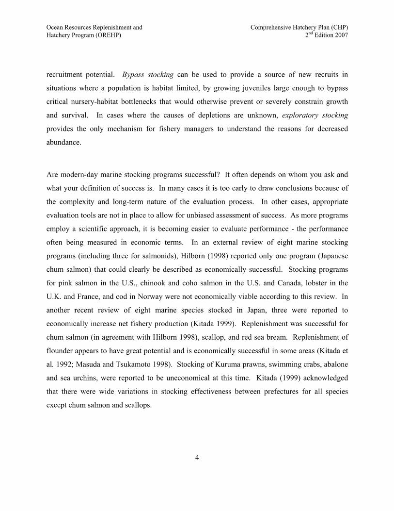
recruitment potential. Bypass stocking can be used to provide a source of new recruits in
situations where a population is habitat limited, by growing juveniles large enough to bypass
critical nursery-habitat bottlenecks that would otherwise prevent or severely constrain growth
and survival. In cases where the causes of depletions are unknown, exploratory stocking
provides the only mechanism for fishery managers to understand the reasons for decreased
abundance.
Are modern-day marine stocking programs successful? It often depends on whom you ask and
what your definition of success is. In many cases it is too early to draw conclusions because of
the complexity and long-term nature of the evaluation process. In other cases, appropriate
evaluation tools are not in place to allow for unbiased assessment of success. As more programs
employ a scientific approach, it is becoming easier to evaluate performance - the performance
often being measured in economic terms. In an external review of eight marine stocking
programs (including three for salmonids), Hilborn (1998) reported only one program (Japanese
chum salmon) that could clearly be described as economically successful. Stocking programs
for pink salmon in the U.S., chinook and coho salmon in the U.S. and Canada, lobster in the
U.K. and France, and cod in Norway were not economically viable according to this review. In
another recent review of eight marine species stocked in Japan, three were reported to
economically increase net fishery production (Kitada 1999). Replenishment was successful for
chum salmon (in agreement with Hilborn 1998), scallop, and red sea bream. Replenishment of
flounder appears to have great potential and is economically successful in some areas (Kitada et
al. 1992; Masuda and Tsukamoto 1998). Stocking of Kuruma prawns, swimming crabs, abalone
and sea urchins, were reported to be uneconomical at this time. Kitada (1999) acknowledged
that there were wide variations in stocking effectiveness between prefectures for all species
except chum salmon and scallops.
4
Ocean Resources Replenishment and Comprehensive Hatchery Plan (CHP) Hatchery Program (OREHP) 2nd Edition 2007
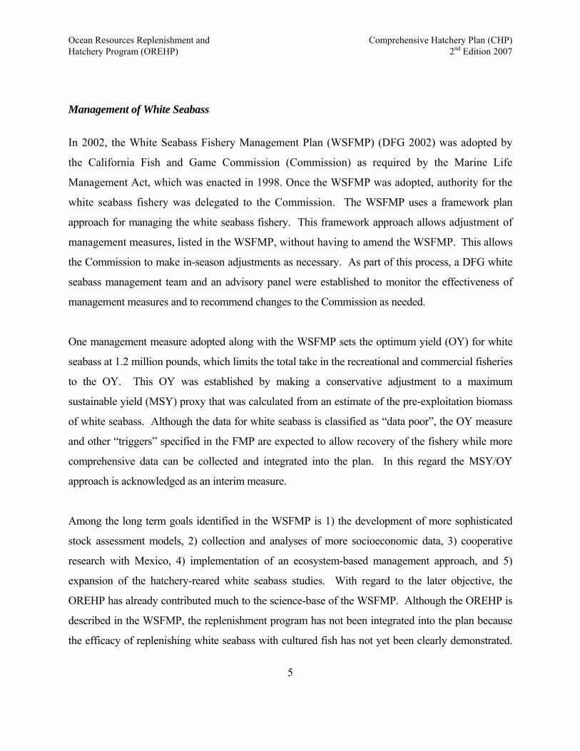
Management of White Seabass
In 2002, the White Seabass Fishery Management Plan (WSFMP) (DFG 2002) was adopted by
the California Fish and Game Commission (Commission) as required by the Marine Life
Management Act, which was enacted in 1998. Once the WSFMP was adopted, authority for the
white seabass fishery was delegated to the Commission. The WSFMP uses a framework plan
approach for managing the white seabass fishery. This framework approach allows adjustment of
management measures, listed in the WSFMP, without having to amend the WSFMP. This allows
the Commission to make in-season adjustments as necessary. As part of this process, a DFG white
seabass management team and an advisory panel were established to monitor the effectiveness of
management measures and to recommend changes to the Commission as needed.
One management measure adopted along with the WSFMP sets the optimum yield (OY) for white
seabass at 1.2 million pounds, which limits the total take in the recreational and commercial fisheries
to the OY. This OY was established by making a conservative adjustment to a maximum
sustainable yield (MSY) proxy that was calculated from an estimate of the pre-exploitation biomass
of white seabass. Although the data for white seabass is classified as “data poor”, the OY measure
and other “triggers” specified in the FMP are expected to allow recovery of the fishery while more
comprehensive data can be collected and integrated into the plan. In this regard the MSY/OY
approach is acknowledged as an interim measure.
Among the long term goals identified in the WSFMP is 1) the development of more sophisticated
stock assessment models, 2) collection and analyses of more socioeconomic data, 3) cooperative
research with Mexico, 4) implementation of an ecosystem-based management approach, and 5)
expansion of the hatchery-reared white seabass studies. With regard to the later objective, the
OREHP has already contributed much to the science-base of the WSFMP. Although the OREHP is
described in the WSFMP, the replenishment program has not been integrated into the plan because
the efficacy of replenishing white seabass with cultured fish has not yet been clearly demonstrated.
5
Ocean Resources Replenishment and Comprehensive Hatchery Plan (CHP) Hatchery Program (OREHP) 2nd Edition 2007
In that regard, the ongoing need for studies within the OREHP is consistent with that of the WSFMP
and we are proceeding conservatively as we gather more information.
We expect that in 5-10 years time, after additional releases and comprehensive assessment, sufficient
information will exist to determine the extent to which the OREHP can contribute to the recovery
and long term sustainability of the white seabass fishery. At that time, the DFG and Commission
will be tasked with deciding whether or not the OREHP should be formally integrated into the
WSFMP and, if so, how best to do it.
6
Ocean Resources Replenishment and Comprehensive Hatchery Plan (CHP) Hatchery Program (OREHP) 2nd Edition 2007
GENERAL HATCHERY DESIGN AND OPERATION
Site Map and General Description Site Map and General Description
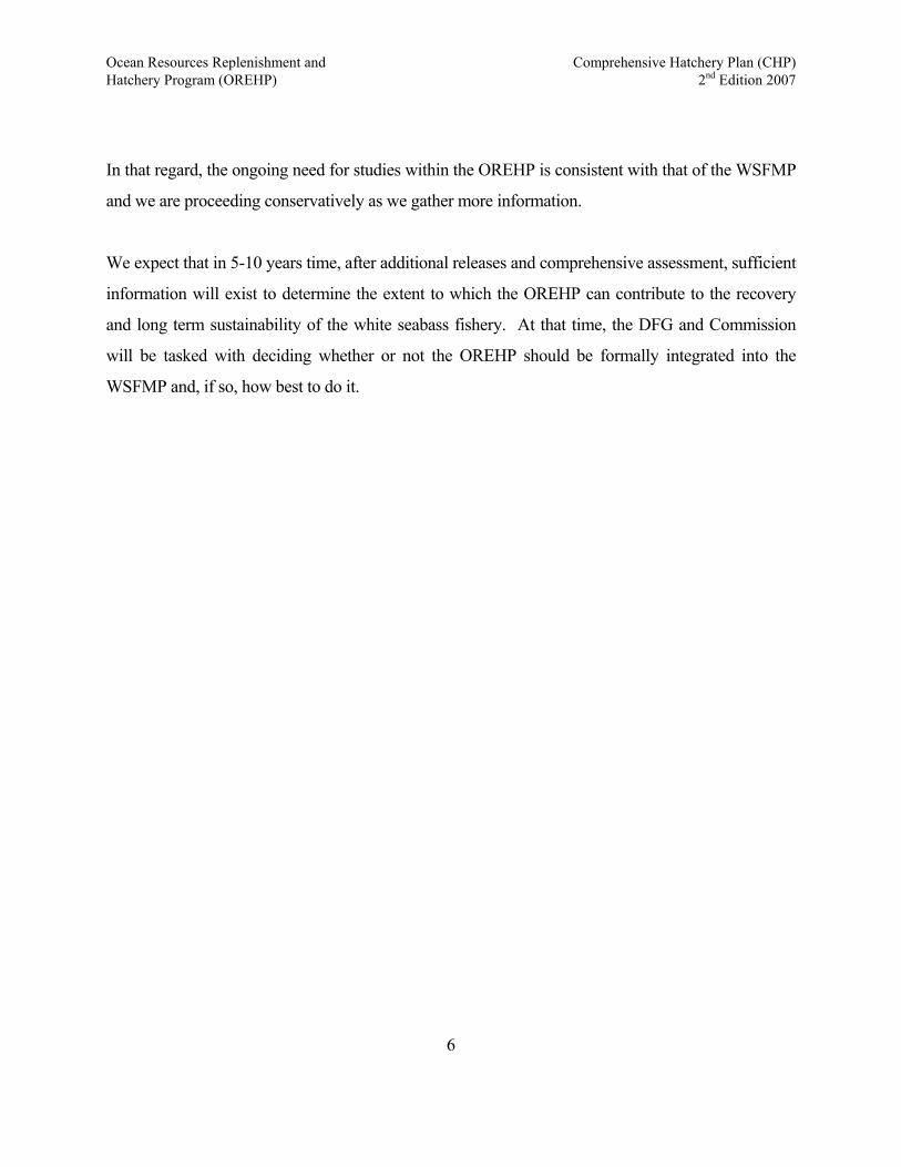
The Carlsbad Hatchery is located north of San Diego at 33.145° N latitude and 117.3393° W
longitude (Figure 1). It is located on a 2.7 hectare (6.6 acre) parcel of land originally owned by
San Diego Gas and Electric but subsequently purchased by Cabrillo Power. Of the total parcel,
approximately 1.3 hectares (3.2 acres) is leased to HSWRI.
Figure 1. Aerial photographs of Carlsbad Hatchery and its geographic location.
7
Ocean Resources Replenishment and Comprehensive Hatchery Plan (CHP) Hatchery Program (OREHP) 2nd Edition 2007
8
Hatchery Layout and Primary Components Hatchery Layout and Primary Components
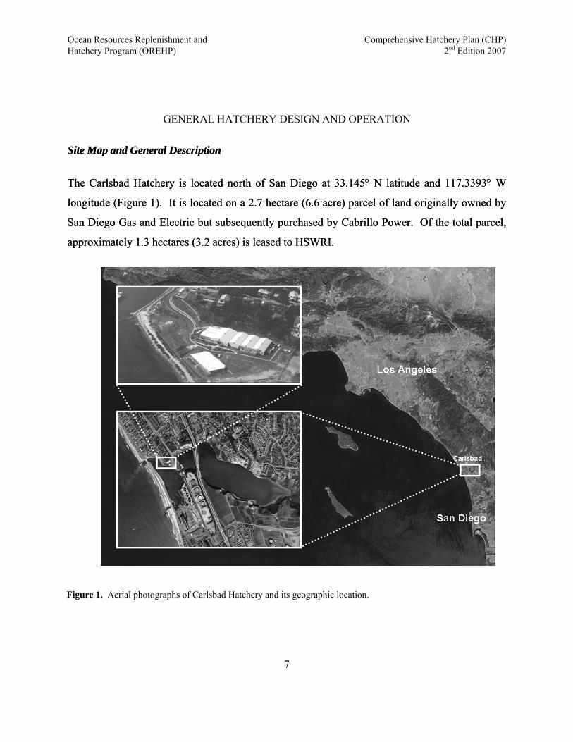
The hatchery facility consists of a main hatchery building and outdoor raceway area that are
interconnected by a seawater supply and drainage system (Figure 2). The main hatchery
building is approximately 2,000 m2 (22,000 ft2) and the raceway area is approximately 700 m2
(7,500 ft2).
The hatchery facility consists of a main hatchery building and outdoor raceway area that are
interconnected by a seawater supply and drainage system (Figure 2). The main hatchery
building is approximately 2,000 m2 (22,000 ft2) and the raceway area is approximately 700 m2
(7,500 ft2).
Figure 2. Site plan of Carlsbad Hatchery site showing main hatchery building and outdoor raceway area.
Internally the hatchery is compartmentalized into specific areas to support the fish culture
research program. These areas are showing in Figure 3 and discussed briefly in the following
section.
Internally the hatchery is compartmentalized into specific areas to support the fish culture
research program. These areas are showing in Figure 3 and discussed briefly in the following
section.

Ocean Resources Replenishment and Comprehensive Hatchery Plan (CHP) Hatchery Program (OREHP) 2nd Edition 2007
Figure 3. Color-coded floor plan of Carlsbad Hatchery showing various culture and infrastructure support areas.
9
Ocean Resources Replenishment and Comprehensive Hatchery Plan (CHP) Hatchery Program (OREHP) 2nd Edition 2007
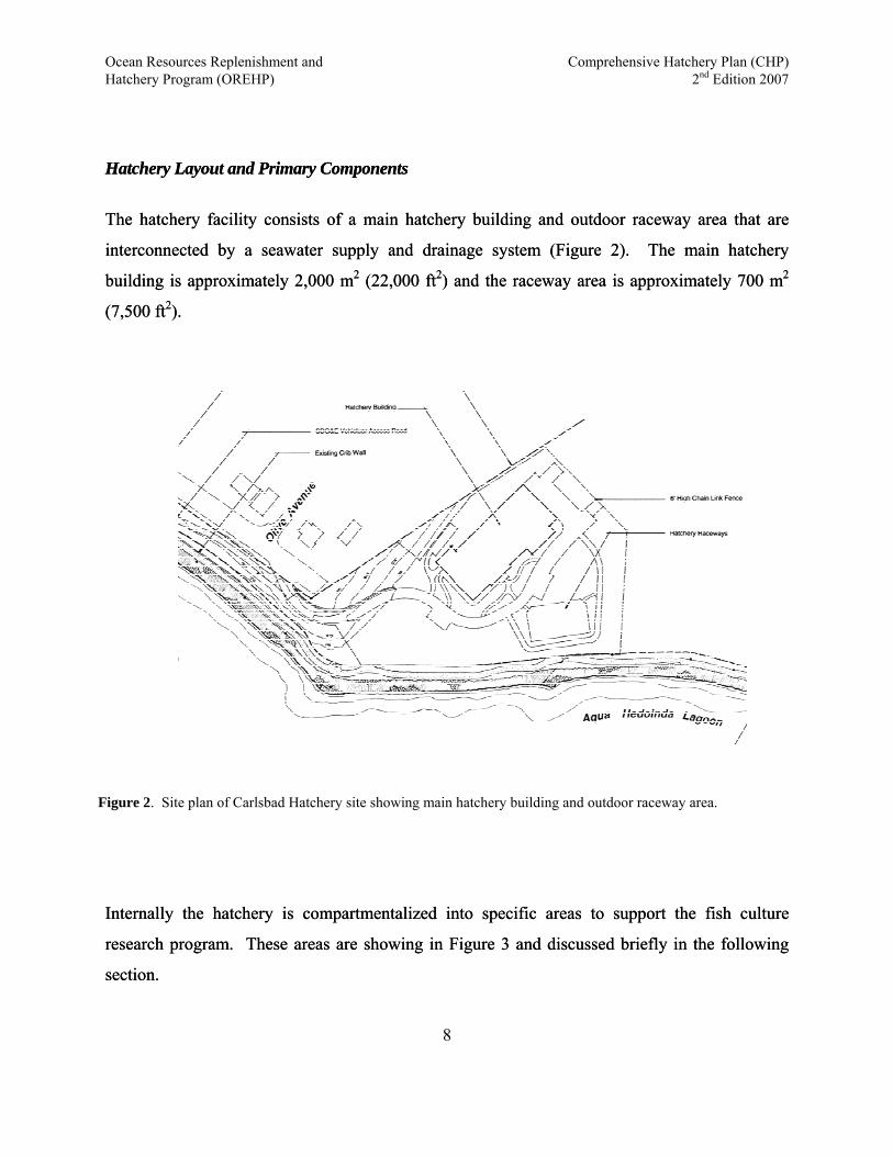
Broodstock Holding. Maturation pools for white
seabass and other candidate species are located
directly along the back wall of the hatchery as
you enter the building. Four white seabass pools
measuring 6.1 m in diameter occupy the majority
of space, while two smaller (4.6 m) pools occupy
the remainder of this area. Each white seabass
breeding pool is recirculated independently from
the others (Figure 4). The two smaller breeding
pools are on a flow-through supply. The breeding pools are particularly important in that they
are the source of eggs used to initiate the culture process.
Figure 4. Two of four breeding pools for white seabass with egg traps in the foreground.
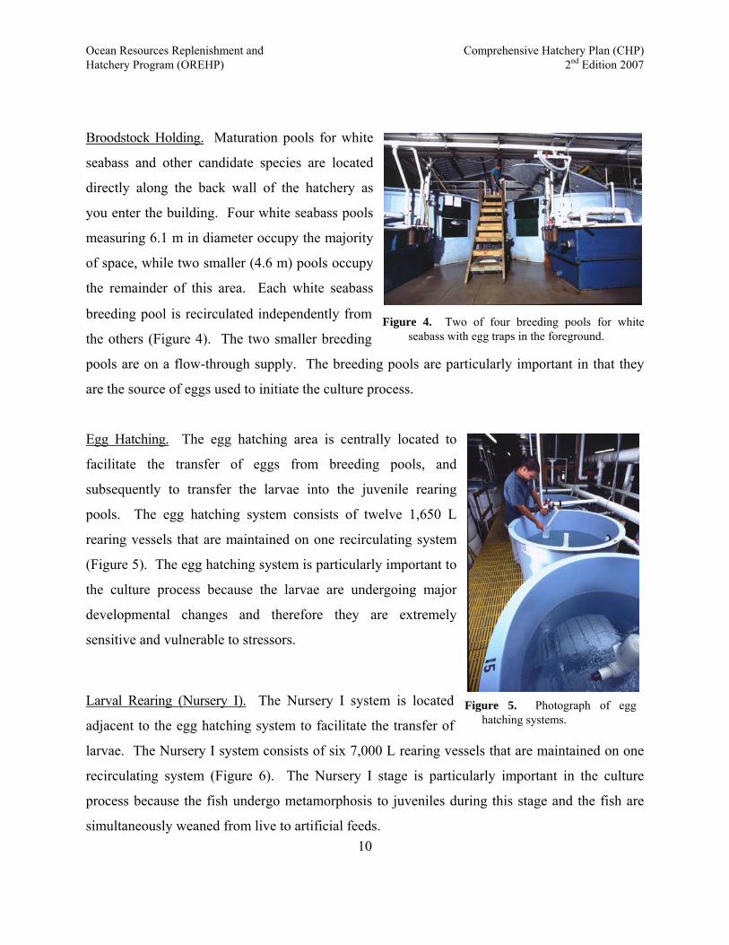
Egg Hatching. The egg hatching area is centrally located to
facilitate the transfer of eggs from breeding pools, and
subsequently to transfer the larvae into the juvenile rearing
pools. The egg hatching system consists of twelve 1,650 L
rearing vessels that are maintained on one recirculating system
(Figure 5). The egg hatching system is particularly important to
the culture process because the larvae are undergoing major
developmental changes and therefore they are extremely
sensitive and vulnerable to stressors.
Larval Rearing (Nursery I). The Nursery I system is located
adjacent to the egg hatching system to facilitate the transfer of
larvae. The Nursery I system consists of six 7,000 L rearing vessels that are maintained on one
recirculating system (Figure 6). The Nursery I stage is particularly important in the culture
process because the fish undergo metamorphosis to juveniles during this stage and the fish are
simultaneously weaned from live to artificial feeds.
Figure 5. Photograph of egg hatching systems.
10

Ocean Resources Replenishment and Comprehensive Hatchery Plan (CHP) Hatchery Program (OREHP) 2nd Edition 2007
Juvenile Rearing (Nursery II). The Nursery II system is adjacent
to the Nursery I system to support the transfer of juveniles from
Nursery I to Nursery II. The Nursery I system consists of eight
7,000 L rearing vessels that are maintained on one recirculating
system. The Nursery II stage is generally straight-forward
because the juveniles are fully metamorphosed and weaned onto
dry feeds.
Live Food Production. Live zooplankton is used to feed the larval
fish and algae is often used to produce the live zooplankton. The
live food production areas accommodate vessels for hatching and
enriching Artemia and rotifers (Figure 7). Artemia
are the principle live food used at the hatchery.
Artemia are hatched at temperatures of 28°C, so an
insulated room was purpose-built for this
important culture area. Enriching Artemia and
raising rotifers are conducted in the main hatchery
building. Live algae is used primarily for
experiments. Large-scale algae production is
conducted in an outdoor greenhouse.
Figure 6. Typical nursery pool.
Figure 7. Artemia hatching room as an example of live food production system.
Experimental Area. Because one of the primary objectives of the OREHP is to continue to refine
cultured techniques for species of interest, an area in the main hatchery building is set aside for
conducting controlled, replicated experiments. The experimental area contains a variety of
culture vessels ranging from 60 to 800 L in size and arranged in replicates. Most of these
systems are on a flow through water supply with the ability to control water temperature.
11
Ocean Resources Replenishment and Comprehensive Hatchery Plan (CHP) Hatchery Program (OREHP) 2nd Edition 2007
Over the years research has been conducted in a variety of specialty areas but the primary focus
has been nutrition and physiology of different life stages of white seabass and other endemic
species of interest. The cornerstone of the experimental areas is a specialized system for
conducting larval rearing studies. The system is designed to conduct experiments to determine
optimum rearing conditions for marine finfish larvae. Four cone-bottom tanks of 1,600 L and
400 L, and twenty-four 60 L capacity were integrated into the system. The three sizes of tanks
are scaled similarly so that we can conduct scaling experiments to determine if tank size has an
effect on larval survival. Each tank can be supplied with temperature-controlled water that is
either flow-through or recirculated. The recirculating water system will provide a very high
quality, biosecure water source for the culture tanks.
Food Storage. Proper food storage is critical to any animal husbandry operation. A walk-in freezer
is located adjacent to the food preparation room in the hatchery building. This freezer is used to
store fish feeds that require cold storage, such as fresh fish and shellfish for the broodstock, and
mysis shrimp for larvae. Pelleted feeds are stored in a fully-sealed storage container that prevents
vermin from accessing the food. A combination air conditioner and dehumidifier unit is built
into the storage container to keep the contents cool and dry.
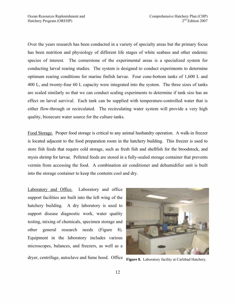
Laboratory and Office. Laboratory and office
support facilities are built into the left wing of the
hatchery building. A dry laboratory is used to
support disease diagnostic work, water quality
testing, mixing of chemicals, specimen storage and
other general research needs (Figure 8).
Equipment in the laboratory includes various
microscopes, balances, and freezers, as well as a
dryer, centrifuge, autoclave and fume hood. Office Figure 8. Laboratory facility at Carlsbad Hatchery.
12

Ocean Resources Replenishment and Comprehensive Hatchery Plan (CHP) Hatchery Program (OREHP) 2nd Edition 2007
13
space is provide to staff for managing data and
writing reports.
Industrial Machinery. Large culture support
equipment such as a boiler, chillers, and an
emergency generator are maintained in one area
of the hatchery to facilitate their maintenance
(Fig Figure 9. 225KVA emergency generator inside hatchery building
ure 9).
Seawater Treatment Processes
Treatment processes for the Carlsbad Hatchery are shown in Figure 10. Seawater is pumped
directly from Agua Hedionda Lagoon, with 50-100 percent passing through rapid sand filters
(Zone 1). Seawater then enters one of two types of rearing units – flow-through (Zone 2) or
recirculating (Zone 4), before being discharged back into the lagoon.

Ocean Resources Replenishment and Comprehensive Hatchery Plan (CHP) Hatchery Program (OREHP) 2nd Edition 2007
14
Figure 10. Process flow diagram for hatchery seawater supply and discharge.
Intake from Agua Hedionda Lagoon
Recirculating Animal Rearing Pools
Rapid Sand Filters
Flow-throughAnimal Rearing
Pools
Primary Filtration
(Bead)
SecondaryFiltration
(Sand)
MunicipalWastewater
SettlingBasin
Outfall to Agua Hedionda Lagoon
ZO
NE
1Z
ON
E 1
ZO
NE
2Z
ON
E 2
ZO
NE
4Z
ON
E 4ZO
NE
5Z
ON
E 5
ZO
NE
7Z
ON
E 7
ZONE 6ZONE 6
40 m3/daypump
6,500 m3/day
6,060 m3/day
Filter Bypass
Ozone Water
TreatmentZO
NE
3Z
ON
E 3 400 m3/day
ZO
NE
3Z
ON
E 3 400 m3/day
39 m3/day
<1.0 m3/day
<1.0 m3/day
pum
p
pum
p
375 m3/day
<1.0 m3/day
pump
Secondary Filtration
(Bead)<1 m3/day
pump
6,475 m3/day
Ocean Resources Replenishment and Comprehensive Hatchery Plan (CHP) Hatchery Program (OREHP) 2nd Edition 2007
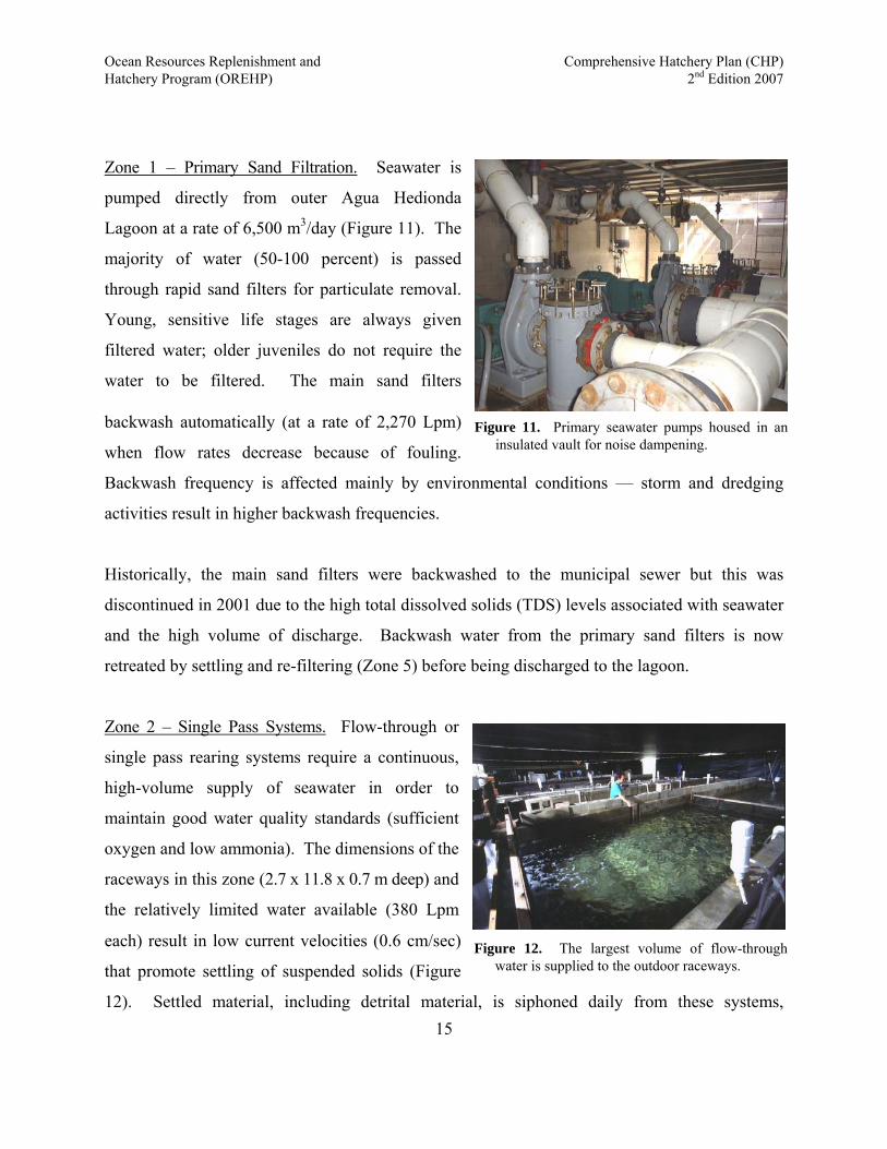
Zone 1 – Primary Sand Filtration. Seawater is
pumped directly from outer Agua Hedionda
Lagoon at a rate of 6,500 m3/day (Figure 11). The
majority of water (50-100 percent) is passed
through rapid sand filters for particulate removal.
Young, sensitive life stages are always given
filtered water; older juveniles do not require the
water to be filtered. The main sand filters
backwash automatically (at a rate of 2,270 Lpm)
when flow rates decrease because of fouling.
Backwash frequency is affected mainly by environmental conditions — storm and dredging
activities result in higher backwash frequencies.
Figure 11. Primary seawater pumps housed in an insulated vault for noise dampening.
Historically, the main sand filters were backwashed to the municipal sewer but this was
discontinued in 2001 due to the high total dissolved solids (TDS) levels associated with seawater
and the high volume of discharge. Backwash water from the primary sand filters is now
retreated by settling and re-filtering (Zone 5) before being discharged to the lagoon.
Zone 2 – Single Pass Systems. Flow-through or
single pass rearing systems require a continuous,
high-volume supply of seawater in order to
maintain good water quality standards (sufficient
oxygen and low ammonia). The dimensions of the
raceways in this zone (2.7 x 11.8 x 0.7 m deep) and
the relatively limited water available (380 Lpm
each) result in low current velocities (0.6 cm/sec)
that promote settling of suspended solids (Figure
12). Settled material, including detrital material, is siphoned daily from these systems,
Figure 12. The largest volume of flow-through water is supplied to the outdoor raceways.
15
Ocean Resources Replenishment and Comprehensive Hatchery Plan (CHP) Hatchery Program (OREHP) 2nd Edition 2007
concentrated using fine screen filters, and rinsed
into the municipal sewer system (Zone 6).
16
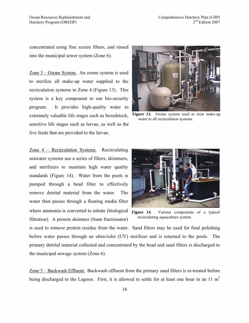
Zone 3 – Ozone System. An ozone system is used
to sterilize all make-up water supplied to the
recirculation systems in Zone 4 (Figure 13). This
system is a key component to our bio-security
program. It provides high-quality water to
extremely valuable life stages such as broodstock,
sensitive life stages such as larvae, as well as the
live feeds that are provided to the larvae.
Figure 13. Ozone system used to treat make-up water to all recirculation systems.
Zone 4 – Recirculation Systems. Recirculating
seawater systems use a series of filters, skimmers,
and sterilizers to maintain high water quality
standards (Figure 14). Water from the pools is
pumped through a bead filter to effectively
remove detrital material from the water. The
water then passes through a floating media filter
where ammonia is converted to nitrate (biological
filtration). A protein skimmer (foam fractionator)
is used to remove protein residue from the water. Sand filters may be used for final polishing
before water passes through an ultraviolet (UV) sterilizer and is returned to the pools. The
primary detrital material collected and concentrated by the bead and sand filters is discharged to
the municipal sewage system (Zone 6).
Figure 14. Various components of a typical recirculating aquaculture system.
Zone 5 – Backwash Effluent. Backwash effluent from the primary sand filters is re-treated before
being discharged to the Lagoon. First, it is allowed to settle for at least one hour in an 11 m3

Ocean Resources Replenishment and Comprehensive Hatchery Plan (CHP) Hatchery Program (OREHP) 2nd Edition 2007
settling basin. Once the settling period is complete, the seawater is pumped through a bead filter
(model PBF5) and discharged at a low flow rate (95 Lpm) into the main hatchery effluent (Zone
7). The rate of discharge from the settling basin is only 4 percent of that entering the basin from
the main sand filters, so the instantaneous dilution is much greater than it would be if the primary
sand filters (Zone 1) were backwashed directly into the main effluent stream.
Zone 6 – Municipal Sewer. As described in the treatment processes above, concentrated fish
wastes (from Zones 2, 4 & 5) are discharged to the municipal sewer system using relatively
small volumes of salt and freshwater.
Zone 7 – Effluent Discharge. As a result of the treatment processes described above and the
biological (non-industrial) nature of our operation, the effluent discharged is of a similar quality
to that of the natural lagoon water drawn into the facility. The characteristics of our effluent in
relation to our influent are monitored under a National Pollution Discharge Elimination System
(NPDES), which is described below.
Monitoring and Control of Life Support Systems
Monitoring and Control System. The hatchery
seawater system and life support components are
monitored continuously by a sophisticated, main
computer control system (MCCS). Automated
valves control filter backwashing and temperature
control processes (Figure 15). Alarm points can
be set to indicate low water or air flow, as well as
temperature variances. Information is transmitted
by pager to multiple hatchery personnel.
Figure 15. Example of screen display from main computer control system.
17
Ocean Resources Replenishment and Comprehensive Hatchery Plan (CHP) Hatchery Program (OREHP) 2nd Edition 2007
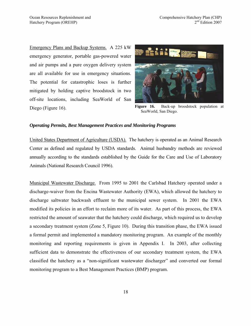
Emergency Plans and Backup Systems. A 225 kW
emergency generator, portable gas-powered water
and air pumps and a pure oxygen delivery system
are all available for use in emergency situations.
The potential for catastrophic loses is further
mitigated by holding captive broodstock in two
Diego (Figure 16).
off-site locations, including SeaWorld of San
perating Permits, Best Management Practices and Monitoring Programs
nited States Department of Agriculture (USDA).
Figure 16. Back-up broodstock population at SeaWorld, San Diego.
O
18
U The hatchery is operated as an Animal Research
unicipal Wastewater Discharge.
Center as defined and regulated by USDA standards. Animal husbandry methods are reviewed
annually according to the standards established by the Guide for the Care and Use of Laboratory
Animals (National Research Council 1996).
M From 1995 to 2001 the Carlsbad Hatchery operated under a
discharge-waiver from the Encina Wastewater Authority (EWA), which allowed the hatchery to
discharge saltwater backwash effluent to the municipal sewer system. In 2001 the EWA
modified its policies in an effort to reclaim more of its water. As part of this process, the EWA
restricted the amount of seawater that the hatchery could discharge, which required us to develop
a secondary treatment system (Zone 5, Figure 10). During this transition phase, the EWA issued
a formal permit and implemented a mandatory monitoring program. An example of the monthly
monitoring and reporting requirements is given in Appendix I. In 2003, after collecting
sufficient data to demonstrate the effectiveness of our secondary treatment system, the EWA
classified the hatchery as a “non-significant wastewater discharger” and converted our formal
monitoring program to a Best Management Practices (BMP) program.
Ocean Resources Replenishment and Comprehensive Hatchery Plan (CHP) Hatchery Program (OREHP) 2nd Edition 2007
National Pollution Discharge Elimination System (NPDES). From 1995 to 2001 the Carlsbad
Hatchery operated under a discharge-waiver from the San Diego Regional Water Quality Control
Board (SDRWQCB) because our fish production levels did not meet their criteria for a
concentrated aquatic animal holding facility. Although we did not require an NPDES permit, we
were required to monitor various parameters of our seawater influent and effluent sources. As a
result of the modifications to our wastewater treatment process described above, we were
required to obtain an NPDES permit in 2001 and a new monitoring program was implemented.
The NPDES monitoring program is intended to:
1. Document short-term and long-term effects of the discharge on receiving waters, sediments, biota, and beneficial uses of the receiving water.
2. Determine compliance with NPDES permit terms and conditions.
3. Be used to determine compliance with water quality objectives.
4. Determine if water-quality based effluent limits are necessary pursuant to the Policy and California Toxics Rule (CTR), 40 CFR 131.38.
The specifications of our permit are given in Appendix II and an example of an annual
monitoring report is provided in Appendix III.
Storm Water Management. As part of its Conditional Use Permit with the City of Carlsbad,
HSWRI has developed an approved Storm Water Management Plan (SWMP). This SWMP
describes the Carlsbad Hatchery and its operations, identifies potential sources of storm water
pollution at the facility, identifies current source control and treatment control BMPs and
provides for periodic review of the SWMP.
The objectives of the SWMP are to:
1. Identify sources of storm water and non-storm water contamination to the storm
water drainage system;
2. Identify and prescribe appropriate "source area control" type best management
19
Ocean Resources Replenishment and Comprehensive Hatchery Plan (CHP) Hatchery Program (OREHP) 2nd Edition 2007
practices designed to prevent storm water contamination from occurring;
3. Identify and prescribe "storm water treatment" type best management practices to
reduce pollutants in contaminated storm water prior to discharge;
4. Prescribe actions needed either to control non-storm water discharges or to remove
these discharges from the storm drainage system.
5. Prescribe an implementation schedule to ensure that the storm water management
actions described in this plan are carried out and evaluated on a regular basis.
The potential sources of pollution identified for this site include the parking lot and access road,
material handling sites, trash disposal area, and chemical storage areas. The parking lot and
access road are susceptible to accumulating oil and grease from vehicles, trash, and sediments.
However, staff keeps the area free of trash and debris and clears gutters of sediment, should any
collect. In addition, the parking lot and access road runoff collects into vegetated swales and a
detention basin before entering the storm drain system. Another source of pollution is the
handling site where material is loaded and unloaded. Materials such as organic fish food,
chlorine, and office supplies are received here. The probability of a release of pollutants in this
area is low because materials are immediately stored inside in spill containment bins. In
addition, chlorine is shipped in sealed drums. The trash disposal area is a source of pollutants
due to trash being transported into the storm drain system by wind, rain, or birds. The trash
dumpsters at the Hubbs Institute are covered and enclosed by a masonry wall, therefore reducing
the risk of debris entering the storm drain system. Lastly, the chemical storage areas pose a risk
to storm water quality due to the possibility of spillage. The three areas are the raceway, the
main building and the outside storage area at the northwest corner of the main building. These
three areas contain sealed 55 gallon drums that are also in spill containment bins.
The non-storm water discharges for this site are seawater effluent and landscape irrigation. The
seawater effluent is covered under NPDES permit #CA0109355 and is monitored by
SDRWQCB Monitoring Program No. 2001-237. Existing landscaping is well established and
20

Ocean Resources Replenishment and Comprehensive Hatchery Plan (CHP) Hatchery Program (OREHP) 2nd Edition 2007
maintained on a regular basis. Landscaping was designed to require a minimum amount of
irrigation due to drought-resistant species of plants.
Chemical Storage. Chemical use and storage protocols are well established and integrated into
each of the operating permits described above. A list of chemicals, their application and storage
is given in Appendix IV. Material Safety Chemical Sheets (MSDS) for all chemicals are
available at the Carlsbad Hatchery.
21
Ocean Resources Replenishment and Comprehensive Hatchery Plan (CHP) Hatchery Program (OREHP) 2nd Edition 2007
CULTURE PROTOCOLS FOR WHITE SEABASS
Culture protocols for marine fish vary depending on the life stage being cultured and the specific
requirements of that life stage. This section describes how white seabass are currently spawned and
reared to juvenile stage.
Broodstock
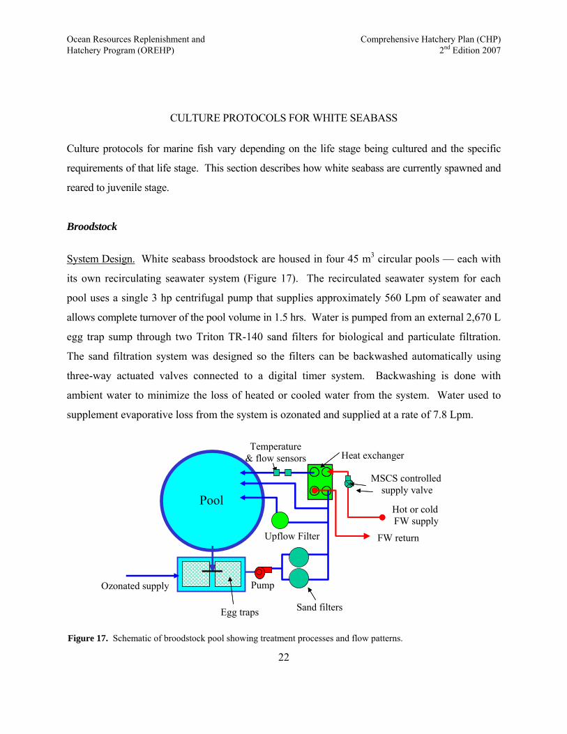
System Design. White seabass broodstock are housed in four 45 m3 circular pools — each with
its own recirculating seawater system (Figure 17). The recirculated seawater system for each
pool uses a single 3 hp centrifugal pump that supplies approximately 560 Lpm of seawater and
allows complete turnover of the pool volume in 1.5 hrs. Water is pumped from an external 2,670 L
egg trap sump through two Triton TR-140 sand filters for biological and particulate filtration.
The sand filtration system was designed so the filters can be backwashed automatically using
three-way actuated valves connected to a digital timer system. Backwashing is done with
ambient water to minimize the loss of heated or cooled water from the system. Water used to
supplement evaporative loss from the system is ozonated and supplied at a rate of 7.8 Lpm.
Pool
Ozonated supply
Sand filters
Pump
Hot or cold FW supply
FW return
MSCS controlled supply valve
Heat exchangerTemperature
& flow sensors
Egg traps
Upflow Filter
Figure 17. Schematic of broodstock pool showing treatment processes and flow patterns.
22
Ocean Resources Replenishment and Comprehensive Hatchery Plan (CHP) Hatchery Program (OREHP) 2nd Edition 2007
From the sand filters water passes through two 650 L clear fiberglass biofiltration columns
(upflow filters) containing either scrub pad or B-Cell biological filtration media to provide
additional nitrification of ammonia and nitrite. Larger particulate matter is concentrated in the
pools using a constant vortex water current that is created by the influent water stream. The
concentrated particulate matter is then drawn out of the pool using an airlift suction pipe and
deposited in the egg traps within the sump. In addition, a manually operated siphon system is
used to remove debris that adheres to the bottom of the pool.
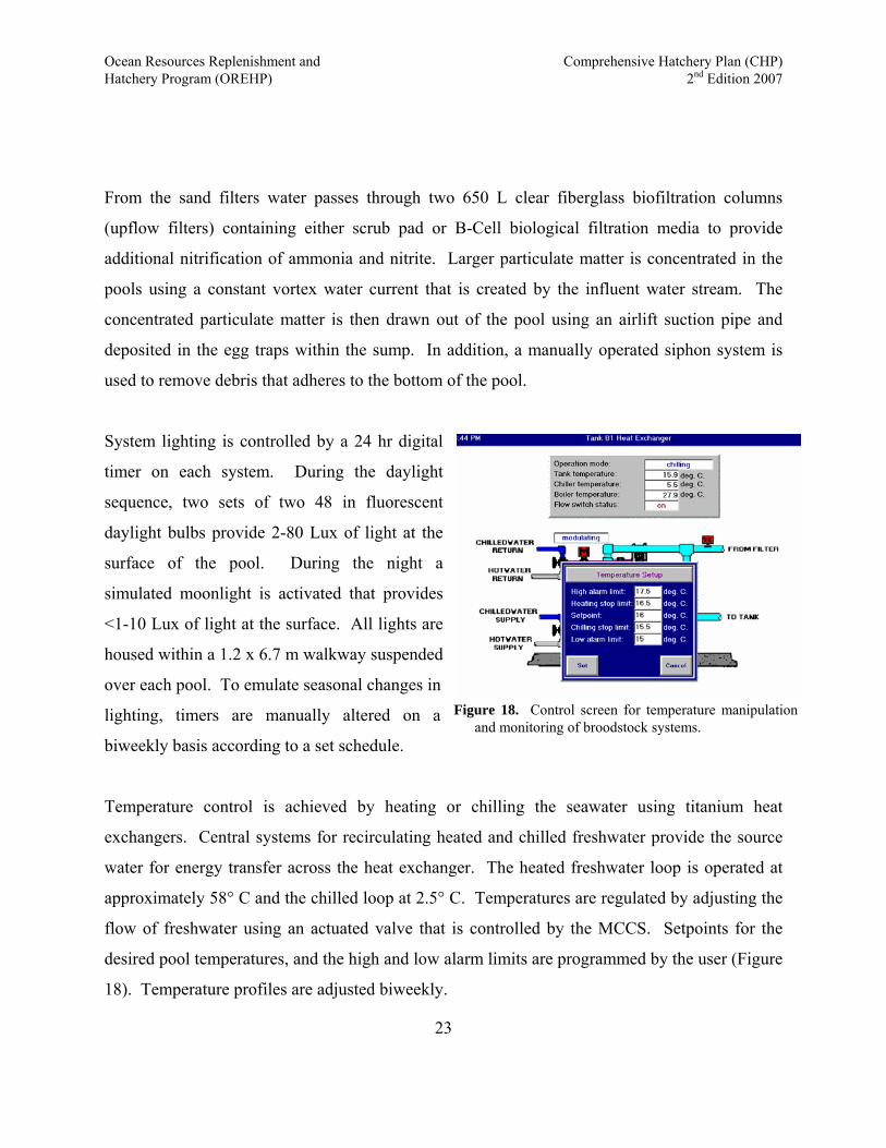
System lighting is controlled by a 24 hr digital
timer on each system. During the daylight
sequence, two sets of two 48 in fluorescent
daylight bulbs provide 2-80 Lux of light at the
surface of the pool. During the night a
simulated moonlight is activated that provides
<1-10 Lux of light at the surface. All lights are
housed within a 1.2 x 6.7 m walkway suspended
over each pool. To emulate seasonal changes in
lighting, timers are manually altered on a
biweekly basis according to a set schedule.
Figure 18. Control screen for temperature manipulation and monitoring of broodstock systems.
Temperature control is achieved by heating or chilling the seawater using titanium heat
exchangers. Central systems for recirculating heated and chilled freshwater provide the source
water for energy transfer across the heat exchanger. The heated freshwater loop is operated at
approximately 58° C and the chilled loop at 2.5° C. Temperatures are regulated by adjusting the
flow of freshwater using an actuated valve that is controlled by the MCCS. Setpoints for the
desired pool temperatures, and the high and low alarm limits are programmed by the user (Figure
18). Temperature profiles are adjusted biweekly.
23
Ocean Resources Replenishment and Comprehensive Hatchery Plan (CHP) Hatchery Program (OREHP) 2nd Edition 2007
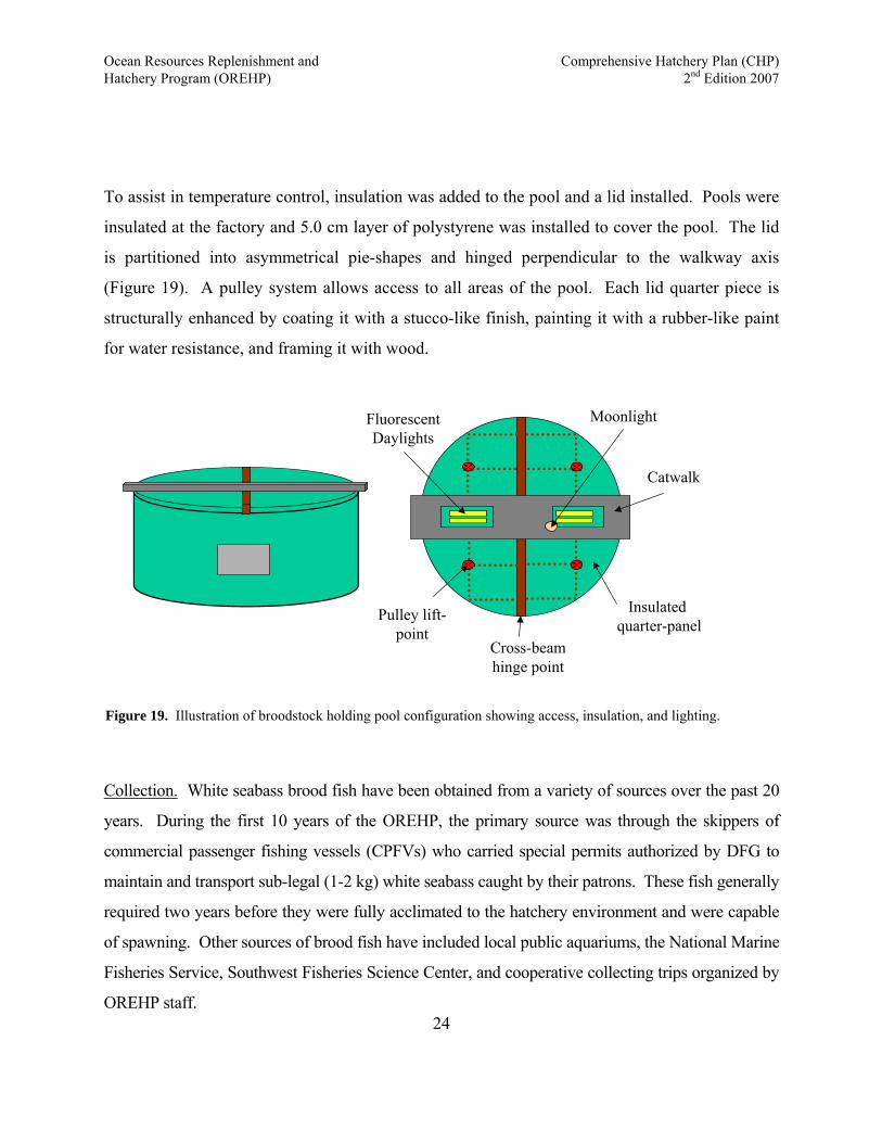
To assist in temperature control, insulation was added to the pool and a lid installed. Pools were
insulated at the factory and 5.0 cm layer of polystyrene was installed to cover the pool. The lid
is partitioned into asymmetrical pie-shapes and hinged perpendicular to the walkway axis
(Figure 19). A pulley system allows access to all areas of the pool. Each lid quarter piece is
structurally enhanced by coating it with a stucco-like finish, painting it with a rubber-like paint
for water resistance, and framing it with wood.
Catwalk
Insulated quarter-panel
Pulley lift-point
Cross-beamhinge point
FluorescentDaylights
Moonlight
Figure 19. Illustration of broodstock holding pool configuration showing access, insulation, and lighting.
24
Collection. White seabass brood fish have been obtained from a variety of sources over the past 20
years. During the first 10 years of the OREHP, the primary source was through the skippers of
commercial passenger fishing vessels (CPFVs) who carried special permits authorized by DFG to
maintain and transport sub-legal (1-2 kg) white seabass caught by their patrons. These fish generally
required two years before they were fully acclimated to the hatchery environment and were capable
of spawning. Other sources of brood fish have included local public aquariums, the National Marine
Fisheries Service, Southwest Fisheries Science Center, and cooperative collecting trips organized by
OREHP staff.
Ocean Resources Replenishment and Comprehensive Hatchery Plan (CHP) Hatchery Program (OREHP) 2nd Edition 2007
From 1995 through 2005, adult fish were targeted in order to rapidly increase the population size to
200 with mature fish that could contribute gametes as soon as they became acclimated to the
hatchery. Recreational fishermen played an active role in these collection efforts through well-
organized collection trips that involved private boaters and CPFVs. Commercial fishermen were
also recruited on a fee basis. During this period procedures for handling adult fish were developed
that included appropriate nets or “slings” for transporting fish and techniques for deflating
swimbladders (Kent et al. 1995).
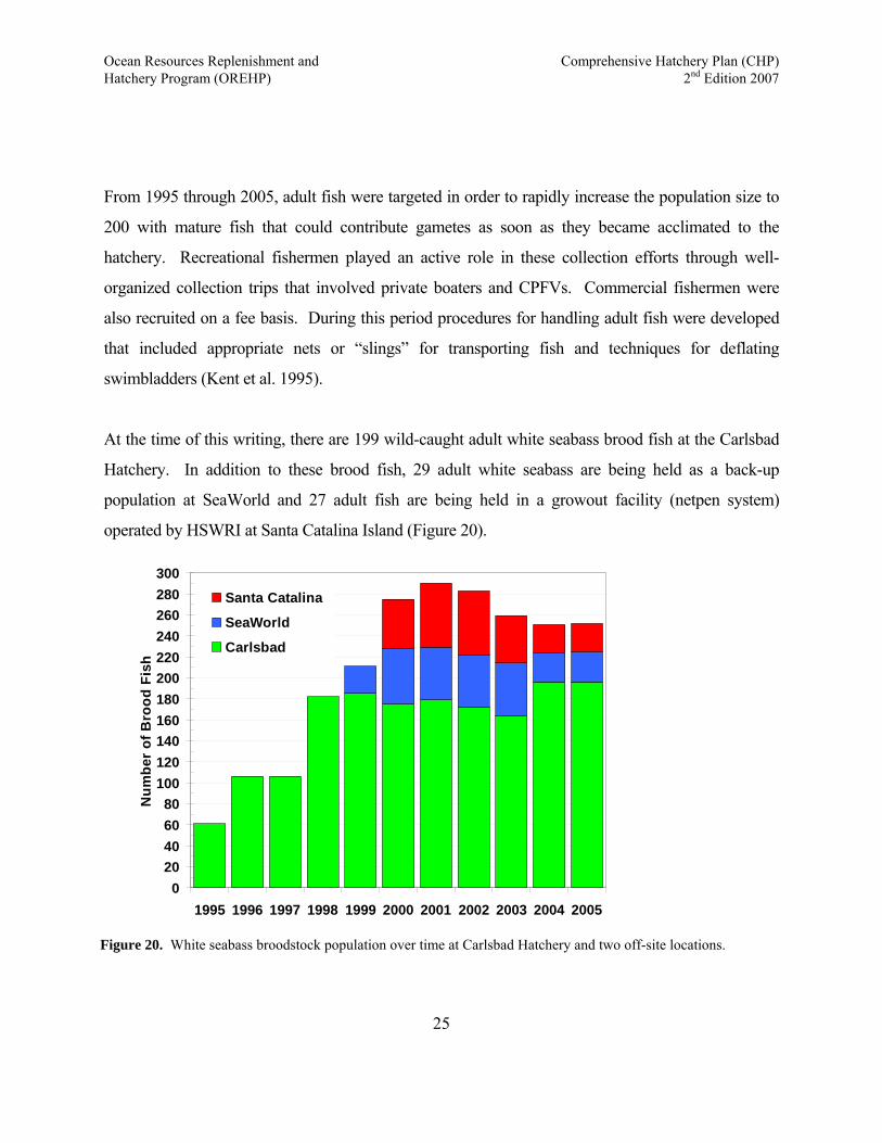
At the time of this writing, there are 199 wild-caught adult white seabass brood fish at the Carlsbad
Hatchery. In addition to these brood fish, 29 adult white seabass are being held as a back-up
population at SeaWorld and 27 adult fish are being held in a growout facility (netpen system)
operated by HSWRI at Santa Catalina Island (Figure 20).
020406080
100120140160180200220240260280300
1995 1996 1997 1998 1999 2000 2001 2002 2003 2004 2005
Num
ber
of B
rood
Fis
h
Santa Catalina
SeaWorld
Carlsbad
Figure 20. White seabass broodstock population over time at Carlsbad Hatchery and two off-site locations.
25

Ocean Resources Replenishment and Comprehensive Hatchery Plan (CHP) Hatchery Program (OREHP) 2nd Edition 2007
Feeding and General Husbandry. White seabass brood fish are fed a diet of fresh frozen sardines
five days per week at a ration of 0.5 percent - 1 percent of their body weight per day. Three times a
week the diet is enhanced by injecting the sardines with a mixture of vitamin premix, ascorbic acid,
lecithin, thiamine and Menhaden oil. All food handling is conducted in accordance with USDA
standards for research facilities holding live vertebrate organisms.
Broodstock Database Management. Information for each brood fish maintained at the hatchery is
stored in a custom-designed Microsoft Access database. Primary information for each individual
brood fish, data such as PIT tag number, sex, collection information, and current location is
maintained in the database in one data table. This data is linked to handling event records for each
fish, which are stored in a separate table according to the PIT tag number of the fish. Event records
include event dates, transfers between pools and sites, and death. Information associated with each
event such as length and weight measurements, blood and tissue sampling, and cannulation is also
recorded. A main data entry screen facilitates data entry for new fish and new events, as well as
rapid search functions (Figure 21). Custom queries and reports are designed to facilitate inventory
control, data analyses and reporting.
26
Figure 21. Example data entry form for broodstock management database.
Ocean Resources Replenishment and Comprehensive Hatchery Plan (CHP) Hatchery Program (OREHP) 2nd Edition 2007
Egg Production
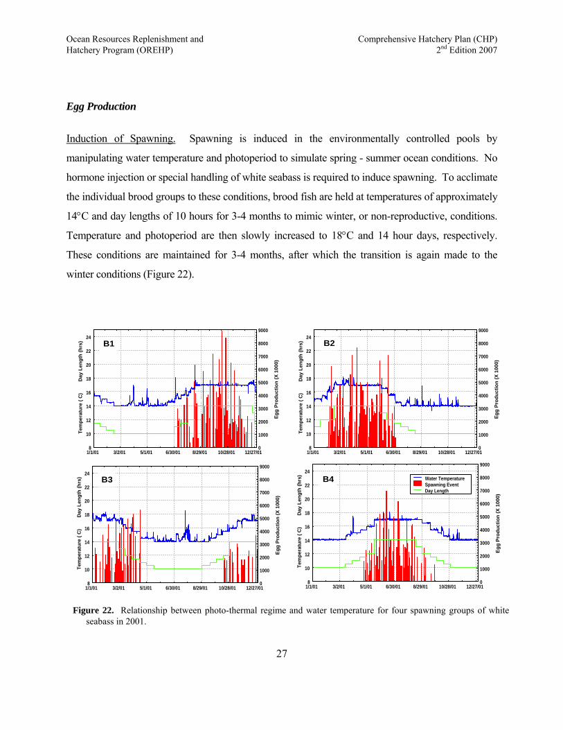
Induction of Spawning. Spawning is induced in the environmentally controlled pools by
manipulating water temperature and photoperiod to simulate spring - summer ocean conditions. No
hormone injection or special handling of white seabass is required to induce spawning. To acclimate
the individual brood groups to these conditions, brood fish are held at temperatures of approximately
14°C and day lengths of 10 hours for 3-4 months to mimic winter, or non-reproductive, conditions.
Temperature and photoperiod are then slowly increased to 18°C and 14 hour days, respectively.
These conditions are maintained for 3-4 months, after which the transition is again made to the
winter conditions (Figure 22).
Tem
pera
ture
( C
)
D
ay L
engt
h (h
rs)
Egg
Prod
uctio
n (X
100
0)
0
1000
2000
3000
4000
5000
6000
7000
8000
9000
8
10
12
14
16
18
20
22
24
1/1/01 3/2/01 5/1/01 6/30/01 8/29/01 10/28/01 12/27/01
Tem
pera
ture
( C
)
D
ay L
engt
h (h
rs)
Egg
Prod
uctio
n (X
100
0)
0
1000
2000
3000
4000
5000
6000
7000
8000
9000
8
10
12
14
16
18
20
22
24
1/1/01 3/2/01 5/1/01 6/30/01 8/29/01 10/28/01 12/27/01
Tem
pera
ture
( C
)
D
ay L
engt
h (h
rs)
Egg
Prod
uctio
n (X
100
0)
0
1000
2000
3000
4000
5000
6000
7000
8000
9000
8
10
12
14
16
18
20
22
24
1/1/01 3/2/01 5/1/01 6/30/01 8/29/01 10/28/01 12/27/01
Tem
pera
ture
( C
)
D
ay L
engt
h (h
rs)
Egg
Prod
uctio
n (X
100
0)
0
1000
2000
3000
4000
5000
6000
7000
8000
9000
8
10
12
14
16
18
20
22
24
1/1/01 3/2/01 5/1/01 6/30/01 8/29/01 10/28/01 12/27/01
Water TemperatureSpawning EventDay Length
B1 B2
B3 B4
Figure 22. Relationship between photo-thermal regime and water temperature for four spawning groups of whiteseabass in 2001.
27
Ocean Resources Replenishment and Comprehensive Hatchery Plan (CHP) Hatchery Program (OREHP) 2nd Edition 2007
The spawning seasons of the environmentally controlled pools are offset to provide a constant
supply of eggs (Figure 22). On the day of a spawn, the abdomens of females containing hydrating
oocytes become distended. Although spawning generally occurs in the early evening, it has been
observed on several occasions during the daytime.
Egg Collection and Enumeration. Spawning generally occurs in the early evening and the eggs are
collected the following morning. Therefore, the first 12 hours of incubation occur inside the
broodstock pool or the egg collection net. Due to their buoyancy at full salinity, white seabass eggs
float and are easily skimmed from the surface with a fine mesh net (<800 μm). The eggs are
concentrated in a container with approximately 5.0 L of seawater and then poured into a clear 4.0 L
graduated cylinder. After allowing the eggs to settle for 3-5 minutes, the volume of eggs is
measured and the number of eggs is estimated using a conversion ratio of 585 eggs per ml. Viable,
undamaged eggs are concentrated at the very top of the graduated cylinder due to their buoyancy,
while non-viable eggs settle to the bottom. The volumes of eggs in both the viable and non-viable
aliquots are measured for each spawn.
Historical Production Levels. Since 1996 over 4.4 billion eggs have been produced during 1,834
spawning events at the hatchery. The number of eggs collected from a single spawning event is
variable, ranging from as few as 58,000 to as many as 17 million. This variability is primarily
attributed to the number of females that spawn on a given day. The multimodal frequency
distributions of numbers of eggs spawned suggest that spawning events resulting in greater than 1.8
million eggs involve more than one female. Based on this estimate, group spawning occurs in about
59 percent of all spawning events in the system. Historically, the percentage of viable (fertile) eggs
has been high in the environmentally controlled pools, with the majority of spawns having viability
of more than 70-80 percent.
28
Ocean Resources Replenishment and Comprehensive Hatchery Plan (CHP) Hatchery Program (OREHP) 2nd Edition 2007
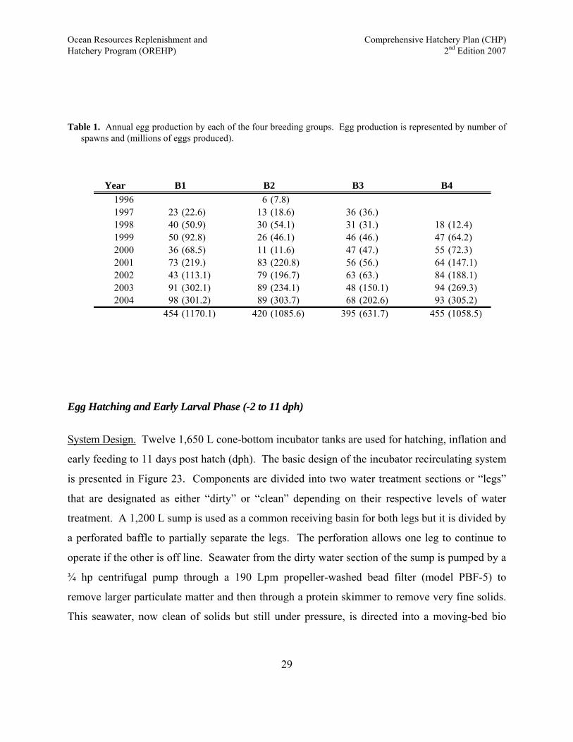
Table 1. Annual egg production by each of the four breeding groups. Egg production is represented by number of
spawns and (millions of eggs produced).
Year1996 6 (7.8)1997 23 (22.6) 13 (18.6) 36 (36.)1998 40 (50.9) 30 (54.1) 31 (31.) 18 (12.4)1999 50 (92.8) 26 (46.1) 46 (46.) 47 (64.2)2000 36 (68.5) 11 (11.6) 47 (47.) 55 (72.3)2001 73 (219.) 83 (220.8) 56 (56.) 64 (147.1)2002 43 (113.1) 79 (196.7) 63 (63.) 84 (188.1)2003 91 (302.1) 89 (234.1) 48 (150.1) 94 (269.3)2004 98 (301.2) 89 (303.7) 68 (202.6) 93 (305.2)
454 (1170.1) 420 (1085.6) 395 (631.7) 455 (1058.5)
B1 B2 B3 B4
Egg Hatching and Early Larval Phase (-2 to 11 dph)
System Design. Twelve 1,650 L cone-bottom incubator tanks are used for hatching, inflation and
early feeding to 11 days post hatch (dph). The basic design of the incubator recirculating system
is presented in Figure 23. Components are divided into two water treatment sections or “legs”
that are designated as either “dirty” or “clean” depending on their respective levels of water
treatment. A 1,200 L sump is used as a common receiving basin for both legs but it is divided by
a perforated baffle to partially separate the legs. The perforation allows one leg to continue to
operate if the other is off line. Seawater from the dirty water section of the sump is pumped by a
¾ hp centrifugal pump through a 190 Lpm propeller-washed bead filter (model PBF-5) to
remove larger particulate matter and then through a protein skimmer to remove very fine solids.
This seawater, now clean of solids but still under pressure, is directed into a moving-bed bio
29
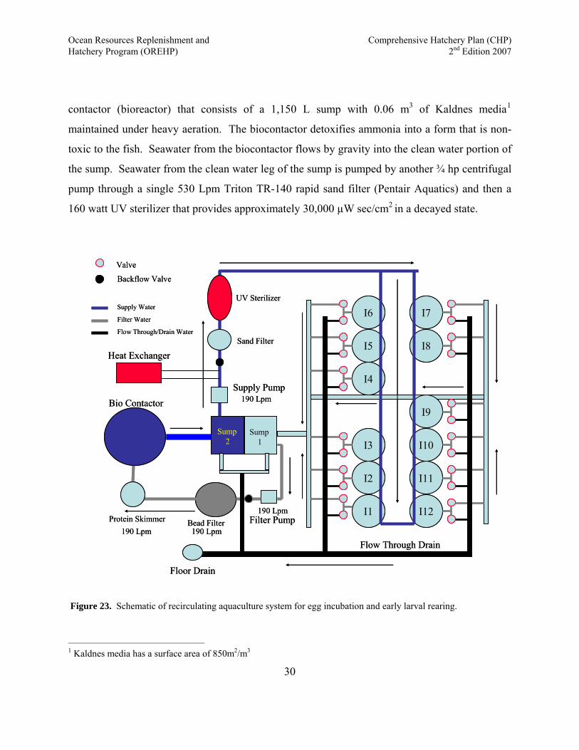
Ocean Resources Replenishment and Comprehensive Hatchery Plan (CHP) Hatchery Program (OREHP) 2nd Edition 2007
contactor (bioreactor) that consists of a 1,150 L sump with 0.06 m3 of Kaldnes media1
maintained under heavy aeration. The biocontactor detoxifies ammonia into a form that is non-
toxic to the fish. Seawater from the biocontactor flows by gravity into the clean water portion of
the sump. Seawater from the clean water leg of the sump is pumped by another ¾ hp centrifugal
pump through a single 530 Lpm Triton TR-140 rapid sand filter (Pentair Aquatics) and then a
160 watt UV sterilizer that provides approximately 30,000 µW sec/cm2 in a decayed state.
I6
Flow Through Drain
Sump2
Sump1
Bead Filter
Bio Contactor
Valve
UV Sterilizer
Filter Pump
Supply Pump
Heat Exchanger
Floor Drain
190 Lpm
190 Lpm
190 Lpm
Backflow Valve
Sand Filter
Protein Skimmer190 Lpm
Supply Water
Filter Water
Flow Through/Drain Water
I5
I7
I8
I4
I9
I10
I11
I12
I3
I2
I1
I6
Flow Through Drain
Sump2
Sump1
Bead Filter
Bio Contactor
Valve
UV Sterilizer
Filter Pump
Supply Pump
Heat Exchanger
Floor Drain
190 Lpm
190 Lpm
190 Lpm
Backflow Valve
Sand Filter
Protein Skimmer190 Lpm
Supply Water
Filter Water
Flow Through/Drain Water
I5
I7
I8
I4
I9
I10
I11
I12
I3
I2
I1
Figure 23. Schematic of recirculating aquaculture system for egg incubation and early larval rearing.
30
1 Kaldnes media has a surface area of 850m2/m3
Ocean Resources Replenishment and Comprehensive Hatchery Plan (CHP) Hatchery Program (OREHP) 2nd Edition 2007
Water temperature in the system is controlled by diverting approximately 38 Lpm of the
incubator supply water (190 Lpm) through a heat exchange system. Hot or cold freshwater is
used as the source water to transfer heat or cold across a titanium heat exchanger. The rate of
heating or chilling is controlled by an electronically actuated valve that regulates flow of the
source water through the heat exchanger. The actuated valve is controlled by the MCCS in a
similar manner to that described for the broodstock systems. Under current protocols the water
temperature is controlled at 18°C until 8 dph, and is increased to 23°C before the larvae are
transferred out of the system at 12 dph.
The treated and temperature controlled water is supplied to each incubator after passing through a
small packed column and spray bar combination unit that strips CO2 and adds oxygen. A center
surface outflow standpipe in each tank is fed through a 0.5 m x 5.0 cm cylindrical screen covered
with a 500 μm mesh to prevent larvae and live food from escaping.
Total system volume, with all components, is approximately 22.8 m3. New water is ozonated
and then added to the clean water sump at rate of 1.0 Lpm, which represents 6 percent
replacement of the system volume per day. Total ammonia levels are usually <0.01 mg/L, nitrite
<0.01 mg/L and nitrate <1.5 mg/L, and dissolved oxygen (DO) levels are at or above 6.0 mg/L.
Feeding and General Husbandry. Eggs are removed from the egg traps and separated into lots of
400 ml, which is the equivalent of 234,000 eggs. Each lot is placed in a 19 L container with 10
L of seawater taken from the incubator system. The egg incubation system is set at 18°C and is
therefore typically ±1ºC of that of the broodstock water temperature. The eggs are disinfected
for one hour in 100 ppm formalin, while the containers are suspended in separate incubators.
Upon completion of the treatment, the containers are emptied into each respective 1,650 L
incubator. A typical production run is comprised of 12 incubators containing 400 ml of eggs per
incubator, which is equivalent to 2.8 million eggs per crop. To maintain greater genetic
31
Ocean Resources Replenishment and Comprehensive Hatchery Plan (CHP) Hatchery Program (OREHP) 2nd Edition 2007
diversity, four incubators are stocked over a 2-4 day period using partial egg batches from three
separate spawning events.
White seabass eggs hatch in 48 hours and start feeding at 5 dph. While in the incubators, the
larvae are fed only live prey. Typically over 90 percent of the larvae inflate their swimbladders
at 5 dph. Immediately following swimbladder inflation, the larvae are provided newly hatched
(1st instar) Artemia nauplii (Artemia franciscana) as a first feed. Because Artemia nauplii lose
much of their nutritional value within the first hour after hatching, we use a batch culture process
for this stage of live food production. The larvae are fed seven times each day between 6:00 a.m.
and midnight, and an individual batch of nauplii is hatched and harvested for each feeding. At
28ºC and 20 - 30 ppt salinity, Artemia hatch in 24 hours. Three hours prior to hatching, 3.0 ml
of a blend of DC Super Selco and AlgaMac 3050 are added to the hatching vessel to boost the
nutritional value of the nauplii. DC Super Selco and AlgaMac 3050 are commercially-produced
concentrates that are specifically designed to enrich the nutritional composition of brine shrimp.
Prior to feeding, the nauplii are sanitized using a fresh water bath to reduce bacterial loading that
can often occur during the Artemia hatching and enriching process.
Nursery Phase I – (12 to 45 dph)
System Design. Culture of late larvae and early juvenile white seabass is conducted in a
recirculating system similar to that of the egg incubation but larger in scale. This system is referred
to as “J1”, which stands for “Juvenile 1” system. The J1 system consists of six 7,000 L (3.6 m
diameter) culture pools. The system was designed for a recirculating water flow of 1,150 Lpm and
a maximum fish density of 5.0 kg/m3. In sizing the system components, we assumed a maximum
biomass of 210 kg (168,000 fish at 1.25 g) and feeding level of 5 percent body weight per day
giving a maximum of 10.5 kg feed/day.
The basic design of the recirculating system is similar to the incubation system except as
32

Ocean Resources Replenishment and Comprehensive Hatchery Plan (CHP) Hatchery Program (OREHP) 2nd Edition 2007
described below (Figure 24). Seawater from the dirty water section of the 2,670 L common
sump is pumped by a two 3.0 hp centrifugal pumps through a 1,150 Lpm propeller-washed bead
filter (model PBF-50) to remove larger particulate matter and then 33 percent of the water is
directed through a protein skimmer to remove very fine solids. This seawater, now clean of
solids but still under pressure, is directed into a moving-bed biocontactor that consists of a 6,690
L sump with 0.84 m3 of Kaldnes media maintained under heavy aeration. Seawater from the
biocontactor flows by gravity into the clean water portion of the sump. Seawater from the clean
water leg of the sump is pumped by two additional 3.0 hp centrifugal pumps through a series of
three 530 Lpm Triton TR-140 rapid sand filters and then a 520 watt UV sterilizer that provides
approximately 30,000 µW sec/cm2 in a decayed state.
Protein Skimmer
P3P6
P2P5
P1
Flow Through Drain
Sump2
Sump1
Bead Filter
P4
Bio Contactor
Valve
UV Sterilizer
Filter Pumps
Supply Pumps
Heat Exchanger
Standpipe
Floor Drain
1,150 Lpm1,150 Lpm
1,150 Lpm
Backflow Valve
Sand Filters
765 Lpm
385 Lpm
Supply Water
Filter Water
Flow Through/Drain Water
Figure 24. Schematic of recirculating aquaculture system for late larval and early juvenile rearing.
Water temperature in the system is controlled by diverting approximately 95 Lpm of the supply
33
Ocean Resources Replenishment and Comprehensive Hatchery Plan (CHP) Hatchery Program (OREHP) 2nd Edition 2007
water through a heat exchange system. Under current protocols the water temperature is
controlled at 23°C throughout this culture stage. The treated and temperature controlled water is
supplied to each pool after passing through a packed column and spray bar combination unit that
helps to strip CO2 and assists in oxygenation. Each pool is equipped with an overflow screen on the
side that can be changed when cleaning or for different screen sizing requirements. A 500 µm
screen size is used for young larvae, while a 1,000 µm screen is used when fish are 25 to 45 dph.
Total system volume, with all components, is approximately 55.2 m3. New water is ozonated
and then added to the clean water sump at rate of 10 Lpm, which represents 26 percent
replacement of the system volume per day. Total ammonia levels are usually <0.2 mg/L, nitrite
<0.15 mg/L and nitrate <6.0 mg/L, and DO levels are maintained at or above 5.0 mg/L.
Feeding and General Husbandry. Larvae are transferred from the incubator system to the J1 system
pools by gravity flow. Typically the larvae from one set of four incubators are moved to a single J1
pool so that one crop fills three of the six available pools initially. The larvae are stocked at 40-60
larvae/L depending on survival in the incubators but they are not actually enumerated because of
their small size.
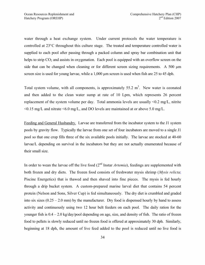
In order to wean the larvae off the live food (2nd Instar Artemia), feedings are supplemented with
both frozen and dry diets. The frozen food consists of freshwater mysis shrimp (Mysis relicta;
Piscine Energetics) that is thawed and then shaved into fine pieces. The mysis is fed hourly
through a drip bucket system. A custom-prepared marine larval diet that contains 54 percent
protein (Nelson and Sons, Silver Cup) is fed simultaneously. The dry diet is crumbled and graded
into six sizes (0.25 – 2.0 mm) by the manufacturer. Dry food is dispensed hourly by hand to assess
activity and continuously using two 12 hour belt feeders on each pool. The daily ration for the
younger fish is 0.4 – 2.0 kg/day/pool depending on age, size, and density of fish. The ratio of frozen
food to pellets is slowly reduced until no frozen food is offered at approximately 30 dph. Similarly,
beginning at 18 dph, the amount of live feed added to the pool is reduced until no live food is
34
Ocean Resources Replenishment and Comprehensive Hatchery Plan (CHP) Hatchery Program (OREHP) 2nd Edition 2007
offered at approximately 25 dph (Figure 25).
1st Instar Brine Shrimp
2nd Instar Brine Shrimp
Shaved Mysis
Ultrafine Starter (dry feed)
Regular Starter (dry feed)
0 5 10 15 20 25 30 35 40
Age (days post hatch)
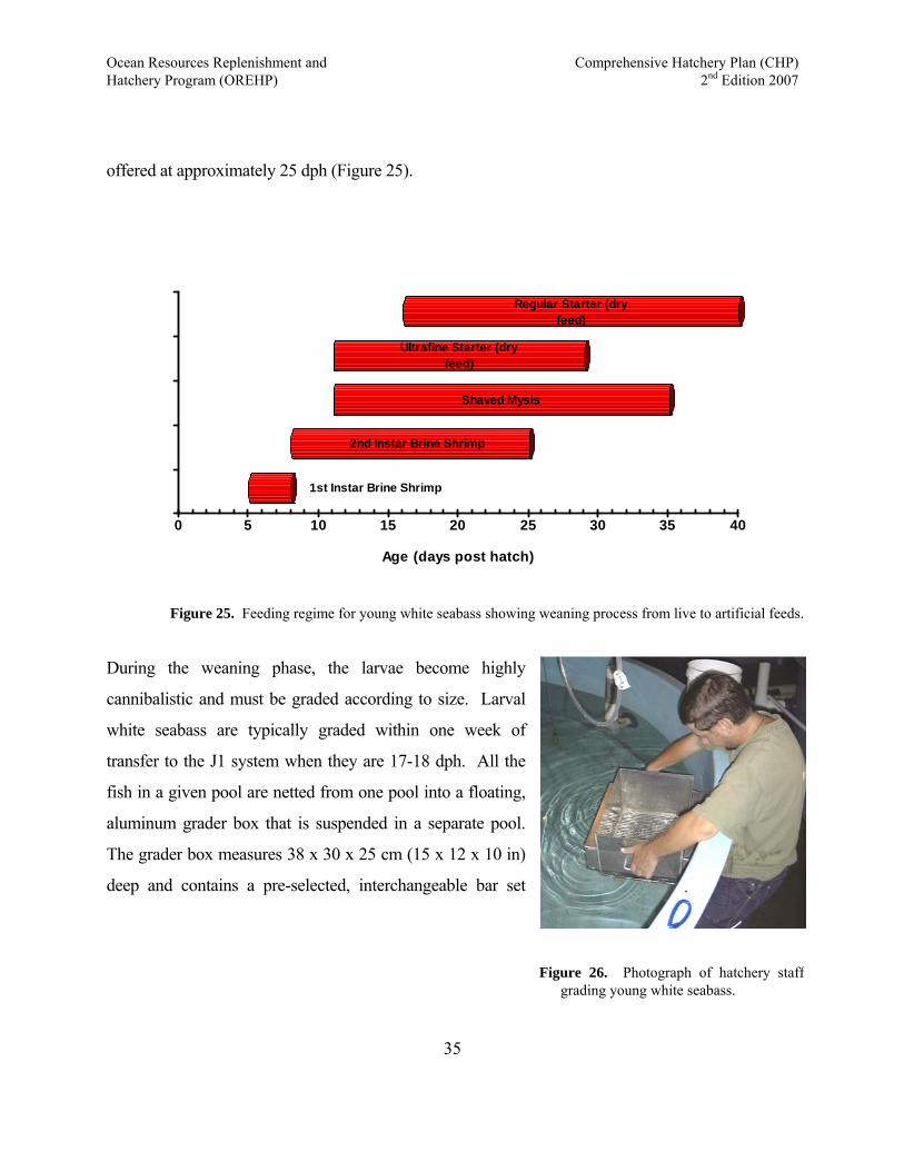
During the weaning phase, the larvae become highly
cannibalistic and must be graded according to size. Larval
white seabass are typically graded within one week of
transfer to the J1 system when they are 17-18 dph. All the
fish in a given pool are netted from one pool into a floating,
aluminum grader box that is suspended in a separate pool.
The grader box measures 38 x 30 x 25 cm (15 x 12 x 10 in)
deep and contains a pre-selected, interchangeable bar set
Figure 25. Feeding regime for young white seabass showing weaning process from live to artificial feeds.
Figure 26. Photograph of hatchery staff grading young white seabass.
35

Ocean Resources Replenishment and Comprehensive Hatchery Plan (CHP) Hatchery Program (OREHP) 2nd Edition 2007
(Figure 26). The grader spacing for the bar sets ranges from 0.8 to 3.2 mm in 0.39 mm (1/64 in)
increments. Smaller fish swim out through the grader bars and into the pool. The larger fish that are
retained by the bars are transferred to another separate pool, which brings the total number of pools
involved in the grading to three with two holding fish at the end of the grading exercise. During
grading, spawn batches are often mixed to maintain efficient stocking densities. Grading is usually
performed on a weekly basis for three consecutive weeks.
Nursery Phase II – (46 to 90 dph)
System Design. Soon after the juvenile white seabass are weaned from live food onto pellets, they
are transferred to the “Juvenile 2” or “J2” recirculation system located at the back of the hatchery
building. The J2 system consists of eight 7,000 L culture pools. The system was designed for a
recirculating water flow of 2,270 Lpm and a maximum fish density of 20 kg/m3. In sizing the
system components, we assumed a maximum biomass of 1,000 kg (50,000 fish at 20 g) and
feeding level of 3 percent body weight per day giving a maximum of 30 kg feed/day.
The design of the J2 system is very similar to J1 except that it has been scaled up to
accommodate a greater biomass. Seawater from the dirty water section of the 9,000 L common
sump is pumped by a four 3.0 hp centrifugal pumps through a 2,270 Lpm propeller-washed bead
filter (model PBF-50S) to remove larger particulate matter and then 33 percent of the water is
directed through a protein skimmer to remove very fine solids. This seawater, now clean of
solids but still under pressure, is directed into a moving-bed biocontactor that consists of a 8,900
L sump with 1.4 m3 of Kaldnes media maintained under heavy aeration. Seawater from the
biocontactor flows by gravity into the clean water portion of the sump. Seawater from the clean
water leg of the sump is pumped by four additional 3.0 hp centrifugal pumps through a series of
four 530 Lpm Triton TR-140 rapid sand filters and then a 650 watt UV sterilizer that provides
approximately 30,000 µW sec/cm2 in a decayed state.
36
Ocean Resources Replenishment and Comprehensive Hatchery Plan (CHP) Hatchery Program (OREHP) 2nd Edition 2007
Water temperature in the system is controlled by diverting approximately 95 Lpm of the supply
water through a heat exchange system. Under current protocols the water temperature is
controlled at 23°C throughout this culture stage. The treated and temperature controlled water is
supplied to each pool after passing through a packed column and spray bar combination unit that
helps to strip CO2 and to assist in oxygenation. Each pool is equipped with a screened overflow on
the side.
Total system volume, with all components, is approximately 114.8 m3. New water is ozonated
and then added to the clean water sump at rate of 19 Lpm, which represents 24 percent
replacement of the system volume per day. Total ammonia levels are usually <0.2 mg/L, nitrite
<0.15 mg/L and nitrate <6.0 mg/L, and DO levels are maintained at or above 4.0 mg/L using a
liquid oxygen delivery system as needed.
Feeding and General Husbandry. Fish in the J2 system are fed using belt feeders at a rate of 3 - 5
percent body wt/day, with the feeing rate being less for larger fish. The diet is 50 percent protein
and 14 percent fat, and is manufactured by Skretting. The extruded pellets are slow-sinking and
typically fed in sizes of 3.0 and 4.0 mm during this stage. Vitamin C is incorporated into the feed at
three times that of typical salmon feeds. Pools are siphoned manually 1-2 times per day.
The size and age of fish at transfer from J2 is currently dictated by ambient water temperature in the
receiving body of water, typically the outdoor raceways. Our experience has shown that juvenile
seabass can be safely transferred to the raceways in warm water conditions (>20°C) at 20 g in size
and roughly 80-90 days old. During colder months the fish are held in the warmer, recirculated
water until they are 40 g and approximately 120 days old.
Prior to moving the fish, the fish are acclimated to ambient temperatures by first diverting the pool
discharge from the recirculation loop to waste. The influent recirculation loop water is then mixed
with ambient water in a ratio that achieves a decrease of 1°C per day until the ambient temperature is
37

Ocean Resources Replenishment and Comprehensive Hatchery Plan (CHP) Hatchery Program (OREHP) 2nd Edition 2007
reached.
38
Ocean Resources Replenishment and Comprehensive Hatchery Plan (CHP) Hatchery Program (OREHP) 2nd Edition 2007
Raceway Culture (91-150 dph)
System Design. After reaching a 20 - 40 g size, the seabass are moved to outdoor raceways that
operate on a flow-through water supply. The raceway system consists of eight 25 m3 concrete
raceways that measure 2.7 x 11.8 x 0.7 m deep. The raceways are located outside of the main
hatchery in an enclosure of chain-link fence covered along the sides and top with shade cloth. The
enclosure provides shade and protection from predators and vandals. The system was designed for
continuous flow rates of 375 Lpm for each raceway and a maximum fish density of 20 kg/m3.
Total ammonia levels are kept below levels of 0.5 mg/L, and DO levels are maintained at or
above 4.0 mg/L using a liquid oxygen delivery system through a low-head oxygenator at the
head of each raceway.
Feeding and General Husbandry. Fish in the raceway system are fed by hand four times per day
at a rate of 2.0 – 3.0 percent body wt/day, with the feeing rate being less in cold water
conditions. The 4.0 mm Skretting diet is fed most commonly during this stage. Detris is
siphoned from the raceways manually once each day.
39
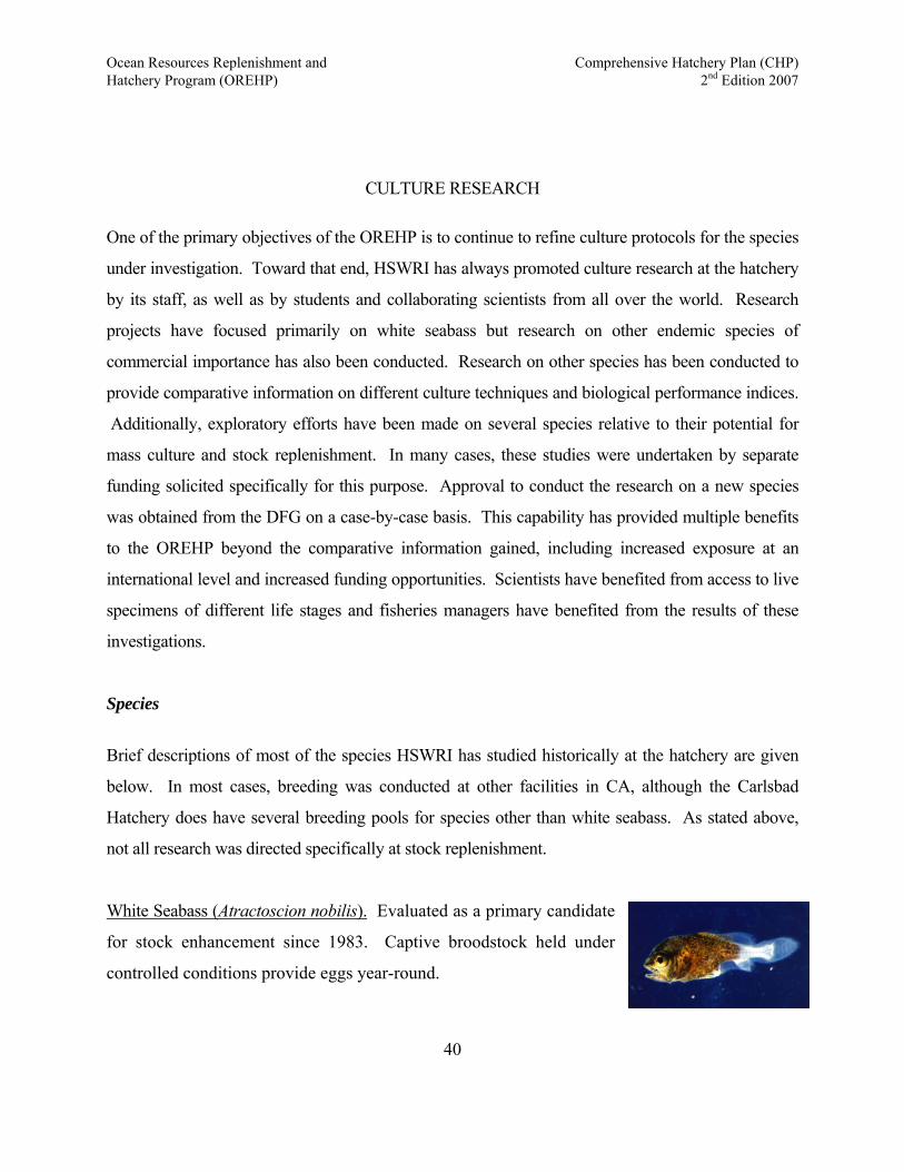
Ocean Resources Replenishment and Comprehensive Hatchery Plan (CHP) Hatchery Program (OREHP) 2nd Edition 2007
CULTURE RESEARCH
One of the primary objectives of the OREHP is to continue to refine culture protocols for the species
under investigation. Toward that end, HSWRI has always promoted culture research at the hatchery
by its staff, as well as by students and collaborating scientists from all over the world. Research
projects have focused primarily on white seabass but research on other endemic species of
commercial importance has also been conducted. Research on other species has been conducted to
provide comparative information on different culture techniques and biological performance indices.
Additionally, exploratory efforts have been made on several species relative to their potential for
mass culture and stock replenishment. In many cases, these studies were undertaken by separate
funding solicited specifically for this purpose. Approval to conduct the research on a new species
was obtained from the DFG on a case-by-case basis. This capability has provided multiple benefits
to the OREHP beyond the comparative information gained, including increased exposure at an
international level and increased funding opportunities. Scientists have benefited from access to live
specimens of different life stages and fisheries managers have benefited from the results of these
investigations.
Species
Brief descriptions of most of the species HSWRI has studied historically at the hatchery are given
below. In most cases, breeding was conducted at other facilities in CA, although the Carlsbad
Hatchery does have several breeding pools for species other than white seabass. As stated above,
not all research was directed specifically at stock replenishment.
White Seabass (Atractoscion nobilis). Evaluated as a primary candidate
for stock enhancement since 1983. Captive broodstock held under
controlled conditions provide eggs year-round.
40

Ocean Resources Replenishment and Comprehensive Hatchery Plan (CHP) Hatchery Program (OREHP) 2nd Edition 2007
California Halibut (Paralichthys californicus). Evaluated as a secondary
candidate for stock enhancement at a modest scale since 1983. Captive
broodstock held under ambient conditions provide eggs during the
spring and summer.
Giant Sea Bass (Stereolepis gigas). Because of overfishing, this species
has been under a moratorium since the early ‘80s. A long-lived, slow
growing fish, this is thought to be a good candidate for conservation-
oriented aquaculture research.
California Sheephead (Semicossyphus pulcher). In recent years, trap-
fishing for a high dollar live fish fishery has left this species heavily
exploited. It is listed as one of 19 high priority nearshore species for
management plan development under California’s Marine Life
Management Act (MLMA).
Bocaccio (Sebastes paucipinis). One of California’s most valuable
groundfishes, bocaccio have been heavily exploited. They were
recently considered for listing as a threatened species under the
Endangered Species Act (ESA).
California Yellowtail (Seriola lalandi). A transitory, seasonally
abundant species in southern California, yellowtail are highly prized as
a game and food fish.
Striped Bass (Morone saxatilis). Their freshwater counterparts, hybrid
41
Ocean Resources Replenishment and Comprehensive Hatchery Plan (CHP) Hatchery Program (OREHP) 2nd Edition 2007
striped bass, represent a 9-million pound aquaculture industry in the US. Striped bass were
historically released for enhancement in central California, and are considered a good species for
comparative study.
Experimental Systems
The hatchery maintains a separate area in the main building for conducting most of its research.
The experimental area contains a variety of culture vessels ranging from 60 to 800 L in size and
arranged in replicates. Most of these systems are on a flow through water supply with the ability
to control water temperature.
The cornerstone experimental system where most of the current research is conducted is
designed for studying fish larvae. Larval rearing is the bottleneck to production of most marine
species because they are very sensitive and difficult to study. The experimental larval rearing
system is designed specifically to conduct replicated studies of larvae under very controlled
conditions as a means of optimizing the rearing conditions for marine finfish larvae (Figure 27).
Four cone-bottom tanks of 1,600 L and 400 L, and twenty-four 60 L capacity are integrated into
the system. The three sizes of tanks are scaled similarly so that scaling experiments can be
conducted to determine if tank size has an effect on larval survival. The large number of small
60 L tanks is used to test several variables simultaneously and to measure the effects on larval
growth and survival. Each tank can be supplied with temperature-controlled water that is either
flow-through or recirculated. The recirculating water system provides a very high quality,
biosecure water source for the culture tanks.
The 60 L cone tanks are placed in a series of six rectangular water baths so the temperature does
not fluctuate with changing ambient air temperature, which is a common problem with small
tanks that are operated statically or with little flowing water. Each of the six water baths has an
independently controlled light source and can hold four 60 L cone tanks. The cone tanks are
42

Ocean Resources Replenishment and Comprehensive Hatchery Plan (CHP) Hatchery Program (OREHP) 2nd Edition 2007
interchangeable among the water baths making, for example, different tank color combinations
possible at a given light level. Lighting for these tanks is provided by high intensity fluorescent
fixtures that contain four 54 watt T5 lamps with a color temperature that is very similar to
daylight – 6,500 K. The lights over each water bath are on independent dimmer switches that
allow them to be controlled from 0 to 15,000 Lux at the surface of each tank.
Figure 27. Experimental system designed to help optimize rearing conditions for marine finfish larvae.
The filtration system consists of a high capacity fluidized bed, bead filter, foam fractionator, and
UV sterilizer. Ozonated make-up water is supplied at 10 L/min. Effluent water from all tanks is
pumped directly into the first stage of the filtration system at up to 380 L/min using a 1 hp pump.
The initial filtration component is a propeller-washed bead filter (PBF-5S, Aquaculture
Systems) for particulate removal and some nitrification. The second filtration component in 43

Ocean Resources Replenishment and Comprehensive Hatchery Plan (CHP) Hatchery Program (OREHP) 2nd Edition 2007
series is a 1,600 L fluidized bed biofilter (Aquaneering Inc.) containing 900 kg of #60 sand.
Water from these filters drops through a degassing column into a 1,500 L sump. A ½ hp pump
supplies water to a foam fractionator (Aquaneering Inc.) at up to 95 L/min on an independent
loop from this same sump. A ¼ hp pump is used to supply seawater to a titanium heat exchanger
at approximately 80 L/min on a second independent loop from the sump. Like our other
recirculating systems, temperature in the system is controlled using an actuated valve that is
connected to our computer control system. Water is supplied to the culture tanks from the sump
after being pumped through a 300 watt UV sterilizer (COM6300, Emperor Aquatics) at a rate of
380 L/min using a 1 hp pump. Total system volume is approximately 18 M3.
A separate seawater supply system consisting of a 2,300 L holding tank filled with sand-filtered
seawater from the hatchery’s temperature-mixing sumps is also available. Two ½ hp pumps
connected to the holding tank can supply each of the tanks independently. This will enable us to
test the effects of recirculated verses raw seawater, and it will serve as a back-up water supply to
the recirculating system.
44
Ocean Resources Replenishment and Comprehensive Hatchery Plan (CHP) Hatchery Program (OREHP) 2nd Edition 2007
GENETIC DIVERSITY CONSIDERATIONS
Genetic quality assurance has been a priority for the OREHP since the early years of the
program. Studies to examine the genetic characteristics of wild white seabass were initiated in
mid-late 1980’s and ran parallel to the culture and assessment research.
Characteristics of Marine Species
Beyond the technical aspects of maintaining brood fish is the concern that genetic variability of the
wild population could be diminished by releasing large numbers of hatchery fish. Diminishing
genetic variability due to selective breeding and survival within the hatchery is an important
consideration. These concerns are driven largely by observations made of some adverse interactions
between wild and hatchery populations of salmonids. However, because the white seabass is a
completely marine species, it does not have the same reproductive behavior of salmonid species.
Specific problems with using observations of anadromous salmonids to set realistic conservation
guidelines for white seabass include:
Homing ability: Because salmon home so precisely to spawn, sub-populations can be
greatly differentiated and adapted to a local drainage or environment (Ricker 1972; Quinn
1982). Most marine fish, including white seabass, do not home as precisely and do not have
as genetically differentiated sub-populations (Gyllensten 1985; Utter and Ryman 1993).
Larval and egg dispersal: Salmon have a more limited egg and larval dispersion than most
marine fish. White seabass eggs and larvae are estimated to be in the water column for 40
days and capable of wide transport by currents along the California coast, thereby providing
a mechanism to break down sub-population structure. Waples (1987) reported that the
genetic structure of populations of 10 inshore marine fish species from the Southern
California Bight were correlated with egg and larval dispersal; eight of these 10 species
45
Ocean Resources Replenishment and Comprehensive Hatchery Plan (CHP) Hatchery Program (OREHP) 2nd Edition 2007
studied by Waples had little population differentiation.
Complex life history: Because salmon have an anadromous life history and strictly defined
migration patterns, which appear to be genetically controlled (Ricker 1972; Bams 1976), the
addition of exotic genes from conspecifics coding for other migration patterns can disrupt the
fine tuning necessary for salmon to migrate to their natal streams or to migrate to the sea at
the appropriate times of the year (Bams 1976). White seabass do not have as complex a life
history and spawn over a longer seasonal period, April to July (Vojkovich and Reed 1983).
Although the study of genetic resources described for salmonids has greatly advanced the field of
applied population genetics and has provided an efficient tool for the management of valuable
salmon populations, using anadromous salmonids as a general model for the conservation and
utilization of genetic resources of many marine species should be done cautiously.
Historical Perspective
Wild Populations. Numerous studies to assess the genetic diversity of wild white seabass have been
funded and supported directly by OREHP (Bartley and Kent 1990; Franklin 1997; and Buonocorssi
et al. 2001).
A survey of the natural population of white seabass from the Southern California Bight (Bartley and
Kent 1990) revealed no stable population sub-structuring in the area. The study evaluated 22
enzyme systems representing 33 distinct loci in 13 different samples that varied spatially and
temporally (ΣN=510 fish). Average heterozygosity values ranged from 0.033 to 0.064, genetic
identity was greater than 99 percent in all pair-wise comparisons and only 3 percent of the genetic
variation was attributed to between sample differences. Gene flow was estimated to be
approximately nine migrants per generation and therefore sufficient to homogenize the genetic
structure of the population. The authors detected no consistent geographic, clinal or temporal
46
Ocean Resources Replenishment and Comprehensive Hatchery Plan (CHP) Hatchery Program (OREHP) 2nd Edition 2007
component to the observed genetic variation in wild southern California populations of white
seabass.
Franklin (1997) examined white seabass DNA (eight microsatellite loci) from fish collected
between 1990 and 1995 in Californian and Mexican waters, including the Sea of Cortez.
Franklin did not examine temporal stability in allele frequencies and therefore was unable to
determine the presence of any distinct, stable subpopulation structure. However, genetic
similarities among the samples he examined suggested that there were broad spawning groups
within the Southern California Bight and Mexico that contribute to the genetic make-up of the
population. Franklin concluded that the white seabass stock in the Eastern Pacific Ocean is
composed of three components: northern (Point Conception to central Baja), southern (southern
Baja), and the Sea of Cortez.
Buonaccorsi et al. (2001), examined tissue samples collected from 240 adult white seabass from
three locations within the geographic range of white seabass – Santa Barbara, Los Angeles and
Baja California. Samples were obtained from commercial fisheries all in the same year. The
same eight microsatellite loci used by Franklin (1997) were used to test heterogeneity among the
sampling locations. Similar to the findings of previous investigators, the results of the study
failed to support the existence of significant population structure within the range of white
seabass. Tests of heterogeneity in allele and genotypic frequencies failed to detect significant
divergence when all samples were considered. Buonaccorsi et al. (2001) concluded that there is
sufficient migration at egg, larval, juvenile, and/or adult stages of white seabass to prevent the
accumulation of significant genetic divergence at this scale. The three populations sampled were
considered homogeneous, from an evolutionary standpoint.
Collectively, these results for white seabass are consistent with genetic studies on other pelagic
marine fishes (Gyllensten 1985; Ramsey and Wakeman 1987; Waples 1987; Graves et al., 1992;
King and Pate 1992). In highly mobile species such as white seabass (Vojkovich and Reed 1983),
47
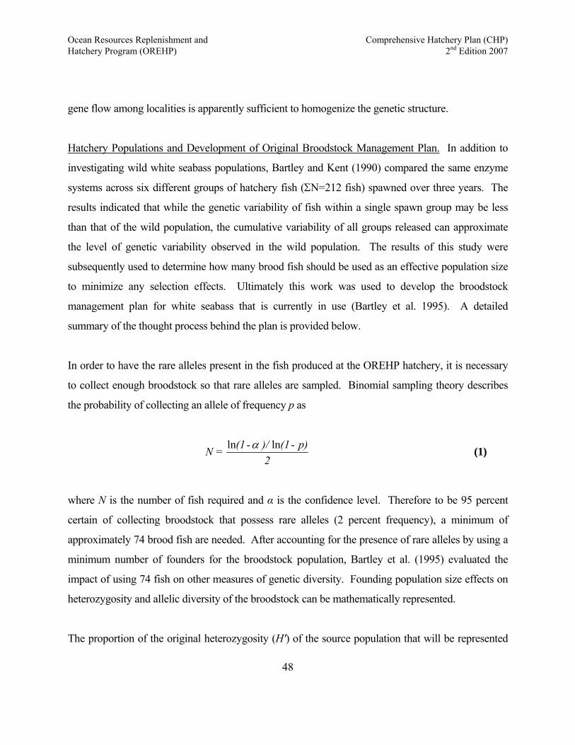
Ocean Resources Replenishment and Comprehensive Hatchery Plan (CHP) Hatchery Program (OREHP) 2nd Edition 2007
gene flow among localities is apparently sufficient to homogenize the genetic structure.
Hatchery Populations and Development of Original Broodstock Management Plan. In addition to
investigating wild white seabass populations, Bartley and Kent (1990) compared the same enzyme
systems across six different groups of hatchery fish (ΣN=212 fish) spawned over three years. The
results indicated that while the genetic variability of fish within a single spawn group may be less
than that of the wild population, the cumulative variability of all groups released can approximate
the level of genetic variability observed in the wild population. The results of this study were
subsequently used to determine how many brood fish should be used as an effective population size
to minimize any selection effects. Ultimately this work was used to develop the broodstock
management plan for white seabass that is currently in use (Bartley et al. 1995). A detailed
summary of the thought process behind the plan is provided below.
In order to have the rare alleles present in the fish produced at the OREHP hatchery, it is necessary
to collect enough broodstock so that rare alleles are sampled. Binomial sampling theory describes
the probability of collecting an allele of frequency p as
2
p)-(1)/-(1=N lnln α (1)
where N is the number of fish required and α is the confidence level. Therefore to be 95 percent
certain of collecting broodstock that possess rare alleles (2 percent frequency), a minimum of
approximately 74 brood fish are needed. After accounting for the presence of rare alleles by using a
minimum number of founders for the broodstock population, Bartley et al. (1995) evaluated the
impact of using 74 fish on other measures of genetic diversity. Founding population size effects on
heterozygosity and allelic diversity of the broodstock can be mathematically represented.
The proportion of the original heterozygosity (H') of the source population that will be represented
48
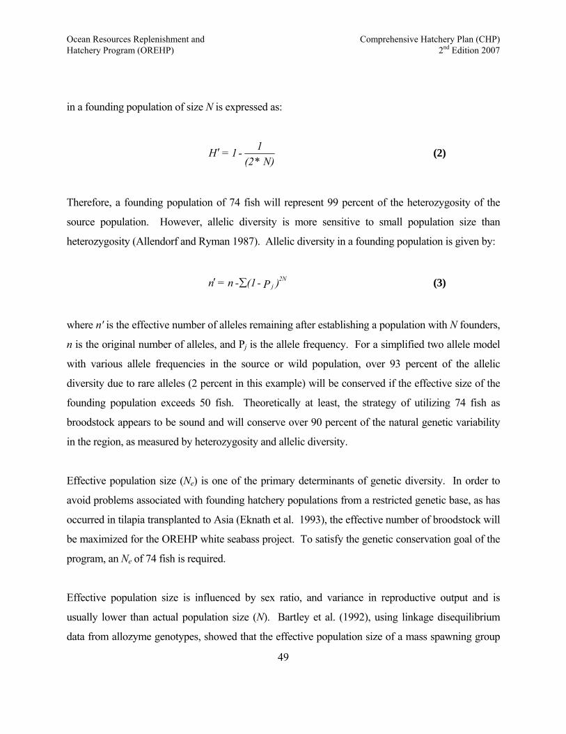
Ocean Resources Replenishment and Comprehensive Hatchery Plan (CHP) Hatchery Program (OREHP) 2nd Edition 2007
in a founding population of size N is expressed as:
N)*(2
1-1=H ′ (2)
Therefore, a founding population of 74 fish will represent 99 percent of the heterozygosity of the
source population. However, allelic diversity is more sensitive to small population size than
heterozygosity (Allendorf and Ryman 1987). Allelic diversity in a founding population is given by:
(3) )P-(1-n=n 2Nj∑′
where n' is the effective number of alleles remaining after establishing a population with N founders,
n is the original number of alleles, and Pj is the allele frequency. For a simplified two allele model
with various allele frequencies in the source or wild population, over 93 percent of the allelic
diversity due to rare alleles (2 percent in this example) will be conserved if the effective size of the
founding population exceeds 50 fish. Theoretically at least, the strategy of utilizing 74 fish as
broodstock appears to be sound and will conserve over 90 percent of the natural genetic variability
in the region, as measured by heterozygosity and allelic diversity.
Effective population size (Ne) is one of the primary determinants of genetic diversity. In order to
avoid problems associated with founding hatchery populations from a restricted genetic base, as has
occurred in tilapia transplanted to Asia (Eknath et al. 1993), the effective number of broodstock will
be maximized for the OREHP white seabass project. To satisfy the genetic conservation goal of the
program, an Ne of 74 fish is required.
Effective population size is influenced by sex ratio, and variance in reproductive output and is
usually lower than actual population size (N). Bartley et al. (1992), using linkage disequilibrium
data from allozyme genotypes, showed that the effective population size of a mass spawning group
49
Ocean Resources Replenishment and Comprehensive Hatchery Plan (CHP) Hatchery Program (OREHP) 2nd Edition 2007
of white seabass broodstock was about 50 percent of the actual population size. Therefore, using the
conservation goals stated above, a total of 150 (2 x 74=148) adult brood fish was recommended. In
practice and to be even more conservative, the Carlsbad Hatchery was designed to accommodate
200 adult fish that are evenly divided among four breeding pools.
A schedule for annually rotating 20 percent of the male brood fish among breeding pools was
originally proposed in the broodstock management plan in order to increase the diversity in progeny
by increasing the number of different matings per broodstock. That rotation schedule assumed that a
total of 200 brood fish (1:1 sex ratio), or 33 percent more than the effective founder population size
described above, were maintained in the hatchery with at least 5 percent being replaced per year. In
practice, rotating males among breeding pools was difficult because seabass are so skittish and the
capture process results in trauma to targeted and non-targeted fish within the breeding pools. Instead
of rotating males among pools, the OREHP increased the rate of adult replacement from the
recommended 5 percent to 10 percent annually since 1996.
Contemporary Findings.
Recently, Coykendall (2005) completed a study of white seabass that examined wild stocks,
hatchery releases, and breeding stocks. This study used the same eight microsatellite DNA loci
described previously by Franklin (1997) and Buonaccorsi et al. (2001). An executive summary of
Coykendall’s work is provided by the author below.
We employed the Ryman-Laikre model of genetic impact of hatchery supplementation to wild populations. The model requires estimates of three parameters: hatchery effective population size (or in this case effective number of breeders), the effective size of the wild population, and the contribution that the hatchery fish make to the overall reproduction of the population. Estimates of these three parameters, caveats associated with them, and our general conclusions are addressed below. Hatchery effective size, Neh – To understand the biology of the hatchery spawns, we
50
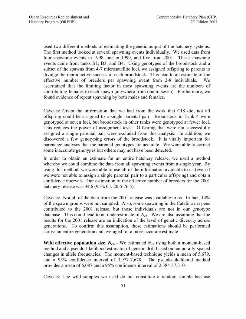
Ocean Resources Replenishment and Comprehensive Hatchery Plan (CHP) Hatchery Program (OREHP) 2nd Edition 2007
used two different methods of estimating the genetic output of the hatchery systems. The first method looked at several spawning events individually. We used data from four spawning events in 1998, one in 1999, and five from 2001. These spawning events came from tanks B1, B3, and B4. Using genotypes of the broodstock and a subset of the spawns from 4-7 microsatellite loci, we assigned offspring to parents to divulge the reproductive success of each broodstock. This lead to an estimate of the effective number of breeders per spawning event from 2-8 individuals. We ascertained that the limiting factor in most spawning events are the numbers of contributing females to each spawn (anywhere from one to seven). Furthermore, we found evidence of repeat spawning by both males and females.
Caveats: Given the information that we had from the work that GIS did, not all offspring could be assigned to a single parental pair. Broodstock in Tank 4 were genotyped at seven loci, but broodstock in other tanks were genotyped at fewer loci. This reduces the power of assignment tests. Offspring that were not successfully assigned a single parental pair were excluded from this analysis. In addition, we discovered a few genotyping errors of the broodstock. It is vitally important for parentage analyses that the parental genotypes are accurate. We were able to correct some inaccurate genotypes but others may not have been detected.
In order to obtain an estimate for an entire hatchery release, we used a method whereby we could combine the data from all spawning events from a single year. By using this method, we were able to use all of the information available to us (even if we were not able to assign a single parental pair to a particular offspring) and obtain confidence intervals. Our estimation of the effective number of breeders for the 2001 hatchery release was 34.6 (95% CI: 20.6-76.5). Caveats: Not all of the data from the 2001 release was available to us. In fact, 14% of the spawn groups were not sampled. Also, some spawning in the Catalina net pens contributed to the 2001 release, but those individuals are not in our genotype database. This could lead to an underestimate of Neh. We are also assuming that the results for the 2001 release are an indication of the level of genetic diversity across generations. To confirm this assumption, these estimations should be performed across an entire generation and averaged for a more accurate estimate. Wild effective population size, New - We estimated New using both a moment-based method and a pseudo-likelihood estimator of genetic drift based on temporally-spaced changes in allele frequencies. The moment-based technique yields a mean of 5,679, and a 95% confidence interval of 3,977-7,678. The pseudo-likelihood method provides a mean of 6,087 and a 95% confidence interval of 2,384-57,310. Caveats: The wild samples we used do not constitute a random sample because
51
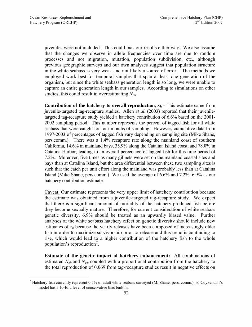
Ocean Resources Replenishment and Comprehensive Hatchery Plan (CHP) Hatchery Program (OREHP) 2nd Edition 2007
juveniles were not included. This could bias our results either way. We also assume that the changes we observe in allele frequencies over time are due to random processes and not migration, mutation, population subdivision, etc., although previous geographic surveys and our own analyses suggest that population structure in the white seabass is very weak and not likely a source of error. The methods we employed work best for temporal samples that span at least one generation of the organism, but since the white seabass generation length is so long, we were unable to capture an entire generation length in our samples. According to simulations on other studies, this could result in overestimating New. Contribution of the hatchery to overall reproduction, xh - This estimate came from juvenile-targeted tag-recapture studies. Allen et al. (2003) reported that their juvenile-targeted tag-recapture study yielded a hatchery contribution of 6.6% based on the 2001-2002 sampling period. This number represents the percent of tagged fish for all white seabass that were caught for four months of sampling. However, cumulative data from 1997-2003 of percentages of tagged fish vary depending on sampling site (Mike Shane, pers.comm.). There was a 1.4% recapture rate along the mainland coast of southern California, 14.6% in mainland bays, 35.9% along the Catalina Island coast, and 78.0% in Catalina Harbor, leading to an overall percentage of tagged fish for this time period of 7.2%. Moreover, five times as many gillnets were set on the mainland coastal sites and bays than at Catalina Island, but the area differential between these two sampling sites is such that the catch per unit effort along the mainland was probably less than at Catalina Island (Mike Shane, pers.comm.) We used the average of 6.6% and 7.2%, 6.9% as our hatchery contribution estimate. Caveat: Our estimate represents the very upper limit of hatchery contribution because the estimate was obtained from a juvenile-targeted tag-recapture study. We expect that there is a significant amount of mortality of the hatchery-produced fish before they become sexually mature. Therefore, for current consideration of white seabass genetic diversity, 6.9% should be treated as an upwardly biased value. Further analyses of the white seabass hatchery effect on genetic diversity should include new estimates of xh because the yearly releases have been composed of increasingly older fish in order to maximize survivorship prior to release and this trend is continuing to rise, which would lead to a higher contribution of the hatchery fish to the whole population’s reproduction2. Estimate of the genetic impact of hatchery enhancement: All combinations of estimated Neh and New coupled with a proportional contribution from the hatchery to the total reproduction of 0.069 from tag-recapture studies result in negative effects on
52
2 Hatchery fish currently represent 0.5% of adult white seabass surveyed (M. Shane, pers. comm.), so Coykendall’s model has a 10-fold level of conservative bias built in.
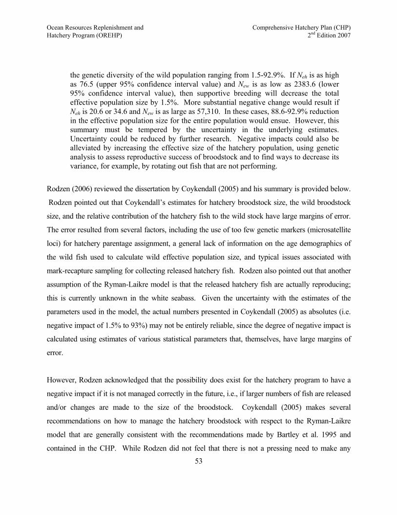
Ocean Resources Replenishment and Comprehensive Hatchery Plan (CHP) Hatchery Program (OREHP) 2nd Edition 2007
the genetic diversity of the wild population ranging from 1.5-92.9%. If Neh is as high as 76.5 (upper 95% confidence interval value) and New is as low as 2383.6 (lower 95% confidence interval value), then supportive breeding will decrease the total effective population size by 1.5%. More substantial negative change would result if Neh is 20.6 or 34.6 and New is as large as 57,310. In these cases, 88.6-92.9% reduction in the effective population size for the entire population would ensue. However, this summary must be tempered by the uncertainty in the underlying estimates. Uncertainty could be reduced by further research. Negative impacts could also be alleviated by increasing the effective size of the hatchery population, using genetic analysis to assess reproductive success of broodstock and to find ways to decrease its variance, for example, by rotating out fish that are not performing.
Rodzen (2006) reviewed the dissertation by Coykendall (2005) and his summary is provided below.
Rodzen pointed out that Coykendall’s estimates for hatchery broodstock size, the wild broodstock
size, and the relative contribution of the hatchery fish to the wild stock have large margins of error.
The error resulted from several factors, including the use of too few genetic markers (microsatellite
loci) for hatchery parentage assignment, a general lack of information on the age demographics of
the wild fish used to calculate wild effective population size, and typical issues associated with
mark-recapture sampling for collecting released hatchery fish. Rodzen also pointed out that another
assumption of the Ryman-Laikre model is that the released hatchery fish are actually reproducing;
this is currently unknown in the white seabass. Given the uncertainty with the estimates of the
parameters used in the model, the actual numbers presented in Coykendall (2005) as absolutes (i.e.
negative impact of 1.5% to 93%) may not be entirely reliable, since the degree of negative impact is
calculated using estimates of various statistical parameters that, themselves, have large margins of
error.
However, Rodzen acknowledged that the possibility does exist for the hatchery program to have a
negative impact if it is not managed correctly in the future, i.e., if larger numbers of fish are released
and/or changes are made to the size of the broodstock. Coykendall (2005) makes several
recommendations on how to manage the hatchery broodstock with respect to the Ryman-Laikre
model that are generally consistent with the recommendations made by Bartley et al. 1995 and
contained in the CHP. While Rodzen did not feel that there is not a pressing need to make any
53

Ocean Resources Replenishment and Comprehensive Hatchery Plan (CHP) Hatchery Program (OREHP) 2nd Edition 2007
drastic changes to the hatchery program at this point in time, the recommendations listed below are
being considered for implementation as a safeguard against decreasing the effective population size.
These include:
1. Rotate broodstock over time to avoid repeat-spawning by the same individuals over multiple year classes;
2. Equalize sibling group sizes as much as possible;
3. Monitor spawning success to identify those individuals who are and are not producing viable gametes; and
4. Develop a formal Genetic Management Plan for white seabass
It is difficult, if not impossible, to state what the optimum size of broodstock and hatchery releases
should be since there is so much uncertainty regarding the size of the wild population and
reproductive success of hatchery produced fish. Rodzen (2006) considers the numbers of
broodstock currently used to be the minimum broodstock size for future years, and would continue
to make attempts to use more broodstock per year and equalize the number of fish stocked across the
families. Once it is more clearly demonstrated that adequate genetic diversity is represented in the
offspring (i.e. more sibling groups), then more fish of a larger size can be stocked.
Contemporary Plans for Managing the White Seabass Broodstock.
Based on the recent genetics results and success in rearing large numbers of white seabass, HSWRI
is actively addressing the recommendations listed above in the following manner.
Rotation of brood fish. This objective involves rotating new stock (males and females) into the
program on a regular basis as well as rotating males among the breeding pools. This must be
accomplished without impacting the health of the fish or the general success of egg production.
In order to achieve this objective, HSWRI is assembling a fifth breeding pool that will be used
initially to move existing brood fish into so that the original systems can be upgraded relative to
54
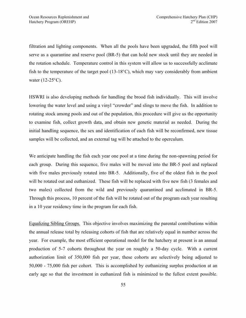
Ocean Resources Replenishment and Comprehensive Hatchery Plan (CHP) Hatchery Program (OREHP) 2nd Edition 2007
filtration and lighting components. When all the pools have been upgraded, the fifth pool will
serve as a quarantine and reserve pool (BR-5) that can hold new stock until they are needed in
the rotation schedule. Temperature control in this system will allow us to successfully acclimate
fish to the temperature of the target pool (13-18°C), which may vary considerably from ambient
water (12-25°C).
HSWRI is also developing methods for handling the brood fish individually. This will involve
lowering the water level and using a vinyl “crowder” and slings to move the fish. In addition to
rotating stock among pools and out of the population, this procedure will give us the opportunity
to examine fish, collect growth data, and obtain new genetic material as needed. During the
initial handling sequence, the sex and identification of each fish will be reconfirmed, new tissue
samples will be collected, and an external tag will be attached to the operculum.
We anticipate handling the fish each year one pool at a time during the non-spawning period for
each group. During this sequence, five males will be moved into the BR-5 pool and replaced
with five males previously rotated into BR-5. Additionally, five of the oldest fish in the pool
will be rotated out and euthanized. These fish will be replaced with five new fish (3 females and
two males) collected from the wild and previously quarantined and acclimated in BR-5.
Through this process, 10 percent of the fish will be rotated out of the program each year resulting
in a 10 year residency time in the program for each fish.
Equalizing Sibling Groups. This objective involves maximizing the parental contributions within
the annual release total by releasing cohorts of fish that are relatively equal in number across the
year. For example, the most efficient operational model for the hatchery at present is an annual
production of 5-7 cohorts throughout the year on roughly a 50-day cycle. With a current
authorization limit of 350,000 fish per year, these cohorts are selectively being adjusted to
50,000 - 75,000 fish per cohort. This is accomplished by euthanizing surplus production at an
early age so that the investment in euthanized fish is minimized to the fullest extent possible.
55
Ocean Resources Replenishment and Comprehensive Hatchery Plan (CHP) Hatchery Program (OREHP) 2nd Edition 2007
Initially, each cohort is established using 3-5 spawns over 3-5 consecutive days from 1-2
breeding pools as dictated by the spawning activity on the 50-day interval. Spawn volumes are
recorded and used as a means of quantifying relative female contribution. Because the eggs are
collect over such a short time period we can assume that different females were involved and
roughly how many. Without other means, we cannot be certain that the same female did not
contribute eggs to subsequent cohorts. Techniques for obtaining this information are described
below.
Monitoring Spawning Success. This objective involves using observational or genetic tools to
assess spawning patterns among breeding fish. By accurately knowing which fish are spawning
during any given event, it is possible to selectively eliminate eggs from females that may have
contributed to a previous cohort. In addition, it provides valuable information regarding the
relative contributions of fish within the populations, so that fish that are more or less productive
can be removed from the populations as appropriate.
Research conducted to date on white seabass, as well as other species, suggests that this
approach is entirely feasible. However, a variety of problems with genotyping, as cited in the
study by Coykendall (2005), necessitate that all brood fish be re-sampled and genotyped to
insure accuracy. This also includes confirming the identity of individuals in the population, their
location among breeding pools, and verification of their gender classification. This will be
facilitated by the activities listed in the first objective above.
In order to minimize problems with genotyping that were experienced in the past, HSWRI is
hiring a full-time geneticist to facilitate this work in collaboration with Dr. Russ Vetter at the
Southwest Fisheries Science Center in La Jolla. We expect that this collaborative effort,
bolstered by proximity and a high level of personal involvement by the genetics research team,
will greatly increase the quality control and overall success of the project. This “renewed”
genetics project will be initiated in 2007 and is expected to run a minimum of three years.
56
Ocean Resources Replenishment and Comprehensive Hatchery Plan (CHP) Hatchery Program (OREHP) 2nd Edition 2007
In addition to the genetic approach, which will take several years to evaluate, HSWRI has
initiated research to evaluate the feasibility of marking the fish individually with an external
“ear” tag adapted from the agriculture industry. This ear tag is being applied to both sides of the
operculum of each brood fish and will be combined with a visual monitoring program to see if
breeding patterns can be elucidated from changes in morphology and color patterns on breeding
fish – specifically females as they become enlarged during egg hydration and darkly colored
during courtship and spawning.
Developing a Genetic Management Plan. This objective involves establishing a Genetics
Management Plan for white seabass that seeks to preserve the genetic diversity of the wild stocks
adaptively as the replenishment program continues to mature and new data are available. A
template for such a plan has been developed by Tringali et al. (2007) and is reproduced in
Appendix V. Among other issues, the plan will address what can be done with surplus fish
production including the potential risks associated with allowing farmers to raise them
commercially in cages. Because more data needs to be collected to adequately develop this plan,
it is expected that this plan will be developed sometime in 2009.
57
Ocean Resources Replenishment and Comprehensive Hatchery Plan (CHP) Hatchery Program (OREHP) 2nd Edition 2007
FISH HEALTH AND DISEASE
As stated previously, the primary goal of the OREHP and the Carlsbad Hatchery is to augment
dwindling wild stocks of several marine fish species with cultured fish. However, while it is
certainly desirable for the hatchery to produce large numbers of cultured fish, it is also necessary
that all fish destined for release be as healthy as possible. Healthy fish have a significantly
greater chance for survival, and are less likely to transmit dangerous diseases to native fish
stocks.
The most dangerous diseases are those that are lethal, highly contagious, and which wild fish
have little or no immunity. Novel pathogens (primarily viruses and rickettsia), which can
emerge and be greatly amplified among cultured fish, pose a significant threat to naïve wild
stocks. Minimizing the disease risk to wild fish populations is a priority for the OREHP.
Infectious diseases that occur in wild and cultured marine fish include a wide variety of parasites
and microbial agents. Parasites can be classified as either protozoan, metazoan, or crustacean.
Protozoan parasites include flagellates, ciliates, and sporozoans; metazoan parasites include
cestodes (tapeworms), nematodes (round worms), or trematodes (flukes). Crustacean parasites
consist of parasitic copepods and isopods. Microbial pathogens include: bacteria, rickettsia,
fungi, and viruses.
In addition to infectious diseases, there are a variety of non-infectious diseases that can develop
in cultured fish. Many non-infectious diseases are associated with poor water quality; others are
related to poor genetics, nutrition, or hatchery practices. Major classes of non-infectious disease
associated with poor water quality include: 1) gas supersaturation (GSS) disease caused by
elevated total dissolved gas (TDG); 2) anoxia or hypoxia caused by low DO; 3) nitrogenous
waste toxicity caused by high ammonia or nitrite; 4) hydrogen sulfide (H2S) toxicity caused by
anaerobic conditions; and 5) xenobiotic exposure (e.g., pesticide or metal toxicity). Poor genetic
58
Ocean Resources Replenishment and Comprehensive Hatchery Plan (CHP) Hatchery Program (OREHP) 2nd Edition 2007
makeup or poor nutrition can lead to a variety of musculoskeletal defects (e.g., craniofacial
malformations, opercular defects, spinal deformities) and swimbladder problems – notably non-
inflation. Poor hatchery practices can exacerbate GSS disease, result in cannibalism (due to
inadequate feeding and/or grading of fish by size), or cause traumatic injuries to fish.
Minimizing hatchery losses from both infectious and non-infectious diseases requires a careful
layout (for pools and equipment), superior water filtration and treatment systems, well thought
out protocols, efficient and well-trained personnel, and a top notch biosecurity program.
Emphasis is placed on disease prevention, rather than on control and treatment. For non-
infectious diseases, prevention hinges on a combination of high water quality, good nutrition and
genetics, and sound hatchery practices. For infectious diseases, prevention depends on a
comprehensive biosecurity program, including quarantine, disinfection, compartmentalization,
disease surveillance and response.
Preventative measures are never 100 percent, so continuous surveillance and rapid response are
keys to limiting the spread of disease once outbreaks occur. Compartmentalization within the
hatchery – physically separating fish based on species and life stage – is used to limit disease
spread. Ultimate response to a disease will depend on the nature of the disease, and the types of
treatments available.
Often taking no action is the best response to a disease outbreak. Some pathogens have minimal
impact on the fish’s health, and some diseases are self-limiting and will resolve on their own. In
addition, having a parasite or disease run through a pool or system can have benefits for the
particular group of fish affected, and for the species overall, as pathogen exposure will help
ensure that immuno-competent fish are the ones being released. Immuno-competent fish have a
much higher chance at survival when compared to cultured fish that have never encountered a
pathogen.
59
Ocean Resources Replenishment and Comprehensive Hatchery Plan (CHP) Hatchery Program (OREHP) 2nd Edition 2007
The major caveat to disease outbreaks among hatchery fish is that even if fish recover, they have
the potential for becoming healthy carriers. Healthy carriers are asymptomatic fish that can, if
released, transmit pathogens to wild fish. And if wild fish have no immunity, then disease
epizootics can occur and decimate the very populations that OREHP seeks to assist. Because of
this, OREHP also actively participates in a comprehensive surveillance program to determine
which diseases are endemic or naturally-occurring among wild marine fish stocks in California.
Identification of naturally-occurring diseases among wild fish, allows OREHP to make informed
decisions regarding disposition of cultured fish when outbreaks of lethal, highly contagious
diseases occur at the hatchery or growout facilities. If the disease has been determined to
already occur among wild stocks, then OREHP has the option of treating or maintaining diseased
fish until they recover; and healthy survivors are allowed to be released. On the other hand, if a
disease is determined to be novel (not found in the wild) for a particular species, then all cultured
fish with that disease are euthanized immediately.
This conservative policy has been in place since the inception of OREHP and will remain in
place for all fish species that OREHP works with. Some exceptions are made for those diseases
which are caused by pathogens which are ubiquitous (e.g., Vibrio spp., Flexibacter spp., and
Uronema marinum). For those ubiquitous pathogens that are widespread in the marine
environment, recovered cultured fish may be released even if specific testing has not been
conducted among wild fish to determine prevalence. Under no circumstances are sick or
diseased cultured fish released to the wild.
60
Ocean Resources Replenishment and Comprehensive Hatchery Plan (CHP) Hatchery Program (OREHP) 2nd Edition 2007
Biosecurity
Biosecurity is an all encompassing concept whose primary goal is to prevent infectious disease
agents from gaining entrance into the hatchery. Failing that, a secondary goal is to detect
infectious diseases and minimize spread. Components of biosecurity include: proper system
layout and compartmentalization, water treatment and sterilization, equipment and system
disinfection, and quarantine. Proper biosecurity remains one of the most important factors
limiting hatchery production of healthy fish, and is critical in the prevention of disease spread to
wild stocks. Biosecurity is dependent on: 1) equipment and systems within the hatchery; 2)
protocols and procedures used by hatchery personnel; 3) proper training of hatchery personnel;
and 4) the proper mind set.
System Layout and Compartmentalization. Proper location and installation of fish rearing
facilities can greatly simplify quarantine and disinfection, and help prevent disease spread.
Assessing traffic patterns (for people, fish, and equipment), along with appropriate positioning of
cleaning and disinfection stations, are also key elements of overall biosecurity. The reason
traffic patterns are so important is that almost anything can act as a disease vector or fomite –
especially in the damp environs of a hatchery where pathogens can survive for extended periods
of time on wet hands, boots, and equipment. Knowing traffic patterns allows disinfection
stations to be positioned at locations where they have the greatest chance of intercepting
pathogens, thus limiting spread.
Another key concept to minimizing disease spread is compartmentalization.
Compartmentalization is separation of different fish species and different age groups within a
species. Separation is accomplished by both physically separating pools and equipment, and by
having separate recirculating systems for different species and age groups. Separation is
beneficial because different species and age groups carry different pathogens, pathogen loads,
and have differing disease susceptibilities. The Carlsbad Hatchery has already done much in the
61
Ocean Resources Replenishment and Comprehensive Hatchery Plan (CHP) Hatchery Program (OREHP) 2nd Edition 2007
way of compartmentalization, having four separate recirculating systems: the adult broodstock
pools; the egg hatching and early larval phase (incubators); the J1 system; and the J2 system. In
addition, older juvenile and subadult fish are housed outside the main hatchery building in the
eight flow-through raceways in the raceway culture area. Physical barriers are used to help to
eliminate short-cuts and minimize the number of people avoiding designated pathways and
footbaths.
Compartmentalization is enhanced by having dedicated supplies and equipment for specific
systems or pools. If a particular system or pool has a set of equipment and supplies that are used
just for that system, then opportunities for disease transfer are greatly reduced. Ensuring that
pieces of equipment stay with a particular pool or system can be enhanced with the use of color
coding. Color coding is preferable to simple labeling (i.e., with letters and numbers) because
colors can quickly and easily be matched with a given pool or system. Ideally, each of the five
major systems (broodstock, incubators, J1, J2, and raceway) at the hatchery would have a
different base color (e.g., red for the broodstock system, blue for the incubators, etc.).
Equipment for different pools, within a given system, would be designated by secondary color
(e.g., nets for B2 would have a thick red band – indicating the broodstock system – and then a
thinner white band – indicating the pool). Color coding would have the added benefit of
reducing the need for disinfection. [Color coding has not been instituted at the hatchery, but is a
recommended goal for future action.]
Water Treatment and Sterilization. Maintenance of overall water quality (high DO; neutral pH;
and low ammonia, nitrite, and nitrate) will do much to keep fish healthy (by keeping stress levels
low), but additional water treatments can serve to further enhance biosecurity. UV sterilizers are
commonly used by commercial and private aquaculture facilities, and the Carlsbad Hatchery
makes use of them on all recirculating systems. UV sterilizers kill a variety of unicellular and
multicellular pathogens. Kill rates, however, can vary greatly depending on number of bulbs in
use, bulb wattage and age, flow rates, and level of suspended particulates. Annual cleaning and
62
Ocean Resources Replenishment and Comprehensive Hatchery Plan (CHP) Hatchery Program (OREHP) 2nd Edition 2007
bulb replacement, along with periodic flow adjustments, will help ensure that kill rates remain
high.
To augment UV sterilizers, the hatchery installed an ozone treatment system for all “make up
water” in the spring of 2003. “Make up water” originates as untreated lagoon water and is used
to replace the small amount (5-10 percent) of recirculating water that is discarded on a daily
basis to help keep nitrogenous wastes at acceptable levels. The new ozone treatment system
essentially sterilizes the water – killing almost all viral, bacterial, and protozoal pathogens – and
has the added benefit of neutralizing many complex organic compounds. Since installation of
the ozone treatment system, there has not been a single outbreak of viral nervous necrosis virus
(VNNV) at the hatchery. In addition, Larval Mass Mortality Syndrome (LMMS, a lethal
syndrome believed to be caused by exposure to organophosphate pesticides) has also virtually
disappeared.
Equipment and System Disinfection. Sodium hypochlorite is used on routine basis to sterilize
equipment, and to periodically treat entire recirculating systems. The main hatchery building
has always had a large (1,000+ liter) central sterilization bath – together with a thiosulfate
neutralization rinse – for disinfection of equipment. In 2004, the hatchery added two large semi-
permanent bleach and thiosulfate baths to the raceway building in order to minimize pathogen
transfer back into the main building. Flushing of entire recirculating systems, between different
spawn groups, with dilute sodium hypochlorite has also become standard practice following
disease outbreaks, to help prevent or minimize disease spread between different age groups of
white seabass.
Another simple technique to minimize pathogen spread is to flush, clean, and dry pools and
raceways when not in use. Cleaning and drying pools and raceways will kill the majority of
free-living opportunistic pathogens and those obligate pathogens which can survive for short
periods of time without a host.
63
Ocean Resources Replenishment and Comprehensive Hatchery Plan (CHP) Hatchery Program (OREHP) 2nd Edition 2007
The same techniques can be used for equipment when disinfection baths are unavailable or
unsuitable (e.g., truck beds, long sections of pipe). Freshwater rinsing, combined with complete
drying in the sun (i.e., using nature’s UV irradiator) will go a long way towards disease
prevention, especially when equipment and supplies have been used at locations outside the
hatchery. All growout facilities have great potential for introducing disease back into the
hatchery. As such, any equipment – boots, nets, coveralls, buckets, scales, etc. – used outside
the hatchery should be considered contaminated and treated as such.
Dilute or “tamed” iodine solutions are used in footbaths to control pathogen spread via
contaminated footwear. Footbaths have been installed at the main entrance to the hatchery,
between major recirculating systems, and at the entrance to the raceway building. These
footbaths are considered to be permanent fixtures and are to be used by everyone at the hatchery
– even visiting dignitaries. People with non-waterproof footwear can be provided with boots or
plastic shoe covers so that they can use the footbaths. Iodine solutions are refreshed or changed
on a regular basis to ensure that they retain their potency.
Disinfection of hard surfaces (e.g., counters and floors) is also routine when fish are brought into
the dry lab. Again, the primary reason for disinfection is because people and equipment can act
as fomites and transfer pathogens to different parts of the hatchery. The dry lab is a high traffic
area, so consistent disinfection is necessary. Disinfection can be done with commercial Lysol ®
(dimethyl benzyl ammonium saccharinate and ethanol) sprays, 100 percent ethanol, or “tamed”
iodine solutions.
Hand washing and glove use are routine but essential components of good biosecurity. Vinyl or
latex gloves are recommended when working with a particular system or pool, and then
discarded when leaving that system or pool. The same goes for equipment and supplies; “new”
(sterilized and preferably dry) equipment is used when switching pools or systems. Again, the
64
Ocean Resources Replenishment and Comprehensive Hatchery Plan (CHP) Hatchery Program (OREHP) 2nd Edition 2007
point is to minimize disease transfer between pools and between systems. If personnel are
participating in some activity which requires them to submerse their hands below wrist level,
then glove use is optional (as gloves will simply fill with water), but hands must be washed
thoroughly prior to moving on to a new pool or system.
Hand washing must be thorough. Antibiotic soaps are NOT necessary – all they do is promote
antibiotic resistance. The most important things are the volume of water used and the duration
of hand washing. The idea is to flush pathogens off areas of hands and arms that have gotten wet
with saltwater. All soap residue must be rinsed and the use of creams and lotions are
discouraged while working – some contain water soluble components that are toxic to larval fish.
Special attention is given to fingernails as these are common sites of pathogen sequestration.
Quarantine. Quarantine is part of the first line of defense in the prevention of disease outbreaks
at the hatchery. All new arrivals are assumed to carry lethal pathogens and are quarantined.
Ideally, quarantine facilities should be completely separate from the main hatchery building.
Whenever possible, the initial quarantine is conducted at another facility. For white seabass
broodstock secondary holding facilities at SeaWorld and Santa Catalina Island offer some
opportunities for an initial quarantine, although a secondary quarantine protocol is initiated at the
hatchery to control for secondary infections that may be caused by handling stress.
Quarantine protocols at the hatchery require that the fish are isolated as much as possible – both
physically and via systems with separate water sources. By no means are new fish placed on a
recirculating system already housing resident hatchery fish. Whenever possible, quarantined
pools have a “buffer zone” of empty pools, or dead space, between resident fish and the new
arrivals. The desired buffer zone is large enough that established hatchery systems are not
contaminated from any drips, overflows, or splashes. Quarantine pools are “flow-through” pools
on ambient lagoon water, so that any pathogens that are shed do not cross-contaminate existing
systems.
65
Ocean Resources Replenishment and Comprehensive Hatchery Plan (CHP) Hatchery Program (OREHP) 2nd Edition 2007
Quarantine is set for a minimum of three weeks but a 6-8 week quarantine period is preferable.
Longer quarantine periods give diseases time to manifest themselves before new fish are mixed
with the general population. All quarantined fish are assumed to carry parasites and therefore
treated immediately with hydrogen peroxide (H202). Baseline treatment is a static bath of 75
ppm H2O2 for 2 hours; new arrivals are treated for three days in a row. Higher concentrations of
peroxide (up to 200 ppm) may be needed for some metazoan parasites.
All fish in quarantine are observed daily for signs of disease. Should new fish break with
disease, necropsy and appropriate diagnostics are performed to determine etiologic agents.
Euthanasia of all new arrivals is an option if they develop novel diseases, or if the diseases are
lethal and highly contagious.
Personnel Training and Attitude. Proper training of hatchery personnel is an essential component
of biosecurity. Hatchery personnel need to be educated in the major facets of biosecurity so that
they understand why specific quarantine, disinfection, and compartmentalization protocols are in
place. Well-informed personnel are more likely to follow biosecurity measures once they
understand that policies are geared towards disease prevention and increasing hatchery
production. Periodic “refresher courses,” along with a two-way dialog, will hopefully allow for
consistent compliance with existing protocols, as well as for making future improvements.
Prevention of Non-infectious Diseases
There is no single word or phrase to encompass all of the disparate subjects involved with
prevention of non-infectious diseases. The reason is that there are a wide variety of causes of
non-infectious diseases in fish. Many, but not all, non-infectious diseases are associated with
poor water quality. Some of these include: GSS disease, hypoxia, nitrogenous waste toxicity,
H2S toxicity, and xenobiotic exposure.
66
Ocean Resources Replenishment and Comprehensive Hatchery Plan (CHP) Hatchery Program (OREHP) 2nd Edition 2007
GSS disease or gas bubble disease is the single worst non-infectious disease that occurs at the
Carlsbad Hatchery. The primary cause is high levels of TDG in ambient lagoon waters
(sometimes reaching as high as 120 percent TDG); the problem is compounded by high
sensitivity of white seabass to GSS, water temperature fluctuations, and possibly the use of H202
and some pieces of equipment. GSS disease in white seabass manifests itself primarily in the
form of ocular lesions, with gas accumulating either inside the eye or within the cornea.
Prevalence of GSS-related ocular lesions can be as high as 20 percent within a particular spawn
group.
Preventative measures for GSS include: limiting the use of untreated ambient lagoon water; use
of a variety of passive degassing towers; and on-going research into the factors which contribute
to GSS. Construction of an apparatus to replicate supersaturation conditions has allowed
controlled experiments to be run. Acute and chronic exposures have helped to define age
susceptibility (among white seabass), pathology, and pathogenesis of the disease. Additional
experiments are underway to determine whether or not water quality (specifically pH and
alkalinity), or H202 therapy, contribute to the prevalence and severity of GSS-related eye lesions.
Assessment of the economic feasibility of vacuum-degassing, for some hatchery systems, is also
underway.
Three common forms of acute toxicity are: hypoxia, nitrogenous waste toxicity, and H2S
toxicity. All three manifest themselves as sudden death with little or no gross lesions. Causative
factors are interrelated and include overcrowding, insufficient oxygen supplementation, and
inadequate filtration. All three are covered in other sections of this document and will not be
described in detail here. Preventative measures revolve around maintenance of good water
quality, consistent water monitoring and system maintenance, and not exceeding the carrying
capacity of hatchery systems.
67
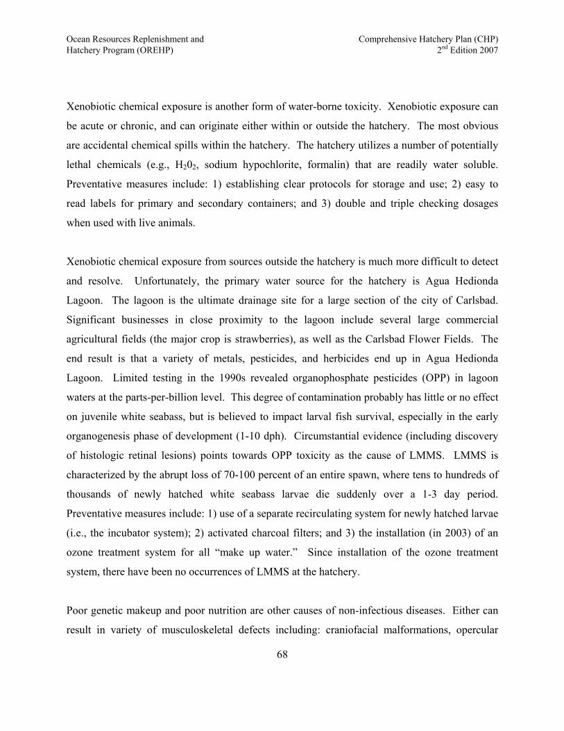
Ocean Resources Replenishment and Comprehensive Hatchery Plan (CHP) Hatchery Program (OREHP) 2nd Edition 2007
Xenobiotic chemical exposure is another form of water-borne toxicity. Xenobiotic exposure can
be acute or chronic, and can originate either within or outside the hatchery. The most obvious
are accidental chemical spills within the hatchery. The hatchery utilizes a number of potentially
lethal chemicals (e.g., H202, sodium hypochlorite, formalin) that are readily water soluble.
Preventative measures include: 1) establishing clear protocols for storage and use; 2) easy to
read labels for primary and secondary containers; and 3) double and triple checking dosages
when used with live animals.
Xenobiotic chemical exposure from sources outside the hatchery is much more difficult to detect
and resolve. Unfortunately, the primary water source for the hatchery is Agua Hedionda
Lagoon. The lagoon is the ultimate drainage site for a large section of the city of Carlsbad.
Significant businesses in close proximity to the lagoon include several large commercial
agricultural fields (the major crop is strawberries), as well as the Carlsbad Flower Fields. The
end result is that a variety of metals, pesticides, and herbicides end up in Agua Hedionda
Lagoon. Limited testing in the 1990s revealed organophosphate pesticides (OPP) in lagoon
waters at the parts-per-billion level. This degree of contamination probably has little or no effect
on juvenile white seabass, but is believed to impact larval fish survival, especially in the early
organogenesis phase of development (1-10 dph). Circumstantial evidence (including discovery
of histologic retinal lesions) points towards OPP toxicity as the cause of LMMS. LMMS is
characterized by the abrupt loss of 70-100 percent of an entire spawn, where tens to hundreds of
thousands of newly hatched white seabass larvae die suddenly over a 1-3 day period.
Preventative measures include: 1) use of a separate recirculating system for newly hatched larvae
(i.e., the incubator system); 2) activated charcoal filters; and 3) the installation (in 2003) of an
ozone treatment system for all “make up water.” Since installation of the ozone treatment
system, there have been no occurrences of LMMS at the hatchery.
Poor genetic makeup and poor nutrition are other causes of non-infectious diseases. Either can
result in variety of musculoskeletal defects including: craniofacial malformations, opercular
68

Ocean Resources Replenishment and Comprehensive Hatchery Plan (CHP) Hatchery Program (OREHP) 2nd Edition 2007
defects, spinal deformities, defects in skin and scale pattern, and swimbladder non-inflation.
Again, genetics and nutrition are covered in detail elsewhere in this document. Fortunately, the
prevalence of congenital deformities, and swimbladder non-inflation, has decreased markedly
over the past five years (2001 to 2005) and are now rare events. Most of the decrease in
deformities has been attributed to improvements in nutrition to both broodstock and larval white
seabass.
Poor hatchery practices can directly cause non-infectious diseases, and can contribute towards
outbreaks of infectious disease. The most common hatchery-associated diseases are traumatic
injuries resulting from: poor system or pool design (e.g., sharp edges, protruding fixtures, square
pools), overcrowding, rough fish handling, or inappropriate netting (stiff or coarse mesh).
Trauma results in cloudy eyes (from corneal edema) and secondary skin infections from bacteria,
fungi, or protozoa. Inadequate temperature acclimation can also contribute to higher prevalence
of infectious disease by impairing the fish’s immune system. Young fish (< 120 dph) are
especially susceptible to thermal stress. The primary preventative measure against these types of
insults is establishment of well thought out protocols and good personnel training.
Another major non-infectious disease related to poor hatchery practices is cannibalism. Larval
and juvenile white seabass are, unfortunately, extremely aggressive and will readily eat each
other given the opportunity and/or when the food supply is inadequate. Characteristic lesions are
curved or circular abrasions over the head, eyes, and jaws (“ring-head” or “grey-head” disease)
and cloudy, punctured, or missing eyes. Preventative measures include feeding adequate
amounts, using the appropriate pellet size, and proper size grading. Proper grading, done on a
regular basis, results in pools with similar sized fish and a much lower incidence of cannibalism.
Occasional culling of over-sized fish will also help reduce the number of cannibalism attacks.
69
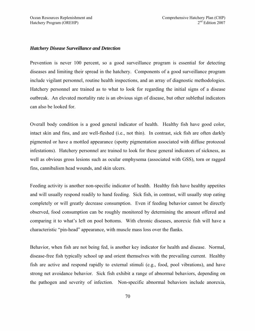
Ocean Resources Replenishment and Comprehensive Hatchery Plan (CHP) Hatchery Program (OREHP) 2nd Edition 2007
Hatchery Disease Surveillance and Detection
Prevention is never 100 percent, so a good surveillance program is essential for detecting
diseases and limiting their spread in the hatchery. Components of a good surveillance program
include vigilant personnel, routine health inspections, and an array of diagnostic methodologies.
Hatchery personnel are trained as to what to look for regarding the initial signs of a disease
outbreak. An elevated mortality rate is an obvious sign of disease, but other sublethal indicators
can also be looked for.
Overall body condition is a good general indicator of health. Healthy fish have good color,
intact skin and fins, and are well-fleshed (i.e., not thin). In contrast, sick fish are often darkly
pigmented or have a mottled appearance (spotty pigmentation associated with diffuse protozoal
infestations). Hatchery personnel are trained to look for these general indicators of sickness, as
well as obvious gross lesions such as ocular emphysema (associated with GSS), torn or ragged
fins, cannibalism head wounds, and skin ulcers.
Feeding activity is another non-specific indicator of health. Healthy fish have healthy appetites
and will usually respond readily to hand feeding. Sick fish, in contrast, will usually stop eating
completely or will greatly decrease consumption. Even if feeding behavior cannot be directly
observed, food consumption can be roughly monitored by determining the amount offered and
comparing it to what’s left on pool bottoms. With chronic diseases, anorexic fish will have a
characteristic “pin-head” appearance, with muscle mass loss over the flanks.
Behavior, when fish are not being fed, is another key indicator for health and disease. Normal,
disease-free fish typically school up and orient themselves with the prevailing current. Healthy
fish are active and respond rapidly to external stimuli (e.g., food, pool vibrations), and have
strong net avoidance behavior. Sick fish exhibit a range of abnormal behaviors, depending on
the pathogen and severity of infection. Non-specific abnormal behaviors include anorexia,
70
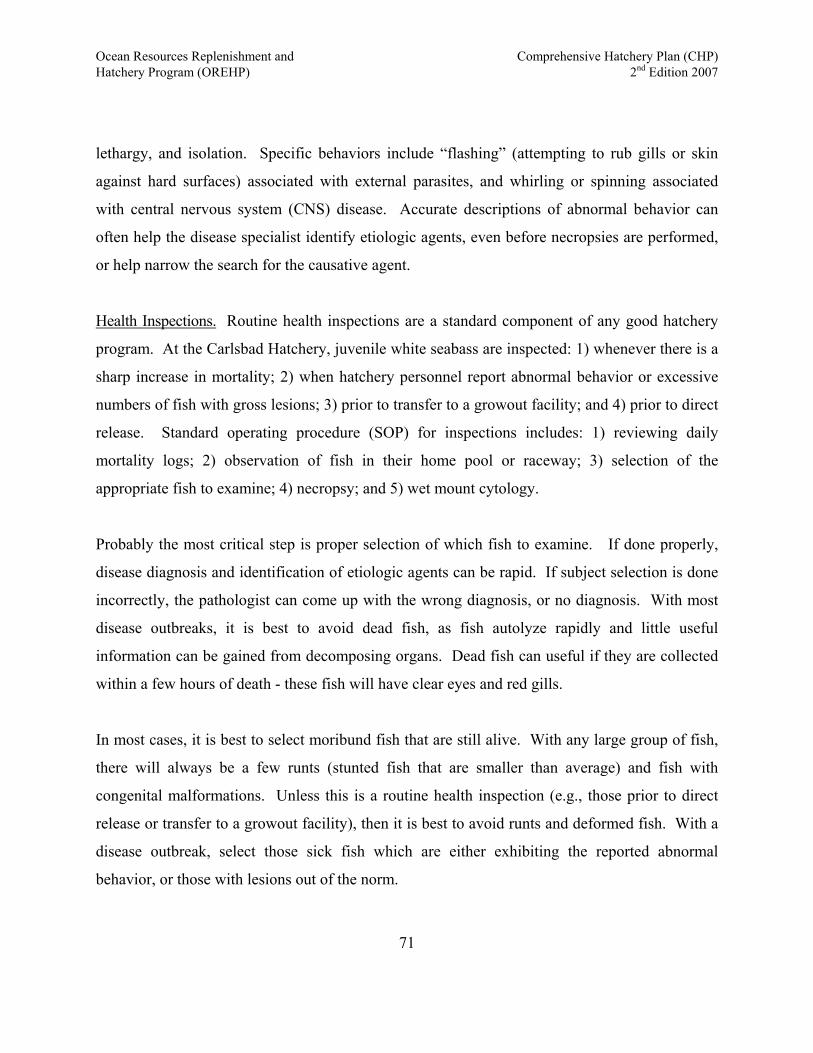
Ocean Resources Replenishment and Comprehensive Hatchery Plan (CHP) Hatchery Program (OREHP) 2nd Edition 2007
lethargy, and isolation. Specific behaviors include “flashing” (attempting to rub gills or skin
against hard surfaces) associated with external parasites, and whirling or spinning associated
with central nervous system (CNS) disease. Accurate descriptions of abnormal behavior can
often help the disease specialist identify etiologic agents, even before necropsies are performed,
or help narrow the search for the causative agent.
Health Inspections. Routine health inspections are a standard component of any good hatchery
program. At the Carlsbad Hatchery, juvenile white seabass are inspected: 1) whenever there is a
sharp increase in mortality; 2) when hatchery personnel report abnormal behavior or excessive
numbers of fish with gross lesions; 3) prior to transfer to a growout facility; and 4) prior to direct
release. Standard operating procedure (SOP) for inspections includes: 1) reviewing daily
mortality logs; 2) observation of fish in their home pool or raceway; 3) selection of the
appropriate fish to examine; 4) necropsy; and 5) wet mount cytology.
Probably the most critical step is proper selection of which fish to examine. If done properly,
disease diagnosis and identification of etiologic agents can be rapid. If subject selection is done
incorrectly, the pathologist can come up with the wrong diagnosis, or no diagnosis. With most
disease outbreaks, it is best to avoid dead fish, as fish autolyze rapidly and little useful
information can be gained from decomposing organs. Dead fish can useful if they are collected
within a few hours of death - these fish will have clear eyes and red gills.
In most cases, it is best to select moribund fish that are still alive. With any large group of fish,
there will always be a few runts (stunted fish that are smaller than average) and fish with
congenital malformations. Unless this is a routine health inspection (e.g., those prior to direct
release or transfer to a growout facility), then it is best to avoid runts and deformed fish. With a
disease outbreak, select those sick fish which are either exhibiting the reported abnormal
behavior, or those with lesions out of the norm.
71
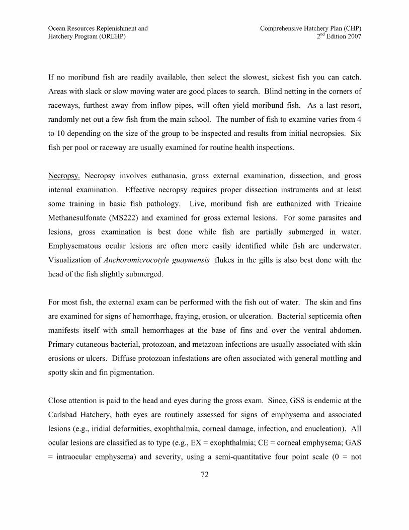
Ocean Resources Replenishment and Comprehensive Hatchery Plan (CHP) Hatchery Program (OREHP) 2nd Edition 2007
If no moribund fish are readily available, then select the slowest, sickest fish you can catch.
Areas with slack or slow moving water are good places to search. Blind netting in the corners of
raceways, furthest away from inflow pipes, will often yield moribund fish. As a last resort,
randomly net out a few fish from the main school. The number of fish to examine varies from 4
to 10 depending on the size of the group to be inspected and results from initial necropsies. Six
fish per pool or raceway are usually examined for routine health inspections.
Necropsy. Necropsy involves euthanasia, gross external examination, dissection, and gross
internal examination. Effective necropsy requires proper dissection instruments and at least
some training in basic fish pathology. Live, moribund fish are euthanized with Tricaine
Methanesulfonate (MS222) and examined for gross external lesions. For some parasites and
lesions, gross examination is best done while fish are partially submerged in water.
Emphysematous ocular lesions are often more easily identified while fish are underwater.
Visualization of Anchoromicrocotyle guaymensis flukes in the gills is also best done with the
head of the fish slightly submerged.
For most fish, the external exam can be performed with the fish out of water. The skin and fins
are examined for signs of hemorrhage, fraying, erosion, or ulceration. Bacterial septicemia often
manifests itself with small hemorrhages at the base of fins and over the ventral abdomen.
Primary cutaneous bacterial, protozoan, and metazoan infections are usually associated with skin
erosions or ulcers. Diffuse protozoan infestations are often associated with general mottling and
spotty skin and fin pigmentation.
Close attention is paid to the head and eyes during the gross exam. Since, GSS is endemic at the
Carlsbad Hatchery, both eyes are routinely assessed for signs of emphysema and associated
lesions (e.g., iridial deformities, exophthalmia, corneal damage, infection, and enucleation). All
ocular lesions are classified as to type (e.g., EX = exophthalmia; CE = corneal emphysema; GAS
= intraocular emphysema) and severity, using a semi-quantitative four point scale (0 = not
72
Ocean Resources Replenishment and Comprehensive Hatchery Plan (CHP) Hatchery Program (OREHP) 2nd Edition 2007
present; 1 = mild; 2 = moderate; 3 = severe; and 4 = massive). Heads are also examined for
evidence of cannibalism and congenital jaw or opercular deformities.
Gills are examined by pulling the operculum away from the body wall with forceps, or by
removing the operculum with scissors. Examine all four sets of gill arches, on both sides, and
note any unusual color (pale gills are indicative of anemia) or lesions. The most common gill
lesions are areas of necrosis, usually characterized by brown or yellow discoloration and/or
sections of missing filaments. With severe gill disease, portions of gill arch will be completely
denuded of filaments. The first gill arch (rostral set) is the most commonly affected arch. The
jaws, gums, oral cavity, and tongue are also inspected.
Following examination of the head, the fish is placed with the right side down on the cutting
board. This position (head to the left, tail to the right) is convention and allows for
standardization of the necropsy process. Total length and standard length (in cm or mm) are
taken. Determining wet body weight (in gm or kg) is optional. Before proceeding with the gross
internal exam, wet mount preparations for cytologic examination can be taken at this time. With
routine health exams, wet mount preps of gill (left first gill arch) and skin (base of left pectoral
fin and dorsal aspect of left flank) are made.
The gross internal exam is started by making an initial sharp incision dorsally from the anus,
using a pair of fine ophthalmic scissors. Once the initial incision has been made, a pair of blunt-
nosed scissors is used to extend the incision dorso-cranially towards the swimbladder, and then
laterally towards the operculum. A third incision is made ventrally, through the opercular cavity
and pericardial sac, exposing the heart. The left wall of the abdominal cavity can be completely
severed from the ventral body margin, or just pulled out of the way. The entire abdominal and
pericardial cavities should be fully exposed.
Once the two body cavities are opened, examine the heart, gastro-intestinal (GI) tract, liver,
73
Ocean Resources Replenishment and Comprehensive Hatchery Plan (CHP) Hatchery Program (OREHP) 2nd Edition 2007
spleen, swimbladder, and urinary bladder. The left lobe of the liver and stomach can be reflected
to visualize the right liver lobe, gall bladder, and pancreatic megaislet. If enteritis is suspected,
the GI tract can be opened and examined for mucosal lesions. Rinsing the GI tract in freshwater
will facilitate identifying lesions, but will ruin it for histology. The swimbladder will have to be
pulled away from the spine to examine the kidney. Any lesions are measured and described.
Additional tissue samples can also be taken at this time.
Following examination of the heart and abdominal cavity organs, the last step is to examine the
brain and extract the otoliths. These two steps are not performed with routine health inspections.
The brain and eyes are sampled if fish are being screened for VNNV, or if fish are exhibiting
clinical signs of CNS disease. Eyes are extracted by grasping the conjunctival tissues with
forceps and using scissors to cut the extra-ocular muscles, conjunctival tissues, and optic nerve.
The brain is exposed by removing the cranial vault with a hack saw (used with larger fish),
scalpel or razor blade (used with smaller fish). Cranial nerves, holding the brain in place, are cut
with fine scissors, or scalpel, while holding the head upside down. Once the brain is out, otoliths
are removed through large openings created in the dorsal roof of the semicircular canals.
Diagnostic Methodologies. Careful necropsy and gross examination of tissues can often provide
enough information with which to make a definitive diagnosis. There are circumstances,
however, where additional diagnostic tools are implemented. Types of methodologies available
to the fish health specialist include: cytology, histology, virology, bacteriology, mycology,
electron microscopy, and hematology. Of the tools available, cytology and histology are
probably the most useful and cost effective.
With cytology, all that is required are some glass slides, coverslips, and a good binocular
microscope. Wet mount preparations of gill and skin are routinely made during standard health
inspections, prior to release or transfer of white seabass to a growout facility. Cytologic
assessment of wet mount preps, using dark field microscopy, allows for visualization of most
74

Ocean Resources Replenishment and Comprehensive Hatchery Plan (CHP) Hatchery Program (OREHP) 2nd Edition 2007
protozoan and metazoan parasites, as well as bacterial and fungal pathogens commonly
encountered. Wet mount preparations should be examined as soon as possible as parasite
motility is often a key to identification. Small unicellular protozoa are often difficult to
distinguish from host cells, once they are dead.
Cytology is also routinely used when fish have open skin or fin lesions. Determining whether or
not protozoan or metazoan parasites are involved with help determine what type of treatment is
used. For example, ulcers associated with Uronema marinum warrant treatment with H202,
while those with Flexibacter require antibiotics. Cytology can also help to evaluate internal
lesions associated with parenchymal organs. Squash preparations (crushing a small lesion
fragment between a glass slide and coverslip) can be used to identify Vibrio induced renal
abscesses or to visualize fungi located in liver granulomas. Cytology is also commonly used to
identify pathogens associated with intraoccular infections.
Histology does not provide immediate feedback during the necropsy process, but formalin-fixed
tissues can be turned around within a day and have the added benefit of providing the hatchery
with a permanent record of a particular disease or lesion. Histology samples are initially fixed in
10 percent formalin for several hours (to several years) before being trimmed to size, placed in
plastic cassettes and shipped to a laboratory for processing. Samples are dehydrated, infiltrated
and embedded in paraffin, and then sectioned at 5-7 microns with a microtome. Sections are
mounted on glass slides and stained with hematoxylin and eosin (HE). HE slides are shipped
back to the hatchery and examined via light microscopy. At $7.00 per slide (2005 costs),
histology is often a much cheaper and faster alternative (when compared with microbiology or
electron microscopy) for confirmation of infectious diseases which cannot be identified with
gross exam or cytology.
Microbiology is a useful tool when in depth assessment of pathogens and pathogenesis is
desired. For marine bacteria, isolation is typically done with simple blood agar plates; Sabourad
75
Ocean Resources Replenishment and Comprehensive Hatchery Plan (CHP) Hatchery Program (OREHP) 2nd Edition 2007
dextrose is used for fungal isolation. Many other bacterial and fungal media are available, but
these two have proved sufficient for pathogens isolated from white seabass. Initial bacterial and
fungal isolations are performed in-house at the hatchery. If more specific identification is
needed, samples are sent to outside commercial laboratories or the University of California at
Davis (UCD). Pathogen isolation has the added benefit of allowing for experimental exposures.
Experimental exposures are useful for determining species and age susceptibility, as well as
pathology and pathogenesis.
For virus isolation, tissue samples are preserved in chilled minimal essential media (MEM).
MEM contains several antibiotics to suppress bacterial growth and is primarily used a transport
medium while samples are shipped to UCD. UCD has a large number of fish cell lines on hand,
and the expertise to propagate viral pathogens. Viral pathogens are identified by cytopathic
effect (CPE) in tissue culture, followed by confirmation with electron microscopy.
Fortunately, viral diseases are relatively uncommon among cultured white seabass. Samples
taken for VNNV assessment include eye and brain for juvenile and adult fish; with larval
infections, whole fish are submitted. At UCD, suspect VNNV samples are cultured with a
Snakehead fish cell line known to support the nodavirus. The only other viral disease known to
occur in cultured white seabass is a suspect herpes virus. This pathogen has been associated
with severe enteritis, but thus far UCD has been unable to grow the virus in tissue culture.
The suspect herpesvirus has only been confirmed in cultured white seabass from one epizootic
which occurred during the fall of 2002. Confirmation was made via assessment of intestinal
mucosal epithelium using transmission electron microscopy (TEM). TEM has also been used to
confirm VNNV infections in eye and brain. With TEM, the SOP is to fix 1 mm3 samples in
Karnovsky’s fixative and then ship the samples to the California Animal Health and Food Safety
laboratory at UCD. Samples are dehydrated, infiltrated and embedded in epoxy resin, and
sectioned at 900Å with an ultramicrotome. Sections are stained with uranyl acetate and lead
76
Ocean Resources Replenishment and Comprehensive Hatchery Plan (CHP) Hatchery Program (OREHP) 2nd Edition 2007
citrate, and then viewed with a transmission electron microscope. TEM is useful for confirming
viral infections, but sample turn-around time can take months.
The last diagnostic tool available for disease assessment is hematology. Hematology is primarily
used to help screen wild fish samples (see below) and has only infrequently been used with
cultured fish at the hatchery. Whole blood samples, taken from cultured white seabass, have
been used as positive and negative controls for enzyme-linked immunosorbent assays (ELISA)
developed by UCD. Whole blood is taken from anesthetized, or recently euthanized white
seabass, using Vacutainer® needles (20 gauge), sleeves, and clot tubes. The large vertebral vein
is accessed using a ventral midline approach, inserting needles adjacent to the anal fin; for larger
fish, the vein is approached by inserting needles into the ventral aspect of the caudal peduncle.
Whole blood is allowed to clot at room temperature for 20 to 30 minutes and then refrigerated
overnight. Chilled samples are centrifuged for three to six minutes; serum is pipetted off and
frozen in 2 ml cryotubes at -60 to -80oC. Frozen serum samples are shipped to UCD on dry ice
for ELISA assessment of antibody levels.
Treatment
Treatment options for cultured marine fish are limited to a select few drugs approved by the U.
S. Food and Drug Association. Drugs are used under guidelines provided by the Center for
Veterinary Medicine. For external parasites, three treatments are available: freshwater, formalin,
and H202.
H202 is the most widely used product at the hatchery, and is effective for a wide range of
metazoan and protozoan parasites. The standard treatment regime used at the hatchery is a 75
ppm solution administered as a static bath for two hours; fish are treated for three days in a row.
During treatment, DO is monitored; water is supplemented with pure oxygen or additional
aeration as needed. H202 breaks down into oxygen and water, and has been considered
77

Ocean Resources Replenishment and Comprehensive Hatchery Plan (CHP) Hatchery Program (OREHP) 2nd Edition 2007
extremely safe. GSS tests conducted in 2004 have identified potential problems associated with
H202 use. TDG was found to spike as high as 120 percent during H2O2 therapy and this could
certainly exacerbate ocular lesions associated with GSS. Controlled experiments are currently
(2005) underway to determine whether or not prevalence and severity of GSS-related eye lesions
are influenced by H2O2 therapy.
Under some circumstances, higher concentrations of H2O2 have been used at the hatchery.
Concentration as high as 175 ppm have been used to control skin and gill flukes in California
sheephead (wild adult fish brought in for use as broodstock). Yearling white seabass are capable
of tolerating H202 levels as high as 175 ppm. Concentrations of H202 >100 ppm have
occasionally been used when H202-resistant strains of Uronema have been encountered.
Formalin has been used occasionally at the Carlsbad Hatchery for parasites (e.g., some flukes
and copepods) that are less susceptible to H202. Formalin use is limited to the hatchery because
waste water has to either be treated on site, or disposed of in the municipal drainage system.
Freshwater has also been occasionally used at the hatchery. Brief (three to five minute)
freshwater treatments have been used successfully with adult sheephead, but have proved fatal to
juvenile white seabass.
Antibiotics for use in fish are limited to Romet® (sulfadimethozine and ormetoprim) and
Terramycin® (oxytetracycline). Both drugs have been used at the hatchery in the past, but
experience has shown that Romet has much greater efficacy and has been used almost
exclusively for the past four years (2001-2005). Applications for Romet use with white seabass
include primary and secondary infections with Flexibacter or Vibrio. Bacterial infections can
either be cutaneous or systemic. Identification of bacterial pathogens is made with wet mount
cytology and culture on blood agar. Antibiotic sensitivity tests are run to determine
susceptibility to Romet or Terramycin.
78

Ocean Resources Replenishment and Comprehensive Hatchery Plan (CHP) Hatchery Program (OREHP) 2nd Edition 2007
Romet is incorporated into the diet, at five grams per kilogram of feed, and fed at three percent
of fish BW for 10 days. Treated fish are usually held for another two weeks to assess efficacy
before they are either transferred to a growout facility or released. Because the average fish
takes two to three years before reaching the legal catch minimum of 28 inches, there is no danger
to the public from consumption of hatchery fish.
Wild Fish Disease Surveillance
An often overlooked component of disease management, for cultured fish intended for release, is
assessing the disease status of wild fish stocks. Disease assessment of wild stocks is critical
because of the potential for disease transfer from cultured fish. The most dangerous diseases are
those for which wild fish have no immunity. And the only way to determine which diseases are
novel to wild fish is to run a comprehensive survey.
OREHP has a wild fish disease surveillance program in place and has been collecting wild fish
for the past four years (2002-2005). Targeted species include white seabass, California halibut,
California sheephead, lingcod, and a variety of Sebastes rockfish species. Emphasis has been on
collection of wild white seabass because that is the only OREHP species currently being
released. To date (March 2005), over 200 wild white seabass have been collected using both gill
nets and hook-and-line gear.
Evaluation of wild fish is dependent on the condition of the fish, where fish are collected (i.e.,
proximity to laboratory facilities), and the types of pathogens being looked for. The majority of
wild fish samples have come from gill netting operations focused on recovery of tagged hatchery
fish. Unfortunately, most of these fish are already dead at the time of sampling and are therefore
unsuitable for detailed morphologic assessment (i.e., histology and electron microscopy). The
majority of these gill net fish are, however, suitable for cytology, hematology, and microbiology.
The best wild fish samples are those caught via hook-and-line, and the few live fish captured in
79
Ocean Resources Replenishment and Comprehensive Hatchery Plan (CHP) Hatchery Program (OREHP) 2nd Edition 2007
gill nets. Live wild fish are either sampled on board boats or transported to HSWRI’s Mission
Bay research facility, the Carlsbad Hatchery, or the DFG laboratory in Oceanside. All wild fish
are scanned with a sensitive metal detector to make sure that they are not tagged hatchery fish.
Although some wild fish are screened via cytology for external parasites, or have samples fixed
for histopathology, the most important assessments are hematologic and microbiologic assays to
determine exposure or infection to pathogens that are highly contagious and lethal. Wild fish
surveys are focused on four major pathogens: VNNV, viral hemorrhagic septicemia virus
(VHSV), Piscirickettsia salmonis, and an as yet uncharacterized enteric virus (possibly a
herpesvirus). Three (VNNV, P. salmonis, and the unidentified enteric virus) of the four have
been isolated from cultured white seabass. The fourth pathogen, VHSV, has never been isolated
from white seabass, but has been recovered from several baitfish species (sardines and herring)
landed in Los Angeles ports. All four have the potential for causing catastrophic epizootics if
wild white seabass populations are naïve and have not previously encountered these pathogens.
To minimize the risk to wild seabass from cultured fish, it is necessary to determine which of
these lethal, highly contagious diseases are endemic or “naturally-occurring” among wild stocks.
Some assessment has been done via direct attempts to recover live pathogens from wild fish.
With VNNV, samples of eye and brain have been collected and shipped to UCD for culture on
Snakehead fish cell lines. With VHSV, samples of spleen and/or kidney have been taken for
culture on a salmonid cell line; liver samples are taken for recovery of P. salmonis. UCD has
been unable to culture the suspect herpesvirus, but over 80 wild fish intestinal/fecal samples
have been assessed via negative staining and direct TEM to look for the virus. Thus far (March
2005), all attempts to recover live pathogens from wild white seabass have failed. This does not,
however, mean that the four pathogens are novel. This is because sample sizes have been
relatively small, and because it is unlikely that infected fish survive for any length of time in the
wild.
80
Ocean Resources Replenishment and Comprehensive Hatchery Plan (CHP) Hatchery Program (OREHP) 2nd Edition 2007
An alternative has been to look for disease exposure, rather than disease infection, among wild
white seabass populations. Assessing disease exposure increases the likelihood of detecting
positive fish because the percentage of wild fish that have simply encountered the four pathogens
in question (but which did not become infected, or were infected and recovered) is much higher.
Disease exposure can be assessed by taking blood samples and determining serum levels of
circulating antibody to specific pathogens.
Circulating antibody levels are determined by enzyme-linked immunosorbent assays (ELISA).
This type of assay is specific for a particular fish species, and for specific pathogens. The major
caveat is that they require large amounts of antigen and therefore pathogens must first be isolated
and cultured under laboratory conditions. Three of the four pathogens being assessed can be
grown in tissue culture, and ELISAs have been developed for them. Unfortunately, thus far the
suspect enteric herpesvirus has not been grown in tissue culture and currently there is no ELISA
to detect this pathogen (2005).
Preliminary ELISA results indicate that VNNV exposure is widespread among wild white
seabass, and that VNNV is almost certainly a “naturally-occurring” disease. Among wild
juvenile or subadult white seabass (i.e., those <72 cm TL), 18 percent (14/78) of serum samples
were ELISA-positive for VNNV exposure. Among wild adult white seabass, 53 percent (9/17)
of serum samples were VNNV-positive with ELISA. Some titers have been equal to or greater
than positive-control fish samples (positive controls obtained from experimental exposures or
from cultured fish sampled during hatchery VNNV epizootics). Piscirickettsia salmonis, in
contrast, is probably not an endemic pathogen. None of the 94 serum samples analyzed thus far,
via ELISA, have been positive for P. salmonis exposure. ELISA results for VHSV are pending
and, unfortunately, currently there is no ELISA assay specific for the herpesvirus that occurs in
white seabass. ELISA assessment of wild fish disease status is generally consistent with
hatchery findings. Prior to installation of the ozone treatment system in 2003, VNNV outbreaks
were a regular occurrence at the Carlsbad Hatchery. In contrast, there have only been two P.
81
Ocean Resources Replenishment and Comprehensive Hatchery Plan (CHP) Hatchery Program (OREHP) 2nd Edition 2007
salmonis epizootics (one in 1998; another in 2005) involving hatchery and/or growout facility
fish.
ELISA results have allowed OREHP the luxury of making informed decisions based on hard
data, rather than making assumptions about the disease status of wild fish stocks. Since VNNV
is an endemic disease for white seabass, OREHP has the option of releasing cultured fish which
have been exposed to VNNV, but which are healthy. Exposed but healthy cultured fish could
still be asymptomatic carriers, but the risk to wild white seabass is minimal since exposure to
VNNV is already widespread. On the other hand, since P. salmonis is an exotic disease, any
cultured white seabass discovered with this pathogen will be euthanized. The disease status of
wild fish to VHSV, and the suspect herpesvirus, is still unknown and these diseases are also
treated as exotic.
Diagnostic and Research Services from the University of California, Davis
OREHP works with a number of private and public agencies to assist with disease surveillance,
diagnosis, and treatment at the hatchery. The most beneficial relationship has been with the
UCD, which has a long history of research involving freshwater and anadromous fish species,
and assists OREHP with many disease problems associated with wild and cultured marine fish
species. UCD has experts in the fields of aquatic toxicology, electron microscopy, fish
physiology, pathology, immunology, and microbiology. Facilities for freshwater and
anadromous fish exposure exist on the main campus (at the Institute of Ecology); facilities for
marine fish experimentation are present at the Bodega Marine Laboratory (BML) at Bodega Bay.
In FY2002-2003 and 2003-2004, DFG contracted with UCD to assist with OREHP’s wild fish
disease surveillance program, and to conduct controlled experimental exposures with known
pathogens. Dr. Ronald Hedrick’s laboratory (Department of Medicine and Epidemiology,
School of Veterinary Medicine) was responsible for developing the ELISAs for detecting
82
Ocean Resources Replenishment and Comprehensive Hatchery Plan (CHP) Hatchery Program (OREHP) 2nd Edition 2007
VNNV, VHSV, and P. salmonis exposure in wild white seabass. Efforts are currently (2005)
underway to develop ELISAs for other OREHP species such as California halibut, sheephead,
and Sebastes rockfish. Dr. Hedrick’s lab has decades of experience with a host of fish pathogens
and has the facilities and expertise to culture a wide variety of viruses, rickettsia, bacteria, and
fungi.
In addition, Dr. Hedrick’s lab has direct ties with the BML. The BML’s Pathogen Containment
Unit (currently run by Dr. Kristen Arkush) has run a number of controlled experiments in which
cultured white seabass (provided by the hatchery) have been exposed to VNNV, P. salmonis,
and VHSV. Experimental exposures have provided OREHP with an extensive data base
regarding susceptibility, pathology, and pathogenesis. Additional experiments will help further
define susceptibility (of age groups and species) and carrier status of recovered fish.
83
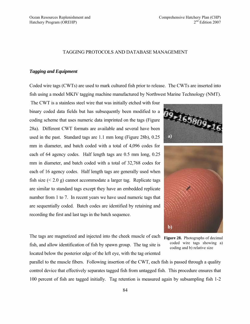
Ocean Resources Replenishment and Comprehensive Hatchery Plan (CHP) Hatchery Program (OREHP) 2nd Edition 2007
TAGGING PROTOCOLS AND DATABASE MANAGEMENT
Tagging and Equipment
Coded wire tags (CWTs) are used to mark cultured fish prior to release. The CWTs are inserted into
fish using a model MKIV tagging machine manufactured by Northwest Marine Technology (NMT).
The CWT is a stainless steel wire that was initially etched with four
binary coded data fields but has subsequently been modified to a
coding scheme that uses numeric data imprinted on the tags (Figure
28a). Different CWT formats are available and several have been
used in the past. Standard tags are 1.1 mm long (Figure 28b), 0.25
mm in diameter, and batch coded with a total of 4,096 codes for
each of 64 agency codes. Half length tags are 0.5 mm long, 0.25
mm in diameter, and batch coded with a total of 32,768 codes for
each of 16 agency codes. Half length tags are generally used when
fish size (< 2.0 g) cannot accommodate a larger tag. Replicate tags
are similar to standard tags except they have an embedded replicate
number from 1 to 7. In recent years we have used numeric tags that
are sequentially coded. Batch codes are identified by retaining and
recording the first and last tags in the batch sequence.
a) a)
b)
The tags are magnetized and injected into the cheek muscle of each
fish, and allow identification of fish by spawn group. The tag site is
located below the posterior edge of the left eye, with the tag oriented
parallel to the muscle fibers. Following insertion of the CWT, each fish is passed through a quality
control device that effectively separates tagged fish from untagged fish. This procedure ensures that
100 percent of fish are tagged initially. Tag retention is measured again by subsampling fish 1-2
Figure 28. Photographs of decimal coded wire tags showing a) coding and b) relative size
84
Ocean Resources Replenishment and Comprehensive Hatchery Plan (CHP) Hatchery Program (OREHP) 2nd Edition 2007
weeks after tagging and immediately prior to release.
CWTs have been used successfully to mark small juveniles of an increasingly wide variety of fish,
including salmon and steelhead (Shaul and Clark 1988; Johnson 1988), striped bass (Dunning et al.
1990), red drum (Bumguardner et al. 1990), largemouth bass (Crumpton 1985; Williamson 1987),
herring (Krieger 1982) and mullet (Leber 1993). The advantages of the coded wire tagging system
include 1) ease of application on a large scale, 2) long-term tag retention, longevity and readability
3) relatively non-invasive application, 4) precise reading of code with no subjective interpretation,
and 5) non-visible method eliminating the bias of selective return.
The coded wire tagging technique has been used with positive results by OREHP since 1990. As
many as 800 fish can be tagged per hour by an experienced operator. Each batch of fish released is
marked with a different code. This tagging system enables a precise identification of the release
group to which recaptured fish belong. With this information more accurate estimates of growth can
be made and patterns of migration can be identified.
Experiments have been conducted to determine the effects of fish size, tag size and operator
experience on both short and long-term tag retention. Our experiences and those of others, indicate
that the majority of tag loss occurs within the first 1-2 weeks. Initial tag loss can generally be
attributed to improper depth or angle of needle penetration. When this occurs, the tag is pushed out
of the epidermis as the tissue heals instead of being encased within the muscle fibers. Tag retention
generally increased with fish size and, to a small degree, with operator experience. Long-term tag
retention rates (>300 days) by white seabass reared in pen systems were high (>90 percent). White
seabass are tagged approximately one month prior to release. At the time of release, 100 fish are
subsampled and checked for tag retention. This percentage is then applied to the total number of
fish released and represents the number of released fish that can be identified as hatchery-reared in
subsequent field surveys.
85
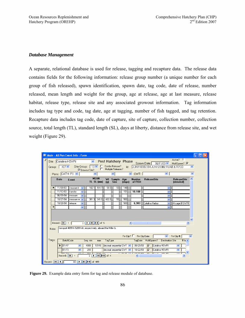
Ocean Resources Replenishment and Comprehensive Hatchery Plan (CHP) Hatchery Program (OREHP) 2nd Edition 2007
Database Management
A separate, relational database is used for release, tagging and recapture data. The release data
contains fields for the following information: release group number (a unique number for each
group of fish released), spawn identification, spawn date, tag code, date of release, number
released, mean length and weight for the group, age at release, age at last measure, release
habitat, release type, release site and any associated growout information. Tag information
includes tag type and code, tag date, age at tagging, number of fish tagged, and tag retention.
Recapture data includes tag code, date of capture, site of capture, collection number, collection
source, total length (TL), standard length (SL), days at liberty, distance from release site, and wet
weight (Figure 29).
86
Figure 29. Example data entry form for tag and release module of database.
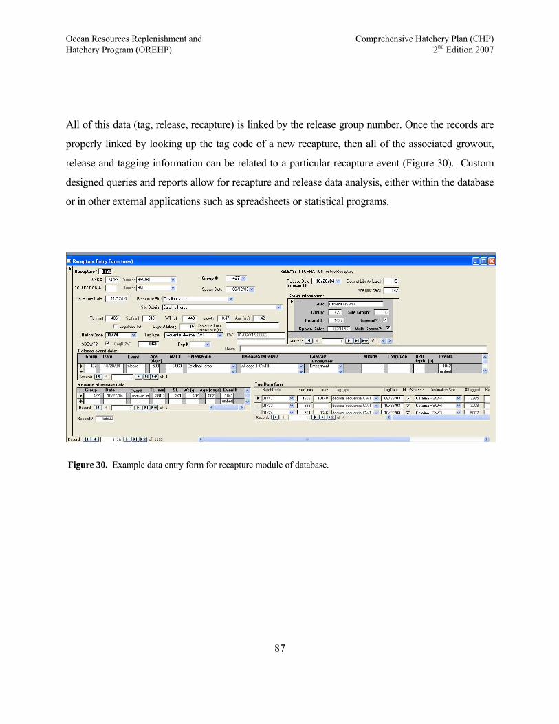
Ocean Resources Replenishment and Comprehensive Hatchery Plan (CHP) Hatchery Program (OREHP) 2nd Edition 2007
All of this data (tag, release, recapture) is linked by the release group number. Once the records are
properly linked by looking up the tag code of a new recapture, then all of the associated growout,
release and tagging information can be related to a particular recapture event (Figure 30). Custom
designed queries and reports allow for recapture and release data analysis, either within the database
or in other external applications such as spreadsheets or statistical programs.
Figure 30. Example data entry form for recapture module of database.
87
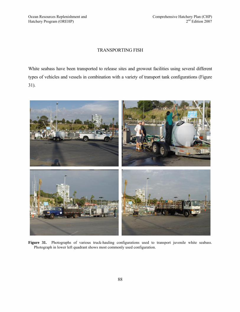
Ocean Resources Replenishment and Comprehensive Hatchery Plan (CHP) Hatchery Program (OREHP) 2nd Edition 2007
TRANSPORTING FISH
White seabass have been transported to release sites and growout facilities using several different
types of vehicles and vessels in combination with a variety of transport tank configurations (Figure
31).
Figure 31. Photographs of various truck-hauling configurations used to transport juvenile white seabass.
Photograph in lower left quadrant shows most commonly used configuration.
88

Ocean Resources Replenishment and Comprehensive Hatchery Plan (CHP) Hatchery Program (OREHP) 2nd Edition 2007
The most commonly used transport tanks are 1,500 L (116.8 x 213.4 x 81.3 cm deep with 5.1 cm
insulation) and constructed of marine-grade aluminum. Two of the three tanks were designed to
fit on a trailer, while the third tank was designed to fit in the back of a stake-bed truck (Figure
32). Each tank was designed so it could be lifted from the truck or trailer fully loaded with fish
and water (approximately 1,800 kg) for offshore transport operations. The tanks were also
designed with independent aeration systems. Two aerators are powered by a 12VDC battery
enclosed in a weather-proof box attached to the tank. As a back-up to the aerators, each tank is
equipped with a 1.5 cubic meter cylinder of
pure oxygen. Like the aerators, the cylinder
and its associated components (i.e.
regulator, flow meter, and diffusers) are
attached to the tank – independent from the
transport vehicles. In order to completely
empty each tank, the bottom is gently sloped
in three directions toward a 10 cm gate
valve. The trailer-mounted tanks were
designed with the dump gate being offset
from the center line of the tank – one tank is
sloped to the right side the other to the left.
This was necessary to allow the tanks to be
grouped side-by-side with a proper weight
distribution and clearance of the wheel-
wells (Figure 32).
Gate valves
Aerators
O2 cylinder
Battery box
Hinged lids
O2 diffusers
Truc
k Ta
nk
Trailer Tanks
Inside View
The fish are starved for 24 hours prior to
shipment and the tanks are stocked at a maximum density of 40 kg/m3. Water in the system is static,
with no renewal or filtration employed. Constant oxygenation is accomplished using compressed
oxygen. Water in the transport tank is treated with Fritzguard to protect the ectodermal mucous
Figure 32. Schematic of primary fish hauling tanks.
89
Ocean Resources Replenishment and Comprehensive Hatchery Plan (CHP) Hatchery Program (OREHP) 2nd Edition 2007
90
to maintain an appropriate electrolyte balance. layer and
The type and size of transport vehicle employed is dependent on the number of fish being
transported and often on the characteristics of the off-loading site. The size and shape of the
transport tanks allow them to be loaded easily into a pickup truck, flatbed truck or boat. Upon
arriving at the release site, the water temperature of transport tank and receiving body of water are
measured. If water temperatures are significantly different (>2.0° C) between these water sources,
water is pumped from the embayment into the transport tank to reduce this difference. Fish are
flushed from the tank into the receiving body of water using a 7.6 cm diameter flexible hose.
Ocean Resources Replenishment and Comprehensive Hatchery Plan (CHP) Hatchery Program (OREHP) 2nd Edition 2007
RELEASING FISH
The methods used to design an efficient release program must consider how, when and where the
fish will be released. These decisions will likely vary depending on the species of fish and the size
or life stage being released. When developing appropriate procedures, those parameters that may
affect the health and survival of released fish must be identified and weighed against any additional
costs incurred. At the time of release all fish are counted by dipnetting them in small batches or
allowing them to swim through a constricted opening in the net or raceway. Hand-counters are
used to keep track of the fish counts when either release method is used. Fish released directly
from the hatchery are typically counted prior to loading into the transport truck, and quite often
this is at the time of tagging.
The methods used to release fish ("How") are substantially more complex than merely determining
the method of transport as described above. Adequate consideration must be given to other
controllable parameters such as the size of fish at release, and the density of each release relative to
the release habitat. The seasonal timing of release ("When") must also be determined in order to
maximize the survival of released fish and optimize the overall efficiency of the program. This is
especially true of programs such as the OREHP, because fish can be spawned year-round. The need
to identify appropriate habitats and sites to release fish ("Where") is also known to be important.
Relative to “How” white seabass are released, the OREHP releases white seabass at a relatively
large size (>20 cm) for several reasons. First, the output from the bioeconomic model suggests that
this size yields the greatest return for the investment. Using that information, a cost-effective
program was developed that utilizes various growout facilities to hold the seabass, allowing them to
grow to a larger size prior to release. This program is operated by volunteer groups, primarily
recreational fishing clubs, and is described in detail in the companion document (Growout
Procedures Manual) to this CHP. Secondly, this approach has been supported by releases of large
91
Ocean Resources Replenishment and Comprehensive Hatchery Plan (CHP) Hatchery Program (OREHP) 2nd Edition 2007
seabass (>30 cm) at Santa Catalina Island. These large fish were found to survive in great numbers
based on the OREHP gillnet survey program. Finally, the gillnets used by the OREHP are effective
at catching seabass >20 cm so the fish are immediately accessible to the survey program. The issue
of fish density has not been addressed specifically by the OREHP but is thought to be less of a
concern for white seabass for two reasons. Firstly, from our gillnet surveys and acoustic tracking
studies, we know that white seabass disperse rapidly from the release areas and subsequently occupy
both embayment and coastal habitats. Secondly, white seabass are released in modest numbers on
an annual basis, and those numbers are further diluted on a site-by-site basis because of the broad
geographical range of the release program.
Because the growout capacity for white seabass along the mainland is currently limited, the OREHP
releases a significant number of juvenile white seabass directly to the ocean. These fish are raised to
the targeted release size in the hatchery and then delivered by truck to one of several embayments.
Intuitively we believe that fish released from growout facilities have a survival advantage over fish
released directly from the hatchery. This is because fish released from growout facilities typically
do not have to be handled excessively immediately prior to release, and they have been acclimated
to the receiving water body for several months. The potential difference in post-release survival
between these two release techniques is currently being assessed using the tag-recovery data.
With regard to “When” white seabass are released, the OREHP continues to release fish year-round,
with a general trend toward releasing fish in the spring and the fall. The efficacy of this approach is
currently being assessed by review of the tag-recovery data. This assessment is complicated by the
fact that juvenile white seabass abundance in southern California is low in the winter and the gillnet
sampling program is limited to the spring and summer months. Nevertheless, the number of tag
recoveries has grown substantially in recent years, so it is likely that an adequate assessment can be
made to address this question.
With regard to “Where” to release juvenile white seabass, it is known that juvenile white seabass
92
Ocean Resources Replenishment and Comprehensive Hatchery Plan (CHP) Hatchery Program (OREHP) 2nd Edition 2007
inhabit both embayments and nearshore coastal habitats. Although the OREHP has conducted
several paired release trials (at coastal and adjacent embayment sites) in recent years, the results
have been inconclusive due to the limited numbers of tagged fish that were collected after release.
The poor recovery rate can be explained by the fact that juvenile white seabass disperse rapidly from
release areas (as noted previously). Furthermore, the gillnet survey program is fixed in time and
space, and therefore does not lend itself readily to customized releases experiments. Regardless of
these limitations, white seabass are released in areas known to be inhabited by wild seabass.
Because cultured seabass disperse readily and naturally occupy several habitat types, the OREHP is
less concerned about targeting precise habitats for releases. Instead, recognizing that the growout
facilities are situated in areas occupied by wild white seabass, and transporting fish off-site creates
significant stress to the fish, we are releasing the fish directly from each growout facility.
93
Ocean Resources Replenishment and Comprehensive Hatchery Plan (CHP) Hatchery Program (OREHP) 2nd Edition 2007
HATCHERY PERFORMANCE STANDARDS
The results of the culture research and ecological studies have been adapted into a bioeconomic
model developed in cooperation with the UCD (Botsford and Hobbs 1988). The bioeconomic
model provides a standard method for evaluating new culture techniques, and for estimating the
culture costs needed to produce fish of various sizes for release. These culture cost estimates are
then used in models describing post-release survival, benefit to cost, and yield-to-the-fishery.
In order to identify performance standards for the expanded replenishment program, it will be
necessary to identify the appropriate "benefit" parameters in the cost to benefit analyses, as well as a
minimum acceptable ratio. Currently, the benefit of the program is measured conservatively
according to an anticipated commercial yield and associated ex-vessel price. The model does not
consider the contribution to the sport fishing industry and its economic impact, which makes the
output very conservative. However, it can be adapted to perform this function, assuming that
adequate data are available on the per weight value of fish caught by recreational anglers.
New growth and survival data are being assimilated in 2007, and we expect to update the
bioeconomic model with this information in 2008. The description below is based on earlier data
but it is useful in describing the capabilities of the model.
Culture Model
Catch per unit effort (CPUE) data obtained from field studies are used to improve both the
bioeconomic and mortality models. Hatchery-reared white seabass that have been recaptured many
years after release have provided data on growth during the post-release period. These data, when
combined with aging studies of young white seabass obtained from the wild, have allowed better
estimation of the pattern of growth and subsequently the theoretical pattern of mortality for the first
two years. Using the assumption that fish exhibit an instantaneous mortality rate inversely 94
Ocean Resources Replenishment and Comprehensive Hatchery Plan (CHP) Hatchery Program (OREHP) 2nd Edition 2007
proportional to their weight (Ricker 1976; Mathews and Buckley 1976), a mathematical model was
developed for post-release survival relative to the size of release up to an age of one year. This
model is based on mortality estimates reported for sockeye salmon of similar size and age (Furnell
and Brett 1986). An optimal size at release is then derived by weighing the cost to culture to a
specific release size by the anticipated survival to one year. The theoretical survival model estimates
that fish should be held to an optimal release size of 165 mm SL (age = 235 days).
Yield-to-the-Fishery Model
Once estimates of the number of hatchery-released white seabass surviving to one year are known, it
is possible to predict the impact of hatchery releases on the natural population and to fishery yields.
This is accomplished by using known growth parameters and various intensities of fishing mortality.
The experimental production hatchery has been scaled to produce approximately one million post
larval fish (30 mm SL) that will eventually result in over 450,000 individuals available to be released
at the predicted optimal size each year. This annual total is apportioned temporally among five
crops (i.e. approximately 90,000 fish per crop). Of the seabass released, we estimate that over
332,000 will survive to one year, which is the value used to initiate the yield-to-the-fishery model.
The model uses a set rate of fishing mortality of 50 percent per year (Botsford and Hobbs 1988),
various growth parameters, and the specific culture parameters listed in Appendix VI. Based on
these parameters, it is predicted that 525 metric tons of white seabass will be contributed to the
standing stock from a single year of releases. Using a fishing yield of 50 percent per year, this
represents a cumulative yield to the fishery of 927 metric tons. If the yield from hatchery releases is
tracked over 20 years of hatchery operation, it is estimated that the contribution to the standing stock
will reach an equilibrium value of over 2,941 metric tons per release after 10 years. Similarly, the
fishery yield is expected to reach an equilibrium value of 185 metric tons per release. If an ex-vessel
price of $4.40/kg and an annual operating budget of $330,000 are used as input parameters, the
benefit to cost model predicts an equilibrium yield of over $817,000 per crop from the fishery. This
95

Ocean Resources Replenishment and Comprehensive Hatchery Plan (CHP) Hatchery Program (OREHP) 2nd Edition 2007
translates into a benefit to cost ratio of 8 to 1.
96
Ocean Resources Replenishment and Comprehensive Hatchery Plan (CHP) Hatchery Program (OREHP) 2nd Edition 2007
REPLENISHMENT MEASURES
Objectives
The level at which "replenishment" is achieved can only be subjectively defined. Several methods
can be employed to provide a quantitative interpretation of the success of the program. Among these
methods is the determination of a benefit-to-cost ratio, which is an economic measure of the value
of the fish returned weighed against the cost to provide those fish. The percent of the catch, can
also be used as an evaluation tool. This value is the calculated percentage of the total catch resulting
from replenishment. A third approach employs the relative abundance of fish as weighed against
the historic catch records for both recreational and commercial fisheries. For strictly mitigation
purposes, the percent of compensation of standing crop lost might be viewed as an appropriate
endpoint for successful replenishment. This method would require that a ratio of lost biomass to
hatchery-supplemented biomass be established prior to releases (e.g. a ratio of 1:1 would represent
100 percent compensation). Successful replenishment would be achieved when this ratio was met.
It should be noted that these methodologies are not mutually exclusive and that a combination of
these approaches might be appropriate. This is especially true when one considers that the agencies
involved may have different replenishment objectives or endpoint goals. Thus, it is important that
the methods to be employed and variables to be measured be established a-priori. A carefully
planned assessment strategy and cooperative recovery effort will ensure that valid results are
available for interpretation by these agencies and by the scientific community at large.
Currently the OREHP is using the “percent catch” index as a measure of replenishment success.
Because all of the fish are tagged, and a bioeconomic model is in place, OREHP will be able to
integrate its results into any of the replenishment objective formats described above.
97
Ocean Resources Replenishment and Comprehensive Hatchery Plan (CHP) Hatchery Program (OREHP) 2nd Edition 2007
Assessment Tools
A discussion of the assessment tools and associated methods is beyond the scope of this document
but a brief summary is provided below.
Juvenile recruitment survey. The juvenile recruitment survey has been ongoing since 1988 and
standardized since 1996. The program uses gillnets to catch age I - IV white seabass both in
bays and estuaries, and along the mainland coast and around Santa Catalina Island. All white
seabass are scanned to determine if they were hatchery raised fish.
Adult head collection program. An adult head collection program began in 2001. In recent years,
personnel have been dedicated to collecting adult heads, increasing the number of heads
collected. This program relies on commercial and recreational fishermen to turn in heads of
white seabass they catch along with information on when and where the fish were caught. The
heads are scanned to determine if it came from a hatchery-raised fish and head measurements are
used to estimate total length.
Acoustic tracking. Acoustic tracking of cultured white seabass has been conducted opportunistically
since 2002. In addition to short-term movement patterns, acoustic tagging studies are providing
valuable information on short-term patterns of mortality, including precise identification of
predators.
98
Ocean Resources Replenishment and Comprehensive Hatchery Plan (CHP) Hatchery Program (OREHP) 2nd Edition 2007
LITERATURE CITED
Allendorf F.W., and S.R. Phelps. 1981. Use of allelic frequencies to describe population
structure. Can. J. Fish. Aquat. Sci., 38, 1507-1514.
Allendorf, F.W., and N. Ryman. 1987. Genetic management of hatchery stocks. Pages 141 – 160
in N. Ryman and F. Utter, eds. Population genetics and fishery management. University of
Washington Press, Seattle, WA, USA.
Bams, R.A. 1976. Survival and propensity for homing as affected by presence or absence of locally
adapted paternal genes in two transplanted populations of pink salmon (Oncorhynchus
gorbuscha). J. Fish. Res. Board Can. 33: 2716-2725.
Bannister, R. C. A. 1991. Stock enhancement (workshop report). Pages 191-192 in S. J.
Lockwood, ed. The ecology and management aspects of extensive mariculture. ICES,
Nantes, France, June 20-23 1989.
Bartley, D.M., and D.B. Kent. 1990. Genetic structure of white seabass populations from the
southern California bight region: applications to hatchery management. Calif. Coop.
Oceanic Fish. Invest. Rep. 31:97-106.
Bartley, D., M. Bagley, G. Gall, and B. Bentley. 1992. Use of linkage disequilibrium data to
estimate effective population size of hatchery and natural fish populations. Conservation
Biology 6: 365 – 375.
99

Ocean Resources Replenishment and Comprehensive Hatchery Plan (CHP) Hatchery Program (OREHP) 2nd Edition 2007
Bartley, D.M., D.B. Kent, and M.A. Drawbridge. 1995. Conservation of genetic diversity in a
white seabass hatchery enhancement program in southern California. In: Schramm, H.L.
and R.G. Piper, Proceedings of the International Symposium and Workshop on the Uses
and Effects of Cultured Fishes in Aquatic Ecosystems; 1994 March 12-17; Albuquerque,
NM. Bethesda, MD.: American Fisheries Society. p 249-258. (American Fisheries
Society Symposium 15).
Botsford, L.W., and R.C. Hobbs. 1988. Economic evaluation of the culture of white seabass
(Atractoscion nobilis) and California halibut (Paralichthys californicus) for fishery
enhancement. Final Report prepared for the Ocean Resources Enhancement and Hatchery
Program. 81 p.
Bumguardner, B.W., R.L. Colura, and A.F. Maciorowski. 1990. Tag retention survival and
growth of red drum fingerlings marked with coded wire tags. Proceedings of the
International Symposium and Educational Workshop on Fish-Marking Techniques held
at the University of Washington Seattle, USA June 27-July 1 1988, American Fisheries
Society Symposium; Issue No.7, pp. 286-292.
Buonaccorsi, V., M. Drawbridge, M. Shane, and K. Jones. 2001. Genetic stock identification of
white seabass (Atractoscion nobilis) using Microsatellite DNA molecular markers. As
cited in Drawbridge et al 2001.
California Department of Fish and Game. 2002. White Seabass Fishery Management Plan.
Available at: http://www.dfg.ca.gov/mrd/wsfmp/index.html.
Crumpton, J.E. 1985. Effects of micromagnetic wire tags on the growth and survival of fingerling
largemouth bass. Proceedings of the Annual Conference Southeastern Association of Fish
100
Ocean Resources Replenishment and Comprehensive Hatchery Plan (CHP) Hatchery Program (OREHP) 2nd Edition 2007
and Wildlife Agencies 37:391-394.
Drawbridge, M.A., D.B. Kent, and R.F. Ford. 2001. Experimental Culture and Evaluation of
Enhancing Marine Fishes in Southern California. Annual Technical Report.
Drawbridge, M.A. 2002. Chapter 11: The Role of Aquaculture in the Restoration of Coastal
Fisheries. In: B. Costa-Pierce, editor. Ecological Aquaculture, the Evolution of the Blue
Revolution. Oxford: Blackwell Science. p 314-336
Dunning, D.J., Q.E. Ross, B.R. Friedman, and K.L. Marcellus. 1990. Coded wire retention by, and
tagging mortality of, striped bass reared at the Hudson River hatchery. [Proceedings of the
International Symposium and Educational Workshop on Fish-Marking Techniques Held
at the University of Washington Seattle, USA June 27-July 1 1988]. American Fisheries
Society Symposium; Issue No.7, pp. 262-266.
Eknath, A.E. and 13 co-authors. 1993. Genetic improvement of farmed tilapia: the growth
performance of eight strains of Oreochromis niloticus tested in different farm environments.
Aquaculture 111(1-4): 171-188.
Franklin, M.P. 1997. An investigation into the population structure of white seabass (Atractoscion
nobilis), in California and Mexican waters using microsatellite DNA analysis. Phd
Dissertation. University of California Santa Barbara. 109 pp.
Furnell, D.J. and J.R. Brett. 1986. Model of monthly marine growth and natural mortality for
Babine Lake sockeye salmon, Oncorhyncus nerka. Can. J. Fish. Aquat. Sci. 43: 999-1004.
Graves, J.E., J.R. Mc Dowell, and M.S. Jones. 1992. A genetic analysis of weakfish Cynoscion
regalis stock structure along the mid-Atlantic Coast. U.S. Fishery Bull. 90:469-475.
101
Ocean Resources Replenishment and Comprehensive Hatchery Plan (CHP) Hatchery Program (OREHP) 2nd Edition 2007
Gyllensten, U. 1985. The genetic structure of fish: differences in the intraspecific distribution of
biochemical genetic variation between marine, anadromous and freshwater species. Journal
of Fish Biology 26: 691 – 699.
Hilborn, R. 1998. The economic performance of marine stock enhancement projects. Bulletin of
Marine Science 62(2): 661-674.
Howell, B., E. Moksness, and T. Svasand, editors. 1999. Stock Enhancement and Sea
Ranching, Fishing news Books, Oxford, 616 pp.
Johnson, J.K. 1990. Regional overview of coded-wire tagging of anadromous salmon and steelhead
in northwest America. [Proceedings of the International Symposium and Educational
Workshop on Fish-Marking Techniques Held at the University of Washington Seattle,
USA June 27-July 1 1988]. American Fisheries Society Symposium; Issue No.7, pp.
782-816.
Kent, D. B., M. A. Drawbridge and R. F. Ford 1995. Accomplishments and roadblocks of a
marine stock enhancement program for white seabass in California. In: Schramm, H.L.
and R.G. Piper, Proceedings of the International Symposium and Workshop on the Uses
and Effects of Cultured Fishes in Aquatic Ecosystems; 1994 March 12-17; Albuquerque,
NM. Bethesda, MD.: American Fisheries Society. p 492-498. (American Fisheries
Society Symposium 15).
King, T.L., and H.O. Pate. 1992. Population structure of spotted seatrout inhabiting the Texas gulf
coast: an allozymic perspective. Trans. Amer. Fish. Soc. 121:746-756.
Kitada, S., Y. Taga and H. Kishino. 1992. Effectiveness of a stock enhancement program evaluated
by a two stage sampling survey of commercial landings. Can. J. of Fish. and Aquat. Sci.
102

Ocean Resources Replenishment and Comprehensive Hatchery Plan (CHP) Hatchery Program (OREHP) 2nd Edition 2007
49(8): 1573-1582.
Kitada, S. 1999. Effectiveness of Japan’s stock enhancement programs: current perspectives. In:
B. R. Howell, E. Moksness and T. Svasand, editors. Stock Enhancement and Sea
Ranching. Fishing news Books, Oxford, p 103-131.
Krieger, K.J. 1982. Tagging herring with coded-wire tags. U.S. National Marine Fisheries Service
Marine Fisheries Review 44(3):18-21
Leber, K., S. Kitada, L. Blankenship, and T. Svasand editors. 2004. Stock Enhancement and Sea
Ranching: development, pitfalls and opportunities. Blackwell Publishing Ltd. 562 p.
Masuda, R. and K. Tsukamoto. 1998. Stock enhancement in Japan: Review and perspective.
Bull. of Mar. Sci. 62(2): 337-358.
Mathews S.B., and R. Buckley. 1976. Marine mortality of Puget Sound coho salmon
(Oncorhynchus kisutch). J. Fish. Res. Board Can. 33:1677-1684.
Munro, J. L., and J. D. Bell. 1997. Enhancement of marine fisheries resources. Reviews in
Fisheries Science 5(2): 185-222.
Nickum, M., P. Mazik, J. Nickum and D. MacKinlay (Editors). 2005. Propagated fish in
resource management; Proceedings from the American Fisheries Society Symposium 44
held in Boise, Idaho, June of 2003. 640 p.
103
Ocean Resources Replenishment and Comprehensive Hatchery Plan (CHP) Hatchery Program (OREHP) 2nd Edition 2007
National Research Council. 1996. Guide for the Care and Use of Laboratory Animals.
Washington, DC: National Academy Press. 125 p.
Quinn, T.P. 1982. Homing and straying in Pacific salmon. In: J.D. McCleave, G.P. Arnold, J.J.
Dodson, and W.H. Neill, editors. Mechanisms of migration in fish. New York: Plenum
Press. p 257-263.
Ramsey, P.R., and J.M. Wakeman. 1987. Population structure of Sciaenops ocellatus and
Cynoscion nebulosus (Pisces). Copeia 1987: 682 – 695.
Ricker, W.E. 1972. Hereditary and environmental factors affecting certain salmonid populations.
In: R.C. Simon and P.A. Larkin, editors. The stock concept of Pacific salmon. (H.R.
Macmillan Lectures in Fisheries.) Vancouver (B.C): University of British Columbia. p 19-
60.
Ricker, W.E. 1976. Review of the rate of growth and mortality of Pacific salmon in salt water, and
noncatch mortality caused by fishing. J. Fish. Res. Board. Can. 33: 1483-1524.
Shaul, L.D., and J.E. Clark. 1990. Use of coded-wire tags to estimate aggregate stock composition
of salmon catches in multiple mixed stock fisheries. Symposium 7: Proceedings from the
International Symposium and Educational Workshop on Fish-Marking Techniques, held in
Seattle, Washington, June 1988. pp. 613-622.
Tringali, M.D., T.M. Bert, F. Cross, J.W. Dodrill, L.M. Gregg, W.G. Halstead, R.A. Krause, K.M.
Leber, K. Mesner, W. Porak, D. Roberts, R. Stout, D. Yeager. 2007. Florida Fish and
Wildlife Conservation Commission Genetic Policy for the Release of Fish in Florida.
Florida Fish and Wildlife Conservation Commission, Florida Fish and Wildlife Research
Institute Publication Number IHR-2007-001. 33p.
104
Ocean Resources Replenishment and Comprehensive Hatchery Plan (CHP) Hatchery Program (OREHP) 2nd Edition 2007
Utter, F.M., and N. Ryman. 1993. Genetic markers and mixed stock fisheries. Fisheries 18: 11 – 21.
Vojkovich, M., and R.J. Reed. 1983. White seabass, Atractoscion nobilis, in California-Mexico
waters: status of the fishery. Reports of the Cal. Coop. Oceanic Fish. Invest. Rep. 24: 79-83.
Waples, R.S. 1987. Multispecies approach to the analysis of gene flow in marine shore fishes.
Evolution 41: 385 – 400.
Waples, R.S. 1991. Genetic interactions between hatchery and wild salmonids: lessons form the
Pacific Northwest. Can. J. of Fish. Aquat. Sci. 48: 124 – 133.
Williamson, J.H. 1987. Evaluation of wire nosetags for marking largemouth bass. Progressive
Fish-Culturist. 49:156-158.
105

Ocean Resources Replenishment and Comprehensive Hatchery Plan (CHP) Hatchery Program (OREHP) 2nd Edition 2007
APPENDICES
106
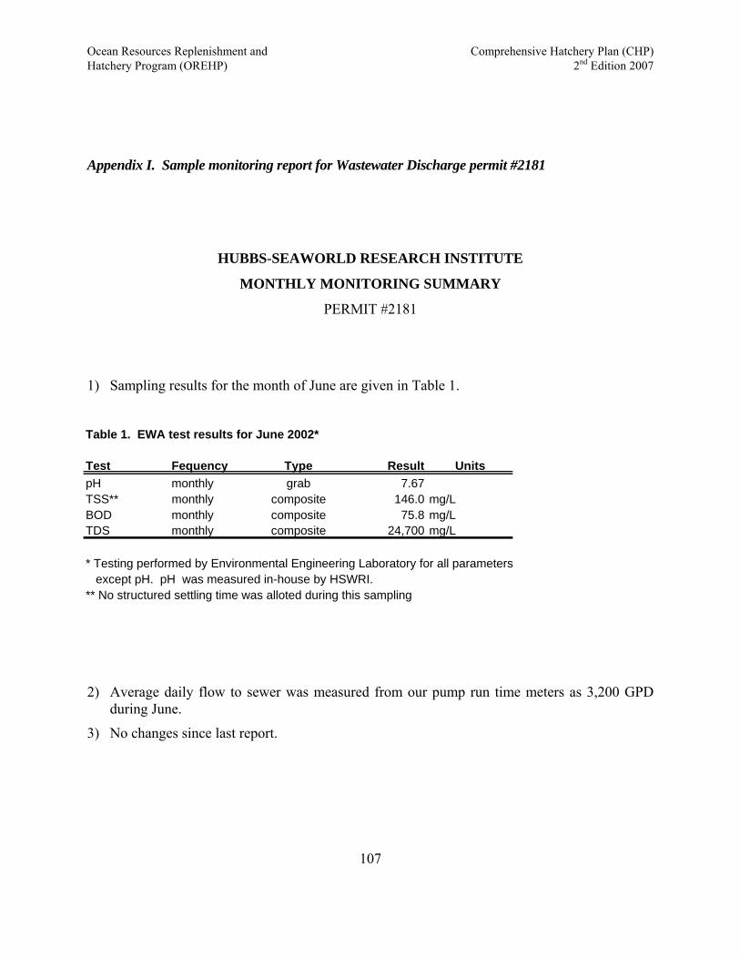
Ocean Resources Replenishment and Comprehensive Hatchery Plan (CHP) Hatchery Program (OREHP) 2nd Edition 2007
Appendix I. Sample monitoring report for Wastewater Discharge permit #2181
HUBBS-SEAWORLD RESEARCH INSTITUTE
MONTHLY MONITORING SUMMARY
PERMIT #2181
1) Sampling results for the month of June are given in Table 1.
Table 1. EWA test results for June 2002*
Test Fequency Type Result UnitspH monthly grab 7.67TSS** monthly composite 146.0 mg/LBOD monthly composite 75.8 mg/LTDS monthly composite 24,700 mg/L
* Testing performed by Environmental Engineering Laboratory for all parameters except pH. pH was measured in-house by HSWRI.** No structured settling time was alloted during this sampling
2) Average daily flow to sewer was measured from our pump run time meters as 3,200 GPD during June.
3) No changes since last report.
107
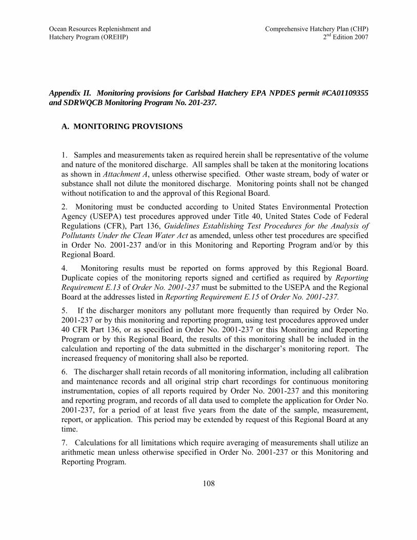
Ocean Resources Replenishment and Comprehensive Hatchery Plan (CHP) Hatchery Program (OREHP) 2nd Edition 2007
Appendix II. Monitoring provisions for Carlsbad Hatchery EPA NPDES permit #CA01109355 and SDRWQCB Monitoring Program No. 201-237.
A. MONITORING PROVISIONS
1. Samples and measurements taken as required herein shall be representative of the volume and nature of the monitored discharge. All samples shall be taken at the monitoring locations as shown in Attachment A, unless otherwise specified. Other waste stream, body of water or substance shall not dilute the monitored discharge. Monitoring points shall not be changed without notification to and the approval of this Regional Board.
2. Monitoring must be conducted according to United States Environmental Protection Agency (USEPA) test procedures approved under Title 40, United States Code of Federal Regulations (CFR), Part 136, Guidelines Establishing Test Procedures for the Analysis of Pollutants Under the Clean Water Act as amended, unless other test procedures are specified in Order No. 2001-237 and/or in this Monitoring and Reporting Program and/or by this Regional Board.
4. Monitoring results must be reported on forms approved by this Regional Board. Duplicate copies of the monitoring reports signed and certified as required by Reporting Requirement E.13 of Order No. 2001-237 must be submitted to the USEPA and the Regional Board at the addresses listed in Reporting Requirement E.15 of Order No. 2001-237.
5. If the discharger monitors any pollutant more frequently than required by Order No. 2001-237 or by this monitoring and reporting program, using test procedures approved under 40 CFR Part 136, or as specified in Order No. 2001-237 or this Monitoring and Reporting Program or by this Regional Board, the results of this monitoring shall be included in the calculation and reporting of the data submitted in the discharger’s monitoring report. The increased frequency of monitoring shall also be reported.
6. The discharger shall retain records of all monitoring information, including all calibration and maintenance records and all original strip chart recordings for continuous monitoring instrumentation, copies of all reports required by Order No. 2001-237 and this monitoring and reporting program, and records of all data used to complete the application for Order No. 2001-237, for a period of at least five years from the date of the sample, measurement, report, or application. This period may be extended by request of this Regional Board at any time.
7. Calculations for all limitations which require averaging of measurements shall utilize an arithmetic mean unless otherwise specified in Order No. 2001-237 or this Monitoring and Reporting Program.
108
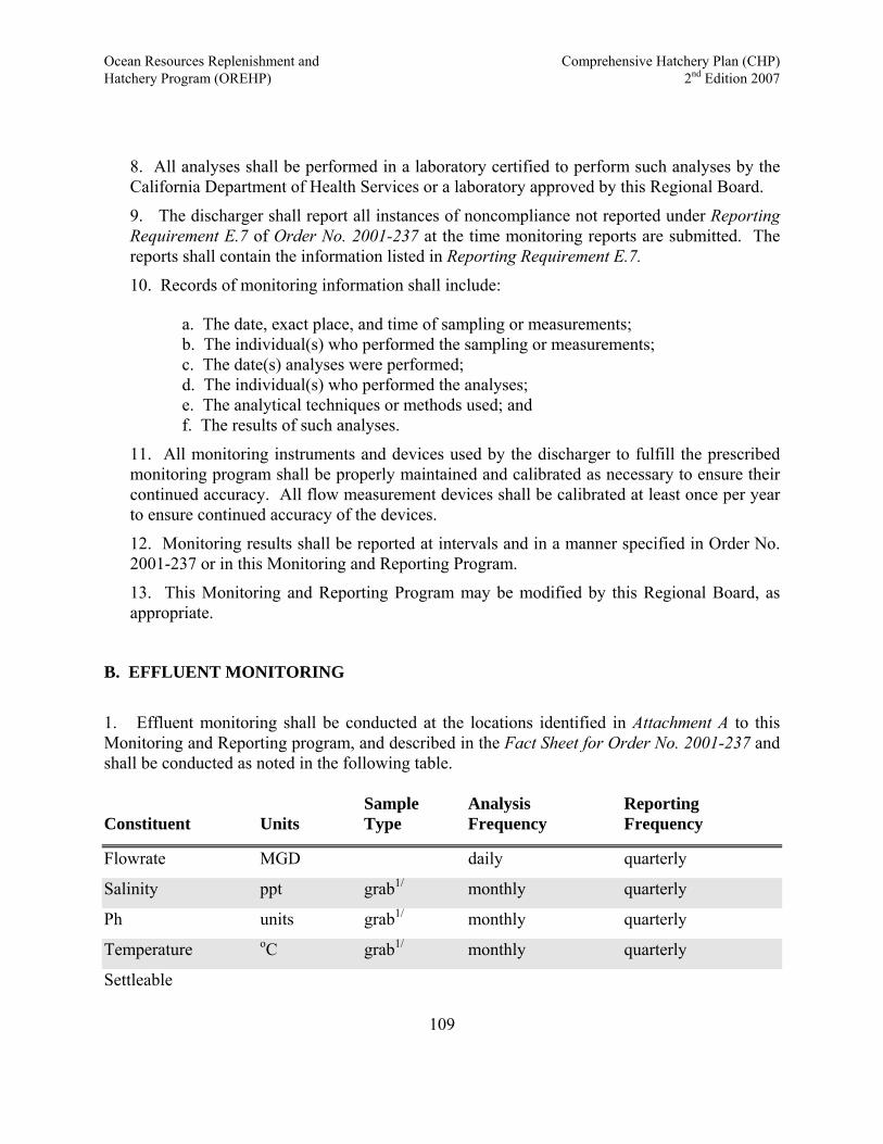
Ocean Resources Replenishment and Comprehensive Hatchery Plan (CHP) Hatchery Program (OREHP) 2nd Edition 2007
8. All analyses shall be performed in a laboratory certified to perform such analyses by the California Department of Health Services or a laboratory approved by this Regional Board.
9. The discharger shall report all instances of noncompliance not reported under Reporting Requirement E.7 of Order No. 2001-237 at the time monitoring reports are submitted. The reports shall contain the information listed in Reporting Requirement E.7.
10. Records of monitoring information shall include:
a. The date, exact place, and time of sampling or measurements; b. The individual(s) who performed the sampling or measurements; c. The date(s) analyses were performed; d. The individual(s) who performed the analyses; e. The analytical techniques or methods used; and f. The results of such analyses.
11. All monitoring instruments and devices used by the discharger to fulfill the prescribed monitoring program shall be properly maintained and calibrated as necessary to ensure their continued accuracy. All flow measurement devices shall be calibrated at least once per year to ensure continued accuracy of the devices.
12. Monitoring results shall be reported at intervals and in a manner specified in Order No. 2001-237 or in this Monitoring and Reporting Program.
13. This Monitoring and Reporting Program may be modified by this Regional Board, as appropriate.
B. EFFLUENT MONITORING
1. Effluent monitoring shall be conducted at the locations identified in Attachment A to this Monitoring and Reporting program, and described in the Fact Sheet for Order No. 2001-237 and shall be conducted as noted in the following table. Sample Analysis Reporting Constituent Units Type Frequency Frequency
Flowrate MGD daily quarterly
Salinity ppt grab1/ monthly quarterly
Ph units grab1/ monthly quarterly
Temperature oC grab1/ monthly quarterly
Settleable
109
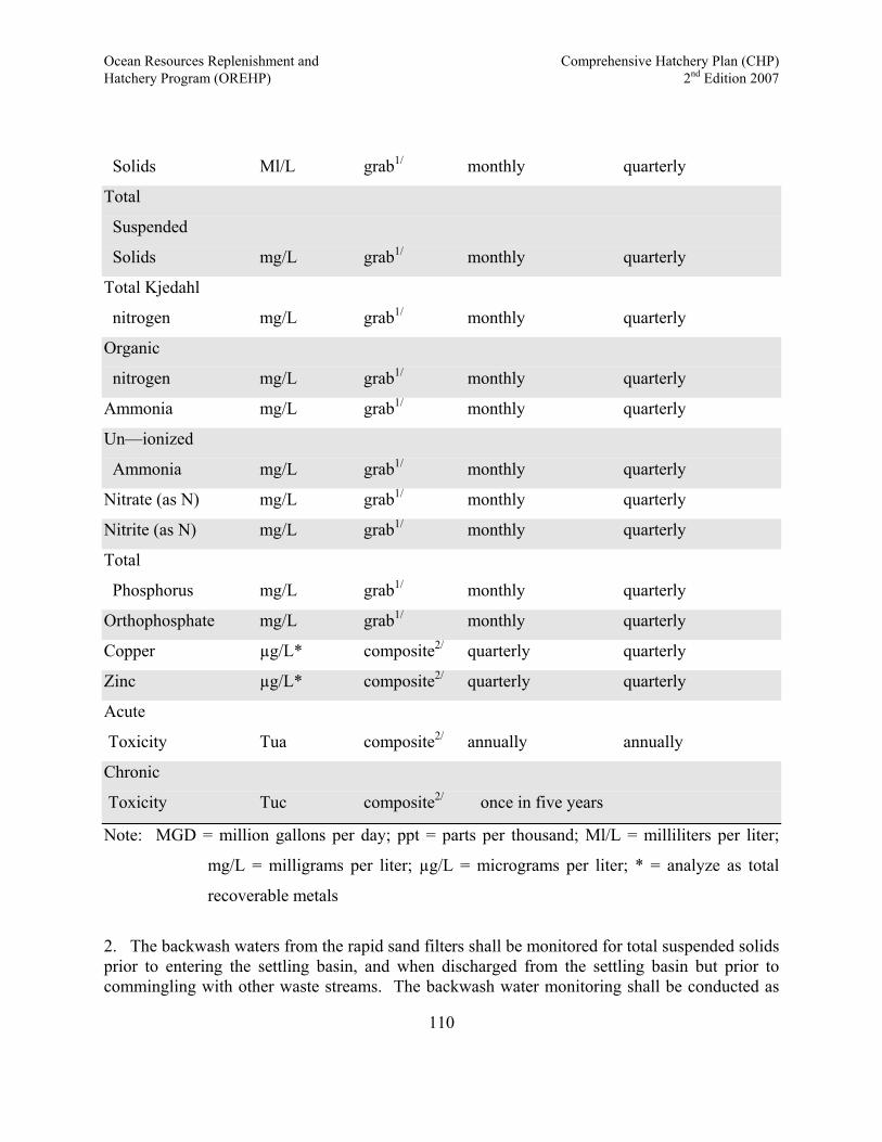
Ocean Resources Replenishment and Comprehensive Hatchery Plan (CHP) Hatchery Program (OREHP) 2nd Edition 2007
Solids Ml/L grab1/ monthly quarterly
Total
Suspended
Solids mg/L grab1/ monthly quarterly
Total Kjedahl
nitrogen mg/L grab1/ monthly quarterly
Organic
nitrogen mg/L grab1/ monthly quarterly
Ammonia mg/L grab1/ monthly quarterly
Un—ionized
Ammonia mg/L grab1/ monthly quarterly
Nitrate (as N) mg/L grab1/ monthly quarterly
Nitrite (as N) mg/L grab1/ monthly quarterly
Total
Phosphorus mg/L grab1/ monthly quarterly
Orthophosphate mg/L grab1/ monthly quarterly
Copper µg/L* composite2/ quarterly quarterly
Zinc µg/L* composite2/ quarterly quarterly
Acute
Toxicity Tua composite2/ annually annually
Chronic
Toxicity Tuc composite2/ once in five years
Note: MGD = million gallons per day; ppt = parts per thousand; Ml/L = milliliters per liter;
mg/L = milligrams per liter; µg/L = micrograms per liter; * = analyze as total
recoverable metals
2. The backwash waters from the rapid sand filters shall be monitored for total suspended solids prior to entering the settling basin, and when discharged from the settling basin but prior to commingling with other waste streams. The backwash water monitoring shall be conducted as
110
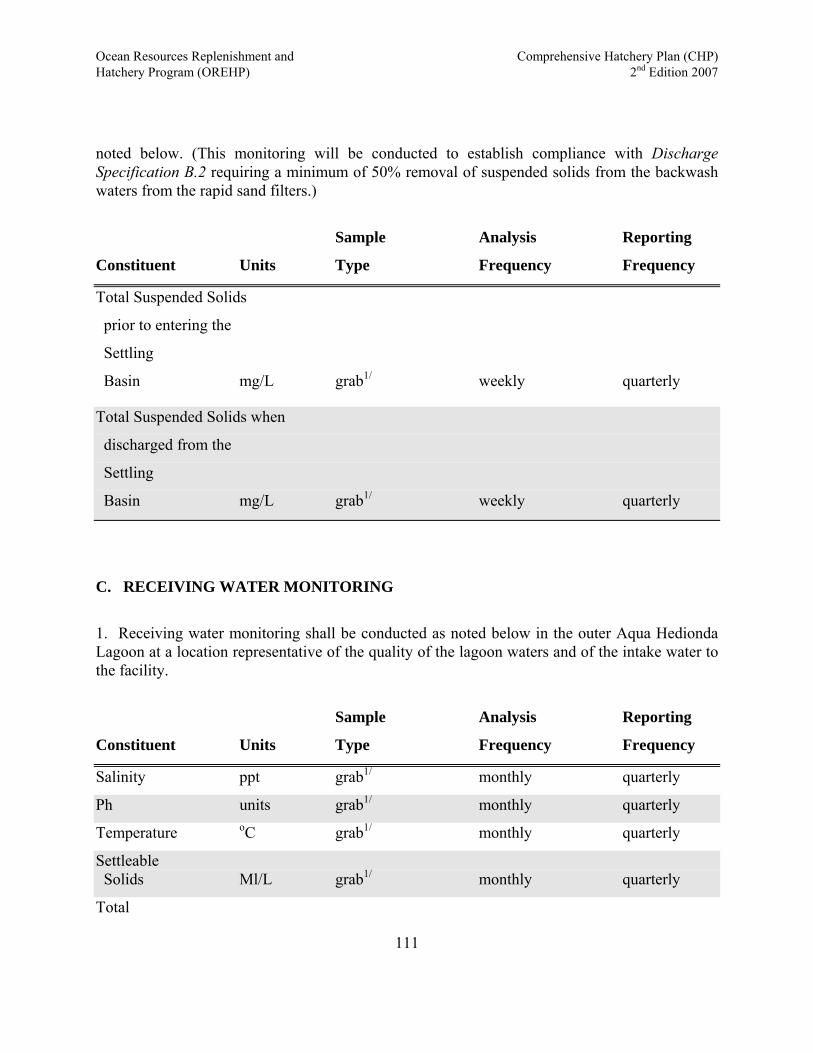
Ocean Resources Replenishment and Comprehensive Hatchery Plan (CHP) Hatchery Program (OREHP) 2nd Edition 2007
noted below. (This monitoring will be conducted to establish compliance with Discharge Specification B.2 requiring a minimum of 50% removal of suspended solids from the backwash waters from the rapid sand filters.)
Sample Analysis Reporting
Constituent Units Type Frequency Frequency
Total Suspended Solids
prior to entering the
Settling
Basin mg/L grab1/ weekly quarterly
Total Suspended Solids when
discharged from the
Settling
Basin mg/L grab1/ weekly quarterly
C. RECEIVING WATER MONITORING
1. Receiving water monitoring shall be conducted as noted below in the outer Aqua Hedionda Lagoon at a location representative of the quality of the lagoon waters and of the intake water to the facility.
Sample Analysis Reporting
Constituent Units Type Frequency Frequency
Salinity ppt grab1/ monthly quarterly
Ph units grab1/ monthly quarterly
Temperature oC grab1/ monthly quarterly
Settleable Solids Ml/L grab1/ monthly quarterly
Total
111
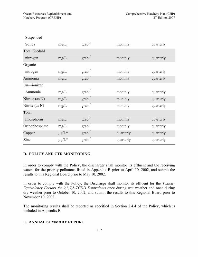
Ocean Resources Replenishment and Comprehensive Hatchery Plan (CHP) Hatchery Program (OREHP) 2nd Edition 2007
Suspended
Solids mg/L grab1/ monthly quarterly
Total Kjedahl
nitrogen mg/L grab1/ monthly quarterly
Organic
nitrogen mg/L grab1/ monthly quarterly
Ammonia mg/L grab1/ monthly quarterly
Un—ionized
Ammonia mg/L grab1/ monthly quarterly
Nitrate (as N) mg/L grab1/ monthly quarterly
Nitrite (as N) mg/L grab1/ monthly quarterly
Total
Phosphorus mg/L grab1/ monthly quarterly
Orthophosphate mg/L grab1/ monthly quarterly
Copper µg/L* grab1/ quarterly quarterly
Zinc µg/L* grab1/ quarterly quarterly
D. POLICY AND CTR MONITORING
In order to comply with the Policy, the discharger shall monitor its effluent and the receiving waters for the priority pollutants listed in Appendix B prior to April 10, 2002, and submit the results to this Regional Board prior to May 10, 2002. In order to comply with the Policy, the Discharge shall monitor its effluent for the Toxicity Equivalency Factors for 2,3,7,8-TCDD Equivalents once during wet weather and once during dry weather prior to October 10, 2002, and submit the results to this Regional Board prior to November 10, 2002. The monitoring results shall be reported as specified in Section 2.4.4 of the Policy, which is included in Appendix B.
E. ANNUAL SUMMARY REPORT
112
Ocean Resources Replenishment and Comprehensive Hatchery Plan (CHP) Hatchery Program (OREHP) 2nd Edition 2007
1. The discharger shall submit an annual tabular and graphical summary of the data collected for this monitoring program. 2. The annual report must include a narrative evaluation of the data collected as specified in Provision D.2 of Order No. 2001-237.
F. MONITORING REPORT SCHEDULE
Monitoring reports shall be submitted to this Regional Board according to the dates in the following schedule:
Reporting Frequency Report Period Report Due
Quarterly January through March May 1
April through June August 1
July through September November 1
October through December February 1
Annually January through December February 1
Once in five years February 1, 2006
Appendix B
Priority
Pollutants Oct. 10, 2001 to
Apr. 10, 2002 May 10, 2002
TEF Oct. 10, 2001 to
Oct. 10, 2002 November 10, 2002
G. Endnote References
1. A grab sample is defined as an individual sample of at least 100 milliliters collected over a period not exceeding 15 minutes. Grab samples shall be collected over a shorter period if
113
Ocean Resources Replenishment and Comprehensive Hatchery Plan (CHP) Hatchery Program (OREHP) 2nd Edition 2007
necessary to ensure that the constituent/parameter concentration in the sample is the same as that at the sampling location at the time the sample is collected. 2. A composite sample is defined as a combination of at least six sample aliquots of at least 100 milliliters, collected at periodic intervals during the operating hours of a facility over an 18-hour period. For volatile pollutants, aliquots must be combined in the laboratory immediately before analysis. The composite must be flow proportional; either the time interval between each aliquot or the volume of each aliquot must be proportional to either the stream flow at the time of sampling or the total stream flow since the collection of the previous aliquot. Aliquots may be collected manually or automatically.
114

Ocean Resources Replenishment and Comprehensive Hatchery Plan (CHP) Hatchery Program (OREHP) 2nd Edition 2007
Appendix III. Sample monitoring report for Carlsbad Hatchery EPA NPDES permit #CA01109355 under SDRWQCB Monitoring Program No. 201-237.
Annual Water Quality Monitoring Report for 2004 Hubbs-SeaWorld Research Institute
NPDES Permit No. CA0109355
prepared for the
San Diego
Regional Water Quality Control Board
IC: 12-0577.01: richp
115
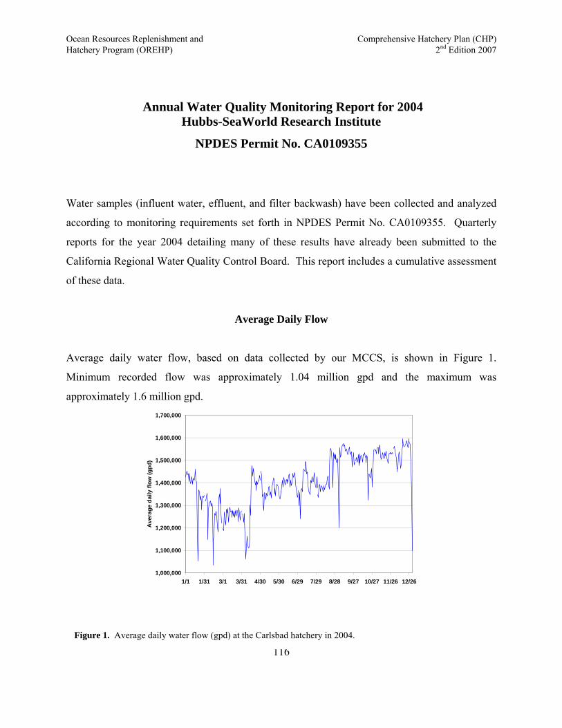
Ocean Resources Replenishment and Comprehensive Hatchery Plan (CHP) Hatchery Program (OREHP) 2nd Edition 2007
Annual Water Quality Monitoring Report for 2004 Hubbs-SeaWorld Research Institute
NPDES Permit No. CA0109355
Water samples (influent water, effluent, and filter backwash) have been collected and analyzed
according to monitoring requirements set forth in NPDES Permit No. CA0109355. Quarterly
reports for the year 2004 detailing many of these results have already been submitted to the
California Regional Water Quality Control Board. This report includes a cumulative assessment
of these data.
Average Daily Flow
Average daily water flow, based on data collected by our MCCS, is shown in Figure 1.
Minimum recorded flow was approximately 1.04 million gpd and the maximum was
approximately 1.6 million gpd.
1,000,000
1,100,000
1,200,000
1,300,000
1,400,000
1,500,000
1,600,000
1,700,000
1/1 1/31 3/1 3/31 4/30 5/30 6/29 7/29 8/28 9/27 10/27 11/26 12/26
Ave
rage
dai
ly fl
ow (g
pd)
116Figure 1. Average daily water flow (gpd) at the Carlsbad hatchery in 2004.

Ocean Resources Replenishment and Comprehensive Hatchery Plan (CHP) Hatchery Program (OREHP) 2nd Edition 2007
General Water Quality Testing
Monthly water quality measurements of influent (receiving) and effluent water samples are
provided in Appendix IIIb. The following sections detail further analyses for many of these
parameters.
Total and Unionized Ammonia
Total ammonia and unionized ammonia were undetectable in all monthly samples of influent
water, with the exception of May 2004. Total ammonia was detectable in the effluent in all
months except April, July, September and December (Figure 2 and Appendix IIIb). Unionized
ammonia was calculated using the methods of Hampson3 (Appendix IIIb).
0.1
0.2
0.3
0.4
0.5
0.6
0.7
0.8
0.9
1.0
1/22 3/24 5/26 7/29 9/22 11/18Date
Tota
l Am
mon
ia (m
g/L)
influent
effluent
Figure 2. Total ammonia measured in monthly water samples during 2004. Detection limit
is 0.1 mg/L.
3 . Hampson, B.L. (1977). The relationship between total ammonia and free ammonia in terrestrial and ocean
waters. J.Cons. Explor. Mer. 37(2):117-122. 117

Ocean Resources Replenishment and Comprehensive Hatchery Plan (CHP) Hatchery Program (OREHP) 2nd Edition 2007
Ph
Measured values of Ph were lower in the effluent than the influent, except in the month of
August. The range of 7.5 to 8.1 for either sample was well within the limits of 6.0 to 9.0 as
specified in our permit (Figure 3).
7.4
7.5
7.6
7.7
7.8
7.9
8.0
8.1
8.2
8.3
8.4
1/1 1/31 3/1 3/31 4/30 5/30 6/29 7/29 8/28 9/27 10/27 11/26 12/26Date
pH
influenteffluent
Figure 3. Monthly recorded measurements of pH in influent and effluent samples during 2004.
Salinity
Salinity varied from 31 to 38 ppt in samples collected during 2004 (Figure 4).
30.0
31.0
32.0
33.0
34.0
35.0
36.0
37.0
38.0
1/1 1/31 3/1 3/31 4/30 5/30 6/29 7/29 8/28 9/27 10/27
11/26
12/26
Date
Salin
ity (p
pt)
influenteffluent
Figure 4. Salinity (ppt) measured in monthly water samples.
118
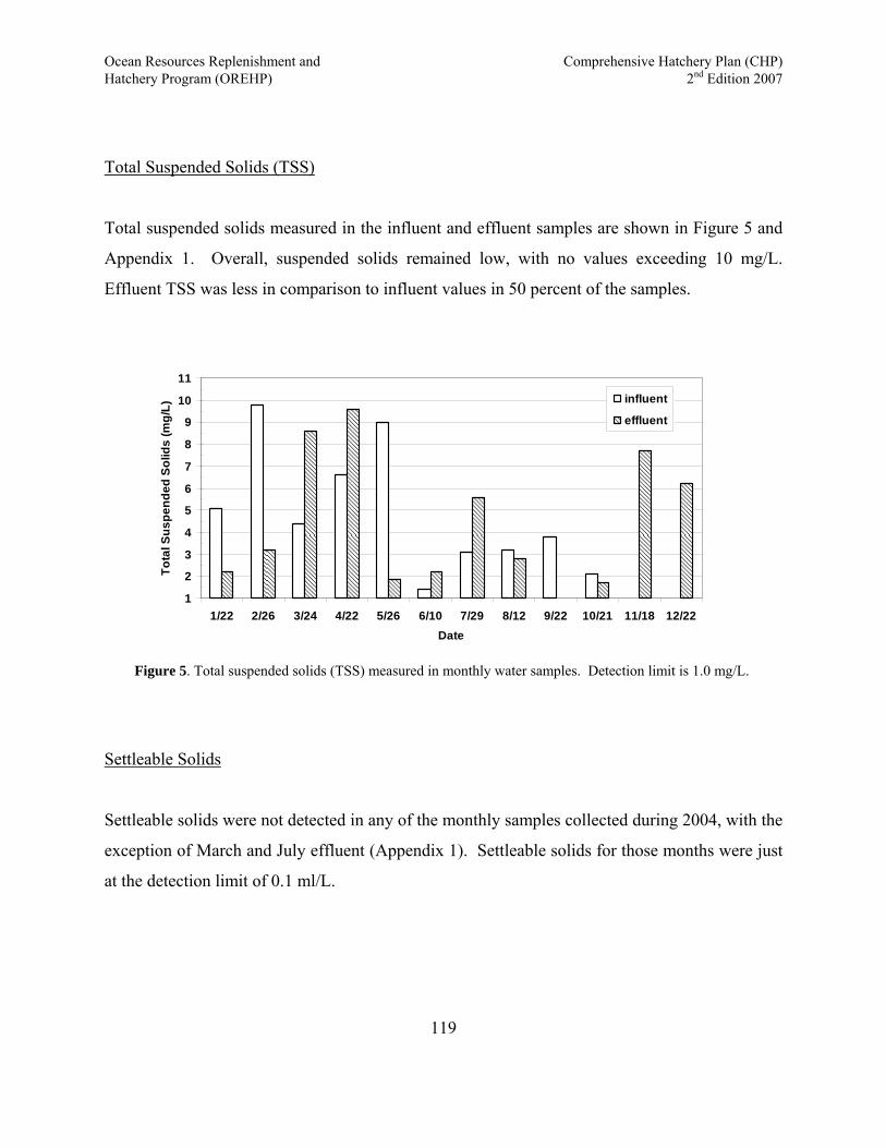
Ocean Resources Replenishment and Comprehensive Hatchery Plan (CHP) Hatchery Program (OREHP) 2nd Edition 2007
Total Suspended Solids (TSS)
Total suspended solids measured in the influent and effluent samples are shown in Figure 5 and
Appendix 1. Overall, suspended solids remained low, with no values exceeding 10 mg/L.
Effluent TSS was less in comparison to influent values in 50 percent of the samples.
1
2
3
4
5
6
7
8
9
10
11
1/22 2/26 3/24 4/22 5/26 6/10 7/29 8/12 9/22 10/21 11/18 12/22Date
Tota
l Sus
pend
ed S
olid
s (m
g/L)
influent
effluent
Figure 5. Total suspended solids (TSS) measured in monthly water samples. Detection limit is 1.0 mg/L.
Settleable Solids
Settleable solids were not detected in any of the monthly samples collected during 2004, with the
exception of March and July effluent (Appendix 1). Settleable solids for those months were just
at the detection limit of 0.1 ml/L.
119
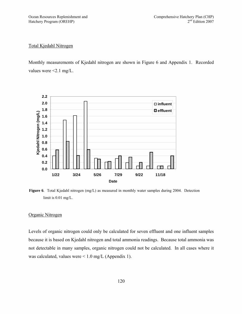
Ocean Resources Replenishment and Comprehensive Hatchery Plan (CHP) Hatchery Program (OREHP) 2nd Edition 2007
Total Kjedahl Nitrogen
Monthly measurements of Kjedahl nitrogen are shown in Figure 6 and Appendix 1. Recorded
values were <2.1 mg/L.
0.0
0.20.4
0.6
0.81.0
1.21.4
1.6
1.82.0
2.2
1/22 3/24 5/26 7/29 9/22 11/18Date
Kje
dahl
Nitr
ogen
(mg/
L)
influent
effluent
Figure 6. Total Kjedahl nitrogen (mg/L) as measured in monthly water samples during 2004. Detection
limit is 0.01 mg/L.
Organic Nitrogen
Levels of organic nitrogen could only be calculated for seven effluent and one influent samples
because it is based on Kjedahl nitrogen and total ammonia readings. Because total ammonia was
not detectable in many samples, organic nitrogen could not be calculated. In all cases where it
was calculated, values were < 1.0 mg/L (Appendix 1).
120
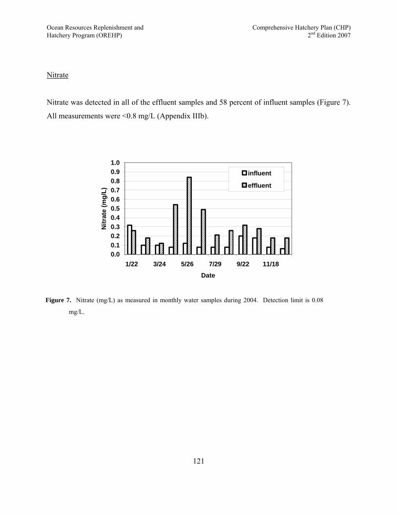
Ocean Resources Replenishment and Comprehensive Hatchery Plan (CHP) Hatchery Program (OREHP) 2nd Edition 2007
Nitrate
Nitrate was detected in all of the effluent samples and 58 percent of influent samples (Figure 7).
All measurements were <0.8 mg/L (Appendix IIIb).
0.00.10.20.30.40.50.60.70.80.91.0
1/22 3/24 5/26 7/29 9/22 11/18
Date
Nitr
ate
(mg/
L)
influent
effluent
Figure 7. Nitrate (mg/L) as measured in monthly water samples during 2004. Detection limit is 0.08
mg/L.
121
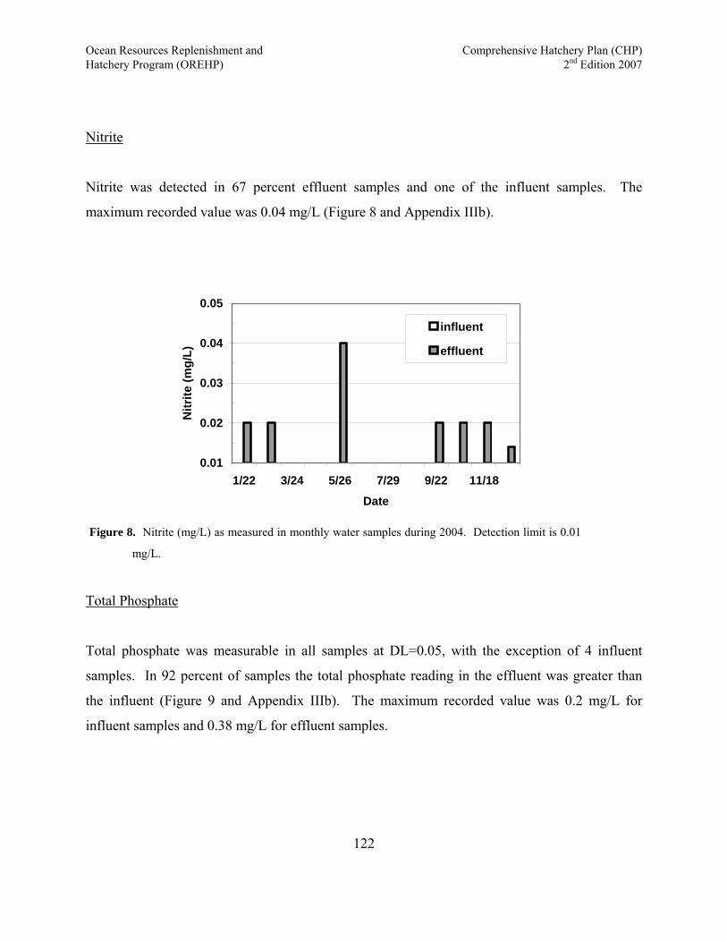
Ocean Resources Replenishment and Comprehensive Hatchery Plan (CHP) Hatchery Program (OREHP) 2nd Edition 2007
Nitrite
Nitrite was detected in 67 percent effluent samples and one of the influent samples. The
maximum recorded value was 0.04 mg/L (Figure 8 and Appendix IIIb).
0.01
0.02
0.03
0.04
0.05
1/22 3/24 5/26 7/29 9/22 11/18
Date
Nitr
ite (m
g/L)
influent
effluent
Figure 8. Nitrite (mg/L) as measured in monthly water samples during 2004. Detection limit is 0.01
mg/L.
Total Phosphate
Total phosphate was measurable in all samples at DL=0.05, with the exception of 4 influent
samples. In 92 percent of samples the total phosphate reading in the effluent was greater than
the influent (Figure 9 and Appendix IIIb). The maximum recorded value was 0.2 mg/L for
influent samples and 0.38 mg/L for effluent samples.
122
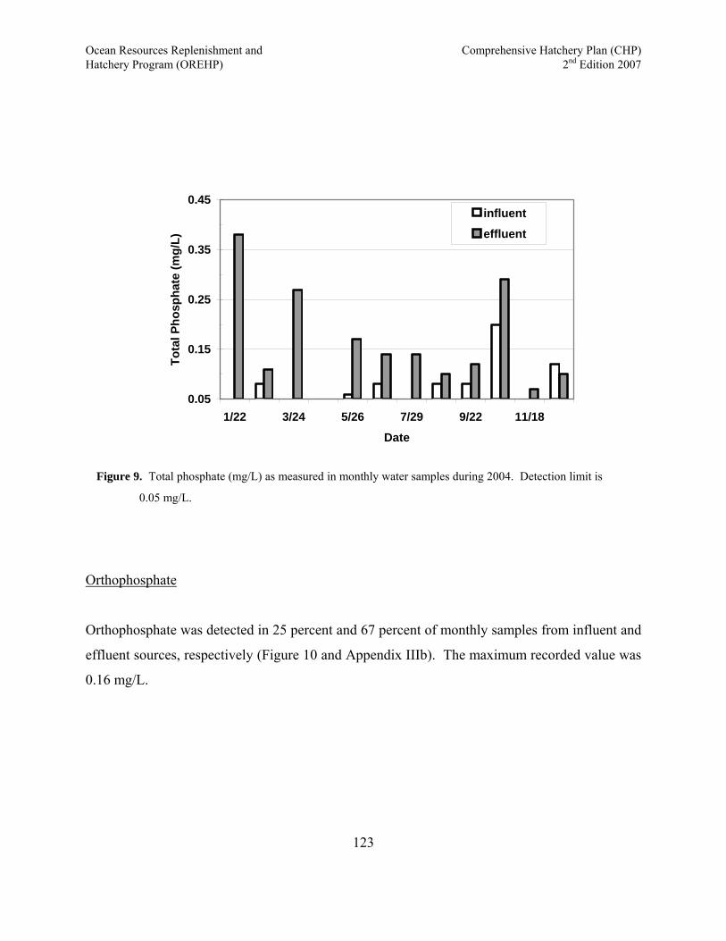
Ocean Resources Replenishment and Comprehensive Hatchery Plan (CHP) Hatchery Program (OREHP) 2nd Edition 2007
0.05
0.15
0.25
0.35
0.45
1/22 3/24 5/26 7/29 9/22 11/18
Date
Tota
l Pho
spha
te (m
g/L)
influent
effluent
Figure 9. Total phosphate (mg/L) as measured in monthly water samples during 2004. Detection limit is
0.05 mg/L.
Orthophosphate
Orthophosphate was detected in 25 percent and 67 percent of monthly samples from influent and
effluent sources, respectively (Figure 10 and Appendix IIIb). The maximum recorded value was
0.16 mg/L.
123

Ocean Resources Replenishment and Comprehensive Hatchery Plan (CHP) Hatchery Program (OREHP) 2nd Edition 2007
0.05
0.10
0.15
0.20
0.25
1/22 3/24 5/26 7/29 9/22 11/18
Date
Ort
hoph
osph
ate
(mg/
L)influent
effluent
Figure 10. Orthophosphate (mg/L) as measured in monthly water samples during 2004. Detection
limit is 0.05 mg/L.
Metals Testing
Influent and effluent seawater sources were tested for copper and zinc on a quarterly basis. A
summary of the results for the year 2004 is shown in Table 1. As requested by the Regional
Water Quality Control Board, copper testing using EPA Method 6010 was initiated in September
2002 to reduce the possible interference of sodium ions. The concentration of zinc and copper in
the influent samples exceeded the concentration in the effluent sample, with the exception of
those taken in September.
124

Ocean Resources Replenishment and Comprehensive Hatchery Plan (CHP) Hatchery Program (OREHP) 2nd Edition 2007
Copper (micro g/L)Sample Date Influent Effluent Test type Method DL Laboratory
03/23/04 4.28 2.95 quarterly metals 1640 0.005 CRG Marine Labs03/23/04 4.90 3.53 quarterly metals 1640 0.005 CRG Marine Labs06/08/04 2.32 2.40 quarterly metals 1640 0.005 CRG Marine Labs06/08/04 2.25 quarterly metals 1640 0.005 CRG Marine Labs09/28/04 2.76 2.20 quarterly metals 1640 0.005 CRG Marine Labs09/28/04 3.23 quarterly metals 1640 0.005 CRG Marine Labs12/14/04 3.41 3.05 quarterly metals 1640 0.005 CRG Marine Labs12/14/04 3.34 quarterly metals 1640 0.005 CRG Marine Labs
One to two replicates of each sample were analyzed by the lab for each of the above dates.
Zinc (micro g/L)Sample Date Influent Effluent Test type Method DL Laboratory
03/23/04 38.3 33.1 quarterly metals 6010B 20 CalScience06/08/04 112 88.5 quarterly metals 6010B 10 CalScience09/28/04 20.4 22.6 quarterly metals 6010B 10 CalScience12/14/04 46.3 29.5 quarterly metals 6010B 10 CalScience
* ND indicates below detectable levels
Table 1. Summary of copper and zinc sampling results for 2004. All values converted to units of micrograms/L.
Discharge Specifications
Data specified in Discharge Specifications B.2 did not consistently exceed the effluent
limitations. Specifically, (1) acute toxicity did not exceed the instantaneous maximum of 2.5
Tua, and (2) TSS levels measured in seawater leaving the settling basin did not exceed 50
percent of the measured influent values (Figure 11, Table 2). As such, there was no need to
conduct toxic reduction evaluation (TRE) as specified in Provision D.2 of Order 2001-237. The
125
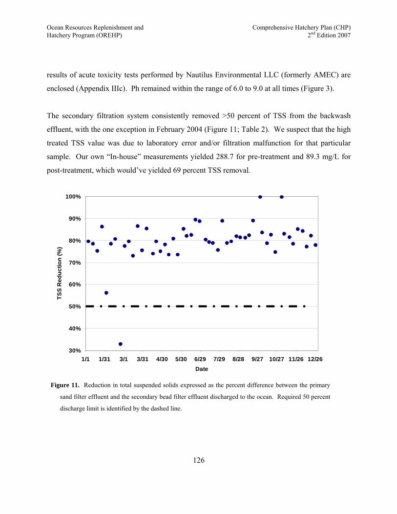
Ocean Resources Replenishment and Comprehensive Hatchery Plan (CHP) Hatchery Program (OREHP) 2nd Edition 2007
results of acute toxicity tests performed by Nautilus Environmental LLC (formerly AMEC) are
enclosed (Appendix IIIc). Ph remained within the range of 6.0 to 9.0 at all times (Figure 3).
The secondary filtration system consistently removed >50 percent of TSS from the backwash
effluent, with the one exception in February 2004 (Figure 11; Table 2). We suspect that the high
treated TSS value was due to laboratory error and/or filtration malfunction for that particular
sample. Our own “In-house” measurements yielded 288.7 for pre-treatment and 89.3 mg/L for
post-treatment, which would’ve yielded 69 percent TSS removal.
30%
40%
50%
60%
70%
80%
90%
100%
1/1 1/31 3/1 3/31 4/30 5/30 6/29 7/29 8/28 9/27 10/27 11/26 12/26Date
TSS
Red
uctio
n (%
)
Figure 11. Reduction in total suspended solids expressed as the percent difference between the primary
sand filter effluent and the secondary bead filter effluent discharged to the ocean. Required 50 percent
discharge limit is identified by the dashed line.
126
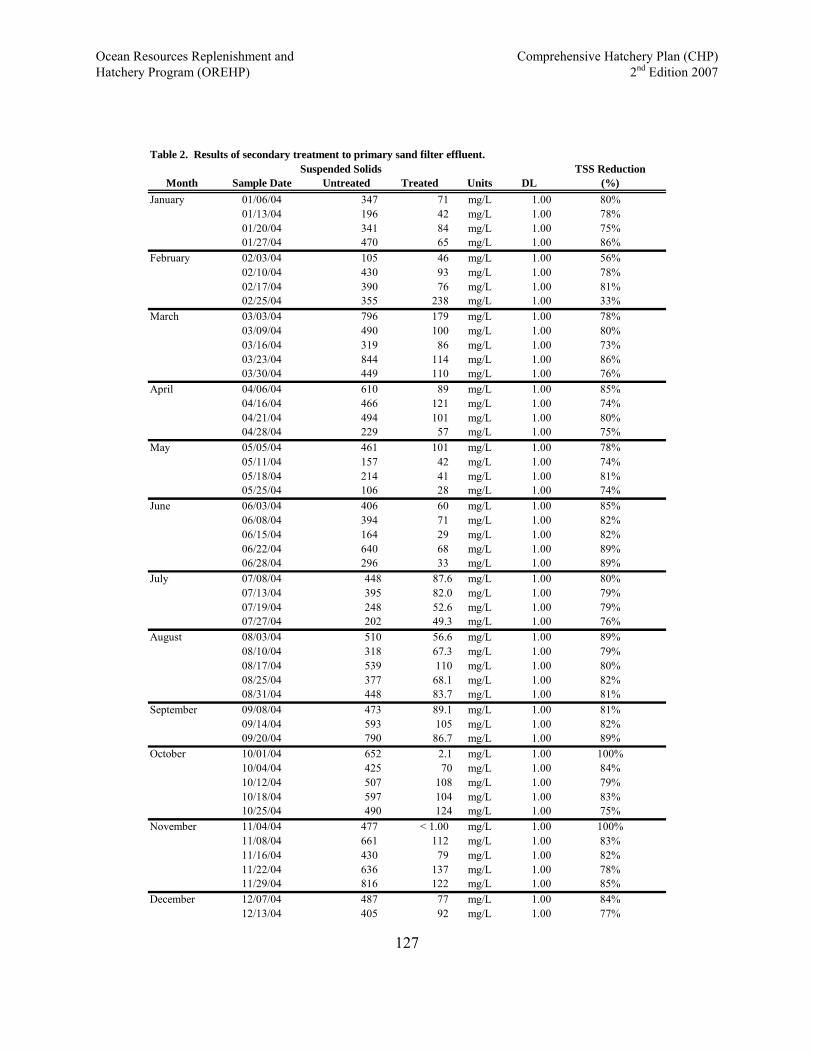
Ocean Resources Replenishment and Comprehensive Hatchery Plan (CHP) Hatchery Program (OREHP) 2nd Edition 2007
Table 2. Results of secondary treatment to primary sand filter effluent. Suspended Solids TSS Reduction
Month Sample Date Untreated Treated Units DL (%)January 01/06/04 347 71 mg/L 1.00 80%
01/13/04 196 42 mg/L 1.00 78%01/20/04 341 84 mg/L 1.00 75%01/27/04 470 65 mg/L 1.00 86%
February 02/03/04 105 46 mg/L 1.00 56%02/10/04 430 93 mg/L 1.00 78%02/17/04 390 76 mg/L 1.00 81%02/25/04 355 238 mg/L 1.00 33%
March 03/03/04 796 179 mg/L 1.00 78%03/09/04 490 100 mg/L 1.00 80%03/16/04 319 86 mg/L 1.00 73%03/23/04 844 114 mg/L 1.00 86%03/30/04 449 110 mg/L 1.00 76%
April 04/06/04 610 89 mg/L 1.00 85%04/16/04 466 121 mg/L 1.00 74%04/21/04 494 101 mg/L 1.00 80%04/28/04 229 57 mg/L 1.00 75%
May 05/05/04 461 101 mg/L 1.00 78%05/11/04 157 42 mg/L 1.00 74%05/18/04 214 41 mg/L 1.00 81%05/25/04 106 28 mg/L 1.00 74%
June 06/03/04 406 60 mg/L 1.00 85%06/08/04 394 71 mg/L 1.00 82%06/15/04 164 29 mg/L 1.00 82%06/22/04 640 68 mg/L 1.00 89%06/28/04 296 33 mg/L 1.00 89%
July 07/08/04 448 87.6 mg/L 1.00 80%07/13/04 395 82.0 mg/L 1.00 79%07/19/04 248 52.6 mg/L 1.00 79%07/27/04 202 49.3 mg/L 1.00 76%
August 08/03/04 510 56.6 mg/L 1.00 89%08/10/04 318 67.3 mg/L 1.00 79%08/17/04 539 110 mg/L 1.00 80%08/25/04 377 68.1 mg/L 1.00 82%08/31/04 448 83.7 mg/L 1.00 81%
September 09/08/04 473 89.1 mg/L 1.00 81%09/14/04 593 105 mg/L 1.00 82%09/20/04 790 86.7 mg/L 1.00 89%
October 10/01/04 652 2.1 mg/L 1.00 100%10/04/04 425 70 mg/L 1.00 84%10/12/04 507 108 mg/L 1.00 79%10/18/04 597 104 mg/L 1.00 83%10/25/04 490 124 mg/L 1.00 75%
November 11/04/04 477 < 1.00 mg/L 1.00 100%11/08/04 661 112 mg/L 1.00 83%11/16/04 430 79 mg/L 1.00 82%11/22/04 636 137 mg/L 1.00 78%11/29/04 816 122 mg/L 1.00 85%
December 12/07/04 487 77 mg/L 1.00 84%12/13/04 405 92 mg/L 1.00 77%
127
Ocean Resources Replenishment and Comprehensive Hatchery Plan (CHP) Hatchery Program (OREHP) 2nd Edition 2007
128
Appendix IIIb
Parameters Measured on Monthly Influent and Effluent Sampling of Carlsbad Fish Hatchery in
2004

Ocean Resources Replenishment and Comprehensive Hatchery Plan (CHP) Hatchery Program (OREHP) 2nd Edition 2007
Date Total Ammonia Unionized Ammonia a pH Suspended Solids Settleable Solids Temperature Salinity(mg/L) (mg/L) (mg/L) (ml/L) ( C) (ppt)
influent effluent influent effluent influent effluent influent effluent influent effluent influent effluent influent effluent01/22/04 ND 0.14 ND 0.01 7.64 7.62 5.1 2.2 ND ND 14 14.5 34.4 33.102/26/04 ND 0.10 ND ND 7.82 7.64 9.8 3.2 ND ND 15 16 31.4 35.303/24/04 ND 0.65 ND 0.03 7.91 7.60 4.4 8.6 ND 0.1 16.5 17 36.9 37.104/22/04 ND ND ND ND 7.96 7.80 6.6 9.6 ND ND 18.0 18..5 35.3 35.705/26/04 0.11 0.30 0.01 0.02 7.97 7.68 9.02 1.84 ND ND 20.7 21.3 36.8 37.806/10/04 ND 0.14 ND 0.01 8.10 7.89 1.4 2.2 ND ND 20.5 20.6 37.5 36.707/29/04 ND ND ND ND 8.07 7.61 3.1 5.6 ND 0.1 21 21.5 35.3 35.208/12/04 ND 0.20 ND 0.01 7.54 8.05 3.2 2.8 ND ND 21 22 35.2 35.209/22/04 ND ND ND ND 8.03 7.73 3.8 1 ND ND 20 20 36.9 37.010/21/04 ND 0.10 ND 0.01 7.9 7.7 2.1 1.7 ND ND 19.5 19 31.0 34.711/18/04 ND 0.14 ND 0.01 8.00 7.68 ND 7.7 ND ND 16 16.5 36.3 36.312/22/04 ND ND ND ND 7.91 7.84 ND 6.2 ND ND 14 15 36.2 35.8
DL = < 0.10 DL = < 0.01 DL = < 1.0 DL = < 0.1
Date Total Kjedahl Organic Nitrogen a Total Phosphate Orthophosphate Nitrate NitriteNitrogen (mg/L) (mg/L) (mg/L) (mg/L) (mg/L) (mg/L)
influent effluent influent effluent influent effluent influent effluent influent effluent influent effluent01/22/04 0.4 0.58 0.44 ND 0.38 ND 0.16 0.32 0.26 ND 0.0202/26/04 1.48 0.84 0.74 0.08 0.11 0.05 0.06 0.10 0.18 ND 0.0203/24/04 1.62 0.41 -0.24 0.05 0.27 0.03 0.12 0.10 0.12 ND ND04/22/04 2.05 0.59 ND 0.02 ND ND ND 0.54 ND ND05/26/04 0.33 0.30 0.22 0.00 0.06 0.17 ND 0.14 0.12 0.84 ND 0.0406/10/04 0.21 0.23 0.09 0.08 0.14 ND 0.03 ND 0.49 ND 0.0107/29/04 0.32 0.40 ND 0.14 ND ND ND 0.21 ND ND08/12/04 0.19 0.36 0.16 0.08 0.10 ND ND ND 0.26 ND 0.0109/22/04 ND 0.20 0.08 0.12 ND 0.06 0.20 0.32 ND 0.0210/21/04 ND 0.51 0.41 0.20 0.29 0.06 0.07 0.18 0.28 0.01 0.0211/18/04 ND ND ND 0.07 ND ND ND 0.18 ND 0.0212/22/04 ND 0.4 0.12 0.1 ND 0.03 0.06 0.18 ND 0.01
DL = < 0.10 DL = < 0.05 DL = < 0.05 DL = < 0.08 DL = < 0.01
Values reported with "ND " reflect concentrations below detectable limits of the analytical equipment
b Organic nitrogen is calculated by the formula: Organic nitrogen = Kjedahl nitrogen - Total Ammonia (when total ammonia is detectable).
a Unionized ammonia calculated using the methods of Hampson, B.L. (1977). Relationship between total ammonia and free ammonia in terrestrial and ocean waters. J.Cons. Explor. Mer. 37(2):117-122.
Appendix IIIb. Parameters measured in monthly influent and effluent waters from January to December 2004.
129
Ocean Resources Replenishment and Comprehensive Hatchery Plan (CHP) Hatchery Program (OREHP) 2nd Edition 2007
Appendix IIIc
Acute toxicity tests performed by AMEC Earth and Environmental
AVAILABLE ON REQUEST
130
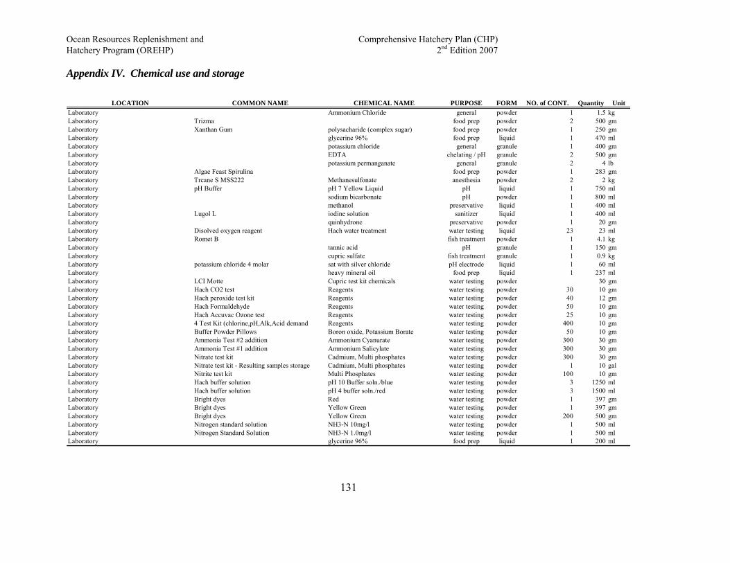
Ocean Resources Replenishment and Comprehensive Hatchery Plan (CHP) Hatchery Program (OREHP) 2nd Edition 2007
Appendix IV. Chemical use and storage
LOCATION COMMON NAME CHEMICAL NAME PURPOSE FORM NO. of CONT. Quantity UnitLaboratory Ammonium Chloride general powder 1 1.5 kgLaboratory Trizma food prep powder 2 500 gmLaboratory Xanthan Gum polysacharide (complex sugar) food prep powder 1 250 gmLaboratory glycerine 96% food prep liquid 1 470 mlLaboratory potassium chloride general granule 1 400 gmLaboratory EDTA chelating / pH granule 2 500 gmLaboratory potassium permanganate general granule 2 4 lbLaboratory Algae Feast Spirulina food prep powder 1 283 gmLaboratory Trcane S MSS222 Methanesulfonate anesthesia powder 2 2 kgLaboratory pH Buffer pH 7 Yellow Liquid pH liquid 1 750 mlLaboratory sodium bicarbonate pH powder 1 800 mlLaboratory methanol preservative liquid 1 400 mlLaboratory Lugol L iodine solution sanitizer liquid 1 400 mlLaboratory quinhydrone preservative powder 1 20 gmLaboratory Disolved oxygen reagent Hach water treatment water testing liquid 23 23 mlLaboratory Romet B fish treatment powder 1 4.1 kgLaboratory tannic acid pH granule 1 150 gmLaboratory cupric sulfate fish treatment granule 1 0.9 kgLaboratory potassium chloride 4 molar sat with silver chloride pH electrode liquid 1 60 mlLaboratory heavy mineral oil food prep liquid 1 237 mlLaboratory LCI Motte Cupric test kit chemicals water testing powder 30 gmLaboratory Hach CO2 test Reagents water testing powder 30 10 gmLaboratory Hach peroxide test kit Reagents water testing powder 40 12 gmLaboratory Hach Formaldehyde Reagents water testing powder 50 10 gmLaboratory Hach Accuvac Ozone test Reagents water testing powder 25 10 gmLaboratory 4 Test Kit (chlorine,pH,Alk,Acid demand Reagents water testing powder 400 10 gmLaboratory Buffer Powder Pillows Boron oxide, Potassium Borate water testing powder 50 10 gmLaboratory Ammonia Test #2 addition Ammonium Cyanurate water testing powder 300 30 gmLaboratory Ammonia Test #1 addition Ammonium Salicylate water testing powder 300 30 gmLaboratory Nitrate test kit Cadmium, Multi phosphates water testing powder 300 30 gmLaboratory Nitrate test kit - Resulting samples storage Cadmium, Multi phosphates water testing powder 1 10 galLaboratory Nitrite test kit Multi Phosphates water testing powder 100 10 gmLaboratory Hach buffer solution pH 10 Buffer soln./blue water testing powder 3 1250 mlLaboratory Hach buffer solution pH 4 buffer soln./red water testing powder 3 1500 mlLaboratory Bright dyes Red water testing powder 1 397 gmLaboratory Bright dyes Yellow Green water testing powder 1 397 gmLaboratory Bright dyes Yellow Green water testing powder 200 500 gmLaboratory Nitrogen standard solution NH3-N 10mg/l water testing powder 1 500 mlLaboratory Nitrogen Standard Solution NH3-N 1.0mg/l water testing powder 1 500 mlLaboratory glycerine 96% food prep liquid 1 200 ml
131
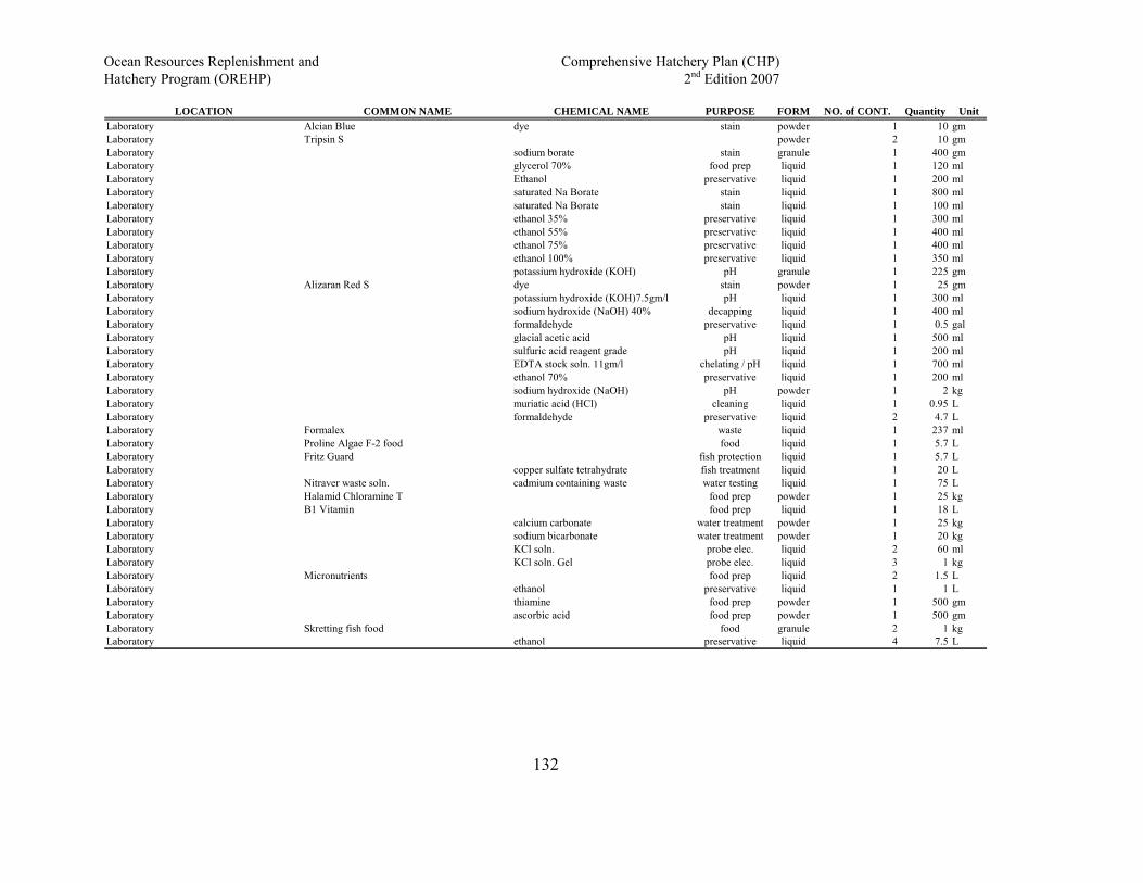
Ocean Resources Replenishment and Comprehensive Hatchery Plan (CHP) Hatchery Program (OREHP) 2nd Edition 2007
LOCATION COMMON NAME CHEMICAL NAME PURPOSE FORM NO. of CONT. Quantity UnitLaboratory Alcian Blue dye stain powder 1 10 gmLaboratory Tripsin S powder 2 10 gmLaboratory sodium borate stain granule 1 400 gmLaboratory glycerol 70% food prep liquid 1 120 mlLaboratory Ethanol preservative liquid 1 200 mlLaboratory saturated Na Borate stain liquid 1 800 mlLaboratory saturated Na Borate stain liquid 1 100 mlLaboratory ethanol 35% preservative liquid 1 300 mlLaboratory ethanol 55% preservative liquid 1 400 mlLaboratory ethanol 75% preservative liquid 1 400 mlLaboratory ethanol 100% preservative liquid 1 350 mlLaboratory potassium hydroxide (KOH) pH granule 1 225 gmLaboratory Alizaran Red S dye stain powder 1 25 gmLaboratory potassium hydroxide (KOH)7.5gm/l pH liquid 1 300 mlLaboratory sodium hydroxide (NaOH) 40% decapping liquid 1 400 mlLaboratory formaldehyde preservative liquid 1 0.5 galLaboratory glacial acetic acid pH liquid 1 500 mlLaboratory sulfuric acid reagent grade pH liquid 1 200 mlLaboratory EDTA stock soln. 11gm/l chelating / pH liquid 1 700 mlLaboratory ethanol 70% preservative liquid 1 200 mlLaboratory sodium hydroxide (NaOH) pH powder 1 2 kgLaboratory muriatic acid (HCl) cleaning liquid 1 0.95 LLaboratory formaldehyde preservative liquid 2 4.7 LLaboratory Formalex waste liquid 1 237 mlLaboratory Proline Algae F-2 food food liquid 1 5.7 LLaboratory Fritz Guard fish protection liquid 1 5.7 LLaboratory copper sulfate tetrahydrate fish treatment liquid 1 20 LLaboratory Nitraver waste soln. cadmium containing waste water testing liquid 1 75 LLaboratory Halamid Chloramine T food prep powder 1 25 kgLaboratory B1 Vitamin food prep liquid 1 18 LLaboratory calcium carbonate water treatment powder 1 25 kgLaboratory sodium bicarbonate water treatment powder 1 20 kgLaboratory KCl soln. probe elec. liquid 2 60 mlLaboratory KCl soln. Gel probe elec. liquid 3 1 kgLaboratory Micronutrients food prep liquid 2 1.5 LLaboratory ethanol preservative liquid 1 1 LLaboratory thiamine food prep powder 1 500 gmLaboratory ascorbic acid food prep powder 1 500 gmLaboratory Skretting fish food food granule 2 1 kgLaboratory ethanol preservative liquid 4 7.5 L
132
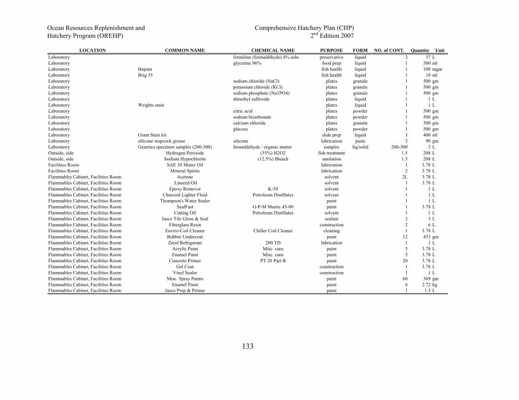
Ocean Resources Replenishment and Comprehensive Hatchery Plan (CHP) Hatchery Program (OREHP) 2nd Edition 2007
LOCATION COMMON NAME CHEMICAL NAME PURPOSE FORM NO. of CONT. Quantity UnitLaboratory formiline (formaldihyde) 4% soln. preservative liquid 2 37 LLaboratory glycerine 96% food prep liquid 1 500 mlLaboratory Hepain fish health liquid 1 180 mgmLaboratory Brig 35 fish health liquid 1 10 mlLaboratory sodium chloride (NaCl) plates granule 1 500 gmLaboratory potassium chloride (KCl) plates granule 1 500 gmLaboratory sodium phosphate (Na1PO4) plates granule 1 500 gmLaboratory dimethyl sulfoxide plates liquid 1 1 LLaboratory Wrights stain plates liquid 1 1 LLaboratory citric acid plates powder 1 500 gmLaboratory sodium bicarbonate plates powder 1 500 gmLaboratory calcium chloride plates granule 1 500 gmLaboratory glucose plates powder 1 500 gmLaboratory Gram Stain kit slide prep liquid 3 400 mlLaboratory silicone stopcock grease silicone lubrication paste 3 90 gmLaboratory Genetics specimen samples (200-300) formaldehyde / organic matter samples liq/solid 200-300 3 LOutside, side Hydrogen Peroxide (35%) H2O2 fish treatment 1.5 208 LOutside, side Sodium Hypochlorite (12.5%) Bleach sanitation 1.5 208 LFacilities Room SAE 30 Motor Oil lubrication 1 3.78 LFacilities Room Mineral Spirits lubrication 2 3.78 LFlammables Cabinet, Facilities Room Acetone solvent 2L 3.78 LFlammables Cabinet, Facilities Room Linseed Oil solvent 1 3.78 LFlammables Cabinet, Facilities Room Epoxy Remover K-50 solvent 1 1 LFlammables Cabinet, Facilities Room Charcoal Lighter Fluid Petroleum Distillates solvent 1 1 LFlammables Cabinet, Facilities Room Thompson's Water Sealer paint 1 1 LFlammables Cabinet, Facilities Room SealFast G-P-M Mastic 45-00 paint 1 3.78 LFlammables Cabinet, Facilities Room Cutting Oil Petroleum Distillates solvent 1 1 LFlammables Cabinet, Facilities Room Jasco Tile Gloss & Seal sealant 3 3 LFlammables Cabinet, Facilities Room Fiberglass Resin construction 2 6 LFlammables Cabinet, Facilities Room Enviro-Coil Cleaner Chiller Coil Cleaner cleaning 1 3.78 LFlammables Cabinet, Facilities Room Rubber Undercoat paint 12 453 gmFlammables Cabinet, Facilities Room Zerol Refrigerant 200 TD lubrication 1 1 LFlammables Cabinet, Facilities Room Acrylic Paint Misc. cans paint 5 3.78 LFlammables Cabinet, Facilities Room Enamel Paint Misc. cans paint 5 3.78 LFlammables Cabinet, Facilities Room Concrete Primer PT 20 Part B paint 20 3.78 LFlammables Cabinet, Facilities Room Gel Coat construction 1 3.78 LFlammables Cabinet, Facilities Room Vinyl Sealer construction 1 1 LFlammables Cabinet, Facilities Room Misc. Spray Paints paint 60 369 gmFlammables Cabinet, Facilities Room Enamel Paint paint 6 2.72 kgFlammables Cabinet, Facilities Room Jasco Prep & Primer paint 1 1.5 L
133
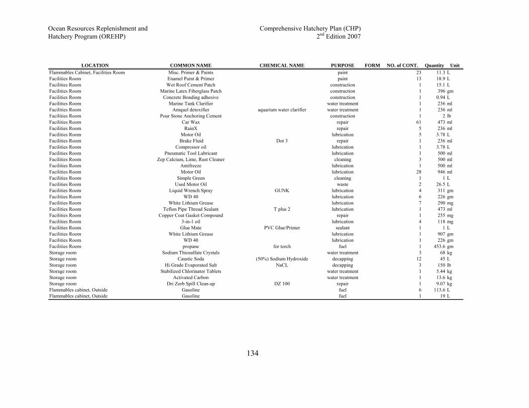
Ocean Resources Replenishment and Comprehensive Hatchery Plan (CHP) Hatchery Program (OREHP) 2nd Edition 2007
134
LOCATION COMMON NAME CHEMICAL NAME PURPOSE FORM NO. of CONT. Quantity UnitFlammables Cabinet, Facilities Room Misc. Primer & Paints paint 23 11.3 LFacilities Room Enamel Paint & Primer paint 13 18.9 LFacilities Room Wet Roof Cement Patch construction 1 15.1 LFacilities Room Marine Latex Fiberglass Patch construction 1 396 gmFacilities Room Concrete Bonding adhesive construction 1 0.94 LFacilities Room Marine Tank Clarifier water treatment 1 236 mlFacilities Room Amquel detoxifier aquarium water clarifier water treatment 1 236 mlFacilities Room Pour Stone Anchoring Cement construction 1 2 lbFacilities Room Car Wax repair 61 473 mlFacilities Room RainX repair 5 236 mlFacilities Room Motor Oil lubrication 5 3.78 LFacilities Room Brake Fluid Dot 3 repair 1 236 mlFacilities Room Compressor oil lubrication 1 3.78 LFacilities Room Pneumatic Tool Lubricant lubrication 1 500 mlFacilities Room Zep Calcium, Lime, Rust Cleaner cleaning 3 500 mlFacilities Room Antifreeze lubrication 1 500 mlFacilities Room Motor Oil lubrication 28 946 mlFacilities Room Simple Green cleaning 1 1 LFacilities Room Used Motor Oil waste 2 26.5 LFacilities Room Liquid Wrench Spray GUNK lubrication 4 311 gmFacilities Room WD 40 lubrication 6 226 gmFacilities Room White Lithium Grease lubrication 7 290 mgFacilities Room Teflon Pipe Thread Sealant T plus 2 lubrication 1 473 mlFacilities Room Copper Coat Gasket Compound repair 1 255 mgFacilities Room 3-in-1 oil lubrication 4 118 mgFacilities Room Glue Mate PVC Glue/Primer sealant 1 1 LFacilities Room White Lithium Grease lubrication 1 907 gmFacilities Room WD 40 lubrication 1 226 gmFacilities Room propane for torch fuel 1 453.6 gmStorage room Sodium Thiosulfate Crystals water treatment 3 68 kgStorage room Caustic Soda (50%) Sodium Hydroxide decapping 12 45 LStorage room Hi Grade Evaporated Salt NaCL decapping 3 150 lbStorage room Stabilized Chlorinator Tablets water treatment 1 5.44 kgStorage room Activated Carbon water treatment 1 13.6 kgStorage room Dri Zorb Spill Clean-up DZ 100 repair 1 9.07 kgFlammables cabinet, Outside Gasoline fuel 6 113.6 LFlammables cabinet, Outside Gasoline fuel 1 19 L
Ocean Resources Replenishment and Comprehensive Hatchery Plan (CHP) Hatchery Program (OREHP) 2nd Edition 2007
Appendix V. Template for Genetic Management Plan (from Tringali et al. 2007)
SECTION 1. GENERAL PROGRAM DESCRIPTION
1.1. Indicate name of hatchery and program.
1.2. Identify responsible organization and individuals:
1.2.1. Name (and title)
1.2.2. Agency
1.2.3. Address
1.2.4. Telephone
1.2.5. Fax
1.2.6. Email
1.2.7. List other agencies, collaborators, or organizations involved, and describe their
extent of involvement in the program.
1.3. List funding sources, staffing level, and annual hatchery program operational costs.
1.4. Identify location(s) of hatchery and associated facilities.
1.5. List all species subject to propagation (note: a separate GMP shall be completed for each
species under consideration).
1.5.1. Specify Endangered Species Act-listing status, if applicable, of each
species (available from www.nmfs.noaa.gov/pr/species/fish/).
1.6. Indicate type of program (e.g., stock enhancement, restoration, put-and-
take, mitigation, commercial aquaculture).
1.7. Identify specific performance goals and quantitative success criteria of the program.
1.8. Describe current program performance if the program is ongoing (indicate the source of
these data).
1.9. Provide the date release activities started or are expected to start.
1.10. State the expected duration of program.
135
Ocean Resources Replenishment and Comprehensive Hatchery Plan (CHP) Hatchery Program (OREHP) 2nd Edition 2007
SECTION 2. RELATIONSHIP OF PROGRAM TO OTHER MANAGEMENT
OBJECTIVES
2.1. Describe the alignment of the program with any management or recovery plan or other
regionally accepted policy. Explain any proposed deviations from the plan or policy.
2.2. Identify existing cooperative agreements, memoranda of understanding, memoranda of
agreement, mitigation requirements or other management plans or court orders under
which program operates.
2.3. Describe the relationship of the program to harvest objectives:
2.3.1. Identify fisheries that will benefit from the program.
2.3.2. Provide harvest levels of those fisheries for the last ten years, if available
SECTION 3. FACILITIES
3.1. Provide detailed descriptions, supplemented with diagrams, of the following: 3.1.1.
Broodfish holding and spawning facilities.
3.1.2. Incubation facilities.
3.1.3. Rearing facilities.
3.1.4. Acclimation/release facilities, if applicable.
SECTION 4. BROODFISH SOURCE
4.1. Indicate the geographic source of broodfish (include GPS coordinates of capture site for
each fish or for the area encompassed by all broodfish captures).
4.2. If possible, provide supporting information for the validation of natural stock
boundaries, including:
4.2.1. Accepted geographic boundaries for natural stocks of target species, if available.
4.2.2. Genetic and/or biological information relevant to natural stock structure of the
proposed recipient population (include literature citations and other sources), if
available.
4.2.3. Estimated current adult abundance or spawning stock biomass of each natural stock
136

Ocean Resources Replenishment and Comprehensive Hatchery Plan (CHP) Hatchery Program (OREHP) 2nd Edition 2007
that will receive fish, if available. Indicate source of information.
4.2.4. Estimated generation interval (average age of female breeders) for the natural
stock, if possible. Indicate source of information.
SECTION 5. BROODFISH COLLECTION
5.1. Describe the collection methods and sampling design for broodfish.
5.2. Describe methods to make individual broodfish identifiable and/or to segregate discrete
spawning groups of broodfish.
5.3. Specify the proposed number of broodfish to be collected from each natural stock, by
general life-history stage (adults, eggs, or juveniles).
5.4. If broodfish are currently on hand, specify the number of these collected from each
natural stock, by year and life-history stage.
5.5. Describe the intended disposition of fish collected in surplus of broodfish needs.
5.6. Describe broodfish transportation and holding methods.
SECTION 6. MATING PROCEDURES
6.1. Provide confirmation that no transgenic modifications will be performed to any fish and
that no such fish on the premises will be involved in the proposed program.
6.2. Provide confirmation that there will be no attempt at genetic improvement or other
intentional trait-specific selection during production.
6.3. Describe the timing of production in comparison to natural production and recruitment.
6.4. Provide a detailed mating scheme, including:
6.4.1. If broodfish are not wild, the number of generations they are removed from the
wild (F1, F2, etc.).
6.4.2. Description of controlled fertilization procedures (e.g., paired mating, strip-
spawning), if applicable.
6.4.3. Description of uncontrolled fertilization procedures (e.g., pond- or tank-spawning),
if applicable.
137

Ocean Resources Replenishment and Comprehensive Hatchery Plan (CHP) Hatchery Program (OREHP) 2nd Edition 2007
6.5. With supporting information, provide an estimate of variance in family size and effective
number of breeders or provide the following:
6.5.1. Minimum number of male and female breeders to be used to produce each progeny
group.
6.5.2. Expected number of progeny groups to be released.
6.5.3. Estimated average progeny group size and variance in progeny group size (at the
time of release).
6.6. Describe your plan for tracking information in 6.5.1 – 6.5.3 during operation of the
program.
SECTION 7. INCUBATION AND REARING
7.1. Describe incubation procedures, including:
7.1.1. Incubation conditions.
7.1.2. Ponding.
7.1.3. Number of eggs taken and survival rates to eye-up and/or ponding, if known.
7.1.4. Causes for, and disposition of surplus eggs, if any.
7.2. Describe your plan for tracking information in 7.1.3 – 7.1.4 during operation of program.
7.3. Describe rearing procedures, including:
7.3.1. Fish rearing conditions.
7.3.2. Provide survival rate data by hatchery life stage (fry to fingerling; fingerling to
advanced size) for the most recent five years, or for years that dependable data are
available.
7.3.3. Indicate weekly or monthly fish growth information, including length, weight, and
condition factor data collected during rearing, if available. 7.3.4. Rates of
cannibalism, if applicable.
7.4 Describe your plan for tracking information in 7.3.2 – 7.3.4 during operation of program.
138
Ocean Resources Replenishment and Comprehensive Hatchery Plan (CHP) Hatchery Program (OREHP) 2nd Edition 2007
SECTION 8. RELEASE PROCEDURES
8.1. Indicate proposed numbers and average sizes of fish to be released for the program, by age
class, release year, and natural stock (size data not required for eggs, larvae, and unfed
fry).
8.2. Indicate specific location(s) of proposed release(s) by natural stock, including the
following information:
8.2.1. For freshwater releases – Name of stream, river, or waterbody and GPS
coordinates for each release point.
8.2.2. For marine/estuarine releases - Name of estuary or description of coastal region
and GPS coordinates for each release point.
8.3. Describe your plan for tracking actual dates of release, release numbers, average sizes of
released fish, and release locations.
8.4. For any fish released to date, list actual numbers and average sizes of fish released, by age
class, release year, and natural stock (size data not required for eggs, larvae, and unfed
fry).
8.5. Describe tags or marks applied, if any, and the proportions of the total hatchery cohort
marked, to identify released individuals in subsequent captures.
8.6. Describe the disposition of fish that may be produced in excess of approved release
levels.
8.7. Describe emergency release procedures in response to flooding or other failure that may
result in unintended fish release.
SECTION 9. BEST MANAGEMENT PRACTICES
Provide a description of the precautionary approaches, procedures, and practices that will be
implemented to mitigate each of the three genetic concerns (i.e., impacts from translocation of
non-native fish, propagation-related genetic changes, and genetic swamping) identified in
sections 4.A.-4.C. of the genetic policy.
139

Ocean Resources Replenishment and Comprehensive Hatchery Plan (CHP) Hatchery Program (OREHP) 2nd Edition 2007
SECTION 10. ATTACHMENTS AND LITERATURE CITATIONS
Please include all supplemental material and literature citations to support statements
provided in sections 1-9 above.
SECTION 11. SIGNATURE OF RESPONSIBLE PARTY
Name, Title, and Signature of Applicant:
Submitted by (print) __________________________ Title
Signature _________________________________ Date __________________________
140
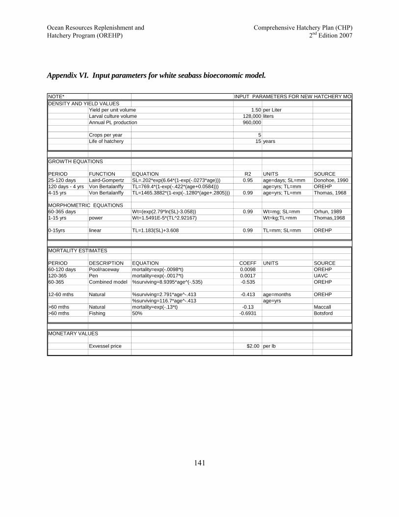
Ocean Resources Replenishment and Comprehensive Hatchery Plan (CHP) Hatchery Program (OREHP) 2nd Edition 2007
141
Appendix VI. Input parameters for white seabass bioeconomic model. NOTE* INPUT PARAMETERS FOR NEW HATCHERY MODDENSITY AND YIELD VALUES
Yield per unit volume 1.50 per LiterLarval culture volume 128,000 litersAnnual PL production 960,000
Crops per year 5Life of hatchery 15 years
GROWTH EQUATIONS
PERIOD FUNCTION EQUATION R2 UNITS SOURCE25-120 days Laird-Gompertz SL=.202*exp(6.64*(1-exp(-.0273*age))) 0.95 age=days; SL=mm Donohoe, 1990120 days - 4 yrs Von Bertalanffy TL=769.4*(1-exp(-.422*(age+0.0584))) age=yrs; TL=mm OREHP4-15 yrs Von Bertalanffy TL=1465.3882*(1-exp(-.1280*(age+.2805))) 0.99 age=yrs; TL=mm Thomas, 1968
MORPHOMETRIC EQUATIONS60-365 days Wt=(exp(2.79*ln(SL)-3.058)) 0.99 Wt=mg; SL=mm Orhun, 19891-15 yrs power Wt=1.5491E-5*(TL^2.92167) Wt=kg;TL=mm Thomas,1968
0-15yrs linear TL=1.183(SL)+3.608 0.99 TL=mm; SL=mm OREHP
MORTALITY ESTIMATES
PERIOD DESCRIPTION EQUATION COEFF UNITS SOURCE60-120 days Pool/raceway mortality=exp(-.0098*t) 0.0098 OREHP120-365 Pen mortality=exp(-.0017*t) 0.0017 UAVC60-365 Combined model %surviving=8.9395*age^(-.535) -0.535 OREHP
12-60 mths Natural %surviving=2.791*age^-.413 -0.413 age=months OREHP%surviving=116.7*age^-.413 age=yrs
>60 mths Natural mortality=exp(-.13*t) -0.13 Maccall>60 mths Fishing 50% -0.6931 Botsford
MONETARY VALUES
Exvessel price $2.00 per lb

Appendix B Procedures Manual for Growout and Release of White Seabass (Atractoscion nobilis) as Part of the Ocean Resources Enhancement and Hatchery Program (OREHP) (GPM)

PROCEDURES MANUAL FOR GROWOUT AND RELEASE OF
WHITE SEABASS (ATRACTOSCION NOBILIS) AS PART OF THE OCEAN RESOURCES ENHANCEMENT AND HATCHERY
PROGRAM (OREHP)
Prepared by:
Mark Drawbridge1 Gabriel Buhr1
Dr. Mark Okihiro2
2nd EDITION 2007
1 Hubbs-SeaWorld Research Institute 2595 Ingraham Street San Diego, CA 92109
2 California Department of Fish and Game Oceanside Fish Pathology Laboratory 4065 Oceanside Blvd - Suite G Oceanside, California 92056
i
TABLE OF CONTENTS
TABLE OF CONTENTS................................................................................................................. I
INTRODUCTION ...........................................................................................................................1
Background ..............................................................................................................................1 Purpose of Procedures Manual ..............................................................................................1 Goals and Objectives ...............................................................................................................2 Definitions .................................................................................................................................3 Historical Perspective ..............................................................................................................5
SITING AND PERMITTING..........................................................................................................7
Site Selection Criteria ..............................................................................................................7 Program requirements .........................................................................................................7 Fish health considerations...................................................................................................7 Operating considerations ....................................................................................................8 Release environment ............................................................................................................9
Permits and Approvals ............................................................................................................9 Local Authorities and Regulations ....................................................................................11 California Environmental Quality Act (CEQA).................................................................12 Aquaculture Registration Permit .......................................................................................12 Coastal Development Permit .............................................................................................13 US Army Corps of Engineers 404 Permit ..........................................................................14 National Pollutant Discharge Eliminations System Permit (NPDES) ..............................15
DESIGN AND CONSTRUCTION ...............................................................................................17
Current Designs and General Features ...............................................................................17 Net pens..............................................................................................................................20 Submerged raceways .........................................................................................................21 Land-based pools ...............................................................................................................22
Components ............................................................................................................................23 Mooring system..................................................................................................................23 Support structure ...............................................................................................................24 Predator barriers ...............................................................................................................27 Containment system ...........................................................................................................29 Feeding systems .................................................................................................................30 Circulation system .............................................................................................................31
CULTURE OPERATIONS ...........................................................................................................33
Receiving Fish ........................................................................................................................33 Food and Feeding ...................................................................................................................34
Food type and size .............................................................................................................34 Feeding schedule and daily ration.....................................................................................35
System Maintenance ..............................................................................................................40 Monitoring ..............................................................................................................................41
ii
Growout facility components .............................................................................................41 Fish losses..........................................................................................................................42 Encounters with marine mammals and birds ....................................................................43 Fish growth ........................................................................................................................45 Water quality......................................................................................................................46
FISH HEALTH..............................................................................................................................52
Assessing Fish Health ............................................................................................................52 Maintaining Growth and Vigor ............................................................................................53 Shipping specimens for examination....................................................................................57 Diseases of Cultured WSB ....................................................................................................58
Vibrio and Flexibacter bacteria ........................................................................................58 Epitheliocystis and Piscirickettsia .....................................................................................60 Viruses ...............................................................................................................................61 Parasites ............................................................................................................................63
Treatment of Diseases............................................................................................................68 Hydrogen peroxide (H2O2) ................................................................................................68 Formalin ............................................................................................................................69 Freshwater .........................................................................................................................70 Antibiotics ..........................................................................................................................70
RECORD KEEPING .....................................................................................................................72
RELEASING FISH........................................................................................................................75
LITERATURE CITED ..................................................................................................................78
APPENDICES ...............................................................................................................................79
Appendix A. Study Design for Benthic Monitoring Program ..........................................80 Appendix B. Composition of Feeds .....................................................................................90 Appendix C. Marine Mammal Mortality/Injury Reporting From (OMB 0648-0292)...91 Appendix D. MSDS for Chemicals ......................................................................................94
Formalin ............................................................................................................................95 Hydrogen Peroxide H2O2...................................................................................................96 Terramycin.........................................................................................................................98 Flexguard XI ....................................................................................................................102
INTRODUCTION
INTRODUCTION
________________________________________________________________________
2nd Edition 2007
1
Background
Since 1984, participants of the Ocean Resources Enhancement and Hatchery Program
(OREHP) have been investigating the feasibility of using cultured fishes to restore depleted wild
stocks. This research program is directed by the California Department of Fish and Game (DFG).
The primary revenues to support the OREHP are accrued from the sale of sport and commercial
marine fishing stamps to fishermen south of Point Arguello, California. Additional monies are
derived from the Federal Sportfish Restoration Act program, various mitigation sources, grants, and
private donations.
Early OREHP research included developing the culture technology (i.e. spawning induction,
larval rearing, nutrition, and disease prevention) for the program’s primary target species, white
seabass (WSB). Much of this work was conducted at Hubbs-SeaWorld Research Institute (HSWRI)
on Mission Bay, in San Diego, CA. In 1991, OREHP researchers and volunteers from the Ventura
Chapter of United Anglers began a pilot program to investigate the feasibility of using cage systems
to cost-effectively extend the growout phase of WSB culture. Based on the success of those initial
efforts, the United Anglers began to recruit other volunteer groups to develop additional growout
facilities that have since been constructed in different locations throughout southern California.
Purpose of Procedures Manual
The purposes of this procedures manual is three-fold. First, it defines all of the resource
requirements necessary to establish a growout facility for those parties interested in participating in
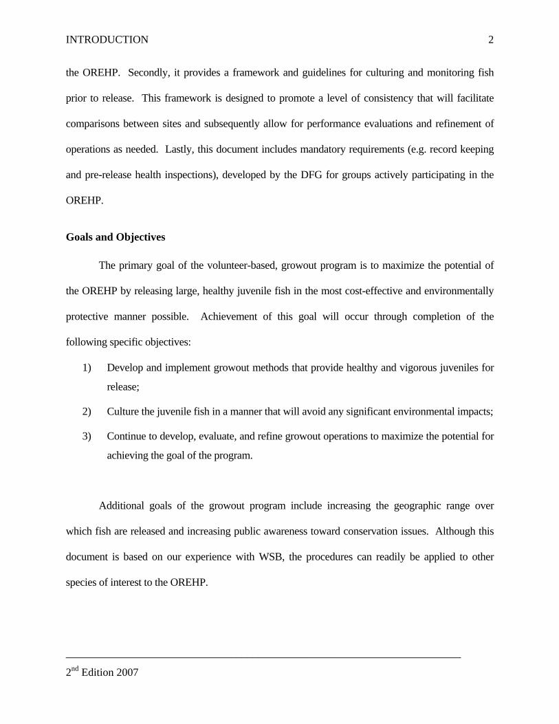
INTRODUCTION
________________________________________________________________________
2nd Edition 2007
2
the OREHP. Secondly, it provides a framework and guidelines for culturing and monitoring fish
prior to release. This framework is designed to promote a level of consistency that will facilitate
comparisons between sites and subsequently allow for performance evaluations and refinement of
operations as needed. Lastly, this document includes mandatory requirements (e.g. record keeping
and pre-release health inspections), developed by the DFG for groups actively participating in the
OREHP.
Goals and Objectives
The primary goal of the volunteer-based, growout program is to maximize the potential of
the OREHP by releasing large, healthy juvenile fish in the most cost-effective and environmentally
protective manner possible. Achievement of this goal will occur through completion of the
following specific objectives:
1) Develop and implement growout methods that provide healthy and vigorous juveniles for
release;
2) Culture the juvenile fish in a manner that will avoid any significant environmental impacts;
3) Continue to develop, evaluate, and refine growout operations to maximize the potential for
achieving the goal of the program.
Additional goals of the growout program include increasing the geographic range over
which fish are released and increasing public awareness toward conservation issues. Although this
document is based on our experience with WSB, the procedures can readily be applied to other
species of interest to the OREHP.
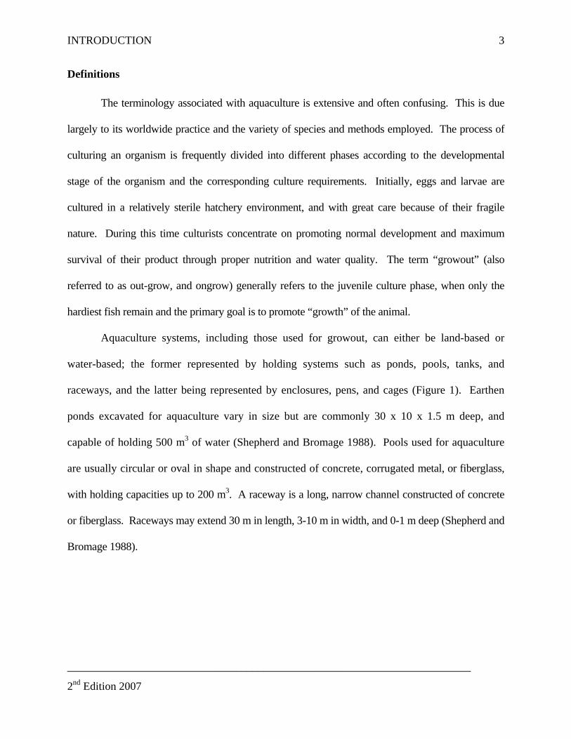
INTRODUCTION
________________________________________________________________________
2nd Edition 2007
3
Definitions
The terminology associated with aquaculture is extensive and often confusing. This is due
largely to its worldwide practice and the variety of species and methods employed. The process of
culturing an organism is frequently divided into different phases according to the developmental
stage of the organism and the corresponding culture requirements. Initially, eggs and larvae are
cultured in a relatively sterile hatchery environment, and with great care because of their fragile
nature. During this time culturists concentrate on promoting normal development and maximum
survival of their product through proper nutrition and water quality. The term “growout” (also
referred to as out-grow, and ongrow) generally refers to the juvenile culture phase, when only the
hardiest fish remain and the primary goal is to promote “growth” of the animal.
Aquaculture systems, including those used for growout, can either be land-based or
water-based; the former represented by holding systems such as ponds, pools, tanks, and
raceways, and the latter being represented by enclosures, pens, and cages (Figure 1). Earthen
ponds excavated for aquaculture vary in size but are commonly 30 x 10 x 1.5 m deep, and
capable of holding 500 m3 of water (Shepherd and Bromage 1988). Pools used for aquaculture
are usually circular or oval in shape and constructed of concrete, corrugated metal, or fiberglass,
with holding capacities up to 200 m3. A raceway is a long, narrow channel constructed of concrete
or fiberglass. Raceways may extend 30 m in length, 3-10 m in width, and 0-1 m deep (Shepherd and
Bromage 1988).
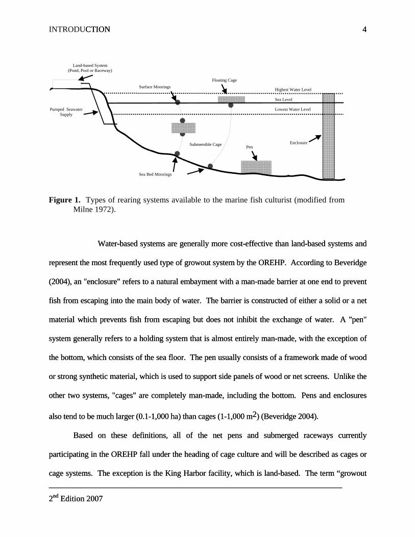
INTRODUCTIONCTION
________________________________________________________________________
2nd Edition 2007
4
________________________________________________________________________
2nd Edition 2007
4
Land-based System(Pond, Pool or Raceway)
Floating Cage
Submersible Cage Pen
Pumped SeawaterSupply
Lowest Water Level
Highest Water Level
Sea Level
Enclosure
Surface Moorings
Sea Bed Moorings
Figure 1. Types of rearing systems available to the marine fish culturist (modified from Milne 1972).
Water-based systems are generally more cost-effective than land-based systems and
represent the most frequently used type of growout system by the OREHP. According to Beveridge
(2004), an "enclosure" refers to a natural embayment with a man-made barrier at one end to prevent
fish from escaping into the main body of water. The barrier is constructed of either a solid or a net
material which prevents fish from escaping but does not inhibit the exchange of water. A "pen"
system generally refers to a holding system that is almost entirely man-made, with the exception of
the bottom, which consists of the sea floor. The pen usually consists of a framework made of wood
or strong synthetic material, which is used to support side panels of wood or net screens. Unlike the
other two systems, "cages" are completely man-made, including the bottom. Pens and enclosures
also tend to be much larger (0.1-1,000 ha) than cages (1-1,000 m2) (Beveridge 2004).
Based on these definitions, all of the net pens and submerged raceways currently
participating in the OREHP fall under the heading of cage culture and will be described as cages or
cage systems. The exception is the King Harbor facility, which is land-based. The term “growout
Based on these definitions, all of the net pens and submerged raceways currently
participating in the OREHP fall under the heading of cage culture and will be described as cages or
cage systems. The exception is the King Harbor facility, which is land-based. The term “growout

INTRODUCTIONCTION
________________________________________________________________________
2nd Edition 2007
5
________________________________________________________________________
2nd Edition 2007
5
facility” is used when talking about all three types of systems (land-based, net pen, and submerged
raceway).
facility” is used when talking about all three types of systems (land-based, net pen, and submerged
raceway).
Historical Perspective Historical Perspective
In 2005 there were fourteen growout facilities in operation at 11 coastal sites (Figure 2 and
Table 1) in southern California. A total of over 225,000 WSB have been successfully cultured,
tagged and released from these facilities, while hundreds of thousands of others have been released
directly from the hatchery.
Figure 2. Site map showing locations of OREHP growout facilities.
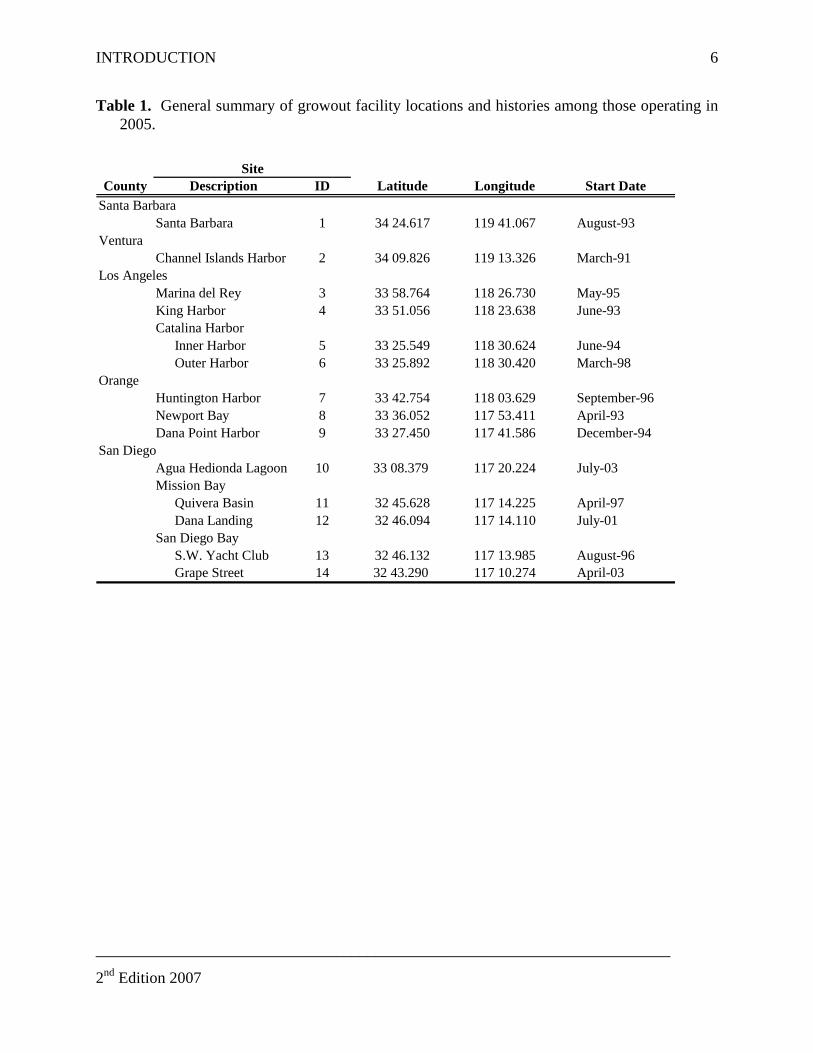
INTRODUCTION
________________________________________________________________________
2nd Edition 2007
6
Table 1. General summary of growout facility locations and histories among those operating in 2005.
County Description ID Latitude Longitude Start Date
Santa Barbara 1 34 24.617 119 41.067 August-93Ventura
Channel Islands Harbor 2 34 09.826 119 13.326 March-91
Marina del Rey 3 33 58.764 118 26.730 May-95King Harbor 4 33 51.056 118 23.638 June-93Catalina Harbor
Inner Harbor 5 33 25.549 118 30.624 June-94Outer Harbor 6 33 25.892 118 30.420 March-98
OrangeHuntington Harbor 7 33 42.754 118 03.629 September-96Newport Bay 8 33 36.052 117 53.411 April-93Dana Point Harbor 9 33 27.450 117 41.586 December-94
Agua Hedionda Lagoon 10 33 08.379 117 20.224 July-03Mission Bay
Quivera Basin 11 32 45.628 117 14.225 April-97Dana Landing 12 32 46.094 117 14.110 July-01
San Diego BayS.W. Yacht Club 13 32 46.132 117 13.985 August-96Grape Street 14 32 43.290 117 10.274 April-03
Santa Barbara
Los Angeles
San Diego
Site
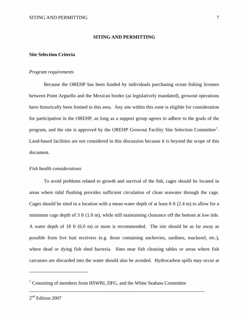
SITING AND PERMITTING
SITING AND PERMITTING
________________________________________________________________________
2nd Edition 2007
7
Site Selection Criteria
Program requirements
Because the OREHP has been funded by individuals purchasing ocean fishing licenses
between Point Arguello and the Mexican border (as legislatively mandated), growout operations
have historically been limited to this area. Any site within this zone is eligible for consideration
for participation in the OREHP, as long as a support group agrees to adhere to the goals of the
program, and the site is approved by the OREHP Growout Facility Site Selection Committee1.
Land-based facilities are not considered in this discussion because it is beyond the scope of this
document.
Fish health considerations
To avoid problems related to growth and survival of the fish, cages should be located in
areas where tidal flushing provides sufficient circulation of clean seawater through the cage.
Cages should be sited in a location with a mean water depth of at least 8 ft (2.4 m) to allow for a
minimum cage depth of 3 ft (1.0 m), while still maintaining clearance off the bottom at low tide.
A water depth of 18 ft (6.0 m) or more is recommended. The site should be as far away as
possible from live bait receivers (e.g. those containing anchovies, sardines, mackerel, etc.),
where dead or dying fish shed bacteria. Sites near fish cleaning tables or areas where fish
carcasses are discarded into the water should also be avoided. Hydrocarbon spills may occur at
1 Consisting of members from HSWRI, DFG, and the White Seabass Committee
SITING AND PERMITTING
________________________________________________________________________
2nd Edition 2007
8
fueling docks, and fine toxic particles may be generated near shipyards where boats are sanded
and painted. Cages should not be placed near sewage outfalls, which may promote algal blooms,
net fouling, and heavy metal accumulation. Thermal effluent from power plant cooling water is
generally not an asset for WSB culture because WSB are highly susceptible to gas bubble
disease, which is primarily caused by supersaturated waters.
Operating considerations
The considerations relative to constructing and operating a cage system include physical
parameters such as the degree of exposure to wind and currents. Cage systems located in exposed
areas will have to withstand more extreme ocean conditions, especially during adverse weather,
which will place greater stresses on the system and may also hinder culture and maintenance
operations. Water depth has obvious implications for the mooring requirements, which will further
impact the stability, maintenance, and cost of the facility.
In addition to the physical site selection criteria for cages, are logistical considerations such
as permitting, access, security, expandability and support. A cage facility sited in a public area will
generally require more permits and approvals than one sited in a private area. A similar statement
can be made about mooring a cage in an area not previously designated for moorings. Accessibility
is one of the primary considerations for siting a cage facility that is to be operated by volunteers.
Because the culture operation is being serviced by volunteers and researchers, cage facilities should
be readily accessible by foot or by a short boat trip. An accessible cage simplifies maintenance of
the system, and transfer, culture and daily maintenance of fish. Access to electricity may also be a
consideration, especially for raceways which have to be vacuumed. Automatic feeders can be
operated easily using solar power. The benefits of easy access must also be weighed against the
SITING AND PERMITTING
________________________________________________________________________
2nd Edition 2007
9
increased risk of vandalism. The ability to physically expand the scale of culture operations is
another consideration when siting a facility. Those involved in start-up operations are advised to
keep their facilities relatively small and simple initially. However, once the site and operation have
been tested, a larger culture volume may be desired to meet OREHP’s annual release goals.
Participants should discuss the option for expanding the cage facility with the appropriate local
agencies early in the planning stage. Adequate local volunteer support is also an important
consideration. The man hours required to maintain a cage culture operation depend primarily on
local water conditions and the facility design. A minimum of 2 hours per day can be expected with
greater time commitments during special activities such as receiving, releasing or treating fish, and
cleaning the cage. If one volunteer group cannot fully support a cage operation, then other groups
should be sought to join the effort.
Release environment
Optimal release areas are not fully defined for WSB, primarily because WSB range freely
along the coast and in and out of embayments. In this regard, consideration of proximity to suitable
release areas is not a high priority. The greatest consideration related to release is the ability to
minimize handling and netting the fish in order to release them. Another priority is to minimize
proximity to areas that attract known predators such as birds, seals and sea lions (e.g. bait receivers
or other haul-out sites).
Permits and Approvals
An extensive discussion of the permitting process for growout facilities is beyond the
scope of this manual, however a general description of the process is provided. The permitting
requirements for development in California's coastal zone are very involved and often requires
SITING AND PERMITTING
________________________________________________________________________
2nd Edition 2007
10
outside consultation. This process is also site and project-specific. Table 2 lists the permits and
permissions required to operate an OREHP growout facility. The GFC and the OREHP
Coordinator (DFG employee) may be able to provide assistance with several of the permitting
authorities including the California Coastal Commission (CCC), US Army Corps of Engineers,
US Coast Guard, US Fish and Wildlife Service, NOAA Fisheries, State Lands Commission and
the State and Regional Water Quality Boards. The growout facility operator will need to contact
the local authority (City, County, and Port Authority) for the necessary permission and provide
information to the GFC and the OREHP Coordinator.
Prior to applying for local and state permits, a verbal approval to participate in the
OREHP should be obtained from the OREHP coordinator and the OREHP Advisory Panel. This
approval will be based largely on the needs of the program, the location of the proposed facility,
and verification that enough volunteers are willing to support the new facility. Once the concept
is approved by the OREHP Coordinator and the OREHP Advisory Panel, then the OREHP
Growout Site Selection Committee should be consulted to ensure that the site meets the criteria
set forth in the previous section.
SITING AND PERMITTING
________________________________________________________________________
2nd Edition 2007
11
Table 2. Permits and permissions required to operate an OREHP growout facility. Regulatory Authority Permit or Permission Department of Fish and Game Permission to participate in OREHP California Coastal Commission Coastal Development Permit (CDP)
State Lands Commission State Lands Lease is required if the tidelands have not been granted to a local authority
State Water Quality Control Board 401 Certification – in the past, this has been waived because the US Army Corps of Engineers has not issued 404 permits 404 permit (large facility) or US Army Corps of Engineers letter of permission (small facility)
US Coast Guard Private Aids to Navigation Permit
US Fish and Wildlife Service Section 7 Endangered Species Act Consultation
NOAA Fisheries Letter of permission indicating no species of concern will be impacted
Local Authority (City, County, Port Authority) Requirements vary depending on the authority National Pollution Discharge Elimination System (NPDES) permit (large facility) or National Pollution Discharge Elimination System (NPDES) waiver (small facility) – may contain monitoring requirements Regional Water Quality Control Board
National Pollution Discharge Elimination System (NPDES) waiver (small facility) – may contain monitoring requirements
Local Authorities and Regulations
Prior to filing applications with the various state and federal government agencies, you
should identify each of the local authorities in the area proposed for siting the facility. These
agencies may include the Harbor Patrol, US Coast Guard, Waterfront Director, County Parks
Department, and City Planning Commission. Plan to meet with each party and discuss the
feasibility of establishing a growout facility. At each meeting be prepared to explain the scope
of the project, as well as give a clear description of your proposal.
SITING AND PERMITTING
________________________________________________________________________
2nd Edition 2007
12
California Environmental Quality Act (CEQA)
The California Environmental Quality Act (CEQA) (Public Resources Code (PRC)
Section 21000 et seq.) was enacted in 1970 as a means of coordinating the development permit
process with the environmental review process. The environmental review process is
characterized as the identification of (1) significant effects that a project may have on the
environment, (2) alternatives to the project, and (3) methods by which significant effects can be
avoided or mitigated. An Environmental Impact Report (EIR) is required when there is
substantial evidence in the record that a project will result in significant impacts to the
environment. The type of environmental analyses required by CEQA is determined by the lead
agency involved in the permitting process. Because cage facilities are below the mean high tide
line, they are subject to the jurisdiction of the CCC. The CCC, through its Coastal Development
Permit (CDP) requirements, provides an equivalency to the environmental review of CEQA.
A CEQA document covering the entire OREHP, including the hatchery and growout
facilities, is currently in preparation. This document will likely be certified in 2007. If a new
facility comes online after adoption of the CEQA document it may trigger an addendum or
supplemental document.
Aquaculture Registration Permit
The DFG maintains regulatory authority over all aquaculture projects, primarily through
its registration process. Every commercial aquaculture project in California must register with
the DFG, which in turn will evaluate the appropriateness of the species being proposed for
culture and the design of the facility.

SITING AND PERMITTING
________________________________________________________________________
2nd Edition 2007
13
OREHP is not a commercial aquaculture venture, but an enhancement program. As a result, an
Enhancement Plan is now required by statute (Fish and Game Code Section 15400). The DFG
will be preparing a White Seabass Enhancement Plan in 2007 for adoption by the Fish and Game
Commission.
Coastal Development Permit
A Coastal Development Permit (CDP) is required by any person or public agency
proposing development within the coastal zone. In general, the coastal zone extends from the
State’s three-mile seaward limit to an average of approximately 1,000 yards inland from the
mean high tide of the sea (California Technology, Trade and Commerce Agency (CTTCA)
2002). When a project is proposed below the mean high tide line (i.e. cage facilities) this permit
must be obtained from the CCC. Land-based facilities must obtain a CDP from the CCC or the
city or county having authority to issue CDPs. Because the OREHP is a DFG program, the DFG
will serve as a co-applicant on the CDP for all growout facilities that are specifically designed as
such for the OREHP.
The California Coastal Act of 1976 (PRC Section 30000 et seq.) authorized the CCC to
issue CDPs until such time as the cities and counties within the coastal zone obtained
certification of their own local coastal development programs. The CCC retains permit authority
over tidelands, submerged lands, and certain lands held in the public trust. The CCC also retains
the authority to determine whether federal project activity in the coastal zone and the Outer
Continental Shelf is consistent with state policies for the coast (CTTCA 2002).
In addition to overseeing and regulating development along California's coast, the CCC
has a chartered responsibility to monitor human impacts to coastal water resources. Public
SITING AND PERMITTING
________________________________________________________________________
2nd Edition 2007
14
Resources Code Section 30230 of the Coastal Act provides that "Marine resources shall be
maintained, enhanced, and where feasible, restored. Special protection shall be given to areas
and species of special biological or economic significance. Uses of the marine environment shall
be carried out in a manner that will sustain the biological productivity of coastal waters and that
will maintain healthy populations of all species of marine organisms adequate for long-term
commercial, recreational, scientific, and educational purposes". In addition, PRC Section 30231
states, in part "The biological productivity and quality of coastal waters . . . appropriate to
maintain optimum populations of marine organisms and for the protection of human health shall
be maintained and where feasible, restored . . . ". It is clear from these statements that the goals
of the OREHP, and its associated volunteer growout facility program, are consistent with the
objectives of the Coastal Act.
The fee for the CDP is typically $600 for projects with development costs under
$100,000. However, for growout facilities associated with DFG through OREHP, this fee may
be waived by the CCC’s Executive Director if the DFG participates as a co-applicant. The
processing time for a CDP is several months. This application should be submitted first.
US Army Corps of Engineers 404 Permit
A 404 permit from the US Army Corps of Engineers (USACE) is required by any person
or public agency proposing to locate a structure, excavate, or discharge dredged or fill material
into waters of the United States or to transport dredged material for the purpose of dumping it
into ocean waters. The USACE permit authority is derived from the Federal Rivers and Harbors
Act of 1899 (Section 10, 33USC 403), the Clean Water Act (Section 404, 33USC 1344), and the
Marine Protection, Research, & Sanctuaries Act (Section 103, 33USC 1413). These Acts give
SITING AND PERMITTING
________________________________________________________________________
2nd Edition 2007
15
the USACE jurisdiction over all navigable waters including marshes, swamps, and diked lands,
even though they may not actually be navigable (CTTCA 2002).
The fee for the USACE 404 Permit is approximately $100 and the processing time is 2-4
months. This application should be submitted concurrent to, or shortly after, the CDP. At this
time, the USACE is issuing a Letter of Permission (LOP) rather than a 404 Permit due to the
small nature of the growout facilities. Despite this, you will still need to fill out the application
so that the USACE can determine whether a LOP or 404 Permit is appropriate. The USACE will
not give final approval on your LOP or 404 permit application until they have received proof of
final approval for the CDP from the CCC.
National Pollutant Discharge Eliminations System Permit (NPDES)
An NPDES permit is required by the owner or operator of any facility that is currently
discharging or will be discharging waste into any surface waters of the state (CTTCA 2002).
Among the NPDES point source categories are Concentrated Aquatic Animal Production
(CAAP) facilities, under which aquaculture projects are regulated. A facility is considered a
CAAP facility if it meets certain US Environmental Protection agency (EPA) criteria or on a
case-by-case basis at the discretion of the NPDES program director (EPA 2004). Most facilities
classified as a CAAP are either flow-through, recirculating or cage systems. The criteria for a
CAAP facility are different for cold water and warm water species. Species of interest to the
OREHP fall into the category of “warm water” because they spawn at temperatures above 16°C
and prefer temperatures above 20°C (Kim Driver, EPA, personal communication). Warm water
facilities that produce less than 45 metric tonnes (MT) (100,000 lbs) do not require permits (EPA
2004).

SITING AND PERMITTING
________________________________________________________________________
2nd Edition 2007
16
Maximum production capacities for all of the OREHP growout facilities fall well below
the 45 MT limit established by the EPA for CAAPs. In fact, 2004 production of 271,000 fish for
the entire OREHP totaled only 41 MT (90,200 lb). The EPA has also established exclusions (of
the 45 MT limit) for non-profit facilities that raise salmon for release into the wild (EPA 2004).
Although OREHP growout facilities are well below the EPA threshold for an NPDES
permit, we have developed a Benthic Monitoring Program that was implemented in 2004
(Appendix A). The Benthic Monitoring Program assesses impacts to the bottom from the
growout facilities.
DESIGN AND CONSTRUCTION
DESIGN AND CONSTRUCTION
________________________________________________________________________
2nd Edition 2007
17
Current Designs and General Features
Currently, there are three facility design categories being used to culture WSB in the
OREHP. The first is a traditional design where the cage is moored in open water or along side a
dock and a net “bag” is used to contain the fish. The net is supported by a flexible frame of free-
floating high-density polyethylene (HDPE) or wood that is buoyed by pontoons. The second design
consists of a submerged, fiberglass raceway that is affixed to a floating dock, typically in a protected
marina. The third growout facility design category currently employed by the OREHP is a land-
based system utilizing fiberglass or vinyl pools to hold the fish and pumps to deliver the water.
Because none of the designs have been standardized and different sites have different water
characteristics, it is difficult to identify the more efficient or “better” system. From a fish production
standpoint, under normal operations, there is no evidence suggesting improved growth or survival of
the WSB in one system over the others. However, catastrophic failures have been most often
associated with land-based systems, followed by submerged raceways and then net cages. From an
operational standpoint, biofouling is a major factor in operating any growout facility and removing
fouling organisms (e.g. shellfish, bryozoans, hydroids and sponges) represents the greatest
maintenance task because the animals clog nets, screens, and pipes.
Photographs of each growout facility are provided in Figure 3 and general design
specifications are given in Table 3.
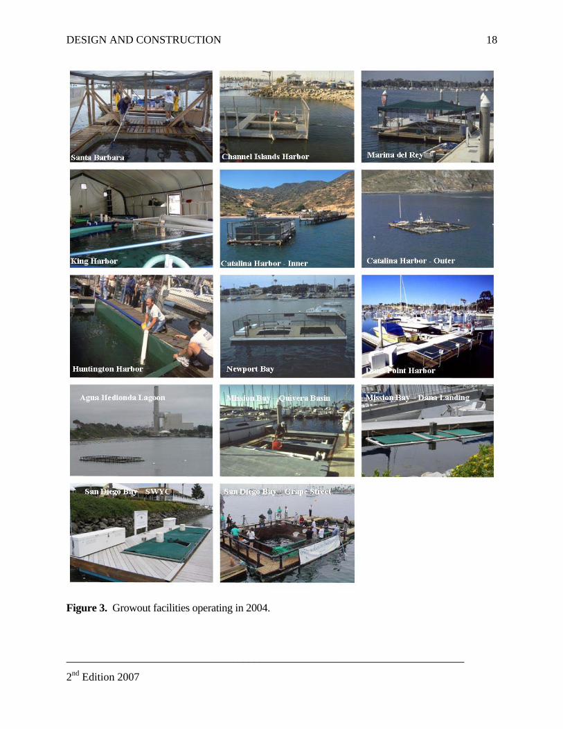
DESIGN AND CONSTRUCTION
________________________________________________________________________
2nd Edition 2007
18
Figure 3. Growout facilities operating in 2004.

DESIGN AND CONSTRUCTIONND CONSTRUCTION
________________________________________________________________________
2nd Edition 2007
19
________________________________________________________________________
2nd Edition 2007
19
Length or Subunit Subunit Total Max. EstimatedSystem Diameter Width Depth Numbers Volume Culture Vol Production
Site Type Access ft (m) ft (m) ft (m) (#)* gal (cubic m)** gal (cubic m) lbs (kg)***
Barbara Net Boat 18 (5.5) 18 (5.5) 10 (3.0) 1 24,240 (92) 24,240 (92) 3,028 (1,376)
annel Islands Harbor Net Doc
Length or Subunit Subunit Total Max. EstimatedSystem Diameter Width Depth Numbers Volume Culture Vol Production
County Site Type Access ft (m) ft (m) ft (m) (#)* gal (cubic m)** gal (cubic m) lbs (kg)***Santa Barbara
Santa Barbara Net Boat 18 (5.5) 18 (5.5) 10 (3.0) 1 24,240 (92) 24,240 (92) 3,028 (1,376)Ventura
Channel Islands Harbor Net Doc
CountySanta Barbara
Santa Ventura
Ch k 16 (4.9) 16 (4.9) 8 (2.4) 3 15,320 (58) 45,960 (174) 5,742 (2,610)Los Angeles
Marina del Rey Raceway Dock 16 (4.9) 8 (2.4) 4 (1.2) 2 3,830 (14) 7,660 (29) 957 (435)King Harbor Pool Land 17 (5.2) 3.2 (1.0) 2 5,518 (21) 11,037 (42) 1,503 (683)
Pool Land 12 (3.7) 3.5 (1.1) 1 2,961 (11) 2,961 (11) 423 (192)Catalina Harbor
Inner Harbor Net Boat 16 (4.9) 8 (2.4) 18 (5.5) 4 17,237 (65) 68,948 (261) 8,613 (3,915)Outer Harbor Net Boat 30 (9.1) 30 (9.1) 22 (6.7) 4 148,131 (561) 592,523 (2,243) 74,017 (33,644)
OrangeHuntington Harbor Raceway Dock 16 (4.9) 8 (2.4) 4 (1.2) 1 3,830 (14) 3,830 (14) 478 (217)Newport Bay Raceway Boat 16 (4.9) 8 (2.4) 3.5 (1.1) 4 3,352 (13) 13,407 (51) 1,675 (761)Dana Point Harbor Net Dock 24 (7.3) 10 (3.0) 4 (1.2) 1 7,182 (27) 71,82 (27) 897 (408)
Net Dock 18 (5.5) 6 (1.8) 4 (1.2) 1 3,232 (12) 3,232 (12) 404 (184)San Diego
Agua Hedionda Lagoon Net Boat 24 (7.3) 24 (7.3) 12 (3.7) 2 51,711 (196) 103,422 (391) 12,919 (5,872)Mission Bay
Quivera Basin Net Dock 20 (6.1) 8 (2.4) 8 (2.4) 1 9,576 (36) 9,576 (36) 1,196 (544)Dana Landing Net Dock 20 (6.1) 3 (1.2) 4 (1.2) 1 2,394 (9) 2,394 (9) 299 (136)
San Diego BayS.W. Yacht Club Raceway Dock 24 (7.3) 6 (1.8) 3.5 (1.1) 1 3,771 (14) 3,771 (14) 471 (214)Grape Street Net Dock 18 (5.5) 18 (5.5) 12 (3.7) 1 29,087 (110) 29,087 (110) 3,634 (1,652)
Net Dock 18 (5.5) 18 (5.5) 7 (2.1) 1 16,968 (64) 16,968 (64) 2,120 (963)total volume 941,772 (3,565) 117,645 (53,475)
* A subunit is defined as one or more separate culture areas within a cage** 1 cubic foot is equal to 7.48 gallons*** Maximum production is based on a conservative harvest density of 0.12 lb/gallon (15kg/m3)
DESIGN AND CONSTRUCTION
________________________________________________________________________
2nd Edition 2007
20
Net pens
Net pens greatly facilitate water exchange because water can move through the net mesh
from any direction. This high surface area for water exchange and lack of mechanical pumping
makes net pens the most “fool proof” system against failures that lead to low dissolved oxygen.
Furthermore, tidal action at well-sited net pens ensures that the water is well oxygenated, which
promotes good growth and overall health. The value of good water exchange and reduced risk of
system failure cannot be understated because those have historically been the most frequent causes
of catastrophic losses among the OREHP growout facilities.
Net pens can also be brushed clean when they become fouled, although it is generally more
difficult because the walls are not rigid. A good method for cleaning containment nets is to use
twine to stitch one end of a clean net to the end of the fouled net while the dirty net is still in the
water holding fish. The fouled net is then pulled out at the opposite end of the net pen (from the
stitched side) and as it is retrieved it is replaced by the clean net. Divers are also commonly used to
clean nets while the nets are submerged and holding fish. Between growout cycles, nets should be
removed, cleaned and repaired as necessary. An EPA-approved antifoulant is also available for
dipping nets2, which is usually done by the manufacturer at the time of purchase. The OREHP has
used treated nets historically but is slowly rotating them out of use by replacing them with untreated
nets as the treated nets age.
2 Flexgard XI, EPA Registration No. 9339-19, Flexabar Corporation, 1969 Rutgers University Blvd, Lakewood, NJ. 08701 (see Appendix C for MSDS).

DESIGN AND CONSTRUCTION
________________________________________________________________________
2nd Edition 2007
21
Feeding fish in net pens can be done by hand or using automatic feeders that are powered
electrically or by solar energy. Overfeeding is not good in any system including net pens. Because
net pens are often much deeper than other growout systems and the food can fall through the
meshing to the ocean floor, it can be difficult to monitor overfeeding. Feeding to excess has a
negative impact on the environment and the economic efficiency of the OREHP and should be
avoided. The OREHP minimizes this as a potential impact by monitoring food usage and fish
growth at each facility from which food conversion rates can be calculated and monitored. In
addition, the OREHP benthic monitoring survey is designed to measure these types of effects.
Crowding fish for sampling is relatively easy in net pens and can be accomplished by slowly
pulling up a portion of the net. Releasing fish is also easily accomplished by lowering a section of
the net and allowing the fish to swim out. Net pen frames can be made of flexible materials, such as
HDPE, which allows them to be placed in more exposed locations.
Submerged raceways
The initial design of submerged raceways used by the OREHP had solid side and bottom
walls with screens at either end. The design changed over time and rigid mesh “windows” of
varying sizes were installed in the sides and the bottom of most systems to promote water exchange,
thus creating a hybrid raceway design. However, some combinations of design and siting still do not
provide adequate water exchange from tidal action and therefore require mechanical devices to help
move water. These devices, primarily pumps or aerators, require electrical power, which cost
money to operate and are also subject to mechanical failure. The most popular feature of raceways
is the smooth surface of the fiberglass walls, which can easily be scrubbed to remove algae and
encrusting organisms that would otherwise create an abrasive surface. Screens at either end of
DESIGN AND CONSTRUCTION
________________________________________________________________________
2nd Edition 2007
22
raceways must be cleaned routinely to remove fouling organisms and maintain good water
exchange. Excessive fouling, especially during warm water conditions, has caused catastrophic
losses of fish in several submerged raceways due to low dissolved oxygen.
Feeding levels are generally easier to monitor in submerged raceways because they are
shallow and the feeding response of the fish is more obvious. Furthermore, except in high current
areas, any uneaten food will remain visible on the bottom of the raceway. Excess food and detritus
in a submerged raceway should be vacuumed from the system routinely so as not to degrade water
quality.
Crowding fish for sampling is easily accomplished in submerged raceways by pulling a
purpose-built seine net from one end of the raceway to the other. Releasing fish is also easily
performed by raising the end gate and allowing the fish to swim out. Because submerged raceways
are rigid, they are better suited for protected waterways. This siting restriction may impose
limitations on the overall size of a given raceway system.
Land-based pools
Land-based pool systems require pumps to provide water flow and aerators to supplement
oxygen. Because these life support systems require electricity, provisions must be made for backup
power and aeration, as well as the daily costs to operate the pumps. Water exchange in pools can be
flow-through or recirculated. Recirculating systems are often very complex because of the number
and variety of components. For this reason they typically require additional expertise to operate. A
thorough discussion of different types of land-based recirculation systems is beyond the scope of this
manual.
DESIGN AND CONSTRUCTION
________________________________________________________________________
2nd Edition 2007
23
As in submerged raceways, feeding levels are generally easy to monitor in pools because the
fish are clearly visible. Circular pools can be made to be self-cleaning by using directional water
currents to create a vortex to move waste to a drain positioned in the center of the pool. Any feed or
detritus not cleaned automatically should be routinely vacuumed from the system so high water
quality standards are maintained in the pool.
Crowding fish for sampling is easy in pools and can be accomplished by lowering the water
level and netting the fish. Releasing fish from land-based pools is generally difficult because fish
must be netted from pools into a transport tank and then driven to the nearest suitable release site.
This process increases the stress on the fish, which likely has a negative effect on post-release
survival.
Components
The major components of a cage system are described in this section and they include the
support frame, predator screens, and the mooring, containment, circulation and feeding systems
(Figure 4). The materials and equipment used to construct and operate the cage system must
withstand local weather conditions and be durable in seawater. Land-based systems are touched on
only briefly because they are beyond the scope of this document. The Comprehensive Hatchery
Plan gives a detailed description of considerations for rearing marine finfish on land.
Mooring system
A mooring system is required to keep open-water cages stationary, even under the forces of
waves, wind, and currents. The requirements for the mooring system are determined largely by the
cage design and the characteristics of the site. When cages are constructed within embayments, the
builder should seek advice from a local boat mooring company for recommendations on how and

DESIGN AND CONSTRUCTION
________________________________________________________________________
2nd Edition 2007
24
where to moor the cage and what the cost will be for installation. If a cage is to be moored offshore,
consultation with a commercial cage manufacturer is recommended. The U.S. Coast Guard will also
have to be consulted to determine requirements for marking the structure (e.g. lights, reflectors)
because of its potential hazard to navigation. A mooring configuration for a two cage system in
Agua Hedionda Lagoon is shown in Figure 5.
Support structure
The support frame provides a solid foundation for the containment and predator nets, and
decking. Larger cage systems, especially those in semi-exposed locations, utilize HDPE pipe for
both support and floatation (Figure 6). Typically, dual floatation pipes of approximately 25.4 cm
(10 in.) diameter are used. HDPE stanchions of approximately 10.1 cm (4 in.) diameter are used to
support inner and outer railings for hanging nets. Treated hardwood is typically used for decking.
Smaller cages in protected embayments often utilize hardwood for the framework. Buoyancy can be
provided by commercially available dock floats or air-filled drums, which are secured to the
underside of the walkway or adjacent to the support frame.

DESIGN AND CONSTRUCTION
________________________________________________________________________
2nd Edition 2007
25
a)
b)
Overhead Predator Barrier(bird netting)
Entry Gate
Support Structure(decking on buoyant
pontoons)
Subsurface Predator Barrier(cargo-type netting)Mooring System
Automatic Feeder
Containment System(Nylon Netting)
Automatic Feeder
Combination Predator BarrierAnd Shade Structure
(chain link with shade cloth)
Optional Aerator(agitator type or air pump)
Combination Predator BarrierAnd Containment System
(fiberglass raceway)
Lock Box(for food and supplies)
Support Structure(boat dock)
Figure 4. Diagram illustrating the different components of two types of cage systems currently being used to culture WSB. a) traditional net pen, b) submerged raceway.
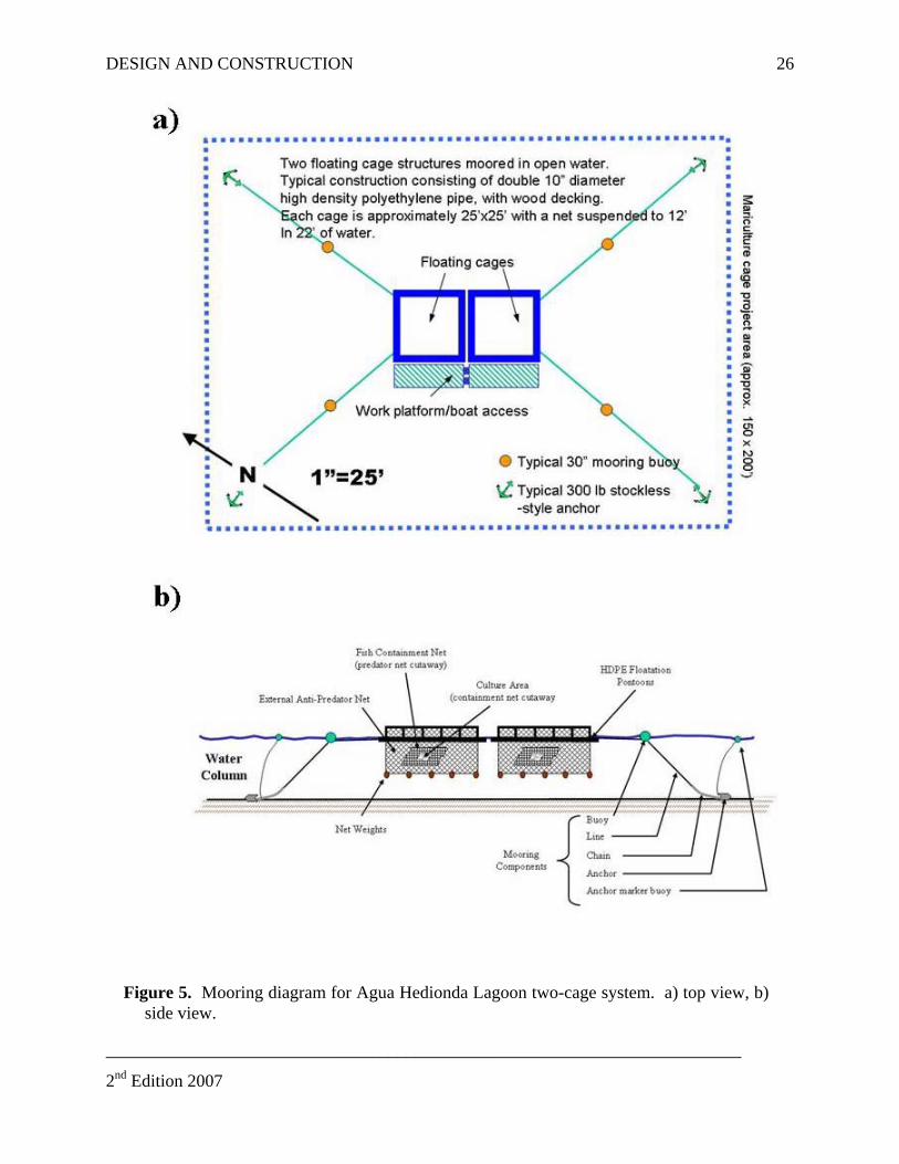
DESIGN AND CONSTRUCTION
________________________________________________________________________
2nd Edition 2007
26
Figure 5. Mooring diagram for Agua Hedionda Lagoon two-cage system. a) top view, b) side view.
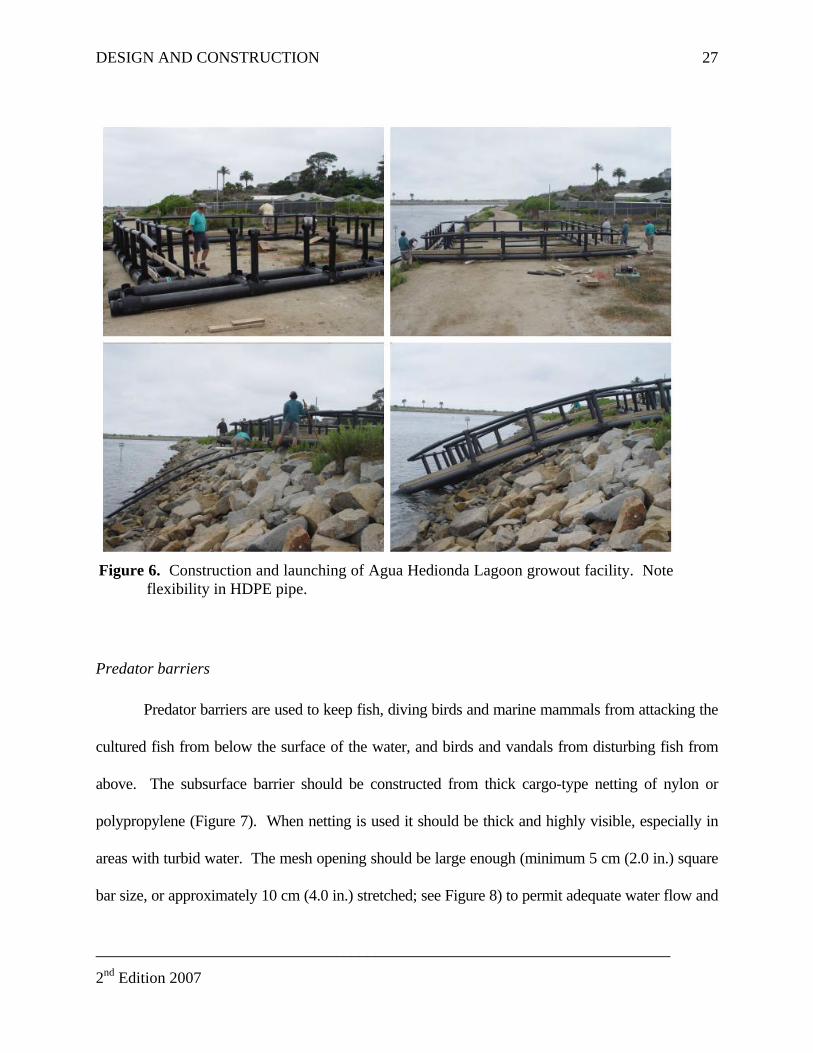
DESIGN AND CONSTRUCTION
________________________________________________________________________
2nd Edition 2007
27
Figure 6. Construction and launching of Agua Hedionda Lagoon growout facility. Note flexibility in HDPE pipe.
Predator barriers
Predator barriers are used to keep fish, diving birds and marine mammals from attacking the
cultured fish from below the surface of the water, and birds and vandals from disturbing fish from
above. The subsurface barrier should be constructed from thick cargo-type netting of nylon or
polypropylene (Figure 7). When netting is used it should be thick and highly visible, especially in
areas with turbid water. The mesh opening should be large enough (minimum 5 cm (2.0 in.) square
bar size, or approximately 10 cm (4.0 in.) stretched; see Figure 8) to permit adequate water flow and
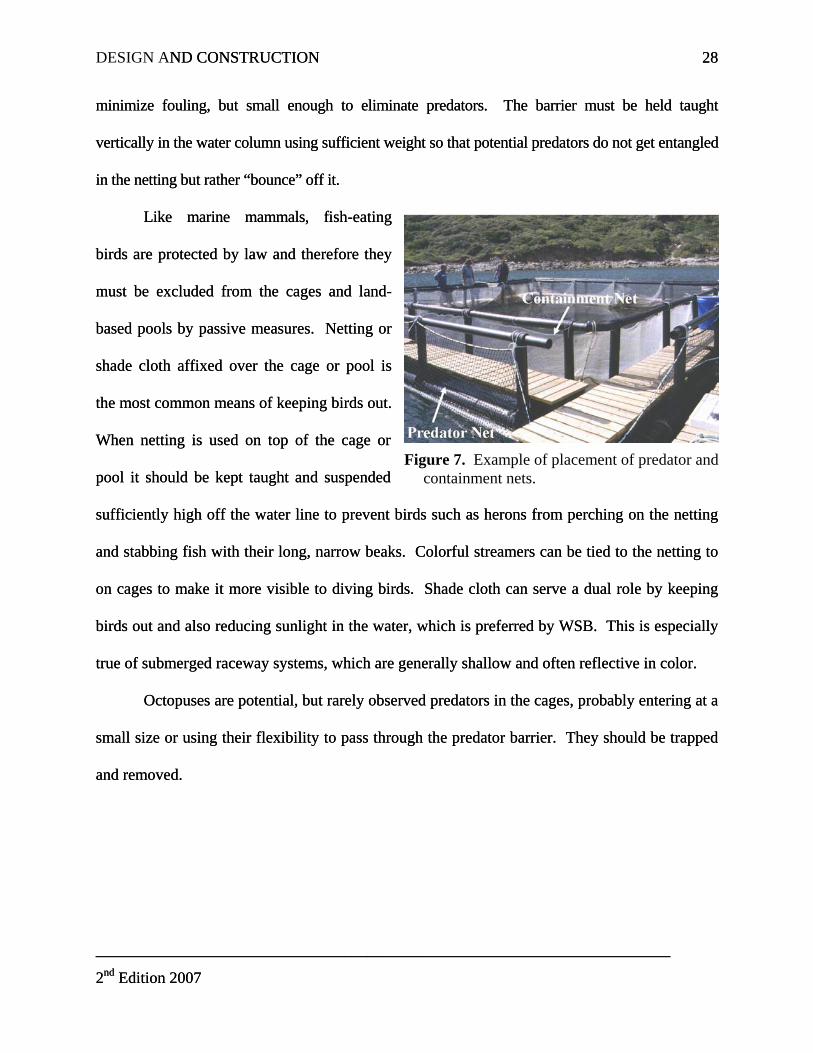
DESIGN AND CONSTRUCTIONND CONSTRUCTION
________________________________________________________________________
2nd Edition 2007
28
pool it should be kept taught and suspended
ely observed predators in the cages, probably entering at a
small s
________________________________________________________________________
2nd Edition 2007
28
pool it should be kept taught and suspended
ely observed predators in the cages, probably entering at a
small s
minimize fouling, but small enough to eliminate predators. The barrier must be held taught
vertically in the water column using sufficient weight so that potential predators do not get entangled
in the netting but rather “bounce” off it.
minimize fouling, but small enough to eliminate predators. The barrier must be held taught
vertically in the water column using sufficient weight so that potential predators do not get entangled
in the netting but rather “bounce” off it.
Like marine mammals, fish-eating
birds are protected by law and therefore they
must be excluded from the cages and land-
based pools by passive measures. Netting or
shade cloth affixed over the cage or pool is
the most common means of keeping birds out.
When netting is used on top of the cage or
sufficiently high off the water line to prevent birds such as herons from perching on the netting
and stabbing fish with their long, narrow beaks. Colorful streamers can be tied to the netting to
on cages to make it more visible to diving birds. Shade cloth can serve a dual role by keeping
birds out and also reducing sunlight in the water, which is preferred by WSB. This is especially
true of submerged raceway systems, which are generally shallow and often reflective in color.
Octopuses are potential, but rar
Figure 7. Example of placement of predator and containment nets.
ize or using their flexibility to pass through the predator barrier. They should be trapped
and removed.
ize or using their flexibility to pass through the predator barrier. They should be trapped
and removed.
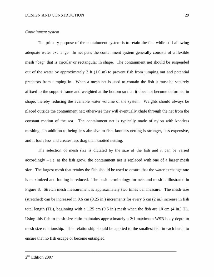
DESIGN AND CONSTRUCTION
________________________________________________________________________
2nd Edition 2007
29
Containment system
The primary purpose of the containment system is to retain the fish while still allowing
adequate water exchange. In net pens the containment system generally consists of a flexible
mesh “bag” that is circular or rectangular in shape. The containment net should be suspended
out of the water by approximately 3 ft (1.0 m) to prevent fish from jumping out and potential
predators from jumping in. When a mesh net is used to contain the fish it must be securely
affixed to the support frame and weighted at the bottom so that it does not become deformed in
shape, thereby reducing the available water volume of the system. Weights should always be
placed outside the containment net; otherwise they will eventually chafe through the net from the
constant motion of the sea. The containment net is typically made of nylon with knotless
meshing. In addition to being less abrasive to fish, knotless netting is stronger, less expensive,
and it fouls less and creates less drag than knotted netting.
The selection of mesh size is dictated by the size of the fish and it can be varied
accordingly – i.e. as the fish grow, the containment net is replaced with one of a larger mesh
size. The largest mesh that retains the fish should be used to ensure that the water exchange rate
is maximized and fouling is reduced. The basic terminology for nets and mesh is illustrated in
Figure 8. Stretch mesh measurement is approximately two times bar measure. The mesh size
(stretched) can be increased in 0.6 cm (0.25 in.) increments for every 5 cm (2 in.) increase in fish
total length (TL), beginning with a 1.25 cm (0.5 in.) mesh when the fish are 10 cm (4 in.) TL.
Using this fish to mesh size ratio maintains approximately a 2:1 maximum WSB body depth to
mesh size relationship. This relationship should be applied to the smallest fish in each batch to
ensure that no fish escape or become entangled.
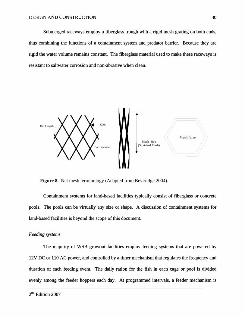
DESIGN AND CONSTRUCTIONND CONSTRUCTION
________________________________________________________________________
2nd Edition 2007
30
________________________________________________________________________
2nd Edition 2007
30
Submerged raceways employ a fiberglass trough with a rigid mesh grating on both ends,
thus combining the functions of a containment system and predator barrier. Because they are
rigid the water volume remains constant. The fiberglass material used to make these raceways is
resistant to saltwater corrosion and non-abrasive when clean.
44 m
mMesh Size
(Stretched Mesh)
Knot
Bar Diameter
Bar Length
32 m
m
Mesh Size
Figure 8. Net mesh terminology (Adapted from Beveridge 2004).
Containment systems for land-based facilities typically consist of fiberglass or concrete
pools. The pools can be virtually any size or shape. A discussion of containment systems for
land-based facilities is beyond the scope of this document.
Containment systems for land-based facilities typically consist of fiberglass or concrete
pools. The pools can be virtually any size or shape. A discussion of containment systems for
land-based facilities is beyond the scope of this document.
Feeding systems Feeding systems
The majority of WSB growout facilities employ feeding systems that are powered by
12V DC or 110 AC power, and controlled by a timer mechanism that regulates the frequency and
duration of each feeding event. The daily ration for the fish in each cage or pool is divided
evenly among the feeder hoppers each day. At programmed intervals, a feeder mechanism is
DESIGN AND CONSTRUCTION
________________________________________________________________________
2nd Edition 2007
31
triggered to dispense food into the cage. The feeder mechanism may consist of a vibrating tray,
rotating arm, or screw drive. Automatic feeders facilitate feeding regimes with feeding events
spread throughout the day and into the night. Feeding responses of captive WSB are generally
most aggressive under dim lighting or in the dark, especially just after sunset and just prior to
sunrise. Although automated feeding systems reduce much of the labor associated with manual
feeding, they must be continuously monitored and adjusted to ensure that the fish are receiving
the proper amount of food. Also, automatic feeders must be tested routinely to ensure that they
are functioning properly. Feed pellets can cause the feeder to jam and continuous outdoor
exposure may also damage mechanical and electrical components of the feeder.
Even when feeding is largely automated, volunteers should feed a small amount of food
by hand each day to gauge how hungry the fish are so the feeding rate can be adjusted
accordingly. Operators should hand feed sparingly to make sure excessive food doesn’t sink
past the fish. Hand-feeding also allows the operator to assess the health of the fish, because sick
fish often lose their appetite.
Circulation system
Cage systems should be located in an area with good tidal flushing. Tidal currents
provide a natural and reliable system for exchanging water in a culture system. In order to
maximize the benefits of tidal currents, the containment and predator barriers should be
constructed of highly permeable materials such as mesh or netting. These materials keep the fish
in and predators out but do not impede water flow. If solid sidewalls are part of the cage design,
tidal currents can still be an asset if the cage is oriented parallel to the direction of the currents
and water is allowed to pass through the screened ends.
DESIGN AND CONSTRUCTION
________________________________________________________________________
2nd Edition 2007
32
Mechanical circulation systems are required for land-based pools and cages that are not
exposed to adequate tidal exchange. Water can be mechanically circulated through a cage
system or land-based pool using a seawater pump, a motor-driven propeller or impeller, or an air
lift. Whatever method is selected, a sustainable turnover rate of one exchange per hour is
recommended, with greater rates possible during periods of high fish density, elevated water
temperatures, or low oxygen.
CULTURE OPERATIONS 33
CULTURE OPERATIONS
Receiving Fish
Prior to receiving fish, the growout facility should be thoroughly inspected, cleaned and
repaired as necessary. Arrangements to receive fish should be made approximately two weeks in
advance by contacting the Growout Facility Coordinator (GFC). Often the GFC will be able to
provide an estimated delivery schedule several weeks to months in advance, which gives
adequate time to prepare the facility and schedule volunteer help. The estimated size of fish and
the number to be delivered should be verified with the GFC at this time. Local ambient water
conditions should also be provided to the GFC, so fish can be acclimated upon arrival as
necessary.
When the fish are delivered to the growout facility site, clean seawater is pumped into the
transport tank from the receiving body of water using a gas powered pump. This procedure
improves the water quality within the tank and acclimates the fish to the local water temperature.
If the ambient water temperature is significantly different than that in transport tank it may take
several hours to completely acclimate the fish. This situation is uncommon and usually occurs in
summer months when transporting fish from the hatchery in the south to growout facilities in the
north.
The physical process of transferring fish from the transport truck involves attaching one
end of a 10.1 cm (4 in.) diameter flexible hose to the outlet of the transport tank, while the
opposite end of the hose is placed in the cage. Seawater is first pumped directly into the
transport hose to “prime” it for the fish and then a valve is turned to divert the pumped water into
the transport tank. The gate valve on the transport tank leading to the transport hose is then ________________________________________________________________________
2nd Edition 2007
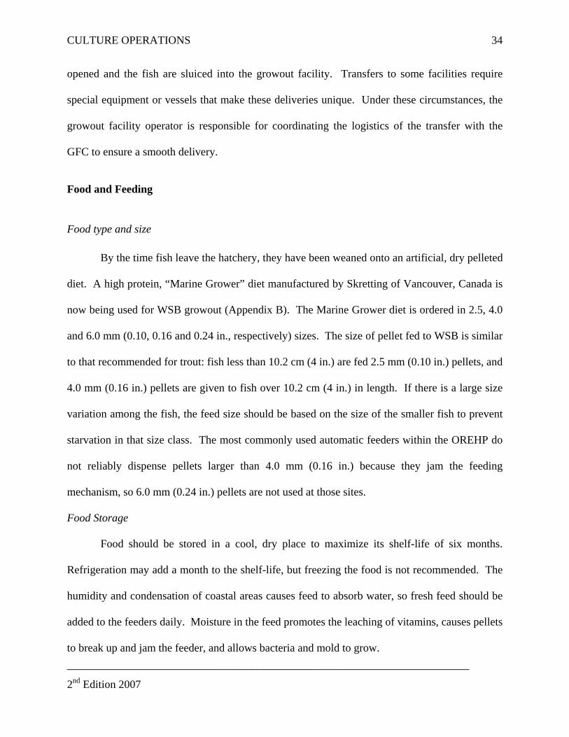
CULTURE OPERATIONS 34
opened and the fish are sluiced into the growout facility. Transfers to some facilities require
special equipment or vessels that make these deliveries unique. Under these circumstances, the
growout facility operator is responsible for coordinating the logistics of the transfer with the
GFC to ensure a smooth delivery.
Food and Feeding
Food type and size
By the time fish leave the hatchery, they have been weaned onto an artificial, dry pelleted
diet. A high protein, “Marine Grower” diet manufactured by Skretting of Vancouver, Canada is
now being used for WSB growout (Appendix B). The Marine Grower diet is ordered in 2.5, 4.0
and 6.0 mm (0.10, 0.16 and 0.24 in., respectively) sizes. The size of pellet fed to WSB is similar
to that recommended for trout: fish less than 10.2 cm (4 in.) are fed 2.5 mm (0.10 in.) pellets, and
4.0 mm (0.16 in.) pellets are given to fish over 10.2 cm (4 in.) in length. If there is a large size
variation among the fish, the feed size should be based on the size of the smaller fish to prevent
starvation in that size class. The most commonly used automatic feeders within the OREHP do
not reliably dispense pellets larger than 4.0 mm (0.16 in.) because they jam the feeding
mechanism, so 6.0 mm (0.24 in.) pellets are not used at those sites.
Food Storage
Food should be stored in a cool, dry place to maximize its shelf-life of six months.
Refrigeration may add a month to the shelf-life, but freezing the food is not recommended. The
humidity and condensation of coastal areas causes feed to absorb water, so fresh feed should be
added to the feeders daily. Moisture in the feed promotes the leaching of vitamins, causes pellets
to break up and jam the feeder, and allows bacteria and mold to grow. ________________________________________________________________________
2nd Edition 2007
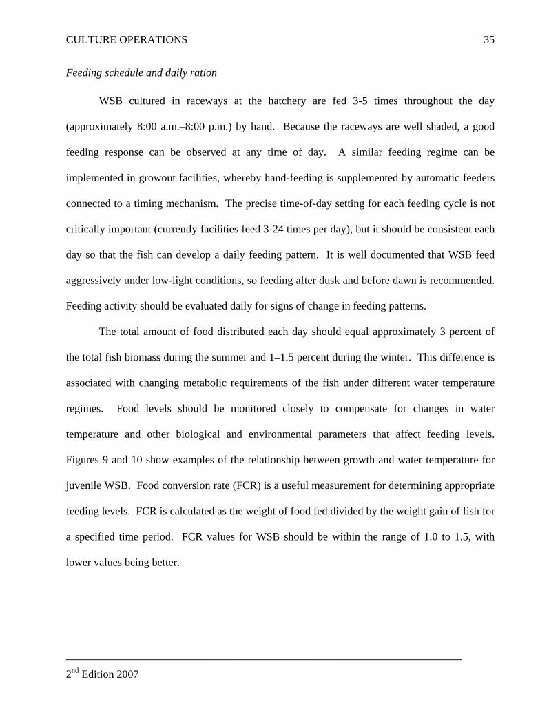
CULTURE OPERATIONS 35
Feeding schedule and daily ration
WSB cultured in raceways at the hatchery are fed 3-5 times throughout the day
(approximately 8:00 a.m.–8:00 p.m.) by hand. Because the raceways are well shaded, a good
feeding response can be observed at any time of day. A similar feeding regime can be
implemented in growout facilities, whereby hand-feeding is supplemented by automatic feeders
connected to a timing mechanism. The precise time-of-day setting for each feeding cycle is not
critically important (currently facilities feed 3-24 times per day), but it should be consistent each
day so that the fish can develop a daily feeding pattern. It is well documented that WSB feed
aggressively under low-light conditions, so feeding after dusk and before dawn is recommended.
Feeding activity should be evaluated daily for signs of change in feeding patterns.
The total amount of food distributed each day should equal approximately 3 percent of
the total fish biomass during the summer and 1–1.5 percent during the winter. This difference is
associated with changing metabolic requirements of the fish under different water temperature
regimes. Food levels should be monitored closely to compensate for changes in water
temperature and other biological and environmental parameters that affect feeding levels.
Figures 9 and 10 show examples of the relationship between growth and water temperature for
juvenile WSB. Food conversion rate (FCR) is a useful measurement for determining appropriate
feeding levels. FCR is calculated as the weight of food fed divided by the weight gain of fish for
a specified time period. FCR values for WSB should be within the range of 1.0 to 1.5, with
lower values being better.
________________________________________________________________________
2nd Edition 2007
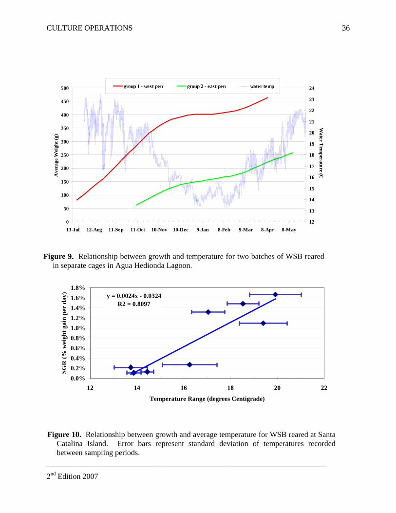
CULTURE OPERATIONS 36
0
50
100
150
200
250
300
350
400
450
500
13-Jul 12-Aug 11-Sep 11-Oct 10-Nov 10-Dec 9-Jan 8-Feb 9-Mar 8-Apr 8-May
Ave
rage
Wei
ght (
g)
12
13
14
15
16
17
18
19
20
21
22
23
24
Water T
emperature (C
)
group 1 - west pen group 2 - east pen water temp
Figure 9. Relationship between growth and temperature for two batches of WSB reared in separate cages in Agua Hedionda Lagoon.
y = 0.0024x - 0.0324R2 = 0.8097
0.0%0.2%0.4%0.6%0.8%1.0%1.2%1.4%1.6%1.8%
12 14 16 18 20 22
Temperature Range (degrees Centigrade)
SGR
(% w
eigh
t gai
n pe
r da
y)
________________________________________________________________________
Figure 10. Relationship between growth and average temperature for WSB reared at SantaCatalina Island. Error bars represent standard deviation of temperatures recordedbetween sampling periods.
2nd Edition 2007
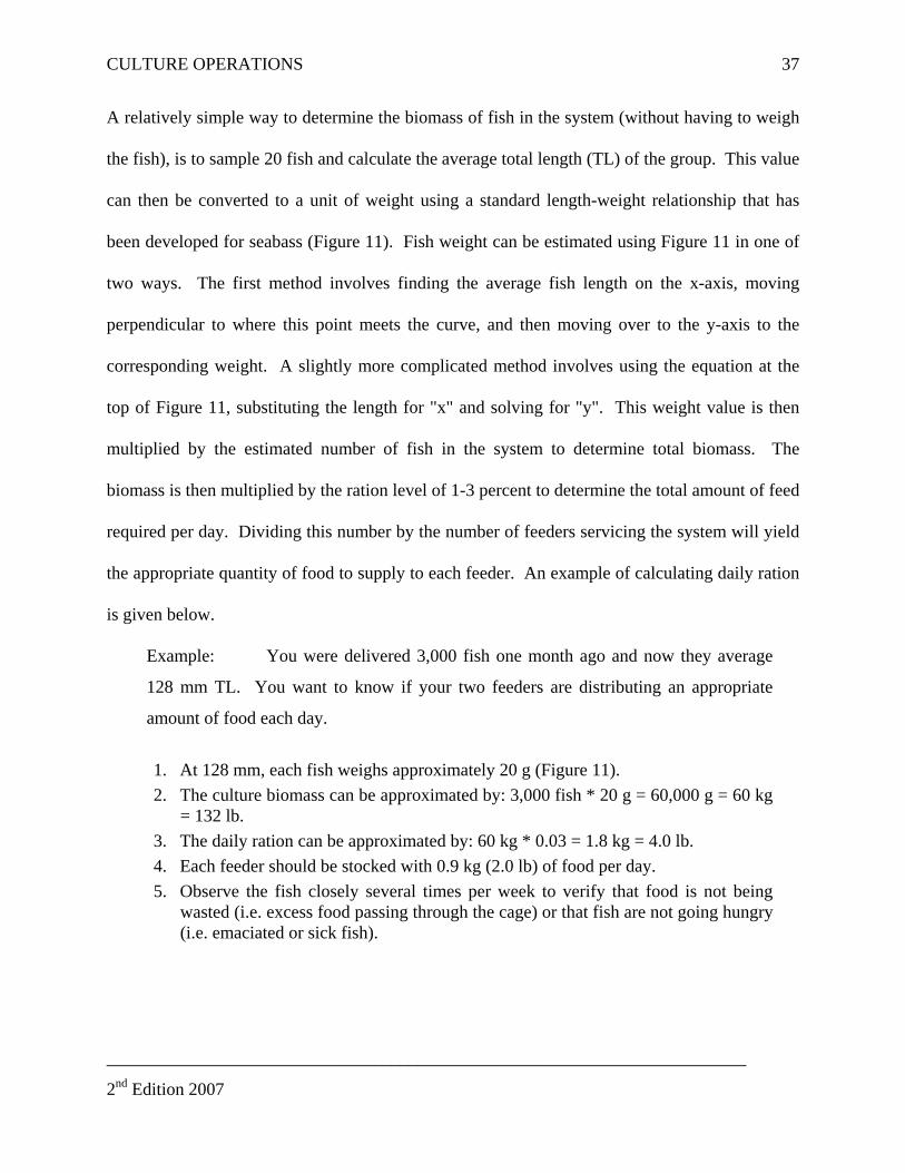
CULTURE OPERATIONS 37
A relatively simple way to determine the biomass of fish in the system (without having to weigh
the fish), is to sample 20 fish and calculate the average total length (TL) of the group. This value
can then be converted to a unit of weight using a standard length-weight relationship that has
been developed for seabass (Figure 11). Fish weight can be estimated using Figure 11 in one of
two ways. The first method involves finding the average fish length on the x-axis, moving
perpendicular to where this point meets the curve, and then moving over to the y-axis to the
corresponding weight. A slightly more complicated method involves using the equation at the
top of Figure 11, substituting the length for "x" and solving for "y". This weight value is then
multiplied by the estimated number of fish in the system to determine total biomass. The
biomass is then multiplied by the ration level of 1-3 percent to determine the total amount of feed
required per day. Dividing this number by the number of feeders servicing the system will yield
the appropriate quantity of food to supply to each feeder. An example of calculating daily ration
is given below.
Example: You were delivered 3,000 fish one month ago and now they average
128 mm TL. You want to know if your two feeders are distributing an appropriate
amount of food each day.
1. At 128 mm, each fish weighs approximately 20 g (Figure 11). 2. The culture biomass can be approximated by: 3,000 fish * 20 g = 60,000 g = 60 kg
= 132 lb. 3. The daily ration can be approximated by: 60 kg * 0.03 = 1.8 kg = 4.0 lb. 4. Each feeder should be stocked with 0.9 kg (2.0 lb) of food per day. 5. Observe the fish closely several times per week to verify that food is not being
wasted (i.e. excess food passing through the cage) or that fish are not going hungry (i.e. emaciated or sick fish).
________________________________________________________________________
2nd Edition 2007
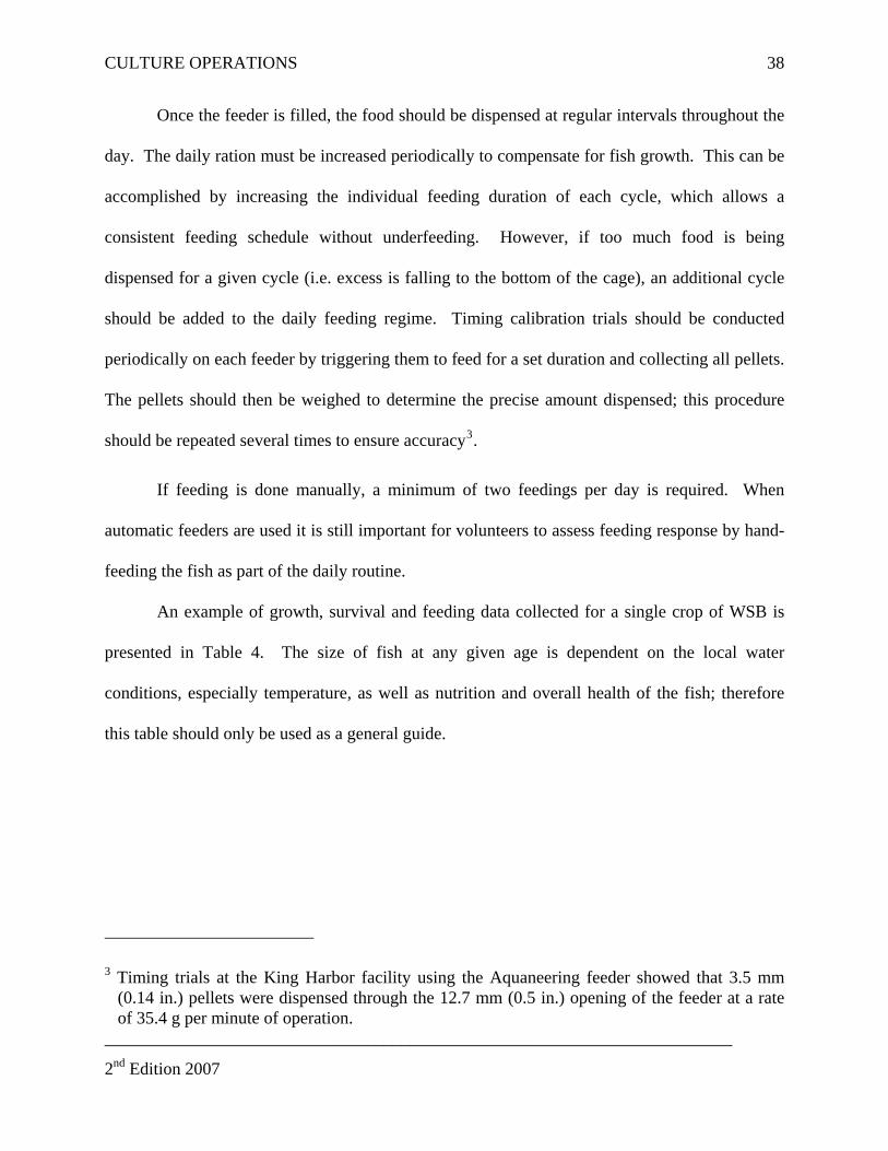
CULTURE OPERATIONS 38
Once the feeder is filled, the food should be dispensed at regular intervals throughout the
day. The daily ration must be increased periodically to compensate for fish growth. This can be
accomplished by increasing the individual feeding duration of each cycle, which allows a
consistent feeding schedule without underfeeding. However, if too much food is being
dispensed for a given cycle (i.e. excess is falling to the bottom of the cage), an additional cycle
should be added to the daily feeding regime. Timing calibration trials should be conducted
periodically on each feeder by triggering them to feed for a set duration and collecting all pellets.
The pellets should then be weighed to determine the precise amount dispensed; this procedure
should be repeated several times to ensure accuracy3.
If feeding is done manually, a minimum of two feedings per day is required. When
automatic feeders are used it is still important for volunteers to assess feeding response by hand-
feeding the fish as part of the daily routine.
An example of growth, survival and feeding data collected for a single crop of WSB is
presented in Table 4. The size of fish at any given age is dependent on the local water
conditions, especially temperature, as well as nutrition and overall health of the fish; therefore
this table should only be used as a general guide.
________________________________________________________________________
3 Timing trials at the King Harbor facility using the Aquaneering feeder showed that 3.5 mm (0.14 in.) pellets were dispensed through the 12.7 mm (0.5 in.) opening of the feeder at a rate of 35.4 g per minute of operation.
2nd Edition 2007
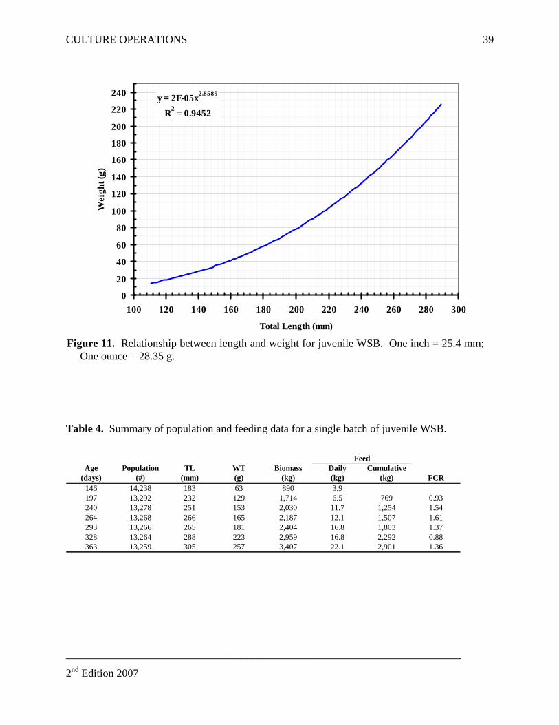
CULTURE OPERATIONS 39
y = 2E-05x2.8589
R2 = 0.9452
0
20
40
60
80
100
120
140
160
180
200
220
240
100 120 140 160 180 200 220 240 260 280 300
Total Length (mm)
Wei
ght (
g)
Figure 11. Relationship between length and weight for juvenile WSB. One inch = 25.4 mm; One ounce = 28.35 g.
Table 4. Summary of population and feeding data for a single batch of juvenile WSB.
Age Population TL WT Biomass Daily Cumulative(days) (#) (mm) (g) (kg) (kg) (kg) FCR
146 14,238 183 63 890 3.9197 13,292 232 129 1,714 6.5 769 0.93240 13,278 251 153 2,030 11.7 1,254 1.54264 13,268 266 165 2,187 12.1 1,507 1.61293 13,266 265 181 2,404 16.8 1,803 1.37328 13,264 288 223 2,959 16.8 2,292 0.88363 13,259 305 257 3,407 22.1 2,901 1.36
Feed
________________________________________________________________________
2nd Edition 2007
CULTURE OPERATIONS 40
System Maintenance
Although maintenance schedules and tasks will vary according to system design and
local water conditions, certain maintenance requirements apply to all growout facilities. Each
facility must be kept clean of debris (e.g. excess food, feces, and dead fish), and clear of
obstructions to water flow (e.g. plant and animal growth, and flotsam). The systems must be
maintained to be structurally sound (e.g. mooring, netting, and support platform) and
mechanically operable (e.g. circulation pump, and feeders). To achieve these requirements,
growout facility operators must perform the following maintenance functions on a regular basis:
1. Check the physical condition of the facility on a daily basis - repair any structural defects
and tears in predator or containment nets.
2. Check the feeding system on a daily basis - clean as needed, verify feeding level and
adjust timer interval as needed, and fill with food. Record feed amount on daily data
sheet. Food storage supply should also be checked and GFC notified if food supplies get
low.
3. Clean sides and bottom of cage as needed - brush can be used on submerged raceways
and net cages, vacuum bottom of raceway or land-based pool, use dip net on bottom of
net cages4. Periodically, nets will need to be removed, cleaned and replaced in net cages.
4. Remove dead fish from the system on a daily basis - register number, length and
mortality information in daily data sheet, bag and discard carcasses in the trash.
5. Clean area surrounding the growout facility on a daily basis to maintain visual esthetics
as well as cleanliness.
6. Record all activities into daily logbook.
________________________________________________________________________
4 The potential environmental impacts of cleaning practices are evaluated by periodic dive surveys and benthic monitoring. Thus far, no negative impacts have been observed.
2nd Edition 2007
CULTURE OPERATIONS 41
Monitoring
Growout facility components
The primary components of the growout facility that require frequent monitoring are the
feeding and water circulation systems as applicable. The feeding system should be evaluated
daily to insure that the appropriate ration is being dispensed. This simply involves making sure
that feed from the previous day has been fed out as expected. Routinely hand-feeding the fish
and observing their feeding response will provide insight as to whether the fish are receiving the
appropriate ration. Aggressive feeding at the surface, especially during daylight hours may be an
indication that fish require additional feed. A diminished feeding response can be a sign of
overfeeding or illness. A substantial accumulation of food on the bottom of the facility is also an
indication that too much feed is being dispensed or that it is being introduced too rapidly.
The mechanical components of the circulation system should be monitored on a daily
basis to insure that the system is functioning properly. Adjustments to increase water circulation
through the culture system are generally made in response to a decline in water quality (see
Water Quality later in this Section).
Additional components that should be inspected weekly include the predator barriers,
containment net and mooring system. These components should also be examined after any
storm event. Predator netting should be examined for signs of intrusion by predators, fouling,
proper weighting and general wear.
________________________________________________________________________
2nd Edition 2007
CULTURE OPERATIONS 42
Fish losses
At the end of the growout cycle, the number of fish that died in culture is subtracted from
the number delivered to get an expected number released. At the time of release all fish are
counted by dip-netting them in small batches or allowing them to swim through a constricted
opening in the net or raceway. Hand-counters are used to keep track of the fish counts when
either release method is used. Invariably there is a discrepancy between the actual number of
fish released and the expected number, which is generally attributed to cannibalism, escape, and
predation by other organisms. The number of fish unaccounted for is generally 5-15 percent of
the total number “lost”.
Fish in the culture system should be visually inspected on a daily basis for signs of stress
or illness. The procedure for monitoring fish health is given in the Fish Health section. Dead
fish should be removed from the cage daily, counted and recorded. Poor water visibility can
limit the ability to collect mortalities. If the visibility remains poor for more than a couple of
days, the nets should be raised until visual inspection of the bottom of the net pen is possible. If
visibility is extremely limited or if the system is a submerged raceway and the bottom is not
visible, a long handled net should be dragged slowly across the bottom of the facility to search
for mortalities. Barring a catastrophic event such as a disease outbreak, the loss of fish in the
growout facilities typically averages a fraction of a percent (several individuals) per day.
However, this relationship is not linear and the growout facility operator can anticipate higher
losses within the first week after delivery (up to 5 percent cumulative) due to the stress of
transport.
________________________________________________________________________
2nd Edition 2007
CULTURE OPERATIONS 43
Encounters with marine mammals and birds
Encounters with marine mammals and birds should be avoided through proper
installation and maintenance of predator barriers. Any incidents of fish escape or intrusion by
bird or mammal predators should also be recorded on the daily log and proper measures taken to
ensure that this event will not recur. In the event any accidental release or escape of fish or
entanglement or other contact with marine mammals or birds occurs at a growout facility GFC
and the OREHP Coordinator from the DFG will be notified immediately. Initiating contact with
marine mammals and birds is prohibited by law.
Marine Mammals
Any injury or mortality of a marine mammal must be reported within 48 hours of
occurrence. The Marine Mammal Authorization Program Mortality/Injury Reporting Form
(OMB 0648-0292; Appendix C) should be filled out and fax to the following individuals:
NOAA Fisheries -- fax: (301) 713-4060
Grow-Out Pen Coordinator -- fax: (760) 434-9502
OREHP Coordinator -- fax: (562) 342-7139
NOAA Fisheries has defined a marine mammal injury as a wound or other physical harm.
Signs of injury include, but are not limited to:
• visible blood flow • loss of or damage to an appendage or jaw • inability to use one or more appendages • asymmetry in the shape of body or body position • noticeable swelling or hemorrhage • laceration • puncture or rupture of eyeball
________________________________________________________________________
2nd Edition 2007
CULTURE OPERATIONS 44
• listless appearance or inability to defend itself • inability to swim or dive upon release from fishing gear • signs of equilibrium imbalance
Any animal that ingests fishing gear, or any animal that is release with fishing gear
entangling, trailing, or perforating any part of the body will be considered injured regardless of
the absence of any wound or other evidence of injury.
Deterrence Measures
Individuals are strictly prohibited from intentionally lethally taking (killing) marine
mammals. An exception is provided for an intentional lethal take imminently necessary in self-
defense or to save the life of another person. If a marine mammal is killed in self-defense or to
save the life of another person a report (see above) must be filed within 48 hours of the
mortality.
Deterrence measures should not separate a female from her offspring; break the skin of
an animal; result in dislocation of or fracture of bones, limbs, or other appendages; be directed at
the head or eyes of an animal; or be used on seals and sea lions hauled out on unimproved
property.
NOAA Fisheries will be publishing guidelines for the safe deterrence of marine
mammals. They will include the following:
• Passive deterrence measures - nets, fences, or other types of physical barriers provided the potential for marine mammal entanglement is not increased.
• Active deterrence measures - mechanical or electrical noisemakers, water spray from a hose, blunt objects to prod animals, or large shielding objects (wood, metal or fabric) to herd animals.
________________________________________________________________________
2nd Edition 2007

CULTURE OPERATIONS 45
Birds
The US Fish and Wildlife Service is responsible for the protection of marine birds. There
are no reporting requirements or any guidelines for the safe deterrence of marine birds. The
deterrence measures for marine mammals listed above can also safely be applied to marine birds.
Fish growth
Periodically, it is desirable to obtain length and weight data from a subsample of fish, so
that the growth of the population can be assessed over time. Due to the stress caused by
handling, growth assessments should be conducted no more than once per month and the GFC
should be on site to assist in the process. The GFC has been trained in fish handling procedures
and has the appropriate equipment for obtaining length and weight information. The GFC can
also administer an anesthetic to subdue the fish, which reduces stress, facilitates handling and
makes the measurements more accurate. Consistent participation by the GFC will also help
reduce sampling error caused operators and instrumentation.
To obtain a subsample of fish, the fish are concentrated using a crowding device in a
raceway or pool, or by slowly pulling one end of the containment net from the water in a net pen
system. Crowding devices, like those used at bait receivers, usually consist of plastic or nylon
meshing strung between two sturdy wooden poles. Fish are then gently removed from the water
in small groups using a bucket or net. The measuring “station” requires two individuals to
operate - one person to measure the fish and the other to record the data. The person making
measurements should wear surgical gloves for their own protection and that of the fish. Each
fish is placed directly on a measuring board and measured for total length (TL) to the nearest 1.0
mm from the tip of the snout to the end of the tail.
________________________________________________________________________
2nd Edition 2007
CULTURE OPERATIONS 46
Because of the relatively small size and active nature of juvenile fish, obtaining
individual weights is more complicated and generally less accurate than making length
measurements. As described previously, the length-weight relationship illustrated in Figure 11
can be used to obtain results that are sufficiently accurate to calculate a daily ration. If more
detailed and accurate data is desired, the GFC will subdue the fish with an anesthetic and weigh
fish individually on a battery-powered electronic scale. The fish should be returned to the water
immediately after the length and weight measurements have been taken and monitored until they
have recovered.
WSB cultured at growout facilities grow at a rate of 0.2-1.3 mm per day or 0.2-1.5 in. per
month. Sub-optimal growth can be caused by many factors including poor health, extreme water
temperatures, and low food consumption. Cold water usually associated with the winter season
can dramatically slow the growth of fish; conversely fish grow rapidly and consume more food
when water temperatures are warm.
Water quality
Monitoring of water quality parameters is critical to understanding variations in growth
and survival between harvested groups of fish. Suboptimal growth, disease outbreaks, and fish
kills are most often associated with poor water quality. Although the biological and
physiological responses of WSB to fluctuations in many water quality parameters have not been
empirically defined in the laboratory, we have many years of field experience from numerous
growout facilities. In addition, we can make generalizations about the water quality
requirements of WSB by drawing on what is known for other closely related species. New
________________________________________________________________________
2nd Edition 2007

CULTURE OPERATIONS 47
facility operators should be diligent about collecting water quality data until a comfort level is
reached after rearing several batches of fish successfully.
Stress caused by an oxygen deficit is one of the most common water quality problems
experienced in high density culture operations. The concentration and availability of dissolved
oxygen (DO) is critical to the health and survival of fish in the growout facility. Critical oxygen
levels vary among species of fish and can vary depending on other water quality parameters (e.g.
temperature). For WSB, it is recommended that levels be kept above 6.0 mg/L (6.0 ppm). The
DO level in the growout facility is controlled by both physical and biological parameters. For
example, as temperature and salinity increase, and as atmospheric pressure decreases, the level
of DO will decrease. Similarly, DO levels are reduced by respiration of other plants and animals
in the system. Although marine algae produce oxygen through photosynthesis during daylight
hours, they continue to respire at night and use oxygen in this process. Respiration is directly
affected by temperature in cold-blooded animals (i.e. fish) and plants; respiratory rates increase
as temperature increases. It should be noted that parasites, disease agents and chemicals can
damage gill filaments and disrupt the flow of oxygen into the blood stream. When this occurs, it
may appear as though there is an oxygen deficit when in fact there is not. In order to avoid
problems with low DO levels, make sure that the growout facility has an unobstructed flow of
water through it at all times. Clean intake and outflow screens, and remove any excess food,
detritus, or dead fish that may create a habitat for bacteria. Monitoring DO levels is done with
an oxygen meter. DO monitoring is not required at OREHP growout facilities but periodic
inspections are suggested, especially during periods of warm water with high fish densities. The
GFC can supply an oxygen probe as needed.
________________________________________________________________________
2nd Edition 2007
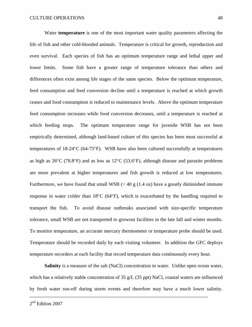
CULTURE OPERATIONS 48
Water temperature is one of the most important water quality parameters affecting the
life of fish and other cold-blooded animals. Temperature is critical for growth, reproduction and
even survival. Each species of fish has an optimum temperature range and lethal upper and
lower limits. Some fish have a greater range of temperature tolerance than others and
differences often exist among life stages of the same species. Below the optimum temperature,
feed consumption and feed conversion decline until a temperature is reached at which growth
ceases and food consumption is reduced to maintenance levels. Above the optimum temperature
feed consumption increases while food conversion decreases, until a temperature is reached at
which feeding stops. The optimum temperature range for juvenile WSB has not been
empirically determined, although land-based culture of this species has been most successful at
temperatures of 18-24°C (64-75°F). WSB have also been cultured successfully at temperatures
as high as 26°C (78.8°F) and as low as 12°C (53.6°F), although disease and parasite problems
are more prevalent at higher temperatures and fish growth is reduced at low temperatures.
Furthermore, we have found that small WSB (< 40 g (1.4 oz) have a greatly diminished immune
response in water colder than 18°C (64°F), which is exacerbated by the handling required to
transport the fish. To avoid disease outbreaks associated with size-specific temperature
tolerance, small WSB are not transported to growout facilities in the late fall and winter months.
To monitor temperature, an accurate mercury thermometer or temperature probe should be used.
Temperature should be recorded daily by each visiting volunteer. In addition the GFC deploys
temperature recorders at each facility that record temperature data continuously every hour.
________________________________________________________________________
Salinity is a measure of the salt (NaCl) concentration in water. Unlike open ocean water,
which has a relatively stable concentration of 35 g/L (35 ppt) NaCl, coastal waters are influenced
by fresh water run-off during storm events and therefore may have a much lower salinity.
2nd Edition 2007

CULTURE OPERATIONS 49
Because water becomes denser as the saline concentration increases, a lens of fresh water may
develop at the surface of a given embayment. This fresh water lens may cause problems in
shallow cage systems if it lingers and the fish are unable to swim down below it. Hyposaline
conditions have not generally been a problem thus far for WSB. WSB can survive short
durations in completely fresh water but require >10 ppt salinity for extended exposure. Salinity
is measured using a refractometer, which measures light refraction; a densitometer, which
measures specific gravity; or certain electronic instruments which measure conductivity.
Salinity monitoring is not required at OREHP growout facilities but periodic inspections are
suggested, especially during periods of rain with high fish densities. The GFC can supply a
refractometer as needed.
The concentration of hydrogen ions in the water is measured as pH. The pH level is
expressed on a scale from 0 (acidic) to 14 (alkaline), with 7 being neutral. Seawater is usually
slightly alkaline with values of 7.5-8.5. Seawater is also well buffered, so it does not change
readily with seasonal or diurnal additions of acidic or alkaline compounds associated with
photosynthesis. The pH level is important to growout facility operators because extreme pH
conditions can lead to gill damage and it also affects the toxicity of several common pollutants.
Because the optimum pH level for most fish is 6.0-8.5, pH levels in marine systems are rarely a
problem and no pH-related problems have been reported for WSB growout facilities. pH is
measured using a pH meter but pH monitoring is not required at OREHP growout facilities.
Ammonia is the primary nitrogenous waste produced by fish. Ammonia is toxic to fish
and the level of its toxicity is dependent on the species of fish, water temperature and pH.
Sublethal levels of ammonia can result in gill and tissue damage, poor growth and increased
susceptibility to disease. Ammonia toxicity should not be a problem at the stocking densities ________________________________________________________________________
2nd Edition 2007
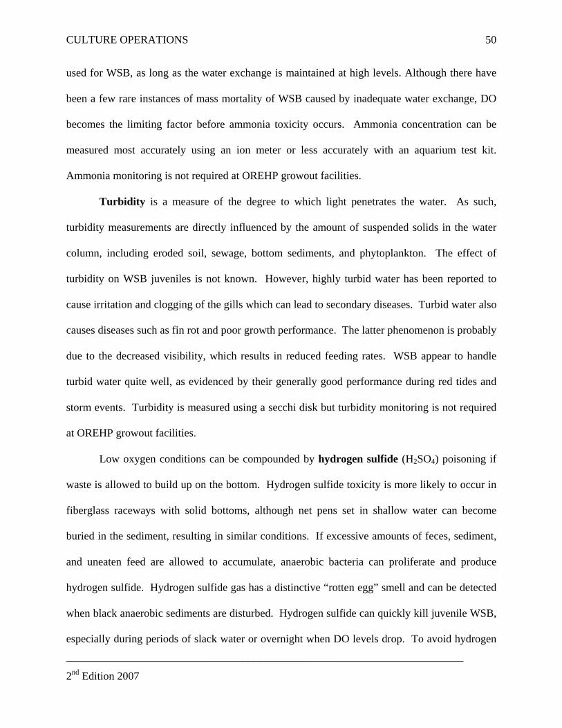
CULTURE OPERATIONS 50
used for WSB, as long as the water exchange is maintained at high levels. Although there have
been a few rare instances of mass mortality of WSB caused by inadequate water exchange, DO
becomes the limiting factor before ammonia toxicity occurs. Ammonia concentration can be
measured most accurately using an ion meter or less accurately with an aquarium test kit.
Ammonia monitoring is not required at OREHP growout facilities.
Turbidity is a measure of the degree to which light penetrates the water. As such,
turbidity measurements are directly influenced by the amount of suspended solids in the water
column, including eroded soil, sewage, bottom sediments, and phytoplankton. The effect of
turbidity on WSB juveniles is not known. However, highly turbid water has been reported to
cause irritation and clogging of the gills which can lead to secondary diseases. Turbid water also
causes diseases such as fin rot and poor growth performance. The latter phenomenon is probably
due to the decreased visibility, which results in reduced feeding rates. WSB appear to handle
turbid water quite well, as evidenced by their generally good performance during red tides and
storm events. Turbidity is measured using a secchi disk but turbidity monitoring is not required
at OREHP growout facilities.
Low oxygen conditions can be compounded by hydrogen sulfide (H2SO4) poisoning if
waste is allowed to build up on the bottom. Hydrogen sulfide toxicity is more likely to occur in
fiberglass raceways with solid bottoms, although net pens set in shallow water can become
buried in the sediment, resulting in similar conditions. If excessive amounts of feces, sediment,
and uneaten feed are allowed to accumulate, anaerobic bacteria can proliferate and produce
hydrogen sulfide. Hydrogen sulfide gas has a distinctive “rotten egg” smell and can be detected
when black anaerobic sediments are disturbed. Hydrogen sulfide can quickly kill juvenile WSB,
especially during periods of slack water or overnight when DO levels drop. To avoid hydrogen ________________________________________________________________________
2nd Edition 2007
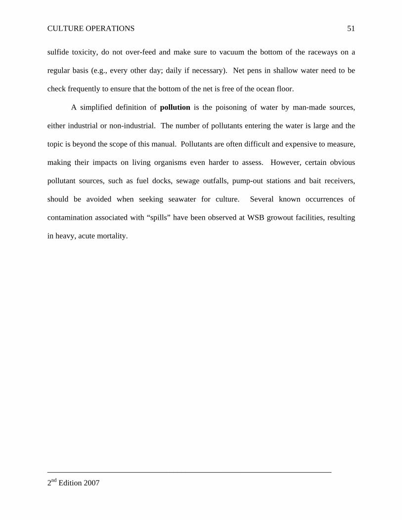
CULTURE OPERATIONS
________________________________________________________________________
2nd Edition 2007
51
sulfide toxicity, do not over-feed and make sure to vacuum the bottom of the raceways on a
regular basis (e.g., every other day; daily if necessary). Net pens in shallow water need to be
check frequently to ensure that the bottom of the net is free of the ocean floor.
A simplified definition of pollution is the poisoning of water by man-made sources,
either industrial or non-industrial. The number of pollutants entering the water is large and the
topic is beyond the scope of this manual. Pollutants are often difficult and expensive to measure,
making their impacts on living organisms even harder to assess. However, certain obvious
pollutant sources, such as fuel docks, sewage outfalls, pump-out stations and bait receivers,
should be avoided when seeking seawater for culture. Several known occurrences of
contamination associated with “spills” have been observed at WSB growout facilities, resulting
in heavy, acute mortality.
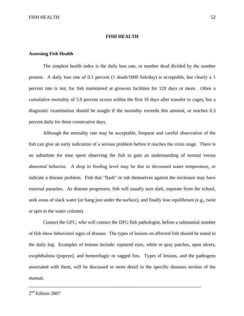
FISH HEALTH 52
FISH HEALTH
Assessing Fish Health
The simplest health index is the daily loss rate, or number dead divided by the number
present. A daily loss rate of 0.1 percent (1 death/1000 fish/day) is acceptable, but clearly a 1
percent rate is not, for fish maintained at growout facilities for 120 days or more. Often a
cumulative mortality of 5.0 percent occurs within the first 10 days after transfer to cages, but a
diagnostic examination should be sought if the mortality exceeds this amount, or reaches 0.3
percent daily for three consecutive days.
Although the mortality rate may be acceptable, frequent and careful observation of the
fish can give an early indication of a serious problem before it reaches the crisis stage. There is
no substitute for time spent observing the fish to gain an understanding of normal versus
abnormal behavior. A drop in feeding level may be due to decreased water temperature, or
indicate a disease problem. Fish that "flash" or rub themselves against the enclosure may have
external parasites. As disease progresses, fish will usually turn dark, separate from the school,
seek areas of slack water (or hang just under the surface), and finally lose equilibrium (e.g., twist
or spin in the water column).
Contact the GFC, who will contact the DFG fish pathologist, before a substantial number
of fish show behavioral signs of disease. The types of lesions on affected fish should be noted in
the daily log. Examples of lesions include: ruptured eyes, white or gray patches, open ulcers,
exophthalmia (popeye), and hemorrhagic or ragged fins. Types of lesions, and the pathogens
associated with them, will be discussed in more detail in the specific diseases section of the
manual. ________________________________________________________________________
2nd Edition 2007
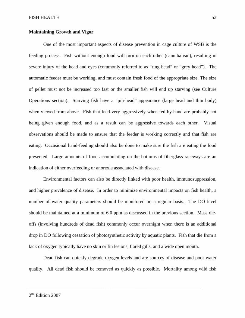
FISH HEALTH 53
Maintaining Growth and Vigor
One of the most important aspects of disease prevention in cage culture of WSB is the
feeding process. Fish without enough food will turn on each other (cannibalism), resulting in
severe injury of the head and eyes (commonly referred to as “ring-head” or “grey-head”). The
automatic feeder must be working, and must contain fresh food of the appropriate size. The size
of pellet must not be increased too fast or the smaller fish will end up starving (see Culture
Operations section). Starving fish have a “pin-head” appearance (large head and thin body)
when viewed from above. Fish that feed very aggressively when fed by hand are probably not
being given enough food, and as a result can be aggressive towards each other. Visual
observations should be made to ensure that the feeder is working correctly and that fish are
eating. Occasional hand-feeding should also be done to make sure the fish are eating the food
presented. Large amounts of food accumulating on the bottoms of fiberglass raceways are an
indication of either overfeeding or anorexia associated with disease.
Environmental factors can also be directly linked with poor health, immunosuppression,
and higher prevalence of disease. In order to minimize environmental impacts on fish health, a
number of water quality parameters should be monitored on a regular basis. The DO level
should be maintained at a minimum of 6.0 ppm as discussed in the previous section. Mass die-
offs (involving hundreds of dead fish) commonly occur overnight when there is an additional
drop in DO following cessation of photosynthetic activity by aquatic plants. Fish that die from a
lack of oxygen typically have no skin or fin lesions, flared gills, and a wide open mouth.
Dead fish can quickly degrade oxygen levels and are sources of disease and poor water
quality. All dead fish should be removed as quickly as possible. Mortality among wild fish
________________________________________________________________________
2nd Edition 2007
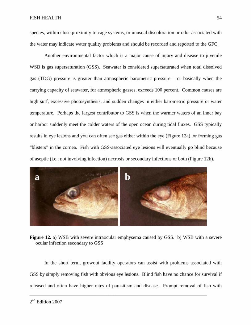
FISH HEALTH 54
species, within close proximity to cage systems, or unusual discoloration or odor associated with
the water may indicate water quality problems and should be recorded and reported to the GFC.
Another environmental factor which is a major cause of injury and disease to juvenile
WSB is gas supersaturation (GSS). Seawater is considered supersaturated when total dissolved
gas (TDG) pressure is greater than atmospheric barometric pressure – or basically when the
carrying capacity of seawater, for atmospheric gasses, exceeds 100 percent. Common causes are
high surf, excessive photosynthesis, and sudden changes in either barometric pressure or water
temperature. Perhaps the largest contributor to GSS is when the warmer waters of an inner bay
or harbor suddenly meet the colder waters of the open ocean during tidal fluxes. GSS typically
results in eye lesions and you can often see gas either within the eye (Figure 12a), or forming gas
“blisters” in the cornea. Fish with GSS-associated eye lesions will eventually go blind because
of aseptic (i.e., not involving infection) necrosis or secondary infections or both (Figure 12b).
a b
Figure 12. a) WSB with severe intraocular emphysema caused by GSS. b) WSB with a severe ocular infection secondary to GSS
In the short term, growout facility operators can assist with problems associated with
GSS by simply removing fish with obvious eye lesions. Blind fish have no chance for survival if
released and often have higher rates of parasitism and disease. Prompt removal of fish with ________________________________________________________________________
2nd Edition 2007
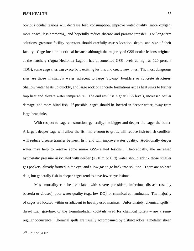
FISH HEALTH 55
obvious ocular lesions will decrease feed consumption, improve water quality (more oxygen,
more space, less ammonia), and hopefully reduce disease and parasite transfer. For long-term
solutions, growout facility operators should carefully assess location, depth, and size of their
facility. Cage location is critical because although the majority of GSS ocular lesions originate
at the hatchery (Agua Hedionda Lagoon has documented GSS levels as high as 120 percent
TDG), some cage sites can exacerbate existing lesions and create new ones. The most dangerous
sites are those in shallow water, adjacent to large “rip-rap” boulders or concrete structures.
Shallow water heats up quickly, and large rock or concrete formations act as heat sinks to further
trap heat and elevate water temperature. The end result is higher GSS levels, increased ocular
damage, and more blind fish. If possible, cages should be located in deeper water, away from
large heat sinks.
With respect to cage construction, generally, the bigger and deeper the cage, the better.
A larger, deeper cage will allow the fish more room to grow, will reduce fish-to-fish conflicts,
will reduce disease transfer between fish, and will improve water quality. Additionally deeper
water may help to resolve some minor GSS-related lesions. Theoretically, the increased
hydrostatic pressure associated with deeper (>2.0 m or 6 ft) water should shrink those smaller
gas pockets, already formed in the eye, and allow gas to go back into solution. There are no hard
data, but generally fish in deeper cages tend to have fewer eye lesions.
Mass mortality can be associated with severe parasitism, infectious disease (usually
bacteria or viruses), poor water quality (e.g., low DO), or chemical contaminants. The majority
of cages are located within or adjacent to heavily used marinas. Unfortunately, chemical spills –
diesel fuel, gasoline, or the formalin-laden cocktails used for chemical toilets – are a semi-
regular occurrence. Chemical spills are usually accompanied by distinct odors, a metallic sheen
________________________________________________________________________
2nd Edition 2007
FISH HEALTH 56
on the surface of the water, and the sudden loss of
large numbers of fish. If a chemical spill is
suspected, try and identify the source of the
pollution, report the spill to the appropriate authority
(e.g., harbor master, harbor patrol), and call the GFC.
Taking a water sample (in a glass container with a
what type of contaminant fish have been exposed to.
The marine environment
screw top lid) may also be helpful in determining
has many
icroo
injury, and subsequent infections, can occur from bird strikes.
Figure 13. WSB with "V" shaped lesion (arrow) indicative of a bird strike.
m rganisms which can infect and kill fish. Some of these are obligate pathogens (e.g., those
which always result in disease) that can invade healthy fish; others are opportunistic pathogens
which cause disease only when fish are immunosuppressed or when fish are injured and breaks
develop in the protective mucus layer and skin. To minimize injuries, and subsequent infections,
rough handling and abrasion of fish should be avoided; wear latex or plastic gloves when
handling fish. Examine the cage enclosures for protruding bolts, screen edges, etc. Dip nets
should be constructed of soft, knotless, fine mesh netting.
Additional traumatic
Typical lesions are linear wounds along the flanks (often two lines will form a “V”; Figure 13)
or puncture wounds into muscle or the abdominal cavity. Larger fish (usually those too big to fit
through the mesh netting) are typically the ones with beak wounds; smaller WSB are simply
consumed whole. All cages attract fish-eating birds; close observation can help determine how
birds are gaining access to the fish. With larger cages, heavy birds can often walk to the center
of the bird netting and use their weight to sink the netting low enough to grab a fish. Bird
________________________________________________________________________
2nd Edition 2007

FISH HEALTH 57
netting must have a small enough mesh for full protection. The netting must also be tightly
strung and cover all entry ports.
________________________________________________________________________
Shipping specimens for examination
isease specialist is not always possible, so it may be An on-site visit from a fish d
necessary to ship fish to the laboratory. Call the GFC before collecting samples and shipping
them. The better the samples, the more help the disease specialist can give you. Fish selected
for shipment should be alive and exhibiting behavioral signs of illness and visible lesions. The
best way to ship live fish is in a tightly sealed plastic bag filled with just enough water to barely
cover the fish (10 percent of the bag by volume) and capped with pure oxygen. If pure oxygen is
not available, cap the water with air. The bag should be placed in an insulated, protected
container for shipment. An alternative method performed by GFC is to euthanize the fish with
tricaine methanesulfonate (MS222), place the fish in a ziplock bag without water and pack it
with ice. DO NOT FREEZE THE FISH. These live or fresh specimens should arrive at the
laboratory within 24 hours of collection. As a last resort, request assistance from the GFC
(qualified to handle formalin) who will help you preserve whole fish or tissue samples using 10
percent formalin. Selecting an appropriate fish sample for examination is critical: a few live
specimens with typical symptoms provide much more information than a bucketful of dead
rotten fish. The use of MS222 and formalin is restricted to the GFC and DFG fish pathologist.
Growout facility operators and their volunteers are not authorized to use these chemicals as
part of OREHP.
2nd Edition 2007
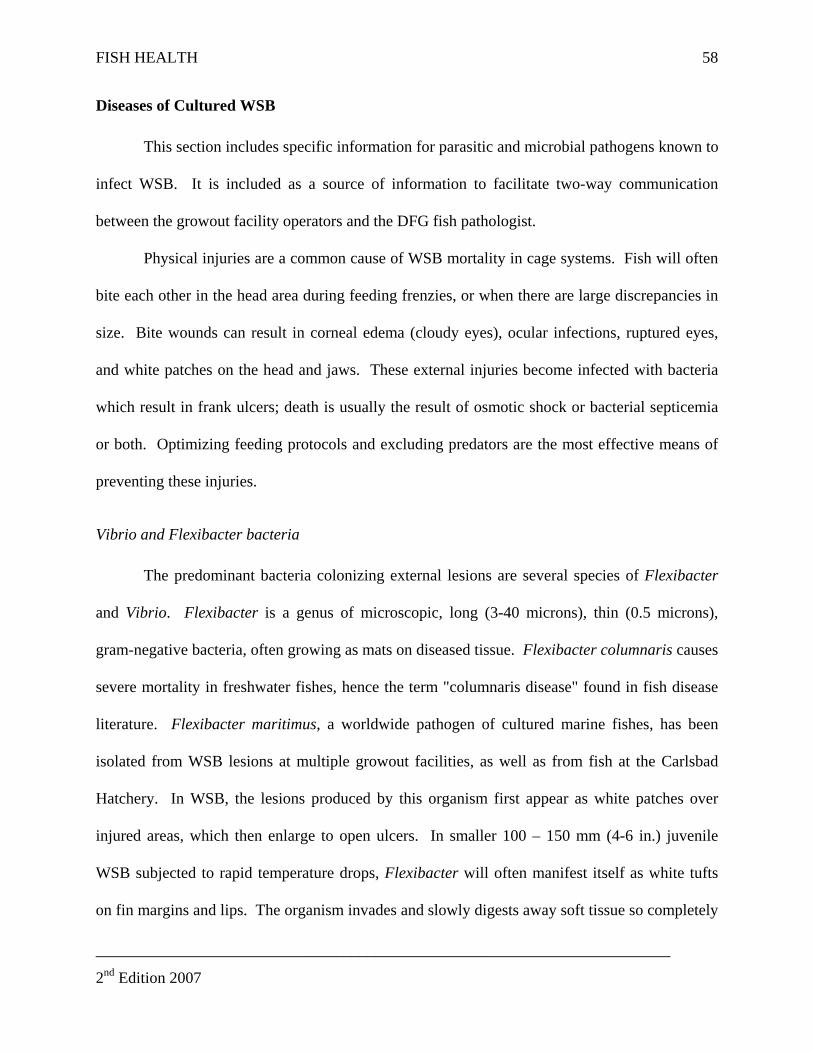
FISH HEALTH 58
Diseases of Cultured WSB
This section includes specific information for parasitic and microbial pathogens known to
infect WSB. It is included as a source of information to facilitate two-way communication
between the growout facility operators and the DFG fish pathologist.
Physical injuries are a common cause of WSB mortality in cage systems. Fish will often
bite each other in the head area during feeding frenzies, or when there are large discrepancies in
size. Bite wounds can result in corneal edema (cloudy eyes), ocular infections, ruptured eyes,
and white patches on the head and jaws. These external injuries become infected with bacteria
which result in frank ulcers; death is usually the result of osmotic shock or bacterial septicemia
or both. Optimizing feeding protocols and excluding predators are the most effective means of
preventing these injuries.
Vibrio and Flexibacter bacteria
The predominant bacteria colonizing external lesions are several species of Flexibacter
and Vibrio. Flexibacter is a genus of microscopic, long (3-40 microns), thin (0.5 microns),
gram-negative bacteria, often growing as mats on diseased tissue. Flexibacter columnaris causes
severe mortality in freshwater fishes, hence the term "columnaris disease" found in fish disease
literature. Flexibacter maritimus, a worldwide pathogen of cultured marine fishes, has been
isolated from WSB lesions at multiple growout facilities, as well as from fish at the Carlsbad
Hatchery. In WSB, the lesions produced by this organism first appear as white patches over
injured areas, which then enlarge to open ulcers. In smaller 100 – 150 mm (4-6 in.) juvenile
WSB subjected to rapid temperature drops, Flexibacter will often manifest itself as white tufts
on fin margins and lips. The organism invades and slowly digests away soft tissue so completely
________________________________________________________________________
2nd Edition 2007
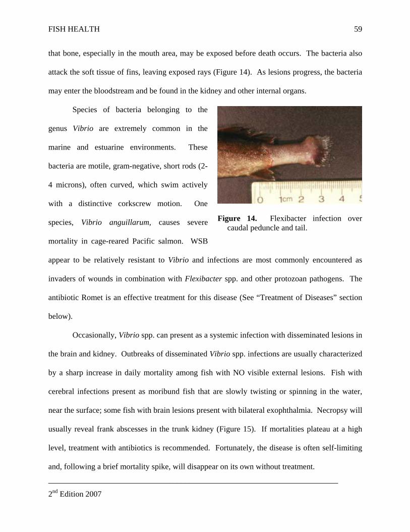
FISH HEALTH 59
that bone, especially in the mouth area, may be exposed before death occurs. The bacteria also
attack the soft tissue of fins, leaving exposed rays (Figure 14). As lesions progress, the bacteria
may enter the bloodstream and be found in the kidney and other internal organs.
________________________________________________________________________
ion
self-limiting
and, following a brief mortality spike, will disappear on its own without treatment.
Species of bacteria belonging to the
genus Vibrio are extremely common in the
marine and estuarine environments. These
bacteria are motile, gram-negative, short rods (2-
4 microns), often curved, which swim actively
with a distinctive corkscrew motion. One
species, Vibrio anguillarum, causes severe
mortality in cage-reared Pacific salmon. WSB
appear to be relatively resistant to Vibrio and infections are most commonly encountered as
invaders of wounds in combination with Flexibacter spp. and other protozoan pathogens. The
antibiotic Romet is an effective treatment for this disease (See “Treatment of Diseases” sect
Figure 14. Flexibacter infection over caudal peduncle and tail.
below).
Occasionally, Vibrio spp. can present as a systemic infection with disseminated lesions in
the brain and kidney. Outbreaks of disseminated Vibrio spp. infections are usually characterized
by a sharp increase in daily mortality among fish with NO visible external lesions. Fish with
cerebral infections present as moribund fish that are slowly twisting or spinning in the water,
near the surface; some fish with brain lesions present with bilateral exophthalmia. Necropsy will
usually reveal frank abscesses in the trunk kidney (Figure 15). If mortalities plateau at a high
level, treatment with antibiotics is recommended. Fortunately, the disease is often
2nd Edition 2007
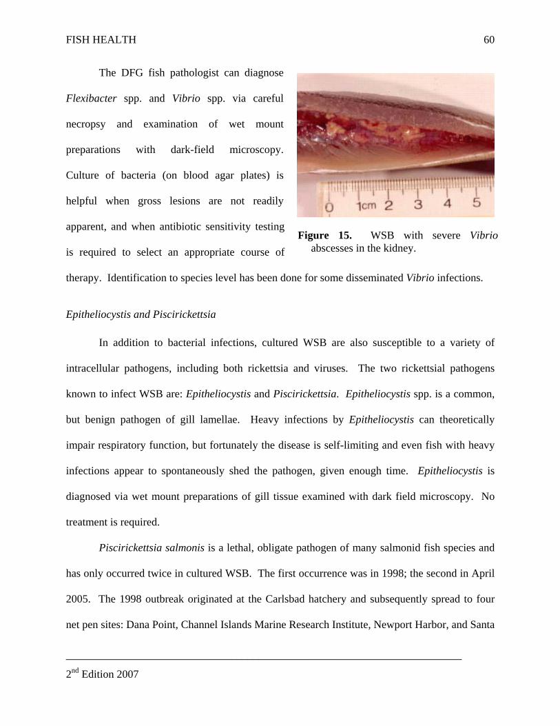
FISH HEALTH 60
________________________________________________________________________
Figure 15. WSB with severe Vibrioabscesses in the kidney.
The DFG fish pathologist can diagnose
Flexibacter spp. and Vibrio spp. via careful
necropsy and examination of wet mount
preparations with dark-field microscopy.
Culture of bacteria (on blood agar plates) is
helpful when gross lesions are not readily
apparent, and when antibiotic sensitivity testing
is required to select an appropriate course of
therapy. Identification to species level has been done for some disseminated Vibrio infections.
Epitheliocystis and Piscirickettsia
In addition to bacterial infections, cultured WSB are also susceptible to a variety of
intracellular pathogens, including both rickettsia and viruses. The two rickettsial pathogens
known to infect WSB are: Epitheliocystis and Piscirickettsia. Epitheliocystis spp. is a common,
but benign pathogen of gill lamellae. Heavy infections by Epitheliocystis can theoretically
impair respiratory function, but fortunately the disease is self-limiting and even fish with heavy
infections appear to spontaneously shed the pathogen, given enough time. Epitheliocystis is
diagnosed via wet mount preparations of gill tissue examined with dark field microscopy. No
treatment is required.
Piscirickettsia salmonis is a lethal, obligate pathogen of many salmonid fish species and
has only occurred twice in cultured WSB. The first occurrence was in 1998; the second in April
2005. The 1998 outbreak originated at the Carlsbad hatchery and subsequently spread to four
net pen sites: Dana Point, Channel Islands Marine Research Institute, Newport Harbor, and Santa
2nd Edition 2007
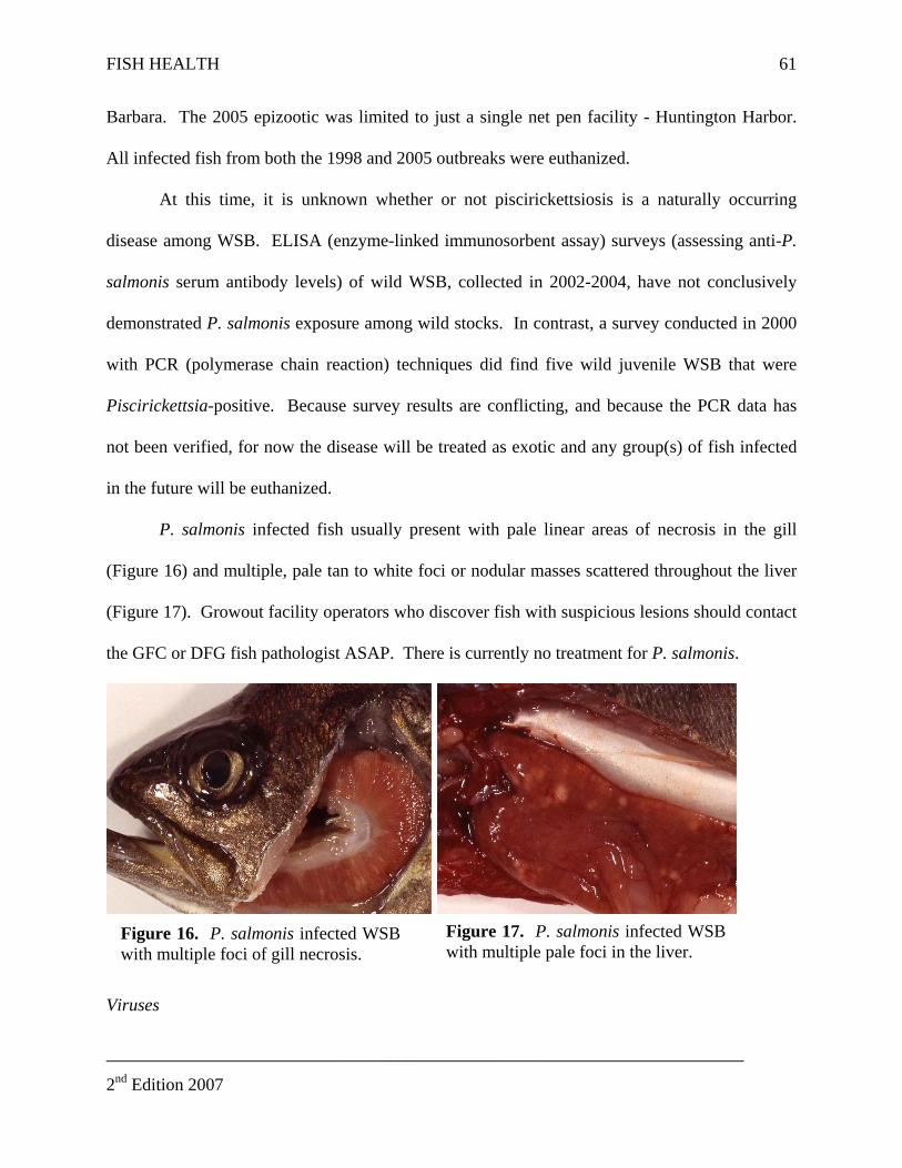
FISH HEALTH 61
Barbara. The 2005 epizootic was limited to just a single net pen facility - Huntington Harbor.
All infected fish from both the 1998 and 2005 outbreaks were euthanized.
At this time, it is unknown whether or not piscirickettsiosis is a naturally occurring
disease among WSB. ELISA (enzyme-linked immunosorbent assay) surveys (assessing anti-P.
salmonis serum antibody levels) of wild WSB, collected in 2002-2004, have not conclusively
demonstrated P. salmonis exposure among wild stocks. In contrast, a survey conducted in 2000
with PCR (polymerase chain reaction) techniques did find five wild juvenile WSB that were
Piscirickettsia-positive. Because survey results are conflicting, and because the PCR data has
not been verified, for now the disease will be treated as exotic and any group(s) of fish infected
in the future will be euthanized.
P. salmonis infected fish usually present with pale linear areas of necrosis in the gill
(Figure 16) and multiple, pale tan to white foci or nodular masses scattered throughout the liver
(Figure 17). Growout facility operators who discover fish with suspicious lesions should contact
the GFC or DFG fish pathologist ASAP. There is currently no treatment for P. salmonis.
Figure 17. P. salmonis infected WSB with multiple pale foci in the liver.
Viruses
Figure 16. P. salmonis infected WSB with multiple foci of gill necrosis.
________________________________________________________________________
2nd Edition 2007
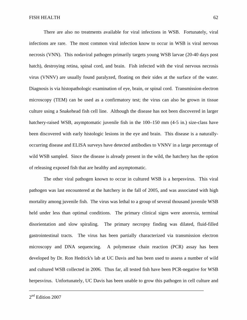
FISH HEALTH 62
There are also no treatments available for viral infections in WSB. Fortunately, viral
infections are rare. The most common viral infection know to occur in WSB is viral nervous
necrosis (VNN). This nodaviral pathogen primarily targets young WSB larvae (20-40 days post
hatch), destroying retina, spinal cord, and brain. Fish infected with the viral nervous necrosis
virus (VNNV) are usually found paralyzed, floating on their sides at the surface of the water.
Diagnosis is via histopathologic examination of eye, brain, or spinal cord. Transmission electron
microscopy (TEM) can be used as a confirmatory test; the virus can also be grown in tissue
culture using a Snakehead fish cell line. Although the disease has not been discovered in larger
hatchery-raised WSB, asymptomatic juvenile fish in the 100–150 mm (4-5 in.) size-class have
been discovered with early histologic lesions in the eye and brain. This disease is a naturally-
occurring disease and ELISA surveys have detected antibodies to VNNV in a large percentage of
wild WSB sampled. Since the disease is already present in the wild, the hatchery has the option
of releasing exposed fish that are healthy and asymptomatic.
The other viral pathogen known to occur in cultured WSB is a herpesvirus. This viral
pathogen was last encountered at the hatchery in the fall of 2005, and was associated with high
mortality among juvenile fish. The virus was lethal to a group of several thousand juvenile WSB
held under less than optimal conditions. The primary clinical signs were anorexia, terminal
disorientation and slow spiraling. The primary necropsy finding was dilated, fluid-filled
gastrointestinal tracts. The virus has been partially characterized via transmission electron
microscopy and DNA sequencing. A polymerase chain reaction (PCR) assay has been
developed by Dr. Ron Hedrick's lab at UC Davis and has been used to assess a number of wild
and cultured WSB collected in 2006. Thus far, all tested fish have been PCR-negative for WSB
herpesvirus. Unfortunately, UC Davis has been unable to grow this pathogen in cell culture and
________________________________________________________________________
2nd Edition 2007

FISH HEALTH 63
we therefore cannot generate sufficient viral
antigen to develop a usable ELISA. And without
the ELISA, there is no easy way to screen wild
WSB for viral exposure. At the present time, the
disease is to be treated as novel and any fish
diagnosed with (or exposed to) herpesviral
enteritis will be euthanized to prevent spread to
wild fish stocks. Figure 18. Cynoscionicola fluke
Parasites
External metazoan and protozoan
parasites are commonly found on the skin and
gills of cultured WSB. Some are incidental
findings that cause no disease; others are obligate
pathogens and result in severe disease and high
mortality. Metazoan parasites encountered in
cultured WSB include a variety of monogenetic trematodes (flukes) and occasional parasitic
isopods; cestodes (tapeworms) have not been found in WSB.
Figure 19. Gyrodactylus fluke.
Cynoscionicola pseudoheterocantha is monogenetic trematode primarily affecting WSB
held at Santa Catalina Island (Figure 18). The disease is usually a problem in the fall (September
and October), but in 2003 and 2004 the parasite turned up early, with infected fish showing up as
early as May or June. The parasite has also been observed at three mainland cage sites: Marina
________________________________________________________________________
2nd Edition 2007
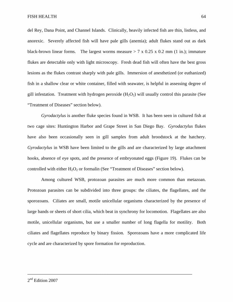
FISH HEALTH 64
del Rey, Dana Point, and Channel Islands. Clinically, heavily infected fish are thin, listless, and
anorexic. Severely affected fish will have pale gills (anemia); adult flukes stand out as dark
black-brown linear forms. The largest worms measure > 7 x 0.25 x 0.2 mm (1 in.); immature
flukes are detectable only with light microscopy. Fresh dead fish will often have the best gross
lesions as the flukes contrast sharply with pale gills. Immersion of anesthetized (or euthanized)
fish in a shallow clear or white container, filled with seawater, is helpful in assessing degree of
gill infestation. Treatment with hydrogen peroxide (H2O2) will usually control this parasite (See
“Treatment of Diseases” section below).
Gyrodactylus is another fluke species found in WSB. It has been seen in cultured fish at
two cage sites: Huntington Harbor and Grape Street in San Diego Bay. Gyrodactylus flukes
have also been occasionally seen in gill samples from adult broodstock at the hatchery.
Gyrodactylus in WSB have been limited to the gills and are characterized by large attachment
hooks, absence of eye spots, and the presence of embryonated eggs (Figure 19). Flukes can be
controlled with either H2O2 or formalin (See “Treatment of Diseases” section below).
Among cultured WSB, protozoan parasites are much more common than metazoan.
Protozoan parasites can be subdivided into three groups: the ciliates, the flagellates, and the
sporozoans. Ciliates are small, motile unicellular organisms characterized by the presence of
large bands or sheets of short cilia, which beat in synchrony for locomotion. Flagellates are also
motile, unicellular organisms, but use a smaller number of long flagella for motility. Both
ciliates and flagellates reproduce by binary fission. Sporozoans have a more complicated life
cycle and are characterized by spore formation for reproduction.
________________________________________________________________________
2nd Edition 2007
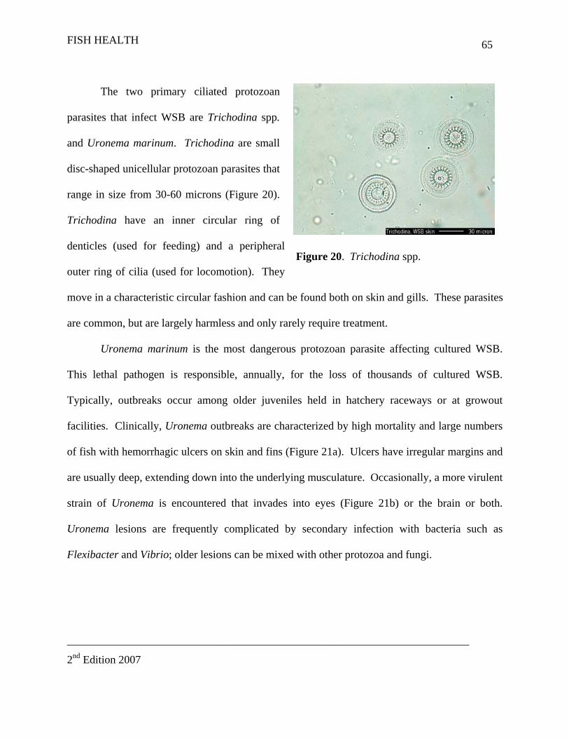
FISH HEALTH 65
________________________________________________________________________
2nd Edition 2007
The two primary ciliated protozoan
parasites that infect WSB are Trichodina spp.
and Uronema marinum. Trichodina are small
disc-shaped unicellular protozoan parasites that
range in size from 30-60 microns (Figure 20).
Trichodina have an inner circular ring of
denticles (used for feeding) and a peripheral
outer ring of cilia (used for locomotion). They
move in a characteristic circular fashion and can be found both on skin and gills. These parasites
are common, but are largely harmless and only rarely require treatment.
Figure 20. Trichodina spp.
Uronema marinum is the most dangerous protozoan parasite affecting cultured WSB.
This lethal pathogen is responsible, annually, for the loss of thousands of cultured WSB.
Typically, outbreaks occur among older juveniles held in hatchery raceways or at growout
facilities. Clinically, Uronema outbreaks are characterized by high mortality and large numbers
of fish with hemorrhagic ulcers on skin and fins (Figure 21a). Ulcers have irregular margins and
are usually deep, extending down into the underlying musculature. Occasionally, a more virulent
strain of Uronema is encountered that invades into eyes (Figure 21b) or the brain or both.
Uronema lesions are frequently complicated by secondary infection with bacteria such as
Flexibacter and Vibrio; older lesions can be mixed with other protozoa and fungi.
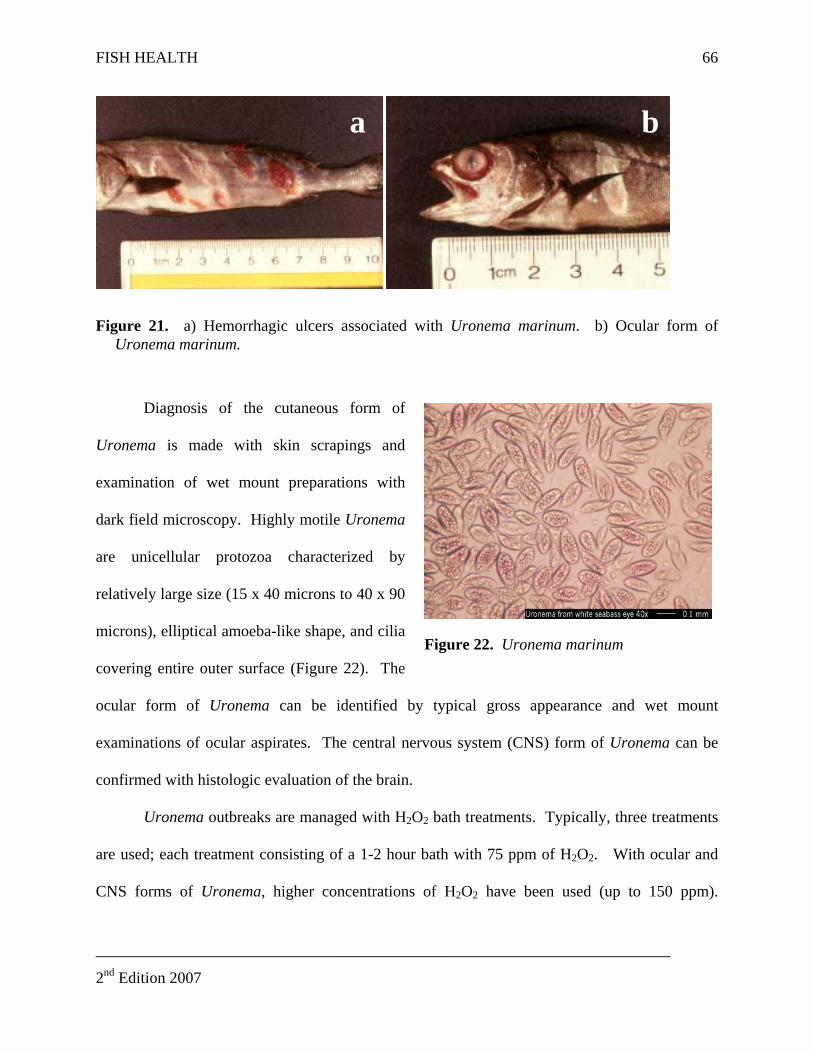
FISH HEALTH 66
a b
Figure 21. a) Hemorrhagic ulcers associated with Uronema marinum. b) Ocular form of Uronema marinum.
Diagnosis of the cutaneous form of
Uronema is made with skin scrapings and
examination of wet mount preparations with
dark field microscopy. Highly motile Uronema
are unicellular protozoa characterized by
relatively large size (15 x 40 microns to 40 x 90
microns), elliptical amoeba-like shape, and cilia
covering entire outer surface (Figure 22). The
ocular form of Uronema can be identified by typical gross appearance and wet mount
examinations of ocular aspirates. The central nervous system (CNS) form of Uronema can be
confirmed with histologic evaluation of the brain.
Figure 22. Uronema marinum
Uronema outbreaks are managed with H2O2 bath treatments. Typically, three treatments
are used; each treatment consisting of a 1-2 hour bath with 75 ppm of H2O2. With ocular and
CNS forms of Uronema, higher concentrations of H2O2 have been used (up to 150 ppm).
________________________________________________________________________
2nd Edition 2007
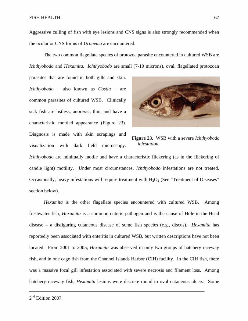
FISH HEALTH 67
Aggressive culling of fish with eye lesions and CNS signs is also strongly recommended when
the ocular or CNS forms of Uronema are encountered.
The two common flagellate species of protozoa parasite encountered in cultured WSB are
Ichthyobodo and Hexamita. Ichthyobodo are small (7-10 microns), oval, flagellated protozoan
parasites that are found in both gills and skin.
Ichthyobodo – also known as Costia – are
common parasites of cultured WSB. Clinically
sick fish are listless, anorexic, thin, and have a
characteristic mottled appearance (Figure 23).
Diagnosis is made with skin scrapings and
visualization with dark field microscopy.
Ichthyobodo are minimally motile and have a characteristic flickering (as in the flickering of
candle light) motility. Under most circumstances, Ichthyobodo infestations are not treated.
Occasionally, heavy infestations will require treatment with H2O2 (See “Treatment of Diseases”
section below).
Figure 23. WSB with a severe Ichthyobodo infestation.
Hexamita is the other flagellate species encountered with cultured WSB. Among
freshwater fish, Hexamita is a common enteric pathogen and is the cause of Hole-in-the-Head
disease – a disfiguring cutaneous disease of some fish species (e.g., discus). Hexamita has
reportedly been associated with enteritis in cultured WSB, but written descriptions have not been
located. From 2001 to 2005, Hexamita was observed in only two groups of hatchery raceway
fish, and in one cage fish from the Channel Islands Harbor (CIH) facility. In the CIH fish, there
was a massive focal gill infestation associated with severe necrosis and filament loss. Among
hatchery raceway fish, Hexamita lesions were discrete round to oval cutaneous ulcers. Some
________________________________________________________________________
2nd Edition 2007
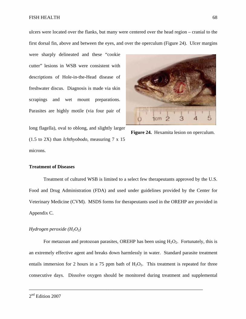
FISH HEALTH 68
ulcers were located over the flanks, but many were centered over the head region – cranial to the
first dorsal fin, above and between the eyes, and over the operculum (Figure 24). Ulcer margins
were sharply delineated and these “cookie
cutter” lesions in WSB were consistent with
descriptions of Hole-in-the-Head disease of
freshwater discus. Diagnosis is made via skin
scrapings and wet mount preparations.
Parasites are highly motile (via four pair of
long flagella), oval to oblong, and slightly larger
(1.5 to 2X) than Ichthyobodo, measuring 7 x 15
microns.
Figure 24. Hexamita lesion on operculum.
Treatment of Diseases
Treatment of cultured WSB is limited to a select few therapeutants approved by the U.S.
Food and Drug Administration (FDA) and used under guidelines provided by the Center for
Veterinary Medicine (CVM). MSDS forms for therapeutants used in the OREHP are provided in
Appendix C.
Hydrogen peroxide (H2O2)
For metazoan and protozoan parasites, OREHP has been using H2O2. Fortunately, this is
an extremely effective agent and breaks down harmlessly in water. Standard parasite treatment
entails immersion for 2 hours in a 75 ppm bath of H2O2. This treatment is repeated for three
consecutive days. Dissolve oxygen should be monitored during treatment and supplemental
________________________________________________________________________
2nd Edition 2007
FISH HEALTH 69
oxygen or aeration provided if the DO drops below 4 ppm. Under certain circumstances (e.g.,
ocular form of Uronema), higher concentrations of H2O2 may be needed; concentrations as high
as 175 ppm H2O2 have been used with one year old juveniles.
When small numbers of fish (<200) need to be treated, fish can be netted into separate
plastic treatment containers. Under most circumstances, however, it is safer, faster, and more
efficient to treat the entire pen. For fiberglass raceways, end-screens and mesh windows are
sealed (usually with plywood or plastic tarps) and the entire enclosure treated. For larger net
pens, the containment net is elevated to 2-3 m (depending on the number and size of fish), sealed
with plastic tarps (five blue plastic tarps are set in place by divers), and the entire pen treated
using concentrated 35 percent H2O2.
Each growout facility operator should take exact measurements of each enclosure in use
and determine the volume in cubic liters. Measurements should be as precise as possible so that
the proper amount of H2O2 can be administered. After you have taken measurements and
determined the metric volume, submit your data to the GFC to have your calculations verified.
Each growout facility operator should have the appropriate measuring and safety equipment on
hand to treat their fish. Growout facility operators should also identify commercial outlets where
35 percent H2O2 can be obtained. Growout facility operators can apply this treatment safely and
effectively after being properly trained, although most treatments are applied by the GFC or
DFG fish pathologist.
Formalin
Formalin has been used occasionally at the Carlsbad Hatchery for parasites that are less
susceptible to H2O2. Formalin use is limited to the hatchery because waste water has to either be
________________________________________________________________________
2nd Edition 2007
FISH HEALTH 70
treated on site, or disposed of in the municipal drainage system. Formalin can only be used by
the GFC or DFG fish pathologist.
Freshwater
Under emergency situations where H2O2 cannot be obtained, freshwater immersion can
be used. As this procedure involves considerable handling of the fish, you should get a
definitive diagnosis before proceeding and have the GFC or DFG fish pathologist help you
administer the treatment. De-chlorinated tap freshwater will kill or remove many external
protozoan and metazoan parasites. Hatchery personnel have experienced some fish mortality
associated with freshwater use, so H2O2 therapy is preferred if available.
For freshwater treatment, the fish are crowded into an area of the cage, then dip-netted
into a container of unchlorinated or dechlorinated freshwater, which is continuously oxygenated.
Fish are held in freshwater for 5 to 10 minutes and then placed back into an empty enclosure.
Ninety-five liter (25 gal) coolers work well as containers, and are filled half-way with bottled
drinking water. About 30 fish of 127-178 mm (5-7 in.) can be treated at a time, and the water
should be changed after about 10 groups of fish (approximately 300 fish) are treated.
Antibiotics
Antibiotics for use in fish are limited to Romet ® (sulfadimethozine and ormetoprim) and
Terramycin® (oxytetracycline). Both drugs have been used at the hatchery and growout
facilities in the past, but experience has shown that Romet has much greater efficacy and has
been used almost exclusively for the past three years. Applications for Romet use with WSB
include primary and secondary infections with Flexibacter or Vibrio. Bacterial infections can
either be cutaneous or systemic. Identification of bacterial pathogens is made with wet mount ________________________________________________________________________
2nd Edition 2007
FISH HEALTH
________________________________________________________________________
2nd Edition 2007
71
cytology and with culture on blood agar. Antibiotic sensitivity tests are then run to determine
susceptibility of the pathogen to Romet or Terramycin.
Romet is incorporated into the diet, at 5 grams per kilogram of feed, and fed at 3 percent
of fish body weight for 10 days. Treated fish are usually held for another two weeks to assess
efficacy before they are either released or re-treated. Because the average fish takes 3-4 years
before reaching the legal catch minimum of 71 cm (28 in.), there is no danger to the public from
consumption of hatchery fish.
RECORD KEEPING 72
RECORD KEEPING
Production information associated with WSB growout is required by the DFG in order to
participate in the OREHP. In order to meet these reporting requirements, daily empirical
observations must be recorded in a concise, quantitative manner. To facilitate and standardize
this process, the OREHP has developed data sheets that are structured primarily toward the entry
of numerical data. A sample data form for daily records is shown in Table 5. This type of
record keeping has several distinct advantages including its suitability for conversion into a
computer database. Once in the computer database, the information can readily be sorted,
analyzed and summarized. Graphic and statistical analyses can be employed to reveal trends in
growth and mortality rates as they relate to environmental and operational variables such as
water temperature and feeding ration.
In order to maintain consistency and accuracy, data forms like that shown in Table 5
accompany each group of fish delivered from the Carlsbad Hatchery. Enough forms are
delivered to accommodate information spanning the entire growout period. Preliminary
information about the batch of fish, including spawn identification, and delivery information are
completed by the GFC prior to delivery. The GFC will also include an initial feeding ration for
the fish but this ration will need to be increased as the fish grow. Growout facility operators are
encouraged to develop data sheets specific to their facilities if they identify unique data that is
not otherwise present on the provided spreadsheets. Data sheets should be combined with a
logbook that allows adequate space for recording detailed observations and notes, including
notes to the volunteer responsible for the next shift. Three-ring binders are recommended for
storage because the information can readily be photocopied and stored off-site in a dry location.
________________________________________________________________________
2nd Edition 2007

RECORD KEEPING
________________________________________________________________________
2nd Edition 2007
73
Records of fish health, mortalities, water quality, system maintenance and feeding levels
should be made daily, and recorded on the forms provided. Fish length measurements should be
made and recorded bimonthly with the assistance of the GFC. These measurements can assist in
determining accurate feeding regimes for the fish. Daily records can be subtotaled weekly and
monthly for average growth, survival and feeding rate estimates.
At the end of each month, photocopies of each monthly summary must be sent to HSWRI
for filing and storage in a computer database. Hard copies can be mailed or sent by facsimile.
Alternatively data can be entered into a spreadsheet by the growout facility operator and emailed
to the hatchery. Log books do not need to be duplicated but should be made accessible to the
DFG fish pathologist and the GFC.
Accurate, thorough, and well organized records will help optimize culture protocols, and
assist the DFG fish pathologist during a disease outbreak. As stated previously, the production
information shown in Table 5 is a mandatory requirement for all OREHP facilities. Failure to
complete the data forms routinely and thoroughly may result in a forfeiture of permits and the
associated ability to participate in the OREHP.
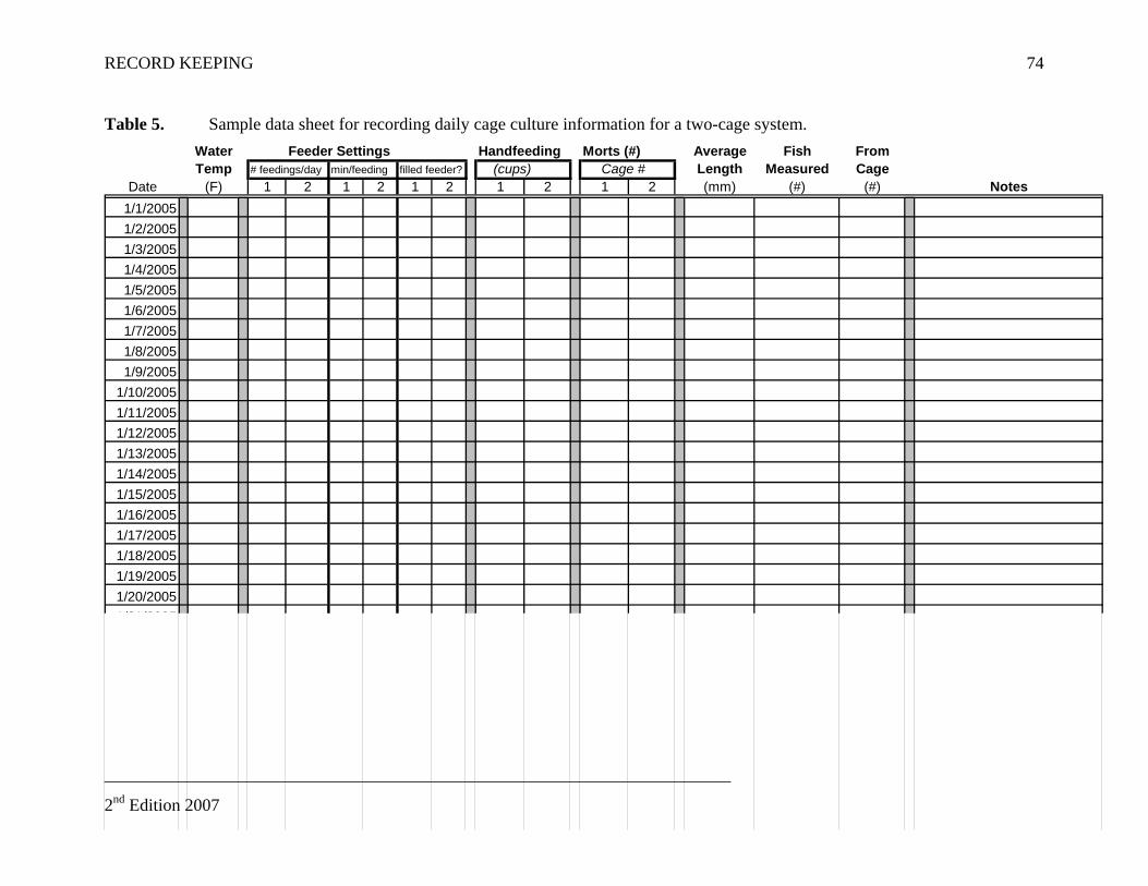
RECORD KEEPING 74
Table 5. Sample data sheet for recording daily cage culture information for a two-cage system.
________________________________________________________________________
2nd Edition 2007
Water Feeder Settings Handfeeding Morts (#) Average Fish FromTemp # feedings/day min/feeding filled feeder? (cups) Cage # Length Measured Cage
Date (F) 1 2 1 2 1 2 1 2 1 2 (mm) (#) (#) Notes1/1/20051/2/20051/3/20051/4/20051/5/20051/6/20051/7/20051/8/20051/9/2005
1/10/20051/11/20051/12/20051/13/20051/14/20051/15/20051/16/20051/17/20051/18/20051/19/20051/20/20051/21/2005
RELEASING FISH
RELEASING FISH
________________________________________________________________________
2nd Edition 2007
75
The majority of work involved in releasing the WSB takes place several weeks before the
actual release event. Prior to release a plan must be formulated including release location,
strategies, and required personnel assistance. It is also necessary for the growout facility
operator to coordinate with the GFC to perform final measurements of the fish (length and
weight), as well as a final check of tag retention. The DFG fish pathologist must also perform a
final health examination on a subsample of the WSB before they are authorized for release.
All juvenile WSB are tagged internally with a CWT by HSWRI biologists prior to being
delivered to the growout facility. Tag retention is checked prior to transport from the Carlsbad
Hatchery and again prior to release to ensure that the tags have not been shed. If the level of tag
retention is less than 90 percent, the fish may need to be sorted and re-tagged.
In addition to coordinating pre-release events, the growout facility operator and GFC
should have a well developed "release plan" prior to the actual event. In order to develop a
release plan, or to modify an existing plan (e.g. different transport mode, release site, etc.), the
GFC should be consulted well in advance. It is advantageous to release fish directly from the
growout facility because it minimizes stress associated with handling and transporting the fish.
The decision tree in Figure 25 can be used to help develop a release plan.
On the day of release, or during the week preceding the release, a subsample of 100 fish
is weighed and measured, and scanned to determine the tag retention rate as an estimate of the
average for that population. All fish are counted on the day of the release. Currently counting is
done manually using hand counters. As OREHP expands, electronic counters may be employed
to reduce the labor and handling time. Alternatively, with more experience and data, we may be
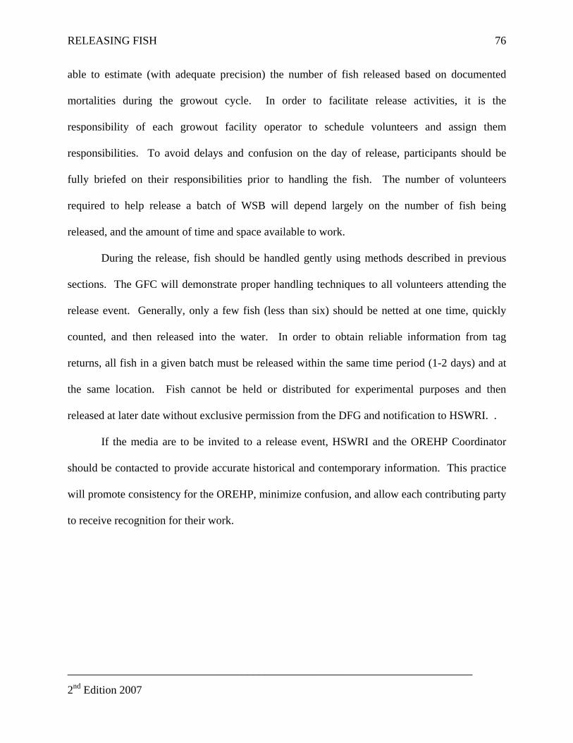
RELEASING FISH
________________________________________________________________________
2nd Edition 2007
76
able to estimate (with adequate precision) the number of fish released based on documented
mortalities during the growout cycle. In order to facilitate release activities, it is the
responsibility of each growout facility operator to schedule volunteers and assign them
responsibilities. To avoid delays and confusion on the day of release, participants should be
fully briefed on their responsibilities prior to handling the fish. The number of volunteers
required to help release a batch of WSB will depend largely on the number of fish being
released, and the amount of time and space available to work.
During the release, fish should be handled gently using methods described in previous
sections. The GFC will demonstrate proper handling techniques to all volunteers attending the
release event. Generally, only a few fish (less than six) should be netted at one time, quickly
counted, and then released into the water. In order to obtain reliable information from tag
returns, all fish in a given batch must be released within the same time period (1-2 days) and at
the same location. Fish cannot be held or distributed for experimental purposes and then
released at later date without exclusive permission from the DFG and notification to HSWRI. .
If the media are to be invited to a release event, HSWRI and the OREHP Coordinator
should be contacted to provide accurate historical and contemporary information. This practice
will promote consistency for the OREHP, minimize confusion, and allow each contributing party
to receive recognition for their work.
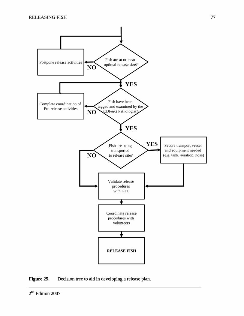
RELEASING FISH G FISH
________________________________________________________________________
2nd Edition 2007
77
________________________________________________________________________
2nd Edition 2007
77
Fish are at or near optimal release size?
Fish have been tagged and examined by the
CDF&G Pathologist?
Postpone release activities
Complete coordination of Pre-release activities
Fish are being transported
to release site?
Secure transport vessel and equipment needed
(e.g. tank, aeration, hose)
Validate release procedures with GFC
Coordinate releaseprocedures with
volunteers
RELEASE FISH
YES
YES
YES
NO
NO
NO
Figure 25. Decision tree to aid in developing a release plan. Figure 25. Decision tree to aid in developing a release plan.
LITERATURE CITED 78
LITERATURE CITED
Beveridge, M.C.M. 2004. Cage Aquaculture. 3rd ed. Cambridge: Blackwell Scientific Publications Inc. 376 p.
California Technology, Trade and Commerce Agency (CTTCA) 2002. California Permit Handbook. Sacramento: State of California. 213 p.
Creswell, L.R. 1993. Aquaculture Desk Reference. New York: Van Nostrand Reinhold. 206 p.
Milne, P.H. 1972. Fish and shellfish farming in coastal waters (Fishing News Books). Surrey: Blackwell Publishing. 208 p.
Shepherd, C.J. and N.R. Bromage, editors. 1988. Intensive Fish Farming. Cambridge: Blackwell Scientific Publications Inc. 404 p.
U.S. EPA 2004. 40 CFR Part 451: Effluent Limitations Guidelines and New Source Performance Standards for the Concentrated Aquatic Animal Production Point Source Category; Final Rule
________________________________________________________________________
2nd Edition 2007

APPENDICES 79
APPENDICES
________________________________________________________________________
2nd Edition 2007
APPENDIX A. BENTHIC MONITORING PROGRAM 80
________________________________________________________________________
Appendix A. Study Design for Benthic Monitoring Program
2nd Edition 2007
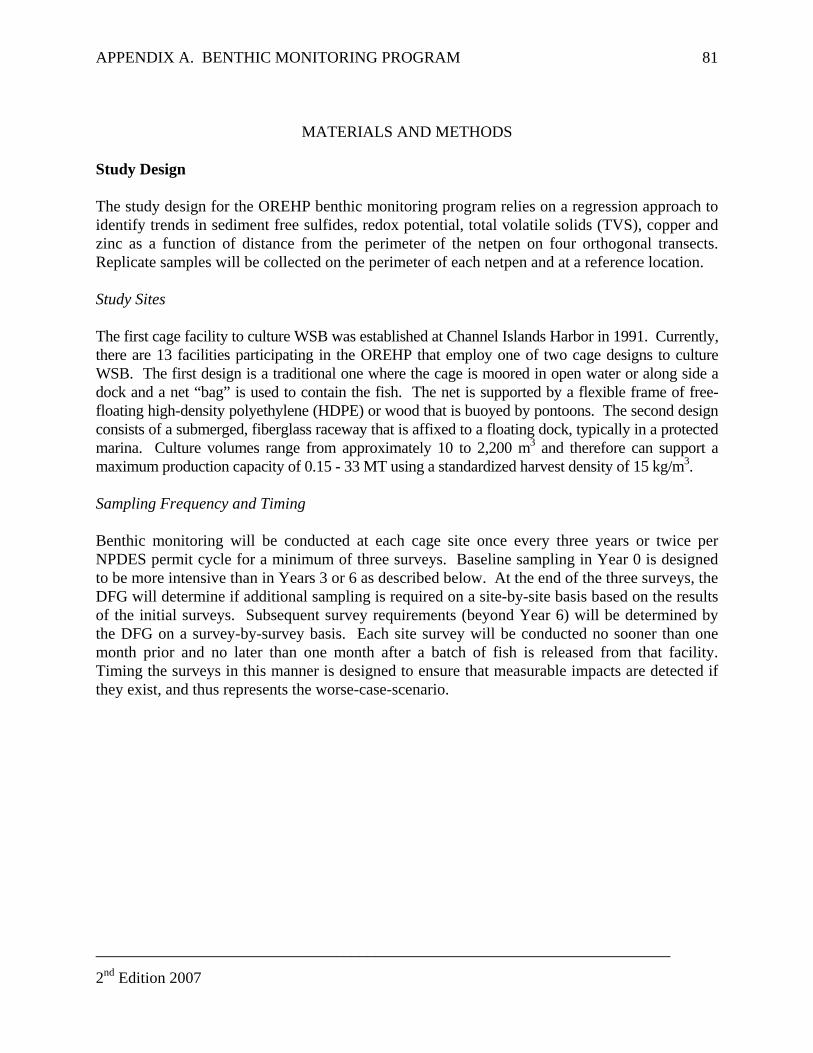
APPENDIX A. BENTHIC MONITORING PROGRAM 81
________________________________________________________________________
MATERIALS AND METHODS
Study Design The study design for the OREHP benthic monitoring program relies on a regression approach to identify trends in sediment free sulfides, redox potential, total volatile solids (TVS), copper and zinc as a function of distance from the perimeter of the netpen on four orthogonal transects. Replicate samples will be collected on the perimeter of each netpen and at a reference location. Study Sites The first cage facility to culture WSB was established at Channel Islands Harbor in 1991. Currently, there are 13 facilities participating in the OREHP that employ one of two cage designs to culture WSB. The first design is a traditional one where the cage is moored in open water or along side a dock and a net “bag” is used to contain the fish. The net is supported by a flexible frame of free-floating high-density polyethylene (HDPE) or wood that is buoyed by pontoons. The second design consists of a submerged, fiberglass raceway that is affixed to a floating dock, typically in a protected marina. Culture volumes range from approximately 10 to 2,200 m3 and therefore can support a maximum production capacity of 0.15 - 33 MT using a standardized harvest density of 15 kg/m3. Sampling Frequency and Timing Benthic monitoring will be conducted at each cage site once every three years or twice per NPDES permit cycle for a minimum of three surveys. Baseline sampling in Year 0 is designed to be more intensive than in Years 3 or 6 as described below. At the end of the three surveys, the DFG will determine if additional sampling is required on a site-by-site basis based on the results of the initial surveys. Subsequent survey requirements (beyond Year 6) will be determined by the DFG on a survey-by-survey basis. Each site survey will be conducted no sooner than one month prior and no later than one month after a batch of fish is released from that facility. Timing the surveys in this manner is designed to ensure that measurable impacts are detected if they exist, and thus represents the worse-case-scenario.
2nd Edition 2007
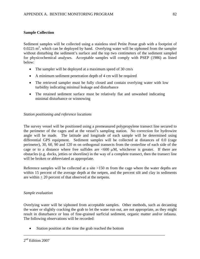
APPENDIX A. BENTHIC MONITORING PROGRAM 82
________________________________________________________________________
Sample Collection
Sediment samples will be collected using a stainless steel Petite Ponar grab with a footprint of 0.0225 m2, which can be deployed by hand. Overlying water will be siphoned from the sampler without disturbing the sediment’s surface and the top two centimeters of the sediment sampled for physicochemical analyses. Acceptable samples will comply with PSEP (1986) as listed below:
• The sampler will be deployed at a maximum speed of 30 cm/s
• A minimum sediment penetration depth of 4 cm will be required
• The retrieved sampler must be fully closed and contain overlying water with low turbidity indicating minimal leakage and disturbance
• The retained sediment surface must be relatively flat and unwashed indicating minimal disturbance or winnowing
Station positioning and reference locations
The survey vessel will be positioned using a premeasured polypropylene transect line secured to the perimeter of the cages and at the vessel’s sampling station. No correction for hydrowire angle will be made. The latitude and longitude of each sample will be determined using differential GPS equipment. Sediment samples will be collected at distances of 0.0 (cage perimeter), 30, 60, 90 and 120 m on orthogonal transects from the centerline of each side of the cage or to a distance where free sulfides are <600 μM, whichever is greater. If there are obstacles (e.g. docks, jetties or shoreline) in the way of a complete transect, then the transect line will be broken or abbreviated as appropriate.
Reference samples will be collected at a site >150 m from the cage where the water depths are within 15 percent of the average depth at the netpen, and the percent silt and clay in sediments are within + 20 percent of that observed at the netpens.
Sample evaluation
Overlying water will be siphoned from acceptable samples. Other methods, such as decanting the water or slightly cracking the grab to let the water run out, are not appropriate, as they might result in disturbance or loss of fine-grained surficial sediment, organic matter and/or infauna. The following observations will be recorded:
• Station position at the time the grab reached the bottom
2nd Edition 2007
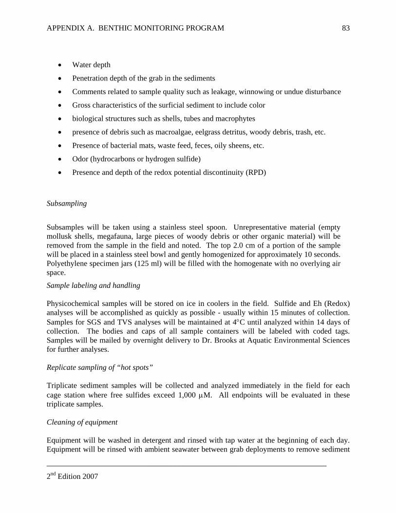
APPENDIX A. BENTHIC MONITORING PROGRAM 83
________________________________________________________________________
• Water depth
• Penetration depth of the grab in the sediments
• Comments related to sample quality such as leakage, winnowing or undue disturbance
• Gross characteristics of the surficial sediment to include color
• biological structures such as shells, tubes and macrophytes
• presence of debris such as macroalgae, eelgrass detritus, woody debris, trash, etc.
• Presence of bacterial mats, waste feed, feces, oily sheens, etc.
• Odor (hydrocarbons or hydrogen sulfide)
• Presence and depth of the redox potential discontinuity (RPD)
Subsampling
Subsamples will be taken using a stainless steel spoon. Unrepresentative material (empty mollusk shells, megafauna, large pieces of woody debris or other organic material) will be removed from the sample in the field and noted. The top 2.0 cm of a portion of the sample will be placed in a stainless steel bowl and gently homogenized for approximately 10 seconds. Polyethylene specimen jars (125 ml) will be filled with the homogenate with no overlying air space.
Sample labeling and handling Physicochemical samples will be stored on ice in coolers in the field. Sulfide and Eh (Redox) analyses will be accomplished as quickly as possible - usually within 15 minutes of collection. Samples for SGS and TVS analyses will be maintained at 4°C until analyzed within 14 days of collection. The bodies and caps of all sample containers will be labeled with coded tags. Samples will be mailed by overnight delivery to Dr. Brooks at Aquatic Environmental Sciences for further analyses. Replicate sampling of “hot spots” Triplicate sediment samples will be collected and analyzed immediately in the field for each cage station where free sulfides exceed 1,000 μM. All endpoints will be evaluated in these triplicate samples. Cleaning of equipment Equipment will be washed in detergent and rinsed with tap water at the beginning of each day. Equipment will be rinsed with ambient seawater between grab deployments to remove sediment
2nd Edition 2007
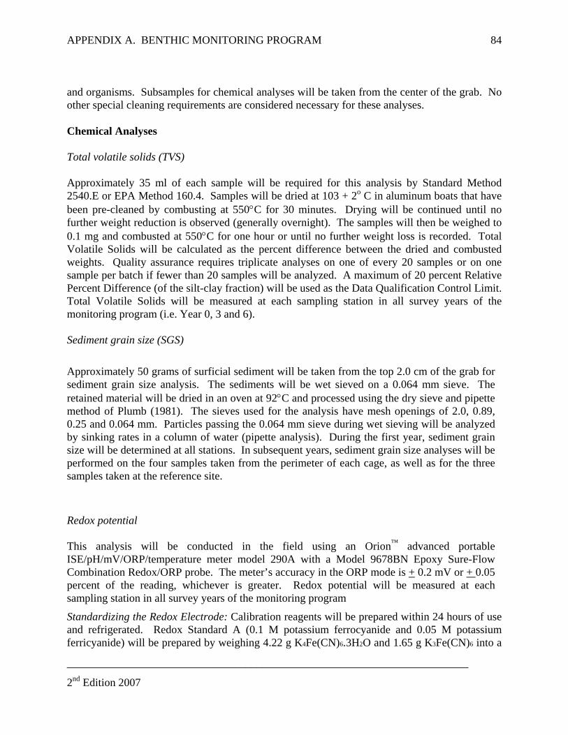
APPENDIX A. BENTHIC MONITORING PROGRAM 84
________________________________________________________________________
and organisms. Subsamples for chemical analyses will be taken from the center of the grab. No other special cleaning requirements are considered necessary for these analyses. Chemical Analyses Total volatile solids (TVS) Approximately 35 ml of each sample will be required for this analysis by Standard Method 2540.E or EPA Method 160.4. Samples will be dried at 103 + 2o C in aluminum boats that have been pre-cleaned by combusting at 550°C for 30 minutes. Drying will be continued until no further weight reduction is observed (generally overnight). The samples will then be weighed to 0.1 mg and combusted at 550°C for one hour or until no further weight loss is recorded. Total Volatile Solids will be calculated as the percent difference between the dried and combusted weights. Quality assurance requires triplicate analyses on one of every 20 samples or on one sample per batch if fewer than 20 samples will be analyzed. A maximum of 20 percent Relative Percent Difference (of the silt-clay fraction) will be used as the Data Qualification Control Limit. Total Volatile Solids will be measured at each sampling station in all survey years of the monitoring program (i.e. Year 0, 3 and 6). Sediment grain size (SGS)
Approximately 50 grams of surficial sediment will be taken from the top 2.0 cm of the grab for sediment grain size analysis. The sediments will be wet sieved on a 0.064 mm sieve. The retained material will be dried in an oven at 92°C and processed using the dry sieve and pipette method of Plumb (1981). The sieves used for the analysis have mesh openings of 2.0, 0.89, 0.25 and 0.064 mm. Particles passing the 0.064 mm sieve during wet sieving will be analyzed by sinking rates in a column of water (pipette analysis). During the first year, sediment grain size will be determined at all stations. In subsequent years, sediment grain size analyses will be performed on the four samples taken from the perimeter of each cage, as well as for the three samples taken at the reference site.
Redox potential
This analysis will be conducted in the field using an Orion™ advanced portable ISE/pH/mV/ORP/temperature meter model 290A with a Model 9678BN Epoxy Sure-Flow Combination Redox/ORP probe. The meter’s accuracy in the ORP mode is + 0.2 mV or + 0.05 percent of the reading, whichever is greater. Redox potential will be measured at each sampling station in all survey years of the monitoring program
Standardizing the Redox Electrode: Calibration reagents will be prepared within 24 hours of use and refrigerated. Redox Standard A (0.1 M potassium ferrocyanide and 0.05 M potassium ferricyanide) will be prepared by weighing 4.22 g K4Fe(CN)6.3H2O and 1.65 g K3Fe(CN)6 into a
2nd Edition 2007
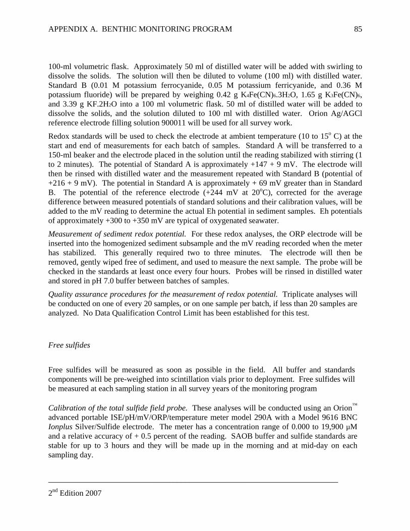
APPENDIX A. BENTHIC MONITORING PROGRAM 85
________________________________________________________________________
100-ml volumetric flask. Approximately 50 ml of distilled water will be added with swirling to dissolve the solids. The solution will then be diluted to volume (100 ml) with distilled water. Standard B (0.01 M potassium ferrocyanide, 0.05 M potassium ferricyanide, and 0.36 M potassium fluoride) will be prepared by weighing 0.42 g K4Fe(CN)6.3H2O, 1.65 g K3Fe(CN)6, and 3.39 g KF.2H2O into a 100 ml volumetric flask. 50 ml of distilled water will be added to dissolve the solids, and the solution diluted to 100 ml with distilled water. Orion Ag/AGCl reference electrode filling solution 900011 will be used for all survey work.
Redox standards will be used to check the electrode at ambient temperature (10 to 15o C) at the start and end of measurements for each batch of samples. Standard A will be transferred to a 150-ml beaker and the electrode placed in the solution until the reading stabilized with stirring (1 to 2 minutes). The potential of Standard A is approximately +147 + 9 mV. The electrode will then be rinsed with distilled water and the measurement repeated with Standard B (potential of +216 + 9 mV). The potential in Standard A is approximately + 69 mV greater than in Standard B. The potential of the reference electrode (+244 mV at 20oC), corrected for the average difference between measured potentials of standard solutions and their calibration values, will be added to the mV reading to determine the actual Eh potential in sediment samples. Eh potentials of approximately +300 to +350 mV are typical of oxygenated seawater.
Measurement of sediment redox potential. For these redox analyses, the ORP electrode will be inserted into the homogenized sediment subsample and the mV reading recorded when the meter has stabilized. This generally required two to three minutes. The electrode will then be removed, gently wiped free of sediment, and used to measure the next sample. The probe will be checked in the standards at least once every four hours. Probes will be rinsed in distilled water and stored in pH 7.0 buffer between batches of samples.
Quality assurance procedures for the measurement of redox potential. Triplicate analyses will be conducted on one of every 20 samples, or on one sample per batch, if less than 20 samples are analyzed. No Data Qualification Control Limit has been established for this test.
Free sulfides
Free sulfides will be measured as soon as possible in the field. All buffer and standards components will be pre-weighed into scintillation vials prior to deployment. Free sulfides will be measured at each sampling station in all survey years of the monitoring program
Calibration of the total sulfide field probe. These analyses will be conducted using an Orion™ advanced portable ISE/pH/mV/ORP/temperature meter model 290A with a Model 9616 BNC Ionplus Silver/Sulfide electrode. The meter has a concentration range of 0.000 to 19,900 µM and a relative accuracy of + 0.5 percent of the reading. SAOB buffer and sulfide standards are stable for up to 3 hours and they will be made up in the morning and at mid-day on each sampling day.
2nd Edition 2007
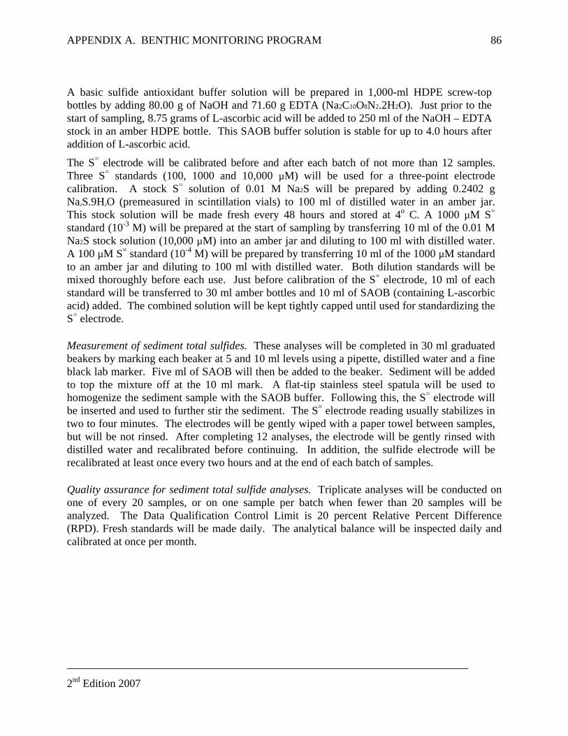
APPENDIX A. BENTHIC MONITORING PROGRAM 86
________________________________________________________________________
A basic sulfide antioxidant buffer solution will be prepared in 1,000-ml HDPE screw-top bottles by adding 80.00 g of NaOH and 71.60 g EDTA (Na2C10O8N2.2H2O). Just prior to the start of sampling, 8.75 grams of L-ascorbic acid will be added to 250 ml of the NaOH – EDTA stock in an amber HDPE bottle. This SAOB buffer solution is stable for up to 4.0 hours after addition of L-ascorbic acid.
The S= electrode will be calibrated before and after each batch of not more than 12 samples. Three S= standards (100, 1000 and 10,000 µM) will be used for a three-point electrode calibration. A stock S= solution of 0.01 M Na2S will be prepared by adding 0.2402 g Na2S.9H2O (premeasured in scintillation vials) to 100 ml of distilled water in an amber jar. This stock solution will be made fresh every 48 hours and stored at 4o C. A 1000 µM S= standard (10-3 M) will be prepared at the start of sampling by transferring 10 ml of the 0.01 M Na2S stock solution (10,000 µM) into an amber jar and diluting to 100 ml with distilled water. A 100 µM S= standard (10-4 M) will be prepared by transferring 10 ml of the 1000 µM standard to an amber jar and diluting to 100 ml with distilled water. Both dilution standards will be mixed thoroughly before each use. Just before calibration of the S= electrode, 10 ml of each standard will be transferred to 30 ml amber bottles and 10 ml of SAOB (containing L-ascorbic acid) added. The combined solution will be kept tightly capped until used for standardizing the S= electrode.
Measurement of sediment total sulfides. These analyses will be completed in 30 ml graduated beakers by marking each beaker at 5 and 10 ml levels using a pipette, distilled water and a fine black lab marker. Five ml of SAOB will then be added to the beaker. Sediment will be added to top the mixture off at the 10 ml mark. A flat-tip stainless steel spatula will be used to homogenize the sediment sample with the SAOB buffer. Following this, the S= electrode will be inserted and used to further stir the sediment. The S= electrode reading usually stabilizes in two to four minutes. The electrodes will be gently wiped with a paper towel between samples, but will be not rinsed. After completing 12 analyses, the electrode will be gently rinsed with distilled water and recalibrated before continuing. In addition, the sulfide electrode will be recalibrated at least once every two hours and at the end of each batch of samples.
Quality assurance for sediment total sulfide analyses. Triplicate analyses will be conducted on one of every 20 samples, or on one sample per batch when fewer than 20 samples will be analyzed. The Data Qualification Control Limit is 20 percent Relative Percent Difference (RPD). Fresh standards will be made daily. The analytical balance will be inspected daily and calibrated at once per month.
2nd Edition 2007
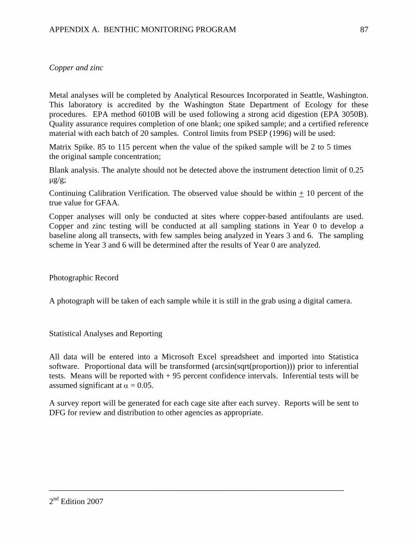
APPENDIX A. BENTHIC MONITORING PROGRAM 87
________________________________________________________________________
Copper and zinc
Metal analyses will be completed by Analytical Resources Incorporated in Seattle, Washington. This laboratory is accredited by the Washington State Department of Ecology for these procedures. EPA method 6010B will be used following a strong acid digestion (EPA 3050B). Quality assurance requires completion of one blank; one spiked sample; and a certified reference material with each batch of 20 samples. Control limits from PSEP (1996) will be used:
Matrix Spike. 85 to 115 percent when the value of the spiked sample will be 2 to 5 times the original sample concentration;
Blank analysis. The analyte should not be detected above the instrument detection limit of 0.25 µg/g;
Continuing Calibration Verification. The observed value should be within + 10 percent of the true value for GFAA.
Copper analyses will only be conducted at sites where copper-based antifoulants are used. Copper and zinc testing will be conducted at all sampling stations in Year 0 to develop a baseline along all transects, with few samples being analyzed in Years 3 and 6. The sampling scheme in Year 3 and 6 will be determined after the results of Year 0 are analyzed.
Photographic Record
A photograph will be taken of each sample while it is still in the grab using a digital camera.
Statistical Analyses and Reporting
All data will be entered into a Microsoft Excel spreadsheet and imported into Statistica software. Proportional data will be transformed (arcsin(sqrt(proportion))) prior to inferential tests. Means will be reported with + 95 percent confidence intervals. Inferential tests will be assumed significant at α = 0.05.
A survey report will be generated for each cage site after each survey. Reports will be sent to DFG for review and distribution to other agencies as appropriate.
2nd Edition 2007
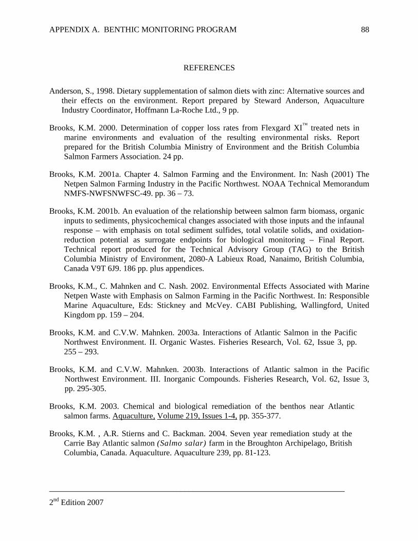
APPENDIX A. BENTHIC MONITORING PROGRAM 88
________________________________________________________________________
REFERENCES
Anderson, S., 1998. Dietary supplementation of salmon diets with zinc: Alternative sources and their effects on the environment. Report prepared by Steward Anderson, Aquaculture Industry Coordinator, Hoffmann La-Roche Ltd., 9 pp.
Brooks, K.M. 2000. Determination of copper loss rates from Flexgard XI™ treated nets in marine environments and evaluation of the resulting environmental risks. Report prepared for the British Columbia Ministry of Environment and the British Columbia Salmon Farmers Association. 24 pp.
Brooks, K.M. 2001a. Chapter 4. Salmon Farming and the Environment. In: Nash (2001) The Netpen Salmon Farming Industry in the Pacific Northwest. NOAA Technical Memorandum NMFS-NWFSNWFSC-49. pp. 36 – 73.
Brooks, K.M. 2001b. An evaluation of the relationship between salmon farm biomass, organic inputs to sediments, physicochemical changes associated with those inputs and the infaunal response – with emphasis on total sediment sulfides, total volatile solids, and oxidation-reduction potential as surrogate endpoints for biological monitoring – Final Report. Technical report produced for the Technical Advisory Group (TAG) to the British Columbia Ministry of Environment, 2080-A Labieux Road, Nanaimo, British Columbia, Canada V9T 6J9. 186 pp. plus appendices.
Brooks, K.M., C. Mahnken and C. Nash. 2002. Environmental Effects Associated with Marine Netpen Waste with Emphasis on Salmon Farming in the Pacific Northwest. In: Responsible Marine Aquaculture, Eds: Stickney and McVey. CABI Publishing, Wallingford, United Kingdom pp. 159 – 204.
Brooks, K.M. and C.V.W. Mahnken. 2003a. Interactions of Atlantic Salmon in the Pacific Northwest Environment. II. Organic Wastes. Fisheries Research, Vol. 62, Issue 3, pp. 255 – 293.
Brooks, K.M. and C.V.W. Mahnken. 2003b. Interactions of Atlantic salmon in the Pacific Northwest Environment. III. Inorganic Compounds. Fisheries Research, Vol. 62, Issue 3, pp. 295-305.
Brooks, K.M. 2003. Chemical and biological remediation of the benthos near Atlantic salmon farms. Aquaculture, Volume 219, Issues 1-4, pp. 355-377.
Brooks, K.M. , A.R. Stierns and C. Backman. 2004. Seven year remediation study at the Carrie Bay Atlantic salmon (Salmo salar) farm in the Broughton Archipelago, British Columbia, Canada. Aquaculture. Aquaculture 239, pp. 81-123.
2nd Edition 2007

APPENDIX A. BENTHIC MONITORING PROGRAM
________________________________________________________________________
2nd Edition 2007
89
Chow, K.W., Schell, W.R., 1978. The minerals, In Fish Feed Technology. Aquac. Dev. Coord. Programme, Rep. ADCP/REP/80/11, FAO, Rome.
Long, E.R., D.D. MacDonald, S.L. Smith and F.D. Calder. 1995. Incidence of Adverse Biological Effects within Ranges of Chemical Concentrations in Marine and Estuarine Sediments, Environmental Management 19(1) pp. 81-97.
MacDonald, D.D. 1994. Approach to the Assessment of Sediment Quality in Florida Coastal Waters. Florida Department of Environmental Protection, Tallahassee, Florida.
U.S. EPA 2004. 40 CFR Part 451: Effluent Limitations Guidelines and New Source Performance Standards for the Concentrated Aquatic Animal Production Point Source Category; Final Rule.
Wildish, D.J., H.M. Akagi, B.T. Hargrave and P.M. Strain. (In-prep) Inter-laboratory calibration of redox potential and total sulfide measurements in interfacial marine sediments and the implications for organic enrichment. Canadian Department of Fisheries and Oceans Technical Report. 33 pp.
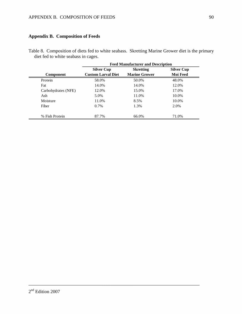
APPENDIX B. COMPOSITION OF FEEDS 90
Appendix B. Composition of Feeds
Table 8. Composition of diets fed to white seabass. Skretting Marine Grower diet is the primary diet fed to white seabass in cages.
Silver Cup Skretting Silver CupComponent Custom Larval Diet Marine Grower Moi Feed
Protein 58.0% 50.0% 48.0%Fat 14.0% 14.0% 12.0%Carbohydrates (NFE) 12.0% 15.0% 17.0%Ash 5.0% 11.0% 10.0%Moisture 11.0% 8.5% 10.0%Fiber 0.7% 1.3% 2.0%
% Fish Protein 87.7% 66.0% 71.0%
Feed Manufacturer and Description
________________________________________________________________________
2nd Edition 2007

APPENDIX C. OMB 0648-0292 91
Appendix C. Marine Mammal Mortality/Injury Reporting From (OMB 0648-0292)
________________________________________________________________________
2nd Edition 2007

APPENDIX C. OMB 0648-0292 92
________________________________________________________________________
2nd Edition 2007
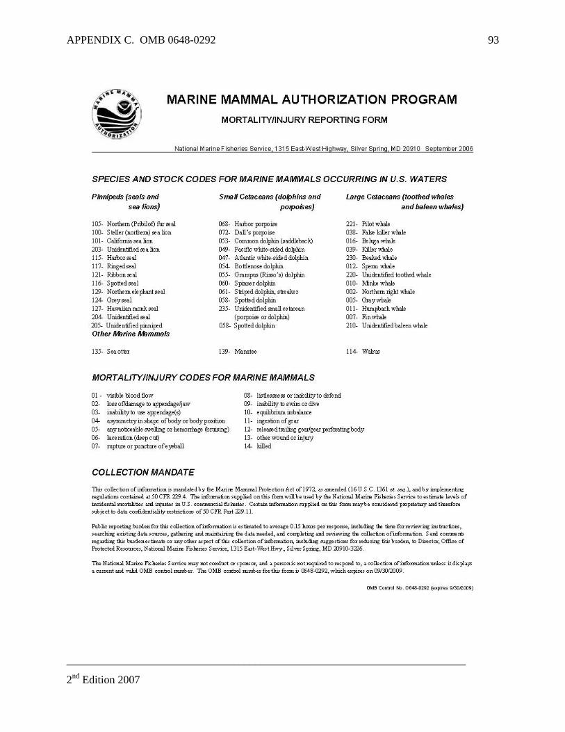
APPENDIX C. OMB 0648-0292
________________________________________________________________________
2nd Edition 2007
93
APPENDIX D. MSDS for Chemicals 94
Appendix D. MSDS for Chemicals
________________________________________________________________________
2nd Edition 2007
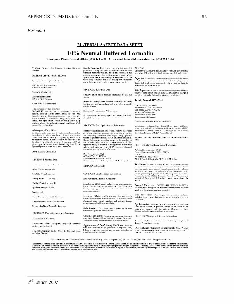
APPENDIX D. MSDS for Chemicals 95
Formalin
________________________________________________________________________
2nd Edition 2007

APPENDIX D. MSDS for Chemicals 96
Hydrogen Peroxide H2O2
________________________________________________________________________
2nd Edition 2007

APPENDIX D. MSDS for Chemicals 97
________________________________________________________________________
2nd Edition 2007
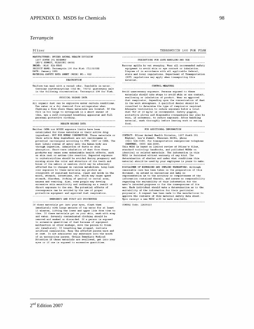
APPENDIX D. MSDS for Chemicals 98
Terramycin
________________________________________________________________________
2nd Edition 2007
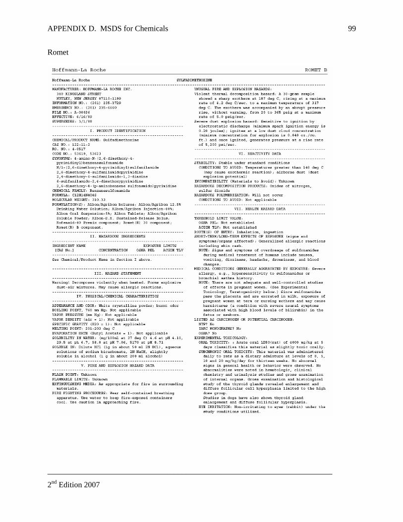
APPENDIX D. MSDS for Chemicals 99
Romet
________________________________________________________________________
2nd Edition 2007
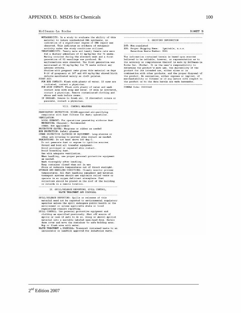
APPENDIX D. MSDS for Chemicals 100
________________________________________________________________________
2nd Edition 2007
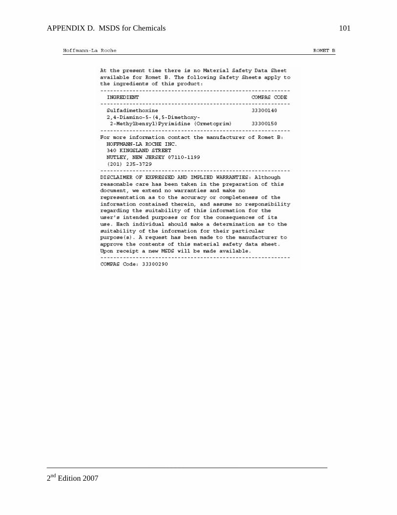
APPENDIX D. MSDS for Chemicals 101
________________________________________________________________________
2nd Edition 2007
APPENDIX D. MSDS for Chemicals 102
Flexguard XI
________________________________________________________________________
2nd Edition 2007

APPENDIX D. MSDS for Chemicals
________________________________________________________________________
2nd Edition 2007
103
Appendix C A Contemporary Plan for Managing White Seabass Broodstock and Production Cohorts for the OREHP
HSWRI Revised WSB BPCMP December 2010 Page 1
A CONTEMPORARY PLAN FOR MANAGING WHITE SEABASS BROODSTOCK AND PRODUCTION COHORTS FOR THE OREHP ORIGINAL April 2008 REVISED January 2011 Prepared by Kristen Gruenthal, PhD Mark Drawbridge, MS Michael Gafford Hubbs-SeaWorld Research Institute 2595 Ingraham St. San Diego, CA 92109 USA Phone: 619-226-3870 Fax: 619-226-3944

2
This document was developed and revised by HSWRI scientists as a contemporary plan for managing white seabass (Atractoscion nobilis; WSB) broodstock and production cohorts in a practical manner that maximizes genetic diversity. This plan is intended to be adaptive and dynamic, taking advantage of the best, most recent information available. It also assumes that sufficient financial support exists to execute the plan, especially resources required to capture, transport, and hold new brood fish each year.
BROODSTOCK MANAGEMENT Background and Contemporary Rationale The original WSB broodstock management plan implemented by HSWRI at the Leon Raymond Hubbard, Jr., Marine Fish Hatchery in Carlsbad, CA, was developed by Bartley et al. (1995). The plan involves four breeding pools that contain 50 adult fish of equal sex ratio in each pool. Each group of fish is conditioned to spawn for 4-5 month photothermally-regulated seasons that are offset from each other throughout the year. The initial plan recommended replacing 20% of the stock (10 fish per pool: five males and five females) and rotating 20% (five) of males from each pool into a different pool annually. During the past 15 years, new stock has been added inconsistently, primarily to replace fish that died or that were suffering from health problems, and replacement has averaged approximately 7% per year. Male fish have not been rotated among pools because of difficulties in handling fish, concerns of harming fish, and potential disruption of spawning cycles. A new plan was developed in early 2008, but the information contained in the document was based on genetic research that had not yet been completed. The contemporary management plan presented in this document seeks to correct and revise these inconsistencies and implement further improvements, including the development of:
1. revised fish replacement and sex ratio schemes 2. fish handling techniques for large brood fish in breeding pools 3. a routine collection and holding program to support introduction of new fish
Each of these areas is covered in detail below. Replacement Scheme Outline
1. Census size (N): a. Bartley et al. (1995)
i. 200 brood fish (50 fish per pool)
3
ii. For a minimum annual genetically effective breeding size (Nb) = 74 and assuming Nb/N for hatchery ~0.5, then a minimum of 148 brood fish was required
iii. Goal: N = 200 to include a conservative buffer of ~50 fish b. Gruenthal and Drawbridge (In prep)
i. 140-200 brood fish (35-50 fish per pool) ii. For Nb = 74 and Nb/N = 0.64, then an absolute minimum of 116
brood fish is required iii. Revised goal: seek to maintain N = 200 brood fish as possible, but
genetic quality assurance objectives can still be conservatively met with N = 140
2. Sex ratio: a. Bartley et al. (1995)
i. 50% female and 50% male ii. Based on assumed wild sex ratio of 50:50
iii. Goal: 50% female and 50% male b. Gruenthal and Drawbridge (In prep)
i. 60% female and 40% male ii. Individual spawn events typically consist of contributions from 1-2
females and 6-7 males; females are limiting for genetic diversity iii. New ratio will increase female diversity, while not significantly
impacting male contribution iv. Revised goal: 60:40 accounts for unequal contribution between
sexes to spawning events and across spawning season 3. Replacement:
a. Bartley et al. (1995) i. Goal: 20% replacement of each sex and 20% rotation of males
among pools ii. Never fully implemented
b. Gruenthal and Drawbridge (In prep) i. 25% replacement of existing brood fish annually with new fish
from the wild ii. Assumes four-year generation time
1. males reach sexual maturity in 1-2 years and females in 2-3 years
2. all reproductively-mature fish assumed to have spawned at least once by four years of age
iii. Revised goal: 25% replacement reduces the potential impact of year-to-year contributions from the same brood fish and maintains broodstock pool that is semi-representative of genetic variation in wild population even without pool rotation of males
1. replace 5-8 females and 3-5 males per year per pool, depending on census size
2. maintain sex ratio @ 60:40 to the extent possible
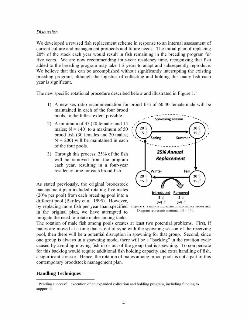
4
Discussion We developed a revised fish replacement scheme in response to an internal assessment of current culture and management protocols and future needs. The initial plan of replacing 20% of the stock each year would result in fish remaining in the breeding program for five years. We are now recommending four-year residency time, recognizing that fish added to the breeding program may take 1-2 years to adapt and subsequently reproduce. We believe that this can be accomplished without significantly interrupting the existing breeding program, although the logistics of collecting and holding this many fish each year is significant.
The new specific rotational procedure described below and illustrated in Figure 1.1
1) A new sex ratio recommendation for brood fish of 60:40 female:male will be maintained in each of the four brood pools, to the fullest extent possible.
2) A minimum of 35 (20 females and 15 males; N = 140) to a maximum of 50 brood fish (30 females and 20 males; N = 200) will be maintained in each of the four pools.
3) Through this process, 25% of the fish will be removed from the program each year, resulting in a four-year residency time for each brood fish.
As stated previously, the original broodstock management plan included rotating five males (20% per pool) from each breeding pool into a different pool (Bartley et al. 1995). However, by replacing more fish per year than specified in the original plan, we have attempted to mitigate the need to rotate males among tanks. The rotation of male fish among pools creates at least two potential problems. First, if males are moved at a time that is out of sync with the spawning season of the receiving pool, then there will be a potential disruption in spawning for that group. Second, since one group is always in a spawning mode, there will be a “backlog” in the rotation cycle caused by avoiding moving fish in or out of the group that is spawning. To compensate for this backlog would require additional fish holding capacity and extra handling of fish, a significant stressor. Hence, the rotation of males among brood pools is not a part of this contemporary broodstock management plan. Handling Techniques 1 Pending successful execution of an expanded collection and holding program, including funding to support it.
Figure 1. Planned replacement scheme for brood fish. Diagram represents minimum N = 140.
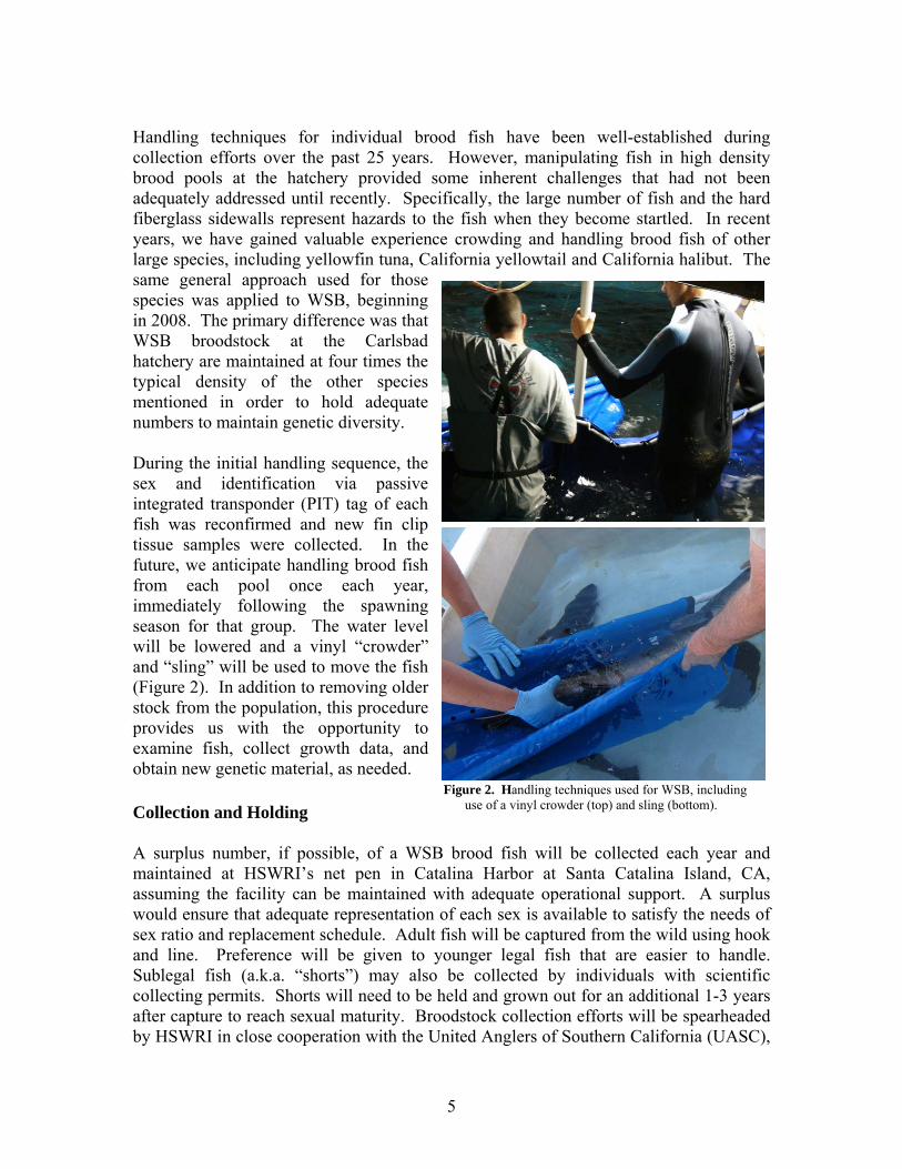
5
Handling techniques for individual brood fish have been well-established during collection efforts over the past 25 years. However, manipulating fish in high density brood pools at the hatchery provided some inherent challenges that had not been adequately addressed until recently. Specifically, the large number of fish and the hard fiberglass sidewalls represent hazards to the fish when they become startled. In recent years, we have gained valuable experience crowding and handling brood fish of other large species, including yellowfin tuna, California yellowtail and California halibut. The same general approach used for those species was applied to WSB, beginning in 2008. The primary difference was that WSB broodstock at the Carlsbad hatchery are maintained at four times the typical density of the other species mentioned in order to hold adequate numbers to maintain genetic diversity. During the initial handling sequence, the sex and identification via passive integrated transponder (PIT) tag of each fish was reconfirmed and new fin clip tissue samples were collected. In the future, we anticipate handling brood fish from each pool once each year, immediately following the spawning season for that group. The water level will be lowered and a vinyl “crowder” and “sling” will be used to move the fish (Figure 2). In addition to removing older stock from the population, this procedure provides us with the opportunity to examine fish, collect growth data, and obtain new genetic material, as needed. Collection and Holding A surplus number, if possible, of a WSB brood fish will be collected each year and maintained at HSWRI’s net pen in Catalina Harbor at Santa Catalina Island, CA, assuming the facility can be maintained with adequate operational support. A surplus would ensure that adequate representation of each sex is available to satisfy the needs of sex ratio and replacement schedule. Adult fish will be captured from the wild using hook and line. Preference will be given to younger legal fish that are easier to handle. Sublegal fish (a.k.a. “shorts”) may also be collected by individuals with scientific collecting permits. Shorts will need to be held and grown out for an additional 1-3 years after capture to reach sexual maturity. Broodstock collection efforts will be spearheaded by HSWRI in close cooperation with the United Anglers of Southern California (UASC),
Figure 2. Handling techniques used for WSB, including use of a vinyl crowder (top) and sling (bottom).
6
the Sportfishing Association of California (SAC), and the California Department of Fish and Game (DFG). When needed for breeding purposes, sexually-mature broodstock will be transported to the mainland for a 45-day quarantine period at the Carlsbad Hatchery before introduction into the brood pools.
7
PRODUCTION RUN MANAGEMENT
Background and Contemporary Rationale The production plan for WSB has historically involved year-round production of multiple cohorts. While numerous spawn events encompassing all four brood groups have been used, the production plan has been somewhat haphazard. Two extensive studies conducted in the past few years have placed us in a much better position to implement a more defined production plan leading toward a more predictable outcome. First, using parentage analyses, we have significantly improved our understanding of spawning patterns among our WSB brood groups, which in turn has improved our ability to maximize genetic diversity effectively within the practical considerations of a hatchery setting (Gruenthal et al. In review). Secondly, with a recently completed and very extensive mark-recapture modeling study, we have an improved understanding of survival rates of cultured seabass under different stocking scenarios that will help guide our production plan toward maximizing return rates (Hervas et al. 2010). Outline
1. Genetically effective population size arguments a. Assumptions
i. Female equivalent (fe; Gruenthal and Drawbridge In prep) 1. Assume that one fe ≡ one effective female contributor (i.e.
Nf = 1) ≡ 3 L of eggs at 585 eggs/mL 2. For fe = Nf = 1, the total effective number of hatchery
breeders (Nb) = 3.12 ii. Nb is assumed to be additive across spawning events
b. Minimum annual Nb = 74 required (Bartley et al. 1995) i. Nb is independent of release limit
ii. Goal: grow out 24-32 fe’s annually spread among the four breeding pools (Gruenthal and Drawbridge In prep)
iii. Spawning events whereby fe > 1 are desirable to more easily meet goal from a production standpoint
2. Annual release limit a. Current limit: A sliding scale based on the number of broodstock as a
proportion of the 200 target number, with a maximum quota of 350,000 fish released per calendar year
i. Limit is reassessed every six months ii. Assuming 350K limit, ~12K juveniles released per fe, based on 24-
32 fe’s per year iii. No genetic basis for sliding scale
b. Genetically defensible quota: >1M annual release limit (Gruenthal and Drawbridge In prep)
3. Operational production considerations a. Releases are planned for all seasons except winter.

8
b. Release size is 20 cm minimum, with larger fish preferred c. Fish are raised in the hatchery to ~100 dph when they are tagged and
ready for transport to outdoor raceways or cages, with cages being preferred
d. When larval production is steady, growout areas become the potential bottleneck because of the volume requirements of larger fish; currently requires overwintering of fish to meet CY release targets
Discussion We will begin maximizing the genetic diversity of the parental contributions within the annual release total to the fullest extent practical. The proposed operational model for the hatchery is to produce cohorts from 24-32 female brood fish, independent of the release limit. Each cohort will be established using eggs from 1-4 spawning events occurring over a seven-day period. Fewer spawns will be used based on the number of fe’s represented within a spawn (see below). Variability in stocking patterns is primarily due to egg availability. The seven-day period is dictated by the length of time during which sibling groups can be mixed with minimal effects from intraspecific aggression in the rearing pools. Spawn volume2 also plays a role in the decision making process for cohort management. Spawn volumes are measured and used to quantify relative female contribution. We estimate that each female contributes an average of 1.8 million eggs (~3 L) at an average fecundity of 100 thousand eggs per kg body mass (Gruenthal et al. In review). That average value is considered one female equivalent (fe; Gruenthal and Drawbridge In prep). Spawn volumes during a given spawning event that are incrementally larger are considered to come from multiple. A female generally exhausts her store of eggs during a single spawning event (although contributions have been noted over 2-4 consecutive days), and the interval between spawns from individuals is close to a minimum of seven days (Gruenthal et al. In review). For simplicity, we assume that each spawn within a cohort is contributed by a different female because the eggs are collected over a short timeframe. Again, the goal is to annually grow out juveniles that are contributed to by 24-32 individual females (24-32 fe’s), partitioned among all four brood groups. Juvenile cohorts should also be divided as equally as possible within the release limit (e.g. for a quota of 350K, ~12,000 juveniles would be released per fe, depending on the actual number of fe’s achieved for that year). References Bartley D.M., Kent D.B., and M.A. Drawbridge. (1995) Conservation of genetic
diversity of white seabass enhancement program in southern California. American Fisheries Society Symposium, 15, 249-25.
2 A volumetric measure of the number of eggs.
9
Gruenthal K.M., Vetter R., and M.A. Drawbridge (In review). Genetic determination of
broadcast spawning dynamics of a pelagic marine finfish in captivity. Can J Fish Aquat Sci. NOAA Awards NA06NMF4720233 and NA09NMF4720396, OREHP Award P07001.
Gruenthal K.M., and M.A Drawbridge (In prep). Towards responsible stock
enhancement: revising broodstock and juvenile production protocols in the California white seabass (Atractroscion nobilis) captive breeding program.
Hervas, S., Lorenzen K., Shane M.A., and M.A. Drawbridge (2010). Quantitative
assessment of a white seabass (Atractoscion nobilis) stock enhancement program in California: post-release dispersal, growth and survival. Fisheries Research. 105:237-243. NOAA Award NA06NMF4720233
Appendix D Sediment Physicochemical Monitoring at Delayed Release Netpens and Raceways for White Seabass Located in Southern California During 2004 and 2005
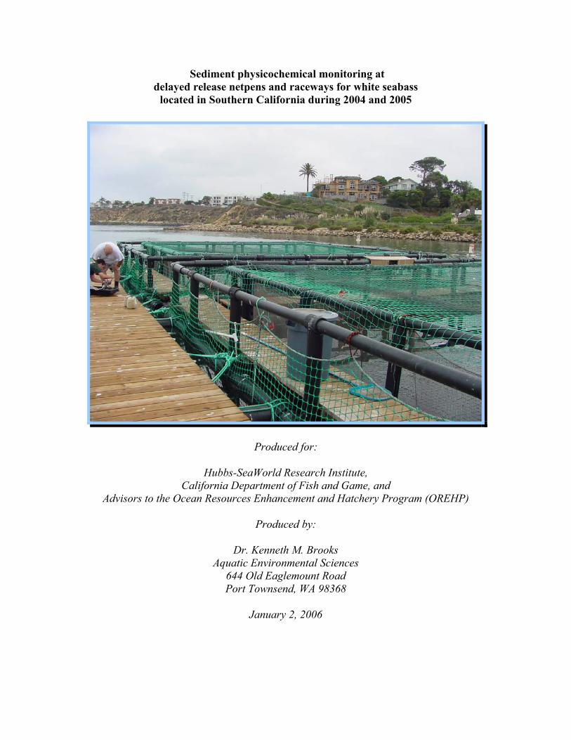
Sediment physicochemical monitoring at delayed release netpens and raceways for white seabass
located in Southern California during 2004 and 2005
Produced for:
Hubbs-SeaWorld Research Institute, California Department of Fish and Game, and
Advisors to the Ocean Resources Enhancement and Hatchery Program (OREHP)
Produced by:
Dr. Kenneth M. Brooks Aquatic Environmental Sciences
644 Old Eaglemount Road Port Townsend, WA 98368
January 2, 2006
ii
Table of Contents
1.0. Introduction 1 2.0. Background 2 2.1. Organic carbon 2 2.2. Macrofaunal response to sulfides 2 2.3. Sedimented zinc 4 2.4. Sedimented copper 4 2.5. Benchmarks for managing sedimented copper and zinc 4 2.6. Chemical and biological remediation of the benthos 5 3.0. Materials and methods 6 3.1. Study design 6 3.2. Sample collection 6 3.3. Station positioning 7 3.4. Sample evaluation 7 3.5. Subsampling 7 3.6. Sample labeling and handling 7 3.7. Cleaning of equipment 7 3.8. Total Volatile Solids (TVS) analysis 7 3.9. Sediment Grain Size (SGS) analysis 8 3.10. Redox potential analysis 8 3.11. Free sulfide analysis 9 3.12. Copper and zinc analyses 10 3.13. Photographic record 10 3.14. Statistical analyses 10 4.0. Results 10 4.1. San Diego 12 4.2. Aqua Hedionda 17 4.3. Santa Catalina (Outer) 23 4.4. Channel Islands Harbor 28 4.5. Dana Point Harbor 35 4.6. Mission Bay (Quivera Basin) 42 4.7. San Diego (SWYC) 50 4.8. Santa Barbara 56 4.9. Mission Bay (Dana Landing) 61 4.10. Marina del Rey 68 5.0. Discussion 75 6.0. Summary 83 References 84 Appendices (1 through 10) Statistica database in MS Excel broken down by site 86
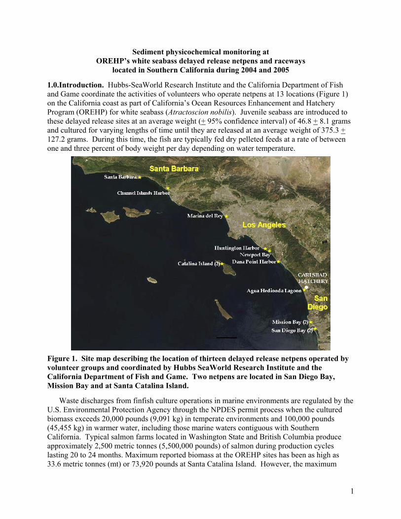
1
Sediment physicochemical monitoring at OREHP’s white seabass delayed release netpens and raceways
located in Southern California during 2004 and 2005 1.0.Introduction. Hubbs-SeaWorld Research Institute and the California Department of Fish and Game coordinate the activities of volunteers who operate netpens at 13 locations (Figure 1) on the California coast as part of California’s Ocean Resources Enhancement and Hatchery Program (OREHP) for white seabass (Atractoscion nobilis). Juvenile seabass are introduced to these delayed release sites at an average weight (+ 95% confidence interval) of 46.8 + 8.1 grams and cultured for varying lengths of time until they are released at an average weight of 375.3 + 127.2 grams. During this time, the fish are typically fed dry pelleted feeds at a rate of between one and three percent of body weight per day depending on water temperature.
Figure 1. Site map describing the location of thirteen delayed release netpens operated by volunteer groups and coordinated by Hubbs SeaWorld Research Institute and the California Department of Fish and Game. Two netpens are located in San Diego Bay, Mission Bay and at Santa Catalina Island. Waste discharges from finfish culture operations in marine environments are regulated by the U.S. Environmental Protection Agency through the NPDES permit process when the cultured biomass exceeds 20,000 pounds (9,091 kg) in temperate environments and 100,000 pounds (45,455 kg) in warmer water, including those marine waters contiguous with Southern California. Typical salmon farms located in Washington State and British Columbia produce approximately 2,500 metric tonnes (5,500,000 pounds) of salmon during production cycles lasting 20 to 24 months. Maximum reported biomass at the OREHP sites has been as high as 33.6 metric tonnes (mt) or 73,920 pounds at Santa Catalina Island. However, the maximum
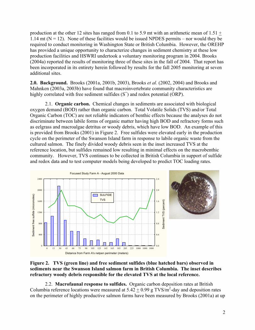
2
production at the other 12 sites has ranged from 0.1 to 5.9 mt with an arithmetic mean of 1.51 + 1.14 mt (N = 12). None of these facilities would be issued NPDES permits – nor would they be required to conduct monitoring in Washington State or British Columbia. However, the OREHP has provided a unique opportunity to characterize changes in sediment chemistry at these low production facilities and HSWRI undertook a voluntary monitoring program in 2004. Brooks (2004a) reported the results of monitoring three of these sites in the fall of 2004. That report has been incorporated in its entirety herein followed by results for the fall 2005 monitoring at seven additional sites. 2.0. Background. Brooks (2001a, 2001b, 2003), Brooks et al. (2002, 2004) and Brooks and Mahnken (2003a, 2003b) have found that macroinvertebrate community characteristics are highly correlated with free sediment sulfides (S=) and redox potential (ORP). 2.1. Organic carbon. Chemical changes in sediments are associated with biological oxygen demand (BOD) rather than organic carbon. Total Volatile Solids (TVS) and/or Total Organic Carbon (TOC) are not reliable indicators of benthic effects because the analyses do not discriminate between labile forms of organic matter having high BOD and refractory forms such as eelgrass and macroalgae detritus or woody debris, which have low BOD. An example of this is provided from Brooks (2001) in Figure 2. Free sulfides were elevated early in the production cycle on the perimeter of the Swanson Island farm in response to labile organic waste from the cultured salmon. The finely divided woody debris seen in the inset increased TVS at the reference location, but sulfides remained low resulting in minimal effects on the macrobenthic community. However, TVS continues to be collected in British Columbia in support of sulfide and redox data and to test computer models being developed to predict TOC loading rates.
Figure 2. TVS (green line) and free sediment sulfides (blue hatched bars) observed in sediments near the Swanson Island salmon farm in British Columbia. The inset describes refractory woody debris responsible for the elevated TVS at the local reference. 2.2. Macrofaunal response to sulfides. Organic carbon deposition rates at British Columbia reference locations were measured at 5.42 + 0.99 g TVS/m2-day and deposition rates on the perimeter of highly productive salmon farms have been measured by Brooks (2001a) at up
Focused Study Farm A - August 2000 Data
Distance from Farm A's netpen perimeter (meters)
Sed
imen
t fre
e su
lfide
(mic
rom
oles
)
Sed
imen
t TV
S (p
erce
nt)
0.0
0.4
0.8
1.2
1.6
2.0
2.4
0
400
800
1200
1600
2000
2400
0 15 30 45 60 75 90 105 125 145 165 185 205 225 1000 1000 1000
SULFIDE
TVS

3
to 41.34 g TVS/m2-day. Sensitive infauna are excluded from sediments when sulfides exceed several hundred micromoles. Other taxa, particularly annelids, proliferate in sediments at sulfide concentrations as high as 15,000 µM S=. Figure 3 describes the overall macrobenthic communities’ response demonstrating that on average, half of the taxa were excluded at sulfide concentrations of 960 µM. However, as labile TVS and sulfides increase, numerous opportunistic taxa proliferate, resulting in increases in some (but not all) environments. The results are provided in Figure 4. In most instances, the abundance of macrobenthic communities is significantly diminished above 6,000 µM S=.
Number of taxa = 89.76 - 21.868*log10(Sulfide)
Sediment free sulfides in micromoles
Num
ber o
f tax
a ob
serv
ed in
0.1
m^2
gra
bs (N
= 4
5)
0
5
10
15
20
25
30
35
40
45
50
55
60
65
70
75
80
85
90
10 100 1000 10000
Mean number taxaLower 90th percentile
50% of the mean
Figure 3. Number of taxa observed in sediments as a function of the concentration of free sediment sulfides. Data are from Brooks and Mahnken (2003a).
Infaunal abundance versus sediment free sulfides
Sediment free sulfide concentrations (micromoles)
Abu
ndan
ce (n
umbe
r org
anis
ms/
0.1m
2
0100020003000400050006000700080009000
10000110001200013000140001500016000170001800019000
2 3 4 5 6 7 8 9 10 20 30 40 50 60 70 80 90 100
200
300
400
500
600
700
800
900
1000
2000
3000
4000
5000
6000
7000
8000
9000
1000
0
Proliferation of Opportunists
Figure 4. Macrofaunal abundance as a function of free sediment sulfides at 7 British Columbia salmon farms (Brooks and Mahnken (2003a).
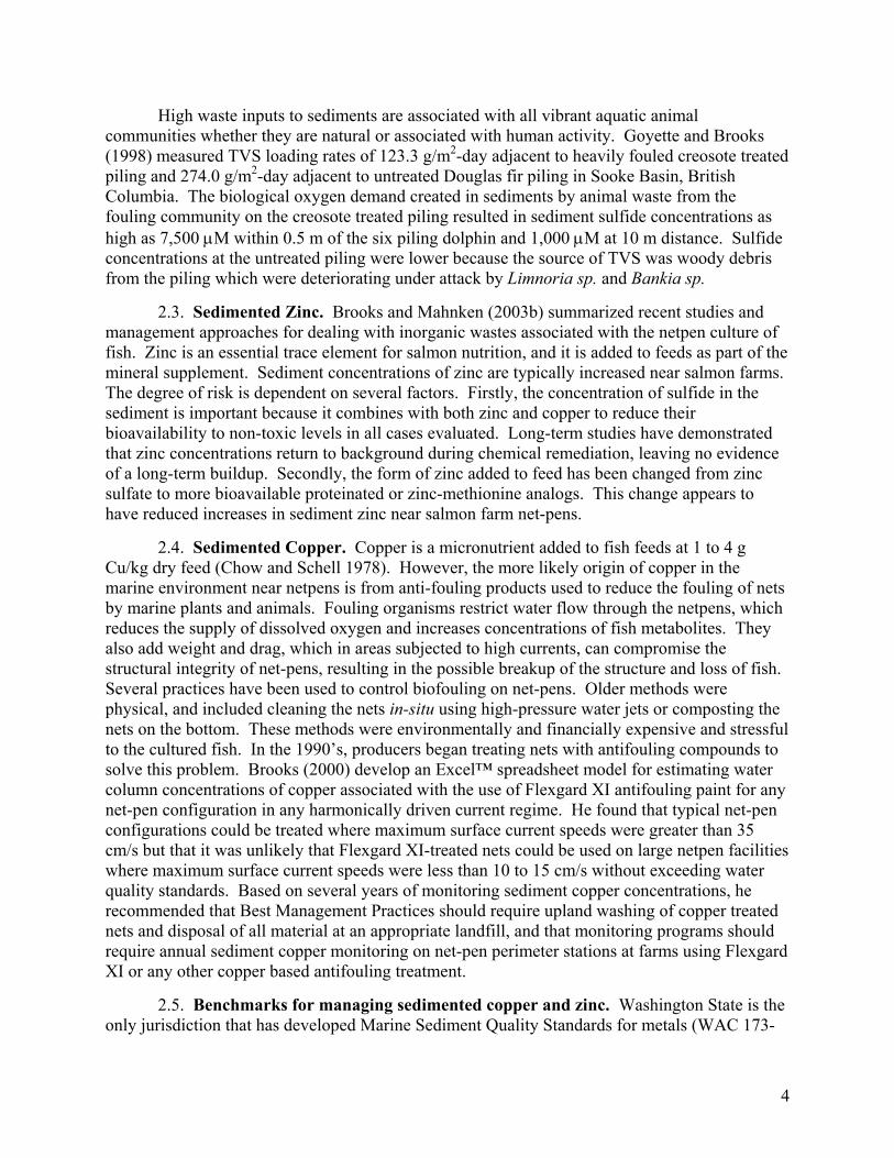
4
High waste inputs to sediments are associated with all vibrant aquatic animal communities whether they are natural or associated with human activity. Goyette and Brooks (1998) measured TVS loading rates of 123.3 g/m2-day adjacent to heavily fouled creosote treated piling and 274.0 g/m2-day adjacent to untreated Douglas fir piling in Sooke Basin, British Columbia. The biological oxygen demand created in sediments by animal waste from the fouling community on the creosote treated piling resulted in sediment sulfide concentrations as high as 7,500 µM within 0.5 m of the six piling dolphin and 1,000 µM at 10 m distance. Sulfide concentrations at the untreated piling were lower because the source of TVS was woody debris from the piling which were deteriorating under attack by Limnoria sp. and Bankia sp. 2.3. Sedimented Zinc. Brooks and Mahnken (2003b) summarized recent studies and management approaches for dealing with inorganic wastes associated with the netpen culture of fish. Zinc is an essential trace element for salmon nutrition, and it is added to feeds as part of the mineral supplement. Sediment concentrations of zinc are typically increased near salmon farms. The degree of risk is dependent on several factors. Firstly, the concentration of sulfide in the sediment is important because it combines with both zinc and copper to reduce their bioavailability to non-toxic levels in all cases evaluated. Long-term studies have demonstrated that zinc concentrations return to background during chemical remediation, leaving no evidence of a long-term buildup. Secondly, the form of zinc added to feed has been changed from zinc sulfate to more bioavailable proteinated or zinc-methionine analogs. This change appears to have reduced increases in sediment zinc near salmon farm net-pens. 2.4. Sedimented Copper. Copper is a micronutrient added to fish feeds at 1 to 4 g Cu/kg dry feed (Chow and Schell 1978). However, the more likely origin of copper in the marine environment near netpens is from anti-fouling products used to reduce the fouling of nets by marine plants and animals. Fouling organisms restrict water flow through the netpens, which reduces the supply of dissolved oxygen and increases concentrations of fish metabolites. They also add weight and drag, which in areas subjected to high currents, can compromise the structural integrity of net-pens, resulting in the possible breakup of the structure and loss of fish. Several practices have been used to control biofouling on net-pens. Older methods were physical, and included cleaning the nets in-situ using high-pressure water jets or composting the nets on the bottom. These methods were environmentally and financially expensive and stressful to the cultured fish. In the 1990’s, producers began treating nets with antifouling compounds to solve this problem. Brooks (2000) develop an Excel™ spreadsheet model for estimating water column concentrations of copper associated with the use of Flexgard XI antifouling paint for any net-pen configuration in any harmonically driven current regime. He found that typical net-pen configurations could be treated where maximum surface current speeds were greater than 35 cm/s but that it was unlikely that Flexgard XI-treated nets could be used on large netpen facilities where maximum surface current speeds were less than 10 to 15 cm/s without exceeding water quality standards. Based on several years of monitoring sediment copper concentrations, he recommended that Best Management Practices should require upland washing of copper treated nets and disposal of all material at an appropriate landfill, and that monitoring programs should require annual sediment copper monitoring on net-pen perimeter stations at farms using Flexgard XI or any other copper based antifouling treatment. 2.5. Benchmarks for managing sedimented copper and zinc. Washington State is the only jurisdiction that has developed Marine Sediment Quality Standards for metals (WAC 173-
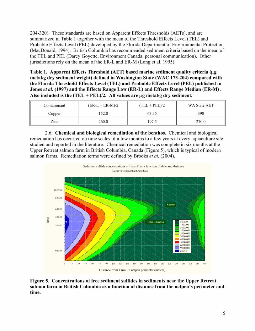
5
204-320). These standards are based on Apparent Effects Thresholds (AETs), and are summarized in Table 1 together with the mean of the Threshold Effects Level (TEL) and Probable Effects Level (PEL) developed by the Florida Department of Environmental Protection (MacDonald, 1994). British Columbia has recommended sediment criteria based on the mean of the TEL and PEL (Darcy Goyette, Environment Canada, personal communication). Other jurisdictions rely on the mean of the ER-L and ER-M (Long et al. 1995).
Table 1. Apparent Effects Threshold (AET) based marine sediment quality criteria (µg metal/g dry sediment weight) defined in Washington State (WAC 173-204) compared with the Florida Threshold Effects Level (TEL) and Probable Effects Level (PEL) published in Jones et al. (1997) and the Effects Range Low (ER-L) and Effects Range Median (ER-M) . Also included is the (TEL + PEL)/2. All values are µg metal/g dry sediment.
Contaminant (ER-L + ER-M)/2 (TEL + PEL)/2 WA State AET
Copper 152.0 63.35 390
Zinc 260.0 197.5 270.0 2.6. Chemical and biological remediation of the benthos. Chemical and biological remediation has occurred on time scales of a few months to a few years at every aquaculture site studied and reported in the literature. Chemical remediation was complete in six months at the Upper Retreat salmon farm in British Columbia, Canada (Figure 5), which is typical of modern salmon farms. Remediation terms were defined by Brooks et al. (2004).
Sediment sulfide concentrations at Farm F as a function of date and distanceNegative Exponential Smoothing
Distance from Farm F's netpen perimeter (meters)
Dat
e
9/13/99
2/26/00
4/22/00
6/12/00
8/24/00
10/15/00
0 15 30 45 60 75 90 105 120 135 150 165 180 195 210 225 240 255 270 285 300
50.000 150.000 300.000 1000.000 2000.000 3000.000 4000.000 5000.000 6000.000 9000.000 above
Peak Biomass
Fallow
Figure 5. Concentrations of free sediment sulfides in sediments near the Upper Retreat salmon farm in British Columbia as a function of distance from the netpen’s perimeter and time.
6
Chemical remediation is defined as the reduction of accumulated organic matter with a concomitant decrease in free sediment sulfide (S=) concentrations and an increase in sediment redox potential under and adjacent to salmon farms to levels at which more than half the reference area taxa can recruit and survive.
Biological remediation is the restructuring of the infaunal community to include those taxa whose individual abundance equaled or exceeded 1% of the total invertebrate abundance at local reference stations. Recruitment of rare species representing <1% of the reference abundance was not considered necessary for complete biological remediation. However, in the worst case known on the Pacific Coast, Brooks et al. (2004) studied the permanently fallowed Carrie Bay salmon farm and found that chemical remediation was nearly complete at the end of seven years. The time required for chemical remediation is influenced by the availability of sulfate, dissolved oxygen in the benthic boundary layer; bottom current speeds; temperatures; the composition of the natural macrobenthic community; and the depth of organic deposits. In general, it appears that chemical remediation requires a few months when the depth of organic deposits is less than a few centimeters. Biological remediation lags chemical remediation and occurs in stanzas characterized by macroinvertebrate feeding guilds. For quickly remediating sites in temperate latitudes, biological remediation also depends on the season in which chemical remediation is complete. Many taxa spawn seasonally and new recruits are available for a limited period of time. In those cases where chemical remediation occurs in the fall, biological remediation may not be complete until the next spring and summer. 3.0. Materials and methods. These facilities are located in shallow water and hold small maximum biomasses of fish. The benthos at these sites has not previously been monitored and an attempt to find appropriate local reference locations was made as part of this survey. Acceptable reference locations should have depths equal to the depth under the netpens + 10% and a proportion sediment fines (silt and clay) equal to that found under the netpens + 20%. 3.1. Study design. The study design relies on a regression approach to identify trends in sediment free sulfides, redox potential, total volatile solids (TVS), copper and zinc as a function of distance from the netpen’s perimeter on four orthogonal transects. Replicate samples were collected on the netpen’s perimeter (N = 4) and at the reference location (N = 3) allowing for inferential tests of the significance of differences.
3.2. Sample collection. This survey used a stainless steel Petite Ponar grab with a footprint of 0.025 m2, which can be deployed by hand. Overlying water was siphoned from the sampler without disturbing the sediment’s surface and the top two centimeters of the sediment sampled for physicochemical analyses. Acceptable samples complied with PSEP (1986):
The sampler was deployed at a maximum speed of 30 cm/s;
A minimum sediment penetration depth of 4 cm was required;
The retrieved sampler must be fully closed and contain overlying water with low
turbidity indicating minimal leakage and disturbance;
The retained sediment surface must be relatively flat and unwashed indicating minimal disturbance or winnowing.
7
3.3. Station positioning. At most locations, the survey vessel was positioned using a premeasured polypropylene transect line secured to the perimeter of the netpens and at the vessel’s sampling station. No correction for hydrowire angle was made. The latitude and longitude of each sample was determined using differential GPS equipment. At a few locations, obstacles prevented use of a transect line and stations were located using GPS.
3.4. Sample evaluation. Overlying water was siphoned from acceptable samples. Other
methods, such as decanting the water or slightly cracking the grab to let the water run out, are not appropriate, as they might result in disturbance or loss of fine-grained surficial sediment, organic matter and/or infauna. The following observations were noted:
• Station position at the time the grab reached the bottom;
• Water depth;
• Penetration depth of the grab in the sediments;
• Comments related to sample quality such as leakage, winnowing or undue disturbance;
• Gross characteristics of the surficial sediment to include color. • biological structures such as shells, tubes and macrophytes
• presence of debris such as macroalgae, eelgrass detritus, woody debris, trash, etc. • Presence of bacterial mats, waste feed, feces, oily sheens, etc. • Odor (hydrocarbons or hydrogen sulfide)
• Presence and depth of the redox potential discontinuity (RPD)
3.5. Subsampling. Subsamples were taken using a stainless steel spoon.
Unrepresentative material (empty mollusk shells, megafauna, large pieces of woody debris or other organic material) was removed in the field and noted. The top 2.0 cm of a portion of the sample was placed in a stainless steel bowl and gently homogenized for approximately 10 seconds. 125 ml polyethylene urine specimen jars were filled with the homogenate with no or minimal overlying air space.
3.6. Sample labeling and handling. Physicochemical samples were stored on ice in coolers in the field. Sulfide and redox analyses were accomplished as quickly as possible - usually within 15 minutes of collection. Samples for SGS and TVS analyses were maintained at 4 oC until analyzed within 14 days of collection. The bodies and caps of all sample containers were labeled with coded tags. Samples were personally returned to Aquatic Environmental Sciences for further analysis by Dr. Brooks.
3.7. Cleaning of equipment. Equipment was washed in detergent and rinsed with tap water at the beginning of each day. Equipment was rinsed with ambient seawater between grab deployments to remove sediment and organisms. Subsamples for chemical analyses were taken from the center of the grab. No other special cleaning requirements were considered necessary for these analyses. 3.8. Total Volatile Solids (TVS) analyses. Approximately 35 ml of each sample was required for this analysis by Standard Method 2540.E or EPA Method 160.4. Samples were dried at 103 + 2o C in aluminum boats that had been pre-cleaned by combusting at 550 oC for 30 minutes. Drying was continued until no further weight reduction was observed (generally overnight). The samples were then weighed to 0.1 mg and combusted at 550 oC for one hour or
8
until no further weight loss was recorded. Total Volatile Solids were calculated as the percent difference between the dried and combusted weights. Quality assurance required triplicate analyses on one of every 20 samples or on one sample per batch if fewer than 20 samples were analyzed. A maximum of 20 percent Relative Percent Difference (of the silt-clay fraction) was established as the Data Qualification Control Limit.
3.9. Sediment Grain Size (SGS) analyses was accomplished on a subset of samples at each study site. Approximately 50 grams of surficial sediment were taken to a depth of 2.0 cm for sediment grain size analysis. The sediments were wet sieved on a 0.064 mm sieve. The retained material was dried in an oven at 92 oC and processed using the dry sieve and pipette method of Plumb (1981). The sieves used for the analysis had mesh openings of 2.0, 0.89, 0.25 and 0.064 mm. Particles passing the 0.064 mm sieve during wet sieving were analyzed by sinking rates in a column of water (pipette analysis). 3.10. Redox potential analyses. This analysis was conducted in the field using an Orion™ advanced portable ISE/pH/mV/ORP/temperature meter model 290A with a Model 9678BN Epoxy Sure-Flow Combination Redox/ORP probe. The meter’s accuracy in the ORP mode is + 0.2 mV or + 0.05% of the reading, whichever is greater. Standardizing the Redox Electrode: Calibration reagents were prepared within 24 hours of use and refrigerated. Redox Standard A (0.1 M potassium ferrocyanide and 0.05 M potassium ferricyanide) was prepared by weighing 4.22 g K4Fe(CN)6.3H2O and 1.65 g K3Fe(CN)6 into a 100-ml volumetric flask. Approximately 50 ml of distilled water was added with swirling to dissolve the solids. The solution was then diluted to volume (100 ml) with distilled water. Standard B (0.01 M potassium ferrocyanide, 0.05 M potassium ferricyanide, and 0.36 M potassium fluoride) were prepared by weighing 0.42 g K4Fe(CN)6.3H2O, 1.65 g K3Fe(CN)6, and 3.39 g KF.2H2O into a 100 ml volumetric flask. 50 ml of distilled water was added to dissolve the solids, and the solution diluted to 100 ml with distilled water. Orion Ag/AGCl reference electrode filling solution 900011 was used throughout this study. Redox standards were used to check the electrode at ambient temperature (10 to 15o C) at the start and end of measurements for each batch of samples. Standard A was transferred to a 150-ml beaker and the electrode placed in the solution until the reading stabilized with stirring (1 to 2 minutes). The potential of Standard A is approximately +147 + 9 mV. The electrode was then rinsed with distilled water and the measurement repeated with Standard B (potential of +216 + 9 mV). The potential in Standard A is approximately + 69 mV greater than in Standard B. The potential of the reference electrode (+244 mV at 20oC), corrected for the average difference between measured potentials of standard solutions and their calibration values, was added to the mV reading to determine the actual Eh potential in sediment samples. Eh potentials of approximately +300 to +350 mV are typical of oxygenated seawater. Measurement of sediment redox potential. For these redox analyses, the ORP electrode was inserted into the homogenized sediment subsample and the mV reading recorded when the meter stabilized. This generally required two to three minutes. The electrode was then removed, gently wiped free of sediment, and used to measure the next sample. The probe was checked in the standards at least once every four hours. Probes were rinsed in distilled water and stored in pH 7.0 buffer between batches of samples.

9
Quality assurance procedures for the measurement of redox potential. Triplicate analyses were conducted on one of every 20 samples, or on one sample per batch, if less than 20 samples are analyzed. No Data Qualification Control Limit has been established for this test. 3.11. Free sediment sulfide analyses were accomplished as soon as possible in the field. All buffer and standards components were pre-weighed into scintillation vials prior to deployment.
Calibration of the total sulfide field probe. These analyses were conducted using
an Orion™ advanced portable ISE/pH/mV/ORP/temperature meter model 290A with a Cole Parmer Silver/Sulfide electrode. The meter has a concentration range of 0.000 to 19,900 µM and a relative accuracy of + 0.5% of the reading. SAOB buffer and sulfide standards are stable for up to 3 hours and they were made up in the morning and at mid-day on each sampling day. A basic sulfide antioxidant buffer solution was prepared in 1,000-ml HDPE screw-top bottles by adding 80.00 g of NaOH and 71.60 g EDTA (Na2C10O8N2.2H2O). Just prior to the start of sampling, 8.75 grams of L-ascorbic acid will be added to 250 ml of the NaOH – EDTA stock in an amber HDPE bottle. This SAOB buffer solution is stable for up to 4.0 hours after addition of L-ascorbic acid. The S= electrode was calibrated before and after each batch of not more than 12 samples. Three S= standards (100, 1000 and 10,000 µM) were used for a three-point electrode calibration. A stock S= solution of 0.01 M Na2S was prepared by adding 0.2402 g Na2S.9H2O (premeasured in scintillation vials) to 100 ml of distilled water in an amber jar. This stock solution was made fresh every 48 hours and stored at 4o C. A 1000 µM S= standard (10-3 M) was prepared at the start of sampling by transferring 10 ml of the 0.01 M Na2S stock solution (10,000 µM) into an amber jar and diluting to 100 ml with distilled water. A 100 µM S= standard (10-4 M) was prepared by transferring 10 ml of the 1000 µM standard to an amber jar and diluting to 100 ml with distilled water. Both dilution standards were mixed thoroughly before each use. Just before calibration of the S= electrode, 10 ml of each standard was transferred to 30 ml amber bottles and 10 ml of SAOB (containing L-ascorbic acid) added. The combined solution was kept tightly capped until used for standardizing the S= electrode. Measurement of sediment total sulfides. These analyses were completed in 30 ml graduated beakers by marking each beaker at 5 and 10 ml levels using a pipette, distilled water and a fine black lab marker. Five ml of SAOB will then added to the beaker. Sediment was added to top the mixture off at the 10 ml mark. A flat-tip stainless steel spatula was used to homogenize the sediment sample with the SAOB buffer. Following this, the S= electrode was inserted and used to further stir the sediment. The S= electrode reading usually stabilized in two to four minutes. The electrodes were gently wiped with a paper towel between samples, but were not rinsed. After completing 12 analyses, the electrode was gently rinsed with distilled water and recalibrated before continuing. In addition, the sulfide electrode was recalibrated at least once every two hours and at the end of each batch of samples. Quality assurance for sediment total sulfide analyses. Triplicate analyses were conducted on one of every 20 samples, or on one sample per batch when fewer than 20 samples were analyzed. The Data Qualification Control Limit is 20% Relative Percent Difference (RPD). Fresh standards were made daily. The analytical balance was inspected daily and calibrated at once per month.
10
3.12. Copper and zinc analyses. Metal analyses were completed by Analytical Resources Incorporated in Seattle, Washington. This laboratory is accredited by the Washington State Department of Ecology for these procedures. EPA method 6010B was used following a strong acid digestion (EPA 3050B). Quality assurance required completion of one blank; one spiked sample; and a certified reference material with each batch of 20 samples. Control limits from PSEP (1996) were used: Matrix Spike. 85 to 115% when the value of the spiked sample was 2 to 5 times the original sample concentration; Blank analysis. The analyte should not be detected above the instrument detection limit of 0.25 µg/g; Continuing Calibration Verification. The observed value should be within + 10% of the true value for GFAA.
3.13. Photographic record. A photograph was taken of each sample while it was still in the grab using a digital camera in macro mode.
3.14. Statistical analyses. All data was entered into a Microsoft Excel spreadsheet and imported in Statistica Version 6 software. Proportional data was transformed (arcsin(sqrt(proportion))) prior to inferential tests. Means are reported with + 95% confidence intervals. Inferential tests were assumed significant at α = 0.05. Unless otherwise specified, distance weighted least squares fits to the data are provided in graphs where appropriate. 4.0. Results. The results of these surveys are provided, by site, in the following paragraphs. No deviations from protocols were necessary and all analyses met their respective data quality objectives. Table 2 summarizes production information for the 13 delayed release sites. All of the sites have been in operation for more than two years and several have produced 14 to 18 cohorts of white seabass. In 2005, all of the monitoring was conducted within 30 days of peak biomass when the fish were released. Three sites located at Huntington Harbor, Newport Bay and in the inner site (of two) in Catalina Harbor were not monitored because they held low biomasses of fish that were released more than 30 days prior to initiating the 2005 survey. These three sites will be monitored in 2006. Specific feed data was available for the three sites monitored in 2004 and a time history of production at those sites is included in their reports. Because of the low biomasses of fish cultured at these sites in 2005, this level of detail was not considered necessary. Entry and release biomass of each cohort is provided. The amount of feed was estimated by assuming a feeding rate of 2.5 percent of the mean biomass on site per day during the culture period.

11

12
Table 2. Production statistics for the 13 delayed white sea bass release facilities operated by Hubbs SeaWorld along the shores of Southern California. Sites monitored in 2005 are highlighted in green and those monitored in 2004 in blue. Delayed release netpens located in the inner harbor of Catalina, Huntington Harbor and Newport Bay were not monitored in these initial surveys because they were harvested more than 30 days prior to initiating the 2005 survey. These three sites will be surveyed at peak biomass in 2006. The cage volume at sites where copper treated nets were used is highlighted in red.
Latitude Longitude System Cage Startup Production Stocking Entry Release Release Maximum
Growout Facility North West Type Volume
(m3) Date Cycles Date Biomass
(kg) Date Biomass
(kg) Production
(mt)
Santa Barbara
1 Santa Barbara 34 24.617 119 41.067 Net 91.7 8/19/1993 7 6/3/2004 255.1 9/20/2004 855.3 1.4
1 Santa Barbara Net 91.7 8/19/1993 7 6/2/2005 569.7 8/29/2005 733.8
Ventura
2 Channel Islands Harbor 34 09.826 119 13.326 Net 116 3/28/1991 14 11/18/2004 313.4 5/4/2005 992.4 1.7
2 Channel Islands Harbor Net 116 3/28/1991 14 6/1/2005 504.8 9/15/2005 1219.7
Los Angeles
3 Marina del Rey 33 58.764 118 26.730 Raceway 14.5 5/9/1995 18 1/31/2005 315.9 5/2/2005 637.3 0.2
3 Marina del Rey Raceway 14.5 5/9/1995 18 6/16/2005 281.5 10/9/2005 644.3
4 Catalina Harbor (Inner) 33 25.549 118 30.624 Net 261 Jun-94 8/25/2005 3.9
5 Catalina Harbor (Outer) 33 25.892 118 30.420 Net 2242.7 Mar-98 33.6
Orange
6 Huntington Harbor 33 42.754 118 03.629 Raceway 14.5 Sep-96 8/10/2005 0.2
7 Newport Bay 33 36.052 117 53.411 Raceway 50.7 Apr-93 9/24/2004 0.8
8 Dana Point Harbor 33 27.450 117 41.586 Net 39.4 12/14/1994 18 12/8/2004 131.9 5/13/2005 277.7 0.6
8 Dana Point Harbor Net 39.4 12/14/1994 18 8/31/2005 89.1 In production
San Diego
9 Agua Hedionda Lagoon 33 08.379 117 20.224 Net 391.5 Jul-03 5.9
10 Mission Bay (Quivira Basin or SDOF) 32 45.628 117 14.225 Net 36.2 4/29/1997 15 11/30/2004 420.4 4/13/2005 657.6 0.7
10 Mission Bay (Quivira Basin or SDOF) Net 36.2 4/29/1997 15 5/23/2005 242.4 9/13/2005 382.2
11 Mission Bay (Dana Landing or PP) 32 46.094 117 14.110 Net 9.1 7/6/2001 8 1/22/2004 79.5 9/10/2004 222.3 0.1
11 Mission Bay (Dana Landing or PP) Net 9.1 7/6/2001 8 4/14/2005 84.7 9/9/2005 222.4
12 San Diego Bay (SW Yacht Club) 32 46.132 117 13.985 Raceway 14.3 8/6/1996 16 12/3/2004 67.4 5/25/2005 221.8 0.2
12 San Diego Bay (SW Yacht Club) Raceway 14.3 8/6/1996 16 6/21/2005 105.5 In production
13 San Diego Bay Grape Street 32 43.290 117 10.274 Net 174.3 Apr-03 2.6
Notes: 1. Sites 5, 9 and 13 were monitored in September of 2004. 2. Sites 1, 2, 3, 8, 10, 11 and 12 were monitored between September 21 and November 7, 2005. 3. Sites 4, 6 and 7 were not near peak biomass during 2005 and were not monitored.
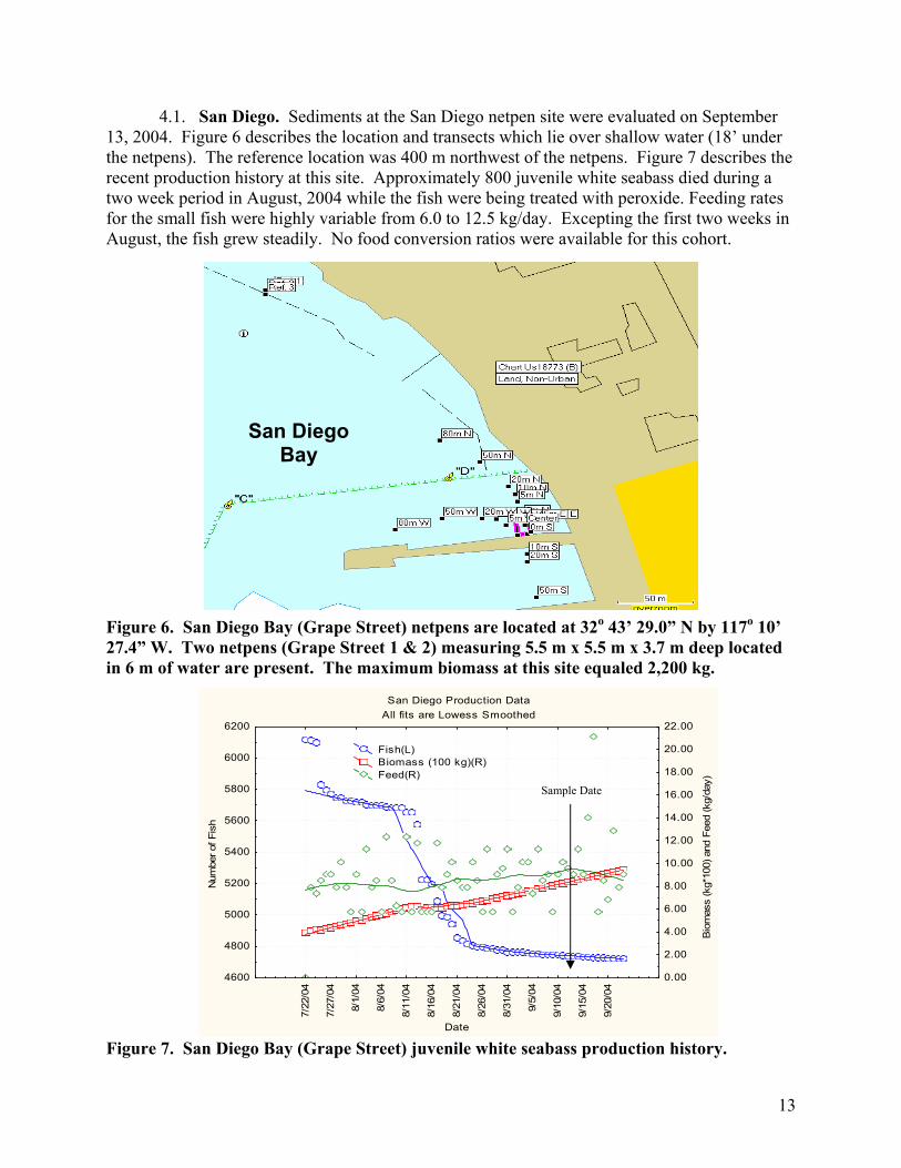
13
4.1. San Diego. Sediments at the San Diego netpen site were evaluated on September 13, 2004. Figure 6 describes the location and transects which lie over shallow water (18’ under the netpens). The reference location was 400 m northwest of the netpens. Figure 7 describes the recent production history at this site. Approximately 800 juvenile white seabass died during a two week period in August, 2004 while the fish were being treated with peroxide. Feeding rates for the small fish were highly variable from 6.0 to 12.5 kg/day. Excepting the first two weeks in August, the fish grew steadily. No food conversion ratios were available for this cohort.
Figure 6. San Diego Bay (Grape Street) netpens are located at 32o 43’ 29.0” N by 117o 10’ 27.4” W. Two netpens (Grape Street 1 & 2) measuring 5.5 m x 5.5 m x 3.7 m deep located in 6 m of water are present. The maximum biomass at this site equaled 2,200 kg.
Figure 7. San Diego Bay (Grape Street) juvenile white seabass production history.
San Diego Bay
San Diego Production DataAll fits are Lowess Smoothed
7/22
/04
7/27
/04
8/1/
04
8/6/
04
8/11
/04
8/16
/04
8/21
/04
8/26
/04
8/31
/04
9/5/
04
9/10
/04
9/15
/04
9/20
/04
Date
4600
4800
5000
5200
5400
5600
5800
6000
6200
Num
ber o
f Fis
h
0.00
2.00
4.00
6.00
8.00
10.00
12.00
14.00
16.00
18.00
20.00
22.00
Bio
mas
s (k
g*10
0) a
nd F
eed
(kg/
day)
Fish(L) Biomass (100 kg)(R) Feed(R)
Sample Date
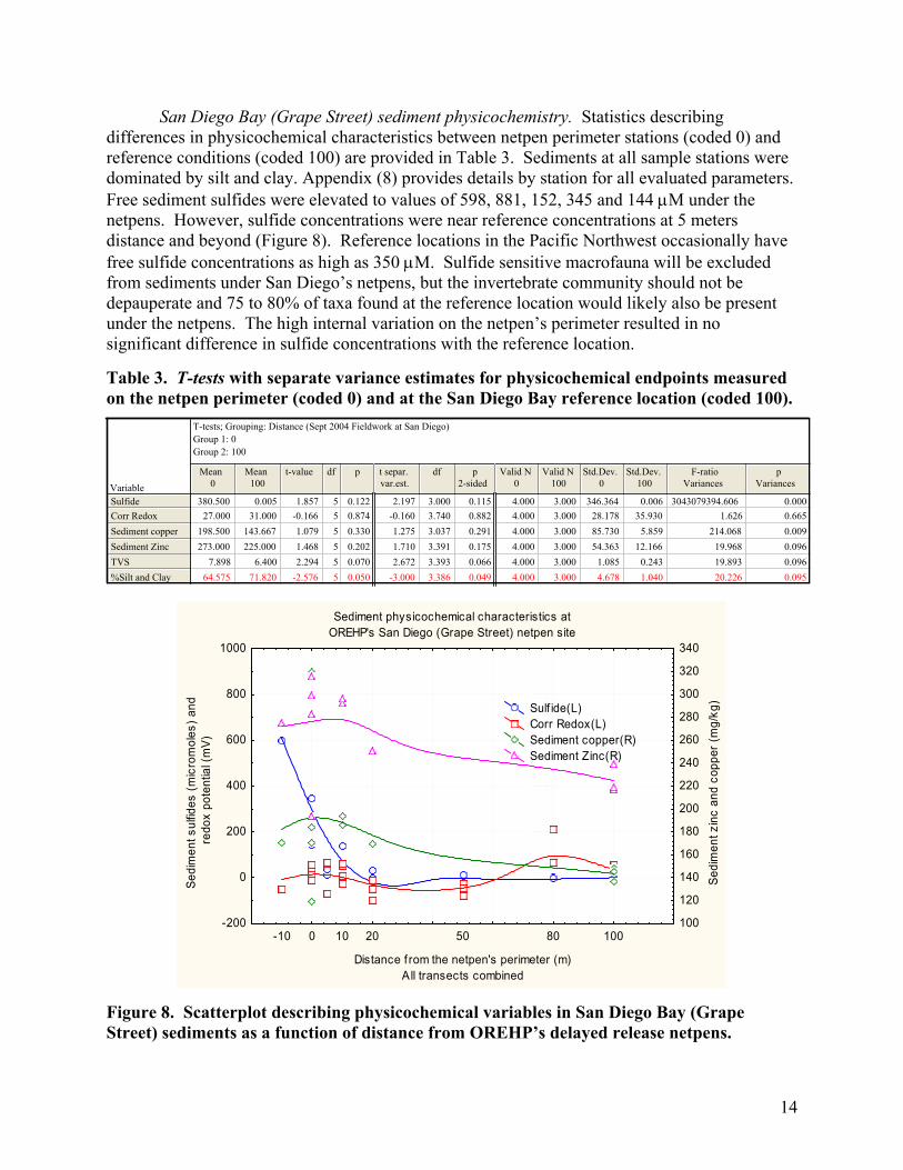
14
San Diego Bay (Grape Street) sediment physicochemistry. Statistics describing differences in physicochemical characteristics between netpen perimeter stations (coded 0) and reference conditions (coded 100) are provided in Table 3. Sediments at all sample stations were dominated by silt and clay. Appendix (8) provides details by station for all evaluated parameters. Free sediment sulfides were elevated to values of 598, 881, 152, 345 and 144 µM under the netpens. However, sulfide concentrations were near reference concentrations at 5 meters distance and beyond (Figure 8). Reference locations in the Pacific Northwest occasionally have free sulfide concentrations as high as 350 µM. Sulfide sensitive macrofauna will be excluded from sediments under San Diego’s netpens, but the invertebrate community should not be depauperate and 75 to 80% of taxa found at the reference location would likely also be present under the netpens. The high internal variation on the netpen’s perimeter resulted in no significant difference in sulfide concentrations with the reference location. Table 3. T-tests with separate variance estimates for physicochemical endpoints measured on the netpen perimeter (coded 0) and at the San Diego Bay reference location (coded 100).
T-tests; Grouping: Distance (Sept 2004 Fieldwork at San Diego)Group 1: 0Group 2: 100
VariableMean
0Mean
100t-value df p t separ.
var.est.df p
2-sidedValid N
0Valid N
100Std.Dev.
0Std.Dev.
100F-ratio
Variancesp
Variances
SulfideCorr RedoxSediment copperSediment ZincTVS%Silt and Clay
380.500 0.005 1.857 5 0.122 2.197 3.000 0.115 4.000 3.000 346.364 0.006 3043079394.606 0.00027.000 31.000 -0.166 5 0.874 -0.160 3.740 0.882 4.000 3.000 28.178 35.930 1.626 0.665
198.500 143.667 1.079 5 0.330 1.275 3.037 0.291 4.000 3.000 85.730 5.859 214.068 0.009273.000 225.000 1.468 5 0.202 1.710 3.391 0.175 4.000 3.000 54.363 12.166 19.968 0.096
7.898 6.400 2.294 5 0.070 2.672 3.393 0.066 4.000 3.000 1.085 0.243 19.893 0.09664.575 71.820 -2.576 5 0.050 -3.000 3.386 0.049 4.000 3.000 4.678 1.040 20.226 0.095
Sediment physicochemical characteristics at
OREHP's San Diego (Grape Street) netpen site
-10 0 10 20 50 80 100
Distance f rom the netpen's perimeter (m)All transects combined
-200
0
200
400
600
800
1000
Sedi
men
t sul
fides
(mic
rom
oles
) and
redo
x po
tent
ial (
mV)
100
120
140
160
180
200
220
240
260
280
300
320
340
Sedi
men
t zin
c an
d co
pper
(mg/
kg) Sulf ide(L)
Corr Redox(L) Sediment copper(R) Sediment Zinc(R)
Figure 8. Scatterplot describing physicochemical variables in San Diego Bay (Grape Street) sediments as a function of distance from OREHP’s delayed release netpens.
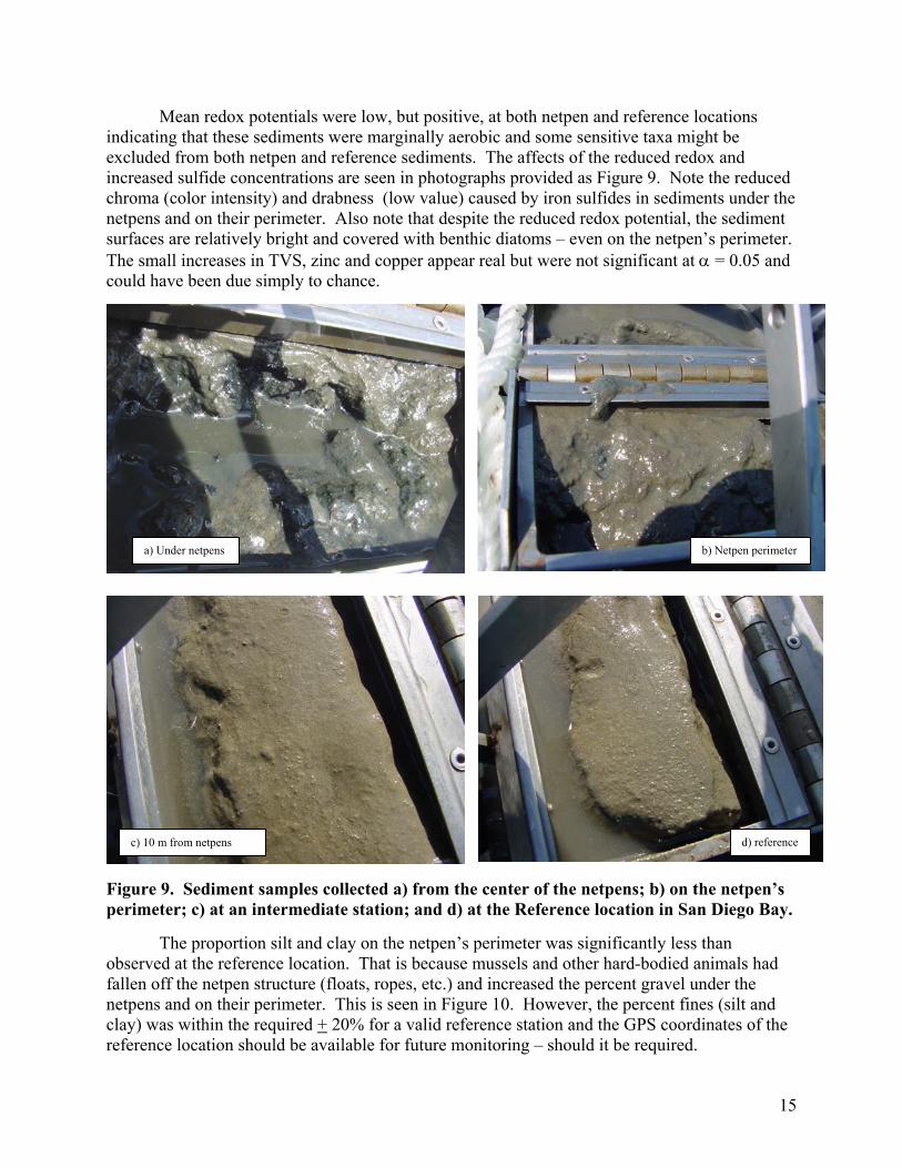
15
Mean redox potentials were low, but positive, at both netpen and reference locations indicating that these sediments were marginally aerobic and some sensitive taxa might be excluded from both netpen and reference sediments. The affects of the reduced redox and increased sulfide concentrations are seen in photographs provided as Figure 9. Note the reduced chroma (color intensity) and drabness (low value) caused by iron sulfides in sediments under the netpens and on their perimeter. Also note that despite the reduced redox potential, the sediment surfaces are relatively bright and covered with benthic diatoms – even on the netpen’s perimeter. The small increases in TVS, zinc and copper appear real but were not significant at α = 0.05 and could have been due simply to chance.
Figure 9. Sediment samples collected a) from the center of the netpens; b) on the netpen’s perimeter; c) at an intermediate station; and d) at the Reference location in San Diego Bay. The proportion silt and clay on the netpen’s perimeter was significantly less than observed at the reference location. That is because mussels and other hard-bodied animals had fallen off the netpen structure (floats, ropes, etc.) and increased the percent gravel under the netpens and on their perimeter. This is seen in Figure 10. However, the percent fines (silt and clay) was within the required + 20% for a valid reference station and the GPS coordinates of the reference location should be available for future monitoring – should it be required.
a) Under netpens
d) reference c) 10 m from netpens
b) Netpen perimeter
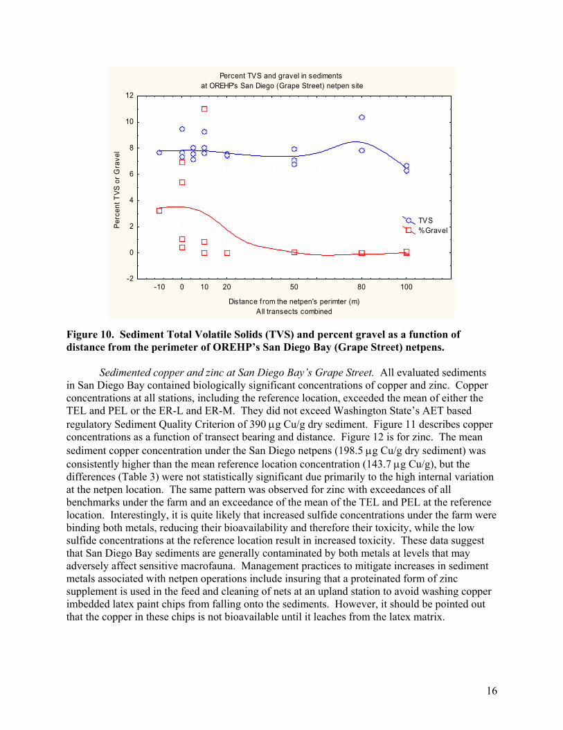
16
Percent TVS and gravel in sediments at OREHP's San Diego (Grape Street) netpen site
-10 0 10 20 50 80 100
Distance f rom the netpen's perimter (m)All transects combined
-2
0
2
4
6
8
10
12
Perc
ent T
VS o
r Gra
vel
TVS %Gravel
Figure 10. Sediment Total Volatile Solids (TVS) and percent gravel as a function of distance from the perimeter of OREHP’s San Diego Bay (Grape Street) netpens. Sedimented copper and zinc at San Diego Bay’s Grape Street. All evaluated sediments in San Diego Bay contained biologically significant concentrations of copper and zinc. Copper concentrations at all stations, including the reference location, exceeded the mean of either the TEL and PEL or the ER-L and ER-M. They did not exceed Washington State’s AET based regulatory Sediment Quality Criterion of 390 µg Cu/g dry sediment. Figure 11 describes copper concentrations as a function of transect bearing and distance. Figure 12 is for zinc. The mean sediment copper concentration under the San Diego netpens (198.5 µg Cu/g dry sediment) was consistently higher than the mean reference location concentration (143.7 µg Cu/g), but the differences (Table 3) were not statistically significant due primarily to the high internal variation at the netpen location. The same pattern was observed for zinc with exceedances of all benchmarks under the farm and an exceedance of the mean of the TEL and PEL at the reference location. Interestingly, it is quite likely that increased sulfide concentrations under the farm were binding both metals, reducing their bioavailability and therefore their toxicity, while the low sulfide concentrations at the reference location result in increased toxicity. These data suggest that San Diego Bay sediments are generally contaminated by both metals at levels that may adversely affect sensitive macrofauna. Management practices to mitigate increases in sediment metals associated with netpen operations include insuring that a proteinated form of zinc supplement is used in the feed and cleaning of nets at an upland station to avoid washing copper imbedded latex paint chips from falling onto the sediments. However, it should be pointed out that the copper in these chips is not bioavailable until it leaches from the latex matrix.
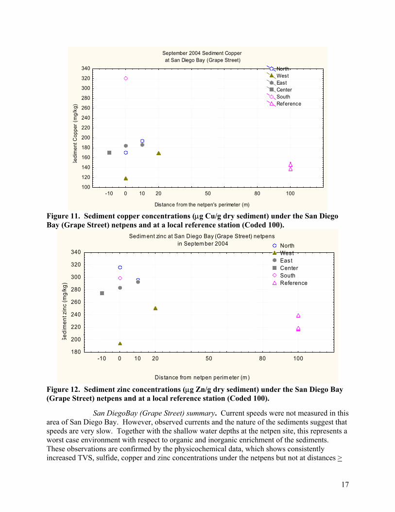
17
September 2004 Sediment Copper at San Diego Bay (Grape Street)
Distance f rom the netpen's perimeter (m)
Sedi
men
t Cop
per (
mg/
kg)
-10 0 10 20 50 80 100100
120
140
160
180
200
220
240
260
280
300
320
340 NorthWestEastCenterSouthReference
Figure 11. Sediment copper concentrations (µg Cu/g dry sediment) under the San Diego Bay (Grape Street) netpens and at a local reference station (Coded 100).
Sedim ent zinc at San Diego Bay (Grape Street) netpens in Septem ber 2004
Dis tance from netpen perim eter (m )
Sedi
men
t zin
c (m
g/kg
)
-10 0 10 20 50 80 100180
200
220
240
260
280
300
320
340NorthWestEastCenterSouthReference
Figure 12. Sediment zinc concentrations (µg Zn/g dry sediment) under the San Diego Bay (Grape Street) netpens and at a local reference station (Coded 100). San DiegoBay (Grape Street) summary. Current speeds were not measured in this area of San Diego Bay. However, observed currents and the nature of the sediments suggest that speeds are very slow. Together with the shallow water depths at the netpen site, this represents a worst case environment with respect to organic and inorganic enrichment of the sediments. These observations are confirmed by the physicochemical data, which shows consistently increased TVS, sulfide, copper and zinc concentrations under the netpens but not at distances >
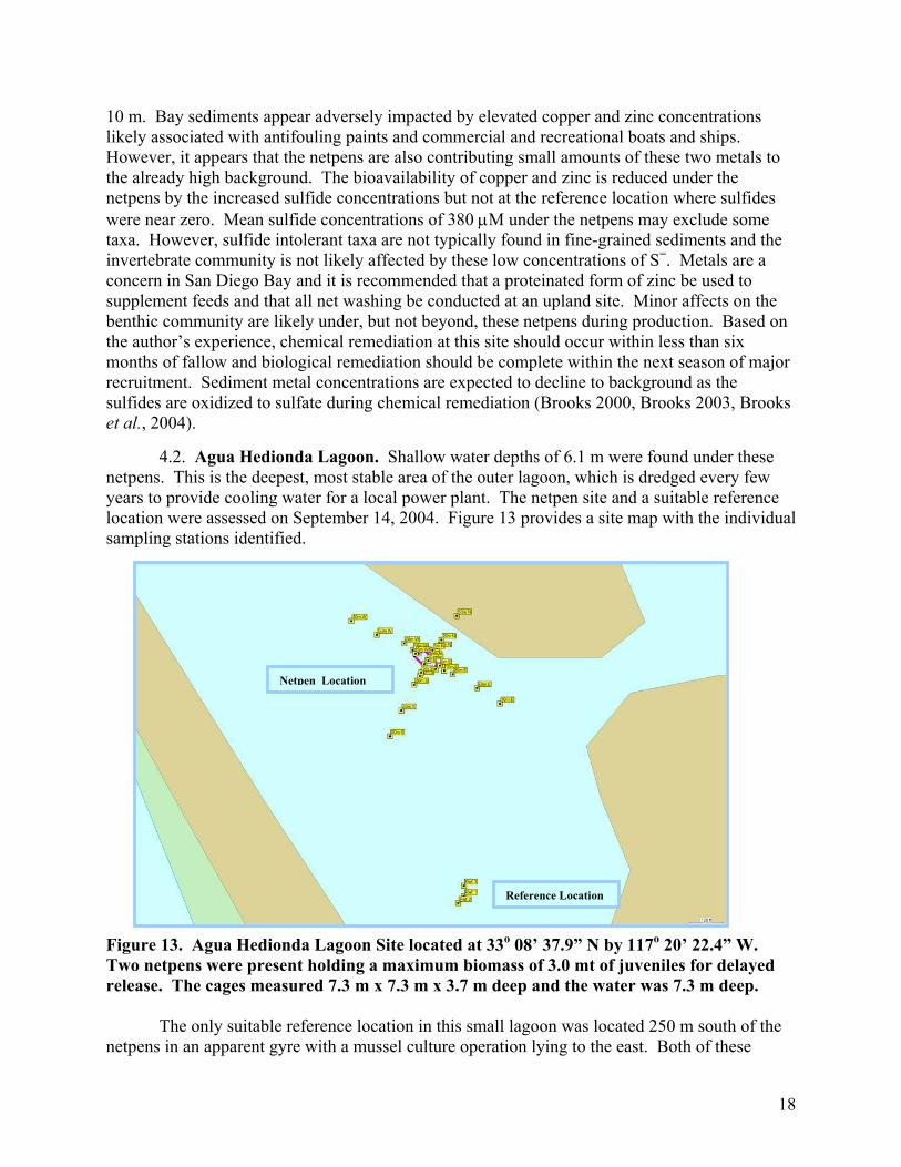
18
10 m. Bay sediments appear adversely impacted by elevated copper and zinc concentrations likely associated with antifouling paints and commercial and recreational boats and ships. However, it appears that the netpens are also contributing small amounts of these two metals to the already high background. The bioavailability of copper and zinc is reduced under the netpens by the increased sulfide concentrations but not at the reference location where sulfides were near zero. Mean sulfide concentrations of 380 µM under the netpens may exclude some taxa. However, sulfide intolerant taxa are not typically found in fine-grained sediments and the invertebrate community is not likely affected by these low concentrations of S=. Metals are a concern in San Diego Bay and it is recommended that a proteinated form of zinc be used to supplement feeds and that all net washing be conducted at an upland site. Minor affects on the benthic community are likely under, but not beyond, these netpens during production. Based on the author’s experience, chemical remediation at this site should occur within less than six months of fallow and biological remediation should be complete within the next season of major recruitment. Sediment metal concentrations are expected to decline to background as the sulfides are oxidized to sulfate during chemical remediation (Brooks 2000, Brooks 2003, Brooks et al., 2004). 4.2. Agua Hedionda Lagoon. Shallow water depths of 6.1 m were found under these netpens. This is the deepest, most stable area of the outer lagoon, which is dredged every few years to provide cooling water for a local power plant. The netpen site and a suitable reference location were assessed on September 14, 2004. Figure 13 provides a site map with the individual sampling stations identified.
Figure 13. Agua Hedionda Lagoon Site located at 33o 08’ 37.9” N by 117o 20’ 22.4” W. Two netpens were present holding a maximum biomass of 3.0 mt of juveniles for delayed release. The cages measured 7.3 m x 7.3 m x 3.7 m deep and the water was 7.3 m deep. The only suitable reference location in this small lagoon was located 250 m south of the netpens in an apparent gyre with a mussel culture operation lying to the east. Both of these
Reference Location
Netpen Location
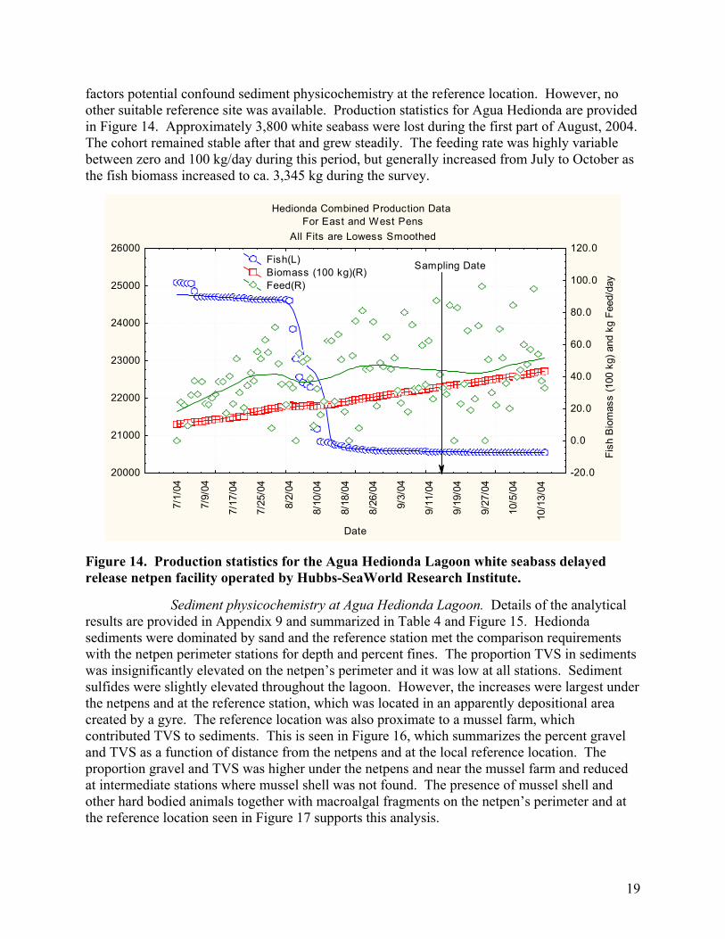
19
factors potential confound sediment physicochemistry at the reference location. However, no other suitable reference site was available. Production statistics for Agua Hedionda are provided in Figure 14. Approximately 3,800 white seabass were lost during the first part of August, 2004. The cohort remained stable after that and grew steadily. The feeding rate was highly variable between zero and 100 kg/day during this period, but generally increased from July to October as the fish biomass increased to ca. 3,345 kg during the survey.
Hedionda Combined Production Data For East and West Pens
All Fits are Lowess Smoothed
7/1/
04
7/9/
04
7/17
/04
7/25
/04
8/2/
04
8/10
/04
8/18
/04
8/26
/04
9/3/
04
9/11
/04
9/19
/04
9/27
/04
10/5
/04
10/1
3/04
Date
20000
21000
22000
23000
24000
25000
26000
-20.0
0.0
20.0
40.0
60.0
80.0
100.0
120.0
Fish
Bio
mas
s (1
00 k
g) a
nd k
g Fe
ed/d
ay
Fish(L) Biomass (100 kg)(R) Feed(R)
Sampling Date
Figure 14. Production statistics for the Agua Hedionda Lagoon white seabass delayed release netpen facility operated by Hubbs-SeaWorld Research Institute. Sediment physicochemistry at Agua Hedionda Lagoon. Details of the analytical results are provided in Appendix 9 and summarized in Table 4 and Figure 15. Hedionda sediments were dominated by sand and the reference station met the comparison requirements with the netpen perimeter stations for depth and percent fines. The proportion TVS in sediments was insignificantly elevated on the netpen’s perimeter and it was low at all stations. Sediment sulfides were slightly elevated throughout the lagoon. However, the increases were largest under the netpens and at the reference station, which was located in an apparently depositional area created by a gyre. The reference location was also proximate to a mussel farm, which contributed TVS to sediments. This is seen in Figure 16, which summarizes the percent gravel and TVS as a function of distance from the netpens and at the local reference location. The proportion gravel and TVS was higher under the netpens and near the mussel farm and reduced at intermediate stations where mussel shell was not found. The presence of mussel shell and other hard bodied animals together with macroalgal fragments on the netpen’s perimeter and at the reference location seen in Figure 17 supports this analysis.
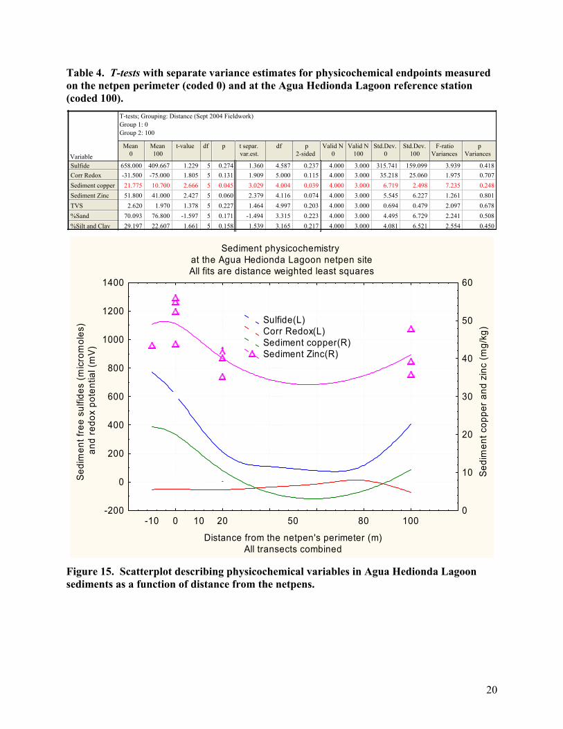
20
Table 4. T-tests with separate variance estimates for physicochemical endpoints measured on the netpen perimeter (coded 0) and at the Agua Hedionda Lagoon reference station (coded 100).
T-tests; Grouping: Distance (Sept 2004 Fieldwork)Group 1: 0Group 2: 100
VariableMean
0Mean100
t-value df p t separ.var.est.
df p2-sided
Valid N0
Valid N100
Std.Dev.0
Std.Dev.100
F-ratioVariances
pVariances
SulfideCorr RedoxSediment copperSediment ZincTVS%Sand%Silt and Clay
658.000 409.667 1.229 5 0.274 1.360 4.587 0.237 4.000 3.000 315.741 159.099 3.939 0.418-31.500 -75.000 1.805 5 0.131 1.909 5.000 0.115 4.000 3.000 35.218 25.060 1.975 0.70721.775 10.700 2.666 5 0.045 3.029 4.004 0.039 4.000 3.000 6.719 2.498 7.235 0.24851.800 41.000 2.427 5 0.060 2.379 4.116 0.074 4.000 3.000 5.545 6.227 1.261 0.801
2.620 1.970 1.378 5 0.227 1.464 4.997 0.203 4.000 3.000 0.694 0.479 2.097 0.67870.093 76.800 -1.597 5 0.171 -1.494 3.315 0.223 4.000 3.000 4.495 6.729 2.241 0.50829.197 22.607 1.661 5 0.158 1.539 3.165 0.217 4.000 3.000 4.081 6.521 2.554 0.450
Sediment physicochemistry at the Agua Hedionda Lagoon netpen siteAll fits are distance weighted least squares
-10 0 10 20 50 80 100
Distance from the netpen's perimeter (m)All transects combined
-200
0
200
400
600
800
1000
1200
1400
Sedi
men
t fre
e su
lfide
s (m
icro
mol
es)
and
redo
x po
tent
ial (
mV)
0
10
20
30
40
50
60
Sedi
men
t cop
per a
nd z
inc
(mg/
kg)
Sulfide(L) Corr Redox(L) Sediment copper(R) Sediment Zinc(R)
Figure 15. Scatterplot describing physicochemical variables in Agua Hedionda Lagoon sediments as a function of distance from the netpens.
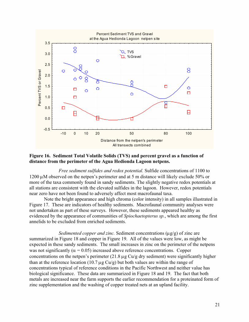
21
Percent Sedim ent TVS and Gravelat the Agua Hedionda Lagoon netpen s ite
-10 0 10 20 50 80 100
Dis tance from the netpen's perim eterAll transects com bined
-0.5
0.0
0.5
1.0
1.5
2.0
2.5
3.0
3.5P
erce
nt T
VS
or G
rave
l
TVS %Gravel
Figure 16. Sediment Total Volatile Solids (TVS) and percent gravel as a function of distance from the perimeter of the Agua Hedionda Lagoon netpens. Free sediment sulfides and redox potential. Sulfide concentrations of 1100 to 1200 µM observed on the netpen’s perimeter and at 5 m distance will likely exclude 50% or more of the taxa commonly found in sandy sediments. The slightly negative redox potentials at all stations are consistent with the elevated sulfides in the lagoon. However, redox potentials near zero have not been found to adversely affect most macrofaunal taxa. Note the bright appearance and high chroma (color intensity) in all samples illustrated in Figure 17. These are indicators of healthy sediments. Macrofaunal community analyses were not undertaken as part of these surveys. However, these sediments appeared healthy as evidenced by the appearance of communities of Spiochaetopterus sp., which are among the first annelids to be excluded from enriched sediments. Sedimented copper and zinc. Sediment concentrations (µg/g) of zinc are summarized in Figure 18 and copper in Figure 19. All of the values were low, as might be expected in these sandy sediments. The small increases in zinc on the perimeter of the netpens was not significantly (α = 0.05) increased above reference concentrations. Copper concentrations on the netpen’s perimeter (21.8 µg Cu/g dry sediment) were significantly higher than at the reference location (10.7 µg Cu/g) but both values are within the range of concentrations typical of reference conditions in the Pacific Northwest and neither value has biological significance. These data are summarized in Figure 18 and 19. The fact that both metals are increased near the farm supports the earlier recommendation for a proteinated form of zinc supplementation and the washing of copper treated nets at an upland facility.
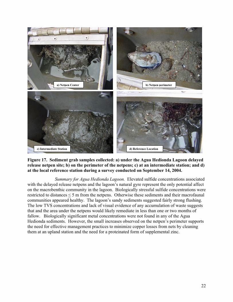
22
Figure 17. Sediment grab samples collected: a) under the Agua Hedionda Lagoon delayed release netpen site; b) on the perimeter of the netpens; c) at an intermediate station; and d) at the local reference station during a survey conducted on September 14, 2004. Summary for Agua Hedionda Lagoon. Elevated sulfide concentrations associated with the delayed release netpens and the lagoon’s natural gyre represent the only potential affect on the macrobenthic community in the lagoon. Biologically stressful sulfide concentrations were restricted to distances < 5 m from the netpens. Otherwise these sediments and their macrofaunal communities appeared healthy. The lagoon’s sandy sediments suggested fairly strong flushing. The low TVS concentrations and lack of visual evidence of any accumulation of waste suggests that and the area under the netpens would likely remediate in less than one or two months of fallow. Biologically significant metal concentrations were not found in any of the Agua Hedionda sediments. However, the small increases observed on the netpen’s perimeter supports the need for effective management practices to minimize copper losses from nets by cleaning them at an upland station and the need for a proteinated form of supplemental zinc.
a) Netpen Center b) Netpen perimeter
d) Reference Locationc) Intermediate Station
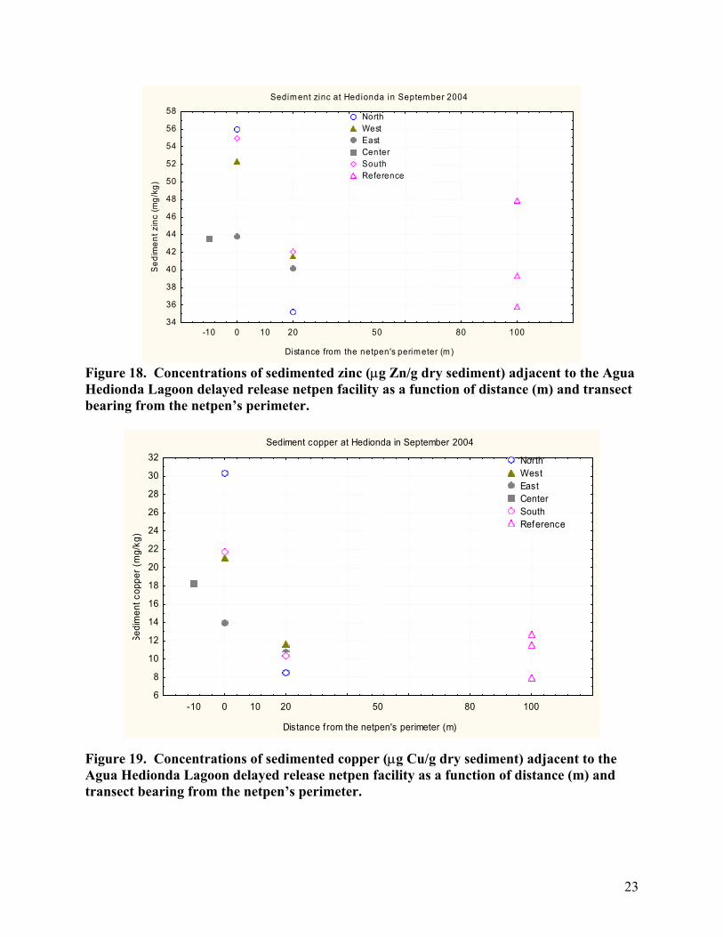
23
Sediment zinc at Hedionda in September 2004
Distance from the netpen's perimeter (m)
Sed
imen
t zin
c (m
g/kg
)
-10 0 10 20 50 80 10034
36
38
40
42
44
46
48
50
52
54
56
58 NorthWestEastCenterSouthReference
Figure 18. Concentrations of sedimented zinc (µg Zn/g dry sediment) adjacent to the Agua Hedionda Lagoon delayed release netpen facility as a function of distance (m) and transect bearing from the netpen’s perimeter.
Sediment copper at Hedionda in September 2004
Distance f rom the netpen's perimeter (m)
Sedi
men
t cop
per (
mg/
kg)
-10 0 10 20 50 80 1006
8
10
12
14
16
18
20
22
24
26
28
30
32 NorthWestEastCenterSouthReference
Figure 19. Concentrations of sedimented copper (µg Cu/g dry sediment) adjacent to the Agua Hedionda Lagoon delayed release netpen facility as a function of distance (m) and transect bearing from the netpen’s perimeter.
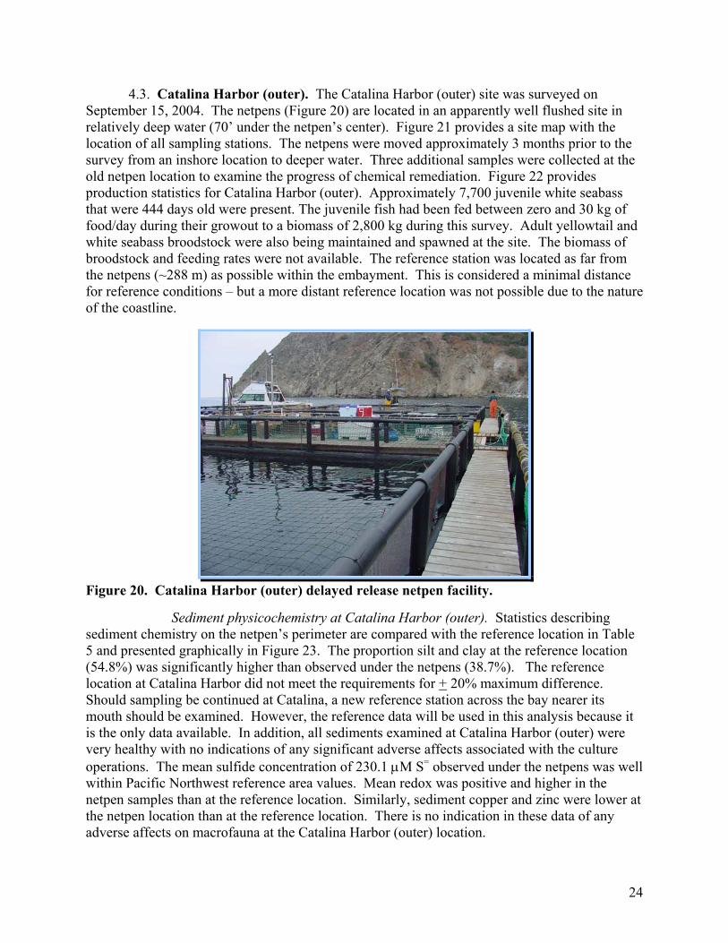
24
4.3. Catalina Harbor (outer). The Catalina Harbor (outer) site was surveyed on September 15, 2004. The netpens (Figure 20) are located in an apparently well flushed site in relatively deep water (70’ under the netpen’s center). Figure 21 provides a site map with the location of all sampling stations. The netpens were moved approximately 3 months prior to the survey from an inshore location to deeper water. Three additional samples were collected at the old netpen location to examine the progress of chemical remediation. Figure 22 provides production statistics for Catalina Harbor (outer). Approximately 7,700 juvenile white seabass that were 444 days old were present. The juvenile fish had been fed between zero and 30 kg of food/day during their growout to a biomass of 2,800 kg during this survey. Adult yellowtail and white seabass broodstock were also being maintained and spawned at the site. The biomass of broodstock and feeding rates were not available. The reference station was located as far from the netpens (~288 m) as possible within the embayment. This is considered a minimal distance for reference conditions – but a more distant reference location was not possible due to the nature of the coastline.
Figure 20. Catalina Harbor (outer) delayed release netpen facility. Sediment physicochemistry at Catalina Harbor (outer). Statistics describing sediment chemistry on the netpen’s perimeter are compared with the reference location in Table 5 and presented graphically in Figure 23. The proportion silt and clay at the reference location (54.8%) was significantly higher than observed under the netpens (38.7%). The reference location at Catalina Harbor did not meet the requirements for + 20% maximum difference. Should sampling be continued at Catalina, a new reference station across the bay nearer its mouth should be examined. However, the reference data will be used in this analysis because it is the only data available. In addition, all sediments examined at Catalina Harbor (outer) were very healthy with no indications of any significant adverse affects associated with the culture operations. The mean sulfide concentration of 230.1 µM S= observed under the netpens was well within Pacific Northwest reference area values. Mean redox was positive and higher in the netpen samples than at the reference location. Similarly, sediment copper and zinc were lower at the netpen location than at the reference location. There is no indication in these data of any adverse affects on macrofauna at the Catalina Harbor (outer) location.
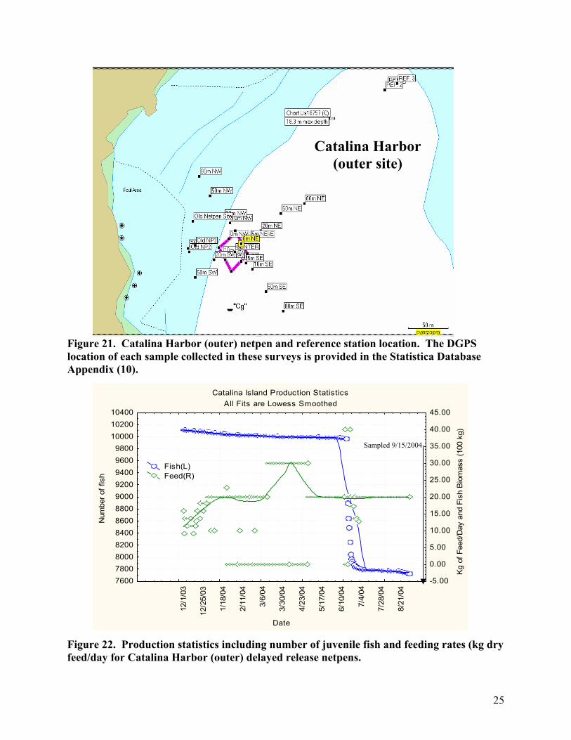
25
Figure 21. Catalina Harbor (outer) netpen and reference station location. The DGPS location of each sample collected in these surveys is provided in the Statistica Database Appendix (10). Figure 22. Production statistics including number of juvenile fish and feeding rates (kg dry feed/day for Catalina Harbor (outer) delayed release netpens.
Catalina Harbor (outer site)
Catalina Island Production StatisticsAll Fits are Lowess Smoothed
12/1
/03
12/2
5/03
1/18
/04
2/11
/04
3/6/
04
3/30
/04
4/23
/04
5/17
/04
6/10
/04
7/4/
04
7/28
/04
8/21
/04
Date
760078008000820084008600880090009200940096009800
100001020010400
Num
ber o
f fis
h
-5.00
0.00
5.00
10.00
15.00
20.00
25.00
30.00
35.00
40.00
45.00
Kg
of F
eed/
Day
and
Fis
h B
iom
ass
(100
kg)
Fish(L) Feed(R)
Sampled 9/15/2004
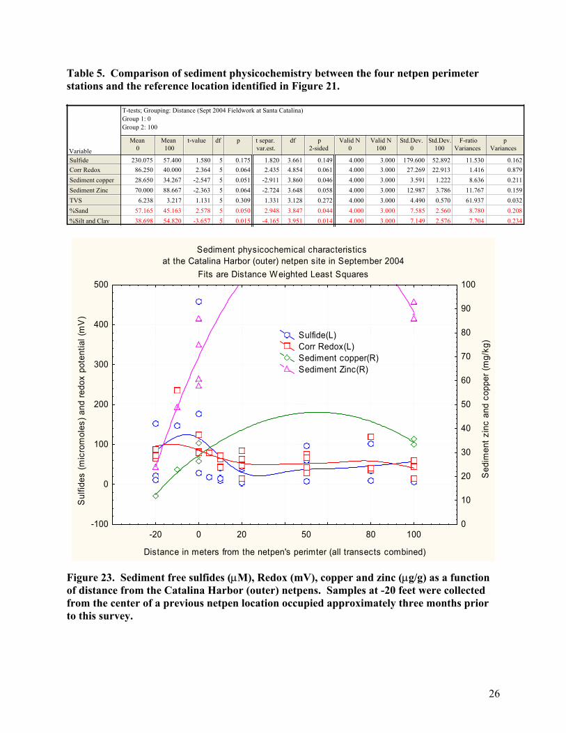
26
Table 5. Comparison of sediment physicochemistry between the four netpen perimeter stations and the reference location identified in Figure 21.
T-tests; Grouping: Distance (Sept 2004 Fieldwork at Santa Catalina)Group 1: 0Group 2: 100
VariableMean
0Mean
100t-value df p t separ.
var.est.df p
2-sidedValid N
0Valid N
100Std.Dev.
0Std.Dev.
100F-ratio
Variancesp
Variances
SulfideCorr RedoxSediment copperSediment ZincTVS%Sand%Silt and Clay
230.075 57.400 1.580 5 0.175 1.820 3.661 0.149 4.000 3.000 179.600 52.892 11.530 0.16286.250 40.000 2.364 5 0.064 2.435 4.854 0.061 4.000 3.000 27.269 22.913 1.416 0.87928.650 34.267 -2.547 5 0.051 -2.911 3.860 0.046 4.000 3.000 3.591 1.222 8.636 0.21170.000 88.667 -2.363 5 0.064 -2.724 3.648 0.058 4.000 3.000 12.987 3.786 11.767 0.159
6.238 3.217 1.131 5 0.309 1.331 3.128 0.272 4.000 3.000 4.490 0.570 61.937 0.03257.165 45.163 2.578 5 0.050 2.948 3.847 0.044 4.000 3.000 7.585 2.560 8.780 0.20838.698 54.820 -3.657 5 0.015 -4.165 3.951 0.014 4.000 3.000 7.149 2.576 7.704 0.234
Sediment physicochemical characteristics
at the Catalina Harbor (outer) netpen site in September 2004Fits are Distance Weighted Least Squares
-20 0 20 50 80 100
Distance in meters from the netpen's perimter (all transects combined)
-100
0
100
200
300
400
500
Sul
fides
(mic
rom
oles
) and
redo
x po
tent
ial (
mV
)
0
10
20
30
40
50
60
70
80
90
100
Sed
imen
t zin
c an
d co
pper
(mg/
kg) Sulfide(L)
Corr Redox(L) Sediment copper(R) Sediment Zinc(R)
Figure 23. Sediment free sulfides (µM), Redox (mV), copper and zinc (µg/g) as a function of distance from the Catalina Harbor (outer) netpens. Samples at -20 feet were collected from the center of a previous netpen location occupied approximately three months prior to this survey.

27
Table 6. Comparison of sediment physicochemistry between three samples collected at the old netpen location and triplicate samples collected at the reference station.
T-tests; Grouping: Distance (Sept 2004 Fieldwork at Santa Catalina's Old Farm Location)Group 1: -20Group 2: 100
Variable
Mean-20
Mean100
t-value df p t separ.var.est.
df p2-sided
Valid N-20
Valid N100
Std.Dev.-20
Std.Dev.100
F-ratioVariances
pVariances
SulfideCorr RedoxSediment copperSediment ZincTVS%Sand%Silt and Clay
61.633 57.400 0.078 4 0.942 0.078 3.508 0.942 3.000 3.000 78.398 52.892 2.197 0.62674.667 40.000 2.353 4 0.078 2.353 2.910 0.103 3.000 3.000 11.240 22.913 4.156 0.38812.000 34.267 -15.780 2 0.004 1.000 3.000 0.000 1.222 0.000 1.00024.000 88.667 -14.792 2 0.005 1.000 3.000 0.000 3.786 0.000 1.000
3.387 3.217 0.482 4 0.655 0.482 2.580 0.668 3.000 3.000 0.220 0.570 6.747 0.25883.190 45.163 12.864 2 0.006 1.000 3.000 0.000 2.560 0.000 1.00016.020 54.820 -13.046 2 0.006 1.000 3.000 0.000 2.576 0.000 1.000
Chemical remediation at the previous netpen location. Sediment physicochemical characteristics at the reference station and at the old netpen location are compared in Table 6. Single samples were analyzed for copper and zinc at the old netpen site and caution is warranted in interpreting the single sample t-test conducted using Statistica. However, the mean concentrations of copper and zinc at the old netpen site are very low by any standard and significantly lower than observed at the reference location. Sulfide concentrations are also low and redox potential moderately high at the old netpen location. Note that TVS concentrations at the old netpen site are essentially identical with those observed at the reference location. This TVS appeared more associated with the vibrant macrobenthic community than with organic inputs from the farm. This site appears to have completely remediated during the three months since the netpens were moved. Visual assessment of sediments at Catalina Harbor (outer). Figure 24 provides photographs of grab samples collected at various distances from the netpens. A vibrant macrofaunal community was observed under and on the perimeter of the netpens. This is likely the result of farm waste, which is not exceeding the assimilative capacity of the sediments and is simply seen as additional food by the macrobenthos. Sediments at intermediate distances were healthy with vibrant annelid and amphipod communities. Many of the grabs, including those from the old netpen location held healthy communities of Spiochaetopterus sp. – which is an organic carbon intolerant species. All of the Catalina sediment samples were bright, had high chroma and appeared very healthy. Summary for the Catalina Harbor (outer) netpen site. No adverse benthic effects were observed. There are several highly productive salmon farms in the Pacific Northwest where fast currents distribute waste such that it does not exceed the assimilative capacity of sediments. The results are enhanced macrofaunal communities with 50 to 100% higher diversity and four plus fold higher abundance of macrofauna. The assimilative capacity of sediments at Santa Catalina are not being exceeded by existing operations and best professional judgment suggests that this site could support culture of a much larger biomass of fish - perhaps as high as 100 tonnes without significant or long-lasting benthic effects. Macrofaunal community assessments were not made in this effort. However, the infaunal and epifaunal communities appear enhanced under the existing netpens and at the previous netpen location. The very low sediment concentrations of copper and zinc at this location suggests that in-situ net cleaning is having little affect on sediment chemistry. There is no apparent need to remove nets from the Catalina site to an upland facility for cleaning.

28
Figure 24. Grab samples collected near the Catalina Harbor (outer) netpens on September 15, 2004.
a) Center of netpens b) Netpen perimeter
c-2) Intermediate station c-1) Intermediate station
d) Old netpen location e) Reference location
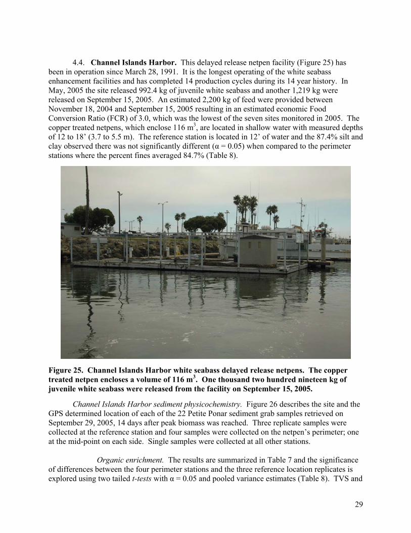
29
4.4. Channel Islands Harbor. This delayed release netpen facility (Figure 25) has
been in operation since March 28, 1991. It is the longest operating of the white seabass enhancement facilities and has completed 14 production cycles during its 14 year history. In May, 2005 the site released 992.4 kg of juvenile white seabass and another 1,219 kg were released on September 15, 2005. An estimated 2,200 kg of feed were provided between November 18, 2004 and September 15, 2005 resulting in an estimated economic Food Conversion Ratio (FCR) of 3.0, which was the lowest of the seven sites monitored in 2005. The copper treated netpens, which enclose 116 m3, are located in shallow water with measured depths of 12 to 18’ (3.7 to 5.5 m). The reference station is located in 12’ of water and the 87.4% silt and clay observed there was not significantly different (α = 0.05) when compared to the perimeter stations where the percent fines averaged 84.7% (Table 8).
Figure 25. Channel Islands Harbor white seabass delayed release netpens. The copper treated netpen encloses a volume of 116 m3. One thousand two hundred nineteen kg of juvenile white seabass were released from the facility on September 15, 2005.
Channel Islands Harbor sediment physicochemistry. Figure 26 describes the site and the GPS determined location of each of the 22 Petite Ponar sediment grab samples retrieved on September 29, 2005, 14 days after peak biomass was reached. Three replicate samples were collected at the reference station and four samples were collected on the netpen’s perimeter; one at the mid-point on each side. Single samples were collected at all other stations.
Organic enrichment. The results are summarized in Table 7 and the significance of differences between the four perimeter stations and the three reference location replicates is explored using two tailed t-tests with α = 0.05 and pooled variance estimates (Table 8). TVS and
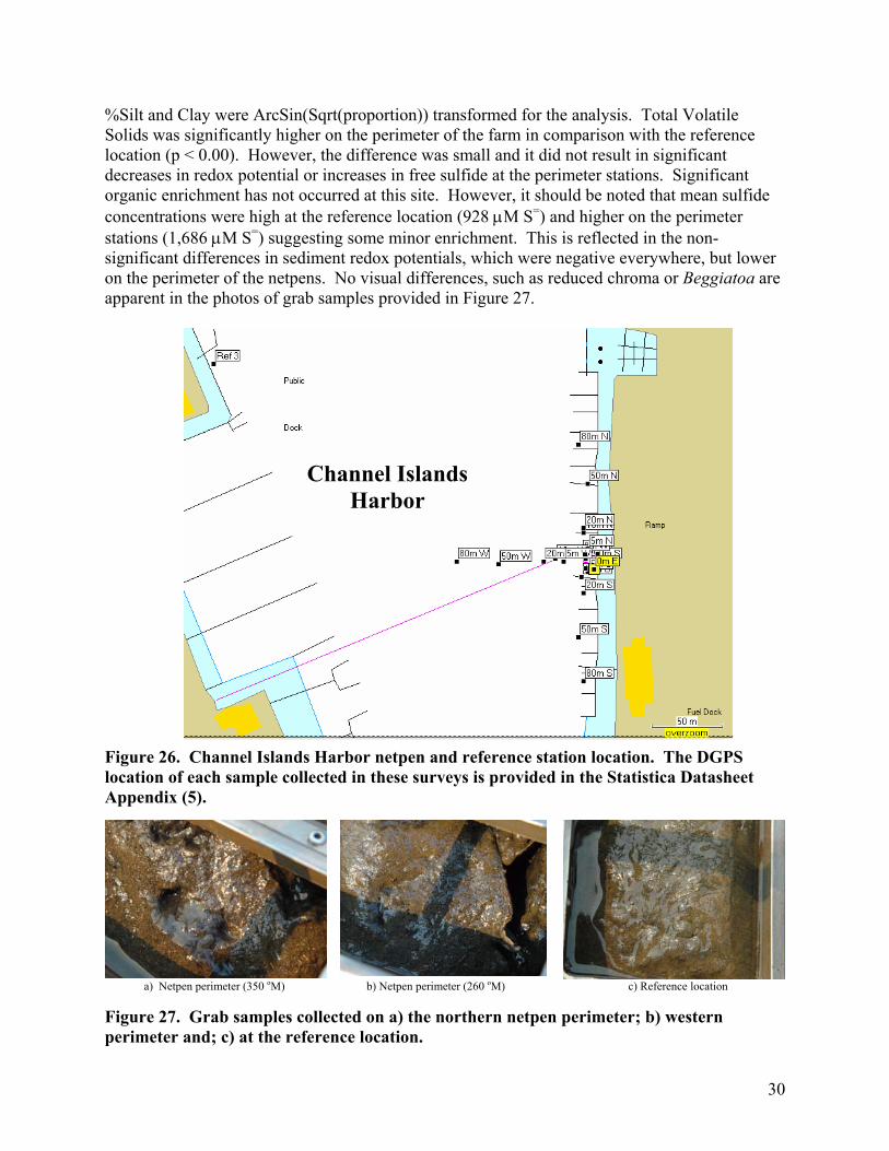
30
%Silt and Clay were ArcSin(Sqrt(proportion)) transformed for the analysis. Total Volatile Solids was significantly higher on the perimeter of the farm in comparison with the reference location (p < 0.00). However, the difference was small and it did not result in significant decreases in redox potential or increases in free sulfide at the perimeter stations. Significant organic enrichment has not occurred at this site. However, it should be noted that mean sulfide concentrations were high at the reference location (928 µM S=) and higher on the perimeter stations (1,686 µM S=) suggesting some minor enrichment. This is reflected in the non-significant differences in sediment redox potentials, which were negative everywhere, but lower on the perimeter of the netpens. No visual differences, such as reduced chroma or Beggiatoa are apparent in the photos of grab samples provided in Figure 27.
Figure 26. Channel Islands Harbor netpen and reference station location. The DGPS location of each sample collected in these surveys is provided in the Statistica Datasheet Appendix (5).
a) Netpen perimeter (350 oM) b) Netpen perimeter (260 oM) c) Reference location Figure 27. Grab samples collected on a) the northern netpen perimeter; b) western perimeter and; c) at the reference location.
Channel Islands Harbor
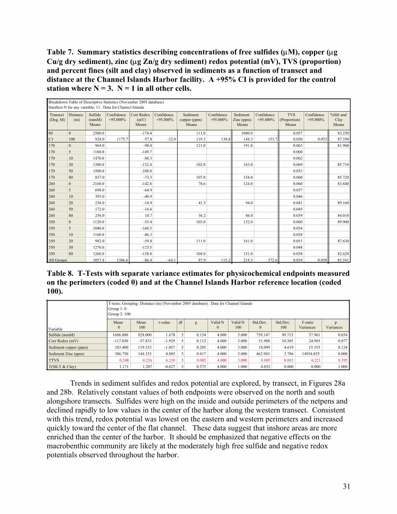
31
Table 7. Summary statistics describing concentrations of free sulfides (µM), copper (µg Cu/g dry sediment), zinc (µg Zn/g dry sediment) redox potential (mV), TVS (proportion) and percent fines (silt and clay) observed in sediments as a function of transect and distance at the Channel Islands Harbor facility. A +95% CI is provided for the control station where N = 3. N = 1 in all other cells. Breakdown Table of Descriptive Statistics (November 2005 database)Smallest N for any variable: 11. Data for Channel Islands
Transect(Deg. M)
Distance (m)
Sulfide(mmM)Means
Confidence+95.000%
Corr Redox(mV)
Means
Confidence+95.000%
Sedimentcopper (ppm)
Means
Confidence+95.000%
SedimentZinc (ppm)
Means
Confidence+95.000%
TVS(Proportion)
Means
Confidence+95.000%
%Silt andClay
Means
80 0 2500.0 -174.4 111.0 1080.0 0.057 83.250C1 100 928.0 1175.7 -57.8 -32.0 119.3 130.8 144.3 153.7 0.050 0.053 87.350170 0 964.0 -98.8 121.0 191.0 0.063 81.960170 5 1160.0 -149.7 0.060170 10 1470.0 -88.3 0.062170 20 1300.0 -132.4 102.0 163.0 0.069 85.710170 50 1500.0 -108.8 0.053170 80 837.0 -73.3 107.0 154.0 0.060 85.720260 0 2160.0 -142.8 78.6 124.0 0.060 83.640260 5 698.0 -64.9 0.057260 10 393.0 -48.9 0.046260 20 236.0 -14.9 41.5 94.0 0.041 89.160260 50 172.0 -16.6 0.045260 80 256.0 10.7 36.2 86.0 0.039 84.010350 0 1120.0 -55.4 103.0 152.0 0.060 89.900350 5 1040.0 -160.3 0.054350 10 1160.0 -86.3 0.058350 20 982.0 -59.8 111.0 161.0 0.051 87.630350 50 1270.0 -123.5 0.048350 80 1260.0 -138.8 104.0 151.0 0.058 82.620All Groups 1057.4 1306.6 -86.4 -64.1 97.9 115.2 214.5 372.6 0.054 0.058 85.541
Table 8. T-Tests with separate variance estimates for physicochemical endpoints measured on the perimeters (coded 0) and at the Channel Islands Harbor reference location (coded 100).
T-tests; Grouping: Distance (m) (November 2005 database). Data for Channel IslandsGroup 1: 0Group 2: 100
VariableMean
0Mean
100t-value df p Valid N
0Valid N
100Std.Dev.
0Std.Dev.
100F-ratio
Variancesp
Variances
Sulfide (mmM)Corr Redox (mV)Sediment copper (ppm)Sediment Zinc (ppm)TTVST(SILT & Clay)
1686.000 928.000 1.678 5 0.154 4.000 3.000 759.147 99.715 57.961 0.034-117.850 -57.833 -1.929 5 0.112 4.000 3.000 51.908 10.385 24.985 0.077103.400 119.333 -1.457 5 0.205 4.000 3.000 18.099 4.619 15.355 0.124386.750 144.333 0.885 5 0.417 4.000 3.000 462.983 3.786 14954.855 0.000
0.248 0.226 6.218 5 0.002 4.000 3.000 0.005 0.003 4.221 0.3951.171 1.207 -0.627 3 0.575 4.000 1.000 0.052 0.000 0.000 1.000
Trends in sediment sulfides and redox potential are explored, by transect, in Figures 28a and 28b. Relatively constant values of both endpoints were observed on the north and south alongshore transects. Sulfides were high on the inside and outside perimeters of the netpens and declined rapidly to low values in the center of the harbor along the western transect. Consistent with this trend, redox potential was lowest on the eastern and western perimeters and increased quickly toward the center of the flat channel. These data suggest that inshore areas are more enriched than the center of the harbor. It should be emphasized that negative effects on the macrobenthic community are likely at the moderately high free sulfide and negative redox potentials observed throughout the harbor.
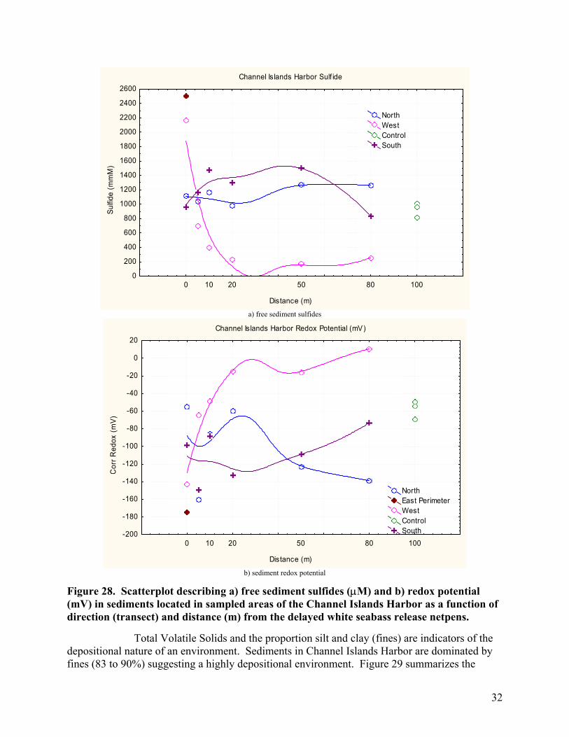
32
Channel Islands Harbor Sulf ide
Distance (m)
Sulfid
e (m
mM
)
0 10 20 50 80 1000
200
400
600
800
1000
1200
1400
1600
1800
2000
2200
2400
2600
NorthWestControlSouth
a) free sediment sulfides
Channel Islands Harbor Redox Potential (mV)
Distance (m)
Cor
r Red
ox (m
V)
0 10 20 50 80 100-200
-180
-160
-140
-120
-100
-80
-60
-40
-20
0
20
NorthEast PerimeterWestControlSouth
b) sediment redox potential
Figure 28. Scatterplot describing a) free sediment sulfides (µM) and b) redox potential (mV) in sediments located in sampled areas of the Channel Islands Harbor as a function of direction (transect) and distance (m) from the delayed white seabass release netpens. Total Volatile Solids and the proportion silt and clay (fines) are indicators of the depositional nature of an environment. Sediments in Channel Islands Harbor are dominated by fines (83 to 90%) suggesting a highly depositional environment. Figure 29 summarizes the
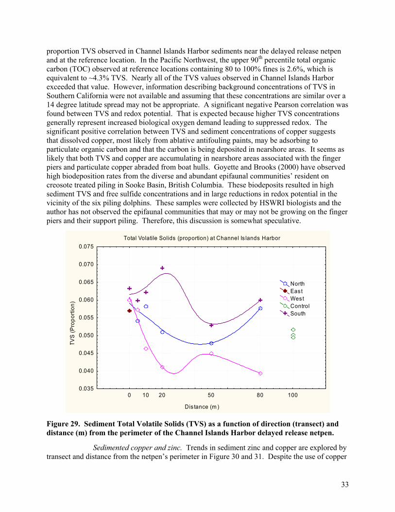
33
proportion TVS observed in Channel Islands Harbor sediments near the delayed release netpen and at the reference location. In the Pacific Northwest, the upper 90th percentile total organic carbon (TOC) observed at reference locations containing 80 to 100% fines is 2.6%, which is equivalent to ~4.3% TVS. Nearly all of the TVS values observed in Channel Islands Harbor exceeded that value. However, information describing background concentrations of TVS in Southern California were not available and assuming that these concentrations are similar over a 14 degree latitude spread may not be appropriate. A significant negative Pearson correlation was found between TVS and redox potential. That is expected because higher TVS concentrations generally represent increased biological oxygen demand leading to suppressed redox. The significant positive correlation between TVS and sediment concentrations of copper suggests that dissolved copper, most likely from ablative antifouling paints, may be adsorbing to particulate organic carbon and that the carbon is being deposited in nearshore areas. It seems as likely that both TVS and copper are accumulating in nearshore areas associated with the finger piers and particulate copper abraded from boat hulls. Goyette and Brooks (2000) have observed high biodeposition rates from the diverse and abundant epifaunal communities’ resident on creosote treated piling in Sooke Basin, British Columbia. These biodeposits resulted in high sediment TVS and free sulfide concentrations and in large reductions in redox potential in the vicinity of the six piling dolphins. These samples were collected by HSWRI biologists and the author has not observed the epifaunal communities that may or may not be growing on the finger piers and their support piling. Therefore, this discussion is somewhat speculative.
Total Volatile Solids (proportion) at Channel Is lands Harbor
Dis tance (m )
TVS
(Pro
porti
on)
0 10 20 50 80 1000.035
0.040
0.045
0.050
0.055
0.060
0.065
0.070
0.075
NorthEastWestControlSouth
Figure 29. Sediment Total Volatile Solids (TVS) as a function of direction (transect) and distance (m) from the perimeter of the Channel Islands Harbor delayed release netpen. Sedimented copper and zinc. Trends in sediment zinc and copper are explored by transect and distance from the netpen’s perimeter in Figure 30 and 31. Despite the use of copper
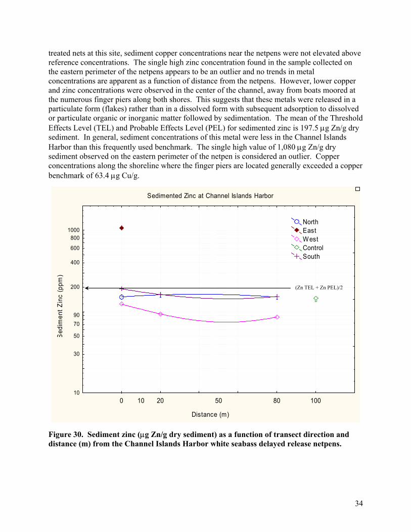
34
treated nets at this site, sediment copper concentrations near the netpens were not elevated above reference concentrations. The single high zinc concentration found in the sample collected on the eastern perimeter of the netpens appears to be an outlier and no trends in metal concentrations are apparent as a function of distance from the netpens. However, lower copper and zinc concentrations were observed in the center of the channel, away from boats moored at the numerous finger piers along both shores. This suggests that these metals were released in a particulate form (flakes) rather than in a dissolved form with subsequent adsorption to dissolved or particulate organic or inorganic matter followed by sedimentation. The mean of the Threshold Effects Level (TEL) and Probable Effects Level (PEL) for sedimented zinc is 197.5 µg Zn/g dry sediment. In general, sediment concentrations of this metal were less in the Channel Islands Harbor than this frequently used benchmark. The single high value of 1,080 µg Zn/g dry sediment observed on the eastern perimeter of the netpen is considered an outlier. Copper concentrations along the shoreline where the finger piers are located generally exceeded a copper benchmark of 63.4 µg Cu/g.
Figure 30. Sediment zinc (µg Zn/g dry sediment) as a function of transect direction and distance (m) from the Channel Islands Harbor white seabass delayed release netpens.
Sedimented Zinc at Channel Islands Harbor
Distance (m)
Sed
imen
t Zin
c (p
pm)
0 10 20 50 80 10010
30
50
7090
200
400
600
8001000
NorthEastWestControlSouth
(Zn TEL + Zn PEL)/2
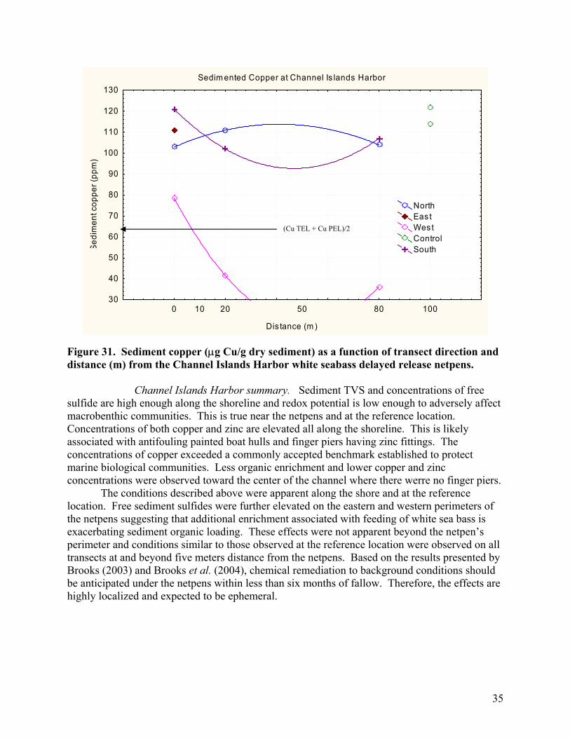
35
Figure 31. Sediment copper (µg Cu/g dry sediment) as a function of transect direction and distance (m) from the Channel Islands Harbor white seabass delayed release netpens. Channel Islands Harbor summary. Sediment TVS and concentrations of free sulfide are high enough along the shoreline and redox potential is low enough to adversely affect macrobenthic communities. This is true near the netpens and at the reference location. Concentrations of both copper and zinc are elevated all along the shoreline. This is likely associated with antifouling painted boat hulls and finger piers having zinc fittings. The concentrations of copper exceeded a commonly accepted benchmark established to protect marine biological communities. Less organic enrichment and lower copper and zinc concentrations were observed toward the center of the channel where there werre no finger piers. The conditions described above were apparent along the shore and at the reference location. Free sediment sulfides were further elevated on the eastern and western perimeters of the netpens suggesting that additional enrichment associated with feeding of white sea bass is exacerbating sediment organic loading. These effects were not apparent beyond the netpen’s perimeter and conditions similar to those observed at the reference location were observed on all transects at and beyond five meters distance from the netpens. Based on the results presented by Brooks (2003) and Brooks et al. (2004), chemical remediation to background conditions should be anticipated under the netpens within less than six months of fallow. Therefore, the effects are highly localized and expected to be ephemeral.
Sedim ented Copper at Channel Is lands Harbor
Dis tance (m )
Sedi
men
t cop
per (
ppm
)
0 10 20 50 80 10030
40
50
60
70
80
90
100
110
120
130
NorthEastWes tControlSouth
(Cu TEL + Cu PEL)/2
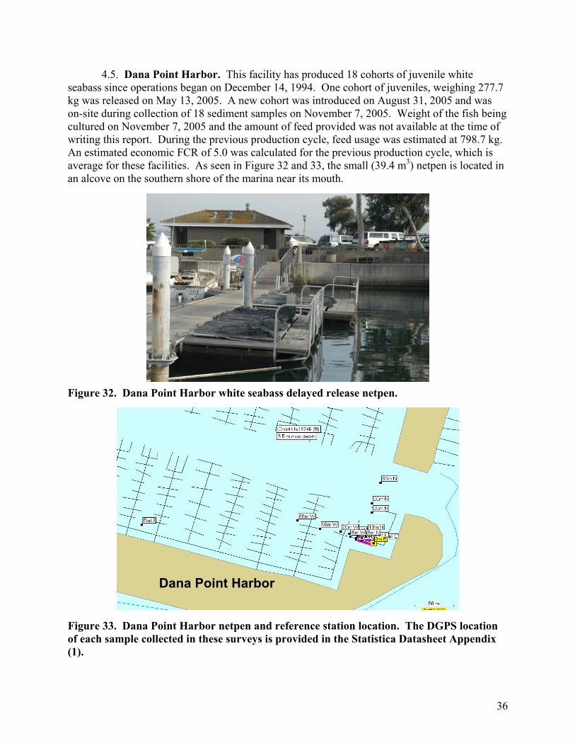
36
4.5. Dana Point Harbor. This facility has produced 18 cohorts of juvenile white seabass since operations began on December 14, 1994. One cohort of juveniles, weighing 277.7 kg was released on May 13, 2005. A new cohort was introduced on August 31, 2005 and was on-site during collection of 18 sediment samples on November 7, 2005. Weight of the fish being cultured on November 7, 2005 and the amount of feed provided was not available at the time of writing this report. During the previous production cycle, feed usage was estimated at 798.7 kg. An estimated economic FCR of 5.0 was calculated for the previous production cycle, which is average for these facilities. As seen in Figure 32 and 33, the small (39.4 m3) netpen is located in an alcove on the southern shore of the marina near its mouth.
Figure 32. Dana Point Harbor white seabass delayed release netpen.
Figure 33. Dana Point Harbor netpen and reference station location. The DGPS location of each sample collected in these surveys is provided in the Statistica Datasheet Appendix (1).
Dana Point Harbor
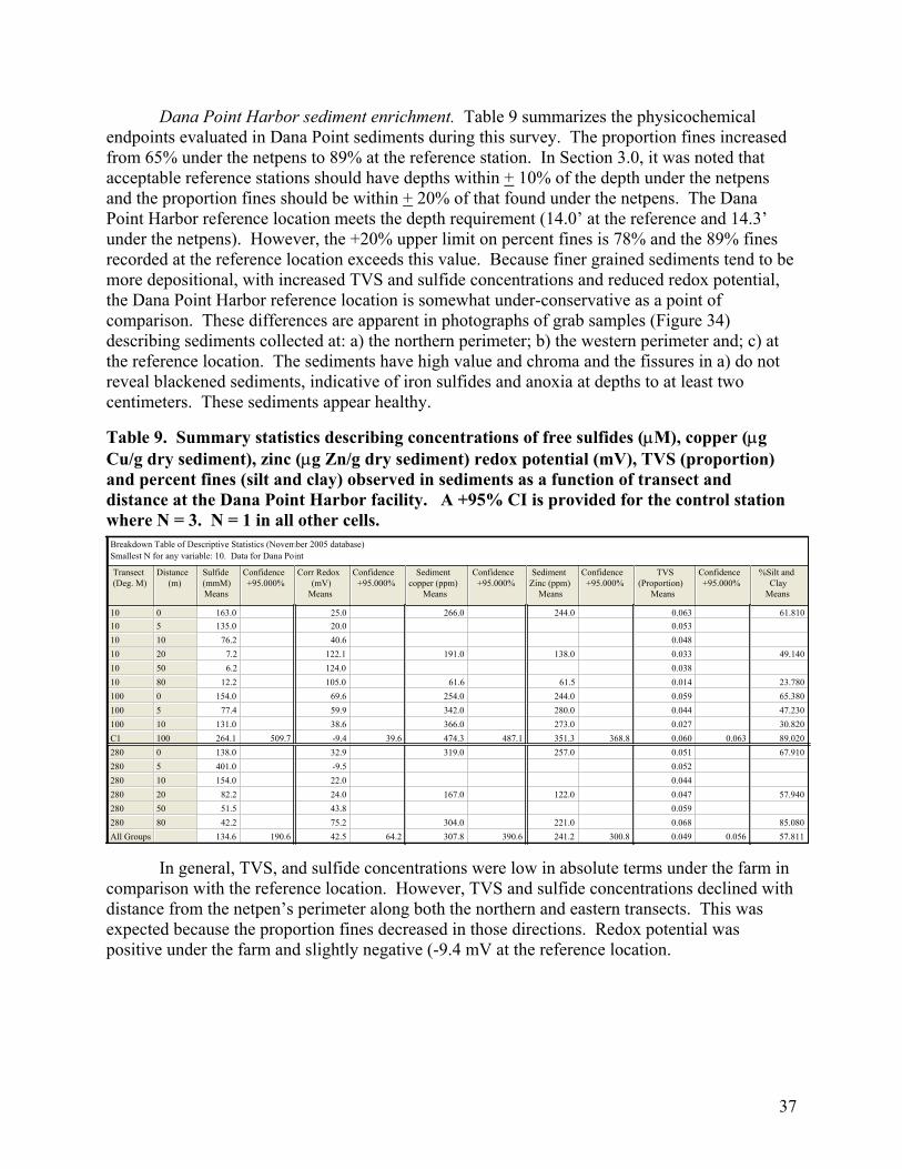
37
Dana Point Harbor sediment enrichment. Table 9 summarizes the physicochemical endpoints evaluated in Dana Point sediments during this survey. The proportion fines increased from 65% under the netpens to 89% at the reference station. In Section 3.0, it was noted that acceptable reference stations should have depths within + 10% of the depth under the netpens and the proportion fines should be within + 20% of that found under the netpens. The Dana Point Harbor reference location meets the depth requirement (14.0’ at the reference and 14.3’ under the netpens). However, the +20% upper limit on percent fines is 78% and the 89% fines recorded at the reference location exceeds this value. Because finer grained sediments tend to be more depositional, with increased TVS and sulfide concentrations and reduced redox potential, the Dana Point Harbor reference location is somewhat under-conservative as a point of comparison. These differences are apparent in photographs of grab samples (Figure 34) describing sediments collected at: a) the northern perimeter; b) the western perimeter and; c) at the reference location. The sediments have high value and chroma and the fissures in a) do not reveal blackened sediments, indicative of iron sulfides and anoxia at depths to at least two centimeters. These sediments appear healthy.
Table 9. Summary statistics describing concentrations of free sulfides (µM), copper (µg Cu/g dry sediment), zinc (µg Zn/g dry sediment) redox potential (mV), TVS (proportion) and percent fines (silt and clay) observed in sediments as a function of transect and distance at the Dana Point Harbor facility. A +95% CI is provided for the control station where N = 3. N = 1 in all other cells.
Breakdown Table of Descriptive Statistics (November 2005 database)Smallest N for any variable: 10. Data for Dana Point
Transect(Deg. M)
Distance(m)
Sulfide(mmM)Means
Confidence+95.000%
Corr Redox(mV)
Means
Confidence+95.000%
Sedimentcopper (ppm)
Means
Confidence+95.000%
SedimentZinc (ppm)
Means
Confidence+95.000%
TVS(Proportion)
Means
Confidence+95.000%
%Silt andClay
Means
10 0 163.0 25.0 266.0 244.0 0.063 61.81010 5 135.0 20.0 0.05310 10 76.2 40.6 0.04810 20 7.2 122.1 191.0 138.0 0.033 49.14010 50 6.2 124.0 0.03810 80 12.2 105.0 61.6 61.5 0.014 23.780100 0 154.0 69.6 254.0 244.0 0.059 65.380100 5 77.4 59.9 342.0 280.0 0.044 47.230100 10 131.0 38.6 366.0 273.0 0.027 30.820C1 100 264.1 509.7 -9.4 39.6 474.3 487.1 351.3 368.8 0.060 0.063 89.020280 0 138.0 32.9 319.0 257.0 0.051 67.910280 5 401.0 -9.5 0.052280 10 154.0 22.0 0.044280 20 82.2 24.0 167.0 122.0 0.047 57.940280 50 51.5 43.8 0.059280 80 42.2 75.2 304.0 221.0 0.068 85.080All Groups 134.6 190.6 42.5 64.2 307.8 390.6 241.2 300.8 0.049 0.056 57.811
In general, TVS, and sulfide concentrations were low in absolute terms under the farm in comparison with the reference location. However, TVS and sulfide concentrations declined with distance from the netpen’s perimeter along both the northern and eastern transects. This was expected because the proportion fines decreased in those directions. Redox potential was positive under the farm and slightly negative (-9.4 mV at the reference location.
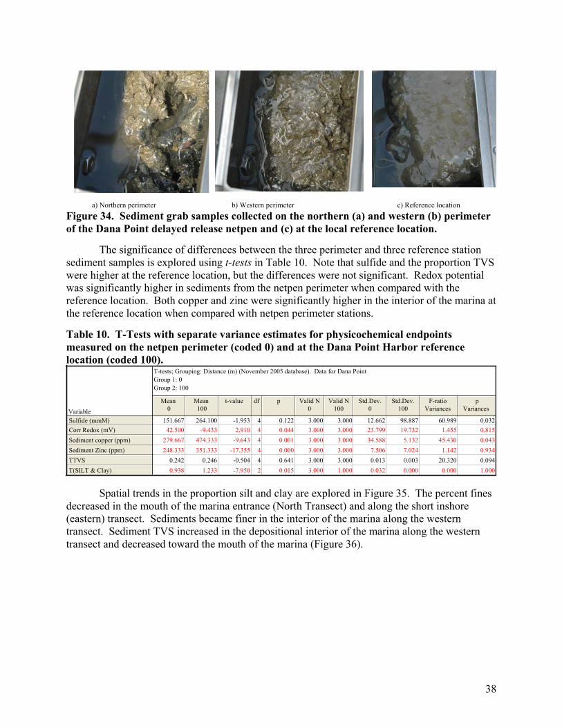
38
a) Northern perimeter b) Western perimeter c) Reference location
Figure 34. Sediment grab samples collected on the northern (a) and western (b) perimeter of the Dana Point delayed release netpen and (c) at the local reference location. The significance of differences between the three perimeter and three reference station sediment samples is explored using t-tests in Table 10. Note that sulfide and the proportion TVS were higher at the reference location, but the differences were not significant. Redox potential was significantly higher in sediments from the netpen perimeter when compared with the reference location. Both copper and zinc were significantly higher in the interior of the marina at the reference location when compared with netpen perimeter stations. Table 10. T-Tests with separate variance estimates for physicochemical endpoints measured on the netpen perimeter (coded 0) and at the Dana Point Harbor reference location (coded 100).
T-tests; Grouping: Distance (m) (November 2005 database). Data for Dana PointGroup 1: 0Group 2: 100
Variable
Mean0
Mean100
t-value df p Valid N0
Valid N100
Std.Dev.0
Std.Dev.100
F-ratioVariances
pVariances
Sulfide (mmM)Corr Redox (mV)Sediment copper (ppm)Sediment Zinc (ppm)TTVST(SILT & Clay)
151.667 264.100 -1.953 4 0.122 3.000 3.000 12.662 98.887 60.989 0.03242.500 -9.433 2.910 4 0.044 3.000 3.000 23.799 19.732 1.455 0.815
279.667 474.333 -9.643 4 0.001 3.000 3.000 34.588 5.132 45.430 0.043248.333 351.333 -17.355 4 0.000 3.000 3.000 7.506 7.024 1.142 0.934
0.242 0.246 -0.504 4 0.641 3.000 3.000 0.013 0.003 20.320 0.0940.938 1.233 -7.950 2 0.015 3.000 1.000 0.032 0.000 0.000 1.000
Spatial trends in the proportion silt and clay are explored in Figure 35. The percent fines decreased in the mouth of the marina entrance (North Transect) and along the short inshore (eastern) transect. Sediments became finer in the interior of the marina along the western transect. Sediment TVS increased in the depositional interior of the marina along the western transect and decreased toward the mouth of the marina (Figure 36).
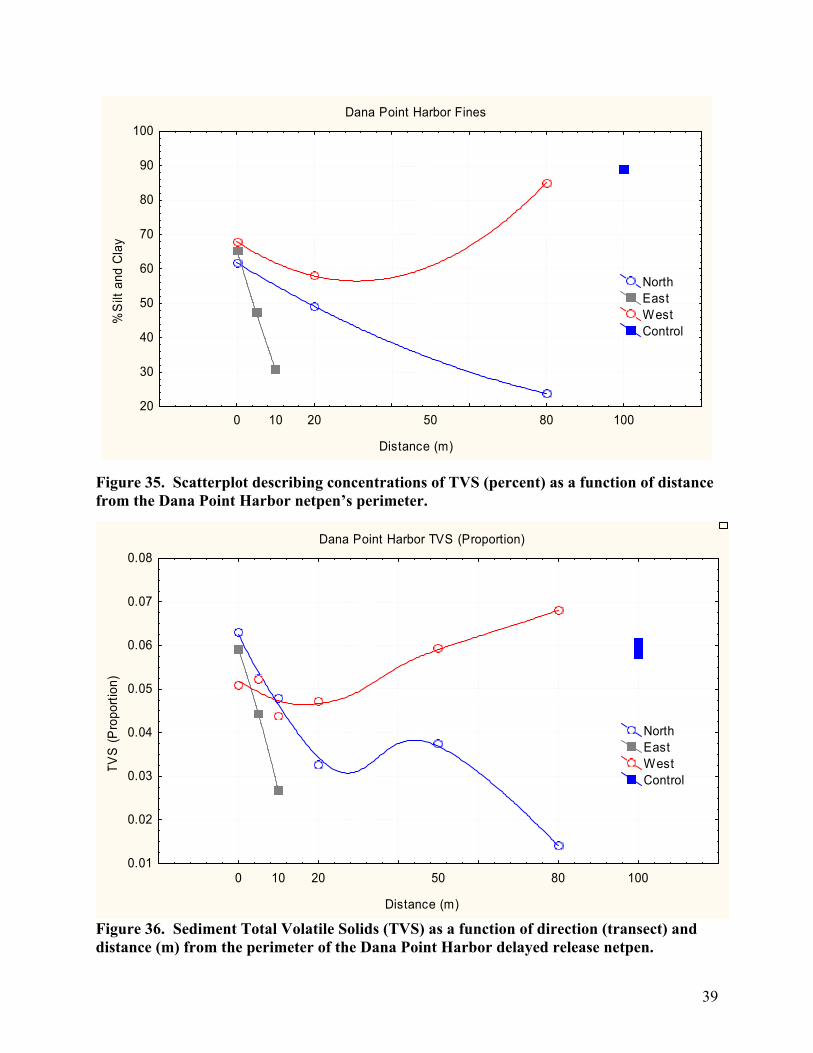
39
Dana Point Harbor Fines
Distance (m)
%S
ilt a
nd C
lay
0 10 20 50 80 10020
30
40
50
60
70
80
90
100
NorthEastWestControl
Figure 35. Scatterplot describing concentrations of TVS (percent) as a function of distance from the Dana Point Harbor netpen’s perimeter.
Dana Point Harbor TVS (Proportion)
Distance (m)
TVS
(Pro
porti
on)
0 10 20 50 80 1000.01
0.02
0.03
0.04
0.05
0.06
0.07
0.08
NorthEastWestControl
Figure 36. Sediment Total Volatile Solids (TVS) as a function of direction (transect) and distance (m) from the perimeter of the Dana Point Harbor delayed release netpen.
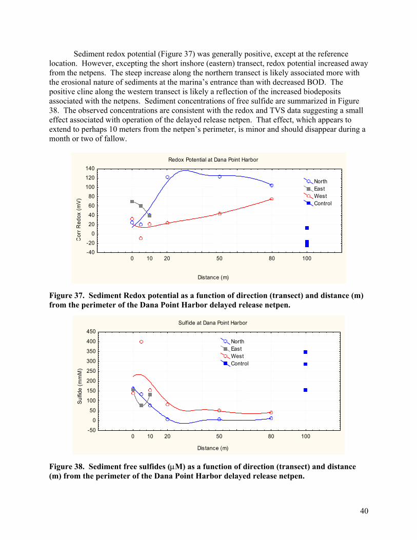
40
Sediment redox potential (Figure 37) was generally positive, except at the reference location. However, excepting the short inshore (eastern) transect, redox potential increased away from the netpens. The steep increase along the northern transect is likely associated more with the erosional nature of sediments at the marina’s entrance than with decreased BOD. The positive cline along the western transect is likely a reflection of the increased biodeposits associated with the netpens. Sediment concentrations of free sulfide are summarized in Figure 38. The observed concentrations are consistent with the redox and TVS data suggesting a small effect associated with operation of the delayed release netpen. That effect, which appears to extend to perhaps 10 meters from the netpen’s perimeter, is minor and should disappear during a month or two of fallow.
Redox Potential at Dana Point Harbor
Distance (m)
Cor
r Red
ox (m
V)
0 10 20 50 80 100-40-20
020406080
100120140
NorthEastWestControl
Figure 37. Sediment Redox potential as a function of direction (transect) and distance (m) from the perimeter of the Dana Point Harbor delayed release netpen.
Sulf ide at Dana Point Harbor
Distance (m)
Sulfid
e (m
mM
)
0 10 20 50 80 100-50
0
50
100
150
200
250
300
350
400
450
NorthEastWestControl
Figure 38. Sediment free sulfides (µM) as a function of direction (transect) and distance (m) from the perimeter of the Dana Point Harbor delayed release netpen.
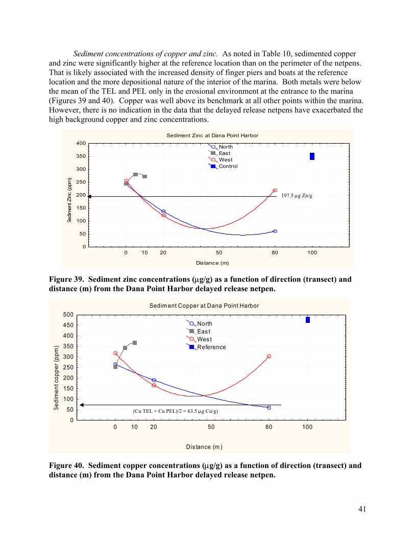
41
Sediment concentrations of copper and zinc. As noted in Table 10, sedimented copper and zinc were significantly higher at the reference location than on the perimeter of the netpens. That is likely associated with the increased density of finger piers and boats at the reference location and the more depositional nature of the interior of the marina. Both metals were below the mean of the TEL and PEL only in the erosional environment at the entrance to the marina (Figures 39 and 40). Copper was well above its benchmark at all other points within the marina. However, there is no indication in the data that the delayed release netpens have exacerbated the high background copper and zinc concentrations.
Figure 39. Sediment zinc concentrations (µg/g) as a function of direction (transect) and distance (m) from the Dana Point Harbor delayed release netpen.
Figure 40. Sediment copper concentrations (µg/g) as a function of direction (transect) and distance (m) from the Dana Point Harbor delayed release netpen.
Sediment Zinc at Dana Point Harbor
Distance (m)
Sedi
men
t Zin
c (p
pm)
0 10 20 50 80 1000
50
100
150
200
250
300
350
400NorthEastWestControl
197.5 µg Zn/g
Sedim ent Copper at Dana Point Harbor
Dis tance (m )
Sedi
men
t cop
per (
ppm
)
0 10 20 50 80 1000
50
100
150
200
250
300
350
400
450
500NorthEas tWes tReference
(Cu TEL + Cu PEL)/2 = 63.5 µg Cu/g)
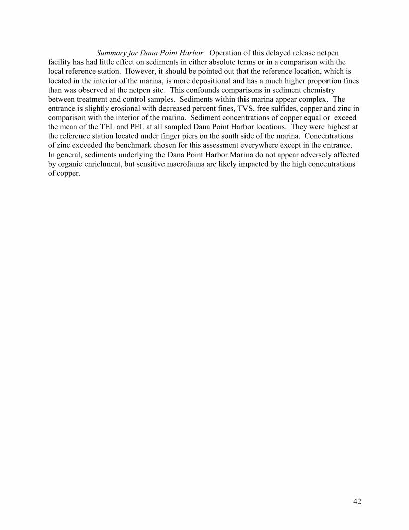
42
Summary for Dana Point Harbor. Operation of this delayed release netpen facility has had little effect on sediments in either absolute terms or in a comparison with the local reference station. However, it should be pointed out that the reference location, which is located in the interior of the marina, is more depositional and has a much higher proportion fines than was observed at the netpen site. This confounds comparisons in sediment chemistry between treatment and control samples. Sediments within this marina appear complex. The entrance is slightly erosional with decreased percent fines, TVS, free sulfides, copper and zinc in comparison with the interior of the marina. Sediment concentrations of copper equal or exceed the mean of the TEL and PEL at all sampled Dana Point Harbor locations. They were highest at the reference station located under finger piers on the south side of the marina. Concentrations of zinc exceeded the benchmark chosen for this assessment everywhere except in the entrance. In general, sediments underlying the Dana Point Harbor Marina do not appear adversely affected by organic enrichment, but sensitive macrofauna are likely impacted by the high concentrations of copper.

43
4.6. Mission Bay (Quivera Basin) delayed release netpen site. This facility began feeding juvenile white seabass on April 29, 1997. Fifteen cohorts of bass have been produced in the last five years. The latest completed production cycle began on May 23, 2005, when 242.4 kg of juveniles were introduced. They were fed an estimated 882 kg of pelleted feed and released on September 13, 2005 when the total biomass was 382.2 kg. The economic FCR was 6.0, which was high average for these facilities. Figure 42 provides a site diagram showing the location of the 36.2 m3 copper treated netpen in the midst of finger piers within the marina. Water depths at the site varied between 7.0 and 8.5 m (23’ to 28’). Water depth at the reference location on the northeast side of the marina varied between 6.7 and 7.0 m (22’ to 23’), which is within + 10% of the mean depth under the netpens (7.8 m = 25.5’). The proportion fines at the reference station was 62.75%, which was within + 20% of the proportion observed under the farm (57.7 + 9.3) and the reference stations meets both criteria.
Figure 42. Mission Bay (Quivera Basin) netpen and reference station location. The DGPS location of each sample collected in these surveys is provided in the Statistica Database (Appendix 4). Organic enrichment at the Mission Bay (Quivera Basin) netpen. Sediment characteristics are summarized in Table 11. Sediments are moderately fine everywhere except in the center of the basin (North or 330 oM - 80 m station) where they were reduced to 28.8 percent (Figure 44). Sediments throughout the marina were highly enriched with high TVS and sulfide and zero to slightly negative redox potentials. Sediment TVS was further elevated under the footprint of the netpen. Note in Figure 43 that sediments on the perimeter of the netpens and at the reference location had low chroma indicative of anaerobic conditions. The BOD associated with this added organic matter has resulted in slightly higher sulfide concentrations and lower redox potential. However, it should be emphasized that the assimilative capacity of the sediments has also been exceeded at the reference station located approximately 260 m from the netpens. Table 11 summarizes the results of two tailed t-tests with separate variance estimates comparing conditions at the reference location (N = 3) with those observed under the four perimeter stations
SDOF – MBay
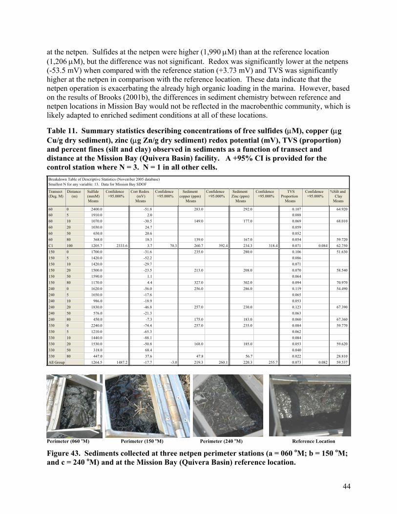
44
at the netpen. Sulfides at the netpen were higher (1,990 µM) than at the reference location (1,206 µM), but the difference was not significant. Redox was significantly lower at the netpens (-53.5 mV) when compared with the reference station (+3.73 mV) and TVS was significantly higher at the netpen in comparison with the reference location. These data indicate that the netpen operation is exacerbating the already high organic loading in the marina. However, based on the results of Brooks (2001b), the differences in sediment chemistry between reference and netpen locations in Mission Bay would not be reflected in the macrobenthic community, which is likely adapted to enriched sediment conditions at all of these locations.
Table 11. Summary statistics describing concentrations of free sulfides (µM), copper (µg Cu/g dry sediment), zinc (µg Zn/g dry sediment) redox potential (mV), TVS (proportion) and percent fines (silt and clay) observed in sediments as a function of transect and distance at the Mission Bay (Quivera Basin) facility. A +95% CI is provided for the control station where N = 3. N = 1 in all other cells. Breakdown Table of Descriptive Statistics (November 2005 database)Smallest N for any variable: 13. Data for Mission Bay SDOF
Transect(Deg. M)
Distance(m)
Sulfide(mmM)Means
Confidence+95.000%
Corr Redox(mV)
Means
Confidence+95.000%
Sedimentcopper (ppm)
Means
Confidence+95.000%
SedimentZinc (ppm)
Means
Confidence+95.000%
TVSProportion
Means
Confidence+95.000%
%Silt andClay
Means
60 0 2400.0 -51.8 283.0 292.0 0.107 64.92060 5 1910.0 2.0 0.08860 10 1070.0 -30.5 149.0 177.0 0.069 68.01060 20 1030.0 24.7 0.05960 50 650.0 20.6 0.05260 80 368.0 18.3 139.0 167.0 0.054 59.720C1 100 1205.7 2333.6 3.7 70.3 260.7 392.4 234.3 318.4 0.071 0.084 62.750150 0 1700.0 -31.6 235.0 280.0 0.106 51.630150 5 1420.0 -52.2 0.086150 10 1420.0 -29.7 0.071150 20 1500.0 -23.5 213.0 208.0 0.070 58.540150 50 1590.0 1.1 0.064150 80 1170.0 4.4 327.0 302.0 0.094 70.970240 0 1620.0 -56.0 256.0 286.0 0.119 54.490240 5 1650.0 -17.6 0.065240 10 986.0 -18.9 0.053240 20 1830.0 -46.8 257.0 230.0 0.123 67.390240 50 576.0 -21.3 0.063240 80 450.0 -7.3 175.0 183.0 0.060 67.360330 0 2240.0 -74.4 257.0 235.0 0.084 59.770330 5 1210.0 -65.3 0.062330 10 1440.0 -88.1 0.084330 20 1530.0 -50.8 168.0 185.0 0.053 59.620330 50 318.0 68.4 0.040330 80 447.0 37.6 47.8 56.7 0.022 28.810All Group 1264.5 1487.2 -17.7 -3.0 219.3 260.1 220.3 255.7 0.073 0.082 59.537
Perimeter (060 oM) Perimeter (150 oM) Perimeter (240 oM) Reference Location
Figure 43. Sediments collected at three netpen perimeter stations (a = 060 oM; b = 150 oM; and c = 240 oM) and at the Mission Bay (Quivera Basin) reference location.
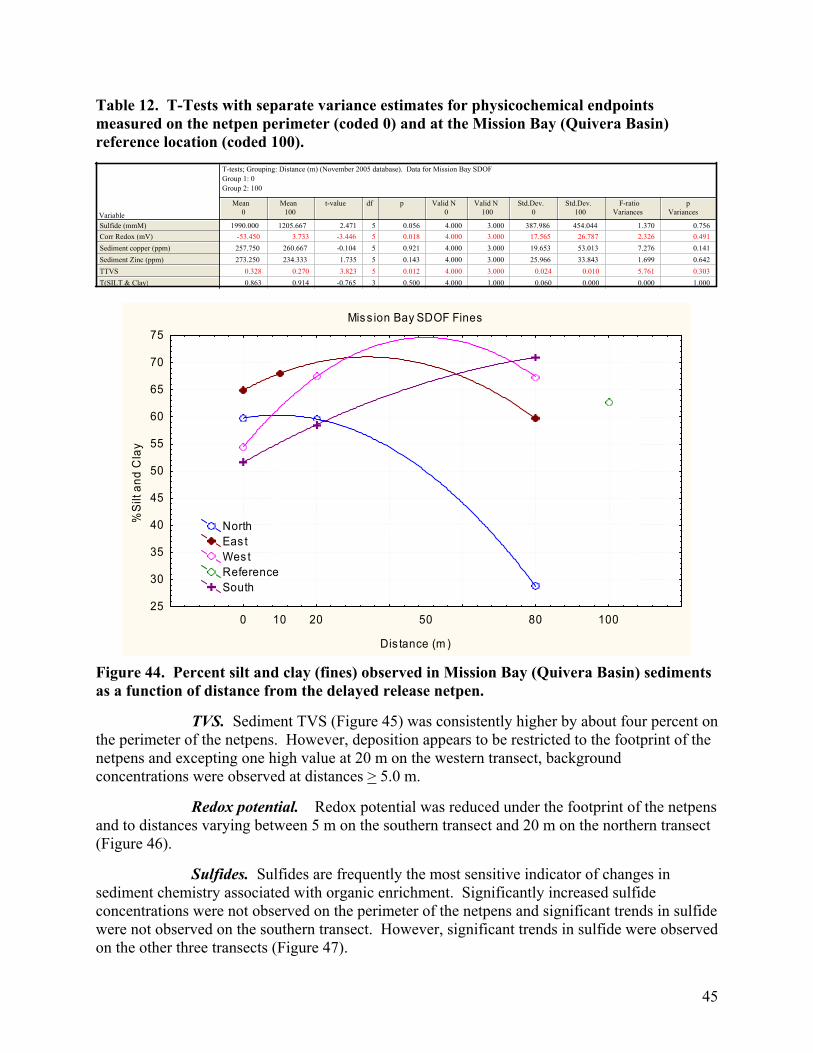
45
Table 12. T-Tests with separate variance estimates for physicochemical endpoints measured on the netpen perimeter (coded 0) and at the Mission Bay (Quivera Basin) reference location (coded 100).
T-tests; Grouping: Distance (m) (November 2005 database). Data for Mission Bay SDOFGroup 1: 0Group 2: 100
VariableMean
0Mean
100t-value df p Valid N
0Valid N
100Std.Dev.
0Std.Dev.
100F-ratio
Variancesp
Variances
Sulfide (mmM)Corr Redox (mV)Sediment copper (ppm)Sediment Zinc (ppm)TTVST(SILT & Clay)
1990.000 1205.667 2.471 5 0.056 4.000 3.000 387.986 454.044 1.370 0.756-53.450 3.733 -3.446 5 0.018 4.000 3.000 17.565 26.787 2.326 0.491257.750 260.667 -0.104 5 0.921 4.000 3.000 19.653 53.013 7.276 0.141273.250 234.333 1.735 5 0.143 4.000 3.000 25.966 33.843 1.699 0.642
0.328 0.270 3.823 5 0.012 4.000 3.000 0.024 0.010 5.761 0.3030.863 0.914 -0.765 3 0.500 4.000 1.000 0.060 0.000 0.000 1.000
Miss ion Bay SDOF Fines
Dis tance (m )
%S
ilt a
nd C
lay
0 10 20 50 80 10025
30
35
40
45
50
55
60
65
70
75
NorthEas tWes tReferenceSouth
Figure 44. Percent silt and clay (fines) observed in Mission Bay (Quivera Basin) sediments as a function of distance from the delayed release netpen. TVS. Sediment TVS (Figure 45) was consistently higher by about four percent on the perimeter of the netpens. However, deposition appears to be restricted to the footprint of the netpens and excepting one high value at 20 m on the western transect, background concentrations were observed at distances > 5.0 m. Redox potential. Redox potential was reduced under the footprint of the netpens and to distances varying between 5 m on the southern transect and 20 m on the northern transect (Figure 46). Sulfides. Sulfides are frequently the most sensitive indicator of changes in sediment chemistry associated with organic enrichment. Significantly increased sulfide concentrations were not observed on the perimeter of the netpens and significant trends in sulfide were not observed on the southern transect. However, significant trends in sulfide were observed on the other three transects (Figure 47).
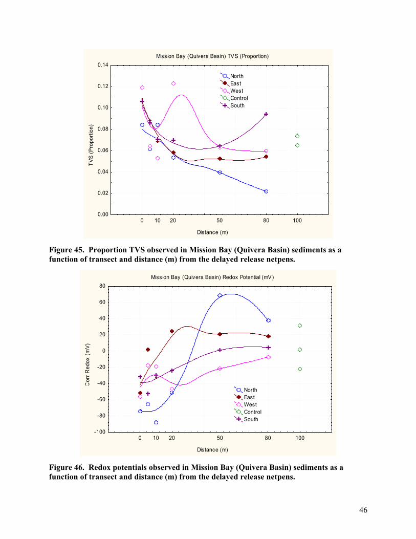
46
Mission Bay (Quivera Basin) TVS (Proportion)
Distance (m)
TVS
(Pro
porti
on)
0 10 20 50 80 1000.00
0.02
0.04
0.06
0.08
0.10
0.12
0.14
NorthEastWestControlSouth
Figure 45. Proportion TVS observed in Mission Bay (Quivera Basin) sediments as a function of transect and distance (m) from the delayed release netpens.
Mission Bay (Quivera Basin) Redox Potential (mV)
Distance (m)
Cor
r Red
ox (m
V)
0 10 20 50 80 100-100
-80
-60
-40
-20
0
20
40
60
80
NorthEastWestControlSouth
Figure 46. Redox potentials observed in Mission Bay (Quivera Basin) sediments as a function of transect and distance (m) from the delayed release netpens.
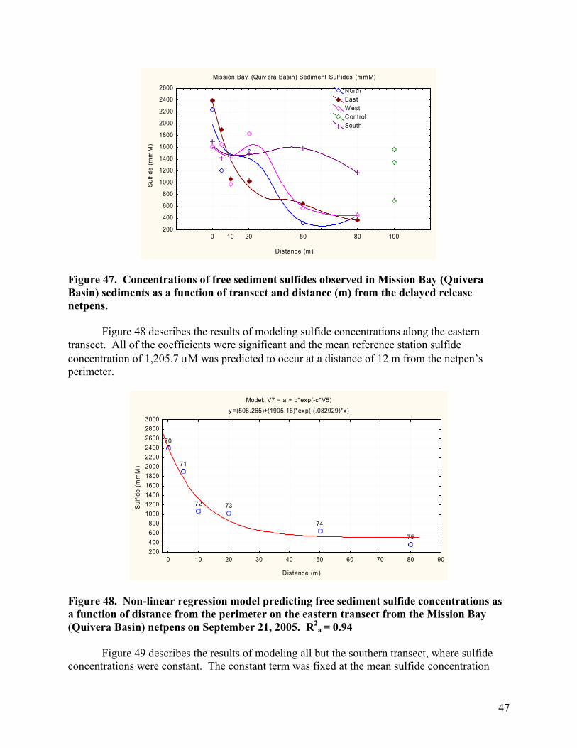
47
Mission Bay (Quiv era Basin) Sediment Sulf ides (mmM)
Distance (m)
Sul
fide
(mm
M)
0 10 20 50 80 100200
400
600
800
1000
1200
1400
1600
1800
2000
2200
2400
2600 NorthEastWestControlSouth
Figure 47. Concentrations of free sediment sulfides observed in Mission Bay (Quivera Basin) sediments as a function of transect and distance (m) from the delayed release netpens. Figure 48 describes the results of modeling sulfide concentrations along the eastern transect. All of the coefficients were significant and the mean reference station sulfide concentration of 1,205.7 µM was predicted to occur at a distance of 12 m from the netpen’s perimeter.
Model: V7 = a + b*exp(-c*V5)
y =(506.265)+(1905.16)*exp(-(.082929)*x)
70
71
72 73
74
75
0 10 20 30 40 50 60 70 80 90
Distance (m)
200400600800
10001200140016001800200022002400260028003000
Sul
fide
(mm
M)
Figure 48. Non-linear regression model predicting free sediment sulfide concentrations as a function of distance from the perimeter on the eastern transect from the Mission Bay (Quivera Basin) netpens on September 21, 2005. R2
a = 0.94 Figure 49 describes the results of modeling all but the southern transect, where sulfide concentrations were constant. The constant term was fixed at the mean sulfide concentration

48
observed at the three 80 m stations and the higher reference station concentrations were excluded from the database. Therefore, this is a more localized model appropriate to the area within 80 m of the netpens. Both coefficients were significant and the model explained 75% of the variation in the dataset. In a more general sense, this model predicts reference concentrations of free sediment at a distance of 16.7 m from the netpens. This analysis suggests that free sulfide concentrations are elevated under the Mission Bay netpens and to a distance of between 12 and 17 m to the north, east and west of the facility. Free sediment sulfides were constant along the southern transect (the coefficient on distance was not significant at α = 0.05).
Mission Bay (Quivera Basin)y=422+(1542.79)*exp(-(.040647)*x)
64
65
6667
6869
70
71
72 73
74
75
82 83
84
85
8687
0 10 20 30 40 50 60 70 80 90
Distance (m)
200
400
600
800
1000
1200
1400
1600
1800
2000
2200
2400
2600
Sulfid
e (m
mM
)
Model is: V7 = 422 + b*exp(-c*V5) (November 2005 database)Dep. Var. : Sulfide (mmM)Level of confidence: 95.0% ( alpha=0.050)Estimate Standard
errort-valuedf = 16
p-level Lo. ConfLimit
Up. ConfLimit
bc
1542.795 160.4453 9.615705 0.000000 1202.666 1882.9230.041 0.0114 3.553073 0.002649 0.016 0.065
Figure 49. Non-linear regression model predicting free sediment sulfide concentrations as a function of distance from the perimeter on the northern, eastern and western transects from the Mission Bay (Quivera Basin) netpens on September 21, 2005. R2
a = 0.75
Sediment copper and zinc. Despite the use of copper treated nets at this site, concentrations of zinc (Figure 50) and copper (Figure 51) were not significantly different between reference and perimeter stations (Table 12). However, both metals were near or above the mean of their respective TEL and PEL at all stations other than in coarser sediments located away from the finger piers and near the center of the open marina. The concentrations of both metals were at levels that would be inimical to many macrobenthic organisms in the absence of free sulfides, which Di Toro et al. (1992) have reported bind both metals. Those authors reported no toxicity when the molar ratio of acid volatile sulfides to copper or zinc were greater

49
than one. These ratios were not computed for this report because there is no evidence of significant increases under the netpens in comparison with reference conditions in Mission Bay. However, the elevated concentrations of sulfide suggest that organic enrichment was likely having a much greater effect on the macrobenthic community and that the same enrichment was significantly mediating the effect of the elevated copper and zinc.
Mission Bay (Quiv era Basin) Sediment Zinc (ppm)
Distance (m)
Sedi
men
t Zin
c (p
pm)
0 10 20 50 80 100406080
100120140160180200220240260280300320
NorthEastWestControlSouth
Figure 50. Sediment copper (µg/g dry) as a function of direction (transect) and distance (m) from the Mission Bay (Quivera Basin) delayed release netpen.
Mission Bay (Quivera Basin) Sediment Copper (ppm)
Distance (m)
Sed
imen
t cop
per (
ppm
)
0 10 20 50 80 1000
50
100
150
200
250
300
350
NorthEastWestControlSouth
Figure 51. Sediment copper (µg/g dry) as a function of direction (transect) and distance (m) from the Mission Bay (Quivera Basin) delayed release netpen. Mission Bay (Quivera Basin) summary. The assimilative capacity of sediments in all surveyed areas of Mission Bay were exceeded leading to reduced sediment oxygen and elevated concentrations of sulfide. The mean sulfide concentration at stations located > 20 m from the netpens was 1,005 + 293 µM (N = 15), which would be sufficient to exclude half of the taxa
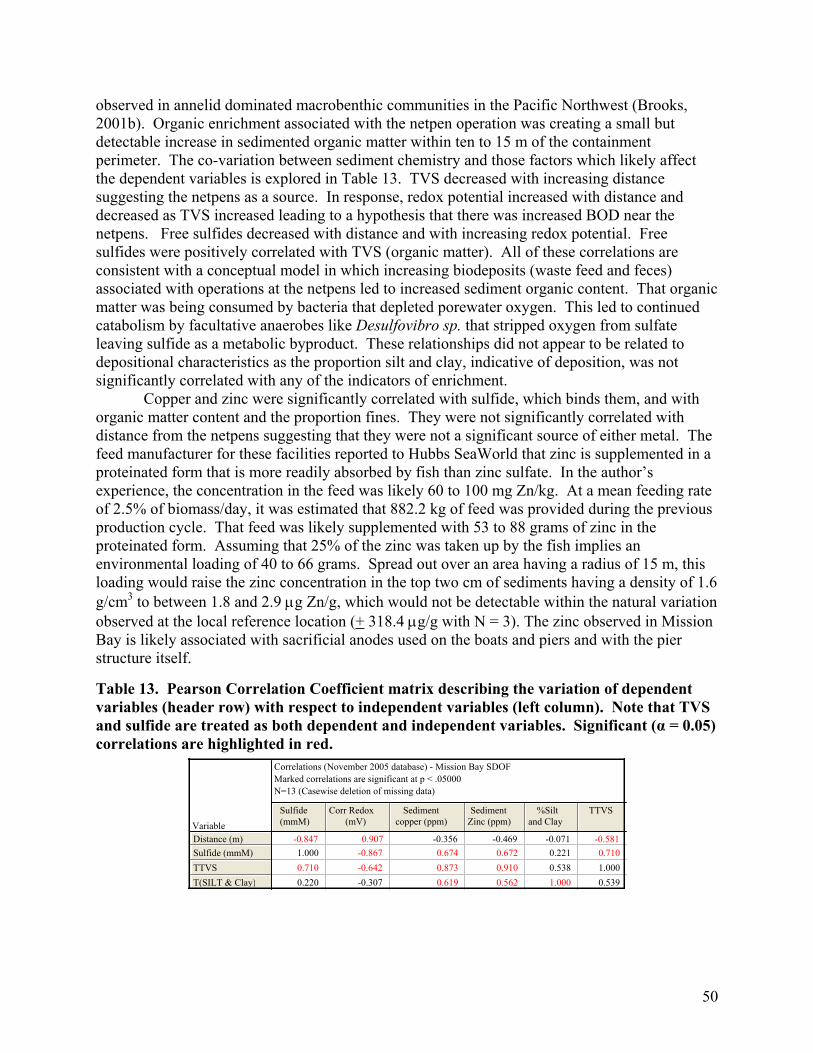
50
observed in annelid dominated macrobenthic communities in the Pacific Northwest (Brooks, 2001b). Organic enrichment associated with the netpen operation was creating a small but detectable increase in sedimented organic matter within ten to 15 m of the containment perimeter. The co-variation between sediment chemistry and those factors which likely affect the dependent variables is explored in Table 13. TVS decreased with increasing distance suggesting the netpens as a source. In response, redox potential increased with distance and decreased as TVS increased leading to a hypothesis that there was increased BOD near the netpens. Free sulfides decreased with distance and with increasing redox potential. Free sulfides were positively correlated with TVS (organic matter). All of these correlations are consistent with a conceptual model in which increasing biodeposits (waste feed and feces) associated with operations at the netpens led to increased sediment organic content. That organic matter was being consumed by bacteria that depleted porewater oxygen. This led to continued catabolism by facultative anaerobes like Desulfovibro sp. that stripped oxygen from sulfate leaving sulfide as a metabolic byproduct. These relationships did not appear to be related to depositional characteristics as the proportion silt and clay, indicative of deposition, was not significantly correlated with any of the indicators of enrichment. Copper and zinc were significantly correlated with sulfide, which binds them, and with organic matter content and the proportion fines. They were not significantly correlated with distance from the netpens suggesting that they were not a significant source of either metal. The feed manufacturer for these facilities reported to Hubbs SeaWorld that zinc is supplemented in a proteinated form that is more readily absorbed by fish than zinc sulfate. In the author’s experience, the concentration in the feed was likely 60 to 100 mg Zn/kg. At a mean feeding rate of 2.5% of biomass/day, it was estimated that 882.2 kg of feed was provided during the previous production cycle. That feed was likely supplemented with 53 to 88 grams of zinc in the proteinated form. Assuming that 25% of the zinc was taken up by the fish implies an environmental loading of 40 to 66 grams. Spread out over an area having a radius of 15 m, this loading would raise the zinc concentration in the top two cm of sediments having a density of 1.6 g/cm3 to between 1.8 and 2.9 µg Zn/g, which would not be detectable within the natural variation observed at the local reference location (+ 318.4 µg/g with N = 3). The zinc observed in Mission Bay is likely associated with sacrificial anodes used on the boats and piers and with the pier structure itself.
Table 13. Pearson Correlation Coefficient matrix describing the variation of dependent variables (header row) with respect to independent variables (left column). Note that TVS and sulfide are treated as both dependent and independent variables. Significant (α = 0.05) correlations are highlighted in red.
Correlations (November 2005 database) - Mission Bay SDOFMarked correlations are significant at p < .05000N=13 (Casewise deletion of missing data)
VariableSulfide(mmM)
Corr Redox(mV)
Sedimentcopper (ppm)
SedimentZinc (ppm)
%Siltand Clay
TTVS
Distance (m)Sulfide (mmM)TTVST(SILT & Clay)
-0.847 0.907 -0.356 -0.469 -0.071 -0.5811.000 -0.867 0.674 0.672 0.221 0.7100.710 -0.642 0.873 0.910 0.538 1.0000.220 -0.307 0.619 0.562 1.000 0.539

51
4.7. San Diego SW Yacht Club (SWYC) raceway delayed release site. This delayed release raceway is located along the shoreline in a dense cluster of finger piers used to moor pleasure craft. The facility began operations on August 6, 1996 and has supported the growout of 16 cohorts of juvenile white seabass. The last complete production cycle began on December 3, 2004 with the introduction of 67.4 kg of juvenile fish that were fed an estimated 625 kg of pelleted feed over a period of 173 days and released on May 25, 2005 when they weighed 221.8 kg. The computed economic FCR was 4, which is among the lowest for the facilities included in this survey. The reference station chosen for this site is located across the basin in a similar arRey of finger piers (Figure 52). Measured depths under the netpen perimeter ranged from 10 to 11 feet. Depth was not recorded at the reference location, but it appears to be located in similarly shallow water. The proportion fines under the netpen’s perimeter varied between 21.0% and 24.6%. The proportion fines at the reference station was 64.0%, which exceeds the guidelines for selecting reference locations (+ 20%). This reference station is relatively depositional whereas the netpen is located in a fairly erosional environment. The differences will confound comparisons between the two and a new reference location with a similar proportion fines should be identified the next time this site is monitored.
Figure 52. San Diego (SWYC) raceway and reference station location. The DGPS location of each sample collected in these surveys is provided in the Statistica Datasheet Appendix (2). Inset photo describes the 14.3 m3 delayed release raceway facility. San Diego (SWYC) sediment physicochemistry. Sediment characteristics are summarized in Table 14. Sediments at all stations along the northwestern shore were dominated by sand suggesting reasonably fast currents at this location (Appendix 2). The proportion silt and clay increased linearly to the south (Figure 54) indicating a more depositional environment. Sediment
San Diego SW Yacht Club
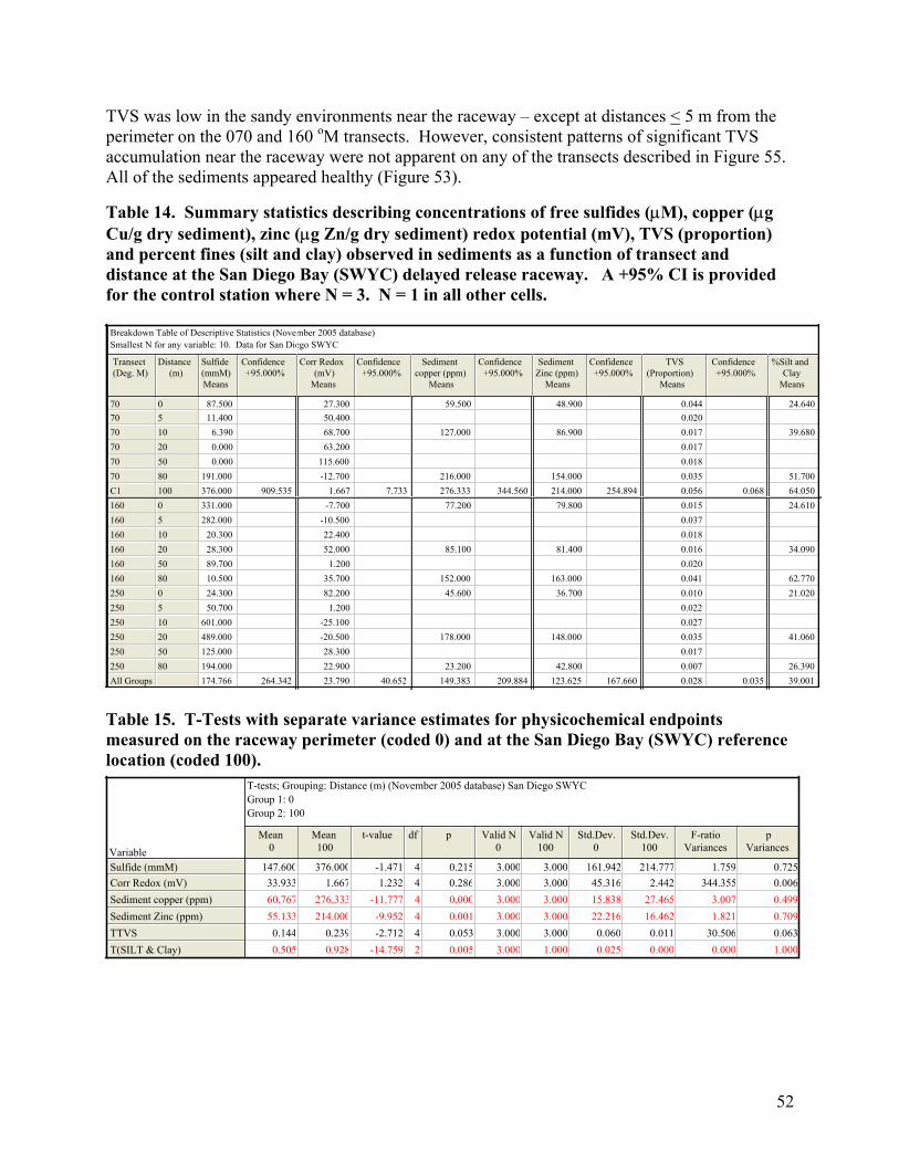
52
TVS was low in the sandy environments near the raceway – except at distances < 5 m from the perimeter on the 070 and 160 oM transects. However, consistent patterns of significant TVS accumulation near the raceway were not apparent on any of the transects described in Figure 55. All of the sediments appeared healthy (Figure 53).
Table 14. Summary statistics describing concentrations of free sulfides (µM), copper (µg Cu/g dry sediment), zinc (µg Zn/g dry sediment) redox potential (mV), TVS (proportion) and percent fines (silt and clay) observed in sediments as a function of transect and distance at the San Diego Bay (SWYC) delayed release raceway. A +95% CI is provided for the control station where N = 3. N = 1 in all other cells.
Breakdown Table of Descriptive Statistics (November 2005 database)Smallest N for any variable: 10. Data for San Diego SWYC
Transect(Deg. M)
Distance(m)
Sulfide(mmM)Means
Confidence+95.000%
Corr Redox(mV)
Means
Confidence+95.000%
Sedimentcopper (ppm)
Means
Confidence+95.000%
SedimentZinc (ppm)
Means
Confidence+95.000%
TVS(Proportion)
Means
Confidence+95.000%
%Silt andClay
Means
70 0 87.500 27.300 59.500 48.900 0.044 24.64070 5 11.400 50.400 0.02070 10 6.390 68.700 127.000 86.900 0.017 39.68070 20 0.000 63.200 0.01770 50 0.000 115.600 0.01870 80 191.000 -12.700 216.000 154.000 0.035 51.700C1 100 376.000 909.535 1.667 7.733 276.333 344.560 214.000 254.894 0.056 0.068 64.050160 0 331.000 -7.700 77.200 79.800 0.015 24.610160 5 282.000 -10.500 0.037160 10 20.300 22.400 0.018160 20 28.300 52.000 85.100 81.400 0.016 34.090160 50 89.700 1.200 0.020160 80 10.500 35.700 152.000 163.000 0.041 62.770250 0 24.300 82.200 45.600 36.700 0.010 21.020250 5 50.700 1.200 0.022250 10 601.000 -25.100 0.027250 20 489.000 -20.500 178.000 148.000 0.035 41.060250 50 125.000 28.300 0.017250 80 194.000 22.900 23.200 42.800 0.007 26.390All Groups 174.766 264.342 23.790 40.652 149.383 209.884 123.625 167.660 0.028 0.035 39.001
Table 15. T-Tests with separate variance estimates for physicochemical endpoints measured on the raceway perimeter (coded 0) and at the San Diego Bay (SWYC) reference location (coded 100).
T-tests; Grouping: Distance (m) (November 2005 database) San Diego SWYCGroup 1: 0Group 2: 100
VariableMean
0Mean100
t-value df p Valid N0
Valid N100
Std.Dev.0
Std.Dev.100
F-ratioVariances
pVariances
Sulfide (mmM)Corr Redox (mV)Sediment copper (ppm)Sediment Zinc (ppm)TTVST(SILT & Clay)
147.600 376.000 -1.471 4 0.215 3.000 3.000 161.942 214.777 1.759 0.72533.933 1.667 1.232 4 0.286 3.000 3.000 45.316 2.442 344.355 0.00660.767 276.333 -11.777 4 0.000 3.000 3.000 15.838 27.465 3.007 0.49955.133 214.000 -9.952 4 0.001 3.000 3.000 22.216 16.462 1.821 0.7090.144 0.239 -2.712 4 0.053 3.000 3.000 0.060 0.011 30.506 0.0630.505 0.928 -14.759 2 0.005 3.000 1.000 0.025 0.000 0.000 1.000

53
a) Perimeter (070 oM) b) Perimeter (250 oM) c) Reference location Figure 53. Grab samples collected at the San Diego Bay (SWYC) white seabass delayed release netpen on a) the eastern perimeter; b) the western perimeter; and c) at the reference station.
San Diego Bay (SWYC) Fines
Dis tance (m )
%S
ilt a
nd C
lay
0 10 20 50 80 10015
20
25
30
35
40
45
50
55
60
65
70
EastWestControlSouth
Figure 54. Proportion silt and clay as a function of direction (transect) and distance (m) from the San Diego Bay (SWYC) delayed release raceway.
Redox potentials at the San Diego Bay (SWYC) raceway (Figure 56). Redox potentials were lower on the eastern and southern perimeters of the raceway and they increased with increasing distance – suggesting higher BOD near the facility. Redox potential was highest on the perimeter of the western transect and it declined with distance to 20 m. However, all of the values were reasonably high and most were positive suggesting no significant adverse effect on the macrobenthos. Sulfide concentrations under and near the San Diego Bay (SWYC) raceway. Sulfide concentrations on the perimeter of the netpens were generally within a range observed at Pacific Northwest reference locations and redox potentials were generally near zero to positive (Figure 57). Sulfides were moderately elevated at the reference location and at 10 and 20 m on the western transect.
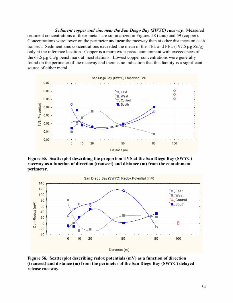
54
Sediment copper and zinc near the San Diego Bay (SWYC) raceway. Measured sediment concentrations of these metals are summarized in Figures 58 (zinc) and 59 (copper). Concentrations were lower on the perimeter and near the raceway than at other distances on each transect. Sediment zinc concentrations exceeded the mean of the TEL and PEL (197.5 µg Zn/g) only at the reference location. Copper is a more widespread contaminant with exceedances of the 63.5 µg Cu/g benchmark at most stations. Lowest copper concentrations were generally found on the perimeter of the raceway and there is no indication that this facility is a significant source of either metal.
San Diego Bay (SWYC) Proportion TVS
Distance (m)
TVS
(Pro
porti
on)
0 10 20 50 80 1000.00
0.01
0.02
0.03
0.04
0.05
0.06
0.07
EastWestControlSouth
Figure 55. Scatterplot describing the proportion TVS at the San Diego Bay (SWYC) raceway as a function of direction (transect) and distance (m) from the containment perimeter.
San Diego Bay (SWYC) Redox Potential (m V)
Dis tance (m )
Cor
r Red
ox (m
V)
0 10 20 50 80 100-40
-200
20
40
6080
100
120
140
Eas tWestControlSouth
Figure 56. Scatterplot describing redox potentials (mV) as a function of direction (transect) and distance (m) from the perimeter of the San Diego Bay (SWYC) delayed release raceway.
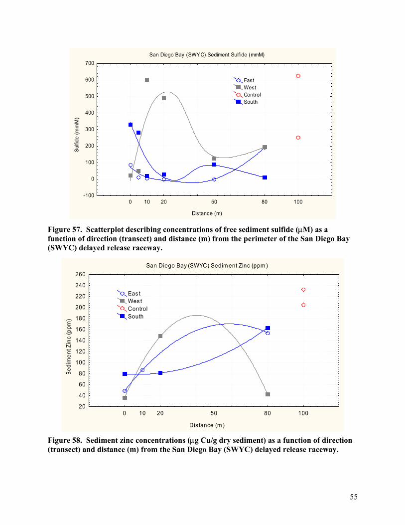
55
San Diego Bay (SWYC) Sediment Sulf ide (mmM)
Distance (m)
Sulfid
e (m
mM
)
0 10 20 50 80 100-100
0
100
200
300
400
500
600
700
EastWestControlSouth
Figure 57. Scatterplot describing concentrations of free sediment sulfide (µM) as a function of direction (transect) and distance (m) from the perimeter of the San Diego Bay (SWYC) delayed release raceway.
San Diego Bay (SWYC) Sedim ent Zinc (ppm )
Dis tance (m )
Sed
imen
t Zin
c (p
pm)
0 10 20 50 80 10020
40
60
80
100
120
140
160
180
200
220
240
260
Eas tWes tControlSouth
Figure 58. Sediment zinc concentrations (µg Cu/g dry sediment) as a function of direction (transect) and distance (m) from the San Diego Bay (SWYC) delayed release raceway.
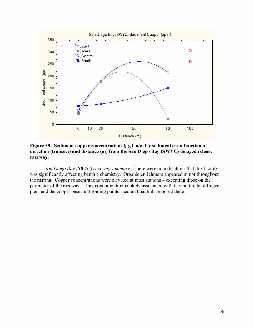
56
San Diego Bay (SWYC) Sediment Copper (ppm )
Dis tance (m)
Sedi
men
t cop
per (
ppm
)
0 10 20 50 80 1000
50
100
150
200
250
300
350
EastWestControlSouth
Figure 59. Sediment copper concentrations (µg Cu/g dry sediment) as a function of direction (transect) and distance (m) from the San Diego Bay (SWYC) delayed release raceway. San Diego Bay (SWYC) raceway summary. There were no indications that this facility was significantly affecting benthic chemistry. Organic enrichment appeared minor throughout the marina. Copper concentrations were elevated at most stations – excepting those on the perimeter of the raceway. That contamination is likely associated with the multitude of finger piers and the copper based antifouling paints used on boat hulls moored there.
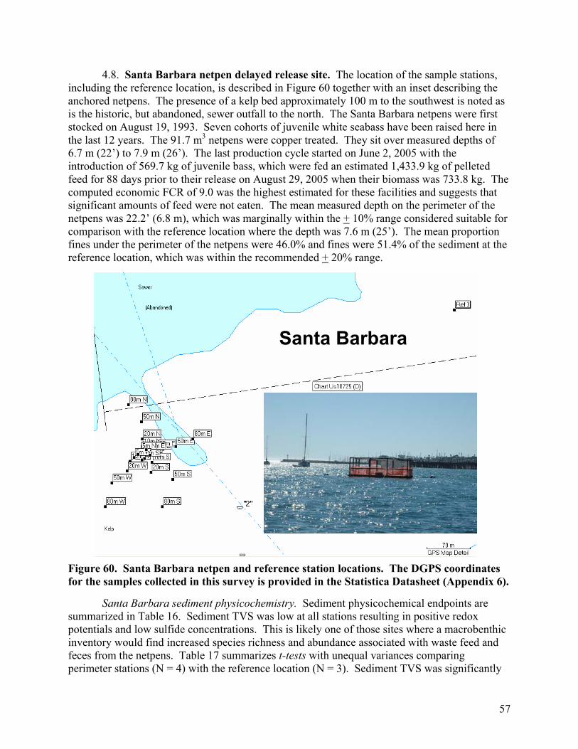
57
4.8. Santa Barbara netpen delayed release site. The location of the sample stations, including the reference location, is described in Figure 60 together with an inset describing the anchored netpens. The presence of a kelp bed approximately 100 m to the southwest is noted as is the historic, but abandoned, sewer outfall to the north. The Santa Barbara netpens were first stocked on August 19, 1993. Seven cohorts of juvenile white seabass have been raised here in the last 12 years. The 91.7 m3 netpens were copper treated. They sit over measured depths of 6.7 m (22’) to 7.9 m (26’). The last production cycle started on June 2, 2005 with the introduction of 569.7 kg of juvenile bass, which were fed an estimated 1,433.9 kg of pelleted feed for 88 days prior to their release on August 29, 2005 when their biomass was 733.8 kg. The computed economic FCR of 9.0 was the highest estimated for these facilities and suggests that significant amounts of feed were not eaten. The mean measured depth on the perimeter of the netpens was 22.2’ (6.8 m), which was marginally within the + 10% range considered suitable for comparison with the reference location where the depth was 7.6 m (25’). The mean proportion fines under the perimeter of the netpens were 46.0% and fines were 51.4% of the sediment at the reference location, which was within the recommended + 20% range.
Figure 60. Santa Barbara netpen and reference station locations. The DGPS coordinates for the samples collected in this survey is provided in the Statistica Datasheet (Appendix 6).
Santa Barbara sediment physicochemistry. Sediment physicochemical endpoints are
summarized in Table 16. Sediment TVS was low at all stations resulting in positive redox potentials and low sulfide concentrations. This is likely one of those sites where a macrobenthic inventory would find increased species richness and abundance associated with waste feed and feces from the netpens. Table 17 summarizes t-tests with unequal variances comparing perimeter stations (N = 4) with the reference location (N = 3). Sediment TVS was significantly
Santa Barbara
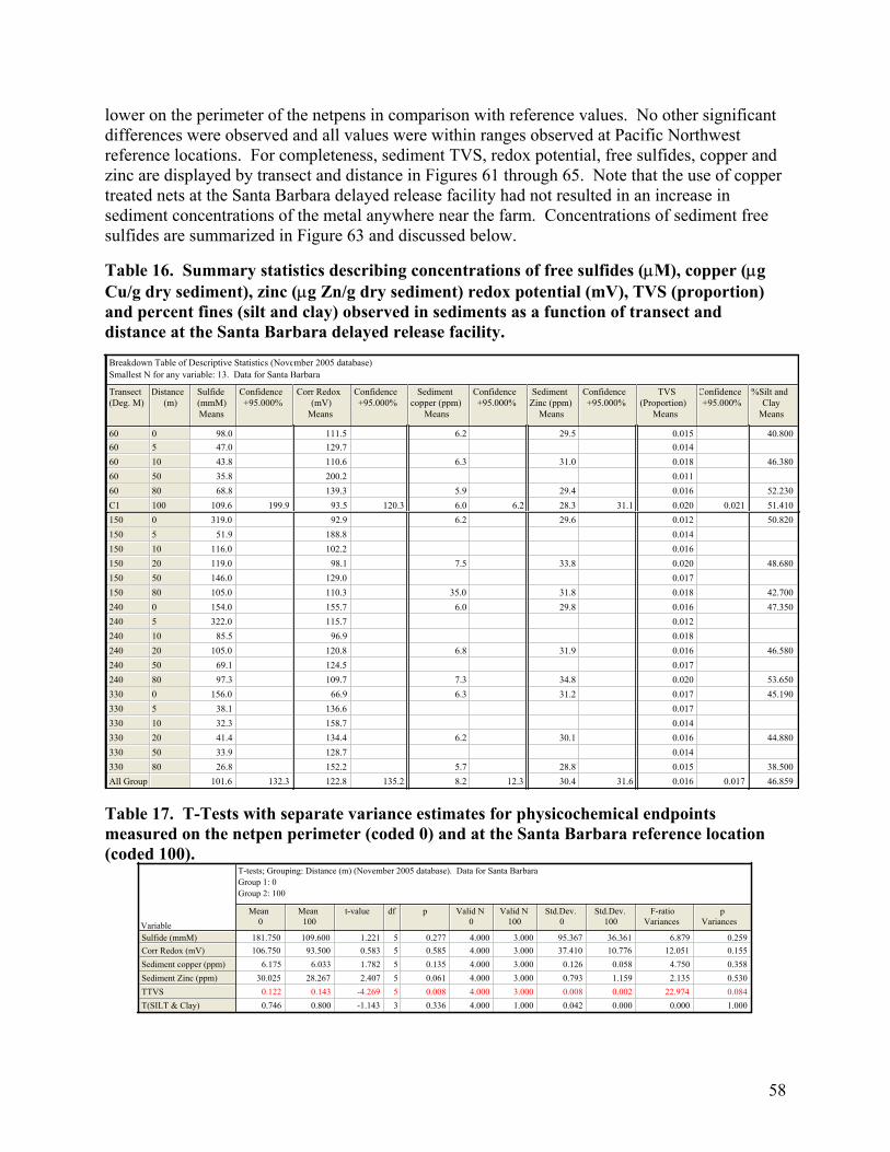
58
lower on the perimeter of the netpens in comparison with reference values. No other significant differences were observed and all values were within ranges observed at Pacific Northwest reference locations. For completeness, sediment TVS, redox potential, free sulfides, copper and zinc are displayed by transect and distance in Figures 61 through 65. Note that the use of copper treated nets at the Santa Barbara delayed release facility had not resulted in an increase in sediment concentrations of the metal anywhere near the farm. Concentrations of sediment free sulfides are summarized in Figure 63 and discussed below.
Table 16. Summary statistics describing concentrations of free sulfides (µM), copper (µg Cu/g dry sediment), zinc (µg Zn/g dry sediment) redox potential (mV), TVS (proportion) and percent fines (silt and clay) observed in sediments as a function of transect and distance at the Santa Barbara delayed release facility. Breakdown Table of Descriptive Statistics (November 2005 database)Smallest N for any variable: 13. Data for Santa Barbara
Transect(Deg. M)
Distance (m)
Sulfide(mmM)Means
Confidence+95.000%
Corr Redox(mV)
Means
Confidence+95.000%
Sedimentcopper (ppm)
Means
Confidence+95.000%
SedimentZinc (ppm)
Means
Confidence+95.000%
TVS(Proportion)
Means
Confidence+95.000%
%Silt andClay
Means
60 0 98.0 111.5 6.2 29.5 0.015 40.80060 5 47.0 129.7 0.01460 10 43.8 110.6 6.3 31.0 0.018 46.38060 50 35.8 200.2 0.01160 80 68.8 139.3 5.9 29.4 0.016 52.230C1 100 109.6 199.9 93.5 120.3 6.0 6.2 28.3 31.1 0.020 0.021 51.410150 0 319.0 92.9 6.2 29.6 0.012 50.820150 5 51.9 188.8 0.014150 10 116.0 102.2 0.016150 20 119.0 98.1 7.5 33.8 0.020 48.680150 50 146.0 129.0 0.017150 80 105.0 110.3 35.0 31.8 0.018 42.700240 0 154.0 155.7 6.0 29.8 0.016 47.350240 5 322.0 115.7 0.012240 10 85.5 96.9 0.018240 20 105.0 120.8 6.8 31.9 0.016 46.580240 50 69.1 124.5 0.017240 80 97.3 109.7 7.3 34.8 0.020 53.650330 0 156.0 66.9 6.3 31.2 0.017 45.190330 5 38.1 136.6 0.017330 10 32.3 158.7 0.014330 20 41.4 134.4 6.2 30.1 0.016 44.880330 50 33.9 128.7 0.014330 80 26.8 152.2 5.7 28.8 0.015 38.500All Group 101.6 132.3 122.8 135.2 8.2 12.3 30.4 31.6 0.016 0.017 46.859
Table 17. T-Tests with separate variance estimates for physicochemical endpoints measured on the netpen perimeter (coded 0) and at the Santa Barbara reference location (coded 100).
T-tests; Grouping: Distance (m) (November 2005 database). Data for Santa BarbaraGroup 1: 0Group 2: 100
Variable
Mean0
Mean100
t-value df p Valid N0
Valid N100
Std.Dev.0
Std.Dev.100
F-ratioVariances
pVariances
Sulfide (mmM)Corr Redox (mV)Sediment copper (ppm)Sediment Zinc (ppm)TTVST(SILT & Clay)
181.750 109.600 1.221 5 0.277 4.000 3.000 95.367 36.361 6.879 0.259106.750 93.500 0.583 5 0.585 4.000 3.000 37.410 10.776 12.051 0.155
6.175 6.033 1.782 5 0.135 4.000 3.000 0.126 0.058 4.750 0.35830.025 28.267 2.407 5 0.061 4.000 3.000 0.793 1.159 2.135 0.530
0.122 0.143 -4.269 5 0.008 4.000 3.000 0.008 0.002 22.974 0.0840.746 0.800 -1.143 3 0.336 4.000 1.000 0.042 0.000 0.000 1.000
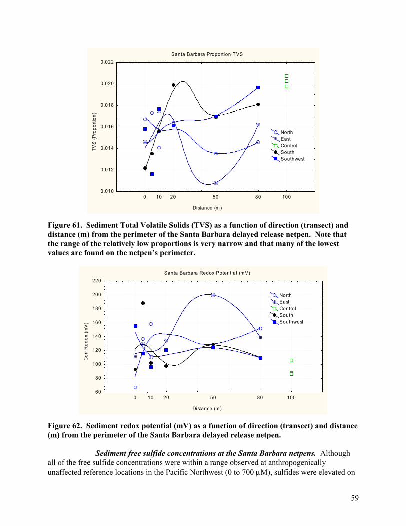
59
Santa Barbara Proportion TVS
Distance (m)
TVS
(Pro
porti
on)
0 10 20 50 80 1000.010
0.012
0.014
0.016
0.018
0.020
0.022
NorthEastControlSouthSouthwest
Figure 61. Sediment Total Volatile Solids (TVS) as a function of direction (transect) and distance (m) from the perimeter of the Santa Barbara delayed release netpen. Note that the range of the relatively low proportions is very narrow and that many of the lowest values are found on the netpen’s perimeter.
Santa Barbara Redox Potential (mV)
Distance (m)
Cor
r Red
ox (m
V)
0 10 20 50 80 10060
80
100
120
140
160
180
200
220
NorthEastControlSouthSouthwest
Figure 62. Sediment redox potential (mV) as a function of direction (transect) and distance (m) from the perimeter of the Santa Barbara delayed release netpen. Sediment free sulfide concentrations at the Santa Barbara netpens. Although all of the free sulfide concentrations were within a range observed at anthropogenically unaffected reference locations in the Pacific Northwest (0 to 700 µM), sulfides were elevated on
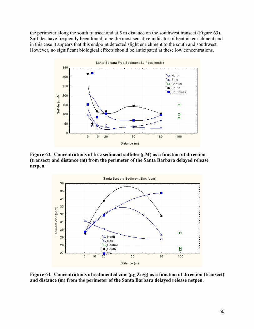
60
the perimeter along the south transect and at 5 m distance on the southwest transect (Figure 63). Sulfides have frequently been found to be the most sensitive indicator of benthic enrichment and in this case it appears that this endpoint detected slight enrichment to the south and southwest. However, no significant biological effects should be anticipated at these low concentrations.
Santa Barbara Free Sediment Sul fides (mmM)
Distance (m)
Sul
fide
(mm
M)
0 10 20 50 80 1000
50
100
150
200
250
300
350
NorthEastControlSouthSouthwest
Figure 63. Concentrations of free sediment sulfides (µM) as a function of direction (transect) and distance (m) from the perimeter of the Santa Barbara delayed release netpen.
Santa Barbara Sediment Zinc (ppm)
Distance (m)
Sed
imen
t Zin
c (p
pm)
0 10 20 50 80 10027
28
29
30
31
32
33
34
35
36
NorthEastControlSouthSW
Figure 64. Concentrations of sedimented zinc (µg Zn/g) as a function of direction (transect) and distance (m) from the perimeter of the Santa Barbara delayed release netpen.
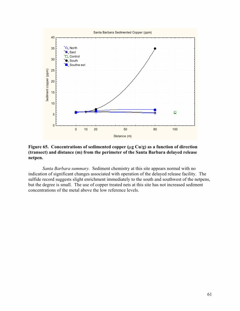
61
Santa Barbara Sedimented Copper (ppm)
Distance (m)
Sedi
men
t cop
per (
ppm
)
0 10 20 50 80 1000
5
10
15
20
25
30
35
40
NorthEastControlSouthSouthw est
Figure 65. Concentrations of sedimented copper (µg Cu/g) as a function of direction (transect) and distance (m) from the perimeter of the Santa Barbara delayed release netpen. Santa Barbara summary. Sediment chemistry at this site appears normal with no indication of significant changes associated with operation of the delayed release facility. The sulfide record suggests slight enrichment immediately to the south and southwest of the netpens, but the degree is small. The use of copper treated nets at this site has not increased sediment concentrations of the metal above the low reference levels.
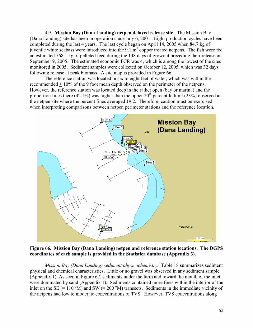
62
4.9. Mission Bay (Dana Landing) netpen delayed release site. The Mission Bay (Dana Landing) site has been in operation since July 6, 2001. Eight production cycles have been completed during the last 4 years. The last cycle began on April 14, 2005 when 84.7 kg of juvenile white seabass were introduced into the 9.1 m3 copper treated netpens. The fish were fed an estimated 568.1 kg of pelleted feed during the 148 days of growout preceding their release on September 9, 2005. The estimated economic FCR was 4, which is among the lowest of the sites monitored in 2005. Sediment samples were collected on October 12, 2005, which was 32 days following release at peak biomass. A site map is provided in Figure 66. The reference station was located in six to eight feet of water, which was within the recommended + 10% of the 9 foot mean depth observed on the perimeter of the netpens. However, the reference station was located deep in the rather open (bay or marina) and the proportion fines there (42.1%) was higher than the upper 20th percentile limit (23%) observed at the netpen site where the percent fines averaged 19.2. Therefore, caution must be exercised when interpreting comparisons between netpen perimeter stations and the reference location.
Figure 66. Mission Bay (Dana Landing) netpen and reference station locations. The DGPS coordinates of each sample is provided in the Statistica database (Appendix 3).
Mission Bay (Dana Landing) sediment physicochemistry. Table 18 summarizes sediment physical and chemical characteristics. Little or no gravel was observed in any sediment sample (Appendix 1). As seen in Figure 67, sediments under the farm and toward the mouth of the inlet were dominated by sand (Appendix 1). Sediments contained more fines within the interior of the inlet on the SE (= 110 oM) and SW (= 200 oM) transects. Sediments in the immediate vicinity of the netpens had low to moderate concentrations of TVS. However, TVS concentrations along
Mission Bay (Dana Landing)
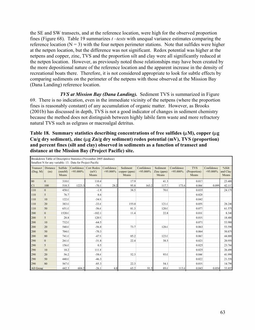
63
the SE and SW transects, and at the reference location, were high for the observed proportion fines (Figure 68). Table 19 summarizes t –tests with unequal variance estimates comparing the reference location (N = 3) with the four netpen perimeter stations. Note that sulfides were higher at the netpen location, but the difference was not significant. Redox potential was higher at the netpens and copper, zinc, TVS and the proportion silt and clay were all significantly reduced at the netpen location. However, as previously noted those relationships may have been created by the more depositional nature of the reference location and the apparent increase in the density of recreational boats there. Therefore, it is not considered appropriate to look for subtle effects by comparing sediments on the perimeter of the netpens with those observed at the Mission Bay (Dana Landing) reference location.
TVS at Mission Bay (Dana Landing). Sediment TVS is summarized in Figure
69. There is no indication, even in the immediate vicinity of the netpens (where the proportion fines is reasonably constant) of any accumulation of organic matter. However, as Brooks (2001b) has discussed in depth, TVS is not a good indicator of changes in sediment chemistry because the method does not distinguish between highly labile farm waste and more refractory natural TVS such as eelgrass or macroalgal detritus.
Table 18. Summary statistics describing concentrations of free sulfides (µM), copper (µg Cu/g dry sediment), zinc (µg Zn/g dry sediment) redox potential (mV), TVS (proportion) and percent fines (silt and clay) observed in sediments as a function of transect and distance at the Mission Bay (Project Pacific) site. Breakdown Table of Descriptive Statistics (November 2005 database)Smallest N for any variable: 13. Data for Project Pacific
Transect(Deg. M)
Distance(m)
Sulfide(mmM)Means
Confidence+95.000%
Corr Redox(mV)
Means
Confidence+95.000%
Sedimentcopper (ppm)
Means
Confidence+95.000%
SedimentZinc (ppm)
Means
Confidence+95.000%
TVS(Proportion)
Means
Confidence+95.000%
%Siltand Clay
Means
80 0 310.0 110.4 17.9 41.3 0.017 23.400C1 100 510.3 1223.3 -70.1 28.2 95.8 163.2 117.7 173.6 0.066 0.099 42.117110 0 458.0 -1.9 38.5 70.0 0.035 24.170110 5 76.7 8.6 0.028110 10 122.0 -34.9 0.042110 20 383.0 -33.6 155.0 121.0 0.059 28.240110 50 651.0 -56.6 81.3 120.0 0.077 61.570200 0 1520.0 -102.1 11.4 22.8 0.010 8.340200 5 28.8 120.9 0.019 18.480200 10 732.0 -64.5 0.071 53.900200 20 540.0 -56.8 73.7 128.0 0.063 53.590200 50 704.0 -70.3 0.064 50.870200 80 741.0 -47.9 85.2 123.0 0.067 44.800290 0 261.0 -31.8 22.4 38.5 0.021 20.950290 5 156.0 0.5 0.025 23.760290 10 10.2 111.8 0.025 26.490290 20 56.2 -58.6 52.3 93.0 0.046 41.990290 50 440.0 -46.3 0.022 21.550290 80 567.0 -85.3 22.3 54.1 0.019 14.790All Group 442.3 604.2 -26.1 4.0 65.2 91.5 89.6 113.6 0.043 0.054 33.855
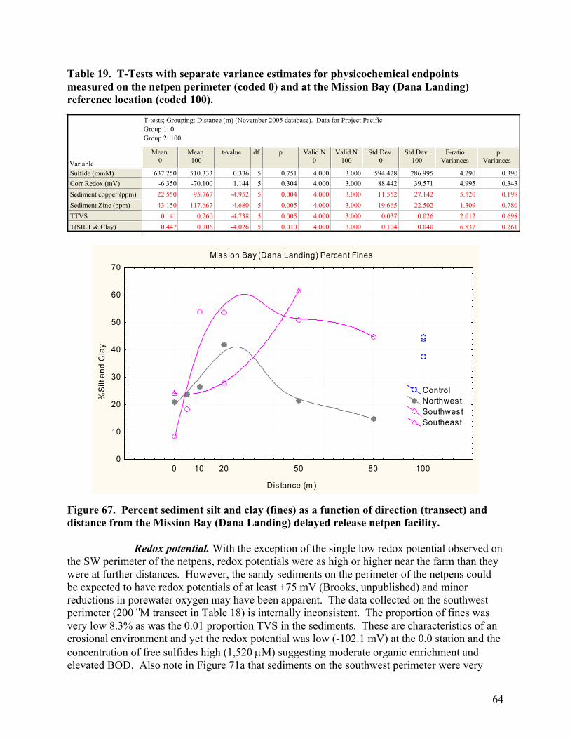
64
Table 19. T-Tests with separate variance estimates for physicochemical endpoints measured on the netpen perimeter (coded 0) and at the Mission Bay (Dana Landing) reference location (coded 100).
T-tests; Grouping: Distance (m) (November 2005 database). Data for Project PacificGroup 1: 0Group 2: 100
VariableMean
0Mean
100t-value df p Valid N
0Valid N
100Std.Dev.
0Std.Dev.
100F-ratio
Variancesp
Variances
Sulfide (mmM)Corr Redox (mV)Sediment copper (ppm)Sediment Zinc (ppm)TTVST(SILT & Clay)
637.250 510.333 0.336 5 0.751 4.000 3.000 594.428 286.995 4.290 0.390-6.350 -70.100 1.144 5 0.304 4.000 3.000 88.442 39.571 4.995 0.34322.550 95.767 -4.952 5 0.004 4.000 3.000 11.552 27.142 5.520 0.19843.150 117.667 -4.680 5 0.005 4.000 3.000 19.665 22.502 1.309 0.780
0.141 0.260 -4.738 5 0.005 4.000 3.000 0.037 0.026 2.012 0.6980.447 0.706 -4.026 5 0.010 4.000 3.000 0.104 0.040 6.837 0.261
Miss ion Bay (Dana Landing) Percent Fines
Dis tance (m )
%S
ilt a
nd C
lay
0 10 20 50 80 1000
10
20
30
40
50
60
70
ControlNorthwes tSouthwestSoutheas t
Figure 67. Percent sediment silt and clay (fines) as a function of direction (transect) and distance from the Mission Bay (Dana Landing) delayed release netpen facility. Redox potential. With the exception of the single low redox potential observed on the SW perimeter of the netpens, redox potentials were as high or higher near the farm than they were at further distances. However, the sandy sediments on the perimeter of the netpens could be expected to have redox potentials of at least +75 mV (Brooks, unpublished) and minor reductions in porewater oxygen may have been apparent. The data collected on the southwest perimeter (200 oM transect in Table 18) is internally inconsistent. The proportion of fines was very low 8.3% as was the 0.01 proportion TVS in the sediments. These are characteristics of an erosional environment and yet the redox potential was low (-102.1 mV) at the 0.0 station and the concentration of free sulfides high (1,520 µM) suggesting moderate organic enrichment and elevated BOD. Also note in Figure 71a that sediments on the southwest perimeter were very
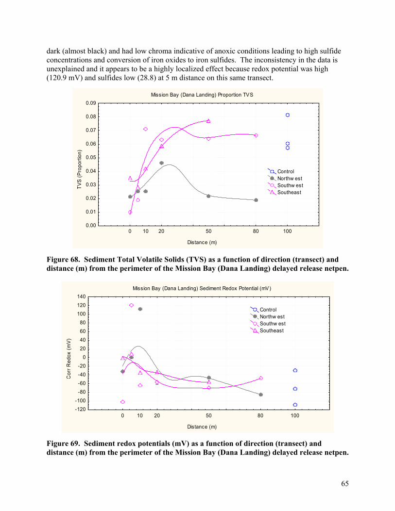
65
dark (almost black) and had low chroma indicative of anoxic conditions leading to high sulfide concentrations and conversion of iron oxides to iron sulfides. The inconsistency in the data is unexplained and it appears to be a highly localized effect because redox potential was high (120.9 mV) and sulfides low (28.8) at 5 m distance on this same transect.
Mission Bay (Dana Landing) Proportion TVS
Distance (m)
TVS
(Pro
porti
on)
0 10 20 50 80 1000.00
0.01
0.02
0.03
0.04
0.05
0.06
0.07
0.08
0.09
ControlNorthw estSouthw estSoutheast
Figure 68. Sediment Total Volatile Solids (TVS) as a function of direction (transect) and distance (m) from the perimeter of the Mission Bay (Dana Landing) delayed release netpen.
Mission Bay (Dana Landing) Sediment Redox Potential (mV)
Distance (m)
Cor
r Red
ox (m
V)
0 10 20 50 80 100-120-100
-80-60-40-20
020406080
100120140
ControlNorthw estSouthw estSoutheast
Figure 69. Sediment redox potentials (mV) as a function of direction (transect) and distance (m) from the perimeter of the Mission Bay (Dana Landing) delayed release netpen.
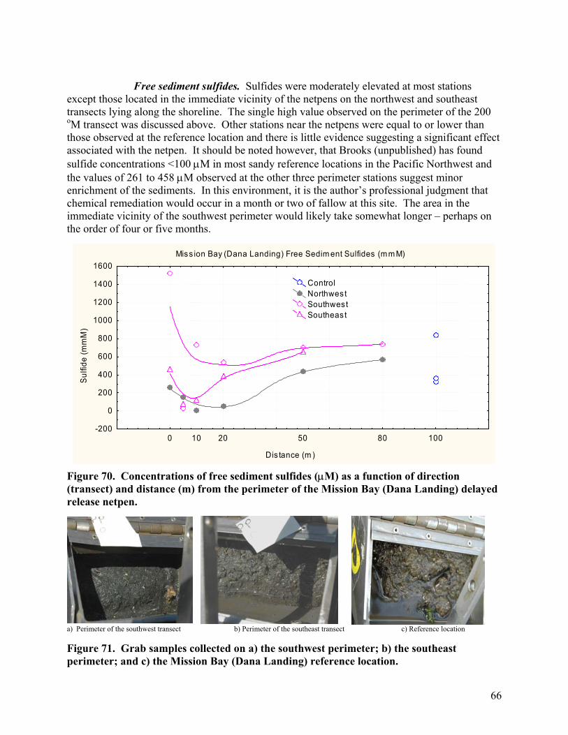
66
Free sediment sulfides. Sulfides were moderately elevated at most stations except those located in the immediate vicinity of the netpens on the northwest and southeast transects lying along the shoreline. The single high value observed on the perimeter of the 200 oM transect was discussed above. Other stations near the netpens were equal to or lower than those observed at the reference location and there is little evidence suggesting a significant effect associated with the netpen. It should be noted however, that Brooks (unpublished) has found sulfide concentrations <100 µM in most sandy reference locations in the Pacific Northwest and the values of 261 to 458 µM observed at the other three perimeter stations suggest minor enrichment of the sediments. In this environment, it is the author’s professional judgment that chemical remediation would occur in a month or two of fallow at this site. The area in the immediate vicinity of the southwest perimeter would likely take somewhat longer – perhaps on the order of four or five months.
Miss ion Bay (Dana Landing) Free Sedim ent Sulfides (mm M)
Dis tance (m )
Sulfi
de (m
mM
)
0 10 20 50 80 100-200
0
200
400
600
800
1000
1200
1400
1600
ControlNorthwes tSouthwestSoutheas t
Figure 70. Concentrations of free sediment sulfides (µM) as a function of direction (transect) and distance (m) from the perimeter of the Mission Bay (Dana Landing) delayed release netpen.
a) Perimeter of the southwest transect b) Perimeter of the southeast transect c) Reference location Figure 71. Grab samples collected on a) the southwest perimeter; b) the southeast perimeter; and c) the Mission Bay (Dana Landing) reference location.
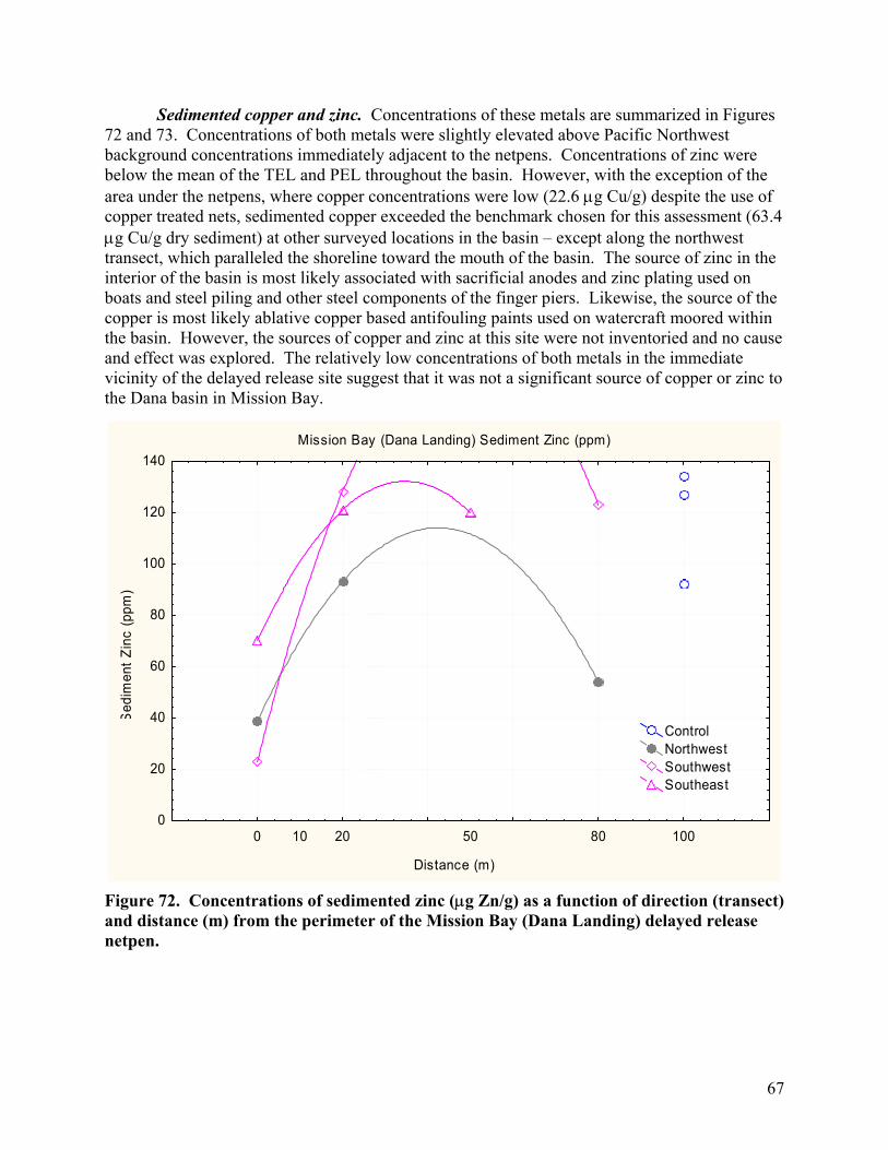
67
Sedimented copper and zinc. Concentrations of these metals are summarized in Figures 72 and 73. Concentrations of both metals were slightly elevated above Pacific Northwest background concentrations immediately adjacent to the netpens. Concentrations of zinc were below the mean of the TEL and PEL throughout the basin. However, with the exception of the area under the netpens, where copper concentrations were low (22.6 µg Cu/g) despite the use of copper treated nets, sedimented copper exceeded the benchmark chosen for this assessment (63.4 µg Cu/g dry sediment) at other surveyed locations in the basin – except along the northwest transect, which paralleled the shoreline toward the mouth of the basin. The source of zinc in the interior of the basin is most likely associated with sacrificial anodes and zinc plating used on boats and steel piling and other steel components of the finger piers. Likewise, the source of the copper is most likely ablative copper based antifouling paints used on watercraft moored within the basin. However, the sources of copper and zinc at this site were not inventoried and no cause and effect was explored. The relatively low concentrations of both metals in the immediate vicinity of the delayed release site suggest that it was not a significant source of copper or zinc to the Dana basin in Mission Bay.
Mission Bay (Dana Landing) Sediment Zinc (ppm)
Distance (m)
Sed
imen
t Zin
c (p
pm)
0 10 20 50 80 1000
20
40
60
80
100
120
140
ControlNorthwestSouthwestSoutheast
Figure 72. Concentrations of sedimented zinc (µg Zn/g) as a function of direction (transect) and distance (m) from the perimeter of the Mission Bay (Dana Landing) delayed release netpen.
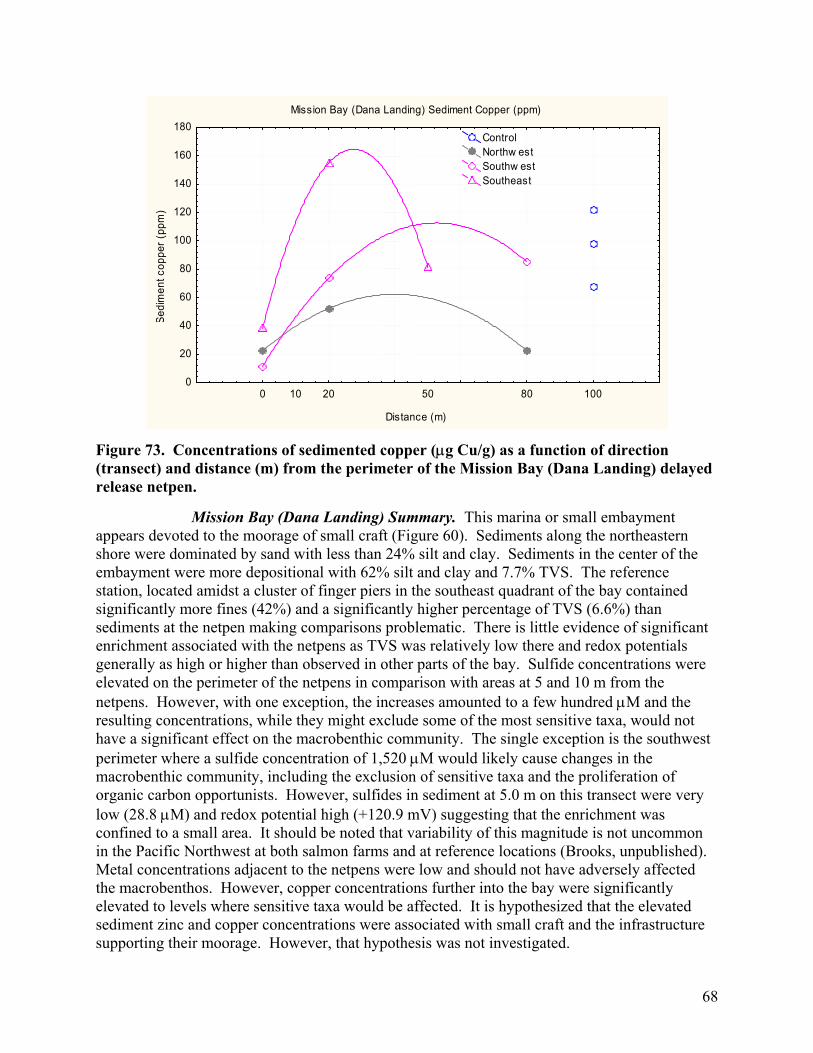
68
Mission Bay (Dana Landing) Sediment Copper (ppm)
Distance (m)
Sedi
men
t cop
per (
ppm
)
0 10 20 50 80 1000
20
40
60
80
100
120
140
160
180ControlNorthw estSouthw estSoutheast
Figure 73. Concentrations of sedimented copper (µg Cu/g) as a function of direction (transect) and distance (m) from the perimeter of the Mission Bay (Dana Landing) delayed release netpen. Mission Bay (Dana Landing) Summary. This marina or small embayment appears devoted to the moorage of small craft (Figure 60). Sediments along the northeastern shore were dominated by sand with less than 24% silt and clay. Sediments in the center of the embayment were more depositional with 62% silt and clay and 7.7% TVS. The reference station, located amidst a cluster of finger piers in the southeast quadrant of the bay contained significantly more fines (42%) and a significantly higher percentage of TVS (6.6%) than sediments at the netpen making comparisons problematic. There is little evidence of significant enrichment associated with the netpens as TVS was relatively low there and redox potentials generally as high or higher than observed in other parts of the bay. Sulfide concentrations were elevated on the perimeter of the netpens in comparison with areas at 5 and 10 m from the netpens. However, with one exception, the increases amounted to a few hundred µM and the resulting concentrations, while they might exclude some of the most sensitive taxa, would not have a significant effect on the macrobenthic community. The single exception is the southwest perimeter where a sulfide concentration of 1,520 µM would likely cause changes in the macrobenthic community, including the exclusion of sensitive taxa and the proliferation of organic carbon opportunists. However, sulfides in sediment at 5.0 m on this transect were very low (28.8 µM) and redox potential high (+120.9 mV) suggesting that the enrichment was confined to a small area. It should be noted that variability of this magnitude is not uncommon in the Pacific Northwest at both salmon farms and at reference locations (Brooks, unpublished). Metal concentrations adjacent to the netpens were low and should not have adversely affected the macrobenthos. However, copper concentrations further into the bay were significantly elevated to levels where sensitive taxa would be affected. It is hypothesized that the elevated sediment zinc and copper concentrations were associated with small craft and the infrastructure supporting their moorage. However, that hypothesis was not investigated.
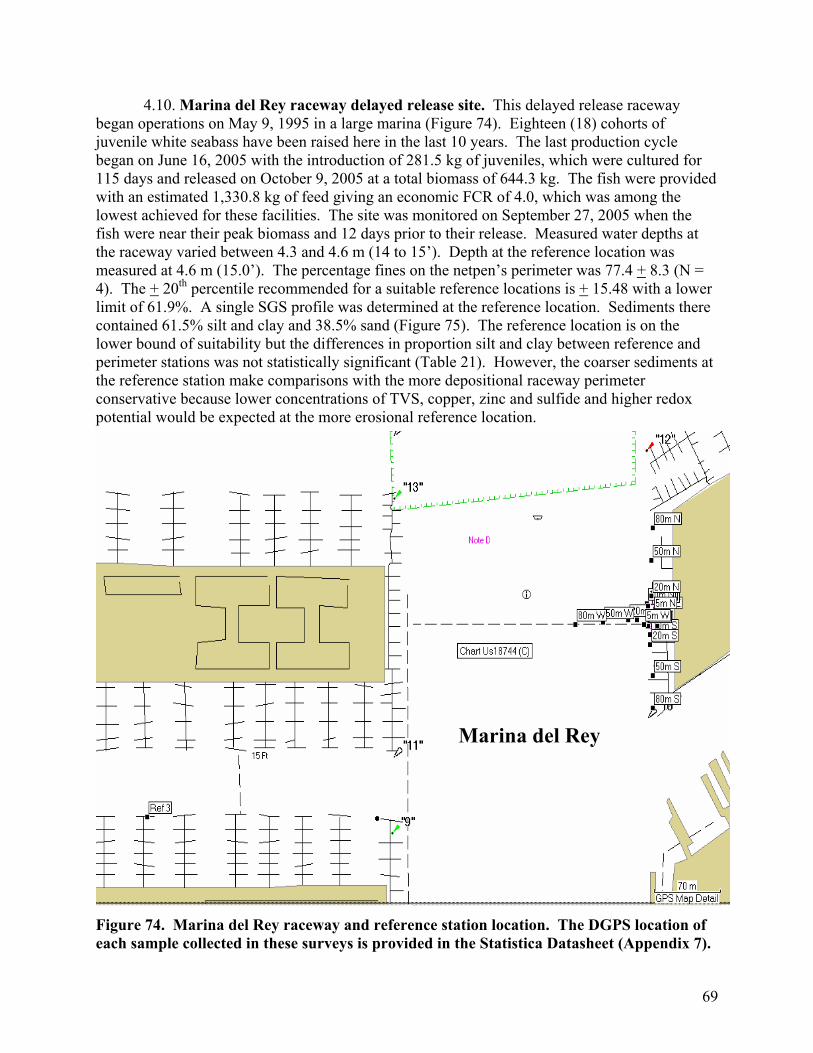
69
4.10. Marina del Rey raceway delayed release site. This delayed release raceway began operations on May 9, 1995 in a large marina (Figure 74). Eighteen (18) cohorts of juvenile white seabass have been raised here in the last 10 years. The last production cycle began on June 16, 2005 with the introduction of 281.5 kg of juveniles, which were cultured for 115 days and released on October 9, 2005 at a total biomass of 644.3 kg. The fish were provided with an estimated 1,330.8 kg of feed giving an economic FCR of 4.0, which was among the lowest achieved for these facilities. The site was monitored on September 27, 2005 when the fish were near their peak biomass and 12 days prior to their release. Measured water depths at the raceway varied between 4.3 and 4.6 m (14 to 15’). Depth at the reference location was measured at 4.6 m (15.0’). The percentage fines on the netpen’s perimeter was 77.4 + 8.3 (N = 4). The + 20th percentile recommended for a suitable reference locations is + 15.48 with a lower limit of 61.9%. A single SGS profile was determined at the reference location. Sediments there contained 61.5% silt and clay and 38.5% sand (Figure 75). The reference location is on the lower bound of suitability but the differences in proportion silt and clay between reference and perimeter stations was not statistically significant (Table 21). However, the coarser sediments at the reference station make comparisons with the more depositional raceway perimeter conservative because lower concentrations of TVS, copper, zinc and sulfide and higher redox potential would be expected at the more erosional reference location.
Figure 74. Marina del Rey raceway and reference station location. The DGPS location of each sample collected in these surveys is provided in the Statistica Datasheet (Appendix 7).
Marina del Rey
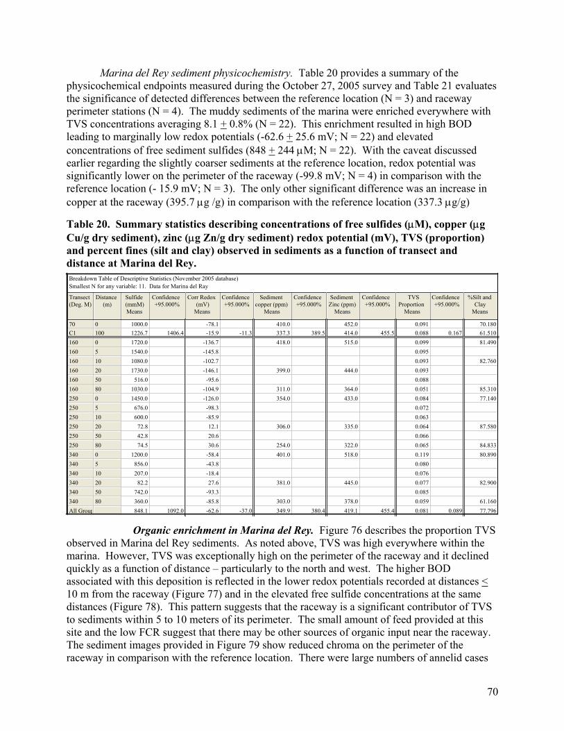
70
Marina del Rey sediment physicochemistry. Table 20 provides a summary of the physicochemical endpoints measured during the October 27, 2005 survey and Table 21 evaluates the significance of detected differences between the reference location (N = 3) and raceway perimeter stations (N = 4). The muddy sediments of the marina were enriched everywhere with TVS concentrations averaging 8.1 + 0.8% (N = 22). This enrichment resulted in high BOD leading to marginally low redox potentials (-62.6 + 25.6 mV; N = 22) and elevated concentrations of free sediment sulfides (848 + 244 µM; N = 22). With the caveat discussed earlier regarding the slightly coarser sediments at the reference location, redox potential was significantly lower on the perimeter of the raceway (-99.8 mV; N = 4) in comparison with the reference location (- 15.9 mV; N = 3). The only other significant difference was an increase in copper at the raceway (395.7 µg /g) in comparison with the reference location (337.3 µg/g)
Table 20. Summary statistics describing concentrations of free sulfides (µM), copper (µg Cu/g dry sediment), zinc (µg Zn/g dry sediment) redox potential (mV), TVS (proportion) and percent fines (silt and clay) observed in sediments as a function of transect and distance at Marina del Rey.
Breakdown Table of Descriptive Statistics (November 2005 database)Smallest N for any variable: 11. Data for Marina del Ray
Transect(Deg. M)
Distance(m)
Sulfide(mmM)Means
Confidence+95.000%
Corr Redox(mV)
Means
Confidence+95.000%
Sedimentcopper (ppm)
Means
Confidence+95.000%
SedimentZinc (ppm)
Means
Confidence+95.000%
TVSProportion
Means
Confidence+95.000%
%Silt andClay
Means
70 0 1000.0 -78.1 410.0 452.0 0.091 70.180C1 100 1226.7 1406.4 -15.9 -11.3 337.3 389.5 414.0 455.5 0.088 0.167 61.510160 0 1720.0 -136.7 418.0 515.0 0.099 81.490160 5 1540.0 -145.8 0.095160 10 1080.0 -102.7 0.093 82.760160 20 1730.0 -146.1 399.0 444.0 0.093160 50 516.0 -95.6 0.088160 80 1030.0 -104.9 311.0 364.0 0.051 85.310250 0 1450.0 -126.0 354.0 433.0 0.084 77.140250 5 676.0 -98.3 0.072250 10 600.0 -85.9 0.063250 20 72.8 12.1 306.0 335.0 0.064 87.580250 50 42.8 20.6 0.066250 80 74.5 30.6 254.0 322.0 0.065 84.833340 0 1200.0 -58.4 401.0 518.0 0.119 80.890340 5 856.0 -43.8 0.080340 10 207.0 -18.4 0.076340 20 82.2 27.6 381.0 445.0 0.077 82.900340 50 742.0 -93.3 0.085340 80 360.0 -85.8 303.0 378.0 0.059 61.160All Group 848.1 1092.0 -62.6 -37.0 349.9 380.4 419.1 455.4 0.081 0.089 77.796
Organic enrichment in Marina del Rey. Figure 76 describes the proportion TVS observed in Marina del Rey sediments. As noted above, TVS was high everywhere within the marina. However, TVS was exceptionally high on the perimeter of the raceway and it declined quickly as a function of distance – particularly to the north and west. The higher BOD associated with this deposition is reflected in the lower redox potentials recorded at distances < 10 m from the raceway (Figure 77) and in the elevated free sulfide concentrations at the same distances (Figure 78). This pattern suggests that the raceway is a significant contributor of TVS to sediments within 5 to 10 meters of its perimeter. The small amount of feed provided at this site and the low FCR suggest that there may be other sources of organic input near the raceway. The sediment images provided in Figure 79 show reduced chroma on the perimeter of the raceway in comparison with the reference location. There were large numbers of annelid cases
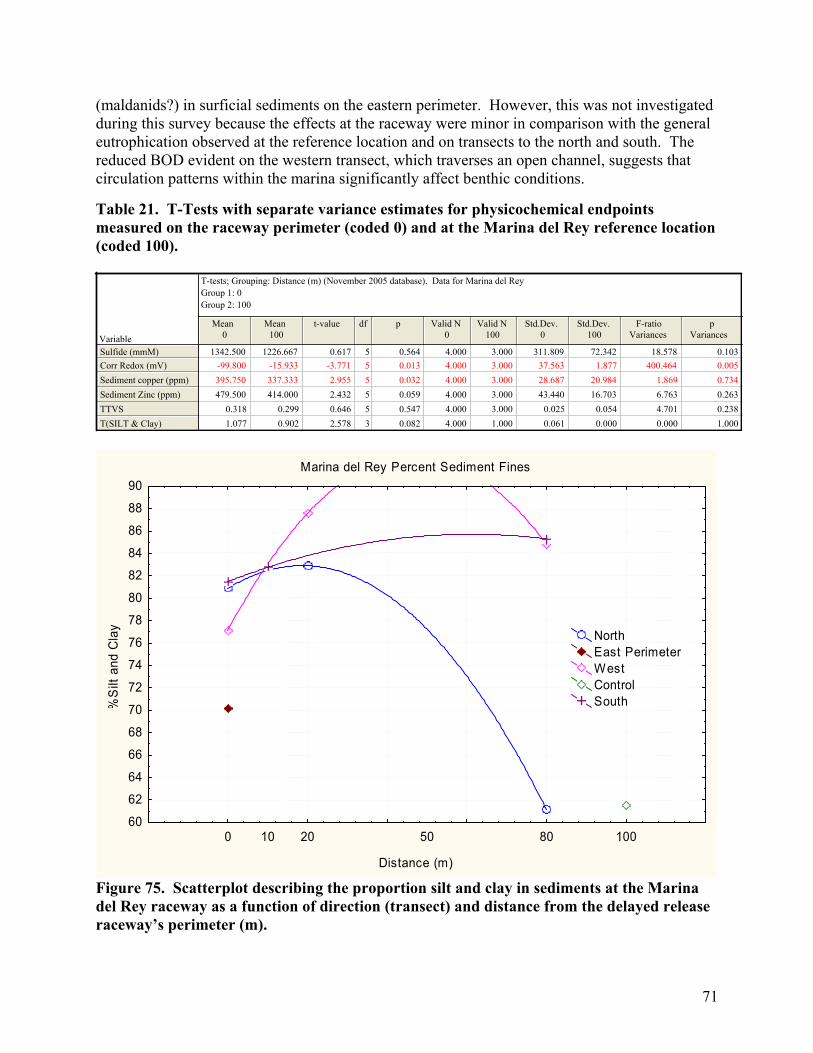
71
(maldanids?) in surficial sediments on the eastern perimeter. However, this was not investigated during this survey because the effects at the raceway were minor in comparison with the general eutrophication observed at the reference location and on transects to the north and south. The reduced BOD evident on the western transect, which traverses an open channel, suggests that circulation patterns within the marina significantly affect benthic conditions. Table 21. T-Tests with separate variance estimates for physicochemical endpoints measured on the raceway perimeter (coded 0) and at the Marina del Rey reference location (coded 100).
T-tests; Grouping: Distance (m) (November 2005 database). Data for Marina del ReyGroup 1: 0Group 2: 100
VariableMean
0Mean
100t-value df p Valid N
0Valid N
100Std.Dev.
0Std.Dev.
100F-ratio
Variancesp
Variances
Sulfide (mmM)Corr Redox (mV)Sediment copper (ppm)Sediment Zinc (ppm)TTVST(SILT & Clay)
1342.500 1226.667 0.617 5 0.564 4.000 3.000 311.809 72.342 18.578 0.103-99.800 -15.933 -3.771 5 0.013 4.000 3.000 37.563 1.877 400.464 0.005395.750 337.333 2.955 5 0.032 4.000 3.000 28.687 20.984 1.869 0.734479.500 414.000 2.432 5 0.059 4.000 3.000 43.440 16.703 6.763 0.263
0.318 0.299 0.646 5 0.547 4.000 3.000 0.025 0.054 4.701 0.2381.077 0.902 2.578 3 0.082 4.000 1.000 0.061 0.000 0.000 1.000
Marina del Rey Percent Sediment Fines
Distance (m)
%S
ilt a
nd C
lay
0 10 20 50 80 10060
62
64
66
68
70
72
74
76
78
80
82
84
86
88
90
NorthEast PerimeterWestControlSouth
Figure 75. Scatterplot describing the proportion silt and clay in sediments at the Marina del Rey raceway as a function of direction (transect) and distance from the delayed release raceway’s perimeter (m).
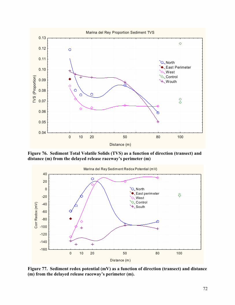
72
Marina del Rey Proportion Sediment TVS
Distance (m)
TVS
(Pro
porti
on)
0 10 20 50 80 1000.04
0.05
0.06
0.07
0.08
0.09
0.10
0.11
0.12
0.13
NorthEast PerimeterWestControlWouth
Figure 76. Sediment Total Volatile Solids (TVS) as a function of direction (transect) and distance (m) from the delayed release raceway’s perimeter (m)
Marina del Rey Sedim ent Redox Potential (mV)
Dis tance (m)
Cor
r Red
ox (m
V)
0 10 20 50 80 100-160
-140
-120
-100
-80
-60
-40
-20
0
20
40
NorthEast perim eterWestControlSouth
Figure 77. Sediment redox potential (mV) as a function of direction (transect) and distance (m) from the delayed release raceway’s perimeter (m).

73
Figure 78. Free sediment sulfides (µM) as a function of direction (transect) and distance (m) from Marina del Rey’s delayed release raceway.
a) Perimeter (070 oM) Perimeter (250 oM) Perimeter (340 oM)
d) Reference location Figure 79. Sediment grab samples collected at Marina del Rey. a) Perimeter (070 oM); b) Perimeter (250 oM); c) Perimeter (340 oM); d) Reference location.
Marina del Rey Free Sediment Sulfides (mmM)
Distance (m)
Sul
fide
(mm
M)
0 10 20 50 80 100-200
0
200
400
600
800
1000
1200
1400
1600
1800
NorthEast PerimeterWestControlSouth

74
Sedimented zinc and copper in Marina del Rey. Concentrations of sedimented zinc and copper are summarized in Figure 80 and 81 respectively. In both cases the means of the TELs and PELs are off the bottom of the charts and absent immobilization of the metals by at least moderately high concentrations of free sulfides, the metal concentrations would have an adverse effect on the marina’s macrobenthos. Because proteinated zinc is used to supplement the feed provided to these fish, the amount of the metal contributed by the delayed release operation is likely very small (<99.8 grams/production cycle). This amount of zinc – spread over a circle with a radius of 15 m to a depth of 2.0 cm would increase the sediment’s concentration by about 4.4 µg/g, which would not be detectable within the variability observed in the marina. Similar to the comment regarding organic loading, other sources of copper and zinc are likely responsible for the increases observed near the raceway. However, the spatial distribution of the metals indicates that the raceway cannot be ruled out as a source.
Marina del Rey Sedimented Zinc (ppm)
Distance (m)
Sedi
men
t Zin
c (p
pm)
0 10 20 50 80 100300
320
340
360
380
400
420
440
460
480
500
520
540
NorthEast PerimeterWestControlSouth
Figure 80. Sedimented zinc (µg Zn/g) as a function of direction (transect) and distance (m) from the delayed release raceway’s perimeter.
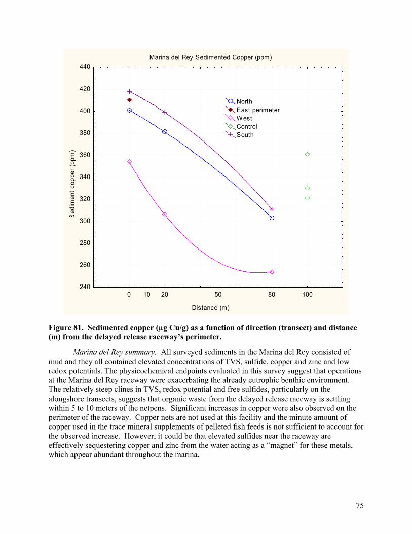
75
Marina del Rey Sedimented Copper (ppm)
Distance (m)
Sed
imen
t cop
per (
ppm
)
0 10 20 50 80 100240
260
280
300
320
340
360
380
400
420
440
NorthEast perimeterWestControlSouth
Figure 81. Sedimented copper (µg Cu/g) as a function of direction (transect) and distance (m) from the delayed release raceway’s perimeter. Marina del Rey summary. All surveyed sediments in the Marina del Rey consisted of mud and they all contained elevated concentrations of TVS, sulfide, copper and zinc and low redox potentials. The physicochemical endpoints evaluated in this survey suggest that operations at the Marina del Rey raceway were exacerbating the already eutrophic benthic environment. The relatively steep clines in TVS, redox potential and free sulfides, particularly on the alongshore transects, suggests that organic waste from the delayed release raceway is settling within 5 to 10 meters of the netpens. Significant increases in copper were also observed on the perimeter of the raceway. Copper nets are not used at this facility and the minute amount of copper used in the trace mineral supplements of pelleted fish feeds is not sufficient to account for the observed increase. However, it could be that elevated sulfides near the raceway are effectively sequestering copper and zinc from the water acting as a “magnet” for these metals, which appear abundant throughout the marina.
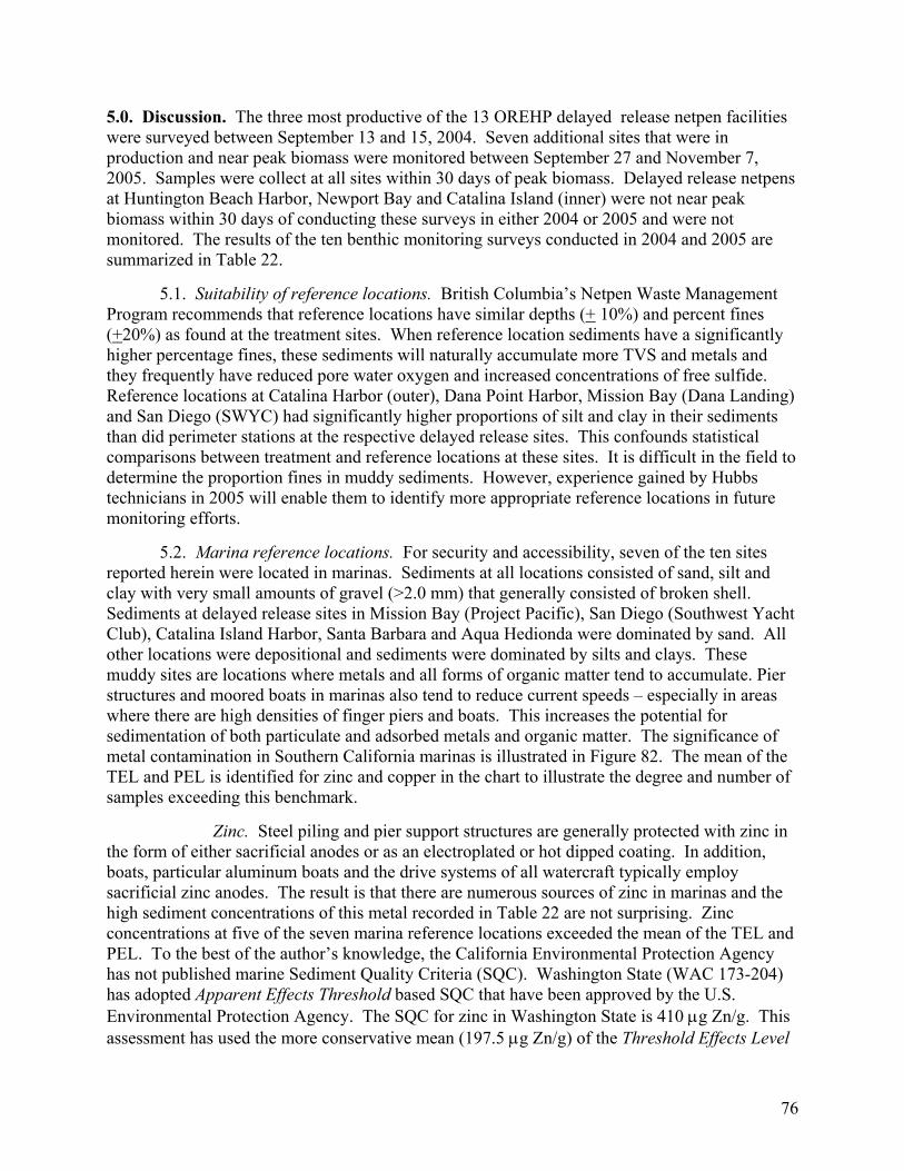
76
5.0. Discussion. The three most productive of the 13 OREHP delayed release netpen facilities were surveyed between September 13 and 15, 2004. Seven additional sites that were in production and near peak biomass were monitored between September 27 and November 7, 2005. Samples were collect at all sites within 30 days of peak biomass. Delayed release netpens at Huntington Beach Harbor, Newport Bay and Catalina Island (inner) were not near peak biomass within 30 days of conducting these surveys in either 2004 or 2005 and were not monitored. The results of the ten benthic monitoring surveys conducted in 2004 and 2005 are summarized in Table 22. 5.1. Suitability of reference locations. British Columbia’s Netpen Waste Management Program recommends that reference locations have similar depths (+ 10%) and percent fines (+20%) as found at the treatment sites. When reference location sediments have a significantly higher percentage fines, these sediments will naturally accumulate more TVS and metals and they frequently have reduced pore water oxygen and increased concentrations of free sulfide. Reference locations at Catalina Harbor (outer), Dana Point Harbor, Mission Bay (Dana Landing) and San Diego (SWYC) had significantly higher proportions of silt and clay in their sediments than did perimeter stations at the respective delayed release sites. This confounds statistical comparisons between treatment and reference locations at these sites. It is difficult in the field to determine the proportion fines in muddy sediments. However, experience gained by Hubbs technicians in 2005 will enable them to identify more appropriate reference locations in future monitoring efforts. 5.2. Marina reference locations. For security and accessibility, seven of the ten sites reported herein were located in marinas. Sediments at all locations consisted of sand, silt and clay with very small amounts of gravel (>2.0 mm) that generally consisted of broken shell. Sediments at delayed release sites in Mission Bay (Project Pacific), San Diego (Southwest Yacht Club), Catalina Island Harbor, Santa Barbara and Aqua Hedionda were dominated by sand. All other locations were depositional and sediments were dominated by silts and clays. These muddy sites are locations where metals and all forms of organic matter tend to accumulate. Pier structures and moored boats in marinas also tend to reduce current speeds – especially in areas where there are high densities of finger piers and boats. This increases the potential for sedimentation of both particulate and adsorbed metals and organic matter. The significance of metal contamination in Southern California marinas is illustrated in Figure 82. The mean of the TEL and PEL is identified for zinc and copper in the chart to illustrate the degree and number of samples exceeding this benchmark. Zinc. Steel piling and pier support structures are generally protected with zinc in the form of either sacrificial anodes or as an electroplated or hot dipped coating. In addition, boats, particular aluminum boats and the drive systems of all watercraft typically employ sacrificial zinc anodes. The result is that there are numerous sources of zinc in marinas and the high sediment concentrations of this metal recorded in Table 22 are not surprising. Zinc concentrations at five of the seven marina reference locations exceeded the mean of the TEL and PEL. To the best of the author’s knowledge, the California Environmental Protection Agency has not published marine Sediment Quality Criteria (SQC). Washington State (WAC 173-204) has adopted Apparent Effects Threshold based SQC that have been approved by the U.S. Environmental Protection Agency. The SQC for zinc in Washington State is 410 µg Zn/g. This assessment has used the more conservative mean (197.5 µg Zn/g) of the Threshold Effects Level
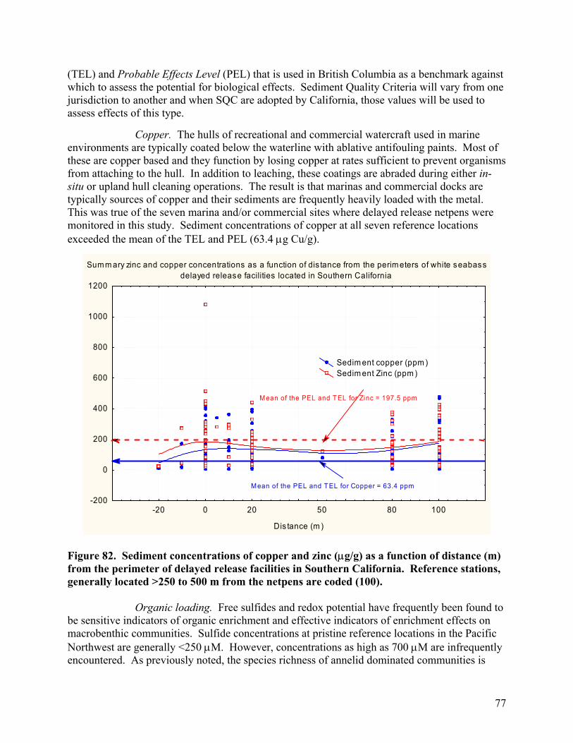
77
(TEL) and Probable Effects Level (PEL) that is used in British Columbia as a benchmark against which to assess the potential for biological effects. Sediment Quality Criteria will vary from one jurisdiction to another and when SQC are adopted by California, those values will be used to assess effects of this type. Copper. The hulls of recreational and commercial watercraft used in marine environments are typically coated below the waterline with ablative antifouling paints. Most of these are copper based and they function by losing copper at rates sufficient to prevent organisms from attaching to the hull. In addition to leaching, these coatings are abraded during either in-situ or upland hull cleaning operations. The result is that marinas and commercial docks are typically sources of copper and their sediments are frequently heavily loaded with the metal. This was true of the seven marina and/or commercial sites where delayed release netpens were monitored in this study. Sediment concentrations of copper at all seven reference locations exceeded the mean of the TEL and PEL (63.4 µg Cu/g).
Summ ary zinc and copper concentrations as a function of dis tance from the perim eters of white seabassdelayed release facilities located in Southern California
-20 0 20 50 80 100
Dis tance (m )
-200
0
200
400
600
800
1000
1200
Sedim ent copper (ppm ) Sedim ent Zinc (ppm )
Mean of the PEL and TEL for Copper = 63.4 ppm
Mean of the PEL and TEL for Zinc = 197.5 ppm
Figure 82. Sediment concentrations of copper and zinc (µg/g) as a function of distance (m) from the perimeter of delayed release facilities in Southern California. Reference stations, generally located >250 to 500 m from the netpens are coded (100). Organic loading. Free sulfides and redox potential have frequently been found to be sensitive indicators of organic enrichment and effective indicators of enrichment effects on macrobenthic communities. Sulfide concentrations at pristine reference locations in the Pacific Northwest are generally <250 µM. However, concentrations as high as 700 µM are infrequently encountered. As previously noted, the species richness of annelid dominated communities is
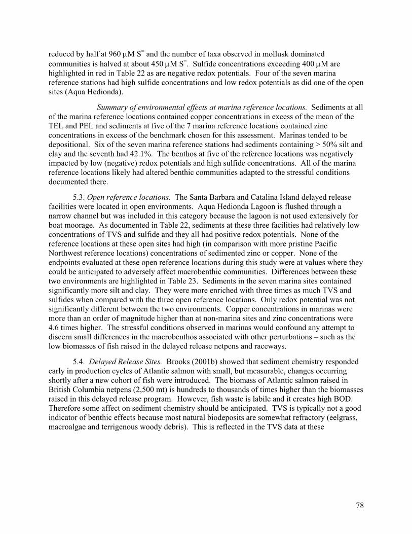
78
reduced by half at 960 µM S= and the number of taxa observed in mollusk dominated communities is halved at about 450 µM S=. Sulfide concentrations exceeding 400 µM are highlighted in red in Table 22 as are negative redox potentials. Four of the seven marina reference stations had high sulfide concentrations and low redox potentials as did one of the open sites (Aqua Hedionda). Summary of environmental effects at marina reference locations. Sediments at all of the marina reference locations contained copper concentrations in excess of the mean of the TEL and PEL and sediments at five of the 7 marina reference locations contained zinc concentrations in excess of the benchmark chosen for this assessment. Marinas tended to be depositional. Six of the seven marina reference stations had sediments containing > 50% silt and clay and the seventh had 42.1%. The benthos at five of the reference locations was negatively impacted by low (negative) redox potentials and high sulfide concentrations. All of the marina reference locations likely had altered benthic communities adapted to the stressful conditions documented there. 5.3. Open reference locations. The Santa Barbara and Catalina Island delayed release facilities were located in open environments. Aqua Hedionda Lagoon is flushed through a narrow channel but was included in this category because the lagoon is not used extensively for boat moorage. As documented in Table 22, sediments at these three facilities had relatively low concentrations of TVS and sulfide and they all had positive redox potentials. None of the reference locations at these open sites had high (in comparison with more pristine Pacific Northwest reference locations) concentrations of sedimented zinc or copper. None of the endpoints evaluated at these open reference locations during this study were at values where they could be anticipated to adversely affect macrobenthic communities. Differences between these two environments are highlighted in Table 23. Sediments in the seven marina sites contained significantly more silt and clay. They were more enriched with three times as much TVS and sulfides when compared with the three open reference locations. Only redox potential was not significantly different between the two environments. Copper concentrations in marinas were more than an order of magnitude higher than at non-marina sites and zinc concentrations were 4.6 times higher. The stressful conditions observed in marinas would confound any attempt to discern small differences in the macrobenthos associated with other perturbations – such as the low biomasses of fish raised in the delayed release netpens and raceways. 5.4. Delayed Release Sites. Brooks (2001b) showed that sediment chemistry responded early in production cycles of Atlantic salmon with small, but measurable, changes occurring shortly after a new cohort of fish were introduced. The biomass of Atlantic salmon raised in British Columbia netpens (2,500 mt) is hundreds to thousands of times higher than the biomasses raised in this delayed release program. However, fish waste is labile and it creates high BOD. Therefore some affect on sediment chemistry should be anticipated. TVS is typically not a good indicator of benthic effects because most natural biodeposits are somewhat refractory (eelgrass, macroalgae and terrigenous woody debris). This is reflected in the TVS data at these
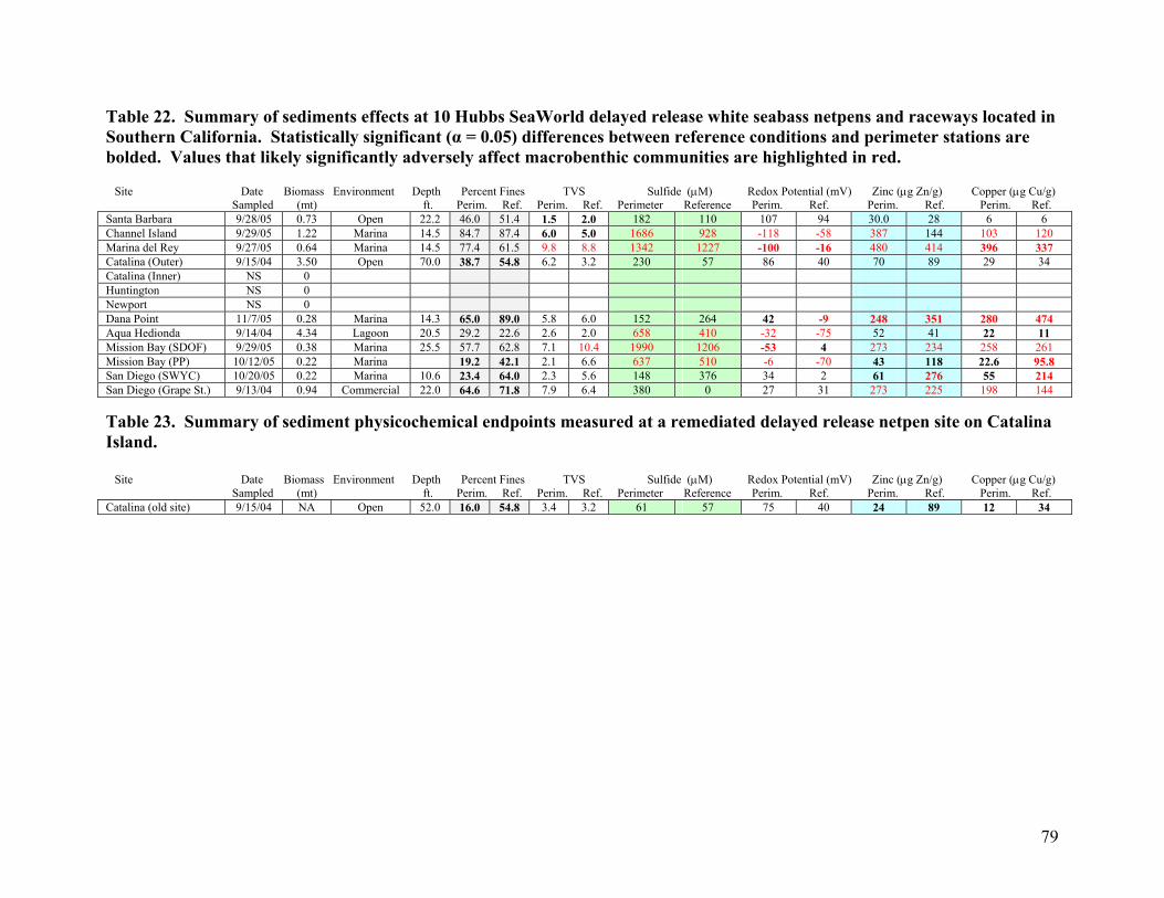
79
Table 22. Summary of sediments effects at 10 Hubbs SeaWorld delayed release white seabass netpens and raceways located in Southern California. Statistically significant (α = 0.05) differences between reference conditions and perimeter stations are bolded. Values that likely significantly adversely affect macrobenthic communities are highlighted in red. Site Date Biomass Environment Depth Percent Fines TVS Sulfide (µM) Redox Potential (mV) Zinc (µg Zn/g) Copper (µg Cu/g) Sampled (mt) ft. Perim. Ref. Perim. Ref. Perimeter Reference Perim. Ref. Perim. Ref. Perim. Ref. Santa Barbara 9/28/05 0.73 Open 22.2 46.0 51.4 1.5 2.0 182 110 107 94 30.0 28 6 6 Channel Island 9/29/05 1.22 Marina 14.5 84.7 87.4 6.0 5.0 1686 928 -118 -58 387 144 103 120 Marina del Rey 9/27/05 0.64 Marina 14.5 77.4 61.5 9.8 8.8 1342 1227 -100 -16 480 414 396 337 Catalina (Outer) 9/15/04 3.50 Open 70.0 38.7 54.8 6.2 3.2 230 57 86 40 70 89 29 34 Catalina (Inner) NS 0 Huntington NS 0 Newport NS 0 Dana Point 11/7/05 0.28 Marina 14.3 65.0 89.0 5.8 6.0 152 264 42 -9 248 351 280 474 Aqua Hedionda 9/14/04 4.34 Lagoon 20.5 29.2 22.6 2.6 2.0 658 410 -32 -75 52 41 22 11 Mission Bay (SDOF) 9/29/05 0.38 Marina 25.5 57.7 62.8 7.1 10.4 1990 1206 -53 4 273 234 258 261 Mission Bay (PP) 10/12/05 0.22 Marina 19.2 42.1 2.1 6.6 637 510 -6 -70 43 118 22.6 95.8 San Diego (SWYC) 10/20/05 0.22 Marina 10.6 23.4 64.0 2.3 5.6 148 376 34 2 61 276 55 214 San Diego (Grape St.) 9/13/04 0.94 Commercial 22.0 64.6 71.8 7.9 6.4 380 0 27 31 273 225 198 144 Table 23. Summary of sediment physicochemical endpoints measured at a remediated delayed release netpen site on Catalina Island. Site Date Biomass Environment Depth Percent Fines TVS Sulfide (µM) Redox Potential (mV) Zinc (µg Zn/g) Copper (µg Cu/g) Sampled (mt) ft. Perim. Ref. Perim. Ref. Perimeter Reference Perim. Ref. Perim. Ref. Perim. Ref. Catalina (old site) 9/15/04 NA Open 52.0 16.0 54.8 3.4 3.2 61 57 75 40 24 89 12 34
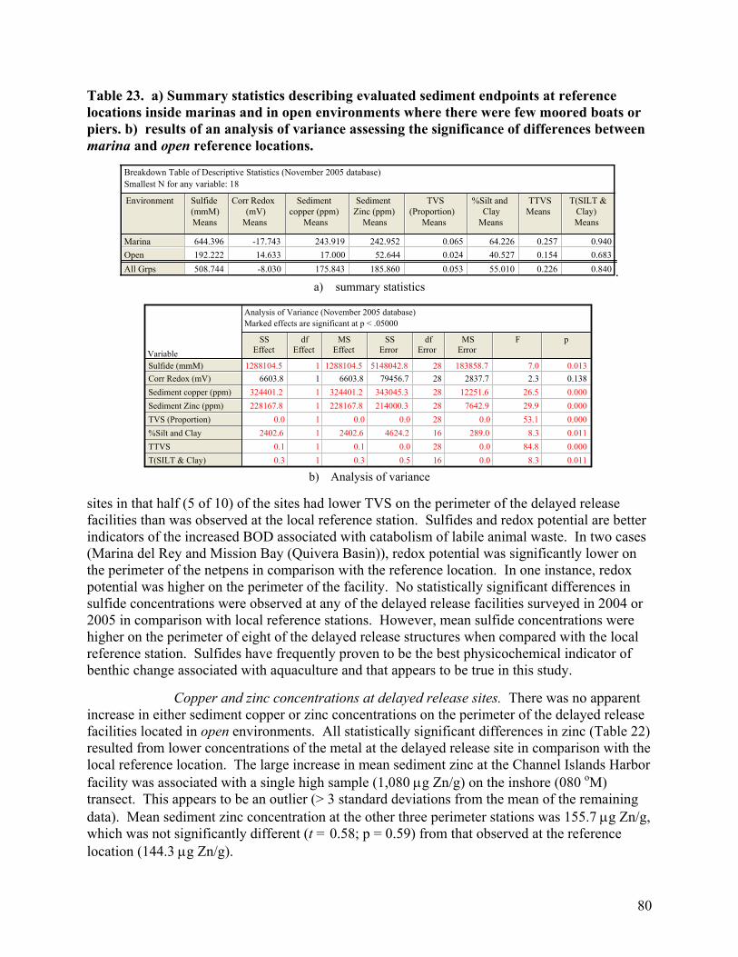
80
Table 23. a) Summary statistics describing evaluated sediment endpoints at reference locations inside marinas and in open environments where there were few moored boats or piers. b) results of an analysis of variance assessing the significance of differences between marina and open reference locations.
Breakdown Table of Descriptive Statistics (November 2005 database)Smallest N for any variable: 18
Environment Sulfide(mmM)Means
Corr Redox(mV)
Means
Sedimentcopper (ppm)
Means
SedimentZinc (ppm)
Means
TVS(Proportion)
Means
%Silt andClay
Means
TTVSMeans
T(SILT &Clay)Means
Marina 644.396 -17.743 243.919 242.952 0.065 64.226 0.257 0.940Open 192.222 14.633 17.000 52.644 0.024 40.527 0.154 0.683All Grps 508.744 -8.030 175.843 185.860 0.053 55.010 0.226 0.840 .
a) summary statistics
Analysis of Variance (November 2005 database)Marked effects are significant at p < .05000
VariableSS
Effectdf
EffectMS
EffectSS
Errordf
ErrorMS
ErrorF p
Sulfide (mmM)Corr Redox (mV)Sediment copper (ppm)Sediment Zinc (ppm)TVS (Proportion)%Silt and ClayTTVST(SILT & Clay)
1288104.5 1 1288104.5 5148042.8 28 183858.7 7.0 0.0136603.8 1 6603.8 79456.7 28 2837.7 2.3 0.138
324401.2 1 324401.2 343045.3 28 12251.6 26.5 0.000228167.8 1 228167.8 214000.3 28 7642.9 29.9 0.000
0.0 1 0.0 0.0 28 0.0 53.1 0.0002402.6 1 2402.6 4624.2 16 289.0 8.3 0.011
0.1 1 0.1 0.0 28 0.0 84.8 0.0000.3 1 0.3 0.5 16 0.0 8.3 0.011
b) Analysis of variance
sites in that half (5 of 10) of the sites had lower TVS on the perimeter of the delayed release facilities than was observed at the local reference station. Sulfides and redox potential are better indicators of the increased BOD associated with catabolism of labile animal waste. In two cases (Marina del Rey and Mission Bay (Quivera Basin)), redox potential was significantly lower on the perimeter of the netpens in comparison with the reference location. In one instance, redox potential was higher on the perimeter of the facility. No statistically significant differences in sulfide concentrations were observed at any of the delayed release facilities surveyed in 2004 or 2005 in comparison with local reference stations. However, mean sulfide concentrations were higher on the perimeter of eight of the delayed release structures when compared with the local reference station. Sulfides have frequently proven to be the best physicochemical indicator of benthic change associated with aquaculture and that appears to be true in this study. Copper and zinc concentrations at delayed release sites. There was no apparent increase in either sediment copper or zinc concentrations on the perimeter of the delayed release facilities located in open environments. All statistically significant differences in zinc (Table 22) resulted from lower concentrations of the metal at the delayed release site in comparison with the local reference location. The large increase in mean sediment zinc at the Channel Islands Harbor facility was associated with a single high sample (1,080 µg Zn/g) on the inshore (080 oM) transect. This appears to be an outlier (> 3 standard deviations from the mean of the remaining data). Mean sediment zinc concentration at the other three perimeter stations was 155.7 µg Zn/g, which was not significantly different (t = 0.58; p = 0.59) from that observed at the reference location (144.3 µg Zn/g).
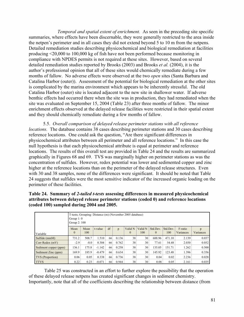
81
Temporal and spatial extent of enrichment. As seen in the preceding site specific summaries, where effects have been discernable, they were generally restricted to the area inside the netpen’s perimeter and in all cases they did not extend beyond 5 to 10 m from the netpens. Detailed remediation studies describing physicochemical and biological remediation at facilities producing <20,000 to 100,000 kg of fish have not been performed because monitoring in compliance with NPDES permits is not required at these sites. However, based on several detailed remediation studies reported by Brooks (2003) and Brooks et al. (2004), it is the author’s professional opinion that all of these sites would chemically remediate during a few months of fallow. No adverse effects were observed at the two open sites (Santa Barbara and Catalina Harbor (outer)). Assessment of the potential for biological remediation at the other sites is complicated by the marina environment which appears to be inherently stressful. The old Catalina Harbor (outer) site is located adjacent to the new site in shallower water. If adverse benthic effects had occurred there when the site was in production, they had remediated when the site was evaluated on September 15, 2004 (Table 23) after three months of fallow. The minor enrichment effects observed at the delayed release facilities were restricted in their spatial extent and they should chemically remediate during a few months of fallow. 5.5. Overall comparison of delayed release perimeter stations with all reference locations. The database contains 38 cases describing perimeter stations and 30 cases describing reference locations. One could ask the question, “Are there significant differences in physicochemical attributes between all perimeter and all reference locations.” In this case the null hypothesis is that each physicochemical attribute is equal at perimeter and reference locations. The results of this overall test are provided in Table 24 and the results are summarized graphically in Figures 68 and 69. TVS was marginally higher on perimeter stations as was the concentration of sulfides. However, redox potential was lower and sedimented copper and zinc higher at the reference locations than on the perimeter of the delayed release structures. Even with 30 and 38 samples, none of the differences were significant. It should be noted that Table 24 suggests that sulfides were the most sensitive indicator of the increased organic loading on the perimeter of these facilities. Table 24. Summary of 2-tailed t-tests assessing differences in measured physicochemical attributes between delayed release perimeter stations (coded 0) and reference locations (coded 100) sampled during 2004 and 2005.
T-tests; Grouping: Distance (m) (November 2005 database)Group 1: 0Group 2: 100
VariableMean
0Mean100
t-value df p Valid N0
Valid N100
Std.Dev.0
Std.Dev.100
F-ratioVariances
pVariances
Sulfide (mmM)Corr Redox (mV)Sediment copper (ppm)Sediment Zinc (ppm)TVS (Proportion)TTVS
731.2 508.7 1.510 66 0.136 38 30 688.96 471.10 2.139 0.037-2.9 -8.0 0.304 66 0.762 38 30 77.61 54.48 2.030 0.052
136.1 175.8 -1.142 66 0.258 38 30 135.05 151.71 1.262 0.500169.9 185.9 -0.479 66 0.634 38 30 145.92 123.48 1.396 0.356
0.06 0.05 0.338 66 0.736 38 30 0.04 0.02 2.236 0.0280.22 0.23 -0.071 66 0.944 38 30 0.08 0.05 2.161 0.035
Table 25 was constructed in an effort to further explore the possibility that the operation of these delayed release netpens has created significant changes in sediment chemistry. Importantly, note that all of the coefficients describing the relationship between distance (from
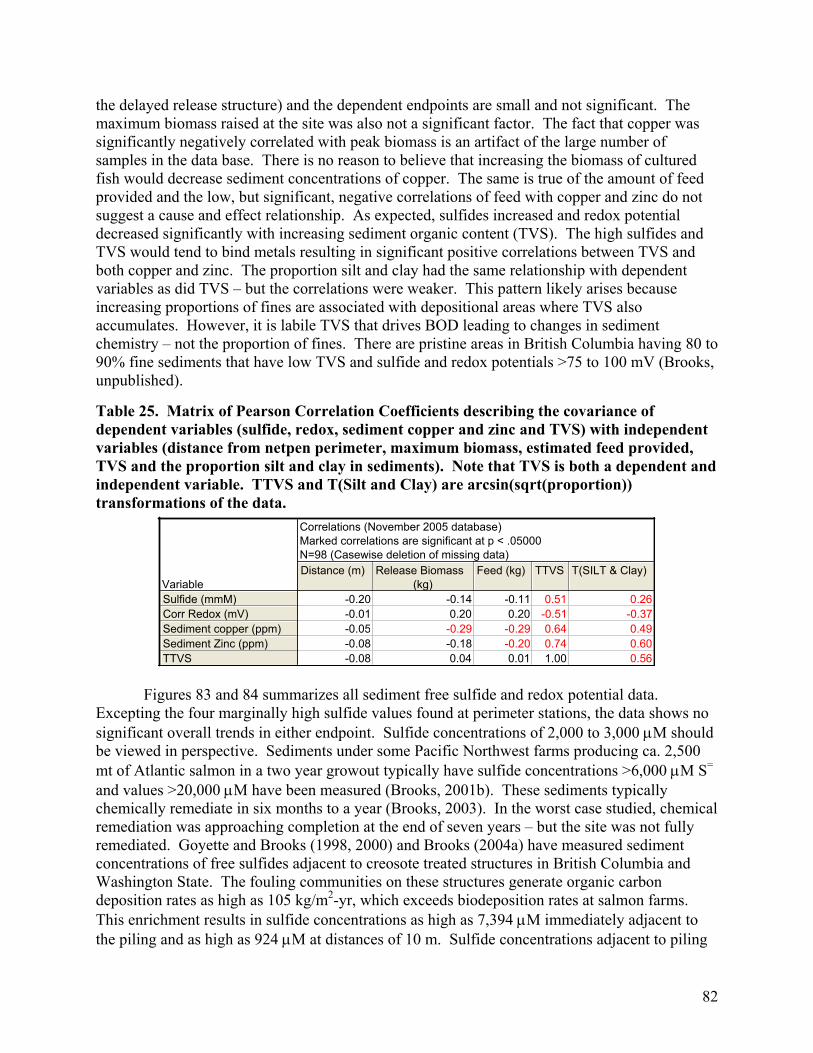
82
the delayed release structure) and the dependent endpoints are small and not significant. The maximum biomass raised at the site was also not a significant factor. The fact that copper was significantly negatively correlated with peak biomass is an artifact of the large number of samples in the data base. There is no reason to believe that increasing the biomass of cultured fish would decrease sediment concentrations of copper. The same is true of the amount of feed provided and the low, but significant, negative correlations of feed with copper and zinc do not suggest a cause and effect relationship. As expected, sulfides increased and redox potential decreased significantly with increasing sediment organic content (TVS). The high sulfides and TVS would tend to bind metals resulting in significant positive correlations between TVS and both copper and zinc. The proportion silt and clay had the same relationship with dependent variables as did TVS – but the correlations were weaker. This pattern likely arises because increasing proportions of fines are associated with depositional areas where TVS also accumulates. However, it is labile TVS that drives BOD leading to changes in sediment chemistry – not the proportion of fines. There are pristine areas in British Columbia having 80 to 90% fine sediments that have low TVS and sulfide and redox potentials >75 to 100 mV (Brooks, unpublished). Table 25. Matrix of Pearson Correlation Coefficients describing the covariance of dependent variables (sulfide, redox, sediment copper and zinc and TVS) with independent variables (distance from netpen perimeter, maximum biomass, estimated feed provided, TVS and the proportion silt and clay in sediments). Note that TVS is both a dependent and independent variable. TTVS and T(Silt and Clay) are arcsin(sqrt(proportion)) transformations of the data.
Correlations (November 2005 database)Marked correlations are significant at p < .05000N=98 (Casewise deletion of missing data)
VariableDistance (m) Release Biomass
(kg)Feed (kg) TTVS T(SILT & Clay)
Sulfide (mmM)Corr Redox (mV)Sediment copper (ppm)Sediment Zinc (ppm)TTVS
-0.20 -0.14 -0.11 0.51 0.26-0.01 0.20 0.20 -0.51 -0.37-0.05 -0.29 -0.29 0.64 0.49-0.08 -0.18 -0.20 0.74 0.60-0.08 0.04 0.01 1.00 0.56
Figures 83 and 84 summarizes all sediment free sulfide and redox potential data. Excepting the four marginally high sulfide values found at perimeter stations, the data shows no significant overall trends in either endpoint. Sulfide concentrations of 2,000 to 3,000 µM should be viewed in perspective. Sediments under some Pacific Northwest farms producing ca. 2,500 mt of Atlantic salmon in a two year growout typically have sulfide concentrations >6,000 µM S= and values >20,000 µM have been measured (Brooks, 2001b). These sediments typically chemically remediate in six months to a year (Brooks, 2003). In the worst case studied, chemical remediation was approaching completion at the end of seven years – but the site was not fully remediated. Goyette and Brooks (1998, 2000) and Brooks (2004a) have measured sediment concentrations of free sulfides adjacent to creosote treated structures in British Columbia and Washington State. The fouling communities on these structures generate organic carbon deposition rates as high as 105 kg/m2-yr, which exceeds biodeposition rates at salmon farms. This enrichment results in sulfide concentrations as high as 7,394 µM immediately adjacent to the piling and as high as 924 µM at distances of 10 m. Sulfide concentrations adjacent to piling
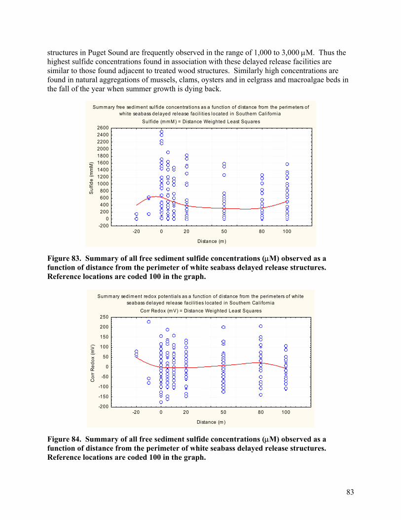
83
structures in Puget Sound are frequently observed in the range of 1,000 to 3,000 µM. Thus the highest sulfide concentrations found in association with these delayed release facilities are similar to those found adjacent to treated wood structures. Similarly high concentrations are found in natural aggregations of mussels, clams, oysters and in eelgrass and macroalgae beds in the fall of the year when summer growth is dying back.
Summary free sediment sul fide concentrations as a function of distance from the perimeters ofwhi te seabass delayed release faci l i ties located in Southern Cal i fornia
Sul fide (mmM) = Distance Weighted Least Squares
-20 0 20 50 80 100
Distance (m)
-2000
200400600800
100012001400160018002000220024002600
Sul
fide
(mm
M)
Figure 83. Summary of all free sediment sulfide concentrations (µM) observed as a function of distance from the perimeter of white seabass delayed release structures. Reference locations are coded 100 in the graph.
Summary sediment redox potentials as a function of distance from the perimeters of whi te
seabass delayed release faci l i ties located in Southern Cal i forniaCorr Redox (mV) = Distance Weighted Least Squares
-20 0 20 50 80 100
Distance (m)
-200
-150
-100
-50
0
50
100
150
200
250
Cor
r Red
ox (m
V)
Figure 84. Summary of all free sediment sulfide concentrations (µM) observed as a function of distance from the perimeter of white seabass delayed release structures. Reference locations are coded 100 in the graph.
84
6.0. Summary. Seven of the 10 delayed release facilities surveyed in this study were located in marinas. Reference stations within these marinas indicated that they tended to be depositional and that their sediments accumulated moderate amounts of organic detritus leading to increased BOD; elevated concentrations of free sediment sulfides; and reduced redox potential. In addition, marina sediments accumulate biologically significant quantities of zinc. Metal source inventories were not completed as part of this study. However, it is hypothesized that zinc from steel structures and sacrificial anodes and copper from bottom paints and the likely sources of these metals. It is also likely that elevated sulfide concentrations associated with organic enrichment mediate the metal toxicity by binding both copper and zinc. White seabass delayed release facilities located in open environments like Santa Barbara and Catalina Harbor (outer) have created no observable changes in sediment chemistry. While increases in sediment sulfides were not statistically significant at any of these sites, the combination of small increases in TVS and sulfides together with small reductions in redox potential suggest some minor enrichment under the delayed release netpens. These effects did not extend beyond 5 to 10 m from the perimeter of the facilities and the small degree of effect suggests that chemical remediation, seen as a decrease in TVS and sulfides and an increase in redox potential to background levels, would occur within a few months of fallow. However, documenting chemical remediation would be problematic when the hypothesized disturbances have not been found to be statistically significant. There is no evidence in this report that the delayed release facilities are significantly exacerbating existing sediment metal contamination. However, the OREHP is encouraged to continue to require the use of proteinated zinc supplements in feed formulations. In addition, it is recommended that where copper treated nets are used, those nets should be cleaned at an upland facility and the dislodged copper properly disposed of. Food conversion ratios determined using estimated feeding rates ranged from 2.0 to 9.0 in this study. Brooks (2004b) reported an FCR of 2.0 for cultured black cod and that seems a reasonable goal for white seabass. Accurate accounting of the feed provided to the fish on a monthly basis together with monthly biomass estimates would allow for determination of more accurate FCRs, which are valuable management tools for identifying overfeeding leading to wasted food (increased cost of production) and increased benthic loading. Net-pen facilities producing less than 100,000 pounds of fish per year in warm water have not been required to obtain NPDES permits or to conduct periodic monitoring. To the best of the author’s knowledge, this is the first instance in which these facilities have been voluntarily surveyed. The results of these surveys and the finding of no significant adverse effects, substantiates the longstanding regulatory practice of not requiring periodic monitoring of these types of facilities.

85
References Anderson, S., 1998. Dietary supplementation of salmon diets with zinc: Alternative sources and
their effects on the environment. Report prepared by Steward Anderson, Aquaculture Industry Coordinator, Hoffmann La-Roche Ltd., 9 pp.
Brooks, K.M. 1999. Stolt Canada Arrow Pass Salmon Farm Benthic and Shellfish Effects Study
1996 – 1997. Produced for Stolt Sea Farm Incorporated, 1405 Spruce Street, Campbell River, British Columbia, Canada V9W 7K1. 107 pp. plus appendices.
Brooks, K.M. 2000. Determination of copper loss rates from Flexgard XI™ treated nets in
marine environments and evaluation of the resulting environmental risks. Report prepared for the British Columbia Ministry of Environment and the British Columbia Salmon Farmers Association. 24 pp.
Brooks, K.M. 2001a. Chapter 4. Salmon Farming and the Environment. In: Nash (2001) The
Net-pen Salmon Farming Industry in the Pacific Northwest. NOAA Technical Memorandum NMFS-NWFS-NWFSC-49. pp. 36 – 73.
Brooks, K.M. 2001b. An evaluation of the relationship between salmon farm biomass, organic
inputs to sediments, physicochemical changes associated with those inputs and the infaunal response – with emphasis on total sediment sulfides, total volatile solids, and oxidation-reduction potential as surrogate endpoints for biological monitoring – Final Report. Technical report produced for the Technical Advisory Group (TAG) to the British Columbia Ministry of Environment, 2080-A Labieux Road, Nanaimo, British Columbia, Canada V9T 6J9. 186 pp. plus appendices.
Brooks, K.M., C. Mahnken and C. Nash. 2002. Environmental Effects Associated with Marine
Netpen Waste with Emphasis on Salmon Farming in the Pacific Northwest. In: Responsible Marine Aquaculture, Eds: Stickney and McVey. CABI Publishing, Wallingford, United Kingdom pp. 159 – 204.
Brooks, K.M. and C.V.W. Mahnken. 2003a. Interactions of Atlantic Salmon in the Pacific
Northwest Environment. II. Organic Wastes. Fisheries Research, Vol. 62, Issue 3, pp. 255 – 293.
Brooks, K.M. and C.V.W. Mahnken. 2003b. Interactions of Atlantic salmon in the Pacific
Northwest Environment. III. Inorganic Compounds. Fisheries Research, Vol. 62, Issue 3, pp. 295-305.
Brooks, K.M. 2003. Chemical and biological remediation of the benthos near Atlantic salmon
farms. Aquaculture, Volume 219, Issues 1-4, pp. 355-377. Brooks, K.M. , A.R. Stierns and C. Backman. 2004. Seven year remediation study at the Carrie
Bay Atlantic salmon (Salmo salar) farm in the Broughton Archipelago, British Columbia, Canada. Aquaculture. Aquaculture 239, pp. 81-123.

86
Brooks, K.M. 2004a. Environmental response to creosote treated wood structures in Puget
Sound, Washington. Technical report prepared for U.S. Creosote Council II, care-of Mr. David Webb, 357 Browns Hill Road, Valencia, PA 16059. 52 pp.
Brooks, K.M. 2004. Environmental feasibility study for aquaculture in Port Angeles Harbor and
the Straits of Juan de Fuca. Technical report prepared for Olympic Aqua Ventures, L.L.C., 111 Hurricane View Lane Port Angeles, WA 98362 42 pp.
Chow, K.W., Schell, W.R., 1978. The minerals, In Fish Feed Technology. Aquac. Dev. Coord.
Programme, Rep. ADCP/REP/80/11, FAO, Rome. Di Toro, D.M., J.D. Mahony, D.J. Hansen, K.J. Scott, A.R. Carlson, and G.T. Ankley. 1992.
Acide Volatile Sulfide Predicts the Acute Toxicity of Cadmium and Nickel in Sediments. Environ. Sci. Technol. Vol. 26. pp. 96-101.
Goyette, D. and K.M. Brooks. 1998. Creosote Evaluation: Phase II. Sooke Basin Study –
Baseline to 535 Days Post Construction 1995 – 1996. Published by Environment Canada. 224 West Esplanade, North Vancouver, British Columbia, Canada V7M 3H7. 568 pp.
Goyette, D. and K.M. Brooks. 2000. Addendum Report – Continuation of the Sooke Basin
Creosote Evaluation Study (Goyette and Brooks, 1998). Year 4 – Days 1360 and 1540. Published by Environment Canada. 224 West Esplanade, North Vancouver, British Columbia, Canada V7M 3H7. 51 pp.
Long, E.R., D.D. MacDonald, S.L. Smith and F.D. Calder. 1995. Incidence of Adverse
Biological Effects within Ranges of Chemical Concentrations in Marine and Estuarine Sediments, Environmental Management 19(1) pp. 81-97.
MacDonald, D.D. 1994. Approach to the Assessment of Sediment Quality in Florida Coastal
Waters. Florida Department of Environmental Protection, Tallahassee, Florida.
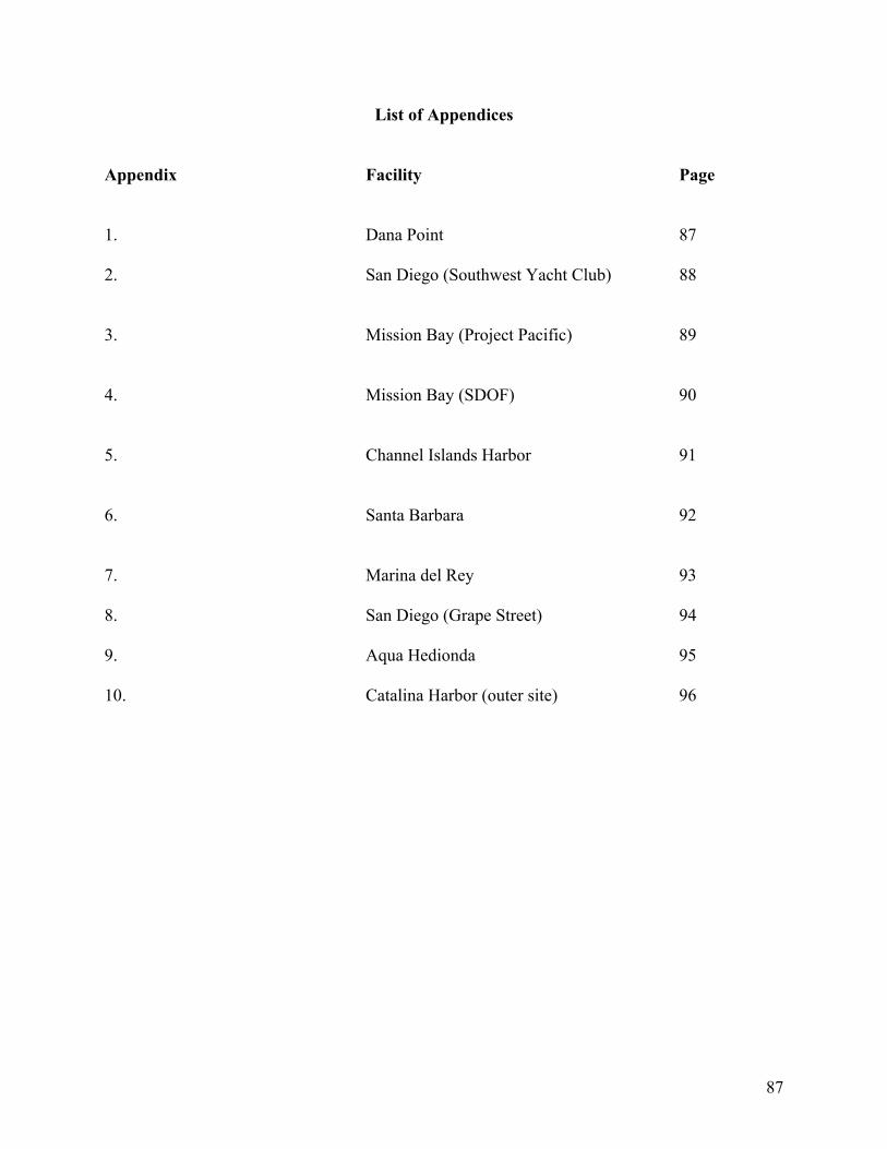
87
List of Appendices
Appendix Facility Page 1. Dana Point 87 2. San Diego (Southwest Yacht Club) 88 3. Mission Bay (Project Pacific) 89 4. Mission Bay (SDOF) 90 5. Channel Islands Harbor 91 6. Santa Barbara 92 7. Marina del Rey 93 8. San Diego (Grape Street) 94 9. Aqua Hedionda 95 10. Catalina Harbor (outer site) 96

88
Site Date Depth
(ft) Transect (Deg. M)
Distance (m) Replicate
Sulfide (mmM)
Redox (mV)
Corr Redox (mV)
Sediment copper (ppm)
Sediment Zinc
(ppm) TVS
(Proportion) %Gravel %Sand
%Silt and Clay
Latitude (N)1
Longitude (W)
Dana Point 11/7/2005 15 10 0 1 163 -182 25.0 266.0 244.0 0.063 0.74 37.45 61.81 33 27.483 117 41.606 Dana Point 11/7/2005 16 10 5 1.0 135.0 -187 20.0 0.05 33 27.484 117 41.603 Dana Point 11/7/2005 16 10 10 1.0 76.2 -166 40.6 0.05 33 27.488 117 41.602 Dana Point 11/7/2005 16 10 20 1.0 7.2 -84.6 122.1 191.0 138.0 0.03 0.75 50.11 49.1 33 27.502 117 41.598 Dana Point 11/7/2005 16 10 50 1.0 6.2 -82.7 124.0 0.04 33 27.509 117 41.598 Dana Point 11/7/2005 16 10 80 1.0 12.2 -102 105.0 61.6 61.5 0.01 2.21 74.01 23.8 33 27.524 117 41.591 Dana Point 11/7/2005 15 100 0 1.0 154.0 -137 69.6 254.0 244.0 0.06 0.68 33.94 65.4 33 27.479 117 41.597 Dana Point 11/7/2005 13 100 5 1.0 77.4 -147 59.9 342.0 280.0 0.04 2.21 50.56 47.2 33 27.482 117 41.596 Dana Point 11/7/2005 13 100 10 1.0 131.0 -168 38.6 366.0 273.0 0.03 4.88 64.29 30.8 33 27.481 117 41.591 Dana Point 11/7/2005 15 280 0 1.0 138.0 -174 32.9 319.0 257.0 0.05 0.63 31.46 67.9 33 27.483 117 41.611 Dana Point 11/7/2005 15 280 5 1.0 401.0 -216 -9.5 0.05 33 27.484 117 41.616 Dana Point 11/7/2005 15 280 10 1.0 154.0 -185 22.0 0.04 33 27.486 117 41.617 Dana Point 11/7/2005 15 280 20 1.0 82.2 -183 24.0 167.0 122.0 0.05 1.25 40.80 57.9 33 27.488 117 41.624 Dana Point 11/7/2005 17 280 50 1.0 51.5 -163 43.8 0.06 33 27.490 117 41.641 Dana Point 11/7/2005 15 280 80 1.0 42.2 -132 75.2 304.0 221.0 0.07 0.00 14.92 85.1 33 27.496 117 41.660 Dana Point 11/7/2005 14 C1 100 1.0 156.0 -194 13.0 473.0 352.0 0.06 33 27.493 117 41.789 Dana Point 11/7/2005 14 C1 100 2.0 350.0 -231 -24.1 480.0 358.0 0.06 0.00 10.98 89.0 33 27.493 117 41.789 Dana Point 11/7/2005 14 C1 100 3.0 286.3 -224 -17.2 470.0 344.0 0.06 33 27.493 117 41.789
Appendix (1)
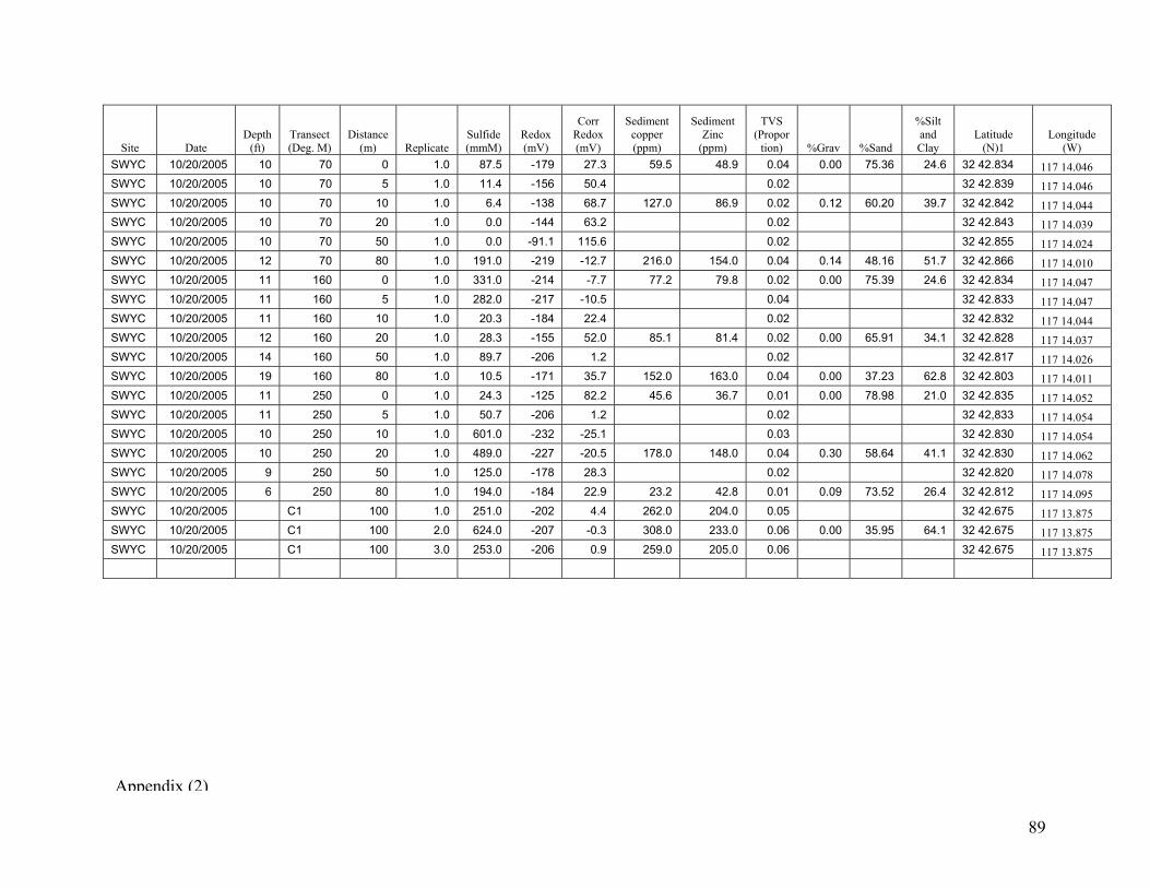
89
Site Date Depth
(ft) Transect (Deg. M)
Distance (m) Replicate
Sulfide (mmM)
Redox (mV)
Corr Redox (mV)
Sediment copper (ppm)
Sediment Zinc
(ppm)
TVS (Propor
tion) %Grav %Sand
%Silt and Clay
Latitude (N)1
Longitude (W)
SWYC 10/20/2005 10 70 0 1.0 87.5 -179 27.3 59.5 48.9 0.04 0.00 75.36 24.6 32 42.834 117 14.046 SWYC 10/20/2005 10 70 5 1.0 11.4 -156 50.4 0.02 32 42.839 117 14.046 SWYC 10/20/2005 10 70 10 1.0 6.4 -138 68.7 127.0 86.9 0.02 0.12 60.20 39.7 32 42.842 117 14.044 SWYC 10/20/2005 10 70 20 1.0 0.0 -144 63.2 0.02 32 42.843 117 14.039 SWYC 10/20/2005 10 70 50 1.0 0.0 -91.1 115.6 0.02 32 42.855 117 14.024 SWYC 10/20/2005 12 70 80 1.0 191.0 -219 -12.7 216.0 154.0 0.04 0.14 48.16 51.7 32 42.866 117 14.010 SWYC 10/20/2005 11 160 0 1.0 331.0 -214 -7.7 77.2 79.8 0.02 0.00 75.39 24.6 32 42.834 117 14.047 SWYC 10/20/2005 11 160 5 1.0 282.0 -217 -10.5 0.04 32 42.833 117 14.047 SWYC 10/20/2005 11 160 10 1.0 20.3 -184 22.4 0.02 32 42.832 117 14.044 SWYC 10/20/2005 12 160 20 1.0 28.3 -155 52.0 85.1 81.4 0.02 0.00 65.91 34.1 32 42.828 117 14.037 SWYC 10/20/2005 14 160 50 1.0 89.7 -206 1.2 0.02 32 42.817 117 14.026 SWYC 10/20/2005 19 160 80 1.0 10.5 -171 35.7 152.0 163.0 0.04 0.00 37.23 62.8 32 42.803 117 14.011 SWYC 10/20/2005 11 250 0 1.0 24.3 -125 82.2 45.6 36.7 0.01 0.00 78.98 21.0 32 42.835 117 14.052 SWYC 10/20/2005 11 250 5 1.0 50.7 -206 1.2 0.02 32 42,833 117 14.054 SWYC 10/20/2005 10 250 10 1.0 601.0 -232 -25.1 0.03 32 42.830 117 14.054 SWYC 10/20/2005 10 250 20 1.0 489.0 -227 -20.5 178.0 148.0 0.04 0.30 58.64 41.1 32 42.830 117 14.062 SWYC 10/20/2005 9 250 50 1.0 125.0 -178 28.3 0.02 32 42.820 117 14.078 SWYC 10/20/2005 6 250 80 1.0 194.0 -184 22.9 23.2 42.8 0.01 0.09 73.52 26.4 32 42.812 117 14.095 SWYC 10/20/2005 C1 100 1.0 251.0 -202 4.4 262.0 204.0 0.05 32 42.675 117 13.875 SWYC 10/20/2005 C1 100 2.0 624.0 -207 -0.3 308.0 233.0 0.06 0.00 35.95 64.1 32 42.675 117 13.875 SWYC 10/20/2005 C1 100 3.0 253.0 -206 0.9 259.0 205.0 0.06 32 42.675 117 13.875
Appendix (2)
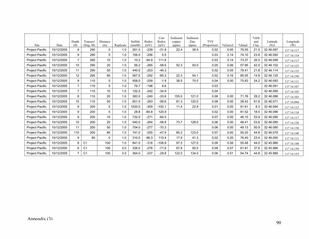
90
Site Date Depth
(ft) Transect (Deg. M)
Distance (m) Replicate
Sulfide (mmM)
Redox (mV)
Corr Redox (mV)
Sediment copper (ppm)
Sediment Zinc
(ppm) TVS
(Proportion) %Gravel %Sand
%Silt and Clay
Latitude (N)1
Longitude (W)
Project Pacific 10/12/2005 9 290 0 1.0 261.0 -239 -31.8 22.4 38.5 0.02 0.00 79.05 21.0 32 46.097 117 14.117 Project Pacific 10/12/2005 9 290 5 1.0 156.0 -206 0.5 0.03 2.14 74.10 23.8 32 46.092 117 14.114 Project Pacific 10/12/2005 7 290 10 1.0 10.2 -94.9 111.8 0.03 0.14 73.37 26.5 32 46.099 117 14.117 Project Pacific 10/12/2005 10 290 20 1.0 56.2 -265 -58.6 52.3 93.0 0.05 0.06 57.95 42.0 32 46.102 117 14.123 Project Pacific 10/12/2005 11 290 50 1.0 440.0 -253 -46.3 0.02 0.05 78.41 21.6 32 46.114 117 14.135 Project Pacific 10/12/2005 12 290 80 1.0 567.0 -292 -85.3 22.3 54.1 0.02 0.16 85.05 14.8 32 46.125 117 14.150 Project Pacific 10/12/2005 9 110 0 1.0 458.0 -209 -1.9 38.5 70.0 0.04 0.00 75.83 24.2 32 46.093 117 14.111 Project Pacific 10/12/2005 7 110 5 1.0 76.7 -198 8.6 0.03 32 46.091 117 14.107 Project Pacific 10/12/2005 7 110 10 1.0 122.0 -242 -34.9 0.04 32 46.090 117 14.105 Project Pacific 10/12/2005 8 110 20 1.0 383.0 -240 -33.6 155.0 121.0 0.06 0.00 71.76 28.2 32 46.086 117 14.103 Project Pacific 10/12/2005 10 110 50 1.0 651.0 -263 -56.6 81.3 120.0 0.08 0.00 38.43 61.6 32 46.071 117 14.094 Project Pacific 10/12/2005 9 200 0 1.0 1520.0 -309 -102.1 11.4 22.8 0.01 0.05 91.61 8.3 32 46.094 117 14.112 Project Pacific 10/12/2005 9 200 5 1.0 28.8 -85.8 120.9 0.02 0.00 81.52 18.5 32 46.096 117 14.118 Project Pacific 10/12/2005 9 200 10 1.0 732.0 -271 -64.5 0.07 0.00 46.10 53.9 32 46.090 117 14.117 Project Pacific 10/12/2005 10 200 20 1.0 540.0 -264 -56.8 73.7 128.0 0.06 0.00 46.41 53.6 32 46.085 117 14.120 Project Pacific 10/12/2005 11 200 50 1.0 704.0 -277 -70.3 0.06 0.00 49.13 50.9 32 46.080 117 14.138 Project Pacific 10/12/2005 110 200 80 1.0 741.0 -255 -47.9 85.2 123.0 0.07 0.00 55.20 44.8 32 46.078 117 14.148 Project Pacific 10/12/2005 9 80 0 1.0 310.0 -96.3 110.4 17.9 41.3 0.02 0.20 76.40 23.4 32 46.095 117 14.111 Project Pacific 10/12/2005 8 C1 100 1.0 841.0 -316 -108.9 97.5 127.0 0.06 0.56 55.48 44.0 32 45.986 117 14.148 Project Pacific 10/12/2005 6 C1 100 2.0 326.0 -278 -71.6 67.8 92.0 0.08 0.57 61.81 37.6 32 45.986 117 14.150 Project Pacific 10/12/2005 7 C1 100 3.0 364.0 -237 -29.8 122.0 134.0 0.06 0.51 54.74 44.8 32 45.989 117 14.153
Appendix (3)
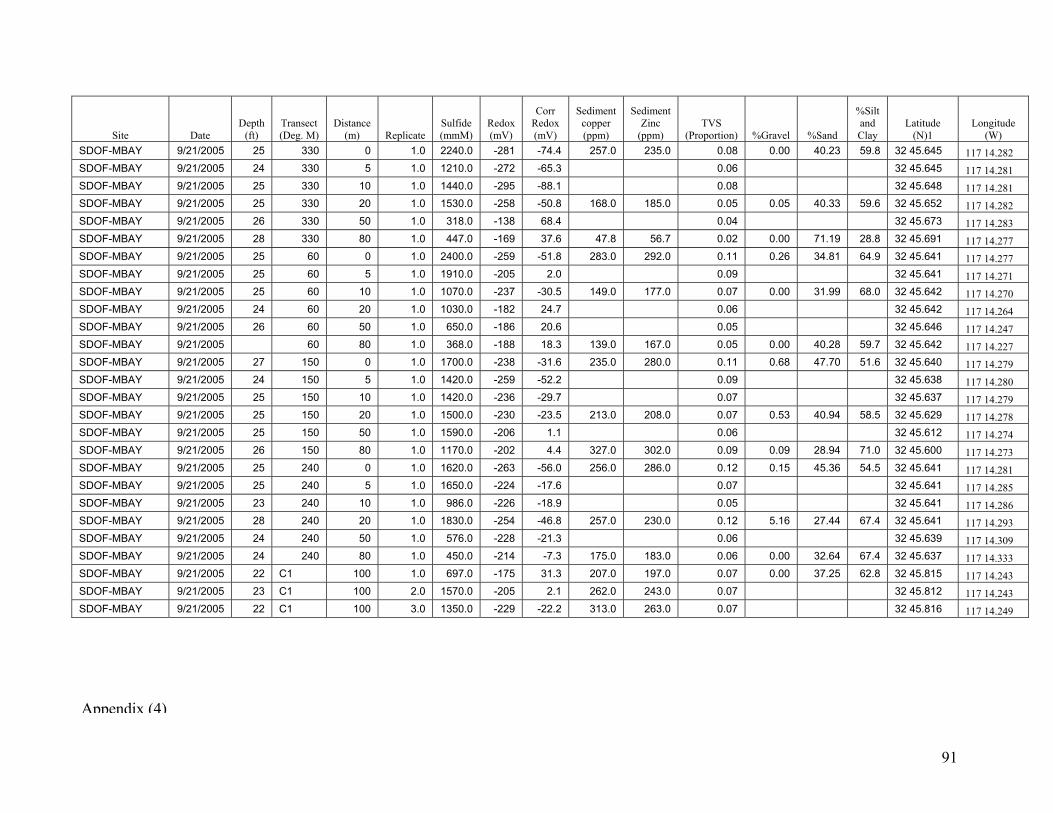
91
Site Date Depth
(ft) Transect (Deg. M)
Distance (m) Replicate
Sulfide (mmM)
Redox (mV)
Corr Redox (mV)
Sediment copper (ppm)
Sediment Zinc
(ppm) TVS
(Proportion) %Gravel %Sand
%Silt and Clay
Latitude (N)1
Longitude (W)
SDOF-MBAY 9/21/2005 25 330 0 1.0 2240.0 -281 -74.4 257.0 235.0 0.08 0.00 40.23 59.8 32 45.645 117 14.282 SDOF-MBAY 9/21/2005 24 330 5 1.0 1210.0 -272 -65.3 0.06 32 45.645 117 14.281 SDOF-MBAY 9/21/2005 25 330 10 1.0 1440.0 -295 -88.1 0.08 32 45.648 117 14.281 SDOF-MBAY 9/21/2005 25 330 20 1.0 1530.0 -258 -50.8 168.0 185.0 0.05 0.05 40.33 59.6 32 45.652 117 14.282 SDOF-MBAY 9/21/2005 26 330 50 1.0 318.0 -138 68.4 0.04 32 45.673 117 14.283 SDOF-MBAY 9/21/2005 28 330 80 1.0 447.0 -169 37.6 47.8 56.7 0.02 0.00 71.19 28.8 32 45.691 117 14.277 SDOF-MBAY 9/21/2005 25 60 0 1.0 2400.0 -259 -51.8 283.0 292.0 0.11 0.26 34.81 64.9 32 45.641 117 14.277 SDOF-MBAY 9/21/2005 25 60 5 1.0 1910.0 -205 2.0 0.09 32 45.641 117 14.271 SDOF-MBAY 9/21/2005 25 60 10 1.0 1070.0 -237 -30.5 149.0 177.0 0.07 0.00 31.99 68.0 32 45.642 117 14.270 SDOF-MBAY 9/21/2005 24 60 20 1.0 1030.0 -182 24.7 0.06 32 45.642 117 14.264 SDOF-MBAY 9/21/2005 26 60 50 1.0 650.0 -186 20.6 0.05 32 45.646 117 14.247 SDOF-MBAY 9/21/2005 60 80 1.0 368.0 -188 18.3 139.0 167.0 0.05 0.00 40.28 59.7 32 45.642 117 14.227 SDOF-MBAY 9/21/2005 27 150 0 1.0 1700.0 -238 -31.6 235.0 280.0 0.11 0.68 47.70 51.6 32 45.640 117 14.279 SDOF-MBAY 9/21/2005 24 150 5 1.0 1420.0 -259 -52.2 0.09 32 45.638 117 14.280 SDOF-MBAY 9/21/2005 25 150 10 1.0 1420.0 -236 -29.7 0.07 32 45.637 117 14.279 SDOF-MBAY 9/21/2005 25 150 20 1.0 1500.0 -230 -23.5 213.0 208.0 0.07 0.53 40.94 58.5 32 45.629 117 14.278 SDOF-MBAY 9/21/2005 25 150 50 1.0 1590.0 -206 1.1 0.06 32 45.612 117 14.274 SDOF-MBAY 9/21/2005 26 150 80 1.0 1170.0 -202 4.4 327.0 302.0 0.09 0.09 28.94 71.0 32 45.600 117 14.273 SDOF-MBAY 9/21/2005 25 240 0 1.0 1620.0 -263 -56.0 256.0 286.0 0.12 0.15 45.36 54.5 32 45.641 117 14.281 SDOF-MBAY 9/21/2005 25 240 5 1.0 1650.0 -224 -17.6 0.07 32 45.641 117 14.285 SDOF-MBAY 9/21/2005 23 240 10 1.0 986.0 -226 -18.9 0.05 32 45.641 117 14.286 SDOF-MBAY 9/21/2005 28 240 20 1.0 1830.0 -254 -46.8 257.0 230.0 0.12 5.16 27.44 67.4 32 45.641 117 14.293 SDOF-MBAY 9/21/2005 24 240 50 1.0 576.0 -228 -21.3 0.06 32 45.639 117 14.309 SDOF-MBAY 9/21/2005 24 240 80 1.0 450.0 -214 -7.3 175.0 183.0 0.06 0.00 32.64 67.4 32 45.637 117 14.333 SDOF-MBAY 9/21/2005 22 C1 100 1.0 697.0 -175 31.3 207.0 197.0 0.07 0.00 37.25 62.8 32 45.815 117 14.243 SDOF-MBAY 9/21/2005 23 C1 100 2.0 1570.0 -205 2.1 262.0 243.0 0.07 32 45.812 117 14.243 SDOF-MBAY 9/21/2005 22 C1 100 3.0 1350.0 -229 -22.2 313.0 263.0 0.07 32 45.816 117 14.249
Appendix (4)
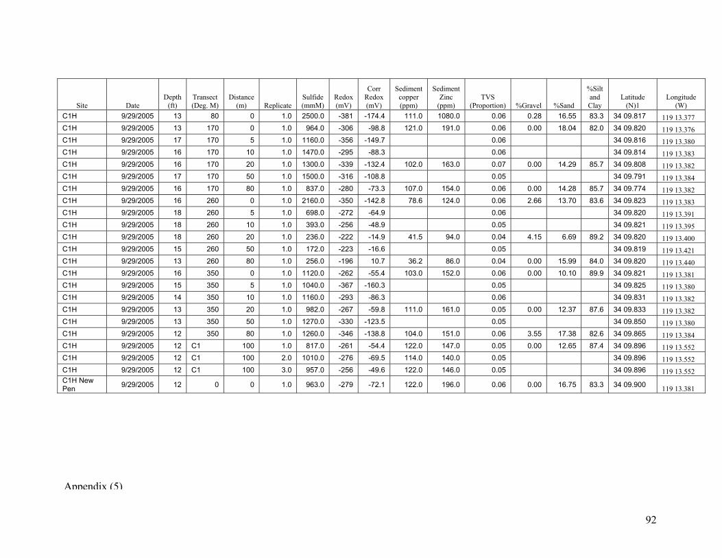
92
Site Date Depth
(ft) Transect (Deg. M)
Distance (m) Replicate
Sulfide (mmM)
Redox (mV)
Corr Redox (mV)
Sediment copper (ppm)
Sediment Zinc
(ppm) TVS
(Proportion) %Gravel %Sand
%Silt and Clay
Latitude (N)1
Longitude (W)
C1H 9/29/2005 13 80 0 1.0 2500.0 -381 -174.4 111.0 1080.0 0.06 0.28 16.55 83.3 34 09.817 119 13.377 C1H 9/29/2005 13 170 0 1.0 964.0 -306 -98.8 121.0 191.0 0.06 0.00 18.04 82.0 34 09.820 119 13.376 C1H 9/29/2005 17 170 5 1.0 1160.0 -356 -149.7 0.06 34 09.816 119 13.380 C1H 9/29/2005 16 170 10 1.0 1470.0 -295 -88.3 0.06 34 09.814 119 13.383 C1H 9/29/2005 16 170 20 1.0 1300.0 -339 -132.4 102.0 163.0 0.07 0.00 14.29 85.7 34 09.808 119 13.382 C1H 9/29/2005 17 170 50 1.0 1500.0 -316 -108.8 0.05 34 09.791 119 13.384 C1H 9/29/2005 16 170 80 1.0 837.0 -280 -73.3 107.0 154.0 0.06 0.00 14.28 85.7 34 09.774 119 13.382 C1H 9/29/2005 16 260 0 1.0 2160.0 -350 -142.8 78.6 124.0 0.06 2.66 13.70 83.6 34 09.823 119 13.383 C1H 9/29/2005 18 260 5 1.0 698.0 -272 -64.9 0.06 34 09.820 119 13.391 C1H 9/29/2005 18 260 10 1.0 393.0 -256 -48.9 0.05 34 09.821 119 13.395 C1H 9/29/2005 18 260 20 1.0 236.0 -222 -14.9 41.5 94.0 0.04 4.15 6.69 89.2 34 09.820 119 13.400 C1H 9/29/2005 15 260 50 1.0 172.0 -223 -16.6 0.05 34 09.819 119 13.421 C1H 9/29/2005 13 260 80 1.0 256.0 -196 10.7 36.2 86.0 0.04 0.00 15.99 84.0 34 09.820 119 13.440 C1H 9/29/2005 16 350 0 1.0 1120.0 -262 -55.4 103.0 152.0 0.06 0.00 10.10 89.9 34 09.821 119 13.381 C1H 9/29/2005 15 350 5 1.0 1040.0 -367 -160.3 0.05 34 09.825 119 13.380 C1H 9/29/2005 14 350 10 1.0 1160.0 -293 -86.3 0.06 34 09.831 119 13.382 C1H 9/29/2005 13 350 20 1.0 982.0 -267 -59.8 111.0 161.0 0.05 0.00 12.37 87.6 34 09.833 119 13.382 C1H 9/29/2005 13 350 50 1.0 1270.0 -330 -123.5 0.05 34 09.850 119 13.380 C1H 9/29/2005 12 350 80 1.0 1260.0 -346 -138.8 104.0 151.0 0.06 3.55 17.38 82.6 34 09.865 119 13.384 C1H 9/29/2005 12 C1 100 1.0 817.0 -261 -54.4 122.0 147.0 0.05 0.00 12.65 87.4 34 09.896 119 13.552 C1H 9/29/2005 12 C1 100 2.0 1010.0 -276 -69.5 114.0 140.0 0.05 34 09.896 119 13.552 C1H 9/29/2005 12 C1 100 3.0 957.0 -256 -49.6 122.0 146.0 0.05 34 09.896 119 13.552 C1H New Pen 9/29/2005 12 0 0 1.0 963.0 -279 -72.1 122.0 196.0 0.06 0.00 16.75 83.3 34 09.900 119 13.381
Appendix (5)
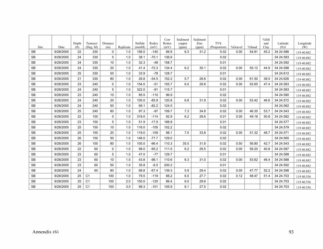
93
Site Date Depth
(ft) Transect (Deg. M)
Distance (m) Replicate
Sulfide (mmM)
Redox (mV)
Corr Redox (mV)
Sediment copper (ppm)
Sediment Zinc
(ppm) TVS
(Proportion) %Gravel %Sand
%Silt and Clay
Latitude (N)1
Longitude (W)
SB 9/28/2005 22 330 0 1.0 156.0 -140 66.9 6.3 31.2 0.02 0.00 54.81 45.2 34 24.586 119 40.882 SB 9/28/2005 24 330 5 1.0 38.1 -70.1 136.6 0.02 34 24.583 119 40.882 SB 9/28/2005 24 330 10 1.0 32.3 -48 158.7 0.01 34 24.592 119 40.882 SB 9/28/2005 24 330 20 1.0 41.4 -72.3 134.4 6.2 30.1 0.02 0.00 55.12 44.9 34 24.598 119 40.882 SB 9/28/2005 25 330 50 1.0 33.9 -78 128.7 0.01 34 24.612 119 40.882 SB 9/28/2005 21 330 80 1.0 26.8 -54.5 152.2 5.7 28.8 0.02 0.00 61.50 38.5 34 24.626 119 40.882 SB 9/28/2005 23 240 0 1.0 154.0 -51 155.7 6.0 29.8 0.02 0.00 52.65 47.4 34 24.583 119 40.882 SB 9/28/2005 24 240 5 1.0 322.0 -91 115.7 0.01 34 24.583 119 40.882 SB 9/28/2005 23 240 10 1.0 85.5 -110 96.9 0.02 34 24.580 119 40.882 SB 9/28/2005 24 240 20 1.0 105.0 -85.9 120.8 6.8 31.9 0.02 0.00 53.42 46.6 34 24.572 119 40.882 SB 9/28/2005 24 240 50 1.0 69.1 -82.2 124.5 0.02 34 24.562 119 40.882 SB 9/28/2005 25 240 80 1.0 97.3 -97 109.7 7.3 34.8 0.02 0.00 46.35 53.7 34 24.543 119 40.882 SB 9/28/2005 22 150 0 1.0 319.0 -114 92.9 6.2 29.6 0.01 0.00 49.18 50.8 34 24.582 119 40.882 SB 9/28/2005 23 150 5 1.0 51.9 -17.9 188.8 0.01 34 24.577 119 40.882 SB 9/28/2005 25 150 10 1.0 116.0 -105 102.2 0.02 34 24.579 119 40.882 SB 9/28/2005 25 150 20 1.0 119.0 -109 98.1 7.5 33.8 0.02 0.00 51.32 48.7 34 24.571 119 40.882 SB 9/28/2005 26 150 50 1.0 146.0 -77.7 129.0 0.02 34 24.565 119 40.882 SB 9/28/2005 26 150 80 1.0 105.0 -96.4 110.3 35.0 31.8 0.02 0.50 56.80 42.7 34 24.543 119 40.882 SB 9/28/2005 22 60 0 1.0 98.0 -95.2 111.5 6.2 29.5 0.02 0.00 59.20 40.8 34 24.587 119 40.882 SB 9/28/2005 23 60 5 1.0 47.0 -77 129.7 0.01 34 24.588 119 40.882 SB 9/28/2005 23 60 10 1.0 43.8 -96.1 110.6 6.3 31.0 0.02 0.00 53.62 46.4 34 24.588 119 40.882 SB 9/28/2005 23 60 50 1.0 35.8 -6.5 200.2 0.01 34 24.592 119 40.882 SB 9/28/2005 24 60 80 1.0 68.8 -67.4 139.3 5.9 29.4 0.02 0.00 47.77 52.2 34 24.598 119 40.882 SB 9/28/2005 25 C1 100 1.0 79.5 -119 88.2 6.0 27.7 0.02 0.12 48.47 51.4 34 24.703 119 40.556 SB 9/28/2005 25 C1 100 2.0 150.0 -120 86.4 6.0 29.6 0.02 34 24.703 119 40.556 SB 9/28/2005 25 C1 100 3.0 99.3 -101 105.9 6.1 27.5 0.02 34 24.703 119 40.556
Appendix (6)

94
Site Date Depth
(ft) Transect (Deg. M)
Distance (m) Replicate
Sulfide (mmM)
Redox (mV)
Corr Redox (mV)
Sediment copper (ppm)
Sediment Zinc
(ppm) TVS
(Proportion) %Gravel %Sand
%Silt and Clay
Latitude (N)1
Longitude (W)
MDREY 9/27/2005 14 340 0 1.0 1200.0 -265 -58.4 401.0 518.0 0.12 0.00 19.11 80.9 33 58.594 118 26.790 MDREY 9/27/2005 13 340 5 1.0 856.0 -251 -43.8 0.08 33 58.591 118 26.792 MDREY 9/27/2005 12 340 10 1.0 207.0 -225 -18.4 0.08 33 58.595 118 26.796 MDREY 9/27/2005 13 340 20 1.0 82.2 -179 27.6 381.0 445.0 0.08 0.00 17.10 82.9 33 58.599 118 26.793 MDREY 9/27/2005 13 340 50 1.0 742.0 -300 -93.3 0.09 33 58.616 118 26.793 MDREY 9/27/2005 13 340 80 1.0 360.0 -293 -85.8 303.0 378.0 0.06 0.09 38.75 61.2 33 58.632 118 26.792 MDREY 9/27/2005 70 0 1.0 1000.0 -285 -78.1 410.0 452.0 0.09 1.06 28.76 70.2 33 58.591 118 26.788 MDREY 9/27/2005 14 160 0 1.0 1720.0 -343 -136.7 418.0 515.0 0.10 0.00 18.51 81.5 33 58.584 118 26.795 MDREY 9/27/2005 14 160 5 1.0 1540.0 -353 -145.8 0.10 33 58.582 118 26.792 MDREY 9/27/2005 14 160 10 1.0 1080.0 -309 -102.7 0.09 0.00 17.24 82.8 33 58.580 118 26.794 MDREY 9/27/2005 14 160 20 1.0 1730.0 -353 -146.1 399.0 444.0 0.09 33 58.575 118 26.794 MDREY 9/27/2005 13 160 50 1.0 516.0 -302 -95.6 0.09 33 58.560 118 26.792 MDREY 9/27/2005 17 160 80 1.0 1030.0 -312 -104.9 311.0 364.0 0.05 0.28 14.41 85.3 33 58.544 118 26.792 MDREY 9/27/2005 15 250 0 1.0 1450.0 -333 -126.0 354.0 433.0 0.08 0.40 22.46 77.1 33 58.584 118 26.796 MDREY 9/27/2005 16 250 5 1.0 676.0 -305 -98.3 0.07 33 58.585 118 26.798 MDREY 9/27/2005 16 250 10 1.0 600.0 -293 -85.9 0.06 33 58.587 118 26.803 MDREY 9/27/2005 15 250 20 1.0 72.8 -195 12.1 306.0 335.0 0.06 0.55 11.87 87.6 33 58.587 118 26.809 MDREY 9/27/2005 15 250 50 1.0 42.8 -186 20.6 0.07 33 58.586 118 26.826 MDREY 9/27/2005 15 250 80 1.0 74.5 -176 30.6 254.0 322.0 0.07 0.00 15.17 84.8 33 58.585 118 26.845 MDREY 9/27/2005 15 C1 100 1.0 1310.0 -221 -13.9 321.0 417.0 0.13 0.00 38.49 61.5 33 58.491 118 26.740 MDREY 9/27/2005 15 C1 100 2.0 1180.0 -224 -17.6 330.0 396.0 0.07 33 58.491 118 26.740 MDREY 9/27/2005 15 C1 100 3.0 1190.0 -223 -16.3 361.0 429.0 0.07 33 58.491 118 26.740
Appendix (7)
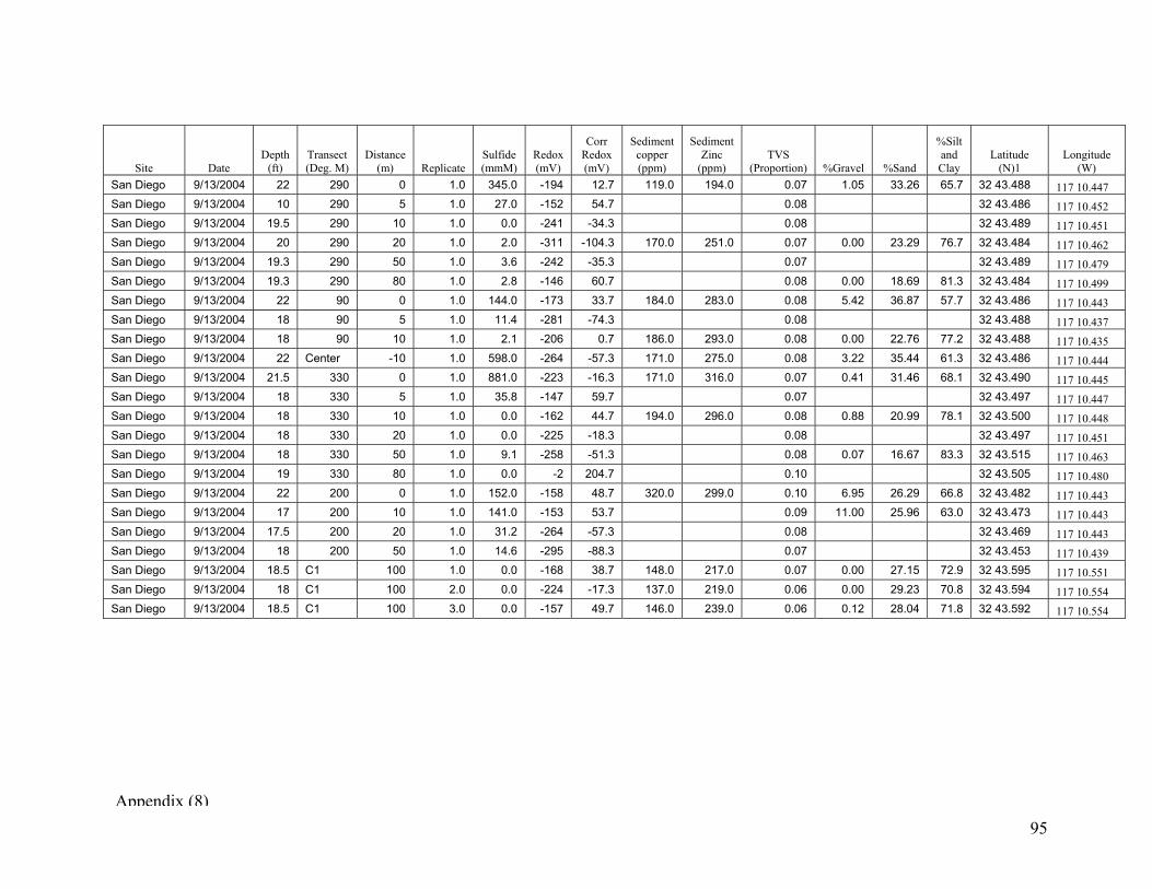
95
Site Date Depth
(ft) Transect (Deg. M)
Distance (m) Replicate
Sulfide (mmM)
Redox (mV)
Corr Redox (mV)
Sediment copper (ppm)
Sediment Zinc
(ppm) TVS
(Proportion) %Gravel %Sand
%Silt and Clay
Latitude (N)1
Longitude (W)
San Diego 9/13/2004 22 290 0 1.0 345.0 -194 12.7 119.0 194.0 0.07 1.05 33.26 65.7 32 43.488 117 10.447 San Diego 9/13/2004 10 290 5 1.0 27.0 -152 54.7 0.08 32 43.486 117 10.452 San Diego 9/13/2004 19.5 290 10 1.0 0.0 -241 -34.3 0.08 32 43.489 117 10.451 San Diego 9/13/2004 20 290 20 1.0 2.0 -311 -104.3 170.0 251.0 0.07 0.00 23.29 76.7 32 43.484 117 10.462 San Diego 9/13/2004 19.3 290 50 1.0 3.6 -242 -35.3 0.07 32 43.489 117 10.479 San Diego 9/13/2004 19.3 290 80 1.0 2.8 -146 60.7 0.08 0.00 18.69 81.3 32 43.484 117 10.499 San Diego 9/13/2004 22 90 0 1.0 144.0 -173 33.7 184.0 283.0 0.08 5.42 36.87 57.7 32 43.486 117 10.443 San Diego 9/13/2004 18 90 5 1.0 11.4 -281 -74.3 0.08 32 43.488 117 10.437 San Diego 9/13/2004 18 90 10 1.0 2.1 -206 0.7 186.0 293.0 0.08 0.00 22.76 77.2 32 43.488 117 10.435 San Diego 9/13/2004 22 Center -10 1.0 598.0 -264 -57.3 171.0 275.0 0.08 3.22 35.44 61.3 32 43.486 117 10.444 San Diego 9/13/2004 21.5 330 0 1.0 881.0 -223 -16.3 171.0 316.0 0.07 0.41 31.46 68.1 32 43.490 117 10.445 San Diego 9/13/2004 18 330 5 1.0 35.8 -147 59.7 0.07 32 43.497 117 10.447 San Diego 9/13/2004 18 330 10 1.0 0.0 -162 44.7 194.0 296.0 0.08 0.88 20.99 78.1 32 43.500 117 10.448 San Diego 9/13/2004 18 330 20 1.0 0.0 -225 -18.3 0.08 32 43.497 117 10.451 San Diego 9/13/2004 18 330 50 1.0 9.1 -258 -51.3 0.08 0.07 16.67 83.3 32 43.515 117 10.463 San Diego 9/13/2004 19 330 80 1.0 0.0 -2 204.7 0.10 32 43.505 117 10.480 San Diego 9/13/2004 22 200 0 1.0 152.0 -158 48.7 320.0 299.0 0.10 6.95 26.29 66.8 32 43.482 117 10.443 San Diego 9/13/2004 17 200 10 1.0 141.0 -153 53.7 0.09 11.00 25.96 63.0 32 43.473 117 10.443 San Diego 9/13/2004 17.5 200 20 1.0 31.2 -264 -57.3 0.08 32 43.469 117 10.443 San Diego 9/13/2004 18 200 50 1.0 14.6 -295 -88.3 0.07 32 43.453 117 10.439 San Diego 9/13/2004 18.5 C1 100 1.0 0.0 -168 38.7 148.0 217.0 0.07 0.00 27.15 72.9 32 43.595 117 10.551 San Diego 9/13/2004 18 C1 100 2.0 0.0 -224 -17.3 137.0 219.0 0.06 0.00 29.23 70.8 32 43.594 117 10.554 San Diego 9/13/2004 18.5 C1 100 3.0 0.0 -157 49.7 146.0 239.0 0.06 0.12 28.04 71.8 32 43.592 117 10.554
Appendix (8)
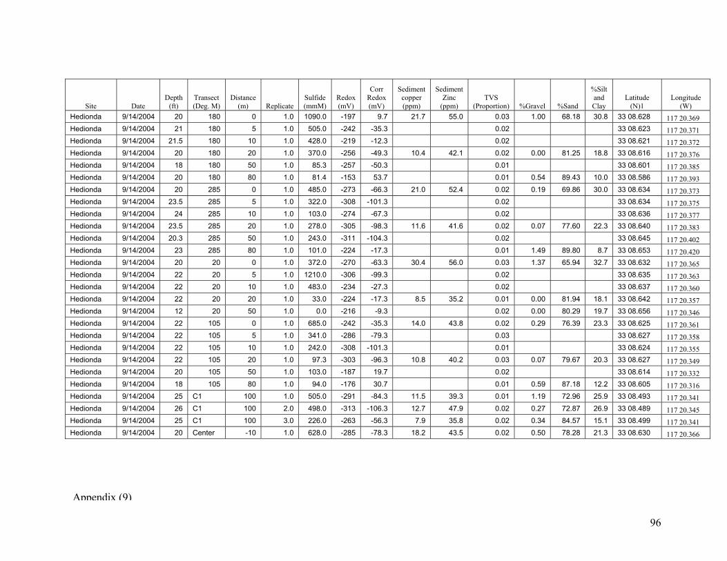
96
Site Date Depth
(ft) Transect (Deg. M)
Distance (m) Replicate
Sulfide (mmM)
Redox (mV)
Corr Redox (mV)
Sediment copper (ppm)
Sediment Zinc
(ppm) TVS
(Proportion) %Gravel %Sand
%Silt and Clay
Latitude (N)1
Longitude (W)
Hedionda 9/14/2004 20 180 0 1.0 1090.0 -197 9.7 21.7 55.0 0.03 1.00 68.18 30.8 33 08.628 117 20.369 Hedionda 9/14/2004 21 180 5 1.0 505.0 -242 -35.3 0.02 33 08.623 117 20.371 Hedionda 9/14/2004 21.5 180 10 1.0 428.0 -219 -12.3 0.02 33 08.621 117 20.372 Hedionda 9/14/2004 20 180 20 1.0 370.0 -256 -49.3 10.4 42.1 0.02 0.00 81.25 18.8 33 08.616 117 20.376 Hedionda 9/14/2004 18 180 50 1.0 85.3 -257 -50.3 0.01 33 08.601 117 20.385 Hedionda 9/14/2004 20 180 80 1.0 81.4 -153 53.7 0.01 0.54 89.43 10.0 33 08.586 117 20.393 Hedionda 9/14/2004 20 285 0 1.0 485.0 -273 -66.3 21.0 52.4 0.02 0.19 69.86 30.0 33 08.634 117 20.373 Hedionda 9/14/2004 23.5 285 5 1.0 322.0 -308 -101.3 0.02 33 08.634 117 20.375 Hedionda 9/14/2004 24 285 10 1.0 103.0 -274 -67.3 0.02 33 08.636 117 20.377 Hedionda 9/14/2004 23.5 285 20 1.0 278.0 -305 -98.3 11.6 41.6 0.02 0.07 77.60 22.3 33 08.640 117 20.383 Hedionda 9/14/2004 20.3 285 50 1.0 243.0 -311 -104.3 0.02 33 08.645 117 20.402 Hedionda 9/14/2004 23 285 80 1.0 101.0 -224 -17.3 0.01 1.49 89.80 8.7 33 08.653 117 20.420 Hedionda 9/14/2004 20 20 0 1.0 372.0 -270 -63.3 30.4 56.0 0.03 1.37 65.94 32.7 33 08.632 117 20.365 Hedionda 9/14/2004 22 20 5 1.0 1210.0 -306 -99.3 0.02 33 08.635 117 20.363 Hedionda 9/14/2004 22 20 10 1.0 483.0 -234 -27.3 0.02 33 08.637 117 20.360 Hedionda 9/14/2004 22 20 20 1.0 33.0 -224 -17.3 8.5 35.2 0.01 0.00 81.94 18.1 33 08.642 117 20.357 Hedionda 9/14/2004 12 20 50 1.0 0.0 -216 -9.3 0.02 0.00 80.29 19.7 33 08.656 117 20.346 Hedionda 9/14/2004 22 105 0 1.0 685.0 -242 -35.3 14.0 43.8 0.02 0.29 76.39 23.3 33 08.625 117 20.361 Hedionda 9/14/2004 22 105 5 1.0 341.0 -286 -79.3 0.03 33 08.627 117 20.358 Hedionda 9/14/2004 22 105 10 1.0 242.0 -308 -101.3 0.01 33 08.624 117 20.355 Hedionda 9/14/2004 22 105 20 1.0 97.3 -303 -96.3 10.8 40.2 0.03 0.07 79.67 20.3 33 08.627 117 20.349 Hedionda 9/14/2004 20 105 50 1.0 103.0 -187 19.7 0.02 33 08.614 117 20.332 Hedionda 9/14/2004 18 105 80 1.0 94.0 -176 30.7 0.01 0.59 87.18 12.2 33 08.605 117 20.316 Hedionda 9/14/2004 25 C1 100 1.0 505.0 -291 -84.3 11.5 39.3 0.01 1.19 72.96 25.9 33 08.493 117 20.341 Hedionda 9/14/2004 26 C1 100 2.0 498.0 -313 -106.3 12.7 47.9 0.02 0.27 72.87 26.9 33 08.489 117 20.345 Hedionda 9/14/2004 25 C1 100 3.0 226.0 -263 -56.3 7.9 35.8 0.02 0.34 84.57 15.1 33 08.499 117 20.341 Hedionda 9/14/2004 20 Center -10 1.0 628.0 -285 -78.3 18.2 43.5 0.02 0.50 78.28 21.3 33 08.630 117 20.366
Appendix (9)
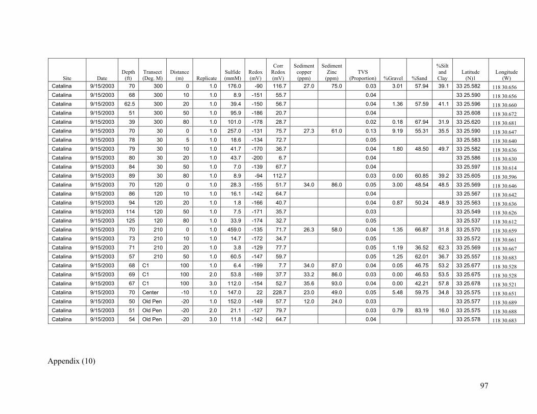
97
Site Date Depth
(ft) Transect (Deg. M)
Distance (m) Replicate
Sulfide (mmM)
Redox (mV)
Corr Redox (mV)
Sediment copper (ppm)
Sediment Zinc
(ppm) TVS
(Proportion) %Gravel %Sand
%Silt and Clay
Latitude (N)1
Longitude (W)
Catalina 9/15/2003 70 300 0 1.0 176.0 -90 116.7 27.0 75.0 0.03 3.01 57.94 39.1 33 25.582 118 30.656 Catalina 9/15/2003 68 300 10 1.0 8.9 -151 55.7 0.04 33 25.590 118 30.656 Catalina 9/15/2003 62.5 300 20 1.0 39.4 -150 56.7 0.04 1.36 57.59 41.1 33 25.596 118 30.660 Catalina 9/15/2003 51 300 50 1.0 95.9 -186 20.7 0.04 33 25.608 118 30.672 Catalina 9/15/2003 39 300 80 1.0 101.0 -178 28.7 0.02 0.18 67.94 31.9 33 25.620 118 30.681 Catalina 9/15/2003 70 30 0 1.0 257.0 -131 75.7 27.3 61.0 0.13 9.19 55.31 35.5 33 25.590 118 30.647 Catalina 9/15/2003 78 30 5 1.0 18.6 -134 72.7 0.05 33 25.583 118 30.640 Catalina 9/15/2003 79 30 10 1.0 41.7 -170 36.7 0.04 1.80 48.50 49.7 33 25.582 118 30.636 Catalina 9/15/2003 80 30 20 1.0 43.7 -200 6.7 0.04 33 25.586 118 30.630 Catalina 9/15/2003 84 30 50 1.0 7.0 -139 67.7 0.04 33 25.597 118 30.614 Catalina 9/15/2003 89 30 80 1.0 8.9 -94 112.7 0.03 0.00 60.85 39.2 33 25.605 118 30.596 Catalina 9/15/2003 70 120 0 1.0 28.3 -155 51.7 34.0 86.0 0.05 3.00 48.54 48.5 33 25.569 118 30.646 Catalina 9/15/2003 86 120 10 1.0 16.1 -142 64.7 0.04 33 25.567 118 30.642 Catalina 9/15/2003 94 120 20 1.0 1.8 -166 40.7 0.04 0.87 50.24 48.9 33 25.563 118 30.636 Catalina 9/15/2003 114 120 50 1.0 7.5 -171 35.7 0.03 33 25.549 118 30.626 Catalina 9/15/2003 125 120 80 1.0 33.9 -174 32.7 0.05 33 25.537 118 30.612 Catalina 9/15/2003 70 210 0 1.0 459.0 -135 71.7 26.3 58.0 0.04 1.35 66.87 31.8 33 25.570 118 30.659 Catalina 9/15/2003 73 210 10 1.0 14.7 -172 34.7 0.05 33 25.572 118 30.661 Catalina 9/15/2003 71 210 20 1.0 3.8 -129 77.7 0.05 1.19 36.52 62.3 33 25.569 118 30.667 Catalina 9/15/2003 57 210 50 1.0 60.5 -147 59.7 0.05 1.25 62.01 36.7 33 25.557 118 30.683 Catalina 9/15/2003 68 C1 100 1.0 6.4 -199 7.7 34.0 87.0 0.04 0.05 46.75 53.2 33 25.677 118 30.528 Catalina 9/15/2003 69 C1 100 2.0 53.8 -169 37.7 33.2 86.0 0.03 0.00 46.53 53.5 33 25.675 118 30.528 Catalina 9/15/2003 67 C1 100 3.0 112.0 -154 52.7 35.6 93.0 0.04 0.00 42.21 57.8 33 25.678 118 30.521 Catalina 9/15/2003 70 Center -10 1.0 147.0 22 228.7 23.0 49.0 0.05 5.48 59.75 34.8 33 25.575 118 30.651 Catalina 9/15/2003 50 Old Pen -20 1.0 152.0 -149 57.7 12.0 24.0 0.03 33 25.577 118 30.689 Catalina 9/15/2003 51 Old Pen -20 2.0 21.1 -127 79.7 0.03 0.79 83.19 16.0 33 25.575 118 30.688 Catalina 9/15/2003 54 Old Pen -20 3.0 11.8 -142 64.7 0.04 33 25.578 118 30.683
Appendix (10)

98
Appendix E California Natural Diversity Database – Spreadsheet
CNDDB Species Lists
DFG Status CodesFP: State fully protected animal SSC: Species of special concern WL: Watch list
Source for list - California Natural Diversity Database: http://www.dfg.ca.gov/biogeodata/cnddb/
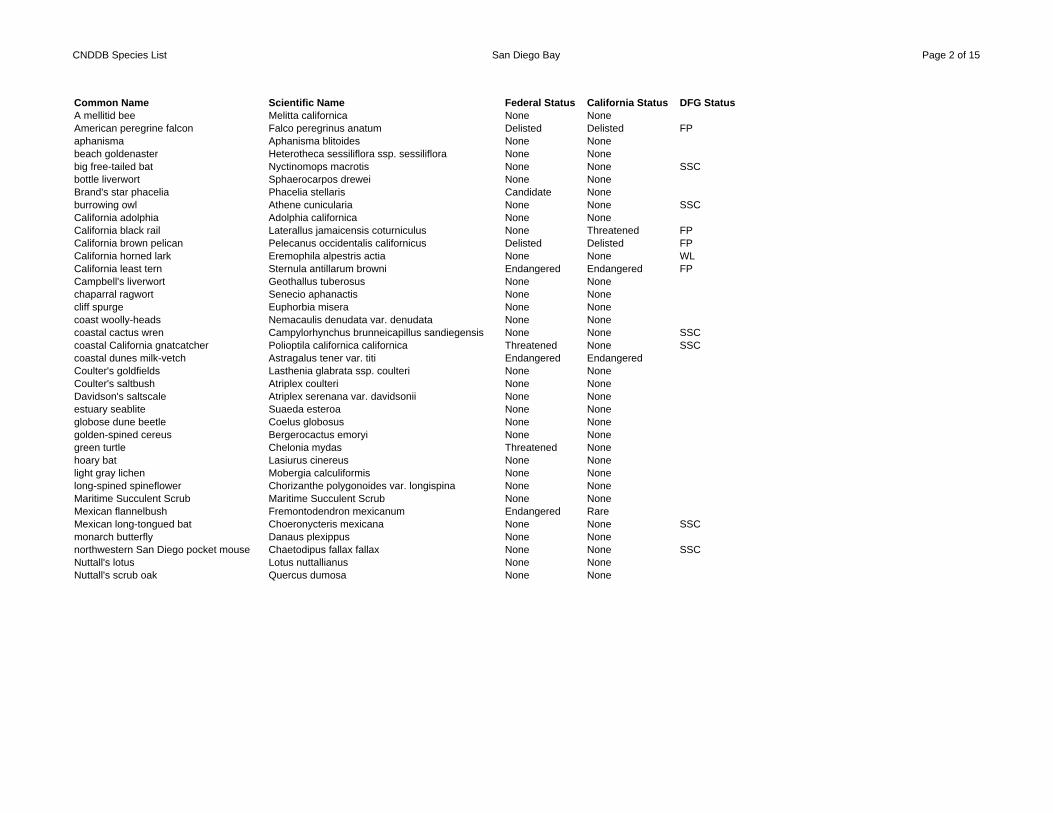
CNDDB Species List San Diego Bay Page 2 of 15
Common Name Scientific Name Federal Status California Status DFG StatusA mellitid bee Melitta californica None NoneAmerican peregrine falcon Falco peregrinus anatum Delisted Delisted FPaphanisma Aphanisma blitoides None Nonebeach goldenaster Heterotheca sessiliflora ssp. sessiliflora None Nonebig free-tailed bat Nyctinomops macrotis None None SSCbottle liverwort Sphaerocarpos drewei None NoneBrand's star phacelia Phacelia stellaris Candidate Noneburrowing owl Athene cunicularia None None SSCCalifornia adolphia Adolphia californica None NoneCalifornia black rail Laterallus jamaicensis coturniculus None Threatened FPCalifornia brown pelican Pelecanus occidentalis californicus Delisted Delisted FPCalifornia horned lark Eremophila alpestris actia None None WLCalifornia least tern Sternula antillarum browni Endangered Endangered FPCampbell's liverwort Geothallus tuberosus None Nonechaparral ragwort Senecio aphanactis None Nonecliff spurge Euphorbia misera None Nonecoast woolly-heads Nemacaulis denudata var. denudata None Nonecoastal cactus wren Campylorhynchus brunneicapillus sandiegensis None None SSCcoastal California gnatcatcher Polioptila californica californica Threatened None SSCcoastal dunes milk-vetch Astragalus tener var. titi Endangered EndangeredCoulter's goldfields Lasthenia glabrata ssp. coulteri None NoneCoulter's saltbush Atriplex coulteri None NoneDavidson's saltscale Atriplex serenana var. davidsonii None Noneestuary seablite Suaeda esteroa None Noneglobose dune beetle Coelus globosus None Nonegolden-spined cereus Bergerocactus emoryi None Nonegreen turtle Chelonia mydas Threatened Nonehoary bat Lasiurus cinereus None Nonelight gray lichen Mobergia calculiformis None Nonelong-spined spineflower Chorizanthe polygonoides var. longispina None NoneMaritime Succulent Scrub Maritime Succulent Scrub None NoneMexican flannelbush Fremontodendron mexicanum Endangered RareMexican long-tongued bat Choeronycteris mexicana None None SSCmonarch butterfly Danaus plexippus None Nonenorthwestern San Diego pocket mouse Chaetodipus fallax fallax None None SSCNuttall's lotus Lotus nuttallianus None NoneNuttall's scrub oak Quercus dumosa None None
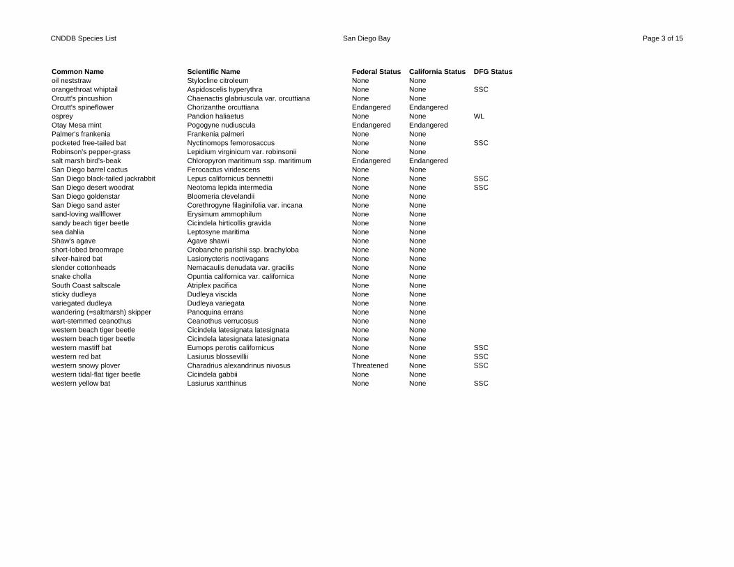
CNDDB Species List San Diego Bay Page 3 of 15
Common Name Scientific Name Federal Status California Status DFG Statusoil neststraw Stylocline citroleum None Noneorangethroat whiptail Aspidoscelis hyperythra None None SSCOrcutt's pincushion Chaenactis glabriuscula var. orcuttiana None NoneOrcutt's spineflower Chorizanthe orcuttiana Endangered Endangeredosprey Pandion haliaetus None None WLOtay Mesa mint Pogogyne nudiuscula Endangered EndangeredPalmer's frankenia Frankenia palmeri None Nonepocketed free-tailed bat Nyctinomops femorosaccus None None SSCRobinson's pepper-grass Lepidium virginicum var. robinsonii None Nonesalt marsh bird's-beak Chloropyron maritimum ssp. maritimum Endangered EndangeredSan Diego barrel cactus Ferocactus viridescens None NoneSan Diego black-tailed jackrabbit Lepus californicus bennettii None None SSCSan Diego desert woodrat Neotoma lepida intermedia None None SSCSan Diego goldenstar Bloomeria clevelandii None NoneSan Diego sand aster Corethrogyne filaginifolia var. incana None Nonesand-loving wallflower Erysimum ammophilum None Nonesandy beach tiger beetle Cicindela hirticollis gravida None Nonesea dahlia Leptosyne maritima None NoneShaw's agave Agave shawii None Noneshort-lobed broomrape Orobanche parishii ssp. brachyloba None Nonesilver-haired bat Lasionycteris noctivagans None Noneslender cottonheads Nemacaulis denudata var. gracilis None Nonesnake cholla Opuntia californica var. californica None NoneSouth Coast saltscale Atriplex pacifica None Nonesticky dudleya Dudleya viscida None Nonevariegated dudleya Dudleya variegata None Nonewandering (=saltmarsh) skipper Panoquina errans None Nonewart-stemmed ceanothus Ceanothus verrucosus None Nonewestern beach tiger beetle Cicindela latesignata latesignata None Nonewestern beach tiger beetle Cicindela latesignata latesignata None Nonewestern mastiff bat Eumops perotis californicus None None SSCwestern red bat Lasiurus blossevillii None None SSCwestern snowy plover Charadrius alexandrinus nivosus Threatened None SSCwestern tidal-flat tiger beetle Cicindela gabbii None Nonewestern yellow bat Lasiurus xanthinus None None SSC
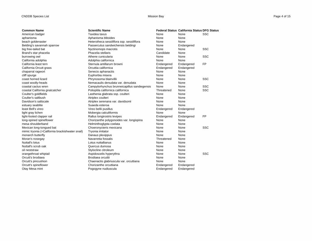
CNDDB Species List Mission Bay Page 4 of 15
Common Name Scientific Name Federal Status California Status DFG StatusAmerican badger Taxidea taxus None None SSCaphanisma Aphanisma blitoides None Nonebeach goldenaster Heterotheca sessiliflora ssp. sessiliflora None NoneBelding's savannah sparrow Passerculus sandwichensis beldingi None Endangeredbig free-tailed bat Nyctinomops macrotis None None SSCBrand's star phacelia Phacelia stellaris Candidate Noneburrowing owl Athene cunicularia None None SSCCalifornia adolphia Adolphia californica None NoneCalifornia least tern Sternula antillarum browni Endangered Endangered FPCalifornia Orcutt grass Orcuttia californica Endangered Endangeredchaparral ragwort Senecio aphanactis None Nonecliff spurge Euphorbia misera None Nonecoast horned lizard Phrynosoma blainvillii None None SSCcoast woolly-heads Nemacaulis denudata var. denudata None Nonecoastal cactus wren Campylorhynchus brunneicapillus sandiegensis None None SSCcoastal California gnatcatcher Polioptila californica californica Threatened None SSCCoulter's goldfields Lasthenia glabrata ssp. coulteri None NoneCoulter's saltbush Atriplex coulteri None NoneDavidson's saltscale Atriplex serenana var. davidsonii None Noneestuary seablite Suaeda esteroa None Noneleast Bell's vireo Vireo bellii pusillus Endangered Endangeredlight gray lichen Mobergia calculiformis None Nonelight-footed clapper rail Rallus longirostris levipes Endangered Endangered FPlong-spined spineflower Chorizanthe polygonoides var. longispina None Nonemesa shoulderband Helminthoglypta coelata None NoneMexican long-tongued bat Choeronycteris mexicana None None SSCmimic tryonia (=California brackishwater snail) Tryonia imitator None Nonemonarch butterfly Danaus plexippus None NoneMoran's nosegay Navarretia fossalis Threatened NoneNuttall's lotus Lotus nuttallianus None NoneNuttall's scrub oak Quercus dumosa None Noneoil neststraw Stylocline citroleum None Noneorangethroat whiptail Aspidoscelis hyperythra None None SSCOrcutt's brodiaea Brodiaea orcuttii None NoneOrcutt's pincushion Chaenactis glabriuscula var. orcuttiana None NoneOrcutt's spineflower Chorizanthe orcuttiana Endangered EndangeredOtay Mesa mint Pogogyne nudiuscula Endangered Endangered
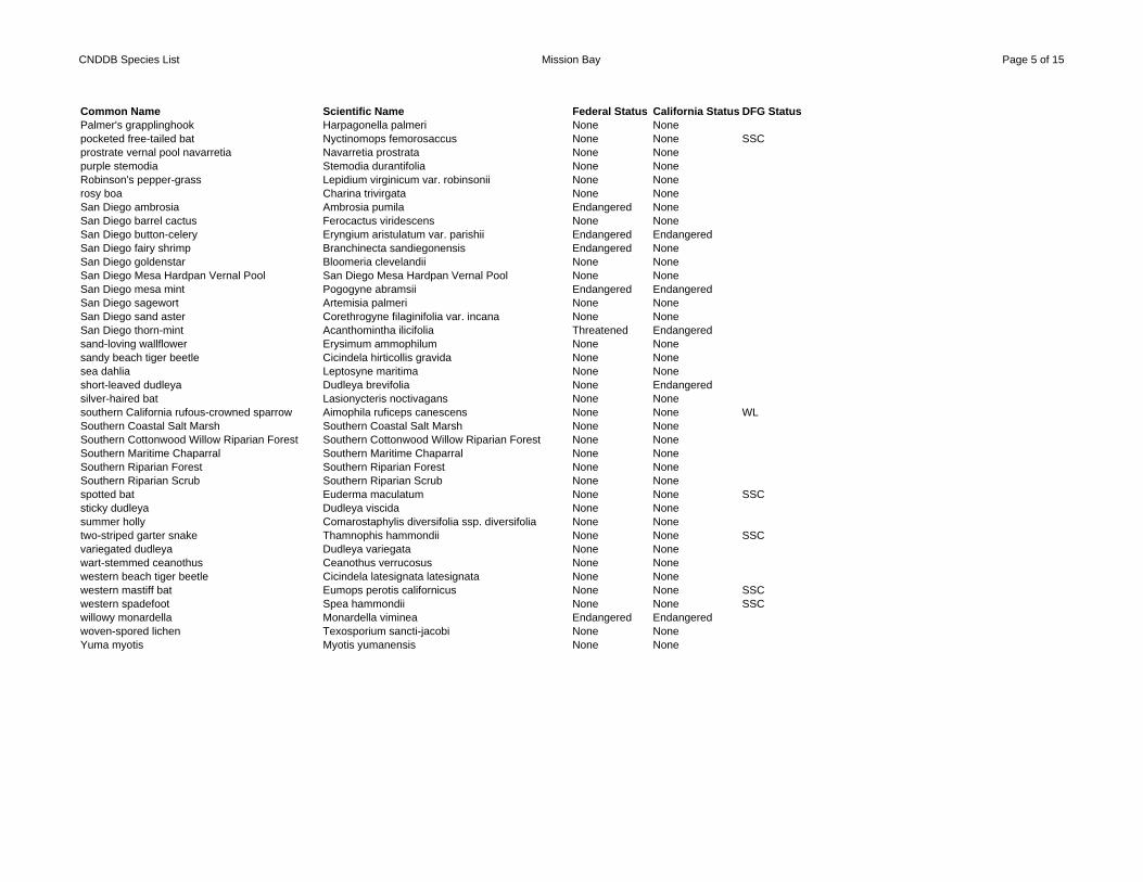
CNDDB Species List Mission Bay Page 5 of 15
Common Name Scientific Name Federal Status California Status DFG StatusPalmer's grapplinghook Harpagonella palmeri None Nonepocketed free-tailed bat Nyctinomops femorosaccus None None SSCprostrate vernal pool navarretia Navarretia prostrata None Nonepurple stemodia Stemodia durantifolia None NoneRobinson's pepper-grass Lepidium virginicum var. robinsonii None Nonerosy boa Charina trivirgata None NoneSan Diego ambrosia Ambrosia pumila Endangered NoneSan Diego barrel cactus Ferocactus viridescens None NoneSan Diego button-celery Eryngium aristulatum var. parishii Endangered EndangeredSan Diego fairy shrimp Branchinecta sandiegonensis Endangered NoneSan Diego goldenstar Bloomeria clevelandii None NoneSan Diego Mesa Hardpan Vernal Pool San Diego Mesa Hardpan Vernal Pool None NoneSan Diego mesa mint Pogogyne abramsii Endangered EndangeredSan Diego sagewort Artemisia palmeri None NoneSan Diego sand aster Corethrogyne filaginifolia var. incana None NoneSan Diego thorn-mint Acanthomintha ilicifolia Threatened Endangeredsand-loving wallflower Erysimum ammophilum None Nonesandy beach tiger beetle Cicindela hirticollis gravida None Nonesea dahlia Leptosyne maritima None Noneshort-leaved dudleya Dudleya brevifolia None Endangeredsilver-haired bat Lasionycteris noctivagans None Nonesouthern California rufous-crowned sparrow Aimophila ruficeps canescens None None WLSouthern Coastal Salt Marsh Southern Coastal Salt Marsh None NoneSouthern Cottonwood Willow Riparian Forest Southern Cottonwood Willow Riparian Forest None NoneSouthern Maritime Chaparral Southern Maritime Chaparral None NoneSouthern Riparian Forest Southern Riparian Forest None NoneSouthern Riparian Scrub Southern Riparian Scrub None Nonespotted bat Euderma maculatum None None SSCsticky dudleya Dudleya viscida None Nonesummer holly Comarostaphylis diversifolia ssp. diversifolia None Nonetwo-striped garter snake Thamnophis hammondii None None SSCvariegated dudleya Dudleya variegata None Nonewart-stemmed ceanothus Ceanothus verrucosus None Nonewestern beach tiger beetle Cicindela latesignata latesignata None Nonewestern mastiff bat Eumops perotis californicus None None SSCwestern spadefoot Spea hammondii None None SSCwillowy monardella Monardella viminea Endangered Endangeredwoven-spored lichen Texosporium sancti-jacobi None NoneYuma myotis Myotis yumanensis None None
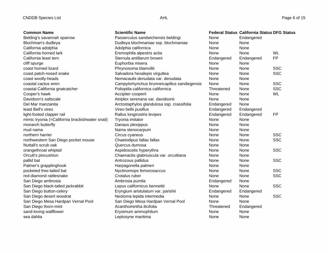
CNDDB Species List AHL Page 6 of 15
Common Name Scientific Name Federal Status California Status DFG StatusBelding's savannah sparrow Passerculus sandwichensis beldingi None EndangeredBlochman's dudleya Dudleya blochmaniae ssp. blochmaniae None NoneCalifornia adolphia Adolphia californica None NoneCalifornia horned lark Eremophila alpestris actia None None WLCalifornia least tern Sternula antillarum browni Endangered Endangered FPcliff spurge Euphorbia misera None Nonecoast horned lizard Phrynosoma blainvillii None None SSCcoast patch-nosed snake Salvadora hexalepis virgultea None None SSCcoast woolly-heads Nemacaulis denudata var. denudata None Nonecoastal cactus wren Campylorhynchus brunneicapillus sandiegensis None None SSCcoastal California gnatcatcher Polioptila californica californica Threatened None SSCCooper's hawk Accipiter cooperii None None WLDavidson's saltscale Atriplex serenana var. davidsonii None NoneDel Mar manzanita Arctostaphylos glandulosa ssp. crassifolia Endangered Noneleast Bell's vireo Vireo bellii pusillus Endangered Endangeredlight-footed clapper rail Rallus longirostris levipes Endangered Endangered FPmimic tryonia (=California brackishwater snail) Tryonia imitator None Nonemonarch butterfly Danaus plexippus None Nonemud nama Nama stenocarpum None Nonenorthern harrier Circus cyaneus None None SSCnorthwestern San Diego pocket mouse Chaetodipus fallax fallax None None SSCNuttall's scrub oak Quercus dumosa None Noneorangethroat whiptail Aspidoscelis hyperythra None None SSCOrcutt's pincushion Chaenactis glabriuscula var. orcuttiana None Nonepallid bat Antrozous pallidus None None SSCPalmer's grapplinghook Harpagonella palmeri None Nonepocketed free-tailed bat Nyctinomops femorosaccus None None SSCred-diamond rattlesnake Crotalus ruber None None SSCSan Diego ambrosia Ambrosia pumila Endangered NoneSan Diego black-tailed jackrabbit Lepus californicus bennettii None None SSCSan Diego button-celery Eryngium aristulatum var. parishii Endangered EndangeredSan Diego desert woodrat Neotoma lepida intermedia None None SSCSan Diego Mesa Hardpan Vernal Pool San Diego Mesa Hardpan Vernal Pool None NoneSan Diego thorn-mint Acanthomintha ilicifolia Threatened Endangeredsand-loving wallflower Erysimum ammophilum None Nonesea dahlia Leptosyne maritima None None
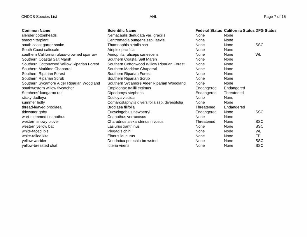
CNDDB Species List AHL Page 7 of 15
Common Name Scientific Name Federal Status California Status DFG Statusslender cottonheads Nemacaulis denudata var. gracilis None Nonesmooth tarplant Centromadia pungens ssp. laevis None Nonesouth coast garter snake Thamnophis sirtalis ssp. None None SSCSouth Coast saltscale Atriplex pacifica None Nonesouthern California rufous-crowned sparrow Aimophila ruficeps canescens None None WLSouthern Coastal Salt Marsh Southern Coastal Salt Marsh None NoneSouthern Cottonwood Willow Riparian Forest Southern Cottonwood Willow Riparian Forest None NoneSouthern Maritime Chaparral Southern Maritime Chaparral None NoneSouthern Riparian Forest Southern Riparian Forest None NoneSouthern Riparian Scrub Southern Riparian Scrub None NoneSouthern Sycamore Alder Riparian Woodland Southern Sycamore Alder Riparian Woodland None Nonesouthwestern willow flycatcher Empidonax traillii extimus Endangered EndangeredStephens' kangaroo rat Dipodomys stephensi Endangered Threatenedsticky dudleya Dudleya viscida None Nonesummer holly Comarostaphylis diversifolia ssp. diversifolia None Nonethread-leaved brodiaea Brodiaea filifolia Threatened Endangeredtidewater goby Eucyclogobius newberryi Endangered None SSCwart-stemmed ceanothus Ceanothus verrucosus None Nonewestern snowy plover Charadrius alexandrinus nivosus Threatened None SSCwestern yellow bat Lasiurus xanthinus None None SSCwhite-faced ibis Plegadis chihi None None WLwhite-tailed kite Elanus leucurus None None FPyellow warbler Dendroica petechia brewsteri None None SSCyellow-breasted chat Icteria virens None None SSC
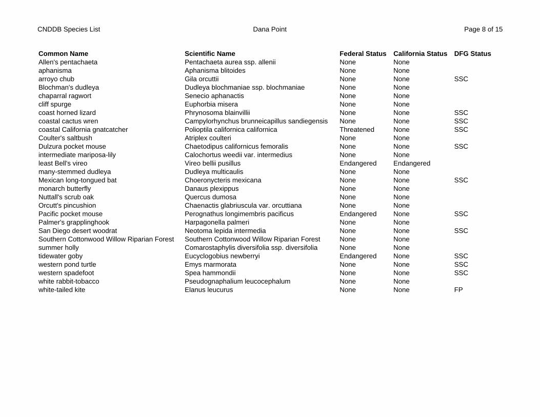
CNDDB Species List Dana Point Page 8 of 15
Common Name Scientific Name Federal Status California Status DFG StatusAllen's pentachaeta Pentachaeta aurea ssp. allenii None Noneaphanisma Aphanisma blitoides None Nonearroyo chub Gila orcuttii None None SSCBlochman's dudleya Dudleya blochmaniae ssp. blochmaniae None Nonechaparral ragwort Senecio aphanactis None Nonecliff spurge Euphorbia misera None Nonecoast horned lizard Phrynosoma blainvillii None None SSCcoastal cactus wren Campylorhynchus brunneicapillus sandiegensis None None SSCcoastal California gnatcatcher Polioptila californica californica Threatened None SSCCoulter's saltbush Atriplex coulteri None NoneDulzura pocket mouse Chaetodipus californicus femoralis None None SSCintermediate mariposa-lily Calochortus weedii var. intermedius None Noneleast Bell's vireo Vireo bellii pusillus Endangered Endangeredmany-stemmed dudleya Dudleya multicaulis None NoneMexican long-tongued bat Choeronycteris mexicana None None SSCmonarch butterfly Danaus plexippus None NoneNuttall's scrub oak Quercus dumosa None NoneOrcutt's pincushion Chaenactis glabriuscula var. orcuttiana None NonePacific pocket mouse Perognathus longimembris pacificus Endangered None SSCPalmer's grapplinghook Harpagonella palmeri None NoneSan Diego desert woodrat Neotoma lepida intermedia None None SSCSouthern Cottonwood Willow Riparian Forest Southern Cottonwood Willow Riparian Forest None Nonesummer holly Comarostaphylis diversifolia ssp. diversifolia None Nonetidewater goby Eucyclogobius newberryi Endangered None SSCwestern pond turtle Emys marmorata None None SSCwestern spadefoot Spea hammondii None None SSCwhite rabbit-tobacco Pseudognaphalium leucocephalum None Nonewhite-tailed kite Elanus leucurus None None FP
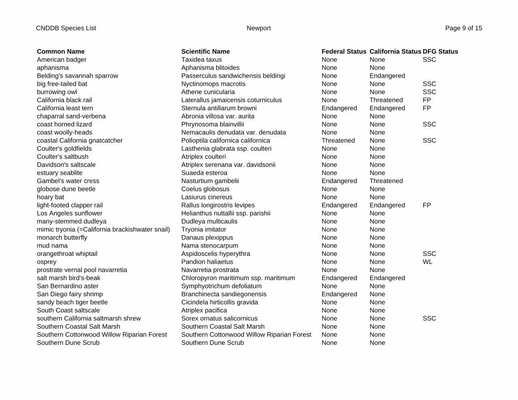
CNDDB Species List Newport Page 9 of 15
Common Name Scientific Name Federal Status California Status DFG StatusAmerican badger Taxidea taxus None None SSCaphanisma Aphanisma blitoides None NoneBelding's savannah sparrow Passerculus sandwichensis beldingi None Endangeredbig free-tailed bat Nyctinomops macrotis None None SSCburrowing owl Athene cunicularia None None SSCCalifornia black rail Laterallus jamaicensis coturniculus None Threatened FPCalifornia least tern Sternula antillarum browni Endangered Endangered FPchaparral sand-verbena Abronia villosa var. aurita None Nonecoast horned lizard Phrynosoma blainvillii None None SSCcoast woolly-heads Nemacaulis denudata var. denudata None Nonecoastal California gnatcatcher Polioptila californica californica Threatened None SSCCoulter's goldfields Lasthenia glabrata ssp. coulteri None NoneCoulter's saltbush Atriplex coulteri None NoneDavidson's saltscale Atriplex serenana var. davidsonii None Noneestuary seablite Suaeda esteroa None NoneGambel's water cress Nasturtium gambelii Endangered Threatenedglobose dune beetle Coelus globosus None Nonehoary bat Lasiurus cinereus None Nonelight-footed clapper rail Rallus longirostris levipes Endangered Endangered FPLos Angeles sunflower Helianthus nuttallii ssp. parishii None Nonemany-stemmed dudleya Dudleya multicaulis None Nonemimic tryonia (=California brackishwater snail) Tryonia imitator None Nonemonarch butterfly Danaus plexippus None Nonemud nama Nama stenocarpum None Noneorangethroat whiptail Aspidoscelis hyperythra None None SSCosprey Pandion haliaetus None None WLprostrate vernal pool navarretia Navarretia prostrata None Nonesalt marsh bird's-beak Chloropyron maritimum ssp. maritimum Endangered EndangeredSan Bernardino aster Symphyotrichum defoliatum None NoneSan Diego fairy shrimp Branchinecta sandiegonensis Endangered Nonesandy beach tiger beetle Cicindela hirticollis gravida None NoneSouth Coast saltscale Atriplex pacifica None Nonesouthern California saltmarsh shrew Sorex ornatus salicornicus None None SSCSouthern Coastal Salt Marsh Southern Coastal Salt Marsh None NoneSouthern Cottonwood Willow Riparian Forest Southern Cottonwood Willow Riparian Forest None NoneSouthern Dune Scrub Southern Dune Scrub None None

CNDDB Species List Newport Page 10 of 15
Common Name Scientific Name Federal Status California Status DFG StatusSouthern Foredunes Southern Foredunes None Nonesouthern tarplant Centromadia parryi ssp. australis None Nonewestern beach tiger beetle Cicindela latesignata latesignata None Nonewestern mastiff bat Eumops perotis californicus None None SSCwestern snowy plover Charadrius alexandrinus nivosus Threatened None SSCwestern tidal-flat tiger beetle Cicindela gabbii None Nonewhite-tailed kite Elanus leucurus None None FP
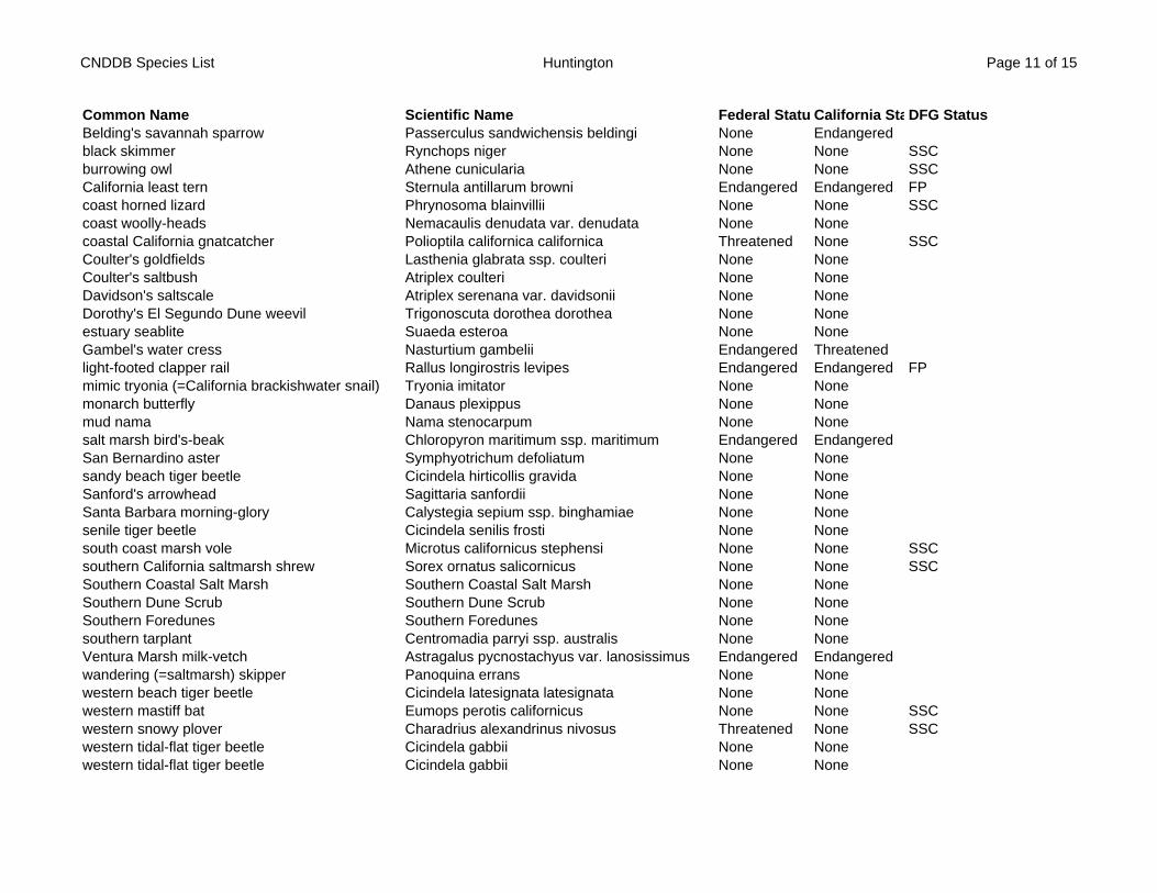
CNDDB Species List Huntington Page 11 of 15
Common Name Scientific Name Federal Statu California StaDFG StatusBelding's savannah sparrow Passerculus sandwichensis beldingi None Endangeredblack skimmer Rynchops niger None None SSCburrowing owl Athene cunicularia None None SSCCalifornia least tern Sternula antillarum browni Endangered Endangered FPcoast horned lizard Phrynosoma blainvillii None None SSCcoast woolly-heads Nemacaulis denudata var. denudata None Nonecoastal California gnatcatcher Polioptila californica californica Threatened None SSCCoulter's goldfields Lasthenia glabrata ssp. coulteri None NoneCoulter's saltbush Atriplex coulteri None NoneDavidson's saltscale Atriplex serenana var. davidsonii None NoneDorothy's El Segundo Dune weevil Trigonoscuta dorothea dorothea None Noneestuary seablite Suaeda esteroa None NoneGambel's water cress Nasturtium gambelii Endangered Threatenedlight-footed clapper rail Rallus longirostris levipes Endangered Endangered FPmimic tryonia (=California brackishwater snail) Tryonia imitator None Nonemonarch butterfly Danaus plexippus None Nonemud nama Nama stenocarpum None Nonesalt marsh bird's-beak Chloropyron maritimum ssp. maritimum Endangered EndangeredSan Bernardino aster Symphyotrichum defoliatum None Nonesandy beach tiger beetle Cicindela hirticollis gravida None NoneSanford's arrowhead Sagittaria sanfordii None NoneSanta Barbara morning-glory Calystegia sepium ssp. binghamiae None Nonesenile tiger beetle Cicindela senilis frosti None Nonesouth coast marsh vole Microtus californicus stephensi None None SSCsouthern California saltmarsh shrew Sorex ornatus salicornicus None None SSCSouthern Coastal Salt Marsh Southern Coastal Salt Marsh None NoneSouthern Dune Scrub Southern Dune Scrub None NoneSouthern Foredunes Southern Foredunes None Nonesouthern tarplant Centromadia parryi ssp. australis None NoneVentura Marsh milk-vetch Astragalus pycnostachyus var. lanosissimus Endangered Endangeredwandering (=saltmarsh) skipper Panoquina errans None Nonewestern beach tiger beetle Cicindela latesignata latesignata None Nonewestern mastiff bat Eumops perotis californicus None None SSCwestern snowy plover Charadrius alexandrinus nivosus Threatened None SSCwestern tidal-flat tiger beetle Cicindela gabbii None Nonewestern tidal-flat tiger beetle Cicindela gabbii None None
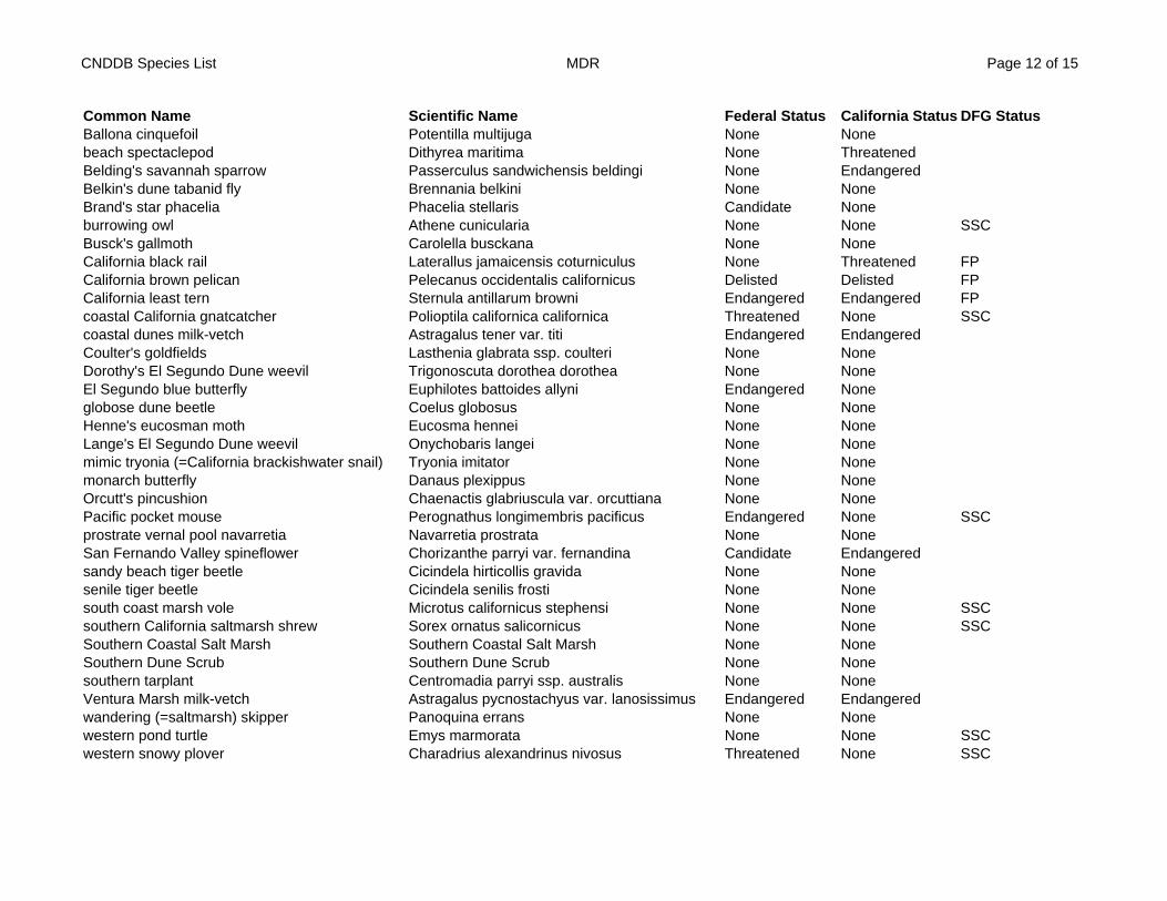
CNDDB Species List MDR Page 12 of 15
Common Name Scientific Name Federal Status California Status DFG StatusBallona cinquefoil Potentilla multijuga None Nonebeach spectaclepod Dithyrea maritima None ThreatenedBelding's savannah sparrow Passerculus sandwichensis beldingi None EndangeredBelkin's dune tabanid fly Brennania belkini None NoneBrand's star phacelia Phacelia stellaris Candidate Noneburrowing owl Athene cunicularia None None SSCBusck's gallmoth Carolella busckana None NoneCalifornia black rail Laterallus jamaicensis coturniculus None Threatened FPCalifornia brown pelican Pelecanus occidentalis californicus Delisted Delisted FPCalifornia least tern Sternula antillarum browni Endangered Endangered FPcoastal California gnatcatcher Polioptila californica californica Threatened None SSCcoastal dunes milk-vetch Astragalus tener var. titi Endangered EndangeredCoulter's goldfields Lasthenia glabrata ssp. coulteri None NoneDorothy's El Segundo Dune weevil Trigonoscuta dorothea dorothea None NoneEl Segundo blue butterfly Euphilotes battoides allyni Endangered Noneglobose dune beetle Coelus globosus None NoneHenne's eucosman moth Eucosma hennei None NoneLange's El Segundo Dune weevil Onychobaris langei None Nonemimic tryonia (=California brackishwater snail) Tryonia imitator None Nonemonarch butterfly Danaus plexippus None NoneOrcutt's pincushion Chaenactis glabriuscula var. orcuttiana None NonePacific pocket mouse Perognathus longimembris pacificus Endangered None SSCprostrate vernal pool navarretia Navarretia prostrata None NoneSan Fernando Valley spineflower Chorizanthe parryi var. fernandina Candidate Endangeredsandy beach tiger beetle Cicindela hirticollis gravida None Nonesenile tiger beetle Cicindela senilis frosti None Nonesouth coast marsh vole Microtus californicus stephensi None None SSCsouthern California saltmarsh shrew Sorex ornatus salicornicus None None SSCSouthern Coastal Salt Marsh Southern Coastal Salt Marsh None NoneSouthern Dune Scrub Southern Dune Scrub None Nonesouthern tarplant Centromadia parryi ssp. australis None NoneVentura Marsh milk-vetch Astragalus pycnostachyus var. lanosissimus Endangered Endangeredwandering (=saltmarsh) skipper Panoquina errans None Nonewestern pond turtle Emys marmorata None None SSCwestern snowy plover Charadrius alexandrinus nivosus Threatened None SSC
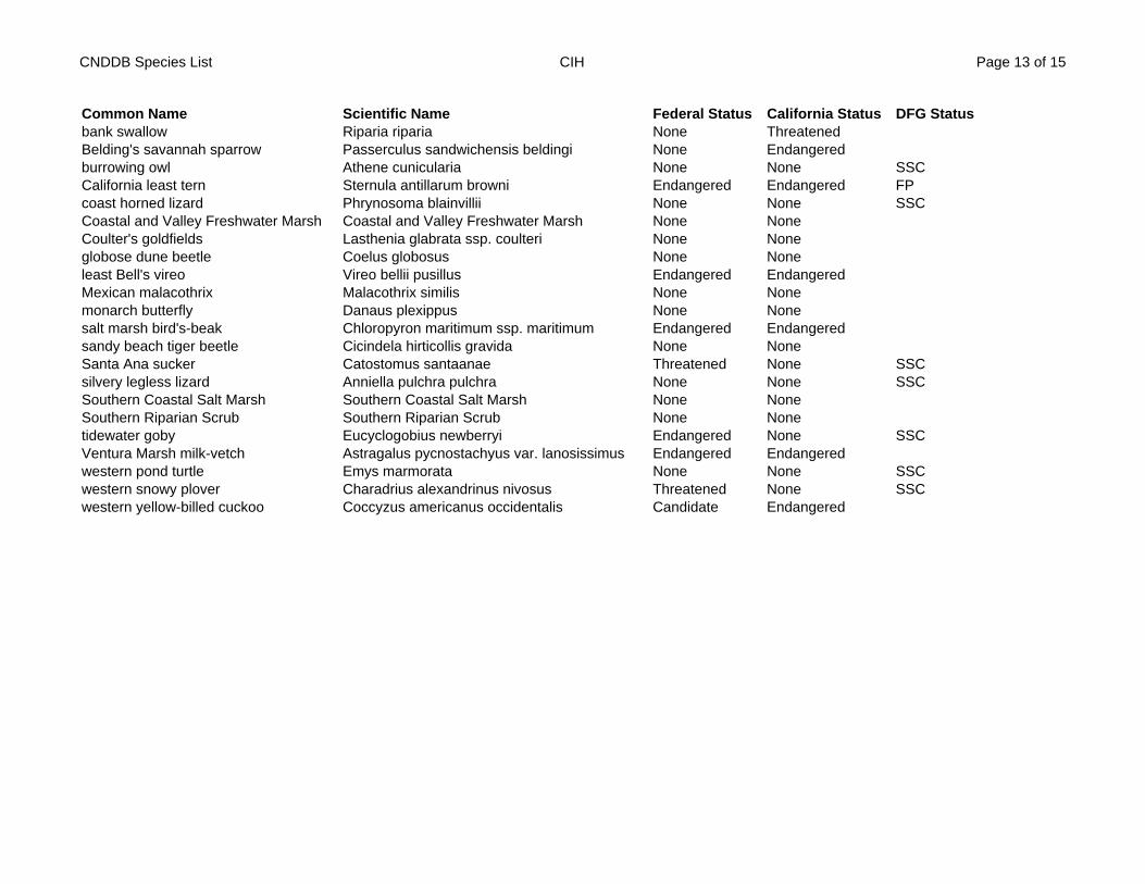
CNDDB Species List CIH Page 13 of 15
Common Name Scientific Name Federal Status California Status DFG Statusbank swallow Riparia riparia None ThreatenedBelding's savannah sparrow Passerculus sandwichensis beldingi None Endangeredburrowing owl Athene cunicularia None None SSCCalifornia least tern Sternula antillarum browni Endangered Endangered FPcoast horned lizard Phrynosoma blainvillii None None SSCCoastal and Valley Freshwater Marsh Coastal and Valley Freshwater Marsh None NoneCoulter's goldfields Lasthenia glabrata ssp. coulteri None Noneglobose dune beetle Coelus globosus None Noneleast Bell's vireo Vireo bellii pusillus Endangered EndangeredMexican malacothrix Malacothrix similis None Nonemonarch butterfly Danaus plexippus None Nonesalt marsh bird's-beak Chloropyron maritimum ssp. maritimum Endangered Endangeredsandy beach tiger beetle Cicindela hirticollis gravida None NoneSanta Ana sucker Catostomus santaanae Threatened None SSCsilvery legless lizard Anniella pulchra pulchra None None SSCSouthern Coastal Salt Marsh Southern Coastal Salt Marsh None NoneSouthern Riparian Scrub Southern Riparian Scrub None Nonetidewater goby Eucyclogobius newberryi Endangered None SSCVentura Marsh milk-vetch Astragalus pycnostachyus var. lanosissimus Endangered Endangeredwestern pond turtle Emys marmorata None None SSCwestern snowy plover Charadrius alexandrinus nivosus Threatened None SSCwestern yellow-billed cuckoo Coccyzus americanus occidentalis Candidate Endangered
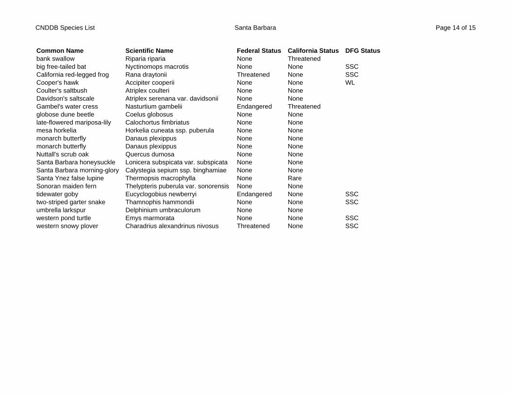
CNDDB Species List Santa Barbara Page 14 of 15
Common Name Scientific Name Federal Status California Status DFG Statusbank swallow Riparia riparia None Threatenedbig free-tailed bat Nyctinomops macrotis None None SSCCalifornia red-legged frog Rana draytonii Threatened None SSCCooper's hawk Accipiter cooperii None None WLCoulter's saltbush Atriplex coulteri None NoneDavidson's saltscale Atriplex serenana var. davidsonii None NoneGambel's water cress Nasturtium gambelii Endangered Threatenedglobose dune beetle Coelus globosus None Nonelate-flowered mariposa-lily Calochortus fimbriatus None Nonemesa horkelia Horkelia cuneata ssp. puberula None Nonemonarch butterfly Danaus plexippus None Nonemonarch butterfly Danaus plexippus None NoneNuttall's scrub oak Quercus dumosa None NoneSanta Barbara honeysuckle Lonicera subspicata var. subspicata None NoneSanta Barbara morning-glory Calystegia sepium ssp. binghamiae None NoneSanta Ynez false lupine Thermopsis macrophylla None RareSonoran maiden fern Thelypteris puberula var. sonorensis None Nonetidewater goby Eucyclogobius newberryi Endangered None SSCtwo-striped garter snake Thamnophis hammondii None None SSCumbrella larkspur Delphinium umbraculorum None Nonewestern pond turtle Emys marmorata None None SSCwestern snowy plover Charadrius alexandrinus nivosus Threatened None SSC
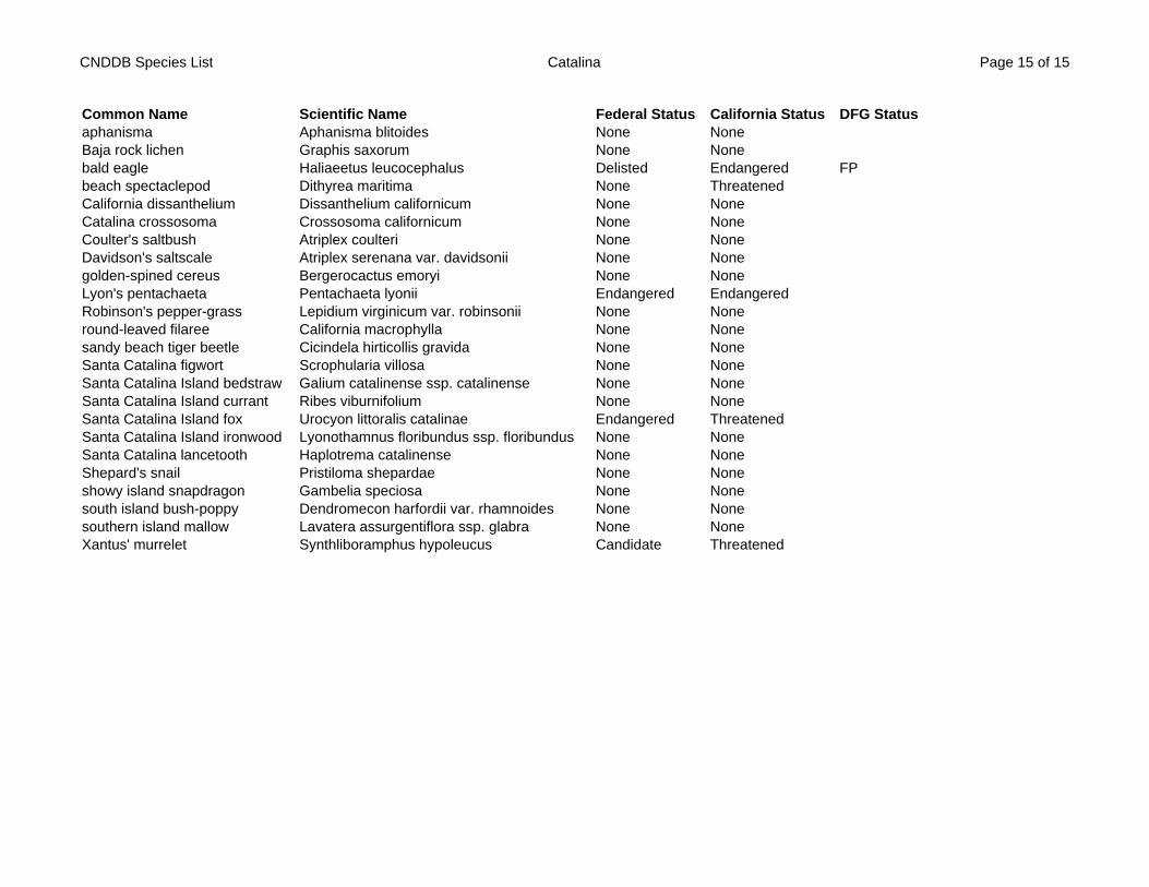
CNDDB Species List Catalina Page 15 of 15
Common Name Scientific Name Federal Status California Status DFG Statusaphanisma Aphanisma blitoides None NoneBaja rock lichen Graphis saxorum None Nonebald eagle Haliaeetus leucocephalus Delisted Endangered FPbeach spectaclepod Dithyrea maritima None ThreatenedCalifornia dissanthelium Dissanthelium californicum None NoneCatalina crossosoma Crossosoma californicum None NoneCoulter's saltbush Atriplex coulteri None NoneDavidson's saltscale Atriplex serenana var. davidsonii None Nonegolden-spined cereus Bergerocactus emoryi None NoneLyon's pentachaeta Pentachaeta lyonii Endangered EndangeredRobinson's pepper-grass Lepidium virginicum var. robinsonii None Noneround-leaved filaree California macrophylla None Nonesandy beach tiger beetle Cicindela hirticollis gravida None NoneSanta Catalina figwort Scrophularia villosa None NoneSanta Catalina Island bedstraw Galium catalinense ssp. catalinense None NoneSanta Catalina Island currant Ribes viburnifolium None NoneSanta Catalina Island fox Urocyon littoralis catalinae Endangered ThreatenedSanta Catalina Island ironwood Lyonothamnus floribundus ssp. floribundus None NoneSanta Catalina lancetooth Haplotrema catalinense None NoneShepard's snail Pristiloma shepardae None Noneshowy island snapdragon Gambelia speciosa None Nonesouth island bush-poppy Dendromecon harfordii var. rhamnoides None Nonesouthern island mallow Lavatera assurgentiflora ssp. glabra None NoneXantus' murrelet Synthliboramphus hypoleucus Candidate Threatened
Appendix F Project-Related Chemical Usage Inventory
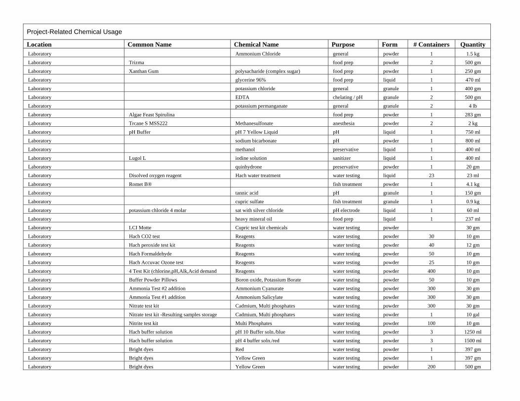
Project-Related Chemical Usage
Location Common Name Chemical Name Purpose Form # Containers Quantity Laboratory Ammonium Chloride general powder 1 1.5 kg
Laboratory Trizma food prep powder 2 500 gm
Laboratory Xanthan Gum polysacharide (complex sugar) food prep powder 1 250 gm
Laboratory glycerine 96% food prep liquid 1 470 ml
Laboratory potassium chloride general granule 1 400 gm
Laboratory EDTA chelating / pH granule 2 500 gm
Laboratory potassium permanganate general granule 2 4 lb
Laboratory Algae Feast Spirulina food prep powder 1 283 gm
Laboratory Trcane S MSS222 Methanesulfonate anesthesia powder 2 2 kg
Laboratory pH Buffer pH 7 Yellow Liquid pH liquid 1 750 ml
Laboratory sodium bicarbonate pH powder 1 800 ml
Laboratory methanol preservative liquid 1 400 ml
Laboratory Lugol L iodine solution sanitizer liquid 1 400 ml
Laboratory quinhydrone preservative powder 1 20 gm
Laboratory Disolved oxygen reagent Hach water treatment water testing liquid 23 23 ml
Laboratory Romet B® fish treatment powder 1 4.1 kg
Laboratory tannic acid pH granule 1 150 gm
Laboratory cupric sulfate fish treatment granule 1 0.9 kg
Laboratory potassium chloride 4 molar sat with silver chloride pH electrode liquid 1 60 ml
Laboratory heavy mineral oil food prep liquid 1 237 ml
Laboratory LCI Motte Cupric test kit chemicals water testing powder 30 gm
Laboratory Hach CO2 test Reagents water testing powder 30 10 gm
Laboratory Hach peroxide test kit Reagents water testing powder 40 12 gm
Laboratory Hach Formaldehyde Reagents water testing powder 50 10 gm
Laboratory Hach Accuvac Ozone test Reagents water testing powder 25 10 gm
Laboratory 4 Test Kit (chlorine,pH,Alk,Acid demand Reagents water testing powder 400 10 gm
Laboratory Buffer Powder Pillows Boron oxide, Potassium Borate water testing powder 50 10 gm
Laboratory Ammonia Test #2 addition Ammonium Cyanurate water testing powder 300 30 gm
Laboratory Ammonia Test #1 addition Ammonium Salicylate water testing powder 300 30 gm
Laboratory Nitrate test kit Cadmium, Multi phosphates water testing powder 300 30 gm
Laboratory Nitrate test kit -Resulting samples storage Cadmium, Multi phosphates water testing powder 1 10 gal
Laboratory Nitrite test kit Multi Phosphates water testing powder 100 10 gm
Laboratory Hach buffer solution pH 10 Buffer soln./blue water testing powder 3 1250 ml
Laboratory Hach buffer solution pH 4 buffer soln./red water testing powder 3 1500 ml
Laboratory Bright dyes Red water testing powder 1 397 gm
Laboratory Bright dyes Yellow Green water testing powder 1 397 gm
Laboratory Bright dyes Yellow Green water testing powder 200 500 gm
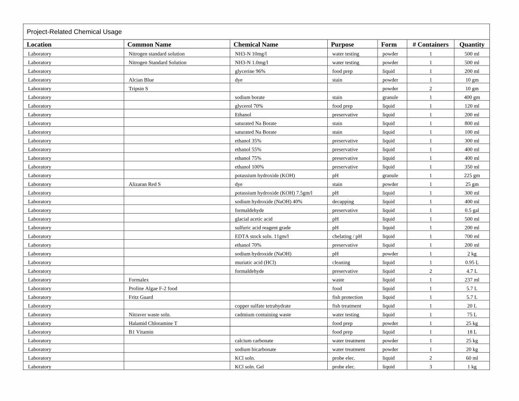
Project-Related Chemical Usage
Location Common Name Chemical Name Purpose Form # Containers Quantity Laboratory Nitrogen standard solution NH3-N 10mg/l water testing powder 1 500 ml
Laboratory Nitrogen Standard Solution NH3-N 1.0mg/l water testing powder 1 500 ml
Laboratory glycerine 96% food prep liquid 1 200 ml
Laboratory Alcian Blue dye stain powder 1 10 gm
Laboratory Tripsin S powder 2 10 gm
Laboratory sodium borate stain granule 1 400 gm
Laboratory glycerol 70% food prep liquid 1 120 ml
Laboratory Ethanol preservative liquid 1 200 ml
Laboratory saturated Na Borate stain liquid 1 800 ml
Laboratory saturated Na Borate stain liquid 1 100 ml
Laboratory ethanol 35% preservative liquid 1 300 ml
Laboratory ethanol 55% preservative liquid 1 400 ml
Laboratory ethanol 75% preservative liquid 1 400 ml
Laboratory ethanol 100% preservative liquid 1 350 ml
Laboratory potassium hydroxide (KOH) pH granule 1 225 gm
Laboratory Alizaran Red S dye stain powder 1 25 gm
Laboratory potassium hydroxide (KOH) 7.5gm/l pH liquid 1 300 ml
Laboratory sodium hydroxide (NaOH) 40% decapping liquid 1 400 ml
Laboratory formaldehyde preservative liquid 1 0.5 gal
Laboratory glacial acetic acid pH liquid 1 500 ml
Laboratory sulfuric acid reagent grade pH liquid 1 200 ml
Laboratory EDTA stock soln. 11gm/l chelating / pH liquid 1 700 ml
Laboratory ethanol 70% preservative liquid 1 200 ml
Laboratory sodium hydroxide (NaOH) pH powder 1 2 kg
Laboratory muriatic acid (HCl) cleaning liquid 1 0.95 L
Laboratory formaldehyde preservative liquid 2 4.7 L
Laboratory Formalex waste liquid 1 237 ml
Laboratory Proline Algae F-2 food food liquid 1 5.7 L
Laboratory Fritz Guard fish protection liquid 1 5.7 L
Laboratory copper sulfate tetrahydrate fish treatment liquid 1 20 L
Laboratory Nitraver waste soln. cadmium containing waste water testing liquid 1 75 L
Laboratory Halamid Chloramine T food prep powder 1 25 kg
Laboratory B1 Vitamin food prep liquid 1 18 L
Laboratory calcium carbonate water treatment powder 1 25 kg
Laboratory sodium bicarbonate water treatment powder 1 20 kg
Laboratory KCl soln. probe elec. liquid 2 60 ml
Laboratory KCl soln. Gel probe elec. liquid 3 1 kg

Project-Related Chemical Usage
Location Common Name Chemical Name Purpose Form # Containers Quantity Laboratory Micronutrients food prep liquid 2 1.5 L
Laboratory ethanol preservative liquid 1 1 L
Laboratory thiamine food prep powder 1 500 gm
Laboratory ascorbic acid food prep powder 1 500 gm
Laboratory Skretting fish food food granule 2 1 kg
Laboratory ethanol preservative liquid 4 7.5 L
Laboratory formiline (formaldihyde) 4% soln preservative liquid 2 37 L
Laboratory glycerine 96% food prep liquid 1 500 ml
Laboratory Hepain fish health liquid 1 180 mgm
Laboratory Brig 35 fish health liquid 1 10 ml
Laboratory sodium chloride (NaCl) plates granule 1 500 gm
Laboratory potassium chloride (KCl) plates granule 1 500 gm
Laboratory sodium phosphate (Na1PO4) plates granule 1 500 gm
Laboratory dimethyl sulfoxide plates liquid 1 1 L
Laboratory Wrights stain plates liquid 1 1 L
Laboratory citric acid plates powder 1 500 gm
Laboratory sodium bicarbonate plates powder 1 500 gm
Laboratory calcium chloride plates granule 1 500 gm
Laboratory glucose plates powder 1 500 gm
Laboratory Gram Stain kit slide prep liquid 3 400 ml
Laboratory silicone stopcock grease silicone lubrication paste 3 90 gm
Laboratory Genetics specimen samples (200-300) formaldehyde / organic matter samples liq/solid 200-300 3 L
Outside, side Hydrogen Peroxide (35%) H2O2 fish treatment 1.5 208 L
Outside, side Sodium Hypochlorite (12.5%) Bleach sanitation 1.5 208 L
Facilities Room SAE 30 Motor Oil lubrication 1 3.78 L
Facilities Room Mineral Spirits lubrication 2 3.78 L
Flammables Cabinet, Facilities Room Acetone solvent 2L 3.78 L
Flammables Cabinet, Facilities Room Linseed Oil solvent 1 3.78 L
Flammables Cabinet, Facilities Room Epoxy Remover K-50 solvent 1 1 L
Flammables Cabinet, Facilities Room Charcoal Lighter Fluid Petroleum Distillates solvent 1 1 L
Flammables Cabinet, Facilities Room Thompson's Water Sealer paint 1 1 L
Flammables Cabinet, Facilities Room SealFast G-P-M Mastic 45-00 paint 1 3.78 L
Flammables Cabinet, Facilities Room Cutting Oil Petroleum Distillates solvent 1 1 L
Flammables Cabinet, Facilities Room Jasco Tile Gloss & Seal sealant 3 3 L
Flammables Cabinet, Facilities Room Fiberglass Resin construction 2 6 L
Flammables Cabinet, Facilities Room Enviro-Coil Cleaner Chiller Coil Cleaner cleaning 1 3.78 L
Flammables Cabinet, Facilities Room Rubber Undercoat paint 12 453 gm

Project-Related Chemical Usage
Location Common Name Chemical Name Purpose Form # Containers Quantity Flammables Cabinet, Facilities Room Zerol Refrigerant 200 TD lubrication 1 1 L
Flammables Cabinet, Facilities Room Acrylic Paint Misc. cans paint 5 3.78 L
Flammables Cabinet, Facilities Room Enamel Paint Misc. cans paint 5 3.78 L
Flammables Cabinet, Facilities Room Concrete Primer PT 20 Part B paint 20 3.78 L
Flammables Cabinet, Facilities Room Gel Coat construction 1 3.78 L
Flammables Cabinet, Facilities Room Vinyl Sealer construction 1 1 L
Flammables Cabinet, Facilities Room Misc. Spray Paints paint 60 369 gm
Flammables Cabinet, Facilities Room Enamel Paint paint 6 2.72 kg
Flammables Cabinet, Facilities Room Jasco Prep & Primer paint 1 1.5 L
Flammables Cabinet, Facilities Room Misc. Primer & Paints paint 23 11.3 L
Facilities Room Enamel Paint & Primer paint 13 18.9 L
Facilities Room Wet Roof Cement Patch construction 1 15.1 L
Facilities Room Marine Latex Fiberglass Patch construction 1 396 gm
Facilities Room Concrete Bonding adhesive construction 1 0.94 L
Facilities Room Marine Tank Clarifier water treatment 1 236 ml
Facilities Room Amquel detoxifier aquarium water clarifier water treatment 1 236 ml
Facilities Room Pour Stone Anchoring Cement construction 1 2 lb
Facilities Room Car Wax repair 61 473 ml
Facilities Room RainX repair 5 236 ml
Facilities Room Motor Oil lubrication 5 3.78 L
Facilities Room Brake Fluid Dot 3 repair 1 236 ml
Facilities Room Compressor oil lubrication 1 3.78 L
Facilities Room Pneumatic Tool Lubricant lubrication 1 500 ml
Facilities Room Zep Calcium, Lime, Rust Cleaner cleaning 3 500 ml
Facilities Room Antifreeze lubrication 1 500 ml
Facilities Room Motor Oil lubrication 28 946 ml
Facilities Room Simple Green cleaning 1 1 L
Facilities Room Used Motor Oil waste 2 26.5 L
Facilities Room Liquid Wrench Spray GUNK lubrication 4 311 gm
Facilities Room WD 40 lubrication 6 226 gm
Facilities Room White Lithium Grease lubrication 7 290 mg
Facilities Room Teflon Pipe Thread Sealant T plus 2 lubrication 1 473 ml
Facilities Room Copper Coat Gasket Compound repair 1 255 mg
Facilities Room 3-in-1 oil lubrication 4 118 mg
Facilities Room Glue Mate PVC Glue/Primer sealant 1 1 L
Facilities Room White Lithium Grease lubrication 1 907 gm
Facilities Room WD 40 lubrication 1 226 gm
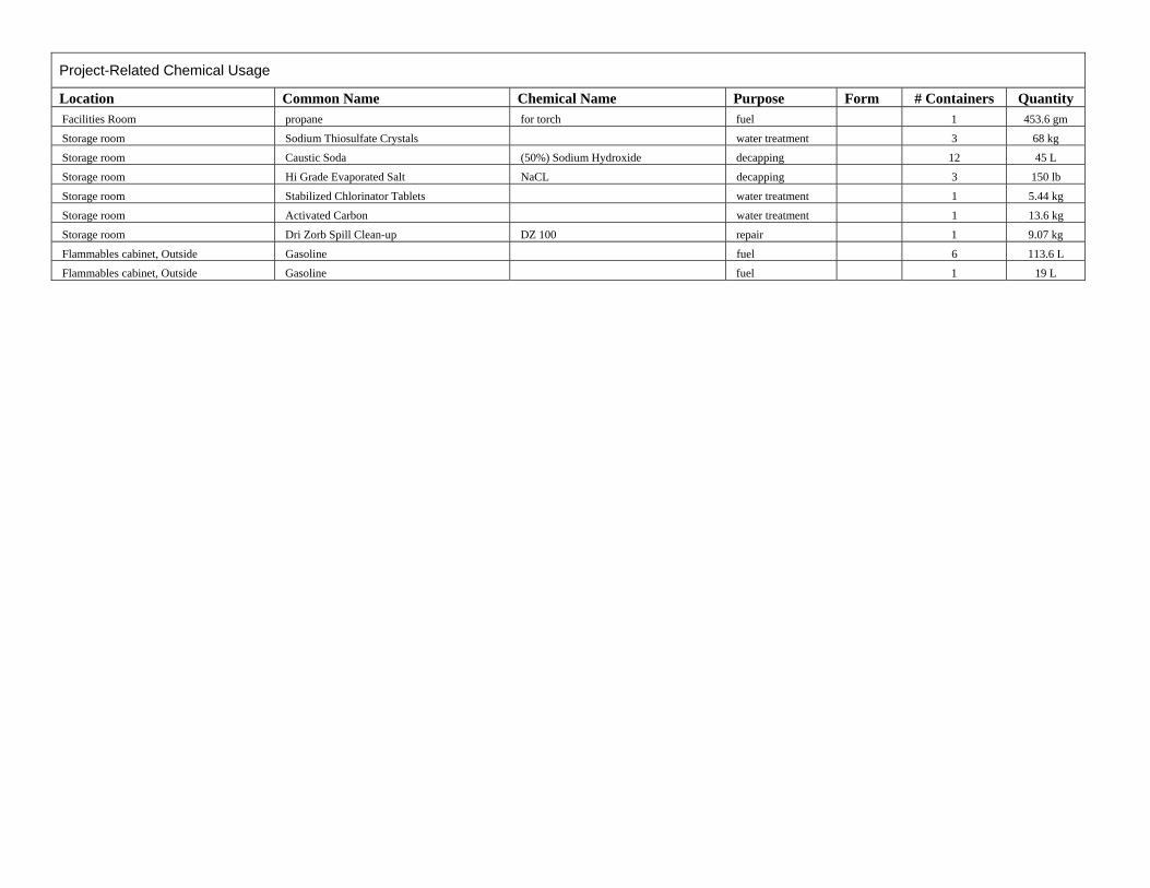
Project-Related Chemical Usage
Location Common Name Chemical Name Purpose Form # Containers Quantity Facilities Room propane for torch fuel 1 453.6 gm
Storage room Sodium Thiosulfate Crystals water treatment 3 68 kg
Storage room Caustic Soda (50%) Sodium Hydroxide decapping 12 45 L
Storage room Hi Grade Evaporated Salt NaCL decapping 3 150 lb
Storage room Stabilized Chlorinator Tablets water treatment 1 5.44 kg
Storage room Activated Carbon water treatment 1 13.6 kg
Storage room Dri Zorb Spill Clean-up DZ 100 repair 1 9.07 kg
Flammables cabinet, Outside Gasoline fuel 6 113.6 L
Flammables cabinet, Outside Gasoline fuel 1 19 L

Appendix G Final White Seabass Fishery Management Plan

FINAL
WHITE SEABASS FISHERY MANAGEMENT PLAN
04 APRIL 2002STATE OF CALIFORNIATHE RESOURCES AGENCYDEPARTMENT OF FISH AND GAMEMARINE REGION
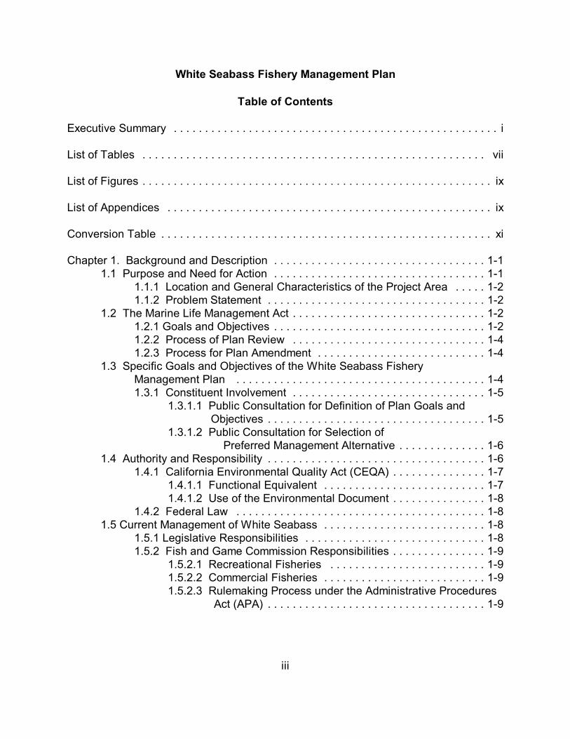
iii
White Seabass Fishery Management Plan
Table of Contents
Executive Summary . . . . . . . . . . . . . . . . . . . . . . . . . . . . . . . . . . . . . . . . . . . . . . . . . . . . i
List of Tables . . . . . . . . . . . . . . . . . . . . . . . . . . . . . . . . . . . . . . . . . . . . . . . . . . . . . . . vii
List of Figures . . . . . . . . . . . . . . . . . . . . . . . . . . . . . . . . . . . . . . . . . . . . . . . . . . . . . . . . ix
List of Appendices . . . . . . . . . . . . . . . . . . . . . . . . . . . . . . . . . . . . . . . . . . . . . . . . . . . . ix
Conversion Table . . . . . . . . . . . . . . . . . . . . . . . . . . . . . . . . . . . . . . . . . . . . . . . . . . . . . xi
Chapter 1. Background and Description . . . . . . . . . . . . . . . . . . . . . . . . . . . . . . . . . . 1-11.1 Purpose and Need for Action . . . . . . . . . . . . . . . . . . . . . . . . . . . . . . . . . . 1-1
1.1.1 Location and General Characteristics of the Project Area . . . . . 1-21.1.2 Problem Statement . . . . . . . . . . . . . . . . . . . . . . . . . . . . . . . . . . . 1-2
1.2 The Marine Life Management Act . . . . . . . . . . . . . . . . . . . . . . . . . . . . . . . 1-21.2.1 Goals and Objectives . . . . . . . . . . . . . . . . . . . . . . . . . . . . . . . . . . 1-21.2.2 Process of Plan Review . . . . . . . . . . . . . . . . . . . . . . . . . . . . . . . 1-41.2.3 Process for Plan Amendment . . . . . . . . . . . . . . . . . . . . . . . . . . . 1-4
1.3 Specific Goals and Objectives of the White Seabass Fishery Management Plan . . . . . . . . . . . . . . . . . . . . . . . . . . . . . . . . . . . . . . . . 1-41.3.1 Constituent Involvement . . . . . . . . . . . . . . . . . . . . . . . . . . . . . . . 1-5
1.3.1.1 Public Consultation for Definition of Plan Goals and Objectives . . . . . . . . . . . . . . . . . . . . . . . . . . . . . . . . . . . 1-5
1.3.1.2 Public Consultation for Selection of Preferred Management Alternative . . . . . . . . . . . . . . 1-6
1.4 Authority and Responsibility . . . . . . . . . . . . . . . . . . . . . . . . . . . . . . . . . . . 1-61.4.1 California Environmental Quality Act (CEQA) . . . . . . . . . . . . . . . 1-7
1.4.1.1 Functional Equivalent . . . . . . . . . . . . . . . . . . . . . . . . . . 1-71.4.1.2 Use of the Environmental Document . . . . . . . . . . . . . . . 1-8
1.4.2 Federal Law . . . . . . . . . . . . . . . . . . . . . . . . . . . . . . . . . . . . . . . . 1-81.5 Current Management of White Seabass . . . . . . . . . . . . . . . . . . . . . . . . . . 1-8
1.5.1 Legislative Responsibilities . . . . . . . . . . . . . . . . . . . . . . . . . . . . . 1-81.5.2 Fish and Game Commission Responsibilities . . . . . . . . . . . . . . . 1-9
1.5.2.1 Recreational Fisheries . . . . . . . . . . . . . . . . . . . . . . . . . 1-91.5.2.2 Commercial Fisheries . . . . . . . . . . . . . . . . . . . . . . . . . . 1-91.5.2.3 Rulemaking Process under the Administrative Procedures
Act (APA) . . . . . . . . . . . . . . . . . . . . . . . . . . . . . . . . . . . 1-9
iv
Cover photo courtesy of Terry Maas
Chapter 2. Description of Stocks . . . . . . . . . . . . . . . . . . . . . . . . . . . . . . . . . . . . . . . . 2-12.1 Species Description . . . . . . . . . . . . . . . . . . . . . . . . . . . . . . . . . . . . . . . . . 2-12.2 Distribution, Genetic Stock Structure, and Migration . . . . . . . . . . . . . . . . 2-12.3 Age and Growth . . . . . . . . . . . . . . . . . . . . . . . . . . . . . . . . . . . . . . . . . . . . 2-22.4 Reproduction, Fecundity and Seasonality . . . . . . . . . . . . . . . . . . . . . . . . 2-32.5 Natural Mortality . . . . . . . . . . . . . . . . . . . . . . . . . . . . . . . . . . . . . . . . . . . . 2-42.6 Parasites and Disease . . . . . . . . . . . . . . . . . . . . . . . . . . . . . . . . . . . . . . . 2-52.7 Predator/Prey Relationships . . . . . . . . . . . . . . . . . . . . . . . . . . . . . . . . . . . 2-62.8 Competition . . . . . . . . . . . . . . . . . . . . . . . . . . . . . . . . . . . . . . . . . . . . . . . . 2-62.9 Critical Habitat . . . . . . . . . . . . . . . . . . . . . . . . . . . . . . . . . . . . . . . . . . . . . 2-62.10 Status of the Stocks . . . . . . . . . . . . . . . . . . . . . . . . . . . . . . . . . . . . . . . . 2-6
Chapter 3. Description of the Fishery . . . . . . . . . . . . . . . . . . . . . . . . . . . . . . . . . . . . 3-13.1 Areas and Stocks Involved . . . . . . . . . . . . . . . . . . . . . . . . . . . . . . . . . . . . 3-13.2 History of Exploitation . . . . . . . . . . . . . . . . . . . . . . . . . . . . . . . . . . . . . . . . 3-1
3.2.1 Description of User Groups . . . . . . . . . . . . . . . . . . . . . . . . . . . . . 3-43.2.2 Fishing Catch and Effort . . . . . . . . . . . . . . . . . . . . . . . . . . . . . . . 3-7
3.3 Social and Economic Characteristics of the Fishery . . . . . . . . . . . . . . . . 3-153.3.1 Recreational Sector . . . . . . . . . . . . . . . . . . . . . . . . . . . . . . . . . 3-163.3.2 Commercial Sector . . . . . . . . . . . . . . . . . . . . . . . . . . . . . . . . . . 3-19
3.4 Non-consumptive Use . . . . . . . . . . . . . . . . . . . . . . . . . . . . . . . . . . . . . . . 3-243.5 Analysis of Impacts . . . . . . . . . . . . . . . . . . . . . . . . . . . . . . . . . . . . . . . . . 3-24
Chapter 4. History of Conservation and Management Measures . . . . . . . . . . . . . . . 4-14.1 Regulatory History in California . . . . . . . . . . . . . . . . . . . . . . . . . . . . . . . . 4-14.2 Regulatory History Specific to White Seabass fisheries . . . . . . . . . . . . . . 4-1
4.2.1 Commercial Fishery . . . . . . . . . . . . . . . . . . . . . . . . . . . . . . . . . . 4-14.2.2 Recreational Fishery . . . . . . . . . . . . . . . . . . . . . . . . . . . . . . . . . . 4-2
4.3 Additional Conservation Measures for White Seabass Stocks . . . . . . . . . 4-4
Chapter 5. Fishery Management Program . . . . . . . . . . . . . . . . . . . . . . . . . . . . . . . . 5-15.1 Potential Management Measures . . . . . . . . . . . . . . . . . . . . . . . . . . . . . . . 5-15.2 Definition of Maximum Sustainable Yield and Optimum Yield . . . . . . . . . 5-45.3 General Fishery Management Plan Framework . . . . . . . . . . . . . . . . . . . . 5-5
5.3.1 Plan Amendment . . . . . . . . . . . . . . . . . . . . . . . . . . . . . . . . . . . . . 5-65.3.2 Framework Actions . . . . . . . . . . . . . . . . . . . . . . . . . . . . . . . . . . . 5-65.3.3 Routine Management Measures . . . . . . . . . . . . . . . . . . . . . . . . . 5-7
5.4 White Seabass FMP Framework . . . . . . . . . . . . . . . . . . . . . . . . . . . . . . . 5-85.4.1 Points of Concern Process . . . . . . . . . . . . . . . . . . . . . . . . . . . . . 5-85.4.2 Socioeconomic Process . . . . . . . . . . . . . . . . . . . . . . . . . . . . . . . 5-95.4.3 Allocation Criteria . . . . . . . . . . . . . . . . . . . . . . . . . . . . . . . . . . . 5-115.4.4 Harvest Control Rules . . . . . . . . . . . . . . . . . . . . . . . . . . . . . . . . 5-11
v
5.5 Trigger Mechanisms . . . . . . . . . . . . . . . . . . . . . . . . . . . . . . . . . . . . . . . . 5-125.6 Management Alternatives . . . . . . . . . . . . . . . . . . . . . . . . . . . . . . . . . . . . 5-13
5.6.1 Alternative A - Status Quo . . . . . . . . . . . . . . . . . . . . . . . . . . . . . 5-145.6.2 Alternative B - OY Proxies Based on National Standard
Guidelines . . . . . . . . . . . . . . . . . . . . . . . . . . . . . . . . . . . . . . . . 5-145.6.2.1 Alternative B1: OY=0.8125 x MSY . . . . . . . . . . . . . . . 5-145.6.2.2 Alternative B2 (Preferred): OY=0.75 x MSY . . . . . . . . 5-15
5.6.3 Alternative C - OY Proxies Based on Recent Catch Levels . . . 5-155.6.3.1 Alternative C1: Based on 1996-2000 Catch Data . . . 5-155.6.3.2 Alternative C2: Based on 1988-1989 and
1993-2000 Catch Data . . . . . . . . . . . . . . . . . . . . . . . 5-155.6.3.3 Alternative C3: Based on 1983-1989
and 1993-2000 Catch Data . . . . . . . . . . . . . . . . . . . 5-165.6.4 Alternative D - OY Proxy Based on 1947-1957 Catch Data . . . 5-16
5.7 Default MSY/OY Control Rule . . . . . . . . . . . . . . . . . . . . . . . . . . . . . . . . . 5-175.8 Trigger Mechanisms for Proposed Alternatives . . . . . . . . . . . . . . . . . . . 5-185.9 Annual Review of Management Measures . . . . . . . . . . . . . . . . . . . . . . . 5-195.10 Reporting and Record Keeping Requirements . . . . . . . . . . . . . . . . . . . 5-19
Chapter 6. Analysis of Proposed Management Alternatives . . . . . . . . . . . . . . . . . . . 6-16.1 Alternative A - Status Quo . . . . . . . . . . . . . . . . . . . . . . . . . . . . . . . . . . . . 6-1
6.1.1 Effects on White Seabass . . . . . . . . . . . . . . . . . . . . . . . . . . . . . . 6-16.1.2 Effects on Non-Target Species . . . . . . . . . . . . . . . . . . . . . . . . . . 6-2
6.1.2.1 Effects on Non-Target Finfish . . . . . . . . . . . . . . . . . . . . 6-36.1.2.2 Effects on Invertebrates . . . . . . . . . . . . . . . . . . . . . . . . 6-46.1.2.3 Effects on Seabirds . . . . . . . . . . . . . . . . . . . . . . . . . . . . 6-56.1.2.4 Effects on Marine Mammals . . . . . . . . . . . . . . . . . . . . . 6-76.1.2.5 Effects on Marine Turtles . . . . . . . . . . . . . . . . . . . . . . . 6-96.1.2.6 Ecological interactions . . . . . . . . . . . . . . . . . . . . . . . . 6-10
6.1.3 Habitat Impacts . . . . . . . . . . . . . . . . . . . . . . . . . . . . . . . . . . . . . 6-116.1.3.1 Effects of Consumptive Use on Environment . . . . . . . 6-116.1.3.2 Effects of Non-consumptive Use on Environment . . . . 6-116.1.4 Economic Implications . . . . . . . . . . . . . . . . . . . . . . . . . . 6-116.1.5 Social Implications . . . . . . . . . . . . . . . . . . . . . . . . . . . . . 6-12
6.2 Alternative B - OY Proxies Based on National Standard Guidelines . . . 6-126.2.1 Effects on White Seabass . . . . . . . . . . . . . . . . . . . . . . . . . . . . . 6-126.2.2 Effects on Non-Target Species . . . . . . . . . . . . . . . . . . . . . . . . . 6-13
6.2.2.1 Effects on Non-Target Finfish . . . . . . . . . . . . . . . . . . . 6-136.2.2.2 Effects on Invertebrates . . . . . . . . . . . . . . . . . . . . . . . 6-136.2.2.3 Effects on Seabirds . . . . . . . . . . . . . . . . . . . . . . . . . . . 6-146.2.2.4 Effects on Marine Mammals . . . . . . . . . . . . . . . . . . . . 6-146.2.2.5 Effects on Marine Turtles . . . . . . . . . . . . . . . . . . . . . . 6-146.2.2.6 Ecological Interactions . . . . . . . . . . . . . . . . . . . . . . . . 6-14
vi
6.2.3 Habitat Impacts . . . . . . . . . . . . . . . . . . . . . . . . . . . . . . . . . . . . . 6-146.2.3.1 Effects of Consumptive Use on Environment . . . . . . . 6-146.2.3.2 Effects of Non-consumptive Use on Environment . . . . 6-14
6.2.4 Economic Implications . . . . . . . . . . . . . . . . . . . . . . . . . . . . . . . 6-146.2.5 Social Implications . . . . . . . . . . . . . . . . . . . . . . . . . . . . . . . . . . 6-14
6.3 Alternative C - OY Proxies Based on Recent Catch Levels . . . . . . . . . . 6-146.3.1 Effects on White Seabass . . . . . . . . . . . . . . . . . . . . . . . . . . . . . 6-146.3.2 Effects on Non-Target Species . . . . . . . . . . . . . . . . . . . . . . . . . 6-16
6.3.2.1 Effects on Non-Target Finfish . . . . . . . . . . . . . . . . . . . 6-166.3.2.2 Effects on Invertebrates . . . . . . . . . . . . . . . . . . . . . . . 6-166.3.2.3 Effects on Seabirds . . . . . . . . . . . . . . . . . . . . . . . . . . . 6-166.3.2.4 Effects on Marine Mammals . . . . . . . . . . . . . . . . . . . . 6-176.3.2.5 Effects on Marine Turtles . . . . . . . . . . . . . . . . . . . . . . 6-176.3.2.6 Ecological Interactions . . . . . . . . . . . . . . . . . . . . . . . . 6-17
6.3.3 Habitat Impacts . . . . . . . . . . . . . . . . . . . . . . . . . . . . . . . . . . . . . 6-176.3.3.1 Effects of Consumptive Use on Environment . . . . . . . 6-176.3.3.2 Effects of Non-consumptive Use on Environment . . . . 6-17
6.3.4 Economic Implications . . . . . . . . . . . . . . . . . . . . . . . . . . . . . . . 6-176.3.5 Social Implications . . . . . . . . . . . . . . . . . . . . . . . . . . . . . . . . . . 6-18
6.4 Alternative D - OY Proxy Based on 1947 to 1957 Catch Data . . . . . . . . 6-196.4.1 Effects on White Seabass . . . . . . . . . . . . . . . . . . . . . . . . . . . . . 6-196.4.2 Effects on Non-Target Species . . . . . . . . . . . . . . . . . . . . . . . . . 6-19
6.4.2.1 Effects on Non-Target Finfish . . . . . . . . . . . . . . . . . . . 6-196.4.2.2 Effects on Invertebrates . . . . . . . . . . . . . . . . . . . . . . . 6-196.4.2.3 Effects on Seabirds . . . . . . . . . . . . . . . . . . . . . . . . . . . 6-196.4.2.4 Effects on Marine Mammals . . . . . . . . . . . . . . . . . . . . 6-196.4.2.5 Effects on Marine Turtles . . . . . . . . . . . . . . . . . . . . . . 6-206.4.2.6 Ecological Interactions . . . . . . . . . . . . . . . . . . . . . . . . 6-20
6.4.3 Habitat Impacts . . . . . . . . . . . . . . . . . . . . . . . . . . . . . . . . . . . . . 6-206.4.3.1 Effects of Consumptive Use on Environment . . . . . . . 6-206.4.3.2 Effects of Non-consumptive Use on Environment . . . . 6-20
6.4.4 Economic Implications . . . . . . . . . . . . . . . . . . . . . . . . . . . . . . . 6-206.4.5 Social Implications . . . . . . . . . . . . . . . . . . . . . . . . . . . . . . . . . . 6-20
6.5 Risk Analysis of the Alternatives . . . . . . . . . . . . . . . . . . . . . . . . . . . . . . . 6-206.6 Effects Found Not to be Significant . . . . . . . . . . . . . . . . . . . . . . . . . . . . 6-216.7 Cumulative Effects . . . . . . . . . . . . . . . . . . . . . . . . . . . . . . . . . . . . . . . . . 6-22
6.7.1 Take of White Seabass Outside California Waters . . . . . . . . . 6-226.7.2 Illegal Take of White Seabass . . . . . . . . . . . . . . . . . . . . . . . . . 6-226.7.3 Coastal Electric Power Generation Operations . . . . . . . . . . . . 6-23
6.8 Summary Analysis of the Proposed Alternatives . . . . . . . . . . . . . . . . . . 6-246.9 Mitigation . . . . . . . . . . . . . . . . . . . . . . . . . . . . . . . . . . . . . . . . . . . . . . . . 6-256.10 Consistency With Statewide/Regional Plans . . . . . . . . . . . . . . . . . . . . 6-25
vii
Chapter 7. Fishery Research Protocols . . . . . . . . . . . . . . . . . . . . . . . . . . . . . . . . . . . 7-17.1 Essential Fishery Information . . . . . . . . . . . . . . . . . . . . . . . . . . . . . . . . . . 7-1
7.1.1 Grouping Essential Fishery Information . . . . . . . . . . . . . . . . . . . 7-27.2 Past and Ongoing Monitoring of the Commercial and
Recreational Fishery . . . . . . . . . . . . . . . . . . . . . . . . . . . . . . . . . . . . . . . 7-57.2.1 Past Fishery-Dependent Monitoring . . . . . . . . . . . . . . . . . . . . . . 7-67.2.2 Problems with Past and Ongoing Fishery-Dependent Monitoring.7-77.2.3 Past Fishery Independent-Research . . . . . . . . . . . . . . . . . . . . . . 7-87.2.4 Problems with Past and Ongoing Fishery Independent-Research.7-8
7.3 Current Knowledge of Essential Fishery Information . . . . . . . . . . . . . . . . 7-97.4 Research Needed to Obtain Essential Fishery Information . . . . . . . . . . 7-10
7.4.1 Short-Term Research Goals and Needs . . . . . . . . . . . . . . . . . 7-107.4.2 Long-Term Research Goals and Needs . . . . . . . . . . . . . . . . . 7-12
7.5 Resources and Time Needed to Fill Essential Fishery Information Gaps.7-147.6 Steps to Monitor the Fishery and Obtain Essential Fishery Information . 7-14
Chapter 8. Implementation Requirements . . . . . . . . . . . . . . . . . . . . . . . . . . . . . . . . . 8-18.1 Enforcement . . . . . . . . . . . . . . . . . . . . . . . . . . . . . . . . . . . . . . . . . . . . . . . 8-18.2 Ongoing and Future Research . . . . . . . . . . . . . . . . . . . . . . . . . . . . . . . . . 8-28.4 Administrative Management . . . . . . . . . . . . . . . . . . . . . . . . . . . . . . . . . . . 8-5
8.4.1 Coordination of the White Seabass Fishery Management Plan . 8-58.4.2 Annual Meetings . . . . . . . . . . . . . . . . . . . . . . . . . . . . . . . . . . . . . 8-68.4.3 Publication of White Seabass Amendments . . . . . . . . . . . . . . . . 8-6
Chapter 9. Other Ecological Concerns . . . . . . . . . . . . . . . . . . . . . . . . . . . . . . . . . . . . 9-19.1 Environmental Variability . . . . . . . . . . . . . . . . . . . . . . . . . . . . . . . . . . . . . 9-19.2 Water Quality . . . . . . . . . . . . . . . . . . . . . . . . . . . . . . . . . . . . . . . . . . . . . . 9-2
9.2.1 Municipal Discharge . . . . . . . . . . . . . . . . . . . . . . . . . . . . . . . . . . 9-29.2.2 Dredge and Non-dredge Material Disposal . . . . . . . . . . . . . . . . . 9-39.2.3 Coastal Shipyards and Industrial Pollutants . . . . . . . . . . . . . . . . 9-49.2.4 Fuel Use . . . . . . . . . . . . . . . . . . . . . . . . . . . . . . . . . . . . . . . . . . . 9-6
9.3 Air Quality . . . . . . . . . . . . . . . . . . . . . . . . . . . . . . . . . . . . . . . . . . . . . . . . . 9-69.4 Importance of Habitat Loss, Degradation, and Modification . . . . . . . . . . . 9-7
9.4.1 Coastal Development and Land Use . . . . . . . . . . . . . . . . . . . . . 9-79.4.2 Gear Use In the Marine Environment . . . . . . . . . . . . . . . . . . . . . 9-89.4.3 Noise Effects in the Marine Environment . . . . . . . . . . . . . . . . . . 9-9
Literature Cited . . . . . . . . . . . . . . . . . . . . . . . . . . . . . . . . . . . . . . . . . . . . . . . . . . . . . . L-1
Personal Communications . . . . . . . . . . . . . . . . . . . . . . . . . . . . . . . . . . . . . . . . . . . . L-15
List of Preparers . . . . . . . . . . . . . . . . . . . . . . . . . . . . . . . . . . . . . . . . . . . . . . . . . . . . P-1
viii
List of Tables
Table 2-1. Mean total length and weight at age for white seabass. . . . . . . . . . . . . . 2-3Table 2-2. Estimates of white seabass natural mortality (M). . . . . . . . . . . . . . . . . . . 2-4Table 3-1. Total white seabass take in U.S. and Mexico by U.S.
commercial and recreational industries from 1936-2000 . . . . . . . . . . . . . . . . . 3-2Table 3-2. Total California landings (pounds) of white seabass by gear type
from 1981-2000 . . . . . . . . . . . . . . . . . . . . . . . . . . . . . . . . . . . . . . . . . . . . . . . . 3-5Table 3-3. Number of vessels landing white seabass by principle landing gear
from 1981-2000. . . . . . . . . . . . . . . . . . . . . . . . . . . . . . . . . . . . . . . . . . . . . . . . . 3-6Table 3-4. Number of fish businesses receiving white seabass by principle
landing area from 1981-2000 . . . . . . . . . . . . . . . . . . . . . . . . . . . . . . . . . . . . . . 3-8Table 3-5. Number of fish markets receiving white seabass by pounds
received from 1981-2000. . . . . . . . . . . . . . . . . . . . . . . . . . . . . . . . . . . . . . . . . 3-8Table 3-6. 1989 participation in white seabass fishing and projected future
participation in response to enhancement of catch rates by county of residence3-16Table 3-7. Total annual trip expenditures for saltwater anglers in southern California
by fishing mode and resident status for 2000 . . . . . . . . . . . . . . . . . . . . . . . . 3-17Table 3-8. Southern California participation estimates for the saltwater recreational
fishery by area of residence,1993-2000 . . . . . . . . . . . . . . . . . . . . . . . . . . . . 3-18Table 3-9. Average annual market price (per pound) for white seabass
from 1981-2000 . . . . . . . . . . . . . . . . . . . . . . . . . . . . . . . . . . . . . . . . . . . . . . . 3-21Table 3-10. Examples of annual operating costs by primary gear type. . . . . . . . . . 3-22Table 3-11. Estimated socioeconomic impact of recreational diving from
boats in CINMS reserve area and surrounding waters during 1997. . . . . . . . 3-24Table 4-1. Summary of White Seabass Regulations from 1931 to the Present.
(Modified from Vojkovich and Reed 1983). . . . . . . . . . . . . . . . . . . . . . . . . . . . 4-3Table 4-2. Revenue generated through the purchase of the ocean enhancement stamp,
1992-2000. . . . . . . . . . . . . . . . . . . . . . . . . . . . . . . . . . . . . . . . . . . . . . . . . . . . . 4-5Table 5-1. Proposed alternatives (harvest control rules) for management of the white
seabass resource. . . . . . . . . . . . . . . . . . . . . . . . . . . . . . . . . . . . . . . . . . . . . . 5-16Table 6-1. Observed incidental catch of finfish in the white seabass gill net
fishery from 1983-1989 (Vojkovich et al. 1990). . . . . . . . . . . . . . . . . . . . . . . . 6-4Table 6-2. Observed incidental catch of invertebrates in the white seabass gill net
fishery from 1983-1989 (Vojkovich et al. 1990). . . . . . . . . . . . . . . . . . . . . . . . 6-5Table 6-3. Pinniped interactions with recreational anglers targeting white seabass in
1999. Interviewed anglers reported pinnipeds within 100 yards of their fishingarea. . . . . . . . . . . . . . . . . . . . . . . . . . . . . . . . . . . . . . . . . . . . . . . . . . . . . . . . . . 6-8
Table 6-4. Reduction estimates of white seabass catch and resulting take usingvarious controls or regulations. . . . . . . . . . . . . . . . . . . . . . . . . . . . . . . . . . . . 6-16
Table 6-5. Number of years for the white seabass stock to become overfished whenmanagement is by one alternative (Y) while stock status suits another alternative(X). . . . . . . . . . . . . . . . . . . . . . . . . . . . . . . . . . . . . . . . . . . . . . . . . . . . . . . . . . 6-21

ix
Table 6-6. Summary of potential effects of proposed alternatives on white seabassfishery management plan (WSFMP) and Marine Life Management Act (MLMA)objectives . . . . . . . . . . . . . . . . . . . . . . . . . . . . . . . . . . . . . . . . . . . . . . . . . . . . 6-24
Table 8-1. Enforcement costs in 2000. . . . . . . . . . . . . . . . . . . . . . . . . . . . . . . . . . . . 8-2Table 8-2. Estimated cost of collection and maintenance of statistical (landing receipt,
CPFV and commercial logbook) data. . . . . . . . . . . . . . . . . . . . . . . . . . . . . . . . 8-3Table 8-3. Estimated cost of fishery dependent biological sampling. . . . . . . . . . . . . 8-3Table 8-4. Cost of fishery independent data collection. . . . . . . . . . . . . . . . . . . . . . . 8-4Table 8-5. Administrative cost of coordination for the WSFMP. . . . . . . . . . . . . . . . . 8-6
Table 8-6. Costs associated with the annual White Seabass Advisory Panel Meeting(seven panelists). . . . . . . . . . . . . . . . . . . . . . . . . . . . . . . . . . . . . . . . . . . . . . . . 8-6
Table 8-7. Publication costs for White Seabass FMP amendments and notices. . . . 8-7Table 9-1. South Coast vessel emissions (tons per day) - 2000. . . . . . . . . . . . . . . . 9-7
List of Figures
Figure 3-1. Commercial Passenger Fishing Vessel (CPFV) landings of white seabass in U.S. and Mexican waters . . . . . . . . . . . . . . . . . . . . . . . . . . . . . . . . . . . . . . . 3-9
Figure 3-2. Total sport take of white seabass (WSB), in thousands of fish, compared topercentage of trips they are targeted. . . . . . . . . . . . . . . . . . . . . . . . . . . . . . . . 3-9
Figure 3-3. Catch-per unit-effort (CPUE) of white seabass (WSB) aboard CommercialPassenger Fishing Vessels (CPFVs) targeting white seabass from 1995-1999. . . . . . . . . . . . . . . . . . . . . . . . . . . . . . . . . . . . . . . . . . . . . . . . . . . . 3-10
Figure 3-4. Recreational catch of white seabass (thousands of fish) by fishingmode from 1980-2000. . . . . . . . . . . . . . . . . . . . . . . . . . . . . . . . . . . . . . . . . . . 3-11
Figure 3-5. Length of white seabass kept by different fishing modes from 1980-2000 . . . . . . . . . . . . . . . . . . . . . . . . . . . . . . . . . . . . . . . . . . . . . . . 3-11
Figure 3-6. Regulation changes and total white seabass commercial catch from U.S. and Mexican waters taken by California fishermen from 1936-2001. . . 3-14
Figure 3-7. Set gill net and drift gill net effort and pounds landed from 1982-2000. 3-14Figure 3-8. Commercial catch-per-unit-effort (CPUE) of white seabass
from 1982-2000. . . . . . . . . . . . . . . . . . . . . . . . . . . . . . . . . . . . . . . . . . . . . . . . 3-15Figure 3-9. Recreational fishing trips (saltwater) taken in southern California
from 1993-1999. . . . . . . . . . . . . . . . . . . . . . . . . . . . . . . . . . . . . . . . . . . . . . . . 3-18Figure 3-10. Annual household incomes of marine anglers in California in 2000 . . 3-19Figure 3-11. Age groups of marine anglers in California in 2000. . . . . . . . . . . . . . . 3-19Figure 3-12. Percentage of white seabass revenue by port area from 1981-
2000. . . . . . . . . . . . . . . . . . . . . . . . . . . . . . . . . . . . . . . . . . . . . 3-20Figure 3-13. Annual white seabass commercial landings and ex-vessel revenue for
California from 1981-2000 . . . . . . . . . . . . . . . . . . . . . . . . . . . . . . . . . . . . . . . 3-21Figure 3-14. White seabass revenue by gear type from 1982-2000. . . . . . . . . . . . 3-22Figure 3-15. Estimated number of white seabass kept and released by
x
anglers who use private/rental boats. . . . . . . . . . . . . . . . . . . . . . . . . . . . . . . 3-25Figure 5-1. Default MSY/OY control rule (modified from Restrepo et al. 1998). . . . 5-18
List of Appendices
Appendix A. Glossary of Terms and Abbreviations . . . . . . . . . . . . . . . . . . . . . . . . . A-1Appendix B. Regulations Specific to the Take of White Seabass . . . . . . . . . . . . . A-11Appendix C. Additional Regulations . . . . . . . . . . . . . . . . . . . . . . . . . . . . . . . . . . . A-13Appendix D. Risk Assessment of Proposed Management Alternatives for the
White Seabass Fishery . . . . . . . . . . . . . . . . . . . . . . . . . . . . . . . . . . . . . . . . A-23Appendix E. Peer Review . . . . . . . . . . . . . . . . . . . . . . . . . . . . . . . . . . . . . . . . . . . A-26Appendix F. Public Input . . . . . . . . . . . . . . . . . . . . . . . . . . . . . . . . . . . . . . . . . . . . A-27Appendix G. Methods and Data Sets . . . . . . . . . . . . . . . . . . . . . . . . . . . . . . . . . . A-50Appendix H. Location in the Fishery Management Plan of Each Requirement of the
Marine Life Management Act . . . . . . . . . . . . . . . . . . . . . . . . . . . . . . . . . . . . A-53Appendix I. Location in the Fishery Management Plan of Each Requirement of the
California Environmental Quality Act . . . . . . . . . . . . . . . . . . . . . . . . . . . . . A-55
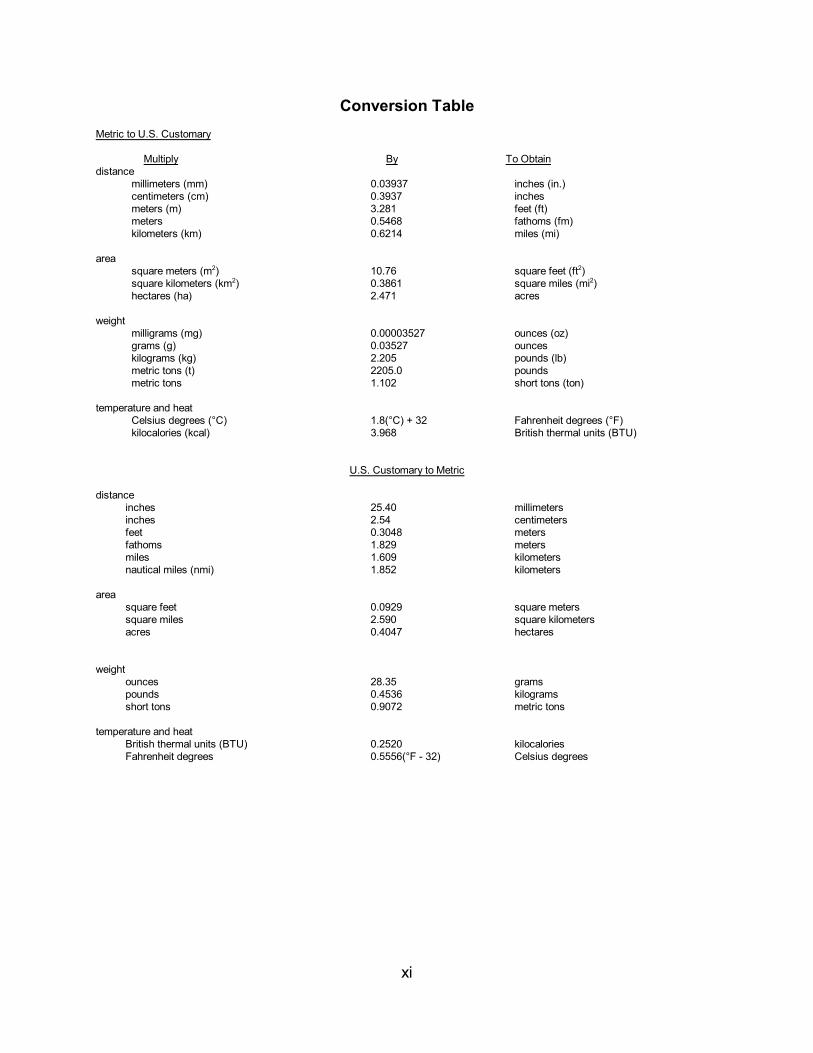
xi
Conversion TableMetric to U.S. Customary
Multiply By To Obtaindistance
millimeters (mm) 0.03937 inches (in.)centimeters (cm) 0.3937 inchesmeters (m) 3.281 feet (ft)meters 0.5468 fathoms (fm)kilometers (km) 0.6214 miles (mi)
areasquare meters (m2) 10.76 square feet (ft2)square kilometers (km2) 0.3861 square miles (mi2)hectares (ha) 2.471 acres
weightmilligrams (mg) 0.00003527 ounces (oz)grams (g) 0.03527 ounceskilograms (kg) 2.205 pounds (lb)metric tons (t) 2205.0 poundsmetric tons 1.102 short tons (ton)
temperature and heatCelsius degrees (°C) 1.8(°C) + 32 Fahrenheit degrees (°F)kilocalories (kcal) 3.968 British thermal units (BTU)
U.S. Customary to Metric
distanceinches 25.40 millimetersinches 2.54 centimetersfeet 0.3048 metersfathoms 1.829 metersmiles 1.609 kilometersnautical miles (nmi) 1.852 kilometers
areasquare feet 0.0929 square meterssquare miles 2.590 square kilometersacres 0.4047 hectares
weightounces 28.35 gramspounds 0.4536 kilogramsshort tons 0.9072 metric tons
temperature and heatBritish thermal units (BTU) 0.2520 kilocaloriesFahrenheit degrees 0.5556(°F - 32) Celsius degrees
i
Executive Summary
White seabass are large, highly prized members of the croaker family, found in watersoff the west coasts of California and Mexico. White seabass are recovering offCalifornia from low population levels in the mid to late 1900s. The current recovery isoccurring under management designed to provide for moderate harvests whileprotecting young white seabass and spawning adults through seasonal closures, gearprovisions, and size and bag limits.
Concern over the decline in white seabass landings and conflict between recreationaland commercial fishermen over this resource resulted in legislation requiring thedevelopment of a white seabass fisheries management plan (WSFMP). The plan wasdeveloped in 1995 through the cooperative efforts of academic and federal fisheryscientists, consultants, and fishery constituents. The plan was adopted by the Fish andGame Commission (Commission) in 1996; however, regulations to implement theWSFMP were not adopted at that time.
California enacted the Marine Life Management Act (MLMA) in 1998, granting broaderregulatory authority to the Commission for specified commercial fisheries, includingwhite seabass. The MLMA declared that the WSFMP shall remain in effect untilamended, but it must be brought into conformance with the MLMA on or before 01January 2002. This deadline was later extended in order to incorporate therecommendations of the peer review panel.
The MLMA further directs that all fisheries be managed on a sustainable basis usingfishery management plans (FMPs). The MLMA specifies the content of FMPs,encourages management to use the best available information, supports research toobtain essential fisheries information, and promotes cooperation and collaboration withfisheries participants and other constituents. This document amends the WSFMP toreflect these goals and others of the MLMA and to otherwise achieve conformance withthe MLMA.
The WSFMP uses a framework plan approach for managing the white seabass fishery.This enables the adjustment of management measures, within the scope and criteriaestablished by this WSFMP and implementing regulations, without the need foramending the FMP. Framework adjustments can be implemented quickly, enablingmore responsive adaptive management of white seabass. In addition to annualmanagement changes, the Commission may make in-season adjustments to addressresource conservation or socioeconomic issues. A Department white seabassmanagement team along with an advisory panel consisting of representatives from thescientific community, recreational and commercial fishing industries, and environmentalgroups will continually monitor the effectiveness of management measures, andrecommend changes to the Commission if needed.
In addition to the framework procedures, initial management alternatives are proposed

ii
for implementation upon approval of the WSFMP. These alternatives representdifferent determinations of a maximum sustainable yield (MSY) and optimum yield (OY)to be used in setting upper harvest limits for white seabass. The OYs range from212,985 pounds to 1.3 million pounds. The preferred alternative is an OY of 1.2 millionpounds. This OY was derived by making a precautionary adjustment to an MSY proxythat was calculated from a previously determined pre-exploitation biomass of whiteseabass.
The preferred alternative, along with a framework plan approach, will allow continuedrecovery of the white seabass resource while important data are collected to yield abetter defined MSY/OY control rule. The WSFMP also includes several triggermechanisms aimed at identifying and minimizing overfishing of the white seabassstock. Socioeconomic and bycatch impacts are not expected to be significant under thepreferred alternative.
The WSFMP identifies specific short-term operational and long-term strategic researchgoals as part of research protocols that address needed essential fisheries informationfor white seabass. The overall goal is to bring our knowledge of white seabass stocksup from data-poor to data-rich; data-poor management of white seabass using anMSY/OY approach should be considered an interim solution. A stock assessment forwhite seabass using existing and ongoing datasets, along with new fishery independentinformation, is of paramount importance for the successful management of whiteseabass. Other short-term research goals include determinations of the size at sexualmaturity, hooking mortality of released fish, amount of bycatch, and validation ofage/growth studies.
Long-term research goals include development of more sophisticated stockassessments and models, expansion of hatchery-reared white seabass studies,collection and analyses of more socioeconomic data, cooperative research with Mexico and implementation of an ecosystem-based management approach.
The costs of implementing the WSFMP are estimated to be high. Most of the costs areassociated with ongoing and future research (data collection and analysis),enforcement of regulations, and document preparation and review; the costs of research alone are estimated to be over $700,000 annually.
1-1
Chapter 1. Background and Description
White seabass, which are targeted by both recreational and commercial fisheries, havegreat economic and intrinsic value to the people of California. White seabass aremigratory fish that are common in Mexican waters and in the Southern California Bight. The fisheries for white seabass have existed since the late 1800s, but increased fishingpressure, oceanographic fluctuations, and habitat degradation have resulted inreductions of white seabass populations. Currently, our monitoring and assessment ofwhite seabass stocks is inadequate for effective management of this importantresource.
1.1 Purpose and Need for Action
The overall trend in commercial and recreational landings of white seabass from 1960to 1997 was one of decline. During the late 1980s and early 1990s, concern over thedecline in white seabass landings and conflict between recreational and commercialfishermen over this resource lead concerned citizens to ask the Legislature formanagement improvements. The resulting legislation required the development of a white seabass fisheries management plan (WSFMP) which was developed in 1995through the cooperative efforts of academic and federal fishery scientists, consultants,and fishery constituents. The plan was adopted by the Fish and Game Commission(Commission) in 1996; however, no regulations were adopted at that time, so the planwas not implemented.
In 1998, the Marine Life Management Act (MLMA) was enacted and changed the wayin which recreational and commercial fisheries are managed in the State of California[Fish and Game Code (FGC) section §7050]. Under MLMA, the Commission wasgranted authority to regulate specific commercial fisheries, including the white seabassfishery (it already had authority over the recreational fishery). Also, MLMA specifiedthat the previously adopted WSFMP should remain in effect until such time as theexisting plan could be amended to comply with MLMA. The amended WSFMP was tobe presented to the Commission no later than 01 January 2002; however, the deadlinewas extended in order to incorporate the recommendations of the peer review panel.
1.1.1 Location and General Characteristics of the Project Area
The sport and commercial harvest of white seabass is proposed statewide in all areasdefined as ocean waters (§27.00 Title 14 CCR) except where prohibited or restricted,as specified, in state refuges, reserves or national parks, and as regulated by provisionof this WSFMP.
The shoreline of California is one of the longest in the nation. There are approximately1,072 miles of shoreline along the mainland coast, and 300 miles around the offshoreislands. The mainland shore consists of about 354 miles of rocky headlands and cliffs;602 miles of sandy beaches; and 110 miles of rocky beach. Major embayments are:
1-2
Humboldt (17,000 surface acres, or 6,880 hectares); Tomales (7,760 surface acres, or3,140 hectares); San Francisco (320,000 surface acres, or 129,504 hectares); Morro(2,101 surface acres, or 8,540 hectares) and San Diego (11,500 surface acres, or4,654 hectares).
The marine environment is composed of numerous micro-habitats which support adistinct assemblage of species uniquely adapted to their environment. A detaileddescription of the oceanographic and geological conditions that make California’smarine environment so complex can be found in the Final Program EnvironmentalDocument Ocean Sport Fishing Regulations. An in-depth description of the habitatpreferences and life history of white seabass is found in Chapter 2, Section 9 of thisdocument.
1.1.2 Problem Statement
Our knowledge of white seabass population dynamics and the role this species plays inthe nearshore ecosystem is limited. Further, there is an urgent need to acquireessential fisheries information which can only be obtained gradually, over a period ofseveral years, and at a considerable cost. As a result, management decisions havelagged behind the development of the fishery and it is difficult to determine whether ornot current fishing is at sustainable levels.
The potential effects of changes in fishing effort, oceanographic conditions, and manyother factors affecting white seabass stocks need to be assessed in order to managethis resource effectively. Since the ban on gill and trammel nets went into effect in1994, the recreational seabass catch has surpassed commercial landings. In addition,white seabass range into Mexican waters and may be heavily impacted by Mexicanharvests. Thus, an essential step to ensure the long term maintenance of a healthywhite seabass resource in California waters is to develop a management plan for thisspecies.
1.2 The Marine Life Management Act
The MLMA was signed into law and incorporated into the FGC (§7050-7090) 01January 1999. The act created state policies, goals, and objectives to govern theconservation, sustainable use and restoration of California’s marine living resources. The MLMA opened a new chapter in the conservation of California’s marine wildlife andthe management of our marine fisheries (Weber and Heneman 2000). The MLMAgives the Fish and Game Commission and the Department specific guidance formanaging marine resources through a comprehensive set of goals and objectivesoutlined below. The WSFMP is being amended under this direction to better facilitateconservation and stewardship of this important resource.
1.2.1 Goals and ObjectivesGoal: To ensure the conservation, sustainable use, and, where feasible, restoration of

1-3
California’s marine living resources for the benefit of all the citizens of the State.
Objectives:• Conserve the health and diversity of marine ecosystems and marine living
resources;• Allow and encourage only those activities and uses that are sustainable;• Recognize the importance of activities and uses that do not involve take;• Recognize the importance to the economy and culture of California of
sustainable sport and commercial fisheries and the development ofcommercial aquaculture;
• Support and promote scientific research on marine ecosystems;• Manage on the basis of the best available scientific and other relevant
information;• Involve all interested parties;• Promote the dissemination of accurate information through the
management process;• Coordinate and cooperate with adjacent states, as well as with Mexico
and Canada, and encourage regional approaches to management.
Goal: To achieve the management goal of sustainability, every fishery shall be managed under a system whose objectives include:
Objectives:• Long-term health of the resource is not sacrificed in favor of short-term
benefits. A fishery managed on the basis of maximum sustainable yieldshall have optimum yield as its objective.
• Health of a habitat is maintained, and to the extent feasible, the habitat isrestored and, where appropriate, enhanced.
• Depressed fisheries are rebuilt to highest sustainable yields consistentwith environmental and habitat conditions.
• Bycatch is limited to acceptable types and amounts.• Fishery participants are allowed to propose methods to prevent or reduce
excess effort in marine fisheries.• Management is closely coordinated when a species is the target of both
sport and commercial fisheries or of a fishery that employs differentgears.
• Fishery management is adaptive and based on best available scientific orother relevant information.
• The management decision-making process is open and seeks advice andassistance of interested parties.
• Adverse impacts of fishery management on small-scale fisheries, coastalcommunities, and local economies are minimized.
• Collaborative and cooperative approaches to management areencouraged and mechanisms are in place to resolve disputes such asaccess, allocation, and gear conflicts.

1-4
• Management is proactive and responds to changing environmentalconditions and market or other socioeconomic factors and concerns offishery participants.
• The management system is periodically reviewed for effectiveness.
1.2.2 Process of Plan Review
The MLMA requires public and peer review for all FMPs (FGC §7075-7078). For publicreview, the Department solicits input and/or assistance from the various user groupswho may be affected by the FMP or other interested parties prior to development of anFMP. The Department can also approach the National Marine Fisheries Service, SeaGrant, the Pacific Fishery Management Council or advisory committees established bythe Department for advice. Once the FMP or amendment has been developed, theplan must be submitted to the Commission for a 30-day public comment period prior toany public hearings. Additionally, the Commission must hold at least two publichearings on the FMP. Any comments or proposals made to the Commission relative tothe FMP may be considered by the Commission and forwarded to the Department forinclusion into the FMP.
For external peer review, the Department is required to set up a formalized procedurefor examining the science that is used as the basis for any managementrecommendation. The peer review panel must be given all pertinent commentsreceived by the Department from fishery participants or other interested parties. Anysuggestions made through external peer review may be used in whole or part; however,if the Department disagrees with the findings and chooses not to use therecommendations, an explanation of why the peer review recommendations were notused must accompany the FMP or amendment.
More information on the review processes for FMPs can be found in The Master Plan:A Guide for the Development of Fishery Management Plans (California Department ofFish and Game 2001).
1.2.3 Process for Plan Amendment
The MLMA also requires a plan amendment process for all FMPs (§7087 FGC). Theamendment process must identify the types of regulations that the Department mayadopt without amending the plan. In addition, any amendment to an FMP mustundergo the review process, as outlined above in section 1.2.2. More information onthe FMP amendment process can be found in The Master Plan: A Guide for theDevelopment of Fishery Management Plans (California Department of Fish and Game2001).
1.3 Specific Goals and Objectives of the White Seabass Fishery Management Plan Goals:1. To manage the white seabass resource for the optimum long-term benefits of

1-5
present and future generations of Californians.2. To bring the management of this valuable commercial and recreational species
under one authority.3. To develop a framework for management that will be responsive to
environmental and socioeconomic changes.
Objectives (not listed in order of priority):• Provide for the sustainable use of the white seabass resource and
provide for stock growth for commercial and sport fisheries;• Use adaptive management to provide for necessary changes and
modifications of management measures in a timely and efficient manner;• Minimize bycatch and waste of white seabass and other species;• Support and promote increased understanding of white seabass natural
history, population dynamics, and its ecosystem’s role to improvemanagement;
• Ensure effective monitoring of the white seabass population and itsfisheries;
• Ensure effective enforcement of regulations and improved compliance;• Identify, protect, and restore critical white seabass habitat; and• Minimize the adverse impacts of management on small-scale fisheries,
coastal communities, and local economies.
1.3.1 Constituent Involvement
The MLMA requires, and the Department is committed to, a collaborative approach toresource management. One of the over-riding objectives of MLMA is constituentinvolvement. The Department believes that broad participation in the development ofan FMP will improve the effectiveness of management and the ability to implement theplan. Constituent involvement also ensures that decision makers are better informedwhen making management decisions by:
• Exploring issues, concerns, and management measures from variousperspectives;
• Providing increased understanding of a resource and its fishery fromparticipants’ and nonparticipants’ perspectives through consensusbuilding; and
• Sharing responsibility of sustainable fisheries management with allinterested constituents.
In addition to the requirements of the MLMA, the California Environmental Quality Act(CEQA) requires public consultation on all environmental projects. The Departmentaccomplishes this through either a 30-day public comment period, scoping sessionswithin the communities involved, or at least two Commission meetings.
1.3.1.1 Public Consultation for Definition of Plan Goals and Objectives
1-6
In 1994 when the initial WSFMP was developed, one of the first actions taken was thecreation of two committees: 1) The White Seabass Subcommittee of the Director’sMarine Resources Advisory Committee, composed of representatives from therecreational and commercial fishing communities; and 2) The White Seabass ScientificAdvisory Committee, composed of fisheries scientists from academia and the federalgovernment (Appendix F). These two bodies met repeatedly in 1995, each timebringing relevant comments from their constituent groups. It was through these actionsthat the goals and objectives identified above were generated. In January 2001, theremaining members of the Scientific Advisory Committee and several members of theformer White Seabass Subcommittee of the Director’s Marine Resources AdvisoryCommittee joined to form the White Seabass Scientific and Constituent Advisory Panel(WSSCAP). The WSSCAP determined that the goals and objectives outlined in theprevious WSFMP were still valid.
1.3.1.2 Public Consultation for Selection of Preferred Management Alternative
Prior to preparing the initial draft environmental document in 1995, the Departmentdeveloped a Notice of Preparation (NOP). The notice was provided to individuals andorganizations that had expressed prior interest in Commission regulatory actions. TheNOP was also submitted to the State Clearinghouse for distribution to appropriateresponsible and trustee agencies for their input and comments. No comments werereceived in response to the initial NOP in 1995.
The Department also conducted three public meetings with a subpanel of the Director'sMarine Resources Advisory Committee (11 October 1994; 31 January 1995; and 31March 1995) and three public meetings with the Scientific Advisory Committee (24October 1995; 06 February 1995; and 09 March 1995) (Appendix F).
In addition to the NOP and six public meetings, discussion of the WSFMP was held attwo Commission meetings (04 August 1995 and 03 November 1995). The result ofthese meetings was the selection of a management framework for the WSFMP.
As with the WSFMP’s goals and objectives, discussions of the preferred alternative andother possible management alternatives were held with members of the WSSCAP andother interested parties on 30 January 2001, 04 June 2001, 18 December 2001, and 22January 2001. Additionally, a presentation of the status of the WSFMP was given tothe MLMA Evaluation Advisory Committee on 09 February 2001.
1.4 Authority and Responsibility
The California Constitution gives authority to the State Legislature which may, bystatute, provide for the seasons and the conditions under which different species of fishmay be taken. California law consists of 29 codes including the FGC. Laws in theFGC consist of statutes and propositions passed by the voters of the state. Statutes,such as MLMA, are chaptered bills that have passed through both houses of the
1-7
Legislature and ultimately signed by the Governor and recorded by the Secretary ofState. The FGC is administered and enforced through regulations.
General policies for the conduct of the Department are formulated by the Commission,a body created by the Constitution and appointed by the Governor. The rulemakingpowers of the Commission are delegated to it by the Legislature.
The Department is the state agency charged with carrying out policies adopted by theState Legislature and the Commission. The Department enforces statutes andregulations governing recreational and commercial fishing activities, conductsbiological research, monitors fisheries, and collects fishery statistics necessary toprotect, conserve, and manage the living marine resources of California.
Other state agencies have functions and responsibilities that directly or indirectly affectthe management of ocean and coastal resources (California Department of Fish andGame, December 1993). In addition, marine resources are also managed by federallaws governing the take of seabirds, marine mammals, fish, and shellfish (Weber andHeneman 2000).
1.4.1 California Environmental Quality Act (CEQA)
The basic goal of CEQA [Public Resources Code (PRC) §21000-21006] is to developand maintain a high-quality environment now and in the future. Projects carried out bypublic agencies are subject to the same level of review and consideration as those ofthe private sector. Most state agencies satisfy this requirement by preparing aNegative Declaration (ND) if it finds no significant impacts, a Mitigated NegativeDeclaration (MND) if it finds significant impacts but revises the project to avoid ormitigate those impacts, or an Environmental Impact Report (EIR) if it finds significantimpacts.
1.4.1.1 Functional Equivalent
The CEQA requires all public agencies in the State to evaluate the environmentalimpacts of projects that they approve or carry out. If there are potentially significantenvironmental impacts, most agencies satisfy this requirement by preparing anEnvironmental Impact Report (EIR). If no potentially significant impacts exist, aNegative Declaration (ND) is prepared. However, an alternative to the EIR/NDrequirement exists for State agencies with activities that include protection of theenvironment as part of their regulatory program. Under this alternative, an agency mayrequest certification of its regulatory program from the Secretary for Resources. Withcertification, an agency may prepare functional equivalent environmental documents inlieu of EIRs or NDs. The regulatory program of the Fish and Game Commission hasbeen certified by the Secretary for Resources. Therefore, the Commission is eligible tosubmit an environmental document in lieu of an EIR (§15252 CEQA Guidelines ).
1-8
The Department and the Commission hold the public trust for managing the State’s fishand wildlife populations. That responsibility is fulfilled by a staff of experts, includingthose with expertise in marine resources management and enforcement issues relatedto the harvesting of white seabass. The knowledge and training represented by thatexpertise qualifies them to perform the review and analysis of the proposed projectcontained in this document.
1.4.1.2 Use of the Environmental Document
This environmental document contains a description of the proposed managementaction, potential effects of the proposed action, reasonable alternatives to the proposal,cumulative effects, and a discussion of mitigation of adverse environmental effectsrelated to the proposal and alternatives. In addition, it considers relevant policies ofthe Legislature and Commission. These standards are contained in §781.5 Title 14California Code of Regulations (CCR). This environmental document presentsinformation to allow a comparison of the potential effects of various alternatives toadoption of sport and commercial fishing regulations for white seabass as they arecurrently written and enforced.
1.4.2 Federal Law
The Federal government manages the marine resources and fishing activities of theUnited States (US) through the Magnuson-Stevens Fishery Conservation andManagement Act (MSFCMA). The purpose of the MSFCMA is to provide conservationand management of US fishery resources, develop domestic fisheries, and phase outforeign fishing activity within the Exclusive Economic Zone (EEZ) consisting of oceanwaters from the edge of State waters three mi (5 km) to 200 mi (322 km) offshore.
Eight Regional Fishery Management Councils implement the goals of the MSFCMA incoordination with the National Marine Fisheries Service. The Pacific FisheryManagement Council manages the fisheries resources off Washington, Oregon, andCalifornia by developing fishery management plans for the EEZ. Although whiteseabass are a trans-boundary stock occurring in Mexican and U.S. waters, the fisheryin both countries has primarily been a coastal fishery (within three miles of shore). Assuch, the fishery in California is not subject to federal management. Even with theremoval of gill nets from state waters along much of the California coast, andsubsequent move to federal waters, the fishery continues to be managed by the statebecause vessels taking white seabass are registered by the State and land their catchin California ports.
1.5 Current Management of White Seabass
Management of the white seabass fishery has been divided between the Legislature
1-9
and the Commission. In the past two decades, the Legislature and the Commissionhave adopted statutes and regulations specific to the management of variouscomponents of the white seabass fishery (Appendix B). The most recent and farreaching management change occurred with the enactment of the MLMA.
1.5.1 Legislative Responsibilities
Statues passed by the State Legislature regulating commercial fishing are contained inthe Fish and Game Code of California. Some provisions of law apply specifically towhite seabass, while others apply generally to the take of all fish such as some areaclosures and gear restrictions. Statutes pertaining specifically to the commercial takeof white seabass are listed in Appendix B.
As mentioned earlier, The MLMA identifies a number of policies, goals, objectives,requirements, and processes for managing California’s marine resources. Theseresources are to be managed to assure long-term economic, recreational, ecological,cultural, and social benefits.
The MLMA requires that fishery management plans (FMPs) form the primary basis formanaging the State’s marine fisheries. An FMP is a planning document that containscomprehensive review of the fishery along with clear objectives and measures to insuresustainability of that fishery. An FMP is based on the best available scientific or otherrelevant information.
1.5.2 Fish and Game Commission Responsibilities
The authority and responsibility of the Commission and the Department to make andenforce regulations governing recreational and commercial fishing are provided by theLegislature. General policies for the conduct of the Department are formulated by theCommission (FGC §704). General policy for conservation of aquatic resources isprovided by FGC §1700, and specific policy for the management of marine resources(MLMA) is provided in FGC §7500- §7090.
1.5.2.1 Recreational Fisheries
Recreational fishing regulations are adopted by the Commission following procedureslisted in the FGC. General provisions applying to the taking and possession of fish byrecreational fishermen are provided in FGC §7100-7400. Specific sportfishingregulations are found in California Code of Regulations (CCR), Title 14, Chapter 4.Regulations specific to the recreational take of white seabass are listed in Appendix B.
1.5.2.2 Commercial Fisheries
Commercial fishing regulations are created by the Legislature and the Commission. Provisions relating to the taking and possession of fish for commercial purposes is
1-10
provided in FGC §7600-9101 and CCR, Title 14, Chapter 6. With the passage of theMLMA, the Commission has been granted broad authority to regulate commercialfisheries, including white seabass.
1.5.2.3 Rulemaking Process under the Administrative Procedures Act (APA)
The California Constitution and Legislative statutes create state agencies and cangrant them certain powers including the ability to make rules and regulations in order tocarry out their duties. The California APA (§11340-11359) of the Government Codeprovides guidance on the rulemaking process.
The Commission’s rulemaking process is provided in FGC §200-221. Basic minimumprocedural requirements for the adoption, amendment or repeal of regulations areprovided in the California Government Code §11346. Emergency rulemakingconsiderations are provided in California Government Code §11346.1 and in FGC§240.
2-1
Chapter 2. Description of Stocks
2.1 Species Description
The croakers (Family Sciaenidae) are among the most important fishes caught bymarine recreational anglers in California. Most croakers emit sounds, which have beenvariously described as 'drumming', 'croaking', 'grunting', 'snoring', 'bellowing', purring','buzzing', and 'whistling' (Welsh and Breder 1923). These sounds are produced byvibrations of the air bladder.
The white seabass, Atractoscion nobilis, is the largest croaker species in Californiawaters (Thomas 1968). Adults are bluish to gray dorsally with dark speckling, andsilver to white colored ventrally. Juveniles have several dark vertical bars. Whiteseabass are relatively large fish which have been recorded to 5 ft (1.5 m) and 90 lbs(41 kg) (Miller and Lea 1972); however, individuals larger than 60 lbs (27 kg) are rarelyobserved (Thomas 1968).
Fossil records of white seabass have been found in several southern CaliforniaPleistocene deposits and in a Pliocene site at San Diego. Some deposits are probably10 to 12 million years old (Fitch and Lavenberg 1971).
2.2 Distribution, Genetic Stock Structure, and Migration
White seabass range over the continental shelf of the Eastern North Pacific ocean fromJuneau, Alaska, to Magdalena Bay, Baja California, Mexico. This species also inhabitsthe upper Gulf of California, Mexico; a subpopulation that appears to be isolated fromthe coastal mainland megapopulation (or stock) (Thomas 1968).
California Cooperative Oceanic Fisheries Investigations (CalCOFI) data collectedbetween 1950 and 1978 indicate that white seabass larvae appear to settle out intocoastal areas extending from Santa Rosa Island, California to Bahia Santa Maria, halfway down the Baja California, Mexico peninsula (Moser et al. 1983). Fifteen percent ofthese occurrences were in California waters. Most of the larvae occurred from May toAugust and peaked in July. White seabass larvae were collected within San FranciscoBay (Richardson Bay) during a 1972 to 1973 study (Eldridge 1977). However, to date,no adults have been found within the bay. That event was correlated with upwelling,implying that the larvae were transported into the bay with warm water currents.
In the past, it was assumed that white seabass off California consisted of non-residentfish that migrated into the Southern California Bight from Baja California, Mexico. However, white seabass off the coasts of California and Baja California, Mexico arecurrently considered to be part of the same breeding population, and the center of thispopulation appears to be off central Baja California, Mexico (Moser et al. 1983;Vojkovich and Reed 1983; Franklin 1997). Franklin (1997) examined white seabass
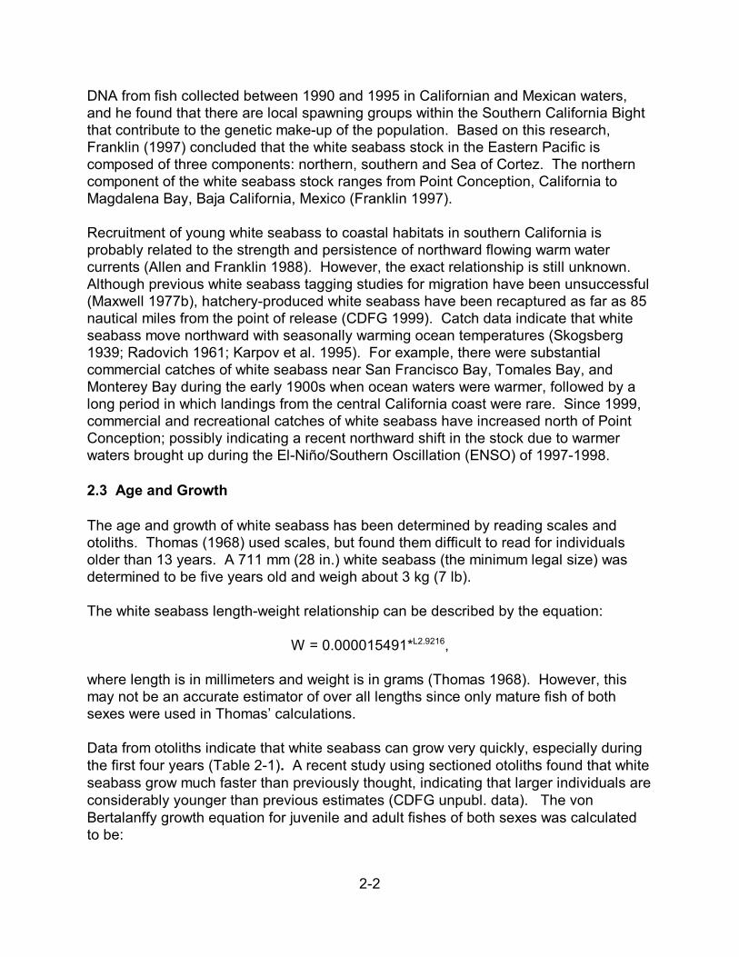
2-2
DNA from fish collected between 1990 and 1995 in Californian and Mexican waters,and he found that there are local spawning groups within the Southern California Bightthat contribute to the genetic make-up of the population. Based on this research,Franklin (1997) concluded that the white seabass stock in the Eastern Pacific iscomposed of three components: northern, southern and Sea of Cortez. The northerncomponent of the white seabass stock ranges from Point Conception, California toMagdalena Bay, Baja California, Mexico (Franklin 1997).
Recruitment of young white seabass to coastal habitats in southern California isprobably related to the strength and persistence of northward flowing warm watercurrents (Allen and Franklin 1988). However, the exact relationship is still unknown. Although previous white seabass tagging studies for migration have been unsuccessful(Maxwell 1977b), hatchery-produced white seabass have been recaptured as far as 85nautical miles from the point of release (CDFG 1999). Catch data indicate that whiteseabass move northward with seasonally warming ocean temperatures (Skogsberg1939; Radovich 1961; Karpov et al. 1995). For example, there were substantialcommercial catches of white seabass near San Francisco Bay, Tomales Bay, andMonterey Bay during the early 1900s when ocean waters were warmer, followed by along period in which landings from the central California coast were rare. Since 1999,commercial and recreational catches of white seabass have increased north of PointConception; possibly indicating a recent northward shift in the stock due to warmerwaters brought up during the El-Niño/Southern Oscillation (ENSO) of 1997-1998.
2.3 Age and Growth
The age and growth of white seabass has been determined by reading scales andotoliths. Thomas (1968) used scales, but found them difficult to read for individualsolder than 13 years. A 711 mm (28 in.) white seabass (the minimum legal size) wasdetermined to be five years old and weigh about 3 kg (7 lb).
The white seabass length-weight relationship can be described by the equation:
W = 0.000015491*L2.9216,
where length is in millimeters and weight is in grams (Thomas 1968). However, this may not be an accurate estimator of over all lengths since only mature fish of bothsexes were used in Thomas’ calculations.
Data from otoliths indicate that white seabass can grow very quickly, especially duringthe first four years (Table 2-1). A recent study using sectioned otoliths found that whiteseabass grow much faster than previously thought, indicating that larger individuals areconsiderably younger than previous estimates (CDFG unpubl. data). The vonBertalanffy growth equation for juvenile and adult fishes of both sexes was calculatedto be:
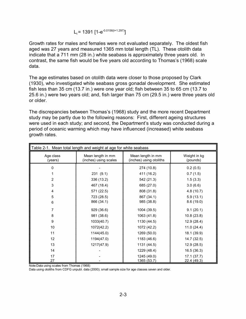
2-3
Lt = 1391 [1-e-0.0156(t+1.297)]
Growth rates for males and females were not evaluated separately. The oldest fishaged was 27 years and measured 1365 mm total length (TL). These otolith dataindicate that a 711 mm (28 in.) white seabass is approximately three years old. Incontrast, the same fish would be five years old according to Thomas’s (1968) scaledata.
The age estimates based on otolith data were closer to those proposed by Clark(1930), who investigated white seabass gross gonadal development. She estimatedfish less than 35 cm (13.7 in.) were one year old; fish between 35 to 65 cm (13.7 to25.6 in.) were two years old; and, fish larger than 75 cm (29.5 in.) were three years oldor older.
The discrepancies between Thomas’s (1968) study and the more recent Departmentstudy may be partly due to the following reasons: First, different ageing structureswere used in each study; and second, the Department’s study was conducted during aperiod of oceanic warming which may have influenced (increased) white seabassgrowth rates.
Table 2-1. Mean total length and weight at age for white seabass
Age class (years)
Mean length in mm(inches) using scales
Mean length in mm (inches) using otoliths
Weight in kg(pounds)
0 - 274 (10.8) 0.2 (0.5)1 231 (9.1) 411 (16.2) 0.7 (1.5)2 336 (13.2) 542 (21.3) 1.5 (3.3)3 467 (18.4) 685 (27.0) 3.0 (6.6)4 571 (22.5) 808 (31.8) 4.8 (10.7)5 723 (28.5) 867 (34.1) 5.9 (13.1)6 866 (34.1) 985 (38.8) 8.6 (19.0)
7 929 (36.6) 1004 (39.5) 9.1 (20.1)8 981 (38.6) 1063 (41.8) 10.8 (23.8)9 1033(40.7) 1130 (44.5) 12.9 (28.4)
10 1072(42.2) 1072 (42.2) 11.0 (24.4)11 1144(45.0) 1269 (50.0) 18.1 (39.9)12 1194(47.0) 1183 (46.6) 14.7 (32.5)13 1217(47.9) 1131 (44.5) 12.9 (28.5)14 - 1229 (48.4) 16.5 (36.3)17 - 1245 (49.0) 17.1 (37.7)27 - 1365 (53.7) 22.4 (49.3)
Note:Data using scales from Thomas (1968)Data using otoliths from CDFG unpubl. data (2000); small sample size for age classes seven and older.
2-4
2.4 Reproduction, Fecundity and Seasonality
Precise spawning areas have not been determined, but data indicate that peakspawning occurs in southern California from April through August (Skogsberg 1925). During this period, mature fish appear to congregate near shore, over rocky habitat,and near kelp beds (Thomas 1968).
A study of white seabass maturity in the late 1920s indicated that females beginmaturing when they are near 24 inches (607 mm) in length or three years old andmales may reach sexual maturity at about 20 inches (508 mm) or two years old (agesbased on otolith data above). All white seabass have probably spawned at least onceby the time they reach 31.5 inches (800 mm) total length (Clark 1930) or four years old.
White seabass have the largest eggs of the West Coast sciaenids. These eggs arebuoyant and drift with the ocean currents. The dark colored larvae appear to settle outin coastal areas (Moser et al. 1983). Fecundity has been determined from artificialpropagation attempts (CDFG 1994). Batch fecundity, the number of eggs released byone female at a single time, has ranged from 0.76 million to 1.5 million eggs, and hasvaried as a function of mean female body weight.
Although it has been reported that white seabass spawn more than once per season,spawning intervals for individual females are unknown. However, it has been estimatedthat females spawn about four to five times during each season.
2.5 Natural Mortality
Thomas (1968) calculated a natural mortality rate of 0.303 for fish caught in commercialgill nets. These fish represented the majority of commercially-caught white seabassand tend to be larger than recreationally-caught fish. Recently, natural mortality rateswere determined for juvenile white seabass based on OREHP data. Kent and Ford(1990) found that natural mortality rates ranged from 0.258 (one and two year old fish)to 0.117 (three and four year old fish). Likewise, MacCall et al. (1976) and Dayton andMacCall (1992) calculated natural mortality rates for white seabass from the recreational and commercial fisheries, which were significantly less than Thomas’(1968) estimate (Table 2-2) . In light of these values, it would seem that Thomas'estimate was high since natural mortality rates usually decline and level off as fish age.
Table 2-2. Estimates of white seabass natural mortality (M)
Source M
Thomas 1968 0.303
2-5
MacCall et al. 1976 0.13
Kent and Ford 1990 0.258 (1 to 2 yr old); 0.117 (3 to 4 yr old)
Dayton and MacCall 1992 0.08
In comparison, natural mortality rates for another sciaenid, the red drum (Sciaenopsocellatus), were similar. Red drum are found in the Gulf of Mexico and the Atlanticocean, and have a life history similar to white seabass. The natural mortality rates forthem are 0.20 to 0.23 for subadults (1 to 5 yr old) and 0.12 to 0.13 for adults (6+ yr old)(SAFMC 2000). These rates are consistent with those calculated for white seabass byKent and Ford (1990).
2.6 Parasites and Disease
Love and Moser (1976) provided a review of parasites commonly associated withmarine fishes, including those common to white seabass taken from Mexican andCalifornian waters. External parasites consisted of three species of copepod(Lepeophtheirus abdominis, L. thompsoni, and Neobrachiella gracilis) and anunidentified monogenetic trematode, which were found attached to the body, fins, andmouth. Internally, three species of cestode worms (Callitetrarhynchus gracilis, Grillotiasmarisgora, and Lacistorhyncus tenuis) have been found in the viscera and mesenteryof white seabass. In addition, two species of digenera trematodes (Pleorchismagniporus, P. californiensis) have been found in the intestines, along with one speciesof nematode worm (Anisakis sp.). Two protozoans (Ceratomyxa venusta and Kudoaclupeidae) have been discovered in the gallbladder and muscle tissue of whiteseabass.
Little is known about disease in wild white seabass stocks. Chen et al. (1995)identified the marine gliding bacteria, Flexibacter maritimus, as the cause of lesions onwhite seabass, Northern anchovy (Engralis mordax) and Pacific sardine (Sardinopssagax) being held in close proximity. They also identified the presence of a secondpathogenic bacteria, Vibrio species on white seabass. The cause of the infections wasattributed to physical trauma such as net abrasions from capture and transfer,aggressive feeding behavior of captive white seabass, and wounds resulting from fish-eating birds (Chen et al. 1995). A third bacteria found to affect hatchery-reared whiteseabass is a Rickettsiales-like bacteria (CDFG 1998), which appeared to be similar toRickettsia bacteria found on net pen-reared salmon in Chile. Whether these and otherbacteria are present on wild fish is currently unknown.
Worldover, scientific information on the diseases of marine fishes is poorly developedcompared to information on the diseases of livestock and avian species. Investigation
2-6
of disease in aquatic animals is more difficult due to the extensive and variable natureof the marine environment and the large number of species involved. Disease eventsare more likely to be recognized in aquaculture facilities than in wild stocks. Thus,information on the health status of commonly cultured species, such as salmonids,tends to be more comprehensive (AQIS 1999).
The effect of external and internal parasites and pathogens on healthy fish are oftenminor, being manifested as inflamation, lesions or increased mucus secretions (Smith1975). However, conditions which stress fish can induce pathogenogenic infectionsthat may result in death.
2.7 Predator/Prey Relationships
Knowledge of the food preferences and habits of white seabass are primarilyanecdotal. However, mysid shrimp (Mysidae) made up a major portion of the diet ofjuvenile white seabass taken in and just outside of San Diego Bay (Crooke 1989a). Adults are known to feed on northern anchovy (Engraulis mordax); market squid (Loligoopalescens); Pacific sardine (Sardinops sagax); blacksmith (Chromis punctipinnis);silversides (Atherinopsidae species); and pelagic red crab (Pleuroncodes planipes)(Thomas 1968). Large white seabass have been found to have eaten only Pacificmackerel (Scomber japonicus) (Fitch 1958).
Commercial fishermen have recorded numerous instances of sea lion and sharkpredation on adult white seabass caught in nets (Fitch and Lavenberg 1971). Studiesto identify the predators of white seabass eggs, larvae, and juveniles have not beendone. Hypothetically, predators would include all piscivorous fishes such as kelp andsand bass (Paralabrax clathratus and P. nebulifer). In laboratory tanks, white seabasslarvae are cannibalistic and must be graded by size (Crooke 1989a). This behaviorprobably takes place in the wild.
2.8 Competition
White seabass are often taken in conjunction with other migratory or seasonallyavailable species such as bonito (Sarda chiliensis), California barracuda (Sphyraenaargentea), and yellowtail (Seriola lalandi). Juveniles have been found mixed with baitfish caught by round haul nets. However, no specific data exist concerning whiteseabass competition with other species.
2.9 Critical Habitat
Young-of-the-year (age 0) white seabass ranging in length from 6 to 57 mm (0.25 to2.25 in.) inhabit the open coast at depths of from 4 to 9 m (12 to 30 ft). These youngfish are closely associated with small drifting debris and algae in shallow areas justoutside the surf zone (Allen and Franklin 1988; 1992). Anecdotal information indicate
2-7
that they are occasionally caught mixed with bait fish (anchovy) schools. By the timewhite seabass are two years old, some have moved into protected bays and are foundin association with eelgrass beds (Crooke 1989b). Larger juveniles (three and fouryears old) are caught off piers and jetties and in kelp beds. Large white seabassschool over rocky substrate in or near the large kelp beds that fringe the beaches andoffshore islands. They are also found several miles offshore in schools swimming at ornear the surface (Skogsberg 1939; Squire 1972).
2.10 Status of the Stocks
Historically, the white seabass resource extended as far north as San Francisco Bay,but as oceanographic conditions changed and the various segments of the fisherygrew, there was a steady decline in availability and subsequently catch. In essence,the resource contracted geographically, so that the bulk of the resource was situatedoff of southern California and northern Baja California, Mexico. Only during ENSOswere white seabass caught in quantity north of Point Conception. However, recentincrease of catches by recreational and commercial fishermen in the Monterey Bayarea during the past two years may indicate expansion of the stock (Departmentunpubl. data). There are few data available concerning the status of white seabasspopulations in Mexican waters, so it is difficult to determine if this is a geographicexpansion of the stock due to increasing numbers or a shifting of the stock northward.
Although a current stock assessment has not been done for white seabass there areindications that the white seabass population in California is recovering from low levelsseen in the 1970s, 1980s, and most of the 1990s. It appears that white seabass maybe entering a pattern similar to the 1940s, where abundance increased following a shiftfrom a period of warmer to colder ocean waters. Warmer waters have occurred in theSouthern California Bight from the late 1970s to mid 1990s, but have become colderthe last few years. During this time, there has also been a steady increase in whiteseabass take in California waters, approaching catch levels of the late 1940s and early1950s. A similar pattern also occurred in the late 1890s and early 1900s when whiteseabass catches were high following a much warmer period that ended in the 1880s(MacCall pers. comm.).
In addition to increased catches of white seabass, there has been a steady increase inthe size of fish taken. For example, the weight of white seabass caught by therecreational fishery averaged about 2.4 kilograms (5 lbs) in the 1980s but increased to6.2 kilograms (14 lbs) in the 1990s (RecFIN 2001). It is difficult to determine if asimilar change has occurred in the commercial fishery since most white seabass takenare well above the legal size limit of 28 inches (711 mm). However, anecdotalinformation from the commercial fishery suggests that a similar trend is occurring.
White seabass recruitment in the Southern California Bight has also increased steadilysince 1982, with large increases occurring in recent years (Crooke pers. comm.; Allenet al. 2001). Fishery-independent data from gill net surveys indicate a significant
2-8
increase in 0 to 4 year old white seabass from 1995-2001 (Allen et al. 2001). Thelargest recruitment during this period occurred in 1999 when a large number of one andtwo year old fish were caught. This was probably a result of a strong year classassociated with the ENSO of 1997-1998.

3-1
Chapter 3. Description of the Fishery
3.1 Areas and Stocks Involved
White seabass occur in or near large kelp beds which fringe beaches and rockyheadlands in southern California and the offshore islands (Skogsberg 1939; Thomas1968). They are also found several miles offshore in schools of various sizes. Duringsome months of the year, white seabass tend to occur close to the seafloor in deeperwater (Skogsberg 1939). These same patterns have been reported for white seabasstaken north of Point Conception (Thomas 1968). Some of the typical areas inhabitedby white seabass are Long Point, Palos Verdes Peninsula; Point Loma; Dana Point; thewest end of Santa Catalina Island; San Clemente Island; Santa Barbara Island; andSanta Cruz Island.
Historically, recreational and commercial white seabass fishing activity occurred alongthe coast between San Pedro and San Diego. Over time, as more recreationalfishermen became interested in white seabass, fishing activity expanded northwardalong the coast to Santa Barbara and out to the northern Channel Islands. Since theseareas had been used by commercial fishermen, user conflicts increased. In the mid-1990's, implementation of the southern California nearshore gill net ban caused a shiftin commercial fishing activity. The San Pedro/Huntington Flats area became lessimportant as effort was focused at San Miguel, Santa Rosa, and Santa Cruz islandsand along the mainland from Goleta northward (Department unpubl. data). Increasedregulation on the use of various commercial gear has created large areas along themainland coast and offshore islands that have become defacto commercial fishingclosures. As a consequence, recreational fishermen have had better access to whiteseabass than ever before over the past two decades and the partitioning of the whiteseabass resource has shifted to the recreational fishery.
3.2 History of Exploitation
The white seabass resource of the Eastern Pacific has been shared by the recreationaland commercial components of the fishery since at least the late 1890's. Documentation of this common usage can be found in the Avalon Tuna Club’s weightrecords for white seabass from the early 1900's (Dayton and MacCall 1992) and inDepartment data (Young 1973; Table 3-1).
Another component of the historical catch is the contribution of white seabass landingsby U.S. boats fishing off Mexico. Until the 1960s, that portion of California landingsaveraged between 35% and 40% of total catches and increased to 75% between 1963and 1980. However, in January 1982, Mexico began denying fishing permits to U.S.commercial fishermen (Vojkovich and Reed 1983). The result was a substantialreduction in total U.S. commercial seabass landings (Table 3-1).
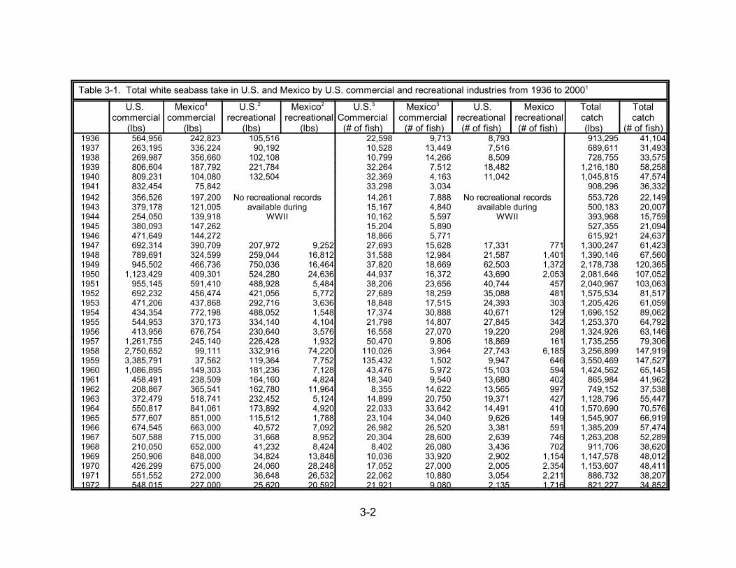
3-2
Table 3-1. Total white seabass take in U.S. and Mexico by U.S. commercial and recreational industries from 1936 to 20001
U.S. commercial
(lbs)
Mexico4 commercial
(lbs)
U.S.2 recreational
(lbs)
Mexico2
recreational (lbs)
U.S.3
Commercial (# of fish)
Mexico3
commercial (# of fish)
U.S.recreational(# of fish)
Mexico recreational
(# of fish)
Total catch (lbs)
Total catch
(# of fish)1936 564,956 242,823 105,516 22,598 9,713 8,793 913,295 41,1041937 263,195 336,224 90,192 10,528 13,449 7,516 689,611 31,4931938 269,987 356,660 102,108 10,799 14,266 8,509 728,755 33,5751939 806,604 187,792 221,784 32,264 7,512 18,482 1,216,180 58,2581940 809,231 104,080 132,504 32,369 4,163 11,042 1,045,815 47,5741941 832,454 75,842 33,298 3,034 908,296 36,3321942 356,526 197,200 No recreational records
available during WWII
14,261 7,888 No recreational records available during
WWII
553,726 22,1491943 379,178 121,005 15,167 4,840 500,183 20,0071944 254,050 139,918 10,162 5,597 393,968 15,7591945 380,093 147,262 15,204 5,890 527,355 21,0941946 471,649 144,272 18,866 5,771 615,921 24,6371947 692,314 390,709 207,972 9,252 27,693 15,628 17,331 771 1,300,247 61,4231948 789,691 324,599 259,044 16,812 31,588 12,984 21,587 1,401 1,390,146 67,5601949 945,502 466,736 750,036 16,464 37,820 18,669 62,503 1,372 2,178,738 120,3651950 1,123,429 409,301 524,280 24,636 44,937 16,372 43,690 2,053 2,081,646 107,0521951 955,145 591,410 488,928 5,484 38,206 23,656 40,744 457 2,040,967 103,0631952 692,232 456,474 421,056 5,772 27,689 18,259 35,088 481 1,575,534 81,5171953 471,206 437,868 292,716 3,636 18,848 17,515 24,393 303 1,205,426 61,0591954 434,354 772,198 488,052 1,548 17,374 30,888 40,671 129 1,696,152 89,0621955 544,953 370,173 334,140 4,104 21,798 14,807 27,845 342 1,253,370 64,7921956 413,956 676,754 230,640 3,576 16,558 27,070 19,220 298 1,324,926 63,1461957 1,261,755 245,140 226,428 1,932 50,470 9,806 18,869 161 1,735,255 79,3061958 2,750,652 99,111 332,916 74,220 110,026 3,964 27,743 6,185 3,256,899 147,9191959 3,385,791 37,562 119,364 7,752 135,432 1,502 9,947 646 3,550,469 147,5271960 1,086,895 149,303 181,236 7,128 43,476 5,972 15,103 594 1,424,562 65,1451961 458,491 238,509 164,160 4,824 18,340 9,540 13,680 402 865,984 41,9621962 208,867 365,541 162,780 11,964 8,355 14,622 13,565 997 749,152 37,5381963 372,479 518,741 232,452 5,124 14,899 20,750 19,371 427 1,128,796 55,4471964 550,817 841,061 173,892 4,920 22,033 33,642 14,491 410 1,570,690 70,5761965 577,607 851,000 115,512 1,788 23,104 34,040 9,626 149 1,545,907 66,9191966 674,545 663,000 40,572 7,092 26,982 26,520 3,381 591 1,385,209 57,4741967 507,588 715,000 31,668 8,952 20,304 28,600 2,639 746 1,263,208 52,2891968 210,050 652,000 41,232 8,424 8,402 26,080 3,436 702 911,706 38,6201969 250,906 848,000 34,824 13,848 10,036 33,920 2,902 1,154 1,147,578 48,0121970 426,299 675,000 24,060 28,248 17,052 27,000 2,005 2,354 1,153,607 48,4111971 551,552 272,000 36,648 26,532 22,062 10,880 3,054 2,211 886,732 38,2071972 548,015 227,000 25,620 20,592 21,921 9,080 2,135 1,716 821,227 34,852
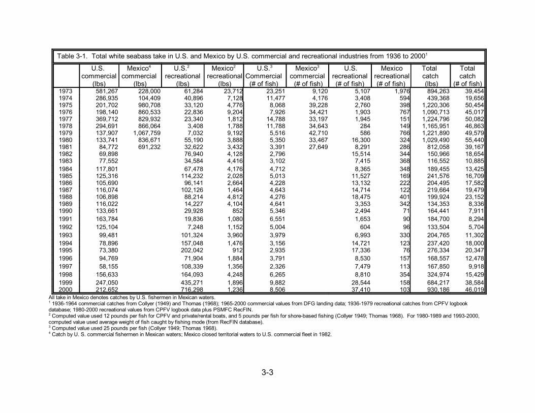
Table 3-1. Total white seabass take in U.S. and Mexico by U.S. commercial and recreational industries from 1936 to 20001
U.S. commercial
(lbs)
Mexico4 commercial
(lbs)
U.S.2 recreational
(lbs)
Mexico2
recreational (lbs)
U.S.3
Commercial (# of fish)
Mexico3
commercial (# of fish)
U.S.recreational(# of fish)
Mexico recreational
(# of fish)
Total catch (lbs)
Total catch
(# of fish)
3-3
1973 581,267 228,000 61,284 23,712 23,251 9,120 5,107 1,976 894,263 39,4541974 286,935 104,409 40,896 7,128 11,477 4,176 3,408 594 439,368 19,6561975 201,702 980,708 33,120 4,776 8,068 39,228 2,760 398 1,220,306 50,4541976 198,140 860,533 22,836 9,204 7,926 34,421 1,903 767 1,090,713 45,0171977 369,712 829,932 23,340 1,812 14,788 33,197 1,945 151 1,224,796 50,0821978 294,691 866,064 3,408 1,788 11,788 34,643 284 149 1,165,951 46,8631979 137,907 1,067,759 7,032 9,192 5,516 42,710 586 766 1,221,890 49,5791980 133,741 836,671 55,190 3,888 5,350 33,467 16,300 324 1,029,490 55,4401981 84,772 691,232 32,622 3,432 3,391 27,649 8,291 286 812,058 39,1671982 69,898 76,940 4,128 2,796 15,514 344 150,966 18,6541983 77,552 34,584 4,416 3,102 7,415 368 116,552 10,8851984 117,801 67,478 4,176 4,712 8,365 348 189,455 13,4251985 125,316 114,232 2,028 5,013 11,527 169 241,576 16,7091986 105,690 96,141 2,664 4,228 13,132 222 204,495 17,5821987 116,074 102,126 1,464 4,643 14,714 122 219,664 19,4791988 106,898 88,214 4,812 4,276 18,475 401 199,924 23,1521989 116,022 14,227 4,104 4,641 3,353 342 134,353 8,3361990 133,661 29,928 852 5,346 2,494 71 164,441 7,9111991 163,784 19,836 1,080 6,551 1,653 90 184,700 8,2941992 125,104 7,248 1,152 5,004 604 96 133,504 5,7041993 99,481 101,324 3,960 3,979 6,993 330 204,765 11,3021994 78,896 157,048 1,476 3,156 14,721 123 237,420 18,0001995 73,380 202,042 912 2,935 17,336 76 276,334 20,3471996 94,769 71,904 1,884 3,791 8,530 157 168,557 12,4781997 58,155 108,339 1,356 2,326 7,479 113 167,850 9,9181998 156,633 164,093 4,248 6,265 8,810 354 324,974 15,4291999 247,050 435,271 1,896 9,882 28,544 158 684,217 38,5842000 212,652 716,298 1,236 8,506 37,410 103 930,186 46,019
All take in Mexico denotes catches by U.S. fishermen in Mexican waters.1 1936-1964 commercial catches from Collyer (1949) and Thomas (1968); 1965-2000 commercial values from DFG landing data; 1936-1979 recreational catches from CPFV logbookdatabase; 1980-2000 recreational values from CPFV logbook data plus PSMFC RecFIN.2 Computed value used 12 pounds per fish for CPFV and private/rental boats, and 5 pounds per fish for shore-based fishing (Collyer 1949; Thomas 1968). For 1980-1989 and 1993-2000,computed value used average weight of fish caught by fishing mode (from RecFIN database).3 Computed value used 25 pounds per fish (Collyer 1949; Thomas 1968). 4 Catch by U. S. commercial fishermen in Mexican waters; Mexico closed territorial waters to U.S. commercial fleet in 1982.

3-4
3.2.1 Description of User Groups
Recreational FisheryWhite seabass are most often fished with hook and line gear using live bait in relativelyshallow water but are also taken with a fast trolled spoon, artificial squid, or bone jig. Live squid appear to be the best and most commonly used white seabassbait, but large anchovies and medium-sized sardines are also effective as live bait. Attimes, large white seabass will bite only on fairly large, live Pacific mackerel (Fitch1958). Frozen squid can also be effective when white seabass are feedingaggressively. When live squid are available, relatively large catches of seabass can bemade around the full moon in the spring and early summer. The fish can be brought tothe surface, or just under the boat, by heavy chumming.
Hook and line anglers can fish for white seabass from shore, including beaches andman-made structures, such as jetties and piers; private or rental boats; and charter orparty boats, known as Commercial Passenger Fishing Vessels (CPFV). In 2000, nearlyfive percent of surveyed angler trips in southern California reported targeting whiteseabass (RecFIN 2000); thus, an estimated 63,000 anglers targeted white seabass thatyear in southern California marine waters.
In addition to hook and line anglers, scuba and free divers contribute to the recreationaltake of white seabass. However, an exact number of active divers who spearfish inCalifornia is unknown. Free diving is a more effective method of targeting and spearingwhite seabass than scuba. Three southern California clubs from Los Angeles and SanDiego Counties (Neptune Free Divers, the Fathomiers, and the San Diego Free Divers)are dedicated to free diving and spearfishing. These clubs have a combinedmembership of approximately 145 free divers; only about 55 are estimated to efficientlytarget and spear white seabass (Romanowski pers. comm.). In addition, approximately165 free divers not affiliated with any clubs in Los Angeles and San Diego Countieseffectively target and spear white seabass (Lum pers. comm.). An estimated 45 freedivers in the Ventura County and Santa Barbara Counties target and successfullyspear white seabass (Lum pers. comm.). The number of non-spearfishing free-diversin California that may have some impact on white seabass is unknown. For example,activities such as under-water photography and under-water filming could potentiallydisrupt the fish’s reproductive behavior.
Commercial FisheryHistorically, commercial fishermen have used gill nets; hook and line; trawl nets; androundhaul gear such as lampara and purse seine nets to take white seabass. Lampara and purse seine nets were used in the early years of the fishery until itbecame unprofitable (Whitehead 1930). Descriptions of the commercial fishery andgear types used prior to 1980 have been given in Skogsberg (1925, 1939); Whitehead(1930); Thomas (1968); Young (1973); MacCall et al. (1976); and Vojkovich and Reed(1983).
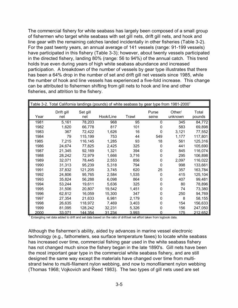
3-5
The commercial fishery for white seabass has largely been composed of a small groupof fishermen who target white seabass with set gill nets, drift gill nets, and hook andline gear with the remaining catches landed incidentally in other fisheries (Table 3-2). For the past twenty years, an annual average of 141 vessels (range: 91-199 vessels)have participated in this fishery (Table 3-3); however, about twenty vessels participatedin the directed fishery, landing 80% (range: 56 to 94%) of the annual catch. This trendholds true even during years of high white seabass abundance and increasedparticipation. A breakdown of the number of vessels by gear type illustrates that therehas been a 64% drop in the number of set and drift gill net vessels since 1985, whilethe number of hook and line vessels has experienced a five-fold increase. This changecan be attributed to fishermen shifting from gill nets to hook and line and otherfisheries, and attrition to the fishery.
Table 3-2. Total California landings (pounds) of white seabass by gear type from 1981-20001
YearDrift gill
netSet gill
net Hook/Line TrawlPurseseine
Other/unknown
Totalpounds
1981 5,161 78,203 968 95 0 345 84,7721982 1,620 66,778 817 101 0 583 69,8981983 367 72,422 1,626 16 0 3,121 77,5521984 79 115,199 753 44 549 1,177 117,8011985 7,215 116,145 1,285 93 18 561 125,3161986 24,674 77,825 2,425 325 0 441 105,6901987 21,345 92,169 1,321 394 0 845 116,0741988 28,242 72,979 1,666 3,716 0 295 106,8981989 32,071 78,445 2,553 856 0 2,097 116,0221990 31,313 95,239 5,318 794 0 998 133,6611991 37,832 121,205 3,745 620 25 357 163,7841992 24,806 95,765 2,584 1,535 0 415 125,1041993 35,824 56,288 6,098 864 0 407 99,4811994 53,244 19,611 5,636 325 0 80 78,8961995 31,506 20,807 19,542 1,451 0 74 73,3801996 62,812 16,059 15,300 347 0 250 94,7691997 27,354 21,633 6,981 2,179 0 8 58,1551998 26,635 118,972 7,469 3,403 0 154 156,6331999 81,095 128,242 32,231 5,326 0 156 247,0502000 33,071 144,354 31,234 3,993 0 175 212,652
1 Entangling net data added to drift and set data based on the ratio of drift/set net effort taken from logbook data.
Although the fishermen’s ability, aided by advances in marine vessel electronictechnology (e.g., fathometers, sea surface temperature faxes) to locate white seabasshas increased over time, commercial fishing gear used in the white seabass fisheryhas not changed much since the fishery began in the late 1890's. Gill nets have beenthe most important gear type in the commercial white seabass fishery, and are stilldesigned the same way except the materials have changed over time from multi-strand twine to multi-filament nylon webbing, and now to monofilament nylon webbing(Thomas 1968; Vojkovich and Reed 1983). The two types of gill nets used are set

3-6
nets and drift gill nets with 6- to 7-inch (152 to 178 mm) mesh (stretched mesh, knot toknot). The most significant change has been the addition of a mechanized net reel,developed in the 1940s. The net reel greatly aides in setting and retrieving nets(Thomas 1968), and it also permits fishermen to increase the length of their nets andthe amount of gear set.
In the late 1970s and 1980s, set nets were the principle gear used to take whiteseabass in California waters while drift gill nets were used primarily in Mexican waters(Vojkovich and Reed 1983). In the mid-1990s, drift gill nets played a larger role in theCalifornia fishery (Table 3-3).
Table 3-3. Number of vessels landing white seabass by principle landing gear from 1981-20001
YearHook/line Trawl
Drift gillnet
Set gillnet Gill nets
Purseseine
Other/unknown
Totalvessels
1981 14 2 130 0 3 1291982 27 5 113 0 19 1421983 12 1 112 0 34 1561984 13 2 141 2 26 1731985 12 3 171 1 18 1991986 21 6 166 0 16 1971987 19 11 146 0 14 1811988 18 11 114 0 7 1451989 23 7 115 0 10 1481990 29 8 102 0 12 1451991 33 11 97 0 7 1361992 26 14 87 0 7 1211993 56 12 68 0 7 1361994 41 11 24 40 53 0 4 1031995 42 15 24 45 57 0 4 1141996 33 10 20 42 50 0 1 911997 32 19 20 47 57 0 1 1061998 40 29 15 53 57 0 2 1181999 64 32 20 65 66 0 4 1502000 84 29 24 65 69 0 3 167
1 Reflects total number of vessels landing white seabass, recognizing that many boats use multiple gears within a year.
The size of gill net vessels has not changed significantly. Most boats range from 29 to40 feet (9 to 12 m) in length and are crewed by a skipper working alone or with at leastone deckhand. The set time nets are in the water depends on the availability of whiteseabass, weather conditions and presence of marine mammals. Most drift gill netsalong the mainland shore are set just prior to sunset and pulled two or three hourslater. At the Channel Islands, drift gill nets may be set for up to twelve hours. Set gillnets remain in the water for about sixteen hours.
The other principle gear used to take white seabass is hook and line. In the early yearsof the fishery, handlines were used to take white seabass (Skogsberg 1925). As
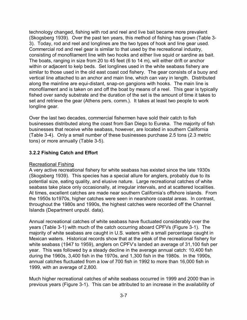
3-7
technology changed, fishing with rod and reel and live bait became more prevalent(Skogsberg 1939). Over the past ten years, this method of fishing has grown (Table 3-3). Today, rod and reel and longlines are the two types of hook and line gear used. Commercial rod and reel gear is similar to that used by the recreational industry,consisting of monofilament line with two hooks and either live squid or sardine as bait. The boats, ranging in size from 20 to 45 feet (6 to 14 m), will either drift or anchorwithin or adjacent to kelp beds. Set longlines used in the white seabass fishery aresimilar to those used in the old east coast cod fishery. The gear consists of a buoy andvertical line attached to an anchor and main line, which can vary in length. Distributedalong the mainline are equi-distant, snap-on gangions with hooks. The main line ismonofilament and is taken on and off the boat by means of a reel. This gear is typicallyfished over sandy substrate and the duration of the set is the amount of time it takes toset and retrieve the gear (Athens pers. comm.). It takes at least two people to worklongline gear.
Over the last two decades, commercial fishermen have sold their catch to fishbusinesses distributed along the coast from San Diego to Eureka. The majority of fish businesses that receive white seabass, however, are located in southern California(Table 3-4). Only a small number of these businesses purchase 2.5 tons (2.3 metrictons) or more annually (Table 3-5).
3.2.2 Fishing Catch and Effort
Recreational FishingA very active recreational fishery for white seabass has existed since the late 1930s(Skogsberg 1939). This species has a special allure for anglers, probably due to itspotential size, eating quality, and elusive nature. Large recreational catches of whiteseabass take place only occasionally, at irregular intervals, and at scattered localities. At times, excellent catches are made near southern California’s offshore islands. Fromthe 1950s to1970s, higher catches were seen in nearshore coastal areas. In contrast,throughout the 1980s and 1990s, the highest catches were recorded off the ChannelIslands (Department unpubl. data).
Annual recreational catches of white seabass have fluctuated considerably over theyears (Table 3-1) with much of the catch occurring aboard CPFVs (Figure 3-1). Themajority of white seabass are caught in U.S. waters with a small percentage caught inMexican waters. Historical records show that at the peak of the recreational fishery forwhite seabass (1947 to 1959), anglers on CPFV’s landed an average of 31,100 fish peryear. This was followed by a steady decline in the average annual catch: 10,400 fishduring the 1960s, 3,400 fish in the 1970s, and 1,300 fish in the 1980s. In the 1990s,annual catches fluctuated from a low of 700 fish in 1992 to more than 16,000 fish in1999, with an average of 2,800.
Much higher recreational catches of white seabass occurred in 1999 and 2000 than inprevious years (Figure 3-1). This can be attributed to an increase in the availability of

3-8
white seabass and fishing effort. More anglers have targeted white seabass in recent
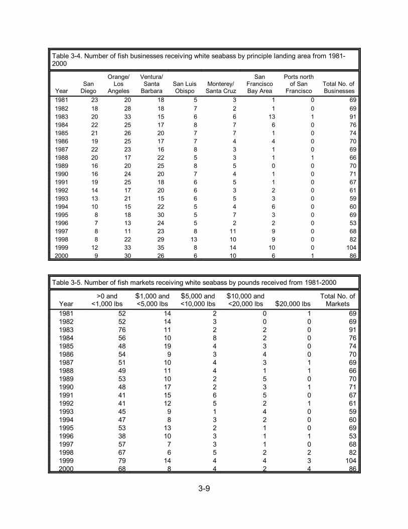
3-9
Table 3-4. Number of fish businesses receiving white seabass by principle landing area from 1981-2000
YearSan
Diego
Orange/Los
Angeles
Ventura/Santa
BarbaraSan LuisObispo
Monterey/Santa Cruz
SanFranciscoBay Area
Ports northof San
FranciscoTotal No. of Businesses
1981 23 20 18 5 3 1 0 691982 18 28 18 7 2 1 0 691983 20 33 15 6 6 13 1 911984 22 25 17 8 7 6 0 761985 21 26 20 7 7 1 0 741986 19 25 17 7 4 4 0 701987 22 23 16 8 3 1 0 691988 20 17 22 5 3 1 1 661989 16 20 25 8 5 0 0 701990 16 24 20 7 4 1 0 711991 19 25 18 6 5 1 0 671992 14 17 20 6 3 2 0 611993 13 21 15 6 5 3 0 591994 10 15 22 5 4 6 0 601995 8 18 30 5 7 3 0 691996 7 13 24 5 2 2 0 531997 8 11 23 8 11 9 0 681998 8 22 29 13 10 9 0 821999 12 33 35 8 14 10 0 1042000 9 30 26 6 10 6 1 86
Table 3-5. Number of fish markets receiving white seabass by pounds received from 1981-2000
Year>0 and
<1,000 lbs$1,000 and<5,000 lbs
$5,000 and<10,000 lbs
$10,000 and<20,000 lbs $20,000 lbs
Total No. ofMarkets
1981 52 14 2 0 1 691982 52 14 3 0 0 691983 76 11 2 2 0 911984 56 10 8 2 0 761985 48 19 4 3 0 741986 54 9 3 4 0 701987 51 10 4 3 1 691988 49 11 4 1 1 661989 53 10 2 5 0 701990 48 17 2 3 1 711991 41 15 6 5 0 671992 41 12 5 2 1 611993 45 9 1 4 0 591994 47 8 3 2 0 601995 53 13 2 1 0 691996 38 10 3 1 1 531997 57 7 3 1 0 681998 67 6 5 2 2 821999 79 14 4 4 3 1042000 68 8 4 2 4 86

3-10
Year
1935 1940 1945 1950 1955 1960 1965 1970 1975 1980 1985 1990 1995 2000
Land
ings
(100
0's
of fi
sh)
0
10
20
30
40
50
60 CA watersMexican waters
Figure 3-1. Commercial Passenger Fishing Vessel (CPFV) landings ofwhite seabass in U.S. and Mexican waters. Data from Department’shistorical logbook database.
years (Figure 3-2), and the CPUE for trips aboard CPFVs targeting white seabassincreased dramatically during 1999 (Figure 3-3).
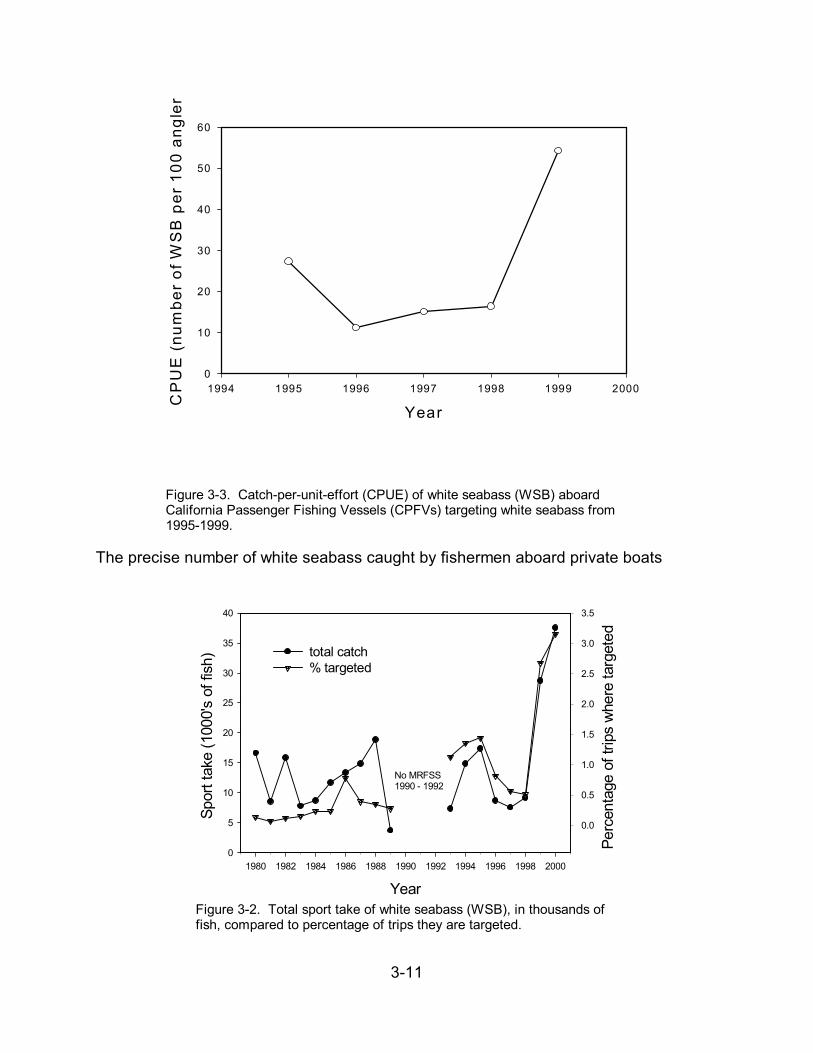
3-11
Year1980 1982 1984 1986 1988 1990 1992 1994 1996 1998 2000
Spor
t tak
e (1
000'
s of
fish
)
0
5
10
15
20
25
30
35
40Pe
rcen
tage
of t
rips
whe
re ta
rget
ed
0.0
0.5
1.0
1.5
2.0
2.5
3.0
3.5
total catch% targeted
No MRFSS1990 - 1992
Figure 3-2. Total sport take of white seabass (WSB), in thousands offish, compared to percentage of trips they are targeted.
Year1994 1995 1996 1997 1998 1999 2000
CP
UE
(nu
mbe
r of
WS
B p
er 1
00 a
ngle
r
0
10
20
30
40
50
60
Figure 3-3. Catch-per-unit-effort (CPUE) of white seabass (WSB) aboardCalifornia Passenger Fishing Vessels (CPFVs) targeting white seabass from1995-1999.
The precise number of white seabass caught by fishermen aboard private boats
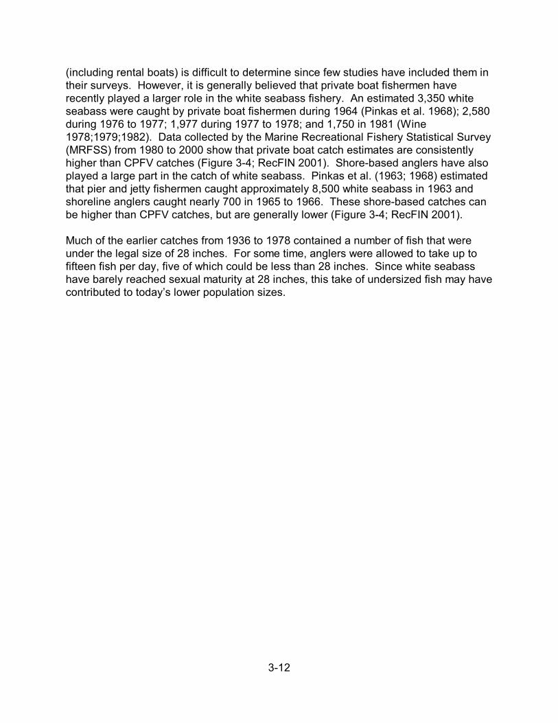
3-12
(including rental boats) is difficult to determine since few studies have included them intheir surveys. However, it is generally believed that private boat fishermen haverecently played a larger role in the white seabass fishery. An estimated 3,350 whiteseabass were caught by private boat fishermen during 1964 (Pinkas et al. 1968); 2,580during 1976 to 1977; 1,977 during 1977 to 1978; and 1,750 in 1981 (Wine1978;1979;1982). Data collected by the Marine Recreational Fishery Statistical Survey(MRFSS) from 1980 to 2000 show that private boat catch estimates are consistentlyhigher than CPFV catches (Figure 3-4; RecFIN 2001). Shore-based anglers have alsoplayed a large part in the catch of white seabass. Pinkas et al. (1963; 1968) estimatedthat pier and jetty fishermen caught approximately 8,500 white seabass in 1963 andshoreline anglers caught nearly 700 in 1965 to 1966. These shore-based catches canbe higher than CPFV catches, but are generally lower (Figure 3-4; RecFIN 2001).
Much of the earlier catches from 1936 to 1978 contained a number of fish that wereunder the legal size of 28 inches. For some time, anglers were allowed to take up tofifteen fish per day, five of which could be less than 28 inches. Since white seabasshave barely reached sexual maturity at 28 inches, this take of undersized fish may havecontributed to today’s lower population sizes.
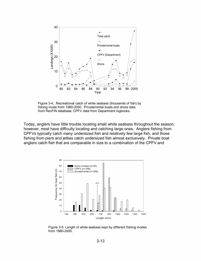
3-13
0
10
20
30
40
Land
ings
(X10
00)
80 82 84 86 88 90 92 94 96 98 2000Year
Total catch
Private/rental boats
CPFV (Department)
Shore
Figure 3-4. Recreational catch of white seabass (thousands of fish) byfishing mode from 1980-2000. Private/rental boats and shore datafrom RecFIN database; CPFV data from Department logbooks.
Length (mm)150 300 450 600 750 900 1050 1200 1350 1500
Freq
uenc
y fo
r kep
t fis
h (n
)
0
10
20
30
40
50
60
70
80
90
shore modes (n=35)CPFV (n=196)private/rental (n=296)
28 in
Figure 3-5. Length of white seabass kept by different fishing modesfrom 1980-2000.
Today, anglers have little trouble locating small white seabass throughout the season;however, most have difficulty locating and catching large ones. Anglers fishing fromCPFVs typically catch many undersized fish and relatively few large fish, and thosefishing from piers and jetties catch undersized fish almost exclusively. Private boatanglers catch fish that are comparable in size to a combination of the CPFV and
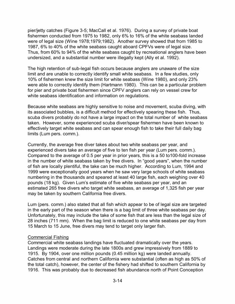
3-14
pier/jetty catches (Figure 3-5; MacCall et al. 1976). During a survey of private boatfishermen conducted from 1975 to 1982, only 6% to 16% of the white seabass landedwere of legal size (Wine 1978;1979;1982). Another survey showed that from 1985 to1987, 6% to 40% of the white seabass caught aboard CPFVs were of legal size.Thus, from 60% to 94% of the white seabass caught by recreational anglers have beenundersized, and a substantial number were illegally kept (Ally et al. 1992).
The high retention of sub-legal fish occurs because anglers are unaware of the sizelimit and are unable to correctly identify small white seabass. In a few studies, only10% of fishermen knew the size limit for white seabass (Wine 1980), and only 23%were able to correctly identify them (Hartmann 1980). This can be a particular problemfor pier and private boat fishermen since CPFV anglers can rely on vessel crew forwhite seabass identification and information on regulations.
Because white seabass are highly sensitive to noise and movement, scuba diving, withits associated bubbles, is a difficult method for effectively spearing these fish. Thus,scuba divers probably do not have a large impact on the total number of white seabasstaken. However, some experienced scuba diver/spear fishermen have been known toeffectively target white seabass and can spear enough fish to take their full daily baglimits (Lum pers. comm.).
Currently, the average free diver takes about two white seabass per year, andexperienced divers take an average of five to ten fish per year (Lum pers. comm.). Compared to the average of 0.5 per year in prior years, this is a 50 to100-fold increasein the number of white seabass taken by free divers. In “good years”, when the numberof fish are locally plentiful, the take can be much higher. According to Lum, 1994 and1999 were exceptionally good years when he saw very large schools of white seabassnumbering in the thousands and speared at least 40 large fish, each weighing over 40pounds (18 kg). Given Lum’s estimate of five white seabass per year, and anestimated 265 free divers who target white seabass, an average of 1,325 fish per yearmay be taken by southern California free divers.
Lum (pers. comm.) also stated that all fish which appear to be of legal size are targetedin the early part of the season when there is a bag limit of three white seabass per day. Unfortunately, this may include the take of some fish that are less than the legal size of28 inches (711 mm). When the bag limit is reduced to one white seabass per day from15 March to 15 June, free divers may tend to target only larger fish.
Commercial FishingCommercial white seabass landings have fluctuated dramatically over the years. Landings were moderate during the late 1800s and grew impressively from 1889 to1915. By 1904, over one million pounds (0.45 million kg) were landed annually. Catches from central and northern California were substantial (often as high as 50% ofthe total catch), however, the center of the fishery had shifted to southern California by1916. This was probably due to decreased fish abundance north of Point Conception

3-15
and to the increased number of fishermen and increased demand in southernCalifornia. The fishery experienced spectacular catches after World War I. Highesttotal landings in the early years of this fishery occurred in 1919 and 1920 when thelandings exceeded two million pounds (0.9 million kg) both years. For the next tenyears, the landings fluctuated between 800,000 and 1.4 million pounds (0.6 million kg).
Declining catches in the late 1920s and early 1930s prompted a series of commercialregulations including closed seasons, bag limits, gear restrictions and minimum sizelimits (Skogsberg 1939). During the 1930s and 1940s, landings ranged from 250,000to 900,000 pounds (113,400 to 408,240 kg). The greatest peak in California landingsoccurred during the warm water year of 1959, when more than 3 million pounds (1.4million kg) were taken. Between 1959 and 1965, landings dropped sharply, falling fromover 1 million to 577,607 pounds (262,003 kg). There was a slight increase in 1966 toover 674,000 pounds (305,726 kg). The remainder of the1960s and all of the 1970'sshow catches below 600,000 pounds (272,160 kg). In the 1980s, catches droppedbelow 200,000 pounds (90,720 kg) and reached a low of fewer than 70,000 pounds(31,752 kg) in 1982. The large decline (91%) in catch seen between 1981 and 1982was the result of the loss of catches from Mexican waters. In the 1990s, thecommercial fishery experienced wide fluctuations in landings. Beginning in 1994,annual landings dropped below 100,000 pounds (45,360 kg) and reached a record lowof 58,554 pounds (26,309 kg) in 1997. This low was followed by three years of largeincreases with 1999 reaching almost 250,000 pounds (113,400 kg) (Table 3-1; Figure3-6).
Declining commercial landings of white seabass are partly due to reductions in effort. A decrease in effort for white seabass is reflected in logbook data collected from thecommercial set and drift gill net fishery (Figure 3-7). The number of white seabass setsmade by fishermen using set gill nets dropped from nearly 2000 in 1982 to less then 50sets in 1994 (Beeson and Hanan 1994).
Since the commercial fishery began, there have been a number of factors that haveaffected fishing effort for white seabass. These factors include increased regulation,improvements in technology, market factors (i.e., demand and price), and changes infish abundance. In the past two decades, there have been two regulatory changes thathave greatly affected the commercial catch of white seabass. The first was the closureof Mexican waters to U.S. fishermen in 1982, and the second was passage of theMarine Life Protection Act of 1990, which banned the use of gill nets in State waterssouth of Point Conception after 1994. Thus, the decline in commercial white seabasslandings can, in part, be attributed to decreased effort and participation by commercialfishermen due to the loss of grounds off of Mexico in the 1980s and in the SouthernCalifornia Bight during the 1990s.
Public demand and fish businesses also influence fishing effort. Because of consumerdemand, white seabass has always commanded relatively high prices for wholedressed (gutted) fish, in the range of $1.60 to $2.00 per lb. At the beginning of the
3-16
season, a premium price is paid for white seabass. However, if availability is high, theprice can drop to as low as $0.60 per lb. This results in fishermen reducing the number
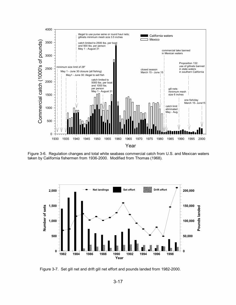
3-17
0
500
1,000
1,500
2,000
Num
ber o
f set
s
0
50,000
100,000
150,000
200,000
Poun
ds la
nded
1982 1984 1986 1988 1990 1992 1994 1996 1998Year
���� ������������
��������
�������� ���
������
������
������
������
������
������
������
������ ���
������
Net landings Set effort
������������������������ Drift effort
Figure 3-7. Set gill net and drift gill net effort and pounds landed from 1982-2000.
Year1930 1935 1940 1945 1950 1955 1960 1965 1970 1975 1980 1985 1990 1995 2000
Com
mer
cial
cat
ch (1
000'
s of
pou
nds)
0
500
1000
1500
2000
2500
3000
3500
4000
California watersMexico
minimum size limit of 28"May 1 - June 30 closure (all fishing)
May1 - June 30: illegal to sell fish
illegal to use purse seine or round haul nets; gillnets minimum mesh size 3.5 inches
catch limited to 2500 lbs. per boatand 500 lbs. per person May 1 - August 31
catch limited to5000 lbs. per boat and 1000 lbs.per personMay 1 - August 31
commercial take banned in Mexican waters
Proposition 132:use of gillnets bannedin state watersin southern California
closed seasonMarch 15 - June 15
one fish/day March 15- June15
gill nets:minimum mesh size 6 inches
catch limiteliminated May - Aug.
Figure 3-6. Regulation changes and total white seabass commercial catch from U.S. and Mexican waterstaken by California fishermen from 1936-2000. Modified from Thomas (1968).
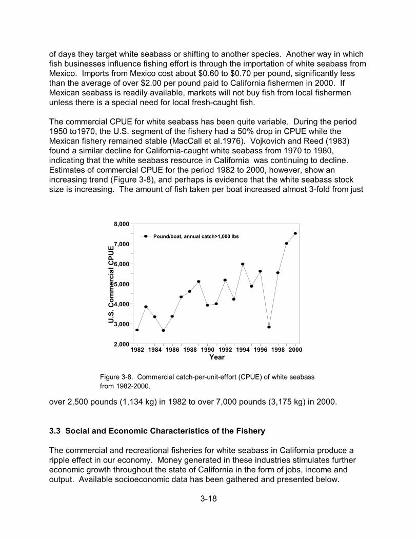
3-18
2,000
3,000
4,000
5,000
6,000
7,000
8,000
U.S
. Com
mer
cial
CPU
E
1982 1984 1986 1988 1990 1992 1994 1996 1998 2000Year
Pound/boat, annual catch>1,000 lbs
Figure 3-8. Commercial catch-per-unit-effort (CPUE) of white seabassfrom 1982-2000.
of days they target white seabass or shifting to another species. Another way in whichfish businesses influence fishing effort is through the importation of white seabass fromMexico. Imports from Mexico cost about $0.60 to $0.70 per pound, significantly lessthan the average of over $2.00 per pound paid to California fishermen in 2000. IfMexican seabass is readily available, markets will not buy fish from local fishermenunless there is a special need for local fresh-caught fish.
The commercial CPUE for white seabass has been quite variable. During the period1950 to1970, the U.S. segment of the fishery had a 50% drop in CPUE while theMexican fishery remained stable (MacCall et al.1976). Vojkovich and Reed (1983)found a similar decline for California-caught white seabass from 1970 to 1980,indicating that the white seabass resource in California was continuing to decline. Estimates of commercial CPUE for the period 1982 to 2000, however, show anincreasing trend (Figure 3-8), and perhaps is evidence that the white seabass stocksize is increasing. The amount of fish taken per boat increased almost 3-fold from just
over 2,500 pounds (1,134 kg) in 1982 to over 7,000 pounds (3,175 kg) in 2000.
3.3 Social and Economic Characteristics of the Fishery
The commercial and recreational fisheries for white seabass in California produce aripple effect in our economy. Money generated in these industries stimulates furthereconomic growth throughout the state of California in the form of jobs, income andoutput. Available socioeconomic data has been gathered and presented below.
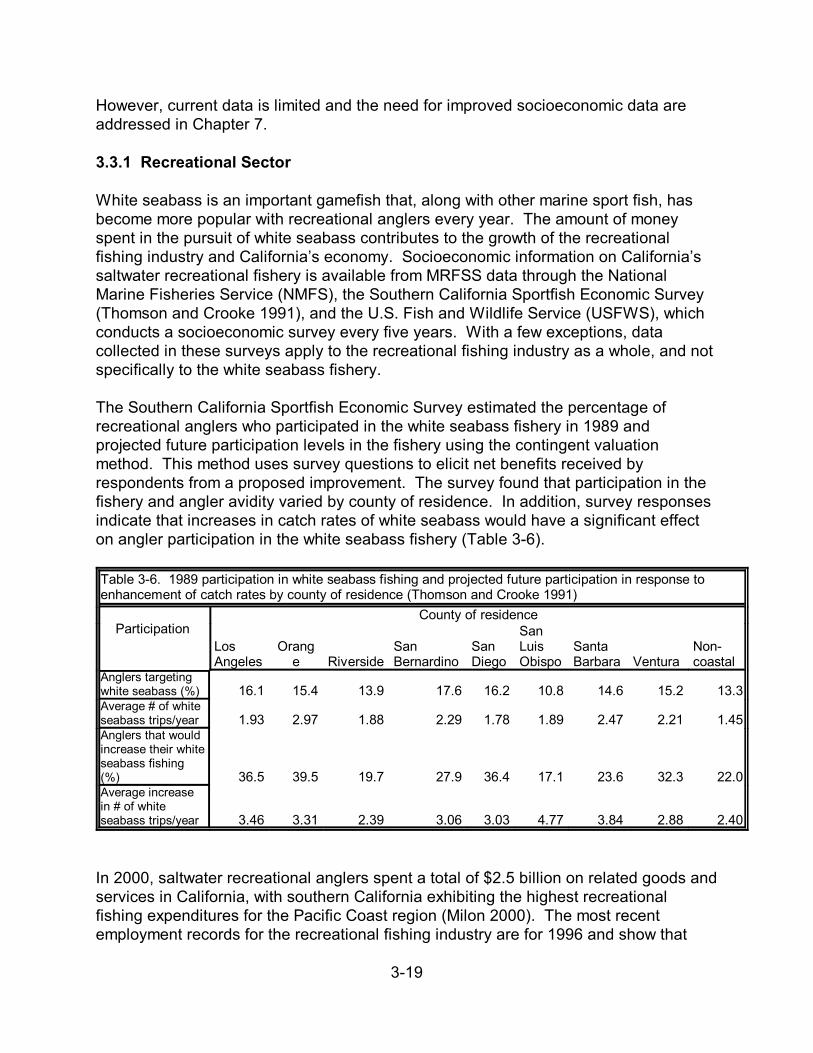
3-19
However, current data is limited and the need for improved socioeconomic data areaddressed in Chapter 7.
3.3.1 Recreational Sector
White seabass is an important gamefish that, along with other marine sport fish, hasbecome more popular with recreational anglers every year. The amount of moneyspent in the pursuit of white seabass contributes to the growth of the recreationalfishing industry and California’s economy. Socioeconomic information on California’ssaltwater recreational fishery is available from MRFSS data through the NationalMarine Fisheries Service (NMFS), the Southern California Sportfish Economic Survey(Thomson and Crooke 1991), and the U.S. Fish and Wildlife Service (USFWS), whichconducts a socioeconomic survey every five years. With a few exceptions, datacollected in these surveys apply to the recreational fishing industry as a whole, and notspecifically to the white seabass fishery.
The Southern California Sportfish Economic Survey estimated the percentage ofrecreational anglers who participated in the white seabass fishery in 1989 andprojected future participation levels in the fishery using the contingent valuationmethod. This method uses survey questions to elicit net benefits received byrespondents from a proposed improvement. The survey found that participation in thefishery and angler avidity varied by county of residence. In addition, survey responsesindicate that increases in catch rates of white seabass would have a significant effecton angler participation in the white seabass fishery (Table 3-6).
Table 3-6. 1989 participation in white seabass fishing and projected future participation in response toenhancement of catch rates by county of residence (Thomson and Crooke 1991)
ParticipationCounty of residence
LosAngeles
Orange Riverside
SanBernardino
SanDiego
SanLuisObispo
SantaBarbara Ventura
Non-coastal
Anglers targetingwhite seabass (%) 16.1 15.4 13.9 17.6 16.2 10.8 14.6 15.2 13.3Average # of whiteseabass trips/year 1.93 2.97 1.88 2.29 1.78 1.89 2.47 2.21 1.45Anglers that wouldincrease their whiteseabass fishing(%) 36.5 39.5 19.7 27.9 36.4 17.1 23.6 32.3 22.0Average increasein # of whiteseabass trips/year 3.46 3.31 2.39 3.06 3.03 4.77 3.84 2.88 2.40
In 2000, saltwater recreational anglers spent a total of $2.5 billion on related goods andservices in California, with southern California exhibiting the highest recreationalfishing expenditures for the Pacific Coast region (Milon 2000). The most recentemployment records for the recreational fishing industry are for 1996 and show that

3-20
19,113 individuals were employed statewide, with combined salaries totaling$498,369,450 (USFWS 1997). These salaries would be valued at $548,206,395 withinflation adjustments for 2000 (BLS 2000). White seabass angling activity occursprimarily in
southern California, so socioeconomic data pertaining to this region will be the focus ofthis section.
Saltwater anglers spend substantial amounts of money on fishing related items such asboat maintenance, fishing licenses, and fishing gear, as well as trip relatedexpenditures such as food, gasoline, parking, lodging, and tickets for CPFV (partyboat) trips. Expenses related to private boat and CPFV angling activities are especiallysignificant. In 2000, anglers in southern California spent nearly $127 million on CPFVtrip related expenses (over 55% of all trip related expenditures), while private andrental boat trip related expenses totaled about $78 million (about 34% of all trip relatedexpenditures) (Table 3-7). Anglers who fished from shore in southern California spentclose to $25 million on trip related expenses, which is about 11% of all marine anglertrip expenditures for this region.
Table 3-7. Total annual trip expenditures for saltwater anglers in southern California by fishing mode andresident status for 2000 (MRFSS data)
Trip expenditure
Party/charter boat Private/rental boat Shore
ResidentNon-
resident ResidentNon-
resident ResidentNon-
resident
Privatetransportation
$8,217,000 $7,599,000 $11,914,000 $5,181,000 $6,754,000 $2,321,000
Food $10,605,000 $4,402,000 $12,712,000 $1,213,000 $5,789,000 $686,000
Lodging $995,000 $6,897,000 $875,000 $1,614,000 $2,873,000 $1,301,000
Publictransportation
$429,000 $29,405,000 $46,000 $4,251,000 $162,000 $504,000
Boat fuel N/A N/A $21,700,000 $1,520,000 N/A N/A
Party/charter fees $46,587,000 $4,332,000 N/A N/A N/A N/A
Access/boatlaunching
$806,000 $342,000 $2,595,000 $164,000 $969,000 $166,000
Equipment rental $1,525,000 $4,050,000 $1,213,000 $534,000 $150,000 $30,000
Bait and ice $225,000 $268,000 $11,570,000 $762,000 $2,750,000 $195,000
Totals $69,388,000 $57,294,000 $62,627,000 $15,241,000 $19,446,000 $5,203,000
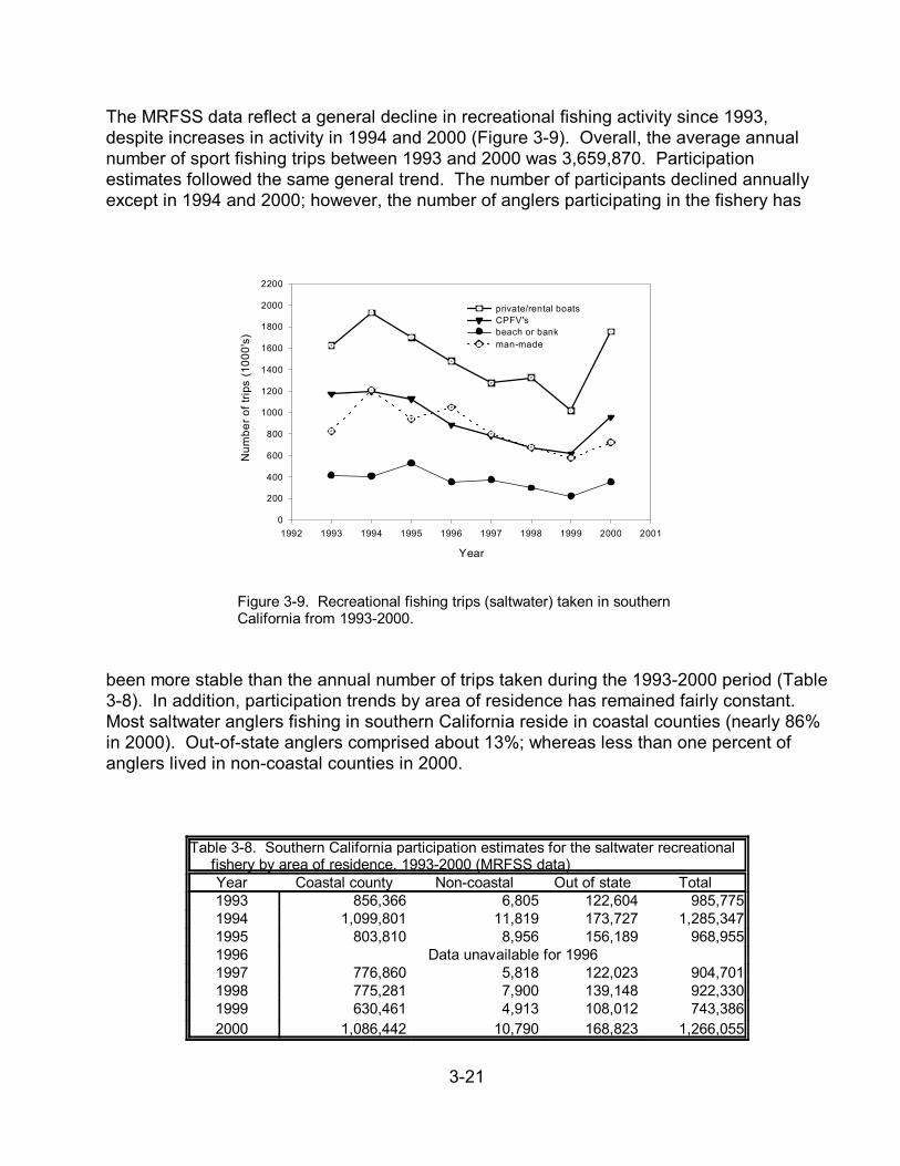
3-21
Year
1992 1993 1994 1995 1996 1997 1998 1999 2000 2001
Num
ber o
f trip
s (1
000'
s)
0
200
400
600
800
1000
1200
1400
1600
1800
2000
2200
private/rental boatsCPFV'sbeach or bankman-made
Figure 3-9. Recreational fishing trips (saltwater) taken in southernCalifornia from 1993-2000.
The MRFSS data reflect a general decline in recreational fishing activity since 1993,despite increases in activity in 1994 and 2000 (Figure 3-9). Overall, the average annualnumber of sport fishing trips between 1993 and 2000 was 3,659,870. Participationestimates followed the same general trend. The number of participants declined annuallyexcept in 1994 and 2000; however, the number of anglers participating in the fishery has
been more stable than the annual number of trips taken during the 1993-2000 period (Table3-8). In addition, participation trends by area of residence has remained fairly constant. Most saltwater anglers fishing in southern California reside in coastal counties (nearly 86%in 2000). Out-of-state anglers comprised about 13%; whereas less than one percent ofanglers lived in non-coastal counties in 2000.
Table 3-8. Southern California participation estimates for the saltwater recreational fishery by area of residence, 1993-2000 (MRFSS data)
Year Coastal county Non-coastal Out of state Total1993 856,366 6,805 122,604 985,7751994 1,099,801 11,819 173,727 1,285,3471995 803,810 8,956 156,189 968,9551996 Data unavailable for 19961997 776,860 5,818 122,023 904,7011998 775,281 7,900 139,148 922,3301999 630,461 4,913 108,012 743,3862000 1,086,442 10,790 168,823 1,266,055
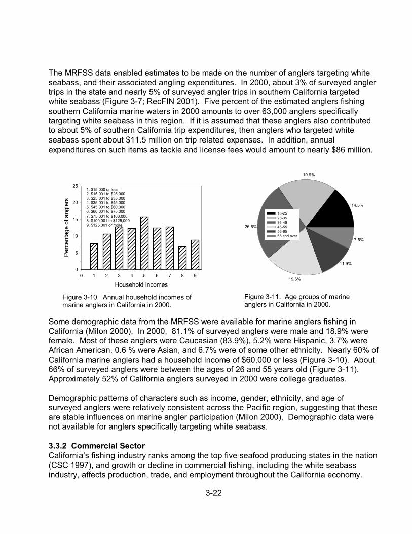
3-22
16-2526-3536-4546-5556-6566 and over
14.5%
7.5%
11.9%
19.6%
26.6%
19.9%
Figure 3-11. Age groups of marineanglers in California in 2000.
Household Incomes0 1 2 3 4 5 6 7 8 9
Perc
enta
ge o
f ang
lers
0
5
10
15
20
251. $15,000 or less2. $15,001 to $25,0003. $25,001 to $35,0004. $35,001 to $45,0005. $45,001 to $60,0006. $60,001 to $75,0007. $75,001 to $100,0008. $100,001 to $125,0009. $125,001 or more
Figure 3-10. Annual household incomes ofmarine anglers in California in 2000.
The MRFSS data enabled estimates to be made on the number of anglers targeting whiteseabass, and their associated angling expenditures. In 2000, about 3% of surveyed anglertrips in the state and nearly 5% of surveyed angler trips in southern California targetedwhite seabass (Figure 3-7; RecFIN 2001). Five percent of the estimated anglers fishingsouthern California marine waters in 2000 amounts to over 63,000 anglers specificallytargeting white seabass in this region. If it is assumed that these anglers also contributedto about 5% of southern California trip expenditures, then anglers who targeted whiteseabass spent about $11.5 million on trip related expenses. In addition, annualexpenditures on such items as tackle and license fees would amount to nearly $86 million.
Some demographic data from the MRFSS were available for marine anglers fishing inCalifornia (Milon 2000). In 2000, 81.1% of surveyed anglers were male and 18.9% werefemale. Most of these anglers were Caucasian (83.9%), 5.2% were Hispanic, 3.7% wereAfrican American, 0.6 % were Asian, and 6.7% were of some other ethnicity. Nearly 60% ofCalifornia marine anglers had a household income of $60,000 or less (Figure 3-10). About66% of surveyed anglers were between the ages of 26 and 55 years old (Figure 3-11). Approximately 52% of California anglers surveyed in 2000 were college graduates.
Demographic patterns of characters such as income, gender, ethnicity, and age ofsurveyed anglers were relatively consistent across the Pacific region, suggesting that theseare stable influences on marine angler participation (Milon 2000). Demographic data werenot available for anglers specifically targeting white seabass.
3.3.2 Commercial SectorCalifornia’s fishing industry ranks among the top five seafood producing states in the nation(CSC 1997), and growth or decline in commercial fishing, including the white seabassindustry, affects production, trade, and employment throughout the California economy.
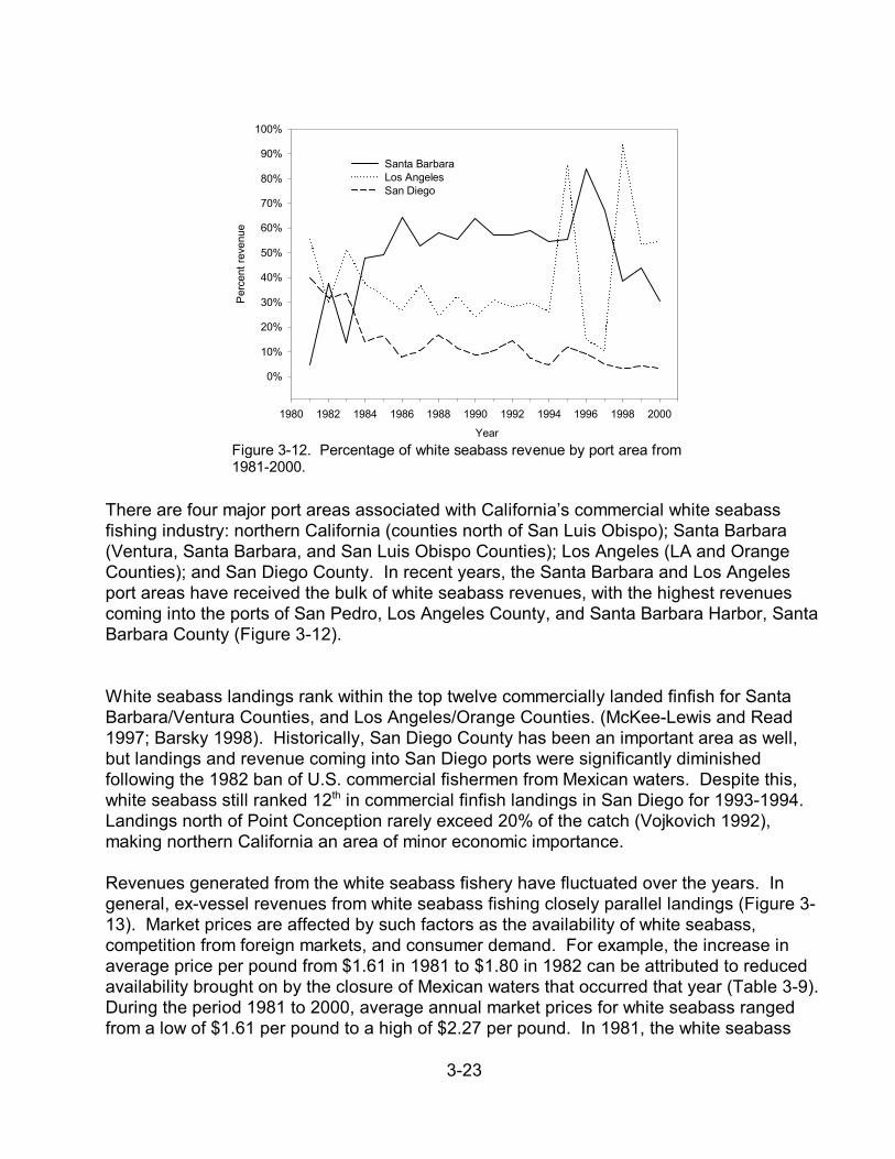
3-23
Year
1980 1982 1984 1986 1988 1990 1992 1994 1996 1998 2000
Perc
ent r
even
ue
0%
10%
20%
30%
40%
50%
60%
70%
80%
90%
100%
Santa BarbaraLos AngelesSan Diego
Figure 3-12. Percentage of white seabass revenue by port area from1981-2000.
There are four major port areas associated with California’s commercial white seabassfishing industry: northern California (counties north of San Luis Obispo); Santa Barbara(Ventura, Santa Barbara, and San Luis Obispo Counties); Los Angeles (LA and OrangeCounties); and San Diego County. In recent years, the Santa Barbara and Los Angelesport areas have received the bulk of white seabass revenues, with the highest revenuescoming into the ports of San Pedro, Los Angeles County, and Santa Barbara Harbor, SantaBarbara County (Figure 3-12).
White seabass landings rank within the top twelve commercially landed finfish for SantaBarbara/Ventura Counties, and Los Angeles/Orange Counties. (McKee-Lewis and Read1997; Barsky 1998). Historically, San Diego County has been an important area as well,but landings and revenue coming into San Diego ports were significantly diminishedfollowing the 1982 ban of U.S. commercial fishermen from Mexican waters. Despite this,white seabass still ranked 12th in commercial finfish landings in San Diego for 1993-1994. Landings north of Point Conception rarely exceed 20% of the catch (Vojkovich 1992),making northern California an area of minor economic importance.
Revenues generated from the white seabass fishery have fluctuated over the years. Ingeneral, ex-vessel revenues from white seabass fishing closely parallel landings (Figure 3-13). Market prices are affected by such factors as the availability of white seabass,competition from foreign markets, and consumer demand. For example, the increase inaverage price per pound from $1.61 in 1981 to $1.80 in 1982 can be attributed to reducedavailability brought on by the closure of Mexican waters that occurred that year (Table 3-9). During the period 1981 to 2000, average annual market prices for white seabass rangedfrom a low of $1.61 per pound to a high of $2.27 per pound. In 1981, the white seabass
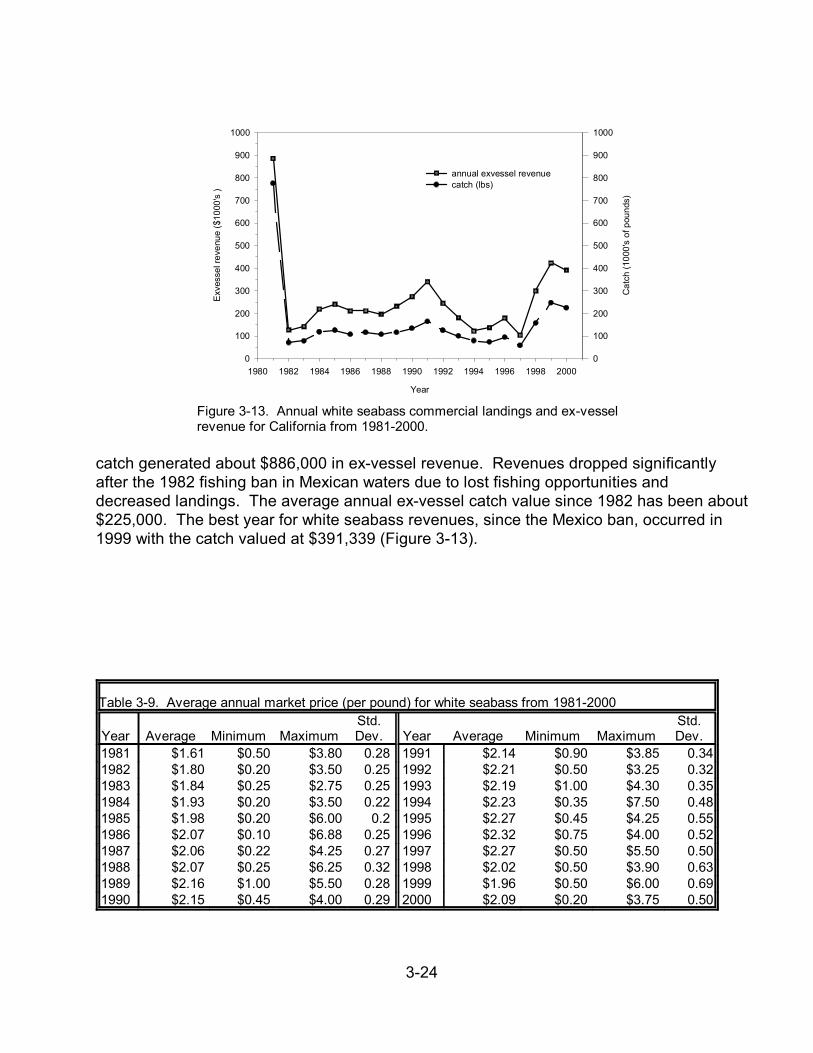
3-24
Year
1980 1982 1984 1986 1988 1990 1992 1994 1996 1998 2000
Exve
ssel
reve
nue
($10
00's
)
0
100
200
300
400
500
600
700
800
900
1000
Cat
ch (1
000'
s of
pou
nds)
0
100
200
300
400
500
600
700
800
900
1000
annual exvessel revenuecatch (lbs)
Figure 3-13. Annual white seabass commercial landings and ex-vesselrevenue for California from 1981-2000.
catch generated about $886,000 in ex-vessel revenue. Revenues dropped significantlyafter the 1982 fishing ban in Mexican waters due to lost fishing opportunities anddecreased landings. The average annual ex-vessel catch value since 1982 has been about$225,000. The best year for white seabass revenues, since the Mexico ban, occurred in1999 with the catch valued at $391,339 (Figure 3-13).
Table 3-9. Average annual market price (per pound) for white seabass from 1981-2000
Year Average Minimum MaximumStd.Dev. Year Average Minimum Maximum
Std.Dev.
1981 $1.61 $0.50 $3.80 0.28 1991 $2.14 $0.90 $3.85 0.341982 $1.80 $0.20 $3.50 0.25 1992 $2.21 $0.50 $3.25 0.321983 $1.84 $0.25 $2.75 0.25 1993 $2.19 $1.00 $4.30 0.351984 $1.93 $0.20 $3.50 0.22 1994 $2.23 $0.35 $7.50 0.481985 $1.98 $0.20 $6.00 0.2 1995 $2.27 $0.45 $4.25 0.551986 $2.07 $0.10 $6.88 0.25 1996 $2.32 $0.75 $4.00 0.521987 $2.06 $0.22 $4.25 0.27 1997 $2.27 $0.50 $5.50 0.501988 $2.07 $0.25 $6.25 0.32 1998 $2.02 $0.50 $3.90 0.631989 $2.16 $1.00 $5.50 0.28 1999 $1.96 $0.50 $6.00 0.691990 $2.15 $0.45 $4.00 0.29 2000 $2.09 $0.20 $3.75 0.50

3-25
Year1982 1984 1986 1988 1990 1992 1994 1996 1998 2000
Rev
enue
($10
00's
)
0
50
100
150
200
250
300
350
400
450gillnetshook and lineall other gear
Figure 3-14. White seabass revenue by gear type from 1982-2000.
Most of this revenue is generated by gill net fishermen who dominate the fishery, but hookand line effort in the fishery has been increasing in recent years. From 1996 to 2000, 89%of landings by weight and 83% of revenues were produced by gill net effort, while hook andline effort accounted for close to 13% of landings and about 15% of revenues (Figure 3-14). An annual average of 141 vessels participate in the white seabass fishery, but only 20 ofthese vessels land 80% of the catch. Assuming that most commercial fishermen employ anaverage of one crew member, it is estimated that over 280 individuals participate in thefishery annually, with about 40 core individuals.
Representative operating costs were obtained through personal communications with whiteseabass fishermen (Table 3-10). Although these costs are associated with white seabassfishing, many white seabass fishermen participate in other fisheries, and some of thesecosts would be shared with other fishing effort.
Table 3-10. Examples of annual operating costs for white seabass fishing by primary gear type
Expense category Set longline Set net Drift netDays fished 220 90 25
Crew members 1 full time; 1 full time; No crewFuel $16,000 $10,800 $1,000
Crew wages 30% share ($40,000) 20 to 35% share N/AMaintenance and repair $25,000 $14,000 $5,000
3-26
Gear and equipment $12,000 $6,500 $1,000Food and provisions $8,571 $2,250 $375
Insurance $9,500 $9,000 $9,000Fishing licences and permits $315 $445 $445
Property tax (vessel) $75 $80 $75Mooring fees $245/mo $50/mo $234/mo
Between 1996 and 2000, 53 to 104 fish businesses received white seabass fromcommercial fishermen. Santa Barbara and Ventura County businesses made up thehighest percentage of these businesses at 23.5%, while Los Angeles and Orange Countybusinesses comprised another 18.7%. All other port areas contained less than 10% ofbusinesses purchasing white seabass. However, 61.8 % of all businesses purchasingwhite seabass during this period obtained less than 1,000 pounds (454 kg) annually. Onlyabout 3.4% the businesses purchased over 10,000 pounds (4,536 kg) on an annual basis(Table 3-4; Table 3-5).
DemographicsThe primary locations for commercial white seabass activity is Los Angeles and SantaBarbara counties. The following demographic information was available for these areas.
Los Angeles CountyThe population of Los Angeles County increased from 8,863,000 to 9,519,338 between1990 and 2000. The number of Caucasians declined from 41% to 31% of the population;the Hispanic population increased from 38% to 45%; the percentage of African Americansdecreased from 11% to 10%; and the Asian population increased from 10% to 12% (CDF2001). In the Los Angeles-Long Beach metropolitan area, the unemployment rate droppedfrom 8.2% in 1991 to 5.9% in 1999 (BLS 2000). In 1998, the average annual wage in LosAngeles County was $36,000, while the average commercial fishing wage was $22,617(CTTCA 2000).
Community profile - San PedroSan Pedro, located in southwest Los Angeles on the southeastern slope of the PalosVerdes Peninsula, is the most important port in Los Angeles County with regard to the whiteseabass fishing industry. The community’s roots developed over a century of participationin fishing and related industries and are described in the San Pedro CommunityEnvironmental Perspectives (1989). The community is relatively small, with a hometownfeeling, enhanced by the fact that many residents are locally employed.
During the 1980s, the commercial fishing industry in Los Angeles continued to decline,directly affecting the local economies of San Pedro and Wilmington. One reason for thedecline was price-cutting competition from foreign fisheries, which allegedly operated withlower labor costs and government subsidies. State and local taxes and high insurancecosts were blamed as additional burdens on the struggling industry. By 1986, only one fishpacking plant remained of the fourteen that operated in 1960 (PFMC 1998).
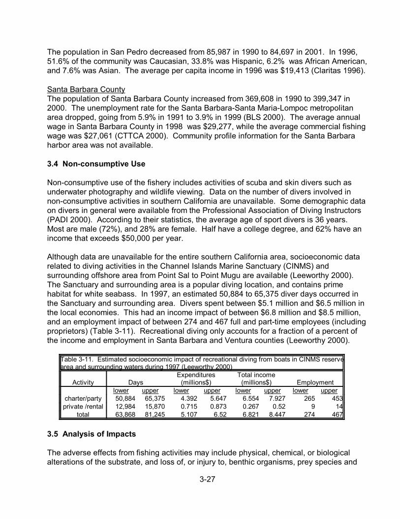
3-27
The population in San Pedro decreased from 85,987 in 1990 to 84,697 in 2001. In 1996,51.6% of the community was Caucasian, 33.8% was Hispanic, 6.2% was African American,and 7.6% was Asian. The average per capita income in 1996 was $19,413 (Claritas 1996).
Santa Barbara CountyThe population of Santa Barbara County increased from 369,608 in 1990 to 399,347 in2000. The unemployment rate for the Santa Barbara-Santa Maria-Lompoc metropolitanarea dropped, going from 5.9% in 1991 to 3.9% in 1999 (BLS 2000). The average annualwage in Santa Barbara County in 1998 was $29,277, while the average commercial fishingwage was $27,061 (CTTCA 2000). Community profile information for the Santa Barbaraharbor area was not available.
3.4 Non-consumptive Use
Non-consumptive use of the fishery includes activities of scuba and skin divers such asunderwater photography and wildlife viewing. Data on the number of divers involved innon-consumptive activities in southern California are unavailable. Some demographic dataon divers in general were available from the Professional Association of Diving Instructors(PADI 2000). According to their statistics, the average age of sport divers is 36 years. Most are male (72%), and 28% are female. Half have a college degree, and 62% have anincome that exceeds $50,000 per year.
Although data are unavailable for the entire southern California area, socioeconomic datarelated to diving activities in the Channel Islands Marine Sanctuary (CINMS) andsurrounding offshore area from Point Sal to Point Mugu are available (Leeworthy 2000). The Sanctuary and surrounding area is a popular diving location, and contains primehabitat for white seabass. In 1997, an estimated 50,884 to 65,375 diver days occurred inthe Sanctuary and surrounding area. Divers spent between $5.1 million and $6.5 million inthe local economies. This had an income impact of between $6.8 million and $8.5 million,and an employment impact of between 274 and 467 full and part-time employees (includingproprietors) (Table 3-11). Recreational diving only accounts for a fraction of a percent ofthe income and employment in Santa Barbara and Ventura counties (Leeworthy 2000).
Table 3-11. Estimated socioeconomic impact of recreational diving from boats in CINMS reservearea and surrounding waters during 1997 (Leeworthy 2000)
Activity DaysExpenditures
(millions$)Total income
(millions$) Employmentlower upper lower upper lower upper lower upper
charter/party 50,884 65,375 4.392 5.647 6.554 7.927 265 453private /rental 12,984 15,870 0.715 0.873 0.267 0.52 9 14
total 63,868 81,245 5.107 6.52 6.821 8.447 274 467
3.5 Analysis of Impacts
The adverse effects from fishing activities may include physical, chemical, or biologicalalterations of the substrate, and loss of, or injury to, benthic organisms, prey species and
3-28
their habitat, and other components of the ecosystem (Bargmann et al. 1998). Fisherymanagement plans must include measures that minimize adverse effects on marineecosystems from fishing, to the extent practicable, and identify conservation andenhancement measures. They must also contain an assessment of the potential adverseeffects of all fishing activities and should consider the relative impacts of all fishingequipment types used in different types of habitat (Bargmann et al. 1998).
The commercial and recreational fisheries for white seabass have exploited different agegroups of the stock over the years. In general, the recreational fishery catches mostlysmaller, younger individuals, whereas the commercial fishery lands relatively larger, olderfish. Immature or undersized white seabass are often caught by recreational and somesegments of the commercial fisheries. Taking smaller fish may have a negative effect onthe overall abundance of the population by removing individuals that have not yet spawned. If the take of immature fish exceeds the rate at which these fish are being replaced, thenthe resource can become overfished. Similarly, taking too many larger, older more fecundfish may limit the amount of recruits in the future.
The catching, handling, and release of smaller white seabass may also have substantialimpacts. These activities may cause injury, permanent damage, or death. White seabassmay be particularly vulnerable due to their weak, soft mouths that are easily torn and theirsusceptibility to barotrauma. Barotrauma (trauma due to rapid changes in atmosphericpressure) injuries affecting the gas bladders of white seabass have been observed in fishbrought up from depths as shallow as 10 feet (3 meters) (Crooke pers. comm.). Fishcaught in depths greater than 50-feet, will most likely suffer barotrauma injuries that resultin death, regardless of proper gas bladder deflation. It is unknown how often white seabassare released and the level of associated mortality. However, MRFSS data shows anincreasing number of white seabass being released by private and rental boat fishermenfrom 1980-2000 (Figure 3-15; RecFIN 2001).
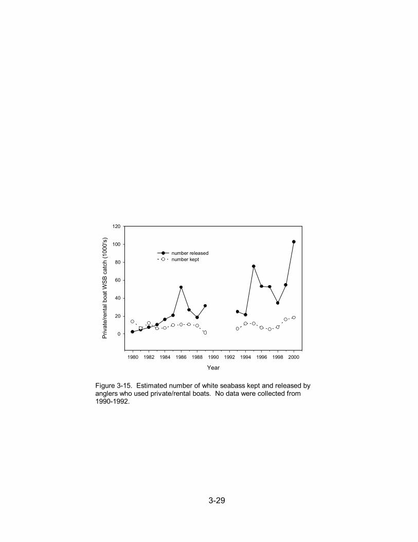
3-29
Year
1980 1982 1984 1986 1988 1990 1992 1994 1996 1998 2000
Priv
ate/
rent
al b
oat W
SB c
atch
(100
0's)
0
20
40
60
80
100
120
number releasednumber kept
Figure 3-15. Estimated number of white seabass kept and released byanglers who used private/rental boats. No data were collected from1990-1992.
4-1
Chapter 4. History of Conservation and Management Measures
4.1 Regulatory History in California
Fisheries regulation in California began in 1851 when the Legislature enacted its firstlaw dealing specifically with fish and game matters by delineating rights to take oystersand to protect aquatic property. The first closed seasons for trout were established in1861 when fishing fees were first collected. Nine years later, in 1870, the Legislatureestablished a Board of Fish Commissioners to provide for the restoration andpreservation of fish in the State's waters. California had the first wildlife conservationagency in the nation, predating even the U.S. Commission of Fish and Fisheries.
By the end of the 19th century, fish and game laws had been expanded and theadministration of these laws had strengthened. In 1871, two wardens were appointed topatrol San Francisco Bay and the Lake Tahoe area. In 1878, the Fish Commission'sauthority was expanded to include game animals as well as fish. The Commissionestablished a Bureau of Patrol and Law Enforcement in 1883 and published the firstcompilation of California fish and game laws in 1885.
The first hunting licenses were issued in 1907 and money from license sales and fineswere deposited in a new Fish and Game Preservation Fund established by theLegislature. The name of the Board of Fish Commissioners was changed to the Fishand Game Commission in 1909; to more accurately reflect the scope of its interests andactivities.
In 1927, the governor approved a Division of Fish and Game within the Department ofNatural Resources. The new Division was unique, because it was administered by theCommission. A separate Fish and Game Code was enacted by the Legislature in1933; replacing portions of the State Penal Code. The Legislature delegated theresponsibility for making state recreational fishing and hunting regulations to theCommission through a constitutional amendment in 1945. Six years later, theReorganization Act of 1951 elevated the Division of Fish and Game to Departmentstatus.
4.2 Regulatory History Specific to White Seabass fisheries
4.2.1 Commercial Fishery
Declining white seabass landings in the late 1920's and during most of the 1930's ledto a series of regulations designed to stabilize the catch (Young 1973) (Table 4-1). The first of these regulations, instituted in 1931, was aimed primarily atthe commercial fishery and imposed a commercial fishing closure during May and June,and a commercial minimum size limit of 28 in. (711 mm). The main purpose of theserestrictions was to protect seabass during spawning and to provide the fish theopportunity to spawn at least twice before they were caught (Skogsberg 1939).
4-2
By the 1940s, commercial gear restrictions were imposed on the fishery. The use ofpurse seine and other roundhaul nets to take white seabass in waters off California wasprohibited in 1940, however, their use in Mexican waters was still allowed andfishermen could transit through California waters with purse seine-caught fish under aDepartment-issued permit. A minimum gill net mesh size of 3.5 in. (89 mm) wasestablished in 1941 and later increased to 6 in. (152 mm) in 1988. Four years later,California voted to ban the use of gill and trammel nets in state waters along themainland shore south of Point Arguello, Santa Barbara County, and one mile offshoreor within 70 fathoms around the Channel Islands.
Since the fishery began, California commercial fishermen fished in Mexican waters forwhite seabass. The catches from Mexico contributed between 30 to 85% of California’swhite seabass fishery depending on market and fishing conditions. In 1982, theMexican government enacted a Foreign Fishery Act which closed Mexico’s waters tothe United States and all other foreign countries. In order to fish in Mexico, a fishbusiness has to have 51% Mexican ownership (Arenas pers. comm.). Currently, thereare no specific commercial white seabass regulations in Mexico, however, whiteseabass are managed under the general Sciaenidae regulations that prohibit increasesin fishing effort in the artisanal fishery where white seabass are taken as bycatch (Arenas pers. comm.).
4.2.2 Recreational Fishery
In 1913, the Anglers License Act made it a misdemeanor for any person over 18 yearsof age to take, catch, or kill any “game fish” for any purpose other than profit, withoutfirst purchasing a license. For purposes of the Act, “game fishes” did not include whiteseabass, but did include tuna; yellowtail; giant sea bass; albacore; barracuda; bonito;rock bass (kelp bass); California whiting (corbina); surf-fish; yellowfin croaker; spotfincroaker; salmon; steelhead; other trout; charr; white-fish (mountain whitefish); stripedbass; and black bass. White seabass was added to the list of “game fish” in 1937. Theaddition of white seabass to the list meant that all persons catching white seabass forsport had to have a sport fishing license (Table 4-1). This change meant that the sizelimit, season closure and bag limit regulations instituted prior to 1937 also applied tosport take.
In 1949, the sport bag limit for white seabass was set at ten fish per day, with not morethan five white seabass less than 28 in. (711mm) in length. In 1957, the allowance forundersized fish was reduced to two fish per day. In 1971, the allowance for undersizedfish was abolished, however, it was reestablished in 1973 when the possession of oneseabass shorter than 28 in. (711 mm) was allowed. In 1978, it once again becameillegal to possess any white seabass less than the minimum size limit, and the daily baglimit was reduced from ten to three fish.
In 1980, a seasonal closure was enacted which prohibited the possession of any whiteseabass from 15 March through 15 June. However, in 1984, an allowance of one legal-
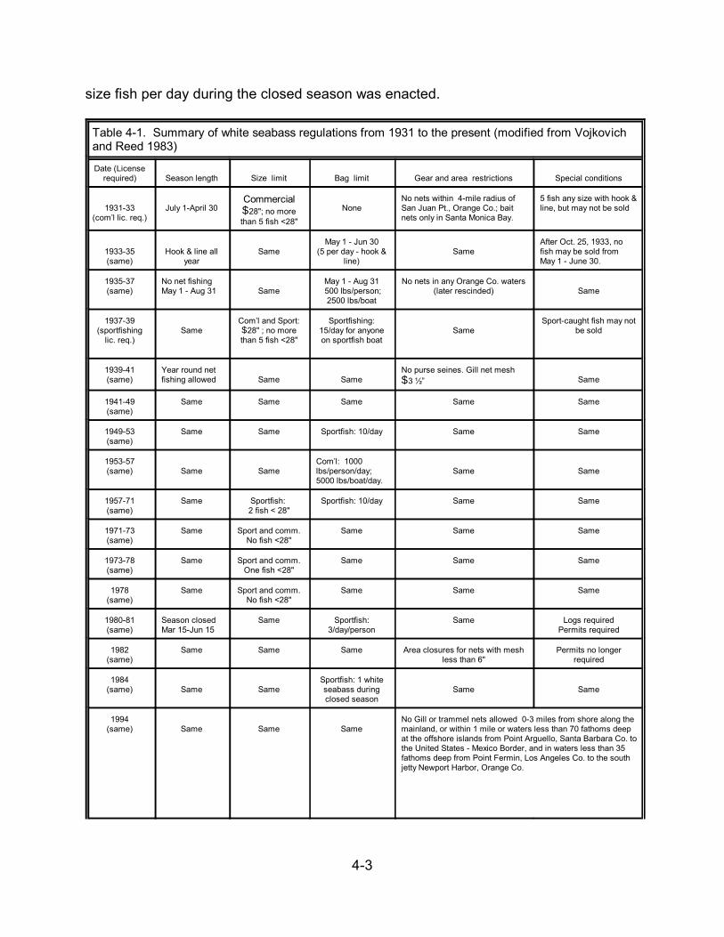
4-3
size fish per day during the closed season was enacted.
Table 4-1. Summary of white seabass regulations from 1931 to the present (modified from Vojkovichand Reed 1983)
Date (Licenserequired) Season length Size limit Bag limit Gear and area restrictions Special conditions
1931-33(com’l lic. req.)
July 1-April 30Commercial$28"; no morethan 5 fish <28"
NoneNo nets within 4-mile radius ofSan Juan Pt., Orange Co.; baitnets only in Santa Monica Bay.
5 fish any size with hook & line, but may not be sold
1933-35(same)
Hook & line allyear
SameMay 1 - Jun 30
(5 per day - hook &line)
SameAfter Oct. 25, 1933, nofish may be sold fromMay 1 - June 30.
1935-37(same)
No net fishingMay 1 - Aug 31 Same
May 1 - Aug 31 500 lbs/person;2500 lbs/boat
No nets in any Orange Co. waters(later rescinded) Same
1937-39(sportfishing
lic. req.)Same
Com’l and Sport:$28" ; no morethan 5 fish <28"
Sportfishing:15/day for anyoneon sportfish boat
SameSport-caught fish may not
be sold
1939-41(same)
Year round netfishing allowed Same Same
No purse seines. Gill net mesh$3 ½” Same
1941-49(same)
Same Same Same Same Same
1949-53(same)
Same Same Sportfish: 10/day Same Same
1953-57(same) Same Same
Com’l: 1000lbs/person/day;5000 lbs/boat/day.
Same Same
1957-71(same)
Same Sportfish: 2 fish < 28"
Sportfish: 10/day Same Same
1971-73(same)
Same Sport and comm.No fish <28"
Same Same Same
1973-78(same)
Same Sport and comm.One fish <28"
Same Same Same
1978(same)
Same Sport and comm.No fish <28"
Same Same Same
1980-81(same)
Season closedMar 15-Jun 15
Same Sportfish:3/day/person
Same Logs requiredPermits required
1982(same)
Same Same Same Area closures for nets with meshless than 6"
Permits no longerrequired
1984(same) Same Same
Sportfish: 1 whiteseabass duringclosed season
Same Same
1994(same) Same Same Same
No Gill or trammel nets allowed 0-3 miles from shore along themainland, or within 1 mile or waters less than 70 fathoms deepat the offshore islands from Point Arguello, Santa Barbara Co. tothe United States - Mexico Border, and in waters less than 35fathoms deep from Point Fermin, Los Angeles Co. to the southjetty Newport Harbor, Orange Co.
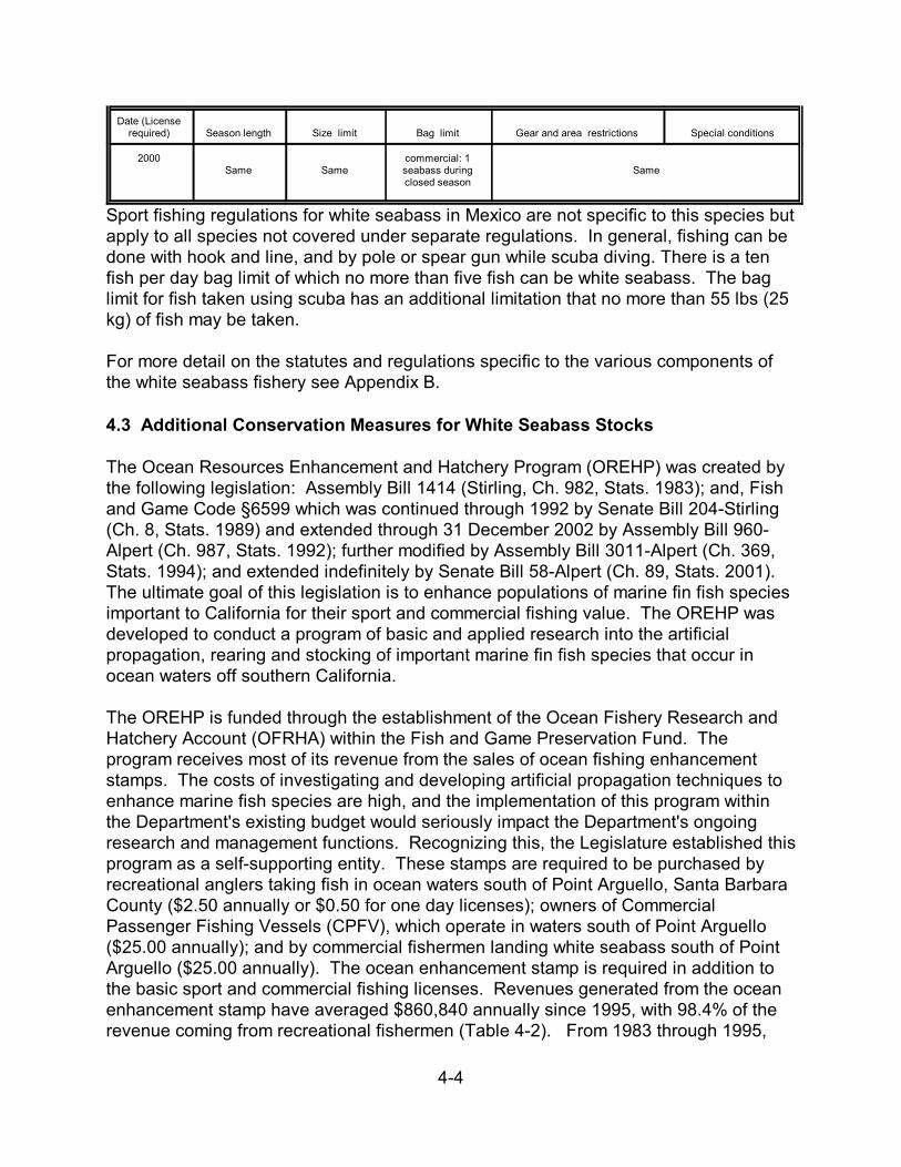
Date (Licenserequired) Season length Size limit Bag limit Gear and area restrictions Special conditions
4-4
2000Same Same
commercial: 1seabass duringclosed season
Same
Sport fishing regulations for white seabass in Mexico are not specific to this species butapply to all species not covered under separate regulations. In general, fishing can bedone with hook and line, and by pole or spear gun while scuba diving. There is a tenfish per day bag limit of which no more than five fish can be white seabass. The baglimit for fish taken using scuba has an additional limitation that no more than 55 lbs (25kg) of fish may be taken.
For more detail on the statutes and regulations specific to the various components ofthe white seabass fishery see Appendix B.
4.3 Additional Conservation Measures for White Seabass Stocks
The Ocean Resources Enhancement and Hatchery Program (OREHP) was created bythe following legislation: Assembly Bill 1414 (Stirling, Ch. 982, Stats. 1983); and, Fishand Game Code §6599 which was continued through 1992 by Senate Bill 204-Stirling(Ch. 8, Stats. 1989) and extended through 31 December 2002 by Assembly Bill 960-Alpert (Ch. 987, Stats. 1992); further modified by Assembly Bill 3011-Alpert (Ch. 369,Stats. 1994); and extended indefinitely by Senate Bill 58-Alpert (Ch. 89, Stats. 2001). The ultimate goal of this legislation is to enhance populations of marine fin fish speciesimportant to California for their sport and commercial fishing value. The OREHP wasdeveloped to conduct a program of basic and applied research into the artificialpropagation, rearing and stocking of important marine fin fish species that occur inocean waters off southern California.
The OREHP is funded through the establishment of the Ocean Fishery Research andHatchery Account (OFRHA) within the Fish and Game Preservation Fund. Theprogram receives most of its revenue from the sales of ocean fishing enhancementstamps. The costs of investigating and developing artificial propagation techniques toenhance marine fish species are high, and the implementation of this program withinthe Department's existing budget would seriously impact the Department's ongoingresearch and management functions. Recognizing this, the Legislature established thisprogram as a self-supporting entity. These stamps are required to be purchased byrecreational anglers taking fish in ocean waters south of Point Arguello, Santa BarbaraCounty ($2.50 annually or $0.50 for one day licenses); owners of CommercialPassenger Fishing Vessels (CPFV), which operate in waters south of Point Arguello($25.00 annually); and by commercial fishermen landing white seabass south of PointArguello ($25.00 annually). The ocean enhancement stamp is required in addition tothe basic sport and commercial fishing licenses. Revenues generated from the oceanenhancement stamp have averaged $860,840 annually since 1995, with 98.4% of therevenue coming from recreational fishermen (Table 4-2). From 1983 through 1995,
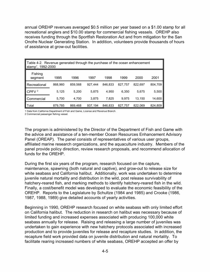
4-5
annual OREHP revenues averaged $0.5 million per year based on a $1.00 stamp for allrecreational anglers and $10.00 stamp for commercial fishing vessels. OREHP alsoreceives funding through the Sportfish Restoration Act and from mitigation for the SanOnofre Nuclear Generating Station. In addition, volunteers provide thousands of hoursof assistance at grow-out facilities.
Table 4-2. Revenue generated through the purchase of the ocean enhancementstamp1, 1992-2000
Fishingsegment 1995 1996 1997 1998 1999 2000 2001
Recreational 868,960 859,568 927,444 846,833 827,757 822,697 804,709
CPFV 2 5,125 5,200 5,875 4,950 6,350 5,675 5,500
Commercial 5,700 4,700 3,875 7,825 9,975 13,150 14,600
Total 879,785 869,468 937,194 846,833 827,757 822,069 824,809
1 Data from California Department of Fish and Game, License and Revenue Branch.2 Commercial passenger fishing vessel.
The program is administered by the Director of the Department of Fish and Game withthe advice and assistance of a ten-member Ocean Resources Enhancement AdvisoryPanel (OREAP). The panel consists of representatives of various user groups,affiliated marine research organizations, and the aquaculture industry. Members of thepanel provide policy direction, review research proposals, and recommend allocation offunds for the OREHP.
During the first six years of the program, research focused on the capture,maintenance, spawning (both natural and captive), and grow-out to release size forwhite seabass and California halibut. Additionally, work was undertaken to determinejuvenile natural mortality and distribution in the wild, post release survivability ofhatchery-reared fish, and marking methods to identify hatchery-reared fish in the wild. Finally, a cost/benefit model was developed to evaluate the economic feasibility of theOREHP. Reports to the Legislature by Schultze (1984 and 1985) and Crooke (1986,1987, 1988, 1989) give detailed accounts of yearly activities.
Beginning in 1990, OREHP research focused on white seabass with only limited efforton California halibut. The reduction in research on halibut was necessary because oflimited funding and increased expenses associated with producing 100,000 whiteseabass annually for release. Raising and releasing a large number of juveniles wasundertaken to gain experience with new hatchery protocols associated with increasedproduction and to provide juveniles for release and recapture studies. In addition, therecapture field work provided data on juvenile distribution and natural mortality. Tofacilitate rearing increased numbers of white seabass, OREHP accepted an offer by
4-6
United Anglers of California to equip and run a pen rearing grow-out facility at Oxnard(Channel Islands Harbor). By the end of 2001, additional pen rearing facilities locatedat San Diego, Mission Bay, Dana Point, Newport Beach, Huntington Harbor, AlamitosBay, Santa Catalina Island, King (Redondo) Harbor, Marina Del Rey, Port Hueneme,and Santa Barbara had joined the volunteer program and accepted fish. (Crooke 1990,1991, 1992; Crooke and Domeier 1993, Crooke 1994, Crooke 1995, Crooke 2000,Crooke 2001). Volunteers from the sportfishing community not only raised money to
build the grow-out pens, but they also contributed over 20,000 hours a year of theirtime to raise and care for the hatchery-bred white seabass.
Concurrent with the passage of new OREHP legislation in 1992, the California CoastalCommission authorized use of $1.2 million in mitigation funds for OREHP capitalconstruction and enhanced recovery of fish in the field. The money was part of amitigation package which Southern California Edison and San Diego Gas and ElectricCompany agreed to for environmental effects of the San Onofre Nuclear GeneratingStation (SONGS). Obtaining the funding was essential to OREHP since it providedconstruction money for an experimental production hatchery. Without increasedfunding, there would only have been adequate resources to continue work at the 1992level for hatchery production and field recoveries. Department and CoastalCommission staff spent 1993 developing a Memorandum of Agreement (MOA) to coverfinancing, construction, and operation of the proposed hatchery. Construction startedduring July 1994 and the hatchery was dedicated on October 13, 1995.
Soon after initial completion of the hatchery, it became apparent that funding forconstruction was not adequate to completely build-out the facility, nor was OREHPstamp revenue sufficient to cover the costs of operating a larger facility. In addition,field sampling to recover tagged fish was proving to be more costly than anticipated. Acting on a recommendation developed by the staff in conjunction with the Department,the Coastal Commission authorized an additional $3.6 million in SONGS mitigation attheir September 1997 meeting. The funds were used to reduce the debt incurredduring initial construction of the hatchery ($428,965), provide funding ($816,800) forequipment to build out the hatchery, and supplement operating funds by $2,189,440over the next eight years.
During 2000, the operator of the hatchery at Carlsbad, Hubbs-Sea World ResearchInstitute (HSWRI), completed build-out of the hatchery and continued operations tosupply juvenile fish to grow-out facilities. Build-out focused on completing theinstallation of three new sea water recirculating (closed) systems. Poor water qualityduring the winter of 1998 due to fresh water run-off and dredging of the lagoonsupplying hatchery water prompted the recirculating experiments. Preliminaryexperiments showed that eggs, larval and juvenile fish survival rates were significantlyenhanced under closed conditions in which temperature and sterility of the water couldbe controlled.
4-7
The primary function of the hatchery is to provide juvenile white seabass, two to threeinches in length, to field-rearing systems operated by volunteer fishermen throughoutthe Southern California Bight. The hatchery is designed to release 400,000 small fishto the grow-out facilities, which will rear them to eight inches and then release the fish. Unfortunately, the hatchery has not reached anticipated production levels because ofwater quality and disease problems. The water quality problems appear to be resolvedbut bacterial and viral diseases contributed to poor production during 1999 and 2000. During 2001, approximately 131,000 juvenile white seabass were released to grow-outfacilities and of those, 100,318 were ultimately released into the open ocean; the bestyear of production in the program’s history. Both the Department and HSWRI arecontinuing to investigate more effective ways to control diseases within the hatcheryand grow-out facilities.
Beginning with 1986, direct releases from the hatchery and grow-out facilities havetotaled 503,000 white seabass. Since it is possible to back calculate the number of fishremaining in the wild on a yearly basis (1.0 - natural mortality) it is possible to estimatethe number of OREHP produced legal size fish (> 28 in.) in the wild population. Usingage specific numbers for natural mortality (see section 2.5) for one- to-four-year-old fishfrom Kent and Ford (1990), and an average of 0.1 for 5+ age fish based on MacCall’spapers, there were 43,000 OREHP-produced adult white seabass in the wild at the endof 2001.
The hatchery now possess 230 adult white seabass to act as brood fish. One hundredseventy-five fish are divided among four tanks and kept at different water temperaturesand day lengths to assure that the program has continued access to viable eggs. Theremaining 55 fish are stored off-site as back-up spawners should something happen tothe fish at the hatchery.
California State University, Northridge (CSUN) and the Center for Marine Studies, SanDiego State University (SDSU) operate the field studies. Sampling to recover taggedwhite seabass was redirected in 1997 to emphasize capture of I to IV year-old juvenilefish (12 to 24 in.). A series of variable mesh gill nets were set in nearshore areas forthe months of April, June, August and October. Nineteen different stations from SanDiego Bay to Santa Barbara were sampled. Thirteen sites were on the open coast,including Santa Catalina Island, and six were in embayments. From April 2000 throughJune 2001, a total of 560 sets yielded 1,372 white seabass. While the fish ranged insize from 6 to 32 inches, most were in the 9 to 24 inch size range.
All fish were scanned for coded wire tags and 111 (8%) were detected. Approximately84% of the fish were recovered from embayments while the remainder were takenalong the open coast. The ratio of tagged to untagged fish for embayments was 1:1.7while the open coast ratio was much lower at 1:64.
Eight adult coded wire tagged fish have been recovered since the summer of 1999. These white seabass represent the first recoveries of legal size fish with a known age
4-8
and release date. Previously, two legal size fish labeled with tetracycline, an antibioticwhich places a permanent mark on the bones, were recovered but the mark on thebones is not specific for a release date so the age of the fish was unknown. One of thecoded wire tagged fish was recovered over 90 miles to the north and another wasrecaptured at the point of release. The fish that was recaptured at it’s release site grewto legal size in three years (four or five years is normal), possibly by remaining in thewarm waters of Mission Bay and living in the vicinity of a live bait receiver (a steadysource of food).
Three additional recoveries of juvenile white seabass during 2000 were especiallysignificant since they showed movement from Santa Catalina Island to the mainland. All previous recoveries only showed movement along the coast.
The OREHP has now progressed to a point where it is possible, with the addition of thenew hatchery in 1995, to culture white seabass in quantity. With the new facility, theprogram has determined many of the factors that are limiting greater production, but allthe factors necessary to increase production are still not understood. White seabassculture continues to hold promise for enhancement of the resource because of thecurrent reduced size of the wild stock.
In addition to hatchery related programs, OREHP has sponsored other research whichrelated directly to white seabass management. Foremost among the programs is thejuvenile white seabass gill net study which is designed to show the relative abundanceof small fish as well as the hatchery contribution to juvenile fish in the wild. Thisrepresents the only fishery independent data base focusing exclusively on whiteseabass recruitment. Researchers working under OREHP grants have examined thegenetic structure of the wild stock and found it to be homogeneous throughout itsrange. Finally, age and growth studies using otoliths to age wild fish and recoveries oftagged fish in the field have shown that white seabass growth is faster than previouslydocumented.
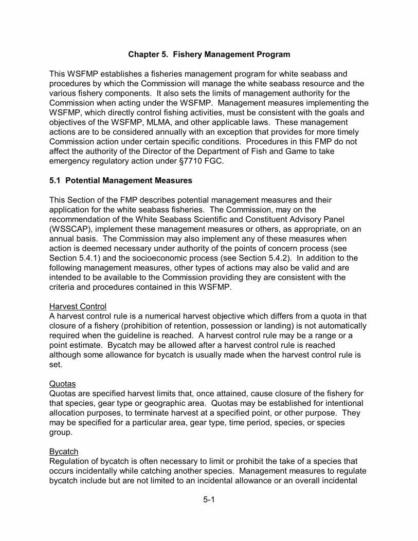
5-1
Chapter 5. Fishery Management Program
This WSFMP establishes a fisheries management program for white seabass andprocedures by which the Commission will manage the white seabass resource and thevarious fishery components. It also sets the limits of management authority for theCommission when acting under the WSFMP. Management measures implementing theWSFMP, which directly control fishing activities, must be consistent with the goals andobjectives of the WSFMP, MLMA, and other applicable laws. These managementactions are to be considered annually with an exception that provides for more timelyCommission action under certain specific conditions. Procedures in this FMP do notaffect the authority of the Director of the Department of Fish and Game to takeemergency regulatory action under §7710 FGC.
5.1 Potential Management Measures This Section of the FMP describes potential management measures and theirapplication for the white seabass fisheries. The Commission, may on therecommendation of the White Seabass Scientific and Constituent Advisory Panel(WSSCAP), implement these management measures or others, as appropriate, on anannual basis. The Commission may also implement any of these measures whenaction is deemed necessary under authority of the points of concern process (seeSection 5.4.1) and the socioeconomic process (see Section 5.4.2). In addition to thefollowing management measures, other types of actions may also be valid and areintended to be available to the Commission providing they are consistent with thecriteria and procedures contained in this WSFMP.
Harvest Control A harvest control rule is a numerical harvest objective which differs from a quota in thatclosure of a fishery (prohibition of retention, possession or landing) is not automaticallyrequired when the guideline is reached. A harvest control rule may be a range or apoint estimate. Bycatch may be allowed after a harvest control rule is reachedalthough some allowance for bycatch is usually made when the harvest control rule isset.
QuotasQuotas are specified harvest limits that, once attained, cause closure of the fishery forthat species, gear type or geographic area. Quotas may be established for intentionalallocation purposes, to terminate harvest at a specified point, or other purpose. Theymay be specified for a particular area, gear type, time period, species, or speciesgroup.
BycatchRegulation of bycatch is often necessary to limit or prohibit the take of a species thatoccurs incidentally while catching another species. Management measures to regulatebycatch include but are not limited to an incidental allowance or an overall incidental
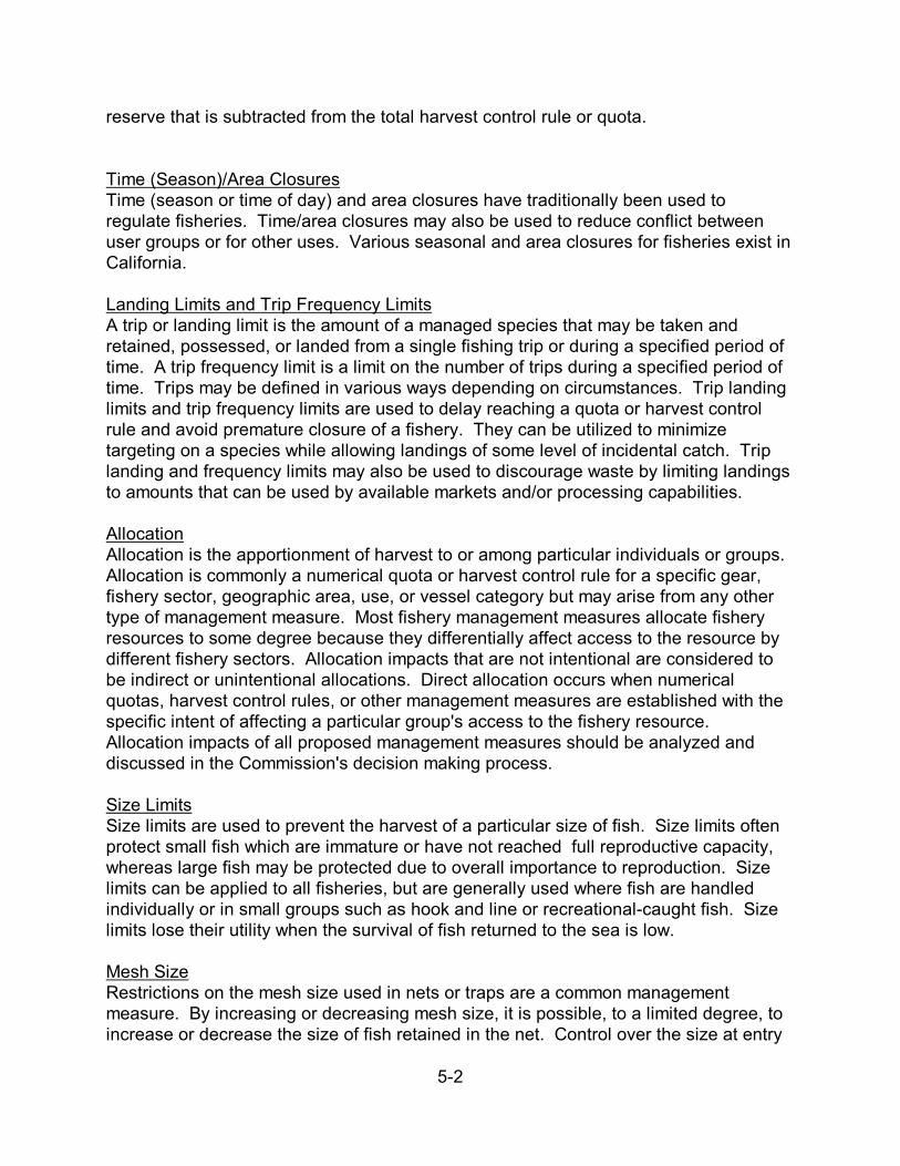
5-2
reserve that is subtracted from the total harvest control rule or quota.
Time (Season)/Area ClosuresTime (season or time of day) and area closures have traditionally been used toregulate fisheries. Time/area closures may also be used to reduce conflict betweenuser groups or for other uses. Various seasonal and area closures for fisheries exist inCalifornia.
Landing Limits and Trip Frequency LimitsA trip or landing limit is the amount of a managed species that may be taken andretained, possessed, or landed from a single fishing trip or during a specified period oftime. A trip frequency limit is a limit on the number of trips during a specified period oftime. Trips may be defined in various ways depending on circumstances. Trip landinglimits and trip frequency limits are used to delay reaching a quota or harvest controlrule and avoid premature closure of a fishery. They can be utilized to minimizetargeting on a species while allowing landings of some level of incidental catch. Triplanding and frequency limits may also be used to discourage waste by limiting landingsto amounts that can be used by available markets and/or processing capabilities.
AllocationAllocation is the apportionment of harvest to or among particular individuals or groups. Allocation is commonly a numerical quota or harvest control rule for a specific gear,fishery sector, geographic area, use, or vessel category but may arise from any othertype of management measure. Most fishery management measures allocate fisheryresources to some degree because they differentially affect access to the resource bydifferent fishery sectors. Allocation impacts that are not intentional are considered tobe indirect or unintentional allocations. Direct allocation occurs when numericalquotas, harvest control rules, or other management measures are established with thespecific intent of affecting a particular group's access to the fishery resource. Allocation impacts of all proposed management measures should be analyzed anddiscussed in the Commission's decision making process.
Size LimitsSize limits are used to prevent the harvest of a particular size of fish. Size limits oftenprotect small fish which are immature or have not reached full reproductive capacity,whereas large fish may be protected due to overall importance to reproduction. Sizelimits can be applied to all fisheries, but are generally used where fish are handledindividually or in small groups such as hook and line or recreational-caught fish. Sizelimits lose their utility when the survival of fish returned to the sea is low.
Mesh SizeRestrictions on the mesh size used in nets or traps are a common managementmeasure. By increasing or decreasing mesh size, it is possible, to a limited degree, toincrease or decrease the size of fish retained in the net. Control over the size at entry
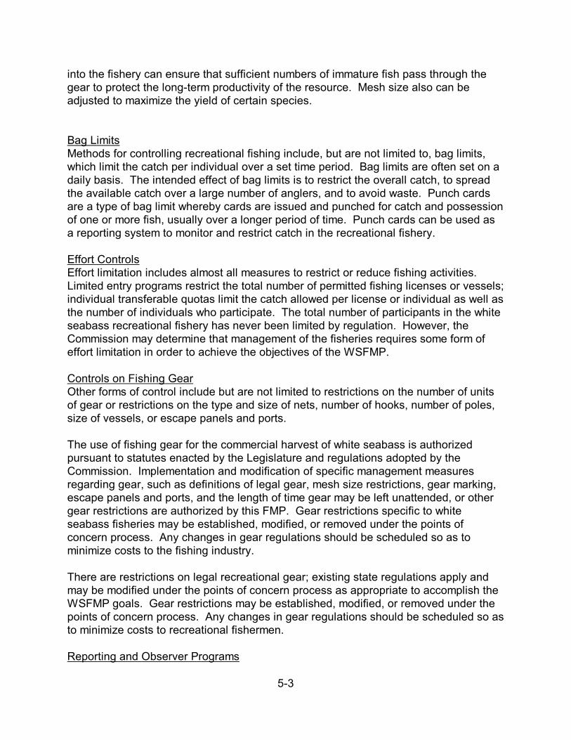
5-3
into the fishery can ensure that sufficient numbers of immature fish pass through thegear to protect the long-term productivity of the resource. Mesh size also can beadjusted to maximize the yield of certain species.
Bag LimitsMethods for controlling recreational fishing include, but are not limited to, bag limits,which limit the catch per individual over a set time period. Bag limits are often set on adaily basis. The intended effect of bag limits is to restrict the overall catch, to spreadthe available catch over a large number of anglers, and to avoid waste. Punch cardsare a type of bag limit whereby cards are issued and punched for catch and possessionof one or more fish, usually over a longer period of time. Punch cards can be used asa reporting system to monitor and restrict catch in the recreational fishery.
Effort ControlsEffort limitation includes almost all measures to restrict or reduce fishing activities. Limited entry programs restrict the total number of permitted fishing licenses or vessels;individual transferable quotas limit the catch allowed per license or individual as well asthe number of individuals who participate. The total number of participants in the whiteseabass recreational fishery has never been limited by regulation. However, theCommission may determine that management of the fisheries requires some form ofeffort limitation in order to achieve the objectives of the WSFMP.
Controls on Fishing GearOther forms of control include but are not limited to restrictions on the number of unitsof gear or restrictions on the type and size of nets, number of hooks, number of poles,size of vessels, or escape panels and ports.
The use of fishing gear for the commercial harvest of white seabass is authorizedpursuant to statutes enacted by the Legislature and regulations adopted by theCommission. Implementation and modification of specific management measuresregarding gear, such as definitions of legal gear, mesh size restrictions, gear marking,escape panels and ports, and the length of time gear may be left unattended, or othergear restrictions are authorized by this FMP. Gear restrictions specific to whiteseabass fisheries may be established, modified, or removed under the points ofconcern process. Any changes in gear regulations should be scheduled so as tominimize costs to the fishing industry.
There are restrictions on legal recreational gear; existing state regulations apply andmay be modified under the points of concern process as appropriate to accomplish theWSFMP goals. Gear restrictions may be established, modified, or removed under thepoints of concern process. Any changes in gear regulations should be scheduled so asto minimize costs to recreational fishermen.
Reporting and Observer Programs
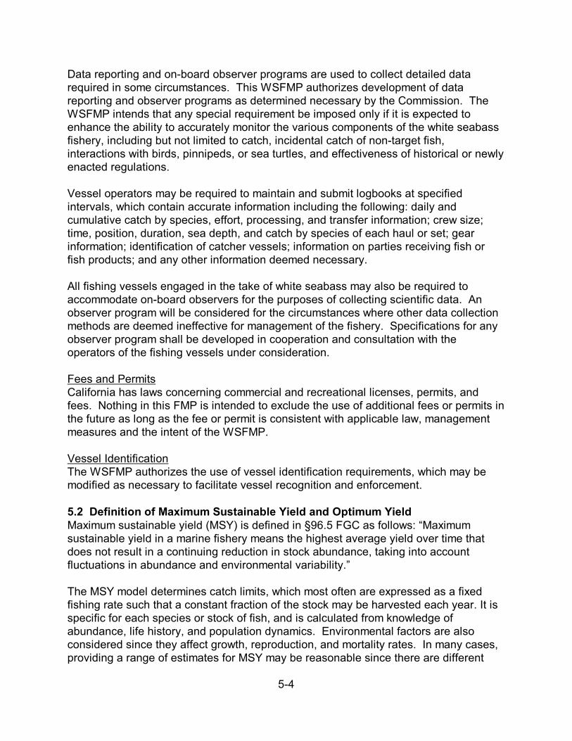
5-4
Data reporting and on-board observer programs are used to collect detailed datarequired in some circumstances. This WSFMP authorizes development of datareporting and observer programs as determined necessary by the Commission. TheWSFMP intends that any special requirement be imposed only if it is expected toenhance the ability to accurately monitor the various components of the white seabassfishery, including but not limited to catch, incidental catch of non-target fish,interactions with birds, pinnipeds, or sea turtles, and effectiveness of historical or newlyenacted regulations.
Vessel operators may be required to maintain and submit logbooks at specifiedintervals, which contain accurate information including the following: daily andcumulative catch by species, effort, processing, and transfer information; crew size;time, position, duration, sea depth, and catch by species of each haul or set; gearinformation; identification of catcher vessels; information on parties receiving fish orfish products; and any other information deemed necessary.
All fishing vessels engaged in the take of white seabass may also be required toaccommodate on-board observers for the purposes of collecting scientific data. Anobserver program will be considered for the circumstances where other data collectionmethods are deemed ineffective for management of the fishery. Specifications for anyobserver program shall be developed in cooperation and consultation with theoperators of the fishing vessels under consideration.
Fees and PermitsCalifornia has laws concerning commercial and recreational licenses, permits, andfees. Nothing in this FMP is intended to exclude the use of additional fees or permits inthe future as long as the fee or permit is consistent with applicable law, managementmeasures and the intent of the WSFMP.
Vessel IdentificationThe WSFMP authorizes the use of vessel identification requirements, which may bemodified as necessary to facilitate vessel recognition and enforcement.
5.2 Definition of Maximum Sustainable Yield and Optimum YieldMaximum sustainable yield (MSY) is defined in §96.5 FGC as follows: “Maximumsustainable yield in a marine fishery means the highest average yield over time thatdoes not result in a continuing reduction in stock abundance, taking into accountfluctuations in abundance and environmental variability.”
The MSY model determines catch limits, which most often are expressed as a fixedfishing rate such that a constant fraction of the stock may be harvested each year. It isspecific for each species or stock of fish, and is calculated from knowledge ofabundance, life history, and population dynamics. Environmental factors are alsoconsidered since they affect growth, reproduction, and mortality rates. In many cases,providing a range of estimates for MSY may be reasonable since there are different

5-5
assumptions in the model. In addition, there may be situations where the scientificinformation is inadequate to directly calculate MSY for a particular species, and a proxyor substitute may be used. For example, recent average catch may be used as a proxyfor MSY if a time period is chosen when there is no evidence of a declining abundance.
Optimum yield (OY) is generally defined as the harvest level for a species, such aswhite seabass, that achieves the greatest overall benefits when considering biological,social and economic factors. Optimum yield differs from MSY because MSY onlyconsiders the biology of the species in question (Wallace et al. 1994).
The Marine Life Management Act provides a definition of OY, which is similar to thegeneralized definition, but which gives specific direction for resource managers:
“Optimum yield, with regard to a marine fishery, means the amount of fishtaken in a fishery that does all of the following: (a) provides the greatestbenefit to the people of California, particularly with respect to foodproduction and recreational opportunities, and takes into account theprotection of marine ecosystems. (b) is the maximum sustainable yield ofthe fishery, reduced by relevant economic, social, or ecological factors; (c)In the case of an overfished fishery, provides for rebuilding to a levelconsistent with producing maximum sustainable yield in the fishery” (§97FGC).
White seabass management through the use of an OY is consistent with the MLMA andthe goals and objectives of the WSFMP. This methodology allows continued utilizationof the white seabass resource while the stock is recovering from low abundance andless than optimal oceanic conditions which occurred during the 1960s and 1970s.
It is not uncommon that the status of knowledge for a given stock is limited to the catchhistory and incomplete life history information. A precautionary approach to calculatingOY in data-moderate or data-poor situations is to multiply MSY, or its proxy, by afraction. A tenet of this principle is that less aggressive (more restrictive) harvestpolicies are adopted as uncertainty increases concerning the status of stocks and theirresponse to fishing pressure (Restrepo et al. 1998).
5.3 General Fishery Management Plan Framework
An FMP framework is a multi-year management plan that describes the processes bywhich the fishery will be managed, including when, how, and within what limitsregulatory changes will be made, and the ranges of the resulting impacts. Preseasonand in-season adjustments to regulations may be made without FMP amendment byimplementing the procedures and provisions established in the FMP framework. Instead of providing a fixed set of management measures to implement at one point intime, the FMP framework establishes mechanisms to adjust the management of thefishery to meet changing circumstances over a longer time frame. This may be

5-6
accomplished through annual adjustments of seasons, quotas, etc., or through in-season adjustments needed in response to factors that cannot be precisely anticipatedduring a review process. Framework adjustments may be implemented more quicklythan FMP amendments, allowing for more timely management response and providingfor adaptive management.
Explicit instructions may be built into an FMP framework to lessen the risk that the FMPcould be considered capricious. However, guidelines that are too specific could restrictthe flexibility and adaptability of fishery management. Included in the FMP frameworkare limits and controls for how adjustments may be made. The FMP framework mustspecify fully the processes to be used in making adjustments including the triggeringmechanisms, procedures to be followed, and actions to be taken.
5.3.1 Plan Amendment
Framework management for FMPs is designed to be flexible and adaptable to a widerange of future conditions and intended to function without the need for frequentamendment. However, unforseen social, economic, environmental or biologicaldevelopments may create an unanticipated situation where the existing FMP does notadequately provide for future management of the fishery. Under such circumstances,the FMP would be amended to allow for efficient and responsive management of thefishery. Fishery management plan amendments are required for major changes orcontroversial actions, which are outside the scope of the original FMP. Examples ofactions that would require an FMP amendment include:
• Changes to management objectives;• Changes to species in the management unit;• A change in the definition of an overfished stock;• Amendments to any procedures required by the FMP; or• Revisions to any management measures that are fixed in the FMP.
An FMP amendment entails an extensive development and adoption process includinginput from advisory committees, public hearings, and an extended period for publiccomment and peer review. In addition, amendment of an FMP requires CEQA analysisof the proposed changes to the document. Once a draft plan amendment is completed,it will have to undergo the full rule-making process described in the next Section.
5.3.2 Framework Actions
There are three different categories of management actions, each of which requires aslightly different process. Management measures may be established, adjusted orremoved using any of the following three procedures:
A. Full Rule Making Actions (Regulatory Amendment) These include any proposed management measure that is highly controversial or any
5-7
measure which directly allocates the resource. The Commission normally will followthe three-meeting procedure, which means the identification of issues and thedevelopment of proposals will begin at a Commission meeting prior to the first decisionmeeting. Subsequent to this meeting there will be two decision meetings, the firstmeeting to develop proposed management measures and their alternatives, the secondmeeting to make a final decision.
Management measures recommended to address a resource conservation issue mustbe based upon the establishment of a point of concern and consistent with the specificprocedures and criteria listed in Section 5.4.1. Management measures recommendedto address social or economic issues must be consistent with the specific proceduresand criteria described in Section 5.4.2.
B. “Notice” ActionsThese include all management actions other than prescribed actions that are eithernon-discretionary or have probable impacts that have been previously analyzed. TheCommission will require at least one Commission meeting to approve routinemanagement measures.
These actions are intended to have temporary effect and the expectation is that theywill need frequent adjustment. They may be recommended at a single Commissionmeeting, although the Commission will provide as much advance information to thepublic as possible concerning the issues it will be considering. The primary examplesare management actions defined as routine in Section 5.3.3. These include trip landingand frequency limits for all gear types and recreational bag limits. Previous analysismust have been specific as to gear type before a management measure can be definedas routine and acted upon at a single Commission meeting.
C. Prescribed ActionsPrescribed management actions may be initiated by the Department Director orCommission without prior public notice, opportunity to comment, or a Commissionmeeting. These actions are ministerial and the impacts must have previously beentaken into account. Examples include fishery, season, or gear type closures when aquota is attained.
5.3.3 Routine Management Measures
Routine management measures are those that the Commission determines are likely tobe adjusted on an annual or more frequent basis. Measures are classified as routineby the Commission through either the full or abbreviated rule making process. In orderfor a measure to be classified as routine, the Commission will determine that themeasure is of the type normally used to address the issue at hand and may requirefurther adjustment to achieve its purpose with accuracy.
As in the case of all proposed management measures, prior to initial implementation as
5-8
routine measures, the Commission will analyze the need for the measures, theirimpacts, and the rationale for their use. Once a management measure has beenclassified as routine through one of the two rule making procedures outlined above, itmay be modified thereafter through the single meeting notice procedure if: (1) themodification is proposed for the same purpose as the original measure, and (2) theimpacts of the modification are within the scope of the impacts analyzed when themeasure was originally classified as routine. The analysis of impacts need not berepeated when the measure is subsequently modified if the Commission determinesthat they do not differ substantially from those contained in the original analysis. TheCommission may also recommend removing a routine classification.5.4 White Seabass FMP Framework
The FMP framework for white seabass resource management is composed of severalelements, which taken individually or together, will allow the Commission to reactquickly to changes in the white seabass population off California without the need for afull amendment. Management measures are normally imposed, adjusted, or removedat the beginning of the fishing year but may, if the Commission deems necessary, beimposed, adjusted, or removed at any time during the year. Management measuresmay be imposed for resource conservation, social or economic reasons consistent withthe criteria, procedures, goals, and objectives set forth in the WSFMP.
The WSFMP framework consists of a points of concern process, socioeconomicprocess, allocation criteria, and harvest control rules, which give the Commissionspecific guidelines for making management decisions. However, these guidelines areintended to be flexible and allow for other management strategies that would effectivelyachieve the goals and objectives of this FMP and MLMA.
5.4.1 Points of Concern Process
The points of concern process is one of the tools the Commission has for exercising itsresource stewardship responsibilities for white seabass. The process is intended tofoster a continuous and vigilant review of the white seabass stocks and fisheries toprevent overfishing or other resource damage. To facilitate this process, a Department White Seabass Management Team (WSMT) will be created to monitor the fisheriesthroughout the year, taking into account any new information on the status of eachspecies or species group to determine whether a resource conservation issue existsthat requires a management response. The points of concern criteria are intended toassist the Commission in determining when a focused review on a particular species iswarranted, and which may result in the need to recommend management measures toaddress the issue.
This FMP framework provides the authority to act based solely on the points ofconcern. Thus, the Commission may act quickly and directly to address a resourceconservation issue. In conducting this review, the WSMT will utilize the most currentcatch, effort, abundance and other relevant data.
5-9
In the course of the continuing review, a “point of concern” occurs when any one ormore of the following is found or expected:
• Catch is projected to significantly exceed the current harvest control ruleor quota;
• Any adverse or significant change in the biological characteristics of thewhite seabass stock (age composition, size composition, age at maturity,or recruitment) is discovered;
• An overfished condition exists or is imminent;• Any adverse or significant change in the availability of white seabass
forage or in the status of a dependent species is discovered;• An error in data or a stock assessment is detected that significantly
changes estimates of impacts due to current management.
Once a point of concern is identified, the WSMT will evaluate current data to determineif a resource conservation issue exists and will provide its findings in writing at the nextscheduled Commission meeting. If the WSMT determines a resource conservationissue exists, it will provide its recommendation, rationale, and analysis for theappropriate management measures that will address the issue. In developing itsrecommendation for management action, the WSMT will recommend alternatives fromone or more of the most commonly used management measures listed in Section 5.1,or other necessary measures, to address resource conservation issues.
Direct allocation of the resource between different segments of the fisheries is, in mostcases, not the preferred response to a resource conservation issue. Commissionrecommendations to directly allocate the resource will be developed, if needed,according to the socioeconomic process and criteria described in Sections 5.4.2 and5.4.3.
After receiving the WSMT’s report, the Commission will take public testimony and, ifappropriate, will implement management measures accompanied by supportingrationale and analysis of impacts. The Commission’s analysis will include a descriptionof (a) how the action will address the resource conservation issue consistent with theobjectives of the WSFMP; (b) likely impacts on other management measures and otherfisheries; and (c) economic impacts, particularly the cost to the commercial andrecreational segments of the fishing industry. Nothing in this Section prevents theDirector from exercising the authority to take emergency action as specified in the Fishand Game Code.
5.4.2 Socioeconomic Process
From time to time, non-biological issues may arise which may require the Commissionto consider management actions to address certain social or economic conditions inthe fisheries. Resource allocation, seasons, or landing limits based on market qualityand timing, safety measures, and prevention of gear conflicts are only a few examples
5-10
of possible management issues with a social or economic basis. In general, there maybe any number of situations where the Commission determines that managementmeasures are necessary to achieve the stated social and/or economic objectives of theWSFMP.
Either on its own initiative or by request, the Commission may evaluate currentinformation and issues to determine if social or economic factors warrant imposition ofmanagement measures to achieve the Commission’s established managementobjectives. Actions that are permitted under this FMP framework include all of thecategories of actions authorized under the points of concern FMP framework with theaddition of direct resource allocation and access limitation measures.If the Commission concludes that a management action is necessary to address asocial or economic issue, it or the WSMT will prepare a report containing the rationalein support of that conclusion. The report will include the proposed managementmeasure, a description of other viable alternatives considered, and an analysis thataddresses the following criteria: (a) how the action is expected to promote achievementof the goals and objectives of the WSFMP; (b) likely impacts on other managementmeasures and other fisheries; (c) biological impacts; (d) economic impacts, particularlythe cost to the fishing industry; and (e) how the action is expected to accomplish atleast one of the following:
• Enable a quota, harvest control rule, or allocation to be achieved;• Avoid exceeding a quota, harvest control rule, or allocation;• Increase sustainable landings;• Reduce discards;• Reduce gear conflicts, or conflicts between competing user groups;• Extend fishing and marketing opportunities as long as practicable during
the fishing year;• Maintain or improve product volume and flow to the consumer or user;• Increase economic yield;• Maintain or improve the safety of fishing operations;• Increase fishing efficiency;• Maintain or improve product quality;• Maintain or improve the recreational fishery;• Maintain or improve data collection, including means for verification;• Maintain or improve monitoring and enforcement; or• Any other measurable benefit to the fishery.
The Commission, following review of the report, supporting data, public comment andother relevant information, may implement management measures accompanied byrelevant background data, information and public comment. The action will explain theurgency, if any, in implementation of the measure(s).
If conditions warrant, the Commission may designate a management measure as aroutine management measure to address social and economic issues provided that the
5-11
criteria and procedures in Section 5.4.2 are followed.
Harvest control rules and quotas, including allocations, implemented through this FMPframework will be set annually and may only be modified in season to reflect technicalcorrections. In contrast, harvest control rules and quotas may be imposed at any timeof year for resource conservation reasons under the points of concern mechanism. Nothing in this FMP framework chapter is intended to preclude or limit theCommission’s access to the socioeconomic process.
5.4.3 Allocation Criteria
In addition to the requirements described in Section 5.4.2, the Commission willconsider at least the following factors when considering direct allocation of theresource:
• Present participation in and dependence on the fisheries, includingalternative fisheries;
• Historical fishing practices in, and historical dependence on, the fisheries;• The economics of the fisheries;• Any existing agreement or negotiated settlement between the affected
participants in the fisheries;• Potential biological impacts on any species affected by the allocation;• Consistency with the goals and objectives of this WSFMP and the MLMA.
These criteria are in keeping with the goals of and objectives of the MLMA and asspecifically outlined in §7072 (c) FGC: “To the extent that conservation andmanagement measures in a fishery management plan either increase or restrict theoverall harvest of a fishery, fishery management plans shall allocate those increases orrestrictions fairly among recreational and commercial sectors participating in thefishery.” §7086 (c) (2) FGC says that in the case of a fishery determined to beoverfished, restrictions and recovery benefits will be allocated fairly and equitablyamong sectors of the fishery.
Management tools such as catch quotas, seasons, area closures, bag limits, and otherregulations can be used to directly or indirectly allocate fishery resources with theintent to increase or restrict a group’s access or harvest of a resource. Decisions onallocation and the tools needed to implement those decisions must take intoconsideration complex biological, social, and economic factors. In addition, modificationof a direct allocation cannot be designated as “routine” unless the specific criteria forthe modification have been established in the regulations.
5.4.4 Harvest Control Rules
5-12
Harvest control rules provide a mechanism to achieve sustainable use, preventoverfishing, and rebuild depressed stocks, each of which are described in the MLMA asprimary conservation standards for fisheries management. Harvest control rules basedon objective, measurable criteria provide assurance that conservation objectives will bemet.
Harvest control rules usually determine target levels and upper limits for take. Inputinformation such as stock size or reproductive potential is necessary to directlycalculate allowable fishing mortality, but proxies may be used in situations where directcalculations are not possible due to inadequate data. Typically, an upper limit onfishing mortality or maximum fishing mortality threshold (MFMT) and a lower boundaryon stock size or minimum stock size threshold (MSST) are set.
Harvest control rules are incorporated into prearranged plans that use information onstocks to make management decisions so the stock remains within safe biologicallimits. The rules include plans for decision making and procedures for invoking presetmeasures to manage the fishery. Objective and measurable stock status criteria, suchas MFMT and MSST, must be specified in an FMP using harvest control rules.
In general, harvest control rules involve methods that are used to determine allowablefishing mortality each year. Often, formulas are given in FMPs that provide for directcalculation of the allowable harvest by using the current stock size, stock productivity,and other factors as inputs. However, in practice there are usually gaps in the currentstate of knowledge for individual species. Since it is common that the requisite dataare not sufficiently known to directly calculate MSY or OY, defaults are sometimesspecified in FMPs to allow use of the MSY/OY approach. In addition, increased riskresulting from such uncertainty is addressed with the precautionary principle, whichestablishes less aggressive harvest policies in response to greater uncertaintyconcerning the status of the stocks and their response to fishing pressure.
The MSY/OY control rule means a harvest strategy which would be expected to resultin a long-term average catch approximating MSY as modified by environmental andsocioeconomic factors. The MLMA does not require that sustainability and otherconservation measures be achieved through MSY and OY control rules. However,alternatives to MSY and OY need objective standards for determining whether or notmanagement measures are accomplishing the intended results.
As data become available, improved, or are updated, the formulas and procedures forsetting OY, harvest guidelines, and quotas for white seabass may need to be modified. Changes and additions to these formulas are authorized by the WSFMP and may beaccomplished through the points of concern process or the socioeconomic process.
5.5 Trigger Mechanisms
5-13
It is vital to have ways that measure or gauge the success of the managementmeasures implemented by the Commission. Measurable long term fishery-dependentand fishery-independent data such as catch trends, recruitment patterns, and forageabundance indices should be used to monitor the effectiveness of current managementmeasures. For example, sustained decreases in catch and or recruitment will alert theWSMT and WSSCAP to potential problems within white seabass stocks. The WSMTand WSSCAP will determine appropriate trigger mechanisms for the white seabassstocks and they will use them to provide management recommendations to theCommission. In turn, the Commission could implement needed management measuresin a timely manner through the points of concern process.
On a continuous basis, the WSMT will review landings for which harvest control rules,quotas or specific routine management measures have been implemented, and it willmake projections of the landings at various times throughout the year. If it becomesapparent that the rate of landing is substantially different than anticipated and that thecurrent routine management measures will not achieve the management objectives,then the WSMT may recommend to the Commission in-season adjustments to thosemeasures. Such adjustments may be implemented through the single meeting noticeprocedure.
5.6 Management Alternatives
In addition to the framework procedures described above, initial managementalternatives are proposed for implementation upon approval of the WSFMP. If adoptedby the Commission and implemented by the Department, these alternatives wouldbecome regulations affecting fisheries for white seabass. They may be modified in the future, or new regulations may be implemented, using the framework proceduresin the WSFMP. Analysis of these alternatives is deferred to Chapter 6.
As mentioned in 5.1, there are many potential measures to be used in the managementof white seabass, and in fact, several of those measures are currently in place (Table4-1; Appendix B and C). The Department and WSSCAP felt that additional measureswere needed to ensure the sustainability of the white seabass resource. In developingthese alternatives, an MSY/OY control rule was decided upon to represent the bestapproach. The reasons for this are that an MSY/OY control rule: 1) containsmeasurable criteria for use in management decisions; 2) requires calculations usingdata that the Department currently collects (commercial landings, recreational catch,and fishing effort); 3) can be linked to future research and data needs; and 4) is similarto the approach taken for the management of the nearshore finfish fishery (nearshoreFMP).
The data used to develop the alternatives consist of commercial landing receipt dataand Commercial Passenger Fishing Vessel (CPFV) logbook data collected by theDepartment in combination with Marine Recreational Fishing Statistics Survey(MRFSS) data (RecFIN 2001) for private/rental boats and all shore-based fishing
5-14
modes (e.g., piers, beaches). Since recreational data are presented in numbers of fish,the numbers were converted to pounds using MRFSS averaged annual white seabassweights by fishing mode. All discussions presented in this chapter are based onweight.
Harvest control rules often address allocation when more than one user group isinvolved. The WSSCAP, however, decided that allocation of the resource was not anissue at this time. As a group, they reached consensus on sharing the resource withoutthe need for separate allotments and advised the Department to pursue a course ofmaintaining status quo; however, the panel felt that this issue should be addressed inthe next few years. To guide any future discussions of allocation, the advisory panelwill use the allocation criteria identified in Section 5.4.3, and any allocation policies thatthe Commission may develop.
The alternatives below (except A) represent different determinations of MSY/OY to beused in a harvest control rule. It is recognized that these alternatives represent onlythe upper target reference points and much needed data are required to determineMSST and the shape of the control rule. Once stock assessments are done andknowledge of the white seabass stock moves from data-poor toward data-rich, a betterdefined MSY control rule can be set. In the interim, it is suggested that the defaultMSY/OY control rule below (Section 5.7) be used in conjunction with one of thefollowing alternatives.
5.6.1 Alternative A - Status Quo
This alternative provides no changes to present management of white seabass. Themanagement of white seabass would continue through a combination of existingrecreational and commercial regulations which include size and bag limits andseasonal closure (See Table 4-1 and Appendix B and C).
5.6.2 Alternative B - OY Proxies Based on National Standard Guidelines
The Magnuson-Stevens Fishery Conservation Management Act uses advisoryguidelines, known as National Standard Guidelines (NSGs), to assist in thedevelopment of federal FMPs. The NSGs allow for situations where MSY cannot beestimated directly: “If a reliable estimate of pristine stock size (i.e., the long-termaverage stock size that would be expected in the absence of fishing) is available, astock size approximately 40 percent of this value may be a reasonable proxy for theMSY stock size, and the product of this stock size and the natural mortality rate may bea reasonable proxy for MSY.”
For white seabass, the pre-exploitation biomass was estimated at 40 million pounds,ranging from 30 to 56 million pounds (Dayton and MacCall 1992). Estimates of naturalmortality rate (M) from recreational and commercial data range from 0.08 to 0.13(MacCall et al. 1976; Dayton and MacCall 1992). Using an intermediate value for

5-15
natural mortality (0.10), the following calculations can be made:
MSY stock size = Pristine stock size (40 million pounds) x 0.40 = 16 million pounds
MSY proxy = MSY stock size (16 million pounds) x natural mortality (0.1) = 1.6 million pounds
This MSY proxy was then used for alternatives B1 and B2 below.
5.6.2.1 Alternative B1: OY=0.8125 x MSY
Under the MLMA, if management is based on an MSY then an OY must be calculated. Thus, a further step is needed that reduces the above MSY proxy to a level where thechances of overfishing are greatly reduced. Although technical guidelines suggest anupper target reference point at 75% of MSY (Restrepo et al. 1998), the advisory paneladvocated an even higher percentage. Based on recent increased catches ofjuveniles, increased landings, and more individuals seen and caught in northernCalifornia (Monterey), the advisory panel reached consensus on an OY of 0.8125 xMSY. This value is 1.3 million pounds (0.8125 x 1.6 million pounds).
5.6.2.2 Alternative B2 (Preferred): OY=0.75 x MSY
This alternative is similar to alternative B1, except there is no deviation from thetechnical guidelines outlined in Restrepo et al. (1998). A target reference point of 75% of MSY is used to represent OY. This value is 1.2 million pounds (0.75 x 1.6 millionpounds).
5.6.3 Alternative C - OY Proxies Based on Recent Catch Levels
This alternative is based on the use of recent catch data as a proxy for MSY, withprecautionary adjustments made for OY. The Pacific Fishery Management Council(PFMC) and Commission have adopted recent catch as a proxy for MSY formanagement of several nearshore finfish species. The PFMC also recognized that aprecautionary adjustment of 0.75 x MSY should be used to determine OY in situationswhen moderate information exists for a particular species. Using this approach, caremust be taken to select a period representing recent catch when the stock was notpresumed in decline.
For white seabass, MSY estimates were developed based on catch levels for thefollowing number of years and time frames: 5 years (1996-2000), 10 years (1988-1989and 1993-2000), and 15 years (1983-1989 and 1993-2000). The same calculationswere done for the alternatives C1, C2, and C3: the U.S. recreational and commercial catch for the specified time frame was averaged, giving an estimate of MSY. Thisnumber was then multiplied by 0.75 to give an estimate of OY.
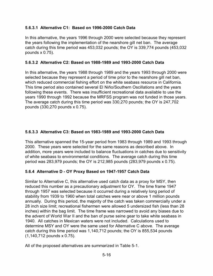
5-16
5.6.3.1 Alternative C1: Based on 1996-2000 Catch Data
In this alternative, the years 1996 through 2000 were selected because they representthe years following the implementation of the nearshore gill net ban. The averagecatch during this time period was 453,032 pounds; the OY is 339,774 pounds (453,032pounds x 0.75).
5.6.3.2 Alternative C2: Based on 1988-1989 and 1993-2000 Catch Data
In this alternative, the years 1988 through 1989 and the years 1993 through 2000 wereselected because they represent a period of time prior to the nearshore gill net ban,which reduced commercial fishing effort on the white seabass resource in California. This time period also contained several El Niño/Southern Oscillations and the yearsfollowing these events. There was insufficient recreational data available to use theyears 1990 through 1992 because the MRFSS program was not funded in those years.The average catch during this time period was 330,270 pounds; the OY is 247,702pounds (330,270 pounds x 0.75).
5.6.3.3 Alternative C3: Based on 1983-1989 and 1993-2000 Catch Data
This alternative spanned the 15-year period from 1983 through 1989 and 1993 through2000. These years were selected for the same reasons as described above. Inaddition, more years were included to balance fluctuations in catches due to sensitivityof white seabass to environmental conditions. The average catch during this timeperiod was 283,979 pounds; the OY is 212,985 pounds (283,979 pounds x 0.75).
5.6.4 Alternative D - OY Proxy Based on 1947-1957 Catch Data
Similar to Alternative C, this alternative used catch data as a proxy for MSY, thenreduced this number as a precautionary adjustment for OY. The time frame 1947through 1957 was selected because it occurred during a relatively long period ofstability from 1939 to 1960 when total catches were near or above 1 million poundsannually. During this period, the majority of the catch was taken commercially under a28 inch size limit; recreational fishermen were allowed 5 undersized fish (less than 28inches) within the bag limit. The time frame was narrowed to avoid any biases due tothe advent of World War II and the ban of purse seine gear to take white seabass in1940. All catches in Mexican waters were not included. Calculations used todetermine MSY and OY were the same used for Alternative C above. The averagecatch during this time period was 1,140,712 pounds; the OY is 855,534 pounds(1,140,712 pounds x 0.75).
All of the proposed alternatives are summarized in Table 5-1.
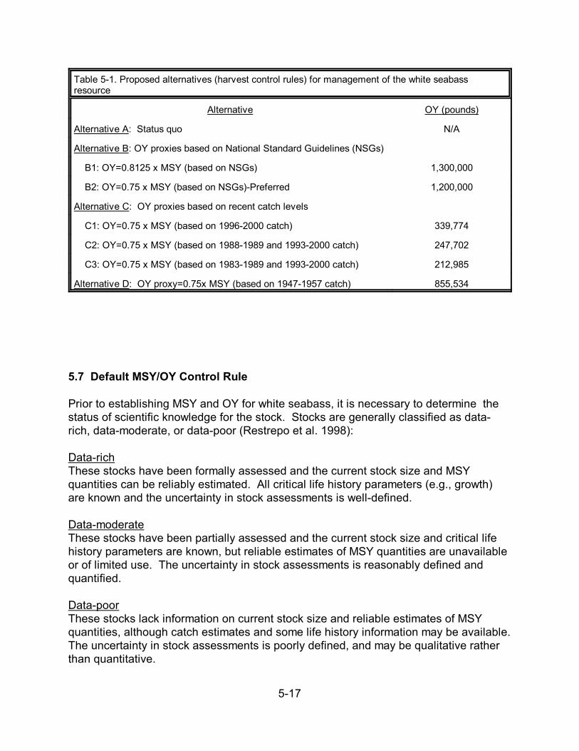
5-17
Table 5-1. Proposed alternatives (harvest control rules) for management of the white seabassresource
Alternative OY (pounds)
Alternative A: Status quo N/A
Alternative B: OY proxies based on National Standard Guidelines (NSGs)
B1: OY=0.8125 x MSY (based on NSGs) 1,300,000
B2: OY=0.75 x MSY (based on NSGs)-Preferred 1,200,000
Alternative C: OY proxies based on recent catch levels
C1: OY=0.75 x MSY (based on 1996-2000 catch) 339,774
C2: OY=0.75 x MSY (based on 1988-1989 and 1993-2000 catch) 247,702
C3: OY=0.75 x MSY (based on 1983-1989 and 1993-2000 catch) 212,985
Alternative D: OY proxy=0.75x MSY (based on 1947-1957 catch) 855,534
5.7 Default MSY/OY Control Rule
Prior to establishing MSY and OY for white seabass, it is necessary to determine thestatus of scientific knowledge for the stock. Stocks are generally classified as data-rich, data-moderate, or data-poor (Restrepo et al. 1998): Data-richThese stocks have been formally assessed and the current stock size and MSYquantities can be reliably estimated. All critical life history parameters (e.g., growth)are known and the uncertainty in stock assessments is well-defined.
Data-moderateThese stocks have been partially assessed and the current stock size and critical lifehistory parameters are known, but reliable estimates of MSY quantities are unavailableor of limited use. The uncertainty in stock assessments is reasonably defined andquantified.
Data-poor These stocks lack information on current stock size and reliable estimates of MSYquantities, although catch estimates and some life history information may be available. The uncertainty in stock assessments is poorly defined, and may be qualitative ratherthan quantitative.
5-18
White seabass stocks are currently data-poor.
In data-rich situations a stock-specific MSY fishing rate is employed if available, anddownward adjustments are made for OY. A default MSY/OY control rule (Restrepo et al. 1998) is shown in Figure 5-1. The upper limit on fishing mortality or Maximum Fishing Mortality Threshold (MFMT) equals Fmsy at higher stock sizes and is reducedproportionately as stock sizes fall slightly below biomass levels associated with MSY(Bmsy). This facilitates rebuilding of the fishery when stock sizes decrease. As aprecautionary measure, the OY target is adjusted downward and equals 0.75 x Fmsy. IfFoy is exceeded, overfishing is occurring. If the stock falls below the Minimum StockSize Threshold (MSST), then the stock is considered overfished. The MSST isconstrained to be greater than 50% of Bmsy, however the precise location of MSSTrelative to Bmsy depends upon the life history characteristics of white seabass and thedynamics of the stock. As more data become available, the exact shape of the controlrule–how fishing mortality is adjusted as stock sizes increase or decrease–may bechanged.
An overfished or depressed stock is defined as a stock that falls below the threshold of50% Bmsy or 25% Bunfished (i.e., the unfished or pristine biomass). For stocks belowtheir overfished/rebuilding threshold, an interim rebuilding adjustment would be madeto OY until a rebuilding plan is developed. Rebuilding times may be influenced bymany factors, including the degree to which a stock has declined, the inherentproductivity of the stock, and the mean generation time for the stock. In general,rebuilding plans allow for recovery to Bmsy or its proxy in 10 years or less. In caseswhere that is not possible due to the biological characteristics of the stock, theallowable time is one generation plus the length of time to recover in the absence offishing.
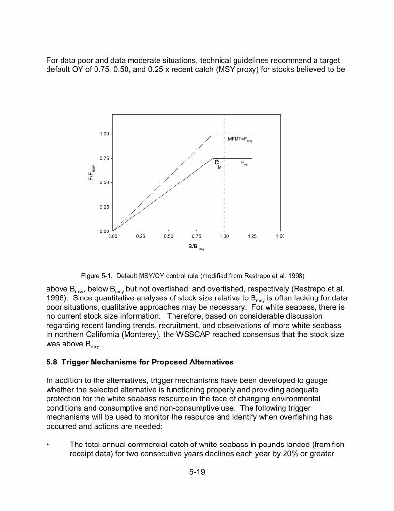
5-19
B/Bmsy
0.00 0.25 0.50 0.75 1.00 1.25 1.50
F/F m
sy
0.00
0.25
0.50
0.75
1.00MFMT=Fmsy
FoyM
ÈÈ
ÈÈ ÈÈ
Figure 5-1. Default MSY/OY control rule (modified from Restrepo et al. 1998)
For data poor and data moderate situations, technical guidelines recommend a targetdefault OY of 0.75, 0.50, and 0.25 x recent catch (MSY proxy) for stocks believed to be
above Bmsy, below Bmsy but not overfished, and overfished, respectively (Restrepo et al.1998). Since quantitative analyses of stock size relative to Bmsy is often lacking for datapoor situations, qualitative approaches may be necessary. For white seabass, there isno current stock size information. Therefore, based on considerable discussionregarding recent landing trends, recruitment, and observations of more white seabassin northern California (Monterey), the WSSCAP reached consensus that the stock sizewas above Bmsy.
5.8 Trigger Mechanisms for Proposed Alternatives
In addition to the alternatives, trigger mechanisms have been developed to gaugewhether the selected alternative is functioning properly and providing adequateprotection for the white seabass resource in the face of changing environmentalconditions and consumptive and non-consumptive use. The following triggermechanisms will be used to monitor the resource and identify when overfishing hasoccurred and actions are needed:
• The total annual commercial catch of white seabass in pounds landed (from fishreceipt data) for two consecutive years declines each year by 20% or greater
5-20
from the prior five-year average of landings;
• A 20% decline occurs in the number of fish and average size of fish (roundweight) for the same two consecutive years for white seabass caught in therecreational fishery as determined from the best available data;
• Recruitment of juvenile white seabass declines each year by 30% or greaterfrom the prior five-year average of recruitment as determined from the bestavailable data.
Overfishing of the white seabass resource occurres when any one of these conditionsare met. If all three of the trigger mechanisms occur, then the white seabass stock isoverfished. Evaluation of recreational and commercial take since 1952 indicates thatthe first two criteria were met eight and nine times, respectively. However, all criteriaoccurred in both fisheries during the same time period only twice (1960-1969). Thisindicates that these trigger mechanisms could be sensitive to identifying overfishing,but would not necessarily trigger an overfished condition. The average weight portionof the second and third criteria were not evaluated since there were too few data.
The Department’s WSMT and the WSSCAP will further investigate situations leading tothe occurrence of any trigger mechanisms, and recommend management measures tothe Commission if needed.
5.9 Annual Review of Management Measures
The Commission will review the WSFMP annually. The review will include the mostrecent fishery-dependent data (e.g., commercial and recreational landings, lengthfrequencies), any fishery-independent data (e.g., recruitment surveys) as well as dataon changes that may have occurred within the social and economic structure of therecreational and commercial industries that utilize the white seabass resource withinCalifornia. Included in this review will also be information about the harvest of whiteseabass in Mexico, if available, and any other pertinent data. This will permit a reviewof the proxies for MSY and OY that the Commission may adopt. These reviews will becarried out so that any recommendations or amendments to the WSFMP can bereviewed by the Commission and the public in accordance with the requirements of theMLMA.
5.10 Reporting and Record Keeping Requirements
Catch, effort, biological, and other data necessary for implementation of the WSFMPwill continue to be collected by California under existing data collection provisions. Ifthe Commission finds that additional data are needed, it will consult with the WSMTand the WSSCAP to determine the best method for addressing their needs. Theimplementation of additional reporting requirements will be done in accordance with theannual review process, and following the FMP framework and public input processes

5-21
as described earlier.
6-1
Chapter 6. Analysis of Proposed Management Alternatives
Several proposed management alternatives for the white seabass fishery, along with aframework approach to management, were described in the previous chapter. As perCEQA guidelines and the MLMA, the effects of these alternatives on target and non-target species, the environment, and the socioeconomics of the fishery are evaluated inthis chapter.
6.1 Alternative A - Status Quo
6.1.1 Effects on White Seabass
This alternative would continue existing white seabass regulations. The managementof white seabass over the years has been complex, consisting of several differentrestrictions on commercial and recreational fisheries (see Section 4.2). Unlike earlieryears, a number of recent laws and regulations pertaining to white seabass haveresulted in reductions of commercial fishing effort and the take of sub-legal fish byrecreational anglers. These regulations in combination with favorable oceanographicconditions and the recovery of several prey populations have probably contributed toincreases in the white seabass stock. Currently, the white seabass resource appearsto be recovering based on catch trends seen in the recreational and commercialfisheries as well as other factors (Section 2.10). The continued abundance of preyitems such as sardines and squid, and the cessation of the El Niño/SouthernOscillation, should contribute to a stable ecosystem for white seabass along theCalifornia coast.
The selection of the status quo alternative, along with a framework approach tomanagement, would meet some of the objectives of the WSFMP and MLMA. Under theFMP framework, management of the white seabass resource avoids being splitbetween the Legislature and the Commission, which often resulted in allocation of theresource at the expense of the different fishery participants. This in turn lead toanimosity and conflict between various user groups. In addition, frameworkmanagement gives the Commission a strict set of procedures and management tools touse as needs arise. This will enable the Commission to act decisively and in a timelymanner in response to changing biological, oceanographic, and socioeconomicconditions affecting the resource.
Another advantage of implementing this alternative is that short-term economic impactsare unlikely. However, if overfishing and collapse of the fishery occur, long-termimpacts would be substantial.
The main disadvantage of this alternative is that is does not meet one of the principleobjectives of developing a sustainable fishery. To adequately accomplish thisobjective, it is important to identify the level at which a population can be maintainedwhile experiencing removals of a portion of the stock through natural and fishing

6-2
mortality. Without identifying this level, resource managers will not have a startingpoint from which to gauge whether or not fluctuations in catch and abundance indicesare of serious concern. Implementation of this alternative involves considerableuncertainty and risk since a harvest limit is not in place to prevent overfishing (seeSection 6.5).
Wide fluctuations in the take of white seabass by commercial and recreational fisherieshave occurred since the fishery began. Fishery landings appear cyclic in which a fewyears of high catches are followed by many years of much lower catches, and thencatches return to high levels. Environmental changes and regulations are partlyresponsible for these fluctuations, but the magnitude of their effects on the whiteseabass stock are unknown. The cyclic nature of the fishery, without upper harvestlimits in place, could put the white seabass resource at considerable risk since high take of white seabass followed by poor recruitment could lead to collapse of the fisheryand a very long time for recovery, despite the return of favorable conditions.
This alternative also does not use the best available information to manage the fishery. Although it is acknowledged that there are gaps in our knowledge of white seabass,enough data exist to develop an estimate of population size which can be used as astarting point for further evaluation and refinement through monitoring and research(see Chapter 7).
6.1.2 Effects on Non-Target Species
The white seabass recreational and commercial fisheries, like most other fisheries,have some bycatch, which is either kept or returned to the marine environment. Inlarge part, gear designs used by fishermen help to lessen the take of non-targetedspecies. Choices such as hook design and size, bait types, mesh sizes, and how andwhere these gears are used help to minimize the risk of catching juvenile or undersizedfish as well as non-targeted species.
Much of the data on bycatch in the white seabass commercial fishery comes from aDepartment study in the 1980s and observations made by NMFS in the 1990s. TheDepartment conducted an onboard observer program that covered the nearshore whiteseabass gill net fishery from 1983-1989 (Vojkovich et al. 1990). During this period, 818sets of gill nets were observed on 250 days (approximately 3% coverage of the totallogged fishing activity). As previously mentioned, the NMFS observer program doesnot cover the white seabass gill net fishery. However, some white seabass sets wereobserved incidentally on vessels primarily targeting halibut in the set net fishery insouthern and central California. In southern California, a total of 521 sets wasobserved from 1990-1993 (Caretta pers. comm.). White seabass was the primarytarget of these sets, but a small fraction also targeted leopard sharks. In centralCalifornia, a total of 52 sets targeting white seabass and soupfin shark was observedfrom 1990-1994 and 1999-2000 (Forney pers. comm.). The results of these studies arepresented below (Sections 6.1.2.1 through 6.1.2.5). It should be noted, however, that
6-3
implementation of Proposition 132 in 1994 has moved the white seabass gill net fisheryfarther from shore, so the composition of incidentally-taken species may be differentfrom these studies.
6.1.2.1 Effects on Non-Target Finfish
Recreational fishery interactionsRecreational fishermen targeting white seabass catch undersized white seabass andother finfish. The MRFSS data shows that anglers targeting white seabass commonlyreturned undersized white seabass, barred sand bass (Paralabrax nebulifer), kelp bass(P. clathratus), California halibut (Paralichthys californicus), California barracuda(Sphyraena argentea), bat rays (Myliobatis californica), shovelnose guitarfish(Rhinobatos productos), Pacific mackerel (Scomber japonicus), soupfin shark(Galeorhinus zyopterus), and other species of sharks. In addition to these species,sargo (Anisotremus davidsonii), yellowfin croaker (Umbrina roncador), and yellowtail(Seriola lalandi) are caught aboard CPFV’s while fishing for white seabass (Conroypers. comm.).
From 1993 to the present, an average of 66,000 white seabass were released afterbeing caught. Unfortunately information is not available on the condition of thereleased white seabass, most of which are under the 28 inch (711 mm) size limit. Anecdotal information from recreational fishermen suggests that there are high levelsof mortality due to damaged air bladders. Preliminary data suggest that hookingmortality of juvenile fish is around 10%, which is similar to the levels reported for reddrum on the Atlantic coast (Crooke pers. comm.). Further investigation is needed todetermine whether this type of interaction could affect the resource (see Chapter 7).
Finfish species, such as Pacific sardine, are occasionally used as bait for whiteseabass. However, the preferred bait is live squid, and impacts on finfish used as baitare not considered significant.
Commercial fishery interactionsA total of 85 finfish species, mostly those associated with kelp beds, were taken in thewhite seabass gill net fishery during the Department’s onboard observer study. Themost common species caught were Pacific sardine (Sardinops sagax), spiny dogfish(Squalus acanthius), Pacific mackerel, swell shark (Cephaloscyllium ventriosum), andwhite seabass (Table 6-1; Vojkovich et al. 1990). Fifty-two percent of the incidentalspecies were released dead, 29% were kept for personal use or sale, and 19% werereleased alive. Over 75% of the incidentally-taken fish released alive were sharkspecies while the discarded dead species consisted of Pacific sardine (60%),miscellaneous fish (22%), spiny dogfish (15%), and white seabass (3%).
Examination of current landing receipt data show that incidental species reported in thewhite seabass gill net fishery include Pacific mackerel, Pacific bonito (Sarda chiliensis),California barracuda, California halibut and other flatfish (Plueronectidae and Bothidae
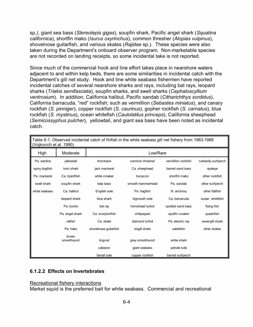
6-4
sp.), giant sea bass (Stereolepis gigas), soupfin shark, Pacific angel shark (Squatinacalifornica), shortfin mako (Isurus oxyrinchus), common thresher (Alopias vulpinus),shovelnose guitarfish, and various skates (Rajidae sp.). These species were alsotaken during the Department’s onboard observer program. Non-marketable speciesare not recorded on landing receipts, so some incidental take is not reported.
Since much of the commercial hook and line effort takes place in nearshore watersadjacent to and within kelp beds, there are some similarities in incidental catch with theDepartment’s gill net study. Hook and line white seabass fishermen have reportedincidental catches of several nearshore sharks and rays, including bat rays, leopardsharks (Triakis semifasciata), soupfin sharks, and swell sharks (Cephaloscylliumventrosium). In addition, California halibut, Pacific sandab (Citharichthys sordidus),California barracuda, “red” rockfish; such as vermillion (Sebastes miniatus), and canaryrockfish (S. pinniger), copper rockfish (S. caurinus), gopher rockfish (S. carnatus), bluerockfish (S. mystinus), ocean whitefish (Caulolatilus princeps), California sheephead(Semicossyphus pulcher), yellowtail, and giant sea bass have been noted as incidentalcatch.
Table 6-1. Observed incidental catch of finfish in the white seabass gill net fishery from 1983-1989(Vojkovich et al. 1990)
High Moderate Low/Rare
Pa. sardine yellowtail thornback common thresher vermillion rockfish rubberlip surfperch
spiny dogfish horn shark jack mackerel Ca. sheephead barred sand bass opaleye
Pa. mackerel Ca. lizardfish white croaker bocaccio shortfin mako other rockfish
swell shark soupfin shark kelp bass smooth hammerhead Pa. sandab other surfperch
white seabass Ca. halibut English sole Pa. hagfish N. anchovy other flatfish
leopard shark blue shark bigmouth sole Ca. barracuda ocean whitefish
Pa. bonito bat ray hornyhead turbot spotted sand bass flying fish
Pa. angel shark Ca. scorpionfish chilipepper spotfin croaker queenfish
ratfish Ca. skate diamond turbot Pa. electric ray sevengill shark
Pa. hake shovelnose guitarfish sixgill shark sablefish other skates
brownsmoothound lingcod grey smoothound white shark
cabezon giant seabass petrale sole
fantail sole copper rockfish barred surfperch
6.1.2.2 Effects on Invertebrates
Recreational fishery interactionsMarket squid is the preferred bait for white seabass. Commercial and recreational

6-5
white seabass fishermen obtain their squid either by purchasing it from a live baitretailer (i.e., bait receiver or barge) or by capturing squid on their own. There is no wayat this time to quantify how much squid is purchased as live bait or taken by anindividual for personal use. Currently, there are approximately 12 live bait vesselsoperating in California that seasonally fish for squid, anchovy, sardine, and mackerel. The amount of squid taken by live bait boats and by individual fishermen is likely to beinsignificant in comparison to the commercial squid fishery for human consumption,which employs over 100 vessels and has a five-year average of 71,000 tons (63,000metric tons) annually.
Commercial fishery interactionsA total of 1,331 invertebrates were taken in the white seabass gill net fishery during theDepartment’s onboard observer study (Table 6-2; Vojkovich et al. 1990). Sixty-ninepercent of the observed invertebrate catch consisted of crab species; over 50% of thiscatch consisted of spider crab (Loxorhynchus sp.), rock crab (Cancer sp.), and boxcrab (Lopholithodes sp.). The remainder consisted of various mollusks and othercrustaceans. About 45% of invertebrates were returned dead, 39% were returnedalive, and 15% were kept or sold.
Table 6-2. Observed incidental catch of invertebrates in the white seabass gill net fisheryfrom 1983-1989 (Vojkovich et al. 1990)
Species Total number Number kept/sold Returned alive Returned deadcrab, box 189 28 39 122crab, decorator 9 0 5 4crab, hermit 2 0 2 0crab, kelp 51 5 29 17crab, marble 3 0 1 2crab, pelagic red 5 0 1 4crab, pointer 92 21 8 63crab, rock 262 108 71 83crab, sand 1 1 0 0crab, spider 303 25 102 176lobster, Ca. spiny 116 3 110 3sea cucumber 94 0 69 26sea star 35 2 31 3sea urchin 53 5 33 15shrimp 3 1 1 1mollusk 2 0 0 2snail 5 0 4 1sea hare 3 0 3 0octopus 3 0 3 0squid, market 1 0 1 0whelk 16 0 16 0unspecified 81 0 1 80TOTAL 1337 199 527 602
6-6
6.1.2.3 Effects on Seabirds
A number of marine bird species, including brown pelicans (Pelecanus occidentaliscalifornicus), various tern species (Sterna spp.), cormorants (Phalacorcorax spp.), andbald eagles (Haliaeetus leucocephalus) occur in areas where white seabass fishingactivities take place. Some of these species, such as the brown pelican and baldeagle, are federally protected.
The brown pelican, an endangered marine bird, may be indirectly affected by marinefishing activities (e.g., motor noise, boat whistles, etc.) near known rookeries. In orderto prevent potential disturbances to the endangered brown pelican rookery andfledgling area at Anacapa Island, Ventura County, the Commission established afishing closure within the boundary of Anacapa Island Ecological Reserve. The closureis from 01 January to 31 October each year, and encompasses an area 4,000 feet(1,219 m) long on the north side of west Anacapa Island, and extends offshore to adepth of approximately 120 feet (37 m).
The California least tern (Sterna albifrons), an endangered species, nests on a fewbeaches bordering the southern California coast and feeds on small live fish. Interactions between least terns and fishing activities are unlikely, since this speciestypically feeds in shallow water areas. However, other tern species are known tobecome entangled in fishing line after getting hooked while going after an angler’s bait. Fishermen normally release the hooked tern by cutting the line. When hooked ternsreturn to their nesting area, they can become entangled when the trailing fishing linesnags on debris. In an attempt to free itself, a bird may thrash itself to death, and itmay entangle other terns in the colony. Between the months of April and August,several species of terns breed at the Bolsa Chica Ecological Reserve (BCER) inHuntington Beach. In addition to a large (up to 2,000 pairs) colony of elegant terns (S.elegans), caspian terns (S. caspia), forster’s terns (S. forsteri) and black skimmers(Rynchops niger), also nest at BCER (Collins pers. comm.; O’Reilly, pers. comm.). Annually, approximately 10 dead terns are found entangled in fishing line at the BCERseabird colony. Since terns feed primarily on small bait fish such as northern anchovy(Engraulis mordax), it is unlikely that interactions would occur with hook and linefishermen targeting while seabass because squid is the primary bait used.
Another protected bird found seasonally along the coast and the islands of California isthe bald eagle (Haliaeetus leucocephalus). A recovery plan is currently in place thatestablishes geographical goals for population enhancement. More than 30 eagleshave been released at Santa Catalina Island and some live on the mainland near SantaBarbara County. The eagles feed on live fish in the waters surrounding their habitat, sofishery interactions may be possible but are considered unlikely.
Recreational fishery interactionsBecause of the fishing techniques employed in the white seabass recreational fishery,it is highly unlikely that there would be any interactions with surface foraging seabirds.
6-7
Baited fishing lines are weighted so they sink rapidly underwater where they areunavailable to birds such as the brown pelican, least tern, and bald eagle. However,these marine birds and cormorants often have interactions with anglers who fish forother species on the surface. The interactions take place when live bait (usuallyanchovy or sardine) is used as chum or for bait. When the bird goes after the bait, itcan become caught on the hook or entangled in the fishing line. In most instances thebird is freed. No data exists to quantify these interactions, but the effect on the totalpopulation is not considered significant.
Commercial fishery interactionsGill nets can capture surface foragers (e.g., gulls) as well as diving birds such as ternsand cormorants. Seabird bycatch has been a problem in the nearshore gill netfisheries of central California, particularly for the marbled murrelet (Brachyramphusmarmoratus), a threatened species, and the common murre (Uria aalge). The marbledmurrelet is rare in southern California, and none have been reported killed in the gillnet fisheries of this region (USFWS 1997). Therefore, the white seabass gill net fisheryis not likely to impact this species since the majority of fishing occurs south of PointConception. Common murres are winter visitors to southern California, so interactionsare possible, but unlikely since the highest level of fishing effort occurs during thesummer months. Eighty-two percent of white seabass landings using gill nets from1995-2000 occurred from June through July, while only 11% of landings occurred fromNovember through February.
During the Department’s onboard observer study, a total of ten cormorants(Phalacrocorax sp.) died as a result of gear interactions. No other bird speciessuffered injuries or died. During the NMFS observer program, 14 cormorants died inthe white seabass gill net fishery in southern California while 20 common murres wereentangled in gill nets in central California.
Set longlines could potentially catch surface feeding birds if birds attempted to take thebait on the line, and be pulled under the water and drown. However, a commercialwhite seabass longliner reported having no seabird interactions (Athens pers. comm.). As in the sport fishery, commercial hook and line (other than longline) fishinginteractions are unlikely, due to the techniques employed. However, current data arenot available on seabird mortalities in the white seabass hook and line commercialfishery.
6.1.2.4 Effects on Marine Mammals
Interactions are possible with a number of marine mammal species, including Californiasea lions (Zalophus californianus), harbor seals (Phoca vitulina), northern elephantseals (Mirounga angustirostris), common dolphins (Delphinus delphis), and Californiagray whales (Eschrichtius robustus) since fishing for white seabass takes placeprimarily throughout the Southern California Bight (south of Point Conception). Allmarine mammals, especially threatened and endangered species, are fully protected by
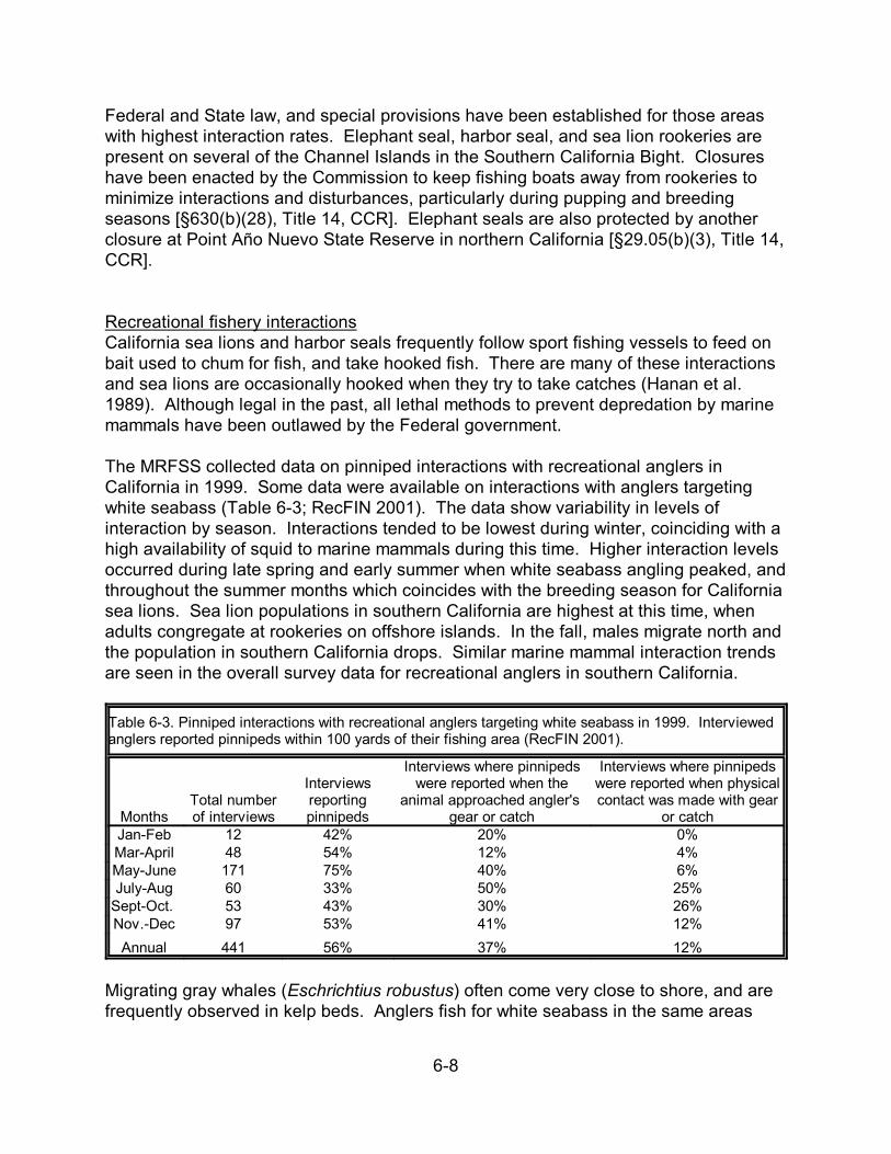
6-8
Federal and State law, and special provisions have been established for those areaswith highest interaction rates. Elephant seal, harbor seal, and sea lion rookeries arepresent on several of the Channel Islands in the Southern California Bight. Closureshave been enacted by the Commission to keep fishing boats away from rookeries tominimize interactions and disturbances, particularly during pupping and breedingseasons [§630(b)(28), Title 14, CCR]. Elephant seals are also protected by anotherclosure at Point Año Nuevo State Reserve in northern California [§29.05(b)(3), Title 14,CCR].
Recreational fishery interactionsCalifornia sea lions and harbor seals frequently follow sport fishing vessels to feed onbait used to chum for fish, and take hooked fish. There are many of these interactionsand sea lions are occasionally hooked when they try to take catches (Hanan et al.1989). Although legal in the past, all lethal methods to prevent depredation by marinemammals have been outlawed by the Federal government.
The MRFSS collected data on pinniped interactions with recreational anglers inCalifornia in 1999. Some data were available on interactions with anglers targetingwhite seabass (Table 6-3; RecFIN 2001). The data show variability in levels ofinteraction by season. Interactions tended to be lowest during winter, coinciding with ahigh availability of squid to marine mammals during this time. Higher interaction levelsoccurred during late spring and early summer when white seabass angling peaked, andthroughout the summer months which coincides with the breeding season for Californiasea lions. Sea lion populations in southern California are highest at this time, whenadults congregate at rookeries on offshore islands. In the fall, males migrate north andthe population in southern California drops. Similar marine mammal interaction trendsare seen in the overall survey data for recreational anglers in southern California.
Table 6-3. Pinniped interactions with recreational anglers targeting white seabass in 1999. Interviewedanglers reported pinnipeds within 100 yards of their fishing area (RecFIN 2001).
MonthsTotal numberof interviews
Interviewsreportingpinnipeds
Interviews where pinnipedswere reported when the
animal approached angler's gear or catch
Interviews where pinnipedswere reported when physicalcontact was made with gear
or catchJan-Feb 12 42% 20% 0%Mar-April 48 54% 12% 4%May-June 171 75% 40% 6%July-Aug 60 33% 50% 25%
Sept-Oct. 53 43% 30% 26%Nov.-Dec 97 53% 41% 12%Annual 441 56% 37% 12%
Migrating gray whales (Eschrichtius robustus) often come very close to shore, and arefrequently observed in kelp beds. Anglers fish for white seabass in the same areas

6-9
during the early spring months. Although gray whales do not eat fish, they could beaffected by the presence of recreational anglers. However, because the number ofgray whales in an area at any one time is very small, the impact of recreational fishingfor white seabass on these animals is probably not significant.
Commercial fishery interactionsThe National Marine Fisheries Service (NMFS) considers the white seabass gill netfishery to be a Category I fishery, which is defined as a fishery in which it is highly likelythat one marine mammal will be taken by a randomly selected vessel during a 20-dayperiod. Currently, neither the Department nor NMFS has a marine mammal observerprogram for the white seabass gill net fishery. However, incidents of marine mammaldeaths and injuries resulting from commercial fishing activities are reported byfishermen through the Marine Mammal Authorization Program (MMAP). Data on whiteseabass gill net interactions collected from this reporting system are combined withdata on other gill net fisheries (angel shark, halibut, barracuda, leopard shark, perchand white croaker, rockfish, yellowtail, soupfin shark, and various other sharksexcluding the swordfish/thresher shark fishery).
Reported marine mammal interactions for all of these fisheries combined consisted ofone common dolphin; ten California sea lions and two harbor seals in 1996; threecommon dolphins and four California sea lions in 1997; and two common dolphins andtwo California sea lions in 1998. It is not clear how many of these interactions, if any,occurred in the white seabass gill net fishery because MMAP data is collected inaggregate for these fisheries. Marine mammal interactions are believed to be under-reported to the MMAP (Forney 2000).
During the Department’s onboard observer study, six common dolphins, one Pacificwhite sided dolphin, and seven California sea lions died as a result of gear interaction. During the NMFS observer program, four California sea lions became entangled inwhite seabass gill nets in southern California while one harbor porpoise and two harborseals were entangled in gill nets in central California.
Other marine mammals can become entangled in active gill net or surface longlinefishing gear, and in fragments of gill net or monofilament line that have been lost ordiscarded. From 1990 through 1998, 37 gray whales were reported entangled invarious fishing gears off the coast of California (Hill 1999). However, theentanglements could have occurred anywhere along the gray whale’s migration route,which extends from Alaska to Baja California, Mexico. No gray whales have beenobserved entangled in active white seabass gill net gear.
No data are currently available on commercial white seabass hook and line interactionswith marine mammals. Interactions with rod and reel are probably similar to those inthe recreational fishery. Longlines employed in this fishery are set on the bottom, andare not likely to hook marine mammals swimming through the water column. A whiteseabass longliner reported having no marine mammal entanglements while fishing
6-10
(Athens pers. comm.).
6.1.2.5 Effects on Marine Turtles
Marine sea turtles, though uncommon, occur in California waters. Four species offederally protected sea turtles are found in California waters: green (Chelonia mydas),leatherback (Dermochelys coriacea), loggerhead (Caretta caretta), and olive ridley seaturtles (Lepidochelys olivacea). Stranding records indicate that the leatherback seaturtle is the most common in our waters. A relatively high level of leatherback sightingsoccurs off the Monterey area, peaking in August. Green sea turtles are thought to bethe second most abundant species off California. A resident population of 50-60 adultslives in San Diego Bay, congregating in the warm water effluents of the local powerplant. Loggerhead sea turtle sightings typically peak from July through September inthe eastern Pacific. Olive Ridley sea turtles are highly pelagic and very rarely found offthe California coast. Recreational fishery interactionsInteractions of recreational hook and line fishing with sea turtles are possible, althoughhighly unlikely. An MRFSS sampler observed a sea turtle become entangled in gearfrom a CPFV off Santa Catalina Island; the turtle was released unharmed (Horeczkopers. comm.). Sea turtles, however, are vulnerable to boat collisions. The NMFSRecovery Plan for the Eastern Pacific green sea turtle states that 80% of recent greensea turtle deaths in San Diego Bay and Mission Bay were associated with boatcollisions.
Commercial fishery interactionsObserver programs conducted by NMFS (1990-2000) have documented all fourspecies interacting with various commercial fishing gears including the halibut andangel shark set net fishery, the shark/swordfish drift gill net fishery, and the high seaslongline fishery (NMFS 2000). The observed take for the halibut/angel shark fisherywas five sea turtles from 1990-1994, with observer coverage ranging from 0% to15.4%; four of these mortalities occurred off Ventura.
During the Department’s onboard observer study, there were no sea turtle interactionswith white seabass gill nets. The lack of interactions, in part, may be due to thedifferences in mesh size that exist between the white seabass fishery (6 to 7.5 inches)and the halibut (8.5 inches) and shark/swordfish (14 inches) fisheries. During theNMFS observer program, no sea turtle entanglements were observed in white seabassgill nets in southern California.
Marine turtles may be vulnerable to ingestion of marine debris. One adult green seaturtle was recently found dead in San Diego Bay with monofilament netting tightlypacked in its esophagus.
6.1.2.6 Ecological interactions
6-11
Most of this document has focused on the direct effects of fishing activities on whiteseabass and other species. However, the removal of white seabass through fishingactivities may also have indirect effects on the ecosystem. Unfortunately, ourknowledge of white seabass and their relationships with other species in the ecosystemis limited.
White seabass are known to prey on squid, sardines, and other pelagic species, and inturn, are eaten by other fish and sea lions. However, it is not known how increasedcatches of white seabass would effect this food chain. There may also be competitionbetween white seabass and other species since they are often caught with othermigratory species, such as bonito and yellowtail, that have similar food habits. Again,we do not know the extent of these interactions and how the removal of white seabassfrom the ecosystem would affect this.
6.1.3 Habitat Impacts
6.1.3.1 Effects of Consumptive Use on Environment
Fishermen engaged in the take of white seabass may dispose of trash and other itemswhile fishing. Evidence suggests that marine vessels and fishing activity are a primarysource for anthropogenic debris in the Southern California Bight (Moore 1998). Lostgill nets can continue to capture marine animals. Lost or discarded monofilamentfishing line can cause death or injury to marine animals if they become entangled (High1984). Marine debris such as plastics and styrofoam can also cause death or injury toanimals in the marine environment when it is ingested or entangles an animal (NOAA1998).
Fishermen often target white seabass in and around kelp habitat. Boat traffic throughkelp beds can damage or cut loose kelp fronds. However, this has no lasting effect onthe kelp beds as a whole (Feder 1974). Giant kelp (Macrocystis spp.) comprises thebulk of the kelp beds in southern California, although forests of Elk kelp are present offSan Diego County. Giant kelp can grow as much as two feet (0.6 meters) per day, andapproximately 60,000 tons ( 54,432 metric tons) are commercially harvested each yearthroughout southern California. Due to the growth characteristics of giant kelp, theeffects on kelp beds by fishing vessels are considered insignificant.
6.1.3.2 Effects of Non-consumptive Use on Environment
Non-consumptive users, such as underwater photographers and animal watchers, canhave an impact on the environment. Divers entering the water from shore may trampleorganisms, or become entangled in kelp, causing temporary damage to kelp beds. Southern California intertidal populations susceptible to trampling include fleshyseaweeds, coralline algae, fragile tube-forming polychaetes, bivalves such as mussels,acorn barnacles, limpets, and grapsid crabs that seek refuge under loose rocks andseaweeds during low tide (Ghazanshahi 1983; Murray 1998).
6-12
The potential impacts and effects of scuba divers on white seabass habitats andbreeding behavior have not been studied. However, the sensitivity of white seabass tonoise suggests that scuba divers could cause some minor disturbances to their matingcycle. If a dive site is a potential spawning ground, and is used frequently by manydivers, a possibility exists that fish would abandon that site for a less disturbed location.
Non-consumptive users may also dispose of trash in the marine environment,contributing to the problem of anthropogenic debris.
6.1.4 Economic Implications
Economic effects are not expected to be significant under this alternative. If it becomesnecessary to modify current management measures, effects on the fishery-basedeconomies would be addressed under the WSFMP framework process, in accordancewith the MLMA.
6.1.5 Social Implications
Social effects are not expected to be significant under this alternative. If it becomesnecessary to modify current management measures, effects on the fishery-basedeconomies would be addressed under the WSFMP framework process, in accordancewith the MLMA.
6.2 Alternative B - OY Proxies Based on National Standard Guidelines
6.2.1 Effects on White Seabass
This alternative estimates the white seabass population based on information about thevirgin biomass (spawning stock) and estimates of natural mortality to obtain a proxy forMSY. An OY was obtained by multiplying MSY by 0.8125 (alternative B1) or 0.75(alternative B2) as a precautionary adjustment (see Section 5.6.2).
The establishment of an OY through this alternative, along with the frameworkmanagement approach, meets one of the principle objectives of developing asustainable fishery. The OY places an upper harvest limit on the total take of whiteseabass to prevent overfishing while the framework management allows for regulationsto be put in place quickly if harvest levels exceed OY. In addition, frameworkmanagement can adjust OY or other control rule parameters, if needed, as morebiological and socioeconomic data become available. This alternative would allowcontinued recovery of white seabass while important data were collected to yield abetter defined MSY/OY control rule.
Unlike alternative A, this alternative provides a good starting point for sustainablefisheries management. However, as noted earlier due to data limitations (see Section
6-13
5.6), alternatives B, C, an D only address the upper harvest limit. Because of this, it isstrongly recommended that the default control rule (Section 5.7) accompany all of thesealternatives. An MSY/OY approach to management should be considered an interimsolution when knowledge of a stock is data-poor, as is the case with white seabass. Therefore, this accentuates the need to do a stock assessment and develop a specificMSY/OY control rule for white seabass (see Section 7.4.1).
The MSY proxy of 1.6 million pounds for this alternative is very similar to sustainedcatch levels seen from the 1940s through the 1960s (with the exception of 1958-1959(Table 3-1). This MSY proxy is almost identical to an MSY estimate produced in thelone stock assessment done for white seabass. For that assessment, MacCall et al.(1976) used catch-per-unit-effort (CPUE) data from United States-based commercialand recreational catches and calculated an MSY for white seabass of 1.65 million pounds. The similarity of the two MSY estimates calculated by different methodssuggests that the MSY proxy has some value.
This alternative assumes that the existing biomass is close to or similar to pristinelevels. This may not be the case and might lead to overfishing and cause the resourceto become overfished. If this is allowed to continue for too long, the fishery couldcollapse. Implementation of this alternative involves some uncertainty and risk (seeSection 6.5).
This alternative assumes that natural mortality approximates fishing mortality, which ismost likely not the case based on recent catch trends. Another factor to consider isthat there appears to be a shift in the catch and effort of the white seabass resourcefrom the commercial to the recreational fishery. This may be important due to the largenumber of white seabass that are recreational-caught and released (see Section 3.6). Many of these fish may become injured or die, but the number of white seabass thatsuffer this fate is unknown and unaccounted for in estimating their total fishingmortality. In the red drum (Sciaenops ocellatus) fisheries, hooking mortality of releasedfish was important and managers considered this effect in their estimates of MSY(NCDMF 2000).
Alternatives B1 and B2 are similar, and differ only in the adjustments of MSY to yieldOY. Since there are many uncertainties in the calculation of an MSY for white seabassbased on our current knowledge, it is prudent to make precautionary adjustments.Technical guidelines (Restrepo et al. 1998) recommend that 75% of an MSY proxy indata-poor situations represent the upper harvest target, in the best of conditions (i.e.,the current stock size is above the biomass level associated with MSY). Although thereare several positive indicators that white seabass numbers are increasing, we feel it isprudent to adhere to the guidelines and be more conservative to help ensure thecontinued recovery of the white seabass resource. Therefore, we recommendalternative B2 over alternative B1.
6.2.2 Effects on Non-Target Species
6-14
6.2.2.1 Effects on Non-Target Finfish
Effects on non-target finfish are not expected to be significant and differ from effectsunder alternative A (see Section 6.1.2.1).
6.2.2.2 Effects on Invertebrates
Effects on invertebrates are not expected to be significant and differ from effects underalternative A (see Section 6.1.2.2).
6.2.2.3 Effects on Seabirds
Effects on seabirds are not expected to be significant and differ from effects underalternative A (see Section 6.1.2.3)
6.2.2.4 Effects on Marine Mammals
Effects on marine mammals are not expected to be significant and differ from effectsunder alternative A (see Section 6.1.2.4).
6.2.2.5 Effects on Marine Turtles
Effects on marine sea turtles are not expected to be significant and differ from effectsunder alternative A (see Section 6.1.2.5).
6.2.2.6 Ecological Interactions
Ecological interactions are largely unknown, but effects on them are not expected to besignificant and differ from effects under alternative A (see Section 6.1.2.6).
6.2.3 Habitat Impacts
6.2.3.1 Effects of Consumptive Use on Environment
Effects of consumptive use on the environment are not expected to be significant anddiffer from effects under alternative A (see Section 6.1.3.1).
6.2.3.2 Effects of Non-consumptive Use on Environment
Effects of non-consumptive use on the environment are not expected to be significantand differ from effects under alternative A (see Section 6.1.3.2).
6.2.4 Economic Implications
6-15
Effects on the fishery-based economy are not expected to be significant and differ fromeffects under alternative A (see Section 6.1.4). However, if harvest limits are reachedand fishing effort is reduced, there could be a negative impact.
6.2.5 Social Implications
Effects on the fishing community structure are not expected to be significant and differfrom effects under alternative A (see Section 6.1.5).
6.3 Alternative C - OY Proxies Based on Recent Catch Levels
6.3.1 Effects on White Seabass
Since our knowledge of white seabass stocks is data-poor, this alternative uses a proxyfor MSY based on recent catch, and adjusts it downward (multiplied by 0.75) as aprecautionary approach to get an OY (see Section 5.6.3).
This alternative and the framework management approach, like alternative B, addressone of the primary objectives of developing a sustainable fishery for white seabass bysetting an upper harvest limit. This is the most conservative of all the alternatives andwould impact the white seabass resource the least. This alternative, like alternative Bwould allow continued recovery of white seabass while important data were collected toyield a better defined MSY/OY control rule. Implementation of C1, C2, or C3 wouldhave some uncertainty, but the risk of overfishing the stock to an overfished conditionrelative to the other alternatives is by far the least (see Section 6.5).
One of the difficulties with selection of this alternative is choosing an appropriate timeperiod for the basis of MSY/OY. Indeed, the creation of three different time framesattests to this fact. Using recent catch for an MSY proxy has been suggested, with thestipulation that the time period be stable, especially showing no declines. Unfortunately, the white seabass commercial and recreational catches have been veryunstable, thus recent catch as a proxy for MSY may be unsuitable.
Implementation of C1, C2, or C3 would require the development of additionalregulations that would limit the take of seabass by each of the fishery componentswhen the upper harvest limit was reached within a particular fishing year. Types ofregulations or controls that could achieve this would be:
• Cessation of fishing when harvest target is reached;• Elimination of catch during the spawning season; • Elimination of fishing during the full moon phase in March, April, May and
June;• Increase of the size limit to 32 inches;• Reduction of the recreational bag limit; and any• Combinations of the above.
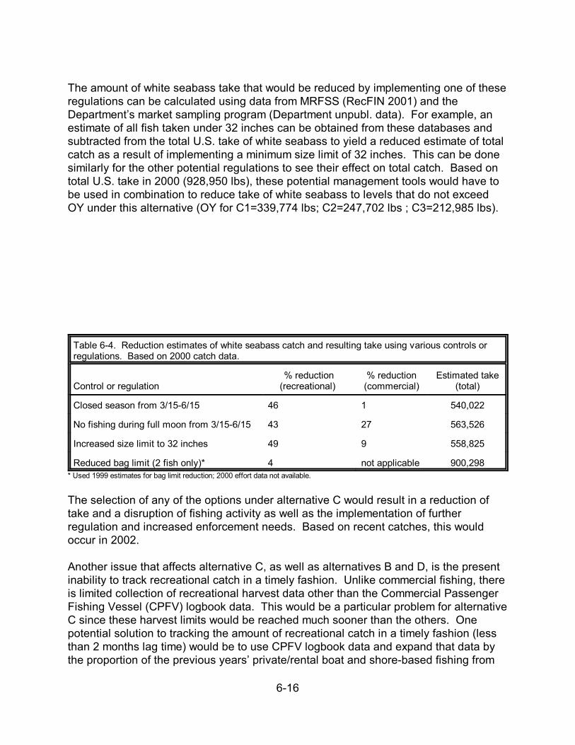
6-16
The amount of white seabass take that would be reduced by implementing one of theseregulations can be calculated using data from MRFSS (RecFIN 2001) and theDepartment’s market sampling program (Department unpubl. data). For example, anestimate of all fish taken under 32 inches can be obtained from these databases andsubtracted from the total U.S. take of white seabass to yield a reduced estimate of totalcatch as a result of implementing a minimum size limit of 32 inches. This can be donesimilarly for the other potential regulations to see their effect on total catch. Based ontotal U.S. take in 2000 (928,950 lbs), these potential management tools would have tobe used in combination to reduce take of white seabass to levels that do not exceedOY under this alternative (OY for C1=339,774 lbs; C2=247,702 lbs ; C3=212,985 lbs).
Table 6-4. Reduction estimates of white seabass catch and resulting take using various controls orregulations. Based on 2000 catch data.
Control or regulation% reduction
(recreational) % reduction
(commercial)Estimated take
(total)
Closed season from 3/15-6/15 46 1 540,022
No fishing during full moon from 3/15-6/15 43 27 563,526
Increased size limit to 32 inches 49 9 558,825
Reduced bag limit (2 fish only)* 4 not applicable 900,298* Used 1999 estimates for bag limit reduction; 2000 effort data not available.
The selection of any of the options under alternative C would result in a reduction oftake and a disruption of fishing activity as well as the implementation of furtherregulation and increased enforcement needs. Based on recent catches, this wouldoccur in 2002.
Another issue that affects alternative C, as well as alternatives B and D, is the presentinability to track recreational catch in a timely fashion. Unlike commercial fishing, thereis limited collection of recreational harvest data other than the Commercial PassengerFishing Vessel (CPFV) logbook data. This would be a particular problem for alternativeC since these harvest limits would be reached much sooner than the others. Onepotential solution to tracking the amount of recreational catch in a timely fashion (lessthan 2 months lag time) would be to use CPFV logbook data and expand that data bythe proportion of the previous years’ private/rental boat and shore-based fishing from
6-17
the MRFSS.
6.3.2 Effects on Non-Target Species
6.3.2.1 Effects on Non-Target Finfish
Effects on non-target finfish are not expected to be significant. Impacts (see Section6.1.2.1) may be greatly reduced if harvest limits are reached and fishing effort for whiteseabass decreases. However, a reduction in allowable take of white seabass as peralternatives C1, C2 , and C3 would probably cause fishing effort to shift to other finfishin the commercial and/or recreational fisheries.
6.3.2.2 Effects on Invertebrates
Effects on invertebrates are not expected to be significant. Impacts (see Section6.1.2.2) may be greatly reduced if harvest limits are reached and fishing effort for whiteseabass decreases.
6.3.2.3 Effects on Seabirds
Effects on seabirds are not expected to be significant. Impacts (see Section 6.1.2.3)may be greatly reduced if harvest limits are reached and fishing effort for white seabassdecreases.
6.3.2.4 Effects on Marine Mammals
Effects on marine mammals are not expected to be significant. Impacts (see Section6.1.2.4) may be greatly reduced if harvest limits are reached and fishing effort for whiteseabass decreases.
6.3.2.5 Effects on Marine Turtles
Effects on marine turtles are not expected to be significant. Impacts (see Section6.1.2.5) may be greatly reduced if harvest limits are reached and fishing effort for whiteseabass decreases.
6.3.2.6 Ecological Interactions
Ecological interactions are largely unknown, but effects on them are not expected to besignificant and differ from effects under alternative A (see Section 6.1.2.6).
6.3.3 Habitat Impacts
6.3.3.1 Effects of Consumptive Use on Environment
6-18
Effects of consumptive use on the environment are not expected to be significant. Impacts (see Section 6.1.2.3) may be greatly reduced if harvest limits are reached andfishing effort for white seabass decreases. However, a reduction in allowable take ofwhite seabass would probably cause fishing effort to shift to other species in thecommercial and/or recreational fisheries, producing an unknown effect.
6.3.3.2 Effects of Non-consumptive Use on Environment
Effects of non-consumptive use on the environment are not expected to be significant. Impacts (see Section 6.1.3.2) may increase if harvest limits result in greater availabilityof white seabass in the environment for photography and wildlife viewing. This couldresult in increased human pressure in white seabass habitat areas such as kelp bedsand rocky reefs.
6.3.4 Economic Implications
This alternative may have a significant impact on the fishery-based economy, affectingboth recreational and commercial industries. The proposed OY proxies under thisalternative would have varying degrees of impacts, ranging from the least disruptive(C1) to the most disruptive (C3). Under the guidelines of C1, no more than 339,774pounds (154,119 kg) could be harvested annually. This harvest level is 53% of theaverage annual harvest (646,459 lbs or 293,229 kg) for the years 1998-2000. UnderC3 an annual harvest limit of 212,985 (96,608 kg) would be set, which is 33% of the1998-2000 average annual harvest. These options could have a severe impact onrevenues generated by recreational and commercial fishing.
Commercial ex-vessel revenues closely parallel landings, so a significant decrease inlandings would be expected to have a severe impact on revenues for commercialfishermen targeting white seabass. Reductions of annual commercial harvests fromalternatives C1 and C3 could result in a loss of ex-vessel revenues ranging from$212,000 to $132,000, based on 2000 revenues. However, many of these fishermenalso participate in other fisheries, and could re-allocate their effort to target alternativespecies, offsetting this potential loss in income. Estimates of losses incurred to thecommercial fishing industry (fish markets, grocery stores, restaurants, etc.) as a wholehave not been estimated. Most fish businesses receiving white seabass are located insouthern California; primarily in Orange, Los Angeles, Ventura, and Santa Barbaracounties. Local economies in these counties would be hardest hit by revenue losses.
The extent of impact on the recreational fishery is difficult to predict, and is largelydependent on a recreational angler’s motivation for fishing. An angler who primarilytargets white seabass may not reduce his fishing effort altogether, but may decide totarget another species such as yellowtail or kelp bass if white seabass fishing wasreduced to meet annual harvest levels. According to the MRFSS estimates, whiteseabass were named as the target species for less than 1% to nearly 5% of angler tripsannually from 1980 to 2000 in southern California, with white seabass popularity

6-19
peaking in 1999 and 2000 when availability to the California recreational fisheryincreased (Figure 3-2). If more conservative catch restrictions were imposed, it is likelythat effort would shift to other species, minimizing economic impacts on the recreationalfishery. If however, effort did not shift and reductions in take resulted in reductions intotal fishing effort, a 53% to 33% decrease in white seabass angling expenditures couldresult. This amounts to a potential maximum estimated loss of $52 million to $32million based on 2000 expenditure estimates, resulting in a 1% to 2% decrease in totalmarine angling expenditures for California (Section 3.3.1).
6.3.5 Social Implications
The proposed OY proxies under this alternative may have a significant impact on thefishing community structure by limiting harvest levels for commercial and recreationalanglers, and therefore potentially limiting revenues generated by both fisheries. Adrop in recreational fishing activity could cause a ripple effect for all industries thatdirectly or indirectly serve white seabass fishermen. A drop in potential earnings forcommercial operators targeting white seabass could result in these operators leavingthe fishery altogether, or expending more effort targeting other commercial species. Dealers, markets, and restaurants handling white seabass may have to supplementbusiness with other species or with white seabass from foreign markets in order tooffset the effects of reduced availability of white seabass in California.
6.4 Alternative D - OY Proxy Based on 1947 to 1957 Catch Data
6.4.1 Effects on White Seabass
This alternative is similar to C, using catch data as a proxy for MSY and then reducingthis number as a precautionary adjustment for OY (see Section 5.6.4).
This alternative and the framework management approach, like alternatives B and C,address one of the primary objectives of developing a sustainable fishery for whiteseabass by setting an upper harvest limit. This alternative is intermediate between thelimits set in the other two alternatives. This alternative, like alternatives B and C, wouldallow continued recovery of white seabass while important data were collected to yielda better defined MSY/OY control rule. Implementation of alternative D would havesome uncertainty and risk, similar to alternative B (see Section 6.5).
This alternative, unlike alternative C, does not use recent catch as a proxy for MSY, butinstead uses catch data from many years ago. Using an earlier time period (1947-1957) when new white seabass regulations were not implemented and catches werefairly stable might provide a better estimate of MSY/OY. However, the use of an earliertime period may not be very reflective of current conditions, yielding an inaccurateMSY/OY value. This may be especially true for white seabass because there has been
6-20
considerable loss and modifications of their habitat, particularly embayments, since1947-1957.
6.4.2 Effects on Non-Target Species
6.4.2.1 Effects on Non-Target FinfishEffects on non-target finfish are not expected to be significant and differ from effectsunder alternative A (see Section 6.1.2.1). Impacts may be reduced if harvest limits arereached and fishing effort is reduced.
6.4.2.2 Effects on Invertebrates
Effects on invertebrates are not expected to be significant and differ from effects underalternative A (see Section 6.1.2.2). Impacts may be reduced if harvest limits arereached and fishing effort is reduced.
6.4.2.3 Effects on Seabirds
Effects on seabirds are not expected to be significant and differ from effects underalternative A (see Section 6.1.2.3). Impacts may be reduced if harvest limits arereached and fishing effort is reduced.
6.4.2.4 Effects on Marine Mammals
Effects on marine mammals are not expected to be significant and differ from effectsunder alternative A (see Section 6.1.2.4). Impacts may be reduced if harvest limits arereached and fishing effort is reduced.
6.4.2.5 Effects on Marine Turtles
Effects on marine turtles are not expected to be significant and differ from effects underalternative A (see Section 6.1.2.5). Impacts may be reduced if harvest limits arereached and fishing effort is reduced.
6.4.2.6 Ecological Interactions
Ecological interactions are largely unknown, but effects on them are not expected to besignificant and differ from effects under alternative A (see Section 6.1.2.6).
6.4.3 Habitat Impacts
6.4.3.1 Effects of Consumptive Use on Environment
Effects of consumptive use on the environment are not expected to be significant and
6-21
differ from effects under alternative A (see Section 6.1.4). Impacts may be reduced ifharvest limits are reached and fishing effort is reduced.
6.4.3.2 Effects of Non-consumptive Use on Environment
Effects of non-consumptive use on the environment are not expected to be significantand differ from effects under alternative A (see Section 6.1.5).
6.4.4 Economic Implications
Effects on the fishery-based economy are not expected to be significant and differ fromeffects under alternative A (see Section 6.1.4). However, if harvest limits are reachedand fishing effort is reduced, there could be a negative impact of unknown magnitude.
6.4.5 Social Implications
Effects on the fishing community structure are not expected to be significant and differfrom effects under alternative A (see Section 6.1.5).
6.5 Risk Analysis of the Alternatives
Managing the white seabass fishery with an MSY/OY control rule when little stockinformation exists undoubtedly has considerable uncertainties and associated risks. Establishment of an OY that is too high (more aggressive take) for the current stocksize can lead to overfishing. If this is allowed to continue for too long, the stock canbecome overfished and the fishery could collapse. On the other hand, if the OY is settoo low (less aggressive take), the fishery could suffer substantial economic losses.
It is impossible to assess the absolute uncertainty and risk of managing under one ofthe proposed alternatives since we do not know the “true“ values for MSY and OY. However, it is possible to determine the relative risk of managing under one of thealternatives (more aggressive take) when one of the other alternatives (less aggressivetake) would be more appropriate (i.e., the current stock size is smaller than predicted). Table 6-5 presents relative risk in number of years it would take for the white seabassresource to become overfished, if fishing continued at an OY that was more appropriatefor a smaller stock size (i.e., overfishing was occurring). Alternative A was notevaluated in the analysis since it does not establish an OY, and therefore has the mostrisk of the alternatives. The assumptions and details of the models used in the analysisare discussed in Appendix D.
The results clearly indicate that the least risk is associated with alternative C,especially C3. Managing white seabass under any of the options under C would notcause the fishery to become overfished for many years. However, management underalternatives B or D could bring about an overfished condition in as few as 2 to 3 years.
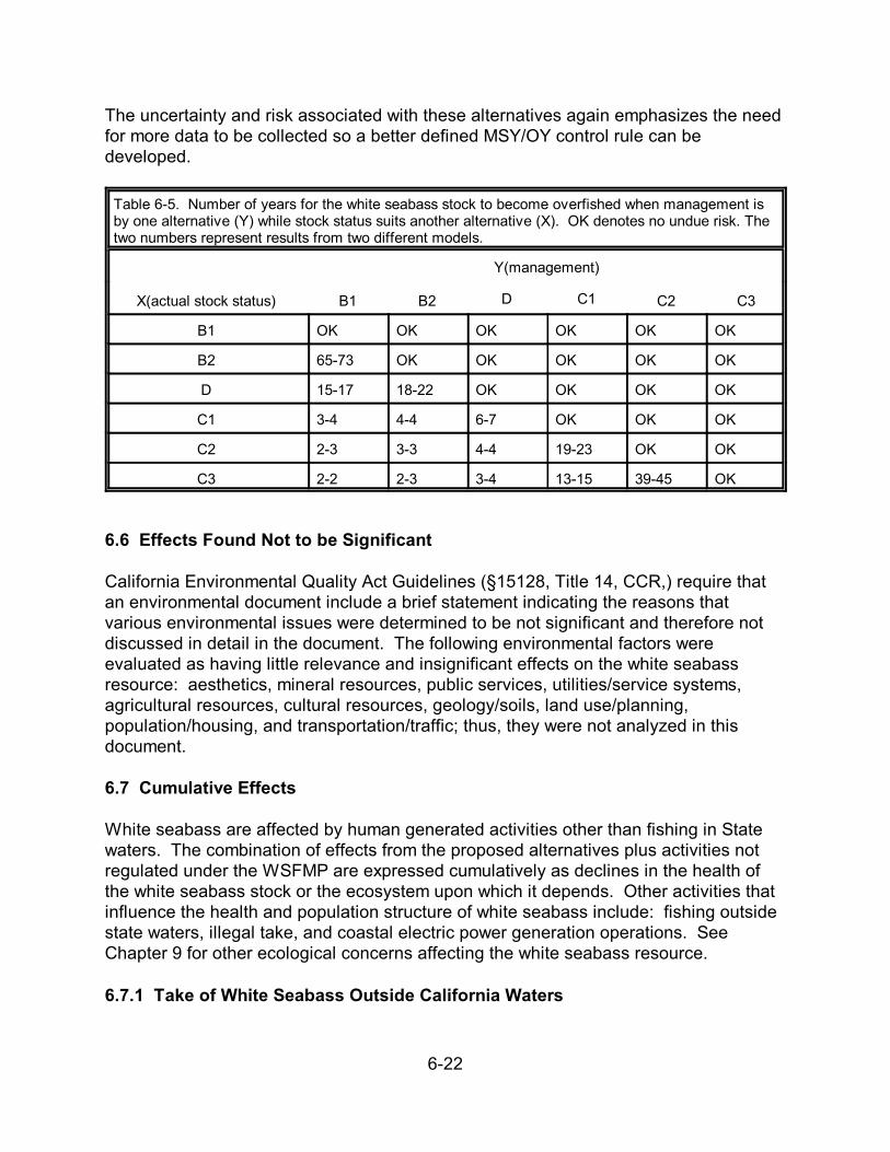
6-22
The uncertainty and risk associated with these alternatives again emphasizes the needfor more data to be collected so a better defined MSY/OY control rule can bedeveloped.
Table 6-5. Number of years for the white seabass stock to become overfished when management isby one alternative (Y) while stock status suits another alternative (X). OK denotes no undue risk. Thetwo numbers represent results from two different models.
X(actual stock status) B1 B2
Y(management)
C2 C3D C1
B1 OK OK OK OK OK OK
B2 65-73 OK OK OK OK OK
D 15-17 18-22 OK OK OK OK
C1 3-4 4-4 6-7 OK OK OK
C2 2-3 3-3 4-4 19-23 OK OK
C3 2-2 2-3 3-4 13-15 39-45 OK
6.6 Effects Found Not to be Significant
California Environmental Quality Act Guidelines (§15128, Title 14, CCR,) require thatan environmental document include a brief statement indicating the reasons thatvarious environmental issues were determined to be not significant and therefore notdiscussed in detail in the document. The following environmental factors wereevaluated as having little relevance and insignificant effects on the white seabassresource: aesthetics, mineral resources, public services, utilities/service systems,agricultural resources, cultural resources, geology/soils, land use/planning,population/housing, and transportation/traffic; thus, they were not analyzed in thisdocument.
6.7 Cumulative Effects
White seabass are affected by human generated activities other than fishing in Statewaters. The combination of effects from the proposed alternatives plus activities notregulated under the WSFMP are expressed cumulatively as declines in the health ofthe white seabass stock or the ecosystem upon which it depends. Other activities thatinfluence the health and population structure of white seabass include: fishing outsidestate waters, illegal take, and coastal electric power generation operations. SeeChapter 9 for other ecological concerns affecting the white seabass resource.
6.7.1 Take of White Seabass Outside California Waters
6-23
As mentioned in Section 2.5, the California fisheries for white seabass target thenorthern component of the resource, which ranges from Point Conception toMagdalena Bay, Baja California. The center of the population appears to be off centralBaja California, Mexico, and could be greatly affected by the Mexican fishery. However, the present and historical size of the Mexican fishery for white seabass isunknown. MacCall et al. (1976) noted that approximately 70,000 pounds (31,752 kg) were commercially-caught annually during the 1960s. By the early 1970s, the catchhad increased to 100,000 pounds (45,360 kg). Assuming an average weight of 25pounds (11.3 kg) per fish, this would equate to an annual catch of 2,500 fish in the1960s and 4,200 fish in the 1970s. This approximates the commercial harvest inCalifornia prior to implementation of Proposition 132. Recent landing figures areunavailable for the Mexican fishery; however, current Mexican regulations recommendthat fishing effort not be increased for the artisan fishery, which takes white seabassand other croaker species.
The number of fish currently being taken by the recreational fishery in Mexico isunknown at this time, although anecdotal information indicates that white seabass lessthan 28 inches are being taken. There are no data to indicate whether the harvest inMexico is affecting the white seabass population. The extent to which small fish aretaken, along with the magnitude of the commercial and recreational Mexican fisheries, could have serious consequences for California’s fishery.
6.7.2 Illegal Take of White Seabass
Some seabass are taken illegally by the recreational fishery either out of ignorance oras a calculated circumvention of the regulations. While there are no accurateestimates of the number taken illegally, Wine (1978;1979;1982) reported that in 1976-77,1977-78, and 1980, private boat fishermen landed nearly 2,400, 1,950, and 1,500undersized white seabass, respectively. This illegal take by a portion of the anglingpublic exceeded the legal take in the CPFV fishery in all three of these time periods. This trend continues today (RecFin 2001).
Poaching (taking fish illegally or during a closed season) and taking undersized whiteseabass also occurs in the commercial fishery. Few undersized white seabass aretaken in the directed white seabass fishery. Vojkovich et al. (1990) found that less than3% of the catch was less than 28 inches. However, the percentage of undersized whiteseabass reported in the halibut and white croaker fisheries totaled more than 50% ofthe incidental white seabass catch; and nearly all were discarded dead. The annualcatch of undersized white seabass in these two fisheries was small (approximately1,700 fish) but together they are similar to the annual catch of the CPFV anglers from1970 through 1998 (see Figure 3-1). There is no longer a fishery for white croakerbecause of the health concerns associated with eating that fish. Movement of thehalibut gill net fishery and white seabass directed fishery outside of State waters hasprobably reduced this take.
6-24
Although a serious issue, it is not possible at this time to determine whether the illegaltake of white seabass poses a significant threat to the long-term survival of the species. Increased enforcement activity and greater public awareness in the past decade hascontributed to lessening this problem.
6.7.3 Coastal Electric Power Generation Operations
Coastal electric power generation stations draw in large amounts of water, millions tobillions of gallons per day, from nearshore waters for cooling purposes. Marine life canbe either entrained or impinged by power plant operations. Entrained organisms arethose not strong enough to swim against the current of the intake system. Impingedorganisms are those that are collected on traveling screens designed to remove largedebris (mostly kelp and trash) from the water entering the power plant. As part ofnormal operations to eliminate the growth of encrusting organisms growing on theinside of the intake pipes, heated water flows out through the intake pipes for anextended period of time, often several hours. Encrusting organisms such as musselsand barnacles, and fish living within the intake pipes are killed by this process.
Power plants kill billions of fish larvae and hundreds of thousands of juveniles andadults each year (Herbinson 1981). Clean Water Act studies have documented thatmore than 80% of the larval fish entrained are less than 10 days old (less than 6 mmlong) indicating that potential local recruitment is being lost due to power plants; thestudies assume that 100 percent of the organisms entrained are killed. In addition tofish, larval forms of invertebrates and adult zooplankton will be lost to the ecosystem.
There are several coastal power plants in southern California. These power plantsoften impinge juvenile white seabass. They also entrain and impinge potential preyitems of white seabass, such as queenfish, white croaker, and northern anchovy, inlarge numbers. For example, the Huntington Beach Generating Station alone killedover 4 million of these three prey species combined from 1979-1998 (MBC AppliedEnvironmental Sciences 2001). During this same period, over 2,400 juvenile whiteseabass were impinged. The number of white seabass eggs and larvae entrained,however, is unknown. These numbers could be substantial since white seabassyoung-of-the-year reside in shallow nearshore waters (Allen and Franklin 1992).
6.8 Summary Analysis of the Proposed Alternatives
Proposed alternatives for management of the white seabass fishery have beenanalyzed in this chapter. A comparison of these alternatives and their effects on theobjectives for the WSFMP and the MLMA enables identification of which alternativeswould best meet management needs. Although each one of the alternatives has somebenefits for management, only alternatives B and D address most of the objectives ofthe WSFMP and MLMA (Table 6-6). Alternatives B and D, with similar risks ofproducing an overfished condition, would allow continued recovery of white seabasswhile important data were collected to yield a better defined MSY/OY control rule.
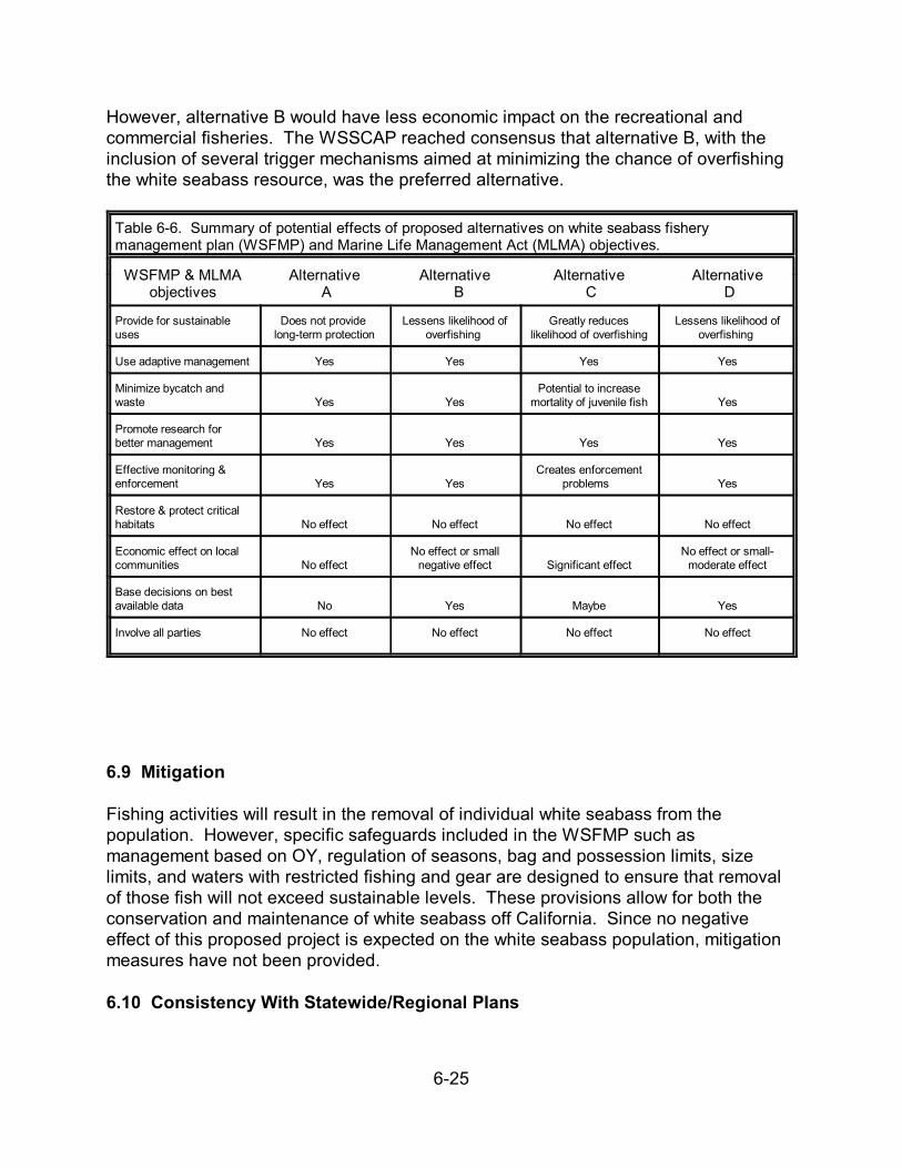
6-25
However, alternative B would have less economic impact on the recreational andcommercial fisheries. The WSSCAP reached consensus that alternative B, with theinclusion of several trigger mechanisms aimed at minimizing the chance of overfishingthe white seabass resource, was the preferred alternative.
Table 6-6. Summary of potential effects of proposed alternatives on white seabass fisherymanagement plan (WSFMP) and Marine Life Management Act (MLMA) objectives.
WSFMP & MLMAobjectives
Alternative A
Alternative B
Alternative C
Alternative D
Provide for sustainableuses
Does not provide long-term protection
Lessens likelihood ofoverfishing
Greatly reduceslikelihood of overfishing
Lessens likelihood ofoverfishing
Use adaptive management Yes Yes Yes Yes
Minimize bycatch andwaste Yes Yes
Potential to increasemortality of juvenile fish Yes
Promote research forbetter management Yes Yes Yes Yes
Effective monitoring &enforcement Yes Yes
Creates enforcementproblems Yes
Restore & protect criticalhabitats No effect No effect No effect No effect
Economic effect on localcommunities No effect
No effect or smallnegative effect Significant effect
No effect or small-moderate effect
Base decisions on bestavailable data No Yes Maybe Yes
Involve all parties No effect No effect No effect No effect
6.9 Mitigation
Fishing activities will result in the removal of individual white seabass from thepopulation. However, specific safeguards included in the WSFMP such asmanagement based on OY, regulation of seasons, bag and possession limits, sizelimits, and waters with restricted fishing and gear are designed to ensure that removalof those fish will not exceed sustainable levels. These provisions allow for both theconservation and maintenance of white seabass off California. Since no negativeeffect of this proposed project is expected on the white seabass population, mitigationmeasures have not been provided.
6.10 Consistency With Statewide/Regional Plans
6-26
The Department has concluded that the WSFMP is not inconsistent with air qualityattainment or maintenance plans, area-wide waste treatment and water quality controlplans, regional transportation plans, regional housing allocation plans, habitatconservation plans, natural community conservation plans, other regional land useplans, or any other terrestrial-based plans.
7-1
Chapter 7. Fishery Research Protocols
Fisheries sustainability is an elusive goal for marine resource managers. Thecornerstone of effective resource management is a comprehensive spatial-temporalknowledge of the resource. However, there is a paucity of this knowledge for mostmarine resources, mainly because of our limited powers of direct observation. In theocean most processes occur out of our view, thus our knowledge of marinecommunities, species abundance patterns and ecological interactions is fragmentary.
Fishery research is necessary to understand the many complex factors that contributeto the health and decline of our resources. This research is needed to providemanagement with guidance in making decisions to ensure sustainable fisheries. TheMLMA recognizes the importance of research and requires all FMPs to contain fisheryresearch protocols (§7081 FGC). These research protocols must:
• describe past and ongoing monitoring of the fishery;• identify essential fishery information (EFI) for the fishery, and if any is
lacking, identify resources and time to acquire it; and• indicate steps to monitor the fishery and obtain EFI.
Little biological information on white seabass has been gathered in the past 30 years. Thus, EFI is lacking in many areas. Future research should work toward acquiring thisEFI, and involve collaborative efforts of the fishing industry (both commercial andrecreational) and qualified university or private fisheries research companies. Inaccordance with MLMA, this chapter describes fishery research protocols designed toimplement the WSFMP; it identifies gaps in the current knowledge of white seabassstocks and fisheries and the steps needed to obtain this information for implementationto be successful.
7.1 Essential Fishery Information
The MLMA provides an opportunity for fishermen, scientists, fishery managers,conservationists, and other concerned constituents to develop a new approach formanaging our marine resources. The MLMA recognizes the importance of a collectivebody of biological, ecological, physical, economic and social information known as"essential fishery information" (EFI). This information is critical for the sustainable useand successful management of the State's marine resources. The MLMA calls for theDepartment to base FMPs on the best available scientific information (§7072(b) FGC). In addition, any gaps in EFI of a fishery are to be identified, along with steps to closethose gaps (§7081 FGC). Essential fishery information generally falls into two broadcategories based on how the data were obtained: fishery-dependent (related to thetake of fishermen), and fishery-independent information (data gathered independent ofthe fishery).
7-2
7.1.1 Grouping Essential Fishery Information
There are numerous parameters that comprise EFI. In an attempt to identify which EFIthe Department should focus its resources on, nine broad EFI groups were created. Itis important to emphasize that these groups are not mutually exclusive of one anothersince one group may include components that also fall under another. These groupswere formed so EFI could be prioritized based on what information was most crucial formanagement. The nine EFI groups are:
Age and growth characteristics:Age and growth studies typically measure how long a species lives, the age at which itreproduces, and how fast individuals grow. This information is very important todetermine a population’s ability to replenish itself, at what rate it might be harvested,and when individuals will reach a harvestable size. Changes in the age structure andgrowth rate of a population also serve as indicators of that population’s health. Thisinformation is often essential for stock assessments and models that guidemanagement strategies. Specific EFI includes von Bertalanffy growth parameters (k),length/weight ratios, longevity, age/length ratios, age/size at sexual maturity, andage/length at recruitment into the fishery.
Distribution of stocks:A stock is a population unit that is selected for management purposes. It may bedefined based on its ecology, genetics, and/or geographic separation. Discrete stocksof a given species may have very different growth rates, reproductive schedules andcapacity, and even ecological relationships. Stock distribution refers to where a stockis found, and is important in addressing jurisdictional issues. Specific EFI includes thedepth and geographic range of a species, the amount of gene flow and geneticstructure of the stock, and whether stocks are separate or continuous.
Ecological interactions:This information identifies the interaction of fishes within the environment, habitat, andecological community. Ecological relationships include the effects of oceanographicregimes and anthropogenic perturbations on physiological, energetic, or behavioralvariables; ecological niches and placement in food webs (prey and predators); density-dependent and density-independent interrelationships within and among species; andthe importance of essential fish habitat and habitat quality to a species. Estimation ofany ecological relationship demands a species-specific within-habitat approach due toenvironment and organism cross correlations.
Estimates of abundance: This information helps to determine how many individuals of a population are out thereand available to the fishery. This information is essential for all predictive modeling ofmarine resources. Estimates of stock size can be determined through direct (e.g.,surveys) or indirect (e.g., examination of the exploitation history) means. Specific EFIincludes relative densities of target and non-target species, habitat-specific absolute
7-3
densities, length frequency distributions, relative density estimates of life stages (i.e.,eggs, larvae, young-of-the-year, juveniles, or adults), recapture rates of tagged fish,and catch-per-unit-effort information.
Movement patterns:This information identifies the spatial distribution of fish and their residence time inspecific habitats. Many species may exhibit movement patterns that are associatedwith specific oceanographic conditions. Certain species may aggregate in specificareas for spawning, move in predictable patterns, or move to certain locales that makethem especially vulnerable to harvest. Insights into the movement patterns of fish areimportant to the development of management strategies based on regional catchquotas or marine protected areas. Specific EFI includes the home range, homingability, seasonal migrations, environmental cues, and spawning grounds of a species.
Recruitment:Recruitment refers to a measure of the number of fish that survive to a particular lifestage, and is often used to predict future population size. In this context, recruitmentrefers to both recruitment to the fishery and recruitment to the population. Manyspecies depend on successful recruitment events for replenishment of the stock. Recruitment success can be highly variable because it depends on the propercombination of many factors. As a result, sustainable harvest of the fishery maydepend on only a few strong cohorts (born the same year) to provide harvestablestocks until the next successful recruitment event. Resource managers must considerthis variable recruitment success when setting harvest levels by allowing sufficientportions of stocks to “escape” harvest and provide spawning biomass for futurerecruitment successes. Specific EFI includes the duration and distribution of egg andlarvae, size and timing of settlement, and annual cohort success. Information on theavailability of habitats and levels of predators and prey items is also important.
Reproductive characteristics:This information helps describe the reproductive potential of a fish stock and its abilityto replenish itself. Understanding key reproductive characteristics allows managers toset appropriate open and closed seasons as well as opened and closed areas basedon important spawning habitat. This information is also crucial in selecting size/slotlimits, escape mechanisms for traps, and mesh-size restrictions. Specific EFI for aspecies includes the number of eggs released, size at maturity, fertilization andspawning period, geographic spawning area, and the nature of mating systems.
Total mortality:This information refers to all removals of fish from the biomass, and is used to predicthow many animals remain to reproduce and replenish the population. Mortality figuresare essential for stock assessments and models to determine the number or weight(biomass) which may be safely harvested from a population or stock on a sustainablebasis. Total mortality is traditionally separated into natural mortality and fishingmortality. Natural and fishing mortality rates comprise the sum of all individuals
7-4
removed from a population over a fixed period of time (often over one year). Fishingmortality is the number of animals which are removed from the population by fishing.Natural mortality refers to all other forms of removal of fish from the population such aspredation, old age, starvation, or disease. Specific EFI includes catch data by species and area, amount and sizes of discarded catch, landings by gear type, and survivabilityof fish that are released.
Socioeconomic:The economic stability of coastal communities and quality of life may be affected bychanges in activities related to recreational fishing, or commercial fishing andprocessing. These changes may be caused by indirect factors or regulatory changesthat directly affect fishing activities. Indirect factors include triggers from consumer orfinancial markets such as 1) changes in consumer demand due to the favorable pricingand supply of a substitute item for a fishery product(s); 2) inflation; and, 3) tax changesthat affect business investments or activities. These effects may be manifested locallythrough resultant changes in business output, employment, population, and publicservice demand. The four broad categories of socioeconomic information include:
1. Employment:Overall impacts to local community earnings and employment can be gauged usinginput-output multipliers to project the changes to local personal income and the numberof local jobs. This procedure takes the direct change in final demand for an industryproduct or service in revenue or sales dollars and multiplies this direct change by atotal income coefficient to estimate total change in local personal income. Similarly,multiplying the direct change by an employment coefficient yields estimates of changesin the number of local jobs.
2. Expenditures:Regulatory changes that directly affect recreational or commercial fishing revenues inlocal economies have a downstream effect on other economic sectors which receiveand re-spend those revenues. This turnover refers to the number of times a dollarchanges hands in the local economy. Output multipliers are used to describe theturnover effect and interrelationships between the basic-sector and downstreambusiness sectors in the local economy.
Additionally, changes that directly affect end-user demand for recreational fishingactivities or commercial fisheries products may change end-user spending patterns.Depending on the nature of end-user demand for a given service or product, end-usersmay spend less if the quantity or quality of the service or product is decreased.Conversely, we would expect end-users to spend more if the quantity or quality wasimproved. These changes in spending patterns may also affect purchases of related orancillary goods or services provided in the local economy.
For example, a recreational fisherman may value a charter fishing trip limited to ten fishat $50 per trip. The fisherman may value this trip more than a fishing trip that is
7-5
restricted to only five fish, for which the fisherman is only willing to pay $35.
Furthermore, the recreational fisherman who plans to take six $50 charter trips per yearmay take only three trips per year if the price is raised to $80 per trip.
Lastly, the costs (usually expenditures) of production of a good, service, or activityprovide a means to compare the relationship between resources used to benefitsderived. Often, this is expressed as the benefits-to-cost comparison. In the case ofcommercial fishing activities, by monitoring costs of production at various levels ofoutput, we can define production where we have maximum economic benefit (or“profits”). This is important in creating harvest guidelines which foster optimumeconomic yield and economic efficiency in the fishing fleet. Economic efficiencyequates to cost and waste minimizing practices.
3. Resource Demand:Changes in the quantity or quality of available fishery-related goods or services affectthe individual end-user’s demand for those goods or services. How much this demandmay be affected depends on individual income, tastes, preferences, and theaccessibility to substitute goods or services. The aggregate demand, based on thecombined responses of individuals to changes in a good or service, yields an overalldemand function for a good or service. This demand function is used to predict thereactions of end-users to changes in the quantity or quality of goods or services, and toestimate the relative value and benefits end-users derive from a good. Consequently,the effects of in-season adjustments to harvest limits, or changes in bag limits, can beprojected in terms of the anticipated response of the target group of end-users, as wellas changes in the corresponding revenue streams.
4. Revenue:This category includes revenue from the sale of local goods or services within thecommunity and those goods or services which are exported out of the community. Revenue information allows resource managers to assess how changes in resources orregulations may affect industry-sector revenues and ultimately, the local community’seconomic output and vitality. Revenue generated by fishery-dependent activities (e.g.,by commercial landings, recreational direct expenditures, or end-user consumption ofcommercial products) provides basic information for calculating contributions to localeconomies and a means to compare relative values of goods and services derived fromthe fishery.
7.2 Past and Ongoing Monitoring of the Commercial and Recreational Fishery
Three major categories of monitoring have been employed by the Department. Theseinclude dockside/skiff surveys, landings/market sampling, and onboard observerprograms. These types of data collection activities have been ongoing for severalyears in both the commercial and recreational sectors of fisheries, and form the bulk ofthe Department’s data collection for white seabass.
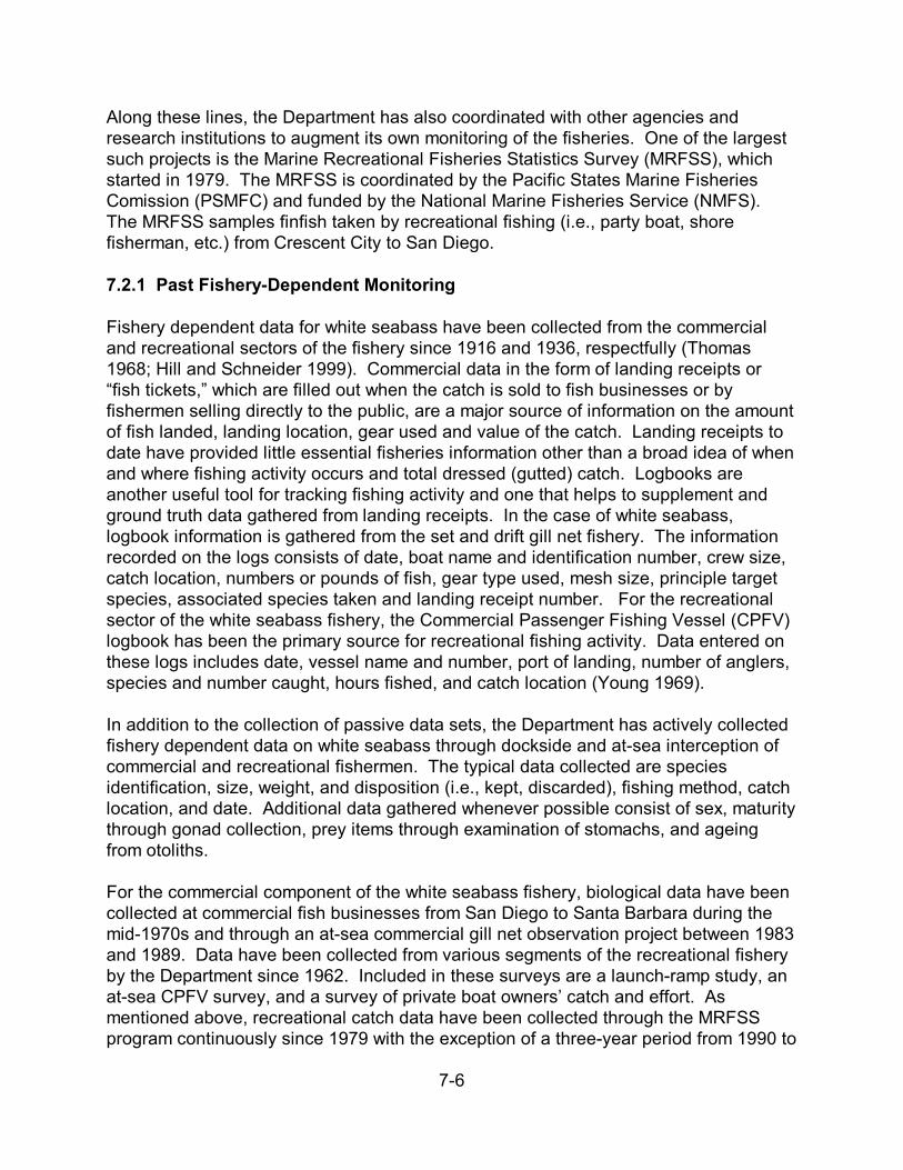
7-6
Along these lines, the Department has also coordinated with other agencies andresearch institutions to augment its own monitoring of the fisheries. One of the largestsuch projects is the Marine Recreational Fisheries Statistics Survey (MRFSS), whichstarted in 1979. The MRFSS is coordinated by the Pacific States Marine FisheriesComission (PSMFC) and funded by the National Marine Fisheries Service (NMFS). The MRFSS samples finfish taken by recreational fishing (i.e., party boat, shorefisherman, etc.) from Crescent City to San Diego.
7.2.1 Past Fishery-Dependent Monitoring
Fishery dependent data for white seabass have been collected from the commercialand recreational sectors of the fishery since 1916 and 1936, respectfully (Thomas1968; Hill and Schneider 1999). Commercial data in the form of landing receipts or“fish tickets,” which are filled out when the catch is sold to fish businesses or byfishermen selling directly to the public, are a major source of information on the amountof fish landed, landing location, gear used and value of the catch. Landing receipts todate have provided little essential fisheries information other than a broad idea of whenand where fishing activity occurs and total dressed (gutted) catch. Logbooks areanother useful tool for tracking fishing activity and one that helps to supplement andground truth data gathered from landing receipts. In the case of white seabass,logbook information is gathered from the set and drift gill net fishery. The informationrecorded on the logs consists of date, boat name and identification number, crew size,catch location, numbers or pounds of fish, gear type used, mesh size, principle targetspecies, associated species taken and landing receipt number. For the recreationalsector of the white seabass fishery, the Commercial Passenger Fishing Vessel (CPFV)logbook has been the primary source for recreational fishing activity. Data entered onthese logs includes date, vessel name and number, port of landing, number of anglers,species and number caught, hours fished, and catch location (Young 1969).
In addition to the collection of passive data sets, the Department has actively collectedfishery dependent data on white seabass through dockside and at-sea interception ofcommercial and recreational fishermen. The typical data collected are speciesidentification, size, weight, and disposition (i.e., kept, discarded), fishing method, catchlocation, and date. Additional data gathered whenever possible consist of sex, maturitythrough gonad collection, prey items through examination of stomachs, and ageingfrom otoliths.
For the commercial component of the white seabass fishery, biological data have beencollected at commercial fish businesses from San Diego to Santa Barbara during themid-1970s and through an at-sea commercial gill net observation project between 1983and 1989. Data have been collected from various segments of the recreational fisheryby the Department since 1962. Included in these surveys are a launch-ramp study, anat-sea CPFV survey, and a survey of private boat owners’ catch and effort. Asmentioned above, recreational catch data have been collected through the MRFSSprogram continuously since 1979 with the exception of a three-year period from 1990 to

7-7
1993.
7.2.2 Problems with Past and Ongoing Fishery-Dependent Monitoring
Currently, some fishery-dependent data suffer from being of limited use or inaccurate. Fishery-dependent monitoring, through the use of landing receipts and logbooks, doesnot provide adequate information about fishing location. The fishing blocks used by theDepartment are 10 nautical miles (nm) by 10 nm representing 100 square nauticalmiles of area. The size of the blocks is too large to identify specific fishing locationsand/or populations of white seabass and does not lend itself to ecosystemmanagement. In addition, the tendency among some fishermen is to alter the locationdata to prevent identification of “secret” fishing sites. In general, fish businesses haveno idea where fishing activity has occurred and will use either a favorite block code toidentify fishing location or fail to record catch information. Spatially explicitunderstanding of fishing spots can lead to identification of stocks, localized fishingmortality, and areas of stock depletion--all of which are important elements for properfishery management.
Another problem area for fishery managers is inconsistent fishery dependent researchand sampling effort. Fishery-dependent research of white seabass is plagued by alack of consistent sampling effort that results from unstable funding, the inability toretain sampling personnel, and the changing nature of the fishing industry. Mostfishery dependent research is funded through a mixture of state and federal programs. Budget shortfalls from one year to the next often result in reduced allocation of funds. This in turn leads to either reduced monitoring and sampling effort or completecessation. In addition, most sampling programs rely on temporary employees, whocan only work up to nine months per year and receive relatively low pay. Thus,constant turn over of temporary staff causes cessation of research and samplingactivities, while permanent staff expends time hiring and training new temporaryemployees.
Finally, there has been a change in the way fish businesses operate. Traditionally, fishbusinesses operated out of a fixed location where sampling of offloaded catch wasrelatively easy. In the past twenty years, however, there has been a transition tomobility commonly known as the white-van fleet. Fish businesses, using large vans ortrucks, now go to various locations within a port complex to meet fishing vessels. Thisshift makes it difficult to sample the catch since there are multiple locations where it canbe offloaded. As a result, a large proportion is often offloaded and driven to marketwithout being sampled.
In general, fishery-dependent data when used alone has performed poorly in predictingstock decline, especially for residential species (National Research Council 2000). Imprecise recording of fish landings, which are documented by fishery-dependent data,
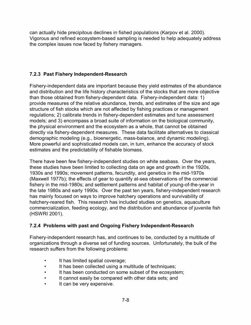
7-8
can actually hide precipitous declines in fished populations (Karpov et al. 2000). Vigorous and refined ecosystem-based sampling is needed to help adequately addressthe complex issues now faced by fishery managers.
7.2.3 Past Fishery Independent-Research
Fishery-independent data are important because they yield estimates of the abundanceand distribution and the life history characteristics of the stocks that are more objectivethan those obtained from fishery-dependent data. Fishery-independent data: 1)provide measures of the relative abundance, trends, and estimates of the size and agestructure of fish stocks which are not affected by fishing practices or managementregulations; 2) calibrate trends in fishery-dependent estimates and tune assessmentmodels; and 3) encompass a broad suite of information on the biological community,the physical environment and the ecosystem as a whole, that cannot be obtaineddirectly via fishery-dependent measures. These data facilitate alternatives to classicaldemographic modeling (e.g., bioenergetic, mass-balance, and dynamic modeling). More powerful and sophisticated models can, in turn, enhance the accuracy of stockestimates and the predictability of fishable biomass.
There have been few fishery-independent studies on white seabass. Over the years,these studies have been limited to collecting data on age and growth in the 1920s,1930s and 1990s; movement patterns, fecundity, and genetics in the mid-1970s(Maxwell 1977b); the effects of gear to quantify at-sea observations of the commercialfishery in the mid-1980s; and settlement patterns and habitat of young-of-the-year inthe late 1980s and early 1990s. Over the past ten years, fishery-independent researchhas mainly focused on ways to improve hatchery operations and survivability ofhatchery-reared fish. This research has included studies on genetics, aquaculturecommercialization, feeding ecology, and the distribution and abundance of juvenile fish(HSWRI 2001).
7.2.4 Problems with past and Ongoing Fishery Independent-Research
Fishery-independent research has, and continues to be, conducted by a multitude oforganizations through a diverse set of funding sources. Unfortunately, the bulk of theresearch suffers from the following problems:
• It has limited spatial coverage;• It has been collected using a multitude of techniques;• It has been conducted on some subset of the ecosystem; • It cannot easily be compared with other data sets; and• It can be very expensive.
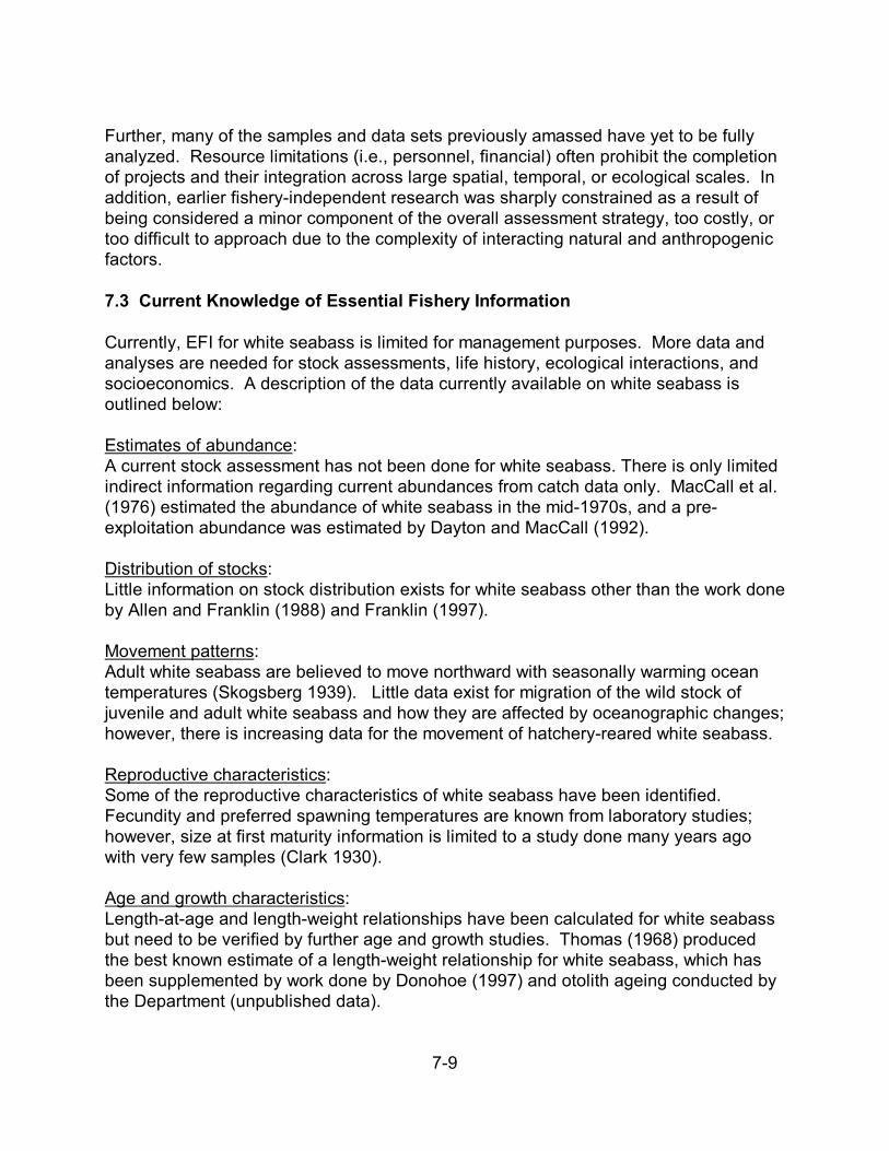
7-9
Further, many of the samples and data sets previously amassed have yet to be fullyanalyzed. Resource limitations (i.e., personnel, financial) often prohibit the completionof projects and their integration across large spatial, temporal, or ecological scales. Inaddition, earlier fishery-independent research was sharply constrained as a result ofbeing considered a minor component of the overall assessment strategy, too costly, ortoo difficult to approach due to the complexity of interacting natural and anthropogenicfactors.
7.3 Current Knowledge of Essential Fishery Information
Currently, EFI for white seabass is limited for management purposes. More data andanalyses are needed for stock assessments, life history, ecological interactions, andsocioeconomics. A description of the data currently available on white seabass isoutlined below:
Estimates of abundance: A current stock assessment has not been done for white seabass. There is only limitedindirect information regarding current abundances from catch data only. MacCall et al.(1976) estimated the abundance of white seabass in the mid-1970s, and a pre-exploitation abundance was estimated by Dayton and MacCall (1992).
Distribution of stocks:Little information on stock distribution exists for white seabass other than the work doneby Allen and Franklin (1988) and Franklin (1997).
Movement patterns:Adult white seabass are believed to move northward with seasonally warming oceantemperatures (Skogsberg 1939). Little data exist for migration of the wild stock ofjuvenile and adult white seabass and how they are affected by oceanographic changes;however, there is increasing data for the movement of hatchery-reared white seabass.
Reproductive characteristics:Some of the reproductive characteristics of white seabass have been identified. Fecundity and preferred spawning temperatures are known from laboratory studies;however, size at first maturity information is limited to a study done many years agowith very few samples (Clark 1930).
Age and growth characteristics: Length-at-age and length-weight relationships have been calculated for white seabassbut need to be verified by further age and growth studies. Thomas (1968) producedthe best known estimate of a length-weight relationship for white seabass, which hasbeen supplemented by work done by Donohoe (1997) and otolith ageing conducted bythe Department (unpublished data).
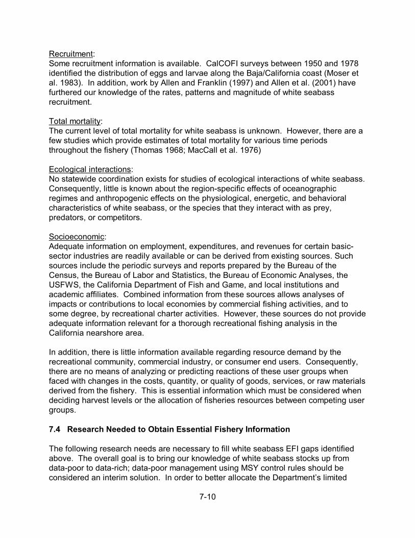
7-10
Recruitment:Some recruitment information is available. CalCOFI surveys between 1950 and 1978identified the distribution of eggs and larvae along the Baja/California coast (Moser etal. 1983). In addition, work by Allen and Franklin (1997) and Allen et al. (2001) havefurthered our knowledge of the rates, patterns and magnitude of white seabassrecruitment.
Total mortality:The current level of total mortality for white seabass is unknown. However, there are afew studies which provide estimates of total mortality for various time periodsthroughout the fishery (Thomas 1968; MacCall et al. 1976)
Ecological interactions:No statewide coordination exists for studies of ecological interactions of white seabass. Consequently, little is known about the region-specific effects of oceanographicregimes and anthropogenic effects on the physiological, energetic, and behavioralcharacteristics of white seabass, or the species that they interact with as prey,predators, or competitors.
Socioeconomic:Adequate information on employment, expenditures, and revenues for certain basic-sector industries are readily available or can be derived from existing sources. Suchsources include the periodic surveys and reports prepared by the Bureau of theCensus, the Bureau of Labor and Statistics, the Bureau of Economic Analyses, theUSFWS, the California Department of Fish and Game, and local institutions andacademic affiliates. Combined information from these sources allows analyses ofimpacts or contributions to local economies by commercial fishing activities, and tosome degree, by recreational charter activities. However, these sources do not provide adequate information relevant for a thorough recreational fishing analysis in theCalifornia nearshore area.
In addition, there is little information available regarding resource demand by therecreational community, commercial industry, or consumer end users. Consequently,there are no means of analyzing or predicting reactions of these user groups whenfaced with changes in the costs, quantity, or quality of goods, services, or raw materialsderived from the fishery. This is essential information which must be considered whendeciding harvest levels or the allocation of fisheries resources between competing usergroups.
7.4 Research Needed to Obtain Essential Fishery Information
The following research needs are necessary to fill white seabass EFI gaps identifiedabove. The overall goal is to bring our knowledge of white seabass stocks up fromdata-poor to data-rich; data-poor management using MSY control rules should beconsidered an interim solution. In order to better allocate the Department’s limited
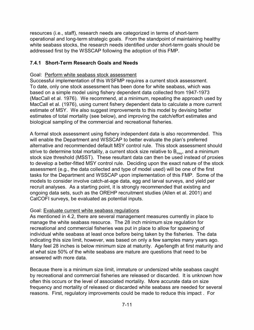
7-11
resources (i.e., staff), research needs are categorized in terms of short-termoperational and long-term strategic goals. From the standpoint of maintaining healthywhite seabass stocks, the research needs identified under short-term goals should beaddressed first by the WSSCAP following the adoption of this FMP.
7.4.1 Short-Term Research Goals and Needs
Goal: Perform white seabass stock assessmentSuccessful implementation of this WSFMP requires a current stock assessment. To date, only one stock assessment has been done for white seabass, which wasbased on a simple model using fishery dependent data collected from 1947-1973(MacCall et al. 1976). We recommend, at a minimum, repeating the approach used byMacCall et al. (1976), using current fishery dependent data to calculate a more currentestimate of MSY. We also suggest improvements to this model by devising betterestimates of total mortality (see below), and improving the catch/effort estimates andbiological sampling of the commercial and recreational fisheries.
A formal stock assessment using fishery independent data is also recommended. Thiswill enable the Department and WSSCAP to better evaluate the plan’s preferredalternative and recommended default MSY control rule. This stock assessment shouldstrive to determine total mortality, a current stock size relative to Bmsy, and a minimumstock size threshold (MSST). These resultant data can then be used instead of proxiesto develop a better-fitted MSY control rule. Deciding upon the exact nature of the stockassessment (e.g., the data collected and type of model used) will be one of the firsttasks for the Department and WSSCAP upon implementation of this FMP. Some of themodels to consider involve catch-at-age data, egg and larval surveys, and yield perrecruit analyses. As a starting point, it is strongly recommended that existing andongoing data sets, such as the OREHP recruitment studies (Allen et al. 2001) andCalCOFI surveys, be evaluated as potential inputs.
Goal: Evaluate current white seabass regulationsAs mentioned in 4.2, there are several management measures currently in place tomanage the white seabass resource. The 28 inch minimum size regulation forrecreational and commercial fisheries was put in place to allow for spawning ofindividual white seabass at least once before being taken by the fisheries. The dataindicating this size limit, however, was based on only a few samples many years ago. Many feel 28 inches is below minimum size at maturity. Age/length at first maturity andat what size 50% of the white seabass are mature are questions that need to beanswered with more data.
Because there is a minimum size limit, immature or undersized white seabass caughtby recreational and commercial fisheries are released or discarded. It is unknown howoften this occurs or the level of associated mortality. More accurate data on sizefrequency and mortality of released or discarded white seabass are needed for severalreasons. First, regulatory improvements could be made to reduce this impact . For
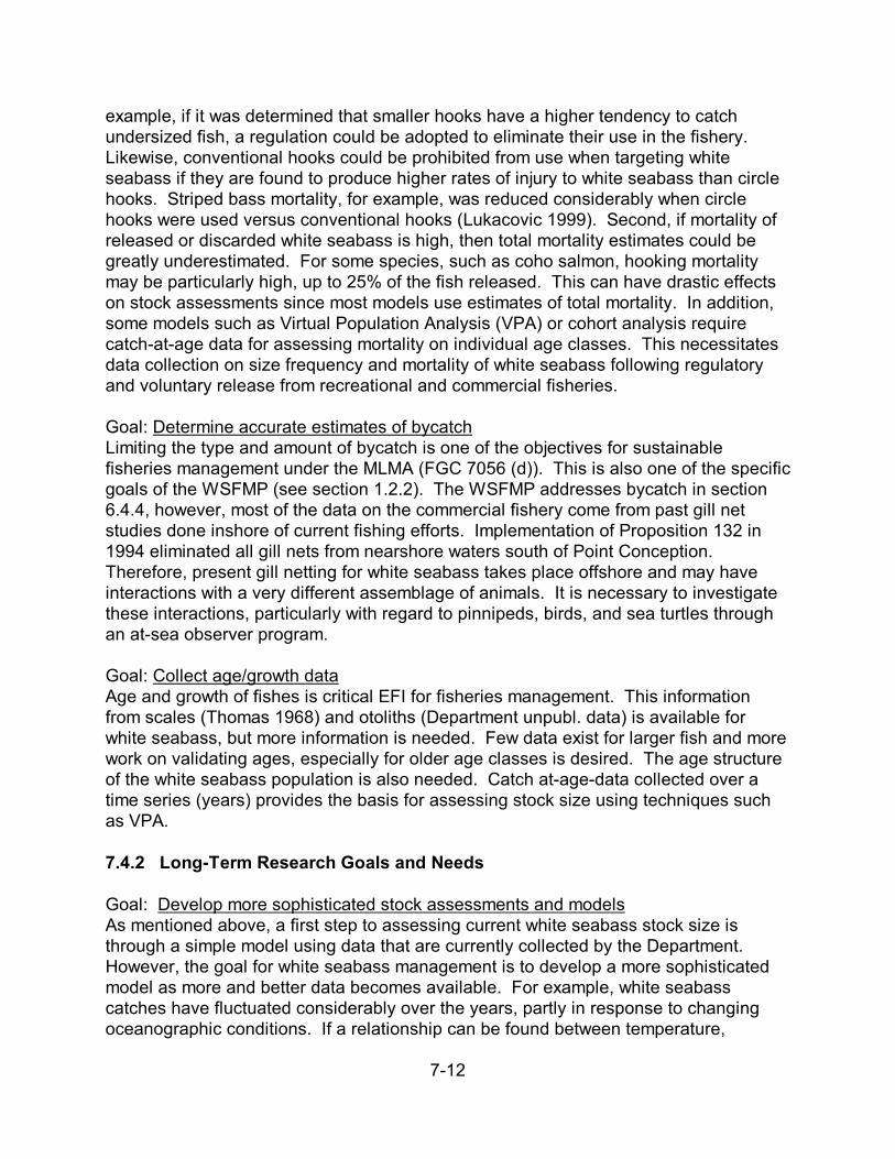
7-12
example, if it was determined that smaller hooks have a higher tendency to catchundersized fish, a regulation could be adopted to eliminate their use in the fishery. Likewise, conventional hooks could be prohibited from use when targeting whiteseabass if they are found to produce higher rates of injury to white seabass than circlehooks. Striped bass mortality, for example, was reduced considerably when circlehooks were used versus conventional hooks (Lukacovic 1999). Second, if mortality ofreleased or discarded white seabass is high, then total mortality estimates could begreatly underestimated. For some species, such as coho salmon, hooking mortalitymay be particularly high, up to 25% of the fish released. This can have drastic effectson stock assessments since most models use estimates of total mortality. In addition,some models such as Virtual Population Analysis (VPA) or cohort analysis requirecatch-at-age data for assessing mortality on individual age classes. This necessitatesdata collection on size frequency and mortality of white seabass following regulatoryand voluntary release from recreational and commercial fisheries.
Goal: Determine accurate estimates of bycatchLimiting the type and amount of bycatch is one of the objectives for sustainablefisheries management under the MLMA (FGC 7056 (d)). This is also one of the specificgoals of the WSFMP (see section 1.2.2). The WSFMP addresses bycatch in section6.4.4, however, most of the data on the commercial fishery come from past gill netstudies done inshore of current fishing efforts. Implementation of Proposition 132 in1994 eliminated all gill nets from nearshore waters south of Point Conception. Therefore, present gill netting for white seabass takes place offshore and may haveinteractions with a very different assemblage of animals. It is necessary to investigatethese interactions, particularly with regard to pinnipeds, birds, and sea turtles throughan at-sea observer program.
Goal: Collect age/growth dataAge and growth of fishes is critical EFI for fisheries management. This information from scales (Thomas 1968) and otoliths (Department unpubl. data) is available forwhite seabass, but more information is needed. Few data exist for larger fish and morework on validating ages, especially for older age classes is desired. The age structureof the white seabass population is also needed. Catch at-age-data collected over atime series (years) provides the basis for assessing stock size using techniques suchas VPA.
7.4.2 Long-Term Research Goals and Needs
Goal: Develop more sophisticated stock assessments and modelsAs mentioned above, a first step to assessing current white seabass stock size isthrough a simple model using data that are currently collected by the Department. However, the goal for white seabass management is to develop a more sophisticatedmodel as more and better data becomes available. For example, white seabasscatches have fluctuated considerably over the years, partly in response to changingoceanographic conditions. If a relationship can be found between temperature,
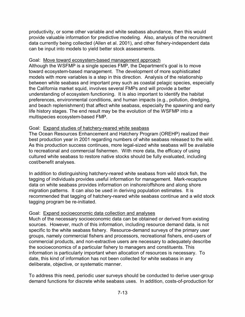
7-13
productivity, or some other variable and white seabass abundance, then this wouldprovide valuable information for predictive modeling. Also, analysis of the recruitmentdata currently being collected (Allen et al. 2001), and other fishery-independent datacan be input into models to yield better stock assessments. Goal: Move toward ecosystem-based management approachAlthough the WSFMP is a single species FMP, the Department’s goal is to movetoward ecosystem-based management. The development of more sophisticatedmodels with more variables is a step in this direction. Analysis of the relationshipbetween white seabass and important prey such as coastal pelagic species, especiallythe California market squid, involves several FMPs and will provide a betterunderstanding of ecosystem functioning. It is also important to identify the habitatpreferences, environmental conditions, and human impacts (e.g., pollution, dredging,and beach replenishment) that affect white seabass, especially the spawning and earlylife history stages. The end result may be the evolution of the WSFMP into amultispecies ecosystem-based FMP.
Goal: Expand studies of hatchery-reared white seabassThe Ocean Resources Enhancement and Hatchery Program (OREHP) realized theirbest production year in 2001 regarding numbers of white seabass released to the wild. As this production success continues, more legal-sized white seabass will be availableto recreational and commercial fishermen. With more data, the efficacy of usingcultured white seabass to restore native stocks should be fully evaluated, includingcost/benefit analyses.
In addition to distinguishing hatchery-reared white seabass from wild stock fish, thetagging of individuals provides useful information for management. Mark-recapturedata on white seabass provides information on inshore/offshore and along shoremigration patterns. It can also be used in deriving population estimates. It isrecommended that tagging of hatchery-reared white seabass continue and a wild stocktagging program be re-initiated.
Goal: Expand socioeconomic data collection and analysesMuch of the necessary socioeconomic data can be obtained or derived from existingsources. However, much of this information, including resource demand data, is notspecific to the white seabass fishery. Resource-demand surveys of the primary usergroups, namely commercial fishers and processors, recreational fishers, end-users ofcommercial products, and non-extractive users are necessary to adequately describethe socioeconomics of a particular fishery to managers and constituents. Thisinformation is particularly important when allocation of resources is necessary. Todate, this kind of information has not been collected for white seabass in anydeliberate, objective, or systematic manner.
To address this need, periodic user surveys should be conducted to derive user-groupdemand functions for discrete white seabass uses. In addition, costs-of-production for
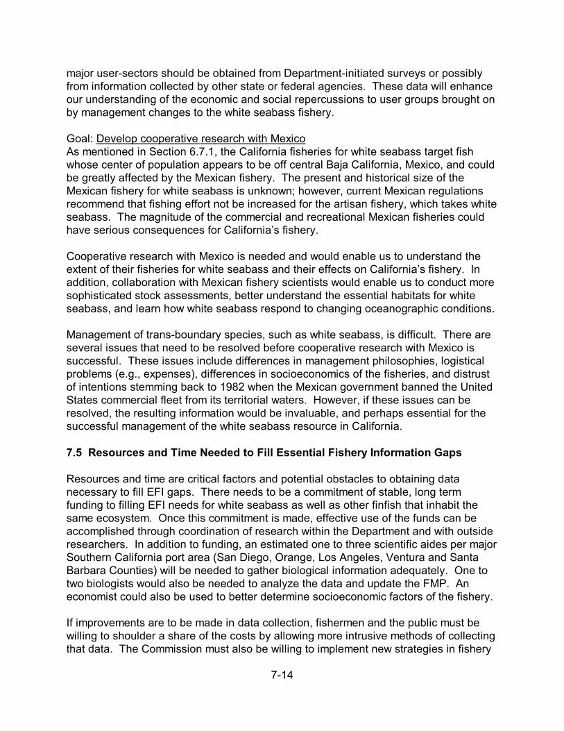
7-14
major user-sectors should be obtained from Department-initiated surveys or possiblyfrom information collected by other state or federal agencies. These data will enhanceour understanding of the economic and social repercussions to user groups brought onby management changes to the white seabass fishery.
Goal: Develop cooperative research with Mexico As mentioned in Section 6.7.1, the California fisheries for white seabass target fishwhose center of population appears to be off central Baja California, Mexico, and couldbe greatly affected by the Mexican fishery. The present and historical size of theMexican fishery for white seabass is unknown; however, current Mexican regulationsrecommend that fishing effort not be increased for the artisan fishery, which takes whiteseabass. The magnitude of the commercial and recreational Mexican fisheries couldhave serious consequences for California’s fishery.
Cooperative research with Mexico is needed and would enable us to understand theextent of their fisheries for white seabass and their effects on California’s fishery. Inaddition, collaboration with Mexican fishery scientists would enable us to conduct moresophisticated stock assessments, better understand the essential habitats for whiteseabass, and learn how white seabass respond to changing oceanographic conditions.
Management of trans-boundary species, such as white seabass, is difficult. There areseveral issues that need to be resolved before cooperative research with Mexico issuccessful. These issues include differences in management philosophies, logisticalproblems (e.g., expenses), differences in socioeconomics of the fisheries, and distrustof intentions stemming back to 1982 when the Mexican government banned the UnitedStates commercial fleet from its territorial waters. However, if these issues can beresolved, the resulting information would be invaluable, and perhaps essential for thesuccessful management of the white seabass resource in California.
7.5 Resources and Time Needed to Fill Essential Fishery Information Gaps
Resources and time are critical factors and potential obstacles to obtaining datanecessary to fill EFI gaps. There needs to be a commitment of stable, long termfunding to filling EFI needs for white seabass as well as other finfish that inhabit thesame ecosystem. Once this commitment is made, effective use of the funds can beaccomplished through coordination of research within the Department and with outsideresearchers. In addition to funding, an estimated one to three scientific aides per majorSouthern California port area (San Diego, Orange, Los Angeles, Ventura and SantaBarbara Counties) will be needed to gather biological information adequately. One totwo biologists would also be needed to analyze the data and update the FMP. Aneconomist could also be used to better determine socioeconomic factors of the fishery.
If improvements are to be made in data collection, fishermen and the public must bewilling to shoulder a share of the costs by allowing more intrusive methods of collectingthat data. The Commission must also be willing to implement new strategies in fishery
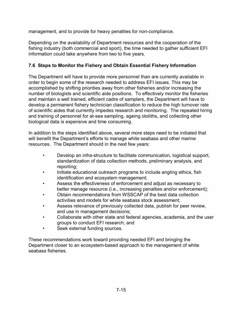
7-15
management, and to provide for heavy penalties for non-compliance.
Depending on the availability of Department resources and the cooperation of thefishing industry (both commercial and sport), the time needed to gather sufficient EFIinformation could take anywhere from two to five years.
7.6 Steps to Monitor the Fishery and Obtain Essential Fishery Information
The Department will have to provide more personnel than are currently available inorder to begin some of the research needed to address EFI issues. This may beaccomplished by shifting priorities away from other fisheries and/or increasing thenumber of biologists and scientific aide positions. To effectively monitor the fisheriesand maintain a well trained, efficient cadre of samplers, the Department will have to develop a permanent fishery technician classification to reduce the high turnover rateof scientific aides that currently impedes research and monitoring. The repeated hiringand training of personnel for at-sea sampling, ageing otoliths, and collecting otherbiological data is expensive and time consuming.
In addition to the steps identified above, several more steps need to be initiated thatwill benefit the Department’s efforts to manage white seabass and other marineresources. The Department should in the next few years:
• Develop an infra-structure to facilitate communication, logistical support,standardization of data collection methods, preliminary analysis, andreporting;
• Initiate educational outreach programs to include angling ethics, fishidentification and ecosystem management;
• Assess the effectiveness of enforcement and adjust as necessary tobetter manage resource (i.e., increasing penalties and/or enforcement);
• Obtain recommendations from WSSCAP of the best data collectionactivities and models for white seabass stock assessment;
• Assess relevance of previously collected data, publish for peer review,and use in management decisions;
• Collaborate with other state and federal agencies, academia, and the usergroups to conduct EFI research; and
• Seek external funding sources.
These recommendations work toward providing needed EFI and bringing theDepartment closer to an ecosystem-based approach to the management of whiteseabass fisheries.

8-1
Chapter 8. Implementation Requirements
This chapter provides estimated costs for the implementation of the WSFMP. Thecosts are grouped into the categories of enforcement, ongoing and future research, andadministrative management. Estimating the individual costs of implementing theWSFMP is made by estimating the time to perform certain tasks such as theenforcement of regulations, collecting data, and reviewing documents. Generally,these kinds of costs are underestimated, because there is no way to determine howdifficult some issues may be. Nevertheless, estimates are useful for determining whatthe actual costs may be and for comparing different options that may be proposed. These cost estimates include expenditures that are incurred regardless of whether ornot the WSFMP is partially or fully adopted. These expenses are termed “sunk” costsand equate to the costs of enforcement, data collection, and monitoring that theDepartment must perform as part of its resource stewardship charge.
8.1 Enforcement
Due to the extensive size of California, it is necessary to employ a variety of measuresto ensure the protection of California’s wildlife and compliance with the laws of theState. These measures include land-based, ocean-based and air-based enforcementactivities. With few exceptions, costs within the Department are attributed to programs(e.g., MLMA, Environmental License Plate Fund) and not to specific species. Thus, it isimpossible to determine exactly how much it costs to enforce existing white seabasslaws and regulations. However, a reasonable approximation can be calculated bydetermining the percentage of white seabass landings within the total number of allnearshore finfish landings made in the year 2000. The resulting percentage can thenbe multiplied by the total cost of nearshore enforcement in 2000. Enforcementpersonnel hours coded to MLMA were used because they represent nearshoreenforcement activity. These hours were further limited to only those in the southernpatrol district (Monterey County line to the U.S./Mexico border) since white seabass areprimarily taken in the nearshore waters of southern California.
The estimated cost of enforcing nearshore Fish and Game laws in the southern patroldistrict in 2000 was approximately $562,591 (Table 8-1). Of this amount, an estimated$50,633 can be attributed to time spent on the enforcement of white seabass laws andregulations. If fishing effort and/or landings increase, the subsequent cost of enforcingFish and Game laws and regulations will increase.
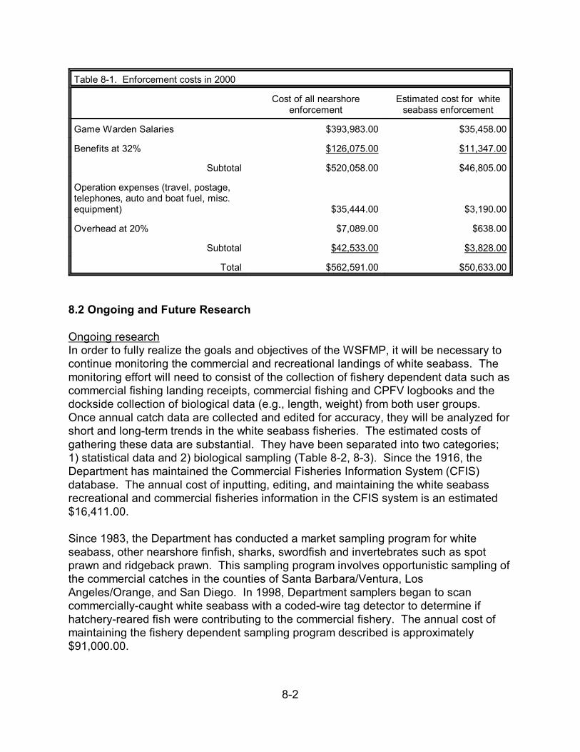
8-2
Table 8-1. Enforcement costs in 2000
Cost of all nearshoreenforcement
Estimated cost for whiteseabass enforcement
Game Warden Salaries $393,983.00 $35,458.00
Benefits at 32% $126,075.00 $11,347.00
Subtotal $520,058.00 $46,805.00
Operation expenses (travel, postage,telephones, auto and boat fuel, misc.equipment) $35,444.00 $3,190.00
Overhead at 20% $7,089.00 $638.00
Subtotal $42,533.00 $3,828.00
Total $562,591.00 $50,633.00
8.2 Ongoing and Future Research
Ongoing researchIn order to fully realize the goals and objectives of the WSFMP, it will be necessary tocontinue monitoring the commercial and recreational landings of white seabass. Themonitoring effort will need to consist of the collection of fishery dependent data such ascommercial fishing landing receipts, commercial fishing and CPFV logbooks and thedockside collection of biological data (e.g., length, weight) from both user groups. Once annual catch data are collected and edited for accuracy, they will be analyzed forshort and long-term trends in the white seabass fisheries. The estimated costs ofgathering these data are substantial. They have been separated into two categories;1) statistical data and 2) biological sampling (Table 8-2, 8-3). Since the 1916, theDepartment has maintained the Commercial Fisheries Information System (CFIS)database. The annual cost of inputting, editing, and maintaining the white seabassrecreational and commercial fisheries information in the CFIS system is an estimated$16,411.00.
Since 1983, the Department has conducted a market sampling program for whiteseabass, other nearshore finfish, sharks, swordfish and invertebrates such as spotprawn and ridgeback prawn. This sampling program involves opportunistic sampling ofthe commercial catches in the counties of Santa Barbara/Ventura, LosAngeles/Orange, and San Diego. In 1998, Department samplers began to scancommercially-caught white seabass with a coded-wire tag detector to determine ifhatchery-reared fish were contributing to the commercial fishery. The annual cost ofmaintaining the fishery dependent sampling program described is approximately$91,000.00.
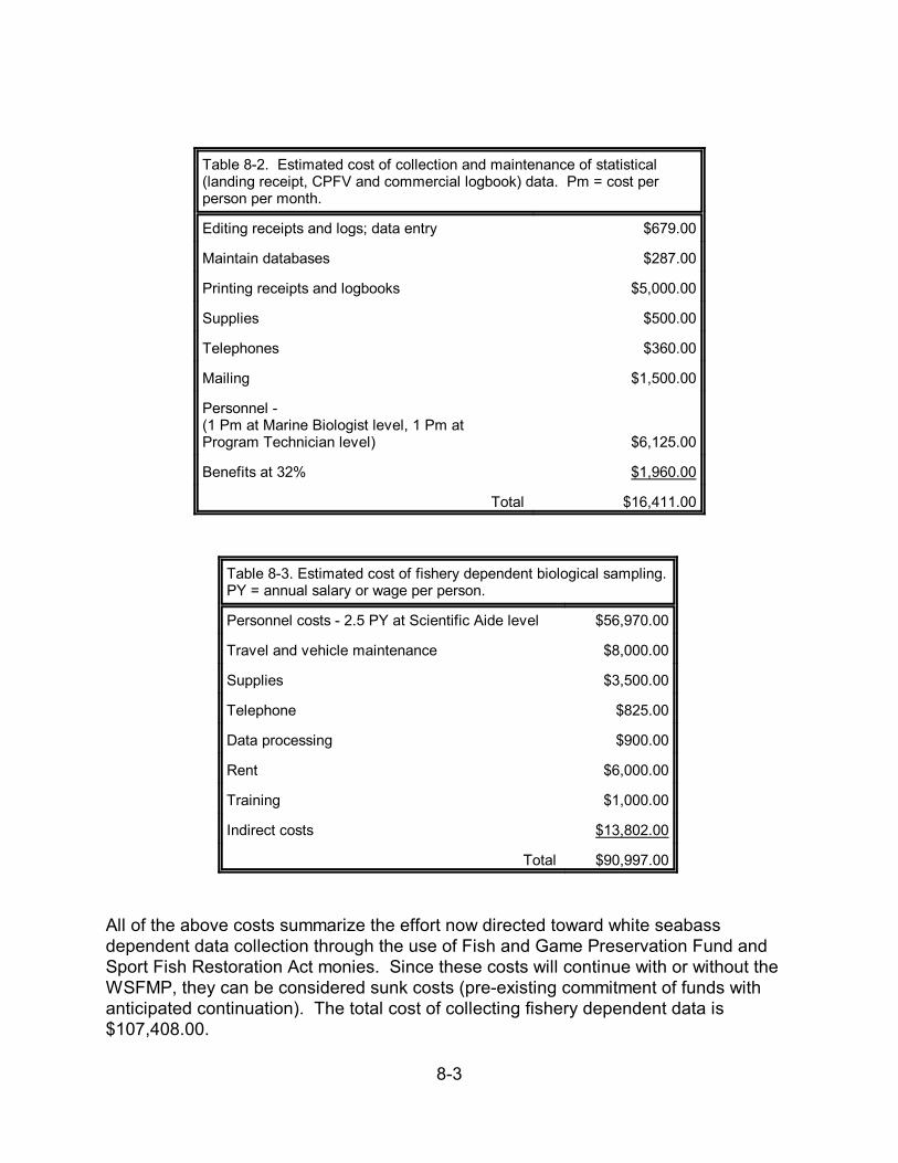
8-3
Table 8-2. Estimated cost of collection and maintenance of statistical (landing receipt, CPFV and commercial logbook) data. Pm = cost perperson per month.
Editing receipts and logs; data entry $679.00
Maintain databases $287.00
Printing receipts and logbooks $5,000.00
Supplies $500.00
Telephones $360.00
Mailing $1,500.00
Personnel -(1 Pm at Marine Biologist level, 1 Pm atProgram Technician level) $6,125.00
Benefits at 32% $1,960.00
Total $16,411.00
Table 8-3. Estimated cost of fishery dependent biological sampling. PY = annual salary or wage per person.
Personnel costs - 2.5 PY at Scientific Aide level $56,970.00
Travel and vehicle maintenance $8,000.00
Supplies $3,500.00
Telephone $825.00
Data processing $900.00
Rent $6,000.00
Training $1,000.00
Indirect costs $13,802.00
Total $90,997.00
All of the above costs summarize the effort now directed toward white seabassdependent data collection through the use of Fish and Game Preservation Fund andSport Fish Restoration Act monies. Since these costs will continue with or without theWSFMP, they can be considered sunk costs (pre-existing commitment of funds withanticipated continuation). The total cost of collecting fishery dependent data is$107,408.00.

8-4
Another heavily relied upon source of fishery dependent data available to the State isthe Marine Recreational Fisheries Statistics Survey (MRFSS), conducted by the PacificStates Marine Fisheries Commission. This coastwide sampling program interceptsrecreational anglers at launch ramps, piers and jetties, and on CPFV vessels. MRFSSdata are presently provided free of charge, and are currently our only source ofinformation on the take of white seabass by shore-based and private or rental boatfishermen. These user groups take more than 50% of the recreational white seabasscatch. In the future, it may become necessary for the Department to provide funding forthe MRFSS program if the current funding provided by NMFS is reduced or eliminated,as in 1991 through 1993, or if the funding is not increased on an annual basis asneeded. Should either of these events occur, the State would need to find another wayto estimate recreational take for private/rental boats and shore-based fishing or provideup to $400,000 annually to maintain the southern California portion of the MRFSSstudy.
Future researchDespite being an important species to the recreational and commercial fisheries of theState, very little biological information has been gathered on white seabass in the past30 years and the current knowledge of the essential fisheries information is limited (seeSection 7.3). One of the most pressing needs is a current stock assessment. Also,there are several fishery-based issues that need to be addressed, such as, hookingmortality and survival rates for white seabass released by commercial and recreationalfishermen. An on-board observer program is needed to determine accurate estimatesof bycatch associated with the commercial white seabass fishery. Genetic studies areneeded to determine the variation within wild seabass stocks and the effect, if any,hatchery-reared stocks may have on these stocks. The costs summarized in Table 8-4can be viewed as either new costs required by the WSFMP, or the reallocation of moreof the Marine Region budget from other species to white seabass.
Table 8-4. Cost of fishery independent data collection. PY =annual salary or wage per person.
Personnel costs (1.5 PY atAssociate Marine Biologist level;1 PY at Permanent IntermittentMarine Biologist level) $123,546.00
Benefits at 32% $39,535.00
Travel, supplies, fuel, gear, etc. $150,000.00
Overhead at 20% $30,000.00
Ship time (20 days) $70,000.00
Special surveys (22 days) $4,400.00
Total $417,481.00
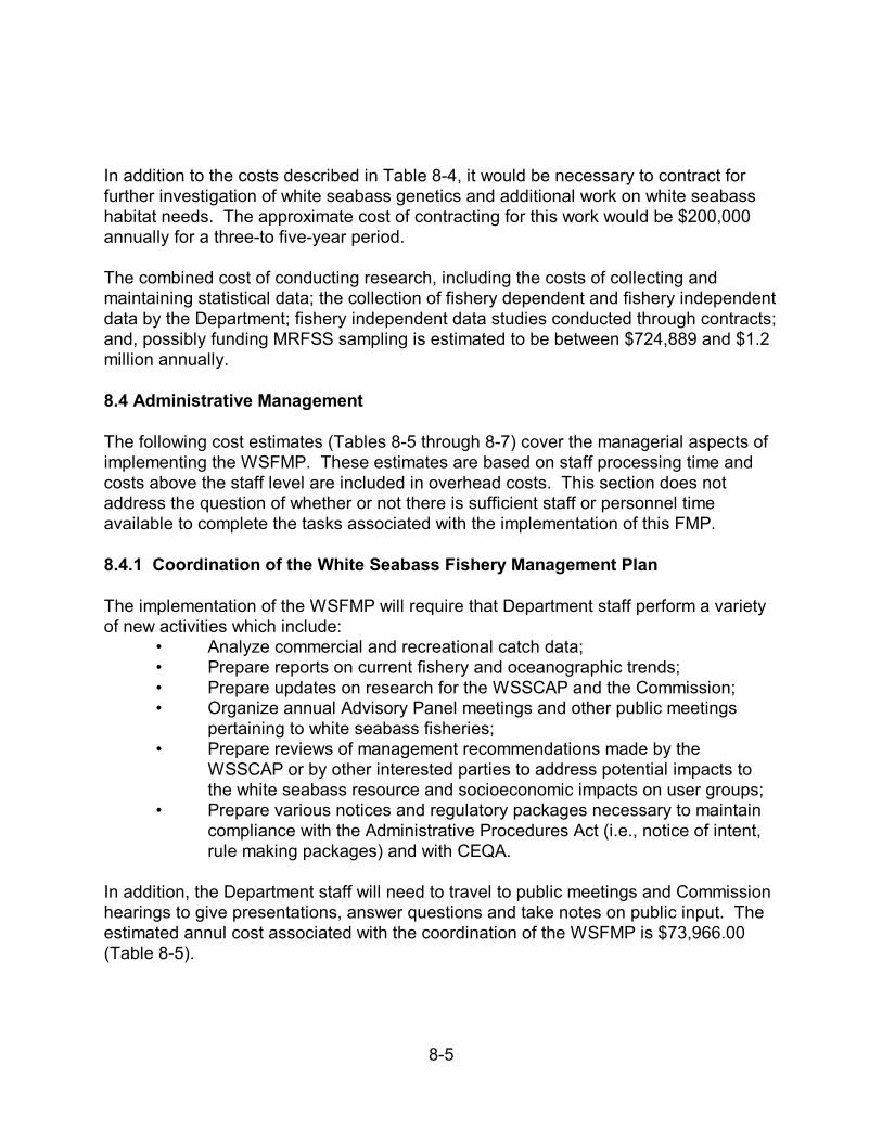
8-5
In addition to the costs described in Table 8-4, it would be necessary to contract forfurther investigation of white seabass genetics and additional work on white seabasshabitat needs. The approximate cost of contracting for this work would be $200,000annually for a three-to five-year period.
The combined cost of conducting research, including the costs of collecting andmaintaining statistical data; the collection of fishery dependent and fishery independentdata by the Department; fishery independent data studies conducted through contracts;and, possibly funding MRFSS sampling is estimated to be between $724,889 and $1.2million annually.
8.4 Administrative Management
The following cost estimates (Tables 8-5 through 8-7) cover the managerial aspects ofimplementing the WSFMP. These estimates are based on staff processing time andcosts above the staff level are included in overhead costs. This section does notaddress the question of whether or not there is sufficient staff or personnel timeavailable to complete the tasks associated with the implementation of this FMP.
8.4.1 Coordination of the White Seabass Fishery Management Plan
The implementation of the WSFMP will require that Department staff perform a varietyof new activities which include:
• Analyze commercial and recreational catch data; • Prepare reports on current fishery and oceanographic trends; • Prepare updates on research for the WSSCAP and the Commission; • Organize annual Advisory Panel meetings and other public meetings
pertaining to white seabass fisheries; • Prepare reviews of management recommendations made by the
WSSCAP or by other interested parties to address potential impacts tothe white seabass resource and socioeconomic impacts on user groups;
• Prepare various notices and regulatory packages necessary to maintaincompliance with the Administrative Procedures Act (i.e., notice of intent,rule making packages) and with CEQA.
In addition, the Department staff will need to travel to public meetings and Commissionhearings to give presentations, answer questions and take notes on public input. Theestimated annul cost associated with the coordination of the WSFMP is $73,966.00(Table 8-5).
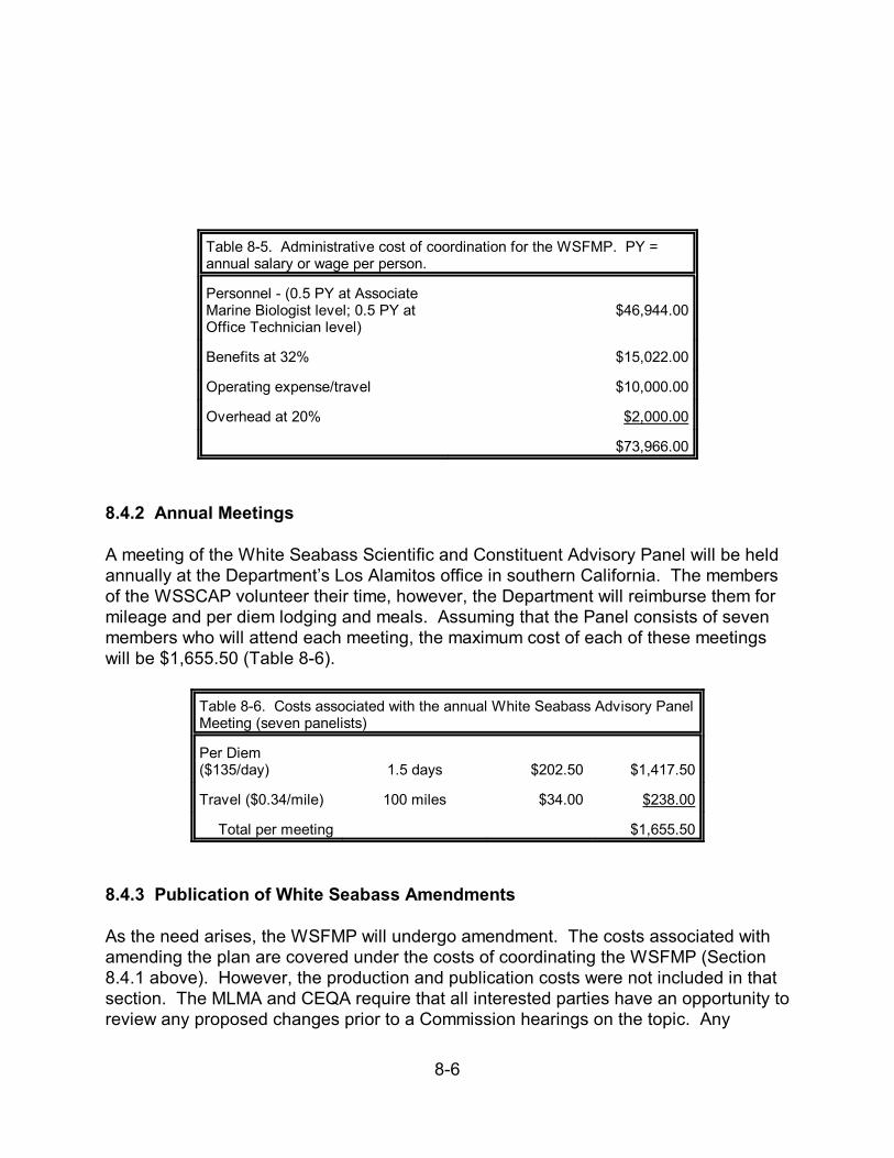
8-6
Table 8-5. Administrative cost of coordination for the WSFMP. PY =annual salary or wage per person.
Personnel - (0.5 PY at AssociateMarine Biologist level; 0.5 PY atOffice Technician level)
$46,944.00
Benefits at 32% $15,022.00
Operating expense/travel $10,000.00
Overhead at 20% $2,000.00
$73,966.00
8.4.2 Annual Meetings
A meeting of the White Seabass Scientific and Constituent Advisory Panel will be heldannually at the Department’s Los Alamitos office in southern California. The membersof the WSSCAP volunteer their time, however, the Department will reimburse them formileage and per diem lodging and meals. Assuming that the Panel consists of sevenmembers who will attend each meeting, the maximum cost of each of these meetingswill be $1,655.50 (Table 8-6).
Table 8-6. Costs associated with the annual White Seabass Advisory PanelMeeting (seven panelists)
Per Diem($135/day) 1.5 days $202.50 $1,417.50
Travel ($0.34/mile) 100 miles $34.00 $238.00
Total per meeting $1,655.50
8.4.3 Publication of White Seabass Amendments
As the need arises, the WSFMP will undergo amendment. The costs associated withamending the plan are covered under the costs of coordinating the WSFMP (Section8.4.1 above). However, the production and publication costs were not included in thatsection. The MLMA and CEQA require that all interested parties have an opportunity toreview any proposed changes prior to a Commission hearings on the topic. Any
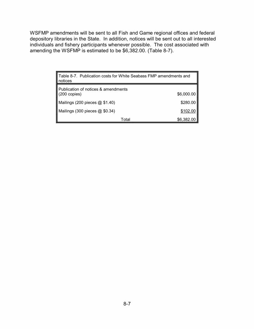
8-7
WSFMP amendments will be sent to all Fish and Game regional offices and federaldepository libraries in the State. In addition, notices will be sent out to all interestedindividuals and fishery participants whenever possible. The cost associated withamending the WSFMP is estimated to be $6,382.00. (Table 8-7).
Table 8-7. Publication costs for White Seabass FMP amendments andnotices
Publication of notices & amendments(200 copies) $6,000.00
Mailings (200 pieces @ $1.40) $280.00
Mailings (300 pieces @ $0.34) $102.00
Total $6,382.00
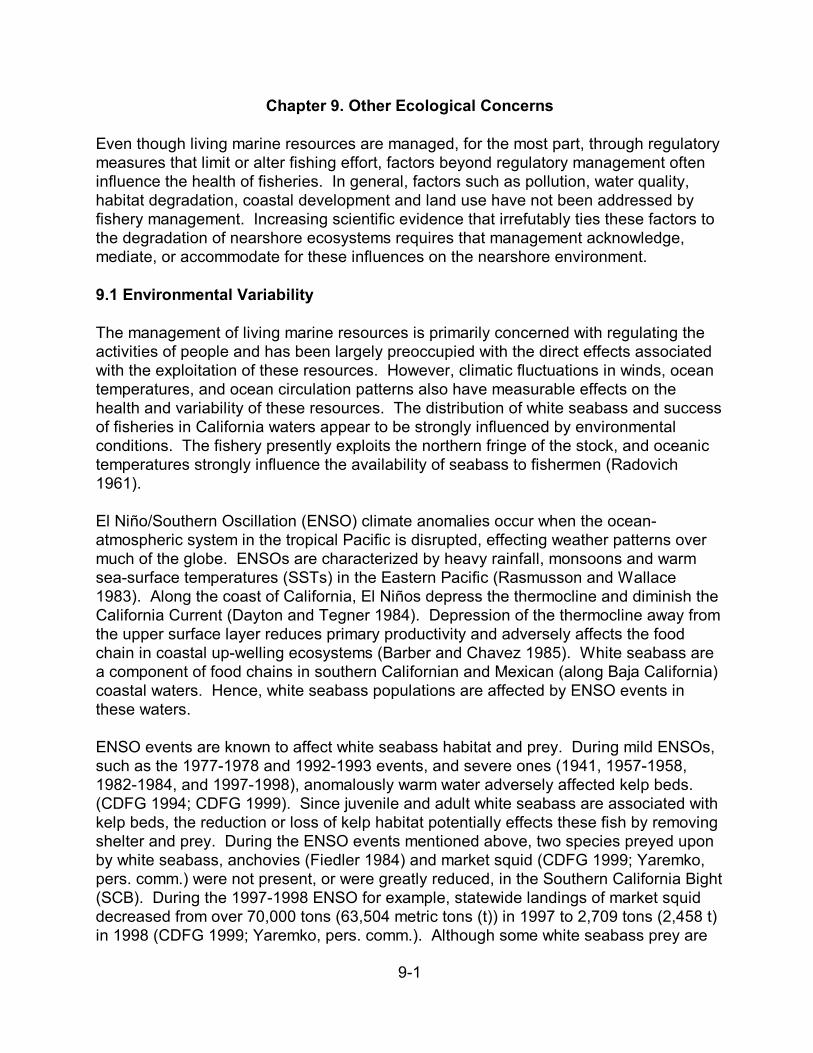
9-1
Chapter 9. Other Ecological Concerns
Even though living marine resources are managed, for the most part, through regulatorymeasures that limit or alter fishing effort, factors beyond regulatory management ofteninfluence the health of fisheries. In general, factors such as pollution, water quality,habitat degradation, coastal development and land use have not been addressed byfishery management. Increasing scientific evidence that irrefutably ties these factors tothe degradation of nearshore ecosystems requires that management acknowledge,mediate, or accommodate for these influences on the nearshore environment.
9.1 Environmental Variability
The management of living marine resources is primarily concerned with regulating theactivities of people and has been largely preoccupied with the direct effects associatedwith the exploitation of these resources. However, climatic fluctuations in winds, oceantemperatures, and ocean circulation patterns also have measurable effects on thehealth and variability of these resources. The distribution of white seabass and successof fisheries in California waters appear to be strongly influenced by environmentalconditions. The fishery presently exploits the northern fringe of the stock, and oceanictemperatures strongly influence the availability of seabass to fishermen (Radovich1961).
El Niño/Southern Oscillation (ENSO) climate anomalies occur when the ocean-atmospheric system in the tropical Pacific is disrupted, effecting weather patterns overmuch of the globe. ENSOs are characterized by heavy rainfall, monsoons and warmsea-surface temperatures (SSTs) in the Eastern Pacific (Rasmusson and Wallace1983). Along the coast of California, El Niños depress the thermocline and diminish theCalifornia Current (Dayton and Tegner 1984). Depression of the thermocline away fromthe upper surface layer reduces primary productivity and adversely affects the foodchain in coastal up-welling ecosystems (Barber and Chavez 1985). White seabass area component of food chains in southern Californian and Mexican (along Baja California)coastal waters. Hence, white seabass populations are affected by ENSO events inthese waters.
ENSO events are known to affect white seabass habitat and prey. During mild ENSOs,such as the 1977-1978 and 1992-1993 events, and severe ones (1941, 1957-1958,1982-1984, and 1997-1998), anomalously warm water adversely affected kelp beds.(CDFG 1994; CDFG 1999). Since juvenile and adult white seabass are associated withkelp beds, the reduction or loss of kelp habitat potentially effects these fish by removingshelter and prey. During the ENSO events mentioned above, two species preyed uponby white seabass, anchovies (Fiedler 1984) and market squid (CDFG 1999; Yaremko,pers. comm.) were not present, or were greatly reduced, in the Southern California Bight(SCB). During the 1997-1998 ENSO for example, statewide landings of market squiddecreased from over 70,000 tons (63,504 metric tons (t)) in 1997 to 2,709 tons (2,458 t)in 1998 (CDFG 1999; Yaremko, pers. comm.). Although some white seabass prey are

9-2
reduced during ENSO years, others such as sardines, increase in abundance.
The above normal water temperatures that result from ENSO events affect the migrationpatterns of white seabass and often increase the availability of these fish to Californiafishermen. During non-ENSO years, white seabass landings center around LosAngeles and San Diego, with few fish landed north of Point Conception. However,during ENSO events, catches north of Point Conception increase (Vojkovich and Reed1983; Karpov et al. 1995 ). For example, during the warm water years of 1957-1959,white seabass were caught as far north as Alaska (Radovich 1961).
9.2 Water Quality
Water quality is important to the health of marine organisms. Some characteristics,such as dissolved oxygen and water quality, are fundamental to life in the marineenvironment. Contamination can also have a profound effect on water quality. Contaminants enter coastal waters in a variety of ways, including ocean outfalls, rivers,ocean dumping, oil operations, and via current transport. Pollutants such as heavymetals, hydrocarbons, and agricultural chemicals (chlorinated hydrocarbons andorgano-phosphates) are of particular concern because of their toxicity to aquatic biota. These substances are not readily transported from the ecosystem, nor are they readilybroken down since the physical, chemical, and biological processes affecting them areslow. Polycyclic aromatic hydrocarbons (PAHs) and polychlorinated byphenyls (PCBs)are known to suppress the immune systems of mammals and increase theirsusceptibility to disease (Ward 1985). PCB’s and dichloro-diphenyl-trichloroethane(DDT) are known to disrupt the endocrine systems of organisms. These chemicals havea negative affect on an organism’s reproduction and other processes regulated byhormones. PAHs, PCBs, and DDT bioaccumulate in marine food chains, thus, the effectof these pollutants are most damaging to apex predators including marine mammals andhumans.
Juvenile white seabass are known to inhabit nearshore areas that are historically high inwater contamination. According to Fitch (1958), juvenile white seabass in nearshoreareas in Los Angeles County such as Belmont Shore, and areas within Santa MonicaBay, may be sensitive to some contaminants. White seabass he studied in these areashad experienced eye hemorrhaging, which often leads to blindness, and these fishfrequently had external parasites attached to fins and other body parts; a sign of stressto the immune system. Although these observations imply that white seabasspopulations may be affected by pollution, the specific effects on white seabass have notbeen studied.
9.2.1 Municipal Discharge
SewageHistorically, municipal wastewater (sewage) has been a significant source ofcontamination in southern California coastal waters and this problem is expected to
9-3
worsen as a result of increases in the human population and the volume of wastewaterdischarged from inland and coastal development projects (Napoli, pers. comm.).
Run-offUrban runoff and storm water contamination in the SCB is a region-wide problem. Thelimited data and high variability of storm water discharge volume make it difficult forresearchers to describe trends in run-off pollution. Associated pollutants include heavymetals, coliform bacteria, enteric viruses, pesticides, nutrients, PAHs, PCBs, organicsolvents, sediments, trash and debris (Swamikannu 1997). White seabass may bedirectly affected by run-off pollutants, and indirectly affected when preying on fish andinvertebrate species that have accumulated toxins in their tissues.
Urban runoff containing nitrogen and phosphorus can be detrimental to bioticcommunities in bays and estuaries. These pollutants cause plankton blooms which canlead to oxygen depletion and the possible reduction of other phytoplankton species thatare an important food source for juvenile fish and invertebrates. Planktonic blooms canalso harm the marine grasses and algae that serve as shelter for juvenile whiteseabass.
Industrial wastewater Industrial wastewater effluent is regulated by the United States EnvironmentalProtection Agency (EPA) through the National Pollution Discharge Elimination System(NPDES) permitting program. Non-power plant industrial dischargers have the potentialto be an important source of ocean contaminants because a large percentage of theireffluents can contain chemicals that are discarded as by-product of the industrial ormanufacturing process (Raco-Rands 1997). In 1995, industrial facilities accounted foronly 0.2% of the combined total volume of effluent generated by municipal wastewaterdischargers, power generating stations, and industrial facilities discharging into thebight. Contributions of constituents from industrial facilities were usually less than 1% ofthe combined mass emissions from these three sources with the exception of selenium(7%), arsenic (4%), and chromium (1%) (Raco-Rands 1997).
9.2.2 Dredge and Non-dredge Material Disposal
Dredging can make formerly isolated contaminants available, several of which areknown to bioaccumulate (SWRCB 1989). Three to five percent of dredged material isconsidered seriously contaminated. Examples of periodic dredging in marine habitatsinclude the removal of sediments from navigation channels and the creation of newprojects such as building marinas. The dredging process involves the removal orredistribution of sediments which changes the ecology of the dredged sea bottom.
Most contaminated material comes from dredging ports and harbors, or from areaswhere municipal and industrial discharges have polluted estuaries and coastal waters. Contaminant-laden sediments on the sea bottom may be resuspended, transported, andredeposited in areas far from the original source. Under certain conditions,

9-4
contaminants may "break free" from sediments (a process known as desorption) and bereleased into the water, making the bottom sediments not only a sink, but also a sourceof contaminants. Desorption is becoming less of a problem, however, because potentialsources are ‘capped’ or covered over with non-contaminated sediments. Pollutantscommonly found in dredge material include metals, chlorinated hydrocarbons, PCBs,DDT, PAHs, and other petroleum products (USHCMMF 1993).
White seabass are known to inhabit both Los Angeles Harbor and San Diego Bay(Emmett et al. 1991). Chemical analysis of outer Los Angeles Harbor sediments hasshown elevated levels of mercury, DDE (the degradation product of DDT), and tributyltin (TBT) in surface and near surface sediments (LAHD 1992). TBT is an activeingredient used in antifouling marine paints. Sediment toxicity was found to occurthroughout much of San Diego Bay, and it was found to be quite severe in isolatedareas near a naval station and in several of the marinas and boat harbors (NOAA 2000). It may be assumed that the effects of contamination from dredged sediments on whiteseabass would be similar to the effects related to municipal discharge and runoff.
Kelp and eelgrass beds are important white seabass habitat and could be significantlyimpacted by turbidity plumes created by dredging activity. Dredging and disposal ofdredge spoils contribute to elevated levels of turbidity. Turbidity from dredging activitieslowers light levels in the water column and leads to a decrease in primary production. Light, temperature, salinity, tidal range, and water motion influence the growth andproductivity of eelgrass beds which are important for larval seabass. Light most oftenappears to be the controlling factor. Processes that increase the overall turbidity of theestuarine environment could have marked effects on eelgrass density and distribution. Suspended sediment can interfere with photosynthesis by lowering light levels and alsocan interfere with kelp recruitment (LAHD 1992). Recent dredging projects that couldpotentially affect white seabass habitat include the 147 acre fill at Pier J in Long BeachHarbor, and the Pier 400 landfill project in Los Angeles Harbor.
The Marine Protection Research and Sanctuaries Act of 1972 (MPRSA) is the principlestatute regulating ocean disposal of dredged material.
9.2.3 Coastal Shipyards and Industrial Pollutants
ShipyardsMarine repair yard services typically include the repair and maintenance of mechanicalsystems, structural components, upholstery, electrical systems, and finished surfaces. Typical wastes generated from these operations include oils, coolants, lubricants, andcleaning agents; various chemicals, paints, and coatings; and dust from sanding, sandblasting, polishing and refinishing operations (EPA 1991). Wastes generated fromthese services that make their way into the marine environment could have adetrimental effect.
Tributyl tin (TBT) and copper are metal-based active ingredients used as pesticides in
9-5
antifouling marine paints. These substances are harmful to non-targeted marine lifeincluding fouling organisms (e.g., tunicates, bivalves, and algae). Metals can enter thewater column and bottom sediments through sloughing of paint while vessels are in useand through the discharge of anti-fouling paint chips and paint removal materials duringvessel maintenance activities. Studies have shown that low levels of TBT causeadverse reproductive effects on shellfish. Concerns about TBT's potency resulted in a1989 federal law banning TBT from all non-aluminum vessels less than 25 m (82 ft) inlength.
Elevated levels of pollutants exist in the bay bottom sediment adjacent to severalshipyards in San Diego Bay (SWRCB 2000). A study conducted at the naval shipyardin San Diego Bay found in water hull cleaning to be a minor source of coppercontamination. However, the leaching of copper from the hulls of naval vessels andrecreational vessels was found to be the major source of copper contamination in thebay (Valkirs 1994). Contamination from shipyards could impact white seabass and theirprey. However, pollution from shipyard contaminants is expected to decrease in thefuture due to increased restrictions in California on the criteria governing the allowablelevels of these pollutants.
Oil and gas productionCurrently, there are twenty-six production platforms, one processing platform, and sixartificial oil and gas production islands located in California offshore waters. Four of theplatforms are located within State waters and are offshore of Santa Barbara and Orangecounties. The principal wastes from oil production are produced water (PW) and drillingmuds (DM). Pollutants found in PW are oil and grease, metals, ammonia, phenols,cyanides, naphthalenes, and BTEX (benzene, toluene, ethylbenzene, and xylene) (MMS2000).
In addition, the possibility of oil spills associated with commercial oil production is apotential threat to white seabass and the nearshore environment in which they live. Thelargest oil spill in the Pacific Outer Continental Shelf (OCS) Region occurred in 1969,when a blowout occurred on Platform A off Santa Barbara and spilled an estimated80,000 barrels into the channel (Van Horn et al. 1988). No spill of this magnitude hassince occurred anywhere on the U.S. OCS. Since then, a number of preventivemeasures have been implemented (MMS 2000).
Research has demonstrated that hydrocarbons and other constituents of petroleumspills can, in sufficient concentrations, cause adverse impacts to fish (NRC 1985,GESAMP 1993). The effects can range from mortality to sublethal effects that inhibitgrowth, longevity, and reproduction. Benthic macrofaunal and intertidal communities,which provide food and habitat to fish, can be severely impacted. Fish can accumulatehydrocarbons from contaminated food and studies have demonstrated food webmagnification in fish. Fish have the capability to metabolize hydrocarbons and canexcrete both metabolites and parent hydrocarbons from the gills and the liver. Nevertheless, oil effects in fish can occur in many ways: histological damage,
9-6
physiological and metabolic perturbations, and altered reproductive potential (NRC1985).
The egg, early embryonic, and larval-to-juvenile stages of fish appear to be the mostsensitive to oil for several reasons (Malins and Hodgins, 1981). Embryos and larvaelack the organs found in adults that can detoxify hydrocarbons, and most are not mobileenough to avoid or escape spilled oil. In addition, the egg and larval stages of manyspecies, including white sea bass, are concentrated at surface waters where they aremore likely to be exposed to the most toxic components of an oil slick (MMS 2000) andthe dispersant chemicals used during oil spill clean-up operations (Napoli, pers. comm).
9.2.4 Fuel Use
According to the Environmental Protection Agency (EPA), spills that occur during boatfueling are a major contributor to the pollution of our waterways. Fuel is easily spilledinto surface waters from the fuel tank air vent while fueling a boat and oil is easilydischarged during bilge pumping (EPA 2001). Small oil spills released from motors andrefueling activities contain petroleum hydrocarbons which attach to waterbornesediments and can persist in the aquatic environment. Fish and shellfish larvae areextremely sensitive to even small amounts of petroleum products. For example, onegallon of used motor oil dumped in one million gallons of water is enough to kill half ofall Dungeness crab larvae (OSPR 2000). Emissions produced by two-cycle marineengines contain substances that have a negative impact on fish at all life stages (Balk1994). Private and commercial fishing vessels engaged in the take of white seabass, inaddition to other marine vessels operating in white seabass habitat, may have acumulative impact on white seabass populations due to the combined effects of fuelspilled into the water column.
9.3 Air Quality
California's concern about air quality is second only to the concern over water quality. The State has adopted air quality standards that are as stringent as federal standards(Aspen Environmental Group 1992). The impacts to air quality are of greater concern inhighly urbanized areas due to the existence of long term land-based impacts. Air qualityis affected by local climatic and meteorological conditions. Therefore, in the LosAngeles basin where there are persistent temperature inversions, predominant onshorewinds, long periods of sunlight, and topography that traps wind currents, the effects ofpollutants are more severe than along the coast of central California where one or moreof these components is missing.
Air quality is determined by measuring ambient concentrations of pollutants that areknown to have deleterious effects. The degree of air quality degradation is thencompared to health-based standards such as the California Ambient Air QualityStandards (CAAQS) and the National Ambient Air Quality Standards (NAAQS).

9-7
Air quality can be affected by emissions from gas and diesel engines in commercial andsport fishing vessels engaged in the take of white seabass. The calculation ofemissions from CPFV’s (commercial passenger fishing vessels) and commercial fishingvessels can be determined using the following emission factors for diesel fuel andgasoline:
DieselCarbon Monoxide (CO) = 110 lb/1000 gal fuelHydrocarbons (HC) = 50 lb/1000 gal fuelNitrogen Oxides (NOx) = 270 lb/1000 gal fuelSulfur Oxides (SOx) = 27 lb/1000 gal fuel
GasolineCarbon Monoxide (CO) = 1,822 lb/1000 gal fuelHydrocarbons (HC) = 11 lb/1000 gal fuelNitrogen Oxides (NOx) = 96 lb/1000 gal fuelSulfur Oxides (SOx) = 6 lb/1000 gal fuel
Table 9-1. South Coast vessel emissions (tons per day) (from Pera 1999)
Pollutant CPFV's All fishing vessels All marine vessels
CO 0 0.9 4.8
HC 0.1 0.3 3.3
NOx 0.6 6.3 44.2
SOx 0.1 1.1 26.7
PM 0 0.1 3.2
Pollution emissions released when vessels are underway are influence by a variety offactors including power source, engine size, fuel use, operating speed, and load. Emission factors can only provide a rough approximation of daily emission rates. Mostcommercial vessels and CPFV’s engaged in the take of white seabass have dieselengines. Currently, two-cycle diesel engines are most common, but four cycle engines,which are more efficient, are becoming more popular for CPFV use (Fadley,pers.comm.). Overall, fishing operations are responsible for less than 1% of the dailyemissions from all sources (mobile and nonmobile) in California (CARB 1989; 1991; 1994), and do not have a significant effect on air quality in the nearshore environment.
9.4 Importance of Habitat Loss, Degradation, and Modification
White seabass have differing habitat needs throughout their lives. The most criticalwhite seabass habitats influenced by human activities include nearshore waters, bays,
9-8
and estuaries. Many changes have occurred in each of these habitats over the lastcentury which could limit the survival of white seabass. In addition to the habitatdegradation caused by sources of pollution described above, 90% of California’sestuaries have been lost to coastal development projects.
9.4.1 Coastal Development and Land Use
Growth along the Southern California coast from Santa Barbara to San Diego has beenrapid. This region of the State accounts for more than 13% of the nation’s coastalpopulation (USDC 1999). Not surprisingly, southern California’s high coastal populationand growth rate has affected nearshore ecosystems.
Since the 1850s, 90% of the California’s coastal wetland acreage has been destroyed, and the remaining 10% is continuously exposed to increasing sedimentation fromeroding watersheds, raw sewage spills, and urban run-off pollutants. Because ofsoaring coastal land prices, wetlands are also subjected to the threat of being filled in. Water quality in some of these areas is very poor and high levels of toxins are present(Marcus 1989). Efforts are being made to change many of these potentially harmfulsituations by improving wastewater discharge requirements, erosion control, pollutioncontrol, and by the purchase of wetland areas for preservation. Juvenile white seabassare found in coastal wetland habitats, so recruitment could be affected by loss anddegredation of this habitat.
An important characteristic of two large coastal wetlands in southern California, MissionBay and San Diego Bay, is the presence of large eelgrass beds. (Marcus 1989). Eelgrass beds are a productive refuge for juvenile fish including white seabass. Eelgrass is an important and often critical component of the nearshore ecosystem. Eelgrass is commonly found in relatively calm estuarine environments and is vulnerableto coastal urbanization that heavily targets these same environments. White seabassare known to inhabit the Mission Bay and San Diego Bay wetlands during their secondyear of their life, and probably during other life stages as well (Crooke 1989b).Degradation of these eelgrass beds could have a negative effect on the survival ofyoung white seabass. Mitigation of this potential loss by the planting of larger eelgrassbeds, has been taking place for more than 15 years and continues to this day.
Another possible threat to white seabass habitat is the introduction of non-nativespecies, which can potentially out compete native species and alter ecosystems thatsupport white seabass. Recently, a green alga native to tropical waters, Caulerpataxifolia, was discovered in a San Diego county lagoon. C. taxifolia poses a substantialthreat to southern California coastal ecosystems, particularly to eelgrass beds and otherbenthic environments (Woodfield 2000).
Very small white seabass are often found with drifting kelp and debris near the surf linealong sandy beaches (Allen and Franklin 1988). The construction of breakwaters andjetties along the coast have altered this habitat by affecting erosion and sedimentation
9-9
processes. For example, approximately 77% of the coastline between Carpinteria andVentura contains engineered structures (Sherman 1997). The effects of this habitatalteration on white seabass are unknown.
9.4.2 Gear Use In the Marine Environment
Gear used in the commercial and sport fisheries of California can impact the nearshoreenvironment inhabited by white seabass. Fishing gear was found to be the mostcommon type of benthic anthropogenic debris in the central region (Point Dume to DanaPoint) of the SCB (Moore 2000). Gill nets used by commercial fishermen can be lostand this gear will continue to capture fish, mammals, and invertebrates which becomeentangled and die. In addition, species that are not targeted during active fishing, canincur physical trauma from contact with nets and this trauma can increase susceptibilityto disease. Finally, fishing debris such as lost hooks may be attractive to fish or otheranimals and cause injury if ingested, and the animals can become entangled in themonofilament line attached to the hooks.
9.4.3 Noise Effects in the Marine Environment
The response of animals to acoustic stimuli will depend upon the species and thecharacteristics of the stimuli (i.e., amplitude, frequency, pulsed or non-pulsed); season;ambient noise; physiological or reproductive state of the animal; and other factors. Thepossible adverse effects from loud sounds include discomfort, potential masking of othersounds, and behavioral responses resulting in avoidance of the noise source (MMS1987).
Very little data on the effects of sound on fish, larvae, and eggs have been collected. There are some data showing that sound can cause some damage to sensory cells ofthe ears of fishes, but not of the lateral line or cristae of the semicircular canals(vestibular receptor) (Hastings et al. 1996). Some behavioral studies of fish suggestthat anthropogenic sounds could affect a fish’s ability to detect biologically meaningfulenvironmental sounds (Gisiner 1998). This may have significance for white seabassbecause sciaenids are known to produce sounds which may be used to communicatewith one another (Moyle 1996). Thus, potential sources of anthropogenic noiseaffecting white seabass are commercial shipping activities, military operations, fishingand recreational vessels, and machinery associated with dredging and other forms ofcoastal construction. Currently, no data exist on the effects of human generated noiseon white seabass.
L-1
Literature Cited
Allen L.G. White Seabass: 2000. The King Croaker.www.csun.edu/~nmfrp/wonanob1.htm
Allen, L.G. and M.P. Franklin. 1988. Distribution and abundance of young-of-the-year white seabass, Atractoscion nobilis, in the vicinity of Long Beach Harbor, California in 1984-1987. Calif. Fish Game 74(4)245-248.
Allen, L.G. and M.P. Franklin. 1992. Abundance, distribution, and settlement of young-of-the-year white seabass Atractoscion nobilis in the Southern California Bight,1988-89. Fishery Bulletin, U.S. 90:633-641
Allen, L.G., D.J. Pondella, R. Ford, and M. Shane. 2001. Nearshore gill net samplingprogram for white seabass (age I-IV). Field Sampling Annual Report for 2000-2001.
Ally, J.R.R., D.S. Ono, R.B Read, and M. Wallace. 1991. Status of major southern California marine sport fish species with management recommendations, based
on analyses of catch and size composition data collected on board commercialpassenger fishing vessels from 1985 through 1987. Calif. Dept. Fish Game, Mar.Res. Div. Admin. Rep., No. 90-2.
Arntz, W.E. 1985 El Niño and Peru: positive aspects. Oceanus 27(2) :36-40.
Balk, L., G. Ericson, E. Lindesjoo, I. Petterson, U. Tjarnlund, and G. Akerman. 1994. Effects of exhaust from two-stroke outboard engines on fish. TemaNord. 528.
Barber, R.T., and F.P. Chavez. 1983. Biological consequences of El Niño. Science 222. p.1203-1210.
Bargmann, G., D. Hanan, S.F.Herrick, K.Hill, L.Jacobson, J.Morgan, R.Parrish, J.Sprattand J.Walker. 1998. Amendment 8 to the Northern Anchovy Fishery Management Plan incorporating a name change to: The Coastal Pelagic Species Fishery Management Plan. December 1998, D-9 pp.
Barlow, J., R. W. Baird, J. E. Heyning, K. Wynne, A. M. Manville II, L. F. Lowry, D. Hanan, J. Sease, and V. N. Burkanov. 1994. A review of cetacean and pinniped mortality in coastal fisheries along the west coast of the USA and Canada and the east coast of the Russian Federation. Rept. Int. Whaling Comm., Special Issue 15:405-425.
Bartley, D.M. and D.B. Kent. 1990. Genetic structure of white seabass populations fromthe southern California bight region: applications to hatchery enhancement.Calif. Coop. Oceanic Fish. Invest. Rep. 31: 97-105.
L-2
Barsky, K.C. 1998. Southern California Fisheries Monitoring Summary for 1995 and 1996. Calif. Dept. of Fish and Game, Mar. Reg. Admin. Rpt. 98-2. 30 pp.
Beeson, M. J. and D. A. Hanan. 1994. Effort estimates of California gill net fisheries: halibut-angel shark set net, shark-swordfish drift net, and white seabass-yellowtail set and drift net for the 1993 calendar year (January 1st, 1992 -December 31st, 1993). Final rep. coop. agreement no. NA37FX0265 submittedto NOAA/NMFS SWR, June 1994. 11 pp.
Beeson, M. J. and D. A. Hanan. 1996. An evaluation of pinniped-fishery interactions in California. Report to the Pacific States Fisheries Commission, 46 p. (Available from Pacific States Marine Fisheries Commission, 45 SE 82nd, Gladstone, OR 97027).
Brown, R. F. and S. J. Jeffries. 1993. Preliminary report on estimated marine mammal mortality in Columbia River fall and winter salmon gillnet fisheries, 1991-1992. Columbia River Area Marine Mammal Observer Program, 53 Portway St., Astoria, OR. 13 pp.
Bureau of Economic Analysis. 2000. Regional accounts data.
www.bea.doc.gov/bea/regional/data.htm. U.S. Dept. of Commerce. (01/01).
Bureau of Labor Statistics. 2000. CPI Inflation Calculator. http://stats.bls.gov/cpihome.htm
Bureau of Labor Statistics. 2000. Data. www.bls.gov/datahome.htm (2/01).
Bureau of Marine Fisheries. 1949. Commercial Fish Catches of California for the year 1947 With an Historical Review 1916-1947. Department of Natural Resources. Div. of Fish and Game. Calif. Fish Bull. 74:126-128.
Caddy, J.F. 1999. Fisheries management in the twenty-first century: will new paradigmsapply? Rev. Fish. Biol. Fish. 9:1-43.
California Air Resources Board. CARB. 1991a. Inventory of air pollutant emissions from marine vessels. Prepared by California Air Resources Board Mobile Source Division. Technical assistance by Booz, Allen, and Hamilton, Inc. 47 pp.
California Air Resources Board. 1991b. Methods for assessing air source emissions in California 1989. Sacramento, California. 100 pp.
California Air Resources Board. 1994. Emission inventory and -1991. Prepared by Technical Support Division. Air Resources Board. California Environmental Protection Agency. Sacramento, California. 36 pp. + appendices.
L-3
California Department of Fish and Game. 1998. Informational Bulletin-Marine Region 8-14-98. 2 pp.
California Department of Fish and Game. 1990. Alternative gear development program,final report. 149 pp.
California Department of Fish and Game 1991. Final program environmental document,ocean sportfishing regulations. 222 pp.
California Department of Fish and Game. 1991. Draft supplement environmental document: ocean sportfishing, white seabass. 75 pp.
California Department of Fish and Game. 1994. Comprehensive hatchery plan (CHP) for the enhancement of white seabass (Atractoscion nobilis): Including Techniques for Culturing , Transporting, Tagging, Releasing, and Bioeconomic Modeling. 38pp. + appendices.
California Department of Fish and Game. 1994. Giant and bull kelp commercial andsport fishing regulations: draft environmental document.
California Department of Fish and Game. 1999. Review of some California fisheries for1998: pacific sardine, pacific mackerel, pacific herring, market squid, sea urchin,groundfishes, swordfish, sharks, nearshore finfishes, abalone, dungeness crab,prawn, ocean salmon, white seabass and recreational. Calif. Coop Oceanic Fish.Invest. Rep. 40:9-28.
California Department of Fish and Game 1999. Recovered hatchery-produced legal-size white seabass. The Reef Report. Vol.4 No.12. 4 pp.
California Department of Fish and Game 2000. Giant and bull kelp commercial andsport fishing regulations, draft final environmental document.
California Department of Fish and Game. Office of Spill Prevention and Response(OSPR). 2000. Oil spills. www.dfg.ca.gov/Ospr/spills.html (11/00).
California Department of Fish Game. 2001. Past and Ongoing Essential FisheryInformation (EFI): Collection and Future Needs prepared by C. Dawson. In DraftMaster Plan: A Guide for the Development of Fisheries Management Plans. pp.5-1 - 5-2.
California Department of Finance. 2000. California demographics. www.dof.ca.gov/html/demograp/druhpar.htm. (01/01).
California Employment Development Department. 2000. Occupational and employmentwage data. Labor market information. www.calmis.cahwhet.gov (01/01).
L-4
California Technology Trade and Commerce Agency. 2000. Labor force andoccupations. www.commerce.ca.gov/california/economy/es202. (02/01).
California Water Quality Control Board, Region 9. 2000 Sediment investigation andcleanup at shipyards. www.swrcb.ca.gov/rwqcbp/Programs/Shipyards.html(12/12/00).
Chen, M.F., D. Henry-Ford, and J.M. Groff. 1995. Isolation and Characterization ofFlexibacter maritimus from Marine Fishes of California. Journal of AquaticAnimal Health. Vol. 7:318-326.
City of Los Angeles. 2000. Demographics. www.lacity.org/COUNCIL/cd9/demogra.htm(2/01).Claritas Inc. 1996. Complimentary marketview comparison report for the San Pedro Chamber of Commerce. 11pp.
Clark, F.N. 1930. Size at first maturity of the white seabass (Cynoscion nobilis). Calif. Fish Game 16(4):319-323.
Clark, W.A. 1991. Groundfish exploitation rates based on life history parameters. Can. J. Fish. Aquat. Sci. 48:734-750.
Collins, R.A. 1981. Pacific coast croaker resources. Pp. 41-49. In: Marine Recreational Fisheries---6 (Henry Clepper, ed.) Sport Fishing Institute, Washington, D.C.
Collyer, R.D. 1949. Marine sportfishing. In: The commercial fish catch of California for the year 1947 with an historical review 1916-1947. Calif. Dept. Fish Game FishBull. 74:180-183.
Committee Staff on Merchant Marine and Fisheries, US House of Representatives(USHCMMF). 1993. The effects of ocean disposal of contaminated materials onour marine environment and potential alternatives to ocean disposal ofcontaminated material. United States House of Representatives. WashingtonD.C. p.50-59.
County of Santa Barbara (CSB). 2001. Census data. www.co.santa-barbara.ca.us/cao/specialprojects/redistricting/censusdata.htm. (5/01).
Croker, R.S. 1937. White Seabass. In: The commercial fish catch of California for the year 1935. Calif. Dept. Fish Game Fish Bull. 49:1-73 pp.
Crooke, S.J. 1989a. The ocean enhancement and hatchery program 1988. Calif. Dept.Fish Game, Rpt. to the Legislature. 25 pp.
Crooke, S.J. 1989b. The ocean enhancement and hatchery program 1989. Calif. Dept.Fish Game, Rpt. to the Legislature. 22 pp.
L-5
Crooke, S.J. 1990. The ocean enhancement and hatchery program 1990. Calif. Dept.Fish Game, Rpt. to the Legislature. 6 pp.
Dayton, P.K., and M.J. Tegner. 1984. Catastrophic storms, El Niño and patch stability in a southern California kelp community. Science 224:283-285.
Dayton, P.K. and A.D. MacCall. 1992. Pre-exploitation Abundances of Important LargeRecreational and Commercial Fishes off Southern California. University ofCalifornia, San Diego. R/F-125. In California Sea Grant biennial report ofCompleted projects 1988-90. Calif. Sea Grant, Publication R-CSGCP-033. Pp91-96.
Donohoe, C.J. 1997. Age, growth, distribution, and food habits of recently settled whiteseabass, Atractoscion nobilis, off San Diego County, California. Fish. Bull.95(4): 709-721.
Eldridge, M.B. 1977. Factors influencing distribution of fish eggs and larvae over eight 24-hr samplings in Richardson Bay, CA. Calif. Fish Game 63(2):101-116.
Emmett, R.L., S.L. Stone, S.A. Hinton, and M.E. Monaco. 1991. Distribution andabundance of fishes and invertebrates in west coast estuaries, Volume II:species life history summaries. ELMR Rep. No. 8. NOAA/NOS StrategicEnvironmental Assessments Division, Rockville, MD, 329 pp.
Environmental Protection Agency. 1991. Guides to pollution prevention: the marinemaintenance and repair industry. EPA/625/7-91/015. pp.5-19.
Environmental Protection Agency. 2001. Draft: national management measures tocontrol nonpoint source pollution from marinas and recreational boating.www.epa.gov/owow/nps/mmsp/index.html (12/11/00).
Feder, H.M., C.H. Turner, C. Limbaugh. 1974. Observations on fishes associated with kelp beds in southern California. Calif. Dept. Fish Game, Fish Bull. 160:1-144
Fiedler, P.C., 1984. Some effects of El Niño 1983 on the northern anchovy. Calif. Coop.Oceanic Fish Invest. Rp, 25:53-58.
Fitch, J.E. 1958. Offshore fishes of California. Calif. Dept. Fish and Game.
Fitch, J.E., R.J. Lavenberg. 1971. Marine food and game fishes of California. Univer. ofCalif. Press.
Forney, K.A., J. Barlow, M.M. Muto, M. Lowry, J. Baker, G. Cameron, J. Mobley,C. Stinchcomb, J.V. Carreta. 2000. Draft U.S. Pacific Marine Mammal Stock
L-6
Assesments:2000. NOAA technical memorandum NOAA-TM-NMFS-SWFSC-XXX. 302 pp.
Franklin, M.P. 1997. An investigation into the population structure of white seabass(Atractoscion nobilis), in California and Mexican waters using microsatellite DNAanalysis. Phd Dissertation. University of California Santa Barbara. 109 pp.
GESAMP (Group of Experts on the Scientific Aspects of Marine Pollution). 1993.Impact of oil and related chemicals on the marine environment. Reports andStudies No. 50. International Maritime Organization, London, 180+ix pp.
Ghanzanshahi, J., T. D. Huchel, and J.S. Devinny. 1983. Alteration of southernCalifornia rocky shore ecosystems by public recreational use. Journal of Environmental Management. 16:379-394
Gisiner, R. 1998. Workshop on the effects of anthropogenic noise in the marineenvironment. Marine Mammal Science Project. Office of Naval Research. 140pp.
Goodyear, C.P. 1993. Spawning stock biomass per recruit in fisheries management: foundation and current use. In S.J. Smith, J.J. Hunt, and D. Rivard [eds.]. Riskevaluation and biological reference points for fisheries management. Can. Spec.Publ. Fish. Aquat. Sci. 120:67-81.
Hanan, D. A., D. B. Holts, and A. L. Coan, Jr. 1993. The California drift gill net fisheryfor sharks and swordfish, 1981-82 through 1990-91. Calif. Dept. Fish Game,Fish. Bull. 175:1- 95.
Hanan, D. A., L. M. Jones, and R. B. Read. 1989. California sea lion interaction and depredation rates with the commercial passenger fishing vessel fleet near SanDiego. Calif. Coop. Oceanic Fish. Invest. Rep. 30:122-126.
Hartmann, A.R. 1980. Southern California partyboat angler survey. Calif. Dept. FishGame, Mar. Res. Admin. Rep. (80-7), 33 pp.
Herbinson, K.T. 1981. 316(b) Fish impingement inventory. Res. Develop. Ser.Southern Californnia Edison, Rosemead, CA. 178pp.
High, W.L. 1984. Some consequences of lost fishing gear. In Proceedings of theworkshop on the fate and impact of marine debris 27-29 November 1984,Honolulu Hawaii. Shomura and Yoshida (eds.). US Dept. of Commerce. p. 430-437.
Hill, P.S. 1999. Gray whale entanglements in California, Oregon/Washington, andAlaska, 1990-98. Unpubl. doc. submitted to the Workshop to Review the Statusof the Eastern North Pacific Stock of Gray Whales, 16-17 March 1999, Seattle,
L-7
WA.
Hill, K.T. , and N. Schneider. 1999. Historical logbook databases from California’sCommercial Passenger Fishing Vessel (Partyboat) Fishery, 1936-1997. SIOReference Series No. 99-19. University of California, San Diego. 13 pgs +tables.
Hubbs Seaworld Research Institute. 2000. Fisheries and Aquaculture ResearchPrograms. Publications. http://www.hswri.org/orehpublications.htm (26 Feb.2001).
Karpov, K.A., D.P. Albin, W.H. Van Buskirk. 1995. The marine recreational fishery innorthern and central California, a historical comparison (1958-86), status ofstocks (1980-86), and effects of changes in the California current. Calif. Dept.Fish Game, Fish Bull. 176:1-192.
Karpov, K.A., P.L. Haaker, I.K. Taniguchi and L. Rogers-Bennett. 2000. Serialdepletion and the collapse of the California abalone (Haliotis spp.) fishery. InWorkshop on Rebuilding Abalone Stocks in British Columbia. A. Campbell, ed.Cn. Spec. Publ. Fish. Aquat. Sci. 130.
Kent, D.B. and R.F. Ford. 1990. Determination of the natural mortality rate for juvenile white seabass (Atractoscion nobilis) and California halibut (Paralichthyscalifornicus). Ann. Prog. Rpt. to ORHEP. 18 pp.
Leeworthy, V. and P. Wiley. 2000. A socioeconomic overview of the Santa Barbara andVentura counties as it relates to marine related industries and activities. Channelisland marine sanctuary revised management plan. NOAA. p.1-60.www.cinms.nos.noaa.gov/pdf/SocEconOV.pdf (02/05/01).
Los Angeles Harbor Dept., and US Army Corps of Engineers. 1992. Finalenvironmental impact statement: environmental impact report, deep draftnavigation improvements, Los Angeles and Long Beach harbors, San PedroBay, California.
Love, M.S. and M. Moser. 1983. A Checklist of Parasites of California, Oregon, andWashington Marine and Estuarine Fishes. NOAA Technical Report NMFSSSRF-777. US Department of Commerce. National Oceanic and AtmosphericAdministration. National Marine Fisheries Service. p. 207-208
Lukacovic, R. 1999. 1999 Striped bass circle hook study. http://www.dnr.state.md.us/ fisheries/fishingreport/crsb.html
MacCall A.D., G.D.Stauffer, and J.P.Troadec. 1976. Southern California recreational and commercial marine fisheries. Mar. Fish. Rev. 38(1):1-32.
L-8
Malins, D.C., and H.O. Hodgins. 1981. Petroleum and marine fishes: A review ofuptake, disposition, and effects. Environmental Science and Technology,15(11):1272-1280.
Marcus, L. 1989. In The coastal wetlands of San Diego County State CoastalConservancy, Sacramento, Ca. 65 pp.
Maxwell, W.D. 1977a. Age composition of California barracuda, Sphyraena argentea; Pacific bonito, Sarda chiliensis; white seabass, Cynoscion nobilis; and yellowtail,Seriola dorsalis from southern California partyboats 1972-74. Calif. Dept. FishGame, Mar. Res. Admin. Rpt. (77-3). 23 pp.
Maxwell, W.D. 1977b. Progress Report of Research on white seabass, Cynoscionnobilis, Calif. Dept. Fish Game, Mar. Res. Admin. Rpt. (77-14), 13pp.
Maxwell, W.D. 1975. The croakers of California. Calif. Dept. Fish Game, Mar. Res.16 pp.
MBC Applied Environmental Sciences. 2001. National Pollutant Discharge EliminationSystem 2000 Receiving Water Monitoring Report. AES Huntington Beach L.L.C.Generating Station Orange County, California. 2000 Survey. 52pp.
McGinnis, M.V. 1990. The multiple uses of the coastal zone and ocean offshore California. Calif. Sea Grant College, Working Paper No. P-T-51. 23 pp.
McKee-Lewis, Kimberly K., and Robert B. Read. 1997. Southern California fisheriesmonitoring summary for 1993 and 1994. Calif. Dept. Fish Game, Mar. Res. Div.Adm. Rep. (97-4). 24 pp.
McWilliams, B. and G. Goldman. 1994. Commercial and recreational fishing inCalifornia - their impact on the state economy. University of California. p. 1-26.
Minerals Management Service. 1987. Northern California proposed oil and gas leasesale 91: draft environmental impact statement. Vol 1. P. IV40-IV46.
Minerals Management Service. 2000. Draft OCS environmental assessment: extended-reach exploratory drilling project cavern point unit, leases OCS-P 0210 andOCS-PO527 Venoco Inc. and Poseiden Petroleum LLC. 62pp.www.mms.gov/omm/pacific/lease/cpufullea.pdf (12/00).
Moore, S.L., and M.J. Allen. 2000. Distribution of anthropogenic and natural debris onthe mainland shelf of the southern California bight. Southern California CoastalWater Research Project. p.1-6.
Moser H.G., D.A. Ambrose, M.S. Busby, J.L. Butler, E.M. Sandknop, B.Y. Sumida, and
L-9
E.G. Stevens. 1983. Description of early stages of white seabass, Atractoscionnobilis, with notes on distribution. Calif. Coop. Oceanic Fish. Invest. Rep. 24:182-193.
Moyle, P.B., and J.J. Cech. 1996. Fishes: an introduction to ichthyology. University ofCalifornia , Davis. Prentice Hall, New Jersey. p.174.
Murray, S.N. 1998. Effectiveness of marine life refuges on southern California shores.In California and the world ocean ‘97. Taking a look at California’s oceanresources: an agenda for the future, O.T. Magoon, H. Converse, B. Baird and M.Miller-Hensen, eds. Reston: American Society of Civil Engineers, p.1453-1465.
National Geographic Society. 1987. Field guide to the birds of north America. Scott,Shirley, ed. 464 pp.
National Marine Fisheries Service 2000b. Biological opinion on issuance of permitunder Section 101 (a) (5) (E) of the Marine Mammal Protection Act (MMPA) tothe California/Oregon drift gilllnet fishery for the taking of listed species underthe Endangered Species Act (ESA) and the continued implementation of thePacific Offshore Cetacean Take Reduction Plan (plan). Endangered SpeciesDivision, Office of Protected Resources, NMFS. 127 pp.
National Marine Fisheries Service and United States Fish and Wildlife Service. 1998a.Recovery plan for the U.S. Pacific populations of the east pacific green turtle(Chelonia mydas). p.40.
National Marine Fisheries Service and United States Fish and Wildlife Service. 1998b.Recovery plan for the U.S. Pacific populations of the leatherback turtle(Demochelys coriacea). p.55.
National Marine Fisheries Service and United States Fish and Wildlife Service. 1998c.Recovery plan for the U.S. Pacific populations of the loggerhead turtle (Carettacaretta). p.49.
National Marine Fisheries Service and United States Fish and Wildlife Service. 1998d.Recovery plan for the U.S. Pacific populations of the olive ridley turtle(Lepidochelys olicacea). p43.
National Oceanic and Atmospheric Administration (NOAA). 1998. Marine debris. Technical Memorandum NMFS F/AKR-9. Editors: Alan R. Bunn and James M.Coe. U.S. Department of Commerce, National Marine Fisheries Service.
National Oceanic and Atmospheric Organization (NOAA). (1999). Sediment toxicity. InNOAA’s state of the coast report. www.state-of-coast.noaa.gov/bulletins/html/sed(12/00).
L-10
National Research Council (NRC). 1985. Oil in the sea: inputs, fates, and effects.National Academy Press, Washington, DC. 601+xviii pp.
North, W.J., D.E. James, and L.G. Jones. 1993. History of kelp beds (Macrocystis) inOrange and San Diego Counties, California. Proc. Fourteenth Int. SeaweedSym. 14:277-283.
Norton, J., D. McLain, R. Brainard, and D. Husby. 1985. The 1982-83 El Niño event ofBaja and Alta California and its ocean climate context. In El Niño North: Niñoeffects in the eastern subarctic pacific ocean. W.S. Wooster and D.L. Fluharty,(eds). p.44-72.
Pacific Fishery Management Council. 1998. The coastal pelagic species fisherymanagement plan draft amendment eight. p.A78-A90.
Pacific Fisheries Management Council. 2000. DRAFT Research and data needs 2000 -2002. Fisheries Research and Data. http://www.pcouncil.org (22 Feb. 2001).
Pacific States Marine Fisheries Commission. 2000. EFIN. Employment and wage data.www.psmfc.org/efin/dataser_desc.html#WAGE-CA (2001).
PADI. 2001. PADI Diver Statistics. Facts for commonly asked questions.
Http://www.padi.com/news/stats/default.stm (29 Jan. 2001).
Pera, C.J. 1996. Marine vessel emissions inventory and control strategies. South CoastAir Quality Management District. Acurex Environmental final report FR-119-96.Sections 10-13.
Pera, C.J. 1999. Analysis of marine emissions in the South Coast air basin. USEnvironmental Protection Agency. Arcadis final report FR-99-100.
Pinkas, L., J.C. Thomas, and J.A. Hanson. 1963. Marine sport fish survey of southern California piers and jetties, 1963. Calif. Dept. Fish Game 53(2):88-104.
Pinkas, L., M.S. Oliphant and C.W. Haugen. 1968. Southern California sport fishing survey: private boats, 1964; shoreline, 1965-1966. Calif. Dept. Fish Game, FishBull. 143:1- 42.
Raco-Rands, V. 1997. Characteristics of effluents from nonpower industrial facilities in1995. Southern California Coastal Water Research Project. 16pp.www.sccwrp.org/annrpt/97/ (11/00).
Raco- Rands, V. 1998. Characteristics of effluents from large municipal wastewatertreatment facilities in 1996. Southern California Coastal Water Research Project.36pp. www.sccwrp.org/annrpt/98/ (11/00).
L-11
Rasmusson, E. M., and J. M. Wallace. 1983. Meteorological aspects of the ElNiño/Southern Oscillation. Science. 222:1195-1202.
Recreational Fisheries Information Network (RecFIN). 2001. Ed. Wade Van Buskirk. Pacific States Marine Fisheries Commission. 2001. www.recfin.org
Radovich, J. 1961. Relationships of some marine organisms of the northeast Pacific towater temperatures, particularly during 1957 through 1959. Calif. Dept. Fish Game, Fish Bull. 54:1- 62.
Restrepo, V.R., G.G. Thompson, P.M. Mace. W.L. Gabriel, L.L. Low, A.D. MacCall,R.D. Methot, J.E. Powers, B.L. Taylor, P.R. Wade, and J.F. Witzig. 1998.Technical guidance on the use of precautionary approaches to implementingnational standard 1 of the Magnuson-Stevens Fishery Conservation andManagement Act. NOAA Technical Memorandum NMFS-F/SPO-#. 22 pp.
Roberts, R.J. 1975. The effects of temperature on diseases and their histopathologicalmanifestations in fish. In The Pathology of Fishes. Edited by W.E. Ribelin andG. Migaki. University of Wisconsin Press. Pp. 477-496.
Salt Water Sportsman.1999. Hooking mortality matters.www.saltwatersportsman.com/news/fishing/990428.6.html
Sherman, D.J. 1997. Human impacts on California’s coastal sediment supply. InCalifornia and the world ocean ‘97. University of Southern California Sea Grant.p.551-559.
Skogsberg, T. 1925. White seabass. In: Preliminary investigations of the purse seine industry of southern California. Calif. Div. Fish Game, Fish Bull. 9:53-63.
Skogsberg, T. 1939. The fishes of the family Sciaenidae (croakers) of California. Calif.Div. Fish Game, Fish Bull. 54:1- 62.
Smith, F.G. (1975). Crustacean parasites of marine fishes. In The Pathology of Fishes. Edited by W.E. Ribelin and G. Migaki. University of Wisconsin Press. Pp. 189-201.
Squire, J.L., Jr. 1972. Apparent abundance of some pelagic marine fishes off thesouthern and central California coast as surveyed by an airborne monitoringprogram. U.S. Fish. Bull 70(3):1005-1019.
Squire, J.L., Jr. 1983. Warm water and southern California recreational fishing: a briefreview and prospects for 1983. Mar. Fish Rev. 45(4-6):27-34.
Swamikannu, X. 1997. An integrated strategy for managing urban runoff pollution in
L-12
Los Angeles county. In Stormwater runoff into Santa Monica Bay: sources andimpacts. California and the world ocean ‘97. San Diego, California. p.876-887.
Tegner, M.J., and P.K. Dayton. 1987. El Niño effects on southern California kelp forestcommunities. Advances in Ecological Research 17:243-279.
Thomas, J.C. 1968. Management of the white seabass (Cynoscion nobilis) in California waters. Calif. Dept. Fish Game, Fish Bull. 142:1- 34.
Thompson, C.J., and S. J. Crooke. 1991. Results of the southern California sportfisheconomic survey. NOAA NMFS Technical Memorandum NOAA-TM-NMFS-SWFSC-78, 70 pp.
United States. 1973. Atomic Energy Commission. Nuclear generating station, Diablo Canyon units 1 & 2, Pacific Gas and Electric Co., Docked Nos. 50-275 and 50-323, Final Environmental Statement. May 1973.
United States. 1974. Department of the Interior, Bureau of Land Management. Asummary of knowledge of the Southern California Coastal Zone and offshoreareas, vol.1 - physical environment. Prep. By: Southern California OceanStudies Consortium of the California State Universities and Colleges. ContractNo. 08550-CT4-1.
United States. 1990. Department of Commerce, National Ocean Survey. Coastalenvironmental quality in the United States, 1990-chemical contamination insediments and tissues. October 1990. 34 pp.
United States Census Bureau. 2000. www.census.gov/ (01/01).
United States Dept. of Comm. 1986. Marine Recreational Fisheries Statistics Survey,Pacific Coast, 1985. Current Fish. Stat. No. 8328., Nat. Oceanic andAtmospheric Admin., Nat. Mar. Fish. Ser.
United States Dept. of Comm. 1999. Trends in United States coastal regions 1970-1998. www.state-of-coast.noaa.gov/natdialog/index.html (12/11/00).
United States Fish and Wildlife Service. 1995. Introduction to fish health management.B.A. Lasee, Editor. U.S. Dept. of Interior. 139 pp.
United States Fish and Wildlife Service. 1997. Recovery plan for the threatenedmarbled murrelet in Washington, Oregon, and California. Region 1, Portland,Oregon. 286 pp.
Valkirs, A.D. , Davidson, Kear, and Fransham. 1994. Environmental effects from in-water hull cleaning of ablative copper antifouling coating. Technical Document
L-13
2662. NCOSC. RDT&E Division.
Van Horn, W., A. Melancon, and J. Sun (eds.). 1988. Outer continental shelf oil andgas program: cumulative effects. U.S. Department of the Interior, MineralsManagement Service, Herndon, VA. OCS Report MMS 88-0005.
Vojkovich, M. 1992. White seabass. In California’s living marine resources and theirutilization. Ca Sea Grant. p. 165-167.
Vojkovich, M., Miller, and D. Aseltine. 1990. A summary of 1983-1989 southernCalifornia gill net observation data with an overview on the effects of gill nets onrecreational catches. Sport Fish Restoration Proj. F-50-R Final Rep. 52 pp.
Vojkovich, M., K.E. Miller, and D.A. Aseltine. 1989. Summary of nearshore gill netobservation data for 1988 and 1989. Calif. Dept. Fish Game. Mar. Res. Div. 45pp.
Vojkovich, M., K.E. Miller, and R.J. Reed. 1988. Progress report: southern Californianearshore gill and trammel net study 1987. Calif. Dept. Fish Game. Mar. Res.Div. 57 pp.
Vojkovich, M., R.J. Reed, and K.A. Hieb. 1987. Progress report: southern Californianearshore gill and trammel net study 1986. Calif. Dept. Fish Game. Mar. Res.Div. 54 pp.
Vojkovich, M., R.A. Collins, R.J. Reed, and K.A. Heib. 1986. Progress report: southernCalifornia nearshore gill and trammel net study 1985. Calif. Dept. Fish Game.Mar. Res. Div. 50 pp.
Vojkovich, M., R.A. Collins, and R.J. Reed. 1985. Progress report: southern Californianearshore gill and trammel net study 1984. Calif. Dept. Fish Game. Mar. Res.Div. 40 pp.
Vojkovich, M., R.A. Collins, A. R. Hartmann, and R.J. Reed. 1984. Progress report:southern California nearshore gill and trammel net study 1983. Calif. Dept. FishGame. Mar. Res. Div. 33 pp.
Vojkovich, M. and R.J. Reed. 1983. White seabass, Atractoscion nobilis, in California-Mexican waters: status of the fishery. Calif. Coop. Oceanic Fish. Invest. Rep. 24:79-83.
Wallace, R.K., W. Hosking, and S.T. Szedlmayer. 1994. Fisheries Management forFishermen: A manual for helping fishermen understand the federal managementprocess. MASGP-94-012 Auburn University Marine Extension & ResearchCenter. Sea Grant Extension. NOAA Award No. NA37FD0079. 56 pp.
L-14
Ward, E.C., M.J. Murray and J. H. Dean. 1985. Immunotoxicity of nonhalogenatedpolycyclic aromatic hydrocarbons. in J. Dean, M. I. Luster and A.E. Munson,editors. Immunotoxicology and Immunopharmacology. Raven Press, New York.p.291-313
Weinstein, M.P. 1981. Biology of adult sciaenids. Pp. 125- 138 in Marine Recreational Fisheries---6 (Henry Clepper, ed.) Sport Fishing Institute, Washington, D.C.
Welsh, W. W. and C.M. Breder, Jr. 1923. Contributions to the life histories of the Sciaenidae of the eastern United States coast. Bull. U.S. Bur. Fish. 39:141-201.
Whitehead, S.S. 1930a. White seabass. In The commercial fish catch of California forthe year 1928. Bureau of Comm. Fish., Calif. Div. Fish Game, Fish Bull. 20: 48-51.
Whitehead, S.S. 1930b. Analysis of boat catches of white seabass (Cynoscion nobilis)at San Pedro, California. Calif. Div. Fish Game, Fish Bull. 21:1- 27.
Wine, V. 1978. Southern California independent sport fishing survey annual report No.2. Calif. Dept. Fish Game, Mar. Res. Admin. Rep. (78-2), 79 pp.
Wine. V. 1979. Southern California independent sport fishing survey annual reportNo.3. Calif. Dept. Fish Game, Mar. Res. Admin. Rep. (79-3), 100 pp.
Wine. V. 1980. Southern California pier fishermen: How familiar are they with the sport fishing regulations? Calif.Dept. Fish Game, Mar. Res. Admin Rep. (80-2), 6 pp.
Wine. V. 1982. Southern California marine sport fishing: private-boat catch and effort during 1981. Calif. Dept. Fish Game, Mar. Res. Admin. Rep. (82-7), 78 pp.
Woodfield, R. 2000. Noxious algae found in southern California coastal waters.www.swr.nmfs.noaa.gov/hcd/caulerpa.htm. (12/00).
Young, P.H. 1969. The California Partyboat Fishery 1947 - 1967. Calif. Dept. FishGame, Fish Bull. 145:1- 91.
Young, P.H. 1973. The status of the white seabass resource and its management. Marine Resources Technical Report 15. Calif. Dept. Fish Game.

L-15
Personal Communications
Arenas, Pablo. Fisheries Biologist. Inter-American Tropical Tuna Commission. La Jolla,CA.
Athens, Tim. Commercial fisherman. F/V Outer Banks. Channel Islands Harbor, CA.
Carreta, James. National Marine Fisheries Service. La Jolla, CA.
Collins, Dr. Charles. Ornithologist. California State University Long Beach, LongBeach, CA.
Conroy, Mike. Captain of the CPFV Aztec. Pierpoint Landing. Long Beach. CA.
Crooke, Steve. Senior Biologist. CDFG. Los Alamitos, CA.
Fadley, Mike. CPFV captain. Redondo Sportfishing. Redondo Beach, CA.
Forney, Dr. Karen. National Marine Fisheries Service. Santa Cruz, Ca.
Horeczko, Michell. Marine Biologist. CDFG. Los Alamitos, CA.
Lum, Mathew. Freediver/spear fisherman. Santa Barbara, CA.
Mardesich, Steve. Commercial fisherman. San Pedro, CA.
Napoli, Thomas. Staff Environmental Scientist. CDFG. Los Alamitos, CA.
O’Reilly, Kelly. Marine Biologist. CDFG. Los Alamitos, CA.
Rasmussen, Andrew. Commercial fisherman. Santa Barbara, CA.
Romanowski, Paul. Freediver/spear fisherman. Fathomiers. Los Angeles, CA.
Yaremko, Marci. Associate Marine Biologist. CDFG. La Jolla, CA.
P-1
List of Preparers
Principal Authors
Larson, Mary. Associate Marine Biologist. CDFG. Los Alamitos, CA
Horeczko, Michelle. Marine Biologist. CDFG. Los Alamitos, CA
Hanan, Dr. Doyle, Senior Biologist. CDFG. La Jolla, CA
Valle, Chuck. Associate Marine Biologist. CDFG. Los Alamitos, CA
O’Reilly, Kelly. Marine Biologist. CDFG. Los Alamitos, CA.
Contributors
Ellsworth, Mary. Office Technician. CDFG. San Diego, CA
Vejar, Alex. Associate Marine Biologist. CDFG. San Diego, CA
Chan, Corey. Scientific Aide. CDFG. San Diego, CA
Laughlin, Leeanne. Marine Biologist. CDFG. Los Alamitios, CA
Crooke, Steve. Senior Biologist. CDFG. Los Alamitos, CA
Weinstein, Joe. Statistical Methods Analyst III. CDFG. Los Alamitos, CA
Fluharty, Marilyn. Environmental Specialist III. CDFG. San Diego, CA
Barnes, Tom. Senior Biologist. CDFG. La Jolla, CA.
Pattison, Christine. Associate Marine Biologist. CDFG. Morro Bay, CA
Dawson, Cindy. Marine Biologist. CDFG. Monterey, CA
Aseltine-Neilson, Debbie. Research Analyst II. CDFG. San Diego, CA.
Tillman, Terry. Senior Marine Biologist. CDFG. Sacramento, CA.

A-1
Appendix A. Glossary of Terms and Abbreviations
Absolute Abundance - The total number of a kind of fish in the population. This israrely known, but usually estimated from relative abundance, although other methodsmay be used.
Abundance - See Relative Abundance or Absolute Abundance
Adaptive Management - In regard to a marine fishery, means a scientific policy thatseeks to improve management of biological resources, particularly in areas of scientificuncertainty, by viewing program actions as tools for learning. Actions are designed sothat even if they fail, they will provide useful information for future actions. Monitoringand evaluation shall be emphasized so that the interaction of different elements withinthe system can be better understood.
Age Class - A group of individual organisms of the same age range in a population. "Year-Class" or "cohort" are terms generally synonymous with age class, but areidentified by the actual year in which the cohort was produced (e.g., 1991 year-class orsardines resulted from the 1991 spawning season).
Age Composition - Identifies the proportions of a population of fishes by age or agegroup.
Allocation - The opportunity to fish is distributed among user groups or individuals. The share which a user group gets is sometimes based on historic harvest amounts.
Allowable Biological Catch (ABC) - A term used by a management agency whichrefers to the range of allowable catch for a species or species group. It is set eachyear by a scientific group created by the management agency. The agency then takesthe ABC estimate and sets the annual Total Allowable Catch (TAC). Assessment - A judgment made by a scientist or scientific body on the state of aresource (e.g., size, health, pollution impacts) usually for passing advice tomanagement authority.
Availability - In a general sense, used to describe periods of poor (low availability) orgood (high availability) catches, regardless of the size or health of a fish population. Ina strict sense, it refers to the fraction of a population which is susceptible to fishingduring a given fishing season.
Biomass - The total weight or numbers of a stock or population of fish at a given pointin time. Spawning Biomass - That portion of total biomass that is mature andspawning.
A-2
Byatch - Catches of non-targeted species in a fishery that is directed primarily atanother species. Also, referred to as incidental catch; the bycatch usually results fromthe use of commercial fishing gear (e.g., trawls, gill nets).
CalCOFI - California Cooperative Oceanic Fisheries Investigations
Catch - Refers sometimes to the total amount (numbers or weight) caught, andsometimes only to the amount landed or kept. Catches which are not landed are calleddiscards.
Catchability - A value that modifies a unit of fishing effort in the calculation of fishingmortality which usually will depend on the habits of the fish, its abundance, and thetype and deployment of fishing gear.
Catch Per Unit Effort (CPUE) - The catch obtained by a vessel, gear or fisherman perunit of fishing effort (e.g., number of fish caught per hour of trawling).
CCR - California Code of Regulations
CDFG - California Department of Fish and Game
CEQA - California Environmental Quality Act
Cohort - A group of fish spawned during a given period, usually within a year. Seealso: age class.
Commission - California Department of Fish and Game Commission
Compensatory Mechanism - A process by which the effect of one factor on apopulation tends to be compensated for by a change in another factor. For example, areduction in the egg production (spawning) may be compensated for by an increase inthe survival rate of eggs.
Competition -Active demand between organisms for a common resource that is inlimited supply.
Condition Factor - Used to compare weight and length in a particular sample orindividual. The heavier a fish is at a given length, the larger the factor and (byimplication) the better "condition" it is in.
CPFV - Commercial Passenger Fishing Vessel
Density Dependence - When the density of a population of organisms directly affects
A-3
other processes which can then affect the abundance of that population. For example,a reduction in the numbers of a population might lead to increased growth perindividual (because of earlier maturity).
Department - California Department of Fish and Game
Depletion Methods - These methods are based on the principle that a decrease inCPUE over time and for finite periods of time (usually years or seasons) bears a directrelationship to the extent of the decrease of the population. If this assumption is true,and a substantial proportion of the population is being removed over time, then thismethod can be used to estimate the population present at the beginning of that time.
Depressed - With regard to a marine fishery, means the condition of a fishery for whichthe best available scientific information, and other relevant information indicates adeclining population trend has occurred over a period of time appropriate to thatfishery. With regard to fisheries for which management is based on maximumsustainable yield, or in which a natural mortality rate is available, "depressed" meansthe condition of a fishery that exhibits declining fish population abundance levels belowthose consistent with maximum sustainable yield.
Direct Enumeration - The counting of individuals in a population through direct visualobservations, or through the use of such aids as sonar or video. Typically involvesestimating species density along sampling transects, and applying the result to anentire survey area in order to estimate abundance. These methods have only limitedvalue for the marine resource manager. Their usefulness has generally been limited toenclosed (freshwater) or anadromous (e.g., salmon) resources, where directobservations and subsequent counts can result in estimates of abundance.
Discards - Fish that are taken in a fishery but are not retained because they are of anundesirable species, size, sex, or quality, or because they are required by law not to beretained.
Drift Net - A negatively buoyant, single walled gill net suspended at or near the surfaceby lines extending from a series of floats attached along its length. Not anchored; thenet remains secured to the vessel and floats with the current.
Ecosystem - The relationships between the sum total biological and non-biologicalfactors present in the area.
Effort - The amount of time and fishing power used to harvest fish. Fishing powerincludes gear size, boat size, and horsepower.
Egg and Larval Surveys - Involves the collection of larvae, usually with a tow net,within a predefined geographic area. These surveys are typically carried out in

A-4
conjunction with other studies in order to determine fishery information such asabundance and recruitment. They can also be used to define the geographic extentand peak time of spawning activity.
Egg Production Method - While this method is very expensive, it can provide areal-time, fishery-independent estimate of spawning biomass, that is directlycalculated from population reproductive values that are measured by extensiveat-sea sampling of eggs and adults on the spawning grounds.
Equilibrium Yield - The yield in weight taken from a fish stock when it is in equilibrium with fishing at a given intensity, and its abundance is not changing from year-to-year. Also called: sustainable yield.
Escapement - That part of the stock which survives at the end of a fishing period (e.g.,season, year).
Essential Fishery Information - With regard to a marine fishery, means informationabout fish life history and habitat requirements; the status and trends of fishpopulations, fishing effort, and catch levels; fishery effects on fish age structure and onother marine living resources and users, and any other information related to thebiology of a fish species or to taking in the fishery that is necessary to permit fisheriesto be managed according to the requirements of §7060 FGC.
Ex-vessel - Refers to activities that occur when a commercial fishing boat lands orunloads a catch. For example, the price received by a captain for the catch is an ex-vessel price.
Fecundity - The production of eggs per individual or per unit weight of an individual.
FGC - Fish and Game Code
Fishery - Population of marine species that is treated as a unit for the purpose ofconservation and management. It is comprised of the species or group of speciesbeing managed, the environment and geographic area in which the species lives,ecological interactions, scientific and technological aspects, and the people that catch,process and market the fish.
Fishing Effort - The amount of effort expended by a gear which is usually standardized(e.g., number of net hauls per unit of time per size of net) and summed before beingused as an index of total effort. Also see Effort.
Fishing Mortality (F) - A measurement of the rate of removal of fish from a populationby fishing. Fishing mortality can be reported as either annual or instantaneous. Annual mortality is the percentage of fish dying in one year. Instantaneous is thatpercentage of fish dying at any one time. The acceptable rates of fishing mortality may

A-5
vary from species to species.
Float Net - A positively buoyant (surface fishing) set net.
FMP - Fishery Management Plan
Fork Length - The length of a fish as measured from the tip of its snout to the fork inthe tail.
Gill Net - A passive capture gear constructed of vertical panels of netting set in astraight line in which fish can become entangled.
Growth Overfishing - A reduction in the proportion of fish caught would be more thancompensated for by an increase in their average size. This is more likely to occurwhen a fishery is taking too many younger individuals;
Growth Rate - Usually refers to the average growth of individuals, in length or weightby successive ages over the life span of the particular species.
Habitat - The physical, chemical, and biological features of the environment where anorganism lives.
Habitat Enhancement - Refers to improving habitat usually for the benefit of a selectnumber of species which depend on that habitat. Wetlands restoration, artificial reefs,and kelp reforestation are examples of habitat enhancement.
Harvest Control - A management measure having a numerical harvest objective,differing from a quota in that closure of a fishery is not automatically required when theharvest goal is reached.
Hook and Line - Includes trolling , jigging, and longline gear types.
Incidental Catch - See Bycatch
Incidentally-Taken Species - See Bycatch
Indices of Abundance - These measures usually do not translate to an estimate ofactual biomass of a population, and are usually collected over time (years) to reflecttrends in a population. The indices can be compiled from a number of sources, usuallyreported annually (e.g., CPUE, aerial spotter, and acoustic, egg, larval, or adultresearch survey data). Indices of abundance, because of their simplicity, are seriouslyevaluated regarding the assumptions in their calculation. When they can be closelymatched to more direct and precise of estimates of abundance, they can becost-effective tools of tracking the trends of a population.
A-6
Landings - The number or weights of fish unloaded at a dock by commercial fishermenor brought to shore by recreational fishermen for personal use. Landings are reportedat the points at which fish are brought to shore. Note that landings, catch, and harvestdefine different things.
Limited Entry - Restriction of the right to participate in a fishery, by the use of permitsor other means.
Longline - A form of hook and line fishing involving multiple baited hooks. A horizontalmain line supports numerous short vertical fishing lines; each having a baited hook.
Marine Living Resources - Includes all wild mammals, birds, reptiles, fish, and plantsthat normally occur in or are associated with salt water, and the marine habitats uponwhich these animals and plants depend for their continued viability.
Marine Mammals - Animals that live in marine waters and breathe air directly. Females give live birth and can produce milk. These include whales, dolphins, seals,walruses, manatees, sea otters, and polar bears.
Mark-Recapture Methods - These methods are most well adapted for use on small,discrete freshwater stocks, and have been applied to wildlife and insect studies. Theyare not generally suited for estimating the abundance of marine organisms, but canprovide valued information on the growth and migration of stocks.
Maximum Sustainable Yield - The largest average catch or yield that cancontinuously be taken from a stock. Theoretically, it is a level or catch that occurs atsome intermediate level of fishing effort, such that to harvest at a lower level of effortwould be to waste fish (that are not really needed to ensure continuing high levels ofrecruitment) and to harvest at a higher level of effort would be wasteful of effort(because annual catches would decline).
Mesh Size - The size of openings in a fishing net. Minimum mesh sizes are oftenprescribed in an attempt to avoid the capture of young fish before they reach theiroptimal size for capture.
MLMA - Marine Life Management Act
Mortality (Total) - The sum total of individual deaths within a population. Usually, it isstated as an annual rate and calculated as the sum of fishing mortality - deaths due tofishing and natural mortality - deaths due to natural causes (e.g., predation, disease)and nonfishing, artificial causes (e.g., pollution, seismic surveys).
MRFSS - Marine Recreational Fishery Statistics Survey
A-7
NMFS - National Marine Fisheries Service
Optimal Sustainable Yield - A sustainable yield that takes into account biological,social, and political values, and the effect of harvesting on dependent or associatedspecies, in an attempt to produce the maximum benefit to society from a stock of fish.
Overfished - With regard to a marine fishery, means both of the following: (a) A depressed fishery. (b) A reduction of take in the fishery is the principal means for
rebuilding the population.
Overfishing - In a general sense, any level of fishing greater than some defined,optimal level. In a classical sense, a level of fishing such that a reduction of this levelwould eventually lead to an increase in the total catch. Two distinct types of classicaloverfishing are recognized: Growth Overfishing and Recruitment Overfishing.
Participants - In regard to a fishery means the sport fishing, commercial fishing, andfish receiving and processing sectors of the fishery.
Party Boat - All boats regardless of size that carry passengers (anglers) for a fee. Usually operated by a skipper knowledgeable in marine sportfishing methods andpractices. Also known as a commercial passenger fishing vessel (CPFV).
Pelagic - Pertaining to the water column, or referring to organisms living in the watercolumn.
Performance Standard - A qualitative and/or quantitative standard used to judgewhether the performance of a particular individual, tool or process is functioningproperly. The standard used must be objective and readily detectable. In fisheriesbiology, a performance standard use to gauge a specific management process couldbe the long-term recruitment success of a particular species as measured through astandard biological survey method.
PFMC - Pacific Fishery Management Council
Population - A distinct group of individuals of a species which are reproductivelyisolated from other populations (see Stock).
Predator - A species that feeds on other species. The species being eaten is the prey.
Prey - A species being fed upon by other species. The species eating the other is thepredator.
A-8
Productivity - Generally used loosely to refer to the capacity of a stock to provide ayield.
PSMFC - Pacific States Marine Fisheries Commission
Purse Seine - A net used to encircle aggregations of fish by closing the bottom of thenet. The net is continuous, with corks along the top and leads along the bottom. Purseseines have a drawstring running the length of the lead line, which is pulled tight afterthe set.
Quota - A limit on the amount of fish which may be landed in any one fishing season oryear. May apply to the total fishery or to an individual share.
Recreational Fishery - Harvesting fish for personal use, fun, and challenge. Recreational fishing does not include sale of catch. Refers to and includes the fisheryresources, fisherman, and businesses providing needed goods and services.
Recruit - A relatively young fish entering the exploitable stage of its life cycle. Prerecruit - A fish which has not yet reached the recruitment stage for the
fishery.
Recruitment - It can mean either the rate of entry of recruits into the fishery or theprocess by which such recruits are generated. It is usually associated with attainmentof a particular age or size, but can also be dependent on such factors as the fishes'appearance on a particular fishing ground, or how they grow to a size large enough tobe captured by a certain mesh gear.
Recruitment Overfishing - A reduction in the proportion of fish caught would be morethan compensated for by the increased number of recruits. It results in a total mortalitythat seriously reduces the reproductive potential of the stock.
Relative Abundance - Usually measured by indices over time that track trends of apopulation biomass (i.e., CPUE), but it is not a direct or usually precise estimate ofbiomass.
Restricted Access - With regard to a marine fishery, means a fishery in which thenumber of persons who may participate, or the number of vessels that may be used intaking a specified species of fish, or the catch allocated to each fishery participant, islimited by statute or regulation.
Selectivity - Refers to selective nature of fishing gear; in that, almost all kinds of gearcatch fish of some sizes more readily than other sizes.
Set Net - A single walled, negatively buoyant (bottom resting) gill net anchored at both
A-9
ends.
Size at Age Composition Analysis - Closely associated with indices of abundance,this is one of the basic tools used by fishery biologists to detect population trends,particularly in a new and developing fishery. An inordinate or substantial change in thecomposition of the catch from older/larger to younger/smaller individuals is often asignal for concern.
Spawning Biomass - See Biomass
Stock (see Population) - In a strict sense, a distinct, reproductively isolatedpopulation. In practice, the members of a species inhabiting any conveniently definedarea, which can be discreetly managed.
Stock Enhancement - Usually refers to increasing the stock by artificial methods, suchas hatchery rearing, improving spawning facilities, or habitat.
Stock-Recruitment Relationship - This defines the dependence of recruitment on thesize of the breeding stock.
Surplus Production - Production of new weight (i.e., growth) by a fish stock, plusrecruitment, minus what is removed by natural mortality. In theory, a harvest increasesproduction per unit stock and so creates this surplus.
Surplus Production Models - These models are useful in calculating yields whereexact aging of fishes, estimates of growth, mortality or reproduction rates are notavailable. In the simplest terms they rely on catch and effort information collected overa number of years.
Survival Rate - Number of fish alive after a specified time interval (usually a year)divided by the initial number.
Sustainable, Sustainable Use, and Sustainability - with regard to a marine fishery,mean both of the following: (a) Continuous replacement of resources, taking into account fluctuations in
abundance and environmental variability. (b) Securing the fullest possible range of present and long-term economic, social,
and ecological benefits, maintaining biological diversity, and, in the case offishery management based on maximum sustainable yield, taking in a fisherythat does not exceed optimum yield.
Total Allowable Catch (TAC) - The annual recommended catch for a species orspecies group. The regional council sets the TAC from the range of the AllowableBiological Catch (ABC).

A-10
Total Length - The length of a fish as measured from the tip of the snout to the tip ofthe tail.
Trammel Net - A two or three walled set net consisting of large meshed outer wall(s) and a small meshed inner wall. Fish become entangled as their forward swimmingmovement creates a bag of small mesh pushed through the large meshed outer wall.
Trawl - A large bag net that is tapered and forms a flattened cone. The mouth of thenet is kept open while it is towed or dragged over the sea bottom.
USC - United States Code
Virtual Population (Cohort) Analyses (VPA) - These methods of analysis result inestimates of abundance derived from long series of age composition data. They areparticularly appropriate for historical analyses and for calibrating other indices ofabundance. They are more precise at estimating the abundance in previous years and,as such, are of little use as a real-time monitoring tool, especially for highly variablefish stocks.
WSSCAP - White Seabass Scientific and Constituent Advisory Panel.
Yield - Sometimes this term is synonymous with catch, but it more often implies adegree of sustainability over a number of years.
Yield-Per-Recruit - The yield (usually expressed in weight) for each recruit. For agiven species with a specific growth curve, and constant natural mortality, theyield-per-recruit will vary as a function of age at first capture and fishing mortality.
Yield-Per-Recruit Model - This model can be used to predict the yield from any givenlevel of recruitment if just the natural mortality, present fishing mortality and growthrates can be estimated. Furthermore, this model can be manipulated to estimate yieldsfor any combination of natural mortality, fishing mortality and age-at-first-capture. Thisinformation could then allow management to adjust mesh sizes and, thusage-at-first-capture, to provide for maximum or optimal yield-per-recruit, regardless ofpopulation size.

A-11
Appendix B. Regulations Specific to the Take of White Seabass
Commercial (From Fish and Game Code)
§2362: White seabass may be imported from Mexico according to regulationsestablished by the Fish and Game Commission.
§8051(a)(a18): Landing tax of $0.0125 per lb.
§8383: Commercial fishing closed 15 March to 15 June, inclusive, between Pt.Conception and the Mexican border. No inter-boat transfers of fish. Restrictionsdo not apply to fish taken in Mexican waters. A valid permit issued by theMexican government is evidence that seabass were taken in Mexican waters.
§8383.5: Unlawful to possess, sell, or purchase any white seabass smaller than28 inches total length.
§8623(a): Unlawful to use purse seine or round haul nets for white seabass.
§8623(b): Unlawful to possess white seabass on a boat carrying or using anypurse seine or round haul net unless taken off Mexico.
§8623(d): Six inches minimum stretched mesh size for gill nets used to takewhite seabass except during 16 June to 14 March when not more than 20% bynumber of white seabass (greater than 28 in.), up to 10 fish per load, can betaken in gill or trammel nets with meshes 3.5 to 6 inches.
§8610(b): Marine Resources Protection Act of 1990, effective as of 01 January1994. Specifies that white seabass, in addition to all other species, cannot betaken by gill and trammel nets in ocean waters: 1) 0-3 miles from the mainlandshore between Point Arguello and the U.S.-Mexico border, 2) in waters less than35 fathoms between Point Fermin and the south jetty at Newport Beach, or 3) inwaters less than 70 fathoms deep or within one mile, whichever is less, of theChannel Islands.
Recreational (From Title 14, California Code of Regulations)
§27.60: Daily bag and possession limit for white seabass is three fish except asprovided in Section 28.35.
§27.65: Fillets taken from white seabass must be a minimum of nineteen inchesin length. Each fillet shall bear intact a one-inch square patch of silver skin.
§28.35: The minimum size for white seabass is twenty-eight inches total length ortwenty and one-half inches alternate length. The season is open all year. The

A-12
daily bag and possession limit for white seabass is three except that only one fishmay be taken in waters south of Pt. Conception, Santa Barbara County, betweenMarch 15 and June 15.

A-13
Appendix C. Additional Regulations
FISH AND GAME CODE
§2362. Yellowtail, barracuda, and white seabass taken in waters lying south of theinternational boundary line between the United States and Mexico, extended westerlyin the Pacific Ocean, may be delivered to California ports aboard boats, including boatscarrying purse seine or round haul nets in accordance with such regulations as thecommission may make governing the inspection and marking of such fish imported intothis State. The cost of such inspection and marking shall be paid by the importer.
§7070. The Legislature finds and declares that the critical need to conserve, utilize,and manage the state's marine fish resources and to meet the policies and otherrequirements stated in this part require that the state's fisheries be managed by meansof fishery management plans.
§7071. (a) Any white seabass fishery management plan adopted by the commission onor before January 1, 1999, shall remain in effect until amended pursuant to this part. Notwithstanding paragraph (2) of subdivision (b) of Section 7073, any white seabassfishery management plan adopted by the commission and in existence on January 1,1999, shall be amended to comply with this part on or before January 1, 2002. (b) Inthe case of any fishery for which the commission has management authority, includingwhite seabass, regulations that the commission adopts to implement a fisherymanagement plan or plan amendment for that fishery may make inoperative, in regardto that fishery, any fishery management statute that applies to that fishery, including,but not limited to, statutes that govern allowable catch, restricted access programs, andtime, area, and methods of taking. (c) On and after January 1, 2000, the commissionmay adopt regulations as it determines necessary, based on the advice andrecommendations of the department, and in a process consistent with Section 7059, toregulate all emerging fisheries, consistent with Section 7090, all fisheries for nearshorefish stocks, and all fisheries for white seabass. Regulations adopted by thecommissionmay include, but need not be limited to, establishing time and area closures, requiringsubmittal of landing and permit information, regulating fishing gear, and establishingrestricted access fisheries.
§7072. (a) Fishery management plans shall form the primary basis for managingCalifornia's sport and commercial marine fisheries. (b) Fishery management plansshall be based on the best scientific information that is available, on other relevantinformation that the department possesses, or on such scientific information or otherrelevant information that can be obtained without substantially delaying the preparationof the plan. (c) To the extent that conservation and management measures in a fisherymanagement plan either increase or restrict the overall harvest in a fishery, fisherymanagement plans shall allocate those increases or restrictions fairly amongrecreational and commercial sectors participating in the fishery. (d) Consistent with
A-14
Article 17 (commencing with Section 8585), the commission shall adopt a fisherymanagement plan for the nearshore fishery on or before January 1, 2002, if funds areappropriated for that purpose in the annual Budget Act or pursuant to any other law.
§7073. (a) On or before September 1, 2001, the department shall submit to thecommission for its approval a master plan that specifies the process and the resourcesneeded to prepare, adopt, and implement fishery management plans for sport andcommercial marine fisheries managed by the state. Consistent with Section 7059, themaster plan shall be prepared with the advice, assistance, and involvement ofparticipants in the various fisheries and their representatives, marine conservationists,marine scientists, and other interested persons. (b) The master plan shall include all ofthe following: (1) A list identifying the fisheries managed by the state, with individualfisheries assigned to fishery management plans as determined by the departmentaccording to conservation and management needs and consistent with subdivision (f)of Section 7056. (2) A priority list for preparation of fishery management plans. Highest priority shall be given to fisheries that the department determines have thegreatest need for changes in conservation and management measures in order tocomply with the policies and requirements set forth in this part. Fisheries for which thedepartment determines that current management complies with the policies andrequirements of this part shall be given the lowest priority. (3) A description of theresearch, monitoring, and data collection activities that the department conducts formarine fisheries and ofany additional activities that might be needed for the department to acquire essentialfishery information, with emphasis on the higher priority fisheries identified pursuant toparagraph (2). (4) A process consistent with Section 7059 that ensures the opportunityfor meaningful involvement in the development of fishery management plans andresearch plans by fishery participants and their representatives, marine scientists, andother interested parties. (5) A process for periodic review and amendment of themaster plan. (c) The commission shall adopt or reject the master plan or master planamendment, in whole or in part, after a public hearing. If the commission rejects a partof the master plan or master plan amendment, the commission shall return that part tothe department for revision and resubmission pursuant to the revision andresubmission procedures for fishery management plans as described in subdivision (a)of Section 7075.
§7074. (a) The department shall prepare interim fishery research protocols for at leastthe three highest priority fisheries identified pursuant to paragraph (2) of subdivision(b) of Section 7073. An interim fishery protocol shall be used by the department until afishery management plan is implemented for that fishery. (b) Consistent with Section7059, each protocol shall be prepared with the advice, assistance, and involvement ofparticipants in the various fisheries and their representatives, marine conservationists,marine scientists, and other interested persons. (c) Interim protocols shall besubmitted to peer review as described in Section 7062 unless the department, pursuantto subdivision (d), determines that peer review of the interim protocol is not justified. For the purpose of peer review, interim protocols may be combined in the following
A-15
circumstances: (1) For related fisheries. (2) For two or more interim protocols that thecommission determines will require the same peer review expertise. (d) Thecommission, with the advice of the department, shall adopt criteria to be applied indetermining whether an interim protocol may be exempted from peer review. §7055. The Legislature finds and declares that it is the policy of the state that: (a)California's marine sport and commercial fisheries, and the resources upon which theydepend, are important to the people of the state and, to the extent practicable, shall bemanaged in accordance with the policies and other requirements of this part in order toassure the long-term economic, recreational, ecological, cultural, and social benefits ofthose fisheries and the marine habitats on which they depend. (b) Programs for theconservation and management of the marine fishery resources of California shall beestablished and administered to prevent overfishing, to rebuild depressed stocks, toensure conservation, to facilitate long-term protection and, where feasible, restorationof marine fishery habitats, and to achieve the sustainable use of the state's fisheryresources. (c) Where a species is the object of sport fishing, a sufficient resource shallbe maintained to support a reasonable sport use, taking into consideration thenecessity of regulating individual sport fishery bag limits to the quantity that is sufficientto provide a satisfying sport. (d) The growth of commercial fisheries, includingdistant-water fisheries, shall be encouraged.
§7056. In order to achieve the primary fishery management goal of sustainability,every sport and commercial marine fishery under the jurisdiction of the state shall bemanaged under a system whose objectives include all of the following: (a) The fisheryis conducted sustainably so that long-term health of the resource is not sacrificed infavor of short-term benefits. In the case of a fishery managed on the basis of maximumsustainable yield, management shall have optimum yield as its objective. (b) Thehealth of marine fishery habitat is maintained and, to the extent feasible, habitat isrestored, and where appropriate, habitat is enhanced. (c) Depressed fisheries arerebuilt to the highest sustainable yields consistent with environmental and habitatconditions. (d) The fishery limits bycatch to acceptable types and amounts, asdetermined for each fishery. (e) The fishery management system allows fisheryparticipants to propose methods to prevent or reduce excess effort in marine fisheries. (f) Management of a species that is the target of both sport and commercial fisheries orof a fishery that employs different gears is closely coordinated. (g) Fisherymanagement decisions are adaptive and are based on the best available scientificinformation and other relevant information that the commission or departmentpossesses or receives, and the commission and department have available to themessential fishery information on which to base their decisions. (h) The managementdecision-making process is open and seeks the advice and assistance of interestedparties so as to consider relevant information, including local knowledge. (i) Thefishery management system observes the long-term interests of people dependent onfishing for food, livelihood, or recreation. (j) The adverse impacts of fisherymanagement on small-scale fisheries, coastal communities, and local economies areminimized. (k) Collaborative and cooperative approaches to management, involving
A-16
fishery participants, marine scientists, and other interested parties are stronglyencouraged, and appropriate mechanisms are in place to resolve disputes such asaccess, allocation, and gear conflicts. (l) The management system is proactive andresponds quickly to changing environmental conditions and market or othersocioeconomic factors and to the concerns of fishery participants. (m) Themanagement system is periodically reviewed for effectiveness in achievingsustainability goals and for fairness and reasonableness in its interaction with peopleaffected by management.
§7057. Notwithstanding Section 7550.5 of the Government Code, on or beforeFebruary 1, 2000, the commission shall make recommendations to the Legislature inregard to changes in statutes governing restricted access commercial fisheries, therecommendations to be based on both of the following: (a) Any restricted accessfishery policies adopted by the commission. (b) The experience of the commission anddepartment in applying the restricted access policies adopted by the commission indeveloping or revising a restricted access program for a fishery managed by the state,with priority given to the pink shrimp fishery, for which a restricted access programstatute is scheduled to be repealed on April 1, 2001.
§7058. Any fishery management regulation adopted pursuant to this part shall, to theextent practicable, conform to the policies of Sections 7055 and 7056. §7059. (a) The Legislature finds and declares all of the following: (1) Successfulmarine life and fishery management is a collaborative process that requires a highdegree of ongoing communication and participation of all those involved in themanagement process, particularly the commission, the department, and those whorepresent the people and resources that will be most affected by fishery managementdecisions, especially fishery participants and other interested parties. (2) In order tomaximize the marine science expertise applied to the complex issues of marine life andfishery management, the commission and the department are encouraged to continueto, and to find creative new ways to, contract with or otherwise effectively involve SeaGrant staff, marine scientists, economists, collaborative fact-finding process anddispute resolution specialists, and others with the necessary expertise at colleges,universities, private institutions, and other agencies. (3) The benefits of thecollaborative process required by this section apply to most marine life and fisherymanagement activities including, but not limited to, the development andimplementation of research plans, marine managed area plans, fishery managementplans, and plan amendments, and the preparation of fishery status reports such asthose required by Section 7065. (4) Because California is a large state with a longcoast, and because travel is time consuming and costly, the involvement of interestedparties shall be facilitated, to the extent practicable, by conducting meetings anddiscussions in the areas of the coast and in ports where those most affected areconcentrated. (b) In order to fulfill the intent of subdivision (a), the commission and thedepartment shall do all of the following: (1) Periodically review marine life and fisherymanagement operations with a view to improving communication, collaboration, and
A-17
dispute resolution, seeking advice from interested parties as part of the review. (2)Develop a process for the involvement of interested parties and for fact-finding anddispute resolution processes appropriate to each element in the marine life and fisherymanagement process. Models to consider include, but are not limited to, the takereduction teams authorized under the Marine Mammal Protection Act (16 U.S.C. Sec.1361 et seq.) and the processes that led to improved management in the Californiaherring, sea urchin, prawn, angel shark, and white seabass fisheries. (3) Consider theappropriateness of various forms of fisheries comanagement, which involves closecooperation between the department and fishery participants, when developing andimplementing fishery management plans. (4) When involving fishery participants in the management process, give particularconsideration to the gear used, involvement of sport or commercial sectors or bothsectors, and the areas of the coast where the fishery is conducted in order to ensureadequate involvement.
§7850. (a) Excepting persons expressly exempted under this code, no person shalluse or operate, or assist in using or operating, any boat, aircraft, net, trap, line, or otherappliance to take fish or amphibia for commercial purposes, and no person shall causeto be brought ashore, any fish or amphibia at any point in the state for the purpose ofselling them in a fresh state or shall contribute materially to the activities on board thecommercial fishing vessel, unless the person holds a commercial fishing license issuedby the department. (b) Any person not required under subdivision (a) to hold acommercial fishing license shall register his or her presence on board the commercialfishing vessel in a log maintained by the owner or operator of the vessel according tothe requirements of the department. (c) As used in this section, "person" does notinclude persons who are less than 16 years of age, a partnership, corporation, orassociation. Any person, partnership, corporation, limited liability company, orassociation may pay the fees for a license issued to any person. (d) This article doesnot apply to the taking, transporting, or selling of live freshwater fish for bait by theholder of a live freshwater bait fish license issued pursuant to Section 8460.
§7145. (a) Except as otherwise provided in this article, every person over the age of16 years who takes any fish, reptile, or amphibia for any purpose other than profit shallfirst obtain a license for that purpose and shall have that license on his or her person orin his or her immediate possession or where otherwise specifically required by law tobe kept when engaged in carrying out any activity authorized by the license. In thecase of a person diving from a boat, the license may be kept in the boat, or in the caseof a person diving from the shore, the license may be kept within 500 yards on theshore.
§7146. A license granting the privilege to take fish, reptiles, and amphibia for purposesother than profit shall be issued and delivered, upon application in writing, by thedepartment or by any person authorized by the department.
§7920. The owner of any boat or vessel who, for profit, permits any person to fish
A-18
therefrom, shall procure a commercial passenger fishing boat license. This articleapplies only to a boat or vessel whose owner or his employee or other representative iswith it when it is used for fishing. A person operating a guide boat, as defined inSection 46, is not required to obtain a commercial passenger fishing boat license.
§7923. The holder of a license shall keep a true record in the English language of allfish taken, and shall comply with such regulations as the commission may prescribe. Such a record and the information contained in it shall be confidential, and the recordshall not be a public record.
§8623. (a) It is unlawful to use any purse seine or round haul net to take yellowtail,barracuda, or white sea bass. (b) It is unlawful to possess any yellowtail, barracuda, orwhite sea bass, except those taken south of the international boundary between theUnited States and Mexico, and imported into the state under regulations of thecommission as provided in Section 2362, on any boat carrying or using any purse seineor round haul net, including, but not limited to, a bait net as described in Section 8780. (c) Gill nets with meshes of a minimum length of 31/2 inches may be used to takeyellowtail and barracuda. (d) Gill nets with meshes of a minimum length of six inchesmay be used to take white sea bass; however, during the period from June 16 toMarch 14, inclusive, not more than 20 percent by number of a load of fish may be whiteseabass 28 inches (711 mm) or more in total length, up to a maximum of 10 whiteseabass per load, if taken in gill nets or trammel nets with meshes from 31/2 to 6inches in length. (e) Notwithstanding the provisions of this section, the departmentmay issue permits to hook and line commercial fishermen to possess a bona fide baitnet on their vessels for the purpose of taking bait for their own use only.
§8383. White sea bass may not be taken for commercial purposes between March15th and June 15th, inclusive, between the United States-Mexico InternationalBoundary and a line extending due west (true) from Point Conception. Any fish sotaken shall not be transferred to any other vessel. The restrictions in this section shallnot apply to white sea bass taken in waters lying south of the International BoundaryLine between the United States and Mexico extended westerly into the Pacific Ocean. A current fishing permit issued by the Mexican Government is evidence that white seabass were taken south of the international boundary.
§8383.5. It is unlawful to take, possess, sell, or purchase any white sea bass less than28 inches in length, measured from the tip of the lower jaw to the end of the longer lobeof the tail.
§8385. No person holding a commercial fishing license while on any barge or boatwhich is for hire and carries any sport fisherman may take or have in his possession inany one day more than the aggregate number of the following kinds of fish permitted inthe case of sport fishing: bluefin tuna, yellowfin tuna, skipjack, yellowtail, marlin,broadbill swordfish, black sea bass, albacore, barracuda, white seabass, bonito, rockbass, kelp bass, California halibut, California corbina, yellowfin croaker, and spotfin
A-19
croaker.
§8576. (a) Drift gill nets shall not be used to take shark or swordfish from February 1 toApril 30, inclusive. (b) Drift gill nets shall not be used to take shark or swordfishingocean waters within 75 nautical miles from the mainland coastline between the westerlyextension of the California-Oregon boundary line and the westerly extension of theUnited States-Republic of Mexico boundary line from May 1 to August 14, inclusive. (c) Subdivisions (a) and (b) apply to any drift gill net used pursuant to a permit issuedunder Section 8561 or 8681, except that drift gill nets with a mesh size smaller thaneight inches in stretched mesh and twine size number 18, or the equivalent of this twinesize, or smaller, used pursuant to a permit issued under Section 8681, may be used totake species of sharks other than thresher shark, shortfin mako shark, and white sharkduring the periods specified in subdivisions (a) and (b). However, during the periods oftime specified in subdivisions (a) and (b), not more than two thresher sharks and twoshortfin mako sharks may be possessed and sold if taken incidentally in drift gill netswhile fishing for barracuda or white seabass and if at least 10 barracuda or five whiteseabass are possessed and landed at the same time as the incidentally taken thresheror shortfin mako shark. No thresher shark or shortfin mako shark taken pursuant to thissubdivision shall be transferred to another vessel prior to landing the fish. Any vesselpossessing thresher or shortfin mako sharks pursuant to this section shall not have anygill or trammel net aboard that is constructed with a mesh size greater than eight inchesin stretched mesh and twine size greater than number 18, or the equivalent of a twinesize greater than number 18. (d) Notwithstanding the closure from May 1 to August14, inclusive, provided by subdivision (b), a permittee may land swordfish or threshershark taken in ocean waters more than 75 nautical miles from the mainland coastlinein that period if, for each landing during that closed period, the permittee signs a writtendeclaration under penalty of perjury that the fish landed were taken more than 75nautical miles from the mainland coastline. (e) If any person is convicted of falselyswearing a declaration under subdivision (d), in addition to any other penaltyprescribed by law, the following penalties shall be imposed: (1) The fish landed shallbe forfeited, or, if sold, the proceeds from the sale shall be forfeited, pursuant toSections 12159, 12160, 12161, and 12162. (2) All shark or swordfish gill netspossessed by the permittee shall be seized and forfeited pursuant to Section 8630 or12157. (f) From August 15 of the year of issue to January 31, inclusive, of thefollowing year, swordfish may be taken under a permit issued pursuant to this article.
§10664. In the Laguna Beach, Newport Beach, Point Fermin, South Laguna Beach,Niguel, Irvine Coast, and Doheny Beach Marine Life Refuges, the following fish,mollusks, and crustaceans may be taken under the authority of a sport fishing licenseas authorized by this code: abalone, lobster, rockfish (Scorpaenidae), greenling,lingcod, cabezon, yellowtail, mackerel, bluefin tuna, kelp bass, spotted sand bass,barred sand bass, sargo, croaker, queenfish, corbina, white seabass, opaleye,halfmoon, surfperch (Embiotocidae), blacksmith, barracuda, sheephead, bonito,California halibut, sole, turbot, and sanddab. Finfish shall be taken only by hook andline or by spearfishing gear. All other fish and forms of aquatic life are protected and

A-20
may not be taken without a written permit from the department.
§10667. (a) In the Dana Point Marine Life Refuge below the intertidal zone, thefollowing fish, mollusks, and crustaceans may be taken under the authority of asportfishing license as authorized by this code: abalone, lobster, rockfish(Scorpaenidae), greenling, lingcod, cabezon, yellowtail, mackerel, bluefin tuna, kelpbass, spotted sand bass, barred sand bass, sargo, croaker, queenfish, corbina, whiteseabass, opaleye, halfmoon, surfperch (Embiotocidae), blacksmith, barracuda,sheephead, bonito, California halibut, sole, turbot, and sanddab. Finfish shall be takenonly by hook and line or by spearfishing gear. All other fish and forms of aquatic lifeare protected and may not be taken without a written permit from the department. (b)Except as expressly provided in this section, it is unlawful to enter the intertidal zone inthe Dana Point Marine Life Refuge for the purpose of taking or possessing, or to takeor possess, any species of fish, plant, or invertebrate, or part thereof, to use or have inpossession any contrivance designed to be used for catching fish, to disturb any nativeplant, fish, wildlife, aquatic organism, or to take or disturb any natural geologicalfeature. This subdivision does not prohibit persons from entering the intertidal zone forthe purpose of entertainment, recreation, and education while having a minimum impacton the intertidal environment and the living organisms therein. For this purpose,minimum impact includes foot traffic, general observation of organisms in theirenvironment with immediate replacement of any unattached organisms to their naturallocation after temporary lifting for examination, and photography. Minimum impactdoes not include removal of attached organisms from their environment, gathering offishing bait, littering, collecting rocks and shells, or turning rocks or other actsdestructive to the environment. (c) For the purposes of this section, "intertidal zone"means the area of the refuge between the mean lower low-water mark and the meanhigh-tide line described in Section 10907. (d) Notwithstanding subdivision (a) or (b),the Director of the Dana Point Marine Life Refuge, or any person, who has a scientificcollector's permit from the department, to whom the Director of the Dana Point MarineLife Refuge has issued a permit pursuant to Section 10502.6, may take, for scientificpurposes, any fish or specimen of marine plant life under the conditions prescribed bythe department pursuant to Section 10502.6. (e) This section does not prohibit theentry of state and local law enforcement officers, fire suppression agencies, andemployees of the department in the performance of their official duties. This sectiondoes not prohibit or restrict navigation in the Dana Point Marine Life Refuge pursuantto federal law.
§15300. Aquatic plants or animals may be legally obtained for use as brood stock fromall of the following sources: (a) A holder of a commercial fishing license. (b) Aregistered aquaculturist. (c) The department. (d) Imported sources authorized byChapter 7 (commencing with Section 15600).
Title 14 Regulations
Definitions
A-21
§1.05. Angling. To take fish by hook and line with the line held in the hand, or with theline attached to a pole or rod held in the hand or closely attended in such manner thatthe fish voluntarily takes the bait or lure in its mouth.
§1.14. Authorization for Taking Fish. Fish, amphibians, reptiles, mollusks andcrustaceans may be taken only in the amounts, only during the open season and onlywith the gear authorized and shall not be taken otherwise.
§1.17. Bag and Possession Limit. No more than one daily bag limit of each kind of fish,amphibian, reptile, mollusk or crustacean named in these regulations may be taken orpossessed by any one person unless otherwise authorized; regardless of whether theyare fresh, frozen, or otherwise preserved. Exceptions: See Sections 7.00 and 7.50(a).
§1.35. Closed or Closure. Refers to waters or areas closed to all fishing unlessotherwise authorized.
§1.38. Closed Season. That period during which the taking of fish, amphibians, reptiles,mollusks or crustaceans is prohibited.
§1.41. Date. Dates of seasons and closures are inclusive.
§1.48. Gill Net. A single wall of webbing, bound at the top by a float line and at thebottom by a weighted line and used for entangling fish.
§1.59. Limit. Refers to daily bag limit and possession limit per person.
§1.62. Minimum Size. No fish, mollusks or crustaceans less than the legal minimumsize (total, fork or alternate) may be possessed, except as otherwise provided. Totallength is the longest straight-line measurement from the tip of the head to the end ofthe longest lobe of the tail. Fork length is the straight-line distance from the tip of thehead to the center of the tail fin. Tip of the head shall be the most anterior point on thefish with the mouth closed and the fish lying flat on its side. Alternate length is thestraight-line distance from the base of the foremost spine of the first dorsal fin to theend of the longest lobe of the tail. Unless otherwise provided, all fish, mollusks orcrustaceans less than the legal minimum size must be returned immediately to thewater from which they were taken.
§1.68. Open Season. That period of time during which the taking of fish, amphibians,reptiles, mollusks and crustaceans is authorized.
§1.80. Take. Hunt, pursue, catch, capture or kill fish, amphibians, reptiles, mollusks,crustaceans or invertebrates or attempting to do so.
§1.85. Trammel Net. Two or more walls of webbing, bound at the top by a float line andat the bottom by a weighted line and used for entangling fish.
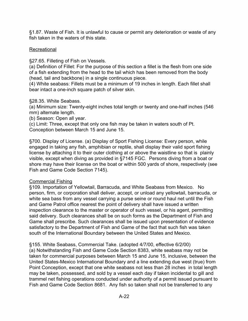
A-22
§1.87. Waste of Fish. It is unlawful to cause or permit any deterioration or waste of anyfish taken in the waters of this state.
Recreational
§27.65. Filleting of Fish on Vessels. (a) Definition of Fillet: For the purpose of this section a fillet is the flesh from one sideof a fish extending from the head to the tail which has been removed from the body(head, tail and backbone) in a single continuous piece. (4) White seabass: Fillets must be a minimum of 19 inches in length. Each fillet shallbear intact a one-inch square patch of silver skin.
§28.35. White Seabass. (a) Minimum size: Twenty-eight inches total length or twenty and one-half inches (546mm) alternate length. (b) Season: Open all year. (c) Limit: Three, except that only one fish may be taken in waters south of Pt.Conception between March 15 and June 15.
§700. Display of License. (a) Display of Sport Fishing License: Every person, whileengaged in taking any fish, amphibian or reptile, shall display their valid sport fishinglicense by attaching it to their outer clothing at or above the waistline so that is plainlyvisible, except when diving as provided in §7145 FGC. Persons diving from a boat orshore may have their license on the boat or within 500 yards of shore, respectively (seeFish and Game Code Section 7145).
Commercial Fishing§109. Importation of Yellowtail, Barracuda, and White Seabass from Mexico. Noperson, firm, or corporation shall deliver, accept, or unload any yellowtail, barracuda, orwhite sea bass from any vessel carrying a purse seine or round haul net until the Fishand Game Patrol office nearest the point of delivery shall have issued a writteninspection clearance to the master or operator of such vessel, or his agent, permittingsaid delivery. Such clearances shall be on such forms as the Department of Fish andGame shall prescribe. Such clearances shall be issued upon presentation of evidencesatisfactory to the Department of Fish and Game of the fact that such fish was takensouth of the International Boundary between the United States and Mexico.
§155. White Seabass, Commercial Take. (adopted 4/7/00, effective 6/2/00) (a) Notwithstanding Fish and Game Code Section 8383, white seabass may not betaken for commercial purposes between March 15 and June 15, inclusive, between theUnited States-Mexico International Boundary and a line extending due west (true) fromPoint Conception, except that one white seabass not less than 28 inches in total lengthmay be taken, possessed, and sold by a vessel each day if taken incidental to gill andtrammel net fishing operations conducted under authority of a permit issued pursuant toFish and Game Code Section 8681. Any fish so taken shall not be transferred to any

A-23
other vessel. (b) The restrictions in this section shall not apply to white seabass taken in waters lyingsouth of the International Boundary Line between the United States and Mexicoextended westerly into the Pacific Ocean. A current fishing permit issued by theMexican Government is evidence that white seabass were taken south of theinternational boundary.

A-24
A-23
Appendix D. Risk assessment of proposed management alternatives for thewhite seabass fishery.
One of the primary objectives of the WSFMP (White Seabass Fishery ManagementPlan) is to provide for future management that will promote long-term sustainability ofthe white seabass stock and fishery. A major proposed management feature is anannual limit on harvested biomass (i.e., pounds of fish taken). Section 5.4 of theWSFMP presents several specific alternatives for this harvest limit. In order of lessrestrictive (more aggressive take) to more restrictive (less aggressive take),alternatives are: A (no limit), B1, B2, D, C1, C2, C3.
One of the fundamental questions regarding the implementation of any one of thesealternatives is to what extent would each of the alternatives involve risk to thesustainability of the stock and fishery? In particular, for each given alternative: underwhat conditions and in how many years would use of that option likely result in anoverfished condition of the stock?
Underlying uncertainty and risk The better the available information about the stock size (e.g., abundance, biomass)the higher the harvest limit that can be allowed, with reasonable guarantee ofsustainability of the stock and fishery.
Two kinds of information about stock size are most needed: a good estimate of thestock size now, and a good idea (model) of the stock dynamics (i.e., how stock size islikely to change). Both sorts of information are now highly uncertain for the whiteseabass stock. Precisely because of this uncertainty, several different alternatives andharvest limits have been proposed instead of a single definitive harvest limit. Each ofthe alternatives is based on a plausible estimate of what the underlying facts might be,but no one of these estimates represents certain knowledge.
One alternative can briefly be discussed now and will not further be analyzed. Alternative A imposes no harvest limit at all. As a result, this alternative imposes noguaranteed safeguard to prevent the stock from becoming overfished, possibly evenwithin a single year. Alternative A represents a policy of maximum possible risk.
Other Alternatives Each other alternative uses a harvest limit which is equal to an estimate of MaximumSustainable Yield (MSY). MSY is the maximum amount which, on average overdifferent years, could in perpetuity be harvested from the stock, so long as the stocksize starts out large enough. If the alternative’s allowed harvest limit is no higher thanthe stock’s actual MSY, and we are willing to assume that the stock’s present initial sizeis sufficiently large, then use of the alternative poses no undue risk. Suppose,however, that the alternative’s allowed harvest limit is higher than the stock’s actual
A-24
MSY. Assume further - as our quantitative analysis below does for simplicity - that infact the fishery takes every year an amount equal to (or anyhow close to) the harvestlimit. Then it will only be a matter of time before the stock becomes overfished. Here,the term ‘overfished’ not only has a readily appreciated practical import but also byconventional definition (National Standard Guidelines) has a precise meaning: thatstock size which is at most half the size needed to sustain an average yield equal toMSY.
Precisely how much time, to becoming overfished, depends on three inputs orassumptions: the harvest limit itself; the stock’s actual status - namely present size andactual MSY; and the underlying model of stock dynamics.
Risk analysis resultsTable J-1 summarizes the results of the risk analysis. Here is how the above threeinputs enter into the Table:Since each of the alternatives makes a precautionary adjustment downward to MSY(multiplied by 0.75) for OY, we have used the OY values in the risk analysis. Each cellin the table corresponds to a given harvest limit - the one corresponding to thealternative noted at the top of the cell’s column. The cell also corresponds to a givenstock status. Namely, the alternative noted at the left of the cell’s row corresponds toan OY value, and the stock size is assumed to be the minimum size needed to yieldthat OY. The cell will contain the entry ‘OK’ if there is no undue risk, that is, if theharvest limit (from the column alternative) is less than the actual OY (from the rowalternative). However, if the column alternative’s harvest limit is greater than the rowalternative’s OY, then the cell contains two numbers, representing number of years tooverfished status. The numbers come from using two different plausible dynamicsmodels described below.
Model details The two dynamics models used are of the same general kind, known as productionmodels, or surplus yield models. Namely, absent fishing, such a model assumes thatevery year the stock size grows - adds extra biomass or ‘yield’. When stock size is verysmall, yield is small. When stock size is very large, near a maximum or ‘carryingcapacity’ value, yield again is small. However, when stock size is intermediate, yield islarger. If yield (vertical coordinate y) is plotted against existing stock size (horizontalcoordinate x) the resulting curve is dome-shaped, with MSY = the largest value of y.
Both models are of the form y = m(xp - x2p), where y = annual yield, and x = stock size(with biomass unit chosen so that 1 = maximum possible stock size (i.e., ‘carryingcapacity’ or ‘virgin biomass’). In each cell, the smaller entry is for a value of p (verynearly p = 3/4) such that the stock size which yields MSY will be equal to 40% of thevirgin biomass. The larger entry is for the value p=1, so that the stock size which yieldsMSY will be equal to 50% of virgin biomass (from a suggestion of Restrepo et al.
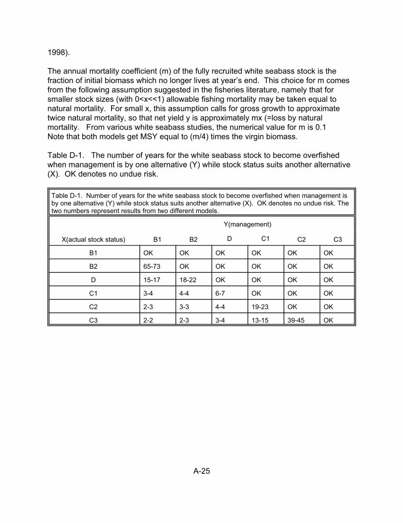
A-25
1998).
The annual mortality coefficient (m) of the fully recruited white seabass stock is thefraction of initial biomass which no longer lives at year’s end. This choice for m comesfrom the following assumption suggested in the fisheries literature, namely that forsmaller stock sizes (with 0<x<<1) allowable fishing mortality may be taken equal tonatural mortality. For small x, this assumption calls for gross growth to approximatetwice natural mortality, so that net yield y is approximately mx (=loss by naturalmortality. From various white seabass studies, the numerical value for m is 0.1Note that both models get MSY equal to (m/4) times the virgin biomass.
Table D-1. The number of years for the white seabass stock to become overfishedwhen management is by one alternative (Y) while stock status suits another alternative(X). OK denotes no undue risk.
Table D-1. Number of years for the white seabass stock to become overfished when management isby one alternative (Y) while stock status suits another alternative (X). OK denotes no undue risk. Thetwo numbers represent results from two different models.
X(actual stock status) B1 B2
Y(management)
C2 C3D C1
B1 OK OK OK OK OK OK
B2 65-73 OK OK OK OK OK
D 15-17 18-22 OK OK OK OK
C1 3-4 4-4 6-7 OK OK OK
C2 2-3 3-3 4-4 19-23 OK OK
C3 2-2 2-3 3-4 13-15 39-45 OK
A-26
Appendix E. Peer Review
Procedure for Selecting Peer Review Panels for the Draft Nearshore and WhiteSeabass Fishery Management Plans (10/18/01)
First, a master list was compiled consisting of 34 names. The list came from severaldifferent sources. The individuals on the list were sorted according to their area ofexpertise (i.e., their field, and specialty within their field). We decided that there shouldbe four reviewers on the white seabass panel and six on the nearshore panel, becausethe nearshore plan was longer, more complex and included 19 species. We alsodecided that on each panel there should be at least one resource economist or socialscientist, one population dynamicist, and one fish ecologist. We thought, too, that itwould be desirable to have representation from outside California, if possible. Withthose criteria in mind we ranked our candidates.
After ranking, we began contacting the candidates to ascertain if they were availableand interested in participating. They were offered an honorarium and reimbursement oftravel costs. For the nearshore plan we needed the peer review report to be completedwithin one month and the panel to be able to meet for a day at the end of that month.For the white seabass plan we had six weeks. Many of the people we contacted werenot able to participate. Reasons included scheduling conflicts/lack of time (the mostfrequent reason), self-declared conflict of interest (several had acted in an advisorycapacity during plan development), and lack of interest (one recent retiree was notready to resume his recently discarded profession). Most of the people who declinedsuggested other candidates. Most of the people suggested were already on our list, buta few were not and they were evaluated. Most of the candidates wished to consider theinvitation for a while before saying yes or no, and this further slowed the process as weapproached our targeted quotas. We didn’t want to have more invitations issued thanwe had positions for. Through this process, we filled both panels. We believe that theC.V.s which will be appended to each report will confirm that both panels werecomprised of highly qualified scientists.
A-27
Appendix F. Public Input
Prior to preparing the initial and amended draft environmental documents, theDepartment developed notices of preparations (NOP). The notices were provided toindividuals and organizations that have expressed prior interest in Commissionregulatory actions. The NOPs were also submitted to the State Clearinghouse fordistribution to appropriate responsible and trustee agencies for their input andcomments. No comments were received in response to the NOPs.
1. Summaries of Public Hearings and Meetings
1.1 Initial White Seabass Fishery Management Plan
In addition to the NOPs, the Department conducted three public meetings with a sub-panel of the Director's Marine Resources Advisory Committee (11 October 1994; 31January 1995; and 31 March 1995) and three public meetings with a panel of scientists(24 October 1995; 06 February 1995; and 09 March 1995) chosen to advise theDepartment on WSFMP preparation.
At the Commission's 04 August 1995 and 03 November 1995 meetings, the Departmentprovided the Commission information regarding background leading to the developmentof the draft WSFMP (environmental document), how the draft WSFMP was developed,and what the draft WSFMP proposed to do. Also, the Commission received publictestimony on the draft WSFMP at these meetings.
The combination of Department and public testimony, and the discussion of the draftWSFMP's proposed consolidation of management and regulatory authority for whiteseabass at the 03 November 1995 meeting prompted the Commission to direct theDepartment to revise the draft WSFMP. The revision, provided for by §7022 FGC, wasto reflect that the Commission would have authority for management and regulation ofthe recreational and commercial white seabass fisheries.
The environmental document that constitutes the WSFMP was revised as directed bythe Commission. To comply with CEQA requirements, the revised WSFMP was sentout for a 45-day public review and comment period. Following the end of the publicreview period, the Department informed the Commission of the public comments andthe Department's responses to those comments. The Commission adopted the revisedWSFMP on 08 March 1996.
1.2 Amended White Seabass Fishery Management Plan
Amendment of the 1996 version of the WSFMP to bring it into compliance with theMLMA began in October 2000. Under FGC Section §7071(a), the previous plan is toremain in effect until the amended version is brought into compliance with the MLMA
A-28
(1998) and adopted by the Commission. On 30 January 2001, the first advisorymeeting concerning the WSFMP revision took place. The purpose of the meeting wasto provide the Department with feedback and recommendations from constituent groupsregarding the development of an MLMA-compliant WSFMP. The next advisory meetingwas held 04 June 2001. Management alternatives were discussed, and a preferredmanagement option was agreed upon.
On 05 July 2001, an amended WSFMP was sent out for a 45-day public review periodto comply with CEQA requirements. The document was presented to the Commissionon 04 August 2001 and public comments were given at the following two Commissionmeetings (24 August 2001 and 05 October 2001). At the 05 October 2001 meeting, theDepartment informed the Commission of public comments following the end of the 45-day public review and the Department's responses to those comments.
On 05 July 2001, the revised WSFMP was sent out to a scientific panel for review. TheDepartment received a summary of the scientific review panel’s comments andrecommendations in early October 2001 and met with the panel on 29 October 2001 todiscuss the panel’s comments at length. As a result of the scientific review panel’scomments on the WSFMP, the Department did not present it to the Commission inJanuary 2002 as originally planned. Also, on 18 December 2001, the Department metwith the ad hoc White Seabass Advisory Committee (WSAC) to inform it of the scientificreview panel’s comments and recommendations. On 22 January 2002, the Departmentand WSAC met a second time to discuss changes the Department was recommendingin order to incorporate several of the scientific review panel’s recommendations into therevised WSFMP. The WSAC agreed to the Department’s recommended changes to theWSFMP. The WSFMP is scheduled to be presented to the Commission for approval on04 April 2002.
2. Persons, Organizations, and Public Agencies Commenting on the WSFMP’s
2.1 Initial White Seabass Fishery Management Plan A) Director's Marine Resources Advisory Subpanel and B) Scientific Advisory Panel
A BMr. John BeuttlerUnited Anglers of Calif ornia
Dr. Larry JacobsenNational Marine Fisheries Serv ice
Mr. Nello Castagnola Calif ornia Gillnetters Association
Ms. Cindy ThomsonNational Marine Fisheries Serv ice
Mr. Dan FrumkesUnited Anglers of Calif ornia
Dr. Larry AllenCalif ornia State Univ ersity , Northridge
Mr. Bill PerkinsWestern Fishboat Owners Association
Dr. Mia TegnerUniv ersity of Calif ornia, San Diego
A-29
Mr. Tony WestCalif ornia Gillnetters Association
Dr. Ashley MullenInter-American Tropical Tuna Commission
Mr. Locky BrownGreater LA Council of Div ers
Dr. John Stephens Jr.Occidental College
Mr. Robert C. Fletcher, PresidentSportf ishing Association of Calif ornia
Dr. Michael DomeierDepartment of Fish and GameMarine Resources Div ision
Dr. Richard GlennUnited Anglers of Calif ornia
Dr. John Stephens Jr.Occidental College
Mr. Tom Raf tican (alternate) Mr. Mike McCorkle (alternate)
2.2 Amended White Seabass Fishery Management Plan
The following individuals acted as members of an ad hoc White Seabass AdvisoryCommittee for the preparation of the amended WSFMP:
Mr. Bob FletcherSporting Association of Calif ornia
Mr. Gary Burke Commercial Fisherman
Mr. Tom Raf ticanUnited Anglers of Calif ornia
Mr. Tony West Calif ornia Gillnetters Association
Mr. Bob OsbornUnited Anglers of Calif ornia
Mr. Tim AthensCommercial Fisherman
Mr. Dan Frumkes Statistician
Mr. Mike McCorkleCommercial Fisherman
Dr. Ashley MullenPopulation Biologist, Inter-American Tropical Tuna Commission
3. Comments Received and Response to Comments
The comments received on the initial WSFMP were incorporated into that documentand will not be discussed here. During the Commission meetings on the amendedWSFMP, several comments were received. The comments were either in support ofthe WSFMP or asked for clarification of some aspect of the plan. The comments andthe Department’s response are listed below:
A-30
Comment A. Ron Gaul, Sea Turtle Restoration Project. 04 August 2001 and 24 August2001.
Mr. Gaul had concerns about the white seabass gill net fishery with regard to potentialmarine mammal, marine turtle, and seabird mortality; the lack of an observer program;and an observed high rate of discard mortality of finfish in white seabass gill nets. Healso wanted the Commission to ensure that the gill net fishery would be conducted in amanner that is safe and sustainable for several named marine resources (See SectionD4).
Response:
A1. Discard mortality rate: With regard to the 52% discard mortality rate that Mr. Gaulattributes to the white seabass drift gill net fishery, this number comes from the six yearaverage of observation data from 1983 through 1988, and does not accurately illustratethe discard mortality rate. Analysis of the data shows that the annual discardedmortality rate ranges from 20 to 80%. The disparity in values was the result of twoanomalous years, 1985 and 1987. In each of these years, there was an unusually highcatch of one species (spiny dogfish in 1985, Pacific sardines in 1987), which skewedthe six year average. If the two years are removed, 40% of the catch taken in whiteseabass drift gill nets were either sold or kept by the fishermen, approximately 35% offish and invertebrates were discarded alive and about 25% of finfish and invertebrateswere discarded dead.
The ratios reported in the study (Vojkovich et al. 1990) do not reflect the bycatchmortality associated with the white seabass gill net fishery relative to the impact of theother gill net fisheries which have higher landings overall. The total number of fish andinvertebrates taken by the white seabass fishery compared to the total taken by all gillnet fisheries accounted for only 5%. In comparison, the halibut gill net fishery and thewhite croaker gill net fishery took eight and ten times the number of animals,respectively. Thus, available data suggests that the white seabass drift gill net fisherytakes significantly fewer fish compared to other net fisheries.
A2. White seabass gill net fishery should be conducted in a manner that is safe fornontarget species such as marine mammals, turtles and birds: As stated in Chapter 6,of the WSFMP, there are few documented interactions between marine mammals andmarine seabirds and no documented take of sea turtles in white seabass drift gill nets. Onboard observation of this fishery during the 1980s found that interactions with marinemammals and seabirds accounted for less than one marine mammal per set day andless than one seabird per every four set days. Based on the NMFS take numbers forpinnipeds, cetaceans and sea birds, this level of take does not impede the long termsustainability of these resources. For this reason, the NMFS does not require onboardobservation of this fishery despite its classification as a Category I fishery.
The Department has identified the need to conduct on-board observations of the white

A-31
seabass commercial fishing fleet to document possible changes in bycatch compositionthat may have occurred following Proposition 132, which moved the fleet furtheroffshore in 1994 (Chapter 7, Section 7.4.1).
A3. White seabass gill net fishery should be conducted in a manner that is sustainablefor targeted species such as sharks, tunas, billfish, halibut and white seabass: It isunclear from Mr. Gaul’s comments if he is addressing the take of the above mentionedspecies in the white seabass fishery specifically or in drift gill net fisheries generally. However, as for the take of sharks, observation of the white seabass drift gill net fisheryidentified about a dozen species that were captured in white seabass drift gill nets. Themajority were nearshore, kelp bed species such as brown and gray smoothounds, hornsharks, swell sharks, and leopard sharks. Several marketable species of shark (i.e.,mako, Pacific angel, soupfin, and thresher) were also taken by this gear. The overalldisposition of the shark catch resulted in 18% kept or sold, 51% discarded alive and31% discarded dead during the six year study. The disposition for unmarketablespecies or those without size limits was 16% kept for personal use, 74% returned aliveand 10% discarded dead. The total number of sharks taken by this fishery during thesix year period was less than 3,000. Additionally, the take of shortfin mako andcommon thresher by all fishing gears has been addressed in the draft Highly MigratorySpecies Fishery Management Plan prepared by the National Marine Fishery Service.
As for billfish, there has never been documented take of either species group in thewhite seabass drift gill net fishery. Bluefin tuna and thresher sharks are occasionallycaptured in gill nets, however, this incidental take is considered insignificant. Further,any questions about the sustainability of these species groups have been addressed inthe Pacific Fisheries Management Council’s draft Highly Migratory Species FisheriesManagement Plan.
Few halibut are taken in the commercial white seabass fishery. During theDepartment’s six year observation project, the entire white seabass fleet took anestimated average of 3,556 lb (1159 kg) of California halibut, which represented lessthan 0.5% of annual landings during the 1980's. This figure is expected to be evensmaller now due to the movement of this fishery outside of three miles along themainland coast and outside of one mile around the islands. Based on these factors, thetake of California halibut by the white seabass fishery is not likely to impact the halibutresource.
Comment B. Mike McCorkle, Commercial fisherman. 04 August 2001.
Mr. McCorkle supported the WSFMP. In addition, he stated that the white seabass driftgill net fishery is one of the cleanest fisheries, and stated that he believed the commentsmade by Mr. Gaul were politically motivated.
Response: no response.
A-32
Comment C. Bob Fletcher, Sportfishing Association of California. 24 August 2001.
Mr. Fletcher stated that allocation was a contentious issue, but it was not necessary todecide that issue now. He went on to say that the Commission should maintainmanagement of white seabass with the existing regulations and with the addition of theproposed harvest guideline.
Response: no response.
Comment D. Eric Hopper, Commercial Fisherman. 24 August 2001.
Mr. Hopper stated that he did not feel that allocation was an issue at this time but he didnot agree with the proposed harvest guideline because up to 75% of fishing areasclosed to commercial take. He stated that he did not support a harvest limit as it wasunnecessary.
Response: no response.
Comment E. Bob Osborne, United Anglers of Southern California. 24 August 2001.
Mr. Osborne agreed with Mr. Fletcher’s comments and requested that the WSFMPundergo scientific peer review to assure the correctness of the proposed harvestguideline. In addition, Mr. Osborne requested that the issue of allocation be addressedin the Marine Life Management Act Master Plan as this would provide direction andconsistency between all fishery management plans.
Response:
The WSFMP was sent out for scientific peer review on 05 July 2001. The conclusionsof the peer review panel were received October 2001 and several of itsrecommendations of have been incorporated into the latest revision of the WSFMP.
Comment F. Chris Hoeflinger, Commercial Fisherman and Nearshore Advisory Panelmember. 24 August 2001.
Mr. Hoeflinger supports the WSFMP proposed project, and hopes that the NearshoreFishery Management Plan will be of as high quality as the WSFMP.
Response: no response.
Comment G. Ron Gaul for Tom Raftican, United Anglers of Southern California. 04August 2001.
Mr. Raftican supported the WSFMP but requested the Commission take intoconsideration the following issues when determining allocation of the white seabass

See e.g. In re Quinn (1973) 35 Cal.App.3d 473; State of California v. San Luis ObispoSportsman’s Association (1978) 22 Cal.3d 440) [recreational]; Paladini v. Superior Court (1918)178 Cal. 369; California Gillnetters Association v. Department of Fish and Game (1995) 39Cal.App.4th 1145 [commercial].
2Paladini, supra, 178 Cal. 372; California Gillnetters, supra, 39 Cal.App.4th 1153.
3Ex parte Parra (1914) 24 Cal.App. 339, 340.
A-33
resource: 1) fishery data, 2) legality of commercial fishing, 3) access, 4) significance touser group, and 5) economic value.
Response:
With the exception of the second item, all of the allocation criteria raised by Mr. Rafticanare already part of the Allocation section of the WSFMP. The previous advisorycommittee spent considerable time on the issue of allocation and their decisionsresulted in the allocation criteria that was adopted in the initial white seabass FMP andhave been brought forward in the amendment (Section 5.4.3).
The question raised regarding the legality of commercial fishing was addressed by Mr.Joseph Milton, DFG staff counsel:
“At the Fish and Game Commission meeting of August 4, 2001, comments onthe White Seabass Fishery Management Plan were submitted on behalf of Mr. TomRaftican of United Anglers of Southern California, which requested that the Commissiontake into consideration several issues when determining allocation of the white seabassresource, including the legality of commercial fishing. Mr. Raftican contends that thestate constitution gives every citizen the right to recreational fish but not commercialfish. Mr. Raftican has also intimated that this right to fish precludes the Fish and GameCommission from barring recreational fishing in Marine Protected Areas (MPAs). Thiscontention is incorrect, for the following reasons.
First, the courts have considered section 25 in the context of both recreationaland commercial fishing.1 The so-called “right to fish” is neither absolute norfundamental, but has been characterized by the courts as only a “privilege” or a“qualified right” subject to the Legislature’s regulation of fishing.2 Indeed, it is well-settled that section 25 must be read in connection with article 4, section 20 (formerlysection 25½), which states that the Legislature may enact appropriate laws forprotection of fish and game, and may delegate to the Fish and Game Commission suchpowers relating to protection and propagation of fish and game.3 In that respect, theCalifornia Supreme Court found it “most apparent” that the purpose of (now) article 4,section 20 “was to clothe the Legislature with ample power to adequately protect the

4In re Makings (1927) 200 Cal. 474, 479.
5In re Phoedovius (1918) 177 Cal. 238, 245-246; People v. Monterey Fish ProductsCompany (1925) 195 Cal. 548, 563.
A-34
fish and game of the state.”4 Further, the California Supreme Court has long declaredthat the power to regulate fishing has always existed as an aspect of the inherent powerof the Legislature to regulate the terms under which a public resource may be taken byprivate citizens.5 Without question, this regulatory power applies to both recreationaland commercial fishing.
Mr. Raftican has also asserted that sportfishing license revenues cannot fund theestablishment of MPAs because such revenues cannot be used to support commercialfishing programs or nongame fish and wildlife programs. (See Fish & G. Code §711(c).) However, the Legislature has yet to appropriate any funds for theimplementation of the MPA program, and neither the Department nor the Commissionhas ever suggested that MPAs should be exclusively funded from sportfishing licenserevenue. This does not mean that sportfishing revenues can never fund a share ofMPA development. In enacting the Marine Life Protection Act, the Legislature declaredthat MPAs are necessary to maintain marine biological diversity, which is “a vital asset”and important to “ocean-dependent industry,” and because of the expansion of fishingactivities to formerly inaccessible marine areas that once recharged nearby fisheries. The enhancement of fishery resources in general is a stated goal as is theenhancement of recreational opportunities in particular. Thus, MPAs are clearlyintended to benefit recreational fisheries, as well as commercial fisheries and nongamefish. The law is clear that a portion of marine resource protection costs may beallocated to those who use and benefit from management of the marine fisheryresources. This reasonably includes ocean sportfishers as well as other extractive andnon-extractive users who benefit from MPAs”.
Comment H. Todd Steiner, Sea Turtle Restoration Project. 26 November, 2001
Mr. Steiner expressed concern that the WSFMP would be implemented “withoutadequate oversight of the environmentally harmful effects of gillnet fishing.” Specifically, he stated that the impact on protected species from the white seabass gillnet fishery may have worsened since the implementation of Proposition 132 whichmoved the fishery farther off shore. Also, the observed coverage of the white seabassgill net fishery during a 1983-1989 DFG study was low relative to total fishing effort andno observer program has been initiated since 1989. Mr. Steiner recommended that anobserver program be initiated for the white seabass fishery and that such a programhave 100% observer coverage.
Mr. Steiner pointed out that several named species observed in the 1983-1989 study aswhite seabass gill net mortalities are protected under the Marine Mammal Protection Actor the Migratory Bird Treaty Act. Mr. Steiner expressed concern about a potential

A-35
impact from white seabass gill nets on sea otters around the Channel Islands andVentura and elephant seals at San Miguel Island. Mr. Steiner also brought up the 52%finfish discard mortality rate recorded in the 1983-1989 DFG study for the white seabassgill net fishery.
Mr. Steiner expressed concern about the recent emergence of a tuna gill net fishery,known as a white seabass fishery because it uses the same size mesh, but that isactually targeting albacore and bluefin tuna and therefore may potentially impactdolphins.
Response:
H1. Need for an observer program: As stated above in our response to Mr. Gaul, theDepartment has identified the need to conduct on-board observations of the whiteseabass commercial fishing fleet to document possible changes in bycatch compositionthat may have occurred following Proposition 132, which moved the fleet furtheroffshore in 1994 (Chapter 7, Section 7.4.1). Although we recognize that a high rate ofobserver coverage is desirable, implementing 100% coverage is unrealistic because ofthe costs involved (i.e., hiring more observers and higher charter boat costs fortransporting those observers to off-shore fishing boats).
H2. Potential gill net mortality of marine mammals, including elephant seals at SanMiguel Island, and seabirds: Please see Response A2 to Comment A above.
H3. Potential gill net mortality of sea otters around the Channel Islands and Ventura, ifthe otter population expands southward from Point Conception: Currently, the southernsea otter (Enhydra lutris nereis) population ranges along the California coastline fromHalf Moon Bay in San Mateo County to Gaviota in Santa Barbara County. Althoughotters have been sited as far south as San Diego County in southern California, they arerare in that portion of the state. The 2001 sea otter survey showed a decrease in thenumber of otters in the southern portion of the species’ range (Pt. Conception toGaviota) from 50 (in 2000) to 26 (G. Sanders, USFWS pers. comm.). With theexception of San Nicholas Island, sea otters are sparsely scattered on the ChannelIslands; though they have been consistently observed on the west end of San MiguelIsland during annual aerial surveys. The Marine Resources Protection Act of 1990(effective 01 January 1994) established a gill and trammel net exclusion zone (Section§8610.2 FGC) which protects areas that include sea otter habitat. Since the whiteseabass gill net fishery is restricted to waters outside typical sea otter habitat, it isunlikely to catch otters in its active nets.
H4. Discard mortality rate: Please see response A1 to Comment A above.
H5. California tuna gill net fishery: no response.

A-36
Comment I. Craig S. Harrison, Pacific Seabird Group. 26 November, 2001
Mr. Harrison complemented the Commission and the Department for the developmentof fishery management plans as mandated by the MLMA. Mr. Harrison expressedconcern about the bycatch associated with the white seabass drift gill net fishery and herecommended that the Department implement an independent fishery research programto collect data on bycatch.
Response: Please see Response A2 to Comment A above.
Comment J. Ashley Mullen, Tuna Commission and Bob Osborn, United Anglers ofCalifornia. 18 December 2001.
Dr. Mullen and Mr. Osborn expressed their concern with regard to Section 51.04(a) ofthe white seabass regulations which refers to the annual white seabass harvestallocation “in pounds”. The gentlemen suggested that removing the words “in pounds”from the regulatory language would improve the flexibility of this regulation and allow forother means of measuring catch, such as number of fish, when determining allocation ofwhite seabass between the recreational and commercial fisheries.
Response: In response to the above comment, and additional discussion during the 18December meeting, the following changes were made in the Title 14 regulations: 1)Section 51.04(a) now reads “Allocation of an annual white seabass harvest betweenrecreational and commercial fisheries will be determined consistent with optionsspecified in the White Seabass Fishery Management Plan.” 2) Section 51.04(b) nowreads “The commission shall consider at least the following factors in the allocation ofwhite seabass:”...
The Pre-adoption Statement of Reasons for Revised White Seabass FisheryManagement Plan containing the above mentioned changes was submitted to the Officeof Administrative Law on 05 February 2002 for publication in the Notice Register.
Comment K. Robert W. Hetzler, President of Harbour Ocean PreservationEnhancement. 18 March 2002
K1. The plan states that the fishery is fully recovered and derives an MSY from datacollected in the 1970s. Mr. Hetzler did not understand the rationale for using a historicalMSY, stating that the historical catch data doesn’t support the plan’s proposed MSY. According to Mr. Hetzler, the fishery has been unable to support an MSY of 1.5 millionpounds since the 1950s. Mr. Hetzler strongly recommended a more conservative OYsuch as option C1 which used recent catch data rather than an OY based on a historicalMSY.
K2. The plan does not address why stock levels remained very low for nearly 20 years(1980s to1997) and why it recently increased during the last three years. “What

A-37
happened to allow the stock to go from depleted to fully recovered in just three years?”
Preliminary landings in 2001 are down significantly, which indicates that the populationcannot withstand the current level of fishing mortality.
K3. The plan is flawed because it lacks a new estimate of mortality and data on yearclasses, spawning biomass capacity, and recruitment levels. The present stock has adifferent year class makeup: the stock of the 1950s and 1960s consisted of moremature fish which provided greater recruitment levels and was able to sustain a higherOY. The current white seabass spawning biomass is substantially below that of the1950s and 1960s and therefore can not sustain as high an MSY .
K4. Mr. Hetzler was concerned about the plan’s call for a reassessment of the stock intwo years, because adjustments that may be made in the fishery at that time may cometoo late and cause a set back in the recovery of the stock. He felt that the proposed OYof 1.2 million pounds could severely deplete the stock before it is determined that theyield was set too high.
Response:
K1. The plan does not state that the fishery is fully recovered, but that it is recovering. The preferred alternative uses National Standard Guidelines (NSGs), which are used toassist in the development of federal FMPs, to derive an MSY proxy for the whiteseabass fishery. The NSGs allow for situations when MSY can not be estimateddirectly. The lone stock assessment for white seabass used catch and effort data in the1970s and came up with an MSY similar to the preferred alternative. The similarity ofthe two MSY estimates suggests that the MSY proxy has some value. Recent catchdata was not used for determining an MSY since recent catches have not been stable.
Harvest levels below 1.5 million pounds since the 1950s may be due to other factors,and not necessarily related to the fishery’s inability to presently support this level. During the 1980s to the present, more restrictive regulations have been implementedthat have limited the number of white seabass that can be landed. Oceanographicchanges favorable for white seabass have also occurred during the last few years (seeresponse K2) and may explain the increased landings since 1997.
K2. This comment was more applicable to an earlier draft of the plan. The present planprovides a possible explanation for this: A pattern seen in the 1890s and 1940s seemsto be occurring today whereby white seabass abundance increases substantiallyfollowing a shift from warmer to colder ocean waters. Warmer waters occurred in theSouthern California Bight from the late 1970s to mid 1990s, but have become colder over the last few years. Again, the plan does not state that the fishery is fully recovered,but that it is recovering.
Although not available at the time of plan preparation, final white seabass landings for
A-38
2001 are actually higher than in 2000, indicating that the stock is supporting the currentlevel of fishing mortality.
K3. We agree that current estimates of mortality, year class strengths, and spawningbiomass are valuable data; we have emphasized that a current stock assessment forwhite seabass is needed. Information on recruitment is currently being collectedthrough studies done by OREHP. We are unaware of any data showing that thepresent stock of white seabass consists of smaller fish and a spawning biomasssubstantially below that of the stock of the 1950s and 1960s. Recreational fishery dataand anecdotal information from the commercial fishery suggest that the average size ofwhite seabass being caught has increased in recent years.
K4. The plan recommends that a current stock assessment be done immediately. Theplan also calls for the Department’s white seabass management team to monitor thefishery throughout the year and for the Commission to evaluate the effectiveness ofmanagement measures annually. The fishery management plan framework allows thecommission to adjust, impose, or remove management measures at any time during theyear for resource conservation, social or economic reasons. This allows for adaptivemanagement of the fishery, enabling quick adjustment of OY if needed.
–End of response to comment K–
The Department presented the White Seabass Management Plan to the Commissionfor adoption at the 04 April 2002 meeting in Long Beach, California. Following Ms.Marija Vojkovich’s presentation, members of the public were invited by the Commissionto comment on the plan. The following individuals spoke at this meeting.
Comment L. Bob Strickland, United Anglers of Southern California
Mr. Strickland directed the following questions to Ms. Vojkovich: What data source wasused to determine that most of the white seabass take is by the recreational componentof the fishery, are these data accurate, and do these data actually capture the take byprivate boaters up and down the whole coast?
Response by Ms. Vojkovich: Marine Recreational Fisheries Statistical Survey (MRFSS)data are used to estimate the take by recreational fishers and to estimate the pounds ofwhite seabass taken by this component of the fishery. Yes, these data estimates couldbe wrong. Yes, these surveys do cover the entire coast of California.
Comment M. Chris Miller, California Lobster and Trap Fisherman’s Association
Mr. Miller stated that he supports the WSFMP and that because we share the whiteseabass resource with Baja California, Mexico, resource managers from Californiashould strive to have a cooperative relationship with their Mexican colleagues for thesharing of data gathered for white seabass stock assessments. Mr. Miller encouraged
A-39
the Commission to consider this issue as it moves forward with the implementation ofthe MLMA.
Response: President Flores thanked Mr. Miller for his comments.
Comment N. Tom Raftican, President of United Anglers of Southern California (UASC)
Mr. Raftican thanked the Department for compiling an impressive compilation of data onthe white seabass resource and he felt that the document (WSFMP) highlighted thenecessity of using fishery management plans for managing fished stocks. Mr. Rafticanstated that the plan lacks any substantial precautions in managing the white seabassfishery because the management options, although within the National StandardGuidelines for managing fisheries, are based on very optimistic assumptions about thecurrent status of the white seabass stock. Mr. Raftican stated that there are importantelements in this plan that still need to be completed and these include 1) ongoingfishery monitoring and review of the plan’s successes and failures; 2) obtainingresearch to fill a wide assortment of data gaps; 3) and establishing an allocation policy. Mr. Raftican continued by saying, “We [UASC] are particularly concerned withperformance standards and triggers that would quickly implement additional regulationsin a timely manner. The plan indicates the Department intends to continue to monitorand develop standards and triggers to better manage the fishery.” Mr. Raftican told theCommission the white seabass fishery is an extremely valuable resource to therecreational fishing community. Mr. Raftican stated that “the success of this plan willhinge upon the speed and precision with which the Department is able to monitor thefishery and ultimately fill the data gaps.” Mr. Raftican commended and thanked “Ms.Marija Vojkovich and the new staff of this plan for stepping in late in the plan processand doing an excellent job of putting together a couple of very productive meetings andproductive revisions to previous drafts that have vastly improved this plan.” Mr. Rafticanstated that the vulnerability of this fishery and the problems associated with managing ithave not been glossed over in the plan and this is an indication of the quality of theplan. Mr. Raftican stressed, however, that “the success of the plan is clearly dependentupon timely and committed implementation.” “In adopting this plan, we [UASC] urge theCommission to establish priorities within the Department to move this fishery to the topof the list of state managed species and to establish active and effective mechanisms toproactively manage the fishery while doing their best to obtain funding to improve thedata situation.”
Response: President Flores thanked Mr. Raftican for his comments and CommissionerSchuchat asked Ms. Vojkovich if there is a priority list by which the Departmentmanages species under the purview of California. Ms. Vojkovich responded that thereis no written document; however, priority is based on what was indicated by theLegislature. For the nearshore species these include the white seabass and squidmanagement plans.
Comment O. Mr. Bob Osborn, United Anglers of Southern California
A-40
Mr. Osborn identified himself to the Commission as one of the members of the WhiteSeabass Advisory Panel and he supported the position expressed by Mr. Raftican.
Response: No response.
Comment P. Robert Hetzler
Mr. Hetzler told the Commission that he considered the plan to be well-developed andhe commended the Department for its work on the plan. Mr. Hetzler questioned theneed for setting an optimal yield (OY) for this fishery at this time because he felt that thisOY was based on historical stock levels and that it had nothing to do with the currentstock size. Mr. Hetzler stated that the current stock size is probably much different thanit was in the past and that there may have been changes in habitat, recruitment andspawning biomass. Mr. Hetzler recommended that the harvest level be set at a lower,more precautionary level in order to build up the stock.
Response: In response to Mr. Hetzler’s comments, President Flores asked Ms.Vojkovich to state why the Department had chosen the annual harvest limit of 1.2 millionpounds for white seabass. Ms. Vojkovich told the Commission that the limit was set asa starting point to begin setting boundaries on the fishery because, under the statusquo, there is no harvest limit.
Once all public comment had been heard, the Commission voted unanimously to adoptthe WSFMP. Mr. Bob Treanor, Executive Director of the Fish and Game Commission,announced that the environmental document would be certified at the 09 May 2002Commission meeting, and the regulations would also be adopted at that time.

A-41
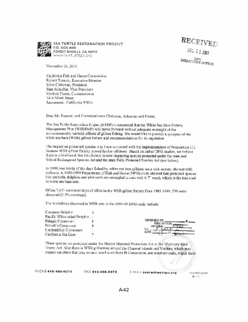
A-42
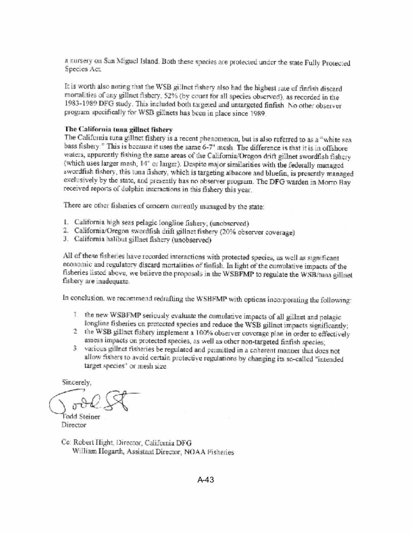
A-43
A-44

A-45
A-46
March 18, 2002
Mr. Micael Flores, PresidentCalifornia Fish & Game Commission1416 Ninth StreetSacramento, CA. 95814
Re: White Sea Bass Management Plan
Dear Mr. Flores:
I recently received a copy of the Department of Fish & Game's (DFG) White Sea Bass.Plan (dated 12/01) (Plan) and after reviewing it, I am concerned about the conclusionsand recommendations made therein. I am a former fishery biologist having workedunder Dr. B. Schaefer at the Inter - American Tropical Tuna Commission, ialso haveworked as an executive for Star-Kist Foods Inc. for 31 years retiring in 1991. Since thenI have been a Director of United Anglers of Southern California (UASC) and ampresently President of Harbour Ocean Preservation Enhancement, a white sea bassgrow out pen located in Huntington Harbour. During all these years I have been a avidrecreational angler. Although I am sure you have received many comments on the plan,I believe my views may be somewhat different than you have received so far.
After pushing for a White Sea Bass Management Plan (Plan) for a number of years, Iam happy to see that it has finally arrived. I would like to commend the DFG for a welldeveloped Plan and the information and data provided therein. They have done a greatjob with the limited available data as acknowledge in the plan itself. This is a concern asthe Plans recommendations and stock assessments are based on very limited currentdata. The average annual fish size cannot be determined from the data presented in theplan because it does not represent the actually number of fish caught (in thecommercial landings) nor the actual weight landed (in the recreational landings) withpossible exception in the most recent years for recreational catches (since 1990). As aresult, the plan has no valid data to determine the fish size and year class strengths inthe fishery. Actually, the plan has no current information as to the year class make up ofthe current sea bass stocks. This information is imperative to have in order to determinewhat spawning level the stock can produce and thereby the level of recruitment ofreplacement fish that is available to harvest.
The historical catch data itself does not support the Plan's proposed MaximumSustainable Yield (MSY). The Plan's position is that the white sea bass fishery has fullyrecovered and has a MSY based on a model calculations derived in the 1970's of 1.6million pounds. Yet when we look at the historic landing data, on an average, the fisherywas not able to support an average catch level of 1.5 million pounds in the 1950's. Thefollowing table taken from the landings table in the Plan reflects the average catch fromonly California waters in ten year average increments.

A-47
1950-1959 1,553,630 Ib.1960- 1969 708,772 Ib.1970- 1979 598,090 Ib.1980- 1989 112.257 Ib.1990- 1999 238,332 Ib.
As is evident from the table, the sea bass stocks could not sustain the higher catches inthe 1950's, dropping by about 55 percent in the 1960's and continued to drop thereafterto a low of only 112, 257 pounds in the 1980's. At the low, the stocks could yield onlyabout eight percent of the 1950's average catch levels. These low catch levels persistedthrough 1997 and reflect the stock reaching an equally low equilibrium size thatsustained these catch amounts.
The Plan does not answer some very important questions about why the stock levelsremained very low for nearly twenty years (1980's through the 1997's) and why itsuddenly increased in the last three years (1998 - 2000). What happened to allow thestock to change from a depleted stock to a fully recovered stock in just three years? Ifone looks at the data through 1997, the indices show the stock is still at a very low level.Based on the growth rates of three to five years from spawning to when a fish enters thefishery and the average age of 7 to 10 years to reach the average size of the pastaverage commercial and recreational fish size (remember the size data is flawed), howdid the fishery fully recover in only three years? The answer is obvious that the stock didimprove, but has definitely not recovered to the 1950's level in such a short period oftime. If this position is correct, can the current recovered stock support the Plan'srecommended 1.2 million pound OY catch level? The answer is no, it cannot and the2000 catch of over nine hundred thousand pounds probably was greater than the MSYyield the current stock could support, meaning the stock has been reduced somewhatwith that catch level. Preliminary landings in 2001 are down significantly, by as much as25 to 30 percent, which is indicative that the population could not support this level offishing mortality. The next few years data will tell, but it appear that the 2000 fishingmortality level reduced the current standing stock.
The Plan's conclusions appear flawed because there is no data as to the year classmake up of the current stock, no evaluation on the spawning biomass capacity nor itsrecruitment level. There are also no new estimates of mortality level. The Plan useshistorical data to make these estimates assuming the parameters are the same todayas they were 30 to 50 years ago when this information was available. The problem isthat the sea bass stock today does not have the same year class make up as it did inthe early years and, as a result, has a different spawn and recruitment level. In the1950's and 1960's, the stock was mature and had a much larger make up of biggerolder fish. Larger fish spawn a much greater quantity of eggs than smaller fish. Themature stock in this earlier period had a high spawn level providing a large recruitment
- 2 -
A-48
into the fishery and thereby a higher optimum fishing yield. The current sea bass stocks are recovering from a depleted state and thereby would appear to have a much younger year class makeup. As as result, its spawning biomass level is substantiallybelow that of the 1950's and 1960's stock and thereby cannot sustain as high a MSY level.
There have been other changes over the years that have probably adversely impactedthe stock and its current potential yield level. The inshore habitat has changedsubstantially with the loss of coastal estuaries and bays. Such loss can reduce the levelof recruitment of fish back into the fishery. The natural mortality levels have probablychanged as well. The increased seal population, as an example, probably has a greaternegative impact on the current recruitment level than in earlier years. All of thesechanges have a negative impact on both the current MSY and OY the current stock cansupport . One positive area that has not been evaluated in the plan is the impact theOREHP hatchery and grow out program will provide. In 2001, over 100,000 sea basswere released into the wild. Because of improvements in the hatchery's process, thenumber of released fish is expected to exceed 200,000 in 2002 and could even meetthe hatchery's capacity of 400,000 fish per year. In 2000, the estimated individual fishcatch was over 46,000. It is obvious that the the hatchery program could become animportant factor in maximizing the yield from the sea bass stocks. In time it could helpraise the MSY level of the stocks.
The Plan calls for a reassessment of the stocks in two years and to make adjustments in the levels of catch at that time. My concern here is that if the recommended OY catchlevel of 1.2 million pound is accepted, at this level, the stocks could be severelydepleted by the time it is determined that the yield was set too high. California and itsfishing industries would then have lost the present level of recovery of the fishery andthe ten years or so to rebuild it back to what it is today (note it has taken 20 years toreach current levels). What I don't understand is why the DFG is recommending thehistorical MSY of 1.6 million pounds (adjusted by twenty-five percent to a OY of 1.2million pounds as a precautionary figure) rather than use the 1996 / 2000 datasupported MSY less the precautionary twenty-five percent of 453,000 pounds asprovided in option C-1. I strongly recommend that the commission take a conservativeapproach in setting the annual catch limits at this lower level so that we do not loose thestock level improvement obtained so far. I think it is far better to be in a position tofurther increase catch limits in the future when the data provides better estimates of thestock size, spawning biomass and recruitment than to have to cut catch limits becausethe Plan erred on the high side.
I hope this letter helps you make the decision on the yield level the Plan should adoptand that it is a correct one that allows the white sea bass fishery to recover to its formerlevel. I have tried to present my views, concerns and question in a concise wayknowing that you do not have the time for a long dissertation on the merits and
-3-
A-49
problems with the Plan. If you have any questions, I would be happy to try to answerthem.
Sincerely,
Robert W. Hetzler16751 Sea Witch LaneHuntington Beach, CA. 92649Phone: (714) 846-4402Fax: (562) 592-3475E-mail: [email protected]
-4-

A-50
Appendix G. Methods and Data Sets
G1 Methods
G1.1 RecreationalCommercial Passenger Fishing Vessel (CPFV) data from Department databases
were used rather than RecFIN, because the Department’s CPFV logbook data isthought to be more accurate than MRFSS’s RecFIN estimates for CPFV. In addition,Department data can be used to identify the DFG block locations where fish arecaught. Although RecFIN data estimates for recreational fishing modes forprivate/rental boats, man-made structures and beaches was the best data available,many of these data sets had high standard errors, especially those for shore-basedfishing modes.
Since RecFIN length data for white seabass was taken in fork lengths (FL), andRecFIN’s total length conversion option yielded the same measurements, 15 mm (0.59in.) was added to RecFIN fork length data to convert to total length (TL). This wasdone in order to better estimate the number of legal size (28 in. (711 mm TL)) fish keptby different recreational fishing modes. Tim Hovey, a former hatchery manager for theHUBBS white seabass hatchery, recommended 15 mm and no other conversion factorwas found.
Historical CPFV logbook dataAnnual estimates of landings, effort, and CPUE were calculated for white
seabass using CPFV logbook data from 1995 to 1999. Annual estimates of landings(number of fish) for white seabass were calculated by summing white seabass landingsfrom all identified white seabass trips from each year. Annual estimates of effort(angler-days) were calculated by summing the total number of passengers from allwhite seabass trips from each year. This effort calculation was based on theassumption that each submitted CPFV log represented one trip-day, and therefore, thenumber of angler-days for each trip was equal to the number of passengers. Annualestimates of CPFV (number of fish per 100 angler-days) was calculated by taking theannual estimate of landings and dividing it by the annual estimate of effort, thenmultiplying the result by 100.
CPFV hook-and-line trips were separated from CPFV diving trips using catchcomposition and trip information from the logs and vessel information. Logs with CDFGblocks for Mexico and the San Francisco Bay Delta were removed from the hook-and-line data. Next, records with invertebrate species, species codes or landings equal tozero, or missing data were deleted. Finally, white seabass trips were selected from theremaining data using the following procedure: Total landings for each trip werecalculated for three groups: A) white seabass, B) white seabass, yellowtail, andCalifornia barracuda, and C) all finfish species except white seabass, yellowtail,California barracuda, Pacific bonito, Pacific mackerel, jack mackerel, and kelp bass. Atrip was considered a white seabass trip if the total landings of white seabass weregreater than 10% of the landings of white seabass in group C combined, or if the totallandings from group B was greater than 50% of the landings of groups B and C
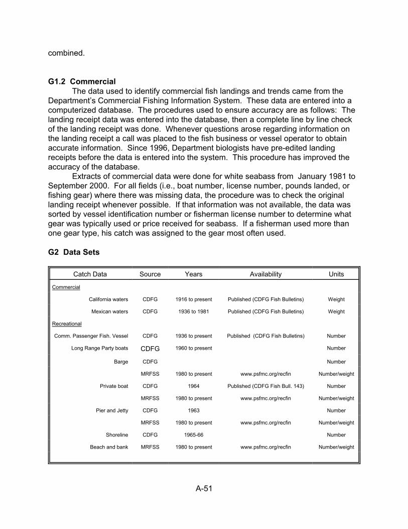
A-51
combined.
G1.2 CommercialThe data used to identify commercial fish landings and trends came from the
Department’s Commercial Fishing Information System. These data are entered into acomputerized database. The procedures used to ensure accuracy are as follows: Thelanding receipt data was entered into the database, then a complete line by line checkof the landing receipt was done. Whenever questions arose regarding information onthe landing receipt a call was placed to the fish business or vessel operator to obtain accurate information. Since 1996, Department biologists have pre-edited landingreceipts before the data is entered into the system. This procedure has improved theaccuracy of the database.
Extracts of commercial data were done for white seabass from January 1981 toSeptember 2000. For all fields (i.e., boat number, license number, pounds landed, orfishing gear) where there was missing data, the procedure was to check the originallanding receipt whenever possible. If that information was not available, the data wassorted by vessel identification number or fisherman license number to determine whatgear was typically used or price received for seabass. If a fisherman used more thanone gear type, his catch was assigned to the gear most often used.
G2 Data Sets
Catch Data Source Years Availability Units
Commercial
California waters CDFG 1916 to present Published (CDFG Fish Bulletins) Weight
Mexican waters CDFG 1936 to 1981 Published (CDFG Fish Bulletins) Weight
Recreational
Comm. Passenger Fish. Vessel CDFG 1936 to present Published (CDFG Fish Bulletins) Number
Long Range Party boats CDFG 1960 to present Number
Barge CDFG Number
MRFSS 1980 to present www.psfmc.org/recfin Number/weight
Private boat CDFG 1964 Published (CDFG Fish Bull. 143) Number
MRFSS 1980 to present www.psfmc.org/recfin Number/weight
Pier and Jetty CDFG 1963 Number
MRFSS 1980 to present www.psfmc.org/recfin Number/weight
Shoreline CDFG 1965-66 Number
Beach and bank MRFSS 1980 to present www.psfmc.org/recfin Number/weight

A-52
Socioeconomic data Source Years Availability Units
commercial
ex-vessel revenue CDFG 1980-2000 unpublished data dollars
market price CDFG 1980-2000 unpublished data dollars
vessels CDFG 1980-2000 unpublished data number
processors CDFG 1980-2000 unpublished data number
recreational
trips MRFSS 1993-1999 www.st.nmfs.gov/recreational/index.html
number
anglers MRFSS 1993-1999 www.st.nmfs.gov/recreational/index.html
number
A-53
Appendix H. Location in the Fishery Management Plan of Each Requirement ofthe Marine Life Management Act
General Policies of Fishery Management Plans Location in the§7070. Findings and Declarations Exec. summary
§7071. Management Authority of the Commission Exec. summary
§7072. Management of Sport and Commercial Fisheries Exec. summary
Plan Preparation, Approval, and Regulations Fisheries.
§7075. Preparation of Fishery Management Plans Chapter 1,
§7076. Advice and Assistance During Development 1.3.1.1; 1.3.1.2
§7077. Notice of Proposed Plans, Plan Amendments, Hearing Schedules, and Agendas Chapter 1
§7078. Public Hearings; Implementing Regulations Chapter1
Marine Life Management Act Requirements
§7080. Best Available Fishery Information
(a) Species and Location 1.5; 2.1
Number of Vessels and Participants 3.2.1; Chapter 7
Fishing Effort 3.2.2
Historical Sport/Commercial Landings 3.2
History of Conservation and Management Measures Chapter 4
(b) Natural History, Population Dynamics, and Effects of Changing Oceanic Conditions 2.5
(c) Habitat and Threats to Habitat 2.9; Chapter 9
(d) Ecosystem Role Related to the Fishery Chapter 6.
(e) Economic and Social Factors of the Fishery 3.3
§7081. Research Protocol Chapter 7
(a) Past Monitoring of the Fishery and Ongoing Monitoring 7.2
(b) Identification of Essential Fishery Information 7.1
Age and Growth 2.3
Minimum Size at Maturity 2.4
Spawning Season 2.4
Population Age Structure
Food 2.7
Predation 2.7
Competition 2.8
§7082. Measures for Conservation Management
(a) Limitations on the Fishery Chapter 5
(b) Creation or Modification of Restricted Access
A-54
(c) Procedure to Establish, Review, and Revise Catch Quota 5.4; 5.9
(d) Requirement for a Permit and Reasonable Fees
§7083. Incorporation of Existing Measures; Effects of Additional Measures
(a) Existing Conservation and Management Measures Chapter 1
(b) Additional Conservation and Management Measures Effects Chapter 6
1. Fish Populations and Habitats
2. Fishery Participants, Coastal Communities, and Businesses
§7084. Measures to Minimize Adverse Effects on Marine Fishery habitat Chapter 5
§7085. Fisheries in which Bycatch Occurs
(a) Amount and Type of Bycatch Chapter 6
(b) Analysis of Bycatch Chapter 6
(c) In the Case of Unacceptable Bycatch, Implementation of Conservation or Management
1. Minimize Bycatch
2. Minimize Mortality of Discards
§7086. Measures to Address Overfishing
(a) Criteria for Identifying Overfishing 5.8
(b) Address and Rectify Overfishing 5.8; 5.4
(c) Address By:
1. Specifying a Time Period for Recovery 5.7
2. Allocation of overfishing restrictions and recovery benefits 5.4.3
§7087 Amendment of plan and adoption of regulations 5.3.1
§7088 Effect of plan on statutes and regulations
A-55
Appendix I. Location in the Fishery Management Plan of Each Requirement of theCalifornia Environmental Quality Act
California Environmental Quality Act Requirements Location in the FMP
Summary of Proposed Project Exec. SummaryProposed Project Exec. SummaryEffects on the Environment Exec. SummaryPublic Input Exec. SummaryAreas of Controversy Exec. SummaryIssues to be Resolved Exec. SummaryConclusion Exec. SummaryTable of Contents ¥i
Project Description Chapter 1Proposed Project Chapter 5Project Objectives 1.3Functional Equivalent 1.4.1.1Scope and Intended Use of Env. Document 1.4.1.2Management Techniques 5.1
Regulatory 4.2Nonregulatory 4.3
Authorities and Responsibilities 1.4Location and General Characteristics 1.1.1
of the Project AreaEnvironmental Settings
General Description of the Environment 1.1.1Habitat 2.9
Life History Chapter 2Taxonomy and Morphology 2.1Distribution 2.2Life Cycle 2.5Reproduction and Development 2.4Dispersal and Recruitment 2.2Age and Growth 2.3Food Habits 2.7Competition 2.8Natural Mortality 2.5
Importance of Habitat Loss, Degradation, 9.4 and Modification
Municipal Discharge 9.2.1Dredge and Non-Dredged Material Disposal 9.2.2Unusual Weather Events 9.1Status of the White Seabass Population (Stock) 2.10

A-56
Socioeconomic Environment 3.3Commercial 3.3.2Recreational 3.3.1
Regulatory/Management Environment 4.1Responsible Agency 1.5Management Concepts and Tools Chapter 4&5Data Collection Methods Appendix GMonitoring Programs 7.2Harvest and Landing Records Chapter 3Surveys 7.2
Significant Environmental Effects Chapter 6Effect of white seabass harvest on Invertebrate Populations Chapter 6Effect of white seabass Harvest on Finfish Populations Chapter 6Effect of white seabass Harvest on Bird Populations Chapter 6Effect of white seabass Harvest on Marine Mammal Populations Chapter 6Land Use 9.4.1Scenic, Recreation, and Noise Impacts 9.4.3Air Quality and Fuel Use 9.2.4; 9.3Growth Inducing Effects Chapter 9
Cumulative Effects 6.7Insignificant Effects 6.6Mitigation 6.9Alternatives (options) Chapter 6
Status quo 6.1Alternative 1 6.2Alternative 2 6.3Alternative 3 6.4
List of Preparers P-1Consultation 1.3.1.1; Appendix F
Response to Public Input (List of Commentors) Appendix FLiterature Cited L-1Personal Communication L-15

Appendix H White Seabass Enhancement Plan
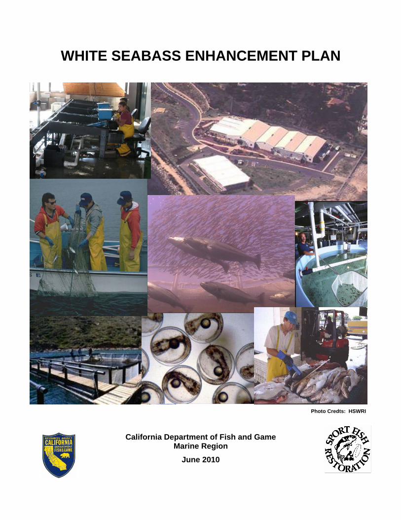
WHITE SEABASS ENHANCEMENT PLAN
Photo Credts: HSWRI
California Department of Fish and Game Marine Region
June 2010
White Seabass Enhancement Plan Executive Summary
The White Seabass Enhancement Plan (WSEP) provides a framework for managing the Ocean Resources Enhancement and Hatchery Program (OREHP) in an environmentally sustainable manner. The WSEP presents detailed information on white seabass and the OREHP and establishes best management practices (BMPs) for hatchery and growout operations, fish health, genetics, and benthic monitoring. It also outlines methods on which to evaluate the OREHP and is designed to be flexible and adaptable to a wide range of future conditions. Minor changes can be made to the BMPs without the need to amend the WSEP by revising the other guidance documents for the OREHP. However, future research, environmental, biological, or economic changes of significance may create a need to amend the WSEP to ensure that the enhancement of white seabass is conducted in a responsible manner. In 1983, the Legislature established the OREHP [Fish and Game Code (FGC) §6590 et. seq.] to conduct a program of basic and applied research into the artificial propagation, rearing, and stocking of important marine finfish species occurring in ocean waters off southern California. Initially, white seabass and California halibut were both chosen for use in the experimental stocking program; however, in 1990, research focused on white seabass because of the depressed condition of the stock at the time and its higher value to recreational and commercial fishermen. Over the years, the Legislature has amended the intent language of the OREHP. Current legislation calls for a focus on determining if hatchery released fish can artificially enhance certain stocks of desirable species through increased production of fish and increased monitoring of fisheries to assess the hatchery contribution. The ultimate goal of the legislation is to enhance populations of marine finfish species important to California for their sport and commercial fishing value. In 2006, the Legislature passed SB 201 (Simitian) Marine Finfish Aquaculture, which amended the statute related to marine aquaculture [FGC §15000 et. seq.]. The statute requires the preparation of an enhancement plan for any artificial propagation, rearing or stocking project for the purpose of recovery, restoration, or enhancement of native fish stocks carried out under either a scientific collecting permit, research permit, or the OREHP [FGC §15400(b)(10)(c)]. The plan shall provide for, among other things, monitoring and protecting of benthic habitat, the prevention of pollution, and the prevention of adverse impacts on wild fish stocks from disease, parasites, and genetic alterations. The legislation also designates the Fish and Game Commission (Commission) the authority to approve an enhancement plan. To manage the State’s commercial and recreational fisheries for white seabass, the Commission adopted a White Seabass Fishery Management Plan (WSFMP) in 2002. The WSFMP provides mainly for a fishery management program based on the concept of an Optimum Yield (estimated as a percentage of Maximum Sustainable Yield) with enforcement of take limits, including minimum size, daily bag, and seasonal restrictions.
6/22/10 i
Currently, the WSFMP does not include the OREHP as a management tool; however, if deemed successful, enhancement could be incorporated in the management of white seabass. The WSEP currently includes twelve chapters and various appendices and supporting materials:
• Chapter 1 – Background outlines 11 components that are integral in developing, evaluating, and managing marine stock enhancement programs. It also lists the primary goal and objectives of the OREHP.
• Chapter 2 – Biological Information for White Seabass includes information on the biology and status of the stock.
• Chapter 3 – History of the Fisheries covers the historical white seabass catch of both the recreational and commercial fisheries.
• Chapter 4 – History of Conservation and Enhancement Efforts summarizes the white seabass regulations from 1931 to present and includes a history of the OREHP.
• Chapter 5 – Hatchery Operations describes the current operating procedures and BMPs for the white seabass hatchery.
• Chapter 6 – Growout Facility Operations describes the current operating procedures and BMPs for the white seabass growout facilities.
• Chapter 7 – Fish Health Management describes the prevention, identification, and treatment of many common white seabass pathogens, including non-infectious and infectious diseases. It also includes the BMPs for the Fish Health Management Program.
• Chapter 8 – Regulatory Considerations lists the permits and permissions required to operate the white seabass hatchery and growout facilities.
• Chapter 9 – Environmental Considerations describes the benthic monitoring program for the growout facilities, including a description of methods used and results of the initial testing for sulfide, reduced oxygen (redox) potential, total volatile solids, zinc, and copper. The BMPs for the growout facilities that identify interim threshold levels of sulfides are included as well.
• Chapter 10 – Genetics includes an overview of the three studies that apply to the genetics of and culturing/management practices for white seabass in southern California. In addition, the goals and objectives of the current genetics research plan are included.
• Chapter 11 – Current Research and Future Needs describes the juvenile and adult sampling programs that will be used to assess the proportion of hatchery-raised fish to the wild population.
• Chapter 12 – Program Evaluation outlines the methods that will be used to evaluate the OREHP. These methods include the creation of a Scientific Advisory Committee (SAC) and an Adaptive Management Plan (AMP); a stock assessment; an update of the bioeconomic model; and an analysis of the adult sampling, genetic management, and benthic monitoring programs. A plan for review and amendment of the WSEP is also included.
6/22/10 ii
The primary goal of both the OREHP and the WSEP is to evaluate the economic and ecological feasibility of releasing hatchery-reared fish to restore depleted, endemic, marine fish populations to a higher, sustainable level. To achieve this goal, the following objectives must be realized: 1) develop and implement hatchery operation and growout methods that provide a supply of healthy and vigorous fish; 2) conduct the replenishment program in a manner that will avoid any significant environmental impacts resulting from operation of either the hatchery or pen rearing facilities; 3) maintain and assess a broodstock management plan that results in progeny being released that have genotypic diversity very similar to that of the wild population; 4) quantify contributions to the standing stock in definitive terms by tagging fish prior to release and assessing their survival in the field; 5) continue to develop, evaluate, and refine hatchery operations to maximize the potential for achieving the goal of the program and; 6) develop quantitative measures of success. To work towards the goal of enhancement, the WSEP addresses each objective through BMPs and ongoing monitoring and evaluation. The BMPs have been developed to manage the program in a manner that will avoid any significant environmental impacts resulting from the operation of either the hatchery or growout facilities. These include, but are not limited to:
• Maintaining separate systems for each aspect of hatchery culture (broodstock, Juvenile 1 and 2 systems, raceway culture, experimental systems, and food production) (Objective 1);
• Maintaining water quality by sterilizing and filtering water at the hatchery and by maintaining clean nets and raceways in the field (Objective 1);
• Monitoring effects to the benthos from growout facility operations by visual inspection and sampling of sediment around growout facilities to analyze sediment free sulfides and redox potential (Objective 2).
• Assessing fish health daily at growout facilities (Objectives 1 and 2); • Releasing only healthy fish that have been inspected by the Department of Fish
and Game (Department) Fish Pathologist (Objectives 1 and 2); • Rotating new broodstock (males and females) into the program following the
procedures as described in the Comprehensive Hatchery Plan for Operation of the Leon Raymond Hubbard, Jr. Marine Fish Hatchery in Carlsbad, California (CHP) (Objective 3);
• Maximizing the genetic diversity of the parental contributions within the annual release total to the fullest extent practical by ensuring that cohorts of released fish are comprised of progeny from at least five females (Objective 3);
• Tagging all fish prior to transfer or release (Objective 4); • Modifying the management of white seabass broodstock as new information
becomes available (Objective 5). The WSEP also includes a formal program evaluation for 2015. The program evaluation will include the following components:
• Adult sampling program review and analysis
6/22/10 iii

• White seabass stock assessment • Bioeconomical model update/rewrite • Juvenile release data review and analysis • Genetic research plan and review • Bethnic monitoring plan and review • Results of ageing work • Habitat assessment study at Santa Catalina Island
To assist the Department in managing the OREHP and evaluating the program, the Department will employ a Scientific Advisory Committee (SAC) made up of experts in white seabass biology, population biology, genetics, environmental quality, and fish pathology. The main purpose of the SAC is to have experts available to review proposed research aimed at evaluating the OREHP, review the AMP, and review the actual program evaluation when completed. The SAC will develop science-based criteria, based on the goals and objectives of the OREHP, to help evaluate the success of the program. The Department also intends to develop an AMP, which will provide a mechanism to continuously evaluate the OREHP. The AMP would then be approved by the SAC and incorporated into the WSEP. The critical issues to be addressed by the AMP are: 1) maximizing the contribution potential of stocked fish through optimized culture and release strategies, 2) maintaining genetic diversity, 3) managing disease, and 4) minimizing impacts to the environment from the hatchery and growout facilities. The WSEP lays out interim steps to ensure that the OREHP has every opportunity of successfully reaching its goals and objectives. If the OREHP proves successful, California recreational and commercial fishing may be more effectively managed by the inclusion of a significant new component (hatchery production) that eliminates natural fluctuations in recruitment that are typical of many fish populations in the wild. This could result in increased opportunities for recreational and commercial fishermen.
6/22/10 iv
White Seabass Enhancement Plan Table of Contents
Executive Summary ......................................................................................................... i Table of Contents............................................................................................................ v List of Figures.................................................................................................................. x List of Tables...................................................................................................................xi List of Acronyms and Abbreviations ...............................................................................xii Acknowledgements .......................................................................................................xiv List of Preparers.............................................................................................................xv Part 1 - The Ocean Resources Enhancement and Hatchery Program.........................1-1 Chapter 1. Background ...............................................................................................1-1
1.1 Introduction and purpose of the enhancement plan .......................................1-1 1.2 Components of a stock enhancement plan....................................................1-1
1.2.1 Selecting target species..........................................................................1-3 1.2.2 Species management plan development ................................................1-4 1.2.3 Quantitative measures of success ..........................................................1-4 1.2.4 Genetic resource management...............................................................1-5 1.2.5 Fish health management ........................................................................1-5 1.2.6 Enhancement objectives and tactics.......................................................1-5 1.2.7 Identify hatchery-raised fish and assess stocking efforts ........................1-6 1.2.8 Define optimum release strategies .........................................................1-6 1.2.9 Economic and policy objectives ..............................................................1-7 1.2.10 Adaptive management ............................................................................1-7 1.2.11 Minimize environmental impacts.............................................................1-8
1.3 Background of the OREHP ............................................................................1-8 1.4 Goals of the OREHP......................................................................................1-9
Chapter 2. Biological Information for White Seabass ..................................................2-1 2.1 Description .....................................................................................................2-1 2.2 Distribution, genetic stock structure, and migration........................................2-1 2.3 Age and growth..............................................................................................2-3 2.4 Reproduction, fecundity, and seasonality ......................................................2-4 2.5 Natural mortality.............................................................................................2-5
Chapter 3. History of the Fisheries ..............................................................................3-1 3.1 Introduction ....................................................................................................3-1 3.2 Recreational fishery .......................................................................................3-1 3.3 Commercial fishery ........................................................................................3-2
Chapter 4. History of Conservation and Enhancement Efforts ....................................4-1 4.1 Regulatory history ..........................................................................................4-1 4.2 History of the OREHP ....................................................................................4-2
Part 2 - Best Management Practices............................................................................5-1 Chapter 5. Hatchery Operations..................................................................................5-1
5.1 Plant management and biosecurity measures ...............................................5-1 5.2 Broodstock care .............................................................................................5-2
5.2.1 Broodstock care and feeding ..................................................................5-2 5.2.2 Broodstock collection and holding ..........................................................5-3
6/22/10 v
5.2.3 Broodstock rotation.................................................................................5-4 5.3 Egg production...............................................................................................5-5
5.3.1 Spawning ................................................................................................5-5 5.3.2 Egg collection .........................................................................................5-5
5.4 Nursery phase................................................................................................5-6 5.4.1 Incubation ...............................................................................................5-6 5.4.2 Juvenile 1 (J1) system ............................................................................5-6 5.4.3 Juvenile 2 (J2) system ............................................................................5-6
5.5 Raceway culture ............................................................................................5-7 5.6 Fish tagging ...................................................................................................5-8 5.7 Fish transport .................................................................................................5-8
Chapter 6. Growout Facility Operations ......................................................................6-1 6.1 General description........................................................................................6-1
6.1.1 Net pens .................................................................................................6-3 6.1.2 Submerged raceways .............................................................................6-4 6.1.3 Land-based pools ...................................................................................6-4
6.2 Stocking density.............................................................................................6-5 6.3 Annual release limit........................................................................................6-5 6.4 Fish feed ........................................................................................................6-6 6.5 Monitoring ......................................................................................................6-7 6.6 Marine mammal interactions ..........................................................................6-8 6.7 Fish releases..................................................................................................6-9
6.7.1 Final inspection and clearance ...............................................................6-9 6.7.2 Coordinating the release.........................................................................6-9 6.7.3 Releasing fish .......................................................................................6-10 6.7.4 Remote releases...................................................................................6-10 6.7.5 Release limit at Catalina Island.............................................................6-10 6.7.6 Direct releases......................................................................................6-11
Chapter 7. Fish Health Management...........................................................................7-1 7.1 Fish health management program .................................................................7-1 7.2 Non-infectious diseases.................................................................................7-3
7.2.1 Gas supersaturation disease ..................................................................7-3 7.2.2 Larval mass mortality syndrome .............................................................7-4 7.2.3 Developmental deformities .....................................................................7-5 7.2.4 Xenobiotic chemical exposure ................................................................7-6 7.2.5 Cannabilism ............................................................................................7-7 7.2.6 Red tides.................................................................................................7-7
7.3 Infectious diseases ........................................................................................7-8 7.3.1 Viral pathogens.......................................................................................7-8
7.3.1.1 Viral nervous necrosis .........................................................................7-8 7.3.1.2 Viral hemorrhagic septicemia ..............................................................7-8 7.3.1.3 Herpesviru enteritis .............................................................................7-9 7.3.1.4 Necrotizing hepatitis (suspect viral hepatitis) ....................................7-10
7.3.2 Bacterial pathogens ..............................................................................7-11 7.3.2.1 Flexibacter maritimus ........................................................................7-11 7.3.2.2 Vibrio .................................................................................................7-11
6/22/10 vi

7.3.3 Rickettsial bacteria................................................................................7-13 7.3.3.1 Epitheliocystis ...................................................................................7-13 7.3.3.2 Piscirickettsia salmonis .....................................................................7-14
7.3.4 Fungal infections...................................................................................7-14 7.3.5 Sporozoans...........................................................................................7-15
7.3.5.1 Renal Myxosporidians .......................................................................7-15 7.3.5.2 Unidentified renal sporozoan pathogen.............................................7-15
7.3.6 Metazoan parasites ..............................................................................7-16 7.3.6.1 Anchoromicrocotyle guaymensis.......................................................7-16 7.3.6.2 Gyrodactylus .....................................................................................7-17
7.3.7 Protozoan parasites ..............................................................................7-17 7.3.7.1 Ciliates ..............................................................................................7-17
7.3.7.1.1 Trichodina ....................................................................................7-17 7.3.7.1.2 Uronema marinum .......................................................................7-18 7.3.7.1.3 Cryptokaryon irritans....................................................................7-18 7.3.7.1.4 Unidentified ciliates ......................................................................7-19
7.3.7.2 Flagellates.........................................................................................7-19 7.3.7.2.1 Ichthyobodo .................................................................................7-19 7.3.7.2.2 Cryptobia .....................................................................................7-20 7.3.7.2.3 Hexamita......................................................................................7-20 7.3.7.2.4 Unidentified flagellates.................................................................7-20
7.3.8 Isopods .................................................................................................7-20 7.3.9 Copepods .............................................................................................7-20
Chapter 8. Regulatory Considerations ........................................................................8-1 8.1 Permit and permissions .................................................................................8-1
8.1.1 California Environmental Quality Act ......................................................8-1 8.1.2 California Endangered Species Act ........................................................8-1 8.1.3 National Pollution Elimination Discharge Permit .....................................8-2 8.1.4 Coastal Development Permit ..................................................................8-2 8.1.5 State Lands Lease..................................................................................8-3 8.1.6 Section 401 and 404 of the Clean Water Act Permit Requirements .......8-3 8.1.7 Private Aids to Navigation Permit ...........................................................8-4 8.1.8 Section 7 Endangered Species Act Consultation....................................8-4 8.1.9 MMPA designation..................................................................................8-5 8.1.10 The Magnuson-Stevens Fishery Conservation and Management Act and Essential Fish Habitat ...........................................................................................8-5 8.1.11 United States Environmental Protection Agency ....................................8-6 8.1.12 Local Authority Permissions....................................................................8-6
Chapter 9. Environmental Considerations...................................................................9-1 9.1 Benthic monitoring program...........................................................................9-1
9.1.1 Chemical remediation .............................................................................9-1 9.1.2 Biological remediation.............................................................................9-1 9.1.3 Materials and methods............................................................................9-2 9.1.4 Sources of organic carbon ......................................................................9-2 9.1.5 Sediment-free sulfides (S∋) .....................................................................9-4
9.1.5.1 Results of sulfide sampling..................................................................9-4
6/22/10 vii
9.1.5.2 Sulfide benchmarks for measuring changes in the benthic community.9-7
9.1.6 Redox potential .......................................................................................9-7 9.1.6.1 Results of redox potential sampling.....................................................9-7 9.1.6.2 Benchmarks for redox potential...........................................................9-8
9.1.7 Total Volatile Solids ................................................................................9-8 9.1.7.1 Results of TVS sampling .....................................................................9-9 9.1.7.2 TVS benchmarks.................................................................................9-9
9.1.8 Sedimented zinc ...................................................................................9-10 9.1.8.1 Results of zinc sampling....................................................................9-10 9.1.8.2 Benchmarks for monitoring zinc ........................................................9-11
9.1.9 Sedimented copper...............................................................................9-11 9.1.9.1 Results of copper sampling ...............................................................9-11 9.1.9.2 Benchmarks for monitoring copper ...................................................9-12
9.2 Water quality monitoring ..............................................................................9-13 9.3 Bird and mammal interactions......................................................................9-13 9.4 Effects on sensitive habitats.........................................................................9-14
Chapter 10. Genetics ................................................................................................10-1 10.1 Genetic considerations ................................................................................10-1 10.2 Conserving genetic diversity ........................................................................10-1
10.2.1 Genetic structure of the wild population................................................10-2 10.2.2 Effective hatchery population size ........................................................10-3
10.3 Genotyping...................................................................................................10-4 10.3.1 Broodstock source and genotyping.......................................................10-4 10.3.2 Progeny genotyping..............................................................................10-4
10.4 Research......................................................................................................10-5 10.4.1 Coykendall’s genetics research ............................................................10-5 10.4.2 Current and future genetics research ...................................................10-9
10.5 Monitoring of the enhanced white seabass population ................................10-9 Part 3 - Evaluation of the Ocean Resources Enhancement and Hatchery Program ..11-1 Chapter 11. Current Research and Future Needs.....................................................11-1
11.1 Juvenile gill net survey.................................................................................11-1 11.1.1 Sample design ......................................................................................11-1 11.1.2 Results of the juvenile gill net surveys ..................................................11-3 11.1.3 Current and future work based on juvenile gill net survey data.............11-4
11.2 Adult surveys ...............................................................................................11-4 11.3 Acoustic studies ...........................................................................................11-7 11.4 Nutrition studies ...........................................................................................11-9
Chapter 12. Program Evaluation ...............................................................................12-1 12.1 Scientific Advisory Committee......................................................................12-1 12.2 Adaptive Management Plan .........................................................................12-1 12.3 Evaluation of the OREHP ............................................................................12-3
12.3.1 Stock assessment.................................................................................12-4 12.3.2 Adult sampling programs ......................................................................12-5 12.3.3 Bioeconomic model ..............................................................................12-5 12.3.4 Genetics research and benthic monitoring............................................12-5
6/22/10 viii
12.3.5 Other data sources ...............................................................................12-6 12.4 White Seabass Enhancement Plan review ..................................................12-6 12.5 Plan amendment..........................................................................................12-6
References.................................................................................................................. R-1 Appendix A. Glossary of Terms and Abbreviations ......................................................A-1 Appendix B. Review of Coykendall’s Dissertation ........................................................A-6
6/22/10 ix
White Seabass Enhancement Plan List of Figures
Figure 3-1. Recreational catch of white seabass in California, 1947 through 2008.....3-2 Figure 3-2. Commercial catch of white seabass in California, 1936 through 2008......3-3 Figure 11-1. Release and capture locations of recovered tagged white seabass 1992 to
2008. ...................................................................................................................11-6 Figure 11-2. Number of tagged white seabass recovered per age group from 1992 to
2008. ...................................................................................................................11-7 Figure 11-3. Number of years tagged white seabass released from 1992 to 2008
remained at liberty until recovery. .......................................................................11-7 Figure 11-4. Diurnal and tidal cycles during which hatchery-raised white seabass with
implanted acoustic pingers emigrated from Mission Bay in San Diego. Boxes represent individual fish identification codes, with lines showing when they were detected at buoy stations outside the bay (Drawbridge et al. 2006)....................11-9
Figure 12-1. The OREHP white seabass releases 1986 to 2008. .............................12-4
6/22/10 x
White Seabass Enhancement Plan List of Tables
Table 1-1. Timeline and progress to date for the OREHP. ..........................................1-2Table 2-1. The commercial catch of white seabass (pounds) in the San Francisco Bay
area, 1986 to 20081...............................................................................................2-2 Table 2-2. Mean total length and weight at age for white seabass (taken from CDFG
2002).....................................................................................................................2-4 Table 2-3. Estimates of white seabass natural mortality (M) (taken from CDFG 2002). 2-
6Table 4-1. Summary of White Seabass Regulations from 1931 to the Present (modified
from Vojkovich and Reed 1983 and CDFG 2002). ................................................4-1 Table 6-1. The OREHP growout facility growing volume.............................................6-1 Table 6-2. Permits or permissions required to operate an OREHP growout facility. ...6-2 Table 9-1. Sulfide concentrations (µM) at the OREHP’s growout facilities (from Brooks
2007).....................................................................................................................9-5 Table 9-2. Release and sample information at the time of benthic monitoring (from
Brooks 2007).........................................................................................................9-6 Table 9-3. Redox potential values (mV) at the OREHP’s growout facilities (from Brooks
2007).....................................................................................................................9-8 Table 9-4. TVS values (percent difference between dry and combusted weight of the
sediment) at the OREHP’s growout facilities (from Brooks 2007). ........................9-9 Table 9-5. Zinc concentration (µg/g sediment) at the OREHP’s growout facilities (from
(Brooks 2007)). ...................................................................................................9-10 Table 9-6. Published sediment zinc and copper benchmarks (µg/g dry sediment). ..9-11 Table 9-7. Copper concentration (µg/g sediment) at the OREHP’s growout facilities
(from Brooks 2007). ............................................................................................9-12 Table 11-1. Juvenile gill net sampling sites, FY 1995-96 to 2007-08. .......................11-1 Table 11-2. Juvenile gill net sampling schedule FY 1995-96 to 2007-08. .................11-2
6/22/10 xi
White Seabass Enhancement Plan
List of Acronyms and Abbreviations
BMPs Best Management Practices BOD Biological Oxygen Demand* CCC California Coastal Commission CalCOFI California Cooperative Oceanic Fisheries Investigations CDP Coastal Development Permit CESA California Endangered Species Act CEQA California Environmental Quality Act CFIS Commercial Fishery Information System CHP Comprehensive Hatchery Plan for Operation of the Leon Raymond
Hubbard, Jr. Marine Fish Hatchery in Carlsbad, California CNS Central Nervous System* CPFV Commercial Passenger Fishing Vessel* CRFS California Recreational Fisheries Survey CSF Catalina Seabass Fund CSUN California State University, Northridge CTR California Toxics Rule* CWT Coded Wire Tag* dph Days Post Hatch EEZ Exclusive Economic Zone* EFH Essential Fish Habitat* ELISA Enzyme-linked Immunosorbent Assay* ESA Federal Endangered Species Act FAT Fluorescent Antibody Testing* FCR Food Conversion Rate* GFC Growout Facility Coordinator GPM Procedures Manual for Growout and Release of White Seabass
(Atractonscion nobilis) as part of the Ocean Resources Enhancement and Hatchery Program (OREHP)
GSS Gas Supersaturation* HSWRI Hubbs-SeaWorld Research Institute LARWQCB Los Angeles Regional Water Quality Control Board LMMS Larval Mass Mortality Syndrome* LOP Letter of Permission* MCCS Main Computer Control System MLLW Mean Lower Low Water MLMA Marine Life Management Act MMPA Marine Mammal Protection Act MND Mitigated Negative Declaration MOA Memorandum of Agreement MRFSS Marine Recreational Fisheries Statistical Survey MSFCMA Magnuson-Stevens Fishery Conservation and Management Act* MS-222 Tricaine methanesulfonate*
6/22/10 xii
NOAA National Oceanic and Atmospheric Administration NOAA Fisheries NOAA’s National Marine Fisheries Service NPDES National Pollution Discharge Elimination System Permit OPP Organophosphate Pesticides* OREHP Ocean Resources Enhancement and Hatchery Program OREAP Ocean Resources Enhancement Advisory Panel OSP Optimum Sustainable Population* PBR Potential Biological Removals* PCR Polymerase Chain Reaction* PIT Passive Integrated Transponder* PSMFC Pacific States Marine Fisheries Commission RBC Red Blood Cell RecFIN Recreational Fisheries Information Network Redox Reduced Oxygen SAC Scientific Advisory Committee SCE Southern California Edison SDRWQCB San Diego Regional Water Quality Control Board SDSU San Diego State University SFA Sustainable Fisheries Act SFRA Sport Fish Restoration Act SLC California State Lands Commission SONGS San Onofre Nuclear Generating Station T&E Threatened and Endangered Species TDG Total Dissolved Gas* TEM Transmission Electron Microscopy* TGP Total Gas Pressure* TOC Total Organic Carbon* TVS Total Volatile Solids* UASC United Anglers of Southern California UCD University of California, Davis USACE United States Army Corp of Engineers USCG United States Coast Guard USDA United States Department of Agriculture USFWS U.S. Fish and Wildlife Service VHS Viral Hemorrhagic Septicemia* VNN Viral Nervous Necrosis* VRG Vantuna Research Group of Occidental College VNNV Viral Nervous Necrosis Virus* WSEP White Seabass Enhancement Plan WSFMP White Seabass Fishery Management Plan *Defined in the Glossary of Terms and abbreviations
6/22/10 xiii
White Seabass Enhancement Plan Acknowledgements
The Department thanks the following Hubbs-SeaWorld Research Institute (HSWRI) staff for their valuable contributions and dedication to the OREHP (in alphabetical order): David Bottinelli; Tim Connerty; Mark Drawbridge; Mike Gafford; Dave Jirsa; Martha Keller, DVM, MS; Don Kent; Eric McIntire; Karen Miller McClune; Mike Shane; George Slim; Jeff Smiley; and Pam Yochem, DVM, Ph. D. Fish health and genetic quality insurance has been a priority to the OREHP since the early years of the program. The Department thanks (in alphabetical order): Kristen Arkush, Ph. D, University of California, Davis; Devin Bartley, Ph. D, Food and Agriculture Organization of the United Nations; Martin Chen, Ph. D, CDFG; Katherine Coykendal, University of Southern California; Dennis Hedgecock, Ph. D, University of Southern California; Kristen Grundenthal, Ph. D, HSWRI; Ron Hedrick, Ph. D, University of California, Davis; and Russ Vetter, Ph. D, NOAA Southwest Fisheries Science Center, for their contributions and commitment towards improving our understanding of white seabass genetics and diseases. Others have also contributed valuable information to the program. The Department thanks (in alphabetical order): Larry Allen, Ph. D, California State University Northridge; Daniel Pondella II, Ph. D, Occidental College; and Mike Shane, HSWRI, for their work on the juvenile white seabass gill net studies. The Department also thanks Kenneth Brooks, Ph. D, Aquatic Environmental Sciences, for his assistance in developing the Benthic Monitoring Program. The Department acknowledges the participation of the members of the Ocean Resources Enhancement Advisory Panel (OREAP). Their suggestions and assistance in the preparation of the plan is appreciated. They are (in alphabetical order): Todd Anderson, California State University; Mark Bailey, commercial industry representative; David Checkley, University of California representative; Ken Franke, Sportfishing Association of California representative; Steve Fukuto, United Anglers of Southern California representative; David Hankin, California State University representative; Philip Hastings, University of California representative; Mike McCorkle, commercial industry representative; Robert Osborn, United Anglers of Southern California; Bill Shedd, American Fishing Tackle Manufacturers Association representative; Tony Vaught, California Aquaculture Association representative; Joe Villareal, Sportfishing Association of California, and Dallas Weaver, Ph. D, California Aquaculture Association. The Department would also like to acknowledge the growout facility operators and all those who have volunteered and donated their time and support towards the OREHP. The Department thanks them for their help and looks forward to working with them in the future.
6/22/10 xiv
White Seabass Enhancement Plan List of Preparers
Fluharty, Marilyn. Environmental Specialist III. CDFG. San Diego, CA. Frey, Vicki. Environmental Scientist. CDFG. Eureka, CA. Johnson, Kathryn. Marine Biologist. CDFG. Los Alamitos, CA. Larinto, Traci. Senior Biologist Specialist. CDFG. Los Alamitos, CA. Mello, John. Senior Biologist Supervisor. CDFG. Eureka, CA. Moore, Tom. Associate Marine Biologist. CDFG. Bodega Bay, CA. Okihiro, Mark. Senior Pathologist. CDFG. Oceanside, CA. Ramey, Kirsten. Associate Marine Biologist. CDFG. Eureka, CA. Reilly, Paul. Senior Biologist Supervisor. CDFG. Monterey, CA. Taylor, Valerie. Associate Marine Biologist. CDFG. Los Alamitos, CA.
6/22/10 xv
Part 1 - The Ocean Resources Enhancement and Hatchery Program
Chapter 1. Background
1.1 Introduction and purpose of the enhancement plan The passage of SB 201 (Simitian) Marine Finfish Aquaculture, in 2006, amended statute related to marine aquaculture [Fish and Game Code (FGC) §15000 et. seq.]. The statute requires the preparation of an enhancement plan for any artificial propagation, rearing or stocking project for the purpose of recovery, restoration, or enhancement of native fish stocks carried out under either a scientific collecting permit, research permit, or the Ocean Resources Enhancement and Hatchery Program (OREHP) [FGC §15400(b)(10)(c)]. The plan shall provide for, among other things, monitoring and protecting of benthic habitat, the prevention of pollution, and the prevention of adverse impacts on wild fish stocks from disease, parasites, and genetic alterations. The legislation also designated the Commission as the authority to approve an enhancement plan. 1.2 Components of a stock enhancement plan Blankenship and Leber (1995) identified 10 components in developing, evaluating and managing marine fish stock enhancement programs. The components include the need to:
(1) Prioritize and select target species for enhancement;
(2) Develop a species management plan that identifies harvest opportunity, stock rebuilding goals, and genetic objectives;
(3) Define quantitative measures of success;
(4) Use genetic resource management to avoid deleterious genetic effects;
(5) Use disease and health management;
(6) Consider ecological, biological, and life history patterns when forming
enhancement objectives and tactics;
(7) Identify released hatchery fish and assess stocking efforts;
(8) Use an empirical process for defining optimum release strategies;
(9) Identify economic and policy guidelines; and
1-1 6/14/2010

(10) Use adaptive management.
Not stated in Blankenship and Leber (1995) but of concern to the OREHP is:
(11) Minimize the environmental effects of the hatchery and growout facilities. The eleven items outlined above also cover the provisions of the Fish and Game Code relative to development of an enhancement plan. Specifically, component 11 covers monitoring and protecting the benthic habitat, and the prevention of pollution. Component 5 covers the prevention of adverse impacts on wild fish stocks from disease and parasites, while component 4 covers the prevention of genetic alterations. Table 1-1 outlines what has already been accomplished within the OREHP for each of these components and what remains to be done. Further discussion of each component can also be found in the following subsections.
Table 1-1. Timeline and progress to date for the OREHP.
Component Subcomponent Status Location Select target species for enhancement
Not applicable Completed Sections 1.2.1 and 4.2
Develop species management plan
Develop goals and objectives of the OREHP
Completed Sections 1.2.2 and 1.4
Identify and manage genetic structure of wild white seabass stock according to objectives of the OREHP
In progress - estimated completion date June 2014
Sections 1.2.2, 2.2, 6.3, and Chapter 10
Estimate post-release survival
In progress – estimated completion date June 2014
Section 1.2.2 and Chapter 11
Define quantitative measures of success
Not applicable Will be developed by June 2014
Section 1.2.3
Use genetic resource management
Determine geographical range of wild stock
Completed Sections 1.2.4 and 2.2
Determine effective broodstock population
Initial studies completed; further research in progress – estimated completion date June 2014
Chapter 10
Develop genetic monitoring protocols
In progress – estimated completion date June 2014
Sections 10.3, 10.4, and 10.5
Conduct genetic monitoring of broodstock and released progeny
In progress – estimated completion date June 2014
Sections 5.2.2, 5.3, 5.4, 6.3, 10.3, and 10.4
Use disease and health management
Develop protocols for routine sampling
Completed Sections 1.2.5, 5.1, 6.5, 6.7.1, and Chapter 7
Conduct research on novel pathogens to determine etiology and treatment
Ongoing/as needed Chapter 7
Develop protocols for treatment/euthanization
Completed – new pathogens to be added as needed
Chapter 7
Develop enhancement Not applicable In progress – estimated Section 1.2.6 and
1-2 6/14/2010

Table 1-1. Timeline and progress to date for the OREHP.
Component Subcomponent Status Location objectives and tactics completion date June 2014 Chapters 2 and 3 Identify hatchery-raised fish and assess stocking efforts
Tag or mark all fish Ongoing Sections 1.2.7 and 5.6
Develop juvenile sampling program
Completed Sections 1.2.7 and 11.1
Develop adult sampling program
Competed Sections 1.2.7 and 11.2
Define optimum release strategies
Evaluate fish size at release Completed Section 1.2.8
Evaluate release season In progress – estimated completion date June 2014
Sections 1.2.8 and 11.1.3
Evaluate release habitat In progress – estimated completion date June 2014
Sections 2.2, 6.7, and 11.1
Evaluate release magnitude In progress – estimated completion date June 2014
Section 1.2.8 and 6.3
Identify economic and policy guidelines
Not applicable Initial evaluation completed; update of evaluation estimated completion date June 2014
Section 1.2.9
Use adaptive management
Not applicable In progress – estimated completion date June 2015
Section 1.2.10 and 12.2
Minimize environmental impacts
Identify best management practices at hatchery and growout facilities
Completed Section 1.2.11 and Chapters 5 and 6
Identify impacts to benthos and ways to minimize
In progress – estimated completion date June 2014
Chapter 9
Identify permits and permissions
Completed Chapter 8
1.2.1 Selecting target species In the beginning, the Ocean Resources Enhancement Advisory Panel (OREAP) and the Department of Fish and Game (Department) selected two species, California halibut (Paralichthys californicus) and white seabass (Atractoscion nobilis), to begin developing culture methods. Original selection criteria included:
• Species indigenous to southern California • Status as a diminished stock • Economic value • Both commercial and sport utilization • Potential for success
During the first six years of the program, research focused on the capture, maintenance, spawning (both natural and artificial), and grow-out to release size for California halibut and white seabass. Additionally, work was undertaken to determine juvenile natural mortality, juvenile distribution in the wild, post-release survivability of hatchery reared
1-3 6/14/2010
fish, and marking methods to identify hatchery reared fish in the wild. In 1990, the Department and the OREAP decided to focus the OREHP’s limited funding on white seabass culture because California halibut commercial and recreational landings began to stabilize while white seabass landings continued to decline. In addition, white seabass was considered a more desirable species to both commercial and recreational fishers. For more information see Section 4.2. 1.2.2 Species management plan development No formal species management plan, that identifies how the enhancement effort fits into the management of white seabass, was developed at the beginning of the program. However, the Comprehensive Hatchery Plan (CHP) for Operation of the Leon Raymond Hubbard, Jr. Marine Fish Hatchery in Carlsbad, California (Drawbridge and Okihiro 2007) and the Procedures Manual for Growout and Release of White Seabass (GPM) (Atractoscion nobilis) as part of the Ocean Resources Enhancement and Hatchery Program (OREHP) (Drawbridge and Okihiro 2007) cover most of the enhancement aspects of such a plan including goals and objectives of the OREHP, identification of genetic stocks to determine the population being enhanced, methods to maintain genetic diversity, and disease management. While the two documents do not estimate post-release survival, two research programs have been aimed at learning about post-release survival, the juvenile gill net sampling program (Section 11.1) and the adult head collection program (Section 11.2). While the adult head collection program is ongoing, the juvenile gill net sampling program operated from 1995 through 2008. A separate document, the White Seabass Fishery Management Plan (WSFMP) (CDFG 2002), adopted by the Commission in 2002, covers the management of white seabass but does not include the OREHP as a management tool. The WSFMP was adopted pursuant to the Marine Life Management Act (MLMA) (AB 1241-Keeley; Fish and Game Code Section 7050 et. seq.), which required the development of a fishery management plan. The main goal of the MLMA is to ensure long-term resource conservation and sustainability. While the MLMA does not mention enhancement as a management tool, it does require the rebuilding of depressed stocks. Once the OREHP has been formally evaluated and if deemed successful, fishery managers can then consider incorporating enhancement into the management of white seabass. 1.2.3 Quantitative measures of success To date, no quantifiable measures of success have been developed for the OREHP. Developing measures of success will be one of the tasks of the Scientific Advisory Committee (SAC) (Section 12.1). These measures of success should be based on the goals and objectives of the OREHP (Section 1.4) and should include criteria such as:
Hatchery releases will contribute at least X percent to the recreational and commercial landings annually.
1-4 6/14/2010
Monitoring will show less than Y percent change in the frequency of rare alleles after 5 years of hatchery releases. Benthic monitoring will show less than Z percent change in key indicators attributable to growout pen operations between each round of benthic monitoring.
The measures of success should be specified by the SAC prior to the planned program evaluation by the Department. 1.2.4 Genetic resource management The OREHP has made genetic resource management a priority since the early years of the program. Genetic resource management includes the genetic status of the stock to be enhanced, genetic goals of the enhancement program, and the approach for managing genetic impacts. Studies to examine the genetic structure of wild seabass were initiated in the mid-late 1980s and have ran parallel to the culture and assessment research (Bartley and Kent 1990). One of the goals of the OREHP is to release cultured white seabass that have genetic diversity very similar to that of the wild population. The OREHP currently uses best management practices (BMPs) (Sections 5.2.3 and 5.3) to maximize the number of parents contributing to white seabass production. These BMPs will remain in place until a genetic management plan is developed and incorporated as part of the White Seabass Enhancement Plan (WSEP). The genetic management plan will be based on the results of genetic research currently being conducted by Hubbs-SeaWorld Research Institute (HSWRI) and should be completed and approved by the SAC within the next five years. 1.2.5 Fish health management Maintaining fish health has always been a part of the OREHP. The goal is to ensure that no ill fish are released into the wild and that no novel disease is introduced into the wild white seabass population. To that end, the Department has committed a fulltime Fish Pathologist to the OREHP since the hatchery was built. HSWRI’s resident veterinarian also participates in disease management for the OREHP. The current Fish Pathologist has greatly expanded our knowledge of pathogens affecting cultured and wild white seabass, enabling the OREHP to manage fish health effectively. Additionally, the OREHP routinely contracts with pathology researchers from the University of California, Davis (UCD). Chapter 7 details the BMPs for fish health management. 1.2.6 Enhancement objectives and tactics An enhancement plan should contain all the available information regarding the ecological and biological mechanisms affecting the species to be enhanced. Information gaps should be filled by research projects designed to answer critical questions.
1-5 6/14/2010
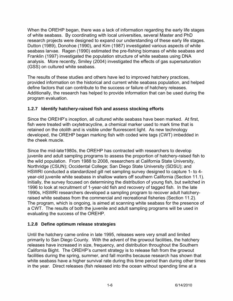
When the OREHP began, there was a lack of information regarding the early life stages of white seabass. By coordinating with local universities, several Master and PhD research projects were designed to expand our understanding of these early life stages. Dutton (1989), Donohoe (1990), and Kim (1987) investigated various aspects of white seabass larvae. Ragen (1990) estimated the pre-fishing biomass of white seabass and Franklin (1997) investigated the population structure of white seabass using DNA analysis. More recently, Smiley (2004) investigated the effects of gas supersaturation (GSS) on cultured white seabass. The results of these studies and others have led to improved hatchery practices, provided information on the historical and current white seabass population, and helped define factors that can contribute to the success or failure of hatchery releases. Additionally, the research has helped to provide information that can be used during the program evaluation. 1.2.7 Identify hatchery-raised fish and assess stocking efforts Since the OREHP’s inception, all cultured white seabass have been marked. At first, fish were treated with oxytetracycline, a chemical marker used to mark time that is retained on the otolith and is visible under fluorescent light. As new technology developed, the OREHP began marking fish with coded wire tags (CWT) imbedded in the cheek muscle. Since the mid-late1980s, the OREHP has contracted with researchers to develop juvenile and adult sampling programs to assess the proportion of hatchery-raised fish to the wild population. From 1988 to 2008, researchers at California State University, Northridge (CSUN); Occidental College; San Diego State University (SDSU); and HSWRI conducted a standardized gill net sampling survey designed to capture 1- to 4- year-old juvenile white seabass in shallow waters off southern California (Section 11.1). Initially, the survey focused on determining the distribution of young fish, but switched in 1996 to look at recruitment of 1-year-old fish and recovery of tagged fish. In the late 1990s, HSWRI researchers developed a sampling program to recover adult hatchery-raised white seabass from the commercial and recreational fisheries (Section 11.2). The program, which is ongoing, is aimed at scanning white seabass for the presence of a CWT. The results of both the juvenile and adult sampling programs will be used in evaluating the success of the OREHP. 1.2.8 Define optimum release strategies Until the hatchery came online in late 1995, releases were very small and limited primarily to San Diego County. With the advent of the growout facilities, the hatchery releases have increased in size, frequency, and distribution throughout the Southern California Bight. The OREHP’s current strategy is to release fish from the growout facilities during the spring, summer, and fall months because research has shown that white seabass have a higher survival rate during this time period than during other times in the year. Direct releases (fish released into the ocean without spending time at a
1-6 6/14/2010

growout facility) will occur in the spring. At present, fish are released when they are 200 to 250 mm (8 to10 in.) total length (TL), based on the results of the bioeconomic model (Section 1.2.9), which suggests that this size yields the greatest return for the investment. Additionally, fish of this size are less vulnerable to disease when stressed than smaller fish. The OREHP also releases the majority of fish from the growout facilities, recognizing that these fish are more likely to survive than fish released directly in the ocean. Additional information on releases can be found in Section 6.7. The Carlsbad hatchery was designed and constructed to support the production of more than 350,000 tagged juveniles per year. However, from 1996 to 2004, the OREHP was operating under a 125,000 fish annual release limit imposed by the California Coastal Commission (CCC) as a condition of the Coastal Development Permits (CDPs) for the growout facilities. This release limit was derived as a proportion of the breeding population that was housed at the hatchery in 1995. During that time, the hatchery increased the breeding population to 200 adult fish as specified in the original plan. Upon meeting the target broodstock population size and demonstrating the capacity to rear several hundred thousand juveniles, the OREHP requested and the CCC granted an increase to the release limit to 350,000 fish from 2004 until 2006. In 2007, the release limit dropped back to the earlier 125,000 fish because the breeding population decreased by 20 percent due to mortalities and the inability to rotate new broodstock into the hatchery. In 2009, the Department and the OREAP submitted a request to the CCC proposing that the release limit be based on a proportion of the current breeding population housed at the hatchery (sliding scale release limit). The CCC agreed to this proposal, and the sliding scale release limit was implemented in 2010. Under this proposal, the annual release limit is calculated by dividing the current number of broodstock by 200 and multiplying that percentage by the production capability of 350,000. The current release limit is set at 287,000 fish. However, because the number of broad fish at the hatchery changes every few months due to mortalities or additions, the release limit is recalculated on January 10 and June 10 of each year. 1.2.9 Economic and policy objectives The goals and objectives of the OREHP were developed early on (Section 1.4) and included determining if it was economically feasible. A bioeconomic model was developed by Botsford et al. (1988) to determine the feasibility of enhancement and guide research and planning. Based on 1988 fishing regulations and a natural mortality rate of 0.13, the cost per stocked fish was estimated to be $2.00. The bioeconomic model was developed before the hatchery was built and has not been updated to reflect hatchery operations or recent research on white seabass. 1.2.10 Adaptive management Adaptive management provides a mechanism to adjust fish production and management via ongoing assessment of the different components of the enhancement
1-7 6/14/2010
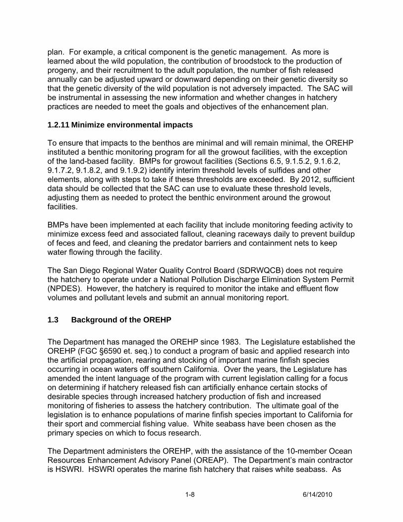
plan. For example, a critical component is the genetic management. As more is learned about the wild population, the contribution of broodstock to the production of progeny, and their recruitment to the adult population, the number of fish released annually can be adjusted upward or downward depending on their genetic diversity so that the genetic diversity of the wild population is not adversely impacted. The SAC will be instrumental in assessing the new information and whether changes in hatchery practices are needed to meet the goals and objectives of the enhancement plan. 1.2.11 Minimize environmental impacts To ensure that impacts to the benthos are minimal and will remain minimal, the OREHP instituted a benthic monitoring program for all the growout facilities, with the exception of the land-based facility. BMPs for growout facilities (Sections 6.5, 9.1.5.2, 9.1.6.2, 9.1.7.2, 9.1.8.2, and 9.1.9.2) identify interim threshold levels of sulfides and other elements, along with steps to take if these thresholds are exceeded. By 2012, sufficient data should be collected that the SAC can use to evaluate these threshold levels, adjusting them as needed to protect the benthic environment around the growout facilities. BMPs have been implemented at each facility that include monitoring feeding activity to minimize excess feed and associated fallout, cleaning raceways daily to prevent buildup of feces and feed, and cleaning the predator barriers and containment nets to keep water flowing through the facility. The San Diego Regional Water Quality Control Board (SDRWQCB) does not require the hatchery to operate under a National Pollution Discharge Elimination System Permit (NPDES). However, the hatchery is required to monitor the intake and effluent flow volumes and pollutant levels and submit an annual monitoring report. 1.3 Background of the OREHP The Department has managed the OREHP since 1983. The Legislature established the OREHP (FGC §6590 et. seq.) to conduct a program of basic and applied research into the artificial propagation, rearing and stocking of important marine finfish species occurring in ocean waters off southern California. Over the years, the Legislature has amended the intent language of the program with current legislation calling for a focus on determining if hatchery released fish can artificially enhance certain stocks of desirable species through increased hatchery production of fish and increased monitoring of fisheries to assess the hatchery contribution. The ultimate goal of the legislation is to enhance populations of marine finfish species important to California for their sport and commercial fishing value. White seabass have been chosen as the primary species on which to focus research. The Department administers the OREHP, with the assistance of the 10-member Ocean Resources Enhancement Advisory Panel (OREAP). The Department’s main contractor is HSWRI. HSWRI operates the marine fish hatchery that raises white seabass. As
1-8 6/14/2010
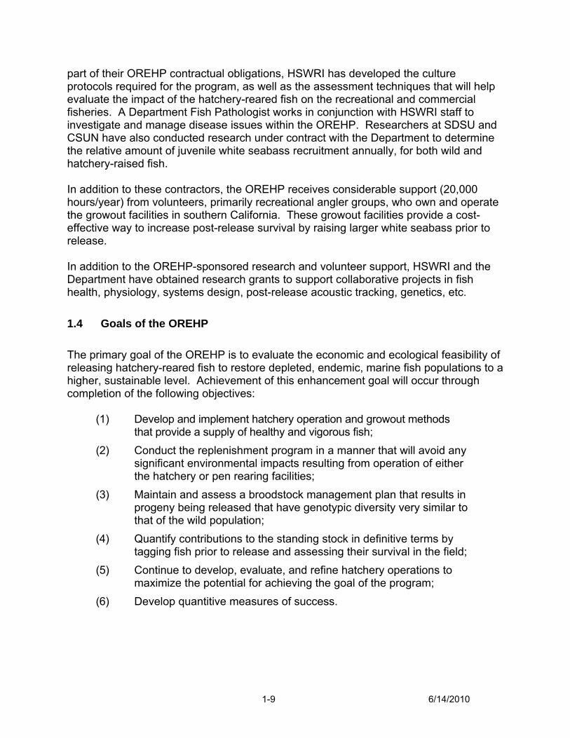
part of their OREHP contractual obligations, HSWRI has developed the culture protocols required for the program, as well as the assessment techniques that will help evaluate the impact of the hatchery-reared fish on the recreational and commercial fisheries. A Department Fish Pathologist works in conjunction with HSWRI staff to investigate and manage disease issues within the OREHP. Researchers at SDSU and CSUN have also conducted research under contract with the Department to determine the relative amount of juvenile white seabass recruitment annually, for both wild and hatchery-raised fish. In addition to these contractors, the OREHP receives considerable support (20,000 hours/year) from volunteers, primarily recreational angler groups, who own and operate the growout facilities in southern California. These growout facilities provide a cost-effective way to increase post-release survival by raising larger white seabass prior to release. In addition to the OREHP-sponsored research and volunteer support, HSWRI and the Department have obtained research grants to support collaborative projects in fish health, physiology, systems design, post-release acoustic tracking, genetics, etc. 1.4 Goals of the OREHP The primary goal of the OREHP is to evaluate the economic and ecological feasibility of releasing hatchery-reared fish to restore depleted, endemic, marine fish populations to a higher, sustainable level. Achievement of this enhancement goal will occur through completion of the following objectives:
(1) Develop and implement hatchery operation and growout methods that provide a supply of healthy and vigorous fish;
(2) Conduct the replenishment program in a manner that will avoid any significant environmental impacts resulting from operation of either the hatchery or pen rearing facilities;
(3) Maintain and assess a broodstock management plan that results in progeny being released that have genotypic diversity very similar to that of the wild population;
(4) Quantify contributions to the standing stock in definitive terms by tagging fish prior to release and assessing their survival in the field;
(5) Continue to develop, evaluate, and refine hatchery operations to maximize the potential for achieving the goal of the program;
(6) Develop quantitive measures of success.
1-9 6/14/2010
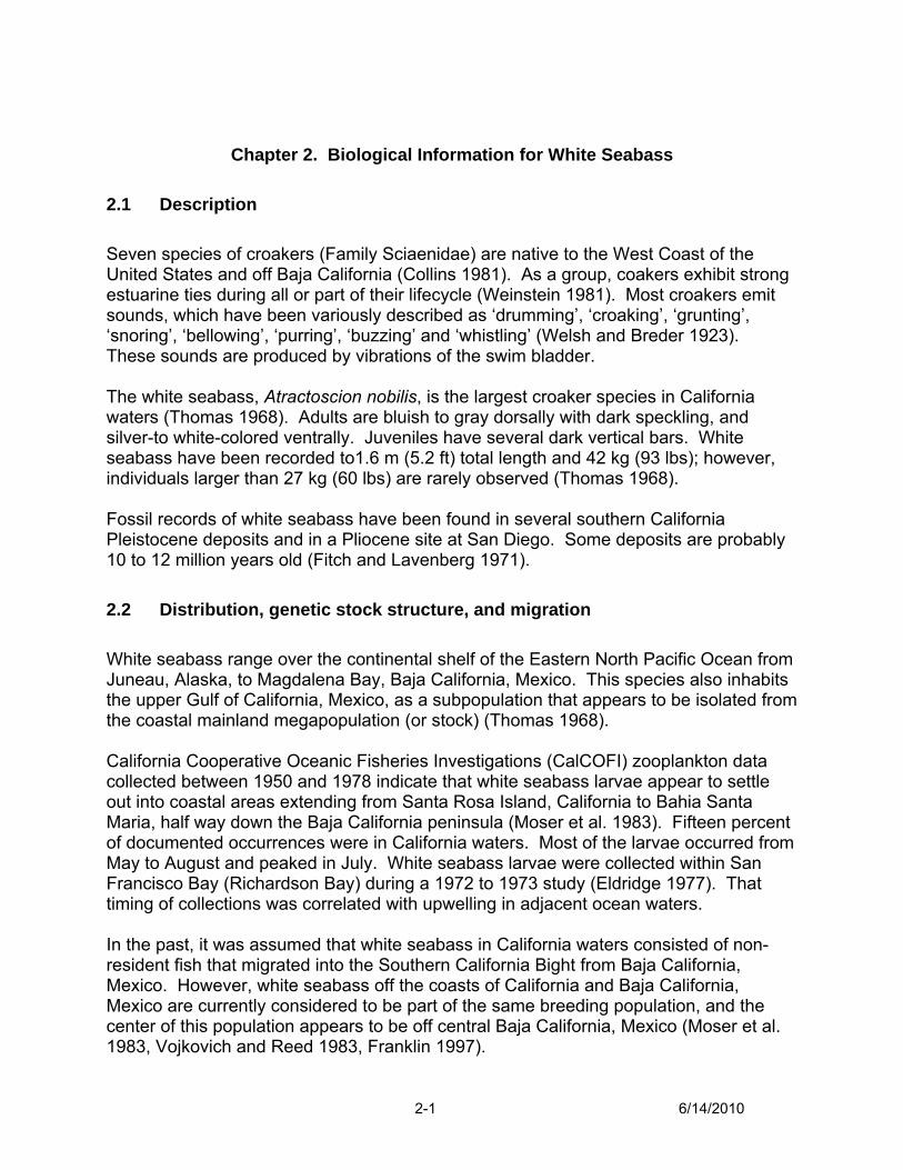
Chapter 2. Biological Information for White Seabass
2.1 Description Seven species of croakers (Family Sciaenidae) are native to the West Coast of the United States and off Baja California (Collins 1981). As a group, coakers exhibit strong estuarine ties during all or part of their lifecycle (Weinstein 1981). Most croakers emit sounds, which have been variously described as ‘drumming’, ‘croaking’, ‘grunting’, ‘snoring’, ‘bellowing’, ‘purring’, ‘buzzing’ and ‘whistling’ (Welsh and Breder 1923). These sounds are produced by vibrations of the swim bladder. The white seabass, Atractoscion nobilis, is the largest croaker species in California waters (Thomas 1968). Adults are bluish to gray dorsally with dark speckling, and silver-to white-colored ventrally. Juveniles have several dark vertical bars. White seabass have been recorded to1.6 m (5.2 ft) total length and 42 kg (93 lbs); however, individuals larger than 27 kg (60 lbs) are rarely observed (Thomas 1968). Fossil records of white seabass have been found in several southern California Pleistocene deposits and in a Pliocene site at San Diego. Some deposits are probably 10 to 12 million years old (Fitch and Lavenberg 1971). 2.2 Distribution, genetic stock structure, and migration White seabass range over the continental shelf of the Eastern North Pacific Ocean from Juneau, Alaska, to Magdalena Bay, Baja California, Mexico. This species also inhabits the upper Gulf of California, Mexico, as a subpopulation that appears to be isolated from the coastal mainland megapopulation (or stock) (Thomas 1968). California Cooperative Oceanic Fisheries Investigations (CalCOFI) zooplankton data collected between 1950 and 1978 indicate that white seabass larvae appear to settle out into coastal areas extending from Santa Rosa Island, California to Bahia Santa Maria, half way down the Baja California peninsula (Moser et al. 1983). Fifteen percent of documented occurrences were in California waters. Most of the larvae occurred from May to August and peaked in July. White seabass larvae were collected within San Francisco Bay (Richardson Bay) during a 1972 to 1973 study (Eldridge 1977). That timing of collections was correlated with upwelling in adjacent ocean waters. In the past, it was assumed that white seabass in California waters consisted of non-resident fish that migrated into the Southern California Bight from Baja California, Mexico. However, white seabass off the coasts of California and Baja California, Mexico are currently considered to be part of the same breeding population, and the center of this population appears to be off central Baja California, Mexico (Moser et al. 1983, Vojkovich and Reed 1983, Franklin 1997).
2-1 6/14/2010
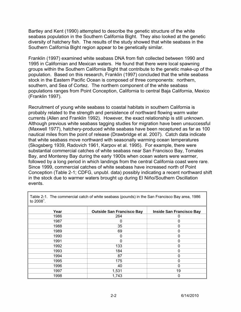
Bartley and Kent (1990) attempted to describe the genetic structure of the white seabass population in the Southern California Bight. They also looked at the genetic diversity of hatchery fish. The results of the study showed that white seabass in the Southern California Bight region appear to be genetically similar. Franklin (1997) examined white seabass DNA from fish collected between 1990 and 1995 in Californian and Mexican waters. He found that there were local spawning groups within the Southern California Bight that contribute to the genetic make-up of the population. Based on this research, Franklin (1997) concluded that the white seabass stock in the Eastern Pacific Ocean is composed of three components: northern, southern, and Sea of Cortez. The northern component of the white seabass populations ranges from Point Conception, California to central Baja California, Mexico (Franklin 1997). Recruitment of young white seabass to coastal habitats in southern California is probably related to the strength and persistence of northward flowing warm water currents (Allen and Franklin 1992). However, the exact relationship is still unknown. Although previous white seabass tagging studies for migration have been unsuccessful (Maxwell 1977), hatchery-produced white seabass have been recaptured as far as 100 nautical miles from the point of release (Drawbridge et al. 2007). Catch data indicate that white seabass move northward with seasonally warming ocean temperatures (Skogsberg 1939, Radovich 1961, Karpov et al. 1995). For example, there were substantial commercial catches of white seabass near San Francisco Bay, Tomales Bay, and Monterey Bay during the early 1900s when ocean waters were warmer, followed by a long period in which landings from the central California coast were rare. Since 1999, commercial catches of white seabass have increased north of Point Conception (Table 2-1; CDFG, unpubl. data) possibly indicating a recent northward shift in the stock due to warmer waters brought up during El Niño/Southern Oscillation events. Table 2-1. The commercial catch of white seabass (pounds) in the San Francisco Bay area, 1986 to 20081.
Year Outside San Francisco Bay Inside San Francisco Bay 1986 264 0 1987 0 0 1988 35 0 1989 69 0 1990 0 0 1991 0 0 1992 133 0 1993 184 0 1994 87 0 1995 175 0 1996 40 0 1997 1,531 19 1998 1,743 0
2-2 6/14/2010
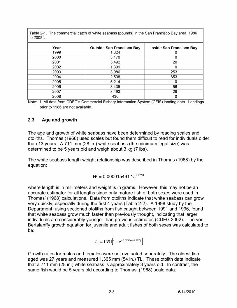
Table 2-1. The commercial catch of white seabass (pounds) in the San Francisco Bay area, 1986 to 20081.
Year Outside San Francisco Bay Inside San Francisco Bay 1999 1,324 0 2000 3,170 0 2001 5,492 20 2002 1,399 0 2003 3,986 253 2004 2,538 853 2005 5,214 0 2006 3,435 56 2007 8,493 29 2008 430 0
Note: 1. All data from CDFG’s Commercial Fishery Information System (CFIS) landing data. Landings prior to 1986 are not available. 2.3 Age and growth The age and growth of white seabass have been determined by reading scales and otoliths. Thomas (1968) used scales but found them difficult to read for individuals older than 13 years. A 711 mm (28 in.) white seabass (the minimum legal size) was determined to be 5 years old and weigh about 3 kg (7 lbs). The white seabass length-weight relationship was described in Thomas (1968) by the equation:
9216.2*000015491.0 LW = where length is in millimeters and weight is in grams. However, this may not be an accurate estimator for all lengths since only mature fish of both sexes were used in Thomas’ (1968) calculations. Data from otoliths indicate that white seabass can grow very quickly, especially during the first 4 years (Table 2-2). A 1998 study by the Department, using sectioned otoliths from fish caught between 1991 and 1996, found that white seabass grow much faster than previously thought, indicating that larger individuals are considerably younger than previous estimates (CDFG 2002). The von Bertalanffy growth equation for juvenile and adult fishes of both sexes was calculated to be:
[ ])297.1(0156.011391 +−−= tt eL
Growth rates for males and females were not evaluated separately. The oldest fish aged was 27 years and measured 1,365 mm (54 in.) TL. These otolith data indicate that a 711 mm (28 in.) white seabass is approximately 3 years old. In contrast, the same fish would be 5 years old according to Thomas’ (1968) scale data.
2-3 6/14/2010
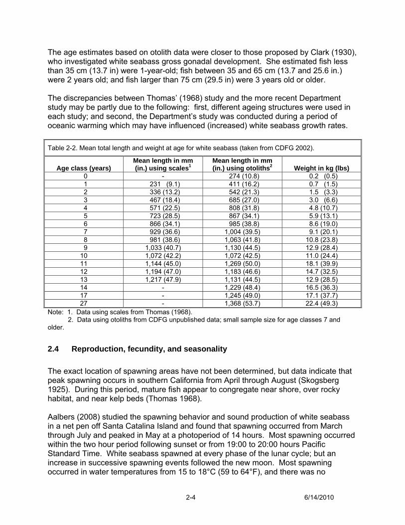
The age estimates based on otolith data were closer to those proposed by Clark (1930), who investigated white seabass gross gonadal development. She estimated fish less than 35 cm (13.7 in) were 1-year-old; fish between 35 and 65 cm (13.7 and 25.6 in.) were 2 years old; and fish larger than 75 cm (29.5 in) were 3 years old or older. The discrepancies between Thomas’ (1968) study and the more recent Department study may be partly due to the following: first, different ageing structures were used in each study; and second, the Department’s study was conducted during a period of oceanic warming which may have influenced (increased) white seabass growth rates. Table 2-2. Mean total length and weight at age for white seabass (taken from CDFG 2002).
Age class (years)
Mean length in mm (in.) using scales1
Mean length in mm (in.) using otoliths2
Weight in kg (lbs)
0 - 274 (10.8) 0.2 (0.5) 1 231 (9.1) 411 (16.2) 0.7 (1.5) 2 336 (13.2) 542 (21.3) 1.5 (3.3) 3 467 (18.4) 685 (27.0) 3.0 (6.6) 4 571 (22.5) 808 (31.8) 4.8 (10.7) 5 723 (28.5) 867 (34.1) 5.9 (13.1) 6 866 (34.1) 985 (38.8) 8.6 (19.0) 7 929 (36.6) 1,004 (39.5) 9.1 (20.1) 8 981 (38.6) 1,063 (41.8) 10.8 (23.8) 9 1,033 (40.7) 1,130 (44.5) 12.9 (28.4) 10 1,072 (42.2) 1,072 (42.5) 11.0 (24.4) 11 1,144 (45.0) 1,269 (50.0) 18.1 (39.9) 12 1,194 (47.0) 1,183 (46.6) 14.7 (32.5) 13 1,217 (47.9) 1,131 (44.5) 12.9 (28.5) 14 - 1,229 (48.4) 16.5 (36.3) 17 - 1,245 (49.0) 17.1 (37.7) 27 - 1,368 (53.7) 22.4 (49.3)
Note: 1. Data using scales from Thomas (1968). 2. Data using otoliths from CDFG unpublished data; small sample size for age classes 7 and older. 2.4 Reproduction, fecundity, and seasonality The exact location of spawning areas have not been determined, but data indicate that peak spawning occurs in southern California from April through August (Skogsberg 1925). During this period, mature fish appear to congregate near shore, over rocky habitat, and near kelp beds (Thomas 1968). Aalbers (2008) studied the spawning behavior and sound production of white seabass in a net pen off Santa Catalina Island and found that spawning occurred from March through July and peaked in May at a photoperiod of 14 hours. Most spawning occurred within the two hour period following sunset or from 19:00 to 20:00 hours Pacific Standard Time. White seabass spawned at every phase of the lunar cycle; but an increase in successive spawning events followed the new moon. Most spawning occurred in water temperatures from 15 to 18°C (59 to 64°F), and there was no
2-4 6/14/2010

apparent correlation with tidal cycles. Seasonal and diel spawning periods were directly correlated with increases in the rate, intensity, and variety of white seabass sounds; this correlation may indicate that sounds function to enhance reproductive success (Aalbers 2008). Aalbers and Drawbridge (2008) reported that gravid females are identifiable during courtship and spawning by shifts in behavior and the development of dark bars across the dorsal region. During numerous observed spawning events in a net pen off Santa Catalina Island, one to nine males were observed to tightly surround a gravid female and the resultant pack shuddered in unison as gametes were simultaneously broadcast into the water column. Five distinct types of sound were reportedly produced by white seabass: single and multiple pulse trains during courtship, drumrolls and thuds during spawning, and booms during yawning and burst swimming. During the actual release of gametes, a rapid succession of overlapping drumroll and thud sounds resulted in identifiable spawning chants lasting 7 to 55 seconds. Consistent physical, behavioral, and acoustical patterns during courtship and spawning indicated that white seabass utilize visual, tactile, and sonic cues to communicate their reproductive state. A study of white seabass maturity in the late 1920s indicated that females begin maturing when they are near 607 mm (24 in.) TL, and males may reach sexual maturity at about 508 mm (20 in.) TL. All white seabass have probably spawned at least once by the time they reach 800 mm (31.5 in.) TL (Clark 1930). White seabass have the largest eggs of the west coast sciaenids at approximately 1.24 mm. These eggs are buoyant and drift with the ocean currents. The dark-colored larvae appear to settle out in coastal areas (Moser et al. 1983). Fecundity has been estimated from ongoing artificial propagation of the species since 1984. Drawbridge (2003) reported that, in the hatchery setting, female seabass starting at 5 kg (11 lbs) released an average of 700,000 eggs per batch, increasing at a rate of approximately 100,000 eggs/kg as the females grew. The relationship between body size and fecundity was evident for fish up to 13 kg (29 lbs) but was not evaluated beyond that to see if it continued (Drawbridge 2003). Although it has been reported that white seabass spawn more than once per season, the number of spawns per female and the spawning intervals for individual females are unknown. Drawbridge (2003) reported that an isolated female of 10 kg (22 lbs) released 1.2 and 1.4 million eggs during spawning events spaced 10 days apart. 2.5 Natural mortality Thomas (1968) calculated a natural mortality rate of 0.303 for fish caught in commercial gill nets. These fish represented the majority of commercially-caught white seabass. Recently, natural mortality rates were determined for juvenile white seabass based on the OREHP data. Kent and Ford (1990) found that natural mortality rates range from 0.258 ( 1 and 2 year-old fish) to 0.117 (3 and 4 year-old fish). Likewise, MacCall et al. (1976) and Dayton and MacCall (1992) calculated natural mortality rates for white
2-5 6/14/2010

seabass from the recreational and commercial fisheries that were significantly lower than Thomas’ (1968) estimate (Table 2-3). In light of these values, it would seem that Thomas’ estimate was an overestimate since natural mortality rates usually decline and level off as fish age. Table 2-3. Estimates of white seabass natural mortality (M) (taken from CDFG 2002).
Source M Thomas (1968) 0.303 MacCall et al. (1976) 0.13 Kent and Ford (1990) 0.258 (1 to 2 yr old); 0.117 (3 to 4 yr old) Dayton and MacCall (1992) 0.08
2-6 6/14/2010
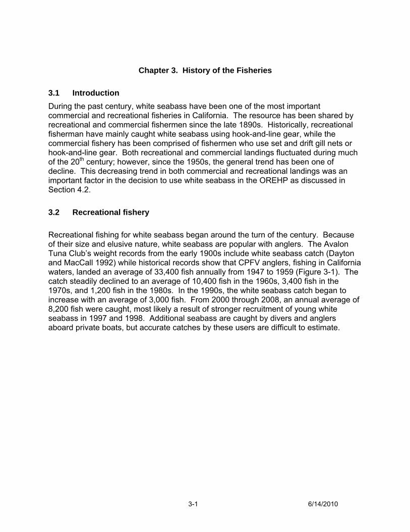
Chapter 3. History of the Fisheries
3.1 Introduction During the past century, white seabass have been one of the most important commercial and recreational fisheries in California. The resource has been shared by recreational and commercial fishermen since the late 1890s. Historically, recreational fisherman have mainly caught white seabass using hook-and-line gear, while the commercial fishery has been comprised of fishermen who use set and drift gill nets or hook-and-line gear. Both recreational and commercial landings fluctuated during much of the 20th century; however, since the 1950s, the general trend has been one of decline. This decreasing trend in both commercial and recreational landings was an important factor in the decision to use white seabass in the OREHP as discussed in Section 4.2. 3.2 Recreational fishery Recreational fishing for white seabass began around the turn of the century. Because of their size and elusive nature, white seabass are popular with anglers. The Avalon Tuna Club’s weight records from the early 1900s include white seabass catch (Dayton and MacCall 1992) while historical records show that CPFV anglers, fishing in California waters, landed an average of 33,400 fish annually from 1947 to 1959 (Figure 3-1). The catch steadily declined to an average of 10,400 fish in the 1960s, 3,400 fish in the 1970s, and 1,200 fish in the 1980s. In the 1990s, the white seabass catch began to increase with an average of 3,000 fish. From 2000 through 2008, an annual average of 8,200 fish were caught, most likely a result of stronger recruitment of young white seabass in 1997 and 1998. Additional seabass are caught by divers and anglers aboard private boats, but accurate catches by these users are difficult to estimate.
3-1 6/14/2010
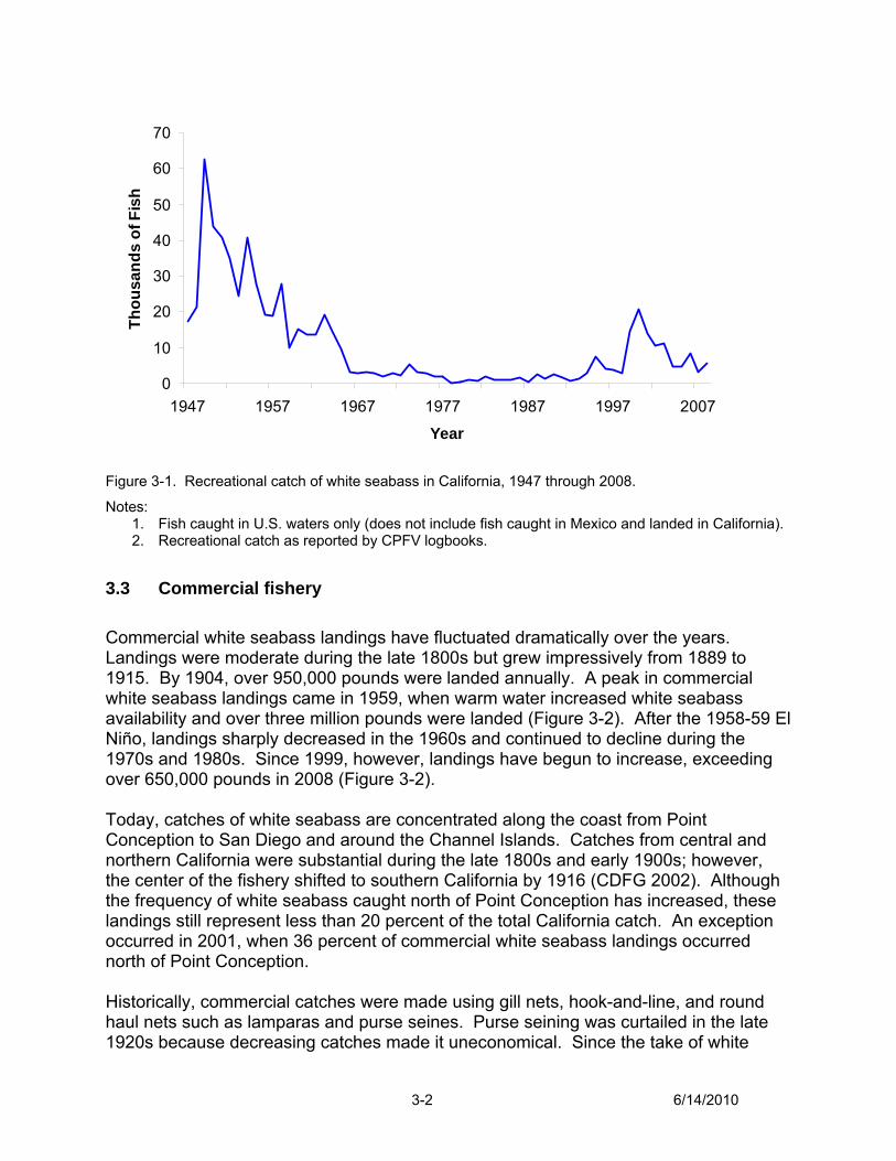
0
10
20
30
40
50
60
70
1947 1957 1967 1977 1987 1997 2007
Year
Thou
sand
s of
Fis
h
Figure 3-1. Recreational catch of white seabass in California, 1947 through 2008.
Notes: 1. Fish caught in U.S. waters only (does not include fish caught in Mexico and landed in California). 2. Recreational catch as reported by CPFV logbooks.
3.3 Commercial fishery Commercial white seabass landings have fluctuated dramatically over the years. Landings were moderate during the late 1800s but grew impressively from 1889 to 1915. By 1904, over 950,000 pounds were landed annually. A peak in commercial white seabass landings came in 1959, when warm water increased white seabass availability and over three million pounds were landed (Figure 3-2). After the 1958-59 El Niño, landings sharply decreased in the 1960s and continued to decline during the 1970s and 1980s. Since 1999, however, landings have begun to increase, exceeding over 650,000 pounds in 2008 (Figure 3-2). Today, catches of white seabass are concentrated along the coast from Point Conception to San Diego and around the Channel Islands. Catches from central and northern California were substantial during the late 1800s and early 1900s; however, the center of the fishery shifted to southern California by 1916 (CDFG 2002). Although the frequency of white seabass caught north of Point Conception has increased, these landings still represent less than 20 percent of the total California catch. An exception occurred in 2001, when 36 percent of commercial white seabass landings occurred north of Point Conception. Historically, commercial catches were made using gill nets, hook-and-line, and round haul nets such as lamparas and purse seines. Purse seining was curtailed in the late 1920s because decreasing catches made it uneconomical. Since the take of white
3-2 6/14/2010
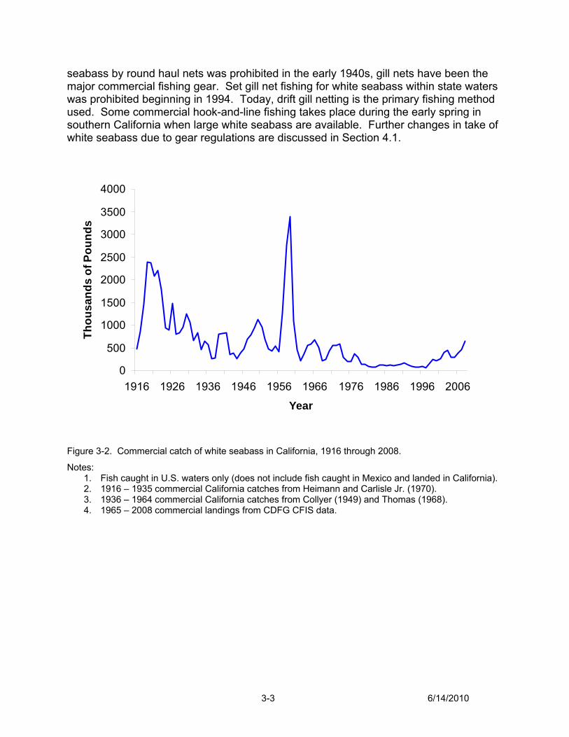
seabass by round haul nets was prohibited in the early 1940s, gill nets have been the major commercial fishing gear. Set gill net fishing for white seabass within state waters was prohibited beginning in 1994. Today, drift gill netting is the primary fishing method used. Some commercial hook-and-line fishing takes place during the early spring in southern California when large white seabass are available. Further changes in take of white seabass due to gear regulations are discussed in Section 4.1.
0
500
1000
1500
2000
2500
3000
3500
4000
1916 1926 1936 1946 1956 1966 1976 1986 1996 2006
Year
Thou
sand
s of
Pou
nds
Figure 3-2. Commercial catch of white seabass in California, 1916 through 2008.
Notes: 1. Fish caught in U.S. waters only (does not include fish caught in Mexico and landed in California). 2. 1916 – 1935 commercial California catches from Heimann and Carlisle Jr. (1970). 3. 1936 – 1964 commercial California catches from Collyer (1949) and Thomas (1968). 4. 1965 – 2008 commercial landings from CDFG CFIS data.
3-3 6/14/2010
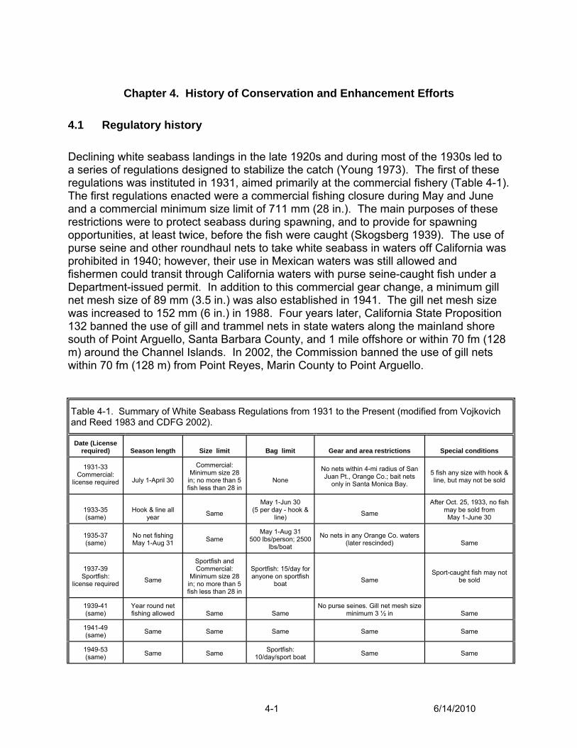
Chapter 4. History of Conservation and Enhancement Efforts
4.1 Regulatory history Declining white seabass landings in the late 1920s and during most of the 1930s led to a series of regulations designed to stabilize the catch (Young 1973). The first of these regulations was instituted in 1931, aimed primarily at the commercial fishery (Table 4-1). The first regulations enacted were a commercial fishing closure during May and June and a commercial minimum size limit of 711 mm (28 in.). The main purposes of these restrictions were to protect seabass during spawning, and to provide for spawning opportunities, at least twice, before the fish were caught (Skogsberg 1939). The use of purse seine and other roundhaul nets to take white seabass in waters off California was prohibited in 1940; however, their use in Mexican waters was still allowed and fishermen could transit through California waters with purse seine-caught fish under a Department-issued permit. In addition to this commercial gear change, a minimum gill net mesh size of 89 mm (3.5 in.) was also established in 1941. The gill net mesh size was increased to 152 mm (6 in.) in 1988. Four years later, California State Proposition 132 banned the use of gill and trammel nets in state waters along the mainland shore south of Point Arguello, Santa Barbara County, and 1 mile offshore or within 70 fm (128 m) around the Channel Islands. In 2002, the Commission banned the use of gill nets within 70 fm (128 m) from Point Reyes, Marin County to Point Arguello.
Table 4-1. Summary of White Seabass Regulations from 1931 to the Present (modified from Vojkovich and Reed 1983 and CDFG 2002).
Date (License required)
Season length
Size limit
Bag limit
Gear and area restrictions
Special conditions
1931-33 Commercial:
license required
July 1-April 30
Commercial: Minimum size 28
in; no more than 5 fish less than 28 in
None
No nets within 4-mi radius of San Juan Pt., Orange Co.; bait nets
only in Santa Monica Bay.
5 fish any size with hook & line, but may not be sold
1933-35 (same)
Hook & line all
year
Same
May 1-Jun 30 (5 per day - hook &
line)
Same
After Oct. 25, 1933, no fish may be sold from May 1-June 30
1935-37 (same)
No net fishing May 1-Aug 31
Same
May 1-Aug 31 500 lbs/person; 2500
lbs/boat
No nets in any Orange Co. waters (later rescinded)
Same
1937-39 Sportfish:
license required
Same
Sportfish and Commercial:
Minimum size 28 in; no more than 5 fish less than 28 in
Sportfish: 15/day for anyone on sportfish
boat
Same
Sport-caught fish may not be sold
1939-41 (same)
Year round net fishing allowed
Same
Same
No purse seines. Gill net mesh size minimum 3 ½ in
Same
1941-49 (same) Same Same Same Same Same
1949-53 (same) Same Same Sportfish:
10/day/sport boat Same Same
4-1 6/14/2010

Table 4-1. Summary of White Seabass Regulations from 1931 to the Present (modified from Vojkovich and Reed 1983 and CDFG 2002).
Date (License required)
Season length
Size limit
Bag limit
Gear and area restrictions
Special conditions
1953-57 (same)
Same
Same
Commercial: 1000 lbs/person/day; 5000
lbs/boat/day.
Same
Same
1957-71 (same) Same
Sportfish: 2 fish less than 28
in
Sportfish: 10/day/sport boat
Same Same
1971-73 (same) Same
Sportfish and Commercial:
No fish less than 28 in
Same Same Same
1973-78 (same) Same
Sportfish and Commercial:
One fish less than 28 in
Same Same Same
1978-80 (same) Same
Sportfish and Commercial:
No fish less than 28 in
Same Same Same
1980-82 (same)
Season closed Mar 15-Jun 15 Same Sportfish:
3/day/person Same Logs required Permits required
1982-84 (same) Same Same Same Area closures for nets with mesh
less than 6 in Permits no longer required
1984-94 (same)
Same
Same
Sportfish: 1 white seabass/day/person
during closed season
Same
Same
1994-00 (same)
Same
Same
Same
No Gill or trammel nets allowed 0-3 mi from shore along the mainland, or within 1 mi or waters less than 70 fm deep at the offshore islands from Point Arguello, Santa Barbara Co. to the United States - Mexico Border, and in waters less than 35
fm deep from Point Fermin, Los Angeles Co. to the south jetty Newport Harbor, Orange Co.
Same
2000-02 (same)
Same
Same
Commercial: 1 seabass/day/boat
during closed season with gill net
Same Same
2002-present (same) Same Same Same
No gill or trammel nets allowed in waters less than 70 fm deep from Point Reyes, Marin Co, to Point
Arguello, Santa Barbara Co.
Same
4.2 History of the OREHP The OREHP began in 1983 as a result of legislation (Assembly Bill 1414) authored by California Assemblyman Larry Stirling. The legislation was adopted to fund research and development into the artificial propagation of marine finfish species whose populations had become depleted, with the intent of enhancing those populations.
4-2 6/14/2010
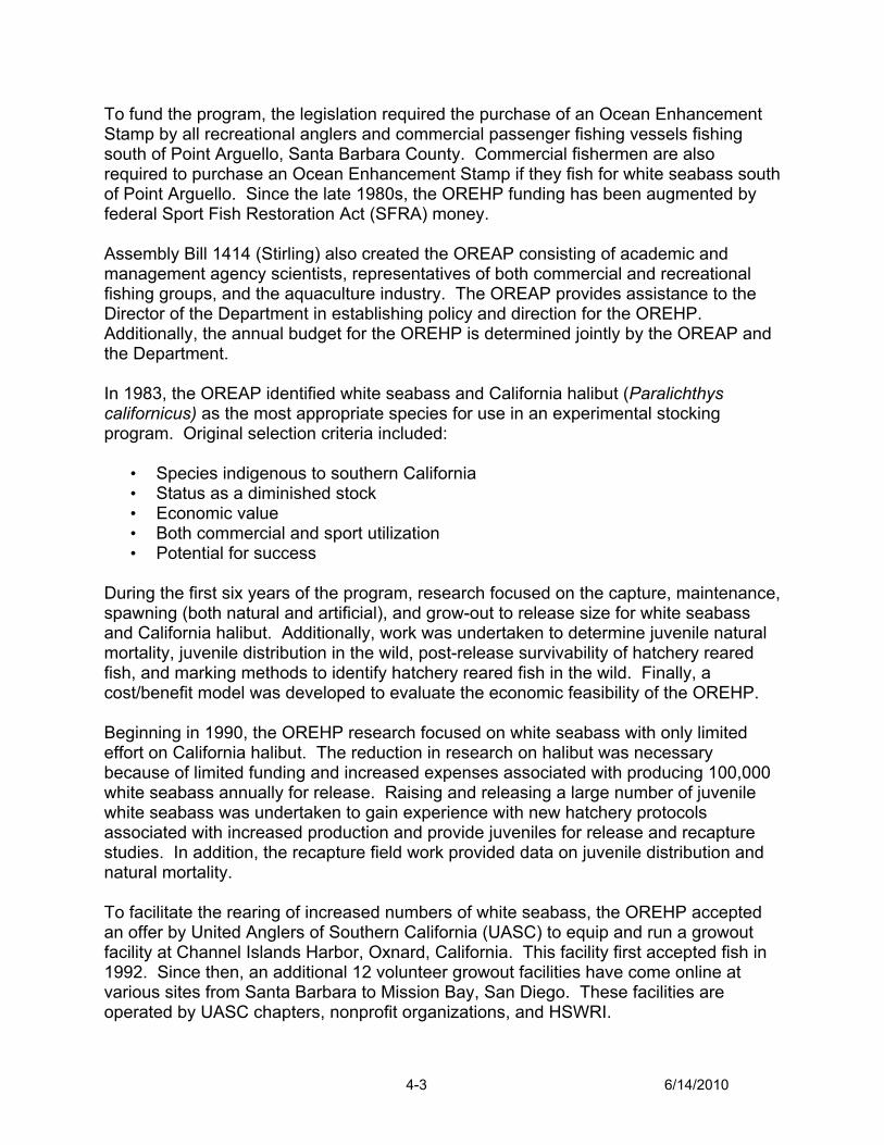
To fund the program, the legislation required the purchase of an Ocean Enhancement Stamp by all recreational anglers and commercial passenger fishing vessels fishing south of Point Arguello, Santa Barbara County. Commercial fishermen are also required to purchase an Ocean Enhancement Stamp if they fish for white seabass south of Point Arguello. Since the late 1980s, the OREHP funding has been augmented by federal Sport Fish Restoration Act (SFRA) money. Assembly Bill 1414 (Stirling) also created the OREAP consisting of academic and management agency scientists, representatives of both commercial and recreational fishing groups, and the aquaculture industry. The OREAP provides assistance to the Director of the Department in establishing policy and direction for the OREHP. Additionally, the annual budget for the OREHP is determined jointly by the OREAP and the Department. In 1983, the OREAP identified white seabass and California halibut (Paralichthys californicus) as the most appropriate species for use in an experimental stocking program. Original selection criteria included:
• Species indigenous to southern California • Status as a diminished stock • Economic value • Both commercial and sport utilization • Potential for success
During the first six years of the program, research focused on the capture, maintenance, spawning (both natural and artificial), and grow-out to release size for white seabass and California halibut. Additionally, work was undertaken to determine juvenile natural mortality, juvenile distribution in the wild, post-release survivability of hatchery reared fish, and marking methods to identify hatchery reared fish in the wild. Finally, a cost/benefit model was developed to evaluate the economic feasibility of the OREHP. Beginning in 1990, the OREHP research focused on white seabass with only limited effort on California halibut. The reduction in research on halibut was necessary because of limited funding and increased expenses associated with producing 100,000 white seabass annually for release. Raising and releasing a large number of juvenile white seabass was undertaken to gain experience with new hatchery protocols associated with increased production and provide juveniles for release and recapture studies. In addition, the recapture field work provided data on juvenile distribution and natural mortality. To facilitate the rearing of increased numbers of white seabass, the OREHP accepted an offer by United Anglers of Southern California (UASC) to equip and run a growout facility at Channel Islands Harbor, Oxnard, California. This facility first accepted fish in 1992. Since then, an additional 12 volunteer growout facilities have come online at various sites from Santa Barbara to Mission Bay, San Diego. These facilities are operated by UASC chapters, nonprofit organizations, and HSWRI.
4-3 6/14/2010
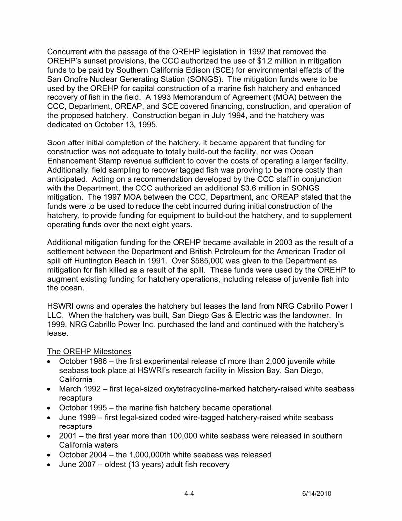
Concurrent with the passage of the OREHP legislation in 1992 that removed the OREHP’s sunset provisions, the CCC authorized the use of $1.2 million in mitigation funds to be paid by Southern California Edison (SCE) for environmental effects of the San Onofre Nuclear Generating Station (SONGS). The mitigation funds were to be used by the OREHP for capital construction of a marine fish hatchery and enhanced recovery of fish in the field. A 1993 Memorandum of Agreement (MOA) between the CCC, Department, OREAP, and SCE covered financing, construction, and operation of the proposed hatchery. Construction began in July 1994, and the hatchery was dedicated on October 13, 1995. Soon after initial completion of the hatchery, it became apparent that funding for construction was not adequate to totally build-out the facility, nor was Ocean Enhancement Stamp revenue sufficient to cover the costs of operating a larger facility. Additionally, field sampling to recover tagged fish was proving to be more costly than anticipated. Acting on a recommendation developed by the CCC staff in conjunction with the Department, the CCC authorized an additional $3.6 million in SONGS mitigation. The 1997 MOA between the CCC, Department, and OREAP stated that the funds were to be used to reduce the debt incurred during initial construction of the hatchery, to provide funding for equipment to build-out the hatchery, and to supplement operating funds over the next eight years. Additional mitigation funding for the OREHP became available in 2003 as the result of a settlement between the Department and British Petroleum for the American Trader oil spill off Huntington Beach in 1991. Over $585,000 was given to the Department as mitigation for fish killed as a result of the spill. These funds were used by the OREHP to augment existing funding for hatchery operations, including release of juvenile fish into the ocean. HSWRI owns and operates the hatchery but leases the land from NRG Cabrillo Power I LLC. When the hatchery was built, San Diego Gas & Electric was the landowner. In 1999, NRG Cabrillo Power Inc. purchased the land and continued with the hatchery’s lease. The OREHP Milestones • October 1986 – the first experimental release of more than 2,000 juvenile white
seabass took place at HSWRI’s research facility in Mission Bay, San Diego, California
• March 1992 – first legal-sized oxytetracycline-marked hatchery-raised white seabass recapture
• October 1995 – the marine fish hatchery became operational • June 1999 – first legal-sized coded wire-tagged hatchery-raised white seabass
recapture • 2001 – the first year more than 100,000 white seabass were released in southern
California waters • October 2004 – the 1,000,000th white seabass was released • June 2007 – oldest (13 years) adult fish recovery
4-4 6/14/2010

4-5 6/14/2010
Part 2 - Best Management Practices The CHP (Drawbridge and Okihiro 2007) covers all aspects of hatchery operations including plant management, broodstock care, egg production (spawning), nursery phase, and raceway culture. The GPM (Drawbridge and Okihiro 2007) covers the growout and subsequent release of juvenile white seabass. The BMPs are taken largely from these two documents.
Chapter 5. Hatchery Operations 5.1 Plant management and biosecurity measures Biosecurity is an all encompassing concept whose primary goal is to prevent infectious disease agents from gaining entrance into the hatchery. Failing that, a secondary goal is to detect infectious diseases at the growout facilities and minimize spread. Components of biosecurity include: proper system layout and compartmentalization, water treatment and sterilization, equipment and system disinfection, and quarantine. Proper biosecurity remains one of the most important factors limiting hatchery production of healthy fish, and is critical in the prevention of disease spread to wild stocks. Biosecurity is dependent on: 1) equipment and systems within the hatchery; 2) protocols and procedures used by hatchery personnel; 3) proper training of hatchery personnel; and 4) the proper mind set. The hatchery has seven separate systems: larval food production, broodstock, egg incubation, juvenile 1 (J1), juvenile 2 (J2), raceway culture, and experimental. These systems are compartmentalized with each system operating on a separate water system to reduce the chance of infection and the spread of disease. Except for raceway culture, each system is a recirculating water system. As the water is recirculated it passes through a series of filters (bead, floating media, and/or sand), foam fractionators, and UV sterilizers. Filtration is different for each system and based on the needs of the different life stages. All “make-up” water (replaces water lost during the recirculation process) is sterilized using an ozone system. Make-up water destined for egg incubation, the J1 system, and the J2 system goes through a sand filter prior to ozone treatment. Sea water for the raceways comes directly from Agua Hedionda Lagoon and is sand-filtered but not sterilized. Water temperature and water turnover rate are controlled by the Main Computer Control System (MCCS). Filter backwashing is also controlled by the MCCS. The MCCS will automatically page hatchery personnel should a change in air or water flow occur. To help prevent the spread of disease, each of the seven systems has equipment (i.e., nets, brooms, scrubbers) dedicated to that system. Iodine foot baths are placed at the entrance of each system to minimize transfer of contaminants, while physical barriers prevent foot bath avoidance. New gloves are applied as hatchery personnel move between any two systems.
5-1 6/14/2010

Hatchery personnel are also well trained to detect stress and the early signs of a disease outbreak. Healthy fish have good color, intact skin and fins, and are not thin. In contrast, sick fish are often darkly pigmented or have a mottled appearance (spotty pigmentation associated with diffuse protozoal infestations). Healthy fish will also school up and orient themselves with the prevailing current. They are typically active, respond rapidly to external stimuli (e.g. food, pool vibrations), and have a strong net avoidance behavior. Sick fish, however, exhibit a range of abnormal behaviors, depending on the pathogen and severity of infection. Non-specific abnormal behaviors include anorexia, lethargy, and isolation. Specific behaviors include “flashing” (attempting to rub gills or skin against hard surfaces) associated with external parasites, and whirling or spinning associated with central nervous system (CNS) disease. Accurate descriptions of abnormal behavior or physical condition can often help the pathologist identify etiologic agents, even before necropsies are performed, or help narrow the search for the causative agent. The SDRWQCB does not require the hatchery to operate under a NPDES permit. However, HSWRI is required to monitor the intake and affluent flow volumes and pollutant levels at the hatchery. Hatchery staff is also required to maintain self-monitoring reports and submit annual reports to the SDRWQCB. BMPs for plant management and biosecurity
• Evaluate traffic patterns and maintain each system separately in accordance with the CHP to prevent the spread of disease
• Disinfect equipment and systems in accordance with the CHP • Label disinfection stations with color-coded signage for chemicals • Maintain regular maintenance schedule for sterilization stations • Maintain water quality in each system in accordance with the CHP • Maintain quarantine protocols in accordance with the CHP • Maintain proper training of hatchery personnel • Conduct monitoring of the intake and effluent flow volumes and pollutant levels
as required by the SDRWQCB Monitoring and Reporting Program No. 2001-237 • Maintain self-monitoring reports and submit an annual reports to the SDRWQCB
5.2 Broodstock care 5.2.1 Broodstock care and feeding Broodstock are maintained in four separate pools that are temperature and photoperiod-controlled by the MCCS. The temperature and photoperiod controls provide for year-round spawning by induction of spawning pool by pool so spawning duty is rotated among the fish by pool. Fifty broodstock are maintained in each of the four pools for a total of 200 broodstock.
5-2 6/14/2010
Broodstock are fed a diet of frozen sardines five times per week at a ratio of 0.5 to 1.0 percent of body weight per day. The diet is enhanced with vitamin supplements injected into the sardines three days per week. All food handling is conducted in accordance with United States Department of Agriculture (USDA) standards for research facilities holding live vertebrate organisms. The broodstock diet has changed over time as the nutritional requirements of white seabass have been examined. As a result, egg quality has increased dramatically compared to early years of OREHP operation. Research into broodstock nutritional requirements is ongoing. 5.2.2 Broodstock collection and holding Each year, a surplus number of broodstock are collected by cooperative collecting trips conducted by HSWRI staff; these broodstock are maintained at HSWRI’s net pen at Santa Catalina Harbor or at additional growout facilities if needed. On these trips, HSWRI staff and volunteers use hook-and-line to target fish approximately 610 mm (24 in.) TL. To help ensure that the genetic diversity of hatchery-released progeny will be similar to wild populations, broodstock are collected only from the northern component of the white seabass population range from Point Conception, California to central Baja California, Mexico. This surplus group does not contribute gametes to the enhancement effort but is available to replace broodstock at the hatchery that die or are removed from the system. After capture, broodstock are weighed, measured, sexed, genotyped, and implanted with a Passive Integrated Transponder (PIT) tag for identification. This information is maintained in the broodstock tracking system, a Microsoft Access database that also includes information regarding fish transfers, disease treatments, and deaths. Broodstock are also scanned for a CWT. If a fish scans positive for a CWT (i.e., the fish was hatchery-raised), it cannot be used as a brood fish and is euathanized to ensure the genetic diversity of the broodstock. Broodstock are transported to the mainland on the return leg following the delivery of juveniles to the growout facility whenever possible. Delivery of juveniles typically occurs twice a year. On the mainland, broodstock are held at either Sea World, San Diego, California or in one of the quarantine pools at the hatchery. Because all new broodstock are assumed to be caring lethal pathogen, they must be quarantined before entering the hatchery system to prevent potential disease outbreaks. Broodstock holding facilities at Sea World and Santa Catalina Island offer some opportunities for initial quarantine, but a secondary quarantine is initiated at the hatchery to control for secondary infections that may be caused by handling stress. When the fish arrive at the hatchery, they are placed in quarantine pools that are plumbed for recirculation and supplied with ozonated water from the main hatchery building. The fish are isolated for 45 days and are observed daily for disease. Should new fish break out with disease, necropsy and appropriate diagnostics are performed to
5-3 6/14/2010
determine etiologic agents. Euthanasia of all new arrivals is an option if some new arrivals break with a novel disease, or if the disease is known to be lethal and highly contagious. A fifth breeding pool has been assembled and will be used initially to move existing brood fish into so the original systems can be upgraded. When all the pools have been upgraded, the fifth pool will serve as a quarantine and reserve pool that can hold new stock until they are needed in the rotation schedule. Temperature control in this system will allow the fish to acclimate to the temperature of the target pool (13 to 18°C; 55 to 64°F), which may vary considerably from ambient water (12-25°C; 54 to 77°F). 5.2.3 Broodstock rotation The original broodstock management plan, developed by Bartley et al. (1995) recommended a 1:1 sex ratio in each of the four broodstock pools, replacing five percent of the stock each year (10 fish), and rotating five males between the four broodstock pools annually to increase genetic diversity. During the past ten years, new stock was added inconsistently, primarily to replace fish that have died or were euthanized for health reasons. The replacement of fish during this time period averaged approximately seven percent annually. Male fish were not rotated among pools because white seabass are very skittish and netting fish can result in other fish jumping out of the tank or injuring themselves on the side of the pool. After reviewing the spawning characteristics of white seabass at the hatchery, a revised broodstock management plan was recently developed to ensure that future program genetic goals are met. The revised plan adjusts the sex ratios (male: female) in each of the broodstock pools to 40:60 to account for unequal reproductive contribution of the sexes. It also replaces brood fish at a rate of 25 per year to ensure genetic mixing and to better account for the effect of generation time on effective population size. The need to rotate five males between each of the four breeding pools has been mitigated by replacing more fish per year than the original plan. Modification of the revised broodstock management plan will occur, if needed, as new information becomes available. BMPs for broodstock care
• Maintain a population of up to 200 white seabass broodstock distributed between the four breeding pools with a 40:60 sex ratio
• Maintain a surplus broodstock population offsite of the hatchery or in quarantine pools at the hatchery
• Maintain sanitary conditions in all food preparation areas according to USDA standards and those set forth in the CHP
• Obtain white seabass broodstock as needed, while maintaining appropriate permits and/or permissions and collecting all pertinent information for each fish
• Scan new broodstock for a CWT to insure that no recaptured hatchery progeny become broodstock
5-4 6/14/2010
• Weigh, measure, sex, genotype, and implant new broodstock with a PIT tag for identification
• Hold new broodstock under quarantine at the hatchery for a minimum of 45 days • Place incoming broodstock in the fifth broodstock pool to acclimate the fish to
conditions in the main broodstock pool • Rotate new stock (males and females) into the program on a regular basis
without impacting the health of the fish or the general success of egg production 5.3 Egg production HSWRI is currently maximizing the genetic diversity of the parental contributions within the annual release total to the fullest extent practical. The current operational protocol for the hatchery is to utilize one to three female equivilants (one female equivilant equals ~2 million eggs) per run for a total of 28 to 32 spawns per year. Eggs are obtained using the approach outlined below. 5.3.1 Spawning Spawning is induced by increasing the temperature from 14 to 18°C (57 to 64°F) and photoperiod from 10 to 14 hour days to simulate spring/summer conditions. No hormone or other manipulation is needed to induce spawning. The temperature and photoperiod are maintained for three to four months and then slowly decreased to 14°C (57°F) and 10-hour days, respectively, to simulate winter or non-spawning conditions. The four broodstock pools temperature and light regimes are staggered so that one pool is in spawning mode throughout the year. Based on hatchery observations, white seabass generally spawn in the early evening with one or more females and typically numerous males participating in each spawning event. While the exact period between individual female spawn events is not formally documented, it is believed to be 10 to 14 days based on hatchery observations. 5.3.2 Egg collection Eggs are collected the morning following a spawn using a fine mesh net (<800 µm). The eggs are concentrated in a container and transferred to a clear graduated cylinder where the volume of eggs is determined. A conversion ratio of 585 eggs per ml is used to determine the number of eggs. Viable, undamaged eggs are buoyant and therefore concentrated at the top of the cylinder. Nonviable eggs settle to the bottom. While both viable and nonviable eggs are enumerated, only viable eggs are stocked for production. BMPs for egg production
• Maintain broodstock pool conditions according to the CHP so that one pool is in spawning mode year round
• Collect eggs daily in accordance with the CHP, maintaining sanitary conditions, keeping only viable eggs for production and destroying nonviable eggs
5-5 6/14/2010
5.4 Nursery phase 5.4.1 Incubation The incubation system has a total of twelve tanks, holding 234,000 eggs each. Temperature is set at 18°C (64°F) to match the broodstock pool temperature, and eggs are disinfected in a 100 ppm formalin bath for one hour prior to placing them in incubation tanks. Eggs are collected from high quality spawns as characterized by the initial viability. Eggs are stocked at a consistent density of 150/L in each incubator. If a second spawn occurs within five to seven days of the first spawn, several incubators are drained and restocked with new eggs such that an equal number of incubators contain eggs from each available spawn. The precise partitioning of eggs among incubators is dictated by spawn volume. Spawning events that include eggs from multiple females are utilized more broadly (i.e. in more incubators) as needed. White seabass eggs hatch at 48 hours and begin feeding at five days post hatch (dph). At this stage, white seabass larvae are fed only live, newly-hatched, and nutrient-enriched Artemia nauplii (Artemia franciscanus). The Artemia have to be enriched because they lose much of their nutritional value within an hour after hatching. The Artemia are rinsed in fresh water prior to feeding to reduce bacterial loading. Larvae are fed seven times a day and each feeding consists of a single batch of Artemia. 5.4.2 Juvenile 1 (J1) system The J1 system consists of six 7,000 L (1,850 gallon) pools. The pools are stocked at 40 to 60 larvae/L, and the temperature is maintained at 23°C (73°F). Late larval white seabass are transferred from the incubation system to the J1 system via gravity feed at 12 dph. At this time, larvae are introduced to dry pelleted feeds to wean them off of live feed (Artemia). The dry pelleted food is a custom-prepared feed containing 50 percent protein. The pellets are crumbled into small pieces (0.25 to 2.0 mm) by the manufacturer. These fish are fed at a rate of five percent of body weight per day. Around 18 dph, the amount of live feed is reduced until no live food is offered at approximately 25 dph. 5.4.3 Juvenile 2 (J2) system Once the white seabass larvae have been weaned onto dry pellets (around 35 dph), they can be transferred to the J2 system which consists of four 7,000 L (1,850 gallon) circular pools and two 19,000 L (5,020 gallon) oval pools. As with the J1 system, temperature is maintained at 23°C (73°F) by the MCCS. Pools are manually siphoned once or twice a day to maintain high water quality. Fish in the J2 system are fed at a rate of three to five percent of body weight per day. The fish are fed a commercially available pelleted diet using belt feeders. This feed
5-6 6/14/2010
contains 50 percent protein, 14 percent fat, and has Vitamin C incorporated into it. The size of the pellets used in the J2 system is typically 3.0 or 4.0 mm, depending on the fish size. Transfer of fish from the J2 system is dictated by the ambient water temperature of the receiving body of water, usually the raceways. The temperature in the J2 pools is gradually decreased to ambient temperatures. Differences in the temperature of the J2 system and the receiving body of water can stress the fish, thereby reducing the immune response. This is especially problematic because this transfer results in the fish’s first exposure to disease as it leaves the sterile, filtered water of the hatchery system. During warm-water months (>18°C; 64°F), fish can be transferred at a smaller size (20 g, 80 to 90 dph) than during colder months where fish are held until they are larger (40 g, 120 dph). BMPs for the nursery phase
• Maintain high quality water standards in accordance with the CHP • Provide nutritious, high quality live and dry feed for larvae in accordance with the
CHP 5.5 Raceway culture The raceway system consists of eight 25 m3 concrete raceways in a separate area enclosed by shade cloth-draped chain link fence away from the main hatchery. This system is flow-through (375 Lpm) with water coming from Agua Hedionda Lagoon through the raceways and then back into the lagoon. The water is not ozone or UV-sterilized but does pass through a sand filter and a low-head oxygenator to maintain proper dissolved oxygen levels (≥ 4.0 mg/L). Fish can be stocked in the raceways at a maximum density of 20 kg/m3. Raceways are vacuumed manually once a day to remove detritus. Fish are fed the same commercial diet as with the J2 system. However, fish in the raceways are fed by hand four times each day at a rate of two to three percent body weight per day. Juvenile white seabass are susceptible to GSS disease caused by high levels of total dissolved gas (TDG) in the water (Smiley 2004). Ambient waters in Agua Hedionda Lagoon can have TDG levels as high as 120 percent. Degassers are used to remove some of the gases from lagoon waters before entering the raceway system. More information on GSS disease can be found in Section 7.2.1. Currently, the raceways are out of operation due to disease issues. Because the raceway system is not on a recirculating water system, and thus has limited filtration, fish contained in it are more susceptible to certain types of disease. Future use of the raceways may rely on installation of a new recirculation and filtration systems for those facilities.
5-7 6/14/2010
BMPs for raceway culture • Stock raceways at no more than maximum density • Vacuum raceways once a day • Provide high quality, nutritious feed in accordance with the CHP
5.6 Fish tagging Prior to transfer to a growout facility or direct release, all fish are tagged with a CWT, a sequentially-numbered, small (1.1 mm long by 0.25 mm diameter), magnetized, stainless steel wire tag. Each fish is tagged in the left cheek muscle below the posterior edge of the left eye. The beginning and end numbers are recorded for each batch of fish tagged. A batch of fish varies in number and is directly proportional to the size of the growout facility that will receive the fish. Thus, a batch of fish represents a proportion of one production run raised at the hatchery or from one growout facility. In this manner, tag returns can be attributed to a specific production run and release, allowing for more accurate estimates of growth, mortality and identifying patterns of movement. In previous years, binary codes were used to identify batches of fish in the same manner. This information is maintained by HSWRI in a central database. The minimum size for tagging fish is approximately 2.0 g or 100 mm, based on the size of the target tissue (cheek muscle). Fish are tagged using a 5-person tagging station built by HSWRI. The tagging station consists of two major components. The upper component is a holding tank that is filled with ozonated water that is recirculated continuously. The lower unit has MS-222 laden water and is designed to deliver anesthetized fish to the taggers. Fish then pass through a quality control device that effectively separates tagged fish from untagged fish. Tagged fish are deposited into a five gallon bucket and then transferred into one of the J2 system tanks. This procedure ensures that 100 percent of the fish are tagged initially. Tag retention is measured again by subsampling fish one to two weeks after tagging and again just prior to release. BMPs for fish tagging
• Tag all fish prior to leaving the hatchery for the growout facilities • Subsample fish for tag retention before transport to the growout facility and before release • Use sequentially-numbered tags so that tag returns can be attributed to individual releases • Maintain tagging data in a central database
5.7 Fish transport Fish are transferred to growout facilities and to remote release sites using different tanks, vehicles, and vessels. The configuration of the transport depends on the number of fish being transported and the conditions at the facility or release site. The most
5-8 6/14/2010
commonly used transport tanks, however, are 1,500 L (400 gallon) and constructed of marine-grade aluminum; the size and shape of the tanks allow them to be easily loaded onto a pickup truck, flatbed truck, or boat. The tanks are designed with independent aeration systems, and as a back-up to the aerators, each tank is equipped with a 1.5 cubic meter cylinder of pure oxygen. Like the aerators, the cylinder and its associated components (i.e. regulator, flow meter, and diffusers) are attached to the tank, not the vehicle. The tanks are not recirculating and have no filtration system. Fish are starved for 24 hours prior to transfer, and the tanks are stocked at a maximum density of 40 kg/m3. Water from the holding facility is used in the tanks to transport the fish. Fritz Guard is added to the water to protect the ectodermal mucous layer, to maintain an appropriate electrolyte balance, and reduce the stress caused by transport. Oxygen supplied from a tank is used to maintain constant oxygenation. If water temperature at the receiving site is significantly different (>2.0°C; 4°F) than that in the tanks, water is pumped into the tanks to reduce the difference. Fish are then flushed from the tank using a flexible hose. BMPs for transporting fish
• Maintain separate aeration systems for each tank • Provide good water quality conditions for transport • Maximum stocking density of 40 kg/m3 • Acclimate fish to receiving body of water’s temperature, if difference is greater
than 2°C (4°F)
5-9 6/14/2010
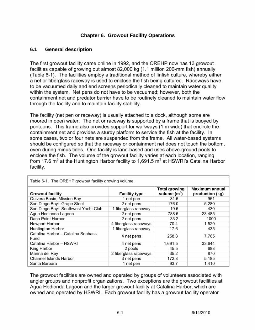
Chapter 6. Growout Facility Operations 6.1 General description The first growout facility came online in 1992, and the OREHP now has 13 growout facilities capable of growing out almost 82,000 kg (1.1 million 200-mm fish) annually (Table 6-1). The facilities employ a traditional method of finfish culture, whereby either a net or fiberglass raceway is used to enclose the fish being cultured. Raceways have to be vacuumed daily and end screens periodically cleaned to maintain water quality within the system. Net pens do not have to be vacuumed; however, both the containment net and predator barrier have to be routinely cleaned to maintain water flow through the facility and to maintain facility stability. The facility (net pen or raceway) is usually attached to a dock, although some are moored in open water. The net or raceway is supported by a frame that is buoyed by pontoons. This frame also provides support for walkways (1 m wide) that encircle the containment net and provides a sturdy platform to service the fish at the facility. In some cases, two or four nets are suspended from the frame. All water-based systems should be configured so that the raceway or containment net does not touch the bottom, even during minus tides. One facility is land-based and uses above-ground pools to enclose the fish. The volume of the growout facility varies at each location, ranging from 17.6 m3 at the Huntington Harbor facility to 1,691.5 m3 at HSWRI’s Catalina Harbor facility. Table 6-1. The OREHP growout facility growing volume.
Growout facility
Facility type
Total growing volume (m3)
Maximum annual production (kg)
Quivera Basin, Mission Bay 1 net pen 31.6 951 San Diego Bay: Grape Steet 2 net pens 176.0 5,280 San Diego Bay: Southwest Yacht Club 1 fiberglass raceway 19.6 430 Agua Hedionda Lagoon 2 net pens 788.6 23,485 Dana Point Harbor 2 net pens 33.2 1000 Newport Harbor 4 fiberglass raceways 70.4 1,520 Huntington Harbor 1 fiberglass raceway 17.6 435 Catalina Harbor – Catalina Seabass Fund 4 net pens 258.8 7,765
Catalina Harbor – HSWRI 4 net pens 1,691.5 33,644 King Harbor 2 pools 45.5 683 Marina del Rey 2 fiberglass raceways 35.2 870 Channel Islands Harbor 3 net pens 172.8 5,185 Santa Barbara 1 net pen 93.7 1,410 The growout facilities are owned and operated by groups of volunteers associated with angler groups and nonprofit organizations. Two exceptions are the growout facilities at Agua Hedionda Lagoon and the larger growout facility at Catalina Harbor, which are owned and operated by HSWRI. Each growout facility has a growout facility operator
6-1 6/14/2010
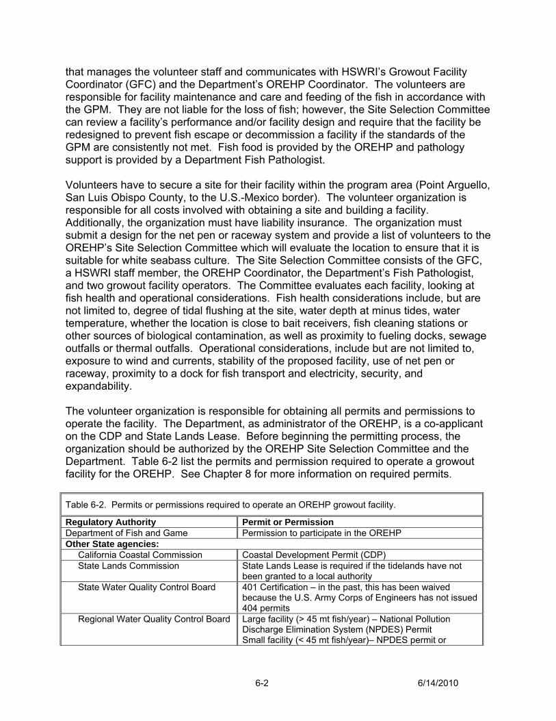
that manages the volunteer staff and communicates with HSWRI’s Growout Facility Coordinator (GFC) and the Department’s OREHP Coordinator. The volunteers are responsible for facility maintenance and care and feeding of the fish in accordance with the GPM. They are not liable for the loss of fish; however, the Site Selection Committee can review a facility’s performance and/or facility design and require that the facility be redesigned to prevent fish escape or decommission a facility if the standards of the GPM are consistently not met. Fish food is provided by the OREHP and pathology support is provided by a Department Fish Pathologist. Volunteers have to secure a site for their facility within the program area (Point Arguello, San Luis Obispo County, to the U.S.-Mexico border). The volunteer organization is responsible for all costs involved with obtaining a site and building a facility. Additionally, the organization must have liability insurance. The organization must submit a design for the net pen or raceway system and provide a list of volunteers to the OREHP’s Site Selection Committee which will evaluate the location to ensure that it is suitable for white seabass culture. The Site Selection Committee consists of the GFC, a HSWRI staff member, the OREHP Coordinator, the Department’s Fish Pathologist, and two growout facility operators. The Committee evaluates each facility, looking at fish health and operational considerations. Fish health considerations include, but are not limited to, degree of tidal flushing at the site, water depth at minus tides, water temperature, whether the location is close to bait receivers, fish cleaning stations or other sources of biological contamination, as well as proximity to fueling docks, sewage outfalls or thermal outfalls. Operational considerations, include but are not limited to, exposure to wind and currents, stability of the proposed facility, use of net pen or raceway, proximity to a dock for fish transport and electricity, security, and expandability. The volunteer organization is responsible for obtaining all permits and permissions to operate the facility. The Department, as administrator of the OREHP, is a co-applicant on the CDP and State Lands Lease. Before beginning the permitting process, the organization should be authorized by the OREHP Site Selection Committee and the Department. Table 6-2 list the permits and permission required to operate a growout facility for the OREHP. See Chapter 8 for more information on required permits. Table 6-2. Permits or permissions required to operate an OREHP growout facility.
Regulatory Authority Permit or Permission Department of Fish and Game Permission to participate in the OREHP Other State agencies: California Coastal Commission Coastal Development Permit (CDP) State Lands Commission State Lands Lease is required if the tidelands have not
been granted to a local authority State Water Quality Control Board 401 Certification – in the past, this has been waived
because the U.S. Army Corps of Engineers has not issued 404 permits
Regional Water Quality Control Board Large facility (> 45 mt fish/year) – National Pollution Discharge Elimination System (NPDES) Permit Small facility (< 45 mt fish/year)– NPDES permit or
6-2 6/14/2010
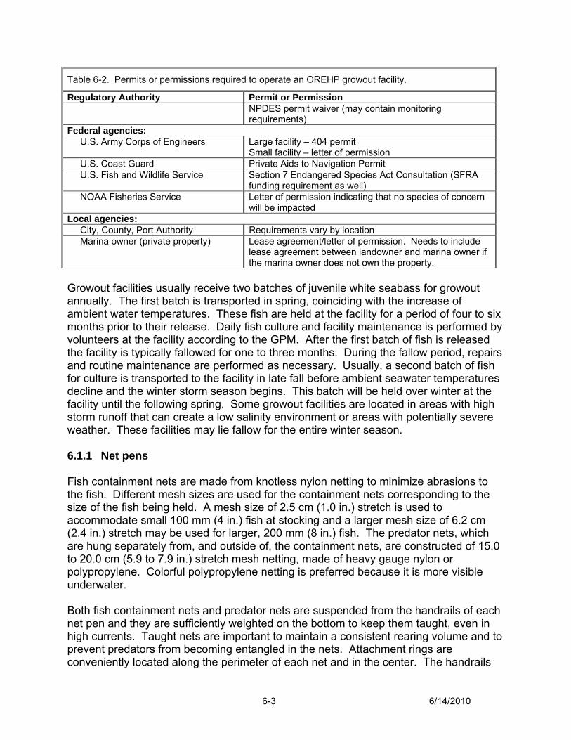
Table 6-2. Permits or permissions required to operate an OREHP growout facility.
Regulatory Authority Permit or Permission NPDES permit waiver (may contain monitoring requirements)
Federal agencies: U.S. Army Corps of Engineers Large facility – 404 permit
Small facility – letter of permission U.S. Coast Guard Private Aids to Navigation Permit U.S. Fish and Wildlife Service Section 7 Endangered Species Act Consultation (SFRA
funding requirement as well) NOAA Fisheries Service Letter of permission indicating that no species of concern
will be impacted Local agencies: City, County, Port Authority Requirements vary by location Marina owner (private property) Lease agreement/letter of permission. Needs to include
lease agreement between landowner and marina owner if the marina owner does not own the property.
Growout facilities usually receive two batches of juvenile white seabass for growout annually. The first batch is transported in spring, coinciding with the increase of ambient water temperatures. These fish are held at the facility for a period of four to six months prior to their release. Daily fish culture and facility maintenance is performed by volunteers at the facility according to the GPM. After the first batch of fish is released the facility is typically fallowed for one to three months. During the fallow period, repairs and routine maintenance are performed as necessary. Usually, a second batch of fish for culture is transported to the facility in late fall before ambient seawater temperatures decline and the winter storm season begins. This batch will be held over winter at the facility until the following spring. Some growout facilities are located in areas with high storm runoff that can create a low salinity environment or areas with potentially severe weather. These facilities may lie fallow for the entire winter season.
6.1.1 Net pens Fish containment nets are made from knotless nylon netting to minimize abrasions to the fish. Different mesh sizes are used for the containment nets corresponding to the size of the fish being held. A mesh size of 2.5 cm (1.0 in.) stretch is used to accommodate small 100 mm (4 in.) fish at stocking and a larger mesh size of 6.2 cm (2.4 in.) stretch may be used for larger, 200 mm (8 in.) fish. The predator nets, which are hung separately from, and outside of, the containment nets, are constructed of 15.0 to 20.0 cm (5.9 to 7.9 in.) stretch mesh netting, made of heavy gauge nylon or polypropylene. Colorful polypropylene netting is preferred because it is more visible underwater. Both fish containment nets and predator nets are suspended from the handrails of each net pen and they are sufficiently weighted on the bottom to keep them taught, even in high currents. Taught nets are important to maintain a consistent rearing volume and to prevent predators from becoming entangled in the nets. Attachment rings are conveniently located along the perimeter of each net and in the center. The handrails
6-3 6/14/2010
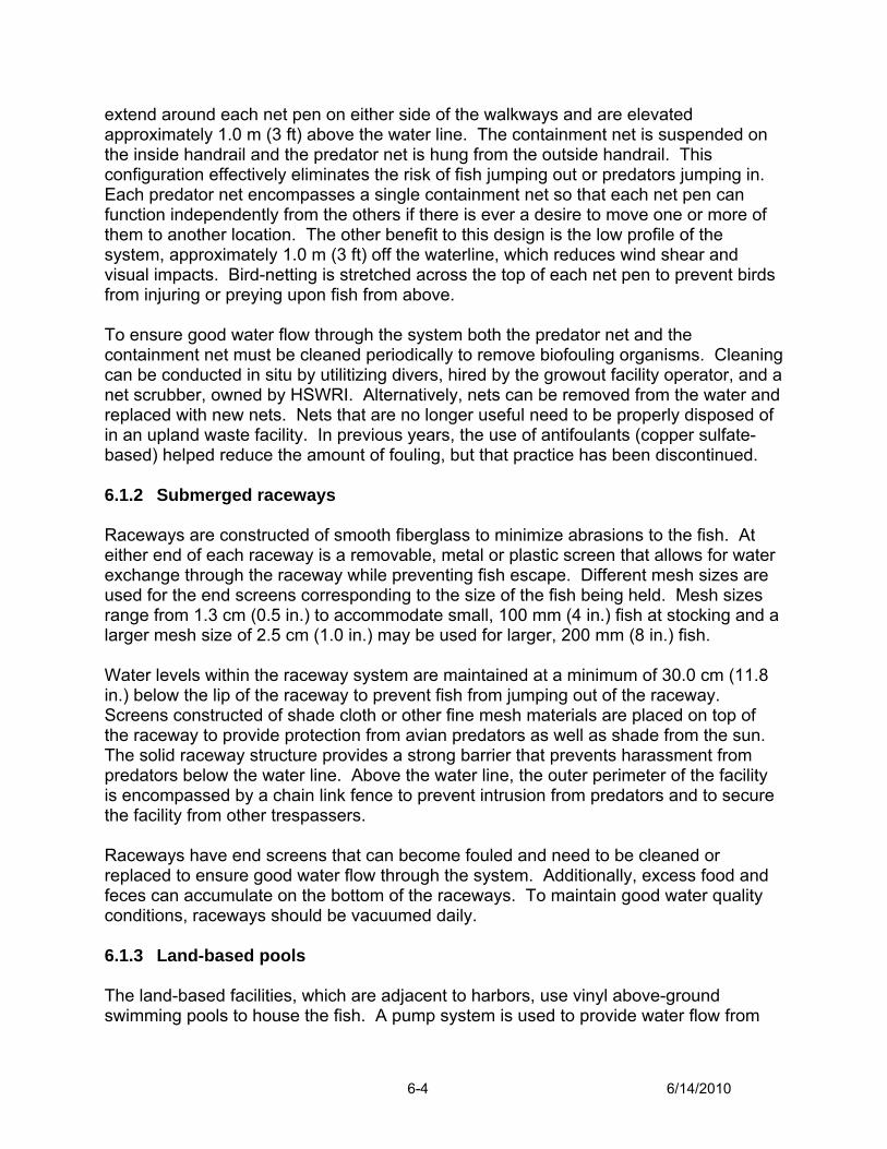
extend around each net pen on either side of the walkways and are elevated approximately 1.0 m (3 ft) above the water line. The containment net is suspended on the inside handrail and the predator net is hung from the outside handrail. This configuration effectively eliminates the risk of fish jumping out or predators jumping in. Each predator net encompasses a single containment net so that each net pen can function independently from the others if there is ever a desire to move one or more of them to another location. The other benefit to this design is the low profile of the system, approximately 1.0 m (3 ft) off the waterline, which reduces wind shear and visual impacts. Bird-netting is stretched across the top of each net pen to prevent birds from injuring or preying upon fish from above.
To ensure good water flow through the system both the predator net and the containment net must be cleaned periodically to remove biofouling organisms. Cleaning can be conducted in situ by utilitizing divers, hired by the growout facility operator, and a net scrubber, owned by HSWRI. Alternatively, nets can be removed from the water and replaced with new nets. Nets that are no longer useful need to be properly disposed of in an upland waste facility. In previous years, the use of antifoulants (copper sulfate-based) helped reduce the amount of fouling, but that practice has been discontinued. 6.1.2 Submerged raceways Raceways are constructed of smooth fiberglass to minimize abrasions to the fish. At either end of each raceway is a removable, metal or plastic screen that allows for water exchange through the raceway while preventing fish escape. Different mesh sizes are used for the end screens corresponding to the size of the fish being held. Mesh sizes range from 1.3 cm (0.5 in.) to accommodate small, 100 mm (4 in.) fish at stocking and a larger mesh size of 2.5 cm (1.0 in.) may be used for larger, 200 mm (8 in.) fish. Water levels within the raceway system are maintained at a minimum of 30.0 cm (11.8 in.) below the lip of the raceway to prevent fish from jumping out of the raceway. Screens constructed of shade cloth or other fine mesh materials are placed on top of the raceway to provide protection from avian predators as well as shade from the sun. The solid raceway structure provides a strong barrier that prevents harassment from predators below the water line. Above the water line, the outer perimeter of the facility is encompassed by a chain link fence to prevent intrusion from predators and to secure the facility from other trespassers. Raceways have end screens that can become fouled and need to be cleaned or replaced to ensure good water flow through the system. Additionally, excess food and feces can accumulate on the bottom of the raceways. To maintain good water quality conditions, raceways should be vacuumed daily. 6.1.3 Land-based pools The land-based facilities, which are adjacent to harbors, use vinyl above-ground swimming pools to house the fish. A pump system is used to provide water flow from
6-4 6/14/2010

the harbor. Aerators are also used to increase the oxygen-carrying capacity of the water in the pools. A back-up generator is employed automatically when the power to the life support systems fails. The pools are housed within a tarped Quonset-hut type enclosure which prevents birds from entering and provides shade for the fish. As with raceways, land-based pools can accumulate excess food and feces and should be vacuumed daily to maintain good water quality in the system. BMPs for growout gacility operations
• Provide a secure environment for raising juvenile fish by maintaining the containment system in good working order
• Maintain adequate freeboard of the containment systems to prevent fish escape
• Provide appropriate barriers to predators both above and below the water • Provide shade from the sun when systems are shallow • Maintain good water quality conditions by removing biofouling as needed, and
regularly vacuuming raceways and land-based pools • For land-based systems, aerate water and provide a back-up generator to
guard against power failures • Maintain good communication among the growout facility operator, GFC, and
the OREHP Coordinator 6.2 Stocking density Fish are maintained at the facilities in modest densities of 12.0 to18.0 kg/m3 to minimize the effects of crowding on fish health and water quality. For modeling purposes a time-at-release density of 15.0 kg/m3 is used. The average size at release is 200 to 250 mm (8 to 10 in.) TL; this equates to approximately 200 fish/m3. BMPs for stocking density
• Stock fish into growout facilities based on a density at time-of-release of 12.0 to 18.0 kg/m3 to minimize the effects of crowding on fish health and water quality
6.3 Annual release limit With inception of the proposal for the Carlsbad hatchery, the OREHP planned on releasing approximately 350,000 juvenile white seabass annually into the ocean waters of southern California. All experimental protocols and economic evaluations were based on this production capability, and the hatchery was designed to produce that many juveniles annually. The broodstock management plan found within the CHP was based on analysis of the wild population's genetic variability and the projected number of broodstock required to minimize impacts to that population (Bartley et al. 1995). That
6-5 6/14/2010
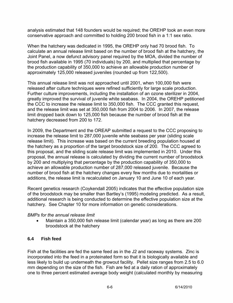
analysis estimated that 148 founders would be required; the OREHP took an even more conservative approach and committed to holding 200 brood fish in a 1:1 sex ratio. When the hatchery was dedicated in 1995, the OREHP only had 70 brood fish. To calculate an annual release limit based on the number of brood fish at the hatchery, the Joint Panel, a now defunct advisory panel required by the MOA, divided the number of brood fish available in 1995 (70 individuals) by 200, and multiplied that percentage by the production capability of 350,000 to achieve an allowable production number of approximately 125,000 released juveniles (rounded up from 122,500). This annual release limit was not approached until 2001, when 100,000 fish were released after culture techniques were refined sufficiently for large scale production. Further culture improvements, including the installation of an ozone sterilizer in 2004, greatly improved the survival of juvenile white seabass. In 2004, the OREHP petitioned the CCC to increase the release limit to 350,000 fish. The CCC granted this request, and the release limit was set at 350,000 fish from 2004 to 2006. In 2007, the release limit dropped back down to 125,000 fish because the number of brood fish at the hatchery decreased from 200 to 172. In 2009, the Department and the OREAP submitted a request to the CCC proposing to increase the release limit to 287,000 juvenile white seabass per year (sliding scale release limit). This increase was based on the current breeding population housed at the hatchery as a proportion of the target broodstock size of 200. The CCC agreed to this proposal, and the sliding scale release limit was implemented in 2010. Under this proposal, the annual release is calculated by dividing the current number of broodstock by 200 and multiplying that percentage by the production capability of 350,000 to achieve an allowable production number of 287,000 released juvenile. Because the number of brood fish at the hatchery changes every few months due to mortalities or additions, the release limit is recalculated on January 10 and June 10 of each year. Recent genetics research (Coykendall 2005) indicates that the effective population size of the broodstock may be smaller than Bartley’s (1995) modeling predicted. As a result, additional research is being conducted to determine the effective population size at the hatchery. See Chapter 10 for more information on genetic considerations. BMPs for the annual release limit
• Maintain a 350,000 fish release limit (calendar year) as long as there are 200 broodstock at the hatchery
6.4 Fish feed Fish at the facilities are fed the same feed as in the J2 and raceway systems. Zinc is incorporated into the feed in a proteinated form so that it is biologically available and less likely to build up underneath the growout facility. Pellet size ranges from 2.5 to 6.0 mm depending on the size of the fish. Fish are fed at a daily ration of approximately one to three percent estimated average body weight (calculated monthly by measuring
6-6 6/14/2010
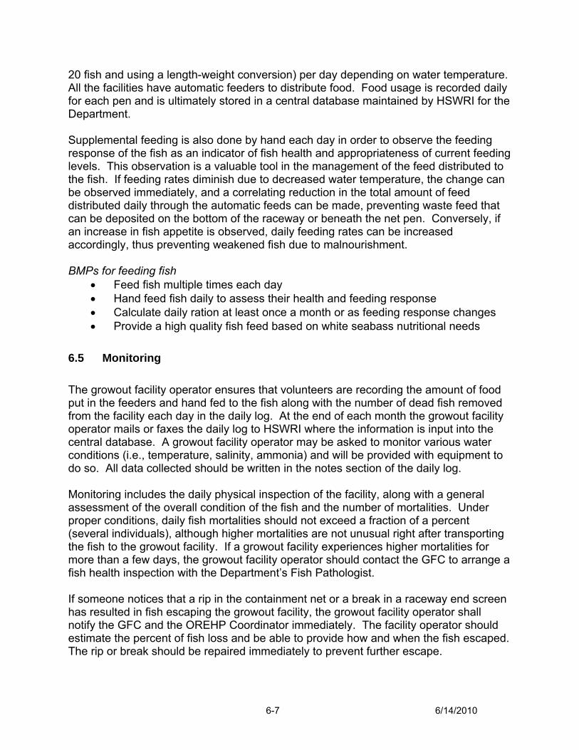
20 fish and using a length-weight conversion) per day depending on water temperature. All the facilities have automatic feeders to distribute food. Food usage is recorded daily for each pen and is ultimately stored in a central database maintained by HSWRI for the Department. Supplemental feeding is also done by hand each day in order to observe the feeding response of the fish as an indicator of fish health and appropriateness of current feeding levels. This observation is a valuable tool in the management of the feed distributed to the fish. If feeding rates diminish due to decreased water temperature, the change can be observed immediately, and a correlating reduction in the total amount of feed distributed daily through the automatic feeds can be made, preventing waste feed that can be deposited on the bottom of the raceway or beneath the net pen. Conversely, if an increase in fish appetite is observed, daily feeding rates can be increased accordingly, thus preventing weakened fish due to malnourishment. BMPs for feeding fish
• Feed fish multiple times each day • Hand feed fish daily to assess their health and feeding response • Calculate daily ration at least once a month or as feeding response changes • Provide a high quality fish feed based on white seabass nutritional needs
6.5 Monitoring The growout facility operator ensures that volunteers are recording the amount of food put in the feeders and hand fed to the fish along with the number of dead fish removed from the facility each day in the daily log. At the end of each month the growout facility operator mails or faxes the daily log to HSWRI where the information is input into the central database. A growout facility operator may be asked to monitor various water conditions (i.e., temperature, salinity, ammonia) and will be provided with equipment to do so. All data collected should be written in the notes section of the daily log. Monitoring includes the daily physical inspection of the facility, along with a general assessment of the overall condition of the fish and the number of mortalities. Under proper conditions, daily fish mortalities should not exceed a fraction of a percent (several individuals), although higher mortalities are not unusual right after transporting the fish to the growout facility. If a growout facility experiences higher mortalities for more than a few days, the growout facility operator should contact the GFC to arrange a fish health inspection with the Department’s Fish Pathologist. If someone notices that a rip in the containment net or a break in a raceway end screen has resulted in fish escaping the growout facility, the growout facility operator shall notify the GFC and the OREHP Coordinator immediately. The facility operator should estimate the percent of fish loss and be able to provide how and when the fish escaped. The rip or break should be repaired immediately to prevent further escape.
6-7 6/14/2010
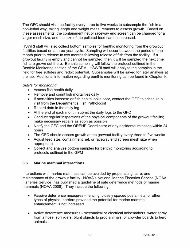
The GFC should visit the facility every three to five weeks to subsample the fish in a non-lethal way, taking length and weight measurements to assess growth. Based on these assessments, the containment net or raceway end screen can be changed for a larger mesh size, and the size of the pelleted feed can be increased. HSWRI staff will also collect bottom samples for benthic monitoring from the growout facilities based on a three-year cycle. Sampling will occur between the period of one month prior to release to two months following release of fish from the facility. If a growout facility is empty and cannot be sampled, then it will be sampled the next time fish are grown out there. Benthic sampling will follow the protocol outlined in the Benthic Monitoring section of the GPM. HSWRI staff will analyze the samples in the field for free sulfides and redox potential. Subsamples will be saved for later analysis at the lab. Additional information regarding benthic monitoring can be found in Chapter 9. BMPs for monitoring
• Assess fish health daily • Remove and count fish mortalities daily • If mortalities increase or fish health looks poor, contact the GFC to schedule a
visit from the Department’s Fish Pathologist • Record data in the daily log • At the end of each month, submit the daily logs to the GFC • Conduct regular inspections of the physical components of the growout facility;
make necessary repairs as soon as possible • Notify the GFC and the OREHP Coordinator of any accidental releases within 24
hours • The GFC should assess growth at the growout facility every three to five weeks • Adjust feed size, containment net, or raceway end screen mesh size when
appropriate • Collect and analyze bottom samples for benthic monitoring according to
protocols outlined in the GPM
6.6 Marine mammal interactions Interactions with marine mammals can be avoided by proper siting, care, and maintenance of the growout facility. NOAA’s National Marine Fisheries Service (NOAA Fisheries Service) has published a guideline of safe deterrence methods of marine mammals (NOAA 2008). They include the following:
• Passive deterrence measures – fencing, closely spaced posts, nets, or other types of physical barriers provided the potential for marine mammal entanglement is not increased.
• Active deterrence measures - mechanical or electrical noisemakers, water spray
from a hose, sprinklers, blunt objects to prod animals, or crowder boards to herd animals.
6-8 6/14/2010

Deterrence measures should not separate a female from her offspring; break the skin of an animal; result in dislocation of or fracture of bones, limbs, or other appendages; be directed at the head or eyes of an animal; or be used on seals and sea lions hauled out on unimproved property. Currently, the only deterrence measures approved by the OREHP are the chain link fencing that surrounds some facilities and barrier nets used below the water. Any injury or mortality of a marine mammal must be reported within 48 hours of occurrence. NOAA Fisheries Service has defined a marine mammal injury as a wound or other physical harm. Signs of injury include, but are not limited to, visible blood flow, loss of or damage to an appendage or jaw, inability to use one or more appendages, asymmetry in the shape of body or body position, noticeable swelling or hemorrhage, laceration, puncture or rupture of eyeball, listless appearance or inability to defend itself, inability to swim or dive upon release from fishing gear, or signs of equilibrium imbalance. The Marine Mammal Authorization Program Mortality/Injury Reporting Form (OMB 0648-0292) should be filled out and faxed to the following individuals:
NOAA Fisheries Service -- fax: (301) 713-4060 Growout Facility Coordinator (GFC) -- fax: (760) 434-9502 OREHP Coordinator -- fax: (562) 342-7139
BMPs for marine mammal interactions
• Maintain proper siting, care, and maintenance of growout facility to avoid interactions with marine mammals
• Notify NOAA Fisheries Service, the GFC, and the OREHP Coordinator of any interactions with marine mammals within 48 hours
6.7 Fish releases 6.7.1 Final inspection and clearance The growout facility operator should contact the GFC when the fish reach 200 to 250 mm to schedule a final inspection. The GFC will come to the growout facility along with the Department’s Fish Pathologist to perform the final inspection, which includes a health check, length and weight measurements of a subsample of fish, and a final tag retention assessment. The fish cannot be released until they have been cleared by the Department’s Fish Pathologist. 6.7.2 Coordinating the release Once the fish are cleared for release, the growout facility operator and GFC will set a release date. The growout facility operator will schedule volunteers to assist with the release. All facilities will need volunteers to count the fish as they are released. At land-based facilities, additional volunteers are needed to crowd the fish in the pool, net them, and walk them to the ocean or a transport vehicle. At water-based facilities,
6-9 6/14/2010
volunteers may be needed to help crowd the fish or pull up on the containment net or raceway end screen. 6.7.3 Releasing fish On the day of the release, the GFC will demonstrate proper handling techniques which include using gloves and netting only a few fish at a time to minimize stress. Fish are to be released at the growout site, or nearest body of water for land-based facilities, and not transported to another site without permission from the GFC and the OREHP Coordinator. Additionally, fish should all be released within the same time period (1 to 2 days) to avoid biasing the post-release assessment of survival. The OREHP’s juvenile recruitment surveys and HSWRI’s acoustic tracking studies (See Sections 11.1 and 11.3) have shown that juvenile white seabass inhabit shallow waters of embayments and the open coast. Thus, while off-site releases are not uncommon, the majority of white seabass are released at the growout site. The growout facility operator shall obtain permission of the GFC and the OREHP Coordinator before releasing fish at any site other than the growout facility. If the media are invited to the release event, the GFC and the OREHP Coordinator should be contacted to provide accurate historical context for the event. 6.7.4 Remote releases Juvenile white seabass can be transported from the hatchery or Catalina Harbor and released along the mainland coast. Juvenile white seabass are to be released in appropriate habitat (embayments or along the mainland coast in shallow water) within the Southern California Bight. There are no limitations on how many fish can be released at one site, except at Catalina Island. General practice is not to release more than 10,000 fish at one location. There are no limitations on distance from the growout site; however, longer distances, and thus longer transport times, can be more stressful to the fish. HSWRI is the only member of the OREHP allowed to conduct remote releases without advance permission of the Department. 6.7.5 Release limit at Catalina Island The topography around Catalina Island is such that juvenile seabass released at the island are concentrated along a very narrow shelf surrounding the island. While the two growout facilities at Catalina Island are capable of growing out over 500,000 juvenile white seabass in a single production run, the OREHP has voluntarily limited releases at Catalina Island to 30,000 fish annually to minimize the potential for inter or intra-specific competitive interactions. The 30,000 fish release limit is not currently based on any scientific studies but rather as a “best guess” of what is appropriate. Directed studies (e.g. acoustic tracking) should be conducted to assess the availability of suitable habitat for juvenile white seabass at Catalina Island, assess the dispersion rate of white
6-10 6/14/2010

seabass released at Catalina Island, and adjust the Catalina Island white seabass annual release limit accordingly. 6.7.6 Direct releases Sometimes fish are held at the Carlsbad hatchery until they reach release size (200 to 250 mm; 8 to 10 in.). Once cleared for release by the Department’s Fish Pathologist, these fish can be released from the raceways into Agua Hedionda Lagoon. Fish can also be transported to remote locations for release (i.e., Mission Bay, Oceanside) to more evenly distribute the fish along the mainland. HSWRI is the only member of the OREHP allowed to conduct remote releases without advance permission by the Department. BMPs for fish releases
• Fish cannot be released until cleared for release by the GFC and the Department’s Fish Pathologist
• The growout facility operator is responsible for requesting a final inspection from the GFC and for setting up the release event, including scheduling volunteers to help with release activities
• Fish are to be released at the growout facility site unless permission is granted by the Department in advance to release the fish remotely
• Proper fish handling techniques will be used during the release event • The annual release limit for Catalina Island is 30,000 fish per calendar year • Excess fish grown out at Catalina Island shall be transported to the mainland
coast and released • There are no limitations on remote releases (number of fish or distance);
however, fish are to be released in the appropriate shallow water habitat
6-11 6/14/2010

Chapter 7. Fish Health Management 7.1 Fish health management program The fish health management program for the OREHP is under the supervision of a Department Fish Pathologist, with assistance from a HSWRI veterinary fish health specialist. This program includes prevention, identification, and treatment of many common white seabass pathogens, including non-infectious and infectious diseases. The goal of the program is to ensure that no sick fish are released into the wild and that no novel diseases or physical deformities are introduced to the wild white seabass population. This goal is achieved by the following protocol:
• Only healthy, asymptomatic fish can be transferred to the growout facilities or released into the wild
• Healthy, asymptomatic fish that have been exposed to a lethal, highly contagious
pathogen known to occur in wild white seabass can be transferred to the growout facilities or released into the wild
• Healthy, asymptomatic fish that have been exposed to a lethal, highly contagious
pathogen that is not known to occur in wild white seabass must be euthanized to prevent the introduction of new disease
To ensure only healthy, asymptomatic fish are released the program requires at least two health inspections by a Department Fish Pathologist or Department-approved Fish Pathologist: 1) before fish are transferred from the hatchery to the growout facility; and 2) prior to release into the wild. In addition to these routine inspections, a fish health inspection should be requested when hatchery staff or growout facility volunteers notice an increase in mortality or a change in fish behavior that lasts more than three days and is not associated with transport mortality. All fish health inspections involve visual inspection and necropsy of three to ten fish per tank, net pen, or raceway. The inspection includes wet mount exams for parasites on gill and skin, and a thorough external and internal screen for gross abnormalities, parasites, and lesions. New and/or unusual pathogens or lesions are documented with line drawings and/or photography, which are subsequently used for identification and classification. If necessary, tissues are fixed in 10 percent formalin or Karnovsky’s fixative, and followed with histopathology or electron microscopy. Unusual or new metatozan parasites are fixed in ethanol and sent to outside parasitologists for identification. Confirmation of some infectious diseases (viral, bacterial, or fungal) is made using pathogen isolation techniques: cell culture – using fish cell lines – for viruses and rickettsial bacteria, and plate agar for bacteria and fungi. Some viral, rickettsial, and sporozoan (e.g., myxosporidian and microsporidian) diagnostics are also done via polymerase chain reaction (PCR) assays performed on fresh or frozen tissue.
7-1 6/14/2010

The UCD typically does all the virology, rickettsial isolation, and PCR assay assessments. The fish health management program is supported by an on-going effort to survey wild stocks of white seabass. The goal of this disease assessment program is to determine which pathogens and diseases are “naturally-occurring” among wild white seabass. Toward this end, blood and tissue samples from wild white seabass are collected, preserved, and analyzed. When a new pathogen is discovered in cultured seabass, the goal is to identify it and then determine if it occurs in wild white seabass. Initial characterization of new pathogens/diseases is done by documenting gross lesions with photography and then using histology to define microscopic features and associated pathology. Morphologic characterization is further refined using transmission electron microscopy (TEM). Attempts are also made to propagate new pathogens on plate agar or fish cell lines so as to simplify identification and characterization. Although morphologic techniques are useful in the initial characterization of a new pathogen or disease among cultured fish, they are of limited value in surveying wild fish stocks. The reason for this is simply that wild fish with diagnostic lesions (i.e., those with moderate to severe infections) rarely survive to be captured and assessed. Sick wild fish either die quickly, or weaken and are consumed by predators. Diagnostic tools used to assess wild fish need to be more sensitive and geared toward detection of fish with: 1) latent infections (i.e., fish that are carriers, but asymptomatic); 2) mild infections (i.e., fish with mild, sublethal infections); or 3) no infections (i.e., fish that were exposed to a pathogen and were either immune, or developed an infection and were able to clear the pathogen). Currently, the two assays with the greatest application to disease assessment among wild fish stocks are the PCR assay and the enzyme-linked immunosorbent assay (ELISA). The PCR assay is a molecular diagnostic tool based on the detection of pathogen DNA. Major advantages over morphologic techniques include a higher level of precision (e.g., positive PCR results can only rarely be confused) and sensitivity (e.g., only a few strands of DNA are necessary for PCR detection). The ELISA is a hematological assay and in contrast to the PCR assay that detects pathogen infection, ELISAs are used to determine level of pathogen exposure. Pathogen exposed fish develop pathogen specific antibodies and these antibodies can persist for months to years in peripheral blood. ELISAs therefore have the distinct advantage of detecting not only fish that are currently infected, but being capable of detecting exposure in fish that have already cleared the pathogen. PCR and ELISA assays are both time consuming and difficult to develop. Both are also dependent on being able to culture the pathogen artificially (on fish cell lines) or in purifying pathogen antigens in sufficiently large quantities. Dr. Ron Hedrick's lab at UCD has been instrumental in the development of PCR and ELISA assays for a number of viral and rickettsial pathogens of white seabass. Once the appropriate diagnostic tools have been developed, blood and/or tissue samples from wild fish are tested to determine if the new pathogen is present, or if wild fish have been exposed to the
7-2 6/14/2010

pathogen. Final disposition of infected or exposed hatchery fish depends on the results of these tests and follows the objectives described above. BMPs for fish health management
• Require fish health inspections before transfer to a growout facility and prior to release into the wild
• Require fish health inspections when daily mortality increases or fish behavior changes
• Allow only the transfer or release of healthy, asymptomatic white seabass • Do not allow the release of fish that have been infected with a highly contagious
lethal disease not known to occur in wild white seabass • Allow an abbreviated health inspection and an early release to help minimize loss
when xenobiotic exposures occurs at a growout facility
7.2 Non-infectious diseases Non-infectious diseases have a major impact on hatchery production of cultured white seabass by killing fish outright, and by increasing the percentage of fish culled (removed due to disease or deformity) from the population. Major categories of non-infectious diseases include: GSS disease, larval mass mortality syndrome, developmental deformities, cannibalism, and exposure to xenobiotic chemicals or red tide (dinoflagellate bloom). 7.2.1 Gas supersaturation disease Prior to hatchery system and procedural changes in 2007 and 2008, GSS disease had been the most important non-infectious disease affecting cultured white seabass. Losses from GSS-associated eye lesions had been in the thousands, annually, but have decreased at least 10 fold in 2007 and 2008. There are many causes of GSS, but within Agua Hedionda Lagoon major influences are: 1) daily fluctuations in water temperature; and 2) photosynthetic activity of plants within the inner portion of the lagoon. Plant photosynthesis puts huge amounts of dissolved oxygen into the water column, and when warm water, heated in the shallow confines of the inner lagoon, hits the colder ocean water (during an outgoing tide), the water in the outer lagoon becomes supersaturated. Gas saturation levels as high as 110 percent total gas pressure (TGP) have been recorded for Agua Hedionda Lagoon on a consistent basis. This supersaturated water is subsequently pumped into the hatchery and severely impacts cultured white seabass. Additional potential sources of GSS within the hatchery include: 1) ozone treatment of ambient Agua Hedionda Lagoon "make-up" water (ozone is used to kill microorganisms and break down complex organic compounds); 2) hydrogen peroxide therapy used to treat external parasites; 3) some pieces of equipment (e.g., protein skimmers); and 4) aeration or oxygen supplementation using gas diffusers.
7-3 6/14/2010
GSS can cause a variety of problems, but with white seabass, the primary target organs are the eyes. Gas slowly accumulates within the eyes, and there is progressive loss of eye sight and eventual blindness. Secondary bacterial and fungal infections are common. GSS eye lesions are an obvious negative survival trait (blind fish do not survive very long in the wild), and fish with lesions are culled on a regular basis. Smiley (2004) studied the effects of GSS on juvenile white seabass. Major findings included: 1) that smaller/younger (50 to 60 dph) white seabass were less susceptible than larger/older (110 to 120 dph) white seabass; 2) ocular lesions were worse in fish exposed in warmer (23°C; 73°F) versus colder (18°C; 64°F) water; and 3) the prevalence and severity of eye lesions increased with increasing TGP exposure. Ocular lesions included: corneal emphysema, orbital emphysema, iridial hemorrhage, subretinal hemorrhage, perineural hemorrhage (surrounding the optic nerve), and inflammation of the iris and subretinal areas. Surprisingly, ocular lesions were not similar to those routinely observed in hatchery fish. Experimentally-exposed fish consistently developed corneal emphysema, while hatchery fish typically develop intraocular emphysema (gas within the globe and not within the cornea). There is no treatment for most forms of GSS-related eye damage. Fish with small gas bubbles could theoretically be placed in deep (5 to 10 m) tanks or net pens, which would allow hydrostatic pressure to shrink lesions, but this is not practical with the physical constraints of the hatchery. Fortunately, there are some management practices and system design alterations that can help reduce GSS levels and prevent eye lesions. The hatchery began implementing a series of changes in 2006 and 2007 to reduce GSS exposure. The most significant change in 2007 was that the hatchery began rearing larval and young juvenile fish in cooler waters (18 to 20°C versus 23°C; 64 to 68°F versus 73°F). Rearing fish in colder water increases the gas carrying capacity of water, at the same time minimizing the thermal expansion of gas pockets that do develop in the fish's eye. The second major alteration was that the J2 system was completely overhauled, with installation of new pumps, plumbing, and degassing towers. Exposure of J2 system fish to GSS was markedly reduced when the system was re-plumbed so that water from the protein skimmer and ozone-treated make-up water were diverted through the new degassing tower prior to reaching the grow-out tanks. The third change was to minimize use of all of the hatcheries eight raceways. The combination of these three changes has significantly reduced the incidence of GSS-related eye disease, in addition to improving cold tolerance. 7.2.2 Larval mass mortality syndrome Prior to 2003, Larval Mass Mortality Syndrome (LMMS) was one of the greatest causes of losses at the Carlsbad hatchery. LMMS is characterized by sudden loss of 80 to 100 percent of an incubator’s population or, in some cases, loss of an entire spawn. Losses typically occur over a one to three day period, with tens of thousands of larvae dying with little or no clinical signs. Newly hatched larval white seabass, from 1 to 10 dph, are
7-4 6/14/2010
the most common age group affected. Wet mount preparations of dead and dying fish have occasionally revealed bacterial or protozoal infections, but often there are no grossly visible lesions or pathogens. The etiology of LMMS is unknown, but one likely explanation is acute toxicity from organophosphate pesticides (OPP). OPPs (e.g., diazinon and chlopyrophos) are commonly used in both commercial and residential applications. OPPs are neurotoxins and are designed to kill insects via chemical inhibition of acetylcholinesterase (an important neurotransmitter in both invertebrates and vertebrates). Unfortunately, larval fish are also highly susceptible to OPP poisoning (Hamm 1997, Hamm et al. 1998, Hamm and Hinton 2000, Hamm et al. 2001). It is hypothesized that runoff from residential homes and commercial businesses into Agua Hedionda creek and lagoon carries with it enough OPP residue to impact newly hatched larval white seabass. There is circumstantial, toxicologic, and pathologic evidence to support the OPP hypothesis for LMMS in cultured white seabass. Circumstantial evidence hinges on the fact that LMMS is typically more common in the spring. Spring is when the surrounding agriculture areas are planted and when residential pesticide use is high; spring runoff following from heavy rainfall events may also be a factor. Both diazinon and chlorpyrophos have been detected, in part per billion (ppb) levels, in water samples taken from Agua Hedionda Lagoon, and some larvae have had retinal and CNS lesions (single cell necrosis) consistent with OPP toxicity. The absence of LMMS events at the hatchery since 2003 is presumptively attributed to the installation of an ozone treatment system for all the make-up water at the hatchery. Treating OPPs with ozone effectively oxidizes many OPPs, including diazinon (Lenntech 2007). 7.2.3 Developmental deformities Developmental deformities are important non-infectious diseases of cultured white seabass. Some developmental defects are congenital (present at the time of hatch), but many manifest themselves when larvae reach a certain age or size. The most common developmental deformities are those involving the curvature of the spine (scoliosis, lordosis, kyphosis) and jaw (prognathisms or brachygnathism). Other deformities include: defects in scale patterns (a peculiar swirling pattern develops posterior to the pectoral fins) or scale loss, spiked “horns” developing on the dosum of the head, incomplete caudal fin development (the tail assumes an oval shape), opercular defects (missing and/or malformed operculae), and “spinal fusion” (a general lack of elongation, resulting in short stumpy fish, possibly caused by fusion of vertebral bodies). Although there had been a general decrease in the number of fish with developmental defects from 2001 to 2006, there has been a sharp resurgence in the prevalence of deformed fish starting in late 2007. Jaw – maxillary and mandibular – deformities continue to be major reasons for culling fish prior to tagging. In addition, the “horn
7-5 6/14/2010

head” phenomenon has become extremely common among hatchery fish. In some 2007 to 2008 spawns, the percentage of culled fish was as high as 60 percent. Although the general trend of decreasing developmental defects, from 2001 to 2006, was largely attributed to improved nutrition, the abrupt increase in deformities since 2007 does not appear to be diet related. Jaw deformities are often discovered as early as five to seven dph when fish are examined for gut contents; the “horn head” deformity has been observed as early as 16 dph. In both cases, deformities arose prior to the start of exogenous feeding with a prepared diet. Several changes in hatchery operations have been made to attempt to identify the source of the developmental abnormalities but with limited success. The incubation tanks have been retrofitted to isolate them from the rest of the hatchery to prevent airborne pathogens from entering the system. In addition, using UV filtration in place of ozonation to eliminate potentially hazardous byproducts (bromates) from that process has not significantly decreased the incidence of deformities. Survival rates have increased by raising larvae to 18 to 20 dph at HSWRI’s Mission Bay facility and then transporting them back to the hatchery; however, this situation is only temporary as the Mission Bay lab is not an OREHP production facility and has its own research and facility needs. Investigations are currently focused on poor water quality associated with exposure to exogenous chemicals. The water quality hypothesis is based on anecdotal and experimental evidence that larval white seabass do better when reared in water other than Agua Hedionda Lagoon water, and the elimination of other major causes of developmental deformities. Potential sources of chemical mutagens include diatom/dinoflagellate blooms (producing biotoxins) and pesticide and herbicide runoff into the lagoon. Research into the cause or causes of developmental deformities are ongoing and are of highest priority for the OREHP. 7.2.4 Xenobiotic chemical exposure Prior to 2007, losses of older juvenile cultured white seabass from exposure to xenobiotic contaminants had been rare. The two most well documented cases were: 1) losses at the Marina Del Rey growout facility in 2002; and 2) a large fish kill at the Quivira Basin (Mission Bay) growout in 2003. The Marina Del Rey incident was traced to a leaking “pump-out station” located on the dock adjacent to the net pen. The pump-out station functions to assist boaters in emptying their chemical toilets, and the one next to the net pen had been observed leaking prior to and throughout the three to four day period when fish were dying. Several hundred juvenile white seabass died before the leaking pump-out station was repaired. Moribund fish were grossly normal, but histology revealed severe hepatic necrosis. Chemical toilets utilize a variety of noxious compounds, including formalin, and fish were probably killed because of a combination of direct toxicity and multiple organ failure.
7-6 6/14/2010
The second example of a chemical spill killing cultured white seabass occurred in 2003 at the Quivira Basin, Mission Bay growout facility. The pen is located in an open boat slip; a nearby boat either accidentally spilled a large quantity of diesel fuel, or purposely pumped contaminated bilge into the water. A metallic sheen was noted on the water, and there was a prominent smell of diesel fuel in and around the net pen at the time fish began dying. Over 1,000 juvenile white seabass died within a three to four day span. The major clinical finding was pale gills; histologically, there was severe necrosis of gill epithelium. In recent years, the Southwestern Yacht Club growout facility, located in San Diego Bay, has experienced a series of chemical exposures that have resulted in the loss of hundreds of juvenile (four to six month old) fish. Most incidents were fuel spills, but at least one was a municipal sewage spill. The OREHP has instituted a quick response policy that includes an abbreviated health inspection and early release to help minimize loss when xenobiotic exposures occur. Xenobiotic chemical exposure to larval white seabass at the Carlsbad Hatchery is also of concern. The hatchery obtains its water from Agua Hedionda Lagoon. Agua Hedionda Lagoon is bordered on the north and west by a densely packed urban environment. Herbicides, insecticides, and fungicides are used annually and drainage is either directly into Agua Hedionda Lagoon or into Agua Hedionda Creek, which subsequently flows into the lagoon. Potential links with larval mass mortality syndrome (see section 7.2.2 above) have already been described. Chemical contaminants, that escape ozone neutralization, may also be associated with immunosuppression and bacterial enteritis, a major killer of larval white seabass 7 to 21 dph. 7.2.5 Cannabilism Cannibalism is a major cause of fish loss and injury among cultured white seabass. Larger fish will frequently eat smaller fish, especially if fish are underfed. Unsuccessful attacks are characterized by fish with a whitish ring of superficial lesions around the head (“ring head”). Bite wounds frequently involve the eyes, resulting in bilaterally symmetrical cloudy corneas. When severe, head injuries can become complicated by secondary bacterial infections. Ensuring that fish are well fed and frequent “grading” (sorting of fish according to size) can help to control cannibalism. 7.2.6 Red tides Dinoflagellate blooms (i.e., red tide) periodically occur along the coasts of Central and Southern California. Although some dinoflagellate species have been associated with domoic acid toxicity to marine mammals and some fish species, there have not been problems with cultured white seabass directly linked to red tides. If blooms are severe, dinoflagellates can become a problem by mechanically impeding respiration (via clogging gill filaments). Heavy blooms have also been associated with a drop in dissolved oxygen, which can stress or kill fish in crowded tanks or raceways. Ensuring
7-7 6/14/2010

good water flow by keeping the end screens clean is the best defense against reduced oxygen levels. 7.3 Infectious diseases Infectious diseases of cultured white seabass include those caused by viruses, bacteria, rickettsia, fungi, and sporozoans (spore-forming protozoan pathogens). Infectious diseases are usually considered the most dangerous of diseases (compared with non-infectious and parasitic diseases) because they have the greatest potential for spread to wild fish stocks, and are generally more lethal and difficult to treat. 7.3.1 Viral pathogens 7.3.1.1 Viral nervous necrosis Viral nervous necrosis (VNN) is caused by a single-stranded RNA virus, the viral nervous necrosis virus (VNNV). VNNV is classified as a nodavirus and predominantly affects central nervous system (CNS) tissue; it is analogous to the human poliovirus. Among cultured white seabass, VNN usually affects larval fish between the ages of 20 and 40 dph. Fish older than 60 dph appear to be resistant to VNN, although some infections do occur. Primary target organs in white seabass (and the majority of other fish species) are retina of the eye, brain, and spinal cord. Larval white seabass with VNN are usually found at the surface of water, floating on their sides, and appear paralyzed, with loss of swim bladder control. Tanks with symptomatic fish usually have high mortality, with up to 50 percent losses. Losses generally continue until fish grow out of the susceptible age range. VNN is a progressive, lethal disease and there is no treatment. The OREHP policy, prior to 2002, was to euthanize all VNN infected and exposed fish – even if exposed fish were clinically healthy and asymptomatic. This sometimes results in euthanizing an entire production run of fish. The OREHP’s wild fish disease surveillance program was initiated early in 2002, with emphasis on collecting as many blood samples from wild white seabass as possible. VNN-infected cultured white seabass were also sampled and an ELISA was developed to detect the presence of VNN-antibodies in wild white seabass. The results of ELISAs run on the blood collected from wild fish revealed that 18 percent (14 of 78) of subadults, and 53 percent (9 of 17) of adult wild white seabass had been exposed to VNNV. These results allowed the OREHP to eventually release thousands of white seabass that had been exposed to VNNV in 2002, but which were clinically healthy, per the fish disease policy. There have been no VNNV outbreaks since 2002. 7.3.1.2 Viral hemorrhagic septicemia
7-8 6/14/2010
Viral Hemorrhagic Septicemia (VHS) has not been identified in white seabass. It is primarily a disease of cultured salmon. However, VHS is of concern because the causative rhabdovirus, VHS virus, has been isolated from asymptomatic Pacific sardines (Sardinops sagax) and Pacific mackerel (Scomber japonicus) taken from the coastal waters of Southern California in 2001. At the present time, the risk to cultured and wild marine fish stocks appears to be minimal. We know that the VHS virus is present in Southern California waters, but there has not been a confirmed case of VHS (i.e., an infected fish with disseminated virus and lesions) in any fish from Southern California, including those baitfish from which the virus was isolated. Additionally, thousands of pounds of frozen baitfish (total estimate = 250,000 tons) have been shipped to Australia since the mid-1990s, and VHS has never been confirmed in any fish from Australian waters. Although the risk appears small, the OREHP will continue to monitor cultured white seabass for clinical signs of VHS. Work in developing ELISA and PCR diagnostics will continue. Should an outbreak of VHS in cultured white seabass be confirmed, these fish would be euthanized, per the fish disease policy, unless ELISA and/or PCR diagnostics can show that it occurs in wild white seabass. 7.3.1.3 Herpesviru enteritis Herpesviruses (family herpesviridae) are common pathogens of teleost fish, so it was not too surprising that a herpesvirus (presumptive diagnosis based on TEM morphology) was detected in cultured white seabass in 2002. The majority of herpesviruses has strict host specificity and rarely produces disease in other species. Among cultured white seabass, there have been three confirmed (via TEM and PCR) outbreaks of herpesvirus at the Carlsbad Hatchery. The first outbreak was in November of 2003; the second was in October of 2005; and the third was in February 2009. All three outbreaks occurred in raceway fish exposed to untreated water from Aqua Hedonia Lagoon, and all were in young juvenile fish between 120 and 240 dph. Peak mortality for the epizootics was hundreds to over a 1,000 dead per day. Although no other outbreaks have been confirmed in cultured white seabass, it is believed that herpesviral epizootics have been an annual occurrence, possibly dating as far back as 1995 when the hatchery was first constructed. Throughout the 10-year life of the hatchery, spikes in raceway mortality have consistently occurred during the colder winter months (November through February) when water temperatures drop as low as 10oC. The combination of smaller/younger fish and cold water appears to trigger the disease. Typically, mortalities spike when smaller juvenile white seabass, 90 to120 dph, are moved from the 23oC recirculating J2 system into the raceway system, which is on ambient flow-through water. It is believed that smaller, younger white seabass are not immunocompetent, and that lower water temperatures further impair their immune systems.
7-9 6/14/2010

Primary clinical signs for herpesviral epizootics include: 1) a sudden increase in mortalities among smaller juvenile fish; 2) well fleshed (i.e., not emaciated) fish with no external lesions; and 3) moribund fish that go into a terminal spiral, in mid-water or near the surface, just prior to death. The virus has proven difficult to culture and as a result no ELISA assay has been developed to test for herpes exposure. A PCR assay has been developed, but only indicates the presence/absence of active virus. To date, no wild white seabass have tested positive for herpesvirus using the PCR assay. Although we believe that herpesvirus is a “normal” pathogen of white seabass, we have no hard evidence and must assume that this virus is a novel pathogen to wild white seabass. As such, the OREHP policy is to quarantine any fish that test positive for herpesvirus via PCR. These fish must be retested one month after mortality levels have returned to normal levels. If and when an ELISA is developed for white seabass herpesvirus, and if wild fish serum samples demonstrate herpesvirus exposure to wild white seabass, the OREHP can then go to the more permissive policy of euthanizing infected fish, but releasing healthy exposed fish. 7.3.1.4 Necrotizing hepatitis (suspect viral hepatitis) A new disease of cultured white seabass was discovered in the summer of 2004. The disease was initially observed in yearling white seabass held at HSWRI’s growout facility in Catalina Harbor on Santa Catalina Island and has since been confirmed in fish held at the Catalina Seabass Fund (CSF) net pen (also in Catalina Harbor), and at the Dana Landing growout facility in Mission Bay, San Diego. Affected fish were discovered as a by-product of routine health inspections, and were clinically healthy – eating well, well muscled, and swimming strongly. The only common denominators between the Catalina fish (both HSWRI and CSF fish) and the Mission Bay fish were: 1) they were cultured hatchery fish; 2) they were older (>365 dph) white seabass; and 3) they had similar liver lesions. Grossly, livers were often smaller than normal, but the most prominent finding was a “mottled” appearance. Mottling was a consequence of randomly distributed colors, consistency, and “elevations.” Color varied from tan to brown to cream and maroon. Darker areas were firmer (consistency) and usually depressed (“elevation”) below the capsular surface. Both left and right liver lobes were affected and the pattern was random. There were no obvious abscesses or granulomas, and the capsular surface was usually smooth (i.e., no peritonitis). Histologically, livers were characterized by multifocal coagulation necrosis, with variable mononuclear inflammation, vacuolar degeneration, hepatocellular regeneration, and occasional pancreatic metaplasia. Samples from the HSWRI pen were sent to UC Davis for virology, and consisted of pooled samples of liver and spleen from 20 fish. Pooled samples were homogenized and inoculated onto several fish cell lines. Additionally, paraffin histology blocks were subsampled and processed for TEM. Virology and TEM were both negative for a viral pathogen. Although a viral etiology
7-10 6/14/2010
cannot be completely ruled out, the liver damage observed at these three growout facilities was likely a result of exposure to some aqueous hepatoxic agent – either manmade or natural. There are numerous compounds in existence that can result in hepatic necrosis with subsequent degeneration, regeneration, and potential pancreatic metaplasia. 7.3.2 Bacterial pathogens 7.3.2.1 Flexibacter maritimus Flexibacter infections are not uncommon among cultured white seabass. Flexibacter are long, thin gram-negative bacilli. Infections occur primarily on the skin, although occasional involvement with gills has been observed. In addition to being a primary obligate pathogen, Flexibacter can also occur as a secondary invader and often complicate cutaneous lesions initiated by protozoan or metazoan infestations. Flexibacter infections coincident with Uronema marinum, a ciliated protozoan parasite, are common. Flexibacter infections are most common among young juvenile white seabass (60 to 90 dph) and occur when the fish are transferred from the warm water, recirculating J2 system into the ambient water raceways or growout facilities. If this move is made during the winter months, when water temperatures range as low as 10oC, then fish can break out with Flexibacter infections. Flexibacter outbreaks also occur in the hatchery raceways, or in net pen systems, when water temperatures fluctuate rapidly. Outbreaks occur under these circumstances because: 1) smaller/younger fish have less well-developed immune systems; 2) smaller/younger fish have been exposed to fewer pathogens; 3) the lower water temperature probably results in vasoconstriction to peripheral organs (fins and skin), reducing immune surveillance; and 4) there is a thermal limit for the immune response, and when ambient temperature dips below that limit, the immune system becomes severely impaired. Control of Flexibacter infections is largely manageable by good husbandry, proper temperature acclimation, and timing transfer of smaller fish to minimize handling and temperature stress. When outbreaks do occur, treatment with medicated feed usually resolves the problem. Although both Romet© (sulfadimethoxine & ormetoprim sulfa) and oxytetracycline feeds have been used, Romet© is generally preferred because of greater palatability and efficacy. Fish are treated at 3 percent of body weight for 10 days. 7.3.2.2 Vibrio Vibrio are small motile, gram-negative bacteria and are common pathogens of marine fish. Among juvenile cultured white seabass, Vibrio are usually associated with lesions involving skin or fins. In most cases, Vibrio infections are secondary to damage caused by protozoan or metazoan parasite infestations. At the hatchery, Vibrio infections commonly occur as secondary infections of Uronema marinum infestations; at net pen
7-11 6/14/2010
sites, Vibrio infections often occur with skin fluke infestations. Mixed infections involving Vibrio, Flexibacter, parasites, and fungi are also relatively common. Disseminated infections are less common but do occur. Diagnosis of Vibriosis is made via wet mount preparations and visualization of motile bacteria with phase contrast or dark field microscopy; bacilli are short rods and Gram-negative. Infections are typically mixed with Flexibacter, protozoa, and sometimes metazoan parasites. Treatment of secondary cutaneous Vibrio infections involves elimination of the primary pathogen. Protozoan and metazoan infestations are managed with aqueous hydrogen peroxide (H2O2). Once the parasites are gone, Vibrio infections often resolve spontaneously. With disseminated infections, treatment with a ten day course of antibiotic feed (usually Romet©) is recommended. Vibrio enteric infections have emerged as the most significant killer of cultured larval white seabass in 2007 and 2008. Vibrio enteritis has been responsible for the deaths of millions of larval white seabass between 5 and 20 dph. Onset is associated with the start of exogenous feeding with live artemia at five dph. Clinically, there is extremely high mortality, with incubator losses ranging from 80 to100 percent. Grossly, fish are small, thin, and dark. Dead fish float at the surface of the water, in large rafts, prior to sinking. Histologically, infected fish have moderate to massive numbers of bacteria in the stomach, intestines, or throughout the gastrointestinal tract. Bacteria cultured from infected larvae have been tentatively identified as Vibrio vulnificus by the California Animal Health and Food Safety Lab (Davis, CA). Additional isolates have been sent to the Washington Aquatic Animal Disease Diagnostic Laboratory (Pullman, WA) for confirmation of genus and species ID. Vibrio enteritis in larval white seabass is believed to be related to poor water quality, poor egg quality, or some combination. The poor egg quality hypothesis is based on the fact that the hatcheries broodstock population is aged. Egg quality, as well as genetic diversity, should improve when younger broodstock fish are introduced into the hatchery. Newly caught wild adult and subadult white seabass will be gradually metered into the four existing broodstock tanks in accordance to the broodstock replacement plan (Section 5.2.3). The water quality hypothesis is based on experimental evidence (experiments done in 2008) that have shown that larval white seabass have higher survival and growth rates when reared in water derived from sources outside Aqua Hedionda Lagoon. Improvements – some dramatic – have been observed when larval white seabass have been reared; 1) at the HSWRI Mission Bay facilities; 2) at a hatchery in Ensenada, Mexico; and 3) in purified Long Beach Harbor water obtained from a commercial source. Interest is currently focused on the possibility that the ozone purification system, at the Carlsbad hatchery, has been improperly used and that toxic bromates are at least partially responsible for the high prevalence and severity of Vibrio enteritis among larval white seabass.
7-12 6/14/2010

The causative relationship between exposure to toxic ozone by-products and bacterial enteritis is thought to be indirect, with bromate exposure resulting in sublethal toxicity and possibly immunosuppression. It is also possible that bromate exposure could simply be improving conditions for bacterial infection and growth by damaging and killing intestinal mucosal epithelium. Other sources of xenobiotic exposure – the commercial agriculture fields and the Carlsbad municipal golf course – have also not been ruled out with respect to involvement with the recent surge in bacterial enteritis. Some of the myriad of chemicals used at these businesses could be escaping destruction by the hatchery’s ozone system. Alternatively, some xenobiotic compounds could be converted into more reactive and dangerous chemicals following ozonation. Larval fish are at a highly sensitive stage of development and exposure to even minute (part per billion or part per trillion) quantities of xenobiotics could result in immunosuppression, sublethal injury, or developmental deformities. 7.3.3 Rickettsial bacteria Rickettsia are bacteria that have evolved to live intracellularly. The two pathogens known to infect cultured white seabass are: Epitheliocystis sp. (a benign gill pathogen); and Piscirickettsia salmonis (a lethal systemic pathogen which primarily targets liver and kidney). 7.3.3.1 Epitheliocystis Epitheliocystis is a common pathogen of both marine and freshwater teleost fish, and has been reported in a variety of cold and warmwater fish species, both cultured and wild (AFIP 2004). This intracellular organism commonly infects gills, nares, and GI tract; it has only rarely been observed in internal organs. Intracellular replication results in massive hypertrophy of individual cells; infected cells eventually rupture to release and disseminate the bacteria. Among cultured white seabass, Epitheliocystis is a common, but benign pathogen. It primarily develops in older (>120 dph) raceway fish, or in older net pen fish. The source of the infection is unknown, but is suspected of being resident wild fish in the lagoon, or living in and around net pen sites. The primary target organ for Epitheliocystis in white seabass is the gill and diagnosis is made via wet mount examinations of gill scrapings. Characteristic lesions observed with dark field illumination, using a compound microscope, are cystic bacterial aggregates that range from 50 to 300 microns in diameter. Cysts are round to oval, with smooth surfaces, and are uniformly filled with thousands of short, non-motile bacilli. Occasionally, infections can be severe, with thousands of cysts lining gill filaments. The presence of massive numbers of Epitheliocystis cysts would appear to severely impair respiration, but no mortality is associated with infection and fish spontaneously shed cysts (or cysts rupture) if held for a long enough period of time (several weeks to months). Experimental treatment with oxytetracycline (in medicated feed) had no effect on the recovery of a group of raceway
7-13 6/14/2010
fish in 2002. Consequently, fish are not treated and the disease is allowed to run its course; healthy, asymptomatic fish are cleared for release. 7.3.3.2 Piscirickettsia salmonis Piscirickettsia salmonis (P. salmonis) is small gram-negative bacillus. The bacterium is a lethal, obligate, intracellular pathogen of many anadromous and marine fish species (Fryer and Hedrick 2003). The initial outbreak occurred in 1998 in the hatchery’s raceways. It was subsequently found at Newport Harbor, Channel Islands Marine Research Institute, Santa Barbara Harbor, and Dana Point Harbor. Once a positive diagnosis was made and samples collected, all fish were euthanized. The initial P. salmonis outbreak is documented in detail by Chen et al. (2000). Samples collected from the first outbreak were used to develop an ELISA diagnostic for wild fish assessment. The results of the wild fish assessment did not detect evidence of P. salmonis in wild white seabass. Thus, any time there is a P. salmonis outbreak the white seabass will have to be euthanized. A second outbreak occurred in April of 2005 at a land-based facility in King Harbor, Redondo Beach. The initial diagnosis was based on gross and histologic findings. Piscirickettsiosis was subsequently confirmed via culture (on chinook salmon embryo cells), PCR, and polyclonal FAT (fluorescent antibody testing). All 3,000 fish were euthanized. 7.3.4 Fungal infections Fungal infections among cultured white seabass are relatively uncommon. The three types of fungal infections seen are: ocular, cutaneous, and disseminated. The ocular form is most common and is believed to be a terminal form of severe intraocular emphysema caused by GSS disease. It is believed that fungi colonize necrotic ocular tissue following damage induced by gas infiltration. Affected eyes are characterized by partial to complete infiltration with friable, brown-yellow, coarsely granular necrotic debris. The cutaneous form had been rare prior to 2004. Cutaneous fungal infections have been an increasingly common phenomenon among the hatchery’s raceway fish. The juvenile white seabass had been previously infected with Flexibacter and Hexamita, and this may have predisposed fish to a higher than normal prevalence of cutaneous mycoses. Disseminated infections, involving multiple internal organs (liver, kidney, spleen) are rare, but have been observed in a few hatchery and growout facility white seabass. The major finding at necropsy is multifocal nodular masses in parenchymal organs. These lesions are similar to fish with chronic Piscirickettsiosis, however, P. salmonis is almost always associated with high mortality, while disseminated mycosis is almost always an incidental finding in one or two fish among a larger healthy population of fish.
7-14 6/14/2010
Diagnosis of fungal infections is made with wet mount preparations and visualization of fungal hyphae under dark field illumination. Fungi have also been successfully isolated on Sabouraud Dextrose agar. Histologic assessment of lesions consistently reveals massive granulomatous inflammation. Fungal hyphae may be difficult to identify on standard HE slides; use of special stains (e.g., GMS or giemsa stains) can enhance detection. Precise identification of the species involved has not been determined, but is suspected of being the same pathogen that occasionally affects cultured California halibut (Paralychthys californicus). There currently is no treatment; vigorous culling of affected fish is recommended to reduce the pathogen load in the water column and to help minimize transmission from fish to fish. 7.3.5 Sporozoans Sporozoans are spore-forming protozoan pathogens that often have complex life cycles associated with more that one host. Although they can broadly be grouped with other external protozoan parasites based on similarities in certain life stages, they are phylogenetically distinct and have significantly different reproductive strategies. The two major classes of sporozoans are microsporidians and myxosporidians. No microsporidian pathogens have been identified for cultured or wild white seabass. 7.3.5.1 Renal Myxosporidians Unidentified Myxosporidian parasites have been observed in the collecting and mesonephric ducts of numerous hatchery and net pen white seabass. Infected fish had no clinical signs and no increase in daily mortality. Various life stages of the parasites have been found in both the lining epithelium, and in the lumen. There is little or no inflammatory response to these parasites and they appear to be an incidental finding and harmless. No treatment has been attempted. 7.3.5.2 Unidentified renal sporozoan pathogen There have been four epizootics involving this new, lethal, highly contagious, sporozoan pathogen: two at Southwestern Yacht Club (2005 and 2007); one at Catalina (2006); and one at the Carlsbad Hatchery (2007). Total losses have been over 106,000. Clinically, the disease is characterized by a gradual increase in daily mortality that eventually tops out at 20 to 50 dead per day in smaller pens with one to 3,000 fish. In larger net pens, losses can be in the hundreds per day. Fish have no external lesions and are usually well muscled (i.e., not thin). Early kidney lesions are presented as multifocal, unencapsulated masses. Histologically, renal lesions were large granulomas and diffuse granulomatous inflammation. The majority of granulomas and macrophage aggregates contained one to 20 unidentified pathogens – possibly a sporozoan or coccidian parasite. Pathogens were characterized by a spherical to oblong shape with variable numbers of dark basophilic, blunt-ended, rod-like structures in the cytoplasm. Nuclei were not observed. The smallest organisms were 5 microns in diameter with six to ten of the basophilic
7-15 6/14/2010
rods. The largest pathogens were 14 microns in diameter and contained up to 100 of the basophilic internal structures. The basophilic rod-like structures were two to four microns long and about one micron in diameter. The rod-like structures were uniformly purple-blue (deeply basophilic). Older kidney lesions were typified by large, coalescing, cystic lesions, as renal tubules and ducts were blocked and filled with fluid. Granulomatous lesions have also been found in the gills, heart, liver, and pyloric cecae. Gill lesions were linear foci of pallor in the filaments. Severe liver lesions can grossly mimic Piscirickettsia salmonis infection, but severe liver lesions are uncommon. This new disease is thought to have originated from one or more wild marine fish species that routinely congregate around net pen facilities. At this time, it is unknown whether or not this is a naturally occurring disease of wild white seabass. As such, any hatchery fish discovered with this disease will be euthanized. UC Davis is assisting with development of a PCR assay and ELISA to help screen wild fish for infection or exposure. Histology, cytology, and TEM will be used to characterize and identify this new pathogen. 7.3.6 Metazoan parasites Metazoan parasites affecting teleost fish include both flukes (trematodes) and tapeworms (cestodes). No tapeworms have been identified in cultured white seabass, but several fluke species are known to infest white seabass. Flukes infesting white seabass have all been monogenetic trematodes – that is they only need one host to complete their lifecycle. 7.3.6.1 Anchoromicrocotyle guaymensis Anchoromicrocotyle guaymensis is a monogenetic trematode primarily affecting white seabass at the two Catalina Harbor growout facilities, and Dana Point Harbor. This fluke had been previously classified as Cynoscionicola pseudoheteracantha, but this was corrected in 2005. The disease is usually a problem in the summer and fall months. Small numbers of wild juvenile and subadult white seabass, captured from Mission Bay, have also been found to have this gill parasite. White seabass afflicted with Anchoromicrocotyle guaymensis are treated with multiple H2O2 treatments. Tarps are used to surround the containment net and fish are treated with 100 ppm H2O2 for one hour for three consecutive days. Clinically, heavily infected fish are thin, listless, and anorexic. Severely affected fish will have pale gills (anemia) and flukes will stand out as dark black-brown linear forms. Individual flukes will appear as pairs of dark streaks (these are macroscopically visible gonads), with the largest worms measuring 7 x 0.25 x 0.2 mm; immature flukes are detectable only with light microscopy. Fresh dead fish (recovered from the surface or bottom of the pen) will often have the best gross lesions as the flukes will stand out sharply against the pale washed out gills. Immersion of euthanized (or anesthetized)
7-16 6/14/2010

fish in a shallow clear or white container, filled with seawater, will also be helpful in assessing all four sets of gills. Eggs are ovoid and symmetrical, with tapered ends attached to long, coiled, thread-like structures. The eggs appear to be designed to entangle structure following expulsion by adults. It is likely that eggs entangle and attach to gill lamellae, and that newly hatched larvae directly infect host fish. Alternatively, eggs could become entangled in containment netting, thereby avoiding treatment when fish are immersed in hydrogen peroxide in separate treatment containers. The eggs of C. pseudoheterocantha are reportedly more resistant to treatment than either larvae or adults, and are probably the cause of rapid recurrence if fish are not given multiple treatments. 7.3.6.2 Gyrodactylus Gyrodactylus is a common skin pathogen of freshwater fish, and has been reported in several marine fish species (Noga 2001). It has only been seen in cultured white seabass at two growout facilities. Gyrodactylus flukes have also been occasionally seen in gill samples from adult broodstock at the hatchery; flukes have never been observed among larval or juvenile hatchery white seabass. Gyrodactylus in white seabass have been limited to the gills and are characterized by large attachment hooks, absence of eye spots, and the presence of embryonated eggs. Flukes can be controlled with H2O2 at the growout facilities or either H2O2 or formalin at the hatchery. Treatment consists of a bath of 100 ppm H2O2 for one to two hours for three consecutive days. 7.3.7 Protozoan parasites A wide variety of protozoan parasites are known to infect fresh and marine fish species. Protozoan parasites can be subdivided into three groups: the ciliates, the flagellates, and the sporozoans. Ciliates are small, motile unicellular organisms characterized by the presence of large bands or sheets of short cilia, which beat in synchrony for locomotion. Flagellates are also motile, unicellular organisms, but use a smaller number of long flagella for motility. Both ciliates and flagellates reproduce by binary fission. 7.3.7.1 Ciliates Three species of ciliated protozoan parasites have been found in cultured white seabass. The most common and benign is Trichodina; the most dangerous and lethal is Uronema marinum. A third as yet unidentified species has been observed in a few fish. 7.3.7.1.1 Trichodina
7-17 6/14/2010
Trichodina are small disc-shaped unicellular protozoan parasites that range in size from 30 to 60 microns. Trichodina have an inner circular ring of denticles (used for feeding) and a peripheral outer ring of cilia (used for locomotion). They move in a characteristic circular fashion and can be found both on the skin and in the gills. These parasites are very common in both hatchery and net pen fish, but are largely harmless, grazing on the surface debris and never invading into deeper tissues. On rare occasions, when massive numbers of Trichodina are present, treatment with H2O2 is required. 7.3.7.1.2 Uronema marinum Uronema marinum is the most dangerous external protozoan parasite affecting cultured white seabass. This lethal pathogen is responsible, annually, for the loss of thousands of hatchery and net pen fish. Typically, epizootics occur in older raceway or net pen juveniles that are on ambient water; Uronema has not been observed in smaller larval or juvenile white seabass, those located within the main hatchery building, during the past three years. Clinically, Uronema epizootics are characterized by high mortality and large numbers of fish with hemorrhagic cutaneous ulcers on skin and fins. Ulcers have irregular margins and are usually deep, extending down into the underlying musculature. An even more virulent strain of Uronema has been observed on a few occasions and is characterized by ocular and central nervous system lesions, with protozoa invading the eyes and sometimes extending through the cranial vault into the brain. Uronema skin ulcers are frequently complicated by secondary infection with Flexibacter and/or Vibrio bacteria; older lesions can be mixed with other protozoa and fungi. Diagnosis of the cutaneous form of Uronema is made with skin scrapings and examination of wet mount preparations with dark field microscopy. Highly motile Uronema are unicellular protozoa characterized by relatively large size (15 x 40 microns to 40 x 90 microns), elliptical amoeba-like shape, and cilia covering entire outer surface. The ocular form of Uronema can be identified by typical gross appearance and wet mount examinations of ocular aspirates. The central nervous system form of Uronema can be confirmed with histology. The most recent form of Uronema is a brachial form which attacks primarily the gill filaments. Uronema epizootics are managed with three one hour, 75 ppm H2O2 bath treatments. With ocular and central nervous system forms of Uronema, higher concentrations of peroxide have been used (up to 150 ppm). Unfortunately, the more virulent forms of Uronema have been resistant to H2O2 treatment. Resistance is probably related to sequestration and, therefore, protection of organisms in the eye and brain. Aggressive culling of fish with eye lesions and moribund fish, used in combination with H2O2 baths, is recommended when the ocular or central nervous system forms of Uronema are encountered. 7.3.7.1.3 Cryptokaryon irritans
7-18 6/14/2010
Cryptokaryon irritans is a common and dangerous pathogen of marine fish but has rarely been encountered with white seabass. The only epizootic to occur over the past seven years was an outbreak that occurred at the King Harbor growout facility in August of 2008. The epizootic was restricted to one of two above ground tanks and fish were treated with hydrogen peroxide prior to release. Treatment with peroxide, just prior to release, is recommended because some organisms penetrate into the skin or branchial mucosa and are able to survive H2O2 therapy. Surviving organisms inevitably result in recurring infections when fish are housed in flow-through systems used at all growout sites. 7.3.7.1.4 Unidentified ciliates A small number of unidentified ciliates have occasionally been observed in moribund white seabass with cutaneous lesions. Almost all of these cases have occurred with mixed infections involving other protozoa and bacteria. Some fish with unidentified ciliated protozoans have had non-inflation of the swim bladder, or were severely moribund, and were in contact with the bottom of raceways. The unidentified ciliates are presumed to be opportunistic pathogens that normally live in the bottom detritus. One unidentified ciliate that has been seen on several occasions is an elongate protozoan with a distinctive baleen-like structure. This baleen-like structure is lined by cilia and is probably the opening of the oral cavity. This motile parasite is longer and slimmer than Uronema, and measures 15 x 60 microns. This parasite has been seen three or four times at the Carlsbad Hatchery, and has always been observed mixed with Uronema marinum. 7.3.7.2 Flagellates 7.3.7.2.1 Ichthyobodo Icthyobodo are small (7 to10 microns), oval, flagellated protozoan parasites that are found in both gills and skin of cultured white seabass. Ichthyobodo, also know as Costia, are common parasites of both raceway and net pen fish. Similar to Trichodina, they are relatively benign parasites and usually not associated with clinical signs, or with increased mortality. Diagnosis is made with skin scrapings and visualization with dark field microscopy. Ichthyobodo are minimally motile and have a characteristic flickering (as in the flickering of candle light) motility. With gill samples, Ichthyobodo are best observed in thin preparations; look for organisms at the periphery of the smear, in areas with large numbers of red blood cells (RBCs). Although Ichthyobodo are small (similar in size to RBCs), parasites can be detected at low magnification (4 and 10X objective fields), by scanning large areas and looking for movement among RBCs. Slides are best checked immediately as Ichthyobodo are fragile and die quickly if slides dry out; dead parasites are almost impossible to detect because they are small and stop moving. Under most circumstances, Ichthyobodo infestations are not treated. Occasionally, heavy infestations will require treatment with H2O2.
7-19 6/14/2010
7.3.7.2.2 Cryptobia Cryptobia is a small flagellated protozoan parasite that is occasionally observed in cultured white seabass. Cryptobia are small (1.5x the size of Ichthyobodo; 5 x 10 microns), oval to pear-shaped, and had two long flagella, one at each pole. 7.3.7.2.3 Hexamita Hexamita is another relatively new pathogen of cultured white seabass. The pathogen is very similar in size and morphology to Spironucleus, and the two are difficult to distinguish. Among freshwater fish, Hexamita is a relatively common enteric pathogen. Hexamita is also the cause of Hole-in-the-head disease – a disfiguring cutaneous disease of a select group of teleost fish species (e.g., discus). Hexamita has reportedly been associated with enteritis in cultured white seabass, but written descriptions have not been located and occurrence in white seabass comes only through anecdotal reports. Fish with Hexamita were successfully treated with H2O2. Affected fish have discrete round to oval ulcers. Some ulcers were located over the flanks, but many were centered over the head region – cranial to the first dorsal fin, above and between the eyes, and above the operculum. Ulcers were full thickness, with complete loss of scales and skin, and were pale white-yellow. Ulcer margins were sharply delineated and these “cookie cutter” lesions in white seabass were consistent with descriptions of Hole-in-the-head disease of freshwater discus. Skin scrapings and wet mount preparations revealed the presence of large numbers of flagellated protozoan parasites. Parasites were highly motile, oval to oblong, and slightly larger (1.5 to 2x) than Ichthyobodo, measuring 7 x 15 microns. The organisms had four paired sets of long flagella: three pair on the anterior end, and a single posterior pair. 7.3.7.2.4 Unidentified flagellates Small numbers of unidentified flagellate protozoan parasites have been observed in a few raceway fish at the hatchery. The pathogens were characterized by two tufts of short flagella (or long cilia) on opposite poles (12 and 7 o’clock) and a distinctive hopping type of motility. The unknown organisms were similar in size to Uronema. 7.3.8 Isopods Parasitic isopods have only been encountered in cultured white seabass held in net pens in Huntington Harbor. Isopods were grey with white horizontal striations; size varied from one to two cm long by three to six mm wide. Since occurrence was very rare, no treatment was required. Parasites can be manually removed from affected fish. 7.3.9 Copepods
7-20 6/14/2010

Parasitic copepods are relatively common among wild white seabass and California sheephead but have only rarely been encountered among cultured white seabass. The only epizootic occurred at the Channel Island Habor growout facility (Oxnard, CA) in June of 2008. Juvenile white seabass were infested with moderate to large numbers of Caligus sp. copepods. The epizootic was associated with moderately elevated mortality. Treatment with hydrogen peroxide was moderately effective in reducing the number and severity of infected fish.
7-21 6/14/2010
Chapter 8. Regulatory Considerations
8.1 Permit and permissions The permit and permissions process for the OREHP often involves consultation with the Department and outside agencies. Section 8.1 lists the permits and permissions required to operate hatchery and growout facilities. This process is site and project specific so not all permits or permissions are required for the hatchery or growout facilities. 8.1.1 California Environmental Quality Act The Department, within the Resources Agency, is the lead State agency responsible for managing living marine resources. The Department is charged with protecting and managing the public's fish and wildlife resources of the State. The Department is a Trustee Agency and a Responsible Agency pursuant to the California Environmental Quality Act (CEQA), Sections 15386 and 15381, respectively. As a Trustee Agency for the State's fish and wildlife resources, the Department has jurisdiction over the conservation, protection, and management of fish, wildlife, native plants, and the habitat necessary for biologically sustainable populations of such species. In this capacity, the Department administers the California Endangered Species Act (CESA), the Native Plant Protection Act, and other provisions of the California Fish and Game Code that afford protection to the State's fish and wildlife public trust resources. A Mitigated Negative Declaration (MND) covering the OREHP has been prepared and will be adopted by the Department in 2010. Preparation and adoption of a CEQA document is necessary to obtain the permits required to operate the hatchery and growout facilities. The MND covers many of the same issues included in the WSEP, including benthic quality and genetic concerns. Each time the permits are renewed the MND should be reviewed. 8.1.2 California Endangered Species Act The CESA is administered by the Department and parallels the federal Endangered Species Act (ESA). The CESA policy is to conserve, protect, restore, and enhance any endangered or threatened species and its habitat. Under the CESA, an “endangered species” is defined as a species of plant, fish, or wildlife that is “in serious danger of becoming extinct throughout all, or a significant portion of its range” and is limited to species or subspecies native to California. The CESA prohibits the “taking” of listed species, including species petitioned for listing (i.e., State candidates), except as otherwise provided in State law. State lead agencies are required to consult with the Department to ensure that any action it undertakes is not likely to jeopardize the continued existence of any endangered or threatened species or result in destruction or adverse modification of essential habitat.
8-1 6/14/2010
The Department has reviewed the location of the growout facilities and determined that they will not adversely affect any State listed endangered or threatened species. 8.1.3 National Pollution Elimination Discharge Permit Waste discharges from finfish culture operations in marine environments are regulated through the National Pollution Discharge Elimination System (NPDES) permit process when they produce more than 45,454 kg (harvest weight) of warm water fish annually (Agency 2008). In California, a NPDES permit is issued by the local Regional Water Board and has monitoring requirements consistent with the type of discharge. Neither the hatchery nor the growout facilities exceed the 45,454 kg threshold requirement; therefore, they are not required to obtain NPDES permit coverage. The hatchery, however, is required to monitor intake and effluent flow volumes and pollutant levels. In addition, they are required to submit an Annual Monitoring Report by Feburary one of each year. Although NPDES permits with monitoring conditions are not required for the growout facilities, the OREHP voluntarily began monitoring benthic conditions in 2004. The purpose of the benthic monitoring is to determine if there are negative impacts to the benthos caused by the growout facilities. Between 2004 and 2006, thirteen of the growout facilities were sampled. The land-based growout facility at King Harbor, Redondo Beach was not sampled. A description of the benthic monitoring program can be found in Section 9.1. The Los Angeles Regional Water Quality Control Board has requested periodic water quality testing for the four facilities within their jurisdiction (Channel Islands Harbor, Marina del Rey, and the two Catalina Harbor growout facilities). 8.1.4 Coastal Development Permit The CCC is responsible for administering the California Coastal Act (Coastal Act) and the federally approved California Coastal Management Program pursuant to the Coastal Zone Management Act. The Coastal Act policies, implemented by the CCC, address issues such as public access and recreation, natural resource protection, agricultural operation, coastal development projects, port activities, and energy production. Jurisdiction is within the 1,100-mile-long coastal zone, which encompasses 1.5 million acres of land, and up to five miles inland from the mean high tide line. This jurisdiction also extends into the ocean to the Federal waters’ limit through the CCC’s federal consistency authority under the Coastal Zone Management Act. Development activities in the coastal zone generally require a CDP from either the CCC or the local government. The hatchery and each growout facility had to obtain a CDP from the CCC. The land-based growout facility in King Harbor growout facility is not required to have one because it operates under a CDP for SEA Lab, a science education center operated by Los Angeles Conservation Corps. Normally, CDPs are issued for development and are
8-2 6/14/2010
not renewed once the development is completed. The OREHP is unique in that the CCC requires the permits to be renewed every five years because development (release of fish) is ongoing. The Department and the growout facility operators are co-applicants on the CDPs for the growout facilities. The Department is also a co-applicant with HSWRI on the hatchery’s CDP. The CDPs for the growout facilities and the hatchery should be renewed in 2010. 8.1.5 State Lands Lease The California State Lands Commission (SLC) has jurisdiction over all of California's tide and submerged lands, and the beds of naturally navigable rivers and lakes each of which are sovereign lands, swamp, overflow lands, and school lands (proprietary lands). Management responsibilities of the SLC extend to activities within submerged land and those within three nautical miles of shore. A lease may be required for activities that occur on state tide and submerged lands including recreational piers, marinas, industrial wharves, tanker anchorages, oil and gas, and geothermal development. Most of the waters in which the growout facilities reside have been leased or purchased by the local city or county and a State Lands Lease is not required. The exceptions are the two growout facilities at Catalina Harbor, which are owned by the State and leased to the Catalina Island Conservancy. The terms of that lease did not include fish culture, therefore the two the OREHP growout facilities had to obtain separate State Lands Leases. The Department was a co-applicant on both the leases. 8.1.6 Section 401 and 404 of the Clean Water Act Permit Requirements Section 404 of the Clean Water Act requires applicants for any project that may result in a discharge of dredge or fill material into jurisdictional waters of the United States to obtain a Section 404 permit from the U.S. Army Corps of Engineers (USACE). Section 10 of the Rivers and Harbors Act requires applicants to obtain authorization from the USACE for projects that involve construction, excavation, or deposition of materials, or for any activities that affect the location and navigable capacity of waters of the United States. The USACE can authorize any of these activities by a standard individual permit, letter of permission (LOP), nationwide general permit, or regional permit. Applicants receiving a permit from the USACE are required under Section 401 of the Clean Waters Act, to obtain Section 401 water quality certification from the local Regional Water Board. This ensures that any discharge will meet State surface water quality standards. Section 401 water quality certification is not required under an LOP because LOPs can only be issued if there is no discharge or fill. When necessary, issuance of these permits requires the USACE to consult with NOAA Fisheries Service and the U.S. Fish and Wildlife Service (USFWS) for ESA issues. Additionally, NOAA Fisheries Service must be consulted with respect to Essential Fish Habitat (EFH) issues.
8-3 6/14/2010

No Section 401 certification is required because the facilities are too small to warrant certification. Eight of the growout facilities obtained individual LOPs when the facilities were built. A provisional group LOP, dated April 3, 2006, has been granted for the five growout facilities that did not previously obtain an LOP. The provisional LOP will be finalized once the CDPs have been renewed. The USACE determined that the hatchery’s outflow structures and associated intake structures comply with the terms and conditions of Nationwide Permit 7. Nationwide Permit 7 covers outfall structures and associated intake structures where the effluent from that outfall is authorized, conditionally authorized, or specifically exempted, or is otherwise in compliance with regulations issued under the National Pollution Discharge Elimination System program (Section 402 of the Clean Water Act). 8.1.7 Private Aids to Navigation Permit A private aid to navigation is a buoy, light, or daybeacon owned and maintained by any individual or organization other than the U.S. Coast Guard (USCG). These aids are designed to allow individuals or organizations to mark privately owned marine obstructions or other similar hazards to navigation. Permission to place a private navigational aid must be obtained from the USCG and the type of aid shall be determined by the USCG. Before applying to the USCG, permission to build any structure used as a private aid to navigation must be granted by the USACE. Installation and maintenance of the aid is the responsibility of the owner or operator. Seven of growout facilities are attached to a dock and do not require any navigational aids to warn vessels of their presence. The other five facilities are not attached to a dock (Agua Hedionda Lagoon, Newport Bay, Santa Barbara, and the two Catalina Harbor facilities). The growout facility located in Agua Hedionda Lagoon does not require any navigational aids because vessels are not allowed within the lagoon. The Newport Bay and Santa Barbara growout facilities are located within permanent mooring fields that are well documented on navigation charts, thus no navigational aids are needed. The Catalina Harbor growout facility operated by Catalina Seabass Fund is located in a temporary mooring field in Catalina Harbor with the facility moving between two mooring sites seasonally. The USCG determined that the facility needed one white light located amidships, flashing at a four second interval. The larger Catalina Harbor growout facility operated by HSWRI is moored near the mouth of Catalina Harbor, and the USCG determined that the facility needed four white flashing lights, one on each corner of the facility, flashing at a four second interval. 8.1.8 Section 7 Endangered Species Act Consultation The U.S. Fish and Wildlife Service (USFWS) and NOAA Fisheries Service grant at-risk species and stocks protection under the federal ESA with endangered, threatened, and depleted status designations. NOAA Fisheries Service is charged with the implementation of the ESA for marine and anadromous species, while the USFWS implements programs and regulations for terrestrial and freshwater species. The ESA
8-4 6/14/2010

requires NOAA Fisheries Service and the USFWS to develop recovery plans for species added to the list of Threatened and Endangered (T&E) species. The plans describe necessary conservation measures to ensure recovery of the species so that it becomes appropriate to remove the species from the T&E list. Section 7 of the ESA of 1973 requires that Federal agencies insure that their actions are not likely to jeopardize the continued existence of endangered or threatened species or result in the destruction or adverse modification of the critical habitat of such species. The OREHP receives funding from the SFRA, which places a tax on fishing gear and fuel. Because of this, the OREHP undergoes Section 7 consultations annually in order to receive the SFRA funds. 8.1.9 MMPA designation In addition to the ESA, the federal Marine Mammal Protection Act (MMPA 1972, amended 1994) also provides designations for at-risk marine mammal stocks. A species or a stock of a species is designated as depleted when it falls below its Optimum Sustainable Population (OSP) or if the species is listed under ESA. The MMPA also lists a stock as strategic if: 1) it is listed as a T&E species under ESA; or 2) the stock is declining and likely to be listed as threatened under the ESA; or 3) the stock is listed as depleted under the MMPA; or 4) the stock has direct human-caused mortality which exceeds that stock's Potential Biological Removals (PBR) level. The term PBR is defined as "the maximum number of animals, not including natural mortalities that may be removed from a marine mammal stock while allowing that stock to reach or maintain its OSP”. NOAA Fisheries Service develops estimates of PBR’s for each marine mammal stock in U.S. waters. Under Section 118 of the MMPA, NOAA Fisheries Service classifies all U.S. commercial fisheries into one of three categories (I, II, III) based on the level of incidental serious injury and mortality of marine mammals that occurs in each fishery. The categorization of a fishery determines whether fishery participants will be required to comply with certain provisions of the MMPA, such as registration, observer coverage, and take reduction plan requirements. Participants in Category I or II are required to be registered under the MMPA. Category III fisheries may incidentally take marine mammals without registering for or receiving an authorization from NOAA Fisheries. In 2004, the OREHP was designated a Category III fishery. There have been only eleven incidences of lethal take of a marine mammal (California sea lion) since the first growout facility became operational in 1992. Any take of marine mammals is reported immediately to NOAA Fisheries, the Growout Facility Coordinator, and the OREHP Coordinator (Section 7.6). 8.1.10 The Magnuson-Stevens Fishery Conservation and Management Act and Essential Fish Habitat
8-5 6/14/2010
The Magnuson-Stevens Fishery Conservation and Management Act (MSFCMA) of 1976 governs the conservation and management of ocean fishing. The MSFCMA establishes sole U.S. management authority over all living resources within the 200-nautical mile exclusive economic zone (EEZ) of the U.S. The 1996 amendments, termed the Sustainable Fisheries Act (SFA) of 1996, designated and conserved Essential Fish Habitat (EFH) for species managed under a Fisheries Management Plan to minimize any adverse effects on habitat caused by fishing or non-fishing activities and to identify other actions to encourage the conservation and enhancement of such habitat. EFH is defined as “those waters and substrate necessary for spawning, breeding, feeding, or growth to maturity”. Federal agencies are required to consult with NOAA Fisheries for any action authorized, funded, or undertaken, or proposed to be authorized, funded or undertaken that may adversely affect any EFH. NOAA Fisheries staff has reviewed the location of the growout facilities and determined that they will not adversely affect any EFH (primarily eelgrass habitat). 8.1.11 United States Environmental Protection Agency The United States Environmental Protection Agency (EPA) was established to perform basically two functions: 1) research and development; and 2) abatement and control of pollution through a combination of research, monitoring, standard-setting, and enforcement activities. Although the EPA has no direct ocean resource management responsibilities, it administers and enforces various environmental protection statutes of general application, including the Federal Insecticide, Fungicide, and Rodenticide Act, under which it registers and regulates the use of pesticides or approves State plans for that purpose. The products regulated include tributyltin, a component of ship bottom antifoulant paints, which has an adverse effect on nontarget marine life. The OREHP does not utilize any insecticides, fungicides, or rodenticides, nor does it use any regulated antifoulants, thus the OREHP did not consult with the EPA. 8.1.12 Local Authority Permissions Local authorities include cities, counties, harbor departments, and private land owners (e.g., marina owners, power plants, Catalina Island Conservancy). The permissions can be a formal permit or lease, or simply a letter of permission from the local authority stating their approval of the growout facility. Information for the local authority varies and may include certification or permits mentioned above. For the purposes of the CDP approval, any permission from a local authority that leases the land from another entity must include the lease agreement. The growout facility operators have all obtained permission for their facilities. The hatchery has a lease agreement with NRG Cabrillo Power II LLC, the local landowner
8-6 6/14/2010
(as well as a conditional use permit from the City of Carlsbad, a wastewater discharge permit, and a regulated stormwater management plan).
8-7 6/14/2010

Chapter 9. Environmental Considerations
9.1 Benthic monitoring program The purpose of the benthic monitoring program is to ensure the growout facilities do not negatively impact the benthos. Salmon farming has been well studied and documented regarding effects on benthic communities, and consequently provides useful examples for the OREHP. Changes in free sediment sulfide concentrations are used in the Pacific Northwest salmon farming industry as a proxy for changes in the benthic community (Brooks and Mahnken 2003a). Other elements from aquaculture operations, such as zinc and copper, may also impact benthic communities, so the OREHP is voluntarily monitoring those too. Benchmarks have been set by some regulatory bodies outside of California for sulfide, zinc, and copper, and are used to minimize impacts of salmon farms to the benthic community. If the benchmarks are exceeded, the salmon farm is required to lie fallow until the benthos has remediated or returned to pre-farm conditions. 9.1.1 Chemical remediation Brooks et al. (2004) defined the term chemical remediation as the reduction of accumulated organic matter with a concomitant decrease in free sediment sulfide (S=) concentrations and an increase in sediment redox potential under and adjacent to salmon farms to levels at which more than half the reference area taxa can recruit and survive. The time required for chemical remediation is influenced by the availability of sulfate; dissolved oxygen in the benthic boundary layer; bottom current speeds; temperatures; the composition of the natural macrobenthic community; and the depth of organic deposits (Brooks 2006). In general, it appears that chemical remediation requires a few months when the depth of organic deposits is less than a few centimeters. The longest documented chemical remediation took seven years (Brooks et al. 2004). Given the low biomass and short growout cycle, chemical remediation is expected to occur in a matter of months at the OREHP growout facilities. 9.1.2 Biological remediation Brooks et al. (2004) defined biological remediation as the restructuring of the infaunal community to include those taxa whose individual abundance equaled or exceeded one percent of the total invertebrate abundance at local reference stations. Recruitment of rare species representing less than one percent of the reference abundance was not considered necessary for complete biological remediation. There is a lag between chemical and biological remediation as the latter occurs in stanzas characterized by macroinvertebrate feeding guilds. For quickly remediating
9-1 6/14/2010
sites in temperate latitudes, biological remediation also depends on the season in which chemical remediation is complete. Many taxa spawn seasonally and new recruits are available for a limited period of time. In those cases where chemical remediation occurs in the fall, biological remediation may not be complete until the next spring and summer (Brooks 2006). Given the low biomass and short growout cycle in the white seabass growout facilities, biological remediation is expected to occur one season after chemical remediation is complete. 9.1.3 Materials and methods These facilities are located in shallow water and hold small maximum biomasses of fish. The benthos at these sites has not previously been monitored and an attempt to find appropriate local reference locations was made part of the benthic monitoring program. Acceptable reference locations should have depths equal to the depth under the growout facility (±1 percent) and a proportion of sediment fines (silt and clay) equal to that found under the growout facility (± 20 percent). The study design relies on a regression approach to identify trends in sediment free sulfides, Total Volatile Solids (TVS), redox potential, zinc, and copper as a function of distance from the growout facility perimeter and at the reference station allowing for an inferential test of the significance of differences. The survey uses a stainless steel bottom grab to collect samples of the sediment. Various qualitative and quantitative parameters are analyzed for each sample. A detailed description of the sample collection and various analyses is available in Brooks (2006). Each growout facility will be sampled on a 3-year cycle for two more cycles. The results of the benthic sampling will be reviewed at the end of the third cycle to determine if monitoring needs to continue. If it is determined that monitoring will continue, the cycle and benchmarks will also be reviewed and adjusted where appropriate. 9.1.4 Sources of organic carbon Chemical changes in sediments are associated with biological oxygen demand (BOD) rather than organic carbon. The causes of organic enrichment at salmon farms are wasted feed and feces (Brooks and Mahnken 2003a) although salmon mortalities and fouling communities may also contribute. BMPs for salmon net pen facilities require the daily removal of carcasses along with the use of antifouling compounds on the nets which would reduce this contribution. Feed Salmon feed contains 40 percent protein, 30 to 35 percent lipids, and about 10 percent digestible carbohydrates (necessary to bind the pellets) (Nash 2001). These high energy diets more closely resemble the natural prey of salmon. The amount of wasted feed is based on feeding efficiency. Early estimates stated that up to 30 percent of feed
9-2 6/14/2010

was lost (Beveridge et al. 1991). Rosenthal et al. (1995) noted even higher loss rates (up to 35 percent) for wet feeds. In other studies, the amount of wasted dry feed was closer to 5 percent (Weston 1986, Gowen and Bradbury 1987, Findlay and Watling 1994). Food conversion rates (FCRs) are used to monitor the waste of feed. A review by Brooks and Mahnken (2003a) revealed that less than 5 percent of the dry feed delivered to salmon net pens in British Columbia was lost to the environment. The OREHP utilizes a marine fish food that contains 50 percent protein, 14 percent fat, and has Vitamin C and proteinated zinc incorporated into it (Curtis 2005, Drawbridge et al. 2007). Biological FCRs for the growout facilities range between 3.0 and 9.0, and average 5.0 (Brooks 2006). These values are likely inflated because they do not take into account actual feeding levels but rather a standardized three percent body weight per day, which is unadjusted for reduced feeding activity and growth during cold water periods. Under controlled laboratory conditions, Lopez et al. (2006) reported FCR values of 0.7 to 1.0 for juvenile white seabass. Under field conditions at the growout facilities where food was precisely measured, Buhr et al. (2006) reported FCR values of 0.91 to 2.45. Additionally, growout facility operators are required to monitor feeding behavior to ensure the fish are fed to satiation but not excessively. As a result lost feed from these facilities should be minimal and should not contribute significantly to organic matter in the benthos below the facilities. Feces Weston (1986) estimated that 25 to 33 percent of the feed eaten by salmon in net pens would be ejected as feces, while a more recent study by Nash (2001) reports that approximately 12.5 percent of the feed weight would be ejected in feces. Of the feed ingested, subtract 87.7 percent for digested protein and 8.25 percent for ash, leaving about four percent to be ejected as organic matter in the feces. Add this to the uneaten feed (five percent) and the result is that about 8.8 percent of the labile organic carbon compounds delivered as feed are discharged from the net pen structure in particulate form, contributing to biological oxygen demand (BOD) in the sediments (Nash 2001, Brooks and Mahnken 2003a). The OREHP growout facilities are placed in areas with good tidal flow to minimize the buildup of feces below the facility. Operators of raceway facilities are required to vacuum the raceways daily to prevent the build up of feces and feed in the raceway. Department divers observed the benthos under the Huntington Harbor facility in 2003, two months before 2,000 fish were released (Valle and Wertz 2003), and found little to no difference under the facility compared to the surrounding area. Fish mortality Winsby et al. (1996) reviewed and analyzed salmon mortality at British Columbia net pens in 1994. Their data suggest approximately nine percent (2,000 t) of the total salmon production (22,000 t) died at the farms. Winsby et al. (1996) concluded that most of the salmon carcasses were removed to approved disposal locations. BMPs of salmon farms require daily physical removal of any carcasses, and therefore do not contribute to any biological loading on the environment.
9-3 6/14/2010

Growout facility operators are required to observe their pens daily and remove dead fish as soon as they are seen. It is much easier to find dead fish in these small facilities compared to commercial aquaculture pens, thus it is likely that very few dead fish are allowed to decompose and fall through the nets. Biofouling Biofouling is a significant factor in coastal environments and can weigh down nets and restrict water flow. Weston (1986) concluded that biofouling organisms on the net pens and the debris released during cleaning were not significant sources of organic input to sediment beneath salmon net pens. No literature was found that quantitatively describes the mass of fouling organisms on net pens at salmon farms. Biofouling can be an issue at all growout facilities. Nets and raceways are usually cleaned in situ and may produce short-term increases in organic matter under the facilities. Cleaning nets and raceways on a regular basis prevents organisms from building up so that it does not accumulate under the facility. 9.1.5 Sediment-free sulfides (S∋) Previous studies have found that macroinvertebrate community characteristics are highly correlated with free sediment sulfides (S=) and redox potential (Brooks 2001, Nash 2001, Brooks et al. 2002, Brooks and Mahnken 2003a, b, Brooks et al. 2003, Brooks et al. 2004). British Columbia’s marine finfish culture waste regulations rely on free sediment sulfides as a regulatory tool (Brooks and Drawbridge 2005). Free sediment sulfides were chosen because they do not exhibit some of the testing problems that other sediment components do. For example, tests cannot distinguish between samples of total volatile solids and total organic carbon with woody debris, and those without. Redox potential is difficult to consistently measure with sufficient accuracy due to contamination of the probe, making it impractical for regulatory programs (Wildish et al. 2004). Brooks and Mahnken (2003a, b) were able to show a relationship between the number of taxa present in the macrobenthic community in the sediment and the free sulfide concentration of the sediment. Sensitive infauna are excluded from sediments when sulfides exceed several hundred µM. Other taxa, particularly annelids, proliferate in sediments at sulfide concentrations as high as 15,000 µM (Brooks 2006). Brooks and Mahnken’s (2003a) work demonstrates that on average, half the taxa are excluded at sulfide concentrations of 960 µM. Thus, measuring sulfide concentration (S=) around the growout facilities can be used to determine potential effects on the benthos. 9.1.5.1 Results of sulfide sampling Initial sulfide sampling at the OREHP growout facilities revealed that six growout facilities had high levels of sulfides in the sediment at the facility perimeter (paired t-test, ∀ = 0.05) (Table 9-1). Of these facilities, four also had high levels of sulfides at the reference station. Huntington Harbor and Agua Hedionda Lagoon growout facilities had
9-4 6/14/2010
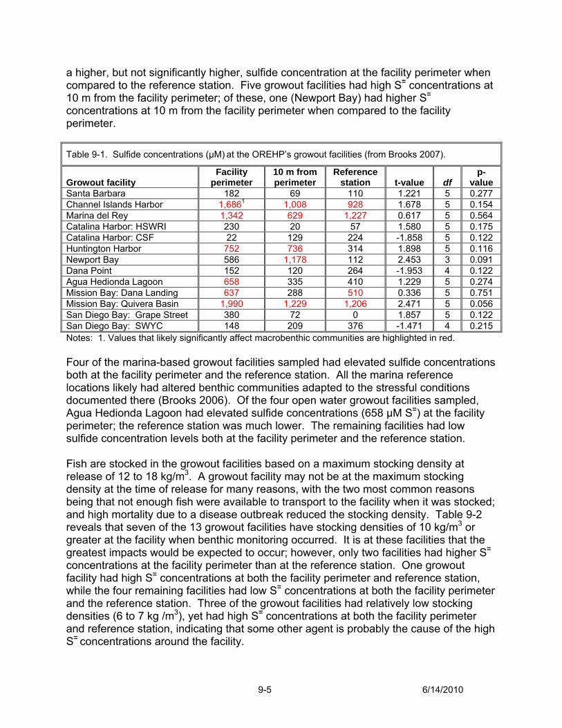
a higher, but not significantly higher, sulfide concentration at the facility perimeter when compared to the reference station. Five growout facilities had high S= concentrations at 10 m from the facility perimeter; of these, one (Newport Bay) had higher S= concentrations at 10 m from the facility perimeter when compared to the facility perimeter. Table 9-1. Sulfide concentrations (µM) at the OREHP’s growout facilities (from Brooks 2007).
Growout facility Facility
perimeter 10 m from perimeter
Reference station t-value df
p-value
Santa Barbara 182 69 110 1.221 5 0.277 Channel Islands Harbor 1,6861 1,008 928 1.678 5 0.154 Marina del Rey 1,342 629 1,227 0.617 5 0.564 Catalina Harbor: HSWRI 230 20 57 1.580 5 0.175 Catalina Harbor: CSF 22 129 224 -1.858 5 0.122 Huntington Harbor 752 736 314 1.898 5 0.116 Newport Bay 586 1,178 112 2.453 3 0.091 Dana Point 152 120 264 -1.953 4 0.122 Agua Hedionda Lagoon 658 335 410 1.229 5 0.274 Mission Bay: Dana Landing 637 288 510 0.336 5 0.751 Mission Bay: Quivera Basin 1,990 1,229 1,206 2.471 5 0.056 San Diego Bay: Grape Street 380 72 0 1.857 5 0.122 San Diego Bay: SWYC 148 209 376 -1.471 4 0.215 Notes: 1. Values that likely significantly affect macrobenthic communities are highlighted in red. Four of the marina-based growout facilities sampled had elevated sulfide concentrations both at the facility perimeter and the reference station. All the marina reference locations likely had altered benthic communities adapted to the stressful conditions documented there (Brooks 2006). Of the four open water growout facilities sampled, Agua Hedionda Lagoon had elevated sulfide concentrations (658 µM S=) at the facility perimeter; the reference station was much lower. The remaining facilities had low sulfide concentration levels both at the facility perimeter and the reference station. Fish are stocked in the growout facilities based on a maximum stocking density at release of 12 to 18 kg/m3. A growout facility may not be at the maximum stocking density at the time of release for many reasons, with the two most common reasons being that not enough fish were available to transport to the facility when it was stocked; and high mortality due to a disease outbreak reduced the stocking density. Table 9-2 reveals that seven of the 13 growout facilities have stocking densities of 10 kg/m3 or greater at the facility when benthic monitoring occurred. It is at these facilities that the greatest impacts would be expected to occur; however, only two facilities had higher S= concentrations at the facility perimeter than at the reference station. One growout facility had high S= concentrations at both the facility perimeter and reference station, while the four remaining facilities had low S= concentrations at both the facility perimeter and the reference station. Three of the growout facilities had relatively low stocking densities (6 to 7 kg /m3), yet had high S= concentrations at both the facility perimeter and reference station, indicating that some other agent is probably the cause of the high S= concentrations around the facility.
9-5 6/14/2010
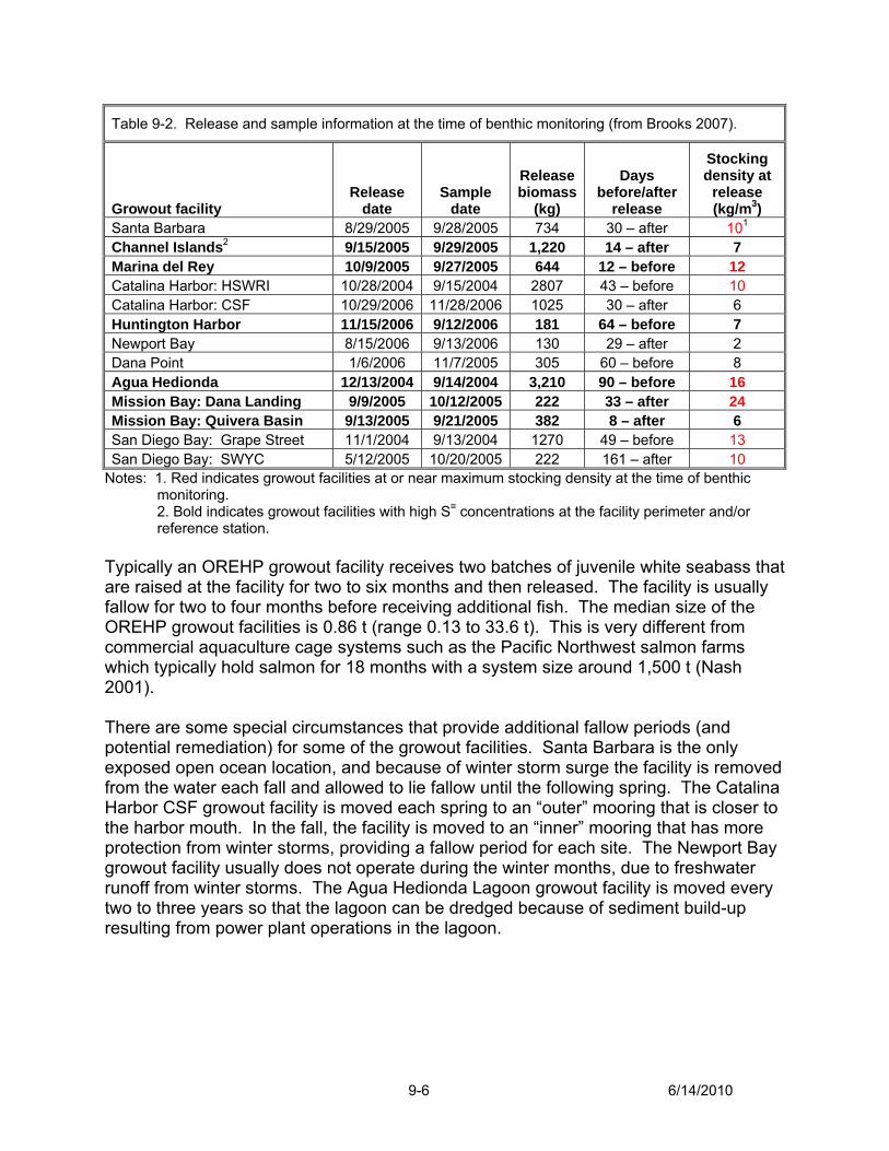
Table 9-2. Release and sample information at the time of benthic monitoring (from Brooks 2007).
Growout facility Release
date Sample
date
Release biomass
(kg)
Days before/after
release
Stocking density at
release (kg/m3)
Santa Barbara 8/29/2005 9/28/2005 734 30 – after 101
Channel Islands2 9/15/2005 9/29/2005 1,220 14 – after 7 Marina del Rey 10/9/2005 9/27/2005 644 12 – before 12 Catalina Harbor: HSWRI 10/28/2004 9/15/2004 2807 43 – before 10 Catalina Harbor: CSF 10/29/2006 11/28/2006 1025 30 – after 6 Huntington Harbor 11/15/2006 9/12/2006 181 64 – before 7 Newport Bay 8/15/2006 9/13/2006 130 29 – after 2 Dana Point 1/6/2006 11/7/2005 305 60 – before 8 Agua Hedionda 12/13/2004 9/14/2004 3,210 90 – before 16 Mission Bay: Dana Landing 9/9/2005 10/12/2005 222 33 – after 24 Mission Bay: Quivera Basin 9/13/2005 9/21/2005 382 8 – after 6 San Diego Bay: Grape Street 11/1/2004 9/13/2004 1270 49 – before 13 San Diego Bay: SWYC 5/12/2005 10/20/2005 222 161 – after 10
Notes: 1. Red indicates growout facilities at or near maximum stocking density at the time of benthic monitoring. 2. Bold indicates growout facilities with high S= concentrations at the facility perimeter and/or reference station.
Typically an OREHP growout facility receives two batches of juvenile white seabass that are raised at the facility for two to six months and then released. The facility is usually fallow for two to four months before receiving additional fish. The median size of the OREHP growout facilities is 0.86 t (range 0.13 to 33.6 t). This is very different from commercial aquaculture cage systems such as the Pacific Northwest salmon farms which typically hold salmon for 18 months with a system size around 1,500 t (Nash 2001). There are some special circumstances that provide additional fallow periods (and potential remediation) for some of the growout facilities. Santa Barbara is the only exposed open ocean location, and because of winter storm surge the facility is removed from the water each fall and allowed to lie fallow until the following spring. The Catalina Harbor CSF growout facility is moved each spring to an “outer” mooring that is closer to the harbor mouth. In the fall, the facility is moved to an “inner” mooring that has more protection from winter storms, providing a fallow period for each site. The Newport Bay growout facility usually does not operate during the winter months, due to freshwater runoff from winter storms. The Agua Hedionda Lagoon growout facility is moved every two to three years so that the lagoon can be dredged because of sediment build-up resulting from power plant operations in the lagoon.
9-6 6/14/2010
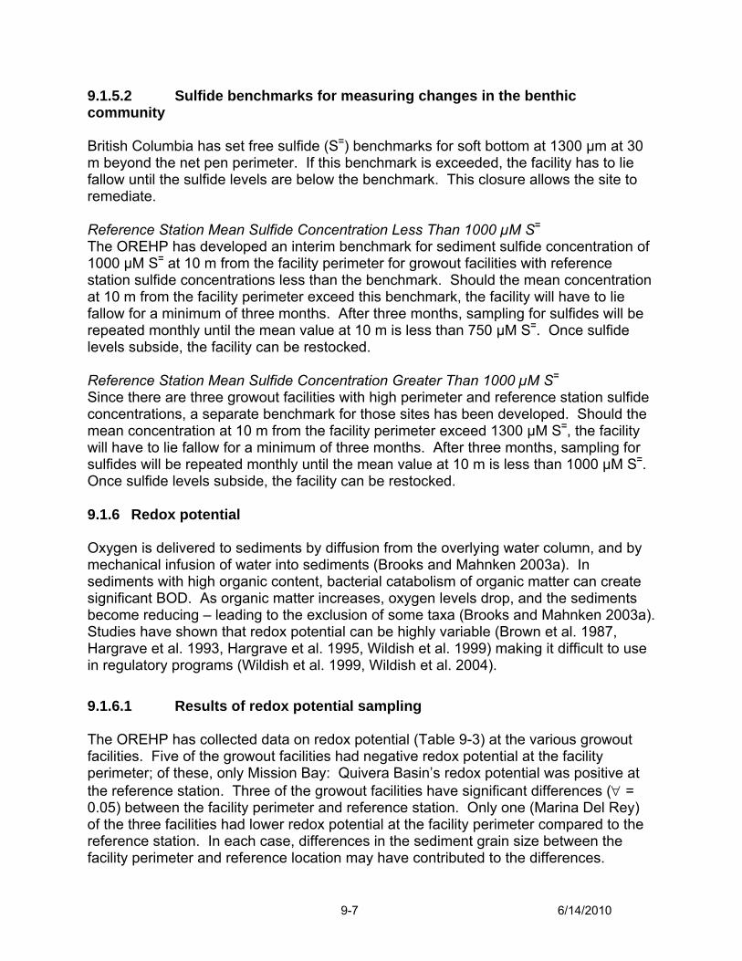
9.1.5.2 Sulfide benchmarks for measuring changes in the benthic community British Columbia has set free sulfide (S=) benchmarks for soft bottom at 1300 µm at 30 m beyond the net pen perimeter. If this benchmark is exceeded, the facility has to lie fallow until the sulfide levels are below the benchmark. This closure allows the site to remediate. Reference Station Mean Sulfide Concentration Less Than 1000 µM S=
The OREHP has developed an interim benchmark for sediment sulfide concentration of 1000 µM S= at 10 m from the facility perimeter for growout facilities with reference station sulfide concentrations less than the benchmark. Should the mean concentration at 10 m from the facility perimeter exceed this benchmark, the facility will have to lie fallow for a minimum of three months. After three months, sampling for sulfides will be repeated monthly until the mean value at 10 m is less than 750 µM S=. Once sulfide levels subside, the facility can be restocked. Reference Station Mean Sulfide Concentration Greater Than 1000 µM S=
Since there are three growout facilities with high perimeter and reference station sulfide concentrations, a separate benchmark for those sites has been developed. Should the mean concentration at 10 m from the facility perimeter exceed 1300 µM S=, the facility will have to lie fallow for a minimum of three months. After three months, sampling for sulfides will be repeated monthly until the mean value at 10 m is less than 1000 µM S=. Once sulfide levels subside, the facility can be restocked. 9.1.6 Redox potential Oxygen is delivered to sediments by diffusion from the overlying water column, and by mechanical infusion of water into sediments (Brooks and Mahnken 2003a). In sediments with high organic content, bacterial catabolism of organic matter can create significant BOD. As organic matter increases, oxygen levels drop, and the sediments become reducing – leading to the exclusion of some taxa (Brooks and Mahnken 2003a). Studies have shown that redox potential can be highly variable (Brown et al. 1987, Hargrave et al. 1993, Hargrave et al. 1995, Wildish et al. 1999) making it difficult to use in regulatory programs (Wildish et al. 1999, Wildish et al. 2004). 9.1.6.1 Results of redox potential sampling The OREHP has collected data on redox potential (Table 9-3) at the various growout facilities. Five of the growout facilities had negative redox potential at the facility perimeter; of these, only Mission Bay: Quivera Basin’s redox potential was positive at the reference station. Three of the growout facilities have significant differences (∀ = 0.05) between the facility perimeter and reference station. Only one (Marina Del Rey) of the three facilities had lower redox potential at the facility perimeter compared to the reference station. In each case, differences in the sediment grain size between the facility perimeter and reference location may have contributed to the differences.
9-7 6/14/2010
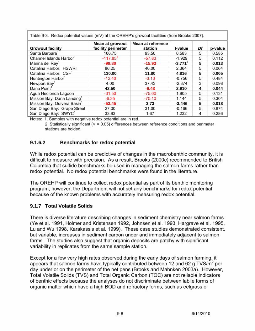
Table 9-3. Redox potential values (mV) at the OREHP’s growout facilities (from Brooks 2007).
Growout facility Mean at growout facility perimeter
Mean at reference station t-value Df p-value
Santa Barbara1 106.75 93.50 0.583 5 0.585 Channel Islands Harbor1 -117.851 -57.83 -1.929 5 0.112 Marina del Rey1 -99.80 -15.93 -3.7712 5 0.013 Catalina Harbor: HSWRI 86.25 40.00 2.364 5 0.064 Catalina Harbor: CSF1 130.00 11.80 4.816 5 0.005 Huntington Harbor1 -12.40 -3.13 -0.756 5 0.484 Newport Bay1 4.00 37.43 -2.374 3 0.098 Dana Point1 42.50 -9.43 2.910 4 0.044 Agua Hedionda Lagoon -31.50 -75.00 1.805 5 0.131 Mission Bay: Dana Landing1 -6.35 -70.10 1.144 5 0.304 Mission Bay: Quivera Basin1 -53.45 3.73 -3.446 5 0.018 San Diego Bay: Grape Street 27.00 31.00 -0.166 5 0.874 San Diego Bay: SWYC1 33.93 1.67 1.232 4 0.286 Notes: 1. Samples with negative redox potential are in red.
2. Statistically significant (∀ = 0.05) differences between reference conditions and perimeter stations are bolded.
9.1.6.2 Benchmarks for redox potential While redox potential can be predictive of changes in the macrobenthic community, it is difficult to measure with precision. As a result, Brooks (2000c) recommended to British Columbia that sulfide benchmarks be used in managing the salmon farms rather than redox potential. No redox potential benchmarks were found in the literature. The OREHP will continue to collect redox potential as part of its benthic monitoring program; however, the Department will not set any benchmarks for redox potential because of the known problems with accurately measuring redox potential. 9.1.7 Total Volatile Solids There is diverse literature describing changes in sediment chemistry near salmon farms (Ye et al. 1991, Holmer and Kristensen 1992, Johnsen et al. 1993, Hargrave et al. 1995, Lu and Wu 1998, Karakassis et al. 1999). These case studies demonstrated consistent, but variable, increases in sediment carbon under and immediately adjacent to salmon farms. The studies also suggest that organic deposits are patchy with significant variability in replicates from the same sample station. Except for a few very high rates observed during the early days of salmon farming, it appears that salmon farms have typically contributed between 12 and 62 g TVS/m2 per day under or on the perimeter of the net pens (Brooks and Mahnken 2003a). However, Total Volatile Solids (TVS) and Total Organic Carbon (TOC) are not reliable indicators of benthic effects because the analyses do not discriminate between labile forms of organic matter which have a high BOD and refractory forms, such as eelgrass or
9-8 6/14/2010
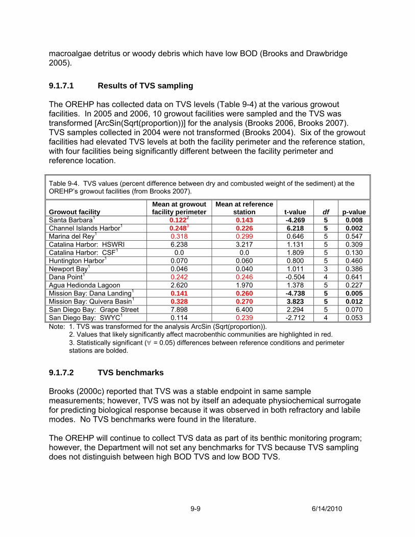
macroalgae detritus or woody debris which have low BOD (Brooks and Drawbridge 2005). 9.1.7.1 Results of TVS sampling The OREHP has collected data on TVS levels (Table 9-4) at the various growout facilities. In 2005 and 2006, 10 growout facilities were sampled and the TVS was transformed [ArcSin(Sqrt(proportion))] for the analysis (Brooks 2006, Brooks 2007). TVS samples collected in 2004 were not transformed (Brooks 2004). Six of the growout facilities had elevated TVS levels at both the facility perimeter and the reference station, with four facilities being significantly different between the facility perimeter and reference location. Table 9-4. TVS values (percent difference between dry and combusted weight of the sediment) at the OREHP’s growout facilities (from Brooks 2007).
Growout facility Mean at growout facility perimeter
Mean at reference station t-value df p-value
Santa Barbara1 0.1222 0.143 -4.269 5 0.008 Channel Islands Harbor1 0.2483 0.226 6.218 5 0.002 Marina del Rey1 0.318 0.299 0.646 5 0.547 Catalina Harbor: HSWRI 6.238 3.217 1.131 5 0.309 Catalina Harbor: CSF1 0.0 0.0 1.809 5 0.130 Huntington Harbor1 0.070 0.060 0.800 5 0.460 Newport Bay1 0.046 0.040 1.011 3 0.386 Dana Point1 0.242 0.246 -0.504 4 0.641 Agua Hedionda Lagoon 2.620 1.970 1.378 5 0.227 Mission Bay: Dana Landing1 0.141 0.260 -4.738 5 0.005 Mission Bay: Quivera Basin1 0.328 0.270 3.823 5 0.012 San Diego Bay: Grape Street 7.898 6.400 2.294 5 0.070 San Diego Bay: SWYC1 0.114 0.239 -2.712 4 0.053 Note: 1. TVS was transformed for the analysis ArcSin (Sqrt(proportion)).
2. Values that likely significantly affect macrobenthic communities are highlighted in red. 3. Statistically significant (∀ = 0.05) differences between reference conditions and perimeter stations are bolded.
9.1.7.2 TVS benchmarks Brooks (2000c) reported that TVS was a stable endpoint in same sample measurements; however, TVS was not by itself an adequate physiochemical surrogate for predicting biological response because it was observed in both refractory and labile modes. No TVS benchmarks were found in the literature. The OREHP will continue to collect TVS data as part of its benthic monitoring program; however, the Department will not set any benchmarks for TVS because TVS sampling does not distinguish between high BOD TVS and low BOD TVS.
9-9 6/14/2010
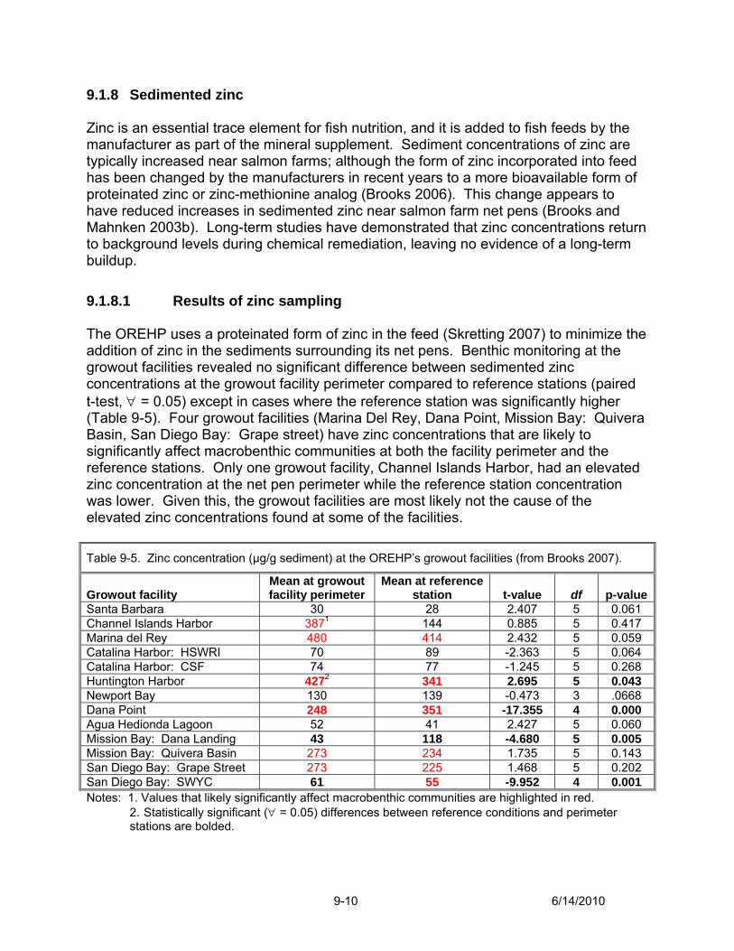
9.1.8 Sedimented zinc Zinc is an essential trace element for fish nutrition, and it is added to fish feeds by the manufacturer as part of the mineral supplement. Sediment concentrations of zinc are typically increased near salmon farms; although the form of zinc incorporated into feed has been changed by the manufacturers in recent years to a more bioavailable form of proteinated zinc or zinc-methionine analog (Brooks 2006). This change appears to have reduced increases in sedimented zinc near salmon farm net pens (Brooks and Mahnken 2003b). Long-term studies have demonstrated that zinc concentrations return to background levels during chemical remediation, leaving no evidence of a long-term buildup. 9.1.8.1 Results of zinc sampling The OREHP uses a proteinated form of zinc in the feed (Skretting 2007) to minimize the addition of zinc in the sediments surrounding its net pens. Benthic monitoring at the growout facilities revealed no significant difference between sedimented zinc concentrations at the growout facility perimeter compared to reference stations (paired t-test, ∀ = 0.05) except in cases where the reference station was significantly higher (Table 9-5). Four growout facilities (Marina Del Rey, Dana Point, Mission Bay: Quivera Basin, San Diego Bay: Grape street) have zinc concentrations that are likely to significantly affect macrobenthic communities at both the facility perimeter and the reference stations. Only one growout facility, Channel Islands Harbor, had an elevated zinc concentration at the net pen perimeter while the reference station concentration was lower. Given this, the growout facilities are most likely not the cause of the elevated zinc concentrations found at some of the facilities. Table 9-5. Zinc concentration (µg/g sediment) at the OREHP’s growout facilities (from Brooks 2007).
Growout facility Mean at growout facility perimeter
Mean at reference station t-value df p-value
Santa Barbara 30 28 2.407 5 0.061 Channel Islands Harbor 3871 144 0.885 5 0.417 Marina del Rey 480 414 2.432 5 0.059 Catalina Harbor: HSWRI 70 89 -2.363 5 0.064 Catalina Harbor: CSF 74 77 -1.245 5 0.268 Huntington Harbor 4272 341 2.695 5 0.043 Newport Bay 130 139 -0.473 3 .0668 Dana Point 248 351 -17.355 4 0.000 Agua Hedionda Lagoon 52 41 2.427 5 0.060 Mission Bay: Dana Landing 43 118 -4.680 5 0.005 Mission Bay: Quivera Basin 273 234 1.735 5 0.143 San Diego Bay: Grape Street 273 225 1.468 5 0.202 San Diego Bay: SWYC 61 55 -9.952 4 0.001 Notes: 1. Values that likely significantly affect macrobenthic communities are highlighted in red.
2. Statistically significant (∀ = 0.05) differences between reference conditions and perimeter stations are bolded.
9-10 6/14/2010

9.1.8.2 Benchmarks for monitoring zinc Washington State is the only jurisdiction that has developed Marine Sediment Quality Standards for metals (WAC 173-204-320) (Brooks 2006). These standards are based on the Apparent Effects Thresholds (AET). The Florida Department of Environmental Protection has developed Threshold Effects Levels (TEL) and Probable Effect Levels (PEL) (MacDonald 1994), while Long et al. (1995) developed an Effects Range-Low (ER-L) and Effects Range-Moderate (ER-M). The State of California has not developed zinc benchmarks. The zinc benchmarks are summarized in Table 9-6. The OREHP has already mitigated for sedimented zinc by using proteinated zinc in the fish feed. Additionally, initial benthic monitoring indicates that the source of zinc around the growout facilities probably comes from other sources rather than the facilities. As a result, the Department will not set zinc benchmarks at this time. The results of the first benthic sampling will be compared to subsequent samples, and should there be significant changes in zinc deposition the Department will reconsider setting zinc benchmarks. Table 9-6. Published sediment zinc and copper benchmarks (µg/g dry sediment).
Contaminant ER-L ER-M (ER-L + ER-M)/2 TEL PEL (TEL + PEL)/2 WA State AET Zinc 150 410 260.0 124 271 197.5 270.0 Copper 152.0 18.7 108 63.35 390.0 9.1.9 Sedimented copper Copper is another micronutrient added to fish feeds (Chow and Schell 1978). Copper is also used in the anti-fouling treatments (e.g., Flexguard XI) for the nets. The latter use is most likely the cause of increased copper levels surrounding salmon net pen facilities. Brooks (2000a) developed a model to estimate water column concentrations of copper surrounding treated net pens. The results of Brooks’ (2000a) monitoring efforts resulted in recommendations for BMPs that include washing copper-treated nets in upland facilities and annual monitoring of copper at growout facilities using copper-treated nets. 9.1.9.1 Results of copper sampling Benthic monitoring at 10 of the OREHP growout facilities revealed that four facilities had significantly different concentrations of sedimented copper between the facility perimeter and reference station (paired t-test, ∀ = 0.05) (Table 9-7); however, only one (Marina Del Rey, a raceway facility that does not use copper as an antifoulant) had a higher copper concentration at the facility perimeter. The other three sites had significantly higher copper concentrations at the reference site. Five of the growout facilities had elevated copper concentrations at the facility perimeter that likely significantly affect macrobenthic communities. Only one, Marina Del Rey, was significantly different (higher) than the reference station. This indicates that the marinas
9-11 6/14/2010

or bays are already in a degraded state and that the effects are not from the use of copper-treated nets but from other inputs to the system. In the past, the OREHP used Flex Guard XI to treat nets at many of its facilities; however, that practice was discontinued in 2006 in response to concerns about potentially increasing the sediment copper loading in the benthos under facilities that are already impacted from other copper sources. Because copper-treated nets are no longer in use, there should be little to no increase in sedimented copper around the growout facilities. Table 9-7. Copper concentration (µg/g sediment) at the OREHP’s growout facilities (from Brooks 2007).
Growout facility Mean at growout facility perimeter
Mean at reference station t-value Df p-value
Santa Barbara 6 6 1.782 5 0.135 Channel Islands Harbor 1031 120 -1.457 5 0.205 Marina del Rey 396 337 2.9552 5 0.032 Catalina Harbor: HSWRI 29 34 -2.547 5 0.051 Catalina Harbor: CSF 27 25 2.087 5 0.091 Huntington Harbor 147 136 0.946 5 0.387 Newport Bay 62 57 0.519 3 0.640 Dana Point 280 474 -9.643 4 0.001 Agua Hedionda Lagoon 22 11 2.666 5 0.045 Mission Bay: Dana Landing 23 96 -4.952 5 0.004 Mission Bay: Quivera Basin 258 261 -0.104 5 0.921 San Diego Bay: Grape Street 198 144 1.079 5 0.330 San Diego Bay: SWYC 276 214 -11.777 4 0.000 Notes: 1. Values that likely significantly affect macrobenthic communities are highlighted in red.
2. Statistically significant (∀ = 0.05) differences between reference conditions and perimeter stations are bolded.
9.1.9.2 Benchmarks for monitoring copper Washington State is the only jurisdiction that has developed Marine Sediment Quality Standards for metals (WAC 173-204-320) (Brooks 2006). These standards are based on AET. The Florida Department of Environmental Protection has developed TEL and PEL for copper (MacDonald 1994), while Long et al. (1995) developed an ER-L and ER-M for copper. The State of California has not developed copper benchmarks. The copper benchmarks are summarized in Table 9-6. The OREHP has mitigated for sedimented copper by discontinuing the use of copper-treated nets. Additionally, initial benthic monitoring indicates that the source of copper around the growout facilities probably comes from other sources rather than the facilities. As a result, the Department will not set copper benchmarks at this time. The results of the first benthic sampling will be compared to subsequent samples, and should there be significant changes in copper deposition the Department will reconsider setting copper benchmarks.
9-12 6/14/2010
9.2 Water quality monitoring Water quality monitoring is usually required by the Regional Water Boards through the NPDES permit. Since none of the growout facilities are required to obtain NPDES permits, water quality monitoring for most facilities has not been required. The Los Angeles Regional Water Quality Control Board (LARWQCB) has requested water quality sampling for facilities within their jurisdiction (Channel Islands Harbor, Marina Del Rey, Catalina Harbor: HSWRI, and Catalina Harbor: CSF). Water quality monitoring includes biannual collection of water temperature, ammonia, and dissolved oxygen levels inside the facility and just outside the facility perimeter. Additionally, each year divers shall make a visual inspection of the bottom to look for adverse conditions. The Department shall submit an annual report to the LARWQCB summarizing the results of the water quality monitoring. Although the hatchery does not operate under a NPDES permit, the SDRWQCB does require water quality monitoring. Influent sampling includes monthly sampling for salinity, pH, temperature, settleable solids, total suspended solids, total Kjeldahl nitrogen, organic nitrogen, ammonia, unionized ammonia, nitrate, nitrite, phosphorus, orthophosphate; quarterly sampling for zinc and copper; annual sampling for acute toxicity; and one-time sampling for chronic toxicity and California Toxics Rule (CTR) priority organic and inorganic pollutants. Effluent sampling includes daily sampling for flow rate; monthly sampling for salinity, pH, temperature, settleable solids, total suspended solids, total Kjeldahl nitrogen, organic nitrogen, ammonia, unionized ammonia, nitrate, nitrite, phosphorus, orthophosphate; quarterly sampling for zinc and copper; annual sampling for acute toxicity; and one-time sampling for chronic toxicity and CTR priority organic and inorganic pollutants. Sand filter backwash is sampled weekly for total suspended solids. Hatchery staff is required to maintain self-monitoring reports and to submit annual reports to the SDRWQCB. 9.3 Bird and mammal interactions Each growout facility takes precautions to prevent the take of marine mammals, birds and other fish. In areas where marine mammals are present, growout facilities utilize raceway systems to provide rigid protection for the white seabass and prevent intrusion of birds and marine mammals. Raceway facilities are generally covered by chain link fencing that has shade cloth stretched over it. This prevents birds from becoming entangled or preying upon the fish and provides shade for the fish. The net pen facilities utilize brightly colored, large mesh nets underwater to surround the smaller containment net. There is generally a one m space between containment net and predator barrier. The predator barrier is held taut by anchors to prevent any entanglement. Above the water, chain link fence surrounding the walkways prevents the haul-out of marine mammals. Shade cloth or bird-netting covers the facility and prevents birds from preying upon the fish. The bird netting is also kept taut to prevent entanglement.
9-13 6/14/2010
The land-based facility is located within a Quonset hut-type building covered by a heavy tarp that provides shade for the fish and protection from birds and other animals. NOAA Fisheries has categorized the white seabass growout facilities as Category III fisheries under the Marine Mammal Protection Act. Category III designates fisheries with a remote likelihood or no known serious injuries or mortalities to marine mammals. Owners of vessels or non-vessel gear in Category III fisheries may incidentally take marine mammals without registering for or receiving a marine mammal authorization. 9.4 Effects on sensitive habitats The OREHP growout facilities generally occur within marinas or established vessel mooring fields; thus, the effects on sensitive habitats should be minimal. NOAA Fisheries staff reviewed the location of the growout facilities and determined that none were located in an area that would impact eelgrass beds, although some facilities are close to eelgrass beds. Dive surveys conducted annually will assure that the effects of the growout facilities, if any, remain localized so that it would not be likely to impact eelgrass or other sensitive habitat.
9-14 6/14/2010

Chapter 10. Genetics
10.1 Genetic considerations Beyond the technical aspects of maintaining brood fish is the concern that genetic variability of the wild population could be diminished by releasing large numbers of hatchery fish. If the effective population size (number of broodstock participating in spawn events) in the hatchery is small, important alleles may be lost in the hatchery progeny; rare alleles would be especially vulnerable to loss. Should the hatchery progeny grow and reproduce with wild fish, this could change the genetic diversity of the wild population, by reducing the frequency of these alleles. Diminishing genetic variability due to selective breeding and survival within the hatchery is an important consideration. These concerns are driven largely by observations made of some adverse interactions between wild and hatchery populations of salmonids. Tringali and Bert (1998) used the Ryman-Laikre model (1991) to compare the genetic risks associated with stock enhancement for the marine species, red drum (Sciaenops ocellatus) a Sciaenid species, and the anadromous species, Gulf sturgeon (Acipenser oxyrinchus desotoi). For red drum, they found that the lack of genetic substructure in the red drum population and the large population size offset the risks to single-locus and quantitative genetic variation. Tringali and Bert (1998) noted that was true as long as there were adequate numbers of effective breeders and the per-generation contribution was modest. On the other hand, Gulf sturgeon breeding populations are very small, making the hatchery contribution quite large (proportionally). Tringali and Bert (1998) found that almost all combinations of the three parameters effective breeders, population size and hatchery contribution could result in a substantial loss of single-locus and polygenic variation and a reduced adaptive potential. Although the study of genetic resources described for salmonids has greatly advanced the field of applied population genetics and has provided an efficient tool for the management of valuable salmon populations, using anadromous salmonids as a general model for the conservation and utilization of genetic resources of many marine species should be done cautiously because their life history strategies are radically different. 10.2 Conserving genetic diversity Genetic quality assurance has been a priority for the OREHP since the early years of the program. Studies to examine the genetic characteristics of wild white seabass were initiated in the mid-late 1980’s and ran parallel to the culture and assessment research (Bartley and Kent 1990). Work by Bartley et al. (1995) developed the protocols for conservation of genetic diversity of white seabass by the OREHP. The suggested protocols address three main factors: 1)
10-1 6/14/2010
the genetic structure of the wild population, 2) the genetic structure of the broodstock, and 3) monitoring of both the wild population and the hatchery population. 10.2.1 Genetic structure of the wild population Initial work conducted by Soulé and Senner ([Date unknown]) focused on finding one or more genetic loci that could be used in determining the population structure of white seabass. Samples were taken from Baja California, Mexico fish and processed using electrophoresis. Polymorphism was detected in only two enzyme systems (acohol dehydrogenase and phosphoglucomutase). Heterozygocity levels ranged from 0.009 to 0.043. A survey of the Southern California Bight (Bartley and Kent 1990) revealed no stable population sub-structuring in the area. Bartley et al. (1995) estimated that gene flow was approximately nine migrants per generation and therefore sufficient to homogenize the genetic structure of the population. The study evaluated 22 enzyme systems representing 33 distinct loci in 13 different samples that varied spatially and temporally (ΣN=510 fish). Average heterozygosity values ranged from 0.033 to 0.064, genetic identity was greater than 99 percent in all pair-wise comparisons and only three percent of the genetic variation was attributed to between sample differences. In highly mobile species such as white seabass (Vojkovich and Reed 1983), gene flow among localities is apparently sufficient to homogenize the genetic structure. However, since several gene loci possessed rare alleles (frequency < 2 percent) that contributed to genetic diversity, Bartley et al. (1995) recommended that a hatchery replenishment program should strive to conserve this allelic diversity. A subsequent study by Franklin (1997) looked at the population structure of white seabass from Point Conception, California to Magdalena Bay, Baja California, Mexico and the northern Gulf of California. Additionally, Franklin analyzed samples from one of the white seabass growout facilities (Channel Islands Harbor). He used microsattellite DNA from eight polymorprhic loci and randomly selected 12 fish from each area (N = 120) for the study. The results of Franklin’s study indicate three major natural spawning groups that are physically segregated by ocean currents and a geographic barrier. On the outer west coast of California and Mexico, the northern spawning group is centered off the Southern California Bight and central Baja California, while the southern spawning group is located off southern Baja California. These two spawning groups are separated by the Southern California Gyre. The third spawning group is located in the Gulf of California. While this group is separated from the other groups by the Baja California peninsula, Franklin’s (1997) results showed some mixing between the southern Baja California and the Gulf of California spawning groups. Franklin’s (1997) analysis of the hatchery-raised fish from the Channel Islands Harbor growout facility revealed a reduction in genetic diversity compared to the wild population, which is expected because the fish came from only one or two spawn events, with each spawn event consisting of one to two females and two to four males.
10-2 6/14/2010
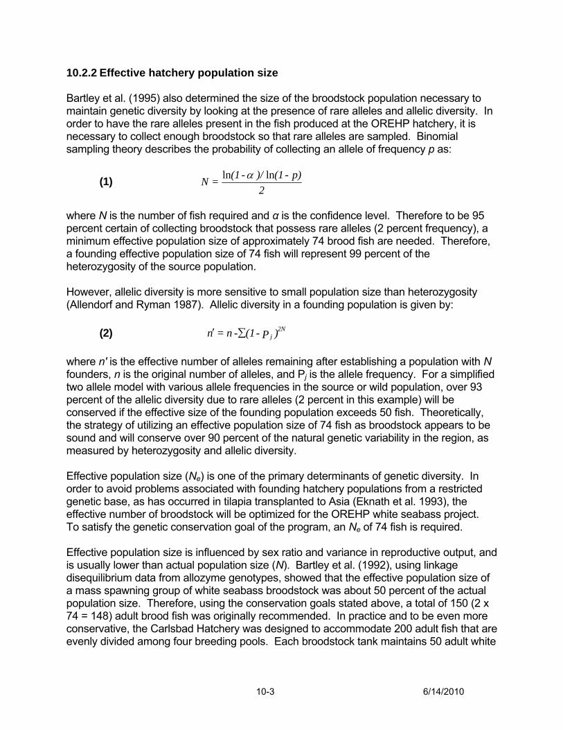
10.2.2 Effective hatchery population size Bartley et al. (1995) also determined the size of the broodstock population necessary to maintain genetic diversity by looking at the presence of rare alleles and allelic diversity. In order to have the rare alleles present in the fish produced at the OREHP hatchery, it is necessary to collect enough broodstock so that rare alleles are sampled. Binomial sampling theory describes the probability of collecting an allele of frequency p as:
(1) 2
p)-(1)/-(1=N lnln α
where N is the number of fish required and α is the confidence level. Therefore to be 95 percent certain of collecting broodstock that possess rare alleles (2 percent frequency), a minimum effective population size of approximately 74 brood fish are needed. Therefore, a founding effective population size of 74 fish will represent 99 percent of the heterozygosity of the source population. However, allelic diversity is more sensitive to small population size than heterozygosity (Allendorf and Ryman 1987). Allelic diversity in a founding population is given by: (2) )P-(1-n=n 2N
j∑′ where n' is the effective number of alleles remaining after establishing a population with N founders, n is the original number of alleles, and Pj is the allele frequency. For a simplified two allele model with various allele frequencies in the source or wild population, over 93 percent of the allelic diversity due to rare alleles (2 percent in this example) will be conserved if the effective size of the founding population exceeds 50 fish. Theoretically, the strategy of utilizing an effective population size of 74 fish as broodstock appears to be sound and will conserve over 90 percent of the natural genetic variability in the region, as measured by heterozygosity and allelic diversity. Effective population size (Ne) is one of the primary determinants of genetic diversity. In order to avoid problems associated with founding hatchery populations from a restricted genetic base, as has occurred in tilapia transplanted to Asia (Eknath et al. 1993), the effective number of broodstock will be optimized for the OREHP white seabass project. To satisfy the genetic conservation goal of the program, an Ne of 74 fish is required. Effective population size is influenced by sex ratio and variance in reproductive output, and is usually lower than actual population size (N). Bartley et al. (1992), using linkage disequilibrium data from allozyme genotypes, showed that the effective population size of a mass spawning group of white seabass broodstock was about 50 percent of the actual population size. Therefore, using the conservation goals stated above, a total of 150 (2 x 74 = 148) adult brood fish was originally recommended. In practice and to be even more conservative, the Carlsbad Hatchery was designed to accommodate 200 adult fish that are evenly divided among four breeding pools. Each broodstock tank maintains 50 adult white
10-3 6/14/2010

seabass in a 1:1 ratio of male to female fish. Deviations necessitate that more broodstock are maintained according to the expression:
(3) ( )
)N+N(N*N4
=Nfm
fme
where m and f are the numbers of males and females, respectively. A schedule for annually rotating 20 percent of the male brood fish among breeding pools was originally proposed in order to increase the diversity in progeny by increasing the number of different matings per broodstock. 10.3 Genotyping 10.3.1 Broodstock source and genotyping To help ensure that the genetic diversity of hatchery-released progeny will be similar to wild populations, broodstock are collected only from the northern component of the white seabass population range from Point Conception, California to central Baja California, Mexico. No captive-bred progeny are used as brood individuals. At the time of capture, all white seabass broodstock have tissue samples (fin clips) taken to genotype the fish. Much of the early work was done by an OREHP contractor, who changed the analytical equipment used during the contract causing calibration problems. Additionally, genotyping was not consistent for all broodstock (some broodstock were genotyped at seven loci, while others were genotyped at fewer loci). These differences resulted in some progeny appearing to have more than two parents which, of course, is not possible. Due to the problems with early genotyping efforts, all hatchery broodstock were genotyped again by a new geneticist hired by HSWRI in collaboration with researchers at the NOAA Fisheries Southwest Fisheries Science Center located in La Jolla, California. 10.3.2 Progeny genotyping Samples for genotyping of spawning events and release batches were collected sporadically from 1997 to 2000 and regularly between 2000 and the present. Early genotyping was conducted by the same contractor that processed the broodstock. Tissue collection was required for a subset of ≥200 yolk sac larvae (YSL) from every spawn and 96 juveniles from every release batch. Current tissue collection protocols for genotyping are experimental. These protocols will be modified based on the results of the experiments, currently being conducted by the new HSWRI geneticist, to determine how many offspring must be sampled to accurately estimate proportional per parent contribution to a single spawn.
10-4 6/14/2010
10.4 Research 10.4.1 Coykendall’s genetics research Recently, Coykendall (2005) completed a study of white seabass that examined wild stocks, hatchery releases, and breeding stocks. This study used the same eight microsatellite DNA loci as Franklin (1997). The executive summary of Coykendall’s dissertation (Coykendall and Hedgecock 2006) that was provided to the Department is supplied below. Coykendall’s study focused on the potential problem that stocking of large numbers of hatchery fish, with different levels of genetic diversity from wild populations, could reduce the genetic resources of enhanced populations. This is known as the Ryman-Laikre effect or model.
We employed the Ryman-Laikre model of genetic impact of hatchery supplementation to wild populations. The model requires estimates of three parameters: hatchery effective population size (or in this case effective number of breeders), the effective size of the wild population, and the contribution that the hatchery fish make to the overall reproduction of the population. Estimates of these three parameters, caveats associated with them, and our general conclusions are addressed below.
Hatchery effective size, Neh – To understand the biology of
hatchery spawns, we used two different methods of estimating the genetic output of the hatchery systems. The first method looked at several spawning events individually. We used data from four spawning events in 1998, one in 1999, and five from 2001. These spawning events came from tanks B1, B3, and B4. Using genotypes of the broodstock and a subset of the spawns from 4 – 7 microsatellite loci, we assigned offspring to parents to divulge the reproductive success of each broodstock. This led to an estimate of the effective number of breeders per spawning event of 2 to 8 individuals. We ascertained that the limiting factor in most spawning events is the number of contributing females to each spawn (anywhere from one to seven). Furthermore, we found evidence of repeat spawning by both males and females.
Caveats: Given the information that we had from the work that GIS did, not all offspring could be assigned to a single parental pair. Broodstock in Tank 4 were genotyped at seven loci, but broodstock in other tanks were genotyped at fewer loci. This reduces the power of assignment tests. Offspring that were not successfully assigned a single parental pair were excluded from this analysis. In addition, we discovered a few genotyping errors of the broodstock. It is vitally important for parentage analyses that the parental genotypes are accurate. We were able to correct some inaccurate genotypes but others may not have been detected.
10-5 6/14/2010

In order to obtain an estimate for an entire hatchery release, we used a method whereby we could combine the data from all spawning events from a single year. By using this method, we were able to use all of the information available to us (even if we were not able to assign a single parental pair to a particular offspring) and obtain confidence intervals. Our estimation of the effective number of breeders for the 2001 hatchery release was 34.6 (95% CI: 20.6 – 76.5). Note that this differs a little from the 56 (95% CI 28 – 159) that Dennis Hedgecock reported to the Joint Panel in June 2004.
Caveats: Not all of the data from the 2001 release was available to
us. In fact, 1.4% of the spawn groups were not sampled. Also, some spawning in the Catalina net pens contributed to the 2001 release, but those individuals are not in our genotype database. This could lead to an underestimate of Neh. We are also assuming that the results for the 2001 release are an indication of the level of genetic diversity across generations. To confirm this assumption, these estimations should be performed across an entire generation and averaged for a more accurate estimate.
Wild effective population size, New – We estimated New using
both a moment-based method and a pseudo-likelihood estimator of genetic drift based on temporally-spaced changes in allele frequencies. The moment-based technique yields a mean of 5,679, and a 95% confidence interval of 3,977 – 7,678. The pseudo-likelihood method provides a mean of 6,087 and a 95% confidence interval of 2,384 – 57,310.
Caveats: The wild samples we used do not constitute a random
sample because juveniles were not included. This could bias our results either way. We also assume that the changes we observe in allele frequencies over time are due to random processes and not migration, mutation, population subdivision, etc., although previous geographic surveys and our own analyses suggest that population structure in the white seabass is very weak and not likely a source of error. The methods we employed work best for temporal samples that span at least one generation of the organism, but since the white seabass generation length is so long, we were unable to capture an entire generation length in our samples. According to simulations on other studies, this could result in overestimating New.
Contribution of the hatchery to overall reproduction, xh – This
estimate came from juvenile-targeted tag-recapture studies. Allen et al. (2003) reported that their juvenile-targeted tag-recapture study yielded a hatchery contribution of 6.6% based on the 2001 to 2002 sampling period. This number represents the percent of tagged fish for all white seabass that were caught for
10-6 6/14/2010
four months of sampling. However, cumulative data from 1997 – 2003 percentages of tagged fish vary depending on sampling site (Mike Shane, pers.comm.). There was a 1.4% recapture rate along the mainland coast of southern California, 14.6% in mainland bays, 35.9% along the Catalina Island coast, and 78.0% in Catalina Harbor, leading to an overall percentage of tagged fish for this time period of 7.2%. Moreover, five times as many gill nets were set on the mainland coastal sites and bays than at Catalina Island, but the area differential between these two sampling sites is such that the catch per unit effort along the mainland was probably less than at Catalina Island (Mike Shane, pers.comm.). Based on these sites, we used the average of 6.6 percent and 7.2%, 6.9% as our hatchery contribution estimate.
Caveat: Our estimate represents the very upper limit of hatchery
contribution because the estimate was obtained from a juvenile-targeted tag-recapture study. We expect that there is a significant amount of mortality of the hatchery-produced fish before they become sexually mature. Therefore, for current consideration of white seabass genetic diversity, 6.9%should be treated as an upwardly biased value. Further analyses of the white seabass hatchery effect on genetic diversity should include new estimates of xh because the yearly releases have been composed of increasingly older fish in order to maximize survivorship prior to release and this trend is continuing to rise, which would lead to a higher contribution of the hatchery fish to the whole population’s reproduction.
Estimate of the genetic impact of hatchery enhancement: All
combinations of estimated Neh and New coupled with a proportional contribution from the hatchery to the total reproduction of 0.069 from tag-recapture studies result in negative effects on the genetic diversity of the wild population ranging from 1.5 – 92.9%. If Neh is as high as 76.5 (upper 95% confidence interval value) and New is as low as 2383.6 (lower 95% confidence interval value), then supportive breeding will decrease the total effective population size by 1.5%. More substantial negative change would result if Neh is 20.6 or 34.6 and New is as large as 57,310. In these cases, 88.6 – 92.9% reduction in the effective population size for the entire population would ensue. However, this summary must be tempered by the uncertainty in the underlying estimates. Uncertainty could be reduced by further research. Negative impacts could also be alleviated by increasing the effective size of the hatchery population, using genetic analysis to assess reproductive success of broodstock and to find ways to decrease its variance, for example, by rotating out fish that are not performing.
Coykendall provided a useful approach to analyzing the genetic impact of hatchery production on wild populations, but the analysis did not take into consideration the specific sampling, breeding, and release protocols used by the ORHEP. As such, the
10-7 6/14/2010
genetic diversity of white seabass produced by the hatchery could be underestimated and therefore their impact on wild populations is overestimated. Department review of Coykendall’s (2005) work found that her results were based on statistical estimates of the hatchery broodstock size, the wild broodstock size, and the relative contribution of the hatchery fish to the wild stock. The estimates of these three parameters have large margins of error. These errors are the result of several factors including the use of too few genetic markers (microsatellite loci) for hatchery parentage assignment, lack of information on the age demographics of the wild fish used to calculate wild effective population size, and the typical issues associated with mark-recapture sampling for collecting released hatchery fish (Rodzen pers. comm.). Another assumption of the Ryman-Laikre model is that the released hatchery fish are actually reproducing; this is unknown with the white seabass. Subsequent review of Coykendall’s analysis by HSWRI staff, including the new fishery geneticist, has provided more specific information on the hatchery spawning and sampling practices that could have influenced Coykendall’s results (Appendix B). Overall, the results have the potential to significantly underestimate the actual genetic diversity of the white seabass produced at the Carlsbad hatchery and, therefore, overestimate the reduction in effective population size of the enhanced population. Coykendall acknowledges the wide error bars in assessing the hatchery’s potential impact on wild populations. Additionally, the figure used to define the contribution of hatchery fish to wild populations may have been overestimated further exaggerating the genetic impact on wild populations. It is possible that the juvenile tag recovery surveys are returning proportions of wild and hatchery juveniles after both have experienced significant (and possibly differential) mortality. If so, the tag recovery survey results might not provide true estimates of the proportion of wild and hatchery juveniles produced by a given group of adults within a time period because of mortality. Because the Ryman-Laikre model estimates the effective size of the current combined spawning adults, an accurate estimate of their offspring output, not a survival estimate of those offspring some time in the future, is needed. Therefore, using the juvenile recruitment survey to estimate hatchery contribution is probably not the optimum Ryman-Laikre model input because it could bias the estimate of parental offspring output that the model is designed to use. Given the above considerations and ongoing genetic analysis that is informed by current hatchery protocols, there is good justification to set the hatchery output to 350,000 individuals. The issues and objectives of the enhancement are clearly defined and a research strategy is in place to gather genetic information. A key component of the research is adaptive management that takes into account newly acquired information. Numbers of released fish and broodstock management can be adapted to guard against reduction in the genetic diversity of wild populations.
10-8 6/14/2010

10.4.2 Current and future genetics research In 2007, HSWRI began working with a fish genetics researcher to establish a working operational plan for replenishment of the white seabass population whereby the genetic integrity of the wild stock is not compromised. This genetic research plan is focused on four primary goals: 1) understanding spawning patterns (specifically, the relative reproductive contribution of individuals among spawning populations at the hatchery), 2) identifying parent-offspring relationships among fish that are released, 3) comparing genetic diversity of released fish to that of the wild stock, and 4) studying the possibility of culture-induced selection in the hatchery and growout environments. The plan is designed to be adaptive, and information gained from the above research will allow HSWRI to evaluate and, if necessary, refine breeding protocols for white seabass to ensure that the stockable fish produced for enhancement match as best possible the genetic diversity of the wild population. In order for adaptive management to provide a useful framework for the ORHEP, target and limit reference points on levels of genetic diversity and effective population size in hatchery populations could be established (see FAO 1997 for general discussion of reference points in a precautionary approach to fisheries). Genetic reference points are not well established, but could include targets for levels of genetic diversity, effective population size and number of alleles in hatchery fish, or limit reference points for percent reduction in effective population size or percent contribution of hatchery fish to wild populations. These reference points will provide guidance for monitoring programs so that management can be adapted, i.e. hatchery procedures modified or not, when reference points are reached. Until the genetics questions are more adequately addressed and reviewed, HSWRI is currently maximizing the genetic diversity of the parental contributions within the annual release total to the fullest extent practical. The current operational protocol for the hatchery is to utilize one to three female equivilants (one female equivilant equals ~2 million eggs) per run for a total of 28 to 32 spawns per year. Approximately 12,500 fish will be released per run totaling 350,000 fish released per year. This protocol is based on the results of HSWRI’s recent genetic work and their observed reproductive behavior within the hatchery. 10.5 Monitoring of the enhanced white seabass population Systematic monitoring of the enhanced (natural and hatchery) populations is essential in evaluating the effectiveness of the enhancement program. The OREHP has until recently (2004) focused efforts on juvenile white seabass because releases have been too low to effectively assess the adult population. Since 2001, the OREHP has released over 100,000 hatchery-raised fish annually. These fish have already recruited to the recreational fishery and have started to recruit to the commercial fishery. Detailed information on current and future monitoring efforts can be found in Chapter 11 of this document.
10-9 6/14/2010
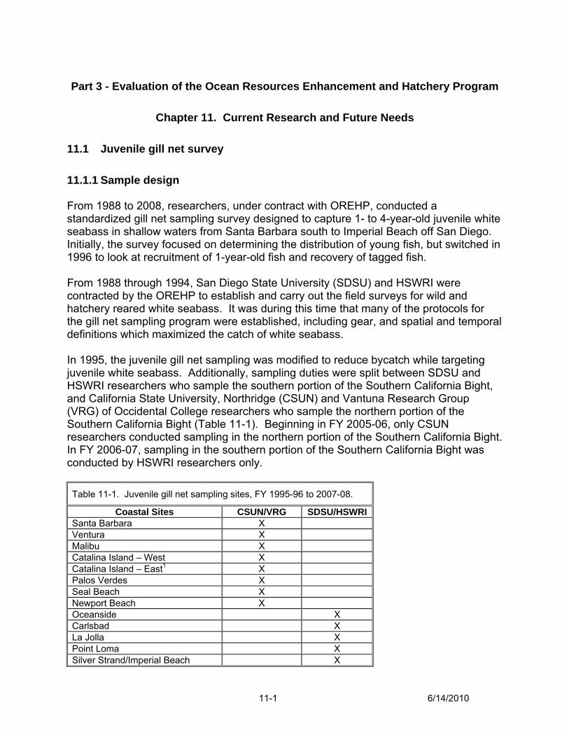
Part 3 - Evaluation of the Ocean Resources Enhancement and Hatchery Program
Chapter 11. Current Research and Future Needs
11.1 Juvenile gill net survey 11.1.1 Sample design From 1988 to 2008, researchers, under contract with OREHP, conducted a standardized gill net sampling survey designed to capture 1- to 4-year-old juvenile white seabass in shallow waters from Santa Barbara south to Imperial Beach off San Diego. Initially, the survey focused on determining the distribution of young fish, but switched in 1996 to look at recruitment of 1-year-old fish and recovery of tagged fish. From 1988 through 1994, San Diego State University (SDSU) and HSWRI were contracted by the OREHP to establish and carry out the field surveys for wild and hatchery reared white seabass. It was during this time that many of the protocols for the gill net sampling program were established, including gear, and spatial and temporal definitions which maximized the catch of white seabass. In 1995, the juvenile gill net sampling was modified to reduce bycatch while targeting juvenile white seabass. Additionally, sampling duties were split between SDSU and HSWRI researchers who sample the southern portion of the Southern California Bight, and California State University, Northridge (CSUN) and Vantuna Research Group (VRG) of Occidental College researchers who sample the northern portion of the Southern California Bight (Table 11-1). Beginning in FY 2005-06, only CSUN researchers conducted sampling in the northern portion of the Southern California Bight. In FY 2006-07, sampling in the southern portion of the Southern California Bight was conducted by HSWRI researchers only. Table 11-1. Juvenile gill net sampling sites, FY 1995-96 to 2007-08.
Coastal Sites CSUN/VRG SDSU/HSWRI Santa Barbara X Ventura X Malibu X Catalina Island – West X Catalina Island – East1 X Palos Verdes X Seal Beach X Newport Beach X Oceanside X Carlsbad X La Jolla X Point Loma X Silver Strand/Imperial Beach X
11-1 6/14/2010
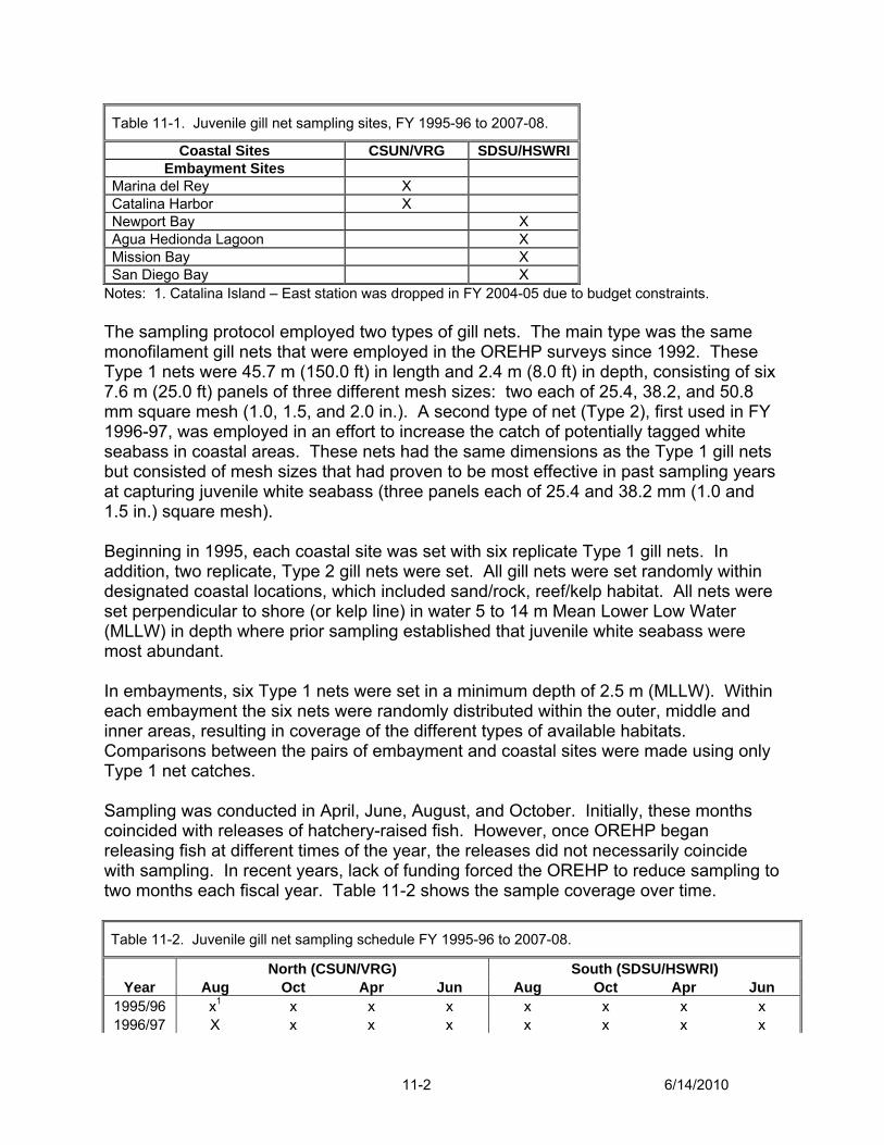
Table 11-1. Juvenile gill net sampling sites, FY 1995-96 to 2007-08.
Coastal Sites CSUN/VRG SDSU/HSWRI Embayment Sites
Marina del Rey X Catalina Harbor X Newport Bay X Agua Hedionda Lagoon X Mission Bay X San Diego Bay X
Notes: 1. Catalina Island – East station was dropped in FY 2004-05 due to budget constraints. The sampling protocol employed two types of gill nets. The main type was the same monofilament gill nets that were employed in the OREHP surveys since 1992. These Type 1 nets were 45.7 m (150.0 ft) in length and 2.4 m (8.0 ft) in depth, consisting of six 7.6 m (25.0 ft) panels of three different mesh sizes: two each of 25.4, 38.2, and 50.8 mm square mesh (1.0, 1.5, and 2.0 in.). A second type of net (Type 2), first used in FY 1996-97, was employed in an effort to increase the catch of potentially tagged white seabass in coastal areas. These nets had the same dimensions as the Type 1 gill nets but consisted of mesh sizes that had proven to be most effective in past sampling years at capturing juvenile white seabass (three panels each of 25.4 and 38.2 mm (1.0 and 1.5 in.) square mesh). Beginning in 1995, each coastal site was set with six replicate Type 1 gill nets. In addition, two replicate, Type 2 gill nets were set. All gill nets were set randomly within designated coastal locations, which included sand/rock, reef/kelp habitat. All nets were set perpendicular to shore (or kelp line) in water 5 to 14 m Mean Lower Low Water (MLLW) in depth where prior sampling established that juvenile white seabass were most abundant. In embayments, six Type 1 nets were set in a minimum depth of 2.5 m (MLLW). Within each embayment the six nets were randomly distributed within the outer, middle and inner areas, resulting in coverage of the different types of available habitats. Comparisons between the pairs of embayment and coastal sites were made using only Type 1 net catches. Sampling was conducted in April, June, August, and October. Initially, these months coincided with releases of hatchery-raised fish. However, once OREHP began releasing fish at different times of the year, the releases did not necessarily coincide with sampling. In recent years, lack of funding forced the OREHP to reduce sampling to two months each fiscal year. Table 11-2 shows the sample coverage over time. Table 11-2. Juvenile gill net sampling schedule FY 1995-96 to 2007-08.
North (CSUN/VRG) South (SDSU/HSWRI) Year Aug Oct Apr Jun Aug Oct Apr Jun
1995/96 x1 x x x x x x x 1996/97 X x x x x x x x
11-2 6/14/2010
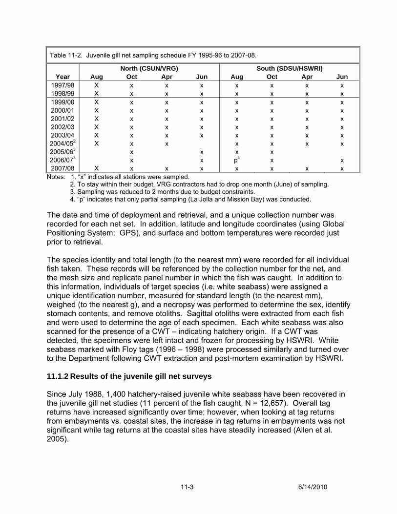
Table 11-2. Juvenile gill net sampling schedule FY 1995-96 to 2007-08.
North (CSUN/VRG) South (SDSU/HSWRI) Year Aug Oct Apr Jun Aug Oct Apr Jun
1997/98 X x x x x x x x 1998/99 X x x x x x x x 1999/00 X x x x x x x x 2000/01 X x x x x x x x 2001/02 X x x x x x x x 2002/03 X x x x x x x x 2003/04 X x x x x x x x 2004/052 X x x x x x x 2005/063 x x x x 2006/073 x x p4 x x 2007/08 X x x x x x x x
Notes: 1. “x” indicates all stations were sampled. 2. To stay within their budget, VRG contractors had to drop one month (June) of sampling. 3. Sampling was reduced to 2 months due to budget constraints. 4. “p” indicates that only partial sampling (La Jolla and Mission Bay) was conducted.
The date and time of deployment and retrieval, and a unique collection number was recorded for each net set. In addition, latitude and longitude coordinates (using Global Positioning System: GPS), and surface and bottom temperatures were recorded just prior to retrieval. The species identity and total length (to the nearest mm) were recorded for all individual fish taken. These records will be referenced by the collection number for the net, and the mesh size and replicate panel number in which the fish was caught. In addition to this information, individuals of target species (i.e. white seabass) were assigned a unique identification number, measured for standard length (to the nearest mm), weighed (to the nearest g), and a necropsy was performed to determine the sex, identify stomach contents, and remove otoliths. Sagittal otoliths were extracted from each fish and were used to determine the age of each specimen. Each white seabass was also scanned for the presence of a CWT – indicating hatchery origin. If a CWT was detected, the specimens were left intact and frozen for processing by HSWRI. White seabass marked with Floy tags (1996 – 1998) were processed similarly and turned over to the Department following CWT extraction and post-mortem examination by HSWRI. 11.1.2 Results of the juvenile gill net surveys Since July 1988, 1,400 hatchery-raised juvenile white seabass have been recovered in the juvenile gill net studies (11 percent of the fish caught, N = 12,657). Overall tag returns have increased significantly over time; however, when looking at tag returns from embayments vs. coastal sites, the increase in tag returns in embayments was not significant while tag returns at the coastal sites have steadily increased (Allen et al. 2005).
11-3 6/14/2010
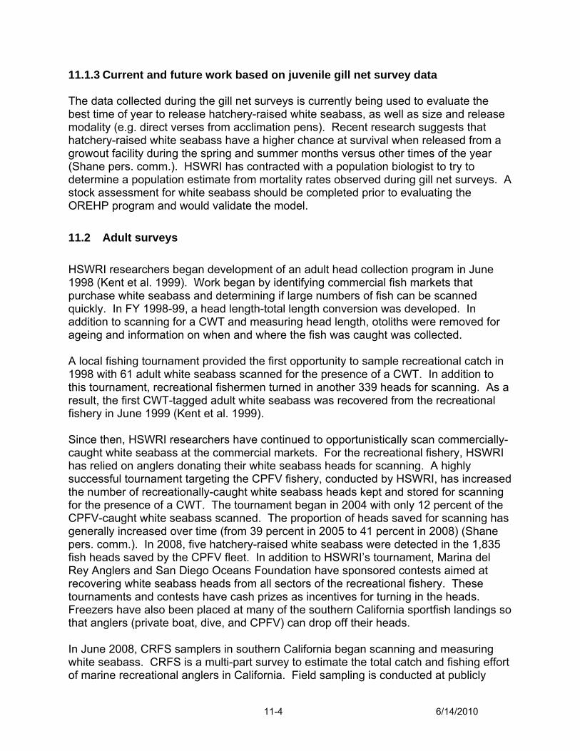
11.1.3 Current and future work based on juvenile gill net survey data The data collected during the gill net surveys is currently being used to evaluate the best time of year to release hatchery-raised white seabass, as well as size and release modality (e.g. direct verses from acclimation pens). Recent research suggests that hatchery-raised white seabass have a higher chance at survival when released from a growout facility during the spring and summer months versus other times of the year (Shane pers. comm.). HSWRI has contracted with a population biologist to try to determine a population estimate from mortality rates observed during gill net surveys. A stock assessment for white seabass should be completed prior to evaluating the OREHP program and would validate the model. 11.2 Adult surveys HSWRI researchers began development of an adult head collection program in June 1998 (Kent et al. 1999). Work began by identifying commercial fish markets that purchase white seabass and determining if large numbers of fish can be scanned quickly. In FY 1998-99, a head length-total length conversion was developed. In addition to scanning for a CWT and measuring head length, otoliths were removed for ageing and information on when and where the fish was caught was collected. A local fishing tournament provided the first opportunity to sample recreational catch in 1998 with 61 adult white seabass scanned for the presence of a CWT. In addition to this tournament, recreational fishermen turned in another 339 heads for scanning. As a result, the first CWT-tagged adult white seabass was recovered from the recreational fishery in June 1999 (Kent et al. 1999). Since then, HSWRI researchers have continued to opportunistically scan commercially-caught white seabass at the commercial markets. For the recreational fishery, HSWRI has relied on anglers donating their white seabass heads for scanning. A highly successful tournament targeting the CPFV fishery, conducted by HSWRI, has increased the number of recreationally-caught white seabass heads kept and stored for scanning for the presence of a CWT. The tournament began in 2004 with only 12 percent of the CPFV-caught white seabass scanned. The proportion of heads saved for scanning has generally increased over time (from 39 percent in 2005 to 41 percent in 2008) (Shane pers. comm.). In 2008, five hatchery-raised white seabass were detected in the 1,835 fish heads saved by the CPFV fleet. In addition to HSWRI’s tournament, Marina del Rey Anglers and San Diego Oceans Foundation have sponsored contests aimed at recovering white seabass heads from all sectors of the recreational fishery. These tournaments and contests have cash prizes as incentives for turning in the heads. Freezers have also been placed at many of the southern California sportfish landings so that anglers (private boat, dive, and CPFV) can drop off their heads. In June 2008, CRFS samplers in southern California began scanning and measuring white seabass. CRFS is a multi-part survey to estimate the total catch and fishing effort of marine recreational anglers in California. Field sampling is conducted at publicly
11-4 6/14/2010
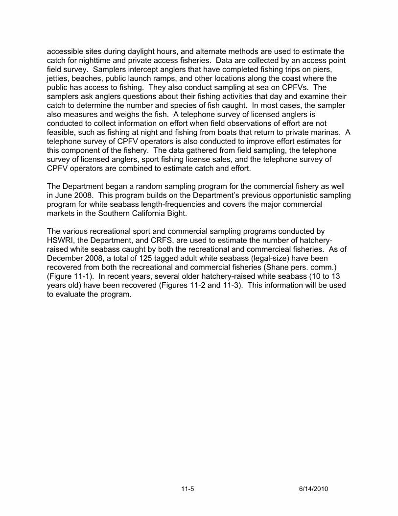
accessible sites during daylight hours, and alternate methods are used to estimate the catch for nighttime and private access fisheries. Data are collected by an access point field survey. Samplers intercept anglers that have completed fishing trips on piers, jetties, beaches, public launch ramps, and other locations along the coast where the public has access to fishing. They also conduct sampling at sea on CPFVs. The samplers ask anglers questions about their fishing activities that day and examine their catch to determine the number and species of fish caught. In most cases, the sampler also measures and weighs the fish. A telephone survey of licensed anglers is conducted to collect information on effort when field observations of effort are not feasible, such as fishing at night and fishing from boats that return to private marinas. A telephone survey of CPFV operators is also conducted to improve effort estimates for this component of the fishery. The data gathered from field sampling, the telephone survey of licensed anglers, sport fishing license sales, and the telephone survey of CPFV operators are combined to estimate catch and effort. The Department began a random sampling program for the commercial fishery as well in June 2008. This program builds on the Department’s previous opportunistic sampling program for white seabass length-frequencies and covers the major commercial markets in the Southern California Bight. The various recreational sport and commercial sampling programs conducted by HSWRI, the Department, and CRFS, are used to estimate the number of hatchery-raised white seabass caught by both the recreational and commercieal fisheries. As of December 2008, a total of 125 tagged adult white seabass (legal-size) have been recovered from both the recreational and commercial fisheries (Shane pers. comm.) (Figure 11-1). In recent years, several older hatchery-raised white seabass (10 to 13 years old) have been recovered (Figures 11-2 and 11-3). This information will be used to evaluate the program.
11-5 6/14/2010
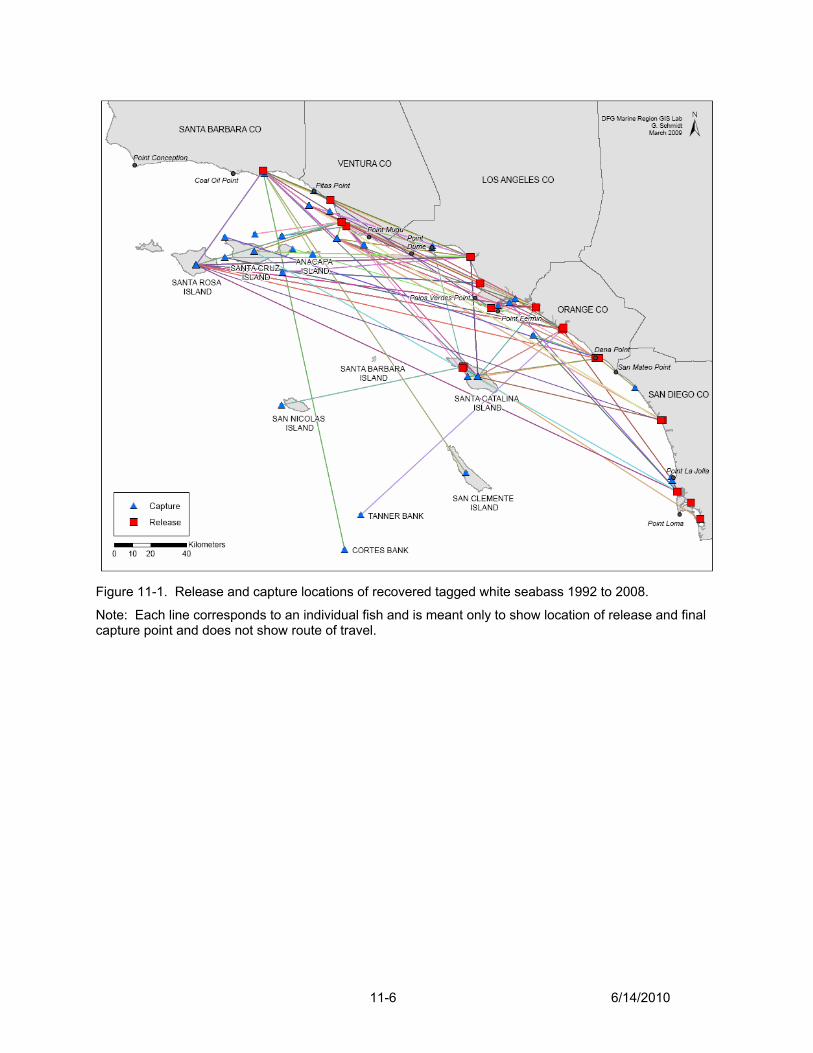
Figure 11-1. Release and capture locations of recovered tagged white seabass 1992 to 2008.
Note: Each line corresponds to an individual fish and is meant only to show location of release and final capture point and does not show route of travel.
11-6 6/14/2010
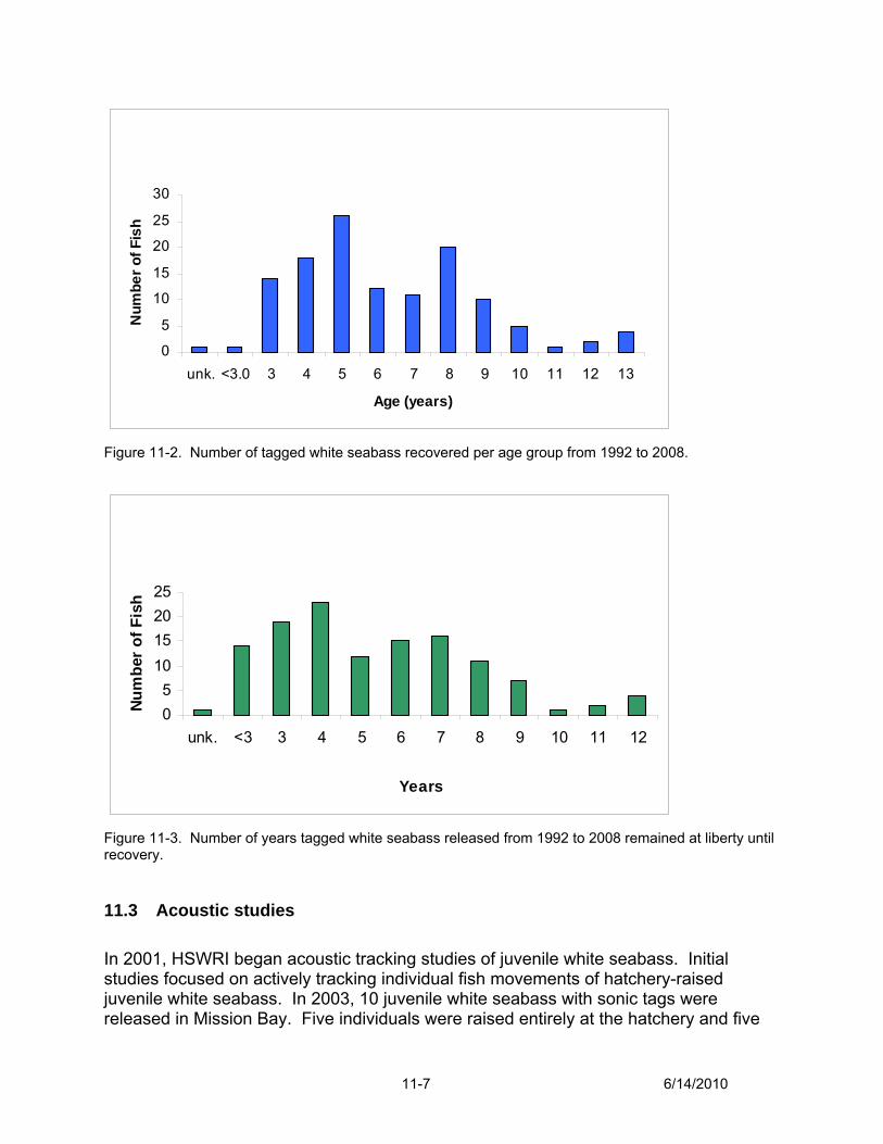
0
5
10
15
20
25
30
unk. <3.0 3 4 5 6 7 8 9 10 11 12 13
Age (years)
Num
ber o
f Fis
h
Figure 11-2. Number of tagged white seabass recovered per age group from 1992 to 2008.
05
10152025
unk. <3 3 4 5 6 7 8 9 10 11 12
Years
Num
ber o
f Fis
h
Figure 11-3. Number of years tagged white seabass released from 1992 to 2008 remained at liberty until recovery.
11.3 Acoustic studies In 2001, HSWRI began acoustic tracking studies of juvenile white seabass. Initial studies focused on actively tracking individual fish movements of hatchery-raised juvenile white seabass. In 2003, 10 juvenile white seabass with sonic tags were released in Mission Bay. Five individuals were raised entirely at the hatchery and five
11-7 6/14/2010

spent several months at a growout facility in Mission Bay. Prior to releasing the fish, 12 hydrophones were submerged in strategic positions in Mission Bay as well as along the adjacent coastal waters. Results of this study revealed that individuals from both groups emigrated from the bay within a few days. Individuals that did not emigrate had low survivorship, as evidenced by the fact that tags were recovered in the bay for all but one individual that did not leave the bay (Drawbridge et al. 2004). In June 2004, 19 juvenile cultured white seabass were implanted with acoustic transmitters and released from a growout facility in Mission Bay along with 4,059 other cultured white seabass. Eight fish emigrated from the bay; seven did so within three days post release. There were five presumed mortalities (based on tag recoveries), likely due to predation. Researchers were unable to determine the disposition of the six remaining fish (Drawbridge et al. 2005). In November 2004, 25 acoustically tagged juvenile white seabass were released from the Agua Hedionda Lagoon growout facility as part of a release of almost 10,000 white seabass. Underwater hydrophones were deployed in the lagoon and along the coastline adjacent to the lagoon entrance. By day five, 14 individuals had emigrated from the lagoon. Upon leaving the lagoon, the hydrophones detected an even dispersion of fish moving to the north and to the south. There were four mortalities due to predation during the first five days based on tag recoveries. Another four fish were likely entrained in the cooling water intake for the power plant in the lagoon based on their last location in the lagoon (near the intake) before the tags went silent. The fate of the three remaining fish is unknown (Drawbridge et al. 2005). The results of the 2004 studies in Mission Bay and Agua Hedionda Lagoon reveal that almost half (48 percent) of the juvenile white seabass emigrated from the embayment within a week of their release, and they all left at night on an ebbing tide (Drawbridge et al. 2006) (Figure 11-4). Fish that did not emigrate from the embayment were likely preyed upon by octopods, birds, or marine mammals. Further acoustical studies have been placed on hold while HSWRI researchers determine whether marine mammals, particularly harbor seals, can hear the pinging of the transmitters. If marine mammals can hear the transmitters, this may bias the observed mortality patterns of the tagged fish and limit this approach as an assessment tool.
11-8 6/14/2010
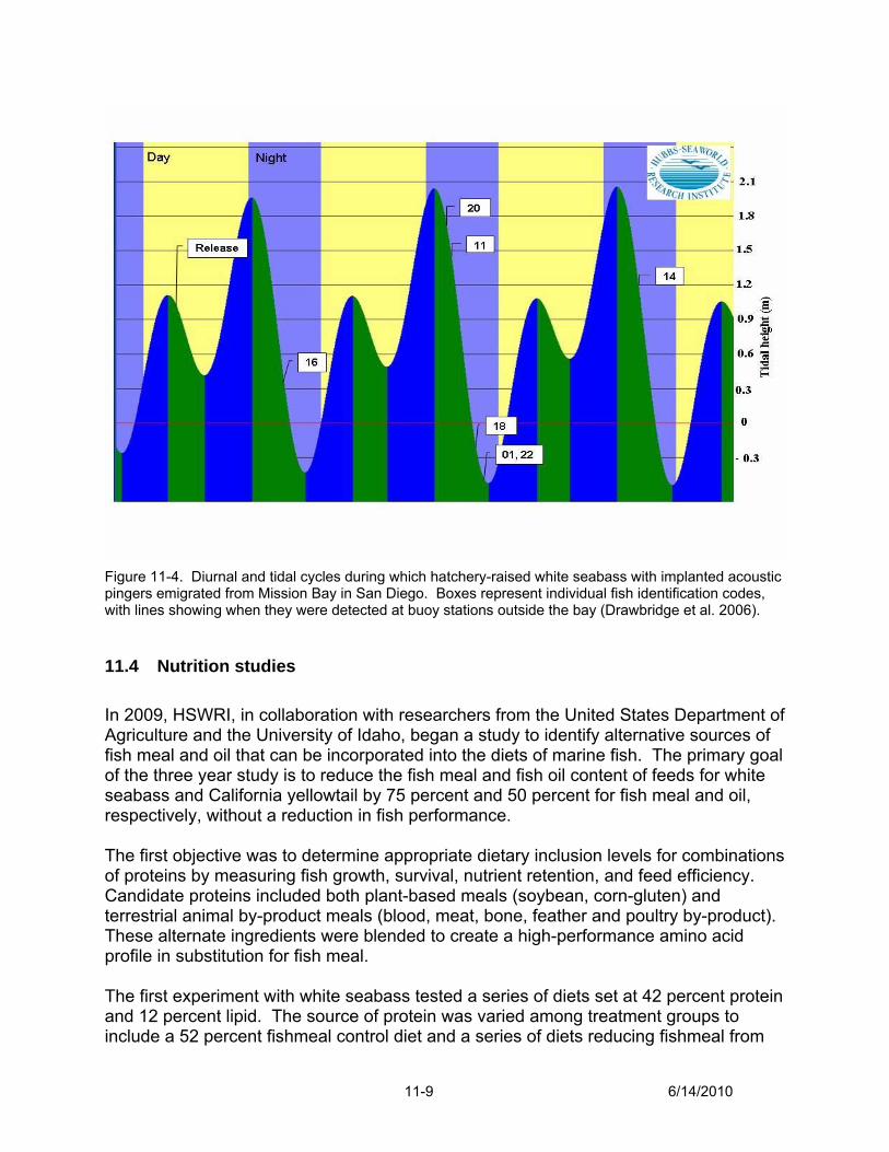
Figure 11-4. Diurnal and tidal cycles during which hatchery-raised white seabass with implanted acoustic pingers emigrated from Mission Bay in San Diego. Boxes represent individual fish identification codes, with lines showing when they were detected at buoy stations outside the bay (Drawbridge et al. 2006).
11.4 Nutrition studies In 2009, HSWRI, in collaboration with researchers from the United States Department of Agriculture and the University of Idaho, began a study to identify alternative sources of fish meal and oil that can be incorporated into the diets of marine fish. The primary goal of the three year study is to reduce the fish meal and fish oil content of feeds for white seabass and California yellowtail by 75 percent and 50 percent for fish meal and oil, respectively, without a reduction in fish performance. The first objective was to determine appropriate dietary inclusion levels for combinations of proteins by measuring fish growth, survival, nutrient retention, and feed efficiency. Candidate proteins included both plant-based meals (soybean, corn-gluten) and terrestrial animal by-product meals (blood, meat, bone, feather and poultry by-product). These alternate ingredients were blended to create a high-performance amino acid profile in substitution for fish meal. The first experiment with white seabass tested a series of diets set at 42 percent protein and 12 percent lipid. The source of protein was varied among treatment groups to include a 52 percent fishmeal control diet and a series of diets reducing fishmeal from
11-9 6/14/2010
20 down to 0 percent of the diet. Results from the first trial showed that one of the protein blends coupled with only 10 percent fish meal outperformed all other diets including the 52 percent fish meal control diet. This high performing treatment yielded an average survival >90 percent, weight gain of > 500 percent, and food conversion rate of <1.0. Recently, two additional trials were completed with white seabass testing a series of 0 percent fish meal diets made with a high quality chicken by-product protein, and corn protein concentrate with Spirulina and liver meal as palatability enhancers. White seabass did very well on these diets, outperforming fish that were fed both a fish meal and a commercial control diet. The diet with Spirulina seemed to be accepted by the fish more quickly at the beginning of the trial than the other diets, suggesting that Spirulina may be a palatability enhancer.
11-10 6/14/2010
Chapter 12. Program Evaluation
Stock enhancement programs are increasing worldwide; however, many early programs lacked this final, critical element – program evaluation. Blankenship and Leber (1995) cite the lack of evaluation as a major obstacle of early stock enhancement efforts. The lack of effective fish-tagging systems and the inability to culture marine fishes past the early life stages contributed to the inability to evaluate stock enhancement efforts. The OREHP has overcome these and other hurdles making program evaluation possible. 12.1 Scientific Advisory Committee To assist the Department in evaluating the OREHP, the Department will establish a Scientific Advisory Committee (SAC) made up of experts in Croaker (white seabass) biology, population dynamics, genetics, environmental quality, economics, and fish pathology. The SAC will develop science-based criteria, based on the goals and objectives of the OREHP, to help evaluate the success of the program. In addition the SAC will review proposed research aimed at evaluating the OREHP, review the Adaptive Management Plan (AMP) (Section 12.2), assist in the Program evaluation and recommend changes. SAC members would be appointed by the Director to advise the Department in the areas of future research, methodology for program evaluation, genetics, benthic monitoring, and changes to current practices outlined in this Plan, the CHP, and GPM. The Department would consider the SAC’s recommendations for changes to current Program practices and future research. The SAC will include:
• One member with demonstrated expertise in the area of fish genetics; • One member with demonstrated expertise in fish pathology; • One member with extensive experience in marine aquaculture; • One member with demonstrated expertise in population biology or dynamics; • One member with demonstrated expertise in the area of benthic and/or water
quality; • One member with demonstrated expertise in the area of Croaker (white seabass)
research; • One member from the California Coastal Commission; • One member of the OREAP, nominated by the OREAP who has expertise or
significant knowledge of or experience with habitats of white seabass, genetics, aquaculture, fisheries management, water quality, or research; and
• One member from the Department.
12.2 Adaptive Management Plan
12-1 6/14/2010
An Adaptive Management Plan (AMP) provides a mechanism to continuously evaluate the OREHP. The AMP, which includes monitoring and experimentation to address critical questions, is the process by which information on key uncertainties will be generated, analyzed, disseminated, and incorporated into project decision-making. The result will ultimately be a better informed and improved white seabass replenishment project. The AMP should specifically:
• Identify performance standards and measures for achieving the OREHP’s goals and objectives based on the best existing baseline/reference conditions;
• Identify monitoring activities to track stock replenishment progress and targeted research (applied studies) to test hypotheses related to adaptive management decisions;
• Include applied studies that can be initiated in the planning phase, which will be during the next CDP cycle;
• Identify specific adaptive management questions and related monitoring/experiments;
• Include processes for identifying applied studies for later phases; and,
• Define a process for synthesizing data from adaptive management studies and incorporating that information into decision-making to improve current phases and design future phases.
The four critical issues surrounding the OREHP that must be included in the AMP are: 1) maximizing the contribution of potential of stocked fish through optimized culture and release strategies, 2) maintaining genetic diversity, 3) managing disease, and 4) minimizing impacts to the environment from the hatchery and growout facilities. The WSEP lays out interim steps to ensure that the OREHP has every opportunity of successfully demonstrating the potential for using stock replenishment as a management tool, while avoiding negative impacts to the environment. Additional research is needed to determine if these interim steps are appropriate and necessary and can be incorporated into the AMP, or if they need to be changed to better protect the population and/or the environment. For example, under the benthic monitoring program, growout facilities have to maintain sulfide levels less than 1000 µM in the sediments around the facility. Should a growout facility exceed the benchmark during the triennial survey, then it must lie fallow until testing shows that the sediment is below the benchmark. Under adaptive management, the benchmark could change (higher or lower), there could be different benchmarks for already impacted areas (marinas, harbors) and more pristine areas (open coast, Catalina harbor), or the periodicity of the survey could change.
12-2 6/14/2010
The OREHP is currently operating under a self-imposed release cap at Catalina Island (30,000 fish/year). The cap was put in place because of concerns that too many fish released at Catalina Island may result in negative effects caused by inter and/or intraspecific competition. Data from the juvenile gill net studies indicate that fish released at Catalina Island stay at Catalina and do not disperse as quickly as they do along the mainland coast. It has been hypothesized that the narrowness of the shelf around the island results in limited juvenile white seabass habitat causing the fish to remain close to shore. It would be beneficial to conduct a study of the dispersion rate at Catalina Island to determine if the cap should remain, and if so at what level. This information could then be included in the AMP. The Department intends to develop the AMP within the next five years to be approved by the SAC. The AMP would then be incorporated into the WSEP. Additionally, the Department may need to adopt regulations to implement the AMP. 12.3 Evaluation of the OREHP The evaluation of marine stock enhancement programs has varied widely. In Texas, evaluation of the red drum enhancement program was conducted by comparing gill net and sport-boat fisherman catches in stocked and unstocked bays. Results of this evaluation showed that the number of fish harvested in bays that have been stocked almost doubled over historic mean harvest rates in those systems (McEachron et al. 1993). In Japan, commercial landings were surveyed to evaluate the effectiveness of the flounder stock enhancement program. The results showed that over a 3-year period the recovery rate was 0.15, and the total income and the benefit estimate was $260,000 and $63,000 U.S., respectively (Kitada et al. 1992). The OREHP has three key elements that will make evaluation of its program easier than other programs. First, since 1990, all white seabass have been tagged with CWTs so that they are identifiable. Second, white seabass husbandry issues have been resolved, and the hatchery is able to consistently raise fish to release size, allowing for larger scale releases. Since 2001, the OREHP has successfully released more than 100,000 fish each year (Figure 12-1). Given that it takes four years for white seabass to reach legal size (710 mm; 28 in.), fish released in 2001 should have entered the fishery in 2005. Third, HSWRI has been collecting data on juvenile and adult recoveries for over 10 years, and the Department implemented its own adult recovery program for the recreational and commercial fisheries in 2008 (Sections 11.1 and 11.2).
12-3 6/14/2010
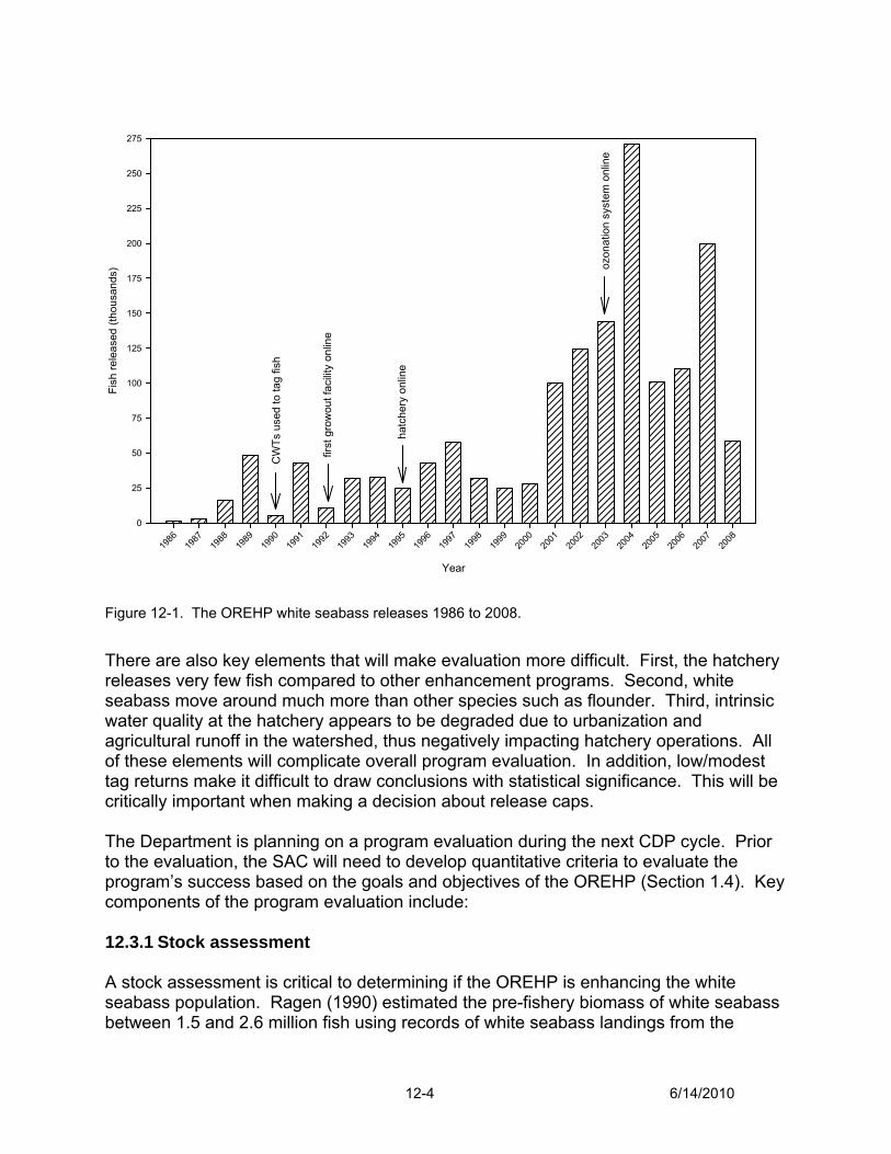
Year
1986
1987
1988
1989
1990
1991
1992
1993
1994
1995
1996
1997
1998
1999
2000
2001
2002
2003
2004
2005
2006
2007
2008
Fish
rele
ased
(tho
usan
ds)
0
25
50
75
100
125
150
175
200
225
250
275
first
gro
wou
t fac
ility
onlin
e
hatc
hery
onl
ine
ozon
atio
n sy
stem
onl
ine
CW
Ts u
sed
to ta
g fis
h
Figure 12-1. The OREHP white seabass releases 1986 to 2008.
There are also key elements that will make evaluation more difficult. First, the hatchery releases very few fish compared to other enhancement programs. Second, white seabass move around much more than other species such as flounder. Third, intrinsic water quality at the hatchery appears to be degraded due to urbanization and agricultural runoff in the watershed, thus negatively impacting hatchery operations. All of these elements will complicate overall program evaluation. In addition, low/modest tag returns make it difficult to draw conclusions with statistical significance. This will be critically important when making a decision about release caps. The Department is planning on a program evaluation during the next CDP cycle. Prior to the evaluation, the SAC will need to develop quantitative criteria to evaluate the program’s success based on the goals and objectives of the OREHP (Section 1.4). Key components of the program evaluation include: 12.3.1 Stock assessment A stock assessment is critical to determining if the OREHP is enhancing the white seabass population. Ragen (1990) estimated the pre-fishery biomass of white seabass between 1.5 and 2.6 million fish using records of white seabass landings from the
12-4 6/14/2010

Avalon Tuna Club. At the time of publication, there has been no stock assessment of white seabass in California. Any such stock assessment should include recreational and commercial fisheries landings, life history information, mortality rates, age and growth data, including recent work done by HSWRI, data from the juvenile and adult studies, information on changes in relative abundance over time, and other sources of data. Data gaps should be identified and prioritized, and efforts should be made to fill those gaps. 12.3.2 Adult sampling programs Both the Department and HSWRI are sampling the commercial and recreational fisheries for hatchery-raised white seabass (Section 11.2). This data is also critical because it will help determine the ratio of hatchery-raised to wild fish. For the recreational fishery, HSWRI uses fish count information to determine how many white seabass were caught, what proportion of the catch were scanned, and how many were hatchery-raised fish. The Department will use expansion calculations that are part of the CRFS program to obtain the same data. For the commercial fishery, HSWRI can determine the proportion of fish scanned that were hatchery-raised, but cannot easily determine how many fish were landed because the information collected from fish processors is in pounds rather than number of fish. The Department’s program will attempt to determine how many white seabass were caught in the commercial fishery, what proportion of the catch were scanned, and how many were hatchery-raised fish. The end result of these analyses should be a recovery rate for each fishery. 12.3.3 Bioeconomic model Some enhancement program evaluations look at the economics of the enhancement program, such as Japan’s flounder enhancement program (Kitada et al. 1992). A bioeconomic model was developed in the early stages of the OREHP (Botsford et al. 1988); however, it needs to be updated to reflect current information. If the model cannot be updated, a new bioeconomic model needs to be developed. Inputs to the bioeconomic model include the costs associated with raising white seabass to release size, fishing levels to determine commercial and recreational proportions, life history parameters, and the recovery rate for each fishery (from the adult sampling programs). Outputs from the program may include the costs per fish, value to each fishery, and/or a cost to benefit ratio and can be used to evaluate the efficacy of the program. 12.3.4 Genetics research and benthic monitoring Genetic risk is another factor that should be reviewed during the program evaluation. Tringali and Bert (1998) examined the genetic risks associated with stock enhancement of two species and found that the genetic risks varied greatly due to differences in biology. Application of the Ryman-Laikre model (1991) can be used to evaluate the genetic effects of enhancement plans. Additional genetic research is being conducted by HSWRI, and the results should be available for the program evaluation. If changes to current hatchery protocols are needed to ensure that there are no negative effects on
12-5 6/14/2010
genetic diversity, based on the review of genetic risks to the wild population, then they should be evaluated by the SAC as well and included in the CHP. Studies have shown that salmon farming pens can affect the benthos, resulting in changes to the macrobenthic community as well as the chemical composition of the sediments (Brooks 2000a, d, c, b, Nash 2001, Brooks and Mahnken 2003a, b, Brooks et al. 2003). The OREHP began sampling the benthos surrounding the growout facilities in 2004 and will continue those efforts according to the BMPs listed in this document. The OREHP’s evaluation should include a review of the benthic monitoring program to determine if the growout facilities are having a negative effect on the benthos. 12.3.5 Other data sources The OREHP contractors and other researchers have conducted studies on different aspects of white seabass biology. The results of these studies can be used during the program evaluation. For example, HSWRI has collected data relative to the release and recapture of hatchery-raised white seabass. Analysis of this data can be used to determine the optimum size at release, optimum release time and release location to minimize mortality and maximize the fishes’ chance of surviving to recruit to the fishery. Ageing studies have been conducted by HSWRI, the Department, and others and could be used as inputs into the stock assessment and bioeconomic model. 12.4 White Seabass Enhancement Plan review The SAC could be used to conduct a review of the WSEP, at least every five years, to determine the effectiveness of the OREHP and suggest changes if needed, particularly to the BMPs and the AMP. 12.5 Plan amendment The WSEP is designed to be flexible and adaptable to a wide range of future conditions and intended to function without the need for frequent amendment. Minor changes to the BMPs can simply be made by revising the other guidance documents for the OREHP, mainly the CHP and GPM. However, future research, environmental, biological, or economic changes may create a need to revise the WSEP to ensure that the enhancement of white seabass is conducted in a responsible manner. Examples of actions that might require a WSEP amendment include:
• Changes to the goals and objectives of the OREHP; and • Changes to the AMP.
The Commission will be asked to approve an amended Plan.
12-6 6/14/2010
References
Aalbers, S. A. 2008. Seasonal, diel, and lunar spawning periodicities, and associated
sound production of white seabass (Atractoscion nobilis). Fish. Bull. 106:143-151.
Aalbers, S. A., and M. A. Drawbridge. 2008. White Seabass Spawning Behavior and Sound Production. Transactions of the Amercian Fishery Society 137:542-550.
AFIP. 2004. Armed Forces Institute of Pathology. Available from: http://www.afip.org.
Agency, U. S. E. P. 2008.
Allen, L. G., and M. P. Franklin. 1992. Abundance, distribution, and settlement of young-of-the-year white seabass, Atractoscion nobilis, in the Southern California Bight, 1988-89. Fish. Bull. 90:633-641.
Allen, L. G., D. J. Pondella II, R. Ford, and M. Shane. 2003. Nearshore gill net sampling program for white seabass (age I-IV). Field sampling annual report for FY 2001-2002. Page 22 [Progress report to CDFG and OREAP], Located at: California Department of Fish and Game, Los Alamitos, CA.
Allen, L. G., D. J. Pondella II, R. Ford, and M. Shane. 2005. Nearshore gill net sampling program for white seabass (age I-IV). Field sampling report for FY 2004-2005. Page 25 [Progress report to CDFG and OREAP]. Located at: California Department of Fish and Game, Los Alamitos, CA.
Allendorf, F. W., and N. Ryman. 1987. Genetic management of hatchery stocks. Population Genetics and Fishery Management:141–159.
Bartley, D., M. Bagley, G. Gall, and B. Bentley. 1992. Use of Linkage Disequilibrium Data to Estimate Effective Size of Hatchery and Natural Fish Populations. Conservation Biology 6:365-375.
Bartley, D. M., and D. B. Kent. 1990. Genetic structure of white seabass populations from the southern California Bight region: Applications to hatchery enhancement. Calif. Coop. Oceanic Fish. Invest. Rep. 31:97-105.
Bartley, D. M., D. B. Kent, and M. A. Drawbridge. 1995. Conservation of genetic diversity in a white seabass hatchery enhancement program in southern California. Pages 248-258 in H. L. Schramm and R. G. Piper, editors. Uses and Effects of Cultured Fishes in Aquatic Ecosystems. American Fisheries Society Symposium 15, Albuquerque, NM.
R-1 6/14/2010
Beveridge, M. C. M., M. J. Phillips, and R. M. Clarke. 1991. A quantitative and qualitative assessment of wastes from aquatic animal production. Aquaculture and Water Quality. Advances in World Aquaculture 3:506-533.
Blankenship, H. L., and K. M. Leber. 1995. A responsible approach to marine stock enhancement. Pages 167-175 in H. L. Schramm and R. G. Piper, editors. Uses and Effects of Cultured Fishes in Aquatic Ecosystems. American Fisheries Society Symposium 15, Albuquerque, NM.
Botsford, L. W., R. C. Hobbs, and R. G. Kope. 1988. Bioeconomic evaluation of the culture/stocking concept for white seabass and California halibut: Models and computer programs. Page 81 [Final Report to CDFG and OREAP], Located at: California Department of Fish and Game, Los Alamitos, CA.
Brooks, K. M. 2000a. Determination of copper loss rates from Flexgard XI™ treated nets in marine environments and evaluation of the resulting environmental risks. Page 30 Report to the Ministry of Environment for the British Columbia Salmon Farmers Association, Available at: http://www.ams.usda.gov/nosb/MeetingAgendas/Nov2007/OrganicAquacultureSymposium/11_07OrgAquaSymposiumPanelists.html.
Brooks, K. M. 2000b. Salmon farm benthic and shellfish effects study 1996–1997. Aquatic Environmental Sciences, Located at: Aquatic Environmental Services, 644 Old Eaglemount Road, Port Townsend, WA, 98368.
Brooks, K. M. 2000c. Sediment concentrations of sulfides and total volatile solids near salmon farms in British Columbia, Canada during the period June through August 2000, and recommendations for additional sampling. Report to the Ministry of Environment prepared for the BC Salmon Farmers Association.
Brooks, K. M. 2000d. Sediment concentrations of zinc near salmon farms in British Columbia, Canada during the period June through August 2000. BC Salmon Farmers Association 1200.
Brooks, K. M. 2001. An evaluation of the relationship between salmon farm biomass, organic inputs to sediments, physiochemical changes associated with those inputs and the infaunal response - with emphasis on total sediment sulfides, total volatile solids, and oxidation-reduction potential as surrogate endpoints for biological monitoring. Final Report,. Page 210 [Prepared for The Technical Advisory Group, British Columbia Ministry of Environment], Available from: http://www.salmonfarmers.org/attachments/focusedstudyfinalreport1.pdf.
Brooks, K. M. 2004. September 2004 sediment physicochemical monitoring at Hubbs-SeaWorld Research Institute’s enhancement netpens located at Santa Catalina Island, Agua Hedionda Lagoon and San Diego Bay. Page 29 [Technical report prepared for HSWRI, CDFG, and OREAP]. Located at: California Department of Fish and Game, Los Alamitos, CA.
R-2 6/14/2010
Brooks, K. M. 2006. Sediment physicochemical monitoring at delayed release netpens and raceways for white seabass located in Southern California during 2004 and 2005. Page 97 [Technical report prepared for HSWRI, CDFG and OREAP]. Located at: California Department of Fish and Game, Los Alamitos, CA.
Brooks, K. M. 2007. Sediment physiochemical monitoring at delayed release netpens and raceways for white seabass located in southern California during the period 2004 through 2006. Page 122 [Technical report prepared for HSWRI, CDFG, and OREAP]. Located at: California Department of fish and Game, Los Alamitos, CA.
Brooks, K. M., and M. A. Drawbridge. 2005. (Proposed) Benthic monitoring program for growout facilities associated with the Ocean Resources Enhancement and Hatchery Program (OREHP). Page 19 [Prepared for the California Department of Fish and Game], Located at: California Department of Fish and Game, Los Alamitos, CA.
Brooks, K. M., and C. V. W. Mahnken. 2003a. Interactions of Atlantic salmon in the Pacific northwest environment-II. Organic wastes. Fisheries Research 62:255-293.
Brooks, K. M., and C. V. W. Mahnken. 2003b. Interactions of Atlantic salmon in the Pacific Northwest Environment. III. Inorganic Compounds. Fisheries Research 62:295-305.
Brooks, K. M., C. V. W. Mahnken, and C. Nash. 2002. Environmental effects associated with marine netpen waste with emphasis on salmon farming in the Pacific Northwest. Pages 159-204 in R. R. Stickney and J. P. McVey, editors. Responsible Aquaculture. CABI Publishing, Wallingford, United Kingdom.
Brooks, K. M., A. R. Stierns, and C. Backman. 2004. Seven year remediation study at the Carrie Bay Atlantic salmon (Salmo salar) farm in the Broughton Archipelago, British Columbia, Canada. Aquaculture 239:81-123.
Brooks, K. M., A. R. Stierns, C. V. W. Mahnken, and D. B. Blackburn. 2003. Chemical and biological remediation of the benthos near Atlantic salmon farms. Aquaculture 219:355-377.
Brown, J. R., R. J. Gowen, and D. S. McLusky. 1987. The effect of salmon farming on the benthos of a Scottish sea loch. Journal of Experimental Marine Biology and Ecology 109:39-51.
Buhr, G., M. A. Drawbridge, and M. S. Okihiro. 2006. A community-based approach to replenishing depleted marine fisheries in southern California.in Presented at the annual meeting of the World Aquaculture Society, Las Vegas, NV.
CDFG. 2002. White Seabass Fishery Management Plan. Page 126 plus appendices.
R-3 6/14/2010
Chen, M. F., S. Yun, G. D. Marty, T. S. McDowell, M. L. House, J. A. Appersen, T. A. Guenther, K. D. Arkush, and R. P. Hedrick. 2000. A Piscirickettsia salmonis-like bacterium associated with mortality of white seabass (Atractoscion nobilis). Diseases of Aquatic Organisms 43:117-126.
Chow, K. W., and W. R. Schell. 1978. The minerals. Fish Feed Technology. A series of lectures presented at the FAO/UNDP training course in fish feed technology held at the College of Fisheries, University of Washington, Seattle, Washington 9.
Clark, F. N. 1930. Size at first maturity of the white seabass (Cynoscion nobilis). Calif. Fish Game 16:319-323.
Collins, R. A. 1981. Pacific coast croaker resources. Marine Recreational Fisheries--6 (Henry Clepper, ed.) Sport Fishing Institute, Washington, D.C.
Collyer, R. 1949. Marine sportfishing. In: The Commercial fish catch of California for the year 1947 with an historical review 1916-1947. Calif. Dept. Fish Game Fish Bull. 74:180-183.
Coykendall, D. K. 2005. Population structure and dynamics of white seabass (Atractoscion nobilis) and the genetic effect of hatchery supplementation on the wild population. dissertation. University of California, Davis, Davis.
Coykendall, D. K., and D. Hedgecock. 2006. Executive summary of genetic results from the white seabass hatchery supplementation program. Page 4 [Prepared for CDFG and OREAP]. Located at: California Department of Fish and Game, Los Alamitos, CA.
Curtis, P. 2005. pers. comm.
Dayton, P. K., and A. D. MacCall. 1992. Pre-exploitation abundances of important large recreational and commercial fishes off Southern California. University of California, San Diego.
Donohoe, C. J. 1990. The distribution, abundance, food habits, age and growth of late larval and juvenile white seabass (Atractoscion nobilis) off San Diego, County, California. MSc. San Diego State University, San Diego.
Drawbridge, M., G. Buhr, and M. Okihiro. 2007. Procedures manual for growout and release of white seabass (Atractoscion nobilis) as part of the Ocean Resources Enhancement and Hatchery Program (OREHP). Page 103, Located at: California Department of Fish and Game, Los Alamitos, CA.
Drawbridge, M. A. 2003. A history of broodstock management and egg production for white seabass (Atractoscion nobilis) in southern California.in American Fisheries Society, San Diego.
R-4 6/14/2010
Drawbridge, M. A., D. B. Kent, and R. F. ford. 2004. Experimental culture and evaluation of enhancing marine fishes in southern California. . [Progress report for the contract period July 1, 2003 to June 30, 2004]. Located at: California Department of Fish and Game, Los Alamitos, CA.
Drawbridge, M. A., D. B. Kent, and R. F. Ford. 2005. Experimental culture and evaluation of enhancing marine fishes in southern California. . Page 78 [Progress report for the contract period July 1, 2004 to June 30, 2005]. Located at: California Department of Fish and Game, Los Alamitos, CA.
Drawbridge, M. A., D. B. Kent, and R. F. Ford. 2006. Experimental culture and evaluation of enhancing marine fishes in southern California. [Progress report for the contract period July 1, 2005 to June 30, 2006]. Located at: California Department of Fish and Game, Los Alamitos, CA.
Drawbridge, M. A., and M. Okihiro. 2007. Comprehensive hatchery plan for operation of the Leon Raymond Hubbard, Jr. marine fish hatchery in Carlsbad, California. Page 147, Located at: California Department of Fish and Game, Los Alamitos, CA.
Dutton, P. H. 1989. The feeding ecology and growth of white seabass larvae, Atractscion nobilis. MSc. San Diego State University, San Diego.
Eknath, A. E., M. M. Tayamen, M. S. Palada-De Vera, J. C. Danting, R. A. Reyes, E. E. Dionisio, J. B. Capili, H. L. Bolivar, T. A. Abella, and A. V. Circa. 1993. Genetic improvement of farmed tilapias: the growth performance of eight strains of Oreochromis niloticus tested in different farm environments. Aquaculture (Amsterdam) 111:171-188.
Eldridge, M. B. 1977. Factors influencing distribution of fish eggs and larvae over eight 24-hour samplings in Richardson Bay, California. Calif. Fish Game 63:101-116.
Findlay, R. H., and L. Watling. 1994. Toward a process level model to predict the effects of salmon net-pen aquaculture on the benthos. Can. Tech. Rep. Fish. Aquat. Sci.:47-77.
Fitch, J. E., and R. J. Lavenberg. 1971. Marine Food and Game Fishes of California. University of California Press, Berkeley.
Franklin, M. P. 1997. An investigation into the population structure of white seabass (Atractoscion nobilis), in California and Mexican waters using microsatellite DNA analysis. dissertation. University of California, Santa Barbara, Santa Barbara.
Fryer, J. L., and R. P. Hedrick. 2003. Piscirickettsia salmonis: a Gram-negative intracellular bacterial pathogen of fish. Journal of Fish Diseases 26:251-262.
Gowen, R. J., and N. B. Bradbury. 1987. The ecological impact of salmonid farming in coastal waters: a review. Oceanogr. Mar. Biol. Ann. Rev. 25:563-575.
R-5 6/14/2010

Hamm, J. T. 1997. Developmental Changes in the Toxicity and Bioactivation of Diazinon by Embryos of Medaka, Oryzias latipes. dissertation. University of California, Davis, Davis.
Hamm, J. T., and D. E. Hinton. 2000. The role of development and duration of exposure to the embryotoxicity of diazinon. Aquatic Toxicology 48:403-418.
Hamm, J. T., B. W. Wilson, and D. E. Hinton. 1998. Organophosphate-induced acetylcholinesterase inhibition and embryonic retinal cell necrosis in vivo in the teleost (Oryzias latipes). Neurotoxicology 19:853-869.
Hamm, J. T., B. W. Wilson, and D. E. Hinton. 2001. Increasing Uptake and Bioactivation with Development Positively Modulate Diazinon Toxicity in Early Life Stage Medaka (Oryzias latipes). Toxicological Sciences 61:304-313.
Hargrave, B. T., D. E. Duplisea, E. Pfieffer, and D. J. Wildish. 1993. Seasonal changes in benthic fluxes of dissolved oxygen and ammonium associated with marine cultured Atlantic salmon. Marine Ecology Progress Series 96:249-257.
Hargrave, B. T., G. A. Phillips, L. I. Doucette, M. J. White, T. G. Milligan, D. J. Wildish, and R. E. Cranston. 1995. Biogeochemical observations to assess benthic impacts of organic enrichment from marine aquaculture in the Western Isles region of the Bay of Fundy, 1994. Can. Tech. Rep. Fish. Aquat. Sci.
Heimann, R. F. G., and J. G. Carlisle Jr. 1970. The California Marine Fish Catch for 1968 and Historical Review 1916-1968. Calif. Dept. Fish Game Fish Bull. 149:70pp.
Holmer, M., and E. Kristensen. 1992. Impact of Marine Fish Cage Farming on Metabolism and Sulfate Reduction of Underlying Sediments. Marine Ecology Progress Series 80.
Johnsen, R. I., O. Grahl-Nielsen, and B. T. Lunestad. 1993. Environmental distribution of organic waste from a marine fish farm. Aquaculture 118:229-244.
Karakassis, I., E. Hatziyanni, M. Tsapakis, and W. Plaiti. 1999. Benthic recovery following cessation of fish farming: a series of successes and catastrophes. Marine Ecology Progress Series 184:205-218.
Karpov, K. A., D. P. Albin, W. H. Van Buskirk, and G. Dept. of Fish and. 1995. The Marine Recreational Fishery in Northern and Central California: A Historical Comparison (1958-86), Status of Stocks (1980-86), and Effects of Changes in the California Current. Calif. Dept. Fish Game Fish. Bul. 176:192pp.
Kent, D., and R. Ford. 1990. Determination of the natural mortality rate for juvenile white seabass (Atractoscion nobilis) and California halibut (Paralichthys californicus). . Page 18 [Progress report to CDFG and OREAP]. Located at: California Department of Fish and Game, Los Alamitos, CA.
R-6 6/14/2010
Kent, D. B., R. F. Ford, and M. A. Drawbridge. 1999. Experimental culture and evaluation of enhancing marine fishes in southern California. . Page 57 [Progress report for the contract period July 1, 1998 to June 30, 1999]. Located at: California Department of Fish and Game, Los Alamitos, CA.
Kim, B. G. 1987. Effects of stocking density and food concentration on survival and growth of larval white seabass. MSc. San Diego State University, San Diego.
Kitada, S., Y. Taga, and H. Kishino. 1992. Effectiveness of a stock enhancement program evaluated by a two-stage sampling survey of commercial landings. Can. J. Fish. Aquat. Sci. 49:1573-1582.
Lenntech. 2007. Lenntech water treatment and purification. Available from: http://www.lenntech.com.
Long, E. R., D. D. Macdonald, S. L. Smith, and F. D. Calder. 1995. Incidence of adverse biological effects within ranges of chemical concentrations in marine and estuarine sediments. Environmental Management 19:81-97.
López, L. M., A. L. Torres, E. Durazo, M. A. Drawbridge, and D. P. Bureau. 2006. Effects of lipid on growth and feed utilization of white seabass (Atractoscion nobilis) fingerlings. Aquaculture 253:557-563.
Lu, L., and R. S. Wu. 1998. Recolonization and succession of marine macrobenthos in organic-enriched sediment deposited from fish farms. Environ Pollut 101:241-251.
MacCall, A. D., G. D. Stauffer, and J. P. Troadec. 1976. Southern California recreational and commercial marine fisheries. Marine Fisheries Review 38:1-32.
MacDonald, D. D. 1994. Approach to the Assessment of Sediment Quality in Florida Coastal Waters. Volume 1. Development and evaluation of sediment quality assessment guidelines. Page 140 [Prepared for Florida Department of Environmental Protection, Tallahassee, Florida], Available at: http://www.dep.state.fl.us/waste/quick_topics/publications/pages/default.htm.
Maxwell, W. D. 1977. Progress report of research on white seabass, Cynoscion nobilis. Calif. Dept. Fish Game, Mar. Res. Admin. Rep. (77-14). CDFG.
McEachron, L. W., C. E. McCarty, and R. R. Vega. 1993. Successful enhancement of the Texas red drum population (Sciaenops ocellatus) population.in M. R. Collie and J. P. McVey, editors. Proceedings of the 22nd U.S.-Japan Meeting on Aquaculture, Homer, Alaska, August 21-22, 1993. . Fairbanks, Alaska : University of Alaska Sea Grant College Program, [1995?]. , .
Moser, H. G., D. A. Ambrose, M. S. Busby, J. L. Butler, E. M. Sandknop, B. Y. Sumida, and E. G. Stevens. 1983. Description of early stages of white seabass,
R-7 6/14/2010
Atractoscion nobilis, with notes on distribution Calif. Coop. Oceanic Fish. Invest. Rpt. 24:182-193.
Nash, C. E. e. 2001. The net-pen salmon farming industry in the Pacific Northwest. U.S. Dept. Commer., NOAA Tech. Memo. NMFS-NWFSC-49.
NOAA. 2008. Potential Deterrence Methods for Pacific Harbor Seals and California Sea Lions. Available from: http://swr.nmfs.noaa.gov/deter/Dets_Property.htm.
Noga, E. J. 2001. Fish Diseases: Diagnosis and Treatment. Iowa State University Press.
Radovich, J. 1961. Relationships of some marine organisms of the northeast Pacific to water temperatures, particularly during 1957 through 1959. Calif. Dept. Fish Game Fish Bull. 112:62pp.
Ragen, T. J. 1990. The estimation of theoretical population levels for natural populations. PhD. University of California, San Diego, San Diego.
Rodzen, J. pers. comm.
Rosenthal, H., D. Scarratt, and M. McInerney-Northcott. 1995. Aquaculture and the environment. Pages 451-500 in A. Boghen, editor. Cold-Water Aquaculture in Atlantic Canada. 2nd edition. The Canadian Institute for Research on Regional Development. Univercité de Moncton. Tribune Press: Sackville.
Ryman, N., and L. Laikre. 1991. Effects of supportive breeding on the genetically effective population size. Conserv. Biol. 5:325-329.
Shane, M. pers. comm.
Skogsberg, T. 1925. Preliminary investigation of the purse seine industry of southern California.
Skogsberg, T. 1939. The fishes of the family Sciaenidae (croakers) of California. Calif. Dept. Fish Game Fish Bull. 54:62pp.
Skretting. 2007. Available from: http://www.skretting.ca.
Smiley, J. E. 2004. Acute Effects of Gas Saturation on Cultured Juvenile White Seabass (Atractoscion Nobilis) in the Laboratory. MSc thesis. University of San Diego, San Diego.
Soulé, M., and J. Senner. [Date unknown]. Enzyme genetic markers in Baja California populations of the white seabass, Cynoscion nobilis. Page 7 [Final report to UCSD and CDFG for agreement F32R1-4], Located at: California Department of Fish and Game, Los Alamitos, CA.
R-8 6/14/2010
Thomas, J. C. 1968. Management of the white seabass (Cynoscion nobilis) in California waters. Calif. Dept. Fish Game Fish Bull. 142:34pp.
Tringali, M., and T. Bert. 1998. Risk to genetic effective population size should be an important consideration in fish stock enhancement programs. Bull. Mar. Sci. 62:641-659.
Valle, C. F., and S. P. Wertz. 2003. pers. comm.
Vojkovich, M., and R. Reed. 1983. White seabass, Atractoscion nobilis, in California-Mexican waters: status of the fishery. Calif. Coop. Oceanic Fish. Invest. Rep 24:79-83.
Weinstein, M. P. 1981. Biology of adult sciaenids. Marine Recreational Fisheries--6 (Henry Clepper, ed.) Sport Fishing Institute, Washington, D.C.:125-138.
Welsh, W. W., and C. M. Breder, Jr. 1923. Contributions to life histories of Sciaenidae of the eastern United States coast. Bulletin of the US Bureau of Fisheries 39:141-201.
Weston, D. P. 1986. The Environmental Effects of Floating Mariculture in Puget Sound. Page 154 [Prepared for Washington Department of Fisheries and Washington Department of Ecology], Available at: http://unicorn.csc.noaa.gov/docs/czic/SH35.W2%5FW437%5F1986/89FF32.pdf.
Wildish, D. J., H. M. Akagi, N. Hamilton, and B. T. Hargrave. 1999. A recommended method for monitoring sediments to detect organic enrichment from mariculture in the Bay of Fundy. Can. Tech. Rep. Fish. Aquat. Sci. 2286:34.
Wildish, D. J., J. E. Hughes-Clarke, G. W. Pohle, B. T. Hargrave, and L. M. Mayer. 2004. Acoustic detection of organic enrichment in sediments at a salmon farm is confirmed by independent groundtruthing methods. Marine Ecology Progress Series 267:99-105.
Winsby, M., B. Sander, D. Archibald, M. Daykin, P. Nix, F. J. R. Taylor, and D. Munday. 1996. The environmental effects of salmon netcage culture in British Columbia. Page 243 [Prepared for the Ministry of Environment, Lands and Parks Environmental Protection Department, Industrial Waste/Hazardous Contaminants Branch], Available at: http://www.llbc.leg.bc.ca/public/PubDocs/bcdocs/351890/salmon_netcage.pdf.
Ye, L. X., D. A. Ritz, G. E. Fenton, and M. E. Lewis. 1991. Tracing the influence on sediments of organic waste from a salmonid farm using stable isotope analysis. Journal of Experimental Marine Biology and Ecology 145:161-174.
Young, P. H. 1973. The status of the white seabass resource and its management. Marine Resources Technical Report 15, Calif. Dept. Fish Game, Mar. Res. Tech. Rep. 15.
R-9 6/14/2010

R-10 6/14/2010

Appendix A. Glossary of Terms and Abbreviations
A-1 6/14/2010
Appendix A. Glossary of Terms and Abbreviations Adaptive Management - In regard to a marine fishery, it means a scientific policy that seeks to improve management of biological resources, particularly in areas of scientific uncertainty, by viewing program actions as tools for learning. Actions shall be designed so that even if they fail, they will provide useful information for future actions. Monitoring and evaluation shall be emphasized so that the interaction of different elements within the system can be better understood. Bag limits - The total amount of fish that may be captured per person per day by law. Benthic - On or relating to the region at the bottom of a sea or ocean. Biological Oxygen Demand (BOD) - Chemical procedure for determining how fast biological organisms use up oxygen in a body of water. Biological remediation - The restructuring of the infaunal community to include those taxa whose individual abundance equaled or exceeded 1 percent of the total invertebrate abundance at local reference stations. Broodstock – A group of sexually mature individuals of a cultured species that is kept separate for breeding purposes. California Toxics Rule (CTR) - An Environmental Protection Agency rule that establishes numeric water quality criteria for priority toxic pollutants and other provisions for water quality standards that are to be applied to waters in the State of California. Central Nervous System (CNS) - Part of the nervous system that functions to coordinate the activity of all parts of the bodies of multicellular organisms. Chemical remediation - The reduction of accumulated organic matter with a concomitant decrease in free sediment sulfide (S=) concentrations and an increase in sediment redox potential under and adjacent to salmon farms to levels at which more than half the reference area taxa can recruit and survive. Coded Wire Tag (CWT) - A sequentially-numbered, small (1.1 mm long by 0.25 mm diameter), magnetized, stainless steel wire tag. Commercial fishing - The act of fishing with the intent of selling the catch. Commercial Passenger Fishing Vessel (CPFV) - A licensed fishing vessel that takes recreational anglers fishing in return for a fee. The vessel operator must follow certain requirements such as providing the Department with a log that, among other things, includes the number of anglers and an enumeration of the catch.
A-2 6/14/2010
Enzyme-linked Immunosorbent Assay (ELISA) - A biochemical technique used mainly in immunology to detect the presence of an antibody or an antigen in a sample. Essential Fish Habitat (EFH) - Those waters and substrate necessary to fish for spawning, breeding, feeding, or growth to maturity. Exclusive Economic Zone (EEZ) - A zone created by the Magnusen-Stevens Fishery Act, extending from 3 nautical miles to 200 miles offshore the United States and its territories, over which the United States has management jurisdiction of natural resources including fisheries, oil, and minerals. Fecundity - The potential reproductive capacity of an organism or population, measured by the number of eggs. Fluorescent Antibody Testing (FAT) - A laboratory test that uses antibodies tagged with fluorescent dye to detect the presence of microorganisms. Food Conversion Rate (FCR) – A measurement for determining appropriate feeding levels. FCR is calculated as the weight of food fed divided by the weight gain of fish for a specified time period. Gas Supersaturation (GSS) – A noninfectious disease, which can develop in cultured fish, that is associated by poor water quality and is caused by elevated total dissolved gas in the water. Genotype – Genetic makeup of an individual; determines the hereditary potentials and limitations of an individual. Gentoyping - The process of determining the genotype of an individual by the use of biological assays. Gill net - A single wall of webbing, bound at the top by a float line and at the bottom by a weighted line and used for entangling fish. Hook-and-line - Any fishing line with attached hooks (e.g., longline, troll and stick gear, among others). Landings - The number or poundage of fish unloaded at a dock by commercial fishermen or brought to shore by recreational fishermen for personal use. Landings are reported at the points where fish are brought to shore. Larval Mass Mortality Syndrome (LMMS) – A lethal syndrome, believed to be caused by exposure to organophosphate pesticides, which is characterized by the sudden loss of 80 to 100 percent of an incubator’s larval population or, in some cases, loss of an entire spawn.
A-3 6/14/2010
Letter of Permission (LOP) – Letter issued by the U.S. Army Corps of Engineers that authorizes projects that involve construction, excavation, or deposition of materials, or for any activities that affect the location and navigable capacity of waters of the United States. Magnuson-Stevens Fishery Conservation and Management Act (MSFCMA) - Created by Congress in 1976, a 200-mile federal fisheries zone and eight regional councils to oversee the U.S. fisheries, which operate under the authority of the U.S. Department of Commerce. Microsatellites - Loci (or regions within DNA sequences) where short sequences of DNA (nucleotides; adenine - A, thiamine - T, guanine - G, cytosine - C) are repeated one right after the other. MS-222 – White powder used for anesthesia, sedation, or euthanasia of fishes. Otolith - One of a number of tiny calcium-containing granules in the inner ear; provides sensory information on the position and movement of the head in space. Patterns of otolith growth provide information on fish age. Organophosphate Pesticides (OPP) - Neurotoxins that are designed to kill insects via chemical inhibition of acetylcholinesterase, an important neurotransmitter in both invertebrates and vertebrates. Optimum Sustainable Population (OSP) –The number of animals which will result in the maximum productivity of the population or the species, keeping in mind the carrying capacity of the habitat and the health of the ecosystem of which they form a constituent element. Passive Integrated Transponder (PIT) - A type of tag applied to or incorporated into an animal for the purpose of identification and tracking using radio waves. Pathogen - An agent that causes disease. Polymerase Chain Reaction (PCR) – A technique used to amplify specific regions of a DNA strand. Potential Biological Removals (PBR) - The maximum number of animals, not including natural mortalities that may be removed from a marine mammal stock while allowing that stock to reach or maintain its OSP. Size limit - The minimum size a fish or other organism must be for it to be possessed. Stock - A species, subspecies, geographical grouping, or other category of fish capable of management as a unit.
A-4 6/14/2010

Stock Structure - Any description of the population attributes of a stock (age, size, sex), usually within a spatial context. This commonly refers to the spatial distribution of breeding groups or genetically-related organisms. Total Dissolved Gas (TDG) - A measure of the sum total of all gas partial pressures (including water vapor) in water. Total Gas Pressure (TGP) - The sum of the partial pressures of each individual gas in the mixture. Partial pressure is defined as the pressure which the gas would have if it alone occupied the volume. Total Organic Carbon (TOC) - The amount of carbon bound in an organic compound and is often used as a non-specific indicator of water quality. Total Volatile Solids (TVS) – The percent difference between the dried and combusted weights of sediment samples collected from the growout facility parameter. Transmission Electron Microscopy (TEM) - A microscopy technique whereby a beam of electrons is transmitted through an ultra thin specimen, interacting with the specimen as it passes through. An image is formed from the interaction of the electrons transmitted through the specimen; the image is magnified and focused onto an imaging device, such as a fluorescent screen, on a layer of photographic film, or to be detected by a sensor such as a CCD camera. Trawl – A large bag net that is tapered and forms a flattened cone. The mouth of the net is kept open while it is towed or dragged over the sea bottom. Viral Hemorrhagic Septicemia (VHS) - A deadly infectious fish disease caused by the viral hemorrhagic septicemia virus. Viral Nervous Necrosis (VNN) – See Viral Nervous Necrosis Virus Viral Nervous Necrosis Virus (VNNV) – A single-stranded RNA virus, which predominately affects the central nervous system of larval and juvenile fish and causes Viral Nervous Necrosis (VNN).
A-5 6/14/2010
Appendix B. Review of Coykendall’s Dissertation
A-6 6/14/2010
Review of Chapters Three and Four from Coykendall
Prepared by:
Kristen Gruenthal Mark Drawbridge
Hubbs-SeaWorld Research Institute
2595 Ingraham Street San Diego, CA 92109
May 5, 2008
A-7 6/14/2010
INTRODUCTION At the request of the California Department of Fish and Game (DFG), and the California Coastal Commission (CCC), we reviewed the PhD dissertation completed in 2005 by D.K. Coykendall under the advisorship of Dr. Dennis Hedgecock formerly at the University of California, Davis and currently at the University of Southern California. The dissertation is entitled “Population structure and dynamics of white seabass (Atractoscion nobilis) and the genetic effect of hatchery supplementation on the wild population.” Because of the importance of genetics to the quality assurance components of the Ocean Resources Enhancement and Hatchery Program (OREHP), new genetic information is vitally important. This is especially true today, when the OREHP is immersed in a CEQA review and simultaneously developing an enhancement plan as mandated by new state law (SB 201). In this regard, the Coykendall work is being viewed as an important document for the OREHP because of the scope of what is covered and the fact that it is contemporary. This document has been previously reviewed separately by two biologists from the DFG (see J. Rodzen 2006 and M. Lacy 2006). The difference between their review and the review presented here is that HSWRI has working knowledge of the genetic sampling program, including its history. Furthermore, HSWRI is intimately familiar with general spawning patterns and partitioning of cohorts into release batches. Here we review Chapters Three and Four from Coykendall. Our original plan was to solely critique conclusions put forth in Chapter Four, which focuses on the potential impacts to the wild WSB population via the Ryman-Laikre model (Ryman and Laikre 1991). In reviewing Chapter Four, however, Chapter Three, which estimates the breeding effective size of the broodstock population per spawn event and per total annual release, came under scrutiny since the results are carried over into Chapter Four. It may be necessary in the future to evaluate Chapters One and Two of Coykendall, as well, but we feel the original purpose of the review – to evaluate our WSB breeding practices in the context of their effect(s) on the wild population and to justify maintaining an annual release target of 350,000 juvenile WSB – has been fulfilled by our critique of Chapters Three and Four alone.
A-8 6/14/2010

CHAPTER THREE Background A primary goal of the hatchery is to maximize the genetic diversity of the juvenile white seabass (WSB) released into the wild in order to minimize the potential negative genetic impact (e.g. reduction in diversity) on the mixed (wild + captive-bred) population. One way to evaluate genetic diversity in a population is to estimate the genetically effective population size (Ne). Ne is a theoretical concept defined as the size of an ideal population (non-overlapping generations, random mating, equal sex ratios, and Poisson distribution of reproductive variance; Wright 1931) having the same amount of random genetic drift as real population (Hartl and Clark 1997). The concept is applicable to both captive-breeding programs, where we are interested in estimating and maximizing the effective number of breeders (Nb) from the parental (broodstock) generation contributing to the hatchery-bred progeny, and wild populations. Discussion Coykendall estimated Ne in the hatchery population three ways by evaluating 254 broodstock and their purported offspring at two levels (spawn events and release batches1):
1. the variance and inbreeding effective sizes (NeV and NeI, respectively) were
calculated for each of ten different spawning events (50-100 offspring per five events from 1998 and 1999 and 85-100 offspring per five events from 2001), 2 and
2. the effective number of breeders (Nb) was calculated for the entire 2001 release (250 offspring proportionally divided among 32 of 46 total release batches). 3
The genetic markers used to establish parentage and perform subsequent analyses of the effective sizes were a subset of seven of the microsatellite loci described in Franklin (1997). Experiment 1: Demographic estimation of Nb per spawning event The purpose of this experiment was to determine the variance (NeV) and inbreeding (NeI) effective sizes for each spawn event. NeV assesses the rate of change in allele frequencies over time due to genetic drift and NeI assesses the rate of increase in inbreeding. The samples included yolksac larvae from four spawn events from 1998 and one from 1999 and fin clips from five release groups from CY2001 supplied by
1 Coykendall refers to release cohorts or batches as “spawning groups”, which is confusing relative to single spawning “events.” “Release batch” is the preferred terminology. 2 It should be noted that the 1998-99 samples were yolksac larvae, while the 2001 samples were fin clips from juvenile fish. The implications of this may require further evaluation. 3 By our accounting (of the text in Coykendall page 53) the number should actually be 36 of 46 total release batches.
A-9 6/14/2010
HSWRI. All samples were originally collected by HSWRI and submitted to Genetic Identification Services (GIS). We are concerned about several aspects of this experiment. First, all parental assignments appear to have been made using the same set of 254 brood fish. The genotypes of the 254 samples were provided by GIS along with the genotypes for yolksac larvae from 1998 and 1999 spawn events. It is unclear how the 254 brood fish relate chronologically to the offspring being analyzed. For example, in 2001 there were only 178 brood fish in all four breeding pools combined. At no single point in time (or year-long period) were there 254 fish spawning in hatchery pools; the broodstock management plan calls for 200 fish total (50 fish per each of four breeding tanks). In addition, the five 2001 release batches that Coykendall sampled were from only two of four breeding tanks (B3 and B4; see Tables 3.1 and 3.2 from Coykendall), meaning that ~100 brood fish, not 254, are actually representative of the 2001 spawn events chosen. This type of error is carried over into the results reported on page 55 when male proportional contributions 0.03 to 0.46 are calculated from numerators of 1 to 16 (males contributors per spawn event). In fact, if a maximum of 25 males exist in any one breeding pool, then the proportional range should be 0.04 to 0.64. It is not clear, but it appears likely, that Coykendall used all males existing in the tanks over a three year time frame and not a more appropriate instantaneous per spawning event approach. The female contributory analysis is similarly flawed. Second, to calculate NeV and NeI per spawn event, the samples should have been collected from single spawn events (e.g. the yolk sac larvae from GIS). However, at least one (2001rel34) of the “spawn events” chosen by Coykendall was actually a release batch comprised of two separate spawn events (see Tables 3.1 and 3.2 from Coykendall). Only juvenile fin clips were used for tissue samples at the time of release because spawn groups were mixed early in the culture process. To choose these release batches comprised of multiple spawn events and label them as individual spawn events introduces a fundamental error, which may be due Coykendall’s own confusion over the nomenclature issue regarding spawn events, groups, and/or batches mentioned previously. Additionally, to further emphasize the impact of this apparent confusion, on page 57 Coykendall states that “only two males contributed to more than one spawn in 2001. BS228M provided the majority of spawning in all three 2001 spawning events and had a total contribution of 52% (Table 3.3c). If the effective number of breeders is calculated as a combination of the spawns within the same breeding tank, then Nbv of Breeding Tank 1 would be 6.0, Nbv of Breeding Tank 3 would be 9.3, and Nbv of Breeding Tank 4 would be 3.8, which are all above the average Nbv’s from their respective tanks (Table 3.1).” When she says “spawning events” she really means release batches. Of the three release batches (her “spawning events”) from pool B4 in 2001 that she is describing (#16=JUL1401B4; #7=AUG2900B4; and #31=AUG2900B4), two are the same spawn AUG2900B4! This would clearly have a significant effect on all of her calculations. As another example, on page 60 of the discussion she writes “If repeat spawning was not a factor, we could calculate Neh of the 2001 release by summing the
A-10 6/14/2010

number of all of the spawning groups scaled by the number of spawning events composing each of them, then multiply that by the mean of the spawning events (or as many as have been estimated). In 2001 release, there were 29 spawning groups consisting of one spawning event, ten consisting of two events, six consisting of three and 60 one consisting of four (Table 3.2). The harmonic mean of the five demographic Neh estimates from the 2001 spawning events is 3.09, so (29x1)+ (10x2)+ (6x3)+ (1x4) =71 x 3.09=220. Therefore, repeat spawning lowered the potential 2001 Neh from 220 to 35, a reduction of 84%.” This analysis is flawed by the fact that all the spawning events are not different (i.e. some of the same spawns are mixed among release batches). In other words, there were not 71 separate spawn events. Third, Coykendall does not explicitly discuss how she chose the specific spawn events or release batches used in her analyses. Each spawn event is a “snapshot in time,” and the Nb per spawn event may change significantly over the course of a single spawning season in a single breeding tank. For example, using relative egg output as an indicator of contributing females per spawn, it is apparent that few brood fish usually contribute to the beginning and end of a season, but the number of contributors tends to rise toward the middle of a season when water temperatures are warmer. One or two spawning events occurring during one or two nights in a 4-5 month spawning season are unlikely to be a good general proxy for all spawn events within a breeding tank. Moreover, Coykendall extrapolates in a very confusing manner the contribution results for individual brood fish in those very few spawn events to an entire year’s worth of production. On page 56 Coykendall states, “Over all three spawning events from Breeding Tank 1, BS135F contributed 66% and BS147F contributed 33% to the reproduction over the entire year.” This sentence is contradictory and confusing relative to the inferred extrapolation. On one hand, the text says “over all three spawning events,” but “over the entire year” is used in the same sentence. Each group of broodstock spawns between 60-90 times per year during a given 4-5 month season. Three spawns represents at most 5% of the spawning events, hardly a large enough proportion to extrapolate over the entire year. On page 57, a similar extrapolation is made where it is said, “Only two males contributed to more than one spawn in 2001.” This conclusion is irresponsible as stated (and likely very erroneous) given the very small group of samples Coykendall analyzed (i.e. five batches from only two of four spawning groups). The sentence should read, “Only two males contributed to more than one of the five spawn events sampled in 2001.” Finally, in the discussion on page 60, Coykendall attributes an 84% reduction in the potential Nb as being due to repeat spawning. This conclusion is extrapolated as an effect for the entire year even though it is based on only five of 36 sampled release batches.
Experiment 2: Allele rarefaction estimation of Nb for the 2001 release A set of 250 fin clips was chosen proportionately from an available 3,456 – 96 fin clips were taken from each of 36 release batches for 2001 – and used in allele rarefaction analyses to estimate Nb for the entire 2001 release of 101,318 fish. An additional 10 release batches for a total of 46 release batches in 2001 were not sampled by HSWRI.
A-11 6/14/2010
To illustrate choosing samples proportionately from the release batches: if release batch 40 contributed 7% of the total 2001 release, then 18 (or 7%) of the 250 samples were chosen from release batch 40. Unlike the previous experiment, the individuals in this experiment were genotyped by Coykendall, not GIS.
First, the sample set chosen may not be representative of the actual 2001 release. Ruzzante et al. (1998) determined that sample sizes of ~50 are required to accurately estimate the allele frequency profile of a population independent of the census size when using microsatellites, and this paper is widely cited regarding proper sample choice in molecular population genetic studies that use microsatellites. Samples were chosen by Coykendall from all 36 available release batches, and Coykendall likely equated the entire 2001 release to a population, in which case genotyping 250 individuals should be sufficient. The point was to estimate allelic richness in the entire 2001 release, but we must consider that a population is defined as a group of individuals within a species that can reproduce with one another and exist in the same place at the same time. With that in mind, the 2001 release is actually the product of four separate populations represented by each of the breeding tanks [aside: failing to partition the broodstock and offspring into “family” groups may have contributed to parental assignment problems in the above experiment]. Coykendall could have genotyped as few as 200 individuals, with release batches pooled according to source tank (release batches from multiple source tanks excluded) and 50 samples chosen randomly from each. Coykendall’s work focused on the release batch level, but it is questionable whether choosing samples proportionally was legitimate. In attempting to elucidate her actual sampling scheme, it appears that she may have used approximately 40-50 individuals per breeding tank, which is good, although it was probably not by intent. However, several of the release batches were comprised of spawning events from more than one tank, so it is unknown how the samples were partitioned among those events. The proportionality requirement also implies that the 17 of 36 release batches (47%) that contained <2000 fish, representing <2% of the 2001 release total of 101,318 fish, would have been represented by <5 individuals. Moreover, up to 14% (5 of 36) of release batches may have been represented in analyses by only one individual. Even though 250 total individuals were genotyped, it seems the allelic richness of the smaller release batches may be significantly under-represented, and it would not be surprising if the total allele count of 65 reported by Coykendall for the 2001 release is somewhat low. It may have been more powerful to genotype an equal number of individuals from each of the 36 release batches than to rely on such small samples sizes for nearly 50% of the release batches. Second, the larger problem may be that the difference in allelic richness of 14 between the broodstock and 2001 total release may, at best, be high or completely wrong if the incorrect broodstock were included. We are again faced with the fact that all analyses appear to have been made assuming 254 brood fish, which may be only partially applicable to the spawn events as discussed for the demographic experiment. The total 2001 release was comprised of spawn events from broodstock in all four breeding
A-12 6/14/2010
tanks, but there are never more than 50 brood fish per tank and, in fact, there were only 178 brood fish at HSWRI during 2001. Third, Coykendall then used a numerical fitting procedure in order to estimate Nb for the entire 2001 release. The method apparently takes into account the sample sizes and allele frequency profiles of the parental and offspring groups and the differences between them. It does not require establishing parentage; all the broodstock and their potential offspring can be used in the analysis. Basically, it can be assumed that the more alleles each group contains and/or the smaller the difference between the two groups, the higher the relative genetic diversity and the higher the relative Nb. Coykendall estimated Nb to be 34.59, but because of the issues we pointed out above regarding sample choice, this number may misrepresent the diversity in and contributing to the 2001 release.
It follows that there are errors in both the numerator and denominator of the Nb to census size (N) ratio, calculated by Coykendall to be 0.14 (or 34.59/254 as stated on page 57). Obviously, Coykendall again uses the 254 brood fish. If Nb = 34.59 is an underestimate and N = 254 is overestimated, then the Nb/N ratio is biased low. Conclusions In essence, this chapter is confusing and often times misleading. Typographical errors made discerning what was actually done difficult (e.g. on page 53, “32” should be “36”; on page 55, spawn event “37” should be “31”; and in Table 3.1, the numbers 1 and 2 are transposed for #males and #females for 2001rel31, when based on data from Table 3.3c). Salient information (e.g. how and why particular samples were chosen for the demographic experiment) was left out of the text, and poor wording and division of subsections made it difficult to discern that there were actually two experiments being performed on two different sets of offspring samples. The most significant problem we found was Coykendall’s apparent confusion in the makeup of a release batch, which she referred to confusingly/erroneously as “spawn groups”. There were also apparent failings in appropriate sample choice that carried over into subsequent analyses. Also problematic was the tendency of Coykendall to extrapolate the results from her limited samples to the production over the course of an entire year. Overall, the results in this chapter have the potential to significantly underestimate the actual genetic diversity of the WSB produced at the Carlsbad hatchery. We also found it curious in this chapter (and the dissertation in general), that Coykendall does not cite the work of Bartley et al. (1995), who developed the broodstock management plan currently being implemented. Clarification from the author on the questions raised in this review is needed before utilizing the results of this chapter in any meaningful capacity.
A-13 6/14/2010
CHAPTER FOUR Background An important goal for WSB enhancement has been to determine the optimal per year hatchery release of juvenile WSB. A useful method to estimate this number is again based on the concept of Ne. The impetus here is to avoid or minimize the Ryman-Laikre effect, or the potential negative impact of a drop in Ne experienced by a mixed population due to hatchery supplementation of the wild population (Ryman and Laikre 1991; Ryman et al. 1995; see also Figure 1 below). A higher proportion of offspring from hatchery broodstock survive earlier life stages than do offspring from wild individuals (although, some of the skew in the variance may be mitigated by higher relative mortality in hatchery-bred juveniles after release into the wild). Stocking of hatchery-bred progeny can cause a reduction in genetic diversity as a result of these large differences in reproductive success, especially if the hatchery broodstock are a small fraction of the wild population. The ultimate concern is that less genetic diversity due to long-term stocking may result in a mixed population that is less responsive to stochastic environmental change. Discussion In order to estimate optimal release and control to our best ability the Ryman-Laikre effect, we must estimate four parameters:
1) initial wild effective size (Ne0); 2) hatchery effective size (Nb); 3) the threshold, or baseline, mixed effective size (Nt); and 4) the current percent hatchery contribution to the natural population (x).
Using a subset of six of the microsatellite loci described in Franklin (1997), Coykendall genotyped 297 wild WSB collected by HSWRI. In this chapter, potential error due to sampling scheme effects (e.g. sample size) was taken into account through corrections in the estimation of F-statistics, which are used in the subsequent estimation of Ne0. Coykendall then estimated Ne0 to be ~6000 (95% confidence intervals (CI) depended on the mode of estimation). An Nb = 34.6 was calculated in Chapter Three for the 2001 release (this Nb estimate is questionable as discussed in the review above, but we will use it here as we have no other estimate available). Coykendall then applied the Ryman-Laikre model to evaluate the effect of the WSB enhancement program on the effective size of the mixed stock after supplementation (Ryman and Laikre 1991).
Coykendall determined that long-term hatchery supplementation may reduce Ne by 2-93%. However, this conclusion included a large range of possible Ne0 estimates, spanning 3,700 via moment-based and ~55,000 via pseudo-likelihood analyses between upper and lower 95% CI. The most dramatic reduction in Ne (89-93%) would result from the pressure of Nb ≤ 34.6 on an Ne0 = 57,310 (the upper 95% CI value from the pseudo-likelihood estimate). However, the pseudo-likelihood distribution of Ne0, if
A-14 6/14/2010

unimodal, must be highly skewed as the mean of 6,087 and lower 95% CI of 2384 are both an order of magnitude smaller. Additionally, the total range for the moment-based analysis of Ne0 was from 3,977 to 7,678. Although the moment-based approach may be less reflective of WSB life history, the distribution does not appear skewed and the estimates are all below 10,000, lending support to an Ne0 of substantially less than 57,310. We cannot propose a more realistic Ne0 without reanalyzing the data (which is unavailable), but we suggest that a negative genetic impact is likely to be much closer to 2% than 93%, especially in light of information discussed next on the preliminary mark-recapture data used by Coykendall.
Included in the above calculations, and more problematic to an accurate and realistic data interpretation, was Coykendall’s use of a 6.9% hatchery contribution (x) to the natural breeding stocks that came from mark-recapture data for juvenile fish (Figure 1). A hatchery contribution of 6.9% will decrease Net+1 (where Net+1 is the first generation following Ne0 for which hatchery-bred fish may have contributed to the gene pool) below Ne0 by some amount between the 2-93% mentioned above. However, this value of x is not reflective of individuals that actually have the potential to contribute to successive generations of the mixed stock and was rightly stated by Coykendall to be upwardly biased. Current mark-recapture data gathered by M. Shane of HSWRI puts x for reproductively-mature hatchery-bred WSB at <1%. According to Ryman-Laikre calculations, a 1% hatchery contribution to the mean pseudo-likelihood estimate of Ne0 = 6,087 with an Nb = 34.6 actually raises Net+1 to 6,101. In fact, for all Ne0 ≤ 6,910 with Nb ≥ 34.6, any hatchery contribution of ≤1% should raise Net+1 above Ne0. Regardless, because x is currently low (<1%), it is highly unlikely that hatchery supplementation to date has had a significant negative impact on genetic diversity of the wild population. It is unclear why Coykendall used 6.9% and not a more accurate number (~1%) that was also available from the OREHP data.
Conclusions The magnitude of the negative genetic impact stated in Chapter Four of Coykendall is likely to be an overestimation. In fact, the small hatchery contributions thus far may have had the potential to even increase diversity in the mixed population due to the fact that broodstock that may have otherwise not successfully reproduced in volume in the wild are given the chance in a hatchery setting.
In addition, the point of the Ryman-Laikre model is not necessarily to couch the results in a negative light as a purely detrimental reduction in genetic diversity as Coykendall has done. Reproduction in the wild without supplementation has the potential to naturally reduce (or increase) genetic diversity through random genetic drift, as well. Because the commonly assumed outcome is a reduction in diversity through supplementation, the objective should be to set a lower acceptable limit for Ne in the mixed population that will maintain a sufficient level of genetic diversity such that the population is still able to withstand stochastic environmental changes without significant risk of severe depletion or extinction. That number (Ne) has been empirically defined at
A-15 6/14/2010
≥500 (Tringali and Bert 1998; see also Figure 1), although its applicability to a species such as the WSB with Type III survivorship is yet to be determined. As concluded in the previous chapter, clarification from the author on the questions raised in this review is needed before utilizing the results of this chapter in any meaningful capacity.
A-16 6/14/2010
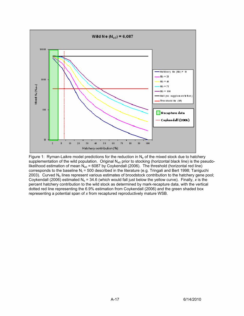
Figure 1: Ryman-Laikre model predictions for the reduction in Ne of the mixed stock due to hatchery supplementation of the wild population. Original Ne0 prior to stocking (horizontal black line) is the pseudo-likelihood estimation of mean Ne0 = 6087 by Coykendall (2006). The threshold (horizontal red line) corresponds to the baseline Nt = 500 described in the literature (e.g. Tringali and Bert 1998; Taniguchi 2003). Curved Nb lines represent various estimates of broodstock contribution to the hatchery gene pool; Coykendall (2006) estimated Nb = 34.6 (which would fall just below the yellow curve). Finally, x is the percent hatchery contribution to the wild stock as determined by mark-recapture data, with the vertical dotted red line representing the 6.9% estimation from Coykendall (2006) and the green shaded box representing a potential span of x from recaptured reproductively mature WSB.
A-17 6/14/2010
REFERENCES Coykendall DK (2005) Population structure and dynamics of white seabass
(Atractoscion nobilis) and the genetic effect of hatchery supplementation on the wild population. Doctoral dissertation, University of California, Davis
Franklin MP (1997) An investigation into the population structure of white seabass (Atractoscion nobilis) in California and Mexican waters using microsatellite DNA analysis. Doctoral dissertation, University of California, Santa Barbara
Hartl DL, Clark AG (1997) Principles of population genetics (3rd edition). Sinauer Associates, Inc., Sunderland
Ruzzante, D.E., 1998. A comparison of several measure of genetic distance and population structure with microsatellite data: bias and sampling variance. Canadian Journal of Fisheries and Aquatic Sciences, 55, 1-14
Ryman N, Laikre L (1991) Effects of supportive breeding on the genetically effective population size. Conservation Biology, 5, 325-329
Ryman N, Jorde PE, Laikre L (1995) Supportive breeding and variance effective population size. Conservation Biology, 9, 1619-1628
Taniguchi N (2003) Genetic factors in broodstock management for seed production. Reviews in Fish Biology and Fisheries, 13, 177-185
Tringali MD, Bert TM (1998) Risk to genetic effective population size should be an important consideration in fish stock-enhancement programs. Bulletin of Marine Science, 62, 641-659
Wright S (1931) Evolution in mendelian populations. Genetics, 16, 114-138
A-18 6/14/2010

Appendix I List of Preparers
List of Preparers Drawbridge, Mark. Senior Research Scientist. HSWRI. San Diego, CA Im, Angie. Scientific Aide. CDFG. Los Alamitos, CA Johnson, Kathryn. Marine Biologist. CDFG. Los Alamitos, CA. Larinto, Traci. Senior Biologist Specialist. CDFG. Los Alamitos, CA. Mello, John. Senior Biologist Supervisor. CDFG. Eureka, CA. Napoli, Tom. Staff Environmental Scientist. CDFG. Los Alamitos, CA Ramey, Kirsten. Associate Marine Biologist. CDFG. Eureka, CA. Taylor, Valerie. Associate Marine Biologist. CDFG. Los Alamitos, CA.

Appendix J Required Review of Hazardous Waste Sites by Public Resources Code §21084
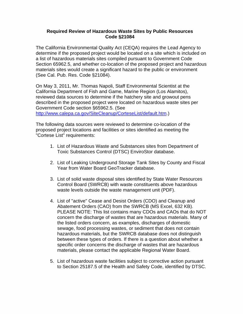
Required Review of Hazardous Waste Sites by Public Resources Code §21084
The California Environmental Quality Act (CEQA) requires the Lead Agency to determine if the proposed project would be located on a site which is included on a list of hazardous materials sites compiled pursuant to Government Code Section 65962.5, and whether co-location of the proposed project and hazardous materials sites would create a significant hazard to the public or environment (See Cal. Pub. Res. Code §21084). On May 3, 2011, Mr. Thomas Napoli, Staff Environmental Scientist at the California Department of Fish and Game, Marine Region (Los Alamitos), reviewed data sources to determine if the hatchery site and growout pens described in the proposed project were located on hazardous waste sites per Government Code section §65962.5. (See http://www.calepa.ca.gov/SiteCleanup/CorteseList/default.htm.) The following data sources were reviewed to determine co-location of the proposed project locations and facilities or sites identified as meeting the "Cortese List" requirements:
1. List of Hazardous Waste and Substances sites from Department of Toxic Substances Control (DTSC) EnviroStor database.
2. List of Leaking Underground Storage Tank Sites by County and Fiscal
Year from Water Board GeoTracker database. 3. List of solid waste disposal sites identified by State Water Resources
Control Board (SWRCB) with waste constituents above hazardous waste levels outside the waste management unit (PDF).
4. List of "active" Cease and Desist Orders (CDO) and Cleanup and
Abatement Orders (CAO) from the SWRCB (MS Excel, 632 KB). PLEASE NOTE: This list contains many CDOs and CAOs that do NOT concern the discharge of wastes that are hazardous materials. Many of the listed orders concern, as examples, discharges of domestic sewage, food processing wastes, or sediment that does not contain hazardous materials, but the SWRCB database does not distinguish between these types of orders. If there is a question about whether a specific order concerns the discharge of wastes that are hazardous materials, please contact the applicable Regional Water Board.
5. List of hazardous waste facilities subject to corrective action pursuant
to Section 25187.5 of the Health and Safety Code, identified by DTSC.

Results from the review of the five aforementioned databases 2011 are provided below:
1. Envirostar Review. Includes SWRCB information on leaking underground fuel tanks. No active sites were situated with any of the growout pens or the hatchery such that the location of the proposed project would create a substantial risk to the public or facility personnel.
• San Diego Bay. Southwest Yacht club Growout Pen
No sites within ¼ mile
• San Diego Bay. Grape Street Growout Pen One site to the northwest approximately 1000 feet. San Diego barracks, military evaluation site, inactive, ID # 80000450. No impact due public from growout pen location.
• Mission Bay: Quivera Basin Growout pen One leaking underground fuel site ~500 feet west of pen. No impacts to public from pen location and site.
• Agua Hedionda Growout Pen. No sites within 2000 feet of hatchery or pens
• Catalina Seabass Fund and Catalina HSWRI Growout Pens. Catalina Island Military Training base located near sites under evaluation not known impact to pens or public from pen locations.
• Dana Point Harbor Growout Pen. No active sites within 2000 feet.
• Newport Bay Growout Pen No active sites within 2000 feet.
• Huntington Harbor Growout Pen No active sites within 2000 feet.
• King Harbor Growout Pen AES is undergoing site remediation. No impacts to public from pen location and site.
• Marina Del Rey: No active sites within 1000 feet.
• Channel Islands Harbor Growout Pen. No active sitees within 1,000 feet.
2. Included in Envirostar listing in item 1. Same results.
3. Sites Identified With Waste Constituents Above Hazardous Waste Levels Outside The Waste Management Unit. No listed sites in any of the proposed project pens or hatchery areas.
4. No site located continuous with growout pens or hatchery.
5. Included in Envirostar listing in item 1. Same results.

Appendix K Leon Raymond Hubbard, Jr. Marine Fish Hatchery in Carlsbad, California - Electrical Usage

Leon Raymond Hubbard, Jr. Marine Fish Hatchery in Carlsbad, California - Electrical usage Tuesday, April 19, 2011
Using Information from Hubbs-SeaWorld Research Institute's Custom Transaction Detail Report (January 1, 2009 through April 19, 2011)
Type Date NameSource Name Account Amount Total Kw Daily Avg Kw
Bill 06/17/2009 CDF&G:5725 MD OREHP '08-10 SDG&E 8221 · Electricity 14,244.03 103,781 3,243Bill 07/17/2009 CDF&G:5725 MD OREHP '08-10 SDG&E 8221 · Electricity 14,921.74 103,459 3,449Bill 08/17/2009 CDF&G:5725 MD OREHP '08-10 SDG&E 8221 · Electricity 15,352.01 103,953 3,584Bill 01/18/2010 CDF&G:5725 MD OREHP '08-10 SDG&E 8221 · Electricity 9,723.53 77,736 2,507Bill 02/17/2010 CDF&G:5725 MD OREHP '08-10 SDG&E 8221 · Electricity 9,596.89 80,111 2,503Bill 03/18/2010 CDF&G:5725 MD OREHP '08-10 SDG&E 8221 · Electricity 10,132.25 81,340 2,804Bill 04/16/2010 CDF&G:5725 MD OREHP '08-10 SDG&E 8221 · Electricity 10,886.81 86,210 2,972Bill 05/18/2010 CDF&G:5725 MD OREHP '08-10 SDG&E 8221 · Electricity 12,690.30 94,185 3,139Bill 06/17/2010 CDF&G:5725 MD OREHP '08-10 SDG&E 8221 · Electricity 12,312.46 98,349 3,073Bill 07/19/2010 CDF&G:5750 MD OREHP '11-12 SDG&E 8221 · Electricity 13,567.16 98,283 3,276Bill 08/17/2010 CDF&G:5750 MD OREHP '11-12 SDG&E 8221 · Electricity 14,465.07 109,733 3,540Bill 09/17/2010 CDF&G:5750 MD OREHP '11-12 SDG&E 8221 · Electricity 14,560.86 109,826 3,542Bill 10/18/2010 CDF&G:5750 MD OREHP '11-12 SDG&E 8221 · Electricity 13,399.57 101,990 3,517Bill 11/16/2010 CDF&G:5750 MD OREHP '11-12 SDG&E 8221 · Electricity 11,611.47 94,449 3,047Bill 12/17/2010 CDF&G:5750 MD OREHP '11-12 SDG&E 8221 · Electricity 8,672.35 69,150 2,305
186,137 1,412,555 3,100
Total
SD APCD Thresholds (tons) see… http://www.co.sandiego.ca.us/dplu/docs/AQ-Guidelines.pdf Percent of threshold
Electricity (kWh) 1,412,555.00CO2 (tons) 533.9 *VOCs (lbs) 5.7 13.7 0.021%NOx (lbs) 706.3 40 0.883%CO (lbs) 141.3 100 0.071%SO2 (lbs) 18.4 40 0.023%PM10 (lbs) 3.8 15 0.013%Mercury (lbs) * *Cadmium (lbs) * *Lead (lbs) * *Mercury compounds (tons) 2.4 *Cadmium compounds (lbs) 696.3 *Lead compounds (tons) 6.2 0.6 0.517%
Page 1 of 1

Appendix L Table of OREHP Facilities, Locations, Total System Footprint, and Percentage of Receiving Body
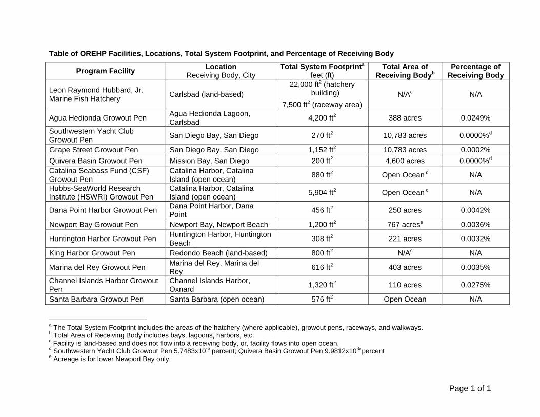
Page 1 of 1
Table of OREHP Facilities, Locations, Total System Footprint, and Percentage of Receiving Body
Program Facility Location Receiving Body, City
Total System Footprinta
feet (ft) Total Area of
Receiving Bodyb Percentage of
Receiving Body
Leon Raymond Hubbard, Jr. Marine Fish Hatchery Carlsbad (land-based)
22,000 ft2 (hatchery building)
7,500 ft2 (raceway area) N/Ac N/A
Agua Hedionda Growout Pen Agua Hedionda Lagoon, Carlsbad 4,200 ft2 388 acres 0.0249%
Southwestern Yacht Club Growout Pen San Diego Bay, San Diego 270 ft2 10,783 acres 0.0000%d
Grape Street Growout Pen San Diego Bay, San Diego 1,152 ft2 10,783 acres 0.0002% Quivera Basin Growout Pen Mission Bay, San Diego 200 ft2 4,600 acres 0.0000%d Catalina Seabass Fund (CSF) Growout Pen
Catalina Harbor, Catalina Island (open ocean) 880 ft2 Open Ocean c N/A
Hubbs-SeaWorld Research Institute (HSWRI) Growout Pen
Catalina Harbor, Catalina Island (open ocean) 5,904 ft2 Open Ocean c N/A
Dana Point Harbor Growout Pen Dana Point Harbor, Dana Point 456 ft2 250 acres 0.0042%
Newport Bay Growout Pen Newport Bay, Newport Beach 1,200 ft2 767 acrese 0.0036%
Huntington Harbor Growout Pen Huntington Harbor, Huntington Beach 308 ft2 221 acres 0.0032%
King Harbor Growout Pen Redondo Beach (land-based) 800 ft2 N/Ac N/A
Marina del Rey Growout Pen Marina del Rey, Marina del Rey 616 ft2 403 acres 0.0035%
Channel Islands Harbor Growout Pen
Channel Islands Harbor, Oxnard 1,320 ft2 110 acres 0.0275%
Santa Barbara Growout Pen Santa Barbara (open ocean) 576 ft2 Open Ocean N/A a The Total System Footprint includes the areas of the hatchery (where applicable), growout pens, raceways, and walkways. b Total Area of Receiving Body includes bays, lagoons, harbors, etc. c Facility is land-based and does not flow into a receiving body, or, facility flows into open ocean. d Southwestern Yacht Club Growout Pen 5.7483x10⁻⁵ percent; Quivera Basin Growout Pen 9.9812x10⁻⁵ percent e Acreage is for lower Newport Bay only.
Appendix M Water Quality Control Board Investigative Order 1209


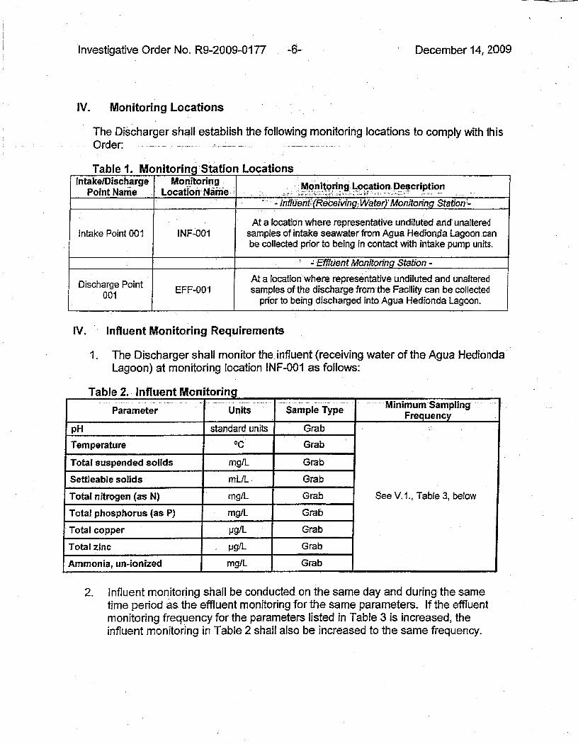

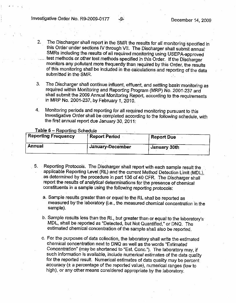
Appendix N Benthic Monitoring Program for the Growout Facilities Associated with the Ocean Resources Enhancement and Hatchery Program (OREHP)
BENTHIC MONITORING PROGRAM FORGROWOUT FACILITIES ASSOCIATED
WITH THE OCEAN RESOURCESENHANCEMENT AND HATCHERY
PROGRAM (OREHP)
Developed by:
Dr. Kenneth M. BrooksAquatic Environmental Sciences
644 Old Eaglemount RoadPort Townsend, WA 98368
And
Mark A. DrawbridgeHubbs-SeaWorld Research Institute
2595 Ingraham StreetSan Diego, CA 92109
For:
California Department of Fish and Game
June 2005
i
TABLE OF CONTENTS
TABLE OF CONTENTS................................................................................................................. iINTRODUCTION .......................................................................................................................... 1BACKGROUND ............................................................................................................................ 2
Organic Carbon........................................................................................................................... 2Macrofaunal Response to Sulfides.............................................................................................. 3Sedimented Zinc ......................................................................................................................... 5Sedimented Copper..................................................................................................................... 5Benchmarks for Managing Sedimented Copper and Zinc.......................................................... 5Chemical and Biological Remediation of the Benthos ............................................................... 6
MATERIALS AND METHODS.................................................................................................... 8Study Design............................................................................................................................... 8
Study Sites .............................................................................................................................. 8Sampling Frequency and Timing............................................................................................ 8
Sample Collection..................................................................................................................... 10Station positioning and reference locations .......................................................................... 10Sample evaluation................................................................................................................. 11Subsampling.......................................................................................................................... 11Sample labeling and handling............................................................................................... 11Replicate sampling of “hot spots”......................................................................................... 12Cleaning of equipment.......................................................................................................... 12
Chemical Analyses.................................................................................................................... 12Total volatile solids (TVS).................................................................................................... 12Sediment grain size (SGS) .................................................................................................... 12Redox potential ..................................................................................................................... 13Free sulfides .......................................................................................................................... 13Copper and zinc .................................................................................................................... 15
Photographic Record................................................................................................................. 15Statistical Analyses and Reporting ........................................................................................... 15
REFERENCES ............................................................................................................................. 16

OREHP BENTHIC MONITORING PROGRAMBROOKS/DRAWBRIDGE
1
INTRODUCTION
Since 1984, participants of the Ocean Resources Enhancement and Hatchery Program (OREHP)have been investigating the feasibility of using cultured fishes to restore depleted wild stocks.This research program is directed by the California Department of Fish & Game (CDF&G).Early OREHP research included developing the culture technology (i.e. spawning induction,larval rearing, nutrition and disease prevention) for the program’s primary target species, white seabass (WSB).
In 1991, OREHP researchers and volunteers from the Ventura Chapter of United Anglers begana pilot program to investigate the feasibility of using cage systems to cost-effectively extend thegrowout phase of WSB culture. Based on the success of those initial efforts, the United Anglersbegan to recruit other volunteer groups to develop additional growout facilities that have sincebeen constructed in different locations throughout southern California. The primary goal of thevolunteer-based, growout program is to maximize the potential of the OREHP by releasing large,healthy juvenile fish in the most cost-effective and environmentally protective manner possible.
In 2005 there are 13 cage facilities in operation at 11 coastal sites in southern California (Figure 1).A total of over 225,000 WSB have been successfully cultured, tagged and released from growoutfacilities during the Program’s history.
Figure 1. Site map showing locations of OREHP cage facilities.
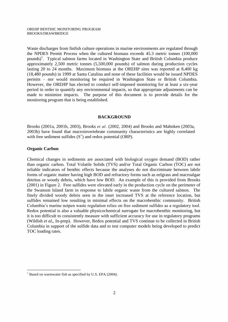
OREHP BENTHIC MONITORING PROGRAMBROOKS/DRAWBRIDGE
2
Waste discharges from finfish culture operations in marine environments are regulated throughthe NPDES Permit Process when the cultured biomass exceeds 45.3 metric tonnes (100,000pounds)1. Typical salmon farms located in Washington State and British Columbia produceapproximately 2,500 metric tonnes (5,500,000 pounds) of salmon during production cycleslasting 20 to 24 months. Maximum biomass at the OREHP sites was reported at 8,400 kg(18,480 pounds) in 1999 at Santa Catalina and none of these facilities would be issued NPDESpermits –nor would monitoring be required in Washington State or British Columbia.However, the OREHP has elected to conduct self-imposed monitoring for at least a six-yearperiod in order to quantify any environmental impacts, so that appropriate adjustments can bemade to minimize impacts. The purpose of this document is to provide details for themonitoring program that is being established.
BACKGROUND
Brooks (2001a, 2001b, 2003), Brooks et al. (2002, 2004) and Brooks and Mahnken (2003a,2003b) have found that macroinvertebrate community characteristics are highly correlatedwith free sediment sulfides (S=) and redox potential (ORP).
Organic Carbon
Chemical changes in sediments are associated with biological oxygen demand (BOD) ratherthan organic carbon. Total Volatile Solids (TVS) and/or Total Organic Carbon (TOC) are notreliable indicators of benthic effects because the analyses do not discriminate between labileforms of organic matter having high BOD and refractory forms such as eelgrass and macroalgaedetritus or woody debris, which have low BOD. An example of this is provided from Brooks(2001) in Figure 2. Free sulfides were elevated early in the production cycle on the perimeter ofthe Swanson Island farm in response to labile organic waste from the cultured salmon. Thefinely divided woody debris seen in the inset increased TVS at the reference location, butsulfides remained low resulting in minimal effects on the macrobenthic community. BritishColumbia’s marine netpen waste regulation relies on free sediment sulfides as a regulatory tool. Redox potential is also a valuable physicochemical surrogate for macrobenthic monitoring, butit is too difficult to consistently measure with sufficient accuracy for use in regulatory programs(Wildish et al,, In-prep). However, Redox potential and TVS continue to be collected in BritishColumbia in support of the sulfide data and to test computer models being developed to predictTOC loading rates.
1 Based on warmwater fish as specified by U.S. EPA (2004).
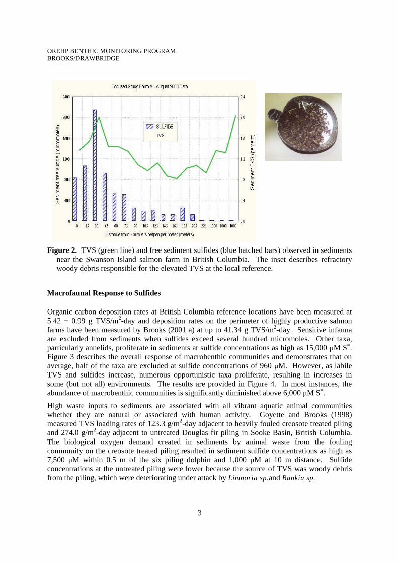
OREHP BENTHIC MONITORING PROGRAMBROOKS/DRAWBRIDGE
3
Figure 2. TVS (green line) and free sediment sulfides (blue hatched bars) observed in sedimentsnear the Swanson Island salmon farm in British Columbia. The inset describes refractorywoody debris responsible for the elevated TVS at the local reference.
Macrofaunal Response to Sulfides
Organic carbon deposition rates at British Columbia reference locations have been measured at5.42 + 0.99 g TVS/m2-day and deposition rates on the perimeter of highly productive salmonfarms have been measured by Brooks (2001 a) at up to 41.34 g TVS/m2-day. Sensitive infaunaare excluded from sediments when sulfides exceed several hundred micromoles. Other taxa,particularly annelids, proliferate in sediments at sulfide concentrations as high as 15,000 µM S=.Figure 3 describes the overall response of macrobenthic communities and demonstrates that onaverage, half of the taxa are excluded at sulfide concentrations of 960 µM. However, as labileTVS and sulfides increase, numerous opportunistic taxa proliferate, resulting in increases insome (but not all) environments. The results are provided in Figure 4. In most instances, theabundance of macrobenthic communities is significantly diminished above 6,000 µM S=.
High waste inputs to sediments are associated with all vibrant aquatic animal communitieswhether they are natural or associated with human activity. Goyette and Brooks (1998)measured TVS loading rates of 123.3 g/m2-day adjacent to heavily fouled creosote treated pilingand 274.0 g/m2-day adjacent to untreated Douglas fir piling in Sooke Basin, British Columbia.The biological oxygen demand created in sediments by animal waste from the foulingcommunity on the creosote treated piling resulted in sediment sulfide concentrations as high as7,500 µM within 0.5 m of the six piling dolphin and 1,000 µM at 10 m distance. Sulfideconcentrations at the untreated piling were lower because the source of TVS was woody debrisfrom the piling, which were deteriorating under attack by Limnoria sp.and Bankia sp.
OREHP BENTHIC MONITORING PROGRAMBROOKS/DRAWBRIDGE
4
Figure 3. Number of taxa observed in sediments as a function of the concentration of freesediment sulfides. Data are from Brooks and Mahnken (2003a).
Figure 4. Macrofaunal abundance as a function of free sediment sulfides at 7 British Columbiasalmon farms (Brooks and Mahnken (2003a).
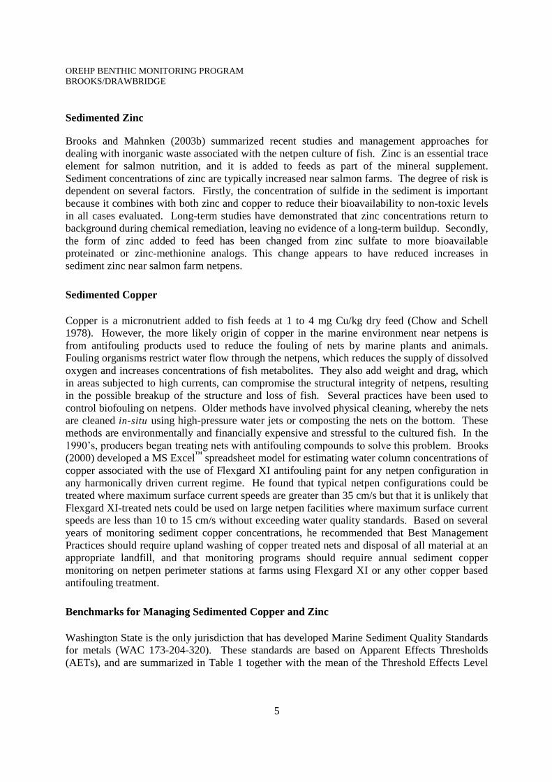
OREHP BENTHIC MONITORING PROGRAMBROOKS/DRAWBRIDGE
5
Sedimented Zinc
Brooks and Mahnken (2003b) summarized recent studies and management approaches fordealing with inorganic waste associated with the netpen culture of fish. Zinc is an essential traceelement for salmon nutrition, and it is added to feeds as part of the mineral supplement.Sediment concentrations of zinc are typically increased near salmon farms. The degree of risk isdependent on several factors. Firstly, the concentration of sulfide in the sediment is importantbecause it combines with both zinc and copper to reduce their bioavailability to non-toxic levelsin all cases evaluated. Long-term studies have demonstrated that zinc concentrations return tobackground during chemical remediation, leaving no evidence of a long-term buildup. Secondly,the form of zinc added to feed has been changed from zinc sulfate to more bioavailableproteinated or zinc-methionine analogs. This change appears to have reduced increases insediment zinc near salmon farm netpens.
Sedimented Copper
Copper is a micronutrient added to fish feeds at 1 to 4 mg Cu/kg dry feed (Chow and Schell1978). However, the more likely origin of copper in the marine environment near netpens isfrom antifouling products used to reduce the fouling of nets by marine plants and animals.Fouling organisms restrict water flow through the netpens, which reduces the supply of dissolvedoxygen and increases concentrations of fish metabolites. They also add weight and drag, whichin areas subjected to high currents, can compromise the structural integrity of netpens, resultingin the possible breakup of the structure and loss of fish. Several practices have been used tocontrol biofouling on netpens. Older methods have involved physical cleaning, whereby the netsare cleaned in-situ using high-pressure water jets or composting the nets on the bottom. Thesemethods are environmentally and financially expensive and stressful to the cultured fish. In the1990’s, producers began treating nets with antifouling compounds to solve this problem. Brooks (2000) developed a MS Excel™ spreadsheet model for estimating water column concentrations ofcopper associated with the use of Flexgard XI antifouling paint for any netpen configuration inany harmonically driven current regime. He found that typical netpen configurations could betreated where maximum surface current speeds are greater than 35 cm/s but that it is unlikely thatFlexgard XI-treated nets could be used on large netpen facilities where maximum surface currentspeeds are less than 10 to 15 cm/s without exceeding water quality standards. Based on severalyears of monitoring sediment copper concentrations, he recommended that Best ManagementPractices should require upland washing of copper treated nets and disposal of all material at anappropriate landfill, and that monitoring programs should require annual sediment coppermonitoring on netpen perimeter stations at farms using Flexgard XI or any other copper basedantifouling treatment.
Benchmarks for Managing Sedimented Copper and Zinc
Washington State is the only jurisdiction that has developed Marine Sediment Quality Standardsfor metals (WAC 173-204-320). These standards are based on Apparent Effects Thresholds(AETs), and are summarized in Table 1 together with the mean of the Threshold Effects Level
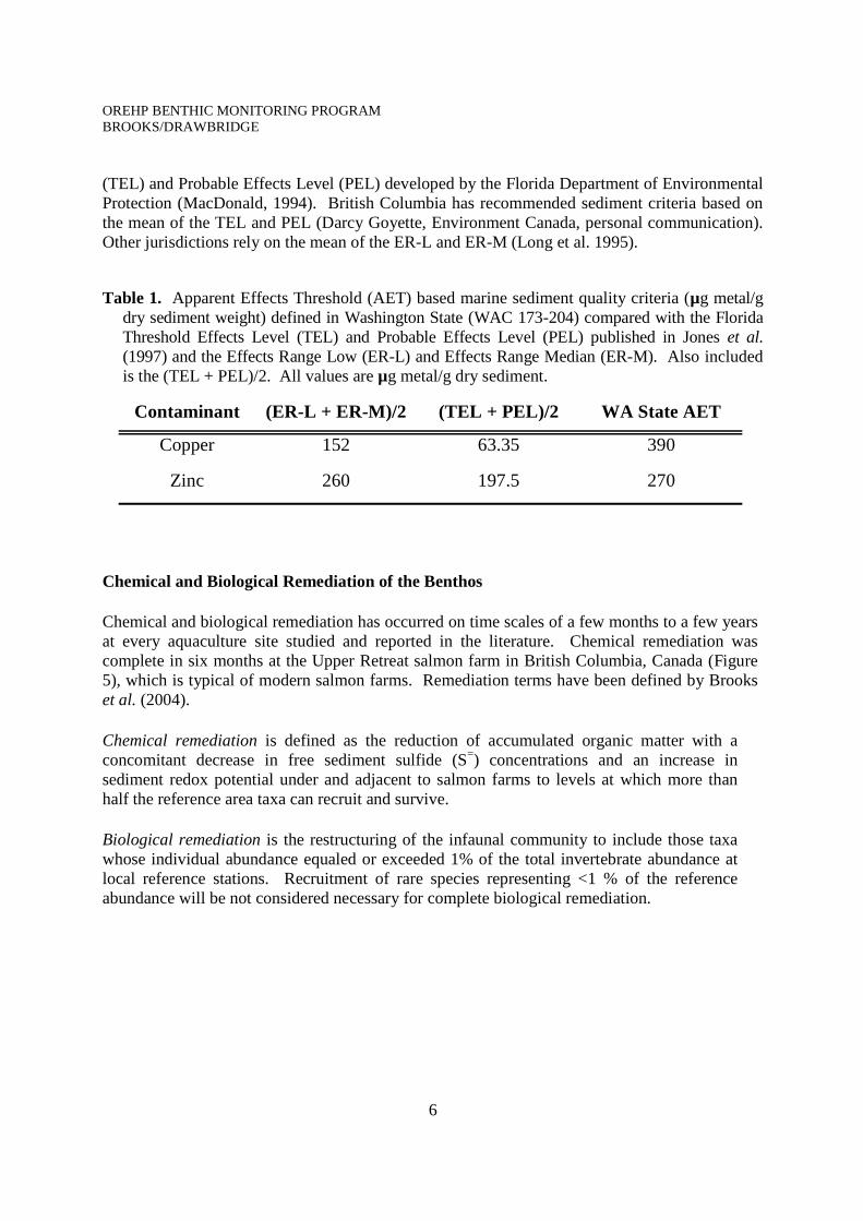
OREHP BENTHIC MONITORING PROGRAMBROOKS/DRAWBRIDGE
6
(TEL) and Probable Effects Level (PEL) developed by the Florida Department of EnvironmentalProtection (MacDonald, 1994). British Columbia has recommended sediment criteria based onthe mean of the TEL and PEL (Darcy Goyette, Environment Canada, personal communication).Other jurisdictions rely on the mean of the ER-L and ER-M (Long et al. 1995).
Table 1. Apparent Effects Threshold (AET) based marine sediment quality criteria (µg metal/gdry sediment weight) defined in Washington State (WAC 173-204) compared with the FloridaThreshold Effects Level (TEL) and Probable Effects Level (PEL) published in Jones et al.(1997) and the Effects Range Low (ER-L) and Effects Range Median (ER-M). Also includedis the (TEL + PEL)/2. All values are µg metal/g dry sediment.
Contaminant (ER-L + ER-M)/2 (TEL + PEL)/2 WA State AET
Copper 152 63.35 390
Zinc 260 197.5 270
Chemical and Biological Remediation of the Benthos
Chemical and biological remediation has occurred on time scales of a few months to a few yearsat every aquaculture site studied and reported in the literature. Chemical remediation wascomplete in six months at the Upper Retreat salmon farm in British Columbia, Canada (Figure5), which is typical of modern salmon farms. Remediation terms have been defined by Brookset al. (2004).
Chemical remediation is defined as the reduction of accumulated organic matter with aconcomitant decrease in free sediment sulfide (S=) concentrations and an increase insediment redox potential under and adjacent to salmon farms to levels at which more thanhalf the reference area taxa can recruit and survive.
Biological remediation is the restructuring of the infaunal community to include those taxawhose individual abundance equaled or exceeded 1% of the total invertebrate abundance atlocal reference stations. Recruitment of rare species representing <1 % of the referenceabundance will be not considered necessary for complete biological remediation.
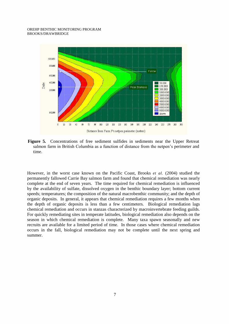
OREHP BENTHIC MONITORING PROGRAMBROOKS/DRAWBRIDGE
7
However, in the worst case known on the Pacific Coast, Brooks et al. (2004) studied thepermanently fallowed Carrie Bay salmon farm and found that chemical remediation was nearlycomplete at the end of seven years. The time required for chemical remediation is influencedby the availability of sulfate, dissolved oxygen in the benthic boundary layer; bottom currentspeeds; temperatures; the composition of the natural macrobenthic community; and the depth oforganic deposits. In general, it appears that chemical remediation requires a few months whenthe depth of organic deposits is less than a few centimeters. Biological remediation lagschemical remediation and occurs in stanzas characterized by macroinvertebrate feeding guilds.For quickly remediating sites in temperate latitudes, biological remediation also depends on theseason in which chemical remediation is complete. Many taxa spawn seasonally and newrecruits are available for a limited period of time. In those cases where chemical remediationoccurs in the fall, biological remediation may not be complete until the next spring andsummer.
Figure 5. Concentrations of free sediment sulfides in sediments near the Upper Retreatsalmon farm in British Columbia as a function of distance from the netpen’s perimeter andtime.
OREHP BENTHIC MONITORING PROGRAMBROOKS/DRAWBRIDGE
8
MATERIALS AND METHODS
Study Design
The study design for the OREHP benthic monitoring program relies on a regression approach toidentify trends in sediment free sulfides, redox potential, total volatile solids (TVS), copper andzinc as a function of distance from the netpen’s perimeter on four orthogonal transects.Replicate samples will be collected on the perimeter of each netpen and at a reference location.
Study Sites
The first cage facility to culture WSB was established at Channel Islands Harbor in 1991.Currently, there are 13 facilities participating in the OREHP that employ one of two cage designs toculture WSB (Table 2). The first design is a traditional one where the cage is moored in open wateror along side a dock and a net “bag” is used to contain the fish. The net is supported by a flexible frame of free-floating high-density polyethylene (HDPE) or wood that is buoyed by pontoons. Thesecond design consists of a submerged, fiberglass raceway that is affixed to a floating dock,typically in a protected marina. Culture volumes range from approximately 10 to 2,200 m3 andtherefore can support a maximum production capacity of 0.15 - 33 MT using a standardized harvestdensity of 15 kg/m3 (Table 2).
Sampling Frequency and Timing
Benthic monitoring will be conducted at each cage site once every three years or twice perNPDES permit cycle for a minimum of three surveys. Baseline sampling in Year 0 is designedto be more intensive than in Years 3 or 6 as described below. At the end of the three surveys, theCDF&G will determine if additional sampling is required on a site-by-site basis based on theresults of the initial surveys. Subsequent survey requirements (beyond Year 6) will bedetermined by the CDF&G on a survey-by-survey basis. Each site survey will be conducted nosooner than one month prior and no later than one month after a batch of fish is released fromthat facility. Timing the surveys in this manner is designed to ensure that measurable impactsare detected if they exist, and thus represents the worse-case-scenario.
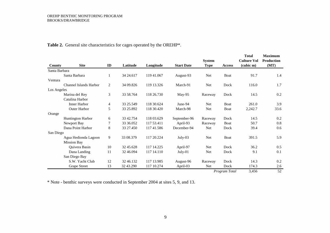
OREHP BENTHIC MONITORING PROGRAMBROOKS/DRAWBRIDGE
9
Table 2. General site characteristics for cages operated by the OREHP*.
Total MaximumSystem Culture Vol Production
County Site ID Latitude Longitude Start Date Type Access (cubic m) (MT)
Santa Barbara 1 34 24.617 119 41.067 August-93 Net Boat 91.7 1.4Ventura
Channel Islands Harbor 2 34 09.826 119 13.326 March-91 Net Dock 116.0 1.7
Marina del Rey 3 33 58.764 118 26.730 May-95 Raceway Dock 14.5 0.2Catalina Harbor
Inner Harbor 4 33 25.549 118 30.624 June-94 Net Boat 261.0 3.9Outer Harbor 5 33 25.892 118 30.420 March-98 Net Boat 2,242.7 33.6
OrangeHuntington Harbor 6 33 42.754 118 03.629 September-96 Raceway Dock 14.5 0.2Newport Bay 7 33 36.052 117 53.411 April-93 Raceway Boat 50.7 0.8Dana Point Harbor 8 33 27.450 117 41.586 December-94 Net Dock 39.4 0.6
Agua Hedionda Lagoon 9 33 08.379 117 20.224 July-03 Net Boat 391.5 5.9Mission Bay
Quivera Basin 10 32 45.628 117 14.225 April-97 Net Dock 36.2 0.5Dana Landing 11 32 46.094 117 14.110 July-01 Net Dock 9.1 0.1
San Diego BayS.W. Yacht Club 12 32 46.132 117 13.985 August-96 Raceway Dock 14.3 0.2Grape Street 13 32 43.290 117 10.274 April-03 Net Dock 174.3 2.6
Program Total 3,456 52
Santa Barbara
Los Angeles
San Diego
* Note - benthic surveys were conducted in September 2004 at sites 5, 9, and 13.
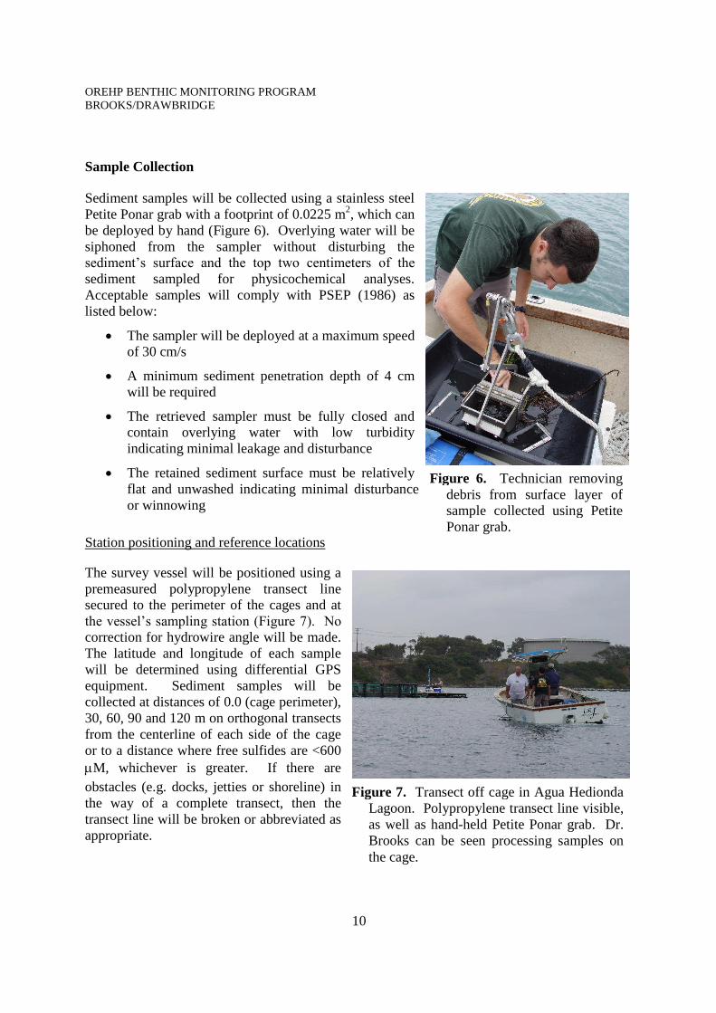
OREHP BENTHIC MONITORING PROGRAMBROOKS/DRAWBRIDGE
10
Sample Collection
Sediment samples will be collected using a stainless steelPetite Ponar grab with a footprint of 0.0225 m2, which canbe deployed by hand (Figure 6). Overlying water will besiphoned from the sampler without disturbing thesediment’s surface and the top two centimeters of the sediment sampled for physicochemical analyses.Acceptable samples will comply with PSEP (1986) aslisted below:
The sampler will be deployed at a maximum speedof 30 cm/s
A minimum sediment penetration depth of 4 cmwill be required
The retrieved sampler must be fully closed andcontain overlying water with low turbidityindicating minimal leakage and disturbance
The retained sediment surface must be relativelyflat and unwashed indicating minimal disturbanceor winnowing
Station positioning and reference locations
The survey vessel will be positioned using apremeasured polypropylene transect linesecured to the perimeter of the cages and atthe vessel’s sampling station (Figure 7). No correction for hydrowire angle will be made.The latitude and longitude of each samplewill be determined using differential GPSequipment. Sediment samples will becollected at distances of 0.0 (cage perimeter),30, 60, 90 and 120 m on orthogonal transectsfrom the centerline of each side of the cageor to a distance where free sulfides are <600M, whichever is greater. If there areobstacles (e.g. docks, jetties or shoreline) inthe way of a complete transect, then thetransect line will be broken or abbreviated asappropriate.
Figure 6. Technician removingdebris from surface layer ofsample collected using PetitePonar grab.
Figure 7. Transect off cage in Agua HediondaLagoon. Polypropylene transect line visible,as well as hand-held Petite Ponar grab. Dr.Brooks can be seen processing samples onthe cage.
OREHP BENTHIC MONITORING PROGRAMBROOKS/DRAWBRIDGE
11
Reference samples will be collected at a site >150 m from the cage where the water depths arewithin 15% of the average depth at the netpen, and the percent silt and clay in sediments arewithin + 20% of that observed at the netpens.
Sample evaluation
Overlying water will be siphoned from acceptable samples. Other methods, such as decantingthe water or slightly cracking the grab to let the water run out, are not appropriate, as they mightresult in disturbance or loss of fine-grained surficial sediment, organic matter and/or infauna.The following observations will be recorded:
Station position at the time the grab reached the bottom
Water depth
Penetration depth of the grab in the sediments
Comments related to sample quality such as leakage, winnowing or undue disturbance
Gross characteristics of the surficial sediment to include color
biological structures such as shells, tubes and macrophytes
presence of debris such as macroalgae, eelgrass detritus, woody debris, trash, etc.
Presence of bacterial mats, waste feed, feces, oily sheens, etc.
Odor (hydrocarbons or hydrogen sulfide)
Presence and depth of the redox potential discontinuity (RPD)
Subsampling
Subsamples will be taken using a stainless steel spoon. Unrepresentative material (emptymollusk shells, megafauna, large pieces of woody debris or other organic material) will beremoved from the sample in the field and noted. The top 2.0 cm of a portion of the samplewill be placed in a stainless steel bowl and gently homogenized for approximately 10 seconds.Polyethylene specimen jars (125 ml) will be filled with the homogenate with no overlying airspace.
Sample labeling and handling
Physicochemical samples will be stored on ice in coolers in the field. Sulfide and Eh (Redox)analyses will be accomplished as quickly as possible - usually within 15 minutes of collection.Samples for SGS and TVS analyses will be maintained at 4C until analyzed within 14 days ofcollection. The bodies and caps of all sample containers will be labeled with coded tags.Samples will be mailed by overnight delivery to Dr. Brooks at Aquatic Environmental Sciencesfor further analyses.
OREHP BENTHIC MONITORING PROGRAMBROOKS/DRAWBRIDGE
12
Replicate sampling of “hot spots”
Triplicate sediment samples will be collected and analyzed immediately in the field for eachcage station where free sulfides exceed 1,000 M. All endpoints will be evaluated in thesetriplicate samples.
Cleaning of equipment
Equipment will be washed in detergent and rinsed with tap water at the beginning of each day.Equipment will be rinsed with ambient seawater between grab deployments to removesediment and organisms. Subsamples for chemical analyses will be taken from the center ofthe grab. No other special cleaning requirements are considered necessary for these analyses.
Chemical Analyses
Total volatile solids (TVS)
Approximately 35 ml of each sample will be required for this analysis by Standard Method2540.E or EPA Method 160.4. Samples will be dried at 103 + 2o C in aluminum boats that havebeen pre-cleaned by combusting at 550C for 30 minutes. Drying will be continued until nofurther weight reduction is observed (generally overnight). The samples will then be weighed to0.1 mg and combusted at 550C for one hour or until no further weight loss is recorded. TotalVolatile Solids will be calculated as the percent difference between the dried and combustedweights. Quality assurance requires triplicate analyses on one of every 20 samples or on onesample per batch if fewer than 20 samples will be analyzed. A maximum of 20 percent RelativePercent Difference (of the silt-clay fraction) will be used as the Data Qualification ControlLimit. Total Volatile Solids will be measured at each sampling station in all survey years of themonitoring program (i.e. Year 0, 3 and 6).
Sediment grain size (SGS)
Approximately 50 grams of surficial sediment will be taken from the top 2.0 cm of the grab forsediment grain size analysis. The sediments will be wet sieved on a 0.064 mm sieve. Theretained material will be dried in an oven at 92C and processed using the dry sieve and pipettemethod of Plumb (1981). The sieves used for the analysis have mesh openings of 2.0, 0.89,0.25 and 0.064 mm. Particles passing the 0.064 mm sieve during wet sieving will be analyzedby sinking rates in a column of water (pipette analysis). During the first year, sediment grainsize will be determined at all stations. In subsequent years, sediment grain size analyses will beperformed on the four samples taken from the perimeter of each cage, as well as for the threesamples taken at the reference site.
OREHP BENTHIC MONITORING PROGRAMBROOKS/DRAWBRIDGE
13
Redox potential
This analysis will be conducted in the field using an Orion™ advanced portableISE/pH/mV/ORP/temperature meter model 290A with a Model 9678BN Epoxy Sure-FlowCombination Redox/ORP probe. The meter’s accuracy in the ORP mode is + 0.2 mV or +0.05% of the reading, whichever is greater. Redox potential will be measured at each samplingstation in all survey years of the monitoring program
Standardizing the Redox Electrode: Calibration reagents will be prepared within 24 hours of useand refrigerated. Redox Standard A (0.1 M potassium ferrocyanide and 0.05 M potassiumferricyanide) will be prepared by weighing 4.22 g K4Fe(CN)6.3H2O and 1.65 g K3Fe(CN)6 into a100-ml volumetric flask. Approximately 50 ml of distilled water will be added with swirling todissolve the solids. The solution will then be diluted to volume (100 ml) with distilled water.Standard B (0.01 M potassium ferrocyanide, 0.05 M potassium ferricyanide, and 0.36 Mpotassium fluoride) will be prepared by weighing 0.42 g K4Fe(CN)6.3H2O, 1.65 g K3Fe(CN)6,and 3.39 g KF.2H2O into a 100 ml volumetric flask. 50 ml of distilled water will be added todissolve the solids, and the solution diluted to 100 ml with distilled water. Orion Ag/AGClreference electrode filling solution 900011 will be used for all survey work.
Redox standards will be used to check the electrode at ambient temperature (10 to 15o C) at thestart and end of measurements for each batch of samples. Standard A will be transferred to a150-ml beaker and the electrode placed in the solution until the reading stabilized with stirring (1to 2 minutes). The potential of Standard A is approximately +147 + 9 mV. The electrode willthen be rinsed with distilled water and the measurement repeated with Standard B (potential of+216 + 9 mV). The potential in Standard A is approximately + 69 mV greater than in StandardB. The potential of the reference electrode (+244 mV at 20oC), corrected for the averagedifference between measured potentials of standard solutions and their calibration values, will beadded to the mV reading to determine the actual Eh potential in sediment samples. Eh potentialsof approximately +300 to +350 mV are typical of oxygenated seawater.
Measurement of sediment redox potential. For these redox analyses, the ORP electrode will beinserted into the homogenized sediment subsample and the mV reading recorded when the meterhas stabilized. This generally required two to three minutes. The electrode will then beremoved, gently wiped free of sediment, and used to measure the next sample. The probe will bechecked in the standards at least once every four hours. Probes will be rinsed in distilled waterand stored in pH 7.0 buffer between batches of samples.
Quality assurance procedures for the measurement of redox potential. Triplicate analyses willbe conducted on one of every 20 samples, or on one sample per batch, if less than 20 samples areanalyzed. No Data Qualification Control Limit has been established for this test.
Free sulfides
Free sulfides will be measured as soon as possible in the field. All buffer and standardscomponents will be pre-weighed into scintillation vials prior to deployment. Free sulfides willbe measured at each sampling station in all survey years of the monitoring program
OREHP BENTHIC MONITORING PROGRAMBROOKS/DRAWBRIDGE
14
Calibration of the total sulfide field probe. These analyses will be conducted using an Orion™
advanced portable ISE/pH/mV/ORP/temperature meter model 290A with a Model 9616 BNCIonplus Silver/Sulfide electrode. The meter has a concentration range of 0.000 to 19,900 µMand a relative accuracy of + 0.5% of the reading. SAOB buffer and sulfide standards are stablefor up to 3 hours and they will be made up in the morning and at mid-day on each samplingday.
A basic sulfide antioxidant buffer solution will be prepared in 1,000-ml HDPE screw-topbottles by adding 80.00 g of NaOH and 71.60 g EDTA (Na2C10O8N2.2H2O). Just prior to thestart of sampling, 8.75 grams of L-ascorbic acid will be added to 250 ml of the NaOH–EDTAstock in an amber HDPE bottle. This SAOB buffer solution is stable for up to 4.0 hours afteraddition of L-ascorbic acid.
The S= electrode will be calibrated before and after each batch of not more than 12 samples.Three S= standards (100, 1000 and 10,000 µM) will be used for a three-point electrodecalibration. A stock S= solution of 0.01 M Na2S will be prepared by adding 0.2402 gNa2S.9H2O (premeasured in scintillation vials) to 100 ml of distilled water in an amber jar. Thisstock solution will be made fresh every 48 hours and stored at 4o C. A 1000 µM S= standard(10-3 M) will be prepared at the start of sampling by transferring 10 ml of the 0.01 M Na2Sstock solution (10,000 µM) into an amber jar and diluting to 100 ml with distilled water. A 100µM S= standard (10-4 M) will be prepared by transferring 10 ml of the 1000 µM standard to anamber jar and diluting to 100 ml with distilled water. Both dilution standards will be mixedthoroughly before each use. Just before calibration of the S= electrode, 10 ml of each standardwill be transferred to 30 ml amber bottles and 10 ml of SAOB (containing L-ascorbic acid)added. The combined solution will be kept tightly capped until used for standardizing the S=
electrode.
Measurement of sediment total sulfides. These analyses will be completed in 30 ml graduatedbeakers by marking each beaker at 5 and 10 ml levels using a pipette, distilled water and a fineblack lab marker. Five ml of SAOB will then be added to the beaker. Sediment will be addedto top the mixture off at the 10 ml mark. A flat-tip stainless steel spatula will be used tohomogenize the sediment sample with the SAOB buffer. Following this, the S= electrode willbe inserted and used to further stir the sediment. The S= electrode reading usually stabilizes intwo to four minutes. The electrodes will be gently wiped with a paper towel between samples,but will be not rinsed. After completing 12 analyses, the electrode will be gently rinsed withdistilled water and recalibrated before continuing. In addition, the sulfide electrode will berecalibrated at least once every two hours and at the end of each batch of samples.
Quality assurance for sediment total sulfide analyses. Triplicate analyses will be conducted onone of every 20 samples, or on one sample per batch when fewer than 20 samples will beanalyzed. The Data Qualification Control Limit is 20% Relative Percent Difference (RPD).Fresh standards will be made daily. The analytical balance will be inspected daily and calibratedat once per month.
OREHP BENTHIC MONITORING PROGRAMBROOKS/DRAWBRIDGE
15
Copper and zinc
Metal analyses will be completed by Analytical Resources Incorporated in Seattle, Washington.This laboratory is accredited by the Washington State Department of Ecology for theseprocedures. EPA method 6010B will be used following a strong acid digestion (EPA 3050B).Quality assurance requires completion of one blank; one spiked sample; and a certified referencematerial with each batch of 20 samples. Control limits from PSEP (1996) will be used:
Matrix Spike. 85 to 115% when the value of the spiked sample will be 2 to 5 times theoriginal sample concentration;
Blank analysis. The analyte should not be detected above the instrument detection limit of 0.25µg/g;
Continuing Calibration Verification. The observed value should be within + 10% of the truevalue for GFAA.
Copper analyses will only be conducted at sites where copper-based antifoulants are used.Copper and zinc testing will be conducted at all sampling stations in Year 0 to develop abaseline along all transects, with few samples being analyzed in Years 3 and 6. The samplingscheme in Year 3 and 6 will be determined after the results of Year 0 are analyzed.
Photographic Record
A photograph will be taken of each sample while it is still in the grab using a digital camera.
Statistical Analyses and Reporting
All data will be entered into a Microsoft Excel spreadsheet and imported into Statisticasoftware. Proportional data will be transformed (arcsin(sqrt(proportion))) prior to inferentialtests. Means will be reported with + 95% confidence intervals. Inferential tests will beassumed significant at = 0.05.
A survey report will be generated for each cage site after each survey. Reports will be sent toCDF&G for review and distribution to other agencies as appropriate.

OREHP BENTHIC MONITORING PROGRAMBROOKS/DRAWBRIDGE
16
REFERENCES
Anderson, S., 1998. Dietary supplementation of salmon diets with zinc: Alternative sources andtheir effects on the environment. Report prepared by Steward Anderson, AquacultureIndustry Coordinator, Hoffmann La-Roche Ltd., 9 pp.
Brooks, K.M. 2000. Determination of copper loss rates from Flexgard XI™ treated nets in marineenvironments and evaluation of the resulting environmental risks. Report prepared for the BritishColumbia Ministry of Environment and the British Columbia Salmon Farmers Association. 24pp.
Brooks, K.M. 2001a. Chapter 4. Salmon Farming and the Environment. In: Nash (2001) The NetpenSalmon Farming Industry in the Pacific Northwest. NOAA Technical Memorandum NMFS-NWFS-NWFSC-49. pp. 36–73.
Brooks, K.M. 2001b. An evaluation of the relationship between salmon farm biomass, organic inputs tosediments, physicochemical changes associated with those inputs and the infaunal response –withemphasis on total sediment sulfides, total volatile solids, and oxidation-reduction potential assurrogate endpoints for biological monitoring –Final Report. Technical report produced for theTechnical Advisory Group (TAG) to the British Columbia Ministry of Environment, 2080-ALabieux Road, Nanaimo, British Columbia, Canada V9T 6J9. 186 pp. plus appendices.
Brooks, K.M., C. Mahnken and C. Nash. 2002. Environmental Effects Associated with Marine NetpenWaste with Emphasis on Salmon Farming in the Pacific Northwest. In: Responsible MarineAquaculture, Eds: Stickney and McVey. CABI Publishing, Wallingford, United Kingdom pp. 159 –204.
Brooks, K.M. and C.V.W. Mahnken. 2003a. Interactions of Atlantic Salmon in the Pacific NorthwestEnvironment. II. Organic Wastes. Fisheries Research, Vol. 62, Issue 3, pp. 255–293.
Brooks, K.M. and C.V.W. Mahnken. 2003b. Interactions of Atlantic salmon in the Pacific NorthwestEnvironment. III. Inorganic Compounds. Fisheries Research, Vol. 62, Issue 3, pp. 295-305.
Brooks, K.M. 2003. Chemical and biological remediation of the benthos near Atlantic salmon farms.Aquaculture, Volume 219, Issues 1-4, pp. 355-377.
Brooks, K.M. , A.R. Stierns and C. Backman. 2004. Seven year remediation study at the Carrie BayAtlantic salmon (Salmo salar) farm in the Broughton Archipelago, British Columbia, Canada.Aquaculture. Aquaculture 239, pp. 81-123.
Chow, K.W., Schell, W.R., 1978. The minerals, In Fish Feed Technology. Aquac. Dev. Coord.Programme, Rep. ADCP/REP/80/11, FAO, Rome.
Long, E.R., D.D. MacDonald, S.L. Smith and F.D. Calder. 1995. Incidence of AdverseBiological Effects within Ranges of Chemical Concentrations in Marine and EstuarineSediments, Environmental Management 19(1) pp. 81-97.
OREHP BENTHIC MONITORING PROGRAMBROOKS/DRAWBRIDGE
17
MacDonald, D.D. 1994. Approach to the Assessment of Sediment Quality in Florida CoastalWaters. Florida Department of Environmental Protection, Tallahassee, Florida.
U.S. EPA 2004. 40 CFR Part 451: Effluent Limitations Guidelines and New SourcePerformance Standards for the Concentrated Aquatic Animal Production Point SourceCategory; Final Rule.
Wildish, D.J., H.M. Akagi, B.T. Hargrave and P.M. Strain. (In-prep) Inter-laboratorycalibration of redox potential and total sulfide measurements in interfacial marinesediments and the implications for organic enrichment. Canadian Department ofFisheries and Oceans Technical Report. 33 pp.

Appendix O Conversion Table