Theoretical and Experimental Analysis of Auctions with Negative

Externalities

Youxin Hu,∗ John Kagel,† and Lixin Ye‡

April 2010

Abstract

We investigate a model in which a single bidder (the “entrant”), on winning the auction,

imposes a negative externality on two “regular” bidders. In an ascending price clock auction, in

equilibrium when all bidders are active a regular bidder free rides, dropping out before reaching

his private value. Despite this free riding problem, in almost all cases, the item is ex post efficiently

assigned. In contrast, in a first-price sealed bid auction incentives for free riding and aggressive

bidding coexist, leading to a lower ex post efficiency. The experiment shows minimal free riding

in the clock auction, but as predicted, when a single regular bidder is left competing with the

“entrant” he bids up to his value plus the externality. In first-price auctions, as predicted regular

bidders bid more aggressively than the “entrant,” and both bid higher than in auctions with no

externality.

Keywords: Auctions, externality, free riding, aggresive bidding, experiments.

JEL: D44, D82, C91.

∗Research Institute of Economics & Management, Southwestern University of Finance and Economics, Chengdu

610074, P. R. China. Email: huyx@swufe.edu.cn.

†Department of Economics, The Ohio State University, 1945 North High Street, Columbus, OH 43210. Email:

kagel.4@osu.edu.

‡Department of Economics, The Ohio State University, 1945 North High Street, Columbus, OH 43210. Email:

ye.45@osu.edu.

1

1 Introduction

The standard literature on auctions considers isolated markets with bidders that are ex ante identical

and independent so that losing bidders get zero payoffs.1 However, in cases where auctions take

place within a broader economic framework this is not always the case as auction participants may

be competitors or cooperators in the relevant aftermarket. This paper considers the case where one

of the competitors on winning the auction imposes a negative externality in the aftermarket. The

negative externality is identity dependent, non-reciprocal, and one-to-more. Specifically, we consider

a single-object auction with three bidders where one bidder (the “entrant”) imposes a negative

externality on the other two (regular) bidders if she wins. If either of the regular bidder’s win, the

losing bidders receive payoff of zero. An example is a takeover auction where one of the bidders is

hostile, and the other bidders will be worse off if the hostile bidder wins. This negative externality is

non-reciprocal since there is no externality if any of the non-hostile bidders win. Another example

is a patent auction where all but one of the bidders are incumbents who already possess similar

technologies, while the remaining bidder is a would be entrant. If the potential entrant wins the

auction, she will add more competition to the industry and take market share from the other bidders.

On the other hand, if an incumbent wins, the market structure will remain more or less the same

and no negative externality will be imposed on the other incumbents.

We examine the effect of a negative externality of this sort in both an English (clock) ascending

price auction and a first-price sealed bid (FPSB) auction. Intuitively, one might expect more ag-

gressive (higher) bids in auctions with negative externalities. In contrast, our equilibrium analysis

shows that conditional on all three bidders being active in the clock auction, a regular bidder with a

relatively low valuation will have an incentive to drop out at a price lower than his value in an effort

to free ride on a regular bidder with a higher valuation. However, once a regular bidder has dropped

out, the remaining regular bidder will bid up to his value plus the absolute value of externality. In a

sense the clock auction provides a mechanism for the regular bidders to “coordinate” on when to free-

ride and when to bid aggressively. The FPSB auction provides no such opportunity for the regular

bidders to coordinate their actions. In this case, both regular bidders bid more aggressively (higher)

than the potential entrant, and the entrant in turn bids more aggressively than in a comparable

1See, for example, Vickrey (1961), Riley and Samuelson (1981), Myerson (1981) and Milgrom and Weber (1982).

2

auction with no negative externality.

We conduct an experiment to examine whether the free-riding feature of the clock auction is

present in the laboratory, as well as how closely subjects follow the other equilibrium predictions.

Although we observe very little free riding relative to the levels predicted for stage-one bids (first

dropouts) in the clock auctions, bidders tend to closely follow other elements of the equilibrium

bidding strategy. Part of the explanation for the low levels of free riding observed in stage-one

relative to predicted levels can be attributed to best responding to other regular bidders failure to

free ride. In the FPSB auction, consistent with the theoretical prediction, both regular bidders bid

more aggressively than the entrant. Further, the entrant tends to bid more aggressively compared

to a FPSB auction without a negative externality. As predicted, with the externality present, the

clock auction has higher efficiency and lower revenue than in the FPSB auction.

There has been considerable theoretical work on closely related questions. Jehiel and Moldovanu

(1995) show that negative externalities may cause delays in negotiation. Jehiel and Moldovanu (1996)

examine a situation where a potential bidder cannot avoid the negative externality even if he does

not participate in the auction. Jehiel, Moldovanu, and Stacchetti (1996) study mechanism design

issues in auctions with negative externalities and show that the seller can sometimes obtain a greater

profit by not selling the item.2 Caillaud and Jehiel (1998) suggest that collusion will be imperfect

if a buyer is worse off when his rival wins the object, to the point that the seller can design an

auction to benefit from the (imperfect) collusive behavior of the bidders. Das Varma (2002) studies

auctions with identity-dependent externalities which are one-to-one and are either reciprocal or non-

reciprocal. Ettinger (2003) considers a situation where the losers of an auction care about the price

paid by the winner as a result of various types of price externalities. He shows that a second-price

auction can exacerbate the price externalities compared to a first price auction.

To the best of our knowledge, we are the first to investigate free riding in an auction where

one specific bidder can impose a negative externality on more than one bidder and to investigate

the model experimentally. Regarding experimental work, Goeree, Offerman, and Sloof (2004) is

closest in spirit to ours. They consider a situation where one bidder imposes a potential negative

externality on two incumbent bidders in a multi-unit demand setting where neither incumbent can

2Jehiel, Moldovanu, and Stacchetti (1999) analyze auctions with externalities following a multidimensional mecha-

nism design approach.

3

purchase the entire supply on their own. As such the regular bidders are faced with a threshold type

problem. They focus on incentives for demand reduction and preemptive bidding in both sealed bid

and ascending price auctions.

The paper is organized as follows. Section 2 establishes the theoretical framework. Section 3

describes our experimental design and procedures. Section 4 analyzes the data and presents the

main results. Section 5 concludes the paper.

2 The model

Three bidders bid for a single object. Each bidder’s private value is assumed to be drawn i.i.d. from

a uniform distribution on the interval of [0, 1]. Two of the bidders are “regulars” (Ri, i = 1, 2) with

private values v1 and v2, respectively. The third bidder is the potential entrant (E) with private value

vE. There is an identity dependent negative externality of the amount −x; if E wins the auction,

both Rs receive a payoff of −x. However, if either R wins the auction, there is no externality so that

losing bidders receive a zero payoff. To focus on nontrivial cases, we assume that the externality x

is a constant and not too large.3

2.1 The English Clock Auction

In the English clock auction the price starts rising from zero. As the price rises, a bidder must decide

whether to stay or drop out (by pressing a button) at the current price. Once a bidder has dropped

out, she cannot re-enter the auction. The auction ends when two bidders have dropped out, with the

remaining bidder winning the item and paying the price at which the second bidder dropped out.

We assume that during this process bidders are aware of the identities of bidders as they drop out,

as well as the drop out prices. Random tie-breaking rules are applied if two or more bidders choose

to drop out at the same price.4

3We need 0 < x ≤ 1 −√3/3 ≈ 0.429 in our equilibrium analysis. Intuitively, if x is too big, it results in an

uninteresting equilibrium in which R bids high enough to guarantee winning the item.

4 If two bidders drop out at the same time, one of them is randomly selected to drop first. Then the other has a

chance to drop out too, at the same price, or to continue bidding. If three bidders drop out at the same time, dropping

priority is decided randomly, with the bidder with the highest priority dropping first, and the remaining two bidders

each deciding whether to drop at the same price or to remain active. If both remaining bidders decide to dropout, one

4

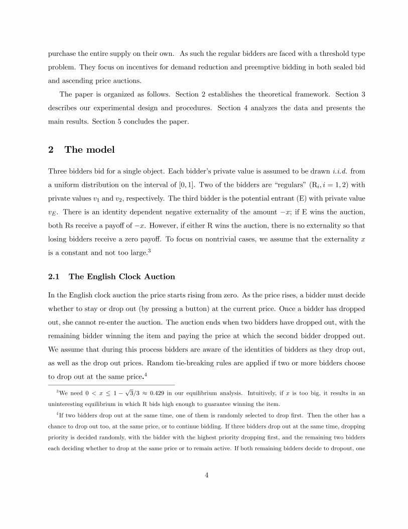
In the appendix, we show that the following strategies constitute an equilibrium of the game:

Bidder E’s dominant strategy is to stay until P = vE.

Ri’s equilibrium strategy, i = 1, 2, is as follows:

(1) If one bidder has already dropped, Ri will stay until

P =

⎧⎨⎩ vi , if the other remaining bidder is R

vi + x , if the other remaining bidder is E

(2) If all three bidders are active, Ri will stay active until

P = B(vi) =

⎧⎪⎪⎪⎨⎪⎪⎪⎩0 , if vi ≤ x

vi − x , if x < vi ≤ 1− x

2vi − 1, if vi > 1− x

The equilibrium strategy of a regular bidder when all three bidders are active is shown in Figure

1.

Figure 1: Equilibrium 1st Drop Price of R in Clock Auction

of them is again randomly selected to drop first. This tie-breaking rule is part of the equilibrium construction.

5

Since E does not suffer from the externality, E’s dominant strategy is to stay active until the

price equals her value. Since we assume that the identities of bidders are public information, it is

easy to show that an R’s equilibrium strategy after one bidder has dropped out is as follows: he

drops at his private value if his rival is an R, and drops at his private value plus x if his rival is an E.

The non-trivial part of the equilibrium is an R’s strategy when nobody has dropped. The proof

is tedious and is relegated to the appendix. But the intuition is clear. In a clock auction without

externalities, a bidder will drop at a price equal to his private value. With a negative externality

one might expect Rs to bid higher since they will receive a negative payoff if E wins. However, in

the equilibrium described above, when all three bidders are active, an R will not stay until the price

reaches his value. Instead, he will drop before the price reaches his private value with his dropping

price equal to vi − x or 0, whichever is larger. Thus, at least to start with, Rs will tend to bid less

aggressively than without a negative externality present. This is a consequence of the fact that the

negative externality is imposed on both Rs, and that as long as either R wins, both will avoid the

externality. By free riding, the R with the lower value pushes the other R to bid above his value.

As long as the other R wins, the free rider earns a zero payoff (as opposed to −x in case he has

to compete to beat E). Thus in a sense the clock auction provides a device for the regular bidders

to “coordinate” on when to free-ride and when to bid aggressively. As can be seen below, such a

coordination device is absent in the FPSB auction, where all bidders need to submit their bids once

and for all.

Note that in practice free riding is risky. An R may not be sure that the other R will win or will

be willing to fight it out with E. If the other R fails to carry out his part of the equilibrium strategy,

and the free rider could have won had he stayed, he is worse off with free riding.

2.2 The First-Price Sealed Bid Auction

We now examine the first-price sealed bid auction (FPSB). Each bidder submits a sealed bid. The

high bidder wins the auction and pays a price equal to his bid. We characterize the symmetric

equilibrium (β(·), γ(·)) where β(·) is the equilibrium bid function for the two Rs and γ(·) is the

equilibrium bid function for E.

Given that R2 adopts the bid function β(·) and E adopts the bid function γ(·), R1 (with value

v1) chooses a bid b to maximize his expected profit:

6

EΠ1 = F (β−1(b)) · F (γ−1(b)) · (v1 − b)− x ·Z 1

γ−1(b)

Z β−1(γ(vE))

0f(v2)f(vE)dv2dvE

= β−1(b) · γ−1(b) · (v1 − b)− x ·Z 1

γ−1(b)

Z β−1(γ(vE))

0dv2dvE.

That β(·) is a best response to (β(·), γ(·)) implies that ∂EΠ1/∂b = 0 if evaluated at b = β(v1) or

β−1(b) = v1. This leads to the following equation:

β0−1(β(v1)) · γ−1(β(v1)) · (v1 − β(v1)) + v1 · γ

0−1(β(v1)) · (v1 − β(v1))

−v1 · γ−1(β(v1)) + x · γ0−1(β(v1)) · v1 = 0

Given bidder E’s value vE, and that both Rs adopt the bid function β(.), E chooses the optimal bid

r to maximize her expected profit:

EΠE = (F (β−1(r)))2 · (vE − r) = (β−1(r))2 · (vE − r).

That γ(·) is a best response to β(·) implies that ∂EΠE/∂r = 0 if evaluated at r = γ(vE) or γ−1(r) =

vE. This leads to the following equation:

2β−1(γ(vE)) · β0−1(γ(vE)) · (vE − γ(vE))− (β−1(γ(vE)))2 = 0.

Thus in equilibrium the following equations should hold simultaneously:

⎧⎨⎩ β0−1(b) · γ−1(b) · (v1 − b) + v1 · γ

0−1(b) · (v1 − b)− v1 · γ−1(b) + x · γ0−1(b) · v1 = 0

2β0−1(r) · β−1(r) · (vE − r)− (β−1(r))2 = 0

(1)

where b = β(v1) and r = γ(vE).

The following equilibrium properties can be established:

(i) β(1) = γ(1) = b.

(ii) γ(0) = 0. E never bids above value.

(iii) β0(v) ≥ 0 , the bid function for R is monotonically increasing.

Since 2β0−1(r) ·β−1(r) · (vE − r)− (β−1(r))2 = 0 holds in equilibrium, (β−1(r))2 ≥ 0, β−1(r) ≥ 0,

and vE − r ≥ 0 (E never bids above vE), we have β0−1(r) ≥ 0 for any r ∈ [0, b].

Hence β0−1(b) ≥ 0 for any b ∈ [0, b], and β0(v) = 1/β

0−1(b) ≥ 0.

7

(iv) Rs bid more aggressively (higher) than E.

Whenever β(v∗) = γ(v∗) = b∗, we have

β0(v∗) =2(v∗ − b∗)

v∗<2(v∗ − b∗ + x)

v∗= γ0(v∗).

Since β(1) = γ(1) = b, by the single crossing lemma we must have β(v) > γ(v) for v ∈ [0, 1).5

Let the inverse bid functions be ϕ1(·) = β−1(·) and ϕE(·) = γ−1(·). Equations (1) can be

rewritten as follows.

⎧⎨⎩ ϕ01(b) · ϕE(b) · (ϕ1(b)− b) + ϕ1(b) · ϕ0E(b) · (ϕ1(b)− b)− ϕ1(b) · ϕE(b) + x · ϕ0E(b) · ϕ1(b) = 0

2ϕ01(b) · ϕ1(b) · (ϕE(b)− b)− (ϕ1(b))2 = 0(2)

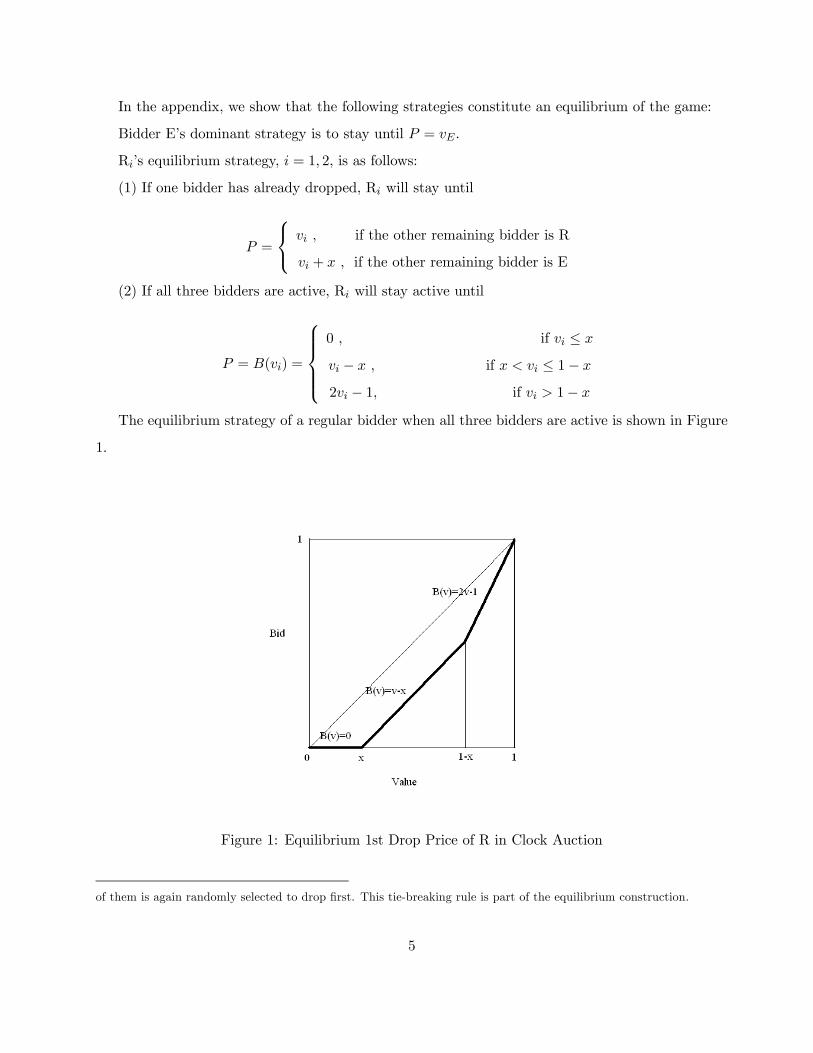
Figure 2 provides the numerical solution along with the equilibrium bid function for a 3-bidder

FPSB auction with no externality (given by b(v) = 23v). R’s bid function lies above E’s, as Rs bid

more aggressively than E in order to avoid the externality. Moreover, E’s bid function lies above

its counterpart in a FPSB auction without an externality. Although the E does not suffer from the

externality, she bids more aggressively than in an auction with no externality due to the greater

competition from Rs’ more aggressive bidding.

5A version of the single crossing lemma can be found in Milgrom (2004, pp. 124).

8

0 10 20 30 40 50 60 70 80 90 1000

10

20

30

40

50

60

70

80

Nash RNash ENash Control

Figure 2: Equilibrium Bidding Functions in FPSB Auction

3 Experimental Design

Each experimental session consisted of two or more 3-bidder markets operating simultaneously. There

were three sessions each for the clock and FPSB auctions with externalities and two sessions for the

FPSB with no externality (FPSB control treatment).6 Instructions were read out loud with subjects

having copies to follow.7 Each session started with 3 dry runs followed by 25 paid periods. There

were no bankruptcies in any of the sessions. All subjects were paid a $6 participation fee along with

their end of experiment cash balance. Table 1 shows the number of sessions along with the number

of subjects under each auction format. Each session lasted for approximately one and a half hours.

Private values for all bidders were iid from a uniform distribution with support [0, 100] (with

integer values only), with new values drawn before each auction. The externality was set at −20

6The control treatment is needed for the FPSB auction since subjects are known to bid well above the risk neutral

Nash equilibrium in these auctions with no negative externality (see, for example, the many references cited in Kagel,

1995). No such widespread overbidding is reported in English clock auctions, and can be confirmed for the present

experiment by looking at bids in the clock auction with only two bidders left.

7A copy of the instructions along with screen shots can be found at http://www.econ.ohio-

state.edu/kagel/instructions_Hu_Kagel_Ye.

9

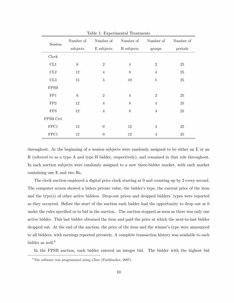
Table 1: Experimental Treatments

SessionNumber of

subjects

Number of

E subjects

Number of

R subjects

Number of

groups

Number of

periods

Clock

CL1 6 2 4 2 25

CL2 12 4 8 4 25

CL3 15 5 10 5 25

FPSB

FP1 6 2 4 2 25

FP2 12 4 8 4 25

FP3 12 4 8 4 25

FPSB Ctrl

FPC1 12 0 12 4 25

FPC1 12 0 12 4 25

throughout. At the beginning of a session subjects were randomly assigned to be either an E or an

R (referred to as a type A and type B bidder, respectively), and remained in that role throughout.

In each auction subjects were randomly assigned to a new three-bidder market, with each market

containing one E and two Rs.

The clock auction employed a digital price clock starting at 0 and counting up by 2 every second.

The computer screen showed a biders private value, the bidder’s type, the current price of the item

and the type(s) of other active bidders. Drop-out prices and dropped bidders’ types were reported

as they occurred. Before the start of the auction each bidder had the opportunity to drop out at 0

under the rules specified or to bid in the auction. The auction stopped as soon as there was only one

active bidder. This last bidder obtained the item and paid the price at which the next-to-last bidder

dropped out. At the end of the auction, the price of the item and the winner’s type were announced

to all bidders, with earnings reported privately. A complete transaction history was available to each

bidder as well.8

In the FPSB auction, each bidder entered an integer bid. The bidder with the highest bid

8The software was programmed using zTree (Fischbacher, 2007).

10

obtained the item and paid a price equal to his bid. In the case of ties the computer determined

who got the item. Losing bidders each incurred a loss of 20 if E won, and zero profit if an R won.

Information feedback after each auction consisted of own bid, the price of the item, and the winner’s

type, with earnings reported privately.

At the beginning of each session, Es were given an initial cash balance of 135 experimental

currency units (ECUs) with Rs having a starting balance of 270 ECUs. The difference in initial cash

balance was calibrated to account for losses due to the externality and for expected differences in

auction earnings between player types. These starting cash balances were private information. In

the FPSB control sessions all players had starting cash balances of 135 ECUs. Subjects were paid

in cash at the end of each session with their accumulated balances converted into US dollars at the

rate of 10ECUs = $1 along with a $6 participation fee. Earnings averaged around $30 per subject.

Subjects were recruited through e-mail solicitation from a database of several thousand students

enrolled in economics classes at the Ohio State University. All subjects had no previous experience

with any type of auction experiment, although some of them may have had experience in another

experiment.

4 Experimental Results

4.1 Bidding in Clock Auctions

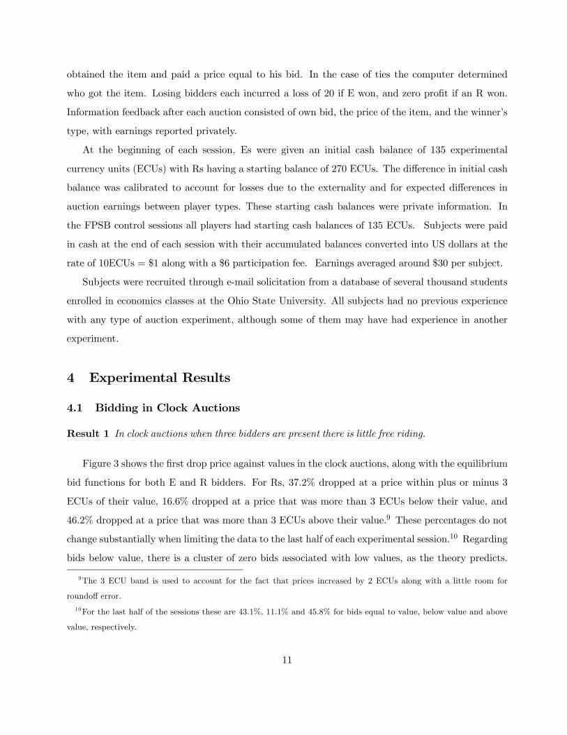
Result 1 In clock auctions when three bidders are present there is little free riding.

Figure 3 shows the first drop price against values in the clock auctions, along with the equilibrium

bid functions for both E and R bidders. For Rs, 37.2% dropped at a price within plus or minus 3

ECUs of their value, 16.6% dropped at a price that was more than 3 ECUs below their value, and

46.2% dropped at a price that was more than 3 ECUs above their value.9 These percentages do not

change substantially when limiting the data to the last half of each experimental session.10 Regarding

bids below value, there is a cluster of zero bids associated with low values, as the theory predicts.

9The 3 ECU band is used to account for the fact that prices increased by 2 ECUs along with a little room for

roundoff error.

10For the last half of the sessions these are 43.1%, 11.1% and 45.8% for bids equal to value, below value and above

value, respectively.

11

But this is matched by a number of zero bids at these low values for Es, as well as very few bids

approaching the free riding equilibrium for higher valuations. Together this suggests that these bids

were not motivated by free riding. Most of Rs’ bids above value involve bidding at value plus 20,

the amount of the negative externality, the opposite of free riding. In contrast, when an E dropped

first, 67.7% of the time they were within plus or minus 3 ECUs of their value, 17.7% were below

value, and 14.6% above value.

 

0 10 20 30 40 50 60 70 80 90 1000

10

20

30

40

50

60

70

80

90

100

Value

Dro

p P

rice

Regular NashEntrant NashRegular ActualEntrant Actual

Figure 3: Stage-One Bids in Clock Auctions: All three bidders active

Result 2 In clock auctions with two bidders active, bids are close to equilibrium levels for both Es

and Rs: Es tend to drop at their value and Rs tend to drop at their value when the remaining bidder

is an R, and at their value plus the externality (20) when the remaining bidder is an E.

Figure 4 shows second drops for the case where the remaining bidders were an Es and an R.

Es generally followed the dominant strategy of dropping at their value (87.0% of the time within

± 3 ECUs of value). Rs were not quite so well behaved as they followed the dominant strategy of

dropping at their value plus the full amount of the externality 46.7% of the time overall. However,

(i) over half of the deviations (69.6%) can be accounted for by four bidders with three or more failures

to pursue the dominant strategy and (ii) there was significant learning over time, with 60.9% of all

12

bids within plus or minus 3 ECUs of value + 20 in the last 12 auctions.

 

0 10 20 30 40 50 60 70 80 90 1000

20

40

60

80

100

120

Value

Dro

p P

rice

Drop Price=ValueDrop Price=Value+20Regular(Opponent is Entrant)Entrant

Figure 4: Stage-Two Bids in Clock Auctions: Both R and E Active

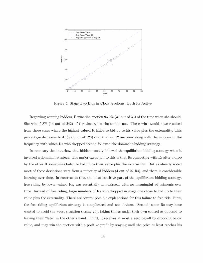
Figure 5 reports second dropouts by Rs when both bidders are Rs. In this case 94.6% of all

bids are within plus or minus 3 ECUs of the dominant bidding strategy. Dropped from Figure 5 are

cases where Rs were bidding above value at the point that the E dropped out. For these Rs there

is an obvious incentive to drop immediately at that point, which virtually all of them did.

13

0 10 20 30 40 50 60 70 80 90 1000

20

40

60

80

100

120

Value

Dro

p P

rice

Drop Price=ValueDrop Price=Value+20Regular (Opponent is Regular)

Figure 5: Stage-Two Bids in Clock Auctions: Both Rs Active

Regarding winning bidders, E wins the auction 93.9% (31 out of 33) of the time when she should.

She wins 5.8% (14 out of 242) of the time when she should not. These wins would have resulted

from those cases where the highest valued R failed to bid up to his value plus the externality. This

percentage decreases to 4.1% (5 out of 123) over the last 12 auctions along with the increase in the

frequency with which Rs who dropped second followed the dominant bidding strategy.

In summary the data show that bidders usually followed the equilibrium bidding strategy when it

involved a dominant strategy. The major exception to this is that Rs competing with Es after a drop

by the other R sometimes failed to bid up to their value plus the externality. But as already noted

most of these deviations were from a minority of bidders (4 out of 22 Rs), and there is considerable

learning over time. In contrast to this, the most sensitive part of the equilibrium bidding strategy,

free riding by lower valued Rs, was essentially non-existent with no meaningful adjustments over

time. Instead of free riding, large numbers of Rs who dropped in stage one chose to bid up to their

value plus the externality. There are several possible explanations for this failure to free ride. First,

the free riding equilibrium strategy is complicated and not obvious. Second, some Rs may have

wanted to avoid the worst situation (losing 20), taking things under their own control as opposed to

leaving their “fate” in the other’s hand. Third, R receives at most a zero payoff by dropping below

value, and may win the auction with a positive profit by staying until the price at least reaches his

14

value. So that free riding involves giving up the chance of winning with a positive profit. Finally,

given that a number of Rs either bid up to their value plus the externality, or up to their value, in

stage one, the equilibrium strategy in stage one is no longer a best response.

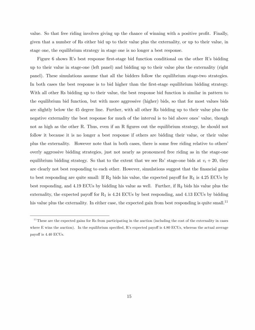
Figure 6 shows R’s best response first-stage bid function conditional on the other R’s bidding

up to their value in stage-one (left panel) and bidding up to their value plus the externality (right

panel). These simulations assume that all the bidders follow the equilibrium stage-two strategies.

In both cases the best response is to bid higher than the first-stage equilibrium bidding strategy.

With all other Rs bidding up to their value, the best response bid function is similar in pattern to

the equilibrium bid function, but with more aggressive (higher) bids, so that for most values bids

are slightly below the 45 degree line. Further, with all other Rs bidding up to their value plus the

negative externality the best response for much of the interval is to bid above ones’ value, though

not as high as the other R. Thus, even if an R figures out the equilibrium strategy, he should not

follow it because it is no longer a best response if others are bidding their value, or their value

plus the externality. However note that in both cases, there is some free riding relative to others’

overly aggressive bidding strategies, just not nearly as pronounced free riding as in the stage-one

equilibrium bidding strategy. So that to the extent that we see Rs’ stage-one bids at vi + 20, they

are clearly not best responding to each other. However, simulations suggest that the financial gains

to best responding are quite small: If R2 bids his value, the expected payoff for R1 is 4.25 ECUs by

best responding, and 4.19 ECUs by bidding his value as well. Further, if R2 bids his value plus the

externality, the expected payoff for R1 is 4.24 ECUs by best responding, and 4.13 ECUs by bidding

his value plus the externality. In either case, the expected gain from best responding is quite small.11

11These are the expected gains for Rs from participating in the auction (including the cost of the externality in cases

where E wins the auction). In the equilibrium specified, R’s expected payoff is 4.80 ECUs, whereas the actual average

payoff is 4.40 ECUs.

15

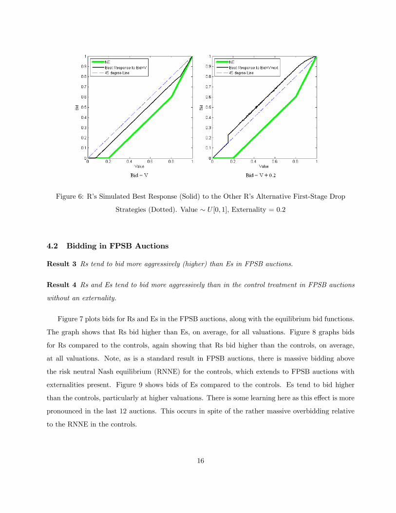
Figure 6: R’s Simulated Best Response (Solid) to the Other R’s Alternative First-Stage Drop

Strategies (Dotted). Value ∼ U [0, 1], Externality = 0.2

4.2 Bidding in FPSB Auctions

Result 3 Rs tend to bid more aggressively (higher) than Es in FPSB auctions.

Result 4 Rs and Es tend to bid more aggressively than in the control treatment in FPSB auctions

without an externality.

Figure 7 plots bids for Rs and Es in the FPSB auctions, along with the equilibrium bid functions.

The graph shows that Rs bid higher than Es, on average, for all valuations. Figure 8 graphs bids

for Rs compared to the controls, again showing that Rs bid higher than the controls, on average,

at all valuations. Note, as is a standard result in FPSB auctions, there is massive bidding above

the risk neutral Nash equilibrium (RNNE) for the controls, which extends to FPSB auctions with

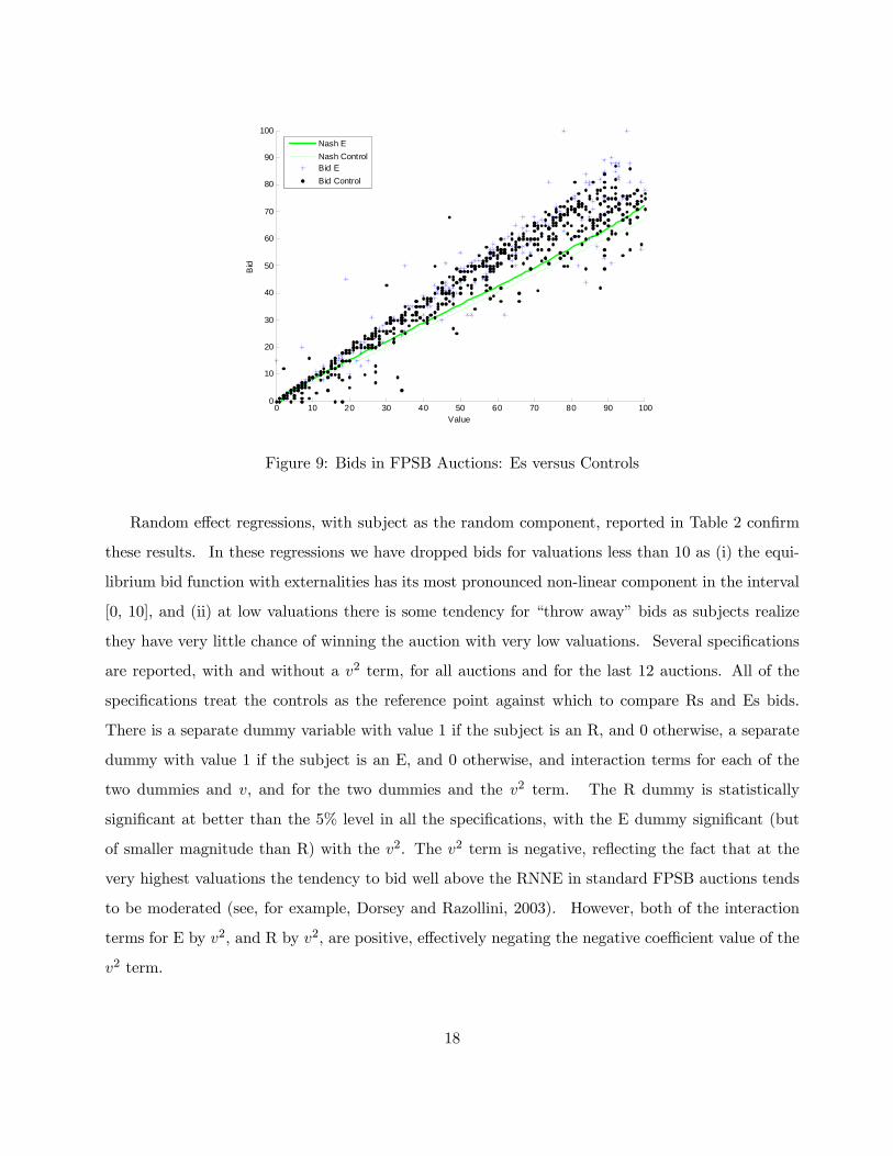
externalities present. Figure 9 shows bids of Es compared to the controls. Es tend to bid higher

than the controls, particularly at higher valuations. There is some learning here as this effect is more

pronounced in the last 12 auctions. This occurs in spite of the rather massive overbidding relative

to the RNNE in the controls.

16

 

0 10 20 30 40 50 60 70 80 90 1000

20

40

60

80

100

120

Value

Bid

Nash RNash EBid RBid E

Figure 7: Bids in FPSB Auctions with Externality Present

 

0 10 20 30 40 50 60 70 80 90 1000

20

40

60

80

100

120

Value

Bid

Nash RNash ControlBid RBid Control

Figure 8: Bids in FPSB Auctions: Rs versus Controls

17

 

0 10 20 30 40 50 60 70 80 90 1000

10

20

30

40

50

60

70

80

90

100

Value

Bid

Nash ENash ControlBid EBid Control

Figure 9: Bids in FPSB Auctions: Es versus Controls

Random effect regressions, with subject as the random component, reported in Table 2 confirm

these results. In these regressions we have dropped bids for valuations less than 10 as (i) the equi-

librium bid function with externalities has its most pronounced non-linear component in the interval

[0, 10], and (ii) at low valuations there is some tendency for “throw away” bids as subjects realize

they have very little chance of winning the auction with very low valuations. Several specifications

are reported, with and without a v2 term, for all auctions and for the last 12 auctions. All of the

specifications treat the controls as the reference point against which to compare Rs and Es bids.

There is a separate dummy variable with value 1 if the subject is an R, and 0 otherwise, a separate

dummy with value 1 if the subject is an E, and 0 otherwise, and interaction terms for each of the

two dummies and v, and for the two dummies and the v2 term. The R dummy is statistically

significant at better than the 5% level in all the specifications, with the E dummy significant (but

of smaller magnitude than R) with the v2. The v2 term is negative, reflecting the fact that at the

very highest valuations the tendency to bid well above the RNNE in standard FPSB auctions tends

to be moderated (see, for example, Dorsey and Razollini, 2003). However, both of the interaction

terms for E by v2, and R by v2, are positive, effectively negating the negative coefficient value of the

v2 term.

18

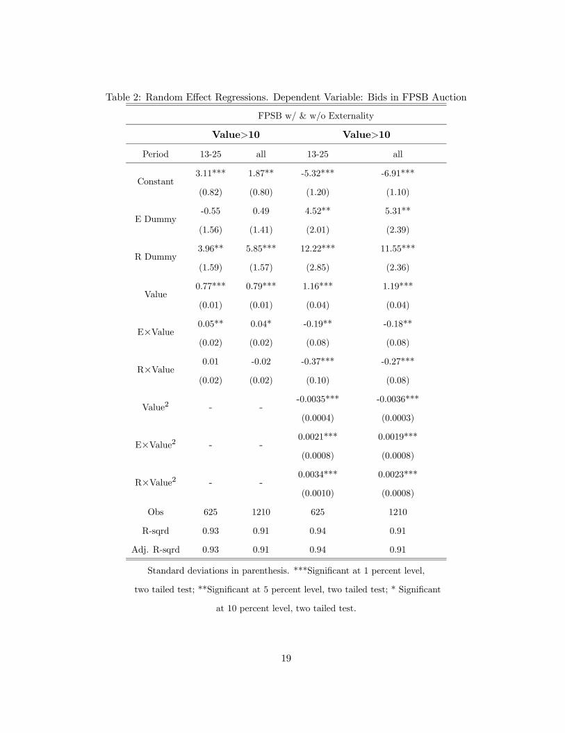
Table 2: Random Effect Regressions. Dependent Variable: Bids in FPSB Auction

FPSB w/ & w/o Externality

Value>10 Value>10

Period 13-25 all 13-25 all

Constant3.11***

(0.82)

1.87**

(0.80)

-5.32***

(1.20)

-6.91***

(1.10)

E Dummy-0.55

(1.56)

0.49

(1.41)

4.52**

(2.01)

5.31**

(2.39)

R Dummy3.96**

(1.59)

5.85***

(1.57)

12.22***

(2.85)

11.55***

(2.36)

Value0.77***

(0.01)

0.79***

(0.01)

1.16***

(0.04)

1.19***

(0.04)

E×Value0.05**

(0.02)

0.04*

(0.02)

-0.19**

(0.08)

-0.18**

(0.08)

R×Value0.01

(0.02)

-0.02

(0.02)

-0.37***

(0.10)

-0.27***

(0.08)

Value2 - --0.0035***

(0.0004)

-0.0036***

(0.0003)

E×Value2 - -0.0021***

(0.0008)

0.0019***

(0.0008)

R×Value2 - -0.0034***

(0.0010)

0.0023***

(0.0008)

Obs 625 1210 625 1210

R-sqrd 0.93 0.91 0.94 0.91

Adj. R-sqrd 0.93 0.91 0.94 0.91

Standard deviations in parenthesis. ***Significant at 1 percent level,

two tailed test; **Significant at 5 percent level, two tailed test; * Significant

at 10 percent level, two tailed test.

19

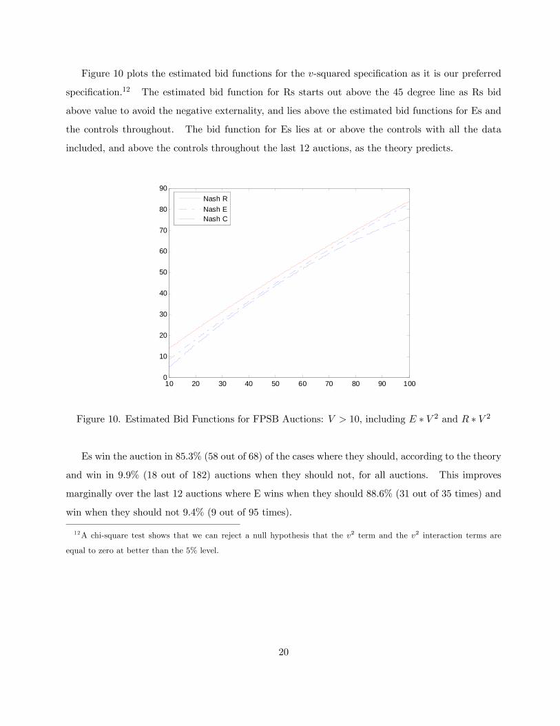
Figure 10 plots the estimated bid functions for the v-squared specification as it is our preferred

specification.12 The estimated bid function for Rs starts out above the 45 degree line as Rs bid

above value to avoid the negative externality, and lies above the estimated bid functions for Es and

the controls throughout. The bid function for Es lies at or above the controls with all the data

included, and above the controls throughout the last 12 auctions, as the theory predicts.

 

10 20 30 40 50 60 70 80 90 1000

10

20

30

40

50

60

70

80

90Nash RNash ENash C

Figure 10. Estimated Bid Functions for FPSB Auctions: V > 10, including E ∗ V 2 and R ∗ V 2

Es win the auction in 85.3% (58 out of 68) of the cases where they should, according to the theory

and win in 9.9% (18 out of 182) auctions when they should not, for all auctions. This improves

marginally over the last 12 auctions where E wins when they should 88.6% (31 out of 35 times) and

win when they should not 9.4% (9 out of 95 times).

12A chi-square test shows that we can reject a null hypothesis that the v2 term and the v2 interaction terms are

equal to zero at better than the 5% level.

20

4.3 Revenue and Efficiency

Result 5 The FPSB auction yields more revenue than the clock auction, and has a smaller variance

in revenue.

Table 3 compares average revenue under the two auction formats for all auctions and for the

last 12 auctions, where predicted revenue is based on auction valuations used in the experiment.

Predicted revenue is higher under the FPSB auction in both cases. Actual revenue is substantially

higher than predicted revenue in the FPSB auctions, which is not unexpected given the typical

overbidding (relative to the RNNE) found in IPV auctions without externalities present. Actual

revenue is a bit higher than predicted revenue in the clock auctions. This is a result of the absence

of free riding in stage one in the data. Revenue is significantly higher in the FPSB auctions, whether

we use the raw data or differences in actual versus predicted revenue for the two auction formats (p

< 0.01 in either case).

Table 3: Revenue

Ascending clock FPSB Difference

Actual Predicted Actual Predicted Actual Predicted

Period 1-2554.14

(1.48)

50.86

(1.42)

64.87

(1.09)

54.93

(0.81)10.73*** 4.07

Period 13-2551.69

(2.09)

48.46

(1.95)

65.30

(1.48)

55.51

(1.09)13.61*** 7.05

Notes: Standard deviation in parenthesis.

*** Significant at the 0.01 level using two-tailed Mann-Witney test

Result 6 The clock auction is more efficient than the FPSB auction when the externality is present.

We measure efficiency strictly in terms of the frequency with which the highest valued bidder

wins the auction. For Rs this measure of value includes the cost of the externality. In equilibrium

the clock auction is almost always predicted to be efficient because free riding only exists in the

first-stage of an auction (when no one drops) and bidders have a dominant strategy to bid up to

21

their valuations after that.13 In contrast, the FPSB auction with the externality present is akin to

an auction with asymmetric valuations, so that efficiency will, in general, be less than 100%.

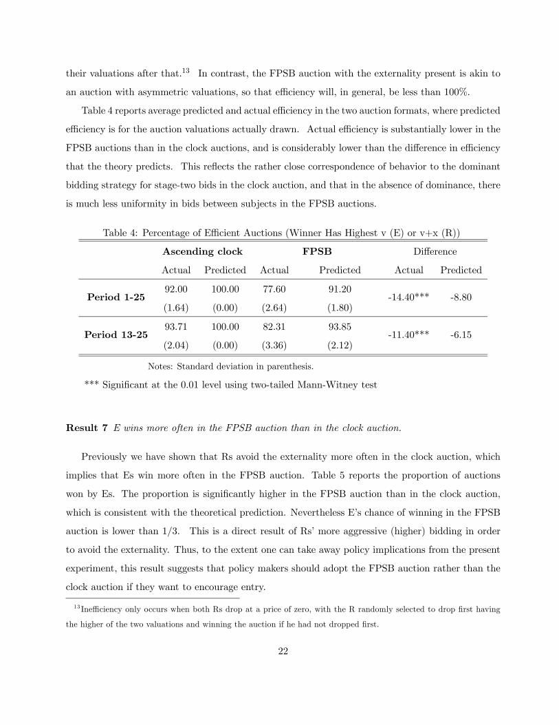
Table 4 reports average predicted and actual efficiency in the two auction formats, where predicted

efficiency is for the auction valuations actually drawn. Actual efficiency is substantially lower in the

FPSB auctions than in the clock auctions, and is considerably lower than the difference in efficiency

that the theory predicts. This reflects the rather close correspondence of behavior to the dominant

bidding strategy for stage-two bids in the clock auction, and that in the absence of dominance, there

is much less uniformity in bids between subjects in the FPSB auctions.

Table 4: Percentage of Efficient Auctions (Winner Has Highest v (E) or v+x (R))

Ascending clock FPSB Difference

Actual Predicted Actual Predicted Actual Predicted

Period 1-2592.00

(1.64)

100.00

(0.00)

77.60

(2.64)

91.20

(1.80)-14.40*** -8.80

Period 13-2593.71

(2.04)

100.00

(0.00)

82.31

(3.36)

93.85

(2.12)-11.40*** -6.15

Notes: Standard deviation in parenthesis.

*** Significant at the 0.01 level using two-tailed Mann-Witney test

Result 7 E wins more often in the FPSB auction than in the clock auction.

Previously we have shown that Rs avoid the externality more often in the clock auction, which

implies that Es win more often in the FPSB auction. Table 5 reports the proportion of auctions

won by Es. The proportion is significantly higher in the FPSB auction than in the clock auction,

which is consistent with the theoretical prediction. Nevertheless E’s chance of winning in the FPSB

auction is lower than 1/3. This is a direct result of Rs’ more aggressive (higher) bidding in order

to avoid the externality. Thus, to the extent one can take away policy implications from the present

experiment, this result suggests that policy makers should adopt the FPSB auction rather than the

clock auction if they want to encourage entry.

13 Inefficiency only occurs when both Rs drop at a price of zero, with the R randomly selected to drop first having

the higher of the two valuations and winning the auction if he had not dropped first.

22

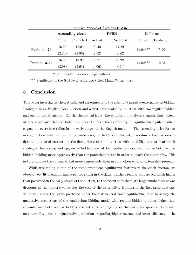
Table 5: Percent of Auctions E Win

Ascending clock FPSB Difference

Actual Predicted Actual Predicted Actual Predicted

Period 1-2516.36

(2.23)

12.00

(1.96)

30.40

(2.92)

27.20

(2.82)14.04*** 15.20

Period 13-2516.08

(3.08)

13.99

(2.91)

30.77

(4.06)

26.92

(3.91)14.69*** 12.93

Notes: Standard deviation in parenthesis.

*** Significant at the 0.01 level using two-tailed Mann-Witney test

5 Conclusion

This paper investigates theoretically and experimentally the effect of a negative externality on bidding

strategies in an English clock auction and a first-price sealed bid auction with two regular bidders

and one potential entrant. On the theoretical front, the equilibrium analysis suggests that instead

of very aggressive (higher) bids in an effort to avoid the externality, in equilibrium regular bidders

engage in severe free riding in the early stages of the English auction. The ascending price format

in conjunction with the free riding enables regular bidders to efficiently coordinate their actions to

fight the potential entrant. In the first price sealed bid auction with no ability to coordinate their

strategies, free riding and aggressive bidding coexist for regular bidders, resulting in both regular

bidders bidding more aggressively than the potential entrant in order to avoid the externality. This

in turn induces the entrant to bid more aggressively than in an auction with no externality present.

While free riding is one of the most prominent equilibrium features in the clock auction, we

observe very little equilibrium type free riding in the data. Rather, regular bidders bid much higher

than predicted in the early stages of the auction, to the extent that there are large numbers stage-one

dropouts at the bidder’s value plus the cost of the externality. Bidding in the first-price auctions,

while well above the levels predicted under the risk neutral Nash equilibrium, tend to satisfy the

qualitative predictions of the equilibrium bidding model with regular bidders bidding higher than

entrants, and both regular bidders and entrants bidding higher than in a first-price auction with

no externality present. Qualitative predictions regarding higher revenue and lower efficiency in the

23

sealed bid versus clock auctions, along with the likelihood of the entrant winning the auction, are

satisfied in the data as well.

Our model follows the literature in using the term “externality” to measure the negative payoff

to an incumbent when losing the auction. Perhaps a more proper term might be “post-auction

effects.” Extensions can be made to enrich the post-auction interactions, so that the “externality”

would be a variable endogenously determined by the post-auction game. Investigation of this issue

is left for future research.

24

Appendix: Proof of the Equilibrium Bidding Strategies in the Clock

Auction

Since the potential entrant (E) does not suffer from the externality, her dominant strategy is to

remain active until the price equals her value no matter how many other bidders are remaining. It

is also easy to show the equilibrium strategy after one bidder has dropped. As we assume that the

identity of bidders is public information, a regular bidder will drop at his private value if his rival is

regular, and drop at his private value plus the absolute value of externality if his rival is an E.

The non-trivial part is the proof of the regular bidders’ equilibrium strategies when nobody has

dropped. Without loss of generality, we will examine (regular) bidder 1’s incentive to deviate, given

that all the other bidders follow the proposed equilibrium strategies. We will consider the following

three cases: (1) v1 ≤ x; (2) x < v1 ≤ 1− x; and (3) v1 > 1− x, where x is the absolute value of the

externality. If bidder 1 deviates by dropping earlier or later than the equilibrium strategy, his payoff

is affected only when the deviation changes the identity of the first dropped bidder. After the first

bidder drops out, the analysis of the 2-bidder subgame is straightforward. If bidder 1’s deviation

does not change the identity of the first dropped bidder and the identities of the remaining bidders,

such a deviation will not affect bidder 1’s payoff, because 1’s payoff is still completely determined by

the values of the bidders in the 2-bidder subgame.

1. When v1 ≤ x, B(v1) = 0

In equilibrium, bidder 1 is supposed to drop at the beginning. Here we need to consider two

cases for bidder 2’s value: (a) v2 > x and (b) v2 ≤ x.

(a) v2 > x:

The equilibrium dictates that bidder 2 and E remain in the auction after bidder 1’s

dropping at P = 0. In this case bidder 1 has no risk of free riding, because if bidder 2

cannot win the auction, bidder 1 cannot win either since v2 > v1. If bidder 1 deviates and

stays longer, his payoff is affected only if bidder 2 or E drops first. If E drops first, bidder

1’s payoff will not be affected since bidder 2 will win anyway. If bidder 2 drops first at

P < v1, bidder 1’s net gain from deviation will be:

−Z v2+x

v1+xxdvE +

Z v1+x

v1

(v1 − vE)dvE +

Z v1

P(v1 − vE)dvE < 0 for all P < v1.

25

This is the expected gain based on three possible outcomes: bidder 1 loses and bidder 2

could have won if he stays; bidder 1 wins with negative payoff; and bidder 1 wins with

positive payoff. The net gain is negative for any deviation to P < v1, so bidder 1 has

no incentive to deviate to P < v1. It is easily seen that he has no incentive to deviate

to P > v1 either because such a deviation implies winning and losing money, or he could

have dropped earlier, free riding on bidder 2 as the latter has a higher value.

(b) v2 ≤ x:

Bidder 2 will drop in the beginning at P = 0. The tie-breaking rule guarantees that

bidder 1 and 2 cannot both drop simultaneously. If they both choose to drop at P = 0,

one is randomly chosen as the first dropped bidder, and the other can choose to stay or

drop out. Of course the 2nd bidder, seeing the other regular bidder dropping out, would

choose to stay and try to win against E to avoid the externality. We will see below that

bidder 1 will find it optimal to drop in the beginning when v1 ≤ x.

If bidder 1 drops at P = 0, while bidder 2 has to remain and compete with E, bidder 1’s

expected payoff is:

−Z x

0

Z 1

v2+xxdvEdv2 = −x

µx− 3

2x2¶

(3)

If bidder 2 drops at P = 0, while bidder 1 has to remain and compete with E, bidder 1’s

expected payoff is

−Z 1

v1+xxdvE +

Z v1+x

0(v1 − vE)dvE =

1

2(x+ v1)

2 − x (4)

Since x > v1, the payoff in (4) is less than 12(x+v1)

2−x = 2x2−x. Since we assume that x

is not too big (i.e., x ≤ 1−√33 ≈ 0.429), we have 3x2−6x+2 > 0, so 2x2−x < −x(x− 32x2),

and hence the payoff in (3) is greater than the payoff in (4). This in turn implies that

even when v2 ≤ x, it is optimal for bidder 1 to drop at the beginning.

To summarize, when v1 ≤ x, bidder 1 has no incentive to deviate from the equilibrium

strategy of dropping at P = 0.

2. When x < v1 ≤ 1− x, B(v1) = v1 − x

26

In equilibrium, bidder 1 is supposed to drop at price v1 − x if nobody has dropped. We will

consider three possible deviations: (a) stay until P ≥ v1; (b) stay until P ∈ (v1 − x, v1); and

(c) drop before v1 − x.

(a) Deviation to Staying Until P ≥ v1:

By the time of P = v1, seeing that nobody has dropped, bidder 1 is aware that v2 ≥ v1.

So he would prefer to drop and free ride on bidder 2.

(b) Deviation to Staying Until P ∈ (v1 − x, v1):

By remaining longer, bidder 1 can alter his payoff only if bidder 2 or E drops first.

If E drops first at any P ∈ (v1 − x, v1), bidder 2 will win regardless of the deviation. So

bidder 1 is indifferent between deviating and not deviating.

If bidder 2 drops first at any P ∈ (v1−x, v1) with bidder 1 and E remaining in the auction,

we must have v2 > v1 and

v2 =

½P + x if P ≤ 1− 2x12(P + 1) if P > 1− 2x

Here bidder 2’s private value is deduced from his dropping price P and equilibrium strat-

egy. If v2 ≤ 1−x, bidder 2 will drop at P = v2−x, which implies v2 = P +x; if v2 > 1−x,

bidder 2 will drop at P = 2v2 − 1, which implies v2 = 12(P + 1). After bidder 2 drops,

bidder 1 will remain active until E drops (1 wins) or the price arrives v1+x (E wins). We

can show that whether P < 1− 2x or P > 1− 2x, bidder 1 has no incentive to deviate:

If P < 1− 2x, thus v2 = P + x < 1− x, bidder 1’s expected gain from deviating is

−Z P+2x

v1+xxdvE +

Z v1+x

v1

(v1 − vE)dvE +

Z v1

P(v1 − vE)dvE < 0 for any P ∈ (v1 − x, v1).

If P > 1− 2x thus v2 = 12(P + 1) > 1− x, bidder 2 can always win against E (though he

may lose money) in the subgame. Bidder 1’s expected net gain from deviating is:Z v1+x

P(v1 − vE)dvE −

Z 1

v1+xxdvE =

1

2(v1 + x− P ) · (v1 − x− P )− x(1− x− v1) < 0

for any v1 − x < P < v1 and x < v1 < 1− x.

Bidder 1’s expected net gain from deviation is negative in both situations. So he has no

incentive to deviate, staying until P ∈ (v1 − x, v1).

27

(c) Deviation to Dropping Before v1 − x:

Such a deviation affects bidder 1’s payoff only when it prevents some other bidder from

dropping first.

If E is prevented from dropping first, bidder 1’s expected payoff is reduced by such a

deviation. His expected net gain from keeping E at P < v1 − x isZ v1

P+x(v2 − v1)dv2 < 0− for any P < v1 − x,

since bidder 1 loses the chance of winning against bidder 2 and getting a positive payoff.

If bidder 2 is prevented from dropping first, we must have v2 < v1. Thus, when bidder

2 is able to win against E in a 2-bidder sub-game, bidder 1 can win too. Bidder 2 free

rides on bidder 1 in this situation. Bidder 1 might be better off by dropping earlier than

dictated by the equilibrium strategy to avoid this situation. However, such a deviation

also eliminates his chance of winning the auction with a positive profit. We can show that

the harm of such deviation outweighs the benefit:

Bidder 1’s expected net gain from deviating and dropping before v1 − x isZ v2+x

v1

(vE − v1)dvE −Z v1+x

v2+x(vE − v1 − x)dvE +

Z v1

P(vE − v1)dvE

= −12(v1 + x− P ) · (v1 − x− P )− x(1− x− v1) < 0 for any P < v1 − x.

So bidder 1 has no incentive to deviate and drop before v1 − x.

To summarize, bidder 1 has no incentive to deviate from B(v1) = v1 − x when x < v1 <

1− x.

3. When v1 ≥ 1− x,B(v1) = 2v1 − 1

In equilibrium, bidder 1 is supposed to drop at P = 2v1−1 if nobody has dropped. We examine

the following possible deviations: (a) stay longer and drop at P ≥ 2v1 − 1; (b) drop earlier at

P < 2v1 − 1.

(a) Deviation to Dropping at P ≥ 2v1 − 1:

When the price reaches P = 2v1 − 1, bidder 1 knows v2 > v1 > 1 − x. It is clear that

bidder 2 will win if bidder 1 drops first. By dropping at P = 2v1 − 1, bidder 1’s expected

28

payoff is 0. If he deviates by staying longer, his payoff is affected only if someone else

drops first at P > 2v1 − 1:

If E drops first, bidder 2 will win. There is no effect on bidder 1’s payoff.

If bidder 2 drops first at P > 2v1 − 1, bidder 1’s expected payoff at P isZ 1

P(vE − v1)dvE = (v1 −

1

2(1 + P )) · (1− P ) < 0,

since P < 1 and v1 − 12(1 + P ) > 0.

So bidder 1 cannot be strictly better off by staying longer than dictated by the equilibrium

strategy.

(b) Deviation to Dropping Earlier at P < 2v1 − 1:

Such a deviation could affect bidder 1’s payoff only if it prevents bidder 2 or E from

dropping first at P < 2v1 − 1.

If E is prevented from dropping first, bidder 1 cannot be better off by deviating. If he

deviates in order to be the first dropped bidder, he earns no more than zero profit. If

he follows the equilibrium strategy and stays, he can get a positive profit if his value is

greater than v2, and will have at least zero profit if his value is less than v2.

If bidder 2 is prevented from dropping first at P < 2v1−1, we can deduce bidder 2’s value

from his dropping price and equilibrium strategies:

v2 =

⎧⎨⎩ P + x if v2 ≤ 1− x

12(P + 1) if v2 > 1− x

In the first case, P = v2 − x ≤ 1 − 2x, bidder 1 has no incentive to drop early; In the

second case, v2 > 1−x and v2 = 12(P +1). By deviating and dropping at P to keep bidder

2 in the game, bidder 1 secures an expected payoff of zero because bidder 2 will certainly

win over E in the 2-bidder subgame. However, following the equilibrium strategy, bidder

1’s expected payoff is positive:Z 1

P(v1 − vE)dvE = (1− P ) · (v1 −

1

2(1 + P )) > 0 for any v1 >

1

2(1 + P ),

since P < 1 and v1 >12(1 + P ).

So it is also clear that bidder 1 will follow the proposed equilibrium if v1 ≥ 1− x.

29

References

[1] Caillaud, B.; Jehiel, P. (1998). Collusions in Actions with Externalities. Rand Journal of Eco-

nomics 29(4): 680-702.

[2] Das Varma, G. (2002). Standard Auctions with Identity-Dependent Externalities. RAND Jour-

nal of Economics 33(4): 689-708.

[3] Dorsey, R. and L. Razzolini (2003). Explaining overbidding in first price auctions using controlled

lotteries. Experimental Economics 6:123-140.

[4] Ettinger, D. (2003). Bidding among Friends and Enemies. Fondazione Eni Enrico Mattei, Work-

ing Papers: 2003.23.

[5] Fishbacker, U. (2007). z-Tree: Zurich Toolbox for Ready-Made Economic Experiments. Experi-

mental Economics 10: 171-178.

[6] Goeree, J.; Offerman, T.; Sloof, R. (2004). Demand Reduction and Preemptive Bidding in

Multi-Unit License Auctions. Tinbergen Institute Discussion Paper.

[7] Jehiel, P.; Moldovanu, B. (1995). Negative Externalities May Cause Delay in Negotiation; Econo-

metrica 63(6): 1321-35.

[8] Jehiel, P.; Moldovanu, B. (1996). Strategic Nonparticipation. RAND Journal of Economics

27(1): 84-98.

[9] Jehiel, P.; Moldovanu, B.; Stacchetti, E. (1996). How (Not) to Sell Nuclear Weapons. American

Economic Review 86(4): 814-29.

[10] Jehiel, P.; Moldovanu, B.; Stacchetti, E. (1999). Multidimensional Mechanism Design for Auc-

tions with Externalities. Journal of Economic Theory 85(2): 258-93.

[11] Kagel, J. (1995). Auctions: A Survey of Experimental Research. In: Kagel, J.H., Roth, A.

(Eds.), The Handbook of Experimental Economics. Princeton University Press, pp. 501-86.

[12] Milgrom, P. (2004). Putting Auction Theory to Work (Churchill Lectures in Economics). Cam-

bridge University Press.

30

[13] Milgrom, P., Weber, R. (1982). A Theory of Auctions and Competitive Bidding. Econometrica

50: 1082-1122.

[14] Myerson, R. (1981). Optimal Auction Design. Mathematics of Operations Research 6: 58-73.

[15] Riley, J., Samuelson, W. (1981). Optimal Auctions. American Economic Review 71: 381-392.

[16] Vickrey, W. (1961). Counterspeculation, Auctions, and Competitive Sealed Tenders. Journal of

Finance 16: 8-37.

31