Evidence on the Uncertainty of Future Earnings from Capital ...

Capitalization versus Expensing: Evidence on the Uncertainty ofFuture Earnings from Capital Expenditures versus R&D Outlays

S.P. KothariSloan School of Management

Massachusetts Institute of Technology50 Memorial Drive, E52-325

Cambridge, MA 02142E-mail: [email protected]

617-253-0994

Ted E. LaguerreAnalysis Group

[email protected]

and

Andrew J. LeoneWilliam E. Simon Graduate School of Business Administration

University of Rochester, Rochester, NY 14627E-mail: [email protected]

716 275-4714

First draft: June 1998Revised: November 2000

We are grateful to two anonymous referees, Anwer Ahmed, Joy Begley, John Core, ElizabethEccher, Wayne Guay, David Guenther, Rob Ingram, Shelly Jain, Larry Weiss, Paul Zarowin, andespecially Jerry Feltham and Jerry Zimmerman, and seminar participants at the University ofBritish Columbia, University of Colorado at Boulder, INSEAD, University of Michigan,University of Tilburg, and University of Technology in Sydney for helpful comments on thepaper. We thank the Bradley Policy Research Center at the Simon School and the John M. OlinFoundation for financial support.

Capitalization versus Expensing: Evidence on the Uncertainty ofFuture Earnings from Capital Expenditures versus R&D Outlays

I. INTRODUCTION

We present evidence on the relation between R&D costs and the uncertainty of future

benefits from those investments using financial data from 1972-1997 for a large sample of firms.

Existing empirical research focuses mainly on examining the relevance of accounting disclosures

about R&D costs (i.e., association of R&D costs with security prices or returns). We believe the

evidence from our study on the uncertainty of benefits from R&D costs, combined with the

evidence from previous research on the relevance of R&D costs for security prices, will

contribute to the on-going debate among academics, practitioners, and regulators on accounting

for R&D. However, based on the evidence in the paper, we are unable to make an unambiguous

policy recommendation as to whether R&D costs should be expensed or capitalized.

An important issue facing U.S. and international accounting standard setters is the

financial reporting of corporate R&D expenditures. U.S GAAP (Statement of Financial

Accounting Standards, SFAS, No. 2, 1974, and Proposed Statement of Position dated April 22,

1997) requires corporations to immediately expense their R&D expenditures. By contrast,

International Accounting Standard No. 9 (1978) and the International Accounting Standards

Committee’s Exposure Draft E60 (1997) on intangible assets allow corporations to capitalize

development expenditures and require expensing only research outlays.

The U.S. standard on the accounting treatment of R&D expenditures (i.e., SFAS No. 2) is

likely influenced by the standard setters’ perceived degree of uncertainty about future economic

benefits from current research and development outlays. Paragraphs 48, 49, and 50 of SFAS No.

2 summarize FASB’s rationale for requiring immediate expensing of R&D costs. FASB applied

the principles for recognizing costs as expenses as set forth in Accounting Principles Board

Statement No. 4, paragraphs 156-160. FASB states “…there is often a high degree of

uncertainty about whether research and development expenditures will provide any future

2

benefits” (paragraph 49). In paragraph 50 it states “…the relationship between current research

and development costs and the amount of resultant future benefits to an enterprise is so uncertain

that capitalization of any research and development costs is not useful in assessing the earnings

potential of the enterprise.” The significant consideration of the uncertainty of future benefits

from R&D costs in the standard-setting process suggests standard setters consider the usefulness

of a balance sheet in credit (or lending) decisions to be an important factor.

FASB continues to employ the degree of uncertainty of future benefits as a criterion in

determining whether a given cost should be capitalized or expensed. This is seen from FASB’s

definition of assets as “probable future economic benefits obtained or controlled by a particular

entity as a result of past transactions or events” (Statement of Financial Accounting Concepts

No. 6, 1980). Thus, the greater the uncertainty of future economic benefits from R&D

expenditures, the weaker would be the case in favor of capitalization (i.e., recognition of R&D as

an asset on the balance sheet) even if on average the future benefits are positive.

The current debate among academics and practitioners on capitalization versus expensing

of R&D expenditures has been without direct empirical evidence on the uncertainty of future

earnings and cash flows attributable to current R&D outlays. Bierman and Dukes (1975) is the

only study to our knowledge that comes close to examining the relation between R&D and the

uncertainty of future benefits. They survey the literature at the time and conclude that FASB

overestimates the risk of future benefits from R&D investments. They argue that when looking

at a company’s R&D investment portfolio, the risks are lower than for an individual project.1

However, no direct evidence is offered on the degree of risk of future benefits (e.g., earnings or

cash flows) associated with R&D investments.

1 SFAS No. 2 deems “not appropriate to consider accounting for research and development activities on anaggregate or total-enterprise basis” (paragraph 52). The reason is that “For accounting purposes the expectation offuture benefits generally is not evaluated in relation to broad categories of expenditures on an enterprise-wide basisbut rather in relation to individual or related transactions or projects” (paragraph 52).

3

Recent research on the accounting treatment of R&D expenditures (e.g., Chambers,

Jennings, and Thompson, 1998, Deng and Lev, 1997, and Lev and Sougiannis, 1996, and

Sougiannis, 1994) provides compelling evidence that on average the market assigns a

statistically and economically significant valuation to corporate R&D activity. This is

interpreted as R&D costs meeting the relevance criterion underlying accounting standard setting.

The evidence, however, does not shed light directly on the degree of uncertainty of the economic

benefits to R&D activity compared to other expenditures that corporations typically capitalize.

Our objective in this study is to provide direct evidence on the relative degree of uncertainty of

future earnings attributable to current R&D investments and to current capital expenditures. The

motivation stems from the fact that, whereas existing evidence is largely on the relevance of

R&D, standard setting is guided by a trade-off between relevance and uncertainty of future

benefits.

The trade-off between relevance and uncertainty of future benefits is in the spirit of the

relevance-reliability trade-off that is often discussed in the context of accounting standards (e.g.,

SFAC No. 2, 1980, Watts and Zimmerman, 1986, pp. 205-206, and Revsine, Collins, and

Johnson, 1998, p. 17). We, however, use the phrase “uncertainty of future benefits,” not

reliability. Accounting information is deemed to be reliable if it “is free of error and bias, is

factual, verifiable, and neutral” (Weygandt, Kieso, and Kell, 1996, p. 496, and SFAC No. 2).

We believe R&D costs would meet the above definition of reliability because the R&D costs

incurred by a firm in a fiscal period can be reasonably accurately established. However, standard

setters are also concerned about the likelihood that future benefits will be realized. If the

definition of reliability is broadened to include uncertainty of future benefits from costs incurred

currently, then our study provides evidence on the reliability component of the relevance-

reliability trade-off in the context of R&D accounting. Interestingly, most readers of our study at

least initially interpret uncertainty of future benefits to be synonymous with reliability.

4

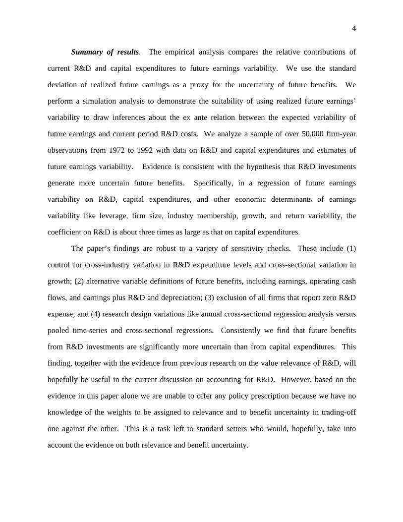
Summary of results. The empirical analysis compares the relative contributions of

current R&D and capital expenditures to future earnings variability. We use the standard

deviation of realized future earnings as a proxy for the uncertainty of future benefits. We

perform a simulation analysis to demonstrate the suitability of using realized future earnings’

variability to draw inferences about the ex ante relation between the expected variability of

future earnings and current period R&D costs. We analyze a sample of over 50,000 firm-year

observations from 1972 to 1992 with data on R&D and capital expenditures and estimates of

future earnings variability. Evidence is consistent with the hypothesis that R&D investments

generate more uncertain future benefits. Specifically, in a regression of future earnings

variability on R&D, capital expenditures, and other economic determinants of earnings

variability like leverage, firm size, industry membership, growth, and return variability, the

coefficient on R&D is about three times as large as that on capital expenditures.

The paper’s findings are robust to a variety of sensitivity checks. These include (1)

control for cross-industry variation in R&D expenditure levels and cross-sectional variation in

growth; (2) alternative variable definitions of future benefits, including earnings, operating cash

flows, and earnings plus R&D and depreciation; (3) exclusion of all firms that report zero R&D

expense; and (4) research design variations like annual cross-sectional regression analysis versus

pooled time-series and cross-sectional regressions. Consistently we find that future benefits

from R&D investments are significantly more uncertain than from capital expenditures. This

finding, together with the evidence from previous research on the value relevance of R&D, will

hopefully be useful in the current discussion on accounting for R&D. However, based on the

evidence in this paper alone we are unable to offer any policy prescription because we have no

knowledge of the weights to be assigned to relevance and to benefit uncertainty in trading-off

one against the other. This is a task left to standard setters who would, hopefully, take into

account the evidence on both relevance and benefit uncertainty.

5

Outline of the paper. Section II surveys the arguments in the literature for and against

R&D capitalization. It also summarizes research on the relevance of R&D cost information in

financial statements. Section III describes the simulation and research design we use to test the

hypothesis that R&D investments produce more uncertain future benefits than capital

expenditures. Section IV presents details of data, sample selection, and descriptive statistics.

Section V contains the results of empirical analysis and sensitivity tests. We conclude in section

VI.

II. ACCOUNTING FOR R&D AND RELATED RESEARCH

This section briefly reviews the arguments that regulators, academics and practitioners

often make for and against expensing R&D costs. We also summarize findings of the accounting

research on R&D expensing versus capitalizing. Almost invariably previous studies focus on

evaluating the relevance of R&D costs. We are unaware of scientific evidence on the relative

degree of uncertainty of benefits from R&D costs versus capital expenditures.

Rationale for expensing R&D expenditures. Some favor immediate expensing of R&D

costs on the grounds that reliable evidence of future economic benefits from current R&D

activity is lacking. For example, the Association for Investment Management and Research

(AIMR) (1993) concurs with the FASB’s expensing of R&D because “it usually is next to

impossible to determine in any sensible or codifiable manner exactly which costs provide future

benefit and which do not” (pp. 50-51). While on average R&D expenditures might generate

future economic benefits, the standard setters’ concern appears to be the lack of compelling

evidence of future benefits to each firm and in each instance to justify R&D capitalization (see

SFAS No. 2, paragraph 52). Moreover, not impressed by the existence of future benefits, AIMR

concludes that the future benefits are so unrelated to costs incurred that the information in the

capitalized amount of R&D costs is largely “irrelevant to the investment valuation process”

(1993, pp. 50-51). This can be interpreted as neither capitalization nor expensing is particularly

helpful or harmful in investors’ valuation of corporations for their investment decisions.

6

The expensing of R&D is consistent with the usefulness of a balance sheet in credit

decisions (i.e., in lending and in writing debt contracts) being an important factor in the standard-

setting process. The high degree of uncertainty of future benefits from R&D costs and the

generally negligible collateral value of R&D investments make R&D less attractive for

capitalization. R&D expenditures have low collateral value in part because there typically are

few alternative uses for them or the liquidation value in the event of project failure is not

substantial. This is unlike the collateral value of tangible assets like buildings, plant, and

equipment. Therefore, the agency cost of borrowing against intangible R&D assets is high and

the debt capacity of R&D costs (intangible assets) is low. Empirical evidence bears out this

prediction. For example, Barclay, Smith, and Watts (1995) show that R&D intensive industries

like biotechnology, pharmaceuticals, and computers and software (which are also industries with

growth options or investment opportunities) finance their businesses mostly with equity.2

Rationale for capitalizing R&D expenditures. Proponents of R&D capitalization point

to the evidence that (as if) earnings that reflect the effects of R&D capitalization and

amortization are significantly more highly associated with stock prices and returns than GAAP

earnings with immediate R&D expensing. This is interpreted as “the R&D capitalization process

yields value-relevant information to investors” (Lev and Sougiannis, 1996, p. 134) and as

contradicting FASB’s objection to R&D capitalization in SFAS No. 2 that direct evidence of

R&D costs and specific future benefits does not exist. The proponents therefore argue that it

behooves standard setters to issue a new standard allowing corporations to capitalize R&D costs.

Previous research. A large body of previous research examines issues surrounding the

accounting treatment of R&D costs. Early research following the promulgation of SFAS 2 in

1974 focuses on the standard’s economic consequences. Economic consequences are estimated

2 We are aware that there are alternative theories and explanations for cross-sectional variation in leverage. Forexample, pecking order and static tradeoff are alternative theories of capital structure (see Shyam-Sunder and Myers,1999, for a discussion and empirical evidence). Our objective in discussing the agency-cost based theory of capitalstructure is merely to state that the expensing treatment of R&D is consistent with that theory, but we acknowledgethat it might be consistent with other theories as well.

7

from security price changes and from the standard’s effect on corporate R&D expenditures (e.g.,

Dukes, Dyckman, and Elliott, 1980, Horwitz and Kolodny, 1980, Elliott, Richardson, Dyckman,

and Dukes, 1984, and Wasley and Linsmeier, 1992). This research produces mixed evidence in

part because it lacks power to detect effects on R&D activity in the presence of confounding

economic events like the energy crisis and recession in the mid-1970s (Ball, 1980).

Much of the recent research on this topic focuses on examining the value relevance of

R&D costs. Lev and Sougiannis (1996) and Chambers, Jennings, and Thompson (1998) show

that financial statements restated to reflect economically plausible rates of amortization applied

to hypothetically capitalized R&D investments are more highly associated with security prices

than with financial-statement numbers based on immediate expensing of R&D. Chambers et al.

(1998) find that in a price level regression the estimated coefficient on capitalized R&D costs is

indistinguishable from that on property, plant, and equipment (PP&E). The equality of the two

coefficients is, however, not a sufficient condition to conclude that future benefits from R&D

and PP&E are equally uncertain. The reason is that the market’s pricing is based on the amount,

timing, and systematic uncertainty of future cash flows, whereas our focus is only on the

(systematic and unsystematic) uncertainty of future cash flows, which cannot be unambiguously

inferred from the price-level regression coefficients. Other research shows that advertising and

R&D expenditures have positive impacts on the market value of a firm (Hirschey and Weygandt,

1985, Woolridge, 1988, and Chan, Martin, and Kensinger, 1990). Collectively, these studies

argue that because R&D investments are on average associated with stock prices or because they

are on average value enhancing, they should be capitalized and amortized rather than

immediately expensed.

Unlike Lev and Sougiannis (1996) and Chambers et al. (1998), for at least two reasons

we do not restate financial statements as if R&D were capitalized to examine whether the

uncertainty of the resulting restated earnings series is more sensitive to R&D than capital

8

expenditures. First, regardless of capitalizing or expensing, the current investment in R&D or

capital expenditure would be the same, so the independent variable in the analysis that regresses

future earnings variability on current R&D and capital expenditures will be unaffected. Second,

the variable of interest is the uncertainty of future benefits from current investments (in R&D or

capital assets). Future benefits as estimated using future earnings are indeed affected by the

choice between capitalization and expensing treatments of the investments. To overcome this

problem, we also summarize results using future earnings plus future R&D and depreciation.

This gross earnings measure is a relatively clean proxy for future benefits compared to future

earnings calculated according to GAAP. Evidence in section V shows that the tenor of the

results is similar using the two measures.

III. SIMULATION AND RESEARCH DESIGN

The main hypothesis we test is whether the ex ante expected variability of future earnings

due to R&D investments is greater than that due to capital expenditures. Since expected

variability of future earnings is not observable, we use the standard deviation of realized future

annual earnings for five years. We regress the standard deviation of future earnings on current

R&D, capital expenditures, and other economic determinants of earnings variability, which are

included as control variables in the regression. A comparison of the coefficients on R&D and

capital expenditures provides an indication of the relative sensitivity of earnings variability to

R&D and capital expenditures. The above regression approach using realized earnings

variability uncovers a relation between ex ante expected variability and current investments for

at least two reasons.

First, we perform a simulation, described in detail below, which shows that, if the ex ante

uncertainty of cash flows from R&D exceeds that from capital expenditures, then in a regression

to explain realized earnings variability, the coefficient on R&D will be greater than that on

capital expenditures.

9

Second, use of realized variables to test for an ex ante relation, as in the case of our

hypothesis, is a standard practice in financial economics and accounting. For example, the ex

ante risk-return relation is tested using cross-sectional regressions of realized returns on beta risk

(Fama and MacBeth, 1973, Fama and French, 1992, and Kothari, Shanken, and Sloan, 1995) and

the effect of risk (or discount rates) on earnings response coefficients is examined in regressions

of realized returns on realized earnings (e.g., Easton and Zmijewski, 1989, and Collins and

Kothari, 1989).

Simulation

The simulation is designed to formalize the intuition that the more uncertain the future

benefit, the larger is the coefficient on current investment in a regression of the variance of future

benefits on the investment. The simulation makes apparent the properties of the coefficients

from the regressions. This facilitates the interpretation of the empirical results using data for

real-life firms later in the paper.

The simulation has two parts: (1) simulate R&D, capital expenditure, and future earnings

observations; and (2) estimate a regression of standard deviation of realized future earnings on

current R&D and capital expenditures. For each simulated firm we generate R&D, capital

expenditure, and future earnings data as follows. We begin by assuming that the levels of R&D

and capital expenditures depend on firm size. We randomly select a level of R&D for each firm

to be distributed uniformly between 1 and 5. We then generate the actual R&D outlay over time

to be up to 25% above or below the randomly selected level of R&D for the firm. The level of

capital expenditures is assumed to be on average twice that of R&D, which is comparable to the

Compustat data that we examine later in the paper. Like R&D, actual capital expenditures over

time are assumed to vary randomly around the mean level of capital expenditures for the firm.

Each year’s R&D and capital expenditures produce uncertain future benefits for TR and

TC years. If the current year’s R&D expenditure is RDI, then it yields an actual benefit in each

of the future TR years equal to a random variable that is distributed N[RDI/ TR, σ2(RD)]. Thus,

10

for each simulated firm and the entire simulation sample the expected future benefit from the

current year’s R&D expenditure is simulated to be exactly equal to the R&D expenditure. Of

course, the actual benefit for a simulated firm will almost invariably be different from the

expected benefit and the absolute difference will be increasing in the variance parameter, σ2(RD)

and the amount of R&D investment, RDI. If the discount rate is zero, then the simulations

assume that the R&D expenditure is, on average, a zero net present value investment. The

σ2(RD) parameter determines the level of uncertainty of future benefit realizations per dollar of

R&D investment. The larger the σ2(RD) parameter value, the more uncertain are future benefits

for every dollar invested in R&D. Thus, the simulations, by construction, ensure a positive

relation between the ex ante expected variability of future benefits and R&D expenditures.

Future benefits from current year’s capital expenditure, CI, are similarly simulated over the

future TC years.

Earnings are defined as the sum of realized benefits from R&D and capital expenditures

in the past TR and TC years.3 For example, assume TR = 10 years and TC = 5 years, which

implies R&D benefits are realized over a longer period than benefits from capital expenditures.

Earnings in year 11 would then be the sum of random realizations of benefits from R&D

investments in years 1 to 10 and from capital expenditures in years 6 to 10. We roll the window

forward one year at a time and calculate earnings for five years, i.e., years 11 to 15, for each

firm. We calculate the standard deviation of earnings using realized earnings for the five years.

We repeat the above procedure to obtain a sample of 1,000 observations.

The objective of the simulation is to examine whether the standard deviation of realized

future earnings for years 11 to 15 is related to R&D and capital expenditures in the current year,

year 10. We therefore regress the standard deviation of earnings on R&D and capital

3 Unlike historical cost GAAP earnings, earnings as we define in the simulation analysis do not deduct the R&Doutlay or depreciation of current and past capital expenditures from the realized future benefits. However, resultsare qualitatively similar if earnings were calculated net of these expenses.

11

expenditures for year 10. We repeat the entire simulation 100 times and examine the average

coefficient on R&D and capital expenditure. We also repeat the analysis by changing the

parameter values for the number of years of future benefit from R&D and capital expenditures,

i.e., TR and TC, the level of capital expenditures relative to R&D, the number of future years used

to calculate the standard deviation of earnings, and the variance of future benefits from R&D and

capital expenditures, i.e., σ2(RD) in N[RDI/TR, σ2(RD)] and similarly σ2(C) for capital

expenditure.

We draw the following conclusions from the simulation regressions of the standard

deviation of future earnings on R&D and capital expenditures:

(1) The coefficients on current R&D and capital expenditures increase in the variance offuture benefits from those expenditures, i.e., in the σ2(RD) and σ2(C) parameters.

(2) Other things equal, the sensitivity of future earnings variability (i.e., the regressionslope coefficient) does not depend on the level of R&D and capital expenditures.Obviously, the larger the investment in R&D or capital expenditure, the larger thevariability of future earnings. However, the marginal impact of an additional dollarof investment in R&D or capital expenditures depends only of the σ2(RD) and σ2(C)parameters, not on the level or size of the investment in R&D or capital expenditures.

(3) The longer the period of future benefits, i.e., TR and TC, the larger the coefficient onR&D and capital expenditure. The intuition is as follows. If TR is large, then anygiven year’s earnings are the sum of TR random benefit realizations corresponding toR&D investments in the past TR years. Since the variance of a sum of independentrandom variables is the sum of the variances of the individual random variables, thelarger the TR parameter, the larger the variance, and thus the larger the coefficient onR&D expenditure.

(4) The tenor of the results is not changed if the standard deviation of future earnings iscalculated using more than five observations. (We experimented using up to 8observations.)

In summary, the simulations provide a reasonable basis to regress the standard deviation

of realized future earnings on current R&D and capital expenditures to test the hypothesis that

the ex ante expected variability of earnings is more sensitive to a firm’s R&D outlays than to

capital expenditures.

12

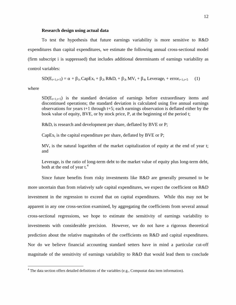
Research design using actual data

To test the hypothesis that future earnings variability is more sensitive to R&D

expenditures than capital expenditures, we estimate the following annual cross-sectional model

(firm subscript i is suppressed) that includes additional determinants of earnings variability as

control variables:

SD(Et+1,t+5) = α + β1t CapExt + β2t R&Dt + β3t MVt + β4t Leveraget + errort+1,t+5 (1)

where

SD(Et+1,t+5) is the standard deviation of earnings before extraordinary items anddiscontinued operations; the standard deviation is calculated using five annual earningsobservations for years t+1 through t+5; each earnings observation is deflated either by thebook value of equity, BVE, or by stock price, P, at the beginning of the period t;

R&Dt is research and development per share, deflated by BVE or P;

CapExt is the capital expenditure per share, deflated by BVE or P;

MVt is the natural logarithm of the market capitalization of equity at the end of year t;and

Leveraget is the ratio of long-term debt to the market value of equity plus long-term debt,both at the end of year t.4

Since future benefits from risky investments like R&D are generally presumed to be

more uncertain than from relatively safe capital expenditures, we expect the coefficient on R&D

investment in the regression to exceed that on capital expenditures. While this may not be

apparent in any one cross-section examined, by aggregating the coefficients from several annual

cross-sectional regressions, we hope to estimate the sensitivity of earnings variability to

investments with considerable precision. However, we do not have a rigorous theoretical

prediction about the relative magnitudes of the coefficients on R&D and capital expenditures.

Nor do we believe financial accounting standard setters have in mind a particular cut-off

magnitude of the sensitivity of earnings variability to R&D that would lead them to conclude

4 The data section offers detailed definitions of the variables (e.g., Compustat data item information).

13

whether R&D capitalization should be permitted. Nevertheless, the evidence should be of

interest because the relative impact of R&D and capital expenditures on future earnings

variability appears to be an important consideration in the current debate on R&D capitalization

versus expensing.

In most of the empirical analysis, we augment model (1) to include advertising expense

as an explanatory variable. The motivation is that advertising costs represent an economically

important outlay as seen from the descriptive statistics in the next section and because

advertising is deemed to be an investment in an intangible asset. Advertising costs thus are

expected to explain future earnings variability, which would mitigate the standard error of the

coefficient estimates from model (1) and also reduce the correlated-omitted variable bias. In

addition to including advertising expense, we also employ other specifications of the regression

model. For example, we discuss results of estimating the model controlling for industry effects

in earnings variability and controlling for growth as determinants of earnings variability.

Furthermore, we summarize results using variance instead of the standard deviation of future

earnings, and deflated change in earnings instead of the deflated level of earnings in calculating

the standard deviation. The tenor of the results is the same for every specification, which

suggests the inference that earnings variability stemming from R&D investments is significantly

greater than that from capital expenditures is robust.

Leverage and size as control variables. The regression model (1) includes financial

leverage and market value of equity as economic determinants of earnings variability. Finance

theory predicts that, other things equal, earnings variability increases in financial leverage (see

Beaver, Kettler, and Scholes, 1970, and White, Sondhi, and Fried, 1994, pp. 987-991, for theory

and evidence).5 Earnings variability is expected to decrease in firm size for at least two reasons.

First, small firms are more likely to be single-project or less diversified firms whereas large firms

are expected to have multiple projects, divisions, or operating segments. To the extent operating

14

earnings from the projects, divisions, or segments are less than perfectly correlated,

diversification leads to a less volatile earnings stream for the large firms than small firms.

Second, Beaver, Kettler, and Scholes (1970) and others show that earnings variability and

a market measure of risk, the CAPM beta, are positively correlated. We use size instead of beta

as a determinant of earnings variability. There exists compelling evidence that firm size is at

least as good as, and frequently better than, an historical estimate of beta as a measure of equity

risk (e.g., Banz, 1981, Fama and French, 1992, and Kothari, Shanken, and Sloan, 1995).

Empirically an historical estimate of beta is a noisy proxy for risk because (1) there is sampling

error in a regression estimate, and (2) an historical beta, typically estimated using past five years

of monthly returns, often reflects stale, not current, economic conditions affecting the firm’s

beta. In addition to the historical beta estimate reflecting stale information, its estimation would

require imposing additional data availability for a firm to be included in the analysis. Typically,

researchers use five years of monthly return data to estimate relatively precise and unbiased betas

(e.g., Fama and French, 1992). This would imply a continuous data availability requirement for

10 years (five years to estimate beta and five years to estimate future earnings variability) for a

security to be included in the empirical analysis. Overall, we believe that, when market

capitalization is included as an independent variable, the incremental benefit of including a

highly correlated variable like the historical beta estimate is small, if any, for the reasons

described above.

Additional control variables. In addition to size and leverage, the empirical analysis

summarizes findings when the model also includes industry membership as a determinant of

earnings variability and controls for the effect of growth in earnings on earnings variability. If

R&D investments are simply a proxy for industry membership that is driving the variability of

future earnings then, in the absence of a control for industry membership, the sensitivity of

earnings variability to R&D would be biased upward. A control for earnings growth makes

5 If interest charges are fixed, then the variability of earnings before and after interest charges would be identical,

15

sense for the following reason. R&D intensive firms are often high growth and investment

opportunity firms. Their R&D success produces high positive earnings growth and failure might

translate into high negative earnings growth. Suppose both are predictable. In this case, even

though there is not a high degree of uncertainty about future benefits, the estimated standard

deviation of future earnings will be high because of earnings growth. Either de-trending the time

series of earnings and/or using first differences in earnings are two means of controlling the

effect of growth on standard deviation. We undertake both the methods to mitigate the potential

upward bias due to growth in the estimated relation between R&D and uncertainty of future

benefits.

As we increase the number of controls, the marginal benefit of an additional control

diminishes rapidly because most of the control variables are highly correlated with each other.

Moreover, there is also a danger that we might potentially remove the treatment effect of R&D

and capital expenditures on earnings variability, which is the main objective of this study. This

appears to be the case when we include stock-return variability as a control variable. Stock

return variability reflects the market’s assessment of a firm’s cash flow uncertainty and therefore

it in itself is a market-based measure of risk and earnings variability (see Beaver et al., 1970, for

theory and evidence). When we include stock return variability in the regression model (1), the

coefficient on R&D remains significant and the point estimate is almost 50% greater than that on

capital expenditures. However, the difference between the coefficients on R&D and capital

expenditures is no longer statistically significant at 5% level.

Future years’ earnings data availability. Since model (1) regresses future earnings

variability on current investments, in order to calculate earnings variability, several future years’

observations are needed. This data requirement is not innocuous in testing our hypothesis.

Firms making risky R&D investments are more likely to experience extreme performance and

thus experience financial distress. Therefore, they might not survive the future five years.

which means leverage will not affect earnings variability. However, empirically we find a strong relation.

16

Mergers and acquisitions might also affect their survival rate. If non-surviving firms are

excluded from the analysis, earnings variability calculated using earnings of ex post surviving,

successful firms might not be an unbiased ex ante forecast of a firm’s earnings variability. The

realized earnings volatility of a surviving firm might understate the market’s ex ante estimate of

earnings volatility at time t. This is expected to bias the results against our hypothesis that R&D

investments generate more variable future earnings than capital expenditures.

In order to maintain both surviving and non-surviving firms in our sample and thus

mitigate a potential sample-selection bias, we adopt the following approach. We calculate

Altman’s (1968) Z-score as a proxy for a firm’s financial health for all stocks at time t. We rank

the firms according to their Z-scores and assign each observation a decile rank. Next, we

calculate earnings variability for each firm with data available for five years beyond year t. We

then calculate the average earnings variability for each Z-score decile. We assign the mean

earnings variability of the Z-score decile to which a firm with missing future earnings data

belongs. For example, if a firm is delisted in year t+3 and belonged to Z-score decile two at time

t, then it is assigned the mean earnings variability of all the decile two Z-score firms for which

earnings variability can be calculated. This approach likely mitigates the bias in estimated

earnings variability that arises if data only on surviving firms are used. However, as it turns out

the tenor of the results is unchanged whether or not we exclude non-surviving firms from the

analysis. We recognize that the survivor bias problem is not entirely circumvented. The decile

portfolio average earnings variability is after all calculated using data for surviving firms only.

IV. SAMPLE SELECTION, DATA, AND DESCRIPTIVE STATISTICS

We obtain financial data from the 1997 Compustat Annual Industrial and Annual

Research files for the period 1972-1997. For each year t from 1972 to 1992, we retain all

observations with non-missing data for the following:

CapExt is capital expenditures, Compustat data #128,

17

R&Dt is research and development expense, data #46, with a zero reported amount nottreated as a missing value,

AdvExt is advertising expenditures, data #45, with a zero reported amount not treated as amissing value,

MVt is the market value of equity, measured as the natural logarithm of the product of thefiscal-year closing price and common shares outstanding [log(data #199*data #54)],

Leveraget is the sum of long-term debt, data #9, and debt in current liabilities, data #34,divided by the sum of long-term debt and the market value of equity,

Et is the primary earnings per share before extraordinary items and discontinuedoperations, data #58,

P is share price, data #199, and

BVE is the stockholders’ equity, data #216, divided by the number of common sharesoutstanding, and we exclude negative BE firms when BE is used as the deflator.

For all the variables except P and BVE, the values are for fiscal year t or at the end of

fiscal year t. In contrast, P and BVE are measured at the end of fiscal year t-1 because they are

used as deflators. Per share values of P, BVE, and future earnings, Et+1 to Et+5, are adjusted for

stock splits and stock dividends using the cumulative adjustment factor, Compustat data #27, so

that they are comparable to the per share values of the remaining variables for year t. Since

earnings variability is calculated using data for five years following year t, the last year of the

sample period is 1992. The earliest year is set at 1972 because prior to that year relatively few

firms on Compustat report information on R&D outlays.

Even though earnings variability is calculated using five years of future earnings data, to

avoid survivor bias, we do not require earnings data availability for years t+1 to t+5 for a firm-

year to be included in the data. As described in the previous section, in cases where earnings

data are missing in any of the periods from t+1 through t+5, the standard deviation of earnings,

SD(Et+1,t+5) is set equal to the mean of SD(Et+1,t+5) for the firms in the same Altman Z-Score

decile portfolio.

18

The sample-selection criteria yield a total of 55,073 firm-year observations when book-

value of equity is used as the deflator and 52,046 observations using price as the deflator. The

use of deflated variables mitigates heteroscedasticity in the regressions. Since no single deflator

is likely to be perfect in controlling heteroscedasticity, we report results using both BVE and

price as deflators. The results are robust to deflator choice.

The number of non-missing firm-year observations on advertising expense is lower at

42,776 using book value as the deflator and at 40,569 using price as the deflator. We report

regression results later in the paper with and without advertising expense as an independent

variable to permit the use of the larger sample with R&D and capital expenditure data and to

ascertain whether results are sensitive to the inclusion of advertising expenditures. Using book

value of equity as the deflator, the number of observations each year ranges from a minimum of

2,003 in 1972 to a maximum of 2,899 in 1992. Using price as the deflator, the numbers range

from a minimum of 1,909 in 1972 to a maximum of 2,680 in 1988. The number of firm-year

observations with one or more of the future years’ data missing is 16,107 using book value as the

deflator and 15,733 using price as the deflator.

Descriptive statistics. Table 1, panel A reports descriptive statistics for variables deflated

by the beginning of the period book value of equity, BVE, and panel B for variables deflated by

the beginning of the period price, P. MV and Leverage variables are not deflated. To mitigate

the impact of outliers on regression coefficients, we winsorize CapExt, R&Dt, AdvExt, MVt, and

Leveraget variables by setting the values in the bottom and top one percentiles to the highest

values of the 1st and 99th percentiles. We winsorize observations with deflated Et values of less

than -1 or greater than 1 at -1 and +1. We obtain qualitatively similar results when extreme 1%

observations are excluded, instead of winsorized, from the analysis.

Average outlays for capital expenditures, R&D, and advertising are substantial. Firms on

average spend 19.8% of the book value of equity on capital expenditures and the corresponding

expenditures on R&D and advertising are 10.8% and 5.7%. The averages, however, exceed the

19

median capital expenditures, R&D, and advertising, which are 7.1%, 1.1%, and 0.8% of the book

value of equity. Moreover, more than a fourth of the sample firms do not report any spending on

advertising or R&D. These firms either did not incur such expenditures or they bundled them

with other expenses for reasons of materiality. The distributions of capital expenditures, R&D,

and advertising are all highly right skewed. This is likely due to the existence of a few high-

growth, high-tech firms that invest heavily in capital assets and/or R&D. It might also result

from a low denominator (P and/or BVE) that is often encountered in relatively young firms.

[Table 1]

The average standard deviation of earnings deflated by the book value of equity is 11.5%

and it is 10% using share price as the deflator. Both the distributions are only moderately right

skewed. Based on the average standard deviation magnitudes, publicly traded corporations’

earnings vary considerably through time.

Univariate cross-correlations. Table 2, panels A and B report 21-year averages of the

annual cross-sectional Pearson correlation coefficients among size, leverage, and the remaining

variables, which are scaled by the book value of equity or share price. The pattern of

correlations is unaffected by the choice of the scaling variable. In both panels A and B, all the

correlations are statistically significant at the 1% level. We infer significance from a t-test on the

mean of the 21 annual cross-correlations estimated for each pair of variables. In calculating the t-

test, we assume the 21 estimated annual cross-correlations are mutually uncorrelated. The

positive correlations among firms’ R&D and capital expenditures, and advertising are consistent

with these investments being complements, not substitutes, in a typical firm’s operations.

Because of non-zero cross-correlations among various investment and control variables, these

variables’ univariate correlations with future earnings variability cannot be unambiguously

interpreted as these investments’ marginal effects on earnings variability. Nevertheless, we find

that earnings variability is positively correlated with R&D, capital expenditures, and advertising.

20

This is also consistent with growth, as proxied for by investments, being positively correlated

with earnings variability, which is a measure of cash flow uncertainty.

[Table 2]

V. EMPIRICAL RESULTS

This section reports results of annual cross-sectional regressions of future earnings

variability on current capital expenditures and R&D costs, advertising expense, and control

variables, firm size and leverage [see equation (1) in section 2]. We report results using four

measures of earnings variability. We estimate earnings variability using either earnings level or

earnings change deflated by either book value of equity or share price. We report regression

results with and without certain independent variables. For each regression specification, we

report sample statistics of the 21 intercept and slope coefficient estimates. The t-statistic is

calculated using the sample mean and standard deviation of the sample of 21 annual coefficient

estimates. The standard deviation of the sample of 21 estimates, however, is likely to understate

the true standard deviation because these estimates are not independent. The likely source of

dependence is twofold.

First, we calculate the standard deviation of future earnings using a five-year rolling

window, so that successive annual estimates of earnings variability (the dependent variable in the

regression) are serially correlated. A portion of this serial dependence might persist in the

regression residuals. In that case successive cross-sections of the annual regression residuals

would be correlated and so the coefficient estimates would also be correlated through time.

Second, even apart from dependence due to the use of overlapping earnings data, true earnings

variability itself is likely highly positively autocorrelated. Earnings variability is a risk

characteristic and firms’ risk characteristics generally are positively serially correlated. For

example, risks of the firms in the gas and electric utility industry have been low for long periods

and high technology, high growth firms tend to be risky year after year.

21

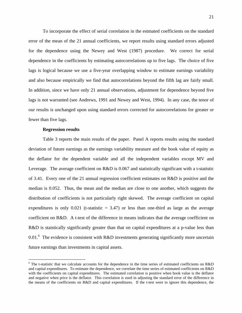
To incorporate the effect of serial correlation in the estmated coefficients on the standard

error of the mean of the 21 annual coefficients, we report results using standard errors adjusted

for the dependence using the Newey and West (1987) procedure. We correct for serial

dependence in the coefficients by estimating autocorrelations up to five lags. The choice of five

lags is logical because we use a five-year overlapping window to estimate earnings variability

and also because empirically we find that autocorrelations beyond the fifth lag are fairly small.

In addition, since we have only 21 annual observations, adjustment for dependence beyond five

lags is not warranted (see Andrews, 1991 and Newey and West, 1994). In any case, the tenor of

our results is unchanged upon using standard errors corrected for autocorrelations for greater or

fewer than five lags.

Regression results

Table 3 reports the main results of the paper. Panel A reports results using the standard

deviation of future earnings as the earnings variability measure and the book value of equity as

the deflator for the dependent variable and all the independent variables except MV and

Leverage. The average coefficient on R&D is 0.067 and statistically significant with a t-statistic

of 3.41. Every one of the 21 annual regression coefficient estimates on R&D is positive and the

median is 0.052. Thus, the mean and the median are close to one another, which suggests the

distribution of coefficients is not particularly right skewed. The average coefficient on capital

expenditures is only 0.021 (t-statistic = 3.47) or less than one-third as large as the average

coefficient on R&D. A t-test of the difference in means indicates that the average coefficient on

R&D is staistically significantly greater than that on capital expenditures at a p-value less than

0.01.6 The evidence is consistent with R&D investments generating significantly more uncertain

future earnings than investments in capital assets.

6 The t-statistic that we calculate accounts for the dependence in the time series of estimated coefficients on R&Dand capital expenditures. To estimate the dependence, we correlate the time series of estimated coefficients on R&Dwith the coefficients on capital expenditures. The estimated correlation is positive when book value is the deflatorand negative when price is the deflator. This correlation is used in adjusting the standard error of the difference inthe means of the coefficients on R&D and capital expenditures. If the t-test were to ignore this dependence, the

22

[Table 3]

Results in panel A also reveal that the average coefficient on advertising expense, 0.025

(t-statistic = 8.52) is approximately of the same magnitude as that on capital expenditures, but

much smaller than that on R&D. There are at least two explanations consistent with this result.

First, benefits from advertising are about as uncertain as those from capital expenditures, perhaps

because most corporate advertising is about products that corporations have already introduced

in the market.

Second, advertising yields fairly short-lived future benefits. Clarke (1976, p. 355)

concludes that “advertising’s effect on sales lasts for months rather than years is strongly

supported.” Batra, Myers, and Aaker (1996, p. 567) in a popular textbook on advertising

management also conclude that “the immediate and carryover effect of advertising usually

occurs in months, not years.” A similar inference can be drawn from Assmus, Farley, and

Lehmann (1984, table 1). Lodish et al. (1996) perform a statistical analysis summarizing the

findings in 389 academic research studies on the effect of advertising on sales. Somewhat

surprisingly to us, their analysis susgests “no obvious relationship” between advertising and

sales. On average the sensitivity of sales to advertising is statistically significantly greater than

zero, but economically modest (see Lodish et al., 1996, pp. 128-129 and table 3). The short-

lived nature of the benefits from advertising is relevant to interpreting the coefficient on

advertising in our regression model. Recall that the simulations demonstrate that, other things

equal, the shorter the future period of benefits from current investments, the smaller the

sensitivity of earnings variability to that investment.

The regressions in panel A of table 3 include two control variables; the natural logarithm

of the market value of equity and leverage (defined as the ratio of the book value of long-term

debt to the sum of the market value of equity and long-term debt). The average coefficients on

standard error of the difference in the coefficients is too large when the dependence is positive and too small whenthe dependence is negative.

23

both the variables are highly significant and have predicted signs. Earnings variability declines

in firm size and it increases in leverage.

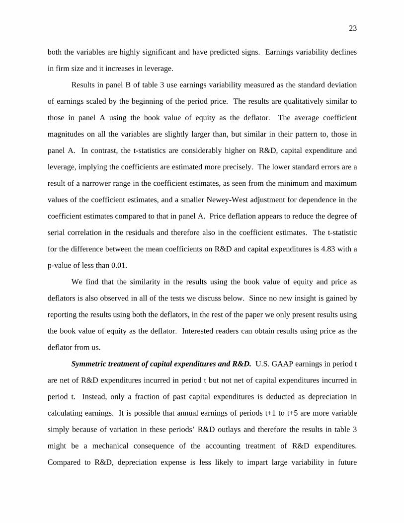
Results in panel B of table 3 use earnings variability measured as the standard deviation

of earnings scaled by the beginning of the period price. The results are qualitatively similar to

those in panel A using the book value of equity as the deflator. The average coefficient

magnitudes on all the variables are slightly larger than, but similar in their pattern to, those in

panel A. In contrast, the t-statistics are considerably higher on R&D, capital expenditure and

leverage, implying the coefficients are estimated more precisely. The lower standard errors are a

result of a narrower range in the coefficient estimates, as seen from the minimum and maximum

values of the coefficient estimates, and a smaller Newey-West adjustment for dependence in the

coefficient estimates compared to that in panel A. Price deflation appears to reduce the degree of

serial correlation in the residuals and therefore also in the coefficient estimates. The t-statistic

for the difference between the mean coefficients on R&D and capital expenditures is 4.83 with a

p-value of less than 0.01.

We find that the similarity in the results using the book value of equity and price as

deflators is also observed in all of the tests we discuss below. Since no new insight is gained by

reporting the results using both the deflators, in the rest of the paper we only present results using

the book value of equity as the deflator. Interested readers can obtain results using price as the

deflator from us.

Symmetric treatment of capital expenditures and R&D. U.S. GAAP earnings in period t

are net of R&D expenditures incurred in period t but not net of capital expenditures incurred in

period t. Instead, only a fraction of past capital expenditures is deducted as depreciation in

calculating earnings. It is possible that annual earnings of periods t+1 to t+5 are more variable

simply because of variation in these periods’ R&D outlays and therefore the results in table 3

might be a mechanical consequence of the accounting treatment of R&D expenditures.

Compared to R&D, depreciation expense is less likely to impart large variability in future

24

earnings because only a fraction of the average capital expenditure over past several years is

deducted in calculating earnings. That is, the time series of depreciation expense is relatively

smooth.

To control for the potential variability in future earnings induced by the accounting

treatment of R&D, we gross up future earnings by adding back both future R&D and

depreciation. The resulting numbers represent future benefits of current and past R&D and

capital expenditures and are less influenced by future R&D and capital expenditures.

Untabulated regression results using the standard deviation of the grossed-up earnings numbers

yield an average coefficient of 0.114 (t-stat = 5.13) on R&D, 0.022 (t-stat = 7.18) on capital

expenditures, and 0.013 (t-stat = 2.02) on advertising expense. The average coefficient on R&D

is significantly greater than that on capital expenditures.

Results excluding zero R&D observations. We observe from the sample descriptive

statistics that more than a fourth of the sample firm-year observations report zero R&D expense,

probably because their R&D outlays are not a material expense to be reported as a separate line

item. A concentration of a large fraction of observations with a zero value for the independent

variable (R&D) might potentially bias upwards the slope coefficient on the independent variable.

We therefore report regression results similar to those in table 3 except that we now exclude all

firm-year observations with zero R&D expense. The results reported in table 4 reveal little

change relative to those in table 3. The average coefficient on R&D is 0.069 (t-statistic = 3.28),

which is more than three times the average coefficient on capital expenditures, 0.018 (t-statistic =

3.04). Once again, the difference is statistically significant at the 1% level of sigificance. Other

coefficients and the model’s explanatory power remain similar using both book value of equity

and price as deflators.

[Table 4]

Results excluding advertising expense. We next discuss regression results for the model

that excludes advertising expense as one of the independent variables. The motivation is that

25

data for advertising expense is reported considerably less frequently than for R&D and capital

expenditures (see descriptive statistics in table 1). Table 5 shows that the tenor of the results is

unaffected when a larger sample without requiring data for advertising is analyzed. The average

coefficient on R&D is 0.072 (t-statistic = 3.21) compared to the average coefficient of 0.024 (t-

statistic = 3.83) on capital expenditure and the average difference between the two coefficints is

significantly positive at a p-value less than 0.01.

[Table 5]

Results using standard deviation of the change in earnings as the variability measure.

So far we have reported regression results using the standard deviation of the earnings level

deflated by the book value of equity or price as the earnings variability measure. While we

believe that variability in deflated earnings is an economically sensible measure, an equally

sensible alternative measure is the standard deviation of the change in earnings deflated by the

book value of equity or share price. If the time series properties of earnings suggest they are

largely permanent, then the standard deviation of earnings changes is likely a better measure of

earnings variability, whereas if there are considerably temporary components to earnings, then

the standard deviation of earnings levels would be a better measure of earnings variability. Since

earnings contain both permanent and transitory components and because previous research

documents both cross-sectional and temporal variation in these components, the standard

deviation of neither the level nor the change in earnings is unambiguously a superior measure of

earnings variability. One advantage of using the standard deviation of earnings changes is that if

there is substantial growth (or decline) in earnings over the estimation period, then the standard

deviation of first differences is largely unaffected by growth. In contrast, ceteris paribus, the

standard deviation of the earnings level is increasing in absolute growth. To control for this

effect on the standard deviation of earnings, either an explicit control for growth is needed or the

earnings series should be detrended (see section 4.2). Empirically we find the standard deviation

of earnings level and differences to be highly correlated in our sample.

26

Table 6 shows that results using the variability of deflated change in earnings more

strongly favor the hypothesis that R&D investments produce future benefits that are more

uncertain than those from capital expenditures. The average explanatory power of the regression

model is similar to that reported in the previous tables.

[Table 6]

Additional robustness checks

We perform the following empirical tests to ascertain whether our results are sensitive to

alternative research design choices and variable definitions. The tests include a control for

industry effects and growth, an analysis with a symmetric treatment of both capital expenditures

and R&D costs in calculating future earnings (benefits), pooled data analysis, and other

robustness checks. In every single case the results are similar to those described so far in the

paper.

Control for industry effects. We begin by providing descriptive evidence on the average

investment in R&D and capital expenditures and the standard deviation of earnings by two-digit

SIC code industries in table 7 and figure 1. The table presents industries in the ascending order

of their R&D investment. Figure 1 graphs the level of R&D investment and the standard

deviation of earnings by industry where industry SIC codes on the horizontal axis are in the

ascending order of R&D investment. The descriptive statistics are striking in that there is little

variation in earnings variability across industries, whereas both capital expenditures and R&D

exhibit substantial cross-industry variation. This is consistent with firms’ choices of other

determinants of earnings variability are such that univariate industry analysis is ineffective in

teasing out R&D’s contribution to earnings variability. The descriptive statistics also reveal that

there is considerable within industry variation in both investment intensities and earnings

variability, which might explain the relation between investments and earnings uncertainty.

Therefore, industry membership by itself does not seem to drive the relation between R&D and

earnings variability seen earlier. A formal test to examine this issue follows.

27

[Table 7 and figure 1]

We augment the regression model (1) to include industry dummies. Industry dummies

control for the variation in the level of earnings variability across industries. Without industry

dummies, it is possible that we document a positive relation between earnings variability and

R&D intensity that is due to industry membership rather than such a relation due to variation in

R&D intensity both within and across industries. The inclusion of industry dummies in the

regression model, however, does not change the result that R&D costs influence earnings

variability more so than capital expenditures. The average coefficient is 0.071 (t-stat = 6.11) on

R&D, 0.027 (t-stat = 6.27) on capital expenditures, and 0.044 (t-stat = 8.06) on advertising

expense. The average coefficient on R&D significantly exceeds that on capital expenditures at

the 1% significance level.

Control for Growth. The standard deviation of earnings estimated using future earnings

in levels can be a misleading indication of earnings uncertainty if growth is predictable. Since

R&D intensive firms are typically high growth firms, it is possible that the more steeply-sloped

relation between the standard deviation of earnings and R&D than capital expenditures is due to

growth as a correlated-omitted variable. We therefore calculate future earnings net of ex post

earnings growth over the estimation period (five years). We regress future earnings on time to

capture growth and reestimate the standard deviation using earnings minus average realized

growth for each firm. Regression analysis using the standard deviation of growth-adjusted

earnings, deflated by the book value, yields an average coefficient of 0.052 (t-statistic = 3.34) on

R&D and 0.015 (t-statistic = 3.22) on capital expenditures, with the difference between the two

average coefficients being significant at a p-value of 0.01.

Earnings growth can also be controlled for using changes in earnings instead of earnings

levels. The mean earnings change over the five-year estimation period represents realized

earnings growth, which does not affect the standard deviation estimated from the five earnings

change observations. Analysts’ growth forecast and past growth are two other growth proxies

28

that can potentially be employed in the analysis here. Lack of the availability of long-term

analysts’ forecasts in machine-readable form for the entire sample period for the large sample

that we use is the primary reason we do not use analysts’ growth forecasts. The use of past

earnings growth requires substantial additional data availability and previous research suggests

that past earnings growth is a poor proxy for future growth because a random walk is a good

description of the time-series property of annual earnings. For these reasons, we do not use past

earnings growth as a proxy for long-term future earnings growth.

Pooled cross-sectional analysis. We estimate a pooled time-series cross-sectional

regression instead of annual cross-sectional regressions. Once again, the results are similar to

those reported earlier. For example, using price as the deflator, the coefficient on R&D is 0.067

(t-statistic = 20.08) and that on capital expenditures is 0.020 (t-statistic = 12.31).

Other robustness checks. First, we examine the effect that replacing firms’ missing

values of earnings variability with the mean earnings variability of their respective Z-score decile

portfolios has on the results. Recall that we substitute decile portfolio mean earnings variability

in approximately a third of the sample. Both pooled regression results and annual cross-sectional

regression results reveal that the exclusion of missing earnings variability observations does not

alter the tenor of the results.

Second, instead of winsorizing the extreme 1% observations, which might have an undue

influence on the estimated coefficients, we repeat the regression analysis using data that excludes

the extreme 1% observations. There is no material effect on the results. Finally, we repeat the

entire analysis using variance instead of the standard deviation as a measure of future earnings’

variability.

VI. SUMMARY AND CONCLUSIONS

The FASB’s statement of Financial Accounting Concepts No. 2 notes that the trade-off

between relevance and uncertainty of future benefits is a major consideration in accounting

standard setting with respect to capitalization and expensing of investment expenditures. The

29

trade-off suggests balancing the demand for value-relevant information by equity investors, with

the demand for reliable information about future benefits, by debt holders and other contracting

parties. However, much of the current research on accounting for R&D expenditures focuses on

the relevance dimension of this tradeoff (e.g., Dukes, Dyckman, and Elliott, 1980, Horwitz and

Kolodny, 1980, Elliott, Richardson, Dyckman, and Dukes, 1984, and Wasley and Linsmeier,

1992). To compliment existing research, we examine the reliability of future benefits of R&D

expenditures relative to other investments such as capital expenditures.

Our analysis compares the relative contributions of current investments in R&D and

capital expenditures to future earnings variability. We use the standard deviation of future

earnings to proxy for future earnings variability. Our sample consists of over 50,000 firm-year

observations, obtained from Compustat’s Annual Industrial and Research files, from 1972-1992.

Our results support the hypothesis that R&D investments generate more uncertain future benefits

compared to capital expenditures. Controlling for other economic determinants of earnings

variability, we find that the coefficient on current R&D expenditures is about three times that of

the coefficient on current capital expenditures. This difference is statistically significant. Our

results are robust to many sensitivity checks, including controls for industry effects and growth,

alternative variable definitions, and research design variations.

We believe that our study contributes to the current debate over accounting for R&D

expenditures. A number of studies report convincing evidence that the capitalization of R&D

would aid in making the balance sheet more value relevant for share prices (e.g., Lev and

Sougiannis, 1996). These studies provide standard setters with useful information on the

relevance dimension of the relevance-reliability tradeoff. Our study provides evidence that the

future benefits of R&D expenditures are less certain than those of investments in capital

expenditures. Hence, we provide standard setters with a relative measure of the reliability of

future benefits component of the relevance-reliability trade-off.

30

References

Accounting Principles Board. 1970. APB Statement Number 4. New York, New York.

Altman, E.I. 1968. Financial ratios, discriminant analysis, and the prediction of corporatebankruptcy. Journal Of Finance 23: 589-609.

Andrews, D. 1991. Heteroskedasticity and autocorrelation consistent covariance matrixestimation. Econometrica 59: 817-858.

Assmus, G.; J. Farley, and D. Lehmann. 1984. How advertising affects sales: Meta-analysis ofeconometric results. Journal of Marketing Research 11: 65-74.

Association for Investment Management and Research. 1993. Financial Reporting in the 1990sand Beyond.

Ball, R. 1980. Discussion of accounting for research and development costs: the impact onresearch and development expenditures. Journal of Accounting Research 18: 17-37.

Banz, R.W. 1981. The relationship between return and market value of common stocks. Journalof Financial Economics 9: 3-18.

Barclay, M.J., C.W. Smith, and R.L. Watts. 1995. The determinants of corporate leverage anddividend policies. Journal of Applied Corporate Finance 7: 4-19.

Batra, R.; J. Myers, and D. Aaker. 1996. Advertising Management. Upper Saddle River, NJ:Prentice Hall.

Beaver, W.H., P. Kettler, and M. Scholes. 1970. The association between market determinedand accounting determined risk measures. The Accounting Review 45: 654-682.

Begley, J., J. Ming, and S. Watts. 1996. Bankruptcy prediction errors in the 1980s: An empiricalanalysis of Altman’s and Ohlson’s Models. Review of Accounting Studies 1: 267-284.

Bierman, Jr, H., and R.E. Dukes. 1975. Accounting for research and development costs. TheJournal of Accountancy (January): 48-55.

Chambers, D., R. Jennings, and R.B. Thompson III. 1998. Evidence on the usefulness ofcapitalizing and amortizing research and development costs. Working Paper, Universityof Texas at Austin.

Chan, S., J. Martin, and J. Kensinger. 1990. Corporate research and development expendituresand share value. Journal of Financial Economics 26: 255-276.

Clarke, D. 1976. Econometric measurement of the duration of advertising effect on sales.Journal of Marketing Research 13: 345-57.

31

Collins, D., and S. P. Kothari. 1989. An analysis of the inter-temporal and cross-sectionaldeterminants of earnings response coefficients. Journal of Accounting & Economics 11:143-181.

Deng, Z., and B. Lev. 1997. Flash-Then-Flush: the valuation of acquired R&D-in-process.Woking Paper, New York University.

Dukes, R.E., T.R. Dyckman, and J.A. Elliott. 1980. Accounting for research and developmentcosts: The impact on research and development expenditures. Journal of AccountingResearch 18 (Supplement): 1-26.

Easton, P., and M. Zmijewski. 1989. Cross-sectional variation in the stock market response to theannouncement of accounting earnings. Journal of Accounting & Economics 11: 117-141.

Elliott, J., G. Richardson, T.R. Dyckman, and R.E. Dukes. 1984. The impact of SFAS No. 2 onfirm expenditures on research and development: replications and extensions. Journal ofAccounting Research 22: 85-102.

Fama, E., and K. French. 1992. The cross-section of expected returns. Journal of Finance 47:427-465.

Fama, E., and J. Macbeth. 1973. Risk, return, and equilibrium: Empirical tests. Journal ofPolitical Economy 81: 607-636.

Financial Accounting Standards Board. 1974. Statement of Financial Accounting Standard No.2: Accounting for Research and Development Costs. Stamford, Conn.: FASB.

Financial Accounting Standards Board. 1980. Statement Of Financial Accounting Concepts No.2. Stanford, CT.

Financial Accounting Standards Board. 1980. Statement Of Financial Accounting Concepts No.6. Stanford, CT.

Hirschey, M., and J. Weygandt. 1985. Amortization policy for advertising and research anddevelopment expenditures. Journal of Accounting Research 23: 326-385.

Horowitz, B., and R. Kolodny. 1980. The economic effects of involuntary uniformity in thefinancial reporting of R&D expenditures. Journal of Accounting Research 18: 38-74.

International Accounting Standards Committee. 1997. Proposed International AccountingStandard: Intangible Assets (Exposure Draft E60): London, IASC.

International Accounting Standard No. 9. 1978. Accounting for Research and DevelopmentActivities. London, England.

32

Kothari, S., J. Shanken, and R. Sloan. 1995. Another look at the cross-section of expected stockreturns. Journal of Finance 50: 185-224.

Lev, B., and T. Sougiannis. 1996. The capitalization, amortization, and value-relevance of R&D.Journal of Accounting And Economics 21: 107-138.

Lodish, L.; M. Abraham, S. Kalmenson; J. Livelsberger; B. Lubetkin; B. Richardson; and M.Stevens. 1995. How T.V. advertising works: A meta-analysis of 389 real world splitcable T.V. advertising experiments. Journal of Marketing Research 32: 125-139.

Newey, W.K., and K.D. West. 1987. A simple, positive semi-definite heteroscedasticity andautocorrelation consistent covariance matrix. Econometrica 55: 703-708.

Newey, W.K., and K.D. West. 1994. Automatic lag selection in covariance matrix estimation.Review of Economic Studies 61: 631-653.

Ohlson, J. 1980. Financial ratios and the probabilistic prediction of bankruptcy. Journal ofAccounting Research 18: 109-131.

Revsine, L., D.W. Collins and W. B. Johnson. 1999. Financial Reporting and Analysis. UpperSaddle River, NJ: Prentice Hall.

Shyam-Sunder, L. and S. C. Myers. 1999. Testing static tradeoff against pecking order models ofcapital structure. Journal of Financial Economics 51: 219-244.

Sougiannis, T. The accounting based valuation of corporate R&D. The Accounting Review 69:44-68.

Wasley, C.E., and T.J. Linsmeier. 1992. A further examination of the economic consequences ofSFAS No. 2. Journal of Accounting Research 30: 156-164.

Watts, R.L., and J.L. Zimmerman. 1986. Positive Accounting Theory. Englewood Cliffs, N.J.:Prentice Hall.

Weygandt, J., D. Kieso, and W. Kell. 1996. Accounting Principles, Fourth Edition. New York,NY: John Wiley & Sons, Inc.

White, G., A. Sondhi, and D. Fried. 1998. The Analysis and Use of Financial Statements. NewYork, N.Y.: John Wiley & Sons, Inc.

Woolridge, R. 1988. Competitive decline and corporate restructuring: is a myopic stock marketto blame? Journal of Applied Corporate Finance 1: 26-36.

2

The full sample consists of all firms on the Compustat Annual Industrial and Industrial Research files from 1972-1992 for which CapExt, R&Dt, MVt and Leveraget are available. Eachof the following variables except MVt and Leveraget is deflated by either the book value of equity (panel A) or the stock price (panel B), at the end of the fiscal year t-1.

R&Dt is R&D expense per share;

CapExt is capital expenditures per share;

AdvExt is advertising expense per share;

MVt is the natural log of the Market Value at the end of fiscal year t;

Leveraget is the book value of debt divided by debt plus the market value of equity both at the end of fiscal year t;

Et is earnings per share;

SD(Et+1,t+5) is the standard deviation of earnings per share before extraordinary items and discontinued operations; the standard deviation is calculated using five annual earningsobservations for years t+1 through t+5.

Variables are winsorized by setting the values in the 1st and 100th percentiles to the minimum and maximum values in the 2nd and 99th percentiles. Observations with deflated EPS values of less than -1or greater than 1 are winsorized at -1 and +1. In cases where EPS data are absent in any of the years from t+1through t+5, SD(Et+1,t+5) is set equal to the mean SD(Et+1, t+5) of the firms in the same AltmanZ-Score decile portfolio (see section 2 for details).

Panel A- Scaled by Book Value of Equity

Variable Description NStandard Deviation Min q1 Median q3 Max

R&Dt R&D Expense 55,073 0.108 0.477 0.000 0.000 0.011 0.064 12.694CapExt Capital Expenditures 55,073 0.198 0.577 0.000 0.027 0.071 0.162 13.561AdvExt Advertising Expense 42,776 0.057 0.168 0.000 0.000 0.008 0.045 5.068MVt Log Market Value 55,073 -3.19 2.02 -8.13 -4.68 -3.42 -1.86 3.18Leveraget Leverage (Debt/MV+Debt) 55,073 0.289 0.243 0.000 0.070 0.241 0.463 0.955Et EPS 55,073 0.061 0.278 -1.000 0.013 0.106 0.181 1.000Var(Et+1,t+5) Variance of Earnings 55,073 0.028 0.051 0.000 0.002 0.012 0.031 0.512SD(Et+1,t+5) Standard Deviation of Earnings 55,073 0.115 0.095 0.000 0.049 0.097 0.139 0.715Panel B- Scaled by Price

Variable Description NStandard Deviation Min q1 Median q3 Max

R&Dt R&D Expense 52,046 0.045 0.125 0.000 0.000 0.007 0.040 3.382CapExt Capital Expenditures 52,046 0.128 0.261 0.000 0.017 0.051 0.133 6.486AdvExt Advertising Expense 40,569 0.043 0.108 0.000 0.000 0.004 0.033 1.513MVt Log Market Value 52,046 -3.142 2.028 -8.131 -4.637 -3.377 -1.798 3.185Leveraget Leverage (Debt/MV+Debt) 52,046 0.294 0.242 0.000 0.078 0.249 0.469 0.955Et EPS 52,046 0.052 0.212 -1.000 0.011 0.074 0.137 1.000Var(Et+1,t+5) Variance of Earnings 52,046 0.024 0.046 0.000 0.002 0.011 0.025 0.512SD(Et+1,t+5) Standard Deviation of Earnings 52,046 0.100 0.089 0.000 0.041 0.085 0.119 0.614

TABLE 1Descriptive Statistics

Mean

Mean

3

Above are thet the means of annual Pearson correlations from 1972-1992. Each of the following variables except MVt and Leveraget is deflated by either the book value of equity (panel A) or thestock price (panel B), at the end of the fiscal year t-1.

SD(Et+1,t+5) is the standard deviation of earnings per share before extraordinary items and discontinued operations; the standard deviation is calculated using five annual earnings observations for yearst+1 through t+5;





Leveraget is the book value of debt divided by debt plus the market value of equity both at the end of fiscal year t.

We obtain data from the Compustat Annual Industrial and Research files. We winsorize all variables by setting the values in the 1st and 100th percentiles to the minimum and maximum values in the2nd and 99th percentiles. Observations with deflated EPS values of less than -1 or greater than 1 are winsorized at -1 and +1. In cases where EPS data are absent in any of the years from t+1throught+5, SD(Et+1,t+5) is set equal to the mean SD(Et+1, t+5) of the firms in the same Altman Z-Score decile portfolio (see section 2 for details).All the correlations are significant at the 0.01 level using a two-tailed test.

Panel A: Pearson Correlation Coefficients - Variables Scaled By Book Value of Equity

Variable Description

R&D t R&D Expense 1.000CapEx t Capital Expenditures 0.266 1.000AdvEx t Advertising Expense 0.218 0.257 1.000MV t Log Market Value -0.081 -0.068 -0.093 1.000Leverage t Leverage -0.073 0.087 0.061 -0.173 1.000SD(E t+1,t+5) Standard Deviation - Earnings 0.166 0.158 0.111 -0.247 0.095 1.000

Panel B: Pearson Correlation Coefficients - Variables Scaled By Price

Variable DescriptionR&D t R&D Expense 1.000CapEx t Capital Expenditures 0.253 1.000AdvEx t Advertising Expense 0.179 0.268 1.000MV t Log Market Value (Billions) -0.120 -0.117 -0.153 1.000Leverage t Leverage 0.049 0.284 0.193 -0.173 1.000SD(E t+1,t+5) Standard Deviation - Earnings 0.140 0.195 0.150 -0.298 0.285 1.000

AdvEx t MV t Leverage t

Mean Correlations Among Independent VariablesTABLE 2

CapEx t

R&D t CapEx t AdvEx t MV t Leverage t SD(E t+1,t+5)

SD(E t+1,t+5)R&D t

4

Each of the following variables except MVt and Leverage is deflated by either the book value of equity (panel A) or the stock price (panel B), at the end of the fiscal year t-1.

SD(Et+1,t+5) is the standard deviation of earnings per share before extraordinary items and discontinued operations; the standard deviation is calculated using five annual earningsobservations for years t+1 through t+5;






We obtain data from the Compustat Annual Industrial and Research files. The sample size is 42,776 in Panel A and 40,569 in panel B. We winsorize all variables by setting the valuesin the 1st and 100th percentiles to the minimum and maximum values in the 2nd and 99th percentiles. Observations with deflated EPS values of less than -1 or greater than 1 arewinsorized at -1 and +1. In cases where EPS data are absent in any of the years from t+1through t+5, SD(Et+1,t+5) is set equal to the mean SD(Et+1, t+5) of the firms in the same Altman Z-Score decile portfolio (see section 2 for details).

Reported t-tests are adjusted for autocorrelation using the Newey-West correction with 5 lags.

Panel A: Scaled by Book Value of Equity

Variable Description t-stat Standard Deviation Min q1 Median q3 Max

Intercept Intercept 0.068 6.40 0.024 0.030 0.046 0.072 0.087 0.108 R&D t R&D Expense 0.067 3.41 0.047 0.004 0.026 0.052 0.097 0.161 CapEx t Capital Expenditures 0.021 3.47 0.015 -0.001 0.011 0.015 0.034 0.055 AdvEx t Advertising Expense 0.025 8.52 0.014 0.002 0.014 0.027 0.034 0.051 MV t Log Market Value (Billions) -0.010 -11.07 0.002 -0.013 -0.011 -0.010 -0.009 -0.006 Leverage t Debt/(Market Value+Debt) 0.025 5.19 0.016 -0.004 0.013 0.022 0.034 0.058

Adjusted R 2 in % 10.2 2.2 6.1 8.5 10.0 11.6 14.4

Panel B: Scaled by Price


Intercept Intercept 0.034 8.25 0.010 0.009 0.028 0.034 0.041 0.049 R&D t R&D Expense 0.072 6.34 0.039 0.003 0.038 0.070 0.100 0.140 CapEx t Capital Expenditures 0.028 9.00 0.016 0.004 0.021 0.026 0.035 0.061 AdvEx t Advertising Expense 0.030 3.81 0.023 -0.020 0.018 0.027 0.048 0.068 MV t Log Market Value (Billions) -0.010 -12.94 0.002 -0.015 -0.012 -0.010 -0.009 -0.007 Leverage t Leverage 0.086 12.42 0.022 0.040 0.074 0.079 0.099 0.143

Adjusted R 2 in % 18.4 2.4 15.0 16.8 17.5 20.6 22.4

SD(E t+1,t+5 ) = α + β 1t R&D t + β 2t CapEx t + β 3t AdvEx t + β 4t MV t + β 5t Leverage t + error t+1,t+5

TABLE 3

Mean

Mean

Summary of 21 Annual Cross-Sectional Regressions From 1972-1992

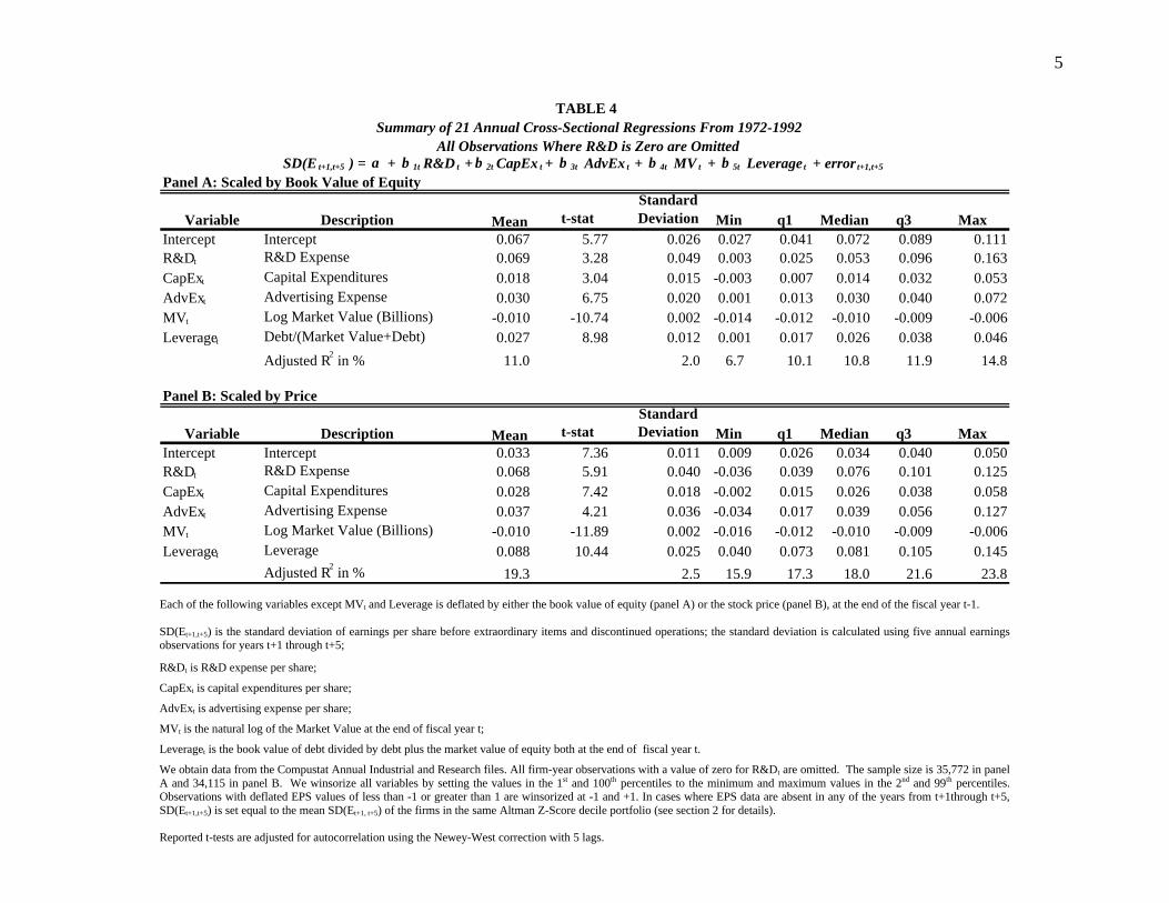
5








We obtain data from the Compustat Annual Industrial and Research files. All firm-year observations with a value of zero for R&Dt are omitted. The sample size is 35,772 in panelA and 34,115 in panel B. We winsorize all variables by setting the values in the 1st and 100th percentiles to the minimum and maximum values in the 2nd and 99th percentiles.Observations with deflated EPS values of less than -1 or greater than 1 are winsorized at -1 and +1. In cases where EPS data are absent in any of the years from t+1through t+5,SD(Et+1,t+5) is set equal to the mean SD(Et+1, t+5) of the firms in the same Altman Z-Score decile portfolio (see section 2 for details).




Intercept Intercept 0.067 5.77 0.026 0.027 0.041 0.072 0.089 0.111 R&D t R&D Expense 0.069 3.28 0.049 0.003 0.025 0.053 0.096 0.163 CapEx t Capital Expenditures 0.018 3.04 0.015 -0.003 0.007 0.014 0.032 0.053 AdvEx t Advertising Expense 0.030 6.75 0.020 0.001 0.013 0.030 0.040 0.072 MV t Log Market Value (Billions) -0.010 -10.74 0.002 -0.014 -0.012 -0.010 -0.009 -0.006 Leverage t Debt/(Market Value+Debt) 0.027 8.98 0.012 0.001 0.017 0.026 0.038 0.046

Adjusted R 2 in % 11.0 2.0 6.7 10.1 10.8 11.9 14.8



Intercept Intercept 0.033 7.36 0.011 0.009 0.026 0.034 0.040 0.050 R&D t R&D Expense 0.068 5.91 0.040 -0.036 0.039 0.076 0.101 0.125 CapEx t Capital Expenditures 0.028 7.42 0.018 -0.002 0.015 0.026 0.038 0.058 AdvEx t Advertising Expense 0.037 4.21 0.036 -0.034 0.017 0.039 0.056 0.127 MV t Log Market Value (Billions) -0.010 -11.89 0.002 -0.016 -0.012 -0.010 -0.009 -0.006 Leverage t Leverage 0.088 10.44 0.025 0.040 0.073 0.081 0.105 0.145

Adjusted R 2 in % 19.3 2.5 15.9 17.3 18.0 21.6 23.8

Summary of 21 Annual Cross-Sectional Regressions From 1972-1992 All Observations Where R&D is Zero are Omitted

TABLE 4

Mean

Mean

SD(E t+1,t+5 ) = α + β 1t R&D t + β 2t CapEx t + β 3t AdvEx t + β 4t MV t + β 5t Leverage t + error t+1,t+5

6







We obtain data from the Compustat Annual Industrial and Research files. The sample size is 55,073 in Panel A and 52,046 in panel B. We winsorize all variables by setting thevalues in the 1st and 100th percentiles to the minimum and maximum values in the 2nd and 99th percentiles. Observations with deflated EPS values of less than -1 or greater than 1are winsorized at -1 and +1. In cases where EPS data are absent in any of the years from t+1through t+5, SD(Et+1,t+5) is set equal to the mean SD(Et+1, t+5) of the firms in the sameAltman Z-Score decile portfolio (see section 2 for details).

Reported t-tests are adjusted for autocorrelation using the Newey-West correction with 5 lags



Intercept Intercept 0.068 6.42 0.024 0.031 0.044 0.073 0.087 0.110 R&D t R&D Expense 0.072 3.21 0.052 0.007 0.026 0.053 0.115 0.178 CapEx t Capital Expenditures 0.024 3.83 0.017 0.007 0.013 0.016 0.035 0.069 MV t Log Market Value (Billions) -0.010 -9.92 0.002 -0.014 -0.011 -0.011 -0.008 -0.006 Leverage t Debt/(Market Value+Debt) 0.022 4.92 0.016 -0.007 0.012 0.016 0.034 0.055

Adjusted R 2 in % 10.1 1.9 6.5 8.6 10.2 11.4 14.0



t-stat Standard Deviation Min q1 Median q3 Max

Intercept Intercept 0.034 8.18 0.010 0.011 0.028 0.035 0.043 0.048 R&D t R&D Expense 0.068 6.26 0.035 -0.003 0.040 0.070 0.082 0.140 CapEx t Capital Expenditures 0.032 8.78 0.014 0.014 0.026 0.029 0.037 0.064 MV t Log Market Value (Billions) -0.011 -13.32 0.002 -0.015 -0.012 -0.010 -0.009 -0.007 Leverage t Leverage 0.085 12.97 0.022 0.049 0.073 0.077 0.095 0.146

Adjusted R 2 in % 17.1 2.6 13.8 15.0 16.3 19.0 21.6

Summary of 21 Annual Cross-Sectional Regressions From 1972-1992 Advertising Expense is Omitted

TABLE 5

Mean

Mean

SD(E t+1,t+5 ) = α + β 1t R&D t + β 2t CapEx t + β 3t MV t + β 4t Leverage t + error t+1,t+5

7

Each of the following variables except MVt and Leveraget is deflated by either the book value of equity (panel A) or the stock price (panel B), at the end of the fiscal year t-1.

SD(∆Et+1,t+5) is the standard deviation of the change in earnings per share before extraordinary items and discontinued operations; the standard deviation is calculated using five annualearnings observations for years t+1 through t+5;






We obtain data from the Compustat Annual Industrial and Research files. The sample size is 42,776 in Panel A and 40,569 in panel B. We winsorize all variables by setting the values inthe 1st and 100th percentiles to the minimum and maximum values in the 2nd and 99th percentiles. Observations with deflated EPS values of less than -1 or greater than 1 are winsorized at -1and +1. In cases where EPS data are absent in any of the years from t+1through t+5, SD(Et+1,t+5) is set equal to the mean SD(Et+1, t+5) of the firms in the same Altman Z-Score decile portfolio(see section 2 for details).





Intercept Intercept 0.091 6.62 0.031 0.043 0.064 0.096 0.114 0.149 R&D t R&D Expense 0.106 3.49 0.075 0.016 0.044 0.072 0.150 0.315 CapEx t Capital Expenditures 0.037 3.52 0.028 0.008 0.018 0.023 0.051 0.107 AdvEx t Advertising Expense 0.035 6.22 0.025 -0.011 0.017 0.034 0.047 0.094 MV t Log Market Value (Billions) -0.013 -7.88 0.004 -0.018 -0.016 -0.013 -0.009 -0.007 Leverage t Debt/(Market Value+Debt) 0.021 3.45 0.022 -0.028 0.004 0.023 0.031 0.064

Adjusted R 2 in % 11.9 3.6 7.1 8.9 12.3 14.0 20.1 Panel B: Scaled by Price



Intercept Intercept 0.037 5.62 0.015 0.006 0.025 0.041 0.049 0.056 R&D t R&D Expense 0.148 10.81 0.062 0.069 0.112 0.134 0.175 0.357 CapEx t Capital Expenditures 0.037 6.61 0.019 0.009 0.028 0.035 0.046 0.090 AdvEx t Advertising Expense 0.046 4.00 0.037 -0.034 0.034 0.045 0.057 0.125 MV t Log Market Value (Billions) -0.013 -14.48 0.002 -0.017 -0.015 -0.012 -0.011 -0.010 Leverage t Leverage 0.121 12.44 0.029 0.067 0.105 0.125 0.136 0.194

Adjusted R 2 in % 20.7 2.1 17.3 19.9 20.0 21.2 27.1

SD( ∆ E t+1,t+5 ) = α + β 1t R&D t + β 2t CapEx t + β 3t AdvEx t + β 4t MV t + β 5t Leverage t + error t+1,t+5

TABLE 6

Mean

Mean

Summary of 21 Annual Cross-Sectional Regressions From 1972-1992

8

This table reports descriptive statistics by 2-digit industry code. The industries are sorted by mean R&D expenditures scaled by bookvalue of equity (R&Dt).

SD(∆Et+1,t+5) is the standard deviation of the change in earnings per share before extraordinary items and discontinuedoperations; the standard deviation is calculated using five annual earnings observations for years t+1 through t+5;


CapExt is capital expenditures per share.

2Digit SIC Industry N Mean STD Median Mean STD Median Mean STD Median

53 General Merchandise Stores 898 0.103 0.028 0.105 0.166 0.445 0.073 0.000 0.001 0.00054 Food Stores 727 0.100 0.028 0.102 0.240 0.495 0.121 0.000 0.003 0.00056 Apparel and Accessory Stores 653 0.106 0.029 0.107 0.196 0.523 0.073 0.000 0.001 0.00058 Eating and Drinking Places 1,070 0.151 0.048 0.143 0.462 0.856 0.219 0.031 0.436 0.00059 Miscellaneous Retail 968 0.109 0.030 0.113 0.157 0.354 0.070 0.005 0.030 0.00067 Holding, Othr Invest Offices 1,987 0.113 0.027 0.107 0.055 0.389 0.000 0.022 0.183 0.00013 Oil and Gas Extraction 1,403 0.133 0.043 0.121 0.563 1.132 0.244 0.028 0.209 0.00051 Nondurable Goods -Wholesale 914 0.111 0.036 0.110 0.182 0.442 0.064 0.055 0.409 0.00050 Durable Goods-Wholesale 1,654 0.113 0.036 0.113 0.154 0.558 0.049 0.061 0.462 0.00099 Other 6,280 0.119 0.039 0.113 0.274 0.761 0.089 0.062 0.428 0.00027 Printing, Publishing and Allied 790 0.101 0.030 0.099 0.117 0.233 0.039 0.016 0.062 0.00023 Apparel & Other Finished Pds 573 0.088 0.024 0.085 0.081 0.226 0.038 0.015 0.136 0.00048 Communications 551 0.137 0.046 0.119 0.285 0.429 0.166 0.106 0.582 0.00120 Food and Kindred Products 1,619 0.103 0.031 0.100 0.136 0.445 0.075 0.024 0.203 0.00225 Furniture and Fixtures 607 0.099 0.024 0.100 0.083 0.139 0.047 0.015 0.045 0.00426 Paper and Allied Products 916 0.111 0.030 0.108 0.158 0.560 0.078 0.032 0.219 0.00429 Pete Refining & Related Inds 588 0.118 0.028 0.114 0.166 0.240 0.116 0.012 0.034 0.00533 Primary Metal Industries 1,161 0.110 0.032 0.106 0.135 0.235 0.081 0.048 0.408 0.00532 Stone, Clay, Glass, Concrete Pd 769 0.110 0.032 0.109 0.177 0.325 0.101 0.032 0.142 0.00622 Textile Mill Products 740 0.094 0.024 0.092 0.109 0.129 0.073 0.023 0.072 0.00734 Fabr Metal, Ex Machny, Trans Eq 1,869 0.104 0.033 0.102 0.186 0.645 0.068 0.046 0.268 0.01030 Rubber & Misc Plastics Prods 1,158 0.109 0.034 0.105 0.149 0.275 0.085 0.043 0.182 0.01239 Misc Manufacturing Industries 900 0.110 0.034 0.109 0.160 0.469 0.065 0.070 0.356 0.01437 Transportation Equipment 1,901 0.106 0.030 0.103 0.152 0.423 0.067 0.098 0.532 0.02387 Engr, Acc, Resh, Mgmt, Rel Sevs 649 0.125 0.045 0.119 0.223 0.577 0.065 0.213 0.666 0.03028 Chemicals & Pharmaceuticals 4,128 0.118 0.036 0.119 0.159 0.518 0.053 0.187 0.648 0.03635 Indl, Comml Machy, Computer Eq 6,204 0.114 0.035 0.113 0.185 0.563 0.068 0.161 0.525 0.04936 Electr, Oth Elec Eq, Ex cmp 5,662 0.114 0.034 0.113 0.179 0.533 0.073 0.158 0.492 0.05538 Meas Instr; Photo Gds; Watches 4,942 0.120 0.037 0.118 0.186 0.545 0.065 0.212 0.597 0.07573 Business Services (including software) 2,792 0.130 0.037 0.125 0.263 0.683 0.085 0.291 0.840 0.076

Total 55,073 0.115 0.095 0.097 0.198 0.577 0.071 0.108 0.477 0.011

SD(Et+1,t+5) CapExt R&Dt

Table 7Descriptive StatisticsBy 2 Digit SIC Code

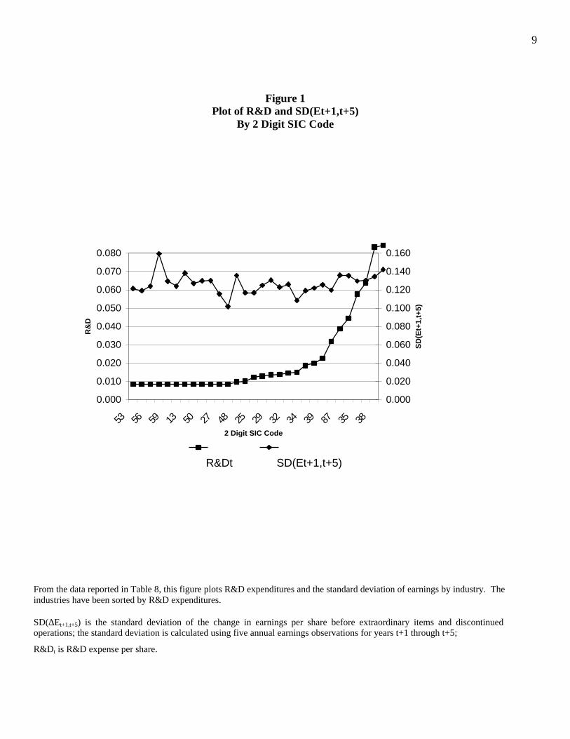
9

Figure 1Plot of R&D and SD(Et+1,t+5)

By 2 Digit SIC Code

From the data reported in Table 8, this figure plots R&D expenditures and the standard deviation of earnings by industry. Theindustries have been sorted by R&D expenditures.

SD(∆Et+1,t+5) is the standard deviation of the change in earnings per share before extraordinary items and discontinuedoperations; the standard deviation is calculated using five annual earnings observations for years t+1 through t+5;

R&Dt is R&D expense per share.

0.000

0.010

0.020

0.030

0.040

0.050

0.060

0.070

0.080

53 56 59 13 50 27 48 25 29 32 34 39 87 35 38

2 Digit SIC Code

R&

D

0.000

0.020

0.040

0.060

0.080

0.100

0.120

0.140

0.160

SD

(Et+

1,t+

5)

R&Dt SD(Et+1,t+5)

Evidence on the Uncertainty of Future Earnings from Capital ...

Documents

Transcript of Evidence on the Uncertainty of Future Earnings from Capital ...