EVAPOTRANSPIRATION AND IRRIGATION WATER REQUIREMENTS FOR JORDAN’S NATIONAL WATER MASTER PLAN:...

1

EVAPOTRANSPIRATION AND IRRIGATION WATER

REQUIREMENTS FOR JORDAN’S NATIONAL WATER MASTER

PLAN: GIS-BASED ET CALCULATIONS

Suzan Taha1, Richard G. Allen2, Klaus Jacobi3, Edward Qunqar4

ABSTRACT

Evapotranspiration (ET) from irrigated cropland is a significant component of

water consumption in Jordan. During 2000 and 2001, the MWI5 created a large

GIS-based system that includes components for processing ET and net irrigation

requirements (NIR) for various agroclimatic zones in Jordan. The NIR system,

named NIR_Calculator, is programmed within Microsoft Access database using a

Visual Basic interface and is highly flexible.

Incorporation of irrigation-specific and culture-specific characteristics for crops

has improved the prediction of evaporation and transpiration inside greenhouses

and under plastic mulch. Computations include partitioning of irrigated crops into

drip, sprinkler and surface irrigated classes, with evaporation from soil surfaces

during initial crop development periods and during nongrowing periods calculated

for each class separately. A monthly soil water balance determines the impact of

stored soil moisture and off-season precipitation on NIR. Evaporation during

nongrowing periods is considered when computing annual effective precipitation.

INTRODUCTION

Studies of projected water demand and supply in Jordan have shown that the

water deficit is increasing with time, with demands on a finite quantity of good

quality water ever increasing. Per capita availability of renewable water today is

less than 175 cubic meters, already far below the projected regional average for

the year 2025, and will decrease to 90 cubic meters by the year 2020 if water

projects are not implemented (Taha and El-Nasser, 2002). In order to meet

minimum current water demands for basic uses, over-pumpage of groundwater

resources in Jordan is estimated to be at 100% above the safe-yield. Of the total

groundwater supplied to all uses in 1998 (485 MCM), irrigated agriculture

consumption accounted for about 53%, at some 258 MCM. Nearly 80% of the

1 Engineer, Ministry of Water and Irrigation, Amman, Jordan,

[email protected] 2 Professor, University of Idaho, 3793 N. 3600 E., Kimberly, Idaho 83341, 1 208

423 6601, [email protected] 3 AHT International GmbH, Essen, Germany 4 Chief Engineer, Ministry of Water and Irrigation, Amman, Jordan 5 Ministry of Water and Irrigation

2 USCID/EWRI Conference

safe yield of the renewable groundwater resources and 40% of the non-renewable

groundwater are currently used for irrigated agriculture throughout the country.

Agriculture constitutes about 70% of the overall water demand in Jordan.

Therefore, it is important to obtain accurate and well-organized estimates of

current and future water consumption by agriculture. This has motivated MWI to

create a software tool for the projection and management of irrigation demand in

the nation, given available water quantity and quality information.

BACKGROUND AND OBJECTIVES

In the early 1990’s, a UN-DP program assisted MWI in refining a computer-based

procedure for structuring and housing water and crop-related data for the country.

Software was in the form of early data-bases and most planning computations and

summaries used spread-sheets. Beginning in the mid-1990’s, and under the scope

of work of the Water Sector Planning Support project funded by the GTZ6, a suite

of digital water balance tools was designed and implemented7. The objective is to

enable the Ministry to carry out nation-wide water balances using recent data and

various development scenarios to support efficient water sector planning. Digital

water balance tools incorporating nine modules were developed for the

assessment of various water demands as well as water resources including

wastewater and water losses.

One of the most important tools implemented for the calculation of water demand

at MWI is the Irrigation Model. The Irrigation Model consists of 3 separate

modules for pre-processing climatic data, calculation of reference ET (ETo) and

computing monthly net irrigation requirements of crops (NIR). These

calculations are combined to estimate present and future irrigation demands for

the whole country and selected planning/development regions. The Irrigation

Model is GIS-based (Jacobi, 2001) and is linked to a Relational Database

Management System under Oracle thus allowing for the updating of data and

visual presentation of the results.

PRINCIPAL DESIGN OF THE TOOL

The Irrigation Model is implemented under the Microsoft Access database, and is

linked to a central Oracle database and GIS databases containing Arc View shape

files. The software system models irrigation water demand in the future based on

existing information regarding cropping patterns, irrigated areas, information on

crop water requirements, in combination with application and conveyance

methods, and leaching requirements given water quality. Prediction of future

6 German Agency for Technical Cooperation 7 Conceptual Design was done by Ministry of Water and Irrigation, whereas

software development was by AHT International GmbH in close cooperation with

GTZ.

Irrigation and Drainage 3

water demand is tied to a reference year demand assessment. This permits the

evaluation of the current irrigation demand situation in the spatial unit under

consideration, with respect to water availability and water quality, prior to

proceeding with assumptions regarding the future. Irrigation demand data are

aggregated to demand centers such as towns and villages, developed irrigated

areas and project areas that are geographically represented via point information

in ArcView GIS.

The Irrigation Model requires entry of various data from databases, including:

Irrigated areas for each crop group and demand center

Distribution of irrigation methods for irrigated areas under the various

application methods

Leaching requirements for every crop group and salinity class

Monthly net water requirements (NIR) for each crop group, given the

agroclimatic zone in which it is grown

Application efficiency tables

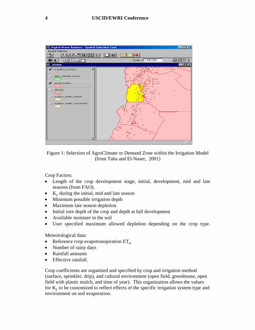
During operation of the Irrigation Model, selection of individual irrigation centers

for which irrigation demand is to be calculated is enforced and performed within

Arc View (Figure 1). The selection of demand centers is possible for various

spatial units of analysis, such as agroclimatic zone, governorate, groundwater

basins, surface water catchments, and subcatchments.

CALCULATION OF NET IRRIGATION REQUIREMENTS (NIR)

Besides statistics on irrigated areas and efficiencies, net irrigation requirements

are the principal factors for determining irrigation demand. Net irrigation

requirements are calculated using an MS Access-based application, namely the

NIR_Calculator and exported to Oracle for further use by the irrigation demand

model. The NIR_Calculator uses climatic data and crop factors for various

growing stages of crops, with consideration for the application method (surface,

drip, and sprinkler) and type of cultivation (open and plastic houses). NIR is

calculated on a monthly basis for each crop group, application method, and

agroclimatic zone under various year types (median, dry or wet). The application

uses monthly ETo computed using an early version of the FAO-56 Penman-

Monteith equation (FAO, 1990) with monthly precipitation, cropping calendars,

and FAO crop coefficients (Kc) for each agroclimatic zone in the country.

The NIR_Calculator was originally coded in a Lotus 123 data base during the

early 1990’s UNDP work, but has been since converted to an Access application

using Visual Basic programming (Jacobi, 2001). Various information compiled

by NIR_Calculator includes:


Figure 1: Selection of AgroClimate or Demand Zone within the Irrigation Model

(from Taha and El-Naser, 2001)

Crop Factors:

Length of the crop development stage; initial, development, mid and late

seasons (from FAO).

Kc during the initial, mid and late season

Minimum possible irrigation depth

Maximum late season depletion

Initial root depth of the crop and depth at full development

Available moisture in the soil

User specified maximum allowed depletion depending on the crop type.

Meteorological data:

Reference crop evapotranspiration ETo

Number of rainy days

Rainfall amounts

Effective rainfall.

Crop coefficients are organized and specified by crop and irrigation method

(surface, sprinkler, drip), and cultural environment (open field, greenhouse, open

field with plastic mulch, and time of year). This organization allows the values

for Kc to be customized to reflect effects of the specific irrigation system type and

environment on soil evaporation.


Two separate means for processing rainfall and ET were applied by the Ministry

and GTZ: a) the calculation of effective rainfall and ET for historic years and b) a

statistical evaluation for dry, median and wet years calculated for agro-climatic

zones rather than for individual stations.

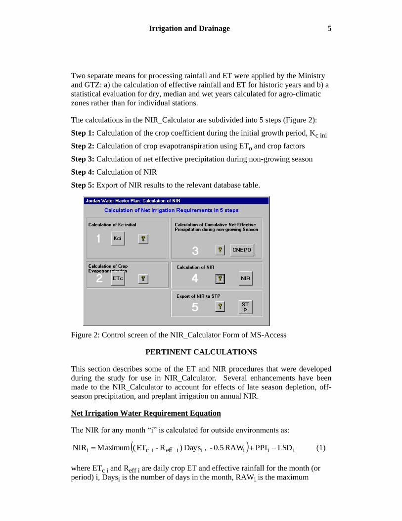
The calculations in the NIR_Calculator are subdivided into 5 steps (Figure 2):

Step 1: Calculation of the crop coefficient during the initial growth period, Kc ini

Step 2: Calculation of crop evapotranspiration using ETo and crop factors

Step 3: Calculation of net effective precipitation during non-growing season

Step 4: Calculation of NIR

Step 5: Export of NIR results to the relevant database table.

Figure 2: Control screen of the NIR_Calculator Form of MS-Access

PERTINENT CALCULATIONS

This section describes some of the ET and NIR procedures that were developed

during the study for use in NIR_Calculator. Several enhancements have been

made to the NIR_Calculator to account for effects of late season depletion, off-

season precipitation, and preplant irrigation on annual NIR.

Net Irrigation Water Requirement Equation

The NIR for any month “i” is calculated for outside environments as:

iiiii effi ci LSDPPIRAW 0.5- , Days )R - ET(Maximum NIR (1)

where ETc i and Reff i are daily crop ET and effective rainfall for the month (or

period) i, Daysi is the number of days in the month, RAWi is the maximum


readily available moisture for month i, PPIi is any net preplant irrigation

requirement for month i (0 unless immediately prior to planting), and LSD is late

season depletion during month i (0 unless during the month or months

immediately prior to harvest).

The maximum of net ETc i and -0.5 RAWi in (1) insures any excess precipitation

during rainy months (where ETc i - Reff i is negative) does not exceed the average

ability of the soil to retain the excess precipitation in the root zone. This average

ability (or capacity) is estimated to be one half of the maximum allowable

depletion of the soil for any month. This way, the total NIR includes the benefit

and effect of useable excess precipitation during the negative value months.

Limits on Negative NIR

When negative values of NIR are encountered that are caused by effective

precipitation exceeding ET requirements, the NIR sub-module calculator

compares the negative values to those for the following month to insure that the

sum of negative NIR for two or more consecutive months is never more negative

than the –RAW. This prevents more storage in the soil than is possible. Excess

storage is assumed to become deep percolation from the root zone, and ultimately,

ground-water recharge. The RAW used in (1) is based on the maximum rooting

depth for the crop. Negative values for cumulative CNIR at the end of the

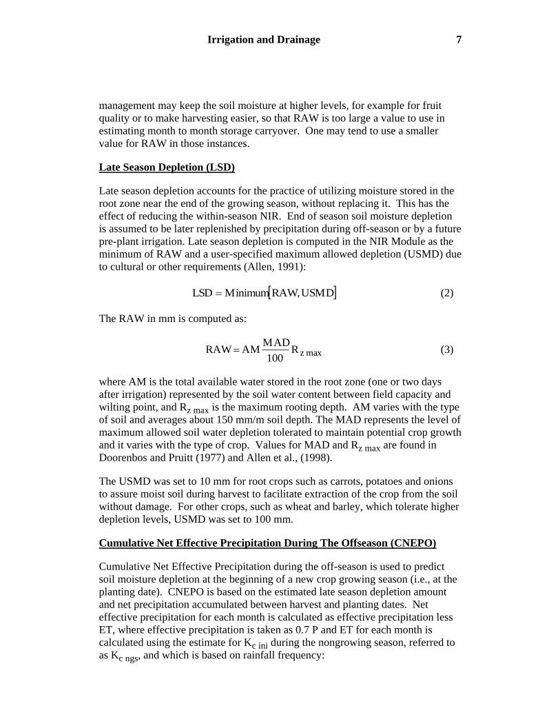
growing season are discarded and set to zero. Table 1 illustrates calculation of

NIR with the –RAW limit invoked during wet months.

Table 1. Example NIR calculation for citrus in zone 5 of Jordan for a wet season,

months Dec. - Feb.

Month ETc, mm/d Reff, mm/d ETc – Reff,

mm

NIR, mm ΣNIR,

mm

12 0.97 3.3 -72 -51 -51

1 1.48 3.1 -51 -51 -102

2 1.95 3.2 -35 0 -102

In the case of the citrus example in Table 1, the RAW equals 102 mm, with only

one-half of this allowed to be added to soil storage during any month. Beginning

with December (the first month having a negative NIR), one would have, by the

end of January, a summed negative NIR = -102 mm, which is just OK (i.e., less

than or equal to RAW). However, by the end of February, which is the third

consecutive month having negative NIR, one would have a summed negative NIR

over the three months = -137 mm, which is more "carryover" than the soil can

hold. Therefore, the NIR for February is set to 0 mm.

This example presumes that the soil is depleted to RAW at the time of harvest.

This is a reasonable assumption for many field crops. For some crops, however,


management may keep the soil moisture at higher levels, for example for fruit

quality or to make harvesting easier, so that RAW is too large a value to use in

estimating month to month storage carryover. One may tend to use a smaller

value for RAW in those instances.

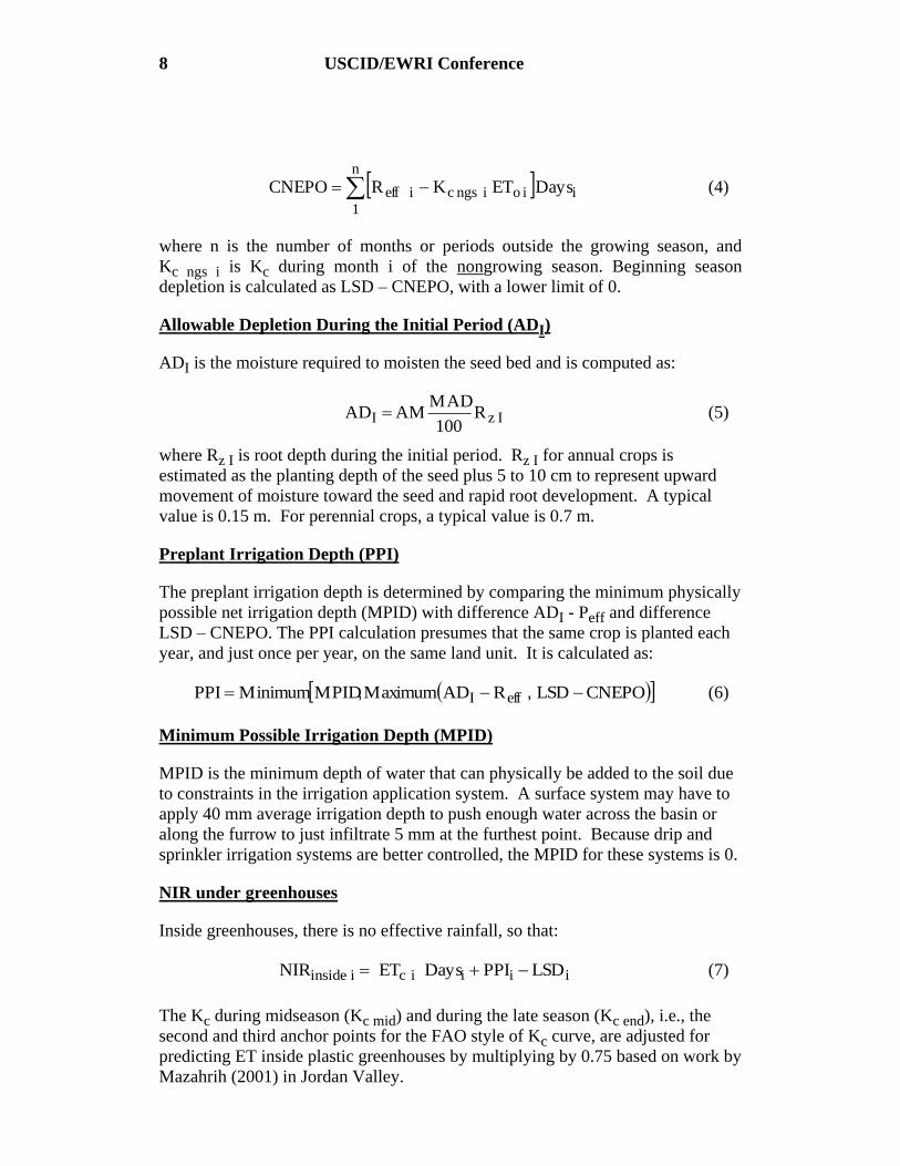
Late Season Depletion (LSD)

Late season depletion accounts for the practice of utilizing moisture stored in the

root zone near the end of the growing season, without replacing it. This has the

effect of reducing the within-season NIR. End of season soil moisture depletion

is assumed to be later replenished by precipitation during off-season or by a future

pre-plant irrigation. Late season depletion is computed in the NIR Module as the

minimum of RAW and a user-specified maximum allowed depletion (USMD) due

to cultural or other requirements (Allen, 1991):

USMDRAWMinimumLSD , (2)

The RAW in mm is computed as:

max zR 100

MAD AM RAW (3)

where AM is the total available water stored in the root zone (one or two days

after irrigation) represented by the soil water content between field capacity and

wilting point, and Rz max is the maximum rooting depth. AM varies with the type

of soil and averages about 150 mm/m soil depth. The MAD represents the level of

maximum allowed soil water depletion tolerated to maintain potential crop growth

and it varies with the type of crop. Values for MAD and Rz max are found in

Doorenbos and Pruitt (1977) and Allen et al., (1998).

The USMD was set to 10 mm for root crops such as carrots, potatoes and onions

to assure moist soil during harvest to facilitate extraction of the crop from the soil

without damage. For other crops, such as wheat and barley, which tolerate higher

depletion levels, USMD was set to 100 mm.

Cumulative Net Effective Precipitation During The Offseason (CNEPO)

Cumulative Net Effective Precipitation during the off-season is used to predict

soil moisture depletion at the beginning of a new crop growing season (i.e., at the

planting date). CNEPO is based on the estimated late season depletion amount

and net precipitation accumulated between harvest and planting dates. Net

effective precipitation for each month is calculated as effective precipitation less

ET, where effective precipitation is taken as 0.7 P and ET for each month is

calculated using the estimate for Kc ini during the nongrowing season, referred to

as Kc ngs, and which is based on rainfall frequency:


n

1

iioingscieff DaysETKRCNEPO (4)

where n is the number of months or periods outside the growing season, and

Kc ngs i is Kc during month i of the nongrowing season. Beginning season

depletion is calculated as LSD – CNEPO, with a lower limit of 0.

Allowable Depletion During the Initial Period (ADI)

ADI is the moisture required to moisten the seed bed and is computed as:

I zI R100

MAD AM AD (5)

where Rz I is root depth during the initial period. Rz I for annual crops is

estimated as the planting depth of the seed plus 5 to 10 cm to represent upward

movement of moisture toward the seed and rapid root development. A typical

value is 0.15 m. For perennial crops, a typical value is 0.7 m.

Preplant Irrigation Depth (PPI)

The preplant irrigation depth is determined by comparing the minimum physically

possible net irrigation depth (MPID) with difference ADI - Peff and difference

LSD – CNEPO. The PPI calculation presumes that the same crop is planted each

year, and just once per year, on the same land unit. It is calculated as:

CNEPOLSDRADMaximumMPIDMinimumPPI effI ,, (6)

Minimum Possible Irrigation Depth (MPID)

MPID is the minimum depth of water that can physically be added to the soil due

to constraints in the irrigation application system. A surface system may have to

apply 40 mm average irrigation depth to push enough water across the basin or

along the furrow to just infiltrate 5 mm at the furthest point. Because drip and

sprinkler irrigation systems are better controlled, the MPID for these systems is 0.

NIR under greenhouses

Inside greenhouses, there is no effective rainfall, so that:

iiii ciinside LSDPPIDays ET NIR (7)

The Kc during midseason (Kc mid) and during the late season (Kc end), i.e., the

second and third anchor points for the FAO style of Kc curve, are adjusted for

predicting ET inside plastic greenhouses by multiplying by 0.75 based on work by

Mazahrih (2001) in Jordan Valley.


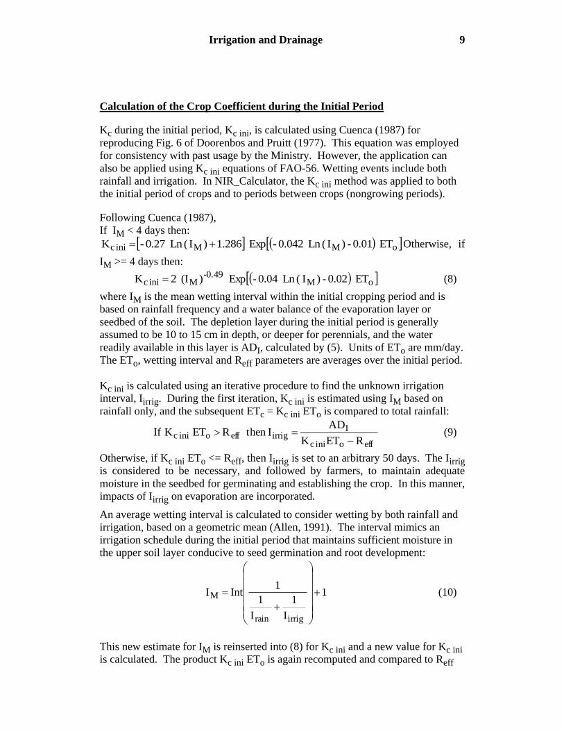
Calculation of the Crop Coefficient during the Initial Period

Kc during the initial period, Kc ini, is calculated using Cuenca (1987) for

reproducing Fig. 6 of Doorenbos and Pruitt (1977). This equation was employed

for consistency with past usage by the Ministry. However, the application can

also be applied using Kc ini equations of FAO-56. Wetting events include both

rainfall and irrigation. In NIR_Calculator, the Kc ini method was applied to both

the initial period of crops and to periods between crops (nongrowing periods).

Following Cuenca (1987),

If IM < 4 days then:

oMMinic ET 0.01 - )I(Ln 0.042-Exp 1.286 )I(Ln 0.27- K Otherwise, if

IM >= 4 days then:

oM-0.49

Minic ET 0.02 - )I (Ln 0.04-Exp )(I 2 K (8)

where IM is the mean wetting interval within the initial cropping period and is

based on rainfall frequency and a water balance of the evaporation layer or

seedbed of the soil. The depletion layer during the initial period is generally

assumed to be 10 to 15 cm in depth, or deeper for perennials, and the water

readily available in this layer is ADI, calculated by (5). Units of ETo are mm/day.

The ETo, wetting interval and Reff parameters are averages over the initial period.

Kc ini is calculated using an iterative procedure to find the unknown irrigation

interval, Iirrig. During the first iteration, Kc ini is estimated using IM based on

rainfall only, and the subsequent ETc = Kc ini ETo is compared to total rainfall:

effoinic

Iirrigeffoini c

RETK

AD I then R ET K If

(9)

Otherwise, if Kc ini ETo <= Reff, then Iirrig is set to an arbitrary 50 days. The Iirrig

is considered to be necessary, and followed by farmers, to maintain adequate

moisture in the seedbed for germinating and establishing the crop. In this manner,

impacts of Iirrig on evaporation are incorporated.

An average wetting interval is calculated to consider wetting by both rainfall and

irrigation, based on a geometric mean (Allen, 1991). The interval mimics an

irrigation schedule during the initial period that maintains sufficient moisture in

the upper soil layer conducive to seed germination and root development:

1

I

1

I

1

1Int I

irrigrain

M

(10)

This new estimate for IM is reinserted into (8) for Kc ini and a new value for Kc ini

is calculated. The product Kc ini ETo is again recomputed and compared to Reff


and a new Iirrig is computed. The process is repeated until Kc ini and IM have

stable values.

Kc ini for Perennials

For perennials, the calculation of Kc ini requires modification, since the ground

surface is not entirely bare, so that the basal condition, Kcb > 0.15. The

calculation of Kc ini perennials considers evaporation from both rainfall and

irrigation. However, the evaporation is reduced due to the shading effects of

vegetation. The “optimal” irrigation frequency is determined to retain sufficient

soil moisture in the initial root zone, which for a perennial is assumed to be

substantially close to maximum rooting depth. In the following computations for

Kc ini perennials, the values for ETo, Irain, and Reff are averages over all months in

the initial period. This procedure, based on Allen (1991 and 2001), uses the

Cuenca equation to retain consistency with early work within the Ministry, but is

applied to evaporation from a partially vegetated surface from FAO-56, and can

be applied with the Kc ini equations of FAO-56.

Evaporation is regulated under perennials by the fraction of exposed area not

covered by vegetation. A simplification of the FAO-56 approach is applied to

predict few for use with Cuenca's equation, where few is the fraction of ground

surface that is exposed and wetted by precipitation or irrigation, predicted as:

alini_residucew K - 1.2 f (11)

with limits of 0.01 < few < 0.99, where Kc ini_residual is the same as the basal Kcb for a perennial crop, and represents ET for the crop when it has a dry soil surface.

It is assumed that evaporation from rainfall occurs in the exposed portion of the

field, in between beds (i.e., in few), when there is no plastic mulch or when the

plastic mulch is covered by sufficient soil. For surface or sprinkle irrigation, the

total "drying" of the soil is computed as a weighted average based on few. The

irrigation frequency of perennials for drip with plastic mulch along the beds is

less coupled with rainfall. For drip, it is assumed that the bed is mulch covered so

that irrigation does not substantially impact Kc ini. The same basic equation for

Kc ini, i.e. that by Cuenca (1987) is used, but with ratioing according to few.

The evaporation from the few area is added to the basal Kc ini residual

K f K K residual ini cew8) (Eqn. ini cperen ini c (12)

where Kc ini (Eqn. 8) is Kc ini from (8). Limits are placed so that:

)K 1.25,Maximum( ,KMinimum K residual ini c12Eqnperen inicperen ini c ).( (13)


Similar to the condition for bare soil, an “optimal” irrigation interval, Iirrig, is

recommended if predicted evaporation exceeds effective rainfall:

effoperen inic

Iirrigeffoperenini c

RETK

AD I then R ET K If

(14)

where ADI is water that is readily available in the rooting zone during the initial

period. If Kc ini peren ETo <= Reff, then Iirrig is set to an arbitrary 50 days. (14) is

not invoked for drip irrigation, where it is assumed that the surface is generally

wetted within the shade of the vegetation, so that no extra evaporation from

irrigation occurs. Therefore, for drip, Iirrig = 50 days. Once a value for Iirrig is

predicted, a geometric mean wetting interval (IM) is calculated using (10). The

process iterates on Kc ini peren and Iirrig and IM until values are stable.

NonGrowing Season ET

The Kc ini function (8) is applied during the nongrowing season to predict total

evaporation and associated effectiveness of precipitation during the nongrowing

season. This calculation is part of the prediction of the net change in soil water

storage during the period from harvest of one crop until the planting of another.

Application of the Kc ini calculation is made on a monthly basis. The calculation

assumes that the soil surface is void of green vegetation. Where green vegetation

exists during the nongrowing season, Kc ini peren from (12) can be used to

approximate Kc ngs. In the application to the nongrowing period, it is assumed

that there is no irrigation, so that IM in (8) is set equal to IRain, and no iteration is

necessary. However, an upper limit is applied, so that:

o

effngsceffongs c

ET

R Kthen R ET K If (15)

where Kc ngs is the Kc during the nongrowing season and is from (8). This

conditional limits evaporation to effective rainfall.

OPERATION OF NIR_CALCULATOR FOR IRRIGATION DEMAND

Following the calculation of monthly NIR, results are exported and saved in the

relevant tables in the Central Oracle database. Irrigation demand assessment

proceeds using the irrigation demand model, which can be linked on-line to this

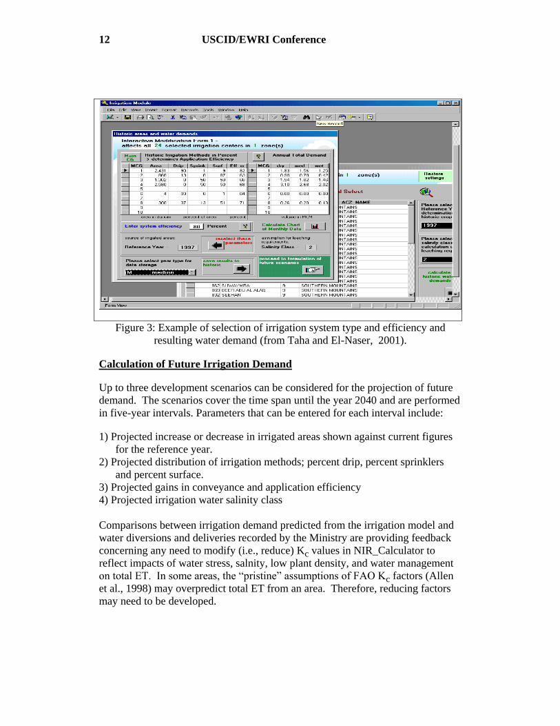
database. Figure 3 illustrates the user interface used in the irrigation model to

specify irrigation types and efficiencies, and resulting water demands.

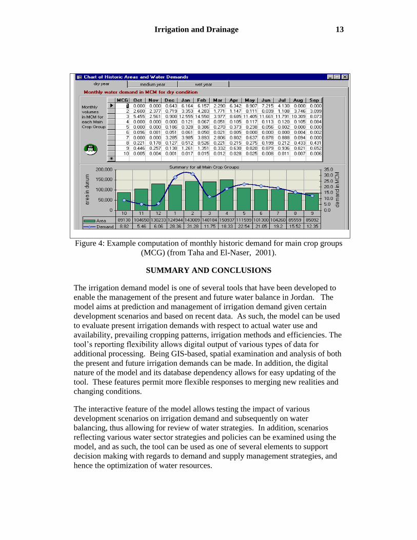
Figure 4 illustrates how monthly water demand data are presented to the user by

main crop group (MCG) and month, in tabular and graphical form, under dry,

median and wet conditions.


Figure 3: Example of selection of irrigation system type and efficiency and

resulting water demand (from Taha and El-Naser, 2001).

Calculation of Future Irrigation Demand

Up to three development scenarios can be considered for the projection of future

demand. The scenarios cover the time span until the year 2040 and are performed

in five-year intervals. Parameters that can be entered for each interval include:

1) Projected increase or decrease in irrigated areas shown against current figures

for the reference year.

2) Projected distribution of irrigation methods; percent drip, percent sprinklers

and percent surface.

3) Projected gains in conveyance and application efficiency

4) Projected irrigation water salinity class

Comparisons between irrigation demand predicted from the irrigation model and

water diversions and deliveries recorded by the Ministry are providing feedback

concerning any need to modify (i.e., reduce) Kc values in NIR_Calculator to

reflect impacts of water stress, salnity, low plant density, and water management

on total ET. In some areas, the “pristine” assumptions of FAO Kc factors (Allen

et al., 1998) may overpredict total ET from an area. Therefore, reducing factors

may need to be developed.


Figure 4: Example computation of monthly historic demand for main crop groups

(MCG) (from Taha and El-Naser, 2001).

SUMMARY AND CONCLUSIONS

The irrigation demand model is one of several tools that have been developed to

enable the management of the present and future water balance in Jordan. The

model aims at prediction and management of irrigation demand given certain

development scenarios and based on recent data. As such, the model can be used

to evaluate present irrigation demands with respect to actual water use and

availability, prevailing cropping patterns, irrigation methods and efficiencies. The

tool’s reporting flexibility allows digital output of various types of data for

additional processing. Being GIS-based, spatial examination and analysis of both

the present and future irrigation demands can be made. In addition, the digital

nature of the model and its database dependency allows for easy updating of the

tool. These features permit more flexible responses to merging new realities and

changing conditions.

The interactive feature of the model allows testing the impact of various

development scenarios on irrigation demand and subsequently on water

balancing, thus allowing for review of water strategies. In addition, scenarios

reflecting various water sector strategies and policies can be examined using the

model, and as such, the tool can be used as one of several elements to support

decision making with regards to demand and supply management strategies, and

hence the optimization of water resources.


The NIR calculator is flexible in regard to programming different relationships

among NIR components, so that it can be updated according to various countries'

needs and to reflect the latest findings in the field.

Acknowlegements

Mr. Lothar Nolte of GTZ, Amman, provided valuable coordinating and

interfacing. Dr. Peter McCornick of ARD, Inc., Amman, provided background

and support. Engineer Rasha Sharkawi of MWI assisted with Access data base

operation and NIR_Calculator debugging. Work by R.G. Allen was supported by

ARD, Inc. with funding by US-AID.

REFERENCES

AHT International GMBH (2001). Water Sector Planning Support at the Ministry

of Water and Irrigation, Digital Balancing Model for Water Resources

Management, 2nd

Phase. PN 92.22.38.1-01.100. Final Report, February 2001.

Allen, R.G. 1991. Net Irrigation Requirements Calculator using Spreadsheets.

Final Report to UNDP and Ministry of Water and Irrigation. Amman, Jordan.

Allen, R.G., L.S. Pereira, D. Raes, and M. Smith. 1998. Crop

Evapotranspiration: Guidelines for Computing Crop Water Requirements.

United Nations FAO, Irrig. and Drain. Paper 56. Rome, Italy. 300 p.

Allen, R.G. 2001. Review and support of developments in the Net Irrigation

Requirement Calculator, Jordan Water Policy Support, Crop Water

Requirements Specialist, Report to ARD, Inc., March, 2001.

Cuenca, R.H. 1987. Irrigation System Design: An Engineering Approach.

Prentice Hall, Englewood Cliffs, New Jersey. 552 p.

Doorenbos, J. and Pruitt, W. O., 1977. "Crop water requirements." Irrigation

and Drainage Paper No. 24, (rev.) FAO, Rome, Italy. l44 p.

FAO, 1990. Report on the Expert consultation on revision of FAO methodologies for

crop water requirements. Annex V, Rome Italy. 26 p.

Taha S., and H. El-Naser. (1999). Water Resources Management in Jordan: The

Use of Interactive Digital Planning Tools based on GIS applications.

Presented to the Seminar on Information Technology applied to resources

management, May 1999, Petra, Jordan

Taha, S. and H. El-Naser. 2001. Projection of Irrigation Demand in Jordan:

Introduction to GIS-based Model for the Projection and Management of

Irrigation Demand. Paper pres. at MedAqua Conf., Amman, Jordan, 6/2001.

Jacobi, K. 2001. Calculation of Net Irrigation Requirements (NIR) with Access

Application NIR_calc.mdb. Report submitted to Jordan Ministry of Water

and Irrigation, Amman, Jordan. 18 p.

Mazahrih, Naem Thiyab. 2001. Evapotranspiration Measurement and Modelling

for Bermuda Grass, Cucumber, and Tomato Grown Under Protected

Cultivation in the Central Jordan Valley. Ph.D. Dissertation, Univ. Jordan,

Amman. 168 p.

EVAPOTRANSPIRATION AND IRRIGATION WATER REQUIREMENTS FOR JORDAN’S NATIONAL WATER MASTER PLAN:...

Documents

Transcript of EVAPOTRANSPIRATION AND IRRIGATION WATER REQUIREMENTS FOR JORDAN’S NATIONAL WATER MASTER PLAN:...