Environmental taxes and equity concerns: A European perspective
Upload
khangminh22Category
view
2download
0
CHARLES UNIVERSITYKAROLINUM PRESS
European Journal of Environmental Sciences
VOLUME 11 / NUMBER 1 2021
ACTA UNIVERSITATIS CAROLINAE

European Journal of Environmental Sciences is licensed under a Creative Commons Attribution License(http://creativecommons.org/licenses/by/4.0), which permits unrestricted use, distribution, and reproduction in any medium, provided the original author and source are credited.
© Charles University, 2021ISSN 1805-0174 (Print)ISSN 2336-1964 (Online)

CONTENTS
Ahmad Pervez and Rupali Sharma: Influence of intraspecific competition for food on the bodyweight of the adult aphidophagous ladybird, Coccinella transversalis ................................................................................................................... 5
Alžběta Vosmíková and Zdenka Křenová: The status of commons in the changing landscape in the Czech Republic .................................................................... 12
Zuzana Štípková and Pavel Kindlmann: Factors determining the distribution of orchids – a review with examples from the Czech Republic .............................................. 21
Senad Murtić, Hamdija Čivić, Emina Sijahović, Ćerima Zahirović, Emir Šahinović, and Adnana Podrug: Phytoremediation of soils polluted with heavy metals in the vicinity of the Zenica steel mill in Bosnia and Herzegovina: Potential for using native flora ..................................................................... 31
Vojtěch Pilnáček, Libuše Benešová, Tomáš Cajthaml, and Petra Inemannová: Comparison of temperature and oxygen concentration driven aeration methods for biodrying of municipal solid waste ..................................................................... 38
Anastasia Linyucheva and Pavel Kindlmann: A review of global land cover maps in terms of their potential use for habitat suitability modelling ............................................. 46


European Journal of Environmental Sciences 5
Pervez, A., Sharma, R.: Influence of intraspecific competition for food on the bodyweight of the adult aphidophagous ladybird, Coccinella transversalis European Journal of Environmental Sciences, Vol. 11, No. 1, pp. 5–11
https://doi.org/10.14712/23361964.2021.1 © 2021 The Authors. This is an open-access article distributed under the terms of the Creative Commons Attribution License (http://creativecommons.org/licenses/by/4.0),
which permits unrestricted use, distribution, and reproduction in any medium, provided the original author and source are credited.
INFLUENCE OF INTRASPECIFIC COMPETITION FOR FOOD ON THE BODYWEIGHT OF THE ADULT APHIDOPHAGOUS LADYBIRD, COCCINELLA TRANSVERSALIS AHMAD PERVEZ* and RUPALI SHARMA
Biocontrol laboratory, Department of Zoology, Radhey Hari Govt. P.G. College, Kashipur, Udham Singh Nagar, Uttarakhand, India* Corresponding author: [email protected]
ABSTRACT
Aggregation of conspecific predators sharing a common prey, influences their bodyweights. We investigated the influence of intraspecific competition of adult ladybirds of Coccinella transversalis Fabricius on their bodyweight feeding on rusty plum aphid, Hysteroneura setariae (Thomas). Adult males and females consumed a significantly greater number of aphids with increase in predator-density, however, the aphid-consumption per predator declined with this increase. The weight gain per predator also decreased linearly with increase in the density of both male and female predators. This indicates that the weight-gain of the predator is a function of the prey consumed. The searching efficiency decreased with increase in predator density due to mutual inference. The mutual interference constants for adult male and female ladybirds were −0.419 and −0.546, respectively. The females consumed a greater number of aphids than males. The killing power of the ladybird denoted by the k-value increased curvilinearly with increase in predator density. We conclude that prey consumption is a function of body size and that the offspring of those that aggregate at low densities in prey-rich habitats develop into large adults.
Keywords: conspecific predator; Coccinella transversalis; intraspecific competition; ladybirds; numerical response
Introduction
Knowledge of the predator-prey interactions of pred-atory ladybirds (Coccinellidae: Coleoptera) is important for understanding their effectiveness in the biocontrol of aphids. Quantitative estimates of ladybirds’ searching ef-ficiency and prey consumption at varying prey-densities indicate their potential as biocontrol agents (Bayoumy 2011; Bayoumy and Michaud 2012). This predator’s func-tional response to the changes in prey density indicates density-dependent prey consumption (Holling 1959). However, the effect of predator density on prey densi-ty may also help predict biocontrol outcomes, estimate the effect of intraspecific competition and interferences among ladybirds. The density-dependent predator-prey dynamics is described by numerous models (Pervez et al. 2018), of which the classical Nicholson and Bailey (1935) model defines “area of discovery”, as a crucial parameter determining the searching efficiency of a predator. An inductive model (Hassell and Varley 1969) including the mutual interference constant (Hassell 1971; Bayoumy et al. 2014), further simplifies this model and indicates that the predator’s searching efficiency declines with increase in its density. These models advocate predation to be a function of both prey- and predator-dependent processes and account for the effect of mutual interference on prey consumption. This interference alters ladybird’s foraging success or may compensate for the decline in foraging activity due to the time required for digestion at high prey densities (Papanikolaou et al. 2016). Kindlmann and Dixon (1993) questioned the biocontrol potential of aphidophagous ladybirds stating that even optimal foraging and laying of eggs may only result in a slight reduction of aphid abundance. Furthermore, the adults
should maximize their fitness by deciding whether to stay in or leave an aphid-patch (Kindlmann and Dixon 2010). In addition, greater generation-time ratio of lady-birds makes them slow developers, thereby impeding the top-down regulation of aphid abundance (Kindlmann and Dixon 1999, 2001, 2015). Kindlmann et al. (2020) further concluded that it is generation-time ratio rather than voracity that drives the dynamics of insect-natural enemy systems, particularly aphid-ladybird system.
Predaceous ladybirds (Coleoptera: Coccinellidae) are potential biological control agents, as they prey upon nu-merous coccid and aphid pests (Hodek et al. 2012; Omkar and Pervez 2016; Pervez et al. 2020). They switch from extensive search to intensive search after capturing a prey (Pervez and Yadav 2018). Complex plant morphology further modifies intensive search (Legrand and Barbosa 2003). Mutual interactions impede their consumption of prey and searching efficiency (Omkar and Pervez 2004a; Bayoumy and Michaud 2012). Their searching efficiency and incidence of mutual interference might be dependent on the type of prey (Al-Deghairi et al. 2014). These coc-cinellid predators may switch from a rare stage of prey to an abundant stage of prey (Fathipour et al. 2020) thereby suppressing prey-abundance and increasing their body size. Dixon (2000) opined that variation in body-size within the species and gender might be associated with the relative effects of food quality and quantity. Further-more, smaller-sized ladybirds may exploit the aphid col-onies earlier, which may later be overtaken by the large ladybirds when aphid densities increase (Dixon 2007). Sloggett (2008) argued that ladybirds’ body size might not be just a function of aphid density, but other complex interactions between density and prey size are also oper-ational. This further raises the question of whether con-

European Journal of Environmental Sciences, Vol. 11, No. 1
6 Ahmad Pervez, Rupali Sharma
tinuous exposure of aphidophagous ladybirds to aphid abundance may increase the growth rate and have evo-lutionary significance. Most species with high biocontrol potential are large and highly fecund, which are favoured by natural selection, particularly in food-abundant habi-tats (Brown and Sibly 2006). Large species have a repro-ductive advantage over smaller indigenous species in prey-rich habitats (Kajita and Evans 2010).
Coccinella transversalis Fabricius is a predator (Coleo-ptera: Coccinellidae) of many insects and acarine pests, particularly, aphids (Omkar and James 2004; Omkar and Pervez 2004b; Maurice et al. 2011). Manipulation of its reproductive parameters may promote its abundance (Michaud et al. 2013). It coexists with other coccinellids and mostly dominates the aphid predatory guild (Omkar et al. 2005a, b) and together with coccinellid, Propylea dissecta (Mulsant) may synergistically suppress popula-tions of Aphis gossypii (Glover) (Omkar and Pervez 2011). We found adults and larvae of C. transversalis preying on rusty plum aphid, Hysteroneura setariae (Thomas) infest-ing creeping bluegrass, Bothriochloa insculpta (Hochst.). This aphid is a cereal pest, attacking rice, wheat, sugar cane, maize and soya bean crops on the Indian sub-con-tinent (Kale et al. 2020). In a banker plant system, H. se-tariae reared on grasses, can be used as a non-pest prey to build-up ladybird populations (Rattanpun 2017). Hence, we designed a laboratory experiment to determine (i) the searching efficiency of adult male and female C. trans-versalis feeding on H. setariae (ii) killing power of adult ladybirds associated with their aggregation, and (iii) the influence of the intraspecific competition for food on the adult bodyweight and its implications.
Materials and Methods
Insect culture and maintenanceWe sampled and collected adults of C. transversalis
from H. setariae infested fields of B. insculpta near our college campus, Kashipur, India (30.2937°N, 79.5603°E). We brought them to the laboratory and paired adult male and female ladybirds in Petri dishes (9.0 cm diameter × 2.0 cm height) containing an ad libitum amount of H. se-tariae infesting host plant twigs. The females mated and laid eggs in clusters that were isolated and kept in other Petri dishes (size as above). We transferred these Petri dishes to an Environmental Test Chamber (ETC) (REMI, Remi Instruments), maintained at 25 ± 1 °C, 65 ± 5% R.H and 12L : 12D. The eggs hatched and the first instar larvae were placed in 500 ml Borosil glass beakers containing sufficient supply of aphid infested twigs. Five first-instar larvae were kept in each beaker and reared on aphids un-til adult emergence. We replenished the aphids daily to avoid contamination. The newly eclosed F1 adults were sexed and isolated in separate Petri dishes, (size as above) for use in the experiments.
Experimental designFifteen-day-old adult male C. transversalis was taken
from the stock and starved for 12 hours to standardize its hunger. Thereafter, we weighed it (W1) using an elec-tronic balance (SHIMADZU, Model ATX-224, 0.1 mg precision) and kept it in a 500ml glass beaker containing 200 third-instar nymphs of H. setariae (as prey). A piece of folded moist filter paper was also kept in the beaker to provide moisture. We covered the beaker with fine mus-lin cloth fastened by a rubber band. We transferred this beaker to ETC maintained at the abiotic conditions men-tioned above. After 3 hours of exposure, we removed the beaker from ETC and counted the number of live aphids to determine the number of aphids consumed (Na). The ladybird was weighed again (W2) (as above) to estimate the gain in weight (We = W2 − W1, i.e. final weight of adult – the initial weight of adult). This experiment was replicated ten times (n = 10). We repeated the exper-iment at predator densities of 2, 4, 8, and 10. Thereaf-ter, the entire experiment was repeated using the above predator densities of 15-day-old adult female C. trans-versalis. The data were subjected to the following data analysis.
Data analysisNicholson–Bailey model gave the following equations
(1) and (2):
( + 1) = ( ) exp[ − ( )]
( + 1) = ( )[ 1 − exp( − ( ))]
= log ( )
=
(1) ( + 1) = ( ) exp[ − ( )]
( + 1) = ( )[ 1 − exp( − ( ))]
= log ( )
=
(2)
where N(t) is the number of hosts (prey) at time t, P(t), the number of predators at time t, λ is the host reproduc-tive rate, and a is the area of discovery. To estimate the area of discovery, the above model (2) can be rearranged (Hassel 1978) after assuming that c = 1, as:
( + 1) = ( ) exp[ − ( )]
( + 1) = ( )[ 1 − exp( − ( ))]
= log ( )
=
(3)
where a is the area of discovery, N is the initial aphid density, Na is the number of aphids consumed, and P is the predator density. We used the above-rearranged model (3) to relate the area of discovery to prey density. After estimating the area of discovery, Hassell and Varley (1969) model (equation 4) was used to estimate Quest constant (Q), while mutual interference (m) constant was determined from the slope of regression of log a (area of discovery) on log P (predator density).
( + 1) = ( ) exp[ − ( )]
( + 1) = ( )[ 1 − exp( − ( ))]
= log ( )
= (4)
Equation (4) can be linearized by using logarithms as follows:
log = log − log
k-value = log10 ( N / S)
(5)

European Journal of Environmental Sciences, Vol. 11, No. 1
Intraspecific competition for food and the bodyweight of Coccinella transversalis 7
Fig. 1 Relationship between prey consumption and predator density for (a) male and (b) female C. transversalis fed the aphid, H. setariae.
k-value, which is the measure of the ‘killing power’ (Ooi 1980) was also estimated by taking the difference between the logarithms of aphid population before and after prey consumption (Varley et al. 1973) at various predator densities using equation (6).
k-value = log10 (N / S) (6)
The number of prey consumed per predator by adult male and female ladybirds at different predator densi-ties was subjected to one-way ANOVA using statistical software SAS 9.0 (SAS 2002). The means were compared using Tukey’s test of significance. We also subjected the prey consumed per predator at particular predator densities for both adult male and female ladybirds to a two-sample t-test using SAS 9.0. All data were tested for normality and variances using the Shapiro-Wilk test. The (i) prey consumption, (ii) area of discovery, (iii) killing power and (iv) mean weight gained or weight gained per predator with the increase in predator density were further subjected to regression analysis to discover the relationship between these variables using SAS 9.0. The log area of discovery and the log predator density
were subjected to linear regression in order to deter-mine the mutual interference and Quest constants using SAS 9.0.
Results
The prey consumption of the adult male and female C. transversalis increased curvilinearly with increase in predator density (Fig. 1). The female ladybirds consumed a significantly greater number of aphids than the males (t = 3.95; P < 0.01; d. f. = 94). The prey consumption per predator decreased significantly with increase in predator density (Table 1). The difference in the prey consumption of males and females was only significant when the num-ber of ladybirds was two (t = –3.11; P < 0.01; d. f. = 17) and ten (t = –2.27; P < 0.05; d. f. = 17) (Table 1). The area of discovery of male and female beetles decreased with increase in predator density (Fig. 2). The log values of area of discovery of male (r2 = 0.5703; P < 0.05) and female (r2 = 0.8099; P < 0.01) beetles showed a significant linear relationship with increase in log predator density (P < 0.01). The mutual interference constants for adult
Table 1 Prey consumption per adult male and female C. transversalis at various predator densities.
Predator density Adult Female Adult male t-value P-value d. f.
1 44.40 ± 10.16 a 37.10 ± 8.93 a −1.71 0.160 17
2 32.10 ± 7.37 b 20.95 ± 8.60 b −3.11 < 0.010 17
4 22.20 ± 1.57 c 20.08 ± 4.07 b −1.58 0.148 17
8 11.90 ± 0.69 d 12.16 ± 0.53 c 0.64 0.533 16
10 10.14 ± 0.76 d 9.36 ± 0.78 c −2.27 < 0.05 17
F-value 63.74 34.15
P-value P < 0.0001 P < 0.0001
d. f. 4, 49 4, 49
Data are Mean ± S.D.; Tukey’s range = 4.02Means compared by using different letters in rows or columns to denote statistically significant differences.

European Journal of Environmental Sciences, Vol. 11, No. 1
8 Ahmad Pervez, Rupali Sharma
Fig. 2 Relationship between area of discovery and predator density for (a) male and (b) female C. transversalis fed the aphid, H. setariae.
Fig. 3 Mutual interference (m) derived from the relationship between logarithm of predator density and area of discovery for the (a) adult male and (b) female ladybird, C. transversalis fed the aphid, H. setariae.
Fig. 4 Relationship between killing power (k-value) and predator density for (a) male and (b) female C. transversalis fed the aphid, H. setariae.
male and female ladybirds were –0.419 and –0.546, re-spectively (Fig. 3), while the quest constants were 0.21 and 0.25, respectively. The killing power of the ladybird denoted by the k-value, increased curvilinearly with increase in predator density (Fig. 4). The mean initial
weight (W1) and the mean final weight (W2) differed sig-nificantly both in the case of adult males and females of C. transversalis (Table 2). The weight gained per predator decreased linearly with increase in predator density of both male and female ladybirds (Fig. 5).

European Journal of Environmental Sciences, Vol. 11, No. 1
Intraspecific competition for food and the bodyweight of Coccinella transversalis 9
Discussion
The consumption of prey by adult males and females of C. transversalis increased with predator density, indi-cating that in aggregating they increase prey mortality. However, the rate of increase per predator declined with increase in the number of predators due to mutual in-terference negatively affecting prey consumption, as re-ported in previous studies (Bayoumy and Michaud 2012; Bayoumy et al. 2014). The females usually consumed more aphids than the males, which might be attributed to their larger body-size and energy demands for egg pro-duction (Lucas et al. 1997; Šipoš et al. 2012). Females of aphidophagous ladybirds need more energy to forage for aphids, search for ovipositional sites and lay eggs, while males just need energy to maintain themselves and to search for females (Hemptinne et al. 1996). Such females tend to search more actively when aphids are scarce or absent than when they are abundant (Evans and Dix-on 1986). Hence, female ladybirds locate and consume more aphids than males. In addition, female foraging and prey-consumption may be directly linked to the nu-merical response, i.e. lay as many eggs as possible, unlike
the males whose activities are seemingly dominated by searching for and copulating with females (Evans 2003). Ives (1981) note that the residence time (i.e. time spent in an aphid colony) of the female coccinellids, Coccinel-la septempunctata L. and Hippodamia variegata (Goeze), is greater than that of males, and aggregation of females was positively correlated with aphid density.
The area of discovery of foraging adults decreased with increase in their density indicating a decline in searching efficiency, the effect of which was greater at high predator-densities implying greater interference be-tween predators. This further indicates that aggregation in a prey patch may result in an increase in mutual in-teractions that may reduce their effect on prey mortality. Hassell (1971) suggests that each predator might spend less time searching for prey and more time interacting with conspecifics when predators aggregate in patches of prey. We confined the ladybirds in an experimental are-na, which resulted in a high incidence of mutual interac-tions. This indicates that the results may not be relevant to what happens in the field, however, as in patches with a low density of aphids ladybirds may experience a lower incidence of mutual interference with similar outcomes.
Table 2 Mean initial weight (W1) and Mean Final weight (W2) of adult male and female C. transversalis at different predator densities when provided with a constant number (200) of the aphid, H. setariae as prey.
Predator density
Adult male Adult female
Mean Initial weight (W1)
Mean Final weight (W2)
t-value and probabilityMean Initial weight (W1)
Mean Final weight (W2)
t-value and probability
1 13.89 ± 1.58 16.61 ± 2.06 t = −3.32; P < 0.01; d.f. = 16 19.08 ± 2.74 22.54 ± 3.12 t = −2.64; P < 0.05; d.f. = 17
2 13.93 ± 0.99 15.99 ± 1.26 t = −4.09; P < 0.001; d.f. = 17 2031 ± 0.69 23.56 ± 1.08t = −7.52; P < 0.0001;
d.f. = 15
4 14.36 ± 0.51 16.05 ± 0.75 t = −5.91; P < 0.001; d.f. = 15 21.74 ± 1.35 23.62 ± 0.91 t = −3.66; P < 0.01; d.f. = 15
8 14.56 ± 0.62 15.23 ± 0.67 t = −4.02; P < 0.001; d.f. = 17 20.33 ± 0.29 21.59 ± 0.34t = −9.00; P < 0.0001;
d.f. = 17
10 14.62 ± 0.64 15.73 ± 0.70 t = −4.09; P < 0.001; d.f. = 17 21.71 ± 0.61 23.03 ± 0.65 t = −4.72; P < 0.001; d.f. = 17
Data are Mean ± S.D.
Fig. 5 Relationship between weight-gain per predator of adult (a) male and (b) female C. transversalis subject to different levels of competition for the aphid, H. setariae.

European Journal of Environmental Sciences, Vol. 11, No. 1
10 Ahmad Pervez, Rupali Sharma
Hence, when there are few conspecific ladybirds present in a patch mutual interference will be low and prey mor-tality higher and vice versa. Thus, it is important to avoid releasing high numbers of conspecific ladybirds, which might result in high levels of mutual interference and have a negative effect on aphid suppression, decrease in mean weight gain and cannibalism of larvae and pupae. Hence, optimal foraging and the laying eggs (Kindlmann and Dixon 1993) may not occur when ladybirds are abundant, but when scarce it is advantageous in terms of gain in bodyweight and avoidance of cannibalism.
The area of discovery and mutual interference are in-dicative parameters of the total time spent interacting with other conspecific predators (Rogers and Hassell 1974). Siddiqui et al. (2015) report that mutual inter-ference of slow and fast developing ladybird, Propylea dissecta (Mulsant) were −0.394 and −0.808, respective-ly, indicating that fast developers search more efficiently and spend less time interacting with conspecifics. Fast developers tend to eat faster than slow developers and are heavier and lay more eggs than the latter (Singh et al. 2014; Dixon et al. 2016). Mutual interference values for unparasitized and parasitized larvae of Nephus includens (Kirsch) were −0.44 and −0.92 respectively, indicating that interference reduces the foraging capacity of para-sitized more than that of unparasitized larvae (Bayoumy and Michaud 2012). Similarly, the mutual interference values for adult male and female C. transversalis were −0.43 and −0.72, respectively, which indicates that fe-males are better foragers and interfere lesser than males.
We recorded a curvilinear increase in aphid con-sumption with increase in predator density. Bayoumy et al. (2014) note that the killing power of the acarophago-us ladybird, Stethorus gilvifrons Mulsant increases with predator aggregation. Adult females consume more aphids than males because they are bigger than males. The mean initial and final adult weights of C. transver-salis differed significantly indicating that prey consump-tion is a function of bodyweight. Ladybird abundance in an aphid-resource rich environment may result in an increase in adult body-size. Individual ladybirds vary in body-size for dietary and genetic reasons. It is widely held that body-size is positively correlated with fitness and is driven by diet (Stearns 1992). Hence, it is likely that the heaviest adults will have a selective advantage. However, small generalist ladybirds, which feed on a wide range of species of aphids, may have an advantage when aphids are scarce (Sloggett 2008). We also recorded that regardless of gender, predator abundance tends to be associated linearly with decrease in the weight gained per predator, which was significantly greater when the number of predators was low, which might indicate that mutual interference was lower and prey consumption per predator higher than when number of predators was high. Hence, selection should favour adults, which as de-scribed by Dixon (2000) are able to avoid laying eggs in patches of aphids already being exploited by ladybirds as
it not only results in an increase fitness but also a reduc-tion in mutual interference between the larvae. However, further research is needed to address this issue.
It is concluded that (i) the searching efficiency of C. transversalis decreased with increase in predator density, (ii) mutual interference negative affected prey consump-tion especially that of adult males, (iii) the difference in the aphid consumption of females and males became more skewed in favour of females with increase in preda-tor density, and (iv) the gain in bodyweight per predator decreased with increase in the number of ladybirds.
Acknowledgements
Authors thank Prof. A.F.G. Dixon, Emeritus Professor, School of Biological Sciences, University of East Anglia, Norwich, UK and Prof. Pavel Kindlmann, Charles Uni-versity, Prague, Czech Republic for improving the Eng-lish and providing fruitful comments and suggestions, Dr. A. Betsy for improving the draft at the initial stage, and Science and Engineering Research Board, Depart-ment of Science and Technology, New Delhi for funding this research (EMR/2016/006296).
REFERENCES
Al-Deghairi MA, Abdel-Baky NF, Fouly MH, Ghanim NM (2014) Foraging behavior of two coccinellid species (Coleoptera: Coc-cinellidae) fed on aphids. J Agric Urban Entomol 30: 12–24.
Bayoumy MH (2011) Foraging behavior of the coccinellid Nephus includens (Coleoptera: Coccinellidae) in response to Aphis gos-sypii (Hemiptera: Aphididae) with particular emphasis on lar-val parasitism. Environ Entomol 40: 835–843.
Bayoumy MH, Michaud JP (2012) Parasitism interacts with mu-tual interference to limit foraging efficiency in larvae of Ne-phus includens (Coleoptera: Coccinellidae). Biol Cont 62: 120–126.
Bayoumy MH, Osman MA, Michaud JP (2014) Host plant medi-ates foraging behavior and mutual interference among adult Stethorus gilvifrons (Coleoptera: Coccinellidae) preying on Tetranychus urticae (Acari: Tetranychidae). Environ Entomol 43: 1309–1318.
Brown JH, Sibly RM (2006) Life-history evolution under a pro-duction constraint. Proc Nat Acad Sci USA 103: 17595–17599.
Dixon AFG (2000) Insect predator–prey dynamics, ladybird bee-tles and biological control. Cambridge University Press, Cam-bridge.
Dixon AFG (2007) Body size and resource partitioning in lady-birds. Popul Ecol 49: 45–50.
Dixon AFG, Sato S, Kindlmann P (2016) Evolution of slow and fast development in predatory ladybirds. J Appl Ent 140: 103–114.
Evans EW (2003) Searching and reproductive behaviour of female aphidophagous ladybirds (Coleoptera: Coccinellidae): a review. Eur J Entomol 100: 1–10.
Evans EW, Dixon AFG (1986) Cues for Oviposition by Ladybird Beetles (Coccinellidae): Response to Aphids. J Anim Ecol 55: 1027–1034.
Fathipour Y, Maleknia B, Bagheri A, Soufbaf M, Reddy GVP (2020) Functional and numerical responses, mutual interference, and

European Journal of Environmental Sciences, Vol. 11, No. 1
Intraspecific competition for food and the bodyweight of Coccinella transversalis 11
resource switching of Amblyseius swirskii on two-spotted spider mite. Biol Cont 146: 104266.
Hassell MP (1971) Mutual interference between searching insect parasites. J Anim Ecol 40: 473–486.
Hassell MP, Varley GC (1969) New inductive population model for insect parasites and its bearing on biological control. Nature 223: 1133–1137.
Hemptinne JL, Dixon AFG, Lognay G (1996) Searching behaviour and mate recognition by males of the two-spot ladybird beetle, Adalia bipunctata. Ecol Ent 21: 165–170.
Hodek I, van Emden HF, Honek I (2012) Ecology and behavior of the ladybird beetles (Coccinellidae). Wiley-Blackwell, Oxford, UK.
Holling CS (1959) Some characteristics of simple types of preda-tion and parasitism. Can Ent 91: 385–398.
Ives PM (1981) Estimation of coccinellid numbers and movement in the field. Can Ent 113: 981–997.
Kajita Y, Evans EW (2010) Relationships of body size, fecundity, and invasion success among predatory lady beetles (Coleop-tera: Coccinellidae) Inhabiting alfalfa fields. Ann Ent Soc Amer 103: 750–756.
Kale P, Bisen A, Naikwadi B, Bhure K, Undirwade DB (2020) Di-versity study of aphids and associated predatory fauna occurred in major Kharif and Rabi crop ecosystems of Akola, Maharash-tra, India. Int J Chem Studies 8: 3868–3876.
Kindlmann P, Dixon AFG (1993) Optimal foraging in ladybird beetles (Coleoptera: Coccinellidae) and its consequences for their use in biological control. Eur J Entomol 90: 443–450.
Kindlmann P, Dixon AFG (1999) Generation Time Ratios – De-terminants of Prey Abundance in Insect Predator–Prey Inter-actions. Biol Cont 16: 133–138.
Kindlmann P, Dixon AFG (2001) When and why top-down regu-lation fails in arthropod predator-prey systems. Basic Appl Ecol 2: 333–340.
Kindlmann P, Dixon AFG (2010) Modelling Population Dynamics of Aphids and Their Natural Enemies. In: Kindlmann P, Dixon AFG, Michaud JP (eds) Aphid biodiversity under environmen-tal change, Patterns and Processes. Springer Dordrecht Heidel-berg London New York, pp 1–20.
Kindlmann P, Stipkova Z, Dixon AFG (2020) Generation time ra-tio, rather than voracity, determines population dynamics of insect – natural enemy systems, contrary to classical Lotka-Vol-terra models. Eur J Environ Sci 10: 133–140.
Kindlmann P, Yasuda H, Kajita Y, Sato S, Dixon AFG (2015) Pred-ator efficiency reconsidered for a ladybird-aphid system. Fron-tiers Ecol Evol 3: 1–5.
Legrand A, Barbosa P (2003) Plant Morphological Complexity Im-pacts Foraging Efficiency of Adult Coccinella septempunctata L. (Coleoptera: Coccinellidae). Environ Entomol 32: 1219–1226.
Lucas E, Coderre D, Vincent C (1997) Voracity and feeding pref-erence of two aphidophagous coccinellids fed on Aphis citricola and Tetranychus urticae. Ent Exp Applic 85: 151–159.
Maurice N, Pervez A, Kumar A, Ramteke PW (2011) Duration of Development and Survival of larvae of Coccinella transversalis fed on essential and alternative foods. Eur J Environ Sci 1: 24–27.
Michaud JP, Bista M, Mishra G, Omkar (2013) Sexual activity di-minishes male virility in two Coccinella species: consequences for female fertility and progeny development. Bull Ent Res 103: 570–577.
Nicholson AJ, Bailey VA (1935) The balance of animal popula-tions. Proc Zool Soc London 105: 551–598.
Omkar, Gupta AK, Pervez A (2005a) Attack, escape and predation rates of the larvae of two aphidophagous ladybirds during con-specific and heterospecific interactions. Biocont Sci Technol 13: 295–305.
Omkar, James BE (2004) Influence of prey species on immature survival, development, predation and reproduction of Coccinel-la transversalis Fabricius (Col., Coccinellidae). J Appl Ent 128: 150–157.
Omkar, Pervez A (2004a) Functional and numerical responses of Propylea dissecta (Mulsant) (Col., Coccinellidae). J Appl Ent 128: 140–146.
Omkar, Pervez A (2004b) Predaceous coccinellids in India: Preda-tor-prey catalogue. Oriental Insects 38: 27–61.
Omkar, Pervez A (2011) Functional response of two aphidopha-gous ladybirds searching in tandem. Biocont Sci Technol 21: 101–111.
Omkar, Pervez A (2016) Ladybird beetles. In Omkar (ed) Ecof-riendly Pest Management for Food Security (pp 281–310), Ac-ademic Press, London, UK.
Omkar, Pervez A, Gupta AK (2005b) Egg cannibalism and in-traguild predation in two co-occurring generalist ladybirds: a laboratory study. Int J Trop Insect Sci 25: 259–265.
Ooi PAC (1980) Laboratory studies of Diadegma cerophagus (Hym.: Ichneumonidae), a parasite introduced to control Plute-lla xylostella (Lepidoptera: Hyponomeutidae) in Malaysia. En-tomophaga 25: 249–259.
Papanikolaou NE, Demiris N, Milonas PG, Preston S, Kypraios T (2016) Does mutual interference affect the feeding rate of aphi-dophagous coccinellids? A modeling perspective. PLoS ONE 11: e0146168. doi: 10.1371/journal.pone.0146168.
Pervez A, Omkar, Harsur MM (2020) Coccinellids on crops: Na-ture’s gift for farmers. In: Chakravarty AK (ed) Innovative pest management approaches for the 21st Century: Harnessing au-tomated unmanned technologies, Springer International Pub-lisher, Singapore, pp 429–460. doi: 10.1007/978-981-15-0794 -6_21.
Pervez A, Singh PP, Bozdogan H (2018) Ecological perspective of the diversity of functional responses. Eur J Environ Sci 8: 5–9.
Pervez A, Yadav M (2018) Foraging behaviour of predaceous lady-bird beetles: a review. Eur J Environ Sci 8: 10–16.
Rattanpun W (2017). Banker plant system using Hysteroneura se-tariae (Thomas) (Hemiptera: Aphididae) as a non-pest prey to build up the lady beetle populations. J Asia Pacific Entomol 20: 437–440.
Rogers DJ, Hassell MP (1974) General models for insect parasite and predator searching behaviour inference. J Anim Ecol 43: 239–253.
SAS 9.0 (2002) SAS/Stat Version 9, SAS Institute Inc., Cary, NC, USA.
Siddiqui A, Omkar, Paul SC, Mishra G (2015) Predatory responses of selected lines of developmental variants of ladybird, Propyl-ea dissecta (Coleoptera: Coccinellidae) in relation to increasing prey and predator densities. Biocont Sci Technol 25: 992–1010.
Singh N, Mishra G, Omkar (2014) Does temperature modify slow and fast development in two aphidophagous ladybirds? J Ther-mal Biol 39: 24–31.
Sloggett JJ (2008) Weighty matters: Body size, diet and specializa-tion in aphidophagous ladybird beetles (Coleoptera: Coccinel-lidae). Eur J Entomol 105: 381–389.
Stearns SC (1992) The evolution of life histories. Oxford University Press, Oxford.
Šipoš J, Kvastegård E, Baffoe KO, Sharmin K, Glinwood R, Kindl-mann P (2012) Differences in the predatory behaviour of male and female ladybird beetles (Coccinellidae). Eur J Environ Sci 2: 51–55.
Varley GC, Gradwell GR, Hassell MP (1973) Insect population ecology: An analytical approach. University of California Press, Berkeley and Los Angeles, CA.

12 European Journal of Environmental Sciences
Vosmíková, A., Křenová, Z.: The status of commons in the changing landscape in the Czech Republic European Journal of Environmental Sciences, Vol. 11, No. 1, pp. 12–20 https://doi.org/10.14712/23361964.2021.2 © 2021 The Authors. This is an open-access article distributed under the terms of the Creative Commons Attribution License (http://creativecommons.org/licenses/by/4.0), which permits unrestricted use, distribution, and reproduction in any medium, provided the original author and source are credited.
THE STATUS OF COMMONS IN THE CHANGING LANDSCAPE IN THE CZECH REPUBLICALŽBĚTA VOSMÍKOVÁ 1,2 and ZDENKA KŘENOVÁ 1,2 ,*
1 Global Change Research Centre AS CR, v.v.i., Bělidla 4a, CZ-60200 Brno, Czech Republic2 Institute for Environmental Studies, Faculty of Science, Charles University, Benátská 2, CZ-12900 Prague, Czech Republic.* Corresponding author: [email protected]
ABSTRACT
Commons were ancient pastures, which once occurred in every village in many countries, including the Czech Republic. They have been a landscape and social phenomenon for decades. However, social and economic changes brought an end to community ownership and traditional management of these commons. The number of commons has been decreasing since the middle of the 19th century and currently very few remain. This paper evaluates the status of former commons in 35 cadastres in south-western Bohemia and describes the changes they have undergone in the last two hundred years. Three historical periods were identified as the main drivers in the changes in the status of commons. We started with a period from the middle of the 19th century to the 1950s, the second from 1950s to 1990s and the last from 1990s to 2019. Aerial images and field surveys revealed that 93% of former commons disappeared due to afforestation, conversion to fields and natural succession occurring on abandoned commons. The social and economic aspects associated with these changes are mentioned. Some of the commons are part of the Territorial system of landscape ecological stability (Ecological networks) and we suggest that more of the remaining commons should be included in this network. They could play a role in maintaining biodiversity and providing stepping stones in a uniform agriculture landscape. We propose to evaluate the conservation and ecosystem value of these commons in more detail and set up the appropriate management essential for the preservation or restoration of commons, an indisputable part of our biological and cultural heritage.
Keywords: aerial images; commons; historical maps; land use changes
Introduction
“The tragedy of Commons” by Hardin (1968) inspired this study, however we see the tragedy of commons from a different point of view. We tried to determine whether the current state of the commons can be described only as a tragedy or whether there is hope that commons pro-vide opportunities for improving uniform landscapes. This study evaluates the status of commons over nearly two hundred years.
The Central European region has been significantly affected by human activities for centuries. Wildness was gradually transformed into a cultural landscape perma-nently managed by humans. The richness and diversity of rural landscapes is a European phenomenon and a consequence of the long history of the Old Continent landscape. However, recently the rural landscape in Cen-tral Europe changed significantly. The scale of change has increased and accelerated during the last decades. Transformation of agriculture, new technologies and socio-economic changes are the main drivers of these changes in land use (Mander et al. 2004). Grazing land is one of the most affected habitats (Palang et al. 2006). Grazing animals, recognised as important drivers of Cen-tral European landscape structure and regional diversity, have almost completely disappeared in recent decades.
Since the Middle Ages, common pastures, often called commons, used to be a common feature of the Central European landscape. They are a traditional phenomenon in many aspects, including biological and cultural. Com-mons were nutrient poor, waterlogged or stony localities,
not suitable for agriculture, and were usually used daily for mixed grazing. The daily regime was controlled by a municipal shepherd, who brought the herd to the com-mon and back to the stables every day. Long term low-in-tensity mix grazing resulted in commons being localities rich in different habitats and species, and home to many protected species. Thanks to small fertilizer input and extensive grassland use, common pastures are semi-nat-ural grasslands with a high conservation value, which are often called “biodiversity hotspots” or “biodiversity refugia” (e.g. Rook and Tallowin 2003 or Hodgson et al. 2011). The importance of commons for the Central Euro-pean fauna and flora has already been confirmed by sev-eral studies. For example, the importance of commons as bird refugia is confirmed by Schwarz et al. (2018). Berg et al. (2011) emphasize the importance of commons for the conservation of large butterfly populations. Their high biological value is enhanced by their high conser-vation value in this area. Many small protected areas (i.e. nature reserves, nature monuments) were established in previous commons.
This study evaluates the status of former commons in south-western Bohemia. The area of interest includes the wider surroundings of the village Těchonice, where many commons were preserved or restored thanks to the en-thusiasm and care of local residents. The commons called “Těchonické draha” are the Arch of biodiversity hosting many specific habitats and species. To better understand the status of commons and how they have changed over time, we analysed the status of commons in four peri-ods: the 1850s, 1950s, late 1990s and 2019 and discuss the

European Journal of Environmental Sciences, Vol. 11, No. 1
Commons in the changing landscape in the Czech Republic 13
changes that occurred in each period. Finally, we discuss the potential of commons for improving the quality of the current landscape and mitigation of effects of climate change.
Methods
Study areaThe area studied is located in the Pilsen region, in the
south-western part of the Czech Republic (Fig. 1). It has an area of 17 km2 and consists of 35 cadastral areas. The largest settlements are Nalžovské Hory with over 1000 in-habitants and Chanovice and Pačejov with over 700 per-manent inhabitants. The area is characterized by a rural landscape with ponds, many pastures, small villages and low density of transport infrastructure. The only trans-
port infrastructure through the area is the railway corri-dor Pilsen – České Budějovice. The area selected is quite similar to other parts of the Czech Republic (e.g. some regions at low altitudes in the Šumava Protected Land-scape Area or the Vysočina region (Culek et al. 2013)).
Climatic conditions in most of the area studied is mild-ly warm and warm in the southern part (Cenia 2017). Most of the area is composed of intrusions of Central Bohemian pluton, especially granodiorites, or granits, which often rise up in the terrain in the form of large boulders or rocks. The soil cover consists mainly of acidic cambisols. Forests, mostly of spruce or pine, cover about 20% of the area (Culek et al. 2013). In general, fields are present in a non-forest landscape, in which pastures and meadows are less abundant. However, meadows and pas-tures predominate in the north-western part of this area (Fig. 2).
Fig. 1 Area studied.
Fig. 2 Map showing the distribution of particular habitats in the area studied.
European Journal of Environmental Sciences, Vol. 11, No. 1
14 Alžběta Vosmíková, Zdenka Křenová
Processing of dataThis study involved: 1) the vectorization of data, 2)
comparison of aerial images with other maps, 3) field re-search in autumn 2019 and spring 2020.
Because the data needed is not yet available for the area studied, we first created a vector layer of former municipal pastures. Imprints of historical maps of Stable Cadastre for half of the 19th century (Semotánová 1998) provided by ČÚZK (2020) were used. Four categories of commons based on their size were distinguished: (i) mi-cro – with a size of 0.5 ha, (ii) small – 0.5–1.5 ha, (iii) me-dium – 1.5–5 ha and (iv) macro– more than 5 ha. In order to analyse their status, the layer of segments of commons was compared with aerial images from 1951, 1999 and 2019. Aerial photographs from 1951 indicate the tradi-tional structure of the landscape before collectivization and the creation of agricultural cooperatives, by which the communists fundamentally changed the economy in the countryside. Aerial photographs from 1999 are of the landscape at the end of the first decade of post-commu-nism, when agricultural land was returned to the former owners, sold or privatised. Finally, the current situation is recorded in the aerial photographs from 2019.
The following commons were categorized in each pe-riod:1) preserved commons – more than 2/3 of which are
covered with a mosaic of grassland vegetation;2) abandoned – more than 2/3 of which are covered with
naturally regenerated trees or shrubs as they are no longer used for grazing animals;
3) afforested – more than 2/3 of which were afforested;4) converted to fields – more than 2/3 of which were
improved by melioration, drainage or other technical adjustments and transformed into arable land;
5) built up – more than 2/3 of which was covered with houses or other infrastructures (e.g. agriculture build-ings, playgrounds, municipal waste landfills etc.);
6) other – more than 2/3 of which was converted to something other than that listed above.The database included all the above data and used in
the following research.Then, the commons in current aerial photographs
categorised as preserved and larger than 0.5 ha (i.e. size category (ii) small, (iii) medium and (iv) large), were se-lected. A layer consisting of these commons was overlaid with the following maps: – consolidated layer of ecosystems,– Natura 2000 habitats, – protected species listed in the Nature Conservation
Finding Database.Finally, the status of preselected commons was veri-
fied in the field. Field surveys were carried out in autumn 2019 and spring 2020 to determine whether the charac-teristics based on the aerial photographs (i.e. the size of the open area and the assumed mosaic nature of the hab-itat) correspond with that observed in the field. The field survey confirmed or refuted the inclusion of a common
on the list of preserved commons. This verification also helped us to determine whether the aerial photographs could also be used to identify preserved commons.
Results
Commons in the middle of the 19th centuryThe typical rural landscape in the middle of the 19th
century consisted mainly of small private fields, sporad-ically distributed in extensive forests, along with com-mons and generally little urbanisation. For centuries, the acreage of arable land increased at the expense of forests. The middle of the 19th century is when the area of for-est in our landscape reached the historically lowest value and there were no further possibilities for increasing the area of agricultural land and the agricultural landscape was formed (Bičík 2010 in Vachuda 2017).
In the middle of the 19th century, large commons oc-curred further from the centres of villages than the small commons that occurred irregularly along paths, between fields, around houses and in gardens. In many areas, all these typical formations were evenly represented in the rural landscape.
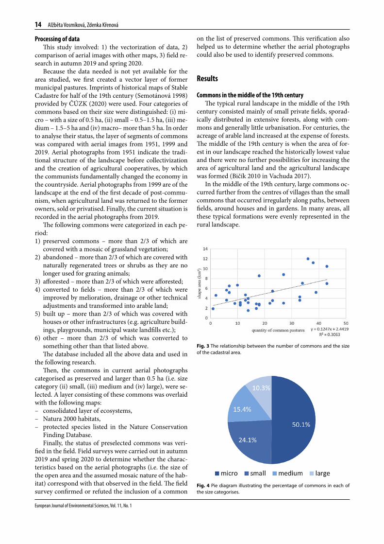
Fig. 3 The relationship between the number of commons and the size of the cadastral area.
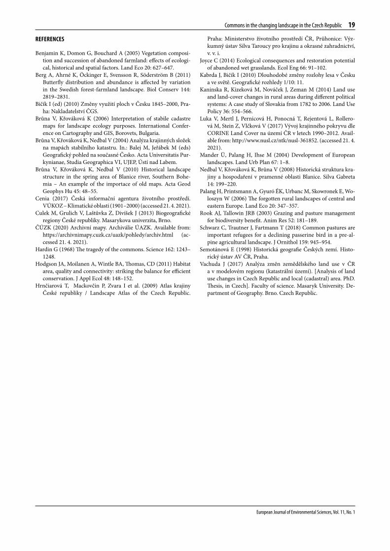
Fig. 4 Pie diagram illustrating the percentage of commons in each of the size categorises.

European Journal of Environmental Sciences, Vol. 11, No. 1
Commons in the changing landscape in the Czech Republic 15
Based on historical maps from the middle of the 19th century, 668 commons were in the area studied. As ex-pected, the number increased with the size of the cadas-tral area, but the relationship is not very strong (Fig. 3).
The size of commons varies markedly and they are not distributed uniformly in terms of size categories (Fig. 4). More than 50% of all commons are smaller than 0.5 ha. These small and often narrow commons were usually used as corridors for moving grazing animals from one pasture to another. Herds of cattle used them for a short stop during their regular trips to large pastures and there-fore they occur more frequently than large commons.
The early 1950sThe aerial photographs from the early 1950s reflect
the situation in Czechoslovakia after World War II and at the beginning of the socialist era. Land reforms started after the Communist revolution in 1948. However, aeri-al photographs from the early 1950s reveal that the area studied has not changed significantly in that individual plots, small fields, forests and other types of individual properties were still present.
Compared with the situation 100 year ago, the per-centage of the land classed as agricultural is similar and only structural changes occurred in the 1950s. During this 100-year period, the area and number of commons decreased only slightly. More than 2/3 of the former commons were preserved (Table 1) and they made up an important part of the landscape. Borders of the com-mons were usually clear and rarely violated. The biggest percentage of commons was lost to afforestation, which occurred at the beginning of the 19th century (Bičík 2010 in Vachuda 2017). About 5% of former commons was converted into fields or meadows. Occasionally, some drainage or landscaping (e.g. removing big stones or levelling of the surface) were necessary. However, the extent of this landscaping was small compared with what happened in the coming decades. The area of agri-cultural land increased, but not very significantly. Some commons were built on and others abandoned and over-grown in the course of natural succession. Based on the aerial photographs, the preserved commons were those
that were not afforested, built on or abandoned and then subject to natural succession.
The late 1990sThe status of commons in the last years of the 20th
century is the result of four decades of socialist agri-culture and not always appropriate management of the Czech landscape. However, at the end of the 1990s, the effects of economic and property changes, which were implemented after the Velvet Revolution in 1989 (includ-ing privatization, abolition of agricultural cooperatives, reduction in arable land, etc.), are also evident. Until the 1990s, the agricultural policy in Czechoslovakia was in-fluenced by farm nationalization and that resulted in sig-nificant changes in the landscape, predominantly in the percentage of arable land. In the early 1990s, landscape was affected by the change in ownership, both with res-titution and privatisation. Especially agricultural land, which was divided among a large number of owners, but only a fraction of them farmed their land again (Kabrda and Bičík 2010). That led to abandonment, renting and changes in the use of these lands. When the restitution and restructuring was complete, comprehensive land ad-justments began. In the aerial images, changes in the use of commons are very noticeable at this time.
The decrease in the number and acreage of commons continued. More than half of all commons disappeared and only one third were preserved (Table 1). The trend in transforming commons into agricultural fields esca-lated. In the late 1990s, a quarter of former commons were already converted into fields and being used as an agriculture field or a part of a large agricultural complex. Another 22.3% of commons was abandoned and left to natural succession. From the middle of the 20th century, there was a very rapid increase in population resulting in a 6% increase in built-up areas on unused parts of former commons. In addition, the percentage of afforested com-mons increased from 8.1% in 1950s to 12.1% in the late 1990s (Table 1).
The status of commons in 2019During the first 20 years of the new millennium there
were still significant changes, which resulted in the trans-formation of former commons into other functional seg-ments of landscape. The changes were not as significant as in the previous period. However, we must consider the length of the period, which was only two decades. The main driver of the transformation of commons in this period was the increase in the number of abandoned commons. In 2019, more than one third of commons had vanished due to natural succession. Abandoned, unman-aged commons became overgrown naturally because of a sequel of privatization in the 1990s and unclear own-ership or speculation over the sale of the land. In addi-tion, because in previous times the commons were often rocky or waterlogged localities with inaccessible terrain, it proved difficult to find an alternative use for them.
Table 1 Percentage of preserved commons present at different times from 1850s to 2019.
State of commons 1850searly
1950slate
1990s2019
preserved 100% 76.5% 30.2% 12.1%
built on 0% 2.5% 6.0% 6.3%
converted to fields 0% 5.1% 25.1% 29.0%
afforested 0% 8.1% 12.1% 12.7%
abandoned 0% 3.7% 22.3% 34.7%
other 0% 0.1% 0.9% 1.3%
combination 0% 3.9% 3.3% 3.7%

European Journal of Environmental Sciences, Vol. 11, No. 1
16 Alžběta Vosmíková, Zdenka Křenová
Large agricultural complexes, commercial forests and urban areas were the most abundant structural elements in the landscape in 2019. The borders of former com-mons are not clearly visible and if so, mostly it is a border of an overgrown area, where natural succession has been occurring for a long time. Currently only about 12% of former commons remain (Table 1), but they have a high conservation value because they host a mosaic of vege-tation.
Almost two centuries of changeThere have been significant changes in the status of
commons in the area studied since the middle of the 19th century. This period was divided into three, in which the changes are visible and can be easily evaluated. An illus-trative series of pictures showing the transformation of commons over almost two centuries is in Appendix 1.
Decrease in the number and acreage of commons during these three periods was not uniform (Table 2). During the first period (1850s–1950s), the largest per-centage of commons was lost due to afforestation. We assume that this was due to the beginning of the large
afforestation at the end of the 19th century. In the follow-ing periods, this transformation was never that visible.
The biggest changes occurred during the second pe-riod (1950s–1990s), although this period was signifi-cantly shorter than the first. The main driver of change was amelioration, when almost a fifth of the commons was drained, big stones removed, ploughed and convert-ed into agriculture fields and meadows (Table 2). Almost the same percentage was abandoned and left to natural succession.
In the last period, the above factors were of little sig-nificance except for abandonment (Table 2). Inappropri-ate management in previous times and ownership chang-es in the 1990s resulted in an increase in them being left to natural selection.
Preserved commons Finally, analyses of maps together with the two-step
field verification (autumn and spring) helped us to iden-tify 49 preserved commons in the area studied. They were open with a mosaic of vegetation and their borders were well preserved and visible. Their distribution in the area of interest is very irregular and the predominant ecosys-tem in the cadastral area has no effect on the number of preserved commons (Fig. 5).
Our field surveys confirmed that many of the pre-served commons consist of a mosaic of significantly valu-able habitats, which are occupied by rare and protected species. The existence of a mosaic of habitats, mostly in extensively managed commons, in the current monoto-nous landscape is highly valuable from the conservation point of view. It is well established that these commons contribute to the conservation of species and habitat biodiversity. Their presence in the landscape is therefore crucial. The majority of the preserved commons are part of the Terrestrial system of ecological stability (Hrnčia-
Table 2 Changes in percentage of different land covers recorded in the different periods.
Status of commons 1850searly
1950slate
1990s2019
preserved 100% −23.5% −46.3% −18.1%
built up 0% 2.5% 3.4% 0.3%
converted to fields 0% 5.1% 20.1% 3.9%
afforested 0% 8.1% 4.0% 0.6%
abandoned 0% 3.7% 18.6% 12.4%
other 0% 0.1% 0.7% 0.4%
combination 0% 3.9% −0.6% 0.4%
Fig. 5 Map showing the predominant ecosystem in each cadastral area and the distribution of preserved commons.

European Journal of Environmental Sciences, Vol. 11, No. 1
Commons in the changing landscape in the Czech Republic 17
rová et al. 2009; ecological networks in the sense of the Czech Nature Conservation Act No. 114/1992; Fig. 6). In total, 51% of the preserved commons mapped are local bio centres or local bio corridors.
Discussion and Conclusions
This study evaluated the current status of former com-mons, which were identified based on the maps of the Stable Cadastre, unique maps that cover the entire area of Bohemia, Moravia and Silesia (Semotánová 1998). Us-ing these maps, it is possible to reconstruct the landscape present in the middle of the 19th century with a high de-gree of accuracy. They are an important source of knowl-edge on the character of the historic landscape and their accuracy enables one to digitally process and implement them in the geographic information system (GIS), which opens up further possibilities for analysing the structure of the historic landscape and comparing it with the cur-rent state (Brůna et al. 2004, 2006). Nedbal et al. (2008) and Brůna et al. (2010) state that the data from the Sta-ble Cadastre are most suitable in terms of precision for monitoring the state and changes in the non-forest land-scape. It was an essential basis for determining land tax-es, and therefore both mapmakers and landowners were very interested in the exact details of the land and the determination of culture, i.e. the current use of land. The suitability of the maps of the Stable Cadastre for monitor-ing landscape changes in areas of increased conservation interest was also confirmed by this study, which focused on a selected type of land – commons.
In the area studied, which included 35 cadastral units, 668 former commons were identified. This area was se-lected because of the many well-preserved commons around Těchonice village, which is located in the mid-
dle of the area studied. This rural countryside with poor infrastructure and many commons was a suitable study area. However, landscape structure in this area is similar to other Czech regions and the methodology used can be easily implemented in other similar areas. Worth notic-ing is that only a small number of commons larger than 1.5 hectares were recorded in this study. These commons can be grazed by large and, above all, more diversified herds, which results in a specific type of farming bene-ficial from the point of view of maintaining diversity. In addition, to the information on the size and frequency of commons in the land register, it was possible to deter-mine whether and how the size of the land area and the size of the commons are related. We found only a slightly positive correlation, which was certainly influenced by the fact that individual cadastres not only differ in area, but also in other parameters (e.g. relief, soil stoniness, historical development, type of colonization, population densities).
The coverage of commons based on aerial images was determined for six basic categories, which were com-bined according to a predetermined procedure. In par-ticular, the recognition of categories “abandoned” and “afforested” in some cases was unclear. Sometimes it was difficult to identify whether the current vegetation cover is the result of spontaneous overgrowth or tree plantings. The actual condition could not be verified in the field in all cases. However, a field survey of a selected subset of locations revealed only a few errors. The identification of the type of cover from the images from the 1950s and 1990s was carried out according to the same methodol-ogy as for the current images. Poor image quality often made it difficult to identify the cover accurately. Howev-er, an important criterion that often offset this inaccurate classification in historical pictures was the preservation of the boundaries of the commons. The boundaries of
Fig. 6 Map showing the location of preserved commons and the Terrestrial system of landscape ecological stability.

European Journal of Environmental Sciences, Vol. 11, No. 1
18 Alžběta Vosmíková, Zdenka Křenová
former commons were, in contrast to the current situ-ation, mostly well distinguishable in images from the 1950s and 1990s.
The significant increase in all combinations of cover between 1950s–1990s and 1990s–2019 is not to be over-looked and was partly expected. This phenomenon is based on the general increasing tendency of land cover to change due to socio-economic changes occurring at that time.
An important period for significant changes in the use of commons was the collectivization of agriculture, which started in 1948. After this process, melioration oc-curred mainly in the 1960s–1970s. Many locations, valu-able from the conservation point of view, however, were drained and converted to agriculture lands even during the second half of the 1980s. As reported by Luka et al. (2017) large-scale drainage significantly changed the Czech landscape.
Its main purpose was to expand the agricultural area and increase food production. The tendency towards food self-sufficiency thus caused the amelioration of a significant part of the landscape, whose functions had so far been other than just production. The commons could be an example of a part of the landscape, which have lost their mosaic and overall biological and cultural value. Commons used to be rich wetland localities, but due to amelioration, they were drained, ploughed and converted into fields. The same trend, i.e. converting of meadows and commons to arable land in the second half of the 20th century, is also mentioned by Kaninska et al. (2014), who examined changes in the landscape in the Slovak foothills. After the 1950s there was almost a 20% increase in the number of abandoned commons. Many of them were abandoned already in 1920s or 1930s; how-ever, successional changes were not too apparent during the first decades. Similarly, some commons recognized as abandoned during the socialist era (1950s–1990s) were in fact unmanaged already before or during WWII. They were not recognised as abandoned based on aerial photo-graphs taken in the early 1950s because the successional changes were not recognizable at that time. Natural suc-cession is usually slower and less apparent during the first years after the ending of management and overgrowth ac-celerates in the later stages of succession (e.g. Joyce 2014). In the area studied, this common trend was supported by social-economical changes during the communist era, when private and municipal ownership of the land com-pletely disappeared and many chaotic measures escalat-ing in succession could happen on abandoned commons (e.g. litter of old hay or manure, municipal waste land-fills, irregular cutting of firewood etc.).
The high percentage of abandoned commons af-ter 1990s can be explained by socio-economic changes during the last 30 years. Although these areas were re-turned to their original owners in the 1990s, not all sub-sequent owners had the tools, capacities, finances and
will to restore the long-term abandoned former com-mons. Many of them continued to be uncultivated and succession continued. The speed of succession and the current amount of woody vegetation on these former commons was influenced by a number of factors, includ-ing both abandonment, previous management, local eco-logical conditions (soil, humidity, nutrient availability, etc.), diaspora source, various disturbances (game activi-ties, casual visitors), change in techniques, etc. (Benjamin et al. 2005).
Answering the question raised by Hardin’s essay (1968), we can say that the history of commons is not a complete tragedy, notwithstanding that our inventory revealed that three quarters of former commons have disappeared for different reasons. There is still, however, a great opportunity to save the rest of them and benefit from these treasures in our landscape. The existence of these extensively managed areas in our humdrum land-scape is very important. This type of ecosystem provides many services. In contrast to intensive grazing, which forms the main part of the homogenized landscape, commons contribute to the preservation of species bio-diversity, provide natural refuges for specific species and, among other functions, significantly help retaining water in the landscape. They significantly contribute to miti-gating climate change and support sustainable landscape management. The cultural and historical significance for the local people and aspects of human well-being are also worth highlighting.
There are mosaics of significantly valuable habitats, in which populations of rare and protected species oc-cur on all of the currently preserved commons. Some of them are managed for their conservation value: there is a nature reserve and several localities with endangered species, the management of which is paid from natural conservation funds. Local farmers or members of hunt-ing clubs occasionally manage several others. However, many of the currently preserved commons lack appropri-ate management. More detailed evaluations of their con-servation value and appropriate management are very much needed. More preserved and eventually restored commons should be included in the Territorial system of landscape ecological stability (i.e. ecological network), because they can play an important role as biodiversity stepping stones and improve the structure of the land-scape.
Acknowledgements
We thank the following institutions and persons: A. F. G. Dixon for revising the language and J. Koreš for his endless and contagious enthusiasm for commons. This study was funded by the Ministry of Education, Youth and Sports of CR within the CzeCOS program, grant number LM2018123.
European Journal of Environmental Sciences, Vol. 11, No. 1
Commons in the changing landscape in the Czech Republic 19
REFERENCES
Benjamin K, Domon G, Bouchard A (2005) Vegetation composi-tion and succession of abandoned farmland: effects of ecologi-cal, historical and spatial factors. Land Eco 20: 627–647.
Berg A, Ahrné K, Öckinger E, Svensson R, Söderström B (2011) Butterfly distribution and abundance is affected by variation in the Swedish forest-farmland landscape. Biol Conserv 144: 2819–2831.
Bičík I (ed) (2010) Změny využití ploch v Česku 1845–2000, Pra-ha: Nakladatelství ČGS.
Brůna V, Křováková K (2006) Interpretation of stabile cadastre maps for landscape ecology purposes. International Confer-ence on Cartography and GIS, Borovets, Bulgaria.
Brůna V, Křováková K, Nedbal V (2004) Analýza krajinných složek na mapách stabilního katastru. In.: Balej M, Jeřábek M (eds) Geografický pohled na současné Česko. Acta Universitatis Pur-kynianae, Studia Geographica VI, UJEP, Ústí nad Labem.
Brůna V, Křováková K, Nedbal V (2010) Historical landscape structure in the spring area of Blanice river, Southern Bohe-mia – An example of the importace of old maps. Acta Geod Geophys Hu 45: 48–55.
Cenia (2017) Česká informační agentura životního prostředí. VÚKOZ – Klimatické oblasti (1901–2000) (accessed 21. 4. 2021).
Culek M, Grulich V, Laštůvka Z, Divíšek J (2013) Biogeografické regiony České republiky. Masarykova univerzita, Brno.
ČÚZK (2020) Archivní mapy. Archiválie ÚAZK. Available from: https://archivnimapy.cuzk.cz/uazk/pohledy/archiv.html (ac-cessed 21. 4. 2021).
Hardin G (1968) The tragedy of the commons. Science 162: 1243–1248.
Hodgson JA, Moilanen A, Wintle BA, Thomas, CD (2011) Habitat area, quality and connectivity: striking the balance for efficient conservation. J Appl Ecol 48: 148–152.
Hrnčiarová T, Mackovčin P, Zvara I et al. (2009) Atlas krajiny České republiky / Landscape Atlas of the Czech Republic.
Praha: Ministerstvo životního prostředí ČR, Průhonice: Výz-kumný ústav Silva Taroucy pro krajinu a okrasné zahradnictví, v. v. i.
Joyce C (2014) Ecological consequences and restoration potential of abandoned wet grasslands. Ecol Eng 66: 91–102.
Kabrda J, Bičík I (2010) Dlouhodobé změny rozlohy lesa v Česku a ve světě. Geografické rozhledy 1/10: 11.
Kaninska R, Kizeková M, Nováček J, Zeman M (2014) Land use and land-cover changes in rural areas during different political systems: A case study of Slovakia from 1782 to 2006. Land Use Policy 36: 554–566.
Luka V, Mertl J, Pernicová H, Ponocná T, Rejentová L, Rollero-vá M, Stein Z, Vlčková V (2017) Vývoj krajinného pokryvu dle CORINE Land Cover na území ČR v letech 1990–2012. Avail-able from: http://www.nusl.cz/ntk/nusl-361852. (accessed 21. 4. 2021).
Mander Ü, Palang H, Ihse M (2004) Development of European landscapes. Land Urb Plan 67: 1–8.
Nedbal V, Křováková K, Brůna V (2008) Historická struktura kra-jiny a hospodaření v pramenné oblasti Blanice. Silva Gabreta 14: 199–220.
Palang H, Printsmann A, Gyuró ÉK, Urbanc M, Skowronek E, Wo-loszyn W (2006) The forgotten rural landscapes of central and eastern Europe. Land Eco 20: 347–357.
Rook AJ, Tallowin JRB (2003) Grazing and pasture management for biodiversity benefit. Anim Res 52: 181–189.
Schwarz C, Trautner J, Fartmann T (2018) Common pastures are important refugees for a declining passerine bird in a pre-al-pine agricultural landscape. J Ornithol 159: 945–954.
Semotánová E (1998) Historická geografie Českých zemí. Histo-rický ústav AV ČR, Praha.
Vachuda J (2017) Analýza změn zemědělského land use v ČR a v modelovém regionu (katastrální území). [Analysis of land use changes in Czech Republic and local (cadastral) area. PhD. Thesis, in Czech]. Faculty of science. Masaryk University. De-partment of Geography. Brno. Czech Republic.

European Journal of Environmental Sciences, Vol. 11, No. 1
20 Alžběta Vosmíková, Zdenka Křenová
1950s
1990s 2019
Appendix 1A series of pictures showing changes over time in Malý Bor cadastre – an illustrative segment of the area studied. Red line – borders of common pastures.
1850s

European Journal of Environmental Sciences 21
Štípková, Z., Kindlmann, P.: Factors determining the distribution of orchids – a review with examples from the Czech Republic European Journal of Environmental Sciences, Vol. 11, No. 1, pp. 21–30
https://doi.org/10.14712/23361964.2021.3 © 2021 The Authors. This is an open-access article distributed under the terms of the Creative Commons Attribution License (http://creativecommons.org/licenses/by/4.0),
which permits unrestricted use, distribution, and reproduction in any medium, provided the original author and source are credited.
FACTORS DETERMINING THE DISTRIBUTION OF ORCHIDS – A REVIEW WITH EXAMPLES FROM THE CZECH REPUBLICZUZ ANA ŠTÍPKOVÁ 1,2 ,* and PAVEL KINDLMANN 1,2
1 Global Change Research Institute, Czech Academy of Science, Bělidla 986/4a, 60300 Brno, Czech Republic2 Institute for Environmental Studies, Faculty of Science, Charles University, Benátská 2, 12801 Prague 2, Czech Republic* Corresponding author: [email protected]
ABSTRACT
The natural environment has been significantly altered by human activity over the past few decades. There is evidence we are now experiencing the sixth mass extinction, as many species of plants and animals are declining in abundance. We focused on the Orchidaceae because this plant family has experienced one of the biggest reductions in distribution. We investigated patterns in species richness and distribution of orchids, the rate and causes of their decrease and extinction, and factors influencing their occurrence in the Czech Republic and Greece. The key findings are: (i) Method of pollination and type of rooting system are associated with their distributions and they are different in the two countries. We assume that these differences might be due to the difference in the orography, distribution of suitable habitats and types of bedrock in these two countries. (ii) The greatest reduction in distribution was recorded for critically endangered taxa of orchids. The number of sites suitable for orchids in the Czech Republic declined by 8–92%. The most threatened orchid species are Spiranthes spiralis, Anacamptis palustris, Epipogium aphyllum and Goodyera repens. The distribution of orchids in the Czech Republic is mainly determined by the distribution of their habitats. (iii) The most important factor affecting the distribution of Czech orchids in South Bohemia is land cover. And the most important types of habitats (types in KVES) are oak and oak-hornbeam forests and agricultural meadows. Based on this information, it should be possible to improve the management that is crucial for maintaining orchid localities.
Keywords: decline; environmental factors; extinction; Maxent; orchids; pollination; root system
Introduction
Worldwide biodiversity is currently decreasing dra-matically. The Intergovernmental Science-Policy Plat-form on Biodiversity and Ecosystem Services (IPBES), working under the UN auspices, published an extensive report on plant and animal biodiversity in May 2019. According to this report, we are facing the sixth global extinction of species with species diversity decreasing worldwide at a fast pace, the rate of species extinction is now a hundred times greater than the average for the last ten million years and one-eighth of existing species are endangered (https://ipbes.net/global-assessment). Fur-thermore, the report of IPBES states that approximate-ly three quarters of the terrestrial and two thirds of the marine environment have been significantly altered by human activity. One of the main reasons for this huge decrease in biodiversity in the world is loss of the nat-ural habitats of plants and animals (https://ipbes.net /global-assessment).
Orchids are known all over the world because of their beautiful flowers in the wild, as well as in our gardens and homes, and have become very popular in the last few decades. There are many publications on the distri-bution of orchids worldwide, which indicate that both professionals and the lay public are interested in orchids (e.g. Millar 1978; Seidenfaden and Wood 1992; Bose et al. 1999; Dykyjová 2003; Vlčko et al. 2003; Jersáková and Kindlmann 2004; Průša 2005; Averyanov et al. 2015; An-tonopoulos and Tsiftsis 2017; Grulich 2017; Tsiftsis and Antonopoulos 2017; Kühn et al. 2019; Knapp et al. 2020;
Wagensommer et al. 2020 and many others). Unfortu-nately, the family Orchidaceae is one of the most threat-ened plant families with a high risk of species extinction (Swarts and Dixon 2009). Orchids are disappearing worldwide, mostly due to habitat loss, but other factors like climate change are likely to increase in importance during the 21st century (Wotavová et al. 2004; Pfeifer et al. 2006). Because of the high risk of extinction, orchids are listed in CITES and protected by law in many countries.
Despite the high number of studies on orchids, we still lack critical information necessary for the conservation of Orchidaceae, especially for species that are known to be threatened or endangered. All aspects that will be mentioned below make orchids an excellent plant family for various studies on various aspects of biology.
Orchids and their Specialized Life Strategies
The orchid family is an important group with respect to conservation biology (Pillon and Chase 2006), because so many are threatened with extinction (Swarts and Dix-on 2009). Many characteristics, such as great species richness, specific role in ecosystems, or threat of extinc-tion, make it crucial to explore the distribution and con-servation status of Orchidaceae (Zhang et al. 2015).
Orchids, with approximately 28 500 species (Gov-aerts 2020) are the most diverse and widespread fami-ly of flowering plants (Swarts and Dixon 2009) and are classified among the most threatened groups worldwide (Cribb et al. 2003; Kull and Hutchings 2006). They are an

European Journal of Environmental Sciences, Vol. 11, No. 1
22 Zuzana Štípková, Pavel Kindlmann
ideal group for exploring determinants of species diver-sity because they are well recorded and studied in many countries in Europe (Kull et al. 2006).
Most species of orchids are threatened in the wild (Cribb et al. 2003) and are disappearing from their natu-ral habitats worldwide (Cribb et al. 2003; Kull and Hutch-ings 2006; Knapp et al. 2020; Wagensommer et al. 2020). In Europe, all orchids are terrestrial and can be found in almost all habitats (Hágsater and Dumont 1996; Delforge 2006; Štípková et al. 2017). The most species-rich area in Europe is Southern Europe, especially the Mediterranean area (Del Prete and Mazzola 1995; Hágsater and Dumont 1996). Certain orchid genera (e.g. Ophrys, Serapias), for which the Mediterranean area is a centre of evolution, are remarkably species diverse (Del Prete and Mazzola 1995; Phitos et al. 1995; Pridgeon et al. 2001), whereas the greatest species diversity of species-rich genera are of more northern origin (e.g. Epipactis, Dactylorhiza) is recorded in central and northern Europe (Averyanov 1990). The availability of detailed records provides op-portunities for comparative analyses of the declines in species over time.
Therefore, it is a pity that despite the high number of studies dealing with orchids, we still lack rigorous analy-ses of this data aimed at determining the relative impor-tance of environmental factors and species traits associ-ated with the decline in the numbers of sites suitable for orchids and particular species. However, such an analysis is crucial for their conservation in terms of an effective management of orchid sites (Kull and Hutchings 2006). Terrestrial orchids are probably one of the best examples of the decline in biodiversity in plants.
There is an important life history trait that plays a significant role in determining orchid presence/absence
and distribution in space: their rooting system, which is thought to represent particular strategies for under-ground storage of resources (Rasmussen 1995). In some species, the rooting system consists of a simple rhizome, whereas in others it is thicker and tuberous and serves as a storage organ. Among the European orchids, the genera Epipactis, Cephalanthera and Cypripedium, which are be-lieved to be the most primitive, have short rhizomes. The most important evolutionary development in the growth forms of Orchidaceae was the production of efficient storage organs (tuberoids). In this evolutionary process, Pseudorchis albida is the most primitive tuberoid orchid, whereas the palmate tuberoids (Dactylorhiza, Coeloglos-sum, Gymnadenia) and those with fusiform tubers (e.g. Platanthera) evolved later (Dressler 1981; Averyanov 1990; Tatarenko 2007). Coarse division of the European orchids in terms of their rooting systems could be useful for testing hypotheses on their patterns of distribution, as this trait has evolved and differentiated in response to changing climatic conditions (Averyanov 1990).
Following the evolutionary trends in temperate or-chids (Dressler 1981; Averyanov 1990; Tatarenko 2007), the species of orchids were classified here in three catego-ries based on the above-mentioned morphology of their root system, which also indicates how primitive or highly evolved an orchid is. Based on this classification, the first species group consists of the rhizomatous orchids (Ceph-alanthera, Corallorhiza, Cypripedium, Epipactis, Epipogi-um, Goodyera, Hammarbya, Limodorum, Liparis, Malaxis and Neottia), the second, those with palmate or fusiform tubers, which is the intermediate stage (hereafter referred to as intermediate) in the evolution of temperate orchids in Eurasia, and includes species of the genera Dactylorhi-za, Gymnadenia, Platanthera and Pseudorchis. The third
Fig. 1 Different types of orchid rooting systems: (a) rhizomatous, (b) intermediate and (c) tuberous.
(a) (b) (c)

European Journal of Environmental Sciences, Vol. 11, No. 1
Factors determining the distribution of orchids 23
species group consists of those orchids with a spheroid or spindle-shaped tuberous root system (Anacamptis, Herminium, Himantoglossum, Neotinea, Ophrys, Orchis, Spiranthes and Traunsteinera). See Fig. 1 for illustrations of these categories.
Relationship between species richness of orchids with different rooting systems and various ecological factors and degree of specialization based on specific environ-mental conditions have not been previously studied in Europe. To fill this gap in our knowledge, we explored the associations of orchid species richness and the degree to which an orchid species is adapted to living in specific environmental conditions (in terms of species specializa-tion index) with altitude in the Czech Republic (Štípková et al. 2021a) and with various ecological factors in Greece (Tsiftsis et al. 2019).
In addition to the differences in their rooting systems, orchids have very complicated pollination strategies. Survival of an orchid population or even a species may strongly depend on pollination and subsequent seed production (Jacquemyn et al. 2005a). As specialized pol-lination systems may be particularly vulnerable to an-thropogenic modification of landscapes (Anderson et al. 2011; Pauw and Bond 2011; Phillips et al. 2015) and may strongly affect species survival.
Generally, orchids are characterized by a diversity and specificity of pollination mechanisms, which may involve the food-foraging, territorial defence, pseudoantago-nism, rendezvous attraction, brood-site and shelter im-itation, sexual response, or habitat-selection behaviour of their pollinators (Ackerman 1986; Tremblay 1992; Tremblay et al. 2005; Jersáková et al. 2006; Micheneau et al. 2009). Most plants pollinated by animals produce and offer rewards to attract pollinators to visit their flowers (nectariferous species; Simpson and Neff 1983). Nec-tar is the most common floral reward (Dressler 1981; Jersáková and Johnson 2006) and can influence several aspects of pollinator behaviour (Jersáková and Johnson 2006). However, some plants attract pollinators, but do not offer any reward (nectarless – often also called de-ceptive – species; Heinrich 1979; Bell 1986). The nectar-less strategy has evolved in many plant families, but most nectarless species are orchids (Renner 2005; Jersáková et al. 2006). In general, plants of nectariferous species are visited more frequently than nectarless plants (Neiland and Wilcock 1998; Pellissier et al. 2010). Pollinators also visit more flowers per inflorescence of nectariferous than nectarless species (Jersáková and Johnson 2006; Hob-bhahn et al. 2017). Nectariferous species are less polli-nator-specific than nectarless species, among which the most pollinator-specific are sexually deceptive species (Cozzolino and Widmer 2005; Phillips et al. 2009). As many as 60–70% of orchids have a single species of pol-linator (Tremblay et al. 2005). This level of specialization (Tremblay 1992; Phillips et al. 2009) makes orchids vul-nerable to fluctuations in pollinator abundance. Nec-tariferous orchids are better competitors for pollinators
than nectarless orchids (Pellissier et al. 2010). All this has consequences for fruit production and the fitness of the plants. As a result, nectariferous species have a higher fruit set than nectarless ones (Neiland and Wilcock 1998; Tremblay et al. 2005; Phillips et al. 2009; Hobbhahn et al. 2017) in all geographical areas (Neiland and Wilcock 1998) due to pollination limitation (Neiland and Wilcock 1998; Tremblay et al. 2005). Based on the above, we pro-pose that pollination strategy plays a role in orchid distri-bution (Štípková et al. 2020b).
All the above and a range of ecological conditions af-fect the altitudinal and spatial distribution of orchids. For example, on La Reunion Island, Jacquemyn et al. (2005b) report that animal-pollinated orchids are more abundant at lower altitudes, whereas at high altitudes orchids tend-ed to be auto-pollinated and cleistogamous. In Switzer-land, the relationship between altitude and frequency of orchids with different reward strategies indicates a signif-icant decrease in the occurrence of nectarless species of orchids with increase in altitude (Pellissier et al. 2010).
In addition to the pollination strategy, pollinator abundance can also affect fruit set in orchids. Pollinator abundance is influenced by the climate (temperature, seasonality) in a given area, which in turn is strongly de-termined by altitude (Arroyo et al. 1982; Körner 2007). Although the testing of the associations of species rich-ness and niche breadth with altitude are frequently re-ferred to in the literature (e.g. Kluge and Kessler 2011; McCreadie et al. 2017; Herrera et al. 2018; Vargas et al. 2008 and so on), none of these studies distinguish be-tween pollination strategies (nectariferous/nectarless).
Mycoheterotrophy allows orchids to adapt to a wide variety of habitats, even those with extreme conditions (e.g. sites with little soil or lack of light). In the upper mountain zone, although it rains equally all year round the upper soil horizons are rich in organic matter (mostly in forested habitats), orchids (mostly rhizomatous and to a lesser extent palmate or fusiform tuberoids) are adapt-ed to the low light conditions, often involving obligate mycoheterotrophy (Jacquemyn et al. 2017). The tuberous orchids mostly occur in open, dry and hot environments around the Mediterranean and in nutrient poor and eroded soils (Averyanov 1990; Delforge 2006). Although in these areas, low availability of soil water and nutri-ents are causes of stress (contrary to light, which is the cause of stress in forested habitats), fungi provide orchids with the water and nutrients necessary for their survival and growth. Moreover, when conditions (e.g. climatic) are unsuitable, the underground organs of orchids can remain alive and dormant, exploiting fungi, for several years (Rasmussen 1995; Shefferson et al. 2018).
Orchids and their Conservation
One of the key goals of conservation is to determine what causes declines in biodiversity and suggest ways

European Journal of Environmental Sciences, Vol. 11, No. 1
24 Zuzana Štípková, Pavel Kindlmann
of stopping or slowing it down (Gaston and Blackburn 2000). This is especially true in Europe, where the num-bers of species, abundances and distributions of many species of plants and animals have dramatically declined during recent decades.
The need for effective conservation measures is ur-gently required for areas and countries that were affected by human activities in past decades, and thus have lost a part of their biodiversity or the distributions of certain species have been greatly reduced (Štípková and Kindl-mann 2021; Štípková et al. 2021b). It is commonly ac-cepted that urbanization, land use changes and intensi-fication of agriculture have resulted in a dramatic loss and fragmentation of habitats (Stewart 1992; Fischer and Stöcklin 1997; Kull et al. 2002, 2016; Bilz et al. 2011; Tsiftsis et al. 2011). The current landscape in Europe is mainly a result of recent changes in farm management (Henle et al. 2008). This affected the composition of the flora and fauna in most areas and resulted in a decline in European biodiversity (Fahrig et al. 2011; Ferreira et al. 2013; Brunbjerg et al. 2017; Fardila et al. 2017; Poschlod and Braun-Reichert 2017; Hass et al. 2018; Kurze et al. 2018). As for most other taxonomic groups, the reasons for the decline in orchid biodiversity include habitat loss, eutrophication and fragmentation (Wotavová et al. 2004; Janečková et al. 2006; Kull and Hutchings 2006; Kull et al. 2016). Central European countries have been intensively affected by changes in land use or agricultural intensifi-cation. Among these countries, the Czech Republic was strongly affected by such changes during the last few de-cades (Štípková et al. 2021b). In the past, there were im-portant changes in the use of land in the Czech Republic, which differed from those that occurred in western parts of Europe due to changes in the political regimes (Adams and Adams 1971; Wädekin 1982; Krčmářová and Jeleček 2017). Before 1948, fields and meadows were tradition-ally managed (Krčmářová and Jeleček 2017), which in-volved mowing and grazing, low intensity agriculture of small fields and low application of fertilizers (Adams and Adams 1971). After 1948, small fields were consol-idated into huge fields (Skaloš et al. 2011) and subsidies for fertilizers were provided, which resulted in high lev-els of nutrient chemicals in the soil (Adams and Adams 1971). As a result, many orchids declined and can now only be found at a small number of sites (Štípková and Kindlmann 2021). After the change in regime in 1989, the subsidies for fertilizers ceased, which resulted for a while in a great decline in the use of fertilizers (Reif et al. 2008). The implications for the survival of sites suitable for orchids, however, were not dramatic (Štípková and Kindlmann 2021).
Knowledge of orchid ecology, including environmen-tal gradients that influence the patterns in orchid abun-dance, distribution, richness and composition, is essen-tial for planning and applying conservation strategies and actions (Tsiftsis et al. 2008; Swarts and Dixon 2009), and lack of such knowledge negatively affects our ability to
identify sites that are worth protecting. We also still lack the knowledge needed to develop management plans for orchids under current or future scenarios of habitat loss and climate change.
Among others, there are two crucially important values when orchid conservation and survival during climate change is considered: number of species per unit area and the degree to which an orchid species is specialized to specific environmental conditions. The former clearly determines the conservation value of an area, while the latter tells us how much a species may be endangered by changes in environmental conditions, e.g., climate change. Both values were used for assessing the factors that affect the distribution of Czech orchids (Tsiftsis et al. 2019; Štípková et al. 2020a; Štípková et al. 2021a).
Patterns in the Distribution of Orchids
Understanding the abundance and patterns in the distributions of species at large spatial scales is one of the key goals of biogeography and macroecology (Gas-ton and Blackburn 2000; Tsiftsis et al. 2019), but effec-tive conservation requires knowledge of species at small spatial scales (Tsiftsis et al. 2008; Swarts and Dixon 2009).
Species richness decreases from the equator towards the poles (Crame 2001; Francis and Currie 2003) and this pattern is among the most consistent in biogeography (Hillebrand 2004). The dependence of species richness on altitude is usually hump-shaped (Vetaas and Grytnes 2002; Bhattarai and Vetaas 2003), or monotonically de-creases with increasing altitude (Bachman et al. 2004; Jacquemyn et al. 2005b), but sometimes species richness increases with altitude or shows an inversely unimodal trend; more rarely there is no obvious trend (Grytnes 2003; Hrivnák et al. 2014). In temperate regions, plant species richness is lower in areas that are cold compared to those that are warm, while species niches and range sizes tend to be broader (Stevens 1989; Thompson 2005). However, in addition to environmental gradients, there are other important factors that influence these patterns and niche breadth, e.g. the life-history strategies of spe-cies (Kostikova et al. 2013). Global warming has a direct effect on species distributions, as over the last few years there has been an increase in the number of species of plant species occurring in high mountains in Europe (Steinbauer et al. 2018). Although distributions of some species now extend further north or to higher altitudes than previously, other species are becoming more re-stricted due to the desertification observed in the south-ern parts of Europe (Karamesouti et al. 2015).
Species distribution models (SDMs) are a useful tool, which over the last few decades were often used in many branches of biogeography, conservation biology and ecology (Elith and Leathwick 2009), especially in stud-

European Journal of Environmental Sciences, Vol. 11, No. 1
Factors determining the distribution of orchids 25
ies on threatened species (Guisan et al. 2013). These nu-merical tools combine species occurrence records with environmental data (Elith and Leathwick 2009). In com-bination with GIS techniques, these models are especial-ly important and useful for predicting the occurrence of rare species (Guisan and Thuiller 2005). Although the results of species distribution models often suffer from high levels of uncertainty due to biases in species distri-bution data, errors in environmental variables used as predictors, spatial resolution and the modelling process (Elith and Graham 2009; Rocchini et al. 2011), SDMs are nevertheless widely used to predict species distributions (Tsiftsis et al. 2012).
The maximum entropy algorithm in the MaxEnt ap-plication (Elith et al. 2006; Phillips et al. 2006; Phillips and Dudík 2008; Elith et al. 2011) is often used for mod-elling species distributions based on presence-only spe-cies records (Elith et al. 2011). This approach is used by conservation practitioners for predicting the distribution of a species from a set of occurrence records and environ-mental variables (Elith et al. 2011; Fourcade et al. 2014). MaxEnt is one of the most robust methods in terms of successfully estimating the area of distribution from only a few records of occurrence (Hernández et al. 2006; Yi et al. 2016). Despite the long history of studies on orchids, very few of the previous papers on the distribution, phy-togeography, or conservation strategies for orchids are based on using species distribution models (e.g., see Kolanowska 2013; Wan et al. 2014; Reina-Rodríguez et al. 2016; Vollering et al. 2016). Presence-only modelling methods require a set of known species occurrences to-gether with predictor variables, such as, topographic, cli-matic, edaphic, biogeographic, and/or remotely sensed data (Phillips et al. 2006; Phillips and Dudík 2008; Štíp-ková et al. 2020a).
Factors Affecting the Distribution of Orchids
Questions concerning species diversity have attracted ecologists for over a century. Recently, this issue became even more important, because the diversity of life on Earth is in rapid decline (Dirzo and Raven 2003). There-fore, one of the most pressing tasks facing the global con-servation community is trying to understand the main factors determining the diversity of species (Possingham and Wilson 2005) and identifying important areas for conserving biodiversity (Tsiftsis et al. 2011). Orchids are also known to be affected by environmental changes (Dirzo and Raven 2003), as well as to their high risk of extinction, compared to other plant families, as a result of natural and/or anthropogenic causes (Hutchings 1989; Kull et al. 2006).
One of the most worrying issues is that we still do not know the optimal abiotic and biotic requirements for population persistence of many species of orchids (Swarts and Dixon 2017). There are only a few studies in
the Czech Republic dealing with the factors that deter-mine orchid presence/absence and distribution in space, and most of them include only one or a few species and/or a limited part of the distribution of the species studied (e.g. Štípková et al. 2017, 2018).
On a regional scale, geological substrate and the dis-tribution of suitable plant communities determine the distribution of species (Tsiftsis et al. 2008), whereas on broad geographical scales, plant species richness is large-ly determined by climatic conditions (Sanders et al. 2007; Acharya et al. 2011; Trigas et al. 2013), which are in turn mostly influenced by the altitude and latitude of the area studied.
A better understanding of how species richness, niche breadth and range size are associated with geographical and/or environmental gradients is of crucial importance for species conservation and may even help us predict the effects of global change, especially when considering the distribution of orchids (Swarts and Dixon 2009; Zhang et al. 2015). In spite of the many atlases of the distribu-tions of orchids, there is only scattered information on the factors determining orchid distribution and species richness throughout the Czech Republic (Štípková et al. 2020a; Štípková et al. 2021a).
Conclusions
In this review, we present a new insight into facts that affect orchid life. Although the majority of the studies are for the Czech Republic, we believe that our results and suggestions are also applicable to other parts of Central Europe, as well as other temperate regions.
The distribution of orchid taxa with different rooting systems and pollination strategies in the Czech Republic strongly depends on the distribution of suitable habitats and types of bedrock, together with mycorrhizal fungi, at different altitudes in the country. The association of altitude with the richness of orchid flora in the Czech Republic is much stronger than that with biogeography. On the contrary, the patterns in the distribution of Greek orchid taxa with different rooting systems are associated with geology and the special topography (particularly in terms of altitude, latitude and climate) as well as with the biogeography of the area.
The distributions of many species have decreased markedly over time. We assume that these changes are directly associated with changes in agriculture practices in the Czech Republic and abandonment of traditional management. We suggest that authors should use the most precise spatial resolution available in order to avoid misinterpretation of their results. We found that the vast majority of orchids have disappeared from many of their historical localities and four orchids became extinct. The most threatened orchids in the Czech Republic are Spi-ranthes spiralis, Anacamptis palustris, Epipogium aphyl-lum and Goodyera repens (Štípková and Kindlmann

European Journal of Environmental Sciences, Vol. 11, No. 1
26 Zuzana Štípková, Pavel Kindlmann
2021, Fig. 2). All these changes seem to be closely asso-ciated with changes in agricultural practices and in the use or alteration of orchid natural habitats. We believe that these results can be used to set up specific conserva-tion measures that are needed either to prevent further decline in orchids or the recovery of specific orchid pop-ulations.
The most important factor that affects the distribu-tion of many orchids in the South Bohemian region of the Czech Republic is land cover. Thanks to potential distribution maps, we found other places with suitable environmental conditions for orchids. These findings may help the conservation of orchids by protecting those habitats with suitable environmental conditions.
Acknowledgements
We thank the Nature Conservation Agency of the Czech Republic for giving us permission to use their dataset. We are greatly indebted to Tony Dixon for help-ful hints on how to improve the style of English in this paper.
REFERENCES
Acharya KP, Vetaas OR, Birks HJB (2011) Orchid species richness along Himalayan elevational gradients. J Biogeogr 38: 1821–1833. doi: 10.1111/j.1365-2699.2011.02511.x.
Ackerman JD (1986) Mechanisms and evolution of food-deceptive pollination systems in orchids. Lindleyana 1: 108–113.
Adams AE, Adams JS (1971) Men Versus Systems. Agriculture in the USSR, Poland, and Czechoslovakia. Free Press, New York, USA.
Anderson SH, Kelly D, Ladley JJ, Molloy S, Terry J (2011) Cas-cading effects of bird functional extinction reduce pollination and plant density. Science 331: 1068–1071. doi: 10.1126/sci-ence.1199092.
Antonopoulos Z, Tsiftsis S (2017) Atlas of the Greek Orchids, vol II. Mediterraneo Editions, Rethymno, Greece.
Arroyo MTK, Primack R, Armesto J (1982) Community Studies in Pollination Ecology in the High Temperate Andes of Central Chile. I. Pollination Mechanisms and Altitudinal Variation. Am J Bot 69: 82. doi: 10.1002/j.1537-2197.1982.tb13237.x.
Averyanov LV (1990) A review of the genus Dactylorhiza. In: Ar-ditti J (ed) Orchid Biology – Reviews and Perspectives. V. Tim-ber Press Inc., Portland, USA, pp. 159–206.
Averyanov LV, Nguyen KS, Tich NT, Nguyen PT, Nong VD, Nguyem VC, Xuan CC (2015) New orchids in the flora of Viet-nam. Wulfenia 22: 137–188.
Bachman S, Baker WJ, Brummitt N, Dransfield J, Moat J (2004) Elevational gradients, area and tropical island diversity: an ex-ample from the palms of New Guinea. Ecography 27: 299–310. doi: 10.1111/j.0906-7590.2004.03759.x.
Bell G (1986) The evolution of empty flowers. J Theor Biol 118: 253–258. doi: 10.1016/S0022-5193(86)80057-1.
Bhattarai KR, Vetaas OR (2003) Variation in plant species richness of different life forms along a subtropical elevation gradient in the Himalayas, east Nepal. Global Ecol Biogeogr 12: 327–340. doi: 10.1046/j.1466-822X.2003.00044.x.
Bilz M, Kell SP Maxted, N, Lansdown RV (2011) European Red List of Vascular Plants. Publication Office of the European Un-ion, Luxembourg, Luxembourg.
Bose TK, Bhattacharjee SK, Das P, Basak UC (1999) Orchids of India. Naya Prokash, Calcutta, India.
Brunbjerg AK, Høye TT, Eskildsen A, Nygaard B, Damgaard CF, Ejrnæs R (2017) The collapse of marsh fritillary (Euphydryas au-rinia) populations associated with declining host plants abun-dance. Biol Conserv 211: 117–124. doi: 10.1016/j.biocon.2017 .05.015.
Cozzolino S, Widmer A (2005) Orchid diversity: An evolutionary consequence of deception? Trends Ecol Evol 20: 487–494. doi: 10.1016/j.tree.2005.06.004.
Crame JA (2001) Taxonomic diversity gradients through geo-logical time. Divers Distrib 7: 175–189. doi: 10.1111/j.1472-4642.2001.00106.x.
Cribb PJ, Kell SP, Dixon KW, Barrett RL (2003) Orchid Conserva-tion: A Global Perspective. In: Dixon KW, Kell SP, Barrett RL, Cribb PJ (eds) Orchid Conservation. Natural History Publica-tions, Kota Kinabalu, Sabah, pp 1–2.
Del Prete C, Mazzola P (1995) Endemism and speciation in the orchids of Mediterranean islands. Flora Mediterranea 21: 119–134.
Delforge P (2006) Orchids of Europe, North Africa and the Middle East. A and C Black, London, UK.
Fig. 2 Photographs of the most threatened species of orchids in the Czech Republic: (a) Spiranthes spiralis, (b) Anacamptis palustris, (c) Epipogium aphyllum and (d) Goodyera repens (a, c, d © Z. Štípková; b © J. Štěpán).
(a) (b) (c) (d)

European Journal of Environmental Sciences, Vol. 11, No. 1
Factors determining the distribution of orchids 27
Dirzo R, Raven PH (2003) Global state of biodiversity and loss. Annu Rev Env Resour 28: 137–167. doi: 10.1146/annurev.ener-gy.28.050302.105532.
Dressler RL (1981) The Orchids: Natural History and Classifica-tion. Harvard University Press: Cambridge, MA, USA.
Dykyjová D (2003) Ekologie středoevropských orchidejí. KOPP, České Budějovice, Česká republika.
Elith J, Graham CH (2009) Do they? How do they? WHY do they differ? On finding reasons for differing performances of species distribution models. Ecography 32: 66–77. doi: 10.1111/j.1600 -0587.2008.05505.x.
Elith J, Graham CH, Anderson RP, Dudík M, Ferrier S, Guisan A, Hijmans RJ, Huettmann F, Leathwick JR, Lehmann A, Li J, Lohmann LG, Loiselle BA, Manion G, Moritz C, Nakamura M, Nakazawa Y, Overton JMCM, Townsend Peterson A, Phillips SJ, Richardson K, Scachetti-Pereira R, Schapire RE, Soberón J, Williams S, Wisz MS, Zimmermann NE (2006) Novel meth-ods improve prediction of species’ distributions from occur-rence data. Ecography 29: 129–151. doi: 10.1111/j.2006.0906 -7590.04596.x.
Elith J, Leathwick JR (2009) Species distribution models: ecological explanation and prediction across space and time. Annu Rev Ecol Evol S 40: 677–697. doi: 10.1146/annurev.ecolsys.110308 .120159.
Elith J, Phillips SJ, Hastie T, Dudik M, Chee YE, Yates CJ (2011) A statistical explanation of MaxEnt for ecologist. Divers Distrib 17: 43–57. doi: 10.1111/j.1472-4642.2010.00725.x.
Fahrig L, Baudry J, Brotons L, Burel FG, Crist TO Fuller RJ, Sirami C, Siriwardena GM, Martin J-L (2011) Functional landscape heterogeneity and animal biodiversity in agricultural land-scapes. Ecol Lett 14: 101–112. doi: 10.1111/j.1461-0248.2010 .01559.x.
Fardila D, Kelly LT, Moore JL, McCarthy MA (2017) A systemat-ic review reveals changes in where and how we have studied habitat loss and fragmentation over 20 years. Biol Conserv 212: 130–138. doi: 10.1016/j.biocon.2017.04.031.
Ferreira PA, Boscolo D, Viana BF (2013) What do we know about the effects of landscape changes on plants-pollinator interaction networks? Ecol Indic 31: 35–40. doi: 10.1016/j.ecolind.2012 .07.025.
Fischer M, Stöcklin J (1997) Local extinction of plants in remnants of extensively used calcareous grasslands 1950-1985. Conserv Biol 11: 727–737. doi: 10.1046/j.1523-1739.1997.96082.x.
Fourcade Y, Engler JO, Rödder D, Secondi J (2014) Mapping spe-cies distributions with MAXENT using a geographically biased sample of presence data: a performance assessment of methods for correcting sampling bias. PLoS One 9: e97122. doi: 10.1371/journal.pone.0097122.
Francis AP, Currie DJ (2003) A globally consistent richness–cli-mate relationship for angiosperms. Am Nat 161: 523–536.
Gaston KJ, Blackburn TM (2000) Patterns and Process in Macroe-cology. Blackwell Science Ltd, Cambridge, UK.
Govaerts R (2020) World checklist of Orchidaceae. Facilitated by the Royal Botanic gardens, Kew. http://wcsp.science.kew.org/. (Accessed 31 January 2020).
Grulich V (2017) The Red List of vascular plants of the Czech Re-public. Příroda 35: 75–132.
Grytnes JA (2003) Species-richness patterns of vascular plants along seven altitudinal transects in Norway. Ecography 26: 291–300. doi: 10.1034/j.1600-0587.2003.03358.x.
Guisan A, Thuiller W (2005) Predicting species distribution: of-fering more than simple habitat models. Ecol Lett 8: 993–1009. doi: 10.1111/j.1461-0248.2005.00795.x.
Guisan A, Tingley R, Baumgartner JB, Naujokaitis-Lewis I, Sut-cliffe PR, Tulloch AIT, Regan TJ, Brotons L, McDonald-Mad-den E, Mantyka-Pringle C, Martin TG, Rhodes JR, Maggini R, Setterfield SA, Elith J, Schwartz MW, Wintle BA, Broennimann O, Austin M, Ferrier S, Kearney MR, Possingham HP, Buckley YM (2013) Predicting species distributions for conservation decisions. Ecol Lett 16: 1424–1435. doi: 10.1111/ele.12189.
Hass AL, Kormann UG, Tscharntke T, Clough Y, Baillod AB, Sir-ami C, Fahrig L, Martin J-L, Baudry J, Bertrand C, Bosch J, Brotons L, Burel F, Georges R, Giralt D, Marcos-García MÁ, Ricarte A, Siriwardena G, Batáry P (2018) Landscape config-urational heterogeneity by small-scale agriculture, not crop diversity, maintains pollinators and plant reproduction in west-ern Europe. P Roy Soc B-Biol Sci 285: 20172242. doi: 10.1098 /rspb.2017.2242.
Hágsater E, Dumont V (1996) Orchids: status, survey and conser-vation action plan. IUCN, Gland, Switzerland.
Heinrich B (1979) Bumblebee Economics. Harvard University Press, Cambridge, USA.
Henle K, Alard D, Clitherow J, Cobb P, Firbank L, Kull T, Mc-Cracken D, Moritz RFA, Niemelä J, Rebane M, Wascher D, Watt A, Young J (2008) Identifying and managing the conflicts between agriculture and biodiversity conservation in Europe – a review. Agr Ecosyst Environ 124: 60–71. doi: 10.1016/j.agee .2007.09.005.
Hernández P, Graham C, Lawrence L, Albert D (2006) The effect of sample size and species characteristics of performance of dif-ferent species distribution modelling methods. Ecography 29: 773–785. doi: 10.1111/j.0906-7590.2006.04700.x.
Herrera JM, Ploquin EF, Rasmont P, Obeso JR (2018) Climatic niche breadth determines the response of bumblebees (Bombus spp.) to climate warming in mountain areas of the Northern Iberian Peninsula. J Insect Conserv 22: 771–779. doi: 0.1007 /s10841-018-0100-x.
Hillebrand H (2004) On the generality of the latitudinal diversity gradient. Am Nat 163: 192–211.
Hobbhahn N, Johnson SD, Harder LD (2017) The mating conse-quences of rewarding vs. deceptive pollination systems: Is there a quantity-quality trade-off? Ecol Monogr 87: 91–104. doi: 10.1002 /ecm.1235.
Hrivnák R, Gömöry D, Slezák M, Ujházy K, Hédl R, Jarčuška B, Ujházyová M (2014) Species richness pattern along altitudinal gradient in central European beech forests. Folia Geobot 49: 425–441. doi: 10.1007/s12224-013-9174-0.
Hutchings MJ (1989) Population biology and conservation of Ophrys sphegodes. In: Pritchard HW (ed) Modern methods in orchid conservation: the role of physiology, ecology and man-agement. Cambridge University Press, Cambridge, UK.
Jacquemyn H, Brys R, Hermy M, Willems JH (2005a) Does nec-tar reward affect rarity and extinction probabilities of orchid species? An assessment using historical records from Belgium and the Netherlands. Biol Conserv 121: 257–263. doi: 10.1016/j .biocon.2004.05.002.
Jacquemyn H, Duffy KJ, Selosse M-A (2017) Biogeography of or-chid mycorrhizas. Ecol Stud 230: 159–177. doi: 10.1007/978-3-319-56363-3_8.
Jacquemyn H, Micheneau C, Roberts DL, Pailler T (2005b) Eleva-tional gradients of species diversity, breeding system and flo-ral traits of orchid species on Réunion Island. J Biogeogr 32: 1751–1761. doi: 10.1111/j.1365-2699.2005.01307.x.
Janečková P, Wotavová K, Schödelbauerová I, Jersáková J, Kindl-mann P (2006) Relative effects of management and environ-mental conditions on performance and survival of population

European Journal of Environmental Sciences, Vol. 11, No. 1
28 Zuzana Štípková, Pavel Kindlmann
of a terrestrial orchid, Dactylorhiza majalis. Biol Conserv 129: 40–49. doi: 10.1016/j.biocon.2005.09.045.
Jersáková J, Johnson SD (2006) Lack of floral nectar reduces self-pollination in a fly-pollinated orchid. Oecologia 147: 60–68. doi: 0.1007/s00442-005-0254-6.
Jersáková J, Johnson SD, Kindlmann P (2006) Mechanisms and evolution of deceptive pollination in orchids. Biol Rev 81: 219–235. doi: 10.1017/S1464793105006986.
Jersáková J, Kindlmann P (2004) Zásady péče o orchidejová stano-viště. KOPP, České Budějovice, Česká republika.
Karamesouti M, Detsis V, Kounalaki A, Vasiliou P, Salvati L, Kosmas C (2015) Land-use and land degradation processes affecting soil resources: evidence from a traditional Mediter-ranean cropland (Greece). Catena 132: 45–55. doi: 10.1016/j .catena.2015.04.010.
Kluge J, Kessler M (2011) Influence of niche characteristics and forest type on fern species richness, abundance and plant size along an elevational gradient in Costa Rica. Plant Ecol 212: 1109–1121. doi: 10.1007/s11258-010-9891-x.
Knapp WM, Frances A, Noss R, Naczi RFC, Weakley A, Gann GD, Baldwin BG, Miller J, McIntyre P, Mishler BD, Moore G, Olm-stead G, Strong A, Kennedy K, Heidel B, Gluesenkamp D (2020) Vascular plant extinction in the continental United States and Canada. Conserv Biol 35: 360–368. doi: 10.1111/cobi.13621.
Kolanowska M (2013) Glacial refugia and migration routes of the neotropical genus Trizeuxis (Orchidaceae). Acta Soc Bot Pol 82: 225–230. doi: 10.5586/asbp.2013.024.
Kostikova A, Litsios G, Salamin N, Pearman PB (2013) Linking life-history traits, ecology, and niche breadth evolution in North American eriogonoids (Polygonaceae). Am Nat 182: 760–774. doi: 10.1086/673527.
Körner C (2007) The use of ‘altitude’ in ecological research. Trends Ecol Evol 22: 569–574. doi: 10.1016/j.tree.2007.09.006.
Krčmářová J, Jeleček L (2017) Czech traditional agroforestry: His-toric and current status. Agroforest Syst 91: 1087–1100. doi: 10 .1007/s10457-016-9985-0.
Kull T, Hutchings MJ (2006) A comparative analysis of decline in the distribution ranges of orchid species in Estonia and the United Kingdom. Biol Conserv 129: 31–39. doi: 10.1016/j.bio-con.2005.09.046.
Kull T, Kindlmann P, Hutchings M, Primack R (2006) Conserva-tion biology of orchids: introduction to the special issue. Biol Conserv 129: 1–3. doi: 10.1016/j.biocon.2005.11.011.
Kull T, Kukk T, Leht M, Krall H, Kukk Ü, Kull K, Kuusk V (2002) Distribution trends of rare vascular plants in Estonia. Biodivers Conserv 11: 171–196.
Kull T, Selgis U, Pecina MV, Metsare M, Ilves A, Tali K, Sepp K, Kull K, Shefferson RP (2016) Factors influencing IUCN threat levels to orchid across Europe in the basis of national red lists. Ecol Evol 6: 6245–6265. doi: 10.1002/ece3.2363.
Kurze S, Heinken T, Fartmann T (2018) Nitrogen enrichment in host plants increases the mortality of common Lepidoptera species. Oecologia 188: 1227–1237. doi: 10.1007/s00442-018-4266-4.
Kühn R, Pedersen HÆ, Cribb P (2019) Field Guide to the Orchids of Europe and the Mediterranean. Kew Publishing, Royal Bo-tanic Gardens, Kew, UK.
McCreadie JW, Hamada N, Grillet ME, Adler PH (2017) Alpha density and niche breadth of a widespread group of aquatic in-sects in Nearctic and Neotropical streams. Freshwater Biol 62: 329–339. doi: 10.1111/fwb.12870.
Micheneau C, Johnson SD, Fay MF (2009) Orchid pollination: from Darwin to the present day. Bot J Linn Soc 161: 1–19. doi: 10.1111/j.1095-8339.2009.00995.x.
Millar A (1978) Orchids of Papua New Guinea, an introduction. Australian National University Press, Canberra, Australia.
Neiland C, Wilcock M (1998) Fruit Set, Nectar Reward, and Rar-ity in the Orchidaceae. Am J Bot 85: 1657–1671. doi: 10.2307 /2446499.
Pauw A, Bond WJ (2011) Mutualisms matter: Pollination rate lim-its the distribution of oil-secreting orchids. Oikos 120: 1531–1538. doi: 10.1111/j.1600-0706.2011.19417.x.
Pellissier L, Vittoz P, Internicola AI, Gigord LDB (2010) General-ized food-deceptive orchid species flower earlier and occur at lower altitudes than rewarding ones. J Plant Ecol 3: 243–250. doi: 10.1093/jpe/rtq012.
Pfeifer M, Wiegand K, Heinrich W, Jetschke G (2006) Long-term demographic fluctuations in an orchid species driven by weath-er: Implications for conservation planning. J Appl Ecol 43: 313–324. doi: 10.1111/j.1365-2664.2006.01148.x.
Phillips SJ, Anderson RP, Schapire RE (2006) Maximum entropy modelling of species geographic distribution. Ecol Model 190: 231–259. doi: 10.1016/j.ecolmodel.2005.03.026.
Phillips SJ, Dudík M (2008) Modelling of species distributions with Maxent: new extensions and a comprehensive evaluation. Ecography 31: 161–175. doi: 10.1111/j.0906-7590.2008.5203.x.
Phillips RD, Faast R, Bower CC, Brown GR, Peakall R (2009) Im-plications of pollination by food and sexual deception for pol-linator specificity, fruit set, population genetics and conserva-tion of Caladenia (Orchidaceae). Aust J Bot 57: 287–306. doi: 10.1071/BT08154.
Phillips RD, Peakall R, Retter BA, Montgomery K, Menz MHM, Davis BJ, Hayes C, Brown GR, Swarts ND, Dixon KW (2015) Pollinator rarity as a threat to a plant with a specialized polli-nation system. Bot J Linn Soc 179: 511–525. doi: 10.1111/boj .12336.
Phitos D, Strid A, Snogerup S, Greuter W (1995) The red data book of rare and threatened plants of Greece. WWF for Nature, Ath-ens, Greece.
Pillon Y, Chase M (2006) Taxonomic exaggeration and its effects on orchid conservation. Conserv Biol 21: 263–265. doi: 10.1111 /j.1523-1739.2006.00573.x.
Poschlod P, Braun-Reichert R (2017) Small natural features with large ecological roles in ancient agricultural landscapes of Cen-tral Europe – history, values, status, and conservation. Biol Conserv 211: 60–68. doi: 10.1016/j.biocon.2016.12.016.
Possingham HP, Wilson KA (2005) Biodiversity – turning up the heat on hotspots. Nature 436: 919–920. doi: 10.1038/436919a.
Pridgeon A, Cribb P, Chase M, Rasmussen F (2001) Genera Or-chidacearum, vol. 2. Orchidoideae (Part 1). Oxford University Press Inc, New York, USA.
Průša D (2005) Orchideje České republiky. Computer press, Brno, Česká republika.
Rasmussen HN (1995) Terrestrial Orchids from Seed to Myco-trophic Plant. Cambridge University Press, Cambridge, UK.
Reif J, Voříšek P, Šťastný K, Bejček V, Petr J (2008) Agricultural intensification and farmland birds: New insight from a central European country. Ibis 150: 596–605. doi: 10.1111/j.1474-919X .2008.00829.x.
Reina-Rodríguez GA, Rubiano JE, Llanos FAC, Otero JT (2016) Spatial distribution of dry forest orchids in the Cauca River Valley and Dagua Canyon: towards a conservation strategy to climate change. J Nat Conserv 30: 32–43. doi: 10.1016/j.jnc .2016.01.004.
Renner SS (2005) Nectarless flowers in the angiosperms and the role of insect cognition in their evolution. In: Waser NM, Olerton J (eds) Plant-animal interactions: from specialization to generali-zation. University of Chicago Press, Chicago, USA, pp 123–144.

European Journal of Environmental Sciences, Vol. 11, No. 1
Factors determining the distribution of orchids 29
Rocchini D, Hortal J, Lengyel S, Lobo JM, Jimenez-Valverde A, Ricotta C, Bacaro G, Chiarucci A (2011) Accounting for un-certainty when mapping species distributions: the need for maps of ignorance. Prog Phys Geog 35: 211–226. doi: 10.1177 /0309133311399491.
Sanders NJ, Lessard J-P, Fitzpatrick MC, Dunn RR (2007) Tem-perature, but not productivity or geometry, predicts elevation-al diversity gradients in ants across spatial grains. Global Ecol Biogeogr 16: 640–649. doi: 10.1111/j.1466-8238.2007.00316.x.
Seidenfaden G, Wood JJ (1992) The Orchids of Peninsular Malay-sia and Singapore. Olsen and Olsen, Fredensborg, Denmark.
Shefferson RP, Kull T, Hutchings MJ, Selosse M-A, Jacquemyn H, Kellett KM, Menges ES, Primack RB, Tuomi J, Alahuhta K, Hurskainen S, Alexander HM, Anderson DS, Brys R, Brzos-ko E, Dostálik S, Gregg K, Ipser Z, Jäkäläniemi A, Jersáková J, Kettle WD, McCormick MK, Mendoza A, Miller MT, Moen A, Øien D-I, Püttsepp Ü, Roy M, Sather N, Sletvold N, Štípková Z, Tali K, Warren RJ, Whigham D (2018) Drivers of vegetative dormancy across herbaceous perennial plant species. Ecol Lett 21: 724–733. doi: 10.1111/ele.12940.
Simpson BB, Neff JL (1983) Evolution and diversity of floral re-wards. In: Jones CE, Little RJ (eds) Handbook of Experimental Pollination Biology. Van Nostrand Reinhold Company, New York, USA, pp 142–159.
Skaloš J, Weber M, Lipský Z, Trpáková I, Šantrůčková M, Uhlířová L, Kukla P (2011) Using old military survey maps and ortho-photograph maps to analyse long-term land cover changes – case study (Czech Republic). Appl Geogr 31: 426–438. doi: 10.1016/j.apgeog.2010.10.004.
Steinbauer MJ, Grytnes J-Α, Jurasinski G, Kulonen A, Lenoir J, Pauli H, Rixen C, Winkler M, Bardy-Durchhalter M, Barni E, Bjorkman AD, Breiner FT, Burg S, Czortek P, Dawes MA, De-limat A, Dullinger S, Erschbamer B, Felde VA, Fernández-Ar-beras O, Fossheim KF, Gómez-García D, Georges D, Grindrud ET, Haider S, Haugum SV, Henriksen H, Herreros MJ, Jarosze-wicz B, Jaroszynska F, Kanka R, Kapfer J, Klanderud K, Kühn I, Lamprecht A, Matteodo M, di Cella UM, Normand S, Od-land A, Olsen SL, Palacio S, Petey M, Piscová V, Sedlakova B, Steinbauer K, Stöckli V, Svenning J-C, Teppa G, Theurillat J-P, Vittoz P, Woodin SJ, Zimmermann NE, Wipf S (2018) Acceler-ated increase in plant species richness on mountain summits is linked to warming. Nature 556: 231–234. doi: 10.1038/s41586-018-0005-6.
Stevens GC (1989) The latitudinal gradient in geographical range: how so many species coexist in the tropics. Am Nat 133: 240–256. doi: 10.1086/284913.
Stewart J (1992) Nature and Environment. In: The Conservation of European Orchids, vol. 57. Council of Europe Press, Stras-bourg, France.
Swarts ND, Dixon WD (2009) Terrestrial orchid conservation in the age of extinction. Ann Bot 104: 543–556. doi: 10.1093/aob /mcp025.
Swarts ND, Dixon KW (2017) Conservation Methods for Terres-trial Orchids. J Ross Publishing, Plantation, USA.
Štípková Z, Kindlmann P (2021) Orchid extinction over the last 150 years in the Czech Republic. Diversity 13: 78. doi: 10.3390 /d13020078.
Štípková Z, Kosánová K, Romportl D, Kindlmann P (2018) Deter-minants of Orchid Occurrence: A Czech Example. In: Sen B, Grillo O (eds) Selected Studies in Biodiversity. InTech Open, London, UK, pp 1–24.
Štípková Z, Romportl D, Černocká V, Kindlmann P (2017) Fac-tors associated with the distributions of orchids in the Jeseníky Mountains, Czech Republic. Eur J Environ Sci 7: 135–145.
Štípková Z, Romportl D, Kindlmann P (2020a) Which environ-mental factors drive distribution of orchids? A case study from South Bohemia, Czech Republic. In: Mérillon J-M, Kodja H (eds) Orchids Phytochemistry, Biology and Horticulture. Springer Nature, Cham, pp 1–33.
Štípková Z, Tsiftsis S, Kindlmann P (2020b) Pollination mecha-nisms are driving orchid distribution in space. Scientific Re-ports 10: 850. doi: 10.1038/s41598-020-57871-5.
Štípková Z, Tsiftsis S, Kindlmann P (2021a) Distribution of orchids with different rooting systems in the Czech Republic. Plants 10: 632. doi: 10.3390/plants10040632.
Štípková Z, Tsiftsis S, Kindlmann P (2021b) How did the agricul-tural policy during the communist period affect the decline in orchid biodiversity in central and eastern Europe? Global Ecol Conserv 26: e01498. doi: 10.1016/j.gecco.2021.e01498.
Tatarenko I (2007) Growth habits of temperate terrestrial orchids. In: Cameron KM, Arditti J, Kull T (eds) Orchid Biology – Re-views and Perspectives, IX. The New York Botanical Garden Press, Bronx, USA, pp 91–161.
Thompson JD (2005) Plant evolution in the Mediterranean. Ox-ford University Press, Oxford, UK.
Tremblay RL (1992) Trends in the pollination ecology of the Or-chidaceae: evolution and systematics. Can J Bot 70: 642–650. doi: 10.1139/b92-083.
Tremblay RL, Ackerman JD, Zimmerman JK, Calvo RN (2005) Variation in sexual reproduction in orchids and its evolution-ary consequences: A spasmodic journey to diversification. Biol J Linn Soc 84: 1–54. doi: 10.1111/j.1095-8312.2004.00400.x.
Trigas P, Panitsa M, Tsiftsis S (2013) Elevational gradient of vas-cular plant species richness and endemism in Crete – the effect of post-isolation mountain uplift on a continental island sys-tem. PLoS ONE 8: e59425. doi: 10.1371/journal.pone.0059425.
Tsiftsis S, Antonopoulos Z (2017) Atlas of the Greek Orchids, vol I. Mediterraneo Editions, Rethymno, Greece.
Tsiftsis S, Štípková Z, Kindlmann P (2019) Role of way of life, lati-tude, elevation and climate on the richness and distribution of orchid species. Biodiversity and Conservation 28: 75–96. doi: 10.1007/s10531-018-1637-4.
Tsiftsis S, Tsiripidis I, Karagiannakidou V, Alifragis D (2008) Niche analysis and conservation of orchids of east Macedo-nia (NE Greece). Acta Oecol 33: 27–35. doi: 10.1016/j.actao .2007.08.001.
Tsiftsis S, Tsiripidis I, Trigas P (2011) Identifying important areas for orchid conservation in Crete. Eur J Environ Sci 1: 28–37. doi: 10.14712/23361964.2015.44.
Tsiftsis S, Tsiripidis I, Trigas R, Karagiannakidou V (2012) The effect of presence/absence vs. continuous suitability data on reserve selection. Eur J Environ Sci 2: 125–137. doi: 10.14712 /23361964.2015.33.
Vargas HA, Rasmann S, Ramirez-Verdugo P, Villagra CA (2018) Lioptilodes friasi (Lepidoptera: Pterophoridae) Niche Breadth in the Chilean Mediterranean Matorral Biome: Trophic and Al-titudinal Dimensions. Neotrop Entomol 47: 62–68. doi: 10.1007 /s13744-017-0514-2.
Vetaas OR, Grytnes JA (2002) Distribution of vascular plant spe-cies richness and endemic richness along the Himalayan eleva-tion gradient in Nepal. Global Ecol Biogeogr 11: 291–301. doi: 10.1046/j.1466-822X.2002.00297.x.
Vlčko J, Dítě D, Kolník M (2003) Orchids of Slovakia. ZO SZOPK, Zvolen, Slovakia.
Vollering J, Schuiteman A, de Vogel E, van Vugt R, Raes N (2016) Phytogeography of New Guinean orchids: patterns of species richness and turnover. J Biogeogr 43: 204–214. doi: 10.1111 /jbi.12612.

European Journal of Environmental Sciences, Vol. 11, No. 1
30 Zuzana Štípková, Pavel Kindlmann
Wagensommer RP, Medagli P, Turco A, Perrino EV (2020) IUCN Red List evaluation of the Orchidaceae endemic to Apulia (Ita-ly) and considerations of the application of the IUCN protocol to rare species. Nat Conserv Res 5: 90–101. doi: 10.24189/ncr .2020.033.
Wan J, Wang C, Han S, Yu J (2014) Planning the priority protect-ed areas of endangered orchid species in northeastern China. Biodivers Conserv 23: 1395–1409. doi: 10.1007/s10531-014-0671-0.
Wädekin KE (1982) Agrarian Policies in Communist Europe. A Critical Introduction. Allanheld, Osmun Publishers, Totowa, USA.
Wotavová K, Balounová Z, Kindlmann P (2004) Factors affecting persistence of terrestrial orchids in wet meadows and impli-cations for their conservation in a changing agricultural land-scape. Biol Conserv 118: 271–279. doi: 10.1016/j.biocon.2003 .09.005.
Yi YJ, Cheng X, Yang ZF, Zhang SH (2016) Maxent modelling for predicting the potential distribution of endangered medic-inal plant (H. riparia Lour) in Yunnan, China. Ecol Eng 92: 260–269. doi: 10.1016/j.ecoleng.2016.04.010.
Zhang ZJ, Yan YJ, Tian Y, Li JS, He JS, Tang ZY (2015) Distribution and conservation of orchid species richness in China. Biol Con-serv 181: 64–72. doi: 10.1016/j.biocon.2014.10.026.

European Journal of Environmental Sciences 31
Murtić, S., Čivić, H., Sijahović, E., Zahirović, Ć., Šahinović, E., Podrug, A.: Phytoremediation of soils polluted with heavy metals in the vicinity of the Zenica steel mill in Bosnia and Herzegovina: potential for using native flora
European Journal of Environmental Sciences, Vol. 11, No. 1, pp. 31–37 https://doi.org/10.14712/23361964.2021.4
© 2021 The Authors. This is an open-access article distributed under the terms of the Creative Commons Attribution License (http://creativecommons.org/licenses/by/4.0), which permits unrestricted use, distribution, and reproduction in any medium, provided the original author and source are credited..
PHYTOREMEDIATION OF SOILS POLLUTED WITH HEAVY METALS IN THE VICINITY OF THE ZENICA STEEL MILL IN BOSNIA AND HERZEGOVINA: POTENTIAL FOR USING NATIVE FLORASENAD MURTIĆ 1,* , HAMDIJA ČIVIĆ 2, EMINA SI JAHOVIĆ 2, ĆERIMA Z AHIROVIĆ 1, EMIR ŠAHINOVIĆ 1, and ADNANA PODRUG 1
1 Department of Plant Physiology, Faculty of Agriculture and Food Sciences University of Sarajevo, Zmaja od Bosne 8, 71000 Sarajevo, Bosnia and Herzegovina2 Department of Plant Nutrition, Faculty of Agriculture and Food Sciences University of Sarajevo, Zmaja od Bosne 8, 71000 Sarajevo, Bosnia and Herzegovina* Corresponding author: [email protected]
ABSTRACT
This study investigates levels of soil pollution and estimates the phytoremediation potential of 7 native plants growing close to the Zenica steel mill. Plant leaves or roots and associated soil samples were collected from this site and characterized in terms of the concentrations of the heavy metals Cr, Cd, Pb, Zn, Cu and Ni. Heavy metal concentrations in soil and plant samples were determined using atomic absorption spectrophotometry. Bioaccumulation factors for heavy metals were also calculated. All plants studied had a low ability to remove or stabilize heavy metals in soil. This was probably associated with the poor mobility and thus poor availability of heavy metals to the plants growing in the vicinity of this steel mill.
Keywords: bioaccumulation factor; leaves; roots; soil properties
Introduction
High concentrations of heavy metals in soils can damage ecosystems and consequently human health (Fazekašová and Fazekaš 2020). Therefore, methods of preventing and for restoring soils polluted with heavy metals are needed. There are some conventional ways of restoring contaminated soils, which are based on phys-ical and/or chemical methods, including soil washing, membrane filtration, chemical precipitation, etc. Despite being widely used, these methods have two main disad-vantages: the chemicals and/or physical treatments used cause significant changes in the physicochemical and biological characteristics of soils and are very expensive (Bradl and Xenidis 2005; DalCorso et al. 2019).
Phytoremediation is a recently developed technolo-gy that reduces or stabilizes heavy metals in soils using plants (Yan et al. 2020). It is defined as plants’ or root-mi-croorganisms’ ability to remove, stabilize, degrade or iso-late toxic substances from the environment. Among the different phytoremediation techniques, phytoextraction and phyto stabilization are the most widely used for the rehabilitation of heavy metal polluted soils because these techniques are low cost, environmentally friendly and thus more acceptable to the public (Rai 2008; Zgorelec et al. 2020). Phytoextraction is the absorption of heavy metals by roots followed by their translocation and accu-mulation in the aboveground parts of plants. Plants that produce high levels of biomass grow rapidly, are easily
cultivated and harvested, and most importantly, tolerate and accumulate high concentrations of heavy metals in the aboveground parts are considered to be appropriate for phytoextraction (Zhou et al. 2018). On the other hand, phytostabilization is the ability of plants to reduce the mo-bility of heavy metals via absorption and accumulation by roots, adsorption onto roots or by changing the solubility of heavy metals by means of root exudates. Plants native to the polluted soil that can retain large quantities of met-al ions in their roots or through root exudates lower their solubility are considered to be appropriate for phytosta-bilization (Monaci et al. 2020). Although phytoremedia-tion is not consistently effective, it is undoubtedly causes less damage to the environment than the use of chem-icals and/or physical methods (Azubuike et al. 2016).
Unfortunately, most soils in the central and north-eastern parts of Bosnia and Herzegovina are polluted with heavy metals due to industrial, mining or agricul-ture. This problem is particularly evident in the Zenica region where industrial activity is constantly increasing. Although the soils in this area are to a greater or lesser ex-tent polluted with heavy metals many plants successfully grow in these soils and, therefore, these plants could be very interesting candidates as potential phytoaccumula-tors or phytostabilizers.
The objectives of this study were to identify the native flora growing in heavy metal polluted soils near the Zen-ica steel mill and evaluate the ability of some of them to remove or stabilize heavy metals in polluted soils.

European Journal of Environmental Sciences, Vol. 11, No. 1
32 Senad Murtić et al.
Materials and Methods
Study areaZenica steel mill is located in the city of Zenica
(44°13′8″ N, 17°53′16″ E), in the Bosnia river valley, about 70 km northwest of Sarajevo. The climate in this area is warm and temperate. According to Köppen and Geiger, this climate is classified as Cfb. The average annual tem-perature in Zenica is 11.3 °C and rainfall is 952 mm. The rainfall in Zenica is significant, with precipitation even during the driest month.
Three soil plots were studied in the immediate vicinity of the Zenica steel mill. All of the plots were located at a distance of about 300 m from the steel mill in a south-easterly direction. The plots were approximately 500 m2 in area and located within 200 m of each other. Accord-ing to Word Reference Base for Soil Resources, the soils are classified as Leptosols (IUSS 2015). Leptosols develop on limestone, marble, dolomite and other carbonate-rich parent rocks, and as a result are neutral or slightly alka-line. Furthermore, Leptosols are well-drained soils with good aeration, but poor moisture retention; however, the capacity of these soils to promote plant growth and de-velopment is very diverse and depends primarily on the depth of the soil profile and the type of carbonate bed-rock.
Flora in the area studiedVegetation surveys were conducted in three plots
measuring 5 × 25 m using a quadrat sampling method to determine the composition of the flora. The high density and cover of native species of plants were the criteria for plot and quadrat selection. D.A.F.O.R scale (Dominant, Abundant, Frequent, Occasional and Rare) was used for measuring species’ abundance, while plant density was determined by counting the number of individual plants of a species and dividing it by the quadrat’s area. A total of 71 species of plants was identified. Also, the vegetation surveys revealed the presence of a large number of native plants belonging to the families Poaceae (12), Fabaceae (9), Asteraceae (7), Chenopodiaceae (5), Brassicaceae (4), Caryophyllaceae (4) and Rosaceae (4). In terms of density sweet clover (Melilotus officinalis (L.) Lam.) was present at the greatest density (sum of mature plant and seedling densities) (41.4 plants/m2) followed by mug wort (Arte-misia vulgaris L.) (24.2 plants/m2), chickweed (Stellaria media L.) (21.3 plants/m2) and blueweed (Echium vul-gare L.) (18.8 plants/m2). Accordingly, these plants were selected for evaluating their ability to remove heavy met-als from polluted soils. Ground cover value was highest for hoary mullein (Verbascum pulverulentum Vill.) and therefore this plant was also evaluated for phytoremedi-ation purposes.
Soil sampling and analysisSoil samples were collected in February 2020 from
the three plots. The samples were taken from a depth of
0–30 cm using a soil sampler probe. For each plot, the samples collected from five spots (north, south, east, west and center of plot) were thoroughly mixed to obtain a composite soil sample. The collected soil samples, each weighing ca. 500 g, were air dried, crushed and sieved through a 2 mm mesh. Soil pH was determined in H2O and 1 M KCl solution (ratio soil/solution 1:2.5) using a pH meter, organic matter using the potassium dichro-mate redox method (ISO 1998) and available forms of phosphorus and potassium using the ammonium lactate (AL) method (Egnér et al. 1960).
Heavy metals in soil samples were extracted us-ing aqua regia with a volume ratio of 1:3 HNO3/HCl as follows: 1 g of air-dried, ground and sieved soil was accurately weighed in a 250 ml round bottom flask and digested with 21 ml of aqua regia under reflux on a hot-plate for 2 hours. Resultant solutions were cooled to room temperature, filtered through Whatman No. 42 fil-ter paper and then diluted to 100 ml with deionized wa-ter (ISO 1995). Heavy metal concentrations in digested soil samples were determined using Atomic Absorption Spectrophotometry and a Shimadzu Atomic Absorption Spectrophotometer (AAS) model AA 7000. Calibration for each element was done using a series of standard solutions (Merck, Germany) and calibration graph with a correlation coefficient (r2) > 0.999.
Plant sampling and analysisNative herbaceous plants were collected during sum-
mer in 2020. For each species of plant, three samples were collected at random in the area where the vegetation was surveyed (quadrat). Each sample consisted of five plants that were carefully collected including as much of their roots as possible, then placed in paper bags and trans-ported to the laboratory. Afterwards, these plants were carefully washed with distilled water, separately dried and ground, and then stored in paper bags.
Only samples of the roots of the native species of woody plants were collected during summer in 2020. Root fragments (<5 mm in diameter) from 5–15 cm deep were collected from five plants of each the selected species growing in the area studied. The root fragments were gently cleaned of soil particles, separately dried and ground, and then stored in bags prior to extrac- tion.
Extraction of heavy metals from samples of plants was done as follows: 1 g of dried and ground plant materi-al was placed in a 100 ml round bottom flask and then 10 ml HNO3 and 4 ml of H2SO4 were added. The flasks were left for few hours at room temperature and heat-ed gently on a hot-plate until light fumes were emitted. Then, the digest was cooled down to room temperature, filtered through a Whatman No.42 filter paper into 50 ml flask and diluted to the mark with deionized water. Heavy metal concentrations in these solutions were also determined using Atomic Absorption Spectrophoto- metry.

European Journal of Environmental Sciences, Vol. 11, No. 1
Phytoremediation of soils polluted with heavy metals 33
Bioaccumulation factor The bioaccumulation factor (BAF) is defined as the
ratio of heavy metal in the harvestable part of plants (aboveground biomass) to that in the soil in which they were growing. Accordingly, BAF was calculated using the following formula used by Kachenko and Singh (2006):
=
(1)
where C shoots and C Soil are the heavy metal con-centrations in the harvested aboveground plant material and soils, respectively. BAF values more than 1 indicate that the plant can tolerate or accumulate heavy metals (Petelka et al. 2019).
Statistical analysis All measurements of plant samples were performed in
triplicate and the results were presented as mean ± stan-dard deviation. The data were analyzed using One-Way Analysis of Variance (ANOVA) and the means compared using least significance difference (LSD) test at 5% signif-icance level (P < 0.05).
Results
Heavy metal concentrations and basic chemical prop-erties of the soils studied
Concentrations of heavy metals (Cr, Cd, Pb, Zn, Cu and Ni) in the soil in the plots are shown in Table 1.
The results indicate that concentrations of the toxic heavy metals Cr, Cd and Pb in the soil in the plots located near the steel mill greatly exceed the threshold established by Bosnia and Herzegovina legislation (OG FBiH 2009). Concentrations of the potentially toxic heavy metals Zn,
Cu and Ni also exceeded the thresholds prescribed by the same legislation, indicating that the soils close to the Ze-nica steel mill are polluted with heavy metals. In addition to heavy metal concentrations, the soil’s basic chemical parameters were recorded (Table 2).
As shown in Table 2, all the soils studied were alkaline, with high CaCO3 concentrations, moderate level of or-ganic matter and relatively low content of available forms of phosphorus and potassium.
Concentrations of heavy metals in aboveground parts of plants
Concentrations of heavy metals (Cr, Cd, Pb, Zn, Cu and Ni) in the aboveground parts of native plants that grow abundantly in the soils studied are shown in Table 3.
For the 5 species of plants included in this study, the highest concentrations of heavy metals were recorded in the aboveground parts of Verbascum pulverulentum Vill. Concentrations of Cr, Cd, Pb, Zn and Ni in the abo-veground parts of the other native plants studied, i.e. Me-lilotus officinalis (L.) Lam., Echium vulgare L., Stellaria media L. and Artemisia vulgaris L. were significantly low-er. Moreover, concentrations of Cd, Pb, Zn and Ni in the above plants were lower or within the normal range of values for these elements in plants, indicating that these plants are unsuitable for phytoremediation purposes. The normal ranges of Cd, Pb, Zn and Ni in the leaves of plants are 0.01–2.4 mg kg−1, 0.5–30 mg kg−1, 20–100 mg kg−1 and 0.02–50 mg kg−1, respectively (Chaney 1989). Inter-estingly, the concentration of Cu recorded in the abo-veground parts of Artemisia vulgaris L. was the highest of the plants studied. This result was unexpected since the efficiency of this plant in removing other heavy metals from the soils was very low.
Table 1 Heavy metal concentrations in the soils.
PlotHeavy metals (mg kg–1)
Cr Cd Pb Zn Cu Ni
1 117.03 6.39 835.04 156.82 92.38 123.11
2 103.19 3.41 698.11 140.11 84.76 84.16
3 122.44 5.17 705.43 153.05 94.23 120.53
Limit value* 100.00 1.50 100.00 200.00 80.00 50.00
* Limit value prescribed by legislation in Bosnia and Herzegovina.
Table 2 Basic chemical properties of the soils studied.
PlotChemical properties
pH (H2O) pH (KCl) humus (%) Available P (mg 100 g–1) Available K (mg 100 g–1) CaCO3 (%)
1 7.80 7.16 3.10 3.21 10.30 8.70
2 7.90 7.26 2.86 2.26 7.10 10.06
3 7.77 7.22 2.90 2.03 9.10 9.61

European Journal of Environmental Sciences, Vol. 11, No. 1
34 Senad Murtić et al.
Table 3 Concentrations of heavy metals in aboveground parts of plants.
PlantHeavy metals (mg kg–1)
Cr Cd Pb Zn Cu Ni
Verbascum pulverulentum Vill. 7.45 ± 2.08a* 0.28 ± 0.12a 28.18 ± 8.20a 71.98 ± 15.06a 16.35 ± 5.05c 4.03 ± 2.09a
Melilotus officinalis (L.) Lam. 0.85 ± 0.20d 0.07 ± 0.07c 1.12 ± 0.84c 26.61 ± 3.83d 13.76 ± 6.56c 0.38 ± 0.30d
Echium vulgare L. 2.62 ± 0.89b 0.03 ± 0.05c 4.48 ± 1.56b 49.34 ± 4.02c 21.01 ± 4.03b 3.11 ± 1.67ab
Stellaria media L. 1.52 ± 0.88cd 0.06 ± 0.04c 1.86 ± 0.82bc 26.47 ± 7.41d 12.89 ± 3.33c 0.68 ± 0.38cd
Artemisia vulgaris L. 2.03 ± 0.37bc 0.14 ± 0.12b 3.73 ± 1.19bc 63.32 ± 8.00b 36.04 ± 5.12a 1.59 ± 1.17c
LSD0.05 0.882 0.069 3.072 6.663 3.814 0.988
* Averages with the same letter are not significantly different (P < 0.05).
Table 4 Concentrations of heavy metals in the roots of plants.
PlantHeavy metals (mg kg-1)
Cr Cd Pb Zn Cu Ni
Rhus typhina L. 5.67 ± 3.99b* 0.29 ± 0.17 25.01 ± 5.03 62.88 ± 5.34 16.06 ± 4.11 4.25 ± 3.11
Populus nigra L. 23.54 ± 4.06a 0.46 ± 0.28 26.13 ± 3.39 63.79 ± 6.11 14.33 ± 5.02 3.19 ± 2.09
LSD0.05 3.13 – – – – –
* Averages with the same letter are not significantly different (P < 0.05).
Table 5 Bioaccumulation factor values for heavy metal transfer from soils to plants.
PlantsBioaccumulation factor
Cr Cd Pb Zn Cu Ni
Verbascum pulverulentum Vill. 0.064 0.044 0.034 0.459 0.177 0.033
Melilotus officinalis (L.) Lam. 0.008 0.021 0.002 0.190 0.162 0.005
Echium vulgare L. 0.021 0.006 0.006 0.322 0.223 0.026
Stellaria media L. 0.015 0.018 0.003 0.189 0.152 0.008
Artemisia vulgaris L. 0.017 0.027 0.005 0.414 0.382 0.013
Rhus typhina L. 0.048 0.045 0.030 0.401 0.174 0.035
Populus nigra L. 0.201 0.072 0.031 0.407 0.155 0.026
Concentrations of heavy metals in the roots of plantsConcentrations of heavy metals (Cr, Cd, Pb, Zn, Cu
and Ni) in the roots of the selected native woody plants growing in the soils studied soils shown in Table 4.
There are no significant differences in the concentra-tions of heavy metals in the roots of the woody plants studied except for Cr, which was significantly higher in roots of black poplar (Populus nigra L.) than staghorn su-mac (Rhus typhina L.).
Bioaccumulation factor values for heavy metal transfer from soils to plants
Bioaccumulation factor (BAF) values for Cr, Cd, Pb, Zn, Cu and Ni for the plants studied area are shown in Table 5.
A total of seven species of plants consisting of five herbaceous plants and two trees had BAF values below 1 for each of the heavy metals, indicating that none of the plants is suitable for phytoremediation purposes.
Discussion
The present study found that the levels of Pb, Cr, Cd, Cu and Ni in the soils studied greatly exceeded the maxi-mum allowable concentrations for agricultural soils. This is not surprising as all the soil studied came from plots situated close to the steel mill. Previous studies carried out in this area also indicate the soils there are pollut-ed with toxic heavy metals (Bikić and Omerović 2012; Prcanović et al. 2012). Therefore, in order to reduce soil pollution caused by heavy metals in the vicinity of steel mills, more attention should be paid to the remediation of contaminated soils.
The present study focuses on the remediation of soils polluted with heavy metals using phytoaccumulation and Phyto stabilization. In order to achieve this goal, the pres-ent study evaluated the phytoaccumulation potential of five native herbaceous plants: Verbascum pulverulentum Vill, Melilotus officinalis (L.) Lam., Echium vulgare L.,

European Journal of Environmental Sciences, Vol. 11, No. 1
Phytoremediation of soils polluted with heavy metals 35
Stellaria media L., Artemisia vulgaris L. and the phyto-stabilization potential of two native woody plants: Rhus typhina L. and Populus nigra L. These plants grow in soils polluted with heavy metals without suffering any toxic effects, which is why they were included in this study. Several studies report that some of the above-mentioned plants can accumulate large amounts of heavy metals (Chandra et al. 2016; Gajić et al. 2018; Jakovljević et al. 2019), however, little is known about their ability to ac-cumulate heavy metals when growing around the Zenica steel mill.
The BAF analyses revealed that these plants are ef-ficient in accumulating Zn and Cu. BAF values for Zn, Cu, Cr, Cd, Ni and Pb, however, ranged from 0.189 to 0.459, 0.152 to 0.382, 0.015 to 0.201, 0.006 to 0.044, 0.005 to 0.035 and 0.002 to 0.034, respectively. This pattern of heavy metal accumulation in plants characterized by high bioaccumulation rates for Cu and Zn and low values for Cr, Cd, Ni and Pb is not surprising considering the importance of these elements for plant growth and de-velopment, as Cu and Zn are essential elements for plants and their presence in acceptable concentrations is crucial for maintaining their metabolic processes. Thus, plants have evolved mechanisms for the uptake and transport of both Zn and Cu (Bahamonde et al. 2019). On the other hand, Cr, Cd, Ni and Pb are highly toxic to plants even at very low concentrations, and therefore, many plants have developed different mechanisms for reducing their up-take and/or translocation. These mechanisms are mainly based on heavy metal compartmentalization in root cells, or biosynthesis of phytochelatins that bind with heavy metals and prevent their transport from roots to abo-veground parts of plants (Anjum et al. 2015).
Interestingly, the lowest bioaccumulation rates re-corded in this study were for Pb, suggesting that plants under Pb stress have mechanisms for reducing Pb uptake and translocation. Huang et al. (2017) report that cell walls of root cells restrict Pb uptake and thus act as an important protective barrier. That is, the Pb fixation by pectates in the walls of root cells prevents the entry of Pb into the internal tissues and its translocation within the plant.
The majority of studies report that ion homeostasis in plasmatic compartments is of great importance for the acclimation of plants to heavy metals stress condi-tions (Wiszniewska et al. 2019; Anwar and Kim 2020). Low toxic heavy metal ion activities in cytosol, nucleop-lasm, mitochondria and other plasmatic compartments ensure regular functioning of metabolic processes and may be achieved mainly by vacuolar compartmentaliza-tion. Thus, in order to avoid heavy metal toxicity, plants accumulate toxic heavy metals in vacuoles, which indi-cate that vacuoles have a detoxification function. That is, non-hyperaccumulator plants largely accumulate toxic heavy metals in root vacuoles, while hyperaccumulator plants usually accumulate them in vacuoles in leaf cells following efficient long-distance transport. The different
strategies of non-hyperaccumulator and accumulator plants are associated with organ-specific differences in cell compartments, particularly in transition metal trans-porters (Sharma et al. 2016).
In view of the fact that all the herbaceous plants grow-ing in the polluted soils in the vicinity of Zenica steel mill studied had relatively low heavy metal concentrations in leaves and low BAF values for toxic heavy metals, it is concluded that the above-mentioned plants cannot be re-garded as hyperaccumulator plants. However, regardless of these findings, interestingly the concentrations of the hazardous heavy metals Cr, Cd and Pb were 5 to 15-fold higher in the leaves of Verbascum pulverulentum Vill., than in leaves of the other plants studied. These findings undoubtedly indicate that the ability of these plants to ac-cumulate heavy metals depends, among other factors, on the plants’ genetic background (Koźmińska et al. 2018).
Regarding BAF values, many scientists argue that a BAF > 1 does not necessarily indicate a plant is a hyper-accumulator (e.g., Robinson et al. 1998; Zhao et al. 2003). A value > 1 is unlikely to be recorded for plants growing on soils contaminated with heavy metals if the soil chem-ical and physical properties negatively affect the mobility of heavy metals and thus their availability to plants. That is, BAF is an effective way of assessing the mobility/avail-ability of heavy metals in soils (Bempah and Ewusi 2016).
The results of this study also indicate that specif-ic chemical properties of soils i.e. a high pH value and CaCO3 content probably result in a significant reduc-tion in the bioavailability of heavy metals, resulting in low BAF values and low accumulation of heavy metals in leaves. Many studies report that with increasing pH, organic matter and CaCO3 content the mobility of most heavy metals in soils decreases due to their increased ad-sorption (Hamid et al. 2018; Palansooriya et al. 2020). In other words, in alkaline soils with high organic matter and CaCO3 content, heavy metal ions tend to form insol-uble hydroxides, carbonates and organic complexes and are unavailable to plants (Rieuwerts et al. 1998).
In this study, the Phyto stabilization potential of two native woody plants: Rhus typhina L. and Populus nigra L. was also evaluated. Unfortunately, the roots of both these plants have low ability to take up and accumulate heavy metals, which indicates that their potential for Phyto stabilization is low. This is probably due to the chemical properties of the soils, which is in accordance with the correlation between soil properties and he availability of heavy metals as described above.
Overall, the results of this study confirmed that the soils in the vicinity of the Zenica steel mill are contam-inated with the hazardous heavy metals Cr, Cd, Ni and Pb. Furthermore, all the plants studied had a low ability to remove or stabilize heavy metals in the soil. This was probably due to the chemical properties of soils restrict-ing the mobility of the heavy metals and thus their avail-ability to plants. Thus, it is concluded that heavy metal uptake by plants is a complex soil-plant process, influ-
European Journal of Environmental Sciences, Vol. 11, No. 1
36 Senad Murtić et al.
enced primarily by plant genetic background and soil physicochemical properties.
Acknowledgements
We are grateful for the financial support for this re-search from the Ministry of Education, Science and Youth of Sarajevo Canton.
REFERENCES
Anjum NA, Hasanuzzaman M, Hossain MA, Thangavel P, Roy-choudhury A, Gill SS, Rodrigo MA, Adam V, Fujita M, Kizek R, Duarte AC, Pereira E, Ahmad I (2015) Jacks of metal/metalloid chelation trade in plants-an overview. Front Plant Sci 6: 192. doi: 10.3389/fpls.2015.00192.
Anwar A, Kim J-K (2020) Transgenic Breeding Approaches for Im-proving Abiotic Stress Tolerance: Recent Progress and Future Perspectives. Int J Mol Sci 21: 2695. doi: 10.3390/ijms21082695.
Azubuike CC, Chikere CB, Okpokwasili GC (2016) Bioremedi-ation techniques – classification based on site of application: principles, advantages, limitations and prospects. World J Mi-crobiol Biotechnol 32: 180. doi: 10.1007/s11274-016-2137-x.
Bahamonde HA, Fernández V, Gyenge J, Mattenet F, Peri PL (2019) Essential Nutrient and Trace Element Foliar Resorption of Two Co-Existing Nothofagus Species Grown Under Different Envi-ronmental Conditions in Southern Patagonia. Front Plant Sci 10: 1542. doi: 10.3389/fpls.2019.01542.
Bempah CK, Ewusi A (2016) Heavy metals contamination and hu-man health risk assessment around Obuasi gold mine in Gha- na. Environ Monit Assess 188: 261. doi: 10.1007/s10661-016 -5241-3.
Bikić F, Omerović L (2012) Analysis of soil sites Tetovo on heavy metals and assessment of pollution. 2nd International Sym-posium on Environmental Management and Material Flow Management EMFM 2012; 2012 June 7–9; Zenica, Bosnia and Herzegovina.
Bradl H, Xenidis A (2005) Remediation techniques. In: Bradl HM (ed) Heavy Metals in the Environment: Origin, Interaction and Remediation. Cambridge (MA), Elsevier, pp 165–261.
Chandra R, Cho W, Kang H (2016) Phytoextraction potential of four poplar hybrids under greenhouse conditions. Forest Sci Technol 12: 199–206. doi: 10.1080/21580103.2016.1180325.
Chaney RL (1989) Toxic element accumulation in soils and crops: Protecting soil fertility and agricultural foodchains. In: Bar-Yo-sef B, Barrow NJ, Goldshmid J (eds) Inorganic contaminants in the Vadose Zone. Berlin, Springer, pp 140–158.
DalCorso G, Fasani E, Manara A, Visioli G, Furini A (2019) Heavy Metal Pollutions: State of the Art and Innovation in Phytore-mediation. Int J Mol Sci 20: 3412. doi: 10.3390/ijms20143412.
Egnér H, Riehm H, Domingo WR (1960) Untersuchungen über die chemische Boden analyse als Grundlage für die Beurtei-lung de Nährstoffzustandes der Böden. II. Chemische Extrak-tions methoden zur Phosphor- und Kaliumbestimmung. Kungl Lantbrukshögsk Ann 26: 199–215.
Fazekašová D, Fazekaš J (2020) Soil Quality and Heavy Metal Pol-lution Assessment of Iron Ore Mines in Nizna Slana (Slovakia). Sustainability 12: 1–15. doi: 10.3390/su12062549.
Gajić G, Djurdjević L, Kostić O, Jarić S, Mitrović M, Pavlović P (2018) Ecological Potential of Plants for Phytoremediation and
Ecorestoration of Fly Ash Deposits and Mine Wastes. Front En-viron Sci 6: 124. doi: 10.3389/fenvs.2018.00124.
Hamid Y, Tang L, Wang X, Hussain B, Yaseen M, Aziz MZ, Yang X (2018) Immobilization of cadmium and lead in contaminated paddy field using inorganic and organic additives. Sci Rep 8: 17839. doi: 10.1038/s41598-018-35881-8.
Huang L, Zhang H, Song Y, Yang Y, Chen H, Tang M (2017) Sub-cellular Compartmentalization and Chemical Forms of Lead Participate in Lead Tolerance of Robinia pseudoacacia L. with Funneliformis mosseae. Front Plant Sci 8: 517. doi: 10.3389/fpls .2017.00517.
ISO (1995) International Standard ISO 11466: Soil quality – Ex-traction of trace elements soluble in aqua regia. International Organization for Standardization, Geneva, Switzerland.
ISO (1998) International Standard ISO 14235: Soil quality – De-termination of organic carbon in soil by sulfochromic oxida-tion. International Organization for Standardization, Geneva, Switzerland.
IUSS International Union of Soil Sciences (2015) World Reference Base for Soil Resources: International soil classification system for naming soils and creating legends for soil maps. Word Soils Resources Reports, Rome, Italy.
Jakovljević K, Đurović S, Antušević M, Mihailović N, Buzurović U, Tomović G (2019) Heavy metal tolerance of Pontechium macu-latum (Boraginaceae) from several ultramafic localities in Ser-bia. Bot Serb 43: 73–83. doi: 10.2298/BOTSERB1901073J.
Kachenko AG, Singh B (2006) Heavy Metals Contamination in vegetables grown in urban and metal smelter contaminated sites in Australia. Water Air Soil Pollut 169: 101–123. doi: 10 .1007/s11270-006-2027-1.
Koźmińska A, Wiszniewska A, Hanus-Fajerska E, Muszyńska E (2018) Recent strategies of increasing metal tolerance and phy-toremediation potential using genetic transformation of plants. Plant Biotechnol Rep 12: 1–14. doi: 10.1007/s11816-017-0467-2.
Monaci F, Trigueros D, Mingorance MD, Rossini-Oliva S (2020) Phytostabilization potential of Erica australis L. and Nerium oleander L.: a comparative study in the Riotinto mining area (SW Spain). Environ Geochem Health 42: 2345–2360. doi: 10 .1007/s10653-019-00391-7.
OG FBiH, Official Gazette of FBiH (2009) Rulebook on determi-nation of allowable quantities of harmful and hazardous sub-stances in soils of Federation of Bosnia and Herzegovina and methods for their testing No 72/09. Sarajevo, Bosnia and Her-zegovina.
Palansooriyaa KN, Shaheen SM, Chen SS, Tsang DCV, Hashimo-to Y, Hou D, Bolan NS, Rinklebe J, Ok YS (2020) Soil amend-ments for immobilization of potentially toxic elements in con-taminated soils: A critical review. Environ Int 134: 105046. doi: 10.1016/j.envint.2019.105046.
Petelka J, Abraham J, Bockreis A, Deikumah JP, Zerbe S (2019) Soil Heavy Metal(loid) Pollution and Phytoremediation Potential of Native Plants on a Former Gold Mine in Ghana. Water Air Soil Pollut 230: 267. doi: 10.1007/s11270-019-4317-4.
Prcanović H, Duraković M, Beganović S (2012) Concentration of lead, cadmium, and iron in sediment dust and total suspended particles before and after initialisation of integral production in iron and steel work plant Zenica. Arh Hig Rada Toksikol 63: 181–188. doi: 10.2478/10004-1254-63-2012-2191.
Rai PK (2008) Heavy Metal Pollution in Aquatic Ecosystems and its Phytoremediation using Wetland Plants: An ecosustain-able approach. Int J Phytoremediat 10: 133–160. doi: 10.1080 /15226510801913918.
Rieuwerts JS, Thornton I, Farago ME, Ashmore MR (1998) Fac-tors influencing metal bioavailability in soils: preliminary in-

European Journal of Environmental Sciences, Vol. 11, No. 1
Phytoremediation of soils polluted with heavy metals 37
vestigations for the development of a critical loads approach for metals. Chem Spec Bioavailab 10: 61–75. doi: 10.3184 /095422998782775835.
Robinson BH, Leblanc M, Petit D, Brooks RR, Kirkman JH, Gregg PEH (1998) The potential of Thlaspi caerulescens for phytore-mediation of contaminated soils. Plant Soil 203: 47–56. doi: 10 .1023/A:1004328816645.
Sharma SS, Dietz KJ, Mimura T (2016) Vacuolar compartmental-ization as indispensable component of heavy metal detoxifica-tion in plants. Plant Cell Environ 39: 1112–1126. doi: 10.1111 /pce.12706.
Wiszniewska A, Muszyńska E, Kołton A, Kamińska I, Hanus-Fajer-ska E (2019) In vitro acclimation to prolonged metallic stress is associated with modulation of antioxidant responses in a woody shrub Daphne jasminea. Plant Cell Tiss Organ Cult 139: 339–357. doi: 10.1007/s11240-019-01688-2.
Yan A, Wang Y, Tan SN, Mohd Yusof ML, Ghosh S, Chen Z (2020) Phytoremediation: A Promising Approach for Revegetation of Heavy Metal-Polluted Land. Front Plant Sci 11: 359. doi: 10.3389 /fpls.2020.00359.
Zgorelec Ž, Bilandžija N, Knez K, Galić M, Žužul S (2020) Cadmi-um and Mercury phytostabilization from soil using Miscanthus × giganteus. Sci Rep 10: 6685. doi: 10.1038/s41598-020-63488-5.
Zhao FJ, Lombi E, McGrath SP (2003) Assessing the potential for zinc and cadmium phytoremediation with the hyperaccumu-lator Thlaspi caerulescens. Plant Soil 249: 37–43. doi: 10.1023 /A:1022530217289.
Zhou J, Zhou T, Li Z, Wu L, Luo Y, Christie P (2018) Differences in phytoextraction by the cadmium and zinc hyperaccumula-tor Sedum plumbizincicola in greenhouse, polytunnel and field conditions. Int J Phytoremediat 20: 1400–1407. doi: 10.1080 /15226514.2018.1488808.

38 European Journal of Environmental Sciences
Pilnáček, V., Benešová, L., Cajthaml, T., Inemannová, P.: Comparison of temperature and oxygen concentration driven aeration methods for biodrying of municipal solid waste European Journal of Environmental Sciences, Vol. 11, No. 1, pp. 38–45 https://doi.org/10.14712/23361964.2021.5 © 2021 The Authors. This is an open-access article distributed under the terms of the Creative Commons Attribution License (http://creativecommons.org/licenses/by/4.0), which permits unrestricted use, distribution, and reproduction in any medium, provided the original author and source are credited.
COMPARISON OF TEMPERATURE AND OXYGEN CONCENTRATION DRIVEN AERATION METHODS FOR BIODRYING OF MUNICIPAL SOLID WASTE VOJTĚCH PILNÁČEK*, LIBUŠE BENEŠOVÁ, TOMÁŠ CAJTHAML, and PETR A INEMANNOVÁ
Institute for Environmental Studies, Faculty of Science, Charles University in Prague, Benátská 2, 128 01, Prague 2, Czech Republic* Corresponding author: [email protected]
ABSTRACT
In this study, we used a model bio drying reactor to optimize the drying of municipal solid waste (MSW). Two methods of aeration were used: one involved controlling the concentration of oxygen (16–20%) and the other the temperature in the upper part of the reactor (temperature 42–45 °C, oxygen concentration 16– 20%). In terms of moisture content, the highest increase recorded was 0.94% and the highest decrease was 27.54%. The highest decrease in lower calorific value recorded was 9.23% and the highest increase was 41.12%. The energy balance in all the trial runs was positive. We noted that aeration using different concentrations of oxygen is strongly influenced by organic content. Thus, it is suitable only for drying wastes with known and stable compositions. The outcomes of the different methods used were influenced by ambient relative air humidity. Moisture gradients, which are often described in the literature, were not consistently reproduced in this study.
Keywords: aeration method; ambient moisture; bio drying; mechanical-biological treatment; municipal solid waste; organic content
Introduction
Bio drying is a process that utilises heat generated by aerobic decomposition of organic matter for drying substrates. The principal of the entire process lies in the air that is blown into the substrate, which is a source of oxygen for aerobic decomposition processes and a means of venting evaporated moisture. However, it also simulta-neously cools the medium and negatively affects the en-ergetic balance of the process. The main purpose of bio drying is to obtain a fuel with a high calorific value (Velis et al. 2009). Thus, it is necessary to determine optimal conditions for achieving a suitably dry substrate with the lowest energy consumption and lowest decomposition of organic matter. One of the main factors affecting this is the rate of aeration.
Rate of aeration was studied by Adani et al. (2002), who report that optimal drying efficiency can be achieved by using higher rates of aeration, which result in lower temperatures in the reactor chamber. Similar results are reported by Zhao et al. (2010), Cai et al. (2013), Yuan et al. (2018) and Zhang et al. (2020). The highest rate of aer-ation resulted in the highest evaporation, lowest decom-position of organic matter and highest calorific value of residue. The higher the rate of aeration, the greater the loss of moisture. However, when the substrate dries out, the microorganisms that decompose the organic matter suffer from a lack of water and become inactive (Walker et al. 1999; Adani et al. 2002; Avalos Ramirez et al. 2012). Huiliñir and Villegas (2014) report, that very high rates of aeration dries out and cools down the substrate and decreases the rate of decomposition of organic matter. Then the moisture content can be further decreased, but the convection drying effect is stronger than the bio dry-ing effect. On the other hand, Vandergheynst et al. (1997)
report that when the rate of aeration is too low there is a deficit of oxygen in the upper parts of the substrate, which results in a decrease in the activity of microorganisms.
In addition, the studies using high rates of aeration also indicate there are gradients in temperature, moisture and calorific value in the reactor chamber (Adani et al. 2002; Sugni et al. 2005; Zhao et al. 2010), which results in the final substrate/fuel not being homogeneous in terms of quality.
The aim of this study was to compare two methods of aeration in order to determine the optimal rate. The two methods of aeration tested was one in which the oxygen concentration was controlled (as in industrial applica-tions, e.g. Comptech biodrying system) and another in which temperature is controlled in the upper part of the reactor. Drying efficiency (decrease in moisture content, increase in calorific value), energy balance and occur-rence of gradients recorded for these two methods were compared.
Material and Methods
Mixed solid waste (MSW) sampleA sample consisting of 1 m3 was collected from the
regular MSW of the town Mníšek pod Brdy in the Czech Republic, which is the site of a proposed mechanical-bi-ological waste treatment facility. Metal, glass and other rigid materials that could damage the equipment used in the subsequent grinding of the waste were removed. The sample was shredded using a grinder until the grain size was approximately 30 mm. The quartering method was used to obtain a 30 kg subsample for this study. This subsample was transported in a plastic barrel directly to the laboratory. A second 1 kg subsample was used for de-

European Journal of Environmental Sciences, Vol. 11, No. 1
Temperature and oxygen concentration driven aeration methods for biodrying 39
termining moisture content, calorific value and volatile matter content. Composition of the MSW sample is de-scribed in Table 1.
Model reactorThe reactor designed specifically for this study, con-
sisted of a reactor chamber, a Secoh SLL 50 blower and a biofilter. The chamber of the reactor consisted of a 120 cm PVC cylinder with an internal diameter of 40 cm. A 3 mm mesh sieve was placed above the bottom of the reactor chamber to stabilise the waste and disperse the air supply. Below the sieve, there was a 10 cm layer of 5 mm glass beads to facilitate the removal of any leachate, which then drains out of the bottom of the reactor into an air-tight Erlenmeyer flask. The air inlet was above the bottom in the drainage layer and the exhaust vent in the lid of the chamber. The entire reactor was enclosed in a 10 cm thick layer of insulating material. Probes for sampling and measuring experimental conditions dur-ing the process were installed within the reactor walls. Papouch THT2 temperature and oxygen probes were placed in the upper and lower air passages. An ASEKO GTE oxygen sensor was placed under the reactor lid. In order to adjust the flow rate, we used an electronical-ly-controlled blower. The reactor was connected to other parts of the system by plastic tubing. To determine the ambient temperature and humidity in the system, an external thermometer and hygrometer Papouch THT2 were attached to the reactor assembly about 0.5 m from the air inlet. These sensors were connected to a computer via signal converters. The blower was operated by a USB I/O module Papouch Quido 2/2. A multi-range BK G4 BO diaphragm gas meter was connected to the blower and the reactor chamber in order to measure the total volume of air that passed through the chamber (Fig. 1).
AerationThe waste was dried using two methods of aeration:
one by controlling the concentration of oxygen and the other by controlling the temperature in the upper part of the reactor.
During the run when the concentration of oxygen was controlled, the concentration in the upper part of the reactor was between 16% and 20%. When oxygen con-centration fell below 16% or rose above 20%, the blower was turned on or off, respectively. According to Avalos Ramirez et al. (2012) an optimum oxygen concentration
for aerobic degradation is between 15% and 20%. During drying, temperature and relative humidity were recorded in the upper and lower layer. The oxygen concentration in the upper part of the reactor was recorded, as were the ambient temperature and moisture outside the re-actor. The oxygen concentration in the upper layer, the moisture and temperature were recorded at five second intervals and the activity of the blower was recorded at one second intervals. The measurements were taken with a Papouch THT2 sensor and ASEKO GTE oxygen sensor using Wix software. The data processing was done using Microsoft Excel and R.
During the run in which the temperature in the upper part of the reactor was controlled, the blower was turned on when the temperature in the upper layer reached 45 °C and switched off when it decreased to 42 °C. The upper temperature limit is based on the study of Adani et al. (2002). In addition, the oxygen concentration in the upper layer was maintained, as mentioned above, in the range 16% to 20% (Table 2).
Product collection and processingThere was four drying runs: two in which tempera-
ture was controlled and two in which the concentration of oxygen was controlled. The runs took from 253 to 259 hours. After every run, using the openings in the re-actor, samples were taken from the upper and lower layer to analyse the drying efficiency. The weight of each sample was approximately 1 kg. Each sample was tested for mois-ture content, volatile matter content and calorific value.
Table 1 Composition of the substrate in the different treatments.
TreatmentPlastics
(%)Biodegradable
(%)Textile (%)
Temperature 1 26.4 59.7 13.9
Temperature 2 24.2 48.7 12.1
Oxygen 1 21.4 65.2 13.4
Oxygen 2 24.6 70.9 4.5
Fig. 1 Diagram of the reactor.1 – Voltage regulator, 2 – Air source, 3 – Gas meter, 4 – Drainage layer, 5 – Erlenmeyer flask to drain leachate, 6 – Perforated sheet, 7 – Dried waste, 8 – Perforated sheet, 9 – Temperature and moisture meters, 10 – Temperature and moisture meters, 11 – Oxygen sensor, 12 – Port for sampling, 13 – Port for sampling, 14 – PC converter, 15 – USB I/O module for switching the air source, 16 – Relay for switching the air source, 17 – Erlenmeyer flask for collecting condensate, 18 – Biofilter (compost, peat, bark, expanded clay), 19 – The nutrient solution needed for the proper functioning of the biofilter (odour control), 20 – Ambient air temperature and moisture meters.

European Journal of Environmental Sciences, Vol. 11, No. 1
40 Vojtěch Pilnáček, Libuše Benešová, Tomáš Cajthaml, Petra Inemannová
Table 2 Conditions in reactor.
Run Waste mass (kg) Time (h) Air consumption (m3) Air flow before (l/s) Air flow after (l/s)
Temperature 1 30.0 257.50 538.707 78 78
Temperature 2 32.9 259.37 408.599 72 72
Oxygen 1 30.0 253.33 76.079 72 71
Oxygen 2 30.0 258.98 119.248 72 70
Table 3 Values of moisture before and after the runs.
RunMoisture before
(%)Moisture after
in upper layer (%)Moisture after
in lower layer (%)Desiccation
of upper layer (%)Desiccation
of lower layer (%)
Temperature 1 41.80 ± 1.88 23.87 ± 3.20 13.74 ± 2.79 17.41 27.54
Temperature 2 43.64 ± 1.16 25.08 ± 0.65 22.87 ± 1.60 18.56 20.77
Oxygen 1 36.88 ± 1.61 37.82 ± 2.12 21.76 ± 0.65 –0.94 15.12
Oxygen 2 38.52 ± 1.26 15.81 ± 0.43 16.09 ± 0.80 22.71 22.43
α = 95%
Table 4 Calorific value before and after the process.
RunLCV before
(MJ/t)LCV after
in upper layer (MJ/t)LCV after
in lower layer (MJ/t)LCV change
in upper layer (%)LCV change
in lower layer (%)
Temperature 1 9,077.12 ± 73.78 13,818.18 ± 344.23 15,415.33 ± 253.22 34.31 41.12
Temperature 2 9,835.66 ± 21.21 13,610.96 ± 772.26 14,817.38 ± 668.71 27.74 33.62
Oxygen 1 12,358.60 ± 219.74 11,314.05 ± 51.51 14,548.64 ± 95.82 −9.23 15.05
Oxygen 2 11,102.23 ± 123.71 14,982.44 ± 197.09 17,001.06 ± 180.99 25.90 34.70
LCV – Lower calorific value, α = 95%
To determine moisture content, three samples weigh-ing 150–200 g were dried to a constant weight at 105 °C and then gravimetrically analysed.
To determine volatile matter content, three 500 g sub-samples were pre-dried at room temperature for 48 hours and then ground to a 1 mm grain size using a Retsch mill. The percentage of volatile matter in the resulting sample was determined. Three 1 g test samples obtained after an-nealing the material in an oven (850 °C, 7 minutes, in a closed porcelain crucible) were gravimetrically analysed.
To determine the calorific value using the heat of combustion, three 1 g samples were analysed using an IKA Werke C2000 unit according to the technical norm ČSN EN 15 400 Solid recovered fuels – Determination of calorific value.
Energy balanceThe energy balance of the process was calculated as
follows:
E = (Hafter · mafter) – (Hbefore · mbefore) – P · t
where E – energy balance, Hafter – calorific value af-ter drying, Hbefore – calorific value before drying, mwaste – mass of dried waste, P – air supply wattage (65 W), t – air supply function time.
Results and Discussion
Removal of waterMoisture contents were in accordance with the rela-
tive air humidity in the upper and lower layers in both methods. The largest decrease in moisture content was recorded when temperature was controlled in run No. 2, when in the lower layer it decreased by 27.54%. This is in accordance with Adani et al. (2002) and Sugni et al. (2005). The moisture content in the upper layer varied by about 10% from that recorded in the lower layer.
When the oxygen concentration was controlled the drying efficiency was the lowest. In fact, we even record-ed a rise in moisture content in the upper layer. This was a result of water condensing on the ceiling of the reactor. Condensation occurred in all runs due to the low lev-el of aeration, but in this run it was particularly marked (Table 3). These results are consistent with those of De Guardia et al. (2012).
Calorific valueThe biggest change in the calorific value was recorded
in run No. 1, in which temperature was controlled, which was because it was well aerated, little decomposition of organic matter and the low relative air humidity in the

European Journal of Environmental Sciences, Vol. 11, No. 1
Temperature and oxygen concentration driven aeration methods for biodrying 41
laboratory. For details, see Table 5 and Fig. 2. Similar re-sults are reported by Adani et al. (2002) and Sugni et al. (2005).
In run No. 1, in which the concentration of oxygen was controlled, we recorded the smallest change in the calorific value and it even a decrease in the upper layer. This was, as mentioned previously, due to the significant condensation on the ceiling of the reactor. Similarly, a minor change in calorific value was recorded in the lower layer. As the rate of aeration was very low its drying effect was low.
Energetic balanceThe best energetic balance was recorded in run No. 2,
in which the oxygen concentration was controlled. This was due to a high calorific value and a significantly lower energy consumption than in the other runs. A very simi-lar energetic balance was recorded when the temperature was controlled in run No. 1. When the temperature was controlled in run No. 2, the energetic balance was slightly worse than in the previously mentioned runs since the drying efficiency was lower and energy consumption higher. The worst energetic balance was recorded when the concentration of oxygen was controlled in run No. 1, due to a very high level of condensation (Table 4).
Both of the methods resulted in a positive yielded of energy. This means that even though some energy was used for drying, when burned, the dry waste produced more energy than when untreated waste was incinerat-ed. Similar results were obtained by Cimpan and Wenzel (2013) and Economopoulos (2010).
Effect of ambient moistureIn the method in which temperature was controlled,
the drying efficiency recorded in run No. 1 and run No. 2 differed. In run No. 1, the moisture decreased from 41.28 ± 1.88% to 23.87 ± 3.20% in the upper layer and to 13.74 ± 2.79% in the lower layer. In run No. 2, the mois-ture decreased from 43.64 ± 1.16% to 25.08 ± 0.65% in the upper layer and to 22.87 ± 1.60% in lower layer. The difference in drying efficiency was due to the difference in ambient air humidity (see Fig. 2). Apart from our study, the effect of ambient air humidity is mentioned only in one of the other studies on bio drying. Colomer-Men-doza et al. (2012) state that ambient air humidity, partic-
ularly the humidity of the air entering the reactor deter-mines the efficiency of drying.
Spatial differences in temperature, moisture level and calorific value
The recordings depicted in Figs 3, 4, 5 and 6 reveal a big difference in temperature in the lower and upper layer in the reactor. This is well described by Adani et al. (2002) and Sugni et al. (2005) and is attributed to the lower part of the reactor being cooled by the surrounding air. This difference was recorded in all of the runs.
The literature indicates there is also a difference in the moisture content. This is due to differences in the drying efficiency in the lower and upper layers of the reactor (Ta-ble 3) as previously reported by Adani et al. (2002), Sugni et al. (2005) and Zhao et al. (2010). The difference can be explained by the fact that the moisture in the upper layer of the reactor is not removed as efficiently by the air sup-plied from the surroundings as it is in the lower layer. The recordings in Figs 3, 5 and 6 support this explanation. In general, there was a lower relative humidity in the lower layer than in the upper layer of the reactor. An exception is shown in Fig. 4, (method in which the concentration of oxygen was controlled, run No. 2), when the relative
Table 5 Energetic balance of the process.
RunAir supply
operational time (s)Energy
consumed (MJ)LCV average
before drying (MJ/t)LCV average
after drying (MJ/t)Energetic
balance (MJ)
Temperature 1 439,338 28.12 9,077 14,617 138.07
Temperature 2 342,441 21.92 9,836 14,214 122.14
Oxygen 1 64,231 4.11 12,359 12,931 13.07
Oxygen 2 101,854 6.52 11,102 15,992 140.17
LCV – Lower calorific value
Oxygen No. 1
30
40
50
60
70
80
Oxygen No. 2 Temp No. 1
Run
Hum
idit
y (%
)
Temp. No. 2
Fig. 2 Ambient air humidity recorded in the different runs.

European Journal of Environmental Sciences, Vol. 11, No. 1
42 Vojtěch Pilnáček, Libuše Benešová, Tomáš Cajthaml, Petra Inemannová
Fig. 3 Temporal dependence of the temperature, relative air humidity and oxygen level measured in the reactor and/or in the lab, temporal dependence of the air supply activity – method in which the concentration of oxygen was controlled, run No. 1.
Fig. 4 Temporal dependence of the temperature, relative air humidity and oxygen level measured in the reactor and/or in the lab, temporal dependence of the air supply activity – method in which the concentration of oxygen was controlled, run No. 2.
Table 6 Changes in volatile matter content.
RunInitial volatile
matter content (%)
Final volatile matter content in
upper layer (%)
Final volatile matter content in
lower layer (%)
Change in vol. matt. in upper
layer (%)
Change in vol. matt. in lower
layer (%)
Temperature 1 63.24 ± 0.80 65.04* 65.44 ± 1.13 1.80 2.20
Temperature 2 69.04 ± 0.45 68.31 ± 0.42 68.25 ± 0.37 −0.73 −0.79
Oxygen 1 63.85 ± 0.42 70.73 ± 0.13 69.75 ± 0.44 6.88 5.90
Oxygen 2 68.64 ± 1.06 66.32 ± 0.80 70.78 ± 0.90 −2.32 2.14
* based on only one measurement, α = 95%

European Journal of Environmental Sciences, Vol. 11, No. 1
Temperature and oxygen concentration driven aeration methods for biodrying 43
Fig. 5 Temporal dependence of the temperature, relative air humidity and oxygen level measured in the reactor and/or in the lab, temporal dependence of the air supply activity - method in which the temperature was controlled, run No. 1.
Fig. 6 Temporal dependence of the temperature, relative air humidity and oxygen level measured in the reactor and/or in the lab, temporal dependence of the air supply activity - method in which the temperature was controlled, run No. 2.
humidity recorded in the lower and upper layers are ap-proximately comparable in the middle of the run. Subse-quently, the relative humidity in the upper layer began to decrease. Relatively balanced moisture values recorded in Table 2 agree with Fig. 4 This effect may be due to a high-er temperature being maintained for longer in the upper layer, which is indicated by the high average temperature and high cumulative temperature recorded in the upper layer. On that account, there was a large difference in cu-mulative temperature between the lower and the upper
layer (Tables 6 and 7). A low temperature in the lower layer and a great difference in temperature between the layers resulted in a reduced moistening of the air flow-ing through the lower layer. In the upper layer, where the temperature was higher, the air had a greater capacity for absorbing moisture and thus greater desiccation of the upper layer. The high temperature in the upper layer was a result of a high rate of decomposition of organic matter, possibly due to the high organic matter content of dry waste and an optimal concentration of oxygen. The high

European Journal of Environmental Sciences, Vol. 11, No. 1
44 Vojtěch Pilnáček, Libuše Benešová, Tomáš Cajthaml, Petra Inemannová
more dependent on the composition of the dried waste used. Thus, it is suitable only for wastes of known com-position.
Differences in temperature, moisture and calorific values recorded during the runs were similar to those reported in the literature. The only exception was the method, in which the concentration of oxygen was con-trolled, run No. 2. In this case, the opposite was record-ed. In the upper layer, there was a lower moisture con-tent and lower relative humidity than in the lower layer. This was probably because of the higher organic matter content of the sample processed. In combination with an optimal concentration of oxygen, the higher organic matter content resulted in a higher rate of decomposition and thus a higher temperature in the upper layer over a longer period of time. This brings us to the important finding that higher organic matter content and aeration regime settings invert the moisture gradient. In the fu-ture, this finding could be used to produce homogenous fuel mixtures.
There were differences in the drying efficiency re-corded in run No. 1 and run No. 2 in which temperature was controlled. These differences were probably due to a difference in ambient air humidity. The characteristics of the ambient air (mainly humidity) could thus have an important effect on the drying efficiency. Ambient air characteristics are not considered in most studies on the bio drying of MSW.
Acknowledgements
The research was supported by the Technology Agen-cy of the Czech Republic, project No. SS02030008, pro-gramme: Prostředí pro život.
REFERENCES
Adani F, Baido D, Enrico Calcaterra E, Genevini P (2002) The in-fluence of biomass temperature on biostabilization-biodrying of municipal solid waste. Bioresour Technol 83: 173–179.
Avalos Ramirez A, Godbout S, Léveillée F, Zegan D, Larouche JP (2012) Effect of temperature and air flow rate on carbon and nitrogen compounds changes during the biodrying of swine manure in order to produce combustible biomasses. J Chem Technol Biotechnol 87: 831–836.
Cai L, Chen TB, Gao D, Zheng GD, Liu HT, Pan TH (2013) Influ-ence of forced air volume on water evaporation during sewage sludge bio-drying. Water Res 47: 4767–4773.
Cimpan C, Wenzel H (2013) Energy implications of mechani-cal and mechanical-biological treatment compared to direct waste-to-energy. Waste Manag 33: 1648–1658.
Colomer-Mendoza FJ, Robles-Martinez F, Herrera-Prats L, Gal-lardo-Izquierdo A, Bovea MD (2012) Biodrying as a biological process to diminish moisture in gardening and harvest wastes. Environ Dev Sustain 14: 1013–1026.
De Guardia A, Petiot C, Benoist JC, Druilhe C (2012) Character-ization and modelling of the heat transfers in a pilot-scale re-
Table 6 Average temperatures.
Run
Average temperature
of upper layer (°C)
Average temperature
of lower layer (°C)
Average difference in temperature
(°C)
Temperature No. 1
41.30 21.28 20.02
Temperature No. 2
39.46 23.40 16.06
Oxygen No. 1 49.69 33.51 16.18
Oxygen No. 2 46.43 27.00 19.44
Table 7 Cumulative temperatures.
Run
Cumulative temperature
of upper layer (°C·s)
Cumulative temperature
of lower layer (°C·s)
Difference in Cumulative
temperatures (°C·s)
Temperature No. 1
7 674 846 3 955 244 3 719 602
Temperature No. 2
7 267 152 4 309 049 2 958 103
Oxygen No. 1 9 063 866 6 112 895 2 950 971
Oxygen No. 2 8 657 955 5 033 945 3 624 011
level of decomposition was confirmed by the low value for volatile organic matter in the upper layer in the meth-od in which the concentration of oxygen was controlled, run No. 2 (Table 5). Zawadzka et al. (2010) describe a similar phenomenon.
The differences in the values of the moisture and cal-orific content are similar in both runs of the method in which the temperature was controlled and run No. 1 in which the oxygen concentration was controlled. In which, the lower the moisture value recorded the high-er the calorific value. The exception was the method in which the concentration of oxygen was controlled in run No. 2. Although the moisture content in the lower and upper layers was the same, there was a difference in the calorific values. This may be due to the decrease in or-ganic matter content that resulted from the high rate of decomposition (Table 5).
Conclusions
Two methods of aeration were compared: in one the oxygen concentration was controlled and in the other temperature was controlled in the upper part of the re-actor. A better performance in terms of removal of wa-ter and increase in calorific value was achieved using the method in which temperature was controlled. The net energetic balance of the bio drying process was positive for both methods. The method, in which the concentra-tion of oxygen was controlled, was slightly better in terms of the energetic balance. The product, however, is much

European Journal of Environmental Sciences, Vol. 11, No. 1
Temperature and oxygen concentration driven aeration methods for biodrying 45
actor during composting under forced aeration. Waste Manag 32: 1091–1105.
Economopoulos A (2010) Technoeconomic aspects of alternative municipal solid wastes treatment methods. Waste Manag 30: 707–715.
Huiliñir C, Villegas M (2014) Biodrying of pulp and paper second-ary sludge: Kinetics of volatile solids biodegradation. Bioresour Technol 157: 206–213.
Sugni M, Calcaterra E, Adani F (2005) Biostabilization-biodrying of municipal solid waste by inverting air-flow. Bioresour Tech-nol 96: 1331–1337.
Vandergheynst JS, Gossett JM, Walker LP (1997) High-solids aero-bic decomposition: pilot-scale reactor development and exper-imentation. Process Biochem 32: 361–365.
Velis CA, Longhurst PJ, Drew GH, Smith R, Pollard SJT (2009) Biodrying for mechanical-biological treatment of wastes: a review of process science and engineering. Bioresour Technol 100: 2747–2761.
Walker LP, Nock TD, Gossett JM, Vandergheynst JS (1999) The role of periodic agitation and water addition in managing mois-ture limitations during high-solids aerobic decomposition. Process Biochem 34: 601–612.
Yuan J, Zhang D, Li Y, Li J, Luo W, Zhang H, Wang G, Li G (2018) Effects of the aeration pattern, aeration rate, and turning fre-quency on municipal solid waste biodrying performance. J En-viron Manage 218: 416–424.
Zawadzka A, Krzystek L, Ledakowicz S (2010) Autothermal bi-odrying of municipal solid waste with high moisture content. Chem Pap 64: 265–268.
Zhang D, Xu Z, Wang G, Huda N, Li G, Luo W (2020) Insights into characteristics of organic matter during co-biodrying of sewage sludge and kitchen waste under different aeration intensities. Environ Technol Innov 20: 101–117.
Zhao L, Gu WM, He PJ, Shao LM (2010) Effect of air-flow rate and turning frequency on bio-drying of dewatered sludge. Water Res 44: 6144–6152.

46 European Journal of Environmental Sciences
Linyucheva, A., Kindlmann, P.: A review of global land cover maps in terms of their potential use for habitat suitability modelling European Journal of Environmental Sciences, Vol. 11, No. 1, pp. 46–61 https://doi.org/10.14712/23361964.2021.6 © 2021 The Authors. This is an open-access article distributed under the terms of the Creative Commons Attribution License (http://creativecommons.org/licenses/by/4.0), which permits unrestricted use, distribution, and reproduction in any medium, provided the original author and source are credited.
A REVIEW OF GLOBAL LAND COVER MAPS IN TERMS OF THEIR POTENTIAL USE FOR HABITAT SUITABILITY MODELLINGANASTASIA LINYUCHEVA 1,* and PAVEL KINDLMANN 1,2
1 Global Change Research Institute, Czech Academy of Science, Bělidla 986/4a, 60300 Brno, Czech Republic2 Institute for Environmental Studies, Faculty of Science, Charles University, Benátská 2, 12801 Prague 2, Czech Republic* Corresponding author: [email protected]
ABSTRACT
Recently, there has been a significant increase in number of land cover maps available to researchers and they are now more commonly used. The broad variety requires some system for determining the differences between maps and for estimating their applicability for specific research purposes. We focused on comparing land cover maps from the point of view of how the land cover categories used characterize potentially suitable habitats for species. This comparison includes only freely available global land cover projects with resolutions from 1 km to 10 m. The criteria chosen were temporal and spatial resolution, number of classes and map precision. To demonstrate the differences, two areas of different sizes were always chosen. Our results reveal that maps can significantly vary in their estimates of different types of land cover, even at the same spatial resolution. Results also revealed that one type of vegetation in this area is poorly recorded in all land cover maps. Copernicus CGLS-LC100 and ESA CCI-LC maps appear to be the most suitable for evaluating potentially suitable habitats.
Keywords: comparison; Copernicus; ESA; FAO; habitat connectivity; habitat suitability
Introduction
The number of land cover maps and their use by re-searchers is greatly increasing. Earth observation satel-lites, such as Sentinel missions, Landsat missions, Terra and others provide data for these maps. Researchers can gain access to satellite imagery data with various levels of processing, such as an image of the Earth’s surface with several bands, or an already processed map that is ready for analysis. Acquiring unprocessed satellite images could be a better option for a relatively small area, especially if it consists of a few images. Land cover maps can be created from satellite images in free open-source programs (Man-ton et al. 2005; Ndegwa Mundia and Murayama 2009; Barik et al. 2021). Precision of such maps depends not only on the quality of satellite imagery (Manton et al. 2005), but also on the classification approach (Li et al. 2017) and on type of data used (Novillo et al. 2018). However, for a global scale study, creating land cover maps from individ-ual satellite images is extremely time consuming and this process will often exceed storage memory and process-ing capacities of a personal computer. Proper measuring of the precision of the final world map is an impossible task for an ordinary researcher. An average research-er, who is not specialized in processing remote sensing data, would be unable to correctly measure the precision of the final world map. Therefore, only land cover maps that do not require further processing were included in this comparative study. Some of these maps were creat-ed using data from several satellite sensors and replicat-ing this method on a personal computer is unrealistic.
Land cover maps can be used in various fields of study: habitat connectivity (Ciudad et al. 2021), effect of chang-es in land use (Barik et al. 2021), conservation planning
(Falcucci et al. 2007), climate change (McMenamin et al. 2008) and forest monitoring (Rawat and Kumar 2015). Here we consider using land cover maps for estimating land cover of habitats that are potentially suitable for spe-cies on a global scale. For example, for epiphytic orchids, tropical forest is one of its suitable habitats. Evaluation of habitat suitability should be based on multiple sourc-es of information (Manton et al. 2005; Hirzel and le Lay 2008). Nevertheless, land cover maps can be used to es-timate, e.g., habitat connectivity (Cisneros-Araujo et al. 2021). Here we concentrate on usefulness of such maps for estimating site connectivity (e.g. that of an island or protected area) and habitat suitability for a species.
For the purpose of this study, maps should have cer-tain characteristics. In order to correctly determine po-tentially suitable habitat, the map should temporally match that at the time the occurrence records were col-lected. It is worth considering using a series of land cover maps to determine changes over time, such as population dynamics (Ndegwa Mundia and Murayama 2009), the effect of changes in land cover on a species’ habitat (Brei-ninger et al. 2006), etc. Obtaining a time series of maps for a single project might minimize the bias in the result-ing estimates of potentially suitable habitat, particularly if the maps were developed using the same algorithms and data from the same satellites. The map should have an appropriate spatial resolution. Choosing the appropri-ate spatial resolution is crucial for evaluating the pattern of potentially suitable habitat, since the final estimate of the extent of suitable habitat is highly dependent on the resolution of the land cover map (Rondinini et al. 2011; Ciudad et al. 2021). This decision is primarily based on the ecology of the species studied and purpose of the re-search. Overall, a too coarse resolution can omit habitat

European Journal of Environmental Sciences, Vol. 11, No. 1
Global land cover maps and their potential use for habitat suitability modelling 47
fragmentation, resulting in an inaccurate estimate of the extent of suitable habitat. Displaying interactive maps in online map viewer, for example on the FAO GeoNet-work, should be treated with caution, as it tends to inflate the real resolution of the map. Number of classes needed for evaluating suitable habitat also depends on the aim of the study. A map with fewer classes, but higher resolu-tion, would better reflect the average distribution of these classes than a coarser map with the same classification. However, for types of vegetation (forests, shrubs, etc.) it is important to provide multiple subcategories, since such categories have critical details for evaluating habitat suit-ability. E.g., category “Mosaic tree and shrub (> 50%) / herbaceous cover (< 50%)” in CCI-LC map (ESA 2017) provides more information than “Shrub Covered Areas” in GLC-SHARE map (Latham et al. 2014).
Materials and Methods
Maps were obtained from a variety of sources, the NASA Earthdata Search, ArcGIS, Zenodo and FAO Geo-Network. 254 maps were found using NASA Earthdata Search using the keywords “Land use/Land cover” and “Global.” The majority were individual satellite images or specific small areas, which often included other categories of maps besides land cover maps (normalized difference vegetation index (NDVI), snow-free albedo, etc.). The names of projects and platforms (satellites or sensors) used in the development of global cover maps were the main results of this search. The agencies that provide final land cover maps, such as ESA, Copernicus and FAO, were discovered after searching individual projects and sen-sor names. GLOBCOVER and GLC-SHARE maps were found in the FAO GeoNetwork. The ArcGIS online Map Viewer was used to visually inspect some of the projects (MODIS, ESA). Maps GLC_FCS30, FROM-GLC10 were downloaded from Zenodo service. ESA and Copernicus maps were obtained directly from the respective agencies.
The final selection of land cover maps is listed in Ta-ble 1. All the maps listed are free to download and links to websites are given at the end of this paper. The maps were selected using the criteria outlined below. Two different sized areas were chosen to illustrate the variations in de-tail captured by each map. The large area is 60 × 115 km in size. It includes part of Croatia and nearby small is-lands: Čiovo (28.8 km²), Drvenik veli (12.07 km²), Drve-nik mali (3.43 km2), Šolta (58.98 km²), Brač (396 km²), Hvar (297.4 km²), Paklinski islands (7.165 km²), Šćedro (8.36 km²). Small area is approximately 4 × 4 km in size. It includes a part of Čiovo island, which has a mosaic of forests, shrubs and open areas, and quite a large amount of urban areas along the coast and there does not seem to be any crops, only orchards, but definitely open her-baceous vegetation. Such a small area was chosen to demonstrate the accuracy of each map. For the smaller area, map classification was compared with Google Earth satellite imagery (Gorelick et al. 2017).
The following criteria for selecting maps were deter-mined based on their potential use in evaluating habitat connectivity or habitat suitability:
Matching time periodsSome projects include land cover maps for earlier pe-
riods (ESA CCI-LC map is available from the year 1992), while others are for a specific short period of time (ESA GLOBCOVER map). There are projects that predict his-torical land use changes, such as ISLSCP II data collection (International Satellite Land-Surface Climatology Proj-ect, Initiative II), which includes 50 global time series data sets from 1986 to 1995 and describes historical changes in land use over a period of 300 years (1700–1990) (Gol-dewijk et al. 2007). Or, for example, a project from the United States Geological Survey (USGS), which is only for the years 1992–1993, but contains more data for this period of time. It provides not only a map of land cover, but also a global ecosystems map, simple biosphere mod-el, biosphere–atmosphere transfer scheme, and vegeta-
Table 1 Final map selection.
Data provided byMap
nameResolution
Number of classes
Approximate file size
Overall mapping accuracy
Temporal coverage
Copernicus CGLS-LC100 100 m 23 53 GB80.6% in 201580.3% in 2019
2015–2019
Food and Agriculture Organization of the United Nations (FAO)
GLC-SHARE 1000 m 11 35.2 MB 80.2% 1998–2012
European Space Agency (ESA) CCI-LC 300 m 37258 MB /2.3 GB
75.4%1992 – present with
one year delay
European Space Agency (ESA) GLOBCOVER 300 m 22 374 MB 67.10%12.2004 – 06.200601.2009 – 12.2009
Liangyun et al. 2020 (open access) GLC_FCS30 30 m 9/16/24 21 GB82.5%/71.4%
/68.7%2015, 2020
Gong et al. 2019 (open access)FROM-GLC10
10 m27 (2015)11 (2017)
unknown 72.76% 2015, 2017

European Journal of Environmental Sciences, Vol. 11, No. 1
48 Anastasia Linyucheva, Pavel Kindlmann
tion lifeform map. Monthly NDVI composites, however, are only available on the continent-scale map (GLCC).
Temporal resolutionThe majority of the final products have the same tem-
poral resolution (one year), which may be insufficient for analyses requiring a finer temporal resolution (Ciudad et al. 2021). Unfortunately, there is no global land cover map with a lower temporal resolution. Indexes, charac-terizing vegetation, such as normalized difference wa-ter index or normalized difference vegetation index are produced monthly and can be used as substitution for a land cover map (Teng et al. 2021). If a land cover map is needed for a particular time period, for a smaller area it can be created using satellite imagery (Pennington et al. 2008; Li et al. 2017).
Spatial resolutionMaps with resolutions greater than 1 km were exclud-
ed from the comparison due to the loss of landscape fea-tures (islands, water bodies, etc.) at such resolutions.
Table 2 Land cover classes included on CGLS-LC100 map, taken from Buchhorn et al. (2020). Corresponding land cover map is shown in Fig. 1.
Land cover class Definition
Closed forest, evergreen needles
Tree canopy > 70%, almost all trees with needles remain green all year. Canopy is never without green foliage.
Closed forest, evergreen, broad leaf
Tree canopy > 70%, almost all trees are broadleaved and remain green all year. Canopy is never without green foliage.
Closed forest, deciduous needles
Tree canopy > 70%, almost all trees bear needles and are deciduous.
Closed forest, deciduous broad leaf
Tree canopy > 70%, almost all trees are broadleaved and deciduous.
Open forest, evergreen needlesTop layer: trees 15–70% and second layer: mixed of shrubs and grassland, almost all the trees bear needles and are evergreen. Canopy is never without green foliage.
Open forest, evergreen broad leaf
Top layer: trees 15–70% and second layer: mixed of shrubs and grassland, almost all the trees are broadleaved and evergreen. Canopy is never without green foliage.
Open forest, deciduous needlesTop layer: trees 15–70% and second layer: mixed of shrubs and grassland, all the trees bear needles and are deciduous.
Open forest, deciduous broad leaf
Top layer: trees 15–70% and second layer: mixed of shrubs and grassland, all the trees are broadleaved and deciduous.
ShrubsThese are woody perennial plants with persistent woody stems and no main stem and are less than 5 m tall the foliage of which can be either evergreen or deciduous
Herbaceous vegetation
Plants without persistent stem or shoots above ground and lacking definite firm structure. Tree and shrub cover is less than 10%.
Cultivated and managed vege-tation/agriculture (cropland)
Land covered with temporary crops followed by harvest and a bare soil (e.g., single and multiple cropping sys-tems). Note that perennial woody crops will be classified as the appropriate type of forest or shrub land cover.
Urban / built up Land covered by buildings and other man-made structures.
Bare / sparse vegetation Lands with exposed soil, sand, or rocks with never more than 10% covered with vegetation.
Snow and ice Lands under snow or ice throughout the year.
Permanent water bodies Lakes, reservoirs, and rivers. Can be either fresh or salt-water.
Temporary water bodies
Herbaceous wetlandLands with a permanent mixture of water and herbaceous or woody vegetation. The vegetation can be present in either salt, brackish, or fresh water.
Open sea Oceans, seas. Can be either fresh or salt-water bodies.
Highest global land cover map resolution that is cur-rently available is 30 m (considering only publicly avail-able projects from major agencies, for which this pre-cision was thoroughly evaluated). There are companies that provide higher-resolution maps, for example, 10 m BaseVue maps from 2005 to the present time (MAXAR 2021). However, these maps have to be purchased and are provided on request, for a user-defined area. Alter-natively, such maps can be obtained from open projects, such as FROM-GLC10 with a resolution of 10 m (Gong et al. 2019).
File sizeSince this is primarily determined by map resolution,
a direct comparison would be unreasonable. Even so, due to the difference in raster compression methods, the size of the final product will vary between maps with a similar resolution. Distributors provide well-compressed maps, but it should be mentioned that file size can drastically change after re-saving, for example, after exporting cate-gories into separate files. This may present a problem, es-

European Journal of Environmental Sciences, Vol. 11, No. 1
Global land cover maps and their potential use for habitat suitability modelling 49
Fig. 1 Land cover map CGLS-LC100, (a) less detailed, legend includes all map classes; (b) more detailed, only the map classes present in the area are shown.
(a)
(b)

European Journal of Environmental Sciences, Vol. 11, No. 1
50 Anastasia Linyucheva, Pavel Kindlmann
Table 3 CCI-LC map categories, adapted from ESA (2017). Corresponding land cover map is shown in Fig. 2.
Global scale class Regional scale class
Cropland, rainfedCropland, rainfed, herbaceous cover
Cropland, rainfed, tree or shrub cover
Cropland, irrigated or post-flooding
Mosaic cropland (> 50%) / natural vegetation (tree, shrub, herbaceous cover) (< 50%)
Mosaic natural vegetation (tree, shrub, herbaceous cover) (> 50%) / cropland (< 50%)
Tree cover, broadleaved, evergreen, closed to open (> 15%)
Tree cover, broadleaved, deciduous, closed to open (> 15%)Tree cover, broadleaved, deciduous, closed (> 40%)
Tree cover, broadleaved, deciduous, open (15–40%)
Tree cover, coniferous, evergreen, closed to open (> 15%)Tree cover, coniferous, evergreen, closed (> 40%)
Tree cover, coniferous, evergreen, open (15–40%)
Tree cover, coniferous, deciduous, closed to open (> 15%)Tree cover, coniferous, deciduous, closed (> 40%)
Tree cover, coniferous, deciduous, open (15–40%)
Tree cover, mixed leaf type (broadleaved and coniferous)
Mosaic tree and shrub (> 50%) / herbaceous cover (< 50%)
Mosaic herbaceous cover (> 50%) / tree and shrub (< 50%)
ShrublandEvergreen shrubland
Deciduous shrubland
Grassland
Lichens and mosses
Sparse vegetation (tree, shrub, herbaceous cover) (< 15%)
Sparse tree cover (< 15%)
Sparse shrub cover (< 15%)
Sparse herbaceous cover (< 15%)
Tree cover, flooded, fresh or brackish water
Tree cover, flooded, saline water
Shrub or herbaceous cover, flooded, fresh/saline/brackish water
Urban areas
Bare areasConsolidated bare areas
Unconsolidated bare areas
Water bodies
Permanent snow and ice
pecially with maps with high spatial resolution and large compressed file sizes.
Number of classesSome projects provide comparison of maps classifica-
tion system with the Land Cover Classification System (LCCS). FAO created this method to provide a standard-ized structure for land cover classification and mapping. As a result, such projects are easier to compare.
Map precisionDue to the global scale of the data, the most reliable
information on the precision of the final map can be ob-tained from the map’s provider. The precision of a map may vary depending on the number of classes (for ex-ample, in the GLC FCS30 map), so the accuracy of same map depends on the number of classes used. Further-more, the precision of a project’s estimate of a specific land cover category can vary; this information is usually given in validation reports.
Results
Copernicus global land service: land cover 100 m (Buchhorn et al. 2020)
This project provides a comparison of map land cover classes with definition from LCCS classification system (Table 2). In addition to a map with 18 land cover classes, Copernicus provides layers that describe probability and quality of classification for each pixel. This map is also accompanied by cover layers, which define the percent-age of pixels covered by a particular class pixel (forest, herbaceous vegetation, shrub, and bare soil) (Buchhorn et al. 2021).
Fig. 1a shows that the map not only depicts a high overall diversity of different types of land cover, but also a diversity on small islands and even the smallest island. Fig. 1b gives a clear indication of the level of detail re-corded. There are clear similarities in the detail in satellite imagery and a map characterization of land cover, even the shapes of urban areas are accurate. The only inaccu-

European Journal of Environmental Sciences, Vol. 11, No. 1
Global land cover maps and their potential use for habitat suitability modelling 51
Fig. 2 Land cover map CCI-LC, (a) less detailed, legend includes all map classes; (b) more detailed, only map classes present in the area are shown.
(a)
(b)

European Journal of Environmental Sciences, Vol. 11, No. 1
52 Anastasia Linyucheva, Pavel Kindlmann
racy is that bare soil is categorized as cropland (one pink pixel bottom right). However, due to the small size of this patch, this misclassification is negligible, as it indicates there is a difference in the landscape.
European Space Agency: Climate Change Initiative Land Cover map (CCI-LC) (ESA 2017)
CCI-LC map categories are compatible with the LCCS coding. This map has two scales of categories (Table 3), in some areas, where certain types cannot be defined, global scale classes are substituted for regional scale classes.
CCI-LC correctly indicates the uneven distribution of different types of land cover, as shown in Fig. 2a, and it also includes the smallest islands. Visual estimates of overall diversity is difficult due to the similar colouration of categories (in Fig. 2a categories have the colours in ESA). This is not a problem if the map has already been
downloaded. The disadvantage is that due to the high-er spatial resolution, the majority of online map viewers will display this map in a very misleading manner (the map can be “upscaled” to a higher spatial resolution for a faster display). It is impossible to determine whether the area of interest is classified on a regional or global scale (all cropland and needle leaved forest classes are indis-tinguishable in terms of colour). In Fig. 2b, similar co-lours were changed. Fig. 2b reveals that the map provides significantly less detail than Copernicus, but overall it is similar. Orchards were identified as rain fed croplands, which are categorized as cropland in this map.
Food and agriculture organization of the United Nations: Global land cover SHARE (GLC-SHARE) (Latham et al. 2014)
This project’s map has only 11 classes, which are not compatible with the LCCS classification system, but in-
Table 4 Map categories with descriptions, taken from Latham et al. 2014.
Land Cover Description
Artificial SurfacesThis category includes any type of area with a predominantly artificial surface. Any urban or related feature is included, for example urban parks (parks, parkland, sport facilities). It also includes industrial areas, waste dumps and extraction sites.
Cropland
Herbaceous crops: includes cultivated herbaceous plants (graminoids or herbaceous plants) and crops used for hay. All the non-perennial crops that do not last for more than two growing seasons and crops like sugar cane where the upper part of the plant is regularly harvested while the root system can remain for more than one year in the field are included.
Woody crops: includes permanent crops (trees and/or shrub crops) and includes all types of orchards and plantations (fruit trees, coffee and tea plantation, oil palm, rubber plantation, Christmas trees etc.).
Multiple or layered crops: includes different land cover situations: – Two layers of different crops (woody + herbaceous): A common case is the presence of woody crops (trees or shrubs) and herbaceous crops, such as, wheat fields with olive trees in the Mediterranean area and intense horticulture, oasis or typical coastal African agriculture where the cover for herbaceous fields is provided by palm trees, etc. – Presence of one important layer of natural vegetation (mainly trees) that cover one layer of cultivated crops: a typical example are coffee plantations shadowed by natural trees in the equatorial area of Africa.
GrasslandIncludes any geographic area dominated by natural herbaceous plants (grasslands, prairies, steppes, and savannahs) with a cover of 10% or more, irrespective of different human and/or animal activities, such as: grazing, selective fire management etc. Woody plants (trees and/or shrubs) can be present providing their cover is less than 10%.
Tree covered areas
Includes any geographic area dominated by trees with a cover of 10% or more. Other types of plants (shrubs and/or herbaceous) can be present, even at a density greater than the trees. Areas planted with trees for afforestation purpos-es and forest plantations are included in this category, which also includes areas seasonally or permanently flooded with fresh water, but not coastal mangroves.
Shrubs covered areas
Includes any geographic area dominated by shrubs with a cover of 10% or more. Other types of plants (herbaceous) can be present, even at a density greater than shrubs.
Herbaceous vegetation, aquatic or regularly flooded
Includes any geographic area dominated by natural herbaceous vegetation (cover of 10% or more) that is permanently or regularly flooded by fresh or brackish water (swamps, marsh areas etc.). Flooding must persist for at least 2 months per year to be considered regular. Woody vegetation (trees and/or shrubs) can be present if their cover is less than 10%.
MangrovesIncludes any geographical area dominated by woody vegetation (trees or shrubs) with a cover of 10% or more that is permanently or regularly flooded by salt and/or brackish water located in coastal areas or in river deltas.
Sparse vegetationIncludes any geographic areas where the cover of natural vegetation is between 2% and 10%. This includes perma-nently or regularly flooded areas.
Bare soilIncludes any geographic area dominated by natural abiotic surfaces (bare soil, sand, rocks, etc.) where the natural veg-etation is absent or almost absent (covers less than 2%) and areas regularly flooded by inland water (lake shores, river banks, salt flats etc.), but not coastal areas affected by the tidal movement of salt water.
Snow, glaciers Includes any geographic area covered by snow or glaciers persistently for 10 months or more.
WaterbodiesIncludes any geographic area covered for most of the year by inland water bodies. In some cases the water can be fro-zen for part of the year (less than 10 months). Because the geographic extent of water bodies can change, boundaries must be consistent with class 11 according to the dominant situation during a year and/or many years.

European Journal of Environmental Sciences, Vol. 11, No. 1
Global land cover maps and their potential use for habitat suitability modelling 53
Fig. 3 Land cover map GLC-SHARE, (a) less detailed, legend includes all map classes; (b) more detailed, only map classes present in the area.
cludes a detailed description of each class (Table 4). This map not only doesn’t accurately capture landscape fea-tures because of its resolution and number of classes, but it also omits several important details: distribution of ur-ban areas, smaller islands, shape of coast line and so on (Fig. 3). Such resolution is hardly suitable for modelling species habitats.
European Space Agency: GlobCover (Arino et al. 2012)Classification of GlobCover (Table 5) is compatible
with the LCCS system. Fig. 4a shows that the map of this region does not truly represent urban areas (there should be more red colour along the coast, as in Fig. 2a, at a sim-ilar resolution). Fig. 4b reveals another misclassification: forest was not identified.
(a)
(b)

European Journal of Environmental Sciences, Vol. 11, No. 1
54 Anastasia Linyucheva, Pavel Kindlmann
Table 5 Land cover classes of GLOBCOVER map, adapted from Arino et al. (2012).
Land cover classes Land cover classes
Post–flooding or irrigated cropland (or aquatic)Closed to open (> 15%) (broadleaved or coniferous, evergreen or deciduous) shrubland (< 5 m)
Rainfed croplandClosed to open (> 15%) herbaceous vegetation (grassland, savannas or lichens/mosses)
Mosaic cropland (50–70%) / vegetation (grassland/shrubland/forest) (20–50%)
Sparse (< 15%) vegetation
Mosaic vegetation (grassland/shrubland/forest) (50–70%) / cropland (20–50%)
Closed to open (> 15%) broadleaved forest regularly flooded (semi–permanently or temporarily) – Fresh or brackish water
Closed to open (> 15%) broadleaved evergreen or semi-deciduous forest (> 5 m)
Closed (> 40%) broadleaved forest or shrubland permanently flooded – Saline or brackish water
Closed (> 40%) broadleaved deciduous forest (> 5 m)Closed to open (> 15%) grassland or woody vegetation on regularly flooded or waterlogged soil – Fresh, brackish or saline water
Open (15–40%) broadleaved deciduous forest/woodland (> 5 m) Artificial surfaces and associated areas (Urban areas> 50%)
Closed (> 40%) coniferous evergreen forest (> 5 m) Bare areas
Open (15–40%) coniferous deciduous or evergreen forest (> 5m) Water bodies
Closed to open (> 15%) mixed broadleaved and coniferous forest (> 5 m) Permanent snow and ice
Mosaic forest or shrubland (50–70%) / grassland (20–50%) No data (burnt areas, clouds…)
Mosaic grassland (50–70%) / forest or shrubland (20–50%)
(a)

European Journal of Environmental Sciences, Vol. 11, No. 1
Global land cover maps and their potential use for habitat suitability modelling 55
Fig. 4 Land cover map GlobCover: (a) less detailed, legend includes all map classes; (b) more detailed, only map classes present in the area.
Table 6 Land cover classes GLC_FCS30 map, adapted from Liangyun et al. (2020). Classes with (*) are not present in map legend, these classes were added to categorize the legend.
Land cover classes Land cover classes
Cropland classes*
Rainfed croplandShrubland
Evergreen shrubland
Orchard Deciduous shrubland
Irrigated cropland Herbaceous cover
Evergreen forest types*
Open evergreen broadleaved forest Tree or shrub cover
Open evergreen broadleaved forest Grassland
Open evergreen needle-leaved forestSparse vegetation
Sparse shrubland
Closed evergreen needle-leaved forest Sparse herbaceous vegetation
Deciduous forest types*
Open deciduous broadleaved forest Lichens and mosses
Closed deciduous broadleaved forest Wetlands
Closed deciduous needle-leaved forest Impervious surfaces
Open deciduous needle-leaved forestBare areas
Unconsolidated bare areas
Mixed leaf forest types*
Open mixed broadleaved and needle-leaved forest Consolidated bare areas
Closed mixed broadleaved and needle-leaved forest Water body
Permanent ice and snow
GLC_FCS30 map, open access (Liangyun et al. 2020)This map has 24 classes (Table 6), but is not compati-
ble with the LCCS classification system. There are some misclassifications in this map along the coastline, but be-cause of its resolution, it captures the finer details (Fig. 5). It also has some minor artefacts, such as: “orchards” along roads; small patches of “shrubland” within “closed forest”, despite the fact that in the various satellite images forest
appears to be homogeneous at such locations; occasion-ally roads are classified as “herbaceous cover”. These mi-nor misclassifications are correctable. However, this map has a more serious problem. Since sections of these maps overlap (Fig. 6a) and classification in the overlapping sections differs (Fig. 6b), these maps must be processed before they can be used for analysis. In contrast, the Co-pernicus (CGLS-LC100 map) map does not have such a
(b)

European Journal of Environmental Sciences, Vol. 11, No. 1
56 Anastasia Linyucheva, Pavel Kindlmann
Fig. 5 Land cover map GLC_FCS30, (a) less detailed, legend includes all map classes; (b) more detailed, only includes classes present in the area.
(a)
(b)

European Journal of Environmental Sciences, Vol. 11, No. 1
Global land cover maps and their potential use for habitat suitability modelling 57
Fig. 6 Land cover map GLC_FCS30, (a) alignment between part 1 (E15N50) and part 2 (E15N45), extent of the area: 45.38, 14.9; 44.48, 16.82; (b) differences between overlapping sections, and the extent of the area: 44.98, 14.91, 44.93, 14.98. Parts’ codes are section designations of GLC FCS30.
(a)
(b)
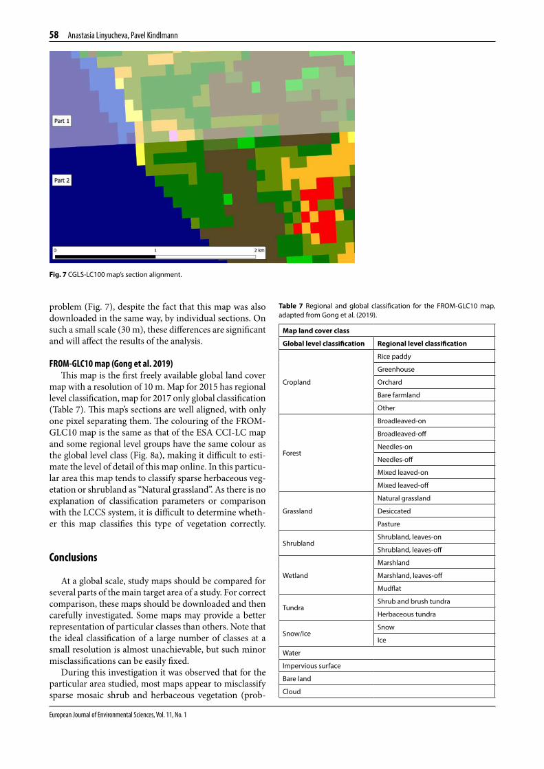
European Journal of Environmental Sciences, Vol. 11, No. 1
58 Anastasia Linyucheva, Pavel Kindlmann
Fig. 7 CGLS-LC100 map’s section alignment.
Table 7 Regional and global classification for the FROM-GLC10 map, adapted from Gong et al. (2019).
Map land cover class
Global level classification Regional level classification
Cropland
Rice paddy
Greenhouse
Orchard
Bare farmland
Other
Forest
Broadleaved-on
Broadleaved-off
Needles-on
Needles-off
Mixed leaved-on
Mixed leaved-off
Grassland
Natural grassland
Desiccated
Pasture
ShrublandShrubland, leaves-on
Shrubland, leaves-off
Wetland
Marshland
Marshland, leaves-off
Mudflat
TundraShrub and brush tundra
Herbaceous tundra
Snow/IceSnow
Ice
Water
Impervious surface
Bare land
Cloud
problem (Fig. 7), despite the fact that this map was also downloaded in the same way, by individual sections. On such a small scale (30 m), these differences are significant and will affect the results of the analysis.
FROM-GLC10 map (Gong et al. 2019)This map is the first freely available global land cover
map with a resolution of 10 m. Map for 2015 has regional level classification, map for 2017 only global classification (Table 7). This map’s sections are well aligned, with only one pixel separating them. The colouring of the FROM-GLC10 map is the same as that of the ESA CCI-LC map and some regional level groups have the same colour as the global level class (Fig. 8a), making it difficult to esti-mate the level of detail of this map online. In this particu-lar area this map tends to classify sparse herbaceous veg-etation or shrubland as “Natural grassland”. As there is no explanation of classification parameters or comparison with the LCCS system, it is difficult to determine wheth-er this map classifies this type of vegetation correctly.
Conclusions
At a global scale, study maps should be compared for several parts of the main target area of a study. For correct comparison, these maps should be downloaded and then carefully investigated. Some maps may provide a better representation of particular classes than others. Note that the ideal classification of a large number of classes at a small resolution is almost unachievable, but such minor misclassifications can be easily fixed.
During this investigation it was observed that for the particular area studied, most maps appear to misclassify sparse mosaic shrub and herbaceous vegetation (prob-

European Journal of Environmental Sciences, Vol. 11, No. 1
Global land cover maps and their potential use for habitat suitability modelling 59
Fig. 8 FROM-GLC10 map, (a) less detailed, legend includes all map classes; (b) more detailed, only those classes present in area are shown.
ably perennial) mixed with bare soil (rocks), visible on satellite imagery. The Copernicus CGLS-LC map tends to indicate that this area is covered by crops or cultivat-ed and managed vegetation, despite the fact that it has more suitable classes. The ESA CCI-LC map, on the other
hand, classifies these areas as “Cropland rainfed”, which is mostly correct; or incorrect as “Tree cover broadleaved deciduous closed to open (> 15%)”. However, this could be a problem unique to this area that requires further in-vestigation. The GLOBCOVER map provides a mislead-
(a)
(b)

European Journal of Environmental Sciences, Vol. 11, No. 1
60 Anastasia Linyucheva, Pavel Kindlmann
ing classification of particular types of vegetation (forest) and incorrect classification of urban areas, which make this map unsuitable for use for studying this area. The resolution of map GLC-SHARE from FAO is too coarse for evaluating habitat suitability as it does not describe the pattern of vegetation or even the shape of the main-land. There may be another version of the GLC_FCS30 map (Liangyun et al. 2020) that is properly aligned and has averaged classification for overlapping parts, which is more accurate. FROM-GLC10 map (Gong et al. 2019) is the first global map that is freely available with such small resolution. This map has some noticeable artefacts due to its resolution, 10 m, however, such minor artefacts can be removed. ESA CCI-LC and Copernicus CGLS-LC100 maps provide the most accurate estimates for the area studied. Incorrect position of classes CCI-LC map against satellite imagery (Gorelick et al. 2017) may be due to the level of resolution. Both maps sometimes misclas-sify certain types of vegetation (sparse vegetation on bare soil), but if this is consistent and exclusive to this region, it can be manually corrected.
This comparison indicates that the Copernicus CGLS-LC100 and ESA CCI-LC maps seem to be the most uni-versal maps for determining potentially suitable habitats. They have a wide range of land cover groups that can be compared (using LCCS classification system), making it easier to decide which spatial resolution to use.
REFERENCES
Arino O, Ramos Perez JJ, Kalogirou V, Bontemps S, Defourny P, van Bogaert E (2012) Global Land Cover Map for 2009 (Glob-Cover 2009). European Space Agency and Université catholique de Louvain. doi: 10.1594/PANGAEA.787668.
Barik S, Saha GK, Mazumdar S (2021) Potentially suitable habitat, connectivity and priority conservation areas for White-breast-ed waterhen (Amaurornis phoenicurus) and Bronze-winged jacana (Metopidius indicus). Wetl 41. doi: 10.1007/s13157-021-01433-6.
Breininger DR, Toland B, Oddy DM, Legare ML (2006) Landcover characterizations and Florida scrub-jay (Aphelocoma coerules-cens) population dynamics. Biol Conserv 128: 169–181.
Buchhorn M, Smets B, Bertels L, Roo BD, Lesiv M, Tsendbazar NE, Herold M, Fritz S (2020) Copernicus Global Land Ser-vice: Land Cover 100m: collection 3: epoch 2015: Globe. doi: org/10.5281/ZENODO.3939038.
Buchhorn M, Smets B, Bertels L, Roo BD, Lesiv M, Tsendbazar NE, Li L, Tarko A (2021) Copernicus Global Land Service: Land Cover 100 m: version 3 Globe 2015–2019: Product User Manual. doi: 10.5281/ZENODO.4723921.
Cisneros-Araujo P, Goicolea T, Mateo-Sánchez MC, García-Viñás JI, Marchamalo M, Mercier A, Gastón A (2021) The Role of Remote Sensing Data in Habitat Suitability and Connectivity Modeling: Insights from the Cantabrian Brown Bear. Remote Sens 13: 1138.
Ciudad C, Mateo-Sánchez MC, Gastón A, Blazquez-Cabrera S, Saura S (2021) Landscape connectivity estimates are affected by spatial resolution, habitat seasonality and population trends. Biodivers and Conserv 30: 1395–1413.
ESA (2017) Land Cover CCI Product User Guide Version 2. Tech Rep. Available at: maps.elie.ucl.ac.be/CCI/viewer/download /ESACCI-LC-Ph2-PUGv2_2.0.pdf.
Falcucci A, Maiorano L, Boitani L (2007) Changes in land-use/land-cover patterns in Italy and their implications for biodiver-sity conservation. Landscape Ecol 22: 617–631.
GLCC Global Land Cover Characterization. United States Geolog-ical Survey Land Cover Products: doi: 10.5066/F7GB230D.
Goldewijk KK, Hall FG, Collatz GJ, Meeson BW, Los SO, Brown De Colstoun E, Landis DR (2007) ISLSCP II Historical Land Cover and Land Use, 1700–1990. ORNL DAAC, Oak Ridge, Tennessee, USA. doi: 10.3334/ORNLDAAC/967.
Gong P, Liu H, Zhang M et al. (2019) Stable classification with lim-ited sample: transferring a 30-m resolution sample set collected in 2015 to mapping 10-m resolution global land cover in 2017. Sci Bull 64: 370–373.
Gorelick N, Hancher M, Dixon M, Ilyushchenko S, Thau D, Moore R (2017) Google Earth Engine: Planetary-scale geospatial anal-ysis for everyone. Remote Sens of Environ 202: 18–27.
Hirzel AH, le Lay G (2008) Habitat suitability modelling and niche theory. J Appl Ecol 45: 1372–1381.
Latham J, Cumani R, Rosati I, Bloise M (2014) FAO Global Land Cover (GLC-SHARE). Beta-Release 1.0 Database. http://www .fao.org/geonetwork/srv/en/main.home?uuid=ba4526fd-cdbf -4028-a1bd-5a559c4bff38.
Li X, Ling F, Foody GM, Ge Y, Zhang Y, Du Y (2017) Generating a series of fine spatial and temporal resolution land cover maps by fusing coarse spatial resolution remotely sensed images and fine spatial resolution land cover maps. Remote Sens of Environ 196: 293–311.
Liangyun L, Xiao Z, Xidong C, Yuan G, Jun M (2020) GLC_FCS30: Global land-cover product with fine classification system at 30 m using time-series Landsat imagery. doi: 10.5281/ZENO-DO.3986872.
Manton MG, Angelstam P, Mikusiński G (2005) Modelling habi-tat suitability for deciduous forest focal species – A sensitivity analysis using different satellite land cover data. Landscape Ecol 20: 827–839.
MAXAR (2021) Basevue LULC, Remote Sensing. https://www .maxar.com/products/basevue-lulc.
McMenamin SK, Hadly EA, Wright CK (2008) Climatic change and wetland desiccation cause amphibian decline in Yellowstone National Park. Proc Natl Acad Sci U.S.A. 105: 16988–16993.
Ndegwa Mundia C, Murayama Y (2009) Analysis of Land Use/Cover Changes and Animal Population Dynamics in a Wildlife Sanctuary in East Africa. Remote Sens 1: 952–970.
Novillo C, Arrogante-Funes P, Romero-Calcerrada R (2018) Im-proving Land Cover Classifications with Multiangular Data: MISR Data in Mainland Spain. Remote Sens 10: 1717.
Pennington DN, Hansel J, Blair RB (2008) The conservation value of urban riparian areas for landbirds during spring migration: Land cover, scale, and vegetation effects. Biol Conserv 141: 1235–1248.
Rawat JS, Kumar M (2015) Monitoring land use/cover change us-ing remote sensing and GIS techniques: A case study of Ha-walbagh block, district Almora, Uttarakhand, India. Egypt J Remote Sens Space Sci 18: 77–84.
Rondinini C, di Marco M, Chiozza F et al. (2011) Global habitat suitability models of terrestrial mammals. Philos T Roy Soc B 366: 2633–2641.
Teng J, Xia S, Liu Y, Yu X, Duan H, Xiao H, Zhao C (2021) Assess-ing habitat suitability for wintering geese by using Normalized Difference Water Index (NDWI) in a large floodplain wetland, China. Ecol Indic 122: 107260.

European Journal of Environmental Sciences, Vol. 11, No. 1
Global land cover maps and their potential use for habitat suitability modelling 61
LINKS TO THE MAPS
1. Copernicus, CGLS- LC100 map (Buchhorn et al. 2020): https://land.copernicus.eu/global/products/lc
2. Food and Agriculture Organization of the United Nations (FAO), GLC-SHARE map (Latham et al. 2014): http://www .fao.org/geonetwork/srv/en/main.home?uuid=ba4526fd-cdbf -4028-a1bd-5a559c4bff38
3. European Space Agency (ESA), CCI-LC map (ESA 2017): http://www.esa-landcover-cci.org/?q=node/164
4. European Space Agency (ESA), GLOBCOVER map (Arino et al. 2012): http://due.esrin.esa.int/page_globcover.php
5. Liangyun et al. 2020, GLC_FCS30 map: https://zenodo.org /record/4280923#.YIzydbUzY2w
6. Gong et al. 2019, FROM-GLC10 map: http://data.ess.tsinghua .edu.cn/fromglc10_2017v01.html

Copyright © 2022 FDOKUMEN