Faculty of Environmental Sciences - Qucosa - TU Dresden
294
Faculty of Environmental Sciences APPLICATION OF GEOGRAPHIC INFORMATION SYSTEM AND REMOTE SENSING IN MULTIPLE CRITERIA ANALYSIS TO IDENTIFY PRIORITY AREAS FOR BIODIVERSITY CONSERVATION IN VIETNAM By: Vu Xuan Dinh Institute of Photogrammetry and Remote Sensing Faculty of Environmental Sciences, TU Dresden Dresden, 08.2020
-
Upload
khangminh22 -
Category
Documents
-
view
0 -
download
0
Transcript of Faculty of Environmental Sciences - Qucosa - TU Dresden

Faculty of Environmental Sciences
APPLICATION OF GEOGRAPHIC INFORMATION SYSTEM
AND REMOTE SENSING IN MULTIPLE CRITERIA
ANALYSIS TO IDENTIFY PRIORITY AREAS FOR
BIODIVERSITY CONSERVATION IN VIETNAM
By: Vu Xuan Dinh
Institute of Photogrammetry and Remote Sensing
Faculty of Environmental Sciences, TU Dresden
Dresden, 08.2020
Faculty of Environmental Sciences
APPLICATION OF GEOGRAPHIC INFORMATION SYSTEM AND REMOTE
SENSING IN MULTIPLE CRITERIA ANALYSIS TO IDENTIFY PRIORITY
AREAS FOR BIODIVERSITY CONSERVATION IN VIETNAM
Dissertation for awarding the academic
degree Doctor of Natural Science
(Dr.rer.Nat.)
Submitted by
MSc. Vu Xuan Dinh
born on 25.09.1982 in Quang Ninh, Vietnam
Supervisors:
Prof. Dr. Elmar Csaplovics
Institute of Photogrammetry and Remote Sensing
Faculty of Environmental Sciences
Technical University of Dresden
PD Dr. Trung Thanh Nguyen
Akademischer Rat
Institute for Environmental Economics and World Trade
School of Economics and Management
Leibniz University Hannover
Prof. Dr. Michael Köhl
Department of Biology
Faculty of Mathematics, Computer Science and Natural Sciences
University of Hamburg
Dresden, 08.2020

Explanation of the doctoral candidate
This is to certify that this copy is fully congruent with the original copy of the thesis
with the topic:
“Application of Geographic Information System and Remote Sensing in Multiple
Criteria Analysis to identify priority areas for biodiversity conservation in Vietnam.”
Dresden, 08.2020
Vu Xuan Dinh
Declaration
I hereby declare that the submission entitled “Application of Geographic Information
System and Remote Sensing in Multiple Criteria Analysis to identify priority areas for
biodiversity conservation in Vietnam,” is my own work and that, to the best of my
knowledge and belief. It contains no material previously published or written by another
person and has not been previously submitted or accepted elsewhere to any other
university or institute for the award of any other degree.
Vu Xuan Dinh

I
Acknowledgement
The study has been completed not only from the best effort of myself all the time but also
from the support of many individuals and organizations. This is the place and opportunity
for some words to express my gratitude to them.
At first and foremost, I want to express my deepest gratitude to Prof. Dr. Elmar
Csaplovics (Chair of Remote Sensing, TU Dresden) and PD Dr. Trung Thanh Nguyen
(Institute for Environmental Economics and World Trade, Leibniz University Hannover)
for their scientific supervision, advice, personal guidance, and unlimited support
throughout the research period. Without their constant support and encouragement, the
completion would not have been possible.
My heartfelt thanks and very special appreciation to Prof. Dr. Michael Köhl (Department
of Biology, Faculty of Mathematics, Computer Science and Natural Sciences, University
of Hamburg) for spending his precious time to review and give me very helpful comments
on my dissertation.
I would like to deeply thank the Ministry of Agriculture and Rural Development and
Ministry of Training and Education of Vietnam for granting me a four-year scholarship
to study at the University of Technology, Dresden, Germany. Thanks, are extended to the
College of Land Management and Rural Development and the Vietnam National
University of Forestry for encouraging and allowing me to pursue my further study in
Germany. My thanks also to all respondents who gave me their valuable time and
opinions on biodiversity conservation in Vietnam. Special thanks and appreciation to the
leaders, staff members, and forest rangers in the three protected areas (Cuc Phuong NP,
Pu Luong NR, and Ngoc Son-Ngo Luong NR) as well as the Institute of Geography,
Vietnam Academy of Science and Technology for supporting and providing the valuable
data during my fieldwork period.
I want to thank the Chair of Remote Sensing, Institute of Photogrammetry and Remote
Sensing, TU Dresden, Germany, where I found the opportunity to do this PhD research.
My gratitude is extended to the Association of Friends and Sponsors (GFF) and the
Graduate Academy (GA) in TU Dresden for financial support during my study.
I would like to express my heartfelt appreciation to Dr. Ngoc Thuan Chu, who is always
behind to help me with the kind support and advice about both science and life. I also

II
thank Christopher Marrs and Ramandeep Jain for spending their time to comment and
proofread my dissertation.
I am very grateful to my colleagues at Chair of Remote Sensing, TU Dresden, for their
help, support, discussion, and cooperation; Marion Pause, Anke Hahn, DildoraAralova,
Mike Salazar Villegas, Daniela Limache de la Fuente, Mohammad Qasim, Taisser Hassan
Deafalla, Babatunde Adeniyi Osunmadewa.
Finally, and most importantly, I am deeply indebted to all of my family for their moral
support and encouragement for all the time of this study. I deeply indebted to my parents
for their exceptional patience during my long absence, for their efforts in educating me
both science and life. To my lovely wife Thi Huong Do, she is not only a friend but also
a colleague whom I could discuss and share to obtain the best solution to each problem.
Without her unconditional support, it was tough to complete this study. I owe thanks to
my son TrungNghia Vu for smiles and laughter in the games that reduced my stress in
many long hard-working days. I know that by no means would I be able to express my
gratitude to them. To all of them, I dedicate this thesis.
I thank you all!
Dresden, Germany, 08. 2020
Vu Xuan Dinh
III
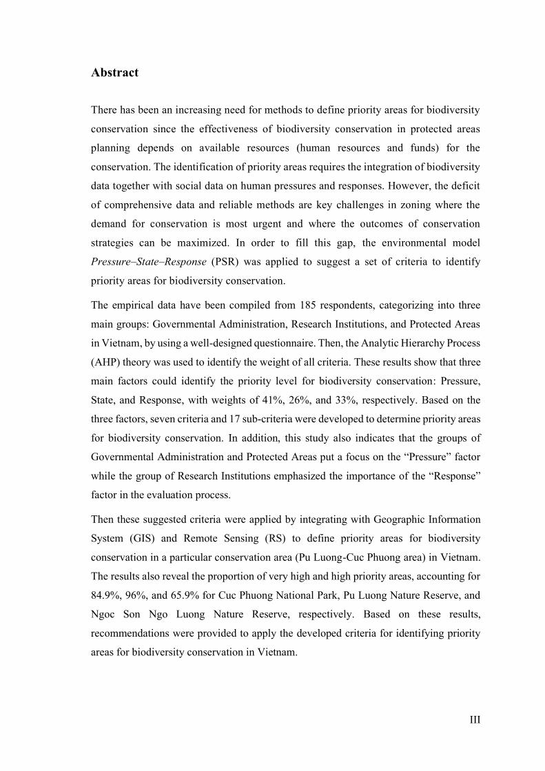
Abstract
There has been an increasing need for methods to define priority areas for biodiversity
conservation since the effectiveness of biodiversity conservation in protected areas
planning depends on available resources (human resources and funds) for the
conservation. The identification of priority areas requires the integration of biodiversity
data together with social data on human pressures and responses. However, the deficit
of comprehensive data and reliable methods are key challenges in zoning where the
demand for conservation is most urgent and where the outcomes of conservation
strategies can be maximized. In order to fill this gap, the environmental model
Pressure–State–Response (PSR) was applied to suggest a set of criteria to identify
priority areas for biodiversity conservation.
The empirical data have been compiled from 185 respondents, categorizing into three
main groups: Governmental Administration, Research Institutions, and Protected Areas
in Vietnam, by using a well-designed questionnaire. Then, the Analytic Hierarchy Process
(AHP) theory was used to identify the weight of all criteria. These results show that three
main factors could identify the priority level for biodiversity conservation: Pressure,
State, and Response, with weights of 41%, 26%, and 33%, respectively. Based on the
three factors, seven criteria and 17 sub-criteria were developed to determine priority areas
for biodiversity conservation. In addition, this study also indicates that the groups of
Governmental Administration and Protected Areas put a focus on the “Pressure” factor
while the group of Research Institutions emphasized the importance of the “Response”
factor in the evaluation process.
Then these suggested criteria were applied by integrating with Geographic Information
System (GIS) and Remote Sensing (RS) to define priority areas for biodiversity
conservation in a particular conservation area (Pu Luong-Cuc Phuong area) in Vietnam.
The results also reveal the proportion of very high and high priority areas, accounting for
84.9%, 96%, and 65.9% for Cuc Phuong National Park, Pu Luong Nature Reserve, and
Ngoc Son Ngo Luong Nature Reserve, respectively. Based on these results,
recommendations were provided to apply the developed criteria for identifying priority
areas for biodiversity conservation in Vietnam.

IV
Table of contents
Acknowledgement ............................................................................................................ I
Abstract ......................................................................................................................... III
Table of contents ........................................................................................................... IV
List of figures ................................................................................................................. VI
List of tables ................................................................................................................... X
Acronyms and Abbreviations .................................................................................... XII
Chapter 1. Introduction ................................................................................................. 1
1.1. Problem statement and motivation ........................................................................ 1
1.2. Research objectives and questions ......................................................................... 2
1.3. Study contribution .................................................................................................. 3
1.4. Thesis structure ...................................................................................................... 6
Chapter 2. Literature review ......................................................................................... 8
2.1. Background information on Vietnam .................................................................... 8
2.2. Environmental Pressure-State-Response model .................................................. 11
2.3. Defining criteria for biodiversity conservation .................................................... 13
2.4. Application of GIS and RS for biodiversity conservation ................................... 16
Chapter 3. Research methodology .............................................................................. 19
3.1. Study areas ........................................................................................................... 19
3.1.1. Terrain ........................................................................................................... 20
3.1.2. Climate .......................................................................................................... 21
3.1.3. Population ..................................................................................................... 21
3.1.4. Biodiversity ................................................................................................... 22
3.2. Data collection ..................................................................................................... 23
3.2.1. Questionnaire ................................................................................................ 23
3.2.2. Interview ....................................................................................................... 24
3.3. Analytic Hierarchy Process ................................................................................. 25
3.4. Remote Sensing ................................................................................................... 27
3.4.1. Pre-processing ............................................................................................... 28
3.4.2. Supervised classification ............................................................................... 31
3.4.3. Post-processing ............................................................................................. 32
3.4.4. Land surface temperature .............................................................................. 33
3.4.5. Visual interpolation ....................................................................................... 34
3.4.6. Time series analysis ...................................................................................... 34
3.5. Geography Information System ........................................................................... 35
3.5.1. Data conversion ............................................................................................ 35
3.5.2. Overlay analysis ............................................................................................ 36
3.5.3. Kernel Density Estimation ............................................................................ 37

V
3.5.4. Jenks Natural Breaks .................................................................................... 39
3.6. Climate change scenarios ..................................................................................... 40
Chapter 4. Establishment of criteria ........................................................................... 42
4.1. Summary of responses ......................................................................................... 44
4.2. Statistic of pairwise comparison .......................................................................... 46
4.3. Weights of criteria based on all respondents ....................................................... 48
4.3.1. Factors ........................................................................................................... 48
4.3.2. Criteria .......................................................................................................... 50
4.3.3. Sub-criteria .................................................................................................... 53
4.3.4. Weights of criteria ........................................................................................ 59
4.4. Weights of criteria based on groups .................................................................... 60
4.4.1. Protected Areas group ................................................................................... 60
4.4.2. Government Organizations group ................................................................. 61
4.4.3. Universities and Research Institutes group ................................................... 62
Chapter 5. Application of Criteria .............................................................................. 64
5.1. Mapping criteria ................................................................................................... 64
5.1.1. Species .......................................................................................................... 64
5.1.2. Ecosystem ..................................................................................................... 77
5.1.3. Nature .......................................................................................................... 104
5.1.4. Human ......................................................................................................... 114
5.1.5. Conservation ............................................................................................... 129
5.1.6. Education .................................................................................................... 136
5.1.7. Law ............................................................................................................. 140
5.2. Synthesis of multiple criteria ............................................................................. 144
5.2.1. All respondents ........................................................................................... 146
5.2.2. Protected Areas group ................................................................................. 149
5.2.3. Government Organizations group ............................................................... 152
5.2.4. Universities and Research Institutes group ................................................. 155
Chapter 6. Conclusions and recommendations ........................................................ 158
6.1. Establishment of criteria .................................................................................... 158
6.2. Application of criteria ........................................................................................ 161
6.3. Recommendations .............................................................................................. 165
References .................................................................................................................... 167
Appendix I. Questionnaire ...................................................................................... 197
Appendix II. Establishment of criteria ................................................................ 207
Appendix III. Application of criteria .................................................................... 234

VI
List of figures
Figure 2.1: Adapted PSR Model for evaluating biodiversity conservation .................... 12
Figure 3.1: Location of three protected areas in the study area ...................................... 19
Figure 3.2: Outline of the questionnaire ......................................................................... 24
Figure 3.3: Land Use-Land Cover classification workflow for Landsat images ............ 28
Figure 3.4: Knowledge-based image analysis system .................................................... 34
Figure 3.5: Change detection model for classified images in this study ........................ 35
Figure 3.6: Data conversion process ............................................................................... 36
Figure 3.7: Overlay operation with spatial and attribute data ......................................... 37
Figure 3.8: A comparison between the Histogram and Kernel Density Estimation ....... 38
Figure 3.9: Applications of Kernel Density Estimation for point and line features ....... 39
Figure 3.10: Comparison between Jenks Natural Breaks and other methods................. 39
Figure 4.1. Criteria system to define priority areas for biodiversity conservation ......... 42
Figure 4.2. Calculating weights of criteria based on the AHP method .......................... 43
Figure 4.3. Locations of respondents .............................................................................. 44
Figure 4.4. Boxplot for responding all criteria of biodiversity conservation ................. 46
Figure 4.5: Weights of criteria based on all respondents for identifying priority areas of
biodiversity conservation in Vietnam ............................................................................. 59
Figure 4.6: Weights of criteria based on Protected Areas group for identifying the
priority areas of biodiversity conservation in Vietnam................................................... 61
Figure 4.7: Weights of criteria based on Government Organization group for identifying
the priority areas of biodiversity conservation in Vietnam ............................................. 62
Figure 4.8: Weights of criteria based on the Universities and Research Institutes group
for identifying the priority areas of biodiversity conservation in Vietnam .................... 63
Figure 5.1: Interactions between internal and external factors of an ecosystem ............ 64
Figure 5.2. Framework for mapping priority areas of species richness .......................... 66
Figure 5.3: Combination to gain the appropriate image in 2007 .................................... 67
Figure 5.4: Land use and land cover maps in Pu Luong – Cuc Phuong (1986, 1998,
2007, and 2017) .............................................................................................................. 69
Figure 5.5: LULC changes in specific regions from 1986 to 2017 ................................ 70
Figure 5.6: Priority levels of richness in the study area.................................................. 71
Figure 5.7: Assessment of priority levels of richness in the study area .......................... 72
Figure 5.8: Framework for mapping evergreen forest in the study area ......................... 73
Figure 5.9: Framework for mapping priority areas of rare species................................. 74
Figure 5.10: Priority areas of rarity in the study area ..................................................... 76
Figure 5.11: Assessment of priority levels of rarity in the study area ............................ 76
Figure 5.12: Framework for mapping priority areas of location .................................... 77

VII
Figure 5.13: Terrain regions in Vietnam ........................................................................ 78
Figure 5.14: Terrestrial ecoregions in Vietnam .............................................................. 78
Figure 5.15: Karst limestone regions and terrestrial ecoregions in the study area ......... 79
Figure 5.16: Priority areas of location in the study area ................................................. 80
Figure 5.17: Assessment of priority levels of location in the study area ........................ 81
Figure 5.18. Framework for mapping priority areas of topography ............................... 82
Figure 5.19:100-slope map .............................................................................................. 83
Figure 5.20:100m-altitude map ....................................................................................... 83
Figure 5.21: Change in forest areas at different slopes from 1986 to 2017 .................... 83
Figure 5.22: Change in forest areas at different altitudes from 1986 to 2017 ................ 84
Figure 5.23: Priority areas of slope ................................................................................. 85
Figure 5.24: Priority areas of altitude ............................................................................. 85
Figure 5.25. Priority areas of topography in the study areas .......................................... 86
Figure 5.26: Assessment of priority levels of topography in the study area .................. 86
Figure 5.27: Positions of 60 hydro-meteorological stations in Vietnam ........................ 87
Figure 5.28: Average Monthly Temperature and Rainfall in Vietnam ........................... 88
Figure 5.29: Monthly change of temperature in three provinces .................................... 89
Figure 5.30: Framework for mapping priority areas of climate...................................... 90
Figure 5.31: Land Surface Temperature in December 2013 .......................................... 91
Figure 5.32: Land Surface Temperature in July 2015 .................................................... 91
Figure 5.33: Land Surface Temperature recalculated in December 2013 ...................... 92
Figure 5.34: Land Surface Temperature recalculated in July 2015 ................................ 92
Figure 5.35: Stable levels of temperature in the study area ............................................ 93
Figure 5.36: Assessment of priority levels of climate in the study area ......................... 93
Figure 5.37: Taxonomic group of threatened species in Vietnam .................................. 94
Figure 5.38: Accumulation curves of species from the four waterbody types ............... 95
Figure 5.39. Framework for mapping priority areas of hydrology ................................. 96
Figure 5.40. Hydrological system in Hoa Binh, Thanh Hoa, and Ninh Binh provinces 97
Figure 5.41: The hydrological system combined of three provinces .............................. 98
Figure 5.42: Priority areas for hydrology in the study area ............................................ 99
Figure 5.43: Assessment of priority levels for hydrology in the study area ................. 100
Figure 5.44. Framework for mapping priority areas regarding forest types ................. 101
Figure 5.45: Maps of forest statistics of Hoa Binh, Thanh Hoa and Ninh Binh in 2015
...................................................................................................................................... 102
Figure 5.46: Forest map updated by Landsat 8 image in 2017 ..................................... 103
Figure 5.47: Priority areas regarding forest types in the study area ............................. 103
Figure 5.48. Assessment of priority levels for forest types in the study area ............... 104
Figure 5.49: The changes in annual temperature (0C) from 1958 to 2014 ................... 105
Figure 5.50: The changes in annual rainfall (%) from 1958 to 2014 ............................ 105

VIII
Figure 5.51. Framework for mapping pressure levels for climate change.................... 107
Figure 5.52. Estimation of annual temperature and rainfall changes from 2045 to 2065
...................................................................................................................................... 108
Figure 5.53. Pressure from temperature changes estimated from 2046 to 2065 .......... 109
Figure 5.54. Pressure from precipitation changes estimated from 2046 to 2065 ......... 109
Figure 5.55. Predicted priority areas of climate changes in the study area (2046 - 2065)
...................................................................................................................................... 110
Figure 5.56. Assessment of pressure of climate change in the study area .................... 111
Figure 5.57. Framework for mapping pressure of natural disasters ............................. 112
Figure 5.58. Locations of Natural Disasters in Vietnam from 1997 to 2018 ............... 113
Figure 5.59. The pressure of natural disasters in the study area (1997 - 2018) ............ 113
Figure 5.60. Framework for mapping pressure of population distribution ................... 115
Figure 5.61. Settlement distribution of districts within and around the study area ...... 116
Figure 5.62. Comparison of settlement area among specific regions in the study area 116
Figure 5.63. Converting Polygons to Points for using Kernel Density Estimation ...... 117
Figure 5.64. Levels of pressure of population distribution in the study area ............... 118
Figure 5.65. Assessment of pressure of settlement distribution in the study area ........ 119
Figure 5.66. Framework for mapping pressure of population density .......................... 120
Figure 5.67. Levels of pressure of population density in the study area ...................... 121
Figure 5.68. Assessment of pressure of population density in the study area .............. 122
Figure 5.69. Framework for mapping pressure of population quantity ........................ 123
Figure 5.70: Levels of pressure of population quantity in the study area ..................... 124
Figure 5.71. Assessment of pressure of population numbers in the study area ............ 124
Figure 5.72. Framework for mapping pressure of human livelihood ........................... 125
Figure 5.73. Land Use - Land Cover Map of communes around the study area .......... 126
Figure 5.74. Comparison between population and areas of livelihood, forest, and bare
land on the districts in the study area ............................................................................ 127
Figure 5.75. The pressure of livelihood in the study area ............................................. 128
Figure 5.76. Assessment of pressure of livelihood in the study area ............................ 129
Figure 5.77. Framework for mapping priority areas of forest management types ....... 130
Figure 5.78. Area comparison of forest management types in the study area .............. 131
Figure 5.79. Map of forest management types in the study area .................................. 132
Figure 5.80. Priority areas of forest management types in the study area .................... 133
Figure 5.81. Assessment of priority areas of forest management types in the study area
...................................................................................................................................... 133
Figure 5.82. Framework for mapping priority areas of size of forest area ................... 134
Figure 5.83. Priority areas based on forest area size in the study area ......................... 135
Figure 5.84. Assessment of priority areas regarding forest size in the study area ........ 136
Figure 5.85. Mapping impact levels of education for biodiversity conservation ......... 137

IX
Figure 5.86. Distribution of schools in districts around the study area ........................ 138
Figure 5.87. Impact levels of education for biodiversity conservation in the study area
...................................................................................................................................... 139
Figure 5.88. Assessment of priority areas of education in the study area .................... 139
Figure 5.89. Framework for mapping impact levels of law for biodiversity conservation
...................................................................................................................................... 140
Figure 5.90. Positions of governmental offices responsible for protecting biodiversity
...................................................................................................................................... 141
Figure 5.91. Levels of protection ability of forest offices in the study area ................. 143
Figure 5.92: Assessment of priority areas of law in the study area .............................. 144
Figure 5.93. Example of application of the weighted sum method .............................. 145
Figure 5.94. Priority areas for biodiversity conservation synthesized by all respondents
...................................................................................................................................... 147
Figure 5.95. Priority areas for biodiversity conservation synthesized by PAs group ... 150
Figure 5.96. Priority areas for biodiversity conservation synthesized by GOs group .. 153
Figure 5.97. Priority areas for biodiversity conservation synthesized by URIs group . 156
Figure 6.1. Area statistics of priority levels for biodiversity conservation based on the
weight set of all respondents as well as from three biggest groups .............................. 162
Figure 6.2. Comparison priority levels among protected areas and other areas in the
study site based on the weight systems calculated for each group ............................... 163

X
List of tables
Table 2.1: The comparison of criteria for defining the conservation values used across
several ENGOs ............................................................................................................... 15
Table 3.1: Area statistics of the protected areas in the study area .................................. 20
Table 3.2: Scale for pair-wise AHP comparisons ........................................................... 26
Table 3.3: The average values of the Random Index...................................................... 27
Table 3.4: Error matrix for accuracy assessment in classification ................................. 32
Table 3.5: Centre wavelength of Landsat bands ............................................................. 34
Table 3.6: Regional climate models for calculating climate change scenarios .............. 40
Table 4.1. Pairwise comparison of factors ...................................................................... 49
Table 4.2: Standardized matrix of factors ....................................................................... 49
Table 4.3: Consistency test of factors ............................................................................. 49
Table 4.4: Pairwise comparison of criteria of state ........................................................ 50
Table 4.5: Standardized matrix of criteria of state .......................................................... 50
Table 4.6: Pairwise comparison of sub-criteria of pressure ............................................ 51
Table 4.7: Standardized matrix of sub-criteria of pressure ............................................. 51
Table 4.8: Pairwise comparison of sub-criteria of response ........................................... 52
Table 4.9: Standardized matrix of sub-criteria of response ............................................ 52
Table 4.10: Consistency test of sub-criteria of response ................................................ 52
Table 4.11: Pairwise comparison of factors of species ................................................... 53
Table 4.12: Standardized matrix of factors of species .................................................... 53
Table 4.13: Pairwise comparison of sub-criteria of ecosystem ...................................... 54
Table 4.14: Standardized matrix of sub-criteria of ecosystem ....................................... 55
Table 4.15: Consistency test of sub-criteria of ecosystem .............................................. 55
Table 4.16: Pairwise comparison of factors of nature .................................................... 56
Table 4.17: Standardized matrix of factors of nature ..................................................... 56
Table 4.18: Pairwise comparison of factors of human ................................................... 57
Table 4.19: Standardized matrix of factors of human..................................................... 57
Table 4.20: Consistency test of factors of human ........................................................... 58
Table 4.21: Pairwise comparison of factors of conservation .......................................... 58
Table 4.22: Standardized matrix of factors of conservation ........................................... 58
Table 5.1: Images used to define the priority areas regarding the richness of species ... 67
Table 5.2: Criteria for defining priority areas for species richness................................. 71
Table 5.3: Satellite images used to establish the map of evergreen forest ..................... 75
Table 5.4: Proposed weights for different locations in the study area ............................ 79
Table 5.5. Priority levels of slope and altitude for biodiversity conservation ................ 85
Table 5.6: Satellite images used to define annual temperature change .......................... 91

XI
Table 5.7: Priority levels of annual temperature change ................................................ 92
Table 5.8. Classification of hydrology in the study area ................................................ 98
Table 5.9: Classification of priority levels for hydrology in the study area ................... 99
Table 5.10. The risk levels of Natural disasters in Vietnam ......................................... 106
Table 5.11. Change levels of temperature and rainfall in the study area (2046 –2065) 108
Table 5.12. Classification of climate change through temperature and rainfall changes
...................................................................................................................................... 110
Table 5.13. Impact levels of settlement types on biodiversity conservation ................ 117
Table 5.14. Categories of forest management types in the study area .......................... 131
Table 5.15. Categories of priority levels of size of forest area ..................................... 135
Table 5.16. Assessing the ability of offices in protecting forest and biodiversity ........ 142
Table 5.17. Categories of protection levels based on the law in the study area ........... 142
Table 5.18. Categories of priority levels for biodiversity conservation by all respondents
...................................................................................................................................... 146
Table 5.19. Area statistics of priority levels for biodiversity conservation calculated
from all respondents in the study area .......................................................................... 148
Table 5.20. Categories of priority levels for biodiversity conservation by PAs group 149
Table 5.21. Area statistic of priority levels for biodiversity conservation calculated for
PAs group in the study area .......................................................................................... 151
Table 5.22. Categories of priority levels for biodiversity conservation by GOs group 152
Table 5.23. Area statistic of priority levels for biodiversity conservation calculated from
GOs group in the study area ......................................................................................... 154
Table 5.24. Categories of priority levels for biodiversity conservation by URIs group
...................................................................................................................................... 155
Table 5.25. Area statistics of priority levels for biodiversity conservation calculated for
the URIs group in the study area .................................................................................. 157
Table 6.1. Comparison between the weights of the groups .......................................... 160
Table 6.2. Data used for mapping sub-criteria .............................................................. 164

XII
Acronyms and Abbreviations
AGCM Atmosphere General Circulation Model
AHP Analytic Hierarchy Process
CCAM Conformal Cubic Atmospheric Model
CPNP Cuc Phuong National Park
DARD Department of Agriculture and Rural Development
DEM Digital Elevation Model
DOS Dark Object Subtraction
EHDP Expert Health Data Programming
ENGO Environmental Non-Government Organization
ESA European Space Agency
FFI Fauna and Flora International
FPD Forest Protection Department
GDLA General Department of Land Administration
GIS Geographic Information System
GOs Government Organizations
GVF Goodness of Variance Fit
HCP Habitat Conservation Planning
IUCN International Union for Conservation of Nature
JNB Jenks Natural Breaks
KDE Kernel Density Estimation
LST Land Surface Temperature
LULC Land Use - Land Cover
MARD Vietnam Ministry of Agriculture and Rural Development
MONRE Vietnam Ministry of Natural Resources and Environment
NDVI Normalized Difference Vegetation Index
NGO Non-Government Organization
NP National Park
NR Nature Reserve
NSNLNR Ngoc Son - Ngo Luong Nature Reserve
OECD Organization for Economic Co-operation and Development
OLI Operational Land Imager
PAs Protected Areas
XIII
PLNR Pu Luong Nature Reserve
PRECIS Providing Regional Climates for Impacts Studies
RCM Regional Climate Model
RegCM Regional Climate Model developed by the International Centre for
Theoretical Physics in Italy
RCP RepresentativeConcentration Pathways
ROIs Regions of Interest
RS Remote Sensing
SA Study Area
SR Specific Region
TIRS Thermal Infrared Sensor
TM Thematic Mapper
TOA Top of Atmosphere
URIs Universities and Research Institutes
USGS United States Geological Survey
UTM Universal Transverse Mercator
VAOF Vietnam Administration of Forestry
VEA Vietnam Environment Administration
VLRI Vietnam Legislative Research Institute
VN2000 Vietnam Projection
VNA Vietnam National Assembly
VNG Vietnam Government
VNRB Vietnam Red Data Book
WGS World Geodetic System
WWF World Wildlife Fund for Nature

1
Chapter 1. Introduction
1.1. Problem statement and motivation
Why does the identification of priority areas matter in biodiversity conservation?
The establishment of Protected Areas (PAs) has received much attention in recent years due
to its vital importance to biodiversity conservation and sustainable development (Naughton-
Treves et al., 2005). A protected area is defined as “a clearly defined geographical space,
recognized, dedicated and managed, through legal or other effective means, to achieve the
long-term conservation of nature with associated ecosystem services and cultural values.”
(Dudley, 2008). Protected areas play an important role in biodiversity conservation (Bruner
et al., 2001). Protected areas are not isolated, but they are components of their surrounding
social and ecological contexts (Brandon et al., 1998). In order to support for planning
conservation through the creation of protected areas, the selection of priority areas for
conservation is crucial. However, the identification of priority areas for conservation requires
the integration of biodiversity data together with social data on human pressures and
responses. The deficit of comprehensive data and reliable methods becomes a key challenge
in zoning priority areas for biodiversity conservation.
There has been an increasing need for methods to demarcate where the need for
conservation actions is most urgent and where the outcomes of conservation strategies
might be maximized (Balram et al., 2004). From a perspective of the geographic scale
of investigation, the establishment of biodiversity conservation priorities can be
classified into three categories (Balram et al., 2004). At the local scale, researchers and
conservationists use criteria on genetic diversity and indicator species to provide a focus
for establishing priority areas of biodiversity conservation (Balram et al., 2004). At the
regional scale, Habitat Conservation Planning (HCP) practice is applied to make use of
information on the home range and condition of organisms to allocate habitat reserves.
At the regional to the global scale, priority areas for biodiversity conservation are
identified by using criteria such as species richness, rarity, endemism,
representativeness, and complementarity to drive the conservation efforts (Kier &
Barthlott, 2001; Myer et al., 2000; Woodhouse et al., 2000). However, the effectiveness
of these strategies mainly relies on the availability of reliable biodiversity data (Balram
et al., 2004). Strategic conservation initiatives cannot wait for the establishment of a
comprehensive database (Miller, 1994; Sutherland et al., 2004). This research

2
contributes to the creation of a criteria system for defining conservation priority areas
through literature review and expert interviews.
Vietnam is one of the important biodiversity hotspots in the world (CEPF & IUCN, 2016).
However, the rate of loss of biodiversity in Vietnam continues at an alarming rate (Gordon
et al., 2005; Myers et al., 2000). Many efforts have been made to protect the remaining
biodiversity and halt the loss of species in Vietnam. Of these, the establishment of
protected areas is considered as a useful tool. The country has 164 protected areas,
including 30 National Parks, 69 Nature Reserves, 45 landscape protection areas, and 20
areas for scientific research (MARD, 2014). The total area of terrestrial protected areas is
2,198,744 hectares, accounting for about 13.5% of the country’s natural land area (MARD,
2014). To establish a protected area in Vietnam, feasibility studies have to be undertaken
to provide information on demarcation, area, and biodiversity. Although the number of
protected areas is expected to increase in the coming years (MARD, 2014), there are still
obstacles to identify priority areas for biodiversity conservation in Vietnam. In this study,
the determined criteria were calculated, interpolated, and assessed by applying Remote
Sensing (RS) and Geographic Information System (GIS) technologies to define priority
areas for biodiversity conservation in a particular conservation area of Vietnam.
1.2. Research objectives and questions
The overall objective of this study is to develop a set of criteria in defining priority areas
for biodiversity conservation and applying these criteria for a particular conservation area
in Northern Vietnam.
Specific objectives are:
❖ To identify criteria for establishing priority areas for biodiversity conservation
❖ To calculate weights of these criteria for biodiversity conservation in Vietnam
❖ To apply the determined criteria by integrating GIS and RS to define priority
areas for a conservation area in Northern Vietnam.
In connection with the above specific objectives, the following questions have been
formulated:
❖ What are the criteria for defining priority areas for biodiversity conservation?
❖ What are the importance levels of these criteria?
❖ How do GIS and RS support for applying these criteria?

3
1.3. Study contribution
To better understand the process of establishing protected areas in Vietnam, we reviewed
the reports of several established protected areas. One crucial step of the process is
monitoring, investigation, and assessment on the status of species and ecosystems of the
proposed areas. However, this process depended to a large extent on field surveys
conducted by experts on species and conservation status throughout the areas and required
a considerable amount of time and effort. Finding a solution to this burden and increasing
the capability of monitoring, assessing, and managing the priority areas for biodiversity
conservation in Vietnam is, therefore, both helpful and necessary.
This study provides a criteria system based on the environmental model (Pressure-
State-Response model) to define priority areas for biodiversity conservation. The
identification of biodiversity components and functions is an invaluable and significant
step in evaluating biodiversity conservation value (Hill, 2005). The environmental model
has been considered a popular conceptual framework to monitor biodiversity based on
three key factors, namely state, pressure, and response (Long et al., 2016). The model
demonstrates the relationships among human activities, biodiversity, and management
solutions to assess the levels of influence on biodiversity conservation (Lee et al., 2005;
Long et al., 2016; OECD, 1993b, 2003). The environmental model is considered to be
able to identify key influences on biodiversity over time (Lee et al., 2005). The model
provides three essential factors based on the concept of causality, including state,
pressure, and response that help decision-makers and the public to identify, understand,
and solve problems that cover the environmental and social challenges of sustainable
development. The selection of priority areas for biodiversity conservation is one of the
most critical tasks for monitoring, management of present protected areas or identifying
potential boundaries for the establishment of new protected areas. A set of criteria was
determined based on the previous studies by several ENGOs across the world, and
Vietnam. They were then selected and organized into three factors of the environmental
model based on their dimensions regarding biodiversity conservation. This combination
formulated a system of indicators with three levels (factors, criteria, and sub-criteria) to
cover many aspects of states, pressures, and responses that influence on biodiversity
conservation in Vietnam.
This study provides the weight of each criterion through the consultation from experts
that assesses its importance levels to define priority areas for biodiversity conservation.

4
The assessment of priority areas for biodiversity conservation should only be
implemented once the importance levels of the proposed criteria are evaluated and
calculated. The Analytic Hierarchy Process (AHP) has been referred to as an essential
method to assist decision-makers in identifying the weights of multiple criteria
(Malczewski, 2004; Saaty, 1977; Saaty & Gholamnezhad, 1982; Zhang, Su, Wu, &
Liang, 2015). To calculate the weights of the criteria, a questionnaire was specifically
designed to gauge the opinions of various experts and scientists in Vietnam who have
responsibilities as well as insight into forestry, biodiversity, and conservation. The
respondents came from across Vietnam and worked in the following five main sectors:
Protected Areas (PAs), Government Organizations (GOs), Non-Government
Organizations (NGOs), Universities and Research Institutes (URIs), and Forestry
Companies (FCs). The data from the interviews were used to identify the pair-wise
comparisons based on the relationship among the criteria. The method does not only
help to reduce the complexity in evaluation for multiple criteria but also increases the
objective aspects of choices (Saaty, 1980). The resulting weights of the criteria were
calculated through the data of three main groups (PAs, GOs, URIs), and all individual
respondents. It shows the common interests as well as the separate interests of the
groups that represent administrators, implementers, decision-makers, researchers,
scientists, and students in the field of biodiversity conservation in Vietnam.
This study provides an insight into the application of Geographic Information System
(GIS) and Remote Sensing (RS) to map each criterion and synthesize all criteria to
define priority areas for biodiversity conservation in Vietnam. GIS is considered a
powerful tool based on its capacity for the capture, storage, retrieval, analysis, and display
of spatial data (Chakhar & Martel, 2003; Elez et al., 2013; Esri, 2010; Hossain & Das,
2010). Meanwhile, RS helps to investigate, monitor, and analyze the environmental
conditions, as well as ecosystem patterns (Franklin, 2010; Gould, 2000). The integration
of RS and GIS has significantly become common in many mapping applications
(Franklin, 2010; Hano, 2013; Hinton, 1996). In this thesis, RS and GIS were applied to
gain the essential inputs, improve the data, analyze and synthesize the maps of the criteria.
The key strength of RS is the ability to provide the primary data sources for many criteria
through various satellite images. Landsat 4-5, Landsat 8, and Sentinel-2 are the sensors
that were used in this research because of their diversity of spatial, temporal, and spectral
resolution, and their accessibility, i.e., freely downloadable and cost-free data. They

5
contributed to establishing the database of the criteria through their capabilities such as
the classification of forest and LULC, detection of changes, determination of land surface
temperature, and editing and updating information for secondary data. At the same time,
GIS is an integral part of this study because of its capabilities for providing many
powerful functions. The collected maps were edited and updated using essential GIS
tools. The advanced tools, such as spatial analysis, geostatistical analysis, density
estimation, provided the ability to analyze and synthesize multiple layers, arranging the
values of different categories in an efficient and usable way. GIS provided a strong tool
to estimate the probability density, especially for determining the impact level and scale
of various concerned targets for biodiversity conservation in Vietnam such as population,
hydrology, natural disasters, schools and organizations responsible for forest protection.
This study provides an actual result of the present status of biodiversity conservation
in the Pu Luong-Cuc Phuong region, which is one of the highest biodiversity areas
in Vietnam. The determined criteria were applied to the Pu Luong-Cuc Phuong region,
the largest area of tropical rainforest and evergreen forest in the North of Vietnam (GEF,
2002). It is an essential area for biodiversity conservation with many endangered species
living on the karst-mountain (Baltzer et al., 2001; Barthlott et al., 2005). Three protected
areas are located in Cuc Phuong National Park, Pu Luong Nature Reserve, and Ngoc
Son-Ngo Luong Nature Reserve. The results, achieved from the field survey in 2017
and the previous reports of three protected areas, show an incomprehensive data set on
the biodiversity status. Critically, there has been no spatial data which can identify the
priority areas for biodiversity conservation in the three protected areas. It is a problem
that has restricted the management of protected areas across Vietnam. The application
of the criteria to define priority areas of biodiversity conservation in the Pu Luong-Cuc
Phuong region is considered a pivotal step to identify the contemporary issues in the
administration and management of the protected areas.
Finally, this study provides a fundamental framework that can apply to many regions
and protected areas in Vietnam. The processes and steps to establish and apply the criteria
to define priority areas for biodiversity conservation were analyzed and documented clearly
in a step-wise manner that is essential for replications in other studies. The result of each
part was calculated and described through the actual numbers in the synthesized tables and
figures. The content of the study was arranged in a scientific process and divided into
chapters such as the introduction, literature review, methodology, establishment of the

6
criteria, application of the criteria. All of these create a framework that can be applied to
other protected areas in Vietnam.
1.4. Thesis structure
The research was implemented to integrate Geographic Information System and Remote
Sensing with multiple determined criteria to define priority areas for biodiversity
conservation in Vietnam. The proposal was written in 2016, and data collection and
fieldwork was conducted in 2017, then the collected data was analyzed, synthesized, and
assessed in 2018, and finally writing the Ph.D. thesis in 2019.
This thesis is elaborated and organized in six chapters, as follows:
Chapter 1: This chapter introduces the problem statement and motivation for research to
open the main research objectives and questions of this study. The problems were
highlighted by showing the opportunities and constraints of establishing, monitoring, and
managing the present protected areas that are considered one of the critical issues for
biodiversity conservation in the world generally and in Vietnam particularly.
Chapter 2: This chapter is devoted to summarizing the theoretical background of the
study based on a review of previous literature that shows the status of biodiversity
conservation, the applied inventory methods, monitoring biodiversity and the
establishment of new protected areas in Vietnam. Focused on defining priority areas for
biodiversity conservation in Vietnam, the environmental Pressure-State-Response model
is revised to deal with the establishment of the criteria. The literature on the establishment
of criteria and application of GIS and RS in defining priority areas for biodiversity
conservation is reviewed to suggest essential criteria and effective methods based on GIS
and RS techniques.
Chapter 3: This chapter presents the study area and describes its terrain, climate,
population, and biodiversity characteristics. The chapter further illustrates the research
methodologies that were used in the study. The methods of Analytic Hierarchy Process,
Remote Sensing, Geography Information System, and Climate Change Scenarios were
introduced explicitly to achieve the research objectives. These methods are presented in
order for the research process employed from the establishment of criteria to application
of GIS and RS to mapping the criteria as well as synthesizing them.
Chapter 4: The data of the interview in 2017 were summarized to help select the
responsible respondents for the analysis of pair-wise comparisons. Then, the Analytic

7
Hierarchy Process method was applied for calculating the weights of criteria with each pair-
wise comparison. The values of the weights were identified based on the opinions of all
individual respondents, and for the three main groups (PAs, GOs, and URIs).
Chapter 5: This chapter describes the application of the determined criteria to define
priority areas for biodiversity conservation in the Pu Luong-Cuc Phuong region. The
characteristics of each criterion were analyzed to find the major representable elements
that can be mapped by using GIS and RS. Then, all the maps representing the criteria
were synthesized based on their calculated weights for all respondents and for three main
groups.
Chapter 6: The final chapter summarizes the achieved results of the thesis and is
categorized into two main sectors. The first part sums up the main findings of the
determined criteria and their weights for defining priority areas for biodiversity
conservation in Vietnam. The second part presents the calculated results of priority areas
and an outlook on potentials and perspectives for monitoring and assessment of
biodiversity conservation in the Pu Luong-Cuc Phuong region.

8
Chapter 2. Literature review
2.1. Background information on Vietnam
Biodiversity conservation has been considered an essential task for sustainable
development. Globally, biodiversity has degraded significantly in many regions as a
result of rapid socio-economic development and weak management systems (Bini et al.,
2005; Quyen & Hoc, 1998; MNRE, 2011b). Vietnam is located in the Indo-Burma region
ranked as one of the top 10 biodiversity hotspots as well as the top five for threat in the
world (CEPF, 2012). Vietnam is one of the priority countries for global conservation,
with about 10% species worldwide, and the area accounts for only 1% of the land area of
the world (PARC, 2002). The loss of biodiversity in Vietnam has been very severe.
Several species are on the brink of extinction because humans have overexploited the
natural resources in unsustainable ways (Nghia, 1999; Primack et al., 1999). Vietnam
has been on the way to achieve the National Biodiversity Strategy to 2020 and vision to
2030 to cover 9% protected areas of the country’s territory (MONRE, 2015).
Cuc Phuong National Park, the first national park in Vietnam - was established in 1962,
marking a significant milestone of forest and biodiversity conservation in Vietnam
(MARD 1998, MARD 2004, and VNG 2003). Moreover, the National Conservation
Strategy (NCS) of Vietnam was introduced in 1985. Various institutions and legislation
for biodiversity conservation and forest utilization have been created and issued by the
Government of Vietnam such as Forest Protection and Development Law in 1991
(updated in 2004), Land Law in 1993 (updated in 1998 and 2003), Environmental
Protection Law in 1993 (updated in 2005), Fisheries Law in 2003, and Biology Diversity
Law in 2008 (VNG, 2008b). The first Vietnam Red Data Book was published in 1992
(updated in 2000 and 2007) (MONRE & VEA, 2010). To date, the system of natural
protected areas of Vietnam comprises 164 PAs, including 30 National Parks, 69 Nature
Reserves, 45 landscape protection areas, and 20 areas of empirical scientific research
(MARD, 2007). Thus, PAs protection and management are of vital significance for
biodiversity conservation in Vietnam (Bruner et al., 2001). However, the loss of
biodiversity in Vietnam remains a critical issue.
Vietnam has been a member country of the international biodiversity conventions, which
comprise three main objects: biodiversity conservation, sustainable use of the natural
resource, and sharing benefits of genetic resources fairly and faithfully. However, the
9
legislation documents of Vietnam have focused solely on biodiversity conservation
(MONRE, 2004), without sufficient consideration of the latter two objectives. The
establishment of special-use forests has been a positive and vital achievement for
biodiversity conservation in Vietnam (MONRE & VEA, 2010).
According to Vietnamese legislation, a nature reserve is a natural land that has a high
value of natural resource and biological diversity (VNG, 2010). The establishment of
nature reserves is to protect and guarantee natural succession and serve biodiversity
conservation and scientific studies. The specific conditions for nature reserve selection
are the following:
- It must be a particular ecosystem in which remain the fundamental characteristics
such as flora and fauna diversity. It is not impacted by or with limited impact from
human activities.
- It has high importance for biogeography, geology, and ecology, as well as the valuable
potential for research, education, landscape, and tourism.
- It also has various endemic species of flora and fauna, but which are in danger of
extinction according to the IUCN Red List.
- The percentage of a natural ecosystem is at least 70 percent of the whole protected
area to guarantee the conservation of an entire ecosystem.
- It must be guaranteed that the direct impacts of local people are prevented.
To implement a project of establishing a protected area, the project has to comply
appropriately with the special-use forest system planning issued by competent state
agencies, and the criteria of special-use forest (VNG, 2010). The process of establishing
a special-use forest area needs to be based on Decree No.117/2010/ND-CP as follows:
- Assessing natural conditions, forest state, natural ecosystems, biodiversity values, gene
source, historical and cultural values, landscape, scientific and practical researchers,
environmental education, providing environmental services from the forest.
- Assessing forest management state, forest utilization, land-use, the water surface of
the project.
- Assessing the state of livelihood, population, economy, and society.
- Identifying the objectives of establishing special-use forest following the criteria in
Decree No.117/2010/ND-CP.
- Identifying boundary and area range of special-use forest on the relevant maps.
10
- Action plans, performance solution, management organization.
- Identifying capital investment estimates, separating investment capital following each
period, regular funding for activities of protection, conservation, enhancing the
income of local people, as well as investment effectiveness and efficiency.
- Organizing project implementation.
According to Vietnamese legislation, a protected area (PA) must be a specific ecosystem
in which remain the fundamental characteristics such as the essential values of
biogeography, geology, and ecology, as well as the valuable potential for research,
education, landscape, and tourism (VNG, 2010). This system must be guaranteed that the
direct impacts of local people are prevented. However, the loss of biodiversity has been
continued due to both direct and indirect causes. Direct impacts include hunting, illegal
logging, harvesting non-timber forest products, grazing, reclamation, forest fire (Dudley et
al., 2006; Naughton-Treves et al., 2005). Indirect impacts consist of population growth,
living habits of the local community, poverty, and inefficiency of forest legal protection as
well as failure of several central and local policies (Dudley et al., 2006; Naughton-Treves
et al., 2005b).
The identification and zoning of a protected area are based on habitat, landscape, priority
species, and the discussion process with stakeholders as well as relevant experts. Forests
have economic, social, and environmental values, and high conservation value of forests
are identified through real meaning for its area (Tordoff, 2003). To define the threats
influencing on biodiversity conservation, there is a need for a conservation strategy based
on situational analysis and a biological assessment to formulate the priority landscape
(Baltzer, 2000). The biodiversity assessment process has many limitations (Tordoff,
2003).
- The critical restrictions give insufficient information about biodiversity, which is
unreliable and imprecise.
- The protected areas that stretch across a large area are struggling with management
issues due to lack of staff as well as their limited capacity and knowledge about
conservation.
- Poverty is the main cause of many conflicts between local people and the objectives
of biodiversity conservation. There are many limitations of implementation of
legislative and institutional frameworks on forest management, biodiversity

11
conservation, and environmental protection, that can result in the illegal exploitation
of natural resources.
- The knowledge of local people and environmental management staff is limited
regarding ecological issues.
- The cooperation of central and local level institutions in biodiversity surveying,
environmental management, and capacity building is insufficient.
- Biodiversity data need to be centralized into an accessible information management
system. The data have to be assessed quickly by environmental managers and
policymakers.
One of the main limitations of the biodiversity assessment process in Vietnam is
incomprehensive data on the conservation status of Vietnam’s PAs. The data for
biodiversity are usually identified through personal surveys, observation or interviews.
Besides, there is a limited capacity of institutions and agencies that are responsible for
forest management and biodiversity conservation. Therefore, this research's aim is to
contribute to addressing current limitations related to the identification of priority areas
for biodiversity conservation that will support the process of establishing new protected
areas as well as contribute to the improvement of protected areas management.
2.2. Environmental Pressure-State-Response model
The Organization for Economic Co-operation and Development (OECD) proposed a
framework with three main factors, including pressure, state, and response (OECD,
1993a). It is considered a necessary framework that can effectively combine
environmental and economic indicators (Chen, 1996; Wolfslehner & Vacik, 2008). The
framework is a strong tool to identify the impact of human activities on nature based on
the information on causes, effects, and responses (Hammond & Institute, 1995;
Wolfslehner & Vacik, 2008). The environmental Pressure-State-Response (PSR) model
is created to identify the positive and negative indicators of biodiversity at regional and
national scales over time (Lee et al., 2005). In this study, the original PSR model is
adapted for defining the priority areas for biodiversity conservation. Three key factors,
including Pressure, State, and Response, are considered as an important base to evaluate
the connections and influences of the proposed indicators. It helps decision-makers and
the public to solve problems that cover the environmental and social interface of
biodiversity conservation (Figure 2.1).

12
Figure 2.1: Adapted PSR Model for evaluating biodiversity conservation
a) Pressure refers to threats to species habitats such as habitat destruction,
unsustainable hunting, and climate change. The rapid increase of population has been
considered one of the critical pressures on biodiversity and natural resources due to the
escalation of logging and hunting (Dudley et al., 2006; Naughton-Treves et al., 2005b;
Sterling & Hurley, 2005), expansion of agricultural fields, shifting cultivation (Phua &
Minowa, 2005), hydropower projects, urbanization (Evans et al., 2011; Poffenberger,
1998). The priority areas of biodiversity conservation are considered those least affected by
the pressure of human activities (Gordon et al., 2005). The threat from human activities to
biodiversity can be estimated through the indicators of distribution, quantity, density, and
economic and societal demands (Saunders et al., 1998). Additional pressure on biological
diversity is due to the disturbances of climate and habitat, which is considered as essential
indicators (Hilton-Taylor & Stuart, 2009; Miller, 1994; Saunders et al., 1998; Sterling &
Hurley, 2005). Several challenges of climate change for biodiversity were estimated with
alarming consequences, potentially leading to mass extinction (Bellard et al., 2012; Thomas
& al, 2004). Global climate change that is causing natural disasters or extreme climatic
events is one of the significant threats to biodiversity (Hilton-Taylor & Stuart, 2009),
including species (Evans et al., 2011) and ecosystems (Sivakumar et al., 2005).
b) State refers to species or site-specific data trends on populations and habitat.
Species and ecosystems are two elements that represent the state of biodiversity (Gordon
et al., 2005; Sterling & Hurley, 2005). Biodiversity conservation is often implemented
State
- Species
- Ecosystems
Pressure
- Human induced
pressure
- Nature pressure
Response
- Conservation
efforts
- Conservation by
education
- Conservation by
Push
Actions

13
and focused on species at a regional scale (Gordon et al., 2005). Ecosystem conditions
are widely accepted to be the necessary data to identify the indicators of biodiversity
(Franklin, 2010; Gordon et al., 2005; Phua & Minowa, 2000, 2005; Wulder et al., 2006).
The condition of habitat is considered as a critical factor in assessing environmental issues
such as the worldwide decline of forest habitats (Baillie et al., 2004; Gordon et al., 2005),
biodiversity loss (Bunce et al., 2013; Firbank et al., 2003), high extinction rates (Evans et
al., 2011) as well as destroying ecosystem services (Baillie et al., 2004). Vietnam’s
biodiversity is shaped by the complexity of geographic location, climate, topography,
hydrology, and forest types, which impact on the distribution of species as well as on
biotic communities (Gordon et al., 2005).
c) Response implies actions to recognize and preserve. Although the establishment of
PAs is considered as an appropriate tool to maintain the biological diversity inside their
boundaries (N. Dudley, 2008) as well as to battle the pressures of habitat loss and
degradation (Hilton-taylor & Stuart, 2009). However, it was not sufficient for a long-time
process of biodiversity conservation (Saunders et al., 1998). The sustainable management
of biodiversity cannot be satisfied if stakeholders lack information and knowledge
(SEAC, 1996). To remove the key impediment to sustainable management, it is necessary
to provide the information, enhance the knowledge (Saunders et al., 1998), as well as
improve awareness and provide funding (Sodhi et al., 2004) to the local communities for
biodiversity conservation.
2.3. Defining criteria for biodiversity conservation
Biodiversity conservation is an important environmental issue, which aims to preserve
the variety of species and communities as well as the genetic and functional diversity of
species (Gordon et al., 2005; Saunders et al., 1998). According to Birdlife International,
the priority areas of biodiversity conservation are Endemic Bird Areas (EBAs) (R. I.
Miller, 1994). The functions of biodiversity conservation are entire to preserve species
diversity, ecosystem diversity, soil and water conservation functions, and prevent
potential threats (Phua & Minowa, 2000, 2005).
An essential step to evaluate biodiversity conservation value is the identification of
biodiversity components or their functions, which are evaluable or significant (Hill,
2005). To understand and identify the elements of biodiversity conservation, it is
necessary to understand the exact concept of biodiversity. Although many authors defined

14
the idea of biodiversity, a popular definition of biodiversity that has been used in this
research refers to the variety of life forms including genetic diversity, species diversity
and ecosystem diversity (DeLong, 1996; IUCN et al., 1991; Noss & Cooperrider, 1994;
Ricketts et al., 1999; United Nations, 1992; Wilson, 1993).
The evaluation of biodiversity conservation is a process that measures the value of many
biodiversity components and at an array of scales (Hill, 2005). A critical aspect of
biodiversity conservation is to evaluate and select the priority areas of biodiversity
conservation, which are drawn out by using a criterion set for biodiversity and
conservation (Bibby, 1998). According to Gordon et al. (2005), biodiversity value is
determined by species richness, species endemism, rarity, outstanding ecological or
evolutionary processes, and the presence of particular species. The criteria for
conservation value are endangered species, species decline, habitat loss, fragmentation,
large intact areas, high impact future threats, and low impact future threats (Gordon et
al., 2005). Evaluation systems for biodiversity conservation typically consist of the
measurement or description of criteria for biological and conservation value, which
have been used for the evaluation of sites (Table 2.1).
The assessment of biodiversity conservation is an important task where conservationists
and policymakers must carefully choose criteria to define potential areas for
biodiversity conservation. The Analytic Hierarchy Process (AHP) is a helpful tool for
handling complicated decision-making, and assist the decision-maker in determining
priorities and making the best decisions for multiple-use planning of forest resources
(Kangas, 1992; Kangas & Kuusipalo, 1993; Guillermo & Sprouse, 1989) as well as in
environmental planning processes (Anselin et al., 1989; Kangas & Kuusipalo, 1993; S.
Liu et al., 2013; Saaty & Gholamnezhad, 1982; Varis, 1989). The pairwise comparison
of the AHP method helps to decrease the sophisticated level of decisions and captures
both subjective and objective aspects of choice (Saaty, 1980). The AHP method is
considered the most suitable tool to determine the weights of assessment factors, which
will impact significantly on decision-making processes (Malczewski, 2004; Saaty,
1977; Saaty & Gholamnezhad, 1982; Zhang et al., 2015).

15
Table 2.1: The comparison of criteria for defining the conservation values used across several ENGOs
Source:(Gordon et al., 2005)
Organization and approach
Gen
etic
Sp
ecies
Eco
system
Biological value Conservation value
Sp
ecies rich
ness
Sp
ecies end
emism
Ra
rity
Ou
tstan
din
g eco
log
ical
or ev
olu
tion
ary
pro
cesses
Presen
ce o
f specia
l
species
Rep
resenta
tion
Th
reaten
ed sp
ecies
Sp
ecies dec
line
Ha
bita
t loss
Fra
gm
enta
tion
La
rge in
tact a
reas
Hig
h im
pa
ct futu
re
threa
t
Lo
w im
pa
ct futu
re
threa
t
Alliance for zero extinction
Aze sites ✓ ✓ ✓
Birdlife international
Endemic bird areas ✓ ✓ ✓ ✓
Birdlife international
Important bird areas ✓ ✓ ✓ ✓ ✓
Conservation International
Biodiversity hotspots ✓ ✓ ✓
Conservation International
High biodiversity wilderness areas ✓ ✓ ✓ ✓
Wildlife conservation society
Range-wide priority setting ✓ ✓ ✓ ✓
Wildlife conservation society
Last of the wild ✓ ✓ ✓ ✓ ✓ ✓ ✓ ✓
World Wildlife Fund
Global 200 ✓ ✓ ✓ ✓ ✓ ✓ ✓ ✓ ✓ ✓ ✓ ✓

16
Although the AHP theory was initiated in the late1970s and used as a decision support tool,
most applications of AHP are in areas outside forestry, agriculture, and natural resources
(Schmoldt et al., 2001). However, there is a potential application of the AHP tool in natural
resource and environmental management that contributes an important basis to develop
further in these fields. Examples of published applications can be mentioned such as
decision making for forest planning (Kangas et al., 1993; Mendoza & Sprouse, 1989;
Pukkala, 2003; Pukkala & Kangas, 1996); selection of risk factors for forest protection
(Jung et al., 2013; Mahdavi et al., 2012; Reynolds & Holsten, 1994; Vadrevu et al., 2010);
forest management (Jalilova, Khadka, & Vacik, 2012; Kaya & Kahraman, 2011; Mendoza
& Prabhu, 2000; Peterson, Silsbee, & Schmoldt, 1994; Schmoldt et al., 1994; Schmoldt &
Peterson, 2000; Segura et al., 2014); suitability analysis of land use (Akinci et al., 2013;
Banai-Kashani, 1989; Hutchinson & Toledano, 1993; Malczewski, 2004; Pourebrahim et
al., 2011; Xiang & Whitley, 1994).
To make the setting of biodiversity conservation priorities more systematic and explicit,
a combination of criteria, scoring, and ranking procedures have been developed during
the last couple of decades (Margules et al., 2002; Smith & Theberge, 1986). In these
processes, multiple criteria such as diversity, rarity, naturalness, and size, among others,
have been determined and given scores based on literature review and participation
techniques (Boteva et al. 2004, Phua & Minowa 2005, Valente & Vettorazzi 2008).
These ratings have then been combined for each selected area. The areas have been
ranked, and the highest priority has been given to the areas with the highest scores
(Margules et al., 2002).
Moreover, the AHP method is integrated with GIS to analyze and assess land suitability,
which helps to increase the effectiveness and accuracy in identifying potential areas (Zhang
et al., 2015). The weight of each factor is identified by the AHP method, and GIS techniques
are used to transform the elements and their weights into map data and then processes the
data (Akinci et al., 2013; Zhang et al., 2015). The various indicators needed to identify and
consider in making a spatial decision, which will be calculated through the overlay equation
integrated into MCDA and GIS (Phua & Minowa, 2005).
2.4. Application of GIS and RS for biodiversity conservation
Dangermond (1986) has shown that: “Geographic Information System (GIS) is not a new
science, but rather a technology which requires a considerable scientific knowledge base

17
for many of its data management functions”. Goodchild (1991) has listed nine research
areas for GIS, including data collection and measurement, display of spatial data, data
modelling, analytic tools, spatial statistics, data structures and indexes, algorithms and
processes, decision theory and risk analysis, and reasoning and cognition.
GIS is a powerful tool referring to the computerized database management system for
capture, storage, retrieval, analysis, and display of spatial data (Chakhar & Martel, 2003;
Elez et al., 2013; Esri, 2010; Hossain & Das, 2010; Prakash & Technology, n.d.). GIS has
been a component in modelling species habitat to link landscape patterns with a range of
ecological and environmental variables for species (Boyd & Foody, 2011). Decision-
makers have favored the integration of GIS and Multi-Criteria Decision Analysis
(MCDA), managers, stakeholders, and interest groups to evaluate several alternatives and
to reduce significances to one dimension or value based on multiple criteria (Gomes &
Lins, 2002). MCDA has helped decision-makers in identifying alternatives based on
multiple incommensurable factors and criteria as well as analyzing potential actions,
aggregating those criteria by using decision rules to rank or rate the alternatives
(Malczewski 1999; Figueira et al. 2005; Eastman 2009). For several years, MCDA
methods of Carver (1991) and Malczewski (2006) have been used for spatial problems
by associating them with GIS. Malczewski (2006) reviewed over 300 articles about the
GIS-based multi-criteria decision analysis (GIS-MCDA) and proposed that remarkable
progress in the quantity and quality of research in integrating GIS and MCDA was
indisputable over the last 15 years. GIS-MCDA is a significant and relevant approach for
a wide variety of fields. The GIS community recognizes the great benefits that can be
gained by incorporating MCDA into a suite of GIS capabilities.
The GIS, its capability in handling spatial aspects, has been used effectively to select
the priority areas for conservation based on the assessment of criteria that the most
are spatial data (Phua & Minowa, 2005). The capability of GIS is undeniable and be
demonstrated in many previous studies. It can be seen in the analysis of climate
conditions and habitat of tropical legumes (beans)(Jones et al., 1997), planning
priority areas for bird conservation based on environmental factors (Muriuki et al.,
1997), solving forest conservation with multi-objectives (Keisler et al., 1997; Pereira
& Duckstein, 1993), zoning potential areas for new protected areas by the GIS-based
multi-criteria decision-making method (Phua & Minowa, 2005).

18
The images acquired by sensors on aircraft or space-borne platforms have been
considered one of the significant sources of data, to derive vegetation maps (Fairbanks &
McGwire, 2004; Gould, 2000; Hurlbert & Haskell, 2002; Johnson et al., 1998), to
understand landscapes and regions (Forman, 1995), to monitor species habitat (Franklin,
2010), and to manage biodiversity (Foody & Cutler, 2006; Griffiths et al., 2000; Kerr et
al., 2001; Nagendra, 2001). Remote Sensing (RS) is an important technology that
processes the data, to investigate the characteristics of movement and behavior of the
individual animal (Altmann & Altmann, 2003), to estimate potential areas containing
endangered species (Franklin, 2010) or habitat suitability (Ferrier, 2002; Guisan &
Thuiller, 2005), and to precisely map species distribution (Castro-Esau et al., 2006).
RS is considered one of the best tools to investigate, monitor, and analyze the
environmental conditions of multiple scales (Franklin, 2010), especially for the
ecosystem patterns of large regions (Gould, 2000). For images of high temporal and
spatial resolution satellites and sensors are the crucial providers that help to explore the
ability of remote sensing techniques to receive the near-real-time data of environment
for assessment of vegetation and land use (Akinyede et al., 2015; Atzberger et al., 2013;
Liang et al., 2012), and establishing maps of forest cover, biomass, and biodiversity in
a global scale (Hansen et al., 2013; Levin et al., 2007). These outputs have been widely
used to make informed decisions for environmental management (Fensholt et al., 2012;
Mao et al., 2012; Notaro et al., 2010).
One of the root limitations for the biodiversity assessment process in Vietnam is an
incomprehensive data set on the conservation status of Vietnam’s protected areas. The
potential of using GIS and RS is to monitor, analyze, and assess the real condition of
biodiversity and guide conservation work. It also estimates and visualizes the trends of
biodiversity changes that help to improve the ability of the agencies to deliver
biodiversity conservation.

19
Chapter 3. Research methodology
3.1. Study areas
Vietnam is located in Southeast Asia, ranging along the longitude from the 230 to 8030’N.
Vietnam occupies around 329,500 km2 of the area and is bordered by China, Laos, and
Cambodia on the north, northwest, and southwest, respectively. The rest of the country is
bordered by the East Sea, which stretches 3,260 km along the eastern coast. Vietnam is
divided into eight different ecoregions, including Northwest, Northeast, Red River Delta,
North Central Coast, South Central Coast, Central Highlands, Southeast, and the Mekong
River Delta.
Figure 3.1: Location of three protected areas in the study area
This study was conducted to establish a criteria system to define priority areas of
biodiversity conservation in Vietnam. GIS and RS were then integrated with the
determined criteria to define priority areas for the Pu Luong - Cuc Phuong area in
Northern Vietnam (Figure 3.1). Pu Luong - Cuc Phuong area, presents a globally
important karst ecosystem with high levels of biodiversity and species endemism. There
are currently three protected areas in the study area. Cuc Phuong National Park was
established in 1962 as Vietnam’s first national park, and it lies in the eastern part of the

20
Pu Luong Cuc Phuong area. Pu Luong nature reserve was created in 1999, and it covers
the western part of the study area. The establishment of the Ngoc Son Ngo Luong nature
reserve in 2004 formed a biodiversity corridor, connecting Cuc Phuong national park and
Pu Luong nature reserve.
The study area is found in the geographical position as follows:
❖ From 20° 14' 15"to 20° 36' 00"North latitude.
❖ From 105° 1' 56"to 105° 44' 11"East longitude.
Table 3.1: Area statistics of the protected areas in the study area
Specific regions
Area
ha %
Cuc Phuong National Park 22,792.5 15.4
Ngoc Son - Ngo Luong Nature Reserve 21,872.8 14.8
Pu Luong Nature Reserve 17,500.1 11.8
Other areas 85,831.0 58.0
Total 147,996.4 100.0
The study area covers 158.000 hectares, including Cuc Phuong national park, Ngoc Son
– Ngo Luong nature reserve, and Pu Luong nature reserve, making up 15.4%, 14.8%, and
11.8% of the total area in the study area, respectively. The rest of the study area accounts
for 58% (85,831 hectares) and lies outside the three current protected areas (Table 3.1).
Information regarding the study area, conservation status or condition of terrain, climate,
population, and economy is described in the next sections.
3.1.1. Terrain
The study area is located in a mountainous region that contains two ranges of karst
ecosystem running from the Northwest (Moc Chau district, Son La province) to the
Southeast (Cuc Phuong commune, Ninh Binh province). The karst ecosystem has created
a complex terrain that is divided into the Northwest region and the North Delta region.
The altitude ranges from 60 m at the Co Lung commune to 1,700 m on the highest peak
of the Pu Luong nature reserve. Many points in the study area are located on steep slopes
with more than 450. The average gradient of the whole region is around 300.

21
The karst ecosystem, which has existed thousands of years, contains lots of beautiful
caves such as Con Moong, Nguoi Xua, Pho Ma Giang, Trang Khuyet, which are known
as attractive destinations for ecological tourism as well as scientific research.
3.1.2. Climate
Pu Luong – Cuc Phuong region lies in the tropical climate under the influence of the
monsoon and the weather of the Northwest region and Laos. It can be divided into two
periods, a rainy season (from May to October) and a dry season (from November to
April). The dry season is usually hot for a long period because of the combination of the
deficient rainfall and the impact of the dry and hot wind from Laos. In the dry season,
forest fires are often a threat to forest management.
The average annual air temperature in the study area is from 200C to 250C. Lowest and
highest temperatures are 30C (in December or January) and 390C (in June or July),
respectively. The range of daily temperature change is from 80C to 100C. The study area
receives between 1,250 mm to 2,800 mm precipitation annually. The average annual air
humidity is 82 % and can range between 75 % and 86 % (FFI, 2005).
3.1.3. Population
The study area is located across the eight districts of Lac Son (43,290 inhabitants), Mai
Chau (13,338 inhabitants), Tan Lac (14,331 inhabitants), Yen Thuy (33,342 inhabitants),
Nho Quan (12,689 inhabitants), Ba Thuoc (32,835 inhabitants), Quan Hoa (14,913
inhabitants), and Thach Thanh (17,260 inhabitants) and lies within the three provinces of
Hoa Binh, Ninh Binh, and Thanh Hoa provinces. The Muong, Kinh, and Thai are the
three main ethnic groups in the study site (FFI, 2005).
The population of three protected areas, including Ngoc Son–Ngo Luong NR, Pu Luong
NR, and Cuc Phuong NP is 26,406, 18,309, and 8,590 people, respectively. Most of the
population in Pu Luong NR and Ngoc Son–Ngo Luong NR are Thai (90.5%) and Muong
(98%) (FPD, 2015; PLNR, 2013). An equal number of Kinh and Muong make up the
communities in Cuc Phuong National Park. It is estimated that the population of this
region will increase at a rate of 0.9% a year or higher (CPNP, 2011).
To date, educational and skill levels of local people living in the study area are still quite
low. The main livelihood of local people has relied mostly on agriculture such as rice
cultivation, livestock, and poultry, and industrial plantations. Only a small proportion of
local population work in non-agricultural sectors, which are currently underdeveloped.

22
The income of local people is generally low, forcing local people to depend to a
considerable extent on the remaining forests for their livelihood.
3.1.4. Biodiversity
Pu Luong–Cuc Phuong region is the largest area of tropical rainforest, as well as the
evergreen forest that remains in the north of Vietnam (GEF, 2002). It is an essential area
for biodiversity conservation with many species on the karst mountain (Baltzer et al.,
2001; Barthlott et al., 2005). The landscape of the area creates a globally important area
for plant diversity (WWF & IUCN, 1994). Pu Luong–Cuc Phuong is known as a hotspot
of endemic and endangered species, especially Delacour’s Langur Monkey
(Trachypithecus delacouri) which has a global population of fewer than 300 individuals
(Nadler et al., 2003). Three protected areas, including Cuc Phuong National Park, Pu
Luong Nature Reserve, and Ngoc Son-Ngo Luong Nature Reserve have created a large
forest corridor that improves significantly natural habitats of many endemic species that
exist in Pu Luong-Cuc Phuong (FFI, 2005).
Cuc Phuong National Park is accounted for 1:1,500 of Vietnam’s land area, while 1,983
plant species that were discovered this region, make up 17.27% of total plants in the
country (CPNP, 2011). Many thousand-year-old plants reach from 45m to 75m in height
and from 1.5m to 5m in diameter such as Cinnamomum balansae (45m high and 2.5m in
diameter), Parashorea chinensis (70m high and 1.5m in diameter), Dracontomelon
duperreanum (45m high and 2.5m in diameter), especially Terminalia myriocarpa (45m
high and 25m crown diameter). The animals of Cuc Phuong National Park are also
diverse. It is shown that Cuc Phuong national park has 89 mammal species, 307 bird
species, 65 fish species, and around 2,000 insect species (FPD, 2015). Many species have
been categorized as endangered or endemic species in the red list of International Union
for Conservation of Nature (IUCN) and Vietnam Red Data Book (VNRB).
Pu Luong Nature Reserve is home to 1,109 species, 447 genera, 152 families belonging to
5 classes of vascular plants (PLNR, 2013). There are 84 mammal species, 162 bird species,
55 fish species, 28 reptile species, 13 amphibian species, and 158 butterfly species
(Averyanow et al., 2003; Can, 2004; Monastyrskii, 2004; Thong, 2004; Yen et al., 2004).
Previous investigations have demonstrated a variety of animal and plant species in Ngoc
Son Ngo Luong Nature Reserve (FPD, 2015). It is found that the number of plants
contains 667 vascular species belonging to 372 genera, 140 families, and five classes.

23
There are 455 vertebrate animal species that belong to 93 mammal species (20.4%), 253
bird species (55.6%), 48 reptile species (10.5%), 34 frog species (7.5%), and 27 fish
species (5.9%) (FPD, 2015).
3.2. Data collection
This study is based on the methods of primary data and secondary data collection (Hox
& Boeije, 2005). The collected data were triangulated to increase their reliability. The
secondary documents were compiled from many different sources such as paper maps,
digital maps, annual reports from the protected areas, conservation project documents,
statistic reports, satellite images, and other publications. The primary data were collected
across Vietnam from March to July 2017 through a national survey by using a well-
designed questionnaire. A detailed survey across three protected areas was conducted to
collect information on the boundaries, land use status, and forest management types.
3.2.1. Questionnaire
In order to assess the preferences for criteria, the questionnaire was designed. The
pairwise comparison was used to identify the importance levels between two criteria,
which are presented as an assessment range. The respondents were requested to show
their opinions for each pairwise, which of the criterion they think is more important. The
questionnaire was designed in two forms for the direct interview, and the indirect
interview via email, telephone calls, and other social media.
The rating scale was considered as a suitable method for this study. Following this,
respondents were asked to express their opinion of biodiversity conservation in Vietnam,
using a rating scale from 1 to 9. The rating scale questions were combined by
corresponding groups and branches in Figure 3.2 as a matrix type. They are presented
with questions, explanations, and figures showing the relationships among the criteria of
each matrix. It helped to obtain the considerations of respondents about the importance
level of each criterion as well as excluding inconsistencies in each pairwise comparison
matrix.
The questionnaire was not only created to consult experts directly about the criteria, but
it also explained the details to avoid misunderstanding and potentially incorrect
responses. The form was created with four parts, including the introduction of research,
information of respondent, assessment of respondent, and acknowledgement and
references (Figure 3.2).

24
Figure 3.2: Outline of the questionnaire
The beginning of the questionnaire is an overview of the content, including a short
introduction and two figures illustrating the questionnaire outline and criteria tree. The
respondents are requested to answer eight questions on personal information such as
full name, gender, age, email, mobile phone number, background, organization name,
and address. After that, the respondents are provided with an explanation on how to
answer the questions of the criteria that respondents will assess the important levels of
factors, criteria, and sub-criteria following the nine levels from 1 (non-influence) to 9
(extreme influence). The diagrams were designed to describe the relationship between
the criteria in each group of pairwise comparisons. They were added to each question
of the questionnaire to help visualize and quickly explain to the respondents. It also
helps to improve the trust level in an assessment of role of each criterion within the
pairwise comparisons. The questionnaire is presented in appendix I.
3.2.2. Interview
Previous studies have pointed out the importance of expert method, which was used in their
studies (Gordon et al., 2005). Specialist opinion significantly influences on habitat and
species mapping, threat identification, data review, data compilation, as well as species
status evaluation (Gordon et al., 2005). The data were mainly collected from interviewing
face to face or via emails. Moreover, several field surveys in Cuc Phuong National Parks,
Ngoc Son – Ngo Luong, and Pu Luong Nature Reserves were conducted to assess the values
of biodiversity conservation that supported the analysis and synthesis of the collected data.
We used two forms of the interview, including face to face and email. An introduction of
goals and explanation was delivered to interviewees. This helps interviewers understand
all questions and provide more precise information. The paper-based questionnaire was
used for face to face interview. Regarding the internet-based interview, each interviewee

25
was provided with an online and PDF questionnaires via email with information on how
to use these questionnaires. The use of three forms of questionnaire could help to increase
the number of responses from interviewees.
3.3. Analytic Hierarchy Process
The selection of potential areas, high diversity, and endemic regions, facilitates to
concentrate research and conservation efforts (Sterling & Hurley, 2005). The biodiversity
is estimated by comparing the importance of the criteria that are known as the weights
(Jyrki Kangas & Kuusipalo, 1993). From proposed indicators, the biodiversity
conservation value of each site is calculated. Equation (3.1) is used to synthesize
biodiversity conservation value for the whole study area.
𝐂𝐤 = ∑ 𝐖𝐢𝐗𝐢𝐤
𝐈
𝐢=𝟏
(3.1)
where:
- Ck is the biodiversity conservation value at the kth intersection region.
- Xik is the score contained within the GIS layer of ith indicators at the kth
intersection region.
- Wi is the weight of ith indicator, which can be changed based on the critical level
of each indicator.
The steps of estimating a biodiversity conservation index are as follows:
a) Criteria and their factors of biodiversity conservation will be selected from the
literature review and expert interviews (AHP model includes objective, criteria,
sub-criteria, and factors).
b) The grade of each factor will be transformed from measured data through the
fuzzy set.
c) The weights of each factor will be assigned by the AHP method based on Saaty’s
scale and the pair-wise comparison matrix (Table 3.2).
d) Biodiversity conservation index will be calculated by a simple linear priority
function (3.1)

26
Table 3.2: Scale for pair-wise AHP comparisons
Intensity of Importance Description
1 Equal importance
2
3 Moderate importance
4
5 Strong or essential importance
6
7 Very strong or demonstrated importance
8
9 Extreme importance
Source: (Fujita et al., 2000; Kouet al., 2012; Saaty & Vargas, 1991)
To use the results calculated by the AHP method, a critical aspect of the AHP is to check
the consistency (Kou et al., 2012; Saaty, 1980; Saaty, 1991). Saaty proposed the
consistency ratio (CR) to identify the consistencies of the pairwise comparison matrices.
The test of consistency must be done when the number of criteria used in a pairwise
comparison matrix is higher than two. When the number of criteria increases, the
pairwise comparisons climb significantly, increasing inconsistencies and complicates
the checking of consistencies.
A pairwise comparison matrix considered as consistency or inconsistency depends on
the test of the Consistency Ratio (3.3). The test can pass when the Consistency Ratio
is less than 0.1.
𝐂𝐈 =𝛌 − 𝐧
𝐧 − 𝟏 (3.2)
𝐂𝐑 =𝐂𝐈
𝐑𝐈 (3.3)
where:
- CR is Consistency Ratio (3.3)
- CI is Consistency Index (3.2)
- RI is the average Random Index based on Matrix Size (Table 3.3)
- n is the number of criteria used in a pairwise comparison matrix (n ≤ 10)
- 𝜆 is the average of the elements of consistency vector

27
Table 3.3: The average values of the Random Index
n 1 2 3 4 5 6 7 8 9 10
RI 0 0 0.52 0.89 1.11 1.25 1.35 1.4 1.45 1.49
Source: (Kou et al., 2012)
The procedure for checking the consistency includes the four steps as follows:
- Step 1: Identify the 𝜆 of the pairwise comparison matrix.
- Step 2: Applying the third equation (3.2) to calculate the Consistency Index (CI)
- Step 3: Applying the second equation (3.3) to estimate the Consistency Ratio (CR).
- Step 4: The judgment of the consistency of the pairwise comparison matrix is
performed through the comparison between the CR value with the consistency
threshold (0.1).
3.4. Remote Sensing
Images from satellites have been considered as an essential source to understand
landscapes and regions (Forman, 1995), and estimate the trends of environmental
modifications for management strategies (Franklin, 2010). Remote sensing can be applied
to sustainable forest management, such as forest modelling, estimation of forest structure,
classification of forest types, and forest change detection (Franklin, 2001). Classification
of satellite images is an important method to detect and identify land cover or other
attributes (Richards & Jia, 2005), as well as to extract and present information acquired
from the images for use in management (Franklin, 2001).
The workflow of land cover classification through Landsat images can be divided into
three main steps containing pre-processing, classification, and post-classification. Figure
3.3 shows the flowchart of the critical steps for using Landsat images as the data sources
to classify land cover in this study.

28
Figure 3.3: Land Use-Land Cover classification workflow for Landsat images
3.4.1. Pre-processing
To use satellite images for acquiring information, preprocessing is a crucial step to
reduce the effects of topography and illumination (Ekstrand, 1996) and atmospheric
attenuation (Chavez, 1996) by using pre-launch sensor coefficients (Mather, 2004;
Mather & Koch, 2011).
The data used in this study contains Landsat 5 TM, Landsat 8 OLI, and Sentinel 2, which
were acquired from the United States Geological Survey (USGS). Landsat 5 TM images
were acquired through the Thematic Mapper (TM) sensor from July 1982 to May 2012.
Landsat 8 satellite is equipped with the Operational Land Imager (OLI) and Thermal
Infrared Sensor (TIRS) and was launched in February of 2013. The USGS has provided the
surface reflectance data (Level 2 data products) of Landsat 5 and Landsat 8 through the
Earth Explorer website. Landsat MTL files packaged inside Landsat images contain
Satellite images
Pre-processing
Classification
Training
shapefile Band set
Definition of the
classification inputs
Land Use–Land Cover
Calculation of
classification accuracy
Calculation of
classification statistics

29
information about data processing and values necessary for enhancing Landsat data, which
were applied through Dark Object Subtraction (DOS1) atmospheric correction method
before use. The metadata files of Landsat 8 were also used to perform Pan-sharpening as
well as to calculate the land surface temperature in the study area.
Sentinel-2 images have been acquired, processed, and generated by the European Space
Agency (ESA). All Sentinel 2 data products are provided with Level – 1C in scaled Top
of Atmosphere (TOA) reflectance by USGS. Therefore, the metadata files were used to
apply DOS1 atmospheric correction before they can be used in this study.
Top of Atmosphere (TOA) Radiance
Landsat 8 images can be converted to TOA spectral radiance using the radiance rescaling
factors provided in the metadata file (Landsat, 2016).
Lλ = ML×Qcal+AL (3.4)
where:
- Lλ = Spectral radiance (W/(m2 * sr * μm))
- ML = Radiance multiplicative scaling factor for the band
(RADIANCE_MULT_BAND_n from the metadata)
- AL = Radiance additive scaling factor for the band (RADIANCE_ADD_BAND_n
from the metadata).
- Qcal = L1 pixel value in DN
Top of Atmosphere (TOA) Reflectance
To reduce the variability through a normalization for solar irradiance, the images in
radiance are converted to reflectance(Landsat, 2016). This TOA reflectance is
calculated by (3.5).
ρp=
(π×Lλ×d2)
(ESUNλ× cos θs)
(3.5)
where:
- Lλ = Spectral radiance at the sensor’s aperture (at-satellite radiance)
- d = Earth-Sun distance in astronomical units (provided with Landsat 8 metadata file)
- ESUNλ= Mean solar exo-atmospheric irradiances

30
- θs = Solar zenith angle in degrees, which is equal to θs = 90° - θe where θe is the
Sun elevation
Surface Reflectance
The disturbance of the reflectance at the ground by the atmosphere was considered
(Moran et al., 1992). In which the land surface reflectance will be calculated by(3.6).
ρ =[𝝅 × (𝑳𝝀 − 𝑳𝒑) × 𝒅𝟐]
[𝑻𝒗 × ((𝑬𝑺𝑼𝑵𝝀 × 𝐜𝐨𝐬 𝜽𝒔 × 𝑻𝒛) + 𝑬𝒅𝒐𝒘𝒏)]
(3.6)
where:
• Lp is the path radiance
• Tv is the atmospheric transmittance in the viewing direction
• Tz is the atmospheric transmittance in the illumination direction
• Edown is the downwelling diffuse irradiance
Dark Object Subtraction Correction
The correction for Dark Object Subtraction (DOS) is based on the explanation of the
complete shadow of some pixels due to atmospheric scattering (path radiance), as well as
existing very few absolute black objects on the ground (Chavez, 1996). The algorithm for
DOS correction is given by Sobrino et al., 2004.
Lp=Lmin−LDO1% (3.7)
where:
- Lminis the radiance obtained with that digital count value (DNmin) (Landsat, 2016)
Lmin=ML∗DNmin+AL
- LDO1% is the radiance of Dark Object (Sobrino et al., 2004)
LDO1%=0.01∗[(ESUNλ∗cosθs∗Tz)+Edown]∗Tv/(π∗d2)
The values of Tv, Tz, and Edownare different in each type of DOS technique, such as
DOS1, DOS2, DOS3, and DOS4, in which DOS1 is the simplest technique offered
(Moran et al., 1992).
- Tv = 1 Tz = 1 Edown= 0

31
Pan-sharpening
The panchromatic band (PAN) of Landsat 7 and Landsat 8 is used for the application of
Pan sharpening methods to obtain the higher spatial resolution (15m) four multispectral
bands (MS), which their original spatial resolution is 30 m. To combine MS and PAN,
the Brovey Transform method was applied in the calculation (Johnson et al., 2012).
MSPAN=MS×PAN
I
(3.8)
where:
- I is intensity which can be calculated by different formulas for Landsat 7 and
Landsat 8.
- Landsat 7: I=(0.42×Blue +0.98×Green+0.6×Red+NIR)
3
- Landsat 8: I=(0.42×Blue +0.98×Green+0.6×Red)
2
3.4.2. Supervised classification
Supervised classification, called a semi-automatic classification, is an essential
technique in remote sensing to process the images for classifying the material on the
ground, such as vegetation, soil, and water through the spectral signatures of the images.
The method requires the users to select the Training Areas named Regions of Interest
(ROIs) for each class of land use – land cover proposed by users. Then the classification
algorithms that are used to calculate the spectral characteristics of ROIs and classify the
whole image by comparing the spectral characteristics of each pixel to the
characteristics of ROIs. There are a few popular classification algorithms, such as
Minimum Distance, Maximum Likelihood, Parallelepiped, and Spectral Angle
Mapping. The most common method of supervised classification is the Maximum
Likelihood algorithm when the distribution of data is normalization (Ronald Eastman
et al., 2009; Thenkabail et al., 2012).
Maximum Likelihood Classification
It is an algorithm related to the Bayes’ theorem, which calculates the probability
distributions for the classes to estimate land use-land cover type to which a pixel belongs
(Richards & Jia, 2005). The algorithm requires a sufficient number of pixels for each

32
reference region (ROI) to calculate the covariance matrix. Richards and Jia describe the
Maximum Likelihood algorithm for the calculation of every pixel in 2006.
gk(x)= ln p(Ck)-
1
2ln |∑
k
| - 1
2(x- y
k)
t∑ (x- y
k)
-1
k
(3.9)
where:
• Ck = land cover class k;
• x = spectral signature vector of an image pixel;
• p(Ck) = probability that the correct class is Ck;
• |Σk| = determinant of the covariance matrix of the data in class Ck;
• Σk-1= inverse of the covariance matrix;
• yk = spectral signature vector of class k.
3.4.3. Post-processing
Table 3.4: Error matrix for accuracy assessment in classification
Reference
Map Class 1 Class 2 … Class k Total
Class 1 a11 a12 … a1k a1+
Class 2 a21 a22 … a2k a2+
… … … … … …
Class k ak1 ak2 … akk ak+
Total a+1 a+2 … a+k n
To define the reliability level of land use-land cover classification, accuracy assessment
will be performed to find and measure the errors. An error matrix in Table 3.4 is calculated
and presented as a comparative table between classified information (map) and reference
data (ground truth data) using sample areas (Congalton & Green, 2008).
where:
- k is the number of classes identified in the land cover classification.
- n is the total number of collected sample units.
- aii are the number of samples correctly identified, while the other items are
classification error.
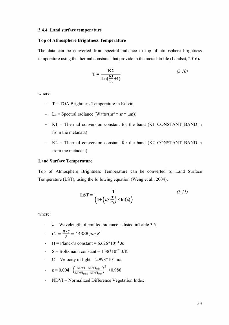
33
3.4.4. Land surface temperature
Top of Atmosphere Brightness Temperature
The data can be converted from spectral radiance to top of atmosphere brightness
temperature using the thermal constants that provide in the metadata file (Landsat, 2016).
T = K2
Ln(K1
Lλ+1)
(3.10)
where:
- T = TOA Brightness Temperature in Kelvin.
- Lλ = Spectral radiance (Watts/(m2 * sr * μm))
- K1 = Thermal conversion constant for the band (K1_CONSTANT_BAND_n
from the metadata)
- K2 = Thermal conversion constant for the band (K2_CONSTANT_BAND_n
from the metadata)
Land Surface Temperature
Top of Atmosphere Brightness Temperature can be converted to Land Surface
Temperature (LST), using the following equation (Weng et al., 2004).
LST = T
(1+ (λ×T
C2) × ln(ε))
(3.11)
where:
- λ = Wavelength of emitted radiance is listed inTable 3.5.
- 𝐶2 =𝐻×𝐶
𝑆= 14388 𝜇𝑚 𝐾
- H = Planck’s constant = 6.626*10-34 Js
- S = Boltzmann constant = 1.38*10-23 J/K
- C = Velocity of light = 2.998*108 m/s
- ε = 0.004× (NDVI - NDVImin
NDVImax- NDVImin)
2
+0.986
- NDVI = Normalized Difference Vegetation Index

34
Table 3.5: Centre wavelength of Landsat bands
Satellite images Band λ (𝝁𝒎)
Landsat 4, 5, and 7 6 11.45
Landsat 8 10 10.8
Landsat 8 11 12
3.4.5. Visual interpolation
Figure 3.4: Knowledge-based image analysis system
Source: (Richards & Jia, 2005)
One of the essential characteristics of digital image data is that it can be classified by
automatic information extraction or by humans through visual inspection (Richards &
Jia, 2005). The visual interpolation is a method which is based on the experiences of
the completed surface as well as perceptual knowledge about elements’ properties of
expert analysts (Lowe, 2012; Nakayama & Shimojo, 1992; Park & Nikamanon, n.d.;
Richards & Jia, 2005). The method is useful for spatial assessment with high-level
decisions through the inference engine, which is associatively connected between
images and surfaces (Figure 3.4). Visual image interpretation techniques are usually
used after the digital processing to improve the accuracy for detection and identification
of land cover or other (Richards & Jia, 2005). The method was used to verify the results
of digital processing. It is an essential part of this research that enables us to infer any
hidden or misclassified objects.
3.4.6. Time series analysis
Time series analysis is considered a powerful tool to detect, monitor, analyze, as well as
predict changes (Franklin, 2001). Application of the time series analysis by remote
sensing data plays a vital role in various research fields, ranging from economics to
Image data
Inference engine
Knowledge base
Thematic map

35
engineering, such as land use - land cover change, climate change, forest change in
seasonal and inter-annual (Bounoua et al., 2015; Dao Minh et al., 2017; Fernández-Manso
et al., 2012; Franklin, 2001).
Figure 3.5: Change detection model for classified images in this study
The analysis requires data collected from different periods. The change map can be
obtained through several different methods. In this study, the multi-temporal satellite
images were classified with the same determined categories before they were overlaid for
detecting changes (Figure 3.5).
3.5. Geography Information System
3.5.1. Data conversion
The demand for spatial data is increasing sharply by existing numerous issues as well as
the rapid development of computer technology that has created the diversity of database,
design, platform, and format (He et al., 2011; Montgomery & Schuch, 1993). Therefore,
data conversion methodologies are particularly essential to enable the effective use of the
available data from various data formats, geolocations, and scales.
Figure 3.6 illustrates the principal tasks and their relationships within the data conversion
process. Data sources are in several different formats, including data files, maps, records,
and field inventory, and other types of information. In the data conversion process,
collected data have been converted into a standard format, and the proposed database
contains the relevant data. The conversion methodology will be identified based on the
Analysis
Change Map
Change figure

36
original formats and the requested format as well as the designed database based on the
required information of each layer in this study.
Figure 3.6: Data conversion process
(Modified from Montgomery &Schuch, 1993)
3.5.2. Overlay analysis
Overlay analysis with various layers has been the most effective application of GIS to
obtain essential results (Walke at al. 2012). Assessment of the conservation suitability
will require the integration of a multidisciplinary database. All collected thematic maps,
which could influence biodiversity conservation, are entered into the GIS system to create
a thematic database with various parameters. The biodiversity database is created from
the overlay process of the defined layers. The final map of biodiversity value is achieved
from the spatial overlay of factors as well as the calculation and analysis of attribute data
for each intersection region in the study area (Figure 3.7).
Data Sources
Data files
Maps
Records
Field Inventory
Database
Design
Platform
& Format
Conversion specification
Conversion
Approach
Conversion Technologies
Technology
Conversion
Methodology
Converted GIS
Database

37
Figure 3.7: Overlay operation with spatial and attribute data
Source: (Author’s work)
3.5.3. Kernel Density Estimation
Kernel Density Estimation method that is considered the most popular non-parametric
method is applied to estimate the probability density function of a random variable (Scott,
2015; Simonoff, 2012; Wand & Jones, 1994). It is an essential tool in the analysis of data
(Silverman, 1998; Botevet al., 2010; Dehnad, 1987; Scott, 2015).
The Kernel Density Estimator is defined as an unknown continuous probability density
function (ƒ) on x with n independent realizations Xn = {X1, X2, …, Xn} (Silverman, 2018).
The formula of Kernel Density Estimator is described as followed:
ƒ̂𝒉(x)=𝟏
𝒏∑ 𝑲𝒉(𝒙 − 𝒙𝒊)
𝒏
𝒊=𝟏
=1
nh∑ K (
𝒙 − 𝒙𝒊
𝒉)
n
i=1
(3.12)
where:
- K is the Kernel function, a non-negative function, to determine the shape of the
bumps.
- h is the window width, called the bandwidth or smoothing parameter.
- Xi is location
Slope Slope
Code
Altitude Altitude
Code
Accessibility Accessibility
Code
0 - 20 11 0 - 200 101 High 1
0 - 20 11 200 - 500 102 High 1
0 - 20 11 > 500 103 Medium 2
> 30 13 0 - 200 101 Medium 2
> 30 13 200 - 500 102 Low 3
> 30 13 > 500 103 Low 3
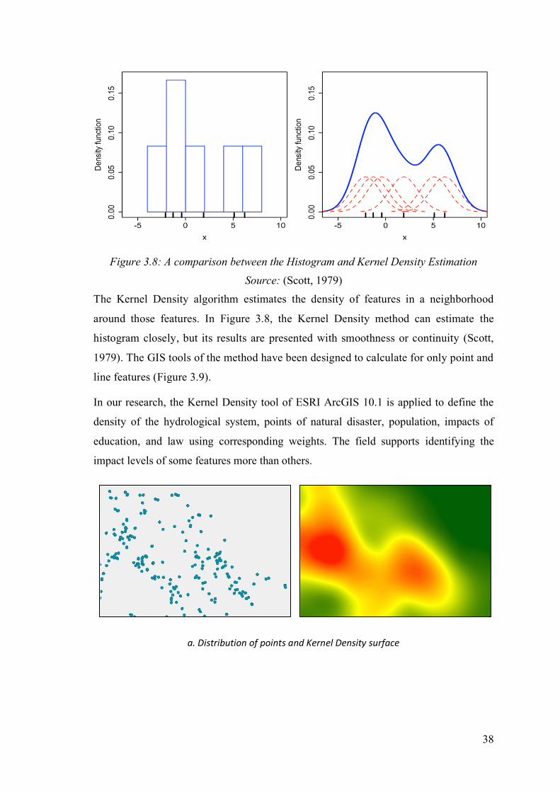
38
Figure 3.8: A comparison between the Histogram and Kernel Density Estimation
Source: (Scott, 1979)
The Kernel Density algorithm estimates the density of features in a neighborhood
around those features. In Figure 3.8, the Kernel Density method can estimate the
histogram closely, but its results are presented with smoothness or continuity (Scott,
1979). The GIS tools of the method have been designed to calculate for only point and
line features (Figure 3.9).
In our research, the Kernel Density tool of ESRI ArcGIS 10.1 is applied to define the
density of the hydrological system, points of natural disaster, population, impacts of
education, and law using corresponding weights. The field supports identifying the
impact levels of some features more than others.
a. Distribution of points and Kernel Density surface

39
b. Lines of hydrology and Kernel Density surface
Figure 3.9: Applications of Kernel Density Estimation for point and line features
Source: (Author’s work)
3.5.4. Jenks Natural Breaks
Figure 3.10: Comparison between Jenks Natural Breaks and other methods
Source: EHDP.com
The Jenks Natural Breaks classification algorithm that is also named the Jenks
optimization method is used to arrange values of different categories in the best way.
The method helps to decrease the variance within classes and maximize the variance
between classes (Jenks, 1967). The data are divided into groups whose boundaries are
determined to show where relatively significant differences in the data values exist.
According to Expert Health Data Programming (EHDP.com), the Jenks Natural Breaks
method can find the best way to split up the ranges. Many comparisons among Jenks
Natural Breaks with other methods such as Equal Counts, and Equal Intervals with the
same data were performed for a series of commonly made maps. Overall, the Jenks
Natural Breaks algorithm is better in almost all the tests with the highest value of GVF

40
(Goodness of Variance Fit) (Figure 3.10). The method was applied to identify the best
thresholds to split the ranges that groups into the different levels of priority areas or
pressure areas in this study.
3.6. Climate change scenarios
Table 3.6: Regional climate models for calculating climate change scenarios
ID Model Developed by Methods Resolution
(km) Location (0)
1 CLWRF
Several organizations
such as NCAE, NCEP,
FSL, AFWA, etc.
1. NorESM1-M 30
3.5–27 N
97.5–116 E
2 PRECIS Hadley Meteorological
Centre United Kingdom
1. CNRM-CM5
2. GFDL-CM3
3. HadGEM2-ES
10
6.5–25 N
99.5–115 E
3 CCAM
Commonwealth Institute
of Science and Industry
Australia
1. ACCESS1-0
2. CCSM4
3. CNRM-CM5
4. GFDL-CM3
5. MPI-ESM-LR
6. NorESM1-M
20 6.5–30 N
99.5-119.5E
4 RegCM
International Centre for
Theoretical Physics,
Italy
1. ACCESS1-0
2. NorESM1-M
20 6.5–30 N
99.5–119.5 E
5 AGCM/
MRI
Japan Meteorological
Research Institute
1. NCAR-SST
2. HadGEM2-SST
3. GFDL-SST
4. Combination of
SSTs
20 Global
Source: (MONRE, 2016)

41
The estimated maps of climate change in Vietnam were used to identify the priority
areas for biodiversity conservation in the study area. The climate change scenarios were
calculated based on five Regional Climate Model (RCM). They consist of Atmosphere
General Circulation Model (AGCM) developed by Japan Meteorological Research
Institute; Providing Regional Climates for Impacts Studies (PRECIS) developed by
Hadley Meteorological Centre of United Kingdom; Conformal-Cubic Atmospheric
Model (CCAM) developed by Commonwealth Institute of Science and Industry in
Australia; Regional Climate Model (RegCM) provided by International Centre for
Theoretical Physics in Italy; and Weather Research And Forecasting Model (WRF)
modified for Regional Climate Modelization (CLWRF). Sixteen methods for
calculating the climate change scenarios in Vietnam were applied through these five
models (Table 3.6).
Application of the five regional climate models with the sixteen methods helps to provide
more objective information, which can increase the accuracy as well as the reliability of the
estimated result (Solomon et al., 2007; Weigel et al., 2008).

42
Chapter 4. Establishment of criteria
The synthesized criteria were combined with the environmental Pressure-State-
Response model to identify key processes that significantly impact on biodiversity
conservation over time (Chanson et al., 2010; Lee et al., 2005). A detailed model to
define the priority areas for protected areas in Vietnam was developed in this study
based on the combination of the criteria of biodiversity conservation and the
environmental Pressure-State-Response model shown in Figure 4.1.
Figure 4.1. Criteria system to define priority areas for biodiversity conservation
Figure 4.1 illustrates a set of criteria to define priority areas of biodiversity conservation
in Vietnam. Three main principles of the environment, including pressure, state, and
response, were used to develop all criteria which have impacts on biodiversity
conservation. The criteria tree of biodiversity conservation in Vietnam was formulated to
illustrate the relationships and arrangements between the indicators.
A hierarchy model with four levels was established based on the Analysis Hierarchy
Process (AHP) method to calculate the weight of the criteria (Figure 4.2). The first class
is the main aim of this study, the evaluation of biodiversity conservation. The second
class is three factors (pressure, state, and response) achieved based on the environment
model. Then the third class is composed of the seven criteria (species, ecosystems, nature,

43
human, conservation, education, and law). Finally, the fourth class is composed of 15
sub-criteria (richness; rarity; location; topography; climate; hydrology; forest types;
climate change; natural disasters; distribution, density, and quantity of population;
livelihood; forest management types; size of forest area).
Figure 4.2. Calculating weights of criteria based on the AHP method
The response of experts achieved through the interviews was synthesized to construct a
set of pair-wise comparison matrices that reflect the relative importance of the indicators
within each matrix. According to the number of criteria, sub-criteria, and factors (Figure
4.1), 27 pairwise comparisons were formulated. Then the process of calculating weights
and Consistency Ratio (CR) was performed. Through the consistency inspection
(0<CR<0.1) shows the reasonable consistency of the pair-wise comparison matrix. The
judgment is performed for the calculated weights of the corresponding matrix.
0<CR<0.1 (Consistency Ratio)
Determined criteria
Hierarchical
construction
Pair-wise comparisons Assessment of
experts
Calculating weights
Consistency inspection
Weights of criteria
No
Yes
Questionnaire

44
4.1. Summary of responses
The questionnaires were delivered to all potential respondents, and completed responses
were received from 185 respondents. The range of age is from 20 years to 70 years; 53
% of respondents are older than 30 years. Of the young respondents (20 to 23 years old),
30% were last-year students of universities who have been trained deeply in biodiversity
conservation and forest management. The remaining respondents are working for
organizations or agencies relating to biodiversity and conservation. The number of
males is double the number of females, accounting for 69% of 185 respondents. Of
these respondents, 133 (69.2%) are interviewed directly, and the rest (30.8%) were
interviewed indirectly via emails. They were from 37 different organizations located
throughout Vietnam (Figure 4.3).
Figure 4.3. Locations of respondents
The respondents are working for various organizations, which can be grouped into five
categories, including in Protected Areas, Government Organizations, NGOs, Universities
and Research Institutes, and Others. Three highest response rates of 50.41%, 34.6%, and

45
10.26% were from Universities and Research Institutes, Protected Areas, and
Government Organizations. The Vietnam National University of Forestry, Cuc Phuong
National Park, Pu Luong Nature Reserve and Ngoc Son – Ngo Luong Nature Reserve
were four main places with the highest rate to the questionnaire with 39.5%, 10.8%, 9.7%,
and 5.4% respectively (Appendix II - Table II. 1).
Appendix II - Table II. 2 shows the assessments of 185 respondents for criteria, sub-
criteria, and factors, which are divided into nine different levels. The ranges of the
requirements fluctuate from 6 to 8 degrees in which “Ecosystem,” “Nature” sub-criteria,
and “Location” factor have the most extensive range. It points out existing various
opposite opinions in assessing the importance level of three measures. Excluding the
“Nature” sub-criterion with two levels of difference between mode and median are 8 and
6, respectively, the majority are close or equal between themselves. If Mode and Median
results are used to identify the opinion of all respondents, it is difficult to compare among
pairwise because of retaining the equilibrium of the essential levels assessed within each
group of criteria.
Moreover, these values do not represent the collective opinions of respondents. The
ultimate purpose of this study is to compare each pair of standard groups. The synthetic
values from all responses for each criterion are not appropriate to calculate the weight set
of the whole criteria system of biodiversity conservation in Vietnam. Therefore, the
processing is performed through analyzing and synthesizing the attitude of all
respondents, respectively, to each pairwise.
Two outlier detection methodologies were applied to find out data points of outliers in
the collected data. 77 and 49 data points were showed by the interquartile range and the
standard deviation, respectively. The numbers of respondents synthesized from the data
points are 38 and 22, which were numbered following the number column in Appendix
II - Error! Reference source not found.. The interquartile range showed that “
Response,” “Human,” and “Forest type” criteria obtained the highest data points of
outliers with 9, 11, and 15 respondents. On the other hand, 3 data points of outliers were
the maximum number showed by the standard deviation method for “Conservation,”
“Hydrology,” and “Climate change” criteria (Appendix II - Table II. 2). However, the
most outliers calculated by the standard deviation also include the outliers of the
interquartile range. The outliers consist of around half of the respondents and are students
of several universities.

46
Figure 4.4. Boxplot for responding all criteria of biodiversity conservation
A visual display of data values is presented to observe and understand the whole of the
interview data from the distribution, the range of each criterion to the data points of
outliers (Appendix II - Table II. 3). The number of respondents was used to label outliers
and extreme cases on the boxplot (Figure 4.4). Various names are shown in the figure,
yet the most outliers of respondents just existed on 1 or 2 criteria, and most respondents
are students indicated in Figure 4.4. Significantly, two titles, labelled more several times
than other, are the number 83 and 161 in which 7 and 17 data points of outliers belonged
to the corresponding respondents. The outlier points of number 83 and 161, one student
and one technician respectively, calculated by both outlier detection methods are
remarkably equivalent. Therefore, it needs to remove the respondents mentioned before
processing the next step of the study.
4.2. Statistic of pairwise comparison
Since the 1950s, numerous methodologies of psychology named multidimensional
scaling (MDS) have been studied and applied in analyzing similarity and preferential
choice data. Nevertheless, the solution has not yet been found to deal with the problem of
gaining the perfect-voting in multidimensionality (Poole, 2005). The Condorcet Winner

47
considered as majority rule games choose the winner, which is preferred in every one-to-
one comparison with the other choices (Poole et al., 2000).
As shown in the heading of the questionnaire, the data of the pairwise comparison was
not gathered directly. The pairwise value was calculated by comparing two criteria in one
pairwise of each respondent and synthesizing as in Appendix II - Table II. 3. The scale of
integers ranging from 1 to 9 is applied to assess their importance levels (Saaty, 1980;
Saaty & Vargas, 1991). For example, A and B are two criteria in one pairwise comparison.
It includes three possible situations; they are A higher than B (A>B), A equal to B (A=B),
and A less than B (A<B). The intensity of importance is 1 represented for the second case
(A=B). Consequently, each pairwise can be presented by 8 cases of A>B, one case of
A=B, and 8 cases of A<B (Appendix II - Table II. 3).
The number of pairwise comparisons was synthesized for each pairwise from all the
respondents (183 people after removing 2 cases of outliers). Twenty-seven pairwise
comparisons and 17 instances of themselves are described entirely in Appendix II -
Table II. 3. According to majority rule (Condorcet Winner), the total of respondents
selecting the same situation of A>B, A=B, and A<B for each pairwise comparison was
calculated to compare together.
The acceptable risk was demonstrated in the formula of error estimation from Cochran in
1977. The chance is commonly called the margin of error, which has been used by
researchers as the limit for willingness to accept (Cochran, 1977). The acceptable margin
of error is 5% and 3% for categorical data and continuous data, respectively (Krejcie &
Morgan, 1970). The appropriate precision for prevalence researches is 5% by experience
(Bartlett et al., 2001; Mandallaz, 2008; Naing et al., 2006). This percentage of difference
(PD) is used to show the reliability of comparison among the number of respondents who
chose A>B, A=B, or A<B. The rules were used to identify the appropriate level of one
pairwise comparison as following:
- 5% of the difference was used to select the majority to belong to A>B, A=B, or
A<B.
- If the number of A>B and A<B is similar or higher than under 5% out of total
respondents, the situation of A=B is the priority option.
- If the highest number of three situations (A>B, A=B, and A<B) are higher than others
above 5% out of total respondents, this situation is the opinion of the majority.
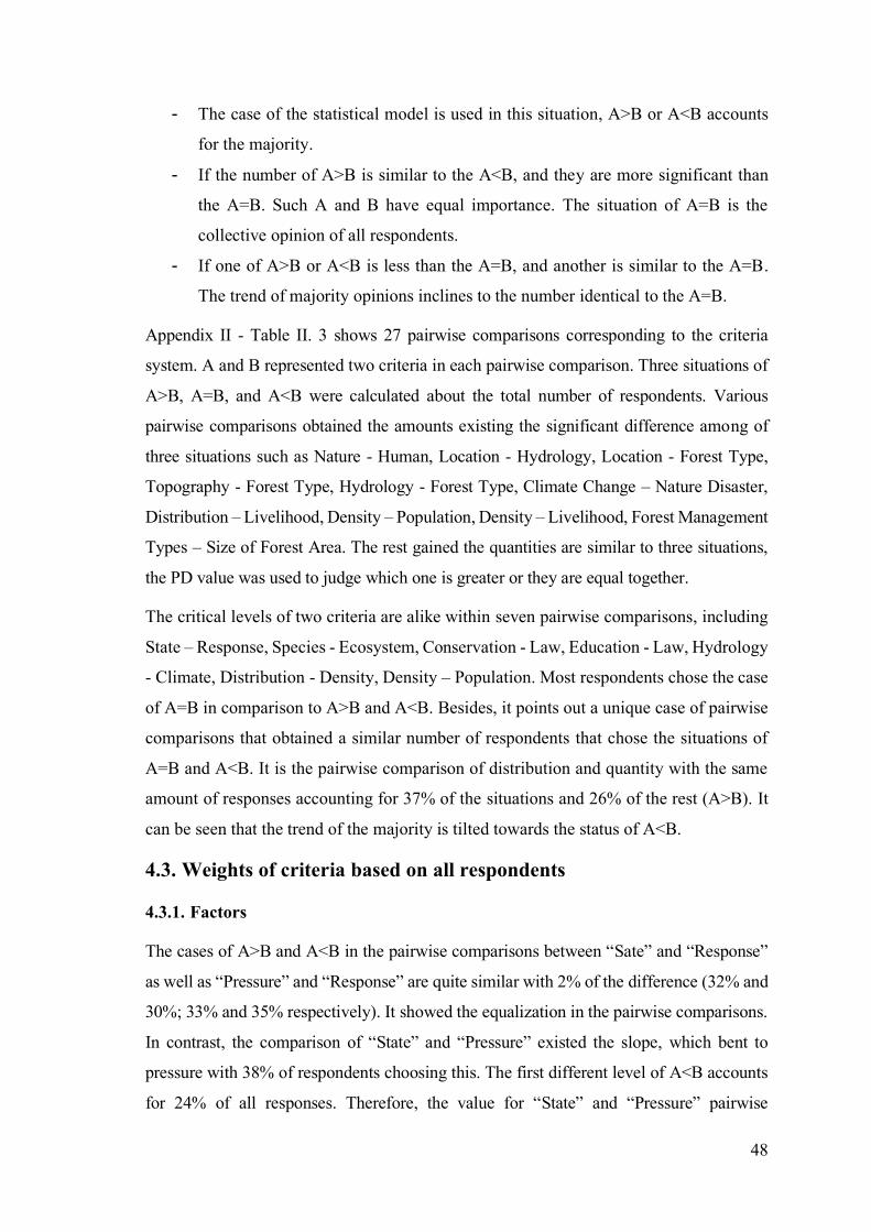
48
- The case of the statistical model is used in this situation, A>B or A<B accounts
for the majority.
- If the number of A>B is similar to the A<B, and they are more significant than
the A=B. Such A and B have equal importance. The situation of A=B is the
collective opinion of all respondents.
- If one of A>B or A<B is less than the A=B, and another is similar to the A=B.
The trend of majority opinions inclines to the number identical to the A=B.
Appendix II - Table II. 3 shows 27 pairwise comparisons corresponding to the criteria
system. A and B represented two criteria in each pairwise comparison. Three situations of
A>B, A=B, and A<B were calculated about the total number of respondents. Various
pairwise comparisons obtained the amounts existing the significant difference among of
three situations such as Nature - Human, Location - Hydrology, Location - Forest Type,
Topography - Forest Type, Hydrology - Forest Type, Climate Change – Nature Disaster,
Distribution – Livelihood, Density – Population, Density – Livelihood, Forest Management
Types – Size of Forest Area. The rest gained the quantities are similar to three situations,
the PD value was used to judge which one is greater or they are equal together.
The critical levels of two criteria are alike within seven pairwise comparisons, including
State – Response, Species - Ecosystem, Conservation - Law, Education - Law, Hydrology
- Climate, Distribution - Density, Density – Population. Most respondents chose the case
of A=B in comparison to A>B and A<B. Besides, it points out a unique case of pairwise
comparisons that obtained a similar number of respondents that chose the situations of
A=B and A<B. It is the pairwise comparison of distribution and quantity with the same
amount of responses accounting for 37% of the situations and 26% of the rest (A>B). It
can be seen that the trend of the majority is tilted towards the status of A<B.
4.3. Weights of criteria based on all respondents
4.3.1. Factors
The cases of A>B and A<B in the pairwise comparisons between “Sate” and “Response”
as well as “Pressure” and “Response” are quite similar with 2% of the difference (32% and
30%; 33% and 35% respectively). It showed the equalization in the pairwise comparisons.
In contrast, the comparison of “State” and “Pressure” existed the slope, which bent to
pressure with 38% of respondents choosing this. The first different level of A<B accounts
for 24% of all responses. Therefore, the value for “State” and “Pressure” pairwise

49
comparison is 1/2 to establish the pairwise comparison matrix (Table 4.1) of three factors
for defining the priority areas of biodiversity conservation in Vietnam.
Table 4.1. Pairwise comparison of factors
State Pressure Response
State 1.00 0.50 1.00
Pressure 2.00 1.00 1.00
Response 1.00 1.00 1.00
Sum 4.00 2.50 3.00
Table 4.2: Standardized matrix of factors
State Pressure Response Weight
State 0.25 0.20 0.33 26%
Pressure 0.50 0.40 0.33 41%
Response 0.25 0.40 0.33 33%
Sum 1.00 1.00 1.00 100%
The value of each cell in a pairwise comparison matrix of Table 4.1 was used to calculate
the standardized matrix of criteria. The matrix includes the weight column, which shows
the weight of “State,” “Pressure,” and “Response” factors with 26%, 41%, and 33%,
respectively (Table 4.2).
Table 4.3: Consistency test of factors
Compositions Values
n 3
RI 0.520
𝜆 3.054
CI 0.027
CR 0.052
Consistency Yes

50
These weights were combined with the pairwise comparison matrix to calculate the
average of the elements of the consistency vector (𝜆 = 3.054). The number of factors
used in the pairwise comparison matrix in Table 4.1 is 3. Hence the average Random
Index found in Table 4.3 is 0.520. Then, two formulas (3.2) and (3.3) are used to calculate
the Consistency Ratio (CR). The derived value is 0.052 less than 0.1 of the consistent
ranking (Table 4.3). Therefore, it results in the pairwise comparison matrix of the criteria
being entirely consistent, and the weights in Table 4.2 can be used.
4.3.2. Criteria
4.3.2.1. State
“Species” and “Ecosystem” criteria are two elements that are under the "State" factor.
One pairwise comparison between “Species” and “Ecosystem” was established and
synthesized from all the respondents to calculate the weight of them. Although the
situation of A=B accounted for 38% just higher 2% than A<B with 36%, it did not reach
the acceptable margin (5%) to select the situation of A=B as the majority of opinions. It
means that “Species” and “Ecosystem” criteria were not equal in the level of importance.
The first level of difference was selected with the situation of A<B. The pairwise
comparison matrix for the criteria is illustrated in Table 4.4.
Table 4.4: Pairwise comparison of criteria of state
Species Ecosystem
Species 1.00 0.50
Ecosystem 2.00 1.00
Sum 3.00 1.50
Table 4.5: Standardized matrix of criteria of state
Species Ecosystem Weight
Species 0.33 0.33 33%
Ecosystem 0.67 0.67 67%
Sum 1.00 1.00 100%

51
The results of the weights are 33% and 67% for “Species” and “Ecosystem” that belong
to the “State” factor (Table 4.5). Besides, the calculation of the Consistency Ratio was
not necessary for the matrix with just one pairwise comparison.
4.3.2.2. Pressure
The “Pressure” factor of biodiversity conservation identified with two criteria: “Nature”
and “Human.” The result of the consultation was evident with many respondents (83%)
choosing the “Human” criterion as the essential element in the “Pressure” factor.
However, the numbers of responses for the critical levels of 1/2, 1/3, 1/4, and 1/5 were
reasonably parallel with 22%, 14%, 19%, and 13%, respectively. To represent the
majority of respondents, the level of 1/3 was an optimal choice in this condition. The
pairwise comparison matrix is established, as shown in Table 4.6.
Table 4.6: Pairwise comparison of sub-criteria of pressure
Nature Human
Nature 1.00 0.33
Human 3.00 1.00
Sum 4.00 1.33
Table 4.7: Standardized matrix of sub-criteria of pressure
Nature Human Weight
Nature 0.25 0.25 25%
Human 0.75 0.75 75%
Sum 1.00 1.00 100%
The results in Table 4.7 show that the importance of the “Human” sub-criterion is higher
three times than the “Nature” sub-criterion with just 25% of the weight. The calculation
of the Consistency Ratio is not necessary for the comparison matrix with only one
pairwise comparison between “Nature” and “Human.”
4.3.2.3. Response
Three criteria, including “Conservation,” “Education,” and “Law” were identified as the
main elements of the “Response” criterion. They created three corresponding pairwise
comparisons, which are shown in Table 4.8. Two pairwise comparisons of “Conservation

52
– Law” and “Education – Law” achieved the same of the most responses in a situation of
A=B with 44% and 48% respectively, while the comparison between “Conservation” and
“Law” was the majority in the situation of A<B. The position of the pairwise comparison
is 1/2, accounting for the majority of A<B situation with 22%.
Table 4.8: Pairwise comparison of sub-criteria of response
Conservation Education Law
Conservation 1.00 0.50 1.00
Education 2.00 1.00 1.00
Law 1.00 1.00 1.00
Sum 4.00 2.50 3.00
Table 4.9: Standardized matrix of sub-criteria of response
Conservation Education Law Weight
Conservation 0.25 0.20 0.33 26%
Education 0.50 0.40 0.33 41%
Law 0.25 0.40 0.33 33%
Sum 1.00 1.00 1.00 100%
The pairwise comparison matrix is established, according to Table 4.8, 26%, 41%, and
33% are the weights of “Conservation,” “Education,” and “Law” sub-criteria calculated
from the standardized matrix in Table 4.9.
Table 4.10: Consistency test of sub-criteria of response
Compositions Values
n 3
RI 0.520
𝜆 3.054
CI 0.027
CR 0.052
Consistency Yes

53
The average Random Index is 0.520, shown in Table 3.3, with three criteria used. The
consistency vector was calculated for identifying the average (𝜆) of the elements of its
self. The average gained was 3.054. The results of processing consistency were 0.027 and
0.052 for the Consistency Index (CI) and Consistency Ratio (CR), respectively. The value
of the Consistency Ratio was less than 0.1 of the consistency limit. Therefore, it results
in the pairwise comparison matrix of the criteria being entirely consistent, and the weights
in Table 4.9 can be used.
4.3.3. Sub-criteria
4.3.3.1. Species
The situation (A<B) reached 40% in a pairwise comparison between “Richness” and
“Rarity” sub-criteria. 12% and 8% are the different values higher than the situations of A>B
and A=B, respectively. The A<B situation received the highest responses in the first level
of moderate importance, with 22%. Thus, the pairwise comparison matrix between
“Richness” and “Rarity” is presented in Table 4.11.
Table 4.11: Pairwise comparison of factors of species
Richness Rarity
Richness 1.00 0.50
Rarity 2.00 1.00
Sum 3.00 1.50
Error! Not a valid bookmark self-reference. shows that the “Rarity” sub-criterion was
moderately more critical than the “Richness” sub-criterion in the “Species” criterion. The
values of weights were 33% of “Richness” and 67% of “Rarity”. The calculation of the
Consistency Ratio was not necessary for the comparison matrix with just two sub-criteria,
including “Richness” and “Rarity.”
Table 4.12: Standardized matrix of factors of species
Richness Rarity Weight
Richness 0.33 0.33 33%
Rarity 0.67 0.67 67%
Sum 1.00 1.00 100%

54
4.3.3.2. Ecosystem
Five main elements of “Location,” “Topography,” “Hydrology,” “Climate,” and “Forest
type” are represented in the “Ecosystem” criterion. The pairwise comparisons among
them were calculated to identify the importance levels for the “Ecosystem”. Seven out
of ten comparisons obtained the clear difference among three situations of A>B, A=B,
and A<B such as “Location – Topography,” “Location – Hydrology,” “Location –
Climate,” “Location – Forest type,” “Topography – Forest type,” “Hydrology – Forest
type,” and “Climate – Forest type.” “Location” and “Forest type” factors were
reasonably different from each other and other sub-criteria. The rest of pairwise
comparisons have the parallel numbers between two out of three situations consisting
of “Topography – Hydrology,” “Topography – Climate,” and “Hydrology – Climate.”
Table 4.13: Pairwise comparison of sub-criteria of ecosystem
Location Topography Hydrology Climate Forest type
Location 1.00 0.50 2.00 0.50 0.50
Topography 2.00 1.00 2.00 1.00 0.50
Hydrology 0.50 0.50 1.00 0.50 0.33
Climate 2.00 1.00 2.00 1.00 0.50
Forest type 2.00 2.00 3.00 2.00 1.00
Sum 7.50 5.00 10.00 5.00 2.83
In most comparisons, it is clear to judge the importance level for each pairwise
comparison. Although the “Forest type” sub-criterion was moderately more important
than “Hydrology,” the numbers of respondents at the first level (1/2) and the second
(1/3) were the same with 23% and 20% respectively. However, in the majority method,
the second level (1/3) was more appropriate for all respondents. The pairwise
comparison matrix of the factors for “Ecosystem” is described in Table 4.13.
The standardized matrix was created from the pairwise comparison matrix to calculate
the weights of the all sub-criteria of the “Ecosystem” criterion that is shown in Table 4.14.
There are three groups of weights. The lowest one includes “Location” and “Hydrology”
sub-criteria with 14% and 10%, respectively. The medium group consists of “Topology”
and “Climate” with the same percentage (21%). The “Forest type” was in the highest

55
group gained more concentrate than others with 34%, nearly more two times than the
lowest group.
Table 4.14: Standardized matrix of sub-criteria of ecosystem
Location Topography Hydrology Climate Forest type Weight
Location 0.13 0.10 0.20 0.10 0.18 14%
Topography 0.27 0.20 0.20 0.20 0.18 21%
Hydrology 0.07 0.10 0.10 0.10 0.12 10%
Climate 0.27 0.20 0.20 0.20 0.18 21%
Forest type 0.27 0.40 0.30 0.40 0.35 34%
Sum 1.00 1.00 1.00 1.00 1.00 100%
The number of elements (n) creating the pairwise comparison matrix was 5. Thus the
average Random Index (RI) in Table 3.3 was 1.11. The consistency vector was
constructed to identify the average (𝜆 = 5.088) of the elements.
Table 4.15: Consistency test of sub-criteria of ecosystem
Compositions Values
n 5
RI 1.110
𝜆 5.088
CI 0.022
CR 0.020
Consistency Yes
The equations of AHP were used to gain the Consistency Ratio (CR). It was 2% less than
10% of the consistency condition (Table 4.15). It showed that the results of processing
AHP were consistent.
4.3.3.3. Nature
The “Nature” criterion impacts biodiversity conservation by two sub-criteria,
“Climate change” and “Nature disaster”. 55% of respondents identified the vital role

56
of the “Climate change” sub-criterion more than “Nature disaster.” The first level (2)
and second level (3) of the situation (A>B) were quite similar to 21% and 18%
respectively, the opinion of the most respondents belonged to the second one.
Therefore, the pairwise comparison matrix of “Climate change” and “Natural disaster”
factors was presented in Table 4.16.
Table 4.16: Pairwise comparison of factors of nature
Climate change Natural disaster
Climate change 1.00 3.00
Natural disaster 0.33 1.00
Sum 1.33 4.00
The results of weights in Error! Not a valid bookmark self-reference. presented the most
critical sub-criterion of the “Nature” criterion that was “Climate change” with 75% of
weight more significant three times than “Natural disaster”. The number of criteria creates
the pairwise comparison matrix in Table 4.16 was 2. Thus, the calculation of the
Consistency Ratio (CR) was unnecessary.
Table 4.17: Standardized matrix of factors of nature
Climate change Natural disaster Weight
Climate change 0.75 0.75 75%
Natural disaster 0.25 0.25 25%
Sum 1.00 1.00 100%
4.3.3.4. Human
The pairwise comparison matrix of the “Human” sub-criterion included six assessments
among four factors, such as “Distribution,” “Density,” “Population,” and “Livelihood.”
Five evaluations of “Distribution – Density,” “Distribution – Livelihood,” “Density –
Population,” “Density – Livelihood,” and “Population – Livelihood” were quite evident
with 9%, 25%, 33%, 39%, and 39% respectively.

57
The pairwise comparison of “Distribution – Population” was unique, with the same
percentage (37%) of respondents choosing equal importance. “Distribution” was less
important than “Density.” The appropriate level of each comparison was determined by
majority rule (Condorcet Winner), and the results are presented in Table 4.18. The pairwise
comparison matrix was standardized to achieve the weights of the entire sub-criteria of the
“Human” criterion. While the “Distribution” sub-criterion was the least important with
15%, “Livelihood” accounts for 43% and stays at the top. The same weights belong to
“Density” and “Population” sub-criteria with 19% and 23%, respectively (Table 4.19).
Table 4.18: Pairwise comparison of factors of human
Distribution Density Population Livelihood
Distribution 1.00 1.00 0.50 0.33
Density 1.00 1.00 1.00 0.50
Population 2.00 1.00 1.00 0.50
Livelihood 3.00 2.00 2.00 1.00
Sum 7.00 5.00 4.50 2.30
Table 4.19: Standardized matrix of factors of human
Distribution Density Population Livelihood Weight
Distribution 0.14 0.20 0.11 0.14 15%
Density 0.14 0.20 0.22 0.21 19%
Population 0.29 0.20 0.22 0.21 23%
Livelihood 0.43 0.40 0.44 0.43 43%
Sum 1.00 1.00 1.00 1.00 100%
The average Random Index (RI) was 0.890, found in Table 3.3, with four factors
participated. The Consistency Index (CI) was 0.015, then the value calculated for the
Consistency Ratio (CR) was 0.017 (Table 5.20). It demonstrated that the pairwise
comparison matrix of the sub-criterion of the “Human” criterion was consistent.

58
Table 4.20: Consistency test of factors of human
Compositions Values
n 4
RI 0.890
𝜆 4.046
CI 0.015
CR 0.017
Consistency Yes
4.3.3.5. Conservation
There are two sub-criteria regarding the “Conservation” criterion that comprise “Forest
management types” and “Size of forest area.” To assess the role of these sub-criteria in
“Conservation,” a pairwise comparison between the two sub-criteria was used. The
synthesized result in Appendix II - Table II. 3 pointed out that “Forest management types”
sub-criterion, accounting for 41%, was more important than “Size of forest area,” with 29%
of the responses from interviewees. “Forest management types” (19%) was considered
more important than “Size of forest area” (15%). The difference was just 4%. Thus the
opinion majority stays at the second level (3). The values are presented in Table 4.21.
Table 4.21: Pairwise comparison of factors of conservation
Forest management types Size of forest area
Forest management types 1.00 3.00
Size of forest area 0.33 1.00
Sum 1.33 4.00
Table 4.22: Standardized matrix of factors of conservation
Forest management types Size of forest area Weight
Forest management types 0.75 0.75 75%
Size of forest area 0.25 0.25 25%
Sum 1.00 1.00 100%

59
The results of weight of “Forest management types” and “Size of forest area” sub-criteria
were 75% and 25%, respectively, that are illustrated in Table 4.22. The number of criteria
in the pairwise comparison matrix was two. Thus, the calculation of the Consistency Ratio
(CR) was unnecessary.
4.3.4. Weights of criteria
The weights of the factors, criteria, and sub-criteria for identifying the priority areas of
biodiversity conservation in Vietnam were calculated using data from respondents. The
values of the Consistency Ratio (CR) of the pairwise comparison matrices were lower
than Consistency Ranking (10%). Thus, the matrices were consistent, and the calculated
weights were appropriate to use. The assignment of percent values of factors, criteria, and
sub-criteria were computed and showed in Figure 4.5.
Figure 4.5: Weights of criteria based on all respondents for identifying priority areas of
biodiversity conservation in Vietnam
Figure 4.5 illustrates the assignment of four levels of criteria system in this study. The
first level, in the center of the figure, is the ultimate purpose (100%) of assessing the
influences of the criteria on biodiversity conservation in Vietnam. The second level is
three factors that used the environmental model to measure biodiversity conservation.
The factors account for 26%, 41%, and 33% of “State,” “Pressure,” and “Response,”
respectively. The third level demonstrates a massive difference among seven criteria, with

60
31% of “Human,” then it is 17% of “Ecosystem,” the rest is distributed relatively similar.
Except for “Education” and “Law” (24%), the fourth level illustrates 15 sub-criteria of
five sub-criteria. The “Livelihood” sub-criterion is highest with 13.12%. The mediate
group consists of “Forest management types,” “Rarity,” “Forest types,” “Climate
change,” “Density,” and “Population,” fluctuating from 5.8% to 7. 71% while the rest of
eight of 15 sub-criteria accounts for 23.84%.
4.4. Weights of criteria based on groups
Beside the data of all respondents, the calculation of weights for the groups was
considered as an essential task. It helped provide an overview to understand the difference
between each group about the importance levels of the criteria to define priority areas for
biodiversity conservation in Vietnam. The respondents were classified according to their
agencies into five groups, including Government Organizations, Protected Areas,
Universities and Research Institutes, NGOs, and Other Companies (Appendix II - Table
II. 1). Two groups of NGOs and Other Companies comprised around 2.5%. Therefore,
the assessment of the groups is only performed for Government Organizations, Protected
Areas, Universities, and Research Institutes with 10.26%, 34.59%, and 50.41%,
respectively. The processed data for each group are presented in appendix II.
4.4.1. Protected Areas group
The respondents who are working at protected areas (PAs) are important elements of the
national survey. Their opinions and experiences help to assess precisely role of the criteria
set in biodiversity conservation. The respondents of PAs, located mostly in the North of
Vietnam, account for 34.59% of the total of 51 respondents (26.27%) were interviewed
directly (Appendix II - Table II. 1).
The data of respondents from PAs were filtered separately to calculate the weights of the
entire presented criteria in the questionnaire. The consistent tests were applied to the
pairwise comparison matrices. The weights were synthesized and described in detail, as
shown in figure 4.6. It can be seen that almost all the distribution of weights in PAs is
relatively similar to the distribution calculated by the respondents. Exceptionally, the
“Richness” and “Rarity” sub-criteria obtained the same percentage (50%) for each instead
of 33% and 67% in synthesizing all respondents, respectively (appendix II).
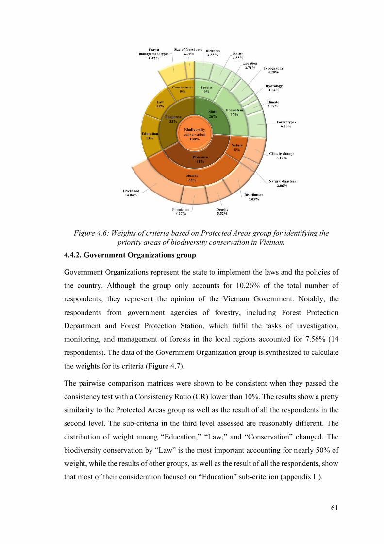
61
Figure 4.6: Weights of criteria based on Protected Areas group for identifying the
priority areas of biodiversity conservation in Vietnam
4.4.2. Government Organizations group
Government Organizations represent the state to implement the laws and the policies of
the country. Although the group only accounts for 10.26% of the total number of
respondents, they represent the opinion of the Vietnam Government. Notably, the
respondents from government agencies of forestry, including Forest Protection
Department and Forest Protection Station, which fulfil the tasks of investigation,
monitoring, and management of forests in the local regions accounted for 7.56% (14
respondents). The data of the Government Organization group is synthesized to calculate
the weights for its criteria (Figure 4.7).
The pairwise comparison matrices were shown to be consistent when they passed the
consistency test with a Consistency Ratio (CR) lower than 10%. The results show a pretty
similarity to the Protected Areas group as well as the result of all the respondents in the
second level. The sub-criteria in the third level assessed are reasonably different. The
distribution of weight among “Education,” “Law,” and “Conservation” changed. The
biodiversity conservation by “Law” is the most important accounting for nearly 50% of
weight, while the results of other groups, as well as the result of all the respondents, show
that most of their consideration focused on “Education” sub-criterion (appendix II).

62
Figure 4.7: Weights of criteria based on Government Organization group for
identifying the priority areas of biodiversity conservation in Vietnam
4.4.3. Universities and Research Institutes group
The group with the highest response rate is the Universities and Research Institutes (URIs)
group, with 50.41%. It includes six universities, five research institutes, and four research
centers (Appendix II - Table II. 1). The Vietnam National University of Forestry (VNUF)
had a 39.46% response rate; all the respondents were questioned directly. The VNUF is one
of the best universities on forestry in Vietnam and has trained numerous officers and
employees in various fields of forestry such as silviculture, forest protection, biodiversity
conservation, forest planning and inventory, and forest economy. Therefore, the
consultation of professors, scientists, researchers, lecturers, and students in the university
is significantly important to assess the criteria for biodiversity conservation in Vietnam.
The pairwise comparison matrices are established by the data from 92 respondents of the
URIs group (49.86% of the total number of respondents). The Consistency Ratio (CR) is
used to check the consistency of the matrices. All the pairwise comparison matrices
obtained the accepted consistency tests appropriate to the standard of Consistency Radio
(10%). The weight set calculated by the respondents of universities and research institutes
is presented in figure 4.8.

63
Figure 4.8: Weights of criteria based on the Universities and Research Institutes group
for identifying the priority areas of biodiversity conservation in Vietnam
There is a significant change in the assignment of the weights when it is compared with
the case of all respondents. In the second level, the “Response” factor has 41% of weight
replacing “Pressure” as the top criteria and, in fact, pushed it to bottom with 26% of the
weight. The third level witnesses the adjustment of the ratio between “Species” and
“Ecosystem” when they are equal in the importance level instead of the “Ecosystem”
criterion is assessed as more critical than “Species” with all respondents. The ratio of the
sub-criteria in the fourth level is firmly unchanged. Remarkably, the “Climate” factor
climbed to a peak of 28% impact on to “Ecosystem” criterion. While “Forest type” sub-
criterion fell from 34% to 22% of importance level in the assessment of the universities
and research institutes (Appendix II).
The result shows that there are differences of opinion between all the respondent groups
while considering the importance of the criteria in defining priority areas for biodiversity
conservation in Vietnam. In the aspect of the factors, the most considerable difference is
inevitably accredited to the URIs group. While the PAs and GOs group are similar and
thus form the collective opinion of all the respondents, it is both clear and essential factor
to consider the difference in responses that reflect the opinion of specific sectors. The
URIs group, representing the field of research and training, focuses significantly on the
“Response” factor. Other groups concerned with the pressure on biodiversity
conservation are those working in planning, policy, decision making, and direct
management of biodiversity conservation.

64
Chapter 5. Application of Criteria
5.1. Mapping criteria
Based on the environmental Pressure-State-Response model, this study has shown that
priority areas for biodiversity conservation could be identified by three factors: State,
Pressure, and Response. Then seven criteria and 17 sub-criteria and their weights were
developed and calculated to support the zoning of priority areas (appendix II). In this
chapter, I applied GIS and RS to establish a database for determined criteria to define
priority areas for biodiversity conservation in Vietnam. To combine the criteria into the
overall indices of biodiversity conservation, the score was used to measure the criteria
(Bedward et al., 1991). Each criterion was generated a GIS layer that was scored
according to its importance level that was considered as a weight (Phua & Minowa, 2005).
In this research, scoring procedures used five ordinal values, including very low, low,
medium, high, and very high rankings for priority levels of each criterion to scores of 1,
2, 3, 4, and 5.
5.1.1. Species
The significant effects of external factors on the ecosystem in general, as well as
biodiversity, are shown in Figure 5.1 that comprise land-use, history, migration, and
climate. Historical factors and levels of species migration are considered significant in
defining the diversity and types of functional groups in a region (Schulze & Mooney, 2012).
Figure 5.1: Interactions between internal and external factors of an ecosystem
(Schulze & Mooney, 2012)

65
Vegetation is one of the most widely used indirect indicators of the distribution of
terrestrial plant and animal species (Austin, 1991). There is a significant increase in
applying empirical remote-sensing models to define plant species richness at various
scales and environmental conditions (Franklin, 2010). A strong relationship was found
between image NDVI and plant species richness (Coops et al., 2004; John et al., 2008;
Levin et al., 2007; Waring et al., 2006). The vegetation maps derived from
classification methods for satellite images have been considered as predictors of
species richness (Fairbanks & McGwire, 2004; Gould, 2000; Hurlbert & Haskell,
2002; Johnson et al., 1998).
The complex geology and climate, as well as the geographical location of Vietnam, has
created a particular ecosystem with high biodiversity. The World Atlas of Biodiversity
indicates the high ranking of Vietnam in the world for species richness (Groombridge et
al., 2002). However, the changes in living conditions and environment are vital causes
that influenced the biological richness in Vietnam (Sterling & Hurley, 2005). The
accumulation of productivity over a long period (>10 years) is considered as a positive
impact on richness (Fargione et al., 2007; Reich et al., 2012). Thus, the higher levels of
species richness are often found in the forest areas that provide sufficient living
environments for many species.
Many studies have shown that habitats or environmental conditions are considered as an
indicator of the existence of species (Feddes & Dam, 2004; Franklin, 2010; Moore, 2008).
Prediction of species distribution based on the existence of their habitat is used to identify
the priority areas for conservation as well as field surveys (Franklin, 2010). Therefore,
one of the primary methods to conserve species is the protection of their habitats (Gordon
et al., 2005). It has shown that the occurrence of rare and sensitive species is determined
within their range of appropriate habitats (Miller, 1994).
5.1.1.1. Richness
To define priority areas for species richness, a time series analysis method was
performed using satellite images to find out how long the forest areas in the study area
have existed (Figure 5.2). Multi-temporal satellite images of Landsat 5 and 8 were used
as input data. The pre-processing was applied to reduce the effects of topography and
atmosphere on the Landsat images. Four types of land use – land cover with forest,
grassland, soil, and water were classified by the images taken in 1986, 1998, 2007, and
2017 using the Maximum Likelihood method. Then a technique of accuracy assessment
66
was conducted to check the precision of the classified images before they were used for
time series analysis.
Figure 5.2. Framework for mapping priority areas of species richness
To monitor land use and land cover changes, the Landsat images are considered as a
unique option to provide a temporal series of imageries. The multi-spectral images were
used for the analysis, including three Landsat 4-5 TM images (1986, 1998, and 2007),
and one Landsat 8 OLI image (2017). Their details are presented in Table 5.1.
These images were applied in various image pre-processing operations of geometric
correction, ETM + gap filling, image enhancement, interpretation, and DOS1 atmospheric
correction (via Semi-Automatic Classification Plugin of QGIS) before they were used
in next steps.
Landsat 5 TM
1986
Landsat 5 TM
1998
Landsat 5 TM
2007
Landsat 8 OLI
2017
Pre-processing
Classification
(Maximum Likelihood)
LULC
- Forest
- Grassland
- Soil
- Water
Accuracy assessment
Time series analysis
Map of priority areas for species richness
Criteria for
defining priority
area for species
richness

67
Table 5.1: Images used to define the priority areas regarding the richness of species
No Acquisition
date Path/ Row
Cloud
cover
(%)
Satellite image Resolution
1 01-07-1986 127/ 46 2
Landsat 5 TM 30 2 18-07-1998 127/ 46 3
3 08-05-2007 127/ 46 0
4 11-07-2007 127/ 46 15
5 04-06-2017 127/ 46 9 Landsat 8 OLI 30
The Landsat 4-5 TM image acquired on 11th July 2007, was covered by 15% cloud. It was
therefore combined with the image taken on 8th May 2007 to create an image without cloud
cover for 2007, which has enabled a better understanding of forest cover (Figure 5.3).
Figure 5.3: Combination to gain the appropriate image in 2007
The data on LULC maps, statistics maps of forest, interview results, and field surveys are
the fundamental basis on which to establish the four groups of training samples, including
Forest, Grassland, Soil, and Water (Appendix III - Figure III. 1). The secondary data of
statistics maps in protected areas, as well as in the provinces, were used for selecting the
training samples of classification to process and check the accuracy of classified images.
08-05-2007 11-07-2007
2007

68
Training sample regions were delimited by polygons selected to represent for each LULC
type. To increase the accuracy of selecting training samples, the visual interpretation
method was integrated with the data collected and investigated during the field surveys
from March to July 2017.
Many studies have shown that the increase of species richness in one region depends on the
stability level of the forest area over time (Fargione et al., 2007; Gould, 2000; Griffiths et
al., 2000; Kerr et al., 2001; Kuusipalo, 1984; Myers, 1988; Oindo & Skidmore, 2002;
Phillips et al., 2008; Reich et al., 2012; Rocchini et al., 2006; Sterling & Hurley, 2005;
Tilman, 1982; Wang et al., 2016; Wickham et al., 1997). Forest is a significant factor in
biodiversity conservation since it provides appropriate habitats for many species. It means
that the level of species richness is higher in areas continually covered by forest for a more
extended period. Therefore, satellite images acquired by Landsat sensors were selected to
monitor the forest changes throughout the study area in 1986, 1998, 2007, and 2017. The
images were classified using the Maximum Likelihood method of Supervised
Classification with four land-use types, namely forest, grassland, soil, and water.
The Semi-Automatic Classification Plugin developed by Luca Congedo of QGIS 3.2.2
was used to detect the forest changes for the whole study area. DOS1 atmospheric
correction was applied to all the Landsat images. The Landsat-8 image in 2017 was
subjected to pan-sharpening to achieve a higher resolution image supporting visual
interpolation in selecting the training samples as well as in assessing the accuracy of the
classified image. The training samples were selected for four types of Land Use Land
Cover (LULC) maps, including forest, grassland, soil, and water, by drawing polygons
around representative sites (Appendix III - Figure III. 2).
The satellite images were classified by applying the Maximum Likelihood method of
supervised classification to achieve thematic raster layers. Then, all collected data were
used as reference sources to assess classification accuracy for these images, including
ground-trusting points, achieved documents, time series of forest statistic maps, LULC
maps, and topographic maps. As a result, an error matrix was formulated for the
classified images, as shown in appendix III - Table III. 1. Our results showed that the
overall accuracy of classified images in 1986, 1998, 2007, and 2017 is 97%, 95%, 96%,
and 92%, respectively. The classified images were integrated with visual interpretation
to improve classification accuracy and reduce misclassifications. Figure 5.4 indicates

69
the LULC maps based on supervised classification and image interpretation in 1986,
1998, 2007, and 2017.
a. Land use and land cover map in 1986 b. Land use and land cover map in 1998
c. Land use and land cover map in 2007 d. Land use and land cover map in 2017
Figure 5.4: Land use and land cover maps in Pu Luong – Cuc Phuong
(1986, 1998, 2007, and 2017)
Based on the classified images, we used time-series analysis to assess LULC changes of
three protected areas and surrounding areas in the selected site. There is no substantial
change observed in the forest area of Cuc Phuong National Park (CPNP) from 1986 to
2017. Forest areas of Pu Luong Nature Reserve (PLNR) experienced a stable increase in
periods between 1986 and 2017. Although Ngoc Son Ngo Luong Nature Reserve
(NSNLNR) was established in 2004, the management board of NSNLNR was only set up
in 2006. Thus, illegal logging continued after the establishment of NSNLNR. Our results
have shown a decline in forest area (7%) in NSNLNR from 1986 to 2007 (Figure 5.5).
However, there is a significant increase in forest areas in NSNLNR from 58.9% in 2007
to 73.9% in 2017 as a consequence of the implementation of forest protection policies by
the Vietnamese Government (Appendix III - Table III. 2).

70
The diversity of plants depends significantly on the disturbance in the past (Moore, 2008).
Therefore, the priority levels of richness for biodiversity conservation are determined by
monitoring the forest cover from 1986 to 2017.
Figure 5.5: LULC changes in specific regions from 1986 to 2017
Table 5.2 shows five levels of priority based on species richness that relies on existing
forest cover in investigated periods (1986, 1998, 2007, 2017). The level of priority
depends on the longevity of the forest area that exists in 2017. The areas covered by the
forest continually during 1986 and 2017, are categorized as the highest level of priority
for richness. The lowest level is attributed to the areas without the forest cover in 2017.

71
Table 5.2: Criteria for defining priority areas for species richness
Levels of
priority
Land Use – Land Cover
2017 2007 1998 1986
4 Forest Forest Forest Forest
3 Forest Forest Forest Others
2 Forest Forest Others
1 Forest Others
0 Others
Four LULC maps were established for 1986, 1998, 2007, and 2017. Then, time series
analysis was used to overlay and determine the levels of priority for richness based on
five categories of priority, as shown in Table 5.2. There are five levels of priority for
species richness, including very low, low, medium, high, and very high (Figure 5.6).
Figure 5.6: Priority levels of richness in the study area
The results indicate that 49.7% of the total study area is categorized as very low and low
levels of priority for richness, with 39.2% lying outside of the three protected areas. 43.2 %
of the total study area is considered as a very high level of priority for richness, with 28.2%
located in the three protected areas. For each protected area, the areas of the very high level

72
of priority for richness were calculated. The results have shown that the proportion of very
high priority areas for CPNP, PLNR, and NSNLNR are 80.9%, 70.3%, and 50.7%,
respectively (Figure 5.7)(Appendix III - Table III. 6).
Figure 5.7: Assessment of priority levels of richness in the study area
5.1.1.2. Rarity
Many rare species that were found in the study area and listed in the IUCN Red List and
Vietnam Red Data Book (VNRB) were analyzed in terms of their preferred habitats as
well as living conditions. The list of rare animals and plants, as well as the
characteristics of their habitat and ecology, is shown in appendix III - Table III. 3. To
define the distribution of the rare species, several maps were required based on the
analyzed characteristics such as evergreen forest, topography, hydrology, geology,
forest types, and valley.
Topography and valley layers were established by the Digital Elevation Model (DEM)
image, acquired on 17 October 2011 by Aster sensor. The hydrological map of the study
area was collected from the layers of rivers and streams shown on existing maps of the
Thanh Hoa, Ninh Binh, and Hoa Binh provinces and updated through Sentinel-2 image
acquired on 9th of April 2018. The data of forest types were acquired by image
classification, as described in Figure 5.44. The time series analysis was applied to the
classified images over five different months of the year to identify the areas of evergreen
forest (Figure 5.8).
0
5,000
10,000
15,000
20,000
25,000
30,000
35,000
40,000
45,000
Cuc Phuong National
Park
Ngoc Son - Ngo
Luong Nature Reserve
Pu Luong Nature
Reserve
Other areas
Are
a (
ha)
Very low Low Medium High Very high

73
Figure 5.8: Framework for mapping evergreen forest in the study area
The distribution of each rare species was zoned based on the overlay analysis method,
which was applied for the required maps (Figure 5.9). Then the maps of all rare species
distribution were combined and classified into priority levels depending on the number
of rare species that could theoretically exist in those areas. Evergreen forest is covered
with leaves throughout a year for photosynthesis (Moore, 2008). Thus, land use and land
cover maps of the study area in June, August, October, December 2017, and April 2018
were overlaid to identify the evergreen forest. In order to create the LULC maps, 2
Landsat 8 images and 3 Sentinel 2 images shown in Table 5.3 were used for classification.
Pre-processing
Satellite images
- 04.06.2017 (Landsat 8)
- 07.08.2017 (Landsat 8)
- 31.10.2017 (Sentinel 2)
- 20.12.2017 (Sentinel 2)
- 09.04.2018 (Sentinel 2)
Classification
(Maximum Likelihood)
Mapping evergreen forest
Land cover
- Forest - Grassland
- Soil
- Water
Time Series Analysis

74
Figure 5.9: Framework for mapping priority areas of rare species
The classification method of Maximum Likelihood was applied for the five images. Training
samples in the five months were selected from the data collected in the field survey in 2017
as well as additional information in 2018 (Appendix III - Figure III. 3). The accuracy
assessment was performed with the appropriate results (Appendix III - Table III. 4).
The DEM image was acquired on 17th October 2011 by the Aster sensor. The image helps
to show topography throughout the study area. The habitat characteristics and ecology of
Rare fauna
Characterization
Overlay analysis
Evergreen
forest
Topography
Hydrology
Limestone
Forest types
Valley
Rare flora
Mapping distribution of rare species
Combination for all rare species
Jenks Natural Breaks
Mapping priority areas for rare species

75
rare species, such as altitude, slope, and elevation zones, were extracted from the DEM.
The data from the field survey, the LULC maps, and the statistic maps of forest were
synthesized to establish the other data illustrating characteristic habitats of rare species
(appendix III - Figure III. 4).
Table 5.3: Satellite images used to establish the map of evergreen forest
No Acquisition date Cloud cover (%) Satellite image Resolution
1 04-06-2017 9 Landsat 8 OLI 15, 30
2 07-08-2017 15 Landsat 8 OLI 15, 30
3 31-10-2017 9
Sentinel 2 10, 20 4 20-12-2017 0
5 09-04-2018 0
Of the species listed in the VNRB and IUCN Red List, six rare animals and 28 rare
plants were found in the study area. Then, we analyzed and selected ecology
characteristics and distributions of these rare species to identify the database for
mapping. Eight maps were established to display the mainly environmental conditions
in the study area (appendix III - Figure III. 4). Based on the eight maps on environmental
conditions and ecological characteristics of all the rare species found in the area, we
formulated maps based on the distribution of each rare species by applying spatial
analysis (appendix III - Figure III. 5, Figure III. 6).
Then, maps of distribution on all the 34 rare species identified were overlaid to identify
the areas within the study area that have a high probability of containing rare species. The
levels of priority for rarity depend on the density of rare species found in the investigated
area. It means that the areas where suitable habitat for many rare species exists will be
classified as the high and very high priority areas regarding the rarity of species. By
applying the Jenks Natural Breaks method of classification, we identified five levels of
priority for rarity, including very low, low, medium, high, and very high (Figure 5.10).
The raster of priority levels was filtered by the majority method in ArcGIS 10.1 before
the image was converted into vector format to analyze and synthesize the priority area for
the protected areas as well as the study site.
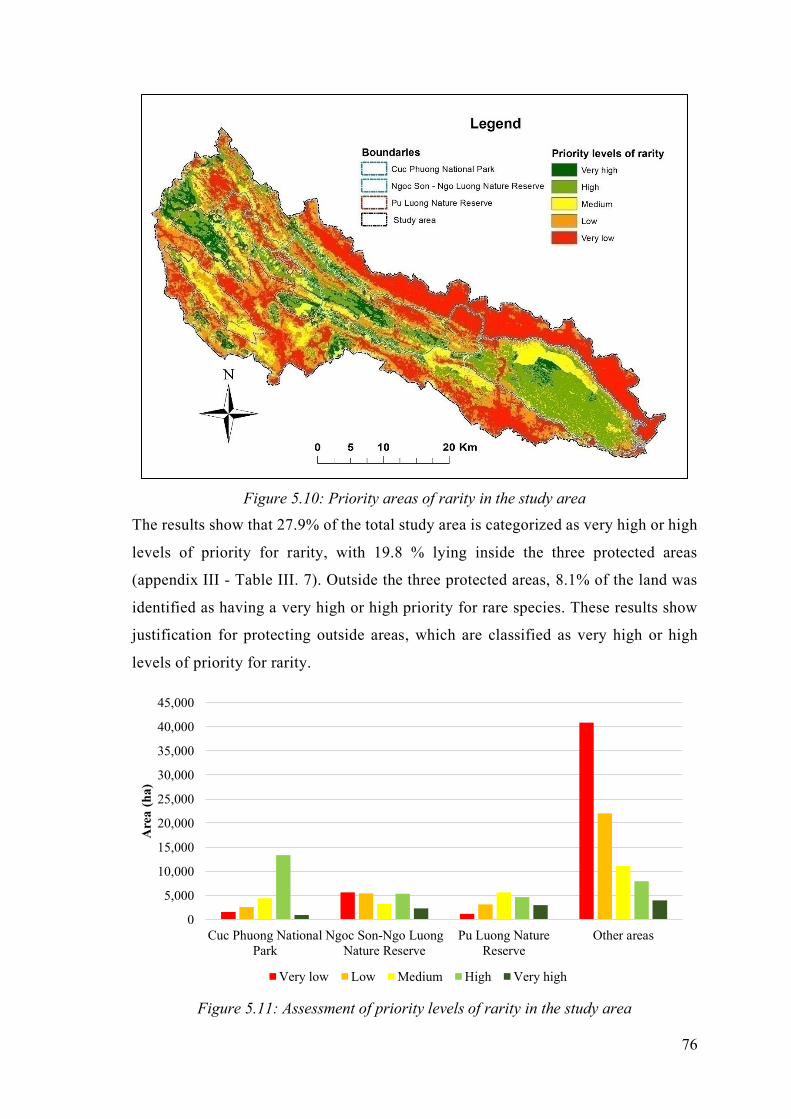
76
Figure 5.10: Priority areas of rarity in the study area
The results show that 27.9% of the total study area is categorized as very high or high
levels of priority for rarity, with 19.8 % lying inside the three protected areas
(appendix III - Table III. 7). Outside the three protected areas, 8.1% of the land was
identified as having a very high or high priority for rare species. These results show
justification for protecting outside areas, which are classified as very high or high
levels of priority for rarity.
Figure 5.11: Assessment of priority levels of rarity in the study area
0
5,000
10,000
15,000
20,000
25,000
30,000
35,000
40,000
45,000
Cuc Phuong National
Park
Ngoc Son-Ngo Luong
Nature Reserve
Pu Luong Nature
Reserve
Other areas
Are
a (
ha)
Very low Low Medium High Very high

77
We also estimated the area at very high and high levels of priority based on rarity criteria
for each protected area. Our findings have indicated that the proportion of areas at very
high and high priority in CPNP, PLNR, NSNLNR are 62.6%, 43.2%, and 34.9%,
respectively (Figure 5.11).
5.1.2. Ecosystem
5.1.2.1. Location
Previous studies show that the highest level of biodiversity in Vietnam was found in three
mountainous regions, including the north-eastern area, Hoang Lien Range, and Truong
Son Range (Pu Luong Nature Reserves is located in the northern Truong Son range)
(Averyanov et al., 2003; Sterling & Hurley, 2005). The Annamites, karst limestone
formations, and the Hoang Lien Mountains are considered as significant ecoregions for
many endemic species (Carew-Reid et al., 2011).
Karst ecosystem is one of the prioritized ecosystems for biodiversity conservation due to
its structure and sensitivity (Furey & Infield, 2005; Vermeulen & Whitten, 1999). The
karst areas are a sensitive ecosystem containing several endemic species. It will be
complicated to restore the species within the karst ecosystem if they are lost (Mickleburgh
et al., 2002; Mittermeier et al., 2007). Therefore, the higher priority was given to the areas
within limestone ecosystem.
Figure 5.12: Framework for mapping priority areas of location
Terrestrial ecoregions Karst
Spatial analysis
Priority levels
for different
locations
Mapping priority areas for location
Data conversion
(Projection and format)

78
Maps of terrestrial ecoregions and karst were used as input data to create the map of
priority areas for our research. The original data were converted into the common
projection type and format before using the spatial analysis method to define priority areas
for biodiversity conservation (Figure 5.12).
Figure 5.13: Terrain regions in Vietnam
Figure 5.14: Terrestrial ecoregions in Vietnam
Vietnam is divided into eight terrain regions, including Northeast, Northwest, Red River
Delta, North Central Coast, Sound Central Coast, Central Highlands, Southeast, and
Mekong River Delta (Figure 5.13). The terrain regions were defined by the different
characteristics of topography as well as regional climates. They meant as administrative
boundaries. Therefore, it is necessary to obtain a precise map of terrestrial ecoregions
for the study area. The terrestrial ecoregions map (Figure 5.14) based on WWF’s
ecoregions was downloaded from the Nature Conservancy (http://maps.tnc.org). It is a
website developed by the Nature Conservancy’s North American Region science team
in partnership with the Technology and Information System group.

79
a. Karst limestone regions
b. Terrestrial ecoregions
Figure 5.15: Karst limestone regions and terrestrial ecoregions in the study area
The identification of priority areas regarding location criterion is based on WWF’s ecoregions
and karst limestone formations in the study area. To synchronize the priority levels of
location with the other criteria for synthesizing all criteria, the weights for different
locations were suggested in Table 5.4. Karst regions in the study area were extracted from
the established maps, such as topography and forest statistic maps. The overlay analysis
method was used to process two data layers, including terrestrial ecoregions and karst
regions (Figure 5.15).
According to terrestrial ecoregions maps from the World Wide Fund for Nature (WWF),
Vietnam includes 14 ecoregions with different biodiversity levels. In Pu Luong Cuc
Phuong, there are two typical ecoregions, namely Northern Indochina subtropical
forests and Northern lowland rain forests. Many previous studies have shown that
northern Indochina subtropical forests have a high level of biodiversity (Averyanov et
al., 2003; Sterling & Hurley, 2005).
Table 5.4: Proposed weights for different locations in the study area
N0 Category Priority levels
1 Northern Indochina subtropical forests + karst limestone
formations 4
2 Northern Indochina subtropical forests 2
3 Karst limestone formations 2
4 Others 0

80
Besides, the limestone ecosystem is one of the priority ecosystems for biodiversity
conservation due to its structure, biodiversity, and sensitivity (Furey & Infield, 2005;
Vermeulen & Whitten, 1999). Therefore, we suggested the priority levels of different
locations in the study site (Table 5.4).
Based on the suggested priority levels for locations, we established a distribution map of
priority areas of location for biodiversity conservation in the study area (Figure 5.16).
There are three levels of priority for location criterion, including high, medium, and low.
It is shown that limestone regions within the study area are categorized as a high priority.
Areas of low priority are found in the eastern part of the study area, which is settled by
local communities and used for agricultural cultivation.
Figure 5.16: Priority areas of location in the study area
Then, area statistics for priority levels for location criterion are presented in appendix
III - Table III. 8. The results have shown that 4.2% of the total study area is classified
as a high priority in CPNP. Areas at high priority in NSNLNR and PLNR are 7.5%
and 6.5%, respectively. The areas of high priority based on location criterion for each
protected area were also estimated. The findings have indicated that the areas of high
priority for CPNP, NSNLNR, and PLNR account for 27.4%, 50.5%, and 55%,
respectively (Figure 5.17).

81
Figure 5.17: Assessment of priority levels of location in the study area
In comparison with the two nature reserves, CPNP has a low proportion of areas of high
priority because CPNP is located in the transitional region between Northern Indochina
subtropical forests and Northern lowland rain forests. Also, 14.7% of the total area of
high priority is distributed outside the three existing protected areas. It suggests a need
for establishing other priority areas for biodiversity conservation in the study area.
5.1.2.2. Topography
A negative relationship has been found in many ecosystem regions between elevation and
diversity of species (Benayas, 1995; Moore, 2008; J G Pausas, 1994; Stevens, 1992).
Uplands of deciduous forests and lowland of tropical forests provide significant habitat
for many threatened animals and have very high plant diversity, respectively. The areas
of the evergreen forest below 800-1000m average sea level (asl) are short dry season
regions with high rainfall, which are suitable for maintaining the highest diversity of tree
species (Carew-Reid et al., 2011).
A significant positive correlation is recognized between altitudinal distribution and forest
cover. The forest loss has happened extensively at lower elevations much more so than at
higher elevations (Tordoff, 2003). It leads to a significant reduction of the habitat in the
lowland forest below 300m asl. It is because the large areas have been narrowed down by
the overexploitation caused by human activities. Therefore, it is necessary to retain and
preserve the lowland forest below 300m (Tordoff, 2003).
0
10,000
20,000
30,000
40,000
50,000
60,000
Cuc Phuong National
Park
Ngoc Son - Ngo
Luong Nature Reserve
Pu Luong Nature
Reserve
Other areas
Are
a (
ha)
Low Medium High

82
Figure 5.18. Framework for mapping priority areas of topography
Regarding the topography criterion, the workflow for mapping priority areas for
biodiversity conservation consists of two periods (1) identifying priority thresholds and (2)
establishing a map for topography criterion. Slope and altitude are two main elements of
topographical assessment in our research. They were interpolated through Digital Elevation
Model data using steps of 10 degrees of slope and 100 meters of altitude. The temporal and
spatial analyses were applied for topographical data and land use – land cover in 1986,
1998, 2007, and 2017 to monitor, assess, and find out the thresholds of topography in the
study area, which are essential for biodiversity conservation (Figure 5.18).
DEM 2011
Slope (100) Altitude (100m)
LULC
- 1986
- 1998
- 2007
- 2017
Time series
analysis Spatial
analysis
Priority thresholds of slope and altitude
Overlay analysis
Jenks Natural Breaks
Mapping priority areas for topography

83
Figure 5.19:100-slope map Figure 5.20:100m-altitude map
The thresholds were used to classify three levels for both slope and altitude. Then they
were overlaid together to analyze and reclassify the whole topographical element. Jenks
Natural Breaks method established a map of priority areas of topography for
biodiversity conservation with five levels of priority (very low, low, medium, high, and
very high). The LULC maps in 1986, 1998, 2007, and 2017 were overlaid on the 100-slope
map and 100m-altitude map to define the priority areas of topography for biodiversity
conservation. The DEM image, acquired on 17 October 2011 by Aster sensor, is used as a
fundamental basis for extracting the slope and altitude data. Then they were overlaid on the
land use - land cover maps from 1986, 1998, 2007, and 2017 to identify how levels of slope
and altitude influence change to the area of forest in the study site. The data of slope in each
100 step and altitude each 100m were estimated by DEM image acquired. They are shown
as in Figure 5.19 and Figure 5.20.
Figure 5.21: Change in forest areas at different slopes from 1986 to 2017
0
5,000
10,000
15,000
20,000
25,000
30,000
10 20 30 40 50 60 70 80 90
Are
a (h
a)
Slope (0)
1986
1998
2007
2017

84
Appendix III - Table III. 5 shows that the forest area of the study site changed significantly
from 1987 to 2017. The establishment of Pu Luong Nature Reserve in 1999 and Ngoc
Son Ngo Luong Nature Reserve in 2004 are the main promotion to rocket up the forest
area in the period (2007 to 2017). The forest cover decreased sharply from 1986 to 1998
and slightly from 1998 to 2007 in slope and altitude under 30 degrees (Figure 5.19) and
500 m (Figure 5.20), respectively.
The steady decline of forest area is found on the slope lower than 300 from 1986 to 1998,
with thousands of hectares of forest loss. The areas on the slope (300–500) were also
deforested significantly from 1998 to 2007 (Figure 5.21). While forest areas covering on
the altitude lower than 500 m were felled/cleared from 1986 to 2007, with the majority
being at an elevation lower than 200 m (Figure 5.22), the reversal of this situation can be
found beginning in 2007 when a large forest area has been planted and restored (Appendix
III - Table III. 5). It was due to improved biodiversity protection in the Pu Luong and
Ngoc Son – Ngo Luong Nature Reserves, which were established in 1999 and 2004,
respectively. Therefore, topographic information is an essential aspect of identifying
vulnerability to human activities, which historically have harmed lowland slopes of a low
gradient.
Figure 5.22: Change in forest areas at different altitudes from 1986 to 2017
The thresholds were used to establish the priority levels of slope and altitude for
biodiversity conservation, as presented in Table 5.5. The synthesis from priority areas of
slope and altitude helped to gain the results of priority areas of topography for biodiversity
conservation in the study area.
0
2,000
4,000
6,000
8,000
10,000
12,000
14,000
16,000
100
200
300
400
500
600
700
800
900
1,0
00
1,1
00
1,2
00
1,3
00
1,4
00
1,5
00
1,6
00
1,7
00
Are
a (
ha)
Altitude (m)
1986
1998
2007
2017

85
Table 5.5. Priority levels of slope and altitude for biodiversity conservation
N0 Slope zones (0) Priority levels N0 Altitude zones (m) Priority levels
1 0 - 20 2 1 0 - 200 2
2 20 - 30 1 2 200 - 500 1
3 > 30 0 3 > 500 0
Based on our analysis of forest area changes in 4 years: 1986, 1998, 2007, and 2017 in
different topographies, priority levels were suggested for biodiversity conservation in
topography (Table 5.5). This study focused on two main elements of topography,
including slope and altitude. Concerning the slope of the topography, there are two
priority levels determined for biodiversity conservation, i.e., 0 – 200 and 20 - 300 since
this is where forest area changes are recorded at the highest level. When it comes to the
altitude, two priority levels for biodiversity conservation are from 0 to 200 m and from
200 m to 500m.
Figure 5.23: Priority areas of slope
Figure 5.24: Priority areas of altitude
Two maps were established on priority levels for biodiversity conservation regarding
slope and altitude in the study area, as shown in Figure 5.23, and Figure 5.24, respectively.
Then these two maps were overlaid to identify priority areas and their levels for
topography criterion (Figure 5.25). The results have shown five priority levels for
topography from very low, low, medium, high, to very high.
The areas at different priority levels were calculated in three protected areas and outside
areas. The results have shown that 7% of the total area is classified as very high or high
priority levels in CPNP. 2.4% and 0.7% of the total area is determined as very high or
high priority levels in NSNLNR and PLNR, respectively (Appendix III - Table III. 9).

86
Figure 5.25. Priority areas of topography in the study areas
The areas at different priority levels for each protected area were also measured. Of the
three protected areas, CPNP has the highest area classified at very high or high priority
levels (45%). The area at very high or high priority levels is 16.5% and 6% for NSNLNR,
and PLNR, respectively (Figure 5.26).
Figure 5.26: Assessment of priority levels of topography in the study area
0
5,000
10,000
15,000
20,000
25,000
30,000
35,000
40,000
45,000
50,000
Cuc Phuong National
Park
Ngoc Son - Ngo
Luong Nature Reserve
Pu Luong Nature
Reserve
Other areas
Are
a (
ha)
Very low Low Medium High Very high

87
5.1.2.3. Climate
Vietnam has a high diversity of species due to its complex geology and diverse climate.
Many systems of hilly and mountainous topography create localized temperature and
humidity at different elevations as well as landscape levels, which affects the
distribution of species (Sterling & Hurley, 2005). Until 2015, the data from 150 hydro-
meteorological stations (Figure 5.27) of the National Centre for Hydro-meteorological
Forecasting (NCHMF) were collected to assess the changes in weather in Vietnam over
a long period. In the north of Vietnam exists four seasons per year, namely winter (from
December to February), spring (from March to May), summer (from June to August),
and autumn (from September to November). The lowest and highest values of
temperature are found each year in January and July, respectively (MONRE, 2011;
MONRE, 2016).
Figure 5.27: Positions of 60 hydro-meteorological stations in Vietnam
Many studies have indicated a positive relationship between the variety of plants and
temperature as well as water resources (Lobo et al., 2001; Juli G Pausas et al., 2003).
Temperature and precipitation are the key climatic conditions relating to forest
production (Clark et al.,2003; Doughty & Goulden, 2009; Feeley et al.,2007) as well as

88
the distribution of species (Austin et al., 1996; Currie & Paquin, 1987; Field et al., 2009;
Hill, 2005; Knight et al., 1982; Miller, 1994; Morrison et al., 2006; Parmesan et
al.,2000; Pausas & Carreras, 1994; Woodward & Williams, 1987). The ranges of
temperature determine the limitations for plants and animals to survive (Moore, 2008).
The tolerance of tropical trees to freezing temperatures is not so high, and many plants
cannot survive in a temperature lower than 100C (Moore, 2008; Parmesan et al., 2000;
Frank, 1987). The ability of photosynthesis of tropical plants decreases when the
temperature is above the range of 26 to 340C (Graham et al., 2003; Ishida et al., 1999;
Keller & Lerdau, 1999; Koch et al., 1994; Lerdau & Throop, 1999; Tribuzy, 2005).
Protection was mentioned as an important function of the forest to cope with many
different hazards (Führer, 2000). The forest helps to retain the climate balance as well
as the atmosphere at the global level(Moore, 2008). Several studies have shown the
potential responses of tropical forests to adjusting temperatures, drought, and other
extreme factors (Deborah A. Clark, 2004).
The data from 13 hydro-meteorological stations in three provinces (Hoa Binh, Ninh
Binh, Thanh Hoa), collected in 2015 were used to determine monthly average
temperature, highest monthly average temperature, lowest monthly average
temperature, highest absolute temperature in a month, lowest absolute temperature in a
month, daily amplitude of monthly average temperature.
Figure 5.28: Average Monthly Temperature and Rainfall in Vietnam
(Source: The World Bank Group)
Figure 5.29 shows that changes in monthly temperature in the three provinces are similar.
The lowest and highest temperature are in from December to January and from June to
July, respectively. The same results were found from the statistic of the World Bank
Group (Figure 5.28).

89
a. Lowest average monthly temperature b. Highest average monthly temperature
c. Lowest absolute temperature month d. Highest absolute temperature month
e. Monthly average temperature f. Daily amplitude of average monthly
temperature
Figure 5.29: Monthly change of temperature in three provinces
Temperature and rainfall are two main aspects of climate that impact biodiversity
conservation in Vietnam. The change of these elements can cause the decline of
biodiversity and the disappearance of endangered species. In this study, we focused on
0
5
10
15
20
25
30
1 2 3 4 5 6 7 8 9 10 11 12
Tem
per
atu
re (
0C
)
Hoa Binh Ninh Binh Thanh Hoa
0
5
10
15
20
25
30
1 2 3 4 5 6 7 8 9 10 11 12
Tem
per
atu
re (
0C
)
Hoa Binh Ninh Binh Thanh Hoa
0
5
10
15
20
25
30
1 2 3 4 5 6 7 8 9 10 11 12
Tem
per
atu
re (
0C
)
Hoa Binh Ninh Binh Thanh Hoa
0
5
10
15
20
25
30
1 2 3 4 5 6 7 8 9 10 11 12
Tem
per
atu
re (
0C
)
Hoa Binh Ninh Binh Thanh Hoa
0
5
10
15
20
25
30
1 2 3 4 5 6 7 8 9 10 11 12
Tem
per
atu
re (
0C
)
Hoa Binh Ninh Binh Thanh Hoa
0
5
10
15
20
25
30
1 2 3 4 5 6 7 8 9 10 11 12
Tem
per
atu
re (
0C
)
Hoa Binh Ninh Binh Thanh Hoa

90
the element of temperature since the change of temperature may largely influence the
distribution of species. We did not have enough data to calculate the changes in rainfall.
Figure 5.30: Framework for mapping priority areas of climate
Landsat 8 images acquired in December 2013 and July 2015 were collected to represent two
specific periods of temperature in Vietnam as well as the study area. The land surface
temperature of the study site in July and December was calculated through three steps,
Landsat 8
02.12.2013
Landsat 8
01.07.2015
Top of Atmosphere
spectral radiance
Top of Atmosphere
Brightness Temperature
Estimation of Land
Surface Temperature
Land Surface Temperature
02.12.2013
Land Surface Temperature
01.07.2015
Jenks Natural Breaks
Spatial analysis Levels of stable
temperature
Mapping priority areas for
climate

91
including top of atmosphere spectral radiance, top of atmosphere brightness temperature, and
estimation of land surface temperature as described in Figure 5.30. The data of land surface
temperature, including the lowest period and the highest period, were compared through
spatial analysis method and classified by Jenks Natural Breaks to establish the map of priority
areas for climate criterion in the study area.
Table 5.6: Satellite images used to define annual temperature change
No Acquisition
date Path/ Row
Cloud cover
(%)
Satellite
image
1 02-12-2013 127/46 4.4 Landsat 8 OLI
2 01-07-2015 127/ 46 4.3 Landsat 8 OLI
Band 10 of Landsat 8 images was used to determine correctly and clearly the lowest and
highest temperature of the study area. Two satellite images acquired in December 2013
and July 2015 were applied (Table 5.6).
Figure 5.31: Land Surface Temperature
in December 2013
Figure 5.32: Land Surface Temperature
in July 2015
Landsat 8 thermal bands were used to calculate the Land Surface Temperature in the
study area. Land Surface Temperature was calculated through Landsat 8 images
acquired in December 2013 and July 2015, which represent two seasons in a year with
the lowest and highest temperature in the study area, as described in Figure 5.31, Figure
5.32 respectively. The temperature data of Landsat 8 images in December 2013 and July
2015 were re-calculated based on the acquired times and the daily temperature
fluctuations of corresponding hydro-meteorological stations. The results are shown in
Figure 5.33 and Figure 5.34.

92
Figure 5.33: Land Surface Temperature
recalculated in December 2013
Figure 5.34: Land Surface Temperature
recalculated in July 2015
The results have shown that the lowest temperatures in the study area could be observed
in December (Figure 5.33), and the highest temperatures could be found in July (Figure
5.34). Maps were created based on surface temperature in these two months and then
overlaid them to show the fluctuation of temperature in the study area. Table 5.7 shows
the five levels of temperature changes in the study area that range from 80C (very low) to
approximately 260C (very high).
Table 5.7: Priority levels of annual temperature change
N0
Categories of annual temperature
fluctuation (0C) Priority levels Weights
1 8.01 - 14.00 Very high 4
2 14.01 - 15.33 High 3
3 15.34 - 16.65 Medium 2
4 16.66 - 18.32 Low 1
5 18.33 - 25.78 Very low 0
The temperature has a relationship with biodiversity of a specific area since the stability of
temperature provides suitable conditions for many species, and these areas often have high
biodiversity. Based on maps on temperature changes, we applied Jenks Natural Breaks to
categorize five levels of stability of annual temperature, including very high, high, medium,
low, and very low (Table 5.7) and present these levels in the study area (Figure 5.35).

93
Figure 5.35: Stable levels of temperature in the study area
Appendix III - Table III. 10 shows the areas with the stability levels of temperature in the
study area. 47.2% of the total area has very high or high stability level of temperature.
The stability levels were also shown for each protected area. Of these, the proportion of
area at very high or high stability level of temperature is 7.9%, 4.7%, and 7.4% for CPNP,
NSNLNR, and PLNR, respectively (Figure 5.36).
Figure 5.36: Assessment of priority levels of climate in the study area
0
5,000
10,000
15,000
20,000
25,000
30,000
Cuc Phuong National
Park
Ngoc Son - Ngo
Luong Nature Reserve
Pu Luong Nature
Reserve
Other areas
Are
a (
ha)
Very low Low Medium High Very high

94
5.1.2.4. Hydrology
Rivers and streams with their many tributaries are an indispensable component of most
low land forests. They are considered as the habitat for numerous forest animals and fish
(Moore, 2008; Williams et al., 2004). Streams and springs do not only provide habitats to
a variety of species and supply food to neighboring ecosystems (Meyer et al., 2007). They
are also an important source to disperse seeds, which help to enrich the number and
distribution of plant species (Moore, 2008). The vital role of every river and wetland
ecosystem is recognized broadly to conserve native biodiversity (Lytle & Poff, 2004; Poff
et al., 1997; Postel & Richter, 2012).
According to the decree of the Vietnam Government on 23rd September 2003 on the
conservation and sustainable development of submerged areas, the forest areas that help
to maintain and protect the water resource, as well as the biological balance, are priority
regions for conservation (VNG, 2003b). Forest in tropical regions plays a vital role in the
water cycle by retaining water resources and intercepting rain and thus reducing the risk
of erosion and floods (Moore, 2008). The relationships between hydrology and
biodiversity of the plant-based on the water demand have been shown clearly from many
studies over the past few decades (Feddes & Dam, 2004). Therefore, the loss of forest
cover has threatened many fishes, which could lead to their extinction (Dudgeon, 2000).
Figure 5.37: Taxonomic group of threatened species in Vietnam
Source: (Ban et al., 2007; IUCN, 2013; Thanh et al., 2007)

95
Additionally, hydrological areas play an essential role as the vital habitat of many endangered
species, including fish and amphibians. Figure 5.37 shows the number of threatened species in
Vietnam by IUCN and Vietnam Red Data Book 45 amphibian and 82 fish species, and 13
amphibian and 89 fish species, respectively. Vietnam Red Data Book in 2007 of animals has
shown much freshwater fish (37 species), and amphibians (13 species) are critically
endangered, endangered, or vulnerable species (Thanh et al., 2007).
A comparison of biodiversity in rivers, streams, ditches, and ponds in a region of Southern
England showed the contrast with national protection strategies that merely concentrate
on large waterbodies (Williams et al., 2004). The number of species recorded from the
samples showed the decreasing trend of biodiversity at ponds, rivers, streams, and ditches,
respectively (Figure 5.38). The hydrological areas do not only impact the diversity of fish
and amphibians, but they also increase the number of terrestrial species.
Figure 5.38: Accumulation curves of species from the four waterbody types
Source: (Williams et al., 2004)
The maps of Hoa Binh, Ninh Binh, and Thanh Hoa provinces have been established on
two central meridians (1050 and 1060) (Vietnam projection). Thus, data conversion is the
first step in transforming the hydrological map in the three provinces into the selected
standard projection and format before they are combined and clipped by the boundary of
the study area (Figure 5.39). Sentinel-2 image acquired on the 9th of April 2018 is used
as the data source to interpolate visually and obtain the map of hydrology in 2018.
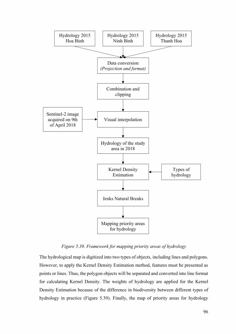
96
Figure 5.39. Framework for mapping priority areas of hydrology
The hydrological map is digitized into two types of objects, including lines and polygons.
However, to apply the Kernel Density Estimation method, features must be presented as
points or lines. Thus, the polygon objects will be separated and converted into line format
for calculating Kernel Density. The weights of hydrology are applied for the Kernel
Density Estimation because of the difference in biodiversity between different types of
hydrology in practice (Figure 5.39). Finally, the map of priority areas for hydrology
Hydrology 2015
Hoa Binh
Hydrology 2015
Ninh Binh
Hydrology 2015
Thanh Hoa
Data conversion
(Projection and format)
Combination and
clipping
Hydrology of the study
area in 2018
Visual interpolation
Sentinel-2 image
acquired on 9th
of April 2018
Kernel Density
Estimation
Jenks Natural Breaks
Mapping priority areas
for hydrology
Types of
hydrology

97
criterion is divided into five groups with different levels ranging from very low to very
high using Jenks Natural Breaks classification. The hydrological map of the study area is
collected from the layers of rivers and streams on the published maps for Thanh Hoa, Ninh
Binh, and Hoa Binh provinces (Figure 5.40).
a- HoaBinh province
b- Thanh Hoa province
c- Ninh Binh province
Figure 5.40. Hydrological system in Hoa Binh, Thanh Hoa, and Ninh Binh provinces
The maps of three provinces were established based on the Vietnam projection called
VN2000. However, the VN2000 projections used in Thanh Hoa, Ninh Binh, Hoa Binh
provinces are different and derived from divergence of positions and area. Therefore,
there is a need to use different methods to convert the coordinate system from VN2000
to UTM (WGS84) for each province to combine and clip the hydrological map for the
study area. A plugin for QGIS of converting coordinates system VN2000 developed by
Green Field Consulting limited company was downloaded and applied in this case. The
data of the hydrological system were synthesized and presented as in Figure 5.41.

98
Figure 5.41: The hydrological system combined of three provinces
The layer of hydrology in the study area, combined and clipped from the published maps
in Thanh Hoa, Ninh Binh, Hoa Binh provinces, was edited and updated by overlaying
with the Sentinel-2 image acquired on the 9th of April 2018. According to Williams et
al., 2004, the influence of waterbodies on biodiversity can be divided into two groups.
The first group with rivers, lakes, and ponds are weighted higher than the second,
including streams, springs, and ditches. The weights of the two groups were considered
and illustrated, as shown in Table 5.8.
Table 5.8. Classification of hydrology in the study area
N0 Category Weight
1 Rivers, lakes, and ponds 3
2 Streams, springs, and ditch 1
Many previous studies have shown the influences of hydrology (i.g. river, stream, lake,
pond) on the level of biodiversity (Moore, 2008; Williams et al., 2004). The level of
biodiversity is higher in the areas which have a high density of hydrological elements
(Lytle & Poff, 2004; Poff et al., 1997; Postel & Richter, 2012).
It has shown that the areas with a high density of hydrological elements are classified
as priority areas for biodiversity conservation. Based on the collected data, we
identified and divided the hydrological system into two categories with priority levels,
as shown in Table 5.8.

99
Table 5.9: Classification of priority levels for hydrology in the study area
N0 Thresholds for priority levels of
hydrology Priority levels Weights
1 ≥ 6.79 Very high 4
2 4.71 - 6.78 High 3
3 2.88 - 4.70 Medium 2
4 1.20 - 2.87 Low 1
5 ≤ 1.19 Very low 0
We applied Kernel Density Estimation to estimate the influence levels of the hydrology
system in the study area. According to the method of Jens Natural Breaks, there are five
levels of priority based on the criterion for hydrology (Table 5.9). Then, we established
maps on priority levels of hydrological density in the study area (Figure 5.42).
Figure 5.42: Priority areas for hydrology in the study area
The results calculated based on the priority areas of hydrology for biodiversity
conservation in the study area show that most areas of high or very high priority levels
of hydrology are outside of three protected areas (Figure 5.42). The area accounts for

100
16.3 % of the study area, with 14.3 % being outside of the protected areas. No priority
areas regarding hydrology exist within the PLNR (Figure 5.43).
Figure 5.43: Assessment of priority levels for hydrology in the study area
The areas of high or very high priority belonging to the protected areas are only 2 % of
the total area of the study area. It accounts for 8.1 % and 5.4 % of the areas of CPNP, and
NSNLNR, respectively (Appendix III - Table III. 11).
5.1.2.5. Forest types
The ecosystem of tropical forests is known as a biodiversity hotspot due to its complex
structure of valleys, mountains, wetlands, and rivers (Moore, 2008). Previous studies have
shown that tropical forests contain many vegetation layers and various plant stratifications
that provide food and appropriate habitats to many species (Coops et al., 2004; John et al.,
2008; Luoto et al., 2004; Waring et al., 2006).
Besides, the Annamites, limestone formations, and Hoang Lien mountains are
significant ecoregions for many endemic species (Carew-Reid et al., 2011). Therefore,
natural forests distributed on limestone mountains are considered as a high priority for
biodiversity conservation since they support the diversity of species and endemism. The
weights for priority level of forest types were calculated based on experts interview during
fieldwork in Vietnam in 2017.
The forest statistic maps of Hoa Binh, Ninh Binh, and Thanh Hoa provinces in 2015 are
primary input data of the framework (Figure 5.44). The data on forest types from the maps
were separated before they were converted to preferred projection and format. Then the
0
5,000
10,000
15,000
20,000
25,000
30,000
35,000
Cuc Phuong NationalPark
Ngoc Son - Ngo LuongNature Reserve
Pu Luong NatureReserve
Other areas
Are
a (h
a)
Very low Low Medium High Very high

101
maps of forest types for the three provinces were combined into one layer, which was
clipped using the boundary of the study area.
Figure 5.44. Framework for mapping priority areas regarding forest types
To understand the changes in forest types from 2015 to now, the forest map of the
study area was updated using Landsat 8 image acquired on 4th June 2017 and the
information from the field survey in 2017. An assessment of priority levels of forest
types for biodiversity conservation was performed to determine the weight of each
forest type. Finally, the spatial analysis was used as a tool to synthesize the data for
establishing the map of priority areas regarding forest type criterion for biodiversity
conservation (Figure 5.44).
Forest statistics 2015
Hoa Binh
Forest statistics 2015
Ninh Binh Forest statistics 2015
Thanh Hoa
Data conversion
(Projection and format)
Combination and
clipping
Forest map 2017
Updating and editing Landsat 8 image acquired on 4th
June 2017
Spatial analysis
Mapping priority areas
for forest types
Field survey in
2017
Assessment of
priority levels
for forest types
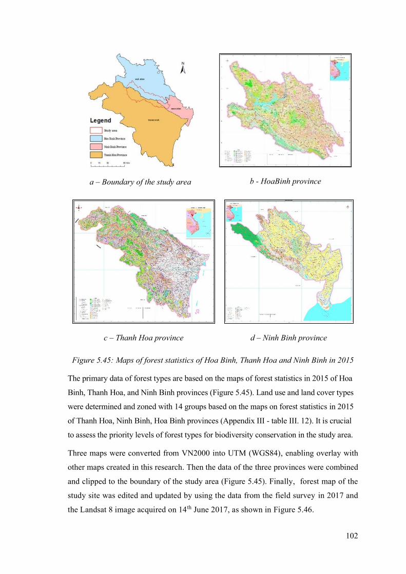
102
a – Boundary of the study area
b - HoaBinh province
c – Thanh Hoa province
d – Ninh Binh province
Figure 5.45: Maps of forest statistics of Hoa Binh, Thanh Hoa and Ninh Binh in 2015
The primary data of forest types are based on the maps of forest statistics in 2015 of Hoa
Binh, Thanh Hoa, and Ninh Binh provinces (Figure 5.45). Land use and land cover types
were determined and zoned with 14 groups based on the maps on forest statistics in 2015
of Thanh Hoa, Ninh Binh, Hoa Binh provinces (Appendix III - table III. 12). It is crucial
to assess the priority levels of forest types for biodiversity conservation in the study area.
Three maps were converted from VN2000 into UTM (WGS84), enabling overlay with
other maps created in this research. Then the data of the three provinces were combined
and clipped to the boundary of the study area (Figure 5.45). Finally, forest map of the
study site was edited and updated by using the data from the field survey in 2017 and
the Landsat 8 image acquired on 14th June 2017, as shown in Figure 5.46.

103
Figure 5.46: Forest map updated by Landsat 8 image in 2017
Figure 5.47: Priority areas regarding forest types in the study area
Forest statistic maps of three provinces have been collected to establish maps on forest
types in the study area. In forest statistic maps, forest types are classified based on the

104
Circular 34/2009/TT-BNNPTNT released by the Vietnamese Ministry of Agriculture and
Rural Development. The maps of forest types were updated using Landsat 8 images in
2017 to increase the accuracy and reliability of these maps. There are 32 types of different
land use – land cover listed, of which 10 are types of forest (Appendix III - Table III. 12).
Based on the maps of forest types, we classified and evaluated priority areas for
biodiversity, as presented in table 27. There are five priority levels in forest types,
including very low, low, medium, high, and very high. A map was then created to show
priority areas for biodiversity conservation based on forest type criterion (Figure 5.47).
Figure 5.48. Assessment of priority levels for forest types in the study area
The areas of different priority levels have been calculated based on forest type criterion
(Appendix III - Table III. 13). Our results show that 14.3% of the total area is classified
as very high or high priority areas with the proportion of CPNP, NSNLNR, and PLNR,
accounting for 9%, 0.1%, and 4% respectively. The rest (1%) is found outside the three
protected areas. We also calculated the areas at very high or high priority levels for each
protected area. It showed that very high or high priority areas accounted for 59%, 0.4%,
and 34% in CPNP, NSNLNR, PLNR, respectively (Figure 5.48).
5.1.3. Nature
Over the last decades, the earth has experienced many considerable changes in the global
climate. These changes have caused a variety of negative impacts such as the sea level
0
5,000
10,000
15,000
20,000
25,000
30,000
35,000
40,000
45,000
Cuc Phuong National
Park
Ngoc Son - Ngo
Luong Nature Reserve
Pu Luong Nature
Reserve
Other areas
Are
a (
ha)
Very low Low Medium High Very high

105
rising, extreme changes in temperature, unpredictable fluctuations of precipitation and its
distribution, and many other natural disasters (Moore, 2008). The human being has been
facing the most complex challenges named climate change (Nguyen & Tenhunen, 2013).
Several studies calculated and predicted the global modelling scenarios after 2050, which
show the principal threats to biodiversity from climate change (IPCC et al., 2007;
Strengers et al., 2004; Watson et al., 2005).
Global warming is the leading cause of climate change, which in turn influences the
entire ecosystem (Kudo, 2016). Modelling analyses of climate change showed that a
small change in temperature (2°C) and precipitation (20%) could have a profound
influence on forest ecosystems (C. Miller & Urban, 1999). The changes in temperature
or lack of vital resources can cause a significant decline in species (Moore, 2008). The
World Bank considers that climate change will bring higher temperatures, extreme
changes in rainfall patterns, sea levels rising, and more frequent natural disasters
(MONRE, 2016).
Figure 5.49: The changes in annual
temperature (0C) from 1958 to 2014
Source: (MONRE, 2016)
Figure 5.50: The changes in annual
rainfall (%) from 1958 to 2014
Source: (MNRE, 2016)
Vietnam is considered as a country that has suffered significantly from the negative
impacts of climate change (MONRE, 2016). To mitigate the impacts of climate change,
five climate models were used to calculate and establish the climate change scenarios for

106
Vietnam including AGCM/MRI model of Japan, PRECIS model from the UK Met
Office, CCAM model from Australia, RegCM model from Italy, and clWRF model from
the United States (MONRE, 2016). To create the 2016 scenario of climate change (Figure
5.49, and Figure 5.50), data from 150 meteorological stations throughout Vietnam from
1986 to 2018 were collected.
The trend of climate change in Vietnam can be summarized as follows (MONRE, 2016):
- The temperature at the number of meteorological stations has increased quickly
in recent decades.
- The average amount of annual rainfall has fallen in the north and risen in the south
of Vietnam.
- The minimum and maximum temperatures recorded at the meteorological stations
have climbed.
- Drought appears more frequently in the dry season.
- The number of large storms has increased.
Vietnam, with a long 3200-kilometres coastline, frequently suffers from many storms (up
to 10 storms per year) from the East Sea. According to the Japan International
Cooperation Agency (2015), storms accounted for 52% of disasters in Vietnam, followed
by floods with 42% (Rylko et al., 2015).
Table 5.10. The risk levels of Natural disasters in Vietnam
High Risk Medium Risk Low Risk
Flood Hail rain/ tornado Earthquake
Typhoon Drought Accident (Technology)
Inundation Landslide Frost
Flash flood Damaging cold
Deforestation
Source: The World Bank
The classification of natural disasters in Vietnam was divided into three groups, including
high risk, medium risk, and low risk (Table 5.10). Flood, Typhoon, and Inundation are
considered the highest risks.
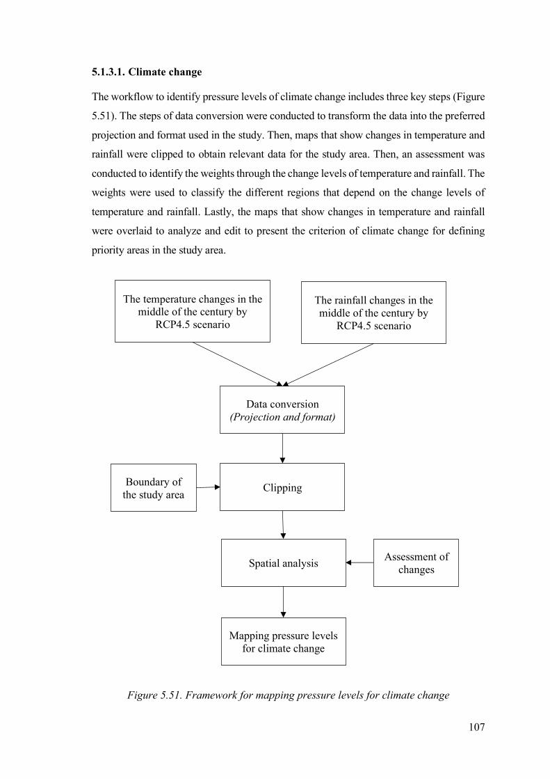
107
5.1.3.1. Climate change
The workflow to identify pressure levels of climate change includes three key steps (Figure
5.51). The steps of data conversion were conducted to transform the data into the preferred
projection and format used in the study. Then, maps that show changes in temperature and
rainfall were clipped to obtain relevant data for the study area. Then, an assessment was
conducted to identify the weights through the change levels of temperature and rainfall. The
weights were used to classify the different regions that depend on the change levels of
temperature and rainfall. Lastly, the maps that show changes in temperature and rainfall
were overlaid to analyze and edit to present the criterion of climate change for defining
priority areas in the study area.
Figure 5.51. Framework for mapping pressure levels for climate change
The temperature changes in the middle of the century by
RCP4.5 scenario
The rainfall changes in the
middle of the century by
RCP4.5 scenario
Data conversion
(Projection and format)
Clipping Boundary of
the study area
Spatial analysis Assessment of
changes
Mapping pressure levels
for climate change

108
a. The changes in annual temperature
(0C) created by RCP4.5 scenario
b. The changes in annual rainfall (%)
created by RCP4.5 scenario
Figure 5.52. Estimation of annual temperature and rainfall changes from 2045 to 2065
Source: (MONRE, 2016)
The data on the changes of temperature and rainfall in the middle of this century (2046 -
2065) by the medium-low of Representative Concentration Pathways (RCP 4.5 scenarios)
in 2016 were collected from the Ministry of Natural Resources and Environment
(MONRE) (Figure 5.52).
Table 5.11. Change levels of temperature and rainfall in the study area (2046 –2065)
Temperature (0C) Change levels of
temperature Rainfall (mm)
Change levels of
rainfall
1.96 Low 110.12 Low
2.23 Medium 118.28 Medium
2.44 High 122.58 High
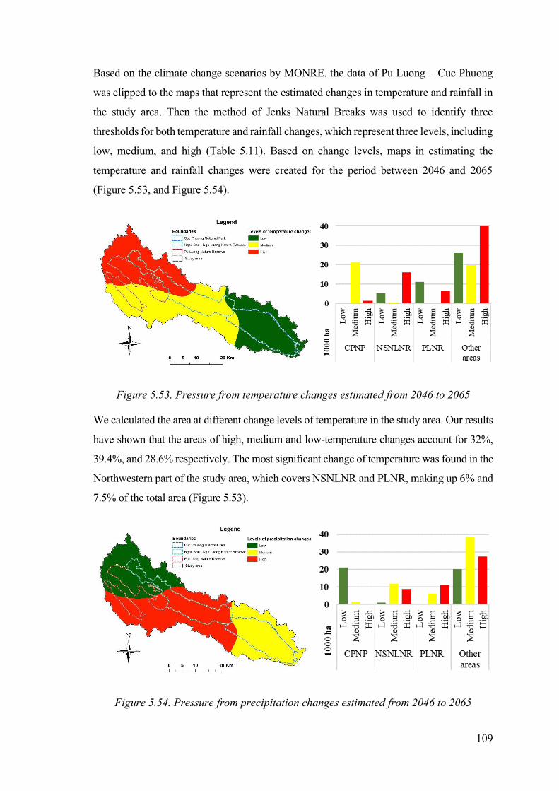
109
Based on the climate change scenarios by MONRE, the data of Pu Luong – Cuc Phuong
was clipped to the maps that represent the estimated changes in temperature and rainfall in
the study area. Then the method of Jenks Natural Breaks was used to identify three
thresholds for both temperature and rainfall changes, which represent three levels, including
low, medium, and high (Table 5.11). Based on change levels, maps in estimating the
temperature and rainfall changes were created for the period between 2046 and 2065
(Figure 5.53, and Figure 5.54).
Figure 5.53. Pressure from temperature changes estimated from 2046 to 2065
We calculated the area at different change levels of temperature in the study area. Our results
have shown that the areas of high, medium and low-temperature changes account for 32%,
39.4%, and 28.6% respectively. The most significant change of temperature was found in the
Northwestern part of the study area, which covers NSNLNR and PLNR, making up 6% and
7.5% of the total area (Figure 5.53).
Figure 5.54. Pressure from precipitation changes estimated from 2046 to 2065

110
The rainfall changes in the study area also presented at high, medium, and low levels,
making up 43.1%, 28.1% and 28.8% of the total area. It has predicted that the most
considerable change in rainfall would affect NSNLNR (10.9%) and a small proportion in
PLNR (4.3%) and CPNP (0.9%) (Figure 5.54).
Table 5.12. Classification of climate change through temperature and rainfall changes
Temperature Rainfall Climate change
High High Very high
High Medium High
Medium High
High Low
Medium Low High
Medium Medium
Medium Low
Low Low Medium
Low Low
In this study, the effects of climate change were predicted based on changes in
temperature and rainfall. Therefore, we overlaid the maps on temperature and rainfall
changes to show different levels of climate change in the study area (Table 5.12). There
are four levels of climate change, which include very high, high, medium, and low.
Figure 5.55. Predicted priority areas of climate changes in the study area (2046 - 2065)

111
Our results have predicted that climate change at high or very high levels would occur
mainly in NSNLNR (10.5%), and a small percentage in PLNR (4.3%) and CPNP (0.9%)
(Figure 5.55).
Figure 5.56. Assessment of pressure of climate change in the study area
We estimated the area at different levels regarding climate change in the study area, as
shown in appendix III - Table III. 14. Our results have indicated that the areas at very
high, high, medium, low levels of climate change account for 4.7%, 37.4%, 28.7%, and
29.2%, respectively. Of these, NSNLNR is predicted to hold a high proportion of area at
the very high or high-level impact of climate change (10.5%). PLNR and CPNP make up
4.3% and 0.9% of the total area (Figure 5.56).
5.1.3.2. Natural disasters
To assess the risks of natural disaster in the study area, disaster information was collected
across Vietnam. The locations of disasters were presented using points and their relative
attributes on the map. The points were grouped into risk levels before they were used to
calculate Kernel Density Estimation. Then the estimated maps were classified by the
Jenks Natural Breaks method to determine the five pressure levels on biodiversity
conservation arising from natural disasters (Figure 5.57).
Information on the natural disasters collected from the website of GLIDE
(http://www.glidenumber.net/) which lists the disaster types, and particular
characteristics such as date of occurrence, name of location, position (latitude, longitude),
as well as the source cited (Appendix III - Table III. 15). The website shows that 119
0
5,000
10,000
15,000
20,000
25,000
30,000
35,000
40,000
Cuc Phuong National
Park
Ngoc Son - Ngo
Luong Nature Reserve
Pu Luong Nature
Reserve
Other areas
Are
a (
ha)
Low Medium High Very high

112
natural disasters in Vietnam have been recorded during the period 1997 and 2018. The
types of natural disasters include tropical cyclones, floods, drought, landslide,
technology-related disaster, and local storms.
Figure 5.57. Framework for mapping pressure of natural disasters
The disasters were classified into three levels of risk based on categories of the World Bank
(Table 5.10) and were used as the weights in the Kernel Density Estimation. The positions
of the natural disasters were displayed as points on the map shown in Figure 5.58. To
evaluate the pressure of natural disasters in the study area, we applied Kernel Density
Estimation to the positions of natural disasters from 1997 to 2018 in Vietnam (Figure 5.59).
Information of natural disasters in
Vietnam from 1997 to 2018
Points of disasters
Kernel Density Estimation
Jenks Natural Breaks
Risk levels of
natural disasters
Mapping pressure of natural disasters

113
Figure 5.58. Locations of Natural Disasters in Vietnam from 1997 to 2018
The results have shown that natural disasters have little influence in the Pu Luong - Cuc
Phuong region. Since there was not much difference in pressure of the natural disasters
in the study area, and the influences of natural disasters were not used to define priority
areas for biodiversity conservation in this research.
Figure 5.59. The pressure of natural disasters in the study area (1997 - 2018)

114
5.1.4. Human
Human beings have been widely accepted as a significant element, indirectly influencing
biodiversity (B. Y. N. Dudley et al., 2006; Gordon et al., 2005; L. Joppa, 2012; L. N.
Joppa et al., 2009; J. Liu et al., 1999; Luck, 2007; Naughton-Treves et al., 2005; Nguyen
et al., 2013; Saunders et al., 1998; Sterling & Hurley, 2005). Among the many activities
of humans, urbanization is considered as an urgent issue that impacts directly on global
biodiversity due to its predicted expansion in the future (Seto et al., 2012). According to
the Vietnam Academy of Forest Sciences, human settlement is an important criterion to
assess and estimate the degradation of headwater-protected forests. The levels of impact
depending on the distance between human settlements and protected forest. Three levels
of influence (high, medium, and low) were identified based on three levels of distance
between human settlement and protected areas, including under 2 km, from 2 to 5 km,
and more than 5 km, respectively (http://vafs.gov.vn).
5.1.4.1. Distribution
The Land Use – Land Cover (LULC) maps in 2015 of Hoa Binh, Ninh Binh, and Thanh
Hoa provinces were used to create the LULC data in 2018 of the study area. The maps
were converted, combined, and clipped to the boundary of the study area before the data
were updated and edited through the Sentinel-2 image acquired on the 9th of April 2018
and the information collected in the field survey in 2017 (Figure 5.60).
To establish the maps on the pressure of population distribution to biodiversity
conservation, the information on settlements in the study area were separated by
applying Kernel Density Estimation with the weight for each settlement class. Then,
five levels of the pressure of the population distribution were identified by the Jenks
Natural Breaks classification (Figure 5.60).
The study area is located on the boundaries of nine districts of three provinces (Hoa Binh,
Ninh Binh, and Thanh Hoa). However, three communes of Trung Xuan, Trung Ha, and
Trung Thuong that are located in Quan Son district were added to analyze the impacts of
population distribution on biodiversity conservation. To acquire the maps on population
distribution, land use-land cover maps released in 2015 of the ten districts and the Sentinel-
2 image acquired on the 9th of April 2018 were used to update and edit the data on
settlement distribution within and around the study area (Figure 5.61).

115
Figure 5.60. Framework for mapping pressure of population distribution
LULC Map 2015
of Hoa Binh
LULC Map 2015
of Ninh Binh LULC Map 2015
of Thanh Hoa
Data conversion
(Projection and format)
Combination and clipping
Updating and editing Sentinel-2 image
acquired on 9th
of April 2018
Field survey in
2017
Boundary of the
study area
Kernel Density Estimation
Jenks Natural Breaks
Weights of
settlement classes
Mapping pressure of
population distribution
LULC Map updated 2018
in the study area
Settlement Map

116
Figure 5.61. Settlement distribution of districts within and around the study area
To better understand population distribution in the study area, an assessment of
settlements in urban and rural areas was performed and shown in Figure 5.62. Appendix
III - Table III. 16 shows only 5.6% of the total area is settled with 5.5% and 0.1% split
between rural and urban areas, respectively. The largest area of settled land exists inside
the protected areas with 1,128 ha (0.8%) in NSNLNR. It is shown that the pressure of
population distribution on the protected areas is small.
Figure 5.62. Comparison of settlement area among specific regions in the study area
0
1,000
2,000
3,000
4,000
5,000
6,000
7,000
Cuc Phuong NationalPark
Ngoc Son - Ngo LuongNature Reserve
Pu Luong NatureReserve
Other areas
Are
a (h
a)
Urban settlement Rural settlement

117
To assess the impacts of population distribution in the study area, the data on settlements
in the study area were used. It is complicated to apply the polygon format of the data by the
Kernel Density Estimation method because only line and point formats can be used in this
method. The polygons were converted into a raster file at a resolution of 10 meters before
it was converted into point format with which it was able to apply the Kernel Density to
define the areas influenced by population distribution (Figure 5.63).
Figure 5.63. Converting Polygons to Points for using Kernel Density Estimation
The impacts of population distribution were assessed with the difference between rural
settlements and urban settlements. The population of the urban regions is often higher
than in the rural region. It means that the demand for wild products, as well as land
resources, is significantly different among the settlement types. Therefore, different
weights were applied to quantify the impacts of rural and urban settlements (Table 5.13).
Table 5.13. Impact levels of settlement types on biodiversity conservation
ID Categories Weight
1 Urban settlement 2
2 Rural settlement 1
Map data have been collected (e.g., land use map 2015, forest statistic map 2015,
topography map, administration map) to gather data on population distribution and
settlement area. Then we used the Sentinel-2 image in April 2018 to update information
on settlement areas, which were then put into two categories: Urban settlement (town,
city) and Rural settlement (commune, village). Two settlement areas were presented on
maps to evaluate their influence on biodiversity conservation (Figure 5.61). It has shown

118
that the influences of urban settlement and rural settlement on biodiversity conservation
are different due to the differences in demand for forest products between the two
settlement areas (Table 5.13).
Figure 5.64. Levels of pressure of population distribution in the study area
In this study, Kernel Density Estimation was applied to identify the influence of population
distribution on biodiversity conservation. Since Kernel Density Estimation can only be
applied to objects which are presented by points or lines, the settlement areas were coded
as points on the map. Based on the Jenks Natural Break method, the influence of population
distribution on biodiversity conservation could be categorized into five levels, including
very high, high, medium, low, and very low. Then a map was established to show five
influence levels of settlement distribution on biodiversity conservation (Figure 5.64).
The results have shown that the influence of settlement distribution on biodiversity
conservation in CPNP is shallow. It is because the population inside CPNP was moved
out of the national park during its establishment. Settlements exist inside NSNLNR and
PLNR, which led to the influences of population distribution on biodiversity at low or
medium levels in PLNR and at a high level in NSNLNR. The influences of settlement
distribution on biodiversity conservation at very low or low levels were found in 40.72%

119
of the total area. 16.8% of the total area was under the powerful influence of settlement
distribution on biodiversity conservation (Appendix III - Table III. 17).
Figure 5.65. Assessment of pressure of settlement distribution in the study area
The influence levels of settlement distribution on biodiversity conservation were
estimated for each protected area. In the CPNP, 3.8% of the national park’s area was
influenced by settlement distribution at very high or high levels. 85.8% of CPNP was
under a low or very low influence from settlement distribution. In NSNLNR, the very
high or high influence of settlement distribution could be found in 10.8% of the NSNLNR
area, while 78.4% of the protected area was affected at the very low or low levels of
settlement distribution. PLNR has only two influence levels: low and very low,
accounting for 21% and 79%, respectively (Figure 5.65).
5.1.4.2. Density
In this study, the influences of population density on defining priority areas for
biodiversity conservation were estimated based on data on the population, settlement
areas, and the boundaries. The information on the population of the communes in the
study area was gathered through the data on the Vietnam population statistic released
in 2011 (Appendix III - Table III. 18).
The data were combined with the distribution of local people in each commune by
overlay analysis. The human density was calculated based on the number of population
0
5,000
10,000
15,000
20,000
25,000
30,000
Cuc Phuong NationalPark
Ngoc Son - Ngo LuongNature Reserve
Pu Luong NatureReserve
Other areas
Are
a (h
a)
Very high High Medium Low Very low

120
and the area of settlement in each commune. The values were then used as the weights
in the Kernel Density Estimation method to define the impact levels of population
density. The map of human density pressure on biodiversity conservation was
established with five influence levels ranging from very high to very low and was
created by the Jenks Natural Breaks classification method (Figure 5.66).
Figure 5.66. Framework for mapping pressure of population density
In this study, population density is defined as the number of people living within an area
unit in each commune. We calculated the area of the settled regions based on the data of
collected maps in each commune. The population was collected from statistics data in 2011
in each commune. Then we employed the Kernel Density Estimation method to analyze
the influence of population density on biodiversity conservation. The used weight is
population density, which is calculated by the number of people within the total area of the
settlement in all communes. The influence of population density was categorized into five
levels ranging from very low to very high that was presented in the map (Figure 5.67).
Kernel Density Estimation
Jenks Natural Breaks
Weights of
population density
Mapping levels of influence by
population density
Settlement Map updated Administrative Map 2011
Overlay analysis
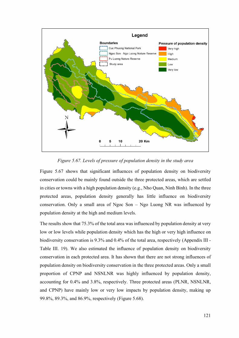
121
Figure 5.67. Levels of pressure of population density in the study area
Figure 5.67 shows that significant influences of population density on biodiversity
conservation could be mainly found outside the three protected areas, which are settled
in cities or towns with a high population density (e.g., Nho Quan, Ninh Binh). In the three
protected areas, population density generally has little influence on biodiversity
conservation. Only a small area of Ngoc Son – Ngo Luong NR was influenced by
population density at the high and medium levels.
The results show that 75.3% of the total area was influenced by population density at very
low or low levels while population density which has the high or very high influence on
biodiversity conservation is 9.3% and 0.4% of the total area, respectively (Appendix III -
Table III. 19). We also estimated the influence of population density on biodiversity
conservation in each protected area. It has shown that there are not strong influences of
population density on biodiversity conservation in the three protected areas. Only a small
proportion of CPNP and NSNLNR was highly influenced by population density,
accounting for 0.4% and 3.8%, respectively. Three protected areas (PLNR, NSNLNR,
and CPNP) have mainly low or very low impacts by population density, making up
99.8%, 89.3%, and 86.9%, respectively (Figure 5.68).
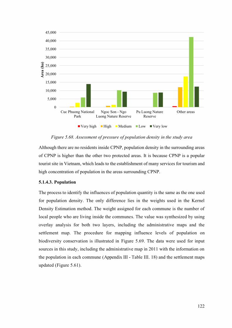
122
Figure 5.68. Assessment of pressure of population density in the study area
Although there are no residents inside CPNP, population density in the surrounding areas
of CPNP is higher than the other two protected areas. It is because CPNP is a popular
tourist site in Vietnam, which leads to the establishment of many services for tourism and
high concentration of population in the areas surrounding CPNP.
5.1.4.3. Population
The process to identify the influences of population quantity is the same as the one used
for population density. The only difference lies in the weights used in the Kernel
Density Estimation method. The weight assigned for each commune is the number of
local people who are living inside the communes. The value was synthesized by using
overlay analysis for both two layers, including the administrative maps and the
settlement map. The procedure for mapping influence levels of population on
biodiversity conservation is illustrated in Figure 5.69. The data were used for input
sources in this study, including the administrative map in 2011 with the information on
the population in each commune (Appendix III - Table III. 18) and the settlement maps
updated (Figure 5.61).
0
5,000
10,000
15,000
20,000
25,000
30,000
35,000
40,000
45,000
Cuc Phuong National
Park
Ngoc Son - Ngo
Luong Nature Reserve
Pu Luong Nature
Reserve
Other areas
Are
a (
ha)
Very high High Medium Low Very low

123
Figure 5.69. Framework for mapping pressure of population quantity
Based on population statistics from 2011, the influences of population on biodiversity
conservation in the study area were estimated by applying the Kernel Density
Estimation method. The weighting is based on the population size in all communes.
The influences of population number on biodiversity conservation could be
categorized into five levels ranging from very low to very high. Then we established
a map to illustrate the influence levels of population number on biodiversity
conservation in the study area (Figure 5.70).
Kernel Density Estimation
Jenks Natural Breaks
Weights of
population quantity
Mapping levels of influence by
population quantity
Settlement Map (updated) Administrative Map 2011
Overlay analysis

124
Figure 5.70: Levels of pressure of population quantity in the study area
Appendix III - Table III. 20 shows that the number of the population influences 9.4 % of
the total area at high or very high levels, but 8.2% out of 9.4% was found outside the three
protected areas, and the rest belongs to NSNLNR (0.8%).
Figure 5.71. Assessment of pressure of population numbers in the study area
0
5,000
10,000
15,000
20,000
25,000
30,000
35,000
40,000
Cuc Phuong National
Park
Ngoc Son - Ngo
Luong Nature Reserve
Pu Luong Nature
Reserve
Other areas
Are
a (
ha)
Very high High Medium Low Very low

125
The influence of population numbers on biodiversity conservation was also estimated for
each protected area in the study area. The results have shown that the influence of population
number on biodiversity conservation is mainly at very low or low levels, accounting for
100%, 90.7%, and 85.9% in PLNR, NSNLNR, and CPNP, respectively (Figure 5.71).
5.1.4.4. Livelihood
Livelihood is defined as the basic demands of people, such as food, water, medicine,
settlement, and clothes (Baumgartner et al., 2004). The sources of livelihood could be diverse,
depending on material sources available for people. Livelihood has been considered as a vital
indicator that increasingly promotes the forest cover as well as biodiversity conservation in
Vietnam (Lambini & Nguyen, 2014; Nguyen et al., 2010, 2014; Nguyen & Nghiem, 2016).
In the study area, most of the activities serving as the livelihood of local people have been
performed using many types of land use – land cover areas such as agricultural lands,
settlements, transport lands, water bodies, and industrial areas, as well as on the forest areas.
Figure 5.72. Framework for mapping pressure of human livelihood
The pressure of livelihood on biodiversity conservation was shown as the stress to the forest
areas. The limitation of livelihood areas excluding forest areas became the primary cause of
Kernel Density Estimation
Jenks Natural Breaks
Weights of pressure of
livelihood
Mapping pressure of human
livelihood
LULC Map updated Administrative Map 2011
Overlay analysis Classification of land
cover types for livelihood

126
creating pressure on the forest as well as biodiversity conservation. Therefore, the population
density on the land, providing the livelihood for local people, was considered as a solution to
determine the pressure of livelihood on the forest area and thus biodiversity conservation.
The pressure of livelihood was estimated through the population density in the areas where
local people can secure their necessary demands such as water, food, animal fodder,
medicine, shelter, and clothing, etc. In this case, the areas of forest cover were excluded for
biodiversity conservation purposes. The classification and assessment of land use – land
cover types for livelihood were important steps that supported developing the weights of the
pressure of livelihood for each commune (Figure 5.72).
The weight is the population density calculated based on the area of livelihood for each
commune. The Kernel Density Estimation method was applied to identify the weights for
the regions of the settlement in each commune. The map of the pressure of human
livelihood on biodiversity conservation was established with five levels of the pressure
after the data were classified by the Jenks Natural Breaks method.
Figure 5.73. Land Use - Land Cover Map of communes around the study area
It was very challenging to synthesize and assess the data of the livelihood of the whole
study area directly. Previous studies demonstrated the relationship between land use -
land cover types and livelihood (Baumgartner et al., 2004; Tschirley, 1998; Turner et
al., 1995). Therefore, to define the impacts of livelihood on the biodiversity
conservation, the land use - land cover map of 57 communes within eight districts and

127
three provinces in the study area was established. The map was acquired by synthesizing
the maps of land use – land cover (LULC) in 2015 in three provinces (Hoa Binh, Ninh
Binh, and Thanh Hoa), updating and editing through the Sentinel-2 image acquired on
the 9th of April 2018. Then, 32 types of LULC which were shown in appendix III - Table
III. 12 were grouped into six classes, including forest land, plantation and rehabilitation,
agricultural land, settlements, bare land, and others (Figure 5.73). The summary of
population and land use – land cover areas of communes in and around the study area,
as illustrated in appendix III - Table III. 18.
Bare land is a unique area that is not the livelihood area. In order to assess the pressures
of humans to the forest, three elements, including forest (forest land, and plantation and
rehabilitation), livelihood (agriculture land, settlement, and others), and bare land were
identified for analyzing and calculating the pressure levels of livelihood in the study
area. The area statistics of the three classes for eight districts within three provinces
were synthesized and compared with the number of population of each district and is
shown in Figure 5.74.
Figure 5.74. Comparison between population and areas of livelihood, forest, and bare
land on the districts in the study area
The results show that Mai Chau and Tan Lac districts have a nearly equal number of
populations with 13,000 and 14,000 people. However, the areas of livelihood have
displayed a significant difference. The area of Tan Lac (4,107 ha) is nearly twice that of
Mai Chau (2,077 ha). It means that the pressure of local people to livelihood in Mai Chau
is much higher than in Tan Lac, where there is a larger forest area.
0
5
10
15
20
25
30
35
40
45
50
0
5
10
15
20
25
30
Lac Son Mai Chau Tan Lac Yen Thuy Nho Quan Ba Thuoc Quan Hoa Thach
Thanh
Hoa Binh Ninh Binh Thanh Hoa
1000 p
eop
le
1000 h
a
Forest Livelihood Bare land Population

128
Figure 5.75. The pressure of livelihood in the study area
Based on the 2015 land use – land cover map of three provinces, data on land use status
of 201 communes were gathered with 59 communes in the study area. Then we created a
map to indicate land use-land cover of 59 communes in the study area (Figure 5.73). This
map was then updated by using a Sentinel-2 image in April 2018. We also identified types
of land use in the study area. Then all types of land use were classified into selected land
types, which provide the main livelihood for local people. There are 34 types of land use
in the study area, which are divided into six main groups: forest land, restoration, and
plantation forest land, agriculture land, settlement land, bare land, and others (Figure
5.73). The results have shown that the livelihood of local people relies on forest land,
agriculture land, settlement land, and other lands. However, the statistics indicated that
the areas of agricultural land, settlement land, and other lands (herein “livelihood land”)
are quite limited in the study area (Appendix III - Table III. 21). Thus, the livelihood
sources of local people mainly come from forest land and other sources. Based on this
fact, pressure on local people to forest land was evaluated by analyzing the area of forest
land and “livelihood land” that provides a livelihood to local people. It means that the
less livelihood land local people have, the more pressure they put on forest land.

129
We calculated the area of “livelihood land” for each commune. The influence of
livelihood on forest land depends on population numbers and the area of “livelihood
area.” To identify the influence level of livelihood on forest and biodiversity
conservation, we used weighting, which is calculated by population density on
“livelihood land” for each commune. The method of Kernel Density Estimation was
applied to create a map that shows the influence of livelihood on forest land as well as
biodiversity in the study area. By using the method of Jenks Natural Break, five levels of
influence were identified, ranging from very low to very high (Figure 5.75).
Figure 5.76. Assessment of pressure of livelihood in the study area
Our results have shown that 10.3% of the total area is influenced by livelihood at very
high or high levels (Appendix III - Table III. 22). This area is found outside three
protected areas. In the three protected areas, the influence of livelihood on biodiversity
is low or very low, accounting for 100%, 86%, and 89% in PLNR, NSNLNR, and
CPNP, respectively (Figure 5.76).
5.1.5. Conservation
More and more attention of scientists and conservationists has been focused on how to
conserve and maintain the biodiversity conservation (Johnson, 1995; Saunders et al.,
1998) since the loss of biodiversity has become a serious environmental issue that can
lead to a mass extinction of species (Myers, 1979; Wilson, 1988). A suitable method of
biodiversity conservation could help to protect and manage biological resources such as
genes, species, habitats, and ecosystems (Gordon et al., 2005; Johnson, 1995).
0
5,000
10,000
15,000
20,000
25,000
30,000
35,000
Cuc Phuong National
Park
Ngoc Son - Ngo
Luong Nature Reserve
Pu Luong Nature
Reserve
Other areas
Are
a (
ha)
Very high High Medium Low Very low

130
In Vietnam, forests have been classified into three main categories based on their
principal use purposes, namely special-use forest, protection forest, and plantation forest.
The levels of protection, as well as contributing to conservation, are implemented based
on their importance (MARD, 2009). The highest priority levels for protection are reserved
for national parks followed by nature reserves, watershed protection forests to the least
priority level of protection by plantation forests.
The fragmentation, including isolated and small patches, is considered a negative index to
identify important places for biodiversity conservation (Groom et al., 2006). The large areas
free from human activities have provided important ecosystems for containing a higher and
more stable number of species through large home ranges (Gordon et al., 2005). It means
that a strong relationship between species richness and size have existed. Larger forest areas
usually contain a higher number of plants and animals (Gordon et al., 2005; Moore, 2008).
5.1.5.1. Forest management types
The maps of the forest statistics and land use-land cover in Thanh Hoa, Hoa Binh, and Ninh
Binh provinces were collected as an input data to identify priority areas regarding
management types of forest (Figure 5.77). Administrative management types were defined
based on the purposes of land use types presented on the maps.
Figure 5.77. Framework for mapping priority areas of forest management types
Mapping priority levels
for conservation types
Weights of
conservation classes
Maps of forests in 2015 of Hoa Binh,
Ninh Binh, and Thanh Hoa provinces
Forest Map updated
Information of forest management
and protection of Hoa Binh, Ninh
Binh, and Thanh Hoa in 2017
Landsat 8 image
acquired on 4th
June 2017
Map of forest
management types
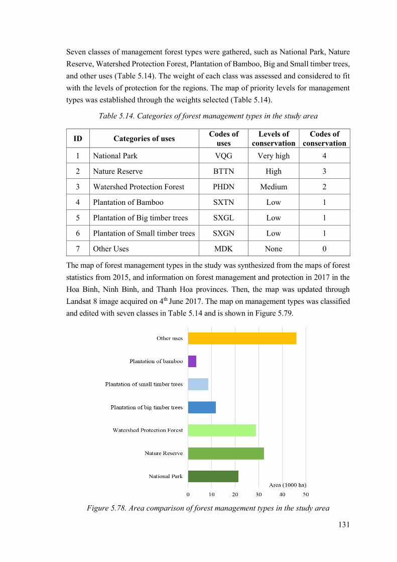
131
Seven classes of management forest types were gathered, such as National Park, Nature
Reserve, Watershed Protection Forest, Plantation of Bamboo, Big and Small timber trees,
and other uses (Table 5.14). The weight of each class was assessed and considered to fit
with the levels of protection for the regions. The map of priority levels for management
types was established through the weights selected (Table 5.14).
Table 5.14. Categories of forest management types in the study area
ID Categories of uses Codes of
uses
Levels of
conservation
Codes of
conservation
1 National Park VQG Very high 4
2 Nature Reserve BTTN High 3
3 Watershed Protection Forest PHDN Medium 2
4 Plantation of Bamboo SXTN Low 1
5 Plantation of Big timber trees SXGL Low 1
6 Plantation of Small timber trees SXGN Low 1
7 Other Uses MDK None 0
The map of forest management types in the study was synthesized from the maps of forest
statistics from 2015, and information on forest management and protection in 2017 in the
Hoa Binh, Ninh Binh, and Thanh Hoa provinces. Then, the map was updated through
Landsat 8 image acquired on 4th June 2017. The map on management types was classified
and edited with seven classes in Table 5.14 and is shown in Figure 5.79.
Figure 5.78. Area comparison of forest management types in the study area

132
The administrative management types of forest were displayed inside the protected areas
as well as outside of PAs in the study area (Figure 5.79). The forest area accounts for near
70 % of the study area. Four categories that include national park, nature reserve,
watershed protection forest, and plantation account for 14.1 %, 21.2%, 18.9%, and 15.7
% in Figure 5.78.
Figure 5.79. Map of forest management types in the study area
Forest management types were identified and classified into seven types, including
National Park, Nature Reserve, Watershed Protection Forest, Plantation Forest of
Bamboo, Plantation Forest of big timber trees, Plantation Forest of small timber trees,
and others. Based on the characteristic of these forest types, their priority levels were
evaluated regarding important levels to forest and biodiversity (Table 5.14) and
presented forest management types on the map (Figure 5.79). Then a map of forest
management types with priority levels regarding biodiversity conservation status was
created (Figure 5.80).
The results show that in CPNP, 14.5% of the total area and 92.1% of the CPNP area are
at a very high priority level for biodiversity conservation in forest management type. The
high priority level could be found in both PLNR and NSNLNR, making up 10.4% and
11.3%, respectively (Figure 5.81).

133
Figure 5.80. Priority areas of forest management types in the study area
The area of medium priority level is fragmented and located outside the three protected
areas, which is a watershed protection area, accounting for 18.9% of the total area. 17.6%
out of 18.9% could be found outside the three existing protected areas (i.e., the remaining
1.3% is found inside the three protected areas). This trend is similar to the area at a low
priority level, making up 15.5% of the total area, with 15% lying outside three existing
protected areas (Appendix III - Table III. 23).
Figure 5.81. Assessment of priority areas of forest management types in the study area
0
5,000
10,000
15,000
20,000
25,000
30,000
35,000
40,000
Cuc Phuong National
Park
Ngoc Son - Ngo
Luong Nature Reserve
Pu Luong Nature
Reserve
Other areas
Are
a (
ha)
Very high High Medium Low Very low

134
5.1.5.2. Size of forest area
The forest map that was updated and edited in 2017 for the study area (Figure 5.46) was
used as input data for this criterion. The forest areas were selected and aggregated based
on the geometrical link among them. The combined regions of forest cover were
calculated in the area before they were classified by the Jenks Natural Breaks method to
estimate five levels concerning the size of the forest areas. The process of establishing
the map on priority areas by the size of the forest area is shown in Figure 5.82.
Figure 5.82. Framework for mapping priority areas of size of forest area
The region’s forest (National Park, Nature Reserve, Watershed Protection Forest, and
Plantation) were selected to classify the levels of the size of forest areas. The small
polygons were combined to define the size of forest areas. Thresholds of area size were
identified by the Natural Breaks (Jenks) method.
The forest status map of the study area was updated by satellite images from 2017 to
identify the forest areas and their sizes. Forest areas are classified based on their sizes by
applying the method of Jenks Natural Break. There are five levels regarding the size of
forest area in the study area ranging from very small to very large (Table 5.15).
Mapping priority areas of size of
forest cover
Forest Map updated 2017 in the
study area
Jenks Natural Breaks
Aggregates features based on forest
cover

135
Table 5.15. Categories of priority levels of size of forest area
ID Area Size (ha) Levels of size Code
1 ≥ 14,290.0 Very large 4
2 5,446.2 – 14,289.9 Large 3
3 2,257.9 – 5,446.1 Medium 2
4 598.2– 2,257.8 Small 1
5 ≤ 598.1 Very small and none 0
The results have shown that 32.4% of the total area is covered by a vast forest area, which
was found mainly in the three protected areas (CPNP, NSNLNR, and PLNR), split 14.1%,
10.3%, and 7.6%, respectively (Figure 5.84).
Figure 5.83. Priority areas based on forest area size in the study area
Large forest areas cover about 9.4% of the total area, with 8.6% lying outside the three
existing protected areas. 49% of the total area includes small forest areas, and 43.7% out
of 49% is distributed outside the three existing protected areas (Appendix III - Table III.

136
24). It means that the majority of small and fragmented forest areas are found outside the
three existing protected areas.
Figure 5.84. Assessment of priority areas regarding forest size in the study area
5.1.6. Education
Many efforts have been made to reduce biodiversity loss in developing countries
(Poffenberger, 1998; Quy & Can, 1994; Sterling & Hurley, 2005). Among these,
education on issues of biodiversity conservation and environmental protection is
considered as an essential tool in changing people’s habits and conceptions towards
more sustainable development goals. UNESCO (2005) has shown that conservation,
education, and sustainable development are keys to preserving the biosphere. However,
the implementation should focus on helping local people to understand and appreciate
positive activities arising from biodiversity conservation rather than just isolating them
away from protected areas (Reid, 2012). Local people can be aware of the values of
natural resources through the knowledge gained from education and training (Mcneely
et al., 1990; Nguyen et al., 2014). The weak awareness of local communities about the
need to protect the environment is considered as the leading cause of biodiversity
decline in the developing countries (Pauchard et al., 2006). Therefore, education and
information are essential to analyze and assess biodiversity conservation projects.
Figure 5.85 illustrates the process of defining the impact levels of education for
biodiversity conservation. The information on schools in and around the study area was
0
10,000
20,000
30,000
40,000
50,000
60,000
Cuc Phuong National
Park
Ngoc Son - Ngo
Luong Nature Reserve
Pu Luong Nature
Reserve
Other areas
Are
a (
ha)
Very high High Medium Low Very low
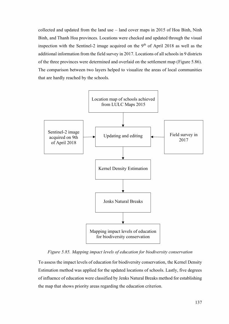
137
collected and updated from the land use – land cover maps in 2015 of Hoa Binh, Ninh
Binh, and Thanh Hoa provinces. Locations were checked and updated through the visual
inspection with the Sentinel-2 image acquired on the 9th of April 2018 as well as the
additional information from the field survey in 2017. Locations of all schools in 9 districts
of the three provinces were determined and overlaid on the settlement map (Figure 5.86).
The comparison between two layers helped to visualize the areas of local communities
that are hardly reached by the schools.
Figure 5.85. Mapping impact levels of education for biodiversity conservation
To assess the impact levels of education for biodiversity conservation, the Kernel Density
Estimation method was applied for the updated locations of schools. Lastly, five degrees
of influence of education were classified by Jenks Natural Breaks method for establishing
the map that shows priority areas regarding the education criterion.
Kernel Density Estimation
Jenks Natural Breaks
Mapping impact levels of education
for biodiversity conservation
Location map of schools achieved
from LULC Maps 2015
Updating and editing Sentinel-2 image
acquired on 9th
of April 2018
Field survey in
2017

138
Figure 5.86. Distribution of schools in districts around the study area
To evaluate the influence of education on biodiversity conservation, the distribution of
schools in the study area is considered as an essential indicator. We argue that the deficit of
schools reduces the opportunities to teach and introduce the concept of protecting the
environment as well as biodiversity conservation. Thus, there is an increasing priority for
biodiversity conservation in the regions that lack schools or educational centers. Based on
the land use status map in 2015, we identified the distribution of schools in the study area
and presented it on the map. The map of the distribution of schools was updated by using
the Sentinel-2 image in April 2018 and the fieldwork in 2017.
The influence of education on biodiversity conservation was identified by applying
the method of Kernel Density Estimation for the positions of the schools in the study
area. There are five influence levels of education that impact on biodiversity
conservation based on the method of Jenks Natural Breaks, ranging from very low to
very high. Then we presented five influence levels of education on biodiversity
conservation on the map, as shown in Figure 5.87. It has shown that a shallow
influence of education was found mainly in CPNP and PLNR. There are high or very
high influence areas of education for biodiversity conservation in Nho Quan city of
Ninh Binh province and a part of NSNLNR.

139
Figure 5.87. Impact levels of education for biodiversity conservation in the study area
The results have shown that 61.7% of the total area has low accessibility to education with
the distribution of CPNP, NSNLNR, and PLNR, being 14.6%, 11.6%, and 4.7%,
respectively (Figure 5.88) (Appendix III - Table III. 25). It shows that there is still a lack of
education system in remote areas around CPNP and NSNLNR. There is an increasing need
to improve the education system and transfer of knowledge on forest and environmental
protection in these areas. Thus, defining priority areas for biodiversity conservation needs
to take into account the influence of education in the criteria system.
Figure 5.88. Assessment of priority areas of education in the study area
0
5,000
10,000
15,000
20,000
25,000
30,000
Cuc Phuong National
Park
Ngoc Son - Ngo
Luong Nature Reserve
Pu Luong Nature
Reserve
Other areas
Are
a (
ha)
Very high High Medium Low Very low

140
5.1.7. Law
The implementation of biodiversity conservation has faced various threats and
challenges. Using legally binding laws are considered as a traditional tool to halt the loss
of biodiversity in many countries (Reid, 2012). The laws are integrated with existing
national policy and legislative frameworks to enable the different levels of administration
that can adapt to the complex and dynamic nature of ecosystems.
Figure 5.89. Framework for mapping impact levels of law for biodiversity conservation
Generally, the fundamental basis of environmental laws and regulations in Vietnam is
well-established (Brunner, 2012). In Vietnam, the laws have been used as a fundamental
tool for the management and implementation of conservation and sustainable
development of biodiversity (VNG, 2008a). Many stakeholders are participating in
biodiversity conservation. Among these, governmental agencies that are responsible for
forest protection and management, including forest stations, forest protection
departments, people’s committees of communes, districts, and provinces. These
organizations directly uphold the governmental laws for protecting and conserving forests
and biodiversity. Thus, positions of these organizations are significant in assessing the
Kernel Density Estimation
Jenks Natural Breaks
Mapping impact levels of law for
biodiversity conservation
Assessment of
protection levels
Map of locations of forest protection achieved
from Maps of forest statistic and LULC in 2015
Updating and editing Sentinel-2 image
acquired on 9th of
April 2018
Field survey in
2017

141
capacity for protecting biodiversity conservation. We assume that the presence of
governmental agencies could influence the competence for protecting forests and
biodiversity in general.
The locations of the official governmental organizations of forest protection were
determined through the maps on forest statistics and LULC in 2015. Then the data were
inspected and updated through the Sentinel-2 image acquired on 9th April 2018 and
associated with the information from the field survey in 2017 (Figure 5.89). The
locations of forest protection administrations were classified and assessed as importance
levels for identifying the weights, which were then used in the Kernel Density
Estimation method for the determined points. The map for law criterion was built up
with five levels ranging from very low to very high impact for biodiversity conservation
through the Jenks Natural Breaks method.
Figure 5.90. Positions of governmental offices responsible for protecting biodiversity
One layer of forest stations, forest protection departments, and people’s committees were
established based on the maps collected and information acquired from the field survey
in 2017. The layer was also checked and edited by overlaying on the 10-meter Sentinel-
2 image. Figure 5.90 shows the positions of governmental organizations inside and
outside 5 km-buffering of communes for protecting forest and biodiversity in the study
area. Kernel Density method for features of points in ArcGIS 10.1 was used to calculate

142
the degrees of influence associated with the distribution of governmental organizations
for protecting the forest area and biodiversity. The impacts of organizations are different
for each group. Thus, the weights were created to show the differences. The weights are
presented in Table 5.16. The maximum range for impact ability of the organizations
considered is around 10 kilometers from their locations.
Table 5.16. Assessing the ability of offices in protecting forest and biodiversity
ID Groups Weight
1 People’s committee of commune 1
2 People’s committee of district 2
3 Forest station 4
4 Forest protection department 5
To evaluate the possibility of forest and biodiversity management by using law and
regulations, we based on the position of agencies related to forest protection and
biodiversity conservation in the study area. Four central agencies are responsible for
forest protection and biodiversity conservation, including forest protection department,
forest station, people’s committee of commune, and people’s committee of district. Based
on collected map data, the locations of these agencies were identified and then updated
by Sentinel-2 in April 2018 and the fieldwork in 2017.
Table 5.17. Categories of protection levels based on the law in the study area
ID Levels of influence Old values New values
1. Very high ≥ 0.308 4
2. High 0.209 - 0.307 3
3. Medium 0.135 - 0.208 2
4. Low 0.066 - 0.134 1
5. Very low ≤ 0.065 0
The positions of these agencies were classified based on their capacities and
responsibilities for forest protection and biodiversity conservation to identify the

143
priority level of these criteria in the assessment process (Table 5.16). Then, by applying
the method of Kernel Density Estimation, we estimated the influence levels of the
positions of these agencies on forest and biodiversity protection in the study area. We
argue that the distribution of forest protection agencies influences forest management.
It means that forest management is considered better in the regions that are closer to
forest protection agencies. Then we established a map on the distribution of forest
protection agencies to identify their influence on biodiversity conservation in all
positions within the study area. Based on the method of Jenks Natural Breaks, there are
five influence levels of the positions of forest protection agencies, ranging from very
low to very high (Table 5.17).
Figure 5.91. Levels of protection ability of forest offices in the study area
The results have shown that in NSNLNR and PLNR have a low distribution of forest
protection agencies, while the distribution of these agencies is medium or high in CPNP
(Figure 5.91). It has shown that 43.2% of the total area has a low distribution of forest
protection agencies, which lead to weak management of forest by law (Appendix III -
Table III. 26). 29.4% out of 43.2% could be found outside three existing protected areas
while the rest of the area belongs to NSNLNR and PLNR, making up 7.9% and 5.9%,
respectively. High distribution of forest protection agencies is found in CPNP, accounting

144
for 42,5% of the national park area. 56.8% of CPNP has a medium distribution of forest
protection agencies (Figure 5.92).
Figure 5.92: Assessment of priority areas of law in the study area
5.2. Synthesis of multiple criteria
According to Gordon et al. (2005), the main target of conservation often focuses on species,
especially on the variety of species and threatened species. It is assumed that the protection
of the species’ habitat is one of the most effective methods for biodiversity conservation.
The priority areas usually tend to be either primitive area where the human activities are at
a minimum, or highly vulnerable and irreplaceable area with less protection in the future or
critical loss of species and their habitat as happened in the past.
In this thesis, we developed criteria and their weights to identify priority areas for
biodiversity conservation in Vietnam. The criteria system includes three factors: pressure,
state, response. Then seven criteria, 15 sub-criteria, and their weights were determined
through the results acquired from the field survey in 2017 (Figure 4.1).
The priority area for biodiversity conservation in the study area was synthesized from 17
layers including two criteria (Education and Law) and 15 sub-criteria (Richness, Rarity,
Location, Topography, Climate, Hydrology, Forest type, Climate change, Natural
disaster, Population Distribution, Population Density, Population Number, Livelihood,
Forest Management Types, and Size of Forest Area). The values of each layer were
multiplied with their weights. Then the layers were overlaid to define the priority areas
for biodiversity conservation in the study area.
0
5,000
10,000
15,000
20,000
25,000
30,000
Cuc Phuong National
Park
Ngoc Son - Ngo
Luong Nature Reserve
Pu Luong Nature
Reserve
Other areas
Are
a (
ha)
Very high High Medium Low Very low
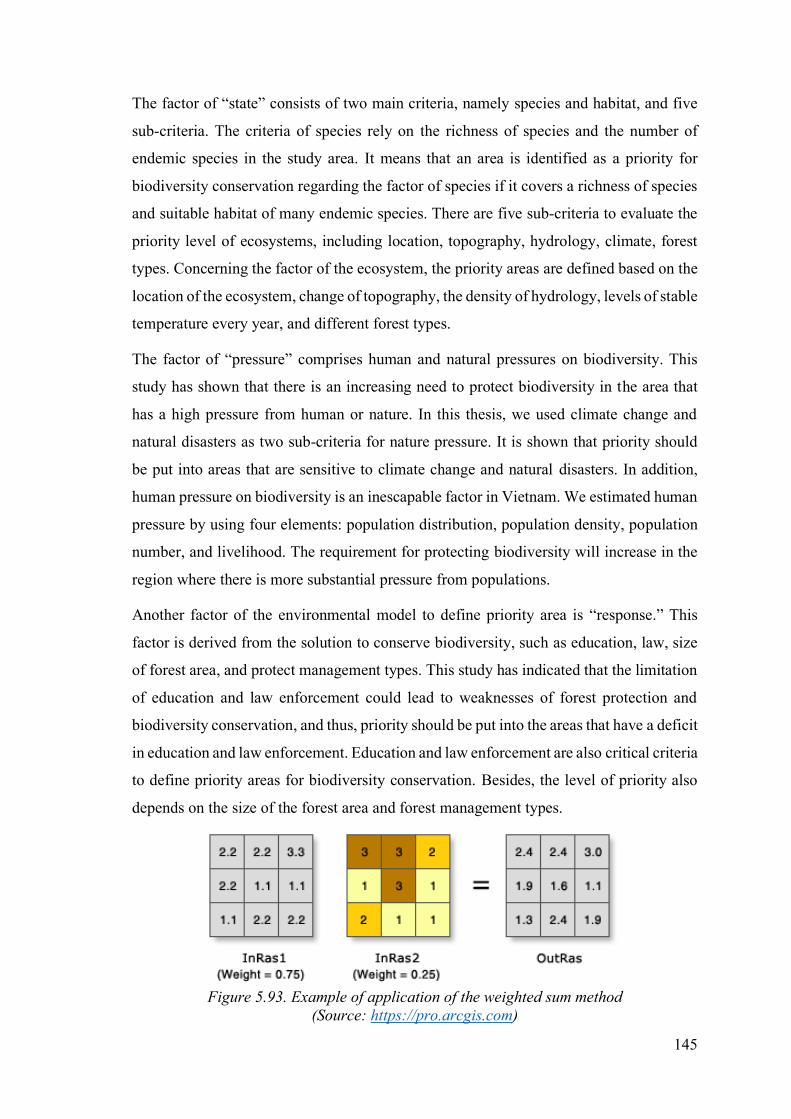
145
The factor of “state” consists of two main criteria, namely species and habitat, and five
sub-criteria. The criteria of species rely on the richness of species and the number of
endemic species in the study area. It means that an area is identified as a priority for
biodiversity conservation regarding the factor of species if it covers a richness of species
and suitable habitat of many endemic species. There are five sub-criteria to evaluate the
priority level of ecosystems, including location, topography, hydrology, climate, forest
types. Concerning the factor of the ecosystem, the priority areas are defined based on the
location of the ecosystem, change of topography, the density of hydrology, levels of stable
temperature every year, and different forest types.
The factor of “pressure” comprises human and natural pressures on biodiversity. This
study has shown that there is an increasing need to protect biodiversity in the area that
has a high pressure from human or nature. In this thesis, we used climate change and
natural disasters as two sub-criteria for nature pressure. It is shown that priority should
be put into areas that are sensitive to climate change and natural disasters. In addition,
human pressure on biodiversity is an inescapable factor in Vietnam. We estimated human
pressure by using four elements: population distribution, population density, population
number, and livelihood. The requirement for protecting biodiversity will increase in the
region where there is more substantial pressure from populations.
Another factor of the environmental model to define priority area is “response.” This
factor is derived from the solution to conserve biodiversity, such as education, law, size
of forest area, and protect management types. This study has indicated that the limitation
of education and law enforcement could lead to weaknesses of forest protection and
biodiversity conservation, and thus, priority should be put into the areas that have a deficit
in education and law enforcement. Education and law enforcement are also critical criteria
to define priority areas for biodiversity conservation. Besides, the level of priority also
depends on the size of the forest area and forest management types.
Figure 5.93. Example of application of the weighted sum method
(Source: https://pro.arcgis.com)
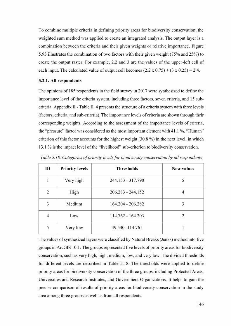
146
To combine multiple criteria in defining priority areas for biodiversity conservation, the
weighted sum method was applied to create an integrated analysis. The output layer is a
combination between the criteria and their given weights or relative importance. Figure
5.93 illustrates the combination of two factors with their given weight (75% and 25%) to
create the output raster. For example, 2.2 and 3 are the values of the upper-left cell of
each input. The calculated value of output cell becomes (2.2 x 0.75) + (3 x 0.25) = 2.4.
5.2.1. All respondents
The opinions of 185 respondents in the field survey in 2017 were synthesized to define the
importance level of the criteria system, including three factors, seven criteria, and 15 sub-
criteria. Appendix II - Table II. 4 presents the structure of a criteria system with three levels
(factors, criteria, and sub-criteria). The importance levels of criteria are shown through their
corresponding weights. According to the assessment of the importance levels of criteria,
the “pressure” factor was considered as the most important element with 41.1 %. “Human”
criterion of this factor accounts for the highest weight (30.8 %) in the next level, in which
13.1 % is the impact level of the “livelihood” sub-criterion to biodiversity conservation.
Table 5.18. Categories of priority levels for biodiversity conservation by all respondents
ID Priority levels Thresholds New values
1 Very high 244.153 - 317.790 5
2 High 206.283 - 244.152 4
3 Medium 164.204 - 206.282 3
4 Low 114.762 - 164.203 2
5 Very low 49.540 -114.761 1
The values of synthesized layers were classified by Natural Breaks (Jenks) method into five
groups in ArcGIS 10.1. The groups represented five levels of priority areas for biodiversity
conservation, such as very high, high, medium, low, and very low. The divided thresholds
for different levels are described in Table 5.18. The thresholds were applied to define
priority areas for biodiversity conservation of the three groups, including Protected Areas,
Universities and Research Institutes, and Government Organizations. It helps to gain the
precise comparison of results of priority areas for biodiversity conservation in the study
area among three groups as well as from all respondents.

147
The reclassified layer was converted to vector format for calculating and synthesizing the
data on priority areas for biodiversity conservation in the study area. The maps on priority
areas for biodiversity conservation in the study area, synthesized following the opinions
of all respondents, were illustrated with five levels represented by five respective colors,
as shown in Figure 5.94. It is easy to see the most important areas for conserving
biodiversity represented on the map with the most areas located in three protected areas.
Figure 5.94. Priority areas for biodiversity conservation synthesized by all respondents
Our results have shown the area and location of priority regions for biodiversity
conservation in the study area (Figure 5.94). The areas at high or very high priority
levels account for 56.1% of the total area with the proportion of the three existing
protected areas (CPNP, NSNLNR, PLNR), making up 13.1%, 9.7% and 11.4%
respectively (Table 5.19).
Table 5.19 also illustrates priority areas for each existing protected area. The results have
indicated that 96% of PLNR are classified as high or very high priorities. The CPNP
comprises 84.9% that are categorized as high or very high priorities. NSNLNR covers the
smallest proportion (65.9%) at high or very high priority levels. 16.4% of NSNLNR are
low or very low priority areas. Also, 21.9% of the total area is classified as high or very
high priority areas, which are found outside the three existing protected areas.

148
Table 5.19. Area statistics of priority levels for biodiversity conservation calculated
from all respondents in the study area
Specific regions Priority
levels
Area
ha % (SR) % (SA)
Cuc Phuong National Park
Very high 14,756.5 64.7 10.0
High 4,608.3 20.2 3.1
Medium 2,514.9 11.0 1.7
Low 765.9 3.4 0.5
Very low 146.9 0.6 0.1
Sum 22,792.5 100.0 15.4
Ngoc Son - Ngo Luong Nature
Reserve
Very high 8,018.7 36.7 5.4
High 6,382.2 29.2 4.3
Medium 3,897.7 17.8 2.6
Low 2,246.7 10.3 1.5
Very low 1,327.6 6.1 0.9
Sum 21,872.8 100.0 14.8
Pu Luong Nature Reserve
Very high 12,405.1 70.9 8.4
High 4,389.1 25.1 3.0
Medium 665.4 3.8 0.4
Low 40.6 0.2 0.0
Very low 0.0 0.0 0.0
Sum 17,500.1 100.0 11.8
Other areas
Very high 9,512.5 11.1 6.4
High 23,004.4 26.8 15.5
Medium 21,506.0 25.1 14.5
Low 15,777.8 18.4 10.7
Very low 16,030.2 18.7 10.8
Sum 85,831.0 100.0 58.0
Total
Very high 44,692.8 30.2 30.2
High 38,384.0 25.9 25.9
Medium 28,584.0 19.3 19.3
Low 18,831.0 12.7 12.7
Very low 17,504.7 11.8 11.8
Sum 147,996.4 100.0 100.0
SR: Specific region SA: Study area

149
5.2.2. Protected Areas group
The respondents who work in the protected areas (PAs) account for more than 34 % (64
people) of all respondents. This group obtains a number of respondents less than the group
of University and Research Institutes. The data achieved through interviews of PAs group
were separated for calculating the weight estimated by the Analytic Hierarchy Process
(AHP) method.
The weights of three factors, seven criteria, and 15 sub-criteria are shown in appendix II
- Table II. 27. The assessment of three factors is similar to the results obtained by asking
the opinion of all respondents. However, the impact of human activities was assessed
higher than the results of all respondents, with 33 % influencing the selection of priority
areas for biodiversity conservation. In which, "Livelihood" sub-criterion still accounts for
14 % that is the highest percentage among sub-criteria.
Table 5.20. Categories of priority levels for biodiversity conservation by PAs group
ID Priority levels Thresholds New values
1 Very high 244.153 – 320.940 5
2 High 206.283 - 244.152 4
3 Medium 164.204 - 206.282 3
4 Low 114.762 - 164.203 2
5 Very low 48.710 -114.761 1
To define the priority areas for biodiversity conservation in the study area, 16 out of 17
criteria were synthesized with the corresponding weights in appendix II - Table II. 27 by
the tool of the weighted sum in ArcGIS 10.1. The maps of all criteria were converted to the
raster format before the weighted sum method was applied. The result is the raster file with
the synthesized values for each pixel. The range of the value is extensive, running from
48.7 to 320.9, as described in Table 5.20.
The thresholds presented in Table 5.18 were applied to the “Protected Areas” group and
divided into five groups of priority levels from very low to very high value of biodiversity
conservation and assigned an integer number from 1 to 5, respectively. The priority levels

150
for biodiversity conservation in the study area are represented with the spatial locations
of color regions on the map, as shown in Figure 5.95.
Figure 5.95. Priority areas for biodiversity conservation synthesized by PAs group
Table 5.21 indicates that 58% of the total study area is categorized as high or very high
levels of priority for biodiversity conservation, with 23.3% lying outside of the three
protected areas. There is only 2.9% of the total study area belonging to the three
protected areas that are considered as low or very low levels of priority for protecting
biodiversity with the highest area (2.4%) found in NSNLNR. The area at high or very
high levels of priority was calculated for each protected area. The results have shown
that the proportion of the priority levels for CPNP, PLNR, and NSNLNR are 86.7%,
96.7%, and 66.6%, respectively.
The results show that PLNR and CPNP have managed large areas that were estimated with
high or very high priority for biodiversity conservation. In contrast, the areas belonging to
high or very high levels in NSNLNR were not covered much. 33.4% of the NSNLNR area
needs to be considered again in the planning of management and development.

151
Table 5.21. Area statistic of priority levels for biodiversity conservation calculated for
PAs group in the study area
Specific regions Priority levels Area
ha % (SR) % (SA)
Cuc Phuong
National Park
Very high 15,744.2 69.1 10.6
High 4,015.7 17.6 2.7
Medium 2,261.0 9.9 1.5
Low 634.5 2.8 0.4
Very low 137.2 0.6 0.1
Sum 22,792.5 100.0 15.4
Ngoc Son - Ngo
Luong Nature
Reserve
Very high 8,857.3 40.5 6.0
High 5,698.7 26.1 3.9
Medium 3,777.8 17.3 2.6
Low 2,201.5 10.1 1.5
Very low 1,337.6 6.1 0.9
Sum 21,872.8 100.0 14.8
Pu Luong Nature
Reserve
Very high 13,701.6 78.3 9.3
High 3,225.8 18.4 2.2
Medium 549.0 3.1 0.4
Low 23.6 0.1 0.0
Very low 0.0 0.0 0.0
Sum 17,500.1 100.0 11.8
Other areas
Very high 11,267.7 13.1 7.6
High 23,247.4 27.1 15.7
Medium 20,185.3 23.5 13.6
Low 14,964.0 17.4 10.1
Very low 16,166.5 18.8 10.9
Sum 85,831.0 100.0 58.0
Total
Very high 49,570.8 33.5 33.5
High 36,187.6 24.5 24.5
Medium 26,773.1 18.1 18.1
Low 17,823.6 12.0 12.0
Very low 17,641.2 11.9 11.9
Sum 147,996.4 100.0 100.0
SR: Specific region SA: Study area
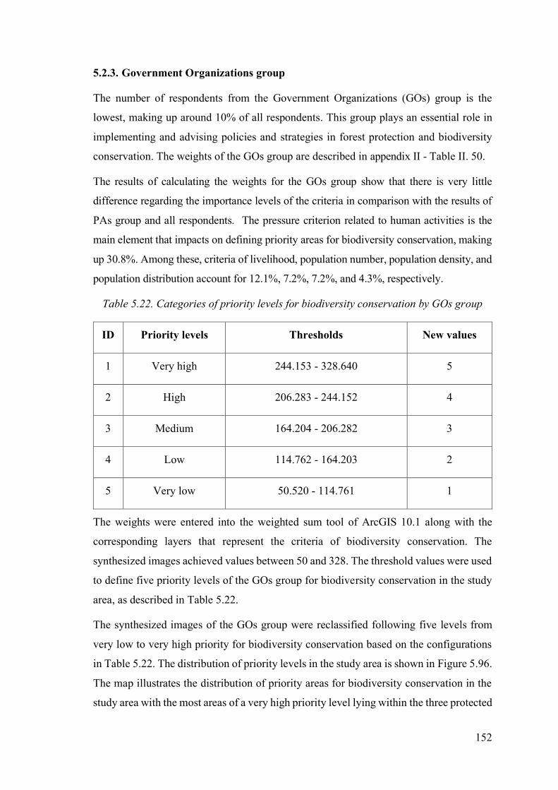
152
5.2.3. Government Organizations group
The number of respondents from the Government Organizations (GOs) group is the
lowest, making up around 10% of all respondents. This group plays an essential role in
implementing and advising policies and strategies in forest protection and biodiversity
conservation. The weights of the GOs group are described in appendix II - Table II. 50.
The results of calculating the weights for the GOs group show that there is very little
difference regarding the importance levels of the criteria in comparison with the results of
PAs group and all respondents. The pressure criterion related to human activities is the
main element that impacts on defining priority areas for biodiversity conservation, making
up 30.8%. Among these, criteria of livelihood, population number, population density, and
population distribution account for 12.1%, 7.2%, 7.2%, and 4.3%, respectively.
Table 5.22. Categories of priority levels for biodiversity conservation by GOs group
ID Priority levels Thresholds New values
1 Very high 244.153 - 328.640 5
2 High 206.283 - 244.152 4
3 Medium 164.204 - 206.282 3
4 Low 114.762 - 164.203 2
5 Very low 50.520 - 114.761 1
The weights were entered into the weighted sum tool of ArcGIS 10.1 along with the
corresponding layers that represent the criteria of biodiversity conservation. The
synthesized images achieved values between 50 and 328. The threshold values were used
to define five priority levels of the GOs group for biodiversity conservation in the study
area, as described in Table 5.22.
The synthesized images of the GOs group were reclassified following five levels from
very low to very high priority for biodiversity conservation based on the configurations
in Table 5.22. The distribution of priority levels in the study area is shown in Figure 5.96.
The map illustrates the distribution of priority areas for biodiversity conservation in the
study area with the most areas of a very high priority level lying within the three protected

153
areas. The area accounts for 34.2 % of the study area, in which the three protected areas
occupy 27.4% (Table 5.23).
Figure 5.96. Priority areas for biodiversity conservation synthesized by GOs group
Our results have shown that 57.9% of the total area is classified as high or very high priority
areas with the proportion of CPNP, NSNLNR, and PLNR, accounting for 13.9%, 10.1%,
and 11.3% respectively. The rest (22.5%) is found outside three protected areas with 15.7%
of that as high level. We also estimated the areas at very high or high priority levels for
each protected area. It is shown that very high or high priority areas account for 90.2%,
68.4%, and 95.9% in CPNP, NSNLNR, PLNR, respectively.
Based on our results, we confirm that both PL NR and CP NP cover most areas at high
levels of biodiversity conservation that were synthesized and classified from all selected
criteria through the opinions of the GOs group while the high or very high priority areas of
NSNLNR are still smaller than other protected areas.

154
Table 5.23. Area statistic of priority levels for biodiversity conservation calculated from
GOs group in the study area
Specific regions Priority
levels
Area
ha % (SR) % (SA)
Cuc Phuong National Park
Very high 17,034.5 74.7 11.5
High 3,533.8 15.5 2.4
Medium 1,657.4 7.3 1.1
Low 451.4 2.0 0.3
Very low 115.4 0.5 0.1
Sum 22,792.5 100.0 15.4
Ngoc Son - Ngo Luong Nature
Reserve
Very high 10,357.0 47.4 7.0
High 4,590.0 21.0 3.1
Medium 3,775.1 17.3 2.6
Low 1,879.3 8.6 1.3
Very low 1,271.5 5.8 0.9
Sum 21,872.8 100.0 14.8
Pu Luong Nature Reserve
Very high 13,192.8 75.4 8.9
High 3,590.1 20.5 2.4
Medium 629.7 3.6 0.4
Low 87.5 0.5 0.1
Very low 0.0 0.0 0.0
Sum 17,500.1 100.0 11.8
Other areas
Very high 10,059.2 11.7 6.8
High 23,301.8 27.1 15.7
Medium 19,867.8 23.1 13.4
Low 17,852.5 20.8 12.1
Very low 14,749.6 17.2 10.0
Sum 85,831.0 100.0 58.0
Total
Very high 50,643.5 34.2 34.2
High 35,015.8 23.7 23.7
Medium 25,930.0 17.5 17.5
Low 20,270.7 13.7 13.7
Very low 16,136.5 10.9 10.9
Sum 147,996.4 100.0 100.0
SR: Specific region SA: Study area

155
5.2.4. Universities and Research Institutes group
The group of Universities and Research Institutes (URIs) had the highest number of
respondents, making up 50% of all respondents. The opinions of the URIs group were
analyzed, synthesized, and calculated by the Analytic Hierarchy Process (AHP) method.
The results have shown the importance levels of criteria for biodiversity conservation in
Vietnam (Appendix II - Table II. 73).
The results have shown a significant difference between the URIs group with other cases.
The URIs group had a greater focus on the “Response” factor (41%), including the
“Education” criterion (17%), the “Law” criterion (13%), and the “Conservation” criterion
(11%). In comparison, the “Pressure” factor has a smaller impact level (26%).
The weights are considered as the fundamental element in combining all criteria for
defining priority areas for biodiversity conservation in Vietnam (Appendix II - Table II.
73). The layers representing the corresponding criteria were synthesized using the
Weighted Sum tool in ArcGIS 10.1.
Table 5.24. Categories of priority levels for biodiversity conservation by URIs group
ID Priority levels Thresholds New values
1 Very high 244.153 – 306.280 5
2 High 206.283 - 244.152 4
3 Medium 164.204 - 206.282 3
4 Low 114.762 - 164.203 2
5 Very low 41.000 -114.761 1
The displayed values on the map synthesized by 16 criteria of the URIs group fluctuate
from 41 to around 306.28 (Table 5.24). To group the values into five classes regarding
the priority levels for biodiversity conservation, the thresholds created by the data of all
respondents in Table 5.18 were applied for the URIs group. The classes are very low, low,
medium, high, and very high priority areas and are illustrated in Figure 5.97 after
reclassifying the synthesized layers.

156
Then, area statistics on priority areas for biodiversity conservation in the study area are
presented in Table 5.25. Our results show that 42.9% of the total study area is classified as
a high or very high priority in the study area. These areas in CPNP, NSNLNR, and PLNR
are 12.3%, 7.5%, and 10.2%, respectively. We also estimated the areas for each protected
area. Our findings indicate that proportions of high or very high priority areas for CPNP,
NSNLNR, and PLNR are 80.1%, 51%, and 85.8%, respectively.
Figure 5.97. Priority areas for biodiversity conservation synthesized by URIs group
In comparison with the rest of the protected areas, NSNLNR has the highest proportion
of areas at very low or low priority levels accounting for 29.2% of the area of the
reserve. This reserve has the lowest level of the areas at high or very high priority levels
that identified using the opinions of the URIs group in comparison with the results of
other groups and all respondents. Our results have raised a critical question about the
accuracy and rationality of defining priority areas for biodiversity conservation in the
Ngoc Son – Ngo Luong nature reserve.

157
Table 5.25. Area statistics of priority levels for biodiversity conservation calculated for
the URIs group in the study area
Specific regions Priority
levels
Area
ha % (SR) % (SA)
Cuc Phuong National Park
Very high 7,694.1 33.8 5.2
High 10,545.1 46.3 7.1
Medium 3,199.5 14.0 2.2
Low 810.4 3.6 0.5
Very low 543.3 2.4 0.4
Sum 22,792.5 100.0 15.4
Ngoc Son - Ngo Luong Nature
Reserve
Very high 3,310.1 15.1 2.2
High 7,858.1 35.9 5.3
Medium 4,314.0 19.7 2.9
Low 3,546.7 16.2 2.4
Very low 2,844.0 13.0 1.9
Sum 21,872.8 100.0 14.8
Pu Luong Nature Reserve
Very high 6,290.3 35.9 4.3
High 8,739.7 49.9 5.9
Medium 1,942.1 11.1 1.3
Low 519.3 3.0 0.4
Very low 8.8 0.1 0.0
Sum 17,500.1 100.0 11.8
Other areas
Very high 4,979.2 5.8 3.4
High 14,006.1 16.3 9.5
Medium 19,984.3 23.3 13.5
Low 23,232.4 27.1 15.7
Very low 23,628.9 27.5 16.0
Sum 85,831.0 100.0 58.0
Total
Very high 22,273.7 15.1 15.1
High 41,149.1 27.8 27.8
Medium 29,439.9 19.9 19.9
Low 28,108.8 19.0 19.0
Very low 27,025.0 18.3 18.3
Sum 147,996.4 100.0 100.0
SR: Specific region SA: Study area

158
Chapter 6. Conclusions and recommendations
6.1. Establishment of criteria
Based on the results, a set of criteria was developed to identify priority areas of
biodiversity conservation in Vietnam. The criteria system was established through a
literature review on biodiversity conservation in the world and Vietnam, and the
application of the Pressure-State-Response environmental model to select the suitable
criteria for applying in Vietnam.
The set of criteria was hierarchically structured, including four levels. The first level was
the critical purposes of biodiversity conservation. The second was three factors of “State,”
“Pressure,” and “Response,” which were analyzed in combination with the environmental
model. These factors were principally used to identify and zone the priority areas of
biodiversity conservation in Vietnam. The third level contained seven criteria assigned
by three factors. “Species” and “Ecosystem” are the two criteria of the “State” factor.
“Nature” and “Human” belong to “Pressure.” “Response” criterion includes elements of
“Education,” “Law,” and “Conservation”. The fourth level contained the highest number
of components with 15 sub-criteria. “Education” and “Law” did not have any components
at the fourth level.
To identify the importance levels of the criteria for biodiversity conservation in Vietnam,
a questionnaire was designed to collect information from the experts and scientists in the
fields of forestry, biodiversity, and conservation. The respondents were diverse regarding
their responsibilities and expertise. They are lecturers and researchers at universities and
research institutes, and staffs of governmental institutions such as the Ministry of
Agriculture and Rural Development, Forest Management Department, Protected Areas,
and rangers from forest protection stations. The field survey in 2017 collected information
and opinions from 185 people across Vietnam. Most of the respondents were categorized
into three groups, including Government Organizations (GOs), Protected Areas (PAs),
and Universities and Research Institutes (URIs) with 19, 64, and 93 respondents,
respectively. The data of all respondents and the three sub-groups were used to calculate
the weight of each criterion through the Analytic Hierarchy Process (AHP) method. It
revealed the different opinions among groups and all respondents regarding importance
levels of each criterion in defining priority areas for biodiversity conservation in Vietnam.
To reconfirm the data, two outlier detection methodologies of interquartile range and
standard deviation were used to identify any errors, different opinions as well as

159
enthusiasm for replying to the questionnaire by respondents. Most outliers calculated by
the standard deviation were also included in the outliers of the interquartile range method.
Many of the outliers from respondents are just one or two elements, and the majority are
students, as indicated in appendix II - Table II. 2. Two respondents, including one student
(no. 83) and one technician (no. 161), were assessed to have 7 and 17 outlying data points.
Therefore, their data was removed before processing the next steps.
The survey provided the opinions of respondents regarding the importance levels of the
established criteria. To use the AHP for identifying the weights, the value of each pairwise
comparison presented the differences of importance level calculated between two criteria
in one pairwise. The relations among the criteria formulated 27 pairwise comparisons.
They were grouped into three different levels, including the factors, the criteria, and the
sub-criteria. There were nine pairwise comparison matrices established, including one
matrix in the second level, three matrices of the third level, and five matrices of the fourth
one. The Consistency Ratio (CR) was used to identify the consistencies of the pairwise
comparison matrices.
The statistics of weight for the groups of respondents played an important role in the
analysis and assessment of each factor, criterion, and sub-criterion. Although the different
values of weight appeared in a few sectors of each group, they did not represent the
opinions of the majority. Table 6.1 shows the percentage values of weights for the three
groups as well as all respondents. The assessments of the criteria based on the Universities
and Research Institutes group were quite different in comparison with the results of other
groups and all respondents, especially regarding the priority levels between “Response”
and “Pressure.” At the third level under the “Response” factor, the opinion of the
Government Organizations group is different from other groups that the “Law” criterion
was considered the essential element opposed to “Education” (Table 6.1).
The synthesis of the weights for each group in Table 6.1 illustrates part of the prevailing
trend of the different fields, such as research, training, planning, policy, decision making,
and implementation. The Protected Areas group assessed the importance level of the
factors in the PSR model is similar to the results of all respondents. The results from the
Universities and Research Institutes group shows that the most crucial factor is the
“Response” factor with 41%. In contrast, the weights of the “Pressure” factor based on
the data collected from the Protected Areas group, Government Organizations group, and
all respondents account for the most significant percentage of 41%.
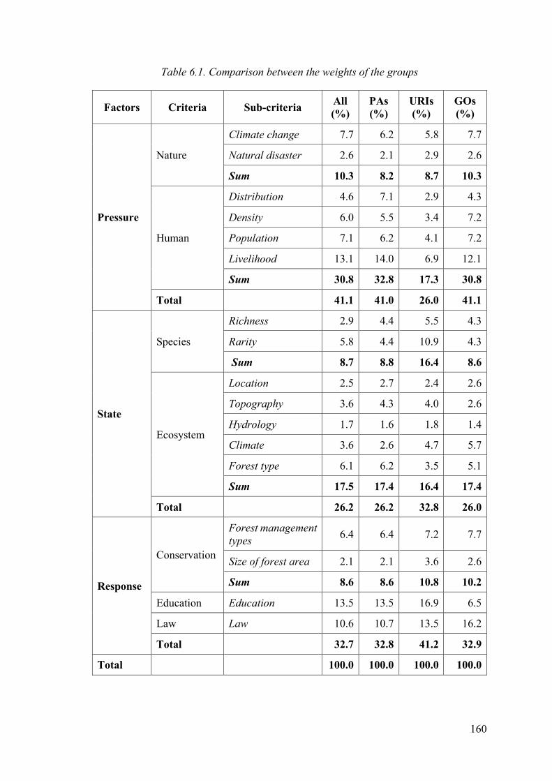
160
Table 6.1. Comparison between the weights of the groups
Factors Criteria Sub-criteria All
(%)
PAs
(%)
URIs
(%)
GOs
(%)
Pressure
Nature
Climate change 7.7 6.2 5.8 7.7
Natural disaster 2.6 2.1 2.9 2.6
Sum 10.3 8.2 8.7 10.3
Human
Distribution 4.6 7.1 2.9 4.3
Density 6.0 5.5 3.4 7.2
Population 7.1 6.2 4.1 7.2
Livelihood 13.1 14.0 6.9 12.1
Sum 30.8 32.8 17.3 30.8
Total 41.1 41.0 26.0 41.1
State
Species
Richness 2.9 4.4 5.5 4.3
Rarity 5.8 4.4 10.9 4.3
Sum 8.7 8.8 16.4 8.6
Ecosystem
Location 2.5 2.7 2.4 2.6
Topography 3.6 4.3 4.0 2.6
Hydrology 1.7 1.6 1.8 1.4
Climate 3.6 2.6 4.7 5.7
Forest type 6.1 6.2 3.5 5.1
Sum 17.5 17.4 16.4 17.4
Total 26.2 26.2 32.8 26.0
Response
Conservation
Forest management
types 6.4 6.4 7.2 7.7
Size of forest area 2.1 2.1 3.6 2.6
Sum 8.6 8.6 10.8 10.2
Education Education 13.5 13.5 16.9 6.5
Law Law 10.6 10.7 13.5 16.2
Total 32.7 32.8 41.2 32.9
Total 100.0 100.0 100.0 100.0

161
The study area was assessed and classified not only by the opinion of all respondents but
also by three specific groups, including Protected Areas, Government Organizations, and
Universities and Research Institutes. These groups were categorized based on their
characteristics and responsibilities of management, policy, and research. Protected Areas
and Government Organizations groups have considered the pressure of humans as the
most influential factor in biodiversity conservation. In contrast, the Universities and
Research Institutes group has focused on the responses of education, law, and
conservation to biodiversity. It leads to varying levels of priority for different criteria by
different groups, which influences policy, funding, and research direction.
6.2. Application of criteria
Many recent studies in Vietnam have pointed out that the process for establishing a
protected area requires long-term monitoring and investigation of many different factors
that impact directly or indirectly on biodiversity. It is a complicated task that needs much
time and human resources. Therefore, in this thesis, the application of Geographical
Information System (GIS) and Remote Sensing (RS) was used to define the priority areas
for biodiversity conservation that could help to define priority areas for establishing new
protected areas in Vietnam and reduce the time and human resources needed. As a result,
a criteria system was suggested to assess the priority levels for biodiversity conservation
in Vietnam. Then this criteria system was applied in Pu Luong – Cuc Phuong area by
integrating GIS and RS to define priority areas for biodiversity conservation in this area.
Based on the results of the survey in 2017, seventeen criteria that have a direct or indirect
impact on biodiversity conservation in Vietnam were identified with the weights calculated
for each criterion. The characteristics of these criteria were analyzed to find out the main
elements that help to present the criteria on the map. The database of each criterion was
established to fit the collected data as well as suitable methodologies. The criteria were
presented in raster format and were classified with five levels of priority areas for
biodiversity conservation, consisting of very low, low, medium, high, and very high levels.
It helped to have the same form for all criteria before they were synthesized into a unique
map defining the essential areas for biodiversity conservation in the study area.
The maps of all criteria were synthesized and performed for four cases to calculate the
results based on the calculated weights from the opinions of all respondents and the
three main groups. Sixteen out of seventeen maps of criteria were used to synthesize

162
and establish the maps of priority areas for biodiversity conservation in the study area
(Pu Luong - Cuc Phuong region). The natural disaster criterion was excluded because
there are no significant differences throughout the study area that demonstrated by
applying the Kernel Density Estimation method for the location points of natural
disasters from 1997 to 2018. The final maps that were calculated for the four cases have
expressed the changes of the distribution of priority areas inside three protected areas
(Cuc Phuong National Park, Ngoc Son – Ngo Luong Nature Reserve, and Pu Luong
Nature Reserve) as well as the entire study area (Figure 6.1). Notably, the differences
are quite significant, with the results synthesized by the opinions of the URIs group.
a. Area statistic of priority levels for biodiversity
conservation calculated from all respondents
b. Area statistic of priority levels for biodiversity
conservation calculated from URIs group
c. Area statistic of priority levels for biodiversity
conservation calculated from PAs group
d. Area statistic of priority levels for biodiversity
conservation calculated from GOs group
Figure 6.1. Area statistics of priority levels for biodiversity conservation based on the
weight set of all respondents as well as from three biggest groups
0
5
10
15
20
25
Ver
y l
ow
Low
Med
ium
Hig
h
Ver
y h
igh
Ver
y l
ow
Low
Med
ium
Hig
h
Ver
y h
igh
Ver
y l
ow
Low
Med
ium
Hig
h
Ver
y h
igh
Ver
y l
ow
Low
Med
ium
Hig
h
Ver
y h
igh
CPNP NSNLNR PLNR Other areas
Are
a (
1000 h
a)
0
5
10
15
20
25
Ver
y l
ow
Low
Med
ium
Hig
h
Ver
y h
igh
Ver
y l
ow
Low
Med
ium
Hig
h
Ver
y h
igh
Ver
y l
ow
Low
Med
ium
Hig
h
Ver
y h
igh
Ver
y l
ow
Low
Med
ium
Hig
h
Ver
y h
igh
CPNP NSNLNR PLNR Other areas
Are
a (
1000 h
a)
0
5
10
15
20
25
Ver
y l
ow
Low
Med
ium
Hig
h
Ver
y h
igh
Ver
y l
ow
Low
Med
ium
Hig
h
Ver
y h
igh
Ver
y l
ow
Low
Med
ium
Hig
h
Ver
y h
igh
Ver
y l
ow
Low
Med
ium
Hig
h
Ver
y h
igh
CPNP NSNLNR PLNR Other areas
Are
a (
1000 h
a)
0
5
10
15
20
25
Ver
y l
ow
Low
Med
ium
Hig
h
Ver
y h
igh
Ver
y l
ow
Low
Med
ium
Hig
h
Ver
y h
igh
Ver
y l
ow
Low
Med
ium
Hig
h
Ver
y h
igh
Ver
y l
ow
Low
Med
ium
Hig
h
Ver
y h
igh
CPNP NSNLNR PLNR Other areas
Are
a (
1000 h
a)

163
Figure 6.2 illustrates the comparison of the proportion of priority levels among three
protected areas and other areas in the study area based on the weight systems calculated for
the groups. The results that acquired by synthesizing the weight systems from the opinions
of all respondents, as well as the main groups (Protected Areas group, Government
Organizations group), are entirely analogous. The percentages of priority areas at high and
very high levels have not changed considerably, 85% - 90% for Cuc Phuong National Park,
around 96% for Pu Luong Nature Reserve, and 66% - 69% for Ngoc Son – Ngo Luong
Nature Reserve. The ratio between the different priority levels, exceptionally high and very
high levels, was changed critically in the case of the URIs group. The areas at very high
priority level in the study area and within three protected areas make up with 33.8%, 15.1%,
and 35.9% in CPNP, NSNLNR, and PLNR, respectively. However, the areas at both high
and very high levels within the three protected areas are not small. Respectively, CPNP,
PLNR, and NSNLNR account for 80.1%, 85.8%, and 51% out of the total area of each
protected area.
Figure 6.2. Comparison priority levels among protected areas and other areas in the
study site based on the weight systems calculated for each group
0
5000
10000
15000
20000
25000
Very
low
Low
Mediu
m
Hig
h
Very
hig
h
Very
low
Low
Mediu
m
Hig
h
Very
hig
h
Very
low
Low
Mediu
m
Hig
h
Very
hig
h
Very
low
Low
Mediu
m
Hig
h
Very
hig
h
CPNP NSNLNR PLNR Other areas
All PAs GOs URIs

164
Table 6.2. Data used for mapping sub-criteria
No Data Number Type
Sub-criteria
Rich
ness
Rarity
Lo
cation
To
po
grap
hy
Clim
ate
Hy
dro
logy
Fo
rest Ty
pes
Clim
ate Ch
ang
e
Natu
ral Disasters
Distrib
utio
n
Den
sity
Po
pu
lation
Liv
eliho
od
Fo
rest Man
agem
ent
Size o
f Fo
rest Areas
Ed
ucatio
n
Law
1 Landsat 5 TM 4 Image X X
2 Landsat 8 OLI 4 Image X X X X X X X
3 Sentinel 2A 3 Image X X X X X X X X X 4 Digital Elevation Model 1 Image X X
5 Maps of Forest 6 Map X X X X X X X 6 Maps of Land Use - Land Cover 3 Map X X X X X X X 7 Administrative Maps 3 Map X X X
8 Terrestrial ecoregions 1 Map X
9 Climate change scenarios (2046-2065) 2 Map X
10 Data of hydro-meteorological stations 1 Text X
11 IUCN Red List 1 Text X
12 Vietnam Red Data Book 2 Text X
13 Data of natural disasters 1 Text X
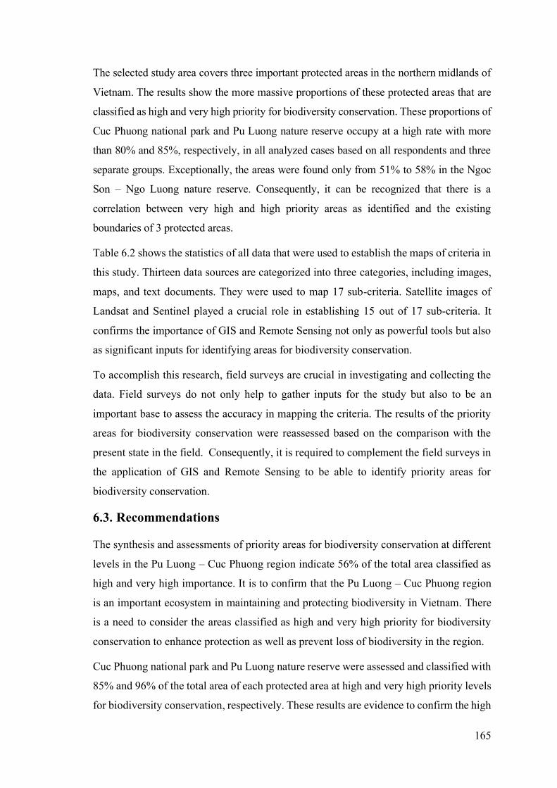
165
The selected study area covers three important protected areas in the northern midlands of
Vietnam. The results show the more massive proportions of these protected areas that are
classified as high and very high priority for biodiversity conservation. These proportions of
Cuc Phuong national park and Pu Luong nature reserve occupy at a high rate with more
than 80% and 85%, respectively, in all analyzed cases based on all respondents and three
separate groups. Exceptionally, the areas were found only from 51% to 58% in the Ngoc
Son – Ngo Luong nature reserve. Consequently, it can be recognized that there is a
correlation between very high and high priority areas as identified and the existing
boundaries of 3 protected areas.
Table 6.2 shows the statistics of all data that were used to establish the maps of criteria in
this study. Thirteen data sources are categorized into three categories, including images,
maps, and text documents. They were used to map 17 sub-criteria. Satellite images of
Landsat and Sentinel played a crucial role in establishing 15 out of 17 sub-criteria. It
confirms the importance of GIS and Remote Sensing not only as powerful tools but also
as significant inputs for identifying areas for biodiversity conservation.
To accomplish this research, field surveys are crucial in investigating and collecting the
data. Field surveys do not only help to gather inputs for the study but also to be an
important base to assess the accuracy in mapping the criteria. The results of the priority
areas for biodiversity conservation were reassessed based on the comparison with the
present state in the field. Consequently, it is required to complement the field surveys in
the application of GIS and Remote Sensing to be able to identify priority areas for
biodiversity conservation.
6.3. Recommendations
The synthesis and assessments of priority areas for biodiversity conservation at different
levels in the Pu Luong – Cuc Phuong region indicate 56% of the total area classified as
high and very high importance. It is to confirm that the Pu Luong – Cuc Phuong region
is an important ecosystem in maintaining and protecting biodiversity in Vietnam. There
is a need to consider the areas classified as high and very high priority for biodiversity
conservation to enhance protection as well as prevent loss of biodiversity in the region.
Cuc Phuong national park and Pu Luong nature reserve were assessed and classified with
85% and 96% of the total area of each protected area at high and very high priority levels
for biodiversity conservation, respectively. These results are evidence to confirm the high

166
accuracy in identifying the boundaries of these protected areas. Therefore, it is suggested
that the boundaries of Cuc Phuong national park and Pu Luong nature reserve should be
maintained, and protection should be strengthened to conserve the remaining biodiversity
in these areas.
Ngoc Son – Ngo Luong nature reserve was formulated in 2004 as a biodiversity corridor
to link Cuc Phuong national park and Pu Luong nature reserve. The results show that the
priority areas at high and very high in Ngoc Son – Ngo Luong nature reserve are smaller
in comparison with Cuc Phuong national park and Pu Luong nature reserve. 19% of the
total area in Ngoc Son – Ngo Luong nature reserve, which ranges at low and very low
priority for biodiversity conservation, are cumulated into several large areas inside the
protected area. Concerning the boundary of the Ngoc Son – Ngo Luong nature reserve,
further biodiversity surveys should be conducted to reappraise biodiversity, its function
areas and redefine its boundary appropriately.
Beside three existing protected areas in the study area, the extended area outside these
protected areas account for 58% of the total area of the study site, which is considered
significant in remaining and protecting biodiversity in Pu Luong – Cuc Phuong. Notably,
38% of the area, that were assessed and identified as a high and very high priority area
for biodiversity conservation should be reconsidered for expansion of the existing
protected areas or formulation of a new protected area covering these areas. This study
provided a system of criteria to support for defining priority areas for biodiversity
conservation in Vietnam. These criteria were applied to identify priority areas for
biodiversity conservation in Pu Luong - Cuc Phuong region by using a combination of
GIS and remote sensing, and field survey.
The results have confirmed the accuracy and rationality in defining the boundaries of
CPNP and PLNR. However, this study also shows a need to re-assess and re-define the
boundary of NSNL NR that should cover the areas at high or very high priority levels
outside the existing protected areas. To expand the application of these criteria in
Vietnam, further research is needed in different biodiversity sites. Based on our results,
we suggested that these criteria should be used to re-assess boundaries of other existing
protected areas or define boundaries of new protected areas.

167
References
Akinci, H., Özalp, A. Y., & Turgut, B. (2013). Agricultural land use suitability analysis
using GIS and AHP technique. Computers and Electronics in Agriculture, 97, 71–
82.
Akinyede, J. O., Adepoju, K. A., Akinluyi, F. O., & Anifowose, A. Y. B. (2015).
Developing a sustainable satellite-based environmental monitoring system in
Nigeria. Earth Resources and Environmental Remote Sensing/GIS Applications VI,
9644, 96440Q.
Altmann, S. A., & Altmann, J. (2003). The transformation of behaviour field studies.
Animal Behaviour, 65(3), 413–423.
Anselin, A., Meire, P. M., & Anselin, L. (1989). Multicriteria techniques in ecological
evaluation: an example using the analytical hierarchy process. Biological
Conservation, 49(3), 215–229.
Atzberger, C., Klisch, A., Mattiuzzi, M., & Vuolo, F. (2013). Phenological metrics
derived over the European continent from NDVI3g data and MODIS time series.
Remote Sensing, 6(1), 257–284.
Austin, M. P. (1991). Vegetation: data collection and analysis. Nature Conservation:
Cost Effective Biological Surveys and Data Analysis. Australia CSIRO, East
Melbourne, 37–41.
Austin, M. P., Pausas, J. G., & Nicholls, a O. (1996). Patterns of tree species richness
in relation to environment in southeastern New South Wales, Australia. Australian
Journal of Ecology, 21(2), 154–164.
Averyanov, L. V, Loc, P. K., Hiep, N. T., & Harder, D. K. (2003). Phytogeographic
review of Vietnam and adjacent areas of Eastern Indochina. Komarovia, 3, 1–83.
Averyanow, L. V., Hiep, N. T., Loc, P. K., Doan, D. T., & Regalado, J. C. (2003).
Preliminary investigation of plants of primary forest in Pu Luong nature reserve,
Thanh Hoa province.
B.W. Silverman. (1998). Density Estimation for Statistics and Data Analysis (U.
Mathematics, School of University of Bath, ed.).
Baillie, J., Hilton-Taylor, C., & Stuart, S. N. (2004). 2004 IUCN red list of threatened
species: a global species assessment.
Balram, S., Dragićević, S., & Meredith, T. (2004). A collaborative GIS method for
integrating local and technical knowledge in establishing biodiversity conservation
priorities. Biodiversity and Conservation, 13(6), 1195–1208.
Baltzer, M. C. (2000). Briefing material for the Central Truong Son Biodiversity
Conservation Programme planning meeting. Biodiversity Conservation of the
Central Truong Son, Hanoi: WWF.
Baltzer, M. C., Dao, N. T., & Shore, R. G. (2001). Towards a vision for biodiversity
conservation in the forests of the lower Mekong ecoregion complex: technical
annex. World Wildlife Fund, Hanoi.
Ban, N. T., Ly, T. D., Tap, N., Dung, V. Van, Thin, N. N., Tien, N. Van, & Khoi, N. K.
(2007). Vietnam Red Data Book, Part II. Plants. Natural Science and Technology
Publishing: Hanoi, Vietnam, 611.
Banai-Kashani, R. (1989). A new method for site suitability analysis: The analytic
hierarchy process. Environmental Management, 13(6), 685–693.
Barthlott, W., Mutke, J., Rafiqpoor, D., Kier, G., & Kreft, H. (2005). Global Centers of

168
Vascular Plant Diversity and Holger KREFT (Bonn). Nova Acta Leopoldina NF,
92(342), 61–83.
Bartlett, J. E., Kotrlik, J. W., & Higgins, C. C. (2001). Organizational research:
Determining appropriate sample size in survey research. Information Technology,
Learning, and Performance Journal, 19(1), 43–50.
Baumgartner, R., Baumgartner, R., & Hogger, R. (2004). In search of sustainable
livelihood systems: Managing resources and change.
Bedward, M., Pressey, R. L., & Nicholls, A. O. (1991). Scores and score classes for
evaluation criteria: A comparison based on the cost of reserving all natural
features. Biological Conservation, 56(3), 281–294.
Bellard, C., Bertelsmeier, C., Leadley, P., Thuiller, W., & Courchamp, F. (2012).
Impacts of climate change on the future of biodiversity. Ecology Letters, 15(4),
365–377.
Benayas, J. M. R. (1995). Patterns of Diversity in the Strata of Boreal Montane Forest
in British-Columbia. Journal of Vegetation Science, 6(1), 95–98.
Bibby, C. J. (1998). Selecting areas for conservation. Conservation Science and Action,
176–201.
Bini, L. M., Diniz - Filho, J. A. F., Carvalho, P., Pinto, M. P., & Rangel, T. F. L. B.
(2005). Lomborg and the litany of biodiversity crisis: what the peer - viewer
litterature says. Conservation Biology, 19(4), 1301–1305.
Botev, Z. I., Grotowski, J. F., & Kroese, D. P. (2010). Kernel density estimation via
diffusion. Annals of Statistics, 38(5), 2916–2957.
Boteva, D., Griffiths, G., & Dimopoulos, P. (2004). Evaluation and mapping of the
conservation significance of habitats using GIS: an example from Crete, Greece.
Journal for Nature Conservation, 12(4), 237–250.
Bounoua, L., Zhang, P., Thome, K., Masek, J., Safia, A., Imhoff, M. L., & Wolfe, R. E.
(2015). Mapping biophysical parameters for land surface modeling over the
continental US using MODIS and landsat. Dataset Papers in Science, 2015.
Boyd, D. S., & Foody, G. M. (2011). An overview of recent remote sensing and GIS
based research in ecological informatics. Ecological Informatics, 6(1), 25–36.
Brandon, K., Redford, K. H., & Sanderson, S. (1998). Parks in peril: people, politics,
and protected areas.
Bruner, A. G., Gullison, R. E., Rice, R. E., & da Fonseca, G. A. (2001). Effectiveness of
parks in protecting tropical biodiversity. Science (New York, N.Y.), 291(5501),
125–128.
Brunner, J. (2012). Biodiversity conservation in Vietnam: A perfect storm.
Bunce, R. G. H., Bogers, M. M. B., Evans, D., Halada, L., Jongman, R. H. G., Mucher,
C. A., … Olsvig-Whittaker, L. (2013). The significance of habitats as indicators of
biodiversity and their links to species. Ecological Indicators, 33, 19–25.
Can, D. N. (2004). Investigation and assessment of animals for conservation in selected
areas of Pu Luong nature reserve, Thanh Hoa province.
Carew-Reid, J., Kempinski, J., & Clausen, A. (2011). Biodiversity and Development of
the Hydropower Sector: Lessons from the Vietnamese Experience – Volume I:
Review of the Effects of Hydropower Development on Biodiversity in Vietnam.
Prepared for the Critical Ecosystem Partnership Fund, I, 79.
Carver, S. J. (1991). Integrating multi-criteria evaluation with geographical information
systems. International Journal of Geographical Information Systems, 5(3), 321–
339.

169
Castro-Esau, K. L., Sánchez-Azofeifa, G. A., Rivard, B., Wright, S. J., & Quesada, M.
(2006). Variability in leaf optical properties of Mesoamerican trees and the
potential for species classification. American Journal of Botany, 93(4), 517–530.
CEPF. (2012). Indo-Burma Biodiversity Hotspot.
CEPF, C. E. P. F., & IUCN, I. U. for C. of N. (2016). Protecting important biodiversity
hotspots The Indo-Burma region : biodiversity in the balance. In CEPF/IUCN
factsheet.
Chakhar, S., & Martel, J. (2003). Enhancing geographical information systems
capabilities with multi-criteria evaluation functions. Journal of Geographic
Information and …, 7(2), 47–71.
Chanson, J., Chenery, A. M., Csirke, J., Davidson, N. C., & Dentener, F. (2010). Global
Biodiversity : Indicators of. (May), 1164–1169.
Chavez, P. S. (1996). Image-based atmospheric corrections-revisited and improved.
Photogrammetric Engineering and Remote Sensing, 62(9), 1025–1035.
Chen, Z. G. (1996). The analysis of indicator frameworks. Cleaner Production
Information, 23, 28–37.
Clark, D. A., Piper, S. C., Keeling, C. D., & Clark, D. B. (2003). Tropical rain forest
tree growth and atmospheric carbon dynamics linked to interannual temperature
variation during 1984-2000. Proceedings of the National Academy of Sciences,
100(10), 5852–5857.
Clark, Deborah A. (2004). Sources or sinks? The responses of tropical forests to current
and future climate and atmospheric composition. Philosophical Transactions of the
Royal Society B: Biological Sciences, 359(1443), 477–491.
Cochran, W. G. (1977). Sampling Techniques (third edition).
Congalton, R. G., & Green, K. (2008). Assessing the accuracy of remotely sensed data:
principles and practices.
Coops, N. C., Wulder, M. A., Culvenor, D. S., & St-Onge, B. (2004). Comparison of
forest attributes extracted from fine spatial resolution multispectral and lidar data.
Canadian Journal of Remote Sensing, 30(6), 855–866.
CPNP. (2011). Operations of tourism in Cuc Phuong national park from 2007 to 2010.
Currie, D. J., & Paquin, V. (1987). Large-scale biogeographical patterns of species
richness of trees. Nature, 329(6137), 326.
Dao Minh, T., Yanagisawa, M., & Kono, Y. (2017). Forest transition in Vietnam: A
case study of Northern mountain region. Forest Policy and Economics, 76, 72–80.
Dehnad, K. (1987). Density estimation for statistics and data analysis.
DeLong, D. C. (1996). Defining biodiversity. Wildlife Society Bulletin (1973-2006),
24(4), 738–749.
Doughty, C. E., & Goulden, M. L. (2009). Are tropical forests near a high temperature
threshold? Journal of Geophysical Research: Biogeosciences, 114(1), 1–12.
Dudgeon, D. (2000). The ecology of tropical Asian rivers and streams in relation to
biodiversity conservation. Annual Review of Ecology and Systematics, 31(1), 239–
263.
Dudley, B. Y. N., Parish, J., Dudley, N., & Parish, J. (2006). Closing the gap. Creating
Ecologically Representative Protected Area Systems: A Guide to Conducting the
Gap Assessments of Protected Area Systems for the Convention on Biological
Diversity. Technical Series, 24.
Dudley, N. (2008). Guidelines for applying protected area management categories. In

170
IUCN (Vol. 46). IUCN.
Eastman, J. R. (2009). IDRISI Taiga: guide to GIS and image processing. In Worcester,
MA: Clark Labs.
Ekstrand, S. (1996). Landsat TM-Based Forest Damage Assessment: Correction for
Topographic Effects. Photogrammetric Engineering & Remote Sensing, 62(2),
151–161.
Elez, J., Cuezva, S., Fernandez-Cortes, A., Garcia-Anton, E., Benavente, D., Cañaveras,
J. C., & Sanchez-Moral, S. (2013). A GIS-based methodology to quantitatively
define an Adjacent Protected Area in a shallow karst cavity: the case of Altamira
cave. Journal of Environmental Management, 118, 122–134.
Esri. (2010). What is GIS? Journal of Geophysical Research, 113(C),
doi:10.1029/2008JB005610 ST-Deformation, seismi.
Evans, M. C., Watson, J. E. M., Fuller, R. A., Venter, O., Bennett, S. C., Marsack, P. R.,
& Possingham, H. P. (2011). The Spatial Distribution of Threats to Species in
Australia. BioScience, 61(4), 281–289.
Fairbanks, D. H. K. K., & McGwire, K. C. (2004). Patterns of floristic richness in
vegetation communities of California: Regional scale analysis with multi-temporal
NDVI. Global Ecology and Biogeography, 13(3), 221–235.
Fargione, J., Tilman, D., Dybzinski, R., Lambers, J. H. R., Clark, C., Harpole, W. S., …
Loreau, M. (2007). From selection to complementarity: shifts in the causes of
biodiversity–productivity relationships in a long-term biodiversity experiment.
Proceedings of the Royal Society of London B: Biological Sciences, 274(1611),
871–876.
Feddes, R. A., & Dam, J. C. van. (2004). Unsaturated-zone Modeling: Progress,
Challenges and Applications.
Feeley, K. J., Joseph Wright, S., Nur Supardi, M. N., Kassim, A. R., & Davies, S. J.
(2007). Decelerating growth in tropical forest trees. Ecology Letters, 10(6), 461–
469.
Fensholt, R., Langanke, T., Rasmussen, K., Reenberg, A., Prince, S. D., Tucker, C., …
Eastman, R. (2012). Greenness in semi-arid areas across the globe 1981–2007—
An Earth Observing Satellite based analysis of trends and drivers. Remote Sensing
of Environment, 121, 144–158.
Fernández-Manso, A., Quintano, C., & Roberts, D. (2012). Evaluation of potential of
multiple endmember spectral mixture analysis (MESMA) for surface coal mining
affected area mapping in different world forest ecosystems. Remote Sensing of
Environment, 127, 181–193.
Ferrier, S. (2002). Mapping Spatial Pattern in Biodiversity for Regional Conservation
Planning: Where to from Here? Systematic Biology, Vol. 51, pp. 331–363.
FFI. (2005). Investigations of biodiversity in kasrt mountain ranges in Pu Luong - Cuc
Phuong.
Field, R., Hawkins, B. A., Cornell, H. V, Currie, D. J., Diniz‐Filho, J. A. F., Guégan, J.,
… Oberdorff, T. (2009). Spatial species‐richness gradients across scales: a meta‐analysis. Journal of Biogeography, 36(1), 132–147.
Figueira, J., Greco, S., & Ehrgott, M. (2005). Multiple criteria decision analysis: state of
the art surveys. In Zhurnal Eksperimental’noi i Teoreticheskoi Fiziki.
Firbank, L. G., Barr, C. J., Bunce, R. G. H., Furse, M. T., Haines-Young, R., Hornung,
M., … Smart, S. M. (2003). Assessing stock and change in land cover and
biodiversity in GB: an introduction to Countryside Survey 2000. Journal of
171
Environmental Management, 67(3), 207–218.
Foody, G. M., & Cutler, M. E. J. (2006). Mapping the species richness and composition
of tropical forests from remotely sensed data with neural networks. Ecological
Modelling, 195(1–2), 37–42.
Forman, R. T. T. (1995). Some general principles of landscape and regional ecology.
Landscape Ecology, 10(3), 133–142.
FPD. (2015). Conservation planning and sustainable development for Ngoc Son - Ngo
Luong nature reserve from 2016 to 2020.
Franklin, S. E. (2001). Remote sensing for sustainable forest management. In New York.
CRC press.
Franklin, S. E. (2010). Remote sensing for biodiversity and wildlife management.
Führer, E. (2000). Forest functions, ecosystem stability and management. Forest
Ecology and Management, 132(1), 29–38.
Fujita, M., Tamagnan, G., Zoghbi, S. S., Al-tikriti, M. S., Baldwin, R. M., Seibyl, J. P.,
& Innis, R. B. (2000). An Introduction to the Analytic Hierarchy Process (AHP)
Using Super Decisions (Vol. 41).
Furey, N., & Infield, M. (2005). Conservation of Limestone Karst Ecosystems in
Vietnam: Challenges and Opportunities. Specialist, 1–9.
GEF. (2002). Project of kasrt mountain landscape conservation in Pu Luong - Cuc
Phuong, Vietnam.
Gomes, E. G., & Lins, M. P. E. (2002). Integrating Geographical Information Systems
and Multi-Criteria Methods: A Case Study. Annals of Operations Research,
116(1–4), 243–269.
Goodchild, M. F. (1991). Geographic information systems. Progress in Human
Geography, 15(2), 194–200.
Gordon, E. a, Franco, O. E., & Tyrrell, M. L. (2005). Protecting Biodiversity : A Guide
to Criteria Used by Global Conservation Organizations. Environmental Studies.
Gould, W. (2000). Remote sensing of vegetation, plant species richness, and regional
biodiversity hotspots. Ecological Applications, 10(6), 1861–1870.
Graham, E. A., Mulkey, S. S., Kitajima, K., Phillips, N. G., & Wright, S. J. (2003).
Cloud cover limits net CO2 uptake and growth of a rainforest tree during tropical
rainy seasons. Proceedings of the National Academy of Sciences, 100(2), 572–576.
Griffiths, G. H., Lee, J., & Eversham, B. C. (2000). Landscape pattern and species
richness: Regional scale analysis from remote sensing. International Journal of
Remote Sensing, 21(13–14), 2685–2704.
Groom, M. J., Meffe, G. K., & Carroll, C. R. (2006). Principles of conservation biology.
Groombridge M.D, B. & J., & Groombridge, B & Jenkins, M. . (2002). World Atlas of
Biodiversity Earth’ S Living Resources.
Guisan, A., & Thuiller, W. (2005). Predicting species distribution: offering more than
simple habitat models. Ecology Letters, 8(9), 993–1009.
Hammond, A., & Institute, W. R. (1995). Environmental indicators: a systematic
approach to measuring and reporting on environmental policy performance in the
context of sustainable development (Vol. 36).
Hano, A. I. A. (2013). Assessment of Impacts of Changes in Land Use Patterns on Land
Degradation/Desertification in the Semi- arid Zone of White Nile State, Sudan, by
Means of Remote Sensing and GIS.
Hansen, M. C., Potapov, P. V, Moore, R., Hancher, M., Turubanova, Sa., Tyukavina,

172
A., … Loveland, T. R. (2013). High-resolution global maps of 21st-century forest
cover change. Science, 342(6160), 850–853.
He, L., Wu, G., Dai, D., Chen, L., & Chen, G. (2011). Data conversion between CAD
and GIS in land planning. Proceedings - 2011 19th International Conference on
Geoinformatics, Geoinformatics 2011, 1–4.
Hill, D. (2005). Handbook of biodiversity methods: survey, evaluation and monitoring.
Hilton-taylor, C., & Stuart, S. N. (2009). Wildlife in a changing world. In IUCN Gland
Switzerland (Vol. 51).
Hinton, J. C. (1996). GIS and remote sensing integration for environmental
applications. International Journal of Geographical Information Systems, 10(7),
877–890.
Hossain, M. S., & Das, N. G. (2010). GIS-based multi-criteria evaluation to land
suitability modelling for giant prawn (Macrobrachium rosenbergii) farming in
Companigonj Upazila of Noakhali, Bangladesh. Computers and Electronics in
Agriculture, 70(1), 172–186.
Hox, J. J., & Boeije, H. R. (2005). Data collection, primary versus secondary.
Hurlbert, A., & Haskell, J. P. (2002). The effect of energy and seasonality on avian
species richness and community composition. American Naturalist, 161(1), 83–97.
Hutchinson, C. F., & Toledano, J. (1993). Guidelines for demonstrating geographical
information systems based on participatory development. International Journal of
Geographical Information Systems, 7(5), 453–461.
IPCC, Solomon, S., Qin, D., Manning, M., Chen, Z., Marquis, M., … Miller, H. L.
(2007). Climate Change 2007: The Physical Basis. Contribution of Working Group
I to the Fourth Assessment Report of the Intergovernmental Panel on Climate
Change.
Ishida, A., Toma, T., & Marjenah. (1999). Limitation of leaf carbon gain by stomatal
and photochemical processes in the top canopy of Macaranga conifera, a tropical
pioneer tree. Tree Physiology, 19(7), 467–473.
IUCN. (2013). Threatened species in each country (totals by taxonomic group)
Amphibians.
IUCN, UNEP, & WWF. (1991). Caring for the earth: a strategy for sustainable living.
Jalilova, G., Khadka, C., & Vacik, H. (2012). Developing criteria and indicators for
evaluating sustainable forest management: A case study in Kyrgyzstan. Forest
Policy and Economics, 21, 32–43.
Jenks, G. F. (1967). The data model concept in statistical mapping. International
Yearbook of Cartography, 7, 186–190.
John, R., Chen, J., Lu, N., Guo, K., Liang, C., Wei, Y., … Han, X. (2008). Predicting
plant diversity based on remote sensing products in the semi-arid region of Inner
Mongolia. Remote Sensing of Environment, 112(5), 2018–2032.
Johnson, B., Tateishi, R., & Hoan, N. (2012). Satellite Image Pansharpening Using a
Hybrid Approach for Object-Based Image Analysis. ISPRS International Journal
of Geo-Information, 1(3), 228–241.
Johnson, D. D. P., Hay, S. I., & Rogers, D. J. (1998). Contemporary environmental
correlates of endemic bird areas derived from meteorological satellite sensors.
Proceedings of the Royal Society B: Biological Sciences, 265(1400), 951–959.
Johnson, N. C. (1995). Biodiversity in the balance: approaches to setting geographic
conservation priorities.
173
Jones, P. G., Beebe, S. E., Tohme, J., & Galwey, N. W. (1997). The use of geographical
information systems in biodiversity exploration and conservation. Biodiversity and
Conservation, 6(7), 947–958.
Joppa, L. (2012). Population change in and around Protected Areas. Journal of
Ecological Anthropology, 15(1), 58–64.
Joppa, L. N., Loarie, S. R., & Pimm, S. L. (2009). On population growth near protected
areas. PLoS ONE, 4(1).
Jung, J., Kim, C., Jayakumar, S., Kim, S., Han, S., Kim, D. H., & Heo, J. (2013). Forest
fire risk mapping of Kolli Hills, India, considering subjectivity and inconsistency
issues. Natural Hazards, 65(3), 2129–2146.
Kangas, J., Karsikko, J., Laasonen, L., & Pukkala, T. (1993). A method for estimating
the suitability function of wildlife habitat for forest planning on the basis of
expertise. Silva Fennica, Vol. 27, pp. 259–268.
Kangas, Jyrki. (1992). Multiple‐use planning of forest resources by using the analytic
hierarchy process. Scandinavian Journal of Forest Research, 7(1–4), 259–268.
Kangas, Jyrki, & Kuusipalo, J. (1993). Integrating biodiversity into forest management
planning and decision-making. Forest Ecology and Management, 61(1–2), 1–15.
Kaya, T., & Kahraman, C. (2011). Fuzzy multiple criteria forestry decision making
based on an integrated VIKOR and AHP approach. Expert Systems with
Applications, 38(6), 7326–7333.
Keisler, J., Sundell, R., Keisler, J. M., & Sundell, R. C. (1997). Combining multi-
attribute utility and geographic information for boundary decisions: An application
to park planning. Journal of Geographic Information and Decision Analysis, 1(2),
100–119.
Keller, M., & Lerdau, M. (1999). Isoprene emission from tropical forest canopy leaves.
Smithsonian, 13(1), 19–29.
Kerr, J. T., Southwood, T. R. E., & Cihlar, J. (2001). Remotely sensed habitat diversity
predicts butterfly species richness and community similarity in Canada.
Proceedings of the National Academy of Sciences, 98(20), 11365–11370.
Kier, G., & Barthlott, W. (2001). Measuring and mapping endemism and species
richness: A new methodological approach and its application on the flora of Africa.
Biodiversity and Conservation, 10(9), 1513–1529.
Knight, R. S., Crowe, T. M., & Siegfried, W. R. (1982). Distribution and species
richness of trees in southern Africa. JS Afr. Bot, 48(4), 455–480.
Koch, G. W., Amthor, J. S., & Goulden, M. L. (1994). Diurnal patterns of leaf
photosynthesis, conductance and water potential at the top of a lowland rain forest
canopy in Cameroon: measurements from the Radeau des Cimes. Tree Physiology,
14(4), 347–360.
Kou, G., Ergu, D., Peng, Y., & Shi, Y. (2012). Data Processing for the AHP/ANP (Vol. 1).
Krejcie, R. V, & Morgan, D. W. (1970). Determining Sample Size for Research
Activities. 607–610.
Kudo, G. (2016). Structure and Function of Mountain Ecosystems in Japan.
Kuusipalo, J. (1984). Diversity pattern of the forest understorey vegetation in relation to
some site characteristics. Silva Fennica (Finland).
Lambini, C. K., & Nguyen, T. T. (2014). A comparative analysis of the effects of
institutional property rights on forest livelihoods and forest conditions: Evidence
from Ghana and Vietnam. Forest Policy and Economics, 38, 178–190.

174
Landsat, U. S. G. S. (2016). Landsat 8 (L8) Data Users Handbook. America, 8(1993).
Lee, W., McGlone, M., & Wright, E. (2005). Biodiversity inventory and monitoring: a
review of national and international systems and a proposed framework for future
biodiversity monitoring by the Department of Conservation. Landcare Research
Contract Report LC0405/122 (Unpublished).
Lerdau, M. T., & Throop, H. L. (1999). Isoprene emissions and photosynthesis in a
tropical forest canopy: implications for model development. Ecological
Applications, 109(November), 1109–1117.
Levin, N., Shmida, A., Levanoni, O., Tamari, H., & Kark, S. (2007). Predicting
mountain plant richness and rarity from space using satellite‐derived vegetation
indices. Diversity and Distributions, 13(6), 692–703.
Liang, S., Li, X., & Wang, J. (2012). Vegetation Production in Terrestrial Ecosystems.
In Advanced Remote Sensing.
Liu, J., Ouyang, Z., Tan, Y., Yang, J., & Zhang, H. (1999). Changes in human
population structure: Implications for biodiversity conservation. Population and
Environment: A Journal of Interdisciplinary Studies, 21(1), 45–58.
Liu, S., Zhao, Q., Wen, M., Deng, L., Dong, S., & Wang, C. (2013). Assessing the
impact of hydroelectric project construction on the ecological integrity of the
Nuozhadu Nature Reserve, southwest China. Stochastic Environmental Research
and Risk Assessment, 27(7), 1709–1718.
Lobo, J. M., Castro, I., & Moreno, J. C. (2001). Spatial and environmental determinants
of vascular plant species richness distribution in the Iberian Peninsula and Balearic
Islands. Biol. J. Linn. Soc., 73, 233–253.
Long, T. T., Đặng, N. X., & Rastall, R. (2016). Giám sát Đa dạng Sinh học có sự Tham
gia : Hướng dẫn phương pháp.
Lowe, D. (2012). Perceptual organization and visual recognition (Vol. 5).
Luck, G. W. (2007). A review of the relationships between human population density
and biodiversity. Biological Reviews, 82(4), 607–645.
Luoto, M., Virkkala, R., Heikkinen, R. K., & Rainio, K. (2004). Predicting bird species
richness using Remote Sensing in boreal agricultural‐forest mosaics. Ecological
Applications, 14(6), 1946–1962.
Lytle, D. A., & Poff, N. L. R. (2004). Adaptation to natural flow regimes. Trends in
Ecology and Evolution, 19(2), 94–100.
Mahdavi, A., Shamsi, S. R. F., & Nazari, R. (2012). Forests and rangelands’ wildfire
risk zoning using GIS and AHP techniques. Caspian Journal of Environmental
Sciences, 10(1), 43–52.
Malczewski, J. (1999). GIS and Multicriteria Decision Analysis. In GIS, Remote
Sensing, & Cartography.
Malczewski, J. (2004). GIS-based land-use suitability analysis: a critical overview.
Progress in Planning, 62(1), 3–65.
Malczewski, J. (2006). GIS-based multicriteria decision analysis: a survey of the literature.
International Journal of Geographical Information Science, 20(7), 703–726.
Mandallaz, D. (2008). Sampling techniques for forest inventories.
Mao, D., Wang, Z., Luo, L., & Ren, C. (2012). Integrating AVHRR and MODIS data to
monitor NDVI changes and their relationships with climatic parameters in
Northeast China. International Journal of Applied Earth Observation and
Geoinformation, 18, 528–536.

175
MARD. (1998). Biodiversity and Conservation of the Special Use Forest in Vietnam. In
Agriculture thematic information and rural development.
MARD. (2004). International BirdLife Program in Vietnam: Information of existing
and proposed protected areas in Vietnam.
MARD. Criteria for forest identification and classification. , Pub. L. No. 34/2009/TT-
BNNPTNT (2009).
MARD. (2014). Report on planning for special use forest to 2020.
Margules, C. R., Pressey, R. L., & Williams, P. H. (2002). Representing biodiversity:
Data and procedures for identifying priority areas for conservation. Journal of
Biosciences, 27(4), 309–326.
Mather, P. M. (2004). Computer processing of remotely-sensed images.
Mather, P. M., & Koch, M. (2011). Computer Processing of Remotel-Sensed Images:
An Introduction.
Mcneely, J. A. A., Miller, K. R. R., Reid, W. V. V, Mittermeier, R. A. A., Werner, T. B.
B., Reid, K. R., … Werner, T. B. B. (1990). Conserving the World’s Biological
Diversity. In IUCN, World Resources Institute, Conservation International, WWF-
US and the World Bank, Washington, DC. UICN, Morges (Suiza) WRI,
Washington DC (EUA) CI, Washington DC (EUA) WWF, Washington DC (EUA)
World Bank, Washington DC (EUA).
Mendoza, G A, & Prabhu, R. (2000). Multiple criteria decision making approaches to
assessing forest sustainability using criteria and indicators: a case study. Forest
Ecology and Management, 131(1–3), 107–126.
Mendoza, Guillermo A, & Sprouse, W. (1989). Forest planning and decision making
under fuzzy environments: an overview and illustration. Forest Science, 35(2),
481–502.
Meyer, J. L., Strayer, D. L., Wallace, J. B., Eggert, S. L., Helfman, G. S., & Leonard, N.
E. (2007). The contribution of headwater streams to biodiversity in river networks.
Journal of the American Water Resources Association, 43(1), 86–103.
Mickleburgh, S. P., Hutson, A. M., & Racey, P. A. (2002). A review of the global
conservation status of bats. Oryx, 36(1), 18–34.
Miller, C., & Urban, D. L. (1999). A model of surface fire, climate and forest pattern in
the Sierra Nevada, California. Ecological Modelling, 114(2–3), 113–135.
Miller, R. I. (1994). Mapping the diversity of nature (Vol. 53; Springer
Science+Business Media Dordrecht, Ed.).
Mittermeier, R. A., Ratsimbazafy, J., Rylands, A. B., Williamson, L., Oates, J. F.,
Mbora, D., … Heymann, E. W. (2007). Primates in peril: the world’s 25 most
endangered primates, 2006–2008. Primate Conservation, 22(1), 1–40.
Monastyrskii, A. L. (2004). Butterfly fauna in Pu Luong Nature Reserve, Thanh Hoa,
Vietnam.
MONRE. (2004). Biology diversity and conservation.
MONRE. (2011a). Climate change scenarious in Vietnam.
MONRE. (2011b). Government report of biodiversity.
MONRE. (2015). Vietnam National Biodiversity Strategy to 2020, Vision to 2030.
MONRE. (2016). Climate change scenarious in Vietnam.
MONRE, & VEA. (2010). National Conference of Environment 2010.
Montgomery, G. E., & Schuch, H. C. (1993). GIS Data Conversion Handbook.
Moore, P. D. (2008). Tropical forests.

176
Moran, M. S., Jackson, R. D., Slater, P. N., & Teillet, P. M. (1992). Evaluation of
simplified procedures for retrieval of land surface reflectance factors from satellite
sensor output. Remote Sensing of Environment, 41(2–3), 169–184.
Morrison, L. M. M., Marcot, G. B. B., Mannan, R. W., Morrison, M. L., Marcot, B.,
Mannan, W., … Mannan, R. W. (2006). Wildlife–Habitat Relationships: Concepts
and Applications. In PhD Proposal (Vol. 1).
Muriuki, J. N., Williams, P. H., Bennun, L. a, & Crowe, T. M. (1997). Using patterns of
distribution and diversity of Kenyan birds to select and prioritize areas for
conservation. Biodiversity and Conservation, 210, 191–210.
Myer, N., Mittermeier, R. A., Mittermeier, C. G., De Fonseca, G. A. B., & Kent, J.
(2000). Biodiversity Conservation priority. Nature, 403, 853–858.
Myers, N. (1979). The sinking ark. A new look at the problem of disappearing species.
Myers, N. (1988). Threatened biotas: “Hot spots” in tropical forests. The
Environmentalist, 8(3), 187–208.
Myers, N., Mittermeier, R. A., Mittermeier, C. G., Da Fonseca, G. A. P. B., & Kent, J.
(2000). Biodiversity hotspots for conservation priorities. Nature, 403(6772), 853–858.
Nadler, T., Momberg, F., Dang, N. X., & Lormee, N. (2003). Vietnam primate
conservation status review 2002. Part 2: Leaf monkeys. Fauna and Flora
International and Frankfurt Zoological Society, Hanoi, 145–164.
Nagendra, H. (2001). Using remote sensing to assess biodiversity. International Journal
of Remote Sensing, 22(12), 2377–2400.
Naing, L., Winn, T., & Rusli, B. N. (2006). Practical Issues in Calculating the Sample
Size for Prevalence Studies. Archives of Orofacial Sciences, 1(Ci), 9–14.
Nakayama, K., & Shimojo, S. (1992). Experiencing and Perceiving Visual Surfaces.
Science, 257(5075), 1357–1363.
Naughton-Treves, L., Holland, M. B., & Brandon, K. (2005). the Role of Protected
Areas in Conserving Biodiversity and Sustaining Local Livelihoods. Annual
Review of Environment and Resources, 30(1), 219–252.
Nghia, N. H. (1999). The conservation of biodiversity.
Nguyen, T. T., Bauer, S., & Uibrig, H. (2010). Land privatization and afforestation
incentive of rural farms in the Northern Uplands of Vietnam. Forest Policy and
Economics, 12(7), 518–526.
Nguyen, T. T., Koellner, T., Le, Q. B., Lambini, C. K., Choi, I., Shin, H. jung, & Pham,
V. D. (2014). An economic analysis of reforestation with a native tree species: The
case of Vietnamese farmers. Biodiversity and Conservation, 23(4), 811–830.
Nguyen, T. T., & Nghiem, N. (2016). Optimal forest rotation for carbon sequestration
and biodiversity conservation by farm income levels. Forest Policy and
Economics, 73, 185–194.
Nguyen, T. T., Pham, V. D., & Tenhunen, J. (2013). Linking regional land use and
payments for forest hydrological services: A case study of Hoa Binh Reservoir in
Vietnam. Land Use Policy, 33, 130–140.
Nguyen, T. T., & Tenhunen, J. (2013). Review of integrated ecological-economic
analyses for bioenergy plants under climate change at local scale. International
Journal of Climate Change Strategies and Management, 5(3), 324–343.
Noss, R. F., & Cooperrider, A. (1994). Saving nature’s legacy: protecting and restoring
biodiversity.
Notaro, M., Liu, Z., Gallimore, R. G., Williams, J. W., Gutzler, D. S., & Collins, S.

177
(2010). Complex seasonal cycle of ecohydrology in the Southwest United States.
Journal of Geophysical Research: Biogeosciences, 115(G4).
OECD. (1993a). Core Set of Indicators for Environmental Performance Reviews: A
Synthesis Report by the Group on the State of the Environment.
OECD. (1993b). Core set of indicators for environmental performance reviews.
OECD. (2003). Environmental Indicators–Development, Measurement and Use.
Oindo, B. O., & Skidmore, A. K. (2002). Interannual variability of NDVI and species
richness in Kenya. International Journal of Remote Sensing, 23(2), 285–298.
Park, D., & Nikamanon, P. (n.d.). Visual Perception: Objects and Scenes From Vision
Science, Stephen E. Palmer.
Parmesan, C., Root, T. L., & Willig, M. R. (2000). Impacts of Etreme Weather and
Climate on Terrestrial Biota. Bulletin of the American Meteorological Society,
81(3), 443–450.
Pauchard, A., Aguayo, M., Peña, E., & Urrutia, R. (2006). Multiple effects of
urbanization on the biodiversity of developing countries: The case of a fast-
growing metropolitan area (Concepción, Chile). Biological Conservation, 127(3),
272–281.
Pausas, J G. (1994). Species richness patterns in the understorey of Pyrenean Pinus
sylvestris forest. Journal of Vegetation Science, 5, 517–524.
Pausas, Juli G, & Carreras, J. (1994). The Effect of Bedrock Type, Temperature and
Moisture on Species Richness of Pyrenean Scots pine (Pinus sylvestris L.) Forests.
116(1), 85–92.
Pausas, Juli G, Carreras, J., Ferre, A., Font, X., & Juli, G. (2003). Coarse-scale plant
species richness in relation to environmental heterogeneity. Journal of Vegetation
Science, 14(5), 661–668.
Pereira, J. M., & Duckstein, L. (1993). A multiple criteria decision-making approach to
GIS-based land suitability evaluation. International Journal of Geographical
Information Systems, 7(5), 407–424.
Peterson, D. L., Silsbee, D. G., & Schmoldt, D. L. (1994). A case study of resources
management planning with multiple objectives and projects. Environmental
Management, 18(5), 729–742.
Phillips, L. B., Hansen, A. J., & Flather, C. H. (2008). Evaluating the species energy
relationship with the newest measures of ecosystem energy: NDVI versus MODIS
primary production. Remote Sensing of Environment, 112(12), 4381–4392.
Phua, M.-H., & Minowa, M. (2000). Evaluation of Environmental Functions of Tropical
Forest in Kinabalu Park, Sabah, Malaysia Using GIS and Remote Sensing
Techniques: Implications to Forest Conservation Planning. J. For. Res, 5, 123–131.
Phua, M.-H., & Minowa, M. (2005). A GIS-based multi-criteria decision making approach
to forest conservation planning at a landscape scale: a case study in the Kinabalu Area,
Sabah, Malaysia. Landscape and Urban Planning, 71(2–4), 207–222.
PLNR. (2013). Investigation of animals and plants in Pu Luong nature reserve, Thanh
Hoa province.
Poff, N. L., Allan, J. D., Bain, M. B., Karr, J. R., Prestegaard, K. L., Richter, B. D., …
Sparks, R. P. E. (1997). The natural flow regime: A paradigm for river
conservation. BioScience, 47(11), 769–784.
Poffenberger, M. (1998). Stewards of Vietnam’s Upland Forests.
Poole, K. T. (2005). Spatial models of parliamentary voting. 252.

178
Poole, K. T., Iii, S. M., & Grofman, B. (2000). A Unified Theory of Voting: Directional
and Proximity Spatial Models. The American Political Science Review, 94(4), 953.
Postel, S., & Richter, B. (2012). Rivers for life: managing water for people and nature.
Pourebrahim, S., Hadipour, M., & Bin Mokhtar, M. (2011). Integration of spatial
suitability analysis for land use planning in coastal areas; case of Kuala Langat
District, Selangor, Malaysia. Landscape and Urban Planning, 101(1), 84–97.
Prakash, A., & Technology, I. (n.d.). Geographical Information Systems – An Overview.
Primack, R. B., Quyen, P. B., Quy, V., & Thang, H. Van. (1999). The foundation of
biology conservation.
Pukkala, T. (2003). Multi-Objective Forest Planning. In Managing Forest Ecosystem
(Vol. 6).
Pukkala, T., & Kangas, J. (1996). A method for integrating risk and attitude toward risk
into forest planning. Forest Science, 42(2), 198–205.
Quy, V., & Can, L. T. (1994). Conservation of forest resources and the greater
biodiversity of Vietnam. Asian Journal of Environmental Management, 2.2, 55–59.
Quyen, P. B., & Hoc, T. Q. (1998). The deep cause of losing biodiversity in Vietnam.
Reich, P. B., Tilman, D., Isbell, F., Mueller, K., Hobbie, S. E., Flynn, D. F. B., &
Eisenhauer, N. (2012). Impacts of biodiversity loss escalate through time as
redundancy fades. Science, 336(6081), 589–592.
Reid, C. T. (2012). Towards a biodiversity law: The changing nature of Wildlife Law in
Scotland. Journal of International Wildlife Law and Policy, 15(3–4), 202–227.
Reynolds, K. M., & Holsten, E. H. (1994). Relative importance of risk factors for
spruce beetle outbreaks. Canadian Journal of Forest Research, 24(October 1994),
2089–2095.
Richards, J. A., & Jia, X. (2005). Remote sensing digital image analysis: an
introduction. In Remote sensing digital image analysis: an introduction. Springer-
Verlag GmbH.
Ricketts, T., Dinerstein, E., Olson, D., Loucks, C., Eichbaum, W., Kavanagh, K., …
Abell, R. (1999). A conservation assessment of the terrestrial ecoregions of North
America. A Report Published by the World Wildlife Fund–US and Canada.
Washington DC 681p.
Rocchini, D., Perry, G. L. W., Salerno, M., Maccherini, S., & Chiarucci, A. (2006).
Landscape change and the dynamics of open formations in a natural reserve.
Landscape and Urban Planning, 77(1), 167–177.
Ronald Eastman, J., Sangermano, F., Ghimire, B., Zhu, H., Chen, H., Neeti, N., …
Crema, S. C. (2009). Seasonal trend analysis of image time series. International
Journal of Remote Sensing, 30(10), 2721–2726.
Rylko, D., Khotko, D., Svetlana, A., & Yunosheva, N. (2015). Country Report:
Vietnam. (612755), 1–50.
Saaty, T. L. (1977). A scaling method for priorities in hierarchical structures. Journal of
Mathematical Psychology, 15(3), 234–281.
Saaty, T. L. (1980). The Analytic Hierarchy Process. Education, 1–11.
Saaty, T. L. (1991). Some Mathematical Concepts of the Analytic Hierarchy Process.
Behaviormetrika, (29), 1–9.
Saaty, T. L., & Gholamnezhad, H. (1982). High-level nuclear waste management:
analysis of options. Environment and Planning B: Planning and Design, 9(2),
181–196.

179
Saaty, T. L., & Vargas, L. G. (1991). The Logic of Priorities. Applications of the
Analytic Hierarchy Process in Business, Energy, Health & Transportation, Vol. III
of the AHP Series.
Saunders, D., Margules, C., & Hill, B. (1998). Environmental indicators for national
state of the environment reporting: biodiversity.
Schmoldt, D L, Peterson, D. L., & Silsbee, D. G. (1994). Developing inventory and
monitoring programs based on multiple objectives. Environmental Management,
18(5), 707–727.
Schmoldt, Daniel L., Kangas, J., Mendoza, G. A., & Pesonen, M. (2001). The Analytic
Hierarchy Process in Natural Resource and Environmental Decision Making.
Schmoldt, Daniel L, & Peterson, D. L. (2000). Analytical Group Decision Making in
Natural Resources: Methodology and Application. 46(608).
Schulze, E.-D., & Mooney, H. A. (2012). Biodiversity and ecosystem function.
Scott, D. W. (1979). On optimal and data-based histograms. Biometrika, 66(3), 605–610.
Scott, D. W. (2015). Multivariate density estimation: theory, practice, and visualization.
SEAC. (1996). Australia: State of the Environment.
Segura, M., Ray, D., & Maroto, C. (2014). Decision support systems for forest
management: A comparative analysis and assessment. Computers and Electronics
in Agriculture, 101, 55–67.
Seto, K. C., Guneralp, B., & Hutyra, L. R. (2012). Global forecasts of urban expansion
to 2030 and direct impacts on biodiversity and carbon pools. Proceedings of the
National Academy of Sciences, 109(40), 16083–16088.
Silverman, B. W. (2018). Density estimation for statistics and data analysis.
Simonoff, J. S. (2012). Smoothing methods in statistics.
Sivakumar, M. V. K., Motha, R. P., & Das, H. P. (2005). Natural disasters and extreme
events in agriculture: Impacts and mitigation. In Natural Disasters and Extreme
Events in Agriculture: Impacts and Mitigation.
Smith, P. G. R., & Theberge, J. B. (1986). A review of criteria for evaluating natural
areas. Environmental Management, 10(6), 715–734.
Sobrino, J. A., Jiménez-Muñoz, J. C., & Paolini, L. (2004). Land surface temperature
retrieval from LANDSAT TM 5. Remote Sensing of Environment, 90(4), 434–440.
Sodhi, N. S., Koh, L. P., Brook, B. W., & Ng, P. K. L. (2004). Southeast Asian
biodiversity: An impending disaster. Trends in Ecology and Evolution, 19(12),
654–660.
Solomon, S., Qin, D., Manning, M., Chen, Z., Marquis, M., Averyt, K. B., … Miller, H.
L. (2007). Climate change 2007: the physical science basis. Contribution of
Working Group I to the Fourth Assessment Report of the Intergovernmental Panel
on Climate Change.
Sterling, E. J., & Hurley, M. M. (2005). Conserving Biodiversity in Vietnam : Applying
Biogeography to Conservation Research. 56(June), 98–118.
Stevens, G. C. (1992). The Elevational Gradient in Altitudinal Range: An Extension of
Rapoport’s Latitudinal Rule to Altitude. The American Naturalist, 140(6), 893–911.
Strengers, B., Leemans, R., Eickhout, B., De Vries, B., & Bouwman, L. (2004). The
land-use projections and resulting emissions in the IPCC SRES scenarios as
simulated by the IMAGE 2.2 model. In GeoJournal (Vol. 61).
Sutherland, W. J., Pullin, A. S., Dolman, P. M., & Knight, T. M. (2004). The need for
evidence-based conservation. Trends in Ecology and Evolution, 19(6), 305–308.

180
Thanh, D. N., Kien, T., Huynh, D. H., Cu, N., Thi, N. N., Yet, N. H., & Dap, D. T.
(2007). Vietnam Red Data Book, Part I. Animals. Natural Science and Technology
Publishing: Hanoi, Vietnam, 513.
Thenkabail, P. S., Knox, J. W., Ozdogan, M., Gumma, M. K., Congalton, R. G., Wu, Z.,
… Nagler, P. (2012). Assessing future risks to agricultural productivity, water
resources and food security: How can remote sensing help? Photogrammetric
Engineering and Remote Sensing, 78(8), 773–782.
Thomas, C. D., & al, et. (2004). Extinction risk from climate change. Nature, 427, 145–148.
Thong, V. D. (2004). Preliminary investigation of bat fauna in Pu Luong Nature
Reserve, Thanh Hoa, Vietnam.
Tilman, D. (1982). Resource competition and community structure.
Tordoff, A. . (2003). A Biological Assessment of the Central Truong Son Landscape.
Central Truong Son Initiative Report, (1).
Tribuzy, E. S. (2005). Variações Da Temperatura Foliar Do Dossel E O Seu Efeito Na
Taxa Assimilatória De CO2 Na Amazônia Central. Ecologia, 84.
Tschirley, J. B. (1998). Land quality indicators and their use in sustainable agriculture
and rural development. FAO Land and Water Bulletin, 5, 217.
Turner, B. L., Skole, D., Sanderson, S., Fischer, G., Fresco, L., & Leemans, R. (1995).
Land-use and land-cover change: science/research plan. In Unknown Host
Publication Title.
United Nations. (1992). Convention on biological diversity. Diversity, 30.
Vadrevu, K. P., Eaturu, A., & Badarinath, K. V. S. (2010). Fire risk evaluation using
multicriteria analysis—a case study. Environmental Monitoring and Assessment,
166(1–4), 223–239.
Valente, R. de O. A., & Vettorazzi, C. A. (2008). Definition of priority areas for forest
conservation through the ordered weighted averaging method. Forest Ecology and
Management, 256(6), 1408–1417.
Varis, O. (1989). The Analysis of Preferences in Complex Environmental. Journal of
Environmental Management, 28, 283–294.
Vermeulen, J., & Whitten, T. (1999). Biodiversity and cultural property in the
management of limestone resources: lessons from East Asia.
VNG. Management Strategies of Special Use Forest System in Vietnam to 2010. , (2003).
VNG. (2003b). The conservation and sustainable development of submerged areas (No.
109/2003/ND-CP).
VNG. (2008a). Biodiversity laws.
VNG. Legislation 20/2008/QH12, Biodiversity Law. , (2008).
VNG. Decree of special use forest organization and management. , Pub. L. No. No.
117/2010/ND-CP, 21 (2010).
Wand, M. P., & Jones, M. C. (1994). Kernel smoothing.
Wang, R., Gamon, J. A., Montgomery, R. A., Townsend, P. A., Zygielbaum, A. I.,
Bitan, K., … Cavender-Bares, J. (2016). Seasonal variation in the NDVI-species
richness relationship in a prairie grassland experiment (cedar creek). Remote
Sensing, 8(2).
Waring, R. H., Coops, N. C., Fan, W., & Nightingale, J. M. (2006). MODIS enhanced
vegetation index predicts tree species richness across forested ecoregions in the
contiguous USA. Remote Sensing of Environment, 103(2), 218–226.
Watson, R. T., Rosswall, T., Steiner, A., Töpfer, K., Arico, S., & Bridgewater, P.

181
(2005). Ecosystems and human well-being. In Ecosystems (Vol. 5).
Weigel, A. P., Liniger, M. A., & Appenzeller, C. (2008). Can multi‐model combination
really enhance the prediction skill of probabilistic ensemble forecasts? Quarterly
Journal of the Royal Meteorological Society, 134(630), 241–260.
Weng, Q., Lu, D., & Schubring, J. (2004). Estimation of land surface temperature –
vegetation abundance relationship for urban heat island studies. Remote Sensing of
Environment, 89, 467–483.
Wickham, J. D., Wu, J., & Bradford, D. F. (1997). A conceptual framework for
selecting and analyzing stressor data to study species richness at large spatial
scales. Environmental Management, 21(2), 247–257.
Williams, P., Whitfield, M., Biggs, J., Bray, S., Fox, G., Nicolet, P., & Sear, D. (2004).
Comparative biodiversity of rivers, streams, ditches and ponds in an agricultural
landscape in Southern England. Biological Conservation, 115(2), 329–341.
Wilson, E. O. (1988). Biodiversity. National Academy press.
Wilson, E. O. (1993). The Diversity of Life. Biodiversity and Conservation, 2, 327–330.
Wolfslehner, B., & Vacik, H. (2008). Evaluating sustainable forest management
strategies with the Analytic Network Process in a Pressure-State-Response
framework. Journal of Environmental Management, 88(1), 1–10.
Woodhouse, S., Lovett, A., Dolman, P., & Fuller, R. (2000). Using a GIS to select
priority areas for conservation. Computers, Environment and Urban Systems,
24(2), 79–93.
Woodward, F. I., & Williams, B. G. (1987). Climate and plant distribution at global and
local scales. Vegetatio, 69(1–3), 189–197.
Woodward, Frank Ian. (1987). Climate and plant distribution.
Wulder, M. A., White, J. C., & Coops, N. C. (2006). Identifying and Describing Forest
Disturbance and Spatial Pattern. In Understanding Forest Disturbance and Spatial
Pattern: Remote Sensing and GIS Approaches (pp. 31–61).
WWF, & IUCN. (1994). Global centres of plant diversity.
Xiang, W.-N., & Whitley, D. L. (1994). Weighting Land Suitability Factors by the PLUS
Method. Environment and Planning B: Planning and Design, 21(3), 273–304.
Yen, M. D., Duc, N. H., & Ngoc, T. Q. (2004). Composition and distribution
characteristics of freshwater fishes in Pu Luong nature reserve, Thanh Hoa,
Vietnam.
Zhang, J., Su, Y., Wu, J., & Liang, H. (2015). GIS based land suitability assessment for
tobacco production using AHP and fuzzy set in Shandong province of China.
Computers and Electronics in Agriculture, 114, 202–211.
Akinci, H., Özalp, A. Y., & Turgut, B. (2013). Agricultural land use suitability analysis
using GIS and AHP technique. Computers and Electronics in Agriculture, 97, 71–82.
Akinyede, J. O., Adepoju, K. A., Akinluyi, F. O., & Anifowose, A. Y. B. (2015).
Developing a sustainable satellite-based environmental monitoring system in
Nigeria. Earth Resources and Environmental Remote Sensing/GIS Applications VI,
9644, 96440Q.
Altmann, S. A., & Altmann, J. (2003). The transformation of behaviour field studies.
Animal Behaviour, 65(3), 413–423.
Anselin, A., Meire, P. M., & Anselin, L. (1989). Multicriteria techniques in ecological
evaluation: an example using the analytical hierarchy process. Biological
Conservation, 49(3), 215–229.

182
Atzberger, C., Klisch, A., Mattiuzzi, M., & Vuolo, F. (2013). Phenological metrics
derived over the European continent from NDVI3g data and MODIS time series.
Remote Sensing, 6(1), 257–284.
Austin, M. P. (1991). Vegetation: data collection and analysis. Nature Conservation:
Cost Effective Biological Surveys and Data Analysis. Australia CSIRO, East
Melbourne, 37–41.
Austin, M. P., Pausas, J. G., & Nicholls, a O. (1996). Patterns of tree species richness
in relation to environment in southeastern New South Wales, Australia. Australian
Journal of Ecology, 21(2), 154–164.
Averyanov, L. V, Loc, P. K., Hiep, N. T., & Harder, D. K. (2003). Phytogeographic
review of Vietnam and adjacent areas of Eastern Indochina. Komarovia, 3, 1–83.
Averyanow, L. V., Hiep, N. T., Loc, P. K., Doan, D. T., & Regalado, J. C. (2003).
Preliminary investigation of plants of primary forest in Pu Luong nature reserve,
Thanh Hoa province.
B.W. Silverman. (1998). Density Estimation for Statistics and Data Analysis (U.
Mathematics, School of University of Bath, ed.).
Baillie, J., Hilton-Taylor, C., & Stuart, S. N. (2004). 2004 IUCN red list of threatened
species: a global species assessment.
Balram, S., Dragićević, S., & Meredith, T. (2004). A collaborative GIS method for
integrating local and technical knowledge in establishing biodiversity conservation
priorities. Biodiversity and Conservation, 13(6), 1195–1208.
Baltzer, M. C. (2000). Briefing material for the Central Truong Son Biodiversity
Conservation Programme planning meeting. Biodiversity Conservation of the
Central Truong Son, Hanoi: WWF.
Baltzer, M. C., Dao, N. T., & Shore, R. G. (2001). Towards a vision for biodiversity
conservation in the forests of the lower Mekong ecoregion complex: technical
annex. World Wildlife Fund, Hanoi.
Ban, N. T., Ly, T. D., Tap, N., Dung, V. Van, Thin, N. N., Tien, N. Van, & Khoi, N. K.
(2007). Vietnam Red Data Book, Part II. Plants. Natural Science and Technology
Publishing: Hanoi, Vietnam, 611.
Banai-Kashani, R. (1989). A new method for site suitability analysis: The analytic
hierarchy process. Environmental Management, 13(6), 685–693.
Barthlott, W., Mutke, J., Rafiqpoor, D., Kier, G., & Kreft, H. (2005). Global Centers of
Vascular Plant Diversity and Holger KREFT (Bonn). Nova Acta Leopoldina NF,
92(342), 61–83.
Bartlett, J. E., Kotrlik, J. W., & Higgins, C. C. (2001). Organizational research:
Determining appropriate sample size in survey research. Information Technology,
Learning, and Performance Journal, 19(1), 43–50.
Baumgartner, R., Baumgartner, R., & Hogger, R. (2004). In search of sustainable
livelihood systems: Managing resources and change.
Bedward, M., Pressey, R. L., & Nicholls, A. O. (1991). Scores and score classes for
evaluation criteria: A comparison based on the cost of reserving all natural
features. Biological Conservation, 56(3), 281–294.
Bellard, C., Bertelsmeier, C., Leadley, P., Thuiller, W., & Courchamp, F. (2012).
Impacts of climate change on the future of biodiversity. Ecology Letters, 15(4),
365–377.
Benayas, J. M. R. (1995). Patterns of Diversity in the Strata of Boreal Montane Forest
in British-Columbia. Journal of Vegetation Science, 6(1), 95–98.

183
Bibby, C. J. (1998). Selecting areas for conservation. Conservation Science and Action,
176–201.
Bini, L. M., Diniz - Filho, J. A. F., Carvalho, P., Pinto, M. P., & Rangel, T. F. L. B.
(2005). Lomborg and the litany of biodiversity crisis: what the peer - viewer
litterature says. Conservation Biology, 19(4), 1301–1305.
Botev, Z. I., Grotowski, J. F., & Kroese, D. P. (2010). Kernel density estimation via
diffusion. Annals of Statistics, 38(5), 2916–2957.
Boteva, D., Griffiths, G., & Dimopoulos, P. (2004). Evaluation and mapping of the
conservation significance of habitats using GIS: an example from Crete, Greece.
Journal for Nature Conservation, 12(4), 237–250.
Bounoua, L., Zhang, P., Thome, K., Masek, J., Safia, A., Imhoff, M. L., & Wolfe, R. E.
(2015). Mapping biophysical parameters for land surface modeling over the
continental US using MODIS and landsat. Dataset Papers in Science, 2015.
Boyd, D. S., & Foody, G. M. (2011). An overview of recent remote sensing and GIS
based research in ecological informatics. Ecological Informatics, 6(1), 25–36.
Brandon, K., Redford, K. H., & Sanderson, S. (1998). Parks in peril: people, politics,
and protected areas.
Bruner, A. G., Gullison, R. E., Rice, R. E., & da Fonseca, G. A. (2001). Effectiveness of
parks in protecting tropical biodiversity. Science (New York, N.Y.), 291(5501),
125–128.
Brunner, J. (2012). Biodiversity conservation in Vietnam: A perfect storm.
Bunce, R. G. H., Bogers, M. M. B., Evans, D., Halada, L., Jongman, R. H. G., Mucher,
C. A., … Olsvig-Whittaker, L. (2013). The significance of habitats as indicators of
biodiversity and their links to species. Ecological Indicators, 33, 19–25.
Can, D. N. (2004). Investigation and assessment of animals for conservation in selected
areas of Pu Luong nature reserve, Thanh Hoa province.
Carew-Reid, J., Kempinski, J., & Clausen, A. (2011). Biodiversity and Development of
the Hydropower Sector: Lessons from the Vietnamese Experience – Volume I:
Review of the Effects of Hydropower Development on Biodiversity in Vietnam.
Prepared for the Critical Ecosystem Partnership Fund, I, 79.
Carver, S. J. (1991). Integrating multi-criteria evaluation with geographical information
systems. International Journal of Geographical Information Systems, 5(3), 321–339.
Castro-Esau, K. L., Sánchez-Azofeifa, G. A., Rivard, B., Wright, S. J., & Quesada, M.
(2006). Variability in leaf optical properties of Mesoamerican trees and the
potential for species classification. American Journal of Botany, 93(4), 517–530.
CEPF. (2012). Indo-Burma Biodiversity Hotspot.
CEPF, C. E. P. F., & IUCN, I. U. for C. of N. (2016). Protecting important biodiversity
hotspots The Indo-Burma region : biodiversity in the balance. In CEPF/IUCN
factsheet.
Chakhar, S., & Martel, J. (2003). Enhancing geographical information systems
capabilities with multi-criteria evaluation functions. Journal of Geographic
Information and …, 7(2), 47–71.
Chanson, J., Chenery, A. M., Csirke, J., Davidson, N. C., & Dentener, F. (2010). Global
Biodiversity : Indicators of. (May), 1164–1169.
Chavez, P. S. (1996). Image-based atmospheric corrections-revisited and improved.
Photogrammetric Engineering and Remote Sensing, 62(9), 1025–1035.
Chen, Z. G. (1996). The analysis of indicator frameworks. Cleaner Production

184
Information, 23, 28–37.
Clark, D. A., Piper, S. C., Keeling, C. D., & Clark, D. B. (2003). Tropical rain forest
tree growth and atmospheric carbon dynamics linked to interannual temperature
variation during 1984-2000. Proceedings of the National Academy of Sciences,
100(10), 5852–5857.
Clark, Deborah A. (2004). Sources or sinks? The responses of tropical forests to current
and future climate and atmospheric composition. Philosophical Transactions of the
Royal Society B: Biological Sciences, 359(1443), 477–491.
Cochran, W. G. (1977). Sampling Techniques (third edition).
Congalton, R. G., & Green, K. (2008). Assessing the accuracy of remotely sensed data:
principles and practices.
Coops, N. C., Wulder, M. A., Culvenor, D. S., & St-Onge, B. (2004). Comparison of
forest attributes extracted from fine spatial resolution multispectral and lidar data.
Canadian Journal of Remote Sensing, 30(6), 855–866.
CPNP. (2011). Operations of tourism in Cuc Phuong national park from 2007 to 2010.
Currie, D. J., & Paquin, V. (1987). Large-scale biogeographical patterns of species
richness of trees. Nature, 329(6137), 326.
Dao Minh, T., Yanagisawa, M., & Kono, Y. (2017). Forest transition in Vietnam: A
case study of Northern mountain region. Forest Policy and Economics, 76, 72–80.
Dehnad, K. (1987). Density estimation for statistics and data analysis.
DeLong, D. C. (1996). Defining biodiversity. Wildlife Society Bulletin (1973-2006),
24(4), 738–749.
Doughty, C. E., & Goulden, M. L. (2009). Are tropical forests near a high temperature
threshold? Journal of Geophysical Research: Biogeosciences, 114(1), 1–12.
Dudgeon, D. (2000). The ecology of tropical Asian rivers and streams in relation to
biodiversity conservation. Annual Review of Ecology and Systematics, 31(1), 239–263.
Dudley, B. Y. N., Parish, J., Dudley, N., & Parish, J. (2006). Closing the gap. Creating
Ecologically Representative Protected Area Systems: A Guide to Conducting the
Gap Assessments of Protected Area Systems for the Convention on Biological
Diversity. Technical Series, 24.
Dudley, N. (2008). Guidelines for applying protected area management categories. In
IUCN (Vol. 46). Iucn.
Eastman, J. R. (2009). IDRISI Taiga: guide to GIS and image processing. In Worcester,
MA: Clark Labs.
Ekstrand, S. (1996). Landsat TM-Based Forest Damage Assessment: Correction for
Topographic Effects. Photogrammetric Engineering & Remote Sensing, 62(2),
151–161.
Elez, J., Cuezva, S., Fernandez-Cortes, A., Garcia-Anton, E., Benavente, D., Cañaveras,
J. C., & Sanchez-Moral, S. (2013). A GIS-based methodology to quantitatively
define an Adjacent Protected Area in a shallow karst cavity: the case of Altamira
cave. Journal of Environmental Management, 118, 122–134.
Esri. (2010). What is GIS? Journal of Geophysical Research, 113(C),
doi:10.1029/2008JB005610 ST-Deformation, seismi.
Evans, M. C., Watson, J. E. M., Fuller, R. A., Venter, O., Bennett, S. C., Marsack, P. R.,
& Possingham, H. P. (2011). The Spatial Distribution of Threats to Species in
Australia. BioScience, 61(4), 281–289.
Fairbanks, D. H. K. K., & McGwire, K. C. (2004). Patterns of floristic richness in

185
vegetation communities of California: Regional scale analysis with multi-temporal
NDVI. Global Ecology and Biogeography, 13(3), 221–235.
Fargione, J., Tilman, D., Dybzinski, R., Lambers, J. H. R., Clark, C., Harpole, W. S., …
Loreau, M. (2007). From selection to complementarity: shifts in the causes of
biodiversity–productivity relationships in a long-term biodiversity experiment.
Proceedings of the Royal Society of London B: Biological Sciences, 274(1611),
871–876.
Feddes, R. A., & Dam, J. C. van. (2004). Unsaturated-zone Modeling: Progress,
Challenges and Applications.
Feeley, K. J., Joseph Wright, S., Nur Supardi, M. N., Kassim, A. R., & Davies, S. J. (2007).
Decelerating growth in tropical forest trees. Ecology Letters, 10(6), 461–469.
Fensholt, R., Langanke, T., Rasmussen, K., Reenberg, A., Prince, S. D., Tucker, C., …
Eastman, R. (2012). Greenness in semi-arid areas across the globe 1981–2007—
An Earth Observing Satellite based analysis of trends and drivers. Remote Sensing
of Environment, 121, 144–158.
Fernández-Manso, A., Quintano, C., & Roberts, D. (2012). Evaluation of potential of
multiple endmember spectral mixture analysis (MESMA) for surface coal mining
affected area mapping in different world forest ecosystems. Remote Sensing of
Environment, 127, 181–193.
Ferrier, S. (2002). Mapping Spatial Pattern in Biodiversity for Regional Conservation
Planning: Where to from Here? Systematic Biology, Vol. 51, pp. 331–363.
FFI. (2005). Investigations of biodiversity in kasrt mountain ranges in Pu Luong -
Cuc Phuong.
Field, R., Hawkins, B. A., Cornell, H. V, Currie, D. J., Diniz‐Filho, J. A. F., Guégan, J.,
… Oberdorff, T. (2009). Spatial species‐richness gradients across scales: a meta‐analysis. Journal of Biogeography, 36(1), 132–147.
Figueira, J., Greco, S., & Ehrgott, M. (2005). Multiple criteria decision analysis: state of
the art surveys. In Zhurnal Eksperimental’noi i Teoreticheskoi Fiziki.
Firbank, L. G., Barr, C. J., Bunce, R. G. H., Furse, M. T., Haines-Young, R., Hornung,
M., … Smart, S. M. (2003). Assessing stock and change in land cover and
biodiversity in GB: an introduction to Countryside Survey 2000. Journal of
Environmental Management, 67(3), 207–218.
Foody, G. M., & Cutler, M. E. J. (2006). Mapping the species richness and composition
of tropical forests from remotely sensed data with neural networks. Ecological
Modelling, 195(1–2), 37–42.
Forman, R. T. T. (1995). Some general principles of landscape and regional ecology.
Landscape Ecology, 10(3), 133–142.
FPD. (2015). Conservation planning and sustainable development for Ngoc Son - Ngo
Luong nature reserve from 2016 to 2020.
Franklin, S. E. (2001). Remote sensing for sustainable forest management. In New York.
CRC press.
Franklin, S. E. (2010). Remote sensing for biodiversity and wildlife management.
Führer, E. (2000). Forest functions, ecosystem stability and management. Forest
Ecology and Management, 132(1), 29–38.
Fujita, M., Tamagnan, G., Zoghbi, S. S., Al-tikriti, M. S., Baldwin, R. M., Seibyl, J. P.,
& Innis, R. B. (2000). An Introduction to the Analytic Hierarchy Process (AHP)
Using Super Decisions (Vol. 41).
Furey, N., & Infield, M. (2005). Conservation of Limestone Karst Ecosystems in

186
Vietnam: Challenges and Opportunities. Specialist, 1–9.
GEF. (2002). Project of kasrt mountain landscape conservation in Pu Luong - Cuc
Phuong, Vietnam.
Gomes, E. G., & Lins, M. P. E. (2002). Integrating Geographical Information Systems
and Multi-Criteria Methods: A Case Study. Annals of Operations Research,
116(1–4), 243–269.
Goodchild, M. F. (1991). Geographic information systems. Progress in Human
Geography, 15(2), 194–200.
Gordon, E. a, Franco, O. E., & Tyrrell, M. L. (2005). Protecting Biodiversity : A Guide
to Criteria Used by Global Conservation Organizations. Environmental Studies.
Gould, W. (2000). Remote sensing of vegetation, plant species richness, and regional
biodiversity hotspots. Ecological Applications, 10(6), 1861–1870.
Graham, E. A., Mulkey, S. S., Kitajima, K., Phillips, N. G., & Wright, S. J. (2003).
Cloud cover limits net CO2 uptake and growth of a rainforest tree during tropical
rainy seasons. Proceedings of the National Academy of Sciences, 100(2), 572–576.
Griffiths, G. H., Lee, J., & Eversham, B. C. (2000). Landscape pattern and species
richness: Regional scale analysis from remote sensing. International Journal of
Remote Sensing, 21(13–14), 2685–2704.
Groom, M. J., Meffe, G. K., & Carroll, C. R. (2006). Principles of conservation biology.
Groombridge M.D, B. & J., & Groombridge, B & Jenkins, M. . (2002). World Atlas of
Biodiversity Earth’ S Living Resources.
Guisan, A., & Thuiller, W. (2005). Predicting species distribution: offering more than
simple habitat models. Ecology Letters, 8(9), 993–1009.
Hammond, A., & Institute, W. R. (1995). Environmental indicators: a systematic
approach to measuring and reporting on environmental policy performance in the
context of sustainable development (Vol. 36).
Hano, A. I. A. (2013). Assessment of Impacts of Changes in Land Use Patterns on Land
Degradation/Desertification in the Semi- arid Zone of White Nile State, Sudan, by
Means of Remote Sensing and GIS.
Hansen, M. C., Potapov, P. V, Moore, R., Hancher, M., Turubanova, Sa., Tyukavina,
A., … Loveland, T. R. (2013). High-resolution global maps of 21st-century forest
cover change. Science, 342(6160), 850–853.
He, L., Wu, G., Dai, D., Chen, L., & Chen, G. (2011). Data conversion between CAD
and GIS in land planning. Proceedings - 2011 19th International Conference on
Geoinformatics, Geoinformatics 2011, 1–4.
Hill, D. (2005). Handbook of biodiversity methods: survey, evaluation and monitoring.
Hilton-taylor, C., & Stuart, S. N. (2009). Wildlife in a changing world. In IUCN Gland
Switzerland (Vol. 51).
Hinton, J. C. (1996). GIS and remote sensing integration for environmental
applications. International Journal of Geographical Information Systems, 10(7),
877–890.
Hossain, M. S., & Das, N. G. (2010). GIS-based multi-criteria evaluation to land
suitability modelling for giant prawn (Macrobrachium rosenbergii) farming in
Companigonj Upazila of Noakhali, Bangladesh. Computers and Electronics in
Agriculture, 70(1), 172–186.
Hox, J. J., & Boeije, H. R. (2005). Data collection, primary versus secondary.
Hurlbert, A., & Haskell, J. P. (2002). The effect of energy and seasonality on avian

187
species richness and community composition. American Naturalist, 161(1), 83–97.
Hutchinson, C. F., & Toledano, J. (1993). Guidelines for demonstrating geographical
information systems based on participatory development. International Journal of
Geographical Information Systems, 7(5), 453–461.
IPCC, Solomon, S., Qin, D., Manning, M., Chen, Z., Marquis, M., … Miller, H. L.
(2007). Climate Change 2007: The Physical Basis. Contribution of Working Group I
to the Fourth Assessment Report of the Intergovernmental Panel on Climate Change.
Ishida, A., Toma, T., & Marjenah. (1999). Limitation of leaf carbon gain by stomatal
and photochemical processes in the top canopy of Macaranga conifera, a tropical
pioneer tree. Tree Physiology, 19(7), 467–473.
IUCN. (2013). Threatened species in each country (totals by taxonomic group)
Amphibians.
IUCN, UNEP, & WWF. (1991). Caring for the earth: a strategy for sustainable living.
Jalilova, G., Khadka, C., & Vacik, H. (2012). Developing criteria and indicators for
evaluating sustainable forest management: A case study in Kyrgyzstan. Forest
Policy and Economics, 21, 32–43.
Jenks, G. F. (1967). The data model concept in statistical mapping. International
Yearbook of Cartography, 7, 186–190.
John, R., Chen, J., Lu, N., Guo, K., Liang, C., Wei, Y., … Han, X. (2008). Predicting
plant diversity based on remote sensing products in the semi-arid region of Inner
Mongolia. Remote Sensing of Environment, 112(5), 2018–2032.
Johnson, B., Tateishi, R., & Hoan, N. (2012). Satellite Image Pansharpening Using a
Hybrid Approach for Object-Based Image Analysis. ISPRS International Journal
of Geo-Information, 1(3), 228–241.
Johnson, D. D. P., Hay, S. I., & Rogers, D. J. (1998). Contemporary environmental
correlates of endemic bird areas derived from meteorological satellite sensors.
Proceedings of the Royal Society B: Biological Sciences, 265(1400), 951–959.
Johnson, N. C. (1995). Biodiversity in the balance: approaches to setting geographic
conservation priorities.
Jones, P. G., Beebe, S. E., Tohme, J., & Galwey, N. W. (1997). The use of geographical
information systems in biodiversity exploration and conservation. Biodiversity and
Conservation, 6(7), 947–958.
Joppa, L. (2012). Population change in and around Protected Areas. Journal of
Ecological Anthropology, 15(1), 58–64.
Joppa, L. N., Loarie, S. R., & Pimm, S. L. (2009). On population growth near protected
areas. PLoS ONE, 4(1).
Jung, J., Kim, C., Jayakumar, S., Kim, S., Han, S., Kim, D. H., & Heo, J. (2013). Forest
fire risk mapping of Kolli Hills, India, considering subjectivity and inconsistency
issues. Natural Hazards, 65(3), 2129–2146.
Kangas, J., Karsikko, J., Laasonen, L., & Pukkala, T. (1993). A method for estimating
the suitability function of wildlife habitat for forest planning on the basis of
expertise. Silva Fennica, Vol. 27, pp. 259–268.
Kangas, Jyrki. (1992). Multiple‐use planning of forest resources by using the analytic
hierarchy process. Scandinavian Journal of Forest Research, 7(1–4), 259–268.
Kangas, Jyrki, & Kuusipalo, J. (1993). Integrating biodiversity into forest management
planning and decision-making. Forest Ecology and Management, 61(1–2), 1–15.
Kaya, T., & Kahraman, C. (2011). Fuzzy multiple criteria forestry decision making

188
based on an integrated VIKOR and AHP approach. Expert Systems with
Applications, 38(6), 7326–7333.
Keisler, J., Sundell, R., Keisler, J. M., & Sundell, R. C. (1997). Combining multi-
attribute utility and geographic information for boundary decisions: An application
to park planning. Journal of Geographic Information and Decision Analysis, 1(2),
100–119.
Keller, M., & Lerdau, M. (1999). Isoprene emission from tropical forest canopy leaves.
Smithsonian, 13(1), 19–29.
Kerr, J. T., Southwood, T. R. E., & Cihlar, J. (2001). Remotely sensed habitat diversity
predicts butterfly species richness and community similarity in Canada.
Proceedings of the National Academy of Sciences, 98(20), 11365–11370.
Kier, G., & Barthlott, W. (2001). Measuring and mapping endemism and species
richness: A new methodological approach and its application on the flora of Africa.
Biodiversity and Conservation, 10(9), 1513–1529.
Knight, R. S., Crowe, T. M., & Siegfried, W. R. (1982). Distribution and species
richness of trees in southern Africa. JS Afr. Bot, 48(4), 455–480.
Koch, G. W., Amthor, J. S., & Goulden, M. L. (1994). Diurnal patterns of leaf
photosynthesis, conductance and water potential at the top of a lowland rain forest
canopy in Cameroon: measurements from the Radeau des Cimes. Tree Physiology,
14(4), 347–360.
Kou, G., Ergu, D., Peng, Y., & Shi, Y. (2012). Data Processing for the AHP/ANP (Vol. 1).
Krejcie, R. V, & Morgan, D. W. (1970). Determining Sample Size for Research
Activities. 607–610.
Kudo, G. (2016). Structure and Function of Mountain Ecosystems in Japan.
Kuusipalo, J. (1984). Diversity pattern of the forest understorey vegetation in relation to
some site characteristics. Silva Fennica (Finland).
Lambini, C. K., & Nguyen, T. T. (2014). A comparative analysis of the effects of
institutional property rights on forest livelihoods and forest conditions: Evidence
from Ghana and Vietnam. Forest Policy and Economics, 38, 178–190.
Landsat, U. S. G. S. (2016). Landsat 8 (L8) Data Users Handbook. America, 8(1993).
Lee, W., McGlone, M., & Wright, E. (2005). Biodiversity inventory and monitoring: a
review of national and international systems and a proposed framework for future
biodiversity monitoring by the Department of Conservation. Landcare Research
Contract Report LC0405/122 (Unpublished).
Lerdau, M. T., & Throop, H. L. (1999). Isoprene emissions and photosynthesis in a
tropical forest canopy: implications for model development. Ecological
Applications, 109(November), 1109–1117.
Levin, N., Shmida, A., Levanoni, O., Tamari, H., & Kark, S. (2007). Predicting
mountain plant richness and rarity from space using satellite‐derived vegetation
indices. Diversity and Distributions, 13(6), 692–703.
Liang, S., Li, X., & Wang, J. (2012). Vegetation Production in Terrestrial Ecosystems.
In Advanced Remote Sensing.
Liu, J., Ouyang, Z., Tan, Y., Yang, J., & Zhang, H. (1999). Changes in human
population structure: Implications for biodiversity conservation. Population and
Environment: A Journal of Interdisciplinary Studies, 21(1), 45–58.
Liu, S., Zhao, Q., Wen, M., Deng, L., Dong, S., & Wang, C. (2013). Assessing the
impact of hydroelectric project construction on the ecological integrity of the
Nuozhadu Nature Reserve, southwest China. Stochastic Environmental Research

189
and Risk Assessment, 27(7), 1709–1718.
Lobo, J. M., Castro, I., & Moreno, J. C. (2001). Spatial and environmental determinants
of vascular plant species richness distribution in the Iberian Peninsula and Balearic
Islands. Biol. J. Linn. Soc., 73, 233–253.
Long, T. T., Đặng, N. X., & Rastall, R. (2016). Giám sát Đa dạng Sinh học có sự Tham
gia : Hướng dẫn phương pháp.
Lowe, D. (2012). Perceptual organization and visual recognition (Vol. 5).
Luck, G. W. (2007). A review of the relationships between human population density
and biodiversity. Biological Reviews, 82(4), 607–645.
Luoto, M., Virkkala, R., Heikkinen, R. K., & Rainio, K. (2004). Predicting bird species
richness using Remote Sensing in boreal agricultural‐forest mosaics. Ecological
Applications, 14(6), 1946–1962.
Lytle, D. A., & Poff, N. L. R. (2004). Adaptation to natural flow regimes. Trends in
Ecology and Evolution, 19(2), 94–100.
Mahdavi, A., Shamsi, S. R. F., & Nazari, R. (2012). Forests and rangelands’ wildfire
risk zoning using GIS and AHP techniques. Caspian Journal of Environmental
Sciences, 10(1), 43–52.
Malczewski, J. (1999). GIS and Multicriteria Decision Analysis. In GIS, Remote
Sensing, & Cartography.
Malczewski, J. (2004). GIS-based land-use suitability analysis: a critical overview.
Progress in Planning, 62(1), 3–65.
Malczewski, J. (2006). GIS-based multicriteria decision analysis: a survey of the literature.
International Journal of Geographical Information Science, 20(7), 703–726.
Mandallaz, D. (2008). Sampling techniques for forest inventories.
Mao, D., Wang, Z., Luo, L., & Ren, C. (2012). Integrating AVHRR and MODIS data to
monitor NDVI changes and their relationships with climatic parameters in
Northeast China. International Journal of Applied Earth Observation and
Geoinformation, 18, 528–536.
MARD. (1998). Biodiversity and Conservation of the Special Use Forest in Vietnam. In
Agriculture thematic information and rural development.
MARD. (2004). International BirdLife Program in Vietnam: Information of existing
and proposed protected areas in Vietnam.
MARD. Criteria for forest identification and classification. , Pub. L. No. 34/2009/TT-
BNNPTNT (2009).
MARD. (2014). Report on planning for special use forest to 2020.
Margules, C. R., Pressey, R. L., & Williams, P. H. (2002). Representing biodiversity:
Data and procedures for identifying priority areas for conservation. Journal of
Biosciences, 27(4), 309–326.
Mather, P. M. (2004). Computer processing of remotely-sensed images.
Mather, P. M., & Koch, M. (2011). Computer Processing of Remotel-Sensed Images:
An Introduction.
Mcneely, J. A. A., Miller, K. R. R., Reid, W. V. V, Mittermeier, R. A. A., Werner, T. B.
B., Reid, K. R., … Werner, T. B. B. (1990). Conserving the World’s Biological
Diversity. In IUCN, World Resources Institute, Conservation International, WWF-
US and the World Bank, Washington, DC. UICN, Morges (Suiza) WRI,
Washington DC (EUA) CI, Washington DC (EUA) WWF, Washington DC (EUA)
World Bank, Washington DC (EUA).

190
Mendoza, G A, & Prabhu, R. (2000). Multiple criteria decision making approaches to
assessing forest sustainability using criteria and indicators: a case study. Forest
Ecology and Management, 131(1–3), 107–126.
Mendoza, Guillermo A, & Sprouse, W. (1989). Forest planning and decision making
under fuzzy environments: an overview and illustration. Forest Science, 35(2),
481–502.
Meyer, J. L., Strayer, D. L., Wallace, J. B., Eggert, S. L., Helfman, G. S., & Leonard, N.
E. (2007). The contribution of headwater streams to biodiversity in river networks.
Journal of the American Water Resources Association, 43(1), 86–103.
Mickleburgh, S. P., Hutson, A. M., & Racey, P. A. (2002). A review of the global
conservation status of bats. Oryx, 36(1), 18–34.
Miller, C., & Urban, D. L. (1999). A model of surface fire, climate and forest pattern in
the Sierra Nevada, California. Ecological Modelling, 114(2–3), 113–135.
Miller, R. I. (1994). Mapping the diversity of nature (Vol. 53; Springer
Science+Business Media Dordrecht, Ed.).
Mittermeier, R. A., Ratsimbazafy, J., Rylands, A. B., Williamson, L., Oates, J. F.,
Mbora, D., … Heymann, E. W. (2007). Primates in peril: the world’s 25 most
endangered primates, 2006–2008. Primate Conservation, 22(1), 1–40.
Monastyrskii, A. L. (2004). Butterfly fauna in Pu Luong Nature Reserve, Thanh Hoa,
Vietnam.
MONRE. (2004). Biology diversity and conservation.
MONRE. (2011a). Climate change scenarious in Vietnam.
MONRE. (2011b). Government report of biodiversity.
MONRE. (2015). Vietnam National Biodiversity Strategy to 2020, Vision to 2030.
MONRE. (2016). Climate change scenarious in Vietnam.
MONRE, & VEA. (2010). National Conference of Environment 2010.
Montgomery, G. E., & Schuch, H. C. (1993). GIS Data Conversion Handbook.
Moore, P. D. (2008). Tropical forests.
Moran, M. S., Jackson, R. D., Slater, P. N., & Teillet, P. M. (1992). Evaluation of
simplified procedures for retrieval of land surface reflectance factors from satellite
sensor output. Remote Sensing of Environment, 41(2–3), 169–184.
Morrison, L. M. M., Marcot, G. B. B., Mannan, R. W., Morrison, M. L., Marcot, B.,
Mannan, W., … Mannan, R. W. (2006). Wildlife–Habitat Relationships: Concepts
and Applications. In PhD Proposal (Vol. 1).
Muriuki, J. N., Williams, P. H., Bennun, L. a, & Crowe, T. M. (1997). Using patterns of
distribution and diversity of Kenyan birds to select and prioritize areas for
conservation. Biodiversity and Conservation, 210, 191–210.
Myer, N., Mittermeier, R. A., Mittermeier, C. G., De Fonseca, G. A. B., & Kent, J.
(2000). Biodiversity Conservation priority. Nature, 403, 853–858.
Myers, N. (1979). The sinking ark. A new look at the problem of disappearing species.
Myers, N. (1988). Threatened biotas: “Hot spots” in tropical forests. The
Environmentalist, 8(3), 187–208.
Myers, N., Mittermeier, R. A., Mittermeier, C. G., Da Fonseca, G. A. P. B., & Kent, J.
(2000). Biodiversity hotspots for conservation priorities. Nature, 403(6772), 853–858.
Nadler, T., Momberg, F., Dang, N. X., & Lormee, N. (2003). Vietnam primate
conservation status review 2002. Part 2: Leaf monkeys. Fauna and Flora
International and Frankfurt Zoological Society, Hanoi, 145–164.

191
Nagendra, H. (2001). Using remote sensing to assess biodiversity. International Journal
of Remote Sensing, 22(12), 2377–2400.
Naing, L., Winn, T., & Rusli, B. N. (2006). Practical Issues in Calculating the Sample
Size for Prevalence Studies. Archives of Orofacial Sciences, 1(Ci), 9–14.
Nakayama, K., & Shimojo, S. (1992). Experiencing and Perceiving Visual Surfaces.
Science, 257(5075), 1357–1363.
Naughton-Treves, L., Holland, M. B., & Brandon, K. (2005). the Role of Protected
Areas in Conserving Biodiversity and Sustaining Local Livelihoods. Annual
Review of Environment and Resources, 30(1), 219–252.
Nghia, N. H. (1999). The conservation of biodiversity.
Nguyen, T. T., Bauer, S., & Uibrig, H. (2010). Land privatization and afforestation
incentive of rural farms in the Northern Uplands of Vietnam. Forest Policy and
Economics, 12(7), 518–526.
Nguyen, T. T., Koellner, T., Le, Q. B., Lambini, C. K., Choi, I., Shin, H. jung, & Pham,
V. D. (2014). An economic analysis of reforestation with a native tree species: The
case of Vietnamese farmers. Biodiversity and Conservation, 23(4), 811–830.
Nguyen, T. T., & Nghiem, N. (2016). Optimal forest rotation for carbon sequestration
and biodiversity conservation by farm income levels. Forest Policy and
Economics, 73, 185–194.
Nguyen, T. T., Pham, V. D., & Tenhunen, J. (2013). Linking regional land use and
payments for forest hydrological services: A case study of Hoa Binh Reservoir in
Vietnam. Land Use Policy, 33, 130–140.
Nguyen, T. T., & Tenhunen, J. (2013). Review of integrated ecological-economic
analyses for bioenergy plants under climate change at local scale. International
Journal of Climate Change Strategies and Management, 5(3), 324–343.
Noss, R. F., & Cooperrider, A. (1994). Saving nature’s legacy: protecting and restoring
biodiversity.
Notaro, M., Liu, Z., Gallimore, R. G., Williams, J. W., Gutzler, D. S., & Collins, S.
(2010). Complex seasonal cycle of ecohydrology in the Southwest United States.
Journal of Geophysical Research: Biogeosciences, 115(G4).
OECD. (1993a). Core Set of Indicators for Environmental Performance Reviews: A
Synthesis Report by the Group on the State of the Environment.
OECD. (1993b). Core set of indicators for environmental performance reviews.
OECD. (2003). Environmental Indicators–Development, Measurement and Use.
Oindo, B. O., & Skidmore, A. K. (2002). Interannual variability of NDVI and species
richness in Kenya. International Journal of Remote Sensing, 23(2), 285–298.
Park, D., & Nikamanon, P. (n.d.). Visual Perception: Objects and Scenes From Vision
Science, Stephen E. Palmer.
Parmesan, C., Root, T. L., & Willig, M. R. (2000). Impacts of Etreme Weather and
Climate on Terrestrial Biota. Bulletin of the American Meteorological Society,
81(3), 443–450.
Pauchard, A., Aguayo, M., Peña, E., & Urrutia, R. (2006). Multiple effects of
urbanization on the biodiversity of developing countries: The case of a fast-
growing metropolitan area (Concepción, Chile). Biological Conservation, 127(3),
272–281.
Pausas, J G. (1994). Species richness patterns in the understorey of Pyrenean Pinus
sylvestris forest. Journal of Vegetation Science, 5, 517–524.

192
Pausas, Juli G, & Carreras, J. (1994). The Effect of Bedrock Type , Temperature and
Moisture on Species Richness of Pyrenean Scots pine (Pinus sylvestris L.) Forests.
116(1), 85–92.
Pausas, Juli G, Carreras, J., Ferre, A., Font, X., & Juli, G. (2003). Coarse-scale plant
species richness in relation to environmental heterogeneity. Journal of Vegetation
Science, 14(5), 661–668.
Pereira, J. M., & Duckstein, L. (1993). A multiple criteria decision-making approach to
GIS-based land suitability evaluation. International Journal of Geographical
Information Systems, 7(5), 407–424.
Peterson, D. L., Silsbee, D. G., & Schmoldt, D. L. (1994). A case study of resources
management planning with multiple objectives and projects. Environmental
Management, 18(5), 729–742.
Phillips, L. B., Hansen, A. J., & Flather, C. H. (2008). Evaluating the species energy
relationship with the newest measures of ecosystem energy: NDVI versus MODIS
primary production. Remote Sensing of Environment, 112(12), 4381–4392.
Phua, M.-H., & Minowa, M. (2000). Evaluation of Environmental Functions of Tropical
Forest in Kinabalu Park, Sabah, Malaysia Using GIS and Remote Sensing Techniques:
Implications to Forest Conservation Planning. J. For. Res, 5, 123–131.
Phua, M.-H., & Minowa, M. (2005). A GIS-based multi-criteria decision making approach
to forest conservation planning at a landscape scale: a case study in the Kinabalu Area,
Sabah, Malaysia. Landscape and Urban Planning, 71(2–4), 207–222.
PLNR. (2013). Investigation of animals and plants in Pu Luong nature reserve, Thanh
Hoa province.
Poff, N. L., Allan, J. D., Bain, M. B., Karr, J. R., Prestegaard, K. L., Richter, B. D., …
Sparks, R. P. E. (1997). The natural flow regime: A paradigm for river
conservation. BioScience, 47(11), 769–784.
Poffenberger, M. (1998). Stewards of Vietnam’s Upland Forests.
Poole, K. T. (2005). Spatial models of parliamentary voting. 252.
Poole, K. T., Iii, S. M., & Grofman, B. (2000). A Unified Theory of Voting: Directional
and Proximity Spatial Models. The American Political Science Review, 94(4), 953.
Postel, S., & Richter, B. (2012). Rivers for life: managing water for people and nature.
Pourebrahim, S., Hadipour, M., & Bin Mokhtar, M. (2011). Integration of spatial
suitability analysis for land use planning in coastal areas; case of Kuala Langat
District, Selangor, Malaysia. Landscape and Urban Planning, 101(1), 84–97.
Prakash, A., & Technology, I. (n.d.). Geographical Information Systems – An Overview.
Primack, R. B., Quyen, P. B., Quy, V., & Thang, H. Van. (1999). The foundation of
biology conservation.
Pukkala, T. (2003). Multi-Objective Forest Planning. In Managing Forest Ecosystem
(Vol. 6).
Pukkala, T., & Kangas, J. (1996). A method for integrating risk and attitude toward risk
into forest planning. Forest Science, 42(2), 198–205.
Quy, V., & Can, L. T. (1994). Conservation of forest resources and the greater
biodiversity of Vietnam. Asian Journal of Environmental Management, 2.2, 55–59.
Quyen, P. B., & Hoc, T. Q. (1998). The deep cause of losing biodiversity in Vietnam.
Reich, P. B., Tilman, D., Isbell, F., Mueller, K., Hobbie, S. E., Flynn, D. F. B., &
Eisenhauer, N. (2012). Impacts of biodiversity loss escalate through time as
redundancy fades. Science, 336(6081), 589–592.

193
Reid, C. T. (2012). Towards a biodiversity law: The changing nature of Wildlife Law in
Scotland. Journal of International Wildlife Law and Policy, 15(3–4), 202–227.
Reynolds, K. M., & Holsten, E. H. (1994). Relative importance of risk factors for
spruce beetle outbreaks. Canadian Journal of Forest Research, 24(October 1994),
2089–2095.
Richards, J. A., & Jia, X. (2005). Remote sensing digital image analysis: an
introduction. In Remote sensing digital image analysis: an introduction. Springer-
Verlag GmbH.
Ricketts, T., Dinerstein, E., Olson, D., Loucks, C., Eichbaum, W., Kavanagh, K., …
Abell, R. (1999). A conservation assessment of the terrestrial ecoregions of North
America. A Report Published by the World Wildlife Fund–US and Canada.
Washington DC 681p.
Rocchini, D., Perry, G. L. W., Salerno, M., Maccherini, S., & Chiarucci, A. (2006).
Landscape change and the dynamics of open formations in a natural reserve.
Landscape and Urban Planning, 77(1), 167–177.
Ronald Eastman, J., Sangermano, F., Ghimire, B., Zhu, H., Chen, H., Neeti, N., …
Crema, S. C. (2009). Seasonal trend analysis of image time series. International
Journal of Remote Sensing, 30(10), 2721–2726.
Rylko, D., Khotko, D., Svetlana, A., & Yunosheva, N. (2015). Country Report:
Vietnam. (612755), 1–50.
Saaty, T. L. (1977). A scaling method for priorities in hierarchical structures. Journal of
Mathematical Psychology, 15(3), 234–281.
Saaty, T. L. (1980). The Analytic Hierarchy Process. Education, 1–11.
Saaty, T. L. (1991). Some Mathematical Concepts of the Analytic Hierarchy Process.
Behaviormetrika, (29), 1–9.
Saaty, T. L., & Gholamnezhad, H. (1982). High-level nuclear waste management:
analysis of options. Environment and Planning B: Planning and Design, 9(2),
181–196.
Saaty, T. L., & Vargas, L. G. (1991). The Logic of Priorities. Applications of the
Analytic Hierarchy Process in Business, Energy, Health & Transportation, Vol. III
of the AHP Series.
Saunders, D., Margules, C., & Hill, B. (1998). Environmental indicators for national
state of the environment reporting: biodiversity.
Schmoldt, D L, Peterson, D. L., & Silsbee, D. G. (1994). Developing inventory and
monitoring programs based on multiple objectives. Environmental Management,
18(5), 707–727.
Schmoldt, Daniel L., Kangas, J., Mendoza, G. A., & Pesonen, M. (2001). The Analytic
Hierarchy Process in Natural Resource and Environmental Decision Making.
Schmoldt, Daniel L, & Peterson, D. L. (2000). Analytical Group Decision Making in
Natural Resources: Methodology and Application. 46(608).
Schulze, E.-D., & Mooney, H. A. (2012). Biodiversity and ecosystem function.
Scott, D. W. (1979). On optimal and data-based histograms. Biometrika, 66(3), 605–610.
Scott, D. W. (2015). Multivariate density estimation: theory, practice, and visualization.
SEAC. (1996). Australia: State of the Environment.
Segura, M., Ray, D., & Maroto, C. (2014). Decision support systems for forest
management: A comparative analysis and assessment. Computers and Electronics
in Agriculture, 101, 55–67.

194
Seto, K. C., Guneralp, B., & Hutyra, L. R. (2012). Global forecasts of urban expansion
to 2030 and direct impacts on biodiversity and carbon pools. Proceedings of the
National Academy of Sciences, 109(40), 16083–16088.
Silverman, B. W. (2018). Density estimation for statistics and data analysis.
Simonoff, J. S. (2012). Smoothing methods in statistics.
Sivakumar, M. V. K., Motha, R. P., & Das, H. P. (2005). Natural disasters and extreme
events in agriculture: Impacts and mitigation. In Natural Disasters and Extreme
Events in Agriculture: Impacts and Mitigation.
Smith, P. G. R., & Theberge, J. B. (1986). A review of criteria for evaluating natural
areas. Environmental Management, 10(6), 715–734.
Sobrino, J. A., Jiménez-Muñoz, J. C., & Paolini, L. (2004). Land surface temperature
retrieval from LANDSAT TM 5. Remote Sensing of Environment, 90(4), 434–440.
Sodhi, N. S., Koh, L. P., Brook, B. W., & Ng, P. K. L. (2004). Southeast Asian
biodiversity: An impending disaster. Trends in Ecology and Evolution, 19(12),
654–660.
Solomon, S., Qin, D., Manning, M., Chen, Z., Marquis, M., Averyt, K. B., … Miller, H.
L. (2007). Climate change 2007: the physical science basis. Contribution of
Working Group I to the Fourth Assessment Report of the Intergovernmental Panel
on Climate Change.
Sterling, E. J., & Hurley, M. M. (2005). Conserving Biodiversity in Vietnam : Applying
Biogeography to Conservation Research. 56(June), 98–118.
Stevens, G. C. (1992). The Elevational Gradient in Altitudinal Range: An Extension of
Rapoport’s Latitudinal Rule to Altitude. The American Naturalist, 140(6), 893–911.
Strengers, B., Leemans, R., Eickhout, B., De Vries, B., & Bouwman, L. (2004). The
land-use projections and resulting emissions in the IPCC SRES scenarios as
simulated by the IMAGE 2.2 model. In GeoJournal (Vol. 61).
Sutherland, W. J., Pullin, A. S., Dolman, P. M., & Knight, T. M. (2004). The need for
evidence-based conservation. Trends in Ecology and Evolution, 19(6), 305–308.
Thanh, D. N., Kien, T., Huynh, D. H., Cu, N., Thi, N. N., Yet, N. H., & Dap, D. T.
(2007). Vietnam Red Data Book, Part I. Animals. Natural Science and Technology
Publishing: Hanoi, Vietnam, 513.
Thenkabail, P. S., Knox, J. W., Ozdogan, M., Gumma, M. K., Congalton, R. G., Wu, Z.,
… Nagler, P. (2012). Assessing future risks to agricultural productivity, water
resources and food security: How can remote sensing help? Photogrammetric
Engineering and Remote Sensing, 78(8), 773–782.
Thomas, C. D., & al, et. (2004). Extinction risk from climate change. Nature, 427, 145–148.
Thong, V. D. (2004). Preliminary investigation of bat fauna in Pu Luong Nature
Reserve, Thanh Hoa, Vietnam.
Tilman, D. (1982). Resource competition and community structure.
Tordoff, A. . (2003). A Biological Assessment of the Central Truong Son Landscape.
Central Truong Son Initiative Report, (1).
Tribuzy, E. S. (2005). Variações Da Temperatura Foliar Do Dossel E O Seu Efeito Na
Taxa Assimilatória De CO2 Na Amazônia Central. Ecologia, 84.
Tschirley, J. B. (1998). Land quality indicators and their use in sustainable agriculture
and rural development. FAO Land and Water Bulletin, 5, 217.
Turner, B. L., Skole, D., Sanderson, S., Fischer, G., Fresco, L., & Leemans, R. (1995).
Land-use and land-cover change: science/research plan. In Unknown Host

195
Publication Title.
United Nations. (1992). Convention on biological diversity. Diversity, 30.
Vadrevu, K. P., Eaturu, A., & Badarinath, K. V. S. (2010). Fire risk evaluation using
multicriteria analysis—a case study. Environmental Monitoring and Assessment,
166(1–4), 223–239.
Valente, R. de O. A., & Vettorazzi, C. A. (2008). Definition of priority areas for forest
conservation through the ordered weighted averaging method. Forest Ecology and
Management, 256(6), 1408–1417.
Varis, O. (1989). The Analysis of Preferences in Complex Environmental. Journal of
Environmental Management, 28, 283–294.
Vermeulen, J., & Whitten, T. (1999). Biodiversity and cultural property in the
management of limestone resources: lessons from East Asia.
VNG. Management Strategies of Special Use Forest System in Vietnam to 2010. , (2003).
VNG. (2003b). The conservation and sustainable development of submerged areas (No.
109/2003/ND-CP).
VNG. (2008a). Biodiversity laws.
VNG. Legislation 20/2008/QH12, Biodiversity Law. , (2008).
VNG. Decree of special use forest organization and management. , Pub. L. No. No.
117/2010/ND-CP, 21 (2010).
Wand, M. P., & Jones, M. C. (1994). Kernel smoothing.
Wang, R., Gamon, J. A., Montgomery, R. A., Townsend, P. A., Zygielbaum, A. I.,
Bitan, K., … Cavender-Bares, J. (2016). Seasonal variation in the NDVI-species
richness relationship in a prairie grassland experiment (cedar creek). Remote
Sensing, 8(2).
Waring, R. H., Coops, N. C., Fan, W., & Nightingale, J. M. (2006). MODIS enhanced
vegetation index predicts tree species richness across forested ecoregions in the
contiguous USA. Remote Sensing of Environment, 103(2), 218–226.
Watson, R. T., Rosswall, T., Steiner, A., Töpfer, K., Arico, S., & Bridgewater, P.
(2005). Ecosystems and human well-being. In Ecosystems (Vol. 5).
Weigel, A. P., Liniger, M. A., & Appenzeller, C. (2008). Can multi‐model combination
really enhance the prediction skill of probabilistic ensemble forecasts? Quarterly
Journal of the Royal Meteorological Society, 134(630), 241–260.
Weng, Q., Lu, D., & Schubring, J. (2004). Estimation of land surface temperature –
vegetation abundance relationship for urban heat island studies. Remote Sensing of
Environment, 89, 467–483.
Wickham, J. D., Wu, J., & Bradford, D. F. (1997). A conceptual framework for
selecting and analyzing stressor data to study species richness at large spatial
scales. Environmental Management, 21(2), 247–257.
Williams, P., Whitfield, M., Biggs, J., Bray, S., Fox, G., Nicolet, P., & Sear, D. (2004).
Comparative biodiversity of rivers, streams, ditches and ponds in an agricultural
landscape in Southern England. Biological Conservation, 115(2), 329–341.
Wilson, E. O. (1988). Biodiversity. National Academy press.
Wilson, E. O. (1993). The Diversity of Life. Biodiversity and Conservation, 2, 327–330.
Wolfslehner, B., & Vacik, H. (2008). Evaluating sustainable forest management
strategies with the Analytic Network Process in a Pressure-State-Response
framework. Journal of Environmental Management, 88(1), 1–10.
Woodhouse, S., Lovett, A., Dolman, P., & Fuller, R. (2000). Using a GIS to select

196
priority areas for conservation. Computers, Environment and Urban Systems,
24(2), 79–93.
Woodward, F. I., & Williams, B. G. (1987). Climate and plant distribution at global and
local scales. Vegetatio, 69(1–3), 189–197.
Woodward, Frank Ian. (1987). Climate and plant distribution.
Wulder, M. A., White, J. C., & Coops, N. C. (2006). Identifying and Describing Forest
Disturbance and Spatial Pattern. In Understanding Forest Disturbance and Spatial
Pattern: Remote Sensing and GIS Approaches (pp. 31–61).
WWF, & IUCN. (1994). Global centres of plant diversity.
Xiang, W.-N., & Whitley, D. L. (1994). Weighting Land Suitability Factors by the PLUS
Method. Environment and Planning B: Planning and Design, 21(3), 273–304.
Yen, M. D., Duc, N. H., & Ngoc, T. Q. (2004). Composition and distribution
characteristics of freshwater fishes in Pu Luong nature reserve, Thanh Hoa,
Vietnam.
Zhang, J., Su, Y., Wu, J., & Liang, H. (2015). GIS based land suitability assessment for
tobacco production using AHP and fuzzy set in Shandong province of China.
Computers and Electronics in Agriculture, 114, 202–211.

197
Appendix I. Questionnaire

198
IDENTIFYING CRITERIA TO DEFINING PRIORITY
AREAS FOR BIODIVERSITY CONSERVATION
Vu Xuan Dinh
-----------------------------------------------------------
Ph.D. Student
Institute for Photogrammetry and Remote Sensing
Faculty of Environmental Sciences
TU Dresden, 01062 Dresden, Germany
Mobile phone: +49 17695837608
-----------------------------------------------------------
Lecturer and researcher Mapping and GIS Department
Institute of Land Management and Rural Development
Vietnam National University of Forestry
Xuan Mai town, Chuong My district, Hanoi city
Mobile phone: +84973250982

199
A. Introduction of research
Vietnam has been recognized as one of the 16 countries with high biodiversity in the
world and is one of the priority countries for global conservation, with about 10% species
worldwide and area accounts for only 1% of the land area of the world (PARC, 2002).
Natural protected areas system comprises 164 PAs, including 30 National Parks, 69
Nature Reserves, and 45 landscape protection areas, 20 areas of empirical scientific
research (MARD, 2007). Thus, PAs protection and management are of vital significance
for biodiversity conservation in Vietnam (Bruner et al. 2001). However, the loss of
biodiversity in Vietnam has been very critical, with many species are on the brink of
extinction due to human exploitation (Nghia 1999, and Primack et al. 1999).
Vietnamisoneofthecountriesintheworldtobeconsideredasthehighestproportionofthrea
tened species (Pilgrim&Tu2007). Vietnam has more than 300 species threaten data
global level, including 49 species are considered in the case of many Endangered,
Threatened, and Rare plant and animal species are at risk on the brink of extinction
(WorldBank,2005). In order to identify threats influencing biodiversity conservation
needs a conservation strategy based on situational analysis and a biological
assessment to formulate the priority landscape (Baltzer2000). The biodiversity
assessment process was facing many limitations (Tordoff,2003). One of the root
limitations for the biodiversity assessment process in Vietnam is the incomprehensive
data set on the conservation status of Vietnam’s protected areas. The data of
biodiversity is usually identified through personal observation, interviews, and the
capacity of institutions responsible for protected areas management. Based on the
previous information described before, it is necessary to carry out a study as follows
“Application of Geoinformation Science (GIS) to establish a database of biodiversity
conservation for regional planning and management of protected areas in the northern
region of Vietnam.”
The figure of the criteria tree in biodiversity conservation:

200
B. Information of respondent
Please provide the following general information about you. All personal information
will be confidential
1. Full name: *
............................................................................................................................................
2. Gender:
Male Female
3. Age:
............................................................................................................................................
4. Email:
............................................................................................................................................
5. Phone number:
............................................................................................................................................
6. Major field: *
............................................................................................................................................
7. Position in organization*
............................................................................................................................................
8. Address of organization: *
Please follow the order: House number, street number, commune, district, province
............................................................................................................................................
............................................................................................................................................
............................................................................................................................................

201
C. Assessment of respondent
1. In order to assess the priority level in biodiversity conservation, we have three
factors, including "State," "Pressure," and "Response." Which importance
level do you think are the below factors influencing the priority areas of
biodiversity conservation? * Please give us your opinion about the level of
importance for each criterion following nine levels from 1 (non-influence) to 9 (extreme
influence)
1 2 3 4 5 6 7 8 9 State Pressure Response
2. "State" factor includes two criteria are "species" and "ecosystem" state.
Which importance level do you think is the below criteria influencing the "State”
factor? *
Please give us your opinion about the level of importance for each criterion following
nine levels from 1 (non-influence) to 9 (extreme influence)
1 2 3 4 5 6 7 8 9 Species Ecosystem

202
3. "Pressure" factor includes two criteria are "Nature" and "Human" pressure.
Which importance level do you think is the below criteria influencing the
"pressure" factor? *
Please give us your opinion about the level of importance for each criterion following
nine levels from 1(non-influence) to 9 (extreme influence)
1 2 3 4 5 6 7 8 9 Nature Human
4. "Response" factor includes three criteria is "Conservation," "Education,"
and "Law." Which importance level do you think is the below criteria
influencing the "response" factor? *
Please give us your opinion about the level of importance for each criterion following
nine levels from 1(non-influence) to 9 (extreme influence)
1 2 3 4 5 6 7 8 9 Conservation Education Law

203
5. "Richness" and "Rarity" are two sub-criteria chosen for showing the
"Species" state. Which importance level do you think is the below sub-criteria
influencing the "species" criterion? *
Please give us your opinion about the level of importance for each criterion following
nine levels from 1(non-influence) to 9 (extreme influence)
1 2 3 4 5 6 7 8 9 Richness Rarity
6. "Location,""Foresttypes,""Climate,""Hydrology,"and"Topography"arethe
sub-criteria that impact the selection of the "Ecosystem" condition for
biodiversity conservation. Which importance level do you think is the below sub-
criteria influencing the "ecosystem” criterion? *
Please give us your opinion about the level of importance for each criterion following
nine levels from 1 (non-influence) to 9 (extreme influence)
1 2 3 4 5 6 7 8 9 Location Forest types Climate Hydrology Topography

204
7. The pressure for biodiversity conservation caused "Nature" is built up by
"Climate change" and "Natural disasters" sub-criteria. Which influence level
of the sub-criteria is fit for "Nature" pressure? *
Please give us your opinion about the level of importance for each criterion following
nine levels from 1(non-influence) to 9 (extreme influence)
1 2 3 4 5 6 7 8 9 Climate change Natural disaster
8. The pressure for biodiversity conservation caused "Human" is built up by
"Distribution," "Density," "Population," and "Livelihood" sub-criteria. Which
influence level of the sub-criteria is fit for "Human" pressure? *
Please give us your opinion about the level of importance for each criterion following
nine levels from 1(non-influence) to 9 (extreme influence)
1 2 3 4 5 6 7 8 9 Distribution Density Population Livelihood

205
9. "Forest management types" and "Size of forest area" are two sub-criteria
that create a protected area. Which importance level do you think is the below
sub-criteria influencing the "Conservation” response? *
Please give us your opinion about the level of importance for each criterion following
nine levels from 1 (non-influence) to 9 (extreme influence)
1 2 3 4 5 6 7 8 9 Forest management types
Size of forest area
10. In your opinion, within biodiversity conservation, which other criteria are
significant, and which influence levels do you choose for them?
If you have any opinion for this question, please give us your assessment for the
following nine levelsfrom1(non-influence) to 9 (extreme influence)
............................................................................................................................................
............................................................................................................................................
............................................................................................................................................
............................................................................................................................................
............................................................................................................................................

206
D. Acknowledgement
My sincere thanks go to all the respondents of the survey, who supported me with
your valuable opinion and knowledge of biodiversity conservation.
I promise that all personal information will be kept confidential.
Sincerely,
Vu Xuan Dinh

207
Appendix II. Establishment of criteria
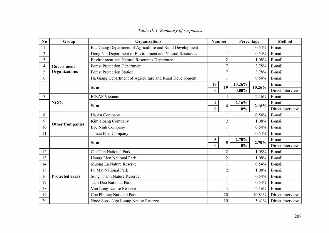
208
Table II. 1. Summary of responses
No Group Organizations Number Percentage Method
1
Government
Organizations
Bac Giang Department of Agriculture and Rural Development 1 0.54% E-mail
2 Dong Nai Department of Environment and Natural Resources 1 0.54% E-mail
3 Environment and Natural Resources Department 2 1.08% E-mail
4 Forest Protection Department 7 3.78% E-mail
5 Forest Protection Station 7 3.78% E-mail
6 Ha Giang Department of Agriculture and Rural Development 1 0.54% E-mail
Sum 19
19 10.26%
10.26% E-mail
0 0.00% Direct interview
7
NGOs
ICRAF Vietnam 4 2.16% E-mail
Sum 4
4 2.16%
2.16% E-mail
0 0% Direct interview
8
Other Companies
Ha An Company 1 0.54% E-mail
9 Kim Hoang Company 2 1.08% E-mail
10 Loc Ninh Company 1 0.54% E-mail
11 Thuan Phat Company 1 0.54% E-mail
Sum 5
5 2.70%
2.70% E-mail
0 0% Direct interview
12
Protected areas
Cat Tien National Park 2 1.08% E-mail
13 Hoang Lien National Park 2 1.08% E-mail
14 Muong La Nature Reserve 1 0.54% E-mail
15 Pu Mat National Park 2 1.08% E-mail
16 Song Thanh Nature Reserve 1 0.54% E-mail
17 Tam Dao National Park 1 0.54% E-mail
18 Van Long Nature Reserve 4 2.16% E-mail
19 Cuc Phuong National Park 20 10.81% Direct interview
20 Ngoc Son - Ngo Luong Nature Reserve 10 5.41% Direct interview

209
21 Pu Hu Protected Area 3 1.62% Direct interview
22 Pu Luong Nature Reserve 18 9.73% Direct interview
Sum 13
64 8.32%
34.59% E-mail
51 26.27% Direct interview
23
Universities and
research institutes
Can Tho University 2 1.09% E-mail
24 Environmental Center 1 0.55% E-mail
25 Hanoi National University 1 0.55% E-mail
26 Hanoi University of Agriculture 1 0.55% E-mail
27 Hanoi University of Mining and Geology 1 0.55% E-mail
28 Hue University of Agriculture and Forestry 1 0.55% E-mail
29 Land Management Center 1 0.55% E-mail
30 Tuyen Quang Center of Agroforestry Management and Planning 1 0.55% E-mail
31 Vietnam Center for Monitoring and Technical Resources 2 1.09% E-mail
32 Vietnam Institute of geography 3 1.64% Direct interview
33 Vietnam Institute of forest inventory and planning 2 1.09% E-mail
34 Vietnam Institute of forest science 1 0.55% Direct interview
35 Vietnam Institute of Management for Agriculture and Rural
Development 2 1.09% E-mail
36 Vietnam Institute of natural resource inventory and planning 1 0.55% E-mail
37 Vietnam national university of forestry 73 39.46% Direct interview
Sum 16
93 8.79%
50.41% E-mail
77 41.62% Direct interview
Total 57
185 30.81%
100% E-mail
128 69.19% Direct interview

210
Table II. 2. Statistic of responding questionnaire
Name of criteria Respondents of important levels
Min Max Range Mean Mode Median Outlier 01 Outlier 02
1 2 3 4 5 6 7 8 9 Sum Q1 Q3 1.5*(Q3-Q1) Stdev |Z| > 3
Crit
eria
State 0 0 1 3 15 19 36 40 71 185 3 9 6 7.6 9.0 8.0 7 9 161 1.4 161
Pressure 0 1 2 2 14 21 33 53 59 185 2 9 7 7.6 9.0 8.0 7 9 46’, 58’, 161 1.4 46’, 58’,161
Response 0 1 8 6 15 10 33 39 73 185 2 9 7 7.5 9.0 8.0 7 9 77’, 81’, 83’, 106, 120,
126, 140, 152, 161 1.7 126
Su
b-c
rit
eria
Sta
te Species 0 0 1 0 9 16 37 54 68 185 3 9 6 7.8 9.0 8.0 7 9 161 1.2 161
Ecosystem 1 1 1 4 4 9 32 51 82 185 1 9 8 7.9 9.0 8.0 7 9 34’, 138, 161 1.4 34, 138, 161
Pres
sure Nature 2 4 15 14 34 34 36 37 9 185 1 9 8 6.0 8.0 6.0 5 7 6, 138 1.8
Human 0 0 1 1 1 8 21 35 118 185 3 9 6 8.4 9.0 9.0 8 9
49’, 59’, 77’, 78’, 81’,
82’, 83’, 95’, 97’, 108, 161
1.0 59’, 95’, 161
Resp
on
se Conservation 0 0 4 2 6 17 37 53 66 185 3 9 6 7.7 9.0 8.0 7 9 77’, 81’, 83’, 161 1.4 77’, 81’, 83’, 161
Education 0 0 1 0 7 18 26 42 91 185 3 9 6 8.0 9.0 8.0 7 9 161 1.2 161
Law 0 0 3 1 10 14 28 44 85 185 3 9 6 7.9 9.0 8.0 7 9 59’, 161, 174 1.4 59’, 161, 174
Fa
ctors
Sp
ecie
s Richness 0 0 1 1 15 26 45 44 53 185 3 9 6 7.5 9.0 8.0 7 9 161 1.3 161
Rarity 0 1 1 0 11 17 43 56 56 185 2 9 7 7.6 8.0 8.0 7 9 4, 161 1.3 4, 161
Eco
syst
em
Location 1 2 1 4 20 24 55 52 26 185 1 9 8 7.0 7.0 7.0 6 8 84’, 108, 169 1.5 84’, 108, 169
Topography 0 0 1 7 20 20 60 41 36 185 3 9 6 7.2 7.0 7.0 6 8 1.4
Hydrology 0 4 2 6 28 30 63 38 14 185 2 9 7 6.6 7.0 7.0 6 8 55’, 56’, 61’,161 1.5 55’, 56’, 61’, 161
Climate 0 0 3 2 21 26 50 43 40 185 3 9 6 7.2 7.0 7.0 6 8 1.4
Forest type 0 1 2 5 7 23 45 59 43 185 2 9 7 7.4 8.0 8.0 7 8 4, 5, 29, 55’, 56’, 61’,
81’, 83’, 84’, 87’, 92’,108, 129, 133, 161
1.4 84’, 108, 161
Na
ture
Climate change 0 2 2 2 16 11 24 50 78 185 2 9 7 7.8 9.0 8.0 7 9 4, 34, 83’, 161 1.5 4, 34, 83’, 161
Natural disaster 0 6 5 10 15 32 40 49 28 185 2 9 7 6.8 8.0 7.0 6 8 4, 65’, 101, 106, 133,
161 1.7
Hu
ma
n Distribution 0 0 4 7 19 33 43 45 34 185 3 9 6 7.0 8.0 7.0 6 8 1.5
Density 0 2 4 5 24 31 43 45 31 185 2 9 7 6.9 8.0 7.0 6 8 83’, 161 1.6 83’, 161
Population 0 2 5 4 24 24 35 48 43 185 2 9 7 7.1 8.0 7.0 6 8 90’, 91’i 1.7 90’, 91’
Livelihood 0 0 2 1 7 14 24 45 92 185 3 9 6 8.0 9.0 8.0 7 9 83’, 161 1.3 83’, 108, 161
Co
nse
r
vati
on
Forest management types
0 0 2 5 8 21 38 45 66 185 3 9 6 7.6 9.0 8.0 7 9 161, 174 1.4 161, 174
Size of forest area 0 0 3 1 18 28 47 36 52 185 3 9 6 7.3 9.0 7.0 6 9 1.4 65’, 83’, 161
Total 38 22
':shows the respondents are students

211
Table II. 3. Synthesizing the numbers of respondents in pairwise
Category A A>B
A=B A<B
B Sum 9 8 7 6 5 4 3 2 1/2 1/3 1/4 1/5 1/6 1/7 1/8 1/9 Sum
Factors
State 59 0 0 2 1 11 5 13 27 54 44 12 10 4 0 0 0 0 70 Pressure
State 58 0 0 2 2 9 9 19 17 71 22 13 11 7 1 0 0 0 54 Response
Pressure 61 0 0 1 3 8 9 15 25 58 33 15 5 10 0 1 0 0 64 Response
Criteria
State Species 48 1 0 0 1 2 3 5 36 70 40 20 4 1 0 0 0 0 65 Ecosystem
Pressure Nature 13 0 0 0 0 1 0 3 9 18 40 26 35 24 10 11 4 2 152 Human
Response
Conservation 44 0 0 0 0 1 3 8 32 68 45 14 9 3 0 0 0 0 71 Education
Conservation 38 0 0 0 1 4 7 8 18 80 44 9 7 5 0 0 0 0 65 Law
Education 53 0 0 2 0 2 4 14 31 87 25 14 2 2 0 0 0 0 43 Law
Sub-
criteria
Species Richness 52 0 0 0 0 2 3 22 25 58 41 23 5 3 1 0 0 0 73 Rarity
Ecosystem
Location 54 0 0 0 1 4 3 16 30 59 44 19 4 1 0 0 2 0 70 Topography
Location 80 0 0 0 5 4 5 24 42 56 35 6 3 1 0 1 0 1 47 Hydrology
Location 56 0 0 0 2 1 4 19 30 56 41 18 6 4 1 0 0 1 71 Climate
Location 51 0 0 0 0 2 6 8 35 46 45 26 11 2 1 0 0 1 86 Forest type
Topography 80 0 0 0 0 1 14 23 42 73 23 4 1 2 0 0 0 0 30 Hydrology
Topography 65 0 0 0 0 1 3 22 39 56 37 15 3 5 2 0 0 0 62 Climate
Topography 48 0 1 0 0 1 4 8 34 56 49 17 8 5 0 0 0 0 79 Forest type
Hydrology 21 0 0 0 0 0 1 4 16 84 41 26 8 3 0 0 0 0 78 Climate
Hydrology 28 0 0 1 0 0 1 7 19 57 42 36 8 10 2 0 0 0 98 Forest type
Climate 60 0 0 0 1 1 2 11 45 50 37 24 7 5 0 0 0 0 73 Forest type
Nature Climate change 100 0 1 3 5 4 16 33 38 58 14 7 1 3 0 0 0 0 25 Nature disaster
Human
Distribution 50 0 0 1 0 1 8 13 27 75 46 11 1 0 0 0 0 0 58 Density
Distribution 47 0 0 1 0 2 5 17 22 68 44 17 7 0 0 0 0 0 68 Quantity
Distribution 19 0 0 0 0 1 4 2 12 59 40 33 21 8 2 1 0 0 105 Livelihood
Density 30 0 0 0 0 0 0 6 24 107 33 9 2 1 1 0 0 0 46 Quantity
Density 21 0 0 0 0 0 0 4 17 45 53 36 15 10 2 1 0 0 117 Livelihood
Quantity 21 0 0 0 0 0 0 4 17 45 53 36 15 10 2 1 0 0 117 Livelihood
Conservation Conservation
type 75 0 0 1 0 4 9 27 34 55 34 14 3 0 1 1 0 0 53 Size of PAs
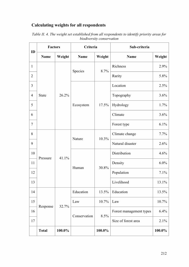
212
Calculating weights for all respondents
Table II. 4. The weight set established from all respondents to identify priority areas for
biodiversity conservation
ID
Factors Criteria Sub-criteria
Name Weight Name Weight Name Weight
1
State 26.2%
Species 8.7%
Richness 2.9%
2 Rarity 5.8%
3
Ecosystem 17.5%
Location 2.5%
4 Topography 3.6%
5 Hydrology 1.7%
6 Climate 3.6%
7 Forest type 6.1%
8
Pressure 41.1%
Nature 10.3%
Climate change 7.7%
9 Natural disaster 2.6%
10
Human 30.8%
Distribution 4.6%
11 Density 6.0%
12 Population 7.1%
13 Livelihood 13.1%
14
Response 32.7%
Education 13.5% Education 13.5%
15 Law 10.7% Law 10.7%
16
Conservation 8.5%
Forest management types 6.4%
17 Size of forest area 2.1%
Total 100.0% 100.0% 100.0%

213
Calculating weights for Protected Areasgroup
Factors
Table II. 5. Pairwise comparison of factors
State Pressure Response
State 1.00 0.50 1.00
Pressure 2.00 1.00 1.00
Response 1.00 1.00 1.00
Sum 4.00 2.50 3.00
Table II. 6. Standardized matrix of factors
State Pressure Response Weight
State 0.250 0.200 0.333 26%
Pressure 0.500 0.400 0.333 41%
Response 0.250 0.400 0.333 33%
Sum 1.000 1.000 1.000 100%
Table II. 7.Consistency test of factors
Compositions Values
n 3
RI 0.520
𝜆 3.054
CI 0.027
CR 0.052
Consistency Yes

214
2. Criteria
Table II. 8. Pairwise comparison of criteria of state
Species Ecosystem
Species 1.00 0.50
Ecosystem 2.00 1.00
Sum 3.00 1.50
Table II. 9. Standardized matrix of criteria of state
Species Ecosystem Weight
Species 0.33 0.33 33%
Ecosystem 0.67 0.67 67%
Sum 1.00 1.00 100%
Table II. 10. Pairwise comparison of criteria of pressure
Nature Human
Nature 1.00 0.25
Human 4.00 1.00
Sum 5.00 1.25
Table II. 11. Standardized matrix of criteria of pressure
Nature Human Weight
Nature 0.20 0.20 20%
Human 0.80 0.80 80%
Sum 1.00 1.00 100%

215
Table II. 12. Pairwise comparison of criteria of response
Conservation Education Law
Conservation 1.00 0.50 1.00
Education 2.00 1.00 1.00
Law 1.00 1.00 1.00
Sum 4.00 2.50 3.00
Table II. 13. Standardized matrix of criteria of response
Conservation Education Law Weight
Conservation 0.25 0.20 0.33 26%
Education 0.50 0.40 0.33 41%
Law 0.25 0.40 0.33 33%
Sum 1.00 1.00 1.00 100%
Table II. 14. Consistency test of criteria of response
Compositions Values
n 3
RI 0.520
𝜆 3.054
CI 0.027
CR 0.052
Consistency Yes
3. Sub-criteria
Table II. 15. Pairwise comparison of sub-criteria of species
Richness Rarity
Richness 1.00 1.00
Rarity 1.00 1.00
Sum 2.00 2.00

216
Table II. 16. Standardized matrix of sub-criteria of species
Richness Rarity Weight
Richness 0.50 0.50 50%
Rarity 0.50 0.50 50%
Sum 1.00 1.00 100%
Table II. 17. Pairwise comparison of sub-criteria of ecosystem
Location Topography Hydrology Climate Forest type
Location 1.00 0.50 3.00 0.50 0.50
Topography 2.00 1.00 3.00 2.00 0.50
Hydrology 0.33 0.33 1.00 1.00 0.33
Climate 2.00 0.50 1.00 1.00 0.33
Forest type 2.00 2.00 3.00 3.00 1.00
Sum 7.33 4.33 11.00 7.50 2.67
Table II. 18. Standardized matrix of sub-criteria of ecosystem
Location Topography Hydrology Climate Forest type Weight
Location 0.14 0.12 0.27 0.07 0.19 15%
Topography 0.27 0.23 0.27 0.27 0.19 25%
Hydrology 0.05 0.08 0.09 0.13 0.13 9%
Climate 0.27 0.12 0.09 0.13 0.13 15%
Forest type 0.27 0.46 0.27 0.40 0.38 36%
Sum 1.00 1.00 1.00 1.00 1.00 100%

217
Table II. 19. Consistency test of sub-criteria of ecosystem
Compositions Values
n 5
RI 1.110
𝜆 5.298
CI 0.074
CR 0.067
Consistency Yes
Table II. 20. Pairwise comparison of sub-criteria of nature
Climate change Natural disaster
Climate change 1.00 3.00
Natural disaster 0.33 1.00
Sum 1.33 4.00
Table II. 21. Standardized matrix of sub-criteria of nature
Climate change Natural disaster Weight
Climate change 0.75 0.75 75%
Natural disaster 0.25 0.25 25%
Sum 1.00 1.00 100%
Table II. 22. Pairwise comparison of sub-criteria of human
Distribution Density Population Livelihood
Distribution 1.00 2.00 1.00 0.33
Density 0.50 1.00 1.00 0.50
Population 1.00 1.00 1.00 0.50
Livelihood 3.00 2.00 2.00 1.00
Sum 5.50 6.00 5.00 2.30

218
Table II. 23. Standardized matrix of sub-criteria of human
Distribution Density Population Livelihood Weight
Distribution 0.18 0.33 0.20 0.14 21%
Density 0.09 0.17 0.20 0.21 17%
Population 0.18 0.17 0.20 0.21 19%
Livelihood 0.55 0.33 0.40 0.43 43%
Sum 1.00 1.00 1.00 1.00 100%
Table II. 24. Consistency test of sub-criteria of human
Compositions Values
n 4
RI 0.890
𝜆 4.119
CI 0.040
CR 0.045
Consistency Yes
Table II. 25. Pairwise comparison of sub-criteria of conservation
Forest management types Size of forest area
Forest management types 1.00 3.00
Size of forest area 0.33 1.00
Sum 1.33 4.00
Table II. 26. Standardized matrix of sub-criteria of conservation
Forest management types Size of forest area Weight
Forest management types 0.75 0.75 75%
Size of forest area 0.25 0.25 25%
Sum 1.00 1.00 100%

219
Table II. 27. The weight set established from the respondents of Protected Areas group
ID
Factors Criteria Sub-criteria
Name Weight Name Weight Name Weight
1
State 26.2%
Species 8.8%
Richness 4.4%
2 Rarity 4.4%
3
Ecosystem 17.4%
Location 2.7%
4 Topography 4.3%
5 Hydrology 1.6%
6 Climate 2.6%
7 Forest type 6.2%
8
Pressure 41.1%
Nature 8.3%
Climate change 6.2%
9 Natural disaster 2.1%
10
Human 32.8%
Distribution 7.1%
11 Density 5.5%
12 Population 6.2%
13 Livelihood 14.0%
14
Response 32.7%
Education 13.5% Education 13.5%
15 Law 10.7% Law 10.7%
16
Conservation 8.5%
Forest management types 6.4%
17 Size of forest area 2.1%
Total 100.0% 100.0% 100.0%

220
Calculating weights for Government Organizationsgroup
Factors
Table II. 28. Pairwise comparison of factors
State Pressure Response
State 1.00 0.50 1.00
Pressure 2.00 1.00 1.00
Response 1.00 1.00 1.00
Sum 4.00 2.50 3.00
Table II. 29. Standardized matrix of factors
State Pressure Response Weight
State 0.25 0.20 0.33 26%
Pressure 0.50 0.40 0.33 41%
Response 0.25 0.40 0.33 33%
Sum 1.00 1.00 1.00 100%
Table II. 30. Consistency test of factors
Compositions Values
n 3
RI 0.520
𝜆 3.054
CI 0.027
CR 0.052
Consistency Yes

221
Criteria
Table II. 31. Pairwise comparison of criteria of state
Species Ecosystem
Species 1.00 0.50
Ecosystem 2.00 1.00
Sum 3.00 1.50
Table II. 32. Standardized matrix of criteria of state
Species Ecosystem Weight
Species 0.33 0.33 33%
Ecosystem 0.67 0.67 67%
Sum 1.00 1.00 100%
Table II. 33. Pairwise comparison of criteria of pressure
Nature Human
Nature 1.00 0.33
Human 3.00 1.00
Sum 4.00 1.33
Table II. 34. Standardized matrix of criteria of pressure
Nature Human Weight
Nature 0.25 0.25 25%
Human 0.75 0.75 75%
Sum 1.00 1.00 100%

222
Table II. 35. Pairwise comparison of criteria of response
Conservation Education Law
Conservation 1.00 2.00 0.50
Education 0.50 1.00 0.50
Law 2.00 2.00 1.00
Sum 3.50 5.00 2.00
Table II. 36. Standardized matrix of criteria of response
Conservation Education Law Weight
Conservation 0.29 0.40 0.25 31%
Education 0.14 0.20 0.25 20%
Law 0.57 0.40 0.50 49%
Sum 1.00 1.00 1.00 100%
Table II. 37. Consistency test of criteria of response
Compositions Values
n 3
RI 0.520
𝜆 3.054
CI 0.027
CR 0.052
Consistency Yes
3. Sub-criteria
Table II. 38. Pairwise comparison of sub-criteria of species
Richness Rarity
Richness 1.00 1.00
Rarity 1.00 1.00
Sum 2.00 2.00

223
Table II. 39. Standardized matrix of sub-criteria of species
Richness Rarity Weight
Richness 0.50 0.50 50%
Rarity 0.50 0.50 50%
Sum 1.00 1.00 100%
Table II. 40. Pairwise comparison of sub-criteria of ecosystem
Location Topography Hydrology Climate Forest type
Location 1.00 1.00 3.00 0.50 0.25
Topography 1.00 1.00 2.00 0.50 0.50
Hydrology 0.33 0.50 1.00 0.33 0.33
Climate 2.00 2.00 3.00 1.00 2.00
Forest type 4.00 2.00 3.00 0.50 1.00
Sum 8.33 6.50 12.00 2.83 4.08
Table II. 41. Standardized matrix of sub-criteria of ecosystem
Location Topography Hydrology Climate Forest type Weight
Location 0.12 0.15 0.25 0.18 0.06 15%
Topography 0.12 0.15 0.17 0.18 0.12 15%
Hydrology 0.04 0.08 0.08 0.12 0.08 8%
Climate 0.24 0.31 0.25 0.35 0.49 33%
Forest type 0.48 0.31 0.25 0.18 0.25 29%
Sum 1.00 1.00 1.00 1.00 1.00 100%

224
Table II. 42. Consistency test of sub-criteria of ecosystem
Compositions Values
n 5
RI 1.110
𝜆 5.256
CI 0.064
CR 0.058
Consistency Yes
Table II. 43. Pairwise comparison of sub-criteria of nature
Climate change Natural disaster
Climate change 1.00 3.00
Natural disaster 0.33 1.00
Sum 1.33 4.00
Table II. 44. Standardized matrix of sub-criteria of nature
Climate change Natural disaster Weight
Climate change 0.75 0.75 75%
Natural disaster 0.25 0.25 25%
Sum 1.00 1.00 100%
Table II. 45. Pairwise comparison of sub-criteria of human
Distribution Density Population Livelihood
Distribution 1.00 0.50 0.50 0.50
Density 2.00 1.00 1.00 0.50
Population 2.00 1.00 1.00 0.50
Livelihood 2.00 2.00 2.00 1.00
Sum 7.00 4.50 4.50 2.50

225
Table II. 46. Standardized matrix of sub-criteria of human
Distribution Density Population Livelihood Weight
Distribution 0.14 0.11 0.11 0.20 14%
Density 0.29 0.22 0.22 0.20 23%
Population 0.29 0.22 0.22 0.20 23%
Livelihood 0.29 0.44 0.44 0.40 40%
Sum 1.00 1.00 1.00 1.00 100%
Table II. 47. Consistency test of sub-criteria of human
Compositions Values
n 4
RI 0.890
𝜆 4.061
CI 0.020
CR 0.023
Consistency Yes
Table II. 48. Pairwise comparison of sub-criteria of conservation
Forest management types Size of forest area
Forest management types 1.00 3.00
Size of forest area 0.33 1.00
Sum 1.33 4.00
Table II. 49. Standardized matrix of sub-criteria of conservation
Forest management
types
Size of forest
area Weight
Forest management
types 0.75 0.75 75%
Size of forest area 0.25 0.25 25%
Sum 1.00 1.00 100%

226
Table II. 50. The weight set established from the respondents of GOs group
ID
Factors Criteria Sub-criteria
Name Weight Name Weight Name Weight
1
State 26.0%
Species 8.6%
Richness 4.3%
2 Rarity 4.3%
3
Ecosystem 17.4%
Location 2.6%
4 Topography 2.6%
5 Hydrology 1.4%
6 Climate 5.7%
7 Forest type 5.1%
8
Pressure 41.1%
Nature 10.3%
Climate change 7.7%
9 Natural disaster 2.6%
10
Human 30.8%
Distribution 4.3%
11 Density 7.2%
12 Population 7.2%
13 Livelihood 12.1%
14
Response 32.9%
Education 6.5% Education 6.5%
15 Law 16.1% Law 16.1%
16
Conservation 10.3%
Forest management types 7.7%
17 Size of forest area 2.6%
Total 100.0% 100.0% 100.0%

227
Calculating weights for Universities and Research Institutesgroup
Factors
Table II. 51. Pairwise comparison of factors
State Pressure Response
State 1.00 1.00 1.00
Pressure 1.00 1.00 0.50
Response 1.00 2.00 1.00
Sum 3.00 4.00 2.50
Table II. 52. Standardized matrix of factors
State Pressure Response Weight
State 0.33 0.25 0.40 33%
Pressure 0.33 0.25 0.20 26%
Response 0.33 0.50 0.40 41%
Sum 1.00 1.00 1.00 100%
Table II. 53. Consistency test of factors
Compositions Values
n 3
RI 0.520
𝜆 3.054
CI 0.027
CR 0.052
Consistency Yes

228
2. Criteria
Table II. 54. Pairwise comparison of criteria of state
Species Ecosystem
Species 1.00 1.00
Ecosystem 1.00 1.00
Sum 2.00 2.00
Table II. 55. Standardized matrix of criteria of state
Species Ecosystem Weight
Species 0.50 0.50 50%
Ecosystem 0.50 0.50 50%
Sum 1.00 1.00 100%
Table II. 56. Pairwise comparison of criteria of pressure
Nature Human
Nature 1.00 0.50
Human 2.00 1.00
Sum 3.00 1.50
Table II. 57. Standardized matrix of criteria of pressure
Nature Human Weight
Nature 0.33 0.33 33%
Human 0.67 0.67 67%
Sum 1.00 1.00 100%

229
Table II. 58. Pairwise comparison of criteria of response
Conservation Education Law
Conservation 1.00 0.50 1.00
Education 2.00 1.00 1.00
Law 1.00 1.00 1.00
Sum 4.00 2.50 3.00
Table II. 59. Standardized matrix of criteria of response
Conservation Education Law Weight
Conservation 0.25 0.20 0.33 26%
Education 0.50 0.40 0.33 41%
Law 0.25 0.40 0.33 33%
Sum 1.00 1.00 1.00 100%
Table II. 60. Consistency test of criteria of response
Compositions Values
n 3
RI 0.520
𝜆 3.054
CI 0.027
CR 0.052
Consistency Yes

230
3. Sub-criteria
Table II. 61. Pairwise comparison of sub-criteria of species
Richness Rarity
Richness 1.00 0.50
Rarity 2.00 1.00
Sum 3.00 1.50
Table II. 62. Standardized matrix of sub-criteria of species
Richness Rarity Weight
Richness 0.33 0.33 33%
Rarity 0.67 0.67 67%
Sum 1.00 1.00 100%
Table II. 63. Pairwise comparison of sub-criteria of ecosystem
Location Topography Hydrology Climate Forest type
Location 1.00 0.50 2.00 0.50 0.50
Topography 2.00 1.00 2.00 1.00 1.00
Hydrology 0.50 0.50 1.00 0.50 0.50
Climate 2.00 1.00 2.00 1.00 2.00
Forest type 2.00 1.00 2.00 0.50 1.00
Sum 7.50 4.00 9.00 3.50 5.00
Table II. 64. Standardized matrix of sub-criteria of ecosystem
Location Topography Hydrology Climate Forest type Weight
Location 0.13 0.13 0.22 0.14 0.10 15%
Topography 0.27 0.25 0.22 0.29 0.20 24%
Hydrology 0.07 0.13 0.11 0.14 0.10 11%
Climate 0.27 0.25 0.22 0.29 0.40 28%
Forest type 0.27 0.25 0.22 0.14 0.20 22%
Sum 1.00 1.00 1.00 1.00 1.00 100%

231
Table II. 65. Consistency test of sub-criteria of ecosystem
Compositions Values
n 5
RI 1.110
𝜆 5.117
CI 0.029
CR 0.026
Consistency Yes
Table II. 66. Pairwise comparison of sub-criteria of nature
Climate change Natural disaster
Climate change 1.00 2.00
Natural disaster 0.50 1.00
Sum 1.50 3.00
Table II. 67. Standardized matrix of sub-criteria of nature
Climate change Natural disaster Weight
Climate change 0.67 0.67 67%
Natural disaster 0.33 0.33 33%
Sum 1.00 1.00 100%
Table II. 68. Pairwise comparison of sub-criteria of human
Distribution Density Population Livelihood
Distribution 1.00 1.00 0.50 0.50
Density 1.00 1.00 1.00 0.50
Population 2.00 1.00 1.00 0.50
Livelihood 2.00 2.00 2.00 1.00
Sum 6.00 5.00 4.50 2.50

232
Table II. 69.Standardized matrix of sub-criteria of human
Distribution Density Population Livelihood Weight
Distribution 0.17 0.20 0.11 0.20 17%
Density 0.17 0.20 0.22 0.20 20%
Population 0.33 0.20 0.22 0.20 24%
Livelihood 0.33 0.40 0.44 0.40 39%
Sum 1.00 1.00 1.00 1.00 100%
Table II. 70. Consistency test of sub-criteria of human
Compositions Values
n 4
RI 0.890
𝜆 4.061
CI 0.020
CR 0.023
Consistency Yes
Table II. 71.Pairwise comparison of sub-criteria of conservation
Forest management types Size of forest area
Forest management types 1.00 2.00
Size of PA 0.50 1.00
Sum 1.50 3.00
Table II. 72. Standardized matrix of sub-criteria of conservation
Forest management types Size of forest area Weight
Forest management types 0.67 0.67 67%
Size of forest area 0.33 0.33 33%
Sum 1.00 1.00 100%

233
Table II. 73. The weight set established from the respondents of URIs group
ID
Factors Criteria Sub-criteria
Name Weight Name Weight Name Weight
1
State 32.8%
Species 16.4%
Richness 5.5%
2 Rarity 10.9%
3
Ecosystem 16.4%
Location 2.4%
4 Topography 4.0%
5 Hydrology 1.8%
6 Climate 4.7%
7 Forest type 3.5%
8
Pressure 26.0%
Nature 8.7%
Climate change 5.8%
9 Natural disaster 2.9%
10
Human 17.3%
Distribution 2.9%
11 Density 3.4%
12 Population 4.1%
13 Livelihood 6.9%
14
Response 41.2%
Education 16.9% Education 16.9%
15 Law 13.5% Law 13.5%
16
Conservation 10.8%
Forest management types 7.2%
17 Size of forest area 3.6%
Total 100.0% 100.0% 100.0%

234
Appendix III. Application of criteria

235
Thanh Hoa Map of forest statistic in 2015 Hoa Binh Map of forest statistic in 2015
Ninh Binh Map of forest statistic in 2015 Cuc Phuong Map of forest statistic in 2015
NSNL Map of forest statistic in 2015 Pu Luong Map of forest statistic in 2015
Figure III. 1: Example of the old maps archived on the fieldwork in 2017

236
Training samples were selected for 1986 Training samples were selected for 1998
Training samples were selected for 2007 Training samples were selected for 2017
Figure III. 2: Samples for supervised classification in 1986, 1998, 2007, and 2017

237
Table III. 1: Overall accuracy of classifications in 1986, 1998, 2007, and 2017
LULC classes
Reference data Total
pixels
Classification accuracy
(%) Kappa
statistic
Overall
accuracy
(%) Forest Grassland Soil Water Producer
accuracy
User
accuracy
1986
Forest 48 0 0 0 48 100.0 100.0 1.00
97.0 Grassland 0 69 1 0 70 98.6 95.8 0.94
Soil 0 3 69 3 75 92.0 98.6 0.98
Water 0 0 0 38 38 100.0 92.7 0.91
1998
Forest 56 0 0 0 56 100.0 96.6 0.96
95.3 Grassland 2 76 0 0 78 97.4 87.4 0.82
Soil 0 11 79 0 90 87.8 100.0 1.00
Water 0 0 0 54 54 100.0 100.0 1.00
2007
Forest 55 0 0 0 55 100.0 100.0 1.00
96.7 Grassland 0 41 0 0 41 100.0 93.2 0.92
Soil 0 3 83 0 86 96.5 93.3 0.90
Water 0 0 6 82 88 93.2 100.0 1.00
2017
Forest 54 0 0 0 54 100.0 87.1 0.83
92.2 Grassland 8 65 0 0 73 89.0 95.6 0.94
Soil 0 3 62 1 66 93.9 91.2 0.88
Water 0 0 6 33 39 84.6 97.1 0.96

238
Table III. 2: Area statistic of LULC changes of specific regions in 1986, 1998, 2007, and 2017
Regions Years Forest Grassland Soil Water Total
ha % ha % ha % ha % ha %
Cuc Phuong
National Park
1986 20,144.3 88.4 1,973.9 8.7 586.1 2.6 88.3 0.4 22,792.6 100.0
1998 19,894.6 87.3 2,642.5 11.6 224.6 1.0 30.8 0.1 22,792.6 100.0
2007 19,246.0 84.4 2,061.9 9.0 1,375.2 6.0 109.5 0.5 22,792.6 100.0
2017 21,197.9 93.0 1,292.6 5.7 266.1 1.2 35.9 0.2 22,792.6 100.0
Ngoc Son – Ngo
Luong Nature
Reserve
1986 14,453.9 66.1 5,660.4 25.9 1,561.9 7.1 196.6 0.9 21,872.8 100.0
1998 13,320.9 60.9 7,293.2 33.3 1,204.9 5.5 53.7 0.2 21,872.8 100.0
2007 12,891.4 58.9 4,791.2 21.9 3,953.1 18.1 237.1 1.1 21,872.8 100.0
2017 16,162.9 73.9 4,914.9 22.5 748.5 3.4 46.5 0.2 21,872.8 100.0
Pu Luong Nature
Reserve
1986 13,177.2 75.3 3,726.7 21.3 567.2 3.2 29.0 0.2 17,500.1 100.0
1998 14,621.1 83.5 2,749.5 15.7 128.6 0.7 1.0 0.0 17,500.1 100.0
2007 15,243.9 87.1 1,205.3 6.9 1,001.7 5.7 49.1 0.3 17,500.1 100.0
2017 16,264.1 92.9 1,102.6 6.3 129.6 0.7 3.7 0.0 17,500.1 100.0
Other areas
1986 33,998.5 39.6 34,051.1 39.7 15,556.4 18.1 2,225.3 2.6 85,831.3 100.0
1998 31,323.1 36.5 41,473.4 48.3 12,406.5 14.5 628.2 0.7 85,831.3 100.0
2007 29,145.5 34.0 28,123.2 32.8 26,905.9 31.3 1,656.6 1.9 85,831.3 100.0
2017 45,075.0 52.5 33,335.5 38.8 6,685.4 7.8 735.3 0.9 85,831.3 100.0

239
Table III. 3: Characteristics of rare species cited by IUCN and VNRB in the study area
No Name IUCN VNRB Land cover Altitude
(m) Others
I Rare animals
1 Scotomanesbeaulieui Least
Concern Vulnerable Forest ≤ 2200
2 Nycticebuspygmaeus Vulnerable Vulnerable Evergreen, semi-evergreen,
limestone forest ≤ 1500
3 Trachypithecusdelacouri Critically
Endangered
Critically
Endangered
Limestone karst forest,
evergreen shrub ≤ 1000
4 Trachypithecusbarbei Data
Deficient Vulnerable Forest
Not in the mix
bamboo forest
5 Hemigalusowstoni Endangered Vulnerable
Suitable forests include some on
limestone and some dominated
by bamboo.
≤ 2600
6 Arctogalidiatrivirgata Least
Concern Lower Risk
Evergreen, semi-evergreen
forest ≥ 600
II Rare plants
7 Alangiumtonkinense Data
Deficient Vulnerable Sparse, secondary forest ≤ 500
Foot of limestone
karst mountain
8 Polyalthiapraeflorens Data
Deficient Endangered Primary forest ≤ 300
9 Vernonia bonapartei Data
Deficient Vulnerable
Sparse, secondary forest on soil
mountain 50 - 500
10 Balanophoracucphuongensis Data
Deficient Endangered
Primary forest on limestone
mountain 200 - 300
11 Balanophoralaxiflora Data
Deficient Endangered Forest 600 - 2300 High moisture

240
12 Rhopalocnemisphalloides Data
Deficient Vulnerable Primary forest 500 - 2000
13 Bursera tonkinensis Vulnerable Vulnerable
Primary and secondary
evergreen forest on limestone
mountains
500 - 700
14 Canariumtramdenum Data
Deficient Vulnerable
Primary and secondary
evergreen forest ≤ 700
15 Codonopsisjavanica Data
Deficient Vulnerable Secondary forest 600 - 2000
16 Vaticasubglabra Endangered Endangered Evergreen forest 300 - 600 Near rivers,
streams
17 Annamocaryasinensis Endangered Endangered Primary forest on limestone
mountains 400 - 1000 Near rivers, valleys
18 Cinnamomumbalansae Endangered Vulnerable Primary evergreen forest ≤ 200
19 Cinnamomumcambodianum Data
Deficient Vulnerable Evergreen forest
20 Aglaia spectabilis Data
Deficient Vulnerable Primary, secondary forest ≤ 700
21 Dysoxylumcauliflorum Data
Deficient Vulnerable
Primary, secondary evergreen
forest on limestone mountain,
valley
≤ 700
22 Dysoxylumloureiri Data
Deficient Vulnerable
Primary, secondary evergreen
forest ≤ 1000
23 Ardisia silvestris Data
Deficient Vulnerable Forest 400 - 1200
Dominated by
shadow, moisture,
humus, around
rivers and streams
24 Rothmanniavietnamensis Data
Deficient Vulnerable
Sparse, secondary forest on
limestone mountains ≈ 400

241
25 Sinoradlkofera minor Vulnerable Endangered Evergreen forest on limestone
mountains and valleys
26 Amorphophallus interruptus Critically
Endangered Lower Risk Limestone forest 300 - 500
Dominated by
humus
27 Amorphophallus
verticillatus Vulnerable Lower Risk
Evergreen forest on limestone
mountain 300 - 450
Dominated by
moisture
28 Calamus platyacanthus Data
Deficient Vulnerable
Primary, secondary evergreen
forest 400 - 900
Dominated by
light, moisture
29 Disporopsislongifolia Data
Deficient Vulnerable
Evergreen forest on limestone
mountain 400 - 1500
Dominated by
moisture, shadow
30 Dendrobium wardianum Data
Deficient Vulnerable Forest 500 - 600
31 Smilax elegantissima Data
Deficient Vulnerable Secondary evergreen forest
Creek, valley, slope
mountain
32 Stemonasaxorum Data
Deficient Vulnerable Forest ≤ 600
Moisture, light, and
near rivers, streams
33 Calocedrusmacrolepis Near
Threatened Endangered Evergreen forest 800 - 2000
34 Cantharelluscibarius Data
Deficient Endangered Forest
❖ IUCN: International Union for Conservation of Nature
❖ VNRB: Vietnam Red Data Book

242
a. Training samples 6. 2017 b. Training samples 8. 2017
c. Training samples 10. 2017 d. Training samples 12. 2017 e. Training samples 4. 2018
Figure III. 3: Training samples for classifications in five months

243
Table III. 4: Error matrices and total classification accuracy in five months
LULC classes
Reference data Total
pixels
Classification
accuracy (%) Kappa
statistic
Overall
accuracy
(%) Forest Grassland Soil Water Producer
accuracy
User
accuracy
June 2017
Forest 54 0 0 0 54 100.0 87.1 0.83
92.2 Grassland 8 65 0 0 73 89.0 95.6 0.94
Soil 0 3 62 1 66 93.9 91.2 0.88
Water 0 0 6 33 39 84.6 97.1 0.96
August 2017
Forest 50 2 0 0 52 96.2 100.0 1.00
88.9 Grassland 0 73 1 0 74 98.6 80.2 0.72
Soil 0 15 44 1 61 72.1 95.7 0.94
Water 0 1 0 39 40 97.5 83.0 0.80
October 2017
Forest 49 2 1 0 52 94.2 100.0 1.00
93.8 Grassland 0 45 3 0 48 93.8 88.2 0.85
Soil 0 4 86 0 90 95.6 90.5 0.85
Water 0 0 5 46 51 90.2 100.0 1.00
December 2017
Forest 52 0 0 0 52 100.0 98.1 0.98
98.5 Grassland 1 69 1 0 71 97.2 98.6 0.98
Soil 0 1 88 0 89 98.9 97.8 0.97
Water 0 0 1 50 51 98.0 100.0 1.00
April 2018
Forest 45 7 0 0 52 86.5 100.0 1.00
84.2 Grassland 0 38 9 1 48 79.2 63.3 0.54
Soil 0 10 81 0 91 89.0 84.4 0.75
Water 0 5 6 39 50 78.0 97.5 0.97

244
Evergreen forest Limestone
Primary forest Secondary forest
Bamboo forest Valley
Hydrology Digital elevation model
Figure III. 4: Layers used to define the suitable habitats of rare species in the study area

245
1. Scotomanes beaulieui 2. Nycticebus pygmaeus
3. Trachypithecus delacouri 4. Trachypithecus barbei
5. Hemigalus owstoni 6. Arctogalidia trivirgata
Figure III. 5: Habitat areas of rare animals in the study area

246
1. Alangium tonkinense 2. Polyalthia praeflorens
3. Vernonia bonapartei 4. Balanophora cucphuongensis
5. Balanophora laxiflora 6. Rhopalocnemis phalloides
7. Bursera tonkinensis 8. Canarium tramdenum
9. Codonopsis javanica 10. Vatica subglabra

247
11. Annamocarya sinensis 12. Cinnamomum balansae
13. Cinnamomum cambodianum 14. Aglaia spectabilis
15. Dysoxylum cauliflorum 16. Dysoxylum loureiri
17. Ardisia silvestris 18. Rothmannia vietnamensis
19. Sinoradlkofera minor 20. Amorphophallus interruptus
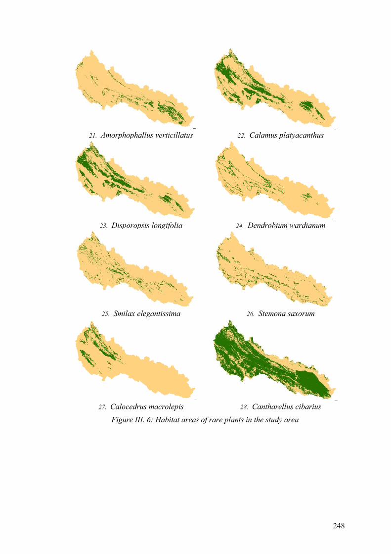
248
21. Amorphophallus verticillatus 22. Calamus platyacanthus
23. Disporopsis longifolia 24. Dendrobium wardianum
25. Smilax elegantissima 26. Stemona saxorum
27. Calocedrus macrolepis 28. Cantharellus cibarius
Figure III. 6: Habitat areas of rare plants in the study area
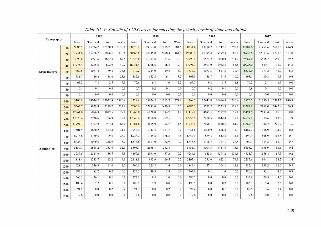
249
Table III. 5: Statistic of LULC areas for selecting the priority levels of slope and altitude
Topography 1986 1998 2007 2017
Forest Grassland Soil Water Forest Grassland Soil Water Forest Grassland Soil Water Forest Grassland Soil Water
Slope (Degree)
10 9886.5 15714.7 12220.9 2028.1 8620.1 19363.0 11285.7 581.5 8331.0 13276.7 16947.1 1295.6 12107.6 21452.6 5615.3 674.9
20 21741.8 15226.7 3876.1 430.6 20366.8 18245.0 2498.4 164.9 19800.4 11395.4 9499.4 580.0 26942.8 12371.6 1777.8 183.0
30 24090.8 9997.6 1657.3 87.5 23628.0 11784.8 387.6 32.7 22990.1 7571.2 5060.0 211.7 29667.0 5576.7 550.2 39.2
40 17975.4 4215.6 692.9 40.2 18041.4 4796.8 76.6 9.3 17294.7 3591.0 1952.5 85.8 20925.0 1809.1 175.7 14.3
50 7667.5 1067.4 189.8 33.8 7710.2 1224.0 19.6 4.7 7337.3 1073.3 517.3 30.4 8532.0 371.2 48.9 6.3
60 1331.7 149.2 38.0 25.5 1382.5 152.5 6.1 3.2 1303.9 158.7 71.5 10.2 1495.1 39.3 9.3 0.6
70 65.2 7.8 2.5 7.3 72.8 6.8 1.0 2.2 67.7 9.8 3.5 1.8 79.2 2.1 1.5 0.0
80 0.4 0.1 0.4 0.0 0.7 0.2 0.1 0.0 0.7 0.2 0.1 0.0 0.9 0.1 0.0 0.0
90 0.1 0.0 0.0 0.0 0.1 0.0 0.0 0.0 0.1 0.0 0.0 0.0 0.1 0.0 0.0 0.0
Altitude (m)
100 3100.9 14034.2 12025.9 2180.4 1228.6 18074.3 11263.7 774.8 768.3 12445.8 16616.9 1510.4 3876.2 21030.5 5593.7 840.9
200 9562.7 9828.9 2279.2 221.8 7606.6 12831.0 1439.8 15.2 6285.5 9752.2 5725.3 129.6 13283.9 7109.0 1442.8 56.9
300 12261.0 5086.3 1012.5 29.1 11965.0 6128.0 294.7 1.2 11119.1 4695.1 2517.7 57.1 15494.5 2691.4 195.0 8.0
400 13020.4 2930.6 786.8 37.1 12648.4 3866.8 259.5 0.2 12256.9 2816.5 1644.0 57.4 14877.1 1710.6 183.2 3.9
500 11794.3 2772.9 967.4 62.4 11584.8 3615.9 394.7 1.5 11226.1 2496.1 1810.5 64.2 13362.9 1984.2 246.2 3.6
600 7501.9 1650.2 423.4 24.1 7753.4 1742.3 101.7 2.2 7644.6 1060.9 856.8 37.3 8487.2 986.9 124.7 0.8
700 6716.6 1350.5 309.5 26.7 6928.2 1345.6 126.8 2.6 6857.1 869.3 642.8 34.1 7490.9 806.9 105.5 0.1
800 6423.3 2080.5 258.9 5.2 6573.8 2111.0 82.9 0.2 6845.5 1118.7 777.1 26.5 7700.3 984.8 82.0 0.7
900 5159.1 2618.2 353.0 52.3 5393.7 2556.1 232.8
5651.7 1014.3 1441.3 75.3 6455.2 1638.9 88.1 0.4
1000 3739.6 2324.0 186.5 7.8 4169.5 2031.0 57.2 0.2 4284.5 545.3 1291.2 136.9 4631.7 1568.8 57.3 0.2
1100 1818.4 1243.7 63.2 4.1 2118.8 993.9 16.5 0.2 2197.4 235.0 622.1 74.9 2287.6 804.1 36.2 1.4
1200 628.8 346.3 11.0 1.2 760.1 225.8 1.4 0.0 844.4 27.1 104.1 11.8 782.4 193.2 11.0 0.8
1300 383.2 85.2 0.2 0.3 427.3 39.3 2.3 0.0 467.6 0.1 1.0 0.2 380.3 83.1 4.6 0.8
1400 360.5 26.1 0.1 0.1 377.2 8.5 1.0 0.0 386.7 0.0 0.0 0.0 355.9 26.3 4.5 0.0
1500 189.4 1.7 0.1 0.0 188.2 2.9 0.0 0.0 190.5 0.0 0.7 0.0 186.3 2.4 2.5 0.0
1600 91.8 0.0 0.2 0.4 91.3 0.8 0.2 0.2 92.4 0.0 0.1 0.0 89.5 1.6 1.4 0.0
1700 7.6 0.0 0.0 0.0 7.6 0.0 0.0 0.0 7.6 0.0 0.0 0.0 7.6 0.0 0.0 0.0

250
Table III. 6: Area statistics of priority levels of richness of specific regions
Regions Levels of
richness Area (ha) %(SR) %(SA)
Pu Luong Nature
Reserve
Very low 1,236.0 7.1 0.8
Low 1,406.5 8.0 1.0
Medium 1,025.9 5.9 0.7
High 1,523.0 8.7 1.0
Very high 12,308.7 70.3 8.3
Sum 17,500.1 100.0 11.8
Ngoc Son - Ngo Luong
Nature Reserve
Very low 5,710.0 26.1 3.9
Low 3,679.2 16.8 2.5
Medium 745.5 3.4 0.5
High 652.4 3.0 0.4
Very high 11,085.8 50.7 7.5
Sum 21,872.8 100.0 14.8
Cuc Phuong National
Park
Very low 1,594.6 7.0 1.1
Low 1,971.6 8.7 1.3
Medium 261.7 1.1 0.2
High 524.0 2.3 0.4
Very high 18,440.6 80.9 12.5
Sum 22,792.6 100.0 15.4
Other areas
Very low 40,756.2 47.5 27.5
Low 17,287.9 20.1 11.7
Medium 3,078.6 3.6 2.1
High 2,562.1 3.0 1.7
Very high 22,146.4 25.8 15.0
Sum 85,831.3 100.0 58.0
Total
Very low 49,296.8 33.3 33.3
Low 24,345.2 16.4 16.4
Medium 5,111.7 3.5 3.5
High 5,261.5 3.6 3.6
Very high 63,981.4 43.2 43.2
Sum 147,996.7 100.0 100.0
SR: Specific region SA: Study area

251
Table III. 7: Area statistic of priority levels of rarity in the study area
Specific Regions Levels of
rarity
Area
ha % (SR) % (SA)
Cuc Phuong National Park
Very low 1,513.1 6.6 1.0
Low 2,600.3 11.4 1.8
Medium 4,408.8 19.3 3.0
High 13,367.2 58.6 9.0
Very high 903.1 4.0 .6
Sum 22,792.5 100.0 15.4
Ngoc Son - Ngo Luong
Nature Reserve
Very low 5,623.2 25.7 3.8
Low 5,397.9 24.7 3.6
Medium 3,229.3 14.8 2.2
High 5,335.2 24.4 3.6
Very high 2,287.3 10.5 1.5
Sum 21,872.8 100.0 14.8
Pu Luong Nature Reserve
Very low 1,156.7 6.6 .8
Low 3,145.3 18.0 2.1
Medium 5,637.7 32.2 3.8
High 4,610.8 26.3 3.1
Very high 2,949.6 16.9 2.0
Sum 17,500.1 100.0 11.8
Other areas
Very low 40,852.4 47.6 27.6
Low 22,018.5 25.7 14.9
Medium 11,103.5 12.9 7.5
High 7,920.4 9.2 5.4
Very high 3,936.5 4.6 2.7
Sum 85,831.3 100.0 58.0
Total
Very low 49,145.3 33.2 33.2
Low 33,162.0 22.4 22.4
Medium 24,379.2 16.5 16.5
High 31,233.7 21.1 21.1
Very high 10,076.6 6.8 6.8
Sum 147,996.7 100.0 100.0

252
Table III. 8: Area statistic of priority levels of location in the study area
Specific regions Priority levels
Area
ha % (SR) % (SA)
Cuc Phuong National Park
Low 1,646.3 7.2 1.1
Medium 14,899.9 65.4 10.1
High 6,246.3 27.4 4.2
Sum 22,792.5 100.0 15.4
Ngoc Son - Ngo Luong
Nature Reserve
Low 0.0 0.0 0.0
Medium 10,829.9 49.5 7.3
High 11,042.9 50.5 7.5
Sum 21,872.8 100.0 14.8
Pu Luong Nature Reserve
Low 0.0 0.0 0.0
Medium 7,870.4 45.0 5.3
High 9,629.7 55.0 6.5
Sum 17,500.1 100.0 11.8
Other areas
Low 9,035.5 10.5 6.1
Medium 55,076.8 64.2 37.2
High 21,718.9 25.3 14.7
Sum 85,831.2 100.0 58.0
Total
Low 10,681.8 7.2 7.2
Medium 88,677.0 59.9 59.9
High 48,637.9 32.9 32.9
Sum 147,996.6 100.0 100.0

253
Table III. 9: Area statistic of priority levels of topography in the study area
Specific regions Levels of
topography
Area
ha % (SR) % (SA)
Cuc Phuong National Park
Very low 1,808.60 7.9 1.2
Low 4,531.20 19.9 3.1
Medium 6,091.70 26.7 4.1
High 8,113.20 35.6 5.5
Very high 2,247.80 9.9 1.5
Sum 22,792.50 100.0 15.4
Ngoc Son - Ngo Luong Nature
Reserve
Very low 8,728.40 39.9 5.9
Low 3,984.10 18.2 2.7
Medium 5,559.00 25.4 3.8
High 3,283.70 15.0 2.2
Very high 317.60 1.5 .2
Sum 21,872.80 100.0 14.8
Pu Luong Nature Reserve
Very low 6,109.30 34.9 4.1
Low 5,417.00 31.0 3.7
Medium 4,931.80 28.2 3.3
High 976.50 5.6 .7
Very high 65.50 .4 .0
Sum 17,500.10 100.0 11.8
Other areas
Very low 46,752.60 54.5 31.6
Low 11,293.00 13.2 7.6
Medium 13,030.50 15.2 8.8
High 8,652.10 10.1 5.8
Very high 6,103.00 7.1 4.1
Sum 85,831.20 100.0 58.0
Total
Very low 63,398.70 42.8 42.8
Low 25,225.30 17.0 17.0
Medium 29,613.20 20.0 20.0
High 21,025.60 14.2 14.2
Very high 8,733.90 5.9 5.9
Sum 147,996.70 100.0 100.0

254
Table III. 10: Area statistic of priority levels of climate in the study area
Specific regions
Stable levels
of
temperature
Area
ha % (SR) % (SA)
Cuc Phuong National Park
Very low 921.0 4.0 .6
Low 4,413.6 19.4 3.0
Medium 5,800.0 25.4 3.9
High 8,458.0 37.1 5.7
Very high 3,199.8 14.0 2.2
Sum 22,792.5 100.0 15.4
Ngoc Son - Ngo Luong
Nature Reserve
Very low 516.2 2.4 .3
Low 6,310.9 28.9 4.3
Medium 8,046.0 36.8 5.4
High 5,347.1 24.4 3.6
Very high 1,652.7 7.6 1.1
Sum 21,872.8 100.0 14.8
Pu Luong Nature Reserve
Very low 154.0 .9 .1
Low 1,658.6 9.5 1.1
Medium 4,736.8 27.1 3.2
High 6,758.3 38.6 4.6
Very high 4,192.4 24.0 2.8
Sum 17,500.1 100.0 11.8
Other areas
Very low 6,989.6 8.1 4.7
Low 17,222.3 20.1 11.6
Medium 21,433.6 25.0 14.5
High 25,124.9 29.3 17.0
Very high 15,060.9 17.5 10.2
Sum 85,831.2 100.0 58.0
Total
Very low 8,580.8 5.8 5.8
Low 29,605.5 20.0 20.0
Medium 40,016.4 27.0 27.0
High 45,688.2 30.9 30.9
Very high 24,105.8 16.3 16.3
Sum 147,996.7 100.0 100.0
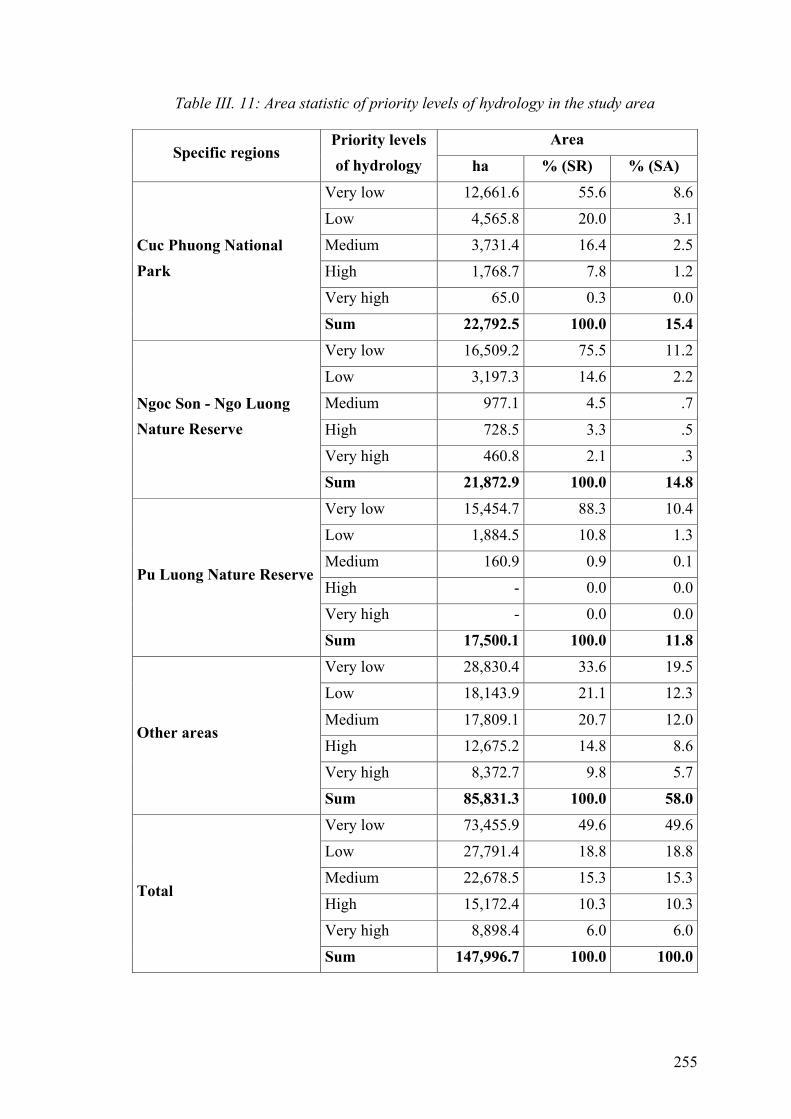
255
Table III. 11: Area statistic of priority levels of hydrology in the study area
Specific regions Priority levels
of hydrology
Area
ha % (SR) % (SA)
Cuc Phuong National
Park
Very low 12,661.6 55.6 8.6
Low 4,565.8 20.0 3.1
Medium 3,731.4 16.4 2.5
High 1,768.7 7.8 1.2
Very high 65.0 0.3 0.0
Sum 22,792.5 100.0 15.4
Ngoc Son - Ngo Luong
Nature Reserve
Very low 16,509.2 75.5 11.2
Low 3,197.3 14.6 2.2
Medium 977.1 4.5 .7
High 728.5 3.3 .5
Very high 460.8 2.1 .3
Sum 21,872.9 100.0 14.8
Pu Luong Nature Reserve
Very low 15,454.7 88.3 10.4
Low 1,884.5 10.8 1.3
Medium 160.9 0.9 0.1
High - 0.0 0.0
Very high - 0.0 0.0
Sum 17,500.1 100.0 11.8
Other areas
Very low 28,830.4 33.6 19.5
Low 18,143.9 21.1 12.3
Medium 17,809.1 20.7 12.0
High 12,675.2 14.8 8.6
Very high 8,372.7 9.8 5.7
Sum 85,831.3 100.0 58.0
Total
Very low 73,455.9 49.6 49.6
Low 27,791.4 18.8 18.8
Medium 22,678.5 15.3 15.3
High 15,172.4 10.3 10.3
Very high 8,898.4 6.0 6.0
Sum 147,996.7 100.0 100.0

256
Table III. 12: Categories of forest types based on maps of forest statistic in three provinces
ID English Categories Levels Vietnamese categories Code Weight Area
(ha)
Area
(%)
1
Natural forest on
limestone mountain
Rich Rõnggçtùnhiªnnói ®¸ LRTX giµu TXDG 4 11,781.05 7.13
2 Medium Rõnggçtùnhiªnnói ®¸ LRTX TB TXDB 3 9,033.35 5.47
3 Poor Rõnggçtùnhiªnnói ®¸ LRTX nghÌo TXDN 2 17,816.29 10.78
4 Rehabilitation
Rõnggçtùnhiªnnói ®¸ LRTX phôchåi TXDP 2 12,276.05 7.43
5 §Êtcãc©ygçt¸isinhnói ®¸ DT2D 2 1,156.16 0.70
6 Very poor Rõnggçtùnhiªnnói ®¸ LRTX nghÌokiÖt
TXDK 1 10,348.08 6.26
7 Mixed forest on
limestone mountain Rõnghçngiaotùnhiªnnói ®¸ HGD 2 19.58 0.01
8
Natural forest on soil
mountain
Rich Rõnggçtùnhiªnnói ®Êt LRTX giµu TXG 3 449.28 0.27
9 Medium Rõnggçtùnhiªnnói ®Êt LRTX TB TXB 2 3,646.12 2.21
10 Poor Rõnggçtùnhiªnnói ®Êt LRTX nghÌo TXN 1 6,919.56 4.19
11 Rehabilitation
Rõnggçtùnhiªnnói ®Êt LRTX phôchåi TXP 1 9,522.97 5.76
12 §Êtcãc©ygçt¸isinhnói ®Êt DT2 1 531.29 0.32
13 Very poor Rõnggçtùnhiªnnói ®Êt LRTX nghÌokiÖt
TXK 0 4,634.94 2.80
14 Mixed forest on soil
mountain
Rõnghçngiao G-TN tùnhiªnnói ®Êt HG1 1 465.70 0.28
15 Rõnghçngiao TN-G tùnhiªnnói ®Êt HG2 1 91.51 0.06
16 Natural forest of Palm
on soil mountain Rõngcaudõatùnhiªnnói ®Êt CD 1 6.14 0.00

257
17 Plantation forest on
limestone mountain Rõnggçtrångnói ®¸ RTGD 2 53.05 0.03
18 Plantation forest on soil
mountain
Rõnggçtrångnói ®Êt RTG 1 22,573.90 13.66
19 Rõngtrångkh¸cnói ®Êt RTK 1 17.81 0.01
20 §Êt ®· trångrõngtrªnnói ®Êt DTR 1 2,634.48 1.59
21 Plantation forest of
Palm Rõngcaudõatrång c¹n RTCD 1 92.08 0.06
22 Bamboo forest on
limestone mountain Rõngtrenøatrångnói ®¸ RTTND 2 156.08 0.09
23
Bamboo forest on soil
mountain
Rõngnøatùnhiªnnói ®Êt NUA 1 19.59 0.01
24 RõngvÇutùnhiªnnói ®Êt VAU 1 49.94 0.03
25 Rõngtre/luångtùnhiªnnói ®Êt TLU 1 97.53 0.06
26 Rõngtrenøatrångnói ®Êt RTTN 1 5,291.70 3.20
27 Water MÆtníc MN 0 32.03 0.02
28 Agricultural land
§Êtn«ngnghiÖpnói ®Êt NN 0 2,374.18 1.44
29 §Êtn«ngnghiÖpnói ®¸ NND 0 31.64 0.02
30 Bare land
§Êttrèngnói ®Êt DT1 0 22,414.27 13.56
31 §Êttrèngnói ®¸ DT1D 0 449.60 0.27
32 Other Lands §Êtkh¸c DK 0 20,265.16 12.27
Total 165,251.09 100.00

258
Table III. 13: Area statistic of priority levels of forest types in the study area
Specific regions Priority levels Area
ha % (SR) % (SA)
Cuc Phuong National Park
Very low 1,220.2 5.4 0.8
Low 4,837.2 21.2 3.3
Medium 3,279.6 14.4 2.2
High 1,848.0 8.1 1.2
Very high 11,607.5 50.9 7.8
Sum 22,792.6 100.0 15.4
Ngoc Son - Ngo Luong
Nature Reserve
Very low 7,237.2 33.1 4.9
Low 6,998.4 32.0 4.7
Medium 7,560.2 34.6 5.1
High 77.0 0.4 0.1
Very high 0.0 0.0 0.0
Sum 21,872.8 100.0 14.8
Pu Luong Nature Reserve
Very low 1,176.2 6.7 0.8
Low 4,598.9 26.3 3.1
Medium 5,769.8 33.0 3.9
High 5,955.2 34.0 4.0
Very high 0.0 0.0 0.0
Sum 17,500.1 100.0 11.8
Other areas
Very low 26,220.3 30.5 17.7
Low 40,585.1 47.3 27.4
Medium 17,432.8 20.3 11.8
High 1,552.6 1.8 1.0
Very high 40.4 0.0 0.0
Sum 85,831.3 100.0 58.0
Total
Very low 35,853.9 24.2 24.2
Low 57,019.7 38.5 38.5
Medium 34,042.5 23.0 23.0
High 9,432.8 6.4 6.4
Very high 11,647.9 7.9 7.9
Sum 147,996.7 100.0 100.0

259
Table III. 14: Area statistic of pressure of climate change in the study area
Specific regions
Pressure of
Climate
Change
Area
ha % (SR) % (SA)
Cuc Phuong National
Park
Low 21,245.5 93.2 14.4
Medium 272.5 1.2 0.2
High 1,274.5 5.6 0.9
Very high 0.0 0.0 0.0
Sum 22,792.5 100.0 15.4
Ngoc Son - Ngo Luong
Nature Reserve
Low 331.2 1.5 .2
Medium 6,112.2 27.9 4.1
High 11,924.8 54.5 8.1
Very high 3,504.7 16.0 2.4
Sum 21,872.9 100.0 14.8
Pu Luong Nature Reserve
Low 607.5 3.5 0.4
Medium 10,469.2 59.8 7.1
High 5,683.0 32.5 3.8
Very high 740.5 4.2 0.5
Sum 17,500.1 100.0 11.8
Other areas
Low 21,023.8 24.5 14.2
Medium 25,609.7 29.8 17.3
High 36,465.6 42.5 24.6
Very high 2,732.1 3.2 1.8
Sum 85,831.3 100.0 58.0
Total
Low 43,207.9 29.2 29.2
Medium 42,463.6 28.7 28.7
High 55,347.9 37.4 37.4
Very high 6,977.3 4.7 4.7
Sum 147,996.8 100.0 100.0

260
Table III. 15: Information on natural disasters in Vietnam from 1997 to 2018
ID Event Date Latitude Longitude Weight
1 Tropical cyclone 2018/8/14 18.671 105.692 2
2 Flood 2018/7/18 22.289 103.489 3
3 Flood 2018/6/23 22.776 104.969 3
4 Tropical cyclone 2017/12/25 10.833 106.650 2
5 Tropical cyclone 2017/11/4 14.058 108.277 2
6 Flood 2017/11/2 13.499 108.622 3
7 Flash flood 2017/10/11 14.058 108.277 2
8 Tropical cyclone 2017/9/14 17.918 106.169 2
9 Flood 2017/8/27 21.908 105.641 3
10 Flash flood 2017/8/3 21.714 104.900 2
11 Tropical cyclone 2017/7/25 17.500 106.500 2
12 Flood 2016/12/13 15.199 108.793 3
13 Tropical cyclone 2016/10/13 17.482 106.584 2
14 Epidemic 2016/4/12 14.058 108.277 1
15 Drought 2015/10/1 14.058 108.277 2
16 Flood 2015/7/26 20.977 107.038 3
17 Other 2015/3/2 10.434 107.145 1
18 Tropical cyclone 2014/7/20 22.426 104.200 2
19 Flood 2013/11/14 14.058 108.277 3
20 Tropical cyclone 2013/11/8 14.058 108.277 2
21 Tropical cyclone 2013/10/15 14.058 108.277 2
22 Tropical cyclone 2013/10/1 14.058 108.277 2
23 Tropical cyclone 2013/9/24 14.058 108.277 2
24 Flood 2013/9/6 14.058 108.277 3
25 Tropical cyclone 2012/10/29 14.058 108.277 2
26 Flood 2012/9/7 19.809 105.777 3
27 Tropical cyclone 2012/8/17 14.058 108.277 2
28 Severe local storm 2012/4/23 14.058 108.277 1
29 Epidemic 2012/3/15 14.058 108.277 1
30 Flood 2011/11/6 14.058 108.277 3
31 Tropical cyclone 2011/9/30 14.058 108.277 2
32 Flood 2011/9/12 14.072 108.958 3
33 Epidemic 2011/8/1 14.058 108.277 1
34 Flood 2010/11/29 14.058 108.277 3
35 Flood 2010/11/17 21.017 105.842 3
36 Flood 2010/10/4 14.058 108.277 3
37 Tropical cyclone 2010/8/24 14.058 108.277 2
38 Tropical cyclone 2010/7/17 20.861 106.680 2

261
39 Flood 2010/5/13 22.655 106.064 3
40 Tropical cyclone 2009/11/4 14.058 108.277 2
41 Flood 2009/9/28 14.058 108.277 3
42 Tropical cyclone 2009/9/30 14.058 108.277 2
43 Flood 2009/7/5 14.058 108.277 3
44 Tropical cyclone 2008/11/18 14.058 108.277 2
45 Flash flood 2008/11/1 14.058 108.277 2
46 Flash flood 2008/10/20 14.058 108.277 2
47 Tropical cyclone 2008/10/1 14.058 108.277 2
48 Flash flood 2008/9/25 14.058 108.277 2
49 Flood 2008/8/26 14.058 108.277 3
50 Flash flood 2008/8/8 14.058 108.277 2
51 Flood 2007/10/17 15.124 108.812 3
52 Flash flood 2007/10/28 14.058 108.277 2
53 Flood 2007/10/28 14.058 108.277 3
54 Tropical cyclone 2007/10/3 14.058 108.277 2
55 Flood 2007/8/6 14.058 108.277 3
56 Tropical cyclone 2006/5/17 14.058 108.277 2
57 Tropical cyclone 2006/12/5 14.058 108.277 2
58 Tropical cyclone 2006/10/1 14.058 108.277 2
59 Flood 2006/8/20 14.058 108.277 3
60 Tropical cyclone 2006/7/11 14.058 108.277 2
61 Tropical cyclone 2006/5/22 14.058 108.277 2
62 Tropical cyclone 2005/11/18 19.807 105.785 2
63 Tropical cyclone 2005/11/2 14.058 108.277 2
64 Flash flood 2005/12/14 14.058 108.277 2
65 Tropical cyclone 2005/11/2 15.539 108.019 2
66 Flood 2005/10/28 14.058 108.277 3
67 Tropical cyclone 2005/9/27 14.058 108.277 2
68 Flood 2005/9/10 14.058 108.277 3
69 Flood 2004/10/5 14.058 108.277 3
70 Tropical cyclone 2004/11/27 15.539 108.019 2
71 Flash flood 2004/7/23 22.803 104.978 2
72 Tropical cyclone 2004/6/14 14.058 108.277 2
73 Flood 2003/10/15 21.017 105.842 3
74 Tropical cyclone 2003/7/23 14.058 108.277 2
75 Severe local storm 2002/10/0 14.058 108.277 1
76 Tech. Disaster 2002/10/29 10.823 106.630 1
77 Flood 2002/9/20 18.341 105.907 3
78 Flood 2002/9/0 10.787 105.190 3
79 Flood 2002/8/1 14.058 108.277 3

262
80 Wildfire 2002/3/23 9.599 105.091 2
81 Drought 2002/3/0 14.058 108.277 2
82 Tropical cyclone 2001/8/11 18.341 105.907 2
83 Tropical cyclone 2001/11/12 14.058 108.277 2
84 Flood 2001/11/4 14.058 108.277 3
85 Severe local storm 2001/11/12 14.058 108.277 1
86 Tech. Disaster 2001/11/11 10.965 107.432 1
87 Flood 2001/10/24 15.441 108.695 3
88 Tech. Disaster 2001/10/15 11.674 108.863 1
89 Flood 2001/8/28 14.058 108.277 3
90 Severe local storm 2001/8/11 14.058 108.277 1
91 Flood 2001/6/30 14.058 108.277 3
92 Tech. Disaster 2001/6/6 14.058 108.277 1
93 Severe local storm 2001/7/4 21.571 105.551 1
94 Tech. Disaster 2001/6/13 21.684 104.566 1
95 Tech. Disaster 2001/4/13 14.058 108.277 1
96 Tech. Disaster 2001/4/7 14.058 108.277 1
97 Tropical cyclone 2000/8/20 14.058 108.277 2
98 Flood 2000/11/0 14.058 108.277 3
99 Slide 2000/10/3 14.058 108.277 2
100 Severe local storm 2000/9/10 18.294 105.675 1
101 Severe local storm 2000/8/24 9.092 104.968 1
102 Severe local storm 2000/8/24 10.022 105.091 1
103 Severe local storm 2000/8/24 10.377 106.344 1
104 Severe local storm 2000/8/20 14.058 108.277 1
105 Severe local storm 2000/7/10 9.972 105.688 1
106 Slide 2000/7/22 14.058 108.277 2
107 Flood 2000/7/7 14.058 108.277 3
108 Severe local storm 2000/6/12 20.231 106.464 1
109 Tech. Disaster 2000/2/14 19.234 104.920 1
110 Flood 1999/12/6 14.058 108.277 3
111 Flood 1999/10/18 14.058 108.277 3
112 Flood 1999/8/0 14.058 108.277 3
113 Drought 1999/3/0 14.058 108.277 2
114 Severe local storm 1998/11/0 14.058 108.277 1
115 Flood 1998/10/0 14.058 108.277 3
116 Drought 1998/5/0 14.058 108.277 2
117 Severe local storm 1997/11/2 14.058 108.277 1
118 Tropical cyclone 1997/9/20 16.052 108.215 2
119 Tropical cyclone 1997/11/2 14.058 108.277 2
Source: http://www.glidenumber.net

263
Table III. 16: Area statistic of settlements in the study area
Specific regions Types of
settlement
Area
ha % (SR) % (SA)
Cuc Phuong National Park
Urban settlement 0.0 0.0 0.0
Rural settlement 143.2 0.6 0.1
Other lands 22,649.4 99.4 15.3
Sum 22,792.5 100.0 15.4
Ngoc Son - Ngo Luong Nature
Reserve
Urban settlement 0.0 0.0 0.0
Rural settlement 1,128.1 5.2 0.8
Other lands 20,744.5 94.8 14.0
Sum 21,872.6 100.0 14.8
Pu Luong Nature Reserve
Urban settlement 0.0 0.0 0.0
Rural settlement 57.2 0.3 0.0
Other lands 17,442.9 99.7 11.8
Sum 17,500.1 100.0 11.8
Other areas
Urban settlement 183.2 0.2 0.1
Rural settlement 6,779.3 7.9 4.6
Other lands 78,868.7 91.9 53.3
Sum 85,831.3 100.0 58.0
Total
Urban settlement 183.2 0.1 0.1
Rural settlement 8,107.8 5.5 5.5
Other lands 139,705.5 94.4 94.4
Sum 147,996.5 100.0 100.0

264
Table III. 17: Area statistic of pressure of population distribution in the study area
Specific regions
Pressure of
population
distribution
Area
ha % (SR) % (SA)
Cuc Phuong National Park
Very high 64.1 0.3 0.0
High 792.2 3.5 0.5
Medium 2,385.0 10.5 1.6
Low 4,438.8 19.5 3.0
Very low 15,112.5 66.3 10.2
Sum 22,792.5 100.0 15.4
Ngoc Son - Ngo Luong Nature
Reserve
Very high 671.0 3.1 0.5
High 1,679.5 7.7 1.1
Medium 2,377.9 10.9 1.6
Low 7,560.1 34.6 5.1
Very low 9,584.3 43.8 6.5
Sum 21,872.8 100.0 14.8
Pu Luong Nature Reserve
Very high 0.0 0.0 0.0
High 0.0 0.0 0.0
Medium 0.0 0.0 0.0
Low 3,676.2 21.0 2.5
Very low 13,823.8 79.0 9.3
Sum 17,500.1 100.0 11.8
Other areas
Very high 10,473.7 12.2 7.1
High 11,117.9 13.0 7.5
Medium 11,906.6 13.9 8.0
Low 27,485.4 32.0 18.6
Very low 24,847.7 28.9 16.8
Sum 85,831.2 100.0 58.0
Total
Very high 11,208.8 7.6 7.6
High 13,589.6 9.2 9.2
Medium 16,669.5 11.3 11.3
Low 43,160.5 29.2 29.2
Very low 63,368.4 42.8 42.8
Sum 147,996.6 100.0 100.0

265
Table III. 18: The population and area of communes in and around the study area
Provinces Districts Communes Population Area(ha)
HoaBinh Lac Son AnNghia 6,210 2,693.3
Chi Dao 2,233 1,086.9
Chi Thien 2,298 717.9
Dinh Cu 3,833 1,099.2
Huong Nhuong 2,646 1,189.9
Lien Vu 4,041 1,097.2
Ngoc Lau 2,164 3,042.7
Ngoc Son 1,785 3,358.2
Phu Luong 2,248 2,171.5
Tan My 5,562 3,143.6
Tu Do 2,044 5,058.3
Vu Lam 3,480 744.8
Yen Nghiep 4,746 2,320.2
Total 43,290 27,723.4
Mai Chau Chieng Chau 3,518 1,715.6
Mai Ha 2,495 1,753.6
Nong Luong 1,314 1,610.2
Pu Pin 1,432 2,147.6
ThungKhe 1,518 1,853.8
Van Mai 3,061 3,553.5
Total 13,338 12,634.2
Tan Lac Bac Son 1,139 1,405.9
Do Nhan 2,158 1,864.3
Gia Mo 2,694 1,986.8
Lo Son 2,860 1,667.9
Lung Van 1,484 2,134.7
Nam Son 1,435 2,034.5
Ngo Luong 1,221 3,845.4
QuyetChien 1,340 2,614.5
Total 14,331 17,554.0
Yen Thuy Lac Thinh 5,066 3,132.3
Ngoc Luong 7,735 2,535.6
Phu Lai 2,824 1,177.3

266
TT. Hang Tram 3,526 188.9
Yen Lac 8,187 3,010.0
Yen Tri 6,004 1,747.5
Total 33,342 11,791.6
NinhBinh Nho Quan Cuc Phuong 2,729 12,348.2
Van Phuong 4,076 883.6
Yen Quang 5,884 1,069.8
Total 12,689 14,301.6
Thanh Hoa Ba Thuoc Ban Cong 5,802 4,270.7
Co Lung 3,386 4,896.3
Ha Trung 2,686 3,734.7
Lung Cao 4,903 7,903.7
Lung Niem 2,705 1,389.9
Luong Noi 3,538 5,680.3
Tan Lap 2,700 1,338.0
Thanh Lam 3,216 2,759.7
Thanh Son 3,899 3,964.0
Total 32,835 35,937.3
Quan Hoa Hoi Xuan 2,989 7,004.7
Phu Le 1,988 4,305.7
Phu Nghiem 981 1,926.7
Phu Thanh 1,583 3,005.9
Phu Xuan 1,943 2,524.4
Thanh Xuan 2,753 7,742.4
TT. Quan Hoa 2,676 389.1
Total 14,913 26,898.9
Thach Thanh Thach Lam 2,288 6,504.3
Thach Quang 4,956 2,033.2
Thach Tuong 3,116 3,865.4
Thanh My 3,994 2,236.6
Thanh Yen 2,906 4,388.9
Total 17,260 19,028.3
(Source: General Statistics Office of Vietnam)

267
Table III. 19: Area statistic of pressure of population density in the study area
Specific regions
Pressure of
population
density
Area
Area % (SR) % (SA)
Cuc Phuong National Park
Very high 0.0 0.0 0.0
High 313.0 1.4 0.2
Medium 2,683.1 11.8 1.8
Low 5,858.7 25.7 4.0
Very low 13,937.7 61.2 9.4
Sum 22,792.5 100 15.4
Ngoc Son - Ngo Luong
Nature Reserve
Very high 0.0 0.0 0.0
High 828.7 3.8 0.6
Medium 1,498.4 6.9 1.0
Low 10,203.5 46.6 6.9
Very low 9,342.3 42.7 6.3
Sum 21,872.8 100 14.8
Pu Luong Nature Reserve
Very high 0.0 0.0 0.0
High 0.0 0.0 0.0
Medium 22.0 0.1 0.0
Low 8,668.7 49.5 5.9
Very low 8,809.4 50.3 6.0
Sum 17,500.1 100 11.8
Other areas
Very high 620.4 0.7 0.4
High 12,040.2 14 8.1
Medium 18,549.2 21.6 12.5
Low 42,254.2 49.2 28.6
Very low 12,367.3 14.4 8.4
Sum 85,831.2 100 58
Total
Very high 620.4 0.4 0.4
High 13,181.9 8.9 8.9
Medium 22,752.6 15.4 15.4
Low 66,985.2 45.3 45.3
Very low 44,456.7 30.0 30.0
Sum 147,996.7 100 100

268
Table III. 20: Area statistic of pressure of population in the study area
Specific regions
Pressure of
population
density
Area
Area % (SR) % (SA)
Cuc Phuong National Park
Very high 1.8 0.0 0.0
High 683.4 3.0 0.5
Medium 2,529.5 11.1 1.7
Low 5,389.2 23.6 3.6
Very low 14,188.6 62.3 9.6
Sum 22,792.5 100.0 15.4
Ngoc Son - Ngo Luong
Nature Reserve
Very high 131.6 0.6 0.1
High 1,044.5 4.8 0.7
Medium 857.3 3.9 0.6
Low 4,573.2 20.9 3.1
Very low 15,266.2 69.8 10.3
Sum 21,872.8 100.0 14.8
Pu Luong Nature Reserve
Very high 0.0 0.0 0.0
High 0.0 0.0 0.0
Medium 0.0 0.0 0.0
Low 2,874.3 16.4 1.9
Very low 14,625.8 83.6 9.9
Sum 17,500.1 100.0 11.8
Other areas
Very high 3,592.5 4.2 2.4
High 8,550.2 10.0 5.8
Medium 14,376.0 16.7 9.7
Low 23,382.8 27.2 15.8
Very low 35,929.7 41.9 24.3
Sum 85,831.2 100.0 58.0
Total
Very high 3,726.0 2.5 2.5
High 10,278.1 6.9 6.9
Medium 17,762.8 12.0 12.0
Low 36,219.6 24.5 24.5
Very low 80,010.3 54.1 54.1
Sum 147,996.7 100.0 100.0

269
Table III. 21: Summary of population and LULC areas of communes around the study area
ID Province District Commune Population Forest Plantation &
Rehabilitation Agriculture Settlement
Bare
land Others Total
A Hoa Binh Total 104,301 39,630.2 2,327.9 2,159.9 5,618.9 5,507.9 14,733.8 69,978.6
I Lac Son Sum 43,290 14,802.7 703.2 803.8 2,820.8 2,296.8 6,394.7 27,821.9
1 AnNghia 6,210 1,176.1 39.0 119.1 380.1 209.9 776.3 2,700.5
2 Chi Dao 2,233 410.2 56.9 62.0 199.9 35.5 330.0 1,094.4
3 Chi Thien 2,298 180.8 95.2 40.6 164.5 13.4 223.4 717.9
4 Dinh Cu 3,833 331.1 74.4 9.9 198.7 72.2 423.0 1,109.4
5 Huong Nhuong 2,646 145.3 235.2 139.8 188.1 127.3 369.2 1,204.9
6 Lien Vu 4,041 339.0 72.9 25.8 174.1 57.8 430.0 1,099.6
7 Ngoc Lau 2,164 1,802.3 8.2 10.7 171.3 623.8 428.7 3,045.0
8 Ngoc Son 1,785 2,390.5 0.9 0.0 238.1 264.3 465.2 3,359.0
9 Phu Luong 2,248 1,132.2 42.2 5.1 303.1 173.2 515.6 2,171.5
10 Tan My 5,562 1,336.4 14.6 265.2 334.3 443.1 789.1 3,182.7
11 Tu Do 2,044 4,379.8 0.6 0.0 81.0 270.0 329.4 5,060.7
12 Vu Lam 3,480 165.8 32.1 23.2 163.4 2.0 368.9 755.4
13 Yen Nghiep 4,746 1,013.1 31.1 102.4 224.3 4.3 946.0 2,321.1
II Mai
Chau
Sum 13,338 9,550.6 41.9 558.4 123.1 986.6 1,396.5 12,657.0
14 Chieng Chau 3,518 1,187.4 0.0 30.8 16.7 207.6 273.1 1,715.5
15 Mai Ha 2,495 1,276.4 0.0 13.7 0.0 164.6 298.9 1,753.6
16 Nong Luong 1,314 1,078.0 0.0 152.0 43.9 154.8 181.5 1,610.1
17 Pu Pin 1,432 1,524.5 0.0 117.0 36.8 253.1 217.1 2,148.4
18 ThungKhe 1,518 1,369.3 3.8 241.1 23.4 93.1 123.2 1,853.9
19 Van Mai 3,061 3,115.0 38.1 3.8 2.3 113.4 302.8 3,575.3

270
III Tan Lac Sum 14,331 10,770.8 706.0 489.9 965.8 2,107.3 2,652.3 17,692.0
20 Bac Son 1,139 631.9 0.0 0.2 140.2 433.1 200.6 1,405.9
21 Do Nhan 2,158 1,383.3 10.4 0.0 173.5 122.7 211.0 1,901.0
22 Gia Mo 2,694 1,138.1 209.5 19.3 191.2 92.5 381.3 2,032.0
23 Lo Son 2,860 593.0 464.1 5.0 159.2 94.9 400.7 1,717.0
24 Lung Van 1,484 1,092.8 18.3 310.7 78.9 274.3 359.7 2,134.7
25 Nam Son 1,435 1,129.1 0.8 6.7 114.1 409.3 374.4 2,034.5
26 Ngo Luong 1,221 2,802.0 0.0 0.2 55.5 578.5 409.2 3,845.4
27 QuyetChien 1,340 2,000.6 2.9 147.7 53.1 102.0 315.3 2,621.5
IV Yen
Thuy
Sum 33,342 4,506.2 876.8 307.9 1,709.3 117.3 4,290.4 11,807.7
28 Lac Thinh 5,066 1,630.6 149.9 267.1 202.2 4.9 884.3 3,139.0
29 Ngoc Luong 7,735 524.7 176.9 0.8 569.3 72.9 1,196.6 2,541.2
30 Phu Lai 2,824 452.5 55.2 11.7 141.9 5.4 510.8 1,177.5
31 TT. Hang Tram 3,526 0.0 0.0 0.0 110.1 0.0 78.8 188.9
32 Yen Lac 8,187 1,333.4 489.6 10.2 296.3 1.1 881.0 3,011.5
33 Yen Tri 6,004 565.0 5.1 18.0 389.6 33.0 738.9 1,749.7
B Ninh
Binh
Total 12,689 11,276.8 38.8 39.0 439.0 102.4 2,431.4 14,327.3
I Nho
Quan
Sum 12,689 11,276.8 38.8 39.0 439.0 102.4 2,431.4 14,327.3
34 Cuc Phuong 2,729 11,217.0 31.6 39.0 147.4 85.1 851.1 12,371.2
35 Van Phuong 4,076 50.1 7.1 0.0 124.1 17.3 685.3 883.9
36 Yen Quang 5,884 9.6 0.0 0.0 167.5 0.0 895.1 1,072.2
C Thanh
Hoa
Total 65,008 60,977.5 1,850.0 79.0 2,676.3 5,140.0 11,767.6 82,490.4
I Ba
Thuoc
Sum 32,835 25,992.4 1,074.3 34.6 1,304.1 1,781.2 5,752.9 35,939.4
37 Ban Cong 5,802 2,720.2 268.0 1.5 323.1 165.0 793.9 4,271.6
38 Co Lung 3,386 3,792.1 148.9 4.0 113.5 391.9 446.1 4,896.4
39 Ha Trung 2,686 2,845.0 63.6 1.9 155.0 71.4 598.1 3,735.1
40 Lung Cao 4,903 6,680.1 126.9 23.0 154.1 187.5 732.9 7,904.4
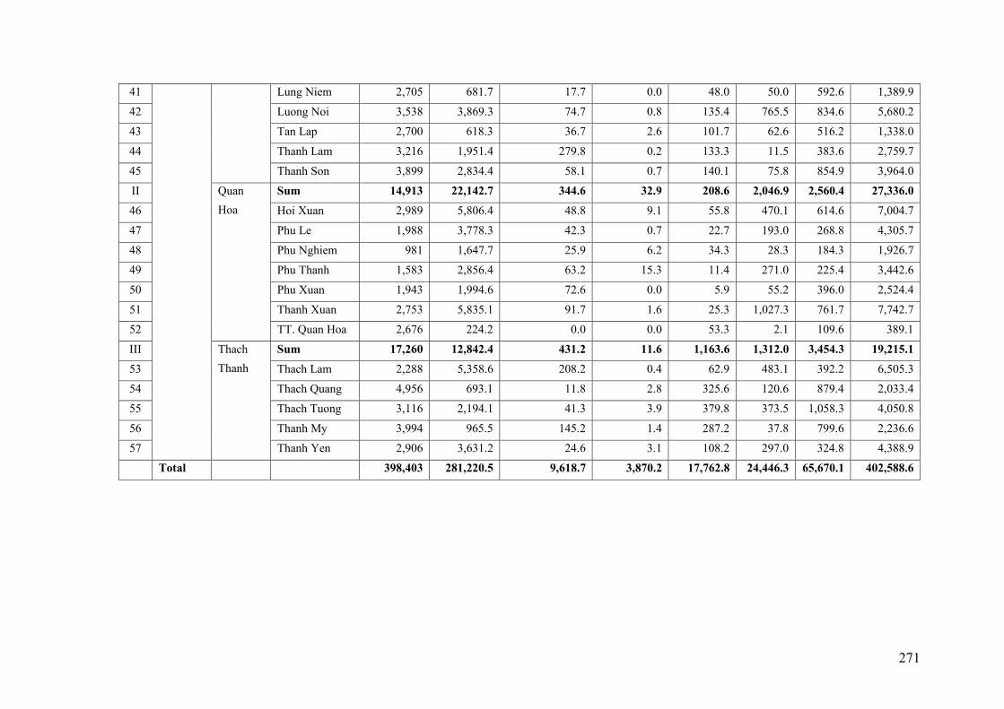
271
41 Lung Niem 2,705 681.7 17.7 0.0 48.0 50.0 592.6 1,389.9
42 Luong Noi 3,538 3,869.3 74.7 0.8 135.4 765.5 834.6 5,680.2
43 Tan Lap 2,700 618.3 36.7 2.6 101.7 62.6 516.2 1,338.0
44 Thanh Lam 3,216 1,951.4 279.8 0.2 133.3 11.5 383.6 2,759.7
45 Thanh Son 3,899 2,834.4 58.1 0.7 140.1 75.8 854.9 3,964.0
II Quan
Hoa
Sum 14,913 22,142.7 344.6 32.9 208.6 2,046.9 2,560.4 27,336.0
46 Hoi Xuan 2,989 5,806.4 48.8 9.1 55.8 470.1 614.6 7,004.7
47 Phu Le 1,988 3,778.3 42.3 0.7 22.7 193.0 268.8 4,305.7
48 Phu Nghiem 981 1,647.7 25.9 6.2 34.3 28.3 184.3 1,926.7
49 Phu Thanh 1,583 2,856.4 63.2 15.3 11.4 271.0 225.4 3,442.6
50 Phu Xuan 1,943 1,994.6 72.6 0.0 5.9 55.2 396.0 2,524.4
51 Thanh Xuan 2,753 5,835.1 91.7 1.6 25.3 1,027.3 761.7 7,742.7
52 TT. Quan Hoa 2,676 224.2 0.0 0.0 53.3 2.1 109.6 389.1
III Thach
Thanh
Sum 17,260 12,842.4 431.2 11.6 1,163.6 1,312.0 3,454.3 19,215.1
53 Thach Lam 2,288 5,358.6 208.2 0.4 62.9 483.1 392.2 6,505.3
54 Thach Quang 4,956 693.1 11.8 2.8 325.6 120.6 879.4 2,033.4
55 Thach Tuong 3,116 2,194.1 41.3 3.9 379.8 373.5 1,058.3 4,050.8
56 Thanh My 3,994 965.5 145.2 1.4 287.2 37.8 799.6 2,236.6
57 Thanh Yen 2,906 3,631.2 24.6 3.1 108.2 297.0 324.8 4,388.9
Total
398,403 281,220.5 9,618.7 3,870.2 17,762.8 24,446.3 65,670.1 402,588.6

272
Table III. 22: Area statistic of pressure of livelihood in the study area
Specific regions Pressure of
livelihood
Area
ha % (SR) % (SA)
Cuc Phuong National Park
Very high 45.0 0.2 0.0
High 572.7 2.5 0.4
Medium 1,873.0 8.2 1.3
Low 5,797.1 25.4 3.9
Very low 14,504.7 63.6 9.8
Sum 22,792.5 100.0 15.4
Ngoc Son - Ngo Luong
Nature Reserve
Very high 0.0 0.0 0.0
High 915.0 4.2 0.6
Medium 2,147.5 9.8 1.5
Low 8,298.4 37.9 5.6
Very low 10,512.0 48.1 7.1
Sum 21,872.9 100.0 14.8
Pu Luong Nature Reserve
Very high 0.0 0.0 0.0
High 0.0 0.0 0.0
Medium 0.0 0.0 0.0
Low 4,961.4 28.4 3.4
Very low 12,538.7 71.6 8.5
Sum 17,500.1 100.0 11.8
Other areas
Very high 2,882.2 3.4 1.9
High 10,805.1 12.6 7.3
Medium 17,577.3 20.5 11.9
Low 28,723.6 33.5 19.4
Very low 25,843.0 30.1 17.5
Sum 85,831.2 100.0 58.0
Total
Very high 2,927.2 2.0 2.0
High 12,292.8 8.3 8.3
Medium 21,597.8 14.6 14.6
Low 47,780.5 32.3 32.3
Very low 63,398.3 42.8 42.8
Sum 147,996.6 100.0 100.0

273
Table III. 23: Area statistic of priority levels of forest management types in the study area
Specific regions Protection
levels
Area
ha % (SR) % (SA)
Cuc Phuong National Park
Very high 20,992.9 92.1 14.2
High 0.6 0.0 0.0
Medium 828.0 3.6 0.6
Low 64.4 0.3 0.0
Very low 906.6 4.0 0.6
Sum 22,792.5 100.0 15.4
Ngoc Son - Ngo Luong
Nature Reserve
Very high 33.5 0.2 0.0
High 15,380.5 70.3 10.4
Medium 1,081.5 4.9 0.7
Low 581.2 2.7 0.4
Very low 4,796.1 21.9 3.2
Sum 21,872.8 100.0 14.8
Pu Luong Nature Reserve
Very high 0.0 0.0 0.0
High 16,759.8 95.8 11.3
Medium 18.2 0.1 0.0
Low 56.2 0.3 0.0
Very low 665.9 3.8 0.4
Sum 17,500.1 100.0 11.8
Other areas
Very high 386.9 0.5 0.3
High 125.9 0.1 0.1
Medium 26,116.4 30.4 17.6
Low 22,236.2 25.9 15.0
Very low 36,965.5 43.1 25.0
Sum 85,831.0 100.0 58.0
Total
Very high 21,413.4 14.5 14.5
High 32,266.8 21.8 21.8
Medium 28,044.1 18.9 18.9
Low 22,938.0 15.5 15.5
Very low 43,334.1 29.3 29.3
Sum 147,996.4 100.0 100.0

274
Table III. 24. Area statistic of priority levels of forest size in the study area
Specific regions Priority
levels of sizes
Area
ha % (SR) % (SA)
Cuc Phuong National Park
Very high 20,874.4 91.6 14.1
High 300.5 1.3 0.2
Medium 30.1 0.1 0.0
Low 481.3 2.1 0.3
Very low 1,106.2 4.9 0.7
Sum 22,792.5 100.0 15.4
Ngoc Son - Ngo Luong
Nature Reserve
Very high 15,285.6 69.9 10.3
High 919.9 4.2 0.6
Medium 112.2 0.5 0.1
Low 0.0 0.0 0.0
Very low 5,555.2 25.4 3.8
Sum 21,872.8 100.0 14.8
Pu Luong Nature Reserve
Very high 11,300.1 64.6 7.6
High 12.4 0.1 0.0
Medium 5,430.4 31.0 3.7
Low 26.8 0.2 0.0
Very low 730.4 4.2 0.5
Sum 17,500.1 100.0 11.8
Other areas
Very high 464.2 0.5 0.3
High 12,729.3 14.8 8.6
Medium 7,980.0 9.3 5.4
Low 10,606.2 12.4 7.2
Very low 54,051.6 63.0 36.5
Sum 85,831.3 100.0 58.0
Total
Very high 47,924.2 32.4 32.4
High 13,962.1 9.4 9.4
Medium 13,552.7 9.2 9.2
Low 11,114.3 7.5 7.5
Very low 61,443.4 41.5 41.5
Sum 147,996.7 100.0 100.0

275
Table III. 25. Area statistic of priority levels of education in the study area
Specific regions
Impact
levels of
education
Area
ha % (SR) % (SA)
Cuc Phuong National Park
Very high 0.0 0.0 0.0
High 55.4 0.2 0.0
Medium 1,184.9 5.2 0.8
Low 4,902.1 21.5 3.3
Very low 16,650.2 73.1 11.3
Sum 22,792.5 100.0 15.4
Ngoc Son - Ngo Luong
Nature Reserve
Very high 16.4 0.1 0.0
High 3,541.7 16.2 2.4
Medium 1,169.4 5.3 0.8
Low 4,033.0 18.4 2.7
Very low 13,112.5 59.9 8.9
Sum 21,872.9 100.0 14.8
Pu Luong Nature Reserve
Very high 0.0 0.0 0.0
High 1,844.5 10.5 1.2
Medium 8,625.0 49.3 5.8
Low 6,694.0 38.3 4.5
Very low 336.7 1.9 0.2
Sum 17,500.1 100.0 11.8
Other areas
Very high 5,536.6 6.5 3.7
High 13,159.2 15.3 8.9
Medium 21,595.3 25.2 14.6
Low 21,672.5 25.3 14.6
Very low 23,867.5 27.8 16.1
Sum 85,831.1 100.0 58.0
Total
Very high 5,552.9 3.8 3.8
High 18,600.8 12.6 12.6
Medium 32,574.5 22.0 22.0
Low 37,301.5 25.2 25.2
Very low 53,966.9 36.5 36.5
Sum 147,996.7 100.0 100.0
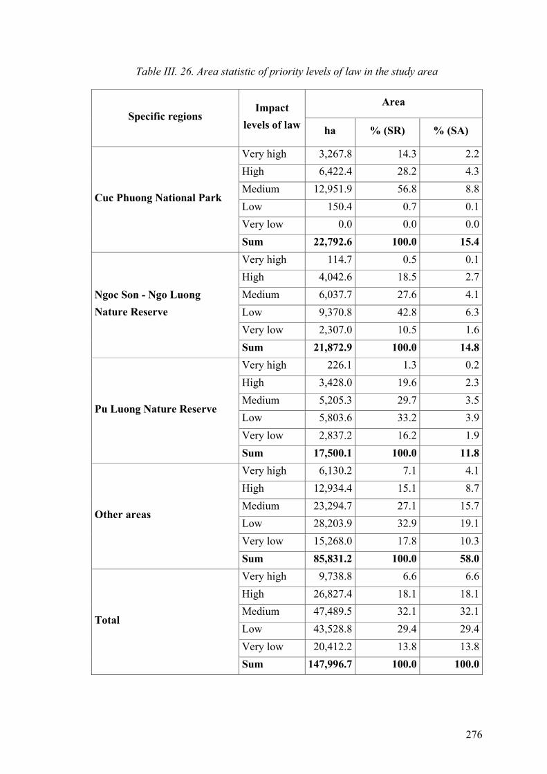
276
Table III. 26. Area statistic of priority levels of law in the study area
Specific regions Impact
levels of law
Area
ha % (SR) % (SA)
Cuc Phuong National Park
Very high 3,267.8 14.3 2.2
High 6,422.4 28.2 4.3
Medium 12,951.9 56.8 8.8
Low 150.4 0.7 0.1
Very low 0.0 0.0 0.0
Sum 22,792.6 100.0 15.4
Ngoc Son - Ngo Luong
Nature Reserve
Very high 114.7 0.5 0.1
High 4,042.6 18.5 2.7
Medium 6,037.7 27.6 4.1
Low 9,370.8 42.8 6.3
Very low 2,307.0 10.5 1.6
Sum 21,872.9 100.0 14.8
Pu Luong Nature Reserve
Very high 226.1 1.3 0.2
High 3,428.0 19.6 2.3
Medium 5,205.3 29.7 3.5
Low 5,803.6 33.2 3.9
Very low 2,837.2 16.2 1.9
Sum 17,500.1 100.0 11.8
Other areas
Very high 6,130.2 7.1 4.1
High 12,934.4 15.1 8.7
Medium 23,294.7 27.1 15.7
Low 28,203.9 32.9 19.1
Very low 15,268.0 17.8 10.3
Sum 85,831.2 100.0 58.0
Total
Very high 9,738.8 6.6 6.6
High 26,827.4 18.1 18.1
Medium 47,489.5 32.1 32.1
Low 43,528.8 29.4 29.4
Very low 20,412.2 13.8 13.8
Sum 147,996.7 100.0 100.0

277