European CO 2 prices and carbon capture investments

Energy Economics 30 (2008) 2992–3015

Contents lists available at ScienceDirect

Energy Economics

j ourna l homepage: www.e lsev ie r.com/ locate /eneco

European CO2 prices and carbon capture investments

Luis M. Abadie 1, José M. Chamorro⁎a Bilbao Bizkaia Kutxa, Gran Vía, 30, 48009 Bilbao, Spainb University of the Basque Country, Dpt. Fundamentos del Análisis Económico I, Av. Lehendakari Aguirre, 83, 48015 Bilbao, Spain

a r t i c l e i n f o

⁎ Corresponding author. Tel.: +34 946013769; fax:E-mail addresses: [email protected] (L.M. A

1 Tel.: +34 607408748; fax: +34 944017996.

0140-9883/$ – see front matter © 2008 Elsevier B.V.doi:10.1016/j.eneco.2008.03.008

a b s t r a c t

Article history:Received 5 July 2007Received in revised form 14 March 2008Accepted 15 March 2008Available online 1 April 2008

We assess the option to install a carbon capture and storage (CCS) unitin a coal-fired power plant operating in a carbon-constrainedenvironment. We consider two sources of risk, namely the price ofemission allowance and the price of the electricity output. First weanalyse the performance of the EU market for CO2 emissionallowances. Specifically, we focus on the contracts maturing in theKyoto Protocol's first commitment period (2008 to 2012) and calibratethe underlying parameters of the allowance price process. Then werefer to the Spanish wholesale electricity market and calibrate theparameters of the electricity price process.We use a two-dimensional binomial lattice to derive the optimalinvestment rule. In particular, we obtain the trigger allowance pricesabove which it is optimal to install the capture unit immediately. Wefurther analyse the effect of changes in several variables on thesecritical prices, among them allowance price volatility and ahypothetical government subsidy.We conclude that, at current permit prices, immediate installationdoes not seem justified from a financial point of view. This need not bethe case, though, if carbon market parameters change dramatically,carbon capture technology undergoes significant improvements, and/or a specific governmental policy to promote these units is adopted.

© 2008 Elsevier B.V. All rights reserved.

JEL classification:C6E2D8G3

Keywords:Emissions Trading SchemeCarbon capture and storageReal options

1. Introduction

According to the 1997 Kyoto Protocol the European Union countries agreed to a cap on their CO2

emissions to be achieved by 2008–2012. In particular, the then fifteen member states committedthemselves to an overall reduction of 8% (from a 1990 base) in annual emissions. This overall reduction

+34 946013891.badie), [email protected] (J.M. Chamorro).

All rights reserved.

mailto:[email protected]

mailto:[email protected]

http://dx.doi.org/10.1016/j.eneco.2008.03.008

http://www.sciencedirect.com/science/journal/01409883

2993L.M. Abadie, J.M. Chamorro / Energy Economics 30 (2008) 2992–3015

obligation was then distributed within the EU15 following a Burden Sharing Agreement (BSA). Both theKyoto Protocol and the BSA allocate emission rights to nations, not to individual legal entities.

In order to ease the fulfilment of these commitments several instruments were developed. Two of themare the so-called Joint Implementation and Clean Development Mechanism credits. The third one is theEmissions Trading Scheme (ETS), a systemwhereby CO2 emission permits are traded.2 In fact, EU memberstates face a second cap on annual emissions, namely the ETS total, i.e. the quantity of allowances that areallocated to each country.3 Henceforth each member state developed its own National Allocation Plan(NAP).4 First, this allocates the country's total BSA target between the trading sectors (those that initiallyparticipate in the ETS) and the non-trading sectors. Second, it specifies how the permits in the tradingsector will be distributed among the individual sources.

The ETS envisages several time phases. The first one goes from 2005 to 2007 and can be considered as atrial or “warm-up” period aimed at getting the scheme “up and running”. The second allocation phase isplanned for the period 2008–2012, which coincides with the Kyoto commitment period. From then on,consecutive five-year periods (starting from the 2013–2017 trading period) would span the potential post-Kyoto commitment periods.5

The trading system started operating officially on January 1st 2005. It covers over 10,000 installationswhich are collectively responsible for some 45% of CO2 emissions.6 According to Böhringer et al. (2005), inits initial stage free allowance allocation has been a necessary condition for the ETS to be accepted bycarbon-intensive industries with political clout.7 In spite of this, as Ellerman et al. (2007) point out, theworld's largest ever market in emissions has been established, and EU firms now face a carbon-constrainedreality in form of legally binding emission targets.8

Following Laurikka and Koljonen (2006), emissions trading is likely to impact cash flows in a given periodthrough four mechanisms: existing cost categories (fuel costs), new costs (value of surrendered allowances),energy outputs (price of power and heat), and additional revenues (free allowances). More specifically,European companies face the choice between investing inprojects that help them to reduce greenhouse gases(GHG) emissions (so as to incur lower carbon payments or get some revenue from spare permits), orpurchasing allowances to release GHG emissions. In this scenario, managers have a pressing need for projectselection methodologies that allow them to sharpen decision making. Some of the issues concerned may besuitably analyzed by means of standard finance theory or cost/benefit analysis. Occasionally, when managersdeal with (significantly) irreversible investments, the returns onwhich are (highly) uncertain, and have (non-negligible) flexibility to defer investment, real options analysis can prove beneficial.

Insley (2003) addresses the decision faced by an electric power company regarding its abatementstrategy to comply with the Clean Air Act (the US Acid Rain Program). In particular, the firm has the optionto install a scrubber to limit sulphur dioxide emissions; if the option is exercised, the need to purchaseemissions permits is eliminated. Obviously, the perceived benefit of a scrubber depends on the firm'sexpectations concerning future allowance prices. The paper considers the effect of uncertainty in the price

2 Directive 2003/87/EC establishing a scheme for GHG emission allowance trading within the Community and amending CouncilDirective 96/61/EC.

3 See Convery and Redmond (2007) for a thorough description of the ETS including its institutional and legal framework. Ellermanand Buchner (2007) focus on the distinctive features that have emerged in the allocation of the allowances created by the ETS.

4 Kruger et al. (2007) examine the decentralized structure of the ETS and explore its implications for the efficiency of the marketitself.

5 The European Commission latest (January 2008) proposal suggests putting 1974 million tons of tradable emissions allowanceson the market in 2013, compared with 2080 million tons today, and then reducing this yearly to 1720 million tons by 2020. Thusemissions by all participants in the ETS would be reduced by 21% relative to 2005. The allowance price is expected to increaseaccordingly. At the same time, knowing the post-2012 trading rules early would stabilize the market and would ultimately make itmore efficient.

6 Currently the ETS covers four broad sectors: iron and steel, certain mineral industries, energy production, and pulp and paper.Transport and households, among other sectors, are not covered by the ETS.

7 Under the ETS, utilities have received at least 95% of the allocated permits for 2005–2007 free of charge. For 2008–2012, thispercentage drops to 90%. According to EC plans, as soon as 2013 power plants and energy-intensive industries would no longerreceive a generous allocation of emissions allowances free of charge. Instead, they would have to buy all allowances at auctionsorganized by the member states.

8 Firms whose emissions exceed the allowances they hold at the end of the accounting period must pay a fine (during the pilotperiod, €40 for each extra metric ton of CO2 emitted, and €100 during the commitment period). Those fined must also make up thedeficit by buying the relevant volume of allowances (Convery and Redmond, 2007).

2994 L.M. Abadie, J.M. Chamorro / Energy Economics 30 (2008) 2992–3015

of emissions permits on the decision to install the scrubber. This is a problem of investment underuncertainty.9 Specifically, the firmmust solve for the dollar value of the investment option as well as for theoptimal exercise time, i.e. the optimal time to invest. This takes the form of a “critical” or “trigger” permitsprice above which 7the scrubber must be installed immediately; otherwise, it is better to wait and keep theoption alive. The paper further examines whether US firms' actual behaviour is consistent with optimalbehaviour as predicted by the real options model.

Sarkis and Tamarkin (2005) consider a project of carbon dioxide re-injection. Sometimes gas extractedfrom a new field contains high CO2 levels that must be removed to comply with pipeline transmissionspecifications. Standard practice is to vent this removed CO2 into the atmosphere. The firm's project involvesre-injection and long-term underground storage of CO2 in the reservoir from which the gas was extracted.Again, the firm has flexibility to defer installation of the unit until some future date. This option to delay has avalue; indeed the firm must exploit it in such a way that flexibility attains its highest value if the firm is tomaximize its own value. Consequently, as before, the firm must determine the optimal time to install theequipment. They use internal estimates from British Petroleum-Amoco (BP) for average carbon price in thecoming future and expected annual growth rate in price. Their conclusion is that, unless carbon prices have adramatic upturn, the installation of this equipment should be delayed for an indeterminate time.

This paper considers an EU-based power company which operates a coal-fired power plant. However,generation of electricity on a sustained basis now requires either the purchase of carbon allowances in theETS in order to release CO2 or, alternatively, the installation of a long-lived CO2 capture and storage (CCS)unit.10 Indeed, if initially the firm holds some emission allowances, installing the capture unit may makesense so as to sell the allowances at a high price; if the firm holds no allowances, installing the capture unitmay make sense so as to avoid the purchase of allowances at a high price. In sum, the firm must comparethe value of the allowances with the cost of the CCS unit. As usual, the initial outlay to this unit is well-known, whereas the future price of the permits is uncertain. The unit, though, also incurs a significantconsumption of the plant's electricity output, the price of which evolves stochastically. Therefore, valuationof the capture unit must account for uncertainty on the revenues side (spared allowances) and theexpenditures side (consumed electricity). The firmwe have in mind assesses this investment option in May2007 but looks ahead while trying to exploit any source of information about the future. The ETS plays acrucial role in this respect, alongside its domestic electricity market. Since two sources of risk areconsidered, we use a two-dimensional binomial lattice to derive the optimal investment rule. In particular,we obtain the trigger allowance prices above which it is optimal to install the capture unit immediately.

Relatedpapers typicallyadopt deterministicmodels oraccount for risk in a relatively simplisticmanner (forexample, assuming an ad hoc value for the risk-adjusted rate of return on the investment).11 Our real optionsapplication, instead, relies on risk-neutral valuation, which enables present-value discounting, at the risklessinterest rate, of expected future payoffs (with actual probabilities replaced by risk-neutral ones).

Not surprisingly, different approaches and methodologies give rise to different estimates of the thresholdcarbon price to overcome for the decision to install the CCS unit to be financially sound.12 Though these figuresare not strictly comparable, theymay serve as a benchmarkwhen discussingour numerical results;we addressthis issue below. Our main conclusion is that, at current permit prices, opting for immediate installation doesnot seem justified fromafinancial point of view. This neednot be the case, though, if carbonmarket parameters

9 Dixit and Pindyck (1994) and Trigeorgis (1996) provide thorough analyses of the topic. Developments can be found in Brennanand Trigeorgis (2000) and Schwartz and Trigeorgis (2001).10 Carbon-capture technologies are often divided into three main categories: (i) precombustion capture chemically splits naturalgas (methane) or synthetic gas (from gasified coal) into hydrogen (which is burned) and CO2 (which is sent underground); (ii) post-combustion capture, which separates CO2 from the flue gas before it goes up the stack by means of chemical absorption or othertechniques (it could be retrofitted to existing coal-fired plants); (iii) oxy fuel firing (or nitrogen-free oxidation) separates oxygenfrom the air, releases nitrogen, and burns coal or gas in pure oxygen in semi-closed systems, producing an exhaust gas consisting ofonly water (easily removable) and CO2. See Kavouridis and Koukouzas (2008) for a discussion of planned CCS projects in Europe;Kemp and Kasim (2008) focus on CCS plans by major UK power plants.11 For example, Sekar et al. (2007) adopt a (real) discount rate of 6%, whereas Rubin et al. (2007) set it at 14.8%. This issue isparticularly disturbing in our case since, as Davison (2007) points out, coal-fired plants are [more] sensitive to discount rate [thangas-fired plants] because they are [more] capital intensive.12 One ton of carbon is carried on 3.67 tons of CO2. Scientists customarily measure carbon prices in terms of carbon weight,whereas allowance prices generally quote in terms of CO2 weight. Even after the corresponding adjustments, different figures for thetrigger price are the rule.


change dramatically, carbon capture technology undergoes significant improvements, and/or a specificgovernmental policy to promote these units is adopted. In either case, for the effective future of CO2 controls, itis important for EU officials to recognize that developments of the emissions scheme that induce volatility tendto discourage immediate investment in carbon capture or storage. Under current conditions, it will take manyyears before investing in this technology looks in the utilities' best interest. Indeed, even generous governmentsubsidies to construction might not be very effective in promoting investment in CCS units.

Section 2 provides some background on the European market for carbon allowances and the Spanishwholesale electricity market (OMEL). Then in Section 3 we propose a stochastic model for the allowanceprice and calibrate its parameters from actual ETS data. In particular, we assume a standard geometricBrownian motion and apply Kalman filter to the price series in order to come up with the underlyingdynamics. Concerning electricity price, we assume a mean-reverting stochastic process; parameters arecalibrated using monthly average OMEL prices. A Supercritical Pulverized Coal-fired power plant is thelong-lived facility to be potentially retrofitted with the CCS unit. Section 5 deals with the valuation of thecapture unit. Savings resulting from not having to purchase allowances (or revenues from selling them)must be weighed against fixed and variable costs incurred by the unit. Section 6 addresses the option toinstall the CCS unit alongside the optimal time to invest; a sensitivity analysis is also performed.We furtherconsider a government subsidy to promote early adoption of the CCS unit by utilities. Section 7 concludes.

2. Features of carbon and electricity markets

Cap-and-trade systems in the world have attracted a fair amount of attention. A theoretical discussion ofthe optimal design, and the ensuing permit allocation, can be found inMontero (2000). He studies the optimaldesign problem following literature on the economics of regulation, instrument choice under uncertainty, andoptimal environmental regulation under imperfect information. Montero (2004) further explores somepractical considerations that have proved relevant in the design of permit markets, among them regulator'suncertainty on costs and benefits from pollution control, incomplete enforcement, incomplete monitoring ofemissions and the possibility of voluntary participation from sources not originally regulated.

As Pindyck (2007) points out, the implications of uncertainty are complicated by the fact that manyenvironmental policy problems involve non-linear damage functions, important irreversibilities, and longtime horizons. Specifically, there are two kinds of irreversibilities. A first example can take the form ofdiscrete investments (e.g. in carbon capture units) or expenditure flows (e.g. burning cleaner coal). Thesesunk costs create an opportunity cost of adopting the policy. At the same time, environmental damage isoften partially or totally irreversible. Therefore adopting a policy now has a sunk benefit. In sum, the twokinds of irreversibilities work in opposite directions. It is important to stress that they only matter if there isuncertainty, and that they interact in a sometimes complicated way with it. This in turn affectsenvironmental policy; precisely how, though, depends on the particular problem.

Regarding the problem at hand, the potential investment in a carbon capture unit certainly displayssome irreversibility features. Its range of possible uses is rather limited and it gets intimately linked to theparticular plant retrofittedwith it. Thus firms require the NPV of this investment to be sufficiently high (notmerely above zero) in order to undertake it.

Owing to this irreversibility, the marginal cost of the capture unit may be lower than the allowanceprice. The wedge between themwould reflect the expected present value of the greater flexibility providedby allowances. See Insley (2003).13

The allowance price is also determined to some extent by public regulation. Hence uncertaintysurrounding allowance price emanates from uncertainty surrounding public regulation. In this sense, asNordhaus (2007) points out, quantity-type (as opposed to price-type) regulations are likely to cause volatiletrading prices of CO2 emissions. To some extent, wild swings can bemoderated if banking and borrowing ofallowances are allowed. Most EU member states, however, do not give much leeway in this respect.Needless to say, such gyrations in the price of a costly input (carbon) have undesirable effects on energymarkets and on investment planning.

13 The importance of irreversibility is further reinforced when a company has the option to defer investment. Indeed, one of thelessons from the US Acid Rain Program is that participants often overlooked this deferral option and over-invested in scrubberswhich in turn pushed the price of emission rights downwards. See de Jong et al. (2005).


Besides, in the specific case of the ETS, a centralized demand (the European Commission specifies thesectors that will participate in the market) combines with a decentralized supply (each member statedecides the number of allowances for its national trading sectors). Following Kruger et al. (2007), thismixed structure adds to the difficulty in predicting the future market price of allowances.

Also, the Kyoto Protocol establishes emission targets over a five-year commitment period. According tothis structure, the ETS also encompasses emission allowances over five-year trading periods. The verylength of these periods is an important factor when considering the risk inherent in allowance price.

Moreover, to the extent that a great deal of uncertainty unfolds at the end of each period, the timesequence inwhich information arrives may give rise to cycles in investment decisions. Certainly, regulatorsmay aim at rapid reforms in the light of experience gained recently. But if the periods are short, a sawteethpattern in investment could arise (which in principle may not be desirable); see Yang et al. (in press).14

On the other hand, there is an important difference between standard commodities (like oil) and carbonallowances. A priori, there is no need for allowances on a daily or hourly basis, whereas industrial facilitiesdepend on a sustained flow of energy to work. Facilities under the ETS are only required to possessallowances matching their emissions once a year; besides, they have already been allocated most of theirneeds under the NAPs. This difference may induce a carbon market which is structurally less liquid anddeep than the oil market, for instance; see Reinaud (2007). In such a context, temporary mismatchesbetween buying and selling orders give rise towide fluctuations in price. Thus volatility in the ETSmaywellbe above standard levels in financial markets.15

This high volatility, coupledwith a significant time to defer investment in an irreversible asset, implies ahigh value of the option to invest. Firms know it and regulators should be aware of it.

2.1. The futures market for emission allowances

In anticipation of the establishment of the ETS, beginning in 2004, a futures market in allowancesdeveloped. In January 2005, there were seven brokers operating in the market. By August 2006, they hadbeen joined by five exchanges. Thus contracts on emission allowances are traded on different platforms (inaddition to over-the-counter markets). Due to its volume of operations and liquidity, the European ClimateExchange (ECX) stands apart. It manages the European Climate Exchange Financial Instruments (ECX CFI),which are traded at the London-based International Petroleum Exchange (later acquired by the InterContinental Exchange). Futures price data from ICE have been used here.

The ICE ECX CFI futures contract is a deliverable contract where each Clearing Member with a positionopen at cessation of trading for a contract month is obliged tomake or take delivery of emission allowancesto or from National Registries in accordance with IPE regulations. Contracts with maturities spanning thenext 12 months have been introduced of late. However, except for those maturing in December, trading issparse.16 Additionally, 5 December contracts are listed from December 2008 to 2012. Contract size is 1000metric ton of carbon dioxide equivalent gas. Prices are quoted in euros/metric ton. Finally, as usual infutures markets, trading takes place continuously and all open contracts are marked-to-market daily.

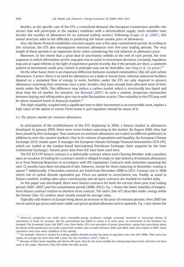
As this paper was developed, there were futures contracts for both the current three-year trial tradingperiod (2005–2007) and the commitment period (2008–2012). Fig. 1 shows the lower volatility of longest-term futures contract relative to shortest-term contract. The latter (Dec-07) describes wider swings whilethe former (Dec-12) evolves more closely around its average value.

Typically cold winters in Europe bring about an increase in the price of emission permits. Over 2005 therise in natural gas prices andmore stable coal prices pushed allowance prices upwards. Fig.1 also shows the

14 America's production tax credit gives renewable-energy producers enough economic incentive to encourage plenty ofinvestment in wind, for instance. But the government has failed to renew it in some years, so investment in the business hasslumped. The Economist (June 2nd 2007) cites Steve Bolze, GE's vice-president of power generation, saying that uncertainty aboutthe future of the production tax credit caused their turbine sales to halve between 2003 and 2004; sales then tripled in 2005, whencustomers were once more confident of the subsidy.15 For example, America's market for trading sulphur-dioxide permits has been in operation since the mid-1990s. Their price hasvaried, on average, by more than 40% a year. See also Nordhaus (2007), Table 4.16 Because of their lower liquidity and shorter life span, they do not seem suitable for valuing long-lived assets and have not beenused in this paper. Moreover, they fall within the pilot period.

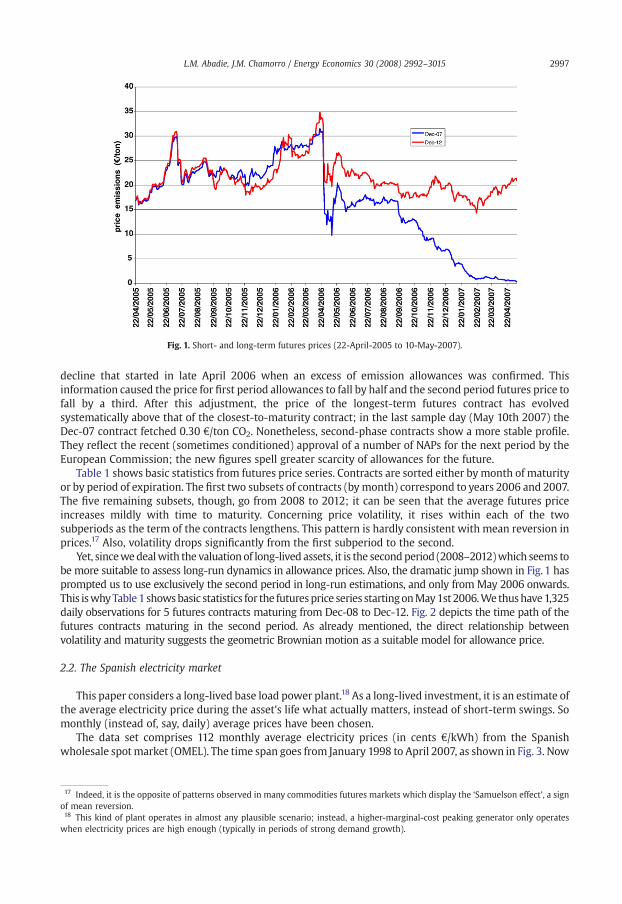
http://dx.doi.org/doi:10.1016/j.eneco.2007.06.004

Fig. 1. Short- and long-term futures prices (22-April-2005 to 10-May-2007).


decline that started in late April 2006 when an excess of emission allowances was confirmed. Thisinformation caused the price for first period allowances to fall by half and the second period futures price tofall by a third. After this adjustment, the price of the longest-term futures contract has evolvedsystematically above that of the closest-to-maturity contract; in the last sample day (May 10th 2007) theDec-07 contract fetched 0.30 €/ton CO2. Nonetheless, second-phase contracts show a more stable profile.They reflect the recent (sometimes conditioned) approval of a number of NAPs for the next period by theEuropean Commission; the new figures spell greater scarcity of allowances for the future.

Table 1 shows basic statistics from futures price series. Contracts are sorted either by month of maturityor by period of expiration. The first two subsets of contracts (bymonth) correspond to years 2006 and 2007.The five remaining subsets, though, go from 2008 to 2012; it can be seen that the average futures priceincreases mildly with time to maturity. Concerning price volatility, it rises within each of the twosubperiods as the term of the contracts lengthens. This pattern is hardly consistent with mean reversion inprices.17 Also, volatility drops significantly from the first subperiod to the second.

Yet, sincewedealwith the valuationof long-lived assets, it is the secondperiod (2008–2012)which seems tobe more suitable to assess long-run dynamics in allowance prices. Also, the dramatic jump shown in Fig. 1 hasprompted us to use exclusively the second period in long-run estimations, and only from May 2006 onwards.This iswhyTable1 showsbasic statistics for the futuresprice series startingonMay1st 2006.We thushave1,325daily observations for 5 futures contracts maturing from Dec-08 to Dec-12. Fig. 2 depicts the time path of thefutures contracts maturing in the second period. As already mentioned, the direct relationship betweenvolatility and maturity suggests the geometric Brownian motion as a suitable model for allowance price.

2.2. The Spanish electricity market

This paper considers a long-lived base load power plant.18 As a long-lived investment, it is an estimate ofthe average electricity price during the asset's life what actually matters, instead of short-term swings. Somonthly (instead of, say, daily) average prices have been chosen.

The data set comprises 112 monthly average electricity prices (in cents €/kWh) from the Spanishwholesale spotmarket (OMEL). The time span goes from January 1998 to April 2007, as shown in Fig. 3. Now

17 Indeed, it is the opposite of patterns observed in many commodities futures markets which display the ‘Samuelson effect’, a signof mean reversion.18 This kind of plant operates in almost any plausible scenario; instead, a higher-marginal-cost peaking generator only operateswhen electricity prices are high enough (typically in periods of strong demand growth).

Table 1Summary statistics for CO2 emission allowances (2006–2012)

Futures contracts Observations Price (€/ton) Maturity (years)

Mean Std. Dev. Mean Std. Dev.

1755 16.80 4.80 3.31 1.92

Grouped by month of maturity1. Dec-06 165 13.67 3.29 0.32 0.182. Dec-07 265 9.58 6.56 1.12 0.303. Dec-08 265 17.49 2.19 2.12 0.304. Dec-09 265 18.06 2.21 3.11 0.305. Dec-10 265 18.63 2.23 4.13 0.306. Dec-11 265 19.20 2.26 5.13 0.307. Dec-12 265 19.77 2.28 6.12 0.30

Grouped by period of expiration2006–2007 430 11.15 5.88 0.81 0.472008–2012 1325 18.63 2.37 4.12 1.45

Daily data from 01-V-2006 to 10-V-2007.


Table 2 displays some basic statistics from the monthly price series. In this case, a price process showingmean reversion seems plausible.

3. Stochastic models and parameter estimates

Our choice of a stochastic model for the price process rests ultimately on the above market data. Also,numerical values of key parameters are derived from them.

3.1. The model for emission allowance price

Table 1 above shows daily price volatility. A standard procedure to get an annualized estimate consistsin multiplying it by the square root of 250 trading days. Restricting ourselves to the five years 2008–2012,

Fig. 2. Long-term futures prices (01-May-2006 to 10-May-2007).

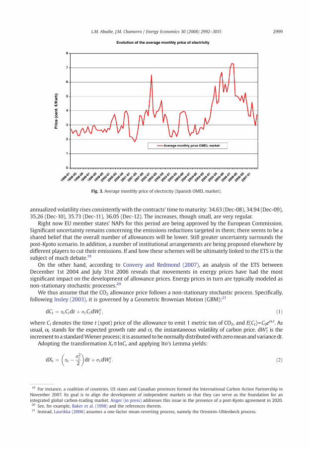
Fig. 3. Average monthly price of electricity (Spanish OMEL market).


annualized volatility rises consistently with the contracts' time tomaturity: 34.63 (Dec-08), 34.94 (Dec-09),35.26 (Dec-10), 35.73 (Dec-11), 36.05 (Dec-12). The increases, though small, are very regular.

Right now EU member states' NAPs for this period are being approved by the European Commission.Significant uncertainty remains concerning the emissions reductions targeted in them; there seems to be ashared belief that the overall number of allowances will be lower. Still greater uncertainty surrounds thepost-Kyoto scenario. In addition, a number of institutional arrangements are being proposed elsewhere bydifferent players to cut their emissions. If and how these schemes will be ultimately linked to the ETS is thesubject of much debate.19

On the other hand, according to Convery and Redmond (2007), an analysis of the ETS betweenDecember 1st 2004 and July 31st 2006 reveals that movements in energy prices have had the mostsignificant impact on the development of allowance prices. Energy prices in turn are typically modeled asnon-stationary stochastic processes.20

We thus assume that the CO2 allowance price follows a non-stationary stochastic process. Specifically,following Insley (2003), it is governed by a Geometric Brownian Motion (GBM):21

19 ForNovemintegrat20 See21 Inst

dCt ¼ acCtdt þ rcCtdWct ; ð1Þ

Ct denotes the time t (spot) price of the allowance to emit 1 metric ton of CO2, and E(Ct)=C0eαct. As
whereusual, αc stands for the expected growth rate and σc the instantaneous volatility of carbon price. dWt
c is theincrement toa standardWienerprocess; it is assumed tobenormallydistributedwithzeromeanandvariancedt.

Adopting the transformation Xt≡ lnCt and applying Ito's Lemma yields:

dXt ¼ ac � r2c2

� �dt þ rcdWc

t : ð2Þ

instance, a coalition of countries, US states and Canadian provinces formed the International Carbon Action Partnership inber 2007. Its goal is to align the development of independent markets so that they can serve as the foundation for aned global carbon-trading market. Anger (in press) addresses this issue in the presence of a post-Kyoto agreement in 2020., for example, Baker et al. (1998) and the references therein.ead, Laurikka (2006) assumes a one-factor mean-reverting process, namely the Ornstein–Uhlenbeck process.


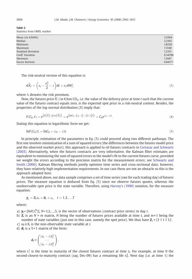
Table 2Statistics from OMEL market

Mean (cts €/kWh) 3.5504Median 3.2165Minimum 1.8250Maximum 7.3140Standard deviation 1.2351Coeff. Variation 0.34788Skewness 1.1447Excess Kurtosis 0.84177


The risk-neutral version of this equation is:

Statin

where

dXt ¼ ac � r2c2

� k

� �dt þ rcdWc

t ; ð3Þ

λ denotes the risk premium.
whereNow, the futures price F(·) in €/ton CO2, i.e. the value of the delivery price at time t such that the current
value of the futures contract equals zero, is the expected spot price in a risk-neutral context. Besides, theproperties of the log-normal distribution (X) imply that:

F C0; tð Þ ¼ e E X� �

þ12Var X

� �� ¼ e lnC0þ ac�r2

2 �k� �

tþr22 t

� �¼ C0e ac�kð Þt : ð4Þ

g this equation in logarithmic form we get:

lnF C0;t� � ¼ lnC0 þ ac � kð Þt: ð5Þ

principle, estimation of the parameters in Eq. (5) could proceed along two different pathways. The
Infirst one involves minimization of a sum of squared errors (the differences between the futures model priceand the observed market price); this approach is applied to oil futures contracts in Cortazar and Schwartz(2003). Alternatively, when the futures contracts are very informative, the Kalman filter estimates areequivalent to minimizing the sum of squared errors in the model's fit to the current futures curve, providedwe weight the errors according to the precision matrix for the measurement errors; see Schwartz andSmith (2000). Kalman filtering methods jointly optimize time series and cross-sectional data; however,they have relatively high implementation requirements. In our case these are not an obstacle so this is theapproach adopted here.
As mentioned above, our data sample comprises a set of time series (one for each trading day) of futuresprices. The measure equation is deduced from Eq. (5) since we observe futures quotes, whereas theunobservable spot price is the state variable. Therefore, using Harvey's (1990) notation, for the measureequation:

yt ¼ Ztat þ dt þ et ; t ¼ 1;2; N ;T

:

a) yt= [lnF(t tN)], N=1,2,…,5, is the vector of observations (contract price series) in day t.b) Zt is an N × m matrix, N being the number of futures prices available at time t, and m=1 being the

number of state variables (just one in this case, namely the spot price). We thus have Zt = [1 1 1 1 1]′.c) αt≡Xt is the non-observable state variable at t.d) dt is a 5×1 matrix of the form:

dtuac � kð Þt1t

: : :

ac � kð Þt5t

0@

1A;

t t1 is the time to maturity of the closest futures contract at time tt. For example, at time 0 the
where
second-closest-to-maturity contract (say, Dec-09) has a remaining life t02. Next day (i.e. at time 1) the

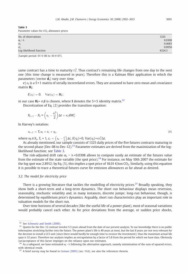
Table 3Parameter values for CO2 allowance prices

No. of observations 1325αc−λ 0.0308σc 0.4683σε 0.0056Log-likelihood function 4324.3

(Sample period: 01-V-06 to 10-V-07).


same contract has a time to maturity t12. Thus contract's remaining life changes from one day to the next

one (this time change is measured in years). Therefore this is a Kalman filter application in which theparameters (vector dt) vary over time.

e) εt is a 5×1 matrix of serially incorrelated errors. They are assumed to have zero mean and covariancematrix Ht:

In Har

22 See23 Quoinformathe decspan is(un)acc24 As awith id25 A b

E etð Þ ¼ 0; Var etð Þ ¼ Ht;

case Ht= σεI is chosen, where I denotes the 5×5 identity matrix.22
in ourDiscretization of Eq. (2) provides the transition equation:
Xtþ1 � Xtc ac � r2c2

� �Dt þ rcdWc

t :

vey's notation:

atþ1 ¼ Ttat þ ct þ gt ; ð6Þαt≡Xt, Tt = 1, ct ¼ ac � r2c

2

� �Dt, E(ηt)=0, Var(ηt)=σ c

2Δt.
whereAs already mentioned, our sample consists of 1325 daily prices of the five futures contracts maturing in
the second phase (Dec-08 to Dec-12).23 Parameter estimates are derived from the maximization of the log-likelihood function; see Table 3.

The risk-adjusted drift rate αc − λ=0.0308 allows to compute easily an estimate of the futures valuefrom the estimate of the state variable (the spot price).24 For instance, on May 10th 2007 the estimate forthe log spot was 2.8912; by Eq. (5), this implies a spot price of 18.01 €/ton CO2. Similarly, using this equationit is possible to trace a theoretical futures curve for emission allowances as far ahead as desired.

3.2. The model for electricity price

There is a growing literature that tackles the modelling of electricity prices.25 Broadly speaking, theyshow both a short-term and a long-term dynamics. The short run behaviour displays mean reversion,seasonality, stochastic volatility and, in many instances, discrete jumps; long-run behaviour, though, isdetermined by equilibrium price's dynamics. Arguably, short run characteristics play an important role invaluation models for the short run.

Over time horizons of several decades (like the useful life of a power plant), most of seasonal variationswould probably cancel each other. As for price deviations from the average, or sudden price shocks,

Schwartz and Smith (2000).tes for the Dec-12 contract involve 5.5 years ahead from the date of our present analysis. To our knowledge there is no publiction stretching further into the future. The power plant's life is 40 years at most, but the last 8 years are not very relevant forision to install a CCS unit (since there would hardly be enough time to recover the investment); thus the maximum actual life32 years. Therefore our analysis implies an extrapolation by a factor of 5.8 from the period for which we have data. Obviouslyeptance of this factor impinges on the reliance upon our estimates.safeguard, we have estimated αc−λ following the alternative approach, namely minimisation of the sum of squared errors,

entical result.rief survey may be found in Geman (2005) (sec. 11.6); see also the references therein.

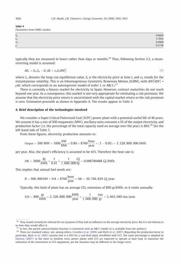
Table 4Parameters from OMEL market

ke 0.9604Le 3.7852σe 0.4968ρ 0.2738


typically they are measured in hours rather than days or months.26 Thus, following Section 2.2, a mean-reverting model is assumed:

per ye

This im

26 Theus how27 In f28 TheparticulDavisonutilisati

dEt ¼ ke Le � Etð Þdt þ reEtdWEt ; ð7Þ

Le denotes the long-run equilibrium value, Et is the electricity price at time t, and σe stands for the
whereinstantaneous volatility. This is an Inhomogeneous Geometric Brownian Motion (IGBM), with dWt
EdWtc =

ρdt, which corresponds to an autoregresive model of order 1, or AR(1).27

There is currently a futures market for electricity in Spain. However, contract maturities do not reachbeyond one year. As a consequence, this market is not very appropriate for estimating a risk premium. Weassume that the electricity price return is uncorrelated with the capital market return so the risk premiumis zero. Estimation proceeds as shown in Appendix A. The results appear in Table 4.

4. Brief description of the technologies involved

We consider a Super Critical Pulverized Coal (SCPC) power plant with a potential useful life of 40 years.We assume it has a size of 500megawatts (MW); ancillary units consume a 5% of the output electricity, andproduction factor (i.e. the percentage of the total capacity used on average over the year) is 80%.28 See theleft-hand side of Table 5.

From these figures, electricity production amounts to:

Output ¼ 500 MW� 1000kWMW

� 0:80� 8760houryear

� 1� 0:05ð Þ ¼ 3;328;800;000 kWh

ar. Also, the plant's efficiency is assumed to be 41%. Therefore the heat rate is:

HR ¼ 3600kJ

kWh� 10:41

� 11;000;000

GJkJ

¼ 0:008780488 GJ=kWh:

plies that annual fuel needs are:

B ¼ 500;000kW� 0:8� 8760houryear

� HR ¼ 30;766;829 GJ=year:

ically, this kind of plant has an average CO2 emissions of 800 gr/kWh, so it emits annually:
Typ
EM ¼ 800gr

kWh� 3;328;800;000

kWhyear

� 11;000;000

tongr

¼ 2;663;040 ton=year:

y would certainly be relevant for our purposes if they had an influence on the average electricity price. But it is not obvious tothey would affect it.act, the partial autocorrelation function is consistent with an AR(1) model (it is available from the authors).se are standard values; see, among others, Coombes et al. (2006) and Blyth et al. (2007). Regarding the production factor inar, Blyth et al. (2007) assume that it is 85% for a coal-fired plant retrofitted with CCS. The same percentage is adopted by(2007); in the short to medium term, power plants with CCS are expected to operate at base load, to maximise the

on of the investment in CCS equipment, yet the situation may be different in the longer term.

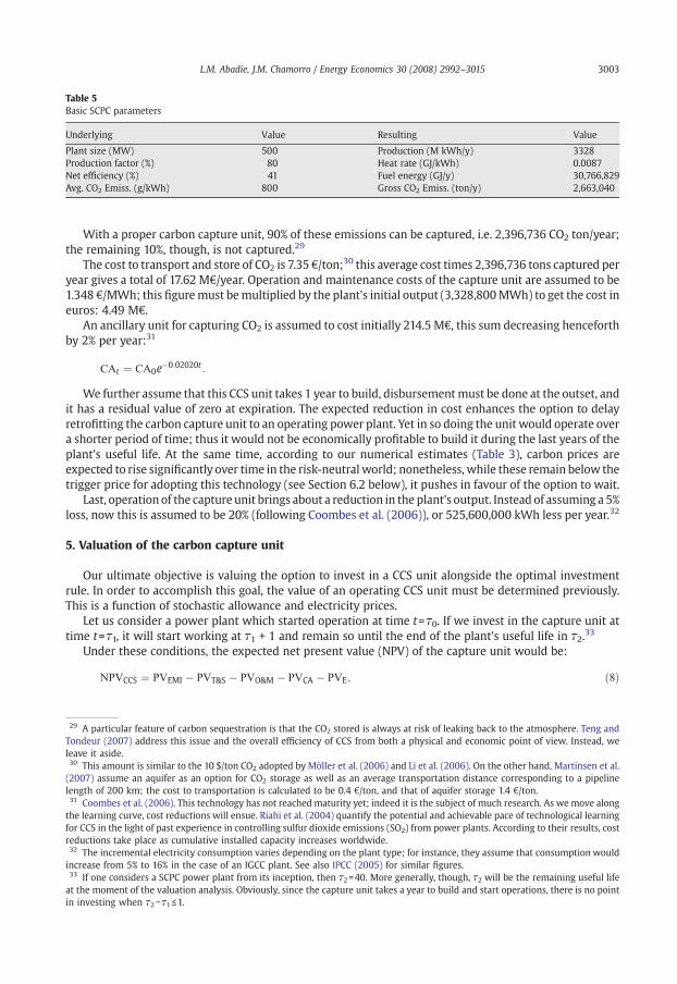
Table 5Basic SCPC parameters

Underlying Value Resulting Value

Plant size (MW) 500 Production (M kWh/y) 3328Production factor (%) 80 Heat rate (GJ/kWh) 0.0087Net efficiency (%) 41 Fuel energy (GJ/y) 30,766,829Avg. CO2 Emiss. (g/kWh) 800 Gross CO2 Emiss. (ton/y) 2,663,040


With a proper carbon capture unit, 90% of these emissions can be captured, i.e. 2,396,736 CO2 ton/year;the remaining 10%, though, is not captured.29

The cost to transport and store of CO2 is 7.35 €/ton;30 this average cost times 2,396,736 tons captured peryear gives a total of 17.62 M€/year. Operation and maintenance costs of the capture unit are assumed to be1.348 €/MWh; this figuremust bemultiplied by the plant's initial output (3,328,800MWh) to get the cost ineuros: 4.49 M€.

An ancillary unit for capturing CO2 is assumed to cost initially 214.5 M€, this sum decreasing henceforthby 2% per year:31

29 A pTondeuleave it30 Thi(2007)length31 Coothe learfor CCSreductio32 Theincrease33 If oat the min inves

CAt ¼ CA0e�0:02020t :

further assume that this CCS unit takes 1 year to build, disbursementmust be done at the outset, and
Weit has a residual value of zero at expiration. The expected reduction in cost enhances the option to delayretrofitting the carbon capture unit to an operating power plant. Yet in so doing the unit would operate overa shorter period of time; thus it would not be economically profitable to build it during the last years of theplant's useful life. At the same time, according to our numerical estimates (Table 3), carbon prices areexpected to rise significantly over time in the risk-neutral world; nonetheless, while these remain below thetrigger price for adopting this technology (see Section 6.2 below), it pushes in favour of the option to wait.
Last, operation of the capture unit brings about a reduction in the plant's output. Instead of assuming a 5%loss, now this is assumed to be 20% (following Coombes et al. (2006)), or 525,600,000 kWh less per year.32

5. Valuation of the carbon capture unit

Our ultimate objective is valuing the option to invest in a CCS unit alongside the optimal investmentrule. In order to accomplish this goal, the value of an operating CCS unit must be determined previously.This is a function of stochastic allowance and electricity prices.

Let us consider a power plant which started operation at time t=τ0. If we invest in the capture unit attime t=τ1, it will start working at τ1 + 1 and remain so until the end of the plant's useful life in τ2.33

Under these conditions, the expected net present value (NPV) of the capture unit would be:

NPVCCS ¼ PVEMI � PVT&S � PVO&M � PVCA � PVE; ð8Þ

articular feature of carbon sequestration is that the CO2 stored is always at risk of leaking back to the atmosphere. Teng andr (2007) address this issue and the overall efficiency of CCS from both a physical and economic point of view. Instead, weaside.s amount is similar to the 10 $/ton CO2 adopted by Möller et al. (2006) and Li et al. (2006). On the other hand, Martinsen et al.assume an aquifer as an option for CO2 storage as well as an average transportation distance corresponding to a pipelineof 200 km; the cost to transportation is calculated to be 0.4 €/ton, and that of aquifer storage 1.4 €/ton.mbes et al. (2006). This technology has not reached maturity yet; indeed it is the subject of much research. As we move alongning curve, cost reductions will ensue. Riahi et al. (2004) quantify the potential and achievable pace of technological learningin the light of past experience in controlling sulfur dioxide emissions (SO2) from power plants. According to their results, costns take place as cumulative installed capacity increases worldwide.incremental electricity consumption varies depending on the plant type; for instance, they assume that consumption wouldfrom 5% to 16% in the case of an IGCC plant. See also IPCC (2005) for similar figures.

ne considers a SCPC power plant from its inception, then τ2=40. More generally, though, τ2 will be the remaining useful lifeoment of the valuation analysis. Obviously, since the capture unit takes a year to build and start operations, there is no pointting when τ2−τ1≤1.

where

where

where

where

where

34 Thechancescapturevaryingoperatinseems cincreasesacrificewhatevanonym


, the present value of the emission allowances spared minus that of transport and storage costs,
that isoperation and maintenance costs, investment outlay in the capture unit, and the present value of foregonerevenues from electricity.34
The corresponding values are computed at time τ1 in the following way:

PVEMI ¼ EM0es2 ac�k�rð Þ � e s1þ1ð Þ ac�k�rð Þ

ac � k� rð Þ ; ð9Þ

EM0=2,396,736 ton/year×18.01 €/ton=43.165 M€.

PVT&S ¼ TA0e�r s1þ1ð Þ � e�s2r

r; ð10Þ

TA0=17.62 M€.

PVO&M ¼ OM0e�r s1þ1ð Þ � e�s2r

r; ð11Þ

OM0=4.49 M€.

PVCA ¼ CA0e�0:02020T ;

CA0=214.5 M€.

PVE ¼ PA0Ler

e�r s1þ1ð Þ � e�40r� �

þ E0ke þ r

� Leke þ r

� �e� keþrð Þ s1þ1ð Þ � e�40 keþrð Þ

� �� ð12Þ

PA0=525,600,000 kWh/year lost, Le = 0.037852 €/kWh, E0=0.04083 €/kWh (as of April 2007,onalised), ke = 0.9604 and r=0.05.
deseas
With these values, if at t=τ1 the decision to install a capture unit was taken (starting operation in oneyear time), the expected NPV would amount to:

NPVCCS ¼ 1162:40� 287:45� 73:21� 214:50� 325:20 ¼ 262:04 M€:

following the NPV criterion investment at that time should be undertaken.
Thus,Alternatively, instead of computing the unit's NPV for a given allowance price, it is possible to determine
the value of the latter such that the former equals zero. In this respect, an allowance (spot) price equal to orhigher than 13.95 €/ton at t=τ1 would be necessary to get a NPV ≥ 0 and to accept the investment underthis criterion (this threshold is obviously surpassed by the estimated current – second period – spot price18.01 €/ton; see Section 3.1). As is well-known, the NPV does not account for the value of the option to deferinvestment in the CO2 capture unit.

Note, though, that this NPV figure rests on a risk-adjusted growth rate of carbon prices close to 3% (αc − λin Table 3). Given the sensitivity of the above result to this rate, the NPV of the capture unit is also computedfor different values of this parameter. Presumably, if allowance price were expected to grow at a lower rate,potential gains from the CCS unit would also be lower. This in turn would translate into a lower NPV of thecapture unit. Indeed this is the case; as shown in the first row of Table 6, the NPV falls from 262 M€ as wemove leftward.

implicit assumption here is that the firm will operate the capture unit as much as possible in an attempt to maximize theof recovering the investment disbursement. Therefore, 90% of total emissions from the base load power plant will be

d, and 20% of its output electricity will be lost. Actually, though, there may be opportunities to increase profitability bythe operation of the capture unit and simultaneously resorting to the allowance market. Davison (2007) suggests someg techniques for reducing the net cost of CO2 capture, though they are not considered here. Anyway their overall effectlear. If the capture unit is flexible enough (so as to interrupt operation when allowance price is low), its profitability will. Somehow the investment will be less irreversible and keeping the option to invest alive will incur higher costs in terms ofd present revenues. The trigger price will fall accordingly and investment will take place sooner rather than later (of course,er costs to switching between modes of operation – active or inactive – should be duly accounted for). We thank anous referee for raising this point.

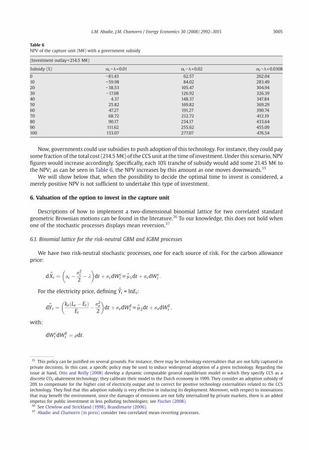
Table 6NPV of the capture unit (M€) with a government subsidy

(Investment outlay=214.5 M€)

Subsidy (%) αc−λ=0.01 αc−λ=0.02 αc−λ=0.0308

0 −81.43 62.57 262.0410 −59.98 84.02 283.4920 −38.53 105.47 304.9430 −17.08 126.92 326.3940 4.37 148.37 347.8450 25.82 169.82 369.2960 47.27 191.27 390.7470 68.72 212.72 412.1980 90.17 234.17 433.6490 111.62 255.62 455.09100 133.07 277.07 476.54


Now, governments could use subsidies to push adoption of this technology. For instance, they could paysome fraction of the total cost (214.5M€) of the CCS unit at the time of investment. Under this scenario, NPVfigures would increase accordingly. Specifically, each 10% tranche of subsidy would add some 21.45 M€ tothe NPV; as can be seen in Table 6, the NPV increases by this amount as one moves downwards.35

We will show below that, when the possibility to decide the optimal time to invest is considered, amerely positive NPV is not sufficient to undertake this type of investment.

6. Valuation of the option to invest in the capture unit

Descriptions of how to implement a two-dimensional binomial lattice for two correlated standardgeometric Brownian motions can be found in the literature.36 To our knowledge, this does not hold whenone of the stochastic processes displays mean reversion.37

6.1. Binomial lattice for the risk-neutral GBM and IGBM processes

We have two risk-neutral stochastic processes, one for each source of risk. For the carbon allowanceprice:

with:

35 Thiprivateissue atdiscrete20% totechnolthat maimpetu36 See37 Aba

d Xt ¼ ac � r2c2

� k

� �dt þ rcdWc

t u A1dt þ rcdWct :

the electricity price, defining Yt = lnEt:
For
dY t ¼ ke Le � Etð ÞEt

� r2e2

� �dt þ redWE

t u A2dt þ redWEt ;

dWct dW

Et ¼ qdt:

s policy can be justified on several grounds. For instance, there may be technology externalities that are not fully captured indecisions. In this case, a specific policy may be used to induce widespread adoption of a given technology. Regarding thehand, Otto and Reilly (2008) develop a dynamic computable general equilibrium model in which they specify CCS as aCO2 abatement technology; they calibrate their model to the Dutch economy in 1999. They consider an adoption subsidy ofcompensate for the higher cost of electricity output and to correct for positive technology externalities related to the CCSogy. They find that this adoption subsidy is very effective in inducing its deployment. Moreover, with respect to innovationsy benefit the environment, since the damages of emissions are not fully internalized by private markets, there is an addeds for public investment in less polluting technologies; see Fischer (2008).Clewlow and Strickland (1998), Brandimarte (2006).die and Chamorro (in press) consider two correlated mean-reverting processes.

http://dx.doi.org/10.1016/j.eneco.2007.07.001



There are four probabilities in the corresponding two-dimensional binomial lattice and, if we want thebranches to recombine, two incremental values (ΔX andΔY). At any time the four probabilitiesmust take onvalues between zero and one, and add to one; also, they must be consistent with means, variances andcorrelations. So there are six restrictions to be satisfied. It can be shown that the solution is:

38 Yandecisionestimat39 Theworkingnodes. Tby the n(i.e. it is

DX ¼ rcffiffiffiffiffiffiffiDt;

pð13Þ

DY ¼ reffiffiffiffiffiffiffiDt;

pð14Þ

puu ¼ DXDY þ DY A1Dt þ DX A2Dt þ qrcreDt4DXDY

; ð15Þ

pud ¼ DXDY þ DY A1Dt � DXA2Dt � qrcreDt4DXDY

; ð16Þ

pdu ¼ DXDY � DY A1Dt þ DXA2Dt � qrcreDt4DXDY

; ð17Þ

pdd ¼ DXDY � DY A1Dt � DXA2Dt þ qrcreDt4DXDY

: ð18Þ

te that the drift rate for the allowance price (μ1) is a constant, whereas that for the electricity price
No(μ2) depends on Et which may vary from node to node. Consequently the four probabilities change from anode to the next. The two subscripts refer to the allowance price and the electricity price, respectively. An udenotes an up jump, whereas a dmeans the opposite. Thus, Pdu stands for the risk-neutral probability that,starting from a certain node, allowance price jumps down and electricity price jumps up. Similarly for thesuperscripts (+, −) in the value of the investment opportunity (W) below.
We set a two-dimensional binomial tree with 6 time steps per year (Δt=1/6). This amounts to6×39=234 steps for a new power plant with 40 years of useful life. The last nodes would take place at time39; a null value would arise as the maximum between building the capture unit in exchange for nothingand zero:

W ¼ max NPVCCS;0ð Þ ¼ 0: ð19Þ

earlier moments, the best option – either to invest in the capture unit or to continue waiting – is
Atchosen at each node:
W ¼ max NPVCCS; puuWþþ þ pudWþ� þ pduW

�þ þ pddW��ð Þe�rDt� �

: ð20Þ

ing yields the unit's NPV for sure; continuing allows to get the expected future value of the
Investinvestment opportunity (i.e. the sum of the values at the four nodes weighted by their respective risk-neutral probabilities) discounted at the risk-free rate.
The lattice is solved backwards. At time t=0 we get the value of the investment option alongside theoptimal time to invest. Then the value of the option towait is just the difference between this value and thatof investing immediately. With 6 steps per year, the difference between the option value and the NPV turnsout to be 344.49 M€. Thus, the value of the option towait is not only positive; it is even bigger than the NPVof the capture unit (262.04 M€). Therefore, waiting to install the CCS unit is in the utility's best interest.38

Table 7 shows the value of the option to wait for different numbers of time steps per year. There is nomonotone pattern in that the value starts increasing with the number of steps but then declines with it.However, when these results are plotted in Fig. 4, convergence towards the solution as the number of stepsincreases can be observed. This profile justifies our choice of six steps per year: no significant improvementis gained with a higher number of steps, whereas the time elapsed in computations rises dramatically.39

g et al. (in press) use a real options approach for analysing the effects of climate change policy uncertainty on private utilities's when there is an option to optimally time the investments in coal, gas and nuclear power. They provide numericales of the option values of waiting for these investments in $/kW units.difference between the solution with 6 steps per year and that with 20 steps is less than 5 per thousand. Besides, whenwith 40 years, the lattice is built for 39 years; using 6 steps per year implies that at the final step (234) there are 54,756he choice of a number of time steps that combines reliable results with reasonable computing time is justified in our workeed to determine the optimal value and timing of exercise of the investment option over the whole two-dimensional latticean American-type option).


Table 7Value of the option to wait (M€)

Steps per year Total steps Option value–NPV

1 39 358.422 78 363.864 156 348.766 234 344.498 312 343.1910 390 342.7012 468 342.5814 546 342.6416 624 342.6318 702 342.1220 780 342.81


6.2. The allowance trigger price for the capture unit

First, we analyze the price of CO2 allowances above which it will be optimal to invest immediately as afunction of the power plant's remaining useful life (remember that, by assumption, the capture unit'sresidual value is zero when the retrofitted plant expires).

Fig. 5 shows that, for useful lives longer than 8 years, optimal investment will only take place forallowance prices above 55 €/ton. However, if the only possibility is to invest immediately or never (that is,when the NPV criterion applies), the threshold price to overcome ranges between 13.95 €/tonwith 40 years(as seen in Section 5) and 25.97 €/ton with 10 years of useful life.

The shape of the curve is determined among other factors by:

a) The pay-back period of the investment, which implies a higher permit price for lives shorter than8 years.

b) The expected rise in the allowance price in a risk-neutral world.c) The expected drop in the CCS unit's investment cost.

Table 8 shows some of the numerical values underlying Fig. 5. They suggest that, from a financial pointof view, the current situation is hardly favourable for utilities to decide to install CCS units right now.Rather, deferring this investment into the future and seeing what happens in the meantime looks moresensible.

Fig. 4. Option value–NPV as a function of the number of time steps.

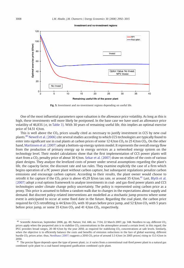
Fig. 5. Investment and no-investment regions depending on useful life.


One of the most influential parameters upon valuation is the allowance price volatility. As long as this ishigh, these investments will more likely be postponed. In the base case we have used an allowance pricevolatility of 46,83% (σc in Table 3). With 30 years of remaining useful life, this implies an optimal exerciseprice of 54.51 €/ton.

This is well above the CO2 prices usually cited as necessary to justify investment in CCS by new coalplants.40 Newell et al. (2006) cite several studies according towhich CCS technologies are typically found toenter into significant use in coal plants at carbon prices of some 12 €/ton CO2 to 25 €/ton CO2. On the otherhand,Martinsen et al. (2007) adopt a bottom-up energy systemmodel. It represents the overall energy flowfrom the production of primary energy up to energy services as a networked energy system on thetechnology level. Their model calculations show that the first implementation of CCS power plants willstart from a CO2 penalty price of about 30 €/ton. Sekar et al. (2007) draw on studies of the costs of variousplant designs. They analyze the levelized costs of power under several assumptions regarding the plant'slife, the capacity factor, the discount rate and tax rules. They examine explicitly the case of a firm whichbegins operation of a PC power plant without carbon capture, but subsequent regulations penalize carbonemissions and encourage carbon capture. According to their results, the plant owner would choose toretrofit it for capture if the CO2 price is above 45.29 $/ton tax rate, or around 35 €/ton.41 Last, Blyth et al.(2007) adopt a real options framework to analyse investments in coal- and gas-fired power plants and CCStechnologies under climate change policy uncertainty. The policy is represented using carbon price as aproxy. This price is assumed to follow a randomwalk due to changes in the expectations about supply anddemand. But discreet policy-related interventions are modelled as a stochastic jump process where someevent is anticipated to occur at some fixed date in the future. Regarding the coal plant, the carbon pricerequired for CCS retrofitting is 44 $/ton CO2 with 10 years before price jump, and 52 $/ton CO2 with 5 yearsbefore price jump, or some 35 €/ton CO2 and 41 €/ton CO2, respectively.

40 Scientific American, September 2006, pp. 49; Nature, Vol. 446, no. 7134, 22 March 2007, pp. 348. Needless to say, different CO2

prices apply when the purported aim is to stabilise CO2 concentrations in the atmosphere around a certain level; in this regard, theIPCC provides broad ranges, 20–80 €/ton by the year 2050, as required for stabilizing CO2 concentrations at safe levels. Similarly,when the objective is to efficiently balance the costs and benefits of emission reductions in the face of global warming, differenthurdle CO2 prices arise; thus, Nordhaus (2007) suggests a 2010 CO2 price of around 3.3 €/ton (in 2005 prices) rising to 13.5 €/ton in2050.41 The precise figure depends upon the type of power plant, i.e. it varies from a conventional coal-fired power plant to a natural gascombined cycle plant to a coal-based integrated gasification combined cycle plant.

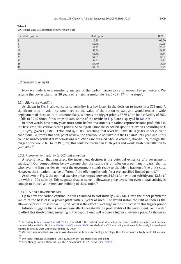
Table 8CO2 trigger price as a function of power plant's life

Useful life (years) Real option NPV

2 112.38 109.005 55.66 39.7510 51.35 25.9715 52.58 21.3920 53.68 18.8425 54.31 17.1130 54.51 15.8135 54.40 14.7940 54.09 13.95


6.3. Sensitivity analysis

Now we undertake a sensitivity analysis of the carbon trigger price to several key parameters. Weassume the power plant has 30 years of remaining useful life (i.e. 6×29=174 time steps).

6.3.1. Allowance volatilityAs shown in Fig. 6, allowance price volatility is a key factor in the decision to invest in a CCS unit. A

significant drop in volatility would reduce the value of the option to wait and would render a widedeployment of these units much more likely. Whereas the trigger price is 57.86 €/ton for a volatility of 50%,it falls to 32.19 €/ton if this drops to 20%. Some of the results in Fig. 6 are displayed in Table 9.

In other words, howmany yearsmust come before investments in carbon capture become profitable? Inthe base case, the critical carbon price is 54.51 €/ton. Since the expected spot price evolves according to E(Ct)=C0eαct, given C0=18.01 €/ton and αc=0.069, reaching that level will take 16.04 years under currentconditions. So, from a financial point of view, the firmwould not invest in the CCS unit until year 2023; thiscould be unacceptable if faster emissions reductions are pursued. Should volatility drop to 30%, though, thetrigger price would fall to 39.19 €/ton; this could be reached in 11.26 years and would hasten installation toyear 2018.42

6.3.2. A government subsidy to CCS unit adoptionA second factor that can affect the investment decision is the potential existence of a government

subsidy.43. Our computations below assume that the subsidy is on offer on a permanent basis; that is,whenever the firm decides to invest the government stands ready to shoulder a fraction of the unit's cost.However, the situation may be different if the offer applies only for a pre-specified limited period.44

As shown in Fig. 7, the optimal exercise price ranges between 54.51 €/ton without subsidy and 42.31 €/ton with a 100% subsidy. This suggests that, at current allowance price levels, not even a total subsidy isenough to induce an immediate building of these units.45

6.3.3. CCS unit's investment costUp to now, the carbon capture unit was assumed to cost initially 214.5 M€. Given the other parameter

values of the base case, a power plant with 30 years of useful life would install the unit as soon as theallowance price surpasses 54.51 €/ton. What is the effect of a change in the unit's cost on this trigger price?

Intuition suggests that a cost increase affects negatively the profitability of the investment. So, in orderto offset this shortcoming, investing in the capture unit will require a higher allowance price. As shown in

42 According to Martinsen et al. (2007), the year 2020 is the earliest point at which power plants with CO2 capture will becomecommercially available. Similarly, Gibbins and Chalmers (2008) conclude that CCS as a policy option could be ready for developedcountry rollout by 2015 and global rollout by 2020.43 We have assumed that investment cost decreases in time as technology develops; thus the absolute subsidy could fall as timeruns.44 We thank Michael Shackleton (Univ. Lancaster, UK) for suggesting this point.45 Even though, with a 100% subsidy, the NPV amounts to 476.54 M€ (see Table 6).

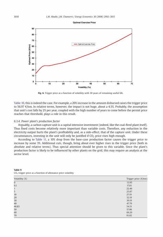
Fig. 6. Trigger price as a function of volatility with 30 years of remaining useful life.


Table 10, this is indeed the case. For example, a 20% increase in the amount disbursed raises the trigger priceto 56.97 €/ton. In relative terms, however, the impact is not huge, about a 4.5%. Probably, the assumptionthat unit's cost falls by 2% per year, coupled with the high number of years to come before the permit pricereaches that threshold, plays a role in this result.

6.3.4. Power plant's production factorArguably, a carbon capture unit is a capital intensive investment (indeed, like the coal-fired plant itself).

Thus fixed costs become relatively more important than variable costs. Therefore, any reduction in theelectricity output hurts the plant's profitability and, as a side-effect, that of the capture unit. Under thesecircumstances, investing in the unit will only be justified if CO2 price rises high enough.

According to Table 11, a 10% drop from the base-case production factor causes the trigger price toincrease by some 3%. Additional cuts, though, bring about ever higher rises in the trigger price (both inabsolute and relative terms). Thus special attention should be given to this variable. Since the plant'sproduction factor is likely to be influenced by other plants on the grid, this may require an analysis at thesector level.

Table 9CO2 trigger price as a function of allowance price volatility

Volatility (%) Trigger price (€/ton)

0 13.950.1 17.811 22.465 25.8710 27.1920 32.1930 39.1940 47.7946.83 54.5150 57.8660 69.2970 81.82

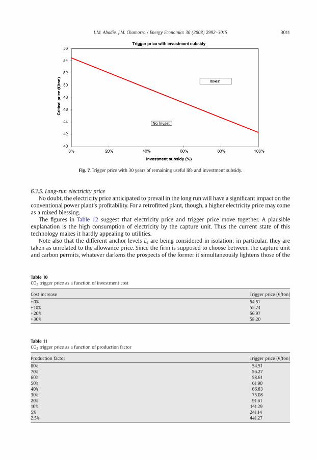
Fig. 7. Trigger price with 30 years of remaining useful life and investment subsidy.


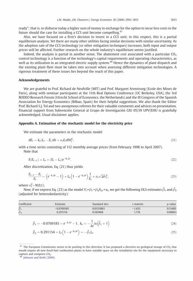
6.3.5. Long-run electricity priceNo doubt, the electricity price anticipated to prevail in the long runwill have a significant impact on the

conventional power plant's profitability. For a retrofitted plant, though, a higher electricity price may comeas a mixed blessing.

The figures in Table 12 suggest that electricity price and trigger price move together. A plausibleexplanation is the high consumption of electricity by the capture unit. Thus the current state of thistechnology makes it hardly appealing to utilities.

Note also that the different anchor levels Le are being considered in isolation; in particular, they aretaken as unrelated to the allowance price. Since the firm is supposed to choose between the capture unitand carbon permits, whatever darkens the prospects of the former it simultaneously lightens those of the

Table 10CO2 trigger price as a function of investment cost

Cost increase Trigger price (€/ton)

+0% 54.51+10% 55.74+20% 56.97+30% 58.20

Table 11CO2 trigger price as a function of production factor

Production factor Trigger price (€/ton)

80% 54.5170% 56.2760% 58.6150% 61.9040% 66.8330% 75.0820% 91.6110% 141.295% 241.142.5% 441.27

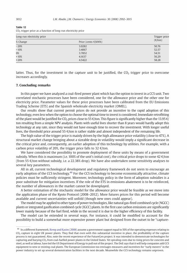
Table 12CO2 trigger price as a function of long-run electricity price

Long-run electricity price Trigger price(€/ton)

% Change Price (cents €/kWh)

−20% 3.0282 50.76−10% 3.4067 52.570% 3.7852 54.51+10% 4.1637 56.29+20% 4.5422 58.28


latter. Thus, for the investment in the capture unit to be justified, the CO2 trigger price to overcomeincreases accordingly.

7. Concluding remarks

In this paperwe have analyzed a coal-fired power plant which has the option to invest in a CCS unit. Twocorrelated stochastic processes have been considered, one for the allowance price and the other one forelectricity price. Parameter values for these price processes have been calibrated from the EU EmissionsTrading Scheme (ETS) and the Spanish wholesale electricity market (OMEL).

Our results show that current permit prices do not provide an incentive to the rapid adoption of thistechnology, even lesswhen the option to choose the optimal time to invest is considered. Immediate retrofittingof the plantwould be justified for CO2 prices close to 55€/ton. Thisfigure is significantly higher than the 13.95€/ton resulting from a simple NPV analysis. Plants with useful lives shorter than 8 years would hardly adopt thistechnology at any rate, since they would not have enough time to recover the investment. With longer usefullives, the threshold price around 55 €/ton is rather stable and almost independent of the remaining life.

The high value of the trigger price is mainly driven by the high allowance price volatility (close to 47%). Astructural market change bringing about a sizeable drop in volatility would imply a significant decrease inthe critical price and, consequently, an earlier adoption of this technology by utilities. For example, with acarbon price volatility of 20%, the trigger price falls to 32 €/ton.

We have considered the possibility to promote deployment of these units by means of a governmentsubsidy. When this is maximum (i.e. 100% of the unit's initial cost), the critical price drops to some 42 €/ton(from 55 €/ton without subsidy, i.e. a 22.38% drop). We have also undertaken some sensitivity analyses toseveral key parameters.

All in all, current technological development and regulatory framework do not seem to encourage anearly adoption of the CCS technology.46 For the CCS technology to become economically attractive, climatepolicies must be sufficiently stringent. Moreover, technology policy in the form of adoption subsidies is apoor substitute for mitigation incentives. If the role of the ETS in emissions abatement is to be reinforced,the number of allowances in the market cannot be downplayed.

A better estimation of the stochastic model for the allowance price would be feasible as we move intothe application phase of the Kyoto Protocol (2008–2012). More futures prices for this period will becomeavailable and current uncertainties will unfold (though new ones could appear).

Themodelmaybeapplied toother typesof power technologies, likenatural gas-fired combinedcycle (NGCC)plants or integrated gasification combined cycle (IGCC) plants. In thefirst case carbon emissions are significantlylower mainly because of the fuel fired, while in the second it is due to the higher efficiency of this facility.

The model can be extended in several ways. For instance, it could be modified to account for thepossibility to build a somewhat more expensive power plant but designed from the outset to be “capture-

46 In a different framework, Kemp and Kasim (2008) assume a government support equal to 50% of the operating expenses relating toCO2 capture in eight UK power plants. They find that even with this substantial incentive in place, the profitability of the captureprocess is not guaranteed. Also, note the recent experience of the FutureGen project. It was intended to demonstrate technologies forcapturing and burying CO2 from coal-fuelled power plants in the United States. Yet spiraling costs due to rising prices for concrete andsteel, aswell as labour, have led theUSDepartment of Energy to pull out of the project. TheDoE says that itwill help companies add CCSequipment to new or existing coal plants. The European Commission too envisages measures and incentives for “early movers” in thepower industry to set up several demonstration facilities in the next decade. Meanwhile the CCS technology remains unproven.


ready”; that is, to disburse today a higher sum of money in exchange for the option to incur less costs in thefuture should the case for installing a CCS unit become compelling.47

Also, we have focused on a firm's decision to invest in a CCS unit; in this respect, this is a partialequilibrium analysis. Yet there are many other utilities facing similar decisions with similar uncertainty. Asthe adoption rate of the CCS technology (or other mitigation techniques) increases, both input and outputprices will be affected. Further research on the whole industry's equilibrium seems justified.

Indeed, the analysis is partial in another sense. The abatement cost associated with a particular CO2

control technology is a function of the technology's capital requirements and operating characteristics, aswell as its utilization in an integrated electric supply system.48 Hence the dynamics of plant dispatch andthe existing plant fleet must be taken into account when assessing different mitigation technologies. Arigorous treatment of these issues lies beyond the reach of this paper.

Acknowledgements

We are grateful to Prof. Richard de Neufville (MIT) and Prof. Margaret Armstrong (Ecole des Mines deParis), along with seminar participants at the 11th Real Options Conference (UC Berkeley, USA), the 3rdRODEO Research Forum (Utrecht School of Economics, the Netherlands) and the III Congress of the SpanishAssociation for Energy Economics (Bilbao, Spain) for their helpful suggestions. We also thank the EditorProf. Richard S.J. Tol and two anonymous referees for their valuable comments and advices on presentation.Financial support from Subvención General al Grupo de Investigación GIU 05/39 UPV/EHU is gratefullyacknowledged. Usual disclaimer applies.

Appendix A. Estimation of the stochastic model for the electricity price

We estimate the parameters in the stochastic model

47 Thewould rcapture48 Joh

dEt ¼ ke Le � Etð Þdt þ reEtdWEt ; ð21Þ

time series consisting of 112 monthly average prices (from February 1998 to April 2007).
with aNote that
E Etþ1ð Þ ¼ Le þ Et � Leð Þe�keDt : ð22Þ

er discretization, Eq. (21) thus yields
Aft
Etþ1 � EtEt

¼ e�keDt � 1� �

þ Le 1� e�keDt� � 1

Etþ re

ffiffiffiffiffiffiDt

p�Et ; ð23Þ

εtE~N(0,1).
where
Now, if we express Eq. (23) as the model Yt=β1+β2X2t+ut, we get the following OLS estimates β1 and β2

(adjusted for heteroskedasticity):

Coefficient

European Commissioequire all new fossil-and compress CO2.

nson and Keith (2004

Estimate

n seems to be pushing in this dfuel combustion plants to have

).

Standard dev.

irection. It has proposed a direcsuitable space on the installation

t-statistic

tive on geological storage ofsite for the equipment nece

p-value

β 1
−0.0769185 0.0535881 −1.435 0.15405 β 2 0.291154 0.169468 1.718 0.08863
b1 ¼ �0:0769185 ¼ e�keDt � 1; ke ¼ � 1Dt

ln b1 þ 1� �

ð24Þ

b2 ¼ 0:291154 ¼ Le 1� e�keDt� �

¼ �b1Le: ð25Þ

CO2 thatssary to


The standard deviation of the residuals is 0.143416. Hence re ¼ 0:143416ffiffiffiffiffiffi12

p¼ 0:4968 ¼ 49:68k.

These values are shown in Table 4.In our computations we assume a risk premium λe=0. Durbin–Watson's statistic takes on a value of

1.77963.With regard to the correlation coefficient, some explanation is in order. There is a mismatch between

the frequency of carbon futures prices (daily) and electricity prices (monthly). Daily errors from futurescontracts have been averaged to get monthly average errors. Next, the correlation between these errors andthose of the electricity price has been computed (this reflects to what extent both series move togetherbeyond their trends).

References

Abadie, L.M., Chamorro, J.M., in press. Valuing flexibility: the case of an Integrated Gasification Combined Cycle power plant. EnergyEconomics. doi: 10.1016/j.eneco.2006.10.004.

Anger, N., in press. Emissions trading beyond Europe: linking schemes in a post-Kyoto world. Energy Economics. doi: 10.1016/j.eneco.2007.08.002.

Baker, M.P., Mayfield, E.S., Parsons, J.E., 1998. Alternative models of uncertain commodity prices for use with modern asset pricingmethods. Energy Journal 19 (1), 115–148.

Blyth, W., Bradley, R., Bunn, D., Clarke, C., Wilson, T., Yang, M., 2007. Investment risk under uncertain climate policy. Energy Policy 35,5766–5773.

Böhringer, C., Hoffman, T., Lange, A., Löschel, A., Moslener, U., 2005. Assessing emission regulation in Europe: an interactive simulationapproach. Energy Journal 26 (4), 1–21.

Brandimarte, P., 2006. Numerical Methods in Finance, 2nd edition. Wiley.Brennan, M.J., Trigeorgis, L., 2000. Project Flexibility, Agency, and Competition. Oxford University Press.Clewlow, L., Strickland, C., 1998. Implementing Derivatives Models. John Wiley and Sons.Convery, F., Redmond, L., 2007. Market and price developments in the European Union Emissions Trading Scheme. Review of

Environmental Economics and Policy 1 (1), 88–111.Coombes, P., Graham, P., Reedman, L., 2006. Using a real-options approach to model technology adoption under carbon price

uncertainty: an application to the Australian electricity generation sector. The Economic Record 82, 64–73 Special Issue.Cortazar, G., Schwartz, E.S., 2003. Implementing a stochastic model for oil futures prices. Energy Economics 25, 215–238.Davison, J., 2007. Performance and costs of power plants with capture and storage of CO2. Energy 32, 1163–1176.Dixit, A.K., Pindyck, R.S., 1994. Investment under Uncertainty. Princeton University Press.Ellerman, A.D., Buchner, B.K., 2007. The European Union Emissions Trading Scheme: origins, allocation and early results. Review of

Environmental Economics and Policy 1 (1), 66–87.Ellerman, A.D., Buchner, B.K., Carraro, C., 2007. Unifying themes. In: Ellerman, A.D., Buchner, B.K., Carraro, C. (Eds.), Allocation in the

European Emissions Trading Scheme: Rights, Rents and Fairness. Cambridge University Press. Ch. 13.Fischer, C., 2008. Emissions pricing, spillovers, and public investment in environmentally friendly technologies. Energy Economics 30,

487–502.Geman, H., 2005. Commodities and Commodity Derivatives. Wiley Finance.Gibbins, J., Chalmers, H., 2008. Preparing for global rollout: a ‘developed country first’ demonstration programme for rapid CCS

deployment. Energy Policy 36, 501–507.Harvey, A.C., 1990. Forecasting, Structural Time Series Models and the Kalman Filter. Cambridge University Press.Johnson, T.L., Keith, D.W., 2004. Fossil electricity and CO2 sequestration: how natural gas prices, initial conditions and retrofits

determine the cost of controlling CO2 emissions. Energy Policy 32, 367–382.Insley, M., 2003. On the option to invest in pollution control under a regime of tradable emissions allowances. Canadian Journal of

Economics 36 (4), 860–883.IPCC, 2005. IPCC Special Report on Carbon Dioxide Capture and Storage. Cambridge University Press.de Jong, C., Oosterom, A., Walet, K., 2005. Dealing with emissions, In: Kaminski, V. (Ed.), Managing Energy Price Risk, 3rd edition. Risk

Books.Kavouridis, K., Koukouzas, N., 2008. Coal and sustainable energy supply challenges and barriers. Energy Policy 36, 693–703.Kemp, A.G., Kasim, A.S., 2008. A least-cost optimisation model of CO2 capture applied to major UK power plants within the EU-ETS

framework. Energy Journal 28, 99–134 Special Issue.Kruger, J.K., Oates, W.E., Pizer, W.A., 2007. Decentralization in the EU Emissions Trading Scheme and lessons for global policy. Review

of Environmental Economics and Policy 1 (1), 112–133.Laurikka, H., 2006. Option value of gasification technology within an emission trading scheme. Energy Policy 34, 3916–3928.Laurikka, H., Koljonen, T., 2006. Emissions trading and investment decisions in the power sector: a case study in Finland. Energy Policy

34, 1063–1074.Li, H., Maréchal, F., Burer, M., Favrat, D., 2006. Multi-objective optimization of an advanced combined cycle power plant including CO2

separation options. Energy 31, 3117–3134.Martinsen, D., Linssen, J., Markewitz, P., Vögele, S., 2007. CCS: a future CO2 mitigation option for Germany? A bottom-up approach.

Energy Policy 35, 2110–2120.Möller, B.F., Assadi, M., Potts, I., 2006. CO2-free power generation in combined cycles: integration of post-combustion separation of

carbon dioxide in the steam cycle. Energy 31, 1520–1532.Montero, J.P., 2000. Optimal design of a phase-in emissions trading program. Journal of Public Economics 75, 273–291.Montero, J.P., 2004. Markets for environmental protection: design and performance. Estudios de Economía 31 (1), 79–99.Newell, R.G., Jaffe, A.B., Stavins, R.N., 2006. The effects of economic and policy incentives on carbon mitigation technologies. Energy

Economics 28, 563–578.


Nordhaus, W.D., 2007. To tax or not to tax: alternative approaches to slowing global warming. Review of Environmental Economicsand Policy 1 (1), 26–44.

Otto, V.M., Reilly, J., 2008. Directed technical change and the adoption of CO2 abatement technology: the case of CO2 capture andstorage. Energy Economics. 30, 2871–2890. doi:10.1016/j.eneco.2007.07.001.

Pindyck, R.S., 2007. Uncertainty in environmental economics. Review of Environmental Economics and Policy 1 (1), 45–65.Riahi, K., Rubin, E.S., Schrattenholzer, L., 2004. Prospects for carbon capture and sequestration technologies assuming their

technological learning. Energy 29, 1309–1318.Reinaud, J., 2007. CO2 Allowance & Electricity Price Interaction. OECD/IEA. February.Rubin, E.S., Chen, C., Rao, A.B., 2007. Cost and performance of fossil fuel power plants with CO2 capture and storage. Energy Policy 35,

4444–4454.Sarkis, J., Tamarkin, M., 2005. Real options analysis for “green trading”: the case of greenhouse gases. The Engineering Economist 50,

273–294.Sekar, R.C., Parsons, J.E., Herzog, H.J., Jacoby, H.D., 2007. Future carbon regulations and current investments in alternative coal-fired

power plant technologies. Economic Policy 35, 1064–1074.Schwartz, E.S., Smith, J.E., 2000. Short-term variations and long-term dynamics in commodity prices. Management Science 46 (7),

893–911.Schwartz, E.S., Trigeorgis, L. (Eds.), 2001. Real Options and Investment under Uncertainty. The MIT Press.Teng, F., Tondeur, D., 2007. Efficiency of carbon storage with leakage: physical and economical approaches. Energy 32, 540–548.Trigeorgis, L., 1996. Real Options — Managerial Flexibility and Strategy in Resource Allocation. The MIT Press.Yang, M., Blyth, W., Bradley, R., Bunn, D., Clarke, C., Wilson, T., in press. Evaluating the power investment options with uncertainty in

climate policy. Energy Economics. doi:10.1016/j.eneco.2007.06.004.

European CO 2 prices and carbon capture investments

Documents

Transcript of European CO 2 prices and carbon capture investments