Evaluating Natural Resource Investments

Evaluating Natural Resource Investments

Michael J. Brennan; Eduardo S. Schwartz

The Journal of Business, Vol. 58, No. 2. (Apr., 1985), pp. 135-157.

Stable URL:

http://links.jstor.org/sici?sici=0021-9398%28198504%2958%3A2%3C135%3AENRI%3E2.0.CO%3B2-P

The Journal of Business is currently published by The University of Chicago Press.

Your use of the JSTOR archive indicates your acceptance of JSTOR's Terms and Conditions of Use, available athttp://www.jstor.org/about/terms.html. JSTOR's Terms and Conditions of Use provides, in part, that unless you have obtainedprior permission, you may not download an entire issue of a journal or multiple copies of articles, and you may use content inthe JSTOR archive only for your personal, non-commercial use.

Please contact the publisher regarding any further use of this work. Publisher contact information may be obtained athttp://www.jstor.org/journals/ucpress.html.

Each copy of any part of a JSTOR transmission must contain the same copyright notice that appears on the screen or printedpage of such transmission.

JSTOR is an independent not-for-profit organization dedicated to and preserving a digital archive of scholarly journals. Formore information regarding JSTOR, please contact [email protected].

http://www.jstor.orgThu May 10 16:27:55 2007

http://links.jstor.org/sici?sici=0021-9398%28198504%2958%3A2%3C135%3AENRI%3E2.0.CO%3B2-P

http://www.jstor.org/about/terms.html

http://www.jstor.org/journals/ucpress.html

Michael J. Brennan Eduardo S. Schwartz University of British Columbia

Evaluating Natural Resource Investments*

Notwithstanding impressive advances in the theory of finance over the past 2 decades, practical procedures for capital budgeting have evolved only slowly. The standard technique, which has remained unchanged in essentials since it was originally proposed (see Dean 1951; Bierman and Smidt 1960), derives from a simple adaptation of the Fisher (1907) model of valuation under certainty: under this technique, expected cash flows from an investment project are discounted at a rate deemed appropriate to their risk, and the resulting present value is compared with the cost of the project. This standard text- book technique reflects modern theoretical de- velopments only insofar as estimates of the discount rate may be obtained from crude application of single period asset pricing theory (but see Brennan 1973; Bogue and Roll 1974; Turnbull 1977; Constantinides 1978).

The inadequacy of this approach to capital budgeting is widely acknowledged, although not widely discussed. Its obvious deficiency is its

* Research support from the Corporate Finance Division of the Department of Finance, Ottawa, is gratefully acknowledged. We especially thank the referee whose insightful com- ments have enabled us to eliminate several errors and to im- prove the presentation. We also thank Robert Pyndyck, Rene Stulz, Suresh Sundaresan, Merton Miller, and participants at seminars in London, Stockholm, Stanford, and Los Angeles.

(Journal of Business, 1985, vol. 58, no. 2) 0 1985 by The University of Chicago. All rights reserved. 0021-939818515802-0004$01.50

The evaluation of mining and other natural resource projects is made particularly difficult by the high de- gree of uncertainty at- taching to output prices. It is shown that the techniques of continuous time arbitrage and stochastic control theory may be used not only to value such projects but also to determine the optimal policies for developing, managing, and abandoning them. The approach may be adapted

*-to a wide variety of contexts outside the natural resource sector where uncertainty about future project revenues is a paramount concern.

136 Journal of Business

total neglect of the stochastic nature of output prices and of possible managerial responses to price variations. While price uncertainty is unimportant in applications for which the relevant prices are reason- ably predictable, it is of paramount importance in many natural resource industries, where price swings of 25%-40% per year are not uncommon.' Under such conditions the practice of replacing distributions of future prices by their expected values is likely to cause errors in the calculation both of expected cash flows and of appropriate discount rates and thereby to lead to suboptimal investment decisions.

The model for the evaluation of investment projects presented in this paper treats output prices as stochastic. While this makes it particularly suitable for analyzing natural resource investment projects, where uncertain prices are a particular concern, the model may be applied in other contexts also. The model also takes explicit account of managerial control over the output rate, which is assumed to be variable in response to the output price; moreover, the possibility that a project may be closed down or even abandoned if output prices fall far enough is also considered. Variation in risk and the discount rate due both to depletion of the resource and to stochastic variation in the output price are explicitly taken into account in deriving the equilibrium condition underlying the valuation model.

Two essentially distinct approaches may be taken to the general problem of valuing the uncertain cash flow stream generated by an investment project. First, the market equilibrium approach requires both complete specification of the stochastic properties of the cash flow stream and an underlying model of capital equilibrium whose parameters are known.2 A general limitation of this approach is that it is difficult to devise adequately powerful tests of the model of market equilibrium and to obtain refined estimates of the model parameters. In the present instance, the market equilibrium approach-is further ham- pered by the difficulty of determining the stochastic properties of the cash flow stream that depend on the stochastic process of the output price: as we have already remarked, it is often very difficult to estimate the expected rate of change in commodity prices. Therefore in this paper we resort to a second approach, which yields the value of one security relative to the value of a portfolio of other traded securities.

Our approach is to find a self-financing portfolio whose cash flows replicate those which are to be ~ a l u e d . ~ The present value of the cash

1. Bodie and Rosansky (1980) report that the standard deviation of annual changes in futures prices over the period 1950-76 was 25.6% for silver, 47.2% for copper, and 25.2% for platinum.

2. See, e.g., the framework developed by Cox, Ingersoll, and Ross (1978); this was used by Brennan and Schwartz (1982a, 1982b) to analyze the valuation of regulated public utilities.

3. A self-financing portfolio has the property that its value at any time is exactly equal to the value of the investment and cash flow distributions required at that time. See

137 Evaluating Natural Resource Investments

flow stream is then equal to the current value of this replicating portfolio. When a replicating self-financing portfolio can be constructed, our approach offers several advantages over the market equilibrium approach; not only does it obviate the need for a discount rate derived from an inade"quate1y supported model of market equilibrium but, most important in the current context, it eliminates the need for estimates of the expected rate of change of the underlying cash flow and therefore of the output price.

Construction of the requisite replicating self-financing portfolio rests on the assumption that the convenience yield on the output commodity can be written as a function of the output price alone and that the interest rate is nonstochastic. These assumptions suffice to yield a deterministic relation between the spot and futures price of the commodity, and the cash flows from the project can then be replicated by a self-financing portfolio of riskless bills and futures contracts.

Specific limitations of the valuation model include the assumptions that the resource to be exploited is homogeneous and of a known amount, that costs are known, and that interest rates are nonstochastic. Any one of these assumptions may be relaxed at the expense of adding one further dimension to the state space on which the model is defined: as a practical matter it would be difficult to obtain tractable results if more than one of these assumptions were relaxed at a time. While the model as presented here presupposes the existence of a futures market in the output commodity, it would be straightforward to derive an analogous model in a general equilibrium context similar to that employed by Brennan and Schwartz (1982a, 1982b).

To allow for dependence of the output rate on the stochastic output price the capital budgeting decision is modeled as a problem of stochastic optimal control. Stochastic optimal control theory has been applied to the investment decision in a general context by Constantinides (1978), and in the specific context of a regulated public utility by Bren- nan and Schwartz (1982a, 19826). Dothan and Williams (1980) have also analyzed the capital-budgeting decision within a similar framework. Pindyck (1980), like us, applies stochastic optimal control to the problem of the optimal exploitation of an exhaustible resource under uncertainty. In some respects Pindyck's analysis is more general than ours: in particular, he allows the level of reserves of the resource to vary stochastically and to be influenced by exploration activities. On the other hand, by confining his attention to risk-neutral firms he ne- glects the issues of risk and valuation that are the focus of the capital- budgeting decision and of this paper. Other writers who have recognized the importance of the option whether or not to exploit a natural

Harrison and Kreps (1979). The notion of a replicating self-financing portfolio is closely relared to the option-pricing models of Black and Scholes (1973) and Merton (1973).


resource, which is inherent in the ownership of the resource, include Tourinho (1979); Brock, Rothschild, and Stiglitz (1982); and Paddock, Siegel, and Smith (1982). These writers have not however analyzed the present value of the decision to exploit a given resource or the optimal operating policy for a given facility, as we do, and Brock et al. do not exploit the arbitrage implications of a replicating self-financing portfolio.

Miller and Upton (1985) develop and test empirically a model for the valuation of natural resources based on the Hotelling model. Although it is close in spirit to our model, in that the spot price of the commodity is a sufficient statistic for the value of the mine, unlike ours their model assumes no upper limit on the output rate and ignores the possibility of closing and reopening the mine in response to current market conditions. As they point out this may be a good approximation when output prices exceed extraction costs by a wide margin, just as the value of a stock option approaches its intrinsic value when it is deep in the money.

The general type of model presented here lends itself to use in a number of related contexts-most obviously, to corporations consid- ering when, whether, and how, to develop a given resource; to financial analysts concerned with the valuation of such corporations; and to policymakers concerned with the social costs of layoffs in cyclical industries and with policies to avert them. The model is well suited to analysis of the effects of alternative taxation, royalty, and subsidy policies on investment, employment, and unemployment in the natural resource sector.

Section I develops a general model for valuing the cash flows from a natural resource investment. A specialized version of the general model is presented in Section 11. Under the assumption of an inex- haustible resource the model allows for only a single feasible operating rate when the project is operating but includes the possibility of costs of closing and reopening the project. Section I11 discusses a numerical example based on the general model. Section IV considers the problem, previously raised by Tourinho (1979), of the optimal timing of natural resource investments. Section V discusses briefly the application of the model to the analysis of fixed price long term purchase contracts for natural resources.

I. The General Valuation Model

The first step in analyzing an investment project is to determine the present value of the future cash flows it will generate and to compare this present value with the required investment. If the present value exceeds the investment a further decision is whether to proceed with the project immediately or to wait. We shall postpone consideration of

139 Evaluating Natural Resource Irtvestments

this second, dynamic aspect of the capital-budgeting decision until Section 111 and in this and the following section will restrict our attention to the problem of determining the present value of the cash flows from a project. In this section we develop a general model, a specializa- tion of which is considered in Section 11.

To focus discussion we will suppose that the project under consideration is a mine that will produce a single homogeneous commodity, whose spot price, S , is determined competitively and is assumed to follow the exogenously given continuous stochastic process

where dz is the increment to a standard Gauss-Wiener process; u , the instantaneous standard deviation of the spot price, is assumed to be known; and p, the local trend in the price, may be stochastic.

As a preliminary to developing the valuation model it will prove useful to consider the relation between spot and futures prices and the convenience yield on the commodity. The convenience yield is the flow of services that accrues to an owner of the physical commodity but not to the owner of a contract for future delivery of the commodity (see Kaldor 1939; Working 1948; Brennan 1958; Telser 1958). Most obviously, the owner of the physical commodity is able to choose where it will be stored and when to liquidate the inventory. Recogniz- ing the time lost and the costs incurred in transporting a commodity from one location to another, the convenience yield may be thought of as the value of being able to profit from temporary local shortages of the commodity through ownership of the physical commodity. The profit may arise either from local price variations or from the ability to maintain a production process as a result of ownership of an inventory of raw material.4

The convenience yield will depend on the identity of the individual holding the inventory and in equilibrium inventories will be held by individuals for whom the marginal convenience yield net of any physical storage costs is highest. We assume that a positive amount of the commodity is always held in inventory, and note that competition among potential storers will ensure that the net convenience yield of the marginal unit of inventory will be the same across all individuals who hold positive inventories. This marginal (net) convenience yield can be expected to be inversely proportional to the amount of the commodity held in inventory. Moreover, when stocks of the physical commodity are high, not only will the marginal convenience yield tend to be low, but so also will be the spot price S , and conversely when

4. Cootner (1967, p. 65) defines the convenience yield of inventory as "the present value of an increased income stream expected as a result of conveniently large inventories." This contrasts with our definition of the convenience yield as a flow.


stocks of the physical commodity are low. We make the simplifying assumption that the marginal net convenience yield of the commodity can be written as a function of the current spot price and time, C(S, t). Detailed modeling of the behavior of the convenience yield is beyond the scope of this paper, and in the interest of tractability we shall sometimes assume simply that the convenience yield is proportional to the current spot price.

Our assumption that the convenience yield is a function only of the current spot price, together with the further assumption which we maintain throughout the paper, that the interest rate is a constant, p, suffices to yield a determinate relation between the spot and futures prices of the commodity. Thus let F(S, T ) represent the futures price at time t for delivery of one unit of the commodity at time T where T = T - t. The instantaneous change in the futures prices is given from Ito's lemma by

Then consider the instantaneous rate of return earned by an individual who purchases one unit of the commodity and goes short (Fs)- ' futures contracts. Since entering the futures contract involves no receipt or outlay of funds, his instantaneous return per dollar of investment in- cluding the marginal net convenience yield, using (2), is

-d s + '(')dl - (SF,) - 1d~ S S

= ( S F s ) - ' [ ~ s C ( ~ )- %FSS u2s2 + FT] dt. (3)

Since this return to nonstochastic and since C(S) is defined as the (net) convenience yield of the marginal unit of inventory, it follows that the return must be equal to the riskless return p dt.-Setting the right hand side of (3) equal to p dt, we obtain the partial differential equation

%FSS u2s2 + Fs(pS - C) - F, = 0. (4)

Thus the futures price is given by the solution to (4) subject to the boundary condition

This establishes that the futures price is a function of the current spot price and the time to maturity. Moreover, the parameters of the convenience yield function may be estimated directly from the relation between spot and futures prices. If the convenience yield is proportional to the spot price,


then following Ross (1978) the futures price is given by

independent of the stochastic process of the spot price. For more general specifications of the convenience yield it is necessary to solve (4) and (5) directly.

Finally, using (4) in expression (2), the instantaneous change in the futures price may be expressed in terms of the convenience yield and the instantaneous change in the spot price as

We are now in a position to derive the partial differential equation that must be satisfied by the value of the mine and to characterize the optimal output policy of the mine.

The output rate of the mine, q, is assumed to be costlessly variable between the upper and lower bounds and q.' The output rate can be reduced below q only by closing the mine, a i d it is costly both to close the mine and t ~ % ~ e n it again. For this reason the value of the mine will depend on whether it is currently open or closed. The value of the mine will also depend on the current commodity price, S ; the physical inventory in the mine, Q; calendar time, t ; and the mine operating policy, 4. We write the value of the mine as

The indicator variable j takes the value one if the mine is open and zero if it is closed. The operating policy is described by the function determining the output rate when the mine is open q(S, Q, t), and three critical commodity output prices: S,(Q, t) is the outpyt price at which the mine is closed down or abandoned if it was p r e ~ i o ~ s l y open; S2(Q, t) is the price at which the mine is opened up if it was previously closed; So (Q, t) is the price at which the mine is abandoned if it is already closed. The distinction between closure and abandonment is that a closed mine incurs fixed maintenance costs but may be opened up again. An abandoned mine incurs no costs but is assumed to be permanently abandoned. It is assumed that abandonment involves no costs.

Applying Ito's lemma to (9), the instantaneous change in the value of the mine is given by

5. These bounds may depend on the amount of inventory remaining in the mine and time.


where the instantaneous change in the mine inventory is determined by the output rate

dQ = -q dt. (1 1)

The after-tax cash flow, or continuous dividend rate, from the mine is

where

A(q, Q, t) is the average cash cost rate of producing at the rate q at time t when the mine inventory is Q;

M(t) is the after-tax fixed-cost rate of maintaining the mine at time t when it is closed;

Aj(j = 0, 1) is proportional rate of tax on the value of the mine when it is closed and open; and

T(q,Q,S,t) is the total income tax and royalties levied on the mine when it is operating. While alternative forms are possible we shall assume that the tax function is

where

t l is the royalty rate and t2 is the income tax rate.6

The parameters A. and A1 are interpreted most simply as property tax rates. However an alternative interpretation may be apposite in some contexts: they may represent the intensities of Poisson processes governing the event of uncompensated expropriation of the owners of the mine. Then the expected loss rate from expropriation is AjH and expression (12) represents the cash flow net of the expkcted cost of expropriation. Under this interpretation the arbitrage strategy outlined below is not entirely risk free; however, we shall assume that there is no risk premium associated with the possibility of expropriation.

To derive the differential equation governing the value of the mine under the output policy I$ consider the return to a portfolio consisting of a long position in the mine and a short position in (HslFs) futures contracts. The return on the mine is given by (10)-(12) and the change in the futures price is given by (8). Combining these and using (I), the return on this portfolio is

6. For simplicity we have ignored depreciation tax allowances.


Ignoring the possibility of expropriation, this return is nonstochastic, and to avoid riskless arbitrage opportunities it must be equal to the riskless return on the value of the investment. Setting expression (14) equal to the riskless return pH, the value of the mine must satisfy the partial differential equation

The mine value satisfies (15) for any operating policy + = { q, So, S I , S2). Under the value maximizing operating policy 4% {q*, S t , ST, $1, the values of the mine when open, V(S, Q, t), and when closed, W(S, Q, t) are given by

W(S, Q, t) = max H(S, Q, t; 0, 4). (17)6

The value-maximizing output and the value of the mine under the value-maximizing policy satisfy the two equations

max [% u 2 ~ 2 ~ S S - C)VS - qVQ+ (pS 4E(q_,T) (18)+ V, + q(S - A) - T - (p + h1)V1 = 0,

! ~ u ~ s ~ w ~ ~- C) Ws + W, - M - (p + Ao)W = 0 (19)+ (pS

(see Merton 1971, theorem 1; Fleming and Rishel 1975, chap. 6; Cox, Ingersoll, and Ross 1978, lemma 1).

Since the policies regarding opening, closing, and abandoning the mine are known to investors, we have <.

where K1(.) and K2(.) are the cost of closing and opening the mine respectively. Assuming that the value of an exhausted mine is zero we also have the boundary condition

Finally, since SO*, ST, Sf are chosen to maximize the value of the mine it follows from the Merton-Samuelson high-contact condition (Samuelson 1965; Merton 1973) that


The value of the mine depends on calendar time only because the costs A , M, K,, and K2 and the convenience yield C depend on time. If there is a constant rate of inflation .ir in all of these and if C(S, t) may be written as KS, then equations (18)-(26) may be simplified as follows:

Define the deflated variables

Then it may be verified that the deflated value of the mine satisfies

max [Y2 u2s2vSs + (r - K)SV,- ~ V Q 4E(q>a

+ q(s - a) - T - (r + A1)v1 = 0, (27)

where r = p - .ir is the real interest rate,

T = tlqs + max {t2q[s(l - tl) - a], 0); (29)

Equations (27)-(36) constitute the general model for the value of a mine. They suffice to determine not only the (deflated) value of the mine when open and closed, but also the optimal policies for opening, closing, and abandoning the mine and for setting the output rates. In


general there exists no analytic solution to the valuation model, though it is straightforward to solve it numerically. In the next section we present a simplified version of the model.

11. The Infinite Resource Case

To obtain a model that is analytically tractable we assume that the physical inventory of the commodity in the mine, Q, is infinite. This infinite resource assumption enables us to replace the partial differential equations (27) and (28) for the value of the mine with ordinary differential equations, since the mine inventory, Q, is no longer a relevant state variable. To facilitate the analysis further we assume that the tax system allows for full loss offset so that (29) becomes

~ ( q , = - - (29')S ) t l q s + t 2 4 [ ~ ( 1 t , ) a ] .

Finally, we assume that the mine has only two possible operating rates, q* when it is open, and zero when it is closed; furthermore, because it is costly to open or close the mine, costs must be incurred in moving from one output rate to the other.'

Under the foregoing assumptions the (deflated) value of the mine when it is open and operating at the rate q" satisfies the ordinary differential equation

1/2 u2s2v,, + (r - K ) S V , + rns - n - (r + X)v = 0 , (37)

where rn = q"(1 - t l ) ( l - t2) ,and n = q"a(1 - t2) . If we assume that f,the periodic maintenance cost for a closed mine,

is equal to zero, then the value of the mine when closed satisfies the corresponding differential equation

The boundary conditions are obtained by ignoring Q in (31), (32) , ( 3 9 , and (36) and by setting w(0) =

The complete solutions to equations (37) and (38)are

v(s) = p3sy1+ p4sy2 + -rns --n

(40)k + K ! ' + A '

7. The App. develops the model under the neoclassical assumption of a continuously variable output rate with convex costs.

8. In the absence of maintenance costs it is never optimal to abandon a closed mine so long as there is a possibility that it will be optimal to reopen it. Hence ~ ' ( 0 ) = 0 and w(s) > Ofor s > 0.


where the p's are constants to be determined by the boundary conditions and

If we assume that (r + A) > o , ~then P2 = 0 since y2 is negative and w(s )must remain finite as s approaches zero. Similarly, since yl > I , P3 = 0 if we impose the requirement that vls remain finite as s -+w. Thus the value of the mine when closed is given by w(s) = PlsY1,and the value when open is

If the possibility of closing the mine when output prices are low is ignored, the value of the mine is given by the last two terms in (41); thus the first term represents the value of the closure option.

The remaining constants and P4, as well as the optimal policy for closing and opening the mine represented by the output prices S T and s2 , are determined by conditions (31), (32), ( 3 9 , and (36),which imply that

%

where e = k l - nl(r + A), b = - k2 - n/(r + A), d = ml(A + K ) ,and x, the ratio of the commodity prices at which the mine is crosed and opened, is the solution to the nonlinear equation

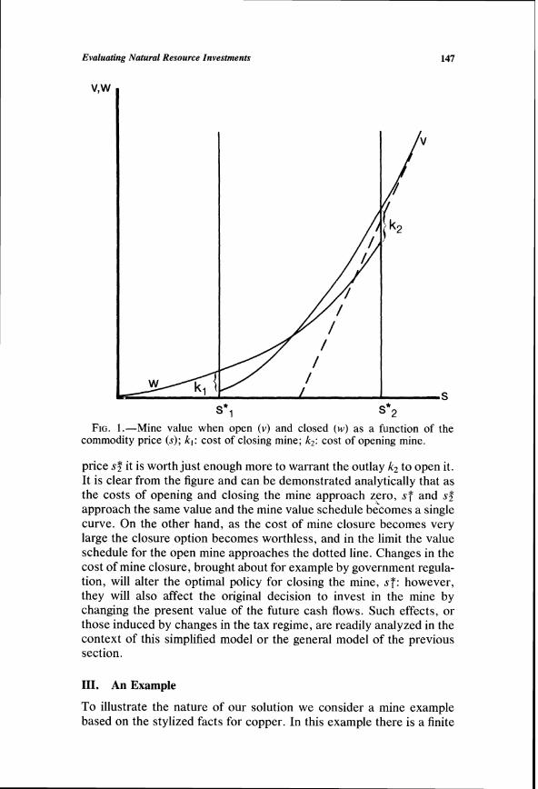
The solution is illustrated in figure 1. In this figure the dotted line represents the present value of the cash flows from the mine assuming that it can never be shut down; this is obtained by setting p4 = 0 in equation (42). Since y2 < 0, the value of the closure option diminishes and approaches zero for high output prices. For very low output prices the mine is worth more when it is closed than when it is open and making losses because of the cost of closure. However, for higher output prices the mine is worth more when open, and at the commodity

9. This is necessary for the present value of the future costs to be finite.

Evaluating Natural Resource Investments

s*1 s*2 FIG.1.-Mine value when open (v) and closed (w)as a function of the

commodity price (s); k l : cost of closing mine; k ~ :cost of opening mine.

price s? it is worth just enough more to warrant the outlay k2 to open it. It is clear from the figure and can be demonstrated analytically that as the costs of opening and closing the mine approach zero, ST and sz approach the same value and the mine value schedule b6comes a single curve. On the other hand, as the cost of mine closure becomes very large the closure option becomes worthless, and in the limit the value schedule for the open mine approaches the dotted line. Changes in the cost of mine closure, brought about for example by government regulation, will alter the optimal policy for closing the mine, S T : however, they will also affect the original decision to invest in the mine by changing the present value of the future cash flows. Such effects, or those induced by changes in the tax regime, are readily analyzed in the context of this simplified model or the general model of the previous section.

111. An Example

To illustrate the nature of our solution we consider a mine example based on the stylized facts for copper. In this example there is a finite

Journal of Business

TABLE 1 Data for a Hypothetical Copper Mine

Mine: Output rate (q*): 10 million poundslyear Inventory (Q): 150 million pounds Initial average cost of production a(q*, Q): $0.50/pound Initial cost of opening and closing (k,, k2): $200,000 Initial maintenance costs (f): $500,00O/year Cost inflation rate (a):8%/year

Copper: Convenience yield (K): l%/year Price variance (cr2): 8%lyear

Taxes: Real estate (A,, A2): 2%lyear Income (t2): 50% Royalty ( t , ) :0% Interest rate (p): lO%/year

mine inventory so that the stochastic optimal control problem represented by equations (27)-(36) must be solved numerically. To simplify matters somewhat we assume that there is a single feasible operating rate when the mine is open. The mine may be closed down or opened at a cost of $200,000 in current prices; it may also be abandoned. Other data required for this example are contained in table 1 .I0

Given an inventory equal to 15 years production, we find that the cost of production is 50 cents per pound, but it is not optimal to incur the cost of opening the mine until the price of copper rises to 76 cents. On the other hand, if the mine is already open and operating, it is not optimal to close it down until the copper price drops to 44 cents. Finally, the mine should be abandoned if the price drops below 20 cents. Obviously these critical prices depend on the assumed costs of opening, closing, and maintaining the mine: they also depend upon the remaining inventory in the mine. The greater the invenlory in the mine the greater is the incentive to extract the copper immediately, since the opportunity cost of immediate extraction falls as the expected life of the mine increases. Thus the greater the inventory the lower is the price at which the mine is opened and closed and, since the mine value is a nondecreasing function of the inventory, the lower the price at which it is abandoned.

Table 2 summarizes the results when the mine has a 15-year inventory. Columns 1 and 3 give the present values of the future cash flows from the mine, assuming that it is open and closed, respectively, for different copper prices. These are the relevant values for the investment decision. Column 4 gives the value of the mine assuming that it

10. The variance rate and convenience yield used in table 1 compare with a variance rate for COMEX monthly settlement prices for copper of 7.8% per year for 1971-82 and an average convenience yield of 0.7% per year computed from annual data on the May contract for the same period, using eq. (7).


TABLE 2 Value of Copper Mine for Different Copper Prices

Mine Value Value of Value of Copper ($ million) Fixed-Output- Closure Value of Mine Price Rate Mine Option under Certainty,

($/pound) Open Closed ($ million) ($ million) Risk a2 = 0 ($ million) (1) (2) (3) (4) (5) (6) (7)

* Optimal to close mine i. Optimal to open mine

cannot be closed down but must be operated at the rate of 10 million pounds per year until the inventory is exhausted in 15 years. The difference between column 4 and the greater of the values shown in columns 2 and 3 represents the value of the option to close down or abandon the mine if the price of copper falls far enough. The value of this closure option is shown in column 5: it amounts to 12% of the value of the fixed-output-rate mine when the copper price is equal to the variable cost of 50 cents per pound; of course this would represent a much higher proportion of the net present value of an investment in the mine.

Column 6 of the table reports the instantaneous risk of the mine at different copper prices. This is the instantaneous standard deviation of the mine value, defined as (v,lv)us when the mine is open and (w,lw)us when the mine is closed. As we would expect, the risk of the mine decreases as the copper price and hence the operating margin increases. Since the copper price is stochastic, so also is the ri+ of the mine and the instantaneous rate of return required by investors, point- ing to the dangers of assuming a single discount rate in a present value analysis.

Ownership of a mine that is not currently operating involves three distinct types of decision possibilities or options: first, the decision to begin operations; second, the decision to close the mine when it is currently operating (and possibly to reopen it later), which we have referred to as the closure option; and third, the decision to abandon the mine early, before the inventory is exhausted.

The decision to begin operations depends in our model on the current spot price of the commodity and the mine inventory. When there is no uncertainty, so that the time path of the commodity price is deterministic, the optimal decision rule for beginning operations can be expressed in calendar time (and the mine inventory). This certainty


case, which has been analyzed extensively under the rubric of the "timing option" (see, e.g., Solow 1974), corresponds to column 7, of table 2: this gives the value of the closed mine under the assumption of certainty, which may be contrasted with the uncertainty case of column 3. For our parameter values it is never optimal under certainty to close or abandon the mine, once it is open, before the inventory is exhausted," so that the closure and early abandonment options are worthless. When the commodity price is in the neighborhood of the production costs the elimination of uncertainty reduces the value of the mine dramatically. Of course this depends on the particular values of the convenience yield and other parameters.

IV. The Investment Decision

Thus far, only the valuation of the cash flows from an investment project has been considered. The investment decision itself requires that a comparison be made between the present value of the project cash flows and the initial investment needed for the project. Continuing with the example of a mine, V(S, Q*, t) represents the (nominal) value at time t of a completed operating mine with inventory Q* when the current output price is S; V(.)is equal to the present value of the cash flows that will be realized from the mine under the optimal operating policy. Similarly, let I(S, Q*, t) represent the investment required to construct an operating mine with inventory Q* on a particular property: the amount of this initial investment may obviously depend on calendar time and upon the size of the mine as represented by Q*, and S is included as an argument for the sake of generality. Then, assuming that construction lags can be neglected, the net present value (NPV) at time t of constructing the mine immediately is given by

NPV(S, Q*, t ) = V(S, Q*, t) - I ( s , Q*: t). (43)

However, once the possibility of postponing an investment decision is recognized, it is clear that it is not in general optimal to proceed with construction simply because the net present value of construction is positive: there is a "timing option" and it may pay to wait in the expectation that the net present value of construction will increase. This dynamic aspect of the investment decision is closely related to the problem of determining the optimal strategy for exercising an option on a share of common stock: the right to make the investment decision and to appropriate the resulting net present value is the ownership right in the undeveloped mine property, and the value of this ownership right corresponds to the value of the stock option.

Define X(S, Q*, t ) as the value of the ownership right to an unde-

11. Because the commodity price is increasing faster than the production costs.

151 Evaluah'ng Natural Resource Investments

veloped mine with inventory Q* at time t when the current output price is S . The stochastic process for X( . ) is obtained from Ito's lemma, using the assumption about the stochastic process for S embodied in expression ( 1 ) . Then the arbitrage argument used to derive the differential equation (15)for the value of a completed mine may be repeated to show that X( . ) must satisfy the partial differential equation

where, as before, A represents either the rate of tax on the value of the property or the intensity of a Poisson process governing the event of expropriation.l2

Since the origin is an absorbing state for the commodity price, S , we have the boundary condition

X(0, Q*, t ) = 0 , (45)

and if the ownership rights are in the form of a lease which expires at time T, then

X ( S , Q*, T ) = 0 . (46)

Assuming that the size of the mine inventory, Q*, is predetermined by technical and geological factors, the optimal strategy for investment can be characterized in terms of a time dependent schedule of output prices S'(t) such that

x(s', Q*, t ) = v(s',Q*, t ) - I(s', Q*, t ) , (47)

Xs(S', Q*, t ) = vs (s ' , Q*, t ) - Is(s', Q*, t ) . (48)

Equation (47)states simply that the value of the property is equal to the net present value of the investment at the time it is made. Equation (48) is the Merton-Samuelson high-contact or envelopccondition for a maximizing choice of s'.

If the amount of the accessible inventory in the mine, Q*,>depends on the amount of the initial investment instead of being determined exogenously, then we have the additional value-maximizing condition to determine the size of the initial mine inventory, Q*:

vQ(S1,Q*, t ) = lQ(S1,Q*, t ) . (49)

Thus the optimal investment strategy is obtained by solving the partial differential equation (44)for the value of the ownership right, subject to boundary conditions (45)-(49). The optimal time to invest is determined by the series of critical output prices ~ ' ( t )described by (47) and (48);the optimal amount to invest is determined by the first order condition (49). Note that the boundary conditions for this problem

12. An alternative assumption is that all costs inflate at the common rate T ;this would convert (44) into an ordinary differential eq. for the deflated mine value x = Xe-"'.


involve V ( S , Q, t), the present value of the cash flows from a completed mine. Thus solving the cash flow valuation problem is a prereq- uisite for the investment decision analysis described in this section.

V. Long-Term Supply Contracts

It is not uncommon for the outputs of natural resource investments to be sold under long-term contracts that fix the price of the commodity but leave the purchase rate at least partially to the discretion of the purchaser. Where they exist, such contracts must be taken into account in valuing ongoing projects. Therefore in this section we show briefly how these contracts may be valued and the equilibrium contract price determined.

Let Y(S , t ; p , T) denote the value at time t of a particular contract to purchase the commodity up to time Tat the contract price p , when the current spot price of the commodity is S . The contract is assumed to permit the purchaser to vary the price rate, q , between the lower and upper bounds q and (7. Since the commodity is by assumption available for purchase 2 the prevailing spot price S , ownership of the contract yields an instantaneous benefit or cash flow q(S - p).

Using Ito's lemma and the stochastic process for S, the instantaneous change in the value of the contract is given by

Then an arbitrage argument analogous to that presented in Section I implies that the value of the coritract must satisfy the partial differential equation:

The value of the contract at maturity, t = T, is equal to zero, so that

In addition, the origin is an absorbing state for the spot price S . This implies that if S = 0, the holder of the contract must incur certain losses at the rate -q p up to the maturity of the contract, so that

Finally, for sufficiently high values of S , the value of the right to vary the purchase rate approaches zero and the value of the contract approaches that of a series of forward contracts to purchase at the rate (7


at the fixed price p . Noting that forward and futures prices are equivalent when the interest rate is nonstochastic (see Cox et al. 1981; Jarrow and Oldfield 1981; Richard and Sundaresan 1981), this implies that

where F(S, T) is the futures price for delivery in T periods as defined previously.

The equilibrium contract price (or price schedule) is that which makes the value of the contract at inception equal to zero, given the prevailing spot price, S, and maturity, T. Writing the equilibrium contract price as p*(S, T), we have

In general there does not exist a closed-form solution for Y(.) or p*(.). However, if the convenience yield can be written as C(s) = KS, then closed-form solutions may be obtained in two special cases.

First, if the purchaser has no discretion over the purchase rate, so that (7 = q = q*, then the contract is equivalent to a series of forward contractswith value given by13

This implies that the equilibrium contract price is

Second, if the contract has an infinite maturity, thd-value of the contract is equal to the sum of the values of two assets we have already valued: a perpetual contract to purchase the commodity at the fixed rate q and a mine with infinite inventory, an average cost of production p , f&sible production rates (7 - q, and with no taxes, maintenance costs, or costs of opening and closing. The former may be valued using equation (56) and the latter is a special case of Section 11. '~ It can then be shown that

13. We thank the referee for this point. 14. As the referee remarks, this contract is equivalent to a perpetuity of European

options on the commodity.

Journal of Business

where

(P - K)] qdp1-y2,P

d - -4 - 4 - 4 9

and y l , y2, and a2are as defined following equation (40). The equilibrium price p*(S, 7) is found from the nonlinear equation obtained by setting either of the expressions (58) equal to zero.

VI. Conclusion

We have shown in the paper how assets whose cash flows depend on highly variable output prices may be valued and how the optimal policies for managing them may be determined by exploiting the properties of replicating self-financing portfolios. The explicit analysis rests on the assumption that such portfolios may be formed by trading in futures contracts in the output commodity, but the general approach can also be developed in a general equilibrium context if the relevant futures markets do not exist.

In addition to providing a rich set of empirical predictions for empirical research, this framework should be useful for the analysis of capital-budgeting decisions in a wide variety of situations in which the distribution of future cash flows is not given exogenously but must be determined by future management decisions.

Appendix

In contrast to the assumption of Section I1 that there are only two feasible output rates, zero and q*, and that it is costly to shift from one to the other, we assume in this case that the output rate is continuously and costlessly variable between zero and ?j;in keeping with this assumption, costs of opening and closing the mine are neglected and this renders the distinction between an open and a closed mine otiose.

We assume that no costs are incurred if the output rate is zero and that for positive output rates the total cost per unit time of the output rate q is c(q) =

q . a(q) = a. + a l q + a2q2, where a, , a2 > 0; this represents a (linearly) increasing marginal cost schedule.

Using these assumptions in equation (27) , the optimal output policy and the value of the mine satisfy

?hu2s2vs, + (r - K)VS + (1 - t2) max [(I - tl)qs 4E(O%Tl


Carrying out the maximization we find that the optimal output policy is

[ s > S "1 - - a ,

s* ( s ) = () S > s > s * s =s s*,

where s* = ( a l + 2 G ) l ( l - t l ) and s = ( a l + 2a24)l(1 - t l ) .Thus the optimal output policy maximizes the instantaneous profit rate; since the profit rate is zero when the output rate is zero, the output rate is positive whenever the net-of-royalty output price exceeds the minimum average cost of production.

The after-tax cash flow from the mine under the optimal output policy, p(s ) , is given by

S > s > s*,

When p(s ) is substituted for the maximand in equation ( A l ) , the complete solutions for the three regions are

s 5 s * , (A21

S > s > s*, (A31

where

Variables yl and y2 are as defined following equation (40), and the coefficients pi ( i = 1 , . . . , 6 ) are constants determined as follows. As in the case of Section I1 the requirements that v and vls remain finite for very small and very large s , respectively, imply that P2 = P5 = 0. The remaining four constants are obtained by solving the four linear equations yielded by imposing the condition that the valuation schedule v ( s ) be continuous and have a finite second derivative at s* and 3:

Journal of Business

FIG.2.-Case ii: Mine value ( v )and optimal output as a function of the output price ( s ) .

Thus the value of the mine is given by the solution to equations (A2) - (A8) with P2 = Ps = 0. Since the equation system (A5)-(A8) is linear it is a straightforward if tedious task to obtain an explicit valuation expression which may be used for comparative statics. The valuation schedule and the optimal output policy are illustrated in figure 2. In this figure the dotted line corresponds to the value of the mine if it is required to operate perpetually at its maximum rate $: thus the difference between the v(s) schedule and this line represents the value of the option to vary the output rate in response to changing output prices.

References

Bierman, H., and Smidt, S. 1960. The Capital Budgeting Decision. New York: Macmil- Ian.

Black, F., and Scholes, M. 1973. The pricing of options and corporate liabilities. Journal of Political Economy 81 (May-June): 637-54.

Bodie, Z. , and Rosansky, V. I . 1980. Risk and return in commodity futures. Financial Analysts Journal 36 (May-June): 27-40.

Bogue M. C. , and Roll, R. 1974. Capital budgeting of risky projects with imperfect markets for physical capital. Journal of Finance 29 (May): 601-13.

Brennan, M. J . 1958. The supply of storage. American Economic Review 48 (March): 50- l L .

Brennan, M. J. 1973. An approach to the valuation of uncertain income streams. Journal of Finance 28 (July): 661-73.

71


Brennan, M. J . , and Schwartz, E. S. 19820.Consistent regulatory policy under uncertainty. Bell Journal of Economics 13 (Autumn): 506-21.

Brennan, M. J. , and Schwartz, E. S. 19826.Regulation and corporate investment policy. Jounzal of Finance 37 (May): 289-300.

Brock, W. A,; Rothschild, M.; and Stiglitz, J . E. 1982.Stochastic capital theory. Finan- cial Research Center Memorandum no. 40. Princeton, N.J.: Princeton University, April.

Constantinides, G. M. 1978. Market risk adjustment in project valuation. Journal of Finance 33 (May): 603-16.

Cootner, P. 1967.Speculation and hedging. Food Research Institute Studies 7 (Suppl.): 65-106.

Cox, J. C.; Ingersoll, J . E.; and Ross, S. A. 1978.A theory of the term structure of interest rates. Research Paper no. 468.Stanford, Calif.: Stanford University.

Cox, J . C. ; Ingersoll. J. E.; and Ross, S. A. 1981.The relation between forward prices and futures prices. Journal of Financial Economics 9 (December): 321-46.

Dean, Joel 1951.Capital Budgeting; Top Management Policy on Plant Equipment and Product Development. New York: Columbia University.

Dothan, U., and Williams, J. 1980.Term-risk structures and the valuation of projects. Journal of Financial and Quantitative Analysis 15 (November): 875-906.

Fama, E. F. 1977.Risk-adjusted discount rates and capital budgeting under uncertainty. Journal of Financial Economics 5 (August): 3-24.

Fisher, Irving. 1907. The Rate of Interest: Its Nature, Determination and Relation to Economic Phenomena. New York: Macmillan.

Fleming, W. H., and Rishel, R. W. 1975.Deterministic and Stochastic Optimal Control. New York: Springer-Verlag.

Harrison, J . M., and Kreps, D. M. 1979.Martingales and arbitrage in multiperiod securities markets. Journal of Economic Theory 20:381-408.

Jarrow, R. A., and Oldfield, G. S. 1981.Forward contracts and futures contracts. Jour-nal of Financial Economics 9 (December): 373-82.

Kaldor, N. 1939.Speculation and economic stability. Review of Economic Studies 7:l-27.

Merton, R. C. 1971. Optimum consumption and portfolio rules in a continuous time model. Journal of Economic Theory 3 (December): 373-413.

Merton, R. 1973.The theory of rational option pricing. Bell Journal of Economic and Management Science 4 (Spring): 141-83.

Miller, M. H.,and Upton, C. W. 1985. A test of the Hotelling valuation principle. Journal of Political Economy 93 (February): In press.

Myers, S. C., and Turnbull, S. M. 1977.Capital budgeting and the capital asset pricing model: Good news and bad news. Journal of Finance 32 (May): 321-32.

Paddock, J . L.; Siegel, D. R.; and Smith, J. L. 1982. Option vahation of claims on physical assets: The case of off-shore petroleum leases. Unpublished manuscript. Evanston, Ill.: Northwestern University.

Pindyck, R. S. 1980.Uncertainty and exhaustible resource markets. Journal of Political Economy 88 (December): 1203-25.

Richard, S. F . , and Sundaresan, M. 1981.A continuous time equilibrium model of forward prices and futures prices in a multigood economy. Journal of Financial Eco- nomics 9 (December): 347-72.

Ross, S. A. 1978.A simple approach to the valuation of risky streams. Journal of Business 51 (July): 453-75.

Samuelson, P. A. 1965. Rational theory of warrant pricing. Industrial Management Review 6 (Spring): 3-3 1.

Solow, R. M. 1974.The economics of resources or the resources of economics. Ameri-can Economic Review 64 (May): 1-14.

Telser, L. G. 1958.Futures trading and the storage of cotton and wheat. In A. E. Peck, ed., Selected Writings on Future Markets. Chicago, 1977.

Tourinho, 0.A. F. 1979.The option value of reserves of natural resources. Unpublished manuscript. Berkeley: University of California.

Working, H. 1948.The theory of price of storage. Journal of Farm Economics 30:l-28. Reprinted in Selected Writings of Holbrook Working. Chicago: Chicago Board of Trade. 1977.

Evaluating Natural Resource Investments

Documents

Transcript of Evaluating Natural Resource Investments