Estimation of Thalamocortical and Intracortical NetworkModels from Joint Thalamic Single-Electrode and CorticalLaminar-Electrode Recordings in the Rat Barrel SystemPatrick Blomquist1, Anna Devor2,3, Ulf G. Indahl1, Istvan Ulbert4,5, Gaute T. Einevoll1*, Anders M. Dale3

1 Department of Mathematical Sciences and Technology and Center for Integrative Genetics, Norwegian University of Life Sciences, As, Norway, 2 Athinoula A. Martinos

Center, Massachusetts General Hospital, Charlestown, Massachusetts, United States of America, 3 Departments of Radiology and Neurosciences, University of California

San Diego, La Jolla, California, United States of America, 4 Institute for Psychology of the Hungarian Academy of Sciences, Budapest, Hungary, 5 Peter Pazmany Catholic

University, Department of Information Technology, Budapest, Hungary

Abstract

A new method is presented for extraction of population firing-rate models for both thalamocortical and intracortical signaltransfer based on stimulus-evoked data from simultaneous thalamic single-electrode and cortical recordings using linear(laminar) multielectrodes in the rat barrel system. Time-dependent population firing rates for granular (layer 4),supragranular (layer 2/3), and infragranular (layer 5) populations in a barrel column and the thalamic population in thehomologous barreloid are extracted from the high-frequency portion (multi-unit activity; MUA) of the recorded extracellularsignals. These extracted firing rates are in turn used to identify population firing-rate models formulated as integralequations with exponentially decaying coupling kernels, allowing for straightforward transformation to the more commonfiring-rate formulation in terms of differential equations. Optimal model structures and model parameters are identified byminimizing the deviation between model firing rates and the experimentally extracted population firing rates. For thethalamocortical transfer, the experimental data favor a model with fast feedforward excitation from thalamus to the layer-4laminar population combined with a slower inhibitory process due to feedforward and/or recurrent connections and mixedlinear-parabolic activation functions. The extracted firing rates of the various cortical laminar populations are found toexhibit strong temporal correlations for the present experimental paradigm, and simple feedforward population firing-ratemodels combined with linear or mixed linear-parabolic activation function are found to provide excellent fits to the data.The identified thalamocortical and intracortical network models are thus found to be qualitatively very different. While thethalamocortical circuit is optimally stimulated by rapid changes in the thalamic firing rate, the intracortical circuits are low-pass and respond most strongly to slowly varying inputs from the cortical layer-4 population.

Citation: Blomquist P, Devor A, Indahl UG, Ulbert I, Einevoll GT, et al. (2009) Estimation of Thalamocortical and Intracortical Network Models from Joint ThalamicSingle-Electrode and Cortical Laminar-Electrode Recordings in the Rat Barrel System. PLoS Comput Biol 5(3): e1000328. doi:10.1371/journal.pcbi.1000328

Editor: Karl J. Friston, University College London, United Kingdom

Received October 10, 2008; Accepted February 10, 2009; Published March 27, 2009

Copyright: � 2009 Blomquist et al. This is an open-access article distributed under the terms of the Creative Commons Attribution License, which permitsunrestricted use, distribution, and reproduction in any medium, provided the original author and source are credited.

Funding: Work was financially supported by the Research Council of Norway under the BeMatA and eVITA programmes, and by the National Institute of Health[R01 EB00790, NS051188]. The funders had no role in study design, data collection and analysis, decision to publish, or preparation of the manuscript.

Competing Interests: The authors have declared that no competing interests exist.

* E-mail: Gaute.Einevoll@umb.no

Introduction

Following pioneering work in the 1970s by, e.g., Wilson and

Cowan [1] and Amari [2] a substantial effort has been put into the

investigation of neural network models, particularly in the form of

firing-rate or neural field models [3]. Some firing-rate network

models, in particular for the early visual system ([4], Ch.2), have

been developed to account for particular physiological data.

However, for strongly interconnected cortical networks, few

mechanistic network models directly accounting for specific

neurobiological data have been identified. Instead most work has

been done on generic network models and has focused on the

investigation of generic features, such as the generation and

stability of localized bumps, oscillatory patterns, traveling waves

and pulses and other coherent structures, for reviews see

Ermentrout [5] or Coombes [6].

We here (1) present a new method for identification of specific

population firing-rate network models from extracellular record-

ings, (2) apply the method to extract network models for

thalamocortical and intracortical signal processing based on

stimulus-evoked data from simultaneous single-electrode and

multielectrode extracellular recordings in the rat somatosensory

(barrel) system, and (3) analyze and interpret the identified firing-

rate models using techniques from dynamical systems analysis.

Our study reveals large differences in the transfer function

between thalamus (VPM) and layer 4 of the barrel column,

compared to that between cortical layers, and thus sheds direct

light on how whisker stimuli is encoded in population firing-

activity in the somatosensory system.

The derivation of biologically realistic, cortical neural-network

models has generally been hampered by the lack of relevant

experimental data to constrain and test the models. Single

electrodes can generally only measure the firing activity of

individual neurons, not the joint activity of populations of cells

typically predicted by population firing-rate models. Kyriazi and

Simons [7] and Pinto et al. [8,9] thus developed models for the

somatosensory thalamocortical signal transformation based on

pooled data from single-unit recordings from numerous animals.

PLoS Computational Biology | www.ploscompbiol.org 1 March 2009 | Volume 5 | Issue 3 | e1000328

By contrast, multielectrode arrays provide a convenient and

powerful technology for obtaining simultaneous recordings from

all layers of the cerebral cortex, at one or more cortical locations

[10]. The signal at each low-impedance electrode contact

represents a weighted sum of the potential generated by synaptic

currents and action potentials of neurons within a radius of a few

hundred micrometers of the contact, where the weighting factors

depend on the shape and position of the neurons, as well as the

electrical properties of the conductive medium [11–13].

In the present paper we describe a new method for extraction of

population firing-rate models for both thalamocortical and

intracortical transfer on the basis of data from simultaneous

thalamic single-electrode and cortical recordings using linear

(laminar) multielectrodes in the rat barrel system. With so called

laminar population analysis (LPA) Einevoll et al. [11] jointly modeled

the low-frequency (local field potentials; LFP) and high-frequency

(multi-unit activity; MUA) parts of such stimulus-evoked laminar

electrode data to estimate (1) the laminar organization of cortical

populations in a barrel column, (2) time-dependent population

firing rates, and (3) the LFP signatures following firing in a

particular population. These ‘postfiring’ population LFP signa-

tures were further used to estimate the synaptic connection

patterns between the various populations using both current source

density (CSD) estimation techniques and a new LFP template-fitting

technique [11].

Here we use the stimulus-evoked time-dependent firing rates for

the cortical populations estimated using LPA, in combination with

single-electrode recordings of the firing activity in the homologous

barreloid in VPM, to identify population firing-rate models. The

models are formulated as nonlinear Volterra integral equations

with exponentially decaying coupling kernels allowing for a

mapping of the systems to sets of differential equations, the more

common mathematical representation of firing-rate models [5,14].

The population responses were found to increase monotonically

both with increasing amplitude and velocity of the whisker flick

[11,15,16]. A stimulus set varying both the whisker-flicking

amplitude and the rise time was found to provide a rich variety

of thalamic and cortical responses and thus to be well suited for

distinguishing between candidate models. The optimal model

structure and corresponding model parameters are estimated by

minimizing the mean-square deviation between the population

firing rates predicted by the models and the experimentally

extracted population firing rates.

A first focus is on the estimation of mathematical models for the

signal transfer between thalamus (VPM) and the layer-4

population, the population receiving the dominant thalamic input.

For this thalamocortical transfer our experimental data favors a

model with (1) fast feedforward excitation, (2) a slower predominantly

inhibitory process mediated by a combination of recurrent (within

layer 4) and feedforward interactions (from thalamus), and (3) a

mixed linear-parabolic activation function. The identified thalamo-

cortical circuits are seen to have a band-pass property, and in the

frequency domain the largest responses for the layer-4 population is

obtained for thalamic firing rates with frequencies around twenty Hz.

Very different population firing-rate models are identified for

the intracortical circuits, i.e., the spread of population activity from

layer 4 to supragranular (layer 2/3) and infragranular (layer 5)

layers. For the present experimental paradigm the extracted firing

rates of the various cortical laminar populations are found to

exhibit strong temporal correlations and simple feedforward

models with linear or mixed linear-parabolic activation function

are found to account excellently for the data. The functional

properties of the identified thalamocortical and intracortical

network models are thus qualitatively very different: while the

thalamocortical circuit is optimally stimulated by rapid changes in

the thalamic firing rate, the intracortical circuits are low-pass and

respond strongest to slowly varying inputs.

Preliminary results from this project were presented earlier in

poster format [17].

Results

Here we illustrate our approach by first showing results from

one of the six experimental data sets considered, and next show the

thalamic and cortical laminar population responses extracted from

these experimental data. Further, we outline the general form of

the neural population models we explore to account for these

population firing. We then go on to test specific candidate

thalamocortical models against the experimentally observed popula-

tion responses in layer 4 using the experimental thalamic response

as driving input to the model. The identified thalamocortical

models found by minimizing the deviation between model

predictions and experimental population firing rates are further

analyzed and explored using tools from dynamical system analysis.

Finally, we correspondingly examine how the experimentally

measured laminar population responses in layer 2/3 and layer 5,

respectively, can be explained by intracortical network models with

the experimental layer-4 population responses as input.

Experimental data and extracted population firing ratesIn Figure 1 we show trial-averaged multi-unit activity (MUA) data

for one of six experiments, labeled ‘experiment 1’, from stimulus

onset, i.e., onset of whisker-flick, until 100 ms after. This is the

time window of data used in the further analysis. Color plots depict

the laminar-electrode recordings while the line plots below show

the corresponding trial-averaged thalamic recordings. Results for 9

of 27 stimulus conditions are shown, corresponding to three

different stimulus rise times t9,t5,t1ð Þ for three different stimulus

amplitudes a1,a2,a3ð Þ. Neurons in the barrel cortex are sensitive

to both stimulus amplitude and stimulus velocity (and thus

stimulus rise time) [11,15,16], and we found that a set of stimuli

Author summary

Many of the salient features of individual cortical neuronsappear well understood, and several mathematical modelsdescribing their physiological properties have beendeveloped. The present understanding of the highlyinterconnected cortical neural networks is much morelimited. Lack of relevant experimental data has in generalprevented the construction and rigorous testing ofbiologically realistic cortical network models. Here wepresent a new method for extracting such models. Inparticular we estimate specific mathematical modelsdescribing the sensory activation of thalamic and corticalneuronal populations in the rat whisker system from jointrecordings of extracellular potentials in thalamus andcortex. The mathematical models are formulated in termsof average firing rates of a thalamic population and a set oflaminarly organized cortical populations, the latter extract-ed from data from linear (laminar) multielectrodes insertedperpendicularly through cortex. The identified modelsdescribing the signal processing from thalamus to cortexare found to be qualitatively very different from themodels describing the processing between cortical pop-ulations; while the thalamocortical circuit is optimallystimulated by rapid changes in the thalamic firing rate, theintracortical circuits respond most strongly to slowlyvarying inputs.

Neural Network Model Estimation

PLoS Computational Biology | www.ploscompbiol.org 2 March 2009 | Volume 5 | Issue 3 | e1000328

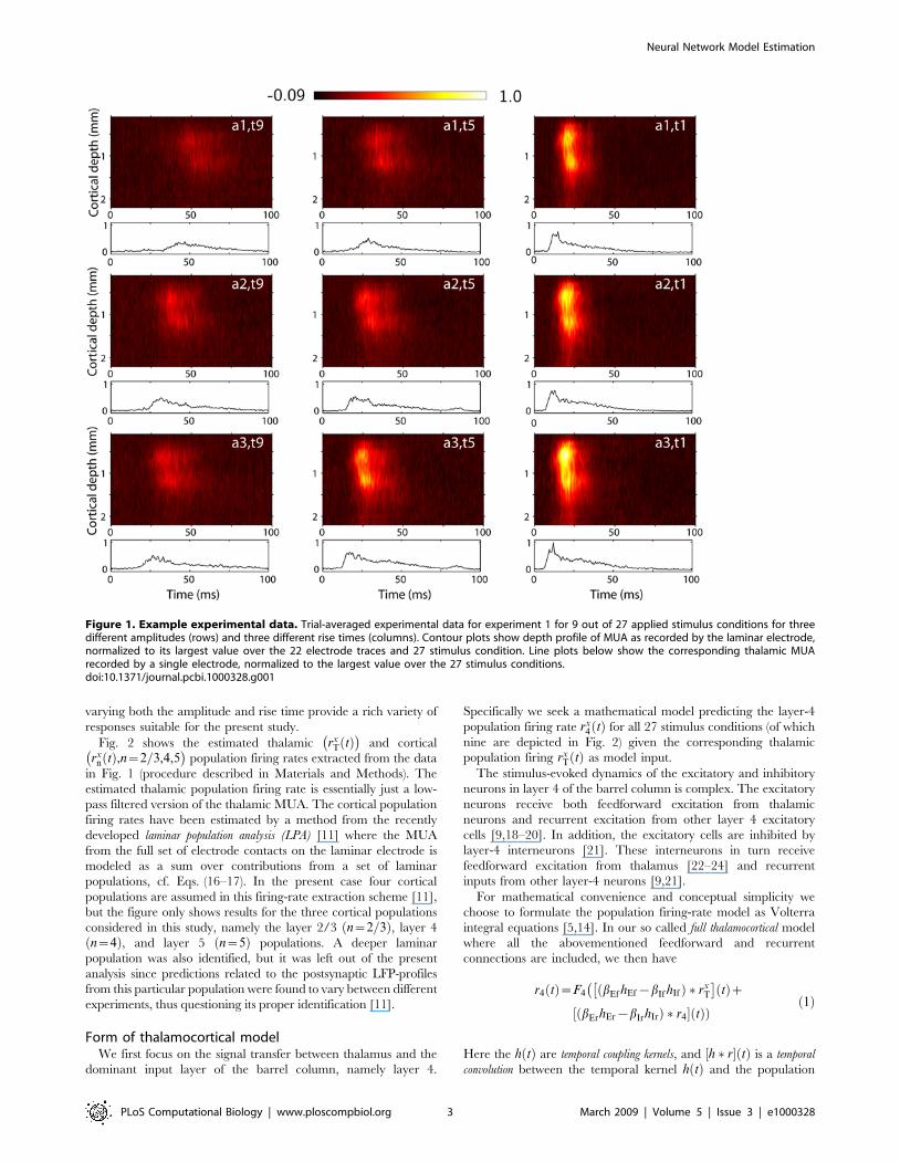
varying both the amplitude and rise time provide a rich variety of

responses suitable for the present study.

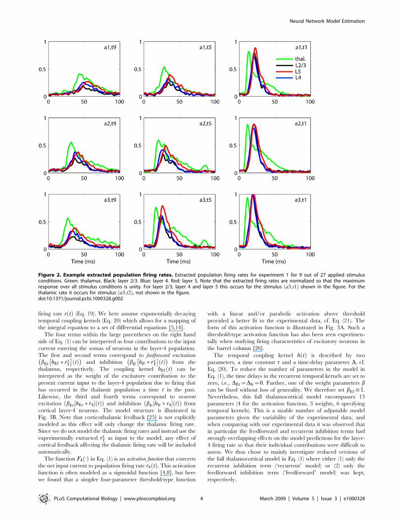
Fig. 2 shows the estimated thalamic rxT tð Þ

� �and cortical

rxn tð Þ,n~2=3,4,5

� �population firing rates extracted from the data

in Fig. 1 (procedure described in Materials and Methods). The

estimated thalamic population firing rate is essentially just a low-

pass filtered version of the thalamic MUA. The cortical population

firing rates have been estimated by a method from the recently

developed laminar population analysis (LPA) [11] where the MUA

from the full set of electrode contacts on the laminar electrode is

modeled as a sum over contributions from a set of laminar

populations, cf. Eqs. (16–17). In the present case four cortical

populations are assumed in this firing-rate extraction scheme [11],

but the figure only shows results for the three cortical populations

considered in this study, namely the layer 2/3 n~2=3ð Þ, layer 4

n~4ð Þ, and layer 5 n~5ð Þ populations. A deeper laminar

population was also identified, but it was left out of the present

analysis since predictions related to the postsynaptic LFP-profiles

from this particular population were found to vary between different

experiments, thus questioning its proper identification [11].

Form of thalamocortical modelWe first focus on the signal transfer between thalamus and the

dominant input layer of the barrel column, namely layer 4.

Specifically we seek a mathematical model predicting the layer-4

population firing rate rx4 tð Þ for all 27 stimulus conditions (of which

nine are depicted in Fig. 2) given the corresponding thalamic

population firing rxT tð Þ as model input.

The stimulus-evoked dynamics of the excitatory and inhibitory

neurons in layer 4 of the barrel column is complex. The excitatory

neurons receive both feedforward excitation from thalamic

neurons and recurrent excitation from other layer 4 excitatory

cells [9,18–20]. In addition, the excitatory cells are inhibited by

layer-4 interneurons [21]. These interneurons in turn receive

feedforward excitation from thalamus [22–24] and recurrent

inputs from other layer-4 neurons [9,21].

For mathematical convenience and conceptual simplicity we

choose to formulate the population firing-rate model as Volterra

integral equations [5,14]. In our so called full thalamocortical model

where all the abovementioned feedforward and recurrent

connections are included, we then have

r4 tð Þ~F4 bEf hEf{bIf hIfð Þ � rxT

� �tð Þz

�bErhEr{bIrhIrð Þ � r4½ � tð ÞÞ

ð1Þ

Here the h tð Þ are temporal coupling kernels, and h � r½ � tð Þ is a temporal

convolution between the temporal kernel h tð Þ and the population

Figure 1. Example experimental data. Trial-averaged experimental data for experiment 1 for 9 out of 27 applied stimulus conditions for threedifferent amplitudes (rows) and three different rise times (columns). Contour plots show depth profile of MUA as recorded by the laminar electrode,normalized to its largest value over the 22 electrode traces and 27 stimulus condition. Line plots below show the corresponding thalamic MUArecorded by a single electrode, normalized to the largest value over the 27 stimulus conditions.doi:10.1371/journal.pcbi.1000328.g001

Neural Network Model Estimation

PLoS Computational Biology | www.ploscompbiol.org 3 March 2009 | Volume 5 | Issue 3 | e1000328

firing rate r tð Þ (Eq. 19). We here assume exponentially decaying

temporal coupling kernels (Eq. 20) which allows for a mapping of

the integral equation to a set of differential equations [5,14].

The four terms within the large parentheses on the right hand

side of Eq. (1) can be interpreted as four contributions to the input

current entering the somas of neurons in the layer-4 population.

The first and second terms correspond to feedforward excitation

bEf hEf � rxT

� �tð Þ

� �and inhibition bIf hIf � rx

T

� �tð Þ

� �from the

thalamus, respectively. The coupling kernel hEf tð Þ can be

interpreted as the weight of the excitatory contribution to the

present current input to the layer-4 population due to firing that

has occurred in the thalamic population a time t in the past.

Likewise, the third and fourth terms correspond to recurrent

excitation bEr hEr � r4½ � tð Þð Þ and inhibition bIr hIr � r4½ � tð Þð Þ from

cortical layer-4 neurons. The model structure is illustrated in

Fig. 3B. Note that corticothalamic feedback [25] is not explicitly

modeled as this effect will only change the thalamic firing rate.

Since we do not model the thalamic firing rates and instead use the

experimentally extracted rxT as input to the model, any effect of

cortical feedback affecting the thalamic firing rate will be included

automatically.

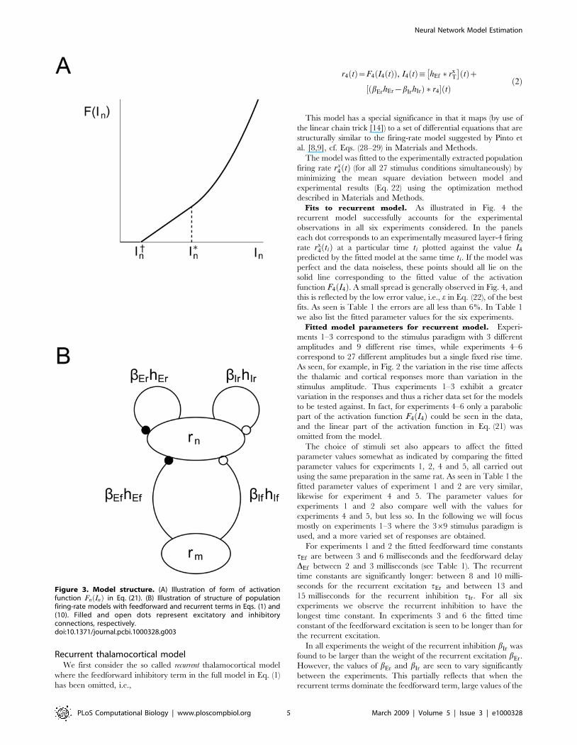
The function F4:ð Þ in Eq. (1) is an activation function that converts

the net input current to population firing rate r4 tð Þ. This activation

function is often modeled as a sigmoidal function [4,8], but here

we found that a simpler four-parameter threshold-type function

with a linear and/or parabolic activation above threshold

provided a better fit to the experimental data, cf. Eq. (21). The

form of this activation function is illustrated in Fig. 3A. Such a

threshold-type activation function has also been seen experimen-

tally when studying firing characteristics of excitatory neurons in

the barrel column [26].

The temporal coupling kernel h tð Þ is described by two

parameters, a time constant t and a time-delay parameter D, cf.

Eq. (20). To reduce the number of parameters in the model in

Eq. (1), the time delays in the recurrent temporal kernels are set to

zero, i.e., DEr~DIr~0. Further, one of the weight parameters bcan be fixed without loss of generality. We therefore set bEf:1.

Nevertheless, this full thalamocortical model encompasses 13

parameters (4 for the activation function, 3 weights, 6 specifying

temporal kernels). This is a sizable number of adjustable model

parameters given the variability of the experimental data, and

when comparing with our experimental data it was observed that

in particular the feedforward and recurrent inhibition terms had

strongly overlapping effects on the model predictions for the layer-

4 firing rate so that their individual contributions were difficult to

assess. We thus chose to mainly investigate reduced versions of

the full thalamocortical model in Eq. (1) where either (1) only the

recurrent inhibition term (‘recurrent’ model) or (2) only the

feedforward inhibition term (‘feedforward’ model) was kept,

respectively.

Figure 2. Example extracted population firing rates. Extracted population firing rates for experiment 1 for 9 out of 27 applied stimulusconditions. Green: thalamus. Black: layer 2/3. Blue: layer 4. Red: layer 5. Note that the extracted firing rates are normalized so that the maximumresponse over all stimulus conditions is unity. For layer 2/3, layer 4 and layer 5 this occurs for the stimulus a3,t1ð Þ shown in the figure. For thethalamic rate it occurs for stimulus a3,t2ð Þ, not shown in the figure.doi:10.1371/journal.pcbi.1000328.g002

Neural Network Model Estimation

PLoS Computational Biology | www.ploscompbiol.org 4 March 2009 | Volume 5 | Issue 3 | e1000328

Recurrent thalamocortical modelWe first consider the so called recurrent thalamocortical model

where the feedforward inhibitory term in the full model in Eq. (1)

has been omitted, i.e.,

r4 tð Þ~F4 I4 tð Þð Þ, I4 tð Þ: hEf � rxT

� �tð Þz

bErhEr{bIrhIrð Þ � r4½ � tð Þð2Þ

This model has a special significance in that it maps (by use of

the linear chain trick [14]) to a set of differential equations that are

structurally similar to the firing-rate model suggested by Pinto et

al. [8,9], cf. Eqs. (28–29) in Materials and Methods.

The model was fitted to the experimentally extracted population

firing rate rx4 tð Þ (for all 27 stimulus conditions simultaneously) by

minimizing the mean square deviation between model and

experimental results (Eq. 22) using the optimization method

described in Materials and Methods.

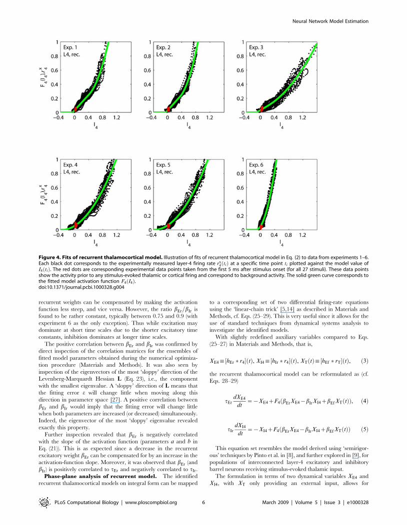
Fits to recurrent model. As illustrated in Fig. 4 the

recurrent model successfully accounts for the experimental

observations in all six experiments considered. In the panels

each dot corresponds to an experimentally measured layer-4 firing

rate rx4 tið Þ at a particular time ti plotted against the value I4

predicted by the fitted model at the same time ti. If the model was

perfect and the data noiseless, these points should all lie on the

solid line corresponding to the fitted value of the activation

function F4 I4ð Þ. A small spread is generally observed in Fig. 4, and

this is reflected by the low error value, i.e., e in Eq. (22), of the best

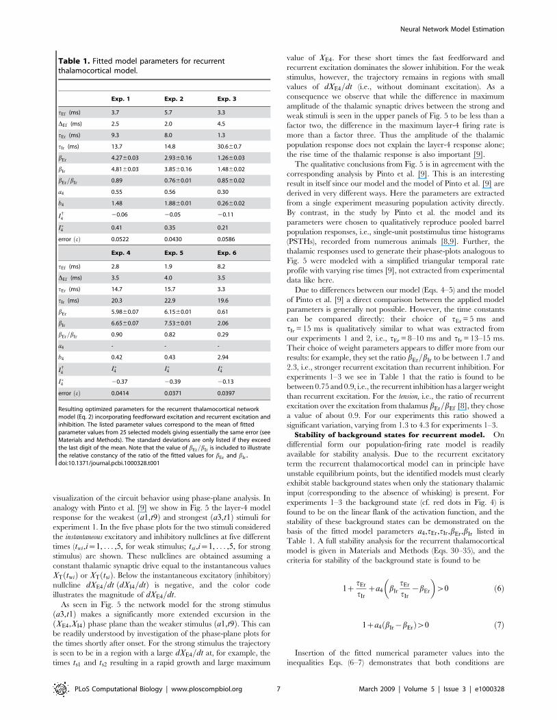
fits. As seen is Table 1 the errors are all less than 6%. In Table 1

we also list the fitted parameter values for the six experiments.

Fitted model parameters for recurrent model. Experi-

ments 1–3 correspond to the stimulus paradigm with 3 different

amplitudes and 9 different rise times, while experiments 4–6

correspond to 27 different amplitudes but a single fixed rise time.

As seen, for example, in Fig. 2 the variation in the rise time affects

the thalamic and cortical responses more than variation in the

stimulus amplitude. Thus experiments 1–3 exhibit a greater

variation in the responses and thus a richer data set for the models

to be tested against. In fact, for experiments 4–6 only a parabolic

part of the activation function F4 I4ð Þ could be seen in the data,

and the linear part of the activation function in Eq. (21) was

omitted from the model.

The choice of stimuli set also appears to affect the fitted

parameter values somewhat as indicated by comparing the fitted

parameter values for experiments 1, 2, 4 and 5, all carried out

using the same preparation in the same rat. As seen in Table 1 the

fitted parameter values of experiment 1 and 2 are very similar,

likewise for experiment 4 and 5. The parameter values for

experiments 1 and 2 also compare well with the values for

experiments 4 and 5, but less so. In the following we will focus

mostly on experiments 1–3 where the 369 stimulus paradigm is

used, and a more varied set of responses are obtained.

For experiments 1 and 2 the fitted feedforward time constants

tEf are between 3 and 6 milliseconds and the feedforward delay

DEf between 2 and 3 milliseconds (see Table 1). The recurrent

time constants are significantly longer: between 8 and 10 milli-

seconds for the recurrent excitation tEr and between 13 and

15 milliseconds for the recurrent inhibition tIr. For all six

experiments we observe the recurrent inhibition to have the

longest time constant. In experiments 3 and 6 the fitted time

constant of the feedforward excitation is seen to be longer than for

the recurrent excitation.

In all experiments the weight of the recurrent inhibition bIr was

found to be larger than the weight of the recurrent excitation bEr.

However, the values of bEr and bIr are seen to vary significantly

between the experiments. This partially reflects that when the

recurrent terms dominate the feedforward term, large values of the

Figure 3. Model structure. (A) Illustration of form of activationfunction Fn Inð Þ in Eq. (21). (B) Illustration of structure of populationfiring-rate models with feedforward and recurrent terms in Eqs. (1) and(10). Filled and open dots represent excitatory and inhibitoryconnections, respectively.doi:10.1371/journal.pcbi.1000328.g003

Neural Network Model Estimation

PLoS Computational Biology | www.ploscompbiol.org 5 March 2009 | Volume 5 | Issue 3 | e1000328

recurrent weights can be compensated by making the activation

function less steep, and vice versa. However, the ratio bEr=bIr is

found to be rather constant, typically between 0.75 and 0.9 (with

experiment 6 as the only exception). Thus while excitation may

dominate at short time scales due to the shorter excitatory time

constants, inhibition dominates at longer time scales.

The positive correlation between bEr and bIr was confirmed by

direct inspection of the correlation matrices for the ensembles of

fitted model parameters obtained during the numerical optimiza-

tion procedure (Materials and Methods). It was also seen by

inspection of the eigenvectors of the most ‘sloppy’ direction of the

Levenberg-Marquardt Hessian L (Eq. 23), i.e., the component

with the smallest eigenvalue. A ‘sloppy’ direction of L means that

the fitting error e will change little when moving along this

direction in parameter space [27]. A positive correlation between

bEr and bIr would imply that the fitting error will change little

when both parameters are increased (or decreased) simultaneously.

Indeed, the eigenvector of the most ‘sloppy’ eigenvalue revealed

exactly this property.

Further inspection revealed that bEr is negatively correlated

with the slope of the activation function (parameters a and b in

Eq. (21)). This is as expected since a decrease in the recurrent

excitatory weight bEr can be compensated for by an increase in the

activation-function slope. Moreover, it was observed that bEr (and

bIr) is positively correlated to tEr and negatively correlated to tIr.

Phase-plane analysis of recurrent model. The identified

recurrent thalamocortical models on integral form can be mapped

to a corresponding set of two differential firing-rate equations

using the ‘linear-chain trick’ [5,14] as described in Materials and

Methods, cf. Eqs. (25–29). This is very useful since it allows for the

use of standard techniques from dynamical systems analysis to

investigate the identified models.

With slightly redefined auxiliary variables compared to Eqs.

(25–27) in Materials and Methods, that is,

XE4: hEr � r4½ � tð Þ, XI4: hIr � r4½ � tð Þ, XT tð Þ: hEf � rT½ � tð Þ, ð3Þ

the recurrent thalamocortical model can be reformulated as (cf.

Eqs. 28–29)

tErdXE4

dt~{XE4zF4 bErXE4{bIrXI4zbEf XT tð Þð Þ, ð4Þ

tIrdXI4

dt~{XI4zF4 bErXE4{bIrXI4zbEf XT tð Þð Þ ð5Þ

This equation set resembles the model derived using ‘semirigor-

ous’ techniques by Pinto et al. in [8], and further explored in [9], for

populations of interconnected layer-4 excitatory and inhibitory

barrel neurons receiving stimulus-evoked thalamic input.

The formulation in terms of two dynamical variables XE4 and

XI4, with XT only providing an external input, allows for

Figure 4. Fits of recurrent thalamocortical model. Illustration of fits of recurrent thalamocortical model in Eq. (2) to data from experiments 1–6.Each black dot corresponds to the experimentally measured layer-4 firing rate rx

4 tið Þ at a specific time point ti plotted against the model value ofI4 tið Þ. The red dots are corresponding experimental data points taken from the first 5 ms after stimulus onset (for all 27 stimuli). These data pointsshow the activity prior to any stimulus-evoked thalamic or cortical firing and correspond to background activity. The solid green curve corresponds tothe fitted model activation function F4 I4ð Þ.doi:10.1371/journal.pcbi.1000328.g004

Neural Network Model Estimation

PLoS Computational Biology | www.ploscompbiol.org 6 March 2009 | Volume 5 | Issue 3 | e1000328

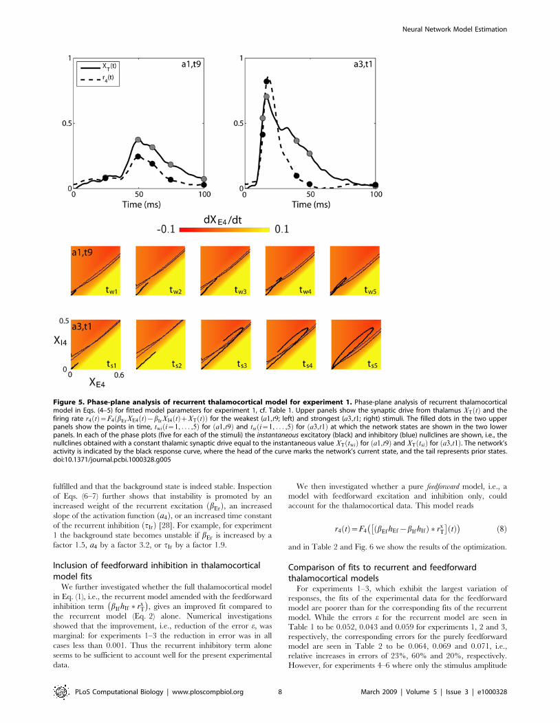
visualization of the circuit behavior using phase-plane analysis. In

analogy with Pinto et al. [9] we show in Fig. 5 the layer-4 model

response for the weakest a1,t9ð Þ and strongest a3,t1ð Þ stimuli for

experiment 1. In the five phase plots for the two stimuli considered

the instantaneous excitatory and inhibitory nullclines at five different

times (twi,i~1, . . . ,5, for weak stimulus; tsi,i~1, . . . ,5, for strong

stimulus) are shown. These nullclines are obtained assuming a

constant thalamic synaptic drive equal to the instantaneous values

XT twið Þ or XT tsið Þ. Below the instantaneous excitatory (inhibitory)

nullcline dXE4=dt dXI4=dtð Þ is negative, and the color code

illustrates the magnitude of dXE4=dt.

As seen in Fig. 5 the network model for the strong stimulus

a3,t1ð Þ makes a significantly more extended excursion in the

XE4,XI4ð Þ phase plane than the weaker stimulus a1,t9ð Þ. This can

be readily understood by investigation of the phase-plane plots for

the times shortly after onset. For the strong stimulus the trajectory

is seen to be in a region with a large dXE4=dt at, for example, the

times ts1 and ts2 resulting in a rapid growth and large maximum

value of XE4. For these short times the fast feedforward and

recurrent excitation dominates the slower inhibition. For the weak

stimulus, however, the trajectory remains in regions with small

values of dXE4=dt (i.e., without dominant excitation). As a

consequence we observe that while the difference in maximum

amplitude of the thalamic synaptic drives between the strong and

weak stimuli is seen in the upper panels of Fig. 5 to be less than a

factor two, the difference in the maximum layer-4 firing rate is

more than a factor three. Thus the amplitude of the thalamic

population response does not explain the layer-4 response alone;

the rise time of the thalamic response is also important [9].

The qualitative conclusions from Fig. 5 is in agreement with the

corresponding analysis by Pinto et al. [9]. This is an interesting

result in itself since our model and the model of Pinto et al. [9] are

derived in very different ways. Here the parameters are extracted

from a single experiment measuring population activity directly.

By contrast, in the study by Pinto et al. the model and its

parameters were chosen to qualitatively reproduce pooled barrel

population responses, i.e., single-unit poststimulus time histograms

(PSTHs), recorded from numerous animals [8,9]. Further, the

thalamic responses used to generate their phase-plots analogous to

Fig. 5 were modeled with a simplified triangular temporal rate

profile with varying rise times [9], not extracted from experimental

data like here.

Due to differences between our model (Eqs. 4–5) and the model

of Pinto et al. [9] a direct comparison between the applied model

parameters is generally not possible. However, the time constants

can be compared directly: their choice of tEr = 5 ms and

tIr = 15 ms is qualitatively similar to what was extracted from

our experiments 1 and 2, i.e., tEr = 8–10 ms and tIr = 13–15 ms.

Their choice of weight parameters appears to differ more from our

results: for example, they set the ratio bEr=bIr to be between 1.7 and

2.3, i.e., stronger recurrent excitation than recurrent inhibition. For

experiments 1–3 we see in Table 1 that the ratio is found to be

between 0.75 and 0.9, i.e., the recurrent inhibition has a larger weight

than recurrent excitation. For the tension, i.e., the ratio of recurrent

excitation over the excitation from thalamus bEr=bEf [8], they chose

a value of about 0.9. For our experiments this ratio showed a

significant variation, varying from 1.3 to 4.3 for experiments 1–3.

Stability of background states for recurrent model. On

differential form our population-firing rate model is readily

available for stability analysis. Due to the recurrent excitatory

term the recurrent thalamocortical model can in principle have

unstable equilibrium points, but the identified models must clearly

exhibit stable background states when only the stationary thalamic

input (corresponding to the absence of whisking) is present. For

experiments 1–3 the background state (cf. red dots in Fig. 4) is

found to be on the linear flank of the activation function, and the

stability of these background states can be demonstrated on the

basis of the fitted model parameters a4,tEr,tIr,bEr,bIr listed in

Table 1. A full stability analysis for the recurrent thalamocortical

model is given in Materials and Methods (Eqs. 30–35), and the

criteria for stability of the background state is found to be

1ztEr

tIrza4 bIr

tEr

tIr{bEr

� �w0 ð6Þ

1za4 bIr{bErð Þw0 ð7Þ

Insertion of the fitted numerical parameter values into the

inequalities Eqs. (6–7) demonstrates that both conditions are

Table 1. Fitted model parameters for recurrentthalamocortical model.

Exp. 1 Exp. 2 Exp. 3

tEf (ms) 3.7 5.7 3.3

DEf (ms) 2.5 2.0 4.5

tEr (ms) 9.3 8.0 1.3

tIr (ms) 13.7 14.8 30.660.7

bEr 4.2760.03 2.9360.16 1.2660.03

bIr 4.8160.03 3.8560.16 1.4860.02

bEr=bIr 0.89 0.7660.01 0.8560.02

a4 0.55 0.56 0.30

b4 1.48 1.8860.01 0.2660.02

I{4

20.06 20.05 20.11

I�4 0.41 0.35 0.21

error eð Þ 0.0522 0.0430 0.0586

Exp. 4 Exp. 5 Exp. 6

tEf (ms) 2.8 1.9 8.2

DEf (ms) 3.5 4.0 3.5

tEr (ms) 14.7 15.7 3.3

tIr (ms) 20.3 22.9 19.6

bEr 5.9860.07 6.1560.01 0.61

bIr 6.6560.07 7.5360.01 2.06

bEr=bIr 0.90 0.82 0.29

a4 - - -

b4 0.42 0.43 2.94

I{4

I�4 I�4 I�4

I�4 20.37 20.39 20.13

error eð Þ 0.0414 0.0371 0.0397

Resulting optimized parameters for the recurrent thalamocortical networkmodel (Eq. 2) incorporating feedforward excitation and recurrent excitation andinhibition. The listed parameter values correspond to the mean of fittedparameter values from 25 selected models giving essentially the same error (seeMaterials and Methods). The standard deviations are only listed if they exceedthe last digit of the mean. Note that the value of bEr=bIr is included to illustratethe relative constancy of the ratio of the fitted values for bEr and bIr.doi:10.1371/journal.pcbi.1000328.t001

Neural Network Model Estimation

PLoS Computational Biology | www.ploscompbiol.org 7 March 2009 | Volume 5 | Issue 3 | e1000328

fulfilled and that the background state is indeed stable. Inspection

of Eqs. (6–7) further shows that instability is promoted by an

increased weight of the recurrent excitation bErð Þ, an increased

slope of the activation function a4ð Þ, or an increased time constant

of the recurrent inhibition tIrð Þ [28]. For example, for experiment

1 the background state becomes unstable if bEr is increased by a

factor 1.5, a4 by a factor 3.2, or tIr by a factor 1.9.

Inclusion of feedforward inhibition in thalamocorticalmodel fits

We further investigated whether the full thalamocortical model

in Eq. (1), i.e., the recurrent model amended with the feedforward

inhibition term bIf hIf � rxT

� �, gives an improved fit compared to

the recurrent model (Eq. 2) alone. Numerical investigations

showed that the improvement, i.e., reduction of the error e, was

marginal: for experiments 1–3 the reduction in error was in all

cases less than 0.001. Thus the recurrent inhibitory term alone

seems to be sufficient to account well for the present experimental

data.

We then investigated whether a pure feedforward model, i.e., a

model with feedforward excitation and inhibition only, could

account for the thalamocortical data. This model reads

r4 tð Þ~F4 bEf hEf{bIf hIfð Þ � rxT

� �tð Þ

� �ð8Þ

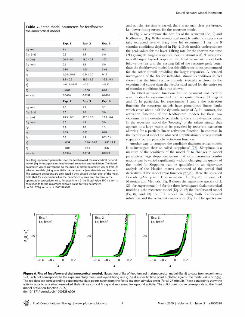
and in Table 2 and Fig. 6 we show the results of the optimization.

Comparison of fits to recurrent and feedforwardthalamocortical models

For experiments 1–3, which exhibit the largest variation of

responses, the fits of the experimental data for the feedforward

model are poorer than for the corresponding fits of the recurrent

model. While the errors e for the recurrent model are seen in

Table 1 to be 0.052, 0.043 and 0.059 for experiments 1, 2 and 3,

respectively, the corresponding errors for the purely feedforward

model are seen in Table 2 to be 0.064, 0.069 and 0.071, i.e.,

relative increases in errors of 23%, 60% and 20%, respectively.

However, for experiments 4–6 where only the stimulus amplitude

Figure 5. Phase-plane analysis of recurrent thalamocortical model for experiment 1. Phase-plane analysis of recurrent thalamocorticalmodel in Eqs. (4–5) for fitted model parameters for experiment 1, cf. Table 1. Upper panels show the synaptic drive from thalamus XT tð Þ and thefiring rate r4 tð Þ~F4 bErXE4 tð Þ{bIrXI4 tð ÞzXT tð Þð Þ for the weakest (a1,t9; left) and strongest (a3,t1; right) stimuli. The filled dots in the two upperpanels show the points in time, twi i~1, . . . ,5ð Þ for a1,t9ð Þ and tsi i~1, . . . ,5ð Þ for a3,t1ð Þ at which the network states are shown in the two lowerpanels. In each of the phase plots (five for each of the stimuli) the instantaneous excitatory (black) and inhibitory (blue) nullclines are shown, i.e., thenullclines obtained with a constant thalamic synaptic drive equal to the instantaneous value XT twið Þ for a1,t9ð Þ and XT tsið Þ for a3,t1ð Þ. The network’sactivity is indicated by the black response curve, where the head of the curve marks the network’s current state, and the tail represents prior states.doi:10.1371/journal.pcbi.1000328.g005

Neural Network Model Estimation

PLoS Computational Biology | www.ploscompbiol.org 8 March 2009 | Volume 5 | Issue 3 | e1000328

and not the rise time is varied, there is no such clear preference,

i.e., lower fitting errors, for the recurrent model.

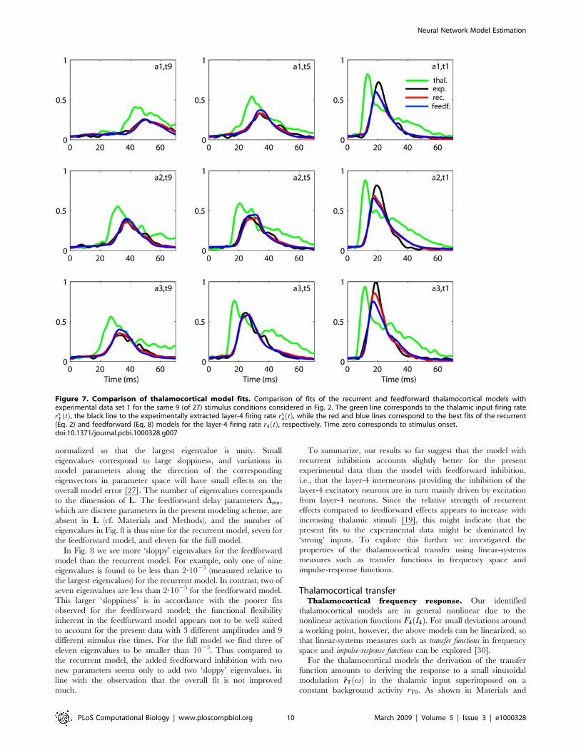
In Fig. 7 we compare the best fits of the recurrent (Eq. 2) and

feedforward (Eq. 8) thalamocortical models with the experimen-

tally extracted layer-4 firing rate for experiment 1 for the 9

stimulus conditions depicted in Fig. 2. Both models underestimate

the peak values for the layer-4 firing rate for the shortest rise time

t1ð Þ giving the largest responses. For the stimulus a3,t1 giving the

overall largest layer-4 response, the fitted recurrent model both

follows the rise and the ensuing fall of the response peak better

than the feedforward model, but this difference is less pronounced

for the other stimuli providing the larger responses. A detailed

investigation of the fits for individual stimulus conditions in fact

shows that the fitted recurrent model typically is closer to the

experimental curves than the feedforward model for the entire set

of stimulus conditions (data not shown).

The fitted activation functions for the recurrent and feedfor-

ward models for experiments 1 to 3 are quite different (cf. Figs. 4

and 6). In particular, for experiments 1 and 2 the activation

functions for recurrent models have pronounced linear flanks

which cover about half the dynamic range of I4. In contrast, the

activation functions of the feedforward models for these two

experiments are essentially parabolic in the entire dynamic range.

In the recurrent model the ‘boosting’ of the salient stimuli thus

appears to a large extent to be provided by recurrent excitation

allowing for a partially linear activation function. In contrast, in

the feedforward model the observed amplification of strong stimuli

requires a purely parabolic activation function.

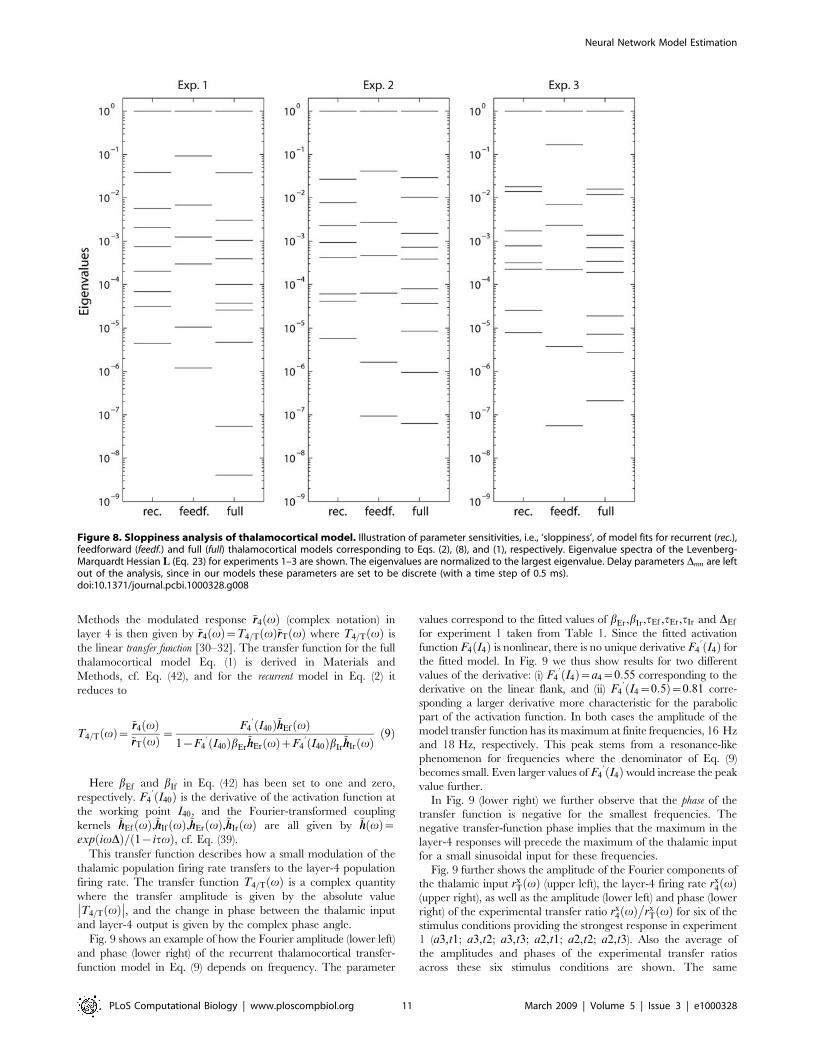
Another way to compare the candidate thalamocortical models

is to investigate their so called ‘sloppiness’ [27]. Sloppiness is a

measure of the sensitivity of the model fit to changes in model

parameters: large sloppiness means that some parameter combi-

nations can be varied significantly without changing the quality of

the model fit. Sloppiness can be quantified by an eigenvalue

analysis of the Hessian matrix composed of the partial 2nd

derivatives of the model error function [27,29]. Here the so called

Levenberg-Marquardt Hessian matrix L (Eq. 23) is used, cf.

Materials and Methods. Fig. 8 shows the eigenvalue spectra of L(23) for experiments 1–3 for the three investigated thalamocortical

models: (1) the recurrent model (Eq. 2), (2) the feedforward model

(Eq. 8), and (3) the full model including both feedforward

inhibition and the recurrent connections (Eq. 1). The spectra are

Figure 6. Fits of feedforward thalamocortical model. Illustration of fits of feedforward thalamocortical model (Eq. 8) to data from experiments1–3. Each dot corresponds to the experimentally measured layer-4 firing rate rx

4 tið Þ at a specific time point ti plotted against the model value of I4 tið Þ.The red dots are corresponding experimental data points taken from the first 5 ms after stimulus onset (for all 27 stimuli). These data points show theactivity prior to any stimulus-evoked thalamic or cortical firing and represent background activity. The solid green curve corresponds to the fittedmodel activation function F4 I4ð Þ.doi:10.1371/journal.pcbi.1000328.g006

Table 2. Fitted model parameters for feedforwardthalamocortical model.

Exp. 1 Exp. 2 Exp. 3

tEf (ms) 8.4 9.8 9.3

DEf (ms) 2.5 3.5 5.0

tIf (ms) 20.560.3 18.260.1 100*

DIf (ms) 2.5 3.5 5.0

bIf 0.94 1.06 3.61

a4 0.2860.02 0.5460.01 0.14

b4 8.960.2 29.561.2 16.260.3

I{4

20.1560.01 20.11 20.52

I�4 20.03 20.00 0.02

error eð Þ 0.0636 0.0691 0.0706

Exp. 4 Exp. 5 Exp. 6

tEf (ms) 8.5 5.2 5.1

DEf (ms) 2.5 3.0 5.0

tIf (ms) 93.560.2 87.360.6 17.760.4

DIf (ms) 2.5 1.5 5.0

bIf 1.8 2.0 1.3

a4 0.09 0.05 0.01

b4 3.2 1.9 8.760.4

I{4

20.54 20.7660.02 25.8061.1

I�4 20.06 20.13 20.07

error eð Þ 0.0394 0.0351 0.0629

Resulting optimized parameters for the feedforward thalamocortical networkmodel (Eq. 8) incorporating feedforward excitation and inhibition. The listedparameter values correspond to the mean of fitted parameter values from 25selected models giving essentially the same error (see Materials and Methods).The standard deviations are only listed if they exceed the last digit of the mean.Note that for experiments 4–6 the parameter a4 was fixed to zero in theoptimization procedure. Also, for experiment 3 the listed value 100 ms for tIf

corresponds to the maximum allowed value for this parameter.doi:10.1371/journal.pcbi.1000328.t002

Neural Network Model Estimation

PLoS Computational Biology | www.ploscompbiol.org 9 March 2009 | Volume 5 | Issue 3 | e1000328

normalized so that the largest eigenvalue is unity. Small

eigenvalues correspond to large sloppiness, and variations in

model parameters along the direction of the corresponding

eigenvectors in parameter space will have small effects on the

overall model error [27]. The number of eigenvalues corresponds

to the dimension of L. The feedforward delay parameters Dmn,

which are discrete parameters in the present modeling scheme, are

absent in L (cf. Materials and Methods), and the number of

eigenvalues in Fig. 8 is thus nine for the recurrent model, seven for

the feedforward model, and eleven for the full model.

In Fig. 8 we see more ‘sloppy’ eigenvalues for the feedforward

model than the recurrent model. For example, only one of nine

eigenvalues is found to be less than 2?1025 (measured relative to

the largest eigenvalues) for the recurrent model. In contrast, two of

seven eigenvalues are less than 2?1025 for the feedforward model.

This larger ‘sloppiness’ is in accordance with the poorer fits

observed for the feedforward model; the functional flexibility

inherent in the feedforward model appears not to be well suited

to account for the present data with 3 different amplitudes and 9

different stimulus rise times. For the full model we find three of

eleven eigenvalues to be smaller than 1025. Thus compared to

the recurrent model, the added feedforward inhibition with two

new parameters seems only to add two ‘sloppy’ eigenvalues, in

line with the observation that the overall fit is not improved

much.

To summarize, our results so far suggest that the model with

recurrent inhibition accounts slightly better for the present

experimental data than the model with feedforward inhibition,

i.e., that the layer-4 interneurons providing the inhibition of the

layer-4 excitatory neurons are in turn mainly driven by excitation

from layer-4 neurons. Since the relative strength of recurrent

effects compared to feedforward effects appears to increase with

increasing thalamic stimuli [19], this might indicate that the

present fits to the experimental data might be dominated by

‘strong’ inputs. To explore this further we investigated the

properties of the thalamocortical transfer using linear-systems

measures such as transfer functions in frequency space and

impulse-response functions.

Thalamocortical transferThalamocortical frequency response. Our identified

thalamocortical models are in general nonlinear due to the

nonlinear activation functions F4 I4ð Þ. For small deviations around

a working point, however, the above models can be linearized, so

that linear-systems measures such as transfer functions in frequency

space and impulse-response functions can be explored [30].

For the thalamocortical models the derivation of the transfer

function amounts to deriving the response to a small sinusoidal

modulation ~rrT vð Þ in the thalamic input superimposed on a

constant background activity rT0. As shown in Materials and

Figure 7. Comparison of thalamocortical model fits. Comparison of fits of the recurrent and feedforward thalamocortical models withexperimental data set 1 for the same 9 (of 27) stimulus conditions considered in Fig. 2. The green line corresponds to the thalamic input firing raterx

T tð Þ, the black line to the experimentally extracted layer-4 firing rate rx4 tð Þ, while the red and blue lines correspond to the best fits of the recurrent

(Eq. 2) and feedforward (Eq. 8) models for the layer-4 firing rate r4 tð Þ, respectively. Time zero corresponds to stimulus onset.doi:10.1371/journal.pcbi.1000328.g007

Neural Network Model Estimation

PLoS Computational Biology | www.ploscompbiol.org 10 March 2009 | Volume 5 | Issue 3 | e1000328

Methods the modulated response ~rr4 vð Þ (complex notation) in

layer 4 is then given by ~rr4 vð Þ~T4=T vð Þ~rrT vð Þ where T4=T vð Þ is

the linear transfer function [30–32]. The transfer function for the full

thalamocortical model Eq. (1) is derived in Materials and

Methods, cf. Eq. (42), and for the recurrent model in Eq. (2) it

reduces to

T4=T vð Þ~ ~rr4 vð Þ~rrT vð Þ~

F4’ I40ð Þ~hhEf vð Þ

1{F4’ I40ð ÞbEr

~hhEr vð ÞzF4’ I40ð ÞbIr

~hhIr vð Þð9Þ

Here bEf and bIf in Eq. (42) has been set to one and zero,

respectively. F4’ I40ð Þ is the derivative of the activation function at

the working point I40, and the Fourier-transformed coupling

kernels ~hhEf vð Þ,~hhIf vð Þ,~hhEr vð Þ,~hhIr vð Þ are all given by ~hh vð Þ~exp ivDð Þ= 1{itvð Þ, cf. Eq. (39).

This transfer function describes how a small modulation of the

thalamic population firing rate transfers to the layer-4 population

firing rate. The transfer function T4=T vð Þ is a complex quantity

where the transfer amplitude is given by the absolute value

T4=T vð Þ�� ��, and the change in phase between the thalamic input

and layer-4 output is given by the complex phase angle.

Fig. 9 shows an example of how the Fourier amplitude (lower left)

and phase (lower right) of the recurrent thalamocortical transfer-

function model in Eq. (9) depends on frequency. The parameter

values correspond to the fitted values of bEr,bIr,tEf ,tEr,tIr and DEf

for experiment 1 taken from Table 1. Since the fitted activation

function F4 I4ð Þ is nonlinear, there is no unique derivative F4’ I4ð Þ for

the fitted model. In Fig. 9 we thus show results for two different

values of the derivative: (i) F4’ I4ð Þ~a4~0:55 corresponding to the

derivative on the linear flank, and (ii) F4’ I4~0:5ð Þ~0:81 corre-

sponding a larger derivative more characteristic for the parabolic

part of the activation function. In both cases the amplitude of the

model transfer function has its maximum at finite frequencies, 16 Hz

and 18 Hz, respectively. This peak stems from a resonance-like

phenomenon for frequencies where the denominator of Eq. (9)

becomes small. Even larger values of F4’ I4ð Þ would increase the peak

value further.

In Fig. 9 (lower right) we further observe that the phase of the

transfer function is negative for the smallest frequencies. The

negative transfer-function phase implies that the maximum in the

layer-4 responses will precede the maximum of the thalamic input

for a small sinusoidal input for these frequencies.

Fig. 9 further shows the amplitude of the Fourier components of

the thalamic input rxT vð Þ (upper left), the layer-4 firing rate rx

4 vð Þ(upper right), as well as the amplitude (lower left) and phase (lower

right) of the experimental transfer ratio rx4 vð Þ

�rx

T vð Þ for six of the

stimulus conditions providing the strongest response in experiment

1 (a3,t1; a3,t2; a3,t3; a2,t1; a2,t2; a2,t3). Also the average of

the amplitudes and phases of the experimental transfer ratios

across these six stimulus conditions are shown. The same

Figure 8. Sloppiness analysis of thalamocortical model. Illustration of parameter sensitivities, i.e., ‘sloppiness’, of model fits for recurrent (rec.),feedforward (feedf.) and full (full) thalamocortical models corresponding to Eqs. (2), (8), and (1), respectively. Eigenvalue spectra of the Levenberg-Marquardt Hessian L (Eq. 23) for experiments 1–3 are shown. The eigenvalues are normalized to the largest eigenvalue. Delay parameters Dmn are leftout of the analysis, since in our models these parameters are set to be discrete (with a time step of 0.5 ms).doi:10.1371/journal.pcbi.1000328.g008

Neural Network Model Estimation

PLoS Computational Biology | www.ploscompbiol.org 11 March 2009 | Volume 5 | Issue 3 | e1000328

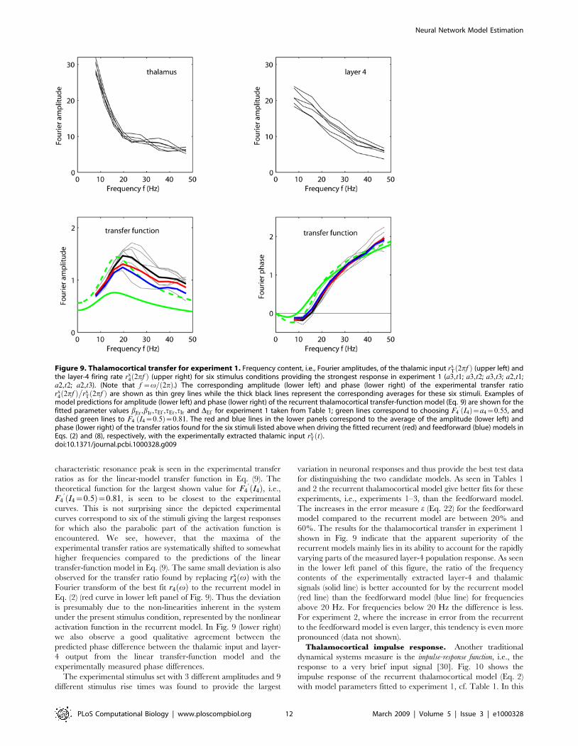
characteristic resonance peak is seen in the experimental transfer

ratios as for the linear-model transfer function in Eq. (9). The

theoretical function for the largest shown value for F4’ I4ð Þ, i.e.,

F4’ I4~0:5ð Þ~0:81, is seen to be closest to the experimental

curves. This is not surprising since the depicted experimental

curves correspond to six of the stimuli giving the largest responses

for which also the parabolic part of the activation function is

encountered. We see, however, that the maxima of the

experimental transfer ratios are systematically shifted to somewhat

higher frequencies compared to the predictions of the linear

transfer-function model in Eq. (9). The same small deviation is also

observed for the transfer ratio found by replacing rx4 vð Þ with the

Fourier transform of the best fit r4 vð Þ to the recurrent model in

Eq. (2) (red curve in lower left panel of Fig. 9). Thus the deviation

is presumably due to the non-linearities inherent in the system

under the present stimulus condition, represented by the nonlinear

activation function in the recurrent model. In Fig. 9 (lower right)

we also observe a good qualitative agreement between the

predicted phase difference between the thalamic input and layer-

4 output from the linear transfer-function model and the

experimentally measured phase differences.

The experimental stimulus set with 3 different amplitudes and 9

different stimulus rise times was found to provide the largest

variation in neuronal responses and thus provide the best test data

for distinguishing the two candidate models. As seen in Tables 1

and 2 the recurrent thalamocortical model give better fits for these

experiments, i.e., experiments 1–3, than the feedforward model.

The increases in the error measure e (Eq. 22) for the feedforward

model compared to the recurrent model are between 20% and

60%. The results for the thalamocortical transfer in experiment 1

shown in Fig. 9 indicate that the apparent superiority of the

recurrent models mainly lies in its ability to account for the rapidly

varying parts of the measured layer-4 population response. As seen

in the lower left panel of this figure, the ratio of the frequency

contents of the experimentally extracted layer-4 and thalamic

signals (solid line) is better accounted for by the recurrent model

(red line) than the feedforward model (blue line) for frequencies

above 20 Hz. For frequencies below 20 Hz the difference is less.

For experiment 2, where the increase in error from the recurrent

to the feedforward model is even larger, this tendency is even more

pronounced (data not shown).

Thalamocortical impulse response. Another traditional

dynamical systems measure is the impulse-response function, i.e., the

response to a very brief input signal [30]. Fig. 10 shows the

impulse response of the recurrent thalamocortical model (Eq. 2)

with model parameters fitted to experiment 1, cf. Table 1. In this

Figure 9. Thalamocortical transfer for experiment 1. Frequency content, i.e., Fourier amplitudes, of the thalamic input rxT 2pfð Þ (upper left) and

the layer-4 firing rate rx4 2pfð Þ (upper right) for six stimulus conditions providing the strongest response in experiment 1 (a3,t1; a3,t2; a3,t3; a2,t1;

a2,t2; a2,t3). (Note that f ~v= 2pð Þ.) The corresponding amplitude (lower left) and phase (lower right) of the experimental transfer ratiorx

4 2pfð Þ�

rxT 2pfð Þ are shown as thin grey lines while the thick black lines represent the corresponding averages for these six stimuli. Examples of

model predictions for amplitude (lower left) and phase (lower right) of the recurrent thalamocortical transfer-function model (Eq. 9) are shown for thefitted parameter values bEr,bIr,tEf ,tEr,tIr and DEf for experiment 1 taken from Table 1; green lines correspond to choosing F4

’ I4ð Þ~a4~0:55, anddashed green lines to F4

’ I4~0:5ð Þ~0:81. The red and blue lines in the lower panels correspond to the average of the amplitude (lower left) andphase (lower right) of the transfer ratios found for the six stimuli listed above when driving the fitted recurrent (red) and feedforward (blue) models inEqs. (2) and (8), respectively, with the experimentally extracted thalamic input rx

T tð Þ.doi:10.1371/journal.pcbi.1000328.g009

Neural Network Model Estimation

PLoS Computational Biology | www.ploscompbiol.org 12 March 2009 | Volume 5 | Issue 3 | e1000328

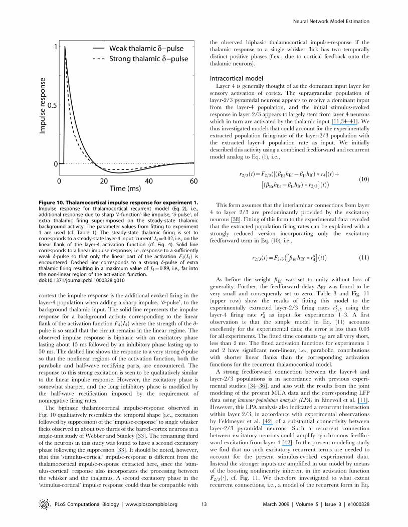
context the impulse response is the additional evoked firing in the

layer-4 population when adding a sharp impulse, ‘d-pulse’, to the

background thalamic input. The solid line represents the impulse

response for a background activity corresponding to the linear

flank of the activation function F4 I4ð Þ where the strength of the d-

pulse is so small that the circuit remains in the linear regime. The

observed impulse response is biphasic with an excitatory phase

lasting about 15 ms followed by an inhibitory phase lasting up to

50 ms. The dashed line shows the response to a very strong d-pulse

so that the nonlinear regions of the activation function, both the

parabolic and half-wave rectifying parts, are encountered. The

response to this strong excitation is seen to be qualitatively similar

to the linear impulse response. However, the excitatory phase is

somewhat sharper, and the long inhibitory phase is modified by

the half-wave rectification imposed by the requirement of

nonnegative firing rates.

The biphasic thalamocortical impulse-response observed in

Fig. 10 qualitatively resembles the temporal shape (i.e., excitation

followed by suppression) of the ‘impulse-response’ to single whisker

flicks observed in about two thirds of the barrel-cortex neurons in a

single-unit study of Webber and Stanley [33]. The remaining third

of the neurons in this study was found to have a second excitatory

phase following the suppression [33]. It should be noted, however,

that this ‘stimulus-cortical’ impulse-response is different from the

thalamocortical impulse-response extracted here, since the ‘stim-

ulus-cortical’ response also incorporates the processing between

the whisker and the thalamus. A second excitatory phase in the

‘stimulus-cortical’ impulse response could thus be compatible with

the observed biphasic thalamocortical impulse-response if the

thalamic response to a single whisker flick has two temporally

distinct positive phases (f.ex., due to cortical feedback onto the

thalamic neurons).

Intracortical modelLayer 4 is generally thought of as the dominant input layer for

sensory activation of cortex. The supragranular population of

layer-2/3 pyramidal neurons appears to receive a dominant input

from the layer-4 population, and the initial stimulus-evoked

response in layer 2/3 appears to largely stem from layer 4 neurons

which in turn are activated by the thalamic input [11,34–41]. We

thus investigated models that could account for the experimentally

extracted population firing-rate of the layer-2/3 population with

the extracted layer-4 population rate as input. We initially

described this activity using a combined feedforward and recurrent

model analog to Eq. (1), i.e.,

r2=3 tð Þ~F2=3 bEf hEf{bIf hIfð Þ � r4½ � tð Þzð

bErhEr{bIrhIrð Þ � r2=3

� �tð Þ� ð10Þ

This form assumes that the interlaminar connections from layer

4 to layer 2/3 are predominantly provided by the excitatory

neurons [38]. Fitting of this form to the experimental data revealed

that the extracted population firing rates can be explained with a

strongly reduced version incorporating only the excitatory

feedforward term in Eq. (10), i.e.,

r2=3 tð Þ~F2=3 bEf hEf � rx4

� �tð Þ

� �ð11Þ

As before the weight bEf was set to unity without loss of

generality. Further, the feedforward delay DEf was found to be

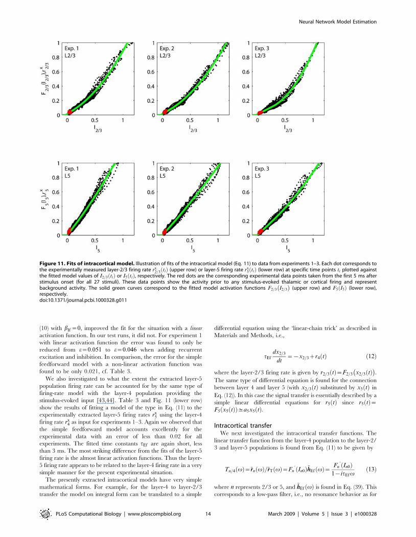
very small and consequently set to zero. Table 3 and Fig. 11

(upper row) show the results of fitting this model to the

experimentally extracted layer-2/3 firing rates rx2=3 using the

layer-4 firing rate rx4 as input for experiments 1–3. A first

observation is that the simple model in Eq. (11) accounts

excellently for the experimental data; the error is less than 0.03

for all experiments. The fitted time constants tEf are all very short,

less than 2 ms. The fitted activation functions for experiments 1

and 2 have significant non-linear, i.e., parabolic, contributions

with shorter linear flanks than the corresponding activation

functions for the recurrent thalamocortical model.

A strong feedforward connection between the layer-4 and

layer-2/3 populations is in accordance with previous experi-

mental studies [34–36], and also with the results from the joint

modeling of the present MUA data and the corresponding LFP

data using laminar population analysis (LPA) in Einevoll et al. [11].

However, this LPA analysis also indicated a recurrent interaction

within layer 2/3, in accordance with experimental observations

by Feldmeyer et al. [42] of a substantial connectivity between

layer-2/3 pyramidal neurons. Such a recurrent connection

between excitatory neurons could amplify synchronous feedfor-

ward excitation from layer 4 [42]. In the present modeling study

we find that no such excitatory recurrent terms are needed to

account for the present stimulus-evoked experimental data.

Instead the stronger inputs are amplified in our model by means

of the boosting nonlinearity inherent in the activation function

F2=3:ð Þ, cf. Fig. 11. We therefore investigated to what extent

recurrent connections, i.e., a model of the recurrent form in Eq.

Figure 10. Thalamocortical impulse response for experiment 1.Impulse response for thalamocortical recurrent model (Eq. 2), i.e.,additional response due to sharp ‘d-function’-like impulse, ‘d-pulse’, ofextra thalamic firing superimposed on the steady-state thalamicbackground activity. The parameter values from fitting to experiment1 are used (cf. Table 1). The steady-state thalamic firing is set tocorresponds to a steady-state layer-4 input ‘current’ I4~0:02, i.e., on thelinear flank of the layer-4 activation function (cf. Fig. 4). Solid linecorresponds to a linear impulse response, i.e., response to a sufficientlyweak d-pulse so that only the linear part of the activation F4 I4ð Þ isencountered. Dashed line corresponds to a strong d-pulse of extrathalamic firing resulting in a maximum value of I4~0:89, i.e., far intothe non-linear region of the activation function.doi:10.1371/journal.pcbi.1000328.g010

Neural Network Model Estimation

PLoS Computational Biology | www.ploscompbiol.org 13 March 2009 | Volume 5 | Issue 3 | e1000328

(10) with bIf~0, improved the fit for the situation with a linear

activation function. In our test runs, it did not. For experiment 1

with linear activation function the error was found to only be

reduced from e~0:051 to e~0:046 when adding recurrent

excitation and inhibition. In comparison, the error for the simple

feedforward model with a non-linear activation function was

found to be only 0.021, cf. Table 3.

We also investigated to what the extent the extracted layer-5

population firing rate can be accounted for by the same type of

firing-rate model with the layer-4 population providing the

stimulus-evoked input [43,44]. Table 3 and Fig. 11 (lower row)

show the results of fitting a model of the type in Eq. (11) to the

experimentally extracted layer-5 firing rates rx5 using the layer-4

firing rate rx4 as input for experiments 1–3. Again we observed that

the simple feedforward model accounts excellently for the

experimental data with an error of less than 0.02 for all

experiments. The fitted time constants tEf are again short, less

than 3 ms. The most striking difference from the fits of the layer-5

firing rate is the almost linear activation functions. Thus the layer-

5 firing rate appears to be related to the layer-4 firing rate in a very

simple manner for the present experimental situation.

The presently extracted intracortical models have very simple

mathematical forms. For example, for the layer-4 to layer-2/3

transfer the model on integral form can be translated to a simple

differential equation using the ‘linear-chain trick’ as described in

Materials and Methods, i.e.,

tEf

dx2=3

dt~{x2=3zr4 tð Þ ð12Þ

where the layer-2/3 firing rate is given by r2=3 tð Þ~F2=3 x2=3 tð Þ� �

.

The same type of differential equation is found for the connection

between layer 4 and layer 5 (with x2=3 tð Þ substituted by x5 tð Þ in

Eq. (12)). In this case the signal transfer is essentially described by a

simple linear differential equations for r5 tð Þ since r5 tð Þ~F5 x5 tð Þð Þ^a5x5 tð Þ.

Intracortical transferWe next investigated the intracortical transfer functions. The

linear transfer function from the layer-4 population to the layer-2/

3 and layer-5 populations is found from Eq. (11) to be given by

Tn=4 vð Þ~~rrn vð Þ=~rrT vð Þ~Fn’ In0ð Þ~hhEf vð Þ~ Fn

’ In0ð Þ1{itEf v

ð13Þ

where n represents 2/3 or 5, and ~hhEf vð Þ is found in Eq. (39). This

corresponds to a low-pass filter, i.e., no resonance behavior as for

Figure 11. Fits of intracortical model. Illustration of fits of the intracortical model (Eq. 11) to data from experiments 1–3. Each dot corresponds tothe experimentally measured layer-2/3 firing rate rx

2=3 tið Þ (upper row) or layer-5 firing rate rx5 tið Þ (lower row) at specific time points ti plotted against

the fitted model values of I2=3 tið Þ or I5 tið Þ, respectively. The red dots are the corresponding experimental data points taken from the first 5 ms afterstimulus onset (for all 27 stimuli). These data points show the activity prior to any stimulus-evoked thalamic or cortical firing and representbackground activity. The solid green curves correspond to the fitted model activation functions F2=3 I2=3

� �(upper row) and F5 I5ð Þ (lower row),

respectively.doi:10.1371/journal.pcbi.1000328.g011

Neural Network Model Estimation

PLoS Computational Biology | www.ploscompbiol.org 14 March 2009 | Volume 5 | Issue 3 | e1000328

the recurrent thalamocortical model in Eq. (9). Further, the

impulse-response function is the simple (monophasic) exponen-

tially decaying function, contrasting the biphasic thalamocortical

impulse-response functions seen in Fig. 10.

In Fig. 12 we compare predictions for the transfer ratio from

this simple linear feedforward model using the fitted parameters

from Table 3 with the corresponding experimental result

rxn vð Þ

�rx

4 vð Þ (n~2=3 or 5) for six of the stimulus conditions

providing the strongest cortical responses in experiment 1

(a3,t1; a3,t2; a3,t3; a2,t1; a2,t2; a2,t3). For the layer-5/layer-4

transfer ratio (lower row in Fig. 12) we see an excellent agreement

between experiments and linear theory. This is as expected since

the fitted layer-5 activity functions F5:ð Þ are essentially linear (cf.

Fig. 11). For the transfer ratio between layer 2/3 and layer 4 a

more substantial deviation between the experimental and linear-

model transfer rations is observed, in particular a slightly growing

transfer-ratio amplitude for large frequencies. This deviation

presumably reflects the non-linearities of the layer-2/3 activity

functions F2=3:ð Þ, because the same effect is also observed for the

transfer ratio between the best model fit r2=3 and rx4 (cf. red line in

upper left panel of Fig. 12).

Discussion

A main objective of the present paper is the description and

application of a new method for extraction of population firing-

rate models for thalamocortical and intracortical signal transfer on

the basis of trial-averaged data from simultaneous cortical

recordings with laminar multielectrodes in a rat barrel column

and single-electrode recordings in the homologous thalamic

barreloid. Below we first discuss the results from the model

estimation for both the thalamocortical and the intracortical signal

transfer, followed by a discussion of the model estimation method

itself.

Thalamocortical modelsFor the thalamocortical signal transfer our investigations clearly

identifies a model with (1) fast feedforward excitation, (2) a slower

predominantly inhibitory process mediated by recurrent (within

layer 4) and/or feedforward interactions (from thalamus), and (3) a

mixed linear-parabolic activation function. The relative impor-

tance of the feedforward compared to the recurrent connections is

more difficult to determine and has been a subject of significant

interest [7–9,16,45]. Here we have compared two alternative

models: (i) a purely feedforward thalamocortical model with

feedforward excitation and inhibition and (ii) a recurrent model

with feedforward excitation, recurrent excitation and recurrent

inhibition (but no feedforward inhibition). In reality the inhibitory

layer-4 neurons receive excitatory inputs both from thalamic

neurons and other layer-4 neurons, and the inhibition felt by the

excitatory layer-4 neurons will thus be both ‘feedforward’ and

‘recurrent’; the different models thus explore what part appears to

dominate in the present experimental situation.

Our results suggest that the model with recurrent inhibition

better accounts for the present experimental data than the model

with feedforward inhibition, i.e., that the layer-4 interneurons

providing the inhibition of the layer-4 excitatory neurons are in

turn mainly driven by excitation from layer-4 neurons. Since the

relative strength of recurrent effects compared to feedforward

effects appears to increase with increasing thalamic stimuli [19],

this might indicate that the present fits to the experimental data is

dominated by ‘strong’ inputs. Alternatively, it may be that a strong

feedforward inhibition is also present, but that it is strongly

overlapping in time with the feedforward excitation. Then the

present modeling scheme and experimental data are unable to

separate them and instead lump the effect of this inhibition

together with the feedforward excitation.

An interesting result from the present investigation is that we

find a similar thalamocortical population model as Pinto et al.

[8,9]: the recurrent model on integral form in Eq. (2) can be mapped

to a set of two differential equations (Eqs. 4–5) structurally similar

to the model suggested and investigated by Pinto and coworkers.

The correspondence between the behavior of these models is

demonstrated by the phase-plane plots in Fig. 5, which exhibits the

same qualitative features as the analogous phase-plane plots in

Ref. [9]. This close correspondence is striking since the methods

used to derive the models are very different. Pinto et al. chose the

model to account for a large collection of single-unit PSTHs

recorded with sharp electrodes from numerous animals. By

contrast, our model parameters were extracted based on

simultaneous thalamic and cortical recordings from individual

animals. As multielectrode arrays allow for convenient simulta-

neous recordings from all layers of the cerebral cortex, even at

more than one cortical location [10], the proposed modeling

approach scales more readily to complex networks involving

multiple, spatially separated, neuronal populations.

Intracortical modelThe presently identified intracortical model for the connection

between the layer-4 and layer-2/3 populations has a very simple

mathematical form including only a single feedforward term

(Eqs. 11–12), but was nevertheless found to account excellently for

the experimental data, cf. Fig. 11. Such a strong feedforward

connection between these populations is in accordance with

previous experimental studies [34–36]. An experimental study by

Feldmeyer et al. [42] found substantial recurrent connectivity

between layer-2/3 pyramidal neurons, but no such excitatory

recurrent terms were needed to account for the present stimulus-

evoked experimental data. Compared to the thalamocortical

Table 3. Fitted model parameters for intracortical models.

L4RL2/3 Exp. 1 Exp. 2 Exp. 3

tEf (ms) 1.2 1.2 1.8

a2=3 0.5160.01 0.45 0.40

b2=3 0.4960.01 0.45 0.89

I{2=3

20.03 20.03 20.02

I�2=3 0.1360.02 0.13 0.27

error (e) 0.0214 0.0141 0.0279

L4RL5 Exp. 1 Exp. 2 Exp. 3

tEf (ms) 3.0 2.1 1.4

a5 0.96 0.8660.01 0.73

b5 0.24 0.10 0.27

I{5

20.009 20.003 20.004

I�5 0.003 0.02460.043 0.26860.004

error (e) 0.0195 0.0193 0.0167

Resulting optimized parameters for the intracortical network model (Eq. 11) forexperiments 1–3. Upper row: Layer-2/3 firing rate predicted from layer-4 input.Lower row: Layer-5 firing rate predicted from layer-4 input (where thesubscripts ‘2/3’ are replaced by ‘5’ in Eq. (11)). The listed parameter valuescorrespond to the mean of estimated parameters from 25 selected modelsgiving essentially the same error (see Materials and Methods). The standarddeviations are only listed if they exceed the last digit of the mean.doi:10.1371/journal.pcbi.1000328.t003

Neural Network Model Estimation

PLoS Computational Biology | www.ploscompbiol.org 15 March 2009 | Volume 5 | Issue 3 | e1000328

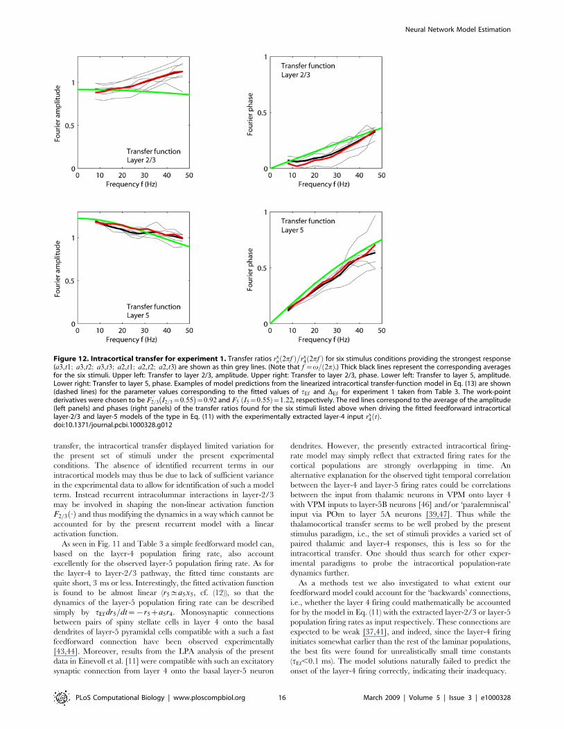
transfer, the intracortical transfer displayed limited variation for

the present set of stimuli under the present experimental

conditions. The absence of identified recurrent terms in our

intracortical models may thus be due to lack of sufficient variance

in the experimental data to allow for identification of such a model

term. Instead recurrent intracolumnar interactions in layer-2/3

may be involved in shaping the non-linear activation function

F2=3:ð Þ and thus modifying the dynamics in a way which cannot be

accounted for by the present recurrent model with a linear

activation function.

As seen in Fig. 11 and Table 3 a simple feedforward model can,

based on the layer-4 population firing rate, also account

excellently for the observed layer-5 population firing rate. As for

the layer-4 to layer-2/3 pathway, the fitted time constants are

quite short, 3 ms or less. Interestingly, the fitted activation function

is found to be almost linear (r5^a5x5, cf. (12)), so that the

dynamics of the layer-5 population firing rate can be described

simply by tEf dr5=dt~{r5za5r4. Monosynaptic connections

between pairs of spiny stellate cells in layer 4 onto the basal

dendrites of layer-5 pyramidal cells compatible with a such a fast

feedforward connection have been observed experimentally

[43,44]. Moreover, results from the LPA analysis of the present

data in Einevoll et al. [11] were compatible with such an excitatory

synaptic connection from layer 4 onto the basal layer-5 neuron

dendrites. However, the presently extracted intracortical firing-

rate model may simply reflect that extracted firing rates for the

cortical populations are strongly overlapping in time. An

alternative explanation for the observed tight temporal correlation

between the layer-4 and layer-5 firing rates could be correlations

between the input from thalamic neurons in VPM onto layer 4

with VPM inputs to layer-5B neurons [46] and/or ‘paralemniscal’

input via POm to layer 5A neurons [39,47]. Thus while the

thalamocortical transfer seems to be well probed by the present

stimulus paradigm, i.e., the set of stimuli provides a varied set of

paired thalamic and layer-4 responses, this is less so for the

intracortical transfer. One should thus search for other exper-

imental paradigms to probe the intracortical population-rate

dynamics further.

As a methods test we also investigated to what extent our

feedforward model could account for the ‘backwards’ connections,

i.e., whether the layer 4 firing could mathematically be accounted

for by the model in Eq. (11) with the extracted layer-2/3 or layer-5

population firing rates as input respectively. These connections are

expected to be weak [37,41], and indeed, since the layer-4 firing

initiates somewhat earlier than the rest of the laminar populations,

the best fits were found for unrealistically small time constants

(tEf,0.1 ms). The model solutions naturally failed to predict the

onset of the layer-4 firing correctly, indicating their inadequacy.

Figure 12. Intracortical transfer for experiment 1. Transfer ratios rxn 2pfð Þ

�rx

4 2pfð Þ for six stimulus conditions providing the strongest response(a3,t1; a3,t2; a3,t3; a2,t1; a2,t2; a2,t3) are shown as thin grey lines. (Note that f ~v= 2pð Þ.) Thick black lines represent the corresponding averagesfor the six stimuli. Upper left: Transfer to layer 2/3, amplitude. Upper right: Transfer to layer 2/3, phase. Lower left: Transfer to layer 5, amplitude.Lower right: Transfer to layer 5, phase. Examples of model predictions from the linearized intracortical transfer-function model in Eq. (13) are shown(dashed lines) for the parameter values corresponding to the fitted values of tEf and DEf for experiment 1 taken from Table 3. The work-pointderivatives were chosen to be F2=3

’ I2=3~0:55� �

~0:92 and F5’ I5~0:55ð Þ~1:22, respectively. The red lines correspond to the average of the amplitude

(left panels) and phases (right panels) of the transfer ratios found for the six stimuli listed above when driving the fitted feedforward intracorticallayer-2/3 and layer-5 models of the type in Eq. (11) with the experimentally extracted layer-4 input rx

4 tð Þ.doi:10.1371/journal.pcbi.1000328.g012

Neural Network Model Estimation

PLoS Computational Biology | www.ploscompbiol.org 16 March 2009 | Volume 5 | Issue 3 | e1000328

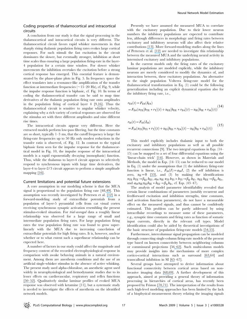
Coding properties of thalamocortical and intracorticalcircuits

A conclusion from our study is that the signal processing in the

thalamocortical and intracortical circuits is very different. The

thalamocortical circuit favors rapid whisker movements in that

sharply rising thalamic population firing rates evokes large cortical

responses. For such stimuli the fast excitation in the circuit

dominates the slower, but eventually stronger, inhibition at short

time scales thus ensuring a large population firing-rate in the layer-

4 population for a certain time window. For slower whisker

movements the inhibition overtakes the excitation before a strong

cortical response has emerged. This essential feature is demon-

strated by the phase-plane plots in Fig. 5. In frequency space the

effect translates into a resonance-like amplification of the transfer

function at intermediate frequencies (,15–20 Hz), cf. Fig. 9, while

the impulse response function is biphasic, cf. Fig. 10. In terms of

coding the thalamocortical transfer can be said to map time

derivatives of the thalamic population firing rate onto amplitudes

in the population firing of cortical layer 4 [9,16]. Thus the

thalamocortical circuit is sensitive to angular whisker velocity,

explaining why a rich variety of cortical responses are observed for

the stimulus set with three different amplitudes and nine different

rise times.

The intracortical circuits appear very different. Here the

extracted models perform low-pass filtering, but the time constants

are so short, typically 1–3 ms, that the cutoff frequency is large: for

firing-rate frequencies up to 50 Hz only modest reductions in the

transfer ratio is observed, cf. Fig. 12. In contrast to the typical

biphasic form seen for the impulse response for the thalamocor-

tical model in Fig. 10, the impulse response of the intracortical

models is a rapid exponentially decaying (monophasic) function.

Thus, while the thalamus to layer-4 circuit appears to selectively

respond to synchronous inputs with large time derivatives, the

layer-4 to layer-2/3 circuit appears to perform a simple amplitude

mapping [16].

Current limitations and potential future extensionsA core assumption in our modeling scheme is that the MUA

signal is proportional to the population firing rate [48,49]. This

assumption was recently investigated by Pettersen et al. [12] in a

forward-modeling study of extracellular potentials from a

population of layer-5 pyramidal cells from cat visual cortex

receiving synchronous synaptic activation resembling the present

stimulus-evoked situation. For trial-averaged data a roughly linear

relationship was observed for a large range of small and

intermediate population firing rates. For large population firing

rates the true population firing rate was found to grow super-

linearly with the MUA due to increasing cancelation of

extracellular potentials for high firing rates. It is, however, unclear

whether or to what extent such a superlinear relationship can be

expected here.

A number of factors in our study could affect the magnitude and

frequency content of the recorded electrophysiological response in

comparison with awake behaving animals in a natural environ-

ment. Among them are anesthesia conditions and the use of an

artificial single-whisker stimulus in the absence of active whisking.

The present study used alpha-chloralose, an anesthetic agent used

widely in neurophysiological and hemodynamic studies due to its

lesser effects on cardiovascular, respiratory and reflex functions

[50–52]. Qualitatively similar laminar profiles of evoked MUA

response was observed with ketamine [11], but a systematic study

is needed to investigate the effects of anesthesia on the identified

network models.

Presently we have assumed the measured MUA to correlate

with the excitatory population. Due to their lower neuron

numbers the inhibitory populations are expected to contribute

less, although differences in morphology and firing rates between

excitatory and inhibitory neurons will also affect their relative

contributions [13]. More forward-modeling studies along the lines

of Pettersen et al. [12] are needed to investigate this relationship

between the measured MUA and the underlying neural activity in

intermixed excitatory and inhibitory populations.

In the current models only the firing rates of the excitatory

laminar populations are modeled explicitly, while the inhibitory

neurons are merely considered to modify the dynamics of, and

interaction between, these excitatory populations. An alternative

to the single population Volterra firing-rate model for the

thalamocortical transformation in Eq. (1) could be the following

generalization including an explicit dynamical equation also for

the inhibitory firing rate, i.e.,

rE4 tð Þ~FE4 IE4ð Þ

~FE4 aTE hTE � rT½ � tð ÞzaEE hEE � rE4½ � tð Þ{aIE hIE � rI4½ � tð Þð Þð14Þ

rI4 tð Þ~FI4 II4ð Þ

~FI4 aTI hTI � rT½ � tð ÞzaEI hEI � rE4½ � tð Þ{aII hII � rI4½ � tð Þð Þð15Þ

This model explicitly includes thalamic input to both the

excitatory and inhibitory populations as well as all possible

recurrent connections [9]. The two integral equations in Eqs. (14–

15) can be mapped to a set of four differential equations using the

‘linear-chain trick’ [14]. However, as shown in Materials and

Methods, the model in Eqs. (14–15) can be reduced to our model

in Eq. (1) under the assumptions that (1) the inhibitory firing-rate

function is linear, i.e., FI4 Ið Þ~aI4I , (2) the self inhibition is

zero, aII~0 [53], and (3) by making the identifications

aTE hTE?bEf hEf , aI4 aIE aTI hTI � hTI?bIf hIf , aEE hEE?bEr hEr,

and aI4aIEaEIhIE � hEI?bIrhIr, cf. Eqs. (43–47).

The analysis of model parameter identifiability revealed that

certain linear combinations of parameters (notably recurrent and

feedforward excitation and inhibition strengths, time constants,

and activation function parameters), do not have a measurable

effect on the measured signals, and thus cannot be confidently

estimated. This problem can be partly addressed by using

intracellular recordings to measure some of these parameters,

e.g., synaptic time constants and firing rates as function of somatic

input currents, directly in the relevant cell types. Model

identification could also be aided by theoretical investigations of

the basic structure of population firing-rate models [54,55].

Furthermore, intercolumnar signal propagation can be modeled

through connecting single-column firing-rate models of the present

type based on known connectivity between neighboring columns

or commissural projections [56–62]. Such multicolumn models

may provide insights into the mechanisms of more complex

cortico-cortical interactions such as surround [63,64] and

transcallosal inhibition in SI [65–67].

Several groups have attempted to derive information about

functional connectivity between cortical areas based on non-

invasive imaging data [68,69]. A further development of this

approach, aimed at providing a general theory of information

processing in hierarchies of cortical areas, has recently been

proposed by Friston [70,71]. The interpretation of the results from

such high-level modeling approaches has been limited by the lack

of a biophysical measurement theory relating the imaging signals

Neural Network Model Estimation

PLoS Computational Biology | www.ploscompbiol.org 17 March 2009 | Volume 5 | Issue 3 | e1000328

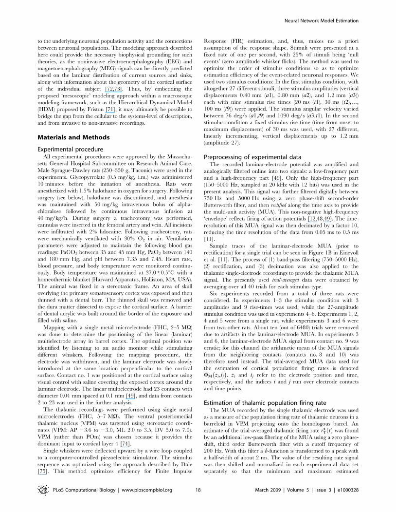
to the underlying neuronal population activity and the connections

between neuronal populations. The modeling approach described

here could provide the necessary biophysical grounding for such

theories, as the noninvasive electroencephalography (EEG) and

magnetoencephalography (MEG) signals can be directly predicted

based on the laminar distribution of current sources and sinks,

along with information about the geometry of the cortical surface

of the individual subject [72,73]. Thus, by embedding the

proposed ‘mesoscopic’ modeling approach within a macroscopic

modeling framework, such as the Hierarchical Dynamical Model

(HDM) proposed by Friston [71], it may ultimately be possible to

bridge the gap from the cellular to the systems-level of description,

and from invasive to non-invasive recordings.

Materials and Methods

Experimental procedureAll experimental procedures were approved by the Massachu-

setts General Hospital Subcommittee on Research Animal Care.

Male Sprague-Dawley rats (250–350 g, Taconic) were used in the

experiments. Glycopyrrolate (0.5 mg/kg, i.m.) was administered

10 minutes before the initiation of anesthesia. Rats were

anesthetized with 1.5% halothane in oxygen for surgery. Following

surgery (see below), halothane was discontinued, and anesthesia

was maintained with 50 mg/kg intravenous bolus of alpha-

chloralose followed by continuous intravenous infusion at

40 mg/kg/h. During surgery a tracheotomy was performed,

cannulas were inserted in the femoral artery and vein. All incisions

were infiltrated with 2% lidocaine. Following tracheotomy, rats

were mechanically ventilated with 30% O2 in air. Ventilation

parameters were adjusted to maintain the following blood gas

readings: PaCO2 between 35 and 45 mm Hg, PaO2 between 140

and 180 mm Hg, and pH between 7.35 and 7.45. Heart rate,

blood pressure, and body temperature were monitored continu-

ously. Body temperature was maintained at 37.060.5uC with a

homeothermic blanket (Harvard Apparatus, Holliston, MA, USA).

The animal was fixed in a stereotaxic frame. An area of skull

overlying the primary somatosensory cortex was exposed and then

thinned with a dental burr. The thinned skull was removed and

the dura matter dissected to expose the cortical surface. A barrier

of dental acrylic was built around the border of the exposure and

filled with saline.

Mapping with a single metal microelectrode (FHC, 2–5 MV)

was done to determine the positioning of the linear (laminar)

multielectrode array in barrel cortex. The optimal position was

identified by listening to an audio monitor while stimulating

different whiskers. Following the mapping procedure, the

electrode was withdrawn, and the laminar electrode was slowly

introduced at the same location perpendicular to the cortical

surface. Contact no. 1 was positioned at the cortical surface using

visual control with saline covering the exposed cortex around the

laminar electrode. The linear multielectrode had 23 contacts with

diameter 0.04 mm spaced at 0.1 mm [49], and data from contacts

2 to 23 was used in the further analysis.

The thalamic recordings were performed using single metal

microelectrodes (FHC, 5–7 MV). The ventral posteriomedial

thalamic nucleus (VPM) was targeted using stereotactic coordi-

nates (VPM: AP 23.6 to 23.0, ML 2.0 to 3.5, DV 5.0 to 7.0).

VPM (rather than POm) was chosen because it provides the

dominant input to cortical layer 4 [74].

Single whiskers were deflected upward by a wire loop coupled

to a computer-controlled piezoelectric stimulator. The stimulus

sequence was optimized using the approach described by Dale

[75]. This method optimizes efficiency for Finite Impulse

Response (FIR) estimation, and, thus, makes no a priori

assumption of the response shape. Stimuli were presented at a

fixed rate of one per second, with 25% of stimuli being ‘null

events’ (zero amplitude whisker flicks). The method was used to

optimize the order of stimulus conditions so as to optimize

estimation efficiency of the event-related neuronal responses. We

used two stimulus conditions: In the first stimulus condition, with

altogether 27 different stimuli, three stimulus amplitudes (vertical

displacements 0.40 mm (a1), 0.80 mm (a2), and 1.2 mm (a3))

each with nine stimulus rise times (20 ms (t1), 30 ms (t2),…,

100 ms (t9)) were applied. The stimulus angular velocity varied

between 76 deg/s (a1,t9) and 1090 deg/s (a3,t1). In the second

stimulus condition a fixed stimulus rise time (time from onset to

maximum displacement) of 30 ms was used, with 27 different,

linearly incrementing, vertical displacements up to 1.2 mm

(amplitude 27).

Preprocessing of experimental dataThe recorded laminar-electrode potential was amplified and

analogically filtered online into two signals: a low-frequency part

and a high-frequency part [49]. Only the high-frequency part

(150–5000 Hz, sampled at 20 kHz with 12 bits) was used in the

present analysis. This signal was further filtered digitally between

750 Hz and 5000 Hz using a zero phase-shift second-order

Butterworth filter, and then rectified along the time axis to provide

the multi-unit activity (MUA). This non-negative high-frequency

‘envelope’ reflects firing of action potentials [12,48,49]. The time-

resolution of this MUA signal was then decimated by a factor 10,

reducing the time resolution of the data from 0.05 ms to 0.5 ms

[11].

Sample traces of the laminar-electrode MUA (prior to

rectification) for a single trial can be seen in Figure 1B in Einevoll

et al. [11]. The process of (1) band-pass filtering (750–5000 Hz),

(2) rectification, and (3) decimation was also applied to the

thalamic single-electrode recordings to provide the thalamic MUA

signal. The presently used trial-averaged data were obtained by

averaging over all 40 trials for each stimulus type.

Six experiments recorded from a total of three rats were

considered. In experiments 1–3 the stimulus condition with 3

amplitudes and 9 rise-times was used, while the 27-amplitude

stimulus condition was used in experiments 4–6. Experiments 1, 2,

4 and 5 were from a single rat, while experiments 3 and 6 were

from two other rats. About ten (out of 6480) trials were removed

due to artifacts in the laminar-electrode MUA. In experiments 3

and 6, the laminar-electrode MUA signal from contact no. 9 was

erratic; for this channel the arithmetic mean of the MUA signals

from the neighboring contacts (contacts no. 8 and 10) was

therefore used instead. The trial-averaged MUA data used for

the estimation of cortical population firing rates is denoted

WM zi,tj

� �. zi and tj refer to the electrode position and time,

respectively, and the indices i and j run over electrode contacts

and time points.

Estimation of thalamic population firing rateThe MUA recorded by the single thalamic electrode was used

as a measure of the population firing rate of thalamic neurons in a

barreloid in VPM projecting onto the homologous barrel. An

estimate of the trial-averaged thalamic firing rate rxT tð Þ was found

by an additional low-pass filtering of the MUA using a zero phase-

shift, third order Butterworth filter with a cutoff frequency of

200 Hz. With this filter a d-function is transformed to a peak with

a half-width of about 2 ms. The value of the resulting rate signal

was then shifted and normalized in each experimental data set

separately so that the minimum and maximum estimated

Neural Network Model Estimation

PLoS Computational Biology | www.ploscompbiol.org 18 March 2009 | Volume 5 | Issue 3 | e1000328

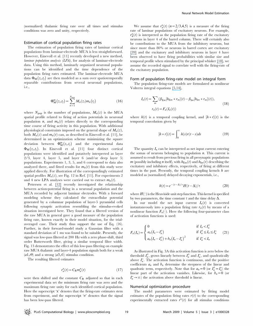
(normalized) thalamic firing rate over all times and stimulus

conditions was zero and unity, respectively.

Estimation of cortical population firing ratesThe estimation of population firing rates of laminar cortical

populations from laminar-electrode MUA is less straightforward.

However, Einevoll et al. [11] recently developed a new method,

laminar population analysis (LPA), for analysis of laminar-electrode

data. Using this method, laminarly organized neuronal popula-

tions can be identified and the time dependence of the

population firing rates estimated. The laminar-electrode MUA

data WM zi,tj

� �are then modeled as a sum over spatiotemporally

separable contributions from several neuronal populations,

i.e.,

WmM zi,tj

� �~XNpop

n~1

Mn zið Þmn tj

� �ð16Þ

where Npop is the number of populations, Mn zð Þ is the MUA

spatial profile related to firing of action potentials in neuronal

population n, and mn tð Þ relates directly to the corresponding

time course of firing activity in this population. With additional

physiological constraints imposed on the general shape of Mn zð Þ,both Mn zð Þ and mn tð Þ can, as described in Einevoll et al. [11], be

determined in an optimization scheme minimizing the square

deviation between WmM zi,tj

� �and the experimental data

WM zi,tj

� �. In Einevoll et al. [11] four distinct cortical

populations were identified and putatively interpreted as layer

2/3, layer 4, layer 5, and layer 6 (and/or deep layer 5)

populations. Experiments 1, 3, 5, and 6 correspond to data also

analyzed there, and fitted results for mn tð Þ from this study were

applied directly. For illustration of the correspondingly estimated

spatial profiles Mn zð Þ, see Fig. 12 in Ref. [11]. For experiments 2

and 4 new LPA analyses were carried out to extract mn tð Þ.Pettersen et al. [12] recently investigated the relationship

between action-potential firing in a neuronal population and the

MUA recorded by adjacent laminar electrodes. With a forward

modeling scheme they calculated the extracellular potential

generated by a columnar population of layer-5 pyramidal cells

following synaptic activation resembling the stimulus-evoked

situation investigated here. They found that a filtered version of

the raw MUA in general gave a good measure of the population

firing rate, known exactly in their model situation, for the trial-

averaged case. Their study thus support the use of Eq. (16).

Further, in their forward-model study a Gaussian filter with a

standard deviation of 1 ms was found to be suitable. Presently, the

signal was low-pass filtered at 200 Hz with a zero phase-shift, third

order Butterworth filter, giving a similar temporal filter width.

Fig. 13 demonstrates the effect of this low-pass filtering on example

raw MUA thalamic and layer-4 population signals both for a weak

(a1,t9) and a strong (a3,t1) stimulus condition.

The resulting filtered estimates

rxn tð Þ~CRms

n tð Þ ð17Þ

were then shifted and the constant CR adjusted so that in each

experimental data set the minimum firing rate was zero and the

maximum firing rate unity for each identified cortical population.

Here the superscript ‘x’ denotes that the firing-rate estimates stem

from experiment, and the superscript ‘s’ denotes that the signal

has been low-pass filtered.

We assume that rxn tð Þ n~2=3,4,5ð Þ is a measure of the firing

rate of laminar populations of excitatory neurons. For example,

rx4 tð Þ is interpreted as the population firing rate of the excitatory

neurons in layer 4 of the barrel column. There will certainly also

be contributions to the MUA from the inhibitory neurons, but

since more than 80% or neurons in barrel cortex are excitatory

[39] and the excitatory and inhibitory neurons in layer 4 have

been observed to have firing probabilities with similar size and

temporal profile when stimulated by the principal whisker [18], we

assume the recorded signal to correlate well with the firing-rate of

the excitatory population.

Form of population firing-rate model on integral formThe population firing-rate models are formulated as nonlinear

Volterra integral equations [5,14],

In tð Þ~X

m

bEm hEm � rm½ � tð Þ{bIm hIm � rm½ � tð Þð Þ,

rn tð Þ~Fn In tð Þð Þð18Þ

where h tð Þ is a temporal coupling kernel, and h � r½ � tð Þ is the

temporal convolution given by

h � r½ � tð Þ~ð?

0

h sð Þr t{sð Þds ð19Þ

The quantity In can be interpreted as net input current entering

the somas of neurons belonging to population n. This current is

assumed to result from previous firing in all presynaptic populations

m (possibly including n itself), with hEm tð Þ and hIm tð Þ describing the

excitatory and inhibitory effects, respectively, of firing at different

times in the past. Presently, the temporal coupling kernels h are

modeled as (normalized) delayed decaying exponentials, i.e.,

h tð Þ~e{ t{Dð Þ=tH t{Dð Þ=t ð20Þ

where H :ð Þ is the Heaviside unit step function. This kernel is specified

by two parameters, the time constant t and the time delay D.

In our model the net input current In tð Þ is converted

instantaneously into a population firing rate rn tð Þ by means of a

nonlinear function Fn:ð Þ. Here the following four-parameter class

of activation functions is used:

Fn Inð Þ~0 if InvI{n

an In{I{n� �

if I{n ƒInƒI�n

an In{I{n� �

zbn In{I�n� �2

if I�n vIn

8><>: ð21Þ

As illustrated in Fig. 3A this activation function is zero below the

threshold I{n , grows linearly between I{n and I�n , and quadratically

above I�n . The activation function is continuous, and the positive

coefficients an and bn determine the steepness of the linear and

quadratic term, respectively. Note that for an~0 (or I{n ~I�n ) the

linear part of the activation vanishes. Likewise, for bn~0 (or

I�n??) the activation above threshold is linear.

Numerical optimization procedureThe model parameters were estimated by fitting model

estimates of the population firing rates r tð Þ to the corresponding

experimentally extracted rates rx tð Þ for all stimulus conditions

Neural Network Model Estimation

PLoS Computational Biology | www.ploscompbiol.org 19 March 2009 | Volume 5 | Issue 3 | e1000328

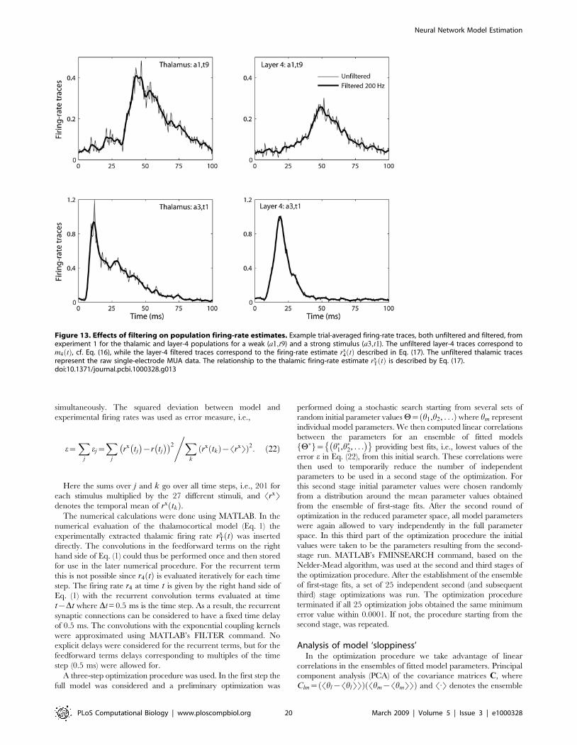
simultaneously. The squared deviation between model and

experimental firing rates was used as error measure, i.e.,

e~X

j

ej~X

j

rx tj

� �{r tj

� �� �2

,Xk

rx tkð Þ{SrxTð Þ2: ð22Þ

Here the sums over j and k go over all time steps, i.e., 201 for

each stimulus multiplied by the 27 different stimuli, and SrxTdenotes the temporal mean of rx tkð Þ.

The numerical calculations were done using MATLAB. In the

numerical evaluation of the thalamocortical model (Eq. 1) the

experimentally extracted thalamic firing rate rxT tð Þ was inserted

directly. The convolutions in the feedforward terms on the right

hand side of Eq. (1) could thus be performed once and then stored

for use in the later numerical procedure. For the recurrent term

this is not possible since r4 tð Þ is evaluated iteratively for each time

step. The firing rate r4 at time t is given by the right hand side of

Eq. (1) with the recurrent convolution terms evaluated at time

t{Dt where Dt = 0.5 ms is the time step. As a result, the recurrent

synaptic connections can be considered to have a fixed time delay

of 0.5 ms. The convolutions with the exponential coupling kernels

were approximated using MATLAB’s FILTER command. No

explicit delays were considered for the recurrent terms, but for the

feedforward terms delays corresponding to multiples of the time

step (0.5 ms) were allowed for.

A three-step optimization procedure was used. In the first step the

full model was considered and a preliminary optimization was

performed doing a stochastic search starting from several sets of

random initial parameter values H~ h1,h2, . . .ð Þ where hm represent

individual model parameters. We then computed linear correlations

between the parameters for an ensemble of fitted models

H�f g~ h�1,h�2, . . .� �

providing best fits, i.e., lowest values of the

error e in Eq. (22), from this initial search. These correlations were

then used to temporarily reduce the number of independent

parameters to be used in a second stage of the optimization. For

this second stage initial parameter values were chosen randomly

from a distribution around the mean parameter values obtained

from the ensemble of first-stage fits. After the second round of

optimization in the reduced parameter space, all model parameters

were again allowed to vary independently in the full parameter

space. In this third part of the optimization procedure the initial

values were taken to be the parameters resulting from the second-

stage run. MATLAB’s FMINSEARCH command, based on the

Nelder-Mead algorithm, was used at the second and third stages of

the optimization procedure. After the establishment of the ensemble

of first-stage fits, a set of 25 independent second (and subsequent

third) stage optimizations was run. The optimization procedure

terminated if all 25 optimization jobs obtained the same minimum

error value within 0.0001. If not, the procedure starting from the

second stage, was repeated.

Analysis of model ‘sloppiness’In the optimization procedure we take advantage of linear

correlations in the ensembles of fitted model parameters. Principal

component analysis (PCA) of the covariance matrices C, where

Clm~ Shl{ShlTTð Þ Shm{ShmTTð Þ and S:T denotes the ensemble

Figure 13. Effects of filtering on population firing-rate estimates. Example trial-averaged firing-rate traces, both unfiltered and filtered, fromexperiment 1 for the thalamic and layer-4 populations for a weak (a1,t9) and a strong stimulus (a3,t1). The unfiltered layer-4 traces correspond tom4 tð Þ, cf. Eq. (16), while the layer-4 filtered traces correspond to the firing-rate estimate rx

4 tð Þ described in Eq. (17). The unfiltered thalamic tracesrepresent the raw single-electrode MUA data. The relationship to the thalamic firing-rate estimate rx

T tð Þ is described by Eq. (17).doi:10.1371/journal.pcbi.1000328.g013

Neural Network Model Estimation

PLoS Computational Biology | www.ploscompbiol.org 20 March 2009 | Volume 5 | Issue 3 | e1000328

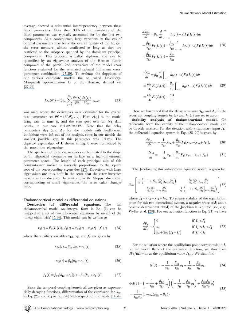
average, showed a substantial interdependency between these

fitted parameters. More than 99% of the variability of the

fitted parameters was typically accounted for by the first two

components. As a consequence, large variations in the sets of

optimal parameters may leave the overall quality of the fit, i.e.,

the error measure, almost unaffected as long as they are

restricted to the subspace spanned by the dominant principal

components. This property is called sloppiness, and can be

quantified by an eigenvalue analysis of the Hessian matrix

composed of the partial 2nd derivatives of the model error

function evaluated for the estimated optimal (minimum error)

parameter combination [27,29]. To evaluate the sloppiness of

our various candidate models the so called Levenberg-

Marquardt approximation L of the Hessian, defined via

[27,29]

Llm h�ð Þ~hlhm

XNR

j~1

Lr tj

� �Lhl

Lr tj

� �Lhm

H~H�j ð23Þ

was used, where the derivatives were evaluated for the overall

best parameter set H�~ h�1,h�2, . . .� �

. Here r tj

� �is the model

firing rate at time tj , and the sum goes over all NR data

points, in our case 201627 = 5427. Note that the delay

parameters DEf (and DIf for the models with feedforward

inhibition) were left out of the analysis, since in our models the

smallest possible step in this parameter was 0.5 ms. The

depicted eigenvalues of L shown in Fig. 8 were normalized by

the maximum eigenvalue.

The spectrum of these eigenvalues can be related to the shape

of an ellipsoidal constant-error surface in a high-dimensional

parameter space. The length of each principal axis of this

constant-error surface is inversely proportional to the square

root of the corresponding eigenvalue [27]. Directions with large

eigenvalues are thus ‘stiff’ in the sense that the error increases

rapidly in this direction. In contrast, in the ‘sloppy’ directions,

corresponding to small eigenvalues, the error value changes

little.

Thalamocortical model as differential equationsDerivation of differential equations. The full

thalamocortical model on integral form in Eq. (1) can be

mapped to a set of two differential equations by means of the

‘linear chain trick’ [5,14]. This model can be written as

r4 tð Þ~F4 I4 tð Þð Þ, I4 tð Þ~xE4 tð Þ{xI4 tð ÞzfT tð Þ ð24Þ

where the auxiliary variables xE4, xI4 and fT are given by

xE4 tð Þ:bEr hEr � r4½ � tð Þ, ð25Þ

xI4 tð Þ:bIr hIr � r4½ � tð Þ, ð26Þ

fT tð Þ:bEf hEf � rT½ � tð Þ{bIf hIf � rT½ � tð Þ ð27Þ

Since the temporal coupling kernels all are given as exponen-

tially decaying functions, differentiation of the expression for xE4

in Eq. (25) and xI4 in Eq. (26) with respect to time yields [14,76]

dxE4

dt~bEr

d

dt

ðt

{?hEr t{sð ÞF4 I4 sð Þð Þds

~bEr

tErF4 I4 tð Þð Þ{ bEr

tEr

ðt

{?hEr t{sð ÞF4 I4 sð Þð Þds

~bEr

tErF4 I4 tð Þð Þ{ xE4

tEr

ð28Þ

dxI4

dt~bIr

d

dt

ðt

{?hIr t{sð ÞF4 I4 sð Þð Þds

~bIr

tIrF4 I4 tð Þð Þ{ bIr

tIr

ðt

{?hIr t{sð ÞF4 I4 sð Þð Þds

~bIr

tIrF4 I4 tð Þð Þ{ xI4

tIr

ð29Þ

Here we have used that the delay constants DEr and DIr in the

recurrent coupling kernels hEr tð Þ and hIr tð Þ are set to zero.

Stability analysis of thalamocortical model. On

differential form the stability of the thalamocortical model can

be directly assessed. For the situation with a stationary input fTs,

the differential equation system in Eqs. (28–29) is given by

dxE4

dt~{

1

tEr

xE4zbEr

tEr

F4 xE4{xI4zfTsð Þ, ð30Þ

dxI4

dt~{

1

tIr

xI4zbIr

tIr

F4 xE4{xI4zfTsð Þ ð31Þ

The Jacobian of this autonomous equation system is given by

J~

1tEr

{1zbErdF4

dI4I4,eq

dI4

dxE4

���� �bEr

tEr

dF4

dI4I4,eq

dI4

dxI4

���bIr

tIr

dF4

dI4I4,eq

dI4

dxE4

��� 1tIr

{1zbIrdF4

dI4I4,eq

dI4

dxI4

���� �264

375ð32Þ

where I4~xE4{xI4zfTs. To ensure stability of the equilibrium

point for this two-dimensional system, a negative trace tr(J) and a

positive determinant det(J) of the Jacobian is required (see, e.g.,

Wyller et al. [28]). For our activation function in Eq. (21) we have

dF4

dI4~

0 if I4vI{4

a4 if I{4 ƒI4ƒI�4

a4z2b4 I4{I�4� �

if I�4 vI4

8><>: ð33Þ

For the situation where the equilibrium point corresponds to I4

on the linear flank of the activation function, we thus have

dF4=dI4~a4 at the equilibrium value I4,eq. We then find

tr Jð Þ~{1

tErz

bEr

tEra4{

1

tIr{

bIr

tIra4, ð34Þ

det Jð Þ~ {1

tErz

bEr

tEra4

� �{

1

tIr{

bIr

tIra4

� �z

bErbIr

tErtIra2

4

~1

tErtIr

1{a4 bEr{bIrð Þð Þð35Þ

Neural Network Model Estimation

PLoS Computational Biology | www.ploscompbiol.org 21 March 2009 | Volume 5 | Issue 3 | e1000328

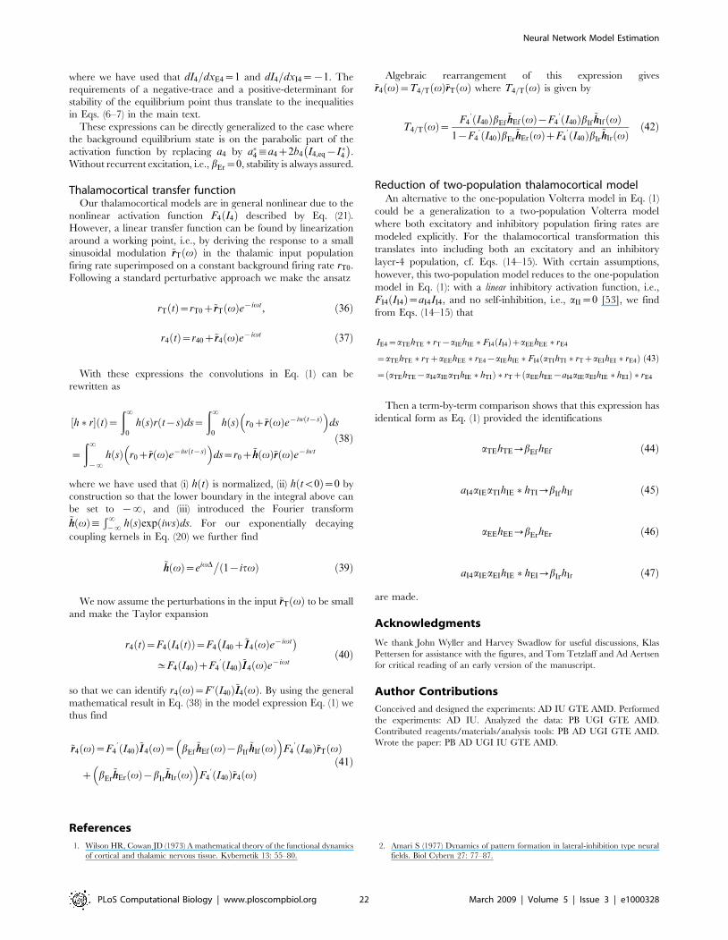
where we have used that dI4=dxE4~1 and dI4=dxI4~{1. The

requirements of a negative-trace and a positive-determinant for

stability of the equilibrium point thus translate to the inequalities

in Eqs. (6–7) in the main text.

These expressions can be directly generalized to the case where

the background equilibrium state is on the parabolic part of the

activation function by replacing a4 by a�4:a4z2b4 I4,eq{I�4� �

.

Without recurrent excitation, i.e., bEr~0, stability is always assured.

Thalamocortical transfer functionOur thalamocortical models are in general nonlinear due to the

nonlinear activation function F4 I4ð Þ described by Eq. (21).

However, a linear transfer function can be found by linearization

around a working point, i.e., by deriving the response to a small

sinusoidal modulation ~rrT vð Þ in the thalamic input population

firing rate superimposed on a constant background firing rate rT0.

Following a standard perturbative approach we make the ansatz

rT tð Þ~rT0z~rrT vð Þe{ivt, ð36Þ

r4 tð Þ~r40z~rr4 vð Þe{ivt ð37Þ

With these expressions the convolutions in Eq. (1) can be

rewritten as

h � r½ � tð Þ~ð?

0

h sð Þr t{sð Þds~

ð?0

h sð Þ r0z~rr vð Þe{iw t{sð Þ� �

ds

~

ð?{?

h sð Þ r0z~rr vð Þe{iw t{sð Þ� �

ds~r0z~hh vð Þ~rr vð Þe{iwt

ð38Þ

where we have used that (i) h tð Þ is normalized, (ii) h tv0ð Þ~0 by

construction so that the lower boundary in the integral above can

be set to {?, and (iii) introduced the Fourier transform~hh vð Þ:

Ð?{? h sð Þexp iwsð Þds. For our exponentially decaying

coupling kernels in Eq. (20) we further find

~hh vð Þ~eivD�

1{itvð Þ ð39Þ

We now assume the perturbations in the input ~rrT vð Þ to be small

and make the Taylor expansion

r4 tð Þ~F4 I4 tð Þð Þ~F4 I40z~II4 vð Þe{ivt� �

^F4 I40ð ÞzF4’ I40ð Þ~II4 vð Þe{ivt

ð40Þ

so that we can identify r4 vð Þ~F ’ I40ð Þ~II4 vð Þ. By using the general

mathematical result in Eq. (38) in the model expression Eq. (1) we

thus find

~rr4 vð Þ~F4’ I40ð Þ~II4 vð Þ~ bEf

~hhEf vð Þ{bIf~hhIf vð Þ

� �F4

’ I40ð Þ~rrT vð Þ

z bEr~hhEr vð Þ{bIr

~hhIr vð Þ� �

F4’ I40ð Þ~rr4 vð Þ

ð41Þ

Algebraic rearrangement of this expression gives

~rr4 vð Þ~T4=T vð Þ~rrT vð Þ where T4=T vð Þ is given by

T4=T vð Þ~ F4’ I40ð ÞbEf

~hhEf vð Þ{F4’ I40ð ÞbIf

~hhIf vð Þ1{F4

’ I40ð ÞbEr~hhEr vð ÞzF4

’ I40ð ÞbIr~hhIr vð Þ

ð42Þ

Reduction of two-population thalamocortical modelAn alternative to the one-population Volterra model in Eq. (1)

could be a generalization to a two-population Volterra model

where both excitatory and inhibitory population firing rates are

modeled explicitly. For the thalamocortical transformation this

translates into including both an excitatory and an inhibitory

layer-4 population, cf. Eqs. (14–15). With certain assumptions,

however, this two-population model reduces to the one-population

model in Eq. (1): with a linear inhibitory activation function, i.e.,

FI4 II4ð Þ~aI4II4, and no self-inhibition, i.e., aII~0 [53], we find

from Eqs. (14–15) that

IE4~aTEhTE � rT{aIEhIE � FI4 II4ð ÞzaEEhEE � rE4

~aTEhTE � rTzaEEhEE � rE4{aIEhIE � FI4 aTIhTI � rTzaEIhEI � rE4ð Þ

~ aTEhTE{aI4aIEaTIhIE � hTIð Þ � rTz aEEhEE{aI4aIEaEIhIE � hEIð Þ � rE4

ð43Þ

Then a term-by-term comparison shows that this expression has

identical form as Eq. (1) provided the identifications

aTEhTE?bEf hEf ð44Þ

aI4aIEaTIhIE � hTI?bIf hIf ð45Þ

aEEhEE?bErhEr ð46Þ

aI4aIEaEIhIE � hEI?bIrhIr ð47Þ

are made.

Acknowledgments

We thank John Wyller and Harvey Swadlow for useful discussions, Klas

Pettersen for assistance with the figures, and Tom Tetzlaff and Ad Aertsen

for critical reading of an early version of the manuscript.

Author Contributions

Conceived and designed the experiments: AD IU GTE AMD. Performed

the experiments: AD IU. Analyzed the data: PB UGI GTE AMD.

Contributed reagents/materials/analysis tools: PB AD UGI GTE AMD.

Wrote the paper: PB AD UGI IU GTE AMD.

References

1. Wilson HR, Cowan JD (1973) A mathematical theory of the functional dynamics

of cortical and thalamic nervous tissue. Kybernetik 13: 55–80.

2. Amari S (1977) Dynamics of pattern formation in lateral-inhibition type neural

fields. Biol Cybern 27: 77–87.

Neural Network Model Estimation

PLoS Computational Biology | www.ploscompbiol.org 22 March 2009 | Volume 5 | Issue 3 | e1000328

3. Deco G, Jirsa VK, Robinson PA, Breakspear M, Friston K (2008) The dynamicbrain: From spiking neurons to neural masses and cortical fields. PLOS Comp

Biol 4: e1000092. doi:10.1371/journal.pcbi.1000092.

4. Dayan P, Abbott LF (2001) Theoretical Neuroscience: Computational andMathematical Modeling of Neural Systems. Cambridge MA: MIT Press.

5. Ermentrout B (1998) Neural networks as spatio-temporal pattern-formingsystems. Rep Prog Phys 61: 353–430.

6. Coombes S (2005) Waves, bumps, and patterns in neural field theories. BiolCybern 93: 91–108.

7. Kyriazi HT, Simons DJ (1993) Thalamocortical response transformations in

simulated whisker barrels. J Neurosci 13: 1601–1615.

8. Pinto D, Brumberg JC, Simons JC, Ermentrout GB (1996) A quantitative

population model of whisker barrels: Re-examining the Wilson-Cowanequations. J Comp Neuroscience 3: 247–264.

9. Pinto DJ, Hartings JA, Brumberg JC, Simons DJ (2003) Cortical damping:

analysis of thalamocortical response transformations in rodent barrel cortex.Cereb Cort 13: 33–44.

10. Buzsaki G (2004) Large-scale recording of neuronal ensembles. Nat Neurosci 7:446–451.

11. Einevoll GT, Pettersen KH, Devor A, Ulbert I, Halgren E, et al. (2007) Laminar

Population Analysis: Estimating firing rates and evoked synaptic Activity frommultielectrode recordings in rat barrel cortex. J Neurophysiol 97: 2174–2190.

12. Pettersen KH, Hagen E, Einevoll GT (2008) Estimation of population firingrates and current source densities from laminar electrode recordings. J Comp

Neurosci 24: 291–313.

13. Pettersen KH, Einevoll GT (2008) Amplitude variability and extracellular low-pass filtering of neuronal spikes. Biophys J 94: 784–802.

14. Nordbø Ø, Wyller J, Einevoll GT (2007) Neural network firing-rate models onintegral form: Effects of temporal coupling kernels on equilibrium-state stability.

Biol Cybern 97: 195–209.

15. Pinto DJ, Brumberg JC, Simons DJ (2000) Circuit dynamics and codingstrategies in rodent somatosensory cortex. J Neurophysiol 83: 1158–1166.

16. Wilent WB, Contreras D (2004) Synaptic responses to whisker deflections in ratbarrel cortex as a function of cortical layer and stimulus intensity. J Neurosci 24:

3985–3998.

17. Blomquist P, Indahl UG, Devor A, Ulbert I, Einevoll GT, et al. (2006)Estimation of cortical microcircuit model from joint thalamic single-unit and

cortical laminar-electrode recordings in rat whisker-barrel system. Soc NeurosciAbstr 53: 23.

18. Kyriazi HT, Carvell GE, Simons DJ (1994) OFF response transformations in thewhisker/barrel system. J Neurophysiol 72: 392–401.

19. Beierlein M, Fall CP, Rinzel J, Yuste R (2002) Thalamocortical bursts trigger

recurrent activity in neocortical networks: layer 4 as a frequency-dependent gate.J Neurosci 22: 9885–9894.

20. Feldmeyer D, Egger V, Lubke J, Sakmann B (1999) Reliable synapticconnections between pairs of excitatory layer 4 neurones within a single

‘‘barrel’’ of developing rat somatosensory cortex. J Physiol 521: 169–190.

21. Beierlein M, Gibson JR, Connors BW (2003) Two dynamically distinctinhibitory networks in layer 4 of the neocortex. J Neurophysiol 90: 2987–3000.

22. Swadlow HA, Gusev AG (2002) Receptive-field construction in corticalinhibitory interneurons. Nature Neurosci 5: 403–404.

23. Swadlow HA (2003) Fast-spike interneurons and feedforward inhibition in

awake sensory neocortex. Cereb Cort 13: 25–32.

24. Sun Q-Q, Huguenard JR, Prince DA (2006) Barrel cortex microcircuits:

thalamocortical feedforward inhibition in spiny stellate cells is mediated by asmall number of fast-spiking interneurons. J Neurosci 26: 1219–1230.

25. Temereanca S, Simons DJ (2004) Functional topography of corticothalamic

feedback enhances thalamic spatial response tuning in the somatosensorywhisker/barrel system. Neuron 41: 639–651.

26. Tateno T, Harsch A, Robinson HPC (2004) Threshold firing frequency-currentrelationships of neurons in rat somatosensory cortex: Type 1 and type 2

dynamics. J Neurophysiol 92: 2283–2294.

27. Gutenkunst RN, Waterfall JJ, Casey FP, Brown KS, Myers CR, et al. (2007)Universally sloppy parameter sensitivities in systems biology models. PLoS

Comp Biol 3: 1871–1878. doi:10.1371/journal.pcbi.0030189.

28. Wyller J, Blomquist P, Einevoll GT (2007) Turing instability and pattern

formation in a two-population neuronal network model. Physica D 225: 75–93.

29. Brown KS, Sethna JP (2003) Statistical mechanical approaches to models with

many poorly known parameters. Phys Rev E 68: 021904.

30. Oppenheim AW, Willsky AS (1996) Signals&Systems. 2nd ed. Upper SaddleRiver, New Jersey: Prentice.

31. Bracewell RN (1999) The Fourier transform and its applications. 3rd ed.Columbus, Ohio: McGraw-Hill.

32. Einevoll GT, Plesser HE (2002) Linear mechanistic models for the dorsal lateral

geniculate nucleus of cat probed using drifting-grating stimuli. Network: CompNeur Syst 13: 503–530.

33. Webber RM, Stanley GB (2004) Nonlinear encoding of tactile patterns in thebarrel cortex. J Neurophysiol 91: 2010–2022.

34. Petersen CCH, Sakmann B (2001) Functionally independent columns of rat

somatosensory barrel cortex revealed with voltage-sensitive dye imaging. JNeurosci 21: 8435–8446.

35. Feldmeyer D, Lubke J, Silver RA, Sakmann B (2002) Synaptic connectionsbetween layer 4 spiny neurone - layer 2/3 pyramidal cell pairs in juvenile rat

barrel cortex: physiology and anatomy of interlaminar signalling within a

cortical column. J Physiol 538.3: 803–822.

36. Lubke J, Roth A, Feldmeyer D, Sakmann B (2003) Morphometric analysis of the

columnar innervation domain of neurons connection layer 4 and layer 2/3 of

juvenile rat barrel cortex. Cereb Cort 13: 1051–1063.

37. Thomson AM, Bannister AP (2003) Interlaminar connections in the neocortex.

Cereb Cort 13: 5–14.

38. Helmstaedter M, de Kock CPJ, Feldmeyer D, Bruno RM, Sakmann B (2007)

Reconstruction of an average cortical column in silico. Brain Res Rev 55:

193–203.

39. Lubke J, Feldmeyer D (2007) Excitatory signal flow and connectivity in a cortical

column: focus on barrel cortex. Brain Struct Funct 212: 3–17.

40. Sarid L, Bruno R, Sakmann B, Segev I, Feldmeyer D (2007) Modeling a layer 4-

to-layer 2/3 module of a singe column in rat neocortex: Interweaving in vitro

and in vivo experimental observations. Proc Natl Acac Sci U S A 41:

16353–16358.

41. Thomson AM, Lamy C (2007) Functional maps in neocortical local circuitry.

Front in Neurosci 1: 19–42.

42. Feldmeyer D, Lubke J, Sakmann B (2006) Efficacy and connectivity of

intracolumnar pairs of layer 2/3 pyramidal cells in the barrel cortex of juvenile

rats. J Physiol 575.2: 583–602.

43. Feldmeyer D, Roth A, Sakmann B (2005) Monosynaptic connections between

pairs of spiny stellate cells in layer 4 and pyramidal cells in layer 5A indicate that

lemniscal and paralemniscal afferent pathways converge in the infragranular

somatosensory cortex. J Neurosci 25: 3423–3431.

44. Schubert D, Kotter R, Luhmann HJ, Staiger JF (2006) Morphology,

electrophysiology and functional input connectivity of pyramidal neurons

characterizes a genuine layer Va in the primary somatosensory cortex. Cereb

Cort 16: 223–236.

45. Bruno RM, Sakmann B (2006) Cortex is driven by weak and synchronously

active thalamocortical synapses. Science 312: 1622–1627.

46. de Kock CPJ, Bruno RM, Spors H, Sakmann B (2007) Layer- and cell-type

specific suprathreshold stimulus representation in rat primary sensory cortex.

J Physiol 581: 139–154.

47. Shepherd GMG, Svoboda K (2005) Laminar and columnar organization of

ascending excitatory projections to layer 2/3 pyramidal neurons in rat barrel

cortex. J Neurosci 25: 5670–5679.

48. Schroeder CE, Lindsley RW, Specht C, Marcovici A, Smiley JF, Javitt DC

(2001) Somatosensory input to auditory association cortex in the macaque

monkey. J Neurophysiol 85: 1322–1327.

49. Ulbert I, Halgren E, Heit G, Karmos G (2001) Multiple microelectrode-

recording system for human intracortical applications. J Neurosci Meth 106:

69–79.

50. Covert RF, Scheriber MD, Leff AR, White SR, Munoz NM, et al. (1992)

Oxygen metabolism and catecholamine secretion during chloralose anesthesia in

lambs. J Dev Physiol 17: 125–132.

51. Lindauer U, Villringer A, Dirnagl U (1993) Characterization of CBF response to

somatosensory stimulation: model and influence of anesthetics. Am J Physiol

264: H1223–1228.

52. Ueki M, Mies G, Hossmann KA (1992) Effect of alpha-chloralose, halothane,

pentobarbital and nitrous oxide anesthesia on metabolic coupling in somato-

sensory cortex of rat. Acta Anaesthesiol Scand 36: 318–322.

53. Pinto D, Ermentrout B (2001) Spatially structured activity in synaptically

coupled neuronal networks: II Lateral inhibition and standing pulses.

SIAM J Appl Math 62: 226–243.

54. Shriki O, Hansel D, Sompolinsky H (2003) Rate models for conductance-based

cortical neuronal networks. Neural Comp 15: 1809–1841.

55. Kriener B, Tetzlaff T, Aertsen A, Diesmann M, Rotter S (2008) Correlations

and population dynamics in cortical networks. Neural Comp 20: 2133–2184.

56. Petreanu L, Huber D, Sobczyk A, Svoboda K (2007) Channelrhodopsin-2-

assisted circuit mapping of long-range callosal projections. Nat Neurosci 10:

663–668.

57. Wise SP, Jones EG (1976) The organization and postnatal development of the

commissural projection of the rat somatic sensory cortex. J Comp Neurol 168:

313–343.

58. White EL, DeAmicis RA (1977) Afferent and efferent projections of the region in

mouse SmL cortex which contains the posteromedial barrel subfield. J Comp

Neurol 175: 455–482.

59. Koralek KA, Olavarria J, Killackey HP (1990) Areal and laminar organization

of corticocortical projections in the rat somatosensory cortex. J Comp Neurol

299: 133–150.

60. Li L, Ebner FF (2006) Balancing bilateral sensory activity: callosal processing

modulates sensory transmission through the contralateral thalamus by altering

the response threshold. Exp Brain Res 172: 397–415.

61. Vogt BA, Gorman AL (1982) Responses of cortical neurons to stimulation of

corpus callosum in vitro. J Neurophysiol 48: 1257–1273.

62. Olavarria J, Van Sluyters RC, Killackey HP (1984) Evidence for the

complementary organization of callosal and thalamic connections within rat

somatosensory cortex. Brain Res 291: 364–368.

63. Derdikman D, Hildesheim R, Ahissar E, Arieli A, Grinvald A (2003) Imaging

spatiotemporal dynamics of surround inhibition in the barrels somatosensory

cortex. J Neurosci 23: 3100–3105.

Neural Network Model Estimation

PLoS Computational Biology | www.ploscompbiol.org 23 March 2009 | Volume 5 | Issue 3 | e1000328

64. Devor A, Tian P, Nishimura N, Teng IC, Hillman EM, et al. (2007) Suppressed

neuronal activity and concurrent arteriolar vasoconstriction may explainnegative blood oxygenation level-dependent signal. J Neurosci 27: 4452–4459.

65. Hlushchuk Y, Hari R (2006) Transient suppression of ipsilateral primary

somatosensory cortex during tactile finger stimulation. J Neurosci 26:5819–5824.

66. Ferbert A, Priori A, Rothwell JC, Day BL, Colebatch JG, et al. (1992)Interhemispheric inhibition of the human motor cortex. J Physiol 453:

525–546.

67. Ogawa S, Lee TM, Stepniski R, Chen W, Zhu XH, et al. (2000) An approach toprobe some neural systems interaction by functional MRI at neural time scale

down to milliseconds. Proc Natl Acad Sci U S A 97: 11026–11031.68. Horwitz B, Tagamets MA, McIntosh AR (1999) Neural modeling, functional

brain imaging, and cognition. Trends Cogn Sci 3: 91–98.69. Buchel C, Friston KJ (2000) Assessing interactions among neuronal systems

using functional neuroimaging. Neural Networks 13: 871–882 2000.

70. Friston KJ (2005) A theory of cortical responses. Philos Trans R Soc Lond B Biol

Sci 360: 815–836.71. Friston K (2008) Hierarchical models in the brain. PLOS Comp Biol 4:

e1000211. doi:10.1371/journal.pcbi.1000211.

72. Dale AM, Sereno MI (1993) Improved localization of cortical activity bycombining EEG and MEG with MRI cortical surface reconstruction: a linear

approach. J Cog Neurosci 5: 162–176.73. Dale AM, Halgren E (2001) Spatiotemporal mapping of brain activity by

integration of multiple imaging modalities. Curr Opin Neurobiol 11: 202–208.

74. Ahissar E, Sosnik R, Baqdasarian K, Haidarliu S (2001) Temporal frequency ofwhisker movement. II. Laminar organization of cortical representations.

J Neurophysiol 86: 354–367.75. Dale AM (1999) Optimal experimental design of event-related fMRI. Hum

Brain Map 8: 109–114.76. Cushing JM (1977) Integrodifferential equations and delay models in population

dynamics, lecture notes in biomathematics. Heidelberg: Springer.

Neural Network Model Estimation

PLoS Computational Biology | www.ploscompbiol.org 24 March 2009 | Volume 5 | Issue 3 | e1000328