AN ABSTRACT OF THE THESIS OF

James Philip Shields for the degree of Doctor of Philosophy in

Chemistry presented on December 10, 1987 .

Title: Design. Construction and Characterization of a

Six-Electrode. Direct Current, Variable Length

Plasma Source for Atomic Emission Spectroscopy

Abstract approved:

Redacted for privacyr /-

Edward H. Piepmeier

The variable length, six-electrode plasma source for atomic

emission spectroscopy described here is operated from three

compact, simple, and inexpensive direct current power supplies. The

vertical arcs formed between the three electrode pairs completely

entrain the sample and are typically operated at 40 V and 20 A.

Three concentric quartz tubes, similar to the ICP, supply argon, as

well as sample, to the plasma. The argon consumption rate of

typically 7.4 L/min is comparable to or less than the consumption

rates of commercial ICP and DCP systems and is achieved without the

need for water cooling of any of the components. The plasma

assembly is completely demountable to facilitate easy replacement

of damaged parts and to provide experimental flexibility.

Spatial shifts in the vertical emission profiles, similar to

those documented for the ICP, occur with changes in the nebulizer

gas flow rate and current. The MgII 280.27-nm emission and

signal-to-background ratio (S/B) increase by factors of 23 and 10,

respectively, for an increase in the current from 16 to 25A. A

twofold increase in the MgII 280.27-nm S/B occurs for an increase

in the plasma length from 14 to 21.5 mm. Detection limits for five

elements range from 15 to 50 times higher than those for the ICP.

These detection limits are achieved without the use of ceramic

sleeves. Movement of the region of maximum emission to positions

below the top of the outer quartz tube, which occur with the

lengthening of the plasma, is thought to be the main reason for the

poorer detection limits. Adding 10% nitrogen to the outer argon

flow causes a 50% enhancement of the Ca ion S/B.

The effect of Na on Ca atom emission is directly opposite to

that for the ICP. The Ca atom vertical profile with Na is depressed

in the region up to 10 mm above the sample bullet, and crosses over

to enhancement at higher regions. Plasma length exhibits a

significant effect on both the Na and P interference on Ca.

Careful selection of the plasma length and observation height can

be used to virtually eliminate the interferences.

Design, Construction, and Characterization of aSix-Electrode, Direct Current, Variable LengthPlasma Source for Atomic Emission Spectroscopy

by

James Philip Shields

A THESIS

submitted to

Oregon State University

in partial fulfillment ofthe requirements for the

degree of

Doctor of Philosophy

Completed December 10, 1987

Commencement June, 1988

APPROVED:

Redacted for privacyProfessor of Chemistry in charge of major

Redacted for privacyChAtMcan of Department of Chemistry

Redacted for privacy

Dean of the Grad ae School

Date thesis is presented December 10. 1987

Typed by James P. Shields for James P. Shields

ACKNOWLEDGMENTS

This work is dedicated to my mother -- for showing me the

rewards of perseverance and hard work and for sending me to summer

camp -- to my father -- for providing the motivation for attending

graduate school -- and to my wife and companion Meredith.

Special thanks also to my sister Kim and my stepfather Ron

for their support.

To Ken, an ever-present friend, and Margaret and Bond for a

home away from home throughout the years.

Special thanks to Scott, Joe, and Glacier Peak for

diversions.

I wish to thank Milton Harris and N. L. Tartar for their

contributions to my efforts.

Special thanks go to professor E. H. Piepmeier for providing

a research environment and an open door. Thanks also to professors

Schuyler, Ingle, Westall, and Hawkes and to Gae Ho Lee for his many

helpful comments.

Finally, I wish to thank professors Field, Taylor, Cummings,

Kolb, Cowan, and Gayhart at Bradley University for teaching me the

fundamentals of chemistry and encouraging graduate work.

TABLE OF CONTENTS

I. Introduction 1

II. Historical 7

A. Spectroscopic Sources For Atomic Emission

Spectroscopy 8

1. Flames as Spectrochemical Sources 9

2. Arcs and High Voltage Sparks as

Spectrochemical Sources 11

3. Plasma Sources 13

a. Direct Current Plasmas 13

b. Other Plasma Sources 22

B. Sample Introduction Techniques 25

1. Sample Introduction into Arc/Spark Excitation

Sources 26

2. Nebulizers 29

3. Laser Ablation For Sample Introduction To

Plasmas 34

4. Arc/Spark Methods For Sample Introduction To

Plasmas 35

5. Electrothermal Methods For Sample

Introduction To Plasmas 37

6. Direct Insertion Methods For Sample

Introduction To Plasmas 39

7. Miscellaneous Methods 41

III. Instrumental 45

A. Plasma Source 45

1. Plasma Torch 47

2. Electrodes 50

B. Plasma Source Electrical Circuitry 50

C. Gas Handling Equipment 52

D. Sample Introduction System 54

E. Optical Table and Associated Support Equipment 55

1. Optical Table and General Table Hardware 57

2. Translation Stages 57

3. Miscellaneous Support Equipment 58

F. Echelle Spectrometer 60

G. Computer Data Collection/Analysis and Interfacing

Hardware 65

1. Computer 65

2. Add-On Boards 67

3. Peripheral Devices 68

4. Computer System for CAD Drawings and Thesis

Preparation 68

H. Data Analysis Software 69

I. Miscellaneous Software 74

1. Assembly Language 74

2. ASYST Stepper Motor Control Software 76

a) Abstract 77

b) Description of Program 77

c) Operation of Program 79

d) Intended Users 80

3. Commercial Software 80

IV. A FORTH-Based Data Acquisition and Control System for

use in Plasma Atomic Emission Spectrometry. 82

A. Abstract 83

B. Introduction 84

C. Instrumentation 85

1. Spectrometer 85

2. Computer and Peripheral Devices 88

3. Software 88

a) P-Code Routines 88

b) ASYST Software 91

D. Application 102

1. Optimization of Aperture Plate and PMT

Positions in Focal Plane 102

2. Monitoring of Plasma Stability 105

3. Monitoring of Nebulizer/Spray Chamber

Wash-Out Time 105

4. Spatial Profiles of the Plasma 105

E. Conclusions 109

V. A Six-Electrode, Direct Current, Variable Length

Plasma Source for Atomic Emission Spectroscopy 111

A. Abstract 112

B. Introduction 113

C. Experimental 115

1. Plasma Torch 115

2. Electrodes 116

3. Electrical System 117

4. Sample Introduction System 117

5. Spectrometer and Data Acquisition System 119

6. Gas Handling Equipment 120

7. Staging System 121

8. Solutions 122

9. Initiation and Operation of the Plasma 122

D. Results 124

1. Plasma Regions 124

2. Affect of Plasma Operating Conditions on

Spatial Emission Profiles 127

a) Affect of Nebulizer Gas Flow Rate 128

b) Affect of Current 130

c) Affect of Plasma Length 136

3. Affect of Adding Nitrogen to Outer Gas Flow 140

4. Analytical Utility 141

E. Conclusions 146

VI. A Spatial Study of the Influence of Plasma Length on

Interference Effects in a Six-Electrode, Direct

Current Plasma 148

A. Abstract 149

B. Introduction 150

C. Experimental 152

D. Results and Discussion 156

1. Effect of Plasma Length on the Interference

of Na on Ca and Zn Emission

2. Effect of Plasma Length on the Interference

of P on Ca Emission

VII. Other Characterizations of the Plasma/Spectrometer

System

A. Investigation of the Blank and Dark Current

Signals

B. Dependence of Relative Standard Deviation on

Integration Time

C. Investigation of Nebulizer Wash-Out

Characteristics

156

165

171

171

180

182

VIII. Conclusion 185

A. Plasma Emission Source 185

B. Echelle Spectrometer 188

C. Data Acquisition System 189

IX. References 191

X. Appendices 206

A. Aperture Plate and PMT Coordinates 206

B. Computer Listings 209

C. Low Flow Nebulizer Development 281

1. Low Gas Flow, Babington Type Nebulizer 281

2. Capillary Array Nebulizer 288

D. Computer Controlled Stepper Motor System 291

1. Introduction 291

2. Description of Stepper Motor Instrumentation 291

a) Stepper Motors 292

b) Stepper Motor and Logic Power Supplies 292

c) Stepper Motor Driver Board 295

d) Computer Digital I/O Card 297

e) Subsystem 1: SAA1027 Chip Selector 297

f) Subsystem 2: Stepper Motor Dropping

Resistors 300

g) Subsystem 3: PI012/K33505 Pulse

Amplification Circuit 300

h) Subsystem 4: Manual/Computer Switching

Control Circuitry 303

i) Subsystem 5: Microswitch Logic Circuitry 306

j) Subsystem 6: Remote Control Circuitry 306

3. Conclusions 310

E. Correction for Echelle Source Mirror Vertical

Off-Axis Movement 312

1. Correction Factor Method 312

2. Horizontal Peaking Method 315

F. Technical Drawings 316

LIST OF FIGURES

Chapter III

Figure Page

111.1. Block diagram of instrumentation. 46

111.2. Diagram of plasma source: upper and pseudo cut-away 48view. (A) upper housing, (B) lower housing, (C)outer quartz tube, (D) inner quartz tube, (E) outerelectrodes, (F) inner electrodes, (G) inner andouter quartz tube adjusting screws, (H) outer andinner argon gas flow inlets, (I) o-ring, (J) sampleaerosol in.

111.3. Schematic diagram of plasma source electrical 51circuitry.

111.4. Diagram of gas handling equipment. 53

111.5. Diagram of sample introduction tube. 56

111.6. Diagram of main vertical translation stage support. 59

111.7. Diagram of plasma source baseplate. 61

111.8. Schematic representation of instrumentation. Image 63

of plasma source is focused onto entrance slit ofechelle spectrometer by a computer-controlledsource mirror. Data from echelle are sent to anIBM-PC compatible microcomputer via an RS-232line. Hardcopy plots are output to a plotter andnumeric data to a printer.

111.9. Screen organization for the data analysis program, 70DATAANAL.

III.10. Main menu for the data analysis program, DATAANAL. 71

III.11. Sub-menus for the data analysis program, DATAANAL. 71

Chapter IV

IV.1 Main Menu of ACQDATA. 92

IV.2 Example of screen during a timed acquisition 94experiment. Top left graphics screen shows mostrecent 32-point data set. Middle graphics screenshows cumulative 32-points average values overtime. Lower portion of screen shows menu window,prompt/message window, status line, and errorwindow.

Figure Page

IV.3 Submenus of ACQDATA. 95

IV.4a Aperture plate scan at the CuI 324.75 nm line 103

before optimization. The profile should becentered about the "P" position for maximum lightthroughput.

IV.4b Aperture plate scan at the CuI 324.75 nm line after 103

the ACQDATA plate optimization routine has beenperformed. Profile is now centered about the "P"position where maximum light throughput and minimumnoise occur.

IV.5 ZnI 213.86 nm emission versus time. Monitoring of 106

plasma stability using the timed acquisition modeof ACQDATA. The dots represent the individualpoints of each 32-point data set. The solid lineand symbol () represent the average value of each32-point data set.

IV.6

IV.7

Monitoring of nebulizer wash-out period uponchange-over from 100 pg/mL Ca to blank. Timedacquisition mode of ACQDATA was used. MonitoringCall 393.37 nm emission. Each symbol ()represents the average of 32 data points taken overa time period of about 1.5 seconds.

Horizontal profiles of plasma at seven differentobservation heights above outer quartz tube.Monitoring the Call 393.37 nm line while aspiratinga 10 pg/mL solution.

Chapter V

107

108

V.1. Schematic diagram of different plasma regions. 125

V.2. Vertical spatial profiles of MgII 280.27 nm and 129

MgI 285.21 nm emission as a function of nebulizergas flow rate. (0) 0.6 L/min; () 0.8 L/min;(A) 1.0 L/min; (A) 1.2 L/min.

V.3. Vertical spatial profiles of the Mg ion-to-atom 131

ratio (MgII 280.27 nm; MgI 285.21 nm) as a functionof nebulizer gas flow rate. (0) 0.6 L/min;(S) 0.8 L/min; (A) 1.0 L/min.

V.4. Vertical spatial profiles of the MgII 280.27 nm and 133

MgI 285.21 nm emission as a function of current.(0) 16 A; (0) 19 A; (A) 22 A; (A) 25 A.

Figure Eu

V.S. Vertical spatial profiles of the Mg ion-to-atomratio (MgII 280.27 nm; MgI 285,21 nm) as a functionof current. (0) 16 A; () 19 A; (A) 22 A;(A) 25 A.

134

V.6. Horizontal spatial profiles of the MgII 280.27 nm 135

and MgI 285.21 nm emission as a function ofcurrent. The observation height is 0.7 mm abovethe top of the outer quartz tube. (0) 16 A;

(a) 19 A; (u) 22 A; () 25 A.

V.7. Vertical spatial profiles of the MgII 280.27 nm and 137

MgI 285.21 nm emission as a function of plasmalength. (0) 14 mm; (I) 16.5 mm; (A) 19.1 mm;(A) 21.6 mm.

V.8. Horizontal spatial profiles of the MgII 280.27 nm 139

emission as a function of plasma length. Theobservation height is 0.7 mm above the top of theouter quartz tube. The profiles in the bottomgraph are all normalized to the 21.6 mm plasmalength. (*) 14 mm; (A) 16.5 mm; (U) 19.1 mm;() 21.6 mm.

V.9. Vertical spatial profiles of the CaII 393.37 nm and 142

CaI 422.67 nm line-to-background ratio. (0) no

N2 added; () 10% N2 added to outer gas flow.

Chapter VI

VI.1. Schematic representation of upper part of plasma 153

source. The position of the 13-mm observationwindow is illustrated.

VI.2. Vertical spatial profiles of the CaI 422.67 nmemission at three different plasma lengths(A, 11.5 mm; B, 18.0 mm; C, 24.5 mm). The Ca:Namolar ratio is: (0) 1:0, (0) 1:300. The Y-axisscales are identical for A, B, and C. The tip ofthe IRZ is 2, 8.5, and 15 mm below the quartz tubefor A, B, and C, respectively.

157

VI.3. Vertical spatial profiles of the CaII 393.37 nm 159

emission at three different plasma lengths(A, 11.5 mm; B, 16.5 mm; C, 21.5 mm). The Ca:Namolar ratio is: (0) 1:0, (0) 1:300. The Y-axisscales are identical for A, B, and C. The tip ofthe IRZ is 2, 7, and 12 mm below the quartz tubefor A, B, and C, respectively.

Figure Page

VI.4. Vertical spatial profiles of the ZnI 213.86 nmemission at three different plasma lengths(A, 11.5 mm; B, 16.5 mm; C, 21.5 mm). The Ca:Namolar ratio is: (0) 1:0, (0) 1:300. The Y-axisscales are identical for A, B, and C. The tip ofthe IRZ is 2, 7, and 12 mm below the quartz tubefor A, B, and C, respectively.

VI.5. Vertical spatial profiles of the CaI 422.67 nmemission at three different plasma lengths(A, 12.5 mm; B, 19.0 mm; C, 25.5 mm). The Ca:Pmolar ratio is: (0) 1:0, () 1:100. The Y-axisscales are identical for A, B, and C. The tip ofthe IRZ is 3, 9.5, and 16 mm below the quartz tubefor A, B, and C, respectively.

160

166

VI.6. Vertical spatial profiles of the CaII 393.37 nm 168

emission at three different plasma lengths(A, 11.5 mm; B, 18.0 mm; C, 24.5 mm). The Ca:Pmolar ratio is: (0) 1:0, () 1:100. The Y-axisscales are identical for A, B, and C. The tip ofthe IRZ is 2, 8.5, and 15 mm below the quartz tubefor A, B, and C, respectively.

Chapter VII

VII.1. Emission from plasma at the CaII 393.37-nm line 172

versus time while aspirating blank. Integrationtime 1.5 sec per 32-point data set.

VII.2. Histogram of blank emission versus time data shown 174

in Figure VII.1.

VII.3. Dark current signal versus time. The PMT is in the 175

"home" position and is powered. Integration time1.5 sec per 32-point data set.

VII.4. Histogram of dark current versus time data shown in 176

Figure VII.3.

VII.5. Dark current signal versus time. The PMT is in the 177

"home" position and is turned off. Integrationtime = 1.5 sec per 32-point data set.

VII.6. Histogram of dark current versus time data shown in 179

Figure VII.4.

Figure Paze

VII.7. (A) Relative standard deviation at theMgI 285.21-nm line versus integration time. ()from hollow cathode lamp; (solid line) theoreticalsquare root of integration time relation. (B) All

conditions identical to (A) except emission is fromplasma instead of hollow cathode lamp.

181

VII.8. Can 393.37-nm emission versus time. Monitoring of 183

nebulizer wash-out characteristics. Blankintroduced at time indicated by arrow on graph.

Chapter X

X.1. Diagram of babington nebulizer glass capillary 282

tube.

X.2. Summary of modifications made to ultra-torr 285

fitting. The glass capillary tube is housed inthis fitting.

X.3. Diagram of babington nebulizer housing. 286

X.4. Diagram of glass capillary array for use as a 289

nebulizer.

X.5. Diagram of stepper motor connectors in back plane 293

of instrumentation rack.

X.6. Diagram of Airpax model 92400 digital linear 294

actuator.

X.7. Diagram of modified Airpax model K33505 stepper 296

motor driver board.

X.8. Diagram of Subsystem 1: SAA1027 Chip Selector 298

Circuit.

X.9. Diagram of Subsystem 2: Stepper Motor Dropping 301

Resistor Circuit.

X.10. Diagram of Subsystem 3: PI012/K33505 Pulse 302

Amplification Circuit.

X.11. Diagram of Subsystem 4: Manual/Computer Switching 304

Control Circuitry.

X.12. Diagram of stepper motor front panel controls 305

located on front of instrumentation rack.

X.13. Diagram of Subsystem 5: Microswitch Logic 307

Circuitry.

Figure Page

X.14. Diagram of controls on the remote control box. 308

X.15. Diagram of Subsystem 6: Remote Control Circuitry. 309

X.16. Diagram of lower housing of plasma torch. 317

X.17. Diagram of upper housing of plasma torch. 318

X.18. Diagram of outer electrode baseplate of plasmatorch.

319

X.19. Diagram of inner electrode baseplate of plasmatorch.

320

X.20. Diagram of inner and outer electrode holders. 321

LIST OF TABLES

Table nIII.1 Quartz tube specifications. 49

111.2. Quartz tube/electrode positions. 49

111.3 Summary of computer and peripherals. 66

V.1. Summary of typical experimental conditions. 123

V.2. Summary of analytical figures of merit. 143

V.3. Comparison of signal/background ratios for this 144work and the ICP.

VI.l Summary of experimental conditions. 155

X.1. Compilation of aperture plate/PMT coordinates used 208

in this work.

X.2. Results of echelle source mirror calibration. 314

Design, Construction, and Characterization of a

Six-Electrode, Direct Current, Variable Length

Plasma Source for Atomic Emission Spectroscopy

I. INTRODUCTION

The use of plasmas as atomic emission sources for analytical

atomic emission spectrometry (AES) has evolved into a very

important and widely used analytical technique. Since the initial

descriptions of analytically useful inductively coupled plasma

(ICP) sources in the early 1960s,1-4 the ICP has dominated the

commercial plasma market. Hundreds of research papers have

appeared on the subject of the ICP and over a dozen different

manufacturers produce ICP systems.

The modern direct current plasma (DCP), which has evolved

from the many different plasma arc and jet devices of the 1950s and

60s, is another widely used plasma system. The DCP was introduced

commercially in 19715and has also been the subject of numerous

publications. At present, only one DCP system is available

commercially. Another major plasma source, the microwave induced

plasma (MIP), has not yet been widely distributed on a commercial

basis as have the ICP and the DCP. However, research on the

analytical applications of the MIP continues to grow.

Although the long-utilized flame atomic absorption and

emission techniques are still widely used, the various plasma

sources offer some unique advantages over the traditional

2

flame source. As a result, the plasma emission systems have

supplanted the flame techniques in many areas. However, for about

45 elements, the graphite furnace AAS technique continues to

provide detection limits superior to those of the ICP and DCP-AES

techniques. For the alkaline earth elements and the alkali metals,

the graphite furnace AAS detection limits range from one to nearly

four orders of magnitude better than the detection limits for the

ICP or DCP. However, there are some elements, such as W and other

refractory elements, for which the graphite furnace method is

unsuitable. Both the ICP and DCP-AES methods are capable of

determining refractory element concentrations down to the low ppb

level. In addition, graphite furnace AAS is inherently sequential,

suffers from poor reproducibility (relative to the plasma

techniques), and has a linear dynamic range of only 2 to 3 orders

of magnitude. So while the excellent detection limits of graphite

furnace AAS make it useful for ultratrace analyses, particularly

when sample volume is limited, it is not as widely applicable as

the ICP and DCP-AES techniques.

To understand the reasons behind the popularity of the plasma

sources, it is beneficial to look at the desirable features of an

"ideal" spectroscopic excitation source.

Among the list of ideal features would be the capability to

sufficiently excite virtually all of the elements of a sample

simultaneously regardless of concentration level. In other words,

this ideal source would allow an element which is difficult to

excite to be determined at the trace or ultra-trace level while

another element, perhaps with a low excitation energy, is

3

determined as a major constituent. This ideal source would be free

of chemical interference effects, spectral interferences, stable

over long periods of time, and inexpensive and easy to operate.

The ability of the excitation source to handle samples in any

physical state (i.e., solid, liquid, or gas) should also be added

to the list of ideal features. Although this is certainly not a

complete list, it does include most of the desirable features of an

excitation source.

No one excitation source has yet succeeded in providing the

analyst with all of the features listed above. However, the ICP

and DCP plasma sources have advanced many of these features one

more step towards realization. One of the major advantages offered

by the ICP and DCP plasma sources over flames is the higher

excitation temperature of the plasma. This often results in more

complete atomization and excitation of elements, particularly for

elements which are difficult to excite. In addition, these types

of plasmas have significantly reduced many of the chemical

interference effects common to combustion flames. However, the

degree to which plasmas are free from chemical interference effects

is generally a function of spatial position in the plasma.

Operating parameters such as nebulizer gas flow and input power

also influence the magnitude of chemical interference effects.

These dependencies often require that a set of compromise

conditions be used to analyze a sample. While these compromise

conditions may minimize interference effects, the powers of

detection under these compromise conditions may not be as good as

they would be if no interferences were present and optimal

4

conditions were used.

The ICP is still expensive to purchase and operate. It

requires an expensive and complex high frequency generator and

impedance matching network, and consumes large volumes of argon.

Although significantly more expensive to purchase than a flame AAS

system, the superior detection limits and simultaneous elemental

analysis capabilities of the ICP provide distinct advantages.

The DCP is less expensive than a comparable ICP system, due

in part to the simpler power supply. One of the unique features of

the DCP is the potential for shaping the plasma by physically

moving the electrodes. In fact, many different combinations of

electrode positions are possible. This concept, the advantageous

shaping of the plasma, has been pursued in this laboratory since

1974. In the early work of Murdick and Piepmeier,6 an inverted

U-shaped plasma was formed between two vertically positioned

tungsten electrodes. The arc is produced in a cylindrical space

into which sample is introduced. Like many of the other plasma arc

devices during the early 1970s, sample contact between the arc and

plasma was limited, particularly because of the short contact

time. In addition, emission was observed in the current carrying

portion of the arc where the background is generally very high.

A major change in the way in which the electrodes were

positioned and in the observation region occurred with the

development of the first three-phase plasma arc device by Mattoon

and Piepmeier.7 While this device used a different means of

supplying electrical power, three-phase alternating current instead

of direct current, three electrodes were positioned horizontally in

5

water-cooled electrode holders at the top of an ICP-like quartz

torch. The tips of the three electrodes formed the vertices of a

horizontal equilateral triangle. A plasma was formed among the

three electrodes and sample introduced up through the center of the

plasma. Emission was observed in the plume-like region above the

electrodes. A modification of this system was developed by Masters

and Piepmeier8 in which a similar ICP-like torch was used.

However, the three electrodes were brought up through the torch

from the bottom without the need for water-cooled electrode

holders. Again, a plasma was formed among the three electrodes,

the sample brought up to the plasma from below, and emission

observed in the plume of the plasma.

One of the major goals of the work to be described here has

been to shape the plasma in such a way as to increase contact

between the sample and the plasma. An additional goal has been to

increase the residence time for the sample in the plasma by making

the plasma physically longer.

It is interesting to note that Meyer 9 has recently reported

a novel modification of a commercial DCP system. This modification

has involved moving the upper cathode down from its usual position

to a position identical to the two anodes. In other words there

are three electrode blocks, positioned at angles of 60° from

vertical, whose electrode tips form the vertices of an equilateral

triangle. One of these electrode blocks acts as the cathode and

the other two as anodes. Meyer has stated9 '1° that one of the

main goals of this modification was to entrain the sample in the

plasma and to allow the sample to penetrate the main body of the

6

plasma, which is not accomplished in the conventional DCP system.

This modification of the commercial DCP has succeeded in producing

what Meyer calls a cone-shaped plasma. Sample is introduced to the

base of the cone-shaped plasma and can be made to pass completely

through the plasma under proper sample gas flow conditions.

This thesis documents the design and construction of a

six-electrode plasma emission source, and the subsequent

characterization of some of the emission characteristics of the

source. In addition, a computer-controlled, real-time data

acquisition and spectrometer control system is described. The

appendices document some additional work of relevance to this

project such as novel nebulizer designs and a computer controlled

stepper motor system.

II. HISTORICAL

Atomic emission spectroscopy has been used for the

quantitative and qualitative determination of elements in various

samples for many years. The atomic emission spectrometric method

relies on an excitation source which converts the elements of

interest in the sample, regardless of their chemical form, into the

free atomic (or ionic) state. This excitation source must also

provide the energy to excite a fraction of the free atoms, and

possibly ions, into an excited electronic state. When an excited

atom or ion returns to a lower electronic energy level or back to

the ground state, a photon is emitted.

The wavelength of this photon is specific to the particular

element under consideration in the excitation source. This

facilitates the qualitative identification of elements in a

sample. The intensity of the emitted light, that is, the number of

photons emitted, is proportional to the number of atoms present in

the excitation source. This allows the quantitation of the element

of interest.

Since each element in the sample, assuming it is effectively

atomized and excited, will produce its own set of spectral lines,

the emission method is inherently a simultaneous method. In other

words, more than one element can be identified and quantified at

the same time.

In addition to an excitation source, the atomic emission

spectrometric method relies on some method of introducing the

sample into the excitation source. The portion of the sample

8

introduced into the excitation source must be representative of the

original sample if quantitative work is to be done. Also, the

sample introduction method must present sample to the excitation

source in a form which allows the elements in the sample to be

properly atomized and excited. Sample introduction has often been

the weakest part of the atomic emission methods and many different

techniques have been developed.

This section will deal with the historical development of

spectrochemical excitation sources and sample introduction systems

for atomic emission spectroscopy. Since this thesis involves the

development of a new plasma source, particular emphasis will be

placed on the evolution of the continuous plasma sources and their

associated sample introduction systems. However, brief mention

will be given to the other major excitation sources since they

have, in many instances, served as a base for the development of

the continuous plasma sources.

A. Spectroscopic Sources For Atomic Emission Spectroscopy

The different sources used for the excitation of samples over

the years include combustion flames, direct and alternating current

arcs, high voltage sparks, glow discharge lamps, lasers, and

continuous plasma sources such as the direct current plasma (DCP),

the microwave induced plasma (MIP), and the inductively coupled

plasma (ICP). Although all of these excitation methods are

interesting and important, the focus of the discussion here will be

on the historical aspects of the many different types of direct

9

current plasma sources. Secondary emphasis will be given to the

inductively coupled plasma and the microwave induced plasma. In

addition, some introductory comments will be made regarding the

flame and arc/spark sources since they have served as predecessors

to the direct current plasmas.

1. Flames as Spectrochemical Sources

In 1556 Georgius Agricola wrote,11 in his work entitled "De

Re Metallica", about the "colour of fumes" from various types of

ores. This is the earliest known record in which the emission of

light from a sample introduced into a flame was used to identify a

substance. 12An excellent account of the history of flame atomic

spectroscopy is given by Mavrodineanu and Boiteux. 13 A more

recent account of the historical development of flame excitation

sources for analytical spectroscopy is given by Schrenk.12 An

excellent discussion of flame atomic spectroscopy is given by

Alkemade et a/. 14

At this time, flames are used as excitation sources for up to

65 elements in both the emission and absorption modes. Although

flames are, at times, overshadowed by the many developments in the

field of plasma spectroscopy, the flame techniques are still used

daily by thousands of analytical, clinical, and other laboratories

throughout the world. However, a number of shortcomings of the

flame as an excitation source have contributed to the motivation

for developing better excitation sources.

For example, the flame falls short of the "ideal"

10

spectrochemical source when considering the chemical environment of

the typical combustion flame. The flame is rich in high

temperature, reactive species brought about by the combustion of

the fuel. Reaction of gas phase analyte atoms with radicals in the

flame gases can cause formation of new gas phase compounds such as

metal monoxides. This will cause a chemical interference effect

regardless of whether absorption, emission, or fluorescence is

being used. In addition, flame temperatures are generally not high

enough to sufficiently atomize and excite elements such as Al and

Ti which form extremely stable refractory oxides. Adjustments in

flame composition (e.g., fuel-rich) can partially compensate for

this problem. However, sensitivity under these conditions is

generally not as good when compared to more easily excited elements

such as Cu, Zn, and Na.

Another frequently cited drawback of the flame when used in

the absorption mode is its strictly sequential nature. Flame

emission can be used as a simultaneous method. However, as

discussed by Willard et a/., 15 the flame emission and

absorption methods are complementary in many respects. Thus, one

set or range of conditions must be used for some elements while

another set or range of conditions must be used for another class

of elements. Ideally, it would be desirable to have one

spectrochemical source which could provide one set of conditions to

allow the satisfactory determination of a wide range of elements in

a variety of sample matrices. The plasma sources, to be discussed

shortly, offer another step forward in the realization of this

ideal spectrochemical source.

11

2. Arcs and High Voltage Sparks as Spectrochemical Sources

Direct and alternating current arcs and high voltage sparks

have been used for elemental analyses for many years. A great deal

of literature exists on these spectrochemical sources. An

excellent overview of arcs and sparks is given by Scribner and

Margoshes16 and Scheeline has recently reviewed high voltage

discharges.17 It is not the purpose here to completely review

the subject of arcs and sparks. The purpose of this section is to

emphasize the importance of these spectrochemical sources to the

historical development of the continuous plasma sources,

particularly the modern direct current plasma.

The direct current and alternating current arcs, and the high

voltage spark sources all consist of an electrical discharge

supported between two electrodes, generally operating in air.

However, the electrical method used to initiate and sustain the

discharge differs.

The direct current arc is produced by applying a moderate

potential difference (typically 40-200 V) between the two

electrodes. The operating current is typically 5-40 A while the

operating voltage drop across the electrode gap is typically

5-40 V. 15Excitation of the sample is nearly always accomplished

by either applying the sample to a graphite electrode or by using

the sample directly as an electrode. These sampling methods are

discussed in a later section.

The direct current arc is generally recognized as a method

with high powers of detection but poor precision. The tendency of

12

the arc to wander on the electrode surface is the predominant cause

of the poor precision. The high powers of detection of the direct

current arc, however, has been responsible for its widespread use

as a method for qualitatively surveying the composition of a

sample.15

Alternating arcs generally operate at higher voltages

(2000-4000 V) than the direct current arc. The alternating nature

of the power source causes the current to reverse direction at

regular time intervals and to periodically pass through zero. This

feature increases the stability of the arc thus leading to improved

reproducibility. 15,16,18

The high voltage spark operates at yet higher voltages,

typically in the range of 10-100 kV. The frequency of electrode

polarity reversal is approximately 1000 to 20000 times per second

and the pulse duration is typically 10-100 psec. The frequency of

oscillation, spark duration, and average current are varied by

changing the inductance and capacitance in the circuit. The

current-time relationship is that of a damped oscillator. The high

peak currents of the spark source cause the population of high

electronic energy levels of atoms. 15 This produces spectra which

are usually more complex than the spectra associated with arc

sources. This can make qualitative determinations somewhat more

difficult. However, spark exposure times are often as long as 30

seconds. During this time, thousands of sparks occur and source

fluctuations tend to be averaged out leading to precision levels

superior to those of the arc sources. 16

One of the major limitations of most of the arc/spark

13

techniques is their inability to directly accept liquid samples on

a continuous basis. In addition, the selective volatilization

phenomena common with arc systems makes the simultaneous

determination of easily and non-easily volatilized elements

difficult. This fractional volatilization of samples can be used

to advantage for the analysis of refractories in what is known as

the carrier distillation method. 15 However, in terms of the

"ideal" spectrochemical source, this phenomenon is undesirable. As

mentioned previously, the wandering of the arc causes severe

precision problems with the direct current (dc) arc. In addition,

the sample introduction aspects of the arc/spark techniques make

the idea of interfacing a gas chromatograph, liquid chromatograph,

or flow injection analysis system a difficult one.

The above limitations of the arc/spark techniques, in part,

led to research, beginning in the 1950s, to overcome these

problems. This will be the subject of the next section on direct

current plasmas.

3. Plasma Sources

a) Direct Current Plasmas

The direct current plasma devices which are in use today have

evolved over a period of nearly three decades. Among the earliest

predecessors are the direct current arc devices described in the

previous section. These arc devices generally utilized relatively

exposed, unshielded electrodes and, in general, were not able to

14

directly accept liquid samples. The combustion flames in

widespread use around the middle of this century complemented the

arc and spark devices very well with the ability of the flame to

accept liquid samples in a continuous manner. However, as

discussed in the two previous sections, flames and arc/spark

sources fell short of the "ideal" spectrochemical source in many

regards. This section will look chronologically at the development

of direct current plasma sources over the last three decades.

The mid-1950s marked the beginning of a great deal of

research to improve upon the flame and arc/spark sources. An

important, early contribution was the introduction of the Stallwood

jet19 in 1954. This device utilizes a circular jet of gas,

concentric with the sample electrode. The Stallwood jet decreased

arc wandering, enhanced sensitivity, and drastically reduced the

selective volatilization problems common with conventional arc

devices. Although the Stallwood jet is much closer to a

conventional dc arc than to todays direct current plasma sources,

it represented an early step towards the many gas and wall

stabilized arcs of the future.

In 1959, Margoshes and Scribner2° in the U.S. and Korolev

and Vainshtein21 in the U.S.S.R. independently described plasma

jet devices for analytical use. These plasma jet devices

represented the first use of the thermal pinch effect for

spectrochemical analyses. The thermal pinch, originally described

by Gerdien and Lotz 22 in 1923, involves the constriction of the

plasma arc by cooling of the outer regions of the arc. This

constriction results in an increase in the current density of the

15

arc as well as an increase in the arc temperature and

conductivity. Other plasma jet devices utilizing the thermal pinch

effect were described previous to 1959. 23-25 However, these

devices were not intended for analytical use.

The Margoshes and Scribner plasma jet2° used a graphite

disk electrode for both the cathode and anode. The anode was

enclosed below the cathode within a chamber through which helium

was introduced. The helium gas caused the arc to be blown out

through the orifice in the cathode disk electrode. A direct

injection nebulizer was used to introduce the sample aerosol up

through the orifice in the anode disk electrode and up into the

plasma jet. A major drawback of this device was the wandering of

the cathode spot around the surface of the cathode.

The original Korolev and Vainshtein plasma jet,21 which was

very similar to that of Margoshes and Scribner, used nitrogen

instead of helium and a spray chamber instead of direct injection

of the sample aerosol. Within the next four years, several papers

appeared describing extensions of the original Korolev and

Vainshtein device. 26-29

In the next several years, many different plasma devices were

described. Many of these devices were produced by only slight

variations of previous configurations. However, in many cases,

these slight variations had a great impact on factors such as

plasma arc stability, sensitivity and sample introduction

capabilities. For instance, in 1961, Owen3° slightly modified

the original Margoshes and Scribner plasma jet by placing a

tungsten electrode, now serving as the cathode, above the original

16

cathode disk electrode. The plasma arc was allowed to transfer to

this external electrode resulting in an improvement of the

stability of the arc. Scribner and Margoshes 31 subsequently

modified the Owen device by placing the upper, tungsten electrode

in its own water-cooled electrode chamber.

A variety of commercial devices became available in the early

1960s from Spex, National Spectroscopic Laboratories, and others,

based on the devices described above. Many publications appeared

during the rest of the 1960s and early 1970s describing practical

applications of these devices as well as further

modifications. 3'

32-42

In 1970, Valente and Schrenk43 made an important

contribution with the introduction of a two-electrode plasma jet.

This device utilized two separate but identical water-cooled

electrode chambers. Each chamber had an electrically neutral

control orifice. During ignition, the electrode chambers were

axial. However, during operation, the chambers are oriented such

that the angle formed between the chambers was 30°. This angular

configuration, along with the plasma jet type electrode chamber,

caused the formation of an inverted V shaped plasma. Sample

aerosol was introduced tangentially within the anode chamber and

analytical observations were made in the plume region above the

current carrying portion of the arc. The observation region of

this device distinguishes it from the devices discussed previously,

which generally involved observation in the current carrying

portion of the arc.

In 1971, Marinkovic and Vickers 44 described a device

17

consisting of two electrically isolated but interconnected

electrode chambers. An arc was formed between the bottoms of the

vertically positioned graphite electrodes thus giving the U-shape.

Analytical observations were made parallel to and through the

bottom of the U-shaped arc in the current carrying portion of the

arc.

Also in 1971, Elliot5 described a device which was sold

commercially by Spectrametrics, Inc.. This device, called the

SpectraJet, was very similar to Owen's device. 30 The upper,

tungsten rod cathode was at a right angle to the lower anode

chamber. This configuration resulted in a nearly 90 o bent arc

with a flame-like plume.

Murdick and Piepmeier6 introduced an inverted U-shaped

plasma arc device in 1974 which was similar to the U-shaped device

of Marinkovic and Vickers. 4Analytical observations were made on

the cathode side of the arc parallel to the top of the inverted

U-shaped arc. The cathode side was used due to self absorption

problems observed when anode side viewing was used.

Another device, similar to Owen's device and the SpectraJet,

was characterized in 1974 by Merchant and Veillon. 45 Also in

1974, Elliot" described the second generation plasma system from

Spectrametrics, Inc. called the SpectraJet II. This device

consisted of two separate, water-cooled electrode chambers, each

containing a tungsten electrode. The electrode chambers contained

a ceramic sleeve into which the tungsten electrodes were partially

retracted. This produced the previously discussed thermal pinch

effect. The electrode holders pointed upwards making an angle of

18

30° from vertical. This produced an inverted V type plasma.

Sample aerosol was introduced up into the apex of the inverted V

and observations were made below the main, current-carrying portion

of the arc. This device produced improvements in detection limits

over the original SpectraJet but suffered from positional

instability of the apex region.

In 1975, Rippetoe et a1.47 added to the U-shaped family

of plasma arcs with a sideways U-shaped configuration. This

configuration was a modification of the design described by

Marinkovic and Dimitrijevic. 42However, unlike the other

U-shaped devices, 6'

44the observation region in this sideways

U-shaped device was in the plasma plume rather than in the current

carrying portion of the arc. The sideways configuration of the arc

was done in an attempt to provide a longer residence time for the

sample in the plasma.

Also in 1975, Rippetoe and Vickers48 described what they

termed a rotating arc plasma jet. This device consisted of an

upper tungsten rod electrode (cathode) and a graphite disk type

anode. Sample aerosol was introduced from below through the anode

disk orifice. A second gas stream of argon was introduced

tangentially into the arc chamber. This caused the arc to rotate

at up to 600Hz on the disk anode causing greater sample-plasma

interaction and slower erosion of the graphite disk electrode.

Further reports on the rotating arc plasma device have been

given.49,50

In the mid-1970s, Spectrametrics, Inc. introduced their third

generation plasma source, the SpectraJet III. This device

19

consisted of two separate electrode chambers positioned as in the

SpectraJet II. However, now both of these chambers housed graphite

electrodes acting as anodes. The tungsten cathode was positioned

above the anodes in a separate water-cooled housing. All three of

the electrode housings held ceramic sleeves into which their

respective electrodes were retracted causing a thermal pinch

effect. The arc shape now resembled an inverted Y instead of the

inverted V shape of the SpectraJet II system. Positioning the

cathode above the anodes had the same effect as it did when Owen

originally positioned the cathode externally in his plasma jet

system back in 1961. 30 The effect was an increase in the

positional stability of the arc.

In 1976, Yudelevich et a/.51 introduced what they

termed a two-jet plasmatron for spectrochemical analyses. This

device consists of two separate electrode chambers. The copper

anode and the tungsten cathode both reside in separate, water

cooled structures. Each of these structures consists of three

water cooled copper discs stacked on top of one another and

separated by rubber rings. The outermost copper ring forms a

nozzle through which the plasma jet passes. A subsequent report

has been published52.

In 1978, Eid et a/.53 described a wall-stabilized dc

arc for trace element analysis of rare-earths in human blood

serum. The analytical gap, consisting of an upper graphite anode

and a lower tungsten cathode, is contained in a closed chamber.

Emission from the arc is viewed through a quartz window and

molecular CN bands have been eliminated from the visible region. A

20

follow up report was given in 1983.54

Paksy and Lakatos 55in 1983 and Paksy56 in 1984 have

discussed the concept of introducing argon gas axially through the

electrode of an arc source. The additional argon produced some

intensity enhancement effects as well as the virtual elimination of

self-reversal phenomena.

A large number of the papers published from the mid-1970s to

present in the field of direct current plasmas have been studies

dealing with the Spectrametrics plasma systems, although other

systems have also been described. Many of these papers have been

applications papers or studies further characterizing the

Spectrametrics systems. There are far too many to mention here.

For more information, the reader is instead referred to several

review articles which either deal specifically with direct current

plasmas57- 6° or include direct current plasmas as part of a more

general review. 61-65In addition, the journal Atomic

Spectroscopy, 66published by Perkin-Elmer, provides a very

useful bibliography of atomic spectroscopy articles.

The current state of the DCP as an analytical tool has been

reviewed recently by Zander 67 and compared to the ICP and the MIP

using several different criteria. The DCP is currently considered

to be a very rugged, sensitive, and dependable excitation source

for AES. More than 70 elements can be determined by DCP-AES and a

dynamic range of up to six orders of magnitude can be realized.

Over 1000 DCP units have been sold since the commercial

introduction of the source and as of 1983, DCP systems claimed

about 25% of the plasma emission market. Despite this wide

21

acceptance, it is interesting to note that only one DCP system is

available commercially. This is the system by Applied Research

Laboratories (formerly offered by Beckman and originally by

Spectrametrics, Inc.). Zander also notes that the potential for

development of the DCP, both theoretical and practical, is very

high. Sequential DCP systems currently start at about $25K while

simultaneous systems can reach $90K.

This section will conclude with a brief discussion of a

relatively new excitation source which is often confused as to its

electrical nature. This is the multi-electrode, three-phase plasma

originally described by Mattoon and Piepmeier7 and subsequently

by Masters and Piepmeier.8 This plasma is not a direct current

plasma and thus, strictly speaking, should not be included in this

section. However, this is precisely the issue because the

three-phase plasma is often thought of as a direct current plasma.

This misconception is exemplified by explicit references in the

literature to the three phase plasma as a direct current

plasma.9,65

The misconception is understandable due to the many similar

features of the three phase plasma and the direct current plasmas.

However, the three-phase plasma, in its simplest form, is produced

by applying one phase of a three phase voltage waveform to each of

three electrodes. The voltage waveforms at each of the three

electrodes are 120° out of phase from one another. This three

phase voltage is obtained via a three phase wall outlet and is

generally stepped down from 120 V to about 30 V. Current to the

electrodes is generally controlled by placing high power rheostats

22

in-line with the electrodes. The three electrodes are positioned

vertically inside of a quartz tube. The ends of the three

electrodes form the vertices of an equilateral triangle. Sample is

passed up through the plasma formed among the three electrodes. In

this respect, the plasma shape and sample contact method resemble

the ICP more than that of the Spectrametrics DCP system.

b) Other Plasma Sources

The "other" plasma sources of significance in analytical

atomic spectroscopy to be considered here are the inductively

coupled plasma (ICP) and the microwave induced plasma (MIP).

Chronological reviews of these sources, as was done for the direct

current plasmas in the previous section, is beyond the scope of

this thesis. However, since references to both the ICP and the MIP

were made in the previous discussion of the DCP, some mention of

these sources is needed.

While low-pressure electrodeless ring discharges were known

back in the late 1800s and early 1900s, 68,69 Babat's work in the

1940s70'71 is generally considered to be the beginning of the

modern atmospheric pressure induction arc. However, it was not

until 1961, with Reed's1'2 introduction of an atmospheric

pressure, gas stabilized induction torch, that major interest began

towards the ICP as a spectrochemical excitation source.

The first example of the annular-shaped type of ICP in common

use today was given by Greenfield in 1964. 3 This paper showed

the feasibility of viewing emission up in the tail-flame region of

23

the plasma away from the high continuum background emission near

the induction coils. In 1965, Wendt and Fassel4 reported a

laminar flow ICP torch.

These reports by the laboratories of Greenfield and Fassel

represented the beginning of a great deal of research into the

analytical use of the ICP. There are many review articles which

comprehensively discuss the development of the ICP. 72-80 In

addition, the reader should consult the "Fundamental Reviews" in

Analytical Chemistry61-65 as well as the bibliographies of

Atomic Spectroscopy. 66

The ICP is clearly the most widely used plasma system in use

today. There are over a dozen commercial manufacturers offering

complete ICP systems (including sample introduction system(s),

monochromator, computer system, etc.) and there are many more

companies which specialize in specific components of ICP systems.

The ICP is free from many of the chemical interference effects

which plague the combustion flame. Detection limits for a large

number of elements are among some of the best attainable and the

ICP provides a wide linear working range of up to 6 orders of

magnitude. A complete ICP system is quite expensive, relative to

DCP and flame systems, ranging from $50K for a simple sequential

system to more than $200K for a deluxe, simultaneous system.

Greenfield et al. 81 have reviewed the early

developments in the field of microwave plasmas and capacitively

coupled high frequency plasmas. The reader is also referred to

several other reviews which deal either specifically with the

microwave plasma, 82-84 which will be emphasized in this

24

discussion, or which discuss the MIP as part of a more general

review. 61-65

The MIP, operating at an applied power ranging from

0.02-0.5 kW, is a lower power plasma than either the DCP

(0.5-0.75 kW max.) or the ICP (0.5-2.5 kW). Traditionally, this

has made the introduction of liquids into the MIP much more

difficult than with the DCP or the ICP. In addition, the MIP has

traditionally suffered from matrix interferences. These drawbacks

of the MIP have been partly responsible for the absence of the MIP

form the commercial marketplace.

A crucial step in overcoming the sample introduction problems

of the MIP involves the development of sample introduction systems

which are compatible with the unique aspects of the MIP discharge.

Much of the previous work with MIP systems has involved the use of

conventional nebulizer systems which were designed for use with

other types of excitation sources. Recent reports involving the

optimization of sample introduction systems, 85,86 and the

utilization of molecular gas MIP's,87-91 have shown great promise

in overcoming some of the limitations of the MIP.

Although the introduction of liquids into the MIP has

presented problems in the past, the capability of the MIP to

analyze gases has been a strong point and the MIP has found a niche

as a detector for gas chromatography. The subject of interfacing

gas chromatography with plasma emission techniques, including the

MIP, have been the subject of extensive review92-96 and many

papers regarding this interface have appeared. The GC-MIP

combination has been particularly successful in the determination

25

,,,106of halogens97 -104and other non-metals. 100101105 The use

of gas chromatographic separation before plasma emission detection

also offers the powerful possibility of gaining speciation

information.

A MIP is available commercially as a multi-channel

chromatographic detector and several companies sell microwave

components such as resonant cavities and generators. However, no

commercial MIP-AES systems are currently offered and MIP's are not

in general use for routine, quantitative, analytical determinations

as are the DCP and the ICP. With the rapid increase in the

analytical capabilities of the MIP and the large amount of research

being done in this area, it is probable that this situation will

change soon.

B. Sample Introduction Techniques

A variety of techniques have been utilized to introduce the

sample into the excitation source. The particular method used

generally depends on the type of excitation source in use, the

physical state of the sample (i.e., solid, liquid, gas, slurry),

the required accuracy, precision, and turnaround time, the amount

of sample available, the lowest level and range of levels that need

to be known, and whether or not any special information is

required, such as speciation information.

Regardless of the method of sample introduction, the major

goal of these sample introduction methods is to introduce the

sample into the source in a way which allows the sample to be

26

efficiently desolvated (if in solution), vaporized, atomized, and

excited. It is also desired that the sample be introduced into the

excitation source in a reproducible manner and in such a way as to

avoid adverse interference effects.

Sample introduction has been called the Achilles' heel of

atomic spectroscopy107 and is often regarded as the weakest step

of an atomic spectrochemical analysis. This section will deal with

the historical aspects of sample introduction systems for plasmas

and will focus on the historical development of the various

nebulization techniques. The reason for this emphasis on

nebulizers is twofold. First, nebulizers have been the predominant

form of sample introduction to plasmas since plasmas have been in

use for analytical purposes. Secondly, the research in this thesis

has involved nebulizer development and thus an emphasis in these

techniques is natural. However, mention will be given to some of

the other sample introduction techniques in use, particularly to

some of the solid sampling and direct insertion techniques. This

is by no means a complete review of all of the techniques which

have been investigated for introducing samples into plasmas.

Browner and Boorn have already provided a review of this

topic. 108

1. Sample Introduction Into Arc/Spark Excitation Sources

The arc and spark methods have traditionally been used for

the analysis of solid samples, although liquids can also be

analyzed. An excellent and detailed description of sampling

27

techniques for arc and spark sources is given by Scribner and

Margoshes. 16

If the sample is in the form of a rod, disk, or plate, it can

generally be used directly as an electrode. This greatly reduces

the sample preparation requirements and is the desired method

whenever possible. Generally, the only sample preparation required

in this case is to grind or machine part of the sample to insure a

fresh surface for the arc to strike to. Of course, care must be

taken in the machining or grinding process to avoid contamination

of the sample.

It is common for a sample to be in the molten stage at some

point in its history. In these cases, a portion of the molten

material can be taken and cast in a special mold to the desired

shape for use as an electrode. Care must be taken to insure that

the sample remains homogeneous during the cooling process.

Another option, for samples which may not be homogeneous

enough or are not able to be shaped properly, is to take chips,

turnings, or filings of the sample. In some cases, these particles

can then be ground into even smaller particles and then pressed

into a pellet. This pellet can then be used as an electrode. In

other cases, it may be necessary to dissolve the particles into

solution and then analyze the solution directly or use an

evaporation technique, both of which are described below.

The techniques described above have all assumed that the

sample is conductive. Often, solid samples are in the form of

non-conductive powders. Samples of this type can be mixed with a

conductive powder and then placed in an electrode, usually

28

graphite, which has a cup-shaped end. Now this sample-containing

electrode can be used to strike the arc.

For liquid samples, there are three major sample introduction

techniques. First, the liquid can be placed in a graphite cup

which has a porous bottom. This porous surface, when heated, is

wetted by the liquid and subsequent arcing to the wetted surface of

the porous cup causes sample introduction and excitation.

The second liquid sample technique involves the use of a

rotating disk electrode. The lower surface of this disk, which is

usually made from graphite, is in contact with the liquid sample.

As the disk rotates, it transfers sample to the arc or spark

discharge region at the top of the disk.

Finally, liquid samples can be transferred to an electrode

surface and allowed to evaporate. Then, when an arc is struck to

this electrode, sample on the electrode is volatilized and excited.

Lasers can also be used to provide the sample introduction

function to the arc or spark. In the laser microprobe, 109 a

laser vaporizes a small portion of the sample, which is usually in

the solid state. The plume of vapor which is produced passes

between two electrodes which are located above the sample surface.

The combination of the partially ionized vapor plume between the

electrodes and the potential difference between the electrodes

causes the electrode gap to break down. This results in excitation

of the sample vapor. The laser microprobe is amenable to the

analysis of very small samples or small areas of a sample. In

addition, the laser microprobe can be used as a virtually

29

non-destructive method for the analysis of larger samples and can

be used to sample and analyze non-conductive samples.

2. Nebulizers

When flames and continuous plasmas are used as the excitation

source, the most common sample introduction methods are the various

nebulization techniques. There are five major types of

nebulization techniques: cross-flow, concentric, Babington, grid,

and ultrasonic. Although the end result of the various

nebulization techniques is the same, namely the production of an

aerosol, the method in which the aerosol is produced is different.

The first four methods mentioned above are similar in that

they all utilize a high velocity gas stream to produce droplets

from the bulk liquid. In the cross-flow design, the gas and sample

are introduced through separate tubes which are perpendicular to

one another and whose tips are in close proximity. The cross-flow

nebulizer was originally used for sample introduction into flames

for atomic absorption spectroscopy. These early designs are

reviewed by Mavrodineanu and Boiteux. 13

Early uses of the cross-flow type nebulizer have been

described for both direct current plasmas 43 and inductively

coupled plasmas. 110While the gas flow rate of these nebulizers

is more compatible with plasma systems than the earlier designs

used with flames, long-term stability is a problem due to the

adjustable nature of the gas and liquid tubes.

111-113More recent designs have overcome the

30

reproducibility and long-term stability problems by permanently

fixing the position of the gas and liquid tubes. In addition,

these cross-flow nebulizers are able to nebulize solutions with up

to 2% total solids for long periods of time without the clogging

problems of the concentric nebulizer, to be described below.

In the concentric design, the sample flows through a tube

which is internal to and concentric with the larger, gas tube. As

in the cross-flow design, the tips of the gas and sample tubes are

located close to one another. The annular space between the gas

and liquid tube outlets is typically 10-35 pm in modern concentric

nebulizers.

Mavrodineanu and Boiteux13 give an excellent discussion of

some of the original concentric nebulizer designs including those

of historical interest and those first used in flame atomic

spectroscopy. Of particular interest is the design of Gouy 114

since it represents the first example of a concentric nebulizer

used for supplying a flame with a liquid sample. The resemblance

of todays modern concentric nebulizers 115 to the Gouy design,

published over 100 years ago, is remarkable.

The first use of a concentric nebulizer in plasma atomic

emission spectroscopy was in 195820 in a direct current plasma

jet. The aerosol from this nebulizer was injected directly into

the plasma. The first commercial concentric nebulizer for the ICP,

and the most popular concentric nebulizer today, is the Meinhard

nebulizer.115 Since the appearance of the Meinhard nebulizer,

several other concentric nebulizer designs have been

116-119reported. The major differences among these nebulizers is

31

in the shape and size of the capillary used for the liquid and in

the annular space between the gas and liquid tubes.

A variety of nebulizers have been developed for use in plasma

and flame atomic spectroscopy based on the original Babington

design. 120,121All of these nebulizers produce an aerosol by

passing a film of liquid sample along a surface and over a small

orifice which is typically 100 pm in diameter. High velocity gas,

which is passed through the orifice, shears the liquid film into an

aerosol. The various designs differ in their orifice sizes,

methods of manufacturing the orifice, and method of sample

introduction over the orifice.

The earliest Babington-based nebulizer was used for the

introduction of high solid content samples into flames for atomic

absorption spectroscopy. 122,123 In these designs, a thin film of

liquid was allowed to flow over the surface of a pressurized sphere

with an orifice on its surface. This design was able to nebulize

very high solids samples, such as tomato sauce. However, since

only a fraction of the sphere was occupied by the orifice, alot of

sample was wasted. In addition, the aspirant flow rates of

8-12 L/min were much too high for direct use with plasma systems.

Suddendorf and Boyer124 reduced the orifice size and

channeled the sample down through a V-groove and directly over the

orifice. Subsequently, a variety of similar designs have been

reported.125-135 These vary mainly in the way in which the gas

orifice is manufactured and in the size and shape of the sample

liquid channel. Very low aspirant flow rates (0.1 L/min) have been

achieved with these designs. Therefore, these nebulizers can be

32

used with plasma systems which may not be able to tolerate the

higher gas flow rates of conventional pneumatic nebulizers.

Apel et al. 136originally described a nebulizer in

which the solution is pumped onto the face of a fine glass frit

through which the aspirant gas passes. As in the Babington

designs, where the liquid sample never passes through a small tube

or orifice, this frit nebulizer offers the possibility of

nebulizing high solids samples.

More recently, Layman and Lichte137 have described a

similar design. Their design achieves a very high nebulization

efficiency, 94%, compared to the typically 5-15% of conventional

pneumatic nebulizers. In addition, the low gas and liquid flow

rates allow the use of this nebulizer in situations where the

sample volume available is limited. Finally, the Layman and Licthe

design has achieved the production of a very fine aerosol fog.

This is evidenced by the very narrow aerosol particle size

distribution and the low average particle size produced, which is

nearly an order of magnitude less than that of the Babington

nebulizer described by Gabarino et al. 126 A glass frit

system has also been described recently138 for use with organic

solvents in the ICP and for use in HPLC/ICP for the determination

of alkyllead compounds.139 A rapid throughput system has also

been described. 140

In the ultrasonic technique, nebulization is achieved by

introducing the liquid sample to the face of a transducer plate

which is vibrating in the MHz frequency range. The earliest

nebulization device utilizing this principle was that of Wood and

33

Loomis. 141The earliest use of ultrasonic nebulization in ICP

spectroscopy was by West and Hume. 142 Wendt and Fassel4 also

used ultrasonic nebulization in the beginning of a large amount of

pioneering work on the ICP. Since then, many papers have appeared

on the subject of ultrasonic nebulization.143-154

Despite this wide interest in the ultrasonic technique, few

papers have appeared describing the routine application of

ultrasonic nebulizers to real samples. 155 In a recent paper,

Fassel and Bear156 point out that despite the many accounts

citing the advantages of ultrasonic nebulization with

desolvation, 145,148-150,152-154 there are also several accounts

describing both real and presumed inadequacies of the ultrasonic

technique. 155,157,158

A potential advantage of the ultrasonic method is that it can

produce high density aerosols with smaller and narrower particle

size distributions than the pneumatic methods. 148,159 This

results in the transport of a greater fraction of the initial

aerosol into the plasma. 148

Another advantage of the ultrasonic technique is that the

production of the aerosol is independent of any gas flow.

Therefore, the flow of aerosol into the plasma can be varied

virtually without limit and independently of the aspiration rate.

The problems commonly associated with ultrasonic nebulization

are lack of short and long term stability, memory effects, long

clean-out times, drift in nebulization efficiency, increased

complexity of operation due to the generally required desolvation

equipment, and relatively high price.155

34

3. Laser Ablation For Sample Introduction To Plasmas

As mentioned in section 1, the combination of laser

vaporization and separate arc or spark excitation for optical

emission spectrometry is a well known method for microprobe

analysis and for the analysis of non-conducting materials. Within

the last 10 years, lasers have also been used to vaporize solid

samples with the resultant vapor introduced into a plasma source

for atomization. This approach separates the vaporization and

atomization steps, which are inherently separate processes, and

allows the separate optimization of each of the steps.

The first accounts of laser vaporization coupled with a

plasma source were given separately at three different conferences

over a period of three years. 160-162 These reports all involved

the inductively coupled plasma as the excitation source. Ishizuka

and Uwamino163 reported the use of laser vaporization coupled to

a microwave induced plasma source. This was the first report of a

direct solid vaporization method used with the MIP.

Thompson et al. 164coupled a commercially available

laser microprobe system with an ICP for the analysis of solid

geological samples. Carr and Horlick165 have described a laser

microprobe-ICP system. They designed a microprobe chamber to fit

within the shielded plasma chamber and directly beneath the torch,

thus keeping to a minimum the distance the sample must travel after

being vaporized. Ishizuka and Uwamino166 have also described a

laser ablation/ICP system. They concluded that their present

35

system is unsuitable for the quantitative analysis of solids due to

poor precision.

Rudnevsky et al.167 have described a method in which

the solid sample is vaporized by a laser, collected on a thin

graphite disk, and then introduced to a dc arc discharge. Their

work has focused on the development of collector media for the

vaporized sample. Finally, Mitchell et al. 168 have described

a sample chamber for solid analysis by laser ablation/DCP

spectrometry. After laser ablation of the sample, the vapor passes

through a chamber much like that of a spray chamber used with

pneumatic nebulizers. Indeed, the function of this chamber is

similar to that of the spray chamber used with aerosols, that is,

to remove the larger solid particles produced from the vaporization

process.

4. Arc/Spark Methods For Sample Introduction To Plasmas

Another method for the direct analysis of solid samples

involves using an arc or spark source to produce material in a

finely divided form. This solid aerosol is then swept into the

excitation source by means of a gas flow. As early as 1951,

Monvoisin and Mavrodineanu169 used a spark source to remove

material from a solid surface and introduce it into a flame for

emission spectrography analysis. In 1971, Winge et al. 170

reported a low current, dc arc discharge for the direct

nebulization of metal samples for flame AES and AAS.

The first mention of an arc or spark nebulization technique

36

in the literature in conjunction with plasmas was by Jones et

a1. 171Here, a 600 V open circuit voltage was maintained

between a silver anode and the sample, which served as the

cathode. The cathode spot moved rapidly over the surface of the

sample within an area restricted by an insulating material. This

provided more uniform sampling of the sample surface. The aerosol

produced from this arc was then swept into a direct current arc by

a stream of argon gas.

Layman and Hieftje172 used what they termed a microarc

sample atomizer to introduce microliter quantities of liquid sample

into a microwave induced plasma. This microarc is actually an

atmospheric pressure glow discharge in which sputtering of the

sample off of the cathode is the predominant atomization

mechanism. The previously described microarc has been modified for

operation with an atmospheric pressure helium MIP173 and an

atmospheric pressure nitrogen MIP. 174

Human et a1.175 used a spark to sample solid,

conducting surfaces with subsequent introduction of the material

into an ICP. Scott176 has applied spark elutriation to the

analysis of powders using an ICP and Marks et al.177 have

applied spark elutriation to the analysis of high temperature

alloys by ICP-AES. Farnsworth and Hieftje178 found that a

grounded conductor, placed below the sample tube of an ICP, can

attract a stable arc filament from the base of the ICP discharge.

Conducting samples were used directly as the conducting base and

nonconducting samples were packed into a graphite cup. Aziz et

al. 179used spark ablation combined with excitation from an ICP

37

to analyze a variety of aluminum alloys. Recently, Ono et

al.180

have reported the use of a commercial spark discharge

source for ultrafine particle introduction into an ICP. A cyclone

chamber is placed between the ultrafine particle generator and the

ICP to exclude larger particles from entering the plasma.

5. Electrothermal Methods For Sample Introduction To Plasmas

Electrothermal atomization techniques have been used in

conjunction with atomic absorption spectrometers for many years.

An excellent discussion of these techniques is given in a book by

Fuller, 181review articles by Kirkbright182 and Syty, 183 and

a special issue of Spectrochimica Acta dedicated to Boris L'vov

on the occasion of the 25th anniversary of his first

publication. 184

Electrothermal AAS methods involve placing the sample in a

small furnace, which is generally made of graphite. The furnace

assembly is positioned directly in place of the flame burner

assembly normally used in flame atomic absorption spectroscopy. A

current is then applied to the furnace and resistive heating of the

graphite results. The resistive heating of the furnace produces

atomic vapor from the sample residing in the furnace. The atomic

vapor passes through the optical path of the spectrometer just as

in the flame AAS procedure. Electrothermal AAS techniques

generally provide better powers of detection than flame AAS methods

and are capable of handling small sample volumes (5-100 ML) or

solid samples directly. However, matrix effects and precision are

38

generally worse when compared to the flame technique.

In furnace AAS, the furnace must desolvate the sample (if in

solution form), volatilize and dissociate the dried sample

particles, and finally provide atomization. In other words, the

furnace is used as a complete atomization source in itself. In the

last 15 years, many investigators have used electrothermal methods

as a means of sample introduction to other sources which then

provide an excitation function (e.g. plasmas). The use of a

graphite furnace combined with a direct current arc was described

as early as 1940.185 An early description of the use of direct

vaporization into an ICP is given by Kleinmann and Svoboda. 186

Since then, many papers have appeared regarding the use of

electrothermal vaporization for sample introduction to plasmas. A

recent review of electrothermal vaporization for sample

introduction in atomic emission spectroscopy is given by Ng and

Caruso.187

Potential advantages of electrothermal sample introduction

into plasma sources include microliter sampling capabilities and

the ability to handle samples of high salt content, viscous

solutions, and some types of solid samples. It has also been shown

that by gradually raising the temperature of the electrothermal

device, speciation of the analyte(s) is possible. 188,189 In

addition, the transport of sample to the plasma can be accomplished

with nearly 100% efficiency compared to the 1-10% typical of liquid

nebulization methods. 108 Finally, Ng and Caruso190 have

compared the detection limits between the continuous solution

nebulization and the carbon cup electrothermal vaporization

39

techniques of sample introduction. They concluded that when using

electrothermal sample introduction, detection limits were commonly

an order of magnitude better than when using continuous solution

nebulization.

6. Direct Insertion Methods For Sample Introduction To Plasmas

Another technique amenable to the introduction of solids and

AL quantities of solutions into a plasma is the direct insertion

method. In this method, the sample is placed in a graphite cup, or

other suitable device, which is then brought directly to the base

of the plasma. Energy from the plasma causes inductive heating of

the graphite cup. This, in turn, causes sample to be vaporized

into the plasma. By controlling the distance between the sample

vessel and the plasma, the sample can be dried (desolvated if in

the liquid form) and/or ashed before actual vaporization.

It is instructive to distinguish between the direct insertion

techniques and the electrothermal techniques discussed in the

previous section. In the direct insertion methods, the heating and

subsequent vaporization of the sample is done by the excitation

source itself. In the electrothermal methods, the sample holder is

heated in order to provide the vaporization step. Then, this vapor

is introduced into a separate excitation source.

A variety of methods have been used to bring the sample up to

the excitation source. The most common of these methods involves

the use of a graphite cup electrode to contain the sample.

However, other devices have been used including metallic filaments

40

and loops as well as graphite yarns, cords, and tubes. In some

cases, these devices are heated electrically and are thus

classified as electrothermal devices. These types of vaporization

sources are reviewed by Ng and Caruso. 187 In other cases, the

device is simply used to transport the sample to the base of the

excitation source and is thus classified as a direct insertion

device.

In 1963, Mavrodineanu and Hughes191 gave an early account

of the direct insertion technique in conjunction with a

radio-frequency discharge. They machined the tips of spectroscopic

grade graphite electrodes to provide three different types of

crater shapes in which sample could be placed. In 1975, Fricke

et al. 192used a carbon cup direct insertion sampling device

in conjunction with an MIP excitation source. In 1979, Salin and

Horlick193 reported the use of a graphite cup electrode for the

direct insertion of small amounts of solid samples into the central

core of an ICP. This prototype system required that the discharge

be restarted on each insertion of the sample electrode.

Since these early reports, many other papers have appeared on

the subject of direct insertion of liquids and solids into plasmas

using either a graphite cup device194-208 or a wire loop

device. 209The graphite cup direct insertion technique, used in

conjunction with an ICP, has evolved from a rather cumbersome

method requiring manual sample changeover 193 to a relatively

sophisticated, automated, computer-controlled method. 207 Shao

and Horlick2" have reported detection limits for 16 elements in

the nanogram to subnanogram range using 10 pL sample aliquots. For

41

powder samples, they reported detection limits for 9 elements in

the ppb range. These nine elements were some of the more easily

volatilized elements such as Li and As. Less volatile elements

required the addition of NaF to enhance volatilization and

quantitative results have not yet been reported for these types of

elements.

The direct insertion technique is now a viable alternative

for powder and AL solution analyses. However, at this time, only

the more volatile elements are amenable to quantitative

determinations. Additional work is needed in the area of detector

electronics, due to the transient nature of the emission signal,

and in the area of automation and in situ sample treatments during

programmed insertions. 207

7. Miscellaneous Methods

There are several sample introduction methods which do not

fall neatly into one of the previous categories. However, many of

these methods are either of novel interest or have potential as

important sample introduction methods of the future.

Jet impact nebulization techniques have been described for

use with flames ,210direct current plasmas ,211 and inductively

coupled plasmas. 212-214 This nebulization technique involves

directing a high velocity stream of liquid at an impaction device.

As the liquid jet stream travels through space, oscillations in the

stream perpendicular to the axis of travel begin to cause

instabilities in the stream. This, in turn, produces droplets with

42

diameters of the order of the diameter of the jet. 214 An

impaction device in the path of the jet stream facilitates the

production of even smaller droplets. When used with an ICP, the

jet impact nebulizer has been shown to offer comparable performance

to concentric nebulizers in terms of precision, linearity,

detection limits, and efficiency. 214 In addition, the jet impact

device produces an aerosol independently of any gas flow. However,

since the sample must pass through a small orifice, clogging of the

nebulizer orifice is a significant drawback.

Browner and Boorn have briefly reviewed the potential for

interfacing high performance liquid chromatography (HPLC) and flow

injection analysis (FIA) with the ICP. 108,215 Some potential

advantages of FIA over continuous flow methods have been described

by Greenfield.216 With regard to FIA, one of the most important

advantages is the ability to rapidly and precisely introduce small

amounts of sample to the ICP. A significant advantage of coupling

HPLC to a plasma source is the ability to obtain speciation

information. When coupled with flame systems, where ionization

buffers and lanthanum releasing reagents are needed, FIA would

allow the introduction of analyte as a spike into a flowing stream

of the desired reagent.215

The major problems associated with coupling FIA and HPLC to a

plasma source involve mass transport inefficiency, 215 post-column

band broadening, and inadequacies of conventional nebulizers.

Aside from the liquid flow rate incompatibility between the HPLC

mobile phase and the optimal flow rate of pneumatic nebulizers, the

inefficient pneumatic nebulizer introduces serious mass transport

43

problems. For example, the analyte may only be present in nanogram

quantities as it exits the column. In the ideal case, where no

additional band broadening occurs between the column and the

nebulizer, the nebulizer will only transport approximately 2% of

the analyte from the column to the plasma. At this level, the

concentration of the analyte will very likely fall below the

detection limit for the plasma method.

An obvious solution to the mass transport problem is to

increase the transport efficiency of analyte to the plasma.

Lawrence et al. 217have attacked this problem with a

microconcentric nebulizer. This system bypasses the conventional

spray chamber and introduces aerosol directly into the plasma from

the nebulizer tip directly below the base of the plasma. Detection

limits using this nebulizer with prior HPLC sample treatment are

encouraging but are worse than detection limits using conventional

continuous nebulization. The high linear velocity (120 m/sec vs

20 m/sec for conventional nebulizers) of the aerosol through the

plasma may account for the poorer detection limits. A subsequent

paper by the same authors218 reports relative detection limits

for the FIA-DIA-ICP comparable to or superior to detection limits

for ICP with electrothermal, graphite cup direct insertion, and

graphite rod direct insertion techniques.

Meyer et a/. 219 and subsequently Elgersma et

a/.220have described the use of a thermospray nebulizer for

use with an ICP. The thermospray nebulizer, originally designed

for interfacing liquid chromatography with mass spectrometry,

produces an aerosol by rapidly heating a solution as it passes

44

through a hot capillary tube. Thermal heating and adiabatic

expansion of the liquid stream cause the formation of an aerosol.

The thermospray nebulizer is capable of producing an aerosol

independently of any gas flow. In addition, Schwartz and

Meyer221 have concluded that the higher efficiencies attainable

with the thermospray nebulizer may be more suitable for higher

energy plasmas. An example of this type of plasma is the molecular

gas plasma which has been shown to exhibit a higher aerosol mass

tolerance than a pure argon plasma. 222

A final method of interest involves the use of a fluidized

bed for the direct introduction of powders into a plasma. A

fluidized bed is a gas-solid mixture which has properties similar

to those of a liquid. In its simplest form, the fluidized bed

consists of a closed vessel containing the powder to be analyzed.

A gas, usually argon, is then blown directly onto the surface of

the powder. This causes the formation of a cloud of solid

particles which can then be swept up a capillary tube and into the

plasma. Early descriptions of these devices, sometimes called

swirl cups, are given by Hoare and Mostyn 223 and Dagnall et

a/.224

A more recent account of a fluidized bed device is

given by De Silva and Guevremont et a1.225

45

III. INSTRUMENTAL

The instrumentation used for this work consists of a

combination of commercially available equipment, modified

commercial equipment, and equipment built in our laboratory. This

instrumentation can be categorized into eleven parts: plasma

source, plasma source electrical circuitry, gas handling equipment,

sample introduction system, optical table and associated

components, spectrometer detection system, computer data collection

and interfacing hardware, and computer software. A general block

diagram of the major components of the plasma system is shown in

Figure III.1. Each of the eleven categories of instrumentation

will now be described.

A. Plasma Source

The plasma emission source developed in this work consists of

several different components including quartz tubes, the

containment housings, electrodes and electrode holders, and several

support pieces. The modular design of the source allows easy

replacement of damaged or worn out parts as well as flexibility in

the positioning of the various components. These components will

now be described. Technical drawings of the various plasma source

components are in Appendix F.

Eche I I e

SpectroneterGas HandlingEquipnent

Plotter Corona Plasna En! ssion Plasna Source

Printer MI crocomputer Source Electronics

Scrip I e

ntroductIonSy st en

Figure 111.1. Block diagram of instrumentation.

47

1. Plasma Torch

A schematic diagram of the plasma torch is shown in

Figure 111.2. The torch consists of two housing pieces. The top

piece, made from aluminum, holds the outer quartz tube by way of an

0-ring seal at the base of the quartz tube. Three adjusting screws

in the top housing piece provide a means of centering the upper

part of the outer quartz tube. These three adjusting screws are

located at angular positions of 120° from one another.

The lower housing, which is machined from a ceramic called

LAVA (Maryland Lava Co., Inc., Bel Air, MD), holds the inner quartz

tube in place by means of a small ledge. Three more screws, which

are contained in the upper housing, allow the inner quartz tube to

be adjusted so that it is concentric with the outer quartz tube.

Again, the three adjusting screws are located at angular positions

of 120° from one another.

Each of the housing pieces contains an inlet for the

introduction of argon gas, as shown in Figure 111.2. The inlet in

the upper housing supplies gas to the space between the outer

quartz tube and the inner quartz tube. The inlet in the lower

housing supplies gas to the inside of the inner quartz tube. Both

of the gas inlets are machined tangentially to the inside diameter

of the respective quartz tube.

Table III.1 provides a summary of the dimensions of the

quartz tubing pieces. Table 111.2 shows the relative positions of

the electrodes and quartz tubes for most of the experimental work.

All measurements are given relative to the top of the inner quartz

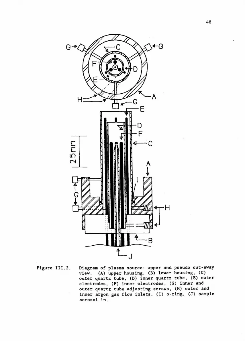
48

Figure 111.2. Diagram of plasma source: upper and pseudo cut-awayview. (A) upper housing, (B) lower housing, (C)outer quartz tube, (D) inner quartz tube, (E) outerelectrodes, (F) inner electrodes, (G) inner andouter quartz tube adjusting screws, (H) outer andinner argon gas flow inlets, (I) o-ring, (J) sampleaerosol in.

49

Table III.1

Quartz Tube Specifications

Outer Quartz Tube

Inner Quartz Tube

Outer Inner LengthDiameter (mm) Diameter (mm) (mm)

23.1 20.4 75

15.0 13.0 81

Table 111.2

Quartz Tube/Electrode Positions

Component Position Relative toInner Quartz Tube (mm)a

Outer Quartz Tube 8 to 10

Outer Electrodes 3.5 to 4

Inner Quartz Tube 0

Inner Electrodes -1 to -23

Sample Introduction -2 to -24Tube

a Negative values indicate distance below inner quartz tube.

50

tube. The outer and inner dimensions of the quartz tubes are

subject to an uncertainty of approximately 0.5 mm due to

manufacturing imperfections.

2. Electrodes

The positions of the six electrodes are shown in

Figure 111.2. All of the electrodes are common 2% thoriated,

tungsten electrodes (Anchor Brand, NASCO, Birmingham, AL). The

outer three electrodes, which are 1/16" in diameter, pass between

the outer quartz tube and the inner quartz tube, through the lower

housing, and down to a baseplate. The inner three electrodes,

which are 3/32" in diameter, pass down through the inner quartz

tube, through the lower housing, through the baseplate for the

outer electrodes, and finally down to a baseplate of their own.

The tips of both the inner and outer sets of electrodes form

the vertices of a horizontal equilateral triangle. All of the

electrodes are anchored at their lower end by simple copper blocks

with a set screw. The copper blocks provide a point of attachment

to the power supplies. These copper blocks are themselves anchored

to baseplates made from LAVA. Since LAVA is an insulator, each

electrode is kept electrically isolated from the others.

B. Plasma Source Electrical Circuitry

The circuitry used to supply power to the plasma is shown in

Figure 111.3. Each of the three inner/outer electrode pairs has

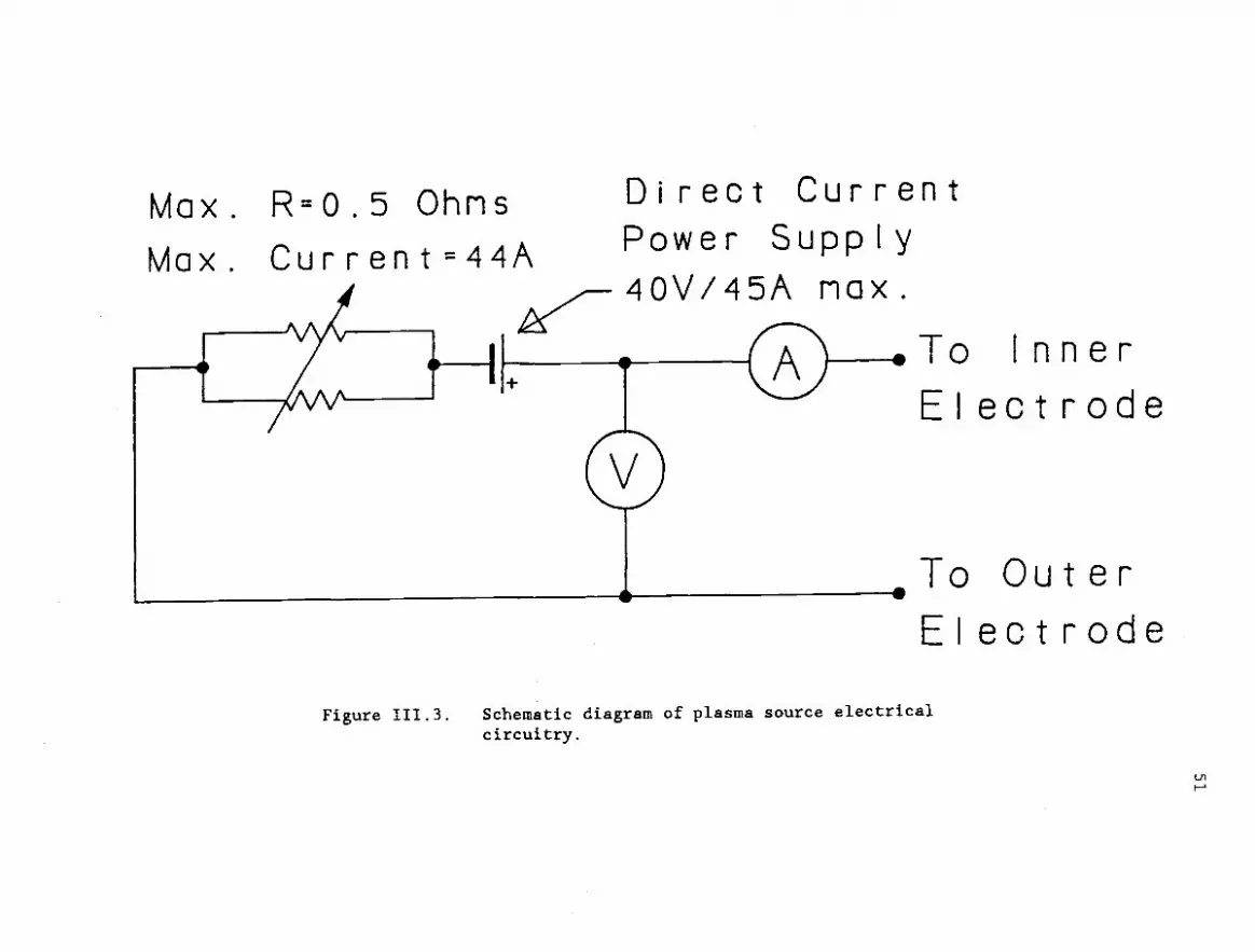
Max. R=0.5 Ohms

Max. Current=44A

Direct CurrentPower Supply

-40V/45A max.

.To InnerElectrode

To OuterElectrode

Figure 111.3. Schematic diagram of plasma source electricalcircuitry.

52

circuitry identical to that shown in Figure 111.3. In addition to

a direct current (dc) power supply (Electronic Measurements, Inc.,

Neptune, NJ), each circuit contains two high power rheostats

(Ohmite, Chicago, IL) connected in parallel. The purpose of the

rheostats is to provide a lengthened RC time constant to the

circuit, particularly when the plasma is first being started. Each

circuit also consists of a dc volt meter and a dc current meter.

For all work, the inner electrodes are anodes and the outer

electrodes are cathodes.

C. Gas Handling Equipment

A diagram of the equipment used to control the distribution

of gases to the plasma and nebulizer is shown in Figure 111.4. Two

separate gas tanks are used to minimize the effect of changing one

gas flow on that of the other gas flows. Each tank has a two-stage

regulator (Airco, Murray Hill, NJ) to control the pressure to the

system.

Four separate gas lines are used to supply gas to the

nebulizer, the inner plasma quartz tube, the outer plasma quartz

tube, and any auxiliary need. Each line contains an identical,

adjustable needle valve (Matheson Gas Products, Secaucus, NJ)

except for the nebulizer line which contains a high precision

needle valve (Matheson Gas Products, Secaucus, NJ). In addition,

each line contains a rotameter (Matheson Gas Products, Secaucus,

NJ). These differ only in their range of operation.

The nebulizer and outer quartz tube gas lines both contain

AuxiliaryGasFlow

OuterGasFlow

InnerGasFlow

Valves

MassFlowneters

NebullzerGasFlow

Rotaneters Part I cl eFilter

MassFlowneterRead Out

HighPrecisionValve

Figure 111.4. Diagram of gas handling equipment.

54

mass flowmeters (Tylan Corp., Carson, CA) which are connected to a

digital read-out unit. The outer quartz tube mass flowmeter (Model

FM360) measures flows ranging from 0-10 L/min and the nebulizer

mass flowmeter (Model FM361) measures flows from 0-1 L/min. Both

of the mass flow units are factory calibrated for argon gas.

A particle filter is placed in line with the nebulizer. This

filter (Model 6183, Matheson Gas Products, Secaucus, NJ) is used

primarily to prevent any particles present in the gas cylinders

from clogging the nebulizer gas orifice. The filter is effective

in retaining particles down to 0.2 pm in diameter. The fittings

used for the many necessary interconnections consist of a

combination of Swagelok components (Crawford Fitting Co., Solon,

OH), Cajon components (Cajon Co., Macedonia, OH), and Clippard

components (Clippard Instrument Laboratory, Inc., Cincinnati, OH).

D. Sample Introduction System

A Meinhard concentric glass nebulizer (Model TR-50-C1, J. E.

Meinhard, Inc., Santa Ana, CA) is used to convert bulk liquid

samples to an aerosol for introduction into the plasma. This

nebulizer is identical to the type commonly used for sample

introduction to the inductively coupled plasma. The nebulizer is

typically operated at an applied pressure of 50 psi and a gas flow

rate ranging from 0.6 L/min to 1.2 L/min. Below 0.6 L/min, the

operation of the nebulizer deteriorates as evidenced by the

formation of many large droplets. Liquid is introduced to the

nebulizer using a peristaltic pump (Minipuls 2, Gilson Medical

55

Electronics, Inc., Middleton, WI). This allows the liquid flow

rate to be kept constant regardless of changes in the nebulizer gas

flow rate.

An in-house constructed spray chamber, very similar to the

one originally introduced by Scott et al., 226 is used to

selectively isolate the smaller aerosol droplets from the larger

ones for introduction into the plasma. The larger droplets, after

condensing on the walls of the spray chamber, are pumped out using

the peristaltic pump. This method ensures that all of the gas used

for nebulization purposes, and registered by the mass flowmeter,

actually passes up to the plasma.

The aerosol which leaves the spray chamber passes up to the

plasma by way of a quartz sample introduction tube. A typical

sample introduction tube is shown in Figure 111.5. Many such tubes

were made by drawing out the end of a piece of stock tubing. Then,

by cutting the drawn out portion at different locations, different

orifice sizes could be obtained. The size of the orifice greatly

influences the velocity with which the sample aerosol exits from

the tube. Therefore, the sample residence time in the plasma can

be altered by changing the sample tube orifice size. Typically, an

orifice size ranging from 0.6 mm to 1.0 mm was utilized.

E. Optical Table and Associated Support Equipment

A variety of equipment is used to provide a stable support

structure for the plasma source and for optical equipment. In

addition to providing structural support, this equipment provides a

56

4- SanpleTubeOrifice

41-- QuartzSanpleIntroductionTube

O.D. = 4 nn

I.D. - 2 nn

Figure 111.5. Diagram of sample introduction tube.

57

reproducible means of moving the various components of the plasma

source, such as the inner electrodes, the outer electrodes, the

sample introduction tube, and the plasma source as a whole. This

equipment will now be described.

1. Optical Table and General Table Hardware

The spectrometer, the plasma source, and other miscellaneous

equipment is located on an in-house constructed optical table. The

design and construction aspects of this table have been previously

described. 227The table, which is made of steel, has a grid of

1/4-20 holes tapped into it at two inch intervals. These holes

allow components to be securely fastened to the table. Easy access

to ac power is provided via power strips on all four sides of the

table. Due to the steel surface of the table, measures had to be

taken to avoid rust formation on the surface of the table. This

was accomplished with a thin coating of bayberry wax applied to the

surface of the table with a suitable solvent.

A variety of general purpose table hardware was used for

tasks such as clamping objects to the optical table and providing

support for other, custom built components. This general purpose

hardware has been described previously. 227

2. Translation Stages

Two types of translation stages were used. The first type

was a simple ball slide translation stage (Model 4410, Daedal) with

58

no inherent means of positional control. It is free moving in one

dimension over its range of three inches. Two such stages are used

for the major infrastructure of the plasma source support system.

One stage provides movement in the vertical direction, the other in

the horizontal direction.

The second type of stage is a simple translation stage whose

position can be controlled manually with a micrometer device.

Three stages of this type are used including two commercial stages

(Newport Corp., Fountain Valley, CA; Brinkman Instruments,

Westbury, NY) and an in-house constructed stage with added

micrometer control. These stages provide independent movement of

the inner electrodes, the outer electrodes, and the sample

introduction tube, relative to the plasma source as a whole.

3. Miscellaneous Support Equipment

There are many pieces of table hardware which were custom

made for a particular situation such as extenders, clamps, and

reinforcers. Many of these pieces are too numerous or trivial to

document. However, some of these miscellaneous pieces are worth

documenting and their description follows.

A support structure, shown in Figure 111.6, was built to

provide an adjustable stop for the main vertical translation

stage. This structure allows the movement of the entire plasma

system in the vertical direction. This aids in roughly positioning

the plasma system at the proper vertical height relative to the

detection system. The support structure provides an adjustable

/Amin SLoge

Is Supported

Here

AdjustableSlop

O

ClompingKnob

*-Support.---0.Rods

Mount ing

Holes

None: Moin St.oge Support_

Mater tat : Aluminum/SLoinlessDesigned By: J. P. Shields

Constructed By: B. Boyer

59

Figure 111.6. Diagram of main vertical translation stage support.

60

stop for the main vertical stage over a range of 3.2 inches. In

addition, this support structure provides a safety feature. A

great deal of weight (about 25 ibs) is put on the main translation

stage by all of the plasma torch equipment. If the main

translation stage bearings were to slip, a potentially catastrophic

fall of the plasma torch would occur. The support structure

provides a catch which would help prevent a complete fall of the

plasma torch.

Another piece of hardware worth documenting is the plate on

which the entire plasma system resides. Since access to the main

spectrometer system was required by other researchers, an easy

method of moving the entire system was needed. The plate shown in

Figure 111.7 provides this capability. It is simply a large 1/2"

thick piece of aluminum on which a grid of 1/4-20 holes was

tapped. These holes then simulate the holes present on the actual

optical table.

F. Echelle Spectrometer

A PLASMA-SPEC (Leeman Labs, Lowell, MA, with a Revision C

Board) high-resolution echelle spectrometer was used to isolate the

analytical spectral line of interest. The merits of echelle

spectrometers for high temperature, line-rich emission sources such

as, plasmas have been described. 228 The most frequently cited of

these merits is the high resolution attainable. A particularly

unique feature of the PLASMA-SPEC spectrometer is the fixed nature

of the two dispersion devices (a grating and a prism).

1/2" Thick Alurilnun

0

All0

0

holes0

0 0 0

drilled0 0 0

0 0

and tapped0 0

0 0

1/4-200 0

0

All holes are 2.0' aparto o o 0 0 0 0 0 0 0

o 0 0 0 0 0 0 0 0 0

o o 0 0 o 0 0 0 0 0

0 0 0 0 0 0 0 0 0 0

0 0 0 0 0 0 0 0 0 0

0 0 0 0 0 0 0 0 0 0

o o 0 0 0 0 0 0 0 0

20.0.

Figure 111.7. Diagram of plasma source baseplate.

61

Ip

At

62

Conventional spectrometers generally rotate a single dispersion

device (a grating) to select which wavelength will fall on a fixed

detector. Indeed, previous echelle spectrometers involved the

movement of both of their dispersion devices to select lines of

interest. 229,230

The PLASMA-SPEC system utilizes fixed dispersion devices. To

achieve line selection, an aperture plate located in the focal

plane is moved in conjunction with a photomultiplier tube (see

Figure 111.8). This aperture plate contains hundreds of exit

slits. To select an analytical line, the aperture plate is moved

so that one of the exit slits is positioned over the image in the

focal plane where the wavelength of light of interest appears in

the appropriate grating order. In addition, the photomultiplier

tube (PMT) is then positioned directly above this exit slit.

The PLASMA-SPEC spectrometer contains a 2-80 microprocessor

which positions the PMT and aperture plate in the focal plane.

However, for our applications, complete control of the movement of

the aperture plate and PMT was required. The reasons for this

requirement are twofold. First, the ROM of the spectrometer

contains the PMT and plate coordinates for 230 lines, which

includes 66 elements. We needed the ability to access other lines

which were not known to the spectrometer, that is, whose plate and

PMT coordinates were not in the ROM of the spectrometer. Secondly,

although the PLASMA-SPEC provides a means of peaking the position

of the aperture plate periodically, no such means is readily

available for the PMT coordinates. When the PMT coordinates in the

ROM of the spectrometer are used, an optimal PMT

..

ECHELLEGRATING

COMPUTERCONTROLLEDMIRROR 4r

PHOTOMULTIPLIERTUBEHOUSING APERTURE

PLATE

442.419w059,4-1

-"471111%\bs,.--41

l'PRISM /LENS

ENTRANCESLIT

I o =1

IlItl

O

i ISERIAL--MICROCOMPUTER I

PARALLEL

PLANEMIRROR

COLLIMATINGMIRROR

PLASMAA-." SOURCE

Plot terPr inter

Figure 111.8. Schematic representation of instrumentation. Image of plasma source is

focused onto entrance slit of echelle spectrometer by a

computer-controlled source mirror. Data from echelle are sent to an

IBM-PC compatible microcomputer via an RS-232 line. Hardcopy plots are

output to a plotter and numeric data to a printer.

64

position is sometimes not achieved with this early version of the

spectrometer. A method was developed to aid in determining an

optimal set of PMT and aperture plate coordinates. This

optimization method is described in Chapter IV.

The PLASMA-SPEC contains one RS-232 communications port

through which ASCII coded commands can be sent to the

spectrometer. In addition, data from the spectrometer can be sent

to an external device via this RS-232 port. Many of the commands

for the spectrometer are carried out using the spectrometer's own

code called P-Code which will be described in the section on

software. Inherent to the design of the PLASMA-SPEC hardware is

the collection of 32 individual data points per acquisition

request. In other words, each time a request is made for the

spectrometer to begin an acquisition, the acquisition set always

consists of 32 samplings which are evenly spaced in time. The

duration of each data point is determined by the integration time

selected, which can vary from 0.3125 s/point to 3 s/point.

As shown in Figure 111.8, the PLASMA-SPEC contains a computer

controllable mirror which focuses an image of the emission source

on the entrance slit of the spectrometer. By moving this mirror

horizontally and vertically, spatial mapping of the emission source

can be achieved. The step resolution of this source mirror is

0.21 mm for horizontal motion and 0.34 mm for vertical motion at

the light source. The calibration method used to determine these

step sizes is given in Appendix E.

65

G. Computer Data Collection/Analysis and Interfacing Hardware

Much of the data collection was done with the aid of an IBM

compatible personal computer. The computer and associated hardware

and software were used for a variety of tasks. These tasks

included computer control of the echelle spectrometer, data

acquisition with real-time display, post-experimental data

analysis, and production of plots and diagrams in hard-copy form.

The hardware aspects of the computer system will now be described.

A summary of the computer system and its peripheral devices is

given in Table 111.3.

1. Computer

A Corona PPC-1, IBM-compatible personal computer was used for

instrument control and data acquisition, display, and analysis.

The computer contains two 360 kilobyte (Kb) floppy disk drives and

512 Kb of random access memory (RAM) on the mother board. The

computer uses an 8088 microprocessor and comes standard with one

RS-232 serial port and one Centronics parallel port. A high

resolution monochrome monitor is internal to the unit.

Subsequently, a 20 megabyte (Mb) 5 1/4 inch internal hard

disk was substituted for one of the floppy disk drives. In

addition, an Intel 8087 math coprocessor chip was added to

complement the 8088 microprocessor. The 8087 chip decreases the

time required for certain mathematical calculations. In addition,

66

Table 111.3

Summary of Computer and Peripherals

Description Manufacturer

Base Computer System:

Corona Model PPC-1 with one floppy Cordata,disk drive and 512 Kb RAM. Thousand Oaks, CA

8087 Math Co-Processor Chip Intel Corp.,Hillsboro, OR

20 Mb Internal Hard Disk Drive Kamerman Labs,Beaverton, OR

Add-On Boards:

Hard Disk Controller, Model Kamerman Labs,Beaverton, OR

JRAM-3 Multi-Function Card Tall Tree Systems,Palo Alto, CA

IBM Compatible Color Graphics Adapter Everex Systems,Fremont, CA

24 Bit Parallel Digital I/O Interface MetraByte Corp.,Stoughton, MA

Other Peripheral Equipment:

Composite Monochrome Monitor, Model Amdek, Elk Grove300A Village, IL

Dot Matrix Printer, Model SD-10 Star Micronics,Irvine, CA

Digital Plotter, Model 7475A Hewlett-Packard,San Diego, CA

67

the 8087 chip is required for the ASYST package, described in the

Computer Software section.

2. Add-On boards

Three of the four of the expansion slots on the mother board

were utilized. One expansion slot was occupied by a hard disk

controller card which was required upon the addition of the

internal hard disk drive.

Secondly, a multi-function board was added to increase the

system memory to the maximum (contiguously) addressable limit of

704 Kb of RAM. The multi-function board also provided an

additional RS-232 serial port, another Centronics parallel port,

clock/calendar hardware, and up to 2 Mb of expanded memory

specification (EMS) RAM. The actual amount of EMS RAM installed

was 596 Kb. This additional RAM was utilized primarily as a large

and fast virtual disk drive.

The third add-on board was an IBM-compatible color graphics

adapter (CGA). Even though a color monitor was not used, some sort

of graphics capability was needed in order to be able to use the

graphics capabilities of the ASYST package (described in the

Computer Software section). The native graphics capabilities of

the Corona are not compatible with the graphics requirements of the

ASYST package.

68

3. Peripheral Devices

A dot matrix printer (Model SD-10, Star Micronics, Irvine,

CA) and a digital, six pen color plotter (Model 7475A,

Hewlett-Packard, San Diego, CA) were used for hardcopy output.

These two devices were interfaced to the Corona through a

Centronics parallel port and an RS-232 serial port, respectively.

A composite monochrome monitor (Model 300A, Amdek, Elk Grove,

IL) was used with the CGA board. This was required in order to

view the graphics produced by the ASYST software. The monochrome

monitor internal to the Corona is incompatible with the CGA board.

4. Computer System for CAD Drawings and Thesis Preparation

A separate computer system was used for the preparation of

drawings, diagrams, and the body of this thesis. This system will

be briefly described.

The computer is a COM-TECH Turbo-Plus (COM-TECH Computers,

Corvallis, OR). The microprocessor is a NEC V20-8 and is

complemented by an 8087-2 math coprocessor chip. The computer

contains 640 Kb of RAM, a 20 Mb 5 1/4" internal hard disk, one 5

1/4" floppy drive, a Hercules compatible monochrome graphics card,

and a monochrome monitor. The hard disk controller card contains

one Centronics parallel port. Subsequently, an AST Six Pack Plus

multi-function card (AST Research, Inc., Irvine, CA) was added to

provide clock/calendar functions, a serial port, and an additional

parallel port. A mouse (PC Mouse, Mouse Systems, Santa Clara, CA)

69

was used as an auxiliary input device (mainly for computer aided

drawing work) and was connected to the computer through the RS-232

serial port. A NEC P660, 24 pin dot matrix printer (NEC

Information Systems, Boxborough, MA) was used for system output.

Finally, a laser printer (LaserJet, Hewlett-Packard, San Diego, CA)

was used to produce the final print-out of this thesis.

H. Data Analysis Software

A program called DATAANAL was written for the purpose of

post-experimental analysis of data. Many of these data analysis

tasks are repetitive in nature, that is, the same manipulations are

performed on many different data files. DATAANAL allows many of

these tasks to be performed simply by selecting a menu option with

a function key on the PC keyboard. DATAANAL was written in the

ASYST environment (Version 1.51, MacMillan Software Co., New York,

NY) and is listed in Appendix B.

The screen setup of DATAANAL is divided into four different

windows, shown in Figure 111.9. The lower right portion of the

screen presents the different menus while the lower left portion

displays prompts and other information regarding the progress of an

operation. All of the menu selections are assigned to function

keys on the PC keyboard. The entire upper half of the screen is

reserved for plotting purposes. The very last line of the screen

is reserved for error messages.

The main menu of DATAANAL is shown in Figure III.10. Each

main menu selection presents a sub-menu. These sub-menus are shown

70

Plotting

Area

Message/PromptWindow

MenuWindow

Error Window Status Line

Figure 111.9. Screen organization for the data analysisprogram, DATAANAL.

71

Data Analysis MenuFl - Timed Data AnalysisF2 - Histogram AnalysisF3 - Plotting UtilitiesF4 - General UtilitiesF5 - File Conversion UtilitiesF10- Main Menu

Figure III.10. Main Menu of DATAANAL

Timed Data Analysis MenuFl - Calculate RSD From A Timed FileF2 - Strip and Catenate Time ArrayF3 - Strip and Catenate Raw ArrayF4 - Print Timed ArraysF10- Main Menu

Plotting Utilities MenuFl - Activate Dotted Hidden LinesF2 - Activate Square SymbolsF3 - Activate Triangle SymbolsF4 - Activate Diamond SymbolsF5 - Change Symbol SizeF10- Main Menu

General Utilities MenuFl - Copy From Subfile To ArrayF2 - Create File From Array(s)F10- Main Menu

,-File Conversion UtilitiesFl - DSURF FormatF2 - LOTUS FormatF10- Main Menu

Figure 1II.11. Sub-menus of DATAANAL.

72

in Figure III.11. Selecting Fl from the main menu displays the

Timed Data Analysis Menu. All of these sub-menu selections assume

the user is interested in working with data which was obtained in

the Timed Acquisition Mode of ACQDATA (ACQDATA is described

separately in Chapter IV). The first selection from the Timed Data

Analysis Menu, Fl, calculates the relative standard deviation of a

32 point data set obtained in the Timed Acquisition Mode. The

desired file and acquisition number are requested before the

calculation begins.

Selection F3 allows several 32 point data sets to be

catenated together. Each 32 point data set is stored in a separate

array as it is collected. If a signal which is stable and constant

in magnitude is monitored in the Timed Acquisition Mode over a

period of time, many of these 32 point arrays will be collected.

For plotting and other data analysis purposes, it is useful to

combine these arrays together, end to end. After being prompted

for the file of interest, the F3 selection performs this task.

Choosing F2 performs essentially the same task as does F3.

However, the catenation is done to the average values of the many

32 point data sets instead of to the individual, raw values

themselves. The F4 selection from the Timed Data Analysis Menu

prints the 32-point averages and their respective standard

deviations to the line printer. Finally, as in all of the

sub-menus, F10 returns to the main menu.

Selecting F2 from the Data Analysis Main Menu puts the system

in the Histogram Calculation Mode. This mode is typically entered

after a catenation has been performed. It is often of interest to

73

perform a histogram or frequency plot of raw data. The histogram

options will determine a histogram or frequency array and a

breakpoint array. The latter type of array determines the

resolution with which the histogram is calculated.

The F3 selection from the main menu displays the Plotting

Utilities Menu shown in Figure III.11. These menu selections allow

the type of plotting symbol, as well as the size of the symbol, to

be changed. In addition, hidden lines in axonometric type plots

can optionally be displayed as dotted or invisible lines.

Selecting F4 from the main menu displays the General

Utilities Menu shown in Figure III.11. The Fl selection allows

data to be copied from the desired subfile of a data file to a

named array in the ASYST environment. The user is prompted for the

name of the data file and the desired name of the data array.

Selecting F2 from the General Utilities Menu allows any number of

arrays created within the ASYST environment to be saved to a disk

file. The conversion process does not assume anything about the

size or shape of the array, that is, the arrays can be of any size

or shape (limited, of course, by system memory).

Choosing F5 from the main menu presents the File Conversion

Utilities Menu shown in Figure III.11. The two selections offered

here allow files created in the ASYST file structure to be

converted to one of two ASCII file structures. The first, called

DSURF format, formats the data in a manner which can be read by the

DSURF plotting program described later. The second file structure,

called LOTUS format, formats the data in a manner which can be read

by the LOTUS file import utility. In both cases, the user is

74

prompted for an input file name, the number of subfiles to be

converted, and an output file name.

I. Miscellaneous Software

1. Assembly Language

Only one routine was written in assembly language. This

routine is entitled GETTIME.ASM and can be found in Appendix II.

GETTIME.ASM was written to overcome a limitation of ASYST regarding

access to the time of day. ASYST is capable of returning the time

to the user. However, the time resolution is only one minute in

absolute time. The timed acquisition mode of ACQDATA required time

resolution capabilities of at least one second. GETTIME.ASM

provided this capability.

The link between ASYST and compiled assembly language

programs is rather cumbersome. The word GET.TIME in the program

ACQDATA is responsible for calling the assembly language routine

which then passes the time back to ASYST. In addition to the

parameters named Hours, Minutes, Seconds, and HSeconds, the CALL

statement in GET.TIME contains an entry address. In this case, the

entry address is hexadecimal 40. This number is obtained from the

.MAP file in the LINK process.

When one or more assembly language routines are to be called

from within ASYST, a special version of ASYST, called ASYSTLDR,

must be loaded. ASYSTLDR is a user compiled assembly language

routine which specifies both the name of the assembly language

75

routine to be used and the name of the ASYST file to load. This

process has been described in detail elsewhere. 231

76

2. ASYST Stepper Motor Control Software

Documentation For

CURSIT.UTL

Submitted By:

James P. Shields

Graduate Research Asst.

Department of Chemistry

Oregon State University

Corvallis, OR 97331

503-754-2081

Submitted To:

ASYST Program Exchange

MacMillan Software Co.

New York, NY

77

a) Abstract

CURSIT.UTL allows one to control an external device from the

cursor keys of a PC by means of the digital I/O lines of a

MetraByte PI012 board. While the specific application of the

author was to control a two-dimensional stepper motor system, the

program is readily adaptable to other control functions. Simple

modifications to the program will allow other keys on the keyboard

to be programmed for specific control functions. The program is

menu driven and provides the option for significant expansion of

the menu structure. Separate windows are used to display menu

selections, prompts, system status, and error messages.

b) Description of Program

This program allows the cursor keys of a PC to be used to

send logical bit patterns to an external device via a MetraByte

(MetraByte Corp., Stoughton, MA) P10-12 Digital I/O board. My

specific application involved control of the movement of a two-axis

stepper motor system via the cursor keys. However, this program

can be applied to any other application which requires digital I/O

lines for control of an external device.

As noted in the source code, the words MOVE.MOTOR,

MOVE.POS.Y, MOVE.POS.Z, MOVE.NEG.Y, and MOVE.NEG.Z are specific to

our stepper motor circuitry. It is not likely that other users

will have circuitry which has exactly the same I/O lines as our

system. These five words have been included here as an example of

78

how the control function could be written. However, other users

who are utilizing a MetraByte P10-12 board could easily substitute

their own words in place of the five words mentioned above.

For instance, since the MOVE.POS.Y word corresponds to the

depression of the "UP" cursor key, MOVE.POS.Y could be redefined to

perform whatever is desired upon depression of the "UP" cursor

key. Perhaps one wants the low four bits of the eight digital I/O

lines of Port B to toggle high and then, after a delay of 20 msec,

to toggle low. In this case, MOVE.POS.Y would be changed to

: MOVE.POS.Y

WRITE.TO.PORTB \ Select Port B as output port.

15 DIGITAL.OUT \ Binary 00001111

20 MSEC.DELAY

0 DIGITAL.OUT \ Binary 0000000

In addition to using the cursor keys for the control of an

external device, the other keys on the numeric keypad, such as HOME

and PAGE UP, could be programmed to perform other functions. In

this case, the keyboard scan code for the key of interest would

need to be added to the CASE statement in the word

GET.MOTOR.CONTROL.INPUT. Indeed, any key could be used in this way

as long as the appropriate key scan code was incorporated into

GET.MOTOR.CONTROL.INPUT.

79

c) Operation of Program

First, a version of ASYST which recognizes the MetraByte

PI012 board must be loaded. This is done using the CONFIG.DAS

program. See Appendix of ASYST Manual for instructions. After

loading ASYST, typing GO will produce a series of windows in the

lower 1/3 of the screen as shown in Figure 111.9. The upper

portion of the screen is left free for other purposes. At this

point, the main menu will display the different options available,

which are selected by pressing the appropriate function key. Since

the scope of this program is limited to digital I/O, only one menu

selection has been supported. The user could easily add other menu

selections.

Selecting Fl causes the display of a sub-menu. This sub-menu

instructs the user to utilize the cursor keys to perform the

digital I/O function which, in this case, is movement of a stepper

motor. As the cursor keys are depressed, the status line keeps

track of the coordinates of the stepper motors. This status line

could be modified to update some other parameter of interest as the

cursor keys are pressed. If any unallowed keys are pressed,

appropriate error routines are initiated with error messages

appearing in the error window (see Figure 111.9). The sub-menu

also offers the user the option of zeroing one or both of the

coordinates. The step size can also be changed

via a sub-menu selection. This step size controls the number of

pulses sent to the digital I/O port each time a cursor key is

80

pressed. The final selection from the sub-menu returns the user to

the main menu.

d) Intended Users

This program is directed at anyone who would like to control

some external device from the keyboard of a PC by means of digital

I/O lines. Applications could include control of stepper motors,

firing mechanisms, heaters, timers, shutters, and a variety of

other electronic equipment. It is also hoped that the menu

structure and windowing concepts used herein will give newer users

some ideas as to how to develop a menu driven program. This

program requires the possession of a MetraByte PI0-12 digital I/O

board. However, note that other boards having digital I/O

capabilities could also be used. This would require some fairly

straightforward modifications of parameters such as the base

address, hardware operating mode, etc., which will not be covered

here.

3. Commercial Software

A variety of commercial software was utilized in this work.

The data analysis software, which has already been described, and

the data acquisition software to be described in Chapter IV, were

developed using the ASYST package (Macmillan Software, New York,

NY). The assembly language routines were compiled using

Fast Assem-86 (Speedware, Sacramento, CA). Most of the coding was

81

initially created using The Norton Editor (Peter Norton Computing

Inc., Santa Monica, CA). The operating system used was MS-DOS

(Microsoft Corp., Redmond, WA) version 2.11.

Nearly all of the technical drawings in this thesis were

produced using a computer aided design (CAD) program called GENERIC

CADD (Version 3.0, Generic Software, Inc., Redmond, WA). The text

of this thesis was created and edited using the Multimate

Advantage II Professional Word Processor (Multimate International,

East Hartford, CT). Lotus 1-2-3 (Lotus Development Corp.,

Cambridge, MA), a spreadsheet/plotting program, was utilized for

data manipulation, calculations, and for producing plots for quick

examination of results.

3-D plots were produced using the ASYST package described

previously. Sigma-Plot (Jandel Scientific, Sausalito, CA) was used

to produce most of the X-Y plots in this thesis.

Fastback (Fifth Generation Systems, Baton Rouge, LA) was used

to periodically produce back-ups of both hard disks. Finally,

version 5.1 of ARC (System Associates, Wayne, NJ), a shareware

archiving program, was used to compress the ASYST and LOTUS data

files for more efficient back-up storage on floppy disk media.

This archiving typically resulted in a 30% reduction in file size

thus saving floppy disk space and money.

82

IV. A FORTH-based Data Acquisition and Control

System for use in Plasma Atomic Emission Spectrometry

James P. Shields and Edward H. Piepmeier*

Department of Chemistry

Oregon State University

Corvallis, OR 97331 U.S.A.

for Submission to Computer Enhanced Spectroscopy

Author to whom correspondence should be addressed.

83

A. Abstract

The characterization of new spectroscopic plasma sources for

use in atomic emission spectroscopy often presents the need for

information about the spatial emission characteristics of the

source. In addition, information about the variation of the

emission over time is often beneficial. This paper describes a

flexible data acquisition system in which an echelle spectrometer

is interfaced to an IBM-PC compatible microcomputer. The

FORTH-based software, which provides real-time display of acquired

data, allows any point in the emission source to be imaged on the

entrance slit of the spectrometer by using the cursor keys of the

PC and a computer controlled mirror. The different acquisition

modes of the system are illustrated with examples of

two-dimensional spatial profiles of the plasma and monitoring of

plasma stability over time. In addition, an illustration of the

optimization of the echelle's aperture plate and photomultiplier

tube positions in the focal plane is given.

KEY WORDS

Atomic Emission Spectroscopy, Direct Current Plasma, Spatial

Profiles, Instrumentation, Echelle Spectrometer, Real-Time Display

84

B. Introduction

A variety of information is useful in attempting to

investigate and improve the analytical capabilities of a new

spectroscopic plasma emission source. For instance, common

analytical figures of merit include determination of detection

limits, linear dynamic range, short and long-term precision, and

susceptibility to chemical interference effects. In addition to

these common analytical figures of merit, several

researchers 157 '

232-235have emphasized the need for spatial

information about the plasma under varying experimental conditions

such as gas flow rates and input power. Spatial information is

also useful for evaluating the effects of matrix components in a

sample on the analytical capabilities of a plasma. 236-239

While spatial and precision studies are useful in the

evaluation of a new plasma emission source, it is often difficult

or cumbersome to obtain this type of information with a

commercially available spectrometer. Commercial systems are often

designed more for the purpose of analyzing samples on a routine to

semi-routine basis rather than for more specialized, diagnostic

studies. As with other researchers, 240 we have also found that

the data analysis and hard-copy output options of commercial

spectrometers are often very limited.

After the completion of an experiment, it is very common for

the analyst to plot the results in some form. Our early work

utilizing this post-experiment plotting often revealed a flaw or an

unexpected result in the experiment that perhaps could have been

85

corrected during the experiment if real-time plotting could have

been done. Therefore, another desirable capability to aid in the

characterization of a new plasma source is a means of real-time

display of acquired data in the form of plots to a graphics screen.

In this work, an IBM-PC compatible microcomputer is

interfaced to a high resolution echelle spectrometer to facilitate

a variety of data acquisition functions. An integrated,

menu-driven program is presented for the purposes of instrument

control, data acquisition, real-time plotting, post-experiment

analysis, and hard-copy output. This program was developed using

ASYST, a commercially available data acquisition and analysis

programming environment. The application of this system to the

characterization of a new plasma emission source will be described.

C. Instrumentation

A schematic representation of the instrumentation is shown in

Figure 111.8. The spectrometer, the computer and its peripherals,

and the ASYST software will each be described separately. The

plasma emission source has been described previously245 and the

instrumentation aspects of the source will not be covered here.

1. Spectrometer

A PLASMA-SPEC (Revision C Board, Leeman Labs, Lowell, MA)

high-resolution echelle spectrometer was used to isolate the

analytical spectral line of interest. The merits of echelle

86

spectrometers for high temperature, line-rich emission sources such

as plasmas have been described. 228 The most frequently cited of

these merits is the high resolution attainable. A particularly

unique feature of the PLASMA-SPEC spectrometer is the fixed nature

of the two dispersion devices (a grating and a prism).

Conventional spectrometers generally move a single dispersion

device (a grating) to select which wavelength will fall on a fixed

detector. Indeed, previous echelle spectrometers involved-the

movement of their dispersion devices to select lines of

interest. 229,230

The PLASMA-SPEC system utilizes fixed dispersion devices. To

achieve line selection, an aperture plate located in the focal

plane is moved in conjunction with a photomultiplier tube. This

aperture plate, shown in Figure 111.8, contains hundreds of exit

slits. To select an analytical line, the aperture plate must be

positioned so that one of the exit slits is positioned over the

point in the focal plane where the wavelength and order of light of

interest appears. In addition, the photomultiplier tube (PMT) must

be positioned directly above this exit slit.

The PLASMA-SPEC spectrometer contains a Z-80 microprocessor

which positions the PMT and aperture plate in the focal plane.

However, for our applications, complete control of the movement of

the aperture plate and PMT was required. The reasons for this

requirement are twofold. First, the ROM of the spectrometer

contains the PMT and plate coordinates for 230 lines, which

includes 66 elements. We needed the ability to access other lines

which were not known to the spectrometer, that is, whose

87

plate and PMT coordinates were not in the ROM of the spectrometer.

Secondly, although the PLASMA-SPEC provided a means of peaking the

position of the aperture plate periodically, no such means was

readily available for the PMT coordinates. When the PMT

coordinates in the ROM of the spectrometer are used, an optimal PMT

position is sometimes not achieved with this early version of the

spectrometer. Therefore, a method of optimizing the PMT and plate

positions in the focal plane was needed.

The PLASMA-SPEC contains one RS-232 communications port

through which ASCII coded commands can be sent to the

spectrometer. In addition, data from the spectrometer can be sent

to an external device via this RS-232 port. Many of the commands

for the spectrometer are carried out using the spectrometer's own

code called P-Code which will be described in the section on

software. Inherent to the design of the PLASMA-SPEC hardware is

the collection of 32 individual data points per acquisition

request. In other words, each time a request is made for the

spectrometer to begin an acquisition, the acquisition set always

consists of 32 samplings which are evenly spaced in time. The

duration of each data point is determined by the integration time

selected, which can vary from 0.3125 s/point to three s/point.

As shown in Figure 111.8, the PLASMA-SPEC contains a computer

controllable mirror which focuses an image of the emission source

on the entrance slit of the spectrometer. By moving this mirror

horizontally and vertically, spatial mapping of the emission source

can be achieved. The step resolution of this source mirror is

0.21 mm for horizontal motion and 0.34 mm for vertical motion.

88

2. Computer and Peripheral Devices

The PLASMA-SPEC was interfaced to a Corona PPC-2 (Cordata,

Thousand Oaks, CA), which is an IBM-PC compatible microcomputer.

Communication between the spectrometer and the computer was

achieved via an RS-232 port on a JRAM-3 multifunction board (Tall

Tree Systems, Palo Alto, CA) installed in the Corona. In addition

to the RS-232 port, the multifunction board also provided an

additional parallel port, clock/calendar functions, and memory

expansion capabilities. Enough memory chips were installed to give

704 Kbyte of contiguous DOS addressable memory and 596 Kbyte of

expanded memory specification (EMS) RAM. An 8087 arithmetic

coprocessor (Intel Corp., Hillsboro, OR) was also installed in the

Corona.

A Star Model SD-10 printer (Star Micronics, Irvine, CA) was

used to print out data both during and after experiments. An

HP7475A plotter (Hewlett-Packard, San Diego, CA) was used as the

output device for plotting purposes.

3. Software

a) P-Code Routines

Before describing the ASYST software, some understanding of

the routines written in the native language of the spectrometer is

necessary. P-Code is the programming code used to control the

89

operation of the PLASMA-SPEC echelle spectrometer. The P-Code

instruction set consists of 44 operation codes or op-codes. These

op-codes are used to control low level functions such as loading

counters and masking bits, as well as higher level functions such

as initiating data collection and serial port data transmission. A

complete list of these op-codes, as well as other details of the

P-Code system, can be found in the echelle spectrometer operation

manual. 241

The execution of these op-codes is totally independent of any

external computer system. The op-codes are processed internally by

the spectrometers' own microprocessor, a Z-80. The op-codes can be

entered into sequential locations in the spectrometers' memory and

executed starting at any location using the regular menu of the

spectrometer. Since any menu selection offered by the spectrometer

can be remotely chosen by ASCII commands sent via the RS-232 line,

P-Code routines can be executed as though they were special

subroutines of some external program. Indeed, the P-Code routines

which were written were generally executed as subroutines from the

ASYST program running on the PC.

A total of nine routines were written. The first four

routines are used to perform aperture plate and PMT fine spectral

scans in the X and Y directions of the focal plane. These routines

are mainly used in conjunction with externally running software to

optimize the aperture plate and PMT positions in the focal plane.

This external software will be described in the next section. When

a given scan is completed, the 32 point data set from the

spectrometer is sent via the spectrometer serial port to the

90

external computer system.

A fifth routine collects data at a specific wavelength and

order. In other words, no spectral scanning is done. The aperture

plate and PMT are stationary during the execution of this routine.

As before, when the 32 point data set has been collected,

transmission via the spectrometer serial port is initiated. This

routine is generally used in conjunction with external software to

collect data once an optimal set of aperture plate and PMT

coordinates has been determined.

A sixth and seventh routine perform aperture plate X and Y

scans, respectively, as do routines 1 and 2. However, these

routines cover a wider spectral range than routine 1 and,

therefore, are useful in investigating the background around an

analytical line and in searching for lines not in the ROM of the

spectrometer.

An eighth routine spatially scans the emission source in the

horizontal direction by moving the source mirror of the

spectrometer. The range of this spatial scan is controlled by

selecting the step size of the source mirror motor.

Finally, routine 9 spatially scans the emission source in the

vertical direction. The range of the scan is controlled by varying

the step size of the motor operation. The primary use of this

routine is to determine the location of the top of the outer quartz

tube. A sharp minimum in the vertical spatial profile generally

occurs at the top of the quartz tube. This allows all subsequent

measurements to be referenced relative to the top of the outer

quartz tube.

91

b) ASYST Software

ASYST (Version 1.51, MacMillan Software Co., New York, NY)

stands for "A Scientific System" and is a data acquisition and

analysis programming environment based on the FORTH

language. 242,243All numeric and string manipulations are stack

oriented. The ASYST environment is a cross between an interpretive

environment, where commands can be given and immediately processed,

and a compiled environment. Many predefined, system commands,

called words, exist for numeric, array, string, plotting, I/O, and

other manipulations. These words can be executed in the ASYST

environment and interpreted immediately by simply typing the name

of the word. Other, user-defined words can be defined based on the

system words. These words can then be compiled and saved as an

executable file; this is how a program is constructed.

Although ASYST is an unstructured language, every effort was

made to maintain a structured program. Two programs were written

in ASYST. The major function of the first program, called ACQDATA,

is for data acquisition and real-time graphics plotting of data.

The second program was used for post-experimental data analysis and

hard-copy plotting. Only ACQDATA will be described here. Since

ACQDATA is a menu-driven, integrated program, it is natural to

approach the discussion of this program by way of the different

menu options.

The main menu of ACQDATA is shown in Figure IV.1. All menu

options are assigned to function keys. These menu selections

92

Main MenuFl - Zero Motor CoordsF2 - NOPF3 - Manual ControlF4 - Data AcquisitionF5 - Optimize Plate/PMT

F6 - Echelle UtilF7 - Echelle Set-UpF8 - NOPF9 - NOPF10- This Menu

Figure IV.1. Main Menu of ACQDATA

93

appear in a specially defined window on the screen. The location

of this menu window is shown in Figure IV.2 which also shows the

rest of the screen setup during a typical acquisition run. In

addition to reserving a special portion of the screen for the

various menus, a special window is devoted to a text screen, where

system prompts and other information appear. The entire middle

section of the screen, and the upper left portion of the screen,

are reserved for real-time plotting of data. The upper right

portion of the screen is another text screen which displays a

variety of information such as the mean value, standard deviation,

and relative standard deviation of a data set immediately after it

is collected. Finally, the uppermost line is divided in half and

each side serves as a title line of what appears below it. The

very bottom line of the screen is also divided in half. The left

side is reserved for displaying error messages and the right side

displays the status of various system variables.

With the exception of the first menu selection, all of the

main menu choices shown in Figure IV.l offer submenus. The various

submenus are shown in Figure IV.3. Note that selections F2, F8,

and F9 are not currently assigned to any main menu operation. This

is indicated by NOP for No OPeration. The one main menu selection

which does not offer a submenu is the Zero Motor Coords option,

which is selected via the Fl key. This selection allows one to

zero the horizontal, vertical, or both of the spatial coordinates.

These spatial coordinates refer to the position of the emission

source relative to the entrance slit of the echelle spectrometer.

When the source mirror of the PLASMA-SPEC is moved under program

3.74

3.68

3.62

3.56

3.50

3.50

2.802.001.20.400

Timed Acquisition Mode

4.00 12.0 20.0 28.0

200.

36..0

600.

it Mean Std. Dev. XRSD

1 36457 527 1.44

2 36364 516 1.42

3 36314 526 1.45

4 36712 597 1.63

5 36218 3e3 1.07

1000 1400

Data Collection Completed.Make a selection from theData Acquisition Menu:._

Error Window

1800

Data Acquisition MenuFi Signal vs TimeF2 Spatial AcquisitionF3 Move To Another LineF10 Main Menu

Horiz Vert HStep VStep BGStep BGMode-10 4 2 2 32 1

Figure IV.2. Example of screen during a timed acquisition experiment. Top left

graphics screen shows most recent 32-point data set. Middle graphics

screen shows cumulative 32-points average values over time. Lower

portion of screen shows menu window, prompt/message window, statusline, and error window. Top right of screen displays informationabout the five most recent acquisition sets. 1/443

95

Manual Control MenuUse Cursor Keys To Move Mirror OR

Fl - Acq Data Point F6 - NOPF2 - Acq Wave Scan F7 - NOPF3 - Gross X Move F8 - Edit Step SizeF4 - Edit Bkgd. Mode F9 - Zero CoordsF5 - Peak Horiz. Pos. F10- Main Menu

Data Acquisition MenuFl - Signal vs TimeF2 Spatial AcquisitionF10- Main Menu

ptimization MenuFl - Plate XF2 - Plate YF3 - PMT XF4 - PMT YF10- Main Menu

Echelle Utilities MenuFl - Ed/Create Coord Set F6 - NOPF2 - Change # Coord Sets F7 - Print Coord SetF3 - Coord Set To File F8 - NOPF4 - Coord Set From File F9 - NOPF5 - Lst Coord Set Files F10- Main Menu

Echelle Set-Up MenuFl - Down Load P-CodeF2 - Load Hg Mirror Motor OpF3 - Set Integration TimeF4 - Edit Background OffsetF5 - Load Hg PMT CoordinatesF6 - Quartz Finder F10-Main Menu

Figure IV.3. Sub-menus of ACQDATA

96

control, the horizontal and vertical spatial coordinates change.

ACQDATA keeps track of these changes. The system status line,

shown in Figure IV.2, displays these coordinates and updates them

as required.

Selecting F3 from the main menu presents the Manual Control

Menu shown in Figure IV.3. This mode allows the most freedom and

flexibility in acquiring data. When in the manual mode, the cursor

keys on the PC keyboard can be used to move the source mirror of

the PLASMA-SPEC. Moving the mirror in this way has the effect of

changing the portion of the emission source which falls on the

entrance slit of the spectrometer. When the source mirror is moved

in this way, the horizontal and vertical spatial coordinates are

kept track of by ACQDATA and updated on the system status line.

The Fl and F2 selections from the Manual Control Menu are the

selections which actually initiate data acquisition. They are both

completely general modes of acquisition, that is, a data set will

be collected irrespective of what the spatial coordinates are. A

typical use of the manual mode is to move the image of the emission

source to the desired position using the cursor keys. Then a data

set is acquired at that position by depressing Fl or F2. Movement

of the emission source image and subsequent data collection can

proceed in this manner indefinitely. When acquisition in this

manner is finished, the user is prompted for information regarding

the optional writing of data to a disk file.

The two manual acquisition keys, Fl and F2, differ in the

following manner. When Fl is used, both the aperture plate and PMT

are stationary during the acquisition. Therefore, all of the data

97

are at a single wavelength (and order). When F2 is used, the

aperture plate actually moves in the wavelength direction

(dimension) of the focal plane. In this way, a spectral scan is

achieved.

Selecting F3 provides the ability to move the source mirror

by a large amount in the horizontal direction. The horizontal

spatial coordinate is adjusted accordingly. F4 allows editing of

the current background correction mode. This background correction

parameter will be discussed later. F5 causes the execution of a

P-Code routine which scans the plasma spatially in the horizontal

direction and moves to the peak emission point when done. F8

allows changing of the step size of the source mirror, that is, the

distance which the source mirror will move each time a cursor key

is depressed. The horizontal and vertical step sizes can be

different. The F9 selection allows one or both of the spatial

coordinates to be zeroed. Note that this does not have any effect

on the position of the source mirror; only the numbers assigned to

the numerical coordinates are set to zero. This is useful, for

instance, when one has found the peak horizontal position at a

particular vertical position in the plasma. Zeroing the horizontal

coordinate then provides a convenient reference point in the

plasma. Finally, F10 returns to the main menu.

Selecting F4 from the Main Menu brings up the Data

Acquisition Menu, shown in Figure IV.3. Aside from the F10

selection, which returns the user to the Main Menu, there are two

options here. Fl puts the system into the timed acquisition mode.

In this mode, data sets, consisting of 32 individual

98

samplings/data set, are collected at periodic intervals. The

length of these intervals depends on the integration time which is

being used.

Before actually beginning an acquisition session in the timed

mode, the user is prompted for information such as whether to

enable real-time plotting. Each raw 32 point data set can be

optionally plotted immediately after it is collected. In addition,

the average value of each 32 point data set can be plotted vs the

time of acquisition of the data set. By default, each 32 point

data set is averaged and the standard deviation and relative

standard deviation is computed and displayed in the upper right

portion of the screen. Figure IV.2 gives an example of the screen

during a timed acquisition session. As can be seen, the raw 32

point values are plotted in the upper left portion of the screen,

the average value of each 32 point data set is plotted in the

middle, and the calculated values are plotted in the upper right.

During acquisition in the timed mode, the user can optionally

halt acquisition and then either continue or exit the acquisition

mode. Upon exiting, prompts appear in the text window which allow

the data to be written to a disk file. This timed mode of

acquisition is particularly useful for investigating phenomena such

as the short and long term precision of the emission source. This

mode is also useful for observing the response of the plasma source

to various changes to the system such as sample change-over or a

change in a gas flow rate. In general, it is not of interest to

move the source mirrors during the timed mode of acquisition. Each

32 point data set is collected by viewing the same portion of the

99

plasma.

The other acquisition mode accessible from the Data

Acquisition Menu is geared towards the collection of spatial

information and is entered by selecting F2. The intent of this

mode of acquisition is to successively collect horizontal profiles

of the plasma at progressively higher points in the plasma. When

the Spatial Acquisition Mode is selected, a variety of user prompts

are displayed in the text window. These prompts ask for

information such as the desired spatial width of each horizontal

profile, the distance to step up vertically after each horizontal

profile has been completed, and the total number of horizontal

profiles to collect.

As with the Signal vs Time Mode of acquisition, plotting of

each raw 32-point data set can be enabled or disabled. However,

the spatial mode of acquisition differs from the timed mode in that

during the collection of each 32-point data set, the source mirror

is stepping in the horizontal direction. Therefore, each one of

the 32 data points corresponds to a different horizontal position

in the plasma. So if the plotting of each 32 point data set is

enabled, one can view the horizontal profile at a particular

vertical position in the plasma immediately after the data are

collected.

Another pre-acquisition prompt requests the type of

background correction to be used. One or two-point off-line

background correction can be selected or the background correction

can be done by introducing blank to the plasma and repeating the

spatial acquisition under the same conditions. If the off-line

100

type of background correction is selected, the background

information is collected immediately after each horizontal

profile. However, the analyte emission data and the background

data consist of independent 32-point data sets.

Finally, the user can optionally interrupt acquisition after

each horizontal profile has been completed. At this point,

acquisition can be restarted or the user can exit. When the user

exits in this manner, or when all of the requested profiles have

been completed, prompts appear which request the necessary

information for saving the data to a disk file.

The fifth choice from the Main Menu facilitates the

optimization of the position of the aperture plate and PMT in the

focal plane of the echelle. Selecting F5 presents the Optimization

Menu, shown in Figure IV.3. Selecting Fl through F4 from the

Optimization Menu initiates a peaking routine which scans the

aperture plate (or PMT) over a very small distance in the

horizontal or vertical dimension of the focal plane. Then, an

algorithm in ACQDATA determines a correction factor. This

correction factor represents the amount by which the aperture plate

(or PMT) must be moved from its current position to achieve maximum

light throughput. The user can enable or disable the display of

the aperture plate and PMT scans. In addition, the user has the

option, after seeing what the scan looks like, of applying the

correction factor. If the correction factor is applied, a library

of aperture plate and PMT coordinates is updated by ACQDATA for the

particular line in use. This library system is described below.

Selecting F6 from the main menu presents the Echelle

101

Utilities Menu, which is shown in Figure IV.3. These menu

selections allow the user to manipulate a library of aperture plate

and PMT coordinates. To set the spectrometer to a wavelength in a

particular order of the grating, a unique set of four coordinates

is required: the horizontal and vertical aperture plate coordinates

and the horizontal and vertical PMT coordinates. From the Echelle

Utilities Menu, the user can create or edit a coordinate set (F1)

and save it to a file (F3). At a later time, the desired

coordinate set can be retrieved (F4) and made known to the system.

In this way, the coordinate sets need not be manually reentered

each time an experiment is performed. The desired coordinate set

can simply be retrieved from the library. F5 lists, to the

monitor, the elements whose coordinates are in the library. F7

prints the actual coordinates for a particular wavelength and order

to either the monitor or the printer. Finally, F2 allows the user

to change the number of coordinate sets which the system will keep

track of.

The final choice offered by the Main Menu (F7) presents the

Echelle Set-Up Menu shown in Figure IV.3. These selections allow

the user to perform a variety of tasks which are required before an

experiment can begin. For instance, the first choice, Fl,

automatically down-loads the P-Code routines to the spectrometer.

These P-Code routines, which were discussed previously, need to be

reloaded occasionally due to the occurrence of a power outage, a

complete power-down of the spectrometer for maintenance purposes,

or if another user down-loads different P-Code routines to the

spectrometer. The F2 and F5 selections relate to an internal Hg

102

lamp which can be used for calibration purposes. F3 allows the

integration time to be set to a value other than the default

value. F4 allows the value of the background offset to be edited.

This background offset determines how far off-line the background

correction will be made. Finally, F6 initiates a routine which

"finds" the top of the quartz tube by looking for the sharp

discontinuity in the vertical emission profile caused by the quartz

tube. The top of the quartz tube can then be used as a reference

point for all subsequent vertical positions. As is the case

throughout all of the menus, F10 will again present the Main Menu.

D. Application

1. Optimization of Aperture Plate and PMT Positions in Focal Plane

As was mentioned previously, there is a need to optimize the

position of the aperture plate and the PMT in the focal plane.

Both the aperture plate and the PMT can vary in two directions. An

example of how a PMT optimization proceeds is as follows. When F3

is selected from the Optimization Menu, the PMT is stepped over a

very narrow distance in the wavelength domain and intensity

readings are taken throughout the scan. A typical profile before

optimization is shown in Figure IV.4a. Although this profile can

be plotted to the upper left portion of the computer monitor, this

particular profile was copied from the display on the monitor of

the spectrometer. The optimization algorithm uses the width at

CU' 724.75a) 81 E:2 83 84

H II H H100-

b)

40-

11

.0046 NM/STEP

3200

2 P 7 4READY

CU1 724.75 .0046 NM/ STEPet E:2 83 84

II II H H 331600-

80

71.1-

READY

tiff1 2 p 3

103

Figure IV.4a. Aperture plate scan at the CuI 324.75 nm line beforeoptimization. The profile should be centered aboutthe "P" position for maximum light throughput.

Figure IV.4b. Aperture plate scan at the CuI 324.75 nm line afterthe ACQDATA plate optimization routine has beenperformed. Profile is now centered about the "P"position where maximum light throughput and minimumnoise occur.

104

half peak maximum to determine the center of the profile. After

this initial profile is obtained, ACQDATA produces a correction

factor to properly center the profile, applies it after user

confirmation, reruns the scan, and displays a corrected profile,

which is shown in Figure IV.4b. A similar procedure occurs for the

other optimization selections in the Optimization Menu.

The consequences of a non-optimal PMT position are twofold.

First, when the PMT coordinates for a given wavelength and order in

the ROM of the spectrometer are used, a profile of the type shown

in Figure IV.4a may result. During a typical experiment, the PMT

would be fixed at the position marked P throughout the data

acquisition period. Therefore, since the Y axis of the profile in

Figure IV.4a represents emission intensity, it is evident that the

maximum possible amount of light is not being collected by the

PMT. This can degrade detection limits and sensitivity.

Secondly, if the PMT is at the position marked P in

Figure IV.4a, as it is when the ROM values of the spectrometer are

used to position the PMT, increased noise will result due to slight

changes in the PMT position. This is due to the positioning of the

PMT on the side of the profile instead of on the plateau region of

the profile. However, after optimization of the PMT position

(Figure IV.4b), the PMT is positioned at the plateau of the

profile. Therefore, a slight change in the PMT position will not

significantly change the signal intensity. Slight changes in the

PMT position can occur over time due to factors such as fluctuation

in the room temperature.

105

2. Monitoring of Plasma Stability

The Signal vs Time Mode, which is selected from the Data

Acquisition Menu (Figure IV.3), can be useful for monitoring the

stability of the plasma over time. Emission resulting from the

introduction of 100 pg/mL of Zn into the plasma was monitored for a

period of 360 seconds. Figure IV.5 shows the results of this

Signal vs Time acquisition session. The dots represent the

individual 32 points in each data set while the + symbols represent

the average value of each 32 point data set taken over the time

period.

3. Monitoring of Nebulizer/Spray Chamber Wash-Out Time

Figure IV.6 illustrates how the emission intensity changes

with time after blank is introduced into the system. The original

sample concentration was 100 pg/mL of Ca. As in the previous

example, the Signal vs Time Mode was used.

4. Spatial Profiles of the Plasma

The Spatial Acquisition Mode, which is selected from the

Data Acquisition Menu, facilitates the acquisition of spatial

information about the plasma source. Figure IV.7 shows a set of

horizontal profiles, each taken successively at a different

vertical height in the plasma. All vertical positions are

>I%

1800-C1-4

01600

E

4

cu1400

4Jco

00"CD

o 1l

CC

ZnI 213.86 nm

IIIIIIII40.0 120 200 280 360

Time (sec)

Figure IV.5. ZnI 213.86 nm emission versus time. Monitoring of plasma stability using

the timed acquisition mode of ACQDATA. The dots represent the individual

points of each 32-point data set. The solid line and symbol ( ) represent

the average value of each 32-point data set. CD01

120Call 393.37 nm

1100.0.1"Pli 100 p,g/mL Ca

80-

40

Blank

300 600 900

Time (sec)

Figure IV.6. Monitoring of nebulizer wash-out period upon change-over from 100 pg/mL Cato blank. Timed acquisition mode of ACQDATA was used. Monitoring

Call 393.37 nm emission. Each symbol (e) represents the average of 32data points taken over a time period of about 1.5 seconds.

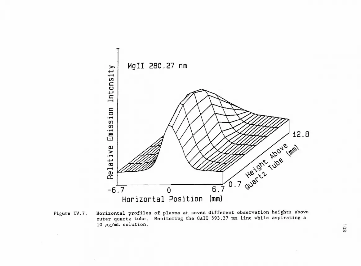
MgII 280.27 nm

C

4.)

a)

C4-)

C0

U)

UJ

a)

4-)oz)

r--ia)

6.7 0

Horizontal Position (mm)

12.8

Figure IV.7. Horizontal profiles of plasma at seven different observation heights above

outer quartz tube. Monitoring the Call 393.37 nm line while aspirating a

10 pg/mL solution.

109

referenced from the top of the outer quartz tube of the plasma

assembly. This particular set of horizontal profiles was obtained

while a solution of 10 pg/mL of Mg was introduced to the plasma.

The ion line at 285.21 nm is being monitored.

E. Conclusions

The software presented here provides a means of obtaining

data of the type that is often very difficult to obtain with the

capabilities of many commercially available systems. In addition,

the software provides the analyst with real-time feedback of data

as it is obtained. This feedback is in the form of plots to a

graphics screen of the computer monitor and is useful in monitoring

the course of an experiment in progress. This real-time feedback

offers an advantage to the common post-experiment type of feedback

in that it allows the analyst to alter the experiment or modify

some parameters to improve subsequent results. The aperture plate

and PMT optimization features of the software allow the analyst to

fine tune the position of the plate and PMT in the focal plane of

the spectrometer. This results in an increase in the amount of

light to the detector thus potentially improving detection limits

and sensitivity.

110

ACKNOWLEDGEMENTS

This work was supported in part by the National Science Foundation,

Grant Number CHE-8206692. The authors also gratefully acknowledge

the support of Leeman Labs, Inc., Lowell, MA. The reception of an

N. L. Tartar Fellowship (J.P.S.) is also gratefully acknowledged.

111

V. A Six-Electrode, Direct Current, Variable Length

Plasma Source for Atomic Emission Spectroscopy

James P. Shields and Edward H. Piepmeier*

Oregon State University

Department of Chemistry

Corvallis, OR 97331

for submission to Applied Spectroscopy

*Author to whom correspondence should be sent.

112

A. Abstract

A variable length plasma source has been developed for

analytical atomic emission spectroscopy. The plasma operates from

three compact, simple, and inexpensive direct current power

supplies. Three concentric quartz tubes supply argon and sample

aerosol to the plasma. The modular design allows the quartz tubing

to be easily replaced and a variety of electrode distances to be

established. The argon consumption, typically 7.4 L/min, is

comparable to or less than commercial DCP and ICP systems. Many of

the vertical spatial characteristics of the plasma described here

are similar to those documented for the ICP. Changes in the

nebulizer gas flow rate produced spatial shifts in the maximum of

the vertical, spatial analyte emission profiles of Mg. Increases

in the signal-to-background ratios at common analytical wavelengths

were observed with increasing plasma length. The movement of the

region of maximum emission to positions below the top of the outer

quartz tube, which occur as a result of increasing the plasma

length, is thought to be the main reason for the worse detection

limits. The addition of 10% nitrogen to the outer argon gas flow

caused a 35% enhancement in the Ca ion and a 28% decrease in the Ca

atom signal-to-background.

Index Headings: Emission spectroscopy; Direct current plasma;

Multi-electrode plasma.

113

B. Introduction

Since the description of the early plasma jets of the

1950s,19 -21 many different and interesting plasma arc and jet

devices have been described for use in atomic emission

3,5,6,30,32-48,51,53-56,244spectrochemical analysis. The large

number of reports describing different configurations reflects, in

part, the flexibility involved with electrode systems. These

multi-electrode systems allow a wide variety of different

positional configurations.

In addition to the many different shapes of plasmas

attainable by appropriate positioning of the electrodes, many

different methods have been used for introducing sample into these

plasmas. In many of the early plasma jet

designs ,20,21,30,43,45,48 sample was introduced into the cathode

or anode chamber from which the plasma jet originated. In this

way, sample was forced through the electrode housing orifice with

the rest of the plasma arc. In many of these devices, emission was

observed in the current carrying portion of the arc. Although a

previous plasma arc had been described with an inverted V

configuration,43 the introduction of the SpectraJet II, with its

introduction of sample to the base of the inverted V arc, brought

about a new type of sample introduction. Emission from this arc

was viewed below the current-carrying portion of the arc.

Subsequent versions of the SpectraJet II, including the most

recent version offered commercially by Applied Research

Laboratories (Sunland, CA), have an have an inverted Y shaped arc.

114

This is achieved by using two lower electrodes (anodes) and one

upper electrode (cathode). Sample introduction in this modern

version is into the base of the inverted Y arc.

Since the late 1970s, research in our laboratory has focused

on using electrodes to advantageously shape the plasma to surround

the sample with hot plasma, as is done with the ICP. Plasmas using

three-phase electrical power have been described by Mattoon and

-Piepmeler7 and subsequently by Masters and Piepmeier. 8 In

these designs, the sample aerosol stream passes up through the

plasma in a manner similar to the ICP.

Meyer9 '1° has recently described an interesting

modification of the commercial Spectraspan IV (Beckman) in which

the stated goal was to entrain the sample in hot plasma. This

modification has involved moving the cathode from its traditional

position above the two anodes, down to the same level as the

anodes. The tips of all three electrodes, now in the same

horizontal plane, then form the vertices of an equilateral

triangle. Under appropriate experimental conditions, sample can be

made to pass up through the plasma where it is completely

surrounded by the plasma.

This paper describes the development and characterization of

a six-electrode, sample-entraining, variable length, direct current

plasma arc. Sample is made to pass up through the plasma in a

manner similar to the ICP and emission is viewed above the

current-carrying portion of the arcs. The effects of several

operating parameters on the spatial emission characteristics of the

source will be presented. In addition, the effect of adding small

115

amounts of nitrogen to the outer plasma gas flow and the analytical

utility of the device will be discussed.

C. Experimental

1. Plasma Torch

A schematic diagram of the plasma torch is shown in

Figure 111.2. The torch consists of two housing pieces. The top

piece, made from aluminum, holds the outer quartz tube by way of an

0-ring seal at the base of the quartz tube. Three adjusting screws

in the top housing piece provide a means of centering the outer

quartz tube. These three adjusting screws are located at angular

positions of 120° from one another.

The lower housing, which is machined from a ceramic called

LAVA (Maryland Lava Co., Inc., Bel Air, MD), holds the inner quartz

tube in place by means of a small ledge. Three more screws, which

are contained in the upper housing, allow the inner quartz tube to

be adjusted so that it is concentric with the outer quartz tube.

Again, the three adjusting screws are located at angular positions

of 120° from one another.

The specifications for the inner, outer, and sample quartz

tubes are given in Table III.1. In addition, the positions of the

quartz tubes and the electrodes relative to the inner quartz tube

are presented in Table 111.2. Each of the housing pieces contains

an inlet for the introduction of argon gas, as shown in

Figure 111.2. The inlet in the upper housing supplies gas to the

116

space between the outer quartz tube and the inner quartz tube. The

inlet in the lower housing supplies gas to the inside of the inner

quartz tube. Both of the gas inlets are machined tangentially to

the inside diameter of the respective quartz tube.

The torch was designed in a modular manner to facilitate the

replacement of parts that have been damaged or that have suffered

excessive wear. In addition, the modular design of the torch

provides a great deal of experimental flexibility, which is

important during the developmental stages of a new plasma source.

Finally, the modular design does not require the construction of a

custom quartz assembly by a skilled glass blower. Inexpensive

stock quartz tubing need only be cut to length before use. This is

particularly advantageous during the testing of the limits of the

plasma source when melting of the quartz tubing is a likely

occurrence.

2. Electrodes

The positions of the six electrodes are shown in

Figure 111.2. All six electrodes are common 2% thoriated tungsten

electrodes (Anchor Brand, NASCO, Birmingham, AL). The tips of both

the inner and outer sets of electrodes form the vertices of an

equilateral triangle. The outer three electrodes, which are 1/16"

in diameter, pass between the inner and outer quartz tubes, through

the lower housing, and down to a baseplate. The inner three

electrodes, which are 3/32" in diameter, pass down through the

inner quartz tube, through the lower housing, through the baseplate

117

for the outer electrodes, and finally down to a baseplate of their

own (not shown).

All of the electrodes are anchored at their lower end by

simple copper blocks with a set screw. These copper blocks are

themselves anchored to baseplates made from LAVA. Since LAVA is an

insulator, the electrodes are kept electrically isolated from one

another. The copper blocks provide a point of attachment to the

direct current power supplies.

3. Electrical System

Each inner/outer electrode pair is independently connected to

a direct current power supply (Electronic Measurements, Inc.,

Neptune, NJ) with maximum ratings of 40 V and 45 A. Each of the

three circuits contains two high power, 1.0 0 (max.) rheostats.

The rheostats are connected in parallel to provide a total

available resistance of 0.5 c. This resistance is in series with

the power supply. Each circuit also contains a DC volt and current

meter. The inner electrodes are anodes and the outer electrodes

are cathodes.

4. Sample Introduction System

A Meinhard concentric glass nebulizer (Model TR-50-C1, J. E.

Meinhard, Inc., Santa Ana, CA) is used to convert bulk liquid

samples to an aerosol for introduction into the plasma. This

nebulizer is identical to the type commonly used for sample

118

introduction to the inductively coupled plasma. The nebulizer is

typically operated at an applied pressure of 50 psi and a gas flow

rate ranging from 0.6 L/min to 1.2 L/min. Liquid is introduced to

the nebulizer using a peristaltic pump (Minipuls 2, Gilson Medical

Electronics, Inc., Middleton, WI). This allows the liquid flow

rate to be kept constant regardless of changes in the nebulizer gas

flow rate.

An in-house constructed spray chamber, very similar to the

one originally introduced by Scott et al., 226 is used to

selectively isolate the smaller aerosol droplets from the larger

ones for introduction into the plasma. The larger droplets, after

impacting on the walls of the spray chamber, are pumped out using

the peristaltic pump. This method ensures that all of the gas used

for nebulization purposes, and registered by the mass flowmeter,

actually passes up to the plasma.

The aerosol which leaves the spray chamber passes up to the

plasma by way of a quartz sample introduction tube. A typical

sample introduction tube is shown in Figure 111.5. The size of the

orifice of the sample tube greatly influences the velocity with

which the sample aerosol exits from the tube. Therefore, the

sample residence time in the plasma can be altered by changing the

sample tube orifice size. Typically, an orifice size of 0.8 mm was

utilized.

119

5. Spectrometer and Data Acquisition System

A PLASMA-SPEC high resolution echelle spectrometer (Leeman

Labs, Lowell, MA) was used to isolate the desired wavelength and

order of light. This system has been described elsewhere. 245

Figure 111.8 summarizes the experimental setup. The spectrometer

is interfaced to an IBM-PC compatible microcomputer (Corona PPC-1,

Cordata, Thousand Oaks, CA) via an RS-232 connection.

All spectrometer control and data acquisition functions were

carried out using software written in the ASYST (MacMillan Software

Co., New York, NY) environment. Details of the software and data

acquisition system have been described in detail. 245,246

Briefly, this menu-driven software controls wavelength and order

selection, initiates all data acquisition functions, and provides

real-time display of acquired data. Three major modes of data

acquisition exist: timed, manual, and spatial acquisition modes.

The timed acquisition mode allows continuous monitoring of

the emission from the plasma at a single wavelength. This mode is

useful for monitoring the short and long term stability of the

emission intensity and for monitoring the sample change-over

characteristics of the system. A plot of the data over time is

displayed to a graphics screen and updated upon each integration.

The manual mode of acquisition, the most flexible of the

three modes, allows the user to move the source mirror of the

spectrometer using the cursor keys on the computer keyboard. This

allows an image of any point in the plasma to be positioned on the

120

entrance slit of the spectrometer. Then, data can be collected at

the desired integration time at this point in the plasma. Another

point in the plasma can then be imaged onto the entrance slit of

the spectrometer using the computer's cursor keys and another

integration performed. Alternatively, a narrow spectral scan can

be performed at any desired point in the plasma. This type of

acquisition can continue indefinitely and is limited only by the

memory capacity of the computer.

Finally, the spatial mode allows the acquisition of

horizontal spatial profiles of the plasma at successively higher

positions in the plasma. Two-point, off-line background correction

or on-line blank correction can be selected. Upon acquisition,

each horizontal profile is plotted to a graphics screen.

6. Gas Handling Equipment

Four separate gas lines are used to supply gas to the

nebulizer, the inner plasma quartz tube, the outer plasma quartz

tube, and any auxiliary need. Each line contains an identical,

adjustable needle valve (Matheson Gas Products, Secaucus, NJ)

except for the nebulizer line which contains a high precision

needle valve (Matheson Gas Products, Secaucus, NJ). In addition,

each line contains a rotameter (Matheson Gas Products, Secaucus,

NJ). These differ only in their range of operation.

The nebulizer and outer quartz tube gas lines both contain

mass flowmeters (Tylan Corp., Carson, CA) which are connected to a

digital read-out unit. The outer quartz tube mass flowmeter

121

(Model FM360) measures flows ranging from 0-10 L/min and the

nebulizer mass flowmeter (Model FM361) measures flows from

0-1 L/min.

Two separate gas tanks are used to provide the argon gas to

the system. One tank is dedicated to supplying gas to the

nebulizer. This helps to minimize the effect on the nebulizer flow

of changing the other gas flows. Each tank has a two-stage

regulator (Airco, Murray Hill, NJ) for pressure control. A

particle filter is placed in line with the nebulizer. This filter

(Model 6183, Matheson Gas Products, Secaucus, NJ) is used primarily

to prevent any particles present in the gas cylinders from clogging

the nebulizer gas orifice. The filter is effective in retaining

particles down to 0.2 Am in diameter.

7. Staging System

The inner and outer baseplates, which serve to anchor the

bases of the electrodes, are independently attached to vertical

translation stages. The nebulizer system is also attached to a

vertical translation stage. By moving the inner or outer electrode

stage, the plasma length can be increased or decreased during

operation of the plasma. In addition, the vertical position of the

sample tube can be adjusted. The nebulizer translation stage is

attached to the translation stage for the inner electrodes.

Therefore, when the plasma length is changed by moving the inner

electrodes, the height of the sample tube is automatically changed

122

so that its position remains constant relative to the inner

electrodes.

8. Solutions

All standard stock solutions were prepared according to the

methods of Dean and Rains247 and Smith and Parsons. 248

Subsequent dilutions included an adjustment of the pH to 2 using

BAKER (J. T. Baker Chemical Co., Phillipsburg, NJ) Analyzed Reagent

HNO3 or HC1, whichever was used to prepare the stock solution.

This pH adjustment was done to avoid any possible bias effects due

to pH, to help preserve the solutions, and to reduce adsorption

effects onto the walls of the storage containers. 249 All

standards were stored in high density polyethylene bottles (Nalge

Co., Rochester, NY).

9. Initiation and Operation of the Plasma

Before actually starting the plasma, the rheostats in each of

the three circuits are adjusted to about 0.4 0. This series

resistance helps provide a quick enough response time for the

electrode potentials to make initiation of the plasma easy. Then,

the three argon gas flows are established: the inner flow up the

inner quartz tube, the outer flow between the inner and outer

quartz tubes, and the nebulizer gas flow. The magnitude of each of

these gas flows is shown in Table V.1 along with typical values for

other operating parameters.

123

Table V.1

Summary of Typical Experimental Conditions

Outer Plasma Gas Flow: 4.5 L/min

Inner Plasma Gas Flow: 2.1 L/min

Nebulizer Gas Flow: 0.8 L/min

Nebulizer Liquid Flow: 1.3 L/min

Power: 20 A at 40 V per electrode pair

Series Resistance: 0.3 0 per electrode pair

Sample Tube Orifice diameter: 0.8 mm (inside diamter)

124

To initiate the plasma, the three power supplies are turned

on in a current-control mode and the inner electrodes are raised

vertically to the height of the outer electrodes. There is a

mechanical means to do this without having to use the micrometer

dial of the translation stage. Then, a graphite

rod is used to briefly short each inner/outer electrode pair.

After a plasma is formed between all three pairs of electrodes, the

inner electrodes are lowered back to their original position. The

plasma can be started with all three of the gas flows at their

normal operating levels. However, the liquid flow to the nebulizer

is not started until the plasma has been established.

After the plasma is started, the resistance of each rheostat

is lowered to about 0.3 0. This decreases the power and voltage

drop across each rheostat and makes more voltage available to each

electrode pair. If the series resistance is made too low, the slow

response and the current-controlled power supply cause the plasma

to be more easily extinguished by small perturbations such as the

introduction of aerosol.

D. Results

1. Plasma Regions

In order to better understand many of the results presented

here, it is important to discuss the structure of the plasma.

Figure V.1 schematically shows the different regions of the

plasma. Many of the structural features of the plasma are similar

Plume ----.

Main Plasma

Initial

RadiationZone(IRZ)

125

QuartzTube

Figure V.1. Schematic diagram of different plasma regions.

126

to those of the ICP. Using the nomenclature of Koirtyohann, 250 a

very distinct bullet or initial radiation zone (IRZ) is observable,

particularly when aspirating solutions of lithium or sodium.

Contrary to the plasma device described by Lee et a1., 251 it

is difficult to visually distinguish the presence of three separate

vertical arcs, even at high sample gas flow rates. Looking down

into the quartz tube, the appearance of the plasma is very

delocalized. This may, in part, be due to the absence of ceramic

sleeves in the present design versus that of the previously

described system.251 The presence of water cooled ceramic

sleeves or other wall cooling devices is known to cause a pinching

and reduction in size of the arc as well as an increase in the

current density of the arc.25' 252-254

An intense background region and a distinctly separate tail

plume extend up approximately 15 mm and 60 mm from the top of the

outer quartz tube, respectively. The exact heights of the

background region and tail plume are dependent on various operating

parameters, particularly plasma length and inner gas flow. As in

the ICP, the height of the IRZ bullet or sample cone is greatly

influenced by sample gas flow and applied power, or in this case,

current. At constant applied current and plasma length, an

increase in the nebulizer gas flow of 0.2 L/min causes the top of

the IRZ to rise by about 4 mm. At nebulizer gas flow rates of

1.1 L/min and higher, the IRZ begins to "trail off" as evidenced by

a thin stream of visible emission above the IRZ. At constant

nebulizer gas flow and plasma length, increasing the applied

current to each pair of electrodes causes the IRZ to move lower.

127

This lowering of the IRZ with increasing current probably results

from a combination of the increased energy available to heat the

sample gas stream and the increase in dc arc radii at higher

currents. This increase in the radii of the arcs with higher

applied current makes it more difficult for the sample stream to

penetrate the plasma in the confined region of the quartz tube.

Finally, increasing the length of the plasma results in a lowering

of the IRZ. When the length of the plasma is increased by lowering

the inner electrodes, the sample tube is automatically lowered

along with the inner electrodes. Therefore, part of the lowering

of the IRZ comes from an actual physical lowering of the sample

tube. However, there is also a longer length of plasma which must

be penetrated by the sample stream.

2. Affect of Plasma Operating Conditions on Spatial Emission

Profiles

An investigation of the affects of varying different

operating parameters on emission intensity has nearly always

accompanied reports on the introduction and development of new

plasma sources. Several researchers145 ,233-236,255-258 have

emphasized the importance of spatially resolved emission

information in the proper interpretation of the factors affecting

analyte emission. In this work, the most important factors

affecting analyte emission in the plasma are nebulizer gas flow,

current, and plasma length. The affects of these parameters on the

vertical emission profiles are presented here. In addition, the

128

affects of other parameters, such as outer and inner gas flow

rates, sample tube height, and nebulizer liquid flow rate are

summarized.

a) Affect of Nebulizer Gas Flow Rate

The vertical emission profiles along the central vertical

axis of the plasma for MgII 280.27 nm and MgI 285.21 nm are shown

in Figure V.2 as a function of nebulizer gas flow rate. For the

ion line, as the nebulizer gas flow rate is increased from 0.6 to

1.2 L/min, the magnitude of the emission intensity decreases. In

addition, the observation height at which the maximum emission is

observed is shifted to positions higher in the plasma as the

nebulizer gas flow rate is increased. For the MgI 285.21-nm line,

a similar trend is observed. As the nebulizer gas flow rate is

increased, the magnitude of the maximum emission decreases and the

observation height at which the maximum occurs is shifted upward in

the plasma.

The nebulizer gas flow rate dependent changes in the vertical

emission profiles which are observed here are strikingly similar to

the effects observed in the ICP. 233-235,258 This downward

spatial shift and decrease in maximum emission intensity at higher

nebulizer gas flow rates reflects the shorter time period that the

sample spends in the plasma. At the higher sample gas flow rates,

less time is available for complete vaporization, atomization, and

excitation of the sample.

The vertical emission profile of the Mg ion-to-atom ratio at

500

400-

300-

200-

100-

0o

400-

300

200

100

129

MgII 280.27 nm

QA

1 2

a

3 4 5 6 7 8 9

00 1 2 3 4 5 6 7 8 6

Height Above Quartz Tube (mm)

MgI 285.21 nm

k>":6-(13

Figure V.2. Vertical spatial profiles of the MgII 280.27-nm andMgI 285.21-nm emission as a function of nebulizer gasflow rate. (0) 0.6 L/min; (S) 0.8 L/min;(a) 1.0 L/min; (A) 1.2 L/min.

130

three different nebulizer gas flow rates is shown in Figure V.3.

While this ratio is not corrected for spectrometer response, the

proximity of the wavelengths involved (280.27 nm vs. 285.21 nm)

should make any differences in spectrometer response negligible in

this case. At low observation heights, the ion-to-atom ratio drops

by over an order of magnitude when the nebulizer gas flow rate is

increased from 0.6 to 1.0 L/min. This indicates that the degree of

ionization is greatly influenced by relatively small changes in the

nebulizer gas flow rate.

Measurements of the widths of the horizontal profiles at half

maximum height indicates a decrease in profile width as the

nebulizer gas flow rate is increased. At an observation height of

3.4 mm, a change in nebulizer gas flow rate from 0.6 to 1.0 L/min

causes the profile width to decrease by about 12% for the Mg ion

line and 23% for the Mg atom line. This decrease in profile width

at higher nebulizer gas flow rates indicates that the analyte atoms

may have less time to be generated and diffuse laterally in the

plasma.

b) Affect of Current

When the current is increased, definite visual changes are

observed in the plasma. The most obvious visual change is the

suppression of the IRZ to lower parts of the plasma. Increasing

the current from 16 A to 19 A causes the tip of the IRZ bullet or

sample cone to be lowered by about 3 mm. A subsequent increase in

the current to 22 A causes an additional 3 mm lowering of the tip

.942.0

ci

r4 1.5

1.0C)

0.5

0.00 1 2 3 4 5 6 7 8

Height Above Quartz Tube (mm)

Figure V.3. Vertical spatial profiles of the Mg ion-to-atom ratio(MgII 280.27 nm; MgI 285.21 nm) as a function of nebulizer gas

flow rate. (0) 0.6 L/min; () 0.8 L/min; (A) 1.0 L/min.

132

of the sample cone.

The vertical emission profiles in the center of the plasma

for MgII 280.27 nm and MgI 285.21 nm are shown in Figure V.4 for

four different currents. Both the atom and the ion line exhibit

overall increases in emission intensity as the current is

increased. For the ion line, the height at which the maximum

emission occurs is shifted slightly to lower positions in the

plasma as the current is increased. No analogous spatial shift is

seen for the atom line. The ion-to-atom ratios for the four

different currents, shown in Figure V.5, show increases in the

ion-to-atom ratio at all observation heights with increasing

current. The largest increases in the ion-to-atom ratio are

observed at low observation heights. At an observation height of

2.8 mm, the MgII emission increases by a factor of 23 for a current

increase from 16 to 25 A (see Figure V.4) while the MgII

signal-to-background increases by a factor of 10. This suggests

that, as the current is increased, the magnitude of the plasma

background at this wavelength increases more rapidly than the MgII

emission.

Figure V.6 shows the horizontal profiles for the

MgII 280.27-nm and MgI 285.21-nm lines at four different currents.

The observation height is 8.7 mm above the outer quartz tube.

Measurements of the width of the profiles at half maximum height

reveal that there is no significant change (<3%) in the width of

the profiles for currents ranging from 16 to 25 A. Similar

measurements at an observation height of 0.7 mm also reveal that

there are only small changes (<4%) in profile widths with current

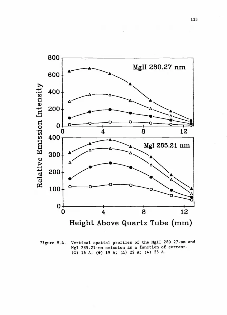
800

133

600-

400-

o 0

(/) 400

rx1

co300

-Icd 200

100

0

MgII 280.27 nm

O O rAo o

4 8 12

A A--, MgI 285.21 nm

O

4 8 12

Height Above Quartz Tube (mm)

Figure V.4. Vertical spatial profiles of the MgII 280.27-nm andMgI 285.21-nm emission as a function of current.(0) 16 A; () 19 A; (A) 22 A; (A) 25 A.

2.5

0

2 4 6 8 10 12

Height Above Quartz Tube (mm)

Figure V.5. Vertical spatial profiles of the Mg ion-to-atom ratio

(MgII 280.27 nm; MgI 285.21 nm) as a function of current.

(0) 16 A; (I) 19 A; (A) 22 A; (A) 25 A.

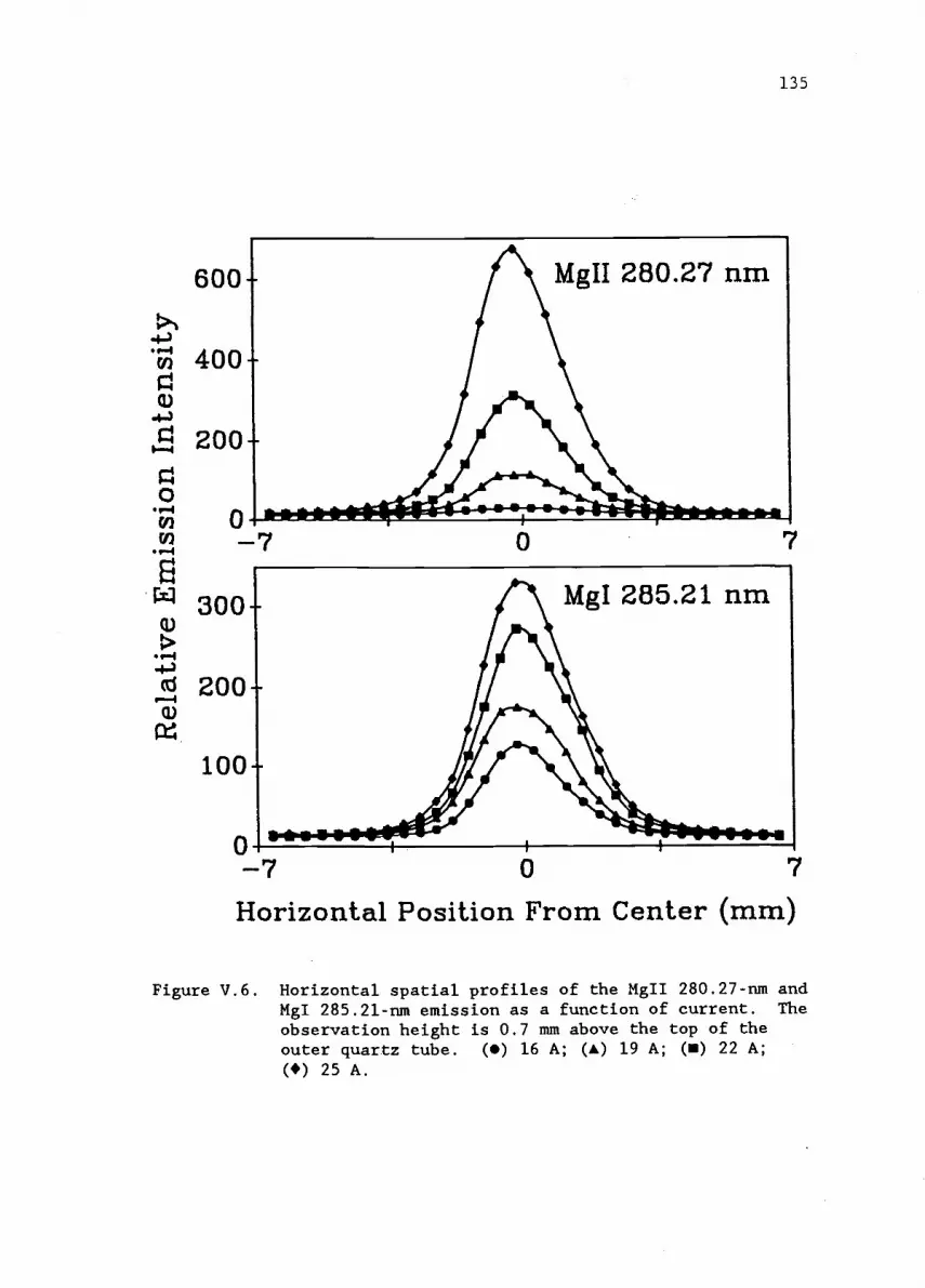
600

4.)inri 400a)

0

00in 0

7"1 300a)

rI4)d 200a)

135

7

07 0 7

Horizontal Position From Center (mm)

0 7

Figure V.6. Horizontal spatial profiles of the MgII 280.27-nm andMgI 285.21-nm emission as a function of current. Theobservation height is 0.7 mm above the top of theouter quartz tube. () 16 A; (A) 19 A; (u) 22 A;

() 25 A.

136

lower in the plasma. At constant current, the ion line profile

width increases by about 20% as the observation height increases

from 0.7 to 8.7 mm above the outer quartz tube. The same width

increases are seen for the atom line at constant current and

increasing observation height. At higher positions in the plasma,

the sample has had more time to diffuse laterally. In addition,

the sample is past the region in the plasma where the greatest

confinement of the sample stream exists, that is, low in the plasma

in the direct vicinity of the three arcs.

c) Affect of Plasma Length

Changing the length of the plasma is accomplished by moving

the inner electrodes up or down. For all changes in the plasma

length the current was kept constant while allowing the voltage to

fluctuate as required by the dc arcs. The plasma length is defined

as the vertical distance between the inner and outer electrode

sets. The overall plasma length, including tail-flame, is much

longer (see Figure V.1). Changing the plasma length produces

definite visual changes in the plasma as well as marked changes in

the vertical emission profiles. Visually, the overall plasma

background emission becomes much more intense as the length of the

plasma is increased. Changes in the vertical emission profiles at

four different plasma lengths are exemplified by the profiles for

MgII 280.27 nm and MgI 285.21 nm shown in Figure V.7.

As the plasma length is increased, the general trend is for

the ion line emission intensity to increase while the atom line

1000800 A

600400

200

137

MgII

280.27

nm

0 t i 10 2 4 6 8 10 12

7060

5040-

3020

100

0

MgI

285.21

nmewe

2 4 6 8 10 12

Height

Above

Quartz

Tube

(mm

)

Figure

V.7.

Vertical

spatial

profiles

of

the

MgII

280.27-nm

and

MgI

285.21-nm

emission

as

a function

of

plasma

length.

(0)

14 mm;

(0)

16.5

mm;

(A)

19.1

mm;

(A)

21.6

mm.

138

emission intensity decreases. For the ion line profiles shown in

Figure V.7, only the 14-mm plasma length explicitly shows a maximum

in the vertical profile. For the longer plasma lengths, the

maximum in the vertical profile occurs below the top of the outer

quartz tube. However, the presence of a downward spatial shift in

the maximum of the vertical profile as the plasma length is

increased is still apparent. At all four plasma lengths, the

vertical profiles converge at an observation height of about

12 mm. This convergence is also observed for the atom line,

although it occurs at about 10 mm.

Under only slightly different experimental conditions (e.g.,

different nebulizer gas flow rate), the vertical profiles for the

atom line can be made to increase in overall magnitude as the

plasma length is increased to moderate lengths and then decrease in

overall magnitude as the plasma length is increased further.

Therefore, the interpretation of trends must be undertaken with the

understanding that they may apply only to a particular set of

experimental conditions.

The upper half of Figure V.8 shows a set of four

MgII 280.27-nm horizontal profiles at an observation height of

0.7 mm above the outer quartz tube. Each profile corresponds to a

different plasma length. In the lower half of Figure V.8 the same

four profiles are shown except that all of the profiles are

normalized to the profile for the longest plasma length of

21.6 mm. The normalized plot is presented to show that the width

of the profiles decreases as the plasma length is decreased. A

possible explanation for this decrease in width at shorter plasma

139

-7 0

Horizontal Position From Center (rn7

Figure V.8. Horizontal spatial profiles of the MgII 280.27-nm

emission as a function of plasma length. The

observation height is 0.7 mm above the top of theouter quartz tube. The profiles in the bottom graph

are all normalized to the 21.6 mm plasma length.

(I) 14 mm; (A) 16.5 mm; (m) 19.1 mm; () 21.6 mm.

140

lengths is that as the plasma length is decreased, the sample

spends less time in the plasma. This may allow less time for

lateral diffusion of analyte atoms.

The fact that the maximum in the vertical profile for

MgII 280.27 nm occurs below the top of the outer quartz tube for

the longer plasma lengths is a potentially important feature.

Since the signal-to-background vertical profiles also show the same

general trends as those illustrated in Figure V.7, it may be that

the observation height with the best signal-to-background is

inaccessible to the analyst under the present experimental

conditions. More will be said about this later.

3. Affect of Adding Nitrogen to Outer Gas Flow

A preliminary look at the influence of the addition of

nitrogen to the outer flow was undertaken. Upon the addition of

10% nitrogen to the outer argon gas flow, the overall plasma size

decreased. This is in agreement with the general observations for

the ICP upon the addition of nitrogen. 259-264The plasma arcs

near the tips of the outer electrodes were pushed up higher above

the outer electrodes before continuing on to their normal path down

towards the inner electrodes. This upward movement of the plasma

arcs in the region near the outer electrodes could not be produced

in a pure argon environment, even by drastic increases in the outer

argon flow (with no nitrogen).

The affect of adding 10% nitrogen to the outer flow on the

vertical signal-to-background emission profile is shown in

141

Figure V.9 for Call 393.37 nm and CaI 422.67 nm. An overall

enhancement is observed for the ion line while an overall

depression is seen for the atom line. The nitrogen-induced ion

line enhancement could be explained by an increase in contact

between the hot plasma and the sample channel due to the inward

contraction of the plasma in the presence of nitrogen. At all

observation heights investigated, the width of the horizontal

profiles are the same with and without the presence of nitrogen. A

decrease in the width of the horizontal profile might be expected

if a nitrogen-induced constriction of the sample channel actually

caused a reduction in the physical width of the sample channel.

However, better contact between the plasma and the sample channel,

possibly brought about by the constriction of the plasma around the

sample channel, may improve heat transfer to the sample channel

resulting in faster lateral diffusion of analyte atoms. This would

have the opposing effect of widening the horizontal profile.

4. Analytical Utility

Table V.2 presents the detection limit, log/log slope of the

calibration line, and relative standard deviation of the background

for five elements. The detection limits range from a factor of 15

to 180 worse than those listed for the ICP. The log/log slopes

shown in Table V.2 indicate that a linear relation exists between

concentration and emission intensity from the detection limit up to

1000 Ag/mL. The uncertainty in the log/log slopes were calculated

at the 95% confidence level. The relative standard deviation of

200

.2cad loo

C4

rd

O0

0c) 5

1 4-O

E-1

3 -CC!

0 2-00

1-

142

3 6 9

o0

CaI 422.67 nin0 3 6

Height Above Quartz Tube (mm)

Figure V.9. Vertical spatial profiles of the CaII 393.37-nm andCal 422.67-nm signal-to-background ratio. (0) no N2added; () 10% N2 added to outer gas flow.

143

Table V.2

Summary of Analytical Figures of Merit

ElementWavelength

(nm)

Detection Limit (pg&L)This Worka ICP'

log/logeSlope

Background%RSD

Can 393.37 0.003 0.0002 0.96 ± 0.03 0.6

CrII 283.56 0.3 0.007 0.96 ± 0.04 1

CuI 324.75 0.2 0.005 1.08 ± 0.07 0.7

MnII 259.37 0.1 0.002 0.6

MnII 257.61 0.3 0.001 1.01 ± 0.05 0.5

ZrII 339.20 0.2 0.008 0.99 ± 0.02 1

a Detection limit defined as concentration required to give signalequal to three times the standard deviation of the background.

b From Ref. 265.c

Slope uncertainties determined at 95% confidence level.d Determined from 32 measurements.

Table V.3

Comparison of signal/background ratios for this work and the ICP

WavelengthElement (nm) S/B

This WorkConc. (pg/ml) S/B

ICPaConc. (µg /ml)

(DL Ratio) X(S/B Ratio)

CaII 393.37 3.02 0.5 89.0 0.5 0.5

CrII 283.56 1.17 10.0 42.0 10.0 1.2

CuI 324.75 1.04 10.0 56.0 10.0 0.7

MnII 259.37 0.84 10.0 190.0 10.0 0.2

MnII 257.61 0.62 10.0 220.0 10.0 0.9

ZrII 339.20 1.34 10.0 39.0 10.0 0.9

a From Ref. 265.

145

the background signal was determined using 32 consecutive one-

second integrations.

The excellent relative standard deviations in the background

indicate a high degree of stability in the background signal.

Therefore, it would not be expected that noise in the background

would be the cause of the difference in detection limits. A

comparison of the signal-to-background ratios for this plasma to

those of the ICP, shown in Table V.3 suggests a possible

explanation for the worse detection limits. The last column in

Table V.3 was obtained by multiplying the ratio of the detection

limits for this work and the ICP, by the ratio of the

signal-to-background ratios for this work and the ICP. These

proximity of these values to one another, which are all within a

factor of 5, indicate a possible correlation of the detection

limits with the signal-to-background ratio.

It is apparent from the plasma length studies presented

earlier that the signal-to-background ratio can be improved by

increasing the plasma length. In addition, it was shown that the

maximum in the vertical emission profiles was below the top of the

outer quartz tube for the longer plasma lengths. Therefore, there

appear to be two opposing factors involved: longer plasma lengths

increase the signal-to-background ratio but also move the point of

maximum emission out of the region of observation, that is, below

the top of the outer quartz tube.

146

E. Conclusions

The variable length plasma source described here is operated

from compact, simple, and inexpensive direct current power

supplies. The argon consumption of the system is typically

7.4 L/min, which is comparable to or less than the consumption

rates of commercial DCP and ICP systems. The inner electrodes do

not require regrinding from day to day. The outer electrodes do

require daily regrinding but the same electrodes can be used

indefinitely. No ceramic sleeves are used and water cooling is not

required.

Many of the vertical spatial characteristics of the plasma

described here are similar to those observed in the ICP. These

spatial features include the well documented spatial shifts which

occur with changes in nebulizer flow rate and input power. The

signal-to-background ratio at common analytical wavelengths can be

increased by increasing the length of the plasma. The

signal-to-background continues to increase up to the maximum length

attainable at present (limited to about 28 mm by the maximum

voltage of the power supplies). The movement of the region of

maximum emission to positions below the top of the outer quartz

tube, which occur with the lengthening of the plasma, is thought to

be the main reason for the poorer detection limits. An improvement

in the method of sample introduction at the long plasma lengths may

help to bring the region of maximum emission up to an observation

height accessible to the analyst.

147

Acknowledgements

The authors gratefully acknowledge the support of Leeman

Labs, Inc., and the National Science Foundation (Grant

#CHE-8206692).

148

VI. A Spatial Study of the Influence of Plasma Length

on Interference Effects in a Six-Electrode,

Direct Current, Variable Length Plasma

James P. Shields and Edward H. Piepmeier*

Department of Chemistry

Oregon State University

Corvallis, OR 97331

for submission to Applied Spectroscopy

Author to whom correspondence should be sent.

149

A. Abstract

Vertical spatial profiles of a six-electrode, direct current

plasma emission source were used to study the influence of plasma

length on the interference, of Na on Ca and Zn and P on Ca. For the

shortest plasma (11.5 mm), depression of the Ca atom line is

observed in the region up to 10 mm above the tip of the sample

bullet when Na is present. A cross-over to enhancement occurs for

higher regions. This is directly opposite to the observations in

the ICP for the Na interference on Ca. Increasing the plasma

length causes downward shifts in the cross-over point which are not

a simple effect of the lowering of the sample bullet. When P is

present, the Ca atom emission is initially depressed in the region

directly above the sample bullet. At higher observation heights,

little effect is observed. Similar behavior is observed for the Ca

ion line in the presence of P suggesting the possibility of a

classical vaporization type interference mechanism. The

interference effects studied here can be minimized by carefully

selecting plasma length and observation height.

150

B. Introduction

Previously, 245,266a new six-electrode, direct current

plasma was described for use in atomic emission spectroscopy. A

unique feature of this plasma device is the ability to change the

plasma length during operation of the plasma. This paper presents

a preliminary report of the way in which the length of the plasma

affects the P interference on Ca emission, and the interference of

Na on Ca and Zn emission. The primary goal in the design of these

experiments was to evaluate the feasibility of using plasma length

as a way to reduce interference effects.

Comparisons between the plasma source for this work and the

ICP are natural. Both of these plasmas entrain the sample stream

in their centers. In addition, the overall plasma shapes are

similar. In these ways, the plasma source for this work more

closely resembles the ICP than the commercial DCP. However, it is

important to view any interpretations made from the comparisons

with caution because of the different ways in which the plasmas are

produced: one with the inductive coupling of radio frequency energy

and the other by a dc potential difference between electrodes. Due

to this significant difference in the way the plasmas are produced,

it might be expected that some of the analyte spatial emission

patterns would be different between the two sources. For this

reason, comparisons between the ICP and this plasma source will be

made with respect to the tip of the sample bullet or initial

radiation zone (IRZ). In a previous report, 266 we adopted the

nomenclature suggested by Koirtyohann et al. 250 to describe

151

the different plasma regions. This report will continue to emply

this nomenclature.

For the inductively coupled plasma (ICP), the magnitude of

interference effects on analyte emission have been shown to be

dependent on experimental parameters such as nebulizer gas flow

rate and applied power. 232,237,267-270 In addition, the

magnitude and direction (enhancement or suppression) of

interference effects in the ICP have been found to exhibit a high

degree of spatial dependence. 232,234,237-239,267-271 Thus,

depending on the observation height, the size of the observation

window, and other experimental conditions, the effect of an

interferant on analyte emission can result in enhancement,

suppression, or no change. Due to the spatial dependence of many

interference effects, many investigators have stressed the need for

obtaining spatial information about analyte emission in the

plasma. 157,232-235 n addition, the importance of correlating

the observation regions under consideration with the position of

the initial radiation zone (IRZ) or sample "bullet" has been

stressed. 250

One conclusion which can be drawn from previous studies of

both vaporization and easily ionizable element (EIE) interference

effects in the ICP is that the magnitude of the effect is in some

way related to the time the analyte spends in the plasma. This is

evident from studies showing decreases in the EIE interference at

lower nebulizer gas flow rates. 232,236,267-270 In addition,

Savage and Hieftje236 have shown that for their mini-ICP, the

atomic Ca vertical emission profile is shifted upward when either

152

Al or P are present as matrix elements. Furthermore, they found

that this spatial shift is minimized at low nebulizer gas flow

rates as well as high applied powers. They suggested the

possibility that longer sample residence times may be required to

allow efficient and complete atomization of the analyte/matrix

particles.

Although decreasing the nebulizer gas flow rate will in

general increase the residence time of the sample in the plasma,

another possible way to increase the time that the sample spends in

the plasma is to increase the length of the plasma. Our previous

work, 266showing that improvements in signal-to-background ratios

could be realized by increasing the plasma length, led to this

investigation of the effect of plasma length on the magnitude and

direction of interference effects.

C. Experimental

All of the interference studies reported here were performed

using a six-electrode, direct current, variable length plasma

emission source. A schematic representation of the upper part of

the plasma source is shown in Figure VI.l. A more in-depth

description of the source has been given elsewhere. 266 The

length of the source, as defined by the vertical distance between

the upper and lower electrode sets, is varied by moving the inner

three electrodes up and down. The range of this movement is from

0 mm, used for igniting the arcs, to a maximum of 28 mm. This

maximum length is imposed by the voltage limitations (40 V max.) of

Plume

Main PlasmaInitial

RadiationZone ( 1RZ )

153

1 3 n

0nnQuart zTube

Figure VI.1. Schematic representation of upper part of plasmasource. The position of the 13-mm observation windowis illustrated.

154

the power supplies currently in use.

While 28 mm is the maximum vertical length between the

electrode sets, the overall plasma length, including tail-plume, is

much longer. The observation of emission for this work begins just

above the outer quartz tube (5.5 mm above the outer electrodes) and

extends up to a maximum of 13 mm above the outer quartz tube, as

shown in Figure VI.1. All observations were made along the central

vertical axis of the plasma.

A PLASMA-SPEC (Leeman Labs, Inc., Lowell, MA) echelle

spectrometer was used for wavelength isolation. An IBM-PC

compatible Corona (Cordata, Thousand Oaks, CA) microcomputer was

interfaced to the spectrometer via an RS-232 line. The

microcomputer, running software written in the ASYST (MacMillan

Software Co., New York NY) environment, controlled all data

acquisition functions. Details of the spectrometer and data

acquisition system have been described elsewhere. 245,246,266

Table VI.1 provides a summary of the experimental conditions used

in this work.

Stock solutions were prepared according to the procedures

recommended by Dean and Rains. 247 For the P experiments, the Ca

concentration was 30 Ag/mL. P was added as H3PO4 to obtain a

Ca:P mole ratio of 1:100. For the Na experiments, the Ca

concentration was 60 pg /mL and the Zn concentration 98 pg /mL. Na,

in the form of NaCl, was added gravimetrically to obtain a final

Ca:Na or Zn:Na mole ratio of 1:300. For both the P and Na

experiments, blank solutions containing only the interferant were

prepared for the purpose of background subtraction.

155

Table VI.1

Summary of Experimental Conditions

Outer Plasma Gas Flow: 4.7 L/min

Inner Plasma Gas Flow: 2.1 L/min

Nebulizer Gas Flow: 0.8 L/min

Nebulizer Liquid Flow: 1.1 L/min

Power: 20 A at 40 V per electrode pair

Series Resistance: 0.3 0 per electrode pair

Sample Tube Orifice diameter: 0.8 mm (inside diamter)

156

D. Results and Discussion

1. Effect of Plasma Length on the Interference of Na on Ca and

Zn Emission.

Vertical profiles of the CaI 422.67-nm emission along the

central vertical axis of the plasma with and without the presence

of Na are shown in Figure VI.2 for three different plasma lengths.

Plots A, B, and C correspond to plasma lengths of 11.5, 18, and

24.5 mm, respectively. The Y-axis scales are identical for the

three different plots. For the 11.5 and the 18-mm plasma lengths,

the general trend is for the atom line emission to be depressed low

in the plasma and enhanced higher in the plasma when the Na is

present. For the longest plasma length, 24.5 mm, little effect is

seen at an observation height of 1 mm. At heights above 1 mm, an

overall enhancement effect with the presence of Na is observed.

A number of important trends are observed in the

Cal. 422.67-nm profiles. First, the cross-over point, that is, the

observation height at which the Na-induced depression changes to

enhancement, is seen to move to lower observation heights as the

plasma length is increased. This does not appear to be just a

simple effect caused by the lengthening of the plasma. For the

11.5-mm length plasma, the cross-over point is at an observation

height of about 8 mm above the outer quartz tube, or approximately

10 mm above the tip of the sample bullet. For the 18-mm plasma

length, the cross-over point is at an observation height of about

6 mm, or 15 mm above the sample bullet tip. Thus, a 2-mm downward

CaI 422.67 nm

4 6 8 10 12

13

4-3 0 2 4 6 8 10 12a)

C

I 1 I -I-- +-2 4 6 8 10 12

Height Above Quartz Tube (mm)

157

Figure VI.2. Vertical spatial profiles of the Cal 422.67 nmemission at three different plasma lengths(A, 11.5 mm; B, 18.0 mm; C, 24.5 mm). The Ca:Namolar ratio is: (0) 1:0, (*) 1:300. The Y-axisscales are identical for A, B, and C. The tip of theIRZ is 2, 8.5, and 15 mm below the quartz tube for A,B, and C, respectively.

158

shift in the cross-over point occurs as a result of a 6.5 mm

increase in the plasma length. For the 24.5-mm plasma length, the

cross-over point, if it exists, is below the top of the outer

quartz tube. Another important observation is that by careful

selection of plasma length and observation height, the interference

can be minimized.

Vertical profiles of the Can 393.37-nm emission along the

central vertical axis of the plasma with and without the presence

of Na are shown in Figure VI.3 for three different plasma lengths.

Plots A, B, and C correspond to plasma lengths of 11.5, 16.5, and

21.5 mm, respectively. The Y-axis scales are identical for the

three different plots. The Ca:Na mole ratio is 1:300. For the

11.5-mm plasma length, essentially no interference is observed low

in the plasma. However, at higher positions in the plasma, the ion

line emission is depressed when Na is present. For the two longer

plasma lengths, an ion line depression is observed at all

observation heights investigated although for the longest plasma

length, the amount of depression decreases at higher observation

heights. The cross-over behavior observed for the Ca atom line is

not observed for the ion line.

Vertical profiles of the ZnI 213.86-nm emission along the

central vertical axis of the plasma with and without the presence

of Na are shown in Figure VI.4 for three different plasma lengths.

Plots A, B, and C correspond to plasma lengths of 11.5, 16.5, and

21.5 mm, respectively. The Y-axis scales are identical for the

three different plots. Contrary to what was observed for the Na

effect on Ca atomic emission, no cross-over points are observed

4.)..-4rn

0

00Inrn1-1

a)

r-44...)

(1)

c:4

Call 393.37 nm

A

2 6 8 10

B

2 4 6 8 10

C

0 2 4 6 8 10

Height Above Quartz Tube (mm)

159

Figure VI.3. Vertical spatial profiles of the Call 393.37 nmemission at three different plasma lengths(A, 11.5 mm; B, 16.5 mm; C, 21.5 mm). The Ca:Namolar ratio is: (0) 1:0, () 1:300. The Y-axisscales are identical for A, B, and C. The tip of theIRZ is 2, 7, and 12 mm below the quartz tube for A,B, and C, respectively.

ZnI 213.86 nm

A

0 2 4 6 8 1.0

B

0 2 4 6 10

/IP

4

C

0 2 4 6 8 10

Height Above Quartz Tube (mm)

160

Figure VI.4. Vertical spatial profiles of the ZnI 213.86 nmemission at three different plasma lengths(A, 11.5 mm; B, 16.5 mm; C, 21.5 mm). The Ca:Namolar ratio is: (0) 1:0, () 1:300. The Y-axisscales are identical for A, B, and C. The tip of theIRZ is 2, 7, and 12 mm below the quartz tube for A,B, and C, respectively.

161

here for the observation region studied (up to about 9 mm above the

quartz tube). Instead, the Zn atomic emission in the presence of

Na is depressed throughout the observation region investigated. At

the longest plasma length of 21.5 mm, the depression has nearly

disappeared at the higher observation heights.

Although the development of a comprehensive mechanism for the

interference effects described above requires more information than

presented here, it is still of interest to attempt to rationalize

some of the observed effects. It is logical to first consider

possible influences caused by changes in the performance of the

nebulizer. Since a peristaltic pump was used in this work to feed

analyte solution to the nebulizer at a constant rate, it is

unlikely that any increases in the solution viscosity caused by the

high salt concentration would effect the solution feed rate. Also,

since the nebulization equipment used in this work is similar to

conventional ICP nebulization equipment, it is likely that other

nebulizer effects, such as the aerosol ionic redistribution

effect,272 will be similar to those found by others,--157 '

237

that is, small when compared to other plasma-dependent causes.

The classical ionization shift mechanism is well known in

flames,273 and involves an increase in the atom population due to

a shift of the atom/ion equilibrium towards the neutral atom

species. This shift is a mass balance adjustment caused by an

increase in the electron density brought about by the ionization of

an easily ionizable element. For this work, if the classical

ionization shift mechanism is operative in a dominant way, it would

be exhibited in the vertical spatial profile by an enhancement of

162

the atom emission and a suppression of the ion emission in the

presence of the EIE relative to the profile with no EIE present.

Looking at the 11.5 mm plasma length results in Figures VI.2A

and VI.3A (noting the slightly different X axis scales), we see

that from 2 to 8 mm, both the Ca atom and ion emission in the

presence of Na are depressed relative to the profile with no Na.

The absence of a simultaneous atom enhancement and ion depression

is not supportive of an ionization mechanism, at least not in this

observation region (about 2 to 10 mm above the tip of the IRZ).

The depression of the Zn atom emission (Figure VI.4A) over the

entire region from 2 to 10 mm above the IRZ also does not support

the presence of the ionization suppression mechanism in this region

of the plasma.

The Ca atom emission does exhibit enhancement at observation

heights above 8 mm. In addition, the ion line is depressed at an

observation height of 8 mm and a reasonable extrapolation of the

profiles to slightly higher observation heights would give

continued depression of the ion emission. Thus for the region well

above the IRZ (10 mm and above), an ionization mechanism appears

more likely to play some role. In addition, for the longer plasma

lengths (Figures VI.2C and VI.3C), a simultaneous atom line

enhancement and ion line depression is present at all of the

heights observed. Since the IRZ for the longer plasma lengths is

now well below the top of the quartz tube, the spatial profiles for

the longer plasma lengths essentially correspond to "high"

observation heights in the context of the shorter, 11.5-mm plasma

length. So again, an ionization mechanism may play some role in

163

regions well above the IRZ. Although these observations are not

conclusive evidence for the presence of an ionization suppression

mechanism, they also do not rule out the possibility of its

existence in regions well above the IRZ.

The 11.5-mm plasma length is probably best suited for

comparison with the ICP because the length of the overall plasma

and the location of the sample bullet relative to the observation

zone most closely resemble the conditions found in the ICP. With

this in mind, the results for the 11.5-mm plasma, Ca/Na system

described above compared with those for the ICP reveal an

interesting difference in the behavior of the Ca atom emission.

For the ICP, Koirtyohann et al. 268 found that the effect of

adding 1000 Ag/mL Li to a 20-Ag/mL Ca solution was to enhance

Cal 422.67-nm emission at lower observation heights in the vicinity

of the IRZ. Higher in the plasma, slightly above the IRZ, they

observed virtually no effect. Qualitatively similar results were

reported by these researchers when Na was the interfering element.

Similar results for the effect of Na on atomic Ca emission

have been obtained by Blades and Horlick. 237 The position of the

IRZ in their work, although not explicitly stated, is presumably

somewhat lower than that of Koirtyohann et al. due to the lower

nebulizer gas flow rate used. Blades and Horlick also observed

enhancement of the Ca atom emission due to Na low in the plasma

near the IRZ. Higher in the plasma, a cross-over to matrix induced

depression was observed.

These observations for the ICP are directly opposite to the

trend observed here for the 11.5-mm plasma. For the 11.5-mm plasma

164

in this work, the Cal 422.67-nm emission in the presence of Na (see

Figure VI.2A) is initially depressed low in the plasma (3 to 10 mm

above the tip of the IRZ) and then crosses over to an enhancement

higher in the plasma (10 to 15 mm above the tip of the IRZ). The

position of the IRZ tip for the Koirtyohann work was 12 mm above

the top of the load coil. Thus, with respect to the tip of the

gz, the region in their work from 14 to 24 mm above the top of the

load coil would coincide with observation heights from 0 to 10 mm

above the outer quartz tube in this work for the 11.5 mm plasma

length. So in the region from 3 to 10 mm above the tip of the IRZ,

Koirtyohann observed only enhancement in the presence of the EIE,

while for this work, depression is observed.

For the Ca ion line, the trend observed in the ICP237 ,268

is for the emission in the presence of Na to be enhanced in the

vicinity of the IRZ. A cross-over point is generally observed a

few mm above the IRZ and suppression occurs at the higher

observation heights. For the 11.5-mm plasma length in this work,

little effect is seen at 3 mm above the IRZ between the

CaII 393.37-nm emission with and without the presence of Na. At

higher observation heights, a depression in the CaII 393.37-nm

emission is seen due to the Na. So the behavior of the Ca ion

emission with and without the presence of Na in this work is

qualitatively similar to that observed in the ICP.

The fact that directly opposite trends are observed for the

Na effect on Ca atom emission in this work versus that for the ICP

suggests that different interference mechanisms are operative in

the two plasmas. While the classic ionization suppression

165

mechanism may be in operation at regions well above the IRZ,

additional measurements, specifically designed for mechanistic

investigations, are needed to clarify the situation. Certainly,

discussions of other possible interference mechanisms, such as

ambipolar diffusion, changes in argon metastable populations,

changes in the degree of collisional excitation, and the

possibility of low atomization efficiencies, require additional

information.

2. Effect of Plasma Length on the Interference of P on Ca

Emission.

Vertical profiles of the CaI 422.67-nm emission along the

central vertical axis of the plasma with and without the presence

of P are shown in Figure VI.5 for three different plasma lengths.

Plots A, B, and C correspond to plasma lengths of 12.5, 19, and

25.5 mm, respectively. The Y-axis scales are identical for the

three different plots.

For the 12.5-mm plasma length, an overall depression in

emission is observed along the entire region investigated when P is

present. Increasing the plasma length to 19 mm brings about a

significant change in the relationship between the profiles. An

initial depression is observed at low observation heights in the

presence of P, just as with the 12.5-mm plasma length. However, a

cross-over point occurs at an observation height of about 8 mm.

Above the 8-mm observation height, little difference is observed in

the CaI 422.67-nm emission in the presence of P. In the highest

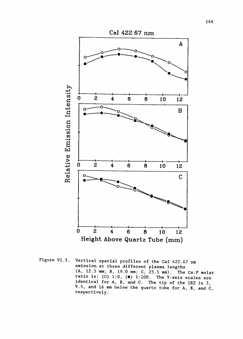
CaI 422.67 rim

0 0

A

\,moo

0 2 4 6 10 1200

0 2 4 6 8 10 12

0 2 4 6 8 10 12Height Above Quartz Tube (mm)

166

Figure VI.5. Vertical spatial profiles of the Cal 422.67 nmemission at three different plasma lengths(A, 12.5 mm; B, 19.0 mm; C, 25.5 mm). The Ca:P molarratio is: (0) 1:0, () 1:100. The Y-axis scales areidentical for A, B, and C. The tip of the IRZ is 3,9.5, and 16 mm below the quartz tube for A, B, and C,respectively.

167

region investigated, there appears to be little difference in the

emission with and without P. Finally, for the 25.5-mm plasma

length, an initial depression is observed at a low observation

height in the presence of P, a cross-over point is observed at an

observation height of about 2.5 mm, and an enhancement in the

presence of P is observed up to about 7 mm. Above 7 mm, little

difference exists between the Cal 422.67-nm emission with and

without P.

The cross-over point, that is, the observation height at

which the matrix-induced depression changes to enhancement (or vice

versa), moves to lower observation heights as the plasma length is

increased. This same plasma length dependent movement of the

cross-over point was observed in the Ca/Na system.

Vertical profiles of the Can 393.37-nm emission along the

central vertical axis of the plasma with and without the presence

of P are shown in Figure VI.6 for three different plasma lengths.

Plots A, B, and C correspond to plasma lengths of 11.5, 18, and

24.5 mm, respectively. The Y-axis scales are identical for the

three different plots. The vertical emission profiles for

Call 393.37 nm exhibit patterns very similar to those observed for

the CaI 422.67-nm line. For the shortest plasma length, 12.5 mm,

an overall depression is observed over the region investigated in

the presence of P. For the 18-mm plasma length, a depression is

seen low in the plasma in the presence of P. Above an observation

height of 9.5 mm, little difference is seen between the

Call 393.37-nm emission with and without P. For the longest plasma

length of 24.5 mm, a depression is seen very low in the observation

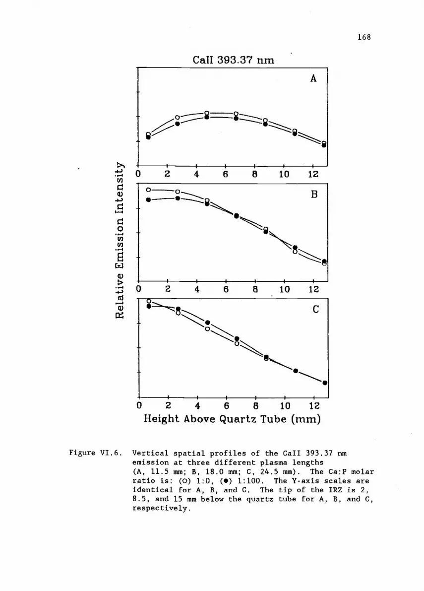
Can 393.37 nmA

0 2 6 8 10 12

0B

0 2 4 6 8 10 12

0 2 4 6 8 10 12Height Above Quartz Tube (mm)

168

Figure VI.6. Vertical spatial profiles of the Can 393.37 nmemission at three different plasma lengths(A, 11.5 mm; B, 18.0 mm; C, 24.5 mm). The Ca:P molarratio is: (0) 1:0, () 1:100. The Y-axis scales areidentical for A, B, and C. The tip of the IRZ is 2,8.5, and 15 mm below the quartz tube for A, B, and C,respectively.

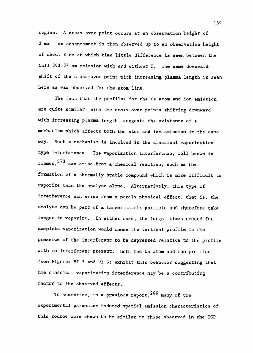
169

region. A cross-over point occurs at an observation height of

2 mm. An enhancement is then observed up to an observation height

of about 8 mm at which time little difference is seen between the

CaII 393.37-nm emission with and without P. The same downward

shift of the cross-over point with increasing plasma length is seen

here as was observed for the atom line.

The fact that the profiles for the Ca atom and ion emission

are quite similar, with the cross-over points shifting downward

with increasing plasma length, suggests the existence of a

mechanism which affects both the atom and ion emission in the same

way. Such a mechanism is involved in the classical vaporization

type interference. The vaporization interference, well known in

flames,273 can arise from a chemical reaction, such as the

formation of a thermally stable compound which is more difficult to

vaporize than the analyte alone. Alternatively, this type of

interference can arise from a purely physical effect, that is, the

analyte can be part of a larger matrix particle and therefore take

longer to vaporize. In either case, the longer times needed for

complete vaporization would cause the vertical profile in the

presence of the interferant to be depressed relative to the profile

with no interferant present. Both the Ca atom and ion profiles

(see Figures VI.5 and VI.6) exhibit this behavior suggesting that

the classical vaporization interference may be a contributing

factor to the observed effects.

To summarize, in a previous report, 266 many of the

experimental parameter-induced spatial emission characteristics of

this source were shown to be similar to those observed in the ICP.

170

However, as shown in this report, some significant differences

exist between this source and the ICP concerning the effects of

easily ionizable elements on analyte emission. Plasma length has

been shown to be an important factor affecting the magnitude and

direction of matrix-induced interferences. By adjusting the plasma

length and by carefully selecting an observation height, the

matrix-induced interferences studied here can be minimized.

Acknowledgments

The authors gratefully acknowledge the support of Leeman

Labs, Inc., and the National Science Foundation (Grant

#CHE-8206692).

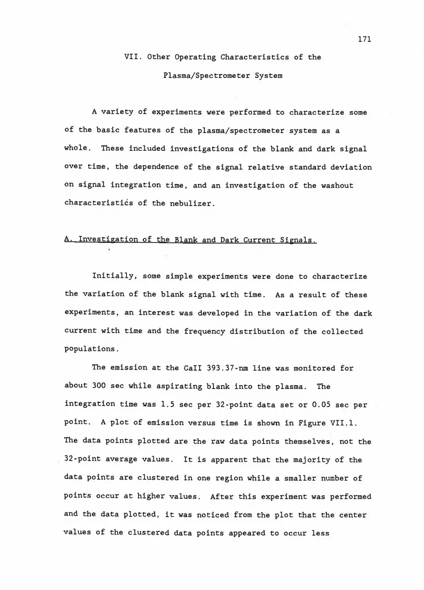
171

VII. Other Operating Characteristics of the

Plasma/Spectrometer System

A variety of experiments were performed to characterize some

of the basic features of the plasma/spectrometer system as a

whole. These included investigations of the blank and dark signal

over time, the dependence of the signal relative standard deviation

on signal integration time, and an investigation of the washout

characteristics of the nebulizer.

A. Investigation of the Blank and Dark Current Signals.

Initially, some simple experiments were done to characterize

the variation of the blank signal with time. As a result of these

experiments, an interest was developed in the variation of the dark

current with time and the frequency distribution of the collected

populations.

The emission at the Can 393.37-nm line was monitored for

about 300 sec while aspirating blank into the plasma. The

integration time was 1.5 sec per 32-point data set or 0.05 sec per

point. A plot of emission versus time is shown in Figure VII.1.

The data points plotted are the raw data points themselves, not the

32-point average values. It is apparent that the majority of the

data points are clustered in one region while a smaller number of

points occur at higher values. After this experiment was performed

and the data plotted, it was noticed from the plot that the center

values of the clustered data points appeared to occur less

rttx

1la

.1-

1

CD

1-C

DD

IIn

g0

I" f

t 0 I"L

n 1E

1I-

h

toC

D

0O

0 Ia.

rAC

DC

DPs

"IC

P 9ca

tv IIa

.cl

nrt

O f

h rt f

trr

0 C

DC

L0

turt P3 to

(.4

(Dvp

rt)-

1V

ft A B

ri o m r 0

O a

)

ZLI

rn

U) co

0 ID 0

Blank Relative Emission Intensity @ 393.37

nm

""*

.:.

a.

. , v

.

01-1

.;,

N O 0

173

frequently than the outer values. Indeed, the frequency histogram

of the blank data, shown in Figure VII.2, reveal this to be the

case. The histogram is a plot of blank signal on the abscissa and

frequency of occurrence of a particular blank signal on the

ordinate. Only the clustered values have been included in the

histogram plot. A definite bimodal characteristic is apparent from

the histogram.

A plot of the dark current vs time is shown in Figure VII.3.

For this experiment, the photomultiplier tube was kept on. In

addition, the photomultiplier tube was sent to its "home" position,

that is, it was not positioned over an exit slit. As with the

blank signal, the dark signal exhibits a clustering of the majority

of the data points about a central value with a much smaller number

of data points occurring at higher values. Also, the same lower

frequency of occurrence of values in the middle of the cluster

which was observed for the blank data is observed here for the dark

current data. This is shown more clearly in the histogram plot

shown in Figure VII.4. The bimodal behavior is apparent. As with

the blank histogram plot, only the clustered values have been

included in the determination of the histogram. The blank emission

and dark current characteristics are very similar in that they both

exhibit the bimodal behavior. Since the magnitude of the blank

signal is only slightly higher than that of the dark current

signal, this might be expected.

The same dark current experiment was repeated with the

photomultiplier tube turned off. The results are shown in

Figure VII.5. The same clustering of points around a central value

27.0

21.0

15.0

A A

A

A6I AAA A A A

A A Li A AA AA A A

A A A A AAA9.00 AA A

O A A A AA A A A

A A A AA A

AA A A A A3.00 A A A A

A LA A A it AA A LA 41.0. 41 IN

324. 342. 360.

Blank Signal

378. 396.

Figure VII.2. Histogram of blank emission versus time data shownin Figure VII.l.

O

t00'

111

ln 0

11

U1

CD

CD

0 0O

ort

M y

CD

111-

0rt

rt1

N.)

0 to

I-1

H.

'0C

Rrn

0p.

10

I-.

0tb

0 a

I-cn

Ca)

00.

to)

0P

3et

rr b

(1)

P)

0(I

)to N

1t

Ct

rtM P

.E1 M

0 m a)a)

......

-,...

mro

0 =

mH

o OIn

Dark Current Signal:

PMT ON/HOME

cri

.....

....._

.....-

.

rt

Hr

0C

Drt

.

II

W...̂

"a)

0

SIT

o

A A

A

CA

A

36.0

A A A AA28.0

A A A A

A A A A OmA A A A OD

AA A A20.0

A CA

AA A. A A

oAA A

AA

AAa A A A12.0

A A A AA A.

A

AA

G AA4.00

A AA A AA

AG6. AIZICCA,

272. 298. 325.

A A

352. 378.

Dark Current Signal: PMT ON/HOME

Figure VII.4. Histogram of dark current versus time data shown inFigure VII.3.

235.U-1DECD

. :

. : : .

CD 215 .. .

.

: .

0- .... .. .co

.c n 195.

L(0

155.

. .

. .

. . .. . . . .

: : . : : . : : .

. : . . : . :

:

70.0 210.I

350. 4910. 6310.

TIME (sec)

Figure VII.5. Dark current signal versus time. The PMT is in the"home" position and is turned off. Integration time1.5 sec per 32-point data set.

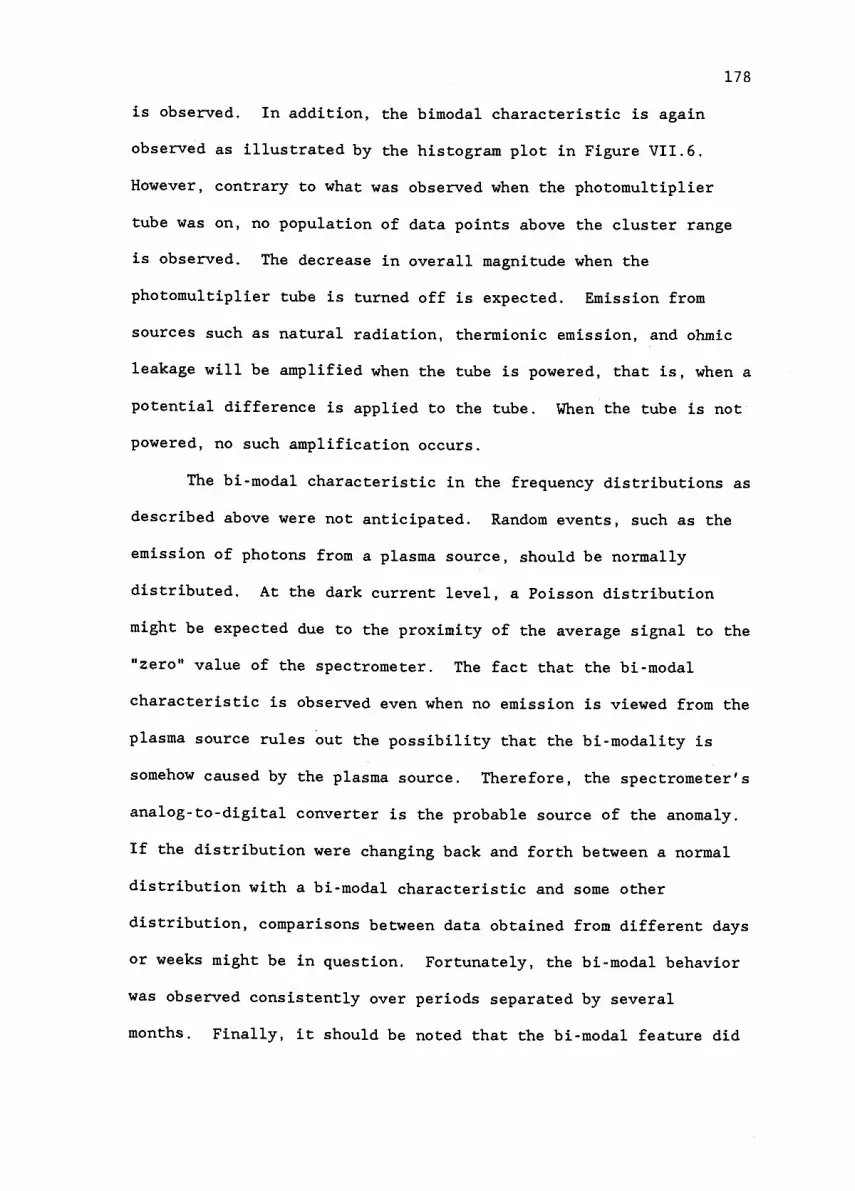
178

is observed. In addition, the bimodal characteristic is again

observed as illustrated by the histogram plot in Figure VII.6.

However, contrary to what was observed when the photomultiplier

tube was on, no population of data points above the cluster range

is observed. The decrease in overall magnitude when the

photomultiplier tube is turned off is expected. Emission from

sources such as natural radiation, thermionic emission, and ohmic

leakage will be amplified when the tube is powered, that is, when a

potential difference is applied to the tube. When the tube is not

powered, no such amplification occurs.

The bi-modal characteristic in the frequency distributions as

described above were not anticipated. Random events, such as the

emission of photons from a plasma source, should be normally

distributed. At the dark current level, a Poisson distribution

might be expected due to the proximity of the average signal to the

"zero" value of the spectrometer. The fact that the bi-modal

characteristic is observed even when no emission is viewed from the

plasma source rules out the possibility that the bi-modality is

somehow caused by the plasma source. Therefore, the spectrometer's

analog-to-digital converter is the probable source of the anomaly.

If the distribution were changing back and forth between a normal

distribution with a bi-modal characteristic and some other

distribution, comparisons between data obtained from different days

or weeks might be in question. Fortunately, the bi-modal behavior

was observed consistently over periods separated by several

months. Finally, it should be noted that the bi-modal feature did

25.0

++

++

+

4--I+

+

-I-

4- + ++ -I-

-I-4- + + +++ +

+ + + ++ + +

+ + -I-+ +

I- + + +++ + -I- +

+ -H-i- -I-

+ +++ ++

+ + ++

+ + +

+ +5.00 + ++ + ++ +++ + -1-1-

4-

1

4-

f 175. I 1915. 1 215. I 1

+

I155. 235.

_111

Dark Current Signal: PMT OFF/HOME

+

Figure VII.6. Histogram of dark current versus time data shown inFigure VII.4.

180

not appear at higher integration times (e.g. 32 sec per 32-point

data set).

B. Dependence of Relative Standard Deviation on Integration Time.

Nearly all of the data acquisition which was performed in

this thesis consisted of collecting 32 data points from the

spectrometer. Then, these 32 points were averaged. This average

value was generally the value used to report the data in graphical

form. The variability of the 32-point data sets is influenced by

the integration time used. The spectrometer's data acquisition

circuitry allowed data collection at integration times from 0.024

to 2.4 sec per individual data point. Thus, the integration times

for the 32-point data sets ranged from 0.77 to 75.4 sec.

It is important to know how the integration time affects the

variability of the mean values of the 32-point data sets. To

investigate this feature, 32-point data sets were collected at

integration times ranging from 1.5 to 74.7 sec per data set. The

relative standard deviation was used as the criteria for evaluating

the change in the variability of the data sets. This experiment

was first performed by monitoring the emission from a hollow

cathode lamp. Then, the experiment was repeated monitoring the

emission from the plasma while aspirating a 100 pg/mL solution of

Mg. Plots of the relative standard deviation vs integration time

for the hollow cathode and plasma sources are shown in

Figure VII.7.

b3 2.0

0

cd 1.0

a)CZ)

"ci 0.00

id 3.0

ccS

C/)2.0

70' 1.0174

181

MgI 285.21 nm

0.00

20 40 60 80

B

20 40 60

Integration Time (sec)80

Figure VII.7. (A) Relative standard deviation at the MgI 285.21-nmline versus integration time. (P) emission fromhollow cathode lamp; (solid line) theoretical squareroot of integration time relation. (B) Relativestandard deviation at the MgI 285.21-nm line versusintegration time. () emission from plasma. Errorbars in both (A) and (B) are at 95% confidence level(N-32).

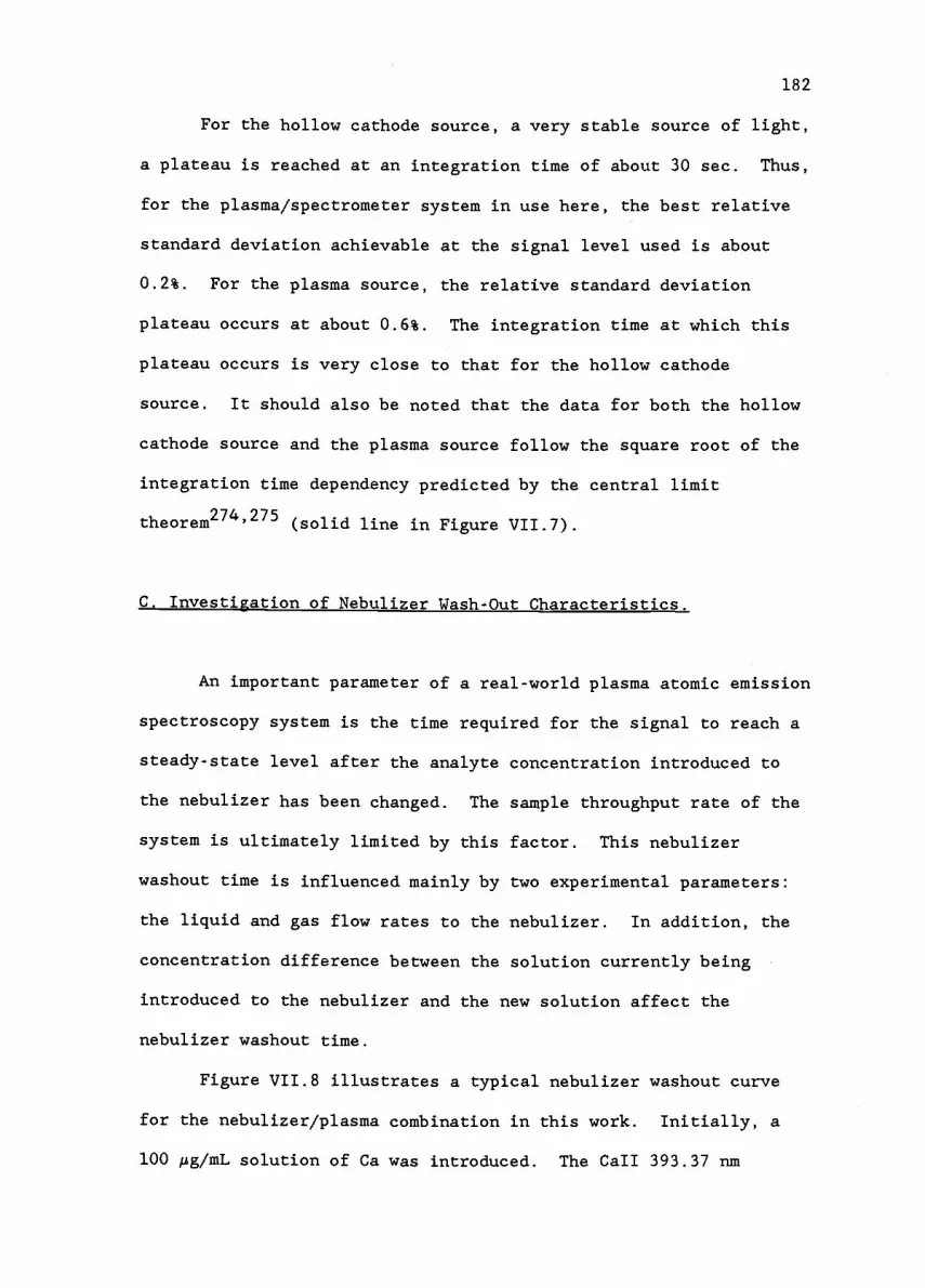
182

For the hollow cathode source, a very stable source of light,

a plateau is reached at an integration time of about 30 sec. Thus,

for the plasma/spectrometer system in use here, the best relative

standard deviation achievable at the signal level used is about

0.2%. For the plasma source, the relative standard deviation

plateau occurs at about 0.6%. The integration time at which this

plateau occurs is very close to that for the hollow cathode

source. It should also be noted that the data for both the hollow

cathode source and the plasma source follow the square root of the

integration time dependency predicted by the central limit

theorem274'275 (solid line in Figure VII.7).

C. Investigation of Nebulizer Wash-Out Characteristics.

An important parameter of a real-world plasma atomic emission

spectroscopy system is the time required for the signal to reach a

steady-state level after the analyte concentration introduced to

the nebulizer has been changed. The sample throughput rate of the

system is ultimately limited by this factor. This nebulizer

washout time is influenced mainly by two experimental parameters:

the liquid and gas flow rates to the nebulizer. In addition, the

concentration difference between the solution currently being

introduced to the nebulizer and the new solution affect the

nebulizer washout time.

Figure VII.8 illustrates a typical nebulizer washout curve

for the nebulizer/plasma combination in this work. Initially, a

100 Ag/mL solution of Ca was introduced. The CaII 393.37 nm

2*Itc 1-

4C

0.9 -C0

ali 0.8 -

Ei-wD" 0.7 -0c>o

.7-, a 0.6 -

0o 30ajEtr: 0.5 -

Ec 0.4 itr)ri 0.3 -atM 0.2 -=o0 0.1 -

1.2

Li

183

Nebulizer WashOut Curve

0

100 200

Time (sec)

300 400

Figure VII.8. CaII 393.37-nm emission versus time. Monitoring of

nebulizer wash-out characteristics. Blankintroduced at time indicated by arrow on graph.

184

emission intensity for this solution was then monitored for

approximately 160 sec. Then, blank was introduced to the nebulizer

and the decay signal was monitored. 148 sec were required for the

signal to reach a level within two standard deviations of the

blank.

While this washout time is typical for the type of nebulizer

in use, it is possible to reduce this change-over time by

momentarily increasing the speed of the peristaltic pump. This

forces the new sample through the nebulizer lines and helps to wash

out the spray chamber more rapidly. Although this high liquid flow

rate to the nebulizer increases the sample loading of the plasma,

under most normal operating conditions, this high flow rate can be

maintained for several seconds without extinguishing the plasma.

185

VIII. CONCLUSIONS

In this section, conclusions about the various aspects of

this work will be given. The strengths and weaknesses of the

plasma source and associated instrumentation will be given with the

intent of providing a direction for future improvements to the

plasma source system as a whole.

A. Plasma Emission Source

The variable length plasma source described here is operated

from three compact, simple, and inexpensive direct current power

supplies. The argon consumption of the system is typically

7.4 L/min, which is comparable to or less than the consumption

rates of commercial DCP and ICP systems. This low gas flow rate is

achieved without the need for water cooling of any of the

components. The staging system allows independent, vertical

movement of the outer and inner electrode sets as well as the

nebulizer assembly. The inner electrodes do not require regrinding

from day to day and can be used indefinitely. The outer electrodes

do require daily regrinding but the same electrodes can be used

indefinitely. No ceramic sleeves are used, as in the commercial

DCP. At present, the outer and inner quartz tubes are generally

replaced after about 5 to 6 hours of operation. This is

necessitated by devitrification of the quartz tube in the vicinity

of the electrodes and by deposition of electrode material onto the

inside of the quartz. If subsequent operation of the plasma is

186

attempted with an "old" quartz tube, arcing to the quartz tube can

occur causing instability of the arcs. Sample tubes can be used

indefinitely. However, if the tip of the sample tube comes closer

than about 1 mm to the base of the plasma, partial melting of the

tip orifice can occur. This causes changes in the sample stream

velocity which have been shown to greatly affect analyte spatial

emission characteristics.

Ignition of the three arcs is simple and is accomplished by

mechanically lifting the three inner electrodes to the same height

as the outer electrodes. Then, shorting of the three electrode

sets with a graphite rod initiates the arcs. Although this method

of ignition is simple, an ignition method which does not require

touching of the electrodes with a potentially contaminating

graphite rod would be an improvement. Possible methods include

shorting the electrodes directly together, applying a momentary

high voltage across the electrode sets, or using a seeding device

which would break down the electrode gap.

Many of the vertical spatial characteristics of the plasma

described here have been shown to be similar to those observed in

the ICP. Plasma length, nebulizer gas flow rate, and current have

all been shown to be important experimental parameters. The unique

ability to change the plasma length during operation has provided

some interesting experimental opportunities. For instance, it has

been shown that the interference of Na on Ca and Zn emission and P

on Ca emission can be virtually eliminated by carefully selecting a

plasma length and observation height. It has also been shown that

the signal-to-background ratio at several common analytical

187

wavelengths can be increased by increasing the length of the

plasma. The signal-to-background ratio continues to increase up to

the maximum length attainable at present. The maximum plasma

length of about 28 mm is imposed by the voltage limitations of the

power supplies (40 V max.). Power supplies capable of supplying

higher voltages would allow even longer plasma lengths to be

attempted with the possibility of attaining even higher

signal-to-background ratios. Higher available voltages may also

help in the future substitution of graphite electrodes for the

tungsten electrodes currently in use thus helping to eliminate some

of the spectral interferences associated with the W and Th in the

electrodes.

The movement of the region of maximum emission to positions

below the top of the outer quartz tube, which occur with the

lengthening of the plasma, is thought to be the main reason for the

poorer detection limits. An improvement in the method of sample

introduction at the long plasma lengths may be required to bring

the region of maximum emission up to an observation height

accessible to the analyst. Simply using higher nebulizer gas flow

rates to raise the maximum region of observation up causes

decreases in the magnitude of the maximum emission. This was

illustrated in the nebulizer gas flow rate studies. Other

possibilities, which would not involve changes in the sample

introduction system, include end-on viewing of emission or viewing

of emission through the quartz tube or a side arm attached to the

quartz tube.

188

B. Echelle Spectrometer

The echelle spectrometer used in this work provided excellent

resolution, a means of imaging the plasma source on the entrance

slit, a variety of peaking and data acquisition routines, and a

serial port for interfacing to the external world. The P-Code

language resident to the spectrometer allowed specific control of

spectrometer functions such as positioning of the aperture plate

and PMT in the focal plane. Through the serial port, these

positioning functions were carried out using a microcomputer. In

addition, the microcomputer was used to position the desired part

of the plasma source on the entrance slit of the spectrometer using

the spectrometer's own mirror. Finally, data was sent to the

external microcomputer through the serial port of the

spectrometer. In these respects, the Leeman Labs echelle

spectrometer was a very versatile and flexible wavelength isolation

device.

Some problems with the spectrometer system were discussed in

Chapter IV. Slight off-axis vertical movement of the source mirror

was compensated for by custom written peaking routines run via the

external microcomputer. In addition, use of the aperture plate and

PMT coordinates stored in the ROM of the spectrometer occasionally

resulted in non-optimal positioning of the plate and PMT. These

non-optimal positions were also corrected using custom written

peaking routines run via the external micrometer.

189

C. Data Acquisition System

In previous work in this laboratory, Eierman276 concluded

that real-time feedback would have been a very useful capability in

his microwave plasma emission/data acquisition system. It was

stated that several experiments were ruined because of the

occurrence of some small problem which was not discovered until the

experiment was completed and the results analyzed. Indeed, early

work with the plasma source described in this thesis involved the

same type of problems, that is, the nonexistence of any sort of

real-time feedback.

The desire for real-time feedback, along with the need for

computer control of the aperture plate, PMT, and source mirror, led

to the development of an integrated menu-driven program, called

ACQDATA, to control all of these functions. ACQDATA also provides

a flexible means of data acquisition of the type that was not

possible with the data acquisition capabilities of the echelle

spectrometer alone. Several modes of data acquisition are possible

including a signal versus time mode and a spatial acquisition

mode. In addition, a completely manual mode of acquisition allows

an image of any point in the plasma to be positioned on the

entrance slit of the spectrometer. This is done by using the

cursor keys on the computer keyboard to control the movement of the

source mirror in the spectrometer. ACQDATA also provides the

analyst with real-time feedback of data as it is collected. This

feedback is in the form of plots to a graphics screen of the

computer monitor and is useful in monitoring the course of an

190

experiment in progress. This real-time feedback offers an

advantage to the common post-experiment type of feedback in that it

allows the analyst to alter the experiment while in progress if an

unforeseen problem arises. The aperture plate and PMT optimization

features of the software allow the analyst to fine tune the

position of the plate and PMT in the focal plane of the

spectrometer. This results in an increase in the amount of light

to the detector thus potentially improving detection limits and

sensitivity.

1.

2.

3. S. Greenfield, I. Ll. Jones, and C. T. Berry, Analyst 89,713 (1964).

4. R. H. Wendt and V. A. Fassel, Anal. Chem. 37, 920 (1965).

5. W. G. Elliot, Am. Lab 3, 45 (1971).

6. D. A. Murdick, Jr. and E. H. Piepmeier, Anal. Chem. 46, 678(1974).

7. T. R. Mattoon and E. H. Piepmeier, Anal. Chem. 55, 1045(1983).

8. R. A. Masters and E. H. Piepmeier, Spectrochim. Acta 40B,85 (1985).

IX. REFERENCES

T. B. Reed, J. Appl. Phys. 32, 821 (1961).

T. B. Reed, J. Appl. Phys. 32, 2534 (1961).

191

9. G. A. Meyer, in Proceedings of 1985 ColloquiumSpectroscopicum Internationale XXIV,(Garmisch-Partenkirchen, Federal Republic of Germany, 1985)vol. 2, p. 226.

10. G. A. Meyer, Spectrochim. Acta 42B, 333 (1987).

11. G. Agricola, De Re Metallica (1556), translated and reprintedby Dover Publications, New York (1950).

12. W. G. Schrenk, Appl. Spectrosc. 40, xix, (1986).

13. R. Mavrodineanu and H. Boiteux, Flame Spectroscopy,Wiley, New York, 1965.

14. C. Th. J. Alkemade, T. J. Hollander, W. Snelleman, and P. J.Th. Zeegers, Metal Vapors in Flames (Pergamon Press, NewYork, 1982).

15. H. H. Willard, L. L. Merritt, Jr., J. A. Dean, and F. A.Settle, Jr., Instrumental Methods of Analysis, Wadsworth,Belmont, CA, 1981.

16. B. F. Scribner and M. Margoshes, "Emission Spectroscopy" inTreatise On Analytical Chemistry, I. M. Kolthoff and P.J. Elving, Eds. (John Wiley & Sons, New York, 1965), 6,Chap. 64, p. 3430.

17. A. Scheeline, Prog. Anal. At. Spectrosc. 7, 21 (1984).

19218. H. A. Strobel, Chemical Instrumentation, (Addison-Wesley,

Reading, MA, 1973), 2nd ed., Chap. 13.

19. B. J. Stallwood, J. Opt. Soc. Amer. 44, 171 (1954).

20. M. Margoshes and B. F. Scribner, Spectrochim. Acta 14, 138(1959).

21. V. V. Korolev and E. E. Vainshtein, J. Anal. Chem. USSR 14,731 (1959).

22. H. Gerdien and A. Lotz, Z. Tech. Phys. 4, 157 (1923).

23. R. Weiss, Z. Physik 138, 170 (1954).

24. R. Peters, Naturwissenschaften 41, 571 (1954).

25. G. M. Ciannini, Sci. Am. 197, 80 (1957).

26. V. V. Korolev and E. E. Vainshtein, J. Anal. Chem. USSR 15,783 (1960).

27. F. A. Korolev and I. K. Kvaratskheli, Opt. Spectrosc. 10,200 (1961).

28. L. I. Grechikhin and V. D. Shimanovich, Opt. Spectrosc. 13,358 (1962).

29. L. I. Greshikhin, J. Anal. Chem. USSR 18, 16 (1963).

30. L. E. Owen, Appl. Spectrosc. 15, 150 (1961).

31. B. F. Scribner and M. Margoshes, Proceedings IXthColloquium Spectroscopicum Internationale (GAMS, Paris,1962), pp. 309-324.

32. R. Lerner, Spectrochim. Acta 20, 1619 (1964).

33. P. A. Serin and K. H. Ashton, Appl. Spectrosc. 18, 166(1964).

34. A. G. Collins and C. A. Pearson, Anal. Chem. 36, 787(1964).

35. E. H. Sirois, Anal. Chem. 36, 2389 (1964).

36. E. H. Sirois, Anal. Chem. 36, 2394 (1964).

37. M. S. Vigler and J. K. Failoni, Appl. Spectrosc. 19, 57(1965).

38. K. E. Friend and A. J. Diefenderfer, Anal. Chem. 38, 1763(1966).

19339. J. Szivek, C. Jones, E. J. Paulson, and L. S. Valberg, Appl.

Spectrosc. 22, 195 (1968).

40. A. W. Fagan and H. M. Klein, Anal. Chem. 40, 2041 (1968).

41. J. F. Chapman, L. S. Dale, and R. N. Whittem, Analyst 98,529 (1973).

42. M. Marinkovic and B. Dimitrijevic, Spectrochim. Acta 23B,257 (1968).

43. S. E. Valente and W. G. Schrenk, Appl. Spectrosc. 24, 197(1970).

44. M. Marinkovic and T. J. Vickers, Appl. Spectrosc. 25, 319(1971).

45. P. Merchant, Jr. and C. Veillon, Anal. Chim. Acta 70, 17(1974).

46. W. G. Elliot, Pittsburgh Conference on Analytical Chemistryand Applied Spectroscopy (1974).

47. W. E. Rippetoe, E. R. Johnson, and T. J. Vickers, Anal. Chem.47, 436 (1975).

48. W. E. Rippetoe and T. J. Vickers, Anal. Chem. 47, 2082(1975).

49. L. Y. Hara, Diss. Abstr. Int. B. 43, 2891 (1983).

50. L. Y. Hara and M. L. Parsons, Anal. Chem. 57, 841 (1985).

51. I. G. Yudelevich and A. S. Cherevko, Spectrochim. Acta 31B,93 (1976).

52. I. G. Yudelevich, A. S. Cherevko, V. S. Engelsht, V. V.Pikalov, A. P. Tagiltsev, and Z. Z. Zheenbajev, Spectrochim.Acta 39B, 777 (1984).

53. M. A. Eid, K.Pure & Appl.

54. M. A. Eid, KSpectrochim.

M. El Behery, and F. A. El Anany, Indian J.Phys. 18, 47 (1980).

. M. El Behery, A. A. Fakhry, and F. A. El Anany,Acta 38B, 495 (1983).

55. L. Paksy and I. J. Lakatos, Spectrochim. Acta 38B, 1099(1983).

56. L. Paksy, Spectrochim. Acta 39B, 1449 (1984).

57. J. Reednick, Am. Lab. 11, 53 (1979).

58. A. T. Zander, Ind. Res. & Dev. 24, No. 2, 146 (1982).

19459. A. T. Zander, Ind. Res. & Dev. 24, No. 3, 142 (1982).

60. S. Greenfield, H. M. McGeachin, and P. B. Smith, Talanta22, 1 (1975).

61. R. M. Barnes, Anal. Chem. 50, 100R (1978).

62. W. J. Boyko, P. N. Keliher, and J. M. Malloy, Anal. Chem.52, 53R (1980).

63. W. J. Boyko, P. N. Keliher, and J. M. Patterson III, Anal.Chem. 54, 188R (1982).

64. P. N. Keliher, W. J. Boyko, J. M. Patterson III, and J. W.Hershey, Anal. Chem. 56, 133R (1984).

65. P. N. Keliher, W. J. Boyko, R. H. Clifford, J. L. Snyder, andS. F. Zhu, Anal. Chem. 58, 335R (1986).

66. Atomic Spectroscopy, Perkin-Elmer, Norwalk, CT.

67. A. T. Zander, Anal. Chem. 58, 1139A (1986).

68. W. Hittorf, Ann. Phys. 21, 90 (1884).

69. J. J. Thomson, Phil. Mat. Ser. 74, 1128 (1927).

70. G. I. Babat, Vestn. Elektroprom. 2, 1 (1942).

71. G. I. Babat, J. Inst. Elec. Eng. (London) 94, 27 (1947).

72. H. U. Eckert, High Temp. Sci. 6, 99 (1974).

73. S. Greenfield, H. M. McGeachin, and P. B. Smith, Talanta23, 1 (1976).

74. R. M. Barnes, CRC Crit. Rev. Anal. Chem. 7, 203 (1978).

75. S. Greenfield, Analyst 105, 1032 (1980).

76. R. M. Barnes, ICP Inf. Newsl. 8, 171 (1983).

77. M. J. Cope and G. F. Kirkbright, J. Phys. E 16, 581 (1983)

78. V. A. Fassel, ICP Inf. Newsl. 8, 69 (1982).

79. G. F. Kirkbright, Pure Appl. Chem. 54, 769 (1982).

80. H. U. Eckert, ICP Inf. Newsl. 10, 529 (1984).

81. S. Greenfield, H. M. McGeachin, and P. B. Smith, Talanta22, 553 (1975).

19582.

83.

84.

85.

86.

R. K. Skogerboe and G. N. Coleman, Anal. Chem. 48, 611A(1976).

A. T. Zander and G. M. Hieftje, Appl. Spectrosc. 35, 357(1981).

S. R. Goode and K. W. Baughman, Appl. Spectrosc. 38, 755(1984).

K. G. Michlewicz and J. W. Carnahan, Anal. Chem. 57, 1092(1985).

K. G. Michlewicz and J. W. Carnahan, Anal. Chem. 58, 3122(1986).

87. R. D. Deutsch and G. M. Hieftje, Appl. Spectrosc. 39, 214(1985).

88. J. J. Urh and J

89. Y. K. Zhang, S.Spectrosc. 39,

. W. Carnahan, Anal. Chem. 57, 1253 (1985).

Hanamura, and J. D. Winefordner, Appl.226 (1985).

90. R. D. Deutsch, J. P. Keilsohn, and G. M. Hieftje, Appl.Spectrosc. 39, 531 (1985).

91. J. J. Urh and J. W. Carnahan, Appl. Spectrosc. 40, 877(1986).

92. P. C. Uden, Developments in Atomic Plasma SpectrochemicalAnalysis, R. M. Barnes, Ed. (Heyden, London, 1981), p. 302.

93. J. W. Carnahan, K. J. Mulligan, and J. A. Caruso, Anal. Chim.Acta 130, 227 (1981).

94. R. Friegieri and R. Fenaroli, Cron. Chim. 70, 3 (1982).

95. 0. Qing-Yu, W. Guo-Chuen, Z. Ke-Wei, and Y. Wei-Lu,Spectrochim. Acta 38B, 419 (1983).

96. T. H. Risby and Y. Talmi, CRC Crit. Rev. Anal. Chem. 14,No. 3, 231 (1984).

97. W. R. McLean, D. L. Stanton, and G. E. Penketh, Analyst 98,432 (1973).

98. B. D. Quimby, M. F. Delaney, P. C. Uden, and R. M. Barnes,Anal. Chem. 51, 875 (1979).

99. B. D. Quimby, M. F. Delaney, P. C. Uden, and R. M. Barnes,Anal. Chem. 52, 259 (1980).

100. K. Tanabe, H. Haraguchi, and K. Fuwa, Spectrochim. Acta36B, 633 (1981).

196101. D. F. Hagen, J. Belisle, and J. S. Marhevka, Spectrochim.

Acta 38B, 377 (1983).

102. C. S. Cerbus and S. J. Gluck, Spectrochim. Acta 38B, 387(1983).

103. M. L. Bruce and J. A. Caruso, Appl Spectrosc. 39, 942(1985).

104. D. L. Haas and J. A. Caruso, Anal. Chem. 57, 846 (1985).

105. Y. Talmi and V. E. Norvell, Anal. Chem. 47, 1510 (1975).

106. K. J. Slatkavitz, L. D. Hoey, P. C. Uden, and R. M. Barnes,Anal. Chem. 57, 1846 (1985).

107. R. F. Browner and A. W. Boorn, Anal. Chem. 56, 787A (1984).

108. R. F. Browner and A. W. Boorn, Anal. Chem. 56, 787A (1984).

109. F. Brech, Analysis Instrumentation 6, 215 (1969).

110. R. H. Knisely, H. Amenson, C. C.Appl. Spectrosc. 28, 285 (1974).

111. J. W. Novak, D. E. Lillie, A. W.Anal. Chem. 52, 576 (1980).

Butler, and V. A. Fassel,

Boorn, and R. F. Browner,

112. H. Anderson, H. Kaiser, and B. Meddings, in Dev. At. PlasmaSpectrochem. Anal., Proc. Int. Winter Conf., R. M. Barnes,Ed. (Heyden, London, 1981), pp 251-277.

113. Y. Fujishiro, M. Kubota, and R. Ishida, Spectrochim. Acta39B, 617 (1984).

114. G. L. Gouy, Ann. Chim. Phys. 18, 5 (1879).

115. J. E. Meinhard, ICP Inform. Newsl. 2, 163 (1976).

116. B. Bogdain, ICP Inform. Newsl. 3, 491 (1978).

117. A. Gustaysson, ICP Inform. Newsl. 5, 312 (1979).

118. H. Howarth, T. N. McKenzie, and M. W. Routh, Appl. Spectrosc.35, 164 (1981).

119. A. Gustaysson, Sectrochim. Acta 39B, 743 (1984).

120. R. S. Babington, Popular Sci., May, 102, (1973).

121. R. S. Babington, U. S. Patents 3,421,692; 3,421,699;3,425,058; 3,425,059; and 3,504,859.

197122. R. C. Fry and M. B. Denton, Anal. Chem. 49, 1413 (1977).

123. R. C. Fry and M. B. Denton, Appl. Spectrosc. 33, 393(1979).

124. R. F. Suddendorf and K. W. Boyer, Anal. Chem. 50, 1769(1978).

125. J. F. Wolcott and C. B. Sobel, Appl. Spectrosc. 32, 591(1978).

126. J. R. Garbarino and H. E. Taylor, Appl. Spectrosc. 34, 584(1980).

127. P. A. M. Ripson and L. de Galan, Spectrochim. Acta 36B, 71(1981).

128. N. Mohamed and R. C. Fry, Anal. Chem. 53, 450 (1981).

129. N. Mohamed, R. M. Brown, Jr., and R. C. Fry, Appl. Spectrosc.35, 153 (1981).

130. B. Thelin, Analyst 106, 54 (1981).

131. C. W. Fuller, R. C. Hulton, and B. Preston, Analyst 106,913 (1981).

132. J. F. Wolcott and C. B. Sobel, Appl. Spectrosc. 36, 685(1982).

133. L. Ebdon and M. R. Cave, Analyst 107, 172 (1982).

134. S. J. Walton and J. E. Goutler, Analyst 110, 531 (1985).

135. P. J. McKinnon, K. C. Giess, and T. V. Knight, in Dev. At.Plasma Spectrochem. Anal., Proc. Int. Winter Conf., R. M.Barnes, Ed. (Heyden, London, 1981), pp 287-301.

136. C. T. Apel and C. N. Duchane, Pittsburgh Conference onAnalytical Chemistry and Applied Spectroscopy, 1979, Paper411.

137. L. R. Layman and F. E. Lichte, Anal. Chem. 54, 638 (1982).

138. W. Nisamaneepong, D. L. Haas, and J. A. Caruso, Spectrochim.Acta 40B, 3 (1985).

139. M. Ibrahim, W. Nisamaneepong, D. L. Haas, and J. A. Caruso,Spectrochim. Acta 40B, 367 (1985).

140. D. R. Luffer and E. D. Salin, Anal. Chem. 58, 654 (1986).

141. R. W. Wood and A. L. Loomis, Phil. Mag. 4, 417 (1927).

198142. C. D. West and D. N. Hume, Anal. Chem. 36, 413 (1964).

143. G. W. Dickinson and V. A. Fassel, Anal. Chem. 41, 1021(1969).

144. P. W. J. M. Boumans and F. J. de Boer, Spectrochim. Acta27B, 391 (1972).

145. P. W. J. M. Boumans and F. J. de Boer, Spectrochim. Acta30B, 309 (1975).

146. P. W. J. M. Boumans, F. J. de Boer, F. J. Dahmen, H. Hoelzel,and A. Meier, Spectrochim. Acta 30B, 449 (1975).

147. V. A. Fassel, C. A. Peterson, F. N. Abercrombie, and R. N.Kniseley, Anal. Chem. 48, 516 (1976).

148. K. W. Olson, W. J. Haas, Jr. and V. A. Fassel, Anal. Chem.49, 632 (1977).

149. M. A. Floyd, V. A. Fassel, R. K. Winge, J. M. Katzenberger,and A. P. D'Silva, Anal. Chem. 52, 431 (1980).

150. S. S. Berman, J. W52, 488 (1980).

. McLaren, and S. N. Willie, Anal. Chem.

151. M. A. Floyd, V. A. Fassel, and A. P. D'Silva, Anal. Chem.52, 2168 (1980).

152. J. M. Mermet and C. Trassy, Dev. At. Plasma Spectrochem.Anal., Proc. Int. Winter Conf., R. M. Barnes, Ed. (Heyden,London, 1981), pp 245-250.

153. C. E. Taylor and T. L. Floyd, Appl. Spectrosc. 35, 408(1981).

154. P. D. Goulden and D. H. J. Anthony, Anal. Chem. 56, 2327(1984).

155. M. Thompson, and J. N. Walsh, A Handbook of InductivelyCoupled Plasma Spectroscopy (Blackie, London, 1983), p 68.

156. V. A. Fassel and B. R. Bear, Spectrochim. Acta, 418, 1089(1986).

157. P. W. J. M. Boumans and F. J. de Boer, Spectrochim. Acta,31B, 355 (1976).

158. P. Schramel, Spectrochim. Acta 38B, 199 (1983).

159. H. J. Issaq and L. P. Morgenthaler, Anal. Chem. 47, 1661(1975).

199160. F. N. Abercrombie, Pittsburgh Conference, Cleveland, Ohio,

1977; paper 406.

161. E. D. Salin, J. Carr, and G. Horlick, Pittsburgh Conference,Cleveland, Ohio, 1979; paper 563.

162. J. Carr and G. Horlick, Pittsburgh Conference, Atlantic City,New Jersey, 1980; paper 56.

163. T. Ishizuka and Y. Uwamino, Anal. Chem. 52, 125 (1980).

164. M. Thompson, J. E. Goulter, and F. Sieper, Analyst 106, 32(1981).

165. J. W. Carr and G. Horlick, Spectrochim. Acta 37B, 1 (1982).

166. T. Ishizuka and Y. Uwamino, Spectrochim. Acta 38B, 519(1983).

167. N. K. Rudnevsky, A. N. Tumanova, and E. V. Maximova,Spectrochim. Acta 39B, 5 (1984).

168. P. G. Mitchell, J. Sneddon, and L. J. Radziemski, Appl.Spectrosc. 40, 274 (1986).

169. J. Monvoisin and R. Mavrodineanu, Spectrochim. Acta 4, 396(1951).

170. R. K. Winge, V. A. Fassel, and R. N. Kniseley, Appl.Spectrosc. 25, 636 (1971).

171. J. L. Jones, R. L. Dahiquist, and R. E. Lee, Appl. Spectrosc.25, 628 (1971).

172. L. R. Layman and G. M. Hieftje, Anal. Chem. 47, 194 (1975).

173. A. T. Zander and G. M.(1978).

174. R. D. Deustch and G. M(1984).

Hieftje, Anal. Chem. 50, 1257

. Hieftje, Anal. Chem. 56, 1923

175. H. G. C. Human, R. H. Scott, A. R. Oakes, and C. D. West,Analyst 101, 265 (1976).

176. R. H. Scott, Spectrochim. Acta 33B, 123 (1978).

177. J. Y. Marks, D. E. Fornwalt, and R. E. Yungk, Spectrochim.Acta 38B, 107 (1983).

178. P. B. Farnsworth and G. M. Hieftje, Anal. Chem. 55, 1417(1983).

200179. A. Aziz, J. A. C. Broekaert, K. Laqua, and F. Leis,

Spectrochim. Acta 39B, 1091 (1984).

180. A. Ono, M. Saeki, and K. Chiba, Appl. Spectrosc. 41, 970(1987).

181. C. W. Fuller, Electrothermal Atomization for AtomicAbsorption Spectroscopy (The Chemical Society, BurlingtonHouse, London, 1977).

182. G. F. Kirkbright, Analyst 96, 609 (1971).

183. A. Syty, Crit. Rev. Anal. Chem. 4, 155 (1974).

184. Special Issue - Graphite Furnace Technology and AtomicAbsorption Spectroscopy, Spectrochim. Acta 39B, 139-523(1984)

185. E. Preuss, Z. Angew. Mineralogie 3, 1 (1940).

186. I. Kleinmann and V. Svoboda, Anal. Chem. 41, 1029 (1969).

187. K. C. Ng and J. A. Caruso, Appl. Spectrosc. 39, 719 (1985).

188. J. W. Robinson and S. Weiss, Spectrosc. Lett. 13, 685(1980).

189. J. W. Robinson and E. M. Skelly, J. Environ. Sci. HealthA17, 391 (1982).

190. K. C. Ng and J. A. Caruso, Anal. Chim. Acta 143, 209(1983).

191. R. Mavrodineanu and R. C. Hughes, Spectrochim. Acta 19,1309 (1963).

192. F. L. Fricke, O. R. Rose, Jr., and J. A. Caruso, Anal. Chem.47, 2018 (1975).

193. E. D. Salin and G. Horlick, Anal. Chem. 51, 2284 (1979).

194. D. Sommer and K. Ohls, Fresenius Z. Anal. Chem. 304, 97(1980).

195. G. F. Kirkbright and S. J. Walton, Analyst 107, 276 (1982).

196. G. F. Kirkbright and Z. Li-Xing, Analyst 107, 617 (1982).

197. G. F. Kirkbright and R. D. Snook, Appl. Spectrosc. 37, 11(1983).

198. Z. Li-Xing, G. F. Kirkbright, M. J. Cope, and J. M. Watson,Appl. Spectrosc. 37, 250 (1983).

201199. N. W. Barnett, M. J. Cope, G. F. Kirkbright, and A. A. H.

Taobi, Spectrochim. Acta 39B, 343 (1984).

200. A. G. Page, S. V. Godbole, K. H. Madraswala, M. J. Kulkarni,V. S. Mallapurkar, and B. D. Joshi, Spectrochim. Acta 39B,551 (1984).

201. D. R. Hull and G. Horlick, Spectrochim. Acta 39B, 843(1984).

202. H. Matusiewicz and R. M. Barnes, Spectrochim. Acta 39B, 891(1984).

203. M. Abdullah, K. Fuwa, and H. Haraguchi, Spectrochim. Acta39B, 1129 (1984).

204. M. M. Habib and E. D. Salin, Anal. Chem. 57, 2055 (1985).

205. M. Abdullah and H. Haraguchi, Anal. Chem. 57, 2059 (1985).

206. A. Lorber and Z. Goldbart, Analyst 110, 155 (1985).

207. W. E. Pettit and G. Horlick, Spectrochim. Acta 41B, 699(1986).

208. Y. Shao and G. Horlick, Appl. Spectrosc. 40, 386 (1986).

209. E. D. Salin and R. L. A. Sing, Anal. Chem. 56, 2596 (1984).

210. R. Herrmann, "Nebulizers and Burners", in Flame Emissionand Atomic Absorption Spectrometry, vol. 2: Components andTechniques, J. A. Dean and T. C. Rains, Eds. (MarcelDekker, Inc., New York, 1971), p.67.

211. P. C. Uden, B. D. Quimby, R. M. Barnes, and W. G. Elliot,Anal. Chim. Acta 101, 99 (1978).

212. G. R. Kornblum, W. van der Waal, and L. de Galan, Anal. Chem.51, 2378 (1979).

213. A. W. Steele and G. M. Hieftje, paper #51 at 8th annual FACSSmeeting, Philadelphia, PA (1981).

214. M. P. Doherty and G. M. Hieftje, Appl. Spectrosc. 38, 405(1984).

215. R. P. Browner and A. W. Boorn, Anal. Chem. 56, 875A (1984).

216. S. Greenfield, Spectrochim. Acta 38B, 93 (1983).

217. K. E. Lawrence, G. W. Rice, and V. A. Fassel, Anal. Chem.56, 289 (1984).

202218. K. E. Lawrence, G. W. Rice, and V. A. Fassel, Spectrochim.

Acta 40B, 1495 (1985).

219. G. A. Meyer, J. S. Roeck, and M. L. Vestal, ICP Inf. Newsl.10, 955 (1985).

220. J. W. Elgersma, F. J. M. J. Maessen, and W. M. A. Niessen,Spectrochim. Acta 41B, 1217 (1986).

221. S. A. Schwartz and G. A. Meyer, Spectrochim. Acta 41B, 1287(1986).

222. G. A. Meyer, Spectrochim. Acta, Part B, in press.

223. H. C. Hoare and R. A. Mostyn, Anal. Chem. 39, 1153 (1967).

224. R. M. Dagnall, D. J.Anal. Chim. Acta 54,

225. K. N. De Silva and R.865 (1986).

Smith, T. S. West, and S. Greenfield,397 (1971).

Guevremont, Spectrochim. Acta 41B,

226. R. H. Scott, V. A. Fassel, R. N. Kniseley, and D. E. Nixon,Anal. Chem. 46, 75 (1974).

227. A. L. Lewis II, Ph.D. Thesis, Oregon State University,Corvallis, OR (1981).

228. P. N. Keliher and C. C. Wohlers, Anal. Chem., 48, 333A(1976).

229. W. G. Elliot, Am. Lab., 2 (3), 67 (1970).

230. G. J. Matz, Am. Lab., 5 (3), 75 (1973).

231. ASYST Reference Manuals, MacMillan Software Co., New York,NY).

232. G. R. Kornblum and L. de Galan, Spectrochim. Acta, 32B,455 (1977).

233. T. E. Edmonds and G. Horlick, Appl. Spectrosc. 31, 536(1977).

234. G. Horlick and M. W. Blades, Appl. Spectrosc. 34, 229(1980).

235. M. W. Blades and G. Horlick, Spectrochim. Acta 36B, 861(1981).

236. R. N. Savage and G. M. Hieftje, Anal. Chem. 52, 1267(1980).

203237. M. W. Blades and G. Horlick, Spectrochim. Acta 36B, 881

(1981).

238. J. P. Rybarczyk, C. P. Jester, D. A. Yates and S. R.Koirtyohann, Anal. Chem. 54, 2162 (1982).

239. L. M. Faires, C. T. Apel, and T. M. Niemczyk, Appl.Spectrosc. 37, 558 (1983).

240. B. R. Hites, J. W. Olesik, A. F. Parisi and G. M. Hieftje,Computer Enhanced Spectrosc. 3, 91 (1986).

241. PLASMA-SPEC Operations Manual, Leeman Labs, Inc., Lowell, MA(U.S.A.).

242. C. H. Moore, Byte 5 (8), 76 (1980).

243. T. J. Reynolds, J. Microcomp. Appl. 8, 255 (1985).

244. C. D. Keirs and T. J. Vickers, Appl. Spectrosc. 31, 273(1977).

245. J. P. Shields, Ph.D. Thesis, Oregon State University,Corvallis, OR (1987).

246. J. P. Shields and E. H. Piepmeier, Computer EnhancedSpectrosc., submitted for publication, December, 1987.

247. J. A. Dean and T. C. Rains, Flame Emission and AtomicAbsorption Spectrometry (Marcel Dekker, New York, 1971),Chap. 13, Append. 1.

248. B. W. Smith and M. L. Parsons, J. Chem. Ed. 50, 679 (1973).

249. R. Massee, F. J. M. J. Maessen, and J. J. M. DeGoeij, Anal.Chim. Acta 127, 181 (1981).

250. S. R. Koirtyohann, J. S. Jones, and D. A. Yates, Anal. Chem.52, 1965 (1980).

251. G. H. Lee, J. P. Shields, and E. H. Piepmeier, Spectrochim.Acta, submitted for publication, December, 1987.

252. R. J. Decker, Spectrochim. Acta 35B, 19 (1980).

253. A. T. Zander and M. H. Miller, Spectrochim. Acta 40B, 1023(1985).

254. M. H. Miller and A. T. Zander, Spectrochim. Acta 41B, 453(1986).

255. G. R. Kornblum and L. de Galan, Spectrochim. Acta 29B, 249(1974).

204256. R. M. Barnes and R. G. Schleicher, Spectrochim. Acta 30B,

109 (1975).

257. D. J. Kalnicky, R. N. Kniseley, and V. A. Fassel,Spectrochim. Acta 30B,511 (1975).

258. G. Dube and M. I. Boulos, Can. J. Spectrosc. 22, 68 (1977).

259. T. B. Reed, J. Appl. Phys. 32, 821 (1961).

260. T. B. Reed, J. Appl. Phys. 32, 2534 (1961).

261. S. Greenfield, I. L. Jones, H. M. McGeachin, and P. B. Smith,Anal. Chim. Acta 74, 225 (1975).

262. S. Greenfield and H. McGeachin, Anal. Chim. Acta 100, 101(1978).

263. A. Montaser and J. Mortazavi, Anal. Chem. 52, 255 (1980).

264. A. Montaser, V. A. Fassel, and J. Zalewski, Appl. Spectrosc.35, 292 (1981).

265. R. K. Winge, V. J. Peterson, and V. A. Fassel, Appl.Spectrosc. 33, 206 (1979).

266. J. P. Shields and E. H. Piepmeier, Appl. Spectrosc.,submitted for publication, December, 1987.

267. G. F. Larson, V. A. Fassel, R. H. Scott, and R. N. Kniseley,Anal. Chem. 47, 238 (1975).

268. S. R. Koirtyohann, J. S. Jones, C. P. Jester, and D. A.Yates, Spectrochim. Acta 36B, 49 (1981).

269. W. H. Gunter, K.37B, 571 (1982).

270. W. H. Gunter, K.40B, 617 (1985).

Visser, and P.

Visser, and P.

B. Zeeman, Spectrochim. Acta

B. Zeeman, Spectrochim. Acta

271. J. E. Roederer, G. J. Bastiaans, M. A. Fernandez,and K. J.Fredeen, Appl. Spectrosc. 36, 383 (1982).

272. J. A. Borowiec, A. W. Boorn, J. H. Dillard, M. S. Cresser, R.F. Browner, and M. J. Matteson, Anal. Chem 52, 1054 (1980).

273. C. T. J. Alkamade, in Flame Emission and Atomic AbsorptionSpectrometry, J. A. Dean and T. C. Rains, Eds. (MarcelDekker, New York, 1969), Chap. 4.

274. H. V. Malmstadt, M. L. Franklin, and G. Horlick, Anal. Chem.44, 63A (1972).

205275. R. K. Skogerboe, P. J. Lamothe, G. J. Bastiaans, S. J.

Freeland, and G. N. Coleman, Appl. Spectrosc. 30, 495(1976).

276. R. J. Eierman, Ph.D. Thesis, Oregon State University,Corvallis, OR (1985).

277. J. B. Willis, Spectrochim. Acta 23A, 811 (1967).

X. APPENDICES

206

A. Aperture Plate and PMT Coordinates

In the course of this work, many different lines were used.

As described in the main text of this work, each line has a unique

set of aperture plate and photomultiplier tube (PMT) coordinates.

Some of these lines are easily found with the echelle

spectrometer's Peak Wavelength routine. Other lines are more

difficult to find. For instance, it is possible for the Peak

Wavelength routine of the spectrometer to miss the finding of a

line. This does, indeed, occur in practice. Also, it is possible

that a line of interest may not be among the lines whose

coordinates are known to the spectrometer, that is, whose

coordinates are stored in the ROM of the spectrometer. In

addition, although only one pair of PMT coordinates is possible for

a given line, it is possible for some lines to have more than one

pair of plate coordinates.

Table X.1 presents a compilation of the plate and PMT

coordinates which were used in this work. It is obviously not a

comprehensive listing. However, it is hoped that these coordinates

will give future investigators using the Leeman Labs echelle

spectrometer a starting place and be beneficial in their search for

new lines.

Variations in ambient temperature, pressure, as well as

mechanical vibrations and maintenance effects, can lead to slight

variations in these coordinates. Therefore, it is possible that

these coordinates could vary by about 10 units high or low. The

207

aperture plate coordinates will be more likely to vary than the PMT

coordinates.

208

Table X.1

Compilation of Aperture Plate and PMT Coorinates

ElementWavelength Line Echelle Echelle

(nm) Type Line # OrderPlateX Y X

PMT

Al 396.15 I 1 57 133 166 -148 807Al 309.27 I 2 73 143 172 -140 696Ca 422.67 I 3 53 151 181 -301 830Ca 393.37 II 1 57 143 192 -284 805Cd 228.80 I 2 99 135 160 - 20 459Co 340.51 I 2 66 147 188 -244 754Co 228.62 II 5 98 144 204 -303 456Cr 425.43 I 1 54 153 163 -178 829Cr

b357.87 I 3 63 131 178 -175 767

Cr 357.87 I 3 63 131 255 -175 767Cr 283.56 II 6 79 125 204 -304 644Cu 324.75 I 1 69 146 184 -297 725Fe 371.99 I 1 60 195 215 -372 788Fe 259.94 II 4 87 110 179 - 87 575Fe 238.20 II 5 95 168 164 - 50 495Li 610.36 I 2 37 205 214 -190 304Mg 285.21 I 1 79 132 182 -178 645

bMg 285.21 I 1 79 182 86 -178 645Mg 279.55 II 2 81 122 223 - 64 631aMg 280.27 II 3 80 112 193 -283 635Mn 403.08 I 1 56 141 217 -155 810Mn 257.61 II 2 88 121 171 - 29 570Mn 259.37 II 3 86 134 194 -294 571Mn 279.83 I 4 81 131 160 - 42 632Si 251.61 I 1 89 140 190 -313 552Si 288.16 I 2 78 134 180 -232 655V 437.92 I 1 51 129 178 -357 842aV 309.31 II 2 73 183 174 -137 695V 310.23 II 3 73 88 175 - 72 696W 400.87 I 3 56 130 179 -262 811

bZn 213.86 I 2 105 122 99 -242 378bZn 213.86 I 2 105 130 181 -242 378Zn 202.55 II 3 111 201 201 -193 304

aZr 339.20 II 1 66 112 194 -316 745Zr 343.82 II 2 66 113 158 85 748Zr 360.12 I 3 63 87 217 - 46 764

aFor the plasma source used in this work, this line has beenfound to be more sensitive than the other lines of the same type

b(i.e., atom or ion) for this element.This listing contains an alternate set of aperture platecoordinates in addition to the primary pair of coordinateslisted.

B. Computer Listings

ECHO.C11

INTEGER

\ Stepper Motor Scalars

SCALAR

UTILITY7.0

James P. ShieldsDepartment of ChemistryCkegon State University

Corvallis, OR 97331(503) 754-2081

Final Revision Completed 10/9/87

This code consists of all of the scalar, array,etc..., definitions and general utility routinesneeded for the main program, MAIN7.0. Inaddition, note the existence of the small startup program called G07.0. It was necessary tokeep 607.0 as a separate program because itcontained code which could not be SAVE'ed usingthe ASYST SAVE word. I believe it is a bug inASYST version 1.51 which caused this problem. Tore-compile AINTA enter ASYST (re-configurewith a larger ctionary, heap, etc..) and LOADboth UTILITY7.0 and MA1N7.0 in that order. ThenSAVE this ASYST system using the name ACQDATA oranother name of your choice. Then, in the future,you can start ASYST by running ACQDATA fran DOS.To complete the working acquisition system, WADG07.0 after running ACQDATA fram DOS. Have fun!!!My thesis contains more informaticn if interested

Scalar Definitions

SCALAR VerticalCoordSCALAR HorizontalCoord

DP.INTEGER

REAL

INTEGER

Flags

--Table 1 of scalars--Ethelle Scalars Utility Scalars

209

MotorEtrorSCALAR NumEchelleCannands

SCALAR Motor#SCALAR DirectionSCALAR CorrectionFactorSCALAR OldMaxIndex#SCALAR IntegrationTime

SCALAR OldMaxIntensitySCALAR HalfMaxIntensity

SCALAR MaxIndex#SCALAR MinLeftlndex#SCALAR MinRightIndSCALAR HalfLeftIndSCALAR fghtIndex#SCALAR NewPeHalRiakIndexi

Table 2 of scalars--Data Acquisition Scalars

SCALAR ArraylndexSCALAR CurrentCoordVariableSCALAR StringLengthSCALAR NumCIsSCALAR CurrentCoDigitordSetNum

SCALAR Number01CoordSetsSCALAR CursorXPositionSCALAR CursorYPosition

SCALAR WideScanFlagSCALAR HorizScanFlagSCALAR OptimizedFlagSCALAR 10r32Flag

SCAAR HoursSCALLAR Minutes

SCALAR HorizontalRangeSCALAR HorizontalCounts/Step

SCALAR NumberOfCoordSetsFlag SCALAR SecondsSCALAR StepperMenuDisplayed? SCALAR HSecondsSCALAR F10F1lag SCALAR OldHoursSCALAR PlotMeanFlag_ SCALAR OldMinutesSCALAR PlotRaWDataFlag SCALAR OldSecondsSCALAR TimedEkitFlag_ SCALAR OldHSecondsSCALAR DecayRescaleFlag SCALAR StoreMinutesSCALAR e&mf --1-eFlag SCALAR StoreHoursSCALAR RestoreMinutesFlag SCALAR SubroutineSCALAR RestoreHoursFlag SCALAR TimedAcqColtricirSCALAR ManualAcqDataFlag SCALAR TimedDelaySCALAR ManualAcqCounter SCALAR NumDataPointsSCALAR ManualRescaleFlag SCALAR PlotTypeSCALAR MotorControlFlag SCALAR HorizontalStepSizeSCALAR tackFlag SCALAR VerticalStepSizeSCALAR tFlag SCALAR GrossNumxStepsSCALAR Plo fileFlag SCALAR BackgroundOffsetSCALAR SpatialEkitFlag SCALAR BackgroundMbdeSCALAR .ag SCALAR OldBackgroundModeSCALAR GetDataFlag SCALAR SpatialCounter

SCALARSCALAR eadip

SpatialBGMbde

SCALAR NumSpatalArraysCl

SCALAR $patialAciqCounterSCALAR ElapsedTimeSCALAR RawMeanSCALAR

SCALAR VerticalStepUpSize

1.*

r

SCALAR NUmHorizontalScansSCALAR metal lagDP.INTEGERREAL

SCALARSCALARSCALARSCALARSCALARSCALARSCALAR

RawSDev%RSDHighestRawMeanLowestRawMeanGrowthYMinGrowthYMaxManualYMinManuaiYMax

INTEGER

Window Definitions\ The EXTENDED.GRAPH1CS.CHARS word reads in the extended graphics\ font and ppaatches it into the ROM char font tables. Requires the\ of the .DAT file. This allows the use of extended chars

lloogics mode. This word is from the ASYST program exchange.DIM( 512 ] ARRAY CHARFONTS

: EXTENDED.GRAPH1CS.CHARSF1LE.OPEN CHARFONT.DAT

1 SUBFILECHARFONTS F1LE>ARRAY

F1LE.CLOSE0 DEF.SEGCHARFUITS ADDRESS \ ( Segment, Offset )DUP 256 MODULO 7CH POKE \ Low byte of offset128 256 / 7DH POKE \ Hi " " "DUP

179\ 42

00

256 MODULO 7EH128 256 / 7FH

196 218 192 21742 42 42 42 42

0 0 39 WINDOW (Left40 0 79 WINDOW

POKE \ Low byte of segmentPOKE \ Hi

191 BORDER.CHARSBORDER.CHARS

Banner Text}Right' Band: Text)

17 1 22 37 WINDOW Text Vindowl2417

039

24 38 WINDOW22 78 WINDOW

Error Window}Menu Pindowl

1

24 39 24 79 WINDOW StatEs window!1 40 7 80 WINDOW Timed Ao Plot Text)

characteravailabilityin

210

211

Vuport Definitions?VID \ Routine determines if graphics display is ON. If not, turn it ON.

?GRAPHICS.DISFLAY NCTIF

GRAPHICS.DISPLAYTHEN

;

: 32POINT.SCREEN \ Screen for plotting current 32 data points(Upper Left).HORIZONTAL GRID.CFF VERTICAL GRID.OFF7VID0. .69 VUPORT.ORIG.49 .26 VUPORT.SIZESOLID

TIMED.SCREEN \ Screen for plotting timed averages(Lower Left and Right).7V1D0. .38 VUPORT.ORIG.97 .29 VUPORT.SIZE

Set-Up\ Note that all RS232 commandRs

S232are in file GOx.x where x.x is revision #

\Parity : Moe

\ Data Bits : 8

\ Stop Bits : 1\ 760 RS232.DEVICE SFECTROMETER.DEV

\ 760 (dec) = 2F8 (hex) = COM2 address\ Associates CCM2 with SPECTROMETER.DEV

\ Set baud rate at 9600\ Set hardware interrupt line to IRQ3 (C0M2).\ Put in interrupt mode (vs. polled mode).

\ 9600 SET.BAUD\ 3 SET.INT.L1NE\ RS232.INT.MODE

TNEGERArray Definitions

IDIM[ 10 , 4 ] ARRAY PLATE.PMT.CCCRDS PLATE.PMT.CCCRDS (]RAMPDIM 10 , 4 , 4 ] ARRAY BROKEN.COORDSDIM 512 ] ARRAY CHARFONTS \ Array for character fonts from CHARFONT.DAT

\ File I/OINTEGER DIM( 4 ARRAY TRANSFER.TO.F1LE TRANSFER.TO.F1LE (]RAMP

DM( 4 ARRAY TRANSFER.FROM.F1LE TRANSFER.FROM.F1LE ORAMP

\ RS232 and data collection arrINTEGER DIM 100 ] ARRAY 23 \ This is a buffer for RS232 comm.DP.INTEGER 32 ARRAY RAW.32POINTS \ Double precision to handle >32,767

DrIamM 32 ARRAY RAW.32POINTS.BG0DIM 32 ARRAY RAW.32P0INTS.BG-1DIM 32 ARRAY RAW.32POINTS.BG+1DIM 10 32 ARRAY RAW.32POINTS.ALLDIM 10 32 ARRAY RAW.32POINTS.BGO.ALLDIM 10 32 ARRAY RAW.32POINTS.BG-1.ALLDIM 10 32 ARRAY RAW.32POINTS.BG+1.ALLDIM 10J ARRAY HORIZCITTAL.COORDS.ALLDIM 10 j ARRAY VERTICAL.COCRDS.ALL

\ Data Acquisition ArraysINTEGER 1 ARRAY DUMMY.ELAPSED.TIME.ARRAY

DIM 1 : ARRAY DUMMY.HORIZ.CCCRDS.ARRAYDIM 1 ARRAY DUMMY.VERT.COORDS.ARRAY

DP. INTE DIM 1 ] ARRAY DUMMY.SDEV.ARRAYDIM 1 ] ARRAY DUMMY.MEAN.ARRAY

212

DIME 4 , 15" Plate X:"" Plate Y:"" PMT X:"" PMT Y:"DIME 4 , 15" Plate X"" Plate Y"" PMT X"" PHT Y"

String Array Definitions] STRING...ARRAY COORDINATE.

COORDINATE.NAMES: " 1 ":=COORDINATE.NAMES: " 2 ":=COORDINATE.NAMES: " 3 ":=COORDINATE.NAMES " 4 ":=

] STUNG.ARRAY COORDINATE.NAMES

COORDINATE.NAMES " 2 ":=COORDINATE.NAMES " 1 ":=

COORDINATE.NAMES " 3 ":=COORDENNTE.NAMES " 4 ":=

DIME 1 , 1472 ] STUNG.ARRAY ASCII.RAW \ String arra for 32 lines t146 chars\ per line of scan data.

\ ASCII.RAW "RS232.BUFFER \ Associate string array with RS232 device.\ Note that above command is in file Glex.x: where x.x is current revision #.

40 STRING GetCoordSetNUmStringlString Definitions

40 STRING GetCoordSetNUmString240 STRING GetCoordinateFileNameStringl40 STRING GetCoordinateFileNameString212 STRING CoordinateSetFileName12 STRING Dir=iiim10 STRING Ste12 STRING FileName40 STRING LeftBannerText0 STRING RightBannerText

General Echelle Utilities: CLEAR.TEXT

{Text Window} SCREEN.CLEAR

: ECHELLE.SET.UP.PROMPT{Text Window} SCREEN.CLEAR ." Make a selection from the" CR." &belle Set-Up Menu: "

SEND.13CRRS232.CUT

: IMELLE.X.MENU \ Send ? X CR to echelle (experimental menu).13 ASCII X 20 3 0 DO RS232.0UT LOOP

: SE D.11 0 W 48 + RS232.CUT LOOP SEND.CR

: SEND.22 0 DO 48 + RS232.0UT LOOP SEND.CR

: SEND.33 0 DO 48 + RS232.0UT LOOP SEND.CR

: DO.PEAK.HORIZINTAL \ Send "Peak" 3 CR to echelle23 RS232.CUT \ "Peak"3 SEND.1 \ 3 CR

: laECUTE.IVIDR.OPERATION

213

ECHELLE.X.101J2 1 SEND.2

: INSERT.MOTal.CPERATICiiFCHELLE.X.MENU9 SEND.1

: SEND.NumEchelleCtemandsNumDchelleCanmands 0 DO 48 + RS232.0UT ICOP SEND.CR

: PLATE.HCMEDZHELLE X MENU1 1 SEND.2 \ Execute pcode7 1 5 SEND.3 \ at address 517

: PMT.HOMEECHELLE.X.MENU1 1 SEND.2 \ EXecute pcode6 1 5 SDID.3 \ at address 516

: PEAK.HORUJWAL.POSITIONCLEAR.TEXT ." Horizontal Peaking in Progress..." CR ." Please WaitDO.PEAK.HOR1ZONTAL8500 MSEC.DELAY." ...Peaking Completed"

: DO.WIDE.SCANECHELLE.X.MENU1 1 SEND.20 8 6 SEND.3 CLEAR.TEXT ." Doing Wide Scan...

It

: DO.IN.PLACE.SCANECHELLE.A.MENU1 1 SEND.20 7 6 SE1+D.3 CLEAR.TEXT ." Doing 'In- Place' Scan..."

: DO.HORI7 WAL.11WILEDZHELLE.X.MENU1 1 SEND.20 9 6 SEND.3 CR CR ." Doing Horizontal Profile..."

: DO.VERTICAL.PROFILEECHELLE.X.MENU1 1 SEND.20 1 7 SEND.3 CR Cl ." Doing Vertical Profile..."

: DO.Motorit.SCANECHELLE.X.MENU1 1

orSEND.2

Mot#

WI

CASE2 OF 0 2 6 SEND.3 CLEAR.TEXT ." Doing Fine Plate X Scan..." ENDOF4 OF 0 4 6 SEND.3 CLEAR.TEXT ." Doing Fine PMT X Scan..." ENDOF5 OF 0 6 6 SEND.3 CLEAR.TEXT ." Doing Fine PMT Y Scan..." ENDOF

10 OF 0 3 6 SEND.3 CLEAR.TEXT ." Doing Fine Plate Y Scan..." ENDOFWCASE

214

: HGAIRROR.MOTOR.CORRECTIONINSERT.MDTOR.OPERATION\ 53 3 0 6 63 5 SEND.2 3 SEND.1 0 SEND.1 6 SEND.1

1000 MSEC.DELEY(Text Windowl SCREEN.CLEAR. " Mg-Mirror Motor" CR." " Maa

ke ai osen

leacti n roo te""C R ." Echelle Set-Up Menu: "

6 SEND.1

: LOAD.MGPMT.COORDINATESINSERT.)vTOR.CFERATION\ 19 4 1 2 161

9 1 SEND.2 4 SEND.1 1 SEND.1 2 SEND.1 1 6 1 SEND.3\ 20 5 0 1 6720 2 SEND.2 5 SEND.1 0 SEND.1 1 SEND.1 2 7 6 SEND.3

1000 MSEC.DELNY(Text Window] SCREEN.CLEAR." PffirCoordinates have been loaded." CR CR." Make a selection from the" CR ." Echelle Set-Up Menu:

lit

BREAK.UP.STUNG \ Requires ication of StringToBreak.\ This routine takes the sped ied string(StringTalreak) of integers and breaks\ it up into its individual digits leaving than on the # stack. It also returns\ S -I. I which includes a leading + or sign and a trailing space.

str eak"LEN tringLength"DROP \ Drop the string frau symbol stack.

D3

StringLength 1 1 \ LOOP indices are (string length -1) to 1

StringToBreakStringLength I 1 "SUB \ Create a 1 char. substring from the

char.0 "NUMBER neop \ Convert

\

theStringLength

char to a #IthDrop the T/FLOOP

S

\: PLATE.HORMOVAL.SCAN.PCCOE

ECBELLEJCASNU8 SEND.10 2 6

P-Code Down- Loading

\ Insert PCode starting atSEND.3 \ address 620

\ Address Op Code Argument Ccmments\ Plate Horizontal Scan\ 620 21 124\ 621 6 2\ 622 21 132\ 623 6 26\ 6 24 14 5\ 625\ 626

26

62325

\ 627 28 12\ 628 23 0\ 629 63 0

1 2 SEND.2 4 2 1 SEND.3 6 SEND.1 5 2 SEND.21 2 SEND.2 2 3 1 SEND.3 6 SEND.1 6 2 SEND.24 1 SEND.2 5 SEND.1 2 SEND.1 3 2 6 SEND.3

6 SEND.1 5 2 SEND.2 8 2 SEND.2 2 1 SEM.23 2 SEND.2 0 SEND.1 3 6 SEND.2 0 SEND.1

: PLATE.VERTICAL.SC.AN.PCOIEEX .LE X ABU

215

8 SEND.1 \ Insert PCode starting0 3 6 SEND.3 \ at address 630

\ Address Op Code Argument Comments\

630Plate Vertical Scan

\ 21 124\ 631 6 3

17\ 632 21 32

\\ 633

3461

3

5864

\ 63536

2 637 3

\ 6 6 3

\ 637 28 12\ 638 23 0\ 639 63 0

3

3

783

2

4542

3 SEND.23 SEND.26 SEND.31 SEND.20 SEND.1

4 SEND.24 SEND.26 SE4D.31 SEND.20 SE1D.1

1 2 SEND.2 4 2 1 SEND.3 6 SEND.'1 2 SEND.2 2 3 1 SEND.3 6 SEND.14 1 SEND.2 5 SEND.1 2 SEND.1

6 SEND.1 7 3 SEND.2 8 2 SEND.23 2 SEND.2 0 SEND.1 3 6 SEND.2

: PMT.HORIZONTAL.SCAN.PCODEECHELLEJLMENU8 SEND.1 \ Insert PCode starting0 4 6 SEND.3 \ at address 640

\ Address Op Code Argument Comments\ PMT Horizontal Scan\ 64\ 641

0621

414 24

\ 642 21 14532

\ 643 6\ 644 14 5\ 645 2 643\ 646 6 44\ 647 28 2\ 648 23

13

\ 649 63 01 2 SEND.2 4 2 1 SEND.3 6 SEND.11 2 SEND.2 2 3 1 SEND.3 6 SEND.14 1 SEND.2 5 SEND.1 2 SEND.16 SEND.1 4 4 SEND.2 8 2 SEND.2

3 2 SEND.2 3 SEND.1 3 6 SEND.2

: PMT.VERTICAL.SCAN.POODEECHELLE.LMENU8 SE4D.1 \ Insert PCode starting0 6 6 SEND.3 \ at address 660

\ Address Op Code Argument Comments\ PMT Vertical Scan\ 660\ 661

216

14247

\ 662 21 32\ 663 6 418

\ 664 14 5\ 665 2 663\ 666 6 47\ 667 28 12\ 668 23 3\ 669 63 0

1 2 SEND.2 4 2 1 SEND.3 6 SEND.1 7 4 SEND.21 2 SEND.2 2 3 1 SEND.3 6 SEND.1 8 4 SEND.24 1 SEND.2 5 SEND.1 2 SEND.1 3 6 6 SEND.36 SEND.1 7 4 SEND.2 8 2 SEND.2 2 1 SEND.2

3 2 SEND.2 3 SEND.1 3 6 SEND.2 0 SEND.1

216

: 1N.PLACE.SCAN.PCODEECHELLE.X.MENU8 SEND.1 \ Insert PCode starting0 7 6 SEND.3 \ at address 670

\ Address Op Code Argument Comments\ 670 21 132 Init. data acq. and set counter for 32 pts\ 671 14 ? Integerate for time period of "IntegrationTimen\ 672 2 671 Dec. counter and jump if not zero\ 673 28 12 Initiate RS232 tansmission\ 674 23 0 Display and stop

1 2 SEND.2 2 3 1 SEND.3 4 1 SEND.2 IntegrationTime SEND.12 SEND.1 1 7 6 SEND.3 8 2 SEND.2 2 1 SEND.2

3 2 SEND.2 0 SEND.1

: WIDE.SCAN.PLATEX.POODEECHELLE.X.MENU8 SEND.1

SEND.3\ Address

6Op21

Code tiument\ 680

\ 682 21 132\ 683 6 24\ 684 14 2

\\ 685 2

2683686 6 3\ 687 28\ 688 23 0

12

1 2 SEND.21 2 SEND.24 1 SEND.26 SEND.1

3 2 SEND.2

4 2 1 SEND.2 3 1 SEND.

SEND3 2

2SEND.

.

CommentsSet counter for scanMove plate 64 steps backSet data acq. for 32 segmentsStep plate 4 steps forwardIntegrate S 2Decrement counter; goto 683 if not zeroMove plate 64 steps backInitiate RS232 transmissionDisplay and halt

3 6 SEND.1 3 2 SEND.23 6 SEND.1 4 2 SEND.21 2 SEND.1 3 8 6 SEND.32 8 2 SEND.2 2 1 SEND.2

0 SEND.1

: HORIZONTAL.PROFILE.PCODEECHELLE.X.MENU8 SEND.10

\ A es9s6 SEND

Cod.3eddr 2! Mument\ 690\692

6\ 21 19032

\\ 693 6694 14

91

\ 695 2 69\ 696 6 90

3

\6698

9723 3

12\ 3\ 699 63 0

1 2 SEND.2 4 2 1 SEND.32 3 1 SEND.3 6 SEND.1

2 SEND.1 3 9 6 SEND.32 1 SEND.2 3 2 SEND.2

: WIDE. SCAN.PLATEY.PCODEECHELLE.X.MENU8 SEND.10 0 7 SEND.3

Comments\ Set counter 8 to 0 for scan\ Step Hbriz. mirror back 32 steps\ Init. data acq. for 32 segs.\ Step Hbriz. mirror forward 1 step\ Integrate for ? time period (Default = 5)\ Decrement counter and loop to 693 if not zero\ Step Hbriz. mirror back 32 steps\ Initiate

\

RS232 transmission\ DisaaPh and halt

Haltpl y bar gr

6 SEND.1 0 9 SEND.2 1 2 SEND.21 9 SEND.2 4 1 SEND.2 5 SEND.16 SEND.1 0 9 SEND.2 8 2 SEND.23 SEND.1 3 6 SEND.2 0 SEND.1

\ Address700\ 21

Op Code tgumen t CommentsSet counter for scan

\ 701 6 35 Move plate Y back 80 steps\ 702 21 132 Set data acq. for 32 segments\ 6 3 6 Step plate 5 steps forward (32x5=80x2)

7703\ 04 14 2 Integrate (i) 2\ 705 2 703 Decrement counter; goto 703 if not zero

217

\ 706 6 35 Move plate Y back 80 steps to original position\ 707 28 12 initiate RS232 transmission\ 708 23 0 Display and halt

1 2 SEND.2 4 2 1 SEND.3 6 SEND.1 5 3 SEND.21 2 SEND.2 2 3 1 SEND.3 6 SEND.1 6 3 SEND.24 1 SEND.2 2 SEND.1 2 SEND.1 3 0 7 SEND.36 SEND.1 5 3 SEND.2 8 2 SEND.2 2 1 SEND.2

3 2 SEND.2 0 SEND.1

:VERTICAL.PROETLE.PCODEECHELLE.X.MENU8 SEND.10 SEND.3

\ Addres1s7

2! Codetiaument\ 710\ 711 6 6132\ 712 1 3

\\

7713

611414 62

\\

716 62 713

61\ 717 23 3

0\ 718 631 2 SEND.2 4 2 1 SEND.3

2 3 1 SEND.3 6 SEND.'2 SEND.1 3 1 7 SEND.33 SEND.1 3 6 SEND.2

CommentsSet counter 8 to 0 for scanStep vert. mirror back 16 stepsInit. data acq for 32 segmentsStep vert. mirror forward 1 stepIntegrate I ? (Default = 2)Decrement counter and goto 713 if not zeroStep back to original positionDisplay bar graphHalt

6 SEND.1 1 6 SEND.2 1 2 SEND.22 6 SEND.2 4 1 SEND.2 2 SEND.1

6 SEND.1 1 6 SEND.2 3 2 SEND.20 SEND.1

: LOAD.BACKGROUND.MOTOR.OPS\ 83 2 0 2 32\ 84 2 1 2 32INSERTACTOR.OPERATION

3 8 SEND.2 2 SEND.14 8 SEND.2 2 SEND.1

0 SEND.11 SEND.1

: LOAD.SOURCEJERROR.MOTOR.CPS1NSERTAOTOR.OPERATION\ Motor ops are:

7675 11 1 0

22 HorizontalStepSize

1 177 12 2 0

22 VerticalStepSize

78 1 15 7 SEND.2 1 1 SEND.2 0 SEND.1

HorizontalStepSize 9 >IF

2 SEND.1 2 3 SEND.22 SEND.1 2 3 SEND.2

2 SEND.1

HorizontalStepSize "." StringTOBreak ":= BREAK.UP.STRING SEND.2ELSE

HbrizontalStepSize SEND.1THEN

6 7 SEND.2 1 1 SEND.2 1 SEND.1 2 SEND.1HorizontalStepSize 9 >IF

HbrizontalStepSize "." StringTOBreak ":= BREAK.UP.STRING SEND.2ELSE

THbrizontalStepSize SEND.1

HEN7 7 SEND.2 2 1 SEND.2 0 SEND.1 2 SEND.1

VerticalStepSize 9 >IF

ELSEVerticalStepSize "." StringToBreak ":= BREAK.UP.STRING SEND.2

VerticalStepSize SEND.1THEN

8 7 SEND.2 2 1 SEND.2 1 SEND.1 2 SEND.1VerticalStepSize 9 >IF

218

"." StringToBreak ":= BREAK.UP.STUNG SEND.2ELSE

VerticalStepSize SE24D.1THEN

: LOAD.SPATIAL.MOOR.OPS\ 90 11 0 2 32\ 91 11 1 2 2\ 92 12 1 2 45\ 93 12 0 2 5

\ 90INSERT.MOTOR.OPERATION

0 9 SEND.2 1 1 SEND.2 0 SEND.1 2 SEND.1HorizontalRange 2 / "." StringToBreak ":= BREAK.UP.STR1NG SEND.2

\ 911 9 SEND.2 1 1 SEND.2 1 SEND.1 2 SEND.1HorizontalCounts/Step SEND.1

\ 922 9 SEND.2 2 1 SEND.2 1 SEND.1 2 SEND.1

VerticalStepUpSize 10 * VerticalStepUpSize - 9 >IF

VerticalStepUpSize 10 * VerticalSteJ ize "."StringToBreak ":= BREAK.UP.STRING 573.2

ELSE0 SEND.1 \ VerticalStepUpSize must have been 0

THEN\ 93

3 9 SEND.2 2 1 SEND.2 0 SEND.1 2 SEND.1IVerticalStepUpSize 9 >

FS'

VerticalStepUpSize "." StringTOBreak ":= BREAK.UP.STUNG SEND.2ELSE

VerticalStepUpSize SEND.1THEN

: DOWN.LOAD.PCODECLEAR.TEXT ." Dm Loading PCode...Please Wait"PLATE.HORIZONTAL.SCAN.PCODE 7000 MSEC.DELAYPLATE.VERTICAL.SCAN.PCODE 7000 MSEC.DELAYPMT.HOR1ZON1'AL.SCAN.PCODE 7000 MSEC.DELAYPMT.VERTICAL.SCAN.FCCOE 7000 MSEC.DELAYIN.PLACE.SCANJCODE 6000 MSEC.DELAYWIDE.SCAN.PLATEX.PCODE 7000 MSEC.DELAYHORIZONTAL.PROFILE.PCODE 7000 MSEC.DELAYWIDE.SCAN.PLATEY.PCODE 7000 MSEC.DELAYVERTICAL.PROFILE.PCODE 7000 MSEC.DELAYIDAD.SOURCE.MIRROR.MaDOR.OPS 3000 MSEC.DELAYLOAD.BACKGROUND.MOTOR.OPS 2000 MSEC.DELAYLOAD.SPATIAL.17TOR.OPS 2000 MSEC.DELAYWEELLE.SET.UP.PROMPT

General Utility Routines\ CLEAR.TEXT is up with the echelle utility routines.: CLEAR.ERROR

{Error Window} SORE EN.CLEAR

: SET.UP.STATUS.L1NE{Dg'} 40 23 GOTO.XY ." Horiz Vert HStep VStep BGStep BGMode"

: CLEAR.MENUDiem Window} SCREEN.CLEAR SET.UP.STATUS.LINE {Menu Window}

219

: CLEAR.STATUS{Status Window} SCREEN.CLEAR

: MAIN.MENU.PROMPTCIZAR.TEXT." Make a selection from" CR ." the MAIN MENU: "

: SAVE.CURSOR.LOCATION?REL.COL CursorXPosition?REL.ROW CUrsorYPosition

: RESTORE.CURSOR.LOCATIONCursorXPosition CursorYPosition GOMM

: GEMINPUTBEGIN

#INPUT NOT \ Waits for input. If valid #, get NOTed True on stack.\ Thus execution goes to after REPEAT.

WHILE \ If non-valid input, execute between while & repeatCLEAR.ERROR BELL ." Entry must be a number. Try again."}Text Window}RESTORE.CURSOR.LOCATION

REPEAT\ Input was OK as far as this routine is concerned.CLEAR.ERROR (Text Window} RESTORE.CURSOR.LOCATION

: YES.OR.NOPCKEYC

?DROP \ Get keyboard input then drop TIP from stack.ASE

89 OF TRUE ENDOF \ If Y entered, put true on stack.78 OF FALSE ENDOF \ If N entered, put false on stack.

BELL CLEAR.ERROR ." Only Y and N are valid entries here!"(Taxt Window} MYSELFENDCASE

: WA1T.FOR.A.KEYPCKEY ?DROP DROP

: CLEAR KEYSFl FUNCTION.KEY.DOES NOPF2 FUNCTION.KEY.ECES NOPF3 FUNCTION.KEY.DOES NOPF4 FUNCT1ON.KEY.DOES NOPF5 FUNCTION.KEY.DOES NOPF6 FUNCTION.KEY.DCES NOPE7 FUNCTION.KEY.DOES NOPF8 FUNCTION.KEY.LOES NOPF9 FaCTION.KEY.DOES NOP

: DISPLALLEFT.BANNER.TEXT}Left Banner Text} SLeftBinnerTeRt "TYPE

CREEN.CLEAR

: DISPLAY.RIGHT.BANNER.TEXT{'''it Banner Text} SCREEN.CLEARRio tannerTea "TYPE

220

: UPDATE.32POINT.SCREENAXIS.DEFAULTSHORIZORTALGRID.OFFVERTICAL GRID.OFFSOLID32P3MT.SCREENRAW.32POINTS Y.AUTO.PLOT

:II

: UPDATE.WIDE.SCAN.TEXT.SCREEN(Timed No Plot Text}CR ManiialAcqCoUnter .TYPE

: UPDATE.HCRIZ.SCAN.TEXT.SCREENRAW.32POINTS OFitNALAXSWAP rem \ Drop the min value{Timed No Plot TextiCR Plan ter *TYPE2 SPACES .TYPE \ This displays max value

: UPDATE.STATUS.L1NECLEAR.STATUS 1 SPACESHbrizontalCoord .TYPE 2 SPACESVerticalCoord .TYPE 3 SPACESHorizontalStepSize .TYPE 3 SPACESVerticalSte ize .TYPE 4 SPACES

fset .TYPE 3 SPACESBackgromdlicde.TYPE

: EDIT.BACKGROUND.,OFFSETCLEAR.TEXT ." Current background offset is " BackgroundCffset .TYPECR Enter new offset(28,i2,or 44 only)SAVLCURSOR.Locmirav GEn. meurCASE

28 OF 28 BackgroundCffset := ENDCF32 OF 32 BackgroundOffset := ENDOF

BL44 Cf 44 BackgroundOffset :=_ENDOFCLEAR.ERROR ." Eater only 28,32,or 44" MYSELFENDCASEUPDATE.STATUS.LINE (Text window!BCHELLE.SELUP.PROMT

:SELINTEGRATION.TINECLEAR.TEXT ." Enter desired integration time." CR." Valid entries are from 1 to 99: "GET1.1NPUT IntegrationTimeintegrationTime 9 >IF

IntegrationTime "." StringTbBreak 7=BREAK.UP.STRING 2 PICK 2 PICK \ This duplicates two digit integration

\ time on stack.ECHELLEA.MENU8 SEND.1 1 7 6 SEND.3 \ Insert P-Code starting at line 6714 1 SEND.2SEND.2 \ This sends the two digit integration time on stack.ECHELLE 2:MENU8 SEND.1 4 9 6 SEND.3 \ Insert P-Code starting at line 6944 1 SEND.2SEND.2 \ This sends the two digit integration time which was

\ "PICKED" onto the stack above.

221

ELSEInteeggrrationTime DUP

8 SEND.1JU

1 7 6 SEND.3 \ Insert P-Code starting at line 6714 1 SEND.2SEND.1 \ This sends the integration time on stack.ECHELLE.X.IMU8 S2lD.1 4 8 6 SEND.3 \ Insert P-Code starting at line 6844 1 SEND.2SEND.1 \ This sends the integration time which was

\ "UAW" onto the stack above.THENCR CR ." Integration time has been" CR ." downloaded."CR ." Make a selection from the" CR ." Echelle Set-Up Menu"

: QUARTZ.F1NDERCLEAR.TEXT ." Quartz Finder Routine" CRDO.VEKTICAL. 5000 NSEC.DELAYCR . ----DONE----" CR.' Enter + or - distance between"." 'P position and minimam" CR" position in profile:

imaxtsca.wcATEN GgruneurCR " Enter Current Vertical Coordinate: "SAVE.CURSOR.LOCATION GETLINPUTSWAP DRIP \ Add distance to current vent. coord.CR ." Quartz: is at Vertical Coord. = ' .TYPECR ." Recommended Spatial" CR1" Starting Point = 2 + .TYPECR CR Press space bar to continue..." WAIT.FOR.A.KEYMOLL SET .UP .PRCMPT

: UPDATE.CURRENT.COORDPLATE.PMT.COORDS [ CurrentCoordSetNumCorrectionFactor +PLATE.PMT.COORDS [ CurrentCoordSetNum

:rOWNDATE.CURRENT.COORDPLATE.PMT.COORDS [ CurrentCoordSetNznCorrectionFactor -PLATE.PMT.CCCREC [ CurrentCoordSetNum

, CurrentCoordVariable ]

, CurrentCoordVariable ] :=

, CurrentCoordVariable ]

, CurrentCoordVariable ] :=

: SPECIFY.MM.COCIID.SETSClEAR.TEXT ." Specify the number of coordinate sets" CR

to be investigated:aAVE.CURSOR.LOCATIONGEMINP[TTNumberOfCoordSets1 NumberCfCcordSetsFlag \ Set flag to lfi.e.,# of coord sets

\ has been specified.

: CHECK.FILE.STATUS?FILE.OPENIF

FILE.CLOSECR ." Had to close a previously' CR ." opened file...continuing..."

THEN

: GET.FILE.NAMECR ." Enter file name for data file."CR ." Do not enter extension(.DAT assumed):" CR"INPUT " .DAT" "CAT FileName ":=

222

: WIDE.SCAN.DATA.TO.FILEVERTICAL.COORDS.ALLHORIZONTAL.COORDS.ALLRAW.32POINTS.ALLCR ." Writing data to file..."CHIOCK.FILE.STATUSFileName DEFER> FILE.CREATEFileName DEFER> FILE.CPENFileName 1 >COMMENT4 1 DO

I SUBFILEARRADFILE

LOOPFILE.CLOSECR ." Writing Completed"

:2.SPATIAL.ARRAYSVERTICAL.COORDS.ALL SUB[ 1 ,NumHorizontalScans]RAW.32POINTS.BGO.ALL SUB[ 1 , NumHorizontalScans ; 1 , 32 ]2 NumSpatialArrays :=

: 3.SPATIAL.ARRAYS.BG-1VERTICAL.COORDS.ALL 1 NumflbrizontalScans ]RAW.32POINTS.BG-1.ALL SUB 1 NumHorizontalScans ; 1 , 32 ]RAW.32POINTS.BGO.ALL SUB 1 NumHorizcntalScans ; 1 , 32 ]3 NumSpatialArrays

:3.SPATIAL.ARRAYS.BG+1VERTICAL.COORDS.ALL 1 NuthorizontalScans ]RAW.32POINTS.BG+1.ALL SUB 1 NumHorizontalScans ; 1 , 32 ]RAW.32POINTS.BGO.ALL SUB 1 NumfbrizontalScans ; 1 , 32 ]3 NumSpatialArrays

: 4.SPATIALARRAYSVERTICAL.COORDS.ALL SUB 1 NumHorizontalScans ]RAW.32POINTS.BG+1.ALL SUB 1 NumHorizontalScans ; 1 , 32RAW.32POINTS.BG-1.ALL SUB 1 NbmflorizontalScans ; 1 , 32RAW.32POINTS.BGO.ALL SUB 1 NumHorizontalScans ; 1 , 324 NumSpatialArrays :=

: SPATIAL.DATA.TO.F1LESoatialBGMode

1 OF 2.SPATIAL.ARRAYS ENDOF2 OF 3.SPATIAL.ARRAYS.BG-1 ENDOF3 OF 3.SPATIAL.ARRAYS.BG+1 ENDOF4 OF 4.SPATIALARRAYS ENDOF

ENDCASECR ." Writing data to file..."CHECK.FILE.STATUSFileName DEFER> FILE.CREATEFileName DEFER> FILE.OPENFileName 1 >COMMENTNumSpatialArrays 1 + 1DO

I SUBFILEARRAY>FILE

LOOPFME.CLOSECR ." Writing Completed"

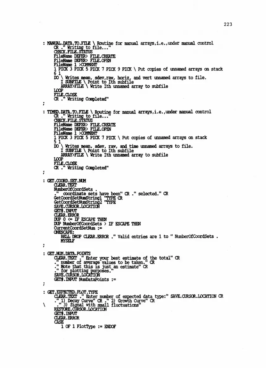
223

: MANUAL.DATA.TD.F1LE \ Routine for manual arrays,i.e.,under manual controlCR ." Writing to file..."CHEK.FILE.STATUSFileName DE R> FILE.CREATEFileName DEFER> FILE.OPENFileName 1 >COMMENT1 PICK 3 PICK 5 PICK 7 PICK 9 PICK \ Put copies of unnamed arrays on stack1

DO \ Writes mean, sdev,raw, horiz, and vert unnamed arrays to file.I SUBFILE \ Point to Ith subfile

LOOPARRAY>F1LE \ Write Ith unnamed array to subfile

FILE.CLOSECR ." Writing Completed"

: T1ED.DATA.TO.FILE \ Routine for manual arrays,i.e.,under manual controlCR ." Writing to file..."CHECK.F1LE.STATUSFileName DEFER> FILE.CREATEFileName DEFER> FILE.OPENFileName 1 >COMMENT1 PICK 3 PICK 5 PICK 7 PICK \ Put copies of unnamed arrays on stack1

DO \ Writes mean, sdev, raw, and time unnamed arrays to file.I SUBFILE \ Point to Ith subfileARRAY>FILE \ Write Ith unnamed array to subfile

LOOPFILE.CLOSECR ." Writing Completed"

GET.CCORD.SCUMUCLEAR.TEXT

M

NumberOfCoordSets .

. coordinate sets have been" CR ." selected." CRGetCoordSetNumStri.ngl "TYPE CRGetCoordSetNumString2 "TYPESAVE.CDRSOR.LOCATIONGEFLINPUTCLEAR.ERRORIMP 0 (= IF ESCAPE THENDUP NumberC1CoordSets > IF ESCAPE THENCurrentCcordSetNum:=ONESCAPE:

BELL DROP CLEAR.ERRCR ." Valid entries are 1 to " NumberOfCoordSetsMYSELF

: GET.NUM.DATA.POINTSCIZAR.TEXT ." Enter your best estimate of the total" CR." number of average values to be taken." CR." Note that this is just an estimate" CR

iAaltir0:420.Pses."GETLINPUT NumDataPoints :=

: GET.EXPECTED.PLF.TYPECLEAR.TEXT ." Enter number of ed data type:" SAVE.CURSOR.LOCAT1ON CR." 1) Decay Curve" CR 2) Gnu Ti Curve" CR

\ " 3) Signal with small fluctuations"RiSTORE.CORSOR.LOCATIONGETLINPUTCLEAR.ERRCRCASE

1 OF 1 PlotType := ENDOF

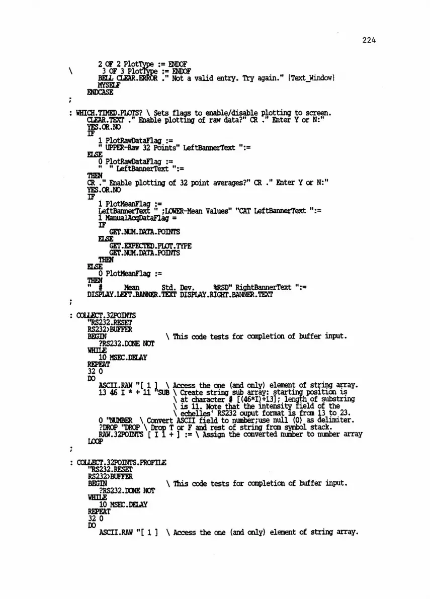
224

2 OF 2 Plot3 OF 3 Plo

BELL CLEAR.MYSELF

ENDCASE

ENDOFENDOF

." Not a valid entry. Try again." (Text Window)

: WHICH.TIMED.PLOWS? \ Sets flags to enable/disable plotting to screen.CLEAR:BLCT ." Enable plotting of raw data?" CR ." Enter Y or N:"YES.OR.NOIF

1 PlotRawDataFlag" UPPER-Raw 32 Points" LeftBannerText ":=

ELSE0 PlotRawDataFlag" "LeftBannerText":=

THENCR ." Enable plotting of 32 point averages?" CR ." Enter Y or N:"YES.OR.10IF

1 PlctMeanFlagLeftBannerText " ;LOWER-Mean Values" "CAT LeftBannerText ":=1 ManualAcgDataFlag =IF

ELSEGET.NUM.DATA.POINFS

GET.EXPECTED.PLOT.TYPE

THENGET.NUM.DATA.PCaNTS

ELSE0 PlotMeanFlag

# Mean Std. De .v USD" RightBannerText ":=DISPLMLEFT.BANNER.TEXT DISPLAY.RIGHT.BANNER.TEXT

: COLLECT.32POINTS"RS232.RESETRS232>BUFFE1BEGIN \ This code tests for completion of buffer input.

?RS232.DCA1E NCRWHILE

10 HSEC.DELAYREPEAT32 0DO

ASCII.RAW "[ 1 1 \ Access the one (and only) element of string array.13 46 I * + 11 SUB \ Create string sub array: starting position is

\ at character # [(46*I)+13]; length of substring\ is 11. Note that the intensity field of the\ echelles' RS232 ouput format is fran 13 to 23.

0 "NUMBER \ Convert ASCII field to numbemse null (0) as delimiter.?DROP "DROP \ Drop T or F and rest of string fran symbol stack.RAW.32P0INTS [ I 1 + ] := \ Assign the converted number to number array

LOOP

: COLLECT.32POINTS.PROFILE"RS232.RESETRS232>BUFFERBEGIN \ This code tests for completion of buffer input.

?RS232.DONE NOTWHILE

10 MSEC.DELAYREPEAT32 0DO

ASCII.RAW "[ 1 ] \ Access the one (and only) element of string array.

13 46 I * + 11 "SUB \ Create string sub array: starting position is\ at character # [(46*I)+13]; length of substring\ is 11. Note that the intensity field of the\ echelles' RS232 ouput format is from 13 to 23.

0 "NUMBER \ Convert ASCII field to number;use null (0) as delimiter.?DROP "DROP \ Drop T or F and rest of string from symbol stack.BackgroundModeCASE

-1 OF RAW.32POINTS.BG-1 I 1 + ENDOF0 OF RAW.32P0INTS.BG0 I 1 + ENDOF+1 OF RAW.32P0INTS.BG+1 I 1 + ENDOF

ENDCASELOOP

SBELL BELL

225

226

ECHO.ON\

RE N7.0

\ James P. Shields\ Department of Chemistry\ Oregon State thiversity\ Corvallis, OR 97331\ (503) 754-2081

Final Revision Completed 10/9/87

\ This code contains most of the menus and main\ control routines. Please refer to my thesis for\ more detailed information about the features of\ this program.

\ Stepper Motor Routines: ZERO.HORIDMITAL.COORD

0 HorizontalCoord :=

: ZERO.VERTICAL.COORD0 VerticalCoord

:210.37111.COORDSZERO.HORIZMITAL.COORD ZERO.VERTICAL.COORD

: GET.ZERO.MOTOR.COORDS.INPUTPCKEY ?DROPCASE

72 OF ZERO.HORMONTAL.COORD ENDOF \ Is input H?86 OF ZERO.VERTICAL.COORD ENDOF \ Is input V?66 OF ZERO.BOTH.COORDS ENDOF \ Is input B?CLEAR.ERROR BELL ." Not a valid choice. Try again"{ Text

scurWindow}

myENDCASE

: ZEROMPOR.COORDS(Text Window) SCREEN.CLEAR

Do you wish to zero the horizontal"OR ." coordinate, the vertical coordinate,"CR ." or both coordinates?" CR 5 SPACES ." Enter H, V, or B: "GET.ZERO.MOTOR.COORDS.1NPUT \ Get input and error trap.CLEAR.ERROR \ Input was OK. Clear any error message.UPDATE.STATUS.L1NE1 MotorControlFlag =IF \ If flag is 1 then are in MANUAL.CONTROL case statement, i.e., do not

\ want to display MA1N.MENU.PROMT(Text Window) SCREE7.CLEAR ." Make a menu selection:"

ELSEMA1N.MENU.PROMPT

THEN

: PRE.MOUNG.MESSAGE(Text Window( CR ." Moving..."

: POST.MOUNG.MESSAGE(Text Window) 2000 MSEC.DELAY CR ." Ready!!!"

: MOVE.HOR1ZONTALLEFT

227

EXECUTE.MUDOR.OPERATION 5 7 SEND.2 PRE.MOWING.MESSAGEHorizontalCoord HorizontalStepSize + HorizontalCoord :1=UPDATE.STATUS.LINE POSTANDE.MESSAGE

: MOVE.HORTZONTAL.RIGHTEXECUTE.MOTOR.CFERATION 6 7 SE1 D.2 PRE.MOVING.MESSAGE 2000 MSEC.DELAYHorizontalCoord HorizontalStepSize HorizontalCoord :=UPDATE.STATUS.LINE FC6T.MOVING.MESSIVE

: MOVE.VERT1CAL.UPEXECUTEACTOR.CPERATION 7 7 SEND.2 PREAVVENG.MESSME 2000 MSEC.DELAYVerticalCoord VerticalSt ize + VerticalCoord :=UPDATE.STATUS.LINE POST. .MESSAGE

: MCNE.VERTICAL.DOWNEXECUTEMBDR.OPERATION 8 7 SEND.2 PREMVINMESSAGE 2000 MSEC.DELAYVerticalCoord VerticalStepSize VerticalCoord :=UPDATE.STATUS.LINE POMMOWING.MESSAGE

: STEPPER.INPUTXENUCLEAR.MENU1 StepperMenuDisplayed?(DM 45 16 GCJIO.XY ." Manual Control Menu "

{Menu Window( 0 0 GOTO.XY4 SPACES ." Use Cursor Keys To Mbve Mirror OR" CR." F1 -Acq Data Point" ." F6-Gross Horiz Mov" CR." F2-Acq Wave Scan" ." F7-NOP" CR." F3-Acq Horiz Scan" ." F8-Edit Step Sizes" CR

F4-Edit Bkgd Mode" ." F9-Zero Coords" CR." F5-Peak Horiz Pos" ." F10-Main Menu"

: STEPPER.1NPUT.PROMPTCLEAR.TEXT ." Make a selection from the menu."CR ." Do not inter-mix the use"CR ." of Fl, F2 and F3 in the"CR ." same acquisition session."

: EDIT.HORIZ/VERT.STEP.SIZESCR ." Current step sizes are:"CR ." Horizontal = " HorizontalStepSize." Vertical = " VerticalStepSizeCR ." Enter new Horizontal Step Size: "SAVE.CURSOR.LCCATICV GETC1NPUT HorizontalStepSize r=CR ." Enter new Vertical Step Size: "SAVE.CURSOLLOCATION GETC1NPUT VerticalStepSize r=UPDATE.STATUS.LINE(Text Window( CR ." Loading new motor ops...Please wait!"LOADMURCE.MIRROR.MOTOR.OPS 4000 MSEC.DELAY CR ." Loading Completed!!!"

INIT.MANUALARRAYSRawMean DUMMY.MEAN.ARRAY [ 1 ] :=DUMMY.MEAN.ARRAY []COPY \ Create unnamed array for future catenation.RawSDev DUMMY.SDEV.ARRAY [ 1 ] :=DUMMY.SDEV.ARRAY []COPY \ Ditto for sdev, raw 32 points, & stepper words.RAW.32P01VDS °COPYHorizontalCoord DUMMY.HOR1Z.000RDS.ARRAY [ 1 ] r=

DUMMY.HORTZ.COORDS.ARRAY ()COPYVerticalCoord DUMMY.VERT.CCORDS.ARRAY [ 1 ] r=DUMMY.VERT.COORDS.ARRAY []COPY

228

: UPDATE.MANUAL.ARRAYSVerticalCoord DUMMY.VERT.COORDS.ARRAY [ 1 ] :=DUMMY.VERT.COORDS.ARRAY CATENATEHorizontalCoord DUMMY.BORIZ.2 ROIL DUMMY.HORIZ.COORDS.ARRAY CATENATE 2 UNROLL3 ROLL RAW.32POINTS LAMINATE 3 UNROLLRawSDev EUMMY.SDEV.ARRAY [ 1 :-4 ROIL DUNKY.SDEV.ARRAY CATENATE -4 UNROLLRawMean DUMMY.MEAN.ARRAY [ 1 ] -5 ROLL DUMMY.MEAN.ARRAY CATENATE5 UNROLL

: SET.MANUAL.WORLDHORIZONTAL 0 NuDataPcdnts WORLD. SET GRID.OFFLowestRawMean 2 / ManualYMin :=Hi tRawMean ManualYMax =VERTICAL ManualYMin ManualYMax WORLD. SET GRID.OFF43 ASCII" SYMBOL

: CHECK.MANUAL.WORLDManualAcqCotmter NtimDataPoints > \ Is horiz. rescale needed?IF

1 ManualRescaleFlag := NbmDataPoints 2 * NtmDataPoints :=THENRawMean ManualYMin <IF

1 ManualRescaleFlag :=RawMean LowestRa0Mean :=

THENRan ManualYMax >

1 ManualRescaleFlagRawMean HighestRawMean

THEN

: MANUAL.PLOT \ See DECAY.PLOT for documentationTIMED.SCREEN1 ManualAcqCounter =IF \ If first time around, set up world.

RawMean LowestRawMean :=RawMean 2 * HighestRawMean :=VUPORT.CLEARSET.MANUAL.WORLDXY.AXIS.PLOT0 DUMMYMAN.ARRAY [ 1 ] =5 PICK DUMMYMAN-ARRAY CATENATEY.DATA.PLaT

ELSECHECK.MANUALACRLD1 ManualRescaleFlag =IF

0 ManualRescaleFlag :=VUPORT.CLEARSET.MANUAL.WORLD

ELSEXY.AXIS.PLOT

SET.MANUAL.WORLDTHEN5 PICKY.DATA.PLOT

THEN

: CALC.MEANODEVRAW.32POINTS MEAN RawMean :=RAW.32POINTS SAMPLE.VARIANCE SQET RawSDev :=

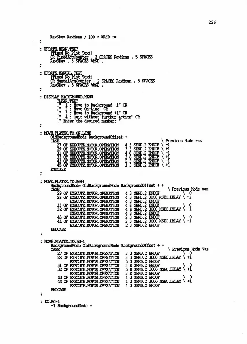
RawSDev RawMean / 100 * %RSD :=

: UPDATE.MEAN.TEXT{Timed No Plot Text'CR TiAE . 2 SPACES RawMean . 5 SPACESRawSDev . 5 SPACES %RSD .

: UPDATE.MANUALTEXT{Timed No Plot Text'CR MarnialIcqCorinter . 2 SPACES RawMean . 5 SPACESRawSDev . 5 SPACES %RSD .

: DISPLAY.BACKGROUND.MENUCLEAR.TEXT

Background -1" CR2 : Move On-Line" CR

." 3 : Move to Background +1" CR

." 4 : Quit without further action" CR

." Enter the desired number: "

:MOVE.PLATEM.CH.LINEOlCASEdBackgroundMode BackgroundOffset +

27 OF EXECUTE.MCITOR.OPERATION29 OF EXECITIE.MCP3R.OPERATION31 OF EXEONE.MOTOR.CFERATION33 OF EXECUTE.MOTOR.CPERATION43 OF EXECUTE.HafOR.OPERATICH45 OF EXECNEADTOR.OPERATION

ENDCASE

\ Previous Mode was4 3 SEND.2 ENDOF \ -13 3 SEND.2 ENDOF \ +14 8 SEND.2 ENDOF \ -13 8 SEND.2 ENDOF \ +12 3 SEND.2 ENDOF \ -11 3 SEND.2 ENDOF \ +1

: MOVE.PLATELTO.BG+1BackgroundMode OldBackgroundMode BackgroundOffset + +CASE \ Previous Mode was

29 OF EXECUTEACTOR.CPERATION 4 3 SEND.2 ENDOF \ 0

28 OF EXECUTEACTOR.CPERATION 4 3 SEND.2 3000 MSEC.DELAY \ -1EXECUTE.MOTOR.OFIRATION

33 OF IMECUTEACTOR.CPERATION32 OF EXECUE.MOTOR.OPERATION

EXECUTE.MOTOR.Cf1RATICN45 OF EXECUTE.ECTOR.OPERATION44 OF EXECUTE.MDTOR.OPERATION

EE

NDCASEXDONE.MOTOR.OPERATION

: MOVE.PLATEX.TO.BG-1BackgroundMode OldBackgroundModeCASE

27 OF EGIUME.11710R.OPERATEIN28 OF EXECUTESOM.OPERATICN

EXECUTEACTOR.CPERATION31 OF EXECUTE.MOTOR.OPERATION32 OF EXECUTE.MOT3LOPERATDON

EXOCINEACTOR.CPERATION43 OF EXECUTE. DTDR.CPERATION44 OF EXECUTE.14110R.OPERATION

ENDCASEMECUILMOIOR.OPERATICN

: DO.BG-1-1 Background Mode =

4 3 SEND.2 ENDOF4 8 SEND.2 ENDOF4 8 SEND.2 3000 MSEC.DELAY

\\ -01

4 8 SEND.2 ENDOF2 3 SEND.2 ENDOF \ 02 3 SEND.2 3000 MSEC.DELAY \ -12 3 SEND.2 ENDOF

BackgroundOffset + +

SEND\ Previous Mode Was

3 3 .2 ENDOF \

3 3 SEND.2 3000 MSEC.DEL \AY +13 3 SEND.2 ENDOF3 8 SEND.2 \ENDOF 03 8 SEND.2 3000 MSEC.DELAY \ +13 8 SEND.2 ENDOF1 3 SEND.2 ENDOF \ 01 3 SEND.2 3000 MSEC.DELAY \ +11 3 SEND.2 ENDOF

229

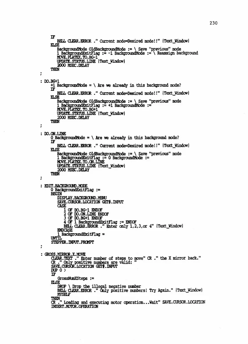
230

IFBELL CLEAR.ERROR ." Current mode=Desired mode!!" {Text Window}

ELSEBackgroundMode OldBackgroundMode ;= \ Save "previous" mode

BackgroundExitFlag r= -1 BackgroundMode := \ Reassign backgroundMOVE.PLATEX.TO.BG-1UPDATE.STATUS.LINE {Text Window}2000 MSEX DELAY

THEN

: DO.BG+1+1 BackgroundMode = \ Are we already in this background mode?IF

BELL CLEAR.ERROR ." Current mode=Desired model!" {Text Window}ELSE

BackgroundMode,OldBackgrondHode = \ Save "previous" mode1 BackgrothidEntFlag := +1 BackgroundMode :=MOVE.PLATEX.TO.BG+1UPDATE.STATUS.L1NE {Text Window}

THEN2000 NSEC.DELAY

: DO.ON.L1NE00F'

BackgroundMode = \ Are we already in this background mode?

ELSEBELL ACLEARWR ." Current mode=Desired mode! !" {Text Window}

BackgroundMode.OldBackgroundlode \ Save "previous" mode1 BackgroundEntFlagi= 0 BackgroundMode r=MOVEJLATEX.TION.L1NEUPDATE.STATUS.LINE {Text Window}2000

TMSW.DELAY

HEN

: EDIT0 .BACKGROUND.MODEBackgroundExitFlag :=

BEGINDISPLAY.BACKGROUND.MENUSAVE.CURSOR.LOCATION GEMINPUTCASE

1 OF DO.BG-1 ENDOF2 OF DO.ON.L1NE ENDOF3 OF DO.BG+1 ENDOF4 OF 1 BackgroundExitFlag EIDOFBELL CLEAR. ERROR ." Enter only 1,2,3,or 4" {Text Window'

ENDCASE1 BackgroundEXitFlag =

UNTILSTEPPER./NPUT.PROMPT

: GROSSAIRROLLMOVECLEAR.TEXT ." Enter number of steps to move" CR ." the X mirror back."CR ." Only positive numbers are valid: "

0SAVE.CURSOR.LOCATION GEMINPUTDUP >

IFGrossNumXSteps :=

ELSEDROP \ Drop the illegal negative numberBELL CLEAR.ERROR ." Only positive numbers! Try Again." {Text Window}MYSELF

THENCR ." LoadiMOTOR ng and

PERATIONexecuting motor operation...Wait" SAVE.CURSOR.LOCATION

INSERT..O

231

9 7 SEND.2 1 1 SEND.2 0 SEND.1 2 SEND.1GrossNumXSteps 9 >IF

GrossNumXSteps "." String'I8reak ":= BREAK.UP.STRENG SEND.2ELSE

GrossNuaSteps SEND.1THENEXECUTEJOTORAMEMIN 9 7 SEND.2GrossNumXSteps HorizontalCoord + HorizontalCoord :=UPDATE.STATUS.LINE {Text Window!2000 MSEC.DELAY RESTORE.CURSOR.LOCATICN CR ." READY"

: GLT.DATA1 ManualAcqDataFlag =IF

DO.IN.PLACE.SCANC0LLECT.32P0INTS CR ." Data collection caapleted."CALC.VEZN&SDEV1 ManualAcqCounter +ManualAcqCounter \ Increment counter1 ManualAcqCounter =IF \ If first time through,

1 GetDataFlag \ GetData mode is active!!!INITANIAL.ARRAYS \ set up unnamed data arrays1 ManualArraysOnStackFlag \ If set, OK to clear arrays from

\ stack at end of session.ELSE

UPDATE.MANUAL.ARRAYSTHEN1 PlotRawDataFlag = IF UPDATE.32POINT.SCREEN THEN1 PlotMeanFlag = IF MANUAL.PLOT THENUPDATEJMANUALTEXT CLEAR.TEXT ." READY!!"

ELSECLEAR.ERROR ."pagsition not active!"STEPPER.INPUT.

THEN

: UPDATE.WIDE.SCANARRAYS33 1 DO

RAW.32POINTS [ I 1RAW.32POINTS.ALL [ManualAcqCounter , I ]

LOOPHorizontalCoord HORIZONTAL.COORDS.ALL [ ManualAcqCounter ]VerticalCoord VERTICAL.CCCRDS.ALL [ ManualAcqCounter ]

: ACQUIRE.WIDE.SCANManualAcqDataFlag =

IF0 ManualAcqCounter =IF \ Is it first time around?

1 WideScanFlag \ If so, then set Wide Scan flag0 RAW.32PCaNTS.ALL := \ Init arrays0 VERTICAL.CCORDS.ALL := 0 HORDEONTAL.COORDS.ALL :=

THENDO.WIDE.SCANCOLLECT.32P0INTS CR ." Wide Scan Completed"1 ManualAcqCounter + ManualAcqCounter :=UPDATE. DE1 PlotRawDataFlag = IF UPDATE.32POINT.SCREEN THENUPDATE.WIDE.SCAN.TEXT.SCREEN CLEAR.TEXT ." READY!!"

ELSECLEAR.ERROR ."Aggsition not active!"STEPPER.INPUT.

THEN

232

: UPDATE.HORIZ.SCAN.TEXT.SCREENRAW.32POINTS 0M1N/MAKSWAP DROP \ Drop the min value(Timed No Plot TextiCR ManiicqColhtter -TYPE2 SPACES .TYPE \ This displays max value

: ACQUIRE.HORIZ.SCAN1 ManualAcqDataFlag = \ Is acquisition active?IF

0 ManualAqCounte =IF \ Is it first

rtine around?

1 HorizScanFlag_p= \ If so, then set this flag0 RAW.32POWS.ALL_:7! \ Init. arra0 VERTICAL.COORDS.ALL := 0 .COORDS.AIL :=

THENDO.HORIZMAL.PROFILECOLLECr.32POINTS CR ." Horizontal Scan Completed"1 ManualAcqCounter + ManualAcqCounter :-UPDATE.WIDE.SCAN.ARRAYS \ Can use this routine here too!!!1 PlotRawDataFlag = IF UPDATE.32POINT.SCREF THENUPDATE.HCRIZ.scAN.TEXT.SCREEN CLEAR.TEXT ." READY!!!"

ELSECLEAR.ERROR "agsition not active!!!"STEPPE:R.1MT.

THEN

:DATAISITION.ACTIVE?CLEAR.TErr ." Do you plan to acquire data?" CR ." (Y or N) :"YES.OR.NO

: CRENTE.MANUAL.FILE.TEMPLATECLEAR.TEXT ." Creating File..."1 PICK 3 PICK 5 PICK 7 PICK 9 PICKFILE.TEMPLATE

1 COMM OFORK.SUBFILE OFORK.SUBFILE OPORM.SUBFILE OFORM.SUBFILE

ENDOFORM.SUBFILE

: CREATESIDE.SCAN.FILLTUIPLATECLEAR.TEXT ." Creating File..."VERTICAL.COORDS.ALL HORMICAL.COORDS.ALL RAW.32POINTS.ALLFILEMMPLATE

ENDcamas OFORM.SUBF1LE OFORM.SUBFILE OFORM.SUBME

:WIDE.SCAN.CUMN.UP0 lian=ftaflag0 Wid

5g :=CLEAR.TEXT Are in WIDE.SCAN.CLEAN.UP" CR. Do you wish to save data to file?" CR ." Enter Y or N:"YES.OR.NOIF

GET.FILE.NAMECREATE.WIDE.SCAN.FILE.TEMPLATEWIDE. SCAN.DATA.TO.F1LE

THEN

: HORIZ.SCAN.CLEAN.UP0 ManualAcqDataFlag0 HorizScanFlagCLEAR.TEXT ." Are in HORIZ.SCAN.CLEAN.UP" CR

233

Do you wish to save data to file?" CR ." Enter Y or N:"."

IFGET.FILE.NAMECREATE.WIDE.SCAN.FTLE.TEMPLATE \ Can use these routinesWIDE.SCAN.DATA.TO.FILE \ here too!!!

THEN

: MANUAL.CLEAN.UP0 Man taFlag := \ Reset flag to zero0 GetDa :=CLEAR.TEXT . Are in MANUAL.CLEAN.UP" CR

Do you want to save data to file?" CR ." Enter Y or N: "iES.OR.NOIF

GELFILE.NAMECREATE.NANUAL.FILE.TENPLATEMiVADILAINA.TO.FILE

THENCR ." Clear arrays from stack? ef or N): "YES.OR.NDIF

CR ." Unnamed arrays are history!!!" DROP DROP DROP DROP DROPELSE

THENCR ." Data arrays have been left on stack!"

ONERR: CLEAR.ERROR BELL__ _"Error #" aRROR# . ." in file I/O.Any_key"WAIT.FOR.A.KEY OLEAR.ERROR ." Error was in MANUAL.CLEAN.uP

: CHECK.MANL1AL.ACQ.MODE1F1 GetDataFlag =

'GetDataFlag1 Cleanup :=

ELSE1 WideScafflag =IF

2 CleanUpELSE

1 HOrizScanFlag =IF

3 CleahUpELSE

0 CleanUp CLEAR.TEXT ." CleanUp = 0 in CHECKANNUAL.ACQ.IME"CR ." This should never appear ill,""'"

THENTHEN

THENeanUp

CASE \ If any acq modes were used, perform appropriate clean up.0 OF ." CleahUp = 0 in CASE!" ENDOF \ In theory, the 0 option should1 OF MANUAL.CLEAN.UP ENDOF \ never be executed.2 OF WIDE.SCAN.CLEAN.UP ENDOF3 OF HORIZ.SCAN.CLEAN.UP ENDOF

ENDCASE

: MANUALOONTROL0 WideScanFlag = 0 HorizScanFlag 0 GetDataFlag0 Fl0Flag := 0 MotorError := 1 MotorControlFlag :=0 ManualArraysOnStackFlag0 CleanUp1 StepperMenuDisplayed? <> \ Is stepper menu flag set?IF

CLEAR.KEYSSTEPPER.INPUT.MENU \ Display menu and prompt if not set.DATLAOQUIS1TION.ACTIVE? \ Returns T if want to acquire data

234

IF1 ManualAcqDataFlag r= \ Manual Data Acq. is active!!0 ManualAcqCounter := \ Initialize counter to 0WHICH.T1MED.PLOTS?

ELSE0 ManualAcqDatanag :=

THEN

THENSTEPPER.INPUT.PROMPT

BEG1N \ EXit condition is Fl0F1ag = 1PCKEY1 MotorEtror = IF CLEAR.ERROR 0 MotorEtror := THENff \ If func key, then I stack is

CASE ss ELSE75 OF HONE.HORIZONTAL.LEFT ENDOF \

truetry agapr9ceinafter error message

77 OF MOVE.HORIZONTAL.RIGHT ENDOF72 OF MOVE.VERTICAL.UP ENDOF80 OF MOVE.VERTICAL.DOWN ENDOFFl OF GET.DATA ENDOFF2 OF r .141DE.SCAN ENDOFF3 OF u r .HOR1Z.SCAN ENDOFF4 OF ED .BACKGROUND.MODE ENDOFF5 OF PEAK.HORIZONTAL.POS1TION ENDOFF6 OF GROSS.M1RROR.ILMOVE ENDOFF8 or EDIT.HOR1Z/VERT.STEP SIZES ENDOFF9 OF ZERMOOR.COORDS ENDOFF10 OF 1 Fl0Flag := ENDOF1 MotorEtror := BILL CLEAR.ERROR \ No match.Display error message.

ENDCASE" Only cursor and Film keys are valid!"

ELSEDROP \ Drop the incorrect entry from the # stack.1 MotorEtror := BELL {Error Window}" Only cursor and Dim keyi are valid!"

THei1 Fl0Flag =

UNTIL0 StepperMenuDisplayed? := 0 MctorControlFlag :=1 ManualAcqDatanag = \ If data acq. is active, check which mode.IF

CHECK.MANUALACIDMODE \ Determine which of the acq. modes was usedTHEN \ and clean house.F10 INTERPRET.KEYONERR

BELL CLEAR.ERROR ." Etrort " ?ERRORC._." detected. Any key." KEY DROPBELL CLEAR.ERROR ." Error was in MANUAL.CONTROL. Any key." KEY DROPSTEPPER.INPUT.PRCion

Plate/PMT Optimization Routines: OFTIMIZE.PLATE.PMT.PROMPT

CLEAR.TEXT ." Make selection fran" CR ." Optimization Menu: "

: BROKEN.COORDS.ON.STACKBROKEN.COORDS [ CurrentCoordSetNUn CurrentCoordVariable , 1 ]DUP thimOtDigits = \ This scalar used for loop index below.NumEchelleCommands = \ The first array element is the actual I of digits.2 ithinCIffigits 1 + DO

BROKEN.COORDS [ CurrentCOordSetNaa,CbrrentCoordVariable , I ]-1 +LOOP \ This puts the individual digits on the stack.

: PLATEX.TOLABS.COORDS1 CurrentCoordVariable =

\ Load pplate X motor operation and execute.EX H}ILE XMENU

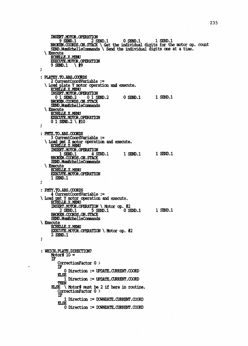
INSERT.MOTOR.OPERATION9 SEND.1 2 SEND.1 0 SEND.1 1 SEND.1

BROKEN.COORDS.ON.STACK \ Get the individual digits for the motor op. countSEND.NUmEchelleCommands \ Send the individual digits one at a time.

\ EkecuteECHELLE.X.MENUEXECUTEMOTOR.OPERATION9 SEND.1 \ #9

: PLATEY.TO.ABS.COORDS2 CurrentCoordVariable :=

\ Load late Y motor operation and execute..X.MENU

INSERTACTORAMOWION0 1 SE2 D.2 0 1 SEND.2 0 SEND.1 1 SEND.1

BROKEN.COORDS.CIN.STACKSEND.NumEchelleCammands

\ ExecuteECHELLE.X.MOWEXECUTE.MOTOR.CfERATION0 1 SEND.2 \ #10

: PMTX.M.ABS.COCRDS3 CurrentCoordVariable :=

\ Load t X motor operation and execute..X.MENU

INSERT.MODOR.OPERATICH1 SEND.' 4 SEND.1 1 SEND.1 1 SOID.1

BROKEN.COCRDS.ON.STACKSEND.NkmiEchelleammands

\ ExecuteECHELLE.X.MENUEXECUTEMOTOR.OPERATION1 SEND.1

PMTY.TD.ABS.COORDS4 CurrentCoordVariable

\ LoaicaLl motor operation and execute.LMENU

INSERT.MCIOR.CPERATION \ Motor op. #22 SEND.1 5 SEND.1 0 SEND.1

BROKON.COORDS.ON.STACKSEND.NumEchelleCannands

\ ExecuteECHELLE.X.MENUEXECUTE.MOTOR.OPERATION \ Motor op. #22 SEND.1

: WHICH.PLATE.DIRECTION?Mbtor# 10 =IF

CorrectionFactor 0 >IF

0 Direction := LTDATE.CURRENT.COCRDELSE

1 Direction := UPDATE.CURREND.COORDTHEN

ELSE \ Motor# must be 2 if here in routine.CorrectionFactor 0 >IF

1 Direction := DOWNDATE.CUREDIT.COORDELSE

0 Direction := DOMRDATE.CLUDIT.COORD

1 SEND.1

235

236

THENTHEN

: WHICH.PMT.DIRECTION? \ If at this routine, Motor# must be 4 or 5.Motor# 4 =IF

Correcticalactor 0 >IF

0 Direction := UPDATE.CURRENT.COORDELSE

1 Direction := UPDATE.CURRENT.COORDTHEN

ELSE \ Mbtor# must be 5 if here in routine.CorrectionFactor 0 >IF

1 Direction DOWNDATE.CURRENT.COORDELSE

0 Direction := DCMNDATE.CURRENT.COCEDTHEN

THEN

: CORREMPLATE/FMT\ Load motor operation 88 with count = correction factorECHELLE.X.MENUINSERT.MCIOR.OPERATION \ Motor op. #888 8 SEND.2

Mbtor# "." StringTOBreak ":= BREAK.UP.STRINGStringLength 3 =IF \ If StringLength= 3,must be motor 2, 4, or 5,i.e., not 10.

SEND.1 \ So just send the one character on the stack.ELSE \ String <>3 so must be motor 10.

SEND.2 \ So send the two chars on stack (0 and 1).THEN

Direction SEND.1 2 SEND.1 \ Send direction and per valuesCorrectionFactor "." StringTOBreak ":=BREAK.UP.STRINGStringLengthL2 - NumEchelleCcomarids :=SENDAtmachelleCcamexis\ EXecute the motor operation.ECHCLIJEXADRIEXECUTEACTOR.CEERAMON8 8 SEND.2 \ Motor op. #88

: CHECK.MAX.INDEXRAW.32POWS SORT&INDEX \ Leaves sorted array 2nd from top, permutation

\ array on top of stack.[ 32 ] MaxIndex# := \ The 32nd element of permutation array is the index

\ of the maximum intensity value in RAW.32POINTS.DROP \ Drop the sorted array.Maxlndex# 32 =IF

1 10r32Flag \ Set flag to TRUE-16 CorrectionFactor :=Mbtor# 2 = Mbtor# 10 = ORIF

2 CorrectionFactor * CorrectionFactorWHICH.PLATE.DIRECTICN?

ELSE

THENWHICH.PMT.DIRECIZCN?

OFERECT.PLATE/PMTMaxim intensity index is" CR

." ." at limit of scan range." CR

."

CouMSECrse ad'Y ustment in progress..."2000

237

THENMax Index, 1 =IF

1 10r32Flag \ Set flag to TRUE16 CorrectionFactorMotor# 2 = Mbtor# 10 = ORIF

2 CorrectionFactor * CorrectionFactorWHICH.PLATEMRECTTON?

ELSEWHICH.PMT.DIRECTICW

THENCORRECT.PLATE/PMT" Maximum intensity index is" CR.

." at limit of scan range." CR" Course adjustment in progress..."

UPDATE.CURRENT.COORD2000 MSEC.DELAY

THEN

: F1ND.HALFAUC.INTENETYRAW.32POINTS (Maxlndex# ] 2 / HalfMaxIntensity

: FIND.HALF.LEFT.INDEKRAW.32POINTS SUB[ 1 , Maxlndex# ] \ Create sub-array of values with

\ indices <=MaxIndexi i.e. to the left.0 ArrayIndex \ Set index to O.BEGIN

1 ArrayIndex + ArrayIndex \ Increment ArrayIndex.DUP \ Dup the unnamed sub-array.[ ArrayIndex] HalfMaxIntensity > \ Is current array value > HalfMaxInt

UNTILDROP \ Drop the unnamed sub-array.ArrayIndex HalfLeftIndex# :=

: FIND.HALF.RIGHT.INDEXRAW.32POINTS SUB( Maxlndex# , 1 32 MaxIndex# + ] \ Create subarray.of

\ values with indices >= MaxIniex# i.e. to the right.2 32 Maxlndex# + Arraylndex :=BEGIN

ArrayIndex 1 - ArrayIndex :=DUP

UNTI(

Arraylndex ] HalfMaxIntensity >L

DROPArraylndex Maxlndex# + 1 - HalfRightlndex# :=

: DETERMINE.PLATE.CORRECTION.FACTOR16.5 Haxindex# - 2 * CorrectionFactor = \ Multiply by 2 here because\ each plate scan step is equal to 2 motor steps.

: DETERMINE.PMT.CORRECTION.FACTORHalfLeftlndex# HalfRightIndex# + 2 / NewPeakIndex#16.5 NewPeakIndex# - CorrectionFactor = \ Do not multiply by 2 here

\ because each PMT scan step = 1 motor step.

: CHECK.PLATE.OPTDIUMMILMITERIACorrectionFactor ABS 1 >

:CHECK.M.OFTIMIZATION.CRITERIACorrectionFactor ABS 1 >

238

: CaRrINUE.OPTIMIZATION?CR ." Continue with optimization?"CR ." Enter Y to continue or"CR ." N to exit to menu level:"POKEY ?DROPCLEAR.ERRORCASE

89 OF FALSE ENDOF \ Is input Y? If so,put False on stack so BEGIN\ UNTIL will not be exited.

78 OF TRUE ENDOF \ Is input N? If so, put True on stack\ to exit the BEGIN...UNTIL

CLEAR.ERBOR BELL " Not a valid choice. Enter Y or N"MYSELF

ENDCASE

: OPTIM1ZE.PLATE0 CadMaxIndex# := 0 CadMaxIntensity0 OptimizedFlag :=

DO.MotorLSCANCOLLECT.32POINTS1 PlotRawDataFlag = IF UPDATE.32POINT.SCREEN THENCHECK.MAX.INDEX0 10r32Flag =IF

DETEMIENE.PLATE.CORRECTION.WPORCHECK.PLATE.OPTMNIZATION.CRIMAIF

CR ." Data collection completed."CR ." Correc. Factor= CorrecticeFactor .TYPECR ." Apply Correction? (Y or N):YES.OR.110IFWHICH.PLATE.DIRECTION?

calRIF-P14TE/PMTCR . New COORDINATE.NAMES "[ CurrentCoordVariable ] "TYPE=

iLATE.PMT.COORDS [ CurrentCoordSetNum , CurrentCoordVariable ]

(.71_1! Executing " COCRDINATE.NARES "[ CurrentCoordVariable ]h77174_,_ Correction Routine...7000 MSEC DELAY \ Give echelle time to do the correction.

ELSECR_." Correction Routine Over- ridden!!!"0 OptimizedFlag \ Make sure exit flag is not set (yet).

THENELSE

1 OptimizedFlag :=THEN

THEN0 10r32Flag._;=1 OptimizedFlag =hCTIF

CORrINUE.OFTIEZATION?ELSE

CLEAR.TEXT ." Data collection completed." CR." Correc. Factor= CorrectionFactor .TYPE

" COORDINATE.NAMES "[ CurrentCoordVariable ] "TYPE ." = "PLATE.PMT.COCRDS [ CurrentCoordSetNum , CurrentCoordVariable ].TYPE CRCOORDINATE.NAMES "f CurrentCoordVariable ] "TYPEiRuEshoud be optimized

THEN

239

UNTIL(Text Window} CR." Select from Optimization Menu:"

OPTIMIZE.MT0 CadMaPxIndex# := 0 01dMaxIntensity :=0 CptimizedFlag \ Make sure exit condition flag _is not set.Mai \ Exit condition for this BEGIN...URTIL is

DO.Motoril.SCAN \ CptimizedFlag = 1COLLECT.32POWSPlotRawDataFlag 1 = IF UPDATE.32POINT.SCREEN THENCHECK.MAX.INDEX \ Routine checks for MaxIndex# = 1 or 320 10r32Flag =IF \ If 1002Flag is set, then skip routines

FIND.HALF.MAX.INTENSITY \ that determine correction factor.FIND.HALF.LEFT.INDEXFIND.HALF.RIGHT.INDEXDETEMIIME.PMT.CORREMON.FACTORCHECK.PLATE.OPTIMIZATICN.CRITERIA \ Returns T if criteriion not metIF

CR ." Data collection ccepleted."CR ." Correc. Factor= CorrectionFactor .TYPECR ." ly Correction? CV or N):YES.CR.

IF \ If T then execute CORRECT.PLATE/PMTWHICH.PMT.DIRECTION?CORRECT.PLATEiPMTCR . New " COORDINATE.NAMES "[ CurrentCoordVariable ] "TYPE

kATE.PMT.COCRDS [ CurrentCoordSetNum , CurrentCoordVariable ]

.

CREXecuting " COORDINATErNAMES "[ CurrentCoordVariable ] "TYPE

" Correction Routine..."8000 MSEC.DELAY

ELSECR_." Correction Routine Over-ridden!!!"0 OptimizeiFlag := \ Make sure exit flag is not set (yet).

THENELSE1 CptimizedFlag := \ Set HEGIN..UNTIL exit condition flag.

THENTHEN0 1002F1 := \ Reset 1002Flag to 01 Opt = \ Is exit condition satisfied?

IF \ Test for exit condition here becauseCONTINUE.OFTIMIZATIM \ don't want to.prompt to continue if

ELSE \ already optimized.CLEAR.TEXT ." Data collection completed. CR. Correc. Factor= CorrectionFactor .TYPE CR1__" New COORDINATE.NAMES "[ CurrentCoordVariable ] "TYPE 1" = "PLATE.PMTCOCEDS [ CurrentCoordSetNum , CurrentCoordVariable ].TYPE CRCOCRUNATE.NAMES "[SurrentCoordVariable ] "TYPE

should be optimized."TRUE \ Replace TRUE value on stack for the UNTIL

THENUNTIL(Text Window' CR ." Select from Optimization Menu: "

: OPT1MIZE.PLATEX2 Motor# := \ 2-->P1ateX;4--)PMTX;5--)PHTY;10-->PlateY1 CurrentCoordVariable := \ 1-->PlateX;2-->PlateY;3-->PMTX;4-->PMTYCPTIMIZE.PLATE

240

: OPTIMIZE.PLATEY10 Motor# :=2 CurrentCoordVariable :=OPTIMIZE PLATE

: OP' 7E PMTX4 Motor# :=3 CurrentCoordVariable :=OPTIMIZE PMT

: OPTIMIZE.PMTY5 Motor# :=4 CurrentCoordVariableOPTIMIZE.PMT

:PLATEMIT.TO.ABS.CCORD.SETCLEAR.TEXT ." Honing Plate..." PLATE.HOME 4000 MSEC.DELAYCR Homing PMT... PMT.#0ME 5000 MSEC.DELAYCR ." Moving Plate X to coordinates..."

PLATEX.TO.ABS.COORDS 9000 MSEC.DELAYCR ." Moving Plate Y..." PLATEY.110.ABS.COORDS 9000 MSEC.DELAYCR ." Moving PMT X..." PMTX.M.ABS.COORDS 9000 MSEC.DELAYCR ." Moving PMT Y..." PMTY.TO.ABS.COORDS 9000 MSEC.DELAY

: BYPASS.PLATE/PMT.113.ABS.000RD.SEI?CLEAR:MKT ." Enter B to Bypass honing and" CR

to-coordinate routines and perform CR."

." optimization at current coordinates." CR

." Otherwise, enter C to Continue: "i'CREY ?DROPCASE

66 OF FALSE ENDOF \ Is input B? If so,67 Cr TRUE ENDCF \ Is input C?CLEAR.ERBOR BELL ." Not a valid choice.(Text WimlowlMYSELF

ENCASE

put FALSE on stack.

Try again"

: OPTIMIZE.PLATE.PMT.MENUCLEALMENUCLEAR.KEYSiDEFI 45 16 GOTO.XY \ Make all of these start at 45. Text can be up to

\ 27 chars with the rest taken up by spaces.," Optimization Menu " CR(Menu Window} 0 0 GC/P3.XY." ." Optimize Plate X" CR." F2" ." - Optimize Plater CR." F3" ." Optimize PMT X" CR." F4" ." Optimize PMT Y" CR" F10" ." - Return TO Main Menu"

: CPTIMIZE.PLATE.PMT1 NumberOfCoordSetsFlag <> \ Has the number of lines been specified yet?IF

SPECIFY.NUM.COORD.SETS

II Enter the number of the coordinate" GetCoordSetNumStringl ":=" set you wish to optimize' GetCoordSetNumString2 ":=GET.COORD.SET.NUMCLEAR.TEXT ." Enable plotting of raw data?" CR ." Eater Y or N:" YES.OR.hDIF

1 PlotRaWDataFlag

241

" Raw 32 Points" LeftBannerText ":= " " RightBannerText ":=ELSE

" RightBannerText ":= " " LeftBannerText ":=0 PlotRawDataFlag

THENDISPLAY.LEFT.BANNER.TEXT DISPLAY.RIGHT.BANNER.TEXTBYPASS.PLATE/PMT.TO.ABS.COORD.SET?IF

PLATE/PMT.TO.ABS.COORD.SETTHENOPTIMIZE PLATE.PMT.MENUOPTIMIZE.PLATE.PMT.PROMPTFl FUNCTION.KEY.DOES CPTIMIZE.PLATEXF2 FUNCTION.KEY.DCES OPTIMIZE PLATE?F3 FUNCITON.KEY.DOES OPTIMIZE PMTXF4 FUNCTION.KEY.DOES OPTIMIZE.PMTY

Echelle Utilities: DISPLALCURRENT.VALUES

51DO

CLEAR.TEXT" Current " COORDINATE.NAMES: "[ I ] "TYPE

ilATE.PMT.COORDS [ CurrentCoordSetNum , I ] .TYPE CREnter new value or 0 to keep" CR .' old value:

iAVE.CURSOR.LOCATDONGEMINPUTDUP 0 <>IF

PLATE.PMT.COORDS CurrentCoordSetNum , I ]ELSE

THENDROP \ Drop the zero entered to keep old value.

LOOP

: ECHEL1,E.UT1L.PROMPTCLEAR.ERROR CLEAR.TEXT ." Make a selection from the" CR." Echelle Utilities Menu: "

: BREAK.UP.CCORDINATES51DO

PLATELPMT.COORDS [ CurrentCoordSetNum , I ] "." StririgToBreak ":=BREAK.UP.STUNG \ Put individual digits on stack. First digit of

\ string ends up on top of stack.StringLeogth 2 - \ Put actual # of digits on stack.StringLength 1DO

BRCEEN.COORDS [ CurrentCoordSetNum J , I ] :=LOOP

LOOP

: ED1T.CREATE.COORDINATE.SET" Which line do you wish to" GetCoordSetNumstringi" specify coordinates for: " GetCoordSetNumString2 '.-GET.00ORD.SET.NUMDISPLAY.CURRENT.VALLESBREAK.UP.COORDINATESECHELLE.UTIL.PFKMPT

: CHANGE.NUM.COORDINATE.SETSCLEAR.TEXT ." The number of coordinate sets has" CR

242

." been previously set to " NuinberOfCoordSets .TYPE ." ."CR

." Enter the desired new number" CR" of coordinate sets: "iAVE.CURSOR.uxAncvGET#.1NPUTNumberWoordSets :=1 NumberOfCoordSetsFlag :=ECHELLEXTIL.PROMPT

: CREATE.00ORDINATE.F1LEFILE.TEMPLATE

1 COMMENTSINTEGER DIME 4 ] SUBFILE

END

: GET.COORDINATE.FILE.NAMECLEAR.TEXTGetCoordinateFileNameStringl "TYPE CRGetCoordinateFileNameString2 "TYPE"INPUT " .PRM" "CAT CoordinateSetFileName ":=

: COORDMATE.SELTO.FILESTXK.CLEA" Eater the number of the coordinate" GetCoordSetNumStringl ":=" set to be written to file: GetCoordSetNumString2 .=

GET.COORD.SELNUM" Enter file name for coordinate set." GetCoordinateFileameString1 ":=" (Automatic .PRM extension): GetCoordinateFileNameString2 .-

GET.COORDINATE.FILE.NAMECLEAR.TEXT ' Wait.. .File being created."CREATE.00cennarEsiazCoordinateSetFileName DEFER> FILE.CREATEPLATE.PNT.COORDS XSEOT[CurrentCoordSetNUm , ! ] TRANSFER.TO.F1LE :=CR beingwEitten to."CoordinateSetFileName DEFER> FILE.CPENCoordinateSetFileName 1 >CCMMENT1 SUBFILE TRANSFER.'IO.FILE ARRAY>FILE FILE.CLOSEECHELLEATTEL.PROWT

ONERR: CLEAR.ERROR BELL " Can't open file for writing"?FILLOPEN FILLCLOSE THENCLEAR.TEXT ." any key to continue..." PCKEY ?DROP DROPECHELLEATTIPROMPT

: COORDINATE.SET.FROM.FILE" Enter file name. Do not enter file" GetCcordinateFileNameStringl "::" extension (.PRM assumed): GetCoordinateFileNameString2 ":-GET.COORDMRATE.FILE.NAME" Enter the number of the coord set" p etCoordSetNumStringl ":=" to be written over by file contents:' GetCoordSetNumString2 ".=GET.COORD.SETJUICLEAR.TEXT_. Wait...Reading File."CoordinateSetFileName DEFER> FILEXPEN1 SUBFILE TRANSFER.FROM.FIIE FILE>ARRAYFILE.C1OSE51DO

TRANSFER.FROK.FILE [ I 3 \ Copy from transfer arrayPLATE.PMT.CCORDS [ CurrentCoordSetNum , I ] \ to working array

LOOPBREAK.UP.COORDINATESCLEAR.TEXT ." The transferred coordinates are:" CR51DO

243

3 I = IF 2 SPACES THENCOORDINATE.NAMES "[ I ] "TYPE TRANSFER.FROM.F1LE [ I ] .TYPE3 I = IF 2 SPACES THEN 1 SPACES

2CO+LOOPORD1NATE.NAMES: "[ I 1 + ] "TYPE TRANSFER.FROM.F1LE [ I 1 + ] .TYPE CR

CLEAR.ERROR (Text Window} ." Make a selection from the" CR." &belle Utilities Menu: "

\ Normally would call ECHELLE.UTIL.PROMPT here\ but use this to prevent near-instant erasure of the\ displayed transferred coordinates.

ONERR: CLEAR.ERROR BELL ." Bad or non-existent file."?FILLOPEN IF F1LE.CLOSE THENCLEAR.TEXT ." Hit any key to continue..." PCKEY ?DROP DROPECHELLE.UT1L.PROMPT

: LIST.COORDINATEISET.FILE.NAMICCLEAR .TEXT Tyauremlm Ecar ; CR ." hit any key." CR

logtRYRtifELEALTEXT DI*.MCR ." Hit anyipsy_to continue" PCKEY ?DROP DROPECHELLEMIL.PROMFT

: SPECIFY.SCAN.PARAMEMS

PARAMETER.PRINT.FROM.CURRENT.COORD.SETthe coordinate" GetCoordSetNumStringl ":=

GetCoordSetNumString2 ":=

OFF \ Set printer as only output device.Coordinate Set Number " .TYPE CR

" Enter the number of" set to print out:GET.COORD.SET.NUMOUT>PRINTER CONSOLE.Cur1 rentCbordSetNum ."5DOI 3 >=IF

2 SPACES COORDINATEMMES: "[ I ] "TYPEPLATE.PMT.COORDS [ CurrentCoordSetNum , I ] .TYPE CR

ELSECOORDINATE.NAMES: "[ I ] "TYPEPLATE.PMT.COORDS [ CurrentCoordSetNum , I ] .TYPE CR

THENLOOP CR CONSOLE

PARAMETER.PRINT.FROM.FILEEater file name. Do not enter file" GetCoordinateFileNaiueStringl ":=

" extension (.PRM assumed): GetCoordinateFileNameString2 ":=GET.COORDINATE.FILE.NAMECoordinateSetFileName DEFER> FILLOPEN1 SUBF1LE TRANSFER.FBOM.FILE FILE>ARRAY FILE.CLOSECoordinateSetFileName \ Put on stack for ID purposes in print outOFT>FRINTER CONSOLE.CFF \ Set)system,output to printer only.' Parameters from the file " "TYPE : CR

51DO

I 3 >=IF

2 SPACES COORDINATE.NAMES: "[ I ] "TYPE TRANSFER.FROM.F1LE [ I ].TYPE CR

ELSECCORDINATE.NAMES: 1 I ] "TYPE TRANSFER.FROM.F1LE [ I ] .TYPE CR

THENLOOPCR CCtISOLE \ Set system output back to console only.

CNERR: CLEAR.ERROR BELL " Bad or non-existent file on read try."

?FILE.OPEN IF FILE.CLOSE THENCLEAR.TEXT ." Hit any key to can inue..." POKEY ?DROP DROPECHELLE.UTIL.PROMPT

: PRINT.A.COORD.ITCLEAR.TEXT ." Should print out ori to from" CR3 SPACES ." 1) . A Parameter e" CR3 SPACES ." 2) "" A Currently Specified Coord Set" CR CR ." Eater a number:

iAVE.CURSCR.ILCATIONGEMINPUTIMP DUP 0 <= OR 3 )=. IF ESCAPE THEN1=IF

PARAMETER.PRINT.FROM.F1LEELSE

PARAMETER.PUNT.FROM.CURRENT.COORD.SETTHENECHELLE.UTIL.PROMPTONESCAPE:

BELL CLEAR.ERROR ." 1 and 2 are the only valid entries here!"DROP MYSELF \ Must drop the invalid entry from stack

: ECHELLE.UTIL.MENUCLEAR.KEYS CLEAR.MEWUTOFF} 45 16 GCTO.XY ." &belle Utilities MenuiMenu Window} 0 0 GOTO.XY." ." -Ed/Create CoordSet." F6-NOP" CR." F2" ." -Chge # CoordSets"." P7" ." -Prnt a CoordSet" CR." F3" ." -CoordSet To File"."

P8' ." -NOP" CR" F4" ." -CoordSet Fran File"

.1111 ...NorCR

" F5" ." -Lst CoordSet Files"." F10" ." -Main Menu"

: ECHELLE.UT1L1 NumberOfCoordSetsFlag <> \ Has the number of lines been specified yet?IF

SPECIFY.NUM.COORD.SETSTHENECHELLE.UTIL.MENUECHELLE.UTIL.PROMPTF1 FUNCrION.KEY.DOES EDIT.CREATE.COCRDINATE.SETF2 FUNCTION.KEY.DOES CHANGE.NUM.COORDINATE.SETSF3 FUNCTICCKEY.DOES COORDINATE.SET.TO.FILEF4 FUNCTION.KEY.DOES COORDINATE.SET.FROM.FILEF5 FUNCTION.KEY.DOES LIST.COORDINATE.SET.FILE.NAMESF6 EUNCTDON.KEY.DOES SPECIFY.SCALPARAMETERSF7 FUNCTION.KEY.ECES PRINT.A.COORD.SET

&belle Set-Up Routines

: ECHELLE.SET.UP.MENUCLEAR.KEYS CLEAR.MENUMEN 45 16 GOMM ." Echelle Set-Up Menu{Menu Window} 0 0 GOTO.XY." Fr- Down Load PCode" CR." F2 Load Ho Mirror Motor Correction" CR." F3 - Set Integration Time (Default=2)" CR

244

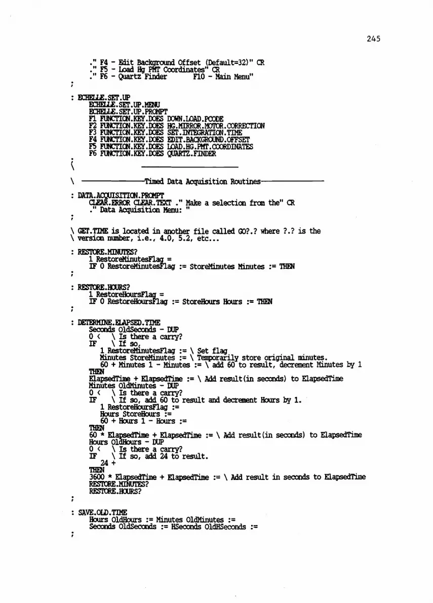
245

." F4 Edit Background Offset (Default=32)" CRHg." F5 - Load PMT Coordinates" CR

." F6 Quartz Finder F10 - Main Menu"

: ECIELLE.SET.UPECHELLE.SET.UP.MENUECEELLE.SET.UP.PROMPTFl IIKTICN.KEY.LOES DOWN.LOAD.PCODEF2 FUNCTION.KEY.DOES HG.MERROR.MCiPOR.CORRECTIalF3 FUNCTION.KEY.DaES SET.INTEGRATICN.TDEF4 FUNCTION.KEY.LOES EDIT.BACKGRCUID.OFFSETF5 PUNCTION.KEY.DOES LOAD.HG.PMT.COORDIMTESF6 FUNCTICN.REY.DOES QUARTZ.FINDER

Timed Data Acquisition Routines

: DATA. SITION.PROMPTEARL .ERROR CLEAR.TEXT ." Make a selection from the" CR

." Data Acquisition Menu: "

\ GELTIME is located in another file called GO?.? where ?.? is the\ version number, i.e., 4.0, 5.2, etc...

: RESPOREJIENUTES?1 RestoreMinutesFlag =IF 0 RestoreMinutesFlag := StoreMinutes Minutes := THEN

: RESTORE.HOURS?1 RestoreHour=IF 0 RestoreHsFlagoursFlag StoreHours Hours := THEN

: DETERMINE.ELAPSED.TIMESeconds OldSeconds DUP0 < \ Is there a carry?IF \ If sot

1 RestoreMinutesFlag \ Set flagMinutes StoreMinutes \ Temporarily store original minutes.60 + Minutes 1 Minutes \ add 60 to result, decrement Minutes by 1

THENElapsedTime + ElapsedTime \ Add result(in seconds) to ElapsedTimeMinutes OldMinutes DUP0 < \ Is there a carry?IF \ If so, add 60 to result and decrement Hours by 1.

1 RestoreHoursFlagHours StoreHours60 + Hours 1 Hours

THEN60 * ElapsedTime + ElapsedTime \ Add result(in seconds) to ElapsedTimeHours OldHours - DUP0 < \ Is there a carry?IF \ If so, add 24 to result.

24 +THEN3600 * ElapsedTime + ElapsedTime := \ Add result in seconds to ElapsedTimeRESTORE.M1NUTES?RESTORE.HOURS?

: SAVE.OLD.T1MEHours OldHours := Minutes OldMinutesSeconds OldSeconds HSeconds OldHSeconds :=

246

: IN1T.UNNAMED.ARRAYSRawMean DUMMMENN.ARRAY [ 1 ]DUMMY.MEAN.ARRAY ()COPY \ Create unnamed [ 1 ] mean array and leave on

\ stack for future catenations.RawSDev DUMMY.SDEV.ARRAY [ 1 ] :=DUMMY.SDEVARRAY []COPY \ Create unnamed [ 1 ] sdev array and leave on

\ stack for future catenations.RAW.32P0INTS ()COPY \ Create [ 1 , 32 ] unnamed raw data array

\ i the first data set) and leave on stack for future lamination.0 DUMMY APSED.TIMEJRRAY [ 1 ]DUMMY.ELAPSED.TIME.ARRAY ()COPY \ Create [ 1 ] unnamed time array from

\ dummy time array and leave on stack for future catenation.

: UPDATE.UNNAMENARRAYSE1apsedTime DUMMY.ELAPSED.T1ME.ARRAY [ 1 ] \ Move scalar value to arrayDUMMY.ELAPSED.TIME.ARRAYCATENATE \ Catenate Dummy time array with unnamed elapsed time

\ array already on stack.2 ROLL \ Bring second unnamed array on stack to top for lamination.RAW.32POINTS LAMINATE \ Laminate with ummaned raw data array

already on tadk.2 UNROLL \ Put it back

\to second on

sstack.

RawSDev DUMMY.SDEV.ARRAY [ 1 ] r=3 ROLL \ Bring third unnamed array on stack to top for catenation.DUMMY.SDEV.ARRAY CATENATE \ Catenate with unnamed sdev array

\ already on stack.3 UNROLL \ Put it back to third on stack.Ra0Mean DUMMMENN.ARRAY [ 1 ] r= \4 ROLL \ Bring fourth unnamed array on stack to top for catenation.DUMMMEAN.ARRAY CATENATE \ Catenate with unnamed mean array

\ already on stack.4 UNROLL \ Put it back to fourth on stack.

: SET.DECAY.WORLDHORIZOITAL 0 NumDataPoints WORLD.SET GRID.OFFVERTICAL O. HighestRawMean DUP 20. / + WORLD.SET GRID.CFFDOTTED \ Use dotted line type

: CHECK.DECAY .WORLDRaftan HighestRawMean > \ Is vertical rescale needed?IF \ If so,

1 DecayRescaleFlag \ set rescale flagRa0Mean HighestRawMean r= \ re- assign highest mean scalar.

THENTimedAcqCounter NumDataPoints > \ Is horizontal rescale needed?IF

1 DecayRescaleFlag r=NumDataPoints 3 / NumDataPoints + NumDataPoints :=

THEN

: DECALPLOTTIMED. SCREEN1 TimedAcgCounter =IF \ If first time around, set up world.

RawMeanahestRawMeanVUPORT.SET.DECAY.WORLDXY.AXIS.PLOT0 DUMMUREANARRAY [ 1 ] = \ This catenates a 0 to unnamed=4 PICK DUHKUKEAN.ARRAY CATENATE \ for plotting first time aroundY.DATA.PLOT \ because can't plot a 1 element array.

ELSECHECK.DECALWORLD \ Check for over range

247

1 DecayRescaleFlag = \ Is a rescale needed?IF \ If so,

0 DecayRescaleFlag r= \ Reset flag to 0VUPORT.CLEARSET.DECAY.WORLD \ Set up new worldMAXIS.PLO \ Plot new axes.

ELSE

THENSET.DECAY:WDRLD

4 PICK \ Duplicate unnamed mean data array(4th on stack) to stack top.Y.DATA.PLOT

THEN

: SET.GROWTH.WORLDHORIZONTAL 0 NumDataPoints WORLD.SETLowestRawMean 5. / GrowthYMin r=HighestRawMean 2. * GrowthYMax :=VERTICAL GrowthYMin GrowthYMax WORLD.SETDOTTED

GRID.OFF

: CHECK.GROWTH.WORLDTimedAcqCounter NumDataPoints > \IF

1 GrowthRescaleFlag r=NumDataPoints 2 / NumDataPoints

THENRawMean GrowthYMinIF

1 GrawthRescaleFlag :=RawMean LowestRawMean :=

THENRawMean GrowthYMax >IF

1 GrowthRescaleFlag :=RawMean HighestRawMean :=

THEN

GRID.OFF

Is horizontal rescale needed?

+ NumDataPoints :1=

: GROWTH.PLOTTIMED. SCREEN1 TimedAcqCounter =IF

RawMean LowestRawMeanRawMean 5. * HigtiestRawMean :=VUPORT.CLEARSET.GROWTH.WORLDXY.AXIS.PLOT0 DUMMY.MENICARRAY [ 1 ] r=4 PICK DUMMY.MEAN.ARRAY CATENATEY.DATA.PLOT

ELSECHECKARDWTH.WORLD1 GrowthRescaleFlag =IF

VUPORT.CLEAR0 GrowthRescaleFlag :=SET.GROWTH.WORLD

ELSEXY.AXIS.PLOT

THENSET.GROWTH.WORLD

4 PICKY.DATA.PLOT

THEN

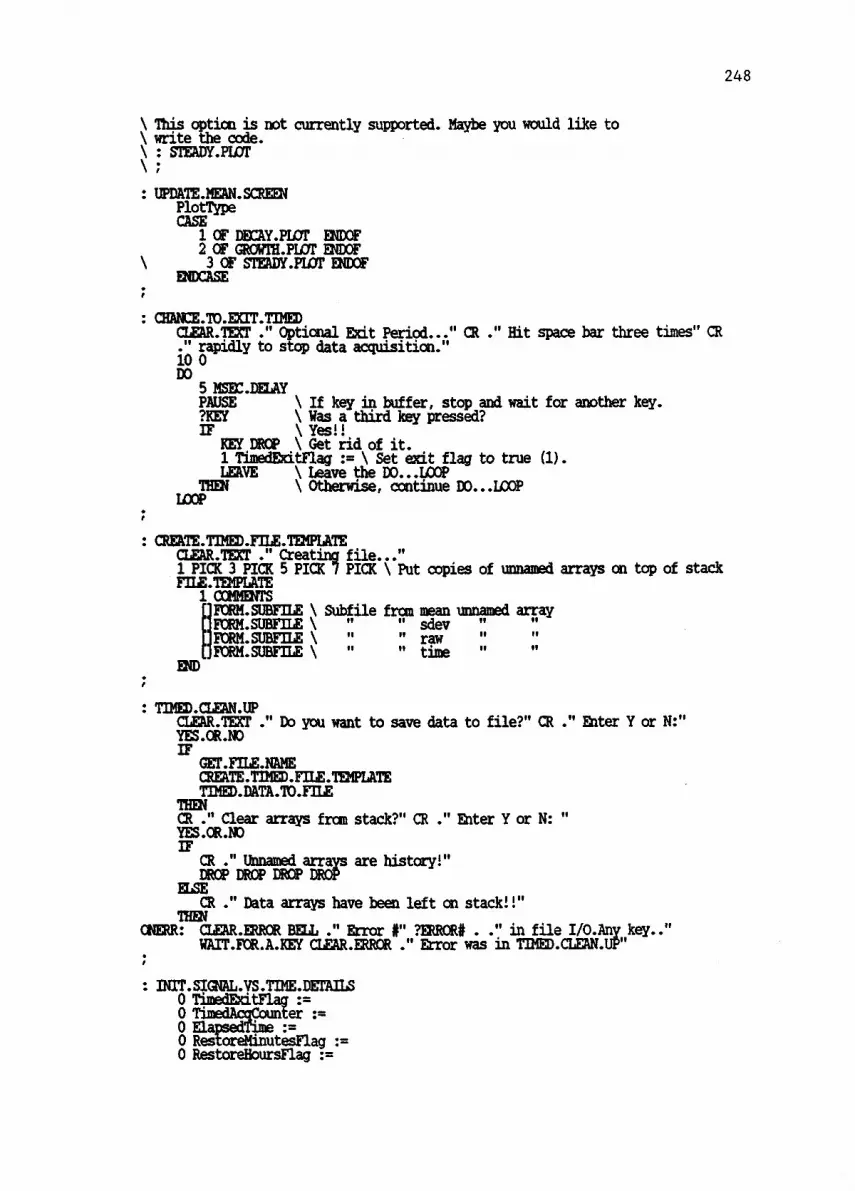
248

\ This option is not currently supported. Maybe you would use to\ write the code.\ : STEADY.PLOT\;

: UPDATE.MEAN.SCREENPlotTypeCASE

1 OF DECAY.PLOT ENDOF2 OF GROWTH.PLOT ENDOF3 Cr STEADY.PLOT ENDOF

ENDCASE

: CHANCE.TO.EXIT.71MEDCLEAR-TEXT Optimal EXit Period..." CR ." Hit space bar three times" CR. rapidly to stop data acquisition."10 0DO

5 MSEC.DELAYPAUSE \ If key in buffer, stop and wait for another key.?KEY \ Was a third key pressed?IF \ Yes!!

KEY DROP \ Get rid of it.1EATimedExi

\

tFlagLeave the

\

eSet

O,exit

LOOPflag to true (1).

LVE D..

LOOPTHEN \ Otherwise, continue DO...LOOP

;

: CREATE.TIMED.FILE.TEMPLATECLEAR.TErr t_ Creating file..."1 PICK 3 PICK 5 PICKK7 PICK \ Put copies of unnamed arrays on top of stackF1LE.TEMPLATE

1 COMMENTSFORM.SUBFILE \ Subfile fran mean unnamed arrayFORK.SUBFILE \ sdevFORM.SUBFILE \

11" raw "

9

FORM.SUBFILE \ " " time11 11

END

: TIMED.CLEAN.UPCLEAR.TErr ." Do you want to save data to file?" CR ." Enter Y or N:"YES.ORADIF

GET.FILE.NAMECREATE.TIMED.FILE.TEMPLATE

TTIMED.DATA.TO.FILE

HENCR ." Clear arrays from stack?" CR ." Enter Y or N: "YES.OR.NOIF

CR ." Unnamed arrays are history!"DROP DROP DROP DROP

ELSE

THENCR ." Data arrays have been left on stack!!"

ONERR: CLEAR.ERIM BELL ." Error #" ?ERRCR# . ." in file I/O.Any key.."WAIT.FOR.A.ICEY CLEAR.ERROR ." Error was in TIMED.CLEAN.UP"

: IN1T.SIGNAL.VS.T1ME.DETA1LS0 TimedEXi0 TimedAcqCoun er0 ElapsedTime0 RestoreMinutesFlag0 RestoreHoursFlag

249

TINED.SCREEN VUPORT.CLEAR32POINT.SCREEN VUPORT.CLEAR

James P. Shields" LeftBannerText _"=

" Data Acq. & Anal. Routines" RightBannerTextDISPLNY. .BANNER.TEXT DISPLAY.RIGHT.BANNER.TEXT

\ SIGNAL.VS.TIME is located in the file called G07.0

\ Code for moving to another set of coordinates while in spatial acq. mode.: MOVE.TO.ANOTHER.LINE

Enter the number of the coordinate" GetCoordSetNUmStringl ":=" set :you wish to move to: " GetCoordSetNumString2 ":=GET.COORD.SET.NUMPLATE/PMT.TO.ABS.COCRD.SETCR ." Make a seleection frau the" CR ." Data Acquisition Menu: "

S

Horizontal Profile routines

: GET.SPATIAL.BG.MODE.MENUCLEAR.TEXT." 1 : No Background Correction" CR." 2 : Background -1 Correction" CR." 3 : Background +1 Correction" CR." 4 : Background -1 & +1 Correction" CR." Enter the desired number: "

: GET.SPNTIAL.BGLMODEGET.SPATIAL.BGMODE.MENUSAVE.CURSOR.LOCATION GEMINPUTCASE

1 OF 1 SpatialBGMode ENDOF2 OF 2 SpatialBGMode := ENDOF3 OF 3 SpatialBGMode := ENDOF4 OF 4 SpatialBGMode ENDOFBELL CLEAR.ERROR ." Enter only 1,2,3,or 4" {Text Window( MYSELF

ENDCASE

: GETAUM.HORIZTEAL.SCANSCLEAR.TEXT ." Enter desired number of" CR ." horizontal scans (10 max.): "GETLINPUTEUP 10 IF CR BELL ." Number must be <=10. Try again." DROP MYSELF THEMNumHorizontalScans :=

: GET.SPATIAL.RANRESLEAR.TEXT ." Current a iticozeters are:" CR

Horizontal Range = " rizont .TYPE CR." Horizontal Counts/Step = HbrizontalCounts/Step.TYPE CR." Vertical Step Up Size = " VerticalStepUpSize .TYPE CR." Do you wish to change any of these?" CR ." Eater Y or N: "YE.OR.NDIFcmigxT

new." Old Horizontal Range = " HbrizontalRange .TYPE CR

iAVECURSOR.LOCATDON GETIalRMIT HogzontalRange_:=CR it'lad

newHorizontaldiuntsint= Rorizontalcounts/Step .TYPE CR

iAVE.,CURSOR.LOCATION GEMINPUT,H:fizontalCounts/StepCR liot5d Vergftligte&Size = '"VerticalStepUpSize .TYPE CR

newiAVE.CURSOR.LOCATION VerticalStepUpSize :=LOAD.SPATIAL.MOTOR.OPS

250

THENCR ." VAIT...icading new motor cps..." 2000 MSEC.DELAY CR CR ." MDT'

: WHICH.SPATIAL.PLPlo

OTS?CLEAR.TET horizontal profiles?" CR

Eater Y or YES.ut.huIF 1 PlotBProfileFlag := THEN

:COLLECT.BG00 BackEroumdMode \ Set this scalar for CASE in COLLECT.32POINTS.PROFILE00.140R1ZCNTAL.PROMECOLLECT.32PCINTS.PROFILE CR ." On Line Profile Completed."\ Data is in the array RAW.32POINTS.BGO

: COLLECT.BGO/BG-1COLLECT.BG0-1 BackgroundMcde := \ Set to -1 to direct raw data to RAW.32POINTS.BG-1

arr COLLECT.32POIN TS .i.e.,0 OldBackgroundMcde :=

\\ We

ayknowin

old mode was 0,PRF1LEe on-line. This is

\ set for CASE in M3NE.PLATEX.TO.BG-1MOVE.PLATEX.TO.BG-1 CR ." Moving PlateX to BC -1..." 3000 MSEC.DELAYDO.HORED3NTAL.PROFILECOLLECT.32POINTS.PROF1LE CR ." Profile completed."\ Data is in RAW.32POINTS.BG-1 arr .

0 BackgroundMode := -1 01 e =MOVE.PLATEX.10.01.LINE CR ." Moving PlateX to on line..." 3000 MSEC.DELAY

: CCLLECT.BGO/BG+1COLLECT.BG0+1 BackgroundMode := \ Set to +1 to direct raw data to RAW.32POINTS.BG+1

\ array in COLLECT.32PC1NTS.PRICIILE0 OldBackgroundMode \ We know old mode was 0, i.e., on-line. This is

\ set for CASE in MOVE.PLATEX.TO.BG+1MOYE.PIAMX.TO.BG+1 CR ." Moving PlateX to BG+1..." 3000 MSEC.DELAYDO.HORIZOTTAL.PROFILECOLLICT.32POINTS.PROFME CR ." BG+1 Profile Completed."\ Data is in RAW.32POINTS.BG+1 arra .0 Bad de := +1 CI eMOVE.PLATEUTD.ON.LINE CR ." Moving PlateX to on line..." 3000 MSEC.DELAY

: C0LLBCT.BGO/BG-1/BG+1COLLECT.BG0 \ Collect on line data-1 BackgroundMode \ Set to -1 to direct raw data to RAW.32POINTS.BG -1

\ array in COLLECT.32POINTS.PROFILE0 CldBackgroundMode \ We know old mode was 0, i.e., on-line. This is

\ set for CASE in MOVE.PLATEX.TO.BG-1MOVE.PLATEX.TO.BG-1 CR ." Moving PlateX to BG-1... 3000 MSEC.DELAYDO.HORIZONTAL.PROF1LECOLLECT.32PC1MTS.PROFILE CR ." BG-1 Profile Completed."\ Data is in RAW.32PC1NTS.BG-1 array.+1 BackgroundMode = -1 OldBackgroundModeMOVE.PLATEX.TD.BG+1 CR ." ?tying PlateX to BG+1..." 3000 MSEC.DELAYDO.HCRIZONTAL.PROF1LECOLLECT.32POINTS.PROFILE CR ." BG+1 Profile Completed."\ Data is in RAW.32POINTS.BG+1 arra .0 B ndMode := +1 CldBac eMOVELEX.T3.0N.LINE CR ." Moving PlateX to On Line..." 3000 MSEC.DELAY

: UPDATE.BGO.ARRAY33 1 DO

RAW.32POINTS.BG0 ( 1RAW.32POINTS.BGO.ALL [ SpatialAcqCounter , I ]

251

ICOP

: UPDATE.BG-1.ARRAY33 1 DO

RAW.32POINTS.BG-1 [ I 1RAW.32POINTS.BG-1.ALL [ SpatialAcqCounter , I J :=

LOOP

: UPDATE.BG+1.ARRAY33 1 DO

RAW.32POINTS.BG+1 [ I 1

LOOPRAW.32POINTS.BG+1.ALL [ SpatialAcqCounter , I 3

: UPDATE.SPATIAL.ARRAYSSpatialBOode

1 OF UPDATE.BGO.ARRAY ENDOF2 OF UPDATE.BGO.ARRAY UPDATE.BG-1.ARRAY ENDOF3 OF UPDATE.BGO.ARRAY UPDATE.BG+1.ARRAY ENDOF4 OF IEDATE.BGO.ARRAYUPTATE.BG-1.ARRAY UPDATE.BG+1.ARRAY Elea

ENDCASEVerticalCcordVERTICAL.COORDS.ALL SpatialAcqCounter 3 :=

: UPDATE.SPATIAL.TEXT.SCREENRAW.32POINTS.BG0 DMIN/MAXSWAP DROP \ Drop the min value{Timed No Plot Text}CR SpaTiAIAcqrounter .TYPE2 SPACES .TYPE \ This displays the max value

: CHANCE.TO.EXIT.SPATIALCLEAR.TEXT Optional Exit Period..." CR ." Hit space bar three times" CR

10rapidly to stop data acquisition."

Do5 MSEC.DELAYPAUSE \ If key in buffer, stop and wait for another key.?KEY \ Was a third key pressed?IF \ Yes!!

KEY DROP \ Get rid of it.1 SpatialEXitFlag := \ Set exit flag to true (1).LEAVE \ Leave the DO...LOOP

THEN \ Otherwise, continue DO...LCOPLOOP

: STEP.UP.FOR.NEXT.PROFTLECR ." Stepping up vertically....Wait..."EXECUTE.MOTOR.OPERATION 3 9 SEND.2 5000 MSEC.DELAYVerticalStepUpSize VerticalCoord + VerticalCoordSAVE.CURSOR.LOCATION UPDATE.STATUS.L1NE'Text Window} RESTORE.CURSOR.LOCATION

: CREATE.SPATIAL.FILE.TEMPLATECLEAR.TEXT ." Creating file..."agialBGMode

1 OF 2.SPATIALARRAYS =OF2 OF 3.SPATIAL.ARRAYS.BG-1 ENDOF3 OF 3.SPATIALARRAYS.BC,41 ENDOF4 OF 4.SPATIALARRAYS ENDOF

252

ENDCASEFILE.TEMPLATE

1 COMMITSNumSpatialArrays 0DO

[IFORM.SUBFILELOOP

END

: SET.HCRIZ/VERT.COORDSCR . Do wish to specify a starting set"CR ." of horyouizontal/vertical coordinates?" CR ." Enter Y or N: "YES.CRAD

CR ."LF

Enter horizontal coordinate: "SAVE.CURSOR.LOCATION GET#.INPUT HorizontalCoordCR__." Enter vertical coordinate : "SAVE.CURSOR.LOCATION GEMINPUT VerticalCoord :=SAVE.CURSOR.LOCATION UPDATE.STATUS.LINE'Text Window! RESTORE.CURSOR.LOCATION

THEN

: PEAK.HORIZ.EACH.TIME?CR Do you want to peak horizontal" CR.1 between each scan?' CR." Enter Y or N:i'ES.OR.N3IF 1 PeakHorizontalFlag := ELSE 0 PeakHorizontalFlag := THEN

: VERT.MIRROR.TO.ORIG.HEIGHTINSERTACTOR.OPERATION\ 94 12 1 2 f(SpatialAcqCounter-1)*VerticalStepU0SizeiCR ." Loading new motor op...WAIT..."

4 9 SEND.2 2 1 SEND.2 1 SEND.1 2 SEND.1SpatialAcqCounter 1 \ This is how many vertical move ups have occured.VerticalStepUpSize * \ This is counts to move back downIMP DUP9)IF "." StringTdBreak ":= BREAK.UP.STRING SEND.2 ELSE SEND.1 THENEKECUTEMOTOR.OPERATION4 9 SEND.2 CR ." Mbving to original height..."VerticalCoord SWAP VerticalCoord :=\ Subtract the value which was DUPed above and reassign VerticalCoordSAVE.CURSOR.LOCATION UPDATE.STATUS.LINE(Text Window! RESPORE.CURSOR.LOCATION4000 HtEr.DELAY CR ." READY"

: SPATIAL.CLEAN.UPCLENUBECT ." This acquisition session has ended."CR ." Do you want to save data to file?" CR ." Enter Y or N: "YES.OR.10IF

GET.FILE.NAMECREATE.SPATIAL.FILE.TEMPLATESPATIAL.DATA.TO.FILE

ThMNVERT.MIRROR.PD.ORIG.HEIGHT

ONERR: CLEAR.ERPJOR BELL ." Error #" ?E2ROR# . ." in SPATIAL.CLEAN.UP"

: INIT.SPATIAL.DETAlLS0 SpatialAcqCounter 0 SpatialEXitFlag := 0 PlotHProfileFlag0 PeakHorizontalFlagTINE .SCREEN VUPORT.CLEAR 32P0INT.SCREEN VUPORT.CLEAR

0

RAW.32POINTS.BGO.ALL

:= 0 R

AW.32POINTS.BG-1.ALL

:=

0

RAW.32POINTS.BG+1.ALL

:= 0 V

ERTICAL.COORDS.ALL

:=

:SPATIAL.ACQUISITION

INIT.SPATIALLETAILS

GET.NUM.HORIZONTAL.SCANS

GET.SPATIAL.BG.MODE

Ger.SPATIAL.RANGE

WHICH.SPATIAL.PLOTS?

PEAK.HORIZ.EACH.TIME?

SET.HOR1Z/VERT.00ORDS

CLEAR.TEXT

."

To

begin

acquisition,"

CR

."

hit

any

key..."

WAIT.FOR.A.KEY

BEGIN

\Exit

condition

is

SpatiaMitFlag

= 1

1

PealdiorizontalFlag

=

IF

PEALHORIZONTAL.POSITION

THEN

MialBGMode

1 OF

COLLECT.BG0

ENDCF

2 OF

COLIKT.BG0/24-1

ENDCF

3 OF

COLLECT.BGO/BG+1

ENDCF

4 OF

COLLECT.BGO/BG-1/BG+1

ENDCF

ENDCASE

SpatialAcqCounter

1 +

SpatialAcqCounter

UPDATE.SPATIALARRAYS

1

PlotHProfileFlag_=

\ Is

plotting

active?

IF

RAW.32POINTS.BG0

RAW.32POINTS

UPDATE.32POINT.SCREEN

THEN

UPDATE.SPATIAL.TEAT.SCREEN

CHANCE.T0.EX1T.SPATIAL

1

SpatialExitFlag

=

IF

CR

."

Are

you

sure

you

want

to

exit?"

CR

."

Enter Y o

r

N:"

YES.CR.NO

CIF

NOP

ELSE 0

SpatialExitFlag

:=

THEN

NtmliorizontalScans

SpatialAmCounter

=

IF

1

SpatialExitFlag

:=

ELSE

1F

SpatialExitrlag

=

NOP

ELSE

THIN

SFEP.UP.FOR.NEXT.PRCFILE

THEN

1

SpatialExitFlag

=

UNTIL

SPATIAL.CLEAN.UP

CR

."

Make

a selection

from

the"

CR

."

Data

Acquisition

Menu:"

SBELL

BELL

253

254

ECHO.ON

G07.0

*****PLEASE NOTE*****This code must be loaded separately AFTER theSAVE'ed program has been run from DOS . In otherwords, you can not SAVE a version of ASYST ifG07.0 is currently loaded. This file was set upso that everything else could be SAVE'ed, thussaving time, except for this stubborn code whichdue to a bug in Version 1.51 can not be SAVE'ed.To begin, type GO.

-James P. ShieldsDepartment of ChemistryOregon State University

Corvallis, OR 97331(503) 754 -2081

Final Revision Completed 10/9/87

760 RS232.DEVICE SPECrROMETER.DEV\ 760 (dec) = 2F8 (hex) = C0M2 address

9600 SET.BAUD\ Associates C0M2

a t 9

wi600th SPECTROMETER.DEV\ Set d rate

3 SET.INT.LINE \ Set hardware interrupt line to IRQ3 (00M2).RS232.INUME \ Put in interrupt mode (vs. polled mode).ASCII.RAW "RS232.BUFF \ Associate string array with RS232 device.

: GET.TIME \ Calls assembly routine for the tine(ASYST only gives\ time to minute)

OH DEF.SEG \ Set segment to 004FEH PEEK \ Low byte of segment address04FFH PEEK 100H * + Subroutine := \ Hi411 byte,i.e.,

\ Segment Address = 256*ChighSegAddr

byte) + (low byte)CALL( SubroutineSegAddr , 40H , HSeconds , Seconds , Minutes , Hours ]\ The value 40 is the segment offset address obtained from the program\ entry point listed in the .MAP file from the LINK process.

: SIGNAL.VS.TIMEINIT.SIGNAL.VS.TIME.DETAILSWHICH.TIMED.FLOTS?CLEAR.TEXT .' To begin data acquisition," CR ." hit any key:"WAIT.FOR.A.HEYBEGIN \ &it condition is TimedElcitFlag = 1

SAVE.OLD.TIMEDO.IN.PUCE.SCANGEr.TIMECOLLECT.32POINTSCR " Data collection completed."CACC.MEAN&SDLV1 TiraedAcqCounter +TimedAcqCounter1 TimedAcqCounter =IF \ First time through, do the following:

INIT.UNNAMED.ARRAYS \ Puts the following unnamed arrays on stack:\ Mean values array,sdev array, raw data array, & elapsed time array.

ELSEDErERM1NE.ELAPSED.TIMEUPDArEAMMED.ARRAYS

THEN1 PlotRawDataFlag = IF UPDATE.32POINT.SCREEN THEN1 PlctMeanFlaur IF UPDATEMAN.SCREEN THENUPDATEJ4EAN.TEKTCHANCE.TO.EXTT.TIMED1 TimedEkitFlag =IF

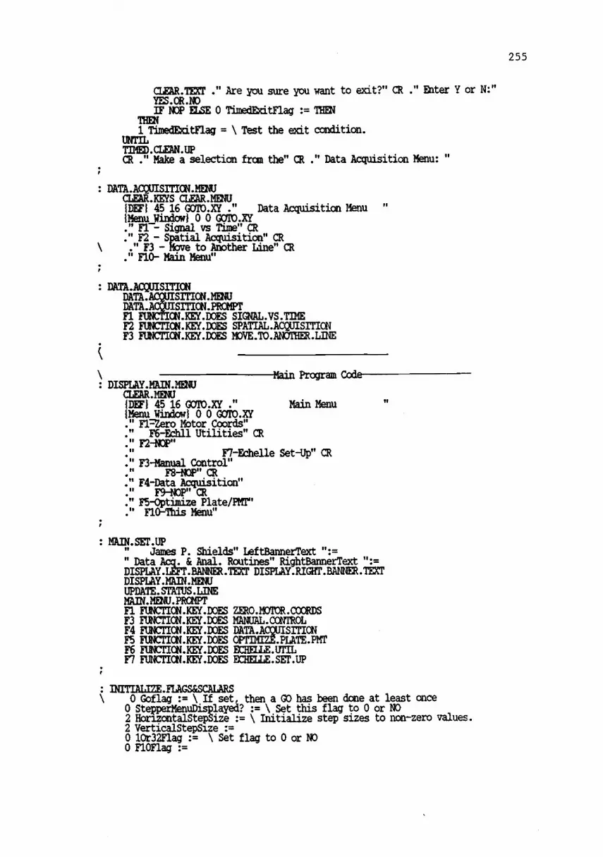
255

CLEAR.TEXT ." Are you sure you want to exit?" CR ." Enter Y or N:"YES.OR.NOIF NOP ELSE 0 TimedEXitFlag := THEN

THEN1

UNTILTimedEXitFlag = \ Test the exit condition.

TIMEB.CLEAN.UPCR ." Make a selection from the" CR ." Data Acquisition Menu: "

: DATLACQUISITION.MENUCLEAR.KEYS CLEAR.MENUMEN 45 16 GOTO.XY ." Data Acquisition MenuMenu Window} 0 0 GOTO.XY." Fl-'-. Signal vs Time" CR." F2 Spatial Acquisition" CR." F3 - More to Another Line" CR

." F10- Main Menu"

: DATA.ACQUISITION

DATA.A SITION.pRoinTi ON.KEY.DOES SIGNAL.VS.TIMEF2 FLVICTION.KEY.EOES SPATIAL.ACQUISMONF3 FUNCTION.KEY.1XES MOVE.TO.ANCTHER.LINE

Main Program CodeDISPLAMA1N.MENU

CLEAR.MENU1DEF1 45 16 GOTO.XY ." Main Menu'Menu Window} 0 0 GOTO.XY." F1=Zero Motor Coords"." F6-EChll Utilities" CR

F2-11OP"F7-Edhelle Set-Up" CR

." F3-Manual Control"F8-NOP" CR

." F4-Data Acquisition"

." F9 -NOP" CR

." F5-Optimize Plate/HIT"

." F10-This Menu"

: MAIN.SET.UPJames P. Shields" LeftBannerText ":=

" Data Acq. & Anal. Routines" RightBannerText ":=DISPLALLEFF.BANNER.TEXT DISPLNY.RIGHT.BANNER.TEXTDISPLAY.MAMMENUUPDATE.STATUS.LINEMAIN.MENU.PROMPTFl FUNCTION.KEY.DOES ZERO.MOTOR.COORDSF3 FUNCTEIN.KEY.DOES MANUAL.CONTROLF4 FUNCTION.KEY.DCES DATA.ACQUISITIONF5 FUNCTION.KEY.DCES 0 PT1MIZE.PLATE.PMTF6 FUKTION.KEY.DOES ECHELLE UTILF7 FUNCTION.KEY.DOES ECHELLE.SET.UP

INITIAL1ZE.FLAGS&SCALARS\ 0 Goflag \ If set, then a GO has been done at least once

0 StepperMenuDisplayed? \ Set this flag to 0 or NO2 HorizontalStepSize \ Initialize step sizes to non-zero values.2 VerticalStepSize_:=0 10r32Flag_:- \ Set flag to 0 or NO0 Fl0Flag

256

ManualAccpatanag :=2 IntegrationTime :=03264 Hbrizont4 VerticalSte2 Horizontal

e := \ Init. background mode to 0, i.e., on-line.fset \ Init. Background offset to 32e := \ Step back 32, over 64, and back again 32.ize := \ Step up 4 counts between each horizontal acq.is /Step :=

. 4,44 .5I

: GO0 GcElal =IF EXTENDED.GRAPHICS.CHARS 1 GoFlag := THENGRAPHICS.DISPLAYSCREEN.CLEAR

{STACMenu

Window} {BORDER} {Text Window} IBCRDERIICCLEAR

CLEAR.KEYSF10 EUNCTION.KEY.DOES MA1N.SET.UPINITIALTZE.FLAGS&SCALARSHAIN.SET.UP

BELL BELL

257

ECHD.ON

DATAANALUTL

James P. ShieldsDepartment of ChemistryOregon State UniversityCorvallis, OR 97331

(503) 754 -2081Final Revision Completed 10/9/87

These routines aid in performing some of theroutine tasks associated with post-experimentaldata analysis. Before this program was written,it was found that many tasks were being repeatedover and over. This often involved trying toremember how it was done the time before and itinvolved alot of repetitive trips to the ASYSTmanuals. These routines make many of the neededfile, data, etc.. manipulations available throughthe function keys of the PC keyboard. The menustructure has been left wide open and has lots ofroam for expansion.

tmys

thesisinformation about hi program.

contains additional

The special symbol plotting routines were obtainedthrough the ASYST program exchange (SYMBOLUTL).The extended character routines were alsoobtained from the exchange (files CHARFONT.UTL andCHARFONT.DAT).

String DefinitionsINTEGER40 STRING ArrayNameMessagel40 STRING ArrayttamASessage240 STRING FormatModeliessage12 STRING DataFileNameDAT12 STRING DataFileNameASC12 STRING DataFileNamePRN20 STRING ArrayName

Scalar DefinitionsINTEGER

SCALAR EktendedCharsLoaded?SCALAR CursotXPositionSCALAR CursorYPositionSCALAR COUNTERSCALAR MiaowSCALAR NUmColumnsSCALAR FormattiodeSAR COUNTER2SCALAR NUMARRAYSSCALAR COUNTER3SCALAR IntegrationTimeSCALAR Subfile#SCALAR NbmSubfilesSCALAR RowsNbde

\Hgartam scalars

TbtaiNumElementsDP.INTEGER

SCALAR NumBreakPtElementsSCALAR Array:MaxSCALAR ArraifflinSCALAR BreakPointInterval

DP.REALSCALAR Milltiply01,

258

Array DefinitionsINTEGER

DIM( 512 ] ARRAY CHARFONTSDP.REAL

DIM( 32 ] ARRAY 32P01RT.TIMES32PDENTMMES °RAMP32POINT.TIMES 132POINT.TIMES :=

INTEGER

General Utility Routines

\ Utility program to read in the extended graphics character\ font and patch it into the ROM char font tables.\ For use with the ASYST Version 1.5 and later.\ R the availability of the CHARFONT.DAT file.

.GRAPHICS.CHARSF1LE.OPEN CHARFONT.DAT

1 SUBFILECHARFCNTS FILE>ARRAY

FILE.CLOSE0 DEF.SEGCHARFCNTS ADDRESS \ ( Segment, Offset )DUP 256 MODULO 7CH POKE \ Low byte of offset128 256 / 7DH POKE \ HiDUP 256 MODULO 7EH POKE \ Low byte of segment128 256 / 7FH POKE \ Hi "

1 ExtendedCharsboaded? \ Set Flag

\ Window Defs179 196 218 192 217 191 BORDER.CHARS17 1 22 37 WINDOW Text Window}24 0 24 38 WINDOW fErroi. Window'17 39 22 78 WINDOW {Menu Window'

: ?VID?GRAPHICS.DISPLAY NOTIF

GRAPHICS.DISPLAYTHEN

: PIS' TTING.AREA?VIDO. .36 VUFORT.CRIG.97 .6 VUPORT.SIZE

: SAVE.CURSOR.LOCATIONMEL.COL CursorXPosition7REL.ROW CursorYPosition

: RESTORE.CURSOLLOCATIONCursorMsition CursorYPosition GOMA'

: CLEAR.MENU{Menu Window' SCREE .CLEAR

: CLEAR.TEXT{Text Window} SCREEN.CLEAR

: CLEAR.ERROR{Error Window' SCREEN.CLEAR

259

: CLEAR.KEYSFl FLINCTICti.KEY.DDES NOPF2 FUNCTION.KEY.DOES NOPF3 FIVION.KEY.DOES NOPF4 FUNCTION.KEY.DOES NOPF5 FUNCTICICKELDOES ACPF6 FUNCTICK.KEY.DOES NOPF7 FICTION.KEY.DOES NOPF8 FUNCTION.KEY.DOES NOPF9 Fitnnmmuces NOP

: ERROR.ROVITNECLEAR.ERROR ." Error #" ?Error# . (Text window'

: MAIN.DATAMAL.PROMPTCR ." Make a selection from the" CR ." Data Analysis Menu:

If

: TIMED.DATA.ANAL.PROMPTCR ." Make a selection from the" CR ." Timed Data Analysis Menu: "

: PIATUNG.UTILITIES.PROMPTCR ." Make a selection from the" CR ." Plotting Utilities Menu: "

: GENERALUTILITIES.PROMPTCR ." Make a selection from the" CR ." General Utilities Menu: "

: CONVERSION.UTIL.PROMPTCR ." Make a selection from the" CR ." File Conversion Utilities Menu: "

: GETLINPUTBEGIN

#INPUT NOT \ Waits for input. If valid #, get NOTed True on stack.\ Thus execution goes to after REPENT.

WHILE \ If non-valid input, execute between while & repeatCLEAR.ERROR BELL " Entry must be a number. Try again."(Text Window(RET STORE.CURSOR.LOCATION

REPEA\ Input was OK as far as this routine is concerned.CLEAR.ERROR (Text Window) RESTORE.CURSOR.LOCATION

: GET4r1LE.NAME.PRNCR

aatrIIRE:name for ASCII" CR

"INPUT " JM4C "CATDataFileNamePRN ":=

: GET.FILE.NAME.ASCCR

aatrleArmfile name)for ASCII" CR

"INPUT " .ASC" "CATDataFileNameASC ":=

: GELFILE.NAME.DATCR ." Enter file name containing desired" CR." information (.DAT assumed):

260

"DPW " .DOT' "CATDataFileNarneDAT ":=

: CHECK.F1LE.STATUS?FlLE.OPENIF

F1LE.CLOSECR

T." Had to close an already open file...continuing..."

HEN

: GET.SUBFILE.NUMBERCR ." Enter number of subfile containing" CR ." desired data: "#INPUT Subfile# :=

: GET.NUM.SUBFILESCR ." Enter number of subfiles to be" CR." processed. Assuming consecutive" CR

subfiles starting with subfile #1: "#INPUT NumSubfiles :=

: GET.PRN.MODECCR Which do want on the horizontal?" CR

ROWS or COUMINS" CR" Eater R or C: "

iCKEY ?DROPCASE

82 OF 1 RowsMode ENDOF \ Turn RowsMode ON67 OF 0 RowsMode = ENDOF \ Turn RowsMode OFF

BELL CLEAR.ERROR_,__OnlyR and C are valid entries here"'Text Window! MYSELF=CASE

GET.ARAY.NAMECRRArrayNameMessagel

"TYPECR ArrayNametimage2 "TYPE"MMMIT ArrayName ":=

: COPy.DATA.TO.ARRAYatFATE.COPY ArrayNatoe "CAT "MEC

CLEAR.TEXT ArrayName "'TYPE ." array has been created."

: Ger.FILE.READYDataFileNameDAT DEFER> FILE.OPENSubfile# SUBFILE

: GET.INTDGRATION.TIMECR ." Enter integration time for this" CR ." time array:#INPUT IntegrationTime :=

: SET.MULT1PLICATION.FAC7ORIntegrationTimeCASE

2 Cr 0.0476 MultiplyBy := ENDOF5 OF 0.1190 MultiplyBy := ENDCF

ENDCA42 OF 1. MultiplyBy := ENDOFSE

: GET.TIME.ARRAY.SIZE

DUP 0 SIZE NumRows :=

: GET.DATA.FROM.FILEDataFileNameDAT IEFER> FILLOPENSubfile# SUBFELEFILE>UNNAMED.ARRAYFILE.CLOSE

: SUBFILE.TO.ARRAYGET.FILE.NAME.DATCHECK.FILE.STATUSGET.SUBFILE.NUMBERGET.DATA.FROM.FILE

Enter name of arr to copy" ArrayNameMessagel ":=" data into: " Arra sage2 ":=GELARRAY.NAMECOPY.DATA.MARRAYGENERALUTILITTES.PROMFT

: F1LE.MAKERCLEAR.TEXT ." Desired arrays must be on stack."

CRLeave last subfile on top. CR

CR . If this is not so, hit ctrl-BREAK," CRinput arrays on stack and restart." CR ." Otherwise, hit space bar..."

CR ." How many arrays are on the stack: " #INPUT ?DROP NUNARRAYS1 COUNTER3 :-NUMARRAYS 0 DO

COUNTER3 PICK2 COUNTER3 + COUNTER3

LOOPF1LE.TEMPLATE

NUMARRAYS 0 DOOFORM.SUBFILELOOP

ENDCR_27_Emter desired file name (DAT assumed): " CR"INPUT .DAT" "CAT "DUPDEFER> F1LE.CREATECHECK.F1LE.STATUSDEFER> F1LE.OPEN1 COUNTER3NUMARRAY 0

CO ES SDOUBF1LENUMARRAYS COUNTER3 1 + ROLL ARRAY >FILECOUNTER3 1 + COUNTER3 :=

LOOPF1LE.CLOSECLEAR.TEXT DataFileNameDAT "TYPE ." has been created."GENERALUTILITTES.PROMPT

: GENERALMILITIES.MENUCLEAR.MENUIDD'} 45 16 GOTD.XY ." General Utilities MenuMenu Window} 0 0 GCMD.XY." Copy From Subfile To Amax" CR." F2 Create File From Array(s) CR." F10- Main Menu

GENERALUMILITTESGENERALUTILITIES.MENU {Text Window}GENERALMILITIES.PROMPTF1 FIIICTION.KEY.DOFS SUBFILE.TO.ARRAY

''

261

262

F2 FUNCTION.REY.DOES FILE.MAKER

STRIP.TIMESTimed Data Analysis Routines

GET.F1LE.NAME.DATCHECK.F1LE.STATUSGET.SUBF1LE.NUMBERGET.DATA.FROM.F1LE \ Leaves unnamed time array on stack.GET.T1ME.ARRAY.SIZEGET.INTEGRATION.T1MECR ." WAIT. .I'm working on your task"SETADLTTPLICATION.FACIORDUP \ First duplicate unnamed array32POINT.TIMES MultiplyBy *SWAP[ 1 ]

2 COUNT R2NUmRows 1 - 0 DO

32POINT.TIMES MultiplyBy *3 PICK[ COUNTER2 ]

CATENATE1 COUNTER2 + COUNTER2 :=

IV Enter name of to copy" ArrayNameMessagel ":=" data into: " Arr sage2 :-GET.ARRAY.NAMECOPY.DATA.TO.ARRAYT1MED.DATA.ANAL.PROMPT

: STRIP.RAWGET.F1LE.NAME.DATCHECK.F1LE.STATUSGET.SUBFILE.NUMBERCR ." WAIT.. I'm working on your task..."GET.DATA.FROM.F1LE \ Leaves unnamed raw 32point data array on stack.DUP []SHAPE DROP NumRows := DROP DROPDUP DUP \ Now have 3 copies of unnamed array on stackSUB[ 1 , 1; 1, 32 ]SWAPSUB[ 2 1 ; 1 , 32 ]CATENATi3 Counter :=NispRows 2 - 0 DO

2 PICK SUB[ COUNTER , 1 ; 1 , 32 ]

CATENATE1 COUNTER + COUNTER :=

LOOPXSECT[ 1 I ] \ Convert [ 1 32*NumRows ] to [ 32*NumRoms ]

Enter name of array to copy" ArrayNamMessagel :=

" data into: " ArrayNameMessage2 ":-GET.ARRAY.NAMECOPY.DATA.TO.ARRAYTIMED.DATA.ANAL.PROMPT

: RSD.CALCGET.FILE.NAME.DATCHECK. FILE. STATUSDataFileNameDAT DEFER> FILE.CeEN2 SUBFILE FILDUNNAMED.ARRAY100. *

1 SUBFILE F1LEHENAMED.ARRAY

RILE.CLOSEEnter name of to copy" ArrayNameMessagel ":=

" data into: Arra sage2 :-GET.ARRAY.NAMECOPY.DATA.TO.ARRAYTMED.DATA.ANAL.PROMPT

CNERR:ERRCR.RCIITNE

: PRINT.T1MED.ARRAYSCLEAR.TEXTCR Routine will print 32 point averages"CR ." and std. devs. to line printer." CRGET.F1LEMBE.DATCHECK.F1LE.STATUSDataFileNameDAT DEFER> F1LE.OPEN1 SUBF1LE F1LE)UNNAMED.ARRAY2 SUBFILE FILE) .ARRAYFILE.CLOSE[SIZE NUmColumnsLAMINATECR CR ." Check to see that printer is on-line."CR . Then press space bar to continue:KEY DROPOUT>PUNTER CONROLE.OFF." Data File = DataFileNameDAT "TYPE CR6

VOSPACES ." Acq. # 32 Point Average Std. Deviation" CR

CRNumColumns 1 + 1 DO

DUP8 SPACES I .

6 SPACES [ 1 , I ] .

DUP15 SPACES [ 2 , I ] .

CRLOOPCONSOLEDROP \ Drop the laminated array.T1MED.DATA.ANAL.PROMPT

: TIMED.DATAANAMENUCLEAR.KEYS CLEAR.MENUIDEFi 45 16 GOTO.XY ." Timed Data Analysis Menu "{Menu Window' 0 0 GOTO.XY." F1= Calculate RSD From A Timed File" CR." F2 - Strip and Catenate Time Arr' CR." F3 - Strip and Catenate Raw Array CR." F4 Print Timed Arrays" CR." F10- Main Menu"

: TIMED.DATLANALTIMED.DATA.ANALAIENU {Text Window}TIED.DATA.ANAL.PRCLIPTF1 FUNCTION.KEY.DOES RSD.CALCF2 FUNCTION.KEY.DCES STRIP.TIMESF3 FUNCrION.KEY.DOES STRIP.RAWF4 FUNCTION.KEY.DOES PRINT.TIMED.ARRAYS

c

: GET.BREAKPOINT.1NTERVAL

Histogram Routines

263

264

CR ." biter breakpoint interval: "#mPur BreakPointlnterval :=

: GET.ARRAY.SPECSSgar"EXEC \ Put array on stack.Return size of array and original array on top of stack

Total/ftElementsCHM/MAX ArrayMax ArrayMin \ Does not leave original array

\ on stack

: CREATE.BREAKPOINLARRAYINTEGER ArrayMax ArrayMin BreakPointlnterval /DUP NUmBreakPtElements

\ This gives number of array elements desired in breakpoint array.RAMP \ Create unnamed array with above number of elements.BreakPointlnterval * \ Multiply each element in array by breakpoint int.ArrayMin + \ Add minimum data array value to offset breakpoint array.BreakPointInterval - \ Subtract out BreakPoint interval. NOw have array\\f from ArrayMin to not quite ArrayMax in intervals of BreakPointlnterval.

DUP [NtmareakPtElements ] BreakPointlnterval + 1 RAMP 1 +CATENATE \ This gives array with one extra element for plotting purposes.SWAP \ SWAP because need breakpoint array first

: CREATE.HISTOGRAMCREATE.BREAKPOWLARRAY \ Returns plotting array and breakpoint arrayArrayName "EXECSWAPHISTOGRAM

: DO.A.HISICXWMCLEAR.TEXT " Enter name of input array." ArrayNameMessagel "47" Need not be sorted but must be 1D: CR ArrayNameMessage2 .

GELARRAY.NAMEGET.BREAKPOINT.MTERVALCR ." WAIL .I'm working on your task..."GELARRAY.SPECSCREATE.HISTOGAM" Enter name of array to copy" ArrayNameMessagel ":="histogram data into: ArrayliameMessage2 :-GELARRAYJNAMECOPY.DATA.TO.ARRAY" Enter name of array to copy" Arr NameMessage1 ":=" breakpoint data into: Arra sage2 .=GELA

"RRAYMME

COPY.DATA.TO.ARRAYMAIN.DATA.ANAL.PROMPT

.

Hidden line definitions for axon plotting: SOLIDLINE

SOLID DRAW.TO

: DOTTED.LINEDOTTED DRAW.TO

: DUTTED.HIDDEN.LINESINSTALL DOTTED.LINE IN HIDDENINSTALL SOLID.LINE IN NOT.HIDDEN

Routines for special plotting symbols\ In order to use these words you must first specify the symbol

265

\ type that you want to use ( SQUARE, TRIANGLE, or DIAMOND )_.\ Once the symbol has been specified then you simply place the\ array to be plotted on the stack and execute the appropriate\ command. You are also able to alter the size of the symbol\ by using the comment SET.SYMBOLSIZE.

XEQ DRAW.SYMBOL \ Setup execution variable to hold current symbolREAL

SCALAR SYMBCL.SIZE \ Determines the size of the symbol1 SYMBOLS= :=

: SET.SYMBOLSIZE \ Set the size of the symbols to be plottedSYMBOLS=CLEAR.TEXT ." Symbol size is now = " SYMBOLS= .

: CHANGE.RYMBOLS1ZECR ." Enter new symbol size where" CR

arri0

lambol Size < 1 :.

DUP 1 > IF CR BELL ." Entry must be < 1. Try Again." DROP MYSELF THENSET.SYMBOLSIZEPLOTTING.UTILITIES.PROMPT

\ using relative coords draw a square, cursor must be in correct location( )

DRAW.SQUARERELATIVE NORMAL.COORDS-.008 SYMBOL.SIZE * .01 SYMBOLS= * POSITION.016 SYMBOL.SIZE * .0 DRAW.TO.0 -.02 SYMBOLS= * DRAW.TO-.016 SYMBOLS= * .0 DRAW.TO.0 .02 SYMBOLS= * DRAW.TO

ABSOLUTE

this word installs the square drawing routine in the XEQ[ ] ( )

: SQUAREINSTALL DRAW. SQUARE IN DRAW.SYMBOLCR ." Square symbol installed!!" PLUrTINGJITILITIES.PROMPT

\ using relative coords draw a triangle, cursor must be in correct location

DRAW.)1113LATIVE NORHALCOCRDS.0 .ca SYMBOL.SIZE * POSITION-.01 SYMBOLS= * -.02 SYMBOL.SIZE * DRAW.10.02 SYMBOL.SIZE * .0 DRAW.TO-.01 SYMBOL.SIZE * .02 SYMBOL.SIZE * DRAM°ABSOURE

\ install the triangle drawing routine in the XEX\ ) ( )

: 1RIANGLEINSTALL DRAW.TRIANGLE IN DRAW.SYMBOLCR ." Triangle symbol installed!!" PLOTING.UTILITIES.PROMPT

\ using relative coords draw diamond, cursor must be in correct location[ 1 ( )

: DRAW.DIAMONDRELATIVE NORMALCOORDS.0 .015 SYMBOL.SIZE * POSITION-.008 SYMBOL.SIZE * -.015 SYMBOL.SIZE * DRAW.TO

266

.008 SYMBOL.SIZE * -.015 SYMBOL.SIZE * DRAW.TO

.008 SYMBOL.SIZE * .015 SYMBOL.SIZE *DRAW.TO-.008 SYMBOL.SIZE * .015 SYMBOLS= * DRAW.TO

ABSOLUTE

\\ i[nsta]ll t ihe diamond drawing routine in the XE

: DIAMONDINSRLL DRAW.DIAMOND IN DRAW.SYMBOLCR ." Diamond symbol installed!!' PLOTTING.UTILITIES.PROMPT

: CEICK.VIDEO.MODE71/1DED.MODEDUP DUP 3 = 7 = 2 = ORIF

GRAPHICS.DISPLAYTHENPLOTTING.AREA

;

\ displays grid and plots data with current symbol\ [ 344:array -- ( )

ECHO.ON: Y.AUPD.SYMBOL

SYMBOL.SIZE 0 (=IF

1 SYMBOLS= :=THENCHECK.VIDEOJODEINDEX.ARRAYXY.DATA.FITSWAP DROPVUPORT.CLEARXY.AXIS.PLOT

5000 MBEC.DELAYSOLID()SIZE 1 + 1DO

DUPI SWAP [ I ]VCRLD.COORDS POSITIONDRAW.SYMBOL

25 MSEC.DELAYLOOPDROPWORLD.COORDS

\ plots data in current world using current symbol

\ 1114111L--

current

): Y.DATA.SYMBOL.SIZE 0 <=IF

1 SYMBOL.SIZETHENSOLID°SIZE 1 + 1DO

DUPI SWAP [ I ]WORLD.COORDS POSITIONDRAW.SYMBOL

10 MSEC.DELAYLOOPDROPWORLD.COORDS

\ ays grid and plots data with current symbol\ 1 .x.array , ld.y.array ] ( )

: XY.AUTO.SYMBOLSYMBOL.SIZE 0 <=IF

1 SYMBOL.SIZETHENCHECK.VIDED.MODEXY.DATA.FITVUPORT.CLEARXY.AXIS.PLOT

5000 MSEC.DELAYSOLIDOSIZE 1 + 1DO

DUP[ I ] ROT DUP [ I ] ROTVORLD.CCCRDS POSITIONDRAW.SYMBOLSWAP

25 MSEC.DELAYLOOPDROPWORLD.COORDS

\

tots data in current world, with current symbol

ltrAld.m.arrYMBOL

.Sayld.y.array ] ( )

SYMBOL.SIZE 0 <=IF

1 SYMBOL.SIZETHENSOLID[]SIZE 1 + 1DO

DUP[ I ] ROT DUP [ I ] ROTWORLD.COORDS POSITIONDRAW.SYMBOLSWAP

10 MSEC.DELAYLOCPDROPWORLD.CCORDS

: PLOTTING.UTILITIES.MENUCLEAR.MENUfDEF1 45 16 GOTO.XY ." Plotting Utilities MenuMenu Window! 0 0 GOTD.XY." F1-- Activate Dotted Hidden Lines" CR." F2 - Activate Square Symbols" CR." F3 Activate Triangle Symbols" CR." F4 Activate Diamond Symbols" CR." F5 Change Symbol Size CR." F10- Main Menu"

: PLOTTING.UTILITIESPLOTTING.UTILITTES.MENU {Text Window!PLOTTING.UTILITIES.PROMPTFl FUNCTION.KEY.DOES DONED.HIDDEN LINESF2 FUNCTION.KEY.DOES WAILEF3 FUNCTION.KEY.DOESF4 FUNCTION.KEY.DOES DIAMOND

It

267

268

F5 mcnaf.KEY. DOES CHANGE. SYMBOL. SIZE

File Conversion Utilities: ONE.NUMBER/CR.FORMAT

NUmRows 1 + 1DO

NumColumns 1 + 1DO

DUP \ DUP the unnamed array[ J I ] \ Access the Row , Column element100. / \ Scale down for what DSURF likes. CR \ Output to current device, i.e., ASCII file. CR after each nun

LOOPMOPCR

: CREATE.ASC.F1LEGET.SUBF1LE.NUMBERGET.F1LE.NAME.ASCCR ." Wbrking...Please Wait..."GET.DATA.FROM.F1LE \ Leaves unnamed array on stack°SHAPE \ Get dimensions [Array---Array, Columns, Rows, Num Dimensions]DROP \ Drop the Num DimensionsNnmecms NumColumnsDataFileNameASC DEFER> OUT>F1LE CONSOLE.OFF \ Begin output to file.ONE.NUMBER/CR.FORMATDROP \ Drop the unnamed array... we are done with it.

: ONE.ROW/CR.FORMATNnecws 1 + 1DO

NumColumns 1 + 1DO

DUP[ J , I ]

100. /

L301;

CR \ CR after each row of dataLOOPCR

: ONE.COLUMN/CR.FUINVTNumColumns 1 + 1DO

NbmRows 1 + 1DO

DUP

100. /J ]

LOOPCR

LOOPCR

: CREATE.PRN.F1LE.SPECIAL\ If here, acq mode was either manual Fl or timed. Therefore, want sUbfile\ 3 of file to be converted. Subfile 3 is the [ N , 32 ] subfile.3 Subfile#GET.F1LLINAKE.PRN \ Get output file name.

269

0 RowsMode := \ Force to column modeCR ." Working... Please Wait..."DataFileNameRN DEFER> OUT>F1LE CONSOLE.OFF \ Open output file. Screen offGET.DATA.FROM.F1LE[]SHAPE \ Get array dimensionsDROP \ Drop the Number of dimensionsMuftis := NumColumnsCR CRONE.COLUMN/CR.FORMNTDROP \ Drop the unnamed array.

: CREATE.PRN.FILEGer.NUM.SUBFILESGET.FILEMANE.PRN \ Get output file nameGET.PRN.MODECR ." Working...Please Wait..."DataFileNamePRN DEFER> OUDFILE CCNSOLE.OFF \ Open output file. Screen offNumSubfiles 1 + 1DO

I Subfile#GET.DATA.FROM.FILE \ Leave the Ith subfile on stack as unnamed arrayOSHAPE \ Get array dimensionsMOP \ Drop the Number of dimensionsNumRows :=NUmColumnsICASE

1 OF ." Fran " DataFileNameDAT "TYPE ." On-Line Data" ENDOF2 OF ." Fran " DataFileNameDAT "TYPE ." Background Data" ENDOF3 OF ." Fran " DataFileNameDAT "TYPE ." Background Data" ENDOF

ENDCASECR CRRowsMbdeCASE

1 OF ONE.ROW/CR.FORMAT ENDOF0 CT ONE.COLUMN/CR.FORMAT ENDOF

ENDCASEDROP

LOOP\ Drop the unnamed array before going through DO..LOCP again

: FoRammurrCLEAR.TEKT ." Routine converts ASYST subfile data" CR

ASCII format." CR FormatModeMessage "TYPEGET.FILE.NAME.DATCHECK.FILE.STATUSFormatlibdeCASE

1 OF CREATE.ASC.FILE ENDOF2 OF CREATE.PRN.FILE ENDOF3 OF CREATE.PRN.FILE.SPECIAL ENDOF

ENDCASEOUT>FILE.CLOF \ Close ASCII output file and return output to CONSOLE onlyCLEAR.TEXT ." DONE!!!" CONVERSION.UTIL.PROTT

: DSURF.PORMATMILITY1 FormatMode

mode ACTIVE-" FormatMcdeMessage ":=FDRMAT.UTILITY

: GET.ACQ.NODECLEAR.TEXT ." Which acquisition mode was used:" CR." Spatial, Timed, Manual F1, F2, or, F3" CR." Enter S, 1, 2, or 3: "KEYCASE

270

83 OF 2 FormatMode ENDOF84 OF 3 FormatMode := ENDOF49 OF 3 FormatMode := ENDOF50 OF 2 FormatMode := ENDOF51 OF 2 FormatMode := ENDOF

ENDCASE

: IDTUS.FORMAT.U'ITLITYFT.ACQ.MODE

---LOTUS rode ACTIVE" FormatModeMessage ":=FCRMAT.UTILITY

: FILE.CCNVERSICW.UTILITIES.MENUCLEAR.MENU IMF) 45 16 GOTD.XY ." File Conversion Utilities "{Menu Window( 0 0 GOTO.XY." DSURF Format" CR." F2 LOTUS Format" CR." F10- Main Menu"

: FILE.CONVERSION.UTILITIESFILE.CCIWERSICN.UTILTTIES.MBIUCLEAR.TEXTCCOVERSICN.UTIL.PROMPTFl FUNCITCS.KEY.DOES DSURF.FORMAT.MTLITYF2 FUNCTION.KEY.DOES IDIUS.FORMAT.MTLIW

S.

Main Code: EaSPLAY.ARALYSIS.MENU

(Menu Window} SCREEN.CLEAR{{DES'} 45 16 GOTO.Xy_,_ Data Analysis MenuMenu Window( 0 0 GOTO.XY." F1- Timed Data Analysis" CR." F2 Histogram Analysis" CR." F3 - Plotting Utilities" CR." F4 General Utilities" CR." F5 File Conversion Utilities" CR." F10- Main Menu

: MAM DATA ANAL SET UPDISPLAY.ANALYSIS.MENU (Text Window( SCREEN.CLEARMAIN. DATA. AIM . PRCMFTFl FLUCTICN.KEY.DOES TIMED.DATA.ANALF2 FUNCTION.KEY.DOES DO.A.HISTOGRAMF3 FUNCTICN.KEY.DDES PLOTTING.WILITIESF4 EMICIT:21.KEY.DOES GENERAL.UTILITIESPS FUNCTICN.KEY.DOES FILE.CCNVERSION.MILTITES

: ANALYZE?VIDSCREEN.CLEARFiCaTING.AREA1 ExtendedCharsLoaded? = NOTIF

EXTENDED.GRAPHICS.CHARS \ Use extended chars in CHARFORT.DATTHEN(Text Window( {BORDER} {Menu Window} {BORDER}HORIZONTAL GRID.OFF VERTICALIUD.OFFCLEAR.KEYSF10 FUNCTION.KEY.DOES MAIN.DATA.ANAL.SET.UPMAIN.DATLANAL.SET.UP

271

BELL BELL \ Done loading!!

DCHO.C11

INTEGER

CURSIT.UTL

-----James P. ShieldsDepartment of Chemistry- Oregon State University

Corvallis, OR 97331--503-754-2081

Final Revision Completed8/6/87

This program facilitates the movement of anexternal device using the cursor keys of thePC keyboard. More complete documentation canbe found in my thesis as well as in the fileCURS1T.DOC

\ Stepper Motor Scalars

SCALAR StepSizeSCALAR YCOordSCALAR ZCoordSCALAR PortOffsetSCALAR GetReadySCALAR GetSetSCALAR GoTriggerDownSCALAR GoTtiggerUpSCALAR AllLow

Scalar Definitions

Utility Scalars Flags

SCALAR ClarsorXPositionSCALAR CursorYPosition

SCALAR StepperMenuDisplayed?SCALAR MotorErrorFlagSCALAR Get#.Input.Error.FlagSCALAR Fl0FlagSCALAR ZeroCoordsElloLFlagSCALAR StepSizeErrorFlag

\ Window up179 196 218 192 217 191 BORDER.CHARS

Set

\ NOTE: The above border chars are the "box and line" characters. To1mpimplement\ these characters, you may need to utilize the routines CHARI TF.UTL\ and CHARFONT.DAT which are available from the ASYST Program Exchange.\ If you do not currently have the CHARFONT routines, you could use\ 42 42 42 42 42 42 BORDER.CHARS instead to produce the * character as\ the entire border.17 1 22 37 WINDOW (Text Window}24 0 24 38 WINDOW (Errti:Winiowl17 39 22 78 WINDOW (Menu Window)24 39 24 79 WINDOW (Staffs Window(

Metrabyte PI0-12 Digital I/O Set-Up

\ Base I/O address = 512(dec) = 200(he).\ This address is set via di switches on P10-12 board.\ 8255 hardware operating 1.e = 10000000 ,i.e.,\ Ports A and B are mode 0 type output ports (See Metrabyte manual)\ Mode Set Active\ Port C not accesible.\ See Metrabyte manual for details\ NOTE: The I/O Address and the Hardware Operating Mode must be specified

by using CONFIG.DAS. See ASYST manual for details of execution.

4 DIGITAL.TEMPLATE WRITE.TO.PORTADIGITAL.INIT

5 DIGITAL.TEMPLATE WRITE.TO.PORTBDIGITAL.INrr

\ 4 is the software template operating mode\ for write byte to Port A.\ See Metrabyte Manual for details.

\ 5 is the software template operating mode\ for write byte to Port B.

272

273

\ See Metrabyte Manual for details.

General Utility Routines

: CLEAR.TEXT{Text Window! SCREEN.CLEAR {BORDER}

: CLEAR.ERROR'Error Wince} SCREEN.CLEAR

: 0LEAR.MENUManu Winiowl SCREEN.CLEAR {BORDER}

: CLEAR.STATUS{Status Window} SCREEN.CLEAR

: MAMMENU.PROMPTCLEAR.TEXT." Make a selection from" CR ." the MAIN MENU: "

: SAVE.CURSOR.LOCATION?REL.COL CursorXPosition :=?REL.ROW CursorYPosition :=

: RESDORE.CURSOR.DOCATIONCursorXPosition CursorYPosition GCMD.XY

: ?VID \ Routine determines if graphics display is ON. If not, turn it ON.?GRAPHICS.DISPLAY NOTIF

GRAPHICS.DISPLAYTHEN

: GEMINPUT \ Calls to this routine should include a SAVE.CURSOR.LOCATION\ e.g. see CHANGE.STEP.SIZE

BEGINimPuT NOT \ Waits for input. If valid #, get NOTed True on stack.

\ Thus execution proceeds to REPEAT.WHILE \ If non-number input, execute between while & repeat

11 Get#LEAR.Input.Error.Flag := \ Set error flag. BELL

." Entry musERRORt be a number. Try again."{Text Window!RETORE.CURSOR.LOCATION

REPEAT\ Input was OK as far as this routine is concerned, i.e., input was a #.1 Getit.Input.Error.Flag = \ Did an error occur?IF \ If so, clear error window

THENCLEAR.ERROR {Text Window}

RESTORE.CURSOR.LOCATION

: CHECK.FOR.MOTOR.ERROR1 MotorEtrorFlag = \ Was there an error last time through routine?

IfIF CLEAR.ERROR 0 MotorErrorFlag \

\clear

so,error window and reset flag.

THEN

274

: YES.OR.NO \ Routine for input requiring a Yes or No response.PCKEY ?DROP \ Get keyboard input then drop T/F from stack.CASE

89 OF TRUE ENDOF \ If Y entered, put true on stack.78 OF FALSE ENDOF \ If N entered, put false on stack.

BELL CLEAR.ERROR

iOnlyY and N are valid entries here!" (Text Windowl

lYSELFENDCASE

: WAIT.PCR.A.KEY \ Routine waits for a key to be depressed before continuing.P C K E Y \ Wait for a key.?DROP DROP \ Drop key code frau # stack and T/F from symbol stack.

: CIZZR.KEYSFl FISMnal.KEY.DOES NOPF2 IINCTION.KEY.DOES NOPF3 FURCTION.KEY.DOES NOPF4 FUNCTION.KEY.DOES NOPF5 ramm.m.ricEs htPF6 FLUMMON.KEY.DOES NOPF7 FaCTEN.KEY.DOES NOPF8 FLINCTTeN.KEY.DOES NOPF9 Facmcw.mysces NOP

STE"ER.IN"T.PEOMPTCUMULTEXT . No t o r Control Is Active

11 .11 1

11

: CAPS.LOZK.MESSAGECLEAR.ERROR BELL ." Engage Caps Lock & Try Again!!" {Text Window!1 ZeroCoordsErrorFlag :=

: UPDATEANCR.STATUS.LINECLEAR.STATUS." Y =P YCoord .TYPE 1 SPACES." Z =r ZCoorl :TYPE 1 SPACES." Step Size =" StepSize AWE

: CHECK.STEP.SrZELOP 100 > DUP 1 < OR \ Check input...Must be integer > 0 & < 101IF

." Entry must t be > 0 & <= 100...Try Again" {Text Window)1 StepSizeEtrotFlag :=DROP \ Drop bad entry from stack.

THEN

: CHANGE.STEP.SrZE \ Routine changes step size of motor per cursor key-stroke.CLEAR.TEXT." NOTE: Actual motor movement per" CR

cursor-stroke =" CR CR." (Step Size) * (Motor Resolution)" CR CR" Enter new step size:iAVE.CURSOR.IACATICNGETLINPUrCHECK.STEP.SUE

275

1 StepSizeEtrorFlagIF

IMESizeEtrorFlag :=

StepTHENSize :R = \ Assign input to scalarCLEAR.ERROUPDATE.MOTOR.STATUS.LINESTEPPER.INPUT.PROMPT

ONESCAPE:MYSELF

Stepper Motor Routines

: ZERD.YCOORD0 ?MORD :=

: ZERD.ZCOORD0 ZCOORD :=

: ZERO.BOTH.COORDSZERD:TOOORD ZERD.ZCOORD

: GET.ZEROMOTOR.COORDS.INPUTPCKEY ?DROP \ Get input.CASE

89 OF ZERD:TOOORD ENDOF \ Is input Y?90 OF ZERD.ZCOORD ENDOF \ Is input Z?66 OF ZERO.BOTH.COORDS ENDOF \ Is input B?121 OF CAPS.LOCK.MESSAGE MYSELF ENDOF122 OF CAPS.LOCK.MESSAGE MYSELF ENDOF98 OF CAPS.LOCK.MESSAGE MYSELF Et DOFCZEAR.ERROR BELL." Not a valid choice. Try again"{Text Window!1 ZerECoordsErrorPlag :=MYSELF

ENDCASE

: ZERDACTOR.COORDS!Text Window{ SCREEN.CLEAR/2 gig wish to zero the"CR .ON ." Y IN .OFF ." Coordinate, "CR INTEN.ON ." Z " IVEN.OFF ." Coordinate, or"CR INTEN.04_1! B" 1NTEN.OFF ." oth Coordinates?"CR CR 3 SPACES Y, Z, or B:

GELZERD.MOTOR.ODoRDS.INPUT \ Get input and error trap.1 ZeroCocrdsErrorFlag = \ Was there an error in input?IF \ If so,

CLEAR .ERROR \ clear error window0 ZeroCoordsErrorFlag := \ Reset error flag

THENUPDATE.MOTOR.STATUS.LINESTEPPER.INPUTSEMPT

\ *** *fir* ***\ The routines MOVE.FtS.Y, MOVE.POS.Z, MOVE.NEG.Y, MOVE.NEG.Z and MOVE.MOTOR\ are stepper motor circuitry dependent. Your system will most likely have\ different requirements. For example, the trigger line, direction line, etc.\ may be different bits of the control word than shown here. Delays may be\ needed between successive triggers of the motor. These routines are included

276

\ here as a typical example of how the control function can be written.\ It shouldralso be noted that this program is not in any way limited to\ the control of a stepper motor system. Virtually any system which has\ digital control lines and which could logically be operated by cursor keypad\ keys could be integrated into these routines. In addition, the other keypad\ keys, such as Home and Page Down, could be utilized

: MOVE.MOTORAliLow DIGITAL.OUT \ Output the preparatory bytesGetReady DIG1TAL.OUTGetSet DIGITAL.=

DOStepSize 0 \ Put DO LOOP values on stack

GdTriggerDown DIG1TAL.OUT \ Do a stepti.e.,trigger line lowGOTriggerUp DIG1TNLOUT \ ....and high for rising edge.

LOOP \ Repeat StepSize number of times.AliLow DIG1TAL.OUT \ All lines low when done to bring back to a

\ reproducible, defined state.

: MOVE.POS.YWRITE.M.PORTB \ Make this the current template.0 AllLow := \ Define digital control scalars globally.3 GetReady := \ NOTE: The scalars AllLow, GetReady, & GetSet7 GetSet := \ are for setting direction of motor movement &

\ initializing trigger line. These values may\ need to be modified or eliminated depending on\ your particular circuitry/motor environment.

6 GoTriggerDown := \ These two scalars are used in MOVE.MOTOR to7 Go'rriggerUp := \ actually toggle the trigger line of the

\ stepper motor circuitry.MOVE.MOTORYCoord StepSize + YCoord := \ Assign updated value to scalar.UPDATEJINDR.STATUS.L1NE

: MOVE.M.Y \ See MCVE.POS.Y for camnentsWRITE.TD.PORTB0 AllLow1 GetReady5 GetSet :=4 GoTriggerDown

MOVE.5 CdtriMOWUP :=YCoord StepSize YCoordUPDATE.MOTOR.STA1US.LINE

: MOVE.POS.Z \ See MOVE.PCS.Y for commentsWRITE.TO.PORTA0 AllLow :=3 GetReady7 GetSet :=6 GOTriggerDown :=7 GoTriggerUp :=MOVEAOTORZCoord StepSize + ZCoord :=UPDATEMTOR.STATUS.L1NE

: MOVE.NEG.ZWRITE.TO.PORTA0 AllLow :=1 GetReady :=5 GetSet :=4 GoTriggerDown5 GoTriggerUp :=

MOVE.MOTORZCoord StepSize ZCoordUPDATEAOTOR.STATUS.L1NE

: STEPPER.INPUT.MENUCLEAR.MENU1 StepperMenuDisplayed?IDES'} 45 16 GOTO.XY ." Motor Mover Menu(Menu Window} 0 0 GOTO.XY

18 SPACES--Us! altEs; keys to move motor--- " CR

INTEN.ON ." F2" ]]TEN.OFF ." Zero Motor Coordinates" CRINTEN.ON ." F3" INTEN.OFF ." Change Step Size" CRIN .ON ." F10" INTEN.OFF ." Main Menu'

: GET.MOTOR.CONTROL.INPUTPCKEY \ Get keyboard input. Should be a function key.CHECK.FOR.MOTOR.ERROR \ Was there an error last time through?IF \ If input was func key, then symbol stack is

CASE \ true...process CASE.75 OF MOVE.NEG.Y ENDOF77 OF MOVE.POS.Y ENDOF72 OF MOVE.POS.Z ENDOF80 OF'MOVE.NEG.Z ENDOFF2 OF ZERDMOTOR.COORDS ENDOFF3 OF CHANGE.STEP.SIZE ENDOFF10 OF 1 Fl0Flag = ENDOFBELL CLEAR.ERROR \ Input was a non- active function key.. NOn-active function key...Try again!" \ Display error message1 MotorEtrorFlag := \ and set error flag.

ENDCASEELSE \ Input was a non-function key.

DROP \ Drop the incorrect entry from the # stack.1 MotorEtrorFlagBELL(Error Window}

Only cursor & function keys are valid!"THEti

MOTOR.CONTROL0 Fl0Flag := 0 MotorErrorFlag1 StepperMenuDisplayed? 0 \

IfIs stepper

t

menu flag not set?IF \ ,

CLEAR.KEYS \ clear all function keysSTEPPER.INPUT.MENU \ and display menuSTEPPER.INPUT.PROMPT \ and prompt.

THENBEGIN \ EXit condition for BEGINUNTIL is Fl0Flag = 1

GET.MOTOR.CONTROL.INPUT1 Fl0Flag = \ Test exit condition.

UNTIL0 StepperMenuDisplayed? := \ Enable di lay of Stepper Menu next time

\ MOTOR. is called.F10 INTERPRET.KEY \ EXecute MA1N.SET.UP

ONERRBELL CLEAR.ERROR ." Erma " ?ERROR# . ." detected. Hit any key.WATT.FOR.A.KEY " GO" "EXEC

c

Main Program Code

: DISPLAY.HA1N.MENUCLEAR.MENUiDEF1 45 16 GOTO.XY INTEN.ON . Main Menu " INTEN.OFF

277

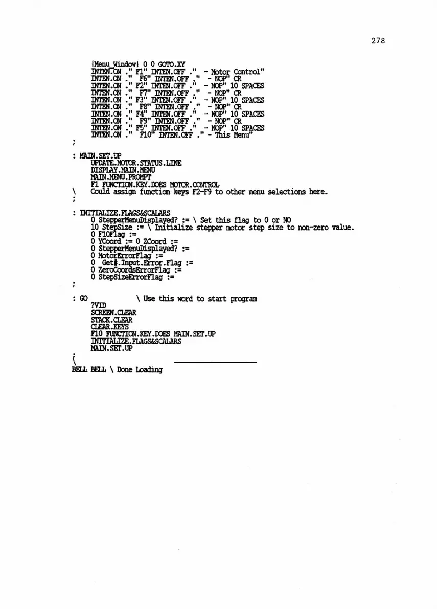
Rim Window) 0 0 GOTO.XYINTEN:CN ." Fl" INTEN.OFF ."INTEN.ON ." F6" INTEN.OFF ."INTEN.ON ." F2" INTEN.OFF ."INTEN.ON " r7" INTEN.OFF .".

INTEN.ON ." F3" INTEN.OFF ." -INTEN.ON ." F8" INTEN.OFF ."INTEN.ON ." F4" INTEN.OFF ."INTEN.ON ." F9" INTEN.OFF ."INTEN.ON ." F5" INTEN.OFF ."INTEN.ON ." F10" INTEN.OFF ."

Motor Control"- NOP" CRNOP" 10 SPACESNOP" CRNOP" 10 SPACES

- NOP" CRNOP" 10 SPACES

- NOP" CRNOP" 10 SPACES

- This Menu"

: MA1N.SET.UPUPDATEaCTOR.STATUS.LINEDISPLNYAAIN.MENUMAIN.MENU.PROMPTFl FUNCTION.KEY.DOES MCTOR.CONTROL

\ Could assign function keys F2-F9 to other menu selections here.

: 1NITIAL1ZE.FLAGS&SCALARS0 StepperNenuDisplayed? \ Set this flag to 0 or NO10 StepSize \ Initialize stepper motor step size to non-zero value.0 FlOFlag :=0 YCoord := 0 ZCoord0 SteppetMendDisplayed?0 MotorEtrotFlag0 Get#.Input.Error.Flag0 ZeroCoordsErrorFlag :=0 StepSizeErrorFlag

: GOAVID

\ Use this word to start program

SCREEN.CLEARSTACK.CLEARCLEARMYSF10 FUNCTION.KEY.DOES MAIN.SET.UPINITIAL1ZE.FLAGS&SCALARSMAIN.SELUP

BELL BELL \ Done Loading

278

TITLE GEITDIEPAM ,132

PROGPROG SIDS

DATA SEGMENT

RETADDRRETSEGDSSAV DWESSAVFLGSAV

DW

ERRMSGDB

reDATA ENDS

279

GETTIME.ASM

James P. ShieldsDepartment of ChemistryOregon State University

Corvallis, OR 97331(503) 754 2081

Final Revision Completed 10/9/87

Program is called from ASYST. Returns time toASYST to nearest hundreth of a second.

BYTE PUBLIC 'CODE'

IUD PUBLIC 'DATA'

DW 0 ; Storage for return program counter addressDW 0 ; Storage for return segment address0 ; Storage for original data segmento ; Storage for original ES registerDW 0 ; Storage for original flags register

DB 13,ERROR Illegal number of subroutine parameters'

13,10,1'

STACK SEGMIT BYTE STACK 'STACK'; No stack needed here. Use stack defined by ASYST.

STACK ENDS

PROG

MAIN

MINTPROCASSUMEPUSHFNOVMOWMOVASSIMEMOVNOVMOVPOPPOPPCP

PCPCMPJNE

WHATIME:MOVINT

HCURS:POPMOV

BYTE PUBLIC 'CODE'

FARCS:PROG

BX,DSAX, DATADS,AXDS:DATADSSAV,BXBX,ESESSAV,BXFW4SAVRETADDRRETSEG

aCX,4PRTERR

Gets timeA11,2CH21H

BPOPxES: [EC ,CE

Move orig. DS register to BX temporarily

; Save orginal DS register

; Save original ES register; Save flags; Save offset return address; Save segment return address

; Get number of parameters from stack; Are there four parameters?

and returns it to ASYST; Get ready for GetTime function call; Function call interruptES ; Get segment address of Hours parameter; Get offset address of Hours parameter; Move hours to memory location addressed by; contents of ES:[BX]

280

MINUTES: PCP ES Get segment address of Minutes parameterPOP BX ; Get offset address of Minutes parameterMOV ES: (BX] ,Cii ;

SECONDS: PCP ES ; Same for seconds...PCP BXMOV ES: Ma MI

HSECONDS: POP ES ; Same for hundredths of seconds...POP BXNOV ES: (BXLIL

JNP SHORT ENDSUB

PRTERR: ; Error messrs,GroutineMOV DX,OFFSET ; Get error message addressMOV AH,9H ; Get ready for print string function callINT 21H ; Function call interrupt

DROP!?: ; Clean up 8088 stack after errorPOP AX ; This routine drops the offset and segmentPOP AX ; addresses of the parameters from the stackLOOP I:ROMP ; if an error occurs. Drop 2 words/parameter.

ENDSUB: ; Get ready to return to ASYST,i.e.,restore stack to original state.PUSH kETSEG ; Push return segment addressPUSH RETADDR ; Push return offset addressPUSH FlaSAV ; Push original flagsPOPF ; Restore flags registerNOV AX,ESSAVMOV ES,AX ; Restore ES registerMOV AX,DSSAVMOV DS,AX ; Restore DS register

RETMAIN ENDP

FROG ENDSEND MAIN

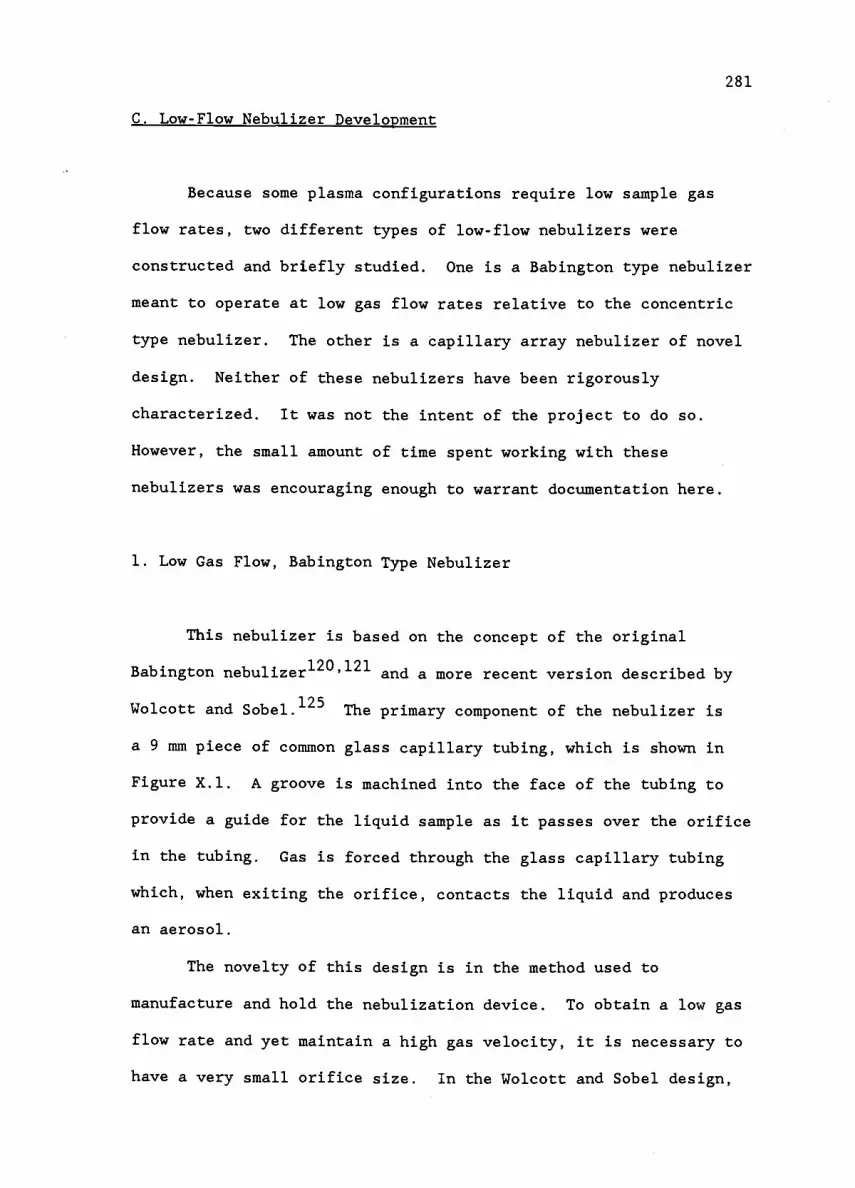
281

C. Low-Flow Nebulizer Development

Because some plasma configurations require low sample gas

flow rates, two different types of low-flow nebulizers were

constructed and briefly studied. One is a Babington type nebulizer

meant to operate at low gas flow rates relative to the concentric

type nebulizer. The other is a capillary array nebulizer of novel

design. Neither of these nebulizers have been rigorously

characterized. It was not the intent of the project to do so.

However, the small amount of time spent working with these

nebulizers was encouraging enough to warrant documentation here.

1. Low Gas Flow, Babington Type Nebulizer

This nebulizer is based on the concept of the original

Babington nebulizer120,121 and a more recent version described by

Wolcott and Sobel. 125The primary component of the nebulizer is

a 9 mm piece of common glass capillary tubing, which is shown in

Figure X.1. A groove is machined into the face of the tubing to

provide a guide for the liquid sample as it passes over the orifice

in the tubing. Gas is forced through the glass capillary tubing

which, when exiting the orifice, contacts the liquid and produces

an aerosol.

The novelty of this design is in the method used to

manufacture and hold the nebulization device. To obtain a low gas

flow rate and yet maintain a high gas velocity, it is necessary to

have a very small orifice size. In the Wolcott and Sobel design,

145

Top View

9 . Orin

Channel ForLiquid Introduction

V-GrooveE

Glass Capillary TubeE cvEap CDr`

Figure X.1. Diagram of babington nebulizer glass capillary tube.

283

the gas orifice was produced by drilling a small hole (0.2 mm) into

the end of a piece of sealed glass tubing. A minimum gas flow rate

of 0.4 L/min was reported. Other researchers127 drilled holes in

the end of test tubes. However, due to manufacturing difficulties,

they were limited to a minimum orifice size of 0.2 mm. These same

researchers then tried to cement a piece of glass capillary tubing

inside of a larger piece of glass tubing. However, they reported

unsatisfactory results when then trying to cut the groove in the

face of the assembly. These researchers finally reported the use

of a piece of stainless steel in which a hole of diameter 0.1 mm

was drilled. Subsequent cutting of the groove was then more

successful than with the glued assembly. However, they cited a

time period of half a day to get the hole correctly placed in the

center of the tubing.

The present design avoids any need for drilling holes by

using a piece of glass capillary tubing. This tubing can be

purchased with a variety of different orifice sizes. In this work,

orifice sizes of 76 Am, 102 Am, and 127 pm were used. The groove

was machined into the face of the capillary using a diamond saw

attached to a milling machine. A jig was made for the dual purpose

of holding the small piece of capillary for machining and to supply

a small flow of compressed air through the orifice. This gas flow

through the orifice helped to prevent clogging of the orifice

during the machining of the groove.

The next problem to overcome was to find a way to hold the

small piece in order to apply the required high pressure. To

maintain a reasonable pressure, it is necessary to keep the

284

capillary length as short as possible. However, the shorter the

length, the harder it is to hold the capillary in place when

applying high pressure. A quick estimate of the pressure needed to

obtain a given gas flow rate for a particular orifice size and

tubing length was made using Poisseuilles Law. For an orifice

diameter of 76 pm, a capillary length of 9 mm, and a desired gas

flow rate of 0.1 L/min, a pressure of about 58 psi is required.

Since this is a reasonable pressure, the length of 9 mm was chosen.

With the length decided upon, a method for holding the

capillary tubing was designed. With simplicity as an important

consideration, an Ultra-Torr fitting (Cajon Co., Macedonia, OH) was

modified to hold the capillary. This consisted of boring out the

ferrule piece to accommodate the 0.157" OD of the capillary. In

addition, a slot was machined into the face of the fitting cap to

allow room for introduction of the liquid sample. These

modifications to the Ultra-Torr fitting are outlined in

Figure X.2. The liquid sample was introduced to the groove using a

syringe needle attached to some peristaltic pump tubing. Finally,

a nebulizer housing was constructed to allow the nebulizer to be

used with a spray chamber. This housing piece is shown in

Figure X.3.

Aerosols were produced successfully at gas flow rates down to

0.1 L/min using the 76 pm diameter orifice and a pressure of

50 psi. A typical liquid flow rate of 0.6 mL/min was used. By

turning off all room light and backlighting the aerosol fog with a

tungsten lamp, the quality of the aerosol can be estimated

visually. It is well established that small droplet sizes are

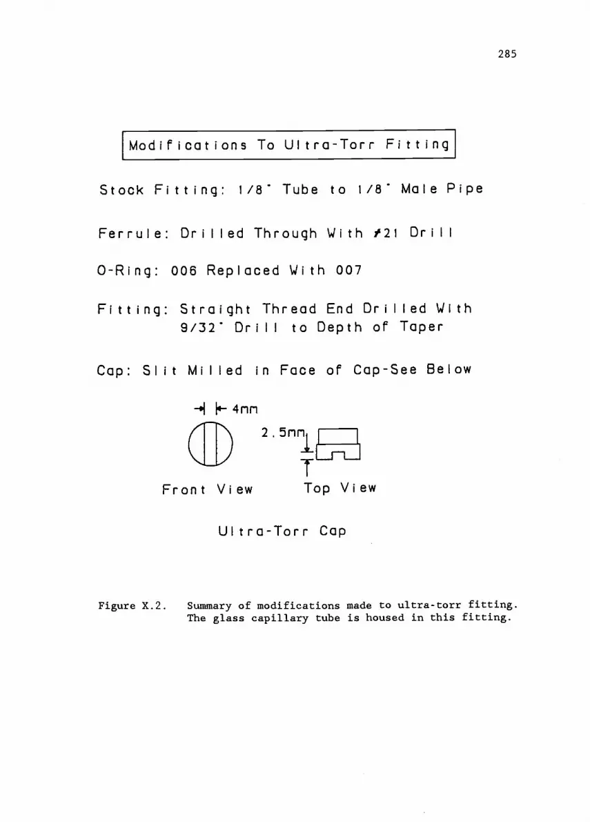
285

Modifications To Ultra-Torr Fitting

Stock Fitting: 1/8' Tube to 1/8' Male Pipe

Ferrule: Drilled Through With /21 Drill

0-Ring: 006 Replaced With 007

Fitting: Straight Thread End Drilled With9/32' Drill to Depth of Taper

Cap: Slit Milled in Face of Cap-See Below

4nn

2 . 5111

Front View Top View

Ultra-Torr Cap

Figure X.2. Summary of modifications made to ultra-torr fitting.The glass capillary tube is housed in this fitting.

Name: Bab i ng t on Nebulizer Housing

Material: Delr in

Designed By:J. P. ShieldsConstructed By:J. Archibald

NebulizerGasEntersHere

1.00

NebulizerUltra-TorrFitting ScrewsIn Here

019 Hole Here ForSolution Introduction

0220 0-Ring

000

0.50'

.23'

1.53'

1.77'

1.90

2.03'

4

4

00co

00

cv

Figure X.3. Diagram of babington nebulizer housing. This housing

contains the ultra-torr fitting.

287

desirable for efficient sample introduction with plasma

sources.277 By viewing the plasma with backlighting, it is easy

to discern the presence of large droplets. This visual method of

observing the droplet sizes is certainly not a rigorous one.

However, in the absence of a particle size analyzer, the visual

method does provide a good estimate of the quality of an aerosol.

Indeed, the visual method was frequently used to troubleshoot the

operation of the commercial concentric nebulizer used in this

work. Scattered light from a helium-neon laser was also used to

observe the aerosol as it exited from the tip of the sample tube

attached to the spray chamber.

The aerosol fog of the low flow nebulizer was visually

compared to the fog produced from a commercial concentric nebulizer

using the backlighting method. Although the total amount of

aerosol was less for the low flow model, as would be expected from

the lower gas flow, there were no gross visual differences in the

aerosol fog. Larger droplets could be seen towards the fringes of

the fog while the middle of the fog consisted of a very fine mist

of droplets.

Low gas flow nebulizers have certain potential advantages

over the higher gas flow nebulizers. For instance, some of the

newer, reduced power inductively coupled plasmas are not able to

accept sample gas flows at the 1 L/min flow rate common to

concentric nebulizers. In addition, the low gas flow nebulizers

generally consume less sample than concentric nebulizers. Finally,

the Babington type of low gas flow nebulizer is capable of

288

nebulizing high solids solutions without the clogging problems of

concentric nebulizers.

2. Capillary Array Nebulizer

The primary component of the capillary array nebulizer is

shown in Figure X.4. The disk is a precursor in the manufacturing

of a microchannel plate electro-optical array and was obtained from

Galileo Electro-Optics Corp. (Sturbridge, MA). This disk is solid

except for a small hexagonal region in the center of the disk.

This hexagonal region contains a honeycomb array of approximately

1025 channels, each nominally 25 pm in diameter.

To force gas through the channels, the glass disk was

inserted into an Ultra-Torr (Cajon Co., Macedonia, OH) stainless

steel 3/4" tube male connector. Aside from the o-ring which is

normally used in the fitting, an additional o-ring was placed on

the other side of the glass disk to provide a cushion from the

tightening of the fitting cap. This second o-ring also helped to

provide a seal.

As before, visual observation of the aerosol fog was

accomplished using the backlighting method. The introduction of

liquid over the array of channels was generally accomplished using

a syringe needle attached to peristaltic pump tubing. However,

introduction of liquid over the channel was more difficult here

than with the low flow nebulizer described above. The liquid

tended to intermittently avoid flowing over the channels. However,

when liquid was flowing over the channels, a very impressive mist

Disk Thickness-3mm

12.5mm,DI

Hexagonal RegionContains Approximately1025 Channels

Figure X.4. Diagram of glass capillary array for use as a

nebulizer.

290

was observed. Visually, the aerosol fog was very dense and very

few large particles were observed. A gas flow rate of 0.6 L/min

and a liquid flow of 0.3 mL/min produced this dense aerosol.

The observation of a dense and very fine mist here is

reasonable when considering the observations of other researchers

in their development of fritted glass nebulizers. 136,137 Very

high efficiencies are claimed for these fritted nebulizers; 70-94%

versus 5-15% for concentric nebulizers. In addition, unusually

fine mists with small mean droplet sizes are characteristic of

fritted type nebulizers.137

Further characterizations of both the low flow nebulizer and

the glass capillary array nebulizer are suggested. Ideally, this

characterization would include measurements of particle size

distributions and certainly should include testing with

introduction into a plasma.

291

D. Computer Controlled Stepper Motor System

1. Introduction

A two-dimensional stepper motor system was constructed as

part of this work. The intended use of the system is for moving a

spectral source (i.e., plasma, hollow cathode, flame) in two

dimensions relative to a detector thus permitting the acquisition

of spatially resolved data. Since the computer controlled mirror

inherent to the echelle spectrometer allowed spatial work to be

done, this stepper motor system was not used in this work for the

collection of spatial data. However, the stepper motor system does

offer some advantages over using the mirror in the spectrometer.

In addition, this stepper motor system can be used in conjunction

with any conventional monochromator which does not possess an

inherent means of spatial acquisition.

2. Description of Stepper Motor Instrumentation

The stepper motor system can be operated either manually via

front panel controls, remotely via a remote control box, or under

computer control. The system consists of a main stepper motor

driver board, the stepper motors themselves, six support

subsystems, and two power supplies. Most of the circuitry is

housed in a standard 19" vector cage installed in an

instrumentation rack. The power supplies are also housed in this

rack. While many of the components of this two-dimensional system

292

exist in duplicate, the description that follows will generally

describe only the components for one of the two dimensions.

Reference to the "other" dimension will be made when confusion may

result from only describing one of the dimensions. Finally,

Figure X.5 illustrates some of the various connector locations in

the back-plane of the instrumentation rack. The circles indicate

multiple pin amphenol-type connectors.

a) Stepper Motors

The stepper motors used can be described more accurately as

digital linear actuators (Series 92400, Airpax Corp., Cheshire,

CT). These actuators are identical to common four coil stepper

motors. However, an internally threaded rotor and an external lead

screw shaft have been incorporated into the motor. Therefore, when

the motor is energized, the lead screw will move in and out. A

diagram of the actuator is shown in Figure X.6 which was adapted

from a drawing in the actuator manual. For the model in use

(L92411-P1), the shaft moves 0.001" for each step of the motor.

The actuator requires 5 V for operation and has a 3" maximum travel

distance.

b) Stepper Motor and Logic Power Supplies

Two separate power supplies were used to help isolate the

logic power supply from the current surges present in the stepper

motor circuitry. Both of these power supplies were purchased as

Back Panel ConnectorsAuxiliary

Enpty

(I)

Z

Z Stepper Motor in

Y

Y Stepper Motor In

Y Microswitches In Digital I/0 In Digital I/O In

Z Microswitches In Renote Switches In Renote Switches In

Figure X.5. Diagram of stepper motor connectors in back plane ofinstrumentation rack.

3.500.

4.000"

.25' Diem. Mounting Holes

5.620'

If 1.020'40.0934111

_4 1_0.323*

LEADW9 #26

S

12 LONG

El0.375

TLEAD

P,QBEWSHAT

Stroke3' Max

-01-0.093'

-4 is-0.227"

-41.030"1*-

Name:92400 Digital Linear ActuatorMaterial: Units: Inches

Designed By:Alrpax CorpConstructed By: Airpax Corp

Figure X.6. Diagram of Airpax model 92400 digital linearactuator.

295

bare components. Each was put in a separate cabinet, and fans,

power cords, on/off switches, and on/off lights were added.

The first power supply provides +12 V to the K33505 and +5 V

to other logic circuitry. The second supplies +24 V to the stepper

motors. Although only +5 V is required at the stepper motor coils,

the product literature recommends a higher supply voltage. The

circuitry which performs the voltage dropping function will be

described in a later section.

c) Stepper Motor Driver Board

The heart of the system is a K33505 Airpax stepper motor

driver board shown in Figure X.7. This board contains a Signetics

SAA1027 (Signetics Corp., Sunnyvale, CA) stepper motor driver

chip. When triggered, this chip produces a four bit pattern which

provides the proper on/off sequence to the four coils of the

stepper motor. The K33505 board also contains an on board

oscillator which provides the pulses necessary for driving the

SAA1027 chip and, therefore, the actuator. The pulses from the

oscillator are turned on or off by a simple logic switch. The

frequency of the pulses, and thus the step frequency of the

actuator, is controlled by a user installed resistor pot. The

K33505 also contains four switching transistors whose on/off state

is controlled by the four output bits of the SAA1027. For more

information on the K33505 board, consult the product literature.

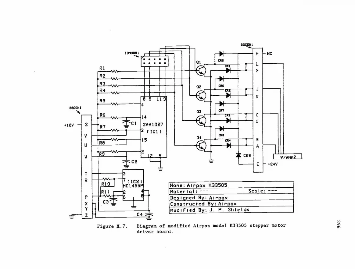
22C;11

+12V

Z

R1

R2

R3

R4

R5

tOPMMU

46 11 9

R6 14

R7 TC1 SAA1027

Ict

R81oNN.

R9

C

15

3

RIO (ICE1MC1455P

R11 2 4--

C3 Ss'

C4

aeCON1

NC

I ?FAMP2

+24V

Name: Airpax K33505Material: --- Scale: ---

Designed By: AirpaxConstructed By: AirpaxModified By: J. P. Shields

Figure X.7. Diagram of modified Airpax model K33505 stepper motordriver board.

297

d) Computer Digital I/O Card

To allow control of the stepping of the motors by a computer,

some means of sending pulses from the computer to the K33505 board

was necessary. A Metrabyte (Metrabyte Corp., Stoughton, MA) PI012

24 bit parallel digital I/O interface card was used to perform this

function. This card, which can be installed into an expansion slot

of a PC, provides 24 individual, TTL/DTL level digital I/O lines.

When operating the motors under computer control, this digital I/O

source takes the place of the oscillator source on the K33505 board

described previously and supplies triggering pulses directly to the

SAA1027 chip.

A total of three I/O lines is required for the control of

each motor. One line provides the necessary trigger pulses to

drive the SAA1027 chip. A second line controls the direction of

the motor movement. Finally, a third line allows the four bit

output of the SAA1027 chip to be "set" to a known condition.

e) Subsystem 1: SAA1027 Chip Selector

This subsystem, shown in Figure X.8, allows an external

SAA1027 chip to be used in place of the SAA1027 chip on the K33505

board. In the original design of the system, it was thought that

the auxiliary SAA1027 chips in the echelle spectrometer may be

useful in controlling the stepper motor system in some future

application. Thus, this flexibility was designed into the system.

The auxiliary SAA1027 chips in the echelle are present to operate

298

To SAM 027Chip In 41---Eche I I e

1 OMHDR 2

Narie: Subsysten 1 -

SAA1027 Chip Selector Circ

Material:NA

Designed By:J.P.Shl el dsConstructed By:J.P.S.

CI rcu I t Boards --

222120A9J8J7J615J413J2AIJO98.7

B5.432.1

X

SW1

41---- 44 CON 1

---E Rack Backp I ane

Figure X.8. Diagram of Subsystem 1: SAA1027 Chip SelectorCircuit.

299

features which are not present in our spectrometer system, such as

an auto-sampler. To allow an external SAA1027 chip to take over

the operation of the stepper motor system, the K33505 board was

modified slightly. The connector labelled 10MHDR1 in Figure X.7, a

male 10 pin header, was inserted between the on-board SAA1027 chip

and the switching transistors. A two pole, twelve throw switch,

located on the front panel controls (see SW1 of Figure X.12),

allows switching between on-board, K33505 control of the SAA1027

and external control of the SAA1027 via the driver board in the

echelle. Four throws of this switch are shown in Figure X.8. The

normal mode of operation is to use the SAA1027 chip on the K33505.

In fact, the SAA1027 chip in the echelle is not currently connected

to the stepper motor system. However, in the spirit of

expendability and flexibility, this option was built in.

300

f) Subsystem 2: Stepper Motor Dropping Resistors

This subsystem, shown in Figure X.9, drops the +24 V from the

power supply to the +5 V required by the stepper motors. Two high

power resistors perform the voltage drop function. As the

manufacturer states, the higher voltage provides added holding

power while the motors are not being moved and provides extra power

for high torque situations. Since these 19 0 resistors pass about

1 A each and are located near other circuitry, a cooling fan was

placed next to the resistors to insure proper removal of dissipated

heat.

g) Subsystem 3: PI012/K33505 Pulse Amplification Circuit

As described previously, the PI012 digital I/O card is

capable of generating TTL level pulses. However, to trigger the

SAA1027 chip, a +12 V high level and a 0 V low level are required.

Therefore, Subsystem 3, shown in Figure X.10, was designed to

amplify the TTL pulses to the required +12 V high level while

maintaining a 0 V low level. In addition to the pulses required to

trigger the SAA1027 chip, two other lines are present to control

the direction of the motor movement and to "set" the SAA1027 four

bit pattern to a known condition. These three I/O lines gain

entrance to Subsystem 3 through connector 7FAMP1 (see

Figure X.10). Pull-up resistors connected to the open collector

outputs of a 7407 are used to amplify the TTL levels to +12V.

22C0N17

04 --E

H

L

M

J

K

C

D

B

A

E

NC

LineorAcLuolor +24V

(From PS2922)C)

R12

SeriesDroppingResistors

R13/

K33505 .4----RockBoard

Beckpl one

301

Name:Subsystem 2 StepperMotor Dropping ResistorsMaterial:NADesigned Dy:J.P. ShieldsConstructed By:J.P. Shields

Figure X.9. Diagram of Subsystem 2: Stepper Motor DroppingResistor Circuit.

C t r cu t t 41----RackBoard Bockp lane

12

14< 1

740713

9

222120.198.1

.17

.16

.15

.14

.13

.1

.112

.10B8.7

5.4

32

If)

17 FAMP 1111

To P 1 01 2

'-44CON1Name:Subsystem 3 - PI0121K33505 Pulse

Amplification CircuitDesigned By: J. P. ShieldsConstructed By:J. P. Shields

Figure X.10. Diagram of Subsystem 3: PI012/K33505 PulseAmplification Circuit.

303

h) Subsystem 4: Manual/Computer Switching Control Circuitry

The Subsystem 4 circuitry shown in Figure X.11 consists of a

variety of switches and one resistor pot. All of these controls

are located on the front panel of the instrumentation rack. These

front panel controls are illustrated in Figure X.12. Note that all

of the component labels in Figure X.11 are shown in Figure X.12 in

parentheses. For the following discussion of Subsystem 4, refer to

Figures X.11 and X.12.

SW2 permits the motors to be controlled either manually (via

the oscillator on the K33505) or using the computer (via the

digital I/O lines). If in the manual mode of motor control, SW3

toggles between front panel manual control or remote manual control

(to be discussed in Subsystem 6). SW4 is essentially an on/off

toggle. In the "Run" position, the motor will move in the

direction dictated by the position of SW6. In the "Stop" position,

no motor movement can take place. SW5 toggles between an enabled

state and a disabled state. This switch is connected directly to

the SET pin of the SAA1027. Therefore, when in the disabled state,

the motor can not move. However, the four output bits of the

SAA1027 are put into a known condition. Refer to the linear

actuator manual for specific information about the nature of the

SET state. Finally, the resistor pot (P1) controls the step

frequency of the motors. The value of the resistance controls the

frequency of the pulses produced by the oscillator on the K33505

board. This pot only has control over the step frequency when the

motors are being controlled manually.

Nome:Subsystem 4-Manual/ComputerSwitching Control Circuitry

Designed By:J. P. ShieldsConstructed By:J. P. Shields

Stop.rIsIC

Run :SW41

t_iNC

Remote

Mnr-P1 A

411'llnwa dSV5

TOutw rd

1D1sa 1SW5

'Set

Mani

C Comp

SW2

222120.19.18.17.16.15.14.13.12.11

.109a78

432

See Subsysten 5

19FAMP11

To Renate

Control - See

Subeyeten

X

Y

7FAMP1

To P1012

Board In

Corona

304

Figure X.11. Diagram of Subsystem 4: Manual/Computer SwitchingControl Circuitry.

L00CO

tr)0Wlr)

Front Panel ControlsY Stepper Motor

Conputer Manual

Z Stepper

Conputer

Motor

Manualvia viaK33505 EchelleDriver Driver

Panel Run Panel Run Board Board

(SW3) (SW4)(SW2) (SWI)

Renate Stop Renate StopSAA1027 Stepper Motor

Enable Inward Enable Inward Driver Chip Selector

(sw5) (st4e)

Disable Outward Disable Outward

MI Max MaxMIStep '(PI) Step

Frequency Frequency

Figure X.12. Diagram of stepper motor front panel controls locatedon front of instrumentation rack.

306

i) Subsystem 5: Microswitch Logic Circuitry

This Subsystem provides the interface between the motor

control circuitry and a pair of remote microswitches (SW7 and SW8

in Figure X.13). The purpose of the microswitches is to sense some

condition and relay this information back to the control

circuitry. This condition may be an over-range of the motors or

some other potentially damaging event. When either of the

microswitches is activated, the logic circuitry within the large

dotted region in Figure X.13 interrupts the train of trigger pulses

to the SAA1027. This has the effect of stopping all motor

movement. In addition, motor movement can't continue until the

appropriate microswitch has been returned to its original state.

j) Subsystem 6: Remote Control Circuitry

The Subsystem 6 circuitry allows the motors to be controlled

by a remote control box, which is illustrated in Figure X.14 and in

the dotted region in Figure X.15. PB1 is a push-button control

which, when depressed, allows trigger pulses from the K33505

oscillator to reach the SAA1027. The remote box also allows the

motor direction to be toggled (SW9).

4---These lines exit

circuit boardvia 10 pin header

7 FAMP 2

7MAMP2

_J

7FAMP37MAMP3

V

SW7

SW8RenateMicroswftches

R18

1R17

R20

7408

R19

16

InNN

13

,12V

R21

7407)

Circuitry within dotted regionIs contained In rack-nountedauxiliary vector box

Name: Subsystem 5Mlcroswltch Logic CircuitryDesigned By:J. P. ShieldsConstructed By:J. P. Shields

Figure X.13. Diagram of Subsystem 5: Microswitch Logic Circuitry.

REMOTE CONTROL BOX

Push To Y

St ep( PB 1 )

Inward(SW9)

Outward()

Figure X.14. Diagram of controls on the remote control box.

222021

A

a, Lcn P

a)R

cn-r

V

2

,r 44C0N1 22CON1

Name: SubsystemRemote Control

6Circuitry

Designed By:J. P. Shields

Constructed By:J. P. Shields

+12V

5FAMP15MAMP1

PB1Inword

SW9

OuLwordRenote Control Box

P

X

Y

309

Figure X.15. Diagram of Subsystem 6: Remote Control Circuitry.

310

3. Conclusions

Although the echelle, with its computer controlled source

mirror, allows spatial work to be performed, the stepper motor

system described above possesses some potential advantages. As

described in Appendix V, the computer controlled source mirror in

the echelle has some off-axis movement in the vertical direction.

While this off-axis movement can be partially compensated for by

moving the mirror in the horizontal direction slightly, the

correction is only partial. The step resolution of the mirror in

the horizontal direction does not permit an exact correction. In a

practical sense, the noise in the spectral source may be such that

any imperfection in the mirror correction can not be detected.

However, in very stable spectral sources which have a high degree

of spatial stability, the inadequacies of the mirror correction may

become important.

Other noteworthy features of this stepper motor system

include its excellent step resolution, which is 0.025 mm in both

dimensions. In comparison, the step resolution of the echelle

mirror system is 0.34 mm in the vertical direction and 0.21 mm for

the horizontal direction. In addition, the system was designed

with flexibility and expandability in mind. For instance, the

computer control function is not limited to the hardware described

here nor is it limited to control using a PC. Any

computer/hardware combination capable of producing TTL level

digital I/O can be used for control of the system. Finally, the

system was designed with the possibility of the future addition of

311

a third axis in mind. This axis could either be a third linear

axis or a rotational axis.

312

E. Correction for Echelle Source Mirror Vertical Off-Axis Movement

During work with the echelle spectrometer, it was discovered

that the computer controlled source mirror possesses some off-axis

movement in the vertical direction. In other words, as the mirror

is moved in the vertical direction, it moves further and further

away from a true vertical path.

The implications of this off-axis movement are potentially

very serious. If the horizontal position low in the plasma is

peaked and then a series of horizontal scans are taken of the

plasma at several different vertical heights, the 3-D plot will

look skewed. This is because as each successive horizontal profile

is collected at progressively higher observation heights, the

off-axis vertical mirror movement causes each horizontal profile to

be shifted over slightly. Frequently, it is the vertical profile

of the central sample channel that is of particular interest.

However, due to the vertical off-axis movement of the source

mirror, a vertical profile extracted from the horizontal/vertical

data will not represent the true vertical emission distribution of

the sample channel. Two methods that were used in this work to

correct this problem are outlined here.

1. Correction Factor Method

If the magnitude and direction of the vertical off-axis

movement were known, it should be possible to correct for the error

by moving the mirror in the horizontal direction. To determine the

313

direction and magnitude of the vertical off-axis movement, a hollow

cathode lamp was mounted on a two-dimensional translation stage.

First, the movement of the translation stage was checked to insure

that it did not posses any significant off-axis movement. This was

done by attaching a plumb bob to the stage and moving the stage in

the horizontal direction. No discernible "slant" in the horizontal

movement of the stage was observed over the distance required for

the mirror calibration. To test for any off-axis movement of the

stage in the vertical direction, an L-square was placed on the

optical table next to the stage. Again, no discernible deviation

from vertical movement was observed over the distance required.

The dials on the stages were calibrated using a pair of high

quality calipers.

The source mirror of the echelle was calibrated in both the

vertical and horizontal directions. For the horizontal direction,

this was done by simply moving the stage a known distance

horizontally and then peaking the mirror X position using the

echelle's Peak X routine. The vertical mirror position was also

verified occasionally by executing the echelle's Peak Y routine.

The vertical mirror position did not vary by more than one vertical

mirror step. A similar procedure was performed to calibrate the

vertical mirror movement. However, in this case it was necessary

to peak both the vertical and the horizontal position each time the

stage was moved. The results of the calibration are summarized in

Table X.2. Note that it is impossible to apply an exact correction

due to the limited horizontal resolution.

314

Table X.2

Results of Echelle Source Mirror Calibration

Horizontal Mirror Calibration

Vertical Mirror Calibration

Off-Axis Correction Factor

SIC

0.21mm

Step

0.34mm

Step

0.26 Horizontal Steps

Vertical Step

315

2. Horizontal Peaking Method

The other method used to correct for the off-axis vertical

mirror movement involves using the Peak X routine of the

spectrometer to peak the horizontal position each time a vertical

move is made. This method does take extra time. However, it

virtually ensures that the correct horizontal position will be

maintained during vertical movement. Note that this method will

maintain the correct horizontal position even if the sample stream

travels in a slightly off-axis direction, as was occasionally

observed. The correction factor method described above would not

compensate for an off-axis sample stream. This horizontal peaking

method was used for most of the interference studies. In addition

to peaking the horizontal position each time a vertical move was

made, the actual horizontal mirror coordinate was monitored after

each peak. The change in the horizontal coordinate was then

quickly compared to the change which would be expected using the

correction factor. This was done as a confirmation of the correct

progression of a spatial experiment.

316

F. Technical Drawings

Technical drawings of the plasma torch and associated

components are presented in Figures X.16 through X.20.

317

Top View

Nome: Lower Housingmoteriol:Lava Scale:

Designed By: Jay ShieldsConstructed By: Bob Boyer

6-32 Clearance0.22' Dian.Counter-Bore

inr-ap

0

1 20°

TangentialGas Inlet

Cut-AwaymView

0

T

0 . 5.8 0 II--410.50014--

2.069' DianeterThrough Hole

I.- 0.1602.100-

10-32 thread

4TangentlalGas Inlet

Figure X.16. Diagram of lower housing of plasma torch.

Top View

1200

Angular Palish-tonof 4-40 Tape(Upomer and Lowerl

Nome: Upper HousingMaterial:Aluminum Scale:Designed By: Jay ShieldsConstructed By: Jay Shields

1200

Anguler Posti. oof 4-40 Taps(Upper end Lowlf,

Cut. -AwayView

311.0SOose

511.411164.

44.411Soo

211.4115io ------41

[j10--- 23.125oo ---A

Angular Position-1-of 4-40 Top(Upper and Lower)

-141411: 4-40 Top Through

See Top View ForAngular PoeLLIone

77.40-4-40 Tap Through

JL

Figure X.17. Diagram of upper housing of plasma torch.

TopView

Through hole #18Through hole #41Through hole #20

319

30°

Side 14

View 1 / 4

Through hole 1133Counter-Bore0.33" dtan. by0.156" deep

3.00'

None: Inner Elect-rode Base...pieLeMaterial:Ls:eve Scale:Designed By:Joy ShieldsConstructed By: Bob Boyer

Figure X.18. Diagram of inner electrode baseplate of plasma torch.

Topiew

Through Hole 0.52 Diem.

Through Hole 016

Through Hole 052

320

S ideiew

3

033 Through HoleCounLer-Bore0.33' dim. by0.156' deep

0

Name:Outer Electrode BeseplmLeLovm

Designed By:Jey ShieldsConstructed Hy:Htlh BAynr-

1/4

Figure X.19. Diagram of outer electrode baseplate of plasma torch.

TopView

Side

View

Outer

-410.54'14-

14-0.2"

0 0

321

Inner

H0.54-14-

H 0.20"

0.250.0125-t

#52 Through Hole

016 Through Hole

#41 Through Hole2-56 Tap

0.250"

0.6"H d0.6"Name: Inner and Outer ElectrodeHolders (Copper)

Designed BI:J. P. ShieldsConstructed By: J. P. Shields

Figure X.20. Diagram of inner and outer electrode holders.