REMOTE SENS. ENVIRON. 40:27-41 (1992)

Estimation of Land Surface Temperature with NOAA9 Data

C. Ottl and D. Vidal-Madjar CNET / CRPE, lssy les Moulineaux, France

/ ' N L]ifferent methods for estimating land surface temperature for NOAA satellites data are pre- sented. All these methods use the infrared channels of the Advanced Very High Resolution Radiometer (AVHRR). The single channel method using ra- diosounding data and a radiative transfer model is compared to the split window method and to other methods using additional High Resolution Infrared Radiation Sounder (HIRS) data. The re- sults show the superiority of the split window method when the spectral variation of the surface emissivity between the two channels 4 and 5 of the AVHRR is negligible.

INTRODUCTION

The knowledge of land surface temperature (LST) is strongly needed for many environmental stud- ies. At regional scale, the only way to map this parameter is to use satellite information. The NOAA-AVHRR radiometers are interesting be- cause they provide infrared data, two times a day, with a resolution of the order of 1 km. Recently, different methods have been proposed to estimate the surface temperature over sea from infrared satellite imagery. But over land, the same methods cannot be applied readily. The main difference is the effect of surface emissivity, which is generally

Address correspondence to C. Ottl~, CNET / CRPE, 38-40 rue du g~n~ral Leclerc, 92131 Issy-les-Moulineaux, France.

Received 15 April 1991; revised 1 November 1991.

0034-4257 / 92 / $5. O0 ©Elsevier Science Publishing Co. Inc., 1992 655 Avenue of the Americas, New York, NY 10010

lower than unity and must be taken into account in all the cases.

However, the problem is that we do not know yet how to estimate soil emissivity from space and at large scale. Consequently, we are obliged to prescribe it according to the type of the surface. This question of determination of land surface emissivity at the satellite pixel scale will not be addressed here. We shall assume that the emissiv- ity is known and discuss the problem of the atmo- spheric absorption of the Earth's radiance.

Various methods have been proposed to elimi- nate the effect of the atmosphere. The first one proposed by Price (1983) uses one single channel of the infrared radiometer and is based on the linearization of the radiative transfer equation. The radiance measured in an atmospheric absorp- tion window (Channel 4 of the AVHRR, for exam- ple) is corrected for residual absorption by estima- tion of the atmospheric transmittance with a forward radiative model. This methodology re- quires a precise description of the atmospheric structure, which can be provided by climatologi- cal data or better by radiosonde measurements.

Here we tested to see whether the atmo- spheric temperature and water vapor profiles re- trieved from the TIROS Operational Vertical Sounder (TOVS) could be used instead of the radiosoundings. This would allow us to use this single channel method in any place and time.

The second method for estimating the surface temperature is the most used over sea surfaces. It is called the split window. The atmospheric

27

28 Ottld and Vidal-Madjar

absorption is eliminated by the use of two infrared radiances measured in two channels in the ther- mal infrared window (Channels 4 and 5 of the AVHRR). The surface temperature is then related to the two brightness temperatures by a linear relationship.

We have discussed and adjusted the values of the coefficients of this relation, for different values of surface emissivities and different values of the satellite viewing angle, using a performant line by line radiative model and a large radiosoundings dataset.

Finally, we have tested the improvement brought when adding HIRS brightness tempera- tures to the simple AVHRR split window. All these different algorithms have been tested on AVHRR and TOVS data acquired during the HAPEX- MOBILHY experiment described by Andr~ et al. (1987), which took place over 100 sq km region in southwestern France during the two years 1985- 1986.

ESTIMATION OF LST WITH AVHRR CHANNEL 4 AND A RADIOSOUNDING

Over land, the surface temperature is generally estimated from the Earth's radiance measured in the best atmospheric window (Channel 4) cor- rected from atmospheric residual absorption with a radiative model. The vertical structure of the atmosphere and the mixing ratio of the absorbing gases are specified with the help of radiosonde measurements. The transmittance of the whole atmosphere is then calculated for the spectral band considered and applied to the brightness temperature to retrieve the surface temperature.

This method gives generally good results pro- vided that the atmosphere is well prescribed, especially in the atmospheric boundary layer where the absorption of the water vapor is maxi- mum; that means that the radiosonde must be exact and simultaneous with the satellite pass, and that the measurements are representative of a larger scale.

During the HAPEX experiment, especially during the Special Observing Period (SOP), be- tween May and July 1986, precise and intensive radiosoundings have been made on the site of Lubbon, inside the 100 km × 100 km area. Conse- quently, if we use a performant radiative model,

we can assume that this method is correct and that we can have good confidence in the surface temperatures retrieved, excluding the emissivity effect. The radiative model chosen is LOW- TRAN6, adjusted by Kneizis et al. (1983). We can use the surface temperatures obtained with this method as a reference and compare them to the retrievals of the other methods.

The second approach consists of replacing the radiosonde measurements by the temperature and water vapor profiles retrieved from TOVS data. The interest lies in having a method self- consistent with NOAA9 data which can be applied everywhere since it does not need ground mea- surements any more.

USE OF TOVS INVERSIONS FOR THE ATMOSPHERIC CORRECTION OF AVHRR CHANNEL 4

TOVS Data and Inversion Procedure

The TIROS-N Operational Vertical Sounder is composed of three passive vertical sounding in- struments: the High Resolution Infrared Radia- tion Sounder (HIRS-2), a radiometer with 19 channels in the infrared and one in the visible, the Microwave Sounding Unit (MSU), a microwave radiometer with four channels around 55 GHz, and the Stratospheric Sounding Unit (SSU), a pressure modulated infrared radiometer with three channels near 15 tzm.

As the upwelling radiance in these spectral regions depends on the physical and chemical structure of the atmosphere, it has been demon- strated that it is possible to find combinations of radiometric channels to uncouple the effects of each influent atmospheric parameter and to de- rive them, integrated over different layers of the atmosphere using the so-called weighting func- tion of each channel (Schwalb, 1978).

The TOVS instrument has been designed on that principle with the purpose of retrieving the atmospheric parameters like temperature and moisture. Different algorithms were developed to derive the water temperature profiles and vapor content in the atmosphere from the multi-spectral measurements of the outgoing earth's radiance. The procedure is called "inversion" of the radia- tive transfer equation.

In our study, we have used the improved

Estimation of Land Surface Temperature 29

initialization inversion ("31") method developed * by Ch6din and Scott (1984). This procedure is 400hl~

both physical and statistical as it is based on a theoretical simulation of the atmospheric trans- mittances and radiances and relies on the use of 500 a large dataset called TIGR (TOVS Initial Guess Retrieval). This dataset contains a great number of atmospheric situations (1207) and observing conditions (viewing angles, surface pressures, 600 surface emissivities and all the sounding chan- nels), the atmospheric profiles, and the associated brightness temperatures. Then, if the observed = 700 brightness temperatures correspond to clear areas =. or have been properly decontaminated from clouds using the so-called psi-method (Ch~din and Scott, 1985), the "3I" algorithm is applied. 800

It follows two steps: retrieval of the initial guess solution among the dataset TIGR and re- trieval of the "exact" solution by a maximum prob- 900 ability estimation procedure. The retrievals are made over a variable number of HIRS-2 spots according to the viewing angle, leading to a spatial resolution of approximately 100 km× 100 km. 1000

Application to HAPEX-MOBILHY Data b 400~

The inversion method has been applied to TOVS data within the framework of the HAPEX- MOBILHY experiment. Thirty-two days taken out of the Special Observing Period of the experi- 500 ment, for which atmospheric radiosoundings were available every hour over the central site (Lub- bon), were used. For the first step of the inversion, the ECMWF (European Center for Medium 600 Range Weather Forecast) analyses were used to help determine the initial guess solution. The TOVS orbits selected are divided in 18 morning ~ 700 .i orbits (taken around 2 a.m.) and 14 afternoon ~. orbits (taken around 2 p.m.). For all these orbits, the temperature and water vapor vertical profiles were retrieved with the "3I" inversion procedure. 800

Local Comparison with R a d i o s o u n d i n g s

For each of the treated orbits, the derived temper- ature and humidity profiles have been compared to radiosoundings measurements.

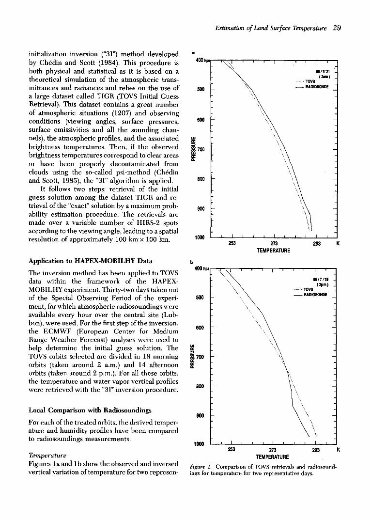
Temperature Figures la and lb show the observed and inversed vertical variation of temperature for two represen-

- ~ . . ~ . , ~171~

....... TOVS (~m)

IOSONDE

i I i i i i I I i

2 5 3 2 7 3 2 9 3

T E M P E R A T U R E

8817119 ( 2 p m )

. . . . . . . TOYS - - RADIOSONDE

900

"';',

\ ' \ 1000

253 273 293 K TEMPERATURE

Figure 1. Comparison of TOVS retrievals and radiosound- ings for temperature for two representative days.

30 Ottl~ and Vidal-Madjar

tative cases: one morning and one afternoon or- bits, 21 and 19 July 1986 (the altitude is given in pressure coordinate). Table 1 also presents the mean differences between the TOVS retrieval and the radiosonde profiles for different layers of the atmosphere, averaged over the whole set of data. We present here only averages over not too cloudy orbits (cloudiness less than 50% in the 100 km × 100 km area), for 10 afternoon orbits and 13 morning orbits. The other ones with root mean square (rms) difference greater than 2 stan- dard deviations were rejected.

For all the morning orbits, the retrieved pro- file is too cold at all levels, but the vertical gradi- ent is generally good especially between 900 hpa and 600 hpa. The mean bias is about 2 K at the surface and increases to 3 K around 700 hpa level, with a mean rms error ranging between 2 K and 4 K below 550 hpa.

For the afternoon orbits, the results are different. The inverse profiles are generally too warm in the low levels until 800 hpa and colder above with a bias of the same order equal to 3 K and a mean rms error, depending on the level and which can overflow 4 K, greater than for morning situations.

Mixing Ratio

The inversion model retrieve the mean water vapor content in three layers: surface to 800 hpa, 800-500 hpa, and 500-300 hpa. Then, it is possi- ble to compute the atmospheric mixing ratio de- fined as the mass (in g) of water vapor per unit mass (kg) of dry air, with the temperature profile. The retrievals are compared to the measurements in Table 1. We have here also rejected the cloudy

orbits. The results differ much from one orbit to another.

For the morning orbits, we see that the re- trieval is generally lower than the measurements, the mean bias is less than 1 g /kg at all levels but the rms ranges between 2 g /kg and 3.6 g /kg below 800 hpa. For the afternoon orbits, the retrieval is greater than the observations in the lower layers. The rms error is greater than for the morning orbits, ranging between 2 g /kg and 4.2 g /kg in the lower levels, and the mean bias is of the order of 2 g/kg. The reason for these large differences cannot be explained by a time lag between the satellite passes and the radiosound- ings because they were nearly simultaneous, nei- ther by locally effects measured by the radiosonde.

This is shown in Table 2, where we compare the radiosonde data to the data from Bordeaux situated at 100 km in the western direction, near the Atlantic Ocean, to prove the representativity of the radiosoundings on the whole region. For all the days where simultaneous radiosoundings were available, (8 days), the vertical profiles at the two sites, Lubbon and Bordeaux, were plot- ted. We present in Table 2 the mean differences for all the orbits between Bordeaux and Lubbon.

The comparison shows that the temperature profiles are very similar, colder for all these days in Bordeaux (less than 0.5 K on average with an rms difference less than 1 K for the morning orbits; for the afternoon orbits, the difference decreases with the altitude from 3 K at the surface to 0 K after 600 hpa). For the humidity profiles, the differences vary during the day: The values are less important in Bordeaux than in Lubbon in the afternoon and greater in the morning, the rms difference being less than 1.5 g /kg on all the

Table 1. A v e r a g e o f t h e D i f f e r e n c e s b e t w e e n T O V S

R e t r i e v a l s a n d R a d i o s o u n d i n g s a t D i f f e r e n t L e v e l s , f o r

Temperature and M i x i n g R a t i o

Morning Afternoon

Surface T (K) q (g/kg) T (K) q (g/kg)

to 980 h p a - 2.0 - 0.2 - 0.3 + 1.6

930 hpa - 1.7 - 0.2 + 3. + 1.8

870 h p a - 1.6 + 0.2 + 3.3 + 1.8

820 hpa - 2.2 + 0.6 + 2.6 + 1.

770 hpa - 2. - 0.9 + 1. - 0.2

690 hpa - 3. - 1.3 - 0.2 - 0.2

610 hpa - 2 . 4 - 1 . 2 - 0 . 8 - 0 . 1

550 hpa - 2. - 0.5 - 1.7 + 0.1

Table 2. A v e r a g e o f t h e D i f f e r e n c e s b e t w e e n B o r d e a u x

a n d L u b b o n R a d i o s o u n d i n g s a t D i f f e r e n t L e v e l s , f o r

T e m p e r a t u r e a n d M i x i n g R a t i o

Morning Afternoon

Surface T (K) q (g/kg) T (K) q (g/kg)

to 980 hpa - 0 . 5 0.1 - 3 . - 0 . 9

930 hpa - 0.4 - 0.1 - 2. - 1.

870 hpa - 0 . 2 0.9 - 0 . 9 - 0 . 8

820 hpa - 1.2 1.2 - 0.2 - 0.2

770 hpa - 0.4 0.4 - 1. - 0.2

690 hpa - 0.03 - 0.2 - 1.8 0.3

610 hpa 0.7 0.5 - O . 1 0.1

550 hpa - 0.6 - 0.2 - 0.9 - 0.2

Estimation of Land Surface Temperature 31

profiles. These differences are very small com- pared to the differences between TOVS retrievals and the radiosoundings and can be easily ex- plained by the maritime influence of the Atlantic Ocean. Then we conclude that the Lubbon ra- diosoundings are representative of the whole re- gion of the HAPEX experiment and the differ- ences with the retrievals cannot be explained by local effects.

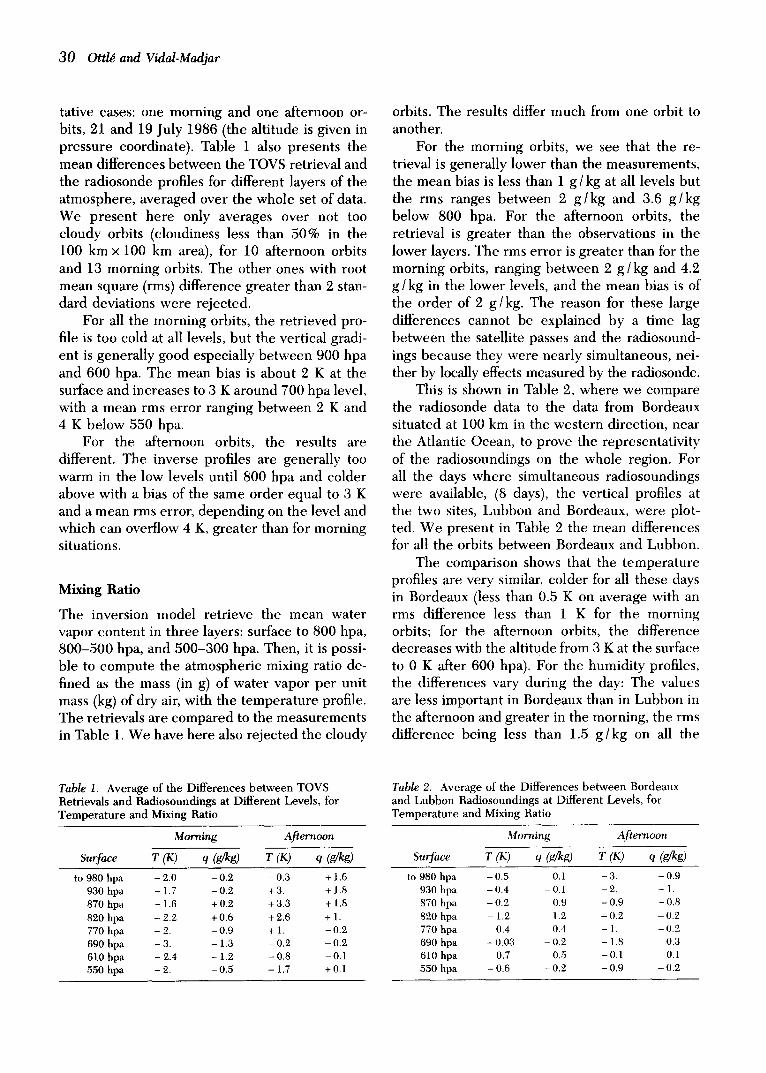
In order to explain these discrepancies, a test on the physical consistency of the afternoon pro- files has been done. As a matter of fact, at this time of the day (2 p.m.), the convection in the atmosphere makes the exchanges between the air masses nearly adiabatic, that is, without exchange of heat with the surroundings. The reason is that heat transfer processes from an air mass to its surroundings are slow in comparison with the air motion. Thus, for an adiabatic ascent, when the air is unsaturated, the rate at which the temperature decreases is constant and equal to 9.8 K/km. Thus it is easy from the surface temperature to calculate what should be the temperature profile if the cooling was adiabatic. The result is shown in Figure 2.

Here we have averaged all the afternoon tem- perature profiles, because their vertical gradient was very similar from one orbit to another. The average of afternoon radiosoundings follows ex- actly the adiabatic cooling until 860 hpa, which seems physically realistic. This is not the case for the retrievals. Consequently, the problem cer- tainly comes from the inversion procedure itself.

D i s c u s s i o n o n t h e I n v e r s i o n M o d e l

We have tried to identify the reasons of the dis- crepancies between the model retrievals and the observations. It may come from the first step of the inversion procedure, which is the research of the initial guess in the TIGR dataset. The first step consists of finding, from the brightness tem- peratures and the ECMWF analyses (surface pres- sure), the nearest atmospheric situations in the dataset. These selected situations are afterwards averaged and used as an initial profile, from which, by a root mean square procedure, the solution profile is determined. In this way, if the initial solution is too far from the exact solution, the procedure is not successful.

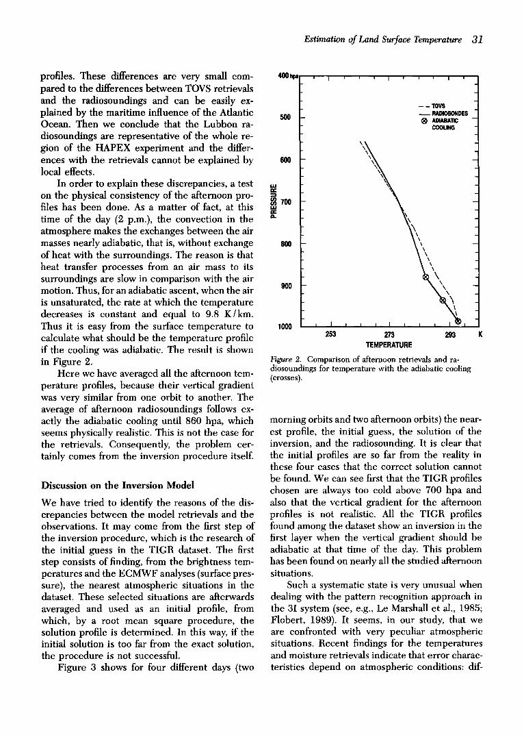
Figure 3 shows for four different days (two

400 hpl ' I ' ' ' I ' ' ' I

500

- - - TOV$

~ . RADIOSONDES

AOIABA'nC COOLING

, \ \ \

n -

¢/) m 700 t . e l -

800 ~ \ \ \

1000 i I ~ i i I i i i I ~ ' l 253 273 293

TEMPERATURE

Figure 2. Comparison of afternoon retrievals and ra- diosoundings for temperature with the adiabatic cooling (crosses).

morning orbits and two afternoon orbits) the near- est profile, the initial guess, the solution of the inversion, and the radiosounding. It is clear that the initial profiles are so far from the reality in these four cases that the correct solution cannot be found. We can see first that the TIGR profiles chosen are always too cold above 700 hpa and also that the vertical gradient for the afternoon profiles is not realistic. All the TIGR profiles found among the dataset show an inversion in the first layer when the vertical gradient should be adiabatic at that time of the day. This problem has been found on nearly all the studied afternoon situations.

Such a systematic state is very unusual when dealing with the pattern recognition approach in the 31 system (see, e.g., Le Marshall et al., 1985; Flobert, 1989). It seems, in our study, that we are confronted with very peculiar atmospheric situations. Recent findings for the temperatures and moisture retrievals indicate that error charac- teristics depend on atmospheric conditions: dif-

32 Ottl# and Vidal-Madjar

500

600

" : -

".i".. °o ~

8 6 / 7 / 2 1 ( 2 a m )

- - TOYS

RADIOSONDE

• • • I N m A L G U E S S

• • • N E A R E S T

PRORLE

b 400 hl~

U,,I El: : l

700 UJ

0, .

500

I • , ' - , ' \ .b

; % w

700 - 14.1 • ..:.. ~.

800 I - ~ - I 800

- \

900 \ 900 \

\ -

\.. 1000 ~ 1000

253 273 293 K TEMPERATURE

c d

1 ' i ~ I ~ l , I i

s \ . ~ • . \ ~ 86/7 /19(2am).

" \ \ - TOYS

= " \ A • • • I N I T I A L G U E S S -

. ; " . . \ \ . . . u . r -

.." ... \ ,,,~o.,.,. - \....... \ ",,':-, \ 4 ~ ", •

v4. .Q o • \ \ X

' , : , . \ \ "-......'::\

• -...?

\N \\.-:...,,,

t I i i I I I i I I I 253 273 293 K

TEMPERATURE

'•*•\ - - - - TOYS

500 - ".:. \ \ - - RJU)X)SONDS 500 • : , \ • - • INITIAL GUESS

" ; .% \ • • •

" . , ' , PROFILE

- \

600 I - ~',, "\ \ --t 600

L \ ~ - ILl u.I ", " : \ " " , : : : : " = ? = ~ 700 ,.

O.n" - "~l-*'~ l% k - O.n" 7

800 \ ".. 800

,'-...

° f ° \ ' , .\ 1000 ~ 1000

o ,

8 6 / 7 / 2 1 ( 2 p n

- - - TOYS

- - RADIOSONDE

• • • I N m N . GUESS

• • • NEAREST

PROFILE

\ \ - . ".. ,, - . . .

, , . . . ". \ \ ' e l I

253 278 293 K 253 273 293 K TEMPERATURE TEMPERATURE

Figure 3. Comparison of temperature profiles: inversed by the "31" system, measured by the radiosonde, the nearest TIGR profile, and the initial guess for two morning and two afternoon orbits.

Estimation of Land Surface Temperature 33

ferent air masses, unstable tropospheres or boun- dary layers.

In the present status of the vertical sounders HIRS and MSU (poor spatial and spectral resolu- tions), a solution to the problem may be found by enlarging the dataset (the TIGR dataset has been recently enlarged to 1800 situations), distinguish- ing the time and the type of the surface (sea or land) of the radiosoundings which determine the initial guess, and introducing physical laws in the research of the initial profile (the behavior of the profile in the planetary boundary layer, for example).

In conclusion, the present 31 procedure is not accurate enough in this very specific situation (inhomogeneous elevation and terrain) to give the temperature and water vapor profiles and the right surface temperature compatible with the pre- cision needed for our thermal infrared atmo- spheric correction problem of AVHRR data.

TRANSMI'I'rANCES

1.0-

,,(9, o.e- X** 0 ~ .6-

-~- 11.4-

O.&

0 , I i I i I , I

0 0.2 0.4 0.6 0.8 1

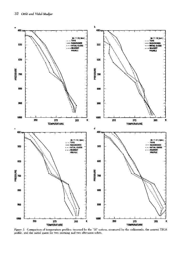
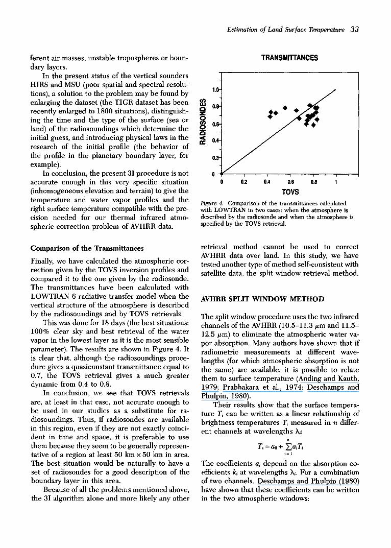
TOVS Figure 4. Comparison of the transmittances calculated with LOWTRAN in two cases: when the atmosphere is described by the radiosonde and when the atmosphere is specified by the TOVS retrieval.

Comparison of the Transmittances

Finally, we have calculated the atmospheric cor- rection given by the TOVS inversion profiles and compared it to the one given by the radiosonde. The transmittances have been calculated with LOWTRAN 6 radiative transfer model when the vertical structure of the atmosphere is described by the radiosoundings and by TOVS retrievals.

This was done for 18 days (the best situations: 100% clear sky and best retrieval of the water vapor in the lowest layer as it is the most sensible parameter). The results are shown in Figure 4. It is clear that, although the radiosoundings proce- dure gives a quasiconstant transmittance equal to 0.7, the TOVS retrieval gives a much greater dynamic from 0.4 to 0.8.

In conclusion, we see that TOVS retrievals are, at least in that case, not accurate enough to be used in our studies as a substitute for ra- diosoundings. Thus, if radiosondes are available in this region, even if they are not exactly coinci- dent in time and space, it is preferable to use them because they seem to be generally represen- tative of a region at least 50 km x 50 km in area. The best situation would be naturally to have a set of radiosondes for a good description of the boundary layer in this area.

Because of all the problems mentioned above, the 31 algorithm alone and more likely any other

retrieval method cannot be used to correct AVHRR data over land. In this study, we have tested another type of method self-consistent with satellite data, the split window retrieval method.

AVHRR SPLIT WINDOW METHOD

The split window procedure uses the two infrared channels of the AVHRR (10.5-11.3/zm and 11.5- 12.5/~m) to eliminate the atmospheric water va- por absorption. Many authors have shown that if radiometric measurements at different wave- lengths (for which atmospheric absorption is not the same) are available, it is possible to relate them to surface temperature (Anding and Kauth, 1979; Prabhakara et al., 1974; Deschamps and Phulpin, 1980).

Their results show that the surface tempera- ture Ts can be written as a linear relationship of brightness temperatures Ti measured in n differ- ent channels at wavelengths k,:

n

T, = ao + ~a,T, i = l

The coefficients ai depend on the absorption co- efficients k~ at wavelengths k,. For a combination of two channels, Deschamps and Phulpin (1980) have shown that these coefficients can be written in the two atmospheric windows:

3 4 Ot t ld a n d V i d a l - M a d j a r

k 2 - k l

al - k2 _ k l ' a2 = k2 _ k l '

assuming that the absorption of the atmospheric gases is low and that the radiance B×(T) can be expanded around the surface temperature using a first-order Taylor approximation.

This method is generally used over oceans and the coefficients of the formula are obtained by regression of measured AVHRR radiances to surface temperature data derived from ocean buoys. Over land, the problem is more compli- cated, because the coefficients depend greatly on the characteristics of the surface and especially on its emissivity. Consequently, these coefficients are valid only locally and cannot be determined once and for all.

Secondly, as land surface temperature is very variable over distances of the order of 1 m, nobody would know how to average ground truth data (if they were available) at the satellite pixel scale. Thus, if one wants to adjust split window tbrmulas over land, the best way to proceed is to work with simulated data from a radiative transfer model.

In this study, we have used a performant line by line radiative transfer model [Automatized Atmospheric Absorption Atlas (4A)] and a large radiosounding dataset (TIGR) to compute syn- thetic radiances in AVHRR and HIRS channels and to deduce split window coefficients in all conditions, different viewing angles and different surface emissivities, and for different formula, classical split window using AVHRR alone, with others using AHVRR + HIRS channels.

Description of the Radiative Transfer Model

The model used is the fast line by line method of Scott and Ch6din (1981): The Automatized Atmospheric Absorption Atlas (4A). This atlas has been built for the whole spectral region covered by the AVHRR and HIRS channels. The mono- chromatic transmittances of individual layers of a stratified atmosphere have been computed with a standard line by line procedure (Scott, 1974) and for a large set of plausible atmospheric condi- tions (Ch6din and Scott, 1984).

From this dataset, the transmittance of the whole atmosphere can be derived for any atmo- spheric conditions assuming the same pressure stratification as for the 4A dataset, by multiplica-

tion of the individual monochromatic layer trans- mittances between the surface and the satellite point. The right mixing ratio of the absorbing gases and the zenith angle are taken into account by simply elevating the predetermined transmit- tances to a corrective power. Since this fast algo- rithm is based upon a monochromatic approach, any kind of apparatus function can be used for the convolution.

This dataset has been applied to NOAA9- AVHRR and TOVS channels. Thus, for all the 1207 atmospheric situations archived in the TIGR dataset, all possible satellite viewing angles, sur- face temperatures, surface emissivities, and syn- thetic radiances for the HIRS and AVHRR radiom- eters have been computed.

AVHRR Channels 4 and 5 Split Window Algorithm

The 4A computed radiometric temperatures in Channels 4 and 5 of the AVHRR radiometer have been used to find the coefficients of the split window formula:

T, = ao + a lT4 + a2T~.

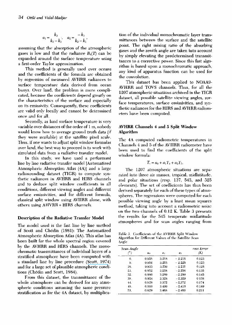
The 1207 atmospheric situations are sepa- rated into three air masses, tropical, midlatitude, and polar situations (resp. 137, 545, and 525 elements). The set of coefficients has thus been derived separately for each of these types of atmo- spheres. The regressions were computed for each possible viewing angle by a least mean squares method, taking into account a radiometric noise on the two channels of 0.12 K. Table 3 presents the results for the 545 temperate midlatitude atmospheres and for scan angles ranging from

Table 3. C o e f f i c i e n t s o f t h e A V H R R S p l i t W i n d o w

A l g o r i t h m f o r D i f f e r e n t V a l u e s o f t h e S a t e l l i t e S c a n

A n g l e

Scan Angle rms Error (°) ao a, ~2 (10

0. 0 .858 3 .218 - 2 ,218 0 .123

9. 0 . 8 5 4 3 .225 - 2 .225 0 .123 16. 0 .833 3 .230 - 2 .231 0 . 1 2 8

23. 0 . 8 5 2 3 .258 - 2 .258 0 .135

32, 0 . 8 8 0 3 .289 - 2 .290 0 . 1 4 5

38. 0 . 9 2 4 3 ,328 - 2 . 3 2 9 0 , 1 5 8 44. 0 . 9 2 8 3 .372 - 2 ,372 0 . 1 7 4

48. 0 . 9 1 0 3 . 4 0 9 - 2 .410 0 . 1 8 9

53. 0 , 9 2 9 3 .468 - 2 .469 0 .211

Estimation of Land Surface Temperature 35

nadir to 53 ° as defined in the sampling of the TIGR dataset, assuming that the surface behaves like a perfect black body in the two spectral bands. The results show first that the approxima- tions of low absorption in the two channels and the first-order Taylor approximation for the devel- opment of the radiance with temperature are valid because we obtain for all the regressions a l+a2= 1.

Also, we notice that the scan angle has low influence on the coefficients value and that the rms error on the surface temperature is very small in all the cases, increasing a little with the angle. The biases are also very small of the order of 0.1 K for all the angles. That low dependency with the scan angle is in contradiction with the results of Schluessel et al. (1987), who found a strong scan angle dependency probably explained by the complex atmospheric structure of their situations.

A stronger effect is certaintly the effect of surface emissivity, which prevents direct use of the split window coefficients over land (Price, 1984; Becker, 1987). Becker (1987) showed theo- retically the impact of neglecting the spectral variations of the emissivity when using a split window method. His calculations demonstrated that an error of 1% on mean emissivity in the two channels yields an error of 1 K on surface temperature, but that an error of 1% on the difference of emissivity in the two channels yields an error of 2.5 K on the estimated surface temper- ature, which is much more important.

Further studies have been done to confirm the spectral variation of the emissivity in the atmospheric window (Ottl~ and Stoll, 1988; Becker and Li, 1990), with NOAA-AVHRR im- ages, and it has been concluded that it is necessary

to take into account the values of surface emissiv- ity in the two channels 4 and 5 of the AVHRR before using a split window method over land.

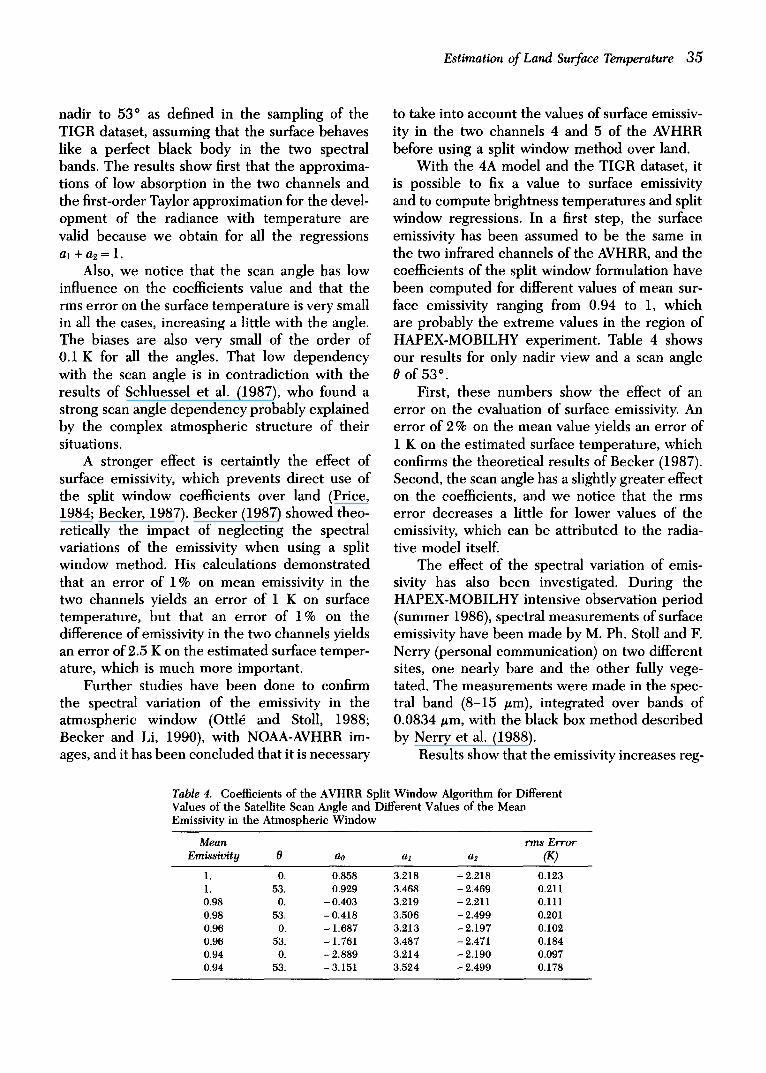
With the 4A model and the TIGR dataset, it is possible to fix a value to surface emissivity and to compute brightness temperatures and split window regressions. In a first step, the surface emissivity has been assumed to be the same in the two infrared channels of the AVHRR, and the coefficients of the split window formulation have been computed for different values of mean sur- face emissivity ranging from 0.94 to 1, which are probably the extreme values in the region of HAPEX-MOBILHY experiment. Table 4 shows our results for only nadir view and a scan angle /9 of 53 °.

First, these numbers show the effect of an error on the evaluation of surface emissivity. An error of 2 % on the mean value yields an error of 1 K on the estimated surface temperature, which confirms the theoretical results of Becker (1987). Second, the scan angle has a slightly greater effect on the coefficients, and we notice that the rms error decreases a little for lower values of the emissivity, which can be attributed to the radia- tive model itself.

The effect of the spectral variation of emis- sivity has also been investigated. During the HAPEX-MOBILHY intensive observation period (summer 1986), spectral measurements of surface emissivity have been made by M. Ph. Stoll and F. Nerry (personal communication) on two different sites, one nearly bare and the other fully vege- tated. The measurements were made in the spec- tral band (8-15 /~m), integrated over bands of 0.0834/~m, with the black box method described by Nerry et al. (1988).

Results show that the emissivity increases reg-

Table 4. C o e f f i c i e n t s o f t h e A V H R R S p l i t W i n d o w A l g o r i t h m f o r D i f f e r e n t

V a l u e s o f t h e S a t e l l i t e S c a n A n g l e a n d D i f f e r e n t V a l u e s o f t h e M e a n

E m i s s i v i t y i n t h e A t m o s p h e r i c W i n d o w

Mean rms Error Emiss iv i ty 0 ao a l a~ (K)

1. 0. 0 . 8 5 8 3 . 2 1 8 - 2 .218 0 . 1 2 3

1. 53. 0 . 9 2 9 3 . 4 6 8 - 2 . 4 6 9 0 .211 0 .98 0. - 0 . 4 0 3 3 . 2 1 9 - 2 .211 0 .111

0 .98 53. - 0 . 4 1 8 3 . 5 0 6 - 2 . 4 9 9 0 .201

0 .96 0. - 1 . 6 8 7 3 . 2 1 3 - 2 . 1 9 7 0 .102

0 .96 53. - 1 .761 3 . 4 8 7 - 2 .471 0 . 1 8 4

0 .94 0. - 2 . 8 8 9 3 . 2 1 4 - 2 . 1 9 0 0 . 0 9 7

0 .94 53. - 3 .151 3 . 5 2 4 - 2 . 4 9 9 0 . 1 7 8

36 Ottl~ and Vidal-Madjar

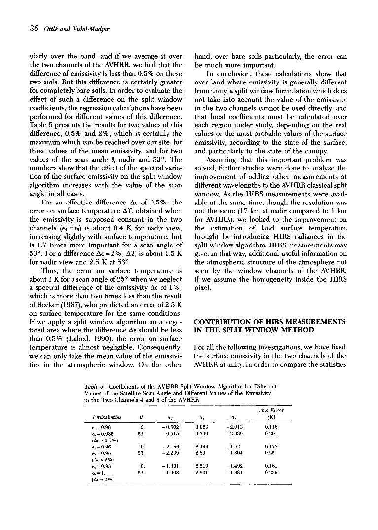
ularly over the band, and if we average it over the two channels of the AVHRR, we find that the difference of emissivity is less than 0.5% on these two soils. But this difference is certainly greater for completely bare soils. In order to evaluate the effect of such a difference on the split window coefficients, the regression calculations have been performed for different values of this difference. Table 5 presents the results for two values of this difference, 0.5% and 2%, which is certainly the maximum which can be reached over our site, for three values of the mean emissivity, and for two values of the scan angle 0, nadir and 53 °. The numbers show that the effect of the spectral varia- tion of the surface emissivity on the split window algorithm increases with the value of the scan angle in all cases.

For an effective difference Ae of 0.5%, the error on surface temperature ATs obtained when the emissivity is supposed constant in the two channels (24--25) is about 0.4 K for nadir view, increasing slightly with surface temperature, but is 1.7 times more important for a scan angle of 53 °. For a difference Ae = 2%, ATs is about 1.5 K for nadir view and 2.5 K at 53 °.

Thus, the error on surface temperature is about i K for a scan angle of 25 ° when we neglect a spectral difference of the emissivity AE of 1%, which is more than two times less than the result of Becker (1987), who predicted an error of 2.5 K on surface temperature for the same conditions. If we apply a split window algorithm on a vege- tated area where the difference A~ should be less than 0.5% (Labed, 1990), the error on surface temperature is almost negligible. Consequently, we can only take the mean value of the emissivi- ties in the atmospheric window. On the other

hand, over bare soils particularly, the error can be much more important.

In conclusion, these calculations show that over land where emissivity is generally different from unity, a split window formulation which does not take into account the value of the emissivity in the two channels cannot be used directly, and that local coefficients must be calculated over each region under study, depending on the real values or the most probable values of the surface emissivity, according to the state of the surface, and particularly to the state of the canopy.

Assuming that this important problem was solved, further studies were done to analyze the improvement of adding other measurements at different wavelengths to the AVHRR classical split window. As the HIRS measurements were avail- able at the same time, though the resolution was not the same (17 km at nadir compared to 1 km for AVHRR), we looked to the improvement on the estimation of land surface temperature brought by introducing HIRS radiances in the split window algorithm. HIRS measurements may give, in that way, additional useful information on the atmospheric structure of the atmosphere not seen by the window channels of the AVHRR, if we assume the homogeneity inside the HIRS pixel.

CONTRIBUTION OF HIRS MEASUREMENTS IN THE SPLIT WINDOW METHOD

For all the following investigations, we have fixed the surface emissivity in the two channels of the AVHRR at unity, in order to compare the statistics

Table 5. C o e f f i c i e n t s o f t h e A V H R R Spl i t W i n d o w A l g o r i t h m fo r D i f f e r e n t

V a l u e s o f t h e S a t e l l i t e S c a n A n g l e a n d D i f f e r e n t V a l u e s o f t h e E m i s s i v i t y

in t h e T w o C h a n n e l s 4 a n d 5 o f t h e A V H R R

rms Error

Emissivities 0 ao a l a2 (K)

~4 = 0.98 0. - 0.502 3.023 - 2.013 0.116

~5 = 0.985 53. - 0.515 3.349 - 2.339 0.201

(a~ = 0.5%) 24 = 0.96 0. - 2.186 2.444 - 1.42 0.173

e~ = 0.98 53. - 2.239 2.83 - 1.804 0.25

24 = 0.98 0. - 1.301 2.510 - 1.492 0.161

25 = 1. 53. - 1.368 2.901 - 1.881 0.239

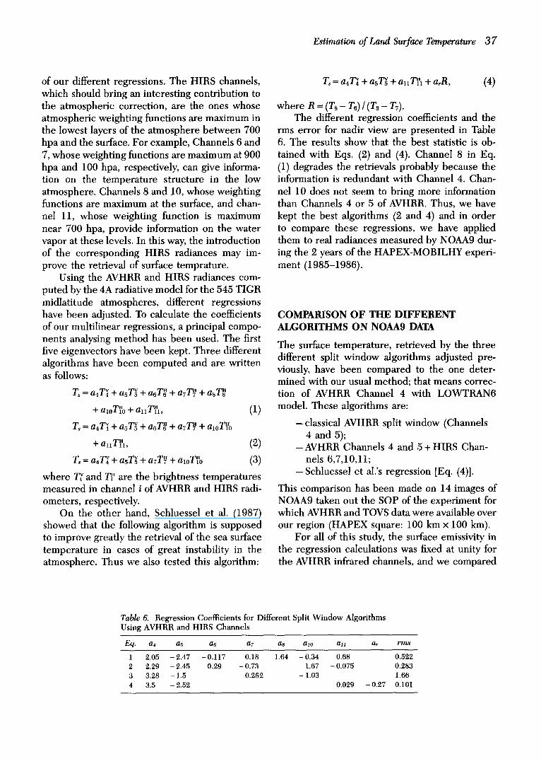
Estimation of Land Surface Temperature 3 7

of our different regressions. The HIRS channels, which should bring an interesting contribution to the atmospheric correction, are the ones whose atmospheric weighting functions are maximum in the lowest layers of the atmosphere between 700 hpa and the surface. For example, Channels 6 and 7, whose weighting functions are maximum at 900 hpa and 100 hpa, respectively, can give informa- tion on the temperature structure in the low atmosphere. Channels 8 and 10, whose weighting functions are maximum at the surface, and chan- nel 11, whose weighting function is maximum near 700 hpa, provide information on the water vapor at these levels. In this way, the introduction of the corresponding HIRS radiances may im- prove the retrieval of surface temprature.

Using the AVHRR and HIRS radiances com- puted by the 4A radiative model for the 545 TIGR midlatitude atmospheres, different regressions have been adjusted. To calculate the coefficients of our multilinear regressions, a principal compo- nents analysing method has been used. The first five eigenvectors have been kept. Three different algorithms have been computed and are written as follows:

Ts = a4T~4 + asT~5 + a~T~ + arTy + a s ~

+ aloT~o + alxT~l, (1)

Ts = a4T~4 + a~T~5 + a6T~ + a7T~7 + al0T~o

+ allT~h (2)

T~ = a4T~4 + a s ~ + a T ~ + aloT~o (3)

where T~ and T~ are the brightness temperatures measured in channel i of AVHRR and HIRS radi- ometers, respectively.

On the other hand, Schluessel et al. (1987) showed that the following algorithm is supposed to improve greatly the retrieval of the sea surface temperature in cases of great instability in the atmosphere. Thus we also tested this algorithm:

T, = a 4 ~ + a ~ + allTr~l + arR, (4)

where R = (Ts - T6) / (Ts - TT). The different regression coefficients and the

rms error for nadir view are presented in Table 6. The results show that the best statistic is ob- tained with Eqs. (2) and (4). Channel 8 in Eq. (1) degrades the retrievals probably because the information is redundant with Channel 4. Chan- nel 10 does not seem to bring more information than Channels 4 or 5 of AVHRR. Thus, we have kept the best algorithms (2 and 4) and in order to compare these regressions, we have applied them to real radiances measured by NOAA9 dur- ing the 2 years of the HAPEX-MOBILHY experi- ment (1985-1986).

COMPARISON OF THE DIFFERENT ALGORITHMS ON NOAA9 DATA

The surface temperature, retrieved by the three different split window algorithms adjusted pre- viously, have been compared to the one deter- mined with our usual method; that means correc- tion of AVHRR Channel 4 with LOWTRAN6 model. These algorithms are:

-classical AVHRR split window (Channels 4 and 5);

--AVHRR Channels 4 and 5 + HIRS Chan- nels 6,7,10,11;

-Schluessel et al.'s regression [Eq. (4)].

This comparison has been made on 14 images of NOAA9 taken out the SOP of the experiment for which AVHRR and TOVS data were available over our region (HAPEX square: 100 km x 100 km).

For all of this study, the surface emissivity in the regression calculations was fixed at unity for the AVHRR infrared channels, and we compared

Table 6. Regress ion Coeff ic ients for Di f fe ren t Split W i n d o w Algor i thms Using A V H R R and H I R S C hanne l s

Eq. a4 a5 a6 a7 a8 alo all ar

1 2.05 -2 .47 -0 .117 0.18 1.64 -0 .34 0.68 0.522 2 2.29 - 2.45 0.29 - 0.73 1.67 - 0.075 0.283 3 3.28 - 1.5 0.262 - 1.03 1.66 4 3.5 -2 .52 0.029 -0 .27 0.101

38 Ottld and Vidal-Madjar

320 K

300

280

260 26(

J .f.

' '

SW

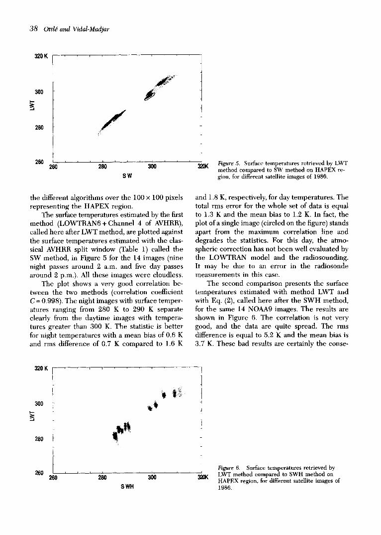
Figure 5. Surface temperatures retrieved by LWT method compared to SW method on HAPEX re- gion, for different satellite images of 1986.

the different algorithms over the 100 × 100 pixels representing the HAPEX region.

The surface temperatures estimated by the first method (LOWTRAN6 + Channel 4 of AVHRR), called here after LWT method, are plotted against the surface temperatures estimated with the clas- sical AVHRR split window (Table 1) called the SW method, in Figure 5 for the 14 images (nine night passes around 2 a.m. and five day passes around 2 p.m.). All these images were cloudless.

The plot shows a very good correlation be- tween the two methods (correlation coefficient C -- 0.998). The night images with surface temper- atures ranging from 280 K to 290 K separate clearly from the daytime images with tempera- tures greater than 300 K. The statistic is better for night temperatures with a mean bias of 0.6 K and rms difference of 0.7 K compared to 1.6 K

and 1.8 K, respectively, for day temperatures. The total rms error for the whole set of data is equal to 1.3 K and the mean bias to 1.2 K. In fact, the plot of a single image (circled on the figure) stands apart from the maximum correlation line and degrades the statistics. For this day, the atmo- spheric correction has not been well evaluated by the LOWTRAN model and the radiosounding. It may be due to an error in the radiosonde measurements in this case.

The second comparison presents the surface temperatures estimated with method LWT and with Eq. (2), called here after the SWH method, for the same 14 NOAA9 images. The results are shown in Figure 6. The correlation is not very good, and the data are quite spread. The rms difference is equal to 5.2 K and the mean bias is 3.7 K. These bad results are certainly the conse-

320 K

300 I - -

280

t i i I ~ 0 260 260 280

S WH

Figure 6. Surface temperatures retrieved by LWT method compared to SWH method on HAPEX region, for different satellite images of 1986.

Estimation of Land Surface Temperature 39

320 K

300

280

2so ' ' ' ' ' ' '

S WS

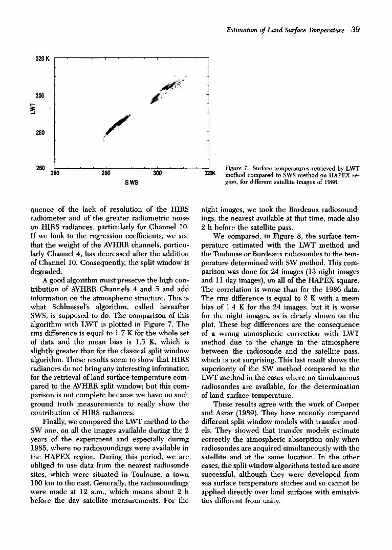
~0K Figure 7. Surface temperatures retrieved by LWT method compared to SWS method on HAPEX re- gion, for different satellite images of 1986.

quence of the lack of resolution of the HIRS radiometer and of the greater radiometric noise on HIRS radiances, particularly for Channel 10. If we look to the regression coefficients, we see that the weight of the AVHRR channels, particu- larly Channel 4, has decreased after the addition of Channel 10. Consequently, the split window is degraded.

A good algorithm must preserve the high con- tribution of AVHRR Channels 4 and 5 and add information on the atmospheric structure. This is what Schluessel's algorithm, called hereafter SWS, is supposed to do. The comparison of this algorithm with LWT is plotted in Figure 7. The rms difference is equal to 1.7 K for the whole set of data and the mean bias is 1.5 K, which is slightly greater than for the classical split window algorithm. These results seem to show that HIRS radiances do not bring any interesting information for the retrieval of land surface temperature com- pared to the AVHRR split window; but this com- parison is not complete because we have no such ground truth measurements to really show the contribution of HIRS radiances.

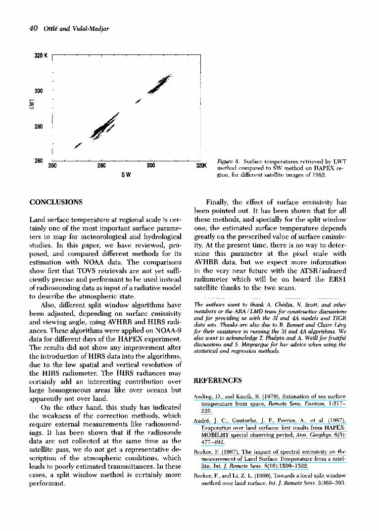
Finally, we compared the LWT method to the SW one, on all the images available during the 2 years of the experiment and especially during 1985, where no radiosoundings were available in the HAPEX region. During this period, we are obliged to use data from the nearest radiosonde sites, which were situated in Toulouse, a town 100 km to the east. Generally, the radiosoundings were made at 12 a.m., which means about 2 h before the day satellite measurements. For the

night images, we took the Bordeaux radiosound- ings, the nearest available at that time, made also 2 h before the satellite pass.

We compared, in Figure 8, the surface tem- perature estimated with the LWT method and the Toulouse or Bordeaux radiosondes to the tem- perature determined with SW method. This com- parison was done for 24 images (13 night images and 11 day images), on all of the HAPEX square. The correlation is worse than for the 1986 data. The rms difference is equal to 2 K with a mean bias of 1.4 K for the 24 images, but it is worse for the night images, as is clearly shown on the plot. These big differences are the consequence of a wrong atmospheric correction with LWT method due to the change in the atmosphere between the radiosonde and the satellite pass, which is not surprising. This last result shows the superiority of the SW method compared to the LWT method in the cases where no simultaneous radiosondes are available, for the determination of land surface temperature.

These results agree with the work of Cooper and Asrar (1989). They have recently compared different split window models with transfer mod- els. They showed that transfer models estimate correctly the atmospheric absorption only when radiosondes are acquired simultaneously with the satellite and at the same location. In the other cases, the split window algorithms tested are more successful, although they were developed from sea surface temperature studies and so cannot be applied directly over land surfaces with emissivi- ties different from unity.

4 0 Ottl~ and Vidal-Madjar

320 K

300 I - . -

280

I I

#

2 6 0 2 6 o ' ' ' '

SW

320K Figure 8. Surface temperatures retrieved by LWT method compared to SW method on HAPEX re- gion, for different satellite images of 1985.

CONCLUSIONS

Land surface temperature at regional scale is cer- tainly one of the most important surface parame- ters to map for meteorological and hydrological studies. In this paper, we have reviewed, pro- posed, and compared different methods for its estimation with NOAA data. The comparisons show first that TOVS retrievals are not yet suffi- ciently precise and performant to be used instead of radiosounding data as input of a radiative model to describe the atmospheric state.

Also, different split window algorithms have been adjusted, depending on surface emissivity and viewing angle, using AVHRR and HIRS radi- ances. These algorithms were applied on NOAA-9 data for different days of the HAPEX experiment. The results did not show any improvement after the introduction of HIRS data into the algorithms, due to the low spatial and vertical resolution of the HIRS radiometer. The HIRS radiances may certainly add an interesting contribution over large homogeneous areas like over oceans but apparently not over land.

On the other hand, this study has indicated the weakness of the correction methods, which require external measurements like radiosound- ings. It has been shown that if the radiosonde data are not collected at the same time as the satellite pass, we do not get a representative de- scription of the atmospheric conditions, which leads to poorly estimated transmittances. In these cases, a split window method is certainly more performant.

Finally, the effect of surface emissivity has been pointed out. It has been shown that for all these methods, and specially for the split window one, the estimated surface tempera ture depends greatly on the prescribed value of surface emissiv- ity. At the present time, there is no way to deter- mine this parameter at the pixel scale with AVHRR data, but we expect more information in the very near future with the ATSR/infrared radiometer which will be on board the ERS1 satellite thanks to the two scans.

The authors want to thank A. Ch~din, N. Scott, and other members or the ARA / LMD team for constructive discussions and for providing us with the 3I and 4A models and TIGR data sets. Thanks are also due to B. Bonnet and Claire Ldvy for their assistance in running the 31 and 4A algorithms. We also want to acknowledge T. Phulpin and A. Weill for fruitful discussions and S. Mayrargue for her advice when using the statistical and regression methods.

REFERENCES

Anding, D., and Kauth, R. (1979), Estimation of sea surface temperature from space, Remote Sens. Environ. 1:217- 220.

Andre, J. C., Goutorbe, J. P., Perrier, A., et al. (1987), Evaporation over land surfaces: first results from HAPEX- MOBILHY special observing period, Ann. Geophys. 6(5): 477-492.

Becker, F. (1987), The impact of spectral emissivity on the measurement of Land Surface Temperature from a satel- lite, Int. J. Remote Sens. 8(10):1509-1522.

Becker, F., and Li, Z. L. (1990), Towards a local split window method over land surface, Int. J. Remote Sens. 3:369-393.

Estimation of Land Surface Temperature 41

Ch6din, A., and Scott, N. (1984), Improve Initialisation inver- sion procedure, in Proc. of the 1st Int. TOVS Study Confer- ence, IGLS, Austria, Aug. 1983, A report from the CIMSS, P. Menzel, Ed., pp. 14-79.

Ch6din, A., and Scott, N. (1985), Initialisation of the radiative transfer equation inversion problem from a pattern recog- nition type approach. Application to the satellites of the TIROS-N series, in Adt~ in Remote Sensing Retrievals Methods, (A. Deepack Ed.), Academic, New York, pp. 495-515.

Cooper, D. I., and Asrar, G. (1989), Evaluating atmospheric correction models for retrieving surface temperatures from the AVHRR over a tallgrass prairie, Remote Sens. Environ. 27:93-102.

Deschamps, P. Y., and Phulpin, T. (1980), Atmospheric cor- rection of infrared measurements of sea surface tempera- ture using channels at 3.7, 11 and 12 t~m, Bound. Layer Meteorol. 18:131-143.

Flobert, J. F., et al. (1989), ECMWF/EUMETSAT Workshop, May 5-9, 1989: the Use of Satellite Data in Operational Numerical Weather Prediction 1989 / 1993, ECMWF edi- tion, Vol. II.

Kneizys, F. X., et al. (1983), Atmospheric transmittance/ radiance: computer code Lowtran6, Air Force Systems Command, USAF, AFGL-TR-83-0817.

Labed, J. (1990), Approche exp~rimentale des probl~mes li~s ~ l'~missivit~ et ~ la temperature de surface, ainsi qu'~ leur variabilit~ spatio-temporelle, dans le cadre de la t~l~d~tection spatiale dans rinfrarouge thermique, Th~se de doctorat, Universit~ de Strasbourg I.

Le Marshall, J. F. (1985), Proceedings of the 2nd International TOVS Study Conference, IGLS: An Intercomparison of Temperature and Moisture Fields Retrieved from TOVS Data.

Nerry, F., Labed, J., and Stoll, M. P. (1988), Emissivity signatures in the thermal infrared band for remote sens- ing, calibration procedure and method of measurement, Appl. Opt. 27(4):758-764.

Ottl~, C., and Stoll, M. (1988), Effect of atmospheric absorp- tion and surface emissivity on the determination of land surface temperature using satellite NOAA9 data, Ocean Air Interaction, forthcoming.

Prabhakara, C., Dalu, G., and Kunde, V. G. (1974), Estima- tion of sea surface temperature from remote sensing in the 11-13/~m window region, J. Geophys. Res. 79:5039- 5044.

Price, J. C. (1983), Estimating surface temperatures from satellite thermal infrared data. A simple formulation for the atmospheric effect, Remote Sens. Environ. 13:353- 361.

Price, J. C. (1984), Land surface temperature measurements from the split window channels of the NOAA7 / AVHRR, J. Geophys. Res. 89:7231-7237.

Schluessel, P., Shin, H. Y., Emery, W. J., and Grassl, H. (1987), Comparison of satellite derived sea surface tem- perature with in situ skin measurements, J. Geophys. Res. 92:2859-2874.

Schwalb, A. (1978), The TIROS N/NOAA A-G satellite series, NOAA Technical Memorandum, NESS 95, Ed. NOAA / NESSDIS.

Scott, N. A. (1974), A direct method of computation of the transmission function of an inhomogeneous gaseous medium, J. Quart. Spectrosc. Radiat, Transfer 14:691- 704.

Scott, N. A., and Ch~din, A. (1981), A fast line by line method for atmospheric absorption computations: the Automatized Atmospheric Absorption Atlas. J. Appl. Mete- orol. 20:802-812.