Economics of Land Degradation, Sustainable Land ...

Zentrum für Entwicklungsforschung

Economics of Land Degradation, Sustainable Land Management

and Poverty in Eastern Africa

The Extent, Drivers, Costs and Impacts

Inaugural – Dissertation

Zur

Erlangung des Grades

Doktor der Agrarwissenschaften

(Dr. agr.)

der

Landwirtschaftlichen Fakultät

der

Rheinischen Friedrich-Wilhelms-Universität Bonn

von

Oliver Kiptoo Kirui

aus

Kericho, Kenya

i

Referent: Professor Dr. Joachim von Braun

Korreferent: Professor Dr. Jan Börner

Tag der mündlichen Prüfung: 25.04.2016

Erscheinungsjahr: 2016

ii

Abstract

Land degradation – defined by the Economics of Land Degradation (ELD) initiative as a

“reduction in the economic value of ecosystem services and goods derived from land” – is a serious

impediment to improving rural livelihoods and food security of millions of people in the Eastern

Africa region. The objectives of this study are fourfold: to identify the state, extent and patterns of

land degradation in Eastern Africa (Ethiopia, Kenya, Malawi and Tanzania), to estimate and

compare the costs and benefits of action versus inaction against land degradation; to assess

simultaneously the proximate and underlying drivers of land degradation and the determinants of

adoption of Sustainable Land Management (SLM); and to assess the causal effects of land

degradation on the welfare of the households.

More recently, satellite–based imagery and remote sensing have been utilized to identify the

magnitude and processes of land degradation at global, regional and national levels. This involves

the use of Normalized Difference Vegetation Index (NDVI) derived from Advanced Very High-

Resolution Radiometer (AVHRR) data and the use of high quality satellite data from Moderate

Resolution Imaging Spectroradiometer (MODIS). Results based on NDVI measures show that

land degradation occurred in about 51%, 41%, 23% and 22% of the terrestrial areas in Tanzania,

Malawi, Ethiopia and Kenya, respectively between the 1982-2006 periods. Some of the key

hotspots areas include west and southern regions Ethiopia, western part of Kenya, southern parts

of Tanzania and eastern parts of Malawi. To ensure accuracy of the NDVI observations, ground-

truthing was carried out in Tanzania and Ethiopia through focused group discussions (FGDs). The

FGDs assessments indicate agreement in 7 sites out of 8 in Tanzania and 5 sites out of 6 in Ethiopia.

Following the Total Economic Value (TEV) framework, the cost of land degradation between

2001-2009 periods is about 2 billion USD in Malawi, 11 billion USD in Kenya, 18 billion USD in

Tanzania and 35 billion USD in Ethiopia. These translate to annual costs of about 248 million

USD in Malawi, 1.3 billion USD in Kenya, 2.3 billion USD in Tanzania, and 4.4 billion USD in

Ethiopia – representing about 5%, 7%, 14% and 23%, of GDP in Kenya, Malawi, Tanzania and

Ethiopia respectively. Taking action against land degradation is more favorable than inaction in

both short-term (6 year) and a long-term (30 year) periods. During the 30-year period, for every

dollar spent on taking action against land degradation users will expect a return of about $ 4.2 in

Ethiopia, $ 4.1 in Kenya, $ 3.8 in Tanzania, and $ 3.7 in Malawi.

The study uses nationally representative household surveys and robust analytical techniques to

capture a wide spectrum of heterogeneous contexts. A logistic regression model was used to

evaluate the drivers of land degradation and to assess the determinants of probability of adoption

of sustainable land management. Findings show that the key proximate drivers of land degradation

include temperature, terrain, topography and agro-ecological zonal classification. Important

underlying drivers of land degradation include factors such as land ownership, distance from the

plot to the market, size of the plot, access to and amount of credit, and household assets. The

adoption of sustainable land management practices is critical in addressing land degradation.

iii

Secure land tenure, access to extension services and market access are significant determinants

incentivizing SLM adoption. This implies that policies and strategies that facilitate secure land

tenure and access to SLM information are likely to incentivize investments in SLM. Local

institutions providing credit services, inputs such as seed and fertilizers, and extension services

must also not be ignored in the development policies.

Evidence from Simultaneous Equation Model with panel data shows significant causality between

land degradation (EVI decline) and poverty. On one hand, land degradation significantly decreases

household consumption per-capita and increases poverty. On the other hand, household poverty

increases the likelihood of land degradation. Specifically, increase in household per-capita

expenditure by 1% reduces the probability of EVI decline by 46% in Malawi and by 27% in

Tanzania. Increase in household per-capita expenditure by 1% also reduces the probability of soil

erosion occurrence by 29% in Malawi and by 26% in Tanzania. Poverty assessments show that

poor households have 69% and 67% more likelihood to experience EVI decline in Malawi and

Tanzania respectively. These findings are consistent with the hypothesis that poverty contributes

to land degradation as a result of poor households’ inability to invest in natural resource

conservation and improvement. Land degradation in turn contributes to low and declining

agricultural productivity, which in turn contributes to worsening poverty.

This study provides comprehensive assessments that highlight the drivers and the adverse

economic consequences of land degradation and attempts to capture full valuation of losses

incurred due to land degradation. It is hoped that this information expedites policy actions and

investments into SLM to successfully address land degradation problems.

iv

Zusammenfassung

Landdegradation – was die Initiative „Economics of Land Degradation“(ELD) als „reduction in

the economic value of ecosystem services and goods derived from land” (ELD, 2013) definiert –

ist ein ernstzunehmendes Hindernis bei der Verbesserung der ländlichen Lebensgrundlage und

Nahrungsmittelsicherheit von Millionen von Menschen in Regionen Ostafrikas. Diese Studie

verfolgt vier Ziele: Den Status, das Ausmaß und das Muster von Landdegradation in Ostafrika

(Äthiopien, Kenia, Malawi und Tansania) zu identifizieren; die Kosten und den Nutzen von

Bekämpfung und Nicht-Bekämpfung von Landdegradation zu schätzen und zu vergleichen;

simultan die unmittelbaren und zugrundeliegenden Faktoren von Landverarmung und die Faktoren

der Annahme von nachhaltigem Land Management (SLM) festzustellen; und die Kausaleffekte

von Landdegradation auf den Haushaltswohlstand zu analysieren.

Seit jüngerer Zeit werden Satelliten- und Fernerkundungsbilder genutzt um das Ausmaß und den

Prozess von Landdegradation auf globalem, regionalem und nationalem Level festzustellen. Das

beinhaltet die Zugrundelegung des „Normalized Difference Vegetation Index“ (NDVI), welcher

von „Advanced Very High Resolution Radiometer“ (AVHRR) Daten abgeleitet wird, sowie das

Nutzen von Satellitendaten hoher Qualität generiert durch „Moderate Resolution Imaging

Spectroradiometer“ (MODIS). Die Ergebnisse, basierend auf NDVI, zeigen, dass zwischen 1982

und 2006 ca. 51%, 41%, 23% und 22% der Bodenflächen in Tansania, Malawi, Äthiopien und

Kenia von Landdegradation betroffen waren. Einige der wichtigsten Hotspotbereiche befinden

sich in Süd- und West-Äthiopien, West-Kenia, Süd-Tansania und Ost-Malawi. Um die Richtigkeit

der NDVI-Beobachtungen sicherzustellen, erfolgte eine Ground-Truth-Datenerhebung in

Tansania und Äthiopien mittels gezielter Gruppendiskussionen (Focused Group Discussion =

FGD). Die Analyse zeigt, dass 7 von 8 Standorten in Tansania und 5 von 6 Standorten in Äthiopien

mit den zuvor ermittelten Werten übereinstimmen.

Basierend auf dem Konzept des ökonomischen Gesamtwertes (Total Economic Value, TEV)

betragen die Kosten der Landdegradation im Zeitraum von 2001 bis 2009 etwa US$ 2 Milliarden

in Malawi, US$ 11 Milliarden in Kenia, US$ 18 Milliarden in Tansania und US$ 35 Milliarden in

Äthiopien. Dies ergibt Jahreskosten von ca. US$ 248 Millionen in Malawi, US$ 1,3 Milliarden in

Kenia, US$ 2,3 Milliarden in Tansania und US$ 4,4 Milliarden in Äthiopien – was etwa 5%, 7%,

14% beziehungsweise 23% des jeweiligen Bruttoinlandproduktes (BIP) entspricht. Das Vorgehen

gegen Landdegradation ist sowohl kurzfristig (6 Jahre), als auch langfristig (30 Jahre) gesehen

günstiger als Untätigkeit. Im 30-Jahres-Zeitraum kann man für jeden investierten Dollar gegen

Landdegradation einen Ertrag von ca. US$ 4,2 in Äthiopien, US$ 4,1 in Kenia, US$ 3,8 in Tansania

und US$ 3,7 in Malawi erwarten.

Die Studie verwendet nationalrepräsentative Haushaltsumfragen und belastbare analytische

Methoden, um ein breites Spektrum heterogener Inhalte zu erfassen. Ein logistisches

Regressionsmodell wurde zur Evaluierung der Faktoren von Landdegradation und den

Determinanten der Annahmewahrscheinlichkeit von nachhaltigem Landmanagement benutzt. Die

v

Ergebnisse zeigen, dass Temperatur, Gelände, Topographie und agrarökologische

Zonenklassifizierung die wichtigsten unmittelbaren Determinanten von Landdegradation sind.

Wesentliche zugrundeliegende Faktoren von Landdegradation sind u. A. Bodenbesitztum,

Entfernung zwischen Grundstück und Markt, Größe des Grundstücks, Kreditzugang und –betrag

sowie Haushaltsbesitztümer. Die Annahme von Verfahren zu nachhaltigem Landmanagement ist

entscheidend bei der Bekämpfung von Landdegradation. Gesicherte Pachtverhältnisse, Zugang zu

landwirtschaftlichen Beratungsdiensten und Märkten sind Entscheidungsfaktoren, die Anreize zur

Annahme von SLM schaffen. Folglich schaffen Richtlinien und Strategien, die gesicherte

Pachtverhältnisse und Zugriff auf SLM-Informationen erleichtern, häufiger Anreize zur

Investition in SLM. Lokale Kreditinstitute, Vertreiber von Samen und Düngemitteln sowie

landwirtschaftliche Beratungsdienste dürfen bei der Entwicklung von Richtlinien allerdings auch

nicht vernachlässigt werden.

Ergebnisse des simultanen Gleichungsmodells (Simultaneous Equation Model) mit Paneldaten

weisen auf einen signifikanten Kausalzusammenhang zwischen Landdegradation (EVI decline)

und Armut hin. Einerseits verringert Landdegradation den pro-Kopf-Konsum signifikant und

erhöht die Armut. Andererseits erhöht Haushaltsarmut die Wahrscheinlichkeit von

Landdegradation. Im Einzelnen reduziert die Erhöhung der pro-Kopf-Ausgaben um 1% die

Wahrscheinlichkeit von Landdegradation (EVI decline) um 46% in Malawi und um 27% in

Tansania. Darüber hinaus reduziert dies auch die Wahrscheinlichkeit von Bodenerosion um 29%

in Malawi und um 26% in Tansania. Armutsschätzungen zeigen, dass arme Haushalte eine um

69% beziehungsweise 67% erhöhte Wahrscheinlichkeit von Landdegradation (EVI decline) in

Malawi und Tansania aufweisen. Diese Ergebnisse bekräftigen die Hypothese, dass Armut zu

Landdegradation beiträgt – als Resultat des Unvermögens armer Haushalte in natürliche

Ressourcenkonservierung und –verbesserung zu investieren. Landdegradation ihrerseits trägt zu

niedriger und zurückgehender landwirtschaftlicher Produktivität bei, was wiederum zur

Verschlimmerung der Armut führt.

Diese Studie bietet umfangreiche Analysen, welche die Treibfaktoren und nachteiligen

ökonomischen Konsequenzen von Landdegradation herausstellen. Des Weiteren wird versucht,

eine vollständige Bewertung der Verluste, die durch Landdegradation verursacht wurden,

vorzunehmen. Diese Informationen werden hoffentlich genutzt um die Entwicklung von

Richtlinien und Investitionen in SLM voranzutreiben und zur erfolgreichen Adressierung von

Landdegradationsproblemen beizutragen.

vi

Table of Contents

Abstract .......................................................................................................................................... ii

Zusammenfassung........................................................................................................................ iv

List of Tables .............................................................................................................................. viii

List of Abbreviations ................................................................................................................... xi

Acknowledgements ..................................................................................................................... xii

Chapter 1 ....................................................................................................................................... 1

1. Introduction .......................................................................................................................... 1

1.1 Background Information and Study Context ......................................................................... 1

1.2 Problem Statement ................................................................................................................. 2

1.3 Economics of Land Degradation (ELD) Initiative ................................................................. 3

1.4 Research Objectives and Questions ....................................................................................... 4

1.5 Contributions of the Study ..................................................................................................... 5

1.6 Organization of the Thesis ..................................................................................................... 7

Chapter 2 ....................................................................................................................................... 8

2. Assessment of Land Degradation ‘from Above and Below’ ............................................ 8

2.1 Overview of Methods of Assessing Land Degradation ......................................................... 8

2.2 The Extent of Land Degradation in Eastern Africa ............................................................. 11

2.3 Assessment of land degradation from ‘above’ ..................................................................... 15

2.3.1 Data sources ......................................................................................................................... 15

2.3.2 Extent of Land Degradation due to NDVI decline .............................................................. 15

2.3.3 Extent of Land Degradation due to LUCC .......................................................................... 18

2.4 Assessment of Land Degradation from ‘Below’ and Ground-truthing of Remote Sensing

Land Degradation Maps ................................................................................................................ 24

2.5 Actions taken to address Ecosystem Services Loss and to enhance or Maintain Ecosystem

Services Improvement .................................................................................................................. 37

2.6 Conclusions .......................................................................................................................... 39

Chapter 3 ..................................................................................................................................... 41

3. Cost of Land Degradation and Improvement ................................................................. 41

3.1 Introduction .......................................................................................................................... 41

3.2 Conceptual Framework ........................................................................................................ 43

3.3 Analytical Approach ............................................................................................................ 48

3.4 Data ...................................................................................................................................... 53

vii

3.5 Cost of Land Degradation due to Land Use Cover Change ................................................. 54

3.6 Cost of land degradation due to use of land degrading practices on cropland .................... 57

3.7 Total Cost of land degradation ............................................................................................. 60

3.8 Costs of action versus inaction against land degradation .................................................... 61

3.9 Conclusions .......................................................................................................................... 69

Chapter 4 ..................................................................................................................................... 71

4. Drivers of Land Degradation and Adoption of Multiple Sustainable Land

Management Practices....................................................................................................... 71

4.1 Introduction .......................................................................................................................... 71

4.2 Relevant Literature............................................................................................................... 73

4.3 Conceptual framework ......................................................................................................... 79

4.4 Data, sampling, choice of variables for econometric estimations ....................................... 80

4.5 Drivers of Land Degradation ............................................................................................... 92

4.6 Determinants of SLM Adoption .......................................................................................... 95

4.7 Conclusions and policy implications ................................................................................. 102

Chapter 5 ................................................................................................................................... 104

5. The Impact of Land Degradation on Household Poverty: Evidence from a Panel Data

Simultaneous Equation Model ........................................................................................ 104

5.1 Introduction ........................................................................................................................ 104

5.2 Relevant literature .............................................................................................................. 105

5.3 Data sources ....................................................................................................................... 108

5.4 Measuring Poverty and Land degradation ......................................................................... 110

5.5 Empirical strategy .............................................................................................................. 121

5.6 The instruments .................................................................................................................. 126

5.7 Results ................................................................................................................................ 127

5.8 Conclusions ........................................................................................................................ 135

Chapter 6 ................................................................................................................................... 136

6. General Conclusions ........................................................................................................ 136

7. References ......................................................................................................................... 141

8. Appendix ........................................................................................................................... 160

viii

List of Tables

Table 2.1: Land degradation types and extent in Sub Saharan Africa .......................................... 12

Table 2.2: Statistics of degraded areas by country for Eastern Africa (1981–2003) .................... 13

Table 2.3: Area (km2 and percentage) of long-term (1982-2006) NDVI decline ........................ 17

Table 2.9: Net change in land area of terrestrial biomes between 2001- 2009 (%) ...................... 23

Table 2.5: Characteristics of Focus Group Discussants in Ethiopia and Tanzania ...................... 27

Table 2.6: Comparison between the Le et al. (2014) land degradation map, the Focus Group

Discussions (FGDs), and the MODIS Land Cover Change analyses ........................................... 31

Table 2.7: Perceptions of Trend in Value Ecosystem Services of major Biomes ........................ 34

Table 2.8: Total Economic Values of forest, grassland and cropland (USD/ha/year) .................. 36

Table 2.9: Total Economic Values of forest, grassland and cropland (USD/ha/year) .................. 36

Table 2.10: Actions to maintain ecosystem services or address loss of ecosystem services ........ 38

Table 3.1: Cost and consequences of land degradation in Eastern Africa .................................... 46

Table 3.2: Terrestrial ecosystem value and cost of land degradation due to LUCC .................... 55

Table 3.3: Change in maize, rice and wheat yields under BAU and ISFM scenarios .................. 58

Table 3.4: Annual Cost of land degradation on static cropland – DSSAT results ........................ 60

Table 3.5: Annual total cost of land degradation (costs on static cropland and LUCC costs) ..... 60

Table 3.6: Cost of action & inaction against LUCC-related land degradation (US$ billion) ....... 61

Table 3.7: Cost of action & inaction against LUCC-related land degradation per hectare .......... 64

Table 3.8: Cost of action and inaction against land degradation in Ethiopia (million USD) ....... 65

Table 3.9: Cost of action and inaction against land degradation in Kenya (million USD) .......... 66

Table 3.10: Cost of action and inaction against land degradation in Malawi (million USD)....... 67

Table 3.11: Cost of action and inaction against land degradation in Tanzania (million USD) .... 68

Table 4.1: Empirical review of proximate and underlying causes of land degradation ............... 75

Table 4.2: Dependent variables used in econometric analysis ..................................................... 84

Table 4.3: Definitions of hypothesized explanatory variables...................................................... 89

Table 4.4: Descriptive statistics of explanatory variables (country and regional level) ............... 91

Table 4.5: Drivers of land degradation (NDVI decline) in Eastern Africa: Logit results ............ 93

Table 4.6: Drivers of adoption of SLM practices in Eastern Africa: Logit regression results ... 100

Table 5.1: Poverty lines per adult equivalent per annum ............................................................ 112

Table 5.2: Poverty results ........................................................................................................... 114

ix

Table 5.3: Poverty Transitions in Malawi and Tanzania, 2008/09 – 2012/13 ............................ 116

Table 5.4: Proportion of Households Experiencing biomass productivity (EVI) decline .......... 118

Table 5.5: Proportion of Households Experiencing Erosion in Malawi and Tanzania .............. 118

Table 5.6: Relationship between land degradation and poverty in Malawi and Tanzania ......... 119

Table 5.7: Relationship between soil erosion and poverty in Malawi and Tanzania ................. 120

Table 5.9: Descriptive statistics of the selected variables for the 2008/2009 and 2012/2013 .... 128

Table 5.10: Second stage results of impact of land degradation (soil erosion and EVI decline) on

poverty and consumption expenditure ........................................................................................ 131

Table 5.11: Second stage results of impact of poverty and consumption expenditure on land

degradation (soil erosion and NDVI decline) ............................................................................. 134

Table 8.1: Land area of terrestrial biomes in Eastern Africa 2001 (‘000 hactares) .................... 160

Table 8.2: Land area of terrestrial biomes in Eastern Africa 2009 (‘000 hactares) .................... 160

Table 8.3: Gained land area of terrestrial biomes between 2001- 2009 (‘000 hactares) ............ 160

Table 8.4: Lost land area of terrestrial biomes between 2001- 2009 (‘000 hactares) ................. 160

Table 8.5: Net change in land area of terrestrial biomes between 2001- 2009 (ha and %) ........ 161

Table 8.6: Land area of terrestrial biomes in Ethiopia in 2009 and change (%) for 2001-2009 161

Table 8.7: Land area of terrestrial biomes in Kenya in 2009 and change (%) for 2001-2009 ... 162

Table 8.8: Land area of terrestrial biomes in Malawi in 2009 and change (%) for 2001-2009 .. 163

Table 8.9: Land area of terrestrial biomes in Tanzania in 2009 and change (%) for 2001-2009 164

x

List of Figures

Figure 2.1: Geographic overview of land degradation in SSA ..................................................... 14

Figure 2.2: Biomass productivity decline in Eastern Africa over 1982-2006. ............................ 16

Figure 2.3: Biomass productivity decline by biome in Eastern Africa over 1982-2006. ............ 16

Figure 2.4: Land area of terrestrial biomes in 2001 and 2009 in Ethiopia (‘000 hactares) .......... 19

Figure 2.5: Land area of terrestrial biomes in 2001 and 2009 in Kenya (‘000 hactares) ............. 19

Figure 2.6: Land area of terrestrial biomes in 2001 and 2009 in Malawi (‘000 hactares) ............ 20

Figure 2.7: Land area of terrestrial biomes in 2001 and 2009 in Tanzania (‘000 hactares) ......... 20

Figure 2.8: Net change in land area of terrestrial biomes between 2001- 2009 (ha) .................... 22

Figure 2.9: Selected ground truthing sites in Ethiopia and Tanzania ........................................... 26

Figure 2.10: Ecosystems services & perception of their importance in Ethiopia (1982 & 2013) 32

Figure 2.11: Ecosystems services & perception of their importance in Tanzania (1982 & 2013) 33

Figure 3.1: Total Economic Value ................................................................................................ 44

Figure 3.2: Location of TEEB database of terrestrial ecosystem service valuation studies ......... 53

Figure 3.3: Cost of land degradation due to LUCC for the period 2001-09. ................................ 56

Figure 3.4: Provisioning verses other components of cost of land degradation ........................... 57

Figure 3.5: Cost of action & inaction against LUCC-related land degradation............................ 62

Figure 3.6: Cost of action against LUCC land degradation in 30 years in different scenarios .... 63

Figure 3.7: Cost of Inaction against LUCC land degradation in 30 years in different scenarios . 63

Figure 4.1: The Conceptual Framework of ELD Assessment ...................................................... 80

Figure 4.2: Distribution of sampled households ........................................................................... 83

Figure 4.3: The distribution of different SLM technologies adopted in Eastern Africa ............... 97

Figure 4.4: The distribution of number of SLM technologies adopted in Eastern Africa ............ 98

Figure 5.1: Conceptual framework land degradation and poverty relationships ........................ 107

Figure 5.2: Trends of Poverty incidence in Malawi and Tanzania, 2008/09 – 2012/13 ............. 114

Figure 5.3: Trends of depth and severity of Poverty in Malawi and Tanzania, 2008– 2013 ...... 115

Figure 5.4: Absolute Poverty Transitions in Malawi and Tanzania, 2008/09 – 2012/13 ........... 116

Figure 5.5: Relationship between land degradation and poverty in Malawi and Tanzania ........ 119

Figure 5.6: Relationship between soil erosion and poverty in Malawi and Tanzania ................ 120

Figure 8.1: Maize, Wheat & Rice Area in Ethiopia, Kenya, Malawi & Tanzania ................... 165

Figure 8.2: Cost of action against LUCC land degradation in 6 years in different scenarios .... 165

Figure 8.3: Cost of inaction against LUCC land degradation in 6 years in different scenarios . 165

xi

List of Abbreviations

AfDB African Development Bank

AGDP Agricultural Gross Domestic Product

AVHRR Advanced Very High Resolution Radiometer

CSA Central Statistical Agency

ELD Economics of Land Degradation

FAO United Nation’s Food and Agriculture Organization

FGDs Focus Group Discussion

FTC Farmer Training Centre

GDP Gross Domestic Product

GIS Geographic Information System

GLADA Global Assessment of Land Degradation and Improvement

ibid ibidem

IFPRI International Food Policy Research Institute

LUCC Land Use land Cover Change

MEA Millennium Ecosystem Assessment

NDVI Normalized Difference Vegetation Index

PES Payment for Ecosystem Services

RUE Rainfall Use Efficiency

SSA Sub-Saharan Africa

SLM Sustainable Land Management

TEEB The Economics of Ecosystems and Biodiversity

TEV Total Economic Value

UNCCD United Nations Convention to Combat Desertification

UNECA United Nation Economic Commission for Africa

USD United States Dollars

ZEF Center for Development Research, University of Bonn

xii

Acknowledgements

I owe my deepest gratitude and appreciation for many people and organizations without whom,

this PhD research would not have been possible.

I would like to thank the German Federal Ministry Federal Ministry for Economic Cooperation

and Development for funding my PhD studies. This research has been supported by the project on

the “Economics of Land Degradation”, funded by the German Federal Ministry Federal Ministry

for Economic Cooperation and Development and jointly conducted by ZEF and IFPRI with many

national partners.

I am extremely thankful to Prof. Dr. Joachim von Braun for his inspiring academic guidance,

advice and support at various stages of my doctoral study. His insightful comments and

suggestions on my work greatly helped me to improve it. I would like to thank to my second

supervisor Prof. Dr. Jan Börner for his interest in my work. I am also highly indebted to my advisor

Dr. Alisher Mirzabaev for his comments and suggestions and reviews of my thesis chapters

throughout the PhD period. I am very grateful to. Dr. Ephraim Nkonya for his useful suggestions

in this work and for sharing the data that made it possible to write up this thesis two chapters of

this thesis.

I would like to express my gratitude to my field research teams in Ethiopia (Dr. Samuel

Gebreselassie, Ensermu Bejiga, and Marlen Krause) and in Tanzania (Clemens Olbreich and

Happiness Zacharia), who put a lot of effort into a successful data collection.

My sincere appreciation to the Doctoral studies program at ZEF, especially Dr. Gunther Manske,

Ms. Maike Retat-Amin, and all friends and colleagues at ZEF.

Last but more importantly, my greatest gratitude goes to my wife, Georgina – your support and

inspiration in my work is immeasurable!

I dedicate this thesis to my loving parents.

1

Chapter 1

1. Introduction

1.1 Background Information and Study Context


“reduction in the economic value of ecosystem services and goods derived from land” (ELD, 2013)

– is a global problem affecting 29% of land area in all agro–ecological zones around the world (Le

et al., 2014). Estimates show that about a 3.2 billion people – most of them in low income countries

– reside on these degraded land (Le et al., 2014). Recent statistics from UNCCD show that about

40 percent of global agricultural land has been degraded in the past 50 years by erosion,

salinization, compaction, nutrient depletion, pollution and urbanization (UNCCD, 2007). About

1.9 billion hectares of land has been degraded worldwide (UN, 1997).

Recent data indicate that globally, an area of about 5–8 million hectares of productive land go out

of production annually due to degradation (TerrAfrica, 2006). More agricultural land is rendered

less productive in developing countries as depicted by considerable decline in crop yields (Vlek et

al., 2010). There is no consensus on the exact extent, severity and impacts of land degradation in

the Eastern Africa region or in sub-Saharan Africa (SSA) as a whole (Reich et al., 2001; Stocking,

2006). However, recent assessments show that land degradation affected 51%, 41%, 23% and 22%

of land area in Tanzania, Malawi, Ethiopia and Kenya respectively (Le et al., 2014).

Resource loss due to land degradation in Eastern Africa is believed to be enormous (Maitima,

2009). To illustrate, about 1 billion tons of topsoil are lost annually in Ethiopia due to soil erosion

(Brown, 2006), costing the country 3% of its Agricultural Gross Domestic Product (AGDP) (Yesuf

et al., 2008). In Tanzania, land degradation has been ranked as the top environmental problem for

more than 60 years (Assey et al., 2007). Soil erosion is considered to have occurred on 61% of the

entire land area in Tanzania (ibid). Chemical land degradation, including soil pollution and

salinization/alkalinisation, has led to 15% loss in the arable land in Malawi and Zambia in the last

decade alone (Chabala et al., 2012).

Investment in sustainable land management (SLM) is a cost-effective and worthwhile way to

address land degradation (MEA, 2005; Akhtar-Schuster et al., 2011; ELD Initiative, 2013). SLM,

2

also referred to as ‘ecosystem approach’, ensures long-term conservation of the productive

capacity of lands and the sustainable use of natural ecosystems. However, estimates show that the

adoption of SLM practices is very low – just about 3% of total cropland in SSA (World Bank,

2010). Several factors limit the adoption of SLM, including; lack of local-level capacities,

knowledge gaps on specific land degradation and SLM issues, inadequate monitoring and

evaluation of land degradation and its impacts, inappropriate incentive structure (such as,

inappropriate land tenure and user rights), market and infrastructure constraints (such as, volatile

prices of agricultural products, increasing input costs, inaccessible markets), and policy and

institutional bottlenecks (such as, difficulty and costly enforcement of existing laws that favor

SLM) (Thompson et al., 2009; Chasek et al., 2011; Akhtar-Schuster et al., 2011; Reed et al., 2011;

ELD Initiative, 2013).

Land degradation poses the greatest long–term threat to human survival and offers one of the

greatest policy challenges in the foreseeable future in many low income countries (Scherr, 1999).

The duo problem of land degradation and poverty is dire in rural areas of low income countries

because the major economic activities hinge on agricultural–based livelihoods (Turner et al.,

1994). This study posits that poverty and land degradation are interwoven and that the linkage

between them is complex and mutually re–enforcing (poverty leads to land degradation while land

degradation also contributes to poverty); a poverty–land degradation viscous cycle. Globally, an

estimated 870 million people are poor – living on less than $1 USD a day; majority of whom reside

in rural degrading areas of developing countries (FAO, 2012). Land degradation is therefore an

important issue particularly on the welfare of the rural households in developing countries because

it is closely linked to household poverty and food (in)security.

1.2 Problem Statement

Despite a backdrop of information on the natural resource loss, large economic losses due to land

degradation and the urgent need for action to prevent and reverse land degradation, the problem

has yet to be appropriately addressed, especially in the developing countries, including in Eastern

Africa. Adequately strong policy action for SLM is lacking, and a coherent and evidence-based

policy framework for action across all agro-ecological zones is missing (Nkonya et al., 2013).

Identifying drivers of land degradation is one step toward addressing them (von Braun, et al.,

3

2012).The assessment of relevant drivers of land degradation by robust techniques at farm and

household levels is necessary. The adoption of sustainable land management practices is critical

in addressing land degradation. There is, thus, an increasing need for evidence-based science to

evaluate the determinants of adoption as well as economic returns from SLM. Reliable estimates

on the exact impact of land degradation on the welfare (poverty) of farm households are not

available.

1.3 Economics of Land Degradation (ELD) Initiative

This doctoral study is carried out under the auspices of a larger global research ‘‘The Economics

of Land Degradation (ELD)’’ implemented by the International Food Policy Institute (IFPRI) and

Center for Development Research (ZEF) which was commissioned in 2010-2011 by the United

Nations Convention to Combat Desertification (UNCCD) in collaboration with the German

Federal Ministry of Economic Cooperation and Development (BMZ). ELD was established to

provide common methods and approaches to highlight the value of sustainable land management

and the costs of land degradation. ELD research seeks to assess the state-of-the-knowledge on the

economics of land degradation around the globe. The ELD research develops an analytical

conceptual framework for a more comprehensive and integrated global assessment of land

degradation by including the value of land ecosystem services. It also provides methods for

assessment of the drivers of land degradation.

ELD methodology make use of satellite data to depict land degradation and improvement areas

based on changes in biomass productivity as shown by the Normalized Differenced Vegetation

Index (NDVI) (Le et al., 2014) and based on the losses or deterioration of ecosystem services as

depicted by Land Use Cover Change (LUCC) (Nkonya et al. 2013). The total economic value

(TEV) approach is used to analyze on-site and off-site direct and indirect societal costs and benefits

of land degradation for both the present and the future periods (ibid). Through these assessments

of the drivers and costs of land degradation and on the returns to investments for rehabilitating

land or preventing land degradation, ELD aims at increasing the awareness and thus provide

opportunities for mobilizing investments in sustainable management of land resources at nationally

and globally.

4

The current study therefore demonstrates the application of these concepts and methods at the

national and regional (district) in four Eastern African countries – Ethiopia, Kenya, Malawi and

Tanzania which have been identified to be seriously affected by land degradation (Le et al., 2014).

It also provide field and community-based information which form a “bottom-up” approach to

assessment of land degradation in contrast to “top-down” satellite data analysis. Additionally (and

unlike the global assessment), this thesis analyses the impact of land degradation on household

welfare (poverty) using a combination of satellite and nationally representative agricultural

household survey data.

1.4 Research Objectives and Questions

Based on the above background, context and research challenge, the aim of this study on the

economics of land degradation, sustainable land management and household welfare is to identify

the extent of land degradation, provide comprehensive assessments that highlight the extent,

drivers and the adverse economic consequences of land degradation and to capture full valuation

of losses incurred due to land degradation. Specifically, this study pursues its objectives as follows.

First, it identifies the state, extent and patterns of land degradation in Eastern Africa (Ethiopia,

Kenya, Malawi and Tanzania) using remotely sensed datasets. This involves the use of Normalized

Difference Vegetation Index (NDVI) derived from Advanced Very High-Resolution Radiometer

(AVHRR) data and the use of high quality satellite data from Moderate Resolution Imaging

Spectroradiometer (MODIS). Second, it assesses simultaneously the proximate and underlying

drivers of land degradation and the determinants of adoption of SLM in Eastern Africa using

national representative agricultural household survey data.

Identifying drivers of land degradation is one step toward addressing them. Thus, the potential

technological, institutional and policy measures to address land degradation are highlighted. Third,

the study evaluates the costs and benefits of action verses inaction against land degradation in

Eastern Africa using Total Economic Value (TEV) approach. TEV is a comprehensive approach

that accounts for the losses of both market-priced provisional land ecosystems services and non-

marketed supporting, regulating and cultural ecosystem services. Finally, this study estimates the

causal relationship between land degradation on household poverty using panel data in Tanzania

with robust analytical approach that accounts for endogeneity. In order to achieve these objectives

5

and based on the preceding background and problem definition, the proposed study pursues

answers to the following research questions:

1. What is the state of knowledge on extent of land degradation in Eastern Africa and how may

remote and ground-level assessments complement each other?

2. What is the cost of land degradation in Eastern Africa and how the costs of action against land

degradation compare with the costs of inaction?

3. What are the drivers (proximate and underlying) of land degradation and determinants of

adoption of SLM practices?

4. What is the impact of land degradation on poverty?

Comprehensive assessments that highlight the drivers of land degradation, capture full valuation

of losses incurred due to land degradation, and establish the adverse economic consequences of

land degradation would expedite policy actions and investments into SLM to successfully address

land degradation problems.

1.5 Contributions of the Study

A summary of some of the contributions from this study are presented in this subsection. Detailed

contributions are highlighted throughout the study. The novelty of this study on the economics of

land degradation, SLM and poverty in Eastern Africa is that it is the first to provide a

comprehensive assessment that make the drivers and the adverse economic consequences of land

degradation visible and capture a full valuation of losses incurred due to land degradation. It also

reviews and ground-truth the land degradation ‘hotspot map’ proposed by Le et al. (2014).

There already exist a body of literature covering the extent and patterns of land degradation in Sub

Saharan Africa (e.g. Bridges and Oldeman, 1999; Berry et al., 2003; Jones et al., 2003; Stringer

and Reed, 2007; Bai et al. 2008; Stoosnijder, 2007; Nachtergaele et al. 2010; Lal & Stewart, 2013;

Zucca et al., 2014), albeit lacking in a number of ways. Most of these studies have not been

successful in quantifying the extent and severity of land degradation in East Africa (Sonneveld,

2003; Berry et al., 2003; Stringer and Reed, 2007; Verchot, et al., 2007). They also vary in the

approaches used to estimate the extent and levels of land degradation. Most of the studies in

Eastern Africa uses expert opinion methodologies (e.g. Oldeman et al., 1991; Bridges and

6

Oldeman, 1999; FAO, 2000; Jones et al., 2003; Sonneveld, 2003; Stringer and Reed, 2007;

Verchot, et al., 2007; Assey et al., 2007). A number of deficiencies are associated with this

approach: Information on expert opinions are perception-based and semi quantitative and therefore

not built on objective measurements (Dejene, 1997; Jones et al., 2003; Kapalanga, 2008). Studies

based on expert opinion methodologies are also said to have unknown magnitudes and directions

of measurement errors (Kasprzyk, 2005; Le et al., 2014).

More recently, quantitative interpretation of satellite imagery (NDVI/NPP), and model-based

approaches involving indicators and proxy variables measurable over large areas and over longer

periods have been used (e.g. Bai et al., 2008; Vlek et al., 2010; Le et al., 2014). Some caveats

associated with NDVI/NPP methodologies include: site-specific effects of vegetation/crop

structure and site conditions autocorrelation, effect of atmospheric fertilization and intensive

fertilizer use on NDVI, seasonal variations in vegetation phenology, and effect of soil moisture in

sparse vegetative areas. Detailed steps on how these caveats were addressed are presented in Le et

al. (2014). NDVI is preferred because it allows the assessment of land degradation over longer

term period and on national and regional scales.

This study is also the first to complement remote sensing with ground level assessment in

evaluating the state of knowledge on the extent of land degradation in Eastern Africa. Remotely-

sensed dataset on biomass productivity decline is based on an updated methodology proposed by

Le et al. (2014) while the remotely-sensed dataset on land use and land cover change (LUCC) is

based on Total Economic Value framework proposed by Nkonya et al. (2015). To ensure accuracy

of these remotely sensed estimations, ground-truthing was done through focused group discussions

(FGDs) in Tanzania and Ethiopia. Besides, ground-truthing, the NDVI and LUCC assessments are

also triangulated with both household and plot level data.

There is a fairly large body of existing literature on causes of land degradation and determinants

of adoption of SLM, however, a number of limitations are evident. These studies either focuses on

some specific location(s) in the region (de Bie, 2005; Stringer and Reed, 2007; Pender and

Gebremedhin, 2006), are considered subjective and lacking in scientific rigor and/or have weak

explanatory power due to smaller sample size (Olwande et al., 2009; Yesuf and Köhlin, 2009;

Oostendorp and Zaal, 2011). Results from different studies are often contradictory regarding any

given variable (Ghadim and Pannell, 1999; Nkonya et al., 2013). The contribution of this study

7

stems from employing nationally representative agricultural household surveys and robust

analytical techniques to capture a wide spectrum of heterogeneous contexts in the three Eastern

Africa countries. This approach could lead to better targeting of policy measures for combating

land degradation and facilitating SLM uptake across different contexts.

A review of existing literature showed that no study has comprehensively tackled the costs of land

degradation and the value of benefits from land improvement either at the household, regional or

national level in Eastern Africa. This study adopts a comprehensive approach (TEV) proposed by

Nkonya et al (2015) that accounts for the losses of both market-priced provisional land ecosystems

services and non-marketed supporting, regulating and cultural ecosystem services. Land

degradation costs and benefits from land improvement are estimated for the 2001-2009 period at

pixel level (and aggregated at district and national level) and simulated for a period of 30 years.

The study is also the first to estimate the causal linkages between land degradation and poverty in

the region. The study utilizes panel data from smallholder farm households which enables

controlling for unobserved heterogeneity and account for endogeneity.

1.6 Organization of the Thesis

This thesis is organized into six chapters crafted to address the proposed research questions.

Following this introduction (chapter 1) to the research context, problem, objectives and research

questions, the first research question on the state of knowledge on the extent of land degradation

in Eastern Africa is enumerated in chapter 2. Detailed description on how remote and ground-level

assessments could complement each other is also described in this chapter. Chapter 3 answers the

third research question on the cost of land degradation and how the costs of action against land

degradation compare with the costs of inaction. Chapter 4 addresses the third research question on

the drivers of land degradation and determinants of adoption of adoption of SLM practices.

Chapter 5 tackles the fourth research question on the causal relationships between poverty and

land degradation. This chapter assesses the impact of land degradation on poverty and vice versa

using panel data. Chapter 6 concludes the thesis by summarizing the main research findings and

providing the implications of the study for policy and practice.

8

Chapter 2

2. Assessment of Land Degradation ‘from Above and Below’

2.1 Overview of Methods of Assessing Land Degradation

Land degradation is defined as ‘‘the persistent reduction of the production capacity of a land, which

may be manifest through any combination of a number of interrelated processes, such as: soil

erosion, deterioration of soil nutrients, loss of biodiversity, deforestation or declining vegetative

health’’ (Le et al., 2012). Assessments of land degradation vary in methodology and outcome

(Stoosnijder, 2007; Lal & Stewart, 2013; Zucca et al., 2014). There are two broad approaches to

evaluate land degradation: ground-based measurements and remote sensing.

Ground-based measurements, also referred to as survey-based (direct) field observations, include

approaches such as experts’ opinions, land users’ opinion, field monitoring and measurements,

productivity changes, farm-level studies, and modeling. These approaches are important in

evaluating land degradation process at the national and local levels (Van Lynden and Kuhlmann

2002). On the other hand, above-ground measurements involves the use of remotely sensed

satellite imagery, Radio Detection and Ranging (RADAR), and GIS data. An extensive review of

these methods including their appropriateness, strengths, and limitations is provided in Nkonya et

al. (2011) and Kapalanga (2008).

Ground-based measurements have been utilized to evaluate the severity, degree and extent of land

and soil degradation at global, regional national and local levels. For example, the Global

Assessment of Human-induced Soil Degradation (GLASOD) which is based on expert opinion,

provides information on the global distribution, intensity and the causes of erosional, chemical,

and physical degradation (Bridges and Oldeman, 1999; Jones et al., 2003). The World Overview

of Conservation Approaches and Technologies (WOCAT) provides information on soil and water

conservation (SWC), conservation approaches, and technologies to combat desertification in 23

countries spread across six continents (Bai et al. 2008; Nachtergaele et al. 2010). Other studies

that use expert opinions conducted at national and local levels include Sonneveld (2003) in

Ethiopia, and Berry et al. (2003) in Chile.

9

Direct field observations using soil erosion indicators such as eroded clods, flow surfaces, pre-rills

and rills have been used to effectively monitor the effects of erosion from tillage and harvesting in

Kenya (de Bie, 2005). Further examples includes the participatory degradation appraisal carried

out in Botswana (Reed and Dougill, 2002). This approach combines three approaches; the land

user opinion, the farm-level field observations and assessment of productivity changes. Stringer

and Reed (2007) also uses a participatory approach that integrates the expert opinions and the

experiences of the local knowledge (key informant interviews, focus group discussions and

questionnaires) to enhance accuracy, coverage and relevance of land degradation assessment in

Botswana and Swaziland.

Soil erosion and its related risks has been studied using various models such as Universal Soil Loss

Equation (USLE), Wind Erosion Equation (WEE) (Arnalds et al., 2001; EUSOILS, 2008), Revised

Universal Soil Loss Equation (RUSLE) (EUSOILS, 2008), Coordination of Information on the

Environment (CORINE) (Dengiz and Akgul, 2004), and Pan-European Soil Erosion Risk

Assessment (PESERA) (Kirkby et al., 2004).

Remote sensing approach is vital in measuring land degradation especially over a larger scale –

regional, national to global scales in a consistent manner. This approach is considered a cost-

effective and time-efficient because one image can be used to assess land degradation over a big

area (Lu et al., 2007; Gao and Liu, 2010). Land degradation can be identified in various ways

using remote sensing techniques, including;

(i) Manual visual approach; such as image differencing of two images – Rasmussen et al.

(2001) in Burkina Faso; Collado et al. (2002) in Argentina; Borak et al. (2000) in sub

Saharan Africa,

(ii) Interpretation of aerial photography and satellite imagery; such as Gupta et al. (2002) in

China; Ries and Marzolf (2003) in Spain;

(iii) Spectral index (“Land degradation Index”) such as Chikhaoui et al. (2005) in Morocco;

(iv) Land-cover mapping and “Steppe Degradation Index” Spatial and temporal metrics of land

cover change: Borak et al. (2000) in sub Saharan Africa.

Recent empirical evaluations of land degradation, however, show a shift from manual visual

approaches, interpretation of aerial photography and satellite imagery to a more model-based

approach involving indicators and proxy variables, measurable over large areas and over longer

10

periods. These approaches have been criticized for exaggerating the result on the levels of land

degradation, and that they are perception-based and semi quantitative, and therefore not built on

objective measurements. Land-cover exercises map degradation using image brightness values on

a snapshot satellite image, thus cannot represent persistent land degradation.

(v) Model-based approach – involving indicators and proxy variables: The most widely used

index for assessment is the vegetation indices such as the Normalized Difference

Vegetation Index (NDVI).

NDVI is an index of plant “greenness” or photosynthetic activity. Vegetation indices have been

used for a long time in a wide range of fields, such as vegetation monitoring; climate modelling;

agricultural activities; drought studies and public health issues (Running et al., 1994). Vegetation

indices are radiometric measures that combine information from the red and near infra-red (NIR)

portions of the spectrum to enhance the 'vegetation signal'. NDVI allows reliable spatial and

temporal inter-comparisons of terrestrial photosynthetic activity and canopy structural variations.

NDVI is generally computed for all pixels in time and space, regardless of biome type, land cover

condition and soil type, and thus represent true surface measurements. There are varied NDVI

datasets available including; the Moderate Resolution Imaging Spectroradiometer (MODIS),

Advanced Very High Resolution Radiometer (AVHRR), and Landsat satellite sensors (Brown et

al., 2006; Fensholt and Proud, 2012; Beck et al., 2011).

Some studies utilizing this approach include: Diouf and Lambin (2001) in Senegal; Prince et al.,

(1998) Nicholson et al. (1998), Herrmann et al., (2005) in the Sahel; Prince (1998, 2002) in

Zimbabwe and Mozambique, Vlek et al. (2010) in SSA, Bai et al. (2008) and Le et al. (2014) at

the global level. de Pinto et al. (2013) extents NDVI estimation to predict/detect future land

degradation and its economic effects globally with inclusion of climate change effects.

However, remote sensing datasets may have structural errors. These structural errors may be

conceptualized as falling into one of three related categories: errors arising from the type of sensor

used, errors arising from the spatial and temporal resolution of the analysis, and errors arising from

the derived data used (i.e. indices, land cover/land use classifications, etc.). A step by step

procedure to address these shortcomings relating to measurement of biomass productivity (NDVI)

changes is presented in Le et al., (2014).

11

The nobility of this study stems from combining remote sensed land degradation dataset and

ground-based surveys (ground-truthing) to evaluate the extent of land degradation. Remotely-

sensed dataset on biomass productivity (NDVI) decline is based on an updated methodology

proposed by Le et al. (2014) while the remotely-sensed dataset on land use and land cover change

(LUCC) is based on Total economic Value framework proposed by Nkonya et al. (2015). Survey-

based datasets collected through Focused Group Discussions (FGDs) are used to complement the

remote-sensing observations. The survey based observations are important because they provide

ground-based estimates of land degradation from the perspectives of the communities involved.

The next sections, describes the datasets used, methods of analysis, and the results. A brief

discussion of the implications of these results is presented in the conclusion.

2.2 The Extent of Land Degradation in Eastern Africa

The total population of Sub-Saharan Africa (SSA) is currently estimated at 750 million people

(UNDP, 2005), but this is projected to grow past the one billion mark by 2020 (UNDP, 2005,

Haub, 2009). The region is the poorest in the world, with an estimated one in every three people

living below the poverty line. The demand for food is putting greater pressures on the natural

resource base. Assessments of land degradation in the region vary in methodology and outcome

(Stoosnijder, 2007; Lal & Stewart, 2013; Zucca et al., 2014). The GLASOD survey, based on

expert opinion, concluded that in the early 1980s about 16.7% of SSA experienced serious human-

induced land degradation (Middleton & Thomas, 1992; Yalew, 2014). Using standardized criteria

and expert judgment, Oldeman (1994) revealed that about 20% of SSA was affected by slight to

extreme land degradation in 1990. These assessments were done based on ‘experts’ opinion and

for varying time period.

The data from the FAO TERRASTAT maps 67% (16.1 million km2) of the total land area of SSA

as degraded (FAO, 2000), with country-to-country variations. These variations are quite large:

Ethiopia is the most seriously affected (25% of territory degraded) while Kenya and Tanzania

records 15% and 13%, respectively. Malawi is the least affected (9%). The figure for Tanzania

(13%) is quite low compared to a later study (Assey et al., 2007) based on expert opinion that

showed about 61% of the territory affected by land degradation. The TERRASTAT dataset allows

the further classification of the degraded lands by the relative degree of severity of degradation.

12

Thus out of the 67% degraded land in SSA, the four sub-categories exist, namely; light (24%),

moderate (18%), severe (15%), and very severe (10%). In contrast, the GLASOD data shows that

about 25%, 14% and 13% of land area is degraded in Ethiopia, Kenya and Tanzania respectively.

However, the main weakness of these studies is that it is based on subjective expert judgment and

must be approached with caution.

GLASOD global survey (Nachtergaele, 2006) and FAO`s global forest resource assessment (2005)

identified six main types of land degradation predominant across SSA countries (Table 2.1).

Among them, water and wind erosion are the most widespread type of land degradation (46% and

38% respectively), followed by chemical and physical deterioration of soils (16%). The other types

of land degradation include salinization and water logging, decline in soil fertility, and loss of

habitat (especially forest and woodland). Previous studies have not been successful in quantifying

the extent and severity of these types of land degradation in East Africa. However, it is notable

that water erosion, declining soil fertility and nutrient depletion are important in all the four

countries. While salinization (irrigated land) is severe in Kenya (30%) and Tanzania (27%), loss

of forest and woodland in these countries is estimated at 0.7% per annum.

Table 2.1: Land degradation types and extent in Sub Saharan Africa

Type of land

degradation

Affected

land

(% of total)

Affected

population

(% of total) Countries affected Main cause(s)

Water Erosion

46

97

All countries in eastern Africa (Kenya,

Tanzania, Ethiopia, Malawi, Zambia)

Deforestation,

overgrazing, agric.

Practices

Wind Erosion

38

18

Botswana, Chad, Djibouti, Eritrea,

Mali, Niger, South Africa and Sudan

Overgrazing,

deforestation

Salinization Severe in Kenya (30%), Tanzania

(27%) Water management

Soil fertility

and nutrient

depletion

Approx. 100 Approx. 100 All countries

Agric. practices,

overgrazing,

deforestation,

Loss of

Habitat

(Deforestation)

0.7% of annual change of

Forest & Woodland area in

East & Southern Africa

Hotspots: Burundi (-5.2%), Comoros

(-7%), Nigeria (-3.3%), Togo (-4.5%),

Uganda (-2.2%), Zimbabwe (-1.7%)

Deforestation,

overgrazing,

agricultural practices

Source: Adopted from Global Forest Resource Assessment (FAO, 2005) & Nachtergaele, (2006).

More recently, satellite–based imagery (remote sensing) have been utilized to identify the



13

Resolution Radiometer (AVHRR) data. Several studies have applied this technique, including;

Evans & Geerken, 2004; Bai et al., 2008; Hellden & Tottrup, 2008; Vlek et al., 2010. While using

rain-use efficiency (RUE) adjusted NDVI, Bai et al. (2008) map the global land degradation trends.

Their assessment shows that land degradation has affected about 26% of SSA. The areas affected

are also different from those reported by GLASOD and TERRASTAT surveys and by Oldeman

(1994).

Unlike this GLASOD and TERRASTAT assessment, Bai et al., (2008) estimated that about 24%

of the global land area has been degrading (significant decline in NDVI) in 25 years. Much of the

areas they identify do not overlap with those indicated in the GLASSOD survey. However, Sub

Saharan Africa region remains the most affected. Country estimates (Table 2.2) show that

Tanzania was the most affected country; 41% of its land territory degraded. Ethiopia and Malawi

both had 26% of their territories degraded while about 18% of Kenya land area was degraded in

the same period. In terms of populations affected; about 40% and 36% of people in Tanzania and

Kenya were living in these degraded areas. Similarly, about 30% and 20% of the Ethiopian and

Malawian population was affected by land degradation over the same period. It is however notable

that these estimates do not take into account the effect of atmospheric fertilization, the rainfall

factor and the effect of soil moisture in sparse vegetative areas.

Table 2.2: Statistics of degraded areas by country for Eastern Africa (1981–2003)

Country

Degrading

area (km2)

%

Territory

% Total

population

Affected

People

% Territory

(GLASOD)

Ethiopia 296,812 26 29 20 million 25

Kenya 104,994 18 36 11 million 15

Malawi 30,869 26 20 2 million 9

Tanzania 386,256 41 40 15 million 13

Source: Bai et al., 2008 and FAO, 2000.

Similarly, the work of Vlek et al. (2008) estimated that 10% of SSA was significantly affected by

land degradation. Vlek et al. (2010) also map the geographic extent of areas in SSA affected by

land degradation processes over the period of 1982–2003 (Figure 2.1). While utilizing long-term

NDVI, they show that about 27% of the land is subject to degradation processes including, soil

degradation, overgrazing, or deforestation. Following Vlek et al., (2010), the land degradation

‘hotspots’ map shows that Ethiopia, Kenya, Tanzania and Malawi are the most affected in the

14

Eastern Africa region, thus they were selected as case studies countries for this assessments. Some

of the key hotspots areas include west and southern regions Ethiopia, western part of Kenya,

southern parts of Tanzania and eastern parts of Malawi (Figure 2.1).

Figure 2.1: Geographic overview of land degradation in SSA1

Source: Vlek et al., 2010.

The hotspot areas in Ethiopia are characterized by high population pressure (on land and forests),

farming activities on steep slopes and frequent famines occasioned by unreliable rainfall. The

hotspots in Kenya are characterized by intensive crop farming that increases pressure on soils. The

arid and semi-arid conditions of the southern parts of Tanzania and eastern parts of Malawi may

also be a contributing factor to the high degradation levels. Detailed studies have been carried out

in these Eastern Africa countries as presented in the next chapters.

1 Note: The geographic spread of the area subject to human-induced degradation processes among the different

climatic zones of SSA. The red spots show the pixels with significantly declining dNDVIhuman/dt.

15

2.3 Assessment of land degradation from ‘above’

Two approaches are used to evaluate the extent of land degradation in this study: biomass

productivity (NDVI) decline and Land Use land Cove Change (LUCC).

2.3.1 Data sources

This study uses the Le et al. (2014) land degradation dataset which builds upon the GLADIS

methodology and recommendations to estimate biomass productivity decline. Le et al. (2014)

dataset is useful in identifying “global geographic degradation hotspots or improvement hotspots”.

Le et al. (2014) calculates statistically significant long-term trends in NDVI from 1982 – 2006

using data obtained from Global Inventory Modeling and Mapping Studies (GIMMS) which is

derived AVHRR. Le et al. (2014) dataset is preferred because it corrects for the effects of rainfall

factor and atmospheric fertilization (Harris et al., 2014). The dataset also addresses some of the

structural challenges associated with NDVI assessments by masking out pixels with unreliable

NDVI trends.

The MODIS data is used to evaluate land cover land use change (LUCC) between 2001-2009

period following Nkonya et al. (2015). MODIS is a valuable source of both NDVI and LUCC

information globally, though it is only available from 2001. For this analysis, the land cover

information was chosen for the period 2001–2013 as a measure of recent degradation trends. This

study used collection 5 of the MODIS land cover type dataset (MCD12Q1), which provides

annually land cover information at a 500 metres spatial resolution (Friedl et al., 2010). Input

datasets used in the classification procedure include information from MODIS bands 1-7, the

enhanced vegetation index, land surface temperature, and nadir BRDF-adjusted reflectance data.

2.3.2 Extent of Land Degradation due to NDVI decline

More recently, Le, Nkonya and Mirzabaev (2014) analyzed global land degradation using decline

in NDVI over 1982-2006 period by main land cover/use types counted globally for each country

in the Global ELD project. Unlike Bai et al., (2008) they carry out a number of adjustments to the

data such as correction of RF (rainfall factor) and AF (atmospheric fertilization), and account for

seasonal variations in vegetation phenology. The land degradation hotspots in Eastern Africa are

presented in Figure 2.2 and Figure 2.3.

16

Figure 2.2: Biomass productivity decline in Eastern Africa over 1982-2006.

Source: Adopted from Le, Nkonya & Mirzabaev (2014). Cartography: Oliver K. Kirui

Figure 2.3: Biomass productivity decline by biome in Eastern Africa over 1982-2006.

Source: Adopted from Le, Nkonya & Mirzabaev (2014). Cartography: Oliver K. Kirui

Legend

Malawi

Ethiopia

Kenya

Tanzania

Tanzania

Ethiopia

Malawi

Kenya

Legend Degraded cropand

Degraded mosaic vegetation-crop

Degraded forest land

Degraded mosaic forest-grassland

Degraded shrubland

Degraded grassland

Degraded sparse vegetation

Improved land

17

The results (Table 2.3) show that a total of about 453,888 km2 (51%) and 38,912 km2 (41%) of

Tanzania’s and Malawi’s land area was degraded respectively. In Ethiopia, land degradation was

reported in about 228,160 km2 (23%) and just about 127,424 km2 (22%) in Kenya. These areas

varied across the main land cover-land use type by country. For example, in Ethiopia much of

degradation (32%) was experienced in areas with sparse vegetation, in Kenya the highest

proportion of degradation was experienced in forested areas (46%) while shrub-land and mosaic

vegetation and crop each had 42%. In Malawi highest proportion of degradation was experienced

in mosaic forest- shrub/grass (57%) and grasslands (56%) while in Tanzania 76% of degradation

reported in degradation was experienced in mosaic forest- shrub/grass and in grasslands.

The results (Table 2.3) show that a total of about 453,888km2 (51%) and 38,912 km2 (41%) of

Tanzania’s and Malawi’s land area was degraded respectively. In Ethiopia, land degradation was

reported in about 228,160 km2 (23%) and just about 127,424 km2 (22%) in Kenya. These areas

varied across the main land cover-land use type by country. For example, in Ethiopia much of

degradation (32%) was experienced in areas with sparse vegetation, in Kenya the highest

proportion of degradation was experienced in forested areas (46%) while shrub-land and mosaic

vegetation and crop each had 42%. In Malawi highest proportion of degradation was experienced

in mosaic forest- shrub/grass (57%) and grasslands (56%) while in Tanzania 76% of degradation

reported in degradation was experienced in grasslands.

Table 2.3: Area (km2 and percentage) of long-term (1982-2006) NDVI decline

Country

Area (km2) of NDVI decline and in percentages for the corresponding land use

Total Cropland

Mosaic

vegetation-

crop

Forested

land

Mosaic

forest-

shrub/grass

Shrub

land Grassland

Sparse

vegetation

Ethiopia 35904

(18%)

30976

(19%)

9984

(16%)

59776

(27%)

37824

(20%)

7808

(14%)

45888

(32%)

228160

(23%)

Kenya 15808

(31%)

40512

(42%)

21568

(46%)

9664

(10%)

21952

(42%)

15232

(18%)

2688

(4%)

127424

(22%)

Malawi 576

(50%)

6720

(31%)

11072

(34%)

1088

(57%)

17984

(51%)

1472

(56%) N/A

38912

(41%)

Tanzania 12608

(32%)

112768

(62%)

139968

(36%)

18688

(66%)

93504

(70%)

75712

(76%)

640

(30%)

453888

(51%)

Source: Adopted from Le, Nkonya & Mirzabaev (2014).

18

In summary, various methods have been used to estimate the extent/levels of land degradation in

the Eastern Africa region all resulting in different results. They include expert opinions and, more

recently, use of NDVI measures. A number of deficiencies are associated with these approaches.

For instance expert opinion methodologies: (i) have unknown magnitudes and directions of

measurement errors, and related point, (ii) they are perception-based and semi quantitative and

therefore not built on objective measurements. However, recent empirical research shows a shift

from expert opinion approach to the quantitative data based interpretation of aerial photography

and satellite imagery (NDVI and NPP) and further to a more model-based approach involving

indicators and proxy variables measurable over large areas and over longer periods (Le, Nkonya

and Mirzabaev (2014)).

Some caveats associated with NDVI/NPP methodologies include: site-specific effects of

vegetation/crop structure and site conditions autocorrelation, effect of atmospheric fertilization

and intensive fertilizer use on NDVI, seasonal variations in vegetation phenology and time-series,

large errors(‘noises’) in the NDVI data, and the effect of soil moisture in sparse vegetative areas

(Huete et al., 2002; Le at al., 2014). Detailed steps to address these caveats are presented in Le et

al., (2014). They include accounting for both rainfall factor (RF), and atmospheric fertilization

(AF) in the final degradation and improvement ‘hotspot maps’. Further, to ensure accuracy of

observations they need to be ground-truthed and triangulated with household/plot level data

analysis. Furthermore, NDVI cannot distinguish between categories of land degradation nor can it

provide information on some types of land degradation, such as loss of biodiversity or soil erosion.

For example, an increase in NDVI from invasive species is often mistaken a land improvement. It

is difficult to isolate the natural or anthropogenic causes of land degradation while using NDVI

approach alone. The use of ground-based measurements will complement these measurements.

2.3.3 Extent of Land Degradation due to LUCC

Based on high quality satellite data from Moderate Resolution Imaging Spectroradiometer

(MODIS), the changes in land use and cover for Ethiopia, Kenya, Malawi and Tanzania during the

2001 and 2009 period are discussed in this subsection. LUCC for SSA is also presented for

comparison purposes. Figure 2.4 shows the size of different land use categories in thousand

hectares in 2001 and in 2009. For the 2001 period, the biggest land use categories in Ethiopia were

19

shrub-land, grassland and woodland – 41.8, 28.5 and 22.4 million ha respectively. For the period

2009, assessment show that the biggest land use categories in Ethiopia were shrub-land (45 million

ha), grassland (29 million ha) and woodland (22 million ha).

Figure 2.4: Land area of terrestrial biomes in 2001 and 20092 in Ethiopia (‘000 hactares)

Source: Author’s compilation based on MODIS data.

Similarly, in Kenya, the largest land use categories in 2001 were shrub-land, grassland and

woodland – 25.2, 21.9 and 3.8 million ha respectively (Figure 2.5). For the period 2009,

assessment show that the largest land use categories were grassland (29 million ha), shrub-land

(19 million ha) and woodland (4 million ha).

Figure 2.5: Land area of terrestrial biomes in 2001 and 2009 in Kenya (‘000 hactares)


2 Tabulation of these land use in 2001 and in 2009 are Appendix Table 8.1 and Table 8.2 respectively.

-

10,000

20,000

30,000

40,000

Forest Cropland Grassland Woodland Shrubland Barenland Water Urban

2001 2009

-

5,000

10,000

15,000

20,000

25,000

30,000


2001 2009

20

In Malawi, the largest land use areas in 2001 were grasslands (5.7 million ha), woodland (3 million

ha) and water (2.4 million ha) (Figure 2.6). For the period 2009, assessment show that the largest

land use categories were grasslands (7 million ha), water (2 million ha) and woodland (2 million

ha). However, in Tanzania (Figure 2.7) the largest land use categories in 2001 were grasslands

(51 million ha), woodland (29 million ha) and water (6 million ha) and the largest land use

categories in 2009 were grasslands (57 million ha), and woodlands (26 million ha).

Figure 2.6: Land area of terrestrial biomes in 2001 and 2009 in Malawi (‘000 hactares)


Figure 2.7: Land area of terrestrial biomes in 2001 and 2009 in Tanzania (‘000 hactares)


Besides showing the state of land use in 2001 and 2009, the land use changes between the two

periods (2001 and 2009) are also depicted in Figure 2.8. The land use changes depicted here

-

1,000

2,000

3,000

4,000

5,000

6,000

7,000


2001 2009

-

10,000

20,000

30,000

40,000

50,000

60,000


2001 2009

21

includes the total area gained, total area lost and the net change. The net change refers to the total

gained area minus the total lost area. The summary Tables presenting the area gained between

2001 and 2009 is presented in Appendix (Table 8.3). Large land areas increase reported in

Ethiopia were grassland (10.1 million ha), woodland (8.1 million ha), shrub-land (7.7 million ha)

and cropland (7.5 million ha). The biggest land area gainers in Kenya were grassland (12 million

ha), shrub-land (3.2 million ha), woodland (2.6 million ha), and cropland (1.7 million ha).

However, the biggest land area gainers in Malawi were grassland (2.1 million ha), woodland (1.1

million ha), and forests (0.21 million ha). Finally, the largest land area increases in Tanzania

included grassland (14.3 million ha), woodland (9 million ha), cropland (1.4 million ha), and forest

(1.3 million ha). Generally, the trend in these countries follows that of SSA – in which the largest

gainers included grassland (169 million ha), woodland (135 million ha), cropland (84 million ha),

shrub-land (75 million ha) and forests (46 million ha).

Large land areas lost reported in Ethiopia were grasslands (13.8 million ha), woodland (8.3 million

ha), shrub-land (4.9 million ha) and cropland (4.7 million ha) (Appendix Table 8.4). The biggest

land area losers in Kenya were shrub-land (9.2 million ha), grasslands (5 million ha), woodland

(2.5 million ha), and cropland (1.7 million ha). However, the biggest land area losers in Malawi

were woodland (2.1 million ha), grasslands (1.1 million ha), and forests (0.18 million ha). While

in Tanzania the largest land area increases included woodland (11.9 million ha), grasslands (8.7

million ha), cropland (2.7 million ha), and forest (2 million ha). Similar to the trend in increase

land area, the trend in land area loses follows that of SSA–in which the largest losers were

grassland (181.8 million ha), woodland (140.4 million ha), shrubland (64.1 million ha) and forests

(53.6 million ha).

The net change in the different LUCC categories is presented in Figure 2.8. The changes as

absolute numbers (gained area-lost area) as well as percentage changes relative to the land areas

in the baseline (2001) are both presented. As depicted in Figure 2.8, the biggest net areas that

increased in Ethiopia in absolute values were cropland (2.8 million ha) and shrub-land (2.6 million

ha) while the net losers were grasslands (3 million ha) and forests (1.4 million ha). The net gainers

in Kenya were grasslands (7 million ha) and woodlands (0.13 million ha) while the net losers were

grasslands (6.1 million ha) and bare-land (0.67 million ha).

22

The net gainers in Malawi were grasslands (1 million ha) and forests (0.03 million ha) while the

net losers were woodland (1 million ha) and bare-land (0.07 million ha). The net gainers in

Tanzania were grasslands (5.6 million ha) and bare-land (0.02 million ha) while the net losers were

woodlands (2.9 million ha) and cropland (1.3 million ha). In the SSA region, net gainers were

cropland (38 million ha) and shrub-land (11 million ha) while net losers were bare-land (21 million

ha), grasslands (12 million ha) and cropland (8 million ha).

Figure 2.8: Net change3 in land area of terrestrial biomes between 2001- 2009 (ha)


To provide a more succinct picture, these changes relative to the baseline (2001) land areas are

presented. On this account, the net gainers in Ethiopia were cropland (33%) and shrub-land (7%)

while net losers were forests (26%), bare-land (12%) and grasslands (11%). The net gainers in

Kenya were grasslands (32 %) and woodlands (3 %) while the net losers were bare-land (32 %),

shrub-land (24%), and forests (23 %). The net gainers in Malawi were bare-land (57 %) and

grasslands (18 %) while the net losers were shrub-land (81 %), cropland (34%), and woodland (31

%). The net gainers in Tanzania were bare-land (29 %) and grasslands (11 %) while the net losers

were shrub-land (59 %), cropland (41%), and forests (17%).

3 Tabulations of the net change in Land use for each of the terrestrial biomes between 2001- 2009 is presented in

Appendix Table 8.5

-6500

-4500

-2500

-500

1500

3500

5500

7500


Ethiopia Kenya Malawi Tanzania

23

Table 2.4: Net change in land area of terrestrial biomes between 2001- 2009 (%)


Detailed land use changes within the country are presented in Appendix (Table 8. 5 to Table 8.9).

In Ethiopia, for example, (Appendix, Table 8.6) while vast increases are reported for cropped

area in Harari (750%), Gambela (101%), Addis Ababa (55%), Amhara (54%) and Tigray (48%);

significant decreases were reported in Benshangul (65%), Afar (36%) and Somali (29%) regions.

These changes may be associated to the conversion of forests and grasslands to cropland. Forests

decreased in all the regions (shift to cropland and shrub-lands) ranging from (16-100%) except

only in Afar and Gambela where it increased by 4% and 32% respectively. Similarly, grasslands

decreased in all regions by about 9% to 70% except only in Amhara region where it increased by

about 7%.

The detailed land use land cover changes by province in Kenya are presented in Appendix Table

8.7. The changes can be summarized into four major categories at the national level:

i) Deforestation, especially in the Rift valley (32%), Nyanza (32%), Nairobi (57%) and North

eastern (59%);

ii) Massive shift from shrub lands (Nyanza and Coast), bare lands North Eastern, Coast and Rift

Valley), and in some areas, from croplands (Eastern, Western and Nairobi) to grasslands.

Human movement and settlement in arid ASAL areas (low lands) as population pressure

mounts in the high potential (highlands);

iii) Considerable reductions in the cropped area in Nyanza, Rift Valley, Western and Eastern

provinces and big increases in the copped area in Coastal (new settlements), North-Eastern

and Central provinces; and

-80

-60

-40

-20

0

20

40

60

Forest Cropland Grassland Woodland Shrub-land Bare land Water Urban


24

iv) Reductions in the extent of water bodies in Western and Coast provinces (frequent droughts

in recent past, but with increased rains the reservoirs are recharging).

Malawi on the other hand showed (Appendix Table 8.8) vast increases for cropped land in

Chiradzulu (85%) and Mulanje (73%) districts but big reduction were reported in Ntcheu (80%),

Nsanje (78%) and Chitipa (74%) districts. Forests increased in Nsanje (190%), Chikwawa (115%)

and Chitipa (48%) districts. However, forests decreased in Dowa (100%), Kasungu (77%) and

Blantyre (70%) districts. It is notable also that the grasslands increased in all districts with greatest

increase reported in Lilongwe (36%), Nkhata Bay (36%) and Mchinji (35%). Wet lands and water

bodies shrank in Balaka (90%), Mulanje (90%) and Lilongwe (89%). No notable change was

reported in shrub-lands and urban areas.

In Tanzania (Appendix Table 8.9), forests decreased in Zanzibar West (76%), Unguja North

(75%) and Tabora (70%). However, forests increased in only two districts; Iringa (15%) and

Mbeya (14%) districts and large reductions reported in Zanzibar West (76%), Unguja North (74%)

and Tabora (69%). Large cropped land increases were reported in Pemba North (82%), Pemba

South (39%) and Mtwara (38%) regions but big reductions were reported in Tabora (76%),

Ruvuma (72%) and Iringa (70%) regions. The land use changes in Tanzania are further

summarized as follows; increased grasslands in Zanzibar West (65%) and Zanzibar South (37%)

and woodlands in Zanzibar South (102%) and Pemba North (88%). However, reduction in

grasslands were exhibited in Kigoma (39%) and Pemba North (26%) and woodlands reductions

exhibited in Mtwara (79%), Mara (73%) and Dodoma (66%).

2.4 Assessment of Land Degradation from ‘Below’ and Ground-truthing of Remote Sensing

Land Degradation Maps

2.4.1 Alternative ways for Ground-truthing

Ground-truthing refers to a process in which a pixel on a satellite image is compared to what is

there in reality. Ground-truthing data is useful in the interpretation, analysis and validation of the

remotely sensed data. Ground-truthing is usually done on site and it involves performing surface

observations or measurements of various properties of the features of the ground resolution ‘cells’

that are being studied on the remotely sensed dataset. ‘‘It also involves taking geographic

https://en.wikipedia.org/wiki/Pixel

https://en.wikipedia.org/wiki/Satellite

25

coordinates of the ground resolution ‘cell’ with GPS technology and comparing those with the

coordinates of the pixel being studied provided by the remote sensing software’’ (Wikipidia).

Other alternative ways to carry out ground-truthing include field measurements and surface

observations, interviews and personal experiences with local communities and key informants.

Ground-truthing is expensive and time consuming exercise. It requires visiting as many sites as

possible so as to have sufficiently large reference dataset. The logistical challenges of accessing

remote locations, communication problems, equipment failure, physical stress, unstable political

environments are some of the challenges associated with ground-truthing exercises. Recent

advances in affordable GPS receivers and digital data field recorders, however, allow the

researcher greater flexibility in the carrying out this exercise easily. Due to budget and time

limitations, ground-truthing work (field observations and interviews with local communities)

described this study was carried out in seven locations in Ethiopia and eight Tanzania as discussed

in the next section.

In this study, the FGDs surveys are used as a complement to the remote-sensing based observations

and to evaluate the accuracy and determining reliability of the land degradation ‘hotspots’ map

developed by Le et al. (2014). The surveys provide ground-based estimates of land degradation

from the perspectives of the land users or the communities involved.

2.4.2 Site Selection

The sites used to evaluate the accuracy of the land degradation ‘hotspots’ map were selected

following a three step procedure for two case study countries – Ethiopia and Tanzania. Firstly, the

sites selection considered different land use categories (forests, croplands, grasslands, shrub-

lands). Secondly, for each of the land use category, both degraded (red) and improved (green) site

were selected following Le et al. (2014). Thirdly, the site chosen consisted of communities (or

groups of communities) that spans at least 8 km2 which is the size of a single pixel in the Le et al.

(2014) dataset. Other dynamics such as accessibility, cost, and security were also considered in

making the final choices. Eight different locations were purposely selected in Tanzania while

seven were selected in Ethiopia with the help local collaborating partners. Thus, the sites represent

a range of agro-ecological zones, different land use categories and include both areas indicated as

degraded and improved (Figure 2.9).

26

Figure 2.9: Selected ground truthing sites4 in Ethiopia and Tanzania

Source: Author’s compilation.

2.4.3 Sampling Procedure of the Focus Group Discussions’ Participants

The processes of land degradation or improvement were identified using FGDs conducted with

local communities in each of the selected sites using semi-structured questionnaires. To ensure

rich discussions on ecosystem values the selection criteria ensured that a broad variety of land

users would be present, especially those knowledgeable of the land use developments from 1982

to 2013. On average, each FGD comprised about 10 voluntary participants. Therefore participants

in the FGDs were diverse and were chosen based on the following criteria:

- The opinion leaders and village elders with knowledge about land use changes over the last

decades and also aware of the size and boundaries of their communities,

- Participants also included other community, women, youth, customary/cultural leaders,

- A balance between males and females in the group was considered,

- Both the old and relatively younger participants were selected because they could provide

informed perception on land use change over the 30 year reference period,

- People with various occupational backgrounds that typically represented the community – such

as local leaders, crop producers, livestock producers, those who earn their livelihoods from

forest and non-agricultural terrestrial biomes (teachers, artisans, and traders) were selected.

4 Note: Dark red indicates pixels that demonstrate both long-term degradation (1982-2006) as well as

degradation in recent (2000-2006) years, green pixels indicate sites with improved land.

27

Table 2.5 summarizes the main information about the participants of the FGDs per village in the

two countries. A total of 58 and 96 people contributed to the FGDs in Ethiopia and Tanzania

respectively. About 34% and 37% of participants were female in Ethiopia and Tanzania

respectively. The average age of the discussants was 46 years and 50 years in Ethiopia and

Tanzania respectively. At least 80% of the participants in Ethiopia and 50% Tanzania had been

involved in discussions about environmental changes/issues during the previous year with

extension agents, forest experts, local and national NGOs etc.

Table 2.5: Characteristics of Focus Group Discussants in Ethiopia and Tanzania

District Village Total

participants

Female

participants

(%)

Average

age

(years)

Average

years of

education

(years)

Discussed

environmental

changes/issues

Previously

(%)

Ethiopia

1. Guba Goricha Kemona 8 50% 45 2 75%

2. Tulo Ifabas 11 36% 45 5 100%

3. Becho Mande Tufisa 13 23% 51 4 77%

4. Lume Jogo 6 17% 51 6 33%

5. Nonsebo Garambabo 9 44% 36 5 100%

6. Kokosa Kawo 12 52% 51 4 86%

7. Lume Koka Negewo 11 36% 47 3 100%

Total 58 34% 46 4 81%

Tanzania

8. Kilosa Zombo 11 45% 46 8 81%

9. Morogoro Dakawa 9 56% 44 7 22%

10. Mufindi Mtili 15 40% 57 8 46%

11. Kongwa Sejeli 13 31% 42 6 92%

12. Dodoma Zuzu 11 36% 55 7 18%

13. Bahi Maya 11 18% 60 5 100%

14. Manyoni Mamba 15 33% 51 7 13%

15. Handeni Mazingira 11 37% 45 7 55%

Total 96 37% 50 7 53%


28

2.4.4 Conducting Focused Group Discussions

The FGDs were conducted in the local language with the help of a translator at the farmer training

centers at the village or in a similar available community meeting room over a period of about 4-

5 hours. The FGDs were organized into three parts: (i) identification of current and previous land

use, forest changes and cropping patterns and intensity, (ii) identification and valuation of the

ecosystem services provided by land, and (iii) actions taken to address land degradation and to

enhance ecosystem services provided by land.

In the first part, the FGDs began with sketching of the community map and identification of

different land use types on a flipchart. Some communities had detailed sketches of community

maps showing the community boundaries and the different allocations of land use categories. Thus,

discussions were carried out around these existing maps to gain a common understanding on the

share of different land use types (forest, shrub-land, grassland, bare soil, water, cropland, and

residential area) of the total community land area. All this information was elicited for 1982, 2000,

2006 and 2013. Information on the main source of livelihoods including crop farming, livestock

farming, mixed farming, forest harvesting, fisheries, or non-agricultural activities etc. Further

information included the trend on deforestation and its drivers. The discussion also identified the

main crops grown in the community, their yields, and the changes in crop farming practices such

as single (mono-cropping), double or triple cropping, and intercropping and mixed cropping

methods, for the years 2000, 2006, and 2013. Various techniques, including relative questions

(such as, were yields this year higher or lower than five years ago? How was the rate of

deforestation in 2006 compared to 2000?), and collaborative sketching of community land use

maps were used elicit the information and guide the discussions. As observed during the FGDs,

intense discussions occurred before an agreed response for each of the questions was recorded.

In the second part, the concept of valuation of ecosystem services (defined by the Millennium

Ecosystem Assessment (MA, 2005)) was introduced. The FGDs participants were asked to identify

the provisioning (direct) ecosystem services including crops, wild foods, livestock, livestock feed,

fuel (fuelwood, dung), genetic resources, fresh water, ornamental resources, and medicinal plants

they derived from land. They were also asked to identify the regulating and supporting (indirect)

ecosystem services such as regulation of air quality, water purification, regulation of diseases and

pests, pollination and seed dispersal, erosion regulation, waste treatment, natural hazard regulation,

29

climate stabilization, nutrient cycling, noise buffering and soil formation. The cultural ecosystem

services such as spiritual values, aesthetics, recreation, ecotourism, cultural heritage and education

were also identified. After identifying the important ecosystem services, the participants were

asked to rate the importance of these services in contributing to their livelihoods, and to identify

the value each of these services in 1982 and 2013.

For ease of discussion, the tangible provisioning services were discussed first, followed be the

support and regulatory services, and the cultural services. All these ecosystem services were

identified for each of the major land use category existing in the community. FGDs participants

were encouraged to provide their responses and where there were variations in these responses,

they were encouraged to build consensus through discussions. There were intense discussions on

these topics and the values reported are the average values as agreed upon by the FGDs

participants. In cases where services were not market-based, the FGDs participants provided their

Willingness to Pay (WTP) for these services. A consensus was also sought for these (WTP) values.

In estimating the value of regulating and supporting and the cultural ecosystem services (non-

marketed services), the participants were asked to estimate the total value of these regulating and

supporting and cultural ecosystem services as a proportion of the already elicited provisioning

ecosystem services. It is notable that all these services were identified and valued both on-site and

off-side. Finally, in the third part, the actions taken to address land degradation and to

enhance/maintain ecosystem services provided by land for each of the major land use type were

identified. The analysis of this data is reported in the next subsections.

2.4.5 Comparison between remote sensing and ground-truthing assessments

The processes of land degradation (or improvement) identified were analyzed at each site using

this FGDs data. The assessment of the information from these randomly selected sites is compared

how they agree or disagree with remote sensing datasets – long term trends in biomass (by Le et

al., 2014) and the land use/cover change analysis based on MODIS dataset. As described earlier,

a decrease in NDVI is considered degradation while an increase is considered improvement (Le et

al., 2014). On the other hand, a qualitative ordinal ranking of Total Economic Value was used as

a guideline to assess whether observed land-cover changes constituted degradation or

improvement.

30

A total of 15 sites (8 in Tanzania and 7 in Ethiopia) were analyzed to compare remote sensing

analyses with survey results for selected sites. The FGDs participants expressed land degradation

or improvement of the major biomes which have occurred in the community over three decades

(1982-2013). Each community was chosen to represent a particular biome as described earlier. The

first section of the FGDs (changes in land use and land cover changes, cropping intensity and

yields, and deforestation) was designed to elicit, either directly or indirectly, the presence or

absence of land degradation and the associated impacts. It was primarily designed to allow direct

comparison to available remote sensing estimates in this analysis. This direct comparison isolates

reliability of remote sensing estimates of land degrading processes.

The comparison between remote sensing data reported by Le et al. (2014), the MODIS land

use/cover change analysis and the responses of the perception about trend of land degradation from

the FGDs conducted at each site are presented in Table 2.6. The FGDs assessment showed a

relatively high degree of agreement with the remote sensing data. There was agreement between

Le et al. (2014) and the FGDs in 7 sites out of 8 in Tanzania and 6 sites out of 7 in Ethiopia. This

presents an accuracy of about 88% and 86% respectively. The disagreement between the Le et al.

(2014) and the FGDs in Tanzania were reported in Mamba village. While remote sensing data

showed improvement, the FGDs perceptions showed degradation. Similarly, remote sensing data

showed improvement in Kemona village in Ethiopia but the community response was mixed.

On the other hand, the comparison between MODIS land cover change assessments and the FGDs

were mixed. There was agreement between MODIS land cover change and the FGDs in 6 sites out

of 8 in Tanzania and in only 3 sites out of 7 in Ethiopia – representing an accuracy rate of 75% in

Tanzania and 43% in Ethiopia. Overall, there was complete agreement (3/3, or 100%) in five sites

in Tanzania (Dakawa, Sejeli, Zuzu, Maya Maya and Mazingira) and two sites in Ethiopia

(Garambabo and Kawo). The other three sites in Tanzania (Zombo, Mtili and Mamba) and the

other six sites in Ethiopia (Kemona, Ifabas, Mande Tufisa, Jogo and Koka Negewo) each had an

agreement of 2/3, or 67%.

31

Table 2.6: Comparison between the Le et al. (2014) land degradation map, the Focus

Group Discussions (FGDs), and the MODIS Land Cover Change analyses

District Village

Biomass

productivity

decline

(Le et al.,

2014)

Focused

Group

Discussion

(FGDs)

Assessment

MODIS

Land-

Cover

Change

Agreement

Tanzania

1. Kilosa Zombo Degraded Degraded Mixed 2/3

2. Morogoro Dakawa Degraded Degraded Degraded 3/3

3. Mufindi Mtili Improved Improved Mixed 2/3

4. Kongwa Sejeli Degraded Degraded Degraded 3/3

5. Dodoma Zuzu Degraded Degraded Degraded 3/3

6. Bahi Maya Maya Degraded Degraded Degraded 3/3

7. Manyoni Mamba Improved Degraded Degraded 2/3

8. Handeni Mazingira Improved Improved Improved 3/3

Ethiopia

9. Guba Goricha Kemona Improved Degraded Improved 2/3

10. Tulo Ifabas Degraded Degraded Mixed 2/3

11. Becho Mande Tufisa Degraded Degraded Mixed 2/3

12. Lume Jogo Degraded Degraded Improved 2/3

13. Nonsebo Garambabo Degraded Degraded Degraded 3/3

14. Kokosa Kawo Improved Improved Improved 3/3

15. Lume Koka Negewo Degraded Mixed Mixed 2/3


FGDs also provide information that may not be observable using satellite imagery such as soil

erosion, nutrient depletion, or change in crop yields. The field surveys also provide clarity on the

ambiguous surface processes such as invasive species that tend to increase vegetative cover which

would lead to erroneous conclusions with remote sensing analysis. However, some of the

information elicited through FGDs – such as land cover, cropping patterns, crop yields – date back

to 30 years, thus, this kind of information rely on the ability of the FGDs to recall these values.

32

2.4.6 Perception of the importance of ecosystems services in 1982 and 2013

The FGDs participants were asked to indicate their perception of the importance of ecosystem

services to their livelihoods in 1982 and in 2013. The ecosystem services can be grouped into three

categories; provisioning, regulating and support services, and cultural services. Figure 2.10

summarizes the perception of the importance of these services to livelihoods of the local

communities in 1982 and 2013 in Ethiopia. Almost all provisioning ecosystem services (crops,

fuelwood, freshwater, and livestock and livestock feed) were rated very important in both 1982

and 2013. Only wild foods (vegetables and fruits) were no longer important in 2013.

The importance of regulating and support services seems to increase from just important in 1982

to very important in 2013. Part of the reason for the change is the rise in awareness by the

government and non-governmental organizations on the importance of maintaining the ecosystems

for sustained development. Assessment further shows a decline in importance for cultural

ecosystem services. Some of the drivers of this change include; change in belief systems, entry of

different religions and destruction of traditional places of worships such as forests.

Figure 2.10: Ecosystems services and perception of their importance in Ethiopia (1982 & 2013) Note: Ecosystem importance index: 0 = Not aware; 1 = Not important; 2 = Important; 3 = Very important

0

1

2

3

Cro

ps

Fu

el

Fre

sh w

ater

Liv

esto

ck

Liv

esto

ck f

eed

Wil

d f

oo

ds

So

il f

orm

atio

n

Nat

ura

l haz

ard

regu

lati

on

Cli

mat

e re

gu

lati

on

Nu

trie

nt

cycl

ing

No

ise

bu

ffer

ing

Cult

ura

l h

erit

age

Sp

irit

ual

val

ues

Aes

thet

ics

Rec

reat

ion

Ed

uca

tion

& K

no

wle

dg

e

syst

ems

Eco

tou

rism

Provisioning Services Regulating & Support Services Cultural Services

1982 2013

33

Figure 2.11 summarizes the trend of importance of these services for both 1982 and 2013 in

Tanzania. Both the provisioning and the supporting and regulating ecosystem services (except soil

formation) remain very important in both 1982 and 2013. Similarly, the cultural ecosystem

services are important both in the baseline period and in 2013.

Figure 2.11: Ecosystems services and perception of their importance in Tanzania (1982 & 2013) Note: Ecosystem importance index: 0 = Not aware; 1 = Not important; 2 = Important; 3 = Very important

The results of the assessment of the perception of trend in value of ecosystem services for major

land use types for seven local communities in Ethiopia and eight communities in Tanzania are

presented in Table 2.7. From the community perspective in Tanzania, results show that the

ecosystem services value of cropland is decreasing in all districts except one (Mufindi). Similarly,

the value of forest ecosystem services is all decreasing in all cases except in Mufindi district. On

the other hand the trend in value of grassland is mixed. Two districts reported an increase (Sejeli

and Zuzu communities), while two districts reported a decline (Dakawa and Mazingira).

In Ethiopia results show that the ecosystem services value of cropland is mixed; the ecosystem

services value is improving in three communities (Ifabas, Jogo and Kawo) but declining in four

other communities (Kemona, Mande Tufisa and Garambombo and Koka Negewo). The value of

forest ecosystem services is all declining in all cases except in Garambombo where it is improving.

The trend in value of grassland is also declining in all communities except in Kawo community

1

2

3

Cro

ps

Fu

el

Fre

sh w

ater

Liv

esto

ck

Liv

esto

ck f

eed

Wil

d f

oo

ds

So

il f

orm

atio

n

Nat

ura

l haz

ard

regu

lati

on

Cli

mat

e re

gu

lati

on

Nu

trie

nt

cycl

ing

No

ise

bu

ffer

ing

Cult

ura

l h

erit

age

Sp

irit

ual

val

ues

Aes

thet

ics

Rec

reat

ion

Ed

uca

tion

&

Kn

ow

led

ge

syst

ems

Eco

tou

rism

Provisioning Services Regulating & Support Services Cultural Services

1982 2013

34

where it is reported to remain constant. The trend in shrubland ecosystem services value is mixed;

declining in Ifabas and Tufisa, improvement in Kemona and constant in Jogo.

Table 2.7: Perceptions of Trend in Value Ecosystem Services of major Biomes5

District Village

Trend of ES

value of

Cropland

Trend of ES

value of

Forest

Trend of ES

value of

Grassland

Trend of ES

value of

Shrubland

Tanzania

1. Kilosa Zombo Declining Declining N/A N/A

2. Morogoro Dakawa Declining Declining Declining N/A

3. Mufindi Mtili Improving Improving N/A N/A

4. Kongwa Sejeli Declining Constant Improving Improving

5. Dodoma Zuzu Declining N/A Improving N/A

6. Bahi Maya Declining Declining N/A Declining

7. Manyoni Mamba Declining N/A Constant Declining

8. Handeni Mazingira Declining Declining Declining N/A

Ethiopia

9. Guba Goricha Kemona Declining Declining Declining Improving

10. Tulo Ifabas Improving Declining Declining Declining

11. Becho Mande Tufisa Declining Declining Declining Declining

12. Lume Jogo Improving Declining Declining Constant

13. Nonsebo Garambabo Declining Improving Declining N/A

14. Kokosa Kawo Improving Declining Constant N/A

15. Lume Koka Negewo Declining Declining Declining N/A


2.4.7 Economic Valuation of Ecosystem Services

After eliciting information on the importance of ecosystem services from the FGDs participants,

these various ecosystem services were valued for both 1982 and 2013. The tangible direct

provisioning services were valued first. This was particularly easier to estimate because most of

these products (crops, animals, animal products, timber, fuelwood, fodder etc.) are tradeable in the

market. Regulatory and support ecosystem services and cultural services are not tradable and thus

Contingent Valuation approach was used to reveal the value of these Ecosystem Services.

Contingent Valuation is a stated-preference method that allows the consideration of non-use values

that can only be elicited by directly asking land users.

5 Note: N/A implies that the biome (land use type) is negligible in the community.

35

The total values of the indirect ecosystem services and the cultural services were thus estimated as

a proportion of the direct ecosystem services. Communities that valued these services stated a high

proportion while the communities that deemed that these services were not that important provided

a lower proportion (Table 2.8).

Results show that the annual TEV of direct provisioning services in forest biome amounted to

about $ 18,330 per hectare in Ethiopia and $ 21,640 per hectare in Tanzania in 1982. These

declined to about $ 14,485 in Ethiopia and $ 12,503 in Tanzania in 2013. In 1982, the value of

indirect (regulatory and support services) represented about 71% and 66% of the value direct

provisioning services in Ethiopia and Tanzania respectively. This declined marginally in 2013 to

about 64% in Ethiopia and 57% in Tanzania. On the other hand, the value of cultural services

obtained from forest biome in 1982 represented about 45% and 62% of the value of direct

provisioning services in Ethiopia and Tanzania respectively. This too declined to about 29% in

Ethiopia and 38% and Tanzania in 2013.

The annual TEV of direct provisioning services in cropland biome amounted to about $ 5,035 per

hectare in Ethiopia and $ 2,173 per hectare in Tanzania in 1982. These declined to about $ 3,666

in Ethiopia and $ 1,257 in Tanzania in 2013. In 1982, the value of regulatory and support services

as a proportion of direct ecosystem services represented about 41% in Ethiopia and 63% in

Tanzania. This increased marginally to about 44% in Ethiopia in 2013 but declined to about 54%

in Tanzania. Further, the value of cultural services obtained from forest biome in 1982 represented

about 37% and 16% of the value of provisioning services in Ethiopia and Tanzania respectively-

declining to about 19% in Ethiopia but increasing to about 20% and Tanzania in 2013.

The annual TEV of direct provisioning services in forest biome amounted to about $ 2,281 per

hectare in Ethiopia and $ 5,096 per hectare in Tanzania in 1982. These declined slightly too to

about $ 2,095 in Ethiopia but increased substantially to about $ 8,803 in Tanzania in 2013. The

value of indirect (regulatory and support services) represented about 58% and 41% of the value

direct provisioning services in Ethiopia and Tanzania respectively. The value of cultural services

obtained from grassland biome in 1982 represented about 26% and 34% of the value of direct

provisioning services in Ethiopia and Tanzania respectively but declined to about 14% in Ethiopia

and 10% and Tanzania in 2013.

36

Table 2.8: Total Economic Values of forest, grassland and cropland (USD/ha/year)

Biome Country

Value of Direct

Ecosystem

(Provisioning) services

Value of Indirect

Ecosystem (Support &

Regulatory) services

Value of Cultural

Ecosystem

services

1982 2013 1982 2013 1982 2013

Forest Ethiopia 18,330 14,485 71% 64% 45% 29%

Tanzania 21,639 12,503 66% 57% 62% 38%

Cropland Ethiopia 5,035 3,666 41% 44% 37% 19%

Tanzania 2,173 1,257 63% 54% 16% 20%

Grassland Ethiopia 2,281 2,095 58% 58% 26% 14%

Tanzania 5,096 8,803 41% 31% 34% 10%


The overall results of the total values of ecosystem services are presented for the three main land

use categories, namely; forest, crop land, and grasslands (Table 2.9). The values presented are on

per hectare basis, converted to USD and corrected for inflation (all values are presented in 2003

real USD) to allow meaningful comparisons. Forest biome is the leading biome in terms of its

annual TEV values - about $ 27,956/ha in 2013 and $ 39,593/ha in 1982 in Ethiopia and about $

24,382/ha in 2013 and $ 49,336/ha in 1982 in Tanzania. Cropland on the other hand has a total

TEV of about $ 5,976/ha in 2013 and $ 8,962/ha in 1982 in Ethiopia and about $ 2,187/ha in 2013

and $ 3,890/ha in 1982 in Tanzania. Finally, grasslands biome has a total TEV of about $ 3,603/ha

in 2013 and $ 4,197/ha in 1982 in Ethiopia and about $ 12,412/ha in 2013 and $ 8,918/ha in 1982

in Tanzania. All these biomes record significant reduction in TEV between 1982 and 2013.

Table 2.9: Total Economic Values of forest, grassland and cropland (USD/ha/year)

Biome Country

Value of Direct

Ecosystem

(Provisioning)

services

Value of Indirect

Ecosystem

(Support and

Regulatory)

services

Value of

Cultural

Ecosystem

services

Total Economic

value of

Ecosystem

services

1982 2013 1982 2013 1982 2013 1982 2013

Forest Ethiopia 18,330 14,485 13,014 9,270 8,249 4,201 39,593 27,956

Tanzania 21,639 12,503 14,281 7,127 13,416 4,751 49,336 24,382

Cropland Ethiopia 5,035 3,666 2,064 1,613 1,863 697 8,962 5,976

Tanzania 2,173 1,257 1,369 679 348 251 3,890 2,187

Grassland Ethiopia 2,281 2,095 1,323 1,215 593 293 4,197 3,603

Tanzania 5,096 8,803 2,089 2,729 1,733 880 8,918 12,412


37

2.5 Actions taken to address Ecosystem Services Loss and to enhance or Maintain Ecosystem

Services Improvement

The actions that the communities take to address loss of ecosystem services or enhance or maintain

ecosystem services improvement are presented in Table 2.10. For example, afforestation is one

key action taken to address loss of forests’ ecosystem services and to enhance ecosystem services

improvement within forest ecosystems in Tanzania (Zombo and Maya communities) and Ethiopia

(Kemona, Ifabas, Jogo and Garambabo communities). To further curtail deforestation, area

closures and stricter enforcement of existing byelaws and enacting new ones were some of the

approaches taken by local communities both Tanzania (Zombo, Dakawa, Mtili, Maya and Handeni

communities) and Ethiopia (Kemona, Ifabas and Koka Negewo communities). The byelaws

constitute community sanctions and fines and imprisonment with the help of government law

enforcement agencies.

A number of actions were applied to maintain or address the deterioration in the quality of

cropland. The most common approach in the two countries was soil fertility management (use of

fertilizer and organic manure). Other SLM practices such as crop rotation and use of soil and water

conservation measures such as crop and fallow rotations, soil and stone bunds, and terracing.

Likewise, area closure controlled grazing and community sanctions for overgrazing were the most

common approaches used to maintain the quality and address decline in grassland ecosystem

service values. Area closures (zoning) were particularly successful way to address degraded

community grasslands in Ethiopia. This zoning was particularly successful when followed by

strong community byelaws to sanction and punish offenders.

38

Table 2.10: Actions to maintain ecosystem services or address loss of ecosystem services

District Village Actions for cropland Actions for forest Actions for grassland

Tanzania

1. Kilosa Zombo

Use tractors to break

land, crop and fallow

rotations, fertilizer use

Afforestation, bylaw

for protection of the

existing forest

-

2. Morogoro Dakawa

Use of inorganic

fertilizer, promotion of

SLM

Strongly enforced

bylaws; fines for

illegal logging

Area closure for

rehabilitation;

controlled grazing

3. Mufindi Mtili Use of inorganic

fertilizers

Bylaw for protection of

the existing forest -

protected areas

-

4. Kongwa Sejeli Leave land fallow,

mulching, crop rotation -

Protected areas;

Bylaws and community

fines and sanctions

5. Dodoma Zuzu Organic manure

application -

Burn dry grasses so that

green grass can re-grow

6. Bahi Maya Apply organic manure

Protected forest

Bylaw and punishment

(fine imprisonment)

Bylaws, punishment -

fine and imprisonment

7. Manyoni Mamba Apply organic manure

SLM practices -

Protected areas;

bylaws; fines and

punishment

8. Handeni Mazingira Use new seed varieties Development of bylaws -

Ethiopia

9. Guba

Goricha

Kemona Fertilizer, composting,

soil and stone bands

Afforestation,

protection of the

existing forest

Area closures Soil and

stone bunds, check-

dam, planting of trees

10. Tulo Ifabas Fertilizer , composting,

soil and stone bands,

terracing

Area closure,

afforestation,

watershed management

None

11. Becho Mande

Tufisa

Fertilizer, composting None Terracing, stone & soil

bunds

12. Lume Jogo Fertilizer, soil and stone

bunds

Afforestation Area closures

13. Nonsebo Garambabo - Afforestation,

watershed management

Water and soil

conservation

14. Lume Koka

Negewo

Fertilizer, composting,

crop rotation

Protected forests None


39

2.6 Conclusions

Land degradation is a serious impediment to improving rural livelihoods and food security of

millions of people in the Eastern Africa region. Proper identification of areas experiencing land

degradation is important in creating policies and practices aimed at restoring the land and in

developing policies to improving livelihoods. Evaluating and monitoring land degradation is a

complex process. Various methods have been used to estimate the patterns, extent and level of

land degradation all resulting in different results. More recently, satellite–based imagery and

remote sensing have been utilized to identify the magnitude and processes of land degradation at

global, regional and national levels. This involves the use of Normalized Difference Vegetation

Index (NDVI) derived from Advanced Very High-Resolution Radiometer (AVHRR) data and the

use of high quality satellite data from Moderate Resolution Imaging Spectroradiometer (MODIS).

Ground-truthing is undertaken to ensure accuracy and to determine the reliability of this satellite

and remote sensing data.

This chapter identified land degradation patterns in Ethiopia, Kenya, Malawi and Tanzania ‘from

above’ (i.e. based on remote sense datasets) and ‘from below’ (ground-truthing of remotely sensed

data). Assessment of land degradation ‘from above’ was based on two measures: (i) biomass

productivity decline based NDVI data, and (ii) Land Use Cover Change using MODIS data. It also

presented the results of the ground-truthing of NDVI hotspots in Ethiopia and Tanzania and actions

taken to address the deterioration of ecosystem services values. Results from the biomass

productivity decline show that land degradation hotspots cover about 51%, 41%, 23% and 22%

of the terrestrial areas in Tanzania, Malawi, Ethiopia and Kenya respectively. Some of the key

‘hotspot’ areas include west and southern regions Ethiopia, western part of Kenya, southern,

eastern and central parts of Tanzania and eastern parts of Malawi. The MODIS LUCC data (for

the period 2001-2009) showed an increase in cropland area in Ethiopia by 33%. However, cropland

area reduced in cropland in Malawi by 34% and in Tanzania by 41%. Forests reduced in Kenya by

23%, Ethiopia by 26% and Tanzania by 17% but forested areas surged in Malawi by 7%. On the

other hand grassland reported increases in Kenya (32 %), Malawi (18%) and Tanzania ((11%) but

reduced in Ethiopia (11%).

To ensure accuracy of the NDVI observations, ground-truthing was carried out in Tanzania and

Ethiopia through focused group discussions (FGDs). The FGDs participants were diverse and were

40

chosen based on robust criteria to represent the communities. The aim of the FGDs was to compare

the remote sensing data reported by Le et al. (2014) and the MODIS land cover change and the

responses from the FGDs participants’ perception on land degradation at each of the selected site.

The FGDs assessment showed moderately high degree of agreement with the remote sensing data.

There was agreement between Le et al. (2014) and the FGDs in 7 sites out of 8 in Tanzania and 6

sites out of 7 in Ethiopia – representing an accuracy of about 88% and 86% respectively. There

was also agreement between MODIS land cover change and the FGDs in 6 sites out of 8 in

Tanzania and 3 sites out of 7 in Ethiopia – representing an accuracy of about 75% and 43%

respectively.

Some of the local level initiatives taken by local communities address loss of ecosystem services

or enhance/maintain ecosystem services improvement in forest biome included afforestation

programs, area closures and stricter enforcement and enacting of bylaws to protect existing forests.

Some actions applied in grassland included area closures, and controlled grazing and community

sanctions for overgrazing. In croplands, actions involved soil fertility management (use of fertilizer

and organic manure) and SLM practices such as crop rotation and use of soil and water

conservation measures such as crop and fallow rotations, soil and stone bunds, and terracing.

Successful actions in managing forest and grassland biomes were largely through

collective/participatory community management at community level. This underscores the

importance of participatory involvement in policy formulation and enforcement for effective

resource management at community level. On the other hand, actions on cropland were undertaken

at household level. Successful actions on cropland biome therefore requires easing the constraints

faced by the resource–scare farmers such as access to and cost of fertilizer, and also improving

their capacity, through training, on the importance of tillage practices such as crop rotations and

mulching.

41

Chapter 3

3. Cost of Land Degradation and Improvement

3.1 Introduction

Land degradation in the Eastern Africa region has substantial environmental, social and economic

costs. Land degradation not only reduces the productive capacity of agricultural land, rangelands

and forest resources but also significantly impacts on the biodiversity (Davidson & Stroud, 2006).

The costs and consequences of land degradation can be direct or indirect. Direct costs may include

costs such as; costs of nutrients lost by soil erosion, lost production due to nutrient and soil loss,

and loss of livestock carrying capacity. On the other hand, indirect costs may include costs such

as; loss of environmental services, silting of dams and river beds, reduced groundwater capacity,

social and community losses due to malnutrition and poverty. Estimating these costs and the

consequences of land degradation continues to be a daunting task (Bojo & Cassells, 1995; Morris,

2007; Croitoru and Sarraf, 2010 Hoffmann et al., 2014).

Sustainable land management is increasingly becoming an important topic in the post-2015

sustainable development agenda because land degradation poses a great challenge for sustainable

development. The economic consequences of land degradation are severe among the poor and

marginalized populations who usually occupying degraded land and heavily depend on natural

resources. Thus, addressing land degradation is important to eradicating poverty and achieving

food security for the poor agricultural-based communities. Despite the increasing need for

addressing land degradation, investments in sustainable land management are low; especially in

low income countries.

To date, few studies have comprehensively tackled the costs and consequences of land degradation

either at the global, regional or national level using different parameters and approaches such as

expert opinion, measurement of top soil losses as a result of erosion, rate of deforestation, soil

fertility (nutrient balance) and vegetation index (as observed through GIS and remote sensing

techniques). Land degradation has adverse effect on productive capacity of land, and thus, on food

security of the farm households (Beinroth et al., 1994; Nkonya et al., 2011; von Braun et al., 2012).

42

Soil fertility degradation is indeed considered the most important food security constraint in SSA

(Verchot, et al., 2007).

Information on the exact effect of land degradation on agricultural productivity for the Eastern

African region (at national, regional and plot/field level) is very scanty. Previous studies have no

consensus on the exact amount of productivity losses in crop and livestock production due to land

degradation in Eastern Africa. Few available country data on the economic costs land degradation

show that the direct cost of loss of soil and nutrients in the case study countries are enormous. For

example, an earlier study by Lal, (1995) showed up to 50% decline in productivity of some crop

lands in SSA due to land degradation processes. Other studies showed yield reduction ranging

from 2% to 40% – a mean of 8.2% (Eswaran, 2001). Lal (1995) estimated that past erosion in SSA

had caused yield reduction of 2–40% (mean of 6.2 %), and that if present trend continued, the yield

reduction would increase to 16.5% by 2020.

It is estimated that about 1 billion tons of topsoil is lost annually in Ethiopia due to soil erosion

(Brown, 2006). The loss of soil by water erosion in Kenya is estimated at 72 tons per hectare per

year (de Graff, 1993) and even higher in Tanzania; 105 tons/ha/year in 1960's and 224 tons/ha/year,

1980’s-90’s). Further, salinization happened in another 30% of the irrigated land of irrigated land

in Kenya and in 27 percent of irrigated land in Tanzania. An earlier study by Dregne (1990)

reported permanent reduction (irreversible) soil productivity losses from water erosion in about

20% of Ethiopia and Kenya. This study is however based only on expert opinion on a few areas

and extrapolated nationwide; thus they are not representative. Odelmann (1998) estimated that

about 25% of cropland and 8-14% of both cropland and pasture were degraded by soil degradation.

The study is also older and largely based on expert opinion and smaller areas.

In Ethiopia the annual costs of land degradation relates to soil erosion and nutrients loss from

agricultural and grazing lands is estimated at about $106 million (about 3% of agricultural GDP)

from a combination of soil and nutrient loss (Bojo & Cossells, 1995; Yesuf et al., 2008). It is

further estimated that other annual losses included $23 million forest losses via deforestation and

$10 million loss of livestock carrying capacity (Yesuf et al., 2008). All these translated to an

annually total loss of about $139 million (about 4% of GDP). In Malawi, the losses may be even

higher; 9.5–11% of GDP in (FAO, 2007). In Kenya, it is reported that irreversible land productivity

losses due to soil erosion occurred in about 20% over the last century (Dregne 1990). Further, a

43

high percentage 30% and 27% of high value irrigated land may have been lost due to salinization

over the last century in Kenya and Tanzania respectively (Tiffen et al., 1994).

This chapter contributes to the existing literature on cost of land degradation by using the Total

Economic Value (TEV) approach following the comprehensive definition of land degradation

proposed by Millennium Ecosystem Assessment (MEA, 2005). The rest of this chapter is

organized as follows; the next section describes the conceptual framework and discusses previous

studies on the costs of land degradation. This is followed by a description of analytical methods

and the data used in the assessment. This is followed by the discussion of the results while the last

section concludes and proposes some policy implications.

3.2 Conceptual Framework

This study utilizes the Total Economic Value (TEV) approach – that captures the comprehensive

definition of land degradation as proposed by ELD initiative (2013). TEV is broadly sub-divided

into two categories; use and non-use values (Figure 3.1). The use value comprises of direct and

indirect use. The direct use includes marketed outputs involving priced consumption (such as crop

production, fisheries, tourism) as well as un-priced benefits (such as local culture and recreation

value). The indirect use value consists of un-priced ecosystem functions such as water purification,

carbon sequestration among others. The non–use value is divided into three categories namely;

bequest, altruistic and existence values. All these three benefits are un-priced. In between these

two major categories, there is the option value, which includes both marketable outputs and

ecosystem services for future direct or indirect use.

Following Remoundou et al., 2009, Noel and Soussan, 2010, Nkonya et al., 2011 and ELD

Initiative, 2013, the TEV framework is represented as follows: Land and its ecosystem services

are naturally occurring and therefore tend to be undervalued; this is especially because ecosystem

services are intangible and lack a ready market like in the case of other tangible market goods. In

an ideal scenario, the ecosystem services should be regarded as capital assets or natural capital

failure to which leads to higher rates of land degradation due to their omission (Daily et al. 2011,

Barbier 2011a). Therefore, in order to foster comprehensive decision making, the economic values

of ecosystem services have to be determined and included. Several methods of evaluating

ecosystem services exist but attaching economic values to ecosystem services has remained a

44

challenge due to prevalent unknowns and actual measurement limitations (Barbier et al. 2010,

2011a, 2011b, Nkonya et al. 2011).

Consequently, Daily et al. (2000) suggests that the assessment of natural capital should follow

three steps: (i) examining of alternative options such as degrading soil ecosystem services verses

their sustainable management, ii) identifying and measuring the costs and benefits of each alternate

option, and iii) comparing the costs and benefits of each of the options while considering their

long-term effects. However, compiling individual preferences and their attached values to

ecosystem services for each alternative option is not an easy task (Daily et al. 2000; Barbier

2011b.) Additionally, economic values are associated to the number of (human) beneficiaries and

their socioeconomic context. Therefore, these services are contingent to local or regional

conditions which contribute to the variability of the values (TEEB 2010).

Figure 3.1: Total Economic Value

Source: ELD Initiative, 2013.

45

TEV approach is not without limitations6. Non-use and indirect-use values are complex and mostly

non-tradable thus posing a challenge in their measurement and in assigning monetary values

(Balmford et al., 2008). Barbier et al (2010) and Balmford et al (2008) further criticize TEV in

that it has the potential of double-counting of benefits from ecosystems services – this arise from

the complex nature of ecosystem services themselves.

Dasgupta (2011) reiterates that the social worth of natural resources can be decomposed into three

parts: their use value, their option value, and their non-use value. These components appear in

different proportions, depending on the resource. It is noteworthy that estimating the value of

environmental (accounting prices) is not just to value the entire environment; rather, it is to

evaluate the benefits and costs associated with changes made to the environment due to human

activities. Earlier, Dasgupta (2000) contends that the links between rural poverty and the state of

the local natural–resource base in poor countries can offer a possible pathway along which poverty

and resource degradation is synergistic over time. This implies that the erosion of the local natural

resource base can make certain categories of people deprived even while the country’s economy

(GNP) increases (ibid).

Some costs and consequences of land degradation documented in literature for the Eastern Africa

region are presented in Table 3.1. For example, in Ethiopia the annual costs of land degradation

relate to soil erosion and nutrients loss from agricultural and grazing lands is estimated at about

$106 million (about 3% of agricultural GDP) from a combination of soil and nutrient loss (Bojo

& Cossells, 1995; Yesuf et al., 2008). Other annual losses included $23 million forest losses via

deforestation and $10 million loss of livestock capacity (Yesuf et al., 2008). All these translated

to an annually total loss of about $139 million (about 4% of GDP). In Malawi, the losses are even

higher; 9.5–11% of GDP (FAO, 2007). Further, high percentage – 30% and 27% – of high value

irrigated land was lost due to salinization over the last century in Kenya and Tanzania respectively

(Tiffen et al., 1994).

World Bank (1992) estimated the annual yield losses for specific crops to be 4–11% in Malawi.

Sonneveld (2002) modeled the impact of water erosion on food production in Ethiopia in which

he concludes that the potential reduction in production would range from 10% –30% by 2030.

However, other non-quantified losses in all these studies include human capital costs of drought

6 See a comprehensive review by Nijkamp et al., 2008 and Seppelt et al., 2011.

46

and malnutrition, rural poverty and environmental services costs due to the impact of

sedimentation of streams and rivers. The other core effect of land degradation is on food supply.

Davidson and Stroud (2006) show that there is continuously decreasing cereal availability per

capita in the Eastern Africa region (from 136 kg/year in the 1980s to 118 kg/year in 2000s) due to

land degradation. This translates to annual economic loss from soil erosion in SSA of about USD

1.6 to 5 billion (ibid).

Table 3.1: Cost and consequences of land degradation in Eastern Africa

Consequence Nature and extent of the effect

Soil nutrient

loss and loss

of productive

land resources

- Average annual soil nutrient losses of 23 kg/ha from 1980s-1990s increased to 48

kg/ha in 2000 (FAO, 2006).

- Loss of soil by water erosion estimated at 72 tons/ha/year in Kenya; and 224

tons/ha/year in 1980-2000 in Tanzania (de Graff, 1993).

Salinization

- 30% of irrigated lands lost in Kenya due to salinization; Loss of irrigated lands due

to salinization in Tanzania (27% of irrigated land) (Liniger et al., 2011).

Loss of Land

Productivity

- The productivity loss in Africa from soil degradation estimated at 25% for cropland

and 8-14 percent for both cropland and pasture (Odelmann, 1998).

- Irreversible soil productivity losses of at least 20% due to erosion reported to have

occurred over the last century in large parts of Ethiopia and Kenya (Dregne, 1990).

Crop Yield

Losses

- Under continuous cropping without nutrient inputs; cereal grain yields declined

from 2-4 tons/ha to under 1 ton/ha in SSA (Sanchez et al., 1997).

- Crop yield losses due to erosion ranged from 2-40% (mean of 6%) for SSA (Lal,

1995). While annual yield losses for specific crops varied from 4-11% in Malawi

(World Bank, 1992).

Loss of forest

resources

- Forest loss over the period 1990 – 2005 was 12.7% in Malawi. Annual forest losses

of 1.1% in Ethiopia, Malawi and Tanzania; and 0.3% in Kenya , chief source of

energy (at least 70%) is fuel wood and charcoal in all Eastern Africa countries (UN-

Habitat, 2011).

Increased food

insecurity

- In 1990-2000 cereal availability per capita in SSA decreased from 136 to

118 kg/year.

- The cereal yields have stagnated over the last 60 years (Morris, 2007).

Increased

poverty

- 45% of SSA’s population lived below the poverty line of less than 1 USD per day;

the number of rural people living below the poverty line were more than twice that

of those in urban settings (Ravallion et al., 2007).

- 73 percent of the rural poor currently residing on marginal and degraded lands

(Scherr, 2001).

Source: Kirui and Mirzabaev, 2014.

47

The decrease in agricultural productivity represents an on-site cost. Other socioeconomic on-site

effects include the increase of production costs due to the need for more inputs to address the

negative physical impacts of land degradation. The indirect effects which are more difficult to

quantify include; conflicts between different land users (such as farmer and herders) as a result of

forced expansion of the agricultural frontier and the migration of households and communities

towards pastoral land and economic losses arising from land degradation which constrain the

development of services in rural areas.

Sonneveld (2002) modeled the impact of water erosion on food production in Ethiopia in which

he concludes that the potential reduction in production would range from 10% –30% by 2030.

However, other non-quantified losses in all these studies include human capital costs of drought

and malnutrition, rural poverty and environmental services costs due to the impact of

sedimentation of streams and rivers. The other core effect of land degradation is on food supply.

Davidson and Stroud (2006) show continuously decreasing cereal availability per capita in the

Eastern Africa region (from 136 kg/year in the 1980s to 118 kg/year in 2000s) due to land

degradation. This translates to annual economic loss from soil erosion in SSA of about USD 1.6

to 5 billion (ibid).

The decrease in agricultural productivity represents an on-site cost. Other socioeconomic on-site

effects include the increase of production costs due to the need for more inputs to address the

negative physical impacts of land degradation. The indirect effects which are more difficult to

quantify include; conflicts between different land users (such as farmer and herders) as a result of

forced expansion of the agricultural frontier and the migration of households and communities

towards pastoral land and economic losses arising from land degradation which constrain the

development of services in rural areas.

48

3.3 Analytical Approach

This study utilizes the Total Economic Value (TEV) approach proposed by Nkonya et al. (2015)

which assigns value to both tradable and non-tradable ecosystem services to estimate the costs of

land degradation. As described in the previous chapter (chapter 2) land degradation happens in

two ways, and the cost of land degradation is computed for each of them as follows:

(i) Land degradation as a result of Land Use and land Cover Change (LUCC): the loss of

ecosystem services could be due to LUCC that leads to replacement of biomes with higher

ecosystem value by those with lower value (i.e. LUCC that leads to loss in the total value of

ecosystem services). There are five major land use types under focus in this study namely;

cropland, grassland, forest, woodland, shrub-lands and barren land.

(ii) Using land degrading management practices on a static land use (i.e. no change in land use

from the baseline to end-line period). Due to data availability and time constraint, this analysis

focusses on the cropland biome (maize, rice and wheat) in this study7. The analysis is

simulated for a 40-year period.

3.3.1 Cost of degradation due to Land Use and land Cover Change (LUCC)

The cost of land degradation due to LUCC (e.g. from forest to crop) is given by:

𝑪𝑳𝑼𝑪𝑪 = ∑ (∆𝒂𝟏 ∗ 𝒑𝟏 − ∆𝒂𝟏 ∗ 𝒑𝟐) 𝑓𝑜𝑟 𝑖 = 1,2, … 𝑘 (𝟑. 𝟏)𝑲𝒊

where; CLUCC = cost of land degradation due to LUCC; 𝑎1 = land area of biome 1 being replaced

by biome 2; P1 and P2 are TEV per unit of area for biome 1 & 2 respectively, and i = biome.

By definition of land degradation, P1 > P2; this means, LUCC that does not lead to lower TEV is

not regarded as land degradation but rather as land improvement or restoration. To obtain the net

loss of ecosystem value, the second term in the equation nets out the value of the biome 1 replacing

the high value.

7 The focus is on anthropogenic land, but due to the lack of relevant TEV data, this study used Value Transfer approach

which assigns ES values from existing studies to ES valuation in other areas with comparable ES (Desvousges et al.,

1998; Troy & Wilson, 2006).

49

3.3.2 Cost of land degradation due to use of land degrading management practices

The estimation of cost of land degradation due to use of land degrading management practices

follows the methodology proposed by Nkonya et al. (2015). The provisioning services of crops

are well known and they have direct influence on the rural households. The ecosystem services

provided by cropland are, however, less known. Carbon sequestration services are easily measured

and in this are done in this study by analyzing the carbon sequestration due to sustainable land

management (SLM) and compare this with land degrading practices.

This study uses the Decision Support System for Agro-technology Transfer (DSSAT) crop

simulation model to determine the impact of SLM practices on crop yield and soil carbon (Gijsman

et al., 2002). DSSAT is one of the most popular crop modeling software packages in the world. It

mathematically describes the growth of crops and its interaction with soils, climate, and

management practices. DSSAT combines crop, soil, and weather databases for access by a suite

of crop models enclosed under one system. The models integrate the effects of crop systems

components and management options to simulate the states of all the components of the cropping

system and their interaction. When calibrated to local environmental conditions, crop models can

help understand the current status of farming systems and test what-if scenarios.

The DSSAT model was modified by incorporating a soil organic matter and residue from the

CENTURY model. Thus, the DSSAT-CENTURY model used in this study was designed to be

more suitable for simulating low-input cropping systems and conducting long-term sustainability

analyses and has been has been calibrated using many experiments around the world.

Two crop simulation scenarios are used as follows:

(i) SLM practices are the combination of organic inputs and inorganic fertilizer. Integrated soil

fertility management (ISFM) – combined use of organic inputs, recommended amount of

chemical fertilizer and improved seeds (Vanlauwe and Giller 2006) is considered as an SLM

practice.

(ii) Business as usual (BAU). The BAU scenario reflects the current management practices

practiced by majority of farmers. These could be land degrading management practices:

CLD = (𝒚𝒄 − 𝒚𝒅)𝑷 ∗ (𝑨 − 𝑨𝒄) +(𝒚𝟏𝒄 − 𝒚𝟐

𝒄 ) ∗ 𝑨𝒄)𝑷 − 𝝉∆𝑪𝑶𝟐 (𝟑. 𝟐)

50

where; CLD =cost of land degradation on cropland, yc = yield with ISFM, yd = yield with BAU,

A=total area that remained under cropland in baseline and end-line periods, Ac = cropland area

under BAU. P = price of crop i; 𝑦1𝑐, 𝑦2

𝑐 are yield under ISFM in period 1 and 2 respectively;

∆CO2=change in the amount of carbon sequestered under SLM and BAU and τ = price of CO2 in

the global carbon market. The net carbon sequestration was compute after considering the amount

of carbon dioxide emission from nitrogen fertilization and from manure application.

The study focuses on three major crops: maize, rice and wheat, which cover about 42% of cropland

in the world (FAOSTAT, 2013) and 35% of cropland in Eastern Africa (Appendix A1). DSSAT

simulated maize, rice and wheat yields at a half degree resolution (about 60 km). To capture the

long-term impacts of land management practices, the model was run for 40 years. The DSSAT,

like other process-based models, have a number of disadvantages as reported by Lobell and Burke

(2010) and Lobell et al. (2011). Process-based crop models give point estimates and do not include

all relevant biological processes. For example, DSSAT cannot simulate the effect of salinity, soil

erosion, phosphorus, potassium, intercropping and other processes that could affect yield.

3.3.3 Total cost of land degradation

The total cost of land degradation was obtained by summing the costs due to LUCC and costs on

static land use, as follows:

𝑻𝑪𝑳𝑫 = ∑(𝑪𝑳𝑼𝑪𝑪 + 𝑪𝑳𝑫) (𝟑. 𝟑)

where; TCLD = total cost of land degradation, CLUCC is cost of land degradation due to LUCC,

CLD = cost of land degrading due to use of land degrading practices on a static biome.

The annual cost of land degradation is obtained by dividing the total costs of land degradation by

the total number of years (eight in this case) – assuming that the rate of land degradation follows

a linear trend:

𝑻𝑪𝑳𝑫𝒂 =𝑻𝑪𝑳𝑫

𝑻 (𝟑. 𝟒)

where; TCLDa = annual cost of land degradation; T = time from baseline to end-line period. T is

also required to reflect a long-term nature of land degradation.

51

3.3.4 Cost of taking action against land degradation

The methodology for establishing the cost of action for degradation due to LUCC has to put into

consideration the cost of regenerating the high value biome lost and the opportunity cost of

foregone benefits derived from the lower value biome being replaced (Torres et al., 2010). For

example, if a forest was swapped with cropland, the cost of planting trees or allowing natural

regeneration (if still feasible) and the cost of maintenance of the new plantation until it reaches

maturity has to be put into consideration; so should be the case for the opportunity cost of the crops

being foregone to replant trees or allow natural regeneration. This means the cost of taking action

against land degradation due to LUCC is given by:

𝑪𝑻𝑨𝒊𝒂 = 𝑨𝒊𝒂𝟏

𝝆𝒕 {𝒛𝒊 + ∑ (𝒙𝒊 + 𝒑𝒋𝒙𝒋)𝑻𝒕=𝟏 } (𝟑. 𝟓)

where; CTAi = cost of restoring high value biome i in agro-ecological zone a; ρt = discount factor

of land user; Ai= area of high value biome i that was replaced by low biome value biome j; zi =

cost of establishing high value biome i; xi = maintenance cost of high value biome i until it reaches

maturity; xj = productivity of low value biome j per hectare; pj = price of low value biome j per

unit; t = time in years and T = planning horizon of taking action against land degradation. The

term pjxj represents the opportunity cost of foregoing production of the low value biome j being

replaced.

The benefits of restoring degraded land goes beyond the maturity period of biome; thus this study

used the land user’s planning horizon to fully capture the entailing costs and benefits. Poor farmers

tend to have shorter planning horizon while better off farmers tend to have longer planning horizon

(Pannell et al 2014). The planning horizon also depends on the type of investment. For example,

tree planting requires longer planning horizon than annual cropland. For brevity however, this

study assumes a 30 year planning horizon for all the biomes considered (Nkonya et al., 2015). This

assumption implies that during this time, farmers will not change their baseline production

strategies dramatically. It is important to consider the biome establishment period since it has

important implications on decision making. Poor land users are less likely to invest in restoration

of high value biomes that take long time to mature. Trees take about 4-6 years to reach maturity

(Wheelwright and Logan 2004). Given this a six year maturity for trees was assumed. A three year

maturity age for natural regeneration or planting for grasslands was assumed. Replanting is

52

necessary if the LUCC involved excessive weeding of grass. Natural regeneration may take longer

than three years but for simplicity a three natural regeneration period was assumed.

The importance of agro-ecological zones is also taken into consideration. The cost of land

degradation is therefore computed for the different agro-ecological zones. For example,

establishing a biome in a semi-arid area is more difficult than would be the case in humid and sub

humid regions. Pender et al. (2009) illustrate this using the survival rate of planted trees in the

Niger, which was only 50%. Other challenges also face farmers in arid and semi-arid areas (with

annual average rainfall below 700 mm) when compared to land users in humid and sub humid

areas (with annual precipitation above 700 mm) (IISD 1996). Hence for any given region, the cost

of establishing any biome in arid and semi-arid areas was assumed to be twice the corresponding

cost in the humid and sub humid regions.

3.3.5 Cost of inaction against land degradation

The cost of inaction will be the sum of annual losses due to land degradation, given by:

𝑪𝑰𝒊𝒂 = ∑ 𝑪𝑳𝑼𝑪𝑪

𝑻

𝒕=𝟏

(𝟑. 𝟔)

where CIi = cost of not taking action against degradation of biome i in agro-ecological zone a.

Land users will take action against land degradation if CTAi<CIia (Nkonya et al., 2013).

53

3.4 Data

a. Land use land cover change (LUCC): The land use land cover change data used in this study

is sourced from the Moderate Resolution Imaging Spectroradiometer (MODIS) for the period

2001 and 2009. The extent of each biome (forest, grassland, cropland, woodland, shrub-land,

and bare land) in 2001 and the corresponding change in 2009 is reported earlier in chapter two

(Figure 2.8).

b. Total Economic Value (TEV): The total economic value data is derived from The

Economics of Ecosystems and Biodiversity (TEEB) database, which is based on more than

300 case studies – reporting more than 1350 Ecosystem Services values (De Groot et al 2012).

The spatial distribution of the terrestrial biome studies is shown in Figure 3.2. Due to a large

variation of the data source and methods used, data were standardized8 to ensure that the

reported values are comparable. The data were converted to 2007 US$ to allow value

comparison across time. Nkonya et al. (2015) describes in detail the criteria used for including

studies in the database; and the weakness of the ecosystem service values included in the

database.

Figure 3.2: Location of TEEB database of terrestrial ecosystem service valuation studies

Source: Nkonya et al. (2015).

8 For details of standardization methods used, see de Groot et al (2010).

54

c. The Gross Domestic Product (GDP): The Gross Domestic Product was obtained from the

World Bank database.

d. Crop yields: The Crop yields for the ten-year baseline period (2001-2010) were sourced from

the Food and Agriculture Organization Corporate Statistical (FAOSTAT) database

e. Crop simulation – Decision Support System for Agrotechnology Transfer (DSSAT): Crop

yields simulation is done for two management scenarios: the integrated soil fertility

management (ISFM) which is the land improvement scenario, and the business-as-usual

(BAU) which is the land degrading management scenario. Secondary data from household

surveys and literature review is used to determine adoption rate of ISFM. Corroborating data

on conservation agriculture was obtained from AQUASTAT website. The DSSAT simulations

are then estimated at each pixel (half degree resolution) to determine the yield under ISFM and

BAU scenarios. The yield differences are then used to estimate the costs of land degradation

on a ‘static cropland biome’.

f. Cost of Action and Cost of Inaction: The data used to estimate the cost of action and the cost

of inaction is sourced from Nkonya et al. (2015). Cost of action data includes data on cost of

establishing high value biome, cost of maintenance of the high value biome and the opportunity

cost of foregoing production of the low value biome (being replaced by high value biome).

3.5 Cost of Land Degradation due to Land Use Cover Change

As noted in the methodology section, the analysis of the costs of land degradation follows the

comprehensive TEV framework. Description of the results therefore begin with the presentation

of the total terrestrial ecosystem value for each of the countries followed by the costs of land

degradation – loss of ecosystems values due to LUCC. The GDP, TEV, and costs of land

degradation due to LUCC are all reported in Table 3.2. These values have been converted to 2007

USD to allow for fair comparisons. The total TEV includes the value of provisioning, regulating,

habitat and cultural ecosystem services. Results show that annual TEV ranged from $ 24.98 billion

in Malawi, $ 127.7 billion in Kenya, $ 206.4 billion in Ethiopia, to $ 223.1 billion in Tanzania.

The GDP values for 2007 ranged from $ 3.6 billion in Malawi, $16.8 billion in Tanzania, $19.3

billion in Ethiopia, to $ 27.2 billion in Kenya.

The cost of land degradation due to LUCC in the four countries (Table 3.2 and Figure 3.3) ranged

from US$ 1.98 billion in Malawi, $10.65 billion in Kenya, $18.47 billion in Tanzania, to US$

55

34.82 billion in Ethiopia. The average annual costs of land degradation in the four countries are

also presented. This is the average of the costs of land degradation per year assuming a linear trend.

These costs ranged from $ 0.25 billion in Malawi, $1.33 billion in Kenya, $2.31 billion in

Tanzania, to $4.35 billion in Ethiopia. The results of costs of land degradation due to LUCC are

further presented in per hectare basis. They range from $38 in Ethiopia and $25 in Tanzania to $23

in Kenya and $21 in Malawi.

To provide a better visibility, the average annual costs of land degradation and further present

these annual costs as a percentage of both GDP and TEV present in Table 3.2. The cost the cost

of land degradation as a percentage of GDP was the highest in Ethiopia (23%) and Tanzania (14%).

Kenya and Malawi experienced the smallest loss of ecosystem services values as a percentage of

GDP (5% and 7% respectively). The costs of land degradation as percentage of TEV is the lowest

Malawi (0.9%), followed by Kenya and Tanzania (both reported at 1%) but highest in Ethiopia

(2.1%). These costs at regional/district level are presented in the subsequent subsection.

Table 3.2: Terrestrial ecosystem value and cost of land degradation due to LUCC

Country GDP TEV

Costs of land

degradation

due to LUCC

(2001-2009)

Annual costs

of land

degradation

due to LUCC

Cost of LD

as % of

2007 GDP

Cost of

LD as %

of TEV

Annual costs of

land degradation

due to LUCC

(per ha)

US$ billion % % US$/ha

Ethiopia 19.346 206.41 34.825 4.353 22.5% 2.11% 38.49

Kenya 27.236 127.74 10.645 1.331 4.9% 1.04% 22.88

Malawi 3.647 24.98 1.980 0.248 6.8% 0.94% 21.01

Tanzania 16.825 223.10 18.474 2.309 13.7% 1.03% 24.53

Source: TEV and Land Degradation –Author’s compilation; GDP – World Bank data

56

Figure 3.3: Cost of land degradation due to LUCC for the period 2001-09.


The cost of land degradation due to LUCC can be presented in terms of loss of provisional

ecosystem services or loss of other ecosystem services (regulating, habitat and cultural services).

Provisioning ecosystem services are services with direct impact on land users while regulating,

habitat and cultural services are indirect local and/or global benefits. Loss of the regulating, habitat

and cultural services is regarded as costs of land degradation borne by the international community

– outside the district or region of analysis.

Figure 3.4 shows that loss of provisioning services account for about 65% and 60% of the cost of

land degradation in Malawi and Tanzania respectively while the loss of regulating, habitat and

cultural services in these two countries accounted only for 35% and 40% of the total costs

respectively. The losses in provisioning services were reported at 57% and 52% in Kenya and

Ethiopia respectively. This results suggests that the costs of and degradation borne ‘outside’

community is substantially high.

Ethiopia

Kenya

Ethiopia

Kenya

Tanzania Tanzania

Malawi Malawi

57

Figure 3.4: Provisioning verses other components of cost of land degradation


3.6 Cost of land degradation due to use of land degrading practices on cropland

As described in the methods section, three crops (maize, wheat and rice) that constitute the bulk

of production were considered for analysis. Data availability also contributed to the choice of these

crops. The simulated results of the yields of rain-fed maize and wheat and irrigated rice yields

under BAU and ISFM scenarios for a period of forty years are presented in Table 3.3. The results

are structured in to two time periods; base-line and end-line. The base-line period refers to the first

10 years while the end-line refers to the last 10 years of the simulation period.

The base-line maize yields in the BAU scenario is 2.4 tons/ha in both Ethiopia and Malawi, 2.1

tons/ha in Tanzania and 1.6 tons/ha in Kenya. In the end-line period, maize yields declined to 1.8

tons/ha in Ethiopia, 1.6 tons/ha in both Malawi and Tanzania and 1.4 tons/ha in Kenya. This

implies a decline of 34% in Malawi, 27% in Tanzania, 25% in Ethiopia and 17% in Kenya

compared to yield in the past 30 years. Results further show that average maize yields are higher

under ISFM scenario as compared to the BAU scenario. During the base-line period, the yield of

ISFM maize yield ranged from 2.8 tons/ha in Ethiopia, 2.5 tons/ha in Malawi, 2.3 tons/ha in

Tanzania to 1.8 tons/ha in Kenya. However, the yield declines to 2.4 tons/ha in Ethiopia, 1.9

tons/ha in both Malawi and Tanzania and 1.8 tons/ha in Kenya in the end-line period. These

represent declines of about 23% in Malawi, 16% in Tanzania 12% in Ethiopia and 3% in Kenya.

The net effect of use of land degrading management practices on maize yields is presented in the

last column of Table 3.3. This is obtained by comparing the simulated end-line yields for both the

52 57 65 60

48 43 35 40

0

20

40

60

80

100


Provisioning services Regulating, habitat & cultural services

58

ISFM and BAU scenarios. Results show that the yield decline due to land degradation is high in

Ethiopia (36%) and Kenya (32%) followed by Malawi (22%) and Tanzania (22%). The inverse of

the yield decline may also be interpreted as benefits of using ISFM. Thus the use of ISFM leads to

increase in maize yields by about 36% in Ethiopia, 32% in Kenya, 22% in Malawi and Tanzania.

The base-line rice yields in the BAU scenario is 6.1 tons/ha in Malawi, 5.9 tons/ha in Tanzania

and 3.6 tons/ha in Kenya. In the end-line period of the BAU, rice yields declined to 4.2 tons/ha in

Tanzania, 4.0 tons/ha in Malawi and 3.2 tons/ha in Kenya. This implies a decline of 33% in

Malawi, 29% in Tanzania, and 9% in Kenya compared to yield in the past 30 years. Results further

show that average rice yields are higher under ISFM scenario as compared to the BAU scenario.

During the base-line period, the yield of rice under ISFM ranged from 6.6 tons/ha in Malawi, 6.2

tons/ha in Tanzania to 4.4 tons/ha in Kenya. However, in the end-line period of the ISFM scenario,

the yield declines to 4.7 tons/ha in Malawi, 4.5 tons/ha in Tanzania, and 4.2 tons/ha in Kenya.

These represent declines of about 32% in Kenya, 16% in Malawi, and 8% in Tanzania as a result

of use of land degrading management practices on irrigated rice.

Table 3.3: Change in maize, rice and wheat yields under BAU and ISFM scenarios

Country

BAU ISFM Yield Change (%)

Change due to land

degradation

Baseline

(𝑦1𝑑)

End-line

(𝑦2𝑑)

Baseline

(𝑦1𝑐 )

End-line (𝑦2

𝑐) BAU ISFM Percent

Yield (tons/ha) Yield (tons/ha) %∆𝑦 =

𝑦2 − 𝑦1

𝑦1∗ 100 %𝐷 =

𝑦2𝑐 − 𝑦2

𝑑

𝑦2𝑑

∗ 100

Maize

Ethiopia 2.39 1.79 2.79 2.44 -25.1 -12.6 36.0

Kenya 1.63 1.35 1.84 1.79 -17.1 -2.5 32.4

Malawi 2.37 1.57 2.51 1.92 -33.5 -23.3 22.0

Tanzania 2.14 1.57 2.29 1.92 -26.6 -16.0 22.3

Rice

Kenya 3.55 3.21 4.36 4.23 -9.4 -3.0 31.6

Malawi 6.06 4.04 6.61 4.68 -33.3 -29.2 15.9

Tanzania 5.88 4.17 6.16 4.51 -29.0 -26.8 8.0

Wheat

Ethiopia 1.67 1.33 1.80 1.66 -20.4 -7.9 24.7

Kenya 2.77 2.34 3.09 3.08 -15.6 -0.3 32.0

Malawi 0.55 0.52 0.53 0.52 -6.4 -2.1 0.2

Tanzania 0.66 0.64 0.67 0.68 -3.5 0.6 5.9 Note: y1 = Baseline yield (average first 10 years); y2 = Yield end-line period (average last 10 years).


59

The base-line wheat yields in the BAU scenario is 2.8 tons/ha in Kenya, 1.7 tons/ha in Ethiopia,

0.7 tons/ha in Tanzania, and 0.6 tons/ha in Malawi. In the end-line period of the BAU scenario,

wheat yields declined to 2.3 tons/ha in Kenya, 1.3 tons/ha in Ethiopia, 0.6 tons/ha in Tanzania, and

0.5 tons/ha in Malawi. This implies a decline of 20% in Ethiopia, 17% in Kenya, 6% in Malawi,

and 4% in Tanzania compared to yield in the past 30 years. Results further show that average

wheat yields are higher under ISFM scenario as compared to the BAU scenario. During the base-

line period, the yield of wheat under ISFM ranged from 3.1 tons/ha in Kenya and 1.8 tons/ha in

Ethiopia to 0.7 tons/ha in Tanzania and 0.5 tons/ha in Malawi. The end-line period, the yield

remain largely unchanged in Kenya, Malawi and Tanzania but declines to 1.7 tons/ha in Ethiopia.

These wheat yield declines in the ISFM scenario are marginal – ranging from about 0.3 % in Kenya

and 0.6% in Tanzania, to 2 % in Malawi and 8% in Ethiopia. Consequently, the analysis show that

yield decline on rain-fed wheat as a result of the use of land degrading management practices are

high in Kenya (32%) and Ethiopia (25%) but lower in Tanzania (6%) and least in Malawi (0.2%).

Ensuing the simulation of the yields for the forty years period, is the estimation of the costs of land

degradation on the static cropland for the three crops. Results (Table 3.4) show that the total annual

costs of land degradation associated with use of land degradation practices were about US$ 305

million in Ethiopia, US$ 270 million in Kenya, US$ 162 million in Tanzania, and US$ 114 million

in Malawi. When these losses are expressed as percent of GDP, Malawi is the most severely

affected by cropland degradation – loses about 3% of its GDP annually. Similarly, Ethiopia loses

about 2%, while Tanzania and Kenya each lose about 1% of GDP. Statistics show that the three

crops (maize, rice and wheat) account for about 42% of the cropland globally. Assuming that the

overall levels of degradation in all cropland is comparable to that occurring on the three major

crops, then these costs range from 2.3% in Tanzania, 2.4% in Kenya, 3.8% in Ethiopia to 7.5% in

Malawi. The annual costs on static maize, wheat, and rice biomes are also presented as a

percentage of the total cropland area to enhance comparison across countries. The annual costs per

hectare ranged from as high as US$ 194 in Malawi and US$ 117 in Kenya to as low as US$ 90 in

Tanzania and just US$ 27 in Ethiopia.

It is noteworthy that the costs of land degradation due soil fertility mining as reported in Table 3.4

are conservative. Other aspects of land degradation on a static cropland biome including soil

erosion and salinity, and offside costs of pesticide use are not considered because of lack of data.

60

Table 3.4: Annual Cost of land degradation on static cropland – DSSAT results

Country

Annual cost of

maize, wheat, rice

degradation

Annual cost of

maize, wheat, rice

degradation

Annual cost of

total cropland

degradation

Annual cost of land

degradation

(per ha)

2007 US$ million (% GDP ) (% GDP ) US$/ha

Ethiopia 304.96 1.58 3.75 27.02

Kenya 269.77 0.99 2.36 116.70

Malawi 114.09 3.13 7.45 194.18

Tanzania 161.94 0.96 2.29 89.63

Source: Author’s compilation

3.7 Total Cost of land degradation

Table 3.5 presents the total annual costs of land degradation – sum of costs due to LUCC and costs

due to use of land degrading practices on a static cropland biome. These costs are also presented

as a percent of GDP. The total annual cost of land degradation ranged from US$ 361 million in

Malawi and US$ 1600 million in Kenya to US$ 2471 million in Tanzania and US$ 4658 million

in Ethiopia. When expressed as a percent of GDP, total costs of land degradation are the highest

in Ethiopia (24%) and Tanzania (15%) followed by Malawi (10%) and the least in Kenya (6%).

For a better comparison between countries, the total annual costs of land degradation are converted

to per hectare basis. Results show that annually, the total costs of land degradation are highest in

Ethiopia ($ 41) and Malawi ($ 31) followed by Kenya ($ 28) but least in Tanzania ($ 26).

Table 3.5: Annual total cost of land degradation (costs on static cropland and LUCC costs)

Country

Cost of land

degradation on static

biome (cropland)

Annual Cost of

land degradation

due to LUCC

Total Annual

Cost of land

degradation

Total cost of land

degradation as %

of GDP

Total Annual

Cost of land

degradation

2007 US$ million % US$/ha

Ethiopia 305.0 4353.1 4658.1 24.1 41.2

Kenya 269.8 1330.6 1600.4 5.9 27.5

Malawi 114.1 247.5 361.6 9.9 30.7

Tanzania 161.9 2309.3 2471.2 14.7 26.2


61

3.8 Costs of action versus inaction against land degradation

This section presents the results of the assessment of the costs of action against land degradation

which help in determining whether the action against land degradation could be justified

economically. Nkonya et al (2013) notes that land users will take action against land degradation

if the cost of inaction is greater than the cost of action. To completely rehabilitate degraded land

due to LUCC in a period of six years, a total of about $ 54 billion in Ethiopia, $ 37 billion in

Tanzania, $ 18 billion in Kenya, and $ 4 billion in Malawi (Table 3.6 and Figure 3.5). But if no

action is taken to rehabilitate degraded lands over the same period, it would lead to a loss of about

$ 169 billion in Ethiopia, $ 103 billion in Tanzania, $ 55 billion in Kenya, and $ 12 billion in

Malawi. The cost of action as a percent of cost of inaction in a 6-year time period represents just

about 32% in Ethiopia, 33% in Kenya, 37% in Malawi and 36% in Tanzania. Consequently, during

the first six years, for every dollar spent on taking action against land degradation users will expect

a return of about $ 3.1 in both Ethiopia and Kenya, $ 2.7 in Malawi and $ 2.8 in Tanzania.

Table 3.6: Cost of action & inaction against LUCC-related land degradation (US$ billion)

Country Cost of

Action

Cost of

Inaction

Cost of

Action as

% cost of

Inaction

Returns

from

action

Cost of

Action

Cost of

Inaction

Cost of

Action as

% cost of

Inaction

Returns

from

action

First 6 years 30–years horizon

Ethiopia 54.05 168.67 32.0 3.1 54.17 228.32 23.7 4.2

Kenya 18.03 55.33 32.6 3.1 18.07 74.89 24.1 4.1

Malawi 4.24 11.52 36.8 2.7 4.25 15.60 27.3 3.7

Tanzania 36.56 102.56 35.6 2.8 36.63 138.83 26.4 3.8 a The inverse of the corresponding percent is the returns to investment


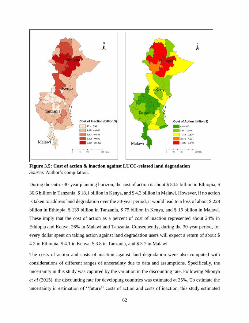
62

Figure 3.5: Cost of action & inaction against LUCC-related land degradation


During the entire 30-year planning horizon, the cost of action is about $ 54.2 billion in Ethiopia, $

36.6 billion in Tanzania, $ 18.1 billion in Kenya, and $ 4.3 billion in Malawi. However, if no action

is taken to address land degradation over the 30-year period, it would lead to a loss of about $ 228

billion in Ethiopia, $ 139 billion in Tanzania, $ 75 billion in Kenya, and $ 16 billion in Malawi.

These imply that the cost of action as a percent of cost of inaction represented about 24% in

Ethiopia and Kenya, 26% in Malawi and Tanzania. Consequently, during the 30-year period, for

every dollar spent on taking action against land degradation users will expect a return of about $

4.2 in Ethiopia, $ 4.1 in Kenya, $ 3.8 in Tanzania, and $ 3.7 in Malawi.

The costs of action and costs of inaction against land degradation were also computed with

considerations of different ranges of uncertainty due to data and assumptions. Specifically, the

uncertainty in this study was captured by the variation in the discounting rate. Following Nkonya

et al (2015), the discounting rate for developing countries was estimated at 25%. To estimate the

uncertainty in estimation of ‘‘future’’ costs of action and costs of inaction, this study estimated

Ethiopia

Kenya

Tanzania

Malawi

Ethiopia

Kenya

Tanzania

Malawi

63

these costs with lower discounting rate (scenarios 1 and 2) and higher discount rates (scenario 3

and 4) for the 30-year period as shown in Figure 3.6 and Figure 3.7. Results show that with lower

discounting rates, the costs of action and costs of inaction are both higher while the costs of action

and costs of inaction are both lower when using a higher discount rate. Results for 6 year-period

are provided in Appendix Figure 8.2 and Figure 8.3.

Figure 3.6: Cost of action (billion USD) against LUCC land degradation in 30 years in

different scenarios


Figure 3.7: Cost of Inaction (billion USD) against LUCC land degradation in 30 years in

different scenarios


The costs of action and inaction against LUCC land degradation for the six-year and thirty-year

periods are also computed on per ha basis as presented in Table 3.7. Analysis show that during

0

20

40

60

80

1=10% 2=15% 25% 3=30% 4=35%


0

150

300

450

600

1=10% 2=15% 25% 3=30% 4=35%


64

the six-year period the costs of action per ha ranged from as high as $ 477 in Ethiopia and $ 384

in Tanzania to as low as $ 343 in Malawi and $ 310 in Kenya. However, the costs of inaction over

the same period is about $ 1491 in Ethiopia, $ 1090 in Tanzania, $ 978 in Malawi and $ 951 in

Kenya. During a 30-year period the costs of action per ha is about $ 478 in Ethiopia, $ 385 in

Tanzania, $ 344 in Malawi and $ 311 in Kenya. However the costs of inaction increase to about $

2019 in Ethiopia, $ 1475 in Tanzania, $ 1323 in Malawi, and $ 1287 in Kenya.

Table 3.7: Cost of action & inaction against LUCC-related land degradation per hectare

Country Cost of Action Cost of Inaction Cost of Action Cost of Inaction

(6 years) (30 years)

Ethiopia 476.6 1491.4 477.7 2018.7

Kenya 309.9 951.1 310.6 1287.4

Malawi 343.0 977.7 343.7 1323.4

Tanzania 384.3 1089.5 385.1 1474.7


The results at district/regional levels for the four countries are varied. In Ethiopia, results show

that the annual cost of land degradation is about $4.1 billion (Table 3.8). Only about $1.7 billion

(42%) of this cost of land degradation represent the loss of provisional ecosystem services. The

other 58% represents the loss of supporting and regulatory and cultural ecosystem services. The

annual costs of land degradation were higher in Southern Nations ($1.6 billion), Dire Dawa ($822

million) and Afar ($654 million) regions but least in Somali ($4 million), Addis Ababa ($4 million)

and Harari ($8 million) regions.

The results further show the costs of action were about $54.1 million in a six-year period and about

$54.2 million over a 30-year horizon whereas the costs of inaction in six-year period were about

$169 million and about $228 million in a 30-year period. This implies that the costs of action

against land degradation are lower than the costs of inaction by about 4.2 times over the 30 year

horizon; i.e. the ratio of action to cost of inaction is 24.8%. This implies that each dollar spent on

addressing land degradation is likely to have about 4.1 dollars of returns. The ratio of costs of

action to cost of inaction in the 30-year period was high in Oromia (27.2%), Harari (26.7%),

Gambela (26.7%), and Amhara (25.2%) regions. The returns from action were the highest in

Tigray ($5.8), Somali ($4.4), and Dire Dawa ($ 4.4) regions and lowest in Oromia ($ 3.7), Harari

($3.8) and Gambela ($3.8) regions.

65

Table 3.8: Cost of action and inaction against land degradation in Ethiopia (million USD)

Region

Annual

costs of

Land

Degradation

Annual

costs of land

degradation

in terms of

provisional

ES only

Cost of

Action

(6 years)

Cost of

Inaction

(6 years)

Cost of

Action

(30 years)

Cost of

Inaction (30 years)

Ratio of

Cost of

action:

cost of

Inaction

(30 years)

Returns

from

action

(30

years)

Million USD % $

Addis Ababa 3.564 0.396 0.045 0.135 0.045 0.182 24.8% 4.04

Afar 654.287 270.585 8.578 26.331 8.595 35.641 24.1% 4.15

Amhara 296.628 140.036 4.504 13.234 4.514 17.913 25.2% 3.97

Benshangul 197.078 106.565 2.685 8.588 2.693 11.625 23.2% 4.32

Dire Dawa 822.324 176.375 9.836 31.973 9.863 43.278 22.8% 4.39

Gambela 107.765 76.750 1.870 5.189 1.873 7.024 26.7% 3.75

Harari 8.268 6.218 0.151 0.419 0.151 0.567 26.7% 3.75

Oromia 128.042 96.575 2.381 6.489 2.385 8.783 27.2% 3.68

Somali 4.200 1.552 0.051 0.168 0.052 0.227 22.7% 4.41

Southern 1569.461 686.605 21.256 64.619 21.301 87.468 24.4% 4.11

Tigray 303.782 138.263 2.691 11.532 2.702 15.609 17.3% 5.78

Total 4095.40 1699.92 54.05 168.67 54.17 228.32 24.8% 4.21


In Kenya, results show that the annual cost of land degradation is about $ 1.3 billion (Table 3.9).

About 51% of this cost (or $ 666 million) represent the loss of provisional ecosystem services. The

other half represents the loss of supporting and regulatory and cultural ecosystem services. The

annual costs of land degradation were higher in Rift valley ($445 million), Coast ($283 million)

and Eastern ($209 million) provinces but least in Nairobi ($2 million), Western ($30 million) and

Nyanza ($70 million) provinces. The results further show the costs of action were about $18

million in a six-year period and about $18.1 million over a 30-year horizon whereas the costs of

inaction in six-year period were about $55 million and about $75 million in a 30-year period.

This implies that the costs of action against land degradation are lower than the costs of inaction

by about 4.1 times over the 30 year horizon; i.e. the ratio of action to cost of inaction is 24%. This

implies that each dollar spent on addressing land degradation is likely to have about 4.1 dollars of

returns. The ratio of costs of action to cost of inaction in the 30-year period was high in Nairobi

(28%), Rif Valley (26%), North Eastern (25%), and Central (25%) provinces. The returns from

action were the highest in Coast ($4.6), Nyanza ($4.5), and Western ($ 4.1) provinces and lowest

in Nairobi ($ 3.6) and Rift Valley ($3.9) provinces.

66

Table 3.9: Cost of action and inaction against land degradation in Kenya (million USD)

Region

Annual

costs of

Land

Degradation

Annual

costs of

land

degradation

in terms of

provisional

ES only

Cost of

Action

(6 years)

Cost of

Inaction

(6 years)

Cost of

Action

(30 years)

Cost of

Inaction (30 years)

Ratio of

Cost of

action:

cost of

Inaction

(30 years)

Returns

from

action

(30

years)

Million USD % $

Central 79.634 35.691 1.085 3.239 1.087 4.384 24.8% 4.034

Coast 282.672 128.895 3.337 11.283 3.346 15.272 21.9% 4.565

Eastern 208.807 125.718 2.993 9.353 3.001 12.660 23.7% 4.219

Nairobi 2.289 1.050 0.036 0.097 0.036 0.131 27.8% 3.602

North Eastern 185.088 110.820 2.815 8.369 2.821 11.328 24.9% 4.016

Nyanza 70.324 30.206 0.818 2.753 0.820 3.727 22.0% 4.544

Rift Valley 444.969 219.726 6.533 18.959 6.546 25.663 25.5% 3.920

Western 30.251 14.043 0.417 1.273 0.418 1.724 24.2% 4.127

Total 1304.03 666.15 18.03 55.33 18.07 74.89 24.1% 4.14


In Malawi, results show that the annual cost of land degradation is about $244 million (Table

3.10). Only about $153 million (62%) of this cost of land degradation represent the loss of

provisional ecosystem services. The other (about 38%) represents the loss of supporting and

regulatory and cultural ecosystem services. The annual costs of land degradation were higher in

Mangochi ($27 million), Nkhata Bay ($24 million), Nkhotakota ($20 million), and Rumphi ($20

million) districts but least in Balaka ($0.8 million), Chiradzulu ($0.9 million) and Blantyre ($2

million) districts.

The results also show that the costs of action were about $4 million in a six-year period and about

$4.3 million over a 30-year horizon whereas the costs of inaction in six-year period were about

$12 million and about $17 million in a 30-year period. This implies that the costs of action against

land degradation are lower than the costs of inaction by about 3.7 times over the 30 year horizon;

i.e. the ratio of action to cost of inaction is 27.3%. This implies that each dollar spent on addressing

land degradation is likely to have about 3.7 dollars of returns. The ratio of costs of action to cost

of inaction in the 30-year period was high in Nkhata Bay (29.8%), Mzimba (28.3%), Ntcheu

(28.3%), and Nsanje (28.1%) districts. The returns from action were the highest in Salima ($4.1),

Mangochi ($3.9), Balaka ($ 3.8) and Karonga ($ 3.8) districts. The lowest returns from action were

reported in Nkhata Bay ($ 3.4), Ntcheu ($3.5) and Mzimba ($3.5) districts.

67

Table 3.10: Cost of action and inaction against land degradation in Malawi (million USD)

Region

Annual

costs of

Land

Degradation

Annual

costs of

land

degradation

in terms of

provisional

ES only

Cost of

Action

(6 years)

Cost of

Inaction

(6 years)

Cost of

Action

(30 years)

Cost of

Inaction

(30 years)

Ratio of

Cost of

action:

cost of

Inaction

(30 years)

Returns

from

action

(30

years)

Million USD % $

Balaka 0.750 0.501 0.013 0.036 0.013 0.049 26.0% 3.84

Lilongwe 9.972 7.022 0.176 0.485 0.176 0.657 26.8% 3.73

Machinga 11.027 7.081 0.197 0.525 0.197 0.710 27.7% 3.61

Mangochi 27.302 14.968 0.403 1.169 0.403 1.583 25.5% 3.92

Mchinji 5.594 4.297 0.104 0.284 0.104 0.384 27.2% 3.68

Mulanje 6.605 4.021 0.112 0.308 0.112 0.416 26.9% 3.72

Mwanza 6.245 4.267 0.111 0.301 0.111 0.408 27.3% 3.66

Mzimba 19.635 13.027 0.367 0.961 0.368 1.301 28.3% 3.54

Nkhata Bay 24.379 9.222 0.415 1.031 0.416 1.395 29.8% 3.36

Nkhotakota 19.988 11.710 0.337 0.916 0.338 1.240 27.2% 3.67

Nsanje 4.219 2.865 0.079 0.210 0.080 0.284 28.1% 3.57

Blantyre 1.934 1.276 0.035 0.095 0.035 0.128 27.3% 3.66

Ntcheu 4.381 3.128 0.086 0.224 0.086 0.303 28.3% 3.53

Ntchisi 5.559 4.002 0.102 0.275 0.103 0.373 27.5% 3.63

Phalombe 3.948 2.739 0.072 0.195 0.072 0.264 27.3% 3.67

Rumphi 19.568 12.281 0.331 0.908 0.331 1.229 26.9% 3.71

Salima 5.023 2.826 0.076 0.227 0.076 0.307 24.7% 4.05

Thyolo 4.655 3.054 0.081 0.226 0.081 0.306 26.6% 3.76

Zomba 4.668 2.744 0.083 0.222 0.083 0.301 27.7% 3.61

Chikwawa 8.780 6.034 0.155 0.428 0.155 0.580 26.7% 3.74

Chiradzulu 0.874 0.587 0.016 0.043 0.016 0.058 26.8% 3.73

Chitipa 9.246 6.722 0.173 0.469 0.174 0.634 27.4% 3.65

Dedza 7.436 5.233 0.135 0.369 0.135 0.499 27.0% 3.70

Dowa 4.889 3.393 0.086 0.242 0.086 0.328 26.4% 3.79

Karonga 12.394 7.899 0.205 0.579 0.206 0.784 26.3% 3.81

Kasungu 15.321 12.205 0.295 0.797 0.296 1.079 27.4% 3.65

Total 244.39 153.11 4.24 11.52 4.25 15.60 27.3 3.67


In Tanzania, results show that the annual cost of land degradation is about $2.3 billion (Table

3.11). Only about $1.3 billion (57%) of this cost of land degradation represent the loss of

provisional ecosystem services. The other (about 43%) represents the supporting and regulatory

and cultural ecosystem services. The annual costs of land degradation were higher in Morogoro

($297 million), Ruvuma ($214 million), and Rukwa ($193 million) districts but least in Zanzibar

West ($3 million), Dar-Es-Salaam ($6 million) and Unguja North ($7 million) districts.

Moreover, results show that the costs of action were about $36.5 million in a six-year period and

about $36.6 million over a 30-year horizon. However, the costs of inaction in six-year period were

about $103 million and about $139 million in a 30-year period. This implies that the costs of action

68

against land degradation are lower than the costs of inaction by about 3.8 times over the 30 year

horizon; i.e. the ratio of action to cost of inaction is 26.4%. This implies that each dollar spent on

addressing land degradation is likely to have about 3.8 dollars of returns. The ratio of costs of

action to cost of inaction in the 30-year period were high in Singida (29.5%), Lindi (29.4%), and

Morogoro (28.2%) regions but lowest in Pemba South (15.3%), Mwanza (17.1%) and Pemba

North (17.4%) regions. The returns from action were the highest in Pemba South ($6.5), Mwanza

($ 5.9) and Pemba North ($ 5.8) regions. The lowest returns from action were reported in Singida

($ 3.4), and Lindi ($3.4) districts.

Table 3.11: Cost of action and inaction against land degradation in Tanzania (million USD)

Region

Annual

costs of

Land

Degradation

Annual

costs of

land

degradation

in terms of

provisional

ES only

Cost of

Action

(6

years)

Cost of

Inaction

(6 years)

Cost of

Action

(30 years)

Cost of

Inaction

(30 years)

Ratio of

Cost of

action:

cost of

Inaction

(30 years)

Returns

from

action

(30

years)

Million USD % $

Arusha 56.032 30.290 0.880 2.479 0.882 3.356 26.3% 3.81

Pemba South 7.337 2.032 0.046 0.223 0.046 0.302 15.3% 6.53

Lindi 122.851 69.604 2.360 5.935 2.364 8.033 29.4% 3.40

Manyara 60.588 41.192 1.108 2.987 1.111 4.044 27.5% 3.64

Mara 42.107 14.759 0.417 1.523 0.418 2.061 20.3% 4.93

Mbeya 160.688 116.777 2.918 8.003 2.924 10.833 27.0% 3.70

Morogoro 297.369 171.086 5.195 13.621 5.204 18.438 28.2% 3.54

Mtwara 15.219 6.292 0.181 0.596 0.182 0.807 22.5% 4.45

Mwanza 70.762 23.992 0.551 2.387 0.552 3.231 17.1% 5.85

Pwani 129.504 62.931 2.139 5.711 2.142 7.731 27.7% 3.61

Rukwa 192.746 122.226 3.083 8.790 3.089 11.898 26.0% 3.85

Dar-Es-Salaam 6.371 2.661 0.070 0.246 0.070 0.333 21.0% 4.76

Ruvuma 214.386 144.504 3.592 10.002 3.599 13.539 26.6% 3.76

Shinyanga 44.896 20.818 0.504 1.737 0.506 2.352 21.5% 4.65

Singida, 55.587 29.423 1.055 2.644 1.056 3.578 29.5% 3.39

Tabora 100.566 73.526 1.839 5.037 1.842 6.817 27.0% 3.70

Tanga 161.926 88.442 2.541 7.113 2.545 9.628 26.4% 3.78

Zanzibar South 9.159 3.047 0.124 0.347 0.124 0.470 26.3% 3.80

Zanzibar West 3.225 0.903 0.038 0.116 0.038 0.157 24.2% 4.14

Dodoma 32.033 18.172 0.475 1.419 0.476 1.920 24.8% 4.03

Iringa 144.596 85.781 2.452 6.631 2.456 8.976 27.4% 3.65

Kagera 157.460 85.285 2.251 6.736 2.256 9.117 24.7% 4.04

Pemba North 8.569 2.397 0.064 0.273 0.064 0.369 17.4% 5.75

Unguja North 6.737 2.120 0.068 0.233 0.068 0.316 21.5% 4.65

Kigoma 157.616 79.468 2.014 6.140 2.017 8.311 24.3% 4.12

Kilimanjaro 36.721 20.272 0.598 1.634 0.599 2.212 27.1% 3.70

Total 2295.05 1318.00 36.56 102.56 36.63 138.83 26.4% 3.79


69

3.9 Conclusions

This chapter demonstrates that the consequences and losses due to land degradation are enormous.

Based on TEV framework, the costs of land degradation due to LUCC between 2001-2009 periods

were $1.98 billion in Malawi, $10.65 billion in Kenya, $18.47 billion in Tanzania, to US$ 34.82

billion in Ethiopia. This represents about 5%, 7%, 14% and 23% of GDP in Kenya, Malawi,

Tanzania and Ethiopia respectively. When these costs are converted to per hectare basis, they range

from $38 in Ethiopia, $25 in Tanzania, $23 in Kenya and $21 in Malawi annually. The total annual

costs of land degradation associated with use of land degradation practices in maize, wheat and

rice croplands were about $305 million in Ethiopia, $270 million in Kenya, $162 million in

Tanzania, and $114 million in Malawi. These costs on static cropland degradation are, however,

conservative. Only three crops were considered, other aspects of land degradation common on a

static biome (cropland) including soil erosion and salinity, and offside costs of pesticide use are

not considered because of lack of data.

It is worthwhile to take action against land degradation. As expected, the TEV computation shows

that the costs of action are lower as compared to costs of inaction against land degradation in all

the countries both in a 6-year and a 30-year cycle. During the entire 30-year planning horizon, the

cost of action is about $ 54.2 billion in Ethiopia, $ 36.6 billion in Tanzania, $ 18.1 billion in Kenya,

and $ 4.3 billion in Malawi. However, if no action is taken to address land degradation over the

30-year period, it would lead to a loss of about $ 228 billion in Ethiopia, $ 139 billion in Tanzania,

$ 75 billion in Kenya, and $ 16 billion in Malawi. These imply that the cost of action as a percent

of cost of inaction represented about 24% in Ethiopia and Kenya, 26% in Malawi and Tanzania.

Consequently, during the 30-year period, returns to investment in action against land degradation

are at least four folds. Specifically, for every dollar spent on taking action against land degradation

land users will expect a return of about $4.2 in Ethiopia, $4.1 in Kenya, $3.8 in Tanzania, and $3.7

in Malawi.

Policies and strategies that incentivize better sustainable land management and discourage

deforestations ought to be emboldened so as to achieve UNCCD’s target of zero net land

degradation by year 2030. The costs of land degradation due to LUCC constitute the biggest

proportion of the total costs of land degradation. Therefore, strategies and mechanisms must be

70

developed to address LUCC such as payment for ecosystem services (PES) and participatory

management of community resources such as forests and grazing lands.

As demonstrated in the previous chapter, local level initiatives have also proven successful in

ensuring sustainable management of land and land resources. Some of the key activities currently

practiced by local communities include; area closures and stricter enforcement and enacting of

bylaws to protect forests, controlled grazing and community sanctions for overgrazing. Thus,

participatory involvement of the local communities is important for successful and effective policy

formulation and enforcement at community level. The next chapter highlights the cause of land

degradation and the determinants of SLM adoption.

71

Chapter 4

4. Drivers of Land Degradation and Adoption of Multiple Sustainable Land

Management Practices

4.1 Introduction

Land degradation is an extensive and serious impediment to improving rural livelihoods and food

security of millions of people in the eastern Africa. Recent estimates show that land degradation

affected about 51%, 41%, 23% and 22% of the terrestrial areas in Tanzania, Malawi, Ethiopia and

Kenya respectively (Le, Nkonya and Mirzabaev, 2014). Addressing land degradation through the

formulation of proper strategies and effective policies requires first the identification of both the

proximate (direct) and underlying (indirect) causes (Vlek et al., 2010; von Braun et al., 2012;

Pingali et al., 2014).

A review of literature show that there exist numerous and complex proximate and underlying

causes of land degradation in the region (Kirui and Mirzabaev, 2014). Relevant proximate causes

include topography and climatic conditions (such as wind, temperature and rainfall). Other

significant human activities identified as the direct drivers of land degradation include

unsustainable and inappropriate land management practices such as land clearing, deforestation,

wood and charcoal extraction, overgrazing/overstocking of herds, cultivation on steep slopes, bush

burning, soil nutrient mining and uncontrolled fires (Eswaran et al., 2001; Lal, 2001; Dregne,

2002; Barac, 2003; Gareng, 2015).

Significant root causes underlying the fore mentioned direct causes of land degradation in the

region include insecure land tenure, poverty, population density, access to information and

markets, and weak policy and regulatory environment in the agricultural and environmental sectors

(Kabubo-Mariara, 2007; Tiffen et al., 1994; Nkonya et al., 2008). Tackling the direct human

causes of land degradation requires an understanding and addressing of these root causes through

appropriate mitigative and remedial strategies.

Different methods have been used to deduce the causes of land degradation. They include the use

of expert opinions (Oldeman et al., 1991), quantitative analyses (Bai et al., 2008; Vlek et al., 2008;

2010), use of inferential statistics (Barbier, 1997; Nkonya et al., 2011), and the use of satellite

72

imagery and remote sensing techniques (Hoffman et al., 1999; FAO, 2003; Archer, 2004; Yang et

al., 2005; Le et al., 2012; 2014). The advantages and inherent weaknesses of each of these

approaches are discussed in detail in the next section.

The adoption and investment in sustainable land management is crucial in reversing and

controlling land degradation, rehabilitating degraded lands and ensuring the optimal use of land

resources for the benefit of present and future generations (Akhtar-Schuster et al., 2011; ELD

Initiative, 2013). Sustainable land management is important for sustainable development because

it facilitates land users to maximize the benefits from their land while maintaining the ecological

support functions of the land resources (TerrAfrica, 2006). The efforts directed at addressing the

causes of land degradation or addressing the constraints to SLM adoption, however, have not been

largely insufficient. Recent reliable estimates show that the adoption of sustainable land

management practices in sub-Saharan Africa is very low – about 3% of total cropland (World

Bank, 2010).

Several studies have been carried out to document significant determinants and constraints to

sustainable land management using different approaches. These studies highlighted the direction

and the magnitude of factors hypothesized to determine the adoption of SLM technologies. Some

examples of these detailed empirical studies in developing countries include that of Pagiola (1996)

in Kenya, Nakhumwa and Hassan (2012) in Malawi, Shiferaw and Holden (1998), Gabremedhin

and Swinton (2003) and Bekele and Drake (2003) in Ethiopia.

Some of the significant factors facilitating the adoption of sustainable land management include;

access to information (education and extension), access to both input and output markets, social,

human and physical capital endowments, credit availability, profitability of the management

technology, and property rights. The adoption of sustainable land management is also influenced

by lack of local-level capacities, knowledge gaps on specific land degradation and SLM issues,

inadequate monitoring and evaluation of land degradation and its impacts, inappropriate incentive

structure (such as, inappropriate land tenure and user rights), inaccessible market and infrastructure

constraints (such as, insecure prices of agricultural products, increasing input costs, inaccessible

markets), and policy and institutional bottlenecks (such as, difficulty and costly enforcement of

existing laws that favor SLM) and risks (Thompson et al., 2009; Chasek et al., 2011; Akhtar-

Schuster et al., 2011 Reed et al., 2011; ELD Initiative, 2013).

73

There is thus a fairly large body of existing literature on causes of land degradation and

determinants of adoption of SLM in eastern Africa, however, a number of limitations that should

be fulfilled in next research are evident. These studies either focuses on some specific location(s)

in the region, are considered subjective and lacking in scientific rigor and/or have weak

explanatory power due to smaller sample size. The results from different studies are often

contradictory regarding any given variable (Ghadim and Pannell, 1999). The current assessment

is unique in that; it uses nationally representative data (at farm level) with diverse variables (both

proximate and underlying) and that it includes socio-economic and behavioral factors. These

include a mix of biophysical, demographic, socio-economic, and institutional variables.

This is particularly important to study the diverse social–ecological context within a national or

international scale. It further addresses and control for the diverse contexts such as regional and

agro-ecological zonation to capture a wide spectrum of heterogeneous contexts in the three Eastern

Africa countries. The approached used in the current study also account for the non-linear

relationship between the drivers of land degradation and determinants of SLM. This approach

could lead to innovative and comprehensive assessment of both causes of land degradation and

SLM use and thus a better targeting of policy measures for combating land degradation and

facilitating SLM uptake across different contexts.

4.2 Relevant Literature

4.2.1 Drivers of land degradation

Drivers of land degradation can be grouped into two categories, namely; proximate and underlying

causes (Lambin & Geist, 2006; Lal & Stewart, 2010; 2013; Belay et al., 2014; Pingali et al., 2014).

Proximate causes are those that have a direct effect on the terrestrial ecosystem. These include

biophysical (natural) conditions related to climatic conditions and extreme weather events such as

droughts and coastal surges. Proximate causes are also related to unsustainable land management

practices (anthropogenic) such as over-cultivation, overgrazing and excessive forest conversion.

On the other hand, the underlying causes are those factors that indirectly affect proximate causes.

Lack of institutions, poverty, and insecure land tenure may underlie land degradation by hampering

incentives to invest in sustainable land management practices (Kabubo-Mariara, 2007; FAO,

74

2011a). Geist & Lambin (2004) and Nkonya et al., (2013) present a review of these proximate and

underlying drivers of land degradation. A summary of some of the empirical studies undertaken to

identify and assess proximate and underlying causes of land degradation in selected countries in

Eastern Africa region are presented in Table 4.1.

Key proximate drivers in Eastern Africa include; climatic conditions, topography, unsuitable land

uses and inappropriate land management practices (such as slash and burn agriculture, timber and

charcoal extraction, deforestation, overgrazing) and uncontrolled fires. The dry aid and semi-arid

arid lands are prone to fires which may lead to serious soil erosion (Voortman et al., 2000;

D’Odorico, 2013). The erratic rainfall in these areas may also be thought to induce salinization of

the soil (Safriel & Adeel, 2005; Wale & Dejenie, 2013). Similarly, practicing unsustainable

agriculture such as land clearing, overstocking of herds, charcoal and wood extraction, cultivation

on steep slopes, bush burning, pollution of land and water sources, and soil nutrient mining

(Eswaran et al., 2001; Lal, 2001; Dregne, 2002; Lal et al., 2012). Most deforestation exercises are

associated with the continued demand for agricultural land, fuel-wood, charcoal, construction

materials, large-scale timber logging and resettlement of people in forested areas. This often

happens at the backdrop of ineffective institutional mechanisms to preserve forests. Grazing

pressure and reduction of the tree cover continues to diminish the productivity of rangelands (Hein

& de Ridder, 2005; Waters et al., 2013).

Arid and semi-arid climatic conditions with high evaporation rates; together with poor

management of irrigation water (in the 4.5% irrigated cropland of SSA) is a major cause of

salinization. Additionally, fragmentation, overexploitation of the forest resources and conversion

of forest lands to agriculture increases deforestation rates in the region. Overstocking is identified

to primarily drive degradation of rangelands, decline of vegetation productivity (and eventually

livestock productivity), and loss of resilience of the rangeland for droughts (WRI, UNEP, and

UNDP, 1994). Indeed, overgrazing was estimated to cause about 50% of all soil degradation in

semi-arid and arid regions of Africa (ibid). The increasing demand for food brought about by an

increasing population but with stagnant or declining agricultural productivity has led to rapid

expansion of agricultural land and reduced rehabilitation of soil fertility through shortening of the

fallow periods in extensive land use systems (Scherr & Yadav, 1996).

75

Important underlying drivers of land degradation in the region include land tenure, poverty,

population density and weak policy and regulatory environment in the agricultural and

environmental sectors (Table 4.1). Insecure land tenure may act as a disincentive to investment in

sustainable agricultural practices and technologies (Kabubo-Mariara, 2007). Similarly, a growing

population without proper land management will exhaust the capacity of land to provide ecosystem

services (Tiffen et al., 1994). It is also argued that population pressure leads to expansion of

agriculture into fragile areas and reduction of fallow periods in the cultivated plots. However, this

is not always the case. Population pressure has been found to increase agricultural intensification

and higher land productivity as well as technological and institutional innovation that reduce

natural resource degradation (Tiffen et al., 1994; Nkonya et al., 2008).

Table 4.1: Empirical review of proximate and underlying causes of land degradation

Country Proximate Drivers Underlying drivers References

Ethiopia Topography, unsustainable

agriculture, fuel wood

consumption, conversion of

forests, woodlands, shrub-

lands to new agricultural land

(deforestation)

Weak regulatory environment and

institutions, demographic growth,

unclear user rights, low

empowerment of local communities,

poverty, infrastructural

development, population density

Pender et al., 2001; Jagger

& Pender, 2003; Holden et

al., 2004; Rudel et al.,

2009, Bai et al., 2008;

Belay et al., 2014; Tesfa &

Mekuria, 2014.

Kenya Topography, deforestation and

charcoal production,

overgrazing, unsustainable

agricultural practices

Poor/weak governance &

institutional weakness in agric.

sector, lack of defined property

rights, poverty, population density

Pender et al., 2004a; Bai

& Dent, 2006; Waswa,

2012; Waswa et al., 2013;

Nesheim et al., 2014.

Malawi Charcoal and wood fuel (for

domestic & commercial),

timber production;

unsustainable agric. methods

(slash and burn with shorter

rotations), mining

Past and current development

processes in energy, forestry,

agriculture & water sectors; poverty;

lack of alternative energy sources;

weak policy environment, lack of

planning; insecure land tenure

Pender, 2004; Lambin &

Meyfroidt, 2010;

Rademaekers et al., 2010;

Thierfelder et al., 2013;

Kiage, 2013; Harris et al.,

2014.

Tanzania Topography, climate change,

settlement and agric.

expansion, overgrazing,

firewood, timber and charcoal

extraction, uncontrolled fires

Market and institutional failures,

rapid population growth, rural

poverty, insecure tenure, and

absence of land use planning,

development of infrastructure

Pender et al., 2004b; de

Fries et al., 2010; Fisher,

2010; Wasige et al., 2013;

Ligonja & Shrestha, 2013;

Hackman, 2014.

Source: Kirui and Mirzabaev, 2014.

Various methods have been utilized to infer the drivers of land degradation. Firstly, the use of

expert opinions (Oldeman et al., 1991) – expert opinions has been utilized especially for the global

level assessments like in the Global Assessment of Human-Induced Soil Degradation (GLASOD).

However, this method is criticized for being subjective and lacking in scientific rigor. Secondly,

the quantitative analyses of drivers of land degradation (Bai et al., 2008; Vlek et al., 2008; 2010).

76

These assessments however, do not provide causation but rather correlation between indicators of

land degradation (such as NDVI) and the hypothesized variables; (iii) thirdly, the use of inferential

statistics (Barbier, 1997; Nkonya et al., 2011) – like the quantitative assessment method, the

estimates from the inferential statistics limit the interpretation of the causal relationships because

of the weak explanatory power (due to smaller sample size). The sample is also highly aggregated

to present regional and/or national aggregates that make interpretation unreasonable for the in-

country diverse settings. Lastly, the other method involves the use of remote sensing techniques

(Hoffman et al., 1999; FAO, 2003; Archer, 2004; Yang et al., 2005; Le et al., 2012; 2014). These

techniques are varied and they include: image differencing of two images (Rasmussen et al., 2001;

Borak et al., 2000), visual interpretation of images (Gupta et al., 2002; Ries & Marzolf, 2003),

spectral index (Chikhaoui et al., 2005), vegetation indices and ratios of signals (Budde et al., 2004;

Khan et al., 2005), land-cover mapping and “Steppe Degradation Index” with ancillary data,

spatial and temporal metrics of land cover change (Borak et al., 2000), and soil adjusted vegetation

index (Mackay & Zietsman, 1996). These approaches have been criticized for the following

weakness: they exaggerate the result on the levels of land degradation, they are perception-based

and semi quantitative, and therefore not built on objective measurements, and that the land-cover

exercises maps degradation using image brightness values on a snapshot satellite image, thus

cannot represent a persistent land degradation.

Recent empirical expeditions, however, show a shift from manual visual approach to the

interpretation of aerial photography and satellite imagery and to further to a more model-based

approach involving indicators and proxy variables, measurable over large areas and over longer

periods. The most widely used index for assessment is the vegetation indices is the NDVI (Prince

et al., 1998; Diouf & Lambin, 2001; Herrmann et al., 2005; Le et al., 2012; de Pinto et al., 2013.

Some advantages of using NDVI are that it uses a single index with readily available dataset, it

can be used for global coverage, and the temporal and spatial extensions are possible with this

method. However, this method is not without limitations. The accuracy of observations is

sometime questioned; hence need for ground-truthing; it is difficult to differentiate land cover and

land use and other human interventions; and the resolution is coarse especially for small coverage.

Land degradation and its accompanying effect of low productivity are not simply a technical issue

but rather more complex including socio-economic and behavioral factors and require a change in

approach. This study therefore include household level variables; missing in the previous studies.

77

This assessment is also unique in that the study uses nationally representative data (at farm level)

with diverse variables (both proximate and underlying). These include a mix of biophysical,

demographic, socio-economic, and institutional variables. This study also address and control for

the diverse contexts such as regional and agro-ecological zone classification (AEZ).

4.2.2 Determinants of SLM Adoption

Empirical review of literature on adoption of production – related technologies dates back to Feder

et al., (1985) which summarizes that the adoption of new technology may be constrained by many

factors such as lack of credit, inadequate and unstable supply of complementary inputs, uncertainty

and risks. A comprehensive review of literature shows several factors determining investment in

sustainable land management practices. These include; household and farm characteristics,

technology attributes, perception of land degradation problem, profitability of the

technology/practice, institutional factors, such as, land tenure, access to credit, information and

markets and risks and uncertainty (Ervin, 1982; Norris & Batie, 1987; Pagioa, 1996; Shiferaw and

Holden; 1998; Kazianga & Masters, 2001; Shively, 2001; Bamire et al., 2002; Barrett et al., 2002;

Gabremedhin & Swinton, 2003; Habron, 2004 ; Kim et al., 2005; Park & Lohr, 2005; Pender et

al., 2006; Gillespie et al., 2007; Prokopy et al., 2008).

Important contributions have been made by these previous studies on identifying the determinants

of adoption of SLM practices, however, a number of limitations are evident. Despite the fact that

a long list of explanatory variables is used, most of the statistical models developed by these studies

have low levels of explanatory power (Ghadim and Pannell, 1999; Ghadim et al., 2005). The

results from different studies are often contradictory regarding any given variable (ibid). Linder

(1997) points out that the inconsistency results in most empirical studies could be explained by

four shortcomings, namely; failure to account for the importance of the dynamic learning process

in adoption, biases from omitted variables, poorly specified models and failure to relate hypotheses

to sound conceptual framework.

Use of binomial or multinomial qualitative choice models in assessing adoption of technologies is

well established in adoption literature (Feder et al., 1985). Greene (2000) argues that qualitative

choice models seek to determine the probability that an individual with a given set of attributes

will make one choice rather than an alternative. The two most popular functional forms used for

78

adoption models are the probit and logit models. Several studies have utilized these two techniques

in modeling determinants of decision to invest in SLM practices in developing countries. Some of

the studies that use probit includes; Feather and Amacher (1994), Khanna (2001), Rahelizatavo

(2002), Zhong (2003), Lichtenberg (2001) and Kim et al. (2005). Some of the studies that use logit

include; Dorfman (1996) Fuglie (1999), Caswell et al. (2001), Hindsley (2002), Daberkow &

McBride (2003), Friedrichsen (2003) Habron (2004), Wu et al. (2004), Moreno & Sunding (2005)

and Prokopy et al., (2008). Others studies use multiple regressions to assess the number of SLM

practices a farmer has invested in; these studies include; Alonge & Martin (1995), Napier et al.

(2000), Rahelizatavo & Gillespie (2004) and Park & Lohr (2005).

Adoption studies using dichotomous adoption decisions models have inherent weakness (Dimara

and Skuras, 2003). The single stage decision making process characterized by a dichotomous

adoption decision models is a direct consequence of the full information assumption entrenched in

the definition of adoption, that is, individual adoption is defined as the degree of use of a new

technology in the long run equilibrium when the farmer has full information about the new

technology and its potential. This assumption of full information is usually violated and hence use

of logit or probit models in modeling adoption decision may lead to model misspecification.

Recent studies have tried to overcome these limitations in different ways: model adoption

sequentially (Leathers and Smale, 1991), include farmers’ personal perceptions, abilities and

capabilities and risk preferences to capture the dynamic learning process (Ghadim and Pannell,

1999), use of stochastic production function to capture importance of risk effects of factors inputs

on production behavior (Fufa and Hassan, 2003), use a partial observability model to capture the

varied access to information and levels of awareness of the new technology (Dimara and Skuras,

2003), use of a double hurdle model to capture the sequential decisions and multiple stages in

investing in SLM (Gabremedhin and Swinton, 2003) and determinants of adoption and intensity

of adoption of SLM may be different, hence use a tobit model rather than probit or logit

(Nakhumwa and Hassan, 2003). To overcome these challenges and concerns, this study adopted a

multivariate probit model (MVP) that accounts for simultaneity of choices and interdependent

(potential correlations) among the adoption decisions (Greene, 2003). The results concerning any

particular variable, however, were not any different from the MVP and Poisson regressions. For

prudence therefore, the MVP and Poisson regression results are not presented in the discussions

because they only serve to confirm the logit results.

79

4.3 Conceptual framework

The ELD conceptual framework is based on comparing the costs and benefits of action against

land degradation versus the costs of inaction (Figure 4.1). There are two broad categories of causes

of land degradation; proximate and underlying. Proximate drivers are those that have a direct effect

on the terrestrial ecosystem. These include both biophysical causes (natural) and unsustainable

land management practices (anthropogenic). On the other hand, underlying drivers are those that

indirectly affect the proximate causes of land degradation (such as institutional, socio-economic

and policy factors). The level of land degradation determines its outcomes and/or effects – whether

on-site or offsite; – on the provision of ecosystem services and the benefits humans derive from

those services. Actors can then take action to control the causes of land degradation, its level, or

its effects.

The green rectangular box (Figure 4.1) depicts the economic analysis conducted while the green

arrow shows information flow that is essential to conduct the different levels of the economic

analysis. All the indirect and off-site effects are incorporated in the economic analysis to ensure a

comprehensive assessment from the society’s point of view; the analysis takes account of all

prevailing externalities in addition to the private land use costs incurred by individuals subsequent

to land use decisions. Similarly, actions against land degradation have direct benefits and costs -

the costs of specific measures and economy-wide indirect effects – or the opportunity costs. This

implies that the resources set aside for these actions cannot be put into use elsewhere and thus,

mobilizing these resources to avert or alleviate land degradation affects other sectors of the

economy as well.

The dotted lines represent institutional arrangements that guide actors’ choice of action against

land degradation and whether their action choices actually and effectively lessen or stop land

degradation. It is important to identify and comprehend these institutional arrangements in order

to come up with sustainable and effective policies of combating land degradation. It is also of

prime importance that the analyses recognizes all the key actors of land degradation such as land

users, land owners, governmental authorities, and industries, as well as identify how institutions

and policies impact those actors. Transaction costs and collective versus market and state actions

are to be considered. In general, the institutional economics aspect should not be left out in the

assessment of land degradation especially when defining and designing the appropriate actions

against land degradation, and the inaction scenarios which serve as a benchmark.

80

Figure 4.1: The Conceptual Framework of ELD Assessment

Source: Nkonya et al. (2011).

4.4 Data, sampling, choice of variables for econometric estimations

4.4.1 Data and sampling procedures

The data used for this study is based on household surveys in three countries; Ethiopia, Malawi

and Tanzania conducted over different time periods. ‘‘The surveys were supported by the Living

Standards Measurement Study - Integrated Surveys on Agriculture (LSMS-ISA) project

undertaken by the Development Research Group at the World Bank. The project aims to support

governments in seven Sub-Saharan African countries to generate nationally representative,

household panel data with a strong focus on agriculture and rural development. The surveys under

the LSMS-ISA project are modeled on the multi-topic integrated household survey design of the

81

LSMS; household, agriculture, and community questionnaires, are each an integral part of every

survey effort’’ (NSO, 2014). The sampling procedure in each of the three countries is described

below.

a. Ethiopia

The Ethiopia Rural Socioeconomic Survey (ERSS) data was collected during the period October

2011- March 2012 by the Central Statistical Agency (CSA). The ERSS sample is designed to be

representative of rural and small town areas of Ethiopia. Based on population estimates from the

2007 Population Census, the CSA categorizes a town with a population of less than 10,000 as

small. The ERSS rural sample is a sub-sample of the Annual Agricultural Sample Survey (AgSS)

while the small town sample comes from the universe of small town Enumeration Areas (EAs).

The sample is a two-stage probability sample. The first stage of sampling entailed selecting

primary sampling units – the CSA’s enumeration areas (EAs). For the rural sample, 290

enumeration areas were selected from the AgSS enumeration areas based on probability

proportional to size of the total enumeration areas in each region. For small town EAs, a total of

43 EAs were selected. The second stage involved random selection of households to be

interviewed in each EAs. For rural EAs, a total of 12 households were sampled in each EA. Of

these, 10 households were randomly selected from the sample of 30 AgSS households. The AgSS

households are households which are involved in farming or livestock activities. Another 2

households were randomly selected from all other households in the rural EA (those not involved

in agriculture or livestock). In some EAs, there is only one or no such households, in which case,

less than two non-agricultural households were surveyed and more agricultural households were

interviewed instead so that the total number of households per EA remains the same. Households

were not selected using replacement. The sample covers a total of 3,969 households (and 24,954

farm plots).

b. Malawi

The Malawi 2010-2011 Integrated Household Survey (IHS) is a national-wide survey collected

during the period March 2010- March 2011 by the national Statistics Office (NSO). The sampling

frame for the IHS is based on the listing information from the 2008 Malawi Population and

82

Housing Census. The targeted universe for the IHS survey included individual households and

persons living in those households within all the districts of Malawi except for Likoma and the

people living in institutions such as hospitals, prisons and military barracks.

The IHS followed a stratified two-stage sample design. The first stage involved selection of the

primary sampling units (PSUs) following proportionate to size sampling procedure. These include

the census enumerations areas (EAs) defined for the 2008 Malawi Population and Housing Census.

An enumerations area was the smallest operational area established for the census with well-

defined boundaries and with an average of about 235 households. A total of 768 EAs (average of

24 EAs in each of the 31 districts) were selected across the country. In the second stage, 16

households were randomly selected for interviews in each EA. In total 12,271 households (18,329

farming plots) were interviewed.

c. Tanzania

The 2010-2011 Tanzania National Panel Survey (TNPS) data was collected during twelve-month

period from September 2010 - September 2011 by the Tanzania National Bureau of Statistics

(NBS). In order to produce nationally representative statistics, the TNPS is based on a stratified

multi-stage cluster sample design. The sampling frame the National Master Sample Frame (from

the 2002 Population and Housing Census); which is a list of all populated enumeration areas in the

country. In this first stage stratification was done along two dimensions: (i) eight administrative

zones (seven on Mainland Tanzania plus Zanzibar as an eighth zone), and (ii) rural versus urban

clusters within each administrative zone. The combination of these two dimensions yields 16

strata. Within each stratum, clusters were then randomly selected as the primary sampling units,

with the probability of selection proportional to their population size. In rural areas a cluster was

defined as an entire village while in urban areas a cluster was defined as a census enumeration area

(from the 2002 Population and Housing Census). In the last stage, 8 households were randomly

chosen in each cluster. Overall, 409 clusters and 3,924 households (6,038 farm plots) were

selected. Figure 4.2 presents the distribution of sampled households in the three countries.

83

Figure 4.2: Distribution of sampled households

Source:Authors’ Compilation.

4.4.2 Variables used in the econometric estimations

a. Dependent variables

Two approaches are used to assess the drivers of land degradation. The first approach is the use of

biomass productivity decline (change in NDVI) for the period of 1982-2006. The net change is

reported as either, decline, no change or improved. In this study thus, the depended was coded 1 =

decline and 0 =otherwise. At country level, the plots showing a decline in NDVI were about 39%

in Malawi, 49% in Ethiopia and 35% in Tanzania (Table 4.2).

In the empirical estimation of the determinants of adoption of SLM practices, the dependent

variable is the choice of SLM option(s) from the set of SLM practices applied in the farm plots as

enumerated by the respondents. The list of the specific SLM practices is also presented in Table

4.2. They include six practices namely; soil and water conservation measures (especially those

Ethiopia

Kenya

Tanzania

Malawi

84

aimed at soil erosion control), manure application, modern crop seeds, inorganic fertilizers

application, crop rotation (cereal-legume), and intercropping (cereal-legume). Soil-water

conservation practices include soil erosion conservation measures such as terraces, grass strips and

gabions. They also include tillage practices that entail minimized soil disturbance (reduced tillage,

zero tillage) and crop residue retention for better improved soil fertility and soil aeration (Delgado

et al., 2011; Teklewold et al., 2013).

Table 4.2: Dependent variables used in econometric analysis

Variable

Malawi

(n=18,162)

Ethiopia

(n=14,170)

Tanzania

(n=5,614)

Total

(weighted)

(n=37,946)

NDVI decline in the plot (% of total plots)

NDVI decline 38.5 48.7 34.7 41.7

Sustainable Land Management (SLM) practices (SLM) (% of plots)

Inorganic fertilizers use 63.6 38.6 12.4 46.7

Modern seeds varieties 58.0 12.5 24.4 36.1

Manure application 10.6 24.1 8.6 15.3

Intercropping 35.1 35.2 32.5 34.7

Crop rotation 0.6 56.2 14.8 23.3

Soil erosion control 41.0 3.9 8.6 22.4

Source: Authors’ compilation

Crop rotation and intercropping systems are considered as temporal diversifications aimed at

maintaining farm productivity (Deressa et al., 2009, Kassie et al., 2013). They also increase crop

productivity through nitrogen (N) fixation (Triboi & Triboi-Blondel, 2014; Lin & Chen, 2014).

The application of manure (farm yard and/or animal manure) on the farm plots aids the long-term

maintenance of soil fertility and supply of nutrients in the soil (Diacono & Montemurro, 2010;

Shakeel et al., 2014). The use of modern seed varieties and inorganic fertilizers (NPK) has the

potential to spur productivity and hence improving the household food security situation and

income (Asfaw et al., 2012, Folberth et al., 2013). In organic fertilizers were applied in about 47%

of the plots while improved seed varieties were used in about 36% of the plots. Manure use is low

– average of 15% of the plots. Crop rotation and cereal-legume intercropping was practiced in

about 23% and 36% of the plots respectively. Soil erosion control measure comprising of soil

bunds, stone bunds terraces, plant barriers and check dams were used in about 22% of the plots.

85

b. Independent variables

The choice of relevant explanatory variables is based on economic theory, empirical review of

previous literature, and data availability. Thus, a total of 34 variables have been utilized for the

empirical estimations in this chapter (34 in the drivers of land degradation regression model and

33 in the SLM adoption model). These can be grouped as biophysical, demographic, plot, and

socio-economic variables. Brief descriptions alongside the direction of the hypothesized effects

of these variables on land degradation and on SLM adoption are presented in Table 4.3 and

discussed below.

Biophysical variables

The biophysical variables included in the drivers of land degradation regression model include

such proximate biophysical factors as temperature, rainfall and topography, land cover type, and

soil properties (soil type). The choice of these variables was guided by numerous previous studies;

Barrow, 1991; Voortman et al., 2000; Safriel & Adeel, 2005; Lu et al., 2007; Gao & Liu 2010;

Bonilla & Johnson 2012; Wasige et al., 2013; Thierfelder et al., 2013; Belay et al., 2014; and

Tesfa & Mekuria, 20149. Unlike the previous studies that considered some of these variables either

at regional (aggregate) scale (Vlek et al., 2008; 2010, Le et al., 2014) or at global scale (Bai et al.,

2008; Le et al., 2012), these variables are explored at household (farm) level using national

representative data in three different countries (Ethiopia, Malawi and Tanzania). It is hypothesized

that farming on steep slope induces land degradation (Waters et al., 2013).

The slope of the farm plot is critical in determining land degradation (especially water run-off/soil

erosion) (Lieu et al., 1994; Sonneveld et al., 2011). Similarly, increasing temperatures

(evaporation rates) together with erratic and declining rainfall are expected to accelerate land

degradation (Safriel & Adeel, 2005; Wale & Dejenie, 2013). Climatic conditions, soils, and land

use vary across different agro-ecologies; thus the analyses include controls for variations in agro-

ecological zones across farm households. Soil properties (soil type) influence choice of farming

activities and hence degradation process (Fischer et al., 2000). Deep fertile loam soils with good

rooting conditions are rich in carbon stocks (Padmanabhan et al., 2013) and thus hypothesized to

be less degraded.

9 See Nkonya et al., (2013) and Kirui & Mirzabaev (2014) for empirical review of drivers of land degradation

86

In the SLM adoption regression model, the relevant biophysical variables included are

temperature, rainfall, soil properties and agro-ecological zonal classification. Adequate and timely

rainfall, optimal temperature and favorable soil conditions are some of the biophysical factors

needed for agricultural production to thrive. Favorable rainfall, temperature and soil conditions are

hypothesized to positively influence adoption of improved seed varieties and use of fertilizers

(Belay & Bewket, 2013; Kassie et al., 2013). On the contrary, inadequate rainfall, increasing

temperatures are thus hypothesized to positively influence the adoption of such SLM practices as

conservation tillage, use of manure and intercropping (Yu et al., 2008). High rainfall is

hypothesized to negatively influence adoption of such SLM as conservation tillage practices

because it may encourage weed growth and also cause water logging (Jansen et al., 2006).

Deplorable soil conditions are not favorable to plant growth (Padmanabhan et al., 2013). Deep

fertile soils are hypothesized to positively be related to adoption of improved seeds but negatively

related to adoption of manure and inorganic fertilizer. On the other hand, poor shallow soils are

positively related to manure application, conservation tillage, and inorganic fertilizer use.

Demographic characteristics

The analyses also include such standard household level variables as age, gender, and education

level of the household head and household size (adult equivalent) and household size. Household

demographic characteristics have been found to affect the adoption of SLM practices (Pender &

Gebremedhin, 2008; Bluffstone & Köhlin, 2011; Belay & Bewket, 2013; Kassie et al., 2013;

Genius et al., 2014). Higher level of education of the household decision maker/head is

hypothesized to have a positive association with adoption of SLM practices and technologies.

Previous studies show a positive relationship between the education level of the household

decision maker and the adoption of improved technologies and land management (Maddison,

2006; Marenya & Barrett, 2007; Kassie et al., 2011; Arslan, 2013 and Teklewold et al., 2013).

Households with more education may have greater access to productivity enhancing inputs as a

result of access to non-farm income (Kassie et al., 2011). Such households may also be more aware

of the benefits of SLM strategies due to their ability to search, decode and apply new information

and knowledge pertaining SLM (Kassie et al., 2011).

Age of the head of household can be used to capture farming experience especially when the

primary occupation is farming. Previous studies provide a mixed relationship between age (years

87

of farming experience) and adoption of SLM (Shiferaw and Holden, 1998; Maddison, 2006;

Nhemachena & Hassan, 2007: Kassie et al., 2011). More experienced farmers may have greater

accumulation of physical, financial and social capital hence more likely to adopt SLM practices

(Quisumbing, 1995, Kassie et al., 2013). Age can however be associated with risk-averse behavior

(Hill et al., 2008; Genius et al., 2014). The hypothesized effect of age on SLM adoption is thus

indeterminate.

Gender of the household decision maker plays a critical role in SLM adoption. Existing cultural

and social setups that dictate access to and control over farm resources (especially land) and other

external inputs (fertilizer and seeds) are deemed to discriminate against women (de Groote &

Coulibaly, 1998, Gebreselassie et al., 2013). Thus male-headed households are hypothesized to

invest more in land conservation measures than their counterparts. Household size may affect SLM

adoption in two ways; larger household sizes may be associated with higher labor endowment,

thus, in peak times such households are not limited with labor supply requirement and are more

likely to adopt SLM practices (Burger & Zaal, 2012; Belay & Bewket, 2013; Kassie et al., 2013).

On the other hand, higher consumption pressure occasioned by increased household size may lead

to diversion of labor to non-farm/off-farm activities (Yirga, 2007; Pender & Gebremedhin, 2008;

Fentie et al., 2013).

Plot characteristics

Relevant plot level characteristics identified from previous literature that determine SLM adoption

include; plot tenure, plot size, and distance from the plot to the markets. Distance from the plot to

market represents the transaction costs related to output and input markets, availability of

information, financial and credit organizations, and technology accessibility. Previous studies do

not find a consistent relationship between market access and land degradation. Good access to

markets is associated with increased opportunity costs of labor as a result of benefits accrued from

alternative opportunities; thus discouraging the adoption of labor-intensive SLM practices such as

conservation farming (von Braun et al., 2012). However, better market access may act as an

incentive to land users to invest in SLM practices because of a reduction in transaction costs of

access to inputs such as improved seed and fertilizers (Pender et al., 2006) and improved access

to output markets (von Braun et al., 2012). Thus this study hypothesizes that the further away the

plot is from markets, the smaller the likelihood of adoption of new seed varieties and fertilizers.

88

However, the study hypothesizes also that the further away the plot is from the markets the bigger

the likelihood of adoption of alternative SLM practices such as conservation farming, crop rotation

and manure application.

Proximity to basic services (proxied by distance to the locational headquarters) is an important

determinant of SLM adoption (Maddison, 2006). This study posits a negative relationship between

adoption of SLM and the distance to the locational headquarters. Agricultural extension services

are important sources of information that is required to make farm decisions. There exists a positive

relationship between contacts with extension agents and farmers’ technology adoption behavior

(Nhemachena & Hassan, 2007). The study posits a positive relationship between access to

extension services and adoption of SLM practices. Security of land tenure/ownership has been

associated with increased investment in long-term SLM practices such as manure application and

conservation tillage practices (Deininger et al., 2009).

Insecure land tenure may act as a disincentive to investment in sustainable agricultural practices

and technologies (Kabubo-Mariara, 2007). It is also argued that insecure land tenure (such as short

term rented plots) is associated with short-term market-based inputs such as improved seeds and

fertilizers (Kassie & Holden, 2007). This study hypothesizes that ownership of a title deed or

official registration document has a positive relationship with adoption of long-term SLM practices

(conservation farming, and manure application). The relationship between land tenure and

intercropping and crop rotations practices is indeterminate. This study also includes country

dummies as proxies for diverse institutional setups will capture regional and spatial differences.

Socio-economic characteristics

The adoption of agricultural technologies is often linked to sufficient financial and asset

endowment. Farm and nonfarm income, farm size and assets ownership denote wealth status of

the household. Farm income has previously been associated with a positive relationship with

technology adoption at the farm (Matuschke & Qaim, 2008; Collier, & Dercon, 2013). Similarly,

alternative (non-farm) income sources are associated with better technology adoption because of

their financial capacity to leverage these technologies and practices (Holden & Shiferaw, 2004,

Shiferaw et al., 2009).

89

Table 4.3: Definitions of hypothesized explanatory variables

Variable Definition

Hypothesized effect

on land degradation

Hypothesized effect

on SLM adoption

Biophysical characteristics

Latitude Latitude coordinates +/− +/−

Longitude Longitude coordinates +/− +/−

Temperature Annual Mean Temperature (0C ) +/− +/−

Rainfall Annual Mean Rainfall (mm) +/− +/−

Land cover Land cover type +/− +/−

Soils Soil rooting conditions, soil type +/− +/−

AEZ Agro-ecological zone +/− +/−

Slope Slope elevation (SRTM) +/− +/−

Demographic characteristics

Age Age of household head (years) +/− +/−

Gender Gender of household head − +

Education Years of formal education of HH head − +

Family size Size of household (adult equivalent) +/− +/−

Plot characteristics

Plot slope Slope of the plot (SRTM) − +

Soil rooting Soil rooting conditions of the soil +/− −

Tenure Land tenure status of the plot + +

Soil type Soil type of the plot +/− +/−

Home dist. Distance to plot from the farmer’s home + −

Market dist. Distance of plot from the market + −

Services dist. Distance to basic services + −

Extension Access to agricultural extension +/− +/−

Socio-economic characteristics

Farm income Farm income − +

Nonfarm income Non-farm income +/− +

Assets value Value of household assets − +

Plot size Size of the plot − +

Credit Amount of credit accessed − +

Group Membership in cooperatives/SACCOs − +

Expenditure Total household expenditure (per capita) +/− +/−

Source: Authors’ compilation.

4.4.3 Descriptive statistics of the independent variables

The results of the descriptive analysis are discussed in this section. Table 4.4 presents the results

of the mean and standard deviation of all the independent variables used in the regression models.

Results show substantial differences in the mean values of the biophysical, demographic, plot-

level, and socioeconomic characteristics by country. Among the biophysical characteristics,

notable differences can be noted in such variables as mean annual rainfall, topography (elevation)

90

and agro-ecological classification. For example, the mean annual rainfall ranged from as low as

1080 mm per annum in Ethiopia to as high as 1227 mm per annum in Tanzania; with the average

for the region being about 1140 mm per annum.

The average plot elevation for the region was 1280 meters above sea level. This varied

substantially across countries. While the mean value of plot elevation in Malawi was 890 meters

above sea level, the mean elevation in Ethiopia was 1916 meters above sea level. Similarly

considerable differences is notable across countries with regards to agro-ecological classification;

a larger proportion (46%) of Malawi is classified as warm arid/semiarid, while in Tanzania a bigger

proportion (55%) is classified as warm humid/sub-humid and about 72% of Ethiopia is classified

as cool humid/sub-humid environment.

Regarding demographic characteristics, no considerable change was reported with regard to such

variables as average age of the household head (45 years) and average family size (4.2 adults).

However, there seems to be a marginal difference in the education level of the household head; a

low of about 1.7 years in Ethiopia, 2.7 years in Malawi and as high as 4.9 years in Tanzania. The

gender of the household head was mainly dominated by men; 78% in Malawi, 79% in Tanzania

and 82% in Ethiopia. Plot characteristics also differed by country. For instance, ownership of the

plots (possession of a plot title-deed) was least in Tanzania (11%) followed by Ethiopia (33%) but

higher in Malawi (79%). The distance from the plot to the farmer’s house was considerable varied

across countries. On average, plots were closer (0.8 km) in Malawi as compared to Ethiopia (3.9

km) and Tanzania (5.4 km). Similarly, the distance to the market from the plots varied substantially

across countries; from 2.4 km in Tanzania to about 10 km in Malawi and 15 km in Ethiopia.

The average size of the plots was 1 acre. These ranged from an average of 0.3 acres in Ethiopia to

2.5 acres in Tanzania. About 18% of the sampled farmers were involved in social capital formation

as shown by participation in collective action groups (farmer groups and cooperatives and savings

and credits cooperatives). The average proportion of sampled farmers with access to credit

financial services was 18% (ranging from as low as 9% in Tanzania to 27% in Ethiopia). The

average household assets were about 174 USD. The total number of plots considered in this

assessment was about 18162 in Malawi, 14170 in Ethiopia and 5614 in Tanzania – representing

about 48%, 37% and 15% respectively.

91

Table 4.4: Descriptive statistics of explanatory variables (country and regional level) Malawi (N=18162) Ethiopia (N=14170) Tanzania (N=5614) Total (N=37946)

Variable Description Mean Std. Dev Mean Std. Dev Mean Std. Dev Mean Std. Dev

Biophysical characteristics

tempamt Annual Mean Temperature (0C*10 ) 216.811 19.097 189.622 27.227 225.374 26.590 207.925 27.639 rainfallan Annual Mean Rainfall (mm) 1079.455 253.774 1227.814 383.878 1104.054 320.785 1138.495 325.415 terr_hlands Terrain (1 = Highlands, 0 = Otherwise) 0.085 0.345 0.484 0.442 0.112 0.232 0.211 0.321 terr_plains Terrain (1 = Plains & lowlands, 0 = Otherwise) 0.463 0.499 0.077 0.267 0.438 0.496 0.315 0.465 terr_plateaus Terrain (1 = Plateaus, 0 = Otherwise) 0.452 0.498 0.540 0.498 0.450 0.498 0.484 0.500 topography Topography – meters above sea level (m) 890.515 348.654 1916.924 450.688 931.311 556.612 1279.838 649.574 aeztwa AEZ (1 = warm arid/semiarid, 0 = Otherwise) 0.464 0.499 0.030 0.172 0.073 0.261 0.244 0.430 aeztwh AEZ (1 = warm humid/sub-humid, 0=Otherwise) 0.327 0.469 0.021 0.143 0.550 0.497 0.246 0.431 aeztca AEZ (1 = cool arid/semiarid, 0 = Otherwise) 0.123 0.329 0.225 0.417 0.029 0.168 0.147 0.354 aeztch AEZ (1 = cool humid/sub-humid, 0 = Otherwise) 0.086 0.213 0.724 0.776 0.338 0.311 0.363 0.298 Demographic characteristics

age Age of household head (years) 43.295 15.928 45.724 14.795 49.298 15.525 45.090 15.592 sex sex of household head (1=Male, 0=Otherwise) 0.780 0.414 0.824 0.381 0.788 0.409 0.797 0.402 edu Years of formal education of head (years) 2.704 4.865 1.725 2.876 4.995 3.921 2.677 4.222 adulteq Size of household (adult equivalent) 4.166 1.876 4.076 1.602 4.863 2.779 4.235 1.963 Plot characteristics

plotslope Slope of the plot (SRTM) 1.459 0.556 1.524 0.665 1.552 0.566 1.497 0.602 tittledeed Possess title deed of plot (1=Yes, 0=Otherwise) 0.786 0.410 0.332 0.471 0.105 0.306 0.516 0.500 sandy Soil type (Sandy soils = Yes, 0 = Otherwise) 0.189 0.392 0.316 0.238 0.161 0.368 0.115 0.318 loam Soil type (Loam soils = Yes, 0 = Otherwise) 0.625 0.484 0.265 0.543 0.508 0.500 0.375 0.484 clay Soil type (Clay soils = Yes, 0 = Otherwise) 0.184 0.387 0.430 0.343 0.145 0.352 0.109 0.312 soilquality Soil quality (1= Poor, 2= Fair, 3=Good) 0.890 0.313 1.301 0.502 0.768 0.422 1.026 0.463 plotdist1 Distance from plot to farmer’s home (km) 0.766 1.174 3.930 110.51 5.442 23.723 2.639 68.173 plotdist2 Distance from plot from the market (km) 9.761 10.403 14.833 14.716 2.363 4.348 10.560 12.350 Socio-economic characteristics

plotsize Size of the plot (acres) 1.025 0.929 0.331 0.804 2.536 6.335 0.990 2.666 extension Access to extension services (1=Yes, 0=No) 0.032 0.176 0.246 0.431 0.158 0.365 0.131 0.337 grpmember Membership in farmer groups (1=Yes, 0=No) 0.118 0.323 0.243 0.429 0.213 0.410 0.179 0.383 creditacs Access to credit (1=Yes, 0 = Otherwise) 0.143 0.350 0.266 0.442 0.086 0.280 0.180 0.385 creditamt Amount of credit accessed (USD) 13.699 148.374 39.669 396.782 28.605 213.204 25.602 276.028 assetsval Value of household assets (USD) 172.35 793.105 200.263 1401.883 114.346 370.743 174.192 1027.631 expmR Annual household expenditure (USD) 1544.842 1590.911 194.589 396.546 1810.742 1460.523 1042.62 1459.205 Country Dummy variables

Malawi (1 = Malawi, 0 = Otherwise) (n=18162) 0.478 Ethiopia (1 = Ethiopia, 0 = Otherwise) (n=14170) 0.373 Tanzania (1 = Tanzania, 0 = Otherwise) (n=5614) 0.148


92

4.5 Drivers of Land Degradation

A logistic regression model is used to assess the drivers of NDVI decline (land degradation) in

Ethiopia, Malawi and Tanzania. The choice of logit model is informed by the nature of the

assessment and the kind of data available. Following Meyfroidt et al (2010) Lambin and Geist

(2006) and Nkonya et al. (2011, 2013), the structural first difference model applied to nationally

representative agricultural household survey data from Ethiopia, Tanzania and Malawi is presented

as follows:

∆𝑵𝑫𝑽𝑰 = 𝜷𝟎 + 𝜷𝟏𝒙𝟏 + 𝜷𝟐𝒙𝟐 + 𝜷𝟑𝒙𝟑 + 𝜷𝟒𝒙𝟒 + 𝜷𝟓𝒛𝒊 + 𝜺𝒊 (4.1)

where, ∆NDVI= Net change in NDVI between 1982 and 2006 (1= decline, 0=otherwise) in the

corresponding pixel which the plot is located; x1 = a vector of biophysical factors (climate

conditions, agro-ecological zones); x2 = a vector of demographic characteristics factors (level of

education, age, gender of the household head); x3 = a vector of farm-level variables (access to

extension, market access, distance to market, distance to market); x4 = vector of socio-economic

and institutional characteristics (access to extension, market access, land tenure, land tenure); zi

= vector of country fixed effects; and 𝜺𝒊 is error term.

The results obtained from the logit regression estimations on the drivers of NDVI decline are

discussed in this subsection. Separate regressions were estimated with data for each of the three

countries (Ethiopia, Malawi and Tanzania) and another ‘combined’ model was estimated with

country dummies. All the regressions were estimated using maximum likelihood method with plot-

level data. The logit estimations (marginal effects) fit the data well (Table 4.5). All the F-test

showed that the models were statistically significant at the 1% level. The Wald tests of the

hypothesis that all regression coefficients in are jointly equal to zero were rejected in all the

equations [(Ethiopia: Wald Chi2 (33) = 419.09, p-value = 0.000, Malawi: Wald Chi2 (33) =

3639.69, p-value = 0.000, Tanzania: Wald Chi2 (33) = 1528.13, p-value = 0.000, combined model:

Wald Chi2 (34) = 4358.08, p-value = 0.000)].

The results (marginal effects) suggest that biophysical, demographic, plot-level, and

socioeconomic characteristics significantly influence NDVI decline (land degradation).

Significant factors are discussed in the subsequent section. Robust checks show no evidence of

93

multicollinearity, heteroskedasticity and omitted variables. The robust checks conducted include

Ramsey reset test for omitted variables, the Breusch-Pagan /Cook-Weisberg test for

Heteroskedasticity and the VIF test for multicollinearity. The standard errors reported are robust.

Table 4.5: Drivers of land degradation (NDVI decline) in Eastern Africa: Logit results

Variables Combined model

(n=37946) Ethiopia

(n=14170) Malawi

(n=18162) Tanzania (n=5614)

Coef. SE Coef. SE Coef. SE Coef. SE

Temperature 0.065*** 0.006 0.036*** 0.009 0.138*** 0.029 0.053* 0.028

Temperature_sq -0.000*** 0.000 -0.000*** 0.000 -0.000*** 0.000 -0.000** 0.000

Rainfall -0.002*** 0.000 -0.002** 0.001 -0.002 0.001 -0.004** 0.002

Rainfall_sq 0.000 0.000 0.000 0.000 0.000 0.000 0.000 0.000

Temp#Rain 0.000*** 0.000 0.000*** 0.000 0.000** 0.000 0.000* 0.000

Terrain_plateaus 0.237*** 0.030 0.260*** 0.083 0.284*** 0.042 0.218** 0.102

Terrain_hills 0.320*** 0.042 0.346*** 0.087 0.357*** 0.074 -0.040 0.167

Elevation 0.000 0.000 0.001*** 0.000 0.000 0.000 0.000 0.000

Warm humid 0.343*** 0.040 -0.490** 0.211 0.280*** 0.064 0.112 0.234

Cool arid 0.194*** 0.049 -0.454*** 0.162 0.124 0.087 0.278 0.353

Cool humid 0.440*** 0.053 -0.086 0.181 0.119 0.112 0.436* 0.252

Log_age -0.016 0.037 -0.004 0.064 -0.025 0.055 0.291** 0.148

Sex -0.054* 0.031 0.038 0.052 -0.022** 0.049 -0.105 0.113

Education -0.024** 0.010 -0.003 0.017 0.022 0.017 0.017 0.030

Education_sq 0.002** 0.001 0.001 0.002 -0.002* 0.001 -0.002 0.002

Family_size -0.004 0.007 -0.036** 0.014 0.070*** 0.012 0.015 0.021

Plot_slope 0.977*** 0.022 0.068** 0.029 2.304*** 0.042 0.058*** 0.085

Tittle_deed -0.145*** 0.028 -0.034** 0.042 -0.026** 0.047 -0.043* 0.143

Sandy_soil -0.052 0.039 0.001 -0.002 -0.145*** 0.050 0.221 0.138

Loam_soil 0.030 0.047 0.012 0.015 -0.108* 0.062 0.219 0.170

Soil_quality -0.708*** 0.043 -0.385*** 0.134 -0.672*** 0.062 -0.615*** 0.139

Lnplotdist_home -0.033 0.023 0.083** 0.035 -0.065 0.053 0.030 0.048

Irrigateion -0.705*** 0.098 -0.608*** 0.102 -0.336 0.264 -0.307 0.411

Lnmarket 0.024** 0.011 -0.013 0.017 -0.002 0.018 0.006 0.059

Extension -0.290*** 0.041 -0.543*** 0.049 0.238** 0.106 -0.221* 0.127

Plot_size 0.006 0.006 0.065*** 0.023 0.026 0.027 0.008 0.008

Group_member 0.041 0.033 0.076 0.046 -0.141** 0.060 -0.150 0.108

Credit_access 0.112*** 0.031 -0.105** 0.042 0.191*** 0.053 0.338** 0.132

Log_credit -0.030* 0.016 -0.078*** 0.022 0.243*** 0.037 0.060 0.087

Log_assests 0.016 0.010 0.068*** 0.024 -0.059*** 0.016 -0.058* 0.032

Constant 5.720*** 0.995 9.189*** 3.451 129.18*** 15.497 -2.328 4.380

Malawi 0.89*** 0.060 - - - - - -

Tanzania -0.72*** 0.105 - - - - - -

Model Characteristics

N = 37946

Wald chi2 (35)=4358

Prob > chi2 = 0.000l

Pseudo R2 = 0.35

N = 14170

Wald chi2 (35)=419

Prob>chi2=0.000

Pseudo R2 = 0.22

N= 18162

Wald chi2 (35)=3639

Prob > chi2=0.000

Pseudo R2 = 0.24

N = 5614

Wald chi2 (35)=1528

Prob> chi2=0.000

Pseudo R2 = 0.35

***, **, and * denotes significance at 1%, 5% and 10% respectively.

The dependent variable – NDVI decline – is binary (1=decline, 0=otherwise)


94

The biophysical variables having significant effect on the probability of NDVI decline included

rainfall, temperature, topography (elevation) and the agro-ecological characteristics. As expected,

rainfall have positive while temperature have negative significant effect on NDVI decline in all

countries and in the combined model. For example, 1% increase in annual mean temperature

increases NDVI decline by 7%, 4%, 1.4% and 5% in the combined model, Ethiopia, Malawi and

Tanzania respectively holding other factors constant. While 1% increase in annual mean rainfall

reduces NDVI decline by 0.2% both in the combined model and in Ethiopia and 0.4% in Tanzania

holding other factors constant. This finding is consistent with Safriel & Adeel (2005), Wale and

Dejenie (2013) and Vu et al. (2014) that increasing temperatures together with erratic and

declining rainfall accelerate land degradation.

As expect, the impact of terrain on the likelihood of NDVI decline is mixed. NDVI decline is less

likely to occur in the plains as compared to the highlands in all countries. NDVI decline is also

less likely to occur in the plateaus in Ethiopia but more likely to occur in both Tanzanian plateaus

and in the combined model. Climatic conditions, soils, and land use vary across different agro-

ecologies. Lowlands were selected as the base terrain. Results show that the probability of NDVI

declining was about 26%, 28% and 22% more in plateaus of Ethiopia, Malawi and Tanzania than

in the lowlands ceteris paribus. The probability of NDVI declining was about 32%, 35% and 36%

in the hilly terrains of combined model, Ethiopia and Malawi respectively as compared to the

lowlands holding other factors constant. As expected, elevation has a positively effect on the

probability of NDVI decline in all countries. 1% increase in elevation leads to an increase in NDVI

decline by 0.1% in Ethiopia and Tanzania holding other factors constant. This finding is similar to

Waters et al. (2013) that farming on steep slope induces land degradation.

Among the demographic variables, the age and gender of the household head and household size

had a significant relationship with the probability of NDVI decline. In Malawi and the combined

model, male headed households are less likely to experienced NDVI decline by 2% and 5%

respectively. This finding corroborates the earlier findings by de Groote and Coulibaly (1998) and

Gebreselassie et al (2013) that the existing cultural and social setups that dictate access to and

control over farm resources (especially land, fertilizer and seeds) are deemed to discriminate

against women. While family size (in adult equivalents) has a negative significant effect on the

probability of NDVI decline in Ethiopia, it has a positive effect in Malawi. 1% increase in

household size leads to an increase in NDVI decline by 7% in Malawi but a 4% decrease in NDVI

95

decline in Ethiopia, holding other factors constant. The negative relationship in Ethiopia may be

explained by the increasing demand for food but with stagnant or declining agricultural

productivity which has led to rapid expansion of agricultural land and reduced rehabilitation of

soil fertility (Scherr and Yadav, 1996). However, the positive relationship in Malawi may be

related to abundance of labor endowment, thus, increased capacity to manage land in a more

sustainable way (Burger and Zaal, 2012).

Regarding plot-level variables, the slope of the plot, plot ownership status, soil type as well as

distance of the plot to the market significantly influence the likelihood of NDVI decline. 1%

increase in slope of the plot increases the probability of NDVI decline by 1%, 0.1%, 0.3% and

0.1% in the combined model, Ethiopia, Malawi and Tanzania respectively holding other factors

constant. Secure land tenure (possession of a title deed) has a negative significant effect on

probability of NDVI decline. Ownership of land title-deed reduces the probability of NDVI decline

by 15%, 3%, 3% and 4% in the combined model, Ethiopia, Malawi and Tanzania respectively

ceteris paribus. This finding is similar to Kabubo-Mariara (2007) that secure land tenure is an

incentive to investment in sustainable agricultural practices and technologies.

Further, membership in farmer cooperatives, access to and amount of credit significantly reduced

the probability of NDVI declining in all countries. As expected these variables are linked to

capacity of households to access productive inputs and technologies and thus manage their lands

in a more sustainable manner. Regarding the regional characteristics as depicted in the combined

model, taking Tanzania as the base country, the probability of NDVI decline is significantly higher

in Malawi but significantly lower in Ethiopia.

4.6 Determinants of SLM Adoption

The adoption of SLM technologies/practices in this study refers to use of one or more SLM

technologies in a given plot. The adoption was of SLM technology/practice in a farm plot was

measured as a binary dummy variable (1= adopted SLM in a farm plot, 0= otherwise).The two

appropriate approaches to estimate such binary dummy dependent variable regression models are

the logit and the probit regression models. The logit and probit models guarantee that the estimated

probabilities lie between the logical limit of 0 and 1 (Wooldridge, 2002). Both probit and logit

models are quite similar (Gujarati, 2004). They generate predicted probabilities that are almost

96

identical. The main difference between the two is in the nature of their distribution which is

captured by Cumulative Distribution Function (CDF); probit has a normal distribution while logit

has a logistic distribution. The choice of probit versus logit regression depends, therefore, largely

on the distribution assumption one makes. Logit is however preferred because of its comparative

mathematical simplicity. Sirak and Rice (1994) argues that logistic regression is powerful,

convenient and flexible and is often chosen if the predictor variables are a mix of continuous and

categorical variables and/or if they are not normally distributed. Some of the predictor variables in

this study objective categorical and therefore this study used logit model to examine the drivers of

SLM adoption.

The reduced form of the logit model applied to nationally representative agricultural household

survey data from Ethiopia, Tanzania and Malawi is presented as:

A= 𝜷𝟎 + 𝜷𝟏𝒙𝟏 + 𝜷𝟐𝒙𝟐 + 𝜷𝟑𝒙𝟑 + 𝜷𝟒𝒙𝟒 + 𝜷𝟓𝒛𝒊 + 𝜺𝒊 (4.4)

where, A=Adoption of SLM technologies; x1 = a vector of biophysical factors (climate conditions,

agro-ecological zones); x2 = a vector of demographic characteristics factors (level of education,

age, gender of the household head); x3 = a vector of farm-level variables (access to extension,

market access, distance to market, distance to market); x4 = vector of socio-economic and

institutional characteristics (access to extension, market access, land tenure, land tenure); zi =

vector of country fixed effects; and 𝜺𝒊 is the error term.

Adoption studies using dichotomous adoption decisions models have inherent weakness (Dimara

and Skuras, 2003). The single stage decision making process characterized by a dichotomous

adoption decision models is a direct consequence of the full information assumption entrenched in

the definition of adoption, that is, individual adoption is defined as the degree of use of a new

technology in the long run equilibrium when the farmer has full information about the new

technology and its potential. This assumption of full information is usually violated and hence use

of logit or probit models in modeling adoption decision may lead to model misspecification.

Robust checks tare carried out to check these misspecifications.

The adoption of the different SLM practices/technologies used in farm plots is presented in Figure

4.3. For example, the adoption of inorganic fertilizers ranged from 12% of farm plots in Tanzania

97

to 39% in Ethiopia to 64% in Malawi. The adoption of improved seeds ranged from 13% in

Ethiopia, 24% in Tanzania to 58% in Malawi. The use of organic manure is low; ranging from

9% in Tanzania, 11% in Malawi to 24% in Ethiopia. Cereal-legume intercropping was adopted in

about 33% of plots in Tanzania, 35% in both Ethiopia and Malawi while crop rotation was done

in just about 1% of farm plots in Malawi but applied in about 15% in Tanzania and 56% in

Ethiopia. Lastly, soil erosion control (soil and water conservation) was adopted in 4% of farm

plots in Ethiopia, 9% in Tanzania and 41% of in Malawi.

Figure 4.3: The distribution of different SLM technologies adopted in Eastern Africa


It is also important to assess the simultaneous use of different SLM practices. The total possible

number of SLM used at any given time ranged from 0 to 6 (Figure 4.4). About 15% of the

surveyed households did not apply any SLM technologies in their farm plots. At country-level,

15%, 11%, and 32% of the plots were not under any SLM technology in Ethiopia, Malawi and

Tanzania respectively.

Further, analysis shows that only one SLM technology was used in about 33% of the plots. At the

country level, the proportion of plots with only on SLM technology was about 33%, 29% and

45%, in Ethiopia, Malawi and Tanzania respectively. Similarly, two SLM technologies were

applied in about 27%, 21% and 16%, in Ethiopia, Malawi and Tanzania respectively. Fewer plots

applied more than two SLM technologies simultaneously in one plot respectively. Three SLM

technologies were simultaneously used in about 17%, 21% and 5%, in Ethiopia, Malawi and

6458

11

35

1

4139

13

24

35

56

412

24

9

33

159

0

10

20

30

40

50

60

70

Inorganic

fertilizers

Improved

seeds

Manure

application

Intercropping Crop Rotation Soil erosion

control

Malawi Ethiopia Tanzania

98

Tanzania respectively while four SLM technologies were simultaneously applied in about 7%,

6% and 2% of the plots in Ethiopia, Malawi and Tanzania respectively.

Figure 4.4: The distribution of number of SLM technologies adopted in Eastern Africa


The results of the logit regression models on the determinants of adoption of SLM technologies

are presented in Table 4.6. An adopter was defined as an individual using at least one SLM

technology. The assessment was carried out using plot level data. The logit models fit the data well

(Table 5). All the F-test showed that the models were statistically significant at the 1% level. The

Wald tests of the hypothesis that all regression coefficients in are jointly equal to zero were rejected

in all the equations at 1% [(Combined model: Chi2 (30) = 2335, Pseudo R2 = 0.0720, p-value =

0.000), (Ethiopia: Chi2 (30) = 1649, Pseudo R2 = 0.1387, p-value = 0.000); (Malawi: Chi2 (30) =

1540, Pseudo R2 = 0.1256, p-value = 0.000); (Tanzania: Chi2 (30) = 394, Pseudo R2 = 0.0563, p-

value = 0.000)]. The results (marginal effects) suggest that biophysical, demographic, plot-level,

and socioeconomic characteristics significantly influence SLM adoption. Significant factors are

discussed for each country model in the subsequent section.

Results show that several biophysical, socioeconomic, demographic, institutional and regional

characteristics dictate the adoption of SLM practices (Table 4.6). Among the proximate

10.58

29.1132.27

21.37

5.957

.7103 .0055

14.83

33.35

26.82

17.23

7.092

.6704 .0071

31.55

44.98

16.39

5.3081.461 .285 .0356

15.27

33.04

27.89

17.45

5.716

.6325 .0105

0

50

0

50

0 1 2 3 4 5 6 0 1 2 3 4 5 6

0 1 2 3 4 5 6 0 1 2 3 4 5 6

Malawi Ethiopia

Tanzania Total

Prop

ortio

n (%

) of P

lots

Number of SLM technologies used

99

biophysical factors that significantly determine the probability of adopting SLM technology

include temperature, rainfall and agro-ecological zonal characteristics. Temperature positively

influences the probability of using SLM technologies in Tanzania and in the combined model. For

every 1% increase in mean annual temperature, the probability of SLM adoption increased by

about 26% and 15% in Tanzania and in the combined model respectively, ceteris paribus. Rainfall

on the other hand showed a negative effect on the probability of adopting SLM technologies in

Tanzania and in the combined model. 1% increase in mean annual rainfall leads to 11% and 24%

increase in probability of SLM adoption in Tanzania and in the combined model respectively,

holding other factors constant. These findings is similar to Yu et al. (2008), Belay and Bewket

(2013) and Kassie et al. (2013) that increasing temperatures and erratic rainfall motivates the

adoption of SLM practices such as conservation tillage, use of manure and intercropping for

agricultural production to thrive.

Results further suggest that elevation and terrain are critical in determining SLM adoption in the

case study countries. While taking lowlands as the base terrain, results show that SLM is more

likely to occur in both the plateaus and the hilly terrains in both Malawi and in the combined model

and also in the hilly terrains in Ethiopia. The probability of SLM adoption is 25% and 13% more

for plots located in the plateaus of Malawi and in the combined model respectively, ceteris paribus.

Similarly, SLM adoption is 70%, 39% and 33% more likely to be adopted in the hilly terrain of

Malawi, Ethiopia and the combined model respectively, holding other factors constant. As

expected, effect of agro-ecological zones on SLM adoption is mixed. For example, the adoption

of SLM practices is 45% more likely to be adopted in warm humid/sub-humid environments of

Malawi but 50% less likely to be adopted in similar environments in Ethiopia, ceteris paribus.

Significant plot level characteristics influencing the adoption of SLM technologies include the

slope of the plot and soil type. While holding other factors constant, 1% increase in the slope of

the plot increases SLM adoption by about 39%, 58% and 23% in Tanzania, Malawi and the

combined model respectively. Further, the adoption of SLM is 15% and 26% more likely to occur

in loam soils (as compared to clay soils) in Malawi and the combined model, ceteris paribus.

The adoption of SLM technologies is also significantly influenced by such household-level

variables as sex age and education level of the household head, and family size. Male-headed

households are 11% less likely to adopt SLM technologies in Malawi but 20% more likely to adopt

100

in Ethiopia compared to their female counterparts, holding other factors constant. This finding is

similar to those of de Groote and Coulibaly (1998) and Gebreselassie et al. (2013) that the existing

cultural and social setups that dictate access to and control over farm resources (especially land)

and other external inputs (such as fertilizer and seeds) tend to discriminate against women.

Table 4.6: Drivers of adoption of SLM practices in Eastern Africa: Logit regression results

Variables

Combined

(n=37946)

Ethiopia

(n=14170)

Malawi

(n=18162)

Tanzania

(n=5614)

Coef. Std. Err. Coef. Std. Err. Coef. Std. Err. Coef. Std. Err.

Log_temperature 26.916*** 3.242 8.111 6.444 5.836 20.789 14.503* 7.906

Log_tempamtsq -0.210*** 0.033 -0.076*** 0.012 -0.006*** 0.011 0.665 0.007

Log_rainfall -23.501*** 2.431 -0.612 4.769 -10.014 15.130 -10.883* 5.886

Log_rainfallsq 0.040*** 0.103 0.041** 0.670 0.022 0.120 0.061 0.004

Log_tempt#l Log_rain 4.689*** 0.455 0.582 0.890 2.010 2.829 1.932* 1.085

Elevation 0.000*** 0.000 0.000 0.000 0.002*** 0.000 0.001** 0.000

terrain_plateaus 0.133*** 0.039 -0.109 0.114 0.246*** 0.058 0.038 0.076

terrai_hills 0.326*** 0.054 0.388*** 0.119 0.703*** 0.150 -0.075 0.134

warm humid/sub-hum 0.514*** 0.054 -0.504* 0.269 0.455*** 0.105 0.119 0.160

cool arid/semi-arid -0.014 0.071 -0.140*** 0.213 0.309** 0.122 -0.035 0.231

cool humid/sub-hum 0.186** 0.076 -0.463* 0.252 -0.076 0.204 0.257 0.186

Plot_slope 0.228*** 0.029 0.051 0.042 0.588*** 0.056 0.388*** 0.069

Sandy_soil -0.031 0.053 0.509 0.072 0.032 0.069 0.035 0.098

Loam_soil -0.263*** 0.065 0.090 0.005 -0.150* 0.086 -0.026 0.118

Age 0.001 0.006 0.036*** 0.010 -0.008 0.010 -0.013 0.013

Age_sq 0.013 0.001 -0.007*** 0.019 0.045 0.030 0.340 0.005

Sex 0.002 0.041 0.203*** 0.073 -0.106 0.068 -0.069 0.086

Education 0.101*** 0.012 0.057** 0.023 0.042* 0.027 0.024** 0.023

Educationsq -0.008*** 0.001 -0.001 0.002 -0.004* 0.002 0.003 0.002

Famiy_size 0.103*** 0.020 0.187*** 0.052 0.026** 0.040 -0.028 0.025

Log_plotdist_home -0.115*** 0.023 -0.105** 0.043 -0.039 0.066 0.085** 0.036

Log_plotdist_market -0.052*** 0.014 -0.099*** 0.025 -0.115*** 0.025 -0.160*** 0.046

Irrigation 0.437*** 0.121 0.906*** 0.157 -0.861*** 0.248 0.514* 0.270

Plot_size 0.004 0.005 0.009 0.034 0.369*** 0.051 0.003 0.004

Tittle_deed 0.431*** 0.036 -0.029 0.061 0.177*** 0.063 0.317*** 0.113

Extension 0.293*** 0.054 0.103*** 0.075 0.206*** 0.303 0.097* 0.090

Group_member 0.206*** 0.044 0.153** 0.071 0.122 0.085 0.080 0.083

Credit_access 0.171*** 0.043 0.177*** 0.062 -0.005 0.075 -0.019 0.120

Log_credit 0.345*** 0.076 0.801*** 0.193 0.025 0.137 0.135* 0.135

Log_assests 0.197*** 0.013 0.064** 0.032 0.156*** 0.023 0.045* 0.024

Constant 137.91*** 17.257 -50.155 32.32 238.29** 115.61 87.59** 43.03

Ethiopia 0.356*** 0.334 - - - - - -

Tanzania -0.421*** 0.627 - - - - - -

Model Characteristics

No. of obs. = 14170 No. of obs. = 18162 No. of obs. = 5614 No of obs. = 37946

LR Chi2(36) = 1649 LR Chi2(34) = 1540 LR Chi2(34) = 394 LR Chi2(34) = 2335

Prob > chi2 = 0.000 Prob > chi2 = 0.000 Prob > chi2 = 0.000 Prob > chi2 = 0.000

Pseudo R2 = 0.2387 Pseudo R2 = 0.2256 Pseudo R2 = 0.1563 Pseudo R2 = 0.1720

***, **, and * denotes significance at 1%, 5% and 10% respectively. The dependent variable – adoption of SLM practices – is binary (1=adopted, 0=otherwise). Source: Author’s compilation.

101

Education and the abundance of labor supply through larger bigger family size positively influence

the adoption of SLM technologies both in all case study countries and in the combined mode. For

instance increase in education by 1 year of formal learning increases the probability of SLM

adoption by about 6%, 4% and 2% in Ethiopia, Malawi and Tanzania respectively, ceteris paribus.

This finding corroborate the previous studies that have shown that households with more education

may have greater access to productivity enhancing inputs as a result of access to non-farm income

(Kassie et al., 2011 Arslan, 2013 and Teklewold et al., 2013). More education is also associated

with greater ability to search, decode and apply new information and knowledge pertaining SLM

(Marenya & Barrett, 2007; Kassie et al., 2011).

Increased in family size by 1 adult increases the probability of SLM adoption by about 10%, 19%

and 3% in the combined model, Ethiopia and Malawi respectively, ceteris paribus. This finding

similar to that of Burger and Zaal (2012), Belay and Bewket (2013) and Kassie et al. (2013) that

larger household sizes may be associated with higher labor endowment, thus, in peak times such

households are not limited with labor supply requirement and are more likely to adopt SLM

practices.

Socio-economic variables including access to agricultural extension services, credit access,

household assets and social capital (group membership) are also significant determinants of SLM

technologies. Secure land tenure (ownership of title deed) positively influences the adoption of

SLM technologies. Ownership of title deed increased the probability of SLM adoption by about

18%, 32% and 43% in Malawi, Tanzania and the combined model respectively, ceteris paribus.

Security of land tenure has previously been associated with increased investment in long-term

SLM practices such as manure application and conservation tillage practices (Kabubo-Mariara,

2007; Deininger et al., 2009).

Access to agricultural extension services increased the probability of SLM adoption by about 29%,

10% 21% and 10% in the combined model, Ethiopia, Malawi and Tanzania respectively, ceteris

paribus. Previous studies indicate that agricultural extension services are important sources of

information that is required to make farm decisions and in influencing farmers’ technology

adoption behavior (Nhemachena & Hassan, 2007).

Market accessed or proximity to markets (shown by distance to the market from the plot) has

negative significant influence on the probability of SLM adoption in Malawi and Tanzania and in

102

the joint models. 1% increase in distance to market reduced the probability of SLM adoption by

0.05%, 0.10%, 0.12% and 0.16% in the combined model, Ethiopia, Malawi and Tanzania

respectively, holding other factors constant. The finding suggests that distance from the plot to

market represents the transaction costs related to output and input markets, availability of

information, financial and credit organizations, and technology accessibility (Pender et al., 2006;

von Braun et al., 2012).

Social capital (membership in farmer organizations) increased probability of SLM adoption by

21% and 15% in the combined model and Ethiopia respectively, ceteris paribus. Findings suggest

that social capital is important in overcoming the transaction costs involved in accessing inputs

and marketing of produce, and in accessing information (Hogest, 2005; Wollni et al., 2010, Kirui

and Njiraini, 2013). Moreover, credit access increased probability SLM adoption by 17% and 18%

in the combined model and Ethiopia respectively, ceteris paribus. Access to credit can ease cash

constraints and facilitates the acquisition of farm implements, irrigation infrastructure, and

purchase of inputs such as fertilizer and improved seed varieties (Pattanayak et al., 2003).

Additionally, the amount of household assets positively influences SLM adoption. Findings show

that 1% increase in assets value of the household increases the probability of SLM adoption by

about 0.20%, 0.06% 0.16% and 0.05% in the combined model, Ethiopia, Malawi and Tanzania

respectively, ceteris paribus. Wealthier households are deemed able to adopt SLM of practices

because of their ability to finance farm inputs such as seeds and fertilizers (McCarthy, 2011).

Finally, results show that the adoption of SLM technologies was significantly higher (by about

36%) in Ethiopia but significantly lower (by about 42%) in Tanzania than in Malawi.

4.7 Conclusions and policy implications

Land degradation is increasingly becoming an important subject due to the increasing number of

causes as well as its effects. This chapter utilizes nationally representative household surveys in

three eastern Africa countries (Ethiopia, Malawi and Tanzania) to comprehensively assess the

causes of land degradation (biomass productivity (NDVI) decline) and to ascertain the

determinants of adoption SLM technologies.

From the assessment of drivers of land degradation, the significant proximate causes of NDVI

decline in the selected case study countries include temperature, terrain, topography and agro-

103

ecological zonal classification. Important underlying drivers of NDVI decline include factors such

as land ownership and distance from the plot to the market. Further, relevant demographic and

socio-economic drivers include age and gender of the household head, the size of the plot, access

to and amount of credit, annual household expenditure and total household assets.

The adoption of sustainable land management practices is critical in addressing land degradation

in Eastern Africa. This chapter highlights that the adoption of SLM technologies is determined by

a series of factors; biophysical, socio-economic and demographic and plot characteristics. The key

proximate biophysical factors influencing the adoption of SLM practices include rainfall,

temperature, elevation and the agro-ecological characteristics. Among the relevant demographic

and socio-economic factors include age and education level of the household head, family size,

land size, membership in farmer cooperatives and savings and credit cooperatives, land tenure,

access to credit and proximity to markets.

Securing land tenure and access to relevant agricultural information pertaining SLM will play an

important role in enhancing the adoption of SLM technologies. This implies that policies and

strategies that facilities secure land tenure is likely incentivize investments in SLM in the long-run

since benefits accrue over time. There is need to improve the capacity of land users through

education and extension as well as improve access to financial and social capital to enhance SLM

uptake. Local institutions providing credit services, inputs such as seed and fertilizers, and

extension services must not be ignored in the development policies. The important role of rainfall

and agro-ecological classification on adoption of SLM technologies suggests the need for proper

geographical planning and targeting of the SLM practices by stakeholders.

104

Chapter 5

5. The Impact of Land Degradation on Household Poverty: Evidence from a

Panel Data Simultaneous Equation Model

5.1 Introduction

The debate on the land degradation – poverty linkages is inconclusive (Nkonya et al., 2013; Gerber

et al., 2014). However, the inter-linkages between land degradation and poverty are thought to be

strong in the rural areas of low income countries where livelihoods predominantly depend on

agriculture (Turner et al., 1994). Earlier studies pointed to a bidirectional link between poverty

and land degradation: while poverty leads to land degradation, land degradation also contributes

to poverty (Barbier, 2000; Lambin et al., 2001; Eswaran et al., 2001). There exist a poverty-land

degradation vicious cycle; that is, though poverty can be argued as an outcome of degrading land,

it is also seen as a cause of land degradation (Reardon and Vosti 1995).

Land degradation contributes to low and declining agricultural productivity, and this in turn

contributes to worsening poverty. Poverty in turn is posited to contribute to land degradation as a

result of poor households’ inability to invest in natural resource conservation and improvement

(ibid). On the other hand, however, it is also argued that the poor depend heavily on land; therefore,

they have a strong incentive to invest their resources into preventing or mitigating land degradation

in efficiently working market conditions (de Janvry et al., 1991; Nkonya et al., 2008; 2011). With

increasing population pressures, absence of proper technologies, lack of appropriate institutional

and economic conditions and poverty situation, there are no incentives for SLM among the rural

farming communities. What is experienced is rather resource mining (FAO, 2011b).

Poverty coupled with population growth may lead to resource degradation and thus exacerbates

poverty (Dasgupta, 1995; Scherr, 2000). Poor farmers are unable to use productivity enhancing

inputs such as fertilizers thus contribute to natural resource degradation. Lack of such

complementary capital as financial, human and physical limits the capacity of farmers to invest in

land management and hence increase poverty among the rural poor. Insecure land tenure rights is

also a considered a disincentive to investment in land management practices among the rural poor

– which further leads to deeper poverty (Gabremedhin & Swinton, 2003; Kabubo-Mariara, 2007).

105

Institutional arrangements that govern access to and use of resources may also undermine resource

management leading to heightening of poverty (Leach et al., 1997).

Despite the inter-linkage between poverty and land degradation, earlier studies have either focused

on land degradation and SLM adoption (see Kirui and Mirzabaev, 2014 for an extensive review)

or on poverty (Bigsten and Shimeles, 2003; Geda et al., 2001). Designing appropriate policies to

address the dual problem of poverty and land degradation requires proper understanding on the

linkages between them. Therefore, this study seeks to contribute to the existing literature by

establishing the causal relationships between poverty and land degradation and examines its

magnitude using nationally representative panel data in Malawi and Tanzania.

5.2 Relevant literature

Research on poverty and its linkages to land degradation has grown immensely in the past few

decades. Yet, there are still major gaps in studying the impact of poverty on land degradation or

vice versa. This is partially due to the complexity and context specificity of the linkages as well as

a lack of systematic approaches adequately dealing with the effects of confounding factors.

Extensive analyses of the complex linkages of these two key variables – poverty and land

degradation – are important, especially in developing countries where the objective of meeting

food security is still not fully achieved.

A summary of the critical review of the vast literature relating to poverty, land degradation and

agricultural productivity is shown in Figure 5.1. This figure is very schematic; the relationships

are not linear and they do not comprehensively cover the entire issues but only the topics and

causal relationships under the focus in the current study. Some of the identified “poverty – land

degradation linkages” are as follows: land degradation is seen to contribute to declining

agricultural productivity, and this in turn increases poverty (Barbier, 2000, Reardon and Vosti,

1995). On the other hand, poverty also leads to land degradation though declining land productivity

(Reardon & Vosti, 1995; Lambin et al., 2001). Land degradation can contribute directly to poverty,

not necessarily through its impact on agricultural productivity (Buys, 2007). Other studies,

however, do not find these relationships tenable. For example, Reardon & Vosti (1995) Scherr &

Yadav (1996), Scherr (2000) and Nkonya et al., (2008) do not find the above correlation between

106

poverty and land degradation to be consistent. Some places with higher poverty rates report less

land degradation (Nkonya et al., 2008).

Poor land management practices are seen to catalyze these dynamics and may thus exhaust the

capacity of land to continue providing ecosystem services. It may drive a region faster to the point

where human activities have harmful consequences on the resource base (Dasgupta 2000). An

increasing population increases demand for fuel, building materials, land for crops and livestock;

forcing people onto new land. The original vegetation cover of the new land is removed as less

fertile (marginal) land is brought into agricultural production. Marginal land is less suitable for

production and more prone to degradation due to its shallow soil, poor soil properties and

unfavorable topographic conditions. However, there is some evidence that increasing population

pressure and land scarcity may act as a stimulus to improved resource management especially

when the population-supporting capacity of the land is not exceeded (Cleaver & Schreiber 1994;

Dasgupta 2000, Nkonya et al., 2008). Similarly, earlier studies postulated that poverty contributes

to rapid population growth (ibid).

Poverty may lead to poor land management, which causes a decline in agricultural productivity

and land degradation. This in turn can cause further impoverishment, i.e. a vicious cycle

(Deininger, 2003). The declines in agricultural productivity and poverty are shown to be a bi-

directional relationship; poverty may reduce agricultural productivity through farmers’ inability to

use productivity enhancing inputs (Deininger and Feder, 2001). This is further exacerbated by a

host of other factors such as poor policies, missing institutions, and unaffordable technologies

(ibid).

The two green boxes to the left of Figure 5.1 show some of important aspects that can reverse the

poverty-land degradation situation. For instance, there is a broad consensus that SLM practices are

critical in reversing the current land degradation trends and in ensuring adequate and sustainable

food supply for the future. Improving agricultural productivity can be achieved by providing

incentives for the development and dissemination of SLM technologies as well as innovative

institutions and land use policies. Some of the good and recommended practices include better

production technologies such as improved seed varieties and cultivars, irrigation, and adaptive

farming systems (Huang et al., 2002; Stoop et al., 2002; Wale & Yalew, 2007). An improved

macroeconomic environment, better access to markets and to public services, better infrastructure,

107

and extension services to farmers may increase the adoption of sustainable land use and

management practices.

Awareness raising, promotion, training and financial or material support for best SLM practices is

also important (Barrett et al., 2001). This may also serve as an indirect means to reducing poverty

by improving agricultural productivity (Barrett et al., 2001; Pretty et al., 2003). Directly targeting

the poor with specific poverty reduction strategies is helpful.

Figure 5.1: Conceptual framework land degradation and poverty relationships10


10 Note: This assessment excludes the opportunity cost of productive soil mining, where returns

from soil mining are invested in non-agricultural productivity.

Improved land

management

technologies,

Land policies,

Institutions

Poor Land

Management

Poverty Land

Degradation

Declining

Agricultural

Productivity

Improved production

technologies,

markets,

infrastructure,

services, education,

price policies, etc.

108

5.3 Data sources

The data used for this chapter is based on two waves of the Tanzania National Panel Survey

(TNPS) and the Malawi Integrated Household Survey (IHPS). Both TNPS and IHPS were

supported by the Living Standards Measurement Study - Integrated Surveys on

Agriculture (LSMS-ISA) project undertaken by the Development Research Group at the World

Bank. ‘‘The project aims to support governments in Sub-Saharan African countries to generate

nationally representative, household panel data with a strong focus on agriculture and rural

development. The surveys under the LSMS-ISA project are modeled on the multi-topic integrated

household survey design of the LSMS; household, agriculture, and community questionnaires are

each an integral part of every survey effort’’ (NSO, 2014, NBS, 2014).

I. Malawi

The Malawi Integrated Household Panel Survey (IHPS) is a multi-topic panel survey with a strong

focus on agriculture that is implemented by the National Statistical Office (NSO) of Malawi. ‘‘The

first round of the panel comprises 3,246 households interviewed from March to November 2010

as part of the larger 2010/11 Integrated Household Survey (IHS3). The second round has a sample

of 4,000 households interviewed between April and December 2013. The sample design for the

second round of the NPS revisits all the households interviewed in the first round of the panel, as

well as tracking adult split-off household members. The IHPS data are representative at the

national, urban/rural and regional levels.

The sampling frame for the IHS is based on the listing information from the 2008 Malawi

Population and Housing Census. The targeted universe for the IHS survey included individual

households and persons living in those households within all the districts of Malawi except for

Likoma and the people living in institutions such as hospitals, prisons and military barracks.

The IPHS followed a stratified two-stage sample design. The first stage involved selection of the

primary sampling units (PSUs) following proportionate to size sampling procedure. These include

the census enumerations areas (EAs) defined for the 2008 Malawi Population and Housing Census.

An enumerations area was the smallest operational area established for the census with well-

defined boundaries and with an average of about 235 households. A total of 768 EAs (average of

109

24 EAs in each of the 31 districts) were selected across the country. In the second stage, 16

households were randomly selected for interviews in each EA. The panel data allow for

comparable measures of household food and non-food consumption, caloric intake, dietary

diversity, and objective and subjective measures of food security at the household-level in 2010

and 2013’’ (NSO, 2014).

II. Tanzania

The 2008-2009 National Panel Survey (NPS) was based on a stratified, multi-stage cluster sample

design. ‘‘The principle strata were Mainland versus Zanzibar, and within these, rural versus urban

areas, with a special stratum set aside for Dar es Salaam. Within each stratum, clusters were chosen

at random, with the probability of selection proportional to their population size. In urban areas a

'cluster' was defined as a census enumeration area (from the 2002 Population and Housing Census),

while in rural areas an entire village was taken as a cluster. This primary motivation for using an

entire village in rural areas was for consistency with the HBS 2007 sample which did likewise.

In this first stage stratification was done along two dimensions: (i) eight administrative zones

(seven on Mainland Tanzania plus Zanzibar as an eighth zone), and (ii) rural versus urban clusters

within each administrative zone. The combination of these two dimensions yields 16 strata. Within

each stratum, clusters were then randomly selected as the primary sampling units, with the

probability of selection proportional to their population size. In rural areas a cluster was defined

as an entire village while in urban areas a cluster was defined as a census enumeration area (from

the 2002 Population and Housing Census). In the last stage, 8 households were randomly chosen

in each cluster. Overall, 409 clusters and 3,280 households were selected.

The sample design for the second round of the NPS revisits all the households interviewed in the

first round of the panel, as well as tracking adult split-off household members. The original sample

size of 3,265 households was designed to representative at the national, urban/rural, and major

agro-ecological zones. The total sample size was 3,265 households in 409 Enumeration Areas

(2,063 households in rural areas and 1,202 urban areas).

Since the TZNPS is a panel survey, the second round of the fieldwork revisits all households

originally interviewed during round one. If a household has moved from its original location, the

members were interviewed in their new location. If a member of the original household had split

110

from their original location to form or join a new household, information was recorded on the

current whereabouts of this member. All adult former household members (those over the age of

15) were tracked to their new location. The total sample size for the second round of the NPS has

a total sample size of 3924 households. This represents 3168 round-one households, a re-interview

rate of over 97 percent’’ (NBS, 2014).

5.4 Measuring Poverty and Land degradation

5.4.1 Measuring Poverty

Poverty analysis requires three main elements, namely welfare indicator, poverty line, and a set of

measures that combine individual welfare indicators into an aggregate poverty figure (Ravallion,

1998; Deaton & Zaidi, 2002; Haughton & Khandker, 2009). Welfare indicator is important in

ranking all the population from the person with the lowest welfare to the person with the highest

welfare. On the other hand, poverty line is used to compare the chosen indicator in order to classify

individuals into poor and non-poor (Ravallion, 1998; Haughton & Khandker, 2009).

Accompanying the Tanzania national Panel survey (TNPS) and the Malawi Integrated Household

Panel Survey (IHPS) is detailed documentation on the construction of the consumption aggregate,

the derivation of the poverty line and the estimation of the poverty measures (National Bureau of

Statistics (NBS) of Tanzania (2014) and National Statistics Office (NSO) of Malawi (2014). The

two panel surveys used a similar approach to arrive at the poverty measures. The next section

summarizes the three components of poverty analysis as presented in the National Bureau of

Statistics (NBS) Tanzania, 2014)

5.4.1.1 The welfare indicator

There is consensus on the use of economic measures of living standards to analyze poverty.

Specifically, consumption is preferred because it is likely to be a more accurate and useful measure

of welfare than income (Ravallion, 1998). The consumption aggregate is guided by theoretical and

practical considerations and is comprised of four components: food, non-food, durable goods and

housing. The panel two waves of panel data for both Malawi and Tanzania collected relevant data

on each of these four components and has been compiled and computed for each of the sampled

111

household – thus available in its aggregated version from the World Bank database and the

National Bureau of Statistics of Tanzania and Malawi.

Food Component was computed by including all possible sources of consumption such as food

produced by the household, purchases in the market, meals eaten away from home, food received

as a gift. The aggregate food consumption was computed to capture only actual consumptions and

not mere total food produced at home or total food purchased. The non-purchased food (home

produced and food received as gifts) were valued by comparing with the similar products

purchased from the markets.

Non-food Component contains a relatively large number of items such as: water, kerosene,

electricity, health, transportation, communications, recreation, education, furnishings, personal

care, etc. data is only collected for the purchases of these non-food items. It is assumed that the

consumption of these items from own-production or as gifts is negligible. Other items such as

financial transactions (payment of mortgages or debts), losses (theft) and sporadic consumptions

(marriages, dowries, births and funerals) are excluded from the consumption aggregate.

Durable Goods Component is measured from the stream of services derived from all durable goods

possessed by the household over a reference period. The utility flow from a particular good though

not observable, can be assumed to be proportional to the value of the good. This component is

possible to compute when information on the number of durable goods owned, their age, and their

value is available. Unfortunately, the data for the two countries provides data only on the number

of durable goods owned by the household and thus the calculation of this consumption was not

possible du to missing information on age, current or original value and the expected lifespan of

the durable goods. Thus this component was excluded to avoid providing imprecise estimates.

The Housing conditions Component is used to compute the flow of services received by the

household from occupying its dwelling. The limited or non-existent rental markets in Malawi and

Tanzania – like in many other developing countries limits the estimation and inclusion of this

component in the consumption aggregate. Some ways to elicit data on this component would be

to ask the household the state the hypothetical rents they would be willing to pay for dwelling in

their houses or to impute rents. However, the hypothetical self-reported rents that the households

would pay for renting their dwelling are not always usable, particularly in rural areas where very

few households rent. Imputed rents were not estimated in the data. Thus, for the sake of

112

consistency, this component is excluded from the consumption aggregate. Further detailed

discussions on how each component was calculated are outlined in (National Bureau of Statistics

of Tanzania (2014) and National Statistics Office of Malawi (2014).

5.4.1.2 Poverty line

Ravallion (1996; 1998) defines poverty line as the monetary cost to a given person, at a given

place and time, of a reference level of welfare. This implies that two persons with the same welfare

level will be treated the same way regardless of the location where they live. Any person that does

not attain that minimum level of standard of living is thus considered poor.

Every country estimates their national poverty line. Thus, the poverty line used for the analysis in

Malawi was derived by the National Statistics Office of Malawi (NSO, 2014) while in Tanzania

the poverty lines were derived by National Bureau of Statistics (NBS) Tanzania, (NBS, 2014. The

real consumption aggregate at prices of each wave of survey was adjusted with a Fisher food price

index to capture the changes in cost of living differences across waves. This allows for assessment

of poverty dynamics between across waves.

It is also noteworthy that total poverty line comprises food and non-food components. The food

poverty line represents the cost of a food bundle that provides the necessary energy requirements

per person per day while the non-food poverty line represents an allowance for basic non-food

needs. The total poverty line is the sum of the food and non-food poverty lines. The poverty lines

for the first wave are updated to the prices of the second wave using the same price index to adjust

for cost-of-living differences across waves. Table 5.1 shows the poverty lines used in this analysis

in local currencies.

Table 5.1: Poverty lines per adult equivalent per annum

Item Malawi Tanzania

Kwacha USD Shillings USD

Food 53,262 202.4 244,183 239.3

Non-food 32,589 123.8 68,028 66.7

Total 85,852 326.2 312,197 306.0

Source: Adopted from (NBS) Tanzania (2014) and NSO (Malawi) (2014).

113

5.4.1.3 Poverty measures

The literature on poverty measurement is extensive, however, following Foster, Greer and

Thorbecke (FGT) (Ravallion, 1998); poverty measures can be summarized by the following

equation:

𝑷𝜶 = 𝟏

𝒏∑ (

𝒛 − 𝒚𝟏

𝒛)

𝜶𝒒

𝒊=𝟏

(𝟓. 𝟏)

where 𝛼 is some non-negative parameter, 𝑧 is the poverty line, 𝑦 denotes consumption, 𝑖 represents

individuals, 𝑛 is the total number of individuals in the population, and 𝑞 is the number of

individuals with consumption below the poverty line.

‘‘The headcount index (𝛼 = 0)gives the share of the poor in the total population, i.e., it measures

the percentage of population whose consumption is below the poverty line. This is the most widely

used poverty measure mainly because it is very simple to understand and easy to interpret.

However, it has some limitations, in that it takes into account neither the gap of the consumption

of the poor with respect to the poverty line, nor the consumption distribution among the poor. The

poverty gap (𝛼 = 1) is the average consumption shortfall of the population relative to the poverty

line. Since the greater the shortfall, the higher the gap, this measure overcomes the first limitation

of the headcount. Finally, the severity of poverty (𝛼 = 2) is sensitive to the distribution of

consumption among the poor: a transfer from a poor person to somebody less poor may leave the

headcount or the poverty gap unaffected but will increase this measure. The larger the poverty gap

is, the higher the weight it carries’’ (Ravallion, 1998).

5.4.1.4 Poverty results

The results presented in Table 5.2, Figure 5.1 and Figure 5.2 is for panel households over time

for both Malawi and Tanzania. Stricter comparisons and analyses of the poverty dynamics over

time, requires the use of panel sample of individuals interviewed during the first wave and tracked

and re-interviewed during the subsequent wave(s). Results show that the incidence of absolute

poverty declined from 33% of the population in 2009/10 to 29% in 2012/13 in Malawi and also

declined from 34% of the population in 2008/09 to 29% in 2012/13 in Tanzania. Extreme poverty

114

also declined, but by a lower degree. The proportion of the population with consumption below

the food poverty line declined from 12% in 2009/10 to 8% in 2012/13 in Malawi and from 20% in

2008/09 to 15% in 2012/13 in Tanzania (Table 5.2 and Figure 5.2).

The depth and severity of poverty also declined in the two countries (Table 5.2 and Figure 5.3).

The depth of poverty (or poverty gap) measures the average consumption expenditure shortfall of

the poor as a share of the basic needs poverty line, while the severity of poverty (or squared poverty

gap) additionally takes into account the distribution of consumption among the poor (i.e. reflects

inequality among the poor).

The poverty gap, which is the average consumption shortfall of the population relative to the

poverty line, declined from 10% to 8% in Malawi and slightly declined from 10% to 9% in

Tanzania (Fig. 5.3).

Table 5.2: Poverty results

Variables

Malawi (n=3727) Tanzania (n=4000)

2009/2010 2012/2013 2008/2009 2012/2013

Mean (S.E) Mean (S.E)

Poverty Incidence (absolute poverty) 32.6 (0.74) 28.5 (0.71) 34.1 (0.78) 28.9 (0.74)

Poverty Incidence (extremely poor) 11.5 (0.50) 8.2 (0.43) 20.4 (0.66) 15.3 (0.59)

Poverty Gap (%) 10.2 (0.8) 7.9 (0.5) 9.9 (0.6) 8.6 (0.3)

Poverty Gap squared (%) 4.4 (0.5) 3.2 (0.3) 4.0 (0.4) 3.7 (0.7)


Figure 5.2: Trends of Poverty incidence in Malawi and Tanzania, 2008/09 – 2012/13


32.628.5

34.1

28.9

11.58.2

20.4

15.3

0

5

10

15

20

25

30

35

40

2009/2010 2012/2013 2008/2009 2012/2013

Malawi (n=3727) Tanzania (n=4000)

Absolute poverty (Basic needs poverty) Extremely poverty (Food Poverty)

115

The results of the estimated poverty gap for 2012/13 implies that the average consumption level

of the poor about 92% of the national poverty line in Malawi and about 91% of the of the national

poverty line in Tanzania. This suggests that majority of the poor are living close to the poverty

line; thus small income transfers would significantly lead to decline in poverty. Similarly, the

severity of poverty is low (3.2% in Malawi and 3.7% in Tanzania) indicating low levels of

inequalities among the poor (Fig. 5.3).

Figure 5.3: Trends of depth and severity of Poverty in Malawi and Tanzania, 2008– 2013


5.4.1.5 Poverty Transition between waves

Panel data provides the possibility of assessing poverty transitions within the sampled population

across time. Results (Table 5.3 and Fig. 5.4) show that about 70% of the people remain in their

respective absolute poverty status in Malawi: 55% stayed out of absolute poverty and 16% stayed

absolutely poor. Out of the remaining 30% of the population, 17% escaped absolute poverty and

the remaining 13% moved into absolute poverty between 2008/9 and 2012/2013. In Tanzania, the

situation is almost similar; 71% of the people remain in their respective absolute poverty status –

54% stayed out of absolute poverty and 17% stayed in absolutely poverty while 17% escaped

absolute poverty and 13% moved into absolute poverty.

Table 5.3 also presents the analysis of poverty transitions with respect to extreme poverty

situation. Results for Malawi indicate that 83% of the population stayed out of extreme poverty

and 2.5% stayed in extreme poverty while 9% escaped extreme poverty and 6% moved into

extreme poverty. In Tanzania, 71% of the population stayed out of extreme poverty, 14% escaped

extreme poverty, 9% moved into extreme poverty while 7% stayed in extreme poverty.

10.2

7.9

9.98.6

4.43.2

4 3.7

0

2

4

6

8

10

12

2009/2010 2012/2013 2008/2009 2012/2013

Malawi Tanzania

Depth of Poverty Severity of Poverty

116

Table 5.3: Poverty Transitions in Malawi and Tanzania, 2008/09 – 2012/13

Poverty measure Country Never

poor

Move out of

poverty

Move into

poverty

Always

poor Total

Absolute

poverty

Malawi 54.7 16.8 12.7 15.8 100

Tanzania 54.0 17.0 11.9 17.1 100

Extreme poverty Malawi 82.8 9.0 5.8 2.5 100

Tanzania 71.1 13.6 8.5 6.8 100


Figure 5.4: Absolute Poverty Transitions in Malawi and Tanzania, 2008/09 – 2012/13


5.4.2 Measuring Land degradation

This study hypothesizes that increased land degradation leads to a reduction in the earnings among

the rural predominant agricultural populations and thus reduces per-capita consumption

expenditure. Different measurements and proxies have been used to impute land degradation in

literature as described in chapter 1 of this thesis. In this chapter however, estimations are limit to

two land degradation proxies, namely; biomass productivity decline and soil erosion occurrence

in the farm plots.

5.4.2.1 Biomass productivity (EVI) decline

Vegetation indices have been used for a long time in a wide range of fields, such as vegetation

monitoring; climate modelling; agricultural activities; drought studies and public health issues

(Running et al., 1994). ‘‘Vegetation indices are radiometric measures that combine information

from the red and near infra-red (NIR) portions of the spectrum to enhance the 'vegetation signal'.

54.7

16.8 12.7 15.8

54

17 11.9 17.1

0

20

40

60

Never poor Move out of poverty Move into poverty Always poor

Malawi Tanzania

117

Such indices allow reliable spatial and temporal inter-comparisons of terrestrial photosynthetic

activity and canopy structural variations. They are generally computed for all pixels in time and

space, regardless of biome type, land cover condition and soil type, and thus represent true surface

measurements. Due to their simplicity, ease of application, vegetation indices have a wide range

of usage’’ (Running et al., 1994). An important uniqueness of the geo-referenced TNPS and IHPS

datasets is that it includes these vegetation measures for both the baseline and end-line periods. On

such measure is the Enhanced Vegetation Index (EVI). EVI, developed by the MODIS Science

Team, take full advantages of the sensor capabilities. In order to increase the sensitivity to the

vegetation signal, EVI uses the measurements in the red and near infrared bands (like NDVI), and

also in the visible blue band, which allows for an extra correction of aerosol scattering. EVI is

measured at pixel level of 1x1 km2 spatial resolution and 16-day frequency. EVI also performs

better than NDVI over high biomass areas, since it does not saturate as easily. The measurement

of EVI can be presented as:

𝑬𝑽𝑰 = 𝑮 𝝆𝑵𝑰𝑹 − 𝝆𝒓𝒆𝒅

𝝆𝑵𝑰𝑹 + 𝑪𝟏 ∗ 𝝆𝒓𝒆𝒅 − 𝑪𝟐 ∗ 𝝆𝒃𝒍𝒖𝒆 + 𝑳 (𝟓. 𝟐)

where; ρ are atmospherically corrected (Rayleigh and ozone absorption) reflectance, L is the

canopy background adjustment, C1 and C2 are coefficients related to aerosol correction and G is

a gain factor. The blue band is used to remove residual atmosphere contamination caused by

smoke and sub-pixel thin clouds.

There are different growing seasons across the country in both Malawi and Tanzania. Thus to

obtain a better measure, the total change in greenness (integral of daily EVI values) was estimated

by adding these values for both 2008/09 and 2009/10 for the baseline period and the 2011/12 and

2012/2013 growing seasons for the end line period for both Malawi and Tanzania. To estimate

degraded (and non-degraded) lands, the total EVI for the baseline growing period (2008/09) was

subtracted from the total EVI for the end line growing period (2012/13) as shown in Equation 5.3.

If the change in EVI is less than zero, then the land is degraded, and if the change is greater or

equal to zero then the land is non-degraded.

𝐃𝐞𝐠𝐫𝐚𝐝𝐚𝐭𝐢𝐨𝐧 𝐬𝐭𝐚𝐭𝐮𝐬 = 𝑬𝑽𝑰𝟐𝟎𝟏𝟑 − 𝑬𝑽𝑰𝟐𝟎𝟎𝟖 (𝟓. 𝟑)

The proportion of household with biomass (EVI) productivity decline (degraded) farms was 49%

in Malawi 26% in Tanzania (Table 5.4). It is noteworthy that the proportion of households that

118

reported a change in the crop planted in the plots in the baseline period and the end-line period

was negligible – just 1.6% thus the change in EVI may not be directly attributed to the change in

crop planted.

Table 5.4: Proportion of Households Experiencing biomass productivity (EVI) decline

Land degradation measure Malawi Tanzania

2008/09 2012/13 2008/09 2012/13

Change in greenness (integral of daily EVI) 114.4 113.9 119.6 135.9

Proportion of households with decline EVI 50.6 25.9


EVI is preferred because it performs well under high aerosol loads and biomass burning conditions

(Huete et al., 2002). Use of EVI is also desirable because it entails uniformity in measurement

within the country and across countries and that it ensures accuracy in the assessment.

5.4.2.2 Households Experiencing Erosion

Soil erosion is a predominant impediment to the agricultural production in Malawi and Tanzania

(Jones, 2002; Matata et al., 2008). To complement and augment EVI measurements, it is important

to include land users’ reported measures such as the occurrence of soil erosion. About 39% and

37% of households in Malawi experienced soil erosion in at least one of their plots in 2008/09 and

2012/2013 respectively (Table 5.5). Similarly, about 23% and 19% households experienced soil

erosion in at least one of their farm plots in 2008/09 and 2012/2013 respectively in Tanzania. The

predominant source of erosion in Tanzania is erosion from rain/water, accounting for more than

90% of all the soil erosion causes. In Malawi, the two important causes of erosion are water erosion

and terrain, each accounting for about 50% of soil erosion.

Table 5.5: Proportion of Households Experiencing Erosion in Malawi and Tanzania

Land degradation measure Malawi Tanzania

2008/09 2012/13 2008/09 2012/13

Proportion of households with at least one

plot subject to erosion 39.3 37.1 22.5 18.9

Cause of erosion

Rain/water/flooding 95.7 96.1 93.8 97.3

Wind 1.1 1.3 2.2 1.5

Animals 2.1 1.2 2.8 0.5


119

5.4.2.3 Relationship between land degradation, soil erosion and poverty

The simple relationship between poverty and land degradation is described in this section before

an in-depth assessment of cause-effect relationship is estimated in the next section. Results (Table

5.6 and Fig. 5.5) show that about 10% of the households in Malawi and 19% in Tanzania are both

poor and living in degraded lands. On the other hand 22% of the households in Malawi and 15%

in Tanzania are poor but their lands are not degraded. Similarly the non-poor households living in

degraded lands are 16% in Malawi and 31% in Tanzania. Finally, 52% of the households in Malawi

and 34% in Tanzania are both not-poor and living in non-degraded lands. The trend and

relationship between land degradation and poverty is not clear to establish with such a simple

descriptive analysis.

Table 5.6: Relationship between land degradation and poverty in Malawi and Tanzania

Country Poor and

Degraded

poor and Not-

degraded

Not-poor and

degraded

Not-poor and

Not degraded Total

Malawi 10.3 22.3 15.6 51.8 100

Tanzania 19.2 14.9 31.5 34.4 100


Figure 5.5: Relationship between land degradation and poverty in Malawi and Tanzania


The relationship between poverty and soil erosion is also describe in Table 5.7 and Fig. 5.6.

Results show that about 13% of the households in Malawi and 11% in Tanzania are both poor and

living in eroded lands in 2008/09 period. This reduced to 11% in Malawi and 4% in Tanzania in

2012/13 period. On the other hand 20% of the households in Malawi and 28% in Tanzania are

1022

16

52

1915

31 34

0

10

20

30

40

50

60

Poor and Degraded Poor and Not-

degraded

Not-poor and

Degraded

Not-poor and Not-

degraded

Malawi Tanzania

120

poor but their lands are not eroded during the baseline period. This also declined to 17% and 25%

in Malawi and Tanzania during the end-line period (20012/13). Similarly the non-poor households

living in eroded lands are 26% in Malawi and 9% in Tanzania at the baseline period but decline

marginally to 25.7% in Malawi and 7% in Tanzania during the end-line period.

Finally, majority of households – 41% of the households in Malawi and 56% in Tanzania are both

not-poor and living in non-eroded lands during the baseline period. This increased to 46% in

Malawi and 64% in Tanzania during the end-line period (2012/13). This assessment also indicates

that is not easy to establish a clear trend and relationship between soil erosion and poverty with a

simple descriptive analysis.

Table 5.7: Relationship between soil erosion and poverty in Malawi and Tanzania

Country Year Poor and

Eroded

Poor but

Not-eroded

Not poor

but Eroded

Not poor

and Not-

eroded

Total

Malawi 2008/09 12.8 19.9 26.3 41.1 100

2012/13 11.4 17.1 25.7 45.9 100

Tanzania 2008/09 6.5 27.6 9.3 56.6 100

2012/13 4.1 24.9 6.8 64.2 100


Figure 5.6: Relationship between soil erosion and poverty in Malawi and Tanzania


13 116 4

20 17

28 2526 26

9 7

4146

5764

010203040506070

2008/09 2012/13 2008/09 2012/13

Malawi Tanzania

Poor and Eroded Poor and Not-eroded

Not-poor and eroded Not poor Not eroded

121

5.5 Empirical strategy

The empirical strategy adopted to assess the causality between poverty and land degradation is

presented in this section. First, the problem of endogeneity encountered in studying the causal

relationship between poverty and land degradation is outlined. This is followed by description of

two-stage probit least squares (2SPLS) and recursive biprobit approaches used to address this

problem.

5.5.1 The problem of endogeneity

The objective of the study and the nature of the problem being estimated dictate the selection of a

proper econometric estimation strategy. The focus of the study is to examine the causal linkages

between poverty and land degradation. To ensure robustness and to validate these assessments,

two different proxies have been applied for each of these two variables as described in the

preceding section. Land degradation proxies are biomass productivity (EVI) decline and

occurrence of soil erosion while poverty proxies are annual per capita consumption expenditure

and poverty status of the household (based on the national poverty line).

This study envisages that there exists a bidirectional link between poverty and land degradation as

described in the conceptual framework section. Poverty and land degradation are jointly

determined as follows:

𝑷 = 𝒇(𝑳, 𝑿𝟏𝒊) (𝟓. 𝟒)

𝑳 = 𝒇(𝑷, 𝑿𝟐𝒊) (𝟓. 𝟓)

where; P = is poverty (measured as a continuous variable (annual household consumption per

capita) or a binary variable (poor=1, 0=otherwise)), L = is land degradation (binary variable;

defined as 1=degraded, 0=otherwise or 1=eroded, 0=otherwise), X1i and X2i = vector of other

exogenous variables in (5.4) and (5.5); X1i and X2i have some variables in common.

Ordinary Least Squares (OLS) estimations are not appropriate because the endogenous variables

are correlated with the error terms. This implies that the application OLS estimation of an equation

that contains an endogenous explanatory variable generally produces biased and inconsistent

122

estimators. One of the widely used approaches to address the problem of endogeneity and

simultaneity is the use of simultaneous equations models with instrumental variables (Greene

2012; Wooldridge, 2010). The simplest and the most common estimation method for the

simultaneous equations model with instrumental variables is the two-stage-least-squares

(2SLS) method, developed independently by Theil (1953) and Basmann (1957). It is an equation-

by-equation technique, where the endogenous regressors on the right-hand side of each equation

are being instrumented with the regressors from all other equation. 2SLS can be used to estimate

any identified equation in a system. Simultaneous equations model applications with panel data

allow to control for unobserved heterogeneity while dealing with simultaneity.

Thus following Maddala (1983), Keshk (2003) and Wooldridge (2010) the recommended

econometric approach to deal with the problem of endogeneity and simultaneity between

household consumption per capita and land degradation (or soil erosion) is a two-stage probit

least squares (2SPLS) specification. This involves a simultaneous equation model in which one

of the endogenous variables is continuous and the other is binary. On the other hand, the

recommended econometric approach to deal with the problem of endogeneity and simultaneity

between poverty and land degradation (or soil erosion) is a recursive biprobit model. This

involves a simultaneous equation model in which both endogenous variables are binary.

5.5.2 The two-stage probit least squares technique

The proper estimation of the SEM in (5.4) and (5.5) depends on the nature of P and L and how

they are observed. P is observable but L is a latent variable (which takes the value of 1 for

households experiencing land degradation (or soil erosion) and zero otherwise). This can be

represented as:

𝑳∗ = {𝟏 𝒊𝒇 𝑳 > 𝟎𝟎 𝒐𝒕𝒉𝒆𝒓𝒘𝒊𝒔𝒆

(𝟓. 𝟔)

Therefore, including the parameters, the relationship between poverty and land degradation is

expressed as follows:

𝑷 = 𝜶𝟏𝑳∗ + 𝜷𝟏′ 𝐗𝟏 + ɛ𝟏 (𝟓. 𝟕)

𝑳∗ = 𝜶𝟐𝑷 + 𝜷𝟐′ 𝑿𝟐 + ɛ𝟐 (𝟓. 𝟖)

123

where; 𝑷 is a continuous endogenous variable – household consumption per capita, 𝑳∗ is a

dichotomous endogenous variable – land degradation (or soil erosion) (observed as 1 if 𝐿∗ > 0, 0

otherwise), 𝐗1 and 𝐗2 are matrices of exogenous variables in (4) and (5) respectively,

𝜷𝟏′ and 𝜷𝟐

′ are vectors of parameters in (4) and (5) respectively, 𝜶𝟏 and 𝜶𝟐 are the parameters of

the endogenous variables in (5.7) and (5.8) respectively, ɛ𝟏and ɛ𝟐 are error terms in (5.7) and (5.8)

respectively. Because L* is not observed, the structural equations (5.7) and (5.8) are rewritten as:

𝑷 = 𝜶𝟏𝝈𝟐𝑳∗ + 𝜷𝟏′ 𝐗𝟏 + ɛ𝟏 (𝟓. 𝟕)

𝑳∗ =𝜶𝟐

𝝈𝟐𝑷 +

𝜷𝟐′

𝝈𝟐𝑿𝟐 +

ɛ𝟐

𝝈𝟐 (𝟓. 𝟖)

Estimation then follows the typical two-stage estimation process. In the first stage, the following

two models are fitted using all of the exogenous variables (i.e., exogenous variables in both (5.7)

and (5.8)),

𝑷 = ℿ𝟏′ 𝐗𝟏 + 𝝊𝟏 (𝟓. 𝟗)

𝑳∗ = ℿ𝟐′ 𝐗𝟐 + 𝝊𝟐 (𝟓. 𝟏𝟎)

where; X1 and X2is a vector of all the exogenous variables in (5.7) and (5.8) respectively, ℿ1and

ℿ2are vectors of parameters to be estimated, 𝜐1and 𝜐2 are error terms.

The reduced form equation for the continuous variable (5.9) is estimated using OLS while the

reduced form of the binary choice variable (5.10) is estimated using a probit model. The parameters

from these reduced-form equations are then used to generate the predicted values for each of the

endogenous variable and the predicted values are then substituted for each endogenous variable as

they appear on the right hand side of the respective equations in the second stage, as follows:

�̂� = ℿ̂𝟏 𝐗 (𝟓. 𝟏𝟏)

�̂�∗ = ℿ̂𝟐 𝐗 (𝟓. 𝟏𝟐)

In the second stage, the original endogenous variables in (5.7) and (5.8) are replaced by their

respective fitted values in (5.11) and (5.12). Thus, in the second stage, the following two models

are fitted:

124

𝑷 = 𝜶𝟏�̂�∗ + 𝜷𝟏 𝐗𝟏 + ɛ𝟏 (𝟓. 𝟏𝟑)

𝑳∗ = 𝜶𝟐�̂� + 𝜷𝟐 𝑿𝟐 + ɛ𝟐 (𝟓. 𝟏𝟒)

Again, Equation 5.13 is estimated by OLS while Equation 5.14 is estimated by probit.

The final step in the procedure involves the correction of the standard errors by bootstrapping.

This is necessary because the outputted standard errors for each model in the second stage in (5.13)

and (5.14) will be based on �̂�∗ and and �̂� not on the appropriate 𝐿∗ and 𝑃. Thus, the estimated

standard errors in (5.13) and (5.14) will be incorrect. The required correction of standard errors

was accomplished by bootstrapping following Timpone (2003) and Mooney (1996) techniques.

This study takes advantage of panel data to better control for unobserved heterogeneity and to

obtain more efficient estimation results than using cross-sectional data.

5.5.3 The recursive biprobit technique

Recursive biprobit technique when both P and L are latent variables. (P takes the value of 1 for

poor and zero otherwise while L takes the value of 1 for households experiencing land degradation

(or soil erosion) and zero otherwise). This can be represented as:

𝑷∗ = {𝟏 𝒊𝒇 𝑷 > 𝟎𝟎 𝒐𝒕𝒉𝒆𝒓𝒘𝒊𝒔𝒆

(𝟓. 𝟏𝟓)

𝑳∗ = {𝟏 𝒊𝒇 𝑳 > 𝟎𝟎 𝒐𝒕𝒉𝒆𝒓𝒘𝒊𝒔𝒆

(𝟓. 𝟏𝟔)

Therefore, including the parameters, the relationship between poverty and land degradation is

expressed as follows:

𝑷∗ = 𝜶𝟏𝑳∗ + 𝜷𝟏′ 𝐗𝟏 + ɛ𝟏 (𝟓. 𝟏𝟕)

𝑳∗ = 𝜶𝟐𝑷∗ + 𝜷𝟐′ 𝑿𝟐 + ɛ𝟐 (𝟓. 𝟏𝟖)

where; 𝑷∗ is a dichotomous endogenous variable – household poverty (observed as 1 if 𝑷∗ > 0, 0

otherwise), 𝑳∗ is a dichotomous endogenous variable – land degradation (or soil erosion) (observed

as 1 if 𝐿∗ > 0, 0 otherwise), 𝐗1 and 𝐗2 are matrices of exogenous variables in (5.17) and (5.18)

respectively, 𝜷𝟏′ and 𝜷𝟐

′ are vectors of parameters in (5.17) and (5.18) respectively, 𝜶𝟏 and 𝜶𝟐 are

the parameters of the endogenous variables in (5.17) and (5.18) respectively, ɛ𝟏and ɛ𝟐 are the error

terms in (5.17) and (5.18)) respectively.

http://onlinelibrary.wiley.com/doi/10.1002/jid.2914/full#jid2914-bib-0038

125

Because both P* and L* is not observed, the structural equations (5.17) and (5.18) are rewritten as:

𝑷∗ =𝜶𝟏

𝝈𝟏𝑳∗ +

𝜷𝟏′

𝝈𝟏𝑿𝟏 +

ɛ𝟏

𝝈𝟏 (𝟓. 𝟏𝟕)

𝑳∗ =𝜶𝟐

𝝈𝟐𝑷∗ +

𝜷𝟐′

𝝈𝟐𝑿𝟐 +

ɛ𝟐

𝝈𝟐 (𝟓. 𝟏𝟖)

Estimation then follows the typical two-stage estimation process. In the first stage, the following

two models are fitted using all of the exogenous variables (i.e., the exogenous variables in both

(5.17) and (5.18)),

𝑷∗ = ℿ𝟏′ 𝐗𝟏 + 𝝊𝟏 (𝟓. 𝟏𝟗)

𝑳∗ = ℿ𝟐′ 𝐗𝟐 + 𝝊𝟐 (𝟓. 𝟐𝟎)

where; 𝑋1 and 𝑋2is a vector of all the exogenous variables in (5.17) and (5.18) respectively,

ℿ1and ℿ2are vectors of parameters to be estimated, 𝜐1and 𝜐2 are error terms.

The two reduced form equations (Equation 5.19 and 5.20) are estimated using probit models. The

parameters from these reduced-form equations are then used to generate the predicted values for

each of the endogenous variable and the predicted values are then substituted for each endogenous

variable as they appear on the right hand side of the respective equations in the second stage, as

follows:

�̂�∗ = ℿ̂𝟏 𝐗 (𝟓. 𝟐𝟏)

�̂�∗ = ℿ̂𝟐 𝐗 (𝟓. 𝟐𝟐)

In the second stage, the original endogenous variables in (5.17) and (5.18) are replaced by their

respective fitted values in (5.21) and (5.22). Thus, in the second stage, the following two models

are fitted:

𝑷∗ = 𝜶𝟏�̂�∗ + 𝜷𝟏 𝐗𝟏 + ɛ𝟏 (𝟓. 𝟐𝟑)

𝑳∗ = 𝜶𝟐�̂�∗ + 𝜷𝟐 𝑿𝟐 + ɛ𝟐 (𝟓. 𝟐𝟒)

Again, both Equation (5.23) and (5.24) are estimated by probit. The final step in the procedure

involves the correction of the standard errors by bootstrapping. This is necessary because the

outputted standard errors for each model in the second stage in (5.23) and (5.24) will be based on

�̂�∗ and and �̂�∗ not on the appropriate 𝐿∗ and 𝑃∗.

126

5.6 The instruments

This study uses a fixed effects and instrumental variable IV (IV-FE) estimation model to account

for possible endogeneity of poverty (and per capita household consumption) on land degradation.

This approach requires an instrument that is correlated with poverty but uncorrelated with the

outcome variable (land degradation). Previous studies (Noor et al., 2008; Elvidge et al., 2009;

Weng et al., 2012; World Bank, 2013) have used nighttime light intensity (NTLI)11 to proxy

poverty at the grid, sub-national, and national levels. The intensity of night lights provides

information on outdoor and some indoor use of lights (Henderson, 2012).

The justification for using the NTLI as an IV is that; as income increases, light usage per person

both for consumption investment activities also increases (Henderson, 2012; Mveyange, 2015).

This study proposes distance from the household to the nearest NTLI as a novel instrument, and

argues that it is both relevant to the endogenous explanatory variable (poverty and per capita

household consumption), and uncorrelated with the error term.

On the other hand, the instrument used to control for possible endogeneity of land degradation on

poverty and per capita household consumption are mean annual temperature and mean annual

rainfall. Several previous studies (such as; de Leeuw and Nyambaka, 1988; Rivas-Arancibia et al.,

2006; Padilla and Pugnaire, 2007; Miranda et al., 2009; Mathias and Chesson, 2012; Kang et al.,

2013; Liu et al., 2014; Yan et al., 2014) have used rainfall/precipitation and/or temperature to

predict biomass productivity. These studies have shown that precipitation and temperature have

an influence on above ground biomass by affecting seed germination, seedling growth, plant

phenology.

This study postulates that the less the rainfall (or the higher the temperature), the less the biomass

productivity (increased degradation). This study, therefore, argues that rainfall can only influence

poverty through biomass productivity (crop yields). Extreme rainfall events such as flooding that

lead to destruction of property and cause poverty in other direct ways are unforeseen in this study.

Changes in the inter-annual biomass productivity as a result of change in the type of crop planted

are considered negligible – the number of households that reported a change in crop type in the

baseline and end-line periods was minimal (1.6%).

11 Nighttime Lights Time Series is collected by US Air Force Weather Agency is obtained at NOAA's National

Geophysical Data Center. Available at: http://www.ngdc.noaa.gov/dmsp/downloadV4composites.html

http://www.ngdc.noaa.gov/dmsp/downloadV4composites.html

127

Literature has also documented the use of monthly precipitation data to estimate the probability of

soil erosion occurrence under different frameworks such as Revised Universal Soil Loss Equation

(RUSLE) (Weesies et al., 1997; Renard and Freimund, 1994; Yu, 1998; Millward and Mersey,

1999; Angulo-Martínez and Beguería, 2009; Hernando and Romana, 2015) and in the GIS-based

Universal Soil Loss model (Angima et al., 2003; Fu et al., 2005; Lufafa et al., 2013). These studies

show that rainfall intensity and duration are the most important factors affecting soil erosion.

Ziadat et al., (2013) further shows that soil erosion could occur at a relatively small intensity on

wet soils as a result of subsequent rainfall events. Data used in this study showed that water was

the leading cause (more than 95%) of erosion in both Malawi and Tanzania (Table 5.5). Therefore,

the instrument used to control for possible endogeneity of soil erosion on poverty and per capita

household consumption is mean annual rainfall.

Controlling for unobserved heterogeneity across districts and regions is crucial. Therefore, a wide

range of district, regional and village-level characteristics are included in the fixed effect

estimations described above.

5.7 Results

5.7.1 Descriptive statistics: Test of means differences between baseline and end-line periods

The results of the test of difference in means between the baseline and the end-line period for the

explanatory variables are discussed in this sub-section. Table 5.9 presents the results of the mean

values of both the dependent and the independent variables used in the regression models for the

baseline year 2008/09, the end-line year 2012/13 and the test of significant difference in means of

these variables.

Among the dependent variables, the proportion of poor households significantly declined from

33% in 2008 to 28% in 2013 in Malawi and from 34% in 2008 to 29% in 2013 in Tanzania. The

difference in the proportion of poor households was highly statistically significant at 1% level.

Further, the mean annual household per capita expenditure increased, though insignificantly, from

about MK. 181,540 to MK. 188, 328 in Malawi and significantly increased form Tsh. 565,895 to

Tsh. 946,521. The total biomass productivity (EVI) increased significantly from about 120 in 2008

to 136 in 2013 in Malawi but declined from 114.4 to 113.9 in 2013, albeit insignificantly.

128

Meanwhile, the proportion of households experiencing soil erosion significantly (marginally)

declined from 39% in 2008/09 to 37% in 2012/13 in Malawi and from 16% to 11% in Tanzania

over the same period.

Table 5.8: Descriptive statistics of the selected variables for the 2008/2009 and 2012/2013

Variable Malawi Tanzania

2012/13 2008/09 Diff. 2012/13 2008/09 Diff.

Poor 28.45 32.63 -4.18*** 28.98 34.10 -5.12*** Expenditure 784243 810211 -25968 3977795 2882156 1095640*** Expenditure_pc 188328 181539 6789 946521 565895 380627*** EVI_total 135.99 119.58 16.41*** 113.86 114.42 -0.56 Erosion 37.06 39.05 -2.01* 10.87 15.72 -4.86*** Temperature 21.28 21.25 0.03 23.33 23.32 0.04 Rainfall 1068.9 1071.2 -2.25 1108.1 1111.3 -3.19 Pot_wetness_index 13.44 13.41 0.03 13.67 13.75 -0.08 Elevation 935.90 938.90 -3.00 755.80 759.10 -3.27 Terrain_plains 42.50 41.43 1.07 63.59 63.41 0.14 Terrain_plateaus 49.88 50.08 -0.20 28.28 28.01 0.27 Terrain_hills 7.63 8.50 -0.87 6.92 7.27 -0.35 Warm_arid aez 45.25 45.03 0.22 6.36 6.65 -0.29 Warm_humid aez 33.28 33.33 -0.05 63.13 63.64 -0.51 Cool_arid aez 9.48 8.80 0.68 3.81 3.73 0.08 Cool_humid aez 12.00 12.85 -0.85 25.03 24.28 0.75 Age 42.42 43.07 -0.65* 46.05 47.54 -1.49*** Sex 76.90 77.60 -0.70** 75.42 75.50 -0.08 No_school 64.15 66.38 -2.23** 23.67 24.98 -1.31 Pri_school 11.03 10.65 0.38 0.05 0.83 -0.78*** Sec_school 10.53 8.88 1.65** 57.31 58.25 -0.94 High_school 8.98 9.35 -0.37 1.56 1.45 0.11 Tech_school 2.95 2.48 0.47 14.49 12.02 2.47*** College_school 1.68 1.65 0.03 1.66 1.34 0.32 Uni_school 0.70 0.63 0.07 1.26 1.13 0.13 Familz_size 4.88 5.11 -0.23*** 5.14 5.83 -0.69*** Market_distance 7.75 7.78 -0.03 32.97 41.48 -8.51*** Farm_size 1.70 1.82 -0.12*** 4.28 5.10 -0.82*** Extension_info 36.38 21.10 15.28*** 37.63 35.70 1.63*** Electricity 14.60 13.05 1.55** 25.57 18.43 7.14*** Radio 0.59 0.63 -0.04 0.79 0.86 -0.07 TV 0.22 0.18 0.04*** 0.24 0.19 0.05*** Cellphones 0.95 0.88 0.07** 1.38 0.81 0.57*** Fridge 0.11 0.08 0.03*** 0.12 0.12 0.00 Bike 0.52 0.49 0.03 0.54 0.58 -0.04** Mbike 0.01 0.01 0.00 0.06 0.04 0.02*** Goats 0.89 1.05 -0.16 2.92 2.80 0.12 Cattle 0.24 0.30 -0.06 1.79 1.91 -0.12 Improved_wall 56.78 50.63 6.15*** 49.50 42.45 7.05*** Improved_roof 46.08 42.18 3.9*** 71.10 63.03 8.07*** Improved_floor 35.48 33.75 1.73 45.21 40.22 4.99*** Improved_water 85.05 83.03 2.02** 52.76 49.85 3.91 Improved_toilet 8.18 11.38 -3.20*** 21.17 13.20 7.97***


129

Results also show significant as well as insignificant differences in the independents variables used

in the econometric estimation (Table 5.9). For example, the differences in the biophysical

variables were largely insignificant in both Malawi and Tanzania. The mean annual rainfall the

mean annual temperature was 21 degrees Celsius for both 2008 and 2013 in Malawi and 23 degrees

Celsius for both 2008 and 2013 in Tanzania. The annual mean rainfall was about 1070 mm per

annum in Malawi for both 2008 and 2013 and about 1110 mm per annum in both 2008 and 2013

in Tanzania. Elevation remained unchanged at about 936 metres above sea level in Malawi and

about 756 metres above sea level in Tanzania. The proportions of households interviewed in

different agro-ecological zones and terrains remained unchanged. This is expected because of the

panel nature of the observations.

Regarding demographic characteristics, marginal changes were reported with regard to variables

such as average age, and proportion of male-headed households. The average age of the head of

the household was 43 years in Malawi and 47 years in Tanzania in 2008 but decreased to 42 years

in Malawi and 46 years in Tanzania in 2013. Male headed households were about 77% in Malawi

and about 75% in Tanzania in both 2008 and 2013 periods. The average family size in 2008 was

4.9 in Malawi and 5.1 individuals in Tanzania. This increased in 2013 to an average of 5.1 and 5.8

individuals in Malawi and Tanzania respectively. These increases were significantly different at

1% level of significance.

There seems to be a substantial decline in the distance to the nearest major market in Tanzania –

about 41 km in 2008 to 33 km in 2013. However, this was marginally significant at 10% level of

significance. The distance to the nearest major market in Malawi remained unchanged at about 8

km. the proportions with access to agricultural extension services increased by 15% (from initial

21% in 2008 to 36% in 2013) in Malawi and by 2% in Tanzania (from initial 36% in 2008 to 38%

in 2013). Similarly households connected to the electricity grid increased significantly from 13%

to 15% in Malawi and from 19% to 26% in Tanzania. The average number of TVs, working

cellphones, fridges and motorcycles owned per households increased significantly in both Malawi

and Tanzania. However, the average number of bicycles owned declined in Tanzania.

The proportion of households with better living conditions as depicted by improved wall, roof, and

floor also significantly increased in both countries. The proportion of households with access to

improved drinking water sources increased from 83% to 85% in Malawi – this was statistically

130

significantly at 5% level of significance. Moreover, the proportion of households with access to

improved toilet facilities in Tanzania increased from 13% to 21%. This was highly statistically

significant at 1% level.

5.7.2 Impact of land degradation on household poverty and household per capita

expenditure

The estimates of the second stage equations for poverty with bootstrapped standard errors are

presented in Table 5.10. As described in the empirical strategy section, different estimation

strategies were applied based on the nature of the variables under assessment as well as for robust

checks. The Wald test suggests that the null hypothesis that land degradation (EVI decline and soil

erosion) is exogenous in the household per capita expenditure equation (column 2 and 4 in Malawi

and column 7 and 8 for Tanzania) is rejected at 1% level of significance; thus justifies the use of

the 2SPLS. Similarly, the Wald test suggests that the null hypothesis that land degradation (EVI

decline and soil erosion) is exogenous in the poverty equation is rejected at 1% level of

significance; thus justifies the use of the recursive biprobit approach. All the presented results in

Table 5.10 are marginal effects.

Results show that land degradation, measured by EVI decline and soil erosion and instrumented

by mean annual rainfall, significantly decreases the household per-capita expenditure and thus

increases poverty in both Malawi and Tanzania.Household reporting EVI decline experienced

reduction in the log of per-capita expenditure by about 1.1% in Malawi (column 1) and 0.38% in

Tanzania (column 5). EVI decline significantly increases the probability of household poverty by

35% in Malawi (column 2) and 48% in Tanzania (column 6). Similarly, soil erosion significantly

decreases the household per-capita expenditure in Tanzania. Households experiencing soil erosion

reported about 2.9% reduction in the log of per-capita expenditure in Tanzania (column 7).

Households experiencing soil erosion are 38% more likely to be poor in Malawi (Column 4) and

26% more likely to be poor in Tanzania (column 8). This study therefore concludes that land

degradation (EVI decline and soil erosion) exacerbates poverty situation among farm households.

This finding corroborates those of Barbier (2000) and Buys (2007). This finding suggests the

importance of including land degradation perspective in poverty analysis among the rural

households in Malawi and Tanzania. The pathways through which land degradation influence

poverty should be explored so as to improving household welfare.

131

Table 5.9: Second stage results of impact of land degradation (soil erosion and EVI decline) on poverty and consumption expenditure

Malawi (N=8000) Tanzania (N=7454)

Log_expm Poverty Log_expm Poverty Log_expm Poverty Log_expm Poverty

2SPLS Biprobit 2SPLS Biprobit 2SPLS Biprobit 2SPLS Biprobit

(1) (2) (3) (4) (5) (6) (7) (8)

degraded -1.072** 0.347** -0.381*** 0.479** eroded -0.035 0.384* -2.913** 0.259*

age -0.015*** 0.006 -0.013*** 0.008 0.012*** -0.009 0.032** -0.005 agesq 0.000** 0.000 0.000* 0.000 -0.000** 0.000 -0.000** 0.000 sex -0.048* 0.013 -0.049* -0.004 -0.099*** 0.028 -0.202*** 0.012 no_school -0.148* 0.796** -0.200*** 0.781** 0.146 0.343*** 0.083 0.341*** pri_school -0.139* 0.670** -0.175** 0.651** 0.228* 0.163** 0.220 0.165** sec_school -0.053 0.642** -0.098 0.637* 0.340** -0.514** 0.689** -0.470 high_school -0.012 0.492 -0.047 0.458 0.244* -0.123 0.184 0.006 tech_school 0.071 0.186 -0.002 0.076 0.223 0.034 0.072 0.741 uni_school 0.142 0.000 0.181 0.000 0.357** 0.715*** 0.277 0.703** hhsize -0.117*** 0.251*** -0.121*** 0.258*** 0.077*** 0.178*** 0.091*** 0.179*** lnmrktdist -0.021 -0.011 -0.01 0.002 0.111*** -0.008 0.070*** 0.003 lndisdist 0.042*** -0.020 0.027*** -0.041** 0.014 0.068 0.080*** -0.011 extinfo 0.013 -0.115*** 0.021 -0.158*** -0.003 0.167*** -0.021 0.140 farmsize 0.030*** -0.052*** 0.021*** -0.065*** 0.001* -0.012*** 0.002 -0.012** goats 0.011*** -0.022*** 0.012*** -0.025*** 0.003** -0.015*** 0.007** -0.015** cattle 0.001 -0.013 -0.001 -0.012 -0.004 -0.023*** -0.007 -0.024*** radio 0.059*** -0.221*** 0.057*** -0.240*** 0.003*** -0.289*** 0.010*** -0.284*** tv 0.100*** -0.520*** 0.121*** -0.514*** 0.085*** -0.460*** 0.036 -0.462*** fridge 0.125*** -0.263 0.104*** -0.286 0.179*** -0.303** 0.208*** -0.298* bike 0.078*** -0.086** 0.072*** -0.127*** 0.048*** -0.050* 0.036 -0.043 mbike 0.199*** -0.757** 0.202*** -0.850** 0.077** -0.119 0.057 -0.130 rooms 0.031*** -0.126*** 0.035*** -0.138*** 0.016*** 0.002 0.026** 0.003

terr_plateau -0.011 -0.073 0.002 0.025 0.243 -0.229 -0.733 -0.108

terr_plains 0.033 0.048 0.048 0.157** 0.347* -0.368** -0.578 -0.266

_cons -0.255** -0.265 0.423** -1.387*** 0.131*** -0.126*** 0.048*** -0.050*

region (district) Yes Yes Yes Yes Yes Yes Yes Yes

p-value 0.000 0.000 0.000 0.000 0.000 0.000 0.000 0.000


132

Most of the other variables in the presented models are consistent with expectations. For example,

positive determinants of household per capita expenditure included rainfall, age, education, access

to extension and ownership of cattle and small ruminants. On the other hand, household per capita

expenditure is negatively and significantly associated with age squared, interaction of rainfall and

temperature, male headed households and distance to the nearest major market. Improved living

standards as depicted by the conditions of the dwelling’s room, floor, toilet and drinking water are

positively correlated with household expenditure and negatively associated with poverty.

5.7.3 Impact of household poverty and household per capita expenditure on land

degradation

The estimates of the second stage equations for EVI decline and soil erosion with bootstrapped

standard errors are presented in Table 5.11. The Wald test suggests that the null hypothesis that

land degradation (EVI decline and soil erosion) is exogenous in the household per capita

expenditure equation (column 1 and 2 in Malawi and column 5 and 6 for Tanzania) is rejected at

1% level of significance; thus justifies the use of the 2SPLS. Similarly, the Wald test suggests that

the null hypothesis that land degradation (EVI decline and soil erosion) is exogenous in the poverty

equation is rejected at 1% level of significance; thus justifies the use of the recursive biprobit

approach. All the presented results in Table 5.11 are marginal effects.

Results show that poverty, measured by household per-capita expenditure, and instrumented by

distance to the nearest nighttime light intensity point, increases the probability of land degradation

(measured by NDVI decline and occurrence of soil erosion). Specifically, 1% increase in

household per-capita expenditure reduces the probability of EVI decline by 46% in Malawi

(column 1) and 27% in Tanzania (column 5). Household per-capita expenditure also reduces the

probability of soil erosion occurrence by 29% in Malawi and by 26% in Tanzania. Poverty

assessments show that poor households have 69% and 67% more likelihood to experience EVI

decline in Malawi and Tanzania respectively. However, the impact of poverty on soil erosion,

though positive, was statistically insignificant.

The finding that poverty aggravates biomass productivity decline (land degradation) is consistent

to Dasgupta and (1995) and Scherr (2000) who argue that poverty coupled with population growth

may lead to resource degradation but contrary to de Janvry et al. (1991) but Nkonya et al., (2008

133

and 2011) who argue that the poor depend heavily on land; therefore, they have a strong incentive

to invest their resources into preventing or mitigating land degradation in efficiently working

market conditions. Poor farmers are unable to use productivity enhancing inputs such as fertilizers

thus contribute to natural resource degradation. Lack of such complementary capital as financial,

human and physical limits the capacity of farmers to invest in land management and hence increase

poverty among the rural poor.

The other variables used in the estimations are consistent with theoretical expectations and

consistent with the findings described in chapter three of this thesis (using cross-sectional plot-

level data). For example, positive determinants of EVI decline included the interaction between

rainfall and temperature, elevation household size and distance to the market. Negative significant

determinants of EVI decline included rainfall and access to extension.

Overall, this finding is consistent with the hypothesis that poverty contributes to land degradation

as a result of poor households’ inability to invest in natural resource conservation and

improvement. Land degradation in turn contributes to low and declining agricultural productivity,

which in turn contributes to worsening poverty. It is important to note that the environment at

which smallholder farmers operate is complex and the challenges they face are compound.

Investment in SLM is not a determined by poverty alone. Other aspects such as the absence of

proper technologies, lack of appropriate institutional and economic conditions and are

disincentives for SLM among the rural farming communities (FAO, 2011a).

134

Table 5.10: Second stage results of impact of poverty and consumption expenditure on land degradation (soil erosion and NDVI decline)

Malawi (N=8000) Tanzania (N=7454) EVI decline EVI decline Erosion Erosion EVI decline EVI decline Erosion Erosion 2SPLS Biprobit 2SPLS Biprobit 2SPLS Biprobit 2SPLS Biprobit (1) (2) (3) (4) (5) (6) (7) (8)

lnexpmr -0.463*** -0.294*** -0.266** -0.263** poor 0.693*** -0.005 0.667*** -0.121 pwi -0.043 -0.016 -0.014 -0.011 -0.019*** -0.024*** -0.007 -0.008 lntemp -8.295*** -8.430*** 2.770*** 2.817*** -2.437*** -2.189*** -0.145 -0.006 lnrain 0.604*** 0.646*** 0.232** 0.247** -1.685*** -1.606*** -0.490*** -0.486*** lnelevation -1.543*** -1.595*** -0.189*** -0.237*** 0.288*** 0.303*** -0.004 0.012 farmsize 0.154*** 0.138*** 0.028** 0.010 0.005* 0.004* 0.004** 0.002 terr_plains -0.245*** -0.239*** -0.443*** -0.453*** -0.730*** -0.736*** 0.204 0.123 terr_plateaus 0.098 0.066 -0.304*** -0.318*** -0.640*** -0.646*** 0.337* 0.276 terr_hills 0.004 0.000 0.000 0.000 -0.957*** -0.953*** 0.564*** 0.504** warm_arid -0.775*** -0.779*** -0.631*** -0.647*** 1.937*** 1.807*** -0.998*** -0.942*** warm_humid -0.795*** -0.830*** -0.213*** -0.270*** -0.293 -0.332 -0.580*** -0.529** cool_arid -0.646*** -0.655*** -0.219*** -0.205** -1.195*** -1.173*** -0.691*** -0.659*** age -0.010 -0.010 0.006 0.005 -0.006 -0.009 0.032*** 0.029*** agesq 0.000 0.000 0.000 0.000 0.000 0.000 -0.000*** -0.000*** sex -0.018 0.005 0.028 0.025 0.006 0.001 0.140*** 0.121** no_school 0.989** 1.504*** 0.131 0.458** 1.023** 1.143*** 0.580 0.797* pri_school 0.841* 1.356*** 0.189 0.478** 1.260** 1.326** 0.276 0.568 sec_school 0.876* 1.374*** 0.058 0.327 1.157*** 1.287*** 0.638 0.829* high_school 0.705 1.142** -0.030 0.184 1.100** 1.231*** 1.052** 1.168*** tech_school 0.736 1.048** -0.062 0.073 1.200*** 1.309*** 0.528 0.662 college_school 0.801 1.033* 0.092 0.179 1.321*** 1.411*** 0.304 0.386 hhsize -0.063*** -0.043*** -0.014 0.029*** 0.006 -0.029*** 0.054*** 0.040*** lnmrktdist 0.222*** 0.227*** 0.073*** 0.084*** -0.159*** -0.160*** 0.022 0.020 lndisdist 0.041* 0.042* 0.016 0.010 0.200*** 0.175*** 0.030 0.019 extension 0.116*** 0.139*** 0.301*** 0.304*** -0.094 -0.129* -0.121** -0.098 cellphones 0.028 -0.036 0.042* -0.034** 0.036 0.006 -0.008 -0.077*** cattle 0.006 0.005 -0.006 -0.008** 0.002 0.001 -0.009*** -0.010*** goats 0.016** 0.012* 0.021*** 0.016*** -0.001 -0.001 0.004* 0.003 region Yes Yes Yes Yes Yes Yes Yes Yes _cons 56.372*** 51.013*** -12.038*** -15.861*** 26.579*** 21.007*** 6.015* 1.479 Chi2 1980.5 700.1 2086.5 2076.6 2141.9 2040.7 537.2 551.8 p-value 0.000 0.000 0.000 0.000 0.000 0.000 0.000 0.000


135

5.8 Conclusions

The debate on the land degradation – poverty linkages is inconclusive. Land degradation

contributes to low and declining agricultural productivity, and this in turn contributes to worsening

poverty. Poverty in turn is posited to contribute to land degradation as a result of poor households’

inability to invest in natural resource conservation and improvement. On the other hand, however,

it is also argued that the poor depend heavily on land; therefore, they have a strong incentive to

invest their resources into preventing or mitigating land degradation in efficiently working market

conditions. This chapter contributes to the debate by empirically estimating the causality between

poverty and land degradation using two waves of nationally representative panel data collected in

Tanzania in 2008 and 2011. The study adopts two-stage probit least squares (2SPLS) specification

(simultaneous equation approach) to deal with the problem of endogeneity and simultaneity

between poverty and land degradation.

The analysis also take advantage of panel data to better control for unobserved heterogeneity and

to obtain more efficient estimation results. The findings are consistent with hypothesis that poverty

contributes to land degradation as a result of poor households’ inability to invest in natural resource

conservation and improvement. Land degradation in turn contributes to low and declining

agricultural productivity, which in turn contributes to worsening poverty.

Specifically, increase in household per-capita expenditure by 1% reduces the probability of EVI

decline by 46% in Malawi and by 27% in Tanzania. Increase in household per-capita expenditure

by 1% also reduces the probability of soil erosion occurrence by 29% in Malawi and by 26% in

Tanzania. Poverty assessments show that poor households have 69% and 67% more likelihood to

experience EVI decline in Malawi and Tanzania respectively. Household experiencing EVI

decline showed a reduction in the log of per-capita expenditure by about 1.1% in Malawi and 38%

in Tanzania. EVI decline significantly increases the probability of household poverty by 35% in

Malawi and 48% in Tanzania. Households experiencing soil erosion are 38% and 26% more likely

to be poor in Malawi and in Tanzania respectively. These findings suggest the importance of

including land degradation perspective in poverty analysis among the rural households who

heavily depend on land resources for their livelihoods. The pathways through which land

degradation influence poverty should be explored so as to improving household welfare.

136

Chapter 6

6. General conclusions


“reduction in the economic value of ecosystem services and goods derived from land”– is a serious

impediment to improving rural livelihoods and food security of millions of people in the Eastern

Africa region. Proper identification of areas experiencing land degradation is important in creating

policies and practices aimed at restoring the land and in developing policies to improving

livelihoods. Evaluating and monitoring land degradation is a complex process. Various methods

have been used to estimate the patterns, extent and level of land degradation all resulting in

different results.

More recently, satellite–based imagery and remote sensing have been utilized to identify the



Resolution Radiometer (AVHRR) data and the use of high quality satellite data from Moderate

Resolution Imaging Spectroradiometer (MODIS).

This study identified land degradation patterns in Ethiopia, Kenya, Malawi and Tanzania ‘from

above’ (i.e. based on remote sense datasets) and ‘from below’ (ground-truthing of remotely sensed

data). Assessment of land degradation ‘from above’ was based on review and application of two

approaches: (i) biomass productivity decline based NDVI data (proposed by Le et al., 2014)

and (ii) Land Use Cover Change using MODIS data (proposed by Nkonya et al., 2015). It also

presented the results of the ground-truthing to check the accuracy and to determine the reliability

of the satellite and remote sensing data in Ethiopia and Tanzania and actions taken to address the

deterioration of ecosystem services values.

Results from the biomass productivity decline show that land degradation hotspots

cover about 51%, 41%, 23% and 22% of the terrestrial areas in Tanzania, Malawi, Ethiopia and

Kenya respectively. Some of the key ‘hotspot’ areas include west and southern regions Ethiopia,

western part of Kenya, southern, eastern and central parts of Tanzania and eastern parts of Malawi.

The MODIS LUCC data (for the period 2001-2009) showed an increase in cropland area in

137

Ethiopia by 33%. However, cropland area reduced in cropland in Malawi by 34% and in Tanzania

by 41%. Forests reduced in Kenya by 23%, Ethiopia by 26% and Tanzania by 17% but forested

areas surged in Malawi by 7%. On the other hand grassland reported increases in Kenya (32 %),

Malawi (18%) and Tanzania ((11%) but reduced in Ethiopia (11%).

To accuracy of the NDVI observations was assessed using ground-truthing exercise carried out in

Tanzania and Ethiopia through focused group discussions (FGDs). The FGDs participants were

diverse and were chosen based on a criteria that allowed wide representation of the communities.

The information elicited from the FGDs participants’ perception on land degradation at each of

the selected site was used to compare the remote sensing data reported by Le et al. (2014) and the

MODIS land cover change. The FGDs assessment showed moderately high degree of agreement

with the remote sensing data. There was agreement between Le et al. (2014) and the FGDs in 7

sites out of 8 in Tanzania and 6 sites out of 7 in Ethiopia – representing an accuracy of about 88%

and 86% respectively. There was also agreement between MODIS land cover change and the

FGDs in 6 sites out of 8 in Tanzania and 3 sites out of 7 in Ethiopia – representing an accuracy of

about 75% and 43% respectively.

This study also demonstrates that losses due to land degradation are enormous. Based on TEV

framework, the costs of land degradation due to LUCC between 2001-2009 periods were about 2

billion USD in Malawi, 11 billion USD in Kenya, 18 billion USD in Tanzania and 35 billion USD

in Ethiopia. Assuming a linear trend, this translate to annual costs of about 248 million USD in

Malawi, 1.3 billion USD in Kenya, 2.3 billion USD in Tanzania, and 4.4 billion USD in Ethiopia

– representing about 5%, 7%, 14% and 23%, of GDP in Kenya, Malawi, Tanzania and Ethiopia

respectively. When these costs are converted to per hectare basis, they range from $38 in Ethiopia,

$25 in Tanzania, $23 in Kenya and $21 in Malawi annually.

The total annual costs of land degradation associated with use of land degradation practices in

maize, wheat and rice croplands were about 305 million USD in Ethiopia, 270 million USD in

Kenya, 162 USD million in Tanzania, and 114 USD million in Malawi. These costs on static

cropland degradation are, however, conservative. Only three crops were considered, other aspects

of land degradation common on a static biome (cropland) including soil erosion and salinity, and

offside costs of pesticide use are not considered because of lack of data.

138

It is worthwhile to take action against land degradation. As expected, the TEV computation shows

that the costs of action are lower as compared to costs of inaction against land degradation in all

the countries both in a 6-year and a 30-year cycle. During the entire 30-year planning horizon, the

cost of action is about 54 billion USD in Ethiopia, 37 billion USD in Tanzania, 18 billion USD in

Kenya, and 4.3 billion USD in Malawi. However, if no action is taken to address land degradation

over the 30-year period, it would lead to a loss of about 228 billion USD in Ethiopia, 139 billion

USD in Tanzania, 75 billion USD in Kenya, and 16 billion USD in Malawi. Consequently, during

the 30-year period, returns to investment in action against land degradation are at least four folds.

Specifically, for every dollar spent on taking action against land degradation land users will expect

a return of about 4.2 USD in Ethiopia, 4.1 USD in Kenya, 3.8 USD in Tanzania, and 3.7 USD in

Malawi.

Policies and strategies that incentivize better sustainable land management and discourage

deforestations ought to be emboldened so as to achieve UNCCD’s target of zero net land

degradation by year 2030. The costs of land degradation due to LUCC constitute the biggest

proportion of the total costs of land degradation. Therefore, strategies and mechanisms must be

developed to address LUCC such as payment for ecosystem services (PES) and participatory

management of community resources such as forests and grazing lands.

Some of the local level initiatives taken by local communities address loss of ecosystem services

or enhance/maintain ecosystem services improvement in forest biome included afforestation

programs, area closures and stricter enforcement and enacting of bylaws to protect existing forests.

Some actions applied in grassland included area closures, and controlled grazing and community

sanctions for overgrazing. In croplands for example, actions such as soil fertility management (use

of fertilizer and organic manure) and SLM practices such as crop rotation and use of soil and water

conservation measures such as crop and fallow rotations, soil and stone bunds, and terracing

proved effective.

Successful actions in managing forest and grassland biomes were largely through

collective/participatory community management at community level. This underscores the

importance of participatory involvement in policy formulation and enforcement for effective

resource management at community level. On the other hand, actions on cropland were undertaken

at household level. Successful actions on cropland biome therefore requires easing the constraints

139

faced by the resource–scare farmers such as access to and cost of fertilizer, and also improving

their capacity, through training, on the importance of tillage practices such as crop rotations and

mulching.

This study further used nationally representative household surveys in three eastern Africa

countries (Ethiopia, Malawi and Tanzania) to comprehensively assess the causes of land

degradation (NDVI decline) and to ascertain the determinants of adoption SLM technologies. A

logit regression model was specified to assess the drivers of NDVI decline. From this assessment,

the significant proximate causes of NDVI decline in the selected case study countries included

variables such temperature, terrain, topography and agro-ecological zonal classification. Important

underlying drivers of NDVI decline included factors such as land ownership, distance from the

plot to the market, and socio-economic variables such as the size of the plot, access to and amount

of credit, and total household assets.

The adoption of sustainable land management practices is critical in addressing land degradation

in Eastern Africa. Logit model was also used to estimate the significant determinants influencing

the decision to adopt SLM technologies. Results highlighted that the adoption of SLM

technologies is determined by a series of factors such as biophysical, socio-economic and

demographic and plot characteristics. The key proximate biophysical factors influencing the

adoption of SLM practices include rainfall, temperature, elevation and the agro-ecological

characteristics. The relevant demographic and socio-economic factors included age and education

level of the household head, family size, land size, membership in farmer cooperatives and savings

and credit cooperatives, land tenure, access to credit and proximity to markets.

Securing land tenure and access to relevant agricultural information pertaining SLM will play an

important role in enhancing the adoption of SLM technologies. This implies that policies and

strategies that facilities secure land tenure is likely incentivize investments in SLM in the long-run

since benefits accrue over time. There is need to improve the capacity of land users through

education and extension as well as improve access to financial and social capital to enhance SLM

uptake. Local institutions providing credit services, inputs such as seed and fertilizers, and

extension services must not be ignored in the development policies. The important role of rainfall

and agro-ecological classification on adoption of SLM technologies suggests the need for proper

geographical planning and targeting of the SLM practices by stakeholders.

140

The debate on the land degradation – poverty linkages is inconclusive. Land degradation

contributes to low and declining agricultural productivity, and this in turn contributes to worsening

poverty. Poverty in turn is posited to contribute to land degradation as a result of poor households’

inability to invest in natural resource conservation and improvement. On the other hand, however,

it is also argued that the poor depend heavily on land; therefore, they have a strong incentive to

invest their resources into preventing or mitigating land degradation in efficiently working market

conditions. This study contributes to the debate by empirically estimating the causality between

poverty and land degradation using two waves of nationally representative panel data collected in

Tanzania in 2008 and 2011. The study adopts two-stage probit least squares (2SPLS) specification

(simultaneous equation approach) to deal with the problem of endogeneity and simultaneity

between poverty and land degradation. The assessment also utilized panel data to better control

for unobserved heterogeneity and to obtain more efficient estimation results. The findings are

consistent with hypothesis that poverty contributes to land degradation and that land degradation

in turn contributes to worsening poverty.

Specifically, increase in household per-capita expenditure by 1% reduces the probability of EVI

decline by 46% in Malawi and by 27% in Tanzania. Increase in household per-capita expenditure

by 1% also reduces the probability of soil erosion occurrence by 29% in Malawi and by 26% in

Tanzania. Poverty assessments show that poor households have 69% and 67% more likelihood to

experience EVI decline in Malawi and Tanzania respectively. Household experiencing EVI

decline showed a reduction in the log of per-capita expenditure by about 1.1% in Malawi and 38%

in Tanzania.

EVI decline significantly increases the probability of household poverty by 35% in Malawi and

48% in Tanzania. Households experiencing soil erosion are 38% and 26% more likely to be poor

in Malawi and in Tanzania respectively. These findings suggest the importance of including land

degradation perspective in poverty analysis among the rural households who heavily depend of

land resources for their livelihoods. The pathways through which land degradation influence

poverty should be explored so as to improving household welfare.

141

7. References

Akhtar‐Schuster, M., Thomas, R. J., Stringer, L. C., Chasek, P. & Sealy, M. (2011). Improving the enabling

environment to combat land degradation: Institutional, financial, legal and science‐policy challenges and

solutions. Land Degradation & Development, 22(2), 299-312.

Alonge, A. J. & Martin, R. A. (1995). Assessment of the adoption of sustainable agriculture practices: Implications

for agricultural education. Journal of Agricultural Education, 36(3), 34-42.

Angima, S. D., Stott, D. E., O’neill, M. K., Ong, C. K. & Weesies, G. A. (2003). Soil erosion prediction using RUSLE

for central Kenyan highland conditions. Agriculture, ecosystems & environment, 97(1), 295-308.

Angulo-Martínez, M. & Beguería, S. (2009). Estimating rainfall erosivity from daily precipitation records: A

comparison among methods using data from the Ebro Basin (NE Spain). Journal of Hydrology, 379(1), 111-121.

Archer, E. R. (2004). Beyond the “climate versus grazing” impasse: using remote sensing to investigate the effects of

grazing system choice on vegetation cover in the eastern Karoo. Journal of Arid Environments, 57(3), 381-408.

Arnalds, O., Gisladottir, F. O. & Sigurjonsson, H. (2001). Sandy deserts of Iceland: an overview. Journal of Arid

Environments, 47(3), 359-371.

Arslan, A., McCarthy, N., Lipper, L., Asfaw, S. & Cattaneo, A. (2013). Adoption and intensity of adoption of

conservation farming practices in Zambia. Agriculture, Ecosystems & Environment.

Asfaw, S., Shiferaw, B., Simtowe, F. & Lipper, L. (2012). Impact of modern agricultural technologies on smallholder

welfare: Evidence from Tanzania and Ethiopia. Food policy, 37(3), 283-295.

Assey, P. (2007). Environment at the Heart of Tanzania's Development: Lessons from Tanzania's National Strategy

for Growth and Reduction of Poverty, MKUKUTA (No. 6). IIED.

Bai, Z. G. & Dent, D. L. (2006). Global assessment of land degradation and improvement: pilot study in Kenya. ISRIC

Report.

Bai, Z. G., Dent, D. L., Olsson, L., & Schaepman, M. E. (2008). Global assessment of land degradation and

improvement. 1. Identification by remote sensing. Wageningen: International Soil Reference and Information Centre

(ISRIC). The Netherlands.

Balmford, A., Rodrigues, A.S., Walpole, M., ten Brink, P., Kettunen, M., Braat, L. & De Groot, R.S. (2008). The

Economics of Ecosystems and Biodiversity: scoping the science. European Commission (contract

ENV/070307/2007/486089/ETU/B2), Cambridge, UK.

Bamire, A.S., Fabiyi, Y. L. & Manyong, V.M. (2002). Adoption pattern of fertiliser technology among farmers in the

ecological zones of south-western Nigeria: a Tobit analysis. Crop and Pasture Science, 53(8), 901-910.

Barac, A.S. (2003). EcoRestore: a decision support system for the restoration of degraded rangelands in southern

Africa/Anuschka Susan Barac (Doctoral dissertation, North-West University).

Barbier, E.B. (1997). The economic determinants of land degradation in developing countries. Philosophical

Transactions of the Royal Society B: Biological Sciences, 352(1356), 891-899.

Barbier, E.B. (2000). The economic linkages between rural poverty and land degradation: some evidence from

Africa. Agriculture, ecosystems & environment, 82(1), 355-370.

142

Barbier, E.B. (2011a). Capitalizing on Nature: Ecosystems as Natural Assets. Cambridge University Press, Cambridge

and New York, 321 pp.

Barbier, E.B. (2011b). "Pricing Nature". Annual Review of Resource Economics 3:337-353.

Barbier, E.B., Hacker, S.D., Kennedy, C., Koch, E.W., Stier, A.C., & Silliman, B.R. (2010). The value of estuarine

and coastal ecosystem services. Ecological Monographs, 81(2), 169-193.

Barrett, C.B., Bezuneh, M. & Aboud, A. (2001). Income diversification, poverty traps and policy shocks in Côte

d’Ivoire and Kenya. Food Policy, 26(4), 367-384.

Barrett, C.B. (2002). Food security and food assistance programs. Handbook of agricultural economics, 2, 2103-2190.

Barrow, C.J. (1991). Land degradation: development and breakdown of terrestrial environments. Cambridge

University Press.

Basmann, R.L. (1957). A generalized classical method of linear estimation of coefficients in a structural

equation. Econometrica: Journal of the Econometric Society, 77-83.

Beck, H. E., McVicar, T.R., van Dijk, A.I., Schellekens, J., de Jeu, R.A., & Bruijnzeel, L.A. (2011). Global evaluation

of four AVHRR–NDVI data sets: Intercomparison and assessment against Landsat imagery. Remote Sensing of

Environment, 115(10), 2547-2563.

Beinroth, F.H., Eswaran, H., Reich, P.F., & Van Den Berg, E. (1994). Land related stresses in

agroecosystems. Stressed Ecosystems and Sustainable Agriculture.

Bekele, W. & Drake, L. (2003). Soil and Water Conservation Decision Behavior of Subsistence Farmers in the Eastern

Highlands of Ethiopia: a case study of the Hunde-Lafto Area. Ecological Economics 46:437-451.

Belay, M. & Bewket, W. (2013). Farmers’ livelihood assets and adoption of sustainable land management practices

in north-western highlands of Ethiopia. International journal of environmental studies, 70(2), 284-301.

Belay, K. T., Van Rompaey, A., Poesen, J., Van Bruyssel, S., Deckers, J. & Amare, K. (2014). Spatial Analysis of

Land Cover Changes in Eastern Tigray (Ethiopia) from 1965 to 2007: Are there signs of a Forest Transition? Land

Degradation & Development.

Berry, L. (2003). Land Degradation in Ethiopia: Its Extent and Impact. A study commissioned by the GM with WB

support.

Bigsten, A. & Shimeles, A. (2003). Prospects for ‘Pro-poor’Growth in Africa. In WIDER Conference on “Inequality,

Poverty and Human Well-Being”, Helsinki, Finland (pp. 30-31).

Bluffstone, R. A., & Köhlin, G. (2011). Agricultural Investments, Livelihoods and Sustainability in East African

Agriculture. RFF Press/Earthscan Oxford, UK.

Bojö J., and Cassells D. (1995). “Land degradation and rehabilitation in Ethiopia: A reassessment”, Working Paper

No. 17, World Bank, 1995, pp. 36.

Bonilla, C. A., & Johnson, O. I. (2012). Soil erodibility mapping and its correlation with soil properties in Central

Chile. Geoderma, 189, 116-123.

Borak, J. S., Lambin, E. F., & Strahler, A. H. (2000). The use of temporal metrics for land cover change detection at

coarse spatial scales. International Journal of Remote Sensing, 21(6-7), 1415-1432.

Bridges, E. M. & Oldeman, L. R. (1999). Global assessment of human-induced soil degradation. Arid soil research

and rehabilitation, 13(4), 319-325.

143

Brown, L. (Ed.), (2006). Plan B 2.0. W.W. Norton, New York.

Brown, M.E., Pinzón, J.E., Didan, K., Morisette, J.T., & Tucker, C.J. (2006). Evaluation of the consistency of long-

term NDVI time series derived from AVHRR, SPOT-vegetation, SeaWiFS, MODIS, and Landsat ETM+

sensors.Geoscience and Remote Sensing, IEEE Transactions on, 44(7), 1787-1793.

Budde, M.E., Tappan, G., Rowland, J., Lewis, J. & Tieszen, L.L. (2004). Assessing land cover performance in

Senegal, West Africa using 1-km integrated NDVI and local variance analysis. Journal of Arid Environments,59(3),

481-498.

Burger, K. & Zaal, F. (Eds.). (2012). Sustainable land management in the tropics: Explaining the miracle. Ashgate

Publishing, Ltd.

Buys, P. (2007). At loggerheads? Agricultural expansion, poverty reduction, and environment in the tropical forests.

World Bank Publications.

Caswell, M., Fuglie, K.O., Ingram, C., Jans, S. & Kascak, C. (2001). Adoption of Agricultural Production Practices:

Lessons Learned from the U.S. Department of Agriculture Area Studies Project, edited by E. R. S. Resource

Economics Division: U.S. Department of Agriculture.

Chabala, L.M., Kuntashula, E., Hamukwala, P., Chishala, B.H. & Phiri, E. (2012). Assessing the Value of Land and

Costs of Land Degradation in Zambia: First Draft Report. University of Zambia, the Global Mechanism United

Nations Convention to Combat Desertification and the Stockholm Environment Institute.

Chasek, P., Essahli, W., Akhtar‐Schuster, M., Stringer, L. C. & Thomas, R. (2011). Integrated land degradation

monitoring and assessment: horizontal knowledge management at the national and international levels. Land

Degradation & Development, 22(2), 272-284.

Chikhaoui, M., Bonn, F., Bokoye, A.I. & Merzouk, A. (2005). A Spectral Index for Land Degradation Mapping Using

ASTER Data: Application to a Semi-arid Mediterranean Catchment. Int. J. Appl. Earth Observ. Geoinfo., 7: 140–153.

Cleaver, K. M. & Schreiber, G. A. (1994). Reversing the spiral. World Bank, Washington, DC.

Collado, A.D., Chuvieco, E. & Camarasa, A. (2002). Satellite remote sensing analysis to monitor desertification

process in the crop-rangeland boundary of Argentina. Journal of Arid Environments 52, 121–133.

Collier P., Dercon S. (2013). African Agriculture In 50 Years: Smallholders In A Rapidly Changing World? World

Development, in press.

Croitoru, L. & Sarraf, M. (Eds.). (2010). The cost of environmental degradation: case studies from the Middle East

and North Africa. World Bank Publications.

D’Odorico, P., Bhattachan, A., Davis, K. F., Ravi, S., & Runyan, C. W. (2013). Global desertification: drivers and

feedbacks. Advances in Water Resources, 51, 326-344.

Daberkow, S. G. & McBride, W. D. (2003). Farm and operator characteristics affecting the awareness and adoption

of precision agriculture technologies in the US. Precision agriculture, 4(2), 163-177.

Daily, G. C. (2000). Management objectives for the protection of ecosystem services. Environmental Science &

Policy, 3(6), 333-339.

Daily, G. C., Kareiva, P. M., Polasky, S., Ricketts, T. H. & Tallis, H., 2011. Mainstreaming natural capital into

decisions. Natural capital: theory and practice of mapping ecosystem services, 3-14.

144

Dasgupta, P.S. (1995). Population, poverty and the local environment. Beijer International Institute of Ecological

Economics.

Dasgupta, P.S. (2000). Population and resources: an exploration of reproductive and environmental

externalities. Population and development Review, 26(4), 643-689.

Dasgupta, P.S. (2011). A matter of trust: Social capital and economic development. ABCDE, 119.

Davidson, N. C., & Stroud, D. A. (2006). African–Western Eurasian Flyways: current knowledge, population status

and future challenges. Waterbirds around the world, 63-73.

de Bei C.A.J.M. (2005). Assessment of soil erosion indicators for maize-based agro-ecosystems in Kenya. Catena 59

(2005) 231–251.

de Fries, R.S., Rudel, T., Uriarte, M. & Hansen, M. (2010). Deforestation driven by urban population growth and

agricultural trade in the twenty-first century. Nature Geoscience 3, 178–181.

de Graff, J. (1993). Soil conservation and sustainable land use: An economic approach. Netherlands: Royal Tropical

Institute.

de Groote, H., & Coulibaly, N. G. (1998). Gender and generation: an intra-household analysis on access to resources

in Southern Mali. African Crop Science Journal, 6(1), 79-95.

de Janvry, A., Fafchamps, M. & Sadoulet, E. (1991). Peasant Household behavior with missing markets: some

paradoxes explained. The Economic Journal 101: 1400-1417.

de Leeuw, P, N. & Nyambaka, R. (1988). The prediction of rangeland production from rainfall data in arid and semi-

arid eastern Africa. In: Pasture Network for Eastern and Southern Africa (PANESA), African forage plant genetic

resources, evaluation of forage germplasm and extensive livestock production systems. Proceedings of the Third

Workshop held at the International Conference Centre, Arusha, Tanzania, 27-30 April 1987. ILCA (International

Livestock Centre for Africa), Addis Ababa, Ethiopia. pp. 260-268.

de Pinto A., Akiko, H., Tingju, Z., Ephraim, N., Nicolas, G., Valerie, G., Edward, K., Julia, K. & Teresa W. (2013).

Predicting Future Land Degradation and its Economic Effects. UNCCD 2nd Scientific Conference. 9 – 12 April 2013.

Bonn, Germany Accessed 1 September 2015. Available online at: http://goo.gl/1OUZT1.

Deaton, A., & Zaidi, S. (2002). Guidelines for constructing consumption aggregates for welfare analysis (Vol. 135).

World Bank Publications.

Deininger, K. (2003). Land Policies for Growth and Poverty Reduction. World Bank Policy Research Report.

Washington, DC: World Bank; Oxford, UK: Oxford University Press.

Deininger, K. & Feder, G. (2001). Land institutions and land markets. Handbook of agricultural economics, 1, 288-

331.

Deininger, K., Ali, D. A. & Alemu, T. (2009). Impacts of land certification on tenure security, investment, and land

markets: Evidence from Ethiopia (No. dp-09-11-efd).

Dejene, A. (Ed.). (1997). Land degradation in Tanzania: perception from the village (Vol. 370). World Bank

Publications.

Delgado, J. A., Groffman, P. M., Nearing, M. A., Goddard, T., Reicosky, D., Lal, R., Kitchen, N. R., Rice, C. W.,

Towery, D. & Salon, P. (2011). Conservation practices to mitigate and adapt to climate change’, Journal of Soil and

Water Conservation, Vol. 66, pp. 118–129.

http://goo.gl/1OUZT1

145

Dengiz, O. & Akgul, S. (2004). Soil erosion risk assessment of the global environmental protection area and its vicinity

using the CORINE model. Turk J Agric For 29 (2005) 439-448.

Deressa, T., R.M. Hassan and C. Ringler. 2009. Assessing Household Vulnerability to Climate Change. IFPRI

Discussion Paper 00935.

Diacono, M. & Montemurro, F. (2010). Long-term effects of organic amendments on soil fertility. A

review. Agronomy for Sustainable Development, 30(2), 401-422.

Dimara, E. & Skuras, D. (2003). Adoption of agricultural innovations as a two‐stage partial observability

process. Agricultural Economics, 28(3), 187-196.

Diouf, A. & Lambin, E.F. (2001). Monitoring land-cover changes in semi-arid regions: remote sensing and field

observations in the Ferlo, Senegal. Journal of Arid Environments 48, 129–148.

Dorfman, J.H., (1996). Modeling multiple adoption decisions in joint framework. American Journal of Agricultural

Economics 78, 547/557.

Dregne, H. E. (1991). Human activities and soil degradation. Semiarid Lands and Deserts: Soil Resource and

Reclamation, 19, 335.

Dregne, H. E. (2002). Land degradation in the drylands. Arid land research and management, 16(2), 99-132.

ELD Initiative. (2013). The rewards of investing in sustainable land management. Interim Report for the Economics

of Land Degradation Initiative: A global strategy for sustainable land management. accessed in September 1, 2015

Available at: www.eld-initiative.org/

Elvidge, C.D., Sutton, P.C., Ghosh, T., Tuttle, B.T., Baugh, K.E. & Bhaduri, B. (2009). A global poverty map derived

from satellite data. Comput. Geosci. 2009, 35, 1652–1660.

Ervin, C. A., & Ervin, D. E. (1982). Factors affecting the use of soil conservation practices: hypotheses, evidence, and

policy implications. Land economics, 277-292.

Eswaran, H., Lal, R. & Reich, P. F. (2001). Land degradation: an overview.Responses to Land degradation, 20-35.

EUSOILS. (2008). Soil erosion: PESERA and Soil erosion in Alps. EUSOILS, internet website:

http://eusoils.jrc.it/ESDB_Archive/pesera/pesera_download.html, accessed in September 10, 2015.

Famoye F., Wulu J.T. & Singh K.P. (2005). On the Generalized Poisson Regression Model with an Application to

Accident Data, Journal of Data Science 2(2004), 287-295

Evans, J. & Geerken, R. (2004). Discrimination between climate and human-induced dryland degradation. Journal of

Arid Environments, 57(4), 535-554.

FAO/UN (2000). FAOCLIM2—Word Wide Agroclimatic Data Base CD-ROM. Food and Agriculture

Organization—Agrometeorology Group, Rome.

FAO. (2003). Data sets, indicators and methods for assessing land degradation in drylands. FAO, internet website:

http://www.fao.org/DOCREP/005/Y4609E/y4609e07.htm, accessed in September 10, 2015

FAO. (2005). Agro-Ecological Zoning and GIS application in Asia with special emphasis on land degradation

assessment in drylands (LADA). Proceedings of a Regional Workshop, Bangkok, Thailand10–14 November 2003.

FAO, internet website: ftp://ftp.fao.org/agl/agll/docs/misc38e.pdf, accessed in September 10, 2015.

FAO. (2006). Preparation of a Global Report on the State of Land and Water Resources, SoLAW. Land and Water

Development Division, FAO, Rome, 2006. In-progress Draft Report – Version 01.

http://www.eld-initiative.org/

http://eusoils.jrc.it/ESDB_Archive/pesera/pesera_download.html

http://www.fao.org/DOCREP/005/Y4609E/y4609e07.htm

ftp://ftp.fao.org/agl/agll/docs/misc38e.pdf

146

FAO. (2007). Paying Farmers for Environmental Services, State of Food and Agriculture 2007, Rome: FAO. Rome,

Italy.

FAO. (2009). Country support tool for scaling-up Sustainable Land Management in Sub-Saharan Africa. Version 1.0.

A TerrAfrica partnership publication.

FAO (2011a). Sustainable Land Management in Practice Guidelines and Best Practices for Sub-Saharan Africa. Rome,

2011.

FAO. (2011b). The state of the world’s land and water resources for food and agriculture (SOLAW) – Managing

systems at risk. Food and Agriculture Organization of the United Nations, Rome and Earthscan, London.

FAO. (2012). FAO publication - Combating Micronutrient Deficiencies: Food-based Approaches. Rome, Italy.

FAOSTAT. (2013). FAOSTAT agricultural data. Food and Agriculture Organisation of the United Nations, Rome,

Italy. http://faostat3.fao.org

Feather, P. M. & Amacher, G. S. (1994). Role of information in the adoption of best management practices for water

quality improvement. Agricultural Economics, 11(2), 159-170.

Feder, G., R.E. Just and D. Zilberman, 1985. Adoption of agricultural innovations in developing countries: A survey.

Econ. Dev. Cult. Change, 33(2): 255-298.

Fensholt, R. & Proud, S. R. (2012). Evaluation of earth observation based global long term vegetation trends—

Comparing GIMMS and MODIS global NDVI time series. Remote sensing of Environment, 119, 131-147.

Fentie, D., Fufa, B. & Bekele, W. (2013). Determinants of the Use of Soil Conservation Technologies by Smallholder

Farmers: The Case of Hulet Eju Enesie District, East Gojjam Zone, Ethiopia. Asian Journal of Agriculture and Food

Sciences (ISSN: 2321–1571), 1(04).

Fischer, G., van Velthuizen, H. & Nachtergaele, F..(2000). Global Agro-Ecological Zones Assessment: Methodology

and Results. Laxenburg, Austria: International Institute for Applied Systems Analysis.

Fisher, M., Chaudhury, M., & McCusker, B. (2010). Do forests help rural households adapt to climate variability?

Evidence from Southern Malawi. World Development, 38(9), 1241-1250.

Folberth, C., Yang, H., Gaiser, T., Abbaspour, K. C. & Schulin, R. (2013). Modeling maize yield responses to

improvement in nutrient, water and cultivar inputs in sub-Saharan Africa. Agricultural Systems, 119, 22-34.

Friedl, M. A., Sulla-Menashe, D., Tan, B., Schneider, A., Ramankutty, N., Sibley, A. & Huang, X. (2010). MODIS

Collection 5 global land cover: Algorithm refinements and characterization of new datasets. Remote Sensing of

Environment, 114(1), 168-182.

Friedrichsen, M. (2003). Marginal Impact of Education, Financial Performance, and Government Programs on the

Adoption of Precision Agriculture Technology. Master’s thesis, North Dakota State University.

Fu, B. J., Zhao, W. W., Chen, L. D., Zhang, Q. J., Lu, Y. H., Gulinck, H. & Poesen, J. (2005). Assessment of soil

erosion at large watershed scale using RUSLE and GIS: a case study in the Loess Plateau of China. Land degradation

& development, 16(1), 73-85.

Fufa, B., & Hassan, R. M. (2003). Stochastic maize production technology and production risk analysis in Dadar

district, East Ethiopia. Agrekon, 42(2), 116-128.

Fuglie, K. (1999). Conservation tillage and pesticide use in the cornbelt. Journal of Agricultural and Applied

Economics 31 (1), 133e147.

http://faostat3.fao.org/

147

Gebremedhin, B., & Swinton, S. M. (2003). Investment in soil conservation in northern Ethiopia: the role of land

tenure security and public programs.Agricultural Economics, 29(1), 69-84.

Gao, J. & Liu, Y. (2010). Determination of Land Degradation Causes in Tongyu County, Northeast China via Land

Cover Change Detection. International Journal of Applied Earth Observation and Geoinformation 12: 9–16.

Gareng Apiu Anyar, A. (2015). Land and Environmental Degradation in South Kordofan State (Case Study on Dilling

Area) (Doctoral dissertation, UOFK).

Gebreselassie, K., De Groote, H. & Friesen, D. (2013). 176-Gender Analysis and Approaches to Gender Responsive

Extension to Promote Quality Protein Maize (QPM) in Ethiopia.

Geda, A., Niek de Jong, G. Mwabu & Kimenyi, M. S. (2001). Determinants of poverty in Kenya: Household-level

analysis. KIPPRA Discussion Paper No. 9. Nairobi: Kenya Institute for Public Policy Research and Analysis.

Geist, H.J. & Lambin, E.F. (2004) Dynamical Causal Patterns of Desertification. BioScience 54 (9): 817– 829.

Genius, M., Koundouri, P., Nauges, C. & Tzouvelekas, V. (2014). Information Transmission in Irrigation Technology

Adoption and Diffusion: Social Learning, Extension Services, and Spatial Effects. American Journal of Agricultural

Economics, 96(1), 328-344.

Gerber, N., Nkonya, E. & von Braun, J. (2014). Land Degradation, Poverty and Marginality. In Marginality (pp. 181-

202). Springer Netherlands.

Ghadim A. A. K., & Pannell, D. J. (1999). A conceptual framework of adoption of an agricultural

innovation. Agricultural Economics, 21(2), 145-154.

Ghadim, A. K. A., Pannell, D. J. & Burton, M. P. (2005). Risk, uncertainty, and learning in adoption of a crop

innovation. Agricultural Economics, 33(1), 1-9.

Gillespie, J., Kim, S. & Paudel, K. (2007). Why don't producers adopt best management practices? An analysis of the

beef cattle industry. Agricultural Economics, 36(1), 89-102.

Greene, W. H. (2000). Econometric analysis (International edition). New York University.

Greene, H. W. (2003). Econometric Analysis: Pearson Education Inc. New York University.

Greene, W.H. (2012). Econometric Analysis, 7th edition. Prentice Hall, Boston, USA.

Gujarati, D.N. (2004). Basic Econometrics, 4th ed. McGraw-Hill, New York, 2007

Gupta, A., Hock, L., Xiaojing, H. & Ping, C. (2002). Evaluation of part of the Mekong River using satellite

imagery. Geomorphology, 44(3), 221-239.

Habron, G. B. (2004). Adoption of conservation practices by agricultural landowners in three Oregon

watersheds. Journal of soil and water conservation,59(3), 109-115.

Heckmann, M. (2014). Farmers, smelters and caravans: Two thousand years of land use and soil erosion in North

Pare, NE Tanzania. Catena, 113, 187-201.

Harris, A., Carr, A. S. & Dash, J. (2014). Remote sensing of vegetation cover dynamics and resilience across southern

Africa. International Journal of Applied Earth Observation and Geoinformation, 28, 131-139.

Haub, C. (2009). Demographic trends and their humanitarian impacts. Humanitarian Horizons Project, FIC.

Haughton, J. H. & Khandker, S. R. (2009). Handbook on poverty and inequality. World Bank Publications.

148

Hein, L. & De Ridder, N. (2006). Desertification in the Sahel: a reinterpretation.Global Change Biology, 12(5), 751-

758.

Helldén, U. & Tottrup, C. (2008). Regional desertification: a global synthesis. Global and Planetary Change, 64(3),

169-176.

Henderson, J.V., Storeygard, A., & Weil, D. N. (2012). Measuring economic growth from outer space. American

Economic Review, 102(2), 994-1028.

Hernando, D., & Romana, M. G. (2015). Estimating the rainfall erosivity factor from monthly precipitation data in

the Madrid Region (Spain). Journal of Hydrology and Hydromechanics, 63(1), 55-62.

Herrmann, S. M., Anyamba, A. & Tucker, C. J. (2005). Recent trends in vegetation dynamics in the African Sahel

and their relationship to climate.Global Environmental Change, 15(4), 394-404.

Hill, J., Stellmes, M., Udelhoven, T., Roder, A. & Sommer, S. (2008). Mediterranean desertification and land

degradation: Mapping related land use change syndromes based on satellite observations. Global and Planetary

Change 64, 146 - 157.

Hindsley, P. (2002). Factors Leading to Implementation of Agricultural Best Management Practices on the Neuse

River Basin, Department of Economics East Carolina University.

Hoffmann, A. A., Hinrichs, A., & Siegert, F. (1999). Fire damage in East Kalimantan in 1997/98 related to land use

and vegetation classes: Satellite radar inventory results and proposal for further actions. IFFM-SFMP Report, (1a).

Hoffmann, T., Todd, S., Ntshona, Z., & Turner, S. (2014). Land degradation in South Africa. University of Cape

Town, Capetown. South Africa.

Hogset, H. 2005. Social Networks and Technology Adoption. Selected Paper, AAEA Annual Meetings, July, 2005

Providence, RI.

Holden, S., Shiferaw, B. & Pender, J. (2004). Non-farm income, household welfare, and sustainable land management

in a less-favoured area in the Ethiopian highlands. Food Policy. 29: 369-392.

Huang, J., Pray, C., & Rozelle, S. (2002). Enhancing the crops to feed the poor. Nature, 418(6898), 678-684.

Huete, A., Didian, K., Miura, T., Rodriquez, E.P., Gao, X., & Ferreira, L.G. (2002). Overview of the radiometric and

biophysical performance of the MODIS vegetation indices. Remote Sensing of Environment 83, 195-213.

IISD (international Institute for Sustainable Development). (1996). Arid and semi-arid lands: 1056 Characteristics and

importance. Available online at http://www.iisd.org/casl/asalprojectdetails/asal.htm. Accessed on April 1, 2015.

Jagger, P. & Pender, J. (2003). The role of trees for sustainable management of less-favored lands: The case of

eucalyptus in Ethiopia. Forest Policy and Economics. 3(1): 83-95.

Jansen, H. G. P., Pender, J., Damon, A., Wielemaker, W. & Schipper, R. (2006). Policies for sustainable development

in the hillside areas of Honduras: A quantitative livelihoods approach’, Agricultural Economics, Vol. 34, pp. 141–

153.

Jones, S. (2002). A framework for understanding on-farm environmental degradation and 706 constraints to the

adoption of soil conservation measures: case studies from highland Tanzania 707 and Thailand. World Development,

30(9), 1607–1620

Jones R, Bissonnais YL, Diaz JS, Duwel O, Oygarden L, Prasuhn PBV, Yordanov Y, Strauss P, Rydell B, Uveges JB,

Loj G, Lane M, Vandekerckhove L. 2003. EU Soil Thematic Strategy: Technical working group on erosion, Work

Package 2: Nature and extent of soil erosion in Europe. Interim report version 3.31, 28 October 2003.

http://www.iisd.org/casl/asalprojectdetails/asal.htm

149

Kabubo-Mariara, J. (2007) Land Conservation and Tenure Security in Kenya: Boserup‘s Hypothesis Revisited.

Ecological Economics 64: 25–35.

Kang, M., Dai, C., Ji, W., Jiang, Y., Yuan, Z., & Chen, H. Y. (2013). Biomass and its allocation in relation to

temperature, precipitation, and soil nutrients in Inner Mongolia grasslands, China. PloS one, 8(7).

Kapalanga, T. S. (2008). A review of land degradation assessment methods. Land Restoration Training Programme

Keldnaholt, 112, 17-68.

Kasprzyk, D. (2005). Measurement error in household surveys: sources and measurement (No. 4832). Mathematica

Policy Research.

Kassie, M., & Holden, S. (2007). Sharecropping efficiency in Ethiopia: threats of eviction and kinship. Agricultural

Economics, 37(2‐3), 179-188.

Kassie, M., Shiferaw, B., & Muricho, G. (2011). Agricultural technology, crop income, and poverty alleviation in

Uganda. World Development, 39(10), 1784-1795

Kassie, M., Jaleta, M., Shiferaw, B., Mmbando, F., & Mekuria, M. (2013). Adoption of interrelated sustainable

agricultural practices in smallholder systems: evidence from rural Tanzania. Technological forecasting and social

change, 80(3), 525-540.

Kazianga, H., & Masters, W.A. (2002). Investing in soils: Field bunds and microcatchments in Burkina

Faso. Environment and Development Economics; 7(03), 571-591.

Keshk, O. M. (2003). CDSIMEQ: A program to implement two-stage probit least squares. The Stata Journal, 3(2), 1-

11

Khan, M.N., Rastoskuev, V., Sato, Y. & Shiozawa, S. (2005). Assesment of sing indicators. Agric. Water Manage.

77: 96-109.

Khanna, M. (2001). Sequential adoption of site-specific technologies and its implications for nitrogen productivity: A

double selectivity model. American Journal of Agricultural Economics 83 (1):35-51.

Kiage, L. M. (2013). Perspectives on the assumed causes of land degradation in the rangelands of Sub-Saharan

Africa. Progress in Physical Geography,37(5), 664-684.

Kim, S., Gillespie, J. M., & Paudel, K. P. (2005). The effect of socioeconomic factors on the adoption of best

management practices in beef cattle production. Journal of Soil and Water Conservation, 60(3), 111-120.

Kirkby, M.J., Jones, R,J.A., Irvine, B., Gobin, A., Govers, G., Cerdan, O., … & Huting, J. (2004). Pan-European Soil

Erosion Risk Assessment: The PESERA Map, Version 1 October 2003. Explanation of Special Publication Ispra 2004

No.73 (S.P.I.04.73). European Soil Bureau Research Report No.16, EUR 21176, 18pp. and 1 map in ISO B1 format.

Office for Official Publications of the European Communities, Luxembourg.

Kirui, O. K., & Mirzabaev, A. (2014). Economics of land degradation in Eastern Africa (No. 128). ZEF Working

Paper Series.

Kirui, O. K., & Njiraini, G. W. (2013). Determinants of agricultural commercialization among the rural poor: Role of

ICT and Collective Action Initiatives and gender perspective in Kenya.

Lal, R. (1995). Erosion-crop productivity relationships for soils of Africa. Soil Science Society of America

Journal, 59(3), 661-667.

Lal, R. (2001). Soil degradation by erosion. Land degradation & development,12(6), 519-539.

150

Lal, R., & Stewart, B. A. (2010). Food security and soil quality. Advances in soil science.

Available at: http://library.wur.nl/WebQuery/clc/1945402

Lal, R., Safriel, U., & Boer, B. (2012). Zero Net Land Degradation: A New Sustainable Development Goal for Rio+

20. [A report prepared for the Secretariat of the United Nations Convention to Combat Desertification].

Lambin, E.F. & Geist, H. (eds). (2006). Land-Use and Land-Cover Change Local Processes and Global Impacts.

Springer.

Lambin, E. F., & Meyfroidt, P. (2010). Land use transitions: Socio-ecological feedback versus socio-economic

change. Land use policy, 27(2), 108-118.

Lambin, E. F., Turner, B. L., Geist, H. J., Agbola, S. B., Angelsen, A., Bruce, J. W., ... & Xu, J. (2001). The causes

of land-use and land-cover change: moving beyond the myths. Global environmental change, 11(4), 261-269.

Le, Q. B., Tamene, L., & Vlek, P. L. (2012). Multi-pronged assessment of land degradation in West Africa to assess

the importance of atmospheric fertilization in masking the processes involved. Global and Planetary Change, 92, 71-

81.

Le, Q. B., Nkonya, E., & Mirzabaev, A. (2014). Biomass Productivity-Based Mapping of Global Land Degradation

Hotspots. ZEF-Discussion Papers on Development Policy, (193).

Leach, M., Mearns, R., & Scoones, I. (1997). Challenges to Community‐Based Sustainable Development: Dynamics,

Entitlements, Institutions. IDS bulletin,28(4), 4-14.

Leathers, H. D., & Smale, M. (1991). A Bayesian approach to explaining sequential adoption of components of a

technological package. American Journal of Agricultural Economics, 73(3), 734-742.

Lichtenberg, E. (2001). Adoption of Soil Conservation Practices: A Revealed Preference Approach. Working Paper

01-12, Department of Agricultural and Resource Economics, University of Maryland, College Park.

Ligonja, P. J., & Shrestha, R. P. (2013). Soil Erosion Assessment In Kondoa Eroded Area In Tanzania Using Universal

Soil Loss Equation, Geographic Information Systems And Socioeconomic Approach. Land Degradation &

Development.

Lin, R., & Chen, C. (2014). Tillage, Crop Rotation, and Nitrogen Management Strategies for Wheat in Central

Montana. Agronomy Journal, 106(2), 475-485.

Lindner, R. K. (1997). Adoption and diffusion of technology: an overview. InACIAR proceedings series.

Liniger, H.P., Mekdaschi R., Studer, C.H., and Gurtner, M. (2011). Sustainable Land Management in Practice –

Guidelines and Best Practices for Sub-Saharan Africa. TerrAfrica, World Overview of Conservation Approaches and

Technologies (WOCAT) and Food and Agriculture Organization of the United Nations (FAO).

Liu, B. Y., Nearing, M. A., & Risse, L. M. (1994). Slope gradient effects on soil loss for steep slopes. Transactions of

the ASAE, 37(6), 1835-1840.

Liu, M., Liu, G., Gong, L., Wang, D., & Sun, J. (2014). Relationships of Biomass with Environmental Factors in the

Grassland Area of Hulunbuir, China.

Lobell, D.B., & Burke, M.B. (2010). On the use of statistical models to predict crop yield responses to climate

change. Agricultural and Forest Meteorology,150(11), 1443-1452.

Lobell, D.B., Schlenker, W., & Costa-Roberts, J. (2011). Climate trends and global crop production since

1980. Science, 333(6042), 616-620.

http://library.wur.nl/WebQuery/clc/1945402

151

Lu, D., Batistella, M., Mausel, P., & Moran, E. (2007). Mapping and monitoring land degradation risks in the Western

Brazilian Amazon using multitemporal Landsat TM/ETM+ images. Land Degradation & Development, 18(1), 41-54.

Lufafa, A., Tenywa, M. M., Isabirye, M., Majaliwa, M. J. G., & Woomer, P. L. (2003). Prediction of soil erosion in a

Lake Victoria basin catchment using a GIS-based Universal Soil Loss model. Agricultural systems, 76(3), 883-894.

Mackay, C.H. & Zietsman, H.L. (1996). Assessing and monitoring rangeland condition in extensive pastoral regions

using satellite remote sensing and GIS techniques: an application to the Ceres Karoo region of South Africa. African

Journal of Range and Forage Science 13, 100-112

Maddala, G. S. (1983). Limited dependent and quantitative variables in economics. Econometric Society Monographs.

Maddison, D. (2006). The perception of and adaptation to climate change in Africa. CEEPA. Discussion Paper No.

10. Centre for Environmental Economics and Policy in Africa. University of Pretoria, Pretoria, South Africa.

Maitima, J. M., Mugatha, S. M., Reid, R. S., Gachimbi, L. N., Majule, A., Lyaruu, H., & Mugisha, S. (2009). The

linkages between land use change, land degradation and biodiversity across East Africa. African Journal of

Environmental Science and Technology, 3(10).

Malawi National Statistical Office (NSO) (2014). Malawi Integrated Household Panel Survey (IHPS) 2013. Basic

Information Document September 2014. Accessed on 1 September 2015. Retrieved from:

http://siteresources.worldbank.org/INTLSMS/Resources/3358986-1233781970982/5800988-

1271185595871/6964312-1404828635943/IHPS_BID_FINAL.pdf

Marenya, P. P., & Barrett, C. B. (2007). Household-level determinants of adoption of improved natural resources

management practices among smallholder farmers in western Kenya. Food Policy, 32(4), 515-536.

Matata, P.Z., Ajayil, O.C., Oduol, P.O. & Agumya, A. (2008). Socioeconomic factors influencing adoption of

improved fallow practices among smallholder farmers in western Tanzania. International NGO Journal 3(4):68–73.

Mathias, A. & Chesson P. (2012). Coexistence and evolutionary dynamics mediated by seasonal environmental

variation in annual plant communities. Theor Popul Biol. 2013; PubMed 84: 56–71.

Matuschke, I., & Qaim, M. (2008). Seed market privatisation and farmers’ access to crop technologies: The case of

hybrid pearl millet adoption in India.Journal of Agricultural Economics, 59(3), 498-515.

McCarthy, N. (2011). Understanding agricultural households' adaptation to climate change and implications for

mitigation: land management and investment options. Living Standards Measurement Study - Integrated Surveys on

Agriculture, LEAD Analytics, Inc., Washington, D.C., USA.

MEA (Millenium Ecosystem Assessment). (2005). Dryland Systems. In Ecosystem and Well-Being: Current State

and Trends, edited by R. Hassan, R. Scholes, and N. Ash, 623–662. Washington, DC: Island Press

Meyfroidt, P., Rudel, T.K. & Lambin, E. (2010). Forest transitions, trade, and the global displacement of land use,

PNAS vol. 107 no. 49, 20917-20922.

Middleton, N.J. & Thomas, D.G. (1992) World atlas of desertification. United Nations Environment Program, Geneva.

Millward, A. A., & Mersey, J. E. (1999). Adapting the RUSLE to model soil erosion potential in a mountainous

tropical watershed. Catena, 38(2), 109-129.

Miranda J.D., Padill, F.M., Lázaro, R. & Pugnaire, F.I. (2009). Do changes in rainfall patterns affect semiarid annual

plant communities? J Veg Sci.; 20:269–276.

Mooney, C. Z. (1996). “Bootstrap Statistical Inference: Examples and Evaluations for Political Science.” American

Journal of Political Science 40(May): 570-602.

http://siteresources.worldbank.org/INTLSMS/Resources/3358986-1233781970982/5800988-1271185595871/6964312-1404828635943/IHPS_BID_FINAL.pdf

http://siteresources.worldbank.org/INTLSMS/Resources/3358986-1233781970982/5800988-1271185595871/6964312-1404828635943/IHPS_BID_FINAL.pdf

152

Moreno, G., & Sunding, D. L. (2005). Joint estimation of technology adoption and land allocation with implications

for the design of conservation policy.American Journal of Agricultural Economics, 87(4), 1009-1019.

Morris, M. L. (2007). Fertilizer use in African agriculture: Lessons learned and good practice guidelines. World Bank

Publications.

Morris, M., Valerie A. K., Ron J. K., & Derek B. (2007). Fertilizer Use in African Agriculture: Lessons Learned and

Good Practice Guidelines. Washington, D.C.: The World Bank.

Mveyange, A. (2015). Night lights and regional income inequality in Africa, United Nations University, WIDER

Working Paper Series: 2015/85 Available at:

http://www.wider.unu.edu/publications/working-papers/2015/en_GB/wp2015-085/

Nachtergaele, F. (2006). The FAO Problem Land approach adapted to EU conditions. In Presentation at the expert

meeting “Land quality assessment for the definition of the EU Less Favoured Areas focusing on natural constraints.

Ispra, Italy (pp. 16-17).

Nachtergaele, F., Petri, M., Biancalani, R., Van Lynden, G., & Van Velthuizen, H. (2010). Global Land Degradation

Information System (GLADIS). Beta Version. An Information Database for Land Degradation Assessment at Global

Level. Land Degradation Assessment in Drylands Technical Report, no. 17. FAO, Rome, Italy.

Nakhumwa, T. O., & Hassan, R. M. (2003). The adoption of soil conservation technologies by smallholder farmers in

Malawi: A selective TOBIT ANALYSIS.Agrekon, 42(3), 271-284.

Nakhumwa, T. O., & Hassan, R. M. (2012). Optimal management of soil quality stocks and long-term consequences

of land degradation for smallholder farmers in Malawi. Environmental and Resource Economics, 52(3), 415-433

Napier, T.L., Tucker, M. & McCarter, S. (2000). Adoption of conservation production systems in three Midwest

watersheds. Journal of Soil and Water Conservation 55 (2), 123e134.

National Bureau of Statistics (NBS) [Tanzania]. (2014). Tanzania National Panel Survey Report (NPS) - Wave 3,

2012 - 2013. Dar es Salaam, Tanzania. NBS. Accessed on 1 September 2015. Available online at:

Nesheim, I., Reidsma, P., Bezlepkina, I., Verburg, R., Abdeladhim, M. A., Bursztyn, M., ... & Sghaier, M. (2014).

Causal chains, policy trade offs and sustainability: Analysing land (mis) use in seven countries in the South. Land Use

Policy, 37, 60-70.

Nhemachena, C., & Hassan, R. (2007). Micro-level analysis of farmers’ adaption to climate change in Southern Africa.

Intl Food Policy Res Inst.

Nicholson, S. E., Tucker, C. J., & Ba, M. B. (1998). Desertification, drought, and surface vegetation: an example from

the West African Sahel. Bulletin of the American Meteorological Society, 79(5), 815-829.

Nkonya, E. M., Pender, J. L., Kaizzi, K. C., Kato, E., Mugarura, S., Ssali, H., & Muwonge, J. (2008). Linkages

between land management, land degradation, and poverty in Sub-Saharan Africa: The case of Uganda (No. 159).

International Food Policy Research Institute (IFPRI).

Nkonya, E., Gerber N., Baumgartner P., von Braun J., De Pinto A., Graw V., Kato E., Kloos J. & Walter T. (2011).

The Economics of Land Degradation: toward an integrated global assessment, Development Economics and Policy

Series vol. 66, Heidhues F, von Braun J and Zeller M (eds), Frankfurt A.M., Peter Lang GmbH.

Nkonya E., D, Phillip, E. Kato, B. Ahmed, A. Daramola, S. B., Ingawa, I. Luby, E.A. Lufadeju, M. Madukwe &

Shettima, A.G. (2012). Medium-term impact of Fadama III project. IFPRI mimeo.

Nkonya, E., Von Braun, J., Alisher, M., Bao Le, Q., Ho Young, K., Kirui, O. ... & Edward, K. (2013). Economics of

Land Degradation Initiative: Methods and Approach for Global and National Assessments. ZEF- Discussion Papers

on Development policy No. 183, Bonn, Germany

http://www.wider.unu.edu/publications/working-papers/2015/en_GB/wp2015-085/

153

Nkonya E., Mirzabaev A. & von Braun J. (Eds.) (2015). Economics of Land Degradation and Improvement - A Global

Assessment for Sustainable Development. Springer, Dordrecht, Netherlands.

Noel, S., & Soussan, J. (2010). Economics of land degradation: supporting evidence-based decision

making. Methodology for assessing costs of degradation and benefits of sustainable land management. Paper

commissioned by the Global Mechanism of the UNCCD to the Stockholm Environment Institute (SEI).

Noor, A.M., Alegana, V.A., Gething, P.W., Tatem, A.J. & Snow, R.W. (2008). Using remotely sensed night-time light

as a proxy for poverty in Africa. Popul. Health Metr. 2008, 6, 5.

Norris, E. & Batie, S. (1987). Virginia farmers’ soil conservation decisions: an application of tobit analysis. Southern

Journal of Agricultural Economics 19 (1), 89–97.

Oldeman, L. R. (1991). Guidelines for general assessment of the status of human-induced soil degradation. Global

Assessment of Soil Degradation (GLASOD) (No. 88/4). Working Paper and Reprint.

Oldeman, L.R. (1994). The global extent of land degradation. In Greenland D.J. and I. Szabolcs (Eds.), Land

Resilience and Sustainable Land Use, pp. 99–118. Wallingford, UK, CABI.

Oldeman, L.R., Hakkeling, R.T.A. & Sombroek, W.G. (1991). World map of the status of human-induced soil

degradation, 2nd edn. ISRIC, Wageningen

Olwande, J., Sikei, G., & Mathenge, M. (2009). Agricultural technology adoption: A panel analysis of smallholder

farmers’ fertilizer use in Kenya.Center of Evaluation for Global Action.

Oostendorp, R. H., & Zaal, F. (2011). Understanding adoption of soil and water conservation techniques: The role of

new owners (No. 2011-05). Centre for the Study of African Economies, University of Oxford.

Padilla, F.M. & Pugnaire, F.I. (2007). Rooting depth and soil moisture control Mediterranean woody seedling survival

during drought. Funct Ecol. 2007; 21: 489–495.

Padmanabhan, P., Starnes, D.L. & Sahi, S.V. (2013). Differential responses of duo grass (Lolium Festuca), a

phosphorus hyperaccumulator to high phosphorus and poultry manure treatments. Afr. J. Biotechnol. 12, 3191e3195.

Pagiola, S. (1996). Price policy and returns to soil conservation in semi-arid Kenya. Environmental and Resource

Economics, 8(3), 225-271.

Pannell, D. J., Llewellyn, R. S., & Corbeels, M. (2014). The farm-level economics of conservation agriculture for

resource-poor farmers. Agriculture, ecosystems & environment, 187, 52-64.

Park, T. A., & Lohr, L. (2005). Organic pest management decisions: a systems approach to technology

adoption. Agricultural Economics, 33(s3), 467-478.

Pattanayak, S. K., Mercer, D. E., Sills, E., & Yang, J. C. (2003). Taking stock of agroforestry adoption

studies. Agroforestry systems, 57(3), 173-186.

Pender, J. (2004). Development pathways for hillsides and highlands: some lessons from Central America and East

Africa. Food Policy. 29: 339-367.

Pender, J., & Gebremedhin, B. (2006). Land management, crop production, and household income in the highlands

of Tigray, Northern Ethiopia: An econometric analysis. Strategies for sustainable land management in the East African

highlands, 107-139.

Pender, J., & Gebremedhin, B. (2008). Determinants of agricultural and land management practices and impacts on

crop production and household income in the highlands of Tigray, Ethiopia. Journal of African Economies, 17(3),

395-450.

154

Pender, J., B. Gebremedhin, S. Benin & S. Ehui. (2001). Strategies for sustainable development in the Ethiopian

highlands. American Journal of Agricultural Economics. 83(5): 1231-40.

Pender, J., P. Jagger, E. Nkonya and D. Sserunkuuma. (2004a). Development pathways and land management in

Uganda. World Development. 32(5): 767-792.

Pender, J., E. Nkonya, P. Jagger, D. Sserunkuuma, & H. Ssali. (2004b). Strategies to increase agricultural productivity

and reduce land degradation: evidence from Uganda. Agricultural Economics. 31(2-3): 181-195.

Pender, J., Nkonya, E., Jagger, P., Sserunkuuma, D., & Ssali, H. (2006). Strategies to increase agricultural productivity

and reduce land degradation in Uganda: an econometric analysis. Strategies for Sustainable Land Management in the

East African Highlands. International Food Policy Research Institute, Washington, DC, USA, 165-190.

Pender, J., Ringler, C., & Magalhaes, M. (2009). The role of sustainable land management (SLM) for climate change

adaptation and mitigation in Sub-Saharan Africa (SSA). Regional Sustainable Management Publication, Terr Africa.

Pingali, P., Schneider, K., & Zurek, M. (2014). Poverty, Agriculture and the Environment: The Case of Sub-Saharan

Africa. In Marginality (pp. 151-168). Springer Netherlands.

Pretty, J. N., Morison, J. I., & Hine, R. E. (2003). Reducing food poverty by increasing agricultural sustainability in

developing countries. Agriculture, ecosystems & environment, 95(1), 217-234.

Prince S. D. (1998) Land crisis in Zimbabwe as seen from space. Accessed 20 April 2015. Available online on:

http://www.geog.umd.edu/LGRSS/Projects/zimbabwe/status1.html

Prince, S.D. (2002). Spatial and Temporal Scales for Detection of Desertification. In: Reynolds, J. F. and D. M Stafford

Smith, 2002. Global Desertification: Do Humans Cause Deserts? Dahlem Workshop Report 88 Dahlem University

Press, Berlin 24–37

Prince, S. D., Colstoun, D., Brown, E., & Kravitz, L. L. (1998). Evidence from rain‐use efficiencies does not indicate

extensive Sahelian desertification.Global Change Biology, 4(4), 359-374.

Prince, S.D., Brown de Colstoun & Kravitz, L. (1998). Evidence from rain use efficiencies does not support extensive

Sahelian desertification. Global Change Biology 4, 359-374.

Prokopy, L. S., Floress, K., Klotthor-Weinkauf, D., & Baumgart-Getz, A. (2008). Determinants of agricultural best

management practice adoption: Evidence from the literature. Journal of Soil and Water Conservation, 63(5), 300-311.

Quisumbing, A. R. (1995). Gender differences in agricultural productivity (No. 5). International Food Policy Research

Institute (IFPRI).

Rademaekers, K., L. Eichler, J. Berg, M. Obersteiner, & P. havlik. (2010). Study on the evolution of some

deforestation drivers and their potential impacts on the costs of an avoiding deforestation scheme. rotterdam, The

netherlands: european commission Directorate-General for environment.

Rahelizatovo, N.C. (2002). Adoption of Best Management Practices in the Louisiana Dairy Industry (Dissertation).

Etd-1112102e180551.

Rahelizatovo, N.C. & Gillespie, J.M. (2004). Factors influencing the implementation of best management practices in

the dairy industry. Journal of Soil and Water Conservation 59 (4), 166e175.

Rasmussen, K., Russell-Smith, J. & Morisette, J.T. (2001). Establishing a validation site network for remote sensing

applications to fire research: a joint activity between GOFCFire and the LPV subgroup, White paper available at

http://modis.gsfc.nasa.gov/MODIS/LAND/VAL/CEOS_WGCV/GOFC_LPV_fire_sites.pdf

Ravallion, M. (1996). Issues in measuring and modelling poverty. The Economic Journal, 1328-1343.

http://www.geog.umd.edu/LGRSS/Projects/zimbabwe/status1.html

http://modis.gsfc.nasa.gov/MODIS/LAND/VAL/CEOS_WGCV/GOFC_LPV_fire_sites.pdf

155

Ravallion, M. (1998). Growth, inequality and poverty: looking beyond averages. World development, 29(11), 1803-

1815.

Ravallion, M., & Chen, S. (1997). What can new survey data tell us about recent changes in distribution and

poverty? The World Bank Economic Review, 11(2), 357-382.

Ravallion, M., Chen, S., & Sangraula, P. (2007). New evidence on the urbanization of global poverty. Population and

Development Review, 33(4), 667-701.

Reardon, T., & S. Vosti. (1995). Links between rural poverty and the environment in developing countries: Asset

categories and investment poverty. World Development 23 (9): 1495–1506.

Reed, M. S., & Dougill, A. J. (2002). Participatory selection process for indicators of rangeland condition in the

Kalahari. The Geographical Journal,168(3), 224-234.

Stringer, L. C. & Reed, M. S. (2007). Land degradation assessment in Southern Africa: integrating local and scientific

knowledge bases. Land Degrad. Dev., 18: 99–116.

Reed, M. S., Buenemann, M., Atlhopheng, J., Akhtar‐Schuster, M., Bachmann, F., Bastin, G., ... & Verzandvoort, S.

(2011). Cross‐scale monitoring and assessment of land degradation and sustainable land management: A

methodological framework for knowledge management. Land Degradation & Development, 22(2), 261-271.

Reich, P.F., S.T. Numbem, R.A. Almaraz & H. Eswaran. (2001). Land resource stresses and desertification in Africa.

In: Bridges, E.M., I.D. Hannam, L.R. Oldeman, F.W.T. Pening de Vries, S.J. Scherr, and S. Sompatpanit (Eds.),

Responses to Land Degradation. Proc. 2nd. International Conference on Land Degradation and Desertification, Khon

Kaen, Thailand. Oxford Press, New Delhi, India.

Remoundou, K., Koundouri, P., Kontogianni, A., Nunes, P. A. L. D., & Skourtos, M. (2009). Valuation of natural

marine ecosystems: an economic perspective. Environmental Science & Policy, 12(7), 1040-1051.

Renard, K. G., & Freimund, J. R. (1994). Using monthly precipitation data to estimate the R-factor in the revised

USLE. Journal of hydrology, 157(1), 287-306.

Ries, J.B. & Marzolff, I. (2003). Monitoring of gully erosion in the Central Ebro Basin by largescale aerial

photography taken from a remotely controlled blimp. Catena 50, 309– 328.

Rivas-Arancibia, S.P., Montaña, C., Velasco, Hernández J.X. & Zavala-Hurtado, J. A. (2006). Germination responses

of annual plants to substrate type, rainfall, and temperature in a semi-arid inter-tropical region in Mexico. J Arid

Environ. 2006; 67: 416–427.

Rudel, T. K., Schneider, L., Uriarte, M., Turner, B. L., DeFries, R., Lawrence, D., ... & Grau, R. (2009). Agricultural

intensification and changes in cultivated areas, 1970–2005. Proceedings of the National Academy of

Sciences, 106(49), 20675-20680.

Running, S. W., Justice, C. O., Salomonson, V., Hall, D., Barker, J., Kaufmann, Y. J., ... & Carneggie, D. (1994).

Terrestrial remote sensing science and algorithms planned for EOS/MODIS. International journal of remote

sensing, 15(17), 3587-3620.

Safriel, U. N., & Adeel, Z. (2005). Dryland Systems. In Ecosystems and Human Well-being: Current State and Trends.

Vol. 1, edited by R. Hassan, R. Scholes, & N. Ash, 623–662.

Sanchez P.A., K.D. Sheperd, M.J. Soule, F.M. Place, R.J. Buresh, A.-M.I. Izac, A.U. Mokwunye, F.R. Kwesiga, C.G.

Ndiritu & P.L. Woomer. (1997). Soil fertility replenishment in Africa: an investment in natural resource capital. In:

Buresh R.J., P.A. Sanchez and F. Calhoun (Eds.), Replenishing Soil Fertility in Africa. Soil Science Society of

America, Madison, Wisconsin.

156

Scherr, S. J. (1999). Poverty- environment interactions in agriculture: Key factors and policy implications. Pa per pre

pared for the United Nations Development Program and the European Commission expert workshop on Poverty and

the Environment, Brussels, Belgium, January 20–21.

Scherr, S. J. (2000). A downward spiral? Research evidence on the relationship between poverty and natural resource

degradation. Food policy, 25(4), 479-498.

Scherr, S. J., & Yadav, S. (1996). Land degradation in the developing world: implications for food, agriculture, and

the environment to 2020.

Scherr, S.J. & S. Yadav (2001). Land degradation in the developing world – Issues and policy options for 2020, Ch.21

in The unfinished agenda – Perspectives on overcoming hunger, poverty, and environmental degradation, eds.

Pinstrup-Andersen, P. and R. Pandya-Lorch, IFPRI, 302 pp.

Shakeel, S., Akhtar, S., & Fatima, S. A. (2014). A Review on the Usage, Suitability and Efficiency of Animal Manures

for Soil Fertility in Developing Countries. Continental Journal of Agronomy, 7(1).

Shiferaw, B., Holden, S. (1998). Resource degradation and adoption of land conservation technologies in the Ethiopian

highlands: case study in Andit Tid, North Shewa. Agricultural Economics 27 (4), 739–752.

Shiferaw, B., Prasanna, B. M., Hellin, J., & Bänziger, M. (2011). Crops that feed the world 6. Past successes and

future challenges to the role played by maize in global food security. Food Security, 3(3), 307-327.

Shively, G. E. (2001). Agricultural change, rural labor markets, and forest clearing: an illustrative case from the

Philippines. Land Economics, 77(2), 268-284.

Sirak, M. & Rice, J.C., (1994). “Logistic Regression: An Introduction.” In B. Thompson, ed., Advances in Social

Science Methodology, Vol3: pp: 191-245. Greenwich, CT: JAI Press.

Sonneveld, B. G. J. S. (2002). Land under pressure: the impact of water erosion on food production in Ethiopia.

Shaker.

Sonneveld, B. G. J. S. (2003). Formalizing the use of expert judgements for land degradation assessment: a case study

for Ethiopia. Proceedings of EU Joint research Centre, Ispra.

Sonneveld, B. G. J. S., Keyzer, M. A., & Stroosnijder, L. (2011). Evaluating quantitative and qualitative models: An

application for nationwide water erosion assessment in Ethiopia. Environmental Modelling & Software, 26(10), 1161-

1170.

Stocking, M. (2006). Land Degradation as a Global Environmental Issue: A Synthesis of Three Studies Commissioned

by the Global Environment Facility to Strengthen the Knowledge Base to Support the Land Degradation Focal Area.

Report for GEF Council, 5-8 December, Document GEF/C.30/Inf.8. Scientific and Technical Advisory Panel, Global

Environment Facility, Washington, D.C., pp. 17.

Stoop, W. A., Uphoff, N., & Kassam, A. (2002). A review of agricultural research issues raised by the system of rice

intensification (SRI) from Madagascar: opportunities for improving farming systems for resource-poor

farmers. Agricultural Systems, 71(3), 249-274.

Stroosnijder, L. (2007). Rainfall and land degradation. In Climate and Land Degradation (pp. 167-195). Springer

Berlin Heidelberg.

Stringer, L. C., & Reed, M. S. (2007). Land degradation assessment in southern Africa: integrating local and scientific

knowledge bases. Land Degradation & Development, 18(1), 99-116.

TEEB (The Economics of Ecosystems and Biodiversity). (2010). Mainstreaming the Economics of Nature: A

Synthesis of the Approach, Conclusions and Recommendations. Malta.

157

Teklewold, H., Kassie, M., & Shiferaw, B. (2013). Adoption of multiple sustainable agricultural practices in rural

Ethiopia. Journal of agricultural economics, 64(3), 597-623.

TerrAfrica. (2006). Assessment of the Nature and Extent of Barriers and Bottlenecks to Scaling Sustainable Land

Management Investments throughout Sub-Saharan Africa. Unpublished TerrAfrica report.

Tesfa, A., & Mekuriaw, S. (2014). The Effect of Land Degradation on Farm Size Dynamics and Crop-Livestock

Farming System in Ethiopia: A Review. Open Journal of Soil Science, 4, 1.

Theil, H. (1953). Repeated least squares applied to complete equation systems. The Hague: central planning bureau.

Thierfelder, C., Chisui, J. L., Gama, M., Cheesman, S., Jere, Z. D., Trent Bunderson, W. ... & Rusinamhodzi, L.

(2013). Maize-based conservation agriculture systems in Malawi: Long-term trends in productivity. Field Crops

Research, 142, 47-57.

Thompson, A., Kotoglou, K., & Deepayan, B. R. (2009). Financing Sources for Sustainable Land Management.

Tiffen, M., M. Mortimore & F. Gichuki. (1994). More People, Less Erosion: Environmental recovery in Kenya. John

Wiley & Sons, p. 311.

Timpone, R. J. (2003). Concerns with endogeneity in statistical analysis: modeling the interdependence between

economic ties and conflict. Economic interdependence and international conflict: new perspectives on an enduring

debate, 289-309.

Torres, A. B., Marchant, R., Lovett, J. C., Smart, J. C., & Tipper, R. (2010). Analysis of the carbon sequestration costs

of afforestation and reforestation agroforestry practices and the use of cost curves to evaluate their potential for

implementation of climate change mitigation. Ecological Economics, 69(3), 469-477.

Triboi, E., & Triboi-Blondel, A. M. (2014). Towards Sustainable, Self-Supporting Agriculture: Biological Nitrogen

Factories as a Key for Future Cropping Systems. In Soil as World Heritage (pp. 329-342). Springer Netherlands.

Turner, R. K., D. Pearce & I. Bateman. (1994). Environmental Economics. London: Harvester Wheat sheaf.

UNCCD (United Nations Convention to Combat Desertification). (2007). Africa action programs.

http://www.unccd.int/actionprogrammes/africa/africa.php.

UNDP, 2005: Human Development Report (2005). United Nations Development Programme, New York, 388 pp.

available at: http://hdr.undp.org/en/reports/global/2005/pdf/%20HDR05_complete.pdf

Un-habitat (Ed.). (2010). State of the World's Cities 2010/2011: Bridging the Urban Divide. UN-HABITAT.

Van Lynden, G. W. J., & Kuhlmann, T. (2002). Review of degradation assessment methods. Land Degradation

Assessment in Dryland Areas (LADA) Draft, FAO: Rome.

Verchot, L. V., Van Noordwijk, M., Kandji, S., Tomich, T., Ong, C., Albrecht, A., & Palm, C. (2007). Climate change:

linking adaptation and mitigation through agroforestry. Mitigation and Adaptation Strategies for Global Change,

12(5), 901-918.

Vlek, P., Bao Le, Q., & Tamene, L. (2008). Land decline in land-rich Africa: a creeping disaster in the making (No.

P01 259).

Vlek, P., Le, Q.B., & Tamene, L. (2010). Assessment of land degradation, its possible causes and threat to food

security in Sub-Saharan Africa. In: Lal, R., Stewart, B.A. (Eds.), Food Security and Soil Quality. CRC Press, Boca

Raton, Florida, pp. 57 - 86.

http://www.unccd.int/actionprogrammes/africa/africa.php

http://hdr.undp.org/en/reports/global/2005/pdf/%20HDR05_complete.pdf

158

von Braun, J., Gerber, N., Mirzabaev, A. and Nkonya, E. (2012). The Economics of Land Degradation. An Issue Paper

for Global Soil Week, 08-22 November, 2012. Berlin, Germany

Voortman, R.L., Sonneveld, B.G. & Keyzer M.A. (2000). African land ecology: Opportunities and constraints for

agricultural development. Center for International Development Working Paper 37. Harvard University, Cambridge,

Mass., U.S.A

Vu, Q. M., Le, Q. B., Frossard, E., & Vlek, P. L. (2014). Socio-economic and biophysical determinants of land

degradation in Vietnam: An integrated causal analysis at the national level. Land Use Policy, 36, 605-617.

Wale, E., & Yalew, A. (2007). Farmers' Variety Attribute Preferences: Implications for Breeding Priority Setting and

Agricultural Extension Policy in Ethiopia. African Development Review, 19(2), 379-396.

Wale, H. A., & Dejenie, T. (2013). Dryland Ecosystems: Their Features, Constraints, Potentials and

Managements. Research Journal of Agricultural and Environmental Management Vol, 2(10), 277-288.

Wasige, J. E., Groen, T. A., Smaling, E., & Jetten, V. (2013). Monitoring basin-scale land cover changes in Kagera

Basin of Lake Victoria using ancillary data and remote sensing. International Journal of Applied Earth Observation

and Geoinformation, 21, 32-42.

Waswa, B.S. (2012). ‘Assessment of land degradation patterns in western Kenya: Implications for restoration and

rehabilitation’, PhD Dissertation. University of Bonn. 220p.

Waswa, B. S., Vlek, P. L., Tamene, L. D., Okoth, P., Mbakaya, D., & Zingore, S. (2013). Evaluating indicators of

land degradation in smallholder farming systems of western Kenya. Geoderma, 195, 192-200.

Waters, C. M., Penman, T. D., Hacker, R. B., Law, B., Kavanagh, R. P., Lemckert, F., & Alemseged, Y. (2013).

Balancing trade-offs between biodiversity and production in the re-design of rangeland landscapes. The Rangeland

Journal.

Weesies, G. A., McCool, D. K., & Yoder, D. C. (1997). Predicting soil erosion by water: a guide to conservation

planning with the Revised Universal Soil Loss Equation (RUSLE) (Vol. 703). Washington, DC: United States

Department of Agriculture.

Weng, W.; Cheng, H. & Zhang, L. (2012). Poverty assessment using DMSP/OLS night-time light satellite imagery at

a provincial scale in China. Adv. Space Res. 2012, 49, 1253–1264.

Wheelwright, N. T., & Logan, B. A. (2004). Previous-year reproduction reduces photosynthetic capacity and slows

lifetime growth in females of a neotropical tree. Proceedings of the National Academy of Sciences of the United States

of America, 101(21), 8051-8055.

Wollni, M., Lee, D. R. & Thies, J. E. (2010). Conservation agriculture, organic marketing, and collective action in the

Honduran hillsides. Agricultural Economics, 41(3-4), 373-384.

Wooldridge, J.M. (2002). Econometric Analysis of Cross Section and Panel Data. MIT Press, Cambridge, MA.

Wooldridge, J. M. (2010). Econometric analysis of cross section and panel data. MIT press

World Bank (1992). Malawi Economic Report on Environmental Policy, World Bank, Lilongwe.

World Bank. (2010). Managing land in a changing climate: an operational perspective for Sub- Saharan Africa. Draft

version Report No.: 54134-AFR. WB, Washington D.C.

World Bank. (2013). Big Data Exploration Final Report; World Bank Group Finances: Washington, DC, USA.

Available online at: http://www.scribd.com/doc/142012481/DC-Big-Data-ExplorationFinal-Report?cid=CTR_-

TwitterWB-openfinances_D_EXT. Accessed on 27 September 2015.

http://www.scribd.com/doc/142012481/DC-Big-Data-ExplorationFinal-Report?cid=CTR_-TwitterWB-openfinances_D_EXT

http://www.scribd.com/doc/142012481/DC-Big-Data-ExplorationFinal-Report?cid=CTR_-TwitterWB-openfinances_D_EXT

159

WRI, UNEP, & UNDP (World Resources Institute, United Nations Environment Programme, and United Nations

Development Programme). (1994). World resources 1994-95. New York: Oxford University Press.

Wu, J., Adams, R.M., Kling, C.L., Tanaka, K. (2004). From microlevel decisions to landscape changes: an assessment

of agricultural conservation policies. American Journal of Agricultural Economics 86 (1), 26e41

Yalew, A. W. (2014). Natural resources management and agriculture in sub-saharan Africa. Research Journal of

Agriculture and Environmental Management. Vol, 3(1), 004-010.

Yan, H., Liang, C., Li, Z., Liu, Z., Miao, B., He, C., & Sheng, L. (2015). Impact of Precipitation Patterns on Biomass

and Species Richness of Annuals in a Dry Steppe. PLoS ONE, 10(4), e0125300. Available online at:

http://doi.org/10.1371/journal.pone.0125300. Accessed on 1 April 2015.

Yaro, J. A., & Hesselberg, J. (2014). Poverty and Land Degradation Linkages in the Developing World. Ghana Journal

of Geography, 2(1), 25-46.

Yesuf, M., Di Falco, S., Deressa, T., Ringler, C., & Kohlin, G. (2008). The impact of climate change and adaptation

on food production in low-income countries: evidence from the Nile Basin, Ethiopia. Free downloads from IFPRI.

Yesuf, M., & Köhlin, G. (2009). Market Imperfections and Farm Technology Adoption Decisions-A Case Study from

the Highlands of Ethiopia.

Yirga, C.T. (2007). The dynamics of soil degradation and incentives for optimal management in Central Highlands of

Ethiopia. Ph.D. Thesis, Department of Agricultural Economics, Extension and Rural Development. University of

Pretoria, South Africa.

Yu, B. (1998). Rainfall Erosivity and It's Estimation for Australia's Tropics.

Yu, L., T. Hurley, J. Kliebenstein, & Orazen, (2008). P.Testing for Complementarity and Substitutability among

Multiple Technologies: The Case of U.S. Hog Farms, Working Paper, No. 08026, Iowa State University, Department

of Economics, Ames, IA, USA.

Zhong, Y. (2003). Economic analysis of the best management practices (bmps) in louisiana sugarcane production.

Masters Thesis, Louisiana State University.

Ziadat, F. M. & Taimeh, A. Y. (2013). Effect of Rainfall Intensity, Slope, Land Use and Antecedent Soil Moisture on

Soil Erosion in an Arid Environment. Land Degrad. Dev., 24: 582–590. doi: 10.1002/ldr.2239.

Zucca, C., Biancalani, R., Kapur, S., Akça, E., Zdruli, P., Montanarella, L., & Nachtergaele, F. (2014). The Role of

Soil Information in Land Degradation and Desertification Mapping: A Review. In Soil Security for Ecosystem

Management (pp. 31-59). Springer International Publishing.

http://doi.org/10.1371/journal.pone.0125300

160

8. Appendix

Table 8.1: Land area of terrestrial biomes in Eastern Africa 2001 (‘000 hactares)

Country Forest Cropland Grassland Woodland Shrub-land Bare land Water Urban

Ethiopia 5485 8505 28534 22379 41826 5653 644 73

Kenya 1632 2303 21921 3821 25257 2070 1119 45

Malawi 396 157 5689 3096 80 11 2351 8

Tanzania 4015 3080 51262 28881 981 84 5759 81

SSA 305041 79736 726706 484846 252659 473895 24514 3458


Table 8.2: Land area of terrestrial biomes in Eastern Africa 2009 (‘000 hactares)


Ethiopia 4072 11288 25498 22045 44580 4957 586 73

Kenya 1261 2312 28958 3946 19188 1403 1056 45

Malawi 427 104 6731 2137 15 17 2349 8

Tanzania 3330 1807 56853 25964 398 108 5602 80

SSA 297021 118070 714001 479810 263701 452629 22538 3086


Table 8.3: Gained land area of terrestrial biomes between 2001- 2009 (‘000 hactares)


Ethiopia 858.2 7506.8 10679.8 8064.9 7679.7 1211.3 11.5 0.1

Kenya 349.4 1672.9 12046.9 2628.0 3156.9 298.4 11.4 0.0

Malawi 214.9 90.9 2117.3 1107.7 8.8 14.7 19.5 0.0

Tanzania 1280.4 1448.1 14329.5 8978.3 276.9 84.6 73.3 0.0

SSA 45578.2 83501.1 169083.9 135381.8 75174.8 14086.5 1782.3 1.8


Table 8.4: Lost land area of terrestrial biomes between 2001- 2009 (‘000 hactares)


Ethiopia 2271.1 4723.4 13715.6 8398.8 4926.1 1907.6 69.5 0.0

Kenya 720.8 1663.8 5010.6 2502.9 9226.4 965.4 73.9 0.1

Malawi 184.3 143.7 1075.3 2067.1 73.8 8.3 21.4 0.0

Tanzania 1964.9 2721.6 8737.7 11895.0 859.3 60.7 230.4 1.4

SSA 53597.8 45167.8 181789.1 140417.9 64132.9 35352.1 3758.9 374.2


161

Table 8.5: Net change in land area of terrestrial biomes between 2001- 2009 (ha and %)


Ethiopia -1412899 2783381 -3035811 -333918 2753523 -696317 -58038 82

(-25.8%) (32.7%) (-10.6%) (-1.5%) (6.6%) -12.3%) (-9.0%) (0.1%)

Kenya -371322 9074 7036319 125040 -6069477 -667004 -62506 -93

(-22.7%) (0.4%) (32.1%) (3.3%) (-24.0%) (-32.2%) (-5.6%) (-0.3%)

Malawi 30597 -52749 1042056 -959338 -65021 6341 -1886 0

(7.7%) (-33.6%) (18.3%) (-31.0%) (-81.4%) (56.9%) (-0.1%) (0.0%)

Tanzania -684551 -1273497 5591728 -2916689 -582400 23928 -157100 -1121

(-17.1%) (-41.3%) (10.9%) (-10.1%) (-59.4%) (28.6%) (-2.7%) (-1.8%)

SSA -8019576 38333300 -12705200 -5036101 11041960 -21265470 -1976578 -372429

(-2.6%) (48.1%) (-1.7%) (-1.0%) (4.4%) (-4.5%) (-8.1%) (-7.8%)


Table 8.6: Land area of terrestrial biomes in Ethiopia in 2009 and change (%) between 2001-2009

Region Forest Cropland Grassland Woodland Shrub-land Bare-land Water Urban

Addis Ababa 547 21346 7639 4168 4359 0 0 16986

(-83%) (55%) (-14%) (-60%) (135%) (0%) (0%) (0%)

Southern

Nations

1601977 1572582 2966063 4399802 592581 25514 75899 5029

(-16%) (32%) (-8%) (6%) (1%) (-60%) (-14%) (0%)

Tigray 2678 883125 2015347 206842 1825997 5986 615 2337

(-96%) (48%) (-25%) (-56%) (62%) (-25%) (-38%) (0%)

Afar 9347 306724 1105000 50180 5152517 3047947 44618 1394

(4%) (-36%) (-24%) (-78%) (45%) (-23%) (-30%) (0%)

Amhara 53050 4718757 7741655 2154996 590340 8705 291419 7871

(-73%) (54%) (7%) (-47%) (-7%) (-8%) (-2%) 1%)

Benshangul 6109 15551 1942578 2999229 1244 0 0 1011

(-89%) (-65%) (-1%) (4%) (658%) (0%) (0%) (0%)

Dire Dawa 0 3799 18394 1599 79561 0 0 1927

(-100%) (8%) (-70%) (-2%) (114%) (0%) (0%) (0%)

Gambela 303322 27181 367905 1851237 2118 96 847 301

(32%) (101%) (-60%) (34%) (1622%) (-53%) (27%) (0%)

Harari 178 11616 15100 287 9580 0 0 328

(-89%) (750%) (-43%) (-57 %) (49%) (0%) (0%) (0%)

Oromia 2093924 3691870 8730579 10300000 7299026 100415 172965 32141

(-31%) (21%) (-11%) (14%) (2%) (-2%) (-10%) (0%)

Somali 697 35394 587443 69080 29000000 1768027 0 3676

(-90%) (-29%) (-46%) (-16%) (1%) (15%) (0%) (0%)

Total 4,071,828 11,287,940 25,497,700 22,045,380 44,579,890 4,956,689 586,363 73,002

(-25.8%) (32.7%) (-10.6%) (-1.5%) (6.6%) (-12.3%) (-9.0%) (0.1%)


162

Table 8.7: Land area of terrestrial biomes in Kenya in 2009 and change (%) for 2001-2009

Region Forest Cropland Grassland Woodland Shrub-land Bare land Water Urban

Central 278491 111675 566330 328781 42322 0 205 2583

(-4%) (73%) (-9%) (0%) (89%) (0%) (200%) (0%)

Coast 102629 696549 5848000 588823 1118269 2774 11971 5521

(-22%) (83%) (25%) (26%) (-58%) (-44%) (-38%) (-2%)

Eastern 148682 142464 7662832 336351 6700583 363423 376009 3471

(7%) (-32%) (33%) (-46%) (-18%) (-7%) (-5%) (0%)

Nairobi 1995 1626 44331 7735 246 55 0 17820

(-57%) (-52%) (-1%) (157%) (64%) (100%) (0%) (0%)

North

Eastern

24830 223651 5055477 249834 7057993 2569 0 5371

(-59%) (264%) (76%) (18%) (-25%) (-83%) (-100%) (0%)

Nyanza 34998 351766 524171 345138 11684 12518 335463 1804

(-32%) (-26%) (3%) (77%) (-58%) (13%) (-4%) (0%)

Rift Valley 606930 587047 9160266 1629349 4243482 1020752 320882 8459

(-32%) (-20%) (26%) (-7%) (-14%) (-38%) (-6%) (0%)

Western 62342 196921 96274 460162 13433 779 11780 342

(-1%) (-47%) (-27%) (92%) (-32%) (200%) (-13%) (0%)

Total 1,260,897 2,311,699 28,957,680 3,946,173 19,188,010 1,402,869 1,056,309 45,370

(-23%) (0%) (32%) (3%) (-24%) (-32%) (-6%) (0%)


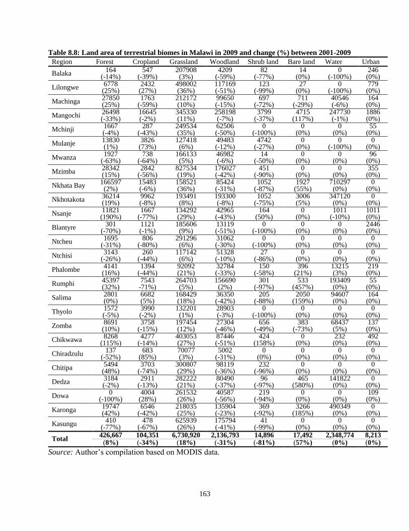
163

Table 8.8: Land area of terrestrial biomes in Malawi in 2009 and change (%) between 2001-2009 Region Forest Cropland Grassland Woodland Shrub land Bare land Water Urban

Balaka 164 547 207908 4209 82 14 0 246

(-14%) (-39%) (3%) (-59%) (-77%) (0%) (-100%) (0%)

Lilongwe 6778 2432 498002 117169 123 27 0 779 (25%) (27%) (36%) (-51%) (-99%) (0%) (-100%) (0%)

Machinga 27850 1763 212172 99650 697 711 40546 164 (25%) (-59%) (10%) (-15%) (-72%) (-29%) (-6%) (0%)

Mangochi 26498 16645 345330 258198 3799 4715 247730 1886 (-33%) (-2%) (11%) (-7%) (-37%) (117%) (-1%) (0%)

Mchinji 1667 287 249534 62506 0 0 0 55 (-4%) (-43%) (35%) (-50%) (-100%) (0%) (0%) (0%)

Mulanje 13830 3826 127418 49483 4742 0 0 0 (1%) (73%) (6%) (-12%) (-27%) (0%) (-100%) (0%)

Mwanza 1927 738 166133 46982 14 0 0 96

(-63%) (-64%) (5%) (-6%) (-50%) (0%) (0%) (0%)

Mzimba 28342 2842 827534 176027 451 0 0 355 (15%) (-56%) (19%) (-42%) (-90%) (0%) (0%) (0%)

Nkhata Bay 166597 15483 158521 85424 1052 1927 710297 0 (2%) (-6%) (36%) (-31%) (-87%) (55%) (0%) (0%)

Nkhotakota 36214 9962 193491 193300 1052 3006 347120 0 (19%) (-8%) (8%) (-8%) (-75%) (5%) (0%) (0%)

Nsanje 11821 1667 134292 42965 164 0 1011 1011 (190%) (-77%) (29%) (-43%) (50%) (0%) (-10%) (0%)

Blantyre 301 1121 185606 13119 0 0 0 2446

(-70%) (-1%) (9%) (-51%) (-100%) (0%) (0%) (0%)

Ntcheu 1695 806 291296 31062 0 0 0 0

(-31%) (-80%) (6%) (-30%) (-100%) (0%) (0%) (0%)

Ntchisi 3143 260 117142 51328 27 0 0 0

(-26%) (-44%) (6%) (-10%) (-86%) (0%) (0%) (0%)

Phalombe 4141 1394 92092 32784 150 396 13215 219 (16%) (-44%) (21%) (-33%) (-58%) (21%) (3%) (0%)

Rumphi 45397 7543 264703 156690 301 533 193409 55 (32%) -71%) (5%) (2%) (-97%) (457%) (0%) (0%)

Salima 2801 6682 168429 36350 205 2050 94607 164 (0%) (5%) (18%) (-42%) (-88%) (159%) (0%) (0%)

Thyolo 1572 3990 132201 28903 0 0 0 0 (-5%) (-2%) (1%) (-3%) (-100%) (0%) (0%) (0%)

Zomba 8691 3758 197454 27304 656 383 68437 137 (10%) (-15%) (12%) (-46%) (-49%) (-73%) (5%) (0%)

Chikwawa 8268 4277 403053 87446 424 0 232 492

(115%) (-14%) (27%) (-51%) (158%) (0%) (0%) (0%)

Chiradzulu 137 683 70077 5002 0 0 0 0

(-52%) (85%) (3%) (-31%) (0%) (0%) (0%) (0%)

Chitipa 5494 3703 300807 98119 232 0 0 0 (48%) (-74%) (29%) (-36%) (-96%) (0%) (0%) (0%)

Dedza 3184 2911 282222 80490 96 465 141822 0 (-2%) (-13%) (21%) (-37%) (-97%) (580%) (0%) (0%)

Dowa 0 4004 261532 40587 219 0 0 109

(-100%) (28%) (26%) (-56%) (-94%) (0%) (0%) (0%)

Karonga 19747 6546 218035 135904 369 3266 490349 0 (42%) (-42%) (25%) (-23%) (-92%) (185%) (0%) (0%)

Kasungu 410 478 625939 175794 41 0 0 0

(-77%) (-67%) (26%) (-41%) (-99%) (0%) (0%) (0%)

Total 426,667 104,351 6,730,920 2,136,793 14,896 17,492 2,348,774 8,213

(8%) (-34%) (18%) (-31%) (-81%) (57%) (0%) (0%)


164

Table 8.9: Land area of terrestrial biomes in Tanzania in 2009 and change (%) between 2001-2009

Region Forest Cropland Grassland Woodland Shrub land Bare land Water Urban

Arusha 165449 56466 3212453 210245 86039 15934 192302 1380 (-1%) (-63%) (7%) (-20%) (-32%) (-12%) (-6%) (0%)

Pemba South

8473 25063 8418 3676 232 123 3608 109 (-46%) (39%) (-10%) (122%) (-53%) (-25%) (-12%) (-11%)

Lindi 105143 69804 5835414 629150 4933 3430 8828 5084 (-41%) (-47%) (20%) (-57%) (-63%) (192%) (-30%) (0%)

Manyara 62383 29764 4027333 334069 36146 4236 6915 328 (-12%) (-63%) (5%) (-18%) (-57%) (-20%) (-13%) (0%)

Mara 18558 136560 1875726 51834 11424 10973 802731 1968 (-40%) (-15%) (12%) (-73%) (-44%) (112%) (-2%) (0

Mbeya 107521 58366 3436255 2070228 3826 1913 145976 957 (18%) (-11%) (6%) (-8%) (-91%) (-43%) (-5%) (0%)

Morogoro 876812 70624 3462985 2322864 4879 0 0 2665 (-11%) (-60%) (17%) (-10%) (-78%) (-100%) (-100%) (0%)

Mtwara 8350 34861 1652539 33317 5589 410 3293 28780

(-31%) (38%) (9%) (-79%) (-60%) (-12%) (-27%) (0%)

Mwanza 84125 246158 1530150 79834 26019 33699 1493171 2528 (-8%) (24%) (0%) (-21%) (-3%) (110%) (-2%) (-1%)

Pwani 135508 132310 2248742 620432 7311 1271 20047 123 (-40%) (-48%) (21%) (-21%) (-45%) (-47%) (-28%) (0%)

Rukwa 160543 106086 1903330 4392368 7420 5070 927566 4059 (-10%) (20%) (3%) (0%) (-55%) (11%) (-3%) (0%)

Dar-Es-Salaam

1640 24174 97613 23628 1421 314 847 12053 (-36%) (-43%) (23%) (10%) (-5%) (130%) (-30%) (-6%)

Ruvuma 237535 19760 1310872 4816835 2091 1175 13625 2214 (-16%) (-72%) (-15%) (8%) (-90%) (72%) (-14%) (0%)

Shinyanga 9170 90835 4159151 749927 27208 123 191 1080

(-64%) (-47%) (15%) (-31%) (-78%) (350%) (-75%) (0%)

Singida, 52872 39876 4533192 199326 28247 2651 36911 437 (-44%) (-33%) (11%) (-63%) (-62%) (-13%) (-18%) (0%)

Tabora 7981 38605 5686472 1903166 7926 1708 19487 3635

(-69%) (-77%) (19%) (-27%) (-82%) (-46%) (29%) (0%)

Tanga 177202 125847 1424023 1077368 14950 929 3635 1462 (-33%) (-28%) (4%) (10%) (-46%) (39%) (-44%) (0%)

Zanzibar South

28165 12586 29641 16836 260 68 2378 0 (-16%) (-43%) (37%) (102%) (-5%) (-58%) (-35%) (0%)

Zanzibar West

1613 7325 9019 3198 424 41 1722 793 (-76%) (25%) (65%) (34%) (-9%) (-40%) (-5%) (-38%)

Dodoma 13310 42814 3951297 165053 15059 3908 36788 1189 (-28%) (-69%) (13%) (-66%) (-49%) (79%) (-34%) (0%)

Iringa 564280 62233 4224391 1320944 7844 2911 21865 2487 (15%) (-70%) (19%) (-27%) (-94%) (70%) (-4%) (0%)

Kagera 111730 249575 1114867 1447091 6068 9935 1044147 970 (-41%) (-49%) (-4%) (35%) (-56%) (35%) (-1%) (0%)

Pemba North

10249 25117 10386 4332 506 260 3047 82 (-47%) (82%) (-26%) (88%) (6%) (12%) (-16%) (-40%)

Unguja North

3362 15210 17396 8391 232 41 2077 0 (-74%) (15%) (14%) (249%) (-60%) (-57%) (-8%) (-10%)

Kigoma 203289 64406 208797 3327121 5261 3649 804412 3225 (-39%) (-43%) (-39%) (11%) (-45%) (28%) (-1%) (0%)

Kilimanjaro 174838 22248 882852 152590 86845 2938 6655 2023 (5%) (-49%) (8%) (-5%) (-31%) (-38%) (45%) (0%)

Total 3,330,100 1,806,674 56,853,310 25,963,820 398,161 107,712 5,602,224 7,9629

(-17%) (-41%) (11%) (-10%) (-59%) (29%) (-3%) (-2%)


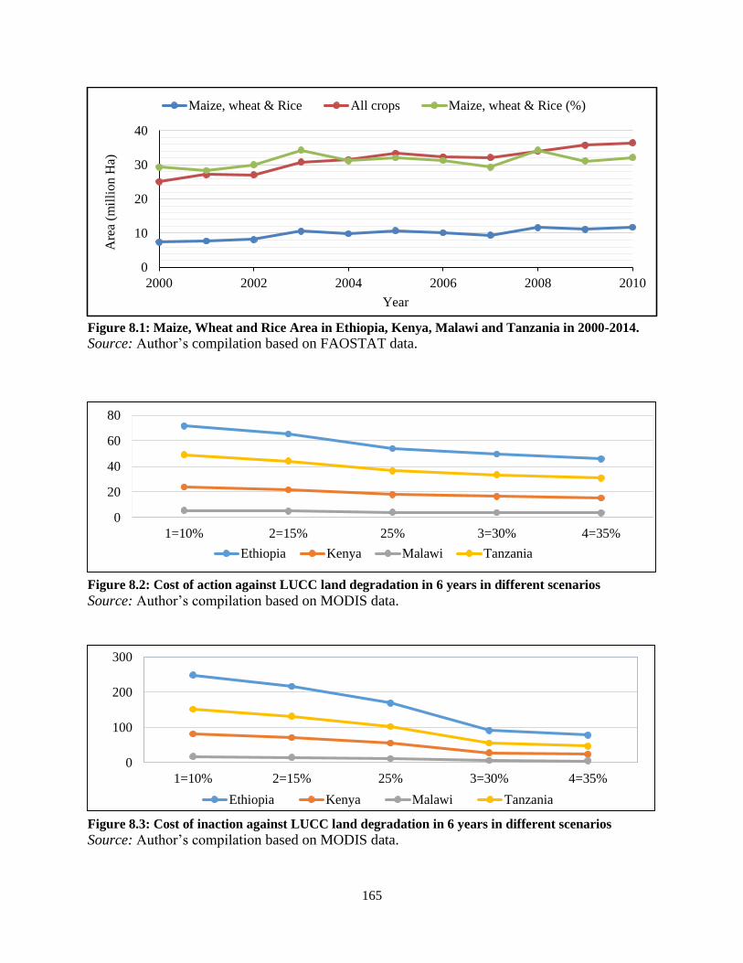
165

Figure 8.1: Maize, Wheat and Rice Area in Ethiopia, Kenya, Malawi and Tanzania in 2000-2014.

Source: Author’s compilation based on FAOSTAT data.

Figure 8.2: Cost of action against LUCC land degradation in 6 years in different scenarios


Figure 8.3: Cost of inaction against LUCC land degradation in 6 years in different scenarios


0

10

20

30

40

2000 2002 2004 2006 2008 2010

Are

a (m

illi

on

Ha)

Year

Maize, wheat & Rice All crops Maize, wheat & Rice (%)

0

20

40

60

80

1=10% 2=15% 25% 3=30% 4=35%


0

100

200

300

1=10% 2=15% 25% 3=30% 4=35%


Economics of Land Degradation, Sustainable Land ...

Documents

Transcript of Economics of Land Degradation, Sustainable Land ...