Socioeconomic development and vulnerability to land degradation in Italy

ORIGINAL ARTICLE

Socioeconomic development and vulnerability to land degradationin Italy

Luca Salvati • Alberto Mancini • Sofia Bajocco •

Roberta Gemmiti • Margherita Carlucci

Received: 22 August 2010 / Accepted: 25 February 2011 / Published online: 22 March 2011

� Springer-Verlag 2011

Abstract In recent years, the surface area affected by

land degradation (LD) has significantly increased in

southern European regions where the socioeconomic

development has been proposed as a basic factor underly-

ing the degree of vulnerability to LD. This paper investi-

gates the correlation between several socioeconomic

indicators and the level of vulnerability to LD in Italy,

expressed as changes (1990–2000) in a composite index of

land vulnerability (DLVI). The analysis was carried out

over 784 local districts. The impact of per capita value

added, agricultural intensity, industrial and tourism con-

centration, and urban growth was separately tested on

DLVI. Results indicate that a lower district value added,

crop intensification, irrigation, and the level of land vul-

nerability to degradation are strongly associated with the

increasing level of land vulnerability over time, highlight-

ing the role of the socioeconomic development as a main

process underlying LD. In this framework, spatially equi-

table sustainable development may represent the effective

strategy to mitigate the detrimental effects of economic

growth and regional disparities on Mediterranean LD.

Keywords Land degradation � Vulnerability �Socioeconomic indicators � Sustainable development �Local district � Mediterranean region

Introduction

Land degradation (LD) is defined as a long-term decline in

ecosystem function and productivity and is worldwide

recognized as an important issue in the political agenda for

the 21st century (Stringer 2008). The LD process appears

particularly severe in developing countries (Africa, south-

ern Asia, and Latin America); however, because of climate

change and growing human pressure, it is becoming critical

also in many developed countries, such as United States,

Australia, and some parts of the Mediterranean basin

(Rubio et al. 2009).

Mediterranean LD is a multifaceted and dynamic pro-

cess depending on biophysical, socioeconomic, cultural,

and institutional factors, with strong negative effects on

food security and quality of life (Conacher and Sala 1998;

Conacher 2000). Due to this complexity, LD was often

approached at ‘on-site’ scale with a focus on the bio-

physical causes (Puigdefabregas and Mendizabal 1998;

Geist and Lambin 2004; Montanarella 2007). To the

L. Salvati

Italian Council of Agricultural Research, Research Centre for

Plant-Soil Systems, Via della Navicella 2-4, 00185 Rome, Italy

A. Mancini (&)

c/o Centre for Economic and International Studies—CEIS,

‘Tor Vergata’ University of Rome, Via Columbia, 2,

00133 Rome, Italy

e-mail: [email protected]

S. Bajocco

Italian Council of Agricultural Research, Research Unit of

Climatology and Meteorology Applied to Agriculture,

Via del Caravita 7a, 00186 Rome, Italy

R. Gemmiti

Department of Geographical, Linguistic, Statistical,

Historical Studies for Regional Analysis, Faculty of Economics,

‘Sapienza’ University of Rome, Via del Castro Laurenziano 9,

00161 Rome, Italy

M. Carlucci

Department of Economics, Faculty of Statistics,

‘Sapienza’ University of Rome, Piazzale A. Moro 5,

00185 Rome, Italy

e-mail: [email protected]

123

Reg Environ Change (2011) 11:767–777

DOI 10.1007/s10113-011-0209-x

contrary, relatively few studies have dealt with the phe-

nomenon at regional scale, analyzing the interaction

between human factors and the ecological variables

(Briassoulis 2004). Moreover, LD is a dynamic attribute of

the territory mainly depending on its biophysical charac-

teristics (climate, soil, vegetation) and possibly changing

over time (Basso et al. 2000; Lavado Contador et al. 2009).

Understanding the spatiotemporal trends (rather than the

present status) of LD may allow to identify and foresee the

spatial distribution of vulnerable areas (Salvati and Ba-

jocco 2011), hence representing a key issue both from the

ecological and from policy points of view.

When dealing with LD, monitoring strategies should be

the major concern and they should encompass the multidis-

ciplinary perspectives of the problem (Reynolds and Stafford

Smith 2002; Gisladottir and Stocking 2005). Accordingly, a

number of recent studies have been carried out and different

methodologies to study LD have been proposed: visual

observation, field measurements, social enquiries, environ-

mental indicators derived from statistical sources, remote

sensing, and mathematical models (Basso et al. 2000; Bath-

urst et al. 2003; Salvati and Zitti 2009). With respect to other

approaches, environmental indicators have the advantage of

(1) producing synthetic information on the spatiotemporal

dynamics of multivariate phenomena, (2) being reasonably

comparable among different countries, and (3) being easily

communicable to both stakeholders and policy-makers.

In this perspective, the aim of this paper was to contribute

to the knowledge of LD through an exploratory analysis of

the relationship between changes in land vulnerability over

time and several socioeconomic underlying factors. The

analysis was carried out in Italy, a southern European

country with different levels of land vulnerability and

marked socioeconomic disparities (Salvati and Zitti 2009).

Materials and methods

Study area

The study area (Italy, ca. 301.330 km2) is divided into 784

districts (Local Labor Market Districts, LLMAs) identified

on the basis of data related to daily labor mobility (ISTAT

1997). LLMAs reflect districts of socioeconomic interest

and are used to analyze the regional development of Italy

(Pellegrini 2002), the local specialization in agriculture

(Giusti and Grassini 2007), and the level of land vulnera-

bility to degradation (Salvati and Zitti 2009).

The distribution of district income in term of per capita

gross value added was mapped in Fig. 1. In 2000, northern

Italy resulted as one of the most developed European

regions, while southern Italy was still an economically

disadvantaged area, with per capita value added about half

of that observed in northern Italy (ISTAT 2006). In

southern Italy, only few districts, featuring industrial con-

centration and high-yield agriculture, showed the levels of

per capita value added greater than 10,000 euros, which

was much lower than the Italian average (14,300 euros).

The land vulnerability index

LD is related, on one hand, to the environmental man-

agement due to human activities and, on the other hand, to

the endowments of land resources that are mostly due to

the geographical location and the biophysical context. The

separate effects of these two components (i.e., land

resources ‘‘management’’ and ‘‘endowments’’) can be

quantified by analyzing the LD changes of a territory over

time rather than its (static) present status, inferring about

the behind processes (Salvati and Zitti 2009).

Based on these considerations, we computed a composite

index estimating changes in the level of land vulnerability

through time in Italy. While the most used LD indexes are

set up by following the Environmental Sensitive Area

(ESA) procedure (Basso et al. 2000; Lavado Contador et al.

2009; Salvati and Bajocco 2011), we used an ESA-like

index of vulnerability to LD (the so-called LVI), which is

better suited to account for some peculiar characteristics of

the Italian landscape and circumvents data limitations at

high-resolution scales (Salvati and Zitti 2008; Salvati et al.

2009). The LVI is composed of three thematic indicators of

climate, soil properties, and vegetation quality, which pro-

duce a ranking of biophysical vulnerability to LD.

Climate variables include the aridity index, the average

annual rainfall, the rainfall variability, and concentration,

as well as the average number of rainy days (all measured

over a 30-year period). Soil variables include the soil depth

and texture, the potential available water capacity, the

organic carbon content, and a proxy for soil erosion risk.

Finally, vegetation variable, derived from land cover,

include sensitivity to drought, fire risk, protection from soil

erosion, and land cover intensity.

The LVI was tested in several field sites in order to

check the relationship between the index scores and several

independent measures of soil and land degradation (Salvati

et al. 2009).

We estimated the LVI for 2 years (1990 and 2000) on a

district basis over the whole Italy; the spatial distribution of

LVI in 2000 was mapped in Fig. 1. We used the difference

in the LVI among the two periods (DLVI) by local district

as the dependent variable in the regression model.

Socioeconomic data and indicators

There is no consensus about the type and number of factors

possibly associated with LD in the Mediterranean region

768 L. Salvati et al.

123

(Mairota et al. 1998). The choice usually depends on data

availability and research objectives. From the economic

point of view, the possible determinants of LD should

cover social, production, policy, and sociodemographic

factors, as well as site-specific variables (Briassoulis 2004).

Wilson and Juntti (2005) introduced various hypotheses to

explain Mediterranean LD, including (1) the ‘‘human

pressure’’ hypothesis, (2) the ‘‘agricultural impact’’

hypothesis, and (3) the ‘‘environmental factors’’ hypothe-

sis. Concerning Italy, the empirical analysis provided by

Salvati and Zitti (2008) corroborates Wilson and Juntti

(2005) approach, suggesting that crop intensification, urban

sprawl, industrial concentration, and tourism pressure

represent potentially important factors affecting LD at

regional scale.

Several variables were selected as predictors in the

regression model and classified into different groups

according to their potential link to land vulnerability

dynamics. Three classes of covariates measured at the

district level were identified, namely (1) socioeconomic

variables, (2) agricultural variables, and (3) environmental

or control variables (Table 1). We chose candidate vari-

ables according to the results illustrated in previous works

(Montanarella 2007; Rubio et al. 2009; Tanrivermis 2003).

The ‘‘socioeconomic’’ covariates (SOC) included seven

variables: per capita gross value added (GVA), the share of

agriculture (AGP) and industry (IND) in total product, land

productivity (LAN), labor productivity in services (SER), as

well as two dummies, respectively, identifying urban dis-

tricts (URB), and tourism-specialized districts (TOU) (these

two variables were fully described in ISTAT 2006). It is

important to note that the term ‘local income’ is used in

this paper as synonym of district value added and does not

directly refer to the average income of private households

within the investigated area.

The ‘‘agricultural’’ covariates (AGR) included five

variables: the percentage of agricultural land on the total

district area indicating the local specialization in agricul-

ture (AUA), the variation of agricultural land surface over a

10-year horizon (1990–2000) indicating potential processes

of land abandonment (LOS), the percentage of irrigated

agricultural land (IRR), the percentage of economically

marginal farms (i.e., Agricultural Utilized Area \ 2 hect-

ares, MAR), and an index of crop intensity describing

potential processes of agricultural intensification (INT).

The ‘‘environmental’’ and control covariates (ENV)

included five variables: the LVI score measured at the

beginning of the study period (LVI), the average district’s

elevation (ELE), surface area (SUR), and population den-

sity (POP), as well as a dummy for the geographical area

(northern ? central Italy districts = 0, southern Italy ?

the two main islands districts = 1; GEO). The classifica-

tion of the Italian territory in two areas (north ? centre,

south ? Islands) follows an economic rationale related to

the EU’s funding strategy. For a long term, EU structural

funds subdivided Italy into eight economically disadvan-

taged target regions (all belonging to southern Italy) and

twelve developed regions (all belonging to central and

northern Italy). This classification reflects the different

environmental conditions occurring in the two analyzed

areas (Salvati and Zitti 2009). All variables were calculated

at the district scale from national accounts and census data

provided by the Italian National Institute of Statistics

(ISTAT 2006) and refer to the years 2000 or 2001 when not

differently specified.

Statistical analyses

In order to avoid redundancy and collinearity among vari-

ables, we carried out a preliminary analysis on the selected

Fig. 1 Left district value added (GVA) across Italy (expressed in Euros per capita). Middle land vulnerability to degradation (LVI) in Italy (both

variables refer to 2000). Right changes in land vulnerability in 1990–2000 (DLVI)

Socioeconomic development and vulnerability 769

123

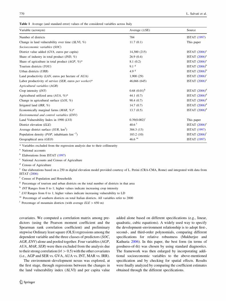
covariates. We computed a correlation matrix among pre-

dictors (using the Pearson moment coefficient and the

Spearman rank correlation coefficient) and preliminary

stepwise Ordinary least square (OLS) regressions among the

dependent variable and the three classes of predictors (SOC,

AGR, ENV) alone and pooled together. Four variables (AGP,

AUA, MAR, SER) were then excluded from the analysis due

to their strong correlation (|r| [ 0.5) with the other covariates

(i.e., AGP and SER vs. GVA, AUA vs. INT, MAR vs. IRR).

The environment–development nexus was explored, at

the first stage, through regressions between the changes in

the land vulnerability index (DLVI) and per capita value

added alone based on different specifications (e.g., linear,

quadratic, cubic equations). A widely used way to specify

the development–environment relationship is to adopt first-,

second-, and third-order polynomials, comparing different

specifications for relative robustness (Mukherjee and

Kathuria 2006). In this paper, the best form (in terms of

goodness-of-fit) was chosen by using standard diagnostics.

The framework was then enlarged by incorporating addi-

tional socioeconomic variables to the above-mentioned

specification and by checking for spatial effects. Results

were finally analyzed by comparing the coefficient estimates

obtained through the different specifications.

Table 1 Average (and standard error) values of the considered variables across Italy

Variable (acronym) Average (±SE) Source

Number of districts 784 ISTAT (1997)

Change in land vulnerability over time (DLVI, %) 11.7 (0.1) This paper

Socioeconomic variables (SOC)

District value added (GVA, euros per capita) 14,300 (215) ISTAT (2006)a

Share of industry in total product (IND, %) 26.9 (0.4) ISTAT (2006)a

Share of agriculture in total product (AGP, %)* 8.1 (0.2) ISTAT (2006)a

Tourism districts (TOU) 9.1 g ISTAT (2006)b

Urban districts (URB) 4.9 g ISTAT (2006)b

Land productivity (LAN, euros per hectare of AUA) 1,900 (29) ISTAT (2006)c

Labor productivity of service (SER, euros per worker)* 46,666 (645) ISTAT (2006)a

Agricultural variables (AGR)

Crop intensity (INT) 0.68 (0.01)h ISTAT (2006)d

Agricultural utilized area (AUA, %)* 44.1 (0.7) ISTAT (2006)d

Change in agricultural surface (LOS, %) 90.4 (0.7) ISTAT (2006)d

Irrigated land (IRR, %) 14.7 (0.7) ISTAT (2006)d

Economically marginal farms (MAR, %)* 13.7 (0.5) ISTAT (2006)d

Environmental and control variables (ENV)

Land Vulnerability Index in 1990 (LVI) 0.39(0.002)i This paper

District elevation (ELE) 40.6 l ISTAT (2006)e

Average district surface (SUR, km2) 384.3 (13) ISTAT (1997)

Population density (POP, inhabitants km-2) 183.2 (10) ISTAT (2006)f

Geographical area (GEO) 46.6 m ISTAT (1997)

* Variables excluded from the regression analysis due to their collinearitya National accountsb Elaborations from ISTAT (1997)c National Accounts and Census of Agricultured Census of Agriculturee Our elaborations based on a 250 m digital elevation model provided courtesy of L. Perini (CRA-CMA, Rome) and integrated with data from

ISTAT (2006)f Census of Population and Householdsg Percentage of tourism and urban districts on the total number of districts in that areah INT Ranges from 0 to 1; higher values indicate increasing crop intensityi LVI Ranges from 0 to 1; higher values indicate increasing vulnerability to LDm Percentage of southern districts on total Italian districts. All variables refer to 2000l Percentage of mountain districts (with average ELE [ 650 m)


123

In detail, the regression analysis estimated a vector of

coefficients, each linked to a single, potential driver of the

specified environmental process, by using the reduced form

E = f (Y, A), where E represents the environmental process

under study, Y is the income variable, and A is a set of

additional variables describing the level of socioeconomic

development. When it is significant, the relation may be linear

or polynomial. In the former case, it was supposed that

socioeconomic development is (positively or negatively)

associated with changes in land vulnerability to degradation

over the entire range of observed income. In the latter case,

development is correlated with decreasing levels of land

vulnerability at lower (or intermediate) levels of district

income, whereas a ‘re-linking’ process (i.e., increasing LD

vulnerability) is expected at higher income. More complex

patterns (e.g., third-order polynomials) may highlight site-

specific responses of land vulnerability to socioeconomic

development. The multidimensionality of this concept

reflects the different behavior of the additional socioeconomic

variables compared with that of income (Galeotti 2007).

The relationship between the DLVI and the socioeco-

nomic features of each district was thus tested here by

specifying different forms starting with the simplest one,

relating DLVI and (district) per capita value added (in

absolute and logarithm numbers) alone (GVA) or with the

vector Xi, which includes the additional covariates. At the

first stage, the following equation was estimated:

DLVI ¼ b0 þ b1ðGVAÞ þ b2ðGVAÞ2 þ b3ðGVAÞ3 þ e ð1Þ

where b0 is the intercept and b(d) are the coefficient terms.

The vector Xi that includes the three classes of (additional)

variables (SOC, AGR, and ENV) was then incorporated in

the selected form as follows:

DLVI ¼ b0 þ b1 GVAð Þ þ b2 GVAð Þ2

þ b3 GVAð Þ3þbm Xið Þ þ e ð2Þ

Equations 1–2 were first estimated through OLS

regression. Collinearity among variables was checked

throughout by using the variance inflation factor and

condition index. Outputs report the variables in each model

with significant coefficients and standard errors. Notably,

OLS regression assumes spatial randomness, which

indicates that any grouping of high or low values of the

study variable in space would be independent. If this

assumption is not true, i.e., a spatial structure exists in the

variable as detected by the presence of spatial correlation,

standard OLS estimates are inefficient. We therefore

studied the spatial variation of both the dependent

variable (DLVI) and the main predictor (GVA) through

exploratory spatial data analysis techniques.

Central to this framework is the choice of the matrix that

describes the interaction structure of the cross-section

units, i.e., the definition of proximity. For each spatial unit,

a relevant neighboring set must be defined consisting of

those units that potentially interact with it. Although in

regional data analysis proximity is usually defined in terms

of contiguity, if the basic units are defined by administra-

tive boundaries, this definition may not be appropriate. We

hence used an alternative approach, i.e., a spatial weight

matrix based on Euclidean distances between the gravita-

tional centers of the local districts. As regards the spatial

distribution of DLVI in Italy, potential interactions between

locations were summarized by the matrix W = {wij},

where wij = 1 if districts i and j are within a fixed distance,

d, of each other and 0 otherwise. We considered eight

values of d ranging from 25 to 200 km with a span of

25 km in order to assess how far the links between spatial

units extend, i.e., the degree of spatial correlation (Anselin

2001). In this way, the analysis of spatial dependence

exhibited by given variables (i.e., DLVI and GVA) using

alternative definitions of neighborhoods (i.e., varying the

d distance) conveys information about the spatial config-

uration that maximizes the intensity of interactions

between districts.

We carried out the assessment of global spatial auto-

correlation through Moran’s I and Geary’s c statistics (Cliff

and Ord 1981). Unfortunately, Moran’s I and Geary’s

c tests provide only a general measure of spatial correla-

tion. To model the spatial correlation in association with

the explanatory variables, two approaches were developed

in this study.

The first approach is based on the spatial regression

model:

Zi ¼ li þ d; ð3Þ

where Zi is the random process at location i (i.e., DLVI), li

is the mean at the same site, which is a linear, square, or

cubic model with (1) GVA alone (i.e., the restricted model),

and (2) all the covariates (i.e., the full model), d–N(0, R)

and R is the covariance matrix of random variables at all

locations. The small-scale variation was modeled by fitting

two different covariance models to R, including conditional

spatial autoregression (CAR) and moving average (MA)

structures. The spatial weight matrix introduced in these

models was chosen according to the results of Moran’s and

Geary’s statistics.

The second approach uses the geographically weighted

regression (GWR) proposed by Fotheringham et al. (2002).

The methodological framework underlying GWR is quite

similar to that of local linear regression models, as it uses a

kernel function to calculate weights for the estimation of

local weighted regression models. Contrary to the standard

regression model, where the regression coefficients are

location invariant, the specification of a basic GWR model

for each location s = 1, …, n, is:


123

yðsÞ ¼ XðsÞbðsÞ þ eðsÞ; ð4Þ

where y(s) is the dependent variable at location s, X(s) is

the row vector of explanatory variables at location s, b(s) is

the column vector of regression coefficients at location s,

and e(s) is the random error at location s. Hence, regression

parameters, estimated at each location by weighted least

squares, vary in space, implying that each coefficient in the

model is a function of s, a point within the geographical

space of the study area. As a result, GWR gives rise to a

distribution of local estimated parameters. The weighting

scheme is expressed as a kernel function that places more

weight on the observations closer to the location s. In this

study, we adopted one of the most commonly used speci-

fications of the kernel function, which is the bi-square

nearest neighbor function.

Finally, based on the linear form: DLVI = b0 ?

b1(GVA), the elasticity of DLVI to GVA (gld/gva) was

computed as

gld=gva ¼dðDLVIÞ

dGVADLVIGVA

¼ b1

b0 þ b1GVAð5Þ

and calculated at a defined income, which coincides with

the average per capita value added (14,300 euros). Income

figures were computed as per capita, logarithmic values

and refer to 2000.

Results

The analysis developed in this paper led to various results:

(1) changes in the level of land vulnerability to degradation

(DLVI) and district per capita value added (GVA), taken as

the key investigated variables, are both spatially depen-

dent; (2) the relationship between these two variables is

linear and negative; (3) the probability to observe

increasing levels of land vulnerability to degradation dur-

ing the investigated period (1990–2000) is higher in low-

income districts where the primary sector contributes more

to the local value added; (4) other socioeconomic variables

(crop intensity, irrigation, and the level of land vulnera-

bility measured at the initial time of study) significantly

contribute to this relationship; (v) spatial effects share a

significant contributing role to the relation itself; (vi) the

results of the regression analysis are model insensitive.

Spatial dependence of DLVI and GVA

Moran’s I and Geary’s c statistics for DLVI and GVA are

reported in Table 2. These tests confirm the positive spatial

autocorrelation across local districts for both variables:

areas with relatively high (low) DLVI (or GVA) are located

close to each other more often than if they were randomly

distributed, and the strongest spatial linkages can be found

Table 2 Measures of global spatial autocorrelation, DLVI and GVA; spatial weight matrix: geodesic distance \ d km

Moran global DLVI GVA

d I z(I) p1 p2 I z(I) p1 p2

25 0.6155 24.40 \0.001 \0.001 0.7626 30.22 \0.001 \0.001

50 0.5131 41.01 \0.001 \0.001 0.7109 56.77 \0.001 \0.001

75 0.4554 52.66 \0.001 \0.001 0.6794 78.48 \0.001 \0.001

100 0.4224 63.02 \0.001 \0.001 0.6588 98.17 \0.001 \0.001

125 0.4048 73.19 \0.001 \0.001 0.6452 116.50 \0.001 \0.001

150 0.3870 81.87 \0.001 \0.001 0.6244 131.90 \0.001 \0.001

175 0.3723 89.76 \0.001 \0.001 0.6032 145.20 \0.001 \0.001

200 0.3624 97.99 \0.001 \0.001 0.5926 160.00 \0.001 \0.001

Geary global c

d c Z(c) p1 p2 c Z(c) p1 p2

25 0.3737 -15.71 \0.001 \0.001 0.3571 -16.13 \0.001 \0.001

50 0.4608 -21.90 \0.001 \0.001 0.3642 -30.93 \0.001 \0.001

75 0.5214 -23.17 \0.001 \0.001 0.3745 -30.29 \0.001 \0.001

100 0.5616 -23.37 \0.001 \0.001 0.3797 -33.07 \0.001 \0.001

125 0.5867 -23.30 \0.001 \0.001 0.3854 -34.65 \0.001 \0.001

150 0.6060 -22.08 \0.001 \0.001 0.3909 -44.80 \0.001 \0.001

175 0.6222 -22.06 \0.001 \0.001 0.3990 -35.09 \0.001 \0.001

200 0.6338 -21.26 \0.001 \0.001 0.4049 -34.56 \0.001 \0.001


123

when ‘close’ areas are considered. Both statistics are highly

significant at all considered distances (see p levels in

Table 2).

The relationship between increasing land vulnerability

and socioeconomic variables

The relationship between DLVI and the socioeconomic

variables was explored by using different specifications

(Table 3). Based on both GVA and log-GVA, squared and

third-order polynomial regressions between DLVI and

GVA gave a goodness of fit similar (or lower) to the linear

form. Lower values of GVA are associated with increasing

levels of land vulnerability (b1 = -0.038).

The linear form incorporating spatial effects gave better

results than squared and third-order (not shown) forms

(Table 4). Lower values of GVA are linearly associated

with higher DLVI with b1 = -0.038 (CAR model) or

b1 = -0.023 (MA model).

GWR provided similar results indicating that DLVI is

linearly associated with GVA with b1 = -0.037. The

elasticity of DLVI to GVA is rather stable through the

various specifications considered: gld/gva amounted to

-0.88, -0.90, and -0.86 by considering standard OLS,

CAR, and GWR models, respectively. Estimates for Eq. 2

are presented in Table 5. An inverse, linear relationship

between GVA and DLVI is observed in all models.

As expected, high-income districts experienced lower

growth rates of DLVI irrespective of any other considered

variable: coefficients for GVA are stable in all considered

models (-0.023). DLVI resulted positively correlated with

INT, IRR, and GEO and negatively correlated with LVI.

LAN, ELE, and POP resulted (weakly) significantly cor-

related with DLVI (with negative coefficients) in MA and

GWR models only. Since second- and third-order polyno-

mial forms showed, in all considered specifications, a

goodness of fit systematically lower than the linear model,

they are neither reported in tables nor discussed in the main

text.

A socioeconomic profile of the vulnerable land

to degradation

In Italy, high vulnerable lands are mainly concentrated in

three areas: (1) the two major islands (Sicily and

Sardinia), Apulia and Basilicata, all located in southern

Italy, (2) a few dry, coastal areas close to Rome and

some located along the Adriatic Sea in central Italy and,

finally, (3) the lowland close to the Po river in north-

eastern Italy.

Table 3 Results of the standard OLS regression analysis among changes in vulnerability to LD (DLVI) and (district) per capita value added

(GVA) in Italy (standard errors of the estimates are reported in brackets)

Linear Quadratic Cubic

b0 0.201 (0.009)*** 0.104 (0.185)ns 0.104 (0.186)ns

GVA -0.038 (0.002)*** 0.010 (0.090)ns 0.010 (0.091)ns

GVA2 -0.006 (0.011)ns -0.006 (0.012)ns

GVA3 *0.000 ns

Adj-R2 0.263 0.262 0.261

F 278.0*** 139.0* 139.0*

df 1, 778 2, 777 2, 777

Stars indicate the probability level of t test associated with each regression coefficient as follows: ns p [ 0.05, * 0.01 \ p \ 0.05,

** 0.01 \ p 0.001, *** p \ 0.001

Table 4 Results of spatial regression (both conditional autoregres-

sive model, CAR, and moving average model, MA: spatial weight

matrix: d = 50 km) and geographically weighted regression (GWR)

analyses among changes in vulnerability to LD (DLVI) and per capita

value added (GVA) in Italy (standard errors of the estimates are

reported in brackets)

CAR spatial regression MA spatial regression GWR

Linear Quadratic Linear Quadratic Linear Quadratic

b0 0.200 (0.009)** 0.108 (0.185) 0.141 (0.011)** 0.230 (0.164) 0.197 (0.010)** 0.118 (0.161)

GVA -0.038 (0.002)** 0.008 (0.091) -0.023 (0.003)** -0.067 (0.080) -0.037 (0.002)** 0.002 (0.079)

GVA2 – -0.006 (0.011) – 0.005 (0.010) – -0.005 (0.010)

Adj-R2 – – – – 0.241 0.240

Log-L 824.8 824.9 935.8 935.9 – –

Stars indicate the probability level of t test associated with each regression coefficient as follows: * 0.001 \ p \ 0.05, ** p \ 0.001


123

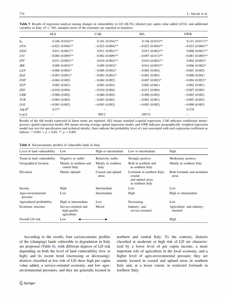
According to the results, four socioeconomic profiles

of the (changing) lands vulnerable to degradation in Italy

are proposed (Table 6), with different degrees of LD risk

depending on both the level of land vulnerability (low or

high) and its recent trend (increasing or decreasing):

districts classified at low risk of LD show high per capita

value added, a service-oriented economy, and low agro-

environmental pressures, and they are generally located in

northern and central Italy. To the contrary, districts

classified at moderate or high risk of LD are character-

ized by a lower level of per capita income, a more

important role of agriculture in the local economy, and a

higher level of agro-environmental pressure; they are

mainly located in coastal and upland areas in southern

Italy and, at a lesser extent, in restricted lowlands in

northern Italy.

Table 5 Results of regression analysis among changes in vulnerability to LD (DLVI), (district) per capita value added (GVA), and additional

variables in Italy (N = 784; standard errors of the estimates are reported in brackets)

OLS CAR MA GWR

b0 0.186 (0.016)** 0.181 (0.016)** 0.146 (0.015)** 0.141 (0.017)**

GVA -0.023 (0.004)** -0.023 (0.004)** -0.023 (0.004)** -0.023 (0.004)**

GEO 0.011 (0.001)** 0.011 (0.001)** 0.015 (0.002)** 0.006 (0.001)**

LVI -0.084 (0.009)** -0.082 (0.009)** -0.097 (0.013)** -0.083 (0.009)**

INT 0.011 (0.002)** 0.010 (0.002)** 0.010 (0.002)** 0.004 (0.002)*

IRR 0.009 (0.003)** 0.009 (0.003)* 0.014 (0.003)** 0.006 (0.002)*

LAN -0.006 (0.002)* -0.006 (0.002)* -0.002 (0.002) -0.001 (0.002)

ELE -0.003 (0.001)* -0.003 (0.001)* -0.001 (0.001) -0.000 (0.001)

POP -0.004 (0.002) -0.004 (0.002) -0.007 (0.002)* -0.004 (0.002)*

SUP 0.002 (0.001) 0.003 (0.001) 0.002 (0.001) 0.002 (0.001)

IND -0.010 (0.004) -0.010 (0.004) -0.012 (0.004) -0.007 (0.005)

URB -0.000 (0.002) -0.000 (0.002) -0.000 (0.002) -0.002 (0.002)

TUR -0.004 (0.002) -0.003 (0.002) -0.001 (0.001) -0.002 (0.002)

LOS -0.003 (0.002) -0.003 (0.002) -0.003 (0.002) -0.000 (0.002)

Adj-R2 0.377 – – 0.278

Log-L – 889.2 1007.0 –

Results of the full model expressed in linear terms are reported; OLS means standard a-spatial regression, CAR indicates conditional autore-

gressive spatial regression model, MA means moving average spatial regression model, and GWR indicates geographically weighted regression

model (see text for specification and technical details). Stars indicate the probability level of t test associated with each regression coefficient as

follows: * 0.001 \ p \ 0.05, ** p \ 0.001

Table 6 Socioeconomic profiles of vulnerable lands in Italy

Level of land vulnerability Low High or intermediate Low or intermediate High

Trend in land vulnerability Negative or stable Relatively stable Strongly positive Moderately positive

Geographical location Mainly in northern and

central Italy

Mainly in southern

Italy

Both in northern and

in southern Italy

Mainly in southern Italy

Elevation Mainly uplands Coastal and upland

areas

Lowlands in northern Italy;

coastal

and upland areas

in southern Italy

Both lowlands and mountain

areas

Income High Intermediate Low Low

Agro-environmental

pressure

Low Intermediate High High or intermediate

Agricultural profitability High or intermediate Low Decreasing Low

Economic structure Service-oriented and

high-quality

agriculture

Mixed Industry- and

service-oriented

Agriculture- and industry-

oriented

Overall LD risk Low High


123

Discussion

This paper provides an exploratory analysis of the rela-

tionship between the increasing level of vulnerability to LD

and the socioeconomic context in Italy during one decade

(1990–2000). The analysis was carried out at the subna-

tional scale that is the most appropriate approach for

finding evidence regarding the different forms of the

human–environment system, their past development, and

their capacity to suggest new directions of policy (Brias-

soulis 2004). Furthermore, some studies (Criado 2008;

Paudel et al. 2005) recently pointed out that data from a

wide homogeneous region or from a single country may

often provide a more reliable set of statistical units than

cross-country analysis; although the limited data variability

is an intrinsic feature of such datasets, the relevancy for

policy-making purposes could be higher.

According to the traditional environmental–develop-

ment literature, focusing on the Environmental Kuznets

Curve, accelerated wealth creation by economic growth

should be regarded as a precondition for technological

progress that in turn would provide a better environment

and the means to sustain it (Spangenberg 2001; Dinda

2004; Stern 2004; Muller-Furstenberger and Wagner

2007). To the contrary, this approach highlights the

importance of considering the socioeconomic development

as a multidimensional phenomenon, where the ‘income’

variable is only one of the dimensions (Galeotti 2007).

Results indicate that in Italy, the probability to observe a

positive trend in the level of land vulnerability during the

last years increases in low-income districts. Moreover,

other variables result as statistically associated with the

conversion from decreasing (or stable) to increasing levels

of land vulnerability, including both ‘agricultural’ variables

(INT, IRR, and LAN) and ‘environmental’ variables (GEO,

LVI, and ELE). By incorporating the spatial dimension in

the regression analysis, global fits indicate that a linear

model including district value added, a set of additional

socioeconomic variables linked to agriculture and spatial

effects may represent the increasing level of land vulner-

ability over time in different LD conditions.

On the whole, results suggest that the district income is a

significant variable determining the development stage of a

country, at both the national and regional scale, and that it

may also have feedback effects on the environment through

indirect mechanisms, for instance, by increasing the

demand for policies promoting higher environmental

quality (Bimonte 2009). The negative association of some

‘agricultural’ and ‘environmental’ variables to the DLVI

may confirm this hypothesis.

These evidences suggest that policies targeting the

economic development of local district should consider the

(potentially negative) impact of some ‘agricultural’

variables on land vulnerability. The resulting territorial

disparities could consolidate the environmental gap

between rich and poor regions (Salvati and Zitti 2009)

possibly promoting negative feedbacks, as clearly repre-

sented by the rural poverty-LD spiral which is typical of

many areas of southern Italy.

The obtained results are particularly relevant when

designing policies addressing LD. On one hand, the sign

and importance of the link among the LD variable, the

level of income, and the other covariates contribute to set

the framework for sustainable development of the Medi-

terranean region by pointing out a possible set of policy

targets at country and regional scale. On the other hand,

different results in northern and southern Italy indicate that

both the environmental and socioeconomic factors have

potentially contrasting impacts on LD in the two regions,

due to different characteristics of the natural environment,

specific economic and production contexts, social and

cultural features of the population, and differentiated

human settlement patterns in northern and southern Italy

(Salvati and Zitti 2009).

Additional factors could contribute to explain the dif-

ferent LD–development relationship observed in the two

Italian regions: the increasing level of education and

environmental awareness in the involved agents (e.g.,

farmers), more open systems of local governance, and

greater income elasticity for environmental quality repre-

sent factors potentially involved in LD and more frequently

observed in northern and central Italy than in southern Italy

(Salvati and Zitti 2009). Taken together, the implications of

these results in terms of policy implementation could be

extended to other Mediterranean regions (and Mediterra-

nean-type ecosystems) featuring strong territorial dispari-

ties and similar socioeconomic characteristics to Italy

(Montanarella 2007; Wilson and Juntti 2005).

Conclusion

Structural changes reflected in major socioeconomic

development (e.g., higher per capita income and lower

share of agriculture in total product) may lead to more

effective policies for the environmental protection and

conservation and contribute to the LD mitigation. Obvi-

ously, policies supporting economic development alone

cannot be sufficient to face (and solve) the issue of LD

mitigation, as additional drivers contribute to reverse the

(potentially) positive effect of economic growth (Span-

genberg 2001). Some of them were identified in this study

as impacting on land quality at regional scale and need

efficient policy responses at that scale. The agricultural

impact on the landscape, especially due to growing crop

intensification, excessive agricultural mechanization, and


123

unsustainable irrigation, is an example of this process.

Moreover, other drivers could effectively work at more

disaggregated scales (e.g., land abandonment). Integrated

policy measures acting at different spatial levels (e.g.,

environmental measures applicable at the farm/local level,

social measures applicable at the municipality/district

level, and economic policies applicable at the regional/

national scales) may represent a coherent response against

several interacting factors that exacerbate LD.

According to the income disparities observed, Italy

represents an example of the possible increasing gap

fuelled by the income-driven dynamics that emerges

between lower- and higher-income areas. In such a context,

a coordination of multiscale (national, regional, local) and

multitarget (economic, social, environmental) policies is

expected to improve the effectiveness of LD mitigation

interventions, by incorporating the objective of reducing

regional disparities (Briassoulis 2004). In this perspective,

implementing the coordination of specific measures with

the final aim to avoid a downward spiral between LD and

lower income is an effective way to fight LD and deserti-

fication in southern Europe. This is in line with the prin-

ciple of spatially equitable sustainable development

(Zuindeau 2007) which should be more clearly applied in

the economically disadvantaged regions of the Mediterra-

nean basin.

Acknowledgments This study was carried out in the framework of

the Italian Project ‘‘Agroscenari’’—Adaptation Scenarios of Italian

Agriculture to Climate Changes.

References

Anselin L (2001) Spatial effects in econometric practice in

environmental and resource economics. Am J Agric Econ

83:705–710

Basso F, Bove E, Dumontet S, Ferrara A, Pisante M, Quaranta G,

Taberner M (2000) Evaluating environmental sensitivity at the

basin scale through the use of geographic information systems

and remotely sensed data: an example covering the Agri basin—

Southern Italy. Catena 40:19–35

Bathurst JC, Sheffield J, Leng X, Quaranta G (2003) Decision support

system for desertification mitigation in the Agri basin, southern

Italy. Phys Chem Earth Parts A/B/C 28:579–587

Bimonte S (2009) Growth and environmental quality: testing the

double convergence hypothesis. Ecol Econ 68:2406–2411

Briassoulis H (2004) The institutional complexity of environmental

policy and planning problems: the example of Mediterranean

desertification. J Environ Plan Manage 47:115–135

Cliff A, Ord JK (1981) Spatial processes, models and applications.

Pion, London

Conacher AJ (2000) Land degradation. Kluwer, Dordrecht

Conacher AJ, Sala M (1998) Land degradation in Mediterranean

environments of the World. Wiley, Chichester

Criado CO (2008) Temporal and spatial homogeneity in air pollutants

panel EKC estimations: Two nonparametric tests applied to

Spanish provinces. Environ Resource Econ 40:265–283

Dinda S (2004) Environmental Kuznets curve hypothesis: a survey.

Ecol Econ 49:431–455

Fotheringham AS, Brunsdon C, Charlton M (2002) Geographically

weighted regression. The analysis of spatially varying relation-

ships. Wiley, Chichester

Galeotti M (2007) Economic growth and the quality of the

environment: taking stock. Environ Dev Sustain 9:427–454

Geist HJ, Lambin EF (2004) Dynamic causal patterns of desertifica-

tion. Bioscience 54:817–829

Gisladottir G, Stocking M (2005) Land degradation control and its

global environmental benefits. Land Degr Dev 16:99–112

Giusti A, Grassini L (2007) Local labour systems and agricultural

activities: the case of Tuscany. Int Adv Econ Res 13:475–487

ISTAT—Italian National Institute of Statistics (1997) I Sistemi locali

del lavoro 1991, Collana Informazioni, Italian National Institute

of Statistics, Rome, http://www.istat.it

ISTAT—Italian National Institute of Statistics (2006) Atlante statis-

tico dei comuni, Italian National Institute of Statistics, Rome,

http://www.istat.it

Lavado Contador JF, Schnabel S, Gomez Gutierrez A, Pulido

Fernandez M (2009) Mapping sensitivity to land degradation

in Extremadura, SW Spain. Land Degr Dev 20:129–144

Mairota P, Thornes JB, Geeson N (1998) Atlas of Mediterranean

environments in Europe. The desertification context. Wiley,

Chichester

Montanarella L (2007) Trends in land degradation in Europe. In:

Sivakumar MV, N’diangui N (eds) Climate and land degrada-

tion. Springer, Berlin, pp 83–105

Mukherjee S, Kathuria V (2006) Is economic growth sustainable?

Environmental quality of Indian states after 1991. Int J Sustain

Dev 9:38–60

Muller-Furstenberger G, Wagner M (2007) Exploring the environ-

mental Kuznets hypothesis: theoretical and econometric prob-

lems. Ecol Econ 62:648–660

Paudel KP, Zapata H, Susanto D (2005) An empirical test of

environmental Kuznets curve for water pollution. Environ

Resource Econ 31:325–348

Pellegrini G (2002) Proximity, Polarization and Local Labour Market

Performances. Netw Sp Econ 2:151–174

Puigdefabregas J, Mendizabal T (1998) Perspectives on desertifica-

tion: western Mediterranean. J Arid Environ 39:209–224

Reynolds JF, Stafford Smith DM (2002) Do humans cause deserts?

In: Reynolds JF, Stafford Smith DM (eds) Global desertification:

Do human cause deserts?. Dahlem University Press, Berlin

Rubio JL, Safriel R, Daussa R, Blum WEH, Pedrazzini F (2009)

Water scarcity, land degradation and desertification in the

Mediterranean region. NATO Science Series C Springer,

Dordrecht

Salvati L, Bajocco S (2011) Land sensitivity to desertification across

Italy: past, present, and future. Appl Geogr 31:223–231

Salvati L, Zitti M (2008) Assessing the impact of ecological and

economic factors on land degradation vulnerability through

multiway analysis. Ecol Indic 9:357–363

Salvati L, Zitti M (2009) Convergence or divergence in desertification

risk? Scale-based assessment and policy implications in a

Mediterranean country. J Environ Plan Manage 52:957–970

Salvati L, Zitti M, Ceccarelli T, Perini L (2009) Developing a

synthetic index of land vulnerability to drought and desertifica-

tion. Geogr Res 47:280–291

Spangenberg JH (2001) The Environmental Kuznets Curve: a

methodological artifact? Popul Environ 23:175–191

Stern DI (2004) The rise and fall of the Environmental Kuznets

Curve. World Dev 32:1419–1439

Stringer L (2008) Can the UN convention to combat desertification

guide sustainable use of the world’s soils? Front Ecol Environ

6:138–144


123

http://www.istat.it

http://www.istat.it

Tanrivermis H (2003) Agricultural land use change and sustainable

use of land resources in the Mediterranean region of Turkey.

J Arid Environ 54:553–564

Wilson GA, Juntti M (2005) Unravelling desertification: Policies and

actor networks in Southern Europe. Wageningen Academic

Publishers, Wageningen

Zuindeau B (2007) Territorial equity and sustainable development.

Environ Values 16:253–268


123

Socioeconomic development and vulnerability to land degradation in Italy

Documents

Transcript of Socioeconomic development and vulnerability to land degradation in Italy