ClickHere

for

FullArticle

Feasibility of soil moisture estimation using passive distributedtemperature sensing

S. C. Steele‐Dunne,1 M. M. Rutten,1 D. M. Krzeminska,1 M. Hausner,2 S. W. Tyler,2

J. Selker,3 T. A. Bogaard,1 and N. C. van de Giesen1

Received 7 June 2009; revised 25 September 2009; accepted 16 October 2009; published 30 March 2010.

[1] Through its role in the energy and water balances at the land surface, soil moisture is akey state variable in surface hydrology and land‐atmosphere interactions. Pointobservations of soil moisture are easy to make using established methods such as timedomain reflectometry and gravimetric sampling. However, monitoring large‐scalevariability with these techniques is logistically and economically infeasible. Here passivesoil distributed temperature sensing (DTS) will be introduced as an experimental methodof measuring soil moisture on the basis of DTS. Several fiber‐optic cables in a verticalprofile are used as thermal sensors, measuring propagation of temperature changes due tothe diurnal cycle. Current technology allows these cables to be in excess of 10 km inlength, and DTS equipment allows measurement of temperatures every 1 m. The passivesoil DTS concept is based on the fact that soil moisture influences soil thermal properties.Therefore, observing temperature dynamics can yield information on changes in soilmoisture content. Results from this preliminary study demonstrate that passive soil DTScan detect changes in thermal properties. Deriving soil moisture is complicated by theuncertainty and nonuniqueness in the relationship between thermal conductivity and soilmoisture. A numerical simulation indicates that the accuracy could be improved if thedepth of the cables was known with greater certainty.

Citation: Steele‐Dunne, S. C., M. M. Rutten, D. M. Krzeminska, M. Hausner, S. W. Tyler, J. Selker, T. A. Bogaard, and N. C.van de Giesen (2010), Feasibility of soil moisture estimation using passive distributed temperature sensing, Water Resour. Res.,46, W03534, doi:10.1029/2009WR008272.

1. Introduction

[2] Because of its role in the water and energy balances atthe land surface, soil moisture has been identified as a keystate variable in surface hydrology and land‐atmosphereinteractions [Entekhabi et al., 1996]. In the coming 5 years,the European Space Agency and the National Aeronauticsand Space Administration will launch the first dedicatedsatellite missions (Soil Moisture and Ocean Salinity (SMOS)and Soil Moisture Active and Passive (SMAP)) to measurethis critical state variable [Anthes et al., 2007; Kerr et al.,2001]. Data from these missions will be used to improveour understanding of the global energy and water budgets.For calibration and validation, a global network of indepen-dent in situ soil moisture measurements over varying soil andland cover types is essential. Point observations of soilmoisture are relatively straightforward to make using estab-lished methods such as time domain reflectometry (TDR) andgravimetric sampling. TDR is a useful method for makingcontinuous, long‐term measurements as it is nondestructive,

and sensors can be installed at the site of interest. However,monitoring large‐scale variability with TDR would involveinstalling a vast and costly network of sensors.[3] Here we propose using distributed temperature sens-

ing (DTS) to obtain simultaneous measurements of soilmoisture over large areas. By providing continuous, high‐resolution observations over a large area, soil DTS couldplay an important role in supporting a modest network oftraditional sensors. Soil moisture fields can maintain spatialpatterns in time because of covariances between soil mois-ture and factors such as topography, soil texture, and veg-etation [Vachaud et al., 1985; Mohanty and Skaggs, 2001;Jacobs et al., 2004; Cosh et al., 2004]. Temporal and spatialstability concepts can be used to identify a single or a fewrepresentative sensor locations, observations which aresimilar to the field or pixel average. Alternatively, they canalso be used to identify locations that are systematicallybiased with respect to the mean, thereby providing a mea-sure of subfield or subpixel heterogeneity. Quantifyingspatiotemporal stability requires an extensive initial networkof sensors to measure soil moisture over a lengthy validationperiod. Soil DTS offers a relatively economical way to makecontinuous observations at thousands of locations within thewatershed or footprint of interest. Furthermore, combining afew accurate, conventional sensors with the distributedobservations from soil DTS to capture fine‐scale variabilityin soil moisture would enhance the usefulness of large‐scaleremote sensing products.

1Water Resources Section, Faculty of Civil Engineering andGeosciences, Delft University of Technology, Delft, Netherlands.

2Department of Geological Sciences and Engineering, University ofNevada, Reno, Reno, Nevada, USA.

3Department of Biological and Ecological Engineering, Oregon StateUniversity, Corvallis, Oregon, USA.

Copyright 2010 by the American Geophysical Union.0043‐1397/10/2009WR008272

WATER RESOURCES RESEARCH, VOL. 46, W03534, doi:10.1029/2009WR008272, 2010

W03534 1 of 12

[4] The idea of observing temperature dynamics to infersoil moisture is far from new. Idso et al. [1975a, 1975b,1976] explored the possibility of using the thermal inertia ofthe surface to infer soil moisture in the top few centimetersof the soil column. Price [1977] proposed an algorithmbased on an “apparent thermal inertia,” calculated fromsatellite observations of daily minimum and maximumtemperature and surface reflectance, which might be used toestimate soil moisture from remote sensing. In addition tothe challenges posed by thermal infrared remote sensing(notably, atmospheric attenuation and vegetation opacity),the thermal inertia approach also needed to account for thesurface energy balance [e.g., Rosema, 1975; Gurney andCamillo, 1984] as well as the subsurface soil moisturelower boundary condition [Van De Griend et al., 1985].[5] The dependence of soil thermal properties on soil

moisture has also been used to design in situ soil moistureprobes. Most are based on the initial dual‐probe heat pulsedesign ofCampbell et al. [1991]. Many have been augmentedwith additional needles to allow for simultaneous measure-ment of water flow, solute, and heat transport properties [e.g.,Mori et al., 2003; Mortensen et al., 2006]. Recent designsinclude a “button” heat pulse probe, in which a ring‐shapedheating element and a central thermistor are embedded in aplastic disk [Kamai et al., 2008]. This new design addressesthe sensitivity of results from conventional heat pulse probesto needle spacing [Kluitenberg et al., 1995; Liu et al., 2008].Nonetheless, these probes still measure soil moisture at asingle location. The proposedmethodology will use hundredsor thousands of temperature measurements over a large areato monitor soil moisture in a distributed fashion.[6] Distributed temperature sensing is a flexible and

powerful tool in environmental monitoring in which tem-perature changes are measured along a fiber‐optic cable [e.g.,Selker et al., 2006]. When laser light is sent through fiber‐optic cable, a small fraction of the energy undergoes inelastic(Raman and Brillouin) scattering whereby light is produced atfrequencies higher (anti‐Stokes signal) and lower (Stokessignal) than the transmitted laser light. The amplitude of thebackscattered anti‐Stokes signal is a function of the cabletemperature and the intensity of illumination. The amplitudeof the Stokes signal is a function of the intensity of illumi-nation alone. Consequently, the ratio of the anti‐Stokes andStokes intensities provides ameasure of the cable temperature[Tyler et al., 2009]. The spatial resolution of commerciallyavailable DTS is typically 1 m for cables up to 10 km long.The precision of the temperature measurement depends onlaser intensity, detector sensitivity, and integration time, butprecision on the order of 0.1 K can be obtained using a 1 kmcable with 1m resolution and a 60 s integration time. Selker etal. [2006] demonstrated the potential usefulness of DTS indiverse hydrological investigations.[7] Recently, Sayde et al. (Feasibility of soil moisture

monitoring with fiber optics, submitted to Water ResourcesResearch, 2009) demonstrated that soil moisture in a labo-ratory column in the range 0.05–0.41 m3 m−3 could bemeasured with a precision of 0.046 m3 m−3 using an activeDTS approach. In active DTS, a heat pulse is applied to thesoil, and the resultant temperature change in the fiber‐opticcable is used to determine soil moisture. Alternatively,passive soil DTS measures the temperature response inburied cables to the diurnal radiation cycle. Because passivesoil DTS avoids applying external energy to the soil column,

the soil temperature and flux profiles are undisturbed andthe natural state can be observed.[8] Active DTS also poses logistical (and economical)

challenges to its implementation in the field. The onlypower demand of passive soil DTS is that of the DTS unitand data recorder, while active DTS also requires a powersource to heat one of the cables. Installing a passive soilDTS system involves plowing the fiber‐optic cable into theground. Active DTS requires electrical connections wherecurrent can be applied to heat the cable. The reduced powerrequirement and simpler installation render passive soil DTSa more flexible and inexpensive tool than active DTS.[9] There are two potential roles for passive soil DTS.[10] 1. If passive soil DTS alone can yield an adequate

estimate of soil moisture, it could be used to monitor soilmoisture over large scales for long time periods.[11] 2. Passive and active soil DTS could be combined.

Active soil DTS could be reserved for periods when the siteis managed because a high‐voltage subsurface installationrequires supervision. Passive soil DTS could provide con-tinuity between managed periods.[12] In this study, results from a feasibility study are

presented which demonstrate that passive soil DTS alonecan yield information on surface soil moisture. From June toSeptember 2008, fiber‐optic cables were used to monitortemperature at two depths at a field site at Monster, Nether-lands. Through its impact on thermal diffusivity, soil mois-ture influences heat transport between the cables. Here it isshown that solving for the optimum parameters of the heatdiffusion equation can yield a time series of estimated soilmoisture. The challenges associated with inferring soilmoisture from temperature data, the lessons learned from thisexperiment, and a new strategy for using this technique infuture field experiments are also discussed.

2. Methods

[13] The hypothesis of this research is that soil moisturecan be determined from temperature data because of thedependence of soil thermal properties on soil moisture. First,the thermal diffusivity must be determined from the observedcable temperatures. Then, the soil moisture must be inferredfrom the thermal diffusivity.

2.1. Soil Thermal Properties From Cable Temperatures

[14] Heat transfer in a soil column can be described by thediffusion equation

@T

@t¼ D �ð Þ @

2T

@z2¼ � �ð Þ

C �ð Þ@2T

@z2; ð1Þ

where T is temperature and D is the thermal diffusivity ofthe soil, the ratio of its thermal conductivity (�) to its thermalcapacity (C). These soil thermal properties are functions ofsoil moisture, so the objective of this feasibility study was todetermine if soil temperature measurements at multiple levelsare sufficient to infer soil thermal properties and hence soilmoisture. Using an approach similar to that employed byBéhaegel et al. [2007], soil moisture was estimated by findingthe diffusivity which gave the best fit between simulated andobserved cable temperature.[15] An implicit finite difference scheme was used to

simulate heat diffusion in a soil column from the surface to

STEELE‐DUNNE ET AL.: PASSIVE SOIL DTS FOR SOIL MOISTURE ESTIMATION W03534W03534

2 of 12

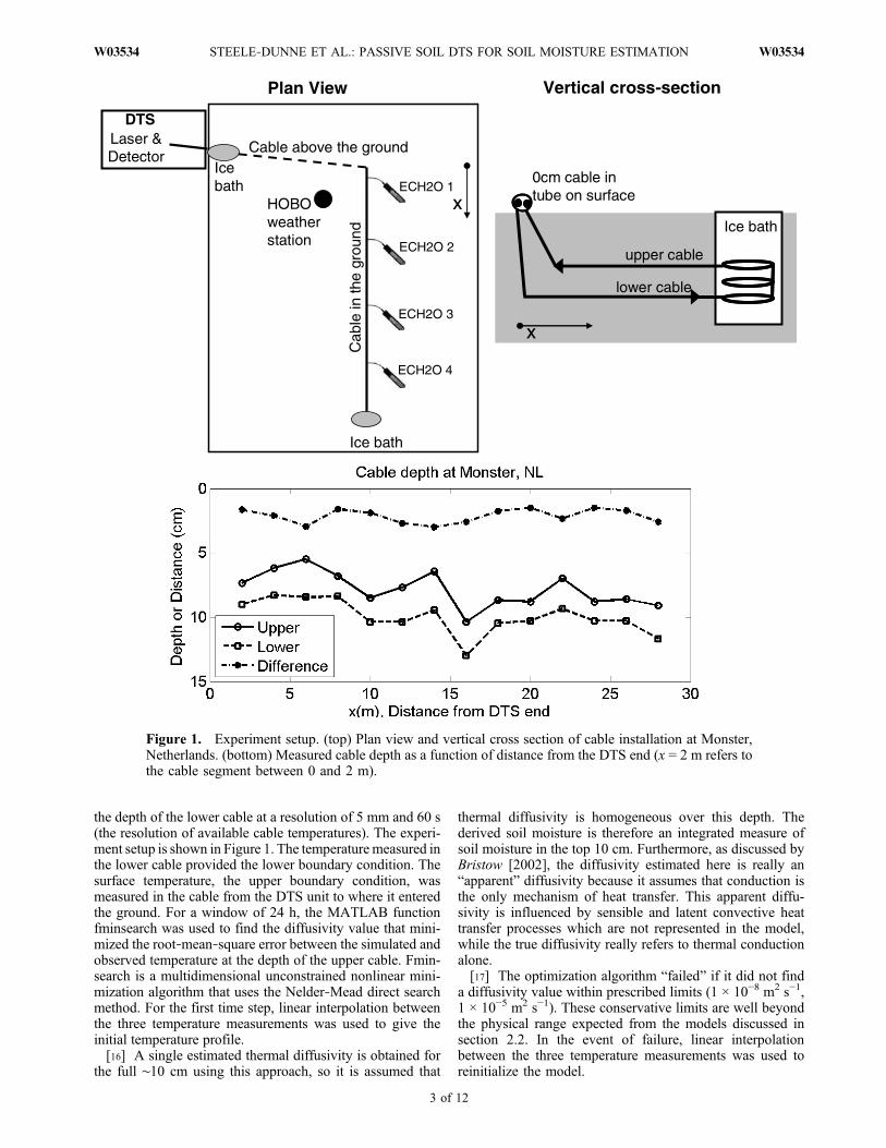
the depth of the lower cable at a resolution of 5 mm and 60 s(the resolution of available cable temperatures). The experi-ment setup is shown in Figure 1. The temperature measured inthe lower cable provided the lower boundary condition. Thesurface temperature, the upper boundary condition, wasmeasured in the cable from the DTS unit to where it enteredthe ground. For a window of 24 h, the MATLAB functionfminsearch was used to find the diffusivity value that mini-mized the root‐mean‐square error between the simulated andobserved temperature at the depth of the upper cable. Fmin-search is a multidimensional unconstrained nonlinear mini-mization algorithm that uses the Nelder‐Mead direct searchmethod. For the first time step, linear interpolation betweenthe three temperature measurements was used to give theinitial temperature profile.[16] A single estimated thermal diffusivity is obtained for

the full ∼10 cm using this approach, so it is assumed that

thermal diffusivity is homogeneous over this depth. Thederived soil moisture is therefore an integrated measure ofsoil moisture in the top 10 cm. Furthermore, as discussed byBristow [2002], the diffusivity estimated here is really an“apparent” diffusivity because it assumes that conduction isthe only mechanism of heat transfer. This apparent diffu-sivity is influenced by sensible and latent convective heattransfer processes which are not represented in the model,while the true diffusivity really refers to thermal conductionalone.[17] The optimization algorithm “failed” if it did not find

a diffusivity value within prescribed limits (1 × 10−8 m2 s−1,1 × 10−5 m2 s−1). These conservative limits are well beyondthe physical range expected from the models discussed insection 2.2. In the event of failure, linear interpolationbetween the three temperature measurements was used toreinitialize the model.

Figure 1. Experiment setup. (top) Plan view and vertical cross section of cable installation at Monster,Netherlands. (bottom) Measured cable depth as a function of distance from the DTS end (x = 2 m refers tothe cable segment between 0 and 2 m).

STEELE‐DUNNE ET AL.: PASSIVE SOIL DTS FOR SOIL MOISTURE ESTIMATION W03534W03534

3 of 12

[18] A “moving window” was used to resolve changes insoil moisture at finer than daily resolution; the 24 h optimi-zation window was shifted in 3‐hourly increments. Insection 4, the diffusivity at each 3‐hourly time step is thatwhich gives the best fit in the subsequent 24 h period. Theinitial condition was given by the best estimate for that timestep from the previous window’s estimation result. Becauseof sensitivity of the solution to depth and the known variabledepth of the cables (Figure 1), each 2 m segment of cablewas modeled separately.

2.2. Soil Moisture From Soil Thermal Properties

[19] The volumetric heat capacity of soil (J m−3 K−1) is asimple, well‐understood linear function of soil moisture:

C ¼ �mcm ¼ Va

Vt�aca þ Vw

Vt�wcw þ Vs

Vt�scs

C ¼ n 1� Srð Þ�aca þ Srn�wcw þ 1� nð Þ�scs;ð2Þ

where the subscripts m, a, t, w, and s denote the bulk soil,air, total, water, and soil solids, respectively; r is the densityin kg m−3; V represents volume; c is the specific heatcapacity; Sr is the relative saturation; and n is the porosity.[20] Thermal conductivity is considerably more compli-

cated. In dry soil, thermal conductivity is dominated by thecontribution of the air fraction, so there is little variability indry thermal conductivity among different soils. As the soilbecomes wetter, a thickening water film increases connec-tivity between soil particles, causing a sharp increase inthermal conductivity. As the soil approaches saturation, thethermal properties of the solids fraction dominate and becausethe particles are already well connected, the rate at whichthermal conductivity increases is reduced.[21] Of the many models available, those of Johansen

[1975] and Campbell [1985] are used here to illustrate thechallenges of obtaining soil moisture given the thermaldiffusivity or conductivity. Johansen [1975] calculates thethermal conductivity as a linear combination of the dry andsaturated thermal conductivities using a Kersten coefficient[Kersten, 1949] which depends on relative saturation andwhether the soil is considered coarse or fine. Calculation ofthe dry and saturated conductivities requires the bulk den-sity, porosity, and quartz content of the soil. Campbell[1985] uses an empirical equation derived from the labora-

tory‐based thermal conductivity measurements of McInnes[1981]. Thermal conductivity is expressed as a function ofvolumetric soil moisture and five coefficients that dependon the volume fractions of soil solids, quartz, and otherminerals as well as the bulk density and the clay massfraction of the soil.[22] Figure 2 presents the thermal conductivity and ther-

mal diffusivity calculated using the Johansen [1975] andCampbell [1985] models for a loamy sand. Because of thehigh thermal conductivity of quartz (7.7 W m−1 K−1) com-pared to that of other minerals (2.0–3.0 W m−1 K−1), bothmodels are sensitive to the quartz fraction. Figure 2 showsthe calculated thermal properties for quartz fractions of 80%and 90%, highlighting the need to determine the quartzcontent accurately. Thermal diffusivity from the Johansenand Campbell models is a monotonic function of relativesaturation up to D = 8.7579 × 10−7 m2 s−1 and D = 9.4809 ×10−7 m2 s−1, respectively. Without additional information, itis impossible to infer a unique relative saturation from athermal diffusivity value above these threshold values. It isclear from Figure 2 that the choice of thermal conductivitymodel will influence the final soil moisture from the esti-mated thermal diffusivity.

3. Experiment Design

[23] This feasibility study was conducted from June toOctober 2008 on the grounds of the drinking water pumpingstation in Monster (52°07′N, 4°17′E), Netherlands. Thissecure site ensured minimal disturbance to the equipment.The site had a calcaire Regosol [European CommissionJoint Research Centre, 2005], with a loamy sand textureand sparse grass cover. The results presented in this paperare based on DTS data collected from 11 September to9 October 2008, during which contemporaneous validationand meteorological data were available.[24] A Halo‐DTS system from Sensornet was used in this

experiment. This system is suitable for use with cables up to4 km long, can detect temperature changes of 0.1 K at ameasurement integration time of 10 s, and has a spatialresolution of 2 m. Here measurements were taken with anintegration time of 60 s, improving the accuracy further.Armored two‐fiber multimode 50/125 mm optic cable fromKaiphone Technology was laid in a loop, as shown inFigure 1, to observe temperatures at two depths. The dis-

Figure 2. Thermal (left) conductivity and (right) diffusivity as functions of relative saturation calculatedusing the models of Johansen [1975] and Campbell [1985] assuming two different values for quartzcontent Q.

STEELE‐DUNNE ET AL.: PASSIVE SOIL DTS FOR SOIL MOISTURE ESTIMATION W03534W03534

4 of 12

turbance due to the plowing of the cable was negligiblebecause of the unstructured and loosely packed loamy sandat the site. Prior to the removal of the cable at the end of theexperiment, trenches were dug along the length of the cable,and the cable depths were measured using a laser level.Figure 1 shows that the depth of cable installation increasedwith distance from the DTS unit. The mean depths of theupper and lower cables were 7.85 and 9.98 cm, with stan-dard deviations of 1.35 and 1.31 cm and ranges of 4.9 and4.7 cm, respectively. The mean distance between the upperand lower cables was 2.13 cm, with a standard deviation of0.55 cm. It is important to note that the surface temperatureobservations were not colocated with those at depth. Thesurface temperatures used here were measured in the PVCtube containing the cable, between the DTS unit and thelocation where the cable enters the ground. In this study,because the study area is small and has uniform soil, cover,and meteorological conditions, it is reasonable to assumethat surface temperature is almost uniform in space.[25] A HOBO® weather station (Onset Computer Corpora-

tion, http://www.onsetcomp.com/products/weather_stations)measured pressure, air temperature, relative humidity, down-ward shortwave radiation, precipitation, wind direction, andwind speed. These data were combined with the surface cabletemperature to calculate net radiation. Downward longwaveradiation (LWdown) from the atmosphere was calculated usingequations (3) and (4) [Bras, 1990]:

LWdown ¼ �EaT4a ; ð3Þ

where s is the Stefan‐Boltzmann constant and Ta is the airtemperature inKelvin.Ea is the atmospheric emissivity given by

Ea ¼ 0:74þ 0:0049e; ð4Þ

where e is the vapor pressure in millibars. Upward longwaveradiation (LWup) from the surface was given by

LWup ¼ �EsT4s ; ð5Þ

where Es is the surface emissivity, assumed to be 0.84 [Arya,2001, Table 3.1], and Ts is the surface temperature in Kelvin.An albedo of 0.18 was assumed to calculate the upwardshortwave radiation [Bras, 1990, Table 2.5]. Hourly relativesaturation of the soil was measured using four ECH2O

® probes,distributed evenly (every ∼9 m) along the length of the cable asillustrated in Figure 1.

4. Results

4.1. Meteorological Observations

[26] Meteorological data are not required in any of thecalculations discussed here. However, precipitation and netradiation data are shown in Figure 3 to identify when changesin soil moisture are expected to be seen.[27] A total of 71 mm of precipitation was recorded during

this period, most of which occurred between 30 Septemberand 6 October following a fortnight of dry weather. Thehighest daily amounts (14.0 and 15.5 mm, respectively)occurred on these two dates.[28] Net radiation was considerably reduced on 13, 24,

and 25 September as well as 1 and 6 October 2008. Insection 4.4, it will be shown that this poses a challenge toretrieving soil moisture using the technique discussed here.

4.2. Relative Saturation Observed With ECH2O Probes

[29] Relative saturation was measured using four ECH2OEC‐10 probes from Decagon Devices (user’s manual avail-able at http://www.decagon.com/pdfs/manuals/EC‐20_EC‐

Figure 3. Precipitation and net radiation at Monster, Netherlands, from 11 September to 9 October2008. Precipitation was measured in 5 min intervals (bars, left axis), and the cumulative precipitationis also shown (dotted line, right axis). Net radiation was calculated using measured shortwave radiation,temperature, and relative humidity, as discussed in section 2.

STEELE‐DUNNE ET AL.: PASSIVE SOIL DTS FOR SOIL MOISTURE ESTIMATION W03534W03534

5 of 12

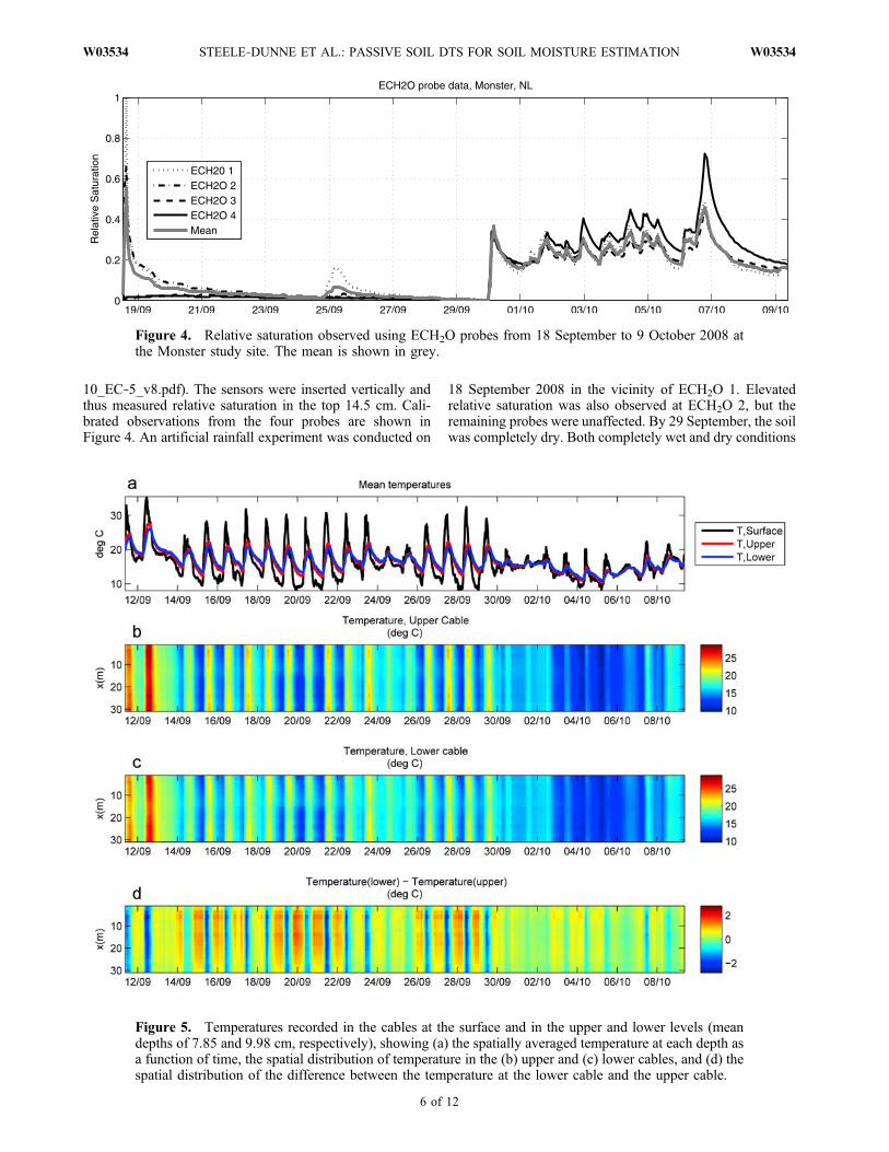
10_EC‐5_v8.pdf). The sensors were inserted vertically andthus measured relative saturation in the top 14.5 cm. Cali-brated observations from the four probes are shown inFigure 4. An artificial rainfall experiment was conducted on

18 September 2008 in the vicinity of ECH2O 1. Elevatedrelative saturation was also observed at ECH2O 2, but theremaining probes were unaffected. By 29 September, the soilwas completely dry. Both completely wet and dry conditions

Figure 4. Relative saturation observed using ECH2O probes from 18 September to 9 October 2008 atthe Monster study site. The mean is shown in grey.

Figure 5. Temperatures recorded in the cables at the surface and in the upper and lower levels (meandepths of 7.85 and 9.98 cm, respectively), showing (a) the spatially averaged temperature at each depth asa function of time, the spatial distribution of temperature in the (b) upper and (c) lower cables, and (d) thespatial distribution of the difference between the temperature at the lower cable and the upper cable.

STEELE‐DUNNE ET AL.: PASSIVE SOIL DTS FOR SOIL MOISTURE ESTIMATION W03534W03534

6 of 12

were observed with ECH2O 1, so it was used to scale the datafrom the other probes by assuming that the precipitation on30 September raised the relative saturation to the same valueat all probes. This assumption is valid because of the smallstudy area and uniform soil and cover. Sharp increases areapparent following the significant events on 30 Septemberand 6 October, while frequent smaller events maintained arelative saturation of about 0.3 between these events.

4.3. Soil Temperatures Observed With DTS

[30] Figure 5 shows the cable temperatures observedusing the DTS system. As required for the successfulapplication of this method, the cable temperatures exhibit aclear diurnal cycle in response to the diurnal variation in netradiation that is damped and attenuated with depth. At agiven time, the range in temperature along both the upperand lower cables varies from 0.1°C to 2.7°C. Maximumvariability occurs at the daily maximum and minimumtemperatures. In general, the range is largest on clear dayswhen downward shortwave radiation and, consequently, netradiation are highest. This spatial variability in temperaturemay be due to variability in soil texture or soil moisture or,more likely, to the variation in cable depth seen in Figure 1.[31] Figure 5 also shows that temperature difference

between the upper and lower cables clearly varies in time andspace. During the night, the lower cable cools more slowlythan the upper cable, while in the late morning to early after-noon the surface is warming and the upper cable heats upmorequickly. Themagnitude of the difference observed between thecables depends on the strength of the diurnal cycle in tem-perature, which is determined by the net radiation (Figure 3).The temperature difference between the cables varies withdepth. Close to the DTS unit, where both cables are closer tothe surface, the difference between them is largest.

4.4. Estimated Thermal Diffusivity

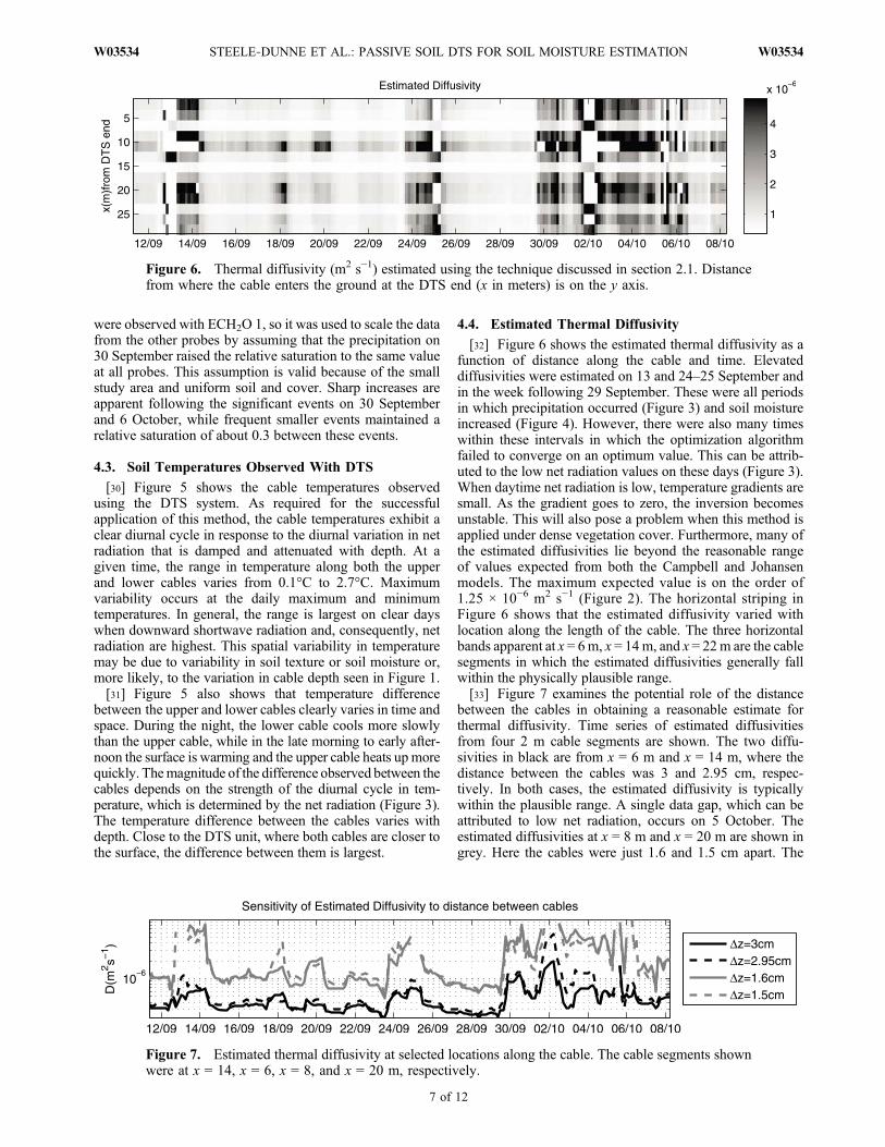
[32] Figure 6 shows the estimated thermal diffusivity as afunction of distance along the cable and time. Elevateddiffusivities were estimated on 13 and 24–25 September andin the week following 29 September. These were all periodsin which precipitation occurred (Figure 3) and soil moistureincreased (Figure 4). However, there were also many timeswithin these intervals in which the optimization algorithmfailed to converge on an optimum value. This can be attrib-uted to the low net radiation values on these days (Figure 3).When daytime net radiation is low, temperature gradients aresmall. As the gradient goes to zero, the inversion becomesunstable. This will also pose a problem when this method isapplied under dense vegetation cover. Furthermore, many ofthe estimated diffusivities lie beyond the reasonable rangeof values expected from both the Campbell and Johansenmodels. The maximum expected value is on the order of1.25 × 10−6 m2 s−1 (Figure 2). The horizontal striping inFigure 6 shows that the estimated diffusivity varied withlocation along the length of the cable. The three horizontalbands apparent at x = 6m, x = 14m, and x = 22m are the cablesegments in which the estimated diffusivities generally fallwithin the physically plausible range.[33] Figure 7 examines the potential role of the distance

between the cables in obtaining a reasonable estimate forthermal diffusivity. Time series of estimated diffusivitiesfrom four 2 m cable segments are shown. The two diffu-sivities in black are from x = 6 m and x = 14 m, where thedistance between the cables was 3 and 2.95 cm, respec-tively. In both cases, the estimated diffusivity is typicallywithin the plausible range. A single data gap, which can beattributed to low net radiation, occurs on 5 October. Theestimated diffusivities at x = 8 m and x = 20 m are shown ingrey. Here the cables were just 1.6 and 1.5 cm apart. The

Figure 6. Thermal diffusivity (m2 s−1) estimated using the technique discussed in section 2.1. Distancefrom where the cable enters the ground at the DTS end (x in meters) is on the y axis.

Figure 7. Estimated thermal diffusivity at selected locations along the cable. The cable segments shownwere at x = 14, x = 6, x = 8, and x = 20 m, respectively.

STEELE‐DUNNE ET AL.: PASSIVE SOIL DTS FOR SOIL MOISTURE ESTIMATION W03534W03534

7 of 12

same temporal pattern is apparent, with increased diffusivityestimated in periods of elevated soil moisture. However,the estimated diffusivities are almost always higher than thereasonable range. There are also more cases when theoptimization algorithm failed to converge on a solution. Thissuggests that the cables must be some minimum distanceapart to reliably estimate the thermal diffusivity. To inves-tigate this further, the diffusion model was used to simulatethe response at depth to a sinusoidal surface temperaturepattern.4.4.1. Hypothetical Cable Depth for OptimumPerformance of Inversion Approach[34] The analysis is in terms of amplitude, which varies

only with depth, rather than temperature, which varies withboth time and depth. For a sinusoidal surface temperaturewith amplitude As and period P, the amplitude at some soildepth z is given by

A zð Þ ¼ As exp �z

ffiffiffiffiffiffiffi�

PD

r� �; ð6Þ

where D is the thermal diffusivity of the soil [e.g., Arya,2001]. To determine soil moisture from the surface todepth z�, cables are placed at the surface (z = 0 cm) and atthe lower boundary (z = z�). The inversion method requiresa third cable somewhere between these two. Figure 8ashows the temperature amplitude difference between ahypothetical cable at depth z and one both at the surface(dashed line) and at 10 cm depth (solid line). The optimumdepth for this hypothetical cable, zopt, is where these ampli-tude differences are equal. This occurs where the amplitudeis the mean of the amplitudes in the surface and lowercables:

A zopt� � ¼ As þ A z�ð Þ

2: ð7Þ

Substituting the values for the amplitude at z� and zopt andrearranging yields the following expression for the opti-mum cable depth:

zopt ¼ �ffiffiffiffiffiffiffiPD

�

rlog

1

2exp �z�

ffiffiffiffiffiffiffi�

PD

r� �þ 1

� � : ð8Þ

This optimum depth is at the intersection of the two curvesin Figure 8a. Note that the optimum depth depends only onthe soil thermal diffusivity and the depth z�. The differencein amplitude between either boundary and zopt, on the otherhand, is proportional to the surface amplitude:

�A zopt� � ¼ As � A zopt

� � ¼ As

21� exp �z�

ffiffiffiffiffiffiffi�

PD

r� �� �: ð9Þ

Higher values ofDA imply that changes in temperature andtherefore diffusivity are more readily detectible. Its depen-dence on As explains why reduced net radiation (whichreduces As) limits our ability to estimate diffusivity and soilmoisture from temperature observations. From Figures 8band 8c, using the lowest value of diffusivity for a givensoil yields the most conservative estimate of zopt, i.e., closestto the surface with the highest value of DA. The thermaldiffusivity of dry soil should therefore be used to determinethe optimum cable depth. Recall from section 2.2 that thereis little variability in this quantity among soil types, so theoptimum depth will vary little by soil type.[35] Assuming D = 2 × 10−7 m2 s−1, Figure 8a shows that

the optimal cable depth to measure soil moisture from 0 to0.10 m is 0.034 m and thatDA at this depth is 5.6 K for As =15 K. Placing the cable at 0.07 or 0.085 m reduces thecorresponding values of DA to just 1.9 or 0.9 K, respec-tively. This explains why the diffusivity estimate appears toimprove with increasing distance between the lower cablesin Figure 7. Placing the cable closer to the optimal depth

Figure 8. Calculating the optimum cable depth to estimate soil moisture between the surface and depthz� (in meters). For As = 15 K and D = 2.5 × 10−7 m2 s−1, (a) the difference in amplitude between a cable atdepth z and the cables at the surface and lower boundary where z� = 0.1 m is shown. (b) The optimumcable depth (zopt) and (c) the difference in amplitude between a cable at zopt and the boundaries are alsoshown.

STEELE‐DUNNE ET AL.: PASSIVE SOIL DTS FOR SOIL MOISTURE ESTIMATION W03534W03534

8 of 12

leads to more reliable estimates of diffusivity and hence soilmoisture.4.4.2. Impact of Uncertainty in Cable Depth[36] A Monte Carlo experiment, with 100 ensemble

members, was conducted to demonstrate the impact thatuncertainty in the cable depth has on the estimated diffu-sivity. The Johansen model (assuming 90% quartz content)was used to generate a time series of thermal diffusivityvalues from the relative saturation values plotted in Figure 4.Assuming these values for diffusivity in the heat diffusionmodel (equation (1)) and forcing the surface boundary withthe temperature data from the surface cable, a time series oftemperature at 4 cm depth was simulated. This depth waschosen as it is close to the optimal hypothetical depth fromsection 4.4.1. The inversion approach was used to estimatethe diffusivity, but assuming that the depths of the upper andlower cables were uncertain, each with an error standarddeviation of 0.5 cm.[37] Figure 9 shows the mean diffusivity estimated for

each pair of uncertain cable depths. The mean value of thetrue diffusivity was 5.1 × 10−7 m2 s−1. The impact of

uncertainty in the depth of the upper cable is much moresignificant than in the lower cable because the temperaturefluctuations at depth are smaller, so there is less differencebetween model layers. An error with a standard deviation of0.5 cm in a cable at 4 cm depth leads to diffusivity estimatesspanning the full dynamic range. If the upper cable depth isassumed to be shallower than the true depth, the diffusivityis underestimated.[38] Figure 10 shows the time series of estimated diffu-

sivity for each assumed cable depth pair, with the true dif-fusivity shown in black. The apparent grouping of diffusivityestimates is due to the discretization of the diffusion model(dz = 0.005m). Figure 10 shows that the impact of uncertaintyin cable depth is most significant at high values of diffusivity.At very high values of diffusivity, assuming the incorrectcable depth can lead to physically implausible (high) valuesof thermal diffusivity. This underscores the importance ofcorrectly determining the cable depths. The overestimationof thermal diffusivity in Figure 7 could be because the cabledepth was overestimated.

4.5. Estimated Soil Moisture

[39] Figure 11 shows the soil moisture inferred from theestimated diffusivities for two 2 m segments, those at 6 and14 m from the DTS unit. These segments are shown inFigure 7 to give the most reasonable estimated diffusivityvalues.[40] For most of the experiment up to 29 September the

estimated diffusivity was very low. Consequently, both theJohansen and Campbell models yield unique and compara-ble estimates for relative saturation. While Figure 4 suggeststhat the soil was completely dry by 29 September, it isimportant to note that both thermal conductivity models areonly defined above relative saturation of 0.1. In dry soils, asmall change in relative saturation leads to a large increasein thermal diffusivities, so, despite the variability in Figure 7during this dry period, the estimated relative saturation isnearly constant.[41] Figure 7 shows that elevated diffusivities were

detected for these segments during the week of 29 Septemberto 6 October, consistent with the increased soil moistureshown in Figure 4. However, these diffusivities were higherthan the maximum expected from both the Johansen andCampbell models for this loamy sand. Consequently, thereare many gaps in estimated soil moisture during this wetperiod. There are three possible causes of this problem:

Figure 9. The impact of uncertainty in the cable depths onthe temporal mean of the estimated diffusivity. The color ofeach dot indicates the value of the estimated diffusivity. Thetrue value refers to the diffusivity value calculated from theobserved relative saturation and was used to simulate thetemperatures at 4 and 10 cm.

Figure 10. Sensitivity of diffusivity estimate to uncertainty in the cable depth. Each grey line is the dif-fusivity estimate from an assumed pair of cable depths. The true (simulated) diffusivity is superimposed inblack.

STEELE‐DUNNE ET AL.: PASSIVE SOIL DTS FOR SOIL MOISTURE ESTIMATION W03534W03534

9 of 12

(1) neither the Johansen nor the Campbell model correctlydescribes the relationship between relative saturation andthermal diffusivity for this soil; (2) the distance betweenthe cables is still too small (section 4.4.1) and/or the cabledepth is incorrect (section 4.4.2); and (3) the diffusionmodel was invalid during this period because of heat advec-tion as water infiltrated the unsaturated zone.[42] Another interesting feature of Figure 11 is attribut-

able to the nature of the relationship between thermal con-ductivity and relative saturation, that above some value theincrease in thermal conductivity with relative saturationslows down. Above this critical value, it is impossible toinfer a unique relative saturation value for a given thermalconductivity or diffusivity. For each model, both possiblesolutions are shown in Figure 11. The threshold in theCampbell model is higher than the maximum value from theJohansen model, so in some cases (e.g., for x = 6 m on25 September), the Campbell model will give two possiblevalues (one greater than and one less than the maximum),while the Johansen model gives none. If the diffusivity isbetween the threshold value from Johansen and that fromCampbell, the Campbell model gives a unique estimate forthe relative saturation, while the Johansen model yields twopossible values (e.g., after initial increase on 29 September,for x = 14 m). Clearly, the inability to distinguish betweenrelative saturation of ∼0.2 and ∼1.0 is unacceptable. Thisindicates that some prior knowledge of soil moisture wouldadd value to this estimate. In section 5, details on how toaddress this serious shortcoming will be presented.

5. Conclusions and Discussion

[43] A feasibility study was conducted to investigate thepossibility of using passive soil DTS to observe soil moisture.Cables were installed at two depths to monitor temperature

changes in response to net radiation. The hypothesis was thatthe cable temperatures could be used to estimate soil thermalproperties from which soil moisture could be inferred.[44] Béhaegel et al. [2007] estimated 15 day soil moisture

in the thermally active layer by simulating heat diffusionand finding the thermal diffusivity which gave the bestagreement with observed temperature at 60 cm. Here asimilar inversion approach was used to estimate soil mois-ture in the top 10 cm of soil, where the boundary conditionsand temperature to be matched were all measured usingpassive soil DTS. Soil moisture was estimated in 24 hmovingwindows shifted in 3‐hourly increments. While it was shownthat changes in soil moisture resulted in detectable changes inthermal diffusivity, the shorter estimation or optimizationwindow posed several problems.[45] 1. In a longer time window, it seems a more rea-

sonable assumption that diffusion is the dominant heattransfer process because the duration of a precipitation eventis a smaller fraction of the study interval.[46] 2. The temperatures vary primarily in response to the

diurnal variability in net radiation. If net radiation is low fora given day, there is very little temperature response tomeasure. In a 15 day estimation window (e.g., as used byBéhaegel et al. [2007]) this is less problematic unless netradiation is low for the entire 15 day window.[47] 3. A longer study interval implies an effective dif-

fusivity for a longer period, so the results are effectivelyaveraged. This reduces the likelihood of obtaining extremevalues beyond the physically reasonable range.[48] The usefulness of inverse methods is further limited

by the nature of the relationship between thermal diffusivityand relative saturation. At low relative saturation, a minutechange in relative saturation leads to a dramatic increase indiffusivity, while diffusivity is largely insensitive to changesat higher relative saturation. Furthermore, it is impossible to

Figure 11. Inferred relative saturation from the estimated thermal diffusivities at (top) x = 6 m and(bottom) x = 14 m using the Campbell [1985] and Johansen [1975] models. Above a diffusivitythreshold in each of the models, relative saturation is a nonunique function of thermal diffusivity. “Low”and “high” assume the relative saturation value less than and greater than that associated with themaximum thermal diffusivity.

STEELE‐DUNNE ET AL.: PASSIVE SOIL DTS FOR SOIL MOISTURE ESTIMATION W03534W03534

10 of 12

infer a single relative saturation from a diffusivity value forat least half of the dynamic range.[49] While this study demonstrated that passive soil DTS

could indeed detect changes in soil moisture, it also high-lighted several reasons why data assimilation might be amore appropriate method of estimating soil moisture thanconventional inverse methods. In a data assimilationapproach, the cable temperatures can be used to constrain acoupled heat‐moisture transport model. Future research willfocus on a dual state‐parameter estimation approach [e.g.,Moradkhani et al., 2005], in which temperature will beestimated as a state and soil moisture will be estimated as aparameter of the model. Thermal properties are calculatedfrom soil moisture in forward simulations, avoiding thenonuniqueness problem in the other direction. The modelcan be adapted to include advection, evaporation, or anyadditional processes considered significant. Accountingfor these processes ensures that the true, rather than the“apparent,” thermal diffusivity is estimated. Soil tempera-ture and moisture content can be estimated at all depths inthe desired profile at the resolution of the coupled model,yielding a profile of surface and root zone soil moisturerather than a single integrated measure between the cables.[50] Even using data assimilation techniques, many of the

technical challenges remain. Several lessons from this studywill be used to address these more practical issues. First, thecable depths must be well known and the cables must besufficiently far apart for there to be a measurable differencein temperature. The plow design and installation methodwill be revised to ensure that cables are installed a fixed andknown distance apart. The cable depth can be determined byamplitude analysis for a given soil moisture if the relation-ship between thermal diffusivity and soil moisture is knownusing probe measurements [e.g., Mori et al., 2003]. Amethod was presented to calculate the optimum cable depthto measure soil moisture over a prescribed depth. To mea-sure soil moisture from 0 to 10 cm, for example, cables arerequired at 0, 10, and 3.4 cm. In this experiment in a finesand Regosol with weak to absent soil structure, there waslittle disturbance due to the plowing of the cable. However,if cables are plowed into soils containing fine sediments orclay, a recovery period would be required before the firstuseful observations to ensure that the measurements could beconsidered representative of the surrounding undisturbed soil.[51] In this experiment, a single series of surface tem-

perature was available. Because the experiment was con-ducted in a very small area with uniform soil, cover, andmeteorological conditions, it is reasonable to assume thatsurface temperature is homogeneous. However, to accountfor spatial variability, future larger‐scale experiments willhave a colocated cable to measure surface temperature.[52] Finally, the relationship between thermal conductiv-

ity and soil moisture is critical. This must be ascertainedthrough in situ measurements over the full dynamic range ofsaturation values. This is the key link between soil moistureand soil temperature, and its significance cannot be under-estimated if passive soil DTS is to be developed into aviable approach to measure large‐scale variability in soilmoisture.

[53] Acknowledgments. Partial support for M.H. and S.W.T. wasprovided from U.S. Bureau of Reclamation agreement 06FC204044. The

authors are grateful to three anonymous reviewers, the Associate Editor,and the Editor, whose comments and suggestions improved the quality ofthe manuscript.

ReferencesAnthes, R., et al. (2007), Earth Science and Applications from Space:

National Imperative for the Next Decade and Beyond, Natl. Acad. Press,Washington, D. C.

Arya, S. P. (2001), Introduction to Micrometeorology, Int. Geophys. Ser.,vol. 79, 2nd ed., 420 pp., Academic, San Diego, Calif.

Béhaegel, M., P. Sailhac, and G. Marquis (2007), On the use of surface andground temperature data to recover soil water content information,J. Appl. Geophys., 62(3), 234–243, doi:10.1016/j.jappgeo.2006.11.005.

Bras, R. L. (1990), Hydrology: An Introduction to Hydrologic Science,Addison‐Wesley, Reading, Mass.

Bristow, K. L. (2002), Soil heat, in Methods of Soil Analysis. Part 4, Phys-ical Methods, edited by J. H. Dane and G. C. Topp, pp. 1183–1248, SoilSci. Soc. of Am., Madison, Wis.

Campbell, G. S. (1985), Soil Physics with BASIC: Transport Models forSoil‐Plant Systems, 3rd ed., 150 pp., Elsevier, New York.

Campbell, G. S., C. Calissendorff, and J. H. Williams (1991), Probe formeasuring soil specific heat using a heat‐pulse method, Soil Sci. Soc.Am. J., 55, 291–293.

Cosh, M. H., T. J. Jackson, R. Bindlish, and J. H. Preuger (2004), Water-shed scale temporal and spatial variability of soil moisture and its role invalidating soil moisture estimates, Remote Sens. Environ., 92, 427–435,doi:10.1016/j.rse.2004.02.016.

Entekhabi, D., I. Rodriguez‐Iturbe, and F. Castelli (1996), Mutual interac-tion of soil moisture state and atmospheric processes, J. Hydrol., 184,3–17, doi:10.1016/0022-1694(95)02965-6.

European Commission Joint Research Centre (2005), Soil Atlas of Europe,128 pp., Eur. Communities, Luxembourg.

Gurney, R. J., and P. J. Camillo (1984), Modelling daily evapotranspirationusing remotely sensed data, J. Hydrol., 69, 305–324, doi:10.1016/0022-1694(84)90170-7.

Idso, S. B., T. J. Schmugge, R. D. Jackson, and R. J. Reginato (1975a), Theutility of surface temperature measurements for the remote sensing ofsurface soil water status, J. Geophys. Res. , 80 , 3044–3049,doi:10.1029/JC080i021p03044.

Idso, S. B., R. D. Jackson, and R. J. Reginato (1975b), Detection of soilmoisture by remote surveillance, Am. Sci., 63, 549–557.

Idso, S. B., R. D. Jackson, and R. J. Reginato (1976), Compensating forenvironmental variability in the thermal inertia approach to remote sens-ing of soil moisture, J. Appl. Meteorol., 15, 811–817, doi:10.1175/1520-0450(1976)015<0811:CFEVIT>2.0.CO;2.

Jacobs, J. M., B. P. Mohanty, E.‐C. Hsu, and D. Miller (2004), SMEX02:Field scale variability, time stability and similarity of soil moisture,Remote Sens. Environ., 92, 436–446, doi:10.1016/j.rse.2004.02.017.

Johansen, O. (1975), Thermal conductivity of soils, Ph.D. thesis, 236 pp.,Univ. of Trondheim, Trondheim, Norway.

Kamai, T., A. Tuli, G. J. Kluitenberg, and J. W. Hopmans (2008), Soilwater flux density measurements near 1 cm d−1 using an improved heatpulse probe design, Water Resour. Res., 44, W00D14, doi:10.1029/2008WR007036.

Kerr, Y. H., P. Waldteufel, J.‐P. Wigneron, J. Martinuzzi, J. Font, andM. Berger (2001), Soil moisture retrieval from space: The Soil Mois-ture and Ocean Salinity (SMOS) mission, IEEE Trans. Geosci. RemoteSens., 39(8), 1729–1735, doi:10.1109/36.942551.

Kersten, M. S. (1949), Thermal Properties of Soils, Minn. Univ. Eng. Exp.Stn. Bull., 52, 227 pp.

Kluitenberg, G. J., K. L. Bristow, and B. S. Das (1995), Error analysis ofheat pulse method for measuring soil heat capacity, diffusivity, and con-ductivity, Soil Sci. Soc. Am. J., 59, 719–726.

Liu, G., B. Li, T. Ren, R. Horton, and B. C. Si (2008), Analytical solutionof heat pulse method in a parallelepiped sample space with inclined nee-dles, Soil Sci. Soc. Am. J., 72, 1208–1216, doi:10.2136/sssaj2007.0260.

McInnes, K. J. (1981), Thermal conductivities of soils from dryland wheatregions of eastern Washington, M.S. thesis, 51 pp., Wash. State Univ.,Pullman.

Mohanty, B. P., and T. H. Skaggs (2001), Spatio‐temporal evolution andtime‐stable characteristics of soil moisture within remote sensing foot-prints with varying soil, slope, and vegetation, Adv. Water Resour., 24,1051–1067, doi:10.1016/S0309-1708(01)00034-3.

Moradkhani, H., S. Sorooshian, H. V. Gupta, and P. R. Houser (2005),Dual state‐parameter estimation of hydrological models using ensem-

STEELE‐DUNNE ET AL.: PASSIVE SOIL DTS FOR SOIL MOISTURE ESTIMATION W03534W03534

11 of 12

ble Kalman filter, Adv. Water Resour., 28, 135–147, doi:10.1016/j.advwatres.2004.09.002.

Mori, Y., J. W. Hopmans, A. P. Mortensen, and G. J. Kluitenberg (2003),Multi‐functional heat pulse probe for the simultaneous measurement ofsoil water content, solute concentration, and heat transport parameters,Vadose Zone J., 2, 561–571, doi:10.2113/2.4.561.

Mortensen, A. P., J. W. Hopmans, Y. Mori, and J. Šimůnek (2006), Multi‐functional heat pulse probe measurements of coupled vadose zoneflow and transport, Adv. Water Resour., 29, 250–267, doi:10.1016/j.advwatres.2005.03.017.

Price, J. C. (1977), Thermal inertia mapping: A new view of the Earth,J. Geophys. Res., 82, 2582–2590, doi:10.1029/JC082i018p02582.

Rosema, A. (1975), Simulation of the thermal behavior of bare soils forremote sensing purposes, in Heat and Mass Transfer in the Biosphere,Adv. Thermal Eng., vol. 3, edited by D. A. deVries and N. H. Afgan,pp. 109–123, Scripta, Washington, D. C.

Selker, J. S., L. Thevenaz, H. Huwald, A. Mallet, W. Luxemburg, N. vande Giesen, M. Stejskal, J. Zeman, M. Westhoff, and M. B. Parlange(2006), Distributed fiber‐optic temperature sensing for hydrologic sys-tems, Water Resour. Res., 42, W12202, doi:10.1029/2006WR005326.

Tyler, S. W., J. S. Selker, M. B. Hausner, C. E. Hatch, T. Torgersen, C. E.Thodal, and S. G. Schladow (2009), Environmental temperature sensingusing Raman spectra DTS fiber‐optic methods, Water Resour. Res., 45,W00D23, doi:10.1029/2008WR007052.

Vachaud, G., A. P. De Silans, P. Balabanis, and M. Vauclin (1985), Tem-poral stability of spatially measured soil water probability density func-tion, Soil Sci. Soc. Am. J., 49, 822–828.

Van De Griend, A. A., P. J. Camillo, and R. J. Gurney (1985), Discrimina-tion of soil physical parameters, thermal inertia, and soil moisture fromdiurnal surface temperature fluctuations,Water Resour. Res., 21(7), 997–1009, doi:10.1029/WR021i007p00997.

T. A. Bogaard, D. M. Krzeminska, M. M. Rutten, S. C. Steele‐Dunne,and N. C. van de Giesen, Water Resources Section, Faculty of CivilEngineering and Geosciences, Delft University of Technology, PO Box5048, NL‐2600 GA Delft, Netherlands. (s.c.steele‐dunne@tudelft.nl)M. Hausner and S. W. Tyler, Department of Geological Sciences and

Engineering, University of Nevada, Reno, Reno, NV 89557, USA.J. Selker, Department of Biological and Ecological Engineering, Oregon

State University, Corvallis, OR 97331, USA.

STEELE‐DUNNE ET AL.: PASSIVE SOIL DTS FOR SOIL MOISTURE ESTIMATION W03534W03534

12 of 12