This article appeared in a journal published by Elsevier. The attachedcopy is furnished to the author for internal non-commercial researchand education use, including for instruction at the authors institution

and sharing with colleagues.

Other uses, including reproduction and distribution, or selling orlicensing copies, or posting to personal, institutional or third party

websites are prohibited.

In most cases authors are permitted to post their version of thearticle (e.g. in Word or Tex form) to their personal website orinstitutional repository. Authors requiring further information

regarding Elsevier’s archiving and manuscript policies areencouraged to visit:

http://www.elsevier.com/copyright

Author's personal copy

Landscape and Urban Planning 102 (2011) 54–63

Contents lists available at ScienceDirect

Landscape and Urban Planning

journa l homepage: www.e lsev ier .com/ locate / landurbplan

Does spatial configuration matter? Understanding the effects of land coverpattern on land surface temperature in urban landscapes

Weiqi Zhoua,∗, Ganlin Huangb, Mary L. Cadenassoa

a Department of Plant Sciences, University of California, Davis, Mail Stop 1, 1210 PES, One Shields Ave, Davis, CA 95616, USAb Center for Regional Change, University of California, Davis, 152 Hunt Hall, One Shields Ave, Davis, CA 95616, USA

a r t i c l e i n f o

Article history:Received 15 November 2010Received in revised form 2 March 2011Accepted 12 March 2011Available online 17 April 2011

Keywords:Urban heat islandLand surface temperatureLand coverLandscape composition and configurationSpatial heterogeneityUrban landscape

a b s t r a c t

The effects of land cover composition on land surface temperature (LST) have been extensively doc-umented. Few studies, however, have examined the effects of land cover configuration. This paperinvestigates the effects of both the composition and configuration of land cover features on LST in Bal-timore, MD, USA, using correlation analyses and multiple linear regressions. Landsat ETM + image datawere used to estimate LST. The composition and configuration of land cover features were measured bya series of landscape metrics, which were calculated based on a high-resolution land cover map withan overall accuracy of 92.3%. We found that the composition of land cover features is more importantin determining LST than their configuration. The land cover feature that most significantly affects themagnitude of LST is the percent cover of buildings. In contrast, percent cover of woody vegetation isthe most important factor mitigating UHI effects. However, the configuration of land cover features alsomatters. Holding composition constant, LST can be significantly increased or decreased by different spa-tial arrangements of land cover features. These results suggest that the impact of urbanization on UHIcan be mitigated not only by balancing the relative amounts of various land cover features, but also byoptimizing their spatial configuration. This research expands our scientific understanding of the effectsof land cover pattern on UHI by explicitly quantifying the effects of configuration. In addition, it mayprovide important insights for urban planners and natural resources managers on mitigating the impactof urban development on UHI.

© 2011 Elsevier B.V. All rights reserved.

1. Introduction

Approximately 50% of the world population lives in urban areas,and this proportion is projected to increase to 60% by 2030 (UnitedNations, 2002). In developed countries like the US, changes in urbanland cover are more rapid than population growth (Alig, Kline, &Lichtenstein, 2004). The population in the US grew approximately24% between 1980 and 2000. During roughly the same time period,however, the amount of urbanized land increased more than 34%(Alig et al., 2004). By 2025, the amount of developed land is pro-jected to increase from 5.2% to 9.2%, or an increase of 79% (Alig et al.,2004). The changes in land use/land cover caused by urbanizationgreatly affect the structure and function of urban ecosystems. A welldocumented consequence of land conversion due to urbanizationis the formation of an urban heat island (UHI) (e.g. Voogt & Oke,2003).

∗ Corresponding author. Tel.: +1 530 754 7230; fax: +1 530 752 4361.E-mail addresses: wqzhou@ucdavis.edu, weiqi.zhou@gmail.com (W. Zhou),

glhuang@ucdavis.edu (G. Huang), mlcadenasso@ucdavis.edu (M.L. Cadenasso).

Urban heat island describes the difference between urban andnon-urban ambient air temperatures, which is directly related toland cover and human energy use (Oke, 1995). These differences aredue to surface modifications brought about by urbanization whichtypically includes replacing soil and vegetation with impervioussurfaces such as concrete and asphalt, and with urban struc-tures such as buildings of various heights and densities (Akbari,Pomerantz, & Taha, 2001; Voogt & Oke, 2003). These modifica-tions change characteristics including albedo, thermal capacity, andheat conductivity over urban areas, which in turn lead to a mod-ified thermal climate that is warmer than surrounding non-urbanareas (Voogt & Oke, 2003). Increased temperatures due to the UHIeffect may increase water consumption and energy use in urbanareas and lead to alterations to biotic communities (White, Nemani,Thornton, & Running, 2002). Excess heat may also affect the com-fort of urban dwellers and lead to greater health risks (Poumadere,Mays, Le Mer, & Blong, 2005). In addition, higher temperatures inurban areas increase the production of ground level ozone whichhas direct consequences for human health (Akbari, Rosenfeld, Taha,& Gartland, 1996; Akbari et al., 2001).

Types of UHI can be loosely categorized into air temperatureUHI and surface UHI (Arnfield, 2003; Nichol, Fung, Lam, & Wong,

0169-2046/$ – see front matter © 2011 Elsevier B.V. All rights reserved.doi:10.1016/j.landurbplan.2011.03.009

Author's personal copy

W. Zhou et al. / Landscape and Urban Planning 102 (2011) 54–63 55

2009). While some studies have reported a close relationship andsimilar spatial patterns between surface and air temperatures (e.g.Ben-Dor & Saaroni, 1997; Nichol, 1994; Nichol et al., 2009), thereis no consistent relationship between these two (Arnfield, 2003).Air temperature UHIs are generally stronger and exhibit greatestspatial variations at night, whereas the greatest difference in sur-face UHIs usually occurs during the daytime (Arnfield, 2003; Frey,Parlow, Vogt, Abdel Wahab, & Harhash, 2010; Nichol et al., 2009). Inthis study, we focus on remotely sensed land surface temperature(LST) and, consequently, surface UHI.

Remotely sensed LST records the radiative energy emitted fromthe ground surface, including building roofs, paved surfaces, veg-etation, bare ground, and water (Arnfield, 2003; Voogt & Oke,2003). Therefore, the pattern of land cover in urban landscapesmay potentially influence LST (Arnfield, 2003; Forman, 1995). Thetwo fundamental aspects of land cover pattern are composition andconfiguration (Gustafson, 1998; Turner, 2005). Composition refersto the abundance and variety of land cover features without con-sidering their spatial character or arrangement (Gustafson, 1998;Leitao, Miller, Ahern, & McGarigal, 2006). Configuration, in contrast,refers to the spatial arrangement or distribution of land cover fea-tures. In addition to influencing LST through direct modificationof surface characteristics, land cover pattern may also influenceLST through its affects on the movements and flows of organ-isms, material, and energy in a landscape (Forman, 1995; Turner,2005).

Previous UHI research has primarily focused on the effects ofland cover composition, especially vegetation abundance, on LST(e.g. Buyantuyev & Wu, 2010; Frey, Rigo, & Parlow, 2007; Weng,Lu, & Schubring, 2004; Weng, 2009). Remotely sensed data hastypically been used to evaluate LST patterns and assess the UHI,especially at vast geographic scales. Using a variety of image data,including NOAA AVHRR (Balling & Brazell, 1988), MODIS (Pu, Gong,Michishita, & Sasagawa, 2006), Landsat TM/ETM+ (Weng et al.,2004), ASTER (Lu & Weng, 2006; Pu et al., 2006) and airborneATLAS (Lo, Quattrochi, & Luvall, 1997), these studies show that sur-face cover characteristics, such as vegetation abundance measuredby NDVI (Normal Difference Vegetation Index), and the relativeamounts of types of land use/land cover, significantly affect LSTin urban areas (e.g. Buyantuyev & Wu, 2010; Liang & Weng, 2008;Weng, 2003; Weng et al., 2004; Xiao et al., 2008).

Rather than just the total amount of vegetation, the effects of thesize and shape of vegetation patches on LST have been the topic ofrecent studies (e.g., Cao, Onishi, Chen, & Imura, 2010; Xu & Yue,2008; Zhang, Zhong, Feng, & Wang, 2009). These studies, however,focused on vegetation patches alone, and only examined the effectsof their size and shape rather than their spatial arrangement in thelandscape. The relationship between landscape pattern and LST hasalso been investigated by examining the variations of a set of land-scape metrics in different LST zones (Liu & Weng, 2009; Weng, Liu,& Lu, 2007), or in different types of land use patches (Weng, Liu,Liang, & Lu, 2008). These studies suggested that variables of land-scape metrics may play an important role in the spatial patterns ofLST. Few studies, however, have explored the quantitative relation-ship between LST and the configuration of different types of landcover features, particularly after adjusting for the effects of landcover composition.

This study investigates the effects of land cover pattern on LSTin the Gwynns Falls watershed, Maryland, USA. The objectives areto: (1) examine the quantitative relationships between LST and thecomposition and configuration of land cover features, and (2) inves-tigate, after adjusting for the effects of composition, whether theconfiguration of land cover features significantly affects LST. Theresults from this study can enhance our understanding of how LSTvaries with changing land cover patterns. In addition, importantinsights can be provided to urban planners and natural resource

managers on how to mitigate the impact of urbanization on UHIthrough urban design and vegetation management.

2. Methods

2.1. Study site

This study was conducted for the Gwynns Falls watershed, thefocal research watershed of the Baltimore Ecosystem Study (BES), along-term ecological research project (LTER) of the National ScienceFoundation (http://www.beslter.org). The Gwynns Falls watershed,approximately 171.5 km2 hectares in size, spans Baltimore Cityand Baltimore County, Maryland, USA and drains into the Chesa-peake Bay (Fig. 1). It traverses an urban–suburban–rural gradientfrom the urban core of Baltimore City, through older inner ringsuburbs to rapidly suburbanizing areas in the middle reaches anda rural/suburban fringe in the upper section. Land cover featuresare typical of those in urban and suburban environments, includ-ing commercial and industrial buildings, detached and multifamilyhouses, impervious surfaces such as concrete parking lots and side-walks and asphalt roadways, and vegetation cover such as trees andgrass. Local climate is classified as humid subtropical, with averagetotal precipitation of 1067 mm distributed evenly throughout theyear, and average monthly temperature ranging from 2 to 27 ◦C(UMCP, 2001).

2.2. Data

2.2.1. Measures of the composition and configuration of landcover features

Numerous metrics have been developed to measure anddescribe the composition and configuration of land cover features(Gustafson, 1998; McGarigal, Cushman, Neel, & Ene, 2002). For thisstudy, we selected the most frequently used composition metric –the percent cover of each land cover feature. Configuration metricsincluded (Gustafson, 1998; McGarigal et al., 2002): (1) fragmenta-tion indices: largest patch index, patch density, and edge density;(2) patch size indices: mean and standard deviation of patch size;(3) shape indices: mean and standard deviation of shape index;(4) proximity metrics: mean and standard deviation of Euclidiannearest neighbor distance; and (5) a connectivity metric: patchcohesion index, with a total of 10 metrics (Table 1). These metricswere selected because of their potential effects on LST (Forman,1995; McGarigal et al., 2002; Turner, Gardner, & O’Neill, 2001), aswell as their application in urban landscape planning (Leitao et al.,2006). The percent cover and the 10 configuration metrics wereused as predictor variables in the statistical analyses to examinethe relationship between LST and land cover pattern (Table 1).

The composition and configuration metrics were calculatedbased on a high spatial resolution land cover classification mapobtained from an object-based classification approach (Zhou &Troy, 2008). Six land cover features were included in the classifica-tion map: (1) coarse-textured vegetation (CV) which includes treesand shrubs, (2) fine-textured vegetation (FV) which includes herbsand grasses, (3) bare soil, (4) pavement, (5) buildings, and (6) water(Cadenasso, Pickett, & Schwarz, 2007; Zhou & Troy, 2008). The landcover classification map was derived from aerial imagery collectedfor the Gwynns Falls watershed in October, 1999. The imageryhas a pixel size of 0.6 m, and is 3-band color-infrared (green:510–600 nm, red: 600–700 nm, and near-infrared: 800–900 nm).The imagery was orthorectified and meets the National MappingAccuracy Standards for scale mapping of 1:3,000 (3-meter accuracywith 90% confidence). The overall accuracy of the classification was92.3%, with producer’s accuracies ranging from 88.3% to 100%, anduser’s accuracies from 83.6% to 97.7% (Zhou & Troy, 2008).

Author's personal copy

56 W. Zhou et al. / Landscape and Urban Planning 102 (2011) 54–63

Fig. 1. The Gwynns Falls watershed includes portions of Baltimore City and Baltimore County, MD, USA, and drains into the Chesapeake Bay.

A patch layer in vector format (i.e., a polygon layer) was usedto define the geographic boundaries within which to measure thecomposition and configuration of land cover features (Fig. 2). Thispatch layer was created based on a classification system called High

Ecological Resolution Classification for Urban Landscapes and Envi-ronmental Systems (HERCULES). HERCULES classifies land coverand focuses on the biophysical structure of urban environments,incorporating six features of urban land heterogeneity (Cadenasso

Table 1Description of the landscape metrics used in this study to measure the composition and configuration of land cover features within a HERCULES patch (aka McGarigal et al.,2002). These metrics were used as predictor variables. We only list the configuration variables for building as an example, but the same configuration variables were calculatedfor the other land cover features: pavement, coarse vegetation (CV) and fine vegetation (FV).

Variable Description Mean Std.Dev.

Metrics of landscape composition (or percent cover of land cover features)PerBuild Percent of buildings 0.117 0.120PerCV Percent of CV 0.261 0.248PerFV Percent of FV 0.306 0.225PerPave Percent of pavement 0.278 0.208PerBS Percent of bare soil 0.032 0.122PerWater Percent of water 0.007 0.065Metrics of landscape configuration (or configuration of land cover features)MNPABuild The average size of buildings within a HERCULES patch, which equals

to the area occupied by buildings divided by the number of buildings.577.15 1425.69

SDPABuild Standard deviation of patch sizes of all building patches within aHERCULES patch; a measure of the variability of the size of buildings.

452.79 1407.93

LPIBuild Largest patch index for building, calculated at class level, which equalsto the area of the largest building within a HERCULES patch divided bythe area of the HERCULES patch, multiplied by 100.

5.02 8.25

PDBuild Patch density of buildings, the number of building patches per km2 338.09 518.72EDBuild Edge density, the total length of all building patches per km2 321.21 313.22MNSIBuild Mean of shape index of all building patches within a HERCULES patch;

shape index is a measure of the shape complexity.1.54 0.64

SDSIBuild Standard deviation of shape index of all building patches within aHERCULES patch; a measure of the variability of shape complexity.

0.27 0.50

MNNNDBuild The average distance of a building patch to its nearest neighborbuilding patch, calculated based on shortest edge-to-edge distance; ameasure of patch isolation..

29.72 30.34

SDNNDBuild Standard deviation of the distance of a building patch to its nearestneighbor building patch; a measure of the variability of nearestneighbor distance.

9.35 13.80

CIBuild Patch cohesion index for building patches; a measure ofconnectedness of building patches.

77.76 37.88

Author's personal copy

W. Zhou et al. / Landscape and Urban Planning 102 (2011) 54–63 57

Fig. 2. HERCULES patches at different scales. Left panel: at a coarse scale (e.g., the whole watershed), HERCULES patches make up the landscape. Right panel: at a fine scale,a HERCULES patch can be viewed as a landscape itself. At this scale, the landscape is made up of patches of various land cover features (e.g., building and pavement). Wefocused on this finer scale and considered the HERCULES patches to be the landscapes and the different land cover features to be the patches in that landscape. The differentcomposition and configuration of land cover features within a HERCULES patch could potentially affect land surface temperature.

et al., 2007). These six features include the first five land cover fea-tures as described above, and building type. HERCULES patcheswere delineated by on-screen digitizing the same imagery dataused for the object-based land cover classification. The total num-ber of patches in the watershed was 2250, with a mean patch sizeof about 7.6 ha (Fig. 3, panel A).

The percent cover of each of the six features, as well as theconfiguration metrics (McGarigal et al., 2002), were calculated inArcGISTM 9.3, using the HERCULES patch layer and the land coverclassification map. Because we focused on the spatial distributionof specific land cover features (e.g., paved surfaces), configurationmetrics were calculated at the class level. A class is a set of patchesof the same type of land cover feature all within a single HERCULESpatch. Metrics at the class level quantify and describe characteris-tics of one type of land cover feature, such as mean patch size ofpaved surfaces (McGarigal et al., 2002). We only calculated config-uration metrics for buildings, pavement, CV and FV. We excludedbare soil and water because these two types of features had a verysmall proportion cover in our study site, and thus were absent frommost of the HERCULES patches.

2.2.2. Land surface temperatureThe LST data were derived from the thermal infrared (TIR) band

(10.44–12.42 um) of a Landsat 7 Enhanced Thematic Mapper Plus(ETM+) image. The image was acquired at approximately 10:15 amlocal time, on July 28, 1999, a day with a highly clear atmosphericcondition. As surface UHI are generally stronger and exhibit greaterspatial variations during the daytime (Arnfield, 2003; Nichol etal., 2009), the selection of a daytime image in the summer isappropriate for this study. The ETM + thermal band has a spatialresolution of 60 m. The radiometric and geometrical distortions ofthe image were first corrected. The image was further rectified to acommon Universal Transverse Mercator coordinate system basedon the 1999 aerial imagery, and was resampled using the near-est neighbor algorithm with a pixel size of 60 m for the thermalband.

The digital number (DN) of the Landsat ETM + high-gain TIRband was first converted to spectral radiance (Landsat Project

Science Office, 2009). The spectral radiance was then converted intoat-satellite temperature (i.e., blackbody temperature) under theassumption of unity emissivity. The at-satellite temperature wascorrected for varied emissivity of different land cover types, basedon a map of emissivity derived from the 1999 land cover map (Lo &Quattrochi, 2003; Snyder, Wan, Zhang, & Feng, 1998). As a result, animage layer of emissivity corrected land surface temperature (unitin Kelvin) was generated (Fig. 3, panel B).

The mean LST was summarized for each HERCULES patch byoverlapping the HERCULES patch boundaries and the image layer ofemissivity corrected LST. The mean of LST was used as the responsevariable in later statistical analyses.

2.3. Statistical analyses

A Pearson correlation matrix was first developed to examine thestrength of bivariate associations between LST and the variablesof composition and configuration of land cover features withinHERCULES patches. We further used multiple-linear regressionsto examine the relationships between LST and the variables ofcomposition and configuration. Five models were constructed andcompared. The models describe LST as a function of: (1) composi-tion variables; (2) composition variables + configuration variablesfor building; (3) composition variables + configuration variables forpavement; (4) composition variables + configuration variables forCV; and (5) composition variables + configuration variables for FV.The first model examines the explanatory power of the composi-tion variables on LST, as well as their relative predictive importance.The other four models investigate whether a combination of com-position variables and configuration variables for different landcover features could yield better predictions of LST. In particular,we investigated whether adding configuration variables could sig-nificantly improve the model to predict LST, after adjusting for theeffects of land cover composition. The composition variables onlyincluded percent cover of building, pavement, CV, FV, and water.Bare soil was not included in the models as a composition variablebecause it had a non-significant correlation with LST according tothe Pearson correlation analysis (Table 2).

Author's personal copy

58 W. Zhou et al. / Landscape and Urban Planning 102 (2011) 54–63

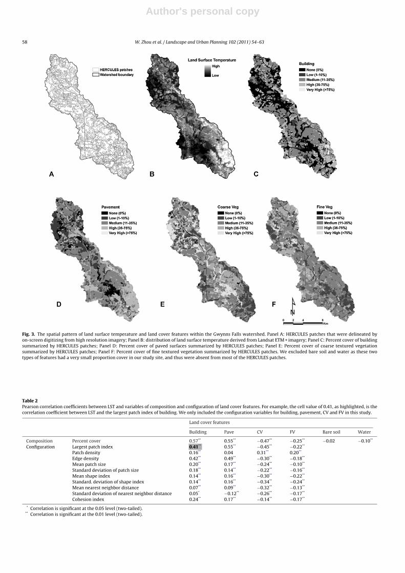
Fig. 3. The spatial pattern of land surface temperature and land cover features within the Gwynns Falls watershed. Panel A: HERCULES patches that were delineated byon-screen digitizing from high resolution imagery; Panel B: distribution of land surface temperature derived from Landsat ETM + imagery; Panel C: Percent cover of buildingsummarized by HERCULES patches; Panel D: Percent cover of paved surfaces summarized by HERCULES patches; Panel E: Percent cover of coarse textured vegetationsummarized by HERCULES patches; Panel F: Percent cover of fine textured vegetation summarized by HERCULES patches. We excluded bare soil and water as these twotypes of features had a very small proportion cover in our study site, and thus were absent from most of the HERCULES patches.

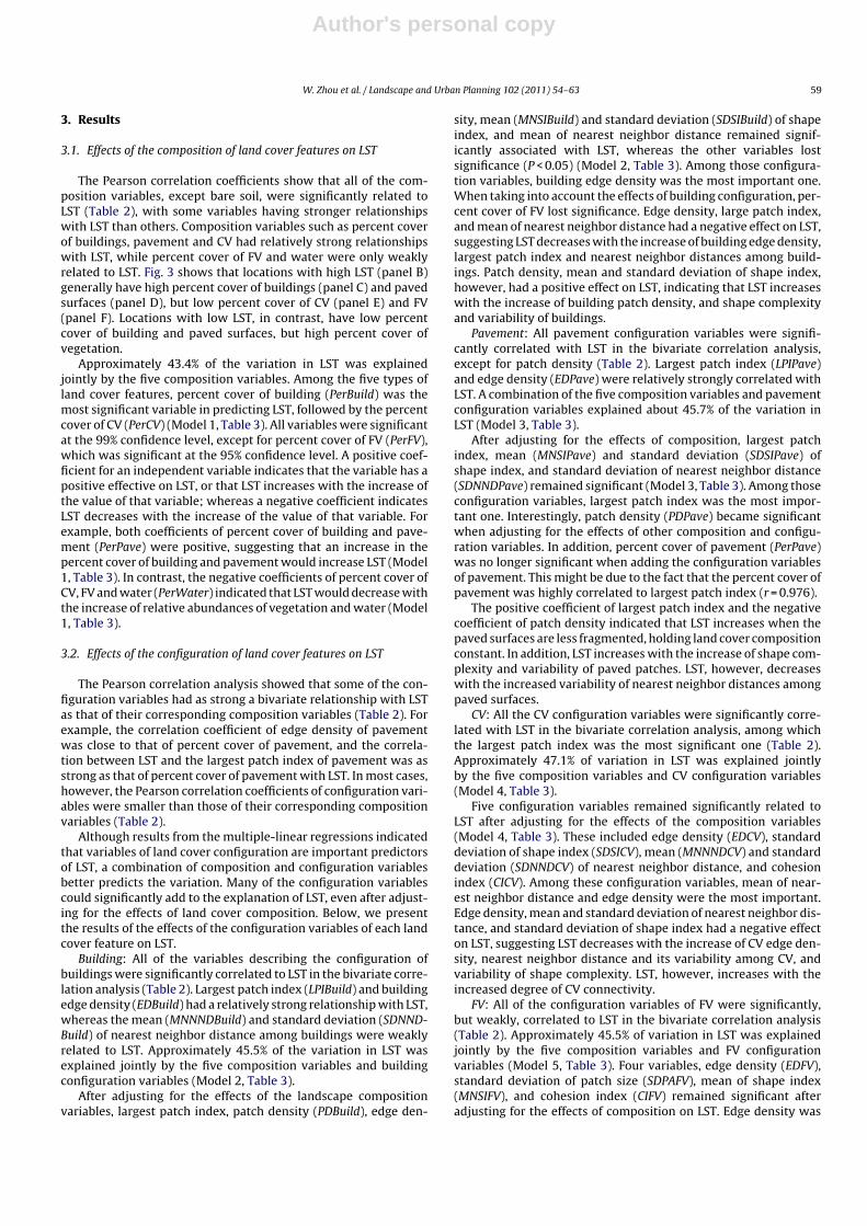
Table 2Pearson correlation coefficients between LST and variables of composition and configuration of land cover features. For example, the cell value of 0.41, as highlighted, is thecorrelation coefficient between LST and the largest patch index of building. We only included the configuration variables for building, pavement, CV and FV in this study.

Land cover features

Building Pave CV FV Bare soil Water

Composition Percent cover 0.57** 0.55** −0.47** −0.25** −0.02 −0.10**

Configuration Largest patch index 0.41** 0.55** −0.45** −0.22**

Patch density 0.16** 0.04 0.31** 0.20**

Edge density 0.42** 0.49** −0.30** −0.18**

Mean patch size 0.20** 0.17** −0.24** −0.10**

Standard deviation of patch size 0.18** 0.14** −0.22** −0.16**

Mean shape index 0.14** 0.16** −0.30** −0.22**

Standard. deviation of shape index 0.14** 0.16** −0.34** −0.24**

Mean nearest neighbor distance 0.07** 0.09** −0.32** −0.13**

Standard deviation of nearest neighbor distance 0.05* −0.12** −0.26** −0.17**

Cohesion index 0.24** 0.17** −0.14** −0.17**

* Correlation is significant at the 0.05 level (two-tailed).** Correlation is significant at the 0.01 level (two-tailed).

Author's personal copy

W. Zhou et al. / Landscape and Urban Planning 102 (2011) 54–63 59

3. Results

3.1. Effects of the composition of land cover features on LST

The Pearson correlation coefficients show that all of the com-position variables, except bare soil, were significantly related toLST (Table 2), with some variables having stronger relationshipswith LST than others. Composition variables such as percent coverof buildings, pavement and CV had relatively strong relationshipswith LST, while percent cover of FV and water were only weaklyrelated to LST. Fig. 3 shows that locations with high LST (panel B)generally have high percent cover of buildings (panel C) and pavedsurfaces (panel D), but low percent cover of CV (panel E) and FV(panel F). Locations with low LST, in contrast, have low percentcover of building and paved surfaces, but high percent cover ofvegetation.

Approximately 43.4% of the variation in LST was explainedjointly by the five composition variables. Among the five types ofland cover features, percent cover of building (PerBuild) was themost significant variable in predicting LST, followed by the percentcover of CV (PerCV) (Model 1, Table 3). All variables were significantat the 99% confidence level, except for percent cover of FV (PerFV),which was significant at the 95% confidence level. A positive coef-ficient for an independent variable indicates that the variable has apositive effective on LST, or that LST increases with the increase ofthe value of that variable; whereas a negative coefficient indicatesLST decreases with the increase of the value of that variable. Forexample, both coefficients of percent cover of building and pave-ment (PerPave) were positive, suggesting that an increase in thepercent cover of building and pavement would increase LST (Model1, Table 3). In contrast, the negative coefficients of percent cover ofCV, FV and water (PerWater) indicated that LST would decrease withthe increase of relative abundances of vegetation and water (Model1, Table 3).

3.2. Effects of the configuration of land cover features on LST

The Pearson correlation analysis showed that some of the con-figuration variables had as strong a bivariate relationship with LSTas that of their corresponding composition variables (Table 2). Forexample, the correlation coefficient of edge density of pavementwas close to that of percent cover of pavement, and the correla-tion between LST and the largest patch index of pavement was asstrong as that of percent cover of pavement with LST. In most cases,however, the Pearson correlation coefficients of configuration vari-ables were smaller than those of their corresponding compositionvariables (Table 2).

Although results from the multiple-linear regressions indicatedthat variables of land cover configuration are important predictorsof LST, a combination of composition and configuration variablesbetter predicts the variation. Many of the configuration variablescould significantly add to the explanation of LST, even after adjust-ing for the effects of land cover composition. Below, we presentthe results of the effects of the configuration variables of each landcover feature on LST.

Building: All of the variables describing the configuration ofbuildings were significantly correlated to LST in the bivariate corre-lation analysis (Table 2). Largest patch index (LPIBuild) and buildingedge density (EDBuild) had a relatively strong relationship with LST,whereas the mean (MNNNDBuild) and standard deviation (SDNND-Build) of nearest neighbor distance among buildings were weaklyrelated to LST. Approximately 45.5% of the variation in LST wasexplained jointly by the five composition variables and buildingconfiguration variables (Model 2, Table 3).

After adjusting for the effects of the landscape compositionvariables, largest patch index, patch density (PDBuild), edge den-

sity, mean (MNSIBuild) and standard deviation (SDSIBuild) of shapeindex, and mean of nearest neighbor distance remained signif-icantly associated with LST, whereas the other variables lostsignificance (P < 0.05) (Model 2, Table 3). Among those configura-tion variables, building edge density was the most important one.When taking into account the effects of building configuration, per-cent cover of FV lost significance. Edge density, large patch index,and mean of nearest neighbor distance had a negative effect on LST,suggesting LST decreases with the increase of building edge density,largest patch index and nearest neighbor distances among build-ings. Patch density, mean and standard deviation of shape index,however, had a positive effect on LST, indicating that LST increaseswith the increase of building patch density, and shape complexityand variability of buildings.

Pavement: All pavement configuration variables were signifi-cantly correlated with LST in the bivariate correlation analysis,except for patch density (Table 2). Largest patch index (LPIPave)and edge density (EDPave) were relatively strongly correlated withLST. A combination of the five composition variables and pavementconfiguration variables explained about 45.7% of the variation inLST (Model 3, Table 3).

After adjusting for the effects of composition, largest patchindex, mean (MNSIPave) and standard deviation (SDSIPave) ofshape index, and standard deviation of nearest neighbor distance(SDNNDPave) remained significant (Model 3, Table 3). Among thoseconfiguration variables, largest patch index was the most impor-tant one. Interestingly, patch density (PDPave) became significantwhen adjusting for the effects of other composition and configu-ration variables. In addition, percent cover of pavement (PerPave)was no longer significant when adding the configuration variablesof pavement. This might be due to the fact that the percent cover ofpavement was highly correlated to largest patch index (r = 0.976).

The positive coefficient of largest patch index and the negativecoefficient of patch density indicated that LST increases when thepaved surfaces are less fragmented, holding land cover compositionconstant. In addition, LST increases with the increase of shape com-plexity and variability of paved patches. LST, however, decreaseswith the increased variability of nearest neighbor distances amongpaved surfaces.

CV: All the CV configuration variables were significantly corre-lated with LST in the bivariate correlation analysis, among whichthe largest patch index was the most significant one (Table 2).Approximately 47.1% of variation in LST was explained jointlyby the five composition variables and CV configuration variables(Model 4, Table 3).

Five configuration variables remained significantly related toLST after adjusting for the effects of the composition variables(Model 4, Table 3). These included edge density (EDCV), standarddeviation of shape index (SDSICV), mean (MNNNDCV) and standarddeviation (SDNNDCV) of nearest neighbor distance, and cohesionindex (CICV). Among these configuration variables, mean of near-est neighbor distance and edge density were the most important.Edge density, mean and standard deviation of nearest neighbor dis-tance, and standard deviation of shape index had a negative effecton LST, suggesting LST decreases with the increase of CV edge den-sity, nearest neighbor distance and its variability among CV, andvariability of shape complexity. LST, however, increases with theincreased degree of CV connectivity.

FV: All of the configuration variables of FV were significantly,but weakly, correlated to LST in the bivariate correlation analysis(Table 2). Approximately 45.5% of variation in LST was explainedjointly by the five composition variables and FV configurationvariables (Model 5, Table 3). Four variables, edge density (EDFV),standard deviation of patch size (SDPAFV), mean of shape index(MNSIFV), and cohesion index (CIFV) remained significant afteradjusting for the effects of composition on LST. Edge density was

Author's personal copy

60 W. Zhou et al. / Landscape and Urban Planning 102 (2011) 54–63

Tab

le3

Sum

mar

yre

sult

sfo

rth

efi

vem

ult

i-li

nea

rre

gres

sion

mod

els.

For

each

ofth

efi

vem

odel

s,th

ere

spon

seva

riab

le,L

ST,w

asp

red

icte

dby

com

pos

itio

nva

riab

les,

i.e.,

per

cen

tcov

erof

five

lan

dco

ver

feat

ure

s(m

odel

1),o

ra

com

bin

atio

nof

thos

eco

mp

osit

ion

vari

able

sw

ith

the

con

figu

rati

onva

riab

les

ofon

ety

pe

ofla

nd

cove

rfe

atu

re.T

he

shad

edco

lum

ns

for

Mod

el2–

5ar

eth

eco

mp

osit

ion

vari

able

s.

Mod

elEx

pla

nat

ory

vari

able

s/re

gres

sion

coef

fici

ent;

stan

dar

diz

edco

effi

cien

tR

-squ

are

(ad

just

ed)a

PerB

uil

dPe

rPav

ePe

rCV

PerF

VPe

rWat

er

Mod

el1

.73**

(0.3

3)3.

41**

(0.2

0)−3

.43**

(−0.

24)

−1.0

3*(−

0.07

)−3

.73**

(−0.

07)

0.43

4(0

.432

)

PerB

uil

dPe

rPav

ePe

rCV

PerF

VPe

rWat

erLP

I-B

uil

dPD

-B

uil

dED

-B

uil

dM

NPA

-B

uil

dSD

PA-

Bu

ild

MN

SI-

Bu

ild

SDSI

-B

uil

dM

NN

ND

-B

uil

dSD

NN

D-

Bu

ild

CIB

uil

d

Mod

el2

18.4

7**

(0.6

3)3.

62**

(0.2

1)−3

.20**

(−0.

23)

−0.7

4(−

0.05

)−4

.23**

(−0.

08)

−0.0

34**

(−0.

08)

3.4E

−4*

(0.0

5)−0

.003

**

(−0.

26)

−9.7

1E−5

(−0.

04)

−5.8

1E−5

(−0.

02)

0.32

**

(0.0

6)0.

48**

(0.0

7)−0

.008

**

(−0.

07)

−0.0

03(−

0.01

)−0

.004

(−0.

04)

0.45

5(0

.452

)

Per-

Bu

ild

Per-

Pave

PerC

VPe

rFV

Per-

Wsa

ter

LPI-

Pave

PD-

Pave

ED-

Pave

MN

PA-

Pave

SDPA

-Pa

veM

NSI

-Pa

veSD

SI-

Pave

MN

NN

D-

Pave

SDN

ND

-Pa

veC

I-Pa

ve

Mod

el3

9.75

**

(0.3

3)−2

.29

(−0.

14)

−3.7

9**

(−0.

27)

−1.3

4**

(−0.

09)

−4.4

3**

(−0.

08)

0.04

7**

(0.2

9)−4

.82E

−4*

(−0.

07)

2.78

E−4

(0.0

4)−1

.27E

−5(−

0.02

)−1

.61E

−5(−

0.04

)0.

32**

(0.0

7)0.

29**

(0.0

6)0.

001

(0.0

0)−0

.015

*

(−0.

04)

−0.0

06(−

0.01

)0.

457

(0.4

53)

Per-

Bu

ild

Per-

Pave

PerC

VPe

rFV

Per-

Wat

erLP

ICV

PDC

VED

CV

MN

P-A

CV

SDP-

AC

VM

NS-

ICV

SDS-

ICV

MN

NN

-D

CV

SDN

N-

DC

VC

ICV

Mod

el4

8.76

**

(0.3

0)2.

46**

(0.1

5)−2

.36*

(−0.

17)

−0.8

4(−

0.05

)−4

.31**

(−0.

08)

0.00

2(0

.02)

−8.7

6E−6

(−0.

01)

−0.0

01**

(−0.

13)

1.87

E−6

(0.0

1)−8

.43E

−6(−

0.04

)0.

027

(0.0

1)−0

.578

**

(−0.

11)

−0.0

31**

(−0.

14)

−0.0

17*

(−0.

05)

0.01

7**

(0.0

5)0.

471

(0.4

67)

Per-

Bu

ild

Per-

Pave

PerC

VPe

rFV

Per-

Wat

erLP

IFV

PDFV

EDFV

MN

PA-

FVSD

PA-

FVM

NSI

-FV

SDSI

-FV

MN

NN

D-

FVSD

NN

D-

FVC

IFV

Mod

el5

9.34

**

(0.3

2)3.

50**

(0.2

1)−3

.26**

(−0.

23)

1.55

(0.1

0)−2

.27*

(−0.

04)

−0.0

06(−

0.04

)1.

35E−

4(0

.03)

−0.0

01**

(−0.

17)

−6.2

8E−6

(−0.

01)

−5.6

2E−5

**

(−0.

07)

−0.5

3**

(−0.

06)

−0.0

85(−

0.01

)−0

.001

(−0.

00)

−0.0

24(−

0.04

)0.

022**

(0.0

4)0.

455

(0.4

51)

aW

ein

clu

ded

both

the

un

stan

dar

diz

edre

gres

sion

coef

fici

ents

and

stan

dar

diz

edco

effi

cien

ts(i

ncl

ud

edin

the

par

enth

eses

).Th

est

and

ard

ized

coef

fici

ents

(bet

aco

effi

cien

ts,o

rbe

taw

eigh

ts)

are

use

dto

det

erm

ine

the

rela

tive

imp

orta

nce

ofex

pla

nat

ory

vari

able

s.Th

ela

rger

the

abso

lute

valu

eof

the

stan

dar

diz

edco

effi

cien

t,th

em

ore

imp

orta

nt

ava

riab

le.

*C

oeffi

cien

tis

sign

ifica

nt

atth

e0.

05le

vel(

two-

tail

ed).

**C

oeffi

cien

tis

sign

ifica

nt

atth

e0.

01le

vel(

two-

tail

ed).

Author's personal copy

W. Zhou et al. / Landscape and Urban Planning 102 (2011) 54–63 61

the most important configuration variable. When considering theeffects of FV configuration on LST, the percent cover of FV (PerFV)was no longer significant. Edge density, standard deviation ofpatch size, and mean of shape index had a negative effect on LST,indicating that LST decreases with the increase of FV edge den-sity, variability of patch size, and shape complexity; whereas LSTincreases with the increase of FV cohesion index.

4. Discussion

Our results indicated that both the composition and configura-tion of land cover features significantly affects the magnitude ofLST. By explicitly describing the quantitative relationships of LSTwith the composition and configuration of land cover features; thisresearch expands our scientific understanding of the effects of landcover pattern on LST in urban landscapes. These results have impor-tant theoretical and management implications. Urban planners andnatural resource managers attempting to mitigate the impact ofurban development on UHI can gain insights into the importanceof balancing the relative amount of various types of land coverfeatures and optimizing their spatial distributions.

4.1. Theoretical implications

The effects of land cover composition on LST have been exten-sively documented (e.g., Buyantuyev & Wu, 2010; Liang & Weng,2008; Weng, 2009; Xiao et al., 2008). Our results are consistent withthose from previous research that land cover composition, or thepercent cover of different types of land cover features, greatly affectthe magnitude of LST. In fact, our results showed that the composi-tion of land cover features is a more important factor in determiningLST than the configuration of those features. Increasing vegetationcover or surface water could significantly decrease LST, and thushelp to mitigate excess heat in urban areas; whereas the increaseof buildings and paved surfaces would significantly increase LST,exacerbating the UHI phenomena.

The land cover feature that most significantly affects the mag-nitude of LST is the percent cover of buildings. In contrast, percentcover of woody vegetation is the most important factor mitigatingUHI effects. These results may be due to the fact that changes in per-cent cover of buildings and woody vegetation lead to modificationsof the land surface characteristics such as albedo and evapotranspi-ration. In addition, an increase in building cover is also associatedwith the production of waste heat from air conditioning and refrig-eration systems, as well from motorized vehicular traffic – all ofwhich exacerbates the UHI effects. These results suggest that theUHI effect can be effectively mitigated by using light-colored mate-rials on houses and roofs, implementing green roofs, and increasingthe amount of tree canopies. Water bodies had a weak relationshipwith LST, and bare soil was not significantly correlated to LST. Thismay be partly due to the very small proportion cover of these twotypes of features in our study area.

The configuration of land cover features also significantly affectsLST. For a fixed relative amount of land cover features, LST can besignificantly increased or decreased by different spatial arrange-ments of those features. This is because the spatial arrangementinfluences the flow of energy, or energy exchange among land coverfeatures (Forman, 1995) and, thus, affects LST.

The configuration of all four land cover features – buildings,pavement, CV and FV – significantly affects the magnitude of LST.The significance and effect of specific configuration variables onLST, however, varied broadly among the land cover features. Forexample, edge density is a very important configuration variablethat affects LST. Given a fixed composition of land cover features,an increase in edge density of woody and herbaceous vegetation

significantly decreases the magnitude of LST. In addition, LST gener-ally decreases with the increase of shape complexity and variabilityof woody and herbaceous vegetation. Increase in edge density andshape complexity of woody vegetation may increase shade, pro-vided by woody vegetation, for surrounding areas and thus, reduceLST. In addition, higher edge density and increased shape com-plexity of woody and herbaceous vegetation may enhance theinteractions between vegetation and built-up areas (building &paved surfaces), and thus facilitate energy exchange among landcover features, resulting in a lower mean LST (Forman, 1995; Xu &Yue, 2008). Land surface temperature is also predicted to decreasewith an increase of the average and variability of nearest neighbordistance among woody vegetation. This suggests that an evenlydistributed, rather than clustered, pattern of woody vegetation canfurther reduce LST. This may be because, given a fixed percent coverof woody vegetation, an even distribution can provide more shadefor surrounding non-woody vegetated areas and enhance the inter-actions between woody vegetation and other land cover featuresthan had the woody vegetation been clustered. This was furthersupported by the effect of the cohesion index which indicated thatan increase in the degree of woody vegetation connectivity wouldincrease LST because, as patch cohesion increases, the woody veg-etation becomes more clumped or aggregated in its distribution(McGarigal et al., 2002).

The effects of the configuration of building and paved surfaces onLST appear more complicated. Land surface temperature decreaseswith the increase of building largest patch index, mean distancesamong buildings, and patch density of paved surfaces. Land surfacetemperature, however, increases with the increase of largest patchindex of paved surfaces, and patch density of buildings. In contrastto vegetation, an increase in shape complexity and variability ofbuildings and paved surfaces leads to an increase in LST. This resultreveals the complex thermal environments characteristic of urbanlandscapes. On the one hand, the increase in shape complexity andvariability of buildings and paved surfaces may facilitate energyexchange between built-up areas and vegetation, and thus cool thebuilt-up areas (Forman, 1995; Xu & Yue, 2008; Zhang et al., 2009).On the other hand, the increase in shape complexity and variabil-ity of buildings and paved surfaces may increase solar heat gainto buildings and paved surfaces because of the increased exposedsurfaces (Voogt & Oke, 1998).

Our results also highlighted that, when testing the effects of con-figuration of land cover features on LST, it is important to controlfor the effects of their composition. This is because configura-tion metrics are commonly correlated with composition metrics(McGarigal et al., 2002; Riitters et al., 1995), resulting in spuri-ous correlations between LST and some configuration variables inbivariate analyses. The surprising result that the mean patch sizeof land cover features was not significantly correlated to LST forany feature type after adjusting for the effects of composition maybe due to the mean patch size and composition variables beingstrongly correlated (McGarigal et al., 2002; Riitters et al., 1995).Our results showed that all configuration variables of the four landcover features were significantly correlated to LST in the bivariateanalysis. Fewer of these variables, however, remained significantafter adjusting for the effects of land cover composition. Similarresults were also found in Weng et al. (2008), when using factoranalysis.

The combination of composition and configuration of land coverfeatures only explained about half of the variance in LST. This islower than reported by some previous studies (e.g. Buyantuyev& Wu, 2010; Liang & Weng, 2008). The research presented here,however, was conducted at a finer scale (a smaller area of unit ofanalysis) than those previous studies. In general, a stronger cor-relation between LST and land cover variables can be found atcoarser scales. Thus, a greater proportion of the variance in LST

Author's personal copy

62 W. Zhou et al. / Landscape and Urban Planning 102 (2011) 54–63

can be explained by land cover variables at the coarser scale (Liang& Weng, 2008). This may suggest that, at a fine scale, more factorsshould be considered to better predict LST than land cover pattern.This may be due to the fine-scale complexity of the urban ther-mal environments (Arnfield, 2003). For example, the impacts ofthe three dimensional structure of urban surfaces at the fine-scale,such as building and tree height and ruggedness of the urban sur-face, should be included to improve the prediction of the models(Arnfield, 2003; Voogt & Oke, 1998; Voogt & Oke, 2003).

4.2. Management implications

There is an increasing interest in linking the emerging theory ofurban ecology to ecological design and management of urban land-scapes (McGrath et al., 2007; Cadenasso & Pickett, 2008; Pickett &Cadenasso, 2008). The results that both the composition and config-uration of land cover features in a landscape significantly affectedthe magnitude of LST can provide important insights into ecologi-cal design and management, and, therefore, may have importantimplications for urban planners and natural resource managers.This suggests that the impact of urbanization on the UHI can bemitigated by balancing the relative amounts of various land coverfeatures and optimizing their spatial configuration.

Vegetation management, particularly increasing tree canopy,has been considered an effective means to mitigate excess urbanheat. For highly urbanized areas, while removal of paved surfacesor buildings maybe expensive and impractical (Kaiser, Godschalk,& Stuart, 1995), the amount and spatial distribution of vegetationcan be altered through vegetation management such as tree plant-ing in selected locations. Many US cities, such as Baltimore andNew York, have established goals to increase tree canopy coverin order to enhance ecosystem services and reduce the impact ofurban development on, for example, heat island effects, water con-sumption and stormwater runoff (Maryland Department of NaturalResources, 2007). Previous research has focused on where treescould potentially be planted (Troy, Grove, O’Neil-Dunne, Pickett, &Cadenasso, 2007; Wu, Xiao, & McPherson, 2008). Results from thisstudy can provide additional insights for urban planners and nat-ural resources managers about how to arrange those trees so thatthe spatial configuration of the tree canopy can be optimized tomaximize the canopy’s mitigating affects on the UHI.

The configuration of land cover features other than trees alsosignificantly affects LST. This result has important implications forurban design and planning, particularly for locations where urban-ization is still in process. It suggests that by designing landscapesthat balance the relative amounts of various land cover features andthat optimize their spatial configuration, the impact of urbanizationon LST can be greatly mitigated.

4.3. Limitations

This study has its limitations. The research was conducted forone region, using only one daytime thermal image to obtain LST.Previous studies have shown that there are diurnal and seasonalvariations in the relationships between LST and land cover fea-tures (e.g. Buyantuyev & Wu, 2010; Yuan & Bauer, 2007). Forexample, vegetation abundance, measured by NDVI, had a strongrelationship with daytime LST, but was only very weakly related tonighttime LST (Buyantuyev & Wu, 2010). The relationship betweenLST and vegetation abundance also varies by seasons (Yuan & Bauer,2007). In addition, different climatic conditions may significantlyinfluence the amplitude of daytime surface UHI (Imhoff, Zhang,Wolfe, & Bounoua, 2010). Therefore, further studies that use mul-tiple daytime and nighttime thermal images for different seasonsare desirable. In addition, comparison studies across metropolitanareas under different climatic conditions are recommended.

5. Summary and conclusions

Urban heat island is a critical consequence of urbanization dueto land cover conversions. Understanding the link between landcover patterns and UHI is important for designing effective mecha-nisms to mitigate the impact of urbanization on UHI. This studyinvestigates the quantitative relationships of LST with both thecomposition and configuration of land cover features in urban land-scapes. The results indicated that not only does the composition ofland cover features significantly affect the magnitude of LST, but sodoes the configuration of those features. However, the compositionof land cover features is more important in determining LST thantheir configuration. The land cover feature that most significantlyaffects the magnitude of LST is the percent cover of buildings. Incontrast, percent cover of woody vegetation is the most importantfactor mitigating UHI effects. These results suggest that the UHIeffect can be effectively mitigated by using light-colored materialson houses and roofs, implementing green roofs, and increasing theamount of tree canopies. The configuration of land cover featuresalso matters. Holding composition constant, LST can be significantlyincreased or decreased by different spatial arrangements of landcover features. For example, an increase in edge density, and shapecomplexity and variability of woody and herbaceous vegetation sig-nificantly decreases the magnitude of LST. In contrast, an increasein shape complexity and variability of buildings and paved surfacesleads to an increase in LST. In addition, an increase of the averageand variability of nearest neighbor distance among woody vege-tation can significantly decrease LST. Similarly, an increase of theaverage nearest neighbor distance among buildings can also sig-nificantly decrease LST. Therefore, the impact of urbanization onUHI can be mitigated not only by balancing the relative amountsof various land cover features, but also by optimizing their spatialconfiguration. This finding provides important insights for urbanplanners and natural resource managers on urban heat mitigationthrough urban design and vegetation management, for both highlyurbanized areas and areas where urbanization is still in process.While we found spatial configuration of land cover features doesmatter, it should be noted that this conclusion is based on LST datafrom one daytime thermal image, and the research was conductedonly for one metropolitan area. Whether this conclusion can beapplied to different seasons and other metropolitan areas shouldbe further explored. Therefore, future comparison studies acrossmetropolitan areas under different climatic conditions, and stud-ies that use multiple daytime and nighttime thermal images fordifferent seasons are recommended.

References

Akbari, H., Rosenfeld, A., Taha, H., & Gartland, L. (1996). Mitigation of summer urbanheat islands to save electricity and smog. In 76th Annual American MeteorologicalSociety Meeting Atlanta, GA,

Akbari, H., Pomerantz, M., & Taha, H. (2001). Cool surfaces and shade trees to reduceenergy use and improve air quality in urban areas. Solar Energy, 70, 295–310.

Alig, R. J., Kline, J. D., & Lichtenstein, M. (2004). Urbanization on the US landscape:Looking ahead in the 21st century. Landscape and Urban Planning, 69, 219–234.

Arnfield, A. J. (2003). Two decades of urban climate research: A review of turbulence,exchanges of energy and water, and the urban heat island. International Journalof Climatology, 23, 1–26.

Balling, R. C., & Brazell, S. W. (1988). High resolution surface temperature pattern ina complex urban terrain. Photogrammetric Engineering and Remote Sensing, 54,1289–1293.

Ben-Dor, E., & Saaroni, H. (1997). Airborne video thermal radiometry as a tool formonitoring microscale structures of the urban heat island. International Journalof Remote Sensing, 18(4), 3039–3053.

Buyantuyev, A., & Wu, J. (2010). Urban heat islands and landscape heterogeneity:Linking spatiotemporal variations in surface temperatures to land-cover andsocioeconomic patterns. Landscape Ecology, 25(1), 17–33.

Cadenasso, M. L., Pickett, S. T. A., & Schwarz, K. (2007). Spatial heterogeneity in urbanecosystems: Reconceptualizing land cover and a framework for classification.Frontier in Ecological Environment, 5, 80–88.

Author's personal copy

W. Zhou et al. / Landscape and Urban Planning 102 (2011) 54–63 63

Cadenasso, M. L., & Pickett, S. T. A. (2008). Urban principles for ecological landscapedesign and maintenance: Scientific fundamentals. Cities and the Environment,1(2), 1–16.

Cao, X., Onishi, A., Chen, J., & Imura, H. (2010). Quantifying the cool island intensityof urban parks using ASTER and IKONOS data. Landscape and Urban Planning,96(4), 224–231.

Forman, R. T. T. (1995). Land mosaics: The ecology of landscape and regions. NY:Cambridge University Press.

Frey, C. M., Rigo, G., & Parlow, E. (2007). Urban radiation balance of two coastal citiesin a hot and dry environment. International Journal of Remote Sensing, 28(12),2695–2712.

Frey, C. M., Parlow, E., Vogt, R., Abdel Wahab, M., & Harhash, M. (2010). Fluxmeasurements in Cairo. Part 1. In situ measurements and their applicabil-ity for comparison with satellite data. International Journal of Climatology, 31,218–231.

Gustafson, E. J. (1998). Quantifying landscape spatial pattern: What is the state ofthe art? Ecosystems, 1, 143–156.

Imhoff, M. L., Zhang, P., Wolfe, R. E., & Bounoua, L. (2010). Remote sensing of theurban heat island effect across biomes in the continental USA. Remote Sensing ofEnvironment, 114(3), 504–513.

Kaiser, E. J., Godschalk, D. R., & Stuart, C. F. (1995). Urban land use planning. Chicago:University of Illinois Press.

Landsat Project Science Office, 2009. Landsat 7 Science Data User’s Handbook. URL:http://landsathandbook.gsfc.nasa.gov/handbook.html, Goddard Space FlightCenter, NASA, Washington, DC (last date accessed: 16 August 2010).

Leitao, A. B., Miller, J., Ahern, J., & McGarigal, K. (2006). Measuring landscapes: Aplanner’s handbook. Washington, DC: Island Press.

Liang, B., & Weng, Q. (2008). Multi-scale analysis of census-based land surface tem-perature variations and determinants in Indianapolis, United States. Journal ofUrban Planning D-ASCE, 134(3), 129–139.

Liu, H., & Weng, Q. (2009). Scaling-up effect on the relationship between landscapepattern and land surface temperature. Photogrammetric Engineering and RemoteSensing, 75(3), 291–304.

Lo, C. P., Quattrochi, D. A., & Luvall, J. C. (1997). Application of high-resolution ther-mal infrared remote sensing and GIS to assess the urban heat island effect.International Journal of Remote Sensing, 18, 287–304.

Lo, C. P., & Quattrochi, D. A. (2003). Land-use and land-cover change, urban heatisland phenomenon, and health implications: A remote sensing approach. Pho-togrammetric Engineering and Remote Sensing, 69, 1053–1063.

Lu, D., & Weng, Q. (2006). Spectral Mixture Analysis of ASTER Images for Examiningthe Relationship between Urban Thermal Features and Biophysical Descrip-tors in Indianapolis, United States. Remote Sensing of Environment, 104(2),157–167.

Maryland Department of Natural Resources, 2007. Chesapeake Bay urbantree canopy goals, http://www.dnr.state.md.us/forests/programs/urban/urbantreecanopygoals.asp (Accessed on October 14, 2009).

McGarigal, K., Cushman, S. A., Neel M. C., & Ene, E. (2002). FRAGSTATS: Spa-tial Pattern Analysis Program for Categorical Maps. Computer softwareprogram produced by the authors at the University of Massachusetts,Amherst. Available at the following web site: http://www.umass.edu/landeco/research/fragstats/fragstats.html.

McGrath, B. P., Marshall, V., Cadenasso, M. L., Grove, J. M., Pickett, S. T. A., & Plunz,R., et al. (2007). Designing Patch Dynamics. Columbia Graduate School of Archi-tecture, Planning and Preservation. New York.

Nichol, J. E. (1994). A GIS-based approach to microclimate monitoring in Singapore’shigh-rise housing estates. Photogrammetric Engineering and Remote Sensing, 60,1225–1232.

Nichol, J. E., Fung, W. Y., Lam, K., & Wong, M. S. (2009). Urban heat island diagnosisusing ASTER satellite images and ‘in situ’ air temperature. Atmospheric Research,94(2), 276–284.

Oke, T. R. (1995). The heat island of the urban boundary layer: Characteristics, causesand effects. In J. E. Cermak (Ed.), Wind climate in cities (pp. 81–107). Netherlands:Kluwer Academic Publishers.

Pickett, S. T. A., & Cadenasso, M. L. (2008). Linking ecological and built componentsof urban mosaics: An open cycle of ecological design. Journal of Ecology, 96, 8–12.

Poumadere, M., Mays, C., Le Mer, S., & Blong, R. (2005). The 2003 heat wave in France:Dangerous climate change here and now. Risk Annual, 25(6), 1483–1494.

Pu, R., Gong, P., Michishita, R., & Sasagawa, T. (2006). Assessment of multi-resolutionand multi-sensor data for urban surface temperature retrieval. Remote Sensingof Environment, 104, 211–225.

Riitters, K. H., O’Neill, R. V., Hunsaker, C. T., Wickham, J. D., Yankee, D. H., Timmins,S. P., et al. (1995). A factor analysis of landscape pattern and structure metrics.Landscape Ecology, 10, 23–39.

Snyder, W. C., Wan, Z., Zhang, Y., & Feng, Y. Z. (1998). Classification-based emissivityfor land surface temperature measurement from space. International Journal ofRemote Sensing, 19(14), 2753–2774.

Troy, A. R., Grove, J. M., O’Neil-Dunne, J. P. M., Pickett, S. T. A., & Cadenasso, M.L. (2007). Predicting patterns of vegetation and opportunities for greening onprivate urban lands. Environmental Management, 40, 394–412.

Turner, M. G., Gardner, R. H., & O’Neill, R. V. (2001). Landscape ecology in theory andpractice. New York: Springer-Verlag.

Turner, M. G. (2005). Landscape ecology: What is the state of the science? AnnualReview of Ecological Evolution and Sensing, 36, 319–344.

United Nations. (2002). World urbanization prospects – the 2001 revision data tableand highlights. New York: Department of Economic and Social Affairs.

University of Maryland, College Park, 2001. Normal Precipitation and TemperatureValues for Baltimore City from 1961 to 1990. Baltimore, Maryland.

Voogt, J. A., & Oke, T. R. (1998). Effects of urban surface geometry on remotely-sensedsurface temperature. International Journal of Remote Sensing, 19, 895–920.

Voogt, J. A., & Oke, T. R. (2003). Thermal remote sensing of urban climates. RemoteSensing of Environment, 86, 370–384.

Weng, Q. (2003). Fractal analysis of satellite-detected urban heat island effect. Pho-togrammetric Engineering and Remote Sensing, 69(5), 555–566.

Weng, Q., Liu, H., & Lu, D. (2007). Assessing the effects of land use and land coverpatterns on thermal conditions using landscape metrics in city of Indianapolis,United States. Urban Ecosystem, 10(2), 203–219.

Weng, Q., Liu, H., Liang, B., & Lu, D. (2008). The spatial variations of urban landsurface temperatures: Pertinent factors, zoning effect, and seasonal variability.IEEE Journal of Selected Topics in Applied Earth Observations & Remote Sensing,1(2), 154–166.

Weng, Q., Lu, D., & Schubring, J. (2004). Estimation of land surface temperature –vegetation abundance relationship for urban heat island studies. Remote Sensingof Environment, 89, 467–483.

Weng, Q. (2009). Thermal infrared remote sensing for urban climate andenvironmental studies: Methods, applications, and trends. ISPRS Journal of Pho-togrammetry and Remote Sensing, 64, 335–344.

White, M. A., Nemani, R. R., Thornton, P. E., & Running, S. W. (2002). Satellite evidenceof phenological differences between urbanized and rural areas of the easternUnited States deciduous broadleaf forest. Ecosystems, 5, 260–277.

Wu, C., Xiao, Q., & McPherson, E. G. (2008). A method for locating potential tree-planting sites in urban areas: A case study of Los Angeles, USA. Urban Forestryand Urban Green, 7(2), 65–76.

Xiao, R., Weng, Q., Ouyang, Z., Li, W., Schienke, E., & Zhang, Z. (2008). Land sur-face temperature variation and major factors in Beijing, China. PhotogrammetricEngineering and Remote Sensing, 74(4), 451–461.

Xu, L., & Yue, W. (2008). A study on thermal environment effect of urban parklandscape. Acta Ecologica Sinica, 28(4), 1702–1710.

Yuan, F., & Bauer, M. E. (2007). Comparison of impervious surface area and normal-ized difference vegetation index as indicators of surface urban heat island effectsin Landsat imagery. Remote Sensing of Environment, 106, 375–386.

Zhang, X., Zhong, T., Feng, X., & Wang, K. (2009). Estimation of the relationshipbetween vegetation patches and urban land surface temperature with remotesensing. International Journal of Remote Sensing, 30(8), 2105–2118.

Zhou, W., & Troy, A. (2008). An object-oriented approach for analyzing and char-acterizing urban landscape at the parcel level. International Journal of RemoteSensing, 29(11), 3119–3135.