estimating land use change and economic value of water quality

ESTIMATING LAND USE CHANGE AND ECONOMIC VALUE OF WATER QUALITY

IN A NORTH GEORGIA ECOSYSTEM

by

DANIEL GEORGE NGUGI

(Under the Direction of Jeffrey Mullen)

ABSTRACT

This study seeks to forecast land use change in an

ecosystem in the Upper Chattahoochee River Basin, model

associated water quality changes and estimate the economic value

of the same using Benefit Transfer. The basin is of significant

source of water, recreational and other ecological amenities,

but encroachment by urban development is a major threat to the

ecosystem. Econometric, vector autoregressive and structural

time series models are applied to land use data and the best

forecasting model is selected. Land use change and resulting

water quality changes are modeled under different scenarios and

the public’s willingness to pay for improving and maintaining

the quality of fishing and drinking water supply is estimated.

INDEX WORDS: Ecosystem, Economic Valuation, Watershed,

Willingness to pay, benefit transfer, Chattahoochee River, Land use, Fish, Forecasting, Water quality, Value, urban growth, Georgia, structural time series, vector autoregressive models, land use change, land use modeling



by

DANIEL GEORGE NGUGI

BS., University of Nairobi, Kenya, 1993

MS., University Of Malawi, Malawi, 1998

A Dissertation Submitted to the Graduate Faculty of The

University of Georgia in Partial Fulfillment of the Requirements

for the Degree

DOCTOR OF PHILOSOPHY

ATHENS, GEORGIA

2007

© 2007

Daniel George Ngugi

All Rights Reserved



by

DANIEL GEORGE NGUGI

Major Professor:Jeffrey Mullen

Committee: John Bergstrom Jack Houston Jimmy Bramblett

Electronic Version Approved: Maureen Grasso Dean of the Graduate School The University of Georgia December 2007

iv

DEDICATION

To “the King eternal, immortal, invisible, the only wise

God, be honor and glory for ever and ever. Amen”. 1 Tim 1:17.

v

ACKNOWLEDGEMENTS

I would like to express my sincere gratitude to all those

who have contributed in one way or another toward making my

doctoral program a success. First and foremost, my heartfelt

appreciations go to my major Professor Dr Jeffrey Mullen for his

time, tireless effort and unspeakable patience in guiding me

through the dissertation process.

I must also thank the members of my committee Dr John

Bergstrom, Dr Jack Houston and Mr Jimmy Bramblett for their

invaluable ideas and support without which I would not have come

thus far. Mr Bramblett, thanks a lot for helping me figure out

data issues and locate the data I desperately needed.

To my office mate Nzaku Kilungu – thanks for being truly a

friend indeed - may you be repaid in full someday. Adelin,

Yassin, Enyam, Lina, Augustus, Gina and in abscencia Wei Bai,

Swagata, and many others - thanks for being my friends. Pastors

Howard Conine and Beth Stephens, thanks for making me feel at

home at NCWC and being excellent ministers.

I must also thank numerous people at UGA who were truly

supportive including Dr Epperson for all your kindness in

diverse times; Dr White - you gave me a job when I desperately

needed funding, I really enjoyed teaching that class; Dr Lohr it

vi

was really nice working with you. Jo Anne Norris – you are an

excellent administrator and a truly nice person. Others that can

not escape mention include Dr David Newman at SUNY, Donna Ross,

Lisa Ayala of OIE, Chris Peters, Yanping Chen, Shirley, and many

other who played a part in making my life at UGA a success.

There are numerous other people in and outside UGA who went out

of their way to assist me with mind boggling data issues, Dr Liz

Kramer of the UGA Ecology School, Scott Griffin of Georgia

Forestry Commission, Dr Plantinga of Oregon State University,

Joan Church of Habersham County and Ellen Mills of the Georgia

Department of Revenue.

Many thanks to mother, father and my siblings – without

your moral and spiritual support, this journey would never have

begun in the first place. Special appreciations go to my beloved

sister Leah - you were beside me whenever I needed help – may

you be truly blessed. I must finally and most importantly thank

the Almighty God for the gift of life, the opportunity to be who

I am, and the grace to go through each day of my academic

endeavor particularly my doctoral program – I am forever

grateful!

vii

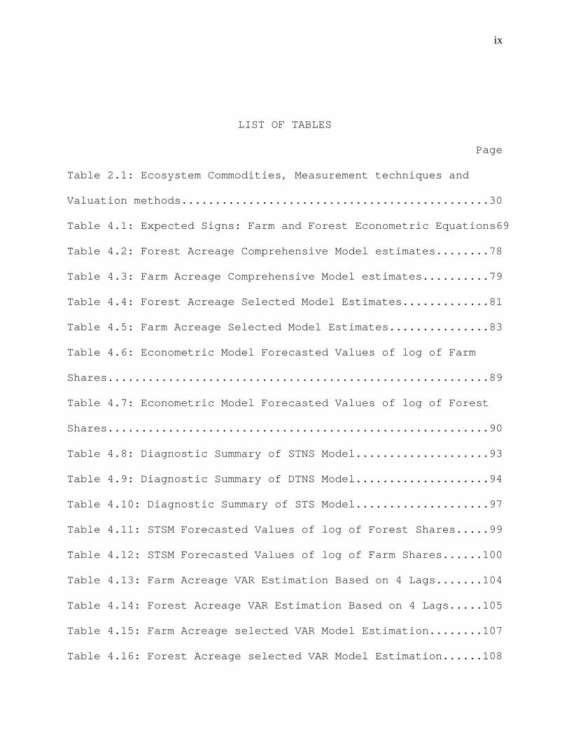
TABLE OF CONTENTS

Page

ACKNOWLEDGEMENTS................................................v

LIST OF TABLES.................................................ix

CHAPTER

I INTRODUCTION ............................................1

Ecosystems and Ecosystem Valuation: An Overview .......1

Problem Statement and Justification of Study ..........4

Objectives ............................................9

II LITERATURE REVIEW: ECOSYSTEM VALUATION AND BENEFIT

TRANSFER .............................................11

Ecosystem Valuation: Review of Literature ............11

Theoretical Measures of Economic Value ...............15

Conventional Environmental Valuation Techniques ......27

Benefit Transfer Estimation ..........................29

Protocol for Meaningful Benefit Transfer .............36

Empirical Methodology and Data Issues ................38

III THEORETICAL LAND USE MODELLING AND PROPOSED METHODOLOGY53

Overview .............................................53

Theoretical Econometric Model ........................54

Structural Time Series Estimation ....................58

The Vector Autoregressive Model ......................61

viii

VI LAND USED MODEL ESTIMATION AND RESULTS .................64

Factors Influencing Land Allocation ..................64

Econometric Model Estimation .........................70

Data and Policy Site .................................71

Results of the Econometric Model .....................76

Structural Time Series Estimation ....................88

Results of the Structural Time Series Model ..........92

Vector Autoregressive Model Estimation ..............101

Results of the Vector Autoregressive Model ..........103

Forecasting Land Use and Land Use Change ............115

V LAND USE CHANGE, WATER QUALITY AND ECOSYSTEM VALUATION 134

The Long-Term Hydrological Impact Assessment Procedure134

Water Pollution and Quality Standards ...............137

Land Use Change: Implications for Water Quality .....145

Benefit Transfer: Empirical Application .............148

Transferring Benefits, Valuing the Ecosystem ........150

VI SUMMARY CONCLUSIONS AND RECOMMENDATION ................158

Summary of Findings .................................159

Conclusions .........................................162

Implications and Future Research Recommendations ....163

REFERENCES....................................................167

APPENDIX......................................................181

ix

LIST OF TABLES

Page

Table 2.1: Ecosystem Commodities, Measurement techniques and

Valuation methods..............................................30

Table 4.1: Expected Signs: Farm and Forest Econometric Equations69

Table 4.2: Forest Acreage Comprehensive Model estimates........78

Table 4.3: Farm Acreage Comprehensive Model estimates..........79

Table 4.4: Forest Acreage Selected Model Estimates.............81

Table 4.5: Farm Acreage Selected Model Estimates...............83

Table 4.6: Econometric Model Forecasted Values of log of Farm

Shares.........................................................89

Table 4.7: Econometric Model Forecasted Values of log of Forest

Shares.........................................................90

Table 4.8: Diagnostic Summary of STNS Model....................93

Table 4.9: Diagnostic Summary of DTNS Model....................94

Table 4.10: Diagnostic Summary of STS Model....................97

Table 4.11: STSM Forecasted Values of log of Forest Shares.....99

Table 4.12: STSM Forecasted Values of log of Farm Shares......100

Table 4.13: Farm Acreage VAR Estimation Based on 4 Lags.......104

Table 4.14: Forest Acreage VAR Estimation Based on 4 Lags.....105

Table 4.15: Farm Acreage selected VAR Model Estimation........107

Table 4.16: Forest Acreage selected VAR Model Estimation......108

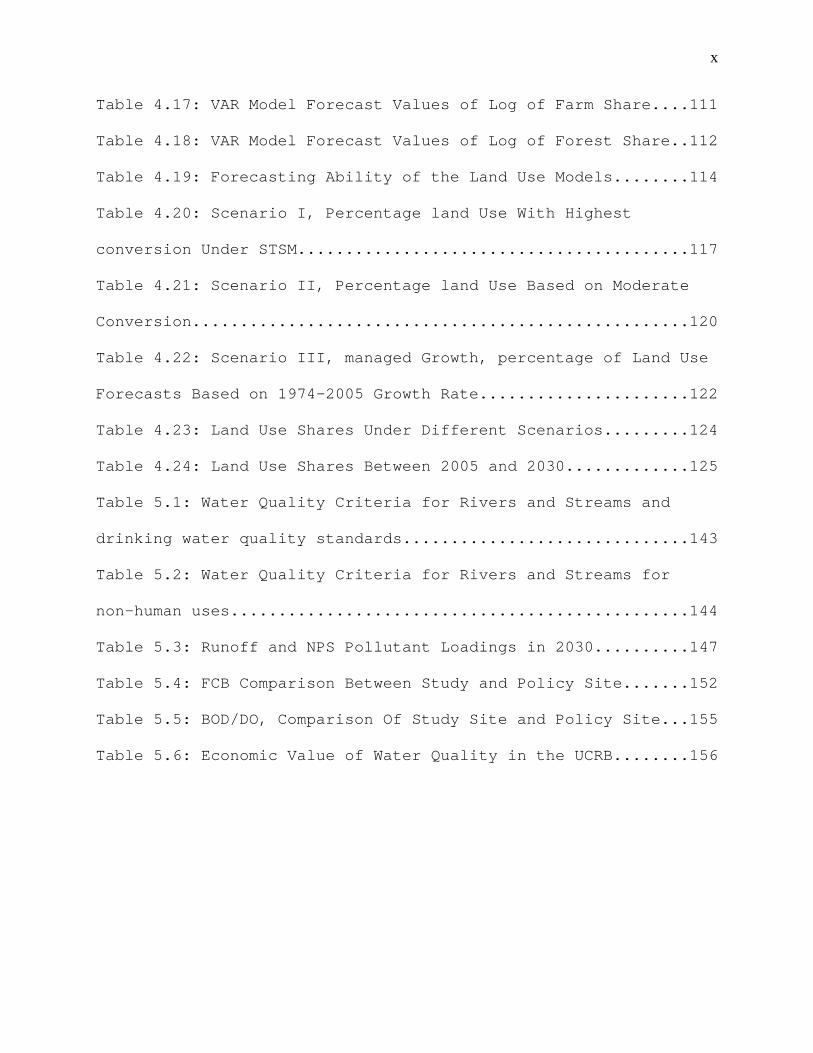
x

Table 4.17: VAR Model Forecast Values of Log of Farm Share....111

Table 4.18: VAR Model Forecast Values of Log of Forest Share..112

Table 4.19: Forecasting Ability of the Land Use Models........114

Table 4.20: Scenario I, Percentage land Use With Highest

conversion Under STSM.........................................117

Table 4.21: Scenario II, Percentage land Use Based on Moderate

Conversion....................................................120

Table 4.22: Scenario III, managed Growth, percentage of Land Use

Forecasts Based on 1974-2005 Growth Rate......................122

Table 4.23: Land Use Shares Under Different Scenarios.........124

Table 4.24: Land Use Shares Between 2005 and 2030.............125

Table 5.1: Water Quality Criteria for Rivers and Streams and

drinking water quality standards..............................143

Table 5.2: Water Quality Criteria for Rivers and Streams for

non-human uses................................................144

Table 5.3: Runoff and NPS Pollutant Loadings in 2030..........147

Table 5.4: FCB Comparison Between Study and Policy Site.......152

Table 5.5: BOD/DO, Comparison Of Study Site and Policy Site...155

Table 5.6: Economic Value of Water Quality in the UCRB........156

1

CHAPTER I

INTRODUCTION

Problem Statement and Justification of Study

An ecosystem is defined as “a geographic area and all its

living components (e.g., people, plants, animals, and

microorganisms), their physical surroundings (e.g., soil, water,

and air), and the natural cycles that sustain them (e.g.,

precipitation, drought, fire, grazing)” (United States Fish and

Wildlife Service (USFWS), 2007). The USFWS also describes a

watershed as “the drainage basin contributing water, organic

matter, dissolved nutrients, and sediments to a water body”.

Thus a watershed or watershed ecosystem is a special type of

ecosystem that drains into a single water body.

Watershed ecosystems play an important role in providing

functions and services that are beneficial to society.

Ecologists see ecosystems as having functions and providing

services (including goods). Ecosystem functions are the

physical, chemical, and biological processes or attributes that

contribute to the self-maintenance of an ecosystem (Saplaco and

Herminia, 2003). Watershed ecosystem functions include provision

2

of wildlife habitat, carbon cycling, trapping of nutrients,

regulation of hydrologic flows and soil formation processes.

Ecosystem services result from ecosystem functions as the

beneficial outcomes of the same to humans and the natural

environment. Watershed ecosystem services include support of the

food chain, harvesting of animals or plants, provision of clean

water, and scenic views.

Ecosystem Valuation: An Overview

Valuing environmental impacts has become increasingly

important with the increase in public awareness of environmental

issues, government requirements such as executive order 12291

that required assessment of benefits and costs of environmental

regulations with major impacts on the economy, and the rising

scarcity of environmental commodities. The impact of land use

change could be negative or positive, depending on which land

use takes what portion of the land. Normally though, land moves

from farms and forests to urban and industrial areas, with

negative consequences for runoff, and biological and chemical

pollutants.

Economic valuation of ecosystems has often been criticized

as putting a price tag on nature. But ecosystems do not exist in

a vacuum; they are daily impacted upon by human activity.

Decisions that touch on ecosystems are made daily by

3

governments, corporations, private property owners, communities

etc. These decisions are based on implicit or explicit valuation

of the ecosystems, so that whether we like it or not, some form

of ecosystem valuation is taking place on a daily basis.

Without some estimate of value, it is possible for decision

makers and society to assume that ecosystem services are

valueless and therefore not provide for them during tight

government budgeting. Without a sense of what ecosystem

services are worth, society is likely to dispose of them without

any regard. It may be that this is the kind of reasoning that

has facilitated environmental and resource degradation in many

countries over the years.

Economic valuation of watersheds and other ecosystems is

complicated by market failure and characterized by three main

factors. For one, the services are public goods in that their

use by one person does not hinder use by another, so no one has

the incentive to pay for them. Secondly, they are affected by

externalities – negative outcomes of people’s activities such as

raw sewage disposal into a river that affect others that are not

party to the negative activities often without compensation.

Thirdly, property rights for most watersheds are not properly

defined or are so broadly defined that there is no incentive for

conservation.

4

Economists have used diverse approaches to valuing

ecosystems in the past. Many have used a combination of

methods, including market prices, to value marketed components

of ecosystem services and direct and indirect techniques of

valuing public goods. Except for market prices, other methods

of valuing ecosystem components or entire ecosystems are costly

both in time and money.

Benefit (or benefits) transfer is a set of techniques used

for estimating the value of public goods whenever it is not

practical to collect primary data on which to base economic

valuation (Bergstrom and Civita, 1999). Benefits Transfer has

been used to value ecosystems in numerous studies, including

Constanza et al (1997), Verna (2000), Toras (2000) and Kramer et

al (1997). We apply benefit transfer techniques to the valuation

of a watershed ecosystem within the Upper Chattahoochee River

Basin in North Georgia.

Resource Constraints in the Chattahoochee River Basin

This study focuses on Habersham and White, two counties

within the Upper Chattahoochee River basin above Lake Lanier in

North Georgia. For the purpose of this study, this ecosystem is

referred to as the Policy Site or Policy Area.

The Chattahoochee River (CR) rises in the Blue Ridge

Mountains about 12 miles south of the Tennessee border (Georgia

5

Environmental Protection Division (GAEPD), 1997). The river

flows for a total of 434 miles through Georgia to its confluence

with the Flint River near Columbia, Alabama, and further south

to terminate in Lake Seminole at the Georgia-Florida border. The

river is part of the Apalachicola-Chattahoochee-Flint River

basin (ACF), which covers about 20,400 sq mi of land (American

Rivers, 1996). The entire Chattahoochee River Basin (CRB) on

its own covers about 8770 square miles.

The policy site contributes to provision of water for

drinking, irrigation, animal, industrial and sewage disposal

purposes to residents of the counties located on the basin.

Additionally, the watershed contributes to quantity and quality

of waters downstream; a variety of recreational uses including

hiking, fishing, sightseeing, bird watching, swimming camping

and game hunting and a variety of ecosystem functions.

The Chattahoochee is the primary source of drinking water

for the city of Atlanta and more than 4.1 million people from

three states (Georgia, Florida, Alabama) drink water from the

Chattahoochee. The United States Geological Survey (USGS)

observes that water withdrawals in Georgia increased by close to

nine percent between 1990 and 1995 (USGS, 2000). Ground water

withdrawals in the state rose by about 240 % between 1970 and

1990, while surface water withdrawals rose by about 29% over the

same period (GAEPD, 2000).

6

Recreation water demand has been markedly high. Lake

Lanier, situated on the river, is the most visited federal

recreation lake in the U.S., generating billions of dollars in

tourism money (Riverkeeper, 1998). The river also provides flow

regulation because of three reservoirs located on the river

besides providing sewage disposal services, hydroelectric power,

supporting recreational activities.

In North Georgia, the UCRB incorporates the Chattahoochee

National Forest, the headwaters of the CR, various creeks and

the 11,200 acre Mark Trail Wilderness (United States Department

of Agriculture, Forest Services (USDAFS), 1992). Complemented by

altitude and its rugged terrain, the Chattahoochee National

Forest has, over the last decade, become a place of growing

attraction to people from all over Georgia and beyond. The once

forgotten city of Helen in White county has come alive; various

sites like the Unicoi State Park, the Mark Trail Wilderness and

Yonah Mountain have become major attractions (Georgia

Conservancy, 2003).

Data provided by the National Resources Spatial Analysis

Laboratory (NARSAL), shows that in 1974 only 3% of the non-

government forest land in the policy area was under

residential/urban use. But thirty years later in 2005, 13% of

the land was under urban development. Additionally, the

proportion of land taken over by urban growth has doubled every

7

10 years between 1984 and 2005 (NARSAL, 2007). In the greater

CRB, total farmland has decreased over the years, while poultry

production has increased, particularly in North Georgia counties

(GAEPD, 2000). The Georgia County Guide reports

confined/concentrated animal operations (poultry, cattle, pigs),

pasture and hay production as the dominant agricultural

activities in North Georgia. The data indicates poultry

production has been increasing over the years. In addition to

increasing the demand for water (quantity wise), increased

concentrated animal production raises the risk of water

contamination with nitrogen and fecal coliform bacteria (FCB).

Over the last decade, Georgia has experienced long periods of

drought that have become both frequent and prolonged to the

extent that in the later part of 2007, the state Governor

declared a state of emergency and imposed water-use

restrictions. All these factors have worked together to

exacerbate the strain on Georgia water resources.

In the future, as population pressure and the demand for

affordable meats increases, people, animal agriculture, and

recreation activities will undoubtedly continue moving further

north of Atlanta, stretching land and natural resources and

increasing the economic value of the policy site.

Although quantity and quality are two different things,

there is a simple connection between the two – assuming constant

8

amounts of, say, dissolved substances, the quality of water is

lower if the quantity is low. The water quality picture in

Georgia may be worse than that of quantity. In 1995, for

example, 49% of assessed stream miles in the entire UCRB were

contaminated with fecal coliform bacteria to a partially-

supporting or non-supporting level (GAEPD, 2000). With regard to

metals (copper, zinc, lead), 24% of assessed miles were

contaminated (GAEPD, 2000). Both fecal coliform bacteria and

metal violations are associated with urban runoff as a primary

source of non-point source pollution.

The prevailing population trends, growing water use,

deteriorating water quality and land use trend (particularly the

growth of the poultry industry), are likely to result in

continued deterioration of environmental recourses. Further, as

conversion of land away from “environment friendly uses” (such

as forestry) continues, there will be an inevitable loss of

ecosystem functions and services. Models of future land use and

land use change could provide information on how the aforesaid

changes would affect the value of ecosystem services and

functions in this key watershed. The next section outlines the

objectives of this study and the layout of the rest of the

document.

9

Objectives

This study seeks to model land use change in the Upper

Chattahoochee River above Lake Lanier and to provide economic

valuation of watershed ecosystem services and functions.

Specifically, the study will seek to:

1. Simulate three likely land use and land cover scenarios (or

changes) and resulting changes in ecosystem services and

functions for the policy site, using the current population

and land use pattern as the benchmark. Projections will be

done to the year 2030. The simulations of population and land

use scenarios will be based on the following projections:

a. The “High Growth” scenario, for instance assuming a high

population growth rate for the site;

b. The moderate growth scenario, say with continuation of

“recent past trends” in population and land use;

c. The “Managed Growth” scenario, e.g. with limited

population growth.

2. Estimate economic value of the changes in the watershed

ecosystem (services and functions) using benefits transfer

techniques, with special emphasis on water quality.

The remainder of this dissertation is arranged as follows:

In the following chapter we discuss theoretical framework and

techniques for valuing environmental (ecosystem) commodities

10

with emphasis on benefit transfer. We review existing literature

on benefit transfer, and propose an empirical methodology and a

road map for applying benefit transfer to measuring the economic

value of the UCRB ecosystem.

In chapter three, we discuss the theory of modeling land

use change and propose a methodology for estimating and

forecasting land allocation in the ecosystem. Chapter four is a

presentation of the empirical analysis of land use and a

discussion of results of the land use model. In chapter five,

we discuss the Long-Term Impact Assessment (L-THIA) model and

its application to water quality assessment in an ecosystem. We

also discuss water quality standards, forecast water quality in

the UCRB based on land use change (discussed in chapter four),

and apply benefit transfer to value water quality in the UCRB.

Chapter six has the summary of our findings, conclusions and

recommendations.

11

CHAPTER II

LITERATURE REVIEW: ECOSYSTEM VALUATION AND BENEFIT TRANSFER

Ecosystem Valuation: Review of Literature

There has been a major movement towards ecosystem-based

(including watershed-based) management of natural resources over

the last decade (Lambert, 2003). This can be attributed to the

realization that ecosystems functions and services are so

intertwined that human activities on one service affect another.

In line with this trend, economists have in the last decade

begun to place emphasis on valuing entire ecosystems as opposed

to individual services. This shift seems to be prompted by the

growing awareness that ecosystem and watershed services are

seldom provided in isolation. Fragmenting ecosystem services

might lead to overvaluation or under-valuation of the ecosystem.

A number of studies have attempted to place value on

ecosystems. The most notable and ambitious attempt was by

Constanza et al. (1997). The authors used existing studies (BT)

to estimate the value of the world’s ecosystem services and

natural capital (stock that provides these services). Their

estimates covered only non-renewable services, and although the

study does not value watersheds separately, it is critical in

12

that it provides “a minimum value” of the world’s ecosystems,

watersheds and watershed services and functions included.

The Constanza study used 100 past studies as a basis for

estimation. As expected for a study of such magnitude, the study

sites are diverse and are not provided in the paper. It is not

clear whether it was values or functions that were transferred

but one would imagine that it would be almost unrealistic to

transfer functions for such a study. Also, one would imagine

that requirements for carrying out BT were not necessarily

strictly adhered to, as it would be impossible to carry out such

a study while adhering to such requirements to the letter. For

instance the question of correspondence between study and policy

sites would be a real challenge in such a situation.

The said study estimates that the world’s ecosystem

services are on average worth US$ 33 trillion ( between US$ 16-

54 trillion) annually about 1.8 times the current global Gross

National Product(GNP) at 1994 US prices. The authors advocate

for giving the natural capital stock adequate weight in the

decision making process to avoid the detriment of current and

future human welfare.

Verma (2000) used benefits transfer to value forests of the

Himalal Pradesh state of India. The study used forest valuation

in India and other countries to come up with economic values for

the state forests. Available study details are sketchy, but

13

although the emphasis is on forests, watersheds values are

specified separately. To estimate watershed values, the study

used the average value of all India watersheds based on case

studies as an estimate for the value of the state’s watersheds.

The sketchy details do not allow for a serious critique of this

study.

Toras (2000) estimated the economic value of the Amazonian

deforestation using data from past studies. The original studies

the author adopted used a mixture of market prices, direct and

indirect methods. For instance, market prices were used to value

marketable commodities like timber and foodstuffs; replacement

costs were used to value nutrient loss due to soil erosion; TCM

was used to value recreational benefits, CVM for valuing

existence benefits etc. The author came then discounted the TEV

of the Amazonian forest and arrived at a Net Present Value (NPV)

of $1175/ha/yr at 1993 prices.

Kramer et al (1997) estimated the value of flood control

services resulting from protection of upland forests in

Madagascar. They used averted flood damage to crops to estimate

the value of the service. They placed the flood protection value

of the watershed at $ 126700.00, the amount of losses the

community avoided from the presence of the forest park.

Alp et al (2002) applied BT to the estimation of the value

of flood control and ecological risk reduction services provided

14

by the Root River watershed (as the policy site) in Wisconsin.

The study sites included Oak Creek and Menomonee River watershed

both located in Milwaukee County, Wisconsin, most of which

neighbors the policy site to the North. They observe that the

sites are very close (geographically), were almost identical and

were affected by the same problem. The authors suggest that

their study findings could be used for the purpose of screening

related projects.

Bouma and Schuijt (2001) documented a case study conducted

by the World Wide Fund for Nature (WWF) to estimate the economic

values of the natural Rhine River basin functions. The authors

used market prices to estimate losses in fish production; and

shadow pricing techniques to estimate losses in provision of

clean drinking water, existence values and natural retention

capacity. The total economic value of the four ecosystem

functions was estimated at USD 1.8 billion per year.

In their study based a county in the Hubei province of

China, Guo et al (2001) applied GIS and simulation models to

estimate the value of some forest ecosystem functions and

services. They used the TCM to estimate the economic value of

forest tours; soil conservation was valued using replacement

cost techniques; timber and marketable forest products,

electricity generation and water retention and storage were

valued using market prices; reservoir siltation control benefits

15

were valued avoidance cost; carbon fixation and oxygen supply

were valued using cost avoidance.

Loomis et al (2000) estimated the total economic value of

restoring ecosystem services in an impaired river basin using

CVM. The services in question were dilution of waste water,

natural purification of water, erosion control, fish and

wildlife habitat, and recreation. Results form contingent

valuation interviews suggested a willingness to pay for

additional ecosystem services ranging from $ 25.00 per month to

$252 per year.

The range of approaches to estimating ecosystem services is

almost as wide as the studies. Benefits transfer seems to be a

common threat that links studies that estimate the value of

entire ecosystems.

Theoretical Measures of Economic Value

Total Economic Value (TEV) can be viewed as the value of

environmental resources, goods or benefits generated as

determined by peoples’ preferences. It is the sum of “Active

use” and “passive-use” values. Watershed ecosystem active use

values (AUV) are values derived from use of a natural resource.

They include option, direct and indirect use values. Direct use

values entail actual use of the ecosystem e.g. as a source of

drinking water, site for bird watching, etc. Indirect use values

16

are unrelated to current use but nonetheless linked to the

ecosystem, e.g. ecosystem functions such as watershed protection

and carbon sequestration by the soil and the forest. Option

values are related to the option of using the site in the

future.

Passive-use values (PUV) on the other hand include

existence, altruistic and bequest values. Existence values have

to do with the 'existence' of part of an ecosystem even though

it has nothing to do with current or future use – many people

derive satisfaction simply from knowing that an ecosystem

exists. Altruistic values refer to values of ecosystem services

that may accrue to other people in the current generation.

Bequest values are related to value of ensuring that future

generations will be able to enjoy ecosystem services.

Most environmental “commodities” (goods, services,

functions) can be viewed as public goods with no real market

transactions take place. This makes it difficult to measure

changes in the quantities of such commodities. Such commodities

are mostly available in fixed unalterable quantities. Policy

changes affecting such commodities result in changes in the

consumer’s bundle hence the consumer’s welfare.

There are two major approaches to measuring changes in

consumer welfare i.e., Marshallian and Hicksian measures.

Marshallian measures are useful when constant marginal utility

17

of income assumption holds. In such cases, change in Marshallian

Surplus (MS) accurately reflects ordinal changes in utility.

Also, constant marginal utility of income implies path

independence (uniqueness) i.e. that the final value will not

depend on the order (path) in which the changes in price or

quantity are evaluated for multiple changes. The assumption of

constant marginal utility of income only holds in rare

circumstances where individuals have homothetic preferences and

changes in utility are very small. Moreover MS is not easy to

measure.

Hicksian (exact) welfare measures (figure 2.1 – 2.4) are

often preferred because they hold utility constant so that the

money metric will always accurately reflect ordinal utility

changes. Equivalent Surplus (ES) and Compensating Surplus (CS)

are two exact welfare measures for imposed or rationed quantity

changes (Freeman, 1993).

Equivalent Surplus can be defined as “The amount of money,

paid or received, which places an individual at his or her

subsequent utility level if the imposed quantity change does not

occur, and optimizing adjustments are not allowed” (Bergstrom,

2002). The same source defines Compensating Surplus as “The

amount of money, paid or received, which places an individual at

his or her initial utility level after a restricted or rationed

18

change in quantity where optimizing adjustments are not

allowed”.

Depending on the assumption we make about property rights

of the individual, we could use either WTP or Willingness to

Accept Compensation (WTA) to measure welfare changes.

Eliciting realistic responses on WTA has been proven to be a

difficult task so that often WTP approaches are used to measure

WTA indirectly (Freeman, 1993).

The following discussion of measures of economic value

follows Freeman (1993). Suppose we want to measure the value of

an increase in environmental quality. We could assume a two

commodities, economy and the environmental resource, Q and a

“numeraire” commodity Y representing “all other goods”, with a

price P0 = $1.00. We could further assume that the individual has

implicit or presumed rights to an initial (pre-policy/program)

quantity Q0 and utility level U0 derived from the bundle (Q0, Y0)

with Y0 as the initial income level (recall P0 = $1.00) as

depicted in figure 2.1. Let us assume also that a new policy

results in increase of Q to Q1. The individual’s initial and

subsequent (post-policy) utility levels can be expressed

respectively as:

0 0 0 0U P Q MV= ( , , )

)

(2.1)

1 0 1 0U P Q MV= ( , , (2.2)

19

where U1 > U0, U1 is post-policy utility level and M0 is initial

income. If we were to bring the individual back to the initial

utility level U0, we would need to take away from them income

equivalent to:

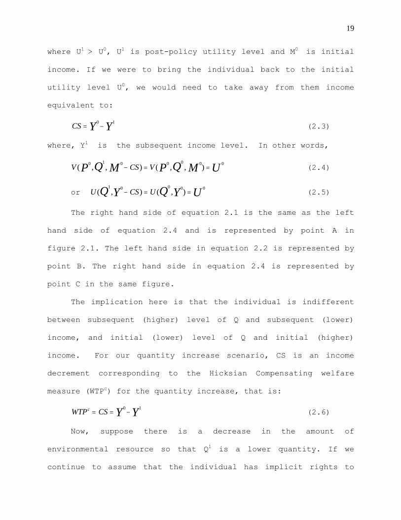
CS Y Y= −0 1

0

0

(2.3)

where, Y1 is the subsequent income level. In other words,

V CS VP Q M P Q M U( , , ) ( , , )0 1 0 0 0 0− = = (2.4)

or U C (2.5) S UQ Y Q Y U( , ) ( , )1 0 0 0− = =

The right hand side of equation 2.1 is the same as the left

hand side of equation 2.4 and is represented by point A in

figure 2.1. The left hand side in equation 2.2 is represented by

point B. The right hand side in equation 2.4 is represented by

point C in the same figure.

The implication here is that the individual is indifferent

between subsequent (higher) level of Q and subsequent (lower)

income, and initial (lower) level of Q and initial (higher)

income. For our quantity increase scenario, CS is an income

decrement corresponding to the Hicksian Compensating welfare

measure (WTPc) for the quantity increase, that is:

WTP CSc Y Y= = −0 1 (2.6)

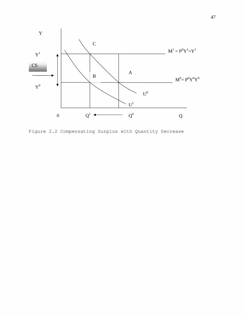
Now, suppose there is a decrease in the amount of

environmental resource so that Q1 is a lower quantity. If we

continue to assume that the individual has implicit rights to

20

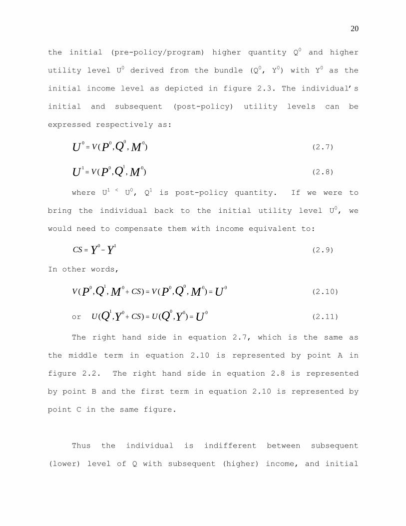
the initial (pre-policy/program) higher quantity Q0 and higher

utility level U0 derived from the bundle (Q0, Y0) with Y0 as the

initial income level as depicted in figure 2.3. The individual’s

initial and subsequent (post-policy) utility levels can be

expressed respectively as:

0 0 0 0U P Q MV= ( , , )

)

(2.7)

1 0 1 0U P Q MV= ( , , (2.8)

where U1 < U0, Q1 is post-policy quantity. If we were to

bring the individual back to the initial utility level U0, we

would need to compensate them with income equivalent to:

CS Y Y= −0 1

0

0

(2.9)

In other words,

V CS VP Q M P Q M U( , , ) ( , , )0 1 0 0 0 0+ = = (2.10)

or U C (2.11) S UQ Y Q Y U( , ) ( , )1 0 0 0+ = =

The right hand side in equation 2.7, which is the same as

the middle term in equation 2.10 is represented by point A in

figure 2.2. The right hand side in equation 2.8 is represented

by point B and the first term in equation 2.10 is represented by

point C in the same figure.

Thus the individual is indifferent between subsequent

(lower) level of Q with subsequent (higher) income, and initial

21

(higher) level of Q with initial (lower) income. Now, CS is an

income increment corresponding to the individual’s willingness

to accept compensation for the lower level of Q or the Hicksian

Compensating Surplus (WTAc), that is:

WTA CS Y Y= = −1 0 (2.12)

One could define CS in terms of the expenditure (instead of

utility) function. Thus for a quantity increase, CS is an income

decrement, representing WTPc for the quantity increase.

WTP CS e ec P Q U P Q U= = −| ( , , ) ( , , )|0 1 0 0 0 0 (2.13)

WTP CSc M M= = −| 1 |0 (2.14)

where M0 > M1 since it would cost less (therefore less income) to

achieve U0 with a higher level of Q = Q1.

For a quantity decrease, CS is an income increment,

representing WTAc for the quantity decrease.

WTA CS e ec P Q U P Q U= = −| ( , , ) ( , , )|0 1 0 0 0 0 (2.15)

WTA CSc M M= = −| | (2.16) 1 0

where M1 > M0 since it takes more expenditure (therefore more

income) to achieve U0 with a lower level of Q = Q1.

Now, if instead of assuming that the individual has

implicit rights to the initial quantity we assumed s/he has

rights to subsequent quantity, we would approach the analysis

22

from the perspective of the other Hicksian measure of welfare

change, i.e. the Equivalent Variation (EV).

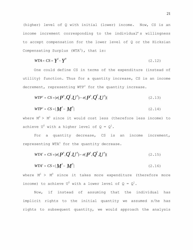
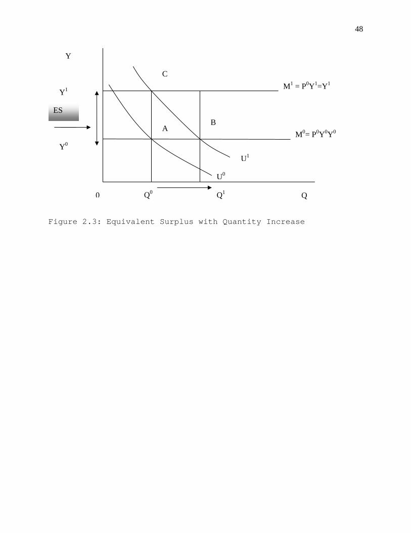
Examining the scenario where a new policy results in an

increase in amount of environmental resource from an initial

quantity Q0 to a subsequent quantity Q1. When the change is an

increase, i.e. Q0 < Q1, the individual’s initial and subsequent

(post-policy) utility levels can be expressed respectively as:

0 0 0 0U P Q MV= ( , , )

)

(2.17)

1 0 1 0U P Q MV= ( , , (2.18)

where U1 > U0, U1 is post-policy utility level. In order to bring

the individual to the subsequent utility level U1, we would need

to compensate them by an amount equal to:

ES Y Y= −1 0

1

1

(2.19)

where, Y1 is the subsequent income level, to bring them up to

the subsequent utility level U1 if the quantity change does not

actually take place. In other words,

V ES VP Q M P Q M U( , , ) ( , , )0 0 0 0 1 0+ = = (2.20)

or U E (2.21) S UQ Y Q Y U( , ) ( , )0 0 1 0+ = =

The second term in equation 2.18 is the same as the second term

in equation 2.20 and is represented by point B in figure 2.3.

The second term in equation 2.17 is represented by point A. The

first term in equation 2.20 is represented by point C. Thus the

23

individual is indifferent between subsequent (higher) level of Q

with initial (lower) income, and initial (lower) level of Q with

subsequent (higher) income. In this case ES represent an is

income increment corresponding to WTAc to forego quantity

increase.

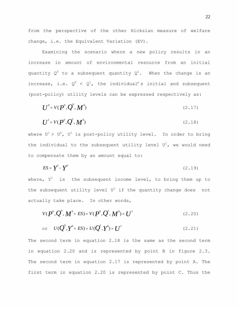
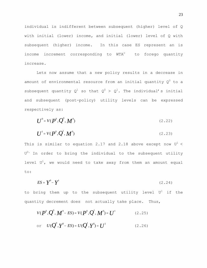
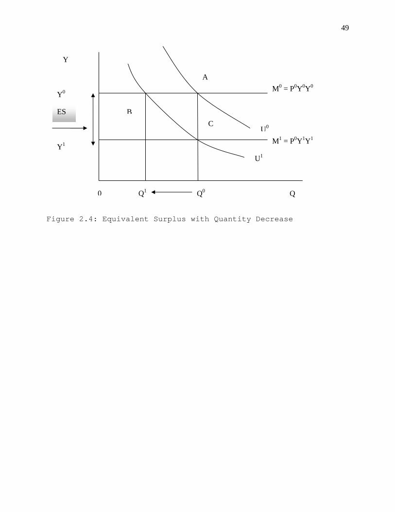
Lets now assume that a new policy results in a decrease in

amount of environmental resource from an initial quantity Q0 to a

subsequent quantity Q1 so that Q0 > Q1. The individual’s initial

and subsequent (post-policy) utility levels can be expressed

respectively as:

0 0 0 0U P Q MV= ( , , )

)

(2.22)

1 0 1 0U P Q MV= ( , , (2.23)

This is similar to equation 2.17 and 2.18 above except now U1 <

U0. In order to bring the individual to the subsequent utility

level U1, we would need to take away from them an amount equal

to:

ES Y Y= −0 1

1

1

(2.24)

to bring them up to the subsequent utility level U1 if the

quantity decrement does not actually take place. Thus,

V ES VP Q M P Q M U( , , ) ( , , )0 0 0 0 1 0− = = (2.25)

or U E (2.26) S UQ Y Q Y U( , ) ( , )0 0 1 0− = =

24

The second term in equation 2.23 is the same as the second term

in equation 2.25 and is represented by point B in figure 2.4.

The second term in equation 2.22 is represented by point A. The

first term in equation 2.25 is represented by point C. The

individual is indifferent between subsequent (lower) level of Q

with initial (higher) income, and initial (higher) level of Q

with subsequent (lower) income. Now ES represents an income

decrement corresponding to WTPe to prevent quantity decrease.

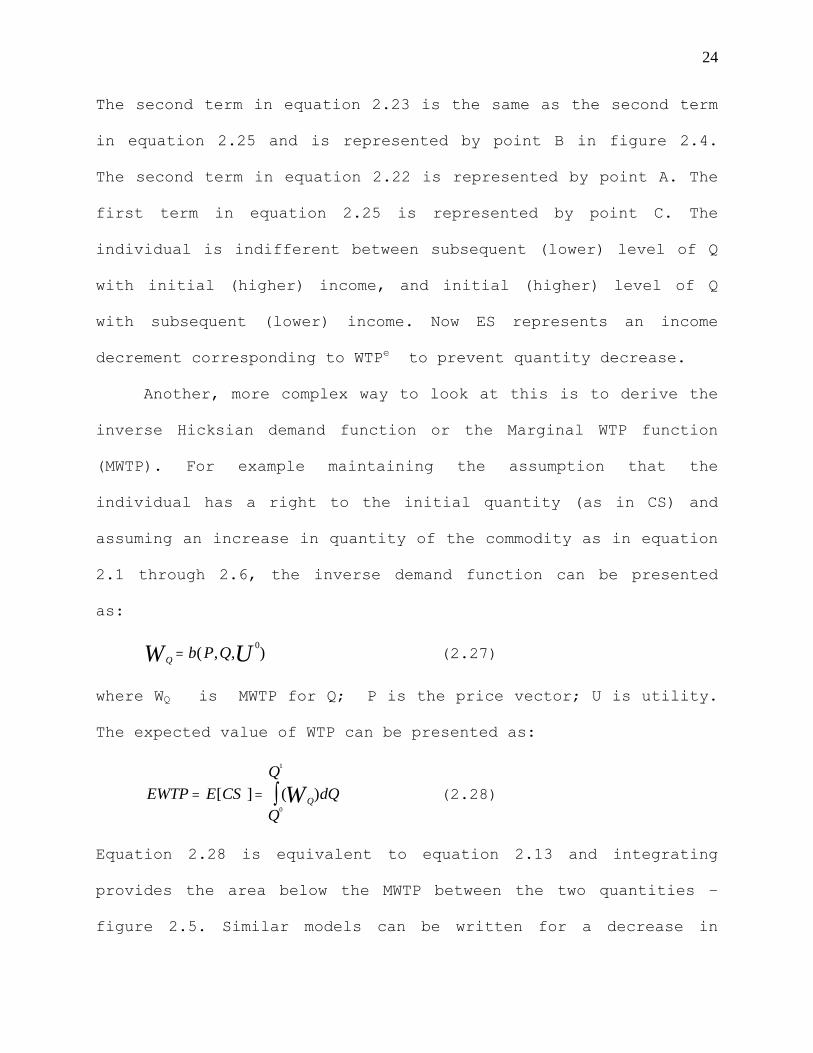
Another, more complex way to look at this is to derive the

inverse Hicksian demand function or the Marginal WTP function

(MWTP). For example maintaining the assumption that the

individual has a right to the initial quantity (as in CS) and

assuming an increase in quantity of the commodity as in equation

2.1 through 2.6, the inverse demand function can be presented

as:

QW b P Q= ( , , )0U (2.27)

where WQ is MWTP for Q; P is the price vector; U is utility.

The expected value of WTP can be presented as:

EWTP E CS dQQ

Q

QW= = ∫[ ] ( )0

1

(2.28)

Equation 2.28 is equivalent to equation 2.13 and integrating

provides the area below the MWTP between the two quantities –

figure 2.5. Similar models can be written for a decrease in

25

quantity and under the ES approach. The parameter estimates of

equation 2.28 can be arrived at by specifying and estimating the

functional form for the observable components of utility.

Most ecosystem values, both active passive use, render

themselves to measurement by ES or CS. Most direct use values

can be measured using market prices since they are marketable.

Moreover, measurement is relatively easy for commodities whose

preference is readily revealed through expenditure eg camping,

hunting, sight seeing, bird-watching which are often measured

using Marshallian Surplus.

In regard to producers, changes in welfare can be measured

using producer surplus. Suppose the environmental resource in

question is used in the production of other goods e.g.

wood/lumber; changes in a watershed ecosystem might entail

increasing the wilderness area and therefore reducing access to

wood for lumbering. This would adversely affect economic rents

accruing to lumbering firms. Total Economic Value for such an

ecosystem would be incomplete without taking to account such

changes.

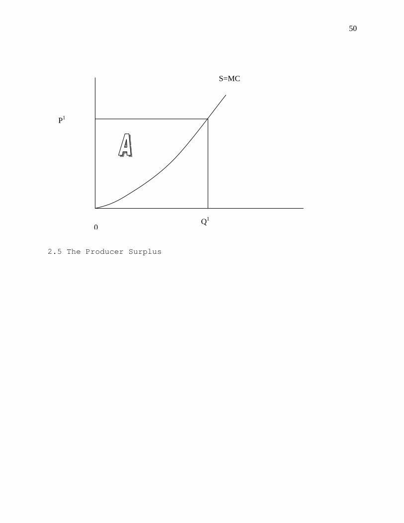
Economic rent is an economic surplus or excess of benefits

over costs. Producer surplus (PS) is a good measure of the

firm’s economic rent. PS TR TVC= − , where TR is total revenue, TVC

is total variable cost. The producer surplus (A in figure 2.5)

can be presented as:

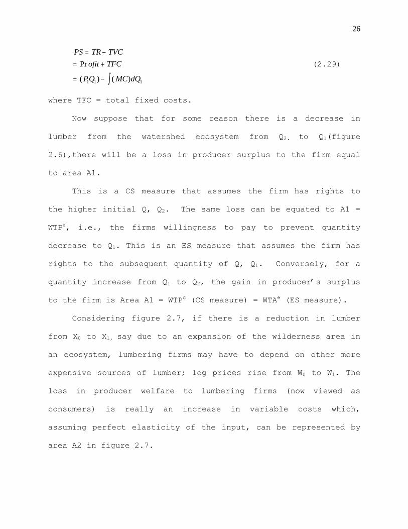
26

PS TR TVCofit TFC

PQ MC dQ

= −= +

= − ∫Pr

( ) ( )1 1 1

(2.29)

where TFC = total fixed costs.

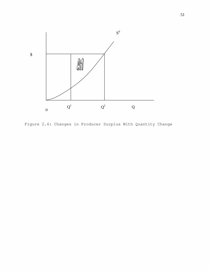
Now suppose that for some reason there is a decrease in

lumber from the watershed ecosystem from Q2. to Q1(figure

2.6),there will be a loss in producer surplus to the firm equal

to area A1.

This is a CS measure that assumes the firm has rights to

the higher initial Q, Q2. The same loss can be equated to A1 =

WTPe, i.e., the firms willingness to pay to prevent quantity

decrease to Q1. This is an ES measure that assumes the firm has

rights to the subsequent quantity of Q, Q1. Conversely, for a

quantity increase from Q1 to Q2, the gain in producer’s surplus

to the firm is Area A1 = WTPc (CS measure) = WTAe (ES measure).

Considering figure 2.7, if there is a reduction in lumber

from X0 to X1, say due to an expansion of the wilderness area in

an ecosystem, lumbering firms may have to depend on other more

expensive sources of lumber; log prices rise from W0 to W1. The

loss in producer welfare to lumbering firms (now viewed as

consumers) is really an increase in variable costs which,

assuming perfect elasticity of the input, can be represented by

area A2 in figure 2.7.

27

Now, for a price increase from W0 to W1, the loss in

producer welfare (“consumer surplus”, since the firm is here

viewed as a consumer of inputs) is area A2 = WTAc (CV measure,

assuming the firm has rights to the lower initial Price, W0) =

WTPc (EV measure, assuming the firm has rights to the higher

subsequent price, W1).Most marketable services of the ecosystem

such as agricultural values like provision of irrigation and

livestock water, and lumbering would be easily valued using

producer surplus.

Conventional Environmental Valuation Techniques

Ecosystem valuation has for a long time been done using

traditional techniques of valuing non-marketed goods and

services including direct and indirect techniques. Direct

(revealed preference) techniques rely on actual expenditure to

reveal the preferences of individuals for environmental goods or

services associated with the expenditure (e.g. the added value

of a house near a forest, or the cost of traveling to a national

park). These techniques include hedonic pricing (HPM) and travel

cost method (TCM). These methods are limited in that they can

only capture use values.

Hedonic pricing is based on the assumption that people

value the characteristics of a good, or the services it

provides, rather than the good itself. It is mostly used to

28

measure the effect of natural amenities on property hence the

value that people attach to the amenity. For instance the

prices of residential property near a lake reflect the value of

a set of property characteristics, including distance from the

lake; structural characteristics of the house; neighborhood

characteristics etc. When factors other than proximity to the

lake are controlled for, any remaining differences in price can

be attributed to differences in proximity to the lake.

With TCM, a survey is used to capture information for all

people visiting a particular site say each year. Data collected

covers distance traveled; cost of travel, county and state of

residence of the visitor; socio-economic characteristics of the

visitor; direct travel-related expenditures.

The correct multiplier is used to isolate travel cost due

to visitation to the site other from all the other purposes of

visit to the area, mostly from a regression equation. Demand for

visits to the site and consumer surplus per person per trip are

estimated and aggregation is done to arrive at the total value.

Indirect (stated preference) techniques rely on

questionnaires to elicit participant’s response to questions

that simulate a market situation. Indirect techniques have the

advantage of being able to capture non-use values. The major one

of these techniques is Contingent Valuation Method (CVM).

29

The Contingent Valuation Method (CVM) seems to be the most

commonly used techniques of measuring the value of improvements

in ecosystem or resource quality. The CVM adopts survey and

questioning techniques to estimate individual’s expressed

preferences (willingness to pay) for changes in the level of

public resources contingent upon a hypothetical market situation

(Jordan and Elnagheeb, 1993). It is assumed that people will

respond to the contingent market as if it were a real market

situation.

Table 2.1 outlines various watershed ecosystem commodities,

types of economic valuation measures that could or have been

used to value the commodities and the respective valuation

methods. The list is not intended to be exhaustive.

Benefit Transfer Estimation

In the recent past, “benefit transfer” (BT), sometimes

called “benefits transfer”, is becoming increasingly useful as

an approach to valuation of non-marketed public goods and

service. Brookshire and Neill (1992) suggest that, “A benefit

transfer is the application of monetary values obtained from a

particular nonmarket goods analysis to an alternative or

secondary policy decision setting”.

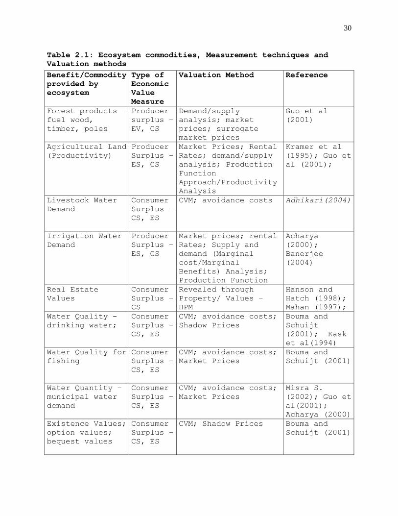
30

Table 2.1: Ecosystem commodities, Measurement techniques and Valuation methods Benefit/Commodity provided by ecosystem

Type of Economic Value Measure

Valuation Method Reference

Forest products – fuel wood, timber, poles

Producer surplus –EV, CS

Demand/supply analysis; market prices; surrogate market prices

Guo et al (2001)

Agricultural Land (Productivity)

Producer Surplus –ES, CS

Market Prices; Rental Rates; demand/supply analysis; Production Function Approach/Productivity Analysis

Kramer et al (1995); Guo et al (2001);

Livestock Water Demand

Consumer Surplus –CS, ES

CVM; avoidance costs Adhikari(2004)

Irrigation Water Demand

Producer Surplus –ES, CS

Market prices; rental Rates; Supply and demand (Marginal cost/Marginal Benefits) Analysis; Production Function

Acharya (2000); Banerjee (2004)

Real Estate Values

Consumer Surplus –CS

Revealed through Property/ Values – HPM

Hanson and Hatch (1998); Mahan (1997);

Water Quality - drinking water;


CVM; avoidance costs; Shadow Prices

Bouma and Schuijt (2001); Kask et al(1994)

Water Quality for fishing


CVM; avoidance costs; Market Prices

Bouma and Schuijt (2001)

Water Quantity – municipal water demand


CVM; avoidance costs; Market Prices

Misra S. (2002); Guo et al(2001); Acharya (2000)

Existence Values; option values; bequest values


CVM; Shadow Prices Bouma and Schuijt (2001)

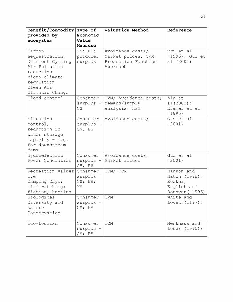
31

Benefit/Commodity provided by ecosystem

Type of Economic Value Measure

Valuation Method Reference

Carbon sequestration; Nutrient Cycling Air Pollution reduction Micro-climate regulation Clean Air Climatic Change

CS; ES; producer surplus

Avoidance costs; Market prices; CVM; Production Function Approach

Tri et al (1996); Guo et al (2001)

Flood control Consumer surplus -CS

CVM; Avoidance costs; demand/supply analysis; HPM

Alp et al(2002); Kramer et al (1995)

Siltation control, reduction in water storage capacity – e.g. for downstream dams

Consumer surplus –CS, ES

Avoidance costs;

Guo et al (2001)

Hydroelectric Power Generation

Consumer surplus –CV, EV

Avoidance costs; Market Prices

Guo et al (2001)

Recreation values i.e Camping Days; bird watching; fishing; hunting

Consumer surplus –CS; ES; MS

TCM; CVM Hanson and Hatch (1998); Bowker, English and Donovan( 1996)

Biological Diversity and Nature Conservation

Consumer surplus –CS; ES

CVM

White and Lovett(1197);

Eco-tourism Consumer surplus –CS; ES

TCM Menkhaus and Lober (1995);

32

Rosenberger and Loomis (2000) add one of the basic tenets

of benefits transfer, that is, the sites have to be similar.

They define Benefits Transfer as - “The adaptation and use of

economic information derived from specific site(s) under certain

resource and policy conditions to a site with similar resources

and conditions”. In BT literature, the site that provides data

is referred to as the study site, while the site to which data

is transferred is called the policy site.

Benefits Transfer Estimation (BTE) is gaining importance

because of its usefulness whenever it may not be practical for

an organization to collect data on which to base economic value

estimation at short notice (Bergstrom and Civita, 1999), and in

cases where a high degree of precision is not critical (Du,

1998). This approach reduces costs (Kask and Shogren, 1994) and

is therefore important during times of public funding cuts. It

enables estimation within a shorter time than traditional

methods, reducing the time it takes for policy makers to make

informed decisions (Bingham, 1992). Economists realize that

benefits transfer estimates can, in the best case scenario, be

only as good as the original studies. Thus benefits transfer is

regarded as a “second best” approach to measuring economic value

(Resenberger and Loomis, 2000) basically because it relies on

secondary data.

33

Benefits Transfer Estimation has been applied in many areas

including valuation of forest and rangeland resources (USDA

forest Service, 1990; Verna, 2000) outdoor recreational services

including recreational water quality (Du, 1999; Rosenberger and

Loomis, 2000; Mitchell and Carson, 1984 ), flood control and

ecological risk reduction services (Alp, Clark and Novotny,

2002) ecosystems ( Constanza et al, 1999), ground water quality

(Bergstrom, Kevin and Boyle, 1992; Denevan and Alp, 2001);

cancer and smog reduction ( Caulkins and Sessions, 1997).

Moreover it is evident that BTE will continue to play a key

role in the policy arena with state and government agencies

using, recommending or allowing use of the technique in public

policies and policies that impact on natural resources and the

environment (NOAA, 1996; USEPA, 1983; US Water resource Council,

1983; USDA Forest Service, 1990; Bergstrom and Civita).

Literature provides a number of types of BT including

expert judgment, value transfer, benefits function transfer, and

meta analysis (Bergstrom and Cavita; Rosenberger and Loomis;

Brookshire and Neill; Loomis, 1992; US Water resource Council,

1983).

Value transfer entails transfer of a single point estimate

or the transfer of a measure of central tendency, e.g. the mean

or median WTP. Single point estimate transfer is based on

estimate from one study or a range of estimates if there are a

34

number of studies. Expert judgment entails aggregating values

derived from an expert or a panel of experts with the relevant

adjustments.

Transfer of benefits function or value estimator model

entails using the benefits function derived from the study site

together with explanatory variable data derived from the policy

site to estimate the total number of units and value per unit at

the policy site. Benefits function transfer enables accounting

for differences in physical and demographic characteristics

between study and policy sites and is considered superior to

fixed value transfer (Loomis, 1992).

In the context of BT, Meta analysis can be viewed as the

statistical summarization of results of individual valuation

studies to be and using the summarized findings to value changes

at a policy site. Thus data for meta analysis is mostly summary

statistics including population characteristics, environmental

resources of study site, and valuation methodology use. In most

cases, meta regression analysis is applied to a benefits

function based on data from previous studies to estimate the

value of the policy site (Poe, Boyle and Bergstrom, 2001;

Rosenberger and Loomis). Although Meta analysis has been used in

BT, a number of authors including Poe, Boyle and Bergstrom;

Delevan and Epp, 2001 do not view meta analysis as a suitable

tool for BT. Delevan and Epp view Meta analysis as an

35

unsatisfactory transfer tool and argue that summarizing a number

of studies and methodologies may lead to erroneous coefficients.

The authors Poe, Boyle and Bergstrom argue that Meta

analysis is based on a number of studies with different

methodologies and resulting values that vary systematically

across the studies. They urge caution in using Meta analysis to

provide value estimate for policy analysis. Given these

misgivings and the trend away from Meta analysis in the recent

past, we opt not to use Meta analysis as a method of BT in this

study. Understandably, the literature seems to lean toward two

major methods of BT namely, value transfer and benefits function

transfer (Bergstrom and Cavita; Rosenberger and Loomis;

Brookshire and Neill; Loomis).

Rosenberger and Loomis outline a number of problems related

to Benefits transfer. The quality of original data affects

quality of process, and data documentation is often

insufficient. In addition there are not many existing studies

and those that are available will not have been conducted with

benefit transfer in mind so the data they provide is not

necessarily amenable to benefit transfer.

Given these problems there has been quite some controversy

surrounding the technique. Brookshire (1992) recommends that the

final use of benefit estimate should determine its required

accuracy and proposes a continuum from “Gains in Knowledge” at

36

the lowest end through “Screening of projects”, “Policy

decision” and “compensating damages/utility externality costs”

at the highest end. Brookshire and Neill (1992) suggest that BT

estimates should only be used towards the low end of the

continuum. Devouges et al (1992) offers a similar continuum but

is more optimistic about potential uses of BT.

It appears as suggested by Smith (1992) and by Bergstrom

and Boyle (1992) that economists are divided into two camps over

the issue of Benefits transfer; those who would rather wait for

the ideal data (idealists) on one hand, and those who believe

that some information is better than none (pragmatists) on the

other.

Protocol for Meaningful Benefit Transfer

A number of conditions necessary to ensure effective and

efficient benefits transfer estimation are discussed by several

authors including Rosenberger and Loomis.

First the policy context should be thoroughly defined to

identify three issues namely: impact of proposed action,

relevant population to be affected and data needs.

Second, the study site data should meet certain conditions

for critical benefits transfer. It should have adequate data,

methods, and empirical analysis; information on benefits/costs

and characteristics of affected pop; information on statistical

37

relationship between benefits/costs and physical characteristics

of the site; and adequate number of individual studies for

credible inference.

Third, there has to be correspondence between study and

policy sites with regard to environmental resources and changes;

markets, population demographics and cultural aspects;

conditions and quality of resource use activities and

experiences.

There seems to be a general consensus that benefits

transfer should be done systematically. Rosenberger and Loomis;

Desvousges, Naughton and Parson (1998); Saplaco and

Herminia(2003) identify a set of steps that should form the

necessary procedure to BTE. From an examination of the two

sources, the procedure can be summarized as follows:

1. Identify the resources (forests, wetlands, wildlife

etc) affected by the proposed action;

2. Translate resource impacts to changes in commodity

(goods, services, functions) use ;

3. Measure commodity use changes;

4. Conduct a literature search for relevant study sites;

5. Assess relevance and applicability of study site data;

6. Depending on the approach selected (value transfer,

function transfer or expert opinion) identify or

38

forecast a benefit measure from the study site to the

policy site.

7. Adjust the benefits measure for any differences in

site characteristics between the study and policy

site. These may not be easy to make, particularly

where the benefits function approach is not feasible.

Adjustment for per capita income or Gross Site Product

(GSP) which is the Gross Domestic Product (GDP) of

study site, and the price level are most common and

are discussed later.

8. Determine total number of affected units (e.g.

households, individuals) in the policy site, Aggregate

the benefits over the entire policy site by

multiplying the benefit measure by affected

population.

Empirical Methodology and Data Issues

This research took place in stages. The first stage was to

establish a benchmark for simulation of land use change, by

taking stock and creating an inventory of resources at the

policy site. In taking stock, an attempt was be made to map out

the current land use (and land cover) patterns. Data and

information for this exercise were sought mainly from NARSAL

(2007).

39

Stock taking was done simultaneously with creating an

inventory of past studies that have measured values that could

be derived from similar ecosystems and ecosystem resources.

These studies were later used for benefit transfer.

The second stage entailed developing a land use and land

use change model for the area, and postulating different land

use scenarios as discussed in chapters three and four. Land use

determines the level of ecosystem services and functions

provided by the watershed. Land use changes therefore precede

changes in ecosystem functions and services.

The third stage entailed quantifying changes in underlying

ecosystem services, specifically water quality, for various land

use scenarios. For instance suppose the amount of land under

forest decreases by a certain amount, and the amount of land

under commercial land use increases by the same amount, we would

at this stage estimate the extent of say an increase in runoff

and subsequent concentration of suspended solids in the streams

in the ecosystem, etc.

The fourth stage entailed quantifying and measuring the

economic value of the aforesaid changes in ecosystem services

and functions resulting from changes in land use. Such effects

will be reflected by changes in value of amenities, services and

functions e.g. change in price/cost of drinking water in the

neighboring counties, changes in number of fish caught in the

40

area streams the and the value of the same, increase in number

of sick-off days, etc. Measurement of the economic values

resulting from the identified economic effects was done using

Benefits Transfer. This study closely followed the procedures

for benefits transfer outlined earlier with regard to valuation.

Below is an hypothetical example of how the protocol would be

(and was) applied.

Benefit Transfer Analysis: A Hypothetical Case

One of the major ecosystem services provided by our policy

site is drinking water quality. Over time, there will be changes

in land use which will cause changes in this service. Let us

postulate a high growth scenario, and imagine that during the

second stage of our study, land use models lead us to believe

that there will be a takeover of some of the wetlands in the

UCRB (identified during the first stage of research) by real

estate developers. Scientific knowledge tells us that such

takeovers will most likely lead to a deterioration of drinking

water quality due to the reduction in runoff sinks so that more

nutrients end up in drinking water sources. This knowledge is

further established in the third stage of our research. In the

fourth stage of the study we ask what people, both within and

outside the policy site, would be willing to pay to fund a

program that forestalls the wetland takeover and therefore

41

protects drinking water quality. Benefits transfer will be used

to value drinking water quality changes, following these general

steps:

The resource affected by the proposed action is identified

as the wetlands;

Translating the impact on wetlands to changes in water

quality is the second step, which is carried out as outlined

above;

Measuring change (reduction) in drinking water quality at

the policy site is the third step – Assuming that the individual

has a right to the initial situation (higher drinking water

quality, with the wetlands), a decrease in drinking water

quality could be measured using CS which represents an income

increment corresponding to the individuals willingness to accept

compensation (WTAc ) for the lower level of water quality. Given

the difficulties of measuring WTAc discussed earlier, we will

follow Freeman (1993) and measure WTAc indirectly through WTPc .

In essence this means that we will assume that the individual

has a right to the subsequent lower quality. Thus we will use

ES, representing an income decrement corresponding to the

individual’s willingness to pay (WTP) to prevent a water quality

decrease.

The fourth step entails conducting a search for relevant

study sites – we will search for published and unpublished

42

articles that have carried out similar studies. Such studies

will most likely use the CVM to value drinking water quality in

relation to wetland removal/sustenance.

The fifth step will entails assessing relevance and

applicability of study site data – This step will involve

identifying and isolating studies based on sites that are as

similar as possible to the policy site with respect to

geography, income, preferences, culture, substitution, social

characteristics.

The next step will entail identifying or forecasting a

benefit measure from the study site to the policy site – This

will depend on the approach we find to be most suitable. Our

method of choice will be the functions transfer approach given

its advantages discussed earlier. To perform this sixth step,

the fifth step, above, would of necessity entail finding out

whether the benefits transfer functions have been specified in

the sources. This step will then entail adapting the benefits

function(s) to the policy site characteristics and forecasting

the benefit measure. For instance where the primary study is

based on CVM the model could be as follows:

WTP = α + β1*Q+ β2SEC + β3SC (2.30)

where α, β1, β2 and β3 are coefficients from the primary study, Q

represents (perceived) quality of drinking water, SEC is a

vector of socioeconomic characteristics of the user population,

43

while SC is a vector of other characteristics of the site.

Incorporating SEC and SC allows us to adjust for differences in

the study and policy sites.

In case there are no relevant and applicable studies where

the benefits functions are specified, then the value transfer

will be our second choice method. In that case we will use the

single unit value for this step where there is only one relevant

study or an average over the several relevant studies. In the

rare event that there are absolutely no relevant studies, the

opinion of a panel of experts will be sought as a last resort.

Such a panel could be composed of persons familiar with the site

and with valuation sourced from academia, USDA, USFS, and USFWS.

Adjusting the benefits measure for any differences in site

characteristics will be done as provided for in the preceding

step. This is not possible for value transfer. Whatever the

transfer method, adjustment for income and time will be done

following the procedure presented below.

The last step will entail determining total number of units

(individuals or households) affected by the reduction in water

quality. This will be done using population data for the area

and the surrounding areas that could be affected. Aggregate the

benefits over the affected population by multiplying the benefit

measure by total number of individuals affected by the wetland

takeover and subsequent water quality change.

44

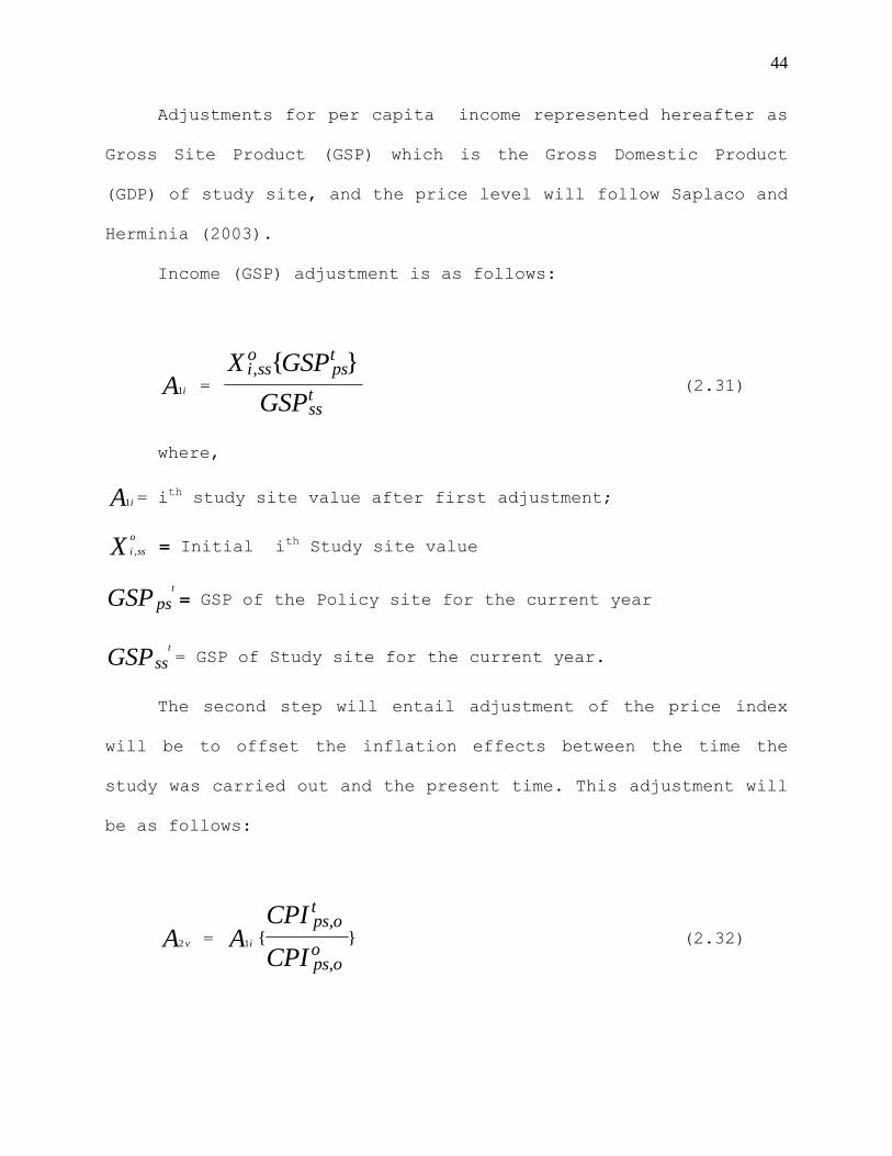
Adjustments for per capita income represented hereafter as

Gross Site Product (GSP) which is the Gross Domestic Product

(GDP) of study site, and the price level will follow Saplaco and

Herminia (2003).

Income (GSP) adjustment is as follows:

1iA = i sso

pst

sst

X GSPGSP

, (2.31)

where,

1iA = ith study site value after first adjustment;

i ssoX , = Initial ith Study site value

t

psGSP = GSP of the Policy site for the current year

t

ssGSP = GSP of Study site for the current year.

The second step will entail adjustment of the price index

will be to offset the inflation effects between the time the

study was carried out and the present time. This adjustment will

be as follows:

2 vA = 1iA ,

,

ps ot

ps oo

CPICPI

(2.32)

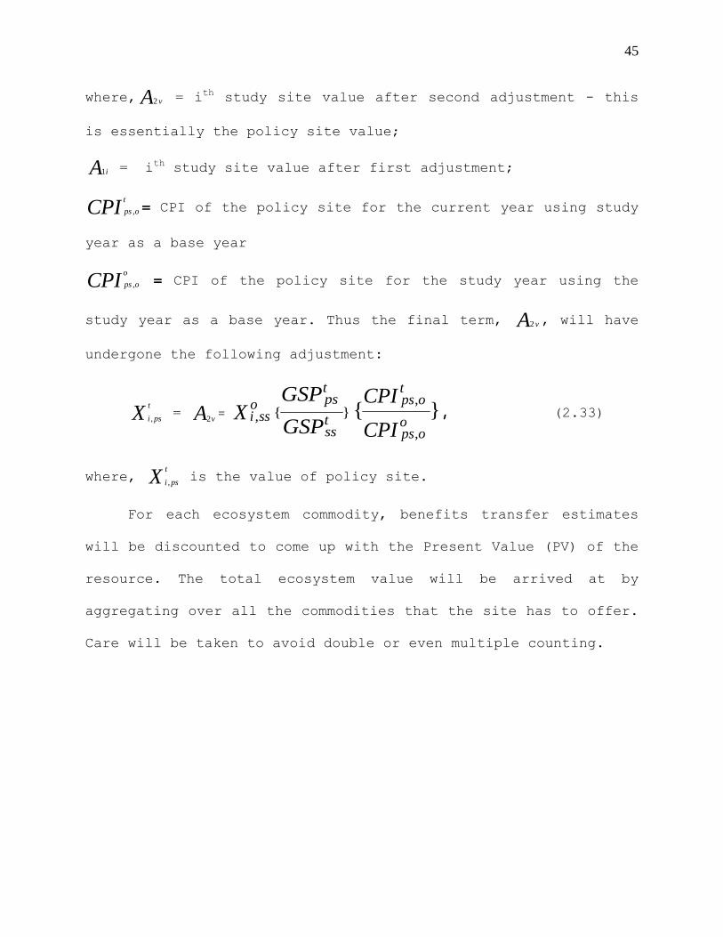
45

where, 2 vA = ith study site value after second adjustment - this

is essentially the policy site value;

1iA = ith study site value after first adjustment;

ps otCPI , = CPI of the policy site for the current year using study

year as a base year

ps ooCPI , = CPI of the policy site for the study year using the

study year as a base year. Thus the final term, 2 vA , will have

undergone the following adjustment:

i pstX , = 2vA = i ss

oX , pst

sst

GSPGSP

,

,

ps ot

ps oo

CPICPI

, (2.33)

where, is the value of policy site. i pstX ,

For each ecosystem commodity, benefits transfer estimates

will be discounted to come up with the Present Value (PV) of the

resource. The total ecosystem value will be arrived at by

aggregating over all the commodities that the site has to offer.

Care will be taken to avoid double or even multiple counting.

46

Figure 2.1 Compensating Surplus with Quantity Increase

M1 = P0Y1Y1

B

Q0

A

Q1

Y0

Y1

Y

CS

M0 = P0Y0Y0

U1C

U0

0 Q

47

Y

Figure 2.2 Compensating Surplus with Quantity Decrease

M0= P0Y0Y0 B

Q1

A

Q0

Y1

Y0

CS

M1 = P0Y1=Y1

U0

U1

Q

C

0

48

Y

Figure 2.3: Equivalent Surplus with Quantity Increase

M0= P0Y0Y0 B

Q0

A

Q1

Y1

Y0

ES

M1 = P0Y1=Y1

U1

U0

Q

C

0

49

Figure 2.4: Equivalent Surplus with Quantity Decrease

M1 = P0Y1Y1

B

Q1

A

Q0

Y0

Y1

Y

ES

M0 = P0Y0Y0

U0C

U1

0 Q

50

S=MC

P1

Q1 0

2.5 The Producer Surplus

51

S0

$

Q1 Q2 Q 0

Figure 2.6: Changes in Producer Surplus With Quantity Change

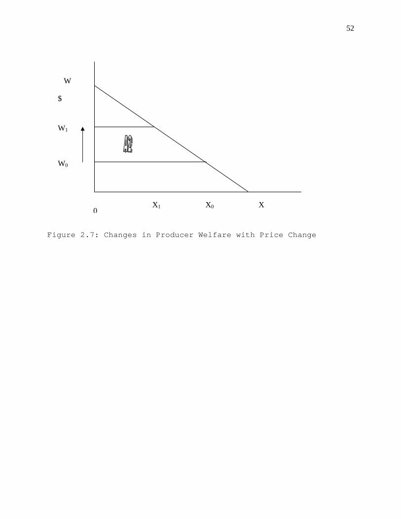
52

W

Figure 2.7: Changes in Producer Welfare with Price Change

$

X0 0

W1

W0

X1 X

53

CHAPTER III

THEORETICAL LAND USE MODEL

Overview

In this section we discuss theoretical land use modeling

under the assumption of risk neutrality. The risk neutrality

assumption is found to provide the best estimates of acreage

allocation, and, it is simple in the sense that there is no need

of incorporating risk taking/aversion behavior of the economic

agent (Miller and Plantinga, 1999; Ahn, Plantinga and Alig,

2000).

Analysis of optimal land allocation has been carried out by

a number of authors including Miller and Plantiga (1999);

Plantinga, Maulding and Miller (1999). The aforesaid studies

have applied econometric models to estimate aggregate (such as

farm and forest as opposed to crop level) land allocation. Land

allocation, and the many factors affecting it, change over time.

This makes land use (and land use change)a suitable candidate

for time series and structural time series modeling.

Farm acreage response/farm land allocation among

(different) crop enterprises have been estimated using

econometric and time series models (Duffy, Shaishali, and

54

Kinnucan 1994; Houston et al., 1999; Wu and Segerson, 1995;

Plantiga, 1996; Lichtenberg, 1989; Banerjee, 2004). Structural

Time Series Models (STSM) pioneered by Harvey (1989) have seen

recent use in estimating farm acreage response models (Houston

et al., 1999; Adhikari, 2004). The STSM has the advantage of

being able to capture structural and technological change, which

are either overlooked or assumed to be deterministic in

conventional econometric and time series modeling. Despite these

benefits, the STSM has not been exploited much in aggregate

acreage response modeling.

This study pursues three approaches to modeling aggregate

land use, namely, econometric, time series and structural time

series analysis. Based on the forecasting ability, we choose the

best model from the three, and apply it to forecast land

allocation in the upper Chattahoochee river basin, in North

Georgia.

Theoretical Econometric Model

Following Wu and Segerson (1995) and Miller and

Plantinga(1999) we develop a model of land allocation at the

aggregate watershed (two-county) level, assuming profit or net

benefit maximization under risk neutrality. Consider a land

manager/owner who maximizes total restricted returns to A acres

of land, by allocating the land optimally among i alternative

55

uses (i= 1,…n). We use discounted (present value) benefits

approach to account for the fact that returns to forestry are

realized over long periods of time. The land allocation process

can then be expressed as:

)(max0

Xn

iiAi ∑

=

∏ (3.1)

Subject to,

AAn

ii =∑

=0

(3.2)

Where X = Matrix of exogenous variables

Ai = Acreage of the ith land use

A = Total available acreage

i∏ = expected returns from land use i.

Solving the constrained profit maximization problem above gives

us the optimal allocation to land use i, denoted by

* ( )i iA f X= for all i=1,…,n (3.3)

We can rewrite equation 3.3 from the land share perspective as

follows:

** ( )i ii

f XSA AA= = (3.4)

)(* XSS ii = (3.5)

where = optimal expected share of land use i. *iS

Analytically, equation 3.5 can be estimated as a flexible

functional form for the restricted benefits function or for the

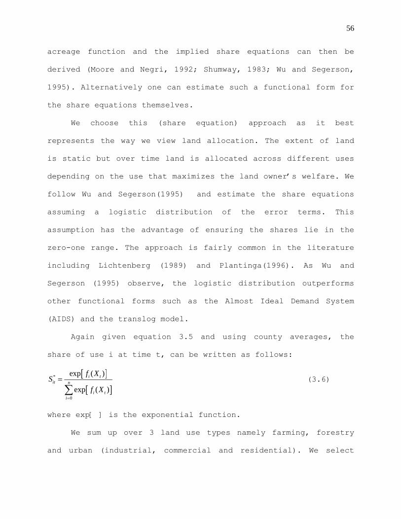
56

acreage function and the implied share equations can then be

derived (Moore and Negri, 1992; Shumway, 1983; Wu and Segerson,

1995). Alternatively one can estimate such a functional form for

the share equations themselves.

We choose this (share equation) approach as it best

represents the way we view land allocation. The extent of land

is static but over time land is allocated across different uses

depending on the use that maximizes the land owner’s welfare. We

follow Wu and Segerson(1995) and estimate the share equations

assuming a logistic distribution of the error terms. This

assumption has the advantage of ensuring the shares lie in the

zero-one range. The approach is fairly common in the literature

including Lichtenberg (1989) and Plantinga(1996). As Wu and

Segerson (1995) observe, the logistic distribution outperforms

other functional forms such as the Almost Ideal Demand System

(AIDS) and the translog model.

Again given equation 3.5 and using county averages, the

share of use i at time t, can be written as follows:

[ ][ ]

*

0

exp ( )

exp ( )

i tit n

i ti

f XS

f X=

=

∑ (3.6)

where exp[ ] is the exponential function.

We sum up over 3 land use types namely farming, forestry

and urban (industrial, commercial and residential). We select

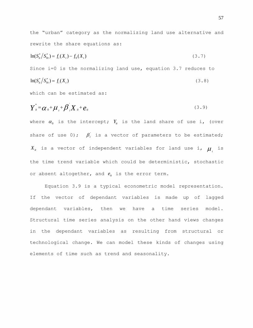
57

the “urban” category as the normalizing land use alternative and

rewrite the share equations as:

* *0ln( ) ( ) ( )it t i t tS S f X f X= − 0 (3.7)

Since i=0 is the normalizing land use, equation 3.7 reduces to

* *0ln( ) ( )it t i tS S f X= (3.8)

which can be estimated as:

'*

0it it itt i eY µ βα= + + +X (3.9)

where 0α is the intercept; is the land share of use i, (over

share of use 0); is a vector of parameters to be estimated;

is a vector of independent variables for land use i,

itY

'iβ

itXtµ is

the time trend variable which could be deterministic, stochastic

or absent altogether, and is the error term. ite

Equation 3.9 is a typical econometric model representation.

If the vector of dependant variables is made up of lagged

dependant variables, then we have a time series model.

Structural time series analysis on the other hand views changes

in the dependant variables as resulting from structural or

technological change. We can model these kinds of changes using

elements of time such as trend and seasonality.

58

Structural Time Series Modeling

A Structural Time Series Model (STSM) of land use is

estimated in order to incorporate existing structural or

technological change. The issue of structural/technological

change seems to have been overlooked in most of the literature

on land use change including crop acreage response models.

Most authors incorporate trend dummy variables in their

models to capture the impacts of technological progress (Chavas

and Holt, 1990; Shideed et al., 1987). However, one limitation

of these studies is that they assume a deterministic trend

component in acreage response and specify the model with a time

trend.

We choose to let the data tell us the nature of the trend,

and by implication the structural/technological change. We do so

by estimating three options that incorporate trend components in

our land use share equations, that is, stochastic trend no

seasonality(STNS); fixed trend no seasonality (FTNS); no trend

no seasonality (NTNS). We assume “no seasonality” because we are

using annual data without the possibility of capturing

seasonality.

The Structural Time Series (STS) Model was first proposed

by Harvey in 1989. Unlike traditional ARIMA models, the STSM is

developed directly in terms of components of interest, such as

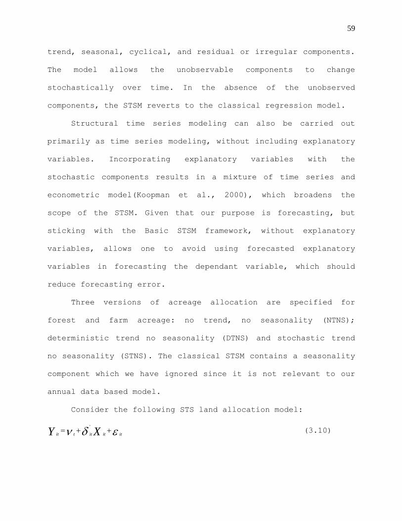
59

trend, seasonal, cyclical, and residual or irregular components.

The model allows the unobservable components to change

stochastically over time. In the absence of the unobserved

components, the STSM reverts to the classical regression model.

Structural time series modeling can also be carried out

primarily as time series modeling, without including explanatory

variables. Incorporating explanatory variables with the

stochastic components results in a mixture of time series and

econometric model(Koopman et al., 2000), which broadens the

scope of the STSM. Given that our purpose is forecasting, but

sticking with the Basic STSM framework, without explanatory

variables, allows one to avoid using forecasted explanatory

variables in forecasting the dependant variable, which should

reduce forecasting error.

Three versions of acreage allocation are specified for

forest and farm acreage: no trend, no seasonality (NTNS);

deterministic trend no seasonality (DTNS) and stochastic trend

no seasonality (STNS). The classical STSM contains a seasonality

component which we have ignored since it is not relevant to our

annual data based model.

Consider the following STS land allocation model:

'

it itt itY X itν δ= + +ε (3.10)

60

Where 0α is the intercept; is the land share of use i; itY 'iδ is

a vector of parameters to be estimated; is a vector of

explanatory variables for land use i,

itX

tν is the trend component,

and itε is the white noise disturbance term.

The simple STSM without explanatory variables may be

represented by,

it t itY ν ε= + (3.11)

If the trend is stochastic, the trend component may be

represented by,

1 1t t t tν ν β− −= + +η (3.12)

ttt ξββ += −1 (3.13)

where ηt ~ NID (0, ση2) and ξt ~ NID (0, σξ2)

Equations (3.12) and (3.13) represent the level and the

slope of the trend, respectively; 1tν − is a random walk with a

drift factor, βt. The drift factor follows a first-order

autoregressive process as provided in equation 3.13. The

stochastic trend variable ( tν ) captures the technological

progress and structural change in the farm and forestry sectors

over the past years.

The form that the trend takes depends on whether the

variances, ση2 and σξ2 (hyper parameters) are zero or not. If

either ση2 or σξ2 or both are non-zero, then the trend is said to

61

be stochastic; STNS is the way to go. Otherwise, if both are

zero, the trend is linear; the model reverts to a deterministic

linear trend (DTNS),

tit itY ν ε= + (3.14)

where, 1t t tν ν −= + β , with tβ being a fixed slope component, or, if

the slope component is zero, then the expression reduces to,

1t tν ν −= .

If tν is zero, there is no trend; the STS model reverts to a

simple classical regression model without a trend term and the

STS model may not be the way to go. Our third approach to

estimating land use is time series analysis.

The Vector Autoregressive Model

Vector Autoregressive (VAR) models are the multivariate

estimation equivalent of Autoregressive Integrated Moving

Average (ARIMA) models in univariate estimation. Various

criticisms of VAR models have been put forward, the major ones

being that they are not based on economic theory, that

individual coefficients of the model estimates are difficult to

interpret, and that they can not be used for policy analysis

(Gujarati, 2003; Kennedy, 1998).

Proponents of VAR approach argue that the models are useful

for forecasting as they often outperform econometric models;

62

they are also useful for describing various relationships in the

data, and testing certain hypothesis and theories (Gujarati,

2003; Kennedy, 1998). Thus the VAR methodology has remained a

line of choice for many economists particularly when the goal is

forecasting as opposed to policy analysis. The basic VAR model

can be represented as follows:

1 1 ...t tY Y Yp t p tµ δ δ −−= + + + +ν (3.15)

where, Yt is a vector of endogenous variables; δ is a

vector of parameters to be estimated, p is the number of lags,

and for all i and t, tν is a vector of uncorrelated error terms;

~ (0, )tν Ω , and Ω is a diagonal matrix. The representation could

also include a trend term.

Individually for two endogenous variables and , based on

two lags (p=2), the equations can be represented as:

1Y 2Y

1 1 11 1 1 12 1 2 13 2 1 14 2 2 1

2 2 21 1 1 22 1 2 23 2 1 24 2 2 2

t t t t t

t t t t t

Y Y Y Y YY Y Y Y Y

t

t

µ δ δ δ δ νµ δ δ δ δ

− − − −

− − − −

= + + + + += + + + + +ν

(3.16)

where the δ s are parameter estimates;1

21 ~ (0, )tν σ and

2

22 ~ (0, )tν σ for

all t.

Given the challenge in interpreting VAR parameter

estimates, proponents of the model recommend inducing shocks or

innovations to the error terms and using an “impulse response

function” to map out the response of the endogenous variables.

We do not need to follow this path to the end since our goal is

63

simply forecasting the endogenous variables – we will stop at

deriving the best forecasting fit for the data. In the next

chapter, we estimate land allocation using the three approaches,

namely econometrics, time series analysis and structural time

series analysis. Our goal in estimation was basically

forecasting land use and land use change. Without a priori

knowledge of the type of model that would perform better in

forecasting land use, between econometric, STS and VAR models,

we opted to run the three types and let the data decide. We

would then select the model with the best forecasting accuracy

and utilize the same to forecast the water quality. Thus, in

addition to the econometric and STSM, we estimated a VAR model

to forecast forest and farm acreage in UCRB.

64

CHAPTER IV

LAND USE MODEL ESTIMATION AND RESULTS

Factors Influencing Land Allocation

A number of studies on aggregate level land use change have

documented factors thought to determine or influence land

allocation. Time trend is one variable that would intuitively

feature in land allocation models so that structural time series

analysis majors on trend as a measure of structural and

technological change. Land allocation from one use to another

changes over time so that as a variable time may capture the

unknown causes of land use change.

In addition to time trend, other factors have been thought

to impact on land use and been used in econometric modeling to

explain land allocation and land use change. It can be

postulated that one major driver of conversion of land to urban

use is population density. As population grows and, people push

into the forest and farmland simply to acquire room for

settlement or to find quality settlement further and further

away from the cities. This urban sprawl like behavior is a major

factor in land allocation. Virtually all studies on land

allocation use population density as an exogenous variable

65

including Plantinga and Miller(1999), Ahn, Plantinga and Alig

(2000), Wu and Sergerson(1995).

Ahn, Plantinga and Alig (2000), document a comprehensive

model of land use at the aggregate level. They assume that land

shares follow a logistic distribution and estimate three panel

data models (OLS, fixed effects, random effects) of land use

shares, normalizing over forest. Independent variables used in

their model include revenues (real and discounted), population

density, and measures of land quality. Using net revenues for

competing land uses makes intuitive sense. Since we assume

profit (or utility or net benefit) maximization, land will move

from lower net revenue uses to higher net revenue uses. In

regard to land quality, we expect that fertile land is most

likely going to be allocated to agriculture over forestry since

will still do better than the former even in land of poor

quality and higher marginal returns to fertile land are likely

to be achieved with farming that forestry (Plantinga, Maulding

and Miller, 1999).

The later study estimates a SURE model (assuming logistic

distribution of share allocations) for forestry and farms (and

normalizing on “other” land use). They estimate three separate

models for South, Carolina, Maine and Wisconsin, using county

level data. The independent variables applied include land

quality, population density, net farm and forest revenues, and

66

for Maine, travel time between the county center to the port.

Higher quality land and shorter travel time (for Maine) tended

to favor/increased allocation to farms.

Miller and Plantinga (1999) estimated least square (assumed

a logistic distribution of share allocations), and maximum

entropy models (of share equations), for the allocation of

cropland between corn and soybean, in three Iowa counties. They

used government payments, fertilizer prices (production costs)

and payment in kind (PIK) dummy variable, farmer prices, cost of

inputs, and wages as independent variables.

Direct government payments to farmers, PIK, Conservation

Reserve Program (CRP), and Wetland Reserve Program (WRP)

incentives all contribute to increasing farm net revenue and the

attractiveness of agriculture over other land uses.

Costs of inputs on the other hand are constraints to net

revenue while producer prices are an addition to the same. These

prices would therefore be applied in the absence of net

revenues. Other prices that could impact on conversion include

interest rates which would mirror the cost of capital. We

envisage that higher interest rates would push allocation of

land to uses with higher returns as cost of capital and

acceptable returns rise.

Wages add to the total revenue available to the land owner.

Higher Off-farm/forest wages as compared to net farm/forest

67

revenues could be an incentive to “sell the land and take a job”

or at some higher levels to keep the farm/forest for non-use

purposes. Ordinarily though, higher wage income in an area

attracts people looking for jobs, increasing population pressure

and conversion of the farm/forest to urban. High wages may also

imply higher cost of production and lower net returns which

would push allocation to urban development as land owners sell

out the land.

Wu and Segerson (1995) estimated a similar model, albeit

covering six major crops (wheat, corn, soybean, Oat, hay and

silage), for 57 Wisconsin counties. They assumed a logistic form

for the shares equations and estimated a SURE-panel data model.

Independent variables for their model included expected prices

of commodities, number of cattle, population density, input

prices, farm wage, and land quality classifications.

The number of cattle and other large animals like hogs and

horses can reduce conversion of farmland to urban development

particularly if large animals are a profitable enterprise. Large

animals normally require a certain amount of land (carrying

capacity)which limits the extent to which urban encroachment can

occur without wiping out farming altogether.

Land quality indices can come in handy in a panel data

estimation setting or in models using geographical information

systems (GIS) whereby land quality can vary across counties. In

68

our kind of scenario however, land quality is assumed to be

constant across the watershed and is therefore not an important

variable.

Farm equity has been applied as an exogenous variable in

modeling allocation among crop enterprises (Banerjee, 2004;

Adhikari, 2004). Wealthier farmers may have higher investments

in the farm and choose to keep it longer hoping for better days,

hence positive effect on farmland; But higher wealth may imply

higher expectations on returns forcing conversion away from

farming if incomes consistently fail to meet expectations.

Per capita income is another factor that may be important

in modeling land allocation. High per capita incomes may create

an incentive for migration of population to counties with higher

incomes, increasing pressure on land. High incomes may also

increase pressure on suburbs to encroach on agricultural and

forest land as richer citizens demand higher quality of life

away from the city core. But like extremely high wages,

extremely high incomes may cause citizens to keep land unspoiled

for aesthetic purposes. Table 4.1 provides a summary of

explanatory variables and the expected signs.

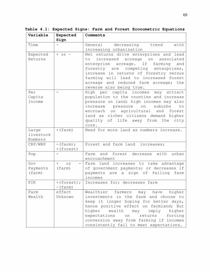
69

Table 4.1: Expected Signs: Farm and Forest Econometric Equations Variable Expected

Sign Comments

Time - General decreasing trend with increasing urbanization

Expected Returns

+ or - Net returns drive enterprises and lead to increased acreage on associated enterprise acreage. If farming and forestry are competing enterprises, increase in returns of forestry versus farming will lead to increased forest acreage and reduced farm acreage; the reverse also being true.

Per Capita Income

- High per capita incomes may attract population to the counties and increase pressure on land; high incomes may also increase pressure on suburbs to encroach on agricultural and forest land as richer citizens demand higher quality of life away from the city core.

Large livestock Numbers

+(farm) Need for more land as numbers increase.

CRP/WRP -(farm); +(forest)

Forest and farm land increases;

Pop - Farm and forest decrease with urban encroachment

Gov Payments (farm)

+ or -(farm)

Farm land increases to take advantage of government payments; or decreases if payments are a sign of falling farm incomes

PIK +(forest); -(farm)

Increases for; decreases farm

Farm Wealth

effect Unknown

Wealthier farmers may have higher investments in the farm and choose to keep it longer hoping for better days, hence positive effect on farmland; But higher wealth may imply higher expectations on returns forcing conversion away from farming if incomes consistently fail to meet expectations.

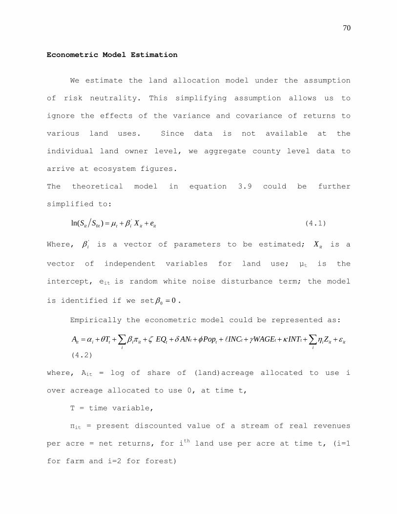
70

Econometric Model Estimation

We estimate the land allocation model under the assumption

of risk neutrality. This simplifying assumption allows us to

ignore the effects of the variance and covariance of returns to

various land uses. Since data is not available at the

individual land owner level, we aggregate county level data to

arrive at ecosystem figures.

The theoretical model in equation 3.9 could be further

simplified to:

'0ln( )it t t i it itS S X eµ β= + + (4.1)

Where, is a vector of parameters to be estimated; is a

vector of independent variables for land use; µt is the

intercept, eit is random white noise disturbance term; the model

is identified if we set

'iβ itX

0 0β = .

Empirically the econometric model could be represented as:

t t t tit i t i it t t i it iti i

A T EQ AN Pop INC WAGE INT Zα θ β π ζ δ φ γ κ η= + + + + + + + + + +∑ ∑ ε

(4.2)

where, Ait = log of share of (land)acreage allocated to use i

over acreage allocated to use 0, at time t,

T = time variable,

πit = present discounted value of a stream of real revenues

per acre = net returns, for ith land use per acre at time t, (i=1

for farm and i=2 for forest)

71

EQt = real farm wealth measured as average state level farm

equity per acre at time t,

Wage = real average wage per job at time t,

INT = Interest rate (20 year constant Treasury bill) rate

at time t,

ANt = Number of large animal(cattle and pig)units per acre,

Popt = Population density at time t.

INCt = real per Capita income at time t,

Zi = matrix of policy variables; including CRP/WRP (CWRP),

PIK, Government payments per acre(GOV),

εit = Gaussian white noise error terms

Wealth, Wage, Interest rate, government payments, and all

income and return variables were deflated/normalized using

Consumer Price Index for the south (CPI), (1982=100). Table 4.1

below outlines the independent variables used in the model and

expected signs.

Data and Policy Site

The policy site (our area of study) area covers two

counties of North Georgia, namely, Habersham and White. Since

data is not available at the individual land owner level, we

aggregate at the county level to get data for the policy site.

Data covering Habersham and White counties, for the period 1974

– 2005 were sourced from various publication and websites

72

including the Georgia county Guide and Georgia Agricultural

Facts. Land use data was compiled from the University of Georgia

(UGA) Odum School of Ecology, Natural Resources Spatial Analysis

Laboratory (NARSAL) database.

Acreage data was available for only six years, 1974, 1985,

1991, 1998, 2001, and 2005. Missing observations were filled-in

using the SAS interpolation “JOIN” method which connects data

points with a straight line by averaging between successive

points. We used this as the best method for filling missing

values, after comparing graphs of interpolated and actual data

derived by various methods.

Timber revenues streams were calculated as weighted

averages of three major types of timber occurring in the policy

site, namely, Oak-Pine, Oak-Hickory and Pine. Rotation rates are

from Griffin (2007), a Georgia Forestry Commission specialist,

based on his field experience. Timber yields are from

Birdsey(1992), Birdsey(2003) and Plantinga (2007). Stumpage

prices are from the Center for Forest Business at the University

of Georgia. Management of forests in North Georgia is not

intense.

Forest management costs were minimal and were compiled from

Dubois, Eric and Straka (1982) based on information provided by

Griffin (2007). Final forest revenue was therefore present

discounted value of streams of real timber revenues per acre.

73

Forest revenues were basically timber revenues discounted

at a rate of 5% as is the practice among studies applying forest

returns as a variable (Plantinga, Maulding and Miller, 1999;

Ahn, Plantinga and Alig, 2000). The choice of discount rates for

valuing natural and environmental resources is subject to

debate. Some economists are of the opinion that high discount

rates may cause environmental degradation. They argue that low

discount rates encourage investment in environmental projects

with even low return rates. Others argue that using very low

rates makes environmental investments unattractive. Federal

discount rates for environmental projects normally vary between

3% and 7%. We chose to follow the most of the authors cited

above and stick to a reasonably low discount rate of 5%, which

ensures comparison purposes.

Population data was compiled from the website of the US

Census Bureau. The Bureau conducts population census every 10

years and provides estimates for the intermediate year. These

estimates and census data covering 1974 to 2005, were used for

this analysis.

Data on government payments, net farm revenue and per

capita income were compiled from the Georgia statistical system

database available online. Data covered the years 1974 Livestock

numbers (cattle, poultry, pigs) were compiled from the various

issues of the Georgia County Guide. These data covered the years

74

between 1974 and 2005. Georgia farm equity data (1974-2005)

were, interest rate (1974-2005) data were from the St Luis

reserve bank. Average wage per job as well as data on the

Consumer Price Index (CPI) were from the Bureau of Labor

Statistics. State Gross Domestic Product (GDP) data (2004-2006)

were compiled from the website of the US Bureau of Economic

Analysis.

Preliminary Model Examination

Preliminary estimation using Ordinary Least Squares (OLS)

and Seemingly Unrelated Regression (SUR) models was done.

Problems of residual autocorrelation are common in OLS

estimation of time series data violating OLS assumption of

uncorrelated error terms. This problem was tested for using

conventional tests, that is, the Durbin Watson (DW) and Breusch-

Godfrey, Lagrange multiplier Test (LM). The later is more

appropriate when lagged dependant variables are included in the

model making DW a weak test, or there is likely to be

contemporaneous correlation in the model (Hendry and Doornik,

2001; Green, 2000). There are 2χ and F forms of the test; the F-

version is shown under the null hypothesis of no

autocorrelation. The null hypothesis is would be rejected if the

test statistic is too high. The residual autocorrelation

function plots were used for the same purpose.

75

Contemporaneous correlation may be a problem in our model

since decisions made for one land use alternative affects the

others. The common solution to this problem is to estimate the

equations in an SUR framework. In this case, equation by

equation OLS is the efficient estimator so long as the

independent variables are the same for all equations in the

system.

Logarithmic transformation of data as in equation 4.1 and

14 is known to induce heteroskedasticity in the model (Ahn,

Plantinga and Alig, 2000), rendering OLS estimates inefficient.

We will test for the same using the F-form of the Breusch-Pagan

Test(BP). High values of the test statistic (low p-values) cause

us to reject the null hypothesis of homoscedasticity.

Although we had no reason to suspect absence of normality

in the distribution of residuals we examined the various

residual plots (including density function and QQ plots) and

applied the Jarque-Bera normality test (N) to the model

residuals. The statistic follows a 2χ distribution with two

degrees of freedom under the null hypothesis of normality

(Gujarati, 2003). The 5% critical value for a is 5.99, and

the 1% critical value is 9.22; N values larger than these may

signify absence of normality.

2(2)χ

76

Econometric Model Fitness and General Forecasting

In addition to the R2, and the F-test are useful measures of

how well the model fits the data and to select between competing

econometric models. Chow’s forecast test also referred to as

Chow’s predictive failure test measures the predictive power of

a regression model. The forecast failure chi-square is another

test similar to the Chow test is test in terms of testing the

constancy of parameters between the sample and post-sample

periods.

For both tests, the null hypothesis is no structural change

in parameter values, meaning there are constant parameters

between the sample and the forecast period. Significantly large

values imply the equation may not provide very accurate ex-ante

predictions.

Whereas the forecast failure chi-square and the Chow test

leans more towards measuring parameter constancy/structural

change in the model, the Root Mean Square Error (RMSE) and the

Mean Absolute Percentage Error (MAPE) are two measures of the

model forecasting accuracy. Higher values imply poor forecasting

performance of the model.

Results of the Econometric Model

We started out with the comprehensive model as outlined in

equation 4.2 and estimated the model by OLS. The results are

77

provided in table 4.2 and 4.3. The all-inclusive model satisfies

most OLS requirements except that it has highly collinear

dependant variables. This is evidenced by the very high R2 (at

least 0.98), and the fact that other than the constant, few

variables are significant at the 5% level. In addition there are

wrong signs on three variables namely per capita income (INC),

PIK, and wage (WAGE).

Examining the independent variables shows a number of

variables have high pair-wise correlation coefficients. Time

trend variable (T), WAGE and INC are highly correlated with POP,

which may explain the source of multicollinearity. As proposed

by Gujarati (2003) we dropped groups of variables with pair-wise

correlation coefficients exceeding 0.8, leaving about two per

“group”, and applied stepwise regression as determined by the

value of partial R2, to settle on the list of variables

ultimately included in the model. We put off other measures of

model suitability till we come up with a model that meets the

requirements of OLS. The final forest acreage model results are

provided in table 4.4.

78

Table 4.2: Forest Acreage Comprehensive Model Estimates

Parameter Estimate SE t-value p-value Constant 2.6981** 0.7936 3.4000 0.0050 POP -0.0349 0.0173 -2.0200 0.0650 INC 0.0183 0.0119 1.5400 0.1480 WAGE 0.0020 0.0100 0.1960 0.8480 PIK -0.0303 0.1009 -0.3000 0.7690 CWRP -0.1384 0.1199 -1.1500 0.2690 INT 1.4443 2.3330 0.6190 0.5470 Π1 4.9459** 0.7501 6.5900 0.0000 GOV -0.0201** 0.0085 -2.3600 0.0350 AN 0.6794 0.3786 1.7900 0.0960 Π2 -0.0519** 0.0220 -2.3600 0.0350 EQ -0.0665 0.0308 -2.1600 0.0500 T -0.0048 0.0484 -0.0989 0.9230 RSS 0.0511 R^2 0.9920 F(12,13) 134.4 [0.000]** DW 2.07 LM, F(2,11) 0.2043 [0.8182] Normality,Chi^2(2) 1.5808 [0.4537] Note: ** - implies significant at 5%;

79

Table 4.3: Farm Acreage Comprehensive Model Estimates

Parameter Estimate SE t-value p-value Constant 1.2111 0.8505 1.4200 0.1780 POP -0.0378 0.0185 -2.0400 0.0620 INC 0.0202 0.0128 1.5800 0.1390 WAGE 0.0017 0.0107 0.1540 0.8800 PIK -0.0359 0.1082 -0.3320 0.7460 CWRP -0.1496 0.1285 -1.1600 0.2650 INT 1.4100 2.5000 0.5640 0.5820 Π1 5.3784** 0.8039 6.6900 0.0000 GOV -0.0214** 0.0091 -2.3500 0.0350 AN 0.7306 0.4057 1.8000 0.0950 Π2 -0.0568** 0.0236 -2.4100 0.0310 EQ -0.0728** 0.0330 -2.2000 0.0460 T 0.0097 0.0519 0.1870 0.8550 RSS 0.0587 R^2 0.9874 F(12,13) 85.16[0.000]** DW 2.08 LM, F(2,11) 0.2299[0.7984] Normality Chi^2(2) 1.5056[0.4711] Note: ** - implies significant at 5%;

80

Both the forest and farm acreage equations meet the

requirements of OLS. The models do not fail the normality,

homoscedasticity and no autocorrelation tests. There are no

signs of multicollinearity in the model and coefficients of

determination for both models are high (0.97 and above).

The F-values are significant (even at 1% level) implying

parameter estimates do not equal zero. In addition to the

intercept that is significant (at 1% level), for both land use

equations, the forest acreage equation yields negative but not

significant signs for farm government payments and wage and

negative and significant signs for farm wealth and population.

The negative sign for population is as expected; as

population density increases there is likely to be increased

encroachment of urban development on forests. The negative sign

on farm wealth may not have a clear-cut explanation. It may be

that higher investment in the farm serves as an incentive to

move land from forestry to agriculture, hence the negative sign.

The equation yields a positive and significant sign for

forest returns implying, in line with expectations, that

increased forest revenue is likely to be an incentive for land

owners to increase forest acreage.

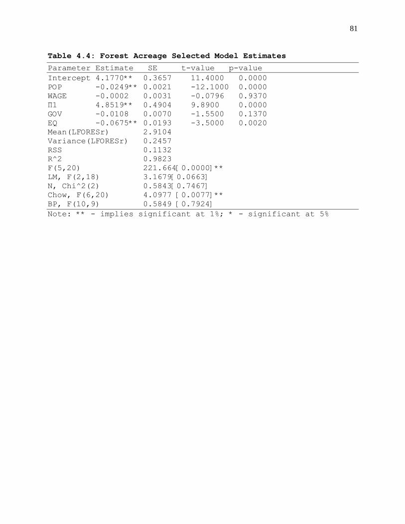
81

Table 4.4: Forest Acreage Selected Model Estimates

Parameter Estimate SE t-value p-value Intercept 4.1770** 0.3657 11.4000 0.0000 POP -0.0249** 0.0021 -12.1000 0.0000 WAGE -0.0002 0.0031 -0.0796 0.9370 Π1 4.8519** 0.4904 9.8900 0.0000 GOV -0.0108 0.0070 -1.5500 0.1370 EQ -0.0675** 0.0193 -3.5000 0.0020 Mean(LFORESr) 2.9104 Variance(LFORESr) 0.2457 RSS 0.1132 R^2 0.9823 F(5,20) 221.664[0.0000]** LM, F(2,18) 3.1679[0.0663] N, Chi^2(2) 0.5843[0.7467] Chow, F(6,20) 4.0977 [0.0077]** BP, F(10,9) 0.5849 [0.7924] Note: ** - implies significant at 1%; * - significant at 5%

82

The results of the final farm acreage model are provided in

tables 4.5. The equation yields significant (at 1% level),

estimates for the intercept, population, and farm wealth. The

equation yields negative but not significant (at 5%) estimates

for farm government payments and wage, and positive and

significant estimates for forest revenue.

As is the case with the forest acreage equation, increased

population is likely to result in increased encroachment of

urban development on farm land hence the negative sign on

population. The negative sign on farm wealth implies increased

farm wealth leads to increased conversion of farms to urban

development. It may be that richer resource farmers have higher

expectations of profits forcing conversion away from farming

when returns fail to meet expectations.

The farm equation yields a positive and significant sign on

forest returns, implying that increased returns from forestry

are likely to be an incentive for land owners to increase farm

acreage.

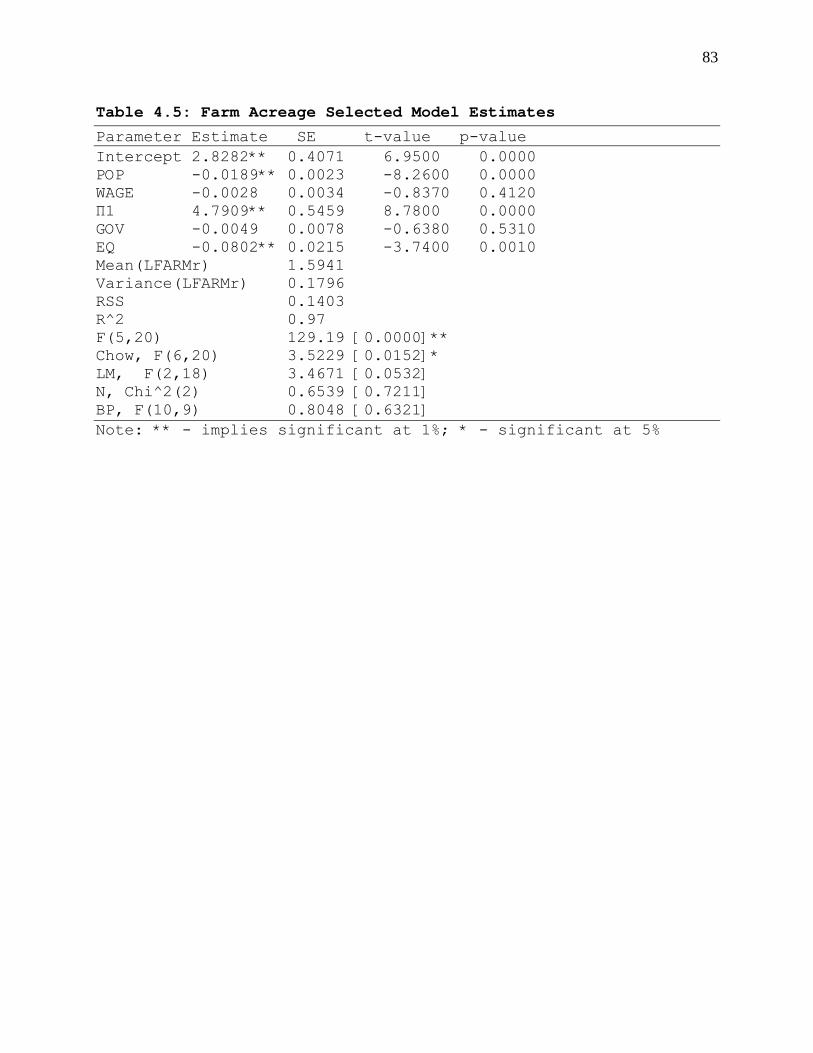
83

Table 4.5: Farm Acreage Selected Model Estimates

Parameter Estimate SE t-value p-value Intercept 2.8282** 0.4071 6.9500 0.0000 POP -0.0189** 0.0023 -8.2600 0.0000 WAGE -0.0028 0.0034 -0.8370 0.4120 Π1 4.7909** 0.5459 8.7800 0.0000 GOV -0.0049 0.0078 -0.6380 0.5310 EQ -0.0802** 0.0215 -3.7400 0.0010 Mean(LFARMr) 1.5941 Variance(LFARMr) 0.1796 RSS 0.1403 R^2 0.97 F(5,20) 129.19 [0.0000]** Chow, F(6,20) 3.5229 [0.0152]* LM, F(2,18) 3.4671 [0.0532] N, Chi^2(2) 0.6539 [0.7211] BP, F(10,9) 0.8048 [0.6321] Note: ** - implies significant at 1%; * - significant at 5%

84

Whereas one would expect this to be the case in regard to

forest acreage, assuming the two land uses are competing, the

reasons for this positive effect on farm acreage is not fully

clear. It may mean that the two are actually complimentary, as

would be the case if, say, land converts to farming first them

to forestry. But the effect may also be simply coincidental

given the high (0.99) correlation between farm and forest

acreage variables. Model diagnostic graphics support the

diagnostic tests outline earlier.

The literature examining cropland allocation across

different crop enterprises is fairly common. But studies of land

allocation at the level of forest versus farm and other uses,

based on economic theory or even time series analysis, are

scarce. In the overall, it is not uncommon for land use models

to fail to provide substantial evidence as to factors that

contribute to land use changes.

Ahn, Plantinga and Alig (2000), document a comprehensive

model of land use at the aggregate level. They take the common

approach of assuming a logistic distribution of share equations

(normalize over forest) and estimate three panel data models

(OLS, fixed effects, random effects) of land use shares.

Independent variables used are revenues (real and discounted),

population density, and measures of land quality. Their models

yield expected signs – farm revenue yields significant and

85

positive signs on the farm equation, while forest revenue yields

a negative and significant sign. They conclude that revenues

tend to “allocate” land to the land use generating the most of

it. Population density does not yield a significant sign

suggesting it affects farm and forest the same way (forest is

the normalizing factor). Land quality yields a positive and

significant sign on farm supporting the notion that fertile land

is most likely going to be allocated to agriculture over

forestry.

Plantinga, Maulding and Miller (1999), estimate a SURE

model (assuming logistic distribution of share allocations) for

forestry and farms (and normalizing on “other” land use). They

estimate three separate models for South, Carolina, Maine and

Wisconsin, using county level data. The independent variables

applied include land quality, population density, net farm and

forest revenues, and for Maine, travel time between the county

center to the port. Unlike, our results that yielded the same

(positive) sign on farm revenue with both equations, they found

farm and forest revenues to have the expected signs (negative

and significant sign on farm revenue in the forest equation;

negative sign on forest revenue in the farm equation). These

results point to the competing nature of the two land uses, farm

and forest. The population variable had expected (and

significant) signs, which tallied with our results. Higher

86

quality land and shorter travel time (for Maine) tended to

favor/increased allocation to farms.

Miller and Plantinga (1999) estimated least square (assumed

a logistic distribution of share allocations), and maximum

entropy models (of share equations), for the allocation of

cropland between corn and soybean, in three Iowa counties. They

found that government payments, fertilizer prices (production

costs) and PIK are significant and negatively related to

acreage. All other factors including farmer prices, cost of

inputs, and wages were not significant. The government payment

variable had a negative but not significant sign in our model.

Wu and Segerson (1995) estimated a similar model, albeit

covering six major crops (wheat, corn, soybean, Oat, hay and

silage), for 57 Wisconsin counties. They assumed a logistic form

for the shares equations and estimated a SURE-panel data model.

Independent variables for their model included expected prices

of commodities, number of cattle, population density, input

prices, farm wage, and land quality classifications. Population

density yielded a negative and significant sign for some of the

crop enterprises (corn and silage) and a positive sign for

others (soybean, wheat). Farm wage, expected commodity prices,

input prices gave mixed signals with significant and negative

sign for some of the crops and positive signs for others.

87

The overall picture that we got from comparison of the

results of our econometric model with those from other studies

is that, aggregate land use models (forest-farms-other, etc)

seem to provide results, consistent with expectation that

cropland share models. One possible explanation for the

differences between our results and past studies could very well

be the kind of data available to us. In regard to land use, we

had only six data points spread over 30 years, and we had to

resort to interpolation to fill in the gaps. Estimating a more

comprehensive model with county level data, in a panel data

framework, would be the better way to go in the future. Even

with six data points, not having to interpolate will most likely

create a data set that would provide more agreeable results,

ceteris paribus.

Econometric Model Forecasting Results

The econometric model (both equations) fails to pass the

Chow forecasting parameter constancy test, meaning there may be

structural change in the data that the model fails to capture.

Structural change is better captured by the Structural Time

Series models results of which are provided later. The RMSE and

MAPE statistics are provided in table 4.6 and 4.7 as well as the

ex ante forecast of the dependant variables.

88

Both equations yield substantially large RMSE and MAPE

values which was not entirely unexpected given the significant

Chow prediction failure test values. The forest acreage equation

yields smaller values for both the RMSE and the MAPE compared to

the farm acreage equation, implying better forecasting accuracy

for that equation.

The MAPE value on the farm acreage equation is particularly

large at 101.68 implying that the equation misses the actual

data values by more than 100 %. We will compare these results

with the STSM and choose the better model for forecasting

purposes.

Structural Time Series Model Estimation

We used the Structural Time Series Analyzer, Modeller, and

Predictor (STAMP) version 6.0 program (Koopman, et. al., 2000)

for STS analysis. The program carries out maximum likelihood

estimation using numerical optimization procedure.

89

Table 4.6: Econometric Model Forecasted Values of Log of Farm Shares

Period Forecast Actual Error 2000 1.147 0.845 -0.302 2001 1.174 0.738 -0.437 2002 1.212 0.638 -0.574 2003 1.176 0.546 -0.631 2004 1.097 0.460 -0.637 2005 1.027 0.379 -0.648 Mean(Error) -0.538 RMSE 0.553 SD(Error) 0.128 MAPE 101.680

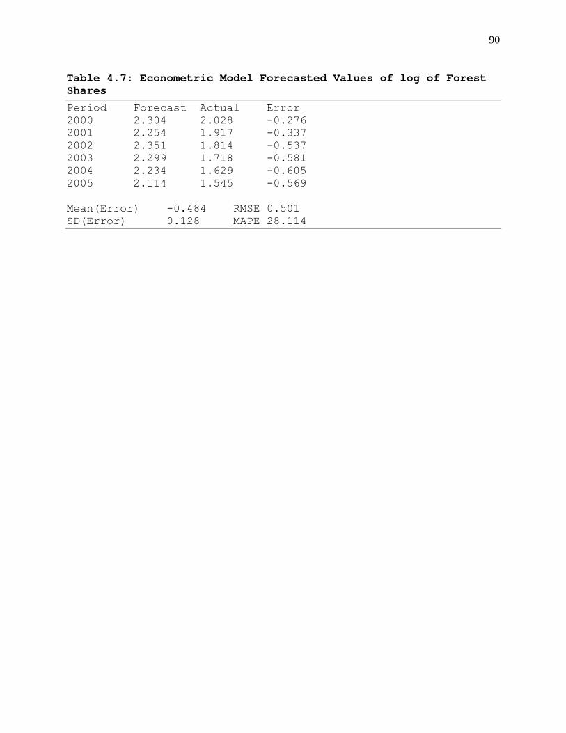
90

Table 4.7: Econometric Model Forecasted Values of log of Forest Shares

Period Forecast Actual Error 2000 2.304 2.028 -0.276 2001 2.254 1.917 -0.337 2002 2.351 1.814 -0.537 2003 2.299 1.718 -0.581 2004 2.234 1.629 -0.605 2005 2.114 1.545 -0.569 Mean(Error) -0.484 RMSE 0.501 SD(Error) 0.128 MAPE 28.114

91

Model diagnostic tests are similar to those of the OLS

(econometric) model and all statistics are as explained earlier

including the Jarque and Bera normality test and the Durbin-

Watson (DW) test. A few diagnostic tests are introduced; Rd2, the

Q statistic and the H statistic.

The STS analysis software, STAMP, uses Rd2 instead of R2 as

the coefficient of determination whenever the model incorporates

trend of seasonality components. The former is a better measure

of goodness of fit where the series appears stationary with no

trend or seasonality (Koopman et al, 2000; Harvey, 1989). This

said alternative coefficient of determination (Rd2) has deviation

of first difference (from its mean) in the denominator, where R2

uses deviation from the levels. The value of Rd2 may be negative

indicating a worse fit than a simple random walk plus drift

model.

In STS analysis, STAMP uses the Box-Ljung Q statistic,

Q(p,q) as a measure of serial correlation. The Q statistic is

based on the first p residual autocorrelations and distributed

as a 2χ (q). We reject the null hypothesis of no autocorrelation

if the p-value is smaller than 0.05, (the test statistic is

larger than the critical value). The Q statistic is

asymptotically equivalent to the Breusch-Godfrey LM test when

there are no lag dependant variables among the set of

explanatory variables.

92

The H(g)test is an F(g,g) non-parametric test of

heteroskedasticity (Koopman, et al, 2000). A large F-value calls

for rejection of the null hypothesis of homoscedasticity.

Results of the Structural Time Series Model

For both the forest and farm equations, we estimated two

versions of the simple STS model (without explanatory

variables), that is, DTNS, and STNS. As with the econometric

model, we assume farm and forest acreage models follow the same

processes and estimate a seemingly unrelated structural time

series equations (SUTSE), which is the same as equation-by-

equation STSM.

The first step is to find the best fit among basic models,

STNS, and DTNS. The next step was to introduce interventions in

the best-fit-model to take care of any poor diagnostics. Typical

interventions in STSM include dummy variables for slope, trend

irregularities or outliers. Such interventions would signal

structural or technological change or simply abnormally large

values.

Diagnostic tests are performed to gauge the goodness of fit

of the model; results are presented in table 4.8 and table 4.9

below.

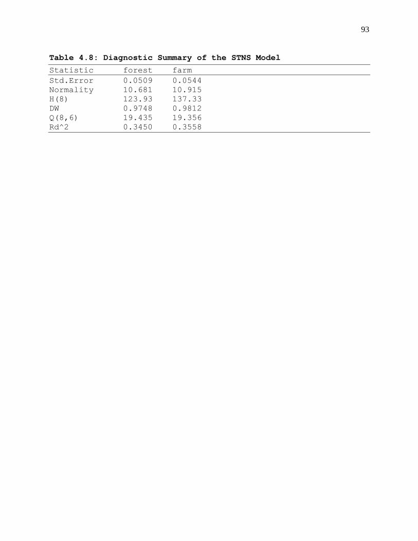
93

Table 4.8: Diagnostic Summary of the STNS Model

Statistic forest farm Std.Error 0.0509 0.0544 Normality 10.681 10.915 H(8) 123.93 137.33 DW 0.9748 0.9812 Q(8,6) 19.435 19.356 Rd^2 0.3450 0.3558

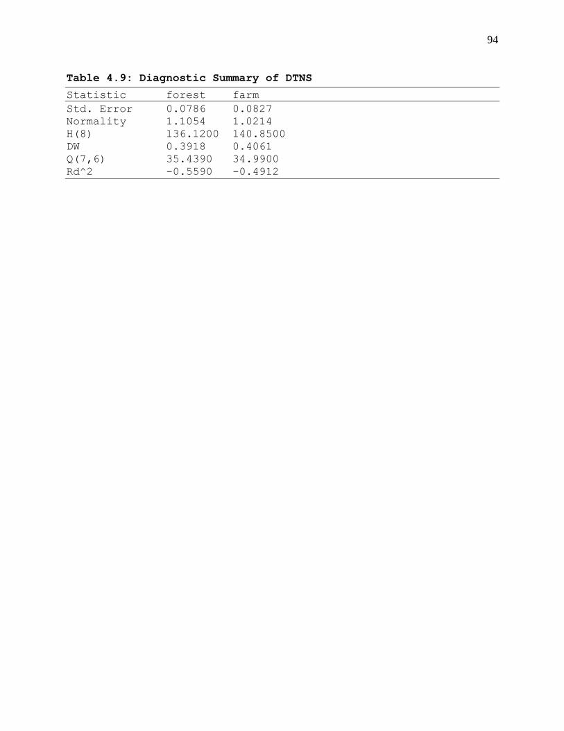
94

Table 4.9: Diagnostic Summary of DTNS

Statistic forest farm Std. Error 0.0786 0.0827 Normality 1.1054 1.0214 H(8) 136.1200 140.8500 DW 0.3918 0.4061 Q(7,6) 35.4390 34.9900 Rd^2 -0.5590 -0.4912

95

Neither the farm nor the forest equation passes the

normality, homoscedasticity, and DW and Q(no

autocorrelation)tests at 5% and 1% levels.

Results of the DTNS model seem better in regard to some of

the statistics but worse for others. The normality (N) values

are below the 5% critical value of 5.99 so we fail to reject the

null hypothesis of normality. Other tests of homoscedasticity,

no autocorrelation are rejected at 5% and 1% levels.

Since both models (STNS and DTNS) fail most diagnostics

test, we select the better of the two and subject it to

interventions to see if it is worth considering versus the

econometric model.

The coefficient of determination (Rd2 version) is the one

thing that separates the two models. We observe that the

stochastic trend (STNS) model explains the variations in the

dependant variables better than the deterministic trend model.

The negative value of Rd2 in the DTNS model is of particular

concern as it implies the model is a worse fit that a simple

random walk with a drift factor.

In STS model interventions include indicator (dummy)

variables to account for outliers and structural breaks.

Outliers can be incorporated as impulse variables which take the

value of one when the outlier occurs and zero elsewhere.

Structural breaks represent instances where the level of the

96

series shifts up or down. Indicator variables taking the value

of one after the break and zero before the break are used to

capture this kind of changes. Structural breaks can also occur

in the slope of the series. Such changes are captured by a

“staircase” intervention in which the trend variable takes the

values, one, two, three, and so on, beginning after the change

in the slope (Koopman, et al, 2000).

The final STSM had a STNS structure and included

interventions for change in the slope (structural breaks) of the

dependant variables. The results of the final STSM are presented

in table 4.10 below.

The diagnostic tests suggest the STNS model explains the

data adequately. The DW statistics are around 1.5 which falls

within the region of indecision but below the 5% (d) critical

value of 1.553, so we fail to reject the hypothesis of no

autocorrelation. The p-values for our Q statistic are 0.0283 for

the forest equation and 0.0279 for the farm equation which

suggests we fail to reject the null hypothesis of no serial

correlation at 1% although the same is not the case at 5%

significance level. Since there were no lagged dependant

variables in the model (we can comfortably use the DW), and both

the DW and the Q statistic support the no residual

autocorrelation hypothesis generally, we conclude that this may

not be a significant problem in the model.

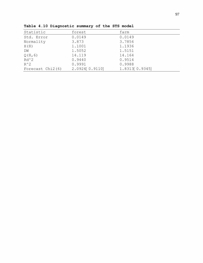
97

Table 4.10 Diagnostic summary of the STS model

Statistic forest farm Std. Error 0.0149 0.0149 Normality 3.873 3.7856 H(8) 1.1001 1.1936 DW 1.5052 1.5151 Q(8,6) 14.119 14.164 Rd^2 0.9440 0.9514 R^2 0.9991 0.9988 Forecast Chi2(6) 2.0926[0.9110] 1.8313[0.9345]

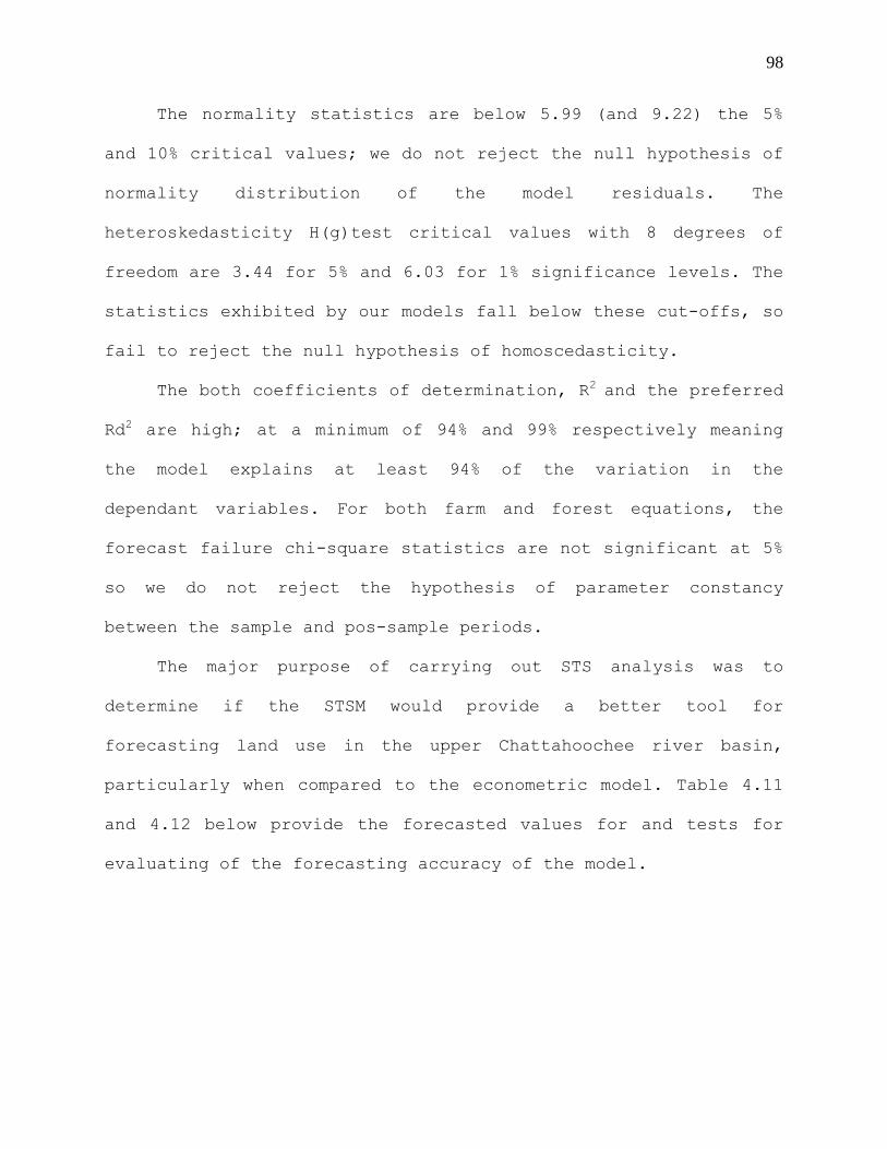
98

The normality statistics are below 5.99 (and 9.22) the 5%

and 10% critical values; we do not reject the null hypothesis of

normality distribution of the model residuals. The

heteroskedasticity H(g)test critical values with 8 degrees of

freedom are 3.44 for 5% and 6.03 for 1% significance levels. The

statistics exhibited by our models fall below these cut-offs, so

fail to reject the null hypothesis of homoscedasticity.

The both coefficients of determination, R2 and the preferred

Rd2 are high; at a minimum of 94% and 99% respectively meaning

the model explains at least 94% of the variation in the

dependant variables. For both farm and forest equations, the

forecast failure chi-square statistics are not significant at 5%

so we do not reject the hypothesis of parameter constancy

between the sample and pos-sample periods.

The major purpose of carrying out STS analysis was to

determine if the STSM would provide a better tool for

forecasting land use in the upper Chattahoochee river basin,

particularly when compared to the econometric model. Table 4.11

and 4.12 below provide the forecasted values for and tests for

evaluating of the forecasting accuracy of the model.

99

Table 4.11: STSM Forecasted Values of Log of Forest Shares

Period Forecast Actual Error 2000 2.0159 2.0276 1.9770 2001 1.8816 1.9167 1.8630 2002 1.7441 1.8137 1.7565 2003 1.6027 1.7182 1.6574 2004 1.4579 1.6290 1.5647 2005 1.3116 1.5451 1.4776 Mean (Error) 0.1061 RMSE 0.0322 SD (Error) 0.0846 MAPE 6.4305

100

Table 4.12: STSM Forecasted Values of Log of Farm Shares

Period Forecast Actual Error 2000 0.8337 0.8454 0.7919 2001 0.7022 0.7377 0.6808 2002 0.5675 0.6379 0.5774 2003 0.4287 0.5456 0.4816 2004 0.2867 0.4596 0.3924 2005 0.1430 0.3789 0.3088 Mean(Error) 0.1072 RMSE 0.0322 SD(Error) 0.0855 MAPE 23.0913

101

Both equations yield substantially smaller RMSE and MAPE

values, particularly when compared to the econometric model.

This causes us to select the STSM as the preferred approach to

forecasting land use in our policy site.

The RMSE statistic yielded by the STSM is 0.0322 for both

farm and forest equation. This is about fifteen times smaller

than the RMSE values from the econometric model which were

between 0.553 (for farm equation) and 0.502 (for forest

equation). The MAPE statistics for the two models are similarly

divergent. The MAPE values of 23.0913, for the farm equation,

and 6.4305, for the forest equation, are about 4 times smaller

than corresponding values from the econometric model; 101.68 for

the farm equation and 28.114 for the forest equation.

The STSM outperforms the econometric model in regard to

forecasting accuracy. In the next chapter, we use the STSM model

to forecast future land use, then model resulting, water quality

changes and assign economic value to the later.

Vector Autoregressive Model Estimation

The VAR model is similar to an econometric simultaneous

equation model, except that all the variables are endogenous.

The assumption is that lagged values of a variable should be

able to explain the variation in the variable. In estimating the

VAR model, we started out with equation 3.15.

102

One critical decision in regard to VAR estimation is the

lag length - including too many lags would reduce degrees of

freedom and induce multicollinearity while too few lags could

results in specification errors (Gujarati, 2003). Use of

decision tools like the Akaike (AIC) and Schwarz (sic)

information criteria is common with smaller values indicating a

better fit for the data. We followed this approach in our

analysis. Because of the expected problem of multicollinearity

(given the use of lags of the same variables), parameters

estimates may not be statistically significant even when a

variable does contribute to the model. We adopted the F-test on

the retained regressors which seems a better tool in making the

decision to drop or keep a variable.

Given that our dependant variables are in logs, we expect

to encounter the problem of heteroskedasticity. To counter this

we will use White (1980) estimation method and estimate

heteroskedasticity consistent standard errors (HCSE).

As in the SURE approach, the problem of identification is

overcome by using the same number of right hand side variables

in all equations in the model. Contemporaneous correlation could

be a problem in VAR model estimation. To circumvent this

problem, we apply equation by equation OLS which is also the

efficient estimation method in a SURE framework.

103

Other problems such as autocorrelation and lack of

normality were tested for using the conventional OLS strategies

discussed earlier.

Results of the Vector Autoregressive Model

We started with a general VAR model based on 4 lags, for

each endogenous variable LFARM (log of farm to urban acreage

ratio) and LFOREST (log of forest to urban acreage ratio). The

results of the VAR model are provided in tables 4.13 and 4.14

below.

The discussion that follows applies to both farm and forest

equations. The Breusch Pagan heteroskedasticity test is omitted

as we applied heteroskedasticity consistent standard errors in

estimation. The R2 (0.99) and overall equation F-statistic (p-

values equal zero) are high suggesting the model may be a good

fit for the data. The DW and LM tests autocorrelation tests

statistics are not significant even at 10% level. The Jarque-

Bera (normality tests) statistic is not significant at 5% level.

These results suggest we can not reject either the normality or

the no autocorrelation (null) hypotheses. The chow parameter

consistency/prediction failure test statistic is not significant

at 5%, suggesting we can not reject the null hypothesis of no

structural change in parameter values.

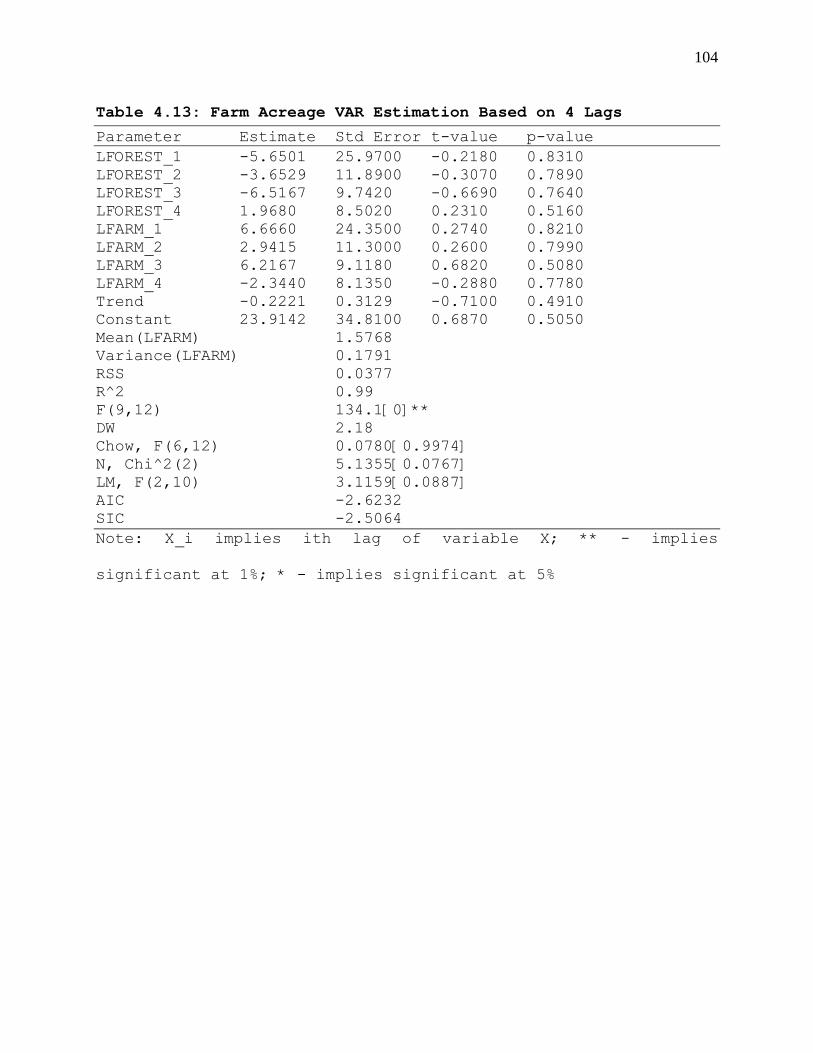
104

Table 4.13: Farm Acreage VAR Estimation Based on 4 Lags

Parameter Estimate Std Error t-value p-value LFOREST_1 -5.6501 25.9700 -0.2180 0.8310 LFOREST_2 -3.6529 11.8900 -0.3070 0.7890 LFOREST_3 -6.5167 9.7420 -0.6690 0.7640 LFOREST_4 1.9680 8.5020 0.2310 0.5160 LFARM_1 6.6660 24.3500 0.2740 0.8210 LFARM_2 2.9415 11.3000 0.2600 0.7990 LFARM_3 6.2167 9.1180 0.6820 0.5080 LFARM_4 -2.3440 8.1350 -0.2880 0.7780 Trend -0.2221 0.3129 -0.7100 0.4910 Constant 23.9142 34.8100 0.6870 0.5050 Mean(LFARM) 1.5768 Variance(LFARM) 0.1791 RSS 0.0377 R^2 0.99 F(9,12) 134.1[0]** DW 2.18 Chow, F(6,12) 0.0780[0.9974] N, Chi^2(2) 5.1355[0.0767] LM, F(2,10) 3.1159[0.0887] AIC -2.6232 SIC -2.5064 Note: X_i implies ith lag of variable X; ** - implies

significant at 1%; * - implies significant at 5%

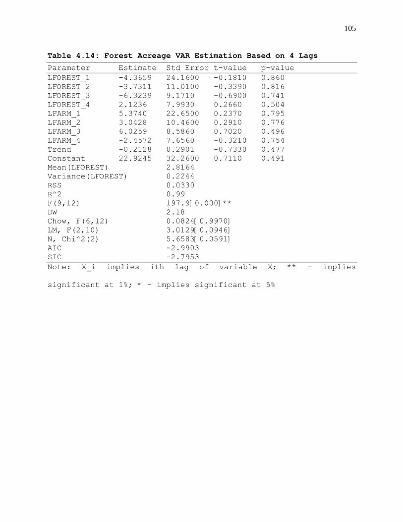
105

Table 4.14: Forest Acreage VAR Estimation Based on 4 Lags

Parameter Estimate Std Error t-value p-value LFOREST_1 -4.3659 24.1600 -0.1810 0.860 LFOREST_2 -3.7311 11.0100 -0.3390 0.816 LFOREST_3 -6.3239 9.1710 -0.6900 0.741 LFOREST_4 2.1236 7.9930 0.2660 0.504 LFARM_1 5.3740 22.6500 0.2370 0.795 LFARM_2 3.0428 10.4600 0.2910 0.776 LFARM_3 6.0259 8.5860 0.7020 0.496 LFARM_4 -2.4572 7.6560 -0.3210 0.754 Trend -0.2128 0.2901 -0.7330 0.477 Constant 22.9245 32.2600 0.7110 0.491 Mean(LFOREST) 2.8164 Variance(LFOREST) 0.2244 RSS 0.0330 R^2 0.99 F(9,12) 197.9[0.000]** DW 2.18 Chow, F(6,12) 0.0824[0.9970] LM, F(2,10) 3.0129[0.0946] N, Chi^2(2) 5.6583[0.0591] AIC -2.9903 SIC -2.7953 Note: X_i implies ith lag of variable X; ** - implies


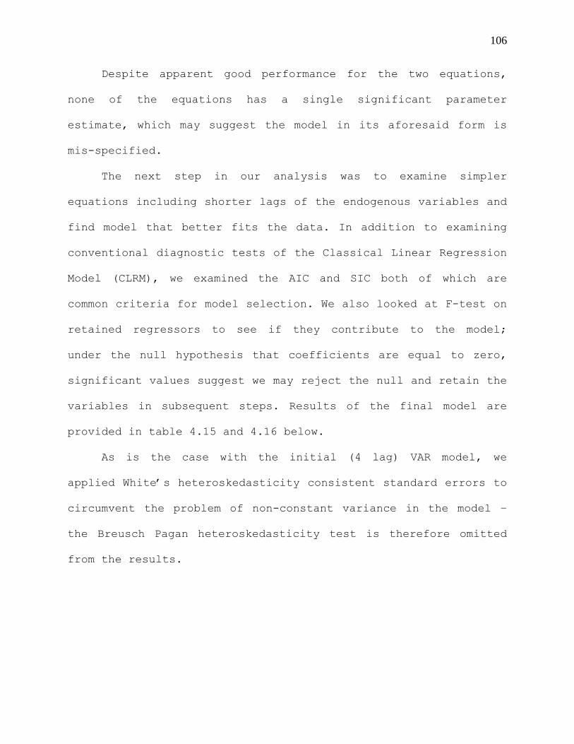
106

Despite apparent good performance for the two equations,

none of the equations has a single significant parameter

estimate, which may suggest the model in its aforesaid form is

mis-specified.

The next step in our analysis was to examine simpler

equations including shorter lags of the endogenous variables and

find model that better fits the data. In addition to examining

conventional diagnostic tests of the Classical Linear Regression

Model (CLRM), we examined the AIC and SIC both of which are

common criteria for model selection. We also looked at F-test on

retained regressors to see if they contribute to the model;

under the null hypothesis that coefficients are equal to zero,

significant values suggest we may reject the null and retain the

variables in subsequent steps. Results of the final model are

provided in table 4.15 and 4.16 below.

As is the case with the initial (4 lag) VAR model, we

applied White’s heteroskedasticity consistent standard errors to

circumvent the problem of non-constant variance in the model –

the Breusch Pagan heteroskedasticity test is therefore omitted

from the results.

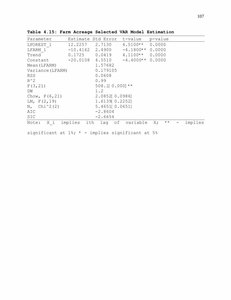
107

Table 4.15: Farm Acreage Selected VAR Model Estimation

Parameter Estimate Std Error t-value p-value LFOREST_1 12.2257 2.7130 4.5100** 0.0000 LFARM_1 -10.4162 2.4900 -4.1800** 0.0000 Trend 0.1725 0.0419 4.1100** 0.0000 Constant -20.0108 4.5510 -4.4000** 0.0000 Mean(LFARM) 1.57682 Variance(LFARM) 0.179105 RSS 0.0608 R^2 0.99 F(3,21) 508.1[0.000]** DW 1.2 Chow, F(6,21) 2.0852[0.0986] LM, F(2,19) 1.6139[0.2252] N, Chi^2(2) 5.4651[0.0651] AIC -2.8604 SIC -2.6654 Note: X_i implies ith lag of variable X; ** - implies


108

Table 4.16: Forest Acreage Selected VAR Model Estimation

Parameter Estimate Std Error t-value p-value LFOREST_1 12.2121 2.5090 4.8700** 0.0000 LFARM_1 -10.4746 2.3040 -4.5500** 0.0000 Trend 0.1580 0.0387 4.0800** 0.0010 Constant -18.3559 4.2090 -4.3600** 0.0000 Mean(LFARM) 2.8939 Variance(LFARM) 0.2415 RSS 0.0534 R^2 0.9911 F(3,21) 784[0.000]** DW 1.2 Chow, F(6,21) 1.9559[0.1184] LM, F(2,19) 1.6414[0.2200] N, Chi^2(2) 5.3485[0.0690] AIC -2.9903 SIC -2.7953 Note: X_i implies ith lag of variable X; ** - implies


109

The final VAR model meets CLRM requirements. For both farm

and forest equations, the DW test yields a d-value of 1.2, which

falls within the indecision region for the 5% level of

significance (1.038 to 1.767) for N=25 and k=4. This implies we

can not conclusively reject the null hypothesis of no

autocorrelation based on this statistic. Nevertheless, for both

equations, the LM autocorrelation tests statistics is not

significant at 5% level. As indicated earlier this is a more

appropriate test when lagged dependant variables are present in

the model as is the case here, so we may not reject the null

hypothesis and conclude that autocorrelation may not be a

problem in the model.

The Jarque-Bera normality tests statistic N is not

significant at 5% level. These results suggest we can not reject

either the normality hypotheses. The chow parameter

consistency/prediction failure test statistic is not significant

at 5%, suggesting we can not reject the null hypothesis of no

structural change in parameter values.

The final model is also a reasonably good fit for the data

with R2 values of 0.99 and above. The overall equation F-

statistics are significant at 1% level which suggests we may

reject the null hypothesis that the coefficients are

collectively equal to zero.

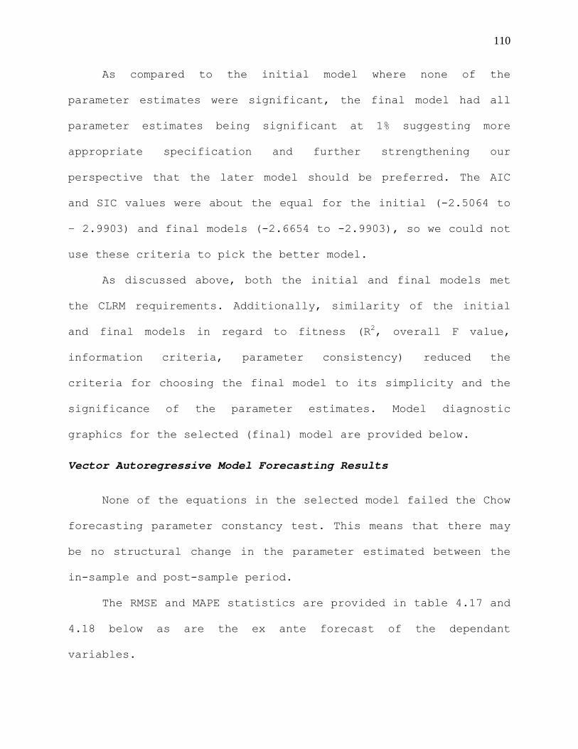
110

As compared to the initial model where none of the

parameter estimates were significant, the final model had all

parameter estimates being significant at 1% suggesting more

appropriate specification and further strengthening our

perspective that the later model should be preferred. The AIC

and SIC values were about the equal for the initial (-2.5064 to

– 2.9903) and final models (-2.6654 to -2.9903), so we could not

use these criteria to pick the better model.

As discussed above, both the initial and final models met

the CLRM requirements. Additionally, similarity of the initial

and final models in regard to fitness (R2, overall F value,

information criteria, parameter consistency) reduced the

criteria for choosing the final model to its simplicity and the

significance of the parameter estimates. Model diagnostic

graphics for the selected (final) model are provided below.

Vector Autoregressive Model Forecasting Results

None of the equations in the selected model failed the Chow

forecasting parameter constancy test. This means that there may

be no structural change in the parameter estimated between the

in-sample and post-sample period.

The RMSE and MAPE statistics are provided in table 4.17 and

4.18 below as are the ex ante forecast of the dependant

variables.

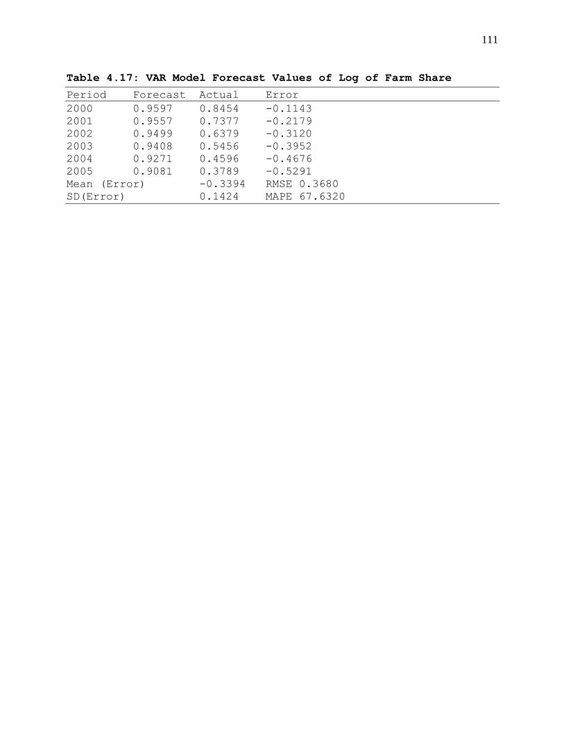
111

Table 4.17: VAR Model Forecast Values of Log of Farm Share

Period Forecast Actual Error 2000 0.9597 0.8454 -0.1143 2001 0.9557 0.7377 -0.2179 2002 0.9499 0.6379 -0.3120 2003 0.9408 0.5456 -0.3952 2004 0.9271 0.4596 -0.4676 2005 0.9081 0.3789 -0.5291 Mean (Error) -0.3394 RMSE 0.3680 SD(Error) 0.1424 MAPE 67.6320

112

Table 4.18: VAR Model Forecast Values of log of Forest Share

Period Forecast Actual Error 2000 2.1312 2.0276 -0.1037 2001 2.1132 1.9167 -0.1965 2002 2.0934 1.8137 -0.2797 2003 2.0704 1.7182 -0.3522 2004 2.0431 1.6290 -0.4141 2005 2.0107 1.5451 -0.4656 Mean (Error) -0.3020 RMSE 0.3266 SD(Error) 0.1244 MAPE 17.8070

113

The model yielded RMSE values of 0.3680 and 0.3266 and MAPE

values of 67.632 and 17.807 for the for the farm and forest

equations respectively. Given the negative mean error, the MAPE

values indicate that model overestimates the farm and forest

acreage shares by about 67% and 17% respectively.

Forecasting Ability: Comparing VAR, STS and Econometric Models

Table 4.19 compares the three land use models, econometric,

VAR and STSM in regard to forecasting ability. Overall, the VAR

model RMSE and MAPE values were smaller than the corresponding

values yielded by the econometric model but smaller than the

STSM. Thus, in terms of model forecasting accuracy, the STSM

would be most preferred followed by the VAR time series model,

with the econometric model being the worst performer. Although

this is as expected, many econometricians are of the opinion

that wherever time series models outperform econometric models,

the econometric model may be miss-specified (Green, 2000;

Kennedy, 2001). It may be important for future research to

examine the validity of this notion in regard to land use

modeling.

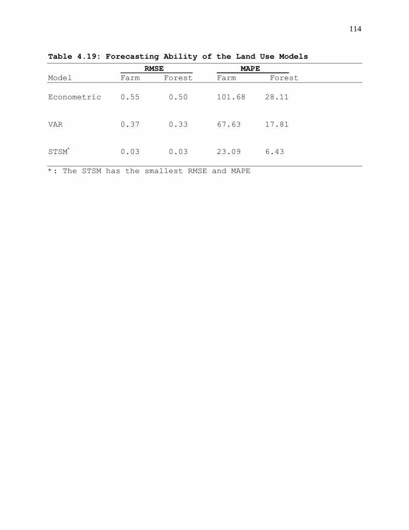
114

Table 4.19: Forecasting Ability of the Land Use Models

RMSE MAPE Model Farm Forest Farm Forest Econometric 0.55 0.50 101.68 28.11 VAR 0.37 0.33 67.63 17.81 STSM* 0.03 0.03 23.09 6.43 *: The STSM has the smallest RMSE and MAPE

115

Whereas both econometric and the VAR models yielded

negative mean error values, the STSM yielded a positive value.

This suggests that the first two models would likely

overestimate land acreages allocated to farms and forests, where

the STSM would likely underestimate these allocations. We

selected the STSM for forecasting on the basis of RMSE and MAPE

statistics.

Forecasting Land Use and Land Use Change

A key objective of our study was to forecast land use in

the Upper Chattahoochee River Basin (UCRB) in North Georgia, in

order to forecast changes in water quality and economic value of

this environmental good. We focused in the are of the basin

north of Lake Lanier, particularly the area covered by Habersham

and white counties. Two approaches to forecasting land use were

applied namely the Seemingly Unrelated Regression, and a

Structural Time Series Model. The STSM results seemed a better

choice for forecasting as evidenced by smaller RMSE and MAPE

statistics.

We proceed to forecast land acreage for farm and forest

uses for the years 2006 to 2030 under three scenarios, that is,

Scenario I, the highest rate of conversion (to urban land use)

as forecasted by the STSM; Scenario III, limited or managed

conversion represented by average growth rate between 1974 and

116

2005; Scenario II, moderate conversion represented by the

average growth rate between the two scenarios above. We would

not expect conversion rates to fall below scenario III levels,

as urbanization and deforestation have been rising steadily over

the years.

Land Use Change Scenario I: The STSM Highest Conversion Rate

The results of the first scenario are presented in table

4.20. Figures in the table are in percentage of land under

indicated use and do not cover government land (about 80,000

acres of forest) and lakes (about 2100 acres) all of which we

assumed would remain unchanged.

The STSM provides us with estimated ratios of the logs of

shares of non-urban to urban land uses, that is, forest to urban

and farm to urban. We used Microsoft Excel software to compute

acres and percentages for the respective land uses.

Only farm and forest figures were actually forecasted;

urban figures were computed as the difference between the total

and the sum of farm and forest acreage proportions. The values

for year 2005 are from actual baseline data and are included

here for comparison purposes. Forecasted values are for selected

years between 2006 and 2030.

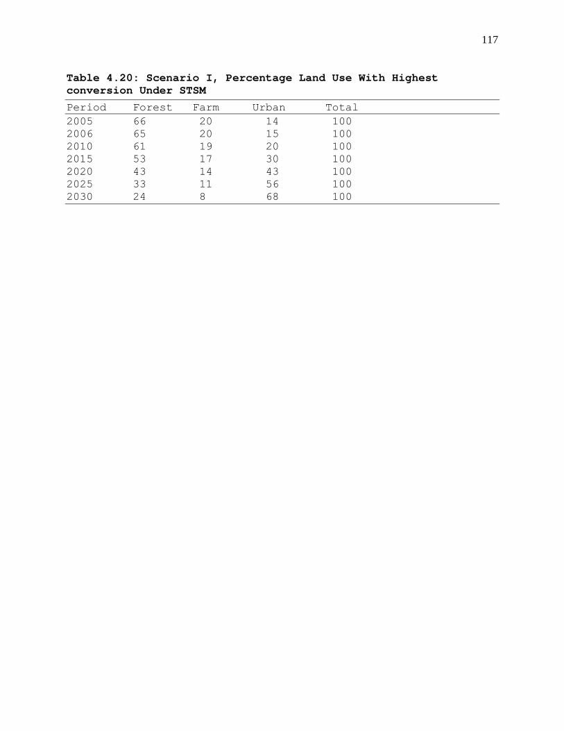
117

Table 4.20: Scenario I, Percentage Land Use With Highest conversion Under STSM

Period Forest Farm Urban Total 2005 66 20 14 100 2006 65 20 15 100 2010 61 19 20 100 2015 53 17 30 100 2020 43 14 43 100 2025 33 11 56 100 2030 24 8 68 100

118

The above results indicate that in 2005, about 66% of the

land was under forestry, 20% was under farms and 14% was under

urban development. It seems that ten years later by the year

2015, the percentage of land under various uses will have

changed to about 53%, 17% and 30% for the forest, farm and urban

categories respectively and by the year 2030, urban development

will have increased to cover about 68% of available land with

forests and farms taking a backseat at 24%, and 8% respectively.

The STSM does not tell us why these changes would take

place; it simply provides the best fit for the data and the

better model for forecasting compared to the econometrics model.

Intuitively, the high population growth rate may have had a

major impact on conversion of farms and forests to urban

development, as human settlement has pushed into forests and

farmlands in the watershed. In the space of about three decades

covered by the data, annual population growth rate averaged 2.2%

increasing over the decades from a low of 1.23% in the first

decade (1974-1984), and a high of 2.99% in the last decade (1995

and 2005). The notion of a strong relationship between

population growth and urbanization is further supported by the

large, negative and significant coefficient on population

density in the econometric model. These forecasts may seem

incredible and we consider that the STSM had significantly large

forecasting error statistics.

119

Scenario II, (Table 4.21) is an average of the two extreme

situations, the highest conversion under STSM, and the limited

growth conversion. Under this scenario, about one half of the

forest cover and one third of farmland are lost to urban

development. By 2030 the proportion of land in forests has

reduced to 37%; farmland has lost 7% to stand at 13%; urban

development space has quadrupled to take a share of 50%.

120

Table 4.21: Scenario II, Percentage Land Use Based On Moderate Conversion


121

These figures may still seem incredible, but this is by no

means a far fetched scenario. Examining existing data for the

last decade or so, the annual rate of loss of forests between

1998 and 2005 was about 1.1%, while farmland was being lost at a

rate of 0.83%. If land conversion continued at these rates, by

2030, forests would cover 53%, farms would cover 15% and urban

development would take over 32% of the ecosystem.

Under scenario III - forecasts are presented in table 4.22

the limited/managed conversion, we assume that land acreage will

change at a rate equivalent to the average growth between 1974

and 2005. During this period forest is lost at a compounded

annual growth rate of 0.61%, farmland increases by about 0.37%

and urban development increases by a 1.7%. By 2030, forest

covers 56% of the land down from 66% in 2005, farmland increases

marginally from 21% to 22%, while commercial and residential

development increases by about 50% from to cover 21% of

available ecosystem land up from 14%. Examining the data, urban

growth was very limited in the 1970s and 1980s but shot up in

the last one and a half decades. Moreover, the 1998 to 2005

growth rates give us a markedly higher conversion rates, than

the managed growth scenario. We therefore have reason to

consider this as a realistic best case land allocation scenario

for this ecosystem. The implications of these changes for water

quality are explored in the next chapter.

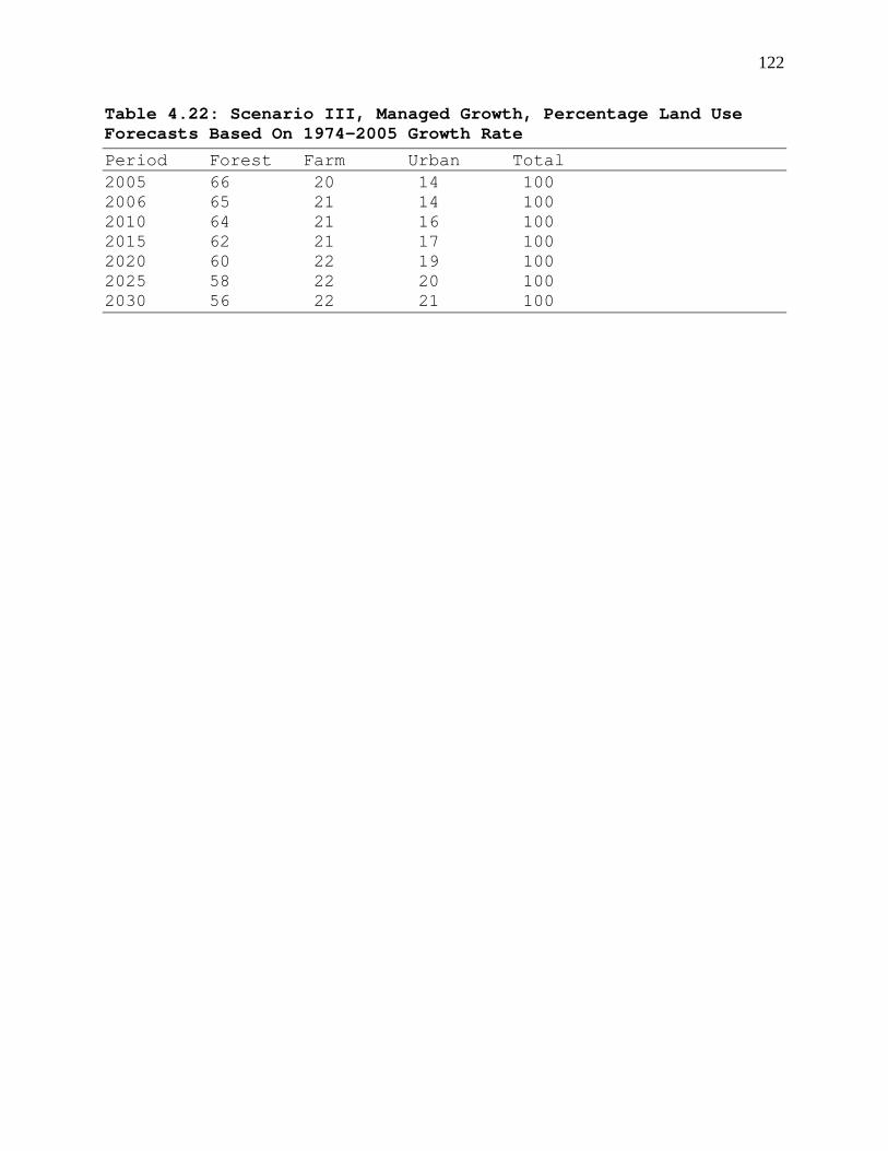
122

Table 4.22: Scenario III, Managed Growth, Percentage Land Use Forecasts Based On 1974-2005 Growth Rate


123

Land Use Change Forecasting

Table 4.23 provides land use shares under different

scenarios from baseline through scenario III. Table 4.24

provides the baseline land use allocations (acreage) and

percentage change in individual land use categories under

different scenarios. The tables depicts the extent to which land

allocation changes (for each category of use) between year 2005

(baseline) and 2030 under different scenarios. This conversion

is discussed in greater detail in the previous chapter.

Summarily, Scenario I (STSM) represents highest conversion.

Under this scenario, urban growth (commercial and residential

areas) encroaches on farms and forests to increase by 390 % as

the later two reduce by about 63 %. In scenario II, moderate

growth, urban growth takes over from farms and forests to

increase by a lower but significant magnitude of 258 %. Land in

farms drops by 35 % while forestry loses 44 %. Under scenario

III with mitigating action/managed growth, urban growth

increases by 53 %, farm acreage increases by 10 %, and forestry

loses 14 %. In the next chapter we explore the implications of

these land use change for water quality.

124

Table 4.23: Land Use Shares Under Different Scenarios Scenario Forest Farm Urban Baseline 2005 66 20 14 I. STSM highest growth 24 8 68 II. Moderate growth 37 13 50 III. Managed growth 56 22 21 Note: Values are percentages

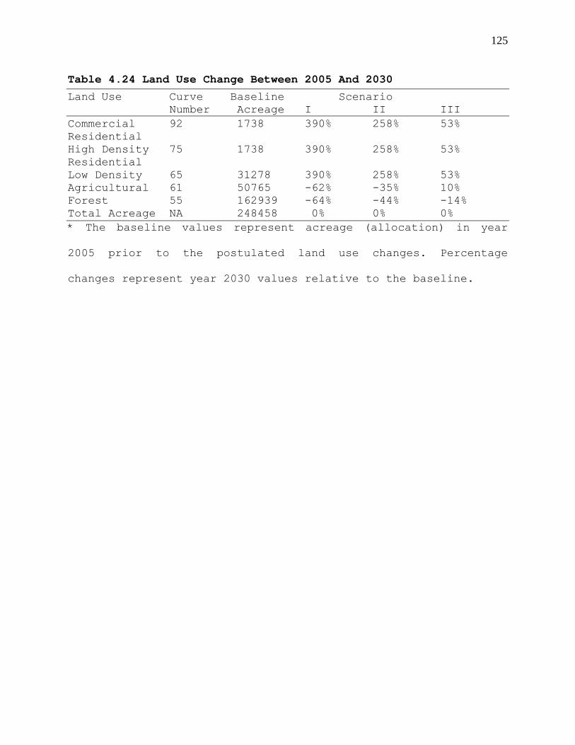
125

Table 4.24 Land Use Change Between 2005 And 2030

Land Use Curve Baseline Scenario Number Acreage I II III Commercial 92 1738 390% 258% 53% Residential High Density 75 1738 390% 258% 53% Residential Low Density 65 31278 390% 258% 53% Agricultural 61 50765 -62% -35% 10% Forest 55 162939 -64% -44% -14% Total Acreage NA 248458 0% 0% 0% * The baseline values represent acreage (allocation) in year

2005 prior to the postulated land use changes. Percentage

changes represent year 2030 values relative to the baseline.

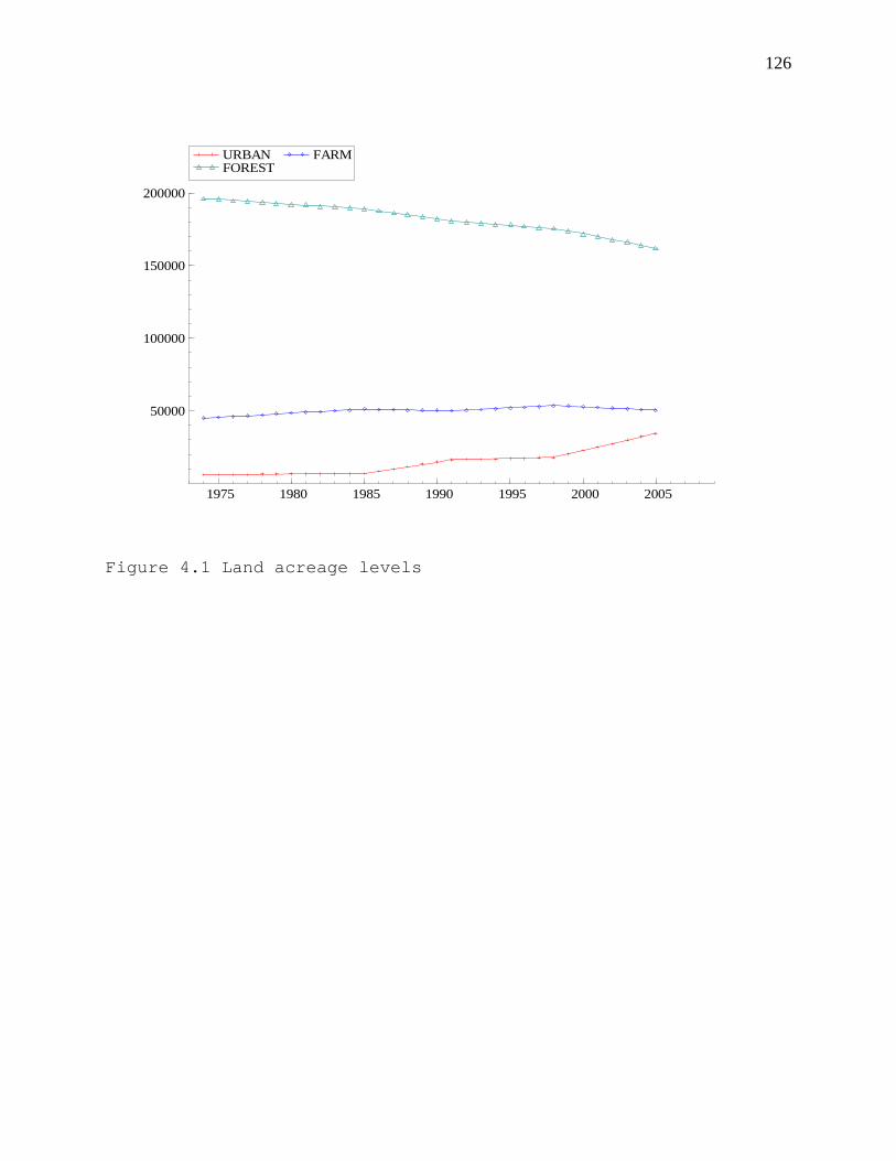
126

1975 1980 1985 1990 1995 2000 2005

50000

100000

150000

200000

URBAN FOREST

FARM

Figure 4.1 Land acreage levels

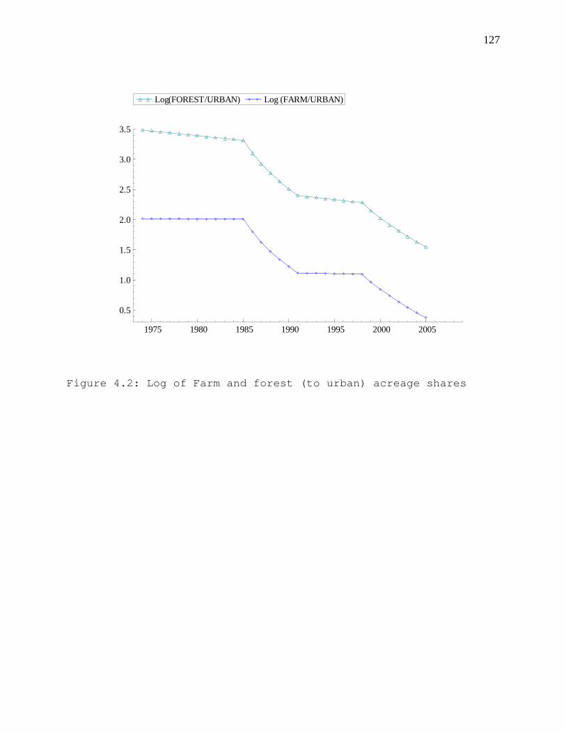
127

1975 1980 1985 1990 1995 2000 2005

0.5

1.0

1.5

2.0

2.5

3.0

3.5

Log(FOREST/URBAN) Log (FARM/URBAN)

Figure 4.2: Log of Farm and forest (to urban) acreage shares

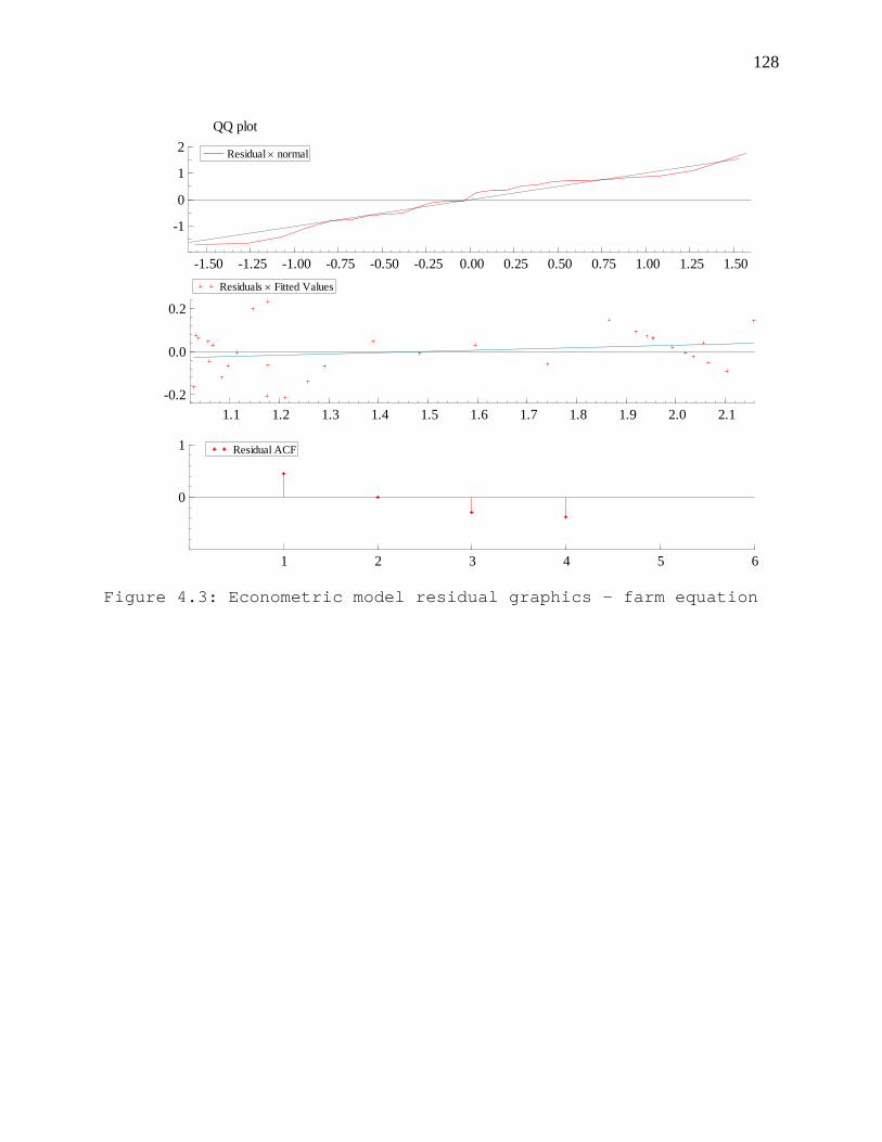
128

1 2 3 4 5 6

0

1 Residual ACF

-1.50 -1.25 -1.00 -0.75 -0.50 -0.25 0.00 0.25 0.50 0.75 1.00 1.25 1.50

-1

0

1

2QQ plot

Residual × normal

1.1 1.2 1.3 1.4 1.5 1.6 1.7 1.8 1.9 2.0 2.1-0.2

0.0

0.2

Residuals × Fitted Values

Figure 4.3: Econometric model residual graphics - farm equation

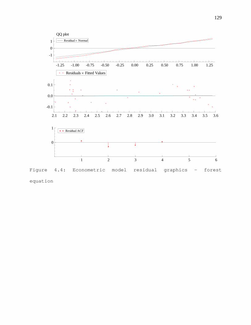
129

1 2 3 4 5 6

0

1Residual ACF

-1.25 -1.00 -0.75 -0.50 -0.25 0.00 0.25 0.50 0.75 1.00 1.25

-1

0

1

QQ plotResidual × Normal

2.1 2.2 2.3 2.4 2.5 2.6 2.7 2.8 2.9 3.0 3.1 3.2 3.3 3.4 3.5 3.6

-0.1

0.0

0.1


Figure 4.4: Econometric model residual graphics - forest

equation

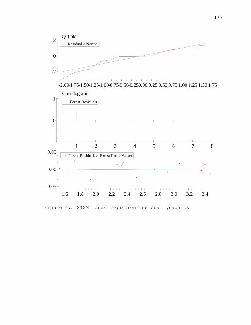
130

-2.00-1.75-1.50-1.25-1.00-0.75-0.50-0.250.00 0.25 0.50 0.75 1.00 1.25 1.50 1.75

-2

0

2QQ plot

Residual × Normal

1 2 3 4 5 6 7 8

0

1Correlogram

Forest Residuals

1.6 1.8 2.0 2.2 2.4 2.6 2.8 3.0 3.2 3.4-0.05

0.00

0.05Forest Residuals × Forest Fitted Values

Figure 4.5 STSM forest equation residual graphics

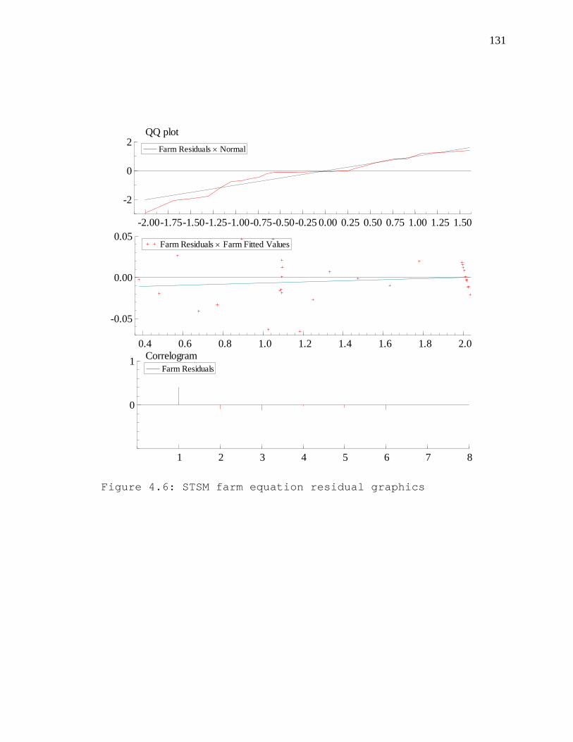
131

-2.00-1.75-1.50-1.25-1.00-0.75-0.50-0.25 0.00 0.25 0.50 0.75 1.00 1.25 1.50

-2

0

2QQ plot

Farm Residuals × Normal

0.4 0.6 0.8 1.0 1.2 1.4 1.6 1.8 2.0

-0.05

0.00

0.05Farm Residuals × Farm Fitted Values

1 2 3 4 5 6 7 8

0

1 CorrelogramFarm Residuals

Figure 4.6: STSM farm equation residual graphics

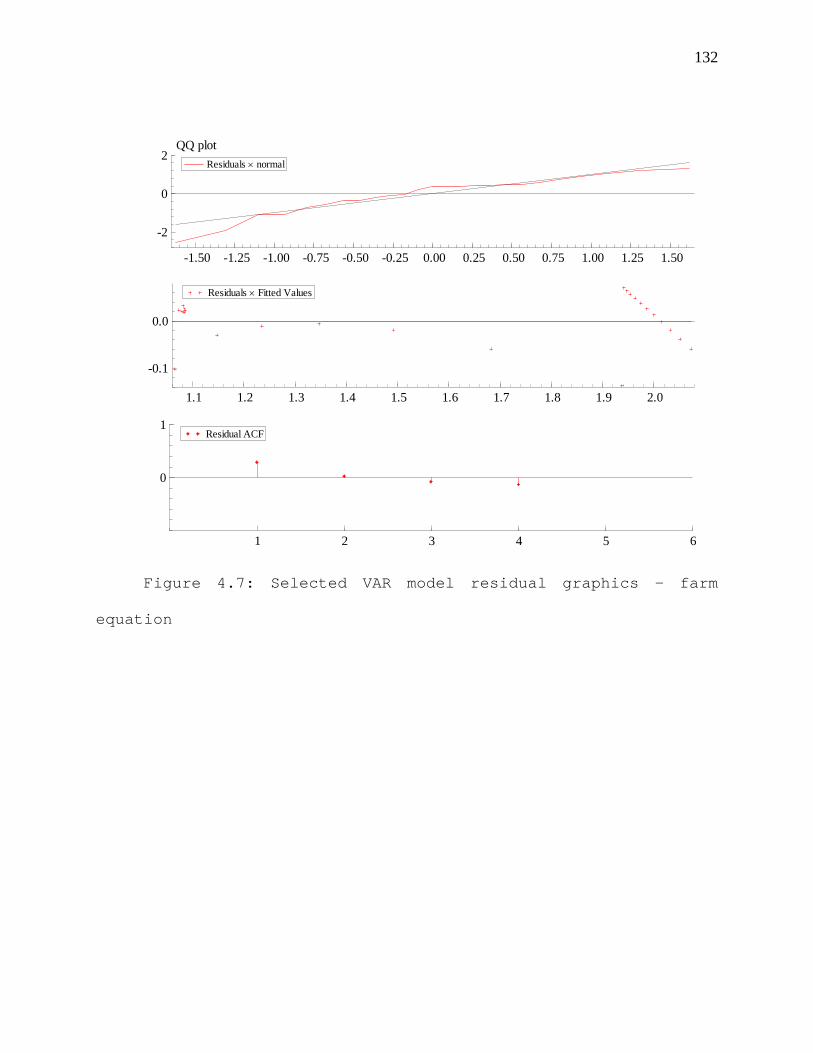
132

1.1 1.2 1.3 1.4 1.5 1.6 1.7 1.8 1.9 2.0

-0.1

0.0


-1.50 -1.25 -1.00 -0.75 -0.50 -0.25 0.00 0.25 0.50 0.75 1.00 1.25 1.50

-2

0

2QQ plot

Residuals × normal

1 2 3 4 5 6

0

1Residual ACF

Figure 4.7: Selected VAR model residual graphics - farm

equation

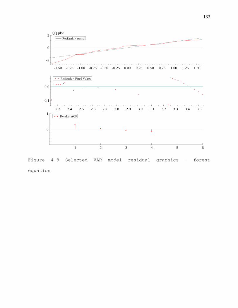
133

2.3 2.4 2.5 2.6 2.7 2.8 2.9 3.0 3.1 3.2 3.3 3.4 3.5

-0.1

0.0


-1.50 -1.25 -1.00 -0.75 -0.50 -0.25 0.00 0.25 0.50 0.75 1.00 1.25 1.50

-2

0

2QQ plot

Residuals × normal

1 2 3 4 5 6

0

1Residual ACF

Figure 4.8 Selected VAR model residual graphics - forest

equation

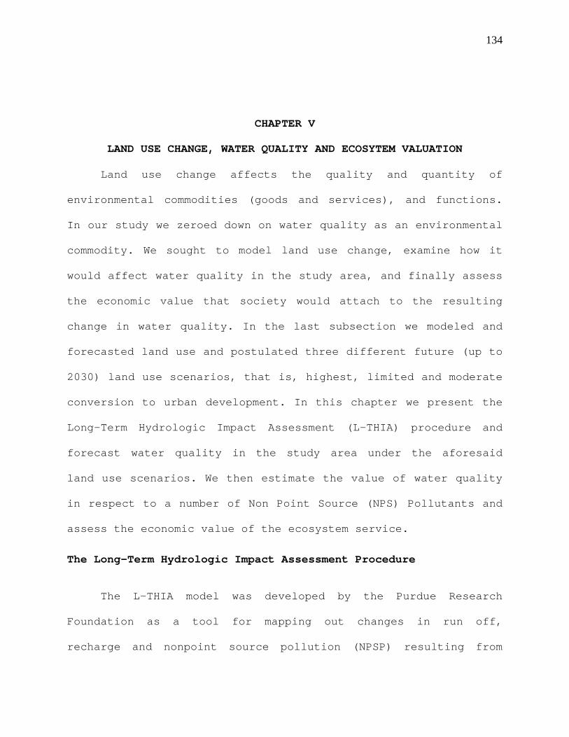
134

CHAPTER V

LAND USE CHANGE, WATER QUALITY AND ECOSYTEM VALUATION

Land use change affects the quality and quantity of

environmental commodities (goods and services), and functions.

In our study we zeroed down on water quality as an environmental

commodity. We sought to model land use change, examine how it

would affect water quality in the study area, and finally assess

the economic value that society would attach to the resulting

change in water quality. In the last subsection we modeled and

forecasted land use and postulated three different future (up to

2030) land use scenarios, that is, highest, limited and moderate

conversion to urban development. In this chapter we present the

Long-Term Hydrologic Impact Assessment (L-THIA) procedure and

forecast water quality in the study area under the aforesaid

land use scenarios. We then estimate the value of water quality

in respect to a number of Non Point Source (NPS) Pollutants and

assess the economic value of the ecosystem service.

The Long-Term Hydrologic Impact Assessment Procedure

The L-THIA model was developed by the Purdue Research

Foundation as a tool for mapping out changes in run off,

recharge and nonpoint source pollution (NPSP) resulting from

135

land use changes (Purdue Research Foundation, 2004; Engel,

et.al., 2003; Bhaduri, et. al.,1999). The L-THIA software,

available online, computes long term average annual estimates of

the aforesaid hydrological parameters for specified land use

scenarios, based on long term historical climatic data at county

level.

The software allows one to input data at two levels of

complexity, basic and detailed. The basic option allows input of

up to eight land use categories, namely, commercial, industrial,

high density residential, low density residential,

grass/pasture, forest, water/wetland, and agriculture. The

detailed option allows input of up to fourteen land use

categories including open spaces, parking/paved spaces, six lot

sizes for residential housing, and the possibility of adding a

custom land use. Irrespective of the option selected, L-THIA

requires input of at least one hydrological soil group, A to D.

These categories are from the National Resource Conservation

Service (NRCS) classifications of soils, and represent

indicators of runoff potential. Group A has the lowest potential

while group D has the highest.

Once the level of complexity is selected, the next step is

to select the location (state and county) of interest. The

software requires selecting the hydrological soil group or

groups and an input of the type and size (acres, hectares,

136

square miles, square kilometers) of land use change. The

software then computes expected runoff depths and volumes and

nonpoint source pollution loadings to waterbodies, based on the

selected hydrological groups and proposed land use and land use

changes. The pollutants covered by the model include chemicals

such as nitrogen, phosphorous, lead and other inorganic

compounds, suspended solids, dissolved oxygen, microbes such as

fecal coliform and fecal streptococcus, urban wastes such as

oil and grease. We zeroed down on nitrogen, total bacteria

(fecal Coliform plus fecal streptococcus), and dissolved oxygen

as they are the most commonly studied pollutants, which would

give us most access to benefit transfer data.

Hydrological Soil Types

The major soils of Habersham and White counties of North

Georgia range from deep fairly well drained sandy loams to

poorly drained sandy clay loams (McIntyre, 1972; Robertson,

McIntyre, and Ritchie, 1963). The deep, well drained Cecil

and Madison, group A like, soils cover about two thirds of

Habersham County. The remaining one third is covered by various

poorly drained sandy clays loams (Robertson, McIntyre, and

Ritchie, 1963) that would fall under hydrological soil group C.

About a half of White county is covered by deep and well

drained Tallapoosa, Tusquitee, Ashe and Edneysville loam soils

137

(McIntyre, 1972), which would fall under category A. The other

half of the County is covered deep to moderately deep, well

drained to moderately well drained soils of various

associations, including, Hayesville-Fannin-Wickam and Hayes-

Rubin-Hiwassee (McIntyre, 1972) which would fit in hydrologic

soil group B. To simplify the analysis we make a compromise and

classify the entire study area under hydrological soil group B.

Water Pollution and Quality Standards

Different land uses are associated with different levels of

nutrient and contaminant loading into ground and surface water.

Under most natural land cover types, a certain (normally

limited) level of nutrients occurs naturally based on the type

of underlying rock, soils, atmospheric and hydrologic

conditions.

Living things (life), both plants and animals are adapted

to survive under varied but often limited concentrations of

nutrients such as nitrogen (for plants), phosphorous (for plants

and animals), etc. In limited amounts many nutrients are

beneficial and often required to sustain life. In high

concentrations however, nutrients become poisonous contaminants

that may impair proper functioning of an organism or even

destroy life. The EPA has developed recommendations (criteria)

138

that states and local authorities should use as a guide to

ensure water quality in their areas (USEPA, 1986a).

There are numerous environmental stressors and sources of

associated pollution with potential to impair water quality.

Attempts to ameliorate nutrient levels in ecosystems naturally

lean toward cultural or “human-made” sources of nutrient

loading/injection as these are often the cause of excessive

loadings as well as being the easiest to control. For the

purpose of this study and given our need for previous studies

with benefit transfer data, we zeroed down on major stressors

identified in the literature and for which the United States

Environmental Protection Agency (USEPA) and the Georgia

Environmental Protection Division (GAEPD have provided

protection guidance criteria. These stressors include Nitrates,

Phosphorous, Total Suspended Solids (TSS), Dissolved oxygen

(DO), Turbidity, and Fecal Coliform (bacteria). The literature

also provides guidelines for other NPS pollutants including

Biochemical Oxygen Demand (BOD).

Nitrates, as nitrogen or otherwise, are about the most

discussed contaminants of drinking water in the literature.

Together with phosphorous, nitrates and nitrites are associated

with agriculture (fertilizers and animal waste) and human

residential waste disposal. Nitrate concentration in ground

water unaffected by human activities is about 2 mg/L (Nolan and

139

Stoner, 2000). In reasonable amounts nitrogen (from nitrates and

nitrites) and phosphorous are needed for plant growth hence the

extensive use in agriculture. But excess and unutilized

nutrients from farms, byproducts of animal waste and poorly

disposed human waste end up in ground and surface water mainly

through leaching and runoff. Pollution by nitrates is especially

a problem with ground water as 22 per cent of domestic wells in

agricultural areas, in the US, report nitrogen contamination.

About 22 % of Georgians including 98 % living in rural areas of

the state (GAEPD, 1997) and about 46 % of all Americans, use

ground wells, as their main source of water supply (Ward, et.,

al., 2005).

In humans, excess nitrogen (more than 10 mg/L) is

associated with blue baby syndrome or Methemoglobinemia (Ward,

et. al.) a situation where the capacity of the blood to

transport oxygen is impaired. In both animals and humans,

nitrogen related compounds can also be transformed into

carcinogenic compounds (Ward, et. al.).

Digestive problems can occur in animals and humans

ingesting high levels of phosphorous (phosphates, etc) but toxic

effects of phosphorous in humans is not common. Excessive levels

of phosphorous and/or nitrates in water bodies stimulates

accelerated growth of planktons and other aquatic plants

(eutrophication) resulting in chocking of the waterways,

140

diminished oxygen (hypoxia) and death of aquatic life (USEPA,

1986a). There is not a major phosphorous pollution in Georgia

waterways and the state has no numeric MCL for phosphorous

(GAEPD, 1997).

In addition to blocking waterways and hindering navigation

of vessels and animals in the water, solids (dissolved and

suspended) lower the level of Dissolved Oxygen (DO) in the water

with associated implications for aquatic life. Among other

problems, sediments (solids, etc), also serve as anchors for

bacteria, increase water treatment costs, damage plant and

animal habitats, destroy fish spawning areas, contribute to

flooding and may change entire aquatic ecosystems (GAEPD, 1997).

Regarding dissolved and suspended solids, the EPA has a

secondary criterion for water quality. Secondary criteria are

more of recommendations than primary enforceable targets. The

EPA’s Total Dissolved Solid (TDS) criterion is 500 mg/L (USEPA,

2000). On the other hand, a Total Suspended Solid (TSS)

concentration of 50 mg/L has been used by some states as a

threshold for potential impairment of water bodies (NEGRDC,

2004). The EPA has minimum in-stream water standard for the DO

level of drinking, recreation, and fishing waters set at 4.0

mg/L. The standard for trout fishing waters is higher at 5.0

mg/L.

141

The amount of oxygen in water (dissolved oxygen) is

important for the survival of aquatic life. Levels of in the

water are dependant on temperature and the level of nutrients

and solids in the water (GAEPD, 1997). Dissolved oxygen criteria

are therefore meant to be lower limits below which aquatic life

is impaired. A low level of DO indicates high levels of

nutrients and solids without specificity as to type. But DO

criteria are not covered by L-THIA making it hard for us to

estimate the levels and changes in dissolved oxygen.

An alternative indicator of DO is Biochemical Oxygen Demand

(BDO). This measures the amount of oxygen that bacteria will

require to decompose organic matter. If runoff or effluence

entering a river is rich in organic matter, there will be

intensive bacterial decomposition organic matter; BOD will be

high resulting in competition, for oxygen, with aquatic life.

This will decrease the amount of DO, at, and downstream of the

point of discharge to the extent that in-stream life could die

(CRC, 2000). High levels of BOD are accompanied by low levels of

DO. Accordingly, BOD is a good indicator of the health of a

stream, river or other water body. Recommendations for BOD are

scarce, but the Australian government recommendation for BOD for

protecting freshwater aquatic life is a maximum of 15 mg/L (CRC,

2000). We adopted this criterion for the purpose of this study.

142

Contamination of drinking water by bacteria, particularly

the Fecal Coliforms group (including the infamous Escherichia

coli), is a major water quality concern. Bacteria are mainly

associated with human and animal waste that finds its way into

ground or surface water. In low levels, fecal coliform bacteria

(FCB) may cause no harm, but high levels they are considered an

indicator of potential health risk to humans.

The GAEPD has water quality standards consisting of two

groups of criteria; the general criteria that apply to all

waters and the specific criteria that vary with the intended use

of the water. Table 5.1 shows various (USEPA, GAEPD, other

states) water quality criteria for some of the stressors, for

drinking water (USEPA,2000; GAEPD,2004). For ease of

presentation, only stressors covered by the L-THIA software are

included in the table.

Although there are not many primary (enforceable) numeric

criteria for pollutants like total nitrogen, in regard to rivers

and streams with fishing as designated use, NPS pollutants do

affect aquatic life in general and fish in particular. For

instance, levels of TN in excess of 0.5 mg/L are toxic to

rainbow trout (North East Georgia Regional development Center

(NEGRDC), 2004). Available water quality criteria for fishing

and recreation are presented in table 5.2.

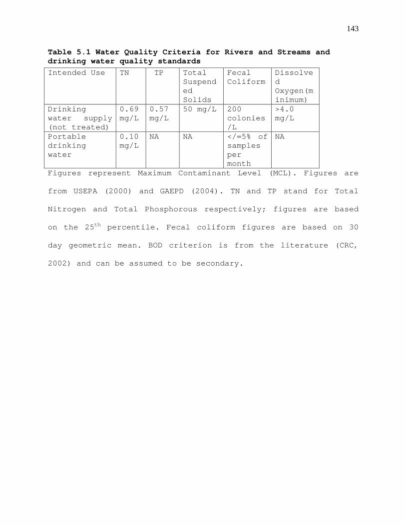
143

Table 5.1 Water Quality Criteria for Rivers and Streams and drinking water quality standards Intended Use TN TP Total

Suspended Solids

Fecal Coliform

Dissolved Oxygen(minimum)

Drinking water supply (not treated)

0.69 mg/L

0.57 mg/L

50 mg/L 200 colonies/L

>4.0 mg/L

Portable drinking water

0.10 mg/L

NA NA </=5% of samples per month

NA

Figures represent Maximum Contaminant Level (MCL). Figures are

from USEPA (2000) and GAEPD (2004). TN and TP stand for Total

Nitrogen and Total Phosphorous respectively; figures are based

on the 25th percentile. Fecal coliform figures are based on 30

day geometric mean. BOD criterion is from the literature (CRC,

2002) and can be assumed to be secondary.

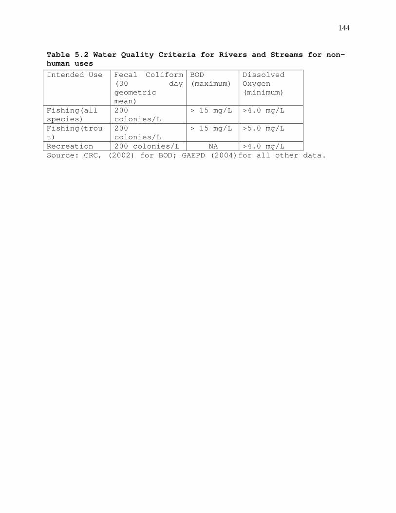
144

Table 5.2 Water Quality Criteria for Rivers and Streams for non-human uses Intended Use Fecal Coliform

(30 day geometric mean)

BOD (maximum)

Dissolved Oxygen (minimum)

Fishing(all species)

200 colonies/L

> 15 mg/L >4.0 mg/L

Fishing(trout)

200 colonies/L

> 15 mg/L >5.0 mg/L

Recreation 200 colonies/L NA >4.0 mg/L Source: CRC, (2002) for BOD; GAEPD (2004)for all other data.

145

Land Use Change: Implications for Water Quality

For the purpose of this study the baseline year for land

use change will be the latest year for which land use data

exists, which is 2005. Although L-THIA software provides up to

12 land use types including industrial, commercial, and high

density residential, our data groups together these three under

high intensity urban. Given the rural nature of the study area,

we assumed that half of the area so classified was under

commercial land use while the remainder was put to high density

residential use. About 40 % of the study area is in White county

while the remaining 60 % is in Habersham, yet the L-THIA model

runs at county level. Nevertheless so long as one has the curve

numbers (CNs), which is are measures of hydrologic soil groups,

one could create run the model on either county. We begun by

running the model at each county level with respective acreages,

then combined the acreages and used weighted averaging to arrive

at CNs for the entire ecosystem. Finally we applied the model

to Habersham county (yields the same results with White county

so long as the CNs are uniform) to come up with runoff, and

level of Non Point Source (NPS) pollutants in the waters within

the ecosystem.

In addition, we assumed that the ratio of high density

urban to low density urban acreage would remain as it was in

146

2005, which is about 10% high density and 90% low density. If

this assumption changes, the higher the proportion of high

density urban acreage the lower the water quality situation and

vis versa.

Table 5.3 provides the L-THIA program output of average

annual water quality parameters for the study area under the

different scenarios - the table covers only major NPS

pollutants.

From the table, it is apparent that runoff levels under

scenario I, II and III exceed baseline levels. Additionally, the

findings seem to suggest that although the level of TSS, BOD and

FCB increase across all scenarios, only fecal coliform and BOD

criteria are likely to be violated in the study area. The BOD

criterion of 15 mg/L is exceeded in scenario I and II. The FCB

criterion of 200 colonies/100 ml is exceeded under all scenarios

including current (2005) baseline land distribution. Current

bacteria violations may be as a result of poor human waste

disposal systems but more likely livestock waste is the culprit

as chicken, hog and cattle farming are the main agricultural

enterprises in the study area.

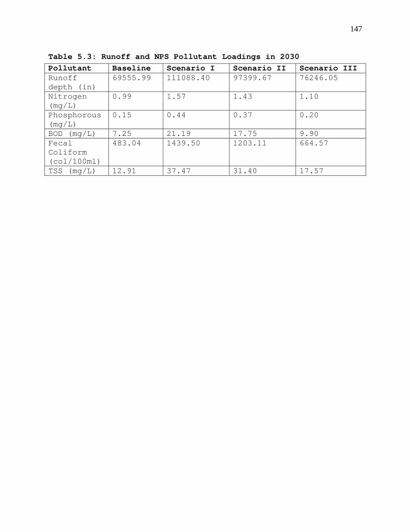
147

Table 5.3: Runoff and NPS Pollutant Loadings in 2030 Pollutant Baseline Scenario I Scenario II Scenario III Runoff depth (in)

69555.99 111088.40 97399.67 76246.05

Nitrogen (mg/L)

0.99 1.57 1.43 1.10

Phosphorous (mg/L)

0.15 0.44 0.37 0.20

BOD (mg/L) 7.25 21.19 17.75 9.90 Fecal Coliform (col/100ml)

483.04 1439.50 1203.11 664.57

TSS (mg/L) 12.91 37.47 31.40 17.57

148

Future violations of biotic criterion may be related to

increased urban development and accompanying problems with human

waste disposal such as untreated/poorly treated waste and

seepage from malfunctioning septic systems. The violations may

also be related to loss of forest cover and increase in

impervious (urban) surfaces, both of which may result in excess

runoff and deposition of solids (TSS increase) and microbes in

the water bodies.

Although farm acreage increases in scenario III, this

happens at the expense of forests which reduce by 14%. The

resulting reduction in land cover and animal waste may be

responsible for increased levels of FCB and TSS. In the next

section we estimate the value of water quality changes discussed

above.

Benefit Transfer: Empirical Application

As discussed in chapter one, we apply Benefit Transfer

method to the valuation of water quality as an ecosystem

service. The BTE protocol (outlined in chapter one) allows us to

estimate what the public would be willing to pay to mitigate

some projected environmental quality violations in an area

without carrying out actual interviews as in HPM, CVM, TCM, etc.

The lands of Habersham and White counties in the UCRB are the

affected area. Land reallocation causes changes to water quality

149

which is manifested by changes in biological oxygen demand

(proxy for dissolved oxygen) and fecal coliform bacteria levels.

We start by assuming the individual has a right to the

initial situation (higher drinking water quality). A decrease in

drinking water quality could be measured using CS which

represents an income increment corresponding to the individuals

willingness to accept compensation (WTAc ) for the diminished

level of water quality.

Given the difficulties of measuring WTA discussed in

chapter one, we follow Freeman (1993) and measure WTA indirectly

through WTP. We assume the individual has a right to the

subsequent lower quality. We proceed to measure the welfare

change using ES representing an income decrement corresponding

to the individuals willingness to pay to prevent a water quality

decrease.

In the next step of our BTE we searched for studies

conducted on relevant study sites. Two main sources of the

studies were the Environmental Valuation Database (ENVALUE) of

the Department of Environment and Conservation of the province

of New South Wales province of Australia (ENVALUE, 2007), and

the Environmental Valuation Reference Inventory (EVRI) a

Canadian based research initiative (EVRI, 1999). Other sources

of relevant studies included the online environmental science

and economic journals. The BT protocol requires that only

150

studies with relevance and applicability to the study site be

used for benefit transfer. Accordingly, the Policy site (new

study area) and the study site (past actual valuation area)

should be as similar as possible with respect to geography,

income, preferences, culture, substitution, social

characteristics.

Numerous studies on water quality valuation have been

documented. Nevertheless most studies cover nitrate (nitrogen)

contamination and studies on water quality as measured by BOD

and FCB are not plentiful.

Transferring Benefits, Valuing the Ecosystem

In the USA, documented past studies on FCB contamination

are few and those that exist offer limited use for BT. This is

so because the in most relevant studies Fecal coliform is but

one of the problems addressed so that it becomes impossible to

extract values that would apply solely to the FCB problem.

Collins and Steinback (1993) apply the cost of averting

behavior to study rural household willingness to pay for reduced

water contamination by FCB, organic chemicals and minerals, in

West Virginia. Average averting expenditure for activities

conducted by individuals and households to realize the state

water quality standards such as boiling or otherwise treating

the water, using alternative or new sources of water, are

151

computed. One important aspect of the study is that unlike

others, this study clearly categorizes the costs for overcoming

the different problems, with drinking water, FCB, organic

chemicals and minerals. Estimates of WTP in this study are

considered lower bounds as actual WTP is likely to be higher

than defensive expenditures (Bartik, 1988) used to estimate WTP

for this study. The study estimates WTP to eliminate FCB problem

in drinking water to be USD 320 per household per year.

Table 5.4 compares the study and policy sites. Surface

water is the predominant source of drinking water north of the

Georgia fall line in the Piedmont province of the Chattahoochee

River Basin (GAEPD, 1997). We can therefore make the assumption

that 100% of the public in the policy site use surface water and

have interest in local surface water quality. In addition, most

agricultural water, used in the UCRB (mainly for livestock and

aquaculture) is surface water. Additionally, rivers and streams

North of Lake Lanier are host to recreational cold-water trout

fisheries (GAEPD, 1997).To transfer this value to the UCRB study

site, we adjust for income and time as outlined in chapter one.

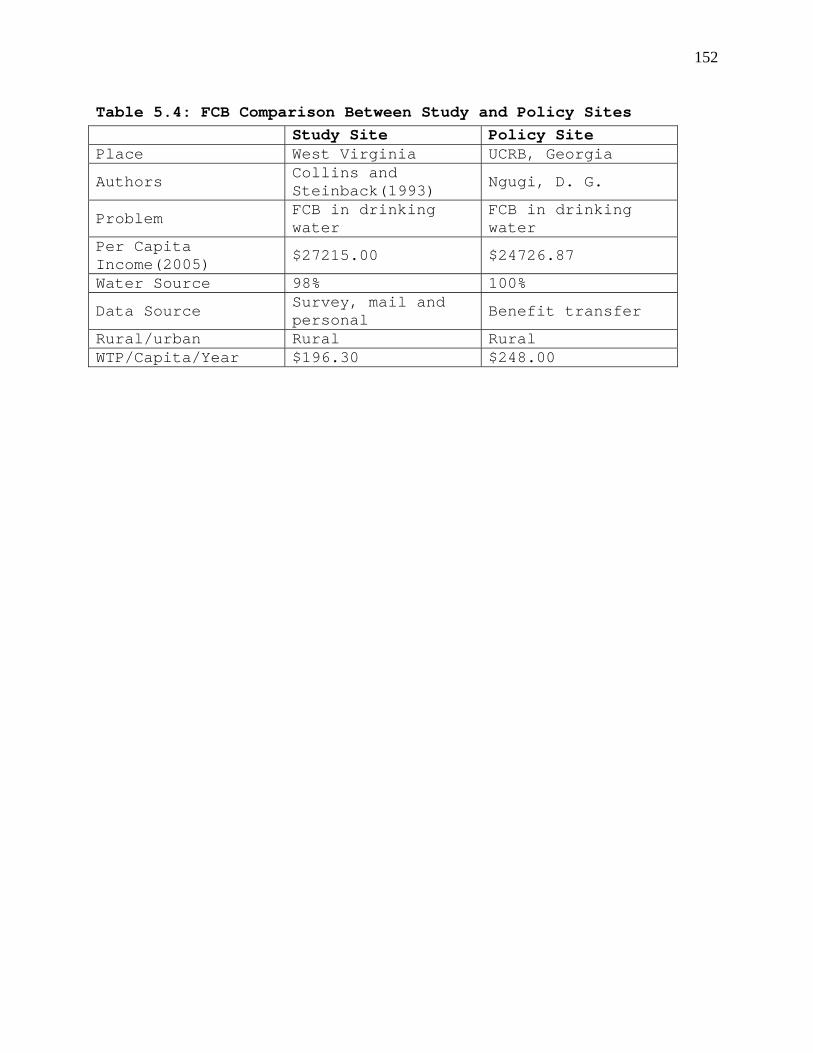
152

Table 5.4: FCB Comparison Between Study and Policy Sites Study Site Policy Site Place West Virginia UCRB, Georgia

Authors Collins and Steinback(1993) Ngugi, D. G.

Problem FCB in drinking water

FCB in drinking water

Per Capita Income(2005) $27215.00 $24726.87

Water Source 98% 100%

Data Source Survey, mail and personal Benefit transfer

Rural/urban Rural Rural WTP/Capita/Year $196.30 $248.00

153

The WTP for programs that would clear the waterways of FCB

is estimated at USD 631.70 per household or USD 248.00 per

capita per year in constant 2005 dollars. This amounts to USD

15,785,740.00 per year for the entire population of the policy

site. The 2005 constant prices WTP for the West Virginia study

site was about USD 196.30 per capita per year. The two values

compare reasonably considering the differences in per capita

income between the two areas. We note that these are lower bound

WTP values since they are derived from defensive expenditures.

A similar limitation was encountered in regard to BOD and

DO water quality benefit valuation. There exist a sizable number

of studies dealing with BOD or DO, but most studies have valued

water quality benefits associated with these parameters in

combination with other parameters so that it is difficult to

extract the share of benefits assignable to DO/BOD.

Russell and Vaughan (1982) applied the Travel Cost Model of

the number of one day fishing trips made by anglers in Indiana

and neighboring fish and wildlife recreation regions in, to

estimate WTP for water quality due to BOD/DO. The authors

obtained data from the 1975 National Survey of Fishing, Hunting

and Wildlife Related Recreation which covered the 48 contiguous

states and the District of Columbia.

Their estimation yields annual economic values of between

USD 2.05 USD 4.56 per capita. These values represent WTP for

154

increasing BOD/DO to national standards through Best Available

Technology (BAT). In preparing the literature, WTP was adjusted

to 1978 current prices. Table 5.5 compares the study and policy

sites for BOD violation.

Transferring these values to the policy site with

appropriate adjustments for income and time yields annual WTP of

between USD 5.58 and USD 12.42 per capita, which translates to

an aggregate WTP of USD 355490.10 and USD 790748.70, for the

entire policy site. A summary of the benefits is provided in

Table 5.6.

The benefits provided in Table 5.6 are really the lower

bounds of the economic value of increasing water quality to

drinking (and fishing) water standards in regard to fecal

coliform bacteria (reducing loading to a maximum of 200

colonies/ 100 ml) and reducing BOD to fishable standards (<15

mg/l). Given that fishable and drinking supply water standards

for BOD and DO standards are almost identical, we will make the

simplifying assumption that waters satisfying BOD standards also

satisfy DO standards, and this is the case for both fishing

(including trout) and drinking water supply purposes. The water

quality forecast results (Table 5.3) seem to suggest that we are

likely to have existing FCB violations in the UCRB. We have

therefore included a valuation for FCB control benefits in Table

5.6 for the baseline year.

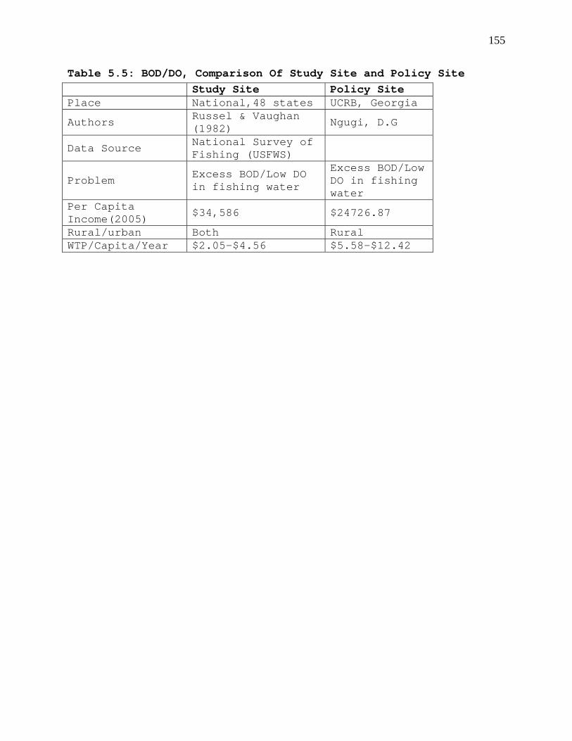
155

Table 5.5: BOD/DO, Comparison Of Study Site and Policy Site Study Site Policy Site Place National,48 states UCRB, Georgia

Authors Russel & Vaughan (1982) Ngugi, D.G

Data Source National Survey of Fishing (USFWS)

Problem Excess BOD/Low DO in fishing water

Excess BOD/Low DO in fishing water

Per Capita Income(2005) $34,586 $24726.87

Rural/urban Both Rural WTP/Capita/Year $2.05-$4.56 $5.58-$12.42

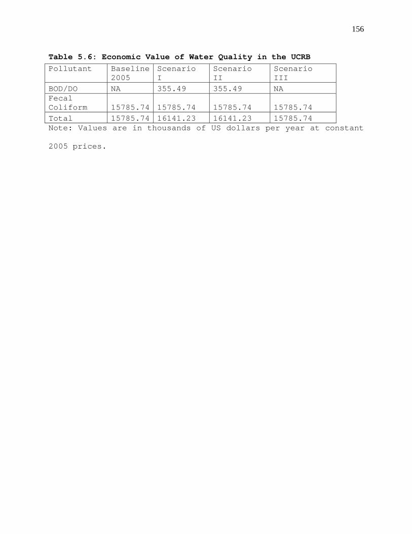
156

Table 5.6: Economic Value of Water Quality in the UCRB Pollutant

Baseline 2005

Scenario I

Scenario II

Scenario III

BOD/DO NA 355.49 355.49 NA Fecal Coliform 15785.74 15785.74 15785.74 15785.74 Total 15785.74 16141.23 16141.23 15785.74 Note: Values are in thousands of US dollars per year at constant

2005 prices.

157

Our results suggest that the lower bound WTP for creating

and maintaining water quality standards for drinking water

supply and fishing are about USD 15,785,740 under baseline and

scenario III (managed growth) conditions and about USD

16,141,230 under scenarios I and II.

158

CHAPTER VI

SUMMARY CONCLUSIONS AND RECOMMENDATIONS

The rivers of the Chattahoochee basin are the primary

source of drinking water for the city of Atlanta, a significant

number of counties north of the Georgia fault line, and more

than 4.1 million people from the three states of Georgia,

Florida, and Alabama. The Basin’s waters including Lake Sydney

Lanier provide ampler recreational amenities and income to the

Georgia. The river also provides flow regulation, sewage

disposal services, hydroelectric power, and valuable wildlife

habitat. The Upper Chattahoochee River Basin encompasses the

headwaters of the Chattahoochee River and is most serene portion

of the ecosystem including the Chattahoochee National Forest.

In this study, we sought to model land use change in the

Upper Chattahoochee River Basin above Lake Lanier and to provide

economic valuation of subsequent changes in watershed ecosystem

services and functions. Towards this end, we developed three

models of land use change, a Structural Time Series Model, an

Econometric Model and a Vector Autoregressive Model. We selected

the Structural Time Series Model for forecasting land use, based

on conventional criteria, namely, Mean Absolute Percentage Error

and Root Mean Square Error. We then proceeded to forecast three

159

likely land use and land use change scenarios based on the

aforesaid results and the resulting changes in ecosystem

services, basically water quality for drinking and fishing, for

the year 2030. We applied Benefit Transfer Techniques to

estimate the economic value of water quality in the Upper

Chattahoochee River Basin.

Summary of Findings

A model of land allocation at the aggregate watershed level

was developed assuming profit/net benefit maximization under

risk neutrality. We assumed a logistic distribution for farm to

urban, and forest to urban, land share equations. The assumption

has the advantage of ensuring the shares lie in the zero-one

range.

The econometric land use model was analyzed as an equation

by equation SURE model as all the independent variables were the

same for both equations. In line with a logistic distribution

assumption, log of land shares formed the dependent variables

for the models. Independent variables in the econometric model

included farm revenue, forest revenue, Georgia farm equity,

average wage per job, interest rate, number of large animal

units, population, per Capita income, government payment to

farms, government conservation and wetland reserve program

(years of operation dummy variable) and Payment in Kind (year

160

of operation dummy variable). The income related variables and

farm equity were deflated using CPI for the southern US.

The final equation retained (through stepwise regression)

net farm revenue, Georgia farm equity, population, and

government payments. The model also satisfied classical OLS

requirements. A key result of the model is that both (farm and

forest share) equations yielded negative and significant signs

for population, showing as expected that increase population

density will all things equal result in increased encroachment

of urban development on forests and farms. The econometric

model had the largest forecasting ability statistics meaning it

was the worst model for forecasting land allocation.

The VAR model yielded significant signs on first lag and

the trend variable. The model also satisfied classical OLS

requirements and had showed better forecasting ability compared

to the econometric model.

Econometric and conventional time series models will

normally include one form of trend or no trend in a model.

Additionally these models may include a dummy variable to cater

for structural change depending on assumptions made about the

same. The STSM has the advantage of allowing the data to reveal

underlying structural and technological change without imposing

such a priori. In our STS analysis we examined models with

stochastic trend no seasonality (STNS) and fixed trend no

161

seasonality (DTNS). Additionally, we assumed farm and forest

acreage models follow the same processes and estimated a

seemingly unrelated structural time series equations (SUTSE).

The model with the best forecasting ability was a STNS model

with structural breaks in the slope component. Ultimately the

STSM seemed the best land use forecasting model among the three

mainly by virtue of having the smallest RMSE and MAPE. The model

also tracked the data well as evidenced by lack non-significant

(at 5%) forecast failure chi-square statistic implying parameter

constancy hypothesis was not rejected.

In analyzing effect of land use change on water quality, we

took year 2005 as our baseline and postulated three land use

scenarios. Forecasts of the STSM represented the highest growth

rate in urban development; the average rate of land use change

in existing data between 1974 and 2005 was taken to be the best

case or limited/managed growth scenario and average of these two

scenarios represented a third, moderate growth scenario.

We proceeded to input land allocations into the L-THIA

model. Land allocations were as forecasted by the three

scenarios above while year 2005 data formed the baseline. The L-

THIA model output was in terms of levels of NPS pollutant

loadings including runoff, TSS, BOD (for DO), FCB in the

ecosystem surface waters. All future scenarios, except limited

growth, showed excesses (worsening water quality) for BOD and

162

FCB and worsening (increasing) runoff. In addition the baseline

also showed violations for FCB.

We applied Benefit Transfer techniques to value water

quality changes resulting from land use change and estimated

lower bounds for WTP to improve water quality to meet the FCB

criterion for drinking water supply and fishing waters and BOD

(DO) criteria for fishing waters.

Conclusions

The data related limitations of the study notwithstanding;

the most important contribution of the econometric land

allocation model was the negative and significant sign on

population. This implies that, ceteris paribus, increased

population density results in increased encroachment of urban

development on forests and farms.

The STSM outperformed both the VAR and the econometric

model in terms of forecasting ability. The presence of a

stochastic trend in the model suggests that models of land use

that ignore the trend variable might be miss-specified and might

lead to erroneous conclusions. In spite of the state of our land

use data, we were confident that the STSM yielded reasonable and

results given the model forecasting ability as evidenced by

small MAPE and RMSE. All land use forecasts pointed toward loss

of forest land to urbanization. Farmland may or may not be

163

spared the encroachment; it would all depend on interventions

that the community takes to control urban growth.

Water quality modeling revealed that land use change would

result in increased runoff, and associated increase in FCB and

BOD/DO violations. But the BOD/DO violations could be curtailed

by managing urban growth as evidenced absence of BOD violations

in the managed growth scenario. Our study finds there may be

problems of FCB under all postulated future land use scenarios.

The findings also support existing literature that there are

problems with FCB violation in the study area at the moment.

Finally, it seems that the people of UCRB would be willing

to pay a lower bound value between USD 15,785,740 and USD

16,141,230 per year to create and maintain quality standards for

fishing and drinking water supply.

Implications and Future Research Recommendations

Thus far, few economic and statistical based ecosystem and

aggregate land use models exist. The few that have been

estimated are based on conventional econometrics and there have

been no significant attempts to apply structural and/or time

series methods in estimating land use. Additionally literature

forecasting land allocation is noticeably scarce and scarcer

still is literature exploring land use change implications for

water quality particularly in the setting of an ecosystem.

164

A key contribution of this study is to estimate land use

model using VAR and STS models as past studies have relied

solely on traditional econometric models. The advantage of STS

models is that they can capture underlying trends, structural

and technological changes that may be missed or miss-specified

by other estimation methods. STSM are also better placed for ex-

ante forecasting as there is a reduction in the number of

variables to be forecasted.

This study was particularly constrained by scarcity of land

use data. The land use component of this study was seriously

impeded by lack of data. The fact that we had to interpolate to

create more than 80% of the observations meant that we would not

be very confident of getting really good results particularly

with the econometric model.

Inconsistencies in farm and forest acreage data compiled by

various bodies including the Census of agriculture, Georgia

County Guide, Georgia Statistical System and the US Forestry

Service, meant that we had to find a “more consistent” data

source for land acreage. The final data set consisted of six

observations spread over the period between 1974 and 2005

compelling us to interpolate between the observation to obtain

sufficient data and degrees of freedom. This may explain which

may explain some of the limitations of our results such as a not

so robust econometric model. Since land use data were available

165

at county level, future research could surmount this problem by

covering using a panel data approach; covering a larger portion

of the watershed, hence having more data points from more

counties.

The L-THIA model made estimating water quality changes

associated with land use change relatively fast and straight

forward. We would recommend the use of this software for land

use-water quality estimation. In estimating WTP for water

quality, a key limitation was lack of similar enough studies.

Many would be relevant studies lumped together numerous NPS

pollutants and separating a few for estimation was not possible.

The few relevant studies also applied diverse subjective

measures of utility such as “concern for preserving an amenity”

that would not be easy to formulate for a policy site.

Ultimately whereas we would have preferred to apply function

transfer we ended up using value transfer to estimate the

benefits in the policy site.

Our study supports the literatures in finding problems of

FCB in the Upper Chattahoochee River Basin. These and the

problems of BOD/DO can be ameliorated by concerted efforts

including introducing best management practices, reducing

impervious surfaces, reducing urban sprawl so as to conserve the

forest, and other activities that involve the community in

watershed management. Efforts geared towards protecting forests

166

and farms, preserving open spaces and riverbed buffer zones

would preserve water quality as evidenced by a higher level of

water quality during the baseline and limited growth scenarios

when forests occupy a major portion of the ecosystem. Such

approaches are likely to cost less than the cost of defensive

behavior or ecosystem restoration after the fact.

167

REFERENCES

Acharya, G. 2000. Approaches to Valuing the Hidden Hydrological

Services of Wetland Ecosystems. Ecol Econ. 35:63-74.

Ahn, S., Plantinga, A.J., Alig, R.J. Predicting Future Foretland

Area: A Comparison of Econometric Approaches. Forest Sci.

46(3)2000:363-376

Alp E. D. Clark. ,R Griffin and V Novotny. 2002. The Application

of Benefit Transfer in a Wisconsin Watershed. International

Conference on Policy Modeling. Free University of

Brussels, Belgium July 4-6.

Adhikari, M. Forecasting Crop Water Demand: Time Series and

Econometric Analysis. Ph.D. Dissertation, Department of

Agricultural and Applied Economics, the University of

Georgia. 2004.

American Rivers 1996. Threats: Untreated Sewage, Urban

Development, Combined Sewer Overflows, Sedimentation.

http://www.amrivers.org/mostendangered/chattahoochee1996.ht

m

http://www.amrivers.org/mostendangered/chattahoochee1996.htm

http://www.amrivers.org/mostendangered/chattahoochee1996.htm

168

Banarjee, S.B. Multiproduct Rational Expectations Forecasting of

Irrigation Water Demand: An Application to the Flint

River Basin in Georgia. Ph.D. Dissertation, Department of

Agricultural and Applied Economics, the University of

Georgia. 2004.

Bartik, T.J, 1988. Evaluating the Benefits of Non-Marginal

Reductions in Pollution Using Information on Defensive

Expenditures. Journal of Environmental Economics and

Management. 15(1)111-127.

Bergstrom, J.C., Boyle, K.J and Poe, G. L.(eds) The Economic

Value of Water Quality. New Horizons in Environmental

Economics. Edward Edgar, Ma. USA.

Bergstrom J.C 2002. Applied Resource Policy and Project

Analysis. Class Notes. University of Georgia.

Bergstrom J.C and Paul De Civita. 1999. Status of Benefits

Transfer in the United States and Canada: A Review.

Canadian J. Ag. Econ. 47:79-87.

Bergstrom J.C and Kevin, J. Boyle. 1992. Groundwater valuation

in Dougherty county, Georgia. In Benefits Transfer:

Procedures, Problems and Research Needs. Proceedings

of the Association of Environmental and Resource

Economists Workshop, Snowbird Utah. June 3-5.

Bhaduri, B., Harbor, J., Engel, B. Lim, K. J., and Jones, D.

1999. Assessing the Long-Term Hydrologic Impact of Land Use

169

Change Using a GIS-NPS Model and the World Wide Web.

Environmental Problem Solving with GIS: A national

Conference organized by the United States Environmental

Protection Agency, September 22-24. Cincinnati. OH.

Bingham, T. H., (ed.) 1992 Benefits Transfer: Procedures,

Problems and Research Needs. Proceedings of the

Environmental and Resource Economists Workshop, Snowbird,

Utah, June 3-5.

Birdsey, R.A. 1992. Carbon Storage and Accumulation in United

States Forest Ecosystems. United States Department of

Agriculture. Forest Service. General Technical Report WO-

59.

Birdsey, R.A. 2003. Carbon in U.S. Forests and Wood products,

1987-1997: State-by-State Estimates. Washington DC. U.S.

Department of Agriculture. Forest Service. General

Technical Report NE-310.

Bouma, J and Schuijt, K. 2001. Ecosystem Valuation and Cost-

Benefit Analysis as Tools in Integrated Water Management.

Erasmus Center for Sustainable Development and Management,

the Netherlands.

Bowker, J.M., Donald, B.K. English and Jason, A. Donovan. 1996.

Toward a Value for Guided Rafting on Southern Rivers. J. Ag

and Applied Econ. 28:2:423-432.

170

Boyle, K.J and Bergstrom, J.C. 1992. Benefit Transfer Studies:

Myths, Pragmatism And Idealism. Water Resources

Research. 28(3): 657-667.

Brookshire, D. 1992. Issues Regarding Benefits Transfer. Paper

Presented at the 1992 Ass. Of Environmental and

Resource Economists Workshop. Snowbird, Utah, June 3-5.

Brookshire, D. S and Neill H.R. 1992 Benefit Transfer:

Conceptual and Empirical Issues. Water Resources

Research. 28(3): 651-655.

CRC. 2002. Dissolved Oxygen: Keep it in the Water. Cooperative

Research Center for Sustainable Sugar Production.

Government of Australia. Townsville. Australia.

Caulkins, P. and Sessions, S.1997.Water Pollution and the

Organic Chemicals Industry.

Chavas, J.P., and Mathew T.Holt. Acreage Decision Under Risk:

The Case of Corn and Soybeans. American Journal of

Agricultural Economics. 72 (1990) 529-538

Collins, A.R., and Steinback, S. 1993. Rural Household Response

to Water Contamination in West Virginia. Water Resources

Bulletin. 29(2): 199-209.

Constanza, R. R.D’Arge, R. De’Groot, S. Farber, M. Grasso,B.

Hannon, K Limburg, S. Naeem, R. V. O’Neill, J Paruelo,

R. Ruskin, P. Sutton and M Van den Belt. 1997. The Value

171

Of the World’s Ecosystem Services and Natural Capital.

Nature. 387 May 15.

Delevan, W. and Epp, J.D. 2001. Benefits Transfer: The Case of

Nitrate Contamination in Pennsylvania, Georgia and Maine.

In Bergstrom, J.C., Boyle,k.J and Poe, G. L. The Economic

Value of Water Quality. New Horizons in Environmental

Economics. Edward Edgar, Ma. USA.

Desvousges, W.H., F.R Johnson, and H.S Banzhaf 1998.

Environmental Policy Analysis With Limited Information:

Principles and Applications of the Transfer Method. 1, 1-

11. http://www28.brinkster.com/Saplaco/ Massachusetts:

Edward Elgar Publishing, Inc.

Desvousges, W.H., Naughton, M.C and George, R.P. 1992. Benefit

Transfer: Conceptual Problems in Estimating Water Quality

Benefits Using existing Studies. Water Resources Research

28(3): 675-683. Ecosystem Valuation. 2002. Website.

http://www.ecosystemvaluation.org/

Doornik. J.A., Hendry D.F. 2001. GiveWin (Version 2): An

Interface to Empirical Modeling. Timberlake Consultants

Ltd. London. UK.

Du, Yaping. 1999. The Use of Benefit Transfer For The Evaluation

Of Water Quality Improvement: An Application In China.

EEPSEA Research Report Series. 1, 1-11.

http://www28.brinkster.com/valuasia/

http://www.ecosystemvaluation.org/

172

Dubois, M.R., Eric, B.C., Straka T.J., Forestry Practices Cost

and Cost Trends for in the South. Southern Journal of

Applied Forestry. 6,3(1982): 130-133.

Duffy, P.A., K.Shaishali, and H.W. Kinnucan. “Acreage Response

Under Farm Programs for Major Southeastern Field Crops.”

Journal of Agricultural and Applied Economics 26 (1994):

367-378.

Environmental Valuation Reference InventoryTM (EVRITM),

Environment Canada, 1999.

Freeman A. M III. 1993. The Measurement of Environmental and

Resource Values. Theory and Methods. Resources for the

Future. Washington, D.C.

Georgia Conservancy. 2003. Longstreet Highroad Guide to the

North Georgia Mountains. Sherpa Guides.

Georgia Environmental Protection Division. 1997. Chattahoochee

River Basin Management Plan. Georgia Department of Natural

Resources. Environment Protection Division.

Georgia Environmental Protection Division. 2004. Water Quality

in Georgia 2002-2003. Georgia Department of Natural

Resources, Environment Protection Division. Atlanta, GA.

Green W.H. 2000. Econometric Analysis. 4th ed. Prentice Hall,

New Jersey.

Gujarati. D.N. 2003. Basic Econometrics. 4th ed. McGraw Hill

Companies. New York.

173

Hanson T.R and L. U. Hatch. 1998. Impact of Reservoir Water

Level Changes on Lakefront Property and Recreational

Values. Mississippi Sate University.

Harvey, A.C. Forecasting Structural Time Series Models and the

Kalman Filter, Cambridge University Press, 1989.

Houston, J.E., Christopher S. McIntosh, Paul A. Stavriotis, and

Steve Turner. Leading Indicators of Regional Cotton

Acreage Response: Structural and Time Series Modeling

Results. Journal of Agricultural and Applied Economics,

31,3(1999):507-517

Houton Mufflin Company.1991. The American Heritage Dictionary 2nd

ed. Houton Mufflin Company. New York.

Jordan, L.J., and A.H. Elnagheeb Willingness to Pay for

Improvements in Drinking Water Quality. Water Resource

Res., 29, 237-245, 1993.

Kask, Susan F. And Jason, F Shogren. 1994. Benefits Transfer

Protocol For Long-Term Health Risk Valuation: A Case

Of Surface Water Contamination, Water Resources

Research,30:2813-23.

Kennedy P. 1998. A Guide to Economentrics. 4th Ed. The MIT

Press. Cambridge, Massachusetts.

Koopman S.J., Harvey, A.C., Doornik, J.A. and Shephard, N.

(2000). Stamp: Structural Time Series Analyser, Modeller

and Predictor, London: Timberlake Consultants Press.

174

Kramer R A, Daniel D R, Subhrendu P and Narendra P S. 1997.

Ecological and economic Analysis of Waterhsed protection in

Eastern Madagascar. J of Evt. Mgt. 49: 227-295.

Lambert, A. 2003. Economic Valuation of Wetland: An Important

Component of watershed Management Strategies at the River

Basin Scale. Ramsar Convention.

Lichtenberg, E., Land Quality, Irrigation Development and

Cropping Patterns in Northern High Plains. American Journal

of Agricultural Economics. 81(1989) 187-194

Loomis. J The Evolution of a More Rigorous Approach to Benefit

Transfer: Benefit Function Transfer. Water Resources Res.

28: March 1992: 701-05

Loomis, J., P. Kent, L. Strange, K. Fausch, and A. Covich.

2000. Measuring the Total Economic Value of Restoring

Ecosystem Services in an Impaired River Basin: Results from

a Contingent Valuation Survey.

Mahan, B. 1997. Valuing Urban wetlands: A Property Pricing

Approach. US Army Corps of Engineers. IWR Report 97-R-1

McIntyre, C.L, 1972. Soil Survey of Dawson, Lumpkin and White

Counties of Georgia, Soil Conservation Service, US

Department of Agriculture, Washington, D.C.

Menkhaus S. and Lober, D.J.1995 International Ecotourism and

the Valuation of Tropical Rainforests in Costa Rica. J. of

Environmental Mgt . 47:1-10.

175

Miller, D.J. and A.J., Plantinga. Modeling Land Use Decisions

With Aggregate Data. American Journal of Agricultural

Economics. 81(1999) 180-194

Misra S. 2002. Use of Contingent Valuation Method for Measuring

Benefits from Water Pollution Abatement by an Industrial

Estate in India. World Bank. Delhi. India.

Mitchell, R.C and R.T. Carson, Using Survey to Value Public

Goods: The contingent Valuation Method, Resources for the

Future, Washington, D.C., 1987.

National Oceanic and Atmospheric Administration. 1996. Natural

Resource Damage Assessments: Final Rule. Federal Register 5

January. 440-510.

National Resources Spatial Analysis Laboratory (NARSAL). 2007.

Georgia Land Use Trends (GLUT). University of Georgia.

Eugene Odum School of Ecology. Athens. Ga.

New South Wales Department of Environment and Conservation.

2007. Environmental Valuation Database (ENVALUE). Sydney,

New South Wales, Australia.

Nolan, T.B., Stoner, J.D. 2000. Nutrients in Groundwaters of

Conterminous United States, 1992-1995. Environ. Sci.

Technol. 34(7): 1145-1165.

North Georgia Regional Development Center. 2004. Watershed

Protection Plan Development Guidebook. North Georgia

Regional Development Center. Athens. GA.

176

Plantinga, A. J. 2007. Personal Communication. Agricultural and

Resource Economics Department. Oregon State University.

Corvallis. OR.

Planting, A.J. The Effect of Agricultural Policies on Land Use

and Environmental Quality. American Journal of Agricultural

Economics. 78(1996):1082-91

Plantinga, J.A., Maulding, T., and Miller, D.J., An Econometric

Analysis of the Cost of Sequestering carbon in Forests.

American Journal of Agricultural Economics. 81(1999):812-

824

Poe, G.L., Boyle, K.J. and Bergstrom, J.C. 2001. A Preliminary

Meta Analysis of Contingent Values for Ground Water Quality

Revised.

Purdue Research Foundation. 2004. Long-Term Hydrological Impact

Assessment(L-THIA). West Lafayette. Indiana.

Richard D. Morgenstern, ed. Economic Analyses at EPA: Assessing

Regulatory Impact Resources for the Future. Washington D.C.

Riverkeeper, 1998. Water Quality. Upper Chattahoochee

Riverkeeper. http://www.ucriverkeeper.org/waterquality.htm

Atlanta. GA.

Robertson, S.M., McIntyre, C.L., Ritchie, F.T., 1963. Soil

Survey of Habersham County Georgia, Soil Conservation

Service, US Department of Agriculture, Washington, D.C.

http://www.ucriverkeeper.org/waterquality.htm

177

Rosenberger R.S and John B Loomis. 2000. Benefits Transfer of

Outdoor Recreation Use Values: A Technical Document

Supporting the Forest Service Strategic Plan. USDA. Forest

Service.

Russell, C.S. and W.J. Vaughan, "The National Recreational

Fishing Benefits of Water Pollution Control.", Journal of

Environmental Economics and Management 9, 328-354. , 1982

Saplaco, R.R., Herminia A.F., 2003. ValuAsia: Benefits Transfer

for SouthEast Asia. Department of Economics. University of

Phillipines, Los Banos.

Shideed, K.H., F.C. White, S.J.Brannen, and R.S.Glover.

“Structural Changes of Corn Supply Response in

Georgia.” Georgia Agricultural Experiment Station Bulletin

No. 367, 1987.

Shumway, C.R., Supply, Demand, and Technology in a Multiproduct

Industry: Texas Field Crops. American Journal of

Agricultural Economics. 64(1982):631-41

Smith V. K. 1992. On Separating Defensible Benefit Transfer

From Smoke and Mirrors. Water Resources Research. 28(3):

685-694.

Center for Forest Business. 2007. Forest Product Prices Southern

States Periodicals. Warnell School of Forestry and Natural

Resources. University of Georgia.

178

Toras Mariano. 2000. The Total Economic Value of Amazonian

Deforestation 1978-1993. Ecol. Econ. 33:283-297.

Tri, N.H, Adger,N., Kelly, M., Granich, S., Nimh, N.H. 1996.

The Role of Natural Resource Management in Mitigating

Climate Impact: Mangrove Restoration in Vietnam. Center for

Social and Economic Research on the Global Environment

(CSERGE). Working Paper GEC 96-06.

United States Department of Agriculture, Forest Service.1990.

The Forest Service Program for Forest and Rangeland

Resources: A Long-Term Strategic Plan. Washington, D.C.

USDA. Forest Service, May. United States Department of

Agriculture, Forest Service. 1992. Management Strategy:

Upper Chattahoochee River Area. Chattooga Ranger District

– Chattahoochee National Forest. United States Department

of Agriculture, Forest Service.

United States Environmental Protection Agency. 1983. Guidelines

for Performing Environmental Impact Analysis. Office of

Policy Analysis. EPA-230-01-84-003.

United States Fish and Wildlife Service. 2007. What is An

Ecosystem?

http://www.fws.gov/midwest/EcosystemConservation/ecosystem.

html

United States Geological Survey (USGS). “Drought in Georgia”.

US Geological Open File Report 00-380. October 2000.

http://www.epa.gov/win/what.html

http://www.epa.gov/win/what.html

179

United States Water Resources Council.1983. Economic and

Environmental Principles and Guidelines for Water and

Related Land Resources Implementation Studies. Washington

D. C: US Water Resources Council. 10 March.

USEPA. 1986. Quality criteria for water. EPA-440/5-86-001. May

1986. U.S. EPA, Washington, DC.

USEPA. 1996. Environmental indicators of water quality in the

United States. EPA-841-R-96-002. U.S. EPA, Office of Water

(4503F), U.S. Gov. Print. Ofc., Washington, DC.

USEPA. 2000. Ambient Water Quality Criteria Recommendations.

Information Supporting the Development of State and Tribal

Nutrient Criteria for Rivers and Streams in Nutrient

Ecoregion IX. U.S. Environmental Protection Agency, Office

of Water, Washington, DC.

USEPA. 2006a. Nutrient Criteria Technical Guidance Manuals. U.S.

Environmental Protection Agency, Office of Water,

Washington, DC.

http://www.epa.gov/waterscience/criteria/nutrient/guidance/

Verna. M. 2000. Economic Valuation of Forests of Himachal

Pradesh. Main Findings: Report Submitted to the

International Institute for Environmental Development. UK.

Ward, M.H., Dekok, T.M., Levallois, P., Brender, J., Gulis, G.,

Nolan, B., and VanDerslice, J. 2005. Working Group Report :

Drinking Water Nitrate and Health – Recent Findings and



180

Research Needs. Environmental Health Perspectives. 113(11):

1607-1614.

White. P.C.L and J. C Lovett. 1997. Public Preferences and

Willingness-to-Pay for Nature Conservation in the North

York Moors National Park, UK. J. of Environmental Mgt.

53:1-13.

Wu, J., and Segerson, K. The Impact of Policies and Land

Characteristics on Potential Groundwater Pollution in

Wisconsin. American Journal of Agricultural Economics.

77(1995):1033-1047

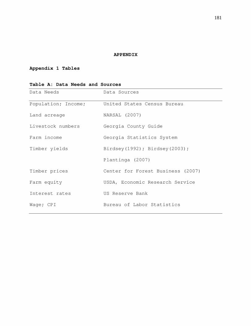
181

APPENDIX

Appendix 1 Tables

Table A: Data Needs and Sources

Data Needs Data Sources

Population; Income; United States Census Bureau

Land acreage NARSAL (2007)

Livestock numbers Georgia County Guide

Farm income Georgia Statistics System

Timber yields Birdsey(1992); Birdsey(2003);

Plantinga (2007)

Timber prices Center for Forest Business (2007)

Farm equity USDA, Economic Research Service

Interest rates US Reserve Bank

Wage; CPI Bureau of Labor Statistics

estimating land use change and economic value of water quality

Documents

Transcript of estimating land use change and economic value of water quality