Vol. 28, No. 6, November–December 2009, pp. 1095–1111issn 0732-2399 �eissn 1526-548X �09 �2806 �1095

informs ®

doi 10.1287/mksc.1090.0513©2009 INFORMS

Estimating the Value of Brand Alliances inProfessional Team Sports

Yupin YangFaculty of Business Administration, Simon Fraser University, Burnaby, British Columbia V5A 1S6, Canada,

yupin_yang@sfu.ca

Mengze Shi, Avi GoldfarbJoseph L. Rotman School of Management, University of Toronto, Toronto, Ontario M5S 3E6, Canada

{mshi@rotman.utoronto.ca, agoldfarb@rotman.utoronto.ca}

Brands often form alliances to enhance their brand equities. In this paper, we examine the alliances betweenprofessional athletes (athlete brands) and sports teams (team brands) in the National Basketball Association

(NBA). Athletes and teams match to maximize the total added value created by the brand alliance. To under-stand this total value, we estimate a structural two-sided matching model using a maximum score method.Using data on the free-agency contracts signed in the NBA during the four-year period from 1994 to 1997, wefind that both older players and players with higher performance are more likely to match with teams withmore wins. However, controlling for performance, we find that brand alliances between high brand equityplayers (defined as receiving enough votes to be an all-star starter) and medium brand equity teams (definedby stadium and broadcast revenues) generate the highest value. This suggests that top brands are not neces-sarily best off matching with other top brands. We also provide suggestive evidence that the maximum salarypolicy implemented in 1998 influenced matches based on brand equity spillovers more than matches based onperformance complementarities.

Key words : branding; brand alliances; sports marketing; matching modelHistory : Received: November 1, 2007; accepted: April 26, 2009; processed by Pradeep Chintagunta. Published

online in Articles in Advance August 14, 2009.

1. IntroductionCreating a brand alliance is a critically importantmarketing decision.1 A brand alliance involves eithershort- or long-term associations of two or more indi-vidual brands, products, or other distinctive pro-prietary assets (Rao and Ruekert 1994). Familiarexamples include brand alliances between Inteland Dell, NutraSweet and Diet Coke, and MichaelJordan and the Chicago Bulls. Despite the preva-lence of brand alliances in practice, it remains empir-ically underexplored how brands form alliances. Forinstance, how do brands choose alliance partners?Does one brand add value to another brand’s equitywhen the two form an alliance? What kinds ofalliances generate the most value? In this paper,we empirically examine these issues in the contextof alliances between professional athlete brands andteam brands.

Professional team sports provide an ideal set-ting in which to study brand alliances. First, brandalliances matter in professional team sports such

1 The term brand alliance is often interchangeably used withcobranding, comarketing, and cross-promotion.

as the National Basketball Association (NBA), theNational Football League (NFL), the National HockeyLeague (NHL), and Major League Baseball (MLB).Star players attract fans to their teams, thus increasingtheir teams’ brand equity. The value a star athlete canadd to a team includes not only the increased produc-tivity of the team’s performance but also the appealof this player to the fans beyond his on-court perfor-mance. At the same time, popular teams can enhancetheir players’ popularity, the key determinant of anathlete’s brand equity. When a player chooses a team,he considers not only the salary offered but also thevalue that the team will add to his brand equity;this value determines the player’s other sources ofincome, such as endorsement deals. Second, the mar-ket lends itself well to rigorous analysis. In most otherindustries, it is challenging (if it is even possible) toconstruct an appropriate data set of brand alliancesfor a robust empirical study. In many cases, onlya handful of potential brand alliance partners exist.Moreover, the set of these potential partners is oftennot well defined. In contrast, in professional teamsports, the rules for team–player matching are known,the set of choices for both players and teams is well

1095

Copyright:

INF

OR

MS

hold

sco

pyrig

htto

this

Articlesin

Adv

ance

vers

ion,

whi

chis

mad

eav

aila

ble

toin

stitu

tiona

lsub

scrib

ers.

The

file

may

notb

epo

sted

onan

yot

her

web

site

,inc

ludi

ngth

eau

thor

’ssi

te.

Ple

ase

send

any

ques

tions

rega

rdin

gth

ispo

licy

tope

rmis

sion

s@in

form

s.or

g.INFORMS

holds

copyrightto

this

article

and

distrib

uted

this

copy

asa

courtesy

tothe

author(s).

Add

ition

alinform

ation,

includ

ingrig

htsan

dpe

rmission

policies,

isav

ailableat

http://journa

ls.in

form

s.org/.

Yang, Shi, and Goldfarb: Estimating the Value of Brand Alliances in Professional Team Sports1096 Marketing Science 28(6), pp. 1095–1111, © 2009 INFORMS

defined, there are many players and many teams, andcontracts are publicly observed.

To study the value of brand alliances, we esti-mate a two-sided matching model of player and teamchoices. A two-sided matching model posits that twotypes of indivisible discrete agents choose their part-ners strategically. Examples of such markets includemarriage markets (Becker 1973, Choo and Siow 2006),labor markets (Jovanovic 1979), brand alliances (notedin Venkatesh et al. 2006), and free agent markets inprofessional sports.

We apply Fox’s (2008) structural estimation methodfor two-sided matching models to player and teamchoices in free agent markets.2 Solving a matchingmodel with many agents is not trivial because onemay have to examine an enormous number of pos-sible matches to ensure that no agent has an incen-tive to deviate from the equilibrium match. Fox (2008)proposes using maximum score estimation (Manski1975) to estimate a local production maximizationcondition, which is closely related to pair-wise stabil-ity in cooperative games. In our context, this modeland estimation strategy give a consistent, computa-tionally feasible estimate of the relative benefits of agiven match while allowing endogenous transfers andnonassortative matching. In parameter estimation, weapply the differential evolution method, a global max-imization route developed by Storn and Price (1997).This optimization method has been applied to findthe global optimum for the nonlinear and nondiffer-entiable continuous space functions that may havemany local optima (Fox 2008, Bajari and Fox 2009,Bajari et al. 2008).

The empirical matching model has two mainadvantages over standard random utility models suchas logit and probit. First, the matching model accom-modates rival choices. Random utility models typi-cally assume that agents on two sides of a market(players and teams) make their partner choices inde-pendently. However, the observed partner choicesresult from the decisions of all agents from bothsides; thus, their partner choices are determined inter-dependently. The two-sided matching model withmaximum score estimation deals with the interde-pendence of all agents’ choices. Second, using amaximum score in a matching model accommodatesprice endogeneity. In a matching game, the endoge-nous transfers that clear the market would be a func-tion of factors unobservable to the econometricians.Random utility models typically use instruments tocontrol for such correlation between the observedprices and omitted factors such as product attributes.In contrast, in the matching models the endogenous

2 For reviews of structural methods in marketing, see Kadiyali et al.(2001) and Chintagunta et al. (2006).

transfers result from an equilibrium function of allagent characteristics. Consequently, the transfer dataare not required in the empirical estimation of thematching models.

Using data on the free agency contracts signed inthe NBA during the four-year period from 1994 to1997, we find that both older players and playerswith higher performance are more likely to matchwith teams with more wins. However, controllingfor performance, matches between the most popularplayers and the highest revenue teams do not gener-ate the highest brand alliance value. Instead, a brandalliance between high brand equity players (definedas receiving enough votes to be an all-star starter) anda medium brand equity team (defined by stadiumand broadcast revenues) generates a higher valuethan an alliance between a high brand equity playerand a high brand equity team and a much highervalue than an alliance between a high brand equityplayer and a low brand equity team. This result indi-cates that the matching between player brand equityand team brand equity is not simply assortative.3

If controls for quality (performance) are included,brand equity matches become nonmonotonic. Themost valuable matches are between brands of differ-ent relative strengths. The best player brands may bebetter off entering brand alliances with middle-levelteam brands because middle-level team brands gainthe most from associating with a top player brand andare willing to pay for it. Interestingly, this result doesnot apply to low-value brands. Both partners needsome brand equity to generate brand spillovers froma brand alliance.

Next, we examine what happens to brand allianceswhen the team brands are restricted from transferringsome of the benefit of an alliance to the player brands.Specifically, in the 1998–1999 season, a change wasmade in the collective bargaining agreement (CBA)between the National Basketball Players Associationand the NBA team owners. The new CBA included amaximum individual salary for players, thereby pre-venting teams from offering the top players their fullvalue to the team.

We show that our estimated parameters on perfor-mance using pre-1998 data do a reasonably good jobof predicting matches both before and after the CBA.In contrast, the parameters on brand equity only do agood job predicting matches before 1998. They predictthe post-1998 out-of-sample matches poorly. We inter-pret this as suggesting that the 1998 CBA had a par-ticularly large influence on matches driven by brand

3 Becker (1973) defines assortative matching as a monotonic rela-tionship between the traits of matched players. His model suggeststhat in the marriage market, positive (negative) assortative match-ing occurs when men’s traits monotonically complement (substitutefor) women’s traits.

Copyright:

INF

OR

MS

hold

sco

pyrig

htto

this

Articlesin

Adv

ance

vers

ion,

whi

chis

mad

eav

aila

ble

toin

stitu

tiona

lsub

scrib

ers.

The

file

may

notb

epo

sted

onan

yot

her

web

site

,inc

ludi

ngth

eau

thor

’ssi

te.

Ple

ase

send

any

ques

tions

rega

rdin

gth

ispo

licy

tope

rmis

sion

s@in

form

s.or

g.INFORMS

holds

copyrightto

this

article

and

distrib

uted

this

copy

asa

courtesy

tothe

author(s).

Add

ition

alinform

ation,

includ

ingrig

htsan

dpe

rmission

policies,

isav

ailableat

http://journa

ls.in

form

s.org/.

Yang, Shi, and Goldfarb: Estimating the Value of Brand Alliances in Professional Team SportsMarketing Science 28(6), pp. 1095–1111, © 2009 INFORMS 1097

equity spillovers. The results suggest that good per-formance may be equally valuable across teams andplayers; however, spillovers from player brands varyby team brand strength. We also provide a simpletheory that shows that matches can change under amaximum salary restriction if the total surplus from abrand alliance cannot be realized because of a restric-tion on transfers from teams to players.

To the best of our knowledge, this is the first empir-ical paper to study the value of brand alliances atthe firm level. Existing research in marketing hasprovided several alternative approaches to measurebrand equity (e.g., Ailawadi et al. 2003, Goldfarb et al.2009, Kamakura and Russell 1993, Simon and Sullivan1993). However, this stream of research focuses onmeasuring the equity of individual brands ratherthan the equity created through the brand interac-tions. Notably, it is this value of brand interactionsthat underlies the partner choices in brand alliances.Thus, our paper contributes to the branding litera-ture with new methods and knowledge for under-standing brand alliances. We show that there can belarge benefits to alliances between brands of moder-ately different relative strengths. There is a small lit-erature that studies the value of brand interactionsin an experimental setting (e.g., Park et al. 1996, Raoet al. 1999, Simonin and Ruth 1998) or through sur-veys (Venkatesh and Mahajan 1997). These studiesexamine how attitudes toward each individual brandare influenced by a brand alliance.4 In contrast, ourpaper uses field data from the NBA to examine thevalue of brand alliances at the firm level.

The remainder of this paper is organized as follows.We describe the data and provide industry back-ground in §2. In §3, we explain the conceptual frame-work of brand alliances in professional team sports.We elaborate on athlete brands, team brands, andtheir relationship. In §4, we explain the two-sidedmatching model, empirical estimation procedure, andidentification. We present the estimation results in §5and study the impact of the maximum individualsalary in §6. Section 7 concludes.

2. Data and Setting2.1. Industry SettingOur data come from the National Basketball Associ-ation (NBA), founded in 1946. It gradually expandedthroughout the 1970s and began to boom in the early1980s as superstars Larry Bird and Magic Johnson

4 Although they do not examine brand alliances, Kadiyali et al.(2000) has a similar underlying objective to our paper. They usea structural framework to separately identify channel power inretailer-manufacturer relationships. In other words, they also usestructure to understand how cross-firm partnerships work.

dominated the league, followed by Michael Jordan inthe late 1980s and the 1990s. League revenues havegrown fairly steadily through the present day. Eventhough national television revenue is shared by allthe teams (Fort and Quirk 1995), local TV and radiobroadcasting and live gate revenues are not. There-fore, teams have strong financial incentives to com-pete for good players.

Before describing the details of data, we discusssome important institutional systems in U.S. profes-sional team sports in general and in the NBA in par-ticular: the free agency system, the draft system, androokie-scale contracts.

2.1.1. FreeAgencySystem. Initially, sports leaguessuch as the NBA, MLB, and the NFL used a eserve sys-tem. In a reserve system, teams have complete own-ership of the players they drafted, and players hadno control over where they played. Thus, playerswere exploited in a monopsony structure. Rottenberg(1956) reviewed this reserve system and speculatedthe outcomes under alternative institutional arrange-ments such as free agency for players and revenuesharing among team owners. Since then, free agencysystem was gradually introduced into the major U.S.sports leagues. In the NBA, the free agency systemwas added to the amendments of the CBA5 in 1976.Under the free agent system, players have the rightto choose their teams once they become a free agent.Thus, the contract between a free agent and a teamresult from the choices from both sides. In this paper,we use two-sided matching model to study thesecontracts.

With the free agent system, athletes’ salaries haveincreased rapidly as have teams’ revenues, and thesalaries of superstar players have climbed especiallyquickly (Scully 1989, MacDonald and Reynolds 1994).For example, the Chicago Bulls paid Michael Jor-dan more than $33 million for the 1997–1998 seasonalone. To control the players’ salaries, NBA team own-ers initiated a lockout in 1998. As a result, a newCBA between the NBA team owners and the players’association implemented a cap on individual play-ers’ salaries, which we label the “maximum individ-ual salary policy.” Because the 1998 CBA requires thatthe top players be paid almost the same money fromevery team, the value that a team adds to a player’sbrand equity (beyond salary) became more importantafter 1998 and the value that a player adds to a team’sbrand equity became less important. In this paper, wealso investigate the impact of this maximum individ-ual salary policy on the matching between players

5 The NBA and its players’ association negotiate a CBA approxi-mately every six years. One key purpose of the CBA is to regulatecontract negotiations between players and teams, with restrictionssuch as minimum salary and maximum contract length.

Copyright:

INF

OR

MS

hold

sco

pyrig

htto

this

Articlesin

Adv

ance

vers

ion,

whi

chis

mad

eav

aila

ble

toin

stitu

tiona

lsub

scrib

ers.

The

file

may

notb

epo

sted

onan

yot

her

web

site

,inc

ludi

ngth

eau

thor

’ssi

te.

Ple

ase

send

any

ques

tions

rega

rdin

gth

ispo

licy

tope

rmis

sion

s@in

form

s.or

g.INFORMS

holds

copyrightto

this

article

and

distrib

uted

this

copy

asa

courtesy

tothe

author(s).

Add

ition

alinform

ation,

includ

ingrig

htsan

dpe

rmission

policies,

isav

ailableat

http://journa

ls.in

form

s.org/.

Yang, Shi, and Goldfarb: Estimating the Value of Brand Alliances in Professional Team Sports1098 Marketing Science 28(6), pp. 1095–1111, © 2009 INFORMS

and teams by simulating the counterfactual matchingif the policy had not been implemented.

2.1.2. Draft System. The draft system has beenthe major way for players to enter the major profes-sional sports leagues. However, the process to draftplayers in the NBA has evolved from a territorial-pick system in the early years to a coin-flipping sys-tem to today’s lottery-pick system. Under the lotterysystem, the teams with worse won–lost records arerewarded with a higher probability of having a higherrank in the prospect draft. Prior to 1989, NBA teamswould select players until they ran out of prospects.Thus, the drafts often ran many rounds; for example,the draft went 21 rounds in 1960. From 1989 onward,the drafts have been limited to two rounds, whichgives undrafted players the chance to try out for anyteam. The draft system is used by sports leagues toincrease the competitiveness of leagues. However, itoften encourages some teams to lose to get highertalent in the draft (Taylor and Trogdon 2002), whichmay contradict the spirit of sports. Massey and Thaler(2006) examine draft-related decisions from the NFLto show that teams often overvalue the top picks intheir draft decisions. They suggest that the overvalu-ation could result from overconfidence, the winner’scurse, or false consensus.

2.1.3. Rookie-Scale Contracts. Before 1995, rookiecontract bargaining over salary and contract lengthwas almost the same as free agent bargaining, eventhough rookies did not have the right to choosetheir teams. However, since 1995 the NBA has lim-ited the contracts of the first-round draftees to spe-cific rookie-scale contracts. In rookie-scale contracts,the first-round draftees are assigned salaries accord-ing to their draft positions. The rookie-scale contractswere initially for three years, and then a team optionwas added for the fourth year. Currently, they aretwo-year contracts with team options for the thirdand fourth year. The first-round picks are guaranteeda rookie-scale contract. However, the second-roundpicks are not guaranteed a contract. Because rookiesdo not have the right to choose their teams and alsohave almost no power to negotiate their contracts, ourtwo-sided matching model does not apply to rookie-scale contracts. Thus, rookie-scale contract signingsare excluded from our data.

2.2. Data DescriptionThe data used in this paper consist of three mainparts: players, teams, and their matching. We collectedmost of the player and team information from http://www.basketball-reference.com/. This website con-tains performance statistics for every player whoever played in the NBA and for every team thathas ever been in the NBA. Team revenue data were

collected from other sources: Financial World (before1996) and Forbes (after 1996). Unlike player and teamdata, no systematic matching (contract signing) dataare available at a single website. We combine infor-mation from several websites to ensure the com-pleteness and accuracy of the matching data. Onesource is USA Today’s online salary database, whichcontains detailed salary information for players ineach season. Another comprehensive source is a per-sonal website, http://www.eskimo.com/∼pbender/index.html, which documents all the contracts signedsince 1994. In addition, we also use player informa-tion on the NBA website to cross-check a large num-ber of the contracts to ensure accuracy.

Next, we describe each part of the data set in detail.

2.2.1. Player Information. For each player, wehave three types of information: player characteris-tics (age and position), popularity, and on-court per-formance. Popularity is measured by the number ofall-star votes a player receives in the all-star ballot.Based on the number of votes, five players per con-ference, including two guards, two forwards, and onecenter, are elected to the all-star game as starters. Eachyear, the NBA reveals only the top 10 vote gettersat each position on the all-star ballot. Therefore, thenumber of all-star votes is truncated and availableonly for those players on the top 10 list. We use thesedata to construct our player brand equity measurebased on relative ranking in this voting. In the NBA,an individual player’s performance is recorded inmany dimensions, including points, rebounds, assists,steals, turnovers, and blocks. Combined, these num-bers measure a player’s on-court contribution to teamperformance. We construct a simple one-dimensionalindex to measure a player’s performance defined asfollows:

player performance = points+ rebounds+ assists

+ blocks+ steals− turnovers.

This is a performance-per-game measure and itranges from 1 to 47.8, with a mean of 15.9 and stan-dard deviation of 8.32. In the estimation, the playerperformance is rescaled to the range from 0 to 1 tomake the results easier to interpret. Our player per-formance measure is similar to the additive struc-tures commonly used in the existing research on NBAplayers’ productivity (e.g., Bellotti 1988, Berri 1999,Berri and Schmidt 2002). Of course, this is one ofmany possible ways to summarize a multidimen-sional attribute. However, this simple additive indexis likely to be highly correlated with the alternatives.Because our focus is on the matching between playerbrand and team brand, and because player perfor-mance is used as a control variable only, we expect theimpact of choosing a different performance formulaon our main results to be minimal.

Copyright:

INF

OR

MS

hold

sco

pyrig

htto

this

Articlesin

Adv

ance

vers

ion,

whi

chis

mad

eav

aila

ble

toin

stitu

tiona

lsub

scrib

ers.

The

file

may

notb

epo

sted

onan

yot

her

web

site

,inc

ludi

ngth

eau

thor

’ssi

te.

Ple

ase

send

any

ques

tions

rega

rdin

gth

ispo

licy

tope

rmis

sion

s@in

form

s.or

g.INFORMS

holds

copyrightto

this

article

and

distrib

uted

this

copy

asa

courtesy

tothe

author(s).

Add

ition

alinform

ation,

includ

ingrig

htsan

dpe

rmission

policies,

isav

ailableat

http://journa

ls.in

form

s.org/.

Yang, Shi, and Goldfarb: Estimating the Value of Brand Alliances in Professional Team SportsMarketing Science 28(6), pp. 1095–1111, © 2009 INFORMS 1099

2.2.2. Team Information. For each team in theNBA, our data contain the population of the team’shost city,6 the team’s winning percentage, the team’sroster, and revenue from live attendance and localand national broadcasting. Unfortunately, we do nothave data on any of the smaller revenue sources suchas food at the stadium and sales of licensed cloth-ing. Therefore, in our analysis, we assume that totalrevenue is highly correlated with revenue from atten-dance and broadcasting. In §4.3, we will divide theteams into categories according to their revenues as ameasure of team brand equity.

2.2.3. Player–Team Matching Information (Con-tracts). Our original data that we have collected coveralmost all the contracts signed including both freeagent signings and rookie contracts from the 1994–1995 season to the 2004–2005 season. Because ourmodel is a two-sided matching model, the contractsshould result from two-sided matching process. How-ever, all the rookie-scale contracts, minimum salarycontracts, and those contracts signing very low perfor-mance players do not result from a two-sided match-ing process. Therefore, we exclude such contractsfrom our analysis. In addition, because of the lock-out in 1998, there was no all-star game in the 1998–1999 season, so we exclude those contracts signed in1999 because of the missing data for all-star votes.Second, if a player did not play for the NBA in theseason prior to signing a contract, his contract is alsoexcluded from the estimation because of the lack ofperformance data.

As a result, we use 199 matching records (con-tracts) from the 1994–1995 season through the 1997–1998 season to estimate our model. We also use 157contracts signed in 1998–1999 and from 2000–2001 to2004–2005 to understand the impact of the maximumsalary restriction. Each contract identifies the match-ing parties—the player and the team and the sign-ing date as well as a variety of other details. These199 matching records represent all non-rookie con-tracts for players who earn above the minimum salaryand achieved a minimum level of performance inthe previous season.7 We do not have informationabout those contracts offered but not signed. Suchdata would be useful to validate our estimates ofbrand alliance values.

6 Population is based on data from the 2000 U.S. Census and 2001Canadian Census.7 We drop players with very low performance because theyare unlikely to hold any brand equity. Specifically, using theperformance measure defined above, we drop all centers with aperformance level below 0.2 and all guards and forwards witha performance level below 0.3. Results change little if they areincluded.

3. Athlete Brands, Team Brands, andthe Alliances

In this section, we conceptually discuss athlete brands(player brands) and team brands, and how theycan add value to each other’s brand equity throughbrand alliances. In the marketing literature, there aremany approaches to measure brand equity. Kellerand Lehmann (2006) divide these measures into threecategories. The first category uses financial marketoutcomes. For example, Simon and Sullivan (1993)use incremental cash flows to estimate brand equityat both the firm and individual brand levels. The sec-ond category is from the consumer’s perspective. Thisapproach often uses survey data to assess the aware-ness, attitudes, associations, attachments, and loyal-ties that consumers have toward a brand (e.g., Keller1993, Park and Srinivasan 1994). The third categorytakes the firm’s perspective and uses product-marketoutcomes such as price premium and market shareto measure brand equity (e.g., Ailawadi et al. 2003,Goldfarb et al. 2009).

In this paper, we are interested in brand-level deci-sions to form alliances but do not have data on cashflows or financial value. Therefore, we take the firm’sperspective—the teams and the players—using anapproach similar to Ailawadi et al. (2003). For teams,we measure brand equity as the team’s revenue frompaid attendance and from local and national broad-cast rights. For players, we measure brand equity byall-star votes in all-star balloting. This measure canbe seen as an aggregate measure of fans’ attitudestoward the athletes. Because our primary interestis in brand spillovers rather than how performanceaffects matching, in the structural analysis that fol-lows we examine how brand equity influences teamand player matches over and above observable mea-sures of performance (in the previous season) for theteam and the player. In this way, we use a variant ofGoldfarb et al. (2009), who argue that brand equityis that value over and above the impact of searchattributes.

3.1. Athlete BrandsIn professional team sports such as football, bas-ketball, baseball, and soccer, although the team’sperformance depends primarily on the entire team,spectators often attend live games or watch tele-vised games because they are attracted by the super-star players. For example, it is well-known thatDavid Beckham in soccer and Michael Jordan inthe NBA have drawn massive audiences to theirteams. This phenomenon is empirically demonstratedby Hausman and Leonard (1997), who find thatNBA superstars such as Michael Jordan, Larry Bird,Shaquille O’Neal, and Charles Barkley have a largeimpact on TV ratings and game attendance. As a

Copyright:

INF

OR

MS

hold

sco

pyrig

htto

this

Articlesin

Adv

ance

vers

ion,

whi

chis

mad

eav

aila

ble

toin

stitu

tiona

lsub

scrib

ers.

The

file

may

notb

epo

sted

onan

yot

her

web

site

,inc

ludi

ngth

eau

thor

’ssi

te.

Ple

ase

send

any

ques

tions

rega

rdin

gth

ispo

licy

tope

rmis

sion

s@in

form

s.or

g.INFORMS

holds

copyrightto

this

article

and

distrib

uted

this

copy

asa

courtesy

tothe

author(s).

Add

ition

alinform

ation,

includ

ingrig

htsan

dpe

rmission

policies,

isav

ailableat

http://journa

ls.in

form

s.org/.

Yang, Shi, and Goldfarb: Estimating the Value of Brand Alliances in Professional Team Sports1100 Marketing Science 28(6), pp. 1095–1111, © 2009 INFORMS

result, teams compete for the service of the bestathletes by offering attractive compensation pack-ages worth millions of dollars every year. Super-star athletes also receive income through endorsementdeals. For example, in 2003 LeBron James signed aseven-year endorsement contract with Nike worth $90million. Such deals further underscore the value ofathlete brands.

Why do superstar athletes have such high brandequities? From the behavior perspective, McCracken(1989) proposes that the brand value could stemfrom the cultural meanings with which these celebrityathletes are endowed. Such cultural meanings mayinclude status, class, gender, and age as well aspersonality and lifestyles. Athlete brands are valu-able because these cultural meanings can be passedfrom the celebrity athletes to consumers through ser-vices provided (e.g., games) and products endorsed.From the economic perspective, Rosen (1981) arguesthat such superstar effects arise because of joint con-sumption technology and imperfect substitution ofconsumers’ preferences. The joint consumption tech-nology indicates that a large number of people canconsume the “celebrity” service together, thus imply-ing great economies of scale for superstars. Theimperfect substitution means that quantity cannotsubstitute for quality; that is, the value of watching asuperstar player is higher than the value of watchingseveral mediocre players. As a consequence of jointconsumption technology and imperfect substitution,in equilibrium only a small number of athletes canenjoy star status and high brand equities.8

We define a player’s brand equity by the votes hereceives in all-star balloting over and above his per-formance during the season. Therefore, a player whoreceives a large number of votes relative to his perfor-mance statistics will have a high level of brand equity.In this way, in examining player–team matches, wecan assess the brand spillovers between players andteams separately from the value of the player’s per-formance to the team.

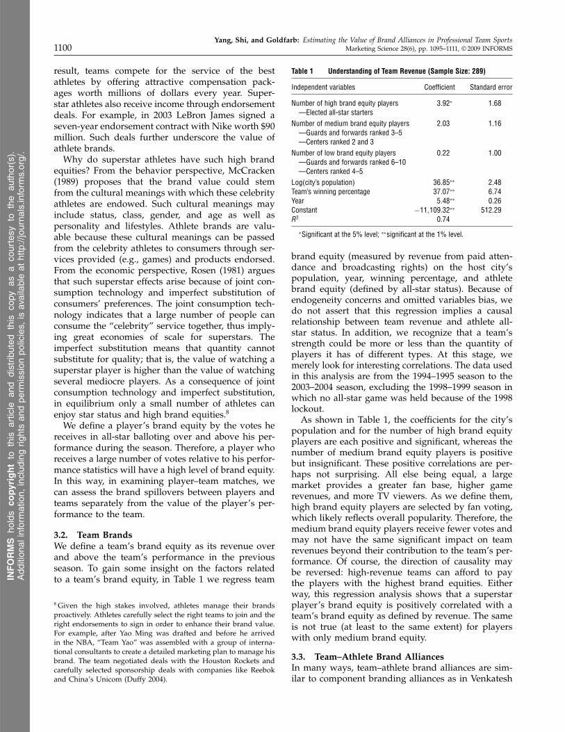
3.2. Team BrandsWe define a team’s brand equity as its revenue overand above the team’s performance in the previousseason. To gain some insight on the factors relatedto a team’s brand equity, in Table 1 we regress team

8 Given the high stakes involved, athletes manage their brandsproactively. Athletes carefully select the right teams to join and theright endorsements to sign in order to enhance their brand value.For example, after Yao Ming was drafted and before he arrivedin the NBA, “Team Yao” was assembled with a group of interna-tional consultants to create a detailed marketing plan to manage hisbrand. The team negotiated deals with the Houston Rockets andcarefully selected sponsorship deals with companies like Reebokand China’s Unicom (Duffy 2004).

Table 1 Understanding of Team Revenue (Sample Size: 289)

Independent variables Coefficient Standard error

Number of high brand equity players 3�92∗ 1�68—Elected all-star starters

Number of medium brand equity players 2�03 1�16—Guards and forwards ranked 3–5—Centers ranked 2 and 3

Number of low brand equity players 0�22 1�00—Guards and forwards ranked 6–10—Centers ranked 4–5

Log(city’s population) 36�85∗∗ 2�48Team’s winning percentage 37�07∗∗ 6�74Year 5�48∗∗ 0�26Constant −11�109�32∗∗ 512�29R2 0�74

∗Significant at the 5% level; ∗∗significant at the 1% level.

brand equity (measured by revenue from paid atten-dance and broadcasting rights) on the host city’spopulation, year, winning percentage, and athletebrand equity (defined by all-star status). Because ofendogeneity concerns and omitted variables bias, wedo not assert that this regression implies a causalrelationship between team revenue and athlete all-star status. In addition, we recognize that a team’sstrength could be more or less than the quantity ofplayers it has of different types. At this stage, wemerely look for interesting correlations. The data usedin this analysis are from the 1994–1995 season to the2003–2004 season, excluding the 1998–1999 season inwhich no all-star game was held because of the 1998lockout.

As shown in Table 1, the coefficients for the city’spopulation and for the number of high brand equityplayers are each positive and significant, whereas thenumber of medium brand equity players is positivebut insignificant. These positive correlations are per-haps not surprising. All else being equal, a largemarket provides a greater fan base, higher gamerevenues, and more TV viewers. As we define them,high brand equity players are selected by fan voting,which likely reflects overall popularity. Therefore, themedium brand equity players receive fewer votes andmay not have the same significant impact on teamrevenues beyond their contribution to the team’s per-formance. Of course, the direction of causality maybe reversed: high-revenue teams can afford to paythe players with the highest brand equities. Eitherway, this regression analysis shows that a superstarplayer’s brand equity is positively correlated with ateam’s brand equity as defined by revenue. The sameis not true (at least to the same extent) for playerswith only medium brand equity.

3.3. Team–Athlete Brand AlliancesIn many ways, team–athlete brand alliances are sim-ilar to component branding alliances as in Venkatesh

Copyright:

INF

OR

MS

hold

sco

pyrig

htto

this

Articlesin

Adv

ance

vers

ion,

whi

chis

mad

eav

aila

ble

toin

stitu

tiona

lsub

scrib

ers.

The

file

may

notb

epo

sted

onan

yot

her

web

site

,inc

ludi

ngth

eau

thor

’ssi

te.

Ple

ase

send

any

ques

tions

rega

rdin

gth

ispo

licy

tope

rmis

sion

s@in

form

s.or

g.INFORMS

holds

copyrightto

this

article

and

distrib

uted

this

copy

asa

courtesy

tothe

author(s).

Add

ition

alinform

ation,

includ

ingrig

htsan

dpe

rmission

policies,

isav

ailableat

http://journa

ls.in

form

s.org/.

Yang, Shi, and Goldfarb: Estimating the Value of Brand Alliances in Professional Team SportsMarketing Science 28(6), pp. 1095–1111, © 2009 INFORMS 1101

Figure 1 The Conceptual Framework on Brand Alliance

Team a’sbrand equity

V(a, 0)

Team a’sbrand equity

V(a, i)

Player i’sbrand equity

U(a, 0)

Player i’sbrand equity

U(a, i)

Team a and player i

Brand alliance (a, i)

The value that team a adds to player i

∆U(a, i)

The value that player i adds to team a

∆V(a, i)

Prematching Postmatching

and Mahajan’s (1997) study of consumer preferencesfor Compaq computers and Intel processors. In team–athlete alliances, an athlete, as a component of theteam, cannot be sold and consumed independentlyof team services. When a team and a player form abrand alliance, their brand equities change, as shownin Figure 1. For the team, the change in its brandequity is defined as the value that the player addsto the team’s brand equity. In our analysis, we try tocontrol for player performance and examine how aplayer’s popularity influences his value to the team.High brand equity players attract fans beyond theirdirect impact on a team’s performance by increasingthe team brand’s awareness and enhancing the teambrand’s positive image. As we saw in Table 1, a team’srevenue is positively related to the number of all-starstarters on the team.

For the player, the change in his brand equity isdefined as the value that the team adds to the player’sbrand equity through their match. This value can beinterpreted as the player’s other sources of incomebeyond current salary, such as endorsement deals andfuture income potential. When matched with the rightteam, an athlete can increase his popularity in severalways, such as reaching a larger market and generatingmore media exposure.

Next, we structurally model how a team and aplayer form their partnership choices and then esti-mate the impact of a team–player brand alliance onboth brand equities.

4. The Two-Sided Matching ModelSince professional sports introduced the free agentsystem, a player has been able to choose his teamwhen he becomes a free agent. Similarly, a teamchooses which players to offer contracts. Therefore,a two-sided matching model is appropriate to jointlystudy the choices of players and teams. To identifythe matching model, we assume no relevant asym-metric information across agents. In other words, eachagent in the market knows the relevant information

about all other agents.9 The observed partner choiceswill be equilibrium outcomes derived from the two-sided matching model based on those added values.Because teams and players choose their best possi-ble matches, observed outcomes can be used to esti-mate the value that a player brand adds to the teambrand, and vice versa. After estimating these values,we can analyze how these values vary across playersand teams, one of this paper’s objectives.

4.1. Local Production MaximizationIn this subsection, we define the equilibrium con-cept used to solve the two-sided matching problem.We use the local production maximization condi-tion developed by Fox (2008) to define equilibrium.Following Fox, we use the economic language of“production” but simply mean the joint value ofthe team–player match. Fox’s definition accommo-dates matching models with unobserved endoge-nous transfers. Accommodating unobserved transfersis important in this context because although weobserve annual salaries and contract length,10 manyfeatures of the contracts are unobserved (such asoptions, incentives, no-trade clauses, etc.).11 In addi-tion, this equilibrium concept can allow for local(i.e., nonglobal) complementarities, which cannot besolved by an assortative matching model. This equi-librium concept is closely related to pairwise stabil-ity in cooperative game theory. A match is stable ifno coalition of agents prefers to deviate and form anew match. Pairwise stability means that no pair ofagents is willing to exchange and form new matches.Similarly, the local production maximization condi-tion means that the total production of any twoobserved matches should exceed the total produc-tion from an exchange of partners. Otherwise, thealternative matches could be formed without disturb-ing any other matches to make all the agents betteroff. In what follows, we derive the local productionmaximization condition based on single-agent bestresponses under price-taking behavior (Fox 2008).

9 With millions of dollars involved in almost every contract, teamsand players will try their best to obtain as much information aspossible when signing a contract. Thus, given the data we use inour analysis, we feel it is reasonable to assume symmetric informa-tion across all the agents.10 Contract length can be an important decision for both players andteams. In our model, the endogenous transfer could be in any for-mat (salaries, incentives, no-trade clause, options, contract length)as long as teams and players value contract length in the sameway. However, if players or teams value money or other incentivesdifferently, then contract length may affect our results.11 Furthermore, no appropriate empirical framework exists forincluding the value of the transfers (i.e., the salaries) in matchinganalysis. This might be an interesting extension of our work (itmight allow separate identification of team and player benefits tomatches), but we need to wait until the methods are developed.

Copyright:

INF

OR

MS

hold

sco

pyrig

htto

this

Articlesin

Adv

ance

vers

ion,

whi

chis

mad

eav

aila

ble

toin

stitu

tiona

lsub

scrib

ers.

The

file

may

notb

epo

sted

onan

yot

her

web

site

,inc

ludi

ngth

eau

thor

’ssi

te.

Ple

ase

send

any

ques

tions

rega

rdin

gth

ispo

licy

tope

rmis

sion

s@in

form

s.or

g.INFORMS

holds

copyrightto

this

article

and

distrib

uted

this

copy

asa

courtesy

tothe

author(s).

Add

ition

alinform

ation,

includ

ingrig

htsan

dpe

rmission

policies,

isav

ailableat

http://journa

ls.in

form

s.org/.

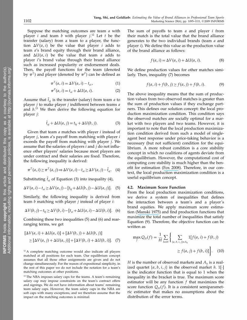
Yang, Shi, and Goldfarb: Estimating the Value of Brand Alliances in Professional Team Sports1102 Marketing Science 28(6), pp. 1095–1111, © 2009 INFORMS

Suppose the matching outcomes are team a withplayer i and team b with player j .12 Let t be thetransfer (salary) from a team to a player, the func-tion �V �a i be the value that player i adds toteam a’s brand equity through their brand alliance,and �U�a i be the value that team a adds toplayer i’s brand value through their brand alliancesuch as increased popularity or endorsement deals.Then, the payoff functions for the team (denotedby �T ) and player (denoted by �P ) can be defined as

�T �a i=�V �a i− tai (1)

�P�a i= tai +�U�a i� (2)

Assume that t̃aj is the transfer (salary) from team a toplayer j to make player j indifferent between teams aand b.13 We then derive the following equation forplayer j :

t̃aj +�U�a j= tbj +�U�b j� (3)

Given that team a matches with player i instead ofplayer j , team a’s payoff from matching with player iexceeds the payoff from matching with player j . Weassume that the salaries of players i and j do not influ-ence other players’ salaries because most players areunder contract and their salaries are fixed. Therefore,the following inequality is derived:

�T �ai≥�T �aj⇒�V �ai−tai≥�V �aj− t̃aj � (4)

Substituting t̃aj of Equation (3) into inequality (4),

�V �ai−tai≥�V �aj−�tbj+�U�bj−�U�aj�� (5)

Similarly, the following inequality is derived fromteam b matching with player j instead of player i:

�V �bj−tbj≥�V �bi−�tai+�U�ai−�U�bi�� (6)

Combining these two inequalities (5) and (6) and rear-ranging terms, we get

��V �a i+�U�a i�+ ��V �b j+�U�b j�

≥ ��V �a j+�U�a j�+ ��V �b i+�U�b i�� (7)

12 A complete matching outcome would also indicate all playersmatched at all positions for each team. Our equilibrium conceptassumes that all those other assignments are given and do notchange simultaneously. For the reason of expositional simplicity, inthe rest of this paper we do not include the notation for a team’smatching outcomes at other positions.13 The NBA imposes salary caps for the teams. A team’s remainingsalary cap may impose constraints on the team’s contract offersand signings. We do not have information about teams’ remainingteam salary caps. However, the team salary caps in the NBA aresoft caps with many exceptions, and we therefore assume that theimpact on the matching outcomes is minimal.

The sum of payoffs to team a and player i fromtheir match is the total value that the brand alliancegenerates to the two individual brands (team a andplayer i). We define this value as the production valueof the brand alliance as follows:

f �a i=�V �a i+�U�a i� (8)

We define production values for other matches simi-larly. Then, inequality (7) becomes

f �a i+ f �b j≥ f �a j+ f �b i� (9)

The above inequality means that the sum of produc-tion values from two observed matches is greater thanthe sum of production values if they exchange part-ners. This defines our solution concept: the local pro-duction maximization condition. This condition saysthe observed matches are socially optimal for a mar-ket with two players and two teams. However, it isimportant to note that the local production maximiza-tion condition derived from such a model of single-agent best response under price-taking behavior is anecessary (but not sufficient) condition for the equi-librium. A more robust condition is a core stabilityconcept in which no coalitions of agents deviate fromthe equilibrium. However, the computational cost ofcomputing core stability is much higher than the ben-efit for estimation (Fox 2008). Therefore, in our con-text, the local production maximization condition is auseful equilibrium concept.

4.2. Maximum Score FunctionFrom the local production maximization conditions,we derive a system of inequalities that definesthe interaction between a team’s and a player’sbrand equities. We apply maximum score estima-tion (Manski 1975) and find production functions thatmaximize the total number of inequalities that satisfyEquation (9). Therefore, the objective function can bewritten as

maxf

QH�f =1H

∑h∈H

{ ∑�a b i j�∈Ah

1�f �a i+ f �b j

≥ f �a j+ f �b i�

}� (10)

H is the number of observed markets and Ah is a real-ized quartet �a b i j� in the observed market h. 1�·�is the indicator function that is equal to 1 when theinequality in the bracket is true. The maximum scoreestimator will be any function f that maximizes thescore function QH�f . It is a consistent semiparamet-ric estimator that makes no assumptions about thedistribution of the error terms.

Copyright:

INF

OR

MS

hold

sco

pyrig

htto

this

Articlesin

Adv

ance

vers

ion,

whi

chis

mad

eav

aila

ble

toin

stitu

tiona

lsub

scrib

ers.

The

file

may

notb

epo

sted

onan

yot

her

web

site

,inc

ludi

ngth

eau

thor

’ssi

te.

Ple

ase

send

any

ques

tions

rega

rdin

gth

ispo

licy

tope

rmis

sion

s@in

form

s.or

g.INFORMS

holds

copyrightto

this

article

and

distrib

uted

this

copy

asa

courtesy

tothe

author(s).

Add

ition

alinform

ation,

includ

ingrig

htsan

dpe

rmission

policies,

isav

ailableat

http://journa

ls.in

form

s.org/.

Yang, Shi, and Goldfarb: Estimating the Value of Brand Alliances in Professional Team SportsMarketing Science 28(6), pp. 1095–1111, © 2009 INFORMS 1103

The maximum score estimator does not suffer fromthe “curse of dimensionality” involved with integrat-ing over multivariate distributions. In particular, stan-dard maximum likelihood and method-of-momentestimators require a nested computation of an equilib-rium for every realization of error terms. These com-plex equilibrium computations are nested within anintegral over the unobserved error terms in the mar-ket, which should be of a dimension equal to thenumber of potential matches in the market. In ouranalysis, this would mean calculating integrals of sev-eral hundred dimensions. Maximum score estimationeliminates the need to calculate this multidimensionalintegral. Maximum score estimation has the furtheradvantage of allowing situations with multiple equi-libria because equilibrium selection rules do not enterthe objective function. Using the maximum score hastwo costs: it can be less efficient than many other esti-mation techniques, and the precision of the estimatescan only be estimated using a subsampling procedure.Following Fox (2008), we believe the numerous bene-fits of this method outweigh these costs.

4.3. Market Definition and ProductionFunction Specification

In this subsection, we first define a market and thenspecify the production function. In each off season,some free agent players enter the market. Meanwhile,teams have vacancies that are filled by free agentplayers. Naturally, each off season can be defined asone market. To account for the fact that players playdifferent positions, we separate markets for guards,forwards, and centers. A market, therefore, containsall players who play the same position and becomefree agents in the same off season and all teams whoneed players in that position in the off season.14

The production function in these markets modelsthe total value of the player–team match. The produc-tion function f consists of three parts: the fixed effectsof the team’s characteristics, the fixed effects of theplayer’s characteristics, and the interaction betweenthe team’s characteristics and the player’s character-istics. The following equation shows the specificationof the production function:

f �a i= �×Xa+�× �Xa×Yi�+�×Yi + �ai� (11)

In Equation (11), Xa are independent variables mea-suring team a’s brand equity and performance, and Yiare independent variables measuring player i’s brandequity, performance, and age. All the variables for

14 Although it is computationally feasible to ignore positions andconsider the free agent signings as part of one large market, webelieve the position-specific markets better reflect the reality of theNBA.

both a team and a player are from the season preced-ing the off-season market. Team vector Xa includesone continuous variable and three dummy variablesto measure the team’s brand equity. The continuousvariable is the team’s performance measured by theteam’s winning percentage. The dummy variables arecategorized from teams’ yearly revenues from atten-dance and broadcasting. We denote the first dummyvariable as high, which equals one if a team’s rev-enue ranks in the league’s top eight. The seconddummy variable, denoted as medium, equals one ifa team’s revenue ranks between 9th and 16th. Thethird dummy variable, denoted as low, equals one if ateam’s revenue ranks worse than 16th. Thus, 8 teamsare types high and medium each year whereas teamtype low contains 11 teams before the 1996–1997 sea-son, 13 teams between the 1996–1997 and 2003–2004seasons, and 14 teams since the 2004–2005 season.

Player vector Yi includes two continuous variables(player performance and age) and four dummy vari-ables based on players’ brand equity. The continu-ous variable player performance is defined in §2 as thesum of a player’s average per-game statistics such aspoints, rebounds, and assists. The other continuousvariable is age, ranging from 21 to 41. To make theresults easier to interpret, we rescale both player per-formance and age to range from zero to one. We mea-sure player brand equity using a series of dummy vari-ables based on ranking in all-star voting. We definea high brand equity player as an all-star starter (i.e.,ranked at the top in all-star voting) for the all-stargame in the preceding season. A medium brand equityplayer was ranked highly in all-star voting but didnot come first. Since two guards and forwards areelected all-star starters per conference, for these posi-tions, medium brand equity players are ranked thirdthrough fifth. For centers, with only one electedstarter per conference, medium brand equity playersare ranked second and third. Low brand equity play-ers are defined as guards and forwards who wereranked sixth through tenth in all-star voting and cen-ters who were ranked fourth and fifth in voting. Allother players are grouped in the very low brand equitycategory.

Thus, we use the team’s revenue in the previousseason as its prematch brand equity and the player’svotes received in the previous season’s all-star bal-loting as his prematch brand equity. Instead of usingcontinuous variables such as the actual team revenueand the number of all-star votes, we construct thedummy variables to allow for richer results. Withthe continuous variables, we can identify whether ateam’s brand equity globally substitutes or comple-ments a player’s brand equity. However, the matchbetween a high brand equity player and a mediumbrand equity team could (and does) generate the

Copyright:

INF

OR

MS

hold

sco

pyrig

htto

this

Articlesin

Adv

ance

vers

ion,

whi

chis

mad

eav

aila

ble

toin

stitu

tiona

lsub

scrib

ers.

The

file

may

notb

epo

sted

onan

yot

her

web

site

,inc

ludi

ngth

eau

thor

’ssi

te.

Ple

ase

send

any

ques

tions

rega

rdin

gth

ispo

licy

tope

rmis

sion

s@in

form

s.or

g.INFORMS

holds

copyrightto

this

article

and

distrib

uted

this

copy

asa

courtesy

tothe

author(s).

Add

ition

alinform

ation,

includ

ingrig

htsan

dpe

rmission

policies,

isav

ailableat

http://journa

ls.in

form

s.org/.

Yang, Shi, and Goldfarb: Estimating the Value of Brand Alliances in Professional Team Sports1104 Marketing Science 28(6), pp. 1095–1111, © 2009 INFORMS

highest match value even though the team revenueglobally complements to player all-star votes. In otherwords, the production functions may exhibit local(rather than global) complementarity, which can beaccommodated with discrete variables.

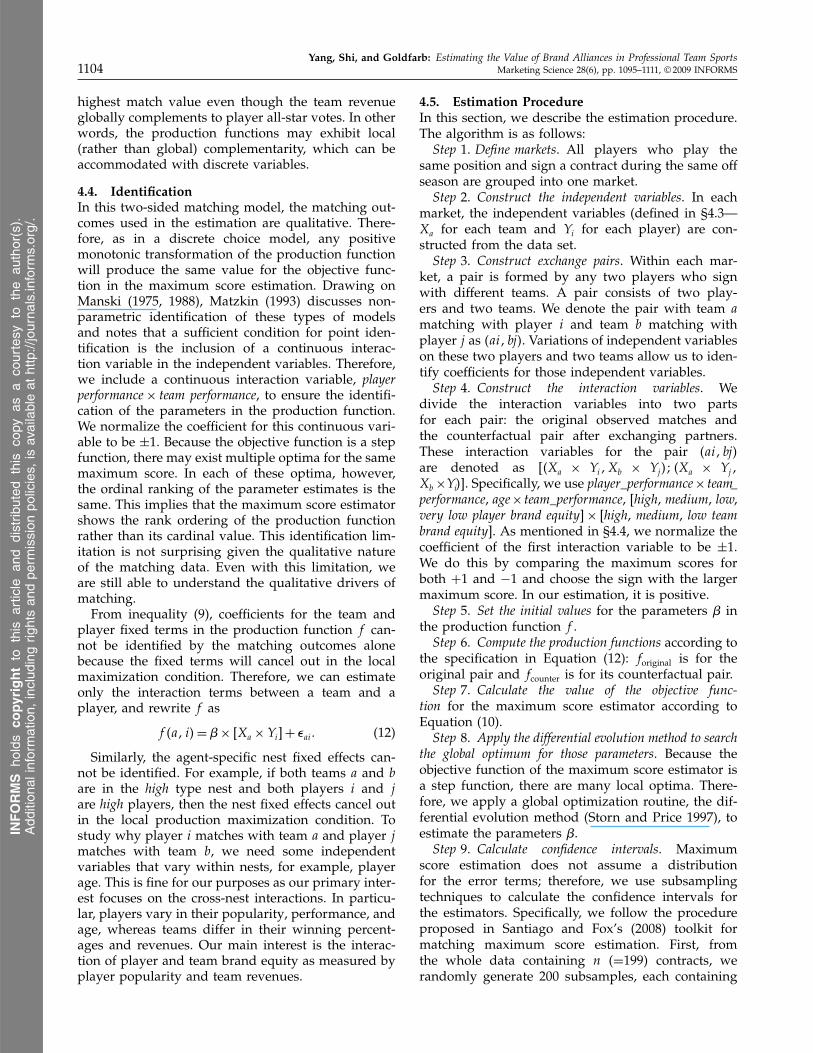
4.4. IdentificationIn this two-sided matching model, the matching out-comes used in the estimation are qualitative. There-fore, as in a discrete choice model, any positivemonotonic transformation of the production functionwill produce the same value for the objective func-tion in the maximum score estimation. Drawing onManski (1975, 1988), Matzkin (1993) discusses non-parametric identification of these types of modelsand notes that a sufficient condition for point iden-tification is the inclusion of a continuous interac-tion variable in the independent variables. Therefore,we include a continuous interaction variable, playerperformance× team performance, to ensure the identifi-cation of the parameters in the production function.We normalize the coefficient for this continuous vari-able to be ±1. Because the objective function is a stepfunction, there may exist multiple optima for the samemaximum score. In each of these optima, however,the ordinal ranking of the parameter estimates is thesame. This implies that the maximum score estimatorshows the rank ordering of the production functionrather than its cardinal value. This identification lim-itation is not surprising given the qualitative natureof the matching data. Even with this limitation, weare still able to understand the qualitative drivers ofmatching.

From inequality (9), coefficients for the team andplayer fixed terms in the production function f can-not be identified by the matching outcomes alonebecause the fixed terms will cancel out in the localmaximization condition. Therefore, we can estimateonly the interaction terms between a team and aplayer, and rewrite f as

f �a i= �× �Xa×Yi�+ �ai� (12)

Similarly, the agent-specific nest fixed effects can-not be identified. For example, if both teams a and bare in the high type nest and both players i and jare high players, then the nest fixed effects cancel outin the local production maximization condition. Tostudy why player i matches with team a and player jmatches with team b, we need some independentvariables that vary within nests, for example, playerage. This is fine for our purposes as our primary inter-est focuses on the cross-nest interactions. In particu-lar, players vary in their popularity, performance, andage, whereas teams differ in their winning percent-ages and revenues. Our main interest is the interac-tion of player and team brand equity as measured byplayer popularity and team revenues.

4.5. Estimation ProcedureIn this section, we describe the estimation procedure.The algorithm is as follows:

Step 1. Define markets. All players who play thesame position and sign a contract during the same offseason are grouped into one market.

Step 2. Construct the independent variables. In eachmarket, the independent variables (defined in §4.3—Xa for each team and Yi for each player) are con-structed from the data set.

Step 3. Construct exchange pairs. Within each mar-ket, a pair is formed by any two players who signwith different teams. A pair consists of two play-ers and two teams. We denote the pair with team amatching with player i and team b matching withplayer j as �ai bj. Variations of independent variableson these two players and two teams allow us to iden-tify coefficients for those independent variables.

Step 4. Construct the interaction variables. Wedivide the interaction variables into two partsfor each pair: the original observed matches andthe counterfactual pair after exchanging partners.These interaction variables for the pair �ai bjare denoted as ��Xa × YiXb × Yj� �Xa × YjXb×Yi�. Specifically, we use player_performance× team_performance, age× team_performance, [high, medium, low,very low player brand equity]× [high, medium, low teambrand equity]. As mentioned in §4.4, we normalize thecoefficient of the first interaction variable to be ±1.We do this by comparing the maximum scores forboth +1 and −1 and choose the sign with the largermaximum score. In our estimation, it is positive.

Step 5. Set the initial values for the parameters � inthe production function f .

Step 6. Compute the production functions according tothe specification in Equation (12): foriginal is for theoriginal pair and fcounter is for its counterfactual pair.

Step 7. Calculate the value of the objective func-tion for the maximum score estimator according toEquation (10).

Step 8. Apply the differential evolution method to searchthe global optimum for those parameters. Because theobjective function of the maximum score estimator isa step function, there are many local optima. There-fore, we apply a global optimization routine, the dif-ferential evolution method (Storn and Price 1997), toestimate the parameters �.

Step 9. Calculate confidence intervals. Maximumscore estimation does not assume a distributionfor the error terms; therefore, we use subsamplingtechniques to calculate the confidence intervals forthe estimators. Specifically, we follow the procedureproposed in Santiago and Fox’s (2008) toolkit formatching maximum score estimation. First, fromthe whole data containing n �=199 contracts, werandomly generate 200 subsamples, each containing

Copyright:

INF

OR

MS

hold

sco

pyrig

htto

this

Articlesin

Adv

ance

vers

ion,

whi

chis

mad

eav

aila

ble

toin

stitu

tiona

lsub

scrib

ers.

The

file

may

notb

epo

sted

onan

yot

her

web

site

,inc

ludi

ngth

eau

thor

’ssi

te.

Ple

ase

send

any

ques

tions

rega

rdin

gth

ispo

licy

tope

rmis

sion

s@in

form

s.or

g.INFORMS

holds

copyrightto

this

article

and

distrib

uted

this

copy

asa

courtesy

tothe

author(s).

Add

ition

alinform

ation,

includ

ingrig

htsan

dpe

rmission

policies,

isav

ailableat

http://journa

ls.in

form

s.org/.

Yang, Shi, and Goldfarb: Estimating the Value of Brand Alliances in Professional Team SportsMarketing Science 28(6), pp. 1095–1111, © 2009 INFORMS 1105

�n− 1 distinct contracts. Second, we repeatedlyapply the above estimation procedure to each of the200 subsamples and obtain 200 sets of parameterestimates. Finally, for each parameter, we use these200 estimates as its empirical distribution from whichwe calculate its confidence interval.

5. Estimation Results andInterpretation

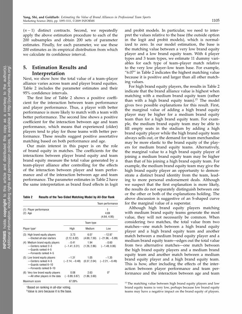
Next, we show how the total value of a team–playeralliance varies across team and player brand equities.Table 2 includes the parameter estimates and their95% confidence intervals.

The first line of Table 2 shows a positive coeffi-cient for the interaction between team performanceand player performance. Thus, a player with betterperformance is more likely to match with a team withbetter performance. The second line shows a positivecoefficient for the interaction between age and teamperformance, which means that experienced (older)players tend to play for those teams with better per-formance. These results suggest positive assortativematching based on both performance and age.

Our main interest in this paper is on the roleof brand equity in matches. The coefficients for theinteractions between player brand equity and teambrand equity measure the total value generated by ateam-player alliance after controlling for the effectsof the interaction between player and team perfor-mance and of the interaction between age and teamperformance. The parameter estimates in Table 2 havethe same interpretation as brand fixed effects in logit

Table 2 Results of the Two-Sided Matching Model by All-Star Rank

Team performance

(1) Player performance 1(2) Age 4.69

(4.64, 4.95)

Team type

Player type∗ High Medium Low

(3) High brand equity players 3�73 6�07 −12�97—Elected all-star starters �2�12�6�02� �4�69�7�50� �−21�96�−5�99�

(4) Medium brand equity players −0�41 1�94 −0�60—Centers ranked 2–3 �−1�41�0�31� �1�26�2�86� �−1�49�0�06�—Guards ranked 4–5—Forwards ranked 4–5

(5) Low brand equity players −1�31 1�05 −1�35—Centers ranked 4–5 �−2�14�−0�48� �0�37�2�04� �−2�21�−0�49�—Guards ranked 6–10—Forwards ranked 6–10

(6) Very low brand equity players 0�08 2�63 0†

—All other players in the data �−0�89�0�87� �1�86�3�60�

Maximum score 67�09%

∗Based on ranking in all-star voting.†Value is zero because it is the base.

and probit models. In particular, we need to inter-pret the values relative to the base (the outside optionin the logit and probit models), which is normal-ized to zero. In our model estimation, the base isthe matching value between a very low brand equityplayer and a low brand equity team. With 4 playertypes and 3 team types, we estimate 11 dummy vari-ables for each type of team–player match relativeto the very low player–low team base. For example,“6.07” in Table 2 indicates the highest matching valuebecause it is positive and larger than all other match-ing values.

For high brand equity players, the results in Table 2indicate that the brand alliance value is highest whenmatching with a medium brand equity team (ratherthan with a high brand equity team).15 The modelgives two possible explanations for this result. First,the marginal value of adding a high brand equityplayer may be higher for a medium brand equityteam than for a high brand equity team. For exam-ple, the medium brand equity team may be able tofill empty seats in the stadium by adding a highbrand equity player while the high brand equity teamalways sells out, or the demand for team merchandisemay be more elastic to the brand equity of the play-ers for medium brand equity teams. Alternatively,the marginal value to a high brand equity player ofjoining a medium brand equity team may be higherthan that of his joining a high brand equity team. Forexample, the medium brand equity team may give thehigh brand equity player an opportunity to demon-strate a distinct brand identity from the team, lead-ing to more personal endorsement deals. Althoughwe suspect that the first explanation is more likely,the results do not separately distinguish between oneor the other or both of the explanations holding. Theabove discussion is suggestive of an S-shaped curvefor the marginal value of a superstar.

Although high brand equity players matchingwith medium brand equity teams generate the mostvalue, they will not necessarily be common. Whenconsidering two matches, the total value from twomatches—one match between a high brand equityplayer and a high brand equity team and anothermatch between a medium brand equity player and amedium brand equity team—edges out the total valuefrom two alternative matches—one match betweenthe high brand equity players and a medium brandequity team and another match between a mediumbrand equity player and a high brand equity team.This is how, after including the effects of the inter-action between player performance and team per-formance and the interaction between age and team

15 The matching value between high brand equity players and lowbrand equity teams is very low, perhaps because low brand equityteams may have a negative impact on the brand equity of players.

Copyright:

INF

OR

MS

hold

sco

pyrig

htto

this

Articlesin

Adv

ance

vers

ion,

whi

chis

mad

eav

aila

ble

toin

stitu

tiona

lsub

scrib

ers.

The

file

may

notb

epo

sted

onan

yot

her

web

site

,inc

ludi

ngth

eau

thor

’ssi

te.

Ple

ase

send

any

ques

tions

rega

rdin

gth

ispo

licy

tope

rmis

sion

s@in

form

s.or

g.INFORMS

holds

copyrightto

this

article

and

distrib

uted

this

copy

asa

courtesy

tothe

author(s).

Add

ition

alinform

ation,

includ

ingrig

htsan

dpe

rmission

policies,

isav

ailableat

http://journa

ls.in

form

s.org/.

Yang, Shi, and Goldfarb: Estimating the Value of Brand Alliances in Professional Team Sports1106 Marketing Science 28(6), pp. 1095–1111, © 2009 INFORMS

performance, we still observe more high brand equityplayers matching with high brand equity teams inour data.

Table 2 shows that, for lower brand equity players,the matching values are highest when matching witha medium brand equity team. Their matching valuesare lower when matched with either a high brandequity team or with a lower brand equity team. Onepossible reason for this result is that medium brandequity teams’ markets are not as saturated as highbrand equity teams’ markets. Still, unlike low brandequity teams, medium brand equity teams possesssome brand value that can spill over to their players.Thus, matching with medium brand equity teams isunlikely to negatively affect players’ personal brandequity, but it can still generate substantial positivespillovers to the teams.

The matching values in Table 2 clearly show thatmatching between players and teams are not assorta-tive. The most valuable matches are between brandsof different relative strengths. More broadly, this sug-gests that top brands are not necessarily better offby matching with other top brands. The total valuegenerated may be higher if top brands match withmiddle-level brands as long as middle brands cancompensate the top brands appropriately.

6. The Impact of MaximumIndividual Salary Policy

So far, our analysis has assumed that a team can offerany salary it is willing to pay. However, as describedin §3, the 1998 CBA imposed a maximum individualsalary for players. As a result, a team cannot give anyplayer more than the maximum salary. In this sec-tion, we first show that parameters on performance(calculated in §5) do a reasonably good job of predict-ing matches both before and after 1998. In contrast,parameters on brand equity only do a good job pre-dicting matches before 1998. They predict the post-1998 out-of-sample matches poorly. We interpret thisas suggesting that the 1998 CBA had a particularlylarge influence on matches driven by brand equityspillovers. We end this section with a simple theoreti-cal model showing how a maximum salary restrictioncan change matching outcomes.

6.1. Counterfactual Simulation forthe Post-1998 Period

To understand the impact of the maximum salaryrestriction on outcomes, we simulate matches bothbefore and after the 1998 CBA. We use three dif-ferent simulations to better understand the effectof the maximum salary restriction on brand equityspillovers in contrast to performance complementar-ities. These are (1) simulated matching based on all

estimated parameters from §5, (2) simulated matchingassuming there are no brand equity spillovers, and(3) simulated matching assuming there are no perfor-mance and age reasons for matching. This separationgives insight into how the maximum salary restrictionaffects matching because of performance separatelyfrom how it affects matching because of brand equityspillovers.

The simulation process contains the followingsteps.

Step 1. Define simulated markets. First, those play-ers who played the same position and sign a con-tract in the same year in the post-1998 period aregrouped into one market. Second, select the one withthe highest performance score from those players whosign with the same teams within each market definedabove. Third, choose the top M players based on theperformance score from the selected ones.

Step 2. Calculate the payoff matrix. Within each sim-ulated market, calculate the total payoff for all thepossible matches between a player and a team usingthe estimates from the pre-1998 period: f �a i = ��×Xa×Yi+"ai, where "ai is a random draw from N�01.Thus, the payoff matrix is an M by M matrix. Whencalculating the counterfactual matching based on onlysome of the parameters, we effectively set the coef-ficients of the others to zero and draw "ai fromN�01/

√2.

Step 3. Simulate the counterfactual matching outcomesusing the linear programming. Construct the matchingproblem using the payoff matrix calculated aboveand solve it by the linear programming (Shapley andShubik 1971) for each simulated market.

When we define the simulated markets, we selectonly one player from each team to make our marketsone-to-one matching. We select a set of M contractsin each market to make sure that it is solvable bythe linear programming. Limiting to only M contractsin each market is not expected to have a signifi-cant effect on the matching outcomes across playerbrand equity types because the eliminated contractsare associated with low performance players. We ransimulations with M = 8 and M = 9 and found lit-tle difference between them. Here, we present theresults for M = 9. The random error in the produc-tion function is a match-specific error. After repeatingSteps 2 and 3 100 times, we obtain the counterfactualresults by computing the average of these 100 simu-lated outcomes.

We simulate the matching outcomes for both thepre-1998 and post-1998 periods. We use the pre-1998period to assess the fitness-of-simulation process andthe separate ability of performance and brand equityparameters to predict outcomes. We then comparethe counterfactual with actual matching outcomes inthe post-1998 period and examine how the maximum

Copyright:

INF

OR

MS

hold

sco

pyrig

htto

this

Articlesin

Adv

ance

vers

ion,

whi

chis

mad

eav

aila

ble

toin

stitu

tiona

lsub

scrib

ers.

The

file

may

notb

epo

sted

onan

yot

her

web

site

,inc

ludi

ngth

eau

thor

’ssi

te.

Ple

ase

send

any

ques

tions

rega

rdin

gth

ispo

licy

tope

rmis

sion

s@in

form

s.or

g.INFORMS

holds

copyrightto

this

article

and

distrib

uted

this

copy

asa

courtesy

tothe

author(s).

Add

ition

alinform

ation,

includ

ingrig

htsan

dpe

rmission

policies,

isav

ailableat

http://journa

ls.in

form

s.org/.

Yang, Shi, and Goldfarb: Estimating the Value of Brand Alliances in Professional Team SportsMarketing Science 28(6), pp. 1095–1111, © 2009 INFORMS 1107

individual salary changed the matching outcomes.We summarize the simulated as well as the observedmatching outcomes for both the pre- and post-1998period in Table 3. We measure the goodness of fitof counterfactual simulations by the mean squarederrors (MSEs) over the possible matching outcomes,defined as follows:

MSE= 112

(∑�actual matching percentage

− simulated matching percentage)2)

where 12 is the number of possible matching types.MSE is a simple and direct measure for goodness offit. The smaller the MSE, the better the goodness of fit.

In the pre-1998 period, the simulated matching out-comes are very close to the actual matching out-comes. This shows that the simulation works verywell in the pre-1998 period. Although this is not sur-prising because the parameters are estimated fromthese data, it provides support for comparing sim-ulated with actual outcomes in the post-1998 data.The simulations on pre-1998 data also show that themodel assuming that matches are entirely based onbrand equity spillovers also predicts the underlyingdata reasonably accurately. The model that simulatesmatches assuming no brand equity spillovers does arelatively poor job matching the actual data.

The simulations for the post-1998 period do a muchworse job fitting the data. Because this is an out-of-sample prediction, this is not entirely surprising.By separately simulating matches based entirely onbrand equity spillovers from matches that assume nobrand equity spillovers, we can assess the reasonswhy the post-1998 simulation fits the data poorly.We find that the performance and age parametersdo nearly as well predicting outcomes in the post-1998 data as in the pre-1998 data. In contrast, thebrand equity parameters do much worse in the post-1998 data. A possible explanation for this discrep-ancy is that salary caps affect matches because theyimpact incentives to form brand alliances. Althoughgood performance is equally valuable across teams,spillovers from player brands vary by team brandstrength. Next, we provide a simple theory that showsthat matches may change under a maximum salaryrestriction. The theory shows that matches can changeif the total surplus from a brand alliance cannot berealized because of the restriction on transfers fromteams to players.

6.2. Theoretical AnalysisTo illustrate the potential impact of maximum indi-vidual salary constraint on the optimal matching out-comes, let us consider a pair of matches �ai bj with

two teams �a b� and two players �i j�.16 If neither ofthe two players’ salaries (or their potential salarieswith the other team) is binding, then the local produc-tion maximization condition remains the same afterthe maximum individual salary constraint is imposed.If both players’ salaries are binding, these two playersare most likely to be the same type of players. In thispaper, we cannot identify the within-group–specificparameters under a local production maximizationmodel, and therefore, we will leave this case to futureresearch. Here, we focus on two situations: in one sit-uation, the player’s salary from the observed match-ing team is binding, and in the other situation, theplayer’s salary from the alternative team is binding.In both situations, only one player’s salary is bindingwith one team. We will examine these two situationsseparately.

Without loss of generality, we assume player i’ssalary or potential salary is binding. To better distin-guish the two players, we call player i the high brandequity player and player j the other player. In thefirst situation, player i’s salary from team a (observedmatching team) is binding; in the second situation,player i’s salary offered by team b (the alternativeteam) is binding.

Situation 1. High Brand Equity Player i’s Salaryfrom the Observed Match Is Binding �tai = t̄. Inthis situation, because player i’s salary from teamb is not binding, team b could offer more moneyto attract player i. However, team b chooses not todo so because it can get more profit from player j .Therefore, this situation is similar to the one withoutthe maximum salary restriction. The maximum indi-vidual salary constraint does not alter the local max-imization condition. (Please refer to the appendix formore details.) That is,

f �a i+ f �b j≥ f �b i+ f �a j

where

f �a i=�V �a i+�U�a i

f �b j=�V �b j+�U�b j�

f �a j=�V �a j+�U�a j

f �b i=�V �b i+�U�b i�

16 This analysis of a two-player and two-team market, althoughnot equivalent to a full equilibrium analysis for a market consist-ing of many players and many teams, sheds useful insight on theimpact of a maximum individual salary on matches and on thebenefits to different teams and players. In a larger market, chainreactions might happen because of the maximum individual salary.For example, the change of one pair of matches might cause thechange of other matches. This question is beyond this paper’s reachand is left to future research.

Copyright:

INF

OR

MS

hold

sco

pyrig

htto

this

Articlesin

Adv

ance

vers

ion,

whi

chis

mad

eav

aila

ble

toin

stitu

tiona

lsub

scrib

ers.

The

file

may

notb

epo

sted

onan

yot

her

web

site

,inc

ludi

ngth

eau

thor

’ssi

te.

Ple

ase

send

any

ques

tions

rega

rdin

gth

ispo

licy

tope

rmis

sion

s@in

form

s.or

g.INFORMS

holds

copyrightto

this

article

and

distrib

uted

this

copy

asa

courtesy

tothe

author(s).

Add

ition

alinform

ation,

includ

ingrig

htsan

dpe

rmission

policies,

isav

ailableat

http://journa

ls.in

form

s.org/.

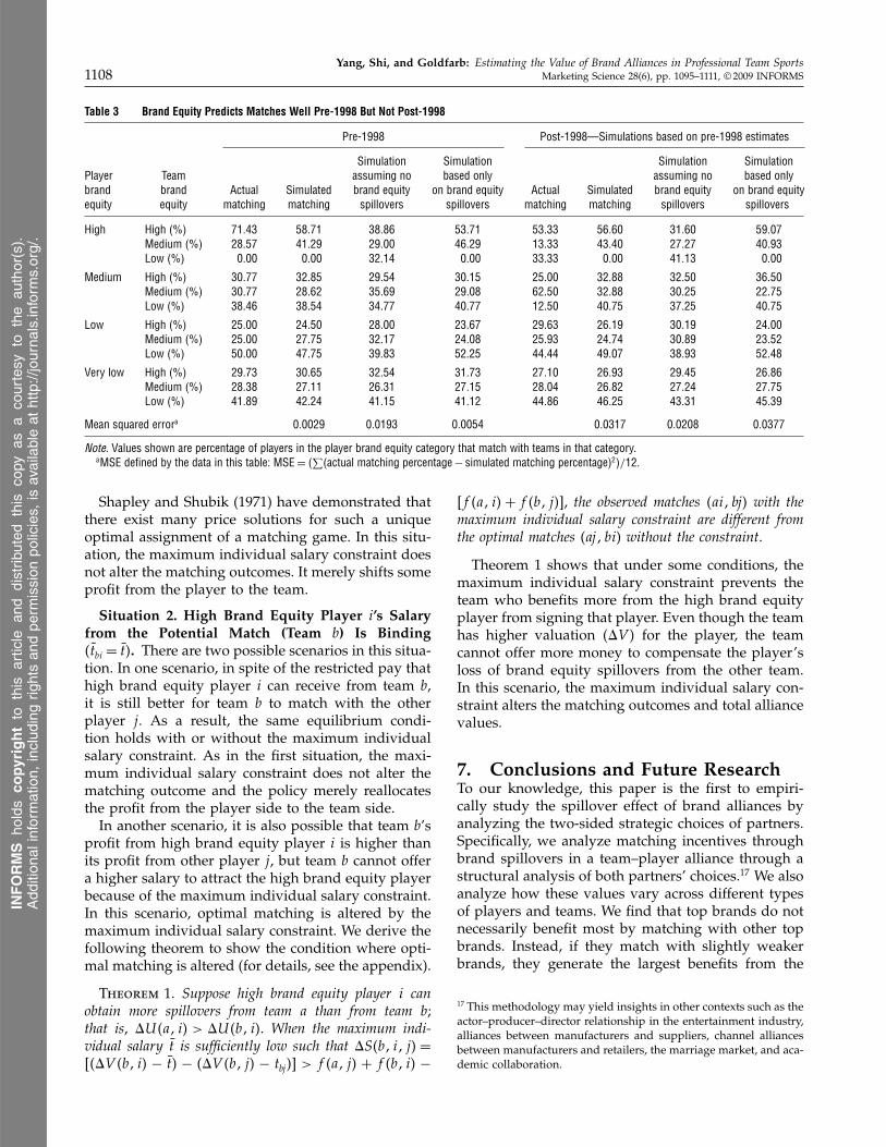
Yang, Shi, and Goldfarb: Estimating the Value of Brand Alliances in Professional Team Sports1108 Marketing Science 28(6), pp. 1095–1111, © 2009 INFORMS

Table 3 Brand Equity Predicts Matches Well Pre-1998 But Not Post-1998

Pre-1998 Post-1998—Simulations based on pre-1998 estimates

Simulation Simulation Simulation SimulationPlayer Team assuming no based only assuming no based onlybrand brand Actual Simulated brand equity on brand equity Actual Simulated brand equity on brand equityequity equity matching matching spillovers spillovers matching matching spillovers spillovers

High High (%) 71�43 58�71 38�86 53�71 53�33 56�60 31�60 59�07Medium (%) 28�57 41�29 29�00 46�29 13�33 43�40 27�27 40�93Low (%) 0�00 0�00 32�14 0�00 33�33 0�00 41�13 0�00

Medium High (%) 30�77 32�85 29�54 30�15 25�00 32�88 32�50 36�50Medium (%) 30�77 28�62 35�69 29�08 62�50 32�88 30�25 22�75Low (%) 38�46 38�54 34�77 40�77 12�50 40�75 37�25 40�75

Low High (%) 25�00 24�50 28�00 23�67 29�63 26�19 30�19 24�00Medium (%) 25�00 27�75 32�17 24�08 25�93 24�74 30�89 23�52Low (%) 50�00 47�75 39�83 52�25 44�44 49�07 38�93 52�48

Very low High (%) 29�73 30�65 32�54 31�73 27�10 26�93 29�45 26�86Medium (%) 28�38 27�11 26�31 27�15 28�04 26�82 27�24 27�75Low (%) 41�89 42�24 41�15 41�12 44�86 46�25 43�31 45�39

Mean squared errora 0.0029 0.0193 0.0054 0.0317 0.0208 0.0377

Note. Values shown are percentage of players in the player brand equity category that match with teams in that category.aMSE defined by the data in this table: MSE= �

∑�actual matching percentage− simulated matching percentage)2�/12.

Shapley and Shubik (1971) have demonstrated thatthere exist many price solutions for such a uniqueoptimal assignment of a matching game. In this situ-ation, the maximum individual salary constraint doesnot alter the matching outcomes. It merely shifts someprofit from the player to the team.

Situation 2. High Brand Equity Player i’s Salaryfrom the Potential Match (Team b) Is Binding�t̃bi = t̄. There are two possible scenarios in this situa-tion. In one scenario, in spite of the restricted pay thathigh brand equity player i can receive from team b,it is still better for team b to match with the otherplayer j . As a result, the same equilibrium condi-tion holds with or without the maximum individualsalary constraint. As in the first situation, the maxi-mum individual salary constraint does not alter thematching outcome and the policy merely reallocatesthe profit from the player side to the team side.

In another scenario, it is also possible that team b’sprofit from high brand equity player i is higher thanits profit from other player j , but team b cannot offera higher salary to attract the high brand equity playerbecause of the maximum individual salary constraint.In this scenario, optimal matching is altered by themaximum individual salary constraint. We derive thefollowing theorem to show the condition where opti-mal matching is altered (for details, see the appendix).

Theorem 1. Suppose high brand equity player i canobtain more spillovers from team a than from team b;that is, �U�a i > �U�b i. When the maximum indi-vidual salary t̄ is sufficiently low such that �S�b i j =���V �b i − t̄ − ��V �b j − tbj � > f �a j + f �b i −

�f �a i+ f �b j�, the observed matches �ai bj with themaximum individual salary constraint are different fromthe optimal matches �aj bi without the constraint.

Theorem 1 shows that under some conditions, themaximum individual salary constraint prevents theteam who benefits more from the high brand equityplayer from signing that player. Even though the teamhas higher valuation ��V for the player, the teamcannot offer more money to compensate the player’sloss of brand equity spillovers from the other team.In this scenario, the maximum individual salary con-straint alters the matching outcomes and total alliancevalues.

7. Conclusions and Future ResearchTo our knowledge, this paper is the first to empiri-cally study the spillover effect of brand alliances byanalyzing the two-sided strategic choices of partners.Specifically, we analyze matching incentives throughbrand spillovers in a team–player alliance through astructural analysis of both partners’ choices.17 We alsoanalyze how these values vary across different typesof players and teams. We find that top brands do notnecessarily benefit most by matching with other topbrands. Instead, if they match with slightly weakerbrands, they generate the largest benefits from the

17 This methodology may yield insights in other contexts such as theactor–producer–director relationship in the entertainment industry,alliances between manufacturers and suppliers, channel alliancesbetween manufacturers and retailers, the marriage market, and aca-demic collaboration.

Copyright:

INF

OR

MS

hold

sco

pyrig

htto

this

Articlesin

Adv

ance

vers

ion,

whi

chis

mad

eav

aila

ble

toin

stitu

tiona

lsub

scrib

ers.

The

file

may

notb

epo

sted

onan

yot

her

web

site

,inc

ludi

ngth

eau

thor

’ssi

te.

Ple

ase

send

any

ques

tions

rega

rdin

gth

ispo

licy

tope

rmis

sion

s@in

form

s.or

g.INFORMS

holds

copyrightto

this

article

and

distrib

uted

this

copy

asa

courtesy

tothe

author(s).

Add

ition

alinform

ation,

includ

ingrig

htsan

dpe

rmission

policies,

isav

ailableat

http://journa

ls.in

form

s.org/.

Yang, Shi, and Goldfarb: Estimating the Value of Brand Alliances in Professional Team SportsMarketing Science 28(6), pp. 1095–1111, © 2009 INFORMS 1109

alliance. Furthermore, our simulations provide sug-gestive evidence that if one partner’s brand gainsmore from an alliance than the other’s, unrestrictedcompensation allows the matches with the highesttotal value to proceed. Overall, we find that brandequity spillovers affect partner choices nonmonotoni-cally. Although our application focuses on brands inprofessional sports, we believe the insight may applymore broadly. Brand alliances between brands of dif-ferent strengths may be the most valuable.

Appendix. Local Production Maximization with aMaximum Individual Salary ConstraintConsider a pair of matches �ai bj under the maximum indi-vidual salary constraint, where player i is a high brandequity player and player j is a lower brand equity player.There are two possible scenarios under the maximum indi-vidual salary constraint.

Situation 1. High Brand Equity Player i’s Salary fromthe Observed Match Is Binding �tai = t̄The salary that makes player i indifferent to switching toteam b is

t̃bi = t̄+�U�a i−�U�b i� (13)

Because the potential salary from team b is not binding, thesalary in (13) should be smaller than the maximum individ-ual salary t̄. Thus, the condition �U�a i≤ �U�b i holds.In other words, player i gets more brand spillovers fromteam b than from team a. Because player j’s salary is notbinding for either team, the salary that makes player j indif-ferent to switching to team a is

t̃aj = tbj +�U�b j−�U�a j� (14)

Because team b’s offer to player i is not binding, team bcould increase the offer to induce player i to switch. How-ever, team b chooses not to do so because the team getshigher profit from its alternative player j . Thus, team b’spayoff from player j should be no smaller than that fromplayer i with the maximum individual salary constraint.That is,

�V �b j− tbj ≥�V �b i− t̃bi� (15)

Because player j’s offers from both teams are not binding,team a’s payoff from player i should be no smaller than thatfrom player j . That is,

�V �a i− t̄ ≥�V �a j− t̃aj � (16)

Substituting Equation (13) into (15) and Equation (14) into(16), we derive the following two inequalities:

�V �b j− tbj ≥�V �b i− t̄−�U�a i+�U�b i (17)

�V �a i− t̄ ≥�V �a j− tbj +�U�b j−�U�a j� (18)

Summing these two inequalities together, we get

�V �b j− tbj +�V �a i− t̄

≥�V �b i− t̄−�U�a i+�U�b i+�V �a j− tbj

+�U�b j−�U�a j�

Cancelling out the salaries and moving some items from theright to the left gives

�V �a i+�U�a i+�V �b j+�U�b j

≥�V �b i+�U�b i+�V �a j+�U�b j� (19)

We assume the same payoff function as without the con-straint (i.e., pre-1998). That is,

f �a i=�V �a i+�U�a i

f �b j=�V �b j+�U�b j�

f �a j=�V �a j+�U�a j

f �b i=�V �b i+�U�b i�

The inequality (19) is the same as the one without maximumindividual salary constraint:

f �a i+ f �b j≥ f �b i+ f �a j�

Shapley and Shubik (1971) demonstrated that there aremany price solutions for a unique optimal assignmentin a matching game. Under this situation, the maximumindividual salary constraint does not alter the matching out-comes or social welfare.

Situation 2. High Brand Equity Player i’s Salary fromthe Potential Match (Team b) Is Binding �t̃bi = t̄Knowing that team b’s offer to player i is binding, team aoffers player i the following amount:

tai = t̄+�U�b i−�U�a i� (20)

Player i’s salary from team a will be lower than the maxi-mum salary. That is,

�U�a i > �U�b i�

Thus, player i gets more brand spillovers from team athan from team b. Because player j’s salary is not bindingfor either team, player j’s salary to make him indifferentswitching to team a is

t̃aj = tbj +�U�b j−�U�a j� (21)

Because we observe that team a matches with player iinstead of player j , team a’s payoff from player i should beno smaller than that from player j . That is,

�V �a i− tai ≥�V �a j− t̃aj � (22)

Substituting Equations (20) and (21) to inequality (22),

�V �a i− t̄−�U�b i+�U�a i

≥ �V �a j− tbj −�U�b j+�U�a j

→�V �a i+�U�a i+�U�b j− t̄

≥ �V �a j+�U�a j+�U�b i− tbj � (23)

Even though we observe team b matching with player jinstead of player i, we still cannot infer that team b’s pay-off from player j is weakly larger than that from player ibecause team b’s offer to player i is binding. There are twopossible scenarios: In one scenario, team b wants to offer

Copyright:

INF

OR

MS

hold

sco

pyrig

htto

this

Articlesin

Adv

ance

vers

ion,

whi

chis

mad

eav

aila

ble

toin

stitu

tiona

lsub

scrib

ers.

The

file

may

notb

epo

sted

onan

yot

her

web

site

,inc

ludi

ngth

eau

thor

’ssi

te.

Ple

ase

send

any

ques

tions

rega

rdin

gth

ispo

licy

tope

rmis

sion

s@in

form

s.or

g.INFORMS

holds

copyrightto

this

article

and

distrib

uted

this

copy

asa

courtesy

tothe

author(s).

Add

ition

alinform

ation,

includ

ingrig

htsan

dpe

rmission

policies,

isav

ailableat

http://journa

ls.in

form

s.org/.

Yang, Shi, and Goldfarb: Estimating the Value of Brand Alliances in Professional Team Sports1110 Marketing Science 28(6), pp. 1095–1111, © 2009 INFORMS

just t̄ to player i because team b gets more profit fromits alternative match player j . In another scenario, team bwants to offer a higher salary to player i to make him switchteams because team b gets more profit from player i thanfrom player j . However, the maximum individual salaryconstraint prevents team b from doing so. We will discussthe two scenarios.

Case 1. Team b’s payoff from player j is no smaller than thatfrom player i. That is,

�V �b j− tbj ≥�V �b i− t̄� (24)

Summing (23) and (24) yields the same equilibrium condi-tion as the one without maximum individual salary con-straint. That is,

�V �a i+�U�a i+�V �b j+�U�b j

≥�V �b i+�U�b i+�V �a j+�U�b j

→ f �a i+ f �b j≥ f �b i+ f �a j�

Similar to Situation 1, the maximum individual salary con-straint does not alter the matching outcome or social wel-fare in this case. It just reallocates the profit from players toteams.

Case 2. Team b’s payoff from player j is smaller than that fromplayer i. That is,

�V �b j− tbj < �V �b i− t̄

→�V �b i− t̄− ��V �b j− tbj � > 0� (25)

Adding �V �b j+�V �b i into both sides of inequality (23),

�V �ai+�U�ai+�U�bj+�V �bj+�V �bi− t̄

≥�V �aj+�U�aj+�U�bi+�V �bj+�V �bi−tbj � (26)

Using the same payoff function as pre-1998,

f �a i=�V �a i+�U�a i

f �b j=�V �b j+�U�b j�

f �a j=�V �a j+�U�a j

f �b i=�V �b i+�U�b i�

Then, inequality (26) becomes the following:

f �a i+ f �b j+�V �b i− t̄

≥ f �a j+ f �b i+�V �b i− tbj �

Moving some items in the left to the right of the aboveinequality, we get

f �a i+ f �b j+ ���V �b i− t̄− ��V �b i− tbj �

≥ f �a j+ f �b i�

Denoting �S�b i j = ���V �b i− t̄− ��V �b j− tbj �, theabove inequality becomes

f �a i+ f �b j+�S�b i j≥ f �a j+ f �b i� (27)

From inequality (25), we derive �S�b i j > 0. Therefore,inequality (27) does not imply that the total payoff fromthe observed two matches is weakly larger than that fromthe alternative matches, which is the local production maxi-mization condition without the maximum individual salaryconstraint. When �S�b i j is large enough, we may havef �a i + f �b j < f �a j + f �b i, in which we shouldobserve matches �aj bi without the maximum individ-ual salary constraint. Instead, we observe �ai bj with themaximum individual salary constraint. As the maximumindividual salary t̄ becomes lower, the value of �S�b i jbecomes larger. Therefore, we can derive the followingtheorem:

Theorem A.1. Suppose high brand equity player i can obtainmore spillovers from team a than from team b; that is, �U�a i >�U�b i. When the maximum individual salary t̄ is sufficientlylow such that �S�b i j= ���V �b i− t̄− ��V �b j− tbj � >f �a j+f �b i−�f �a i+f �b j�, the observed matches �ai bjwith the maximum individual salary constraint are different fromthe optimal matches �aj bi without the constraint.

ReferencesAilawadi, K. L., D. R. Lehmann, S. A. Neslin. 2003. Revenue pre-

mium as an outcome measure of brand equity. J. Marketing67(4) 1–17.

Bajari, P., J. Fox. 2009. Measuring the efficiency of an FCC spectrumauction. Working paper, University of Chicago, Chicago.

Bajari, P., J. Fox, S. P. Ryan. 2008. Evaluating wireless carrier consol-idation using semiparametric demand estimation. Quant. Mar-keting Econom. 6(4) 299–338.

Becker, G. S. 1973. A theory of marriage: Part I. J. Political Econom.81(4) 813–846.

Bellotti, R. 1988. Basketball’s Hidden Game: Points Created, BoxscoreDefense and Other Revelations. Night Work Publishing, NewBrunswick, NJ.

Berri, D. J. 1999. Who is most valuable? Measuring the player’sproduction of wins in the NBA. Managerial Decision Econom.20(8) 411–427.

Berri, D. J., M. B. Schmidt. 2002. Instrumental versus boundedrationality: A comparison of Major League Baseball and theNational Basketball Association. J. Socio-Econom. 31(3) 191–214.

Chintagunta, P., T. Erdem, P. E. Rossi, M. Wedel. 2006. Structuralmodeling in marketing: Review and assessment. Marketing Sci.25(6) 604–616.

Choo, E., A. Siow. 2006. Who marries whom and why. J. PoliticalEconom. 14(1) 175–201.

Duffy, B. 2004. Introducing Team Yao. Business Week (October 25).Fox, J. T. 2008. Estimating matching games with transfers. Working

paper, University of Chicago, Chicago.Fort, R., J. Quirk. 1995. Cross-subsidization, incentives and out-

comes in professional team sports leagues. J. Econom. Literature33(3) 1265–1299.

Goldfarb, A., Q. Lu, S. Moorthy. 2009. Measuring brand value inan equilibrium framework. Marketing Sci. 28(1) 69–86.

Hausman, J. A., G. K. Leonard. 1997. Superstars in the NationalBasketball Association: Economic value and policy. J. LaborEconom. 15(4) 586–624.

Jovanovic, B. 1979. Job matching and the theory of turnover.J. Political Econom. 87(5) 972–990.

Kadiyali, V., P. Chintagunta, N. Vilcassim. 2000. Manufacturer-retailer channel interactions and implications for channelpower: An empirical investigation of pricing in a local market.Marketing Sci. 19(2) 127–148.

Copyright:

INF

OR

MS

hold

sco

pyrig

htto

this

Articlesin

Adv

ance

vers

ion,

whi

chis

mad

eav

aila

ble

toin

stitu

tiona

lsub

scrib

ers.

The

file

may

notb

epo

sted

onan

yot

her

web

site

,inc

ludi

ngth

eau

thor

’ssi

te.

Ple

ase

send

any

ques

tions

rega

rdin

gth

ispo

licy

tope

rmis

sion

s@in

form

s.or

g.INFORMS

holds

copyrightto

this

article

and

distrib

uted

this

copy

asa

courtesy

tothe

author(s).

Add

ition

alinform

ation,

includ

ingrig

htsan

dpe

rmission

policies,

isav

ailableat

http://journa

ls.in

form

s.org/.

Yang, Shi, and Goldfarb: Estimating the Value of Brand Alliances in Professional Team SportsMarketing Science 28(6), pp. 1095–1111, © 2009 INFORMS 1111

Kadiyali, V., K. Sudhir, V. R. Rao. 2001. Structural analysis ofcompetitive behavior: New Empirical Industrial Organiza-tion methods in marketing. Internat. J. Res. Marketing 18(1–2)161–186.

Kamakura, W. A., G. J. Russell. 1993. Measuring brand value withscanner data. Internat. J. Res. Marketing 10(1) 9–22.

Keller, K. L. 1993. Conceptualizing, measuring, and managingcustomer-based brand equity. J. Marketing 57(1) 1–22.

Keller, K. L., D. R. Lehmann. 2006. Brands and branding: Researchfindings and future priorities. Marketing Sci. 25(6) 740–759.

MacDonald, D. N., M. O. Reynolds. 1994. Are baseball playerspaid their marginal products. Managerial Decision Econom. 15(5)443–457.

Manski, C. F. 1975. Maximum score estimation of the stochasticutility model of choice. J. Econometrics 33(3) 205–228.

Manski, C. F. 1988. Identification of binary response models(in theory and methods). J. Amer. Statist. Assoc. 83(403) 729–738.

Massey, C., R. H. Thaler. 2006. The loser’s curse: Overconfidence vs.market efficiency in the National Football League draft. Work-ing paper, Duke University, Durham, NC.

Matzkin, R. L. 1993. Nonparametric identification and estimation ofpolychotomous choice models. J. Econometrics 58(1–2) 137–168.

McCracken, G. 1989. Who is the celebrity endorser? Cultural foun-dations of the endorsement process. J. Consumer Res. 16(3)310–321.

Park, C. S., V. Srinivasan. 1994. A survey-based method for mea-suring and understanding brand equity and its extendability.J. Marketing Res. 31(2) 271–288.

Park, C. W., S. Y. Jun, A. D. Shocker. 1996. Composite brand-ing alliances: Investigation of extension and feedback effects.J. Marketing Res. 33(4) 453–466.

Rao, A. R., R. W. Ruekert. 1994. Brand alliances as signals ofproduct quality. Sloan Management Rev. 36(Fall) 87–97.

Rao, A. R., L. Qu, R. W. Ruekert. 1999. Signaling unobservableproduct quality through a brand ally. J. Marketing Res. 36(2)258–268.

Rosen, S. 1981. The economics of superstars. Amer. Econom. Rev.71(5) 845–858.

Rottenberg, S. 1956. The baseball players’ labour market. J. PoliticalEconom. 64(June) 242–258.

Santiago, D., J. T. Fox. 2008. A toolkit for matching maximum scoreestimation and point and set identified subsampling inference.Working paper, University of Chicago, Chicago.

Scully, G. W. 1989. The Business of Major League Baseball. Universityof Chicago Press, Chicago.

Shapley, L. S., M. Shubik. 1971. The assignment game I: The core.Internat. J. Game Theory 1(1) 111–130.

Simon, C. J., M. W. Sullivan. 1993. The measurement and deter-minants of brand equity: A financial approach. Marketing Sci.12(1) 28–52.

Simonin, B. L., J. Ruth. 1998. Is a company known by the companyit keeps? Assessing the spillover effects of brand alliances onconsumer brand attitudes. J. Marketing Res. 35(1) 30–42.

Storn, R., K. Price. 1997. Differential evolution—A simple and effi-cient heuristic for global optimization over continuous spaces.J. Global Optim. 11(4) 341–359.

Taylor, B. A., J. G. Trogdon. 2002. Losing to win: Tournament incen-tives in the National Basketball Association. J. Labor Econom.20(1) 23–41.

Venkatesh, R., V. Mahajan. 1997. Products with branded compo-nents: An approach for premium pricing and partner selection.Marketing Sci. 16(2) 146–165.

Venkatesh, R., P. Chintagunta, V. Mahajan. 2006. Sole entrant, co-opter, or component supplier: Optimal end-product strategiesfor manufacturers of proprietary component brands. Manage-ment Sci. 52(4) 613–622.

Copyright:

INF

OR

MS

hold

sco

pyrig

htto

this

Articlesin

Adv

ance

vers

ion,

whi

chis

mad

eav

aila

ble

toin

stitu

tiona

lsub

scrib

ers.

The

file

may

notb

epo

sted

onan

yot

her

web

site

,inc

ludi

ngth

eau

thor

’ssi

te.

Ple

ase

send

any

ques

tions

rega

rdin

gth

ispo

licy

tope

rmis

sion

s@in

form

s.or

g.INFORMS

holds

copyrightto

this

article

and

distrib

uted

this

copy

asa

courtesy

tothe

author(s).

Add

ition

alinform

ation,

includ

ingrig

htsan

dpe

rmission

policies,

isav

ailableat

http://journa

ls.in

form

s.org/.