ERGODIC DYNAMICS IN SIGMA-DELTA QUANTIZATION:

TILING INVARIANT SETS AND SPECTRAL ANALYSIS OF ERROR

C. SINAN GUNTURK AND NGUYEN T. THAO

Abstract. This paper has two themes that are intertwined: The first is the dynamics ofcertain piecewise affine maps on Rm that arise from a class of analog-to-digital conversionmethods called Σ∆ (sigma-delta) quantization. The second is the analysis of reconstructionerror associated to each such method.

Σ∆ quantization generates approximate representations of functions by sequences thatlie in a restricted set of discrete values. These are special sequences in that their local av-erages track the function values closely, thus enabling simple convolutional reconstruction.In this paper, we are concerned with the approximation of constant functions only, a basiccase that presents surprisingly complex behavior. An mth order Σ∆ scheme with inputx can be translated into a dynamical system that produces a discrete-valued sequence(in particular, a 0–1 sequence) q as its output. When the schemes are stable, we showthat the underlying piecewise affine maps possess invariant sets that tile Rm up to a finitemultiplicity. When this multiplicity is one (the single-tile case), the dynamics within thetile is isomorphic to that of a generalized skew translation on Tm.

The value of x can be approximated using any consecutive M elements in q with in-creasing accuracy in M . We show that the asymptotical behavior of reconstruction errordepends on the regularity of the invariant sets, the order m, and some arithmetic proper-ties of x. We determine the behavior in a number of cases of practical interest and providegood upper bounds in some other cases when exact analysis is not yet available.

1. Introduction

This paper is motivated by the mathematical problems exhibited in and suggested by aclass of real-world practical algorithms that are used to perform analog-to-digital conversionof signals. There will be two themes in our study of these mathematical problems. The firsttheme is the dynamics of certain piecewise affine maps on Rm that are associated with thesealgorithms. The second theme is the analysis of the reconstruction error. While the firsttheme is somewhat independent of the second and is of great interest on its own, the secondtheme turns out to be crucially dependent on the first and is of interest for theoretical aswell as practical reasons.

Let us start with the following abstract algorithm for analog-to-digital encoding: Foreach input real number x in some interval I, there is a map Tx on a space S, and a finitepartition Πx = Ωx,1, . . . ,Ωx,K of S. For a fixed set of real numbers d1 < · · · < dK , anda typically fixed (but arbitrary) initial point u0 ∈ S, we define a discrete-valued outputsequence q := qx via

q[n] = di if u[n−1] := Tn−1x (u0) ∈ Ωx,i. (1.1)

Date: Initial submission: September 5, 2003, acceptance: November 17, 2003.This work has been supported in part by the National Science Foundation Grants DMS-0219072, DMS-

0219053 and CCR-0209431.

1

2 C. SINAN GUNTURK AND NGUYEN T. THAO

We would like the mapping x 7→ q to be invertible in a very special way: For an input-

independent family of averaging kernels φM ∈ ℓ1(Z), M = 1, 2, . . . , we require that for allx ∈ I, as M → ∞,

(q ∗ φM )[n] :=∑

k

φM [k]q[n− k] −→ x, uniformly in n. (1.2)

For normalization, we ask that the size of the averaging window (i.e., the support of φM )grow linearly in M ,1 and the weights satisfy

∑n φM [n] = 1.

Note that such an encoding of real numbers is inherently different from binary-expansion(or any other expansion in a number system) in that, due to (1.2), equal length segmentsof the sequence q are required to be equally good in approximating the value of x. Hence,there is a “translation-invariance” property in the representation.

This setting is a special case of a more general one in which x = (x[n])n∈Z is a boundedsequence taking values in I and

q[n] = di if u[n−1] ∈ Ωx[n],i, (1.3)

where we now define u[n] := Tx[n](u[n−1]), and require that

(q − x) ∗ φM −→ 0 uniformly. (1.4)

The basic motivation behind this type of encoding is the following intuitive idea: Let theelements x[n] be closely and regularly spaced samples of a smooth function X : R → I. Sincelocal averages of these samples around any point k would approximate x[k], i.e., x∗φM ≈ xfor suitable φM , (1.4) would then imply that the sequence x (and therefore the function X)can be approximated by the convolution q ∗ φM .

Such analog-to-digital encoding algorithms have been developed and used in electricalengineering for a few decades now. Most notable examples are the Σ∆ quantization (alsocalled Σ∆ modulation) of audio signals and the closely related error-diffusion in digitalhalftoning of images. There are several sources in the electrical engineering literature onthe theoretical and practical aspects of Σ∆ quantization [6, 10, 22]. Digital halftoning andits connections to Σ∆ quantization can be found in [1, 2, 4, 20, 26]. Recently, Σ∆ quantiza-tion has also received interest in the mathematical community, especially in approximationtheory and information theory, since a very important question is the rate of convergencein (1.4) [5, 9, 13, 14, 16].

We give in Section 2 the original description of an mth order Σ∆ modulation scheme interms of difference equations. The underlying specific map Tx, which we then refer to as Mx

(the “modulator map”), is described in Section 4; Mx is the piecewise affine transformationon S = Rm defined by

Mx(v) = Lv + (x− di)1 if v ∈ Ωx,i, (1.5)

where L := Lm is the m×m lower triangular matrix of 1’s and 1 := 1m := (1, . . . , 1)⊤ ∈ Zm.Each Σ∆ scheme is therefore characterized by its orderm, the partition Πx, and the numbersdi. A scheme is called k-bit if the size K of the partition Πx satisfies 2k−1 < K ≤ 2k. If thenumbers di are in an arithmetic progression, this is referred to as uniform quantization.As a consequence of the normalization

∑n φM [n] = 1, the input numbers x are chosen in

I ⊂ [d1, dK ]. A scheme is said to be stable if for each x, forward trajectories under the action

1It will be of interest to use infinitely supported kernels as well. We will define the necessary modificationsto handle this situation later.

ERGODIC DYNAMICS IN Σ∆ QUANTIZATION 3

of Mx are bounded in Rm. (More refined definitions of stability will be given in Section 4.)The partition Πx is an essential part of the algorithm for its central role in stability.

It is natural to measure the accuracy of a scheme by how fast the worst case error‖(x− q)∗φM‖∞ converges to zero. It is known that for an mth order stable scheme, and anappropriate choice for the family F = φM of filters,2 this quantity is O(M−m) [9]. Thehidden constant depends on the scheme as well as the input sequence x. Here, the exponentm is not sharp; in fact, for m = 1 and m = 2, improvements have been given for variousschemes [13, 15]. We will review the basic approximation properties of Σ∆ quantization inSection 2.

In applications, it is also common to measure the error in the root mean square norm dueits more robust nature (this norm is defined in Section 3). It is known for a small class ofschemes we call ideal, and a small class of sequences (basically, constants and pure sinusoids)that this norm, when averaged over a smooth distribution of values of x, has the asymptoticbehavior O(M−m−1/2) [8, 11, 17]. The analyses employed in obtaining these results relyon very special properties of these ideal schemes, such as employing an (effective) m-bituniform quantizer for the mth order scheme. It was not known how to extend these resultsto low-bit schemes (in particular, 1-bit schemes) of high order for which experimental resultsand simulation suggested similar asymptotical behavior for the root mean square error.

It is the topic of this paper to provide a general framework and methodology to analyzeΣ∆ quantization in an arbitrary setup (in terms of partition and number of bits) wheninputs are constant sequences. With regards to the first theme of this paper, we provein Section 5 that the maps Mx have an outstanding property of yielding tiling invariantsets, up to a multiplicity that is determined by the map. In the particular case of singletiles being invariant under Mx (which also appears to be systematically satisfied by allpractical Σ∆ quantization schemes), we develop a spectral theory of Σ∆ quantization.This constitutes the second theme of the paper. The particular consequence of tiling thatenables our spectral analysis is presented in Section 6. The resulting new error analysis forgeneral and particular cases is presented in the remainder of the paper.

Some notation. The symbols R, Z, and N denote the set of real numbers, the set ofintegers and the set of natural numbers, respectively. T denotes the set of real numbersmodulo 1, i.e., T = R/Z. Functions on Rm that are 1-periodic in each dimension areassumed to be defined on Tm via the identification T = [0, 1), and functions defined on Tm

are extended to Rm by periodization.Vectors and matrices are denoted in boldface letters. Transpose is denoted by an upper-

script ⊤. The j’th coordinate of a vector v is denoted by vj , unless otherwise specified.Sequence elements are denoted using brackets, such as in ω =

(ω[n]

)n∈Z

. The sequence ω

denotes time reversal of ω defined by ω[n] := ω[−n], and the symbol ∗ is used to denote theconvolution operation.

We define two types of autocorrelation. For a square integrable real-valued function f ,we define

Af (t) := (f ∗ f)(t) =

∫f(ξ)f(ξ + t) dξ.

2We shall adopt the electrical engineering terminology “filter” to refer to a sequence (or function) thatacts convolutionally.

4 C. SINAN GUNTURK AND NGUYEN T. THAO

On the other hand, we define the autocorrelation ρω for a bounded (real-valued) sequenceω by the formula

ρω[k] := limN→∞

1

N

N∑

n=1

ω[n]ω[n+ k],

provided the limit exists.The Fourier series coefficients of a measure µ on T are given by

µ[n] :=

∫

T

e−2πinξ dµ(ξ),

and the Fourier transform of a sequence h = (h[n])n∈Z is denoted by the capital letter H,i.e.,

H(ξ) :=∑

n∈Z

h[n]e2πinξ.

Hence, when Fourier inversion holds, we have H[n] = h[n].The “big oh” f = O(g) and the “small oh” f = o(g) notations will have their usual

meanings. When it matters, we also use the notation f .α g to denote that there existsa constant C that possibly depends on the parameter (or set of parameters) α such thatf ≤ Cg. We write f ≍ g if f . g and g . f , which is the same as f = Θ(g).

2. Basic theory of Σ∆ quantization

In this section, we describe the principles of Σ∆ quantization (modulation) via a set ofdefining difference equations. The description in terms of piecewise affine maps on Rm willbe given in Section 4. Although the schemes representable by these difference equations donot constitute the whole collection of algorithms called by the name Σ∆ modulation, theyare sufficiently general to cover a large class of algorithms that are used in practice andmany more to be investigated.

Let m be the order of the scheme, and x = (x[n])n∈Z be the input sequence. Then asequence of state-vectors, denoted

u[n] =(u1[n], . . . , um[n]

)⊤, n = 0, 1, . . .

and a sequence of output quantized values (or symbols), denoted q[n], n = 1, 2, . . . , aredefined recursively via the set of equations

q[n] = Q(x[n],u[n−1]),u1[n] = u1[n−1] + x[n] − q[n]u2[n] = u2[n−1] + u1[n],

... =...

um[n] = um[n−1] + um−1[n],

(2.1)

where the mapping Q : Rm+1 → d1, . . . , dK, called the quantization rule, or simply thequantizer of the Σ∆ modulator, is specific to the scheme. In circuit theory, these equationsare represented as a feedback-loop system via the block diagram given in Figure 1.

In addition to producing the output sequence q, the role of the quantizer Q of a Σ∆modulator is to keep the variables uj bounded. A more precise definition of this notionof stability will be given later. Let us see how boundedness of uj results in a simple

ERGODIC DYNAMICS IN Σ∆ QUANTIZATION 5

[ ]I

2

I1−

+[ ] [ ]

I

1

DD

DD

[ ]

2

1[ −1]

[ −1]

[ −1]

[ ]

delayintegrator

x n

q n

u n u n

u n

u n u n

u n

u n

x n

mm

u[ −1][ ]u n n

Q

quantizer

[ ]q nu n2

[ ]

[ ]

[ ]

Figure 1. Block diagram of an mth order Σ∆ modulator.

reconstruction algorithm. It can be seen directly from (2.1) that for each j = 1, . . . ,m, thestate variable uj satisfies

x− q = ∆juj , (2.2)

where ∆ is the difference operator defined by (∆v)[n] = v[n]− v[n−1]. Consider j = 1, andassume that x is constant. From this, it follows that

∣∣∣∣∣x− 1

M

n+M∑

k=n+1

q[k]

∣∣∣∣∣ =1

M

∣∣∣∣∣

n+M∑

k=n+1

(x− q[k])

∣∣∣∣∣

=1

M

∣∣∣∣∣

n+M∑

k=n+1

(u1[k] − u1[k−1])

∣∣∣∣∣

=1

M

∣∣u1[n+M ] − u1[n]∣∣

≤ 2

M

∥∥u1

∥∥∞. (2.3)

This means that simple averaging of any M consecutive output values q[k] yields a recon-struction within O(M−1).

This approximation result can be generalized easily. For simplicity of the discussion, letus assume that the difference equation (2.2) is satisfied on the whole of Z (with some care,this can be achieved via backwards iteration of (2.1)). For a given averaging filter φ ∈ ℓ1(Z)with

∑nφ[n] = 1, let

ex,φ := x− q ∗ φ (2.4)

be the error sequence. Since x is a constant sequence, we have x = x ∗ φ. Therefore

ex,φ = (x− q) ∗ φ = (∆mum) ∗ φ = um ∗ (∆mφ), (2.5)

where at the last step we have used commutativity of convolutional operators. From this,we obtain ∥∥ex,φ

∥∥∞

≤∥∥um

∥∥∞

∥∥∆mφ∥∥

1. (2.6)

It is not hard to show that there is a family of averaging kernels φM,m (which can be,for instance, discrete B-splines of degree m) with support size growing linearly in M suchthat ‖∆mφM,m‖1 ≤ CmM

−m. Combined with (2.6), this yields the bound O(M−m) on

6 C. SINAN GUNTURK AND NGUYEN T. THAO

the uniform approximation error. A proof of this result in the more general setting ofoversampling of bandlimited functions can be found in [9, 12].

3. Mean square error and its spectral representation

For the rest of this paper, we shall be interested in the mean square error (also called,the time-averaged square error) of approximation defined by

E(x, φ) := limN→∞

1

N

N∑

n=1

∣∣ex,φ[n]∣∣2, (3.1)

provided the limit exists (otherwise the lim is replaced by a lim sup). The root mean square

error is defined to be√

E(x, φ). For convenience in the notation, we shall work with E(x, φ).The mean square error enjoys properties that are desirable from an analytic point of

view. The definition of autocorrelation sequence yields an alternative description given by

E(x, φ) = ρex,φ[0]. (3.2)

Using the formula (2.5) and the standard relation ρω∗g = ρω ∗ g ∗ g whenever ρω exists andg ∈ l1, we find that

E(x, φ) = (ρum ∗ (∆mφ) ∗ (∆mφ))[0]. (3.3)

We shall abbreviate ρum by ρu.The computation of E(x, φ) can also be carried out in the spectral domain. Since ρu is

positive-definite, it constitutes, by Herglotz’ theorem [19, p. 38], the Fourier coefficients ofa non-negative measure µ on T (the power spectral measure), i.e.,

ρu[k] =

∫

T

e−2πikξ dµ(ξ). (3.4)

Combining this result with (3.3) and elementary Fourier analysis yields the spectral formula

E(x, φ) =

∫

T

|2 sin(πξ)|2m|Φ(ξ)|2 dµ(ξ), (3.5)

where Φ has the absolutely convergent Fourier series representation

Φ(ξ) =∑

n

φ[n]e2πinξ .

This computational alternative is effective when the measure µ has a simple description.On the other hand, it can happen that this measure is too complex to compute withdirectly. In our case, as we shall demonstrate, µ will generally have a pure point (discrete)component µpp, and an absolutely continuous component µac. (There will not be anycontinuous singular component.) We will denote the Radon-Nikodym derivative of µac byΨ (i.e., dµac(ξ) = Ψ(ξ)dξ, where Ψ ∈ L1(T)), and call it the spectral density of µac. Weshall analyze these two components µpp and µac via their Fourier series coefficients. Undercertain conditions, we will be able to describe both of these components explicitly andcompute the asymptotical behavior of E(x, φM ) as M → ∞.

ERGODIC DYNAMICS IN Σ∆ QUANTIZATION 7

4. Piecewise affine maps of Σ∆ quantization

In this section, we study the difference equations of Σ∆ modulation as a dynamicalsystem arising from the iteration of certain piecewise affine maps on Rm. It easily followsfrom the equations in (2.1) that

uj [n] =

j∑

i=1

ui[n−1] + (x[n] − q[n]), 1 ≤ j ≤ m, (4.1)

or in short,u[n] = Lu[n−1] + (x[n] − q[n])1, (4.2)

where the matrix L and the vector 1 were defined in (1.5). Using the definition of q[n] in(2.1), we introduce a one-parameter family of maps Mxx∈I on Rm defined by

Mx(v) := Lv + (x−Q(x,v))1. (4.3)

Hence, the evolution of the state vector u[n] is given by

u[n] = Mx[n](u[n−1]). (4.4)

According to the formulation presented in the introduction, the elements of the partition Πx

are then given by Ωx,i = v ∈ Rm : Q(x,v) = di, and the expression (4.3) is equivalentto (1.5). For the rest of the paper, we shall assume that x[n] = x is a constant sequence sothat

u[n] = Mnx(u[0]), (4.5)

andq[n] = Q

(x,Mn−1

x (u[0])). (4.6)

A variety of choices for the quantizer Q have been introduced in the practice of Σ∆modulation. Most of these are designed with circuit implementation in mind, and thereforenecessitate simple arithmetic operations, such as linear combinations and simple threshold-ing. A canonical example would be

Q0(x,v) = ⌊α0x+ α1v1 + · · · + αmvm + β0⌋ + β1, (4.7)

where the coefficients αi and βi are specific to each scheme. We will call these rules “linear”,referring to the fact that the sets Ωx,i are separated by translated hyperplanes in Rm. Therehas also been recent research on more general quantization rules and their benefits [9, 15, 16].

Typically, an electrical circuit cannot handle arbitrarily large amplitudes, and clips offquantities that are beyond certain values. This is called overloading. In this case, theeffective mapping Q is given by

Q(x,v) =

Q0(x,v) if Q0(x,v) ∈ d1, . . . , dK,d1 if Q0(x,v) < d1,dK if Q0(x,v) > dK .

(4.8)

For the rest of the paper, we assume that the di form a subset of an arithmetic progressionof spacing 1, such as the case for the rule (4.7). Since we can always subtract a fixedconstant from x and the di, we also assume, without loss of generality, that the di are simplyintegers. We shall be most interested in one-bit quantization rules, i.e., rules for whichRan(Q) = d1, d2. Let us mention that one-bit Σ∆ modulators are usually overloaded bytheir nature.

Let us emphasize once again that the quantization rule is crucial in the stability ofthe system. For a given x, we call a Σ∆ scheme defined by the quantization rule Q(x, ·)

8 C. SINAN GUNTURK AND NGUYEN T. THAO

−1 −0.5 0 0.5 1 1.5

−1

−0.5

0

0.5

1

1.5

2

2.5

v1

v 2 Γ0

Γ1

Γ2

Γ

Ωx1

Ωx2

Figure 2. The decreasing family of nested sets Γk = Mkx(Γ0) indicated by

decreasing brightness. The limit set Γ is invariant (see Theorem 5.1).

orbit stable, or simply stable, if for every initial condition u[0] in an open set, the forwardtrajectory under the map Mx is bounded in Rm, and positively stable, if there exists abounded set Γ0 ⊂ Rm with nonempty interior that is positively invariant under Mx, i.e.,Mx(Γ0) ⊂ Γ0. These two notions are closely related. Clearly, positive stability impliesstability. On the other hand, in a stable scheme, if the forward trajectories of points inan open set are bounded with a uniform bound, then this would also imply the existenceof a positively invariant bounded set. In practice, it is also desirable that stability holdsuniformly in x. However, we shall not need this kind of uniformity in this paper.

In Figure 2, we depict a positively invariant set Γ0 under the map Mx which is definedby a one-bit linear rule in R2. The set Γ0 was found by a computer algorithm. In general,constructing positively invariant sets for these maps is a non-trivial task [24, 27]. Despitethe presence of a vast collection of Σ∆ schemes that are used in hardware, only a smallset of them are proved to be stable. Most of the engineering practice relies on extensivenumerical simulation.

In Figure 2, we also show in decreasing brightness the forward iterates of Γ0 given byΓk = Mk

x(Γ0). (In this picture, each set Γk is the union of the region in which the label “Γk”is placed and all the other regions that are shaded in darker colors.) These sets converge toa limit set Γ, or the attractor, which is shaded in black. These invariant sets are the topicof discussion of next section.

To avoid heavy and awkward notation, we shall drop the real parameter x from our nota-tion except when we need it for a specific purpose or for emphasis. It must be understood,however, that unless noted otherwise, all objects that are derived from these dynamicalsystems generally depend on x.

ERGODIC DYNAMICS IN Σ∆ QUANTIZATION 9

5. Stability implies tiling invariant sets

In this section we prove a crucial property of the dynamics involved in positively stableΣ∆ schemes. This is called the tiling property and refers to the fact that there exist trappinginvariant sets that are disjoint unions of a finite collection of disjoint tiles in Rm. Here a tile,or a Zm-tile, means any subset S of Rm with the property that S + kk∈Zm is a partitionof Rm. Later in the paper, this property will lead us to an exact spectral analysis of themean square error when the multiplicity of tiling is one.

We consider a slightly more general class of piecewise affine maps M := Mx on Rm, whichare defined by

M(v) = Ax,i(v) := Lv + x1 + di if v ∈ Ωx,i, (5.1)

where L is the lower triangular matrix of all 1’s, and Ωx,iKi=1 is a finite Lebesgue measur-

able partition of Rm, and di ∈ Zm for all i = 1, . . . ,K. When di = −di1, these maps arethe same as those that arise from Σ∆ quantization.

Theorem 5.1. [25] Assume that there exists a bounded set Γ0 ⊂ Rm that is positivelyinvariant under M, i.e., M(Γ0) ⊂ Γ0. Then, the set Γ ⊂ Γ0 defined by

Γ :=⋂

k≥0

Mk(Γ0) (5.2)

satisfies the following properties:

(a) M(Γ) = Γ,(b) if Γ0 contains a tile, then so does Γ.

Proof. This was previously proved in [25]. For completeness of the discussion, we includethe proof here.

(a) Clearly, M(Γ) ⊂ Γ ⊂ Γ0 since Γ0 is positively invariant. We need to show thatΓ ⊂ M(Γ). Let v ∈ Γ be an arbitrary point. Define Γk := Mk(Γ0), k ≥ 0. The sets Γk

form a decreasing sequence, and so is the case for the sets Fk := M−1(v) ∩ Γk. Note thatM−1(v) is always finite since there are only finitely many Ax,i’s in the definition of M, eachof which is 1-1. (Fk would be finite even if there were infinitely many sets Ωx,i becauseinverse images under M have to differ by points in Zm and only finitely many of them canbe present in Γk.) On the other hand v ∈ Γk+1 = M(Γk), therefore v has an inverse imagein Γk, i.e., Fk is non-empty. Since Fk form a decreasing sequence of non-empty finite sets,it follows that M−1(v) ∩ Γ =

⋂k≥0 Fk 6= ∅, i.e., v ∈ M(Γ). Hence Γ ⊂ M(Γ).

(b) Let Γ0 contain a tile G0, and define Gk = Mk(G0). Each Gk is a tile. To see this,note that for any given i, Ax,i maps tiles to tiles, and for all v ∈ Rm, M(v)−Ax,i(v) ∈ Zm

so that M maps tiles to tiles as well. For an arbitrary point w ∈ Rm, define the decreasingsequence of sets Hk = (Zm + w) ∩ Γk. Because Γ0 is bounded, each Hk is finite. Onthe other hand, Γk ⊃ Gk implies that each Γk contains a tile, yielding Hk 6= ∅. Hence(Zm + w) ∩ Γ =

⋂k≥0Hk 6= ∅. Since w is arbitrary, this means that Γ contains a tile.

In what follows, measurable means Lebesgue measurable, and m(S) denotes the Lebesguemeasure of a set S.

Theorem 5.2. Under the condition of Theorem 5.1, assume moreover that x is irrationaland that Γ0 is measurable and m(Γ0) 6= 0. Then, the set Γ defined in (5.2) differs from theunion of a finite and non-empty collection of disjoint Zm-tiles at most by a set of measurezero.

10 C. SINAN GUNTURK AND NGUYEN T. THAO

Proof. Clearly, Γ is measurable since M is piecewise affine. Let us show that Lebesguemeasure on Γ is invariant under M. From now on, we identify M with its restriction on Γ.From Theorem 5.1, M(Γ) = Γ which implies M−1(Γ) = Γ as well. Let us define A to be theset of points in Γ with more than one pre-image. A is measurable, simply because

A =⋃

i6=j

M(Γ ∩ Ωi) ∩ M(Γ ∩ Ωj).

We claim that m(A) = 0. Definition of M implies that M preserves the measure of sets onwhich it is 1-1. Since M is 1-1 on M−1(Γ\A), we have m(Γ\A) = m(M−1(Γ\A)). On theother hand, since each point in A has at least 2 pre-images, we have 2m(A) ≤ m(M−1(A)).This implies

2m(A) ≤ m(M−1(A)) = m(M−1(Γ)) − m(M−1(Γ\A)) = m(Γ) − m(Γ\A) = m(A).

Therefore m(A) = m(M−1(A)) = 0. Hence, for any measurable subset B of Γ, the disjointunion B = (B ∩A) ∪ (B\A) yields

m(M−1(B)) = m(M−1(B ∩A)) + m(M−1(B\A)) = m(B\A) = m(B),

i.e., M preserves Lebesgue measure on Γ.Let π : Γ → Tm be the projection defined by π(v) = 〈v〉. Here we identify [0, 1)m with

Tm. Let ν be the transformation of the measure m|Γ on Tm under the projection π, whichis defined on the Lebesgue measurable subsets of Tm by ν(B) = m(π−1(B)). Let L = Lx

be the generalized skew translation on Tm defined by

Lv := Lv + x1 (mod 1). (5.3)

Note that πM = Lπ. Hence, for any measurable B ⊂ Tm, we have

ν(L−1(B)) = m(π−1L−1(B)) = m(M−1π−1(B)) = m(π−1(B)) = ν(B),

i.e., ν is invariant under L.At this point, we note that when x is irrational, L is uniquely ergodic, i.e., there is a

unique normalized non-trivial measure invariant under L, which, in this case, is the Lebesguemeasure. (See, for example, [7], [23, p.17] for m = 2, and [18, p.159] for general m.3) Hence,ν = cm for some c ≥ 0; this includes the possibility of the trivial invariant measure ν ≡ 0.

For each j = 0, 1, . . . , define

Tj = v ∈ Tm : card(π−1(v)) = j.Tjj≥0 is a finite measurable partition of Tm. The finiteness is due to the fact that Γ is abounded set and measurability is simply due to the relation

Tj =

v ∈ Rm :

∑

k∈Zm

χΓ+k

(v) = j

.

Note that

cm(Tj) = ν(Tj) = m(π−1(Tj)) = jm(Tj).

This shows that there cannot exist two such sets Ti and Tj both with non-zero measure.Hence, there exists a (unique) j, namely, j = c, such that m(Tm\Tj) = 0. This implies thatΓ is the union of j copies of Tm, possibly with the exception of a set of zero measure.

3Here, unique ergodicity is stated for the map (v1, . . . , vm) 7→ (v1 + x, v2 + v1, . . . , vm + vm−1), which iseasily shown to be isomorphic to L.

ERGODIC DYNAMICS IN Σ∆ QUANTIZATION 11

Let us now show that j ≥ 1. Consider π on the whole Rm with the same definition.Note that the relation πM = Lπ continues to hold. Let Σ0 := π(Γ0) ⊂ Tm. Since Γ0 ispositively invariant, we find that L(Σ0) = πM(Γ0) ⊂ π(Γ0) = Σ0. Since L is 1-1, we haveL−1(Σ0) ⊃ Σ0. Hence, L−1(Σ0) Σ0 = L−1(Σ0)\Σ0 = L−1(Σ0\L(Σ0)). This implies,since L is measure-preserving,

m(L−1(Σ0) Σ0) = m(L−1(Σ0\L(Σ0)))

= m(Σ0\L(Σ0))

= m(Σ0) − m(L(Σ0))

= 0.

Ergodicity of L implies that m(Σ0) is 0 or 1. The first case is not possible, since eachpoint in Σ0 has at most finitely many inverse images under π−1 and this would violatem(Γ0) > 0. Therefore m(Σ0) = 1, implying that m(Γ0) ≥ 1. Define Σk := π(Γk). We thenhave L(Σk) = Lπ(Γk) = πM(Γk) = π(Γk+1) = Σk+1, which implies that m(Σk) = 1 andm(Γk) ≥ 1 for all k ≥ 0. Hence m(Γ) = limk→∞ m(Γk) ≥ 1.

When x is irrational, Theorem 5.2 improves Theorem 5.1(b) in two respects. First, theoutcome is that Γ not only contains a tile, but in fact is composed of disjoint tiles, up toa set of measure zero. Second, it suffices to check that Γ0 has positive measure, instead ofthe stronger (though equivalent) requirement that Γ0 contain a tile. On the other hand,Theorem 5.1(b) is still interesting due to its purely algebraic nature: It can be used to testif Γ contains an exact tile (i.e., π(Γ) = Tm), and it remains valid even when x is rational.

Let us also note as an application of Theorem 5.2 that whenever a positively invariantset Γ0 of Mx (for irrational x) can be found with 0 < m(Γ0) < 2, the invariant set Γ is asingle tile.

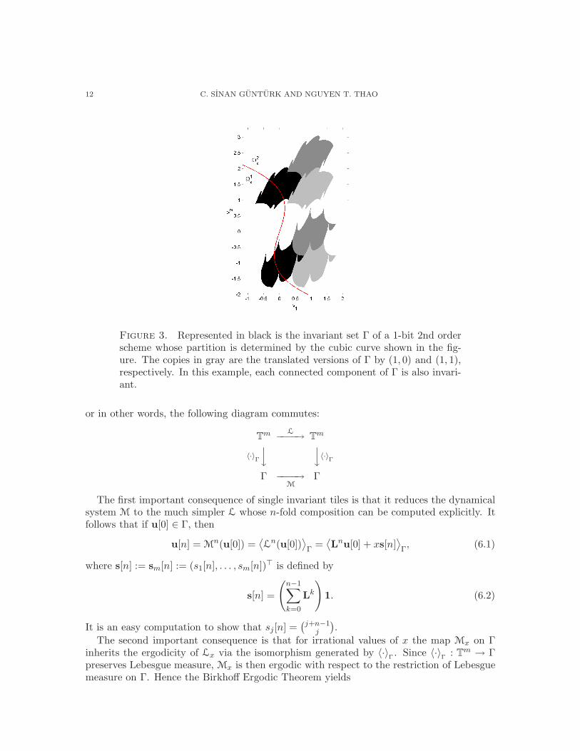
In Figure 3, we show an illustration of an invariant set which is composed of two tiles. Inthis example, the Σ∆ scheme is 1-bit 2nd order and the partition is determined by a cubiccurve.

6. The single-tile case and its consequence

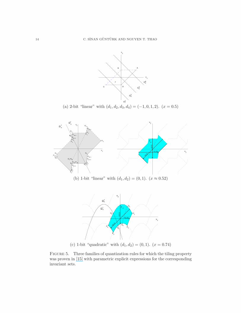
Since the initial experimental discovery of the tiling property in [12, 15], we have observedthat the invariant sets Γ resulting from stable second order Σ∆ schemes that are used inpractice systematically appear to be single tiles. We show in Figure 4 experimental examplesof Γ on some of these second order schemes. In Figure 5, we show the set Γ in three caseswhere an explicit analytical derivation has been possible [15]. (In these particular cases, Γis actually proven to be an exact tile.) A fundamental question is to characterize maps Mx

which yield a single invariant tile. For the rest of this paper, we will simply assume thatthis condition is realized. As will be seen, the analysis of the dynamics becomes particularlysimplified. Furthermore, a whole new set of tools for error analysis becomes available.

A tile Γ intrinsically generates a unique projection 〈·〉Γ

: Rm → Γ such that v−〈v〉Γ∈ Zm

for all v ∈ Rm. The restriction of this Zm-periodic projection to the unit cube [0, 1)m (whichwe identify with Tm) is a measure preserving bijection (note that the inverse of 〈·〉

Γ: Tm → Γ

is the map π that was defined in the proof of Theorem 5.2). When Γ is invariant underM, the map 〈·〉

Γ: Tm → Γ establishes an isomorphism between M on Γ and the affine

transformation L := Lx on Tm defined by (5.3). Indeed, the definition of L easily yieldsL(v)−M(〈v〉

Γ) ∈ Zm. Hence,

〈L(v)〉Γ

= M(〈v〉Γ) ,

12 C. SINAN GUNTURK AND NGUYEN T. THAO

Figure 3. Represented in black is the invariant set Γ of a 1-bit 2nd orderscheme whose partition is determined by the cubic curve shown in the fig-ure. The copies in gray are the translated versions of Γ by (1, 0) and (1, 1),respectively. In this example, each connected component of Γ is also invari-ant.

or in other words, the following diagram commutes:

Tm L−−−−→ Tm

〈·〉Γ

yy〈·〉

Γ

Γ −−−−→M

Γ

The first important consequence of single invariant tiles is that it reduces the dynamicalsystem M to the much simpler L whose n-fold composition can be computed explicitly. Itfollows that if u[0] ∈ Γ, then

u[n] = Mn(u[0]) =

⟨L

n(u[0])⟩Γ

=⟨Lnu[0] + xs[n]

⟩Γ, (6.1)

where s[n] := sm[n] := (s1[n], . . . , sm[n])⊤ is defined by

s[n] =

(n−1∑

k=0

Lk

)1. (6.2)

It is an easy computation to show that sj[n] =(j+n−1

j

).

The second important consequence is that for irrational values of x the map Mx on Γinherits the ergodicity of Lx via the isomorphism generated by 〈·〉

Γ. Since 〈·〉

Γ: Tm → Γ

preserves Lebesgue measure, Mx is then ergodic with respect to the restriction of Lebesguemeasure on Γ. Hence the Birkhoff Ergodic Theorem yields

ERGODIC DYNAMICS IN Σ∆ QUANTIZATION 13

(a) (b)

(c) (d)

Figure 4. Representation in black of several consecutive state points u[n]of various second order Σ∆ modulators with the irrational input x ≈ 3/4.The copies in gray are the translated versions of the state points by (1, 0)and (1, 1), respectively.

Proposition 6.1. Let x be an irrational number and Γ be a Lebesgue measurable Zm-tile(up to a set of measure zero) that is invariant under M. Then for any function F ∈ L1(Γ),

limN→∞

1

N

N∑

n=1

F (u[n]) =

∫

ΓF (v) dv =

∫

Tm

F (〈v〉Γ) dv (6.3)

for almost every initial condition u[0] ∈ Γ.

This formula will be the fundamental computational tool for the analysis of the autocor-relation sequence ρu. For the remainder of this paper, we shall assume that we are workingwith quantization rules for which the invariant sets are composed of single tiles. This willsave us from repetition in the assumptions of our results. However, it will also be importantto know certain geometric features of these invariant tiles. We will state these explicitlywhen needed.

14 C. SINAN GUNTURK AND NGUYEN T. THAO

x

x

x

x

4

3

2

1

AB

C D

Γ Ω

Ω

Ω

Ω

v

v

1

2

(a) 2-bit “linear” with (d1, d2, d3, d4) = (−1, 0, 1, 2). (x = 0.5)

v2

v1

P’3

P0

P2

P2k−2

P2k

=P’2kQ

1

Q’3=Q

3

P4

P’2

P’4

P’2k−2

Q’1

QT

PT P

1

P3

P2k−1

Q2

P’0

Q0

P’2k−1

Q’2

P’1

Q’0 Ω

Ω

x

x 1

2

P’2k−3

P2k−3

P’2k−4

−(1,

1)+(1,0)

−(0

,1)

v1

v2

x Γ

(b) 1-bit “linear” with (d1, d2) = (0, 1). (x ≈ 0.52)

−(1,

1)

+(1,0)

−(0

,1)

v1

v2

Q4

Q3

P3

P2

Q2

Q1

P1

P4

Γ x Ω 1

x

Ω 2 x

(c) 1-bit “quadratic” with (d1, d2) = (0, 1). (x = 0.74)

Figure 5. Three families of quantization rules for which the tiling propertywas proven in [15] with parametric explicit expressions for the correspondinginvariant sets.

ERGODIC DYNAMICS IN Σ∆ QUANTIZATION 15

7. Analysis of the autocorrelation sequence ρu

Let P(v) = vm be the projection of a vector v ∈ Rm onto its mth coordinate. If we definethe function

Fk(v) = P(v)P(Mk(v)), (7.1)

then it follows that

um[n]um[n+ k] = P(u[n])P(Mk(u[n])) = Fk(u[n]),

and therefore Proposition 6.1 gives an expression for the value of ρu[k]:

ρu[k] =

∫

ΓFk(v) dv =

∫

Tm

Fk(〈v〉Γ) dv. (7.2)

A direct evaluation of ρu[k] in either of these forms is not easy, because the k-fold iteratedmap Mk as well as the invariant set Γ are implicitly-defined and complex objects. Theproblem can be somewhat simplified via the conjugate map Lk. Indeed, one has

Fk 〈·〉Γ

=(P 〈·〉

Γ

)(P M

k 〈·〉Γ

)=(P 〈·〉

Γ

)(P 〈·〉

Γ L

k),

so that if we define

GΓ = P 〈·〉Γ,

then via (6.1), we obtain the formula

ρu[k] =

∫

Tm

GΓ(v)GΓ(Lk(v)) dv =

∫

Tm

GΓ(v)GΓ(Lkv + xs[k]) dv, (7.3)

which now only depends on Γ.As it is standard in the spectral theory of dynamical systems (see, e.g., [23]), let U := UL

be the unitary operator on L2(Tm) defined by (Uf)(v) = f(L(v)). Then (7.3) reduces to

ρu[k] =(GΓ, UkGΓ

)

L2(Tm). (7.4)

For any f ∈ L2(Tm), the inner products(f, Ukf

)L2(Tm)

, k ∈ Z, define a positive-definite

sequence so that there exists a unique non-negative measure νf on T with Fourier coefficients

νf [k] =(f, Ukf

)

L2(Tm)(7.5)

for all k ∈ Z. Note that when f = GΓ, it follows from (7.4) that the corresponding measureνGΓ

= µ, where µ is the spectral measure that was mentioned in Section 3, with µ = ρu.

7.1. Decomposition of the mixed spectrum: General results. We shall separate theautocorrelation sequence ρu into two additive components that result from two differenttypes of spectral behavior. Using the spectral theorem for unitary operators, we decomposeL2(Tm) into two U -invariant, orthogonal subspaces as L2(Tm) = Hpp ⊕ Hc, where

Hpp = f ∈ L2(Tm) : νf is purely atomic,which is also equal to the closed linear span of the set of all eigenfunctions of U , and

Hc = H⊥pp = f ∈ L2(Tm) : νf is non-atomic (continuous).

16 C. SINAN GUNTURK AND NGUYEN T. THAO

In the particular case of the transformation L, it turns out that every spectrum on H⊥pp is

absolutely continuous (see Appendix A). Therefore we denote Hc by Hac. Any f ∈ L2(Tm)can now be uniquely decomposed as

f = fpp + fac,

where fpp ∈ Hpp and fac ∈ Hac. For L, it is known (and as we also show in Appendix A),that

Hpp = f ∈ L2(Tm) : f(v) only depends on v1,and the orthogonal projection of f onto Hpp is given by

fpp(v) =

∫

Tm−1

f(v1,v′) dv′. (7.6)

In order to avoid double subscripts (e.g., when f = GΓ), we will use the alternative notation

f := fpp and f := fac whenever it will be convenient.We now consider the decomposition

GΓ = GΓ + GΓ. (7.7)

Because of orthogonality and U -invariance of Hpp and Hac, (7.4) implies that

ρu[k] =(GΓ, UkGΓ

)

L2(Tm)+(GΓ, UkGΓ

)

L2(Tm), (7.8)

providing the decomposition

ρu = ρu + ρu.

Here, using formula (6.1) and the fact that functions in the subspace Hpp depend only onthe first variable, we obtain

ρu[k] =(GΓ, UkGΓ

)

L2(Tm)=

∫

T

GΓ(v1)GΓ(v1 + kx) dv1 (7.9)

and

ρu[k] =(GΓ, UkGΓ

)

L2(Tm)=

∫

Tm

GΓ(v)GΓ(Lkv + xs[k]) dv. (7.10)

This decomposition provides the Fourier coefficients of the pure-point µpp and the absolutelycontinuous µac components of the spectral measure, respectively. It also yields an explicitsimple formula for µpp in terms of the Fourier coefficients of GΓ. We have

Theorem 7.1.

µpp =∑

n∈Z

∣∣∣∣GΓ[n]

∣∣∣∣2

δnx, (7.11)

where δa denotes the unit Dirac mass at a ∈ T.

Proof. Let ν denote the measure given on the right hand side of (7.11). It suffices to verifythat ν[k] = ρu[k] for all k ∈ Z. We find by direct evaluation that

ν[k] =∑

n∈Z

∣∣∣∣GΓ[n]

∣∣∣∣2

e−2πiknx =

∫

T

GΓ(v)GΓ(v + kx) dv = ρu[k];

hence the result follows.

ERGODIC DYNAMICS IN Σ∆ QUANTIZATION 17

Note: It is easy to see that this result holds for any function f ∈ L2(Tm) in the sense that

(νf )pp =∑

n∈Z

∣∣∣f [n]∣∣∣2δnx. (7.12)

On the other hand, the computation of µac is not easy. Since absolute continuity of µac

results in an integrable density Ψ, where dµac(ξ) = Ψ(ξ)dξ, the Riemann-Lebesgue lemmaimplies that the Fourier coefficients ρu[k] → 0 as |k| → ∞. However, the rate of decay isdetermined by further properties of this measure, which turn out to be intrinsically relatedto the geometry of Γ.

7.2. Properties of ρu for the class of vm-connected invariant tiles. In this section,we derive explicit formulae for ρu[k] when the invariant tile Γ has a certain type of geometricregularity. For a given tile Γ for Rm, let us define

ΛΓ :=⋃

k′∈Zm−1

Γ + (k′, 0), (7.13)

and for any v′ ∈ Rm−1,

ΛΓ(v′) := P(ΛΓ ∩ v′×R) =vm ∈ R : (v′, vm) ∈ ΛΓ

. (7.14)

Proposition 7.2. For each v′ ∈ Rm−1, the set ΛΓ(v′) is a tile in R with respect to Z-translations, and

GΓ(v′, vm) =⟨vm

⟩ΛΓ(v′)

. (7.15)

Proof. Since Γ is a tile, the collection of sets ΛΓ + (0, k) : k ∈ Z forms a partition of Rm.Therefore for any v′ ∈ Rm−1, the vm-section of this collection given by ΛΓ(v′)+k : k ∈ Z,is a partition of R. This shows that ΛΓ(v′) is a tile. For the second part of the claim, letv = (v′, vm). The definition of P immediately yields

(v′, GΓ(v)) = (v′,P(〈v〉Γ)) = 〈v〉

Γ+ (k′, 0)

for some k′ ∈ Zm−1. This says that (v′, GΓ(v)) ∈ ΛΓ and therefore GΓ(v) ∈ ΛΓ(v′). Theresult follows since GΓ(v′, vm)−vm ∈ Z.

Definition 7.3. We say that a tile Γ ⊂ Rm is vm-connected if for each v′ ∈ Rm−1, theone dimensional tile ΛΓ(v′) is a connected set, i.e. a unit-length interval. In this case, wedenote by λΓ(v′) the midpoint of ΛΓ(v′) and call λΓ the midpoint function.

In Figure 6, we display examples of the function ΛΓ for various schemes. The tiles in (a),(c) and (d) are v2-connected whereas the tile in (b) is not. Note that vm-connectedness ofa tile is different from its vm-sections being connected.

Let us use the shorthand notation 〈α〉0

:= 〈α〉[− 1

2, 12) = 〈α + 1

2〉 − 12 . For a vm-connected

tile, we have the following simple observation:

Corollary 7.4. If the tile Γ is vm-connected, then for any v′ ∈ Rm−1

GΓ(v′, vm) = 〈vm − λΓ(v′)〉0+ λΓ(v′) (7.16)

and

GΓ = λΓ. (7.17)

18 C. SINAN GUNTURK AND NGUYEN T. THAO

Proof. If Γ is vm-connected, then ΛΓ(v′) = [λΓ(v′) − 12 , λΓ(v′) + 1

2). Now, (7.16) followsfrom Proposition 7.2 and the identity 〈β〉[α− 1

2,α+ 1

2) = 〈β−α〉

0+α which holds for any α and

β. Next, (7.17) is a simple consequence of the fact that the first term in (7.16) integratesto zero over vm.

Before we state the following proposition, let J := Jm be the “backward identity” per-mutation matrix defined by (Jm)ij = δi,m+1−j , for 1 ≤ i, j ≤ m. Note that the matrix

Lk := Lkm can now be decomposed as

Lkm =

Lkm−1 0

s⊤m−1[k]Jm−1 1

, (7.18)

which easily follows from (6.2); note that s[k] = Ls[k−1] + 1 with s[0] = 0.

Proposition 7.5. Let the invariant tile Γ be vm-connected. Define for each k ∈ Z, andv′ ∈ Rm−1,

gk(v′) = s⊤m−1[k]Jm−1v

′ + xsm[k] − λΓ(Lkm−1v

′ + xsm−1[k]) + λΓ(v′).

Then

ρu[k] =

∫

Tm−1

A〈·〉0(gk(v

′)) dv′ +(λΓ, UkλΓ

)

L2(Tm−1). (7.19)

In particular, if m = 2 or if P(Γ) is an interval of unit length, then the second term drops.

Proof. We employ Corollary 7.4 for the evaluation of GΓ(v) and GΓ(Lkv + xs[k]). Let usagain write v = (v′, vm). Note first that from (7.18) we obtain

Lkv + xs[k] = (Lkm−1v

′ + xsm−1[k], vm + s⊤m−1[k]Jm−1v′ + xsm[k]).

It follows that∫

T

GΓ(v)GΓ(Lkv + xs[k]) dvm =

∫

T

⟨vm−λΓ(v′)

⟩0

⟨vm+s⊤m−1[k]Jm−1v

′+xsm[k]−λΓ(Lkm−1v

′+xsm−1[k])⟩

0dvm

+ λΓ(v′)λΓ(Lkm−1v

′ + xsm−1[k]),

where the cross terms have dropped because∫

T〈vm + ϕ(v′)〉

0dvm = 0 for any function ϕ.

The first term above is equal to A〈·〉0(gk(v′)), whereas if the second term is integrated over

Tm−1 we find(λΓ, UkλΓ

)L2(Tm−1)

. The result follows since λΓ = GΓ.

If m = 2, then moreover λΓ = GΓ, so that we have λΓ = 0. If P(Γ) is an interval ofunit length, then it is necessarily the case that ΛΓ = Rm−1 × P(Γ). In this case, λΓ is a

constant function so that λΓ = λΓ and hence λΓ = 0. Hence the second term drops in bothcases.

ERGODIC DYNAMICS IN Σ∆ QUANTIZATION 19

(a)

−1.5 −1 −0.5 0 0.5 1 1.5

−0.8

−0.6

−0.4

−0.2

0

0.2

0.4

0.6

0.8

1

Γx

v1

v 22−bit "linear" ideal

−1.5 −1 −0.5 0 0.5 1 1.5

−0.8

−0.6

−0.4

−0.2

0

0.2

0.4

0.6

0.8

1

v1

v 2

2−bit "linear" ideal

ΛΓGo

Γ

ΛΓ(1)

(b)

−1.5 −1 −0.5 0 0.5 1 1.5

−0.8

−0.6

−0.4

−0.2

0

0.2

0.4

0.6

0.8

1

Γx

v1

v 2

1−bit "linear" standard

−1.5 −1 −0.5 0 0.5 1 1.5

−0.8

−0.6

−0.4

−0.2

0

0.2

0.4

0.6

0.8

1

v1

v 2

1−bit "linear" standard

ΛΓ

Go

Γ

ΛΓ (1)

(c)

−1.5 −1 −0.5 0 0.5 1 1.5

−0.8

−0.6

−0.4

−0.2

0

0.2

0.4

0.6

0.8

1

Γx

v1

v 2

1−bit "linear"

−1.5 −1 −0.5 0 0.5 1 1.5

−0.8

−0.6

−0.4

−0.2

0

0.2

0.4

0.6

0.8

1

v1

v 2

1−bit "linear"

ΛΓ Go

Γ

ΛΓ(1)

(d)

−1.5 −1 −0.5 0 0.5 1 1.5

−0.8

−0.6

−0.4

−0.2

0

0.2

0.4

0.6

0.8

1

v1

v 2

1−bit "quadratic"

P 1 P 0

P 2 P 3

Γx

−(1,0)

+(0,1)

+(1,0)

−1.5 −1 −0.5 0 0.5 1 1.5

−0.8

−0.6

−0.4

−0.2

0

0.2

0.4

0.6

0.8

1

v1

v 2

1−bit "quadratic"

ΛΓ Go

Γ

ΛΓ(1)

(i) (ii)

Figure 6. Invariant tiles of various second order modulators: (i) Invarianttile Γx, (ii) corresponding set ΛΓ.

20 C. SINAN GUNTURK AND NGUYEN T. THAO

7.3. Special case when P(Γ) = [−12 ,

12). There is a class of quantization rules [8, 11,

17], for which um[n] ∈ [−12 ,

12 ) for all n (for all x), so that the invariant tile Γ satisfies

P(Γ) = [−12 ,

12 ). These are the “ideal” rules that were mentioned in Section 1, and represent

essentially the simplest possible situation. It turns out that the spectral measure µ is quitedifferent in its nature for m = 1 and m ≥ 2.

For m = 1, by definition we have GΓ = GΓ = 〈·〉0. Hence µ is pure-point, and Theorem

7.1 yields

µ =∑

n 6=0

1

4π2n2δnx.

For m ≥ 2, we simply note that λΓ ≡ 0, so that GΓ(v) = 〈vm〉0

by (7.16). The fact

that∫

T〈vm〉

0dvm = 0 implies GΓ ≡ 0. Hence µpp = 0, i.e., µ is absolutely continuous. In

addition, Proposition 7.5 yields

ρu[k] =

∫

Tm−1

A〈·〉0(s⊤m−1[k]Jm−1v

′ + xsm[k]) dv′.

For k = 0, the argument of the integrand is identically zero, so we obtain ρu[0] = A〈·〉0(0) =

112 . On the other hand, for all k 6= 0, we find that ρu[k] = 0 since the integrand is of theform A〈·〉

0(kvm−1 + α) which integrates to zero over the variable vm−1. Therefore,

ρu[k] =

112 if k = 0,0 if k 6= 0,

and consequently µ is flat, and equal to 112 times Lebesgue measure on T, and the spectral

density Ψ is the constant function Ψ(ξ) ≡ 112 .

These two results were previously obtained, in the case m = 1 in [11], and in the casem ≥ 2 in [8, 17].

8. Analysis of the mean square error

We are interested in the asymptotical behavior of E(x, φ) for a given Σ∆ modulationscheme of order m as the support of φ increases and its Fourier transform Φ localizesaround zero frequency. There will be two standard choices for Φ:

(1) The ideal low-pass filter given by

ΦidM(ξ) := χ[− 1

M, 1

M](ξ),

(2) The “sinc” family4 given by

ΦsincM,p(ξ) :=

(1

M

M−1∑

n=0

e2πinξ

)p

=

(sin(πMξ)

M sin(πξ)eiπ(M−1)ξ

)p

.

Note that ΦsincM,p has Fourier coefficients given by

φsincM,p[n] := r

(p)M [n] := (rM ∗ rM ∗ · · · ∗ rM︸ ︷︷ ︸

p times

)[n],

4The terminology for this filter is derived from its continuous analog which is related to sinc(x) :=sin(x)/x.

ERGODIC DYNAMICS IN Σ∆ QUANTIZATION 21

where rM denotes the rectangular sequence

rM [n] =

1/M, 0 ≤ n < M,0, otherwise.

It is a standard fact that φsincM,p is a discrete B-spline of degree p− 1.

For any filter φ, we decompose the mean square error E(x, φ) as

E(x, φ) = Epp(x, φ) + Eac(x, φ)

which correspond to the additive contributions of µpp and µac, respectively, in the formula(3.5). Note that both terms are non-negative. Note also that for the above two filter choiceswe have

|ΦidM (ξ)| .p |Φsinc

M/2,p(ξ)|, ∀ξ ∈ T; (8.1)

hence it suffices to prove lower bounds for the ideal low-pass filter and upper bounds forsinc filters.

8.1. The pure-point contribution Epp(x, φ). Our first formula follows directly fromplugging the expression for µpp given by Theorem 7.1 in (3.5):

Epp(x, φ) =∑

n∈Z

|2 sin(πnx)|2m|Φ(nx)|2∣∣∣∣GΓ[n]

∣∣∣∣2

. (8.2)

Before we carry out our analysis of this expression, let us recall some elementary factsabout Diophantine approximation. For α ∈ R, let ‖α‖ denote the distance of α to thenearest integer, that is ‖α‖ := min(〈α〉, 〈−α〉). We say that α is (Diophantine) of type η ifη is the infimum of all numbers σ for which

‖nα‖ &σ,α |n|−σ ∀n ∈ Z\0.Almost every real number (in the sense of Lebesgue measure) is of type 1, the smallestattainable type.

The following theorem shows that for almost every x, if the function GΓ has a sufficientlyregular projection GΓ, then the pure-point part of the mean square error after filtering withφsinc

M,m+1 decays faster than M−2m−1.

Theorem 8.1. Let x be Diophantine of type η. If for some β > η/2 the invariant tileΓ = Γx of an m’th order Σ∆ modulator with input x satisfies

∣∣∣∣GΓ[n]

∣∣∣∣ . |n|−β

for all n ∈ Z\0, then

Epp(x, φsincM,m+1) .x,m,α,β M−2m−1−α (8.3)

for all M , where α is any number satisfying 0 ≤ α < min(1, 2βη − 1).

Proof. Formula (8.2) reads

Epp(x, φsincM,m+1) =

22m

M2m+2

∑

n∈Z\0

sin2m+2(πMnx)

sin2(πnx)

∣∣∣∣GΓ[n]

∣∣∣∣2

. (8.4)

22 C. SINAN GUNTURK AND NGUYEN T. THAO

Since | sin(πθ)| ≍ ‖θ‖, 1 − α ≤ 2m+ 2, and ‖Mnx‖ ≤ min(1,M‖nx‖), we have

sin2m+2(πMnx)

sin2(πnx).m

‖Mnx‖2m+2

‖nx‖2≤ ‖Mnx‖1−α

‖nx‖2≤ M1−α

‖nx‖1+α.

Given the decay of | GΓ[n]|, we then obtain

Epp(x, φsincM,m+1) .m

1

M2m+1+α

∞∑

n=1

1

n2β‖nx‖1+α. (8.5)

Since 1 + α ≥ 1, it suffices to show the convergence of the sum

∞∑

n=1

1

n2β/(1+α)‖nx‖ .

Let λ := 2β/(1 + α). Since 1 + α < 2β/η, we have λ > η. Now, summation by parts showsthat

∞∑

n=1

1

nλ‖nx‖ .λ

∞∑

n=1

1

nλ+1

(n∑

k=1

1

‖kx‖

), (8.6)

and furthermore it is well-known [21, Ex. 3.11] that

n∑

k=1

1

‖kx‖ .x,σ nσ

for any σ > η. Choosing σ such that λ > σ > η, we obtain the convergence of (8.6) with asum depending on x and λ. Combining this result with (8.5) the result follows.

Note: The Diophantine condition on x can be removed if GΓ is a trigonometric polyno-mial. In this case, (8.4) reduces to a finite sum, and therefore it is always convergent.

On the other hand, our next result shows that if GΓ does not have enough regularity ina certain sense as specified in the following theorem, then the result of Theorem 8.1 is thebest one can get in the following sense: There is a dense set of exceptional values of x forwhich the exponent of the error decay rate is never better than 2m, even for the ideal lowpass filter.

Theorem 8.2. Given a Σ∆ modulator of order m, let φM , M = 1, 2, . . . , be a sequenceof averaging filters such that |ΦM (ξ)| ≥ c1 on the interval |ξ| ≤ c2/M , where c1 and c2are positive constants that do not depend on M . There exists a dense set E of irrationalnumbers with the following property: For any x ∈ E, if we can find positive constants βx

and Cx such that the invariant tile Γ = Γx satisfies∣∣∣∣GΓ[n]

∣∣∣∣ ≥ Cx|n|−βx

for all but finitely many n ∈ Z, then for all δ > 0,

lim supM→∞

Epp(x, φM )M2m+δ = ∞. (8.7)

Proof. It suffices to find, for any open interval J , a point x ∈ J with the property (8.7) forall δ > 0. Given an open interval J , let x0 ∈ J be a dyadic rational. Let l = max(b, d)for the minimum b and d such that b! − 1 is an upper bound for the length of the binary

ERGODIC DYNAMICS IN Σ∆ QUANTIZATION 23

expansion of x0 and 2−d!+1 is a lower bound for the distance of x0 to the boundary of J .Set

x = x0 +∑

k≥l

2−k!.

Then clearly x ∈ J . It is also a standard fact that x is irrational, in fact x is a Liouvillenumber.

Note that for q ≥ l, we have

〈2q!x〉 =

∞∑

k=q+1

2−k!+q! = 2−q·q! +

∞∑

k=q+2

2−k!+q!.

For q = 1, 2, . . . , let nq = 2q! andMq = 2q·q!−r where r is a fixed integer such that 2−r+1 ≤ c2.Note that Mq = 2−rnq

q is integer valued for all sufficiently large values of q. We also have

2−r

Mq= 2−q·q! < ‖nqx‖ < 2−q·q!+1 ≤ c2

Mq. (8.8)

The right side of this chain of inequalities implies |ΦMq(nqx)| ≥ c1 by our assumption

on φM. On the other hand, the left side implies |2 sin(πnqx)| ≥ 4‖nqx‖ > 2−r+2/Mq.Therefore

Epp(x, φMq) ≥ |2 sin(πnqx)|2m|ΦMq(nqx)|2∣∣∣∣GΓ[nq]

∣∣∣∣2

≥ C2xc

212

2m(−r+2)2−2rβx/q M−2mq M−2βx/q

q . (8.9)

The result of the theorem follows by letting q → ∞ and therefore exhibiting the subsequenceMq → ∞ for which (8.7) holds for any δ > 0.

8.2. The absolutely continuous contribution Eac(x, φ). Let us denote by Ψ the Radon-Nikodym derivative of the absolutely continuous spectral measure µac, i.e., dµac = Ψ(ξ)dξ.A priori, we only know that Ψ ∈ L1(T), which is somewhat weak for what we would liketo achieve in terms of understanding the decay of Eac(x, φ). Our first theorem concerns thedecay rate of

Eac(x, φsincM,m+1) =

∫

T

|2 sin(πξ)|2m|ΦsincM,m+1(ξ)|2Ψ(ξ) dξ

when it is known that Ψ belongs to a smaller Lp space .

Theorem 8.3. If the measure µac has density Ψ ∈ Lp(T) for some 1 ≤ p ≤ ∞, then

Eac(x, φsincM,m+1) .m,p ‖Ψ‖Lp(T)M

−2m−1+1/p. (8.10)

Proof. Let p′ be the dual index of p, i.e., 1/p + 1/p′ = 1. Note that

|2 sin(πξ)|2m|ΦsincM,m+1(ξ)|2 = |2 sin(πMξ)|2m|Φsinc

M,2(ξ)|M−2m (8.11)

.m |ΦsincM,2(ξ)|M−2m, (8.12)

so that Holder’s inequality yields

Eac(x, φsincM,m+1) .m

∥∥Ψ∥∥

Lp(T)

∥∥ΦsincM,2

∥∥Lp′(T)

M−2m.

Furthermore, the simple bound |ΦsincM,1(ξ)| ≤ min

(1, (2M |ξ|)−1

)implies

∥∥ΦsincM,2

∥∥Lp′ (T)

.p′ M−1/p′ , (8.13)

hence the theorem follows.

24 C. SINAN GUNTURK AND NGUYEN T. THAO

On the other hand, it turns out that if Ψ is continuous at 0, then one can calculate theexact asymptotics of Eac(x, φ

sincM,m+1) without additional assumptions.

Theorem 8.4. If the spectral density Ψ is continuous at 0, then

Eac(x, φsincM,m+1) =

(2m

m

)Ψ(0)M−2m−1 + o(M−2m−1). (8.14)

Proof. The proof has two parts. First part is the easy calculation∫

T

|2 sin(πξ)|2m|ΦsincM,m+1(ξ)|2 dξ =

(2m

m

)M−2m−1. (8.15)

To see this, note that (8.11) and the definition of ΦsincM,m+1 imply

|2 sin(πξ)|2m|ΦsincM,m+1(ξ)|2 =

(eiπMξ − e−iπMξ

i

)2m M−1∑

k=0

M−1∑

j=0

e2πi(k−j)ξM−2m−2.

The right hand side is the product of two trigonometric polynomials; the first polynomialhas frequencies only at integer multiples of 2πM and the second polynomial has frequenciesbetween −2π(M − 1) and 2π(M − 1). The zero frequency term of the product is thereforegiven only by the product of the zero frequency terms of each factor, which is equal to

(2m

m

)(−1)mi−2m

(M−1∑

k=0

1

)M−2m−2 =

(2m

m

)M−2m−1,

hence the result.The second part of the proof concerns the residual term

∣∣∣∣∫

T

∣∣2 sin(πξ)∣∣2m∣∣Φsinc

M,m+1(ξ)∣∣2(Ψ(ξ) − Ψ(0)

)dξ

∣∣∣∣ ,

which is bounded, using (8.11), by

22mM−2m

∫

T

ΦsincM,2(ξ)|Ψ(ξ) − Ψ(0)|dξ = 22mM−2m−1

∫

T

KM−1(ξ)|Ψ(ξ) − Ψ(0)|dξ,

where

KM−1(ξ) =1

M

(sin(πMξ)

sin(πξ)

)2

is the Fejer kernel. The limit

limM→∞

∫

T

KM−1(ξ)|Ψ(ξ) − Ψ(0)|dξ

is the Cesaro sum of the Fourier series of the function f(t) = |Ψ(−t) − Ψ(0)| evaluated att = 0. Since f is continuous at 0, the Cesaro sum converges to f(0) = 0, and therefore thelimit is 0. This concludes the proof.

Notes:

(1) A similar calculation shows that for the ideal filter φidM , the error has the asymptotics

given by

Eac(x, φidM ) =

(2π)2m+1

m+ 1/2Ψ(0)M−2m−1 +O(M−2m−3) (8.16)

again assuming that Ψ is continuous at 0.

ERGODIC DYNAMICS IN Σ∆ QUANTIZATION 25

(2) The value of Ψ(0) is equal to the sum of its Fourier coefficients ρu[k].

9. Estimates for second order schemes with v2-connected invariant tiles

Second order Σ∆ modulators with v2-connected invariant tiles are interesting becausethe value of x and the midpoint function λΓ = GΓ completely describe the MSE behaviorvia the theorems we have stated in the previous sections. In particular, Proposition 7.5provides us with the formula

ρu[k] =

∫

T

A〈·〉0

(kv1 + k(k+1)

2 x− λΓ(v1 + kx) + λΓ(v1))

dv1

=

∫

T

A〈·〉0

(kv − λΓ(v − x

2 + k x2 ) + λΓ(v − x

2 − k x2 ))

dv, (9.1)

where we have used the change of variable v = v1 + (k + 1)x/2 to obtain the secondrepresentation.

By Riemann-Lebesgue lemma, we already know that ρu[k] must converge to zero as

|k| → ∞ since ρu[k] = Ψ[k], where Ψ ∈ L1(T) is the spectral density. However, we wouldlike to quantify the rate of decay in |k| as this would then allow us to draw conclusionsabout Ψ. Intuitively speaking, it is not hard to see from this formula that the smoother λΓ

is, the faster ρu[k] must decay in |k| as |k| → ∞, since A〈·〉0

is a zero mean function on T.

Our objective in this section is to study this relation rigorously.Let BV(T) denote the space of functions on T that have bounded variation, where ‖·‖TV

denotes the total variation semi-norm, and let A(T) denote the space of functions on T with

absolutely convergent Fourier series with the norm ‖f‖A(T) given by∑ |f [n]|. We have the

following lemma, whose proof is given in the Appendix.

Lemma 9.1. Let f ∈ A(T) and ϕ be two real valued functions on T, where f has zeromean. Consider the integrals

c[k] =

∫

T

f(kv + ϕ(v)) dv. (9.2)

The following bounds hold:

(1) If ϕ ∈ BV(T), then for all k ∈ Z\0,∣∣c[k]

∣∣ ≤ 1

|k| ‖f‖A(T)‖ϕ‖TV . (9.3)

(2) If ϕ is differentiable almost everywhere and ϕ′ ∈ BV(T), then for all k ∈ Z\0,∣∣c[k]

∣∣ ≤ 1

k2

(1√12

‖f‖L2(T)‖ϕ′‖TV + ‖f‖L∞(T)‖ϕ′‖2L2(T)

). (9.4)

Theorem 9.2. Let x be given and Γ be the invariant tile corresponding to a second orderΣ∆ modulator. Then we have the following:

(1) If the midpoint function λΓ has bounded variation on T, then

∣∣ρu[k]∣∣ ≤ 1

6|k|∥∥λΓ

∥∥TV. (9.5)

Consequently, one has

Eac(x, φsincM,3) .x,ǫ M−5+ǫ (9.6)

26 C. SINAN GUNTURK AND NGUYEN T. THAO

for any ǫ > 0. If the type η of x is strictly less than 2, then

Epp(x, φsincM,3) .x,δ M−5−δ (9.7)

for any 0 ≤ δ < (2 − η)/η.(2) If the midpoint function λΓ has a derivative that has bounded variation on T, then

∣∣ρu[k]∣∣ ≤ 1

k2

(1

12√

15‖λ′Γ‖TV +

1

3‖λ′Γ‖2

L2(T)

). (9.8)

In particular, the spectral density Ψ is continuous. Consequently, one has

Eac(x, φsincM,3) = 6Ψ(0)M−5 + o(M−5), (9.9)

where

Ψ(0) ≤ 1

12+π2

3

(1

12√

15‖λ′Γ‖TV +

1

3‖λ′Γ‖2

L2(T)

). (9.10)

If the type η of x is strictly less than 4, then

Epp(x, φsincM,3) .x,δ M−5−δ (9.11)

for any 0 ≤ δ < min(1, (4 − η)/η

).

Proof. Let

f(v) := A〈·〉0(v) =

∑

n 6=0

1

4π2n2e2πinv.

For each k, define

ϕk(v) := −λΓ(v − x2 + k x

2 ) + λΓ(v − x2 − k x

2 ).

For these functions, we have the following exact formulas and bounds:

‖f‖A(T) =1

12(9.12)

‖f‖L∞(T) =1

12(9.13)

‖f‖L2(T) =1

12√

5(9.14)

‖ϕk‖TV ≤ 2 ‖λΓ‖TV (9.15)

‖ϕ′k‖TV ≤ 2 ‖λ′Γ‖TV (9.16)

‖ϕ′k‖2

L2(T) ≤ 4 ‖λ′Γ‖2L2(T). (9.17)

(1) In this case we only know that λΓ is of bounded variation.The decay estimate (9.5) simply follows from the bound (9.3) coupled with (9.12)

and (9.15).

Given that the Fourier coefficients ρu[k] = Ψ[k] decay like 1/k, it follows fromRiesz-Thorin interpolation theorem that the spectral density Ψ ∈ Lp(T) for anyp <∞. Therefore Theorem 8.3 implies, with m = 2 and ǫ = 1/p, the bound (9.6).

For the pure-point estimate, we use Theorem 8.1 with β = 1 and m = 2. If wedefine δ = α, where α is as defined in Theorem 8.1, then the result follows as stated.

(2) In this case we know that λΓ has a derivative that is of bounded variation.The decay estimate (9.8) follows from the bound (9.4) coupled with (9.13), (9.14),

(9.16) and (9.17).

ERGODIC DYNAMICS IN Σ∆ QUANTIZATION 27

Since ρu is summable, it follows that Ψ is continuous. We therefore apply Theorem8.4 to compute the exact asymptotics of Eac(x, φ

sincM,3). In this case, the nonnegative

number Ψ(0) will be bounded by∑ |ρu[k]|. We simply, add up the bounds given

by (9.8), including the trivial case |ρu[0]| ≤ ‖f‖L∞(T). This computation yields thebound (9.10).

For the pure-point estimate, we again use Theorem 8.1, but now with β = 2. Wedefine δ = α, where α is as defined in Theorem 8.1, and note that the conditionα ≤ 1 must be imposed, which was automatically satisfied in case (1). Then theresult follows as stated.

10. Further remarks

In this paper, we have covered only a portion of the mathematical problems that con-cern Σ∆ quantization. We believe that the following currently unresolved problems areinteresting both from the dynamical systems standpoint and the engineering perspective:

1. Which maps M are stable? Satisfactory answers of this question would include non-trivial sufficient conditions in terms of the quantization rule Q, or in terms of the partitionΠx and the quantization levels di.

2. Which stable maps M yield single invariant tiles? One can include in this the casewhen Γ is composed of tiles each of which is invariant under M. In principle, each of theseinvariant tiles would represent a different “mode of operation”.

3. What is an appropriate generalization of our spectral analysis of mean square errorwhen Γ is composed of more than one tile?

4. Given the quantization rule, what can be said about the geometric regularity of Γ?We used two types of geometric information about Γ in deriving our analytical resultson the mean square error asymptotics. The first type concerned “shape” (such as vm-connectedness), and the second concerned “regularity” (such as the decay of Fourier coeffi-

cients of GΓ). At this stage, the relation between the quantization rule and these two issuesis highly unclear, although we have partial understanding in some cases. Even for “linear”rules, there seems to be a wide range of possibilities.

5. What are the universal principles behind tiling? Tiling invariant sets are found evenwhen x is rational. In addition, trajectories seem to remain within exact tiles, and not justtiles “up to sets of measure zero”.

Appendix A. On the spectral theory of the map L

In this section, we will review some basic facts about the spectral theory of the mapL = Lx on Tm, where Lxv = Lv + x1, and x is an irrational number. Most of whatfollows below can be derived or generalized from Anzai’s work on ergodic skew producttransformation [3].

The eigenfunctions of UL. We start by showing that the set of all eigenfunctions ofU = UL, where ULf := f UL, is precisely given by the collection of complex exponentialsfn, where

fn(v) = e2πinv1 , n ∈ Z.

28 C. SINAN GUNTURK AND NGUYEN T. THAO

To see this, let f ∈ L2(Tm) be an eigenfunction of U with eigenvalue λ. Since U is unitary,|λ| = 1. Consider the Fourier series expansion of f given by

f(v) =∑

n∈Zm

c[n]e2πin·v.

Since f = 1λ

(Uf), we have the relation

∑

n∈Zm

c[n]e2πin·v =1

λ

∑

n∈Zm

c[n]e2πixn·1e2πin·(Lv)

=1

λ

∑

n∈Zm

c[Kn]e2πix(Kn)·1e2πin·v,

where K = (L−1)⊤. Comparing the coefficients, we obtain the equality∣∣c[n]

∣∣ =∣∣c[Kn]

∣∣, ∀n ∈ Zm.

Since f ∈ L2(Tm), we can conclude that c[n] = 0 for any n that is not preserved under Kj

for some positive integer j, for otherwise we would have the infinite sequence of coefficientsc[n], c[Kn], c[K2n], . . . of equal and strictly positive magnitude.

On the other hand, it is a simple exercise to show that the only vectors that satisfyn = Kjn for some power j ≥ 1 are those of the form n = (n1, 0, . . . , 0). Hence, anyeigenfunction of U depends only on the first variable v1. On the first coordinate v1 of v, L

reduces to the irrational rotation by x, and hence as it is well-known, these eigenfunctionsare nothing but the given complex exponentials fnn∈Z. These eigenfunctions span thesubspace Hpp of L2(Tm).

The absolutely continuous spectrum. We shall next show that continuous part of thespectrum is in fact absolutely continuous. This is in fact a consequence of the fact thatthere exists an orthonormal basis ψj,k : j ∈ Z, k ∈ N of H⊥

pp with the property that

Uψj,k = ψj+1,k for all j and k. (I.e., L has countable Lebesgue spectrum on H⊥pp.) First we

will construct such a basis, and then we shall prove the statement on the absolute continuity.From the discussion above on the eigenfunctions of U , we know that the complex expo-

nentialsfn(v) = e2πin·v, n ∈ Zm\

(Z × 0m−1

),

form an orthonormal complete set in H⊥pp. Note also that

Ufn = e2πixn·1fL⊤n.

Therefore we consider the orbit of each n ∈ Zm under L⊤, given by

O(n) =

(L⊤)j

n

j∈Z

.

It is easy to see that each n ∈ Z × 0m−1 is a fixed point of L⊤ and every other n is suchthat the orbit is an infinite sequence of distinct points in Zm\

(Z × 0m−1

). Since L⊤ is

invertible, orbits do not intersect. Hence we can divide Zm\(Z × 0m−1

)into equivalence

classes of orbits O(nk), k ∈ N, and define

ψ0,k = fnk, ψj,k = U jψ0,k, j ∈ Z, k ∈ N.

Each ψj,k is equal to some complex exponential fn multiplied by a complex number of unitmagnitude. The collection of ψj,k is distinct, and all frequencies n ∈ Zm\

(Z × 0m−1

)

ERGODIC DYNAMICS IN Σ∆ QUANTIZATION 29

appear, hence ψj,kj∈Z,k∈N form an orthonormal basis of H⊥pp with the property that

Uψj,k = ψj+1,k.

Let us show that every spectral measure is absolutely continuous on H⊥pp. Let g and h

be arbitrary functions in L2(Tm) with representations g =∑aj,kψj,k and h =

∑bj,kψj,k.

Let the functions Ak and Bk be defined on T for each k with Fourier coefficients (aj,k)j∈Z

and (bj,k)j∈Z, respectively. From orthogonality, we have

‖g‖2 =∑

k

∫

T

|Ak(ξ)|2dξ <∞,

and similarly for h and Bk.Now, we have Unh =

∑bj,kψj+n,k, so that

(g,Unh)L2(Tm) =∑

k

∑

j

aj+n,kbj,k

=∑

k

∫

T

∑

j

aj+n,ke2πijξBk(ξ) dξ

=

∫

T

e−2πinξ

(∑

k

Ak(ξ)Bk(ξ)

)dξ,

the nth Fourier coefficient of the function∑

k Ak(ξ)Bk(ξ). On the other hand, applyingCauchy-Schwarz inequality twice, we have

∫

T

∣∣∣∣∣∑

k

Ak(ξ)Bk(ξ)

∣∣∣∣∣dξ ≤∫

T

(∑

k

|Ak(ξ)|2)1/2(∑

k

|Bk(ξ)|2)1/2

dξ

≤(∫

T

∑

k

|Ak(ξ)|2dξ)1/2(∫

T

∑

k

|Bk(ξ)|2dξ)1/2

= ‖g‖L2‖h‖L2

< ∞.

Hence the inner products (g,Unh)L2(Tm) are in fact the Fourier coefficients of an L1 function.This shows that the measure associated to these inner products is absolutely continuous.

Appendix B. Proof of Lemma 9.1

Let us start by writing f(t) =∑n 6=0

f [n]e2πint so that we have

c[k] =∑

n 6=0

f [n]

∫

T

e2πin(kv+ϕ(v))dv, (B.1)

where we have changed the order of summation and integration. Applying integration byparts we obtain

∫

T

e2πinϕ(v)e2πinkvdv = − 1

2πink

∫

T

e2πinkvd[e2πinϕ(v)

]

= −1

k

∫

T

e2πinkve2πinϕ(v)dϕ(v). (B.2)

30 C. SINAN GUNTURK AND NGUYEN T. THAO

Part (1). For the integral in (B.2), we use the bound∣∣∣∣−

1

k

∫

T

e2πinkve2πinϕ(v)dϕ(v)

∣∣∣∣ ≤1

|k|

∫

T

|dϕ(v)| =1

|k| ‖ϕ‖TV ,

and we simply get∣∣c[k]

∣∣ ≤∑

n 6=0

1

|k| ‖ϕ‖TV |f [n]| ≤ 1

|k| ‖ϕ‖TV ‖f‖A(T).

Part (2). Let ϕ be differentiable and ϕ′ ∈ BV(T). Substitute dϕ(v) = ϕ′(v)dv and applyanother integration by parts to (B.2) obtain

−1

k

∫

T

ϕ′(v)e2πinϕ(v)e2πinkvdv =1

k(2πink)

∫

T

e2πinkvd[ϕ′(v)e2πinϕ(v)

].

Now,

d[ϕ′(v)e2πinϕ(v)

]= e2πinϕ(v)dϕ′(v) + (ϕ′(v))2(2πin)e2πinϕ(v) dv,

so that substituting the above two formulas together with (B.2) in (B.1), we get

c[k] =1

k2

∑

n 6=0

f [n]

2πin

∫

T

e2πin(kv+ϕ(v)) dϕ′(v) +∑

n 6=0

f [n]

∫

T

(ϕ′(v))2e2πin(kv+ϕ(v)) dv

(B.3)

For the first part of this sum we use∣∣∣∣∫

T

e2πin(kv+ϕ(v)) dϕ′(v)

∣∣∣∣ ≤∫

T

|dϕ′(v)| = ‖ϕ′‖TV ,

and

∑

n 6=0

|f [n]|2π|n| ≤

∑

n 6=0

1

(2πn)2

1/2(

∑

n

|f [n]|2)1/2

=1√12

‖f‖L2(T),

so that ∣∣∣∣∣∣

∑

n 6=0

f [n]

2πin

∫

T

e2πin(kv+ϕ(v)) dϕ′(v)

∣∣∣∣∣∣≤ 1√

12‖f‖L2(T)‖ϕ′‖TV .

On the other hand, the second term reduces to∑

n 6=0

f [n]

∫

T

(ϕ′(v))2e2πin(kv+ϕ(v)) dv =

∫

T

(ϕ′(v))2∑

n 6=0

f [n]e2πin(kv+ϕ(v)) dv

=

∫

T

(ϕ′(v))2f(kv + ϕ(v)) dv.

We bound this integral by ‖f‖L∞(T)‖ϕ′‖2L2(T). Combining these, the expression of (B.3) can

now be bounded from above in absolute value as∣∣c[k]

∣∣ ≤ 1

k2

(1√12

‖f‖L2(T)‖ϕ′‖TV + ‖f‖L∞(T)‖ϕ′‖2L2(T)

),

concluding the proof.

Acknowledgements

The authors would like to thank Ingrid Daubechies, Ron DeVore, Ozgur Yılmaz andYang Wang for conversations on the topic of Σ∆ quantization, tiling, and related issues.

ERGODIC DYNAMICS IN Σ∆ QUANTIZATION 31

References

[1] R. L. Adler, B. P. Kitchens, M. Martens, C. P. Tresser, C. W. Wu, “The mathematics of halftoning,”IBM J. Res. & Dev., vol. 47, no. 1, Jan 2003.

[2] D. Anastassiou, “Error diffusion coding for A/D conversion,” IEEE Trans. on Circuits and Systems,vol. 36, no. 3, pp. 1175–1186, Sept. 1989.

[3] H. Anzai, “Ergodic Skew Product Transformation on the Torus,” Osaka Math. J., 3 (1951), pp. 83–99.[4] T. Bernard, “From Σ − ∆ modulation to digital halftoning of images,” Proc. IEEE Int. Conf. on

Acoustics, Speech and Signal Proc., May 1991, pp. 2805–2808, Toronto.[5] R. Calderbank and I. Daubechies, “The Pros and Cons of Democracy,” IEEE Trans. in Inform. Theory,

vol. 48, pp. 1721–1725, June 2002.[6] J. C. Candy and G. C. Temes, Eds., Oversampling Delta-Sigma Data Converters: Theory, Design and

Simulation, IEEE Press, 1992.[7] H. Furstenberg, “Strict ergodicity and transformations of the torus,” Amer. J. Math., vol. 83, pp.

573–601, 1961.[8] W. Chou, P. W. Wong, and R. M. Gray, “Multistage Σ∆ modulation,” IEEE Trans. Inform. Theory,

vol. 35, pp. 784–796, July 1989.[9] I. Daubechies, R. DeVore, “Reconstructing a Bandlimited Function From Very Coarsely Quantized

Data: A Family of Stable Sigma-Delta Modulators of Arbitrary Order”, Ann. of Math., vol. 158, no. 2,pp. 679–710, Sept. 2003.

[10] R. M. Gray, “Oversampled sigma-delta modulation,” IEEE Trans. on Comm., vol. COM-35, pp. 481–489, May 1987.

[11] R. M. Gray, “Spectral Analysis of Quantization Noise in a Single-Loop Sigma-Delta Modulator with dcInput,” IEEE Trans. on Comm., vol. COM-37, pp. 588–599, June 1989.

[12] C. S. Gunturk, Harmonic Analysis of Two Problems in Signal Quantization and Compression, Ph.D.thesis, Princeton University, 2000.

[13] C. S. Gunturk “Approximating a Bandlimited Function Using Very Coarsely Quantized Data: ImprovedError Estimates in Sigma-Delta Modulation”, J. Amer. Math. Soc., 17 (2004), no. 1, 229–242.

[14] C. S. Gunturk, J. C. Lagarias, and V. A. Vaishampayan, “On the robustness of single loop sigma-deltamodulation,” IEEE Trans. Inform. Theory, 47 (2001), no. 5, 1735–1744.

[15] C. S. Gunturk and N. T. Thao, “Refined Error Analysis in Second Order Σ∆ Modulation with ConstantInputs,” IEEE Trans. Inform. Theory, 50 (2004), no. 5, 839–860.

[16] C. S. Gunturk, “One-Bit Sigma-Delta Quantization with Exponential Accuracy,” Comm. Pure Appl.

Math., vol. 56, pp. 1608–1630, no. 11, 2003.[17] N. He, F. Kuhlmann, and A. Buzo, “Multi-loop Σ∆ quantization,” IEEE Trans. Inform. Theory, vol.

38, pp. 1015–1028, May 1992.[18] A. Katok, and B. Hasselblatt, Introduction to the Modern Theory of Dynamical Systems, Cambridge

University Press, 1995.[19] Y. Katznelson, An Introduction to Harmonic Analysis, John Wiley & Sons, 1968 (reprint: Dover Publs.

Inc.).[20] T. D. Kite, B. L. Evans, A. C. Bovik, and T. L. Sculley, “Digital image halftoning as 2-D Delta-

Sigma modulation”, Proc. IEEE Int. Conf. on Image Proc., vol. I, pp. 799-802, Oct. 26-29, 1997, SantaBarbara, CA.

[21] L. Kuipers and H. Niederreiter, Uniform Distribution of Sequences, Wiley, 1974.[22] S. R. Norsworthy, R. Schreier, and G. C. Temes, Eds., Delta-Sigma Data Converters: Theory, Design

and Simulation, IEEE Press, 1996.[23] W. Parry, Topics in Ergodic Theory, Cambridge University Press, 1981.[24] R. Schreier, M. V. Goodson, and B. Zhang, “An algorithm for computing convex positively invariant

sets for delta-sigma modulators,” IEEE Trans. on Circuits and Systems, I, vol. 44, pp. 38–44, Jan.1997.

[25] N. T. Thao, “Breaking the feedback loop of a class of Sigma-Delta A/D converters,” IEEE Trans. Signal

Processing, to appear.[26] R. Ulichney, Digital Halftoning, MIT Press, Cambridge, 1987.

[27] O. Yılmaz, “Stability analysis for several second-order sigma-delta methods of coarse quantization ofbandlimited functions,” Constr. Approx. 18 (2002), no. 4, 599–623.

32 C. SINAN GUNTURK AND NGUYEN T. THAO

Courant Institute of Mathematical Sciences, New York University, 251 Mercer Street,

New York, NY 10012.

E-mail address: gunturk@cims.nyu.edu

Department of Electrical Engineering, City College and Graduate School, City Univer-

sity of New York, Convent Avenue at 138th Street, New York, NY 10031.

E-mail address: thao@ee-mail.engr.ccny.cuny.edu