A Pumping Algorithm for Ergodic Stochastic Mean PayoffGames with Perfect Information

Endre Boros1, Khaled Elbassioni2, Vladimir Gurvich1, and Kazuhisa Makino3

1 RUTCOR, Rutgers University, 640 Bartholomew Road, Piscataway NJ 08854-8003boros,gurvich@rutcor.rutgers.edu

2 Max-Planck-Institut fur Informatik, Stuhlsatzenhausweg 85, 66123 Saarbrucken, Germany;elbassio@mpi-sb.mpg.de

3 Graduate School of Information Science and Technology, University of Tokyo, Tokyo, 113-8656, Japan;makino@mist.i.u-tokyo.ac.jp

Abstract. We consider two-person zero-sum stochastic mean payoff games with perfect in-formation, or BWR-games, given by a digraph G = (V = VB ∪VW ∪VR, E), with local rewardsr : E → R, and three types of vertices: black VB, white VW , and random VR. The game isplayed by two players, White and Black: When the play is at a white (black) vertex v, White(Black) selects an outgoing arc (v, u). When the play is at a random vertex v, a vertex u

is picked with the given probability p(v, u). In all cases, Black pays White the value r(v, u).The play continues forever, and White aims to maximize (Black aims to minimize) the lim-iting mean (that is, average) payoff. It was recently shown in [BEGM09a] that BWR-gamesare polynomially equivalent with the classical Gillette games, which include many well-knownsubclasses, such as cyclic games, simple stochastic games (SSG), stochastic parity games, andMarkov decision processes.In this paper, we give a new algorithm for solving BWR-games in the ergodic case, that is whenthe optimal values do not depend on the initial position. Our algorithm solves a BWR-gameby reducing it, using a potential transformation, to a canonical form in which the value andoptimal strategies of both players are obvious for every initial position, since a locally optimalmove in it is optimal in the whole game. We show that this algorithm is pseudo-polynomialwhen the number of random nodes is constant. We also provide an almost matching lowerbound on its running time, and show that this bound holds for a wider class of algorithms.Our preliminary experiments with the algorithm indicate that it behaves much better than itsestimated worst-case running time. This and the fact that every iteration is simple and canbe implemented in a distributed way makes it a good candidate for practical applications.

Keywords: mean payoff games, local reward, Gillette model, perfect information, potential,stochastic game

2

1 Introduction

1.1 BWR-games

We consider two-person zero-sum stochastic games with perfect information and meanpayoff: Let G = (V,E) a digraph whose vertex-set V is partitioned into three subsetsV = VB ∪ VW ∪ VR that correspond to black, white, and random positions, controlled re-spectively, by two players, Black - the minimizer and White - the maximizer, and by nature.We also fix a local reward function r : E → R, and probabilities p(v, u) for all arcs (v, u)going out of vertices v ∈ VR. Vertices v ∈ V and arcs e ∈ E are called positions and moves,respectively. In a personal position v ∈ VW or v ∈ VB the corresponding player White orBlack selects an outgoing arc (v, u), while in a random position v ∈ VR a move (v, u) ischosen with the given probability p(v, u). In all cases Black pays White the reward r(v, u).

From a given initial position v0 ∈ V the game produces an infinite walk (called a play).White’s objective is to maximize the limiting mean payoff

c = lim infn→∞

∑ni=0 bi

n + 1, (1)

where bi is the reward incurred at step i of the play, while the objective of Black is the

opposite, that is, to minimize lim supn→∞∑n

i=0 bi

n+1 .For this model it was shown in [BEGM09b] that a saddle point exists in pure positional

uniformly optimal strategies. Here ”pure” means that the choice of a move (v, u) in apersonal position v ∈ VB ∪ VR is deterministic, not random; ”positional” means that thischoice depends solely on v, not on previous positions or moves; finally, ”uniformly optimal”means that it does not depend on the initial position v0, either. The results and methodsin [BEGM09b] are similar to those of Gillette [Gil57]; see also Liggett and Lippman [LL69]:First, we analyze the so-called discounted version, in which the payoff is discounted by afactor βi at step i, giving the effective payoff: aβ = (1− β)

∑∞i=0 βibi, and then we proceed

to the limit as the discount factor β ∈ [0, 1) tends to 1.This class of the BWR-games was introduced in [GKK88]; see also [CH08]. It was

recently shown in [BEGM09a]) that the BWR-games and classical Gillette games [Gil57]are polynomially equivalent.

The special case when there are no random positions, VR = ∅, is known as cyclic,or mean payoff, or BW-games. They were introduced for the complete bipartite digraphsin [Mou76b,Mou76a], for all (not necessarily complete) bipartite digraphs in [EM79], andfor arbitrary digraphs in [GKK88]. A more special case was considered extensively in theliterature under the name of parity games [BV01a,BV01b,CJH04,Hal07,Jur98,JPZ06], andlater generalized also to include random nodes in [CH08].

A BWR-game is reduced to a minimum mean cycle problem in case VW = VR = ∅, seefor example [Kar78]. If one of the sets VB or VW is empty, we obtain a Markov decisionprocess; see, for example, [MO70]. Finally, if both are empty VB = VW = ∅, we get a weightedMarkov chain.

It was noted in [BG09] that ”parlor games”, like Backgammon (and even Chess) can besolved in pure positional uniformly optimal strategies, based on their BWR-model.

In the special case of a BWR-game, when all rewards are zero except at a single node tcalled the terminal, at which there is a self-loop with reward 1, we obtain the so-called sim-ple stochastic games (SSG), introduced by Condon [Con92,Con93] and considered in severalpapers [GH08,Hal07]. In these games, the objective of White is to maximize the probabilityof reaching the terminal, while Black wants to minimize this probability. Recently, it was

3

shown that Gillette games (and hence BWR-games by [BEGM09a]) are equivalent to SSG’sunder polynomial-time reductions [AM09]. Thus, by recent results of Bjorklund, Vorobyov[BV05], and Halman [Hal07], all these games can be solved in randomized strongly subex-ponential time 2O(

√nd log nd), where nd = |VB |+ |VW | is the number of deterministic vertices.

Let us also note that several pseudo-polynomial and subexponential algorithms existsfor BW-games [GKK88,KL93,Pis99,BV05,BV07,HBV04,Hal07,ZP96]; see also [DG06] for aso called policy iteration method, and [JPZ06] for parity games.

Besides their many applications (see e.g. [Lit96,Jur00]), all these games are of interestto complexity theory: Karzanov and Lebedev [KL93] (see also [ZP96]) proved that thedecision problem ”whether the value of a BW-game is positive” is in the intersection ofNP and co-NP. Yet, no polynomial algorithm is known for these games, see e.g., the recentsurvey by Vorobyov [Vor08]. A similar complexity claim can be shown to hold for SSG andBWR-games, see [AM09,BEGM09a].

While there are numerous pseudo-polynomial algorithms known for the BW-case, itis a challenging open question whether a pseudo-polynomial algorithm exists for SSG orBWR-games.

1.2 Potential transformations and canonical forms; Sketch of our results

Given a BWR-game, we consider potential transformations x : V → R, assigning a real-value x(v) to each vertex v ∈ V , and transforming the local reward on each arc (v, u) torx(v, u) = r(v, u) + x(v) − x(u). It is known that for BW-games there exists a potentialtransformation such that, in the obtained game the locally optimal strategies are globallyoptimal, and hence, the value and optimal strategies become obvious [GKK88]. This resultwas extended for the more general class of BWR-games in [BEGM09a]: in the transformedgame, the equilibrium value µ(v) = µx(v) is given simply by the maximum local reward forv ∈ VW , the minimum local reward for v ∈ VB , and the average local reward for v ∈ VR. Inthis case we say that the transformed game is in canonical form.

It is not clear how the algorithm given in [GKK88] for the BW-case can be generalizedto BWR-case. The proof in [BEGM09a] follows by considering the discounted case andthen taking the discount factor β to the limit. While such an approach is sufficient toprove the existence of a canonical form, it does not provide an algorithm to compute thepotentials, since the corresponding limits appear to be infinite. In this paper, we give suchan algorithm that does not go through the discounted case. Our method computes anoptimal potential transformation in case the game is ergodic, that is, when the optimalvalues do not depend on the initial position. If the game is not ergodic then our algorithmterminates with a proof of non-ergodicity, by exhibiting at least two vertices with provablydistinct values. Unfortunately, our approach cannot be reapplied recursively in this case.This is not a complete surprise, since this case is at least as hard as SSG-s, for which nopseudo-polynomial algorithm is known.

Theorem 1. Consider a BWR-game with k random nodes, a total of n vertices, and in-teger rewards in the range [−R,R], and assume that all probabilities are rational whosecommon denominator is bounded by W . Then there is an algorithm that runs in timeO(nO(k)W O(k2)R log(nRW )) and either brings the game by a potential transformation tocanonical form, or proves that it is non-ergodic.

Let us remark that the ergodic case is frequent in applications. For instance, it is thecase when G = (VW ∪ VB ∪ VR, E) is a complete tripartite digraph (where p(v, u) > 0 forall v ∈ VR and (v, u) ∈ E); see Section 3 for more general sufficient conditions.

4

Theorem 1 states that our algorithm is pseudo-polynomial if the number of randomnodes is fixed. To the best of our knowledge, this is the first algorithm with such a guarantee(in comparison, for example, to strategy improvement methods [HBV04,HK66,VJ00], forwhich exponential lower bounds are known [Fri09]). In fact, we are not aware of any previousresults bounding the running time of an algorithm for a class of BWR-games in terms ofthe number of random nodes, except for [GH08] which shows that simple stochastic gameson k random nodes can be solved in time O(k!(|V ||E| + L)), where L is the maximum bitlength of a transition probability. It is worth remarking here that even though BWR-gamesare polynomially reducible to simple stochastic games, under this reduction the number ofrandom nodes k becomes a polynomial in n, even if the original BWR-game has constantlymany random nodes. In particular, the result in [GH08] does not imply a bound similar tothat of Theorem 1 for general BWR-games.

One should also contrast the bound in Theorem 1 with the subexponential bounds in[Hal07]: roughly, the algorithm of Theorem 1 will be more efficient if |VR| is O((|VW |+|VB |)

14 )

(assuming that W and R are polynomials in n). However, our algorithm could be practicallymuch faster since it can stop much earlier than its estimated worst-case running time (unlikethe subexponential algorithms [Hal07], or those based on dynamic programming [ZP96], seeExample 2 in Appendix F). In fact, as our experiments indicate, to approximate the valueof a random game on upto 15, 000 nodes within an additive error ε = 0.001, the algorithmtakes no more than a few hundred iterations, even if the maximum reward is very large (seeTable 1 in Appendix G for details).

One more desirable property of this algorithm is that it is of the certifying type (see e.g.[KMMS03]), in the sense that, given an optimal pair of strategies, the vector of potentialsprovided by the algorithm can be used to verify optimality in linear time (otherwise verifyingoptimality requires solving two linear programs).

1.3 Overview of the techniques

Our algorithm for proving Theorem 1 is quite simple. Starting form zero potentials, anddepending on the current locally optimal rewards (maximum for White, minimum for Black,and average for Random), the algorithm keeps selecting a subset of nodes and reducing theirpotentials by some value, until either the locally optimal rewards at different nodes becomesufficiently close to each other, or a proof of non-ergodicity is obtained in the form of acertain partition of the nodes. The upper bound on the running time consists of threetechnical parts. The first one is to show that if the number of iterations becomes too large,then there is a large enough potential gap to ensure an ergodic partition. In the secondpart, we show that the range of potentials can be kept sufficiently small throughout thealgorithm, namely ‖x∗‖∞ ≤ nRk(2W )k, and hence the range of the transformed rewardsdoes not explode. The third part concerns the required accuracy. In Appendix D, we showthat it is enough in our algorithm to get the value of the game within an accuracy of

ε =1

n2(k+1)k2k(2W )4k+2k2+2, (2)

in order to guarantee that it is equal to the exact value. To the best of our knowledge, sucha bound in terms of k is new, and could be of independent interest.

We also show the lower bound W Ω(k) on the running time of the algorithm mentionedin Theorem 1 by providing an instance of the problem, with only random nodes.

5

The paper is organized as follows. In the next section, we formally define BWR-games,canonical forms, and state some useful propositions. In Section 3, we give a sufficient condi-tion for the ergodicity of a BWR-game, which will be used as one possible stopping criterionin our algorithm. We give the algorithm in Section 4.1, and prove it converges in Section 4.2.In Section 5, we show that this convergence proof can, in fact, be turned into a quantitativestatement giving the precise bounds stated in Theorem 1. The last section gives a lowerbound example for the algorithm. Some of the proofs will be given in Appendix C. Twoillustrative example are given in Appendix F. The first one illustrates the existence of asaddle point in pure strategies, while the second one shows, among other things, that localoptimality does not imply global optimality, if the game is not in canonical form.

2 Preliminaries

2.1 BWR-games

A BWR-game is defined by the quadruple G = (G,P, v0, r), where G = (V = VW ∪ VB ∪VR, E) is a digraph that may have loops and multiple arcs, but no terminal vertices4, i.e.,vertices of out-degree 0; P is the set of probability distributions for all v ∈ VR specifyingthe probability p(v, u) of a move form v to u; v0 ∈ V is an initial position from which theplay starts; and r : E → R is a local reward function. We assume that

∑

u | (v,u)∈E p(v, u) =1 ∀v ∈ VR. For convenience we will assume that p(v, u) > 0 whenever (v, u) ∈ E andv ∈ VR, and set p(v, u) = 0 for (v, u) 6∈ E.

Standardly, we define a strategy sW ∈ Sw (respectively, sB ∈ SB) as a mapping thatassigns a move (v, u) ∈ E to each position v ∈ VW (respectively, v ∈ VB). A pair of strategiess = (sW , sB) is called a situation. Given a BWR-game G = (G,P, v0, r) and situations = (sB, sW ), we obtain a (weighted) Markov chain Gs = (G,Ps, v0, r) with transitionmatrix Ps in the obvious way:

Ps(v, u) =

1 if v ∈ VW and u = sW (v) or v ∈ VB and u = sB(v);0 if v ∈ VW and u 6= sW (v) or v ∈ VB and u 6= sB(v);P (v, u) if v ∈ VR.

In the obtained Markov chain Gs = (G,Ps, v0, r), we define the limiting (mean) effectivepayoff cs(v0) as

cs(v0) =∑

v∈V

p∗(v)∑

u

Ps(v, u)r(v, u), (3)

where p∗ : V → [0, 1] is the limiting distribution for Gs starting from v0 (see Appendix Afor details). Doing this for all possible strategies of Black and White, we obtain a matrixgame Cv0 : SW × SB → R, with entries Cv0(sW , sB) defined by (3).

2.2 Solvability and ergodicity

It is known that every such game has a saddle point in pure strategies [Gil57,LL69].Moreover, there are optimal strategies (s∗W , s∗B) that do not depend on the starting

position v0, so-called ergodic optimal strategies. In contrast, the value of the game µ(v0) =Cv0(s

∗W , s∗B) can depend on v0.

The triplet G = (G,P, r) is called a not initialized BWR-game. Furthermore, G is calledergodic if the value µ(v0) of each corresponding BWR-game (G,P, v0, r) is the same for allinitial positions v0 ∈ V .

4 This assumption is without loss of generality since otherwise one can add a loop to each terminal vertex

6

2.3 Potential transforms

Given a BWR-game G = (G,P, v0, r), let us introduce a mapping x : V → R, whose valuesx(v) will be called potentials, and define the transformed reward function rx : E → R as:

rx(v, u) = r(v, u) + x(v) − x(u), where (v, u) ∈ E. (4)

It is not difficult to verify that the two normal form matrices Cx and C, of the obtainedgame Gx and the original game G, are equal (see [BEGM09a]). In particular, their optimal(pure positional) strategies coincide, and the values also coincide: µx(v0) = µ(v0).

2.4 Ergodic canonical form

Given a BWR-game G = (G,P, r), let us define a mapping m : V → R as follows:

m(v) =

max(r(v, u) | u : (v, u) ∈ E) for v ∈ VW ,min(r(v, u) | u : (v, u) ∈ E) for v ∈ VW ,mean(r(v, u) | u : (v, u) ∈ E) =

∑

u|(v,u)∈E r(v, u) p(v, u), for v ∈ VR.(5)

A move (v, u) ∈ E in a position v ∈ VW (respectively, v ∈ VB) is called locally optimal if itrealizes the maximum (respectively, minimum) in (5). A strategy sW of White (respectively,sB of Black) is called locally optimal if it chooses a locally optimal move (v, u) ∈ E in everyposition v ∈ VW (respectively, v ∈ VB).

Definition 1. We say that a BWR-game G is in ergodic canonical form if function (5) isconstant: m(v) ≡ m for some number m.

Proposition 1. If a BWR-game is in ergodic canonical form then(i) every locally optimal strategy is optimal and(ii) the game is ergodic: m is its value for every initial position v0 ∈ V .

3 Sufficient conditions for ergodicity of BWR-games

A digraph G = (VW ∪ VB ∪ VR, E) (whose vertices are partitioned in three subsets, V =VW∪VB∪VR) is called ergodic if every corresponding not initialized BWR-game G = (G,P, r)is ergodic, that is, the values of the games G = (G,P, v0, r) do not depend on v0.

We will give a simple characterization of ergodic digraphs, which, obviously, providessufficient conditions for ergodicity of the BWR-games.

In addition to partition Πp : V = VW ∪ VB ∪ VR, let us consider one more partitionΠr : V = V W ∪ V B ∪ V R with the following properties:

(i) Sets V W and V B are not empty (while V R might be empty).

(ii) There is no arc (v, u) ∈ E such that [v ∈ (VW ∪ VR) ∩ V B and u 6∈ V B ] or, viceversa, [v ∈ (VB ∪ VR) ∩ V W and u 6∈ V W ]. In other words, White cannot leave V B , Blackcannot leave V W , and there are no random moves from V W ∪ V B.

(iii) For each v ∈ VW ∩ V W (respectively, v ∈ VB ∩ V B) there is a move (v, u) ∈ E suchthat u ∈ V W (respectively, u ∈ V B). In other words, White (Black) cannot be forced toleave V W (respectively, V B). In particular, this implies that the induced subgraphs G[V W ]and G[V B] have no dead-ends.

Partition Πr : V = V W ∪ V B ∪ V R satisfying (i), (ii), and (iii) will be called a contra-ergodic partition for digraph G = (VW ∪ VB ∪ VR, E).

7

Theorem 2. Digraph G is ergodic if and only if it has no contra-ergodic partitions.

The “only if part” can be strengthened as follows:

Proposition 2. Given a BWR-game G whose graph has a contra-ergodic partition, if m(v) >m(u) for every v ∈ V W , u ∈ V B then µ(v) > µ(u) for every v ∈ V W , u ∈ V B.

Definition 2. A contra-ergodic decomposition of G is a contra-ergodic partition Πr : V =V W ∪ V B ∪ V R such that m(v) > m(u) for every v ∈ V W and u ∈ V B.

By Proposition 2, if G has a contra-ergodic decomposition, then G is not ergodic.For example, no contra-ergodic partition can exist if G = (VW ∪VB∪VR, E) is a tripartite

digraph such that the underlying non-directed tripartite graph is complete; see, for instance,the example in Appendix F, where each part consists of only one vertex.

4 Pumping algorithm for the ergodic BWR-games

4.1 Description of the algorithm

Given a BWR-game G = (G,P, r), let us compute m(v) for all v ∈ V using (5). Through-

out, we will denote by [m]def= [m−,m+] and [r]

def= [r−, r+] the range of m(·) and r(·, ·),

respectively. Given a potential vector x : V → R, we denote by mx(·) the function m(·) in(5) in which r is replaced by the transformed reward function rx.

Given a subset I ⊆ [m], let V (I) = v ∈ V | m(v) ∈ I ⊆ V . In the following algorithm,set I will always be a closed or semi-closed interval within [m].

Let m− = t0 < t1 < t2 < t3 < t4 = m+ be given thresholds. We will successivelyapply potential transforms x : V → R such that no vertex ever leaves the interval [t0, t4],nor the interval [t1, t3]; in other words, Vx[t0, t4] = V [t0, t4] and Vx[t1, t3] ⊇ V [t1, t3] for allconsidered transforms x, where Vx(I) = v ∈ V | mx(v) ∈ I.

Let us initialize potentials x(v) = 0 for all v ∈ V . We will fix

t0 := m−x , t1 := m−

x +1

4|[mx]|, t2 := m−

x +1

2|[mx]|, t3 := m−

x +3

4|[mx]|, t4 := m+

x . (6)

Then, let us reduce all potentials of Vx[t2, t4] by a maximum constant δ such that no vertexleaves the closed interval [t1, t3]; in other words, we stop the iteration whenever a vertexfrom this interval reaches its border. After this we compute potentials x(v), new valuesmx(v), for v ∈ V , and start the next iteration.

It is clear that δ can be computed in linear time: it is the maximum value δ such thatmδ

x(v) ≥ t1 for all v ∈ Vx[t2, t4] and mδx(v) ≤ t3 for all v ∈ Vx[t0, t2), where mδ

x(v) is the newvalue of mx(v) after all potentials in Vx[t2, t4] have been reduce by δ (see Equations (8) inAppendix B for the exact formula).

It is also clear from our update method (and important) that δ ≥ |[mx]|/4. Indeed,vertices from [t2, t4] can only go down, while vertices from [t0, t2) can only go up. Eachof them must traverse a distance of at least |[mx]|/4 before it can reach the border ofthe interval [t1, t3]. Moreover, if after some iteration one of the sets Vx[t0, t1) or Vx(t3, t4]becomes empty then range of mx is reduced at least by 25%.

Procedure PUMP(G, ε) below tries to reduce any BWR-game G by a potential trans-formation x into one in which |[mx]| ≤ ε. Two subroutines are used in the procedure.REDUCE-POTENTIALS(G, x) replaces the current potential x with another potential with

8

a sufficiently small norm (cf. Lemma 3 below). This reduction is needed since, without it,the potentials and hence the transformed local rewards can grow exponentially. The sec-ond routine FIND-PARTITION(G, x) uses the current potential vector x to construct acontra-ergodic decomposition of G (cf. line 19).

We will prove in Lemma 2 that if the number of pumping iterations performed is largeenough, namely,

N =8n2Rx

|[mx]|θk−1+ 1, (7)

where Rx = r+x − r−x , θ = minp(v, u) : (v, u) ∈ E, and k is the number of random

nodes, and yet the range of mx is not reduced, then we will be able to find a contra-ergodicdecomposition.

In Section 4.2, we will first argue that the algorithm terminates in finite time if ε = 0and the considered BWR-game is ergodic. In the following section, this will be turned intoa quantitative argument with the precise bound on the running time. Yet, in Section 6, wewill show that this time can be exponential already for R-games.

Algorithm 1 PUMP(G, ε)

Input: A BWR-game G = (G = (V, E), P, r) and a desired accuracy ε

Output: a potential x : V → R s.t. |mx(v) − mx(u)| ≤ ε for all u, v ∈ V if the game is ergodic, and acontra-ergodic decomposition otherwise

1: let x0(v) := x(v) := 0 for all v ∈ V ; i := 12: let t0, t1, . . . , t4, and N be as defined by (6) and (7)3: while i ≤ N do

4: if |[mx]| ≤ ε then

5: return x

6: end if

7: δ := maxδ′| mδ′

x (v) ≥ t1 for all v ∈ Vx0 [t2, t4] and mδ′

x (v) ≤ t3 for all v ∈ Vx0 [t0, t2)8: if δ = ∞ then

9: return the ergodic partition Vx0 [t0, t2) ∪ Vx0 [t2, t4]10: end if

11: x(v) := x(v) − δ for all v ∈ Vx0 [t2, t4]12: if Vx0 [t0, t1) = ∅ or Vx0(t3, t4] = ∅ then

13: x := x0:=REDUCE-POTENTIALS(G, x); i := 114: recompute the thresholds t0, t1, . . . , t4 and N using (6) and (7)15: else

16: i := i + 1;17: end if

18: end while

19: V W ∪ V B ∪ V R:=FIND-PARTITION(G,x)20: return contra-ergodic partition V W ∪ V B ∪ V R

4.2 Proof of finiteness for the ergodic case

Let us assume without loss of generality that range of m is [0, 1], and the initial potentialx0 = 0. Suppose that during N iterations no new vertex enters the interval [1/4, 3/4]. Then,−x(v) ≥ N/4 for each v ∈ V (3/4, 1], since these vertices “were pumped” N times, andx(v) ≡ 0 for each v ∈ V [0, 1/4), since these vertices “were not pumped” at all. We will showthat if N is sufficiently large then the considered game is not ergodic.

Consider infinitely many iterations i = 0, 1, . . ., and denote by V B ⊆ V (respectively,by V W ⊆ V ) the set of vertices that were pumped just finitely many times (respectively,

9

always but finitely many times); in other words, mx0(v) ∈ [1/2, 1] if v ∈ V W (respectively,mx0(v) ∈ [0, 1/2) if v ∈ V B ) for all but finitely many i′s. It is not difficult to verify thatthe partition Πr : V = V W ∪ V B ∪ V R, where V R = V \ (V W ∪ V B), is contra-ergodic.It is also clear that after sufficiently many iterations mx0(v) > 1/2 for all v ∈ V W , whilemx0(v) ≤ 1/2 for all v ∈ V B . Thus, by Proposition 2, the considered game G is not ergodic,or in other words, our algorithm is finite for the ergodic BWR-games.

But how many times a vertex can oscillate around 1/2 until it finally settles itself downin [1/4, 1/2) or in (1/2, 3/4]? We shall give an upper bound below.

5 Running time analysis

Consider the execution of the algorithm on a given BWR-game. We define a phase to be aset of iterations during which the range of mx, defined with respect to the current potentialx, is not reduced by a constant factor of what it was at the beginning of the phase, i.e., noneof the sets Vx[t0, t1) or Vx(t3, t4] becomes empty (cf. line 12 of the procedure). Note thatthe number of iterations in each phase is at most N defined by (7). Lemma 2 states that ifN iterations are performed in a phase then, the game is not ergodic. Lemma 4 bounds thetotal number of phases and estimates the overall running time.

5.1 Finding a contra-ergodic decomposition

We assume throughout this section that we are inside phase h of the algorithm, whichstarted with a potential xh, and that |[mx]| > 3

4 |[mxh ]| in all N iterations of the phase, andhence we proceed to step 19. For convenience, we will write (·)xh as (·)h, where (·) could bem, r, r+, etc, (e.g., m−

h = m−xh , m+

h = m+xh). We assume that the phase starts with local

reward function r = rh and hence 5 xh = 0.Given a potential vector x, we use the following notation:

EXTx = (v, u) ∈ E : v ∈ VB ∪ VW and rx(v, u) = mx(v), ∆x = minx(v) : v ∈ V .

Let tl < 0 be the largest value satisfying the following conditions:

(i) there are no arcs (v, u) ∈ E with v ∈ VW ∪ VR, x(v) ≥ tl and x(u) < tl;(i) there are no arcs (v, u) ∈ EXTx with v ∈ VB , x(v) ≥ tl and x(u) < tl.

Let X = v ∈ V : x(v) ≥ tl. In other words, X is the set of nodes with potential as closeto 0 as possible, such that no white or random node in X has an arc crossing to V \X, andno black node has an extremal arc crossing to V \ X. Similarly, define tu > ∆x to be thesmallest value satisfying the following conditions:

(i) there are no arcs (v, u) ∈ E with v ∈ VB ∪ VR, x(v) ≤ tu and x(u) > tu;(i) there are no arcs (v, u) ∈ EXTx with v ∈ VW , x(v) ≤ tu and x(u) > tu,

and let Y = v ∈ V : x(v) ≤ tu. Note that the sets X and Y can be computed inO(|E| log |V |) time.

Lemma 1. It holds that max−tl, tu − ∆x ≤ nRh

(

1θ

)k−1.

The correctness of the algorithm follows from the following lemma.

5 in particular, note that rx(v, u) and mx(v) are used, for short, to actually mean rx+xh(v, u) and mx+xh(v),respectively

10

Lemma 2. Suppose that pumping is performed for Nh ≥ 2nTh + 1 iterations, whereT = 4nRh

|[mh]|θk−1 , and neither the set Vh[t0, t1) nor Vh(t3, t4] becomes empty. Let V B = X and

V W = Y be the sets constructed as above, and V R = V \ (X ∪ Y )). Then V W ∪ V B ∪ V R

is a contra-ergodic decomposition.

Proof. As noted above (see (8)) we pump in each iteration by δ ≥ |[mh]|4 . Furthermore, our

formula for δ implies that once a vertex enters the region Vh[t1, t3], it will never leave it. Inparticular, there are vertices v0 ∈ X ∩ Vh[t0, t1) and vn ∈ Y ∩ Vh(t3, t4] with x(v0) = 0 andx(vn) = ∆x.

For a vertex v ∈ V , let N(v) denote the number of times the vertex was pumped. ThenN(v0) = 0 and N(vn) = Nh.

We claim that N(v) ≤ T for any v ∈ X, and N(v) ≥ Nh − T for all v ∈ Y (i.e.,every vertex in X was not pumped in all steps but at most T , and every vertex in Y waspumped in all steps but at most T ). Indeed, if v ∈ X (respective;y, v ∈ Y ) was pumpedgreater than (respectively, less than) T times then x(v) − x(v0) ≤ − nRh

θk−1 (respectively,

x(vn) − x(v) ≤ − nRh

θk−1 ), in contradiction to Lemma 1.Since Nh > 2T , it follows that X ∩ Y = ∅. Furthermore, among the first 2nT + 1

iterations, in at most nT iterations some vertex v ∈ X was pumped, and in at most nTiterations some vertex in Y was not pumped. Thus, there must exist an iteration at whichevery vertex v ∈ X was not pumped and every vertex v ∈ Y was pumped. At that particulariteration, we must have X ⊆ Vh[t0, t2) and Y ⊆ Vh[t2, t4], and hence mx(v) < t2 for everyv ∈ X and mx(v) ≥ t2 for every v ∈ Y . By the way the sets X and Y were constructed andfrom (8), we can easily see that X and Y will continue to have this property till the end ofthe Nh iterations, and hence they induce a contra-ergodic partition. The lemma follows. ⊓⊔

5.2 Potential reduction

One problem that arises during the pumping procedure is that the potentials can increaseexponentially in the number of phases, making our bounds on the number of iteration perphase also exponential in n. For the BW-case Pisaruk [Pis99] solved this problem by givinga procedure that reduces the range of the potentials after each round, while keeping all itsdesired properties needed for the running time analysis. (For convenience, we give a variantof this procedure in Appendix E.)

Pisaruk’s potential reduction procedure can be thought of as a combinatorial procedurefor finding an extreme point of a polyhedron, given a point in it. Indeed, given a BWR-game and a potential x, let us assume without loss of generality, by shifting the potentialsif necessary, that x ≥ 0, and let E′ = (v, u) ∈ E : rx(v, u) ∈ [m−

x ,m+x ], v ∈ VB ∪ VW,

where r is the original local reward function. Then the following polyhedron is non-empty:

Px =

x′ ∈ R

V

∣

∣

∣

∣

∣

∣

∣

∣

∣

∣

∣

∣

∣

∣

∣

∣

m−

x ≤ r(v, u) + x′(v) − x′(u) ≤ m+x , ∀(v, u) ∈ E′

r(v, u) + x′(v) − x′(u) ≤ m+x , ∀v ∈ VW , (v, u) ∈ E \ E′

m−

x ≤ r(v, u) + x′(v) − x′(u), ∀v ∈ VB, (v, u) ∈ E \ E′

m−

x ≤∑

u∈Vp(v, u)(r(v, u) + x′(v) − x′(u)) ≤ m+

x , ∀v ∈ VR

x(v) ≥ 0 ∀ v ∈ V

.

Moreover, Px is pointed, and hence must have an extreme point.

Lemma 3. Consider a BWR-game in which all rewards are integral with range R = r+−r−,and probabilities p(v, u) are rational with common denominator at most W , and let k = |VR|.Then any extreme point x∗ of Px satisfies ‖x∗‖∞ ≤ nRk(2W )k.

11

Note that any point x′ ∈ Px satisfies [mx′ ] ⊆ [mx], and hence replacing x by x∗ does notincrease the range of mx.

5.3 Proof of Theorem 1

Consider a BWR-game G = (G = (V,E), P, r) with |V | = n vertices and k random nodes.Assume r to be integral in the range [−R,R] and all transition probabilities are rationalwith common denominator W . From Lemmas 2 and 3, we can conclude the following bound.

Lemma 4. Procedure PUMP(G, ε) terminates in O(nk(2W )k(1ε + n2|E|)R log(R

ε )) time.

Theorem 1 follows by setting ε sufficiently small:

Corollary 1. When procedure PUMP(G, ε) is run with ε as in (2), it either outputs apotential vector x such mx(v) is constant for all v ∈ V , or it finds a contra-ergodic partition.The total running time is O(nk3(2W )k(n2(k+1)(2W )4k+2k2+2) + n2|E|)R log(RWn)).

6 Lower bound example

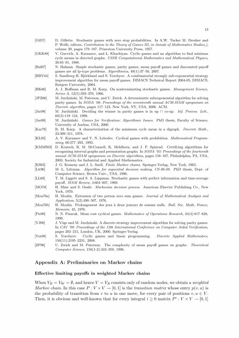
We show now that the execution time of the algorithm, in the worst case, can be exponentialin the number of random nodes k, already for weighted Markov chains, that is, for R-games.Consider the following example.

Let G = (V,E) be a digraph on k = 2l + 1 vertices ul, . . . , u1, u0 = v0, v1, . . . , vl, andwith the following set of arcs:

E = (ul, ul), (vl, vl) ∪ (ui−1, ui), (ui, ui−1), (vi−1, vi), (vi, vi−1) : i = 1, . . . , l.

Let W ≥ 1 be an integer. All nodes are random with the following transition probabilities:p(ul, ul) = p(vl, vl) = 1− 1

W+1 , p(u0, u1) = p(u0, v1) = 12 , p(ui−1, ui) = p(vi−1, vi) = 1− 1

W+1 ,

for i = 2, . . . , l, and p(ui, ui−1) = p(vi, vi−1) = 1W+1 , for i = 1, . . . , l. The local rewards are

zero on every arc, except for r(ul, ul) = −r(vl, vl) = 1. Clearly this Markov chain consists ofa single recurrent class, and it is easy to verify that the limiting distribution p∗ is as follows:

p∗(u0) =W − 1

(W + 1)W l − 2, p∗(ui) = p∗(vi) =

W i−1(W 2 − 1)

2((W + 1)W l − 2), for i = 1, . . . , l.

The optimal expected reward at each vertex is

µ(ui) = µ(vi) = −1 · (1 −1

W + 1)p∗(ul) + 1 · (1 −

1

W + 1)p∗(ul) = 0,

for i = 0, . . . , l. Upto a shift, there is a unique set of potentials that transform the Markovchain into canonical form, and they satisfy the following system of equations:

0 = −1

2∆1 −

1

2∆′

1,

0 = −(1 −1

W + 1)∆i+1 +

1

W + 1∆i, for i = 1, . . . , k − 1

0 = −(1 −1

W + 1)∆′

i+1 +1

W + 1∆′

i, for i = 1, . . . , k − 1

0 = −(1 −1

W + 1) +

1

W + 1∆l,

0 = 1 −1

W + 1+

1

W + 1∆′

l,

12

v1 v2 v3 v4u1u2u4

1

W+1

1

W+1

W

W+1u0

1

W+1

1

W+1

1

W+1

1

W+1

W

W+1

1

2

1

W+1

1

W+1

1

2

W

W+1

W

W+1

W

W+1W

W+1

W

W+1

W

W+1

u3

1 −1

Fig. 1. An exponential Example.

where ∆i = ui−ui−1 and ∆′i = vi−vi−1; solving we get ∆i = −∆′

i = W k−i+1, for i = 1, . . . , l.

Lower bound on pumping algorithms. Any pumping algorithm that starts with 0potentials and modifies the potentials in each iteration by at most γ will not have a numberof iterations less than W l−1

2γ on the above example. By (8), the algorithm in Section 4 hasγ ≤ 1/minp(v, u) : (v, u) ∈ E, p(v, u) 6= 0, which is Ω(W ) in our example. We concludethat the running time of the algorithm is O(W l−2) = Ω(W Ω(k)) on this example.

References

[AM09] D. Andersson and P.B. Miltersen. The complexity of solving stochastic games on graphs. InLecture Notes in Computer Science, ISAAC, to appear, 2009.

[BEGM09a] E. Boros, K. Elbassioni, V. Gurvich, and K. Makino. Every stochastic game with perfectinformation admits a canonical form. RRR-09-2009, RUTCOR, Rutgers University, 2009.

[BEGM09b] E. Boros, K. Elbassioni, V. Gurvich, and K. Makino. Nash-solvable bidirected cyclic 2-persongame forms. RRR-09-2009, RUTCOR, Rutgers University, 2009.

[BG09] E. Boros and V. Gurvich. Why chess and back gammon can be solved in pure positionaluniformly optimal strategies? RRR-21-2009, RUTCOR, Rutgers University, 2009.

[BV01a] E. Beffara and S. Vorobyov. Adapting gurvich-karzanov-khachiyan’s algorithm for parity games:Implementation and experimentation. Technical Report 2001-020, Department of InformationTechnology, Uppsala University, available at: https://www.it.uu.se/research/reports/#2001,2001.

[BV01b] E. Beffara and S. Vorobyov. Is randomized gurvich-karzanov-khachiyan’s algorithm for paritygames polynomial? Technical Report 2001-025, Department of Information Technology, UppsalaUniversity, available at: https://www.it.uu.se/research/reports/#2001, 2001.

[BV05] H. Bjorklund and S. Vorobyov. Combinatorial structure and randomized subexponential algo-rithms for infinite games. Theoretical Computer Science, 349(3):347–360, 2005.

[BV07] H. Bjorklund and S. Vorobyov. A combinatorial strongly sub-exponential strategy improvementalgorithm for mean payoff games. Discrete Applied Mathematics, 155(2):210–229, 2007.

[CH08] K. Chatterjee and T. A. Henzinger. Reduction of stochastic parity to stochastic mean-payoffgames. Inf. Process. Lett., 106(1):1–7, 2008.

[CJH04] K. Chatterjee, M. Jurdzinski, and T. A. Henzinger. Quantitative stochastic parity games. InSODA ’04: Proceedings of the fifteenth annual ACM-SIAM symposium on Discrete algorithms,pages 121–130, Philadelphia, PA, USA, 2004. Society for Industrial and Applied Mathematics.

[Con92] A. Condon. The complexity of stochastic games. Information and Computation, 96:203–224,1992.

[Con93] A. Condon. An algorithm for simple stochastic games. In Advances in computational complexitytheory, volume 13 of DIMACS series in discrete mathematics and theoretical computer science,1993.

[DG06] V. Dhingra and S. Gaubert. How to solve large scale deterministic games with mean pay-off by policy iteration. In valuetools ’06: Proceedings of the 1st international conference onPerformance evaluation methodolgies and tools, page 12, New York, NY, USA, 2006. ACM.

[EM79] A. Eherenfeucht and J. Mycielski. Positional strategies for mean payoff games. InternationalJournal of Game Theory, 8:109–113, 1979.

[Fri09] O. Friedmann. An exponential lower bound for the parity game strategy improvement algorithmas we know it. Logic in Computer Science, Symposium on, 0:145–156, 2009.

[GH08] H. Gimbert and F. Horn. Simple stochastic games with few random vertices are easy to solve.In FoSSaCS, pages 5–19, 2008.

13

[Gil57] D. Gillette. Stochastic games with zero stop probabilities. In A.W. Tucker M. Dresher andP. Wolfe, editors, Contribution to the Theory of Games III, in Annals of Mathematics Studies,),volume 39, pages 179–187. Princeton University Press, 1957.

[GKK88] V. Gurvich, A. Karzanov, and L. Khachiyan. Cyclic games and an algorithm to find minimaxcycle means in directed graphs. USSR Computational Mathematics and Mathematical Physics,28:85–91, 1988.

[Hal07] N. Halman. Simple stochastic games, parity games, mean payoff games and discounted payoffgames are all lp-type problems. Algorithmica, 49(1):37–50, 2007.

[HBV04] S. Sandberg H. Bjorklund and S. Vorobyov. A combinatorial strongly sub-exponential strategyimprovement algorithm for mean payoff games. DIMACS Technical Report 2004-05, DIMACS,Rutgers University, 2004.

[HK66] A. J. Hoffman and R. M. Karp. On nonterminating stochastic games. Management Science,Series A, 12(5):359–370, 1966.

[JPZ06] M. Jurdzinski, M. Paterson, and U. Zwick. A deterministic subexponential algorithm for solvingparity games. In SODA ’06: Proceedings of the seventeenth annual ACM-SIAM symposium onDiscrete algorithm, pages 117–123, New York, NY, USA, 2006. ACM.

[Jur98] M. Jurdzinski. Deciding the winner in parity games is in up ∩ co-up. Inf. Process. Lett.,68(3):119–124, 1998.

[Jur00] M. Jurdzinski. Games for Verification: Algorithmic Issues. PhD thesis, Faculty of Science,University of Aarhus, USA, 2000.

[Kar78] R. M. Karp. A characterization of the minimum cycle mean in a digraph. Discrete Math.,23:309–311, 1978.

[KL93] A. V. Karzanov and V. N. Lebedev. Cyclical games with prohibition. Mathematical Program-ming, 60:277–293, 1993.

[KMMS03] D. Kratsch, R. M. McConnell, K. Mehlhorn, and J. P. Spinrad. Certifying algorithms forrecognizing interval graphs and permutation graphs. In SODA ’03: Proceedings of the fourteenthannual ACM-SIAM symposium on Discrete algorithms, pages 158–167, Philadelphia, PA, USA,2003. Society for Industrial and Applied Mathematics.

[KS63] J. G. Kemeny and J. L. Snell. Finite Markov chains. Springer-Verlag, New York, 1963.

[Lit96] M. L. Littman. Algorithm for sequential decision making, CS-96-09. PhD thesis, Dept. ofComputer Science, Brown Univ., USA, 1996.

[LL69] T. M. Liggett and S. A. Lippman. Stochastic games with perfect information and time-averagepayoff. SIAM Review, 4:604–607, 1969.

[MO70] H. Mine and S. Osaki. Markovian decision process. American Elsevier Publishing Co., NewYork, 1970.

[Mou76a] H. Moulin. Extension of two person zero sum games. Journal of Mathematical Analysis andApplication, 5(2):490–507, 1976.

[Mou76b] H. Moulin. Prolongement des jeux a deux joueurs de somme nulle. Bull. Soc. Math. France,Memoire, 45, 1976.

[Pis99] N. N. Pisaruk. Mean cost cyclical games. Mathematics of Operations Research, 24(4):817–828,1999.

[VJ00] J. Voge and M. Jurdzinski. A discrete strategy improvement algorithm for solving parity games.In CAV ’00: Proceedings of the 12th International Conference on Computer Aided Verification,pages 202–215, London, UK, 2000. Springer-Verlag.

[Vor08] S. Vorobyov. Cyclic games and linear programming. Discrete Applied Mathematics,156(11):2195–2231, 2008.

[ZP96] U. Zwick and M. Paterson. The complexity of mean payoff games on graphs. TheoreticalComputer Science, 158(1-2):343–359, 1996.

Appendix A: Preliminaries on Markov chains

Effective limiting payoffs in weighted Markov chains

When VB = VW = ∅, and hence V = VR consists only of random nodes, we obtain a weightedMarkov chain. In this case P : V ×V → [0, 1] is the transition matrix whose entry p(v, u) isthe probability of transition from v to u in one move, for every pair of positions v, u ∈ V .Then, it is obvious and well-known that for every integral i ≥ 0 matrix P i : V × V → [0, 1]

14

(the i-th power of P ) is the i-move transition matrix, whose entry pi(v, u) is the probabilityof transition from v to u in exactly i moves, for every v, u ∈ V .

Let qi(v, u) be the probability that arc (v, u) ∈ E will be the (i + 1)-st move, given theoriginal distribution p0 = ev0 , where i = 0, 1, 2, . . . and ev0 is the n-dimensional unit vectorwith 1 in position v0, and denote by qi : E → [0, 1] the corresponding probabilistic |E|-vector. For convenience, we introduce |V | × |E| vertex-arc transition matrix Q : V × E →[0, 1] whose entry q(ℓ, (v, u)) is equal to p(v, u) if ℓ = v and 0 otherwise, for every ℓ ∈ Vand (v, u) ∈ E. Then, it is clear that qi = p0P

iQ.

Let r be the |E|-dimensional vector of local rewards, and bi denote the expected rewardfor the (i + 1)-st move; i = 0, 1, 2, . . ., i.e., bi =

∑

(v,u)∈E qi(v, u)r(v, u) = p0PiQr. Then the

effective payoff of the weighted Markov chain is defined to be the average expected rewardon the limit, i.e., c = limn→∞

1n+1

∑ni=0 bi. It is well-known (see e.g. [MO70]) that this is

equal to c = p0P∗Qr, where P ∗ is the limit Markov matrix (see next subsection).

Limiting distribution of Markov chains

Let (G = (V,E), P ) be a Markov chain, and let C1, . . . , Ck ⊆ V be the vertex sets of thestrongly connected components (classes) of G. For i 6= j, let us (standardly) write Ci ≺ Cj ,if and only if there is an arc (v, u) ∈ E such that v ∈ Ci and u ∈ Cj . The components Ci,such that there is no Cj with Ci ≺ Cj are called the absorbing (or recurrent) classes, whilethe other components are called transient or non-recurrent. Let J = i : Ci is absorbing,A = ∪i∈JCi, and T = V \ A. For X,Y ⊆ V , a matrix H ⊆ R

V ×V , a vector h ⊆ RV , we

denote by H[X;Y ] the submatrix of P induced by X as rows and Y as columns, and by h[X]the subvector of h induced by X. Let I = I[V ;V ] be the |V |× |V | identity matrix, e = e[V ]be the vector of all ones of dimension |V |. For simplicity, we drop the indices of I[·, ·] ande[·], when they are understood from the context. Then P [Ci;Cj ] = 0 if Cj ≺ Ci, and hencein particular, P [Ci;Ci]e = e for all i ∈ J , while P [T, T ]e has at least one component ofvalue strictly less than 1.

The following are well-known facts about P i and the limiting distribution pw = ewP ∗,when the initial distribution is the wth unit vector ew of dimension |V | (see, e.g., [KS63]):

(L1) pw[A] > 0 and pw[T ] = 0;

(L2) limi→∞ P i[V ;T ] = 0;

(L3) rank(I−P [Ci;Ci]) = |Ci|−1 for all i ∈ J , rank(I−P [T ;T ]) = |T |, and (I−P [T ;T ])−1 =∑∞

i=0 P [T ;T ]i;

(L4) the absorption probabilities yi ∈ [0, 1]V into a class Ci, i ∈ J , are given by the uniquesolution of the linear system: (I − P [T ;T ])yi[T ] = P [T ;Ci]e, yi[Ci] = e and yi[Cj ] = 0for j 6= i;

(L5) the limiting distribution pw ∈ [0, 1]V is given by the unique solution of the linear system:pw[Ci](I − P [Ci;Ci]) = 0, pw[Ci]e = yi(w), for all i ∈ J , and pw[T ] = 0.

Appendix B: Formula for mδ

x(·)

Recall that in every iteration of the algorithm in Section 4.1, we reduce the potentials ofall nodes in Vx[t2, t4] by δ. For a vertex v, the new value of mx(v) is given by the followingformula:

15

max

max(v,u)∈E,u∈Vx[t2,t4]

rx(v, u), max(v,u)∈E,u∈Vx[t0,t2)

rx(v, u) − δ

for v ∈ VW ∩ Vx[t2, t4],

min

min(v,u)∈E,u∈Vx[t2,t4]

rx(v, u), min(v,u)∈E,u∈Vx[t0,t2)

rx(v, u) − δ

for v ∈ VB ∩ Vx[t2, t4],

∑

(v,u)∈E,u∈V

p(v, u)rx(v, u) − δ∑

(v,u)∈E,u∈Vx[t0,t2)

p(v, u) for v ∈ VR ∩ Vx[t2, t4],

max

max(v,u)∈E,u∈Vx[t2,t4]

rx(v, u) + δ, max(v,u)∈E,u∈Vx[t0,t2)

rx(v, u)

for v ∈ VW ∩ Vx[t0, t2),

min

min(v,u)∈E,u∈Vx[t2,t4]

rx(v, u) + δ, min(v,u)∈E,u∈Vx[t0,t2)

rx(v, u)

for v ∈ VB ∩ Vx[t0, t2),

∑

(v,u)∈E,u∈V

p(v, u)rx(v, u) + δ∑

(v,u)∈E,u∈Vx[t2,t4]

p(v, u) for v ∈ VR ∩ Vx[t0, t2).

(8)

Appendix C: Proofs

Proof of Proposition 1. Indeed, if White (Black) applies a locally optimal strategy thenafter every own move (s)he will get (pay) m, while for each move of the opponent the localreward will be at least (at most) m, and finally, for each random position the expected localreward is m. Thus, every locally optimal strategy of a player is optimal. Furthermore, ifboth players choose their optimal strategies then the expected local reward bi equals m forevery step i. Hence, the value of the game limn→∞

1n+1

∑ni=0 bi equals m, too. ⊓⊔

Proof of Theorem 2. “Only if part”. Let Πr : V = V W ∪ V B ∪ V R be a contra-ergodicpartition of G. Let us assign arbitrary strictly positive probabilities to random moves suchthat

∑

u | (v,u)∈E p(v, u) = 1 for all v ∈ VR. We still have to assign a local reward r(v, u) to

each move (v, u) ∈ E. Let us define r(v, u) = 1 whenever v, u ∈ V W , r(v, u) = −1 wheneverv, u ∈ V B , and r(v, u) = 0 otherwise. Clearly, if the initial position is in V W (respectively, inV W ) then the value of the obtained game is 1 (respectively, −1). Hence, the correspondingnot initialized game is not ergodic.

“If part”. Given a not initialized and not ergodic BWR-game G = (G,P, r), let µ(v)denote the value of the corresponding initialized game G = (G,P, v, r) for each initialposition v ∈ V . The obtained function µ(v) is not constant, since G is not ergodic. Let µW

and µB denote the maximum and minimum values, respectively. Then, let us set V W =v ∈ V | µ(v) = µW , V B = v ∈ V | µ(v) = µB , and V R = V \(V W ∪V B). It is not difficultto verify that the obtained partition Πr : V = V W ∪ V B ∪ V R is contra-ergodic. ⊓⊔

Proof of Proposition 2. Let us choose a number µ such that m(v) > µ > m(u) for everyv ∈ V W and u ∈ V B; it exists, because set V of positions is finite. Obviously, properties(i,ii,iii) imply that White (Black) can guarantee at least (at most) µ for every initial positionv ∈ V W (respectively, v ∈ V B . Hence, µ(v) > µ > µ(u) for every v ∈ V W and u ∈ V B . ⊓⊔

To prove Lemma 1, we need the following lemma.

Lemma 5. Consider any two nodes u, v ∈ E and let x be the current potential. Then

x(u) ≥

x(v) − (m+h − r−h ) if either v ∈ VW , (v, u) ∈ E or v ∈ VB, (v, u) ∈ EXTx

x(v)−(m+h−r−

h)

θ if v ∈ VR and (v, u) ∈ E,

16

and

x(u) ≤

x(v) + r+h − m−

h if either v ∈ VB, (v, u) ∈ E or v ∈ VW , (v, u) ∈ EXTxx(v)+r+

h−m−

h−(1−θ)∆x

θ if v ∈ VR and (v, u) ∈ E.

Proof. We only consider the case for v ∈ VR, as the other claims are obvious from thedefinitions. For the first claim, assume that x(v) ≥ x(u), since otherwise there is nothing toprove. Then from mx(v) ≤ m+

0 , it follows that

m+h − r−h ≥ m+

h −∑

u′

p(v, u′)rh(v, u′)

≥ p(v, u)(x(v) − x(u)) +∑

u′ 6=u

p(v, u′)(x(v) − x(u′))

≥ θ(x(v) − x(u)) + x(v)(1 − θ),

from which our claim follows. The other claim can be proved by a similar argument (byreplacing x(·) by ∆x − x(·) and m+

h − r−h by r+h − m−

h ). ⊓⊔

Proof of Lemma 1. By definition of X, for every node v ∈ X there must exist (notnecessarily distinct) nodes v0, v1, . . . , v2j = v ∈ X such that x(v0) = 0, and for i = 1, 2, . . . , j,x(v2i) ≥ x(v2i−1), and either (v2i−2, v2i−1) ∈ E and v2i−2 ∈ VW ∪ VR or (v2i−2, v2i−1) ∈EXTx and v2i−2 ∈ VB . Among the even-numbered nodes, let v2i1−2, . . . , v2il−2 be the onesbelonging to VR. Using Lemma 5, we obtain the following inequality by a telescoping sum:

x(v2iq+1−2) ≥ x(v2iq−1) − (iq+1 − iq − 1)(m+h − r−h ), for q = 1, . . . , l, (9)

and x(v2i1−2) ≥ −i1(m+h − r−h ).

Now applying Lemma 5 to the pair v2iq−2 ∈ VR and v2iq−1, for q = 1, . . . , l, and using(9) we obtain:

xq+1 ≥xq

θ−

(

1

θ+ iq+1 − iq − 1

)

(m+h − r−h ), (10)

where we write, for convenience, xq = x(v2iq−2), for q = 1, . . . , l. Iterating, we obtain:

xl ≥ −

1

θl−1+

l∑

q=2

1

θl−q

(

1

θ+ iq − iq−1 − 1

)

(m+h − r−h ).

Combining this with the inequality x(v) ≥ xl − (j − iq − 1)(m+h − r−h ) and using θ < 1, we

get

x(v) ≥ −1

θl−1(j − i1 + 1) (m+

h − r−h ) ≥ −1

θk−1|X|(m+

h − r−h ).

Similarly, one can prove for any v ∈ Y that x(v) ≤ ∆x + 1θk−1 |Y |(r+

h −m−h ), and the lemma

follows. ⊓⊔

Proof of Lemma 3. Consider such an extreme point x∗. Then x∗ is uniquely determinedby a system of n linearly independent equations chosen from the given inequalities. Thusthere exist subsets V ′ ⊆ V , V ′

R ⊆ VR and E′′ ⊆ E such that, |V ′|+ |V ′R|+ |E′′| = n, and x∗

is the unique solution of the subsystem x′(v) = 0 for all v ∈ V ′, x′(v)−x′(u) = m∗x − r(v, u)

for (v, u) ∈ E′′, and x′(v)−∑

u∈V p(v, u)x′(u) = m∗x−

∑

u∈V p(v, u)r(v, u) for v ∈ V ′R, where

m∗x stands for either m−

x or m+x .

17

Note that all variables x′(v) must appear in this subsystem, and that the underlyingundirected graph of the digraph G′ = (V,E′′) must be a forest (otherwise the subsystemdoes not uniquely fix x∗, or it is not linearly independent).

Consider first the case VR = ∅. For i ≥ 0, let Vi be the set of vertices of V at (undirected)distance i from V ′ (observe that i is finite for every vertex). Then we claim by inductionon i that x∗(v) ≤ iγ for all v ∈ Vi, where γ = maxm+

x − r−, r+ − m−x . This is trivially

true for i = 0. So let us assume that it is also true for some i > 0. For any v ∈ Vi+1,there must exist either an arc (v, u) or an arc (u, v) where u ∈ Vi−1. In the former case, wehave x∗(v) = x∗(u) + m∗

x − r(v, u) ≤ iγ + U − r− ≤ (i + 1)γ. In the latter case, we havex∗(v) = x∗(u) − (m∗

x − r(u, v)) ≤ iγ + r+ − L ≤ (i + 1)γ.Now suppose that |VR| > 0. For each connected component Cl in the forest G′, let us

fix a node vl as follows: if Cl has a node in V ′, vl is chosen to be such a node, otherwise, vl

is chosen arbitrarily.For every node v ∈ Cl let Pv be an undirected path from v to vl. Thus, we can write

x′(v) uniquely as

x′(v) = x′(vl) + ℓv,1m+x + ℓv,2m

−x +

∑

(u′,u′′)∈Pv

ℓv,u′,u′′r(u′, u′′), (11)

for some ℓv,1, ℓv,2 ∈ Z, and ℓv,u′,u′′ ∈ −1, 1. Thus if x∗(vl) = 0 for some component Cl,then by a similar argument as above, x∗(v) ≤ γ|Cl| for every v ∈ Cl.

Note that, upto this point, we have used all equations corresponding to arcs in G′ andto vertices in V ′. The remaining set of |V ′

R| equations should uniquely determine the valuesof the variables in any component which has no node in V ′. Substituting the values of x′(v)from (11), for the nodes in any such component, we end-up with a linearly independentsystem on k′ = |V ′

R| variables (I − P ′)x = b, where P ′ is a k′ × k′ matrix in which, forv, u ∈ V ′

R, P ′(v, u) =∑

u′∈U p(v, u′) for some U ⊆ V (and hence each row sums up to atmost 2 in absolute value), and ‖b‖∞ ≤ n(|[r]| + |[mx]|) ≤ 2nR.

The rest of the argument follows (in a standard way) by Cramer’s rule. Indeed, the valueof each component in the solution is given by ∆′/∆, where ∆ is the determinant of I − P ′

and ∆′ is the determinant of a matrix A obtained by replacing one column of I − P ′ byb. We upper bound ∆′ by k′‖b‖∞∆max, where ∆max is the maximum absolute value of asubdeterminant of A of size k′ − 1. To bound ∆max, let us consider such a subdeterminantwith rows a1, . . . , ak′−1, and use Hadamard’s inequality:

∆′ ≤k′−1∏

i=1

‖ai‖ ≤ 2k′−1,

since ‖ai‖1 ≤ 2, for all i. To lower bound ∆, we note that W k′

∆ is a non-zero integer, andhence has absolute value at least 1. Combining the above inequalities, the lemma follows.

⊓⊔

Proof of Lemma 4. We note the following:

1. By (7), the number of iterations per phase h is at most Nh = 8n2Rh

|[mh]|θk−1 + 1.

2. Each iteration requires O(|E|) time, and the end of a phase we need an additionalO(n2|E|) (which is dominated by the time required for REDUCE-POTENTIALS).

3. By Lemma 3, for any (v, u) ∈ E, we have rx(v, u) = r(v, u) + x(v) − x(u) ≤ (1 +4nk(2W )k)R, and similarly, rx(v, u) ≥ −(1 + 4nk(2W )k)R. In particular, Rh ≤ (1 +4nk(2W )k)R at the beginning of each phase h in the procedure.

18

Since |[mh]| ≤ 34 |[mh−1]| for h = 1, 2, . . ., the maximum number of such phases until we

reach the required accuracy is at most H = log4/3

(

|[m0]|ε

)

. Putting all the above together,

we get that the total running time is

(1 + 4nk(2W )k)R

H∑

h=0

1

|[mh]|+ O(n2|E|)H.

Noting that |[m0]| ≤ 2R and |[mH ]| ≥ ε, the lemma follows. ⊓⊔

Appendix D: An upper bound on the required accuracy

Consider a BWR-game in which all local rewards are integral in the range [−R,R], and allprobabilities p(v, u), for (v, u) ∈ E and v ∈ VR, are rational numbers with least commondenominator W . Fix an arbitrary situation s and a starting vertex w, and let respectively P ∗

s

and p∗s = ewP ∗s be the limiting transition matrix and distribution corresponding to s. Using

the notation in Appendix A, we let Ci, i ∈ J be the absorbing classes and T = V \ (∪i∈JCi)be the set of transient nodes. For i ∈ J , let yi ∈ [0, 1]T be the absorbing probability vectorinto class Ci.

Lemma 6. The numbers yi(v) : i ∈ J and v ∈ T are rational with common denomina-tor at most (2W )k.

Proof. Consider the system of equations defining yi: (I − P ′)yi = p′i, for some i ∈ J , whereP ′ = P ∗

s [T ;T ] and p′i = Ps[T ;Ci]e (see Appendix A for details). As in the proof of Lemma3, the idea is to eliminate the variables corresponding to black and white nodes and get asystem only on random nodes. Let E′ = (v, u) ∈ E : v ∈ VB ∪ VW and P ′(v, u) = 1 andG′ = (V,E′). Then by linear independence of the system (recall (L3)), G′ is a forest. For anode v ∈ VB ∪VW , the equation is yi(v) = yi(u) + p′i(v). In particular, if for each connectedcomponent Cl in the forest G′, we fix a node vl arbitrarily, we can express yi(v), for everynode v ∈ Cl, uniquely as yi(v) = yi(vl) +

∑

(u,u′)∈Pvℓv,u,u′p′i(u), for some ℓv,u,u′ ∈ −1, 1,

where Pv is the undirected path between v to vl.Substituting these values of yi(v) in the remaining k′ ≤ k equations

yi(v) =∑

u P ′(v, u)yi(u) + p′i(v), for v ∈ VR, we end-up with a linearly independent systemon k = |V ′| variables: (I − P ′′)x = b, where P ′′ is a k′ × k′ matrix in which, for v, u ∈ V ′,P ′′(v, u) =

∑

u′∈U P ′(v, u′) for some U ⊆ V (and hence each row sums up to at most 2 inabsolute value), and for v ∈ V ′, b(v) =

∑

u ℓup′i(u), where ℓu ∈ Z.The rest of the argument follows as in Lemma 3. The value of each component in the

solution is given by ∆′/∆, where ∆ is the determinant of I −P ′′ and ∆′ is the determinantof a matrix A obtained by replacing one column of I − P ′′ by b. The lemma follows byobserving that ∆ ≤ 2k′

and that both W k′

∆, and W k′

∆′ are integral. ⊓⊔For a situation s (that is a pair of strategies), let κ(s) be the number of absorbing classes

(and hence, directed cycles) with only black and white nodes.

Lemma 7. The numbers p∗s(v) : v ∈ V are rational with with common denominator atmost nκ(s)+kkk(2W )k+k2+kκ(s).

Proof. Let J ′ ⊆ J , be the set of indices such that Ci ∩ VR = ∅. Note by definition thatκ(s) = |J ′|, and |J \J ′| ≤ k. Consider any absorbing class Ci. Let E′ = (v, u) ∈ E : v, u ∈Ci and P ∗

s (v, u) > 0 and G′ = (V,E′). Assume first that i ∈ J ′. Then p∗s(v) = yi(w)/|Ci|

19

for all v ∈ Ci, where w is the starting vertex and yi(w) is the absorbing probability of winto Ci (so yi(w) = 1 if w ∈ Ci). It follows from Lemma 6 that p∗s(v) : v ∈ Ci are rationalwith common denominator Mi ≤ |Ci|(2W )k.

Now consider the case i ∈ J \ J ′. For v ∈ Ci, let R(v) be the set of vertices that canreach v by a directed path in G′, all whose internal nodes (if any) are in VB ∪VR. Note thatR(v) ∩ VR 6= ∅ for each v ∈ (VB ∪ VW ) ∩Ci. Otherwise, there is a node v ∈ (VB ∪ VW ) ∩ Ci

such that no random node in Ci can reach v, and hence the whole component Ci must bea cycle of black and white nodes only.

Consider the system of equations in (L5) defining p∗s(v):

π(v) =∑

u∈(VB∪VW )∩Ci

π(u) +∑

u∈VR∩Ci

p(u, v)π(u),

for v ∈ Ci, and∑

v∈Ciπ(v) = yi(w). Eliminating the variables π(v) for v ∈ (VB ∪ VW )∩Ci,

we end-up with a system on only random nodes v ∈ VR∩Ci: π(v) =∑

u∈R(v)∩VRp′(u, v)π(u),

where p′(u, v) = p(u, v) +∑

u′∈R(v)∩(VB∪VW ) p(u, u′) (note that∑

u∈VR∩Cip′(v, u) = 1 for

all v ∈ VR ∩ Ci). Similarly, we can reduce the normalization equation to∑

v∈VR∩Ci(1 +

∑

u∈VB∪VW , v∈R(u) p′(v, u))π(v) = yi(w).

This gives a system on ki = |Ci ∩ VR| variables of the form (I − P ′)x = 0, bx = yi(w),where the matrix P ′ and the vector b have rational entries with common denominator atmost W , each column of P ′ sums up to at most 1, and ‖b‖1 ≤ ki|Ci|. Any non-zero compo-nent p∗s(v) in the solution of this system takes the form yi(w) ∆

∑kii=1 bi∆i

, where ∆,∆1, . . . ,∆ki

are subdeterminants of I − P ′ of rank ki − 1. Using ∆i ≤ 2ki−1 and Lemma 6, we get thatall p∗s(v), for v ∈ VR ∩ Ci are rational with common denominator Mi ≤ |Ci|ki(2W )ki−1+k.

After solving this system, we can get the value of p∗s(v), for v ∈ (VW ∩VB)∩Ci from theequation: π(v) =

∑

u∈R(v)∩VRp′(u, v)π(u). Again, we get rational numbers with common

denominator at most Mi ≤ |Ci|ki(2W )ki+k.It follows that all components of p∗s are rational with common denominator at most:

h∏

i=1

Mi ≤∏

i∈J ′

[

|Ci|(2W )k]

∏

i∈J\J ′

[

|Ci|ki(2W )ki+k]

≤ [n(2W )k]κ(s)(nk)k(2W )k+k2. (12)

⊓⊔

The following example shows that the bound in Lemma 7 cannot be made, in general, todepend exponentially only on the number of random nodes, if we consider an arbitrary situ-ation s. Consider a graph with one random node w and κ disjoint directed cycles C1, . . . , Cκ,of sizes ni = |Ci| which are relatively prime. There is an arc from w to one arbitrary nodein each cycle with transition probability 1/κ, and the total reward of each cycle is 1. Thenthe limiting distribution starting from w is p∗s(w) = 0 and p∗s(v) = 1/ni and the value atnode w is given by 1

κ

∑κi=1

1ni

. This has a denominator exponential in n =∑κ

i=1 ni + 1.In view of this example, in order to get stronger bounds, one needs to consider special

situations, namely, those that can be returned by our pumping algorithm. Let s be sucha situation. Then for every v ∈ VB ∪ VW , the arc (v, s(v)) selected by s is extremal, i.e.,mx(v) = rx(v, s(v)) given the current potential x. We call such a situation extremal withrespect to x.

Lemma 8. Suppose that s is an extremal situation with respect to a potential vector x,such that C and C ′ are absorbing classes (and hence cycles) with only black and white

20

nodes C,C ′ ⊆ VB ∪ VW . If |[mx]| < 1n2 , then r(C)

|C| = r(C′)|C′| , where r(C), r(C ′) are the local

rewards of the cycles C and C ′, respectively (that is, r(C) =∑

v∈C r(v, s(v))).

Proof. Since s is extremal, we have r(C) = rx(C) =∑

v∈C mx(v) ∈ [m−x |C|,m+

x |C|],and hence r(C)/|C| ∈ [m−

x ,m+x ]. Similarly, r(C ′)/|C ′| ∈ [m−

x ,m+x ]. Thus, if r(C)/|C| 6=

r(C ′)/|C ′|, we must have

1

n2≤

∣

∣

∣

∣

|C ′|r(C) − |C|r(C ′)|C||C ′|

∣

∣

∣

∣

=

∣

∣

∣

∣

r(C)

|C|−

r(C ′)|C ′|

∣

∣

∣

∣

≤ m+x − m−

x <1

n2.

⊓⊔

Lemma 9. Let s be an extremal situation with respect to some potential x such that |[mx]| <1n2 . Then cs (the expected limiting payoff corresponding to situation s) is rational with

denominator at most nk+1kk(2W )2k+k2+1.

Proof. Let C1, . . . , Cκ(s) be the absorbing classes with no random nodes, in the Markov chain

defined by s, and let V ′ ⊆ V \∪κ(s)i=1 Ci be the set of nodes in the remaining absorbing classes.

Since s is extremal, Lemma 8 implies that either κ(s) ≤ 1 or r(Ci)/|Ci| is some constant γfor all i = 1, . . . , κ(s). In the former case, c(s) = p∗sQsr =

∑

v∈V p∗s(v)∑

u p(v, u)r(v, u) is

rational with denominator at most nk+1kk(2W )2k+k2+1 by Lemma 7. In the latter case, weget

c(s) =

κ(s)∑

i=1

yi(w)r(Ci)

|Ci|+

∑

v∈V ′

p∗s(v)∑

u

p(v, u)r(v, u) = γ

κ(s)∑

i=1

yi(w)+∑

v∈V ′

p∗s(v)∑

u

p(v, u)r(v, u),

which by (12) is again rational with denominator as stated in the lemma. ⊓⊔The next lemma shows that it is enough in our pumping algorithm to take

ε =1

n2(k+1)k2k(2W )4k+2k2+2. (13)

Lemma 10. Assume that the given BWR-game is ergodic, and let ε be as defined in (13).Consider two situations s and s′ such that s is optimal, s′ is extremal with respect to somepotential x for which |[mx]| ≤ ε. Then cs = cs′.

Proof. Since both s an s′ are extremal with respect to some potentials, and ε < 1n2 ,

Lemma 9 implies that both c(s) and c(s′) are rational with denominator at most M =nk+1kk(2W )2k+k2+1. It follows that |c(s)− c(s′)| is rational with denominator at most M2,and hence if c(s) 6= c(s′), then |c(s) − s(s′)| ≥ 1

M2 . ⊓⊔

Appendix E: Potential reduction for BW-games

For completeness, we give here a version of the potential reduction procedure of Pisaruk[Pis99] for BW-games.

Lemma 11. Let G = (G, r) be a BW-game and x be a given potential vector. Then inO(n|E|) time, procedure REDUCE(G, x) returns another potential vector x′ such that

(a) 0 ≤ x′(v) ≤ m+−m−

2 (n − 1) for all v ∈ V ;(b) [mx′ ] ⊆ [mx].

21

Algorithm 2 REDUCE-BW(G, x)

Input: A BW game G = (G = (V, E), P, r) and a current set of potentials x : V → R

Output: A reduced potential x′

1: X := emptyset; x′ := x

2: while X 6= V do

3: ǫ1 := minm+x − rx′(v, u) : v ∈ X, u ∈ V \ X, (v, u) ∈ E, rx′(v, u) ≤ m+

x 4: ǫ2 := minrx′(v, u) − m−

x : v ∈ V \ X, u ∈ X, (v, u) ∈ E, rx′(v, u) ≥ m−

x 5: ǫ3 := minx′(v) : v ∈ V \ X6: x′(v) := x′(v) − minǫ1, ǫ2, ǫ3 for all v ∈ V \ X

7: while ∃v ∈ V \ X such that x′(v) ≤m+

x−m−

x

2|X| do

8: X := X ∪ v9: end while

10: end while

11: return x′

Proof. After the first iteration of the outer while loop, we are guaranteed that the newpotential x′ satisfies x′(v) ≥ 0, and it will remain so for the rest of the iterations. Inparticular, condition (a) will be satisfied when the procedure terminates (provided it doesterminate) as follows from the way the set X is updated. Condition (b) is maintainedthroughout the procedure by our choice of ǫ = minǫ1, ǫ2, ǫ3. So it remains to show thatthe procedure terminates in at most n steps. Consider any iteration of the outer whileloop, where the potential is x′ at the beginning of the iteration, and note that any v ∈ X

and u ∈ V \ X have a potential difference of x′(v) − x′(u) < −m+x −m−

x

2 . Thus, if v ∈ X,u ∈ V \ X (respectively, v ∈ V \ X, u ∈ X), (v, u) ∈ E, and rx′(v, u) ≤ m+

x (respectively,

rx′(v, u) ≥ m−x ) then rx′(v, u) = rx(v, u) + x′(v) − x′(u) < m+

x +m−x

2 ≤ m+x (respectively,

rx′(v, u) > m+x +m−

x

2 ≥ m−x ). This implies that ǫ1 > m+

x +m−x

2 and ǫ2 > m+x +m−

x

2 . Also ǫ3 > 0(except possibly for the first iteration). Thus ǫ > 0. When ǫ = ǫ3, then with respect tothe new potentials x′′ (obtained by updating x′: x′′(v) = x′(v) − ǫ for all v ∈ V \ X),there is a vertex v having x′′(v) = 0 which will be added to X. On the other hand, whenǫ = ǫ1 (respectively, ǫ = ǫ2), then there is an edge (v, u) ∈ E such that v ∈ X, u ∈ V \ Xand ǫ1 = m+

x − rx′(v, u) (respectively, v ∈ V \ X, u ∈ X and ǫ2 = rx′(v, u) − m−x ), i.e.,

m+x = rx′′(v, u) = rx(v, u) + x′′(v) − x′′(u) ≤ m+

x + x′′(v) − x′′(u) (respectively, m−x =

rx′′(v, u) = rx(v, u) + x′′(v) − x′′(u) ≥ m−x + x′′(v) − x′′(u)), from which follows x′′(u) ≤

x′′(v) ≤ m+x −m−

x

2 (|X| − 1) (respectively, x′′(v) ≤ x′′(u) ≤ m+x −m−

x

2 (|X| − 1)). (Note that weused the fact that rx(v, u) ≤ rx′(v, u) for all (v, u) ∈ E such that v ∈ X and u ∈ V \X, andrx(v, u) ≥ rx′(v, u) for all (v, u) ∈ E such that v ∈ V \X and u ∈ X.) Thus u (respectively,v) will be added to X. ⊓⊔

Appendix F: Examples

Example 1: Solvability in pure positional strategies

Let us consider a graph in which all three classes, White, Black, and Random positions, arenot empty. A minimal such graph G = (V,E) contains three vertices V = 0, 1, 2, whereVR = 0, VW = 1, and VB = 2. Furthermore, let E consists of six arcs [i, j) for alli, j ∈ 0, 1, 2 such that i 6= j. Thus, G is a complete tripartite graph without loops andmultiple edges. For all local costs and probabilities, the obtained game has a value (in purepositional strategies).

22

Yet, even for this simple example the reduction to canonical form would demand a longcase analysis. Instead, let us consider the normal form. Each player, White and Black, hasonly two strategies: s1

W = (1, 2), s2W = (1, 0) for White and s1

B = (2, 1), s2B = (2, 0) for

Black. We will consider the corresponding 2×2 matrix, with entries a1,1, a1,2, a2,1, a2,2, andshow that it has a saddle point in pure strategies for all possible parameters of the game.

As usual, we denote by r(i, j) the cost of the move (i, j) and by p1 = p0,1 and p2 = p0,2

the probabilities to move from 0 to 1 and to 2, respectively; assuming that p1 > 0, p2 > 0and p1 + p2 = 1.

Let us consider all four situations. It is easy to see that (s1W , s1

B) results in a simple cycleon vertices 1 and 2 and, hence, a1,1 = (1/2)(r(1, 2) + r(2, 1)).

Situation (s1W , s2

B) results in a Markov chain with the limit distribution:

P1 = p1/(2 + p1), P0 = P2 = 1/(2 + p1) and, hence,

a1,2 = (p1/(2 + p1))(r(0, 1) + r(1, 2)) + (p2/(2 + p1))r(0, 2) + (1/(2 + p1))r(2, 0).

By symmetry, (s2W , s1

B) results in a Markov chain with the limit distribution:

P2 = p2/(2 + p2), P0 = P1 = 1/(2 + p2) and, hence,

a2,1 = (p2/(2 + p2))(r(0, 2) + r(2, 1)) + (p1/(2 + p2))r(0, 1) + (1/(2 + p2))r(1, 0).

Finally, (s2W , s2

B) results in

a2,2 = (1/2)[p1(r(0, 1) + r(1, 0))) + p2(r(0, 2) + r(2, 0))] .

Let us remark that all four limit distributions do not depend on the initial position, inagreement with the ergodicity of G.

Multiplying all entries by 2(2 + p1)(2 + p2) we obtain:

a′1,1 = (2 + p1)(2 + p2)(r(1, 2) + r(2, 1));

a′1,2 = 2(2 + p2)[p1(r(0, 1) + r(1, 2)) + p2r(0, 2) + r(2, 0)];

a′2,1 = 2(2 + p1)[p2(r(0, 2) + r(2, 1)) + p1r(0, 1) + r(1, 0)];

a′2,2 = (2 + p1)(2 + p2)[p1(r(0, 1) + r(1, 0)) + p2(r(0, 2) + r(2, 0))].

We claim that this matrix game has a saddle point in pure strategies for all valuesr(i, j) and p1, p2 such that p1 > 0, p2 > 0, and p1 + p2 = 1. It is well-known that a2 × 2 matrix game has no saddle point in pure strategies if and only if each entry of onediagonal is strictly larger than each entry of the other diagonal. Let us assume indirectlythat maxa1,1, a2,2 < mina1,2, a2,1, that is,

a1,1 < a1,2 , a1,1 < a2,1 , a2,2 < a1,2 , and a2,2 < a2,1.

Substituting four entries ai,j we can rewrite this system as follows:

2p1r(0, 1) + 2p2r(0, 2) + 2r(2, 0) − (2 − p1)r(1, 2) − (2 + p1)r(2, 1) > 0,

2p2r(0, 2) + 2p1r(0, 1) + 2r(1, 0) − (2 − p2)r(2, 1) − (2 + p2)r(1, 2) > 0,

−p21r(0, 1) − p1p2r(0, 2) + (2 − (2 + p1)p2)r(2, 0) + 2p1r(1, 2) − (2 + p1)p1r(1, 0) > 0

−p22r(0, 2) − p2p1r(0, 1) + (2 − (2 + p2)p1)r(1, 0) + 2p2r(2, 1) − (2 + p2)p2r(2, 0) > 0

If we assume that mina1,1, a2,2 > maxa1,2, a2,1 then we obtain the same four inequal-ities multiplied by −1. In both cases we get a contradiction, since their linear combinationwith the strictly positive coefficients: p1p

22, p2p

21, p2, and p1 results in 0 in the left hand side.

23

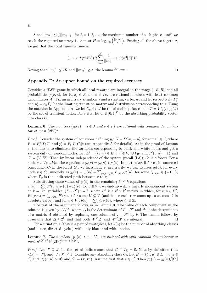
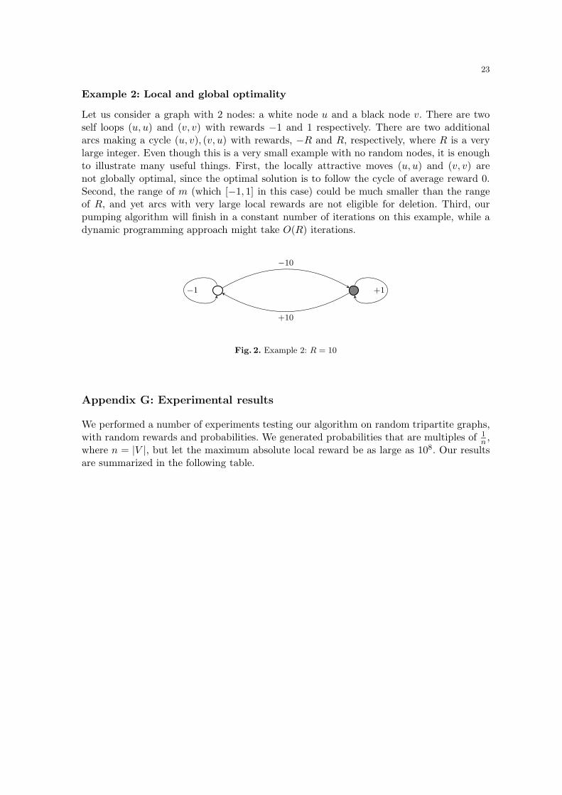
Example 2: Local and global optimality

Let us consider a graph with 2 nodes: a white node u and a black node v. There are twoself loops (u, u) and (v, v) with rewards −1 and 1 respectively. There are two additionalarcs making a cycle (u, v), (v, u) with rewards, −R and R, respectively, where R is a verylarge integer. Even though this is a very small example with no random nodes, it is enoughto illustrate many useful things. First, the locally attractive moves (u, u) and (v, v) arenot globally optimal, since the optimal solution is to follow the cycle of average reward 0.Second, the range of m (which [−1, 1] in this case) could be much smaller than the rangeof R, and yet arcs with very large local rewards are not eligible for deletion. Third, ourpumping algorithm will finish in a constant number of iterations on this example, while adynamic programming approach might take O(R) iterations.

−1 +1

−10

+10

Fig. 2. Example 2: R = 10

Appendix G: Experimental results

We performed a number of experiments testing our algorithm on random tripartite graphs,with random rewards and probabilities. We generated probabilities that are multiples of 1

n ,where n = |V |, but let the maximum absolute local reward be as large as 108. Our resultsare summarized in the following table.

24

R = 103 R = 106 R = 108

n N N N N N N

600 91 338 142 810 144 496

1200 91 385 152 566 172 545

1800 110 643 122 428 162 806

2400 104 318 159 508 178 767

3000 118 338 155 551 162 544

3600 113 397 138 541 180 576

4200 114 283 153 569 213 693

4800 126 681 164 680 194 702

5400 124 328 169 586 246 5284

6000 118 290 170 620 210 845

6600 138 535 173 565 202 718

7200 125 442 161 664 181 750

7800 143 860 170 588 188 604

8400 115 296 185 541 200 717

9000 121 368 171 543 202 1071

9600 128 361 171 532 201 624

10200 122 523 173 639 166 566

10800 142 532 172 815 211 759

11400 131 778 155 666 219 928

12000 141 587 198 2107 194 831

12600 159 918 180 664 187 747

13200 137 642 173 752 210 638

13800 116 355 172 701 198 768

14400 125 804 156 715 228 809

15000 139 511 165 632 227 1593

Table 1. Experimental results showing the average number of iterations N on random graphs with n ∈300, . . . , 15000 nodes, |VW | = |VB | = |VR| = n

3, and maximum reward R ∈ 103, 106, 108. N is the

maximum number of iterations encountered in all experiments with the given selection of parameters.