1  

Investment Analysis of the Framo Cargo Pumping System

Erling Hekland Teigland

Supervisor: Siri Pettersen Strandenes

Master in International Business

NORWEGIAN SCHOOL OF ECONOMICS

This thesis was written as a part of the Master of Science in Economics and Business Administration at NHH. Please note that neither the institution nor the examiners are responsible − through the approval of this thesis − for the theories and methods used, or results and conclusions drawn in this work.

Norwegian  School  of  Economics    Bergen,  December  2014  

 

  2  

Acknowledgments

This thesis is written in conjunction with my final semester as Master student at the

Norwegian School of Economics. The process of completing this paper has been both

rewarding as well as challenging. I would like to express my sincere gratitude towards a

couple of persons that have been very helpful in finalizing this thesis; Area Manager in Frank

Mohn AS, Alf Morten Utvær, for both giving me the idea to look at the hydraulic pumps, and

providing me with data and inputs, Michael Sungot, Bunker Manager at SKS Tankers, for

providing me with data relevant for my thesis, my parents, Anne Grethe Teigland and Hans

Hekland, for reading through the thesis and giving inputs. And last but not least a special

thanks to my academic advisor, Professor Siri Pettersen Strandenes, for her support and

guidance through the whole process. I am very grateful for their help, all constructive

comments and timely recommendations.

Erling Hekland Teigland

Bergen, December 2014

  3  

Abstract

This paper looks into whether or not it can be profitable for a shipping company operating in

the product tanker segment, to change from a steam driven cargo pumping system to a

hydraulic cargo pumping system by Frank Mohn AS. By looking at two triangulation

scenarios, one between the U.S. and Europe transporting dirty products and the other between

the U.S. and Asia transporting both dirty and clean products, I have been able to show that

there are both market factors such as economical, political and technological, as well as the

vessel speed and bunker price influencing the profitability for the different route alternatives.

In order to make the results as realistic as possible, I have used three different variables;

vessel speed, bunkers price, and investment cost. The methods used to estimate whether the

investment is sound or not, is the discounted cash flow (DCF) model and the adjusted present

value (APV) model. In addition to the main scenarios, I have also looked at the profitability of

the first route, without the use of triangulation, in order to find out whether the use of

triangulation is an important factor for the profitability of the pumping system. I have also

looked into which factors that might impede on the trade for the two triangulation routes in

the future, by use of the PESTLE analysis.

The two analyses show that the new cargo pumping system will be profitable with the use of

triangulation and the competitive advantage of quite easily switching from dirty to clean

cargo. There are however some market conditions one have to keep in mind; for the first

route, it is important to not forget that the U.S. are getting less dependent on foreign oil, as a

result of their own increasing production. For the second route, one have to keep in mind the

changing economical and political situations in the concerned countries. With these

conditions in mind, one would be hard pressed to not see the potential profit from the new

cargo pumping system.

  4  

Table of Contents

ABSTRACT  ......................................................................................................................................................  3  

TABLE OF CONTENTS  ...............................................................................................................................  4  

BACKGROUND  ..............................................................................................................................................  5  

STRUCTURE  ...................................................................................................................................................  5  

1. PRESENTATION OF THE MARKETS, THE TECHNOLOGY AND TRIANGULATION  ..  6  1.1 THE SHIPPING MARKETS  ..........................................................................................................................................  6  1.2 THE TANKER MARKET  ..............................................................................................................................................  7  1.3 VESSEL TYPE  ...............................................................................................................................................................  8  1.4 PUMP TECHNOLOGY  .................................................................................................................................................  9  1.5 TRIANGULATION  ........................................................................................................................................................  9  

2. METHODOLOGY  ...................................................................................................................................  10  2.1 PESTLE  .....................................................................................................................................................................  10  2.2 DISCOUNTED CASH FLOW (DCF)  .....................................................................................................................  12  2.3 ADJUSTED PRESENT VALUE (APV)  .................................................................................................................  15  

3. ANALYSIS OF THE MACRO-ENVIRONMENT  ............................................................................  19  3.1 TRIANGULATION SCENARIO 1  ............................................................................................................................  19  

Political  ............................................................................................................................................................................  20  Economical  ......................................................................................................................................................................  21  Social  .................................................................................................................................................................................  21  Technological  .................................................................................................................................................................  21  Legal  ..................................................................................................................................................................................  22  Environmental  ................................................................................................................................................................  23  Conclusion  .......................................................................................................................................................................  23  

3.2 TRIANGULATION SCENARIO 2  ............................................................................................................................  24  Political  ............................................................................................................................................................................  24  Economical  ......................................................................................................................................................................  26  Social  .................................................................................................................................................................................  30  Technological  .................................................................................................................................................................  30  Legal  ..................................................................................................................................................................................  30  Environmental  ................................................................................................................................................................  31  Conclusion  .......................................................................................................................................................................  31  

4. THE PROFITABILITY OF THE HYDRAULIC PUMP TECHNOLOGY  ................................  32  Economical Inputs  ........................................................................................................................................................  32  Technical Inputs  ............................................................................................................................................................  33  

4.1 SCENARIO 1  ..............................................................................................................................................................  35  4.2 SCENARIO 1 WITHOUT THE USE OF TRIANGULATION  .................................................................................  37  4.3 SCENARIO 2  ..............................................................................................................................................................  39  4.4 COMPARING THE RESULT OF THE SCENARIOS  ...............................................................................................  41  5. CONCLUSION  ..............................................................................................................................................................  42  

GLOSSARY  ....................................................................................................................................................  43  

BIBLIOGRAPHY  .........................................................................................................................................  45  

APPENDIX  .....................................................................................................................................................  49  

  5  

Background

I got the first idea for this paper, during a summer job working for Kristian Gerhard Jebsens

Skipsrederi AS. They are the last company in the world still using the once very popular Oil-

Bulk-Ore carriers, a vessel designed for triangulation. My initial idea was to look into whether

these vessels might become popular again, however after some research, I realized that this

would be difficult, due to the lack of data available. But the triangulation concept still

intrigued me, and after discussing the data challenge with Alf Utvær at Frank Mohn AS, I

developed the idea for a new research question that would let me write about triangulation,

and at the same time far more relevant for a larger part of the shipping industry. Thus my

main research question became: Is substitution to a new hydraulic cargo pump system

economic viable for the shipowners of Long Range 2 product tankers? Are there other factors

beside the new technology, which play an important role in the profitability of the system?

And finally, do the use of triangulation play an important role in the profitability of the

investment?  

Structure

The structure of this paper is as follows. First I conduct a presentation of the shipping

markets, the technology of the hydraulic cargo pump system and triangulation. This will

hopefully give the reader a basic understanding of the shipping industry and important

elements of this research. Then I will describe the different methods used, before I start

looking into the markets in the scenarios, starting off with the route between the U.S. and

Europe, and then end with the route between the U.S. and Asia.

Next up I will talk about how I came up with the different inputs used in the investment

analysis and show some of the results the analysis of the different routes gave me.

I will round up with a conclusion and a summary of my most important findings.

  6  

1. Presentation of the Markets, the technology and triangulation

1.1 The shipping markets The shipping industry comprises four different but closely linked markets. Sea transport

services are dealt in the spot freight market and the time charter market, new ships are ordered

and built in the new building market, used ships are traded in the second-hand market, and old

or obsolete ships are scrapped in the demolition market. The interactions of buyers and sellers

of these four markets determine the prices. We can further categorize these markets in real

and auxiliary markets. The spot freight market and the new building and scrapping market are

real markets as their activities affect the market clearing prices for transport services and

transport capacity respectively. While the time charter market and the second-hand market are

auxiliary markets, as their transactions do not change existing shipping capacity.

The spot freight market is a place where buyers and sellers are brought together to trade sea

transport services. As previously mentioned, the interaction between the supply and demand

of shipping services determines the freight rate. Due to the derived demand, demand for sea

tanker shipping services depends on seaborne trade volume. On the other hand, supply of

shipping service is inelastic in the short run. Excessive supply of shipping capacity not only

causes reduction in freight rate but also extra costs to lay up ships. On the other hand,

shortage in ships leads to an increase in freight rate to motivate shipping firms for adjusting

their shipping capacity.

The new building market and the freight market are positively correlated, however usually

with a time lag, due to the time it takes to build a ship. Shipping firms order new ships to

expand their fleet sizes during a freight boom. In the tanker shipping industry, the demand for

new vessels reflects the need for shipping capacity. An increase in orders of new builds,

indicate that ship owners expects the freight rates to increase in the near future, as there is a 2-

4 years delay between ordering a new vessel and delivery.

From the perspective of business operations, prices of new building ships have a stabilizing

effect in tanker shipping. When the demand for shipping services increase the freight rate

increases, and thus shipping firms orders new ships in order to increase their capacity. The

increase in orders of new builds will in turn increase the prices in the shipbuilding market,

and hence the capital costs of shipping firms’ increase. Such rise in the prices of new ships

could be seen as a “stabilizer” to set a barrier for shipping firms for excessive profit.

  7  

The second-hand market can, as mentioned, be categorized as an auxiliary market, as the

buying and selling of used ships are unlikely to alter the existing number of ships and the

carrying capability in the tanker shipping market. The sales and purchase market facilitates

the entry of shipping firms to the shipping market as shipping firms may acquire ships to a

lower capital cost than in the new-build market. Further more the second-hand market allows

for easier exit and restructuring of the fleet in response to the changing demand. As the

demand for second-hand ships increase during a freight boom, the second-hand market is also

closely linked with the freight market. At the time of high freight rate, demand for second-

hand ships are high as shipping firms can deploy these ships to earn higher than normal profit.

And as such the price of second-hand vessels increases with the increase of the freight rate,

and decreases with the decrease of the freight rate.

The demolition market is the last of the four closely linked markets, and as the new buildings

market, its activity determine the tanker shipping capacity. With exception of old ships that

are unable to meet the safety requirements and regulations, the scrapping decision made by

ship owners depends on expected financial return from scrapping the shipping and the future

freight rate. The activity in the scrapping market is as such linked to the second-hand market.

If the freight rate is high, during a boom, a ship owner might keep the vessel to increase

profits or sell the vessel in the second-hand market, and if the prices in the second-hand

market are low, he might choose to scrap it instead, especially if the scrapping prices are high,

due to increased demand for steel. (Lun, et al. 2013)

1.2 The tanker market

The oil trade accounted for about 27.5% of the total world seaborne trade in 2013. We can

mainly divide the vessels transporting oil, into two categories, crude tankers and product

tankers, where the crude tankers accounts for 18% of the world trade and the product tankers

accounts for 9.5%. (Clarksons Research Services 2014)The crude tankers are mainly used for

the deep-sea transportation of unrefined oil from extraction locations to the refineries, and

range in size from 55,000 dwt to 550,000 dwt. The main trading routes are from the

production areas in the Arabian Gulf and West Africa, to Asia, USA and Europe. While the

product tankers transport refined oil products such as gasoline, kerosene, diesel, jet or fuel oil

to consuming markets. They range in size from around 10,000 dwt to around 160,000 dwt,

and one of the traditional trading routes are between North America and Europe, carrying

gasoline to the US and diesel fuel back to Europe. We can categorize the tankers after size,

  8  

General Purpose (10,000-25,000 dwt), Medium Range, MR (25,000-45,000 dwt), Long

Range 1, LR1 (45,000-80,000 dwt), Long Range 2, LR2 (80,000-160,000 dwt), Very Large

Crude Carriers or VLCC (160,000-320,000 dwt) and Ultra Large Crude Carriers or ULCC

(320,000-550,000 dwt). (Hamilton 2014)

Tanker shipping provides an economical and convenient way to transport wet bulk for

international seaborne trade. It is the belief of many maritime economists that the supply of

tanker shipping operates under perfect competition, characterized by several conditions. The

first is the number of shipping service providers, there are a number of ship owners that own

tankers that provide identical shipping services. The second characteristic is the availability of

information, due to institutions such as the Baltic Index, shipping service providers are unable

to manipulate the freight rate and as such the price. There are some entry and exit barriers, but

these are mainly due to the cost of buying vessels in either the new building market or the

second-hand market and losses due to sale of vessels in the second-hand market, and not due

to marketing condition, as it does not exist in the tanker market. As for governmental

restrictions, there are no restrictions on entry, but there is however some restrictions on

quality, i.e. restriction on the use of heavy fuel oil (HFO) while in port in emission control

areas (ECA). (IMO 2014)

The price level (i.e., freight rate) in tanker shipping is influenced by the supply of shipping

service and the demand for shipping service. The supply of shipping service is determined by

the fleet size in terms of dwt, and the demand for shipping service depends on consumption

levels of refined oil products. (Lun, et al. 2013)

1.3 Vessel type

Product tankers are built to transport refined oil products from the oil refinery to another

refinery or the end user. The product tanker can carry both clean and dirty products, giving

them a trading flexibility across both clean and dirty petroleum markets. However due to

strict regulations switching from dirty to clean, the cargo tanks needs a thorough cleaning

before switching to clean products. They are characterized by having coated tanks to prevent

corrosion and to facilitate the cleaning of the tanks. The product tankers are classified in

segments according to vessel size, most commonly divided into the Long Range 2 (LR2),

Long Range 1 (LR1) and Medium Range (MR).

The MR ranges in size from 25,000 to 45,000 dwt, while the LR1 ranges in size from 45,000

to 80,000 dwt. The (LR2), often referred to as a “coated Aframax”, due to its abilities to carry

  9  

an array of refined crude products which require special handling, ranges in size from 80,000

to 160,000 dwt and is as such the largest specialized petroleum product tanker. (Hamilton

2014)

The LR2 tankers usually transport clean products on the long distances from the Middle East

to countries in Asia or Northern Europe, and dirty products on the long or intermediate

distances out of the Black Sea to the Mediterranean or to the USA, or from the Baltic or the

North Sea to Northern Europe or the USA.

(Taurus Tankers Ltd. 2011) (Danish Ship Finance A/S 2012)

1.4 Pump technology

The new pump technology from Framo AS, hydraulically driven submerged cargo pumps,

provide a safe, efficient and flexible cargo handling of any type of wet cargo. This new and

improved cargo handling performance gives a quicker turnaround time, which results in more

ton-miles. With the new technology one can transport a petroleum product on one voyage,

and then transport an acid on the next, making it possible to obtain triangulation opportunities

for a product tanker, and as such reduce time in ballast.

The Framo cargo pump is a vertical single stage centrifugal pump powered by a hydraulic

motor for safe and efficient operation. The pump design allows operation with a minimum of

liquid in the tank, which saves time spent for drainage and tank cleaning, reducing port-time.

Further more, by combining the cargo pumps in each cargo tank with submerged ballast

pumps inside the ballast tanks, the pump room becomes redundant. The arrangement provides

a safer ship design and increases space available for cargo, as there is no need for a pump

room anymore. In addition to this, it also consumes less fuel per discharge than its steam

turbine driven counterpart. (Frank Mohn AS 2014)

1.5 Triangulation

Triangulation is a way for shipowners to reduce the time in ballast, for example by

transporting gasoline from the U.S. gulf to Brazil, and after unloading it can sail up to

Venezuela, to load road fuel bound for the U.S. Atlantic Coast. Then after unloading sail back

to the U.S. gulf, to load diesel for Europe, returning to the U.S. Atlantic Coast with gasoline.

By using triangulation, one can increase a ship’s utilization rate and boost earnings.

(Overseas Shipholding Group, Inc. 2009)

According to Pareto’s shipping outlook from 2013, we now see a change in the tanker market.

In the past, the oil refineries were often situated quite far away from the oil reserves, creating

  10  

a market for the crude oil tankers, and the refineries were closer to the end users, creating a

good market for the MR product carriers. However in the last couple of years we have seen a

trend, that the refineries are built closer to the oil reserves, thus reducing the need for crude

oil tankers, while creating a market for the larger product carriers like LR2. There has also

been a change in the transport pattern, as the U.S. oil production increases, lessening the

demand for imports of oil products from Europe. Further more it is expected that the product

trade from the Middle East to Asia will grow rapidly going forward, despite increasing

refinery capacity in India and China, as the expected demand of products to be used as power

sources for domestic households will increase with more than what the local refineries are

able to produce, due to an increased urban population. (EIA 2014) (Pareto Shipping AS 2013)

(BIMCO 2013)

2. Methodology

2.1 PESTLE The market changes everyday, and in a matter of seconds the scenario before us may have

changed. Some of these changes are controllable, however there is also some we cannot

control, these are called systematic factors. Systematic things happen in the environment that

surrounds us, and very often they influence our agenda. It is as a result of this, that we need to

constantly check and analyse the environment in which we operate. A detailed analysis of the

macro-environment is called PESTLE analysis. The analysis consists of factors, Political,

Economic, Social, Technical, Legal and Environmental, which directly or indirectly affect the

business environment. The PESTLE analysis is used as a tool for the managers and strategists

to ascertain the current market situation and what the future might look like.

Political

Political factors take into account the political situation of a country and the world in relation

to the country. All of the policies, tax laws, and every tariff that a government levies over a

trade fall under this category of factors.

Economic

These factors include all the determinants of an economy and its condition. The inflation rate,

the interest rates, monetary or fiscal policies, the foreign exchange rates that affect imports

and exports, all these determine the direction in which an economy might move.

  11  

Social

As every country differs, and the importance of cultural understanding becomes more and

more important in this global world, it is important to look at the social aspect as well.

Especially since the social factors like social lifestyle, domestic structures and connected

demographics influences the market.

Technological

Technology has always and will always influence the business world, take for example the

assembly line technique and how it revolutionised the manufacturing industry at the

beginning of the 20th century. This is also why technology is one of the factors in the Pestle

analysis. If one is not up-to-date on new relevant technology, one might end up losing income

compared to competitors with the new technology. Another reason of analysing the

technological factor is to understand how consumers react to technological trends and how to

utilize them for their benefit.

Legal

Legislative changes occur from time to time and many of them affect the business-

environment. For example in 1992 MARPOL was amended to make it mandatory for tankers

of 5,000 dwt and more ordered after 6th of July 1993 to be fitted with double hulls, or an

alternative design approved by IMO (regulation 19 in Annex 1 of MARPOL).

(International Maritime Organisation 2014) The law had an impact on most of the businesses

in the tank industry, and regulations in other industries have a similar impact, making it

important for businesses to analyse the legal development happening in their environment.

Environmental

Environmental factors also have a tendency to influence the business, and especially how we

do things in an industry. For example, due to the climate changes happening, there have been

an increased focus on clean energy, which have a potential to reduce the demand of coal,

which will lead to reduced coal prices and a slow down in the coal industry. The

environmental factors include geographical location, the climate, weather and other such

factors that are not just limited to climatic conditions like the wildlife and other factors.

(Constantinides 2011)

  12  

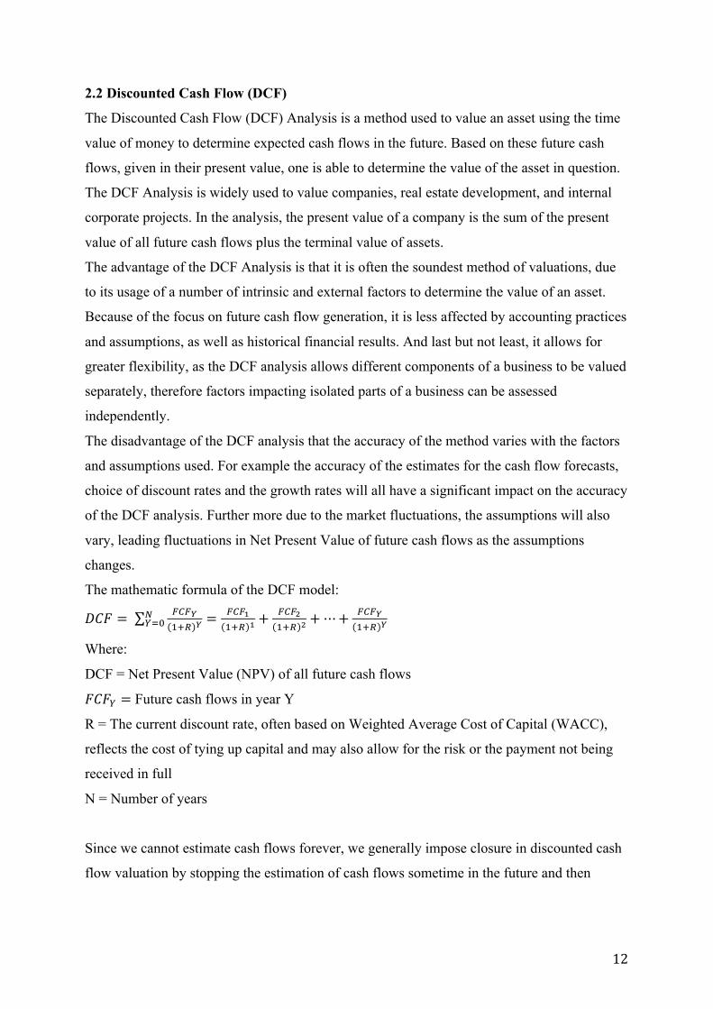
2.2 Discounted Cash Flow (DCF)

The Discounted Cash Flow (DCF) Analysis is a method used to value an asset using the time

value of money to determine expected cash flows in the future. Based on these future cash

flows, given in their present value, one is able to determine the value of the asset in question.

The DCF Analysis is widely used to value companies, real estate development, and internal

corporate projects. In the analysis, the present value of a company is the sum of the present

value of all future cash flows plus the terminal value of assets.

The advantage of the DCF Analysis is that it is often the soundest method of valuations, due

to its usage of a number of intrinsic and external factors to determine the value of an asset.

Because of the focus on future cash flow generation, it is less affected by accounting practices

and assumptions, as well as historical financial results. And last but not least, it allows for

greater flexibility, as the DCF analysis allows different components of a business to be valued

separately, therefore factors impacting isolated parts of a business can be assessed

independently.

The disadvantage of the DCF analysis that the accuracy of the method varies with the factors

and assumptions used. For example the accuracy of the estimates for the cash flow forecasts,

choice of discount rates and the growth rates will all have a significant impact on the accuracy

of the DCF analysis. Further more due to the market fluctuations, the assumptions will also

vary, leading fluctuations in Net Present Value of future cash flows as the assumptions

changes.

The mathematic formula of the DCF model:

𝐷𝐶𝐹 =   !"!!!!! !

!!!! = !"!!

!!! ! +!"!!!!! ! +⋯+ !"!!

!!! !

Where:

DCF = Net Present Value (NPV) of all future cash flows

𝐹𝐶𝐹! = Future cash flows in year Y

R = The current discount rate, often based on Weighted Average Cost of Capital (WACC),

reflects the cost of tying up capital and may also allow for the risk or the payment not being

received in full

N = Number of years

Since we cannot estimate cash flows forever, we generally impose closure in discounted cash

flow valuation by stopping the estimation of cash flows sometime in the future and then

  13  

computing a terminal value that reflects the value of the firm at that point. Thus we can use

this formula to find the value of the firm:

𝐹𝐶𝐹!1+ 𝑅 !

!

!!!

+𝑇𝑒𝑟𝑚𝑖𝑛𝑎𝑙  𝑉𝑎𝑙𝑢𝑒!

1+ 𝑅 !

Where:

The formula for terminal value is:

 𝐹𝐶𝐹!!!(𝑅 − 𝑔)

Where:

𝐹𝐶𝐹!!!= Future cash flow in year Y+1

𝑅 = The current discount rate (often based on WACC)

𝑔 = The growth rate

Since we already have assumed that the cash flows will grow at a constant rate, we can use

the formula of compounded annual growth rate to find the expected growth rate needed in the

terminal value formula:

𝑔 = 𝐶𝐴𝐺𝑅 =𝐸𝑛𝑑𝑖𝑛𝑔  𝑉𝑎𝑙𝑢𝑒

𝐵𝑒𝑔𝑖𝑛𝑛𝑖𝑛𝑔  𝑉𝑎𝑙𝑢𝑒!

− 1

Where:

𝑁 = Number of years

WACC

The weighted average cost of capital (WACC) represents the opportunity cost that investors

face for investing their funds in one particular business instead of others with similar risk. The

most important principle underlying successful implementation of the cost of capital is

consistency between the components of the WACC and free cash flow. In its simplest form

the weighted average cost of capital equals the weighted average of the after-tax cost of debt

and cost of equity:

𝑊𝐴𝐶𝐶 =𝐸𝑉 𝑘! +

𝐷𝑉 𝑘! 1− 𝑇!

Where:

E/V = Target level of equity (E) to enterprise value (V) using market-based values

  14  

D/V = Target level of debt (D) to enterprise value (V) using market-based values

𝑘! = Cost of equity

𝑘! = Cost of debt

𝑇! = Company’s marginal income tax rate

In order to determine the WACC for a particular project or enterprise, one need to estimate

the three components of WACC; the cost of equity, the after-tax cost of debt, and the

project’s/company’s target capital structure.

The cost of equity is again determined by three components; the risk-free rate of return, the

market-wide risk premium (the expected return of the market portfolio less the return of risk-

free bonds), and a risk adjustment that reflects each company’s riskiness relative to the

average company. We can use the capital asset pricing model (CAPM) to estimate the cost of

equity.

The capital asset pricing model (CAPM) says that the expected return on a portfolio should

exceed the risk-free rate of return by an amount that is proportional to the portfolio beta. That

is, the relationship between return and risk should be linear. (Modigliani and Pogue 1974)

𝐸 𝑅! = 𝑟! + 𝛽! 𝐸 𝑅! − 𝑟!

Where:

𝐸 𝑅! = Expected return of security i

𝑟! = Risk-free rate

𝛽! = Stock’s sensitivity to the market

𝐸 𝑅! = Expected return of the market

In the CAPM, the risk-free rate and market premium, defined as the difference between

𝐸 𝑅! and 𝑟!, are common to all companies; only beta varies across companies. The beta

represents a stock’s incremental risk to a diversified investor, where risk is defined as the

extent to which the stock covaries with the aggregate stock market.

In order to estimate the beta, we can use the theories of Modigliani and Miller, according to

them; the weighted average risk of a company’s financial claims equals the weighted average

risk of a company’s economic assets. Using the beta to represent risk and rearrange the

equation to solve for the beta of equity (𝛽!), we get:

  15  

𝛽! = 𝛽! +𝐷𝐸 𝛽! − 𝛽! −  

𝑉!"#𝐸 𝛽! − 𝛽!"#

Where:

𝛽! = The beta of the unlevered company

𝛽! = The beta of debt

𝑉!"# = The value of the company’s interest tax shields

𝛽!"# = The beta of the tax shields

In order to simplify this even further, we can use two additional restrictions; (1) due to the

fact that debt claims have priority, the beta of debt tends to be low, and thus we can for

simplicity assume it is 0. (2) If the company maintains a constant capital structure, the value

of the tax shields will fluctuate with the value of operating assets, and the beta of the tax

shields will equal the beta of the unlevered company. By setting these two components equal

to each other, we eliminate the final part of the formula and end up with:

𝛽! = 𝛽! + 1+𝐷𝐸

As a result we get that the company’s equity beta equals the company’s unlevered beta times

a leverage factor.

In order to estimate the cost of debt we can use the yield to maturity of the company’s long

term, option-free bonds. This method is however only useful if the company’s debt rating is

not lower than BBB. The use of a debt rating lower than BBB or so called junk bonds, will

overstate the true cost of capital and as such paint a wrong picture of the company. Thus if the

debt rating is lower than BBB, one should not use the WACC at all, but rather the adjusted

present value (APV) based on the unlevered cost of equity rather than the WACC to value the

company. (Koller, Goedhart and Wessels, Valuation Measuring and Managing the Value of

Companies 2010)

2.3 Adjusted Present Value (APV)

When doing a DCF analysis, we assume that the company manages its capital structure to a

target debt-to-value ratio. However, suppose the company we are analysing have a high

proportion of debt, and pays it down as cash flow improves, lowering their future debt-to-

value ratios. In this case the use of WACC would overstate the value of the tax shields, unless

one adjust the WACC yearly in order to handle the changing capital structure. This is

  16  

however a complex process, which is why we use an alternative model, the adjusted present

value (APV).

The adjusted present value separates the value of operations into three components: the value

of operations as if the company were all-equity financed, the value of tax shields that arise

from debt financing and the value of distress costs. (Koller, Goedhart and Wessels 2010)

The first step is the estimation of the value of the unlevered firm. In this step we value the

firm as if it was all-equity financed, by discounting the expected free cash flow to the firm at

the unlevered cost of equity. If we assume the cash flow to grow at a constant rate, the value

of the firm is easily computed.

Value of Unlevered Firm:

𝐹𝐶𝐹𝐹!×(1+ 𝑔)𝑘! − 𝑔

Where:

𝐹𝐶𝐹𝐹! = The current after-tax operating cash flow to the firm

𝑘! = The unlevered cost of equity

𝑔 = The expected growth rate (see CAGR in 2.2.)

In order to find the unlevered cost of equity, we first need to find the unlevered beta of equity.

We can find the unlevered beta of equity, by reformulating the formula we used in the DCF

analysis to compute the beta of equity:

𝛽! = 𝛽! 1+𝐷𝐸

Where:

𝛽! = The unlevered beta of equity

𝛽! = The beta of equity

𝐷/𝐸 = The debt/equity ratio

We can then use the CAPM to estimate the unlevered cost of equity, the same way we did in

the DCF analysis, just using the unlevered beta of equity instead of the beta of equity.

If we assume that the tax rate will be constant over time, we can find the value of the tax

shield by multiplying the marginal tax rate with the value of the debt.

Value of the tax shield:

𝑡!×𝐷

Where:

  17  

𝑡! = The marginal tax rate

𝐷 = The value of the debt

The third and last part of the APV, the distress costs, poses the most significant estimation

problem, since neither the probability of bankruptcy nor the cost of bankruptcy can be

estimated directly. We can divide the distress costs into two parts the probability of

bankruptcy and the costs of bankruptcy. One-way of estimating the probability of bankruptcy

is to estimate a bond rating, at each level of debt and use the empirical estimates of

bankruptcy probabilities for each rating. For instance, the table underneath, extracted from a

study by Altman and Ramayanam, summarizes the probability of bankruptcy over ten years

by bond rating class in 2007 (Appendix XX). (Altman 2007)

The cost of bankruptcy can be estimated, according to Andrade and Kaplan (1998), by the use

of this relationship:

𝐸𝑉! − 𝐿! = 𝐵! + 𝐵!

Where 𝐸𝑉! is the value of the firm before onset of financial distress, 𝐿! the value of the

liquidated assets, 𝐵! is the direct costs of bankruptcy (such as court-related fees) and 𝐵! is the

indirect costs of bankruptcy (such as the loss of customers and suppliers). In this case, we do

not need to split the cost of bankruptcy into the indirect and direct costs of bankruptcy, which

make the estimation a bit easier. By rearranging the formula above, we get

𝐵 = 𝐸𝑉! − 𝐿!

Thus, we have an expression for the costs of bankruptcy that can be used for estimation

purposes. Values of the liquidated assets can be found by looking at the net asset value in the

bankruptcy files. The enterprise value can be found by calculating the market capitalization

and then add the book value of net debt. We can further find the cost of bankruptcy ratio by

dividing the cost of bankruptcy on the enterprise value. (Andrade and Kaplan 1998)

Once we have calculated the cost of bankruptcy ratio and the probability of default, we can

find the expected bankruptcy costs, by multiplying the two factors with the unlevered firm

value.

  18  

The adjusted present value can now be calculated by taking the unlevered firm value, adding

the present value of tax shields and subtracting the expected bankruptcy costs. (Damodaran

2005)

  19  

3. Analysis of the macro-environment

In the following, I will look at two scenarios of triangulation in the tanker market.

The first scenario uses a route that has been used quite frequently for several years and goes

between the United States and Europe. The second scenario looks at a route between the U.S.

South America and East Asia, an area that will become even more important as the refineries

are moved closer to the oil wells, and due to the expected economic growth in this area.

I will first use the previously introduced PESTLE theory to analyse the industry factors in the

product tanker market for each of the two scenarios, starting with the triangulation

opportunity between the US and Europe. Following the strategic analysis, I will do an

Investment Analysis for both scenarios using the new pump technology, to see whether the

new technology makes the LR2 product tanker even more profitable than without the new

technology.

3.1 Triangulation scenario 1

The first triangulation route goes from the U.S. Gulf to Europe with diesel, then from Europe

to New Haven with gasoline, and the last leg, sail in ballast from New Haven to the U.S. Gulf.

As previously mentioned and described, the PESTLE analysis are made up by six different

factors: Political, Economical, Social, Technological, Legal and Environmental. This is also

the same way I will structure my analysis, starting with the Political factor.

 Figure 1: Triangulation Route 1

Corpus Christi

New Haven Rotterdam

  20  

Political

Since the beginning of the 90’s both the EU and the United States have been part of many

large conflicts, from the war on Balkan to the war in Iraq. It would be quite logical to assume

that these conflicts especially those in the middle east would have some influence on the oil

price, and through that the price on diesel and gasoline.

 Figure 2: Oil price fluctuation  (Anderson  and  Kahya  2011)

As we can see from the graph, the biggest fluctuation in the prices was not due to the

conflicts, but due to the financial crisis in 2008/2009. This and an article, “Recent oil price

fluctuations linked to world economy”, by Professor Lutz Kilian at the University of

Michigan, supports the theory that the economic environment is the most important factor

when it comes to oil prices. (Kilian 2011)

Furthermore, the political environment in both the EU and the United States are relatively

stable especially if we look at its impact on the diesel and gasoline trade between the two.

There are of course some new regulations on the emission standards for diesel and gasoline,

but nothing that cannot be handled by the refineries. In fact, as a result of the conflict in

Ukraine, it looks like that the European Union are less focused on the environmental impact

of how the oil is produced and more focused on being less dependent on Russian oil and gas.

(Gallo 2014)

  21  

Economical

In the economic aspect of the product tanker trade between the US and the European Union,

we can see from the graph above, that the recession did have some impact on the price per

barrel. However, as the graph also clearly shows, the drop in price per barrel did not last, and

already in 2011, were we back at the same level as before the recession. One reason for this

quick recovery is probably the fiscal stimuli brought forward by both the Federal Reserve in

the US and the ECB, the European Central Bank. The stimuli have ensured that companies

have stayed afloat, investments are recovering and thus also the unemployment rate is reduced

compared to the 2009 levels. Which again had a positive impact on the demand for diesel and

gasoline as people can afford to drive their cars.

There are however some factors which might reduce the demand for gasoline in the US, and

thus reducing the profitability of the triangulation between the US and the EU. Firstly, the

increased oil production in the US, making them less dependent on oil product imports.

Secondly, due to the recession, we have seen a shift from larger and less fuel-efficient

vehicles, to smaller and more economical vehicles. In the future we might also see a reduction

in demand for fuel, as the electric cars become more popular, however for the time being the

decrease in operational cost for an electric car versus a conventional vehicle does not

outweigh the difference in purchase cost. (Todd, Chen and Clogston 2013)

Social

When looking at the social aspect of the analysis there are few factors, if any that might have

an impact on the trade between the US and EU. They are quite similar both culturally and

when it comes to social lifestyle. The only factor the could have had some impact, would be

that the inhabitants of the US used to use large vehicles, however in the last couple of years

the carpool have become more and more alike, the one in Europe. Thus there is no need to

focus on the social aspect when looking at the triangulation opportunity and product tanker

trade between the US and the European Union.

Technological

Technologically there are some aspects that might have an impact on the trade. Firstly, the

new tare sand technology, which already have increased and will further increase the oil

production in the US, making them less dependent on oil and oil products from other

countries. Secondly, as mentioned before, we have seen a shift to more fuel-efficient vehicles

  22  

in the US. This shift and the new hybrid and electric engine technology, will further lessen the

demand for fuel. However, due to the power of the car industry in the US, it might take some

time before we see the full effect of this change. According to an article written in Dagens

Næringsliv, the governor of Michigan signed a bill that prohibits the worlds leading electric

car manufacturer, Tesla, from selling their cars directly to the consumer, lessening their

competition power against GM, Chrysler and Ford. (Hartwig 2014)

And last but not least, the new technology for product tankers, like for instance the new pump

technology. The new technology have the potential to reduces port costs, and increase the

amount of cargo carried, making it possible to transfer more to a lower cost. Which will have

a positive effect in the long run, making the trade more profitable. But in the short run, it

might have a negative impact, as reduced travel time and the ability to carry more, will

increase the number of vessels available, leading to lower charter prices.

Legal

The legal aspect is an important one, but have a relatively small impact on the trade, at least in

the long run. As we get new technology and more knowledge, there will probably occur new

legislative changes, like the change in MARPOL of 1992, making it mandatory for new

vessels above 5,000 dwt to be fitted with a double hull. However most of these changes will

be mandatory for all vessels, and in the case of the EU and the US, both follow the legislative

changes made by the IMO, the International Maritime Organisation. Which means that any

new changes will not impede on the trade, at least not in the long run. It might have some

effect in the short run, due to the fact that the market supply of vessels might decrease for

some time, resulting in increased chartering prices, but it is not likely as most changes have

incorporated an outfacing time for the vessels in question. (International Maritime

Organisation 2014)

There is however one legislative factor that could impede a big impact on the trade, the Jones

Act. The Jones Act is a US freight cabotage law saying that only American built and

registered ships, with American crew can transport cargo between ports in the US. However

since the product tanker in this scenario goes in ballast between USNH and the US gulf, it is

not affected by the Act. (Maritime Law Center n.d.)

  23  

Environmental

The last aspect in the PESTLE analysis is the environmental aspect. In the last couple of

decades, we have seen an increased focus on the environment in the shipping industry, mainly

due to the Marine Environmental Protection Committee (MEPC), a subsidiary of the IMO.

The MEPC is empowered to consider any matter within the scope of the organisation

concerned with prevention and control of pollution from ships. (IMO 2014) The regulations

made by the MEPC, closely links the environmental aspect to the legal aspect as well as the

technological, due to the fact that new regulations may enforce shipowners to either improve

their vessels or scrap them. Which again will have an impact on the trade, at least for the

shipping companies who are registered or do business with member states of the IMO. Both

of the countries in this scenario are members of the IMO, thus any shipping company

transporting oil products between these two, will have to follow the regulations set down by

the MEPC.

Conclusion

In the analysis we have seen that the main factors that might influence the profitability for this

triangulation route is mainly the economical and technological factors, as the U.S. becomes

less dependent on the import of oil products, as a result of the switch to more fuel efficient

cars and its increased oil production.

  24  

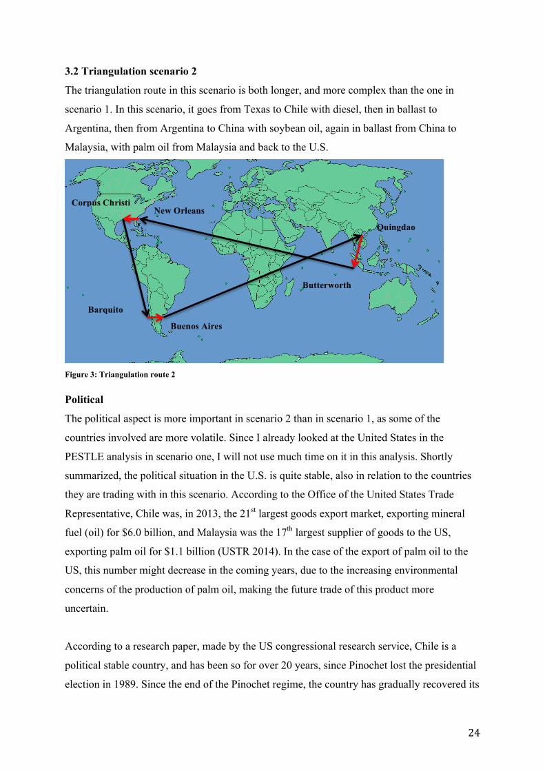
3.2 Triangulation scenario 2

The triangulation route in this scenario is both longer, and more complex than the one in

scenario 1. In this scenario, it goes from Texas to Chile with diesel, then in ballast to

Argentina, then from Argentina to China with soybean oil, again in ballast from China to

Malaysia, with palm oil from Malaysia and back to the U.S.

 Figure 3: Triangulation route 2

Political

The political aspect is more important in scenario 2 than in scenario 1, as some of the

countries involved are more volatile. Since I already looked at the United States in the

PESTLE analysis in scenario one, I will not use much time on it in this analysis. Shortly

summarized, the political situation in the U.S. is quite stable, also in relation to the countries

they are trading with in this scenario. According to the Office of the United States Trade

Representative, Chile was, in 2013, the 21st largest goods export market, exporting mineral

fuel (oil) for $6.0 billion, and Malaysia was the 17th largest supplier of goods to the US,

exporting palm oil for $1.1 billion (USTR 2014). In the case of the export of palm oil to the

US, this number might decrease in the coming years, due to the increasing environmental

concerns of the production of palm oil, making the future trade of this product more

uncertain.

According to a research paper, made by the US congressional research service, Chile is a

political stable country, and has been so for over 20 years, since Pinochet lost the presidential

election in 1989. Since the end of the Pinochet regime, the country has gradually recovered its

Corpus Christi New Orleans

Barquito

Buenos Aires

Quingdao

Butterworth

  25  

democracy and new economic, social and political reforms have been implemented, despite

political challenges from the Pinochet regime. The political, social and economic reforms

implemented have resulted in Chile being one of the fastest growing economies in Latin

America, with an average economic growth of 5.38 % from 1987 to 2014. (USTR 2014)

(Meyer 2014)

Where as Chile has had political stability and an exceptional economic growth for over two

decades, Argentina’s story is quite the opposite. In the last 13 years Argentina has defaulted

its loans twice, making the political environment quite unstable. Even more so, looking at

how it affects international trade. In order to try to solve its economical problems, the

Argentinian governments have enforced an increasingly complex strategy of trade

protectionism, using relatively high tariffs, import restrictions, export taxes, and limiting

foreign exchange transactions. With reference to the triangulation route used in this scenario,

there was, according to a trade report made by USTR in 2013, a 32 % export tax on soybean

oil. (USTR 2013)This strategy of trade protectionism in addition to other governmental

issues, like nationalising the largest oil company in Argentina, Yacimientos Petrolifero

Fiscales (YPF), have brought retaliation from countries around the world, as well as

denouncement at the WTO. (Hornbeck 2013)

China on the other hand, has a relatively stable political environment, however different from

Argentina in the sense that Argentina is a democracy, while China is a one-party state.

However whereas there have been little change in the governing of Argentina, we have seen

quite big change in China, economic and trade reforms begun in 1979 have helped transform

China into one of the world’s fastest-growing economies. The economic growth and trade

liberalisation, including comprehensive trade commitments made upon entering the World

Trade Organisation (WTO) in 2001, have led to a sharp expansion in China’s commercial ties

around the world. (Morrison 2014)

Even though China has become more liberal when it comes to trade, there is still a long way

to go. According to an annual report by Global Trade Alert, Argentina and China, are the only

two countries in the world that are in the top 10 list of offenders for all major categories of

discriminatory harm it measures by the number of (1) discriminatory measures, (2) tariff

lines, (3) sectors affected, and (4) trading partners involved. China tops the list in terms of

trading partners harmed; in part due to its extensive export management policies through

selective VAT rebates for exporters (Evenett 2012).

  26  

The last of the five countries of the triangulation route is Malaysia. Since its independence in

1957, there has been a high degree of political stability. Political coalitions led by the

dominant political party, United Malays National Organisation (UMNO), have been in power

without interruption since the Malaysian independence. Still the outlook for the future, may

not be that stable as there is a growing resentment with corruption and discriminatory pro-

Malay affirmative action policies. In relation to the trade between the U.S. and Malaysia,

Malaysia was in 2013 the 17th largest supplier of goods to the U.S. and the 25th largest

importer of U.S. goods (USTR 2014). They are also part of the on-going negotiations to

create a new trade agreement, know as the Trans-Pacific Partnership (TPP). There are

however some issues that hamper the negotiations, like the Malaysia’s government

procurement policies, which give preferential treatment for certain types of Malaysian-owned

companies, provisions for intellectual property rights (IPR) protection, and market access for

key commodities and services (Rinehart 2014).

Economical

In this scenario the economical aspect for the United States, are less important for the trade,

than in scenario 1, at least for the trade to Chile. The recession in 2008/2009 did have some

effect on trade, but as the United States are considered to be back on track, and since they are

the exporter of fuel oil, the other aspect mentioned, are not that problematic. For instance the

fact that they have changed to smaller and more fuel efficient cars and that they are becoming

more self supplied with fuel, are actually more positive for the trade with Chile, as they can

export more, than before. There is however one problem that might put a dent in the trade

between the U.S. and Chile, and that’s the falling oil prices. According to an article in the

Guardian, there are a rising number of factors pointing in the direction of an even further

reduction in oil prices, as economic growth in China and the U.S. have weakened, and the

supply of oil have increased, due to increased production in the U.S., Russia and OPEC.

(Farrell 2014)

As mentioned earlier, Chile has had an average growth of 5.38 % from 1987 to 2014, making

Chile the most competitive and fundamentally sound country in Latin America. The

economic success stems from policies implemented since the fall of Pinochet, opening the

country to investment, secured access to foreign markets and mitigated the effects of external

shocks, like the financial crisis. The strong economic growth paired with targeted social

  27  

assistance programs, has also contributed to a significant decline in the poverty rate. There are

however still high levels of inequality, contributing to some discontent among the population.

In relation to the trade, the economic growth and especially the free trade agreement with the

U.S., entering in to force in 2004, have increased trade between the two countries, as we can

see from the figure above.

According to the U.S. Department of Commerce, the export of goods from the U.S. to Chile,

were valued at 18.9 billion USD in 2012, with refined oil products, heavy machinery and

motor vehicles accounting for the majority. Whereas the export of goods from Chile to the

U.S. were valued at 9.4 billion USD, with top products including copper, edible fruit and

seafood, leaving the U.S. with a substantial trade surplus. (Meyer 2014)

Whereas Chile is doing quite well economically, the same cannot be said for Argentina. As

previously mentioned, they have defaulted twice on their loans in the last 13 years, and have

an inflation rate, second only to Venezuela in the world. The default in 2002 left the

government unavailable to access the international bond markets, making it harder to finance

their debt, without harming the population even further through taxes or printing more money.

In the end they have managed to reduce their debt, mainly due to restructuring and increased

taxes on financial transactions and on export. So far these taxes have improved the

Argentinian situation to some extent, as we can see from the table above, the growth in GDP

has been quite high in the last couple of years.

  28  

However, the taxes do also have a negative effect, as it raises costs, which can reduce the

incentive to produce and invest, ultimately leading to reduced revenue and economic growth.

Furthermore, the taxes on export makes the goods exported from Argentina less competitive

in the global markets, which might suggest that these financial schemes might jeopardise the

future growth and development and as such does not really fix the problem, only postponing

it, leaving the future Argentina in even bigger problems than they have today. In relation to

trade, this is not yet a big problem for Argentina, as they are still the biggest producer of

soybean and soybean oil. However, should for instance China or other major importers go

into a recession, they might go looking for cheaper sources of soybean and soybean oil,

leaving Argentina bare. (Hornbeck 2013)

The latest figures from the IMF, adjusted for purchasing power, shows that China has

surpassed the U.S. as the largest economy in the world, with a PPP adjusted GDP of 17.632

trillion USD. (Bird 2014) Since the first initiations of market reforms in 1978, China has seen

an unprecedented economic growth with an average of 10 percent GDP growth. Even the

financial crisis of 2008/2009 did not put a dent in the growth, at least not compared to the

west, with a growth of 9.635 and 9.214 percent respectively. The market reforms have also

given them one of the most diverse spread of industry production in the world, and made

Table 1: Argentina: Selected economic data, 2000-2012 (Hornbeck 2013)

  29  

them the world’s second largest trading nation behind the U.S., being the largest exporter, and

the second biggest importer in the world. Since its accession into the WTO in 2001, the

country’s share in the global trade has doubled, accounting for about 10 percent of both the

worlds merchandise trade exports and imports. Even though it looks like China are doing

pretty good for them and being an engine of the world, there are some growing concerns

about the big trade imbalances between China and the rest of the world. Further more there

have also been a growing number of trade disputes, mainly for dumbing, unfair subsidies by

the Chinese government, intellectual property rights (IPR) and the valuation of the Yuan.

(EW World Economy Team 2013)

In relation to trade, the big question is whether the growth we have seen in China, will still

continue or if it will slow down, causing waves that might affect the world trade. According

to an article by Pritchett and Summers, there are a consensus by forecasters that China will

continue to grow strongly, both over the medium and long term. However, according to

arguments by Pritchett and Summers, there are many reasons to a more pessimistic outcome.

Firstly, they argue that the past growth performance is of very little value for forecasting

future growth. Secondly, abnormally rapid growth is rarely persistent and “regression to the

mean” is an empirically robust feature of economic growth. Further more, they argue, that

rapidly growing countries are substantially more likely to suffer a sharp downward change in

growth than gradual and small and even more so for countries with high levels of state control

and limited respect for the rule of law. (Pritchett and Summers 2013) Taking into

consideration the latest numbers from the Chinese economy, and the arguments made by

Pritchett and Summers, it seem wisely to start preparing for a downturn in the Chinese

economy, specially due to the effects it might have on the world economy and through that,

the world trade.

China and Malaysia have some common traits, looking at economic performance, both have

been among the fastest growing economies over the last 30 years, and recovered rather

quickly from the financial crisis in 2008/2009. Numbers from the World Bank, show that the

Malaysian economy was back on track at its pre-crisis levels earlier this year.

There are however some concerns with the Malaysian economy. First and foremost, the

diversification within the country, Most of the nation’s GDP contribution comes from four of

the nine Malaysian regions; the State of Selangor, which surrounds the capital Kuala Lumpur,

Kuala Lumpur, the State of Johor, located next to Singapore, and the state of Sarawak, on the

  30  

island of Borneo. These four regions are the most prosperous and form the core of Malaysia’s

manufacturing and service sectors. The five other states, mainly concentrated along the border

of Thailand, except for the state of Sabah on the northern tip of Borneo, are relatively poor

regions with less manufacturing and service activity.

In addition to the regional diversity, there is also large economic differences between urban

and rural areas, as well as ethnicities, where the Chinese Malaysians are those with the most

power and wealth, whereas the majority of the population, the Malays and other indigenous

people have traditionally been considered economically disadvantaged. In relation to trade,

and especially with the U.S., there are raised some concerns about Malaysia’s IPR protection

and limited market access, as a result of tariffs and other restrictions on imports, like

automobiles, and agricultural goods. (Rinehart 2014)

Social

The social aspect of this analysis is, as in the first analysis, not especially relevant for this

scenario, even though there are bigger social and cultural differences in this scenario, there

are still few social factors that might have an impact on the trade. The most realistic factor

would be increasing differences between the rich minority and a growing middle class,

resulting in an uprising limiting trade for some time.

Technological

Technically there are also few factors that could impact the trade in this scenario. The main

one is the new hydraulic pump technology, which has the potential of shortening port time,

increase the amount of cargo carried, and make it possible to be able to switch between clean

and dirty products, a lot more efficient than product tankers without the technology. However

as soon as this becomes know within the industry, this advantage will disappear.

Legal

The legal aspect in relation to the shipping industry in this scenario is not much different from

the first scenario, as all the countries are members of the IMO, and as such have to abide the

same regulations like the MARPOL. The only aspect that is different in relation to the first

scenario is the Emission Control Areas (ECA), which prohibits vessels from using Heavy

Fuel Oil (HFO) in coastal areas. As of yet, these areas have not been created outside Europe

and the U.S. As a result one can reduce some port costs when loading and discharging outside

  31  

Europe and the U.S., as the price of the HFO is cheaper than the Marine Diesel Oil, allowed

in the ECA.

Environmental

In regard to the last aspect of the PESTLE analysis, the environmental aspect, there are no big

differences from this scenario to the first scenario. Due to the fact that all of the countries

described in this scenario, are members of the IMO, and as such have to abide by the same

regulations mentioned in the first scenario, like the MEPC.

Conclusion

In the analysis we have seen that the main factors that might influence the profitability for this

triangulation route is mainly the political and economical factors, and especially the

economical situation in China and Argentina. The Argentinian government are trying to solve

their economic problems with increased tax on trade, and as for China, many analysts are just

waiting for an economic crisis that might create ripples affecting the whole region or the

whole world.

  32  

4. The Profitability of the hydraulic pump technology

For both of the two scenarios, I have used the discounted cash flow model as my primary

valuation model, in order to find out the profitability of the hydraulic pump technology. I

have also used the adjusted present value (APV) model, as a sort of fail-safe, due to the fact

that the average shipping company, do not have a bond rating of BBB and above.

Furthermore, both of these models need inputs that are relatively hard to find or get access to,

resulting in the need to both assume some of these values, and estimate others. However, in

order to find a relevant approximation, I have used the average of five listed companies within

the product tanker industry; Scorpio Tankers Inc., Teekay Tankers, Capital Product Partners

LP, Tsakos Energy Navigation Ltd, and DHT Holdings Inc.

Economical Inputs

In the DCF analysis, as mentioned under 2.2, we need to calculate the weighted average cost

of capital, and in order to find the cost of capital, we need the cost of equity, cost of debt,

equity to value, debt to value, and the marginal tax rate.

In order to estimate these values, I have had to make some assumptions:

Cost of equity: From 2.2 we know that we can estimate the cost of equity, using the

capital asset pricing model (CAPM) and Modigliani & Miller’s theories on risk. In the

CAPM, I have assumed an equity risk premium of 5.00%, and used the 10-year U.S.

government bond yield as the risk free rate (2,32%). The beta of equity, the last of the values

needed, I found using the betas listed at Reuters, then I unlevered and relevered them and

calculated the industry average of the relevered beta’s of the five previously mentioned

companies (Appendix 1).

Cost of debt: As mentioned under 2.2, we can use the yield to maturity (YTM) to find

the cost of debt, if the company has a bond rating equal or above BBB. However since most

shipping companies have a bond rating below BBB, I used the 12 months U.S. dollar LIBOR

rate (03.12.2014), and applied “the rule of thumb” adding 4.00 % to the rate, leading to a cost

of debt of 4.57%.

Equity to value and debt to value: As with most of the other values related to the five

companies, I used their balance sheet and then calculated the average of both the equity to

value and the debt to value, leading to an E/V ratio of 53.91% and a D/V of 46.09%.

Marginal tax rate: Due to the fact that the shipping industry in most countries only pay

a freight tax, or a tonnage tax, I have assumed for simplicity that the marginal tax rate equals

  33  

zero. This is mainly due to the fact that the tonnage tax might differ from country to country,

and from contract to contract, making it quite complex to estimate.

Using these numbers and a marginal tax rate of 0%, I arrive at WACC=8.17%

In addition to find the future free cash flow, we also need to calculate the terminal value, as

mentioned under 2.2. In order to do this we need a growth rate, but due to the fluctuations

within the shipping industry, it is quite difficult to estimate a realistic growth rate. However as

mentioned in the presentation of the shipping industry, the growth varies as a result of supply

and demand, when there are few vessels available, the growth increases, and when there are

too many, the growth dwindles. Assuming that the fleet growth paints a picture of the growth

of the industry, I have used the CAGR formula to estimate a growth rate of 3.9%, using

annual average dwt in the Aframax tanker market from 1987 to 2014 (Appendix 3)

I have also had to make some assumptions regarding the APV model, as with the DCF model,

I have assumed a marginal tax rate of 0% and a growth rate of 3.9%. In addition I have had to

make some assumptions regarding the probability of bankruptcy and the cost of bankruptcy.

As mentioned earlier, most shipping companies have a bond rating below BBB, due to the

fluctuations of the shipping industry, centralising around B, thus I have assumed a bond rating

of B, which give a probability of bankruptcy of 37.06% (Appendix 2). The cost of bankruptcy

on the other hand was much harder to calculate, as I could not find any relevant data. Further

more, according to studies on the cost of bankruptcy, it varies between 10% and 90% of the

firm value. As a result, I have assumed an average cost of bankruptcy of 45%. (Prakt and

Larsson 2014)

Technical Inputs

In addition to the DCF and APV inputs, we also need some technical inputs to be able to

calculate the cash flow. As mentioned in the description of the pump technology, the pumps

will reduce the time needed in port, as well as reduce the amount of fuel needed while being

in port. According to FRAMO, the hydraulic pumps will use about 50 ton less fuel while

discharging, and according to the calculation beneath, 4.5 hours less at each discharge

compared to an Aframax product tanker using steam turbine driven pumps. The technical

inputs used in this analysis, are derived from a collaboration paper between Framo and the

National Technical University of Athens, and a presentation on the hydraulic pumps from

  34  

Framo.

 Table 2 Calculation of total discharge time for each of the two cargo pumping systems (FRAMO 2014) (Plessas, Chroni and Papanikolaou 2014)

We also need to calculate the total length of the route, as well as the time a vessel with

hydraulic pumps and with steam turbine driven pumps will use at different speed for one

voyage. The total distance of the triangulation voyages in scenario 1 and scenario 2, are

10,519 nm in the first and 38,580 nm in the latter. (Sea-Distances.org 2014)

Once we have the total distance, we need to calculate the total traveling time, including the

time needed at port. In this calculation I have assumed loading time of 24 hours, and an

average speed, depending on the market situation, of 10.5 knots (nm/h) during a trough, 14.5

knots in a normal market, and 16.5 knots during a peak. See appendix 4, for tables showing

the number of voyages that can be done in one year, and the total time used for discharging in

one year, with the two pump technologies, and for each speed.

The next input needed to be able to start calculating the cash flow using the hydraulic pump

technology, is the total fuel consumption per discharge and per year, at each of the three

different speeds, see appendix 5.

In relation to this input, we also need one final input, and that is the bunker price. For most

part of the voyage, the vessels will use heavy fuel oil (HFO), however while in port, they have

to use marine diesel oil (MDO), which have a lower sulphur grade than HFO. This means that

I will only look at the price of the MDO, as the hydraulic pumps only have an effect on the

profit while discharging. In order to take into account the fluctuations in the oil price, I have

decided to use the highest value, the lowest value, and the median value of the MDO prices,

from the 1991 until 2013, see appendix 6 for more details on the movement of the MDO

price.

Using the technical and financial data, I have calculated the net present value of the

investment using both the discounted cash flow model and the adjusted present value model

for three different sailing speeds (10.5, 14.5, and 16.5 knots), which in turn becomes three

yearly number of discharges depending on the chosen route, at three different bunker oil

  35  

prices (MDO) ($119.03/MT, $612.92/MT, and $1106.82/MT), and with three different

investment costs ($6m (low), $7m (medium), and $8m (high)). The reason for why I have

done this is the cyclicality of the shipping market. As mentioned in the presentation of the

shipping markets, the shipping market moves in cycles, from a trough to a peak and down

again to a trough, following the supply and demand of vessels. This means that when the

market is in a trough, the shipping companies often chooses to travel at a lower speed than

normal, and the shipyards have often few orders, meaning they would lower their prices to

prevent closing down part of their operations. During a peak, however, the shipping

companies will try to increase the number of discharges to increase their profits, thus

increasing the speed of the vessel, and the same goes for the shipyards, with a full order book,

their prices will increase. The bunker price, on the other hand, does not follow this cyclicality,

as it is more closely linked to political situation in the world, and especially the situation of

the OPEC. For instance, the wars in the Middle East have had a tendency to make the oil price

skyrocket, and the main reason for the recent reduction in the oil price, is mainly due to the

OPEC wanting to show the world, that they still are a major player in the oil export.

Following the reasoning above, it is important to take these variables into consideration, when

trying to paint a full picture of the profitability of the investment. Thus I will first look at the

result of the net present value, DCF method when the investment cost is medium, and then I

will compare the DCF and the APV methods. I will not look at the graphs of the low

investment cost and the high, as these are the same as the one with a medium investment cost,

with the exception of an increase or a decrease in NPV equal the difference in investment

cost.

4.1 Scenario 1

The triangulation route used in this scenario goes between the U.S. and Europe with diesel

and gasoline. For more information on the ports and distances between them, see the table

underneath. The calculations and structure used are the ones described above, and I will also

follow the same structure as presented earlier.

 Table 3 Scenario 1 ports and distances (Sea-Distances.org 2014)

  36  

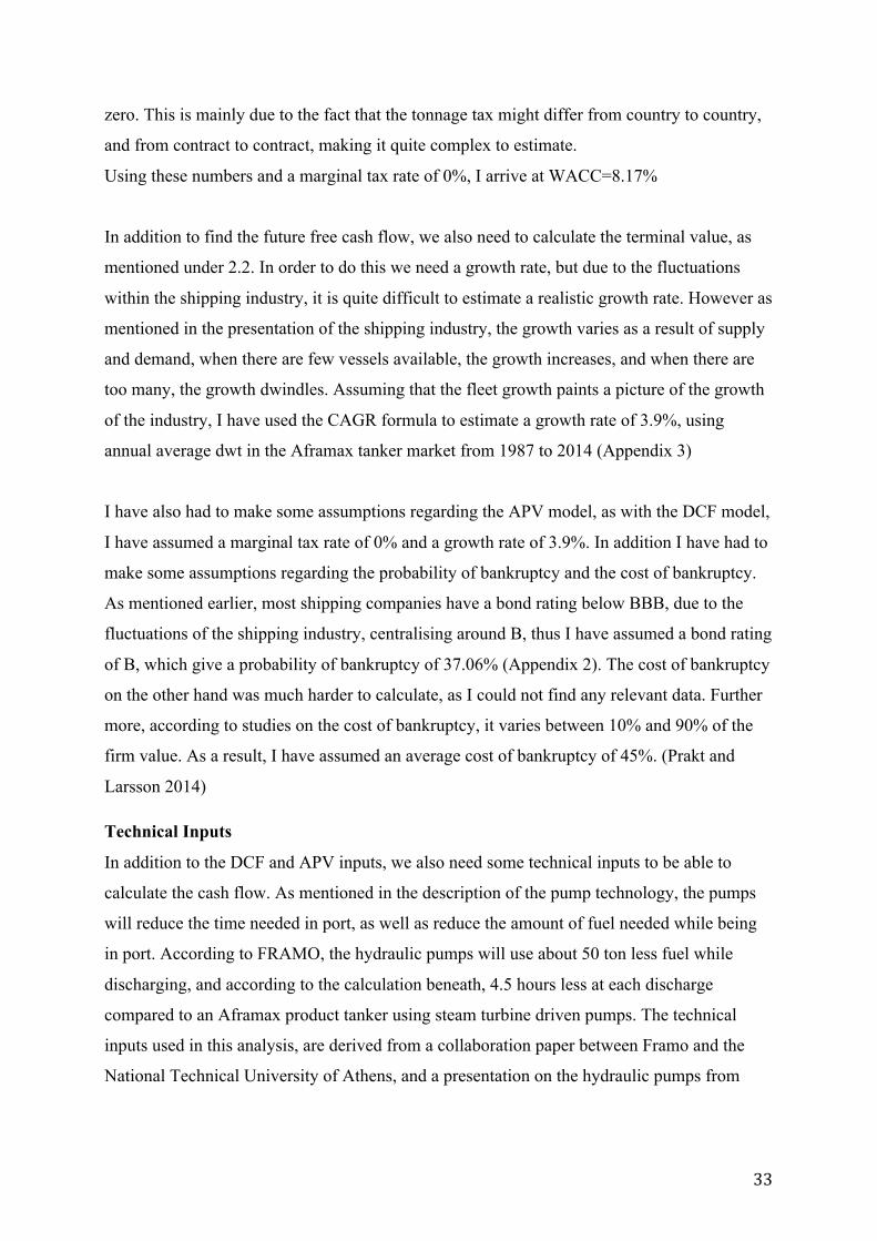
 Figure 4: Profitability of the investment in Scenario 1 with a medium investment cost using the DCF method

 Figure 5: Difference between the APV method and the DCF method with a medium investment cost

As we can see from the first graph, the most important variable is the bunker price. This is

mostly a result of the lower fuel consumption when discharging the cargo compared to the

steam turbine pumps. The speed or the number of discharges is also an important variable, as

we can see from the first graph, the NPV increases with the number of discharges.

Comparing the two graphs, we see some difference between the two, however not enough to

suggest that, in the case of shipping companies, the bond rating playes an important role.

-10,000,000.00

-5,000,000.00

-

5,000,000.00

10,000,000.00

15,000,000.00

20,000,000.00

16   22   24  Net

Pre

sent

Val

ue

Number of Discharges

DCF Medium Investment Cost

MDO: USD 119.03

MDO: USD 612.92

MDO: USD 1106.82

- 1,000,000.00 2,000,000.00 3,000,000.00 4,000,000.00 5,000,000.00 6,000,000.00

16 22 24

Net

Pre

sent

Val

ue

Number of discharges

APV vs DCF Medium Investment Cost

MDO: USD 119.03

MDO: USD 612.92

MDO: USD 1106.82

  37  

4.2 Scenario 1 without the use of triangulation

The route in this scenario is similar to the route in the scenario above, with the exception that

the LR2 product tanker only travels from the U.S. to Europe with diesel and then travels in

ballast back to the U.S. By doing this we will be able to find out whether or not triangulation

improves the profitability of the cargo pumping system and as such whether it has the

potential to improve profitability whether one chooses to invest or not.

The calculations used are the same as in the scenario above, with the exception of a reduction

in the number of loadings and discharges, as well as a reduction in travel distance due to the

fact that the vessel only travels back and forth between Corpus Christi, TX and Rotterdam,

NL. Following the same structure and reasoning as in the scenario above, I will start with the

DCF analysis, and compare the DCF and the APV method while looking at the medium

investment cost.

 Figure 6: Profitability of the investment in Scenario 1 without triangulation with a medium investment cost using the DCF method

-8,000,000.00 -6,000,000.00 -4,000,000.00 -2,000,000.00

- 2,000,000.00 4,000,000.00 6,000,000.00 8,000,000.00

9 12 13

Net

Pre

sent

Val

ue

Number of Discharges

DCF medium investment cost

MDO: USD 119.03

MDO: USD 612.92

MDO: USD 1106.82

  38  

 Figure 7: Difference between the APV method and the DCF method with a Medium investment cost

Looking at the graph above, we see, as we saw in the first scenario, that the APV method

provides us with a higher profit than the DCF method, which in this case would have made

the investment profitable during a trough.

Looking at the DCF graph we see that the bunker price have a huge impact on the profitability

of the cargo pumping system, and if the bunker price stays low during a trough, it will not be

profitable no matter whether the investment cost is high or low. Further more, if we look at

the graph above, we see that during a trough two out of three bunker prices will result in

losses.

Comparing the two DCF medium investment graphs in 4.1 and 4.2, we see that the

triangulation plays an important role in the profitability of the cargo pumping system for this

route. Both have a deficit when the MDO price is around USD 120/MT, however at the two

higher prices the graph with triangulation has a substantially higher NPV, compared to the

one without triangulation. Suggesting that triangulation is smart way to increase the profit of a

route.

             

-

1,000,000.00

2,000,000.00

3,000,000.00

4,000,000.00

9 12 13

Net

Pre

sent

Val

ue

Number of discharges

APV vs DCF Medium investment cost

MDO: USD 119.03

MDO: USD 612.92

MDO: USD 1106.82

  39  

4.3 Scenario 2

The triangulation route in this scenario is both longer, and more complex than the one in

scenario 1. In this scenario, it goes from Texas to Chile with diesel, then in ballast to

Argentina, then from Argentina to China with soybean oil, again in ballast from China to

Malaysia, with palm oil from Malaysia and back to the U.S. In the table beneath you can see

the ports used and the distance between them.

The calculations of this scenario are more or less the same as in scenario 1, with the exception

of the time used while in port. In this scenario, I have also added the time to clean the tanks,

making them ready to transport clean products. According to Michael Sangolt, Bunker

Manager at SKS Tankers, the LR2 product tankers with the hydraulic pumps, use between 3

and 5 days to clean the tanks, as such I have used 4 days. As for the LR2 with steam driven

pumps, there is a problem with dirty product residue in the pipes, which can ruin the clean

products. Thus it normally takes one or more trips carrying gas condensate, in order to switch

from dirty to clean products, according to Alf M. Utvær, Area Manager at Frank Mohn AS. I

could not find any export of gas condensate from Chile to Argentina, instead I assume that it

will take 30 days to make the vessel ready to transport clean products.

With the exception of the time used to switch from dirty to clean products, I follow the same

reasoning as in scenario 1, thus I will also follow the same structure as well.

Table 4: Scenario 2 ports and the distance between them (Sea-Distances.org 2014)

  40  

 Figure 8: Profitability of the investment in Scenario 2 with a medium investment cost using the DCF method

 Figure 9: Difference between the APV method and the DCF method with a medium investment cost

As we can see from the graph above, there is not much difference between the two methods,

with the exception that the APV method has a bit higher net present value. From the first

graph we can see that the bunker price has quite a big impact on the net present value,

however this can be explained by the big difference between the MDO prices, especially if we

compare them to the difference between the numbers of discharge. This might suggest that

there might be another factor influencing the analysis. This becomes even more apparent if

we look at the graph beneath where we assume that they use the same switching time.

- 1,000,000.00 2,000,000.00 3,000,000.00 4,000,000.00 5,000,000.00 6,000,000.00 7,000,000.00 8,000,000.00

5 6 7

Net

Pre

sent

Val

ue

Number of Discharges

DCF medium investment cost

MDO: USD 119.03

MDO: USD 612.92

MDO: USD 1106.82

 -­‐        

 1,000,000.00    

 2,000,000.00    

 3,000,000.00    

 4,000,000.00    

5   6   7  

Net  Present  Value  

Number  of  discharges  

APV  vs  DCF  Medium  Investment  Cost  

MDO:  USD  119.03  

MDO:  USD  612.92  

MDO:  USD  1106.82  

  41  

 Figure 10: Profitability of the investment in Scenario 2 with a medium investment cost, no switching time difference, using the DCF method

As we can see from the graph, only with the lowest investment cost, and the highest MDO

price, would it be profitable to switch from steam driven pumps to the new pumping system if

the time to switch from dirty to clean cargo were the same for the two pump systems. This

suggests that reduction in travelling time is quite important when sailing longer distances.

4.4 Comparing the result of the scenarios

If we compare the result of the scenarios it becomes quite apparent that it is a good

investment to change from steam driven pumps to hydraulic pumps. However there is a but, if

one chooses not to take advantage of the triangulation opportunity, the profitability of the

investment becomes more dependent on the market situation, as we saw looking at scenario 1

without the use of triangulation. Further more, the fact that it is easier to switch between clean

and dirty products, gives the company a competitive advantage compared to companies with

vessels utilizing steam driven pumps, as one can transport a larger spectre of tradable goods.

And as such increase the laden-to-ballast ratio, which again will result in increased profits.

However if one choose to contract the vessel on long voyages suitable for the LR2 product

tanker, like the one in scenario 2, with few discharges and only transporting either dirty or

clean products, it is not profitable to take on the investment. Further more, due to the fact that

the distances in scenario 1 is more suitable for a smaller vessel, such as the MR2 or the LR1,

it might be more profitable to equip those with the hydraulic pumps instead, at least if one

have long-term contracts, and do not operate in the spot market. As a last comment to the

graphs, it might seem strange that one should need to slow steam during a period with high

investment cost. However as a result of the two to four years time lag between the cycles of

-­‐8,000,000.00    

-­‐6,000,000.00    

-­‐4,000,000.00    

-­‐2,000,000.00    

 -­‐        

 2,000,000.00    

5   6   7  

Net  Present  Value  

Number  of  Discharges  

DCF  medium  investment  cost    

MDO:  USD  119.03  

MDO:  USD  612.92  

MDO:  USD  1106.82  

  42  

the shipping market and the shipbuilding market, which is the time it normally takes from the

order of a new vessel is placed and until the vessel is delivered, such a situation might occur.

5. Conclusion

In the strategic analysis of the two different triangulation routes, we saw that there are some

factors that might influence the profitability of the routes. In scenario 1, it is mainly the

economic and technological factors, as the United States are becoming less dependent on oil

and as such can produce more of the gasoline they need by them selves and in addition there

has also been a switch to more fuel efficient cars, reducing this need even further. This

development might result in a scenario similar to the one without the use of triangulation,

where one transports diesel to Europe and travels empty back to the U.S. And as we saw, in

the investment analysis, one will be more dependent on the fluctuation of the market,

reducing the profitability of the investment. However, it will still take some time until we will

see any effect of this development in the product tanker trade, and if we take into account

both the increased profit one will gain from the use of triangulation and switching to the

hydraulic pumping system, it is quite apparent, that this is a sound investment. Especially due

to the larger spectre of products one can transport with the new pumps.

In scenario 2, it is mainly the political and the economical factors from the pestle analysis that

might impede on the trade, and especially the economical situation in Argentina and China.

Argentina has been and is still in deep economical problems, which might lead to increased

taxes, which will make importers look for other suppliers to buy their supplies. China on the

other hand seems to be in a good economical situation, at least if we believe the governmental

officials. However, many analysts are just waiting for an economic crisis that might create

ripples affecting the whole region, if not the whole world, which will most definitely have an

impact on the proposed trading route, being a large importer of soybean oil. In the case that

this would result in only transporting dirty products over similar long distances, it would not

be profitable to invest in the new pumps, as the last graph in scenario 2 suggests. However

such a crisis would not last the entire lifetime of the pumps, take for instance the financial

crisis, we are already seeing improved rates with forecasts of higher rates in the coming years.

And with this in mind, it would be profitable to invest in the hydraulic pumps, as one have the

possibility to switch between different cargoes, dirty and clean, and also have the opportunity

to choose shorter hauls, and as such reduce the cost of discharging, increasing the profit.

  43  

Glossary

Aframax: A tanker size ranging between 80,000 and 120,000 dwt

Ballast voyage: A voyage with no cargo on board to get a ship in position for the next

loading port or docking. On voyage the ship is said to be in ballast.

Bulk Cargo: Unpackaged cargoes such as coal, ore and grain

Bunkers: The ship’s fuel

Capesize: Bulk ship size ranged as 100,000 dwt or larger

Combination

Carrier:

Ship capable of carrying oil or dry bulk cargoes, thereby increasing the

productivity of the vessel. Typically termed OBO or Ore/Oiler.

Dwt:

ECA:

Deadweight ton. A measure expressed in metric tons (1000 kg) or long

tons (1,016 kg) of a ship’s carrying capacity, including bunker oil,

fresh water, crew and provisions. This is the most important

commercial measure of capacity.

Emission Control Areas

FFA: A Forward Freight Agreement is a cash contract for differences

requiring no physical delivery based on freight rates on standardised

trade routes.

Freight rate: The Agreed charge for the carriage of cargo expressed per ton(ne) of

cargo (also Worldscale in the tanker market) or as a lump sum.

Handysize/

Handymax:

Bulk ships size ranges of ships defined as 10-40,000 dwt and 40-

60,000 dwt.

IMO:

IPR:

International Maritime Organisation: A United Nations agency

devoted to shipping

Intellectual Property Rights.

ISM code:

LR1

International Safety Management code for the safe operation of ships

and for pollution prevention as adopted by the IMO.

Long Range 2 product tanker, size ranging from 45-80,000 dwt.

LR2:

MARPOL:

MEPC:

MR:

Long Range 2 product tanker, size ranging from 80-160,000 dwt.

The International Convention for the Prevention of Pollution from

Ships.

Marine Environment Protection Committee.

Medium Range product tanker, size ranging from 25-40,000 dwt.

Oil Tanker: Tanker Carrying crude oil or Refined oil products.

  44  

Panamax: Bulk ship size ranging from 60-100,000 dwt. Strictly speaking the

largest ship capable of navigating in the Panama Canal.

Product Tanker:

GP:

Tanker that carries refined oil products.

General Purpose product tanker, size ranging from 10-25,000 dwt

Spot market: Short-term contracts for voyage, trip or short term time charters,

normally no longer than three months in duration.

Suezmax: A tanker size ranging from 120-200,000 dwt.

Time charter (t/c): An arrangement whereby a shipowner places a crewed ship at a

charterer’s disposal for a certain period. Freight is customarily paid

periodically in advance. The charterer also pays for bunker, port and

canal charges.

Time Charter

Equivalent (TCE):

Gross freight income less voyage costs (bunker, port and canal

charges), usually expressed in US$ per day.

ULCC: Ultra Large Crude Carrier. Tanker of more than 320,000 dwt.

VLCC: Very Large Crude Carrier. Tanker between 200,000 and 320,000 dwt.

USNH:

USTR:

United States North of (Cape) Hatteras (northern range).

Office of the United States Trade Representative

Voyage Charter: The transportation of cargo from port(s) of loading to port(s) of

discharge. Payment is normally per tonne of cargo, and the shipowner

pays for bunker, port, and canal charges

Voyage costs: Costs directly related to a specific voyage (e.g. Bunker, port and canal

charges).

Worldscale (WS): An international index of freight for tankers. Worldscale is a schedule

of freight rates for a standard ship in US dollars per tonne of oil for an

array of oil routes. The rates listed in the table are designated as

Worldscale flat of WS100 and are revised annually.

  45  

Bibliography Altman,  Edward  I.  “About  Corporate  Default  Rates.”  NYU  STERN.  2007.  http://people.stern.nyu.edu/ealtman/AboutCorporateDefaultRates.pdf  (accessed  November  12,  2014).    Anderson,  Richard,  and  Damian  Kahya.  “The  cost  of  petrol  and  oil:  How  it  breaks  down.”  BBC  News.  8  November  2011.  http://www.bbc.com/news/business-­‐15462923  (accessed  September  25,  2014).    Andrade,  G,  and  S.  N.  Kaplan.  “How  Costly  is  Financial  (Not  Economic)  Distress?  Evidence  from  Highly  Leveraged  Transactions  That  Became  Distressed.”  Journal  of  Finance,  October  1998:  1443-­‐1493.    BIMCO.  Market  Analysis  2013:  Tanker  Shipping  -­‐  Improving  Asset  Prices  for  Product  Tankers.  19  August  2013.    https://www.bimco.org/Reports/Market_Analysis/2013/0819_TankerSMOO2013-­‐4.aspx  (accessed  September  18,  2014).    Bird,  Mike.  “China  Just  Overtook  The  US  As  The  World's  Largest  Economy.”  Business  Insider.  8  October  2014.  http://www.businessinsider.com/china-­‐overtakes-­‐us-­‐as-­‐worlds-­‐largest-­‐economy-­‐2014-­‐10  (accessed  November  1,  2014).    Clarksons  Research  Services.  World  Seaborne  Trade  Tables  November  2014.  Report,  EC3R  6HE:  Clarcksons  Research  Services,  2014.  Clarksons  SIN.  “Clarksons  Shipping  Intelligence  Network  2010.”  Published  Tables.  2014.  http://www.clarksons.net/sin2010/search/Default.aspx?q=historical+fleet+growth+tankers  (accessed  November  10,  2014).    Constantinides,  Dimitries.  Pestle  Analysis:  Business  Environmental  Analysis.  15  December  2011.  http://pestleanalysis.com/pestle-­‐analysis-­‐business-­‐environmental-­‐analysis/  (accessed  September  15,  2014).    Damodaran,  Aswath.  “Adjusted  Present  Value  Approach.”  NYU  STERN.  2  February  2005.  http://pages.stern.nyu.edu/~adamodar/New_Home_Page/valquestions/apv.htm  (accessed  November  12,  2014).    Danish  Ship  Finance  A/S.  Product  Tankers:  Segments.  2012.  http://www.shipfinance.dk/en/SHIPPING-­‐RESEARCH/Tankskibe/Produkttankskibe/Segmenter  (accessed  September  12,  2014).    EIA.  China.  4  February  2014.  http://www.eia.gov/countries/analysisbriefs/China/china.pdf  (accessed  December  4,  2014).  —.  India.  26  June  2014.  http://www.eia.gov/countries/analysisbriefs/India/india.pdf  (accessed  December  4,  2014).  Evenett,  Simon  J.  “Excecutive  Summary.”  Débâcle:  The  11th  GTA  report  on  protectionism,  June  2012:  6.    

  46  

EW  World  Economy  Team.  “China  Economy.”  Economy  Watch.  4  June  2013.  http://www.economywatch.com/world_economy/china  (accessed  November  3,  2014).    Farrell,  Sean.  “Brent  crude  oil  price  drops  below  $86  in  face  of  rising  global  supply.”  The  Guardian.  27  October  2014.  http://www.theguardian.com/business/2014/oct/27/brent-­‐crude-­‐oil-­‐price-­‐drops-­‐goldman-­‐sachs-­‐forecast  (accessed  October  31,  2014).    FRAMO.  “FRAMO  LR2  Presentation.”  Presentation,  2014.    Frank  Mohn  AS.  “Cargo  Pumping  System.”  Bergen,  Hordaland,  2014.    Gallo,  Claudio.  “Europe  sticking  its  head  in  the  sand  over  environmental  issues.”  RT  Op-­‐Edge.  9  June  2014.  http://rt.com/op-­‐edge/164800-­‐ecology-­‐europe-­‐russian-­‐oil/  (accessed  September  25,  2014).    Hamilton,  T.  Mason.  Today  in  Energy.  16  September  2014.  http://www.eia.gov/todayinenergy/detail.cfm?id=17991  (accessed  October  12,  2014).    Hartwig,  Kathinka.  “Amerikansk  stat  forbyr  salg  av  Tesla.”  Dagens  Næringsliv.  23  October  2014.  http://www.dn.no/nyheter/2014/10/23/1150/Tesla/amerikansk-­‐stat-­‐forbyr-­‐salg-­‐av-­‐tesla  (accessed  October  23,  2014).    Hornbeck,  J.  F.  Argentina's  Post-­‐Crisis  Economic  Reform:  Challenges  for  U.S.  Policy.  Report,  Washington,  D.C.:  Congressional  Research  Service,  2013.  IMO.  “Structure  of  IMO.”  IMO.  2014.  http://www.imo.org/About/Pages/Structure.aspx#4  (accessed  October  25,  2014).    —.  Sulphur  oxides  (SOx)  –  Regulation  14.  2014.  http://www.imo.org/OurWork/Environment/PollutionPrevention/AirPollution/Pages/Sulphur-­‐oxides-­‐(SOx)-­‐–-­‐Regulation-­‐14.aspx  (accessed  October  15,  2014).    International  Maritime  Organisation.  Construction  Requriements  for  Oil  Tankers.  1  Januar  2014.  http://www.imo.org/OurWork/Environment/PollutionPrevention/OilPollution/Pages/constructionrequirements.aspx  (accessed  September  12,  2014).    Kilian,  Lutz.  Recent  Oil  Price  Fluctuations  Linked  to  World  Economy.  Faculty  Research,  Economics,  University  of  Michigan,  University  of  Michigan,  2011.    Koller,  Tim,  Marc  Goedhart,  and  David  Wessels.  Valuation  Measuring  and  Managing  the  Value  of  Companies.  Vol.  5.  5  vols.  New  Jersey:  John  Wiley  &  Sons,  Inc.,  2010.    —.  Valuation  Measuring  and  Managing  the  Value  of  Companies.  Hoboken,  New  Jersey:  John  Wiley  &  Sons,  Inc.,  2010.  Lun,  Venus  Y.H.,  Olli-­‐Pekka  Hilmola,  Alexandros  Goulielmos,  Kee-­‐hung  Lai,  and  T.C.  Edwin  Cheng.  Vol.  VIII,  in  Oil  Transport  Management,  13-­‐25.  Springer,  2013.    

  47  

Maritime  Law  Center.  “The  Jones  Act.”  Maritime  Law  Center.  http://www.maritimelawcenter.com/html/the_jones_act.html  (accessed  October  23,  2014).    Meyer,  Peter  J.  Chile:  Political  and  Economic  Conditions  and  U.S.  Relations.  Report,  Washington,  D.C.:  Congressional  Research  Service,  2014.    Modigliani,  Franco,  and  Gerald  A.  Pogue.  “An  Introduction  to  Risk  and  Return:  Concepts  and  Evidence.”  Financial  Analysts  Journal,  1  June  1974:  69-­‐86.    Morrison,  Wayne  M.  China-­‐U.S.  Trade  Issues.  Report,  Washington,  D.C.:  Congressional  Research  Service,  2014.    Overseas  Shipholding  Group,  Inc.  Newsletter  Article:  The  Advantages  of  Commercial  Shipping  Pools.  20  February  2009.  http://www2.osg.com/index.cfm?pageid=74&itemid=13  (accessed  September  16,  2014).    Pareto  Shipping  AS.  Shipping  Market  Outlook  2013-­‐'16.  Oslo:  Pareto  Research,  2013.    Plessas,  T.,  D.  Chroni,  and  A.  Papanikolaou.  “The  Potential  Use  of  FRAMO  Cargo  Handling  Arrangement  as  a  Retrofit  Solution  for  an  Aframax  Tanker.”  Thesis,  National  Technical  University  of  Athens,  2014.    Prakt,  Marcus  Johansson,  and  Oscar  Larsson.  “Indirect  Bankruptcy  Costs.”  Master  Thesis,  Centre  for  Finance,  University  of  Gothenburg,  Gothenburg,  2014.    Pritchett,  Lant,  and  Lawrence  Summers.  “Asiaphoria  Meets  Regression  to  the  Mean.”  Asia  Economic  Policy  Conference,  5  November  2013:  33-­‐71.    Reuters.  Reuters.  1  November  2014.  http://www.reuters.com/finance/stocks/  (accessed  November  1,  2014).    Rinehart,  Ian  E.  Malaysia:  Background  and  U.S.  Relations.  Report,  Washington,  D.C.:  Congressional  Research  Service,  2014.    Sea-­‐Distances.org.  “Sea-­‐Distances.org.”  Sea-­‐Distances.org.  2014.  http://www.sea-­‐distances.org  (accessed  September  20,  2014).    Taurus  Tankers  Ltd.  About  the  LR2.  2011.  http://www.taurustankers.com/company/long_range_2/  (accessed  September  12,  2014).    Todd,  Jennifer,  Jess  Chen,  and  Frankie  Clogston.  Creating  the  Clean  Energy  Economy:  Analysis  of  the  Electric  Vehicle  Industry.  Analysis,  International  Economic  Development  Council,  2013.  USTR.  “Argentina.”  Office  of  the  United  States  Trade  Representative.  2013.  https://www.ustr.gov/sites/default/files/2013%20NTE%20Argentina%20Final.pdf  (accessed  October  29,  2014).  

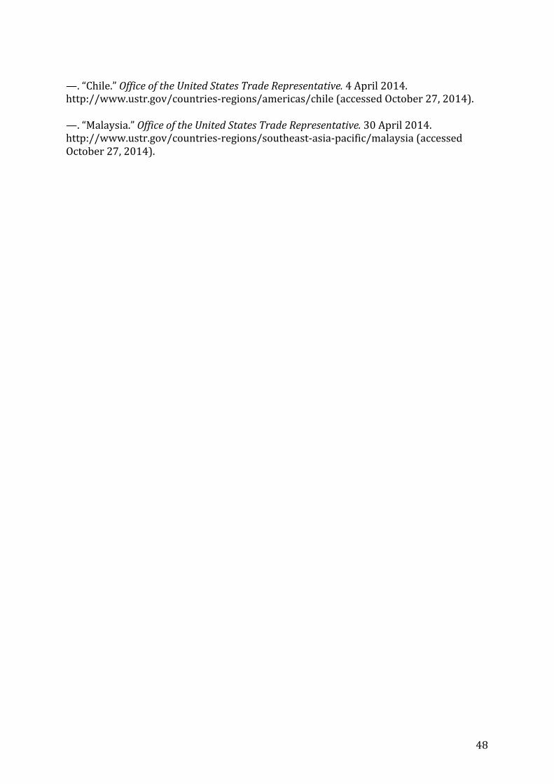
  48  

 —.  “Chile.”  Office  of  the  United  States  Trade  Representative.  4  April  2014.  http://www.ustr.gov/countries-­‐regions/americas/chile  (accessed  October  27,  2014).    —.  “Malaysia.”  Office  of  the  United  States  Trade  Representative.  30  April  2014.  http://www.ustr.gov/countries-­‐regions/southeast-­‐asia-­‐pacific/malaysia  (accessed  October  27,  2014).  

 

 

 

 

 

 

 

 

 

 

 

 

 

 

 

 

 

 

 

 

 

  49  

Appendix

 Appendix 1

(Reuters 2014)

Appendix 2

(Altman 2007)

  50  

Appendix 3

(Clarksons SIN 2014)

Appendix 4

Average speed 10.5 knots:

  51  

Average speed 14.5 knots:

Average speed 16.5 knots:

Appendix 5

Average speed 10.5 knots:

  52  

Average speed 14.5 knots

Average speed 16.5 knots:

Appendix 6

MDO prices from 1991 to 2013

Shipping Intelligence Network Timeseries    

        41586 41583 41592 41587 41584

   

Date

MDO bunker prices,

Houston

MDO bunker prices,

Rotterdam

MDO bunker prices, Japan

MDO bunker prices,

Singapore

MDO bunker prices, Los

Angeles

Average

    $/Tonne $/Tonne $/Tonne $/Tonne $/Tonne $/Tonne    1991-Q1 204.69 206.50 324.15 265.92 235.54 247.36

1991-Q2 147.62 151.85 253.46 170.00 206.42 185.87 1991-Q3 159.04 147.69 228.50 167.65 198.15 180.21 1991-Q4 171.38 170.96 230.31 179.81 198.62 190.22

   1992-Q1 149.81 156.54 230.54 159.12 183.92 175.99    1992-Q2 161.92 166.69 228.19 166.81 192.77 183.28    1992-Q3 173.42 165.31 226.77 164.77 202.96 186.65    1992-Q4 172.46 156.65 230.69 165.62 190.42 183.17    1993-Q1 163.04 152.85 231.58 165.85 186.58 179.98    1993-Q2 161.15 162.04 238.81 166.12 199.65 185.55    1993-Q3 159.19 144.62 233.69 148.54 202.96 177.80    1993-Q4 157.93 143.46 231.89 146.79 206.61 177.34    1994-Q1 151.62 131.50 228.75 138.29 204.17 170.87    

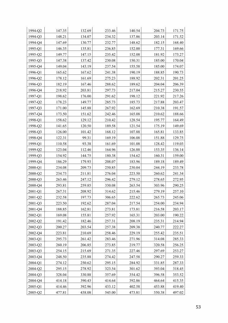
  53  

1994-Q2 147.35 132.69 233.46 140.54 204.73 171.75    1994-Q3 148.21 134.07 234.32 137.86 203.14 171.52    1994-Q4 147.69 130.77 232.77 148.62 182.15 168.40    1995-Q1 146.35 135.81 236.85 152.00 177.31 169.66    1995-Q2 149.77 147.15 235.42 152.08 181.92 173.27    1995-Q3 147.38 137.42 230.08 150.31 185.00 170.04    1995-Q4 149.04 143.19 237.54 155.58 185.00 174.07    1996-Q1 165.62 167.62 241.38 190.19 188.85 190.73    1996-Q2 178.12 161.69 275.23 188.92 202.31 201.25    1996-Q3 182.19 167.46 288.62 189.62 204.04 206.39    1996-Q4 218.92 203.81 297.73 217.04 215.27 230.55    1997-Q1 198.62 176.00 291.62 198.12 221.92 217.26    1997-Q2 178.23 149.77 285.73 185.73 217.88 203.47    1997-Q3 171.00 145.88 267.92 162.69 210.38 191.57    1997-Q4 173.50 151.62 242.46 165.08 210.62 188.66    1998-Q1 158.62 129.12 210.42 128.54 195.77 164.49    1998-Q2 141.65 120.50 189.58 121.54 175.19 149.69    1998-Q3 126.00 101.42 168.12 107.88 165.81 133.85    1998-Q4 122.31 99.31 169.19 106.08 151.88 129.75    1999-Q1 110.58 93.38 161.69 101.08 128.42 119.03    1999-Q2 123.04 112.46 164.96 126.88 153.35 136.14    1999-Q3 154.92 144.75 180.38 154.62 160.31 159.00    1999-Q4 186.29 179.93 208.07 183.96 189.18 189.49    2000-Q1 234.08 209.73 250.85 230.04 244.19 233.78    2000-Q2 234.73 211.81 276.04 223.50 260.62 241.34    2000-Q3 263.46 247.12 296.42 279.12 278.65 272.95    2000-Q4 293.81 259.85 330.08 263.54 303.96 290.25    2001-Q1 267.31 208.92 314.62 215.46 279.19 257.10    2001-Q2 232.58 197.73 306.65 222.62 265.73 245.06    2001-Q3 223.50 192.62 287.04 217.54 254.00 234.94    2001-Q4 188.85 162.81 273.81 173.81 216.58 203.17    2002-Q1 169.08 155.81 257.92 165.31 203.00 190.22    2002-Q2 191.42 182.46 257.31 208.19 235.31 214.94    2002-Q3 200.27 203.54 257.38 209.38 240.77 222.27    2002-Q4 223.81 210.69 258.46 229.19 255.42 235.51    2003-Q1 295.73 261.42 283.46 271.96 314.08 285.33    2003-Q2 260.19 206.85 273.85 219.77 320.58 256.25    2003-Q3 254.15 215.69 271.35 227.46 297.69 253.27    2003-Q4 248.50 235.88 274.42 247.58 290.27 259.33    2004-Q1 274.12 250.62 295.15 284.92 331.85 287.33    2004-Q2 295.15 278.92 323.54 301.62 393.04 318.45    2004-Q3 328.04 330.88 357.69 354.42 396.58 353.52    2004-Q4 414.18 390.43 414.64 392.86 464.64 415.35    2005-Q1 414.46 392.96 433.12 402.58 453.88 419.40    2005-Q2 477.81 438.08 545.00 473.81 550.38 497.02    

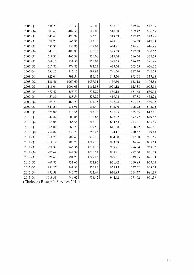
  54  

2005-Q3 538.21 519.39 520.00 538.21 619.46 547.05    2005-Q4 602.69 482.50 518.08 510.58 669.42 556.65    2006-Q1 547.69 493.92 542.58 519.69 612.42 543.26    2006-Q2 576.27 566.35 612.15 629.81 704.38 617.79    2006-Q3 582.31 553.85 629.04 644.81 674.81 616.96    2006-Q4 541.12 480.81 585.23 528.58 617.38 550.62    2007-Q1 518.31 465.38 570.00 517.54 616.54 537.55    2007-Q2 568.17 531.50 566.04 597.65 696.42 591.96    2007-Q3 617.81 579.85 594.23 635.54 703.65 626.22    2007-Q4 735.23 712.12 694.92 741.50 827.96 742.35    2008-Q1 822.04 791.54 836.15 845.50 893.08 837.66    2008-Q2 1138.46 1060.69 1037.31 1159.50 1138.12 1106.82    2008-Q3 1110.04 1006.08 1162.88 1071.12 1125.38 1095.10    2008-Q4 672.42 555.77 703.27 559.12 661.62 630.44    2009-Q1 457.35 388.54 528.27 419.04 467.88 452.22    2009-Q2 469.73 462.23 521.15 492.08 503.42 489.72    2009-Q3 547.27 531.96 563.46 562.00 608.92 562.72    2009-Q4 624.00 576.58 615.38 596.23 675.85 617.61    2010-Q1 644.42 603.88 678.65 628.62 692.77 649.67    2010-Q2 669.04 665.54 715.38 664.54 713.81 685.66    2010-Q3 665.00 660.77 707.50 641.88 708.92 676.81    2010-Q4 754.82 739.71 758.25 724.11 770.57 749.49    2011-Q1 910.79 887.67 908.75 884.00 917.08 901.66    2011-Q2 1018.19 983.77 1018.15 973.38 1034.96 1005.69    2011-Q3 976.39 946.36 1001.36 938.21 986.54 969.77    2011-Q4 975.69 944.38 1006.54 939.81 992.50 971.78    2012-Q1 1029.62 991.23 1048.96 997.31 1039.85 1021.39    2012-Q2 960.85 931.62 962.96 921.92 1060.85 967.64    2012-Q3 995.27 941.31 936.88 939.15 1027.62 968.05    2012-Q4 995.58 946.77 962.69 936.85 1064.77 981.33    2013-Q1 1019.38 946.62 974.42 944.62 1071.92 991.39    (Clarksons Research Services 2014)