arX

iv:a

stro

-ph/

0401

025v

1 5

Jan

200

4

Environmental Effects in the Structural Parameters of Galaxies in

the Coma Cluster

J. A. L. Aguerri

Instituto de Astrofısica de Canarias, C/ Vıa Lactea s/n, 38205 La Laguna, Spain

jalfonso@ll.iac.es

J. Iglesias-Paramo

Laboratoire d’Astrophysique de Marseille, BP8, Traverse du Siphon, 13376 Marseille,

France

jorge.iglesias@oamp.fr

J. M. Vılchez

Instituto de Astrofısica de Andalucıa, Consejo Superior de Investigaciones Cientıficas,

Camino Bajo de Huetor 24, Apdo. 3004, 18080 Granada, Spain

jvm@iaa.es

and

C. Munoz-Tunon

Instituto de Astrofısica de Canarias, Vıa Lactea s/n, 38205 La Laguna. Spain.

cmt@ll.iac.es

ABSTRACT

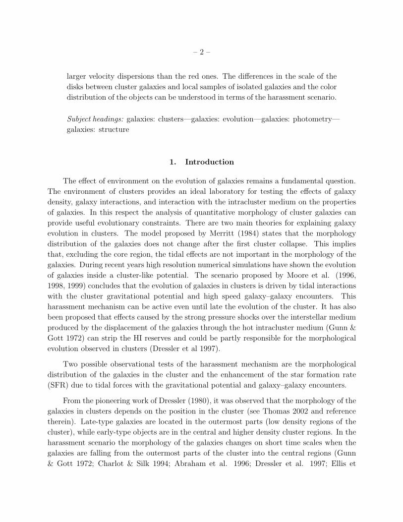
We have studied 116 bright galaxies from the Coma cluster brighter than

mr = 17 mag. From a quantitative morphological analysis we find that the

scales of the disks are smaller than those of field spiral galaxies. There is a

correlation between the scale of the disks and the position of the galaxy in the

cluster; no large disks are present near the center of the cluster or in high density

environments. The structural parameters of the bulges are not affected by the

environment. We have analyzed the distribution of blue and red objects in the

cluster. For spirals there is a trend between color and position in the cluster.

The bluest spiral galaxies are located at larger projected radii; they also show

– 2 –

larger velocity dispersions than the red ones. The differences in the scale of the

disks between cluster galaxies and local samples of isolated galaxies and the color

distribution of the objects can be understood in terms of the harassment scenario.

Subject headings: galaxies: clusters—galaxies: evolution—galaxies: photometry—

galaxies: structure

1. Introduction

The effect of environment on the evolution of galaxies remains a fundamental question.

The environment of clusters provides an ideal laboratory for testing the effects of galaxy

density, galaxy interactions, and interaction with the intracluster medium on the properties

of galaxies. In this respect the analysis of quantitative morphology of cluster galaxies can

provide useful evolutionary constraints. There are two main theories for explaining galaxy

evolution in clusters. The model proposed by Merritt (1984) states that the morphology

distribution of the galaxies does not change after the first cluster collapse. This implies

that, excluding the core region, the tidal effects are not important in the morphology of the

galaxies. During recent years high resolution numerical simulations have shown the evolution

of galaxies inside a cluster-like potential. The scenario proposed by Moore et al. (1996,

1998, 1999) concludes that the evolution of galaxies in clusters is driven by tidal interactions

with the cluster gravitational potential and high speed galaxy–galaxy encounters. This

harassment mechanism can be active even until late the evolution of the cluster. It has also

been proposed that effects caused by the strong pressure shocks over the interstellar medium

produced by the displacement of the galaxies through the hot intracluster medium (Gunn &

Gott 1972) can strip the HI reserves and could be partly responsible for the morphological

evolution observed in clusters (Dressler et al 1997).

Two possible observational tests of the harassment mechanism are the morphological

distribution of the galaxies in the cluster and the enhancement of the star formation rate

(SFR) due to tidal forces with the gravitational potential and galaxy–galaxy encounters.

From the pioneering work of Dressler (1980), it was observed that the morphology of the

galaxies in clusters depends on the position in the cluster (see Thomas 2002 and reference

therein). Late-type galaxies are located in the outermost parts (low density regions of the

cluster), while early-type objects are in the central and higher density cluster regions. In the

harassment scenario the morphology of the galaxies changes on short time scales when the

galaxies are falling from the outermost parts of the cluster into the central regions (Gunn

& Gott 1972; Charlot & Silk 1994; Abraham et al. 1996; Dressler et al. 1997; Ellis et

– 3 –

al. 1997; Oemler et al. 1997). This mechanism is very efficient at transforming late-type

galaxies into dwarf spheroidals and early-types into S0s, and at reducing the size of the

disks. The role of the cluster environment in galaxy evolution has been analyzed in the past

by studying different aspects of galaxies: asymmetries in the rotation curves of galaxies in

clusters (Rubin et al. 1988; Whitmore et al. 1988; Dale et al. 2001; Dale & Uson 2003), the

HI deficiency of cluster spirals (Cayatte et al. 1990; Haynes et al. 1984; Solanes et al. 2001),

and observations of head–tail radio sources and ram pressure stripped spirals (Kenney &

Koopman 1999).

Galaxy clusters at medium redshift (z = 0.2–0.5) show an excess of blue objects com-

pared with clusters at the present epoch (Kodama & Bower 2001). This is the so-called

Butcher–Oemler effect (Butcher & Oemler 1978). Several mechanism have been proposed

in order to explain this effect. Fujita (1998) demonstrates that the star-forming activity

can be enhanced because of the tidal force from the potential of the cluster, or high speed

galaxy–galaxy encounters. He also predicted a different distribution of the blue galaxies in

the cluster depending on the responsible mechanism of the star formation. Blue galaxies

have also been observed in nearby clusters (McIntosh et al. 2003), but in smaller numbers

than at medium redshifts. They are located at the outermost regions of the clusters and

are consistent with galaxies undergoing the first harassment when they are falling into the

cluster center.

The aim of this paper is to perform a quantitative analysis of the distribution of the

morphology and colors of a large sample of bright galaxies in the Coma cluster in order to

compare the structural parameters of Coma galaxies and isolated local samples. We will

also study the distribution of dwarfs and bright galaxies in the cluster. This will tell us

about the role of the cluster environment in galaxy evolution. Coma is a rich and nearby

cluster which has been analyzed extensively in the past. It is one of the brightest X-ray

emission clusters (White et al. 1993). Dynamical studies confirmed that this is not a relaxed

cluster (Fitchett & Webster 1987; Baier et al. 1990). Coma ellipticals have been used is

several studies of the fundamental plane (Mobasher et al. 1999; Scodeggio et al. 1998;

Khosroshahi et al. 2000). Morphological studies have also been made (Lucey et al. 1991;

Jorgensen & Franx 1994; Andreon et al. 1996, 1997; Gerbal et al. 1997; Khosroshahi et

al. 2000), although most of them have been based on qualitative or visual classifications.

Recently, Gutierrez et al. (2003) made the quantitative morphology of a sample of galaxies

in the core region of Coma cluster, the central 0.25 �2. Our study is the first to analyze

extensively quantitative morphology of the Coma galaxies for a wide field of view (≈ 1�2).

The advantages of the quantitative morphology are that it is reproducible and biases can be

understood and carefully characterized through simulations that are treated as real data. The

use of quantitative morphology allows the recovery of reliable information on the structural

– 4 –

parameters of the galaxies. The information contained in the structural parameters plays a

necessary role in the understanding of the evolution and origin of galaxies. In this paper we

will compare the structural parameters of the Coma cluster galaxies with those from field.

The observations were taken with the Wide Field Camera (WFC) at the prime focus of

the 2.5 m Isaac Newton Telescope (INT) at the Roque de los Muchachos Observatory (La

Palma), in 2000 April. The plate-scale of the CCD was 0.333 arcsec/pixel, and the seeing

of the images was about 1.5′′. Four exposures of the Coma cluster were obtained under

photometrical conditions, covering an area of ≈ 1 deg2. The images were obtained using the

broad band Sloan–Gunn r′ filter of the WFC. For a detailed description of the observations,

data reduction and calibration see Iglesias-Paramo et al. (2002, 2003).

2. Surface brightness decomposition

We have fitted the isophotal surface brightness profiles of the galaxies with two com-

ponents (bulge and disk). The surface brightness profiles of the bulges were modeled by a

Sersic (1968) law, given by

I(r) = Ie10−bn(( rre

)1/n−1), (1)

where re is the effective radius, which encloses half of the intensity of the profile, Ie is

the effective intensity, and n is the profile shape parameter. The parameter bn is given by

bn = 0.868n − 0.142 (Caon et al. 1993).

The disks were fitted by exponential profiles (Freeman 1970):

I(r) = I0e−r/h, (2)

where I0 is the central intensity and h is the scale length of the profile. A Levenberg–

Marquardt nonlinear fitting algorithm was used to determine the parameter set that min-

imizes χ2. We used the algorithm design by Trujillo et al. (2001). This algorithm takes

into account the seeing effects on the surface brightness profiles and the intrinsic ellipticity

of the galaxies. It was successfully applied in determining the quantitative morphology of

field galaxies (Aguerri & Trujillo 2002) and galaxies in clusters (Trujillo et al. 2001, 2002).

Extensive Monte Carlo simulations were carried out in order to determine the uncertainties

in the determination of the structural parameters.

– 5 –

2.1. Monte Carlo Simulations

The proper determination of the structural parameters of the objects depends mainly

on the signal-to-noise ratio of the images. In order to quantify this effect, we have run Monte

Carlo simulations to determine the limiting magnitude for which the recovered parameters

are well determined. These simulations allow us to detect possible biases in the recovered

parameters. We have generated galaxies with similar sizes and luminosities to those expected

in Coma. We simulated two types of galaxies: those formed only by a bulge component

(Sersic’s law) and others formed by a bulge and disk (Sersic + exponential). We have added

random noise to the models, which was the obtained from a region free from sources from

the images (see Trujillo et al. 2001 for a more detailed about the simulations).

The magnitudes of the simulated objects were in the interval 13 mag ≤ mr ≤ 19 mag.

The scales of the objects simulated by a Sersic profile (bulge galaxies) were 0.5 kpc ≤ re ≤ 10

kpc, and 1 ≤ n ≤ 6. The bulges of the bulge + disk galaxies have scales of 0.3 kpc ≤ re ≤ 5

kpc and 1 ≤ n ≤ 6, and the scales of the disks were h ≤ 6 kpc. The bulge-to-total ratio,

B/T , of the objects varies in the interval 0 < B/T ≤ 1. The parameters of the 300 simulated

objects were chosen randomly distributed on the previous intervals. In this paper we will

use the value H0 = 75 km s−1 Mpc−1.

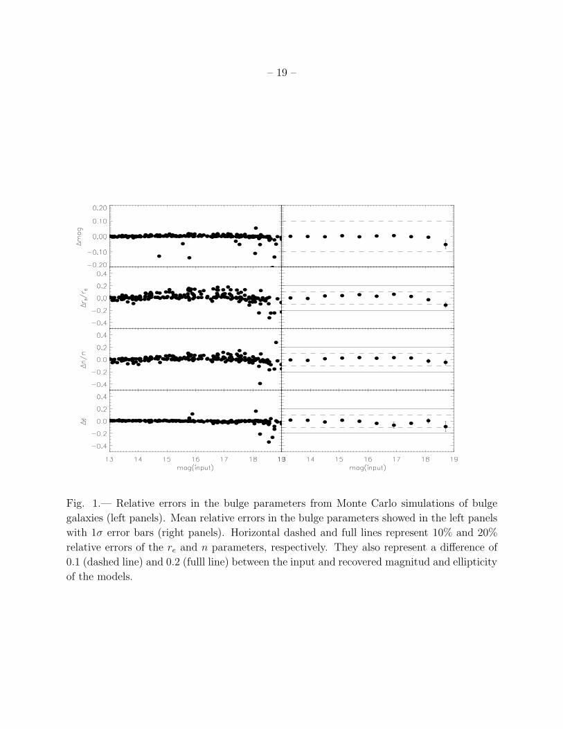
Figure 1 shows the relative errors between the input and output parameters for the

simulations for bulge galaxies. All the parameters are recovered with errors less than 20%

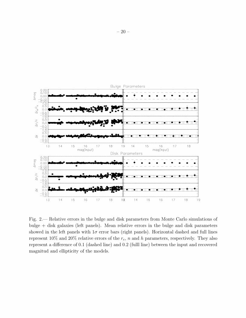
down to mr = 19 mag. Figure 2 shows the relative errors for the parameters of the simulated

bulge + disk galaxies. Although, these simulations show larger errors in the recovered

parameters, all the parameters can be obtained with errors of less than 20% for the objects

with mr ≤ 17 mag.

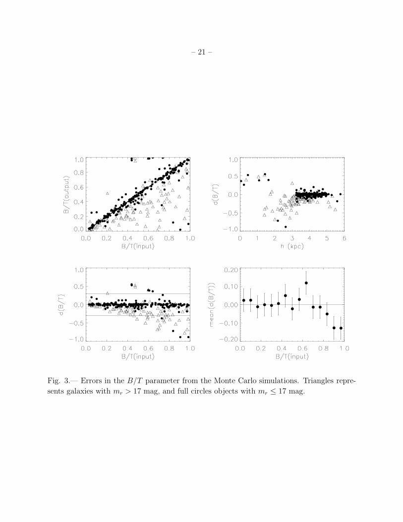
Figure 3 shows the recovered B/T ratio. This parameter is recovered with a mean

difference of less than 0.1 for galaxies with mr ≤ 17 mag and simulated objects with input

B/T ≤ 0.8: objects with B/T > 0.8 were recovered with a mean difference larger than 0.1.

It should be noted that disks with h < 2kpc are not recovered well, even in those objects

with mr ≤ 17 mag. They are very small and unrealistic disks. We adopted mr = 17 mag

as the limiting magnitude for our fits. All galaxies with mr ≤ 17 mag were decomposed in

bulge and disk, those with B/T > 0.8 or those not well fitted by a bulge + disk, were fitted

by a single Sersic profile.

– 6 –

2.2. Galaxy classification

Our images cover an area of 1 square degree of Coma cluster. We have selected in

this area all galaxies with mr ≤ 20 (see Iglesias-Paramo et al 2003). Only those galaxies

in Coma1 with mr ≤ 17 (215 objects) were taken into account in the present work. They

are the 86% of the galaxies in Coma with mr ≤ 17.0. This will be the completeness of our

sample.

First, we classified the galaxies by luminosity. We distinguish two main classes: bright

and dwarf objects. Dwarf galaxies are those with MB ≥ −18 mag,2 and bright ones, those

with MB < −18 mag. This classification gave 99 dwarfs and 116 bright objects.

The bright objects were classified into morphological types according to their B/T

parameter, following Simien & de Vaucouleurs (1986). Galaxies with B/T > 0.8 were

classified as elliptical (E), and their surface brightness profiles were fitted by a single Sersic

law. The galaxies with B/T ≤ 0.8 were classified into four types: late-type galaxies (Spl),

0 ≤ B/T ≤ 0.24; early-type (Spe), 0.24 < B/T ≤ 0.48; lenticular (S0), 0.48 < B/T ≤ 0.6,

and ellipticals with disk (Ed), 0.6 < B/T ≤ 0.8. The number of objects of each galaxy type

are: 16 Spl, 20 Spe, 13 S0, 12 Ed, and 34 E. The remaining 21 objects were edge-on galaxies,

irregular objects for which we could not determine isophotes, or galaxies with prominent

bars for which we did not perform the decomposition of the surface brightness profiles.

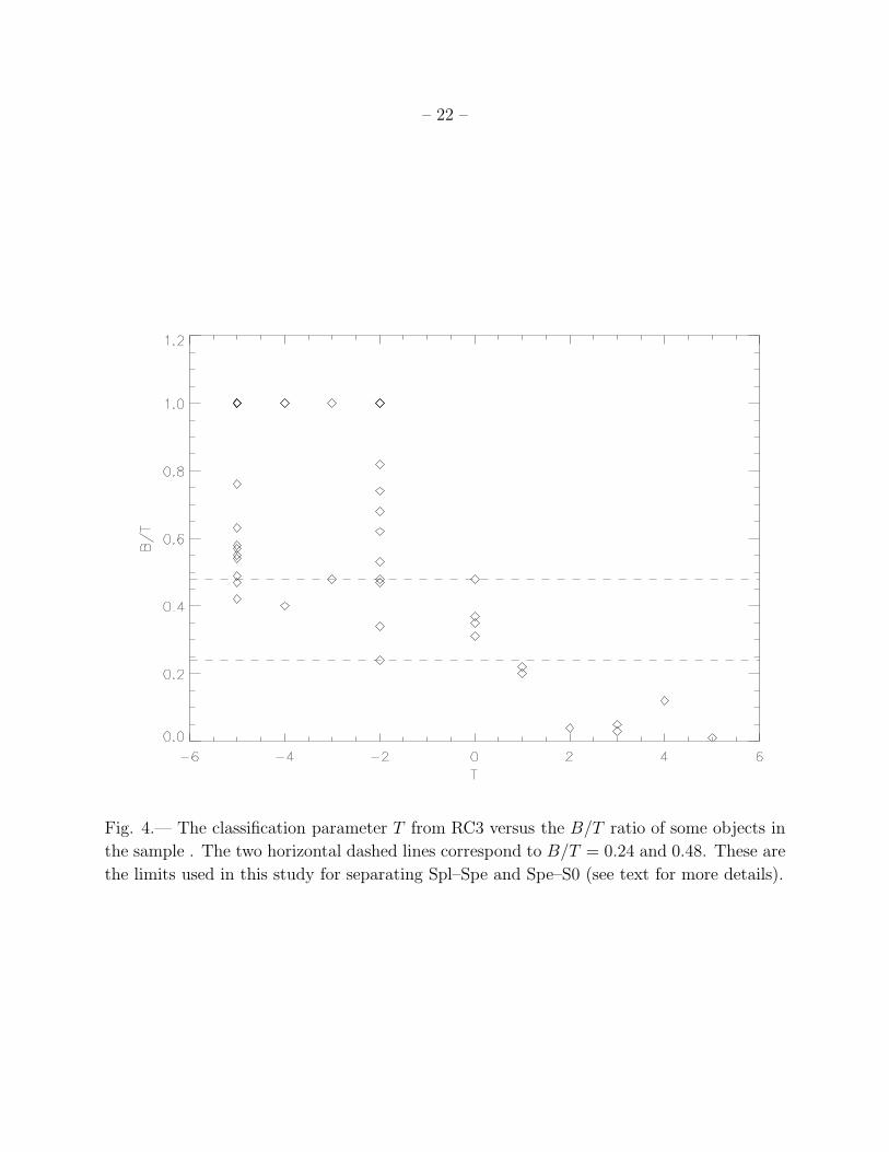
We have compared our classification with visual classifications available for some of the

galaxies of the sample. Figure 4 shows the comparison between the classification based on

the B/T ratio and the T morphological parameter given by de Vaucouleurs et al. (1991)

(hereafter RC3). The classification of late-type galaxies coincides with both methods, but the

agreement is weaker for early-type objects, in particular for E, Ed, and S0 galaxies. Based

on this result, we will group E and Ed galaxies into one group, hereafter called elliptical (E).

We will define the S0 galaxies as a separate group. These types of objects are the transition

between disk-dominated galaxies (normal spirals) and bulge-dominated objects.

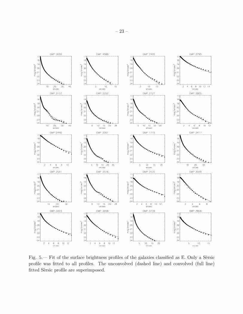
Figure 5 shows the fits of the isophotal surface brightness profiles for bulge galaxies, and

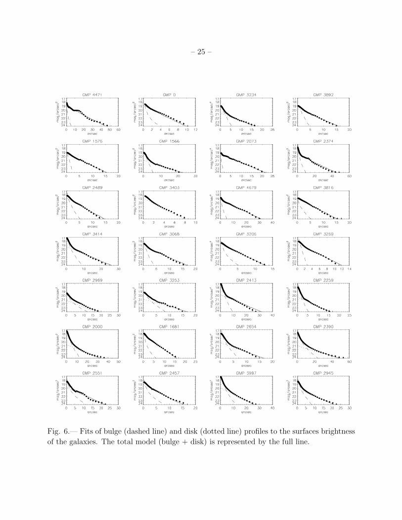
Fig 6 shows the isophotal fits for bulge + disk galaxies. Andreon et al (1997) measured from

the luminosity curve the effective radius of the early type galaxies brighter than mB = 16.5,

assuming a mean color B − R = 1.5 for Coma, they studied all galaxies within one degree

from the center brighter than mR = 15.0. Our sample goes deeper (mr = 17.0). We have

1We assumed that Coma members are those with 4000 km s−1 ≤ cz ≤ 10000 . The radial velocities were

taken from Nasa Extragalactic Database (NED).

2The B magnitude of the objects were obtained from Godwin et al. (1983).

– 7 –

10 early type galaxies in common with Andreon et al (1997). We have compared their

effective radius of those galaxies and our effective radius determined from the fits of the

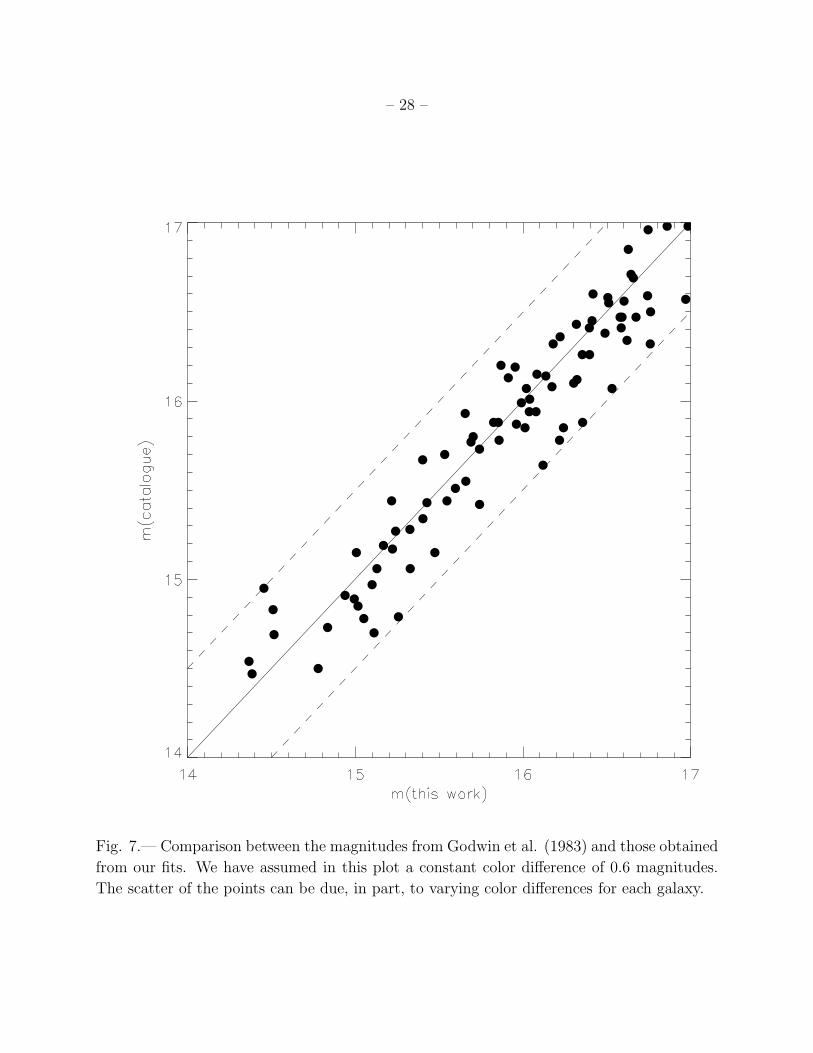
surface brightness profiles. The agreement is better than 10%. We have also compared the

magnitudes of the galaxies calculated by the fitted models and those given by Godwin et al.

(1983) (see Fig. 7). It can be seen that the agreement between the magnitudes is in all cases

better than 0.5 mag. Gutierrez el al (2003) showed the quantitative morphology for Coma

galaxies in the core cluster region. Although the method applied was the same, the surface

brightness profiles of the galaxies were different, because they were obtained from different

images. The final classification of the galaxies were also slightly different. In Gutierrez et al

(2003) it was considered as E galaxy those with B/T > 0.6, the surface brightness profile

of these objects were fitted with only one Sersic profile. In the present work, E galaxies

were objects with B/T > 0.8. We have compared the structural parameters of the objects

in common in both samples and with B/T < 0.6 and B/T > 0.8. They correspond to E

and Spirals in both samples. For the E galaxies the mean relative errors of the structural

parameters are: ∆µe = 0.007, ∆re = 0.043 and ∆n = −0.075. For the bulges of the spiral

galaxies the mean relative errors are: ∆µe = 0.038, ∆re = −0.064 and ∆n = 0.083,and for

the disks: ∆µo = 0.052 and ∆h = 0.093. These differences are smaller than the typical errors

in the determination of the parameters (≈ 10%), and they come mainly due to differences in

seeing or sky substraction on the images. The largest errors are in the case of the parameters

of the discs, which are more affected by the sky background substraction.

3. Morphological distribution of the galaxies in the cluster

From the pioneering work of Dressler (1980), it is well known that there is a morpholog-

ical segregation of galaxies in clusters. Early-type objects are located in denser regions and

are therefore closer to the center of the cluster than late-type galaxies. We have studied the

morphological segregation in Coma based on our galaxy classification. The morphological

evolution of galaxies in clusters is mainly driven by global and local conditions. In order

to study the global conditions in the cluster, the distribution of the different morphologi-

cal types is studied as a function of the projected distance of each galaxy to the center of

the cluster. Meanwhile, the local conditions are usually parameterized by a local projected

density (Dressler 1980).

– 8 –

3.1. Morphology–radius relation

We have computed the projected radius of each galaxy to the center of the cluster.

The center adopted was that of Godwin et al. (1983): α(J2000) = 12:59:42, δ(J2000) =

27:58:15.6. The projected radius was scaled to the scale-length of the mass profile of the

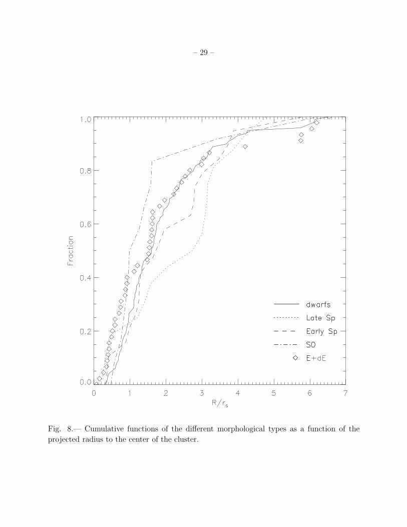
cluster: rs = 0.26 Mpc (Geller et al. 1999). Figure 8 shows the cumulative functions of the

different types of galaxies vs. projected radius. The Kolmogorov-Smirnov probabilities for

the Spe-Spl, Spe-S0 and Spl-S0 cumulative functions are: 0.67, 0.23 and 0.09, respectively.

According with these probabilities, we can not disprove that the cumulative functions of

Spe-Spl, Spe-S0 and Spl-S0 come from the same distribution function. The mean positions,

< R/rs >, of Spl, Spe and S0 galaxies are: 2.28, 2.07 and 1.61, respectively. So, Spls are

located in average at larger distances than Spes and S0s. The increment of E galaxies for

R/rs > 4 corresponds to a group of early-type galaxies (8 objects, mainly Es) located at

Coma NE region. Dwarf galaxies show a gap in their distribution. There are no dwarfs

within R/rs ≈ 0.3.

The absence of dwarf galaxies in the central region of the cluster could be related to

disruption caused by tidal interactions. Debris of these kinds of systems has already been

observed in the innermost regions of Coma (Gregg & West 1998). In their study of the

central region of Coma, Trujillo et al. (2002) showed that dwarfs have a constant galaxy-

light concentration. In their models, this was compatible with dwarfs being removed from

the center of the cluster. Other authors have given other evidence to prove this result

(Thompson & Gregory 1993; Secker & Harris 1997; Gregg & West 1998; Adami et al. 2001;

Andreon 2002).

3.2. The morphology-density relation

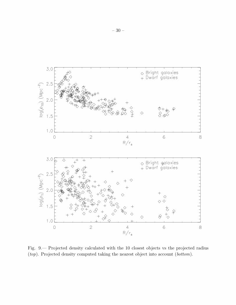
This relation takes local effects on morphological segregation into account. Dressler

(1980) defined the projected density by taking into account the ten nearest neighbors to

each galaxy, ρ10. In Fig. 9 we show ρ10 vs. the projected radius. It can be seen that there

is a correlation between these two quantities. This means that ρ10 is giving us the same

information as the projected radius, i.e., it is related to global effects in the cluster. That

was also proposed by Thomas (2002). Figure 9 also shows the projected density defined with

the nearest neighbors, ρ1, vs, the projected radius. It is clear that these two parameters are

weakly correlated: therefore, we will use ρ1 as an indicator of local effects in the cluster.

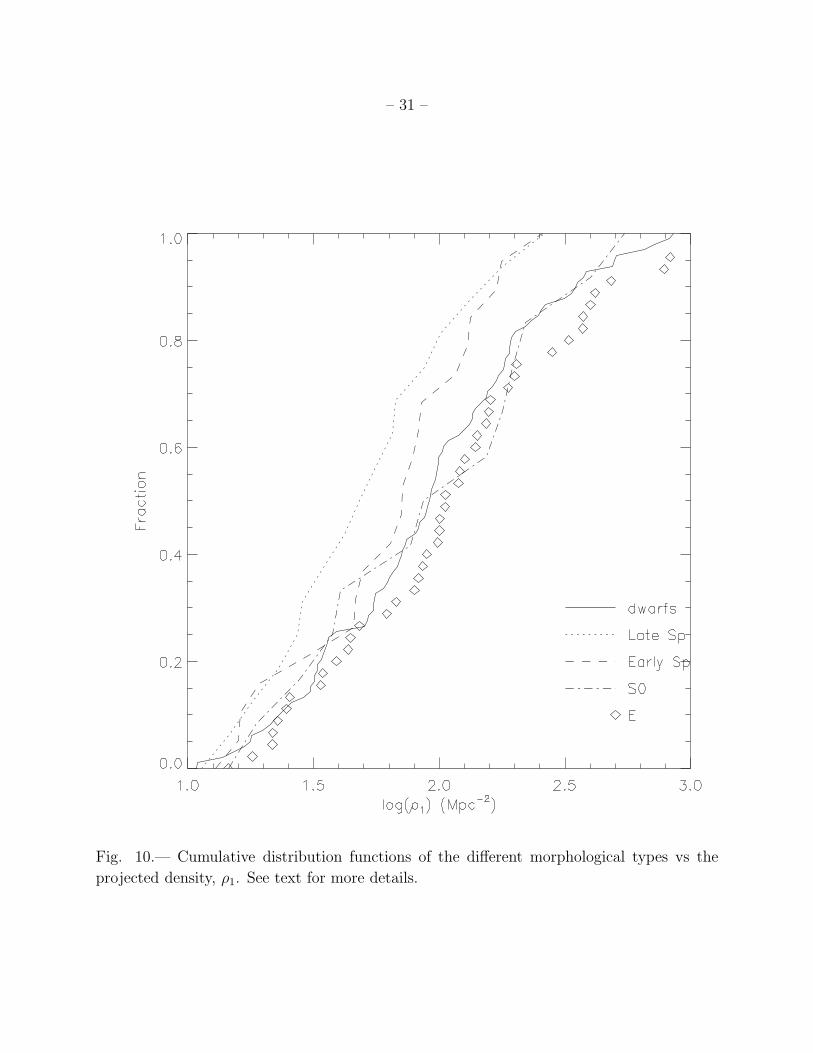
Figure 10 shows the cumulative distributions of the different morphological types as a

function of ρ1. The mean density, < log(ρ1) >, of E, Spl, Spe, S0 and dwarfs are: 2.06, 1.69,

– 9 –

1.79, 1.94 1.95, respectively. This means that E and Spl galaxies are located at the largest

and lowest local densities, respectively. The Kolmogorov-Smirnov probabilities for the Spe-

Spl, Spe-S0 and Spl-S0 cumulative functions are: 0.66, 0.27 and 0.19, respectively. This

means that we can not disprove that the cumulative functions of Spl-Spe, Spe-S0 and S0-Spl

galaxies come from the same distribution function. We have also computed the Kolmogorov–

Smirnov probability for the S0–E, S0–dwarf, and E–dwarf cumulative functions to be 0.81,

0.99, and 0.62, respectively. This means that the S0s and dwarf galaxies are compatible with

the same cumulative distribution function. But, we can not disprove that S0–E and E–dwarf

have the same distribution function. It is also clear from Fig. 10 that no spirals (early- or

late-type) are located at log(ρ1) > 2.4, while S0s, Es, and dwarfs are located at higher local

densities.

3.3. Density images

We can define the surface number density of galaxies on the plane of the sky. We have

followed the definition given by Trevese et al. (1992). For each point we find the distance,

Rn, to the nth neighboring galaxy. The surface density at the point (x, y) is then given by

σ(x, y) =C

R2n

, (3)

where C is a constant determined by the condition that the integral of σ(x, y) over the total

area is equal to the total number of galaxies. We have taken into account ten neighboring

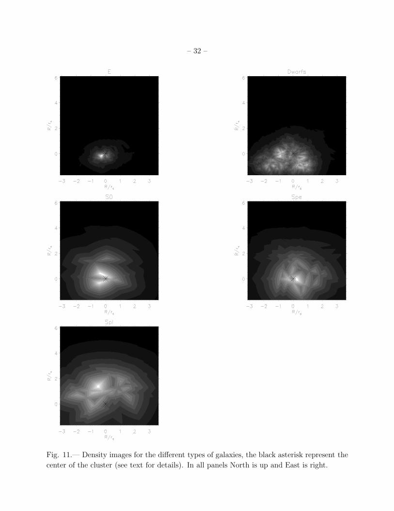
galaxies as the definition of the density. Figure 11 shows the density image for each type

of galaxy. E galaxies are located at the center of the cluster and show a very concentrated

density. Dwarf galaxies are distributed in a shell surrounding the center of the cluster. S0s

have two density peaks near the cluster center and show a more extended density map than

the Es. The density peak of the Es is located between the two density peaks of the S0

galaxies. Spirals (Spe and Spl) show density peaks far from the cluster center and also the

most extended density maps. Late-type spirals show a peak in density farther from the

cluster center than the peak of the Spes. An asterisk in Fig. 11 marks the center of the

cluster. The E and Spe density peaks are close to the cluster center, and the Spl the peak

is the most distant from the center.

– 10 –

4. Structural parameters

In this section, we will study the structural parameters of the bright galaxies analyzed

in Coma. In particular, we will compare the disk and bulge parameters with those from local

and isolated galaxies in order to explore the influence of the environment. The local samples

used as comparison were: Graham (2001, 2003), de Jong (1996), and Mollenhoff & Heidt

(2001). The sample of 86 spiral galaxies from Graham (2001, 2003) covers all spiral galaxy

types and provides the largest homogeneous set of structural parameters for spiral galaxies

modeled with an R1/n bulge. We took the structural parameters in the R band of these

galaxies, for a direct comparison with our data. We will also compare our results with those

given by de Jong (1996), hereafter DJ96, and Mollenhoff & Heidt (2001), hereafter MH01.

The structural parameter of the sample from DJ96 are obtained in the B and K bands with

an assumed exponential profile for the surface brightness of the bulge. This will make a

direct comparison with the parameters of our bulges impossible. The sample of MH01 is in

the near-IR J , H , and K bands, with Sersic profiles used for the bulges of the galaxies.

4.1. Disk parameters

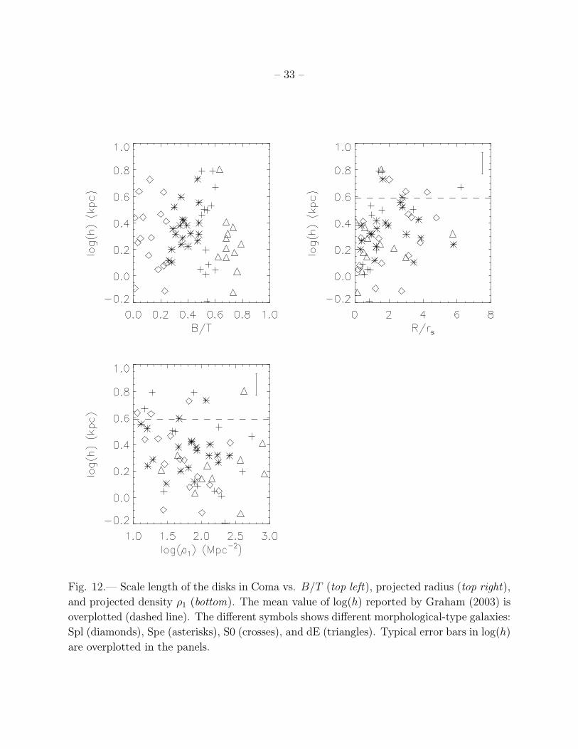
Figure 12 shows the correlations of the scale length of the disks with B/T , the projected

radius, and ρ1. There is no trend in the scale of the disk with B/T . Assuming that the

morphological type of the objects is correlated with the B/T ratio (Simien & de Vaucouleurs

1986), we can infer that the scale of the disk is independent of the morphological type. Similar

results were obtained in the samples from Graham (2001, 2003), DJ96 and MH01. Our mean

value of log(h) is 0.33, which is smaller than the mean value obtained by Graham (2001,

2003): log(h) = 0.59 ± 0.03 in the R band.3 This result is in agreement with the obtained

recently by Gutierrez et al. (2003) for the central region of the cluster (R/rs ≈ 1.6).

Figure 12 also shows the relation of the scale length of the disks and the local and

global environmental parameters. We have overploted the mean h of the disks from the

Graham (2001, 2003) sample. It can be seen that the scales of the disks from Coma are

smaller than those in isolated galaxies. From Fig. 12 we can infer that no large disks are

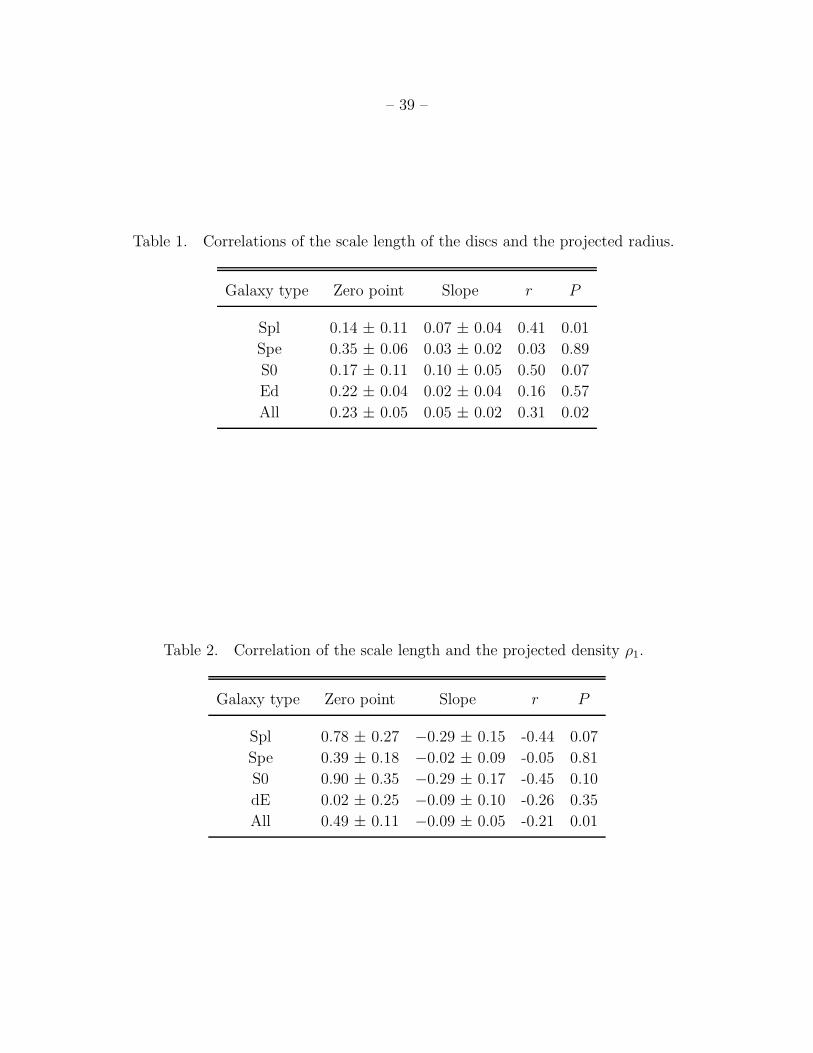
located at the center and high densities in the cluster. Tables 1 and 2 show the parameters of

these relations, the Pearson correlation coefficient (r), and the significance of the correlation

(P ), that is, the probability that | r | should be larger than its observed value in the null

3The mean value of log(h) from the sample of Graham (2003) has been obtained taking into ac-

count the galaxies that lie in the same range of absolute magnitudes as the galaxies in our sample

(MB = [−18.0,−21.3]).

– 11 –

hypothesis. From table 1 can be seen that the strongest correlation between h and projected

radius is for Spl galaxies. Table 2 shows that the strongest correlation between local density

and radius is when we consider all galaxies together.

4.2. Bulge parameters

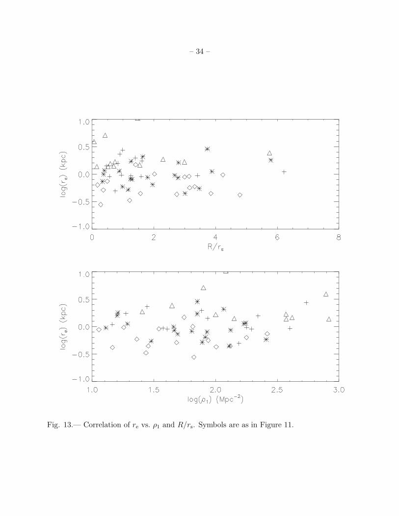
Figure 13 shows the correlations of the bulge effective radius, re with the projected radius

and projected density. There is no correlation between the bulge scale and the environment.

This lack of correlation confirms a previous result by Andreon (1996)

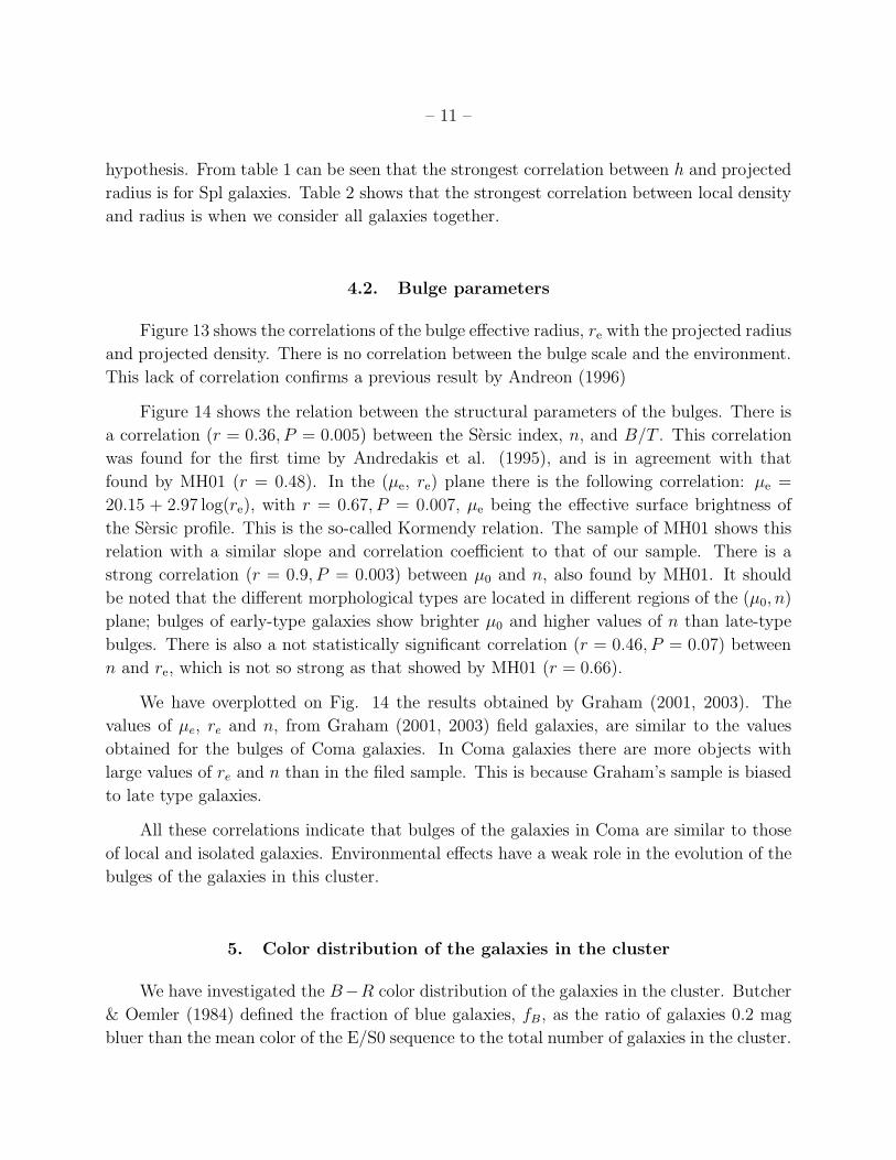
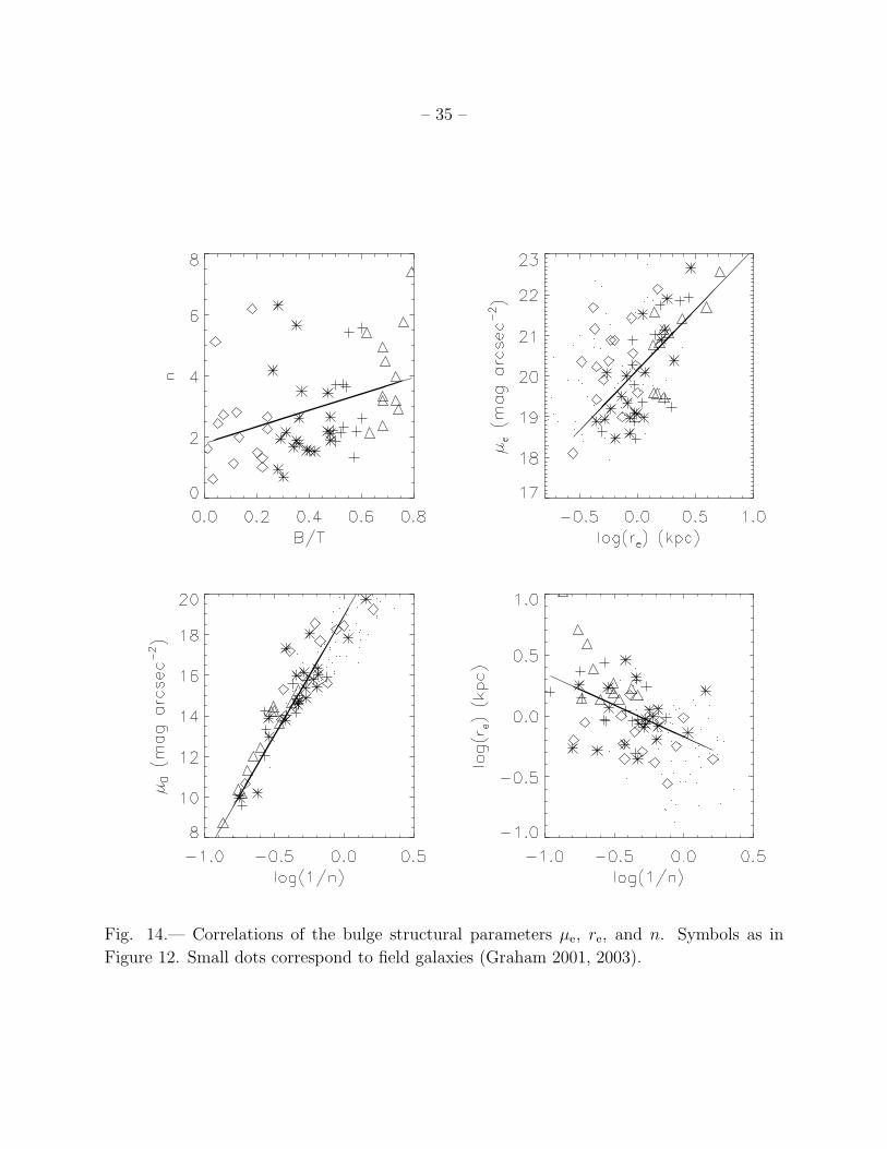
Figure 14 shows the relation between the structural parameters of the bulges. There is

a correlation (r = 0.36, P = 0.005) between the Sersic index, n, and B/T . This correlation

was found for the first time by Andredakis et al. (1995), and is in agreement with that

found by MH01 (r = 0.48). In the (µe, re) plane there is the following correlation: µe =

20.15 + 2.97 log(re), with r = 0.67, P = 0.007, µe being the effective surface brightness of

the Sersic profile. This is the so-called Kormendy relation. The sample of MH01 shows this

relation with a similar slope and correlation coefficient to that of our sample. There is a

strong correlation (r = 0.9, P = 0.003) between µ0 and n, also found by MH01. It should

be noted that the different morphological types are located in different regions of the (µ0, n)

plane; bulges of early-type galaxies show brighter µ0 and higher values of n than late-type

bulges. There is also a not statistically significant correlation (r = 0.46, P = 0.07) between

n and re, which is not so strong as that showed by MH01 (r = 0.66).

We have overplotted on Fig. 14 the results obtained by Graham (2001, 2003). The

values of µe, re and n, from Graham (2001, 2003) field galaxies, are similar to the values

obtained for the bulges of Coma galaxies. In Coma galaxies there are more objects with

large values of re and n than in the filed sample. This is because Graham’s sample is biased

to late type galaxies.

All these correlations indicate that bulges of the galaxies in Coma are similar to those

of local and isolated galaxies. Environmental effects have a weak role in the evolution of the

bulges of the galaxies in this cluster.

5. Color distribution of the galaxies in the cluster

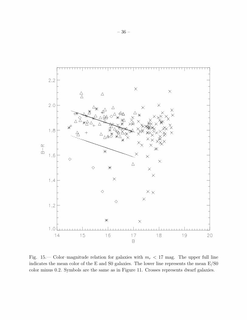
We have investigated the B−R color distribution of the galaxies in the cluster. Butcher

& Oemler (1984) defined the fraction of blue galaxies, fB, as the ratio of galaxies 0.2 mag

bluer than the mean color of the E/S0 sequence to the total number of galaxies in the cluster.

– 12 –

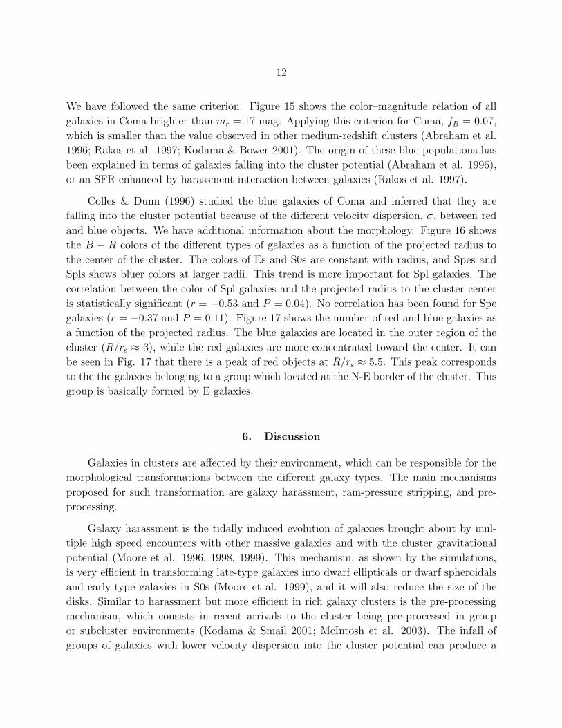
We have followed the same criterion. Figure 15 shows the color–magnitude relation of all

galaxies in Coma brighter than mr = 17 mag. Applying this criterion for Coma, fB = 0.07,

which is smaller than the value observed in other medium-redshift clusters (Abraham et al.

1996; Rakos et al. 1997; Kodama & Bower 2001). The origin of these blue populations has

been explained in terms of galaxies falling into the cluster potential (Abraham et al. 1996),

or an SFR enhanced by harassment interaction between galaxies (Rakos et al. 1997).

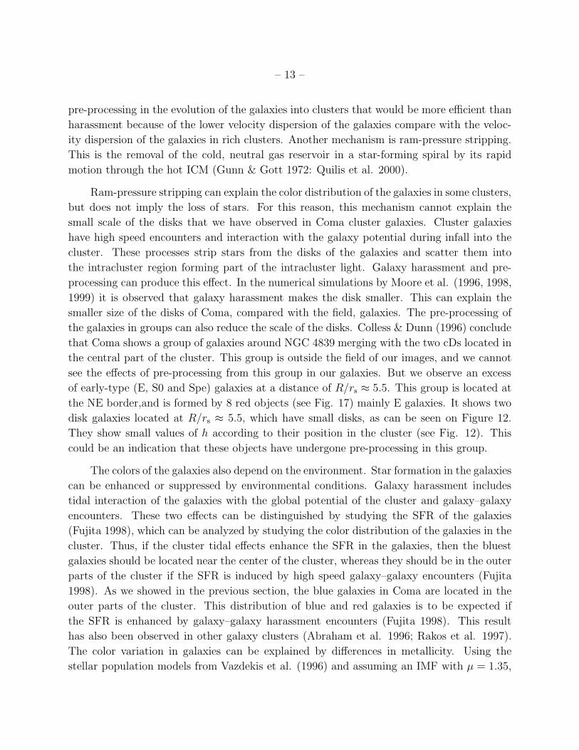
Colles & Dunn (1996) studied the blue galaxies of Coma and inferred that they are

falling into the cluster potential because of the different velocity dispersion, σ, between red

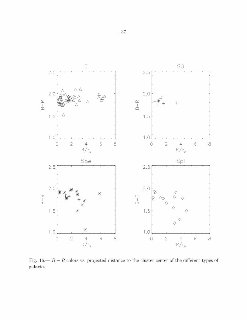
and blue objects. We have additional information about the morphology. Figure 16 shows

the B − R colors of the different types of galaxies as a function of the projected radius to

the center of the cluster. The colors of Es and S0s are constant with radius, and Spes and

Spls shows bluer colors at larger radii. This trend is more important for Spl galaxies. The

correlation between the color of Spl galaxies and the projected radius to the cluster center

is statistically significant (r = −0.53 and P = 0.04). No correlation has been found for Spe

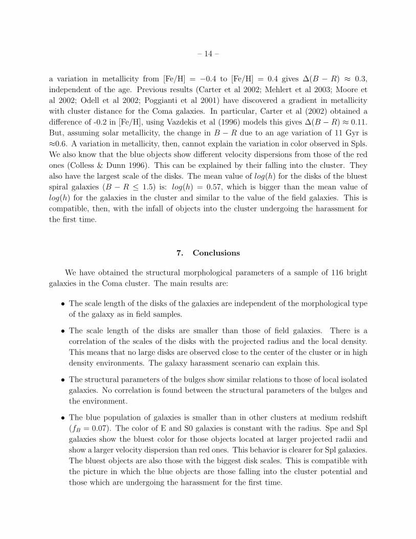
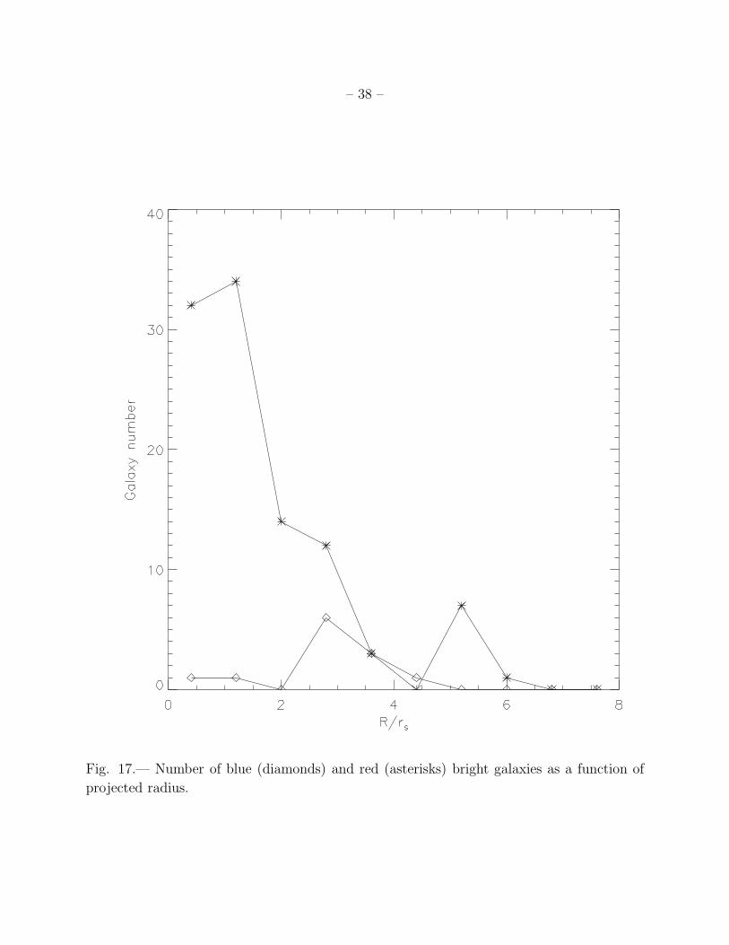
galaxies (r = −0.37 and P = 0.11). Figure 17 shows the number of red and blue galaxies as

a function of the projected radius. The blue galaxies are located in the outer region of the

cluster (R/rs ≈ 3), while the red galaxies are more concentrated toward the center. It can

be seen in Fig. 17 that there is a peak of red objects at R/rs ≈ 5.5. This peak corresponds

to the the galaxies belonging to a group which located at the N-E border of the cluster. This

group is basically formed by E galaxies.

6. Discussion

Galaxies in clusters are affected by their environment, which can be responsible for the

morphological transformations between the different galaxy types. The main mechanisms

proposed for such transformation are galaxy harassment, ram-pressure stripping, and pre-

processing.

Galaxy harassment is the tidally induced evolution of galaxies brought about by mul-

tiple high speed encounters with other massive galaxies and with the cluster gravitational

potential (Moore et al. 1996, 1998, 1999). This mechanism, as shown by the simulations,

is very efficient in transforming late-type galaxies into dwarf ellipticals or dwarf spheroidals

and early-type galaxies in S0s (Moore et al. 1999), and it will also reduce the size of the

disks. Similar to harassment but more efficient in rich galaxy clusters is the pre-processing

mechanism, which consists in recent arrivals to the cluster being pre-processed in group

or subcluster environments (Kodama & Smail 2001; McIntosh et al. 2003). The infall of

groups of galaxies with lower velocity dispersion into the cluster potential can produce a

– 13 –

pre-processing in the evolution of the galaxies into clusters that would be more efficient than

harassment because of the lower velocity dispersion of the galaxies compare with the veloc-

ity dispersion of the galaxies in rich clusters. Another mechanism is ram-pressure stripping.

This is the removal of the cold, neutral gas reservoir in a star-forming spiral by its rapid

motion through the hot ICM (Gunn & Gott 1972: Quilis et al. 2000).

Ram-pressure stripping can explain the color distribution of the galaxies in some clusters,

but does not imply the loss of stars. For this reason, this mechanism cannot explain the

small scale of the disks that we have observed in Coma cluster galaxies. Cluster galaxies

have high speed encounters and interaction with the galaxy potential during infall into the

cluster. These processes strip stars from the disks of the galaxies and scatter them into

the intracluster region forming part of the intracluster light. Galaxy harassment and pre-

processing can produce this effect. In the numerical simulations by Moore et al. (1996, 1998,

1999) it is observed that galaxy harassment makes the disk smaller. This can explain the

smaller size of the disks of Coma, compared with the field, galaxies. The pre-processing of

the galaxies in groups can also reduce the scale of the disks. Colless & Dunn (1996) conclude

that Coma shows a group of galaxies around NGC 4839 merging with the two cDs located in

the central part of the cluster. This group is outside the field of our images, and we cannot

see the effects of pre-processing from this group in our galaxies. But we observe an excess

of early-type (E, S0 and Spe) galaxies at a distance of R/rs ≈ 5.5. This group is located at

the NE border,and is formed by 8 red objects (see Fig. 17) mainly E galaxies. It shows two

disk galaxies located at R/rs ≈ 5.5, which have small disks, as can be seen on Figure 12.

They show small values of h according to their position in the cluster (see Fig. 12). This

could be an indication that these objects have undergone pre-processing in this group.

The colors of the galaxies also depend on the environment. Star formation in the galaxies

can be enhanced or suppressed by environmental conditions. Galaxy harassment includes

tidal interaction of the galaxies with the global potential of the cluster and galaxy–galaxy

encounters. These two effects can be distinguished by studying the SFR of the galaxies

(Fujita 1998), which can be analyzed by studying the color distribution of the galaxies in the

cluster. Thus, if the cluster tidal effects enhance the SFR in the galaxies, then the bluest

galaxies should be located near the center of the cluster, whereas they should be in the outer

parts of the cluster if the SFR is induced by high speed galaxy–galaxy encounters (Fujita

1998). As we showed in the previous section, the blue galaxies in Coma are located in the

outer parts of the cluster. This distribution of blue and red galaxies is to be expected if

the SFR is enhanced by galaxy–galaxy harassment encounters (Fujita 1998). This result

has also been observed in other galaxy clusters (Abraham et al. 1996; Rakos et al. 1997).

The color variation in galaxies can be explained by differences in metallicity. Using the

stellar population models from Vazdekis et al. (1996) and assuming an IMF with µ = 1.35,

– 14 –

a variation in metallicity from [Fe/H] = −0.4 to [Fe/H] = 0.4 gives ∆(B − R) ≈ 0.3,

independent of the age. Previous results (Carter et al 2002; Mehlert et al 2003; Moore et

al 2002; Odell et al 2002; Poggianti et al 2001) have discovered a gradient in metallicity

with cluster distance for the Coma galaxies. In particular, Carter et al (2002) obtained a

difference of -0.2 in [Fe/H], using Vazdekis et al (1996) models this gives ∆(B − R) ≈ 0.11.

But, assuming solar metallicity, the change in B − R due to an age variation of 11 Gyr is

≈0.6. A variation in metallicity, then, cannot explain the variation in color observed in Spls.

We also know that the blue objects show different velocity dispersions from those of the red

ones (Colless & Dunn 1996). This can be explained by their falling into the cluster. They

also have the largest scale of the disks. The mean value of log(h) for the disks of the bluest

spiral galaxies (B − R ≤ 1.5) is: log(h) = 0.57, which is bigger than the mean value of

log(h) for the galaxies in the cluster and similar to the value of the field galaxies. This is

compatible, then, with the infall of objects into the cluster undergoing the harassment for

the first time.

7. Conclusions

We have obtained the structural morphological parameters of a sample of 116 bright

galaxies in the Coma cluster. The main results are:

• The scale length of the disks of the galaxies are independent of the morphological type

of the galaxy as in field samples.

• The scale length of the disks are smaller than those of field galaxies. There is a

correlation of the scales of the disks with the projected radius and the local density.

This means that no large disks are observed close to the center of the cluster or in high

density environments. The galaxy harassment scenario can explain this.

• The structural parameters of the bulges show similar relations to those of local isolated

galaxies. No correlation is found between the structural parameters of the bulges and

the environment.

• The blue population of galaxies is smaller than in other clusters at medium redshift

(fB = 0.07). The color of E and S0 galaxies is constant with the radius. Spe and Spl

galaxies show the bluest color for those objects located at larger projected radii and

show a larger velocity dispersion than red ones. This behavior is clearer for Spl galaxies.

The bluest objects are also those with the biggest disk scales. This is compatible with

the picture in which the blue objects are those falling into the cluster potential and

those which are undergoing the harassment for the first time.

– 15 –

REFERENCES

Abraham, R. G. et al. 1996, ApJ, 471, 694

Adami, C., Mazure, A., Ulmer, M. P., & Savine, C. 2001, A&A, 371, 11

Aguerri, J. A. L. & Trujillo, I. 2002, MNRAS, 333, 633

Andredakis, Y. C., Peletier, R. F., & Balcells, M. 1995, MNRAS, 275, 874

Andreon, S., Davoust, E., & Poulain, P. 1997, A&AS, 126, 67

Andreon, S., Davoust, E., Michard, R., Nieto, J.-L., & Poulain, P. 1996, A&AS, 116, 429

Andreon, S. 1996, A&A, 314, 763

Andreon, S. 2002, A&A, 382, 821

Baier, F. W., Fritze, K., & Tiersch, H. 1990, Astronomische Nachrichten, 311, 89

Butcher, H. & Oemler, A. 1984, ApJ, 285, 426

Butcher, H. & Oemler, A. 1978, ApJ, 219, 18

Caon, N., Capaccioli, M., & D’Onofrio, M. 1993, MNRAS, 265, 1013

Carter, D. et al. 2002, ApJ, 567, 772

Cayatte, V., van Gorkom, J. H., Balkowski, C., & Kotanyi, C. 1990, AJ, 100, 604

Charlot, S. & Silk, J. 1994, ApJ, 432, 453

Colless, M. & Dunn, A. M. 1996, ApJ, 458, 435

Dale, D. A. & Uson, J. M., 2003, ApJ in press.

Dale, D. A., Giovanelli, R., Haynes, M. P., Hardy, E., & Campusano, L. E. 2001, AJ, 121,

1886

de Jong, R. S. 1996, A&A, 313, 45 (DJ96)

de Vaucouleurs, G., de Vaucouleurs, A., Corwin, H. G., Buta, R. J., Paturel, G., & Fouque,

P. 1991, Volume 1-3, XII, 2069 pp. 7 figs.. Springer-Verlag Berlin Heidelberg New

York (RC3)

Dressler, A. et al. 1997, ApJ, 490, 577

– 16 –

Dressler, A. 1980, ApJ, 236, 351

Ellis, R. S., Smail, I., Dressler, A., Couch, W. J., Oemler, A. J., Butcher, H., & Sharples,

R. M. 1997, ApJ, 483, 582

Fitchett, M. & Webster, R. 1987, ApJ, 317, 653

Freeman, K. C. 1970, ApJ, 160, 811

Fujita, Y. 1998, ApJ, 509, 587

Geller, M. J., Diaferio, A., & Kurtz, M. J. 1999, ApJ, 517, L23

Gerbal, D., Lima Neto, G. B., Marquez, I., & Verhagen, H. 1997, MNRAS, 285, L41

Godwin, J. G., Metcalfe, N., & Peach, J. V. 1983, MNRAS, 202, 113

Graham, A. W. 2003, AJ, 125, 3398

Graham, A. W. 2001, AJ, 121, 820

Gregg, M. D. & West, M. J. 1998, Nature, 396, 549

Gunn, J. E. & Gott, J. R. I. 1972, ApJ, 176, 1

Gutierrez, C., Trujillo, I., Aguerri, J. A. L., Graham, A. W., Caon, N., 2003, ApJ, in press.

Haynes, M. P., Giovanelli, R., & Chincarini, G. L. 1984, ARA&A, 22, 445

Iglesias-Paramo, J., Boselli, A., Gavazzi, G., Cortese, L., & Vılchez, J. M. 2003, A&A, 397,

421

Iglesias-Paramo, J., Boselli, A., Cortese, L., Vılchez, J. M., & Gavazzi, G. 2002, A&A, 384,

383

Jorgensen, I. & Franx, M. 1994, ApJ, 433, 553

Kenney, J. & Koopmann, R. 1999, IAU Symp. 186: Galaxy Interactions at Low and High

Redshift, 186, 387

Khosroshahi, H. G., Wadadekar, Y., Kembhavi, A., & Mobasher, B. 2000, ApJ, 531, L103

Kodama, T. & Bower, R. G. 2001, MNRAS, 321, 18

Kodama, T. & Smail, I. 2001, MNRAS, 326, 637

– 17 –

Lucey, J. R., Bower, R. G., & Ellis, R. S. 1991, MNRAS, 249, 755

McIntosh, D. H., Rix, H. W. & Caldwell, N. 2003, ApJ, in press.

Mehlert, D., Thomas, D., Saglia, R. P., Bender, R., & Wegner, G. 2003, A&A, 407, 423

Merritt, D. 1984, ApJ, 276, 26

Mobasher, B., Guzman, R., Aragon-Salamanca, A., & Zepf, S. 1999, MNRAS, 304, 225

Mollenhoff, C. & Heidt, J. 2001, A&A, 368, 16 (MH01)

Moore, S. A. W., Lucey, J. R., Kuntschner, H., & Colless, M. 2002, MNRAS, 336, 382

Moore, B., Lake, G., Quinn, T., & Stadel, J. 1999, MNRAS, 304, 465

Moore, B., Lake, G., & Katz, N. 1998, ApJ, 495, 139

Moore, B., Katz, N., Lake, G., Dressler, A., & Oemler, A. 1996, Nature, 379, 613

Odell, A. P., Schombert, J., & Rakos, K. 2002, AJ, 124, 3061

Oemler, A. J., Dressler, A., & Butcher, H. R. 1997, ApJ, 474, 561

bibitem[] Poggianti, B. M. et al. 2001, ApJ, 563, 118

Quilis, V., Moore, B., & Bower, R. 2000, Science, 288, 1617

Rakos, K. D., Odell, A. P., & Schombert, J. M. 1997, ApJ, 490, 194

Rubin, V. C., Ford, W. K. J., & Whitmore, B. C. 1988, ApJ, 333, 522

Scodeggio, M., Gavazzi, G., Belsole, E., Pierini, D., & Boselli, A. 1998, MNRAS, 301, 1001

Secker, J. & Harris, W. E. 1997, PASP, 109, 1364

Sersic, J. L. 1968, Atlas de Galaxes Australes (Cordoba: Obs. Astron.)

Simien, F. & de Vaucouleurs, G. 1986, ApJ, 302, 564

Solanes, J. M., Manrique, A., Garcıa-Gomez, C., Gonzalez-Casado, G., Giovanelli, R., &

Haynes, M. P. 2001, ApJ, 548, 97

Thomas, T., 2002, PhD Thesis. Leiden University.

Thompson, L. A. & Gregory, S. A. 1993, AJ, 106, 2197

– 18 –

Trevese, D., Flin, P., Migliori, L., Hickson, P., & Pittella, G. 1992, A&AS, 94, 327

Trujillo, I., Aguerri, J. A. L., Gutierrez, C. M., Caon, N., & Cepa, J. 2002, ApJ, 573, L9

Trujillo, I., Aguerri, J. A. L., Gutierrez, C. M., & Cepa, J. 2001, AJ, 122, 38

Vazdekis, A., Casuso, E., Peletier, R. F., & Beckman, J. E. 1996, ApJS, 106, 307

White, S. D. M., Briel, U. G., & Henry, J. P. 1993, MNRAS, 261, L8

Whitmore, B. C., Forbes, D. A., & Rubin, V. C. 1988, ApJ, 333, 542

This preprint was prepared with the AAS LATEX macros v5.2.

– 19 –

Fig. 1.— Relative errors in the bulge parameters from Monte Carlo simulations of bulge

galaxies (left panels). Mean relative errors in the bulge parameters showed in the left panels

with 1σ error bars (right panels). Horizontal dashed and full lines represent 10% and 20%

relative errors of the re and n parameters, respectively. They also represent a difference of

0.1 (dashed line) and 0.2 (fulll line) between the input and recovered magnitud and ellipticity

of the models.

– 20 –

Fig. 2.— Relative errors in the bulge and disk parameters from Monte Carlo simulations of

bulge + disk galaxies (left panels). Mean relative errors in the bulge and disk parameters

showed in the left panels with 1σ error bars (right panels). Horizontal dashed and full lines

represent 10% and 20% relative errors of the re, n and h parameters, respectively. They also

represent a difference of 0.1 (dashed line) and 0.2 (fulll line) between the input and recovered

magnitud and ellipticity of the models.

– 21 –

Fig. 3.— Errors in the B/T parameter from the Monte Carlo simulations. Triangles repre-

sents galaxies with mr > 17 mag, and full circles objects with mr ≤ 17 mag.

– 22 –

Fig. 4.— The classification parameter T from RC3 versus the B/T ratio of some objects in

the sample . The two horizontal dashed lines correspond to B/T = 0.24 and 0.48. These are

the limits used in this study for separating Spl–Spe and Spe–S0 (see text for more details).

– 23 –

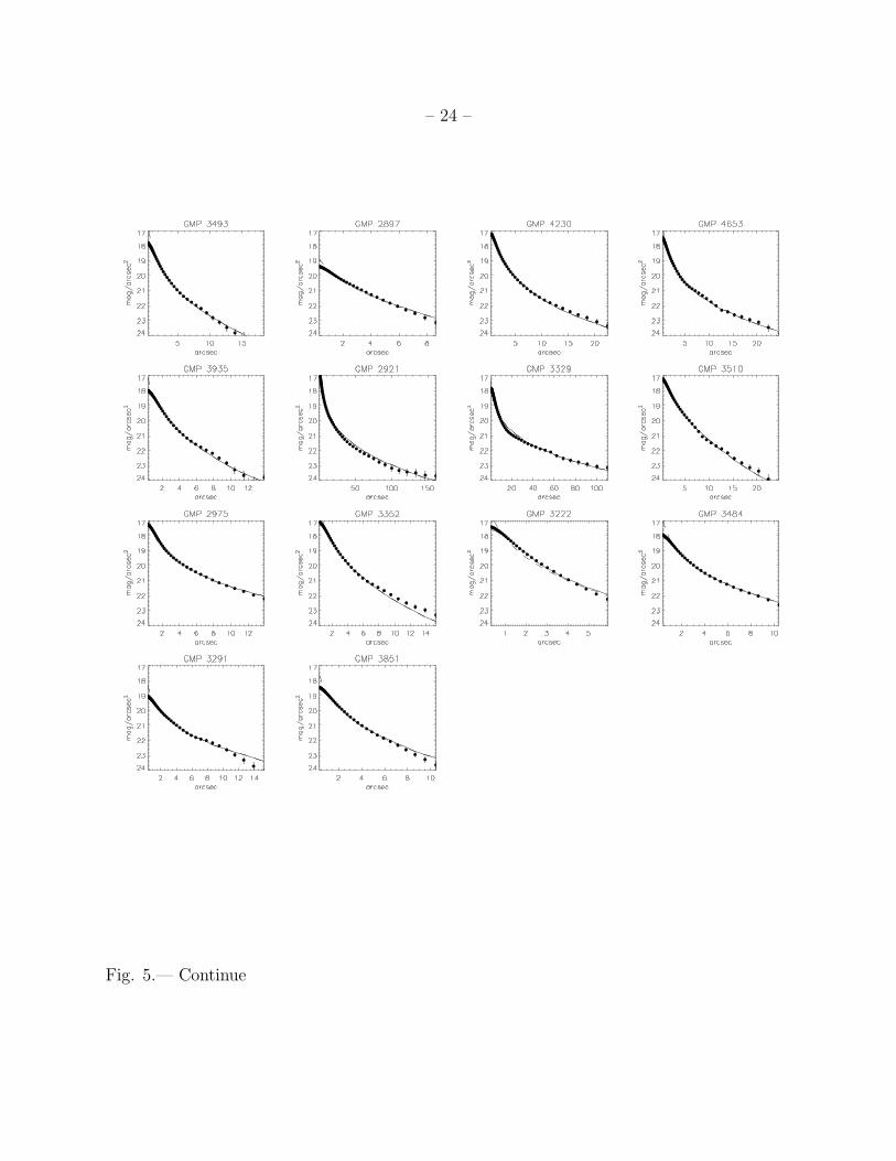
Fig. 5.— Fit of the surface brightness profiles of the galaxies classified as E. Only a Sersic

profile was fitted to all profiles. The unconvolved (dashed line) and convolved (full line)

fitted Sersic profile are superimposed.

– 24 –

Fig. 5.— Continue

– 25 –

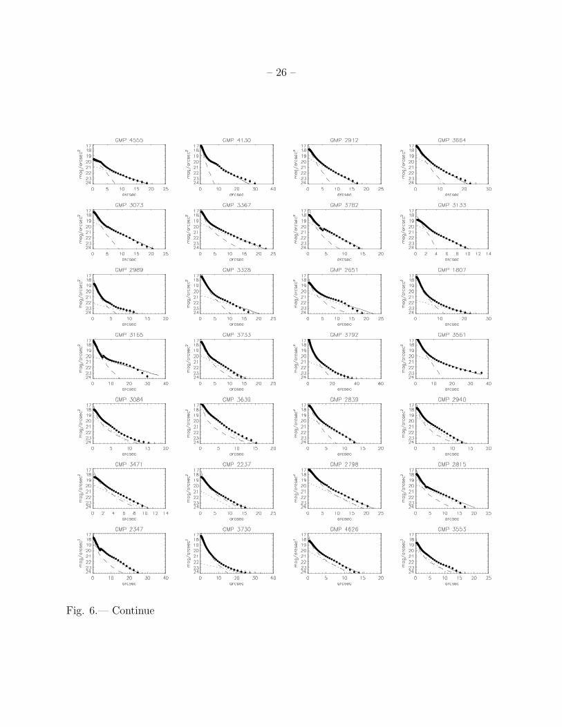
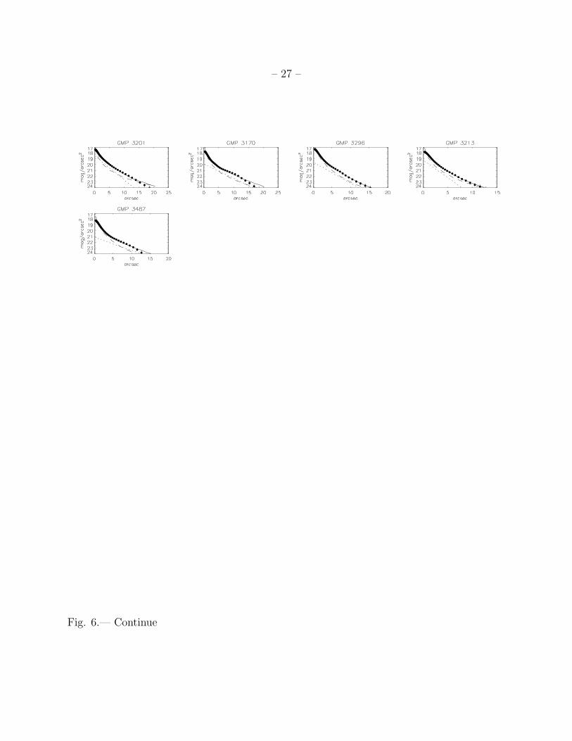
Fig. 6.— Fits of bulge (dashed line) and disk (dotted line) profiles to the surfaces brightness

of the galaxies. The total model (bulge + disk) is represented by the full line.

– 26 –

Fig. 6.— Continue

– 27 –

Fig. 6.— Continue

– 28 –

Fig. 7.— Comparison between the magnitudes from Godwin et al. (1983) and those obtained

from our fits. We have assumed in this plot a constant color difference of 0.6 magnitudes.

The scatter of the points can be due, in part, to varying color differences for each galaxy.

– 29 –

Fig. 8.— Cumulative functions of the different morphological types as a function of the

projected radius to the center of the cluster.

– 30 –

Fig. 9.— Projected density calculated with the 10 closest objects vs the projected radius

(top). Projected density computed taking the nearest object into account (bottom).

– 31 –

Fig. 10.— Cumulative distribution functions of the different morphological types vs the

projected density, ρ1. See text for more details.

– 32 –

Fig. 11.— Density images for the different types of galaxies, the black asterisk represent the

center of the cluster (see text for details). In all panels North is up and East is right.

– 33 –

Fig. 12.— Scale length of the disks in Coma vs. B/T (top left), projected radius (top right),

and projected density ρ1 (bottom). The mean value of log(h) reported by Graham (2003) is

overplotted (dashed line). The different symbols shows different morphological-type galaxies:

Spl (diamonds), Spe (asterisks), S0 (crosses), and dE (triangles). Typical error bars in log(h)

are overplotted in the panels.

– 34 –

Fig. 13.— Correlation of re vs. ρ1 and R/rs. Symbols are as in Figure 11.

– 35 –

Fig. 14.— Correlations of the bulge structural parameters µe, re, and n. Symbols as in

Figure 12. Small dots correspond to field galaxies (Graham 2001, 2003).

– 36 –

Fig. 15.— Color–magnitude relation for galaxies with mr < 17 mag. The upper full line

indicates the mean color of the E and S0 galaxies. The lower line represents the mean E/S0

color minus 0.2. Symbols are the same as in Figure 11. Crosses represents dwarf galaxies.

– 37 –

Fig. 16.— B − R colors vs. projected distance to the cluster center of the different types of

galaxies.

– 38 –

Fig. 17.— Number of blue (diamonds) and red (asterisks) bright galaxies as a function of

projected radius.

– 39 –

Table 1. Correlations of the scale length of the discs and the projected radius.

Galaxy type Zero point Slope r P

Spl 0.14 ± 0.11 0.07 ± 0.04 0.41 0.01

Spe 0.35 ± 0.06 0.03 ± 0.02 0.03 0.89

S0 0.17 ± 0.11 0.10 ± 0.05 0.50 0.07

Ed 0.22 ± 0.04 0.02 ± 0.04 0.16 0.57

All 0.23 ± 0.05 0.05 ± 0.02 0.31 0.02

Table 2. Correlation of the scale length and the projected density ρ1.

Galaxy type Zero point Slope r P

Spl 0.78 ± 0.27 −0.29 ± 0.15 -0.44 0.07

Spe 0.39 ± 0.18 −0.02 ± 0.09 -0.05 0.81

S0 0.90 ± 0.35 −0.29 ± 0.17 -0.45 0.10

dE 0.02 ± 0.25 −0.09 ± 0.10 -0.26 0.35

All 0.49 ± 0.11 −0.09 ± 0.05 -0.21 0.01