Ensemble dispersion forecasting—Part I: concept, approach and indicators

ARTICLE IN PRESS

Atmospheric Environment 38 (2004) 4607–4617

*Correspond

E-mail addr

1352-2310/$ - se

doi:10.1016/j.at

Ensemble dispersion forecasting—Part I: concept,approach and indicators

S. Galmarinia,*, R. Bianconib, W. Klugc, T. Mikkelsend, R. Addise,S. Andronopoulosf, P. Astrupd, A. Baklanovg, J. Bartnikif, J.C. Bartzish,R. Bellasiob, F. Bompayi, R. Buckleye, M. Bouzomi, H. Championm,

R. D’Amoursn, E. Davakisf, H. Eleveldj, G.T. Geertsemak, H. Glaabl, M. Kollaxo,M. Ilvonenu, A. Manningm, U. Pechingerp, C. Perssono, E. Polreichp, S. Potemskiq,

M. Prodanovar, J. Saltbonesh, H. Slaperj, M.A. Sofievt, D. Syrakovr,J.H. Sørenseng, L. Van der Auweras, I. Valkamat, R. Zelaznyq

a IES/REM, European Commission, Joint Research Center, TP 441, 21020 Ispra, ItalybEnviroware srl, C.Dir. Colleoni, Pzo Andromeda 1 20041 Agrate Brianza, Italy

cMittermayer weg 49, Darmstadt, GermanydRISØ National Laboratory, Wind Energy Department, P.O.Box 49, DK-4000, Roskilde, Denmark

eSavannah River Technology Center, Savannah River Site, Aiken, SC 29808, USAfEnvironmental Research Laboratory, NCSR Demokritos, 15310 Aghia Paraskevi Attikis, Greece

gDanish Meteorological Institute, Lyngbyvej 100, DK-2100, Copenhagen, DenmarkhNorwegian Meteorological Institute, P.O. Box 43, Blindern, N-0313 Oslo, NorwayiMETEOFRANCE, Dir.Prod., Serv./Environ., 42 av. Coriolis, 31057 Toulouse, France

jRIVM, Laboratory of Radiation Research, P.O. Box 1, Bilthoven, NetherlandskKNMI, P.O. Box 201, 3730 AE De Bilt, Netherlands

lGerman Weather Service (DWD), P.O. Box 10 04 65, 63004 Offenbach a.M., GermanymMeteorological Office, FitzRoy Road, Exeter EX1 3PB, UK

nCanadian Meteorological Centre, 2121 Voie de Service Nord, Rte Transcan., Dorval, QC, Canada H9P 1J3oSMHI, SE-601 76 NORRKOPING, Sweden

pCentral Institute for Meteorology and Geodynamics, Hohe Warte 38, A-1191 Vienna, Austriaq Institute of Atomic Energy, Research Group B1P, 05-400 Otwock-Swierk, Poland

rNMHI, 66 Tzarigradsko shaussee, Sofia 1784, BulgariasKMI, Ringlaan 3, 1180 Brussels, Belgium

tFMI, Air Quality Reas., Sahaajankatu 20 E, FIN-00810 Helsinki, FinlanduVTT-Processes, P.O. Box 1604, FIN-02044 VTT, Espoo, Finland

Received 16 January 2004; received in revised form 16 May 2004; accepted 26 May 2004

Abstract

The paper presents an approach to the treatment and analysis of long-range transport and dispersion model

forecasts. Long-range is intended here as the space scale of the order of few thousands of kilometers known also as

continental scale. The method is called multi-model ensemble dispersion and is based on the simultaneous analysis of

several model simulations by means of ad-hoc statistical treatments and parameters. The models considered in this

study are operational long-range transport and dispersion models used to support decision making in various countries

ing author.

ess: [email protected] (S. Galmarini)

e front matter r 2004 Elsevier Ltd. All rights reserved.

mosenv.2004.05.030

ARTICLE IN PRESSS. Galmarini et al. / Atmospheric Environment 38 (2004) 4607–46174608

in case of accidental releases of harmful volatile substances, in particular radionuclides to the atmosphere. The

ensemble dispersion approach and indicators provide a way to reduce several model results to few concise

representations that include an estimate of the models’ agreement in predicting a specific scenario. The parameters

proposed are particularly suited for long-range transport and dispersion models although they can also be applied to

short-range dispersion and weather fields.

r 2004 Elsevier Ltd. All rights reserved.

Keywords: Long-range transport and dispersion; Multi-model ensemble dispersion forecast and analysis

1. Introduction

Ensemble modeling, originally developed for weather

prediction, is lately being extended to atmospheric

dispersion applications (Krishnamurti et al., 1999;

Dabberdt and Miller, 2000; Straume, 2001; Galmarini

et al., 2001; Draxler, 2002; Warner, 2002; Delle

Monache and Stull, 2003). Ensemble Dispersion Model-

ing (EDM) can be defined as the statistical analysis and

treatment of several dispersion simulations of a common

case study that aims at estimating the dependency of the

dispersion patterns on:

* The atmospheric flow fields used to calculate the

dispersion;* The approach to dispersion modeling;1

* The source characteristics;* The level of agreement among different model

approaches (flow and dispersion).

The estimate of the dependency on these factors aims at

determining the most probable dispersion patterns and

at the reduction of model and/or case-study uncertainty.

In general, in EDM, the atmospheric dispersion

model simulations constituting the ensemble (ensemble

members) can be obtained by means of a variety of

techniques, (the approaches presented here are depicted

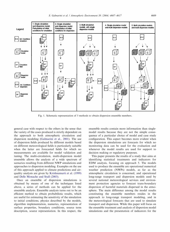
in the sketch of Fig. 1) namely:

1. Single circulation model and single dispersion model

with perturbation of initial conditions for circulation: For

a given case study, a number of atmospheric flow

simulations are performed by means of a single model

that uses different initial conditions. The flow fields can

in turn be the result of ensemble weather forecasting as

shown by Straume et al. (2001). The dispersion case is

simulated by means of a single dispersion model that

uses the various flow fields. As it was demonstrated, the

ensemble dispersion produced with this technique

accounts for the dependency of the case study on the

atmospheric circulation variability.

1 In this context dispersion modeling is intended as dispersion

from a single point-source. There is no specification on the scale

to which the circulation or the dispersion models relate. The

categorization presented applies to dispersion at any scale from

short range to global.

2. Single circulation model and single dispersion model

with ensemble perturbation of initial conditions for

dispersion: Given a single flow field obtained from a

circulation model, a single dispersion model is used to

simulate several dispersion scenarios. The latter are

obtained by varying the dispersion case configuration

(e.g. emission height, vertical distribution of mass

released). The dispersion cases can be obtained from

ad-hoc definitions or by means of Monte Carlo

techniques (e.g. Burmaster and Anderson, 2003), which

produce a number of cases randomly selected from a

predefined distribution of the dispersion initial para-

meters. The resulting ensemble takes into account the

dependency of the dispersion simulation on the disper-

sion initial conditions. Warner et al. (2002) presented

such an analysis for an application of dispersion models

at the mesoscale in the Arabic peninsula.

3. Multi circulation models with single dispersion

models: A suite of models generates circulation fields

of the same case study. The models can be different from

one another or be the same model used with different

parameterization schemes for physical or sub-grid

processes (Warner et al., 2002). By means of these fields,

a single dispersion model produces an ensemble of

dispersion fields. This approach is somewhat similar to

1, although the ensemble includes also the impact of

the circulation modeling approach on the dispersion

simulation.

4. Single circulation model and multi dispersion models:

A suite of dispersion models uses the results of a single

circulation model simulation. The ensemble obtained

accounts for the impact of dispersion modeling on the

case study. Examples of this type of application are

ATMES (Klug et al., 1992) and ATMES-II (Mosca

et al., 1998) in which however such an approach was

used for dispersion model validation studies rather than

for ensemble treatment.

5. Multi-circulation models and multi-dispersion mod-

els: Different circulation models calculate the circulation

fields. Dispersion models, which are conceptually

different from one another, use atmospheric circulation

fields from different models to produce dispersion

simulations on the same dispersion case study. The

dispersion fields resulting from each of the models

constitute the members of an ensemble. This is quite a

ARTICLE IN PRESS

Fig. 1. Schematic representation of 5 methods to obtain dispersion ensemble members.

S. Galmarini et al. / Atmospheric Environment 38 (2004) 4607–4617 4609

general case with respect to the others in the sense that

the variety of the cases produced is strictly dependent on

the approach to both atmospheric circulation and

dispersion modeling (Galmarini et al., 2001). The use

of dispersion fields produced by different models based

on different meteorological fields is particularly suitable

when the latter are forecasted fields for which no

measurements are available for model validation and

tuning. The multi-circulation, multi-dispersion model

ensemble allows the analysis of a wide spectrum of

scenarios resulting from different NWP simulations and

approaches to dispersion modeling. Examples on the use

of this approach applied to climate predictions and air-

quality analysis are given by Krishnamurti et al. (1999)

and Delle Monache and Stull (2003).

Once an ensemble of dispersion simulations is

obtained by means of one of the techniques listed

above, a series of methods can be applied for the

ensemble analysis. Ensemble analysis turns out to be an

efficient method to obtain probabilistic results, which

are useful for estimating the sensitivity of the simulation

to initial conditions, physics described by the models,

algorithm implementation, numerics, representation of

surface properties, boundary conditions, source term

description, source representation. In this respect, the

ensemble results contain more information than single-

model results because they are not the simple conse-

quence of a particular choice of model and case study

configuration. This aspect becomes more evident when

the dispersion simulations are forecasts for which no

monitoring data can be used for the evaluation and

whenever the model results are used for support to

decision making or regulatory purposes.

This paper presents the results of a study that aims at

identifying statistical treatments and indicators for

EDM analysis, focusing on approach 5. The models

used to produce the ensemble are operational numerical

weather prediction (NWPs) models, as far as the

atmospheric circulation is concerned, and operational

long-range transport and dispersion models used by

several national meteorological services and environ-

ment protection agencies to forecast trans-boundary

dispersion of harmful materials dispersed in the atmo-

sphere. The main difference among the model results

constituting the ensemble members resides in the

approach to long-range transport modeling, and in

the meteorological forecasts that are used to simulate

transport and dispersion. While this paper will focus on

the ensemble treatment and analysis of dispersion model

simulations and the presentation of indicators for the


multi-model ensemble analysis, Part II will show a

specific application of the technique and a quantitative

evaluation of the ensemble approach.

2. Framework: the ENSEMBLE project

The ENSEMBLE project2 was set up with the intent

of developing a system for the rapid exchange of long-

range transport and dispersion forecasts produced by

meteorological offices and radiation-protection agencies

in Europe and around the world. The dispersion models

are used in case of accidental releases of radioactive

material in the atmosphere. ENSEMBLE not only is

intended as a platform where several forecasts are

exchanged, but also as a tool for the simultaneous

analysis of the results of several models and for the

ensemble analysis. Briefly, ENSEMBLE is an Internet-

based server-side system (http://ensemble.ei.jrc.it) that

collects in real-time the long-range dispersion forecast

produced by 15 European, one US, and one Canadian

institute (Table 1). The forecasts are produced by

operational long-range transport and dispersion models

based on different concepts that use meteorological

fields produced by different NWP models (namely

ECMWF, various versions of HIRLAM, ARPEGE,

ALADIN, RAMS, GME, UM and LM). Model results

are produced over a domain bounded at (15E, 60W) and

(30N, 75N) with 0.5� resolution N–S and E–W and at 3-

hourly intervals for 60 h in the future from the notified

release time. More details on the ENSEMBLE system

and its technical specifications are described elsewhere

(Bianconi et al., 2004) and go beyond the scope of this

paper.

The ENSEMBLE system has been used during

exercises consisting of the notification to all the

participating institutes on the occurrence of a fictitious

release with defined characteristics (location of the

source, radio-nuclide released, release time, release

duration, release rate, release height). Upon notification

each institute produces a forecast of: air concentration

of a radio nuclide at 0, 200, 500, 1300, 3000m a.g.l.; time

integrated concentration at 0m a.g.l.; cumulated dry

deposition; cumulated wet deposition; Precipitation as

obtained from NWP. In total, 11 exercises were

performed as from Table 2. For each exercise, each

institute is requested to provide several dispersion

forecasts depending on the meteorological forecast

available during the evolution of the exercise. Therefore,

all dispersion forecasts submitted are initially based on a

completely forecasted meteorology, then on partly

forecasted and partly analyzed meteorology and finally

on completely analyzed meteorology. We will refer to

2Sponsored by the European Union DG-Research Technical

Development.

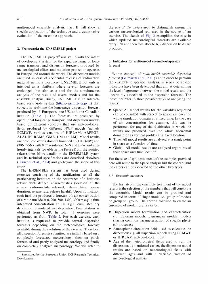
the age of the meteorology to distinguish among the

various meteorological sets used in the course of an

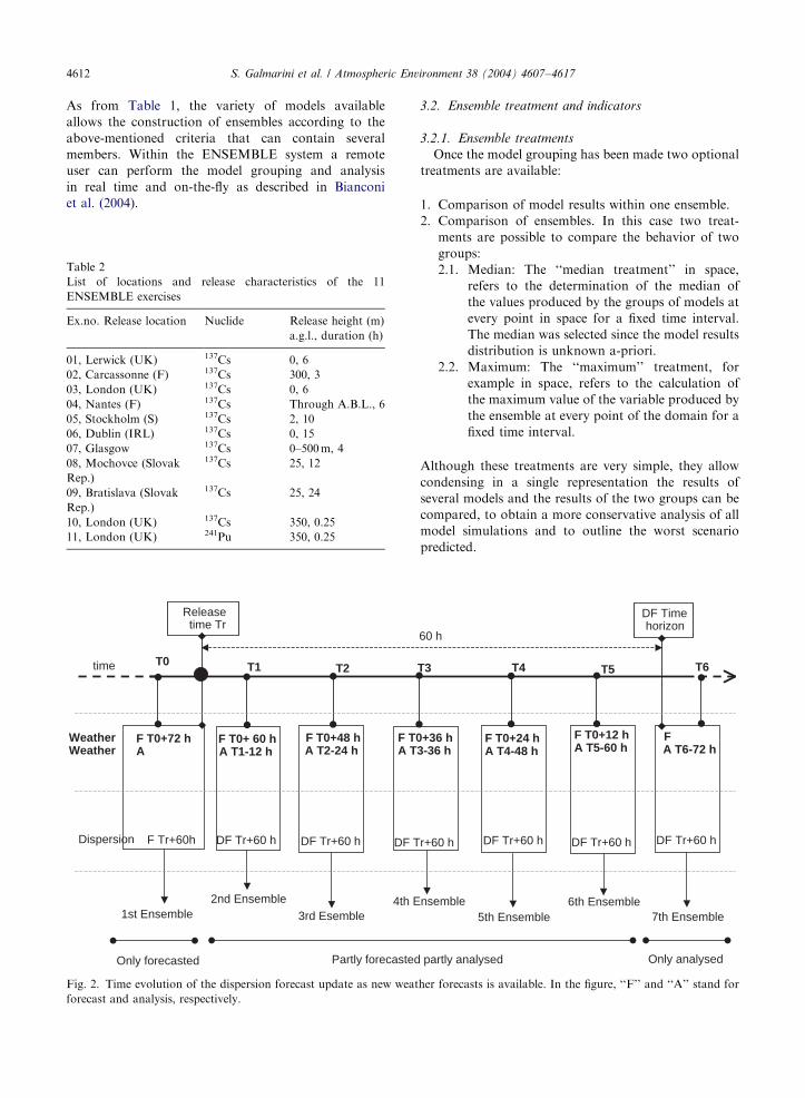
exercise. The sketch of Fig. 2 exemplifies the case in

which updated meteorological forecasts are available

every 12 h and therefore after 60 h, 7 dispersion fields are

produced.

3. Indicators for multi-model ensemble-dispersion

forecast

Within concept of multi-model ensemble dispersion

forecast (Galmarini et al., 2001) and in order to perform

the ensemble dispersion analysis, a series of ad-hoc

indicators have been developed that aim at determining

the level of agreement between the model results and the

uncertainty associated to the dispersion forecast. The

indicators refer to three possible ways of analyzing the

results:

* Space: All model results for the variables requested

can be consulted with respect to space: i.e. over the

whole simulation domain at a fixed time. In the case

of air concentration for example, this can be

performed for any of the 5 altitudes at which the

results are produced over the whole horizontal

domain or as vertical profiles at a fixed location.* Time: All model results are analyzed at a single point

in space as a function of time.* Global: All model results are analyzed regardless of

their space and time location.

For the sake of synthesis, most of the examples provided

here will relate to the Space analysis but the concept and

indicators can be extended to the other two types.

3.1. Ensemble members

The first step in the ensemble treatment of the model

results is the selection of the members that will constitute

the ensemble. Model results can be grouped and

compared in terms of single model vs. group of models

or group vs. group. The criteria followed to create an

ensemble of model results can be:

* Dispersion model formulation and characteristics:

e.g. Eulerian models, Lagrangian models, models

sharing common parameterization of specific physi-

cal processes;* Atmospheric circulation fields used to calculate the

dispersion: e.g. all dispersion models using ECMWF

or HIRLAM meteorological input;* Age of the meteorological fields used to run the

dispersion: as mentioned earlier, the dispersion model

results are based on meteorological fields with

different ages and with a variable fraction of

meteorological analysis.

http://ensemble.ei.jrc.it

ARTIC

LEIN

PRES

S

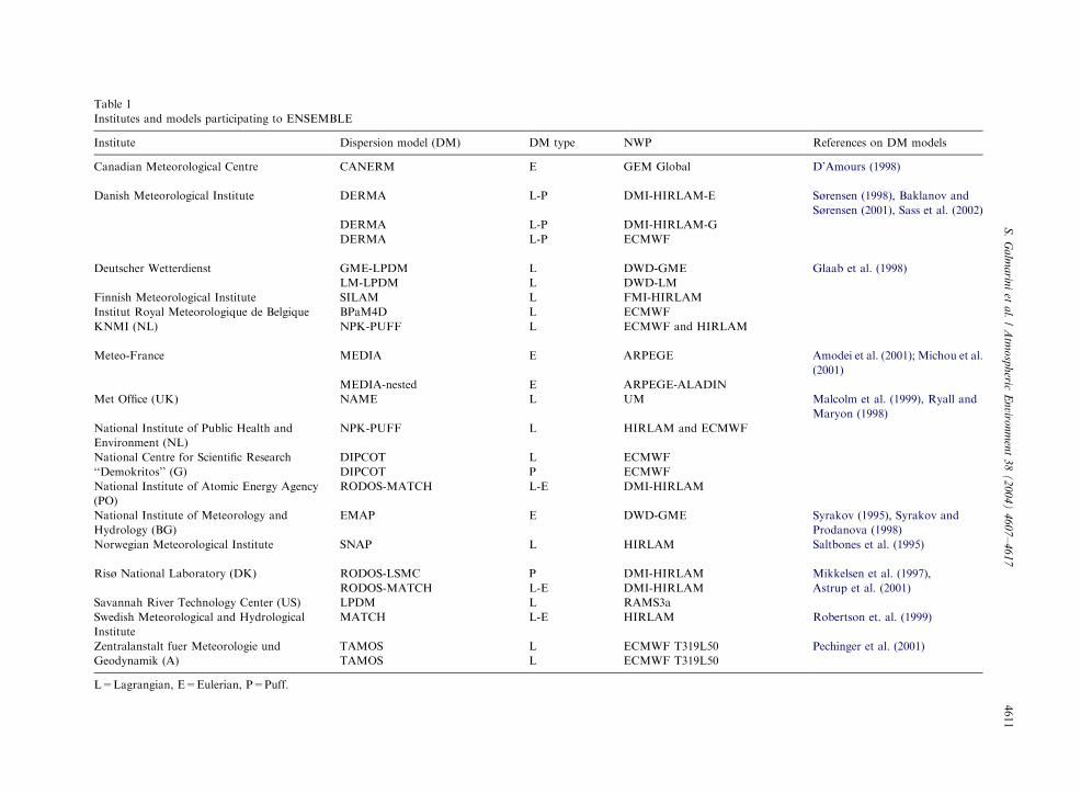
Table 1

Institutes and models participating to ENSEMBLE

Institute Dispersion model (DM) DM type NWP References on DM models

Canadian Meteorological Centre CANERM E GEM Global D’Amours (1998)

Danish Meteorological Institute DERMA L-P DMI-HIRLAM-E Sørensen (1998), Baklanov and

Sørensen (2001), Sass et al. (2002)

DERMA L-P DMI-HIRLAM-G

DERMA L-P ECMWF

Deutscher Wetterdienst GME-LPDM L DWD-GME Glaab et al. (1998)

LM-LPDM L DWD-LM

Finnish Meteorological Institute SILAM L FMI-HIRLAM

Institut Royal Meteorologique de Belgique BPaM4D L ECMWF

KNMI (NL) NPK-PUFF L ECMWF and HIRLAM

Meteo-France MEDIA E ARPEGE Amodei et al. (2001); Michou et al.

(2001)

MEDIA-nested E ARPEGE-ALADIN

Met Office (UK) NAME L UM Malcolm et al. (1999), Ryall and

Maryon (1998)

National Institute of Public Health and

Environment (NL)

NPK-PUFF L HIRLAM and ECMWF

National Centre for Scientific Research DIPCOT L ECMWF

‘‘Demokritos’’ (G) DIPCOT P ECMWF

National Institute of Atomic Energy Agency

(PO)

RODOS-MATCH L-E DMI-HIRLAM

National Institute of Meteorology and

Hydrology (BG)

EMAP E DWD-GME Syrakov (1995), Syrakov and

Prodanova (1998)

Norwegian Meteorological Institute SNAP L HIRLAM Saltbones et al. (1995)

Risø National Laboratory (DK) RODOS-LSMC P DMI-HIRLAM Mikkelsen et al. (1997),

RODOS-MATCH L-E DMI-HIRLAM Astrup et al. (2001)

Savannah River Technology Center (US) LPDM L RAMS3a

Swedish Meteorological and Hydrological

Institute

MATCH L-E HIRLAM Robertson et. al. (1999)

Zentralanstalt fuer Meteorologie und TAMOS L ECMWF T319L50 Pechinger et al. (2001)

Geodynamik (A) TAMOS L ECMWF T319L50

L=Lagrangian, E=Eulerian, P=Puff.

S.

Ga

lma

rini

eta

l./

Atm

osp

heric

En

viron

men

t3

8(

20

04

)4

60

7–

46

17

4611


As from Table 1, the variety of models available

allows the construction of ensembles according to the

above-mentioned criteria that can contain several

members. Within the ENSEMBLE system a remote

user can perform the model grouping and analysis

in real time and on-the-fly as described in Bianconi

et al. (2004).

Table 2

List of locations and release characteristics of the 11

ENSEMBLE exercises

Ex.no. Release location Nuclide Release height (m)

a.g.l., duration (h)

01, Lerwick (UK) 137Cs 0, 6

02, Carcassonne (F) 137Cs 300, 3

03, London (UK) 137Cs 0, 6

04, Nantes (F) 137Cs Through A.B.L., 6

05, Stockholm (S) 137Cs 2, 10

06, Dublin (IRL) 137Cs 0, 15

07, Glasgow 137Cs 0–500m, 4

08, Mochovce (Slovak

Rep.)

137Cs 25, 12

09, Bratislava (Slovak

Rep.)

137Cs 25, 24

10, London (UK) 137Cs 350, 0.25

11, London (UK) 241Pu 350, 0.25

F T0+72 h A

F T0+ 60 hA T1-12 h

F T0+48 hA T2-24 h

F T0A T

T0

F Tr+60h

1st Ensemble

DF Tr+60 h

2nd Ensemble

DF Tr+60 h

3rd Esemble

DF T

4th E

WeatherWeather

Dispersion

time

Only forecasted Partly forecasted

Release time Tr

T1 T2

Fig. 2. Time evolution of the dispersion forecast update as new weat

forecast and analysis, respectively.

3.2. Ensemble treatment and indicators

3.2.1. Ensemble treatments

Once the model grouping has been made two optional

treatments are available:

1. Comparison of model results within one ensemble.

2. Comparison of ensembles. In this case two treat-

ments are possible to compare the behavior of two

groups:

2.1. Median: The ‘‘median treatment’’ in space,

refers to the determination of the median of

the values produced by the groups of models at

every point in space for a fixed time interval.

The median was selected since the model results

distribution is unknown a-priori.

2.2. Maximum: The ‘‘maximum’’ treatment, for

example in space, refers to the calculation of

the maximum value of the variable produced by

the ensemble at every point of the domain for a

fixed time interval.

Although these treatments are very simple, they allow

condensing in a single representation the results of

several models and the results of the two groups can be

compared, to obtain a more conservative analysis of all

model simulations and to outline the worst scenario

predicted.

+36 h 3-36 h

F T0+24 hA T4-48 h

F T0+12 hA T5-60 h

r+60 h

nsemble

DF Tr+60 h

5th Ensemble

DF Tr+60 h

6th Ensemble

DF Time horizon

60 h

DF Tr+60 h

7th Ensemble

F A T6-72 h

partly analysed Only analysed

T3 T4 T5 T6

her forecasts is available. In the figure, ‘‘F’’ and ‘‘A’’ stand for

ARTICLE IN PRESS

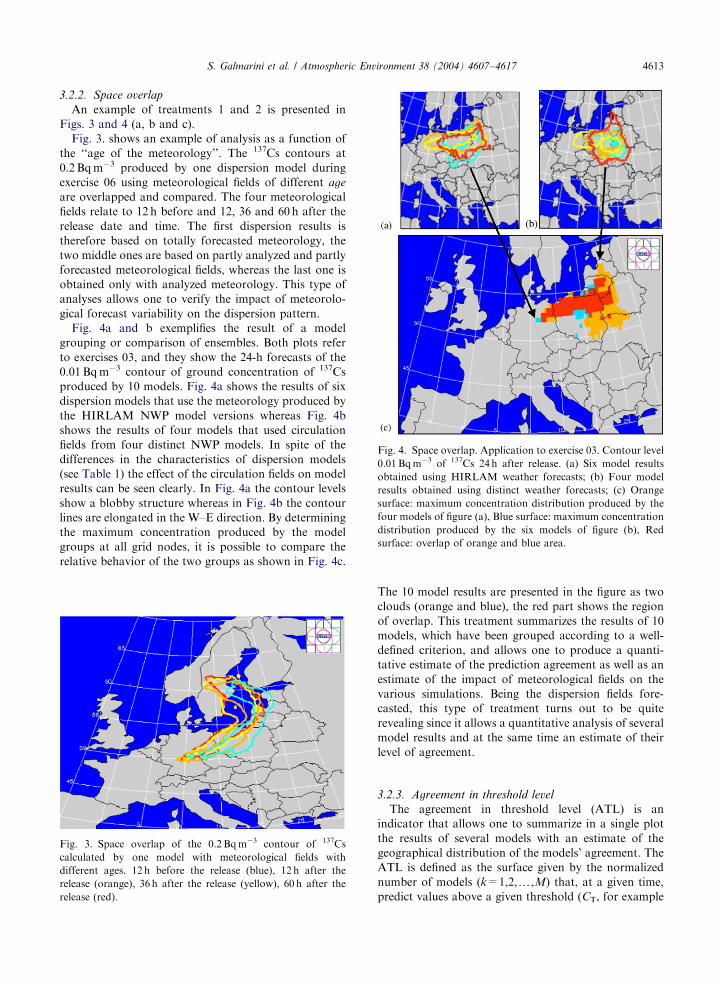
Fig. 4. Space overlap. Application to exercise 03. Contour level

0.01Bqm�3 of 137Cs 24 h after release. (a) Six model results

obtained using HIRLAM weather forecasts; (b) Four model

results obtained using distinct weather forecasts; (c) Orange

surface: maximum concentration distribution produced by the

four models of figure (a), Blue surface: maximum concentration

distribution produced by the six models of figure (b), Red

surface: overlap of orange and blue area.


3.2.2. Space overlap

An example of treatments 1 and 2 is presented in

Figs. 3 and 4 (a, b and c).

Fig. 3. shows an example of analysis as a function of

the ‘‘age of the meteorology’’. The 137Cs contours at

0.2 Bqm�3 produced by one dispersion model during

exercise 06 using meteorological fields of different age

are overlapped and compared. The four meteorological

fields relate to 12 h before and 12, 36 and 60 h after the

release date and time. The first dispersion results is

therefore based on totally forecasted meteorology, the

two middle ones are based on partly analyzed and partly

forecasted meteorological fields, whereas the last one is

obtained only with analyzed meteorology. This type of

analyses allows one to verify the impact of meteorolo-

gical forecast variability on the dispersion pattern.

Fig. 4a and b exemplifies the result of a model

grouping or comparison of ensembles. Both plots refer

to exercises 03, and they show the 24-h forecasts of the

0.01Bqm�3 contour of ground concentration of 137Cs

produced by 10 models. Fig. 4a shows the results of six

dispersion models that use the meteorology produced by

the HIRLAM NWP model versions whereas Fig. 4b

shows the results of four models that used circulation

fields from four distinct NWP models. In spite of the

differences in the characteristics of dispersion models

(see Table 1) the effect of the circulation fields on model

results can be seen clearly. In Fig. 4a the contour levels

show a blobby structure whereas in Fig. 4b the contour

lines are elongated in the W–E direction. By determining

the maximum concentration produced by the model

groups at all grid nodes, it is possible to compare the

relative behavior of the two groups as shown in Fig. 4c.

Fig. 3. Space overlap of the 0.2Bqm�3 contour of 137Cs

calculated by one model with meteorological fields with

different ages. 12 h before the release (blue), 12 h after the

release (orange), 36 h after the release (yellow), 60 h after the

release (red).

The 10 model results are presented in the figure as two

clouds (orange and blue), the red part shows the region

of overlap. This treatment summarizes the results of 10

models, which have been grouped according to a well-

defined criterion, and allows one to produce a quanti-

tative estimate of the prediction agreement as well as an

estimate of the impact of meteorological fields on the

various simulations. Being the dispersion fields fore-

casted, this type of treatment turns out to be quite

revealing since it allows a quantitative analysis of several

model results and at the same time an estimate of their

level of agreement.

3.2.3. Agreement in threshold level

The agreement in threshold level (ATL) is an

indicator that allows one to summarize in a single plot

the results of several models with an estimate of the

geographical distribution of the models’ agreement. The

ATL is defined as the surface given by the normalized

number of models (k=1,2,y,M) that, at a given time,

predict values above a given threshold (CT, for example

ARTICLE IN PRESS

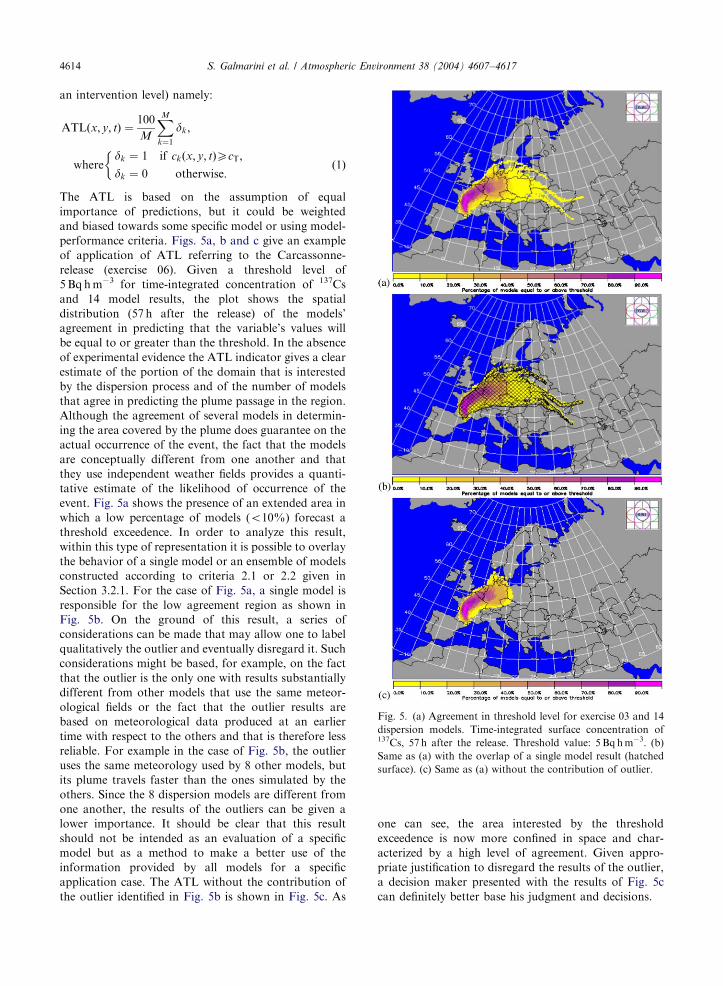
Fig. 5. (a) Agreement in threshold level for exercise 03 and 14

dispersion models. Time-integrated surface concentration of137Cs, 57 h after the release. Threshold value: 5 Bqhm�3. (b)

Same as (a) with the overlap of a single model result (hatched

surface). (c) Same as (a) without the contribution of outlier.

S. Galmarini et al. / Atmospheric Environment 38 (2004) 4607–46174614

an intervention level) namely:

ATLðx; y; tÞ ¼100

M

XM

k¼1

dk;

wheredk ¼ 1 if ckðx; y; tÞXcT;

dk ¼ 0 otherwise:

�ð1Þ

The ATL is based on the assumption of equal

importance of predictions, but it could be weighted

and biased towards some specific model or using model-

performance criteria. Figs. 5a, b and c give an example

of application of ATL referring to the Carcassonne-

release (exercise 06). Given a threshold level of

5Bqhm�3 for time-integrated concentration of 137Cs

and 14 model results, the plot shows the spatial

distribution (57 h after the release) of the models’

agreement in predicting that the variable’s values will

be equal to or greater than the threshold. In the absence

of experimental evidence the ATL indicator gives a clear

estimate of the portion of the domain that is interested

by the dispersion process and of the number of models

that agree in predicting the plume passage in the region.

Although the agreement of several models in determin-

ing the area covered by the plume does guarantee on the

actual occurrence of the event, the fact that the models

are conceptually different from one another and that

they use independent weather fields provides a quanti-

tative estimate of the likelihood of occurrence of the

event. Fig. 5a shows the presence of an extended area in

which a low percentage of models (o10%) forecast athreshold exceedence. In order to analyze this result,

within this type of representation it is possible to overlay

the behavior of a single model or an ensemble of models

constructed according to criteria 2.1 or 2.2 given in

Section 3.2.1. For the case of Fig. 5a, a single model is

responsible for the low agreement region as shown in

Fig. 5b. On the ground of this result, a series of

considerations can be made that may allow one to label

qualitatively the outlier and eventually disregard it. Such

considerations might be based, for example, on the fact

that the outlier is the only one with results substantially

different from other models that use the same meteor-

ological fields or the fact that the outlier results are

based on meteorological data produced at an earlier

time with respect to the others and that is therefore less

reliable. For example in the case of Fig. 5b, the outlier

uses the same meteorology used by 8 other models, but

its plume travels faster than the ones simulated by the

others. Since the 8 dispersion models are different from

one another, the results of the outliers can be given a

lower importance. It should be clear that this result

should not be intended as an evaluation of a specific

model but as a method to make a better use of the

information provided by all models for a specific

application case. The ATL without the contribution of

the outlier identified in Fig. 5b is shown in Fig. 5c. As

one can see, the area interested by the threshold

exceedence is now more confined in space and char-

acterized by a high level of agreement. Given appro-

priate justification to disregard the results of the outlier,

a decision maker presented with the results of Fig. 5c

can definitely better base his judgment and decisions.

ARTICLE IN PRESS

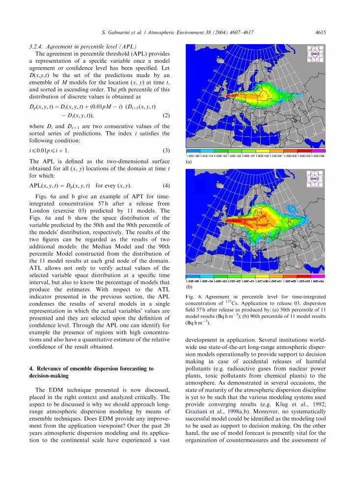
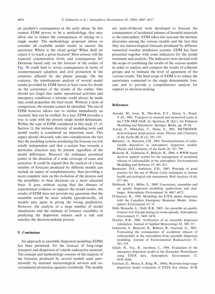
Fig. 6. Agreement in percentile level for time-integrated

concentration of 137Cs. Application to release 03, dispersion

field 57 h after release as produced by: (a) 50th percentile of 11

model results (Bq hm�3); (b) 90th percentile of 11 model results

(Bq hm�3).


3.2.4. Agreement in percentile level (APL)

The agreement in percentile threshold (APL) provides

a representation of a specific variable once a model

agreement or confidence level has been specified. Let

D(x,y,t) be the set of the predictions made by an

ensemble of M models for the location (x, y) at time t,

and sorted in ascending order. The pth percentile of this

distribution of discrete values is obtained as

Dpðx; y; tÞ ¼Diðx; y; tÞ þ ð0:01pM � iÞ�ðDiþ1ðx; y; tÞ

� Diðx; y; tÞÞ; ð2Þ

where Di and Di+1 are two consecutive values of the

sorted series of predictions. The index i satisfies the

following condition:

ip0:01ppi þ 1: ð3Þ

The APL is defined as the two-dimensional surface

obtained for all (x, y) locations of the domain at time t

for which:

APLðx; y; tÞ ¼ Dpðx; y; tÞ for evey ðx; yÞ: ð4Þ

Figs. 6a and b give an example of APT for time-

integrated concentration 57 h after a release from

London (exercise 03) predicted by 11 models. The

Figs. 6a and b show the space distribution of the

variable predicted by the 50th and the 90th percentile of

the models’ distribution, respectively. The results of the

two figures can be regarded as the results of two

additional models: the Median Model and the 90th

percentile Model constructed from the distribution of

the 11 model results at each grid node of the domain.

ATL allows not only to verify actual values of the

selected variable space distribution at a specific time

interval, but also to know the percentage of models that

produce the estimates. With respect to the ATL

indicator presented in the previous section, the APL

condenses the results of several models in a single

representation in which the actual variables’ values are

presented and they are selected upon the definition of

confidence level. Through the APL one can identify for

example the presence of regions with high concentra-

tions and also have a quantitative estimate of the relative

confidence of the result obtained.

4. Relevance of ensemble dispersion forecasting to

decision-making

The EDM technique presented is now discussed,

placed in the right context and analyzed critically. The

aspect to be discussed is why we should approach long-

range atmospheric dispersion modeling by means of

ensemble techniques. Does EDM provide any improve-

ment from the application viewpoint? Over the past 20

years atmospheric dispersion modeling and its applica-

tion to the continental scale have experienced a vast

development in application. Several institutions world-

wide use state-of-the-art long-range atmospheric disper-

sion models operationally to provide support to decision

making in case of accidental releases of harmful

pollutants (e.g. radioactive gases from nuclear power

plants, toxic pollutants from chemical plants) to the

atmosphere. As demonstrated in several occasions, the

state of maturity of the atmospheric dispersion discipline

is yet to be such that the various modeling systems used

provide converging results (e.g. Klug et al., 1992;

Graziani et al., 1998a,b). Moreover, no systematically

successful model could be identified as the modeling tool

to be used as support to decision making. On the other

hand, the use of model forecast is presently vital for the

organization of countermeasures and the assessment of


an accident’s consequences in the early phase. In this

context EDM proves to be a methodology that may

allow one to reduce the consequences of relying on a

single model. The methodology proposed allows to

consider all available model results to answer the

questions: Where is the cloud going? When shall we

expect it to reach a given location? How serious will the

expected concentration levels and consequences be?

Decisions based only on the forecast of the outlier of

Fig. 5b could lead to severe consequences in terms of

countermeasure adoption and civil protection in the

countries affected by the plume passage. On the

contrary, the simultaneous analysis of several model

results provided by EDM leaves at least room for doubt

on the correctness of the results of the outlier. One

should not forget that under operational activities and

emergency conditions a mistake could always be made

that could jeopardize the final result. Without a term of

comparison, the mistake cannot be identified. The use of

EDM however allows one to outline immediately an

anomaly that can be verified. In a way, EDM provides a

way to cope with the present single model deficiencies.

Within the type of EDM considered in this study (5. cf.

Section 1), the intrinsic diversity of modeling tools and

model results is considered an important asset. This

aspect should obviously take into consideration the fact

that the modeling systems producing the forecast are not

totally independent and that a certain bias towards a

particular situation may be present regardless of the

model differences. However the technique presented

points in the direction of a wide coverage of cases and

scenarios. It could be argued that the analysis of a large

number of forecasts produced by different models can

include an aspect of complementarity, thus providing a

more complete view on the evolution of the process and

the possibility to base decisions on a more educated

basis. It goes without saying that the absence of

experimental evidence to support the model results, the

results of EDM does not provide any guarantee that the

ensemble would be more reliable (paradoxically, all

models may agree in giving the wrong prediction).

However, the analysis of a large number of model

simulations and the estimate of forecast variability in

predicting the dispersion reduces such a risk and

enriches the decision-making process.

5. Conclusions

An approach to ensemble dispersion modeling (EDM)

has been presented, for the forecast of long-range

transport and dispersion of volatile radioactive material.

The concept and methodology consists of the analysis of

the forecasts produced by several models used oper-

ationally by national meteorological services and en-

vironmental protection agencies worldwide. The models

are state-of-the-art tools developed to forecast the

consequences of accidental releases of harmful materials

to the atmosphere. EDM takes into account the intrinsic

diversities among the various models and the fact that

they use meteorological forecasts produced by different

numerical weather prediction systems. EDM has been

presented together with some indicators for the model

treatment and analysis. The indicators were devised with

the scope of combining the results of the various models

in order to analyze and compare the results of coherent

groups and to estimate the level of agreement of the

various results. The final scope of EDM is to reduce the

uncertainty connected to the single deterministic fore-

cast and to provide a comprehensive analysis for

support to decision-making.

References

Amodei, M., Josse, B., Nho-Kim, E-Y., Simon, S., Peuch,

V.-H., 2001. Transport at resolved and unresolved scales in

the CTM MOCAGE. In: Sportisse, B. (Ed.), Air Pollution

Modelling and Simulation. Springer, Berlin, pp. 59–68.

Astrup, P., Mikkelsen, T., Deme, S., 2001. METRODOS:

meteorological preprocessor chain. Physics and Chemistry

of the Earth (B) 26 (2), 105–110.

Baklanov, A., Sørensen, J.H., 2001. Parameterisation of radio-

nuclide deposition in atmospheric dispersion models.

Physics and Chemistry of the Earth 26, 787–799.

Bianconi, R., Galmarini, S., Bellasio, R., 2004. A WWW-based

decision support system for the management of accidental

releases of radionuclides in the atmosphere. Environmental

Modelling and Software 19, 401–411.

Burmaster, D.E., Anderson, P.D., 2003. Principle of good

practice for the use of Monte Carlo techniques in human

health and ecological risk assessments. Risk Analysis 14 (4),

477–481.

Dabberdt, W.F., Miller, E., 2000. Uncertainty, ensembles and

air quality dispersion modelling: applications and chal-

lenges. Atmospheric Environment 34, 4667–4673.

D’Amours, R., 1998. Modelling the ETEX plume dispersion

with the Canadian Emergency Response Model. Atmo-

spheric Environment 32, 35.

Delle Monache, L., Stull, R.B., 2003. An ensemble air-quality

forecast over Europe during an ozone episode. Atmospheric

Environment 37, 3469–3474.

Draxler, R.R., 2002. Verification of an ensemble dispersion

calculation. Journal of Applied Meteorology 42, 308–317.

Galmarini, S., Bianconi, R., Bellasio, R., Graziani, G., 2001.

Forecasting the consequences of accidental releases of

radionuclides in the atmosphere from ensemble dispersion

modelling. Journal of Environmental Radioactivity 57,

203–219.

Glaab, H., Fay, B., Jacobsen, I., 1998. Evaluation of the

emergency dispersion model at the Deutscher Wetterdienst

using ETEX data. Atmospheric Environment 32,

4359–4366.

Graziani, G., Mosca, S., Klug, W., 1998a. Real-time long-range

dispersion model evaluation of ETEX first release. EUR

ARTICLE IN PRESSS. Galmarini et al. / Atmospheric Environment 38 (2004) 4607–4617 4617

17754/EN. Office for Official Publications of the European

Commission, Luxembourg.

Graziani, G., Klug, W., Galmarini, S., Grippa, G., 1998b. Real-

time long-range dispersion model evaluation of ETEX

second release. EUR 17755/EN. Office for Official Publica-

tions of the European Commission, Luxembourg.

Klug, W., Graziani, G., Grippa, G., Pierce, D., Tassone, C.,

1992. Evaluation of long range atmospheric models using

environmental radioactivity data from the Chernobyl

accident. ATMES Report. Elsevier Science Publishers

Ltd., Barking, UK, 366 pp.

Krishnamurti, T.N., Kishtawal, C.M., LaRow, T.E.,

Bachiochi, D.R., Zhang, Z., Willford, C.E., Gadfil, S.,

Surendran, S., 1999. Improved weather and seasonal climate

forecast from multimodel superensemble. Science 285,

1548–1550.

Malcolm, A.L., Derwent, R.G., Maryon, R.H., 1999. Model-

ling the long range transport of secondary PM10 to the UK.

Atmospheric Environment 34, 881–894.

Michou, M., Brocheton, F., Dufour, A., Peuch, V.-H., 2001.

Surface exchanges in the multiscale chemistry and transport

model MOCAGE. In: Sportisse, B. (Ed.), Air Pollution

Modelling and Simulation. Springer, Berlin, pp. 578–581.

Mikkelsen, T., Thykier-Nielsen, S., Astrup, P., Santabarbara,

J.M., Soerensen, J.H., Rasmussen, A., Robertson, L.,

Ullerstig, A., Bartzis, J.G., Deme, S., Martens, R., Dsler-

Sauer, J.P., 1997. MET-RODOS: a comprehensive atmo-

spheric dispersion module. Radiation Protection Dosimetry

73 (1–4), 45–56.

Mosca S., Bianconi, R., Bellasio, R., Graziani, G., Klug, W.,

1998. ATMES II—Evaluation of long-range

dispersion models using data of the 1st ETEX release.

EUR 17756 EN. Office for Official Publications of the

European Communities, Luxembourg, ISBN 92-828-3655-X,

458 pp.

Pechinger, U., Langer, M., Baumann, K., Petz, E., 2001. The

Austrian emergency response modelling system TAMOS.

Physics and Chemistry of the Earth (B) 26 (2), 99–103.

Robertson, L., Langner, J., Engardt, M., 1999. An Eulerian

limited-area atmospheric transport model. Journal of

Applied Meteorology 38, 190–209.

Ryall, D.B., Maryon, R.H., 1998. Validation of the UK Met.

Office’s NAME model against the ETEX dataset. Atmo-

spheric Environment 32 (24), 4265–4276.

Saltbones, J., Foss, A., Bartnicki, J., 1995. SANP: Severe

Nuclear Accident Program. Technical description. DNMI

Report No. 15. Norwegian Meteorological Institute, Oslo,

Norway.

Sass, B.H., Nielsen, N.W., Jørgensen, J.U., Amstrup, B., Kmit,

M., Mogensen, K., 2002. The operational HIRLAM system

2002 version. DMI Technical Report 02-05.

Sørensen, J.H., 1998. Sensitivity of the DERMA long-range

dispersion model to meteorological input and diffusion

parameters. Atmospheric Environment 32, 4195–4206.

Straume, A.G., 2001. A more extensive investigation of the use

of ensemble forecasts for dispersion model evaluation.

Journal of Applied Meteorology 40, 425–445.

Syrakov, D., 1995. On a PC-oriented Eulerian multi-level

model for long-term calculations of the regional sulphur

deposition. In: Gryning, S.E., Schiermeier, F.A. (Eds.), Air

Pollution Modelling and its Application XI 21. Plenum

Press, NY, London, pp. 645–646.

Syrakov, D., Prodanova, M., 1998. Bulgarian emergency

response models—validation against ETEX first release.

Atmospheric Environment 32, 4367–4375.

Warner, T.T., Sheu, R.S., Bowers, J.F., Sykes, R.I., Dodd,

G.C., Henn, D.S., 2002. Ensemble simulations with coupled

atmospheric dynamic and dispersion models: illustrating

uncertainties in dosage simulations. Journal of Applied

Meteorology 41, 488–504.

Ensemble dispersion forecasting—Part I: concept, approach and indicators

Documents

Transcript of Ensemble dispersion forecasting—Part I: concept, approach and indicators