5228 IEEE JOURNAL OF SELECTED TOPICS IN APPLIED EARTH OBSERVATIONS AND REMOTE SENSING, VOL. 10, NO. 12, DECEMBER 2017

A Deep-Learning-Based Forecasting Ensemble toPredict Missing Data for Remote Sensing Analysis

Monidipa Das , Student Member, IEEE, and Soumya K. Ghosh , Member, IEEE

Abstract—The problem of missing data in remote sensing anal-ysis is manifold. The situation becomes more serious during multi-temporal analysis when data at various a-periodic timestamps aremissing. In this work, we have proposed a deep-learning-basedframework (Deep-STEP_FE) for reconstructing the missing datato facilitate analysis with remote sensing time series. The idea is toutilize the available data from both earlier and subsequent times-tamps, while maintaining the causality constraint in spatiotemporalanalysis. The framework is based on an ensemble of multiple fore-casting modules, built upon the observed data in the time-seriessequence. The coupling between the forecasting modules is accom-plished with the help of dummy data, initially predicted using theearlier part of the sequence. Then, the dummy data are progres-sively improved in an iterative manner so that it can best conformto the next part of the sequence. Each of the forecasting modules inthe ensemble is based on Deep-STEP, a variant of the deep stackingnetwork learning approach. The work has been validated using acase study on predicting the missing images in normalized differ-ence vegetation index time series, derived from Landsat-7 TM-5satellite imagery over two spatial zones in India. Comparative per-formance analysis demonstrates the effectiveness of the proposedforecasting ensemble.

Index Terms—Causality constraint, deep learning, ensemble,missing data, prediction, remote sensing.

I. INTRODUCTION

R EMOTE sensing data play a significant role in land coverchange analysis, climate change detection, anthropogenic

impacts analysis, ecosystem monitoring, and so on [1], [2].However, one of the common obstacles, often appearing in re-mote sensing time-series analyses, is the nonavailability of datain the temporal sequence. The origin of such missing informa-tion is the unavailable source satellite imagery, which mainlyhappens due to low temporal frequency, defective sensor, pooratmospheric condition, or other image-specific problems. Amore grave situation arises in a multitemporal analysis whenall the complementary spatial information for a particular timeinstant is missing. Such an example has been depicted in Fig. 1.It shows a sequence of normalized difference vegetation index(NDVI) images, derived from Landsat-7 TM-5 raw satellite im-agery, where the image at time instant (t+ 3) is missing in the

Manuscript received March 14, 2017; revised July 27, 2017; accepted Septem-ber 19, 2017. Date of current version November 27, 2017. (Correspondingauthor: Monidipa Das.)

The authors are with the Department of Computer Science and Engi-neering, Indian Institute of Technology, Kharagpur 721302, India (e-mail:monidipadas@hotmail.com; skg@iitkgp.ac.in).

Color versions of one or more of the figures in this paper are available onlineat http://ieeexplore.ieee.org.

Digital Object Identifier 10.1109/JSTARS.2017.2760202

Fig. 1. Missing image in the sequence of NDVI imagery.

sequence from time t to (t+ 5). This may hinder the subsequentinterpretation, leading to inefficient performance of any analyt-ical process, like urban sprawl detection, land cover changeprediction, and so on. It is, therefore, necessary to somehowretrieve such missing images in order to facilitate the furtheranalyses with these data.

In this work, we aim at predicting such derived (single band)missing imagery by utilizing the available spatial information atthe other time instants in the given sequence, without disobey-ing the causality constraint in spatiotemporal (ST) analysis.As per the causality constraint, the conditioning neighborhoodshould consist of only the data from earlier timestamps [3].According to Snepvangers et al. [4], using values from futureevents to explain the past is “conceptually awkward” and canlead to “physically unrealistic” results, especially when suddeninputs in the system appear. Similar situation arises while usingbackcasting models (prediction in backward direction) or usingforward–backward ensembles [5] during prediction. In order tomaintain the causality constraint, one may choose to use onlypast measurements for missing value prediction; however, thisfails to properly utilize all the available information, especiallythose from future time instants.

In our work, we attempt to utilize the available values evenfrom the future timestamps, without contradicting with thecausality constraint. Our proposed Deep-STEP_FE is an ensem-ble of a number of forecasting modules (based on Deep-STEP[6]), each of which uses the consecutively available time-seriesdata (image) from past time instants to predict the immediatenext missing data (image) in the sequence. Each of these pre-dicted data items is further progressively tuned in an iterative

1939-1404 © 2017 IEEE. Personal use is permitted, but republication/redistribution requires IEEE permission.See http://www.ieee.org/publications standards/publications/rights/index.html for more information.

DAS AND GHOSH: DEEP-LEARNING-BASED FORECASTING ENSEMBLE TO PREDICT MISSING DATA FOR REMOTE SENSING ANALYSIS 5229

manner so that it best conforms to the next part of the entire se-quence. During the data tuning process also, we apply forecast-ing (prediction in forward direction) to maintain the causalityconstraint. While tuning, all the predicted data at intermediatetime instants are used along with the other available data in thesequence to predict the data for the latest available timestamp.The predicted data for this final timestamp are compared withthe original data of the corresponding timestamp. The processcontinues until the prediction accuracy reaches a particular levelof satisfaction. Since the overall prediction process is performedin the forward direction and the feature set of the training sam-ples is prepared using the data from the past time instants, thecausality constraints are maintained. The available spatial infor-mation from future is only used to check the conformity of thepredicted image with the corresponding original one.

A. Related Work and Motivation

Several techniques for predicting or reconstructing missingdata in the remote sensing imagery have been proposed tilldate. Depending on the source of complementary informationused for missing data reconstruction, these techniques can becategorized into four groups: spatial methods, spectral methods,temporal methods, and hybrid methods [7].

The spatial methods work without any other auxiliary infor-mation source. The propagated diffusion methods [8], spatialinterpolation methods [9], etc., are some widely used spatialmethods for regenerating the missing information in remotesensing analysis. However, since, in spatial methods, the recon-struction is done using the remaining data in the same imageonly, these methods cannot utilize the other data available in thetemporal sequence. Therefore, in the present context of multi-temporal analyses, the spatial methods are comparatively lessuseful. The spectral methods [10] utilize the spectral domainas the source of complementary information. These are suitablefor predicting missing data in multispectral and hyperspectralimagery, having redundant spectral information. However, thesemethods also fail to utilize the information available for the othertime instants. On the other hand, the temporal methods use thedata acquired at different time periods (at the same position)as the complementary information. The temporal replacementmethods, temporal learning models [11], etc., are somepopular methods of this kind. However, even with the availablespatial information, the temporal methods cannot utilize thesefor missing data prediction. Therefore, various hybrid methodshave recently been proposed, which attempt to make better useof the information hidden in the spatial, spectral, and tempo-ral dimensions. The combined ST [9] and spatiospectral [12]methods belong to this category.

Among these hybrid techniques, the spatiospectral meth-ods are not suitable for multitemporal analysis. On theother side, the ST methods, like STAR, STARMA [3], STkriging [9], STMRF [7], etc., are commonly used for ST predic-tion purpose. However, computation with a very large datasetcontaining several thousands of records/features becomes achallenging issue for most of these techniques. Moreover, themodels such as STAR, STARMA, etc., follow the causality

constraint, which restricts these techniques to use data from thesubsequent part of the temporal sequence.

In this work, we have proposed a deep-learning-based hy-brid ST model to predict the missing image for multitemporalremote sensing analysis. In our work, we are dealing with thedata derived from satellite remote sensing imagery containingmillions of pixels. In order to extract the intrinsic spatial/STfeatures/patterns from such voluminous data, we need someadvanced data mining techniques. Since deep learning offersefficient algorithms that can learn in multiple levels correspond-ing to different levels of abstractions, we have chosen the samein our present work of ST prediction. Our proposed model isan ensemble of multiple forecasting modules, each based on theDeep-STEP approach [6]. The objective behind the use of Deep-STEP as a constituent forecasting module is that the Deep-STEPhas been able to show encouraging performance in ST predictionof remote sensing data containing several thousands to millionsof pixels [6]. However, one of the limitations of the Deep-STEPis that, similar to the STAR and STARMA techniques, it is builton the base of causality constraint, which confines Deep-STEPto take advantage of the ST information in the subsequent partof the time series. Motivated by this fact, the present work pro-poses an ensemble model (Deep-STEP_FE), where the couplingbetween the Deep-STEP-based forecasting modules is done insuch a way that all the available data, both in the earlier andsubsequent timestamps with respect to the missing image, areproperly utilized without contradicting with the constraint.

B. Problem Statement and Contributions

The overall problem addressed in the present paper can beformally defined as follows.

1) Given a sequence of derived remote sensing imageryI1 , . . . , Im−1 , ?, Im+1 , . . . , Ix−1 , ?, Ix+1 , . . . , It over anyvariable for t number of timestamps, where the sign “?” in-dicates the missing images of some a-periodic timestamps,the problem is to predict or reconstruct the missing imagesIm , . . . , Ix , . . ., considering the same ST framework.

In this regard, our major contributions are as follows.1) Proposing a forecasting ensemble model (Deep-

STEP_FE) to predict missing data for remote sensinganalysis, by utilizing available ST data from both earlierand subsequent timestamps.

2) Exploring deep-learning-based ST analysis techniquesfor missing image reconstruction purpose.

3) Overcoming the limitation of the Deep-STEP approach[6] while maintaining the causality constraints in spatialtime-series analysis.

4) Validating the proposed Deep-STEP_FE approach in pre-dicting missing NDVI imagery (derived from Landsat-7TM-5 raw satellite time series [13] over two spatial zonesin India), each containing several thousands of pixels.

The rest of this paper is organized as follows. The architectureand learning procedure of our proposed deep-learning-basedforecasting ensemble has been illustrated in Section II. Theexperimentation and results are discussed in Section III. Finally,the concluding remarks have been made in Section IV.

5230 IEEE JOURNAL OF SELECTED TOPICS IN APPLIED EARTH OBSERVATIONS AND REMOTE SENSING, VOL. 10, NO. 12, DECEMBER 2017

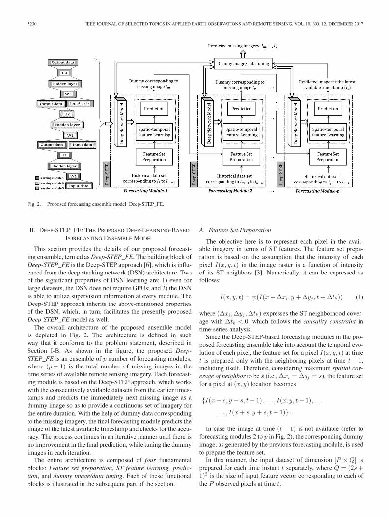
Fig. 2. Proposed forecasting ensemble model: Deep-STEP_FE.

II. DEEP-STEP_FE: THE PROPOSED DEEP-LEARNING-BASED

FORECASTING ENSEMBLE MODEL

This section provides the details of our proposed forecast-ing ensemble, termed as Deep-STEP_FE. The building block ofDeep-STEP_FE is the Deep-STEP approach [6], which is influ-enced from the deep stacking network (DSN) architecture. Twoof the significant properties of DSN learning are: 1) even forlarge datasets, the DSN does not require GPUs; and 2) the DSNis able to utilize supervision information at every module. TheDeep-STEP approach inherits the above-mentioned propertiesof the DSN, which, in turn, facilitates the presently proposedDeep-STEP_FE model as well.

The overall architecture of the proposed ensemble modelis depicted in Fig. 2. The architecture is defined in suchway that it conforms to the problem statement, described inSection I-B. As shown in the figure, the proposed Deep-STEP_FE is an ensemble of p number of forecasting modules,where (p− 1) is the total number of missing images in thetime series of available remote sensing imagery. Each forecast-ing module is based on the Deep-STEP approach, which workswith the consecutively available datasets from the earlier times-tamps and predicts the immediately next missing image as adummy image so as to provide a continuous set of imagery forthe entire duration. With the help of dummy data correspondingto the missing imagery, the final forecasting module predicts theimage of the latest available timestamp and checks for the accu-racy. The process continues in an iterative manner until there isno improvement in the final prediction, while tuning the dummyimages in each iteration.

The entire architecture is composed of four fundamentalblocks: Feature set preparation, ST feature learning, predic-tion, and dummy image/data tuning. Each of these functionalblocks is illustrated in the subsequent part of the section.

A. Feature Set Preparation

The objective here is to represent each pixel in the avail-able imagery in terms of ST features. The feature set prepa-ration is based on the assumption that the intensity of eachpixel I(x, y, t) in the image raster is a function of intensityof its ST neighbors [3]. Numerically, it can be expressed asfollows:

I(x, y, t) = ψ(I(x+ Δxi, y + Δyj , t+ Δtk )) (1)

where (Δxi,Δyj ,Δtk ) expresses the ST neighborhood cover-age with Δtk < 0, which follows the causality constraint intime-series analysis.

Since the Deep-STEP-based forecasting modules in the pro-posed forecasting ensemble take into account the temporal evo-lution of each pixel, the feature set for a pixel I(x, y, t) at timet is prepared only with the neighboring pixels at time t− 1,including itself. Therefore, considering maximum spatial cov-erage of neighbor to be s (i.e., Δxi = Δyj = s), the feature setfor a pixel at (x, y) location becomes

{I(x− s, y − s, t− 1), . . . , I(x, y, t− 1), . . .

. . . , I(x+ s, y + s, t− 1)} .

In case the image at time (t− 1) is not available (refer toforecasting modules 2 to p in Fig. 2), the corresponding dummyimage, as generated by the previous forecasting module, is usedto prepare the feature set.

In this manner, the input dataset of dimension [P ×Q] isprepared for each time instant t separately, where Q = (2s+1)2 is the size of input feature vector corresponding to each ofthe P observed pixels at time t.

DAS AND GHOSH: DEEP-LEARNING-BASED FORECASTING ENSEMBLE TO PREDICT MISSING DATA FOR REMOTE SENSING ANALYSIS 5231

B. Spatiotemporal (ST) Feature Learning

The ST feature learning within each forecasting module in theproposed ensemble is based on the deep network model used inthe Deep-STEP approach.

1) Deep Network Architecture: The deep network archi-tecture is an integral part of Deep-STEP, which has beenused in each of the forecasting modules within the proposedensemble model (Deep-STEP_FE). The central idea of this ar-chitecture is the concept of stacking, like that in the DSN [14],where the simple modules of functions are composed first, andthen, these are stacked on top of each other for learning complexfunctions. A simplified architecture of the network model withonly three such modules is shown in the left-hand side of Fig. 2.Each of the feature learning modules in the deep network modelis basically perceptron with single layers of hidden neurons andhas been denoted by distinct patterns/shades. However, in anactual prediction scenario, the total number of learning modulein the network will be equal to the total number of consecu-tive training images available for the corresponding forecastingmodule. Thus, if the number of training images is increased,the number of modules and, hence, the depth of the architecturewill also increase.

The output of each learning module (except the top mostone) is the learned spatial feature set for the corresponding timeinstant, whereas the input to each learning module is the com-bined raw spatial feature set as prepared in the above-discussedmanner (see Section II-A) and the spatial feature set learned bythe previous learning module. In case of the first forecastingmodule, the input to the bottom-most learning module is onlythe raw spatial feature set corresponding to the first availableimage in the sequence. The output of the top-most module is thepredicted value at a given pixel location in the correspondingmissing image. After the required processing, these values areused as the dummy values to aid the feature set preparation inthe subsequent forecasting module. In case of the final forecast-ing module, the output of the top-most learning module is thepredicted value at a given pixel location in the latest availableimage (It) in the sequence.

2) Deep Network Learning: Let, for any learning module inthe deep network model, the training vectors are denoted byX =[x1 , x2 , . . . , xP ]T , in which each input vector xi is of dimensionD and is denoted by xi = [xi1 , xi2 , . . . , xiD ], and P is the totalnumber of training samples. Also, let H = [h1 , h2 , . . . , hP ]T

denote the activity matrix over all training samples in the hiddenlayer, let L denote the number of hidden units, and let C denotethe output vector dimension for any learning module. Then, theoutput of any learning module can be expressed as follows

Y = σ(σ(XWT

)UT

)(2)

where U is a [C × L]-dimensional weight matrix at the upperlayer within the module, W is an [L×D]-dimensional weightmatrix at the lower layer within the same module, and σ(.) is asigmoid function. Moreover, as per the Deep-STEP approach,the value of D for the bottom-most module is Q, whereas thatfor all the higher level modules is 2Q.

Under this deep learning architectural setting, the weight ma-trices W and U in each learning module are learned as per theDeep-STEP approach in the following manner.

Let the target vectors over P samples be T =[t1 , t2 , . . . , tP ]T , where each ti = [ti1 , ti2 , . . . , tiC ]. Then, thecost function is as follows:

J=− 1P

P∑

i=1

C∑

j=1

[tij log yij + (1 − tij ) log (1 − yij )] +G (3)

where G is the regularization term computed as follows:

G =λ

2P

⎡

⎣L∑

i=1

D∑

j=1

w2ij +

C∑

i=1

L∑

j=1

u2ij

⎤

⎦ (4)

where λ is the regularization parameter; uij and wij are theelements in the ith row and the jth column in the matrices Uand W , respectively.

Then, as per Deep-STEP, the gradient calculation for the costfunction is performed using backpropagation in the followingway.

For the lower layer weights, we have

∂J

∂W=

1P

[[((Y − T )U) ◦ σ′(

XWT)]T

X

]+

λ

PW (5)

=1P

[[((Y − T )U) ◦ σ′(

XWT)]T

X + λW

](6)

where

σ′(XWT

)= σ

(XWT

) ◦ (1 − σ

(XWT

))(7)

and symbol “◦” denotes elementwise multiplication.Similarly, for the upper layer weights in the module, we have

∂J

∂U=

1P

[(Y − T )T σ

(XWT

)]+

λ

PU (8)

=1P

[(Y − T )T σ

(XWT

)+ λU

]. (9)

During the learning process, the output Y of each precedinglearning module is merged with the input feature set correspond-ing to the immediate next time instant and then the merged out-put is fed as the set of input vectors in the succeeding learningmodule (see Fig. 2). It helps to incorporate the temporal evo-lution of the pixels/data points in the feature learning process.Moreover, the input dataset X is normalized so that it remainsconsistent with the learning module outputs, which are forcedto be in the range [0, 1], because of using the binary sigmoidfunction (σ(.)).

C. Prediction

On the basis of the updated weight values and ST featureslearned at the bottom levels, the top-most layer in the deep net-work within each forecasting module generates aP -dimensionalvector Y , denoting the predicted values. Since the predictedvalues are obtained in normalized form within the range [0, 1],these are further mapped to the original scale by means of linearstretching to obtain the actual prediction values. The predictedvalues from the final or pth forecasting module are used to

5232 IEEE JOURNAL OF SELECTED TOPICS IN APPLIED EARTH OBSERVATIONS AND REMOTE SENSING, VOL. 10, NO. 12, DECEMBER 2017

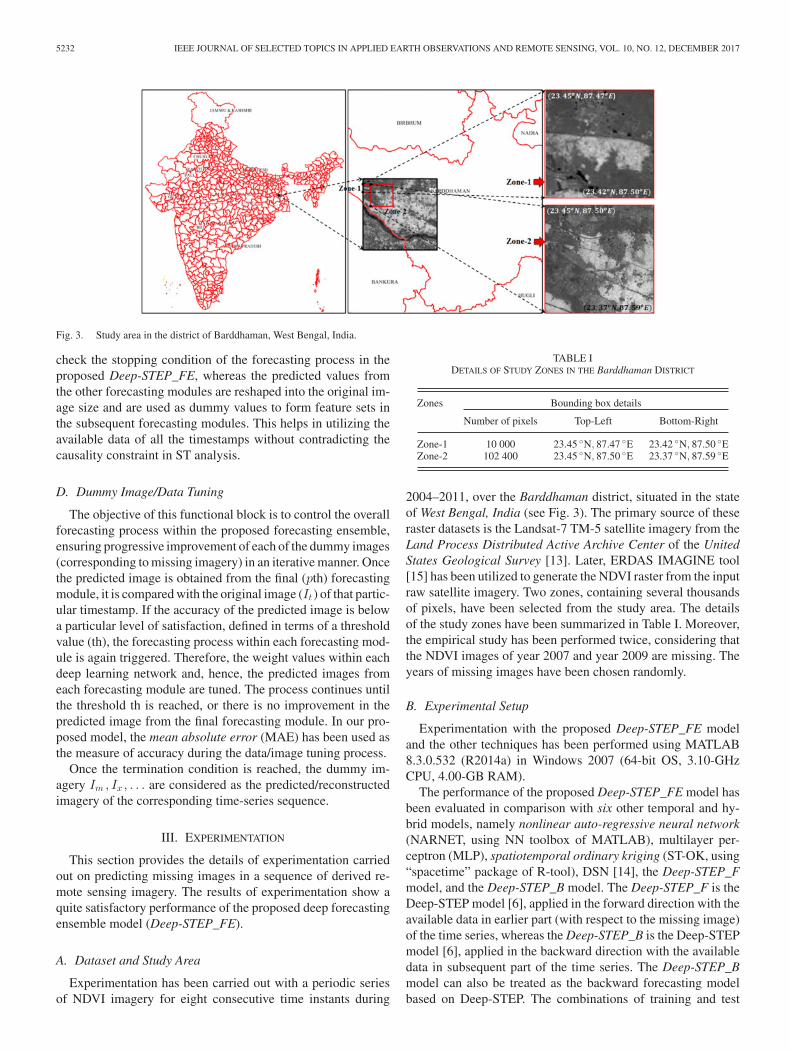
Fig. 3. Study area in the district of Barddhaman, West Bengal, India.

check the stopping condition of the forecasting process in theproposed Deep-STEP_FE, whereas the predicted values fromthe other forecasting modules are reshaped into the original im-age size and are used as dummy values to form feature sets inthe subsequent forecasting modules. This helps in utilizing theavailable data of all the timestamps without contradicting thecausality constraint in ST analysis.

D. Dummy Image/Data Tuning

The objective of this functional block is to control the overallforecasting process within the proposed forecasting ensemble,ensuring progressive improvement of each of the dummy images(corresponding to missing imagery) in an iterative manner. Oncethe predicted image is obtained from the final (pth) forecastingmodule, it is compared with the original image (It ) of that partic-ular timestamp. If the accuracy of the predicted image is belowa particular level of satisfaction, defined in terms of a thresholdvalue (th), the forecasting process within each forecasting mod-ule is again triggered. Therefore, the weight values within eachdeep learning network and, hence, the predicted images fromeach forecasting module are tuned. The process continues untilthe threshold th is reached, or there is no improvement in thepredicted image from the final forecasting module. In our pro-posed model, the mean absolute error (MAE) has been used asthe measure of accuracy during the data/image tuning process.

Once the termination condition is reached, the dummy im-agery Im , Ix , . . . are considered as the predicted/reconstructedimagery of the corresponding time-series sequence.

III. EXPERIMENTATION

This section provides the details of experimentation carriedout on predicting missing images in a sequence of derived re-mote sensing imagery. The results of experimentation show aquite satisfactory performance of the proposed deep forecastingensemble model (Deep-STEP_FE).

A. Dataset and Study Area

Experimentation has been carried out with a periodic seriesof NDVI imagery for eight consecutive time instants during

TABLE IDETAILS OF STUDY ZONES IN THE Barddhaman DISTRICT

Zones Bounding box details

Number of pixels Top-Left Bottom-Right

Zone-1 10 000 23.45 ◦N, 87.47 ◦E 23.42 ◦N, 87.50 ◦EZone-2 102 400 23.45 ◦N, 87.50 ◦E 23.37 ◦N, 87.59 ◦E

2004–2011, over the Barddhaman district, situated in the stateof West Bengal, India (see Fig. 3). The primary source of theseraster datasets is the Landsat-7 TM-5 satellite imagery from theLand Process Distributed Active Archive Center of the UnitedStates Geological Survey [13]. Later, ERDAS IMAGINE tool[15] has been utilized to generate the NDVI raster from the inputraw satellite imagery. Two zones, containing several thousandsof pixels, have been selected from the study area. The detailsof the study zones have been summarized in Table I. Moreover,the empirical study has been performed twice, considering thatthe NDVI images of year 2007 and year 2009 are missing. Theyears of missing images have been chosen randomly.

B. Experimental Setup

Experimentation with the proposed Deep-STEP_FE modeland the other techniques has been performed using MATLAB8.3.0.532 (R2014a) in Windows 2007 (64-bit OS, 3.10-GHzCPU, 4.00-GB RAM).

The performance of the proposed Deep-STEP_FE model hasbeen evaluated in comparison with six other temporal and hy-brid models, namely nonlinear auto-regressive neural network(NARNET, using NN toolbox of MATLAB), multilayer per-ceptron (MLP), spatiotemporal ordinary kriging (ST-OK, using“spacetime” package of R-tool), DSN [14], the Deep-STEP_Fmodel, and the Deep-STEP_B model. The Deep-STEP_F is theDeep-STEP model [6], applied in the forward direction with theavailable data in earlier part (with respect to the missing image)of the time series, whereas the Deep-STEP_B is the Deep-STEPmodel [6], applied in the backward direction with the availabledata in subsequent part of the time series. The Deep-STEP_Bmodel can also be treated as the backward forecasting modelbased on Deep-STEP. The combinations of training and test

DAS AND GHOSH: DEEP-LEARNING-BASED FORECASTING ENSEMBLE TO PREDICT MISSING DATA FOR REMOTE SENSING ANALYSIS 5233

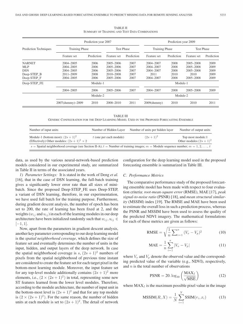
TABLE IISUMMARY OF TRAINING AND TEST DATA COMBINATIONS

Prediction year 2007 Prediction year 2009

Prediction Techniques Training Phase Test Phase Training Phase Test Phase

Feature set Prediction Feature set Prediction Feature set Prediction Feature set Prediction

NARNET 2004–2005 2006 2005–2006 2007 2004–2007 2008 2005–2008 2009MLP 2004–2005 2006 2005–2006 2007 2004–2007 2008 2005–2008 2009DSN 2004–2005 2006 2005–2006 2007 2004–2007 2008 2005–2008 2009Deep-STEP_B 2011–2009 2008 2010–2008 2007 2011 2010 2010 2009Deep-STEP_F 2004–2005 2006 2005–2006 2007 2004–2007 2008 2005–2008 2009

Deep-STEP_FE Module-1 Module-1

2004–2005 2006 2005–2006 2007 2004–2007 2008 2005–2008 2009

Module-2 Module-2

2007(dummy)–2009 2010 2008–2010 2011 2009(dummy) 2010 2010 2011

TABLE IIIGENERIC CONFIGURATION FOR THE DEEP LEARNING MODEL USED IN THE PROPOSED FORECASTING ENSEMBLE

Number of input units Number of Hidden Layer Number of units per hidden layer Number of output units

Module-1 (bottom most): (2s + 1)2 t (one per each module) (2s + 1)2 Top most module:1(Effectively) Other modules: (2s + 1)2 × 2 Other modules:(2s + 1)2

s = Spatial neighborhood coverage (see Section II-A); t = Number of training images; m = Module sequence number; m = 1, 2, . . . , t

data, as used by the various neural-network-based predictionmodels considered in our experimental study, are summarizedin Table II in terms of the associated years.

1) Parameter Settings: It is stated in the work of Deng et al.[16], that in the case of DSN learning, the full-batch traininggives a significantly lower error rate than all sizes of mini-batch. Since the proposed Deep-STEP_FE uses Deep-STEP,a variant of DSN learning, therefore, in our experimentation,we have used full batch for the training purpose. Furthermore,during gradient descent analysis, the number of epoch has beenset to 200, the rate of learning has been fixed at 2, and theweights (wij anduij ) in each of the learning modules in our deeparchitecture have been initialized randomly such that wij , uij ∈[−1, 1].

Now, apart from the parameters in gradient descent analysis,another key parameter corresponding to our deep learning modelis the spatial neighborhood coverage, which defines the size offeature set and eventually determines the number of units in theinput, hidden, and output layers of the deep network. In casethe spatial neighborhood coverage is s, (2s+ 1)2 numbers ofpixels from the spatial neighborhood of previous time instantare considered to create the feature set for each target pixel in thebottom-most learning module. Moreover, the input feature setfor any top-level module additionally contains (2s+ 1)2 moreelements, i.e., (2 × (2s+ 1)2) in total, representing some newST features learned from the lower level modules. Therefore,according to the module architecture, the number of input unit inthe bottom-most level is (2s+ 1)2 and that for any top moduleis (2 × (2s+ 1)2). For the same reason, the number of hiddenunits at each module is set to (2s+ 1)2 . The detail of network

configuration for the deep learning model used in the proposedforecasting ensemble is summarized in Table III.

C. Performance Metrics

The comparative performance study of the proposed forecast-ing ensemble model has been made with respect to four evalua-tion criteria: root-mean-square error (RMSE), MAE [17], peaksignal-to-noise ratio (PSNR) [18], and mean structural similar-ity (MSSIM) index [19]. The RMSE and MAE have been usedto estimate the overall loss in such a prediction process, whereasthe PSNR and MSSIM have been used to assess the quality ofthe predicted NDVI imagery. The mathematical formulationsfor each of these metrics are given as follows:

RMSE =

√1n

∑n

i=1(Vo − Vp)2 (10)

MAE =1n

n∑

i=1

|Vo − Vp | (11)

where Vo and Vp denote the observed value and the correspond-ing predicted value of the variable (e.g., NDVI), respectively,and n is the total number of observations

PSNR = 20. log10

(MAXI√

MSE

)(12)

where MAXI is the maximum possible pixel value in the image

MSSIM(R,X) =1N

N∑

i=1

SSIM(ri, xi) (13)

5234 IEEE JOURNAL OF SELECTED TOPICS IN APPLIED EARTH OBSERVATIONS AND REMOTE SENSING, VOL. 10, NO. 12, DECEMBER 2017

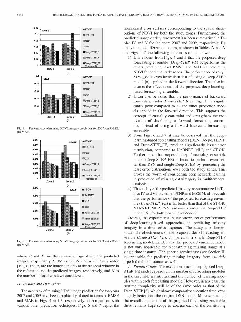
Fig. 4. Performance of missing NDVI imagery prediction for 2007. (a) RMSE.(b) MAE.

Fig. 5. Performance of missing NDVI imagery prediction for 2009. (a) RMSE.(b) MAE.

where R and X are the reference/original and the predictedimages, respectively, SSIM is the structural similarity index[19], ri and xi are the image contents at the ith local window inthe reference and the predicted images, respectively, and N isthe number of local windows considered.

D. Results and Discussion

The accuracy of missing NDVI image prediction for the years2007 and 2009 have been graphically plotted in terms of RMSEand MAE in Figs. 4 and 5, respectively, in comparison withvarious other prediction techniques. Figs. 6 and 7 depict the

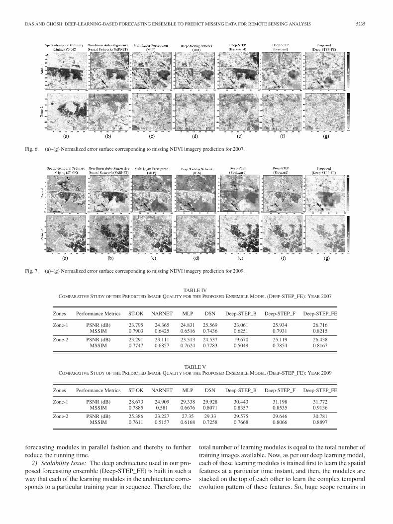
normalized error surfaces corresponding to the spatial distri-butions of NDVI for both the study zones. Furthermore, thepredicted image quality assessment has been summarized in Ta-bles IV and V for the years 2007 and 2009, respectively. Byanalyzing the different outcomes, as shown in Tables IV and Vand Figs. 4–7, the following inferences can be drawn.

1) It is evident from Figs. 4 and 5 that the proposed deepforecasting ensemble (Deep-STEP_FE) outperforms theothers producing least RMSE and MAE in predictingNDVI for both the study zones. The performance of Deep-STEP_FE is even better than that of a single Deep-STEPmodel [6], applied in the forward direction. This also in-dicates the effectiveness of the proposed deep-learning-based forecasting ensemble.

2) It can also be noted that the performance of backwardforecasting (refer Deep-STEP_B in Fig. 4) is signifi-cantly poor compared to all the other prediction mod-els applied in the forward direction. This supports theconcept of causality constraint and strengthens the mo-tivation of developing a forward forecasting ensem-ble, instead of using a forward–backward forecastingensemble.

3) From Figs. 6 and 7, it may be observed that the deep-learning-based forecasting models (DSN, Deep-STEP_F,and Deep-STEP_FE) produce significantly lesser errordistribution, compared to NARNET, MLP, and ST-OK.Furthermore, the proposed deep forecasting ensemblemodel (Deep-STEP_FE) is found to perform even bet-ter than DSN and single Deep-STEP, by generating theleast error distributions over both the study zones. Thisproves the worth of considering deep network learningin prediction of missing data/imagery in multitemporalanalysis.

4) The quality of the predicted imagery, as summarized in Ta-bles IV and V in terms of PSNR and MSSIM, also revealsthat the performance of the proposed forecasting ensem-ble (Deep-STEP_FE) is far better than that of the ST-OK,NARNET, MLP, DSN, and even stand-alone Deep-STEPmodel [6], for both Zone-1 and Zone-2.

Overall, the experimental study shows better performanceof deep-learning-based approaches in predicting missingimagery in a time-series sequence. The study also demon-strates the effectiveness of the proposed deep forecasting en-semble (Deep-STEP_FE), compared to a single Deep-STEPforecasting model. Incidentally, the proposed ensemble modelis not only applicable for reconstructing missing image at asingle time instance. The generic architecture (see Section II)is applicable for predicting missing imagery from multiplea-periodic time instances as well.

1) Running Time: The execution time of the proposed Deep-STEP_FE model depends on the number of forecasting modulesin the ensemble architecture and the number of learning mod-ules within each forecasting module. However, in any case, theruntime complexity will be of the same order as that of theDeep-STEP [6], which shows comparative execution time, evenslightly better than the original DSN model. Moreover, as perthe overall architecture of the proposed forecasting ensemble,there remains huge scope to execute each of the constituting

DAS AND GHOSH: DEEP-LEARNING-BASED FORECASTING ENSEMBLE TO PREDICT MISSING DATA FOR REMOTE SENSING ANALYSIS 5235

Fig. 6. (a)–(g) Normalized error surface corresponding to missing NDVI imagery prediction for 2007.

Fig. 7. (a)–(g) Normalized error surface corresponding to missing NDVI imagery prediction for 2009.

TABLE IVCOMPARATIVE STUDY OF THE PREDICTED IMAGE QUALITY FOR THE PROPOSED ENSEMBLE MODEL (DEEP-STEP_FE): YEAR 2007

Zones Performance Metrics ST-OK NARNET MLP DSN Deep-STEP_B Deep-STEP_F Deep-STEP_FE

Zone-1 PSNR (dB) 23.795 24.365 24.831 25.569 23.061 25.934 26.716MSSIM 0.7903 0.6425 0.6516 0.7436 0.6251 0.7931 0.8215

Zone-2 PSNR (dB) 23.291 23.111 23.513 24.537 19.670 25.119 26.438MSSIM 0.7747 0.6857 0.7624 0.7783 0.5049 0.7854 0.8167

TABLE VCOMPARATIVE STUDY OF THE PREDICTED IMAGE QUALITY FOR THE PROPOSED ENSEMBLE MODEL (DEEP-STEP_FE): YEAR 2009

Zones Performance Metrics ST-OK NARNET MLP DSN Deep-STEP_B Deep-STEP_F Deep-STEP_FE

Zone-1 PSNR (dB) 28.673 24.909 29.338 29.928 30.443 31.198 31.772MSSIM 0.7885 0.581 0.6676 0.8071 0.8357 0.8535 0.9136

Zone-2 PSNR (dB) 25.386 23.227 27.35 29.33 29.575 29.646 30.781MSSIM 0.7611 0.5157 0.6168 0.7258 0.7668 0.8066 0.8897

forecasting modules in parallel fashion and thereby to furtherreduce the running time.

2) Scalability Issue: The deep architecture used in our pro-posed forecasting ensemble (Deep-STEP_FE) is built in such away that each of the learning modules in the architecture corre-sponds to a particular training year in sequence. Therefore, the

total number of learning modules is equal to the total number oftraining images available. Now, as per our deep learning model,each of these learning modules is trained first to learn the spatialfeatures at a particular time instant, and then, the modules arestacked on the top of each other to learn the complex temporalevolution pattern of these features. So, huge scope remains in

5236 IEEE JOURNAL OF SELECTED TOPICS IN APPLIED EARTH OBSERVATIONS AND REMOTE SENSING, VOL. 10, NO. 12, DECEMBER 2017

training the learning modules in CPU cluster, in parallel fashion,to handle the load of large-scale remote sensing data/imagery.Otherwise, if the proposed Deep-STEP_FE model is executedin a single stand-alone machine, then the size of the imageshould be restricted within a particular limit. In our present casestudy, we have used single stand-alone CPU and our model hasbeen found to work well even with images containing one mil-lion pixels. In this respect, the proposed forecasting ensemblemodel (Deep-STEP_FE) can be considered to be fairly scalable.However, as already mentioned, in case the size of the imagebecomes too large, the approach may need to use CPU cluster,and in this regard, we have a plan for extending our approach toits parallel version for dealing with such a situation.

IV. CONCLUSION

The performance of remote sensing analyses is often severelydeteriorated because of missing data, which could not be gen-erated due to unavailability of source satellite imagery. Thispaper proposes a deep-learning-based model (Deep-STEP_FE)for predicting missing data in the remote sensing time series.The proposed prediction approach is based on Deep-STEP [6].However, the novelty of the proposed approach is that, unlikeDeep-STEP and other ST prediction models, the proposedensemble model utilizes both the earlier and subsequent datain the remote sensing time series, without contradicting withthe causality constraint. Consequently, this offers a useful wayof utilizing available data/information in an effective manner.Experimentation has been carried out to predict missing NDVIimagery during the time period from 2004 to 2011 for twospatial zones in Barddhaman, India, comprising of severalthousands of pixels. Comparative performance analysis withthe state-of-the-art deep-learning-based ST prediction models(DSN, Deep-STEP, etc.) and conventional time-series predictionusing ST-OK, MLP, and NARNET learning techniques demon-strates the superiority and effectiveness of the proposed deepforecasting ensemble model (Deep-STEP_FE) for missing dataprediction. In future, the work can be extended to predict miss-ing raw satellite imagery, consisting of multiple bands/layers ofspectral information. The proposed model can also be upgradedto deal with very large scale remote sensing datasets by parallelexecution of the constituting forecasting modules.

REFERENCES

[1] B. P. Salmon, J. C. Olivier, K. J. Wessels, W. Kleynhans, F. Van denBergh, and K. C. Steenkamp, “Unsupervised land cover change detection:Meaningful sequential time series analysis,” IEEE J. Sel. Topics Appl.Earth Observ. Remote Sens., vol. 4, no. 2, pp. 327–335, Jun. 2011.

[2] A. Rahman, S. P. Aggarwal, M. Netzband, and S. Fazal, “Monitoringurban sprawl using remote sensing and GIS techniques of a fast growingurban centre, India,” IEEE J. Sel. Topics Appl. Earth Observ. Remote Sens.,vol. 4, no. 1, pp. 56–64, Mar. 2011.

[3] J. L. Crespo, M. Zorrilla, P. Bernardos, and E. Mora, “A new imageprediction model based on spatio-temporal techniques,” Vis. Comput.,vol. 23, no. 6, pp. 419–431, 2007.

[4] J. Snepvangers, G. Heuvelink, and J. Huisman, “Soil water content in-terpolation using spatio-temporal kriging with external drift,” Geoderma,vol. 112, no. 3, pp. 253–271, 2003.

[5] T. A. Moahmed, N. El Gayar, and A. F. Atiya, “Forward and backwardforecasting ensembles for the estimation of time series missing data,”in Proc. IAPR Workshop Artif. Neural Netw. Pattern Recognit., 2014,pp. 93–104.

[6] M. Das and S. K. Ghosh, “Deep-step: A deep learning approach forspatiotemporal prediction of remote sensing data,” IEEE Geosci. RemoteSens. Lett., vol. 13, no. 12, pp. 1984–1988, Dec. 2016.

[7] H. Shen et al., “Missing information reconstruction of remote sensingdata: A technical review,” IEEE Geosci. Remote Sens. Mag., vol. 3, no. 3,pp. 61–85, Sep. 2015.

[8] T. F. Chan and J. Shen, “Nontexture inpainting by curvature-driven diffu-sions,” J. Vis. Commun. Image Representation, vol. 12, no. 4, pp. 436–449,2001.

[9] N. Cressie and C. K. Wikle, Statistics for Spatio-Temporal Data. NewYork, NY, USA: Wiley, 2015.

[10] X. Li, H. Shen, L. Zhang, H. Zhang, and Q. Yuan, “Dead pixel completionof aqua modis band 6 using a robust m-estimator multiregression,” IEEEGeosci. Remote Sens. Lett., vol. 11, no. 4, pp. 768–772, Apr. 2014.

[11] X. Li, H. Shen, L. Zhang, H. Zhang, Q. Yuan, and G. Yang, “Recoveringquantitative remote sensing products contaminated by thick clouds andshadows using multitemporal dictionary learning,” IEEE Trans. Geosci.Remote Sens., vol. 52, no. 11, pp. 7086–7098, Nov. 2014.

[12] S. Benabdelkader and F. Melgani, “Contextual spatiospectral postrecon-struction of cloud-contaminated images,” IEEE Geosci. Remote Sens.Lett., vol. 5, no. 2, pp. 204–208, Apr. 2008.

[13] “USGS EarthExplorer: Land Processes Distributed Active ArchiveCenter,” 2014. [Online]. Available: https://lpdaac.usgs.gov/data_access/usgs_earthexplorer

[14] L. Deng and D. Yu, “Deep learning: Methods and applications,” Found.Trends Signal Process., vol. 7, nos. 3/4, pp. 197–387, 2014.

[15] “ERDAS IMAGINE: Hexagon Geospatial,” 2014. [Online]. Avail-able: http://www.hexagongeospatial.com/products/remote-sensing/erdas-imagine/overview

[16] L. Deng, B. Hutchinson, and D. Yu, “Parallel training for deep stack-ing networks,” in Proc. 13th Annu. Conf. Int. Speech Commun. Assoc.,2012, pp. 1–4.

[17] T.-H. Lee, “Loss functions in time series forecasting,” Int. EncyclopediaSoc. Sci., vol. 9, pp. 495–502, 2008.

[18] C. Dong, C. C. Loy, K. He, and X. Tang, “Image super-resolution usingdeep convolutional networks,” IEEE Trans. Pattern Anal. Mach. Intell.,vol. 38, no. 2, pp. 295–307, Feb. 2016.

[19] Z. Wang, A. C. Bovik, H. R. Sheikh, and E. P. Simoncelli, “Image qualityassessment: From error visibility to structural similarity,” IEEE Trans.Image Process., vol. 13, no. 4, pp. 600–612, Apr. 2004.

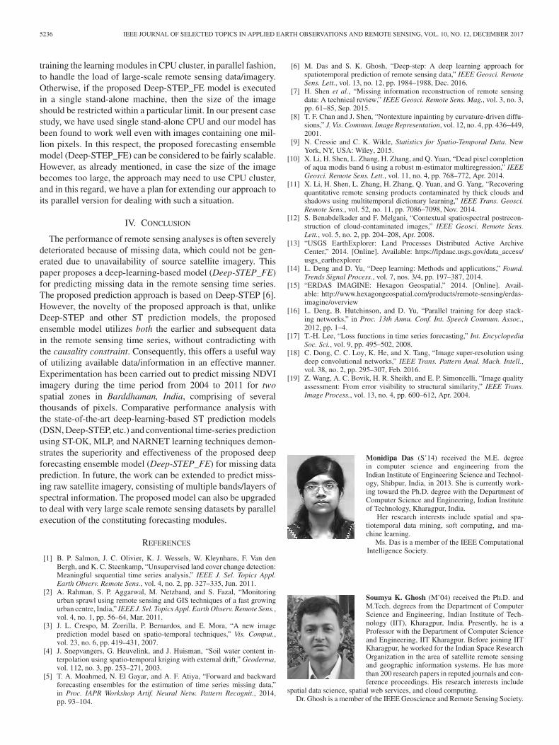
Monidipa Das (S’14) received the M.E. degreein computer science and engineering from theIndian Institute of Engineering Science and Technol-ogy, Shibpur, India, in 2013. She is currently work-ing toward the Ph.D. degree with the Department ofComputer Science and Engineering, Indian Instituteof Technology, Kharagpur, India.

Her research interests include spatial and spa-tiotemporal data mining, soft computing, and ma-chine learning.

Ms. Das is a member of the IEEE ComputationalIntelligence Society.

Soumya K. Ghosh (M’04) received the Ph.D. andM.Tech. degrees from the Department of ComputerScience and Engineering, Indian Institute of Tech-nology (IIT), Kharagpur, India. Presently, he is aProfessor with the Department of Computer Scienceand Engineering, IIT Kharagpur. Before joining IITKharagpur, he worked for the Indian Space ResearchOrganization in the area of satellite remote sensingand geographic information systems. He has morethan 200 research papers in reputed journals and con-ference proceedings. His research interests include

spatial data science, spatial web services, and cloud computing.Dr. Ghosh is a member of the IEEE Geoscience and Remote Sensing Society.