Evaluation of a Wind-Wave System for Ensemble Tropical Cyclone Wave Forecasting. Part I: Winds

Evaluation of a Wind-Wave System for Ensemble Tropical CycloneWave Forecasting. Part I: Winds

STEVEN M. LAZARUS, SAMUEL T. WILSON, MICHAEL E. SPLITT, AND GARY A. ZARILLO

Florida Institute of Technology, Melbourne, Florida

(Manuscript received 17 May 2012, in final form 13 September 2012)

ABSTRACT

A computationally efficient method of producing tropical cyclone (TC) wind analyses is developed and

tested, using a hindcast methodology, for 12 Gulf of Mexico storms. The analyses are created by blending

synthetic data, generated from a simple parametric model constructed using extended best-track data and

climatology, with a first-guess field obtained from the NCEP–NCAR North American Regional Reanalysis

(NARR). Tests are performed whereby parameters in the wind analysis and vortex model are varied in an

attempt to best represent the TCwind fields.A comparison between nonlinear and climatological estimates of

the TC size parameter indicates that the former yields a much improved correlation with the best-track radius

of maximum wind rm. The analysis, augmented by a pseudoerror term that controls the degree of blending

between the NARR and parametric winds, is tuned using buoy observations to calculate wind speed root-

mean-square deviation (RMSD), scatter index (SI), and bias. The bias is minimized when the parametric

winds are confined to the inner-core region. Analysis wind statistics are stratified within a storm-relative

reference frame and by radial distance from storm center, storm intensity, radius ofmaximumwind, and storm

translation speed. The analysis decreases the bias and RMSD in all quadrants for both moderate and strong

storms and is most improved for storms with an rm of less than 20 n mi. The largest SI reductions occur for

strong storms and storms with an rm of less than 20 n mi. The NARR impacts the analysis bias: when the bias

in the former is relatively large, it remains so in the latter.

1. Introduction

Various studies have demonstrated the importance of

the surface wind field in wave forecasts (e.g., Janssen

et al. 1997; Makin and Kudryavtsev 1999; Young 2003).

Due to advancements in meteorological modeling, in-

creased availability of measured wind data over the

ocean surface, and improved methods for integrating

observations with model-generated wind fields, the

quality of wind input that is available for use in both

wave forecasting and hindcasting has vastly improved

over the past several decades. There has also been im-

provement in the wave models, evolving from second to

third generation (e.g., Holt and Hall 1992). However,

despite progress in wave modeling, problems persist.

This is especially apparent in the specification of wave

heights in very high sea states, as well as large errors in

the specification of 2D wave spectra in complicated

wave regimes such as tropical cyclones (Cardone et al.

2000). In particular, the issues germane to the work

presented here are 1) the failure to resolve subgrid-scale

flow features in extreme events such as tropical cyclones

(TCs) and 2) extreme wind events outside the range for

which the wavemodels are tuned. Although the hindcast

methodology has been used extensively to tune wave

models for tropical cyclones, the forecast applications

have been somewhat limited. Given the potential high

impact and relatively large uncertainty of TC intensity

forecasts, ensembles are now also beginning to take root

in operational wave forecasting (e.g., Roulston et al.

2005; Chen 2006). Probabilistic wave forecasts may ul-

timately be more useful in extreme wind events, but in

order for the ensemble approach to be viable, the fore-

casts should be free of bias (e.g., Hamill 2000).

Wave hindcasting can be computationally expensive,

especially when high-resolution atmospheric models are

used to generate the surface wind field (Cardone et al.

2000). Here, an efficient method by which to produce

a TC wind analysis using hindcasts is developed and

Corresponding author address: Steven M. Lazarus, Florida In-

stitute of Technology, 150 W. University Blvd., Melbourne, FL

32901.

E-mail: [email protected]

VOLUME 28 WEATHER AND FORECAST ING APRIL 2013

DOI: 10.1175/WAF-D-12-00054.1

� 2013 American Meteorological Society 297

evaluated. The approach taken is designed to minimize

errors in the significant wave height by reducing the

wind speed bias, with the eventual goal of generating

operational ensemble wave forecasts. The cost-effective

approach combines output from a simple parametric-

derived wind field with background (i.e., first guess)

winds from a large-scale NWP model (e.g., Desjardins

et al. 2004;Mousavi et al. 2009). The parametricmodel is

used to replace the poorly resolved first-guess inner-core

wind field. Using hindcasts, the parametric model is

constructed and tuned with observations from the ‘‘ex-

tended best track’’ dataset (DeMuth et al. 2006) and

wind measurements from National Data Buoy Center

(NDBC) buoys. A total of 12 Gulf of Mexico (GOM)

TC events of varying intensities are examined. The data

used to generate the wind analyses, theNational Centers

for Environmental Prediction–National Center for At-

mospheric Research (NCEP–NCAR) North American

Regional Reanalysis (NARR; Kalnay et al. 1996), and

the best track are described in sections 2b and 2c, re-

spectively. The parametric model, described in section

3a, is based on a modified asymmetric Rankine vortex

described by Knaff et al. (2007, hereafter K07). The

analysis wind fields are generated via blending the

parametric model with the coarse-resolution NARR.

The blending technique is described in detail in sections

3b and 3c. Systematic tests are performed whereby pa-

rameters in both the wind analysis and vortex model are

varied in an attempt to best represent the TC wind fields

(sections 4a–c). In section 4d, analysis wind statistics are

stratified within a storm-relative reference frame as well

as by radial distance from storm center, storm intensity,

translation speed, and radius of maximum wind.

2. Data

a. Buoy

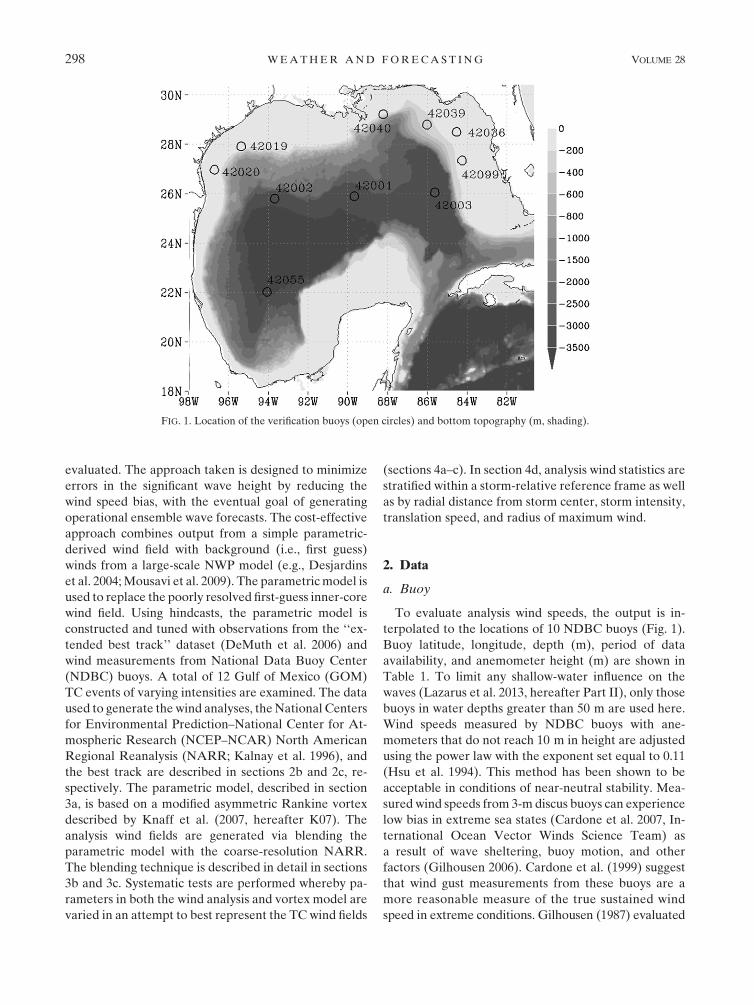
To evaluate analysis wind speeds, the output is in-

terpolated to the locations of 10 NDBC buoys (Fig. 1).

Buoy latitude, longitude, depth (m), period of data

availability, and anemometer height (m) are shown in

Table 1. To limit any shallow-water influence on the

waves (Lazarus et al. 2013, hereafter Part II), only those

buoys in water depths greater than 50 m are used here.

Wind speeds measured by NDBC buoys with ane-

mometers that do not reach 10 m in height are adjusted

using the power law with the exponent set equal to 0.11

(Hsu et al. 1994). This method has been shown to be

acceptable in conditions of near-neutral stability. Mea-

sured wind speeds from 3-m discus buoys can experience

low bias in extreme sea states (Cardone et al. 2007, In-

ternational Ocean Vector Winds Science Team) as

a result of wave sheltering, buoy motion, and other

factors (Gilhousen 2006). Cardone et al. (1999) suggest

that wind gust measurements from these buoys are a

more reasonable measure of the true sustained wind

speed in extreme conditions. Gilhousen (1987) evaluated

FIG. 1. Location of the verification buoys (open circles) and bottom topography (m, shading).

298 WEATHER AND FORECAST ING VOLUME 28

the performance of several NDBC buoys in tropical

cyclones. The bias and standard deviation were both

quite low in their ‘‘high wind’’ dataset, which included

wind speeds up to 33 m s21 for the dual-anemometer

comparison and up to 20 m s21 for the platform com-

parison. Calibration and comparison of stepped-frequency

microwave radiometer (SFMR) performance is con-

fined to GPS dropwindsonde (e.g., Uhlhorn et al. 2007),

which appears to be a pragmatic approach given the

problems with space–time syncing either of these with

in situ buoys. Here, with the exception of the height ad-

justment, no other changes weremade to the wind speeds

measured by the NDBC buoys.

b. North American Regional Reanalysis (NARR)

The NARR is a 40-yr record of global atmospheric

analyses that includes the assimilation of ship, aircraft,

satellite, buoy, and other relevant data (Kalnay et al.

1996). The NARR has a horizontal grid of 32 km, 45

vertical levels, and is available at 3-h intervals from 1979

to the present. In a high-resolution wave modeling study

over the North Atlantic, Cardone et al. (1999) showed

that wave hindcasts forced with NARR winds were

improved over those using the operational wind fields at

NWP centers. While the quality and resolution of op-

erational wind fields continues to increase, the NARR is

used here because the adoption of a hindcast approach

allows for the integration of a relatively data-rich global

product. For operational purposes, the backgroundwind

field could be obtained from any of the suite of NCEP

forecast models—with themost obvious candidate being

the Global Forecast System (GFS) since its wind fields

are not limited regionally. Regardless, the NARR and

global atmospheric models still suffer from poor spatial

resolution on the scale of TCs.

c. Extended best track

The extended best-track dataset, developed to serve

as a supplement to theNationalHurricaneCenter (NHC)

climatological TC database known as HURDAT, pro-

vides information regarding storm structure and size.

The data include the radius ofmaximumwind speed, eye

diameter, pressure and radius of the outer closed isobar,

and maximum radial extent of the 34-, 50-, and 64-kt

wind to the NE, SE, SW, and NW of storm center. The

data for the Atlantic basin are available at 6-h intervals

and extend back to 1988. The data used by the para-

metric model include the storm latitude; longitude; 1-min

maximum sustained surface wind speed; the maximum

radial extent of the 34-, 50-, and 64-kt wind in four

quadrants; and the radius of maximum wind speed.

These data were linearly interpolated to 3 h in order to

match the availability of the NARR winds and to gen-

erate the subsequent wind forcing.

3. Models and analysis

a. Parametric wind field

A parametric model that employs climatology to

predict TC wind radii estimates is used in this study. The

simple model, based on a modified asymmetric Rankine

vortexmodel of K07, is chosen as it approximates known

structural TC variations and it provides a single meth-

odology by which a baseline estimate of the TC wind

field can be made given standard NHC best-track input.

The parametric model is given by

V(r, u)5 (ym 2 a)�rmr

�x1 a cos(u2 uo) for r$ rm and

V(r, u)5 (ym 2 a)

�r

rm

�1 a cos(u2 uo) for r, rm ,

(1)

where V(r, u) is the wind speed as a function of radial

distance from storm center (r) and azimuth (u), ym is the

maximumwind speed, rm is the radius of maximumwind

speed, x is a size parameter, a is the wavenumber 1

TABLE 1. GOM NDBC buoys used for evaluation. Buoys selected are those that measure significant wave height and are in water

depths . 50 m. Latitude and longitude locations correspond to the current buoy locations.

Buoy Lat (8) Lon (8) Depth (m) Period Anemometer height (m)

42020 26.966 96.695 88.1 1990–present 5

42002 25.790 93.666 3566.2 1973–present 10

42001 25.888 89.658 3246.0 1975–present 5

42019 27.913 95.353 83.2 1990–2010 5

42040 29.212 88.207 274.3 1995–present 10

42036 28.500 84.517 54.5 1994–present 5

42039 28.791 86.008 307.0 1995–present 5

42099 27.340 84.245 93.9 2007–present None

42003 26.044 85.612 3282.7 1976–present 10

42055 22.017 94.046 3380.5 2005–present 10

APRIL 2013 LAZARUS ET AL . 299

asymmetry magnitude, and uo is the degree of rotation

of ym from the direction 908 to the right of the storm

motion vector. A storm motion–relative coordinate

system, where azimuth is measured counterclockwise

starting from the direction 908 to the right of the storm

motion vector, is used here (K07). Equation (1) has one

known parameter (ym) and four free parameters (rm, x,

a, and uo). Using standard regression, K07 represent the

free parameters as functions of climatological factors

that are available in the best-track data (latitude, storm

translational speed, and maximum wind speed).

b. Wind analysis theory

Wind analyses are generated via a combination of the

NARR 10-m wind field (U10) and the parametric model

described by Eq. (1). The blending, based on a modified

version of the successive corrections method (SCM;

Cressman 1959; Barnes 1964), applies the NARR as the

first guess and uses the parametric wind model to create

synthetic observations on a 2-km grid. The basic idea is

to replace the NARR’s poorly resolved inner-core wind

field with parametric winds while assuming that the

NARR captures the wind speeds at distances farther

away from the storm center. Pseudo observations are

first generated using Eq. (1) and then spread, aniso-

tropically, using the curvature of a parametric vortex

model in lieu of the streamline curvature originally

defined by Benjamin and Seaman (1985, hereafter

BS85). The axisymmetric vortex model (DeMaria et al.

1992) is

V0 5 r0 exp�1

b(12 r0b)

�, (2)

where V 0 and r0 are the normalized tangential velocity

(i.e., y/ym) and radial distance from storm center (r/rm),

respectively, and b is a size parameter. Integrating Eq.

(2) with respect to r0(to simplify the integration and its

application, b is set equal to 1) yields

s[

ðr0V 0 dr05

ðr0r0 exp[(12 r0)]dr0 5 e1e2r(11 r) . (3)

The anisotropy factor is determined by subtracting

(from 1) the absolute value of the difference in s be-

tween the grid point (i, j) and observation (k):

wijk 5 exp

2d2mR2

!(12 jsij 2 skj) , (4)

where R is the radius of influence and dm is defined by

Eq. (5) in BS85. Figure 2 illustrates the new weight

[Eq. (4)] and the original banana weight of BS85 for

an idealized TC wind field. The curvature in the mod-

ified weighting scheme is clearly enhanced over that

of the banana-shaped weights of BS85, preferentially

spreading the synthetic observation in the azimuthal

direction.

A pseudoerror term is introduced into the analysis.

To allow for operational flexibility, the error is based on

the nth-order Butterworth low-pass filter (Butterworth

1930), which is defined as

H (v) H (v)*51

11

�v

vc

�2N, (5)

where H(v) H(v)* is the amplitude of the response

function R(v), v is the distance from storm center, N is

the filter order, and vc the cutoff distance. We define N

and vc as

N5

ln

�effiffiffiffiffiffiffiffiffiffiffiffiffiffi

A22 1p

�

ln

�vp

vs

� (6)

and

vc 5vp

e1/N, (7)

FIG. 2. Normalized parametric wind field (y/ym, thin solid lines)

based onEq. (2), the Benjamin and Seaman bananaweight (dashed

lines), and a modified banana weight (thick solid lines) based on

Eq. (4). Each of the weights is centered on an observation located

at the 3.


where vp and vs are the pass and stop band edges, re-

spectively; A5 1/ffiffiffiffiffiffiffiffiffiffiffiffiR(vs)

p; and e5 1/

ffiffiffiffiffiffiffiffiffiffiffiffiffiffiffiffiffiffiffiffiffiR(vp)2 1

p. The

user specifies vp, vs, R(vp), and R(vs), from which the

filter order, cutoff distance, and response function can

then be determined via Eqs. (5)–(7). An example

response curve is shown in Fig. 3. Because the objective

is to inflate the observation error as the distance from

the storm center increases so that the analysis is

weighted more toward the background field (NARR),

the observation (parametric) to background (NARR)

FIG. 3. Butterworth filter example for which the responseR(v) at the start edge (vp) is 0.8, at

the stop edge (vs) is 0.2, and dv 5 200 km. When R(v) 5 1 (0), the analysis is parametric

(NARR) only.

FIG. 4. The climatological size parameter xc (open squares) and nonlinear size parameter

xn (plus signs) for TC Ike. Also shown is the best-track radius of maximumwind (n mi, black

circles) and analysis filter width dv (n mi, open triangles). See text for other parameter

values.


error variance is set equal to the inverse square of

Eq. (5).

c. Wind analysis application

The basic idea is to link the analysis parameters with

observable (or forecast) quantities, ensuring function-

ality for operational applications. The pass edge vp of

the response function is determined by setting a 5 0 in

Eq. (1) and solving for r such that

vp 5 rm 3

�ymyt

�1/x

, (8)

where r5 vp and y5 yt, which is a user-defined velocity

for which the response function is reduced by 1 2 R

(vp). For the wind analyses presented in the following

sections, yt is set equal to ym; thus, vp 5 rm [Eq. (8)].

The response function value at vp[R(vp)] is set equal

to 0.99, resulting in an analysis that is heavily weighted to

the parametric model at rm. Both rm and ym are given in

the best-track dataset while x is calculated indirectly us-

ing two different methodologies: 1) wind radii in-

formation and 2) climatology (K07; see following

paragraph). The difference between the pass and stop

ends of the filter (vs – vp), referred to as the filter width

dv, is linearly related to the size parameter x; that is,

dv5D3 (d2 x), where d is a constant (set equal to 2

here) and D is a nonlinear function of rm defined as

D(rm)5 ar 2m 2 brm 1 c , (9)

where a, b, and c are user-defined constants. In addi-

tion, D is designed to replace the TC inner core, which,

in general, is poorly resolved by the coarse-resolution

NARR—especially for tight storms (i.e., small rm).

Thus, for a fixed size parameter x,D and dv decrease as

rm increases. Conversely, for fixedD (i.e., rm fixed), as x

increases (i.e., a decrease in the radial extent of the wind

field), dv decreases. In either case, the analysis transi-

tions to the first-guess field (i.e., NARR) at smaller radii.

Once dv andvp are known,vs is calculated as a residual.

The response function value at vs [R(vs)] is set equal to

0.01, and thus the analysis at radii beyond the filter stop

edge is essentially the background.

As previously mentioned, two different approaches

are used to estimate the size parameter. In the first

(where x 5 xc), a multilinear regression equation that

depends on maximum wind speed and latitude is used

[K07, Eq. (2)]. The coefficients used are the climato-

logical values given for the North Atlantic in K07 (see

their Table 1). The climatology is based on a least

squares method that minimizes the squared difference

between observed and analytic wind radii over a 16-yr

period (1988–2003). It is also possible to take direct

advantage of the radial quadrant information (i.e., the

maximum radial extent of the 34-, 50-, and 64-kt wind in

four quadrants) in the best-track data. A nonlinear size

parameter (x 5 xn) is calculated by simultaneously fit-

ting the three wind radii in each of the four quadrants

and solving Eq. (1) using the least squares method of

differential evolution (Storn and Price 1997; Mishra

2007). In this case, both the asymmetry factor (a) and the

degree of rotation (uo) are determined using their cli-

matological values [i.e., Eq. (2) and Table 1 in K07) and

rm is obtained from the best-track data. Given the

number of points (there is a maximum of 12) fromwhich

the size estimate is made, this limits the degrees of

freedom to one and produces a stable solution. In ad-

dition, of the three remaining free parameters [in Eq.

(1)], tests (not shown) indicate that x appears to exhibit

a more direct correlation with the best-track TC wind

radii, which are based on a poststorm analysis of all

available information. In particular, as will be shown, xnyields an improved wind analysis compared to that

produced by xc. Experiments where both a and xwere fit

FIG. 5. Composite statistics for wind speed bias (m s21) vs

RMSD (m s21) within 100 n mi of storm center for TCs Ike, Ivan,

Rita, and Katrina. Here, yt 5 ym, x 5 xn, and D [Eq. (9)] is set to

linear (a5 0.0, b5 0.5) for the five experiments shown.Values for c

[Eq. (9)] are 50, 75, 100, 150, and 200 n mi for experiments 1–5,

respectively. Also shown are the statistics for all 12 storms for c

equal to 100 n mi (filled circle) and quadratic D with c equal to 50

(and a 5 0.005, b 5 1; filled square). The 3 and open triangle

symbols depict the four-storm subset for the quadratic D and the

NARR, respectively. Zero bias is depicted by the dashed line.


simultaneously, and for a only (i.e., with x 5 xc), were

also attempted; however, the results were noisy. Ulti-

mately, the size parameter is considered a priority here

because the best-track TCwind radii are directly related

to the observed storm size. Estimates of the nonlinear

size parameter could also be generated using the fore-

cast permutations in track, intensity, and structure from

the NHC’s Monte Carlo model (DeMaria et al. 2009),

making this a viable approach with respect to generat-

ing ensemble wind analyses. This is discussed further in

section 5.

4. Results

a. Size parameter

Estimates of the size parameters xn and xc are com-

pared with the best-track rm over an 81-h window for

Hurricane Ike (Fig. 4). It is not surprising that xn (plus

signs) is sensitive to variations in rm (black circles) while

xc is not (open squares). For example, during the 12-h

period beginning 1200 UTC 11 September when Ike is

undergoing an eyewall replacement, rm increases from

10 to 80 n mi with a corresponding increase in xn (from

0.2 to 0.8) while xc remains constant (approximately

0.6). The r2 value for xn (versus rm) is considerably larger

than those for xc (0.79 and 0.13, respectively). Onemight

actually expect a smaller size parameter as rm increases.

However, during the eyewall replacement cycle, the 34-,

50-, and 64-kt wind radii [V and r; Eq. (1)], themaximum

wind speed (ym), and the asymmetry coefficient [a; Eq.

(1)] are relatively constant and thus an increase in rmresults in a larger xn.

b. Filter width and shape

Using data from four TCs (Katrina, Rita, Ivan, and

Ike), the impact of changes in D [Eq. (9)] on the wind

analysis is evaluated. Bias, scatter index (SI, defined

here as the ratio of the standard deviation of the dif-

ferences to the mean of the measurements) and root-

mean-square deviation (RMSD) are calculated using

10 GOM buoys (Fig. 1, Table 1) and are confined to

observations within 100 n mi of the storm center. Five

experiments are performed where D is linearly related

to rm (a5 0.0,b5 0.5, and c5 50, 75, 100, 150, and200 nmi)

and one for which D and rm are related via a quadratic

fit (a 5 0.005, b 5 1, c 5 50 n mi). Results are shown in

Fig. 5, where EXP1–EXP5 (open squares) correspond to

the wind analyses created using the linear D,3 denotes

the analyses generated using the quadratic relationship,

and the NARR-only results are depicted by the open

triangle. Also shown are the results for all 12 storms

using the linear fit from EXP3, which produced the

lowest bias of the four-storm subset (filled circle) and

FIG. 6. The filter parameter space (vp vs vs, n mi) using the quadraticD [Eq. (9)] and size

parameters ranging from 0.0 to 1.0 (in increments of 0.1), R(vp) 5 0.99, R(vs) 5 0.01, and

c 5 50 n mi. Here, yt 5 ym and vp 5 rm [Eq. (8)]. For example, the filter width dv (dashed

lines) is 100 n mi if both x and rm 5 0. The gray box is the filter width for the analysis shown

in Fig. 7b.


the quadratic fit (filled square). All of the wind analyses

are a significant improvement over that of the NARR-

only analysis. For the four-storm subset, the bias is

lowest for EXP3 (c 5 100 n mi), while the RMSD is

lowest for EXP1 (c 5 50 n mi; Fig. 5). The bias, clearly

more sensitive to variations in c, changes sign with

a range of 4 m s21, compared to less than 1 m s21 for the

RMSD. The parameter selection that produces the

FIG. 7. Values of U10 (kt) for Hurricane Katrina valid 1800 UTC 28 Aug 2005: (a) NARR only, (b) AOC using best-track parameters

and xn, (c) analysis with x 5 0.2 (EXPA; Table 2), (d) x 5 1.0 (EXPB; Table 2), (e) analysis with rm 5 10 n mi (EXPC; Table 2), and (f)

analysis with rm 5 60 n mi (EXPD; Table 2).


lowest bias for the four storms (EXP3) yields a higher

bias for all storms (filled circle), but it does fall within the

bias envelope of the five experiments. A single standard

deviation (cross hairs in Fig. 5) is shown for the 12-storm

composites. Given the relatively large spread, it might

also be prudent to allow for variations in c as well. Re-

gardless, there appears to be a sweet spot, a blending

width that minimizes the analysis bias. The quadratic fit

is selected here as the analysis of choice (AOC) as it

yields a lower wind speed bias and RMSD compared to

the wind analyses from EXP3 when extended to all

storms. This does not mean that the AOC is optimal for

any one particular analysis; rather it is only true in

the bulk sense. Also, the AOCwill invariably depend on

the quality, number, and distribution of the verifying

observations—a limitation here.

The resulting filter parameter space (vp, vs) using the

quadratic D is shown in Fig. 6 for size parameters

ranging from 0.0 to 1.0, R(vp)5 0.99, and R(vs)5 0.01.

The maximum dv is 100 n mi if both x and rm 5 0. The

size of dv is relatively large for small x (i.e., large storm)

and/or small rm, but is more sensitive to variations in

the latter. As rm increases, all size parameters converge

toward a zero filter width (i.e., a NARR-only wind

analysis), and do so more rapidly for small x. For ex-

ample, consider Hurricane Ike during 0600–1800 UTC

12 September 2008, where rm is constant (50 nmi) but xnincreases from 0.63 to 0.71. In this case, dv decreases

only slightly from 17 to 16 n mi (open triangles in Fig.

4). Conversely, a 5-n mi decrease in rm during 0600–

1200UTC 10 September 2008 while xn is approximately

constant (0.22) produces a larger change in dv, in-

creasing from 64 to 72 n mi. The abrupt change in the

parameters captures the eyewall replacement cycle in

which the inner windmaximum dissipates and the outer

wind maximum contracts, becoming the more domi-

nant feature by 1800 UTC 11 September 2008 (Berg

2009).

c. Sensitivity experiments

Four sensitivity tests, using Hurricane Katrina, are

performed to ensure that the modeled TC wind field

responds appropriately to variations in x and rm. As

previously discussed, variations in rm have a more pro-

nounced effect on dv, which should be apparent in the

gridded wind fields. Experiments are performed in

which x is varied within the bounds of climatology (0.2

and 1.0) while holding rm constant (15 n mi). Two ad-

ditional tests are conducted in which rm is set to 10 and

60 n mi while fixing x (0.5). For comparison purposes,

the NARR-only results and the AOC generated using

the best-track data are also shown. The resulting wind

analyses (valid 1800 UTC 28 August 2008) and related

parameters are shown in Fig. 7 and Table 2, respectively.

TheNARRwind field is poorly resolved in this case with

peak winds (60 kt) well below the observed (150 kt).

The impact of the size parameter on the analysis is as

expected, with a shrinking inner-core wind field as x

increases. The peak wind speeds for the analysis are

much higher, are closer to the observed, and wrap

around the northern semicircle to the northwest of the

center for x 5 0.2. An increase in rm results in an out-

ward expansion of the highest winds in the storm core.

The AOC, which is produced by using the rm and non-

linear size parameter derived from the wind radii in the

best-track data (rm,5 20, xn 5 0.65), yields a relatively

tight core. Because the filter parameters are fixed for

these experiments, all of the analyses quickly relax to the

NARR outside of the 100-n mi radius.

An additional wind analysis (not shown in Fig. 7) is

generated for Katrina using xc (50.94) for comparison.

Figure 8 depicts north–south and west–east transects

through the storm center (dashed lines in Figs. 7a and

7b) and includes the NARR,H*Wind (see next section),

EXP3, EXP5, and xn analyses. Compared to xc, the xnanalysis produces a marginally broader storm with

slightly higher winds that are closer to the best-track

peak wind speed. With the exception of the eastern

transect, the difference between the NARR winds

(dashed line) and the best-track TC wind radii (open

circles) increases inward. The inner-core structure of the

AOC (i.e., within 50 n mi) and H*Wind are quite simi-

lar; however, both EXP3 and EXP5 exhibit a better

overall fit than the AOC and do not have the ‘‘un-

dershoot’’ seen on the north side of theAOC. These two

experiments have a smoother transition from the para-

metric model to the NARR. If we examine the statistics

for Katrina only (not shown), we find that the best

analysis comes not from the AOC, but rather from

EXP3. The AOC is defined from a bulk set of statis-

tics that minimize the bias in the entire storm set and,

thus, will be suboptimal for some of the analyses. Even

though the analysis has built-in degrees of freedom (i.e.,

TABLE 2. Parameters and values for sensitivity tests in which x

and rm are systematically varied. For all experiments, R(vp)5 0.99

and R(vs) 5 0.01. See text for details.

Expt

Parameter A B C D

x 0.2 1.0 0.5 0.5

rm (n mi) 15 15 10 60

vp (n mi) 15 15 10 60

D (n mi) 36.1 36.1 40.5 8.0

dv (n mi) 65.0 36.1 60.8 12.0

vs (n mi) 80.0 51.1 70.8 62.0


x and rm) in an effort to capture storm-to-storm vari-

ability, the AOC snapshot shown is not the ‘‘best’’

analysis for this time (hence the term AOC rather than

‘‘optimal’’ or best, etc.). It is worth pointing out that

EXP5, which appears to be a better fit to the best track

and H*Wind, is not the best analysis for Katrina overall.

The 1800 UTC 28 August 2005 buoy (42001) observation

(square box in Fig. 8a), which is located 63 n mi west of

the storm, is consistent with the NARR and supports the

tighter analysis (compared to H*Wind and the best-track

wind radii), at least on the west side of the storm. The

filterwidth, for theAOCinFig. 7b, is on theorderof 43 nmi

(gray box in Fig. 6). Hence, the stop edge of the filter is

near 60 n mi (i.e., vs 5 dv 1 rm, where rm 5 20 n mi),

FIG. 8. The U10 (kt) (a) west–east and (b) south–north cross sections taken along the lines

shown in Fig. 7a (NARRonly, dashed line) and Fig. 7b (analysis with nonlinear size parameter,

solid line). Also shown are the wind analysis using the climatological size parameter (dotted

line), EXP3 (dashed–dotted line), EXP5 (solid gray line), HWIND (3), the average 34-, 50-,

and 64-kt best-track wind radii and their spread (open circles, horizontal error bars), buoy

42001 wind speed valid 1800 UTC 28 Aug 2005 [gray square box in (a)], and the best-track

maximum wind (1). See text for details.


which is evident with the analysis relaxing to the NARR

at a radius of approximately 60 n mi. Any discrepancies

in the NARR winds outside vs will remain in the wind

analysis.

d. Wind analysis evaluation

For a few representative cases, the AOC storm struc-

ture is compared to tropical cyclone wind analyses

generated by the Hurricane Research Division. The

product, referred to as H*Wind, blends available data

including aircraft reconnaissance, dropsonde, buoy, and

Coastal-Marine Automated Network (C-MAN) plat-

forms (Powell et al. 1998). The wind data are processed

within a storm-relative framework and reduced to a

common 10-m reference height. Rather than a snapshot,

an H*Wind analysis represents the TC wind field over a

window ranging from 4 to 6 h. Bias (analysis–background

minus observed wind speed), RMSD, and SI statistics are

also presented in which the AOC is compared against

wind measurements from 10 NDBC buoys (Table 1).

NARR wind error statistics are also provided for com-

parison purposes. The 12 TCs evaluated in this study

are split into two categories based on maximum storm

strength (i.e., Saffir–Simpson category) in the GOM.

TCs of categories 3–5 are referred to as strong (Table 3),

and categories 1–2 as moderate (Table 4).

1) H*WIND COMPARISON

The 10-m wind analyses for H*Wind (dashed con-

tours) and the AOC (solid contours) are shown along

with the NARR (shaded contours) for Ivan, Rita, and

Katrina (Fig. 9). The times selected were driven by the

presence of proximity buoy observations that are shown

in the accompanying cross sections (Fig. 10). In each of

the storms, the NARR fails to capture the detail of the

inner-core storm structure. In the Ivan example shown

(Fig. 9a), the NARR center is displaced southwest of the

best-track position. Despite the offset, the AOC is able

to relocate the center and yields an inner-core analysis

that is consistent with H*Wind. The impact of the shift

in storm position and the broad nature of the NARR

wind field can be seen in theW–E cross section, as a local

minimum in the wind speed around 50 n mi west of the

storm center (Fig. 10a). This AOC feature disappears

for the larger blending widths (e.g., EXP3 and EXP5).

Given that the analyses are targeted for ensemble wave

forecasts with many track, structure, and intensity per-

mutations, the blending width might, in the future, be

more strongly coupled to the forecast wind radii. Both

the H*Wind and AOC depict the asymmetry, with the

strongest winds on the east side of the storm. The

H*Wind eyewall is a bit tighter, however. In this case, all

three analyses are in agreement with the buoy obser-

vation (42001) 124 n mi west of the storm center (the

buoy is actually 0.38 north of due west). Buoy 42003,

100 n mi east of the storm, lies midway between the

H*Wind analysis and the AOC and is best fit to the

storm structure in EXP5. The H*Wind Katrina analysis

(taken near peak intensity) has somewhat more asym-

metry than does that of the AOC, with a slightly elon-

gated (contracted) wind field along the N–S (W–E) axes

(Fig. 9b). Both H*Wind and the AOC wrap a wind

maximum (120 kt) around the north side of the storm.

However, the AOC brings the wind maximum farther

into the NW quadrant to the west of the storm center

and it is displaced radially outward from that of H*Wind.

TABLE 3. Strong TCs (Saffir–Simpson categories 3–5).

Storm Saffir–Simpson category Evaluation period

Opal (1995) 4 1800 UTC 27 Sep–1800 UTC 5 Oct

Isidore (2002) 3 1800 UTC 17 Sep–0600 UTC 27 Sep

Lili (2002) 4 1200 UTC 30 Sep–1200 UTC 4 Oct

Ivan (2004) 5 1200 UTC 10 Sep–0900 UTC 17 Sep

Dennis (2005) 4 1200 UTC 7 Jul–1200 UTC 12 Jul

Katrina (2005) 5 0000 UTC 24 Aug–1200 UTC 30 Aug

Rita (2005) 5 1200 UTC 19 Sep–1200 UTC 25 Sep

Gustav (2008) 4 0000 UTC 30 Aug–0000 UTC 4 Sep

TABLE 4. Moderate TCs (Saffir–Simpson categories 1–2).

Storm Saffir–Simpson category Evaluation period

Earl (1998) 2 1200 UTC 31 Aug–1200 UTC 4 Sep

Georges (1998) 2 1200 UTC 23 Sep–600 UTC 1 Oct

Ike (2008) 2 0000 UTC 9 Sep–0000 UTC 14 Sep

Ida (2009) 2 0600 UTC 6 Nov–0600 UTC 11 Nov


As in the 1800 UTC W–E cross section (Fig. 8a), the

1500 UTC buoy wind speed 82 n mi west of the storm

center is close to that of the AOC (and below that of

H*Wind and the best-track wind radii; Fig. 10b). The

Rita analyses exhibit somewhat of a different structure

from that of the other storms shown, with a relatively

tight inner core embedded within a relatively relaxed

outer wind field (Fig. 9c). In terms of this structure, the

FIG. 9. Horizontal cross sections of the 10-m wind speed (kt)

for (a) Ivan valid 0600 UTC 15 Sep 2004, (b) Katrina valid

1500 UTC 28 Aug 2005, and (c) Rita valid 2100 UTC 22 Sep 2005.

Shown are the AOC (solid contours), H*Wind (dashed contours),

and NARR (shaded). For Rita, H*Wind is valid at 2230 UTC.

FIG. 10. As in Fig. 8, but for (a) Ivan (west–east) valid 0600 UTC

15 Sep 2004, (b) Katrina (west–east) valid 1500 UTC 28 Aug 2005,

and (c) Rita (south–north) valid 2100 UTC 22 Sep 2005.


AOC is consistent with H*Wind. Both analyses wrap

a 100-kt wind maximum around the north and west sides

of the storm—although as with Katrina, the AOC wind

maximum is displaced slightly outward from that of

H*Wind. Again, there is a slight elongation in the N–S

direction in the H*Wind analysis. The wind asymmetry

is evident in the S–N cross section (Fig. 10c), with the

strongest winds on the north side of both the AOC and

H*Wind. The 2100 UTC buoy (42001) wind speed

(84 kt) 11 n mi north of the storm is less than either the

AOC or H*Wind result, both of which indicate a maxi-

mum wind speed around 110 kt.

2) TIME SERIES

Time series ofU10 at NDBC buoy 42001 are shown for

Rita and Ike and at 42040 for Ivan in Fig. 11. TheU10 for

the AOC (solid line), buoy (circles), and the NARR

(dashed gray line) are shown in each panel in Fig. 11. In

each of these three cases the cyclones passed very close

to the buoys. For both Rita and Ike, the analysis better

resolves the inner-core wind field compared to the

NARR. In particular, there is a large discrepancy be-

tween the peak wind speed in the analysis versus that of

the NARR associated with the passage of TC Rita. In

this case, the NARR underforecasts the peak winds

by more than 20 m s21, whereas the analysis peak is

close to that observed. During this time, wave heights

monotonically increase to near 12 m (see Part II). For

TC Ivan, the analysis appears to overestimate the max-

imum wind speed observed at buoy 42040. Note, how-

ever, that the buoy broke loose of its mooring around

2100 UTC 15 September 2004 (filled circles in Fig. 11a),

drifting southwest and then southeast over the latter

36 h of the analysis period (Stone et al. 2005). While the

buoy reported a maximum wind speed near 27 m s21,

the NHC best track indicates a maximum wind speed of

57 m s21, a radius of maximum wind of 20 n mi, and

a position about 35 km (19 n mi) south of the anchored

buoy location at 0000 UTC 16 September 2004. Given

that the buoy appears to be situated near the eyewall,

any drift may result in significant wind speed discrep-

ancies. While previous data were presented in nautical

miles and knots (consistent with best track), the error

statistics that follow use the meter–kilogram–second

(MKS) convention.

3) BULK

Table 5 lists error statistics, the amount of buoy data

used for validation, and the number of missing obser-

vations for all storms. The U10 bias is quite low and is

slightly better for the NARR while the RMSD is about

0.5 m s21 lower for the analysis. The SI is also slightly

lower for the AOC. Given that the analysis increases

the wind speeds, it is no surprise that the U10 analysis

FIG. 11. The U10 (kt) time series for NARR (dashed gray line),

analysis (solid black line), and buoy (open circles) at buoys (a) 42040

(Ivan), (b) 42001 (Rita), and (c) 42001 (Ike).

TABLE 5. NARR and analysis (BLND) 10-m wind speed (U10)

bias (m s21), RMSD (m s21), SI, total number of observations for

all storms, and missing data.

U10 NARR BLND No. of data points Miss data

Bias 0.04 0.22 8542 144

RMSD 2.8 2.28

SI 0.30 0.24


bias is slightly larger than theNARR (both are positive).

However, the amount of proximity buoy data (i.e., at

small radii) where the blending is important is over-

whelmed by the bulk of the observations, which lie on

the periphery of the storms where the background wind

field is of relatively good quality. Hereafter, with the

exception of storm intensity, the bias and RMSD are

presented only for observations that lie within 100 n mi

of the storm center.

4) STRATIFICATION BY STORM CHARACTERISTICS

The statistics are stratified by storm-relative quadrant

(i.e., with respect to TCmotion), storm intensity (Saffir–

Simpson category), rm, and storm translation speed. This

approach is designed to allow for a more physical as-

sessment of the varying wave field in a TC environment

(Part II). Moon et al. (2004b) show that the translation

speed plays a critical role in determining the wave age

and drag coefficient; both of which vary by storm

quadrant. Storm intensity is important as well, with re-

cent studies indicating a leveling off or reduction in

drag at high wind speeds. Four storm-relative quad-

rants (Q1–Q4) are defined counterclockwise, starting

from the right-front quadrant (Q1) with respect to storm

motion, for which the statistics are separately analyzed.

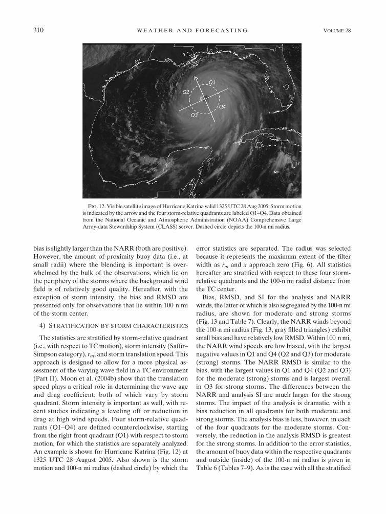
An example is shown for Hurricane Katrina (Fig. 12) at

1325 UTC 28 August 2005. Also shown is the storm

motion and 100-n mi radius (dashed circle) by which the

error statistics are separated. The radius was selected

because it represents the maximum extent of the filter

width as rm and x approach zero (Fig. 6). All statistics

hereafter are stratified with respect to these four storm-

relative quadrants and the 100-n mi radial distance from

the TC center.

Bias, RMSD, and SI for the analysis and NARR

winds, the latter of which is also segregated by the 100-nmi

radius, are shown for moderate and strong storms

(Fig. 13 and Table 7). Clearly, the NARR winds beyond

the 100-n mi radius (Fig. 13, gray filled triangles) exhibit

small bias and have relatively lowRMSD.Within 100 nmi,

the NARR wind speeds are low biased, with the largest

negative values in Q1 andQ4 (Q2 andQ3) for moderate

(strong) storms. The NARR RMSD is similar to the

bias, with the largest values in Q1 and Q4 (Q2 and Q3)

for the moderate (strong) storms and is largest overall

in Q3 for strong storms. The differences between the

NARR and analysis SI are much larger for the strong

storms. The impact of the analysis is dramatic, with a

bias reduction in all quadrants for both moderate and

strong storms. The analysis bias is less, however, in each

of the four quadrants for the moderate storms. Con-

versely, the reduction in the analysis RMSD is greatest

for the strong storms. In addition to the error statistics,

the amount of buoy data within the respective quadrants

and outside (inside) of the 100-n mi radius is given in

Table 6 (Tables 7–9). As is the case with all the stratified

FIG. 12. Visible satellite image ofHurricaneKatrina valid 1325UTC28Aug 2005. Stormmotion

is indicated by the arrow and the four storm-relative quadrants are labeled Q1–Q4. Data obtained

from the National Oceanic and Atmospheric Administration (NOAA) Comprehensive Large

Array-data Stewardship System (CLASS) server. Dashed circle depicts the 100-n mi radius.


FIG. 13. Storm motion–relative error statistics (by quadrant) for the back-

ground (NARR, filled triangles) and analysis (BLND, filled squares) for (left)

moderate and (right) strong storms. NARR and analysis statistics (top) wind

speed bias (m s21), (middle) wind speed RMSD (m s21), and (bottom) SI are

shown for data inside (black fill) and outside (gray fill) a 100-n mi radius.


statistics, the amount of validation (buoy) data is greatly

reduced within the 100-n mi radius.

The model and buoy data (within 100 n mi only) for

the strong and moderate TCs are combined and strati-

fied with respect to the best-track rm and presented in

Table 8. Note that rm is selected because it is related to

the size of the TC and is used herein to estimate the filter

width. Based on examination of the data, an rm value of

20 n mi is chosen such that the data are relatively evenly

split above and below this threshold. Hereafter, values

of rm greater than or equal to (less than) 20 n mi are

referred to RMG20 (RML20). As one might expect for

the NARR, the RML20 RMSD is larger for all quad-

rants compared to RMG20 and is largest on the right

side (quadrants Q1 and Q4). For RMG20, the NARR

wind bias is most negative and the RMSD is largest on

the left side (Q2 and Q3) while the opposite is true for

RML20, which has the largest negative bias–largest

RMSD on the right side. The analysis reduces the

RMSD, SI, and bias in all quadrants but has the largest

impact for the RML20 storms. Although the overall

analysis bias is higher for the RML20 storms, the analysis

has a larger impact on the RML20 RMSD, reducing it by

over 8.5 m s21 to a value (4.8 m s21) that is less than its

RMG20 counterpart (5.5 m s21). The overall SI reduction

(from 0.46 to 0.19) is larger than for the moderate-to-

strong storms. These numbers suggest, in part, that itmight

be possible to further reduce the errors for the RMG20

storms by enlarging the filter width. However, as is shown

in Part II of this paper, the broader and seemingly im-

proved wind field actually increases the wave height error.

The asymmetric structure of the TC wind field is, in

part, a function of the storm translation speed. In gen-

eral, wind speeds increase to the right and decrease to

the left of a TC as its speed increases (Schwerdt 1979). In

addition, the wave containment time, and ultimately the

amount of wave enhancement, is critically linked and

extremely sensitive to storm motion and speed (Bowyer

and MacAfee 2005). Data from moderate and strong

TCs are combined and are stratified with respect to

storm translation speed. A storm speed threshold value

of 10 kt is chosen here, in part because it represents the

lower bound for which the fetch enhancement is maxi-

mized (Bowyer and MacAfee 2005) while maintaining

a relatively even data distribution. TCs with storm

speeds greater than or equal to (less than) 10 kt are re-

ferred to as fast (slow) TCs hereafter. Wind speed bias

and RMSD for fast and slow TCs are discussed with

respect to two storm-relative quadrants here in which

Q1 and Q4 (Q2 and Q3) comprise the right (left)

quadrant. Statistics are shown for radii within 100 n mi

of the TC center only (Table 9).

Overall, the NARR bias and RMSD are largest on

the left side of the slow TCs. For the fast TCs only, the

NARR bias and RMSD are larger on the right side. The

analysis bias reduction is on the order of 5 m s21 for

the left and right sides of the slow and fast storms, and is

largest on the right side for fast TCs. The analysis RMSD

is also around 5 m s21 lower for all but the left side of

the fast TCs. The SI is consistent with the RMSD with

the analysis showing a decrease on the order of 0.15

with the exception of the left quadrant of fast TCs. In

addition, the largestRMSDdecrease, on the left side of the

slowTCs, is associatedwith the largest SI drop (0.18) of the

left–right quadrants. Although the maximum RMSD for

the NARR occurs in the left quadrant for slow storms,

the analysis has an RMSDmaximum in the left quadrant

for fast storms, but the bias is relatively low there. The

TABLE 6. Number of observations by quadrant (see Fig. 10) for the

various stratified statistical subsets and r . 100 n mi.

r . 100 n mi

Q2 Q3 Q1 Q4

Left Right

Moderate 689 479 771 809

Strong 1284 1172 1503 1507

RMG20 996 1460 1125 1873

RML20 977 191 1149 443

Slow TCs 1448 2424

Fast TCs 2176 2166

TABLE 7. Storm motion–relative error statistics by quadrant (see Fig. 10) for the background (NARR) and analysis (BLND) as

a function of storm intensity (strong andmoderate, Tables 3 and 4, respectively). Statistics shown are for r, 100 nmi only. The all column

represents the total for the four quadrants.

Moderate Strong

U10 Q1 Q2 Q3 Q4 All Q1 Q2 Q3 Q4 All

NARR bias –6.44 –5.02 –4.38 –7.34 –5.73 –4.31 –7.27 –9.27 –5.97 –6.06

BLND bias –1.52 0.10 –0.87 0.16 –0.53 –1.76 –0.25 –4.54 –1.44 –1.77

NARR RMSD 8.79 7.53 7.66 10.46 8.61 8.96 11.91 12.91 11.58 10.93

BLND RMSD 5.68 5.72 5.85 5.23 5.64 3.90 5.30 7.09 4.42 4.90

NARR SI 0.30 0.32 0.35 0.37 0.34 0.34 0.40 0.38 0.42 0.39

BLND SI 0.28 0.33 0.33 0.26 0.30 0.15 0.22 0.23 0.18 0.20

No. of data points 41 46 43 38 168 62 32 23 43 160


analysis RMSD is lower, in the respective quadrants, for

slow TCs compared to the fast TCs. Clearly, the NARR

impacts the analysis: when the bias in the former is rel-

atively large, it remains so in the latter. However, this

does not appear to be the case for the fast TC analysis

RMSD, where it is lowest on the right side, which has the

largest background RMSD. Wind speed error is critical

in terms of wave heights, particularly in extreme events

(Cardone et al. 1996), while bias reduction is an essential

component in terms of generating skillful ensembles

(Hamill 2000). Efforts to further reduce the analysis

error (RMSD) by decreasing the blending width re-

introduces the low bias inherent in the NARR (within

100 n mi) and, in light of the analysis sensitivity to the

bias (section 4b), are not prudent.

5. Discussion and issues

The difference between the fast and slow TCs may, in

part, be due to the limitations of the simple parametric

model used here. The model depicts wavenumber 1

asymmetries only, and thus complex asymmetries will

be problematic (K07). For example, a double-eyewall

structure where the wind field exhibits multiple maxima

along a radial cannot be recovered by a simple first-

order parametric representation of the wind field. If

either the observed asymmetry factor or its degree of

rotation [see Eq. (1)] differs from the climatological

values used here, the estimation of wind radii will be

influenced. The climatological asymmetry factor and the

degree of rotation depend on storm speed and latitude

only. Different parameterizations of these factors and

an extension of the parametric model to include higher-

order asymmetries would be instructive.

Although the blending between the NARR and AOC

is smooth, the analysis wind field tends to decrease more

rapidly along a radial than does H*Wind or the best

track, especially for TCs with relatively small rm. This is

primarily an artifact of the blending width and can

produce a wind speed profile that undershoots the

NARR as the analysis asymptotically approaches the

background (e.g., see Fig. 8b). Although this has little or

no impact on the forecast wave field (Part II), as dem-

onstrated here, it can be mitigated by increasing the

influence of the parametric wind field outward from the

storm center. The best approach would be a modifica-

tion of the simple parameterization used here [Eq. (9)],

such that the filter stop end depends on matching the

vortex wind speed with that of the background. Cur-

rently, the filter stop end is calculated as a residual (i.e.,

a difference between the filter width and pass end).

Alternatively, the bulk estimate of c [Eq. (9)] as defined

for the AOC (50 n mi) was selected based on all (12) of

the storms. Allowing c (and thusD) to vary as a function

of the distance between rm and either the 64- or 50-kt

radii is worth investigating. In some cases, the NARR

eye is offset from the ‘‘official’’ location in the best-track

data. A higher-resolution and improved background

field will likely alleviate some, but not all, of these mis-

matches. The intent of this study is to lay the groundwork

for using short-term (i.e., on the order of a day) forecast

track–intensity permutations and associated parameters

generated by the operational (NHC)Monte Carlo model

TABLE 8. Storm motion–relative error statistics by quadrant (see Fig. 10) for the background (NARR) and analysis (BLND) as

a function radius of maximum winds rm for moderate and strong storms combined. RMG20 (RML20) represents storms with rm $ (,)

20 n mi. Statistics shown are for r , 100 n mi only. The all column represents the total for the four quadrants.

RMG20 RML20

U10 Q1 Q2 Q3 Q4 All Q1 Q2 Q3 Q4 All

NARR bias 24.16 26.54 26.20 24.75 25.32 27.95 23.95 25.57 211.60 27.69

BLND bias 21.51 20.09 22.38 0.08 20.98 22.10 0.12 21.13 22.75 21.63

NARR RMSD 6.67 9.14 9.56 8.49 8.40 13.27 10.89 10.90 16.06 13.31

BLND RMSD 4.50 6.17 6.72 4.39 5.45 5.20 2.54 3.99 5.82 4.75

NARR SI 0.26 0.32 0.36 0.35 0.33 0.42 0.49 0.54 0.40 0.46

BLND SI 0.21 0.31 0.31 0.22 0.27 0.19 0.12 0.22 0.19 0.19

No. of data points 76 60 54 59 249 27 18 12 22 79

TABLE 9. Storm motion–relative error statistics (m s21, by

quadrant) for the background (NARR) and analysis (BLND) as

a function of storm speed for moderate and strong storms com-

bined. Statistics shown are for r , 100 n mi only. Slow (fast) TCs

have storm motions , ($) 10 kt. Left (right) includes storm

quadrants Q2 and Q3 (Q1 and Q4) as shown in Fig. 12.

Slow TCs Fast TCs

U10

Q2/Q3

left

Q1/Q4

right

Q2/Q3

left

Q1/Q4

right

NARR bias 27.14 25.29 25.39 26.39

BLND bias 22.04 20.35 20.44 22.27

NARR RMSD 10.95 9.30 8.92 10.58

BLND RMSD 5.11 4.48 6.31 5.04

NARR SI 0.41 0.36 0.36 0.37

BLND SI 0.23 0.21 0.32 0.20

No. of data points 51 99 93 85


(DeMaria et al. 2009) to generate wave ensembles.

Under this paradigm, even short-term track forecasts

can have considerable spread. In this case it will, in

general, be better to remove the background vortex al-

together, hole fill the wind field, and then generate an

analysis for a given forecast time (e.g., Sampson et al.

2010). This approach is economical in the sense that it

uses a single background field, for a given forecast time,

that can then be merged with the Monte Carlo re-

alizations. Nonetheless, this still requires N 3 F/n dis-

tinct analyses and wave model simulations, where N is

the number of realizations, F the forecast cycle length

(in h), and n the wind forcing interval (in h). Hence,

unlike the long-term wave hindcast studies previously

discussed, the computational challenge here is not the

resolution of the atmospheric model, but rather the

number of wind analyses and subsequent wave forecasts.

In terms of the latter, the cubic relationship between the

resolution and computational time is obviously prob-

lematic from an operational perspective.

Despite adjusting the buoy wind speeds to 10 m, it is

possible that the speeds remain low biased as a result of

temporal averaging and high gustiness (Cardone et al.

1996). However, if this is the case, then the first-guess

low bias that is prevalent in all quadrants within the

100-n mi radius is actually worse than shown here. In

addition, no static stability corrections were applied.

However, these are not likely large for a GOM TC en-

vironment (Powell et al. 2003). The sparseness of the

buoy observations is likelymore important here, making

it difficult to effectively tune the analysis parameters. In

terms of the analysis, the low wind bias can be mitigated

by increasing the grid resolution from the 10 km used

herein. However, experiments for which the wind

analysis resolution was reduced to 6 km (not shown) did

not result in improved wave forecasts (Part II). In ad-

dition, whatever benefits increased spatial resolution

provides must be considered in the context of main-

taining computational efficiency, that latter of which is

a key element driving the configuration presented here.

Acknowledgments. The publication of this work would

not have been possible without institutional support from

the Florida Institute of Technology office of the executive

vice president and chief operating officer, T. Dwayne

McCay.

REFERENCES

Barnes, S. L., 1964: A technique for maximizing details in numer-

ical weather map analysis. J. Appl. Meteor., 3, 396–409.Benjamin, S. G., and N. L. Seaman, 1985: A simple scheme for ob-

jective analysis in curved flow.Mon.Wea. Rev., 113, 1184–1198.

Berg, R., 2009: Hurricane Ike (AL092008) 1–14 September 2008.

National Hurricane Center Tropical Cyclone Rep., 55 pp.

Bowyer, P. J., and A. W. MacAfee, 2005: The theory of trapped-

fetch waves with tropical cyclones—An operational perspec-

tive. Wea. Forecasting, 20, 229–244.

Butterworth, S., 1930: On the theory of filter amplifiers. Wireless

Eng., 7, 536–541.Cardone, V. J., R. E. Jensen, D. T. Resio, V. R. Swail, and

A. T. Cox, 1996: Evaluation of contemporary ocean wave

models in rare extreme events: The ‘‘Halloween Storm’’ of

October 1991 and the ‘‘Storm of the Century’’ of March 1993.

J. Atmos. Oceanic Technol., 13, 198–230.

——, A. T. Cox, and V. R. Swail, 1999: Evaluation of NCEP re-

analysis surface marine wind fields for ocean wave hindcasts.

Preprints, CLIMAR 1999, Vancouver, BC, Canada, Joint

WMO/IOC Technical Commission for Oceanography and

Marine Meteorology (JCOMM), 68–85.

——, ——, and ——, 2000: Specification of global wave climate:

Is this the final answer? Proc. Sixth Int. Workshop on Wave

Hindcasting and Forecasting, Monterey, CA, Environment

Canada–U.S. Army Engineer Research and Development

Center’s Coastal and Hydraulics Laboratory–JCOMM,

211–223.

——,——, andG. Z. Forristall, 2007: Hindcast of winds, waves and

currents in northern Gulf of Mexico in Hurricanes Katrina

(2005) and Rita (2005). Proc. Offshore Technology Confer-

ence, Houston, TX, OTC 18652.

Chen, H. S., 2006: Ensemble prediction of ocean waves at

NCEP. Proc. 28th Ocean Engineering Conference, Kaohsiung,

Taiwan, National Sun Yat-Sen University, 10 pp.

Cressman, G. P., 1959: An operational objective analysis system.

Mon. Wea. Rev., 87, 367–374.

DeMaria, M., S. D. Aberson, K. V. Ooyama, and S. J. Lord, 1992:

A nested spectral model for hurricane track forecasting.Mon.

Wea. Rev., 120, 1628–1643.

——, J. A. Knaff, R. Knabb, C. Lauer, C. R. Sampson, and

R. T. DeMaria, 2009: A new method for estimating tropical

cyclone wind speed probabilities. Wea. Forecasting, 24, 1573–

1591.

Demuth, J., M. DeMaria, and J. A. Knaff, 2006: Improvement of

AdvancedMicrowave Sounder Unit tropical cyclone intensity

and size estimation algorithms. J. Appl. Meteor. Climatol., 45,

1573–1581.

Desjardins, S., R. Lalbeharry, H. Ritchie, and A. Macafee, 2004:

Blending parametric hurricane surface fields into CMC fore-

casts and evaluating impact on the wave model of hurricane

Juan and others. Proc. Eighth Int. Workshop on Wave Hind-

casting and Forecasting,Oahu, HI, Environment Canada–U.S.

Army Engineer Research and Development Center’s Coastal

and Hydraulics Laboratory–JCOMM, F2.

Gilhousen, D. B., 1987: A field evaluation of NDBC moored buoy

winds. J. Atmos. Oceanic Technol., 4, 94–104.

——, 2006: A complete explanation of whymoored buoy winds are

less than ship winds. Mar. Wea. Log, 50, 4–7.Hamill, T. M., 2000: Interpretation of rank histograms for verifying

ensemble forecasts. Mon. Wea. Rev., 129, 550–560.

——, S. L. Mullen, C. Snyder, D. P. Baumhefner, and Z. Toth,

2000: Ensemble forecasting in the short to medium range:

Report from a workshop. Bull. Amer. Meteor. Soc., 81, 2653–

2664.

Holt, M. W., and B. J. Hall, 1992: A comparison of 2nd generation

and 3rd generation wave model physics. Met Office Short-

Range Forecasting Research Division Tech. Rep. 10, 23 pp.


Hsu, S. A., E. A. Meindl, and D. B. Gilhousen, 1994: Determining

the power-law wind-profile exponent under near-neutral sta-

bility conditions at sea. J. Appl. Meteor., 33, 757–765.

Janssen, P. A. E.M., B. Hansen, and J. R. Bidlot, 1997: Verification

of the ECMWF wave forecasting system against buoy and

altimeter data. Wea. Forecasting, 12, 763–784.

Kalnay, E., and Coauthors, 1996: The NCEP/NCAR 40-Year Re-

analysis Project. Bull. Amer. Meteor. Soc., 77, 437–471.Knaff, J. A., C. R. Sampson, M. DeMaria, T. P. Marchok,

J. M. Gross, and C. J. McAdie, 2007: Statistical tropical cy-

clone wind radii prediction using climatology and persistence.

Wea. Forecasting, 22, 781–791.Lazarus, S. M., S. T. Wilson, M. E. Splitt, and G. A. Zarillo, 2013:

Evaluation of a wind–wave system for ensemble tropical cyclone

wave forecasting. Part II: Waves.Wea. Forecasting, 28, 316–330.Makin, V. K., and V. N. Kudryavtsev, 1999: Coupled sea surface-

atmosphere model 1. Wind over waves coupling. J. Geophys.

Res., 104 (C4), 7613–7623.

Mishra, S. K., 2007: NLINLS: A differential evolution based non-

linear least squares Fortran 77 program. Social Science Re-

search Network, 10 pp. [Available online at http://mpra.ub.

uni-muenchen.de/4949/1/MPRA_paper_4949.pdf.]

Moon, I. J., I. Ginis, and T. Hara, 2004b: Effect of surface waves on

air–sea momentum exchange. Part II: Behavior of drag co-

efficient under tropical cyclones. J. Atmos. Sci., 61, 2334–2348.

Mousavi, S. M., F. Jose, and G. Stone, 2009: Simulating Hurricane

Gustav and Ike wave fields along the Louisiana Innershelf:

Implementation of an unstructured third-generation wave

model, SWAN. Oceans 2009—Marine Technology for Our

Future: Global and Local Challenges, Biloxi, MS, MTS/IEEE.

Powell, M. D., S. H. Houston, L. R. Amat, and N. Morisseau-

Leroy, 1998: The HRD real-time hurricane wind analysis

system. J. Wind Eng. Indust. Aerodyn., 77–78, 53–64.

——, P. J. Vickery, and T. A. Reinhold, 2003: Reduced drag co-

efficient for high wind speeds in tropical cyclones.Nature, 422,

279–283.

Roulston, M. S., J. Ellepola, J. Hardenberg, and L. A. Smith,

2005: Forecasting wave height probabilities with numer-

ical weather prediction models. J. Ocean Eng., 32, 1841–

1863.

Sampson, C. R., P. A.Wittman, andH. L. Tolman, 2010: Consistent

tropical cyclone wind and wave forecasts for the U.S. Navy.

Wea. Forecasting, 25, 1293–1306.

Schwerdt, R.W., F. P. Ho, andR.R.Watkins, 1979:Meteorological

criteria for standard project hurricane and probable maximum

hurricane wind fields, Gulf and east coasts of the United

States. NOAA Tech. Rep. NWS 23, 317 pp.

Stone, G. W., N. D. Walker, S. A. Hsu, A. Babin, B. Liu,

B. D. Keim, W. Teague, D. Mitchell, and R. Leben, 2005:

Hurricane Ivan’s impact along the northern Gulf of Mexico.

Eos, Trans. Amer. Geophys. Union, 86, 497–500.

Storn, R., and K. Price, 1997: Differential evolution—A simple and

efficient heuristic for global optimization over continuous

spaces. J. Global Optim., 11, 341–359.

Uhlhorn, E. W., P. G. Black, J. L. Franklin, M. Goodberlet,

J. Carswell, and A. S. Goldstein, 2007: Hurricane surface wind

measurements from an operational stepped frequency mi-

crowave radiometer. Mon. Wea. Rev., 135, 3070–3085.

Young, I. R., 2003: A review of the sea state generated by hurri-

canes. Mar. Struct., 16, 210–218.


Evaluation of a Wind-Wave System for Ensemble Tropical Cyclone Wave Forecasting. Part I: Winds

Documents

Transcript of Evaluation of a Wind-Wave System for Ensemble Tropical Cyclone Wave Forecasting. Part I: Winds